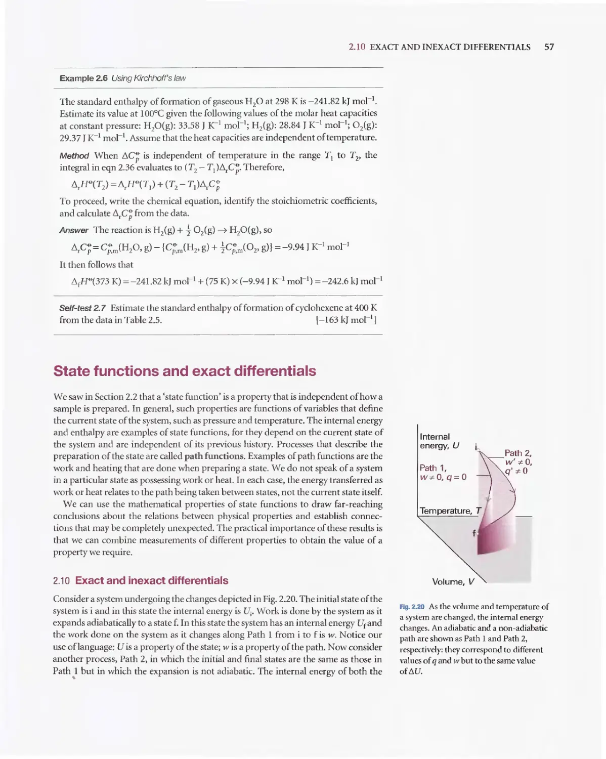
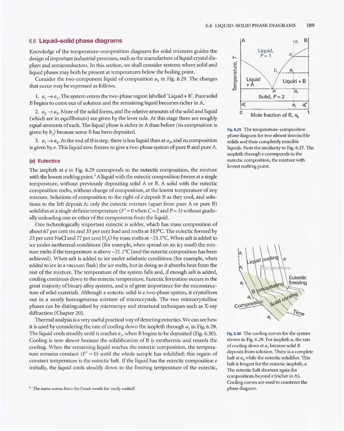
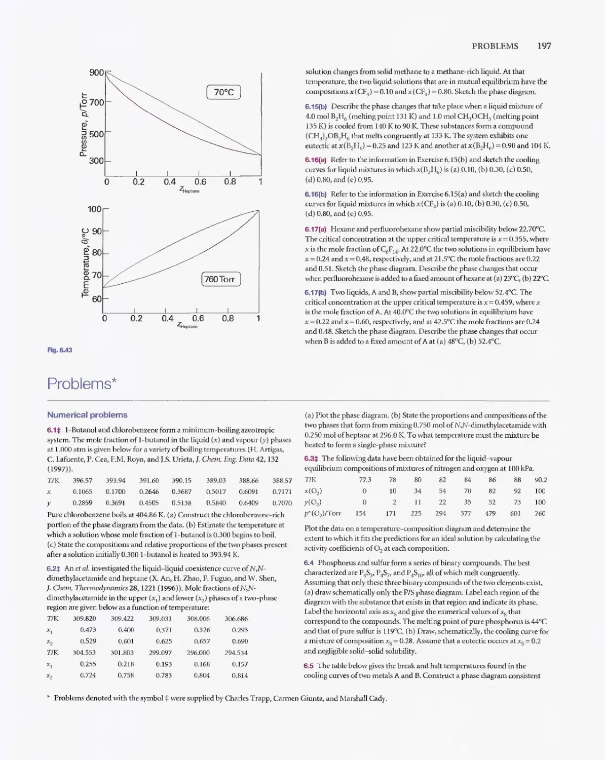
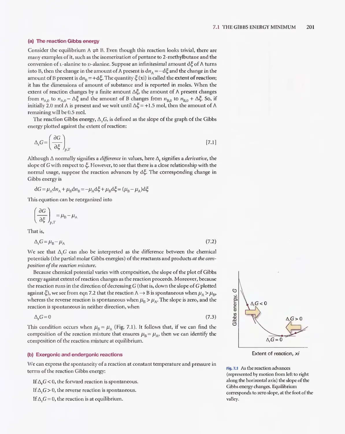
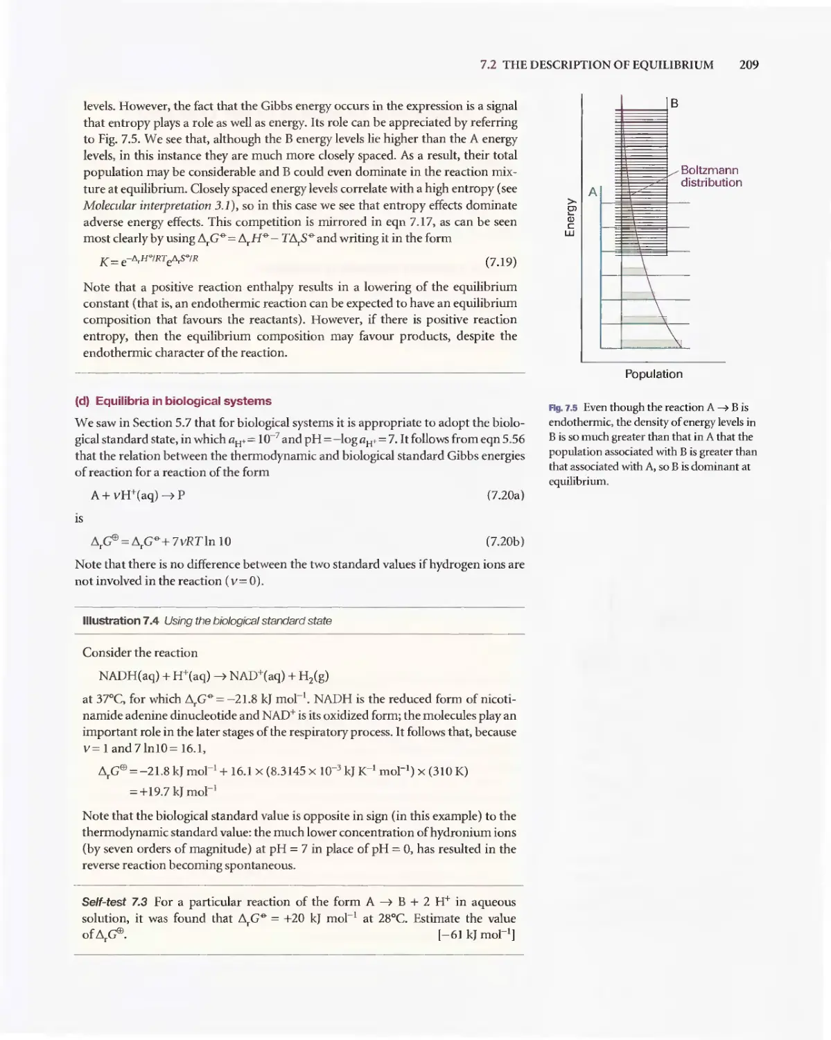
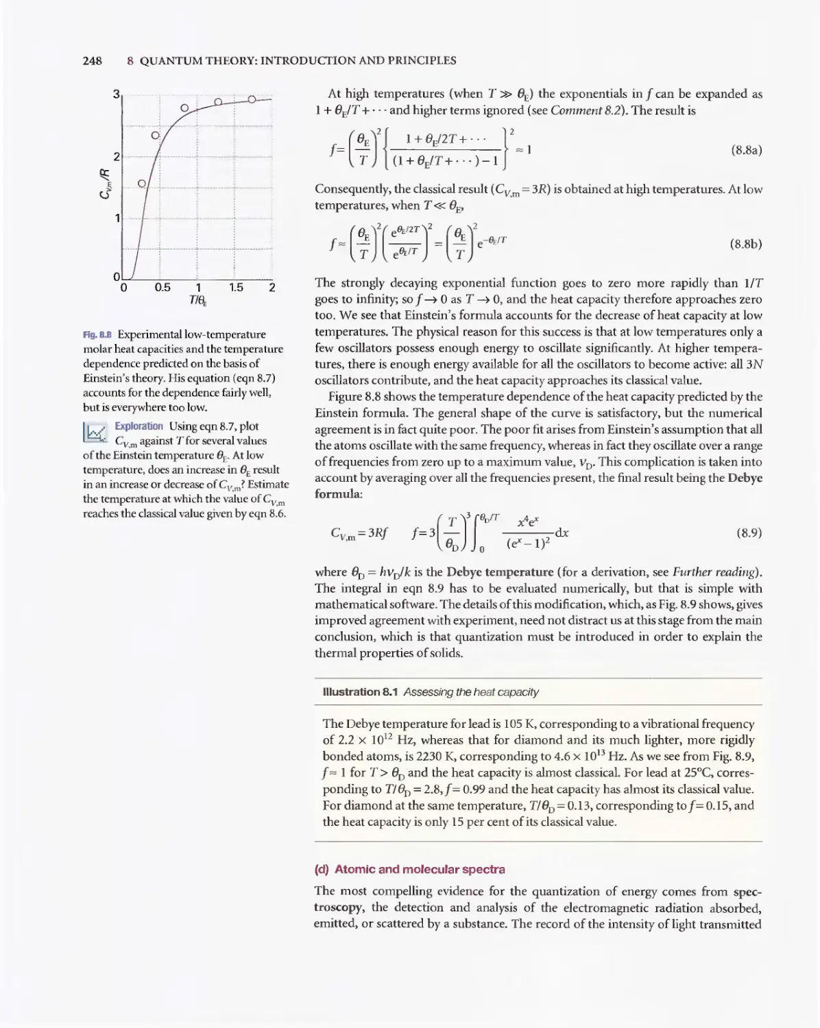
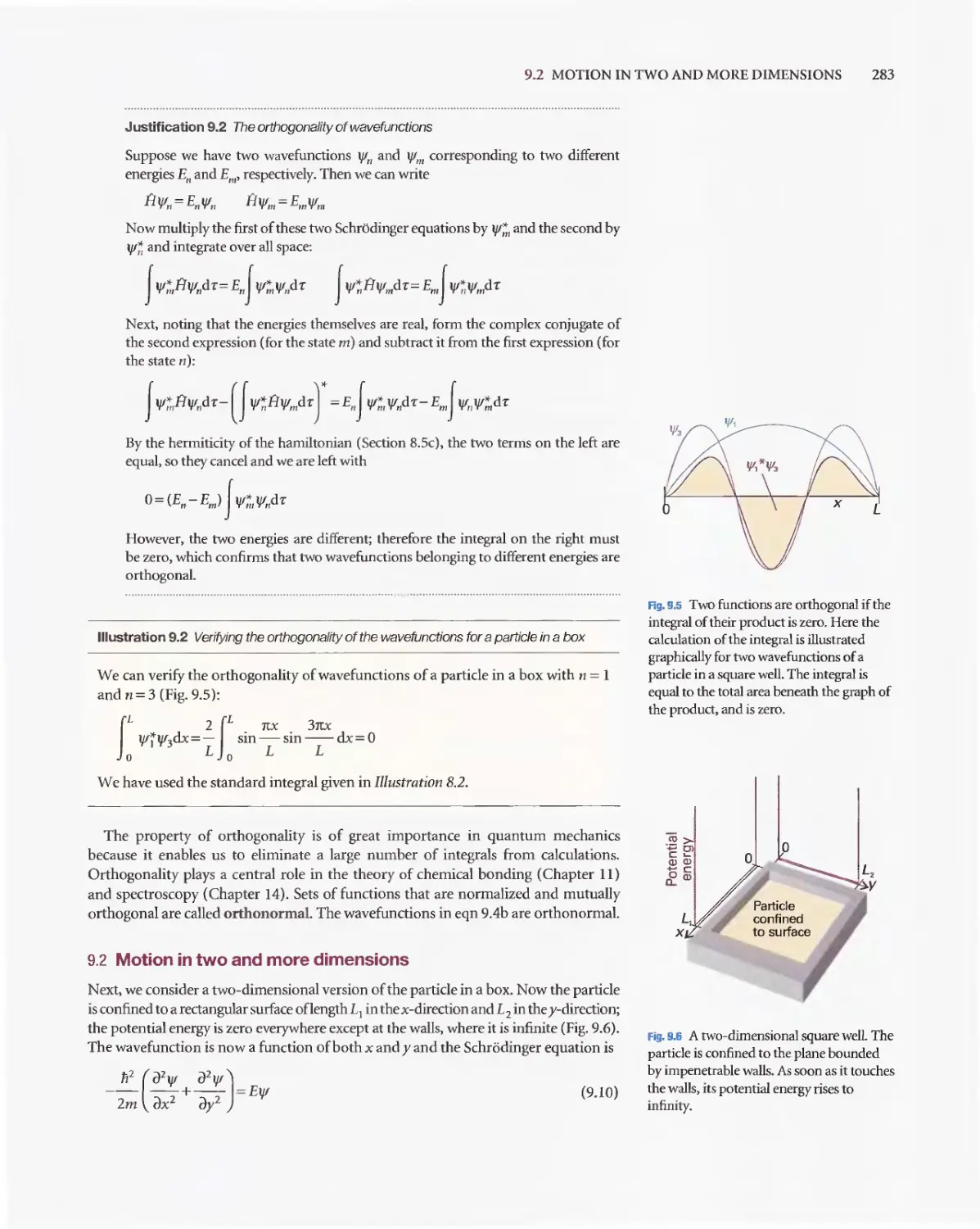
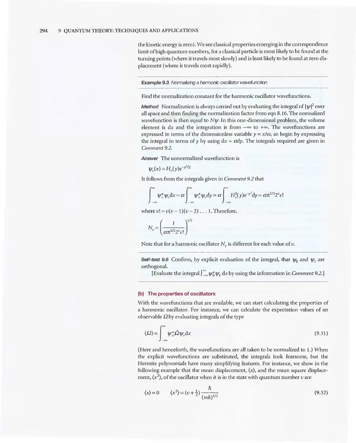
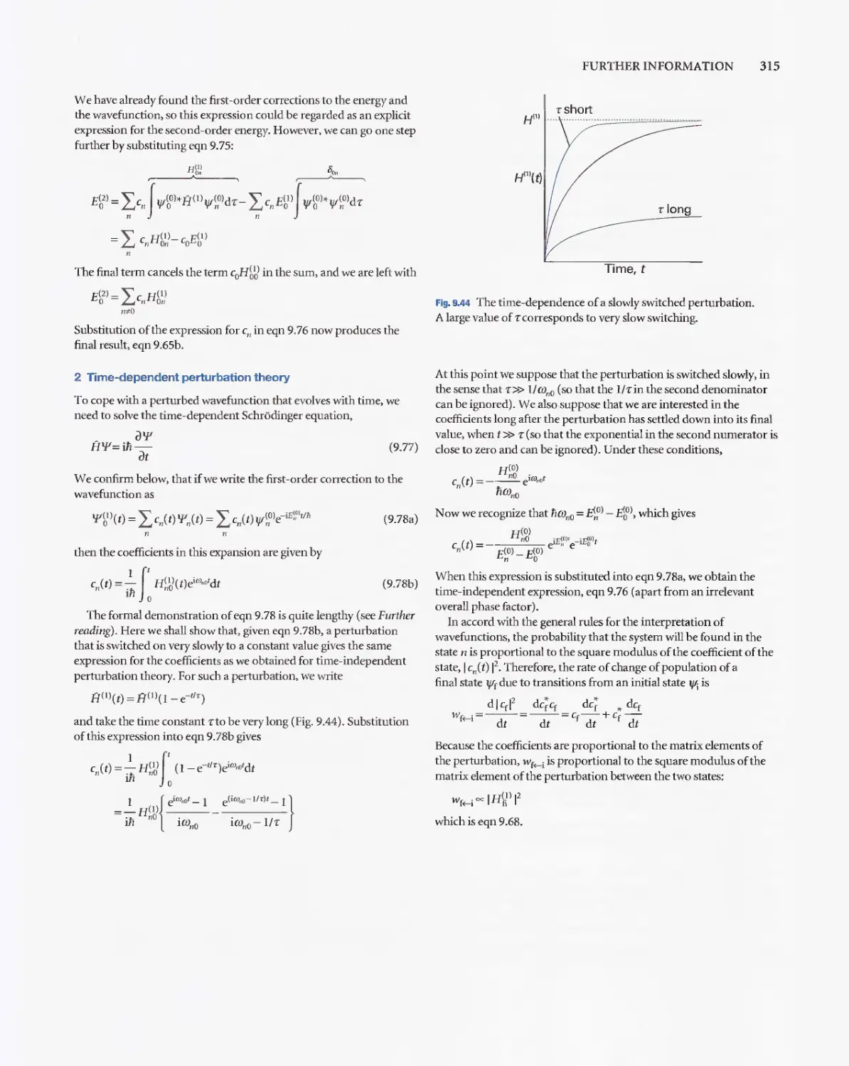
/


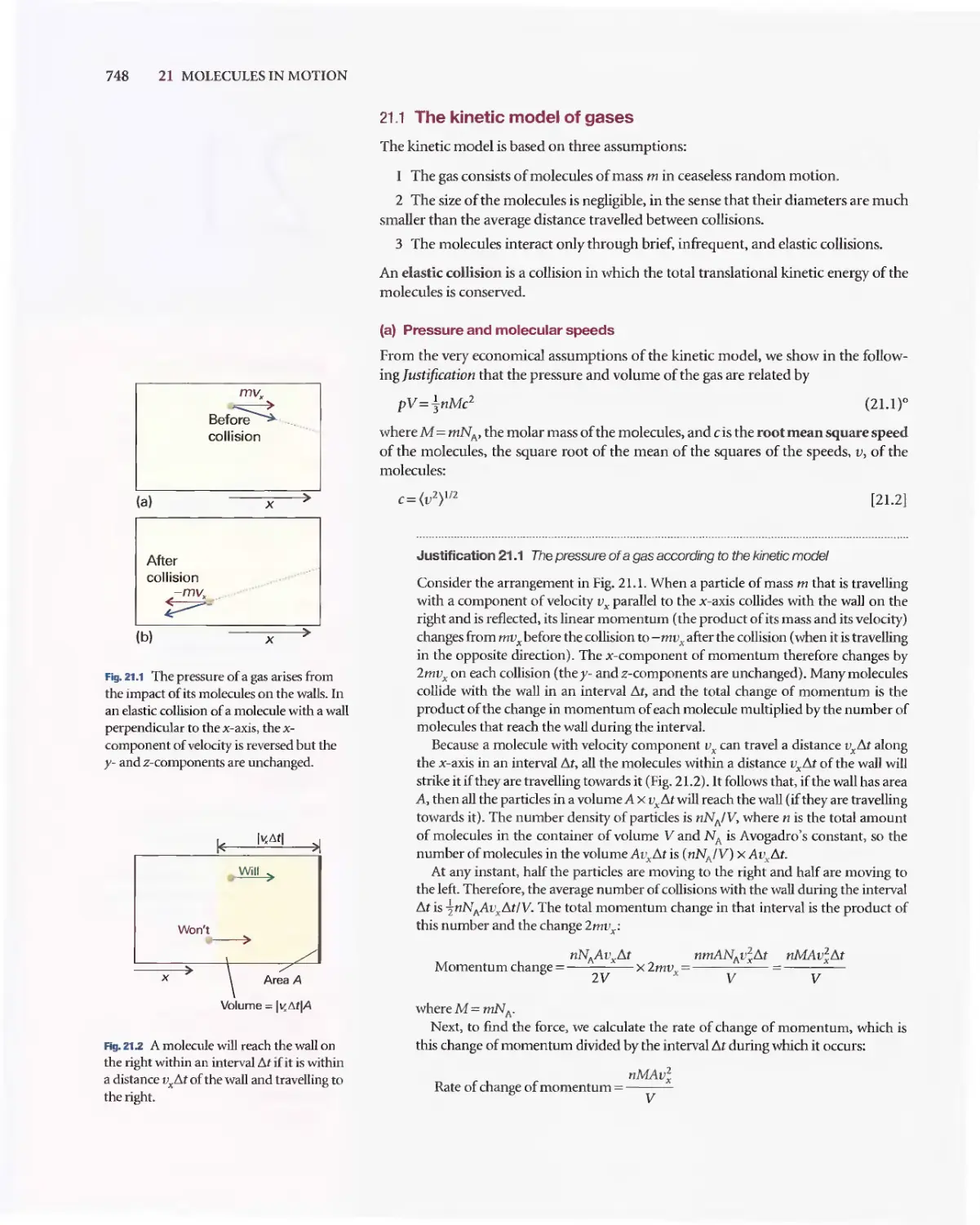


Текст
OXFORD
TH EDITIOr I
410....._
-
ATKINS'
PHYSICAL
CHEMISTRY
PETER ATKINS · JULIO DE PAULA
online
resource
'- centre
ATKINS'
PHYSICAL
CHEMISTRY
ATKINS'
PHYSICAL
CHEMISTRY
Eighth Edition
Peter Atkins
Professor of Chemistry,
University of Oxford,
and Fellow of Lincoln College, Oxford
Julio de Paula
Professor and Dean of the College of Arts and Sciences,
Lewis and Clark College,
Portland, Oregon
OXFORD
UNIVERSITY PRESS
OXFORD
UNIVERSITY PRESS
Great Clarendon Street, Oxford OX2 6DP
Oxford University Press is a department of the University of Oxford.
It furthers the University's objective of excellence in research, scholarship,
and education by publishing worldwide in
Oxford New York
Auckland Cape Town Dar es Salaam Hong Kong Karachi
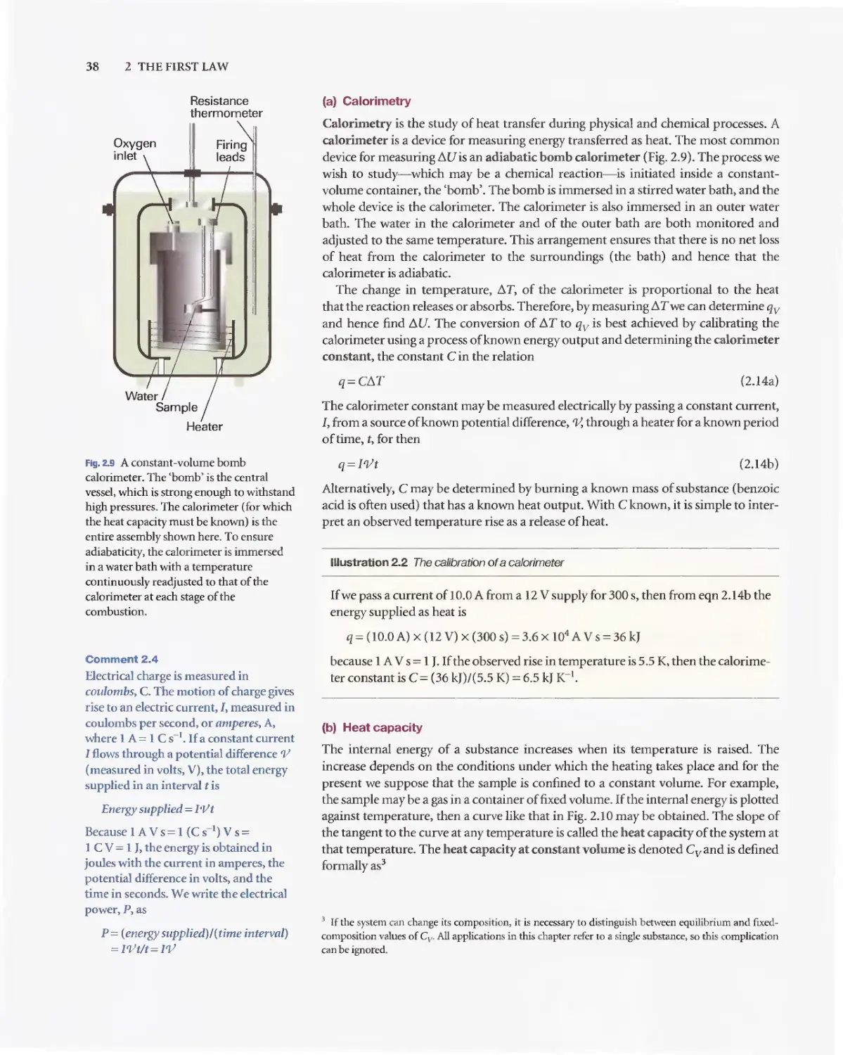
Kuala Lumpur Madrid Melbourne Mexico City Nairobi
New Delhi Shanghai Taipei Toronto
With offices in
Argentina Austria Brazil Chile Czech Republic France Greece
Guatemala Hungary Italy Japan Poland Portugal Singapore
South Korea Switzerland Thailand Turkey Ukraine Vietnam
Oxford is a registered trade mark of Oxford University Press
in the UK and in certain other countries
Published in the United States and Canada
by W. H. Freeman and Company
@ Peter Atkins 1978, 1982, 1986, 1990, 1994,1998
and @ Peter Atkins & Julio de Paula 2002, 2006
The moral rights of the authors have been asserted
Database right Oxford University Press (maker)
First published 2006
All rights reserved. No part of this publication may be reproduced,
stored in a retrieval system, or transmitted, in any form or by any means,
without the prior permission in writing of Oxford University Press,
or as expressly permitted by law, or under terms agreed with the appropriate
reprographics rights organization. Enquiries concerning reproduction
outside the scope of the above should be sent to the Rights Department,
Oxford University Press, at the address above
You must not circulate this book in any other binding or cover
and you must impose the same condition on any acquirer
British Library Cataloguing in Publication Data
Data available
Library of Congress Cataloging in Publication Data
Data available
Typeset by Graphicraft Limited, Hong Kong
Printed in Italy
on acid-free paper by Lito Terrazzi s.d.
ISBN 9780198700722 ISBN 0198700725
1 3 5 7 9 10 8 6 4 2
Preface
We have taken the opportunity to refresh both the content and presentation of this
text while-as for all its editions-keeping it flexible to use, accessible to students,
broad in scope, and authoritative. The bulk of textbooks is a perennial concern: we
have sought to tighten the presentation in this edition. However, it should always be
borne in mind that much of the bulk arises from the numerous pedagogical features
that we include (such as Worked examples and the Data section), not necessarily from
density of information.
The most striking change in presentation is the use of colour. We have made every
effort to use colour systematically and pedagogically, not gratuitously, seeing it as a
medium for making the text more attractive but using it to convey concepts and data
more clearly. The text is still divided into three parts, but material has been moved
between chapters and the chapters have been reorganized. We have responded to the
shift in emphasis away from classical thermodynamics by combining several chapters
in Part 1 (Equilibrium), bearing in mind that some of the material will already have
been covered in earlier courses. We no longer make a distinction between 'concepts'
and 'machinery', and as a result have provided a more compact presentation of ther-
modynamics with fewer artificial divisions between the approaches. Similarly, equi-
librium electrochemistry now finds a home within the chapter on chemical equilibrium,
where space has been made by reducing the discussion of acids and bases.
In Part 2 (Structure) the principal changes are within the chapters, where we have
sought to bring into the discussion contemporary techniques of spectroscopy and
approaches to computational chemistry. In recognition of the major role that phys-
ical chemistry plays in materials science, we have a short sequence of chapters on
materials, which deal respectively with hard and soft matter. Moreover, we have
introduced concepts of nanoscience throughout much of Part 2.
Part 3 has lost its chapter on dynamic electrochemistry, but not the material. We
regard this material as highly important in a contemporary context, but as a final
chapter it rarely received the attention it deserves. To make it more readily accessible
within the context of courses and to acknowledge that the material it covers is at home
intellectually with other material in the book, the description of electron transfer
reactions is now a part of the sequence on chemical kinetics and the description of
processes at electrodes is now a part of the general discussion of solid surfaces.
We have discarded the Boxes of earlier editions. They have been replaced by more
fully integrated and extensive Impact sections, which show how physical chemistry is
applied to biology, materials, and the environment. By liberating these topics from
their boxes, we believe they are more likely to be used and read; there are end-of-
chapter problems on most of the material in these sections.
In the preface to the seventh edition we wrote that there was vigorous discussion in
the physical chemistry community about the choice of a 'quantum first' or a 'thermo-
dynamics first' approach. That discussion continues. In response we have paid particu-
lar attention to making the organization flexible. The strategic aim of this revision
is to make it possible to work through the text in a variety of orders, and at the end of
this Preface we once again include two suggested road maps.
The concern expressed in the seventh edition about the level of mathematical
ability has not evaporated, of course, and we have developed further our strategies
for showing the absolute centrality of mathematics to physical chemistry and to make
it accessible. Thus, we give more help with the development of equations, motivate
viii PREFACE
them, justify them, and comment on the steps. We have kept in mind the struggling
student, and have tried to provide help at every turn.
We are, of course, alert to the developments in electronic resources and have made
a special effort in this edition to encourage the use of the resources in our online
resource centre (at www.oxfordtextbooks.co.ukJorc/pchem8el) where you can also
access the eBook. In particular, we think it important to encourage students to use the
Living graphs and their considerable extension as Explorations in Physical Chemistry.
To do so, wherever we callout a Living graph (by an icon attached to a graph in the
text), we include an Exploration in the figure legend, suggesting how to explore the
consequences of changing parameters.
Overall, we have taken this opportunity to refresh the text thoroughly, to integrate
applications, to encourage the use of electronic resources, and to make the text even
more flexible and up to date.
Oxford
Portland
P.W.A.
J.de P.
PREFACE IX
Traditional approach
Equilibrium thermodynamics
Chapters 1-7
Chemical kinetics
Chapters 21, 22, and 24
Quantum theory and spectroscopy
Chapters 8-11, 13-15
Special topics
Chapters 12. 18-20, 23, and 25
Statistical thermodynamics
Chapters 16 and 17
Molecular approach
Ouantum theory and spectroscopy
Chapters 8-11,13-15
Statistical thermodynamics
Chapters 16 and 17
Chemical kinetics
Chapters 21, 22, and 24
Equilibrium thermodynamics
Chapters 1-7
Special topics
Chapters 12,18-20,23, and 25
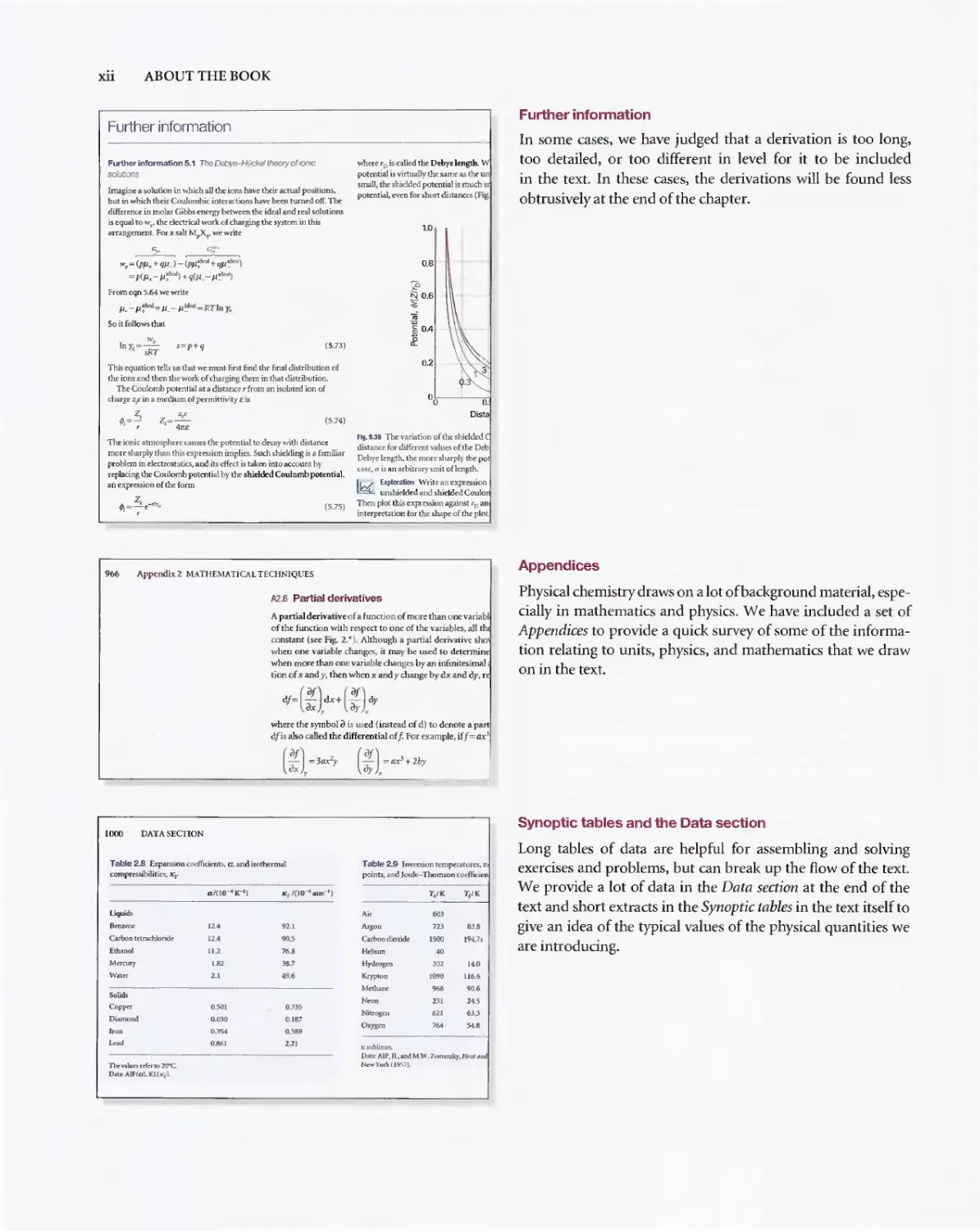
About the book
There are numerous features in this edition that are designed to make learning phys-
ical chemistry more effective and more enjoyable. One of the problems that make the
subject daunting is the sheer amount of information: we have introduced several
devices for organizing the material: see Organizing the information. We appreci-
ate that mathematics is often troublesome, and therefore have taken care to give
help with this enormously important aspect of physical chemistry: see Mathematics
and Physics support. Problem solving-especially, 'where do I start?' -is often a
challenge, and we have done our best to help overcome this first hurdle: see Problem
solving. Finally, the web is an extraordinary resource, but it is necessary to know
where to start, or where to go for a particular piece of information; we have tried to
indicate the right direction: see About the Online Resource Centre. The following
paragraphs explain the features in more detail.
Organizing the information
Checklist of key ideas
D 1. A gas is a form of matter that fills any container it occupies.
D 2. An equation of state interrelates pressure, volume,
temperature. and amount of substance: p = fiT. V.n).
o 3. The pressure is the force divided by the area to which the force
is applied. The standard pressure is p""'= 1 bar (10 5 Pa).
D 4. Mechanical equilibrium is the condition of equa1ity of
pressure on either side of a movable walL
D 5. Temperature is the property that indicates the direction of the
flow of energy through a thermally conducting. rigid wall.
D 6. A diathermic boundary is a boundary that permits the passage
of energy as heat. An adiabatic boundary is a boundary that
prevents the passage of energy as heat.
D 7. Thermal equilibrium is a condition in which no change of
state occurs when two objects A and B are in contact through
a diathermic boundary.
D 8. The Zeroth Law of thermodynamics states that> if A is in
thermal equilibrium with B, and B is in thermal equilibrium
with C, then C is a1so in thermal equilibrium with A.
D 9. The Celsius and thermodynamic temperature scales are
related by TIK= erc + 273.15.
D 10. A perfect gas obeys the perfect gas equation, pV = nRT, exactly
D 12. The partial pressure of any gas
xJ= I1ll1 is its mole fraction in
pressure.
D 13. In real gases, molecular interac
state; the true equation of state
coefficientsB, C,... :pVm=R
D ] 4. The vapour pressure is the pres
with its condensed phase.
D 15. The critical point is the point a
end of the horizontal part of th
a single point. The critical cons
pressure, molar volume, and te
critical point.
D 16. A supercritical fluid is a dense
temperature and pressure.
D 17 The van der Waals equation of
the true equation of state in wh
by a parameter a and repulsion
parameter b: p = nRTI(V -nb)
D 18. A reduced variable is the actual
corresponding critical constan
IMPACTONNANOSDENCE
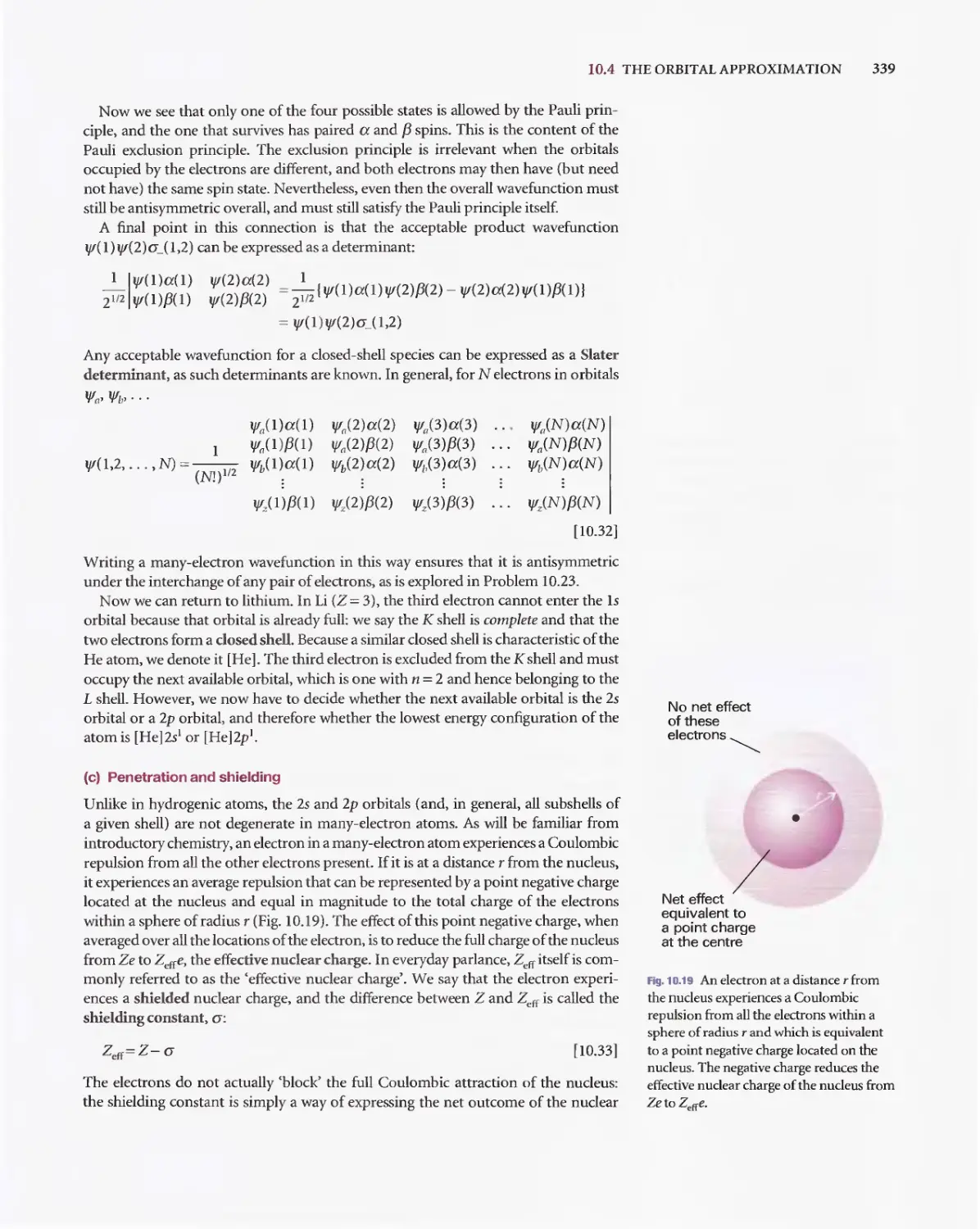
120.2 Nanowires
We have already remarked (Impacts 19.1, 19.2, and 119.3) that research on nano-
metre-sized materials is motivated by the possibility that they will form the basi
for
cheaper and smaller electronic devices. The synthesis of nanowires, nanometrc-sized
atomic assemblies that conduct electricity. is a major step in the fabrication of
nanodevices. An important type of nanowire is based on carbon nanotubes, which,
like graphite, can conduct electrons through delocalized tr molecular orbitals that
form from unhybridized 2p orbitals on carbon. Recent studies have shown a cor-
relation between structure and conductivity in single-walled nanotubes (SWNTs)
that does not occur in graphite. The SWNT in Fig. 20.45 is a semiconductor. If the
hexagons are rotated by 60 D about their sixfold axis, the resulting SWNT is a metallic
conductor.
Carbon nanotubes are promising building blocks not only because they have useful
electrical properties but also because they have unusual mechanical properties. For
example, an SWNT has a Young's modulus that is approximately five times larger and
a tensile strength that is approximately 375 times larger than that of steel.
Silicon nanowires can be made by focusing a pulsed laser beam on to a solid target
composed of silicon and iron. The laser ejects Fe and Si atoms from the surface of the
Checklist of key ideas
Here we collect together the major concepts introduced in the
chapter. We suggest checking off the box that precedes each
entry when you feel confident about the topic.
Impact sections
Where appropriate, we have separated the principles from
their applications: the principles are constant and straightfor-
ward; the applications come and go as the subject progresses.
The Impact sections show how the principles developed in
the chapter are currently being applied in a variety of modern
contexts.
A note on good practice We write T = 0, not f = 0 K tor the zero temperature
on the thermodynamic temperature sca1e. This scale is absoJute. and the lowest
temperature is 0 regardless of the size of the divisions on the sca)e (just as we write
p = 0 for zero pressure. regardless of the size of the units we adopt. such as bar or
pascal). However. we write O°C because the Celsius scale is not absolute.
5.8 The activities of regular solutions
The material on regular solutions presented in Section 5.4 gives further insight into
the origin of deviations from Raoult's law and its relation to activity coefficients. The
starting point is the expression for the Gibbs energy of mixing for a regular solution
(eqn 5.31). We show in the following Jilstification that eqn 5-31 implies that the activ-
ity coefficients are given by expressions of the form
In YA
fJx
In YB
px,; (5.57)
These relations are called the Margules equations.
Justification 5.4 The Margules equations
The Gibbs energy of mixing to form a nonideal solution is
G=nRTtxAlnaJ\ +xBlnaBI
This [dation follows from the derivation of eqn 5.31 with actj,;ties in place of mole
fractions. If each activity is replaced bv yx, this expression becomes
G=nRTtxAlnxA +xBlnxB+xAln >A+xB1n Y.BI
Now we introduce the two expressions in eqn 5.57. and use x A + x B = 1. which gives
IJ.G = nRT{x,\)n xII. + xB lnx B + I3xAx
+ J3xBX
}
=nRTlxA Inx A +x e Inx B + I3x A x B (x A +xBH
= I1RT{x A In xII. + x B In x B + I3x...x B I
as required by eqn 5.31. Note. moreover. that the activity coefficients behave cor-
rectlyfor dilute soJutions: YA -+ 1 asx B -+ 0 and Y.B-+ 1 asx.-\ -+0.
Molecular interpretation 5.2 The Iowenng of vapour pressure of a so/vent in a mixture
The molecular origin of the lowering of the chemica} potential is not the energy of
interaction of the solute and soh'ent particles. because the lowering occurs even in
an ideal solution (for which the enthalpy of mixing is zero)_ If it is not an enthalpy
effect. it must be an entropy effect.
The pure liquid solvent has an entropy that reflects the number of microstates
available to its molecules. Its vapour pressure reflects the tendency of the solu-
tion towards greater entropy. which can be achieved if the liquid vaporizes to
form a gas. When a solute is present, there is an additional contribution to the
entropy of the liquid. even in an ideal solution. Because the entropy of the liquid i::;
already higher than that of the pure liquid. there is a weaker tendency to form the
gas (Fig. 5.22). The effect of the solute appears as a lowered vapour pressure. and
hence a higher boiling point.
Similarly. the enhanced molecu1ar randomness of the solution opposes the
tendency to freeze. Consequently. a lower temperature must be reached before
equilibrium between solid and solution is achieved. Hence. the freezing point is
lowered.
ABOUT THE BOOK
Notes on good practice
Science is a precise activity and its language should be used
accurately. We have used this feature to help encourage the use
of the language and procedures of science in conformity to
international practice and to help avoid common mistakes.
Justifications
On first reading it might be sufficient to appreciate the 'bottom
line' rather than work through detailed development of a
mathematical expression. However, mathematical develop-
ment is an intrinsic part of physical chemistry, and it is
important to see how a particular expression is obtained. The
Justifications let you adjust the level of detail that you require to
your current needs, and make it easier to review material
Molecular interpretation sections
Historically, much of the material in the first part of the text
was developed before the emergence of detailed models of
atoms, molecules, and molecular assemblies. The Molecular
interpretation sections enhance and enrich coverage of that
material by eA-plaining how it can be understood in terms of
the behaviour of atoms and molecules.
xii ABOUT THE BOOK
Further information
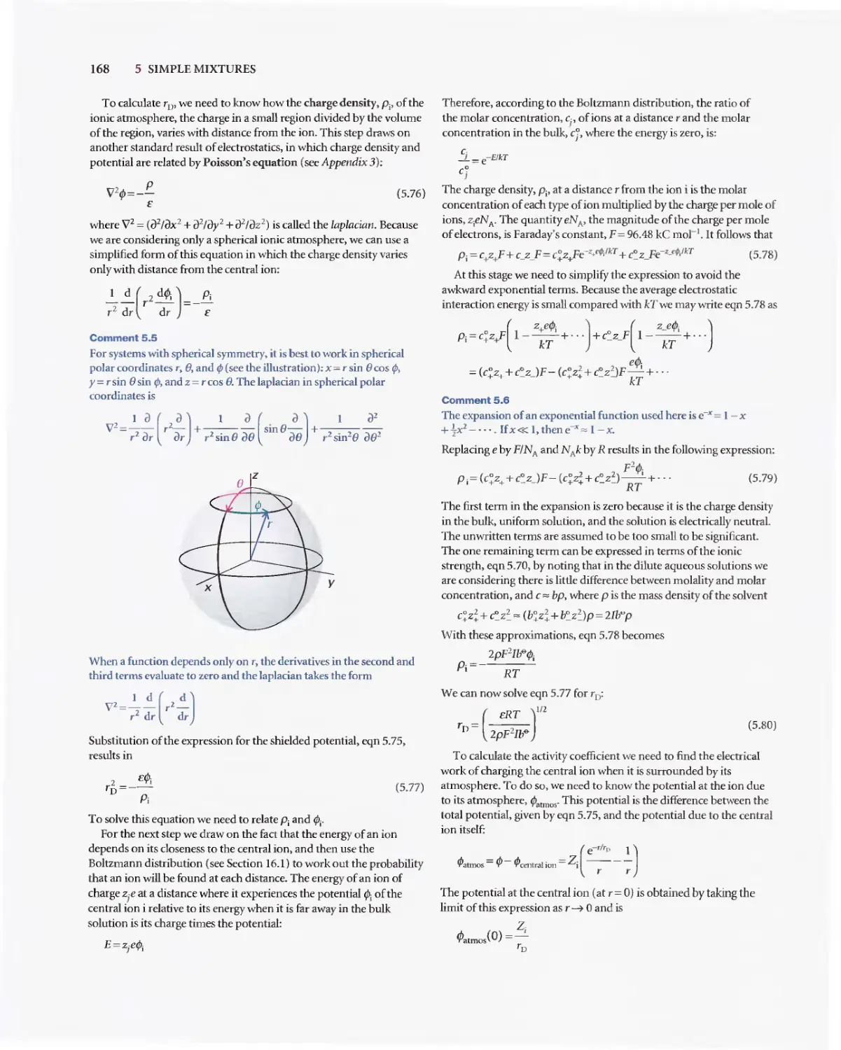
Further information 5.1 The Debye-HOckef theory of romc
solutJons
Imagine a solution in which all the ions have their acmal positions.
but in which tbrir Coulombic intcl4ctions have
n turned off. The
difference in molar Gibbs energy betwem the ideal and real solutions
is equa1 to we the electrical work of charging. the system in this
arrangement. For a salt M"xq' we write
C'
w
=(pjJ+ +qJ1J- (pJ.l
daJ+qJl
da.l)
=p{p+ -Jl:
)+q(J.l_ -Jl
)
From cqn 5.64 we write
J4 - J1
dnI=11- -Jl
deaJ.=RTln r...
So it follows that
In r I = s;
s=p+q
This equation tells us that we must first find the final distribution of
the ions and then the work of charging them in that distribution.
The Coulomb potential at a distance r from an isol
ted ion of
charge z,e in a medium of permittivity E is
j=
2j= :
:
The ionic atmosphere causes the potential to decay with distdnce
more sharply than this expres5ion implies. Such shielding is a familiar
problem in electrostatics, and its effect is taken into account by
replacing the Coulomb potential by the shielded Coulomb potential.
an expression of the form
z
iP;=-;-e- 1rD
where r D is called tbe Debye length. W
potential is virtually the same a5 the un
small. the shielded potential is much s
potential, even for short distances (Fig
1.0
0.8
:?>
NO.6
'i<
(5.73)
:!!!
OA
.1"
0.2
00
(5.74)
(5.75)
Flg.5.36 The vanation of the shielded
distance for different values of the Deb
Debye length. the more sharply the pot
case. a is an arbitrary unit oflength.
lki. =;
:;:d :
t:
I
:r
:;
Then plot this expression against r D an
interpretation for the shape of me plot
966 Appendix2 MATHEMATICAL TECHNIQUES
A2.6 Partial derivatives
A partial derivative of a functlOn of more than one variabl
of the function with respect to one of the variables. aU th
constant (see Fig. 2.>1). Although a partiaI derivative sho
when one variable changes, it may be used to ddermine
when more than one variable changes by an infinitesima)
tion ofxandy, then when x andy change bydxand dy. re
df=(
ldx+(
ldY
where the symbol a is used (instead of d) to denote a part
dfis aJso caJled the differential off For example. iff = ax'
( !!. ) = 3ax'y ( !!. )
ax' + 2by
ax y ay x
--
1000 DATA SECTION
Table 2.8 Expansion coefficients, a, and isothermal
compressibilities. Kr
a/(lO-"K-I) K T /(1O- fi Btm- l )
liquids
B
nzem 12.4 92_1
Carbon tctrachlonde 11_4 90.5
Ethanol 11.2 76.8
M
rcul}' 1.82 35.7
Wat(r 2.t 4'.6
Solids
Copper 0.501 0_735
Diamond 0.030 0_187
Iron 0.354 0.589
I.e.d 0_861 2.21
Theva]u(sr(fcrto2O"C..
Data: AJP(aJ. KL(KTt
Table 2.9 Inversion temperatures, n
points, and Jome-Thomson coefficicn
T./K T,/K
All 603
","on 713 83.8
Carbon dioxid( 1500 194.7s
Helium 4{J
Hydrogen 202 14.0
Kryplon 1090 116.6
Methane 968 90.6
N
n 231 24S
Nitrogm 6zt 633
Oxygen 764 54.8
s:subhmes..
Dat:r: AlP.JL,andM.W_Zemansky, H(lIr and
NewYork(1957J_
Further information
In some cases, we have judged that a derivation is too long,
too detailed, or too different in level for it to be included
in the text. In these cases, the derivations will be found less
obtrusively at the end of the chapter.
Appendices
Physical chemistry draws on a lot of background material, espe-
cially in mathematics and physics. We have included a set of
Appendices to provide a quick survey of some of the informa-
tion relating to units, physics, and mathematics that we draw
on in the text.
Synoptic tables and the Data section
Long tables of data are helpful for assembling and solving
exercises and problems, but can break up the flow of the text.
We provide a lot of data in the Data section at the end of the
text and short extracts in the Synoptic tables in the text itself to
give an idea of the typical values of the physical quantities we
are introducing.
Mathematics and Physics support
Comment 1.2
A h""pcrbola is a curve obtainrd by
plouingyagainst.\. withxy=coDstanl.
Comment 2.5
The partial-diffcTcntial operation
(n::::/dx),_ consists oftaking the fust
deriutive of .:::(x.y} "ltb respect to x,
trcatingyas a constant. For example,
if z(x.y) =x 2 y. then
[ dz J ( d(X'YI dx'
a; = ----a;- J =y dx =2yx
Partial derivatives ace revie\ved in
Appelldix 2.
978
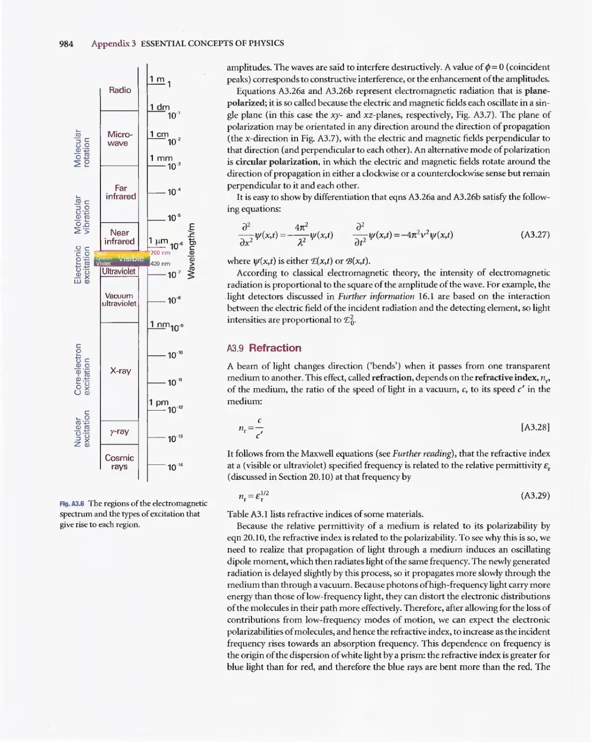
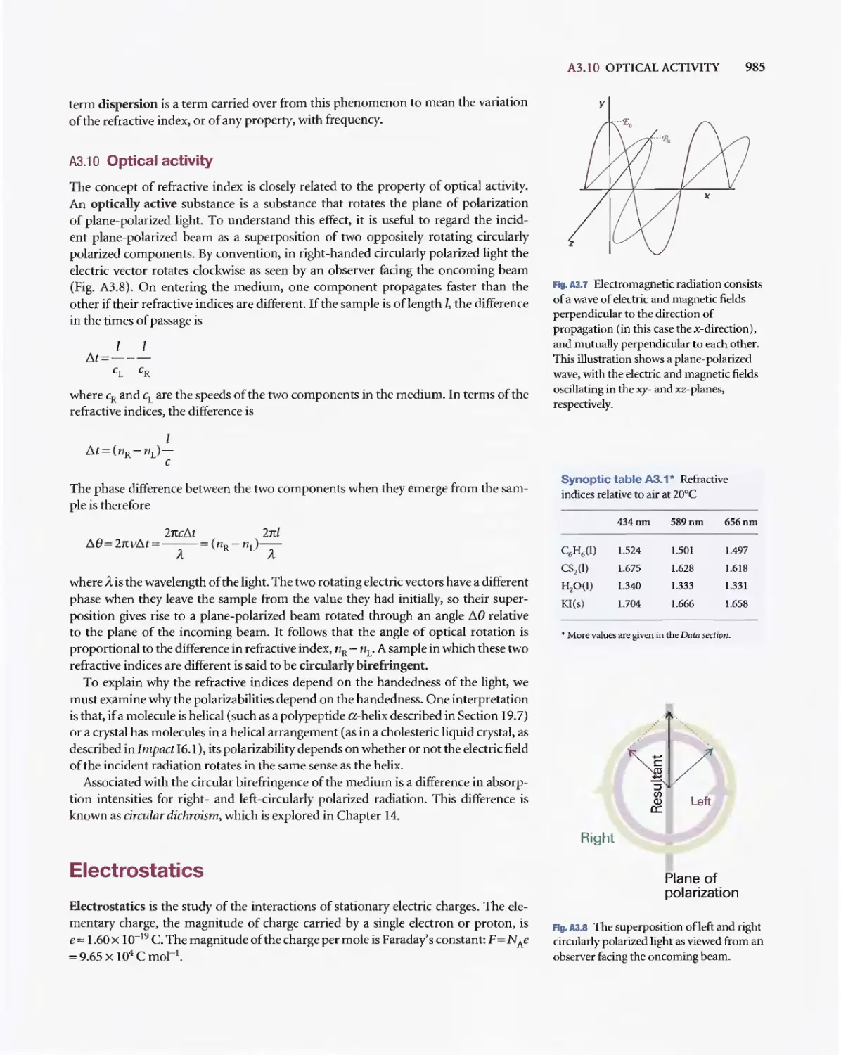
Appendix 3 ESSENTIAL CONCEPTS OF PHYSICS
Classical mechanics
fJ,
Classical mechanics describes the behaviour of objects in
expresses the fact that the total energy is constant in the a
other expresses the response of particles to the forces act
..p
A3.3 The trajectory in terms of the energy
P.
The velocity. v. of a partIcle IS the rate of change of its p
dr
v=-
d,
fJ
The velocity is a vector, WIth both direction and magn'
velocity is the speed. 1'_ The linear momentum, p. of a p
its velocity. v. by
13.1 The linear momentum of a particle IS
a vector property and points in th.:=
direction of motion.
p=mv
Like the velocity vector. the linear momentum vector po
of the particle (Fig. AJ.I). In terms of the linear moment
tide is
Problem solving
Illustration 5.2 Using Henry's Jaw
To estimate the molar solubihty of oxygen in water at 25 c C and a partial pressure
vf21 kPa, its partial pressure in the atmosphere at sea level, we write
b Po. 21 kPa 2.9 X 10⁻⁴ mol kg-I
0, K o , 7.9x lo'kPakgmol I
The molality of the saturated solution is therefore 0.29 mmol kg-I. To convert this
quantity to a molar concentration. we assume that the masS density of this dilute
solution is essentially that of pure water at 25 c C. or PH.O = 0.99709 kg dm- 3 . It fol-
lows that the molar concentration of oxygen is
[02] = b o . x PHp =0.29 mmol kg-I x 0.99709 kg dm- 3 = 0.29 mmol dm- 3
A note on good practice The number of significant ngures in the result of a calcu-
lation shouId not exceed the number in the data (only two in this case).
Self-test 5.5 Calculate the molar solubility of nitrogen in water exposed to air at
25 c C; partial pressures were cakwated in Example 1.3. [0.51 mmol dm- J ]
ABOUT THE BOOK JOll
Comments
A topic often needs to draw on a mathematical procedure or a
concept of physics; a Comment is a quick reminder of the pro-
cedure or concept.
Appendices
There is further information on mathematics and physics in
Appendices 2 and 3, respectively. These appendices do not go
into great detail, but should be enough to act as reminders of
topics learned in other courses.
Illustrations
An Illustration (don't confuse this with a diagram!) is a short
example of how to use an equation that has just been intro-
duced in the text. In particular, we show how to use data and
how to manipulate units correctly.
v ABOUT THE BOOK
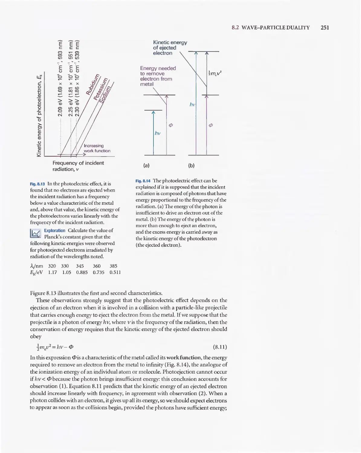
Example 8.1 Ca/cu/atlng the number of photons
Calculate the number of photons enutted bya 100 W yeUow lamp in LOs. Take the
wavelength of yellow light as 560 nm and assume 100 per cent efficiency.
Method Each photon has an energy hv, so the rota) number of photons needed to
produce an energy E is Elhv. To use this equation. we need to know the frequency
of the radiation (from v= cJ.:1.) and the total energy emitted by the lamp. The latter
is given by the product of the power (P, in watts) and the time interval for which
the lamp is turned on (E=Pllt).
Answer The number of photons is
E PI>., API>.,
N=-=-=-
hv hle/).) he
Substitution of the data gives
(5.60 x 10- 7 m) x (100 / s-.) x (1.0 s)
N (6.626x1O-"/s)x(2.998x1O s ms-')
2.8 X 10 20
Note that it wou1d take nearly 40 min to produce I mol of these photons.
A note on good practice To avoid rounding and other numerical errors, it is best
to carry out algebraic mainpulations first, and to substitute numerical values into
a single, final formula. Moreover, an analytical result may be used for other data
without having to repeat the entire calculation.
Self-test 8.1 How many photons does a monochromatic (single frequency)
infrared rangefinder of power 1 mW and wavdength 1000 nm emit in 0.1 s?
[5X10 14 ]
Self-test 3.12 Calcu1ate the change in GIn for ice at -UfC, with density 917 kg m- 3 .
when the pressure is increased from 1.0 bar to 2.0 bar. [+2.0 J mol-I]
-
Discussion questions
1.1 Explain bow th
perfect gasequation ofstal
ar]ses bycombmation of
BO}'lco's law. Charles's law. andAvogadro's principle.
1.4 \\'11atistl1esignificanceoftbecrilicil
1.5 Describe tl1e formulation oftl1evan de
rationale for one otl1er equation of state in
1.6 Explain 11(n'ltnevan cler Waa1s e'juati
hehaviour.
1.2 Explain the term 'paniaJ pressurc' and explain why Dalton's law is a
lIrnitmglaw.
1.3 Exp]ain huw the compression factor varies with pressure and temperature
and clescrlbe how it reveals information about intermolecular inleradions in
real gases.
Worked examples
A Worked example is a much more structured form of
Illustration, often involving a more elaborate procedure. Every
Worked example has a Method section to suggest how to set up
the problem (another way might seem more natural: setting up
problems is a highly personal business). Then there is the
worked-out Answer.
Self-tests
Each Worked example, and many of the Illustrations, has a Self-
test, with the answer provided as a check that the procedure has
been mastered. There are also free-standing Self-tests where we
thought it a good idea to provide a question to check under-
standing. Think of Self-tests as in-chapter Exercises designed to
help monitor your progress.
Discussion questions
The end-of-chapter material starts with a short set of questions
that are intended to encourage reflection on the material and
to view it in a broader context than is obtained by solving nu-
merical problems.
Exercises
14.1a Tbeterm symbol for the groundstatc: ofN; iSlE," What is tbetotal
spin and total orbital angular momentum of the molecule? Show that tbeterm
symbol agrees wi.th the elcctron configuration that would be predicted using
the building-up principle.
14.1b One ofthe excited states ofthe C z molecule has the valc:m:c: electron
configuratIOn la
lO'.
l1r
l1r
. Give the multiplicity and panty oflhe term.
14.2a The: molar absorption coeffi(Jcnt of a substance dissolved in hexane is
known to be 855 dm) mol-I em-I at 270 nm. Calculate thl:' percentage
reduction in intensity when lIghtoftbatwavdc:ngth passes through 2_5 nun of
asolution of concentration 3.25 mmol dnC'.
14.2b The molar absorption coefficient of a substance dissolved in hexane is
known to be: 3D dm) mor l em-I at300 nm. Calcu1atc the percentage
roouctlOnm lDtc'nsitywhen light oftbslwavelength passes tbrougb L50 mm
oh. solution ofconcenuation 2..22 mmol dnC'.
14.3a A solulion of an unknown component of a biological sample when
placed in an absorption cell of path length LOOcm transmits 20.1 per cent of
lightof340 om incident upon it. Iftheconcenuation of the component is
0.111 mmoldnC', what is the molarabsorplion coefficient?
14.3b When light ofwavdcngth 400 nm passes through 3.S mID of a solutIOn
of an absorbing substance at a concentration 0.667 mmol dnC', the
transmission is 65.5 per cent. Calculate the molar absorption codfiaentol the
solute at this wavelength and express the answer in cm 2 mol-[.
Problems
A55ume aU gases are perfect umessstatcd otherwi.se. Note that 1 atm=
].013 25 bar. Unless otherwise stated. thennoche-mlca] data are for 298.15 K.
Numerical problems
2.1 A sampleconslSling of I mol of perfect gasatoms (for which
C".m = {oR) is taken through tbeqcle shown in Fig. 2 34. (a.) Determine the
lemperarureal the points I, 2. and 3. (b) Calcu1ateq, w, AU, andAH for each
step and for theoverall c:ycIc. If a numerical answer cannot be obtained from
the information given. then write in +, -, O. or? asappropriale.
E too
E
f!!
"- 0.50
1 2
\-::1 ,
22.44 44.88
Volume, Vldm:J
....2.34
2.2 A sample consistingofLO mol CaCO,(s) was heated to800"C, when it
decomposed. The heating was carried out ma container fined with a piston
that was initially resting on the solld_ Calculate the work done during
completedccomposition at LO am. Whatwork would be done ifinstead of
having a piston the container was open to the atmosphne 1
w
£",..
.0
;;:
8
"
o
E.
g
.g
..
o
:;;
.(V)
...{1
Wavenum
.........
14.7b The foUowmgdata were obtamed for
in methylbenzene using a 2.50 mm cell. Cat
coefficient of the dye at th
wavekngth
mpl
(dyeJ/(mul dm-') 0.0010 0.0050 o.
T/(percent) 73 21 4.
Table 2.2. Calculate: the standard enthalpy
from liS value at 298 K.
2.8 A sample of the sugar D-ribosc (
HI
in a ca]orimeter and tben ignited in tbe p
temperature rose byO.91O K.ln a upar
t('
tbe- combustion of 0.825 g of benzoic acid,
combusuon IS -3251 kJ mor l , gave a ten
tbe inlernal energy of combustion of D .
2.9 T
slandardentbalpyoffonnationof
bis(benzmdchromium was measured in a
reaction Cr(C 6 H 6 h(s)
Cr(s) + 2 C6H
(8)
Find the correspondmg reaction enthalpy a
of Cormation of the compound at 583 K.
heat capacity of benzene is 136.1 J K- 1 mol-
81.67JK- 1 mol-' asa gas.
2.1ot From the enthaJpy of combustion da
alkanes methane tlrrough octane, test the e
tJ...H.""kl(M/(g mol-I))" hol.ds and find the
Predict l!1)f.fordecane and compare totb
2.11 It is possible to invatigate the thenna
hydrocarbons with molecular modelling m
software to praltct .A)t.ValUICS for tbe
calculate .A)t.valUICS, c:5timate the 5
C..H!'II+II(g) byperforming semi-m1pirical
or PM3 methods) and usccxperimental
values forCO!(g) and H!O(l). (b) Comp"
experimental values of .A)t.(Table 2.5)
the molecular modellmg method. (c) Test
/Vf.=kj(MJ(gmol-I)I" hol.dsand find the
ABOUT THE BOOK
:v.....
Exercises and Problems
The real core of testing understanding is the collection of end-
of-chapter Exercises and Problems. The Exercises are straight-
forward numerical tests that give practice with manipulating
numerical data. The Problems are more searching. They are di-
vided into 'numerical', where the emphasis is on the manipu-
lation of data, and 'theoretical', where the emphasis is on the
manipulation of equations before (in some cases) using nu-
merical data. At the end of the Problems are collections of
problems that focus on practical applications of various kinds,
including the material covered in the Impact sections.
About the Online Resource Centre
The Online Resource Centre provides teaching and learning resources. It is free of
charge, complements the textbook, and offers additional materials which can be
downloaded. The resources it provides are fully customizable and can be incorpor-
ated into a virtual learning environment. Go to:
www.oxfordtextbooks.co.ukJorc/pchem8e/
I Seilrchlhlssde
I:1Im:! .,. axma:r. ,AiIr.....AdeflIUlr.PnpKIIIC'-'-try.1e
n:lAd!lPw..ooo-_
"-""..
'DUD ThRrIrv-TatllP-S
EJ
online
resource
centre
Atkins & de Paula: Physical Chemistry: Be
s.e.o:hf9r"Or*-
R"-""WI'oeCcnr"
Studeont resou en:
L
8b:I<!
(:erfr""
--"*"
RMcuceCerVe
/Yf'hLm" -
--...........
,....
Lecturer mourcn
L8mJIIIDOIjTntBerts
.....
---->mi
" About the book
lJ!:am mom aboutlhe bOok
....--
....-
....,....,.
-..
.. COn!alnSm!l!!rat1IW!lIIaII'II:ad8WOJ'1CSneetsan(liEJlte.
kS.£ompieI2W11h
SIIfllUlalnghln:ISKS(llrIals"ltents'
,* I1JIJS
1J1l r Pdt;
_9rlphk$."'swnuta1lonpararnet8t';.an(l$o"",eqU1llromID9iIInd9l!PVrin
ltIklp¥l
alltft"rllsn Nen.h
InclUdedwllhPUfthase oflnele'Xlllrougnlleu!l!'oflhe atIiVaIioncode
rd IncluHdwltl Ff&t3k81
nJISoy8e
!J'rqp11i!'(UlItwrt
n-d.I1!JW
""""
Stnd..t'tU
PhyslealO
L r. r "" 'I Th cr < ,
F'" "
.......
.. AnonilnewersJOnflllheklUbook. ThtebookPrOndl'l.nthteilnW\geqJeri9ncelWtillQngful
or"'Nehnkmldlum
Aueum"'eI!ook"IIICIUcledv.eIPl,ftha..fIl"'1PI1tvougtI"'useof1headwatM'ode'IItrCIIfICIucIe(IWII'I
/
..
......rd<!...h......,
,........Irao.
«tM:I
.-.
0eI.hi:te1'DF1'DDdor
IKililB
Ii I(PPD m p U D d a t PdabDut
Ihi>..1ib:
-::
=
;::.'"
dolS......ft...-..c.c:_..
Si..,Iy.....1I>c....II.
6e"""
a....
.Il_'
..
",-.f.,
The material includes:
Living graphs
A Living graph is indicated in the text by the icon I b{ attached
to a graph. This feature can be used to explore how a property
changes as a variety of parameters are changed. To encourage
the use of this resource (and the more extensive Explorations in
Physical Chemistry) we have added a question to each figure
where a Living graph is called out.
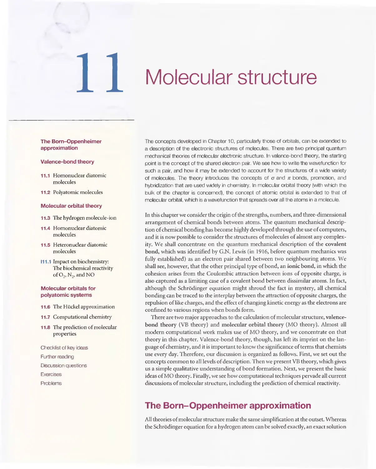
IUB The boundary surfaces of II orbitals.
Two nodal planes in each orbital intersect
at the nucleus and separate the Iobes of
each orbitaL The dark and light areas
denote regions of opposite sign ofthe
wavcfunction.
11.
Exploration To gain insight into the
shapesoftheforbitals.use
mathematical software to plot the
boundary surfaces ofthe spherical
harmonics Y'.m.( e,tp).
......
-.Y
x/
d..
d.,,>
.
/"
d q
d
d
Artwork
An instructor may wish to use the illustrations from this text
in a lecture. Almost all the illustrations are available and can
be used for lectures without charge (but not for commercial
purposes without specific permission). This edition is in full
colour: we have aimed to use colour systematically and help-
fully, not just to make the page prettier.
Tables of data
All the tables of data that appear in the chapter text are avail-
able and may be used under the same conditions as the figures.
Web links
There is a huge network of information available about phys-
ical chemistry, and it can be bewildering to find your way to
it. Also, a piece of information may be needed that we have
not included in the text. The web site might suggest where to
find the specific data or indicate where additional data can be
found.
Group theory tables
Comprehensive group theory tables are available for down-
loading.
Explorations in Physical Chemistry
Physical chemistry describes the dynamic processes that shape
the world around us; it is far removed from the perception of
abstract theories and relationships held by so many students.
But how can students make the jump from abstract equation
to the reality of physical chemistry in action? Explorations in
Physical Chemistry offers a unique way to bring physical chem-
istry to life.
Explorations in Physical Chemistry consists of interactive
Mathcad@ worksheets and interactive Excel@ workbooks,
complete with thought-stimulating exercises. They motivate
students to simulate physical, chemical, and biochemical phe-
nomena with their personal computers. Harnessing the com-
putational power of Mathcad@ by Mathsoft, Inc. and Excel@
by Microsoft Corporation, students can manipulate over 75
graphics, alter simulation parameters, and solve equations to
gain deeper insight into physical chemistry.
Explorations in Physical Chemistry is available on-line
at www.oxfordtextbooks.co.uk/orc/explorations/.using the
activation code card included with Atkins' Physical Chemistry
8e.1t can also be purchased as a CD-ROM (978-019-928894-6).
Physical Chemistry, Eighth Edition eBook
A complete online version of the textbook. The eBook pro-
vides a rich learning experience by taking full advantage of the
ABOUT THE ONLINE RESOURCE CENTRE XVll
electronic medium integrating all student media resources
and adds features unique to the eBook. The eBook also offers
lecturers unparalleled flexibility and customization options
not previously possible with any printed textbook. Access to
the eBook is included with purchase of the text through the
use of the activation code card included with Atkins' Physical
Chemistry 8e.
Key features of the eBook include:
. Easy access from any Internet -connected computer via a
standard Web browser.
. Quick, intuitive navigation to any section or subsection,
as well as any printed book page number.
. Integration of all Living Graph animations.
. Text highlighting, down to the level of individual phrases.
. A book marking feature that allows for quick reference to
any page.
. A powerful Notes feature that allows students or instruc-
tors to add notes to any page.
. A full index.
. Full-text search, including an option to also search the
glossary and index.
. Automatic saving of all notes, highlighting, and bookmarks.
Additional features for lecturers:
. Custom chapter selection: Lecturers can choose the chap-
ters that correspond with their syllabus, and students will
get a custom version of the eBook with the selected chap-
ters only.
. Instructor notes: Lecturers can choose to create an
annotated version of the eBook with their notes on any
page. When students in their course log in, they will see
the lecturer's version.
. Custom content: Lecturer notes can include text, web
links, and even images, allowing lecturers to place any
content they choose exactly where they want it.
Solutions manuals
As with previous editions, Charles Trapp, Carmen Giunta,
and Marshall Cady have produced the solutions manuals to
accompany this book. A Student's Solutions Manual (978-019-
928858-8) provides full solutions to the 'a' exercises and the
odd-numbered problems. An Instructor's Solutions Manual
(978-019-928857-1) provides full solutions to the 'b' exercises
and the even-numbered problems.
About the authors
o -
-
Julio de Paula is Professor of Chemistry and Dean of the College of Arts & Sciences at
Lewis & Clark College. A native of Brazil, Professor de Paula received a B.A. degree in
chemistry from Rutgers, The State University of New Jersey, and a Ph.D. in biophys-
ical chemistry from Yale University. His research activities encompass the areas of
molecular spectroscopy, biophysical chemistry, and nanoscience. He has taught
courses in general chemistry, physical chemistry, biophysical chemistry, instrumental
analysis, and writing.
.-
iF
. -,
,..1.
-,1'...
",'it'
Peter Atkins is Professor of Chemistry at Oxford University, a fellow of Lincoln
College, and the author of more than fifty books for students and a general audience.
His texts are market leaders around the globe. A frequent lecturer in the United States
and throughout the world, he has held visiting prefessorships in France, Israel, Japan,
China, and New Zealand. He was the founding chairman of the Committee on
Chemistry Education of the International Union of Pure and Applied Chemistry and
a member ofIUPAC's Physical and Biophysical Chemistry Division.
Acknowledgements
A book as extensive as this could not have been v,'Yitten without
significant input from many individuals. We would like to reiterate
our thanks to the hundreds of people who contributed to the first
seven editions. Our warm thanks go Charles Trapp, Carmen Giunta,
and Marshall Cady who have produced the Solutions manuals that
accompany this book.
Many people gave their advice based on the seventh edition, and
others reviewed the draft chapters for the eighth edition as they
emerged. We therefore wish to thank the following colleagues most
warmly:
Joe Addison, Governors State University
Joseph Alia, University of Minnesota Morris
David Andrews, University of East Anglia
Mike Ashfold, University of Bristol
Daniel E. Autrey, Fayetteville State University
Jeffrey Bartz, Kalamazoo College
Martin Bates, University of Southampton
Roger Bickley, University of Bradford
E.M. Blokhuis, Leiden University
Jim Bowers, University of Exeter
Mark S. Braiman, Syracuse University
Alex Brown, University of Alberta
David E. Budil, Northeastern University
Dave Cook, University of Sheffield
Ian Cooper, University of Newcastle-up on- Tyne
T. Michael Duncan, Cornell University
Christer Elvingson, Uppsala University
Cherice M. Evans, Queens College-CUNY
Stephen Fletcher, Loughborough University
Alyx S. Frantzen, Stephen F. Austin State University
David Gardner, Lander University
Roberto A. Garza-Lopez, Pomona College
Robert 1- Gordon, University of Illinois at Chicago
Pete Griffiths, Cardiff University
Robert Haines, University of Prince Edward Island
Ron Haines, University of New South Wales
Arthur M. Halpern, Indiana State University
Tom Halstead, University of York
Todd M. Hamilton, Adrian College
Gerard S. Harbison, University Nebraska at Lincoln
UlfHenriksson, Royal Institute of Technology, Sweden
Mike Hey, University of Nottingham
Paul Hodgkinson, University of Durham
Robert E. Howard, University of Tulsa
Mike Jezercak, University of Central Oklahoma
Clarence Josefson, Millikin University
Pramesh N. Kapoor, University of Delhi
Peter Karadakov, University ofY ork
Miklos Kertesz, Georgetown University
Neil R. Kestner, Louisiana State University
Sanjay Kumar, Indian Institute of Technology
reffry D. Madura, Duquesne University
Andrew Masters, University of Manchester
Paul May, University of Bristol
Mitchell D. Menzmer, Southwestern Adventist University
David A. Micha, University of Florida
Sergey Mikhalovsky, University of Brighton
Jonathan Mitschele, Saint Joseph's College
Vicki D. Moravec, Tri-State University
Gareth Morris, University of Manchester
Tony Morton-Blake, Trinity College, Dublin
Andy Mount, University of Edinburgh
Maureen Kendrick Murphy, Huntingdon College
John Parker, Heriot Watt University
JozefPeeters, University ofLeuven
Michael J. Perona, CSU Stanislaus
Nils-Ola Persson, Link6ping University
Richard Pethrick, University ofStrathclyde
John A. Pojman, The University of Southern Mississippi
Durga M. Prasad, University of Hyderabad
Steve Price, University College London
S. Rajagopal, Madurai Kamaraj University
R. Ramaraj, Madurai Kamaraj University
David Ritter, Southeast Missouri State University
Bent Ronsholdt, Aalborg University
Stephen Roser, University of Bath
Kathryn Rowberg, Purdue University Calumet
S.A. Safron, Florida State University
Kari Salmi, Espoo-Vantaa Institute of Technology
Stephan Sauer, University of Copenhagen
Nicholas Schlotter, Hamline University
Roseanne J. Sension, University of Michigan
A.J. Shaka, University of California
Joe Shapter, Flinders University of South Australia
Paul D. Siders, University of Minnesota, Duluth
Harjinder Singh, Panjab University
Steen Skaarup, Technical University of Denmark
David Smith, University of Exeter
Patricia A. Snyder, Florida Atlantic University
Olle Soderman, Lund University
Peter Stilbs, Royal Institute of Technology, Sweden
Svein Stolen, University of Oslo
Fu-Ming Tao, California State University, Fullerton
Eimer Tuite, University of Newcastle
Eric Waclawik, Queensland University of Technology
Y an Waguespack, University of Maryland Eastern Shore
Terence E. Warner, University of Southern Denmark
xx ACKNOWLEDGEMENTS
Richard Wells, University of Aberdeen
Ben Whitaker, University of Leeds
Christopher Whitehead, University of Manchester
Mark Wilson, University College London
Kazushige Yokoyama, State University of N ew York at Geneseo
Nigel Young, University of Hull
Sidney H. Young, University of South Alabama
We also thank Fabienne Meyers (ofthe IUPAC Secretariat) for help-
mg us to bring colour to most of the illustrations and doing so on a
very short timescale. We would also like to thank our two publishers,
Oxford University Press and W.H. Freeman & Co., for their constant
encouragement, advice, and assistance, and in particular our editors
Jonathan Crowe, Jessica Fiorillo, and Ruth Hughes. Authors could
not wish for a more congenial publishing environment.
Summary of contents
PART 1 Equilibrium 1
1 The properties of gases 3
2 The First Law 28
3 The Second Law 76
4 Physical transformations of pure substances 117
5 Simple mixtures 136
6 Phase diagrams 174
7 Chemical equilibrium 200
PART 2 Structure 241
8 Quantum theory: introduction and principles 243
9 Quantum theory: techniques and applications 277
10 Atomic structure and atomic spectra 320
11 Molecular structure 362
12 Molecular symmetry 404
13 Molecular spectroscopy 1 : rotational and vibrational spectra 430
14 Molecular spectroscopy 2: electronic transitions 481
15 Molecular spectroscopy 3: magnetic resonance 513
16 Statistical thermodynamics 1 : the concepts 560
17 Statistical thermodynamics 2: applications 589
18 Molecular interactions 620
19 Materials 1 : macromolecules and aggregates 652
20 Materials 2: the solid state 697
PART 3 Change 745
21 Molecules in motion 747
22 The rates of chemical reactions 791
23 The kinetics of complex reactions 830
24 Molecular reaction dynamics 869
25 Processes at solid surfaces 909
Appendix 1 : Quantities, units and notational conventions 959
Appendix 2: Mathematical techniques 963
Appendix 3: Essential concepts of physics 979
Data section 988
Answers to exercises 1028
Answers to problems 1040
Index 1051
Contents
PART 1 Equilibrium
1 The properties of gases
The perfect gas
1.1 The states of gases
1.2 The gas laws
11.1 Impact on environmental science: The gas laws
and the weather
Real gases
1.3 Molecular interactions
1.4 The van der Waals equation
1.5 The principle of corresponding states
Checklist of key ideas
Further reading
Discussion questions
Exercises
Problems
2 The First Law
The basic concepts
2.1 Work, heat, and energy
2.2 The interna] energy
2.3 Expansion work
2.4 Heat transactions
2.5 Enthalpy
12.1 impact on biochemistry and materials science:
Differential scanning calorimetry
2.6 Adiabatic changes
Thermochemistry
2.7 Standard enthalpy changes
12.2 Impact on biology: Food and energy reserves
2.8 Standard enthalpies of formation
2.9 The temperature-dependence of reaction enthalpies
State functions and exact differentials
2.10 Exact and inexact differentials
2.11 Changes in internal energy
2.12 The Joule-Thomson effect
Checklist of key ideas
Further reading
Further information 2.1 : Adiabatic processes
Further information 2.2: The relation between heat capacities
1
Discussion questions
Exercises
Problems
3
3
3
7
3 The Second Law
76
L I
The direction of spontaneous change
3.1 The dispersal of energy
3.2 Entropy
13.1 Impact on engineering: Refrigeration
3.3 Entropy changes accompanying specific processes
3.4 The Third Law of thermodynamics
14
14
17
21
Concentrating on the system
3.5 The Helmholtz and Gibbs energies
3.6 Standard reaction Gibbs energies
23
23
23
24
25
Combining the First and Second Laws
3.7 The fundamental equation
3.8 Properties of the internal energy
3.9 Properties of the Gibbs energy
28
Checklist of key ideas
Further reading
Further information 3.1: The Born equation
Further information 3.2: Real gases: the fugacity
Discussion questions
Exercises
Problems
28
29
30
33
37
40
46
47
4 Physical transformations of pure substances
49
49
52
54
56
Phase diagrams
4.1 The stabilities of phases
4.2 Phase boundaries
14.1 Impact on engineering and technology:
Supercritical fluids
4.3 Three typical phase diagrams
57
57
59
63
Phase stability and phase transitions
4.4 The thermodynamic criterion of equilibrium
4.5 The dependence of stability on the conditions
4.6 The location of phase boundaries
4.7 The Ehrenfest classification of phase transitions
67
68
69
69
Checklist of key ideas
Further reading
Discussion questions
70
70
73
77
77
78
85
87
92
94
95
100
102
102
103
105
109
110
110
111
112
113
114
117
117
117
118
119
120
122
122
122
126
129
131
132
132
xxiv CONTENTS
Exercises
Problems
5 Simple mixtures
132 7 Chemical equilibrium 200
133
Spontaneous chemical reactions 200
136 7.1 The Gibbs energy minimum 200
7.2 The description of equilibrium 202
136 The response of equilibria to the conditions 210
136 How equilibria respond to pressure
7.3 210
141
7.4 The response of equilibria to temperature 211
143
17.1 Impact on engineering: The extraction
of metals from their oxides 215
147
148 Equilibrium electrochemistry 216
148 7.5 Half-reactions and electrodes 216
150 7.6 Varieties of cells 217
7.7 The electromotive force 218
156 7.8 Standard potentials 222
7.9 Applications of standard potentials 224
158 17.2 Impact on biochemistry: Energy conversion
158 in biological cells 225
159
162 Checklist of key ideas 233
163 Further reading 234
Discussion questions 234
166 Exercises 235
167 Problems 236
167
169 PART 2 Structure
169 241
171
8 Quantum theory: introduction and principles 243
174
The origins of quantum mechanics 243
174 8.1 The failures of classical physics 244
174 8.2 Wave-particle duality 249
176 18.1 Impact on biology: Electron microscopy 253
179 The dynamics of microscopic systems 254
179 8.3 The Schrodinger equation 254
182 8.4 The Born interpretation of the wavefunction 256
185
189 Quantum mechanical principles 260
191 8.5 The information in a wavefunction 260
8.6 The uncertainty principle 269
192 8.7 The postulates of quantum mechanics 272
193 Checklist of key ideas 273
194 Further reading 273
194 Discussion questions 274
195 Exercises 274
197 Problems 275
The thermodynamic description of mixtures
5.1 Partial molar quantities
5.2 The thermodynamics of mixing
5.3 The chemical potentials ofliquids
15.1 Impact on biology: Gas solubility and
breathing
The properties of solutions
5.4 Liquid mixtures
5.5 Colligative properties
15.2 Impact on biology: Osmosis in physiology
and biochemistry
Activities
5.6 The solvent activity
5.7 The solute activity
5.8 The activities of regular solutions
5.9 The activities ofions in solution
Checklist of key ideas
Further reading
Further information 5.1 : The Debye-Huckel theory
of ionic solutions
Discussion questions
Exercises
Problems
6 Phase diagrams
Phases, components, and degrees of freedom
6.1 Definitions
6.2 The phase rule
Two-component systems
6.3 Vapour pressure dIagrams
6.4 Temperature-composition diagrams
6.5 Liquid-liquid phase diagrams
6.6 Liquid-solid phase diagrams
16.1 Impact on materials science: Liquid crystals
16.2 Impact on materials science: Ultrapurity
and controlled impurity
Checklist of key ideas
Further reading
Discussion questions
Exercises
Problems
9 Quantum theory: techniques and applications
277
Translational motion
9.1 A particle in a box
9.2 Motion in two and more dimensions
9.3 Tunnelling
19.1 Impact on nanoscience: Scanning
probe microscopy
Vibrational motion
9.4 The energy levels
9.5 The wavefunctions
Rotational motion
9.6 Rotation in two dimensions: a particle on a ring
9.7 Rotation in three dimensions: the particle on a
sphere
19.2 Impact on nanoscience: Quantum dots
9.8 Spin
Techniques of approximation
9.9 Time-independent perturbation theory
9.10 Time-dependent perturbation theory
Checklist of key ideas
Further reading
Further information 9.1: Dirac notation
Further information 9.2: Perturbation theory
Discussion questions
Exercises
Problems
10 Atomic structure and atomic spectra
The structure and spectra of hydrogenic atoms
10.1 The structure of hydro genic atoms
10.2 Atomic orbitals and their energies
10.3 Spectroscopic transitions and selection rules
The structures of many-electron atoms
10.4 The orbital approximation
10.5 Self-consistent field orbitals
The spectra of complex atoms
110.1 Impact on astrophysics: Spectroscopy of stars
10.6 Quantum defects and ionization limits
10.7 Singlet and triplet states
10.8 Spin-orbit coupling
10.9 Term symbols and selection rules
Checklist of key Ideas
Further reading
Further information 10.1: The separation of motion
Discussion questions
Exercises
Problems
277
278
283
286
290
291
292
297
297
301
306
308
310
310
311
312
313
313
313
316
316
317
320
320
321
326
335
336
336
344
345
346
346
347
348
352
356
357
357
358
358
359
CONTENTS xxv
11 Molecular structure
362
The Born-Oppenheimer approximation
Valence-bond theory
11.1 Homonuclear diatomic molecules
11.2 Polyatomic molecules
288
Molecular orbital theory
11.3 The hydrogen molecule-ion
11.4 Homonuclear diatomic molecules
11.5 Heteronuclear diatomic molecules
111.1 Impact on biochemistry: The
biochemical reactivity of O 2 , N 2 , and NO
Molecular orbitals for polyatomic systems
11.6 The Hiickel approximation
11.7 Computational chemistry
11.8 The prediction of molecular properties
Checklist of key ideas
Further reading
Discussion questions
Exercises
Problems
12 Molecular symmetry
362
363
363
365
368
368
373
379
385
386
387
392
396
398
399
399
399
400
404
The symmetry elements of objects
12.1 Operations and symmetry elements
12.2 The symmetry classification of molecules
12.3 Some immediate consequences of symmetry
Applications to molecular orbital theory and
spectroscopy
12.4 Character tables and symmetry labels
12.5 Vanishing integrals and orbital overlap
12.6 Vanishing integrals and selection rules
Checklist of key ideas
Further reading
Discussion questions
Exercises
Problems
13 Molecular spectroscopy 1: rotational and
vibrational spectra
404
405
406
411
413
413
419
423
425
426
426
426
427
430
General features of spectroscopy
13.1 Experimental techniques
13.2 The intensities of spectral lines
13.3 Linewidths
113.1 Impact on astrophysics: Rotational and
vibrational spectroscopy of interstellar space
431
431
432
436
438
XXVI CONTENTS
Pure rotation spectra 441 Discussion questions 508
13.4 Moments of inertia 441 Exercises 509
13.5 The rotational energy levels 443 Problems 510
13.6 Rotational transitions 446
13.7 Rotational Raman spectra 449 Molecular spectroscopy 3: magnetic resonance
15 513
13.8 Nuclear statistics and rotational states 450
The vibrations of diatomic molecules 452 The effect of magnetic fields on electrons and nuclei 513
13.9 Molecular vibrations 452 15.1 The energies of electrons in magnetic fields 513
13.10 Selection rules 454 15.2 The energies of nuclei in magnetic fields 515
13.11 Anharmonicity 455 15.3 Magnetic resonance spectroscopy 516
13.12 Vibration-rotation spectra 457
13.13 Vibrational Raman spectra of diatomic Nuclear magnetic resonance 517
molecules 459 15.4 The NMR spectrometer 517
The vibrations of polyatomic molecules 460 15.5 The chemical shift 518
13.14 Normal modes 460 15.6 The fine structure 524
13.15 Infrared absorption spectra of polyatomic 15.7 Conformational conversion and exchange
molecules 46] processes 532
113.2 Impact on environmental science: Global Pulse techniqes in NMR 533
warming 462
13.16 Vibrational Raman spectra of polyatomic 15.8 The magnetization vector 533
molecules 464 15.9 Spin relaxation 536
113.3 Impact on biochemistry: Vibrational microscopy 466 115.1 Impact on medicine: Magnetic resonance imaging 540
13.17 Symmetry aspects of molecular vibrations 466 15.10 Spin decoupling 541
15.11 The nuclear Overhauser effect 542
Checklist of key ideas 469 15.12 Two-dimensional NMR 544
Further reading 470 15.13 Solid-state NMR 548
Further information 13.1 : Spectrometers 470
Further information 13.2: Selection rules for rotational Electron paramagnetic resonance 549
and vibrational spectroscopy 473 15.14 The EPR spectrometer 549
Discussion questions 476 15.15 Theg-value 550
Exercises 476 15.16 Hyperfine structure 551
Problems 478 115.2 Impact on biochemistry: Spin probes 553
Checklist of key ideas 554
14 Molecular spectroscopy 2: electronic transitions 481 Further reading 555
Further information 15.1: Fourier transformation of the
The characteristics of electronic transitions 481 FID curve 555
14.1 The electronic spectra of diatomic molecules 482 Discussion questions 556
14.2 The electronic spectra of polyatomic molecules 487 Exercises 556
114.1 Impact on biochemistry: Vision 490 Problems 557
The fates of electronically excited states 492
14.3 Fluorescence and phosphorescence 492 16 Statistical thermodynamics 1: the concepts 560
114.2 Impact on biochemistry: Fluorescence
microscopy 494 The distribution of molecular states 561
14.4 Dissociation and predissociation 495 16.1 Configurations and weights
561
Lasers 496 16.2 The molecular partition function 564
14.5 General principles oflaser action 496 116.1 Impact on biochemistry: The helix-coil
14.6 Applications oflasers in chemistry 500 transition in polypeptides 57]
Checklist of key ideas 505 The internal energy and the entropy 573
Further reading 506 16.3 The internal energy 573
Further information 14.1 : Examples of practical lasers 506 16.4 The statistical entropy 575
The canonical partition function
16.5 The canonical ensemble
16.6 The thermodynamic information in the
partition function
16.7 Independent molecules
Checklist of key ideas
Further reading
Further information 16.1: The Boltzmann distribution
Further information 16.2: The Boltzmann formula
Further information 16.3: Temperatures below zero
Discussion questions
Exercises
Problems
17 Statistical thermodynamics 2: applications
577
577
578
579
581
582
582
583
584
585
586
586
589
Fundamental relations
17.1 The thermodynamic functions
17.2 The molecular partition function
Using statistical thermodynamics
17.3 Mean energies
17.4 Heat capacities
17.5 Equations of state
17.6 Molecular interactions in liquids
17.7 Residual entropies
17.8 Equilibrium constants
Checklist of key ideas
Further reading
Discussion questions
Exercises
Problems
18 Molecular interactions
589
589
591
599
599
601
604
606
609
610
615
615
617
617
618
620
Electric properties of molecules
18.1 Electric dipole moments
18.2 Polarizabilities
18.3 Relative permittivities
Interactions between molecules
18.4 Interactions between dipoles
18.5 Repulsive and total interactions
118.1 Impact on medicine: Molecular recognition
and drug design
Gases and liquids
18.6 Molecular interactions in gases
18.7 The liquid-vapour interface
18.8 Condensation
620
620
624
627
629
629
637
638
640
640
641
645
CONTENTS
Checklist of key ideas
Further reading
Further information 18.1: The dipole-dipole interaction
Further information 18.2: The basic principles of
molecular beams
Discussion questions
Exercises
Problems
19 Materials 1: macromolecules and aggregates
Determination of size and shape
19.1 Mean molar masses
19.2 Mass spectrometry
19.3 Laser light scattering
19.4 Ultracentrifugation
19.5 Electrophoresis
119.1 Impact on biochemistry: Gel electrophoresis in
genomics and proteomics
19.6 Viscosity
Structure and dynamics
19.7 The different levels of structure
19.8 Random coils
19.9 The structure and stability of synthetic polymers
119.2 Impact on technology: Conducting polymers
19.10 The structure of proteins
19.11 The structure of nucleic acids
19.12 The stability of proteins and nucleic acids
Self-assembly
19.13 Colloids
19.14 Micelles and biological membranes
19.15 Surface films
119.3 Impact on nanoscience: Nanofabrication with
self-assembled monolayers
Checklist of key ideas
Further reading
Further information 19.1: The Rayleigh ratio
Discussion questions
Exercises
Problems
20 Materials 2: the solid state
Crystal lattices
20.1 Lattices and unit cells
20.2 The identification oflattice planes
20.3 The investigation of structure
120.1 Impact on biochemistry: X-ray crystallography
of biological macromolecules
20.4 Neutron and electron diffraction
xxvii
646
646
646
647
648
648
649
652
652
653
655
657
660
663
664
665
667
667
668
673
674
675
679
681
681
682
685
687
690
690
691
691
692
692
693
697
697
697
700
702
711
713
xxviii CONTENTS
Crystal structure 715 22 The rates of chemical reactions 791
20.5 Metallic solids 715
20.6 Ionic solids 717 Empirical chemical kinetics 791
20.7 Molecular solids and covalent networks 720 22.1 Experimental techniques 792
The properties of solids 721 22.2 The rates of reactions 794
20.8 Mechanical properties 721 22.3 Integrated rate laws 798
20.9 Electrical properties 723 22.4 Reactions approaching equilibrium 804
120.2 Impact on nanoscience: Nanowires 728 22.5 The temperature dependence of reaction rates 807
20.10 Optical properties 728 Accounting for the rate laws 809
20.11 Magnetic properties 733 22.6 Elementary reactions 809
20.12 Superconductors 736 22.7 Consecutive elementary reactions 811
Checklist of key ideas 738 122.1 Impact on biochemistry: The kinetics of the
Further reading 739 helix-coil transition in polypeptides 818
Discussion questions 739 22.8 Unimolecular reactions 820
Exercises 740 Checklist of key ideas 823
Problems 741 Further reading 823
Further information 22.1 : The RRK model of
unimolecular reactions 824
PART 3 Change 745 Discussion questions 825
Exercises 825
21 Molecules in motion 747 Problems 826
Molecular motion in gases 747 23 The kinetics of complex reactions 830
21.1 The kinetic model of gases 748
121.1 Impact on astrophysics: The Sun as a ball of Chain reactions 830
perfect gas 754 23.1 The rate laws of chain reactions 830
21.2 Collision with walls and surfaces 755 23.2 Explosions 833
21.3 The rate of effusion 756
21.4 Transport properties of a perfect gas 757 Polymerization kinetics 835
23.3 Stepwise polymerization 835
Molecular motion in liquids 761 23.4 Chain polymerization 836
21.5 Experimental results 761
21.6 The conductivities of electrolyte solutions 761 Homogeneous catalysis 839
21.7 The mobilities of ions 764 23.5 Features of homogeneous catalysis 839
21.8 Conductivities and ion-ion interactions 769 23.6 Enzymes 840
121.2 Impact on biochemistry: Ion channels and ion Photochemistry 845
pumps 770
23.7 Kinetics of photophysical and photochemical
Diffusion 772 processes 845
21.9 The thermodynamic view 772 123.1 Impact on environmental science: The chemistry
21.10 The diffusion equation 776 of stratospheric ozone 853
121.3 Impact on biochemistry: Transport of non- 123.2 Impact on biochemistry: Harvesting oflight
electrolytes across biological membranes 779 during plant photosynthesis 856
21.11 Diffusion probabilities 780 23.8 Complex photochemical processes 858
21.12 The statistical view 781 123.3 Impact on medicine: Photodynamic therapy 860
Checklist of key ideas 783 Checklist of key ideas 861
Further reading 783 Further reading 862
Further information 21.1: The transport characteristics of Further information 23.1 : The Forster theory of resonance
a perfect gas 784 energy transfer 862
Discussion questions 785 Discussion questions 863
Exercises 786 Exercises 863
Problems 788 Problems 864
24 Molecular reaction dynamics
869
Reactive encounters
24.1 Collision theory
24.2 Diffusion-controlled reactions
24.3 The material balance equation
Transition state theory
24.4 The Eyring equation
24.5 Thermodynamic aspects
The dynamics of molecular collisions
24.6 Reactive collisions
24.7 Potential energy surfaces
24.8 Some results from experiments and calculations
24.9 The investigation of reaction dynamics with
ultrafast laser techniques
Electron transfer in homogeneous systems
24.10 The rates of electron transfer processes
24.11 Theory of electron transfer processes
24.12 Experimental results
124.1 Impact on biochemistry: Electron transfer in and
between proteins
Checklist of key ideas
Further reading
Further information 24.1: The Gibbs energy of activation
of electron transfer and the Marcus cross-relation
Discussion questions
Exercises
Problems
25 Processes at solid surfaces
The growth and structure of solid surfaces
25.1 Surface growth
25.2 Surface composition
The extent of adsorption
25.3 Physisorption and chemisorption
25.4 Adsorption isotherms
25.5 The rates of surface processes
125.1 Impact on biochemistry: Biosensor analysis
Heterogeneous catalysis
25.6 Mechanisms of heterogeneous catalysis
25.7 Catalytic activity at surfaces
125.2 Impact on technology: Catalysis in the
chemical industry
Processes at electrodes
25.8 The electrode-solution interface
25.9 The rate of charge transfer
25.10 V oltammetry
25.11 Electrolysis
869
870
876
879
880
880
883
885
886
887
888
892
894
894
896
898
900
902
903
903
904
904
905
909
909
910
911
916
916
917
922
925
926
927
928
929
932
932
934
940
944
CONTENTS XXIX
25.12 Working galvanic cells
125.3 [mpact on technology: Fuel cells
25.13 Corrosion
125.4 [mpact on technology: Protecting materials
against corrosion
Checklist of key ideas
Further reading
Further information 25.1 : The relation between electrode
potential and the Galvani potential
Discussion questions
Exercises
Problems
Appendix 1 Quantities, units, and notational
conventions
945
947
948
949
951
951
952
952
953
955
959
Names of quantities
Units
Notational conventions
Further reading
Appendix 2 Mathematical techniques
959
960
961
962
963
Basic procedures
A2.1 Logarithms and exponentials
A2.2 Complex numbers and complex functions
A2.3 Vectors
Calculus
A2.4 Differentiation and integration
A2.5 Power series and Taylor expansions
A2.6 Partial derivatives
A2.7 Functionals and functional derivatives
A2.8 Undetermined multipliers
A2.9 Differential equations
Statistics and probability
A2.10 Random selections
A2.11 Some results of probability theory
Matrix algebra
A2.12 Matrix addition and multiplication
A2.13 Simultaneous equations
A2.14 Eigenvalue equations
Further reading
Appendix 3 Essential concepts of physics
963
963
963
964
965
965
967
968
969
969
971
973
973
974
975
975
976
977
978
979
Energy
A3.1 Kinetic and potential energy
A3.2 Energy units
979
979
979
xxx CONTENTS
Classical mechanics 980 Electrostatics 985
A3.3 The trajectory in terms of the A3.11 The Coulomb interaction 986
energy 980 A3.12 The Coulomb potential 986
A3.4 Newton's second law 980 A3.13 The strength of the electric field 986
A3.5 Rotational motion 981 A3.14 Electric current and power 987
A3.6 The harmonic oscillator 982
Further reading 987
Waves 983
A3.7 The electromagnetic field 983 Data section 988
A3.8 Features of electromagnetic radiation 983 Answers to exercises 1028
A3.9 Refraction 984 Answers to problems 1040
A3.10 Optical activity 985 Index 1051
List of impact sections
11.1 Impact on environmental science: The gas laws and the weather 11
12.1 Impact on biochemistry and materials science: Differential scanning calorimetry 46
12.2 Impact on biology: Food and energy reserves 52
13.1 Impact on engineering: Refrigeration 85
14.1 Impact on engineering and technology: Supercritical fluids 119
15.1 Impact on biology: Gas solubility and breathing 147
15.2 Impact on biology: Osmosis in physiology and biochemistry 156
16.1 Impact on materials science: Liquid crystals 191
16.2 Impact on materials science: Ultrapurity and controlled impurity 192
17.1 Impact on engineering: The extraction of metals from their oxides 215
17.2 Impact on biochemistry: Energy conversion in biological cells 225
18.1 Impact on biology: Electron microscopy 253
19.1 Impact on nanoscience: Scanning probe microscopy 288
19.2 Impact on nanoscience: Quantum dots 306
110.1 Impact on astrophysics: Spectroscopy of stars 346
111.1 Impact on biochemistry: The biochemical reactivity of O 2 , N 2 , and NO 385
113.1 Impact on astrophysics: Rotational and vibrational spectroscopy
interstellar space 438
113.2 Impact on environmental science: Global warming 462
113.3 Impact on biochemistry: Vibrational microscopy 466
114.1 Impact on biochemistry: Vision 490
114.2 Impact on biochemistry: Fluorescence microscopy 494
115.1 Impact on medicine: Magnetic resonance imaging 540
115.2 Impact on biochemistry: Spin probes 553
116.1 Impact on biochemistry: The helix-coil transition in polypeptides 571
118.1 Impact on medicine: Molecular recognition and drug design 638
119.1 Impact on biochemistry: Gel electrophoresis in genomics and proteomics 664
119.2 Impact on technology: Conducting polymers 674
119.3 Impact on nanoscience: Nanofabrication with self-assembled monolayers 690
120.1 Impact on biochemistry: X-ray crystallography of biological macromolecules 711
120.2 Impact on nanoscience: Nanowires 728
121.1 Impact on astrophysics: The Sun as a ball of perfect gas 754
121.2 Impact on biochemistry: Ion channels and ion pumps 770
121.3 Impact on biochemistry: Transport of non-electrolytes across biological
membranes 779
122.1 Impact on biochemistry: The kinetics of the helix-coil transition in
polypeptides 818
123.1 Impact on environmental science: The chemistry of stratospheric ozone 853
123.2 Impact on biochemistry: Harvesting oflight during plant photosynthesis 856
123.3 Impact on medicine: Photodynamic therapy 860
124.1 Impact on biochemistry: Electron transfer in and between proteins 900
125.1 Impact on biochemistry: Biosensor analysis 925
125.2 Impact on technology: Catalysis in the chemical industry 929
125.3 Impact on technology: Fuel cells 947
125.4 Impact on technology: Protecting materials against corrosion 949
PART 1
Equilibrium
Part 1 of the text develops the concepts that are needed for the discussion of
equilibria in chemistry. Equilibria include physical change, such as fusion and
vaporization, and chemical change, including electrochemistry. The discussion is
in terms of thermodynamics, and particularly in terms of enthalpy and entropy.
We see that we can obtain a unified view of equilibrium and the direction of
spontaneous change in terms of the chemicaf potentials of substances. The
chapters in Part 1 deal with the bulk properties of matter; those of Part 2 will
show how these properties stem from the behaviour of individual atoms.
1 The properties of gases
2 The First Law
3 The Second Law
4 Physical transformations of pure substances
5 Simple mixtures
6 Phase diagrams
7 Chemical equilibrium
The properties
of gases
This chapter establishes the properties of gases that will be used throughout the text. It
begins with an account of an idealized version of a gas, a perfect gas, and shows how its
equation of state may be assembled experimentally. We then see how the properties of real
gases differ from those of a perfect gas, and construct an equation of state that describes
their properties.
The simplest state of matter is a gas, a form of matter that fills any container it
occupies. Initially we consider only pure gases, but later in the chapter we see that the
same ideas and equations apply to mixtures of gases too.
The perfect gas
We shall find it helpful to picture a gas as a collection of molecules (or atoms) in con-
tinuous random motion, with average speeds that increase as the temperature is raised.
A gas differs from a liquid in that, except during collisions, the molecules of a gas are
widely separated from one another and move in paths that are largely unaffected by
intermolecular forces.
1.1 The states of gases
The physical state of a sample of a substance, its physical condition, is defined by its
physical properties. Two samples of a substance that have the same physical proper-
ties are in the same state. The state of a pure gas, for example, is specified by giving its
volume, V, amount of substance (number of moles), n, pressure, p, and temperature,
T. However, it has been established experimentally that it is sufficient to specify only
three of these variables, for then the fourth variable is fixed. That is, it is an experi-
mental fact that each substance is described by an equation of state, an equation that
interrelates these four variables.
The general form of an equation of state is
p = f(T,v,n)
(Ll)
This equation tells us that, if we know the values of T, V, and n for a particular sub-
stance, then the pressure has a fixed value. Each substance is described by its own
equation of state, but we know the explicit form of the equation in only a few special
cases. One very important example is the equation of state of a 'perfect gas', which has
the form p = nRT/V, where R is a constant. Much of the rest ofthis chapter will exam-
ine the origin of this equation of state and its applications.
The perfect gas
1.1 The states of gases
1.2 The gas laws
11.1 Impact on environmental
science: The gas laws and the
weather
Real gases
1.3 Molecular interactions
1.4 The van der Waals equation
1.5 The principle of corresponding
states
Checklist of key ideas
Further reading
Discussion questions
Exercises
Problems
4 1 THE PROPERTIES OF GASES
Comment 1.1
The International System of units (SI,
from the French Systeme International
d'Unites) is discussed in Appendix 1.
Movable
wall
High
pressure
Low
pressure
(a)
Motion
Equal pressures
J i I
Low High
pressure pressure
J ; I
Fig.1.1 When a region of high pressure is
separated £rom a region oflow pressure by
a movable wall, the wall will be pushed into
one region or the other, as in (a) and (c).
However, if the two pressures are identical,
the wall will not move (b). The latter
condition is one of mechanical equilibrium
between the two regions.
Table 1.1 Pressure units
Name
Symbol
Value
pascal
bar
atmosphere
torr
millimetres of mercury
pound per square inch
1 N m- 2 , 1 kg m- 1 s-2
10 5 Pa
101.325 kPa
(l01 325/760) Pa = 133.32 . . . Pa
133.322 . . . Pa
6.894 757 . . . kPa
1 Pa
1 bar
1 atm
1 Torr
1 mmHg
1 psi
(a) Pressure
Pressure is defined as force divided by the area to which the force is applied. The
greater the force acting on a given area, the greater the pressure. The origin of the force
exerted by a gas is the incessant battering of the molecules on the walls of its container.
The collisions are so numerous that they exert an effectively steady force, which is
experienced as a steady pressure.
The SI unit of pressure, the pascal (Pa), is defined as 1 newton per metre-squared:
1 Pa = 1 N m- 2
[L2a]
In terms of base units,
1 Pa = 1 kg m- 1 S-2
[1.2b]
Several other units are still widely used (Table 1.1); ofthese units, the most commonly
used are atmosphere (1 atm = 1.013 25 x 10 5 Pa exactly) and bar (1 bar = 10 5 Pa). A
pressure of 1 bar is the standard pressure for reporting data; we denote it p<3-.
Self-test 1.1 Calculate the pressure (in pascals and atmospheres) exerted bya mass
of 1.0 kg pressing through the point of a pin of area 1.0 x 10- 2 mm 2 at the surface
of the Earth. Hint. The force exerted by a mass m due to gravity at the surface of the
Earth is mg, where g is the acceleration of free fall (see endpaper 2 for its standard
value). [0.98 GPa, 9.7 x 10 3 atm]
If two gases are in separate containers that share a common movable wall (Fig. 1.1),
the gas that has the higher pressure will tend to compress (reduce the volume of) the
gas that has lower pressure. The pressure ofthe high-pressure gas will fall as it expands
and that of the low-pressure gas will rise as it is compressed. There will come a stage
when the two pressures are equal and the wall has no further tendency to move. This
condition of equality of pressure on either side of a movable wall (a 'piston') is a state
of mechanical equilibrium between the two gases. The pressure of a gas is therefore
an indication of whether a container that contains the gas will be in mechanical equi-
librium with another gas with which it shares a movable wall.
(b) The measurement of pressure
The pressure exerted by the atmosphere is measured with a barometer. The original
version of a barometer (which was invented by T orricelli, a student of Galileo) was an
inverted tube of mercury sealed at the upper end. When the column of mercury is in
mechanical equilibrium with the atmosphere, the pressure at its base is equal to that
exerted by the atmosphere. It follows that the height of the mercury column is pro-
portional to the external pressure.
Example 1.1 Calculating the pressure exerted by a column of liquid
Derive an equation for thc pressurc at the base of a column of liquid of mass
density p (rho) and height h at the surface of the Earth.
Method Pressure is defined as p = PIA where F is the force applied to the area A,
and F = mg. To calculate F we need to know the mass m of the column of liquid,
which is its mass density, p, multiplied by its volume, V: m = pV. The first step,
therefore, is to calculate the volume of a cylindrical column ofliquid.
Answer Let the column have cross-sectional area A; then its volume is Ah and its
mass is m = pAh. The force the column of this mass exerts at its base is
F=mg=pAhg
The pressure at the base of the column is therefore
F pAhg
p=-=-=pgh
A A
(1.3)
Note that the pressure is independent of the shape and cross-sectional area of the
column. The mass of the column of a given height increases as the area, but so does
the area on which the force acts, so the two cancel.
Self-test 1.2 Derive an expression for the pressure at the base of a column ofliquid
oflength 1 held at an angle 8 (theta) to the vertical (1). [p = pgl cos 8]
The pressure of a sample of gas inside a container is measured by using a pressure
gauge, which is a device with electrical properties that depend on the pressure. For
instance, a Bayard-Alpert pressure gauge is based on the ionization of the molecules
present in the gas and the resulting current of ions is interpreted in terms of the pres-
sure. In a capacitance manometer, the deflection of a diaphragm relative to a fixed elec-
trode is monitored through its effect on the capacitance of the arrangement. Certain
semiconductors also respond to pressure and are used as transducers in solid-state
pressure gauges.
(c) Temperature
The concept of temperature springs from the observation that a change in physical
state (for example, a change of volume) can oCCur when two objects are in contact
with one another, as when a red-hot metal is plunged into water. Later (Section 2.1)
we shall see that the change in state can be interpreted as arising from a flow of energy
as heat from one object to another. The temperature, T, is the property that indicates
the direction of the flow of energy through a thermally conducting, rigid wall. If
energy flows from A to B when they are in contact, then we say that A has a higher
temperature than B (Fig. 1.2).
It will prove useful to distinguish between two types of boundary that can separate
the objects. A boundary is diathermic (thermally conducting) if a change of state is
observed when two objects at different temperatures are brought into contact. l A
1 The word dia is from the Greek for 'through'.
1.1 THE STATES OF GASES 5
Diathermic
wall
High
temperature
Low
temperature
(a)
Energy as heat
Equal temperatures
(b)
Low
temperature
High
temperature
(c)
Fig.1.2 Energy flows as heat from a region
at a higher temperature to one at a lower
temperature if the two are in contact
through a diathermic wall, as in (a) and
(c). However, if the tvvo regions have
identical temperatures, there is no net
transfer of energy as heat even though the
two regions are separated by a diathermic
wall (b). The latter condition corresponds
to the two regions being at thermal
equilibrium.
6 1 THE PROPERTIES OF GASES
A
EqUilibr uilibrium
Equilibrium
Fig.1.3 The experience summarized by the
Zeroth Law of thermodynamics is that, if
an object A is in thermal equilibrium with
Band B is in thermal equilibrium with C,
then C is in thermal equilibrium with A.
metal container has diathermic walls. A boundary is adiabatic (thermally insulating)
if no change occurs even though the two objects have different temperatures. A
vacuum flask is an approximation to an adiabatic container.
The temperature is a property that indicates whether two objects would be in
' ermal equilibrium' iftheywere in contact through a diathermic boundary. Thermal
equilibrium is established if no change of state occurs when two objects A to B are in
contact through a diathermic boundary. Suppose an object A (which we can think of
as a block of iron) is in thermal equilibrium with an object B (a block of copper), and
that B is also in thermal equilibrium with another object C (a flask of water). Then it
has been found experimentally that A and C will also be in thermal equilibrium when
they are put in contact (Fig. 1.3). This observation is summarized by the Zeroth Law
of thermodynamics:
If A is in thermal equilibrium with B, and B is in thermal equilibrium with C, then
C is also in thermal equilibrium with A.
The Zeroth Law justifies the concept of temperature and the use of a thermometer,
a device for measuring the temperature. Thus, suppose that B is a glass capillary con-
taining a liquid, such as mercury, that expands significantly as the temperature
increases. Then, when A is in contact with B, the mercury column in the latter has a
certain length. According to the Zeroth Law, if the mercury column in B has the same
length when it is placed in thermal contact with another object C, then we can predict
that no change of state of A and C will occur when they are in thermal contact. More-
over, we can use the length of the mercury column as a measure of the temperatures
of A and C.
In the early days of thermometry (and still in laboratory practice today), tempera-
tures were related to the length of a column of liquid, and the difference in lengths
shown when the thermometer was first in contact with melting ice and then with
boiling water was divided into 100 steps called 'degrees', the lower point being labelled
o. This procedure led to the Celsius scale of temperature. In this text, temperatures
on the Celsius scale are denoted e and expressed in degrees Celsius (OC). However,
because different liquids expand to different extents, and do not always expand
uniformly over a given range, thermometers constructed from different materials
showed different numerical values ofthe temperature between their fixed points. The
pressure of a gas, however, can be used to construct a perfect-gas temperature scale
that is independent of the identity of the gas. The perfect-gas scale turns out to be
identical to the thermodynamic temperature scale to be introduced in Section 3.2c,
so we shall use the latter term from now on to avoid a proliferation of names. On
the thermodynamic temperature scale, temperatures are denoted T and are normally
reported in kelvins, K (not OK). Thermodynamic and Celsius temperatures are related
by the exact expression
TIK= erc+ 273.15
(1.4)
This relation, in the form erc = TIK - 273.15, is the current definition of the Celsius
scale in terms of the more fundamental Kelvin scale. It implies that a difference in
temperature of 1°C is equivalent to a difference of 1 K.
A note on good practice We write T = 0, not T = 0 K for the zero temperature
on the thermodynamic temperature scale. This scale is absolute, and the lowest
temperature is 0 regardless of the size of the divisions on the scale (just as we write
p = 0 for zero pressure, regardless of the size of the units we adopt, such as bar or
pascal). However, we write O°C because the Celsius scale is not absolute.
Illustration 1.1 Converting temperatures
To express 25.00°C as a temperature in kelvins, we use eqn 1.4 to write
T/K= (25.00°CWC + 273.15 = 25.00 + 273.15 = 298.15
Note how the units (in this case, °C) are cancelled like numbers. This is the proced-
ure called 'quantity calculus' in which a physical quantity (such as the temperature)
is the product of a numerical value (25.00) and a unit (l 0e). Multiplication of both
sides by the unit K then gives T = 298.15 K.
A note on good practice When the units need to be specified in an equation, the
approved procedure, which avoids any ambiguity, is to write (physical quantity){
units, which is a dimensionless number, just as (25.00°CWC = 25.00 in this
Illustration. Units may be multiplied and cancelled just like numbers.
1.2 The gas laws
The equation of state of a gas at low pressure was established by combining a series of
empirical laws.
(a) The perfect gas law
We assume that the following individual gas laws are familiar:
Boyle's law: p V = constant, at constant n, T
Charles's law: V = constant x T, at constant n, p
p = constant x T, at constant n, V
Avogadro's principle: 2 V = constant x n at constant p, T
(1.5 )0
(1.6a)0
( 1.6b )0
(1.7)0
Boyle's and Charles's laws are examples of a limiting law, a law that is strictly true only
in a certain limit, in this case p --7 O. Equations valid in this limiting sense will be
signalled by a ° on the equation number, as in these expressions. Avogadro's principle
is commonly expressed in the form 'equal volumes of gases at the same temperature
and pressure contain the same numbers of molecules'. In this form, it is increasingly
true as p --7 O. Although these relations are strictly true only at p = 0, they are
reasonably reliable at normal pressures (p '" 1 bar) and are used widely throughout
chemistry.
Figure 1.4 depicts the variation of the pressure of a sample of gas as the volume is
changed. Each of the curves in the graph corresponds to a single temperature and
hence is called an isotherm. According to Boyle's law, the isotherms of gases are
hyperbolas. An alternative depiction, a plot of pressure against 1/volume, is shown in
Fig. 1.5. The linear variation of volume with temperature summarized by Charles's
law is illustrated in Fig. 1.6. The lines in this illustration are examples of isobars, or
lines showing the variation of properties at constant pressure. Figure 1.7 illustrates the
linear variation of pressure with temperature. The lines in this diagram are isochores,
or lines showing the variation of properties at constant volume.
2 Avogadro's principle is a principle rather than a law (a summary of experience) because it depends on
the validity of a model, in this case the existence of molecules. Despite there now being no doubt about the
existence of molecules, it is still a model-based principle rather than a law.
3 To solve this and other Explorations, use either mathematical software or the Living graphs from the
text's web site.
1.2 THE GAS LAWS 7
Q.
<Ii"
...
:J
en
en
Q)
...
a..
_......_-,-----------
Incr asing :
_t_ r.'... __.._,
00
Volume, V
Fig.1A The pressure-volume dependence
of a fixed amount of perfect gas at different
temperatures. Each curve is a hyperbola
(p V = constant) and is called an isotherm.
I. . /' Exploration 3 Explore how the
1.9..,. pressure of 1.5 mol COig) varies
with volume as it is compressed at
(a) 273 K, (b) 373 K from 30 dm 3 to
15 dm 3 .
Comment 1.2
A hyperbola is a curve obtained by
plotting y against x with xy = constant.
Q.. :::,. Q..
Q)
:J E :J
(J)
(J) :J (J)
(J) Q)
Q)
... a:
a...
8 1 THE PROPERTIES OF GASES
:.....:.:...j..
:.....-..!".....
J rapolatipn
o :--
o 1/V
Fig.1.5 Straight lines are obtained when the
pressure is plotted against 1/\"at constant
temperature.
11....( Exploration Repeat Exploration 1.4,
but plotthe data as p against 1/\".
__::f;xtrapolation
o ."
o
Xtrapolation
o
o
Temperature. T
Temperature. T
Fig. 1.6 The variation of the volume of a
fixed amount of gas with the temperature
at constant pressure. Note that in each case
the isobars extrapolate to zero volume at
T= 0, or e=-273°C.
II ../ Exploration Explore how the volume
of 1.5 mol CO 2 (g) in a container
maintained at (a) 1.00 bar, (b) 0.50 bar
varies with temperature as it is cooled from
373 K to 273 K.
Fig.1.1 The pressure also varies linearly
with the temperature at constant volume,
and extrapolates to zero at T= 0 (-273°C).
I. . /' Exploration Explore how the pressure
of 1.5 mol CO 2 (g) in a container of
volume (a) 30 dm 3 , (b) 15 dm 3 varies with
temperature as it is cooled from 373 K to
273 K.
A note on good practice To test the validity of a relation between two quantities, it
is best to plot them in such a way that they should give a straight line, for deviations
from a straight line are much easier to detect than deviations from a curve.
The empirical observations summarized by eqns 1.5-7 can be combined into a
single expression:
p V = constant x nT
This expression is consistent with Boyle's law (p V = constant) when nand T are con-
stant, with both forms of Charles's law (p <X T, V <X T) when n and either V or pare
held constant, and with Avogadro's principle (V <X n) when p and Tare constant. The
constant of proportionality, which is found experimentally to be the same for all
gases, is denoted R and called the gas constant. The resulting expression
pV=nRT
( 1.8)°
is the perfect gas equation. It is the approximate equation of state of any gas, and
becomes increasingly exact as the pressure of the gas approaches zero. A gas that obeys
eqn 1.8 exactly under all conditions is called a perfect gas (or ideal gas). A real gas,
an actual gas, behaves more like a perfect gas the lower the pressure, and is described
exactly by eqn 1.8 in the limit of p O. The gas constant R can be determined by
evaluating R = pV/nT for a gas in the limit of zero pressure (to guarantee that it is
behaving perfectly). However, a more accurate value can be obtained by measuring
the speed of sound in a low-pressure gas (argon is used in practice) and extrapolating
its value to zero pressure. Table 1.2 lists the values of R in a variety of units.
Molecular interpretation 1.1 The kinetic model of gases
The molecular explanation of Boyle's law is that, if a sample of gas is compressed
to half its volume, then twice as many molecules strike the walls in a given period
of time than before it was compressed. As a result, the average force exerted on
the walls is doubled. Hence, when the volume is halved the pressure of the gas is
doubled, and p x V is a constant. Boyle's law applies to all gases regardless of their
chemical identity (provided the pressure is low) because at low pressures the aver-
age separation of molecules is so great that they exert no influence on one another
and hence travel independently. The molecular explanation of Charles's law lies
in the fact that raising the temperature of a gas increases the average speed of its
molecules. The molecules collide with the walls more frequently and with greater
impact. Therefore they exert a greater pressure on the walls of the container.
These qualitative concepts are expressed quantitatively in terms of the kinetic
model of gases, which is described more fully in Chapter 21. Briefly, the kinetic
model is based on three assumptions:
1. The gas consists of molecules of mass m in ceaseless random motion.
2. The size of the molecules is negligible, in the sense that their diameters are
much smaller than the average distance travelled between collisions.
3. The molecules interact only through brief, infrequent, and elastic collisions.
An elastic collision is a collision in which the total translational kinetic energy ofthe
molecules is conserved. From the very economical assumptions of the kinetic
model, it can be deduced (as we shall show in detail in Chapter 21) that the pres-
sure and volume of the gas are related by
pV= tnMc2 (1.9)°
where M = mNA> the molar mass of the molecules, and c is the root mean square
speed of the molecules, the square root of the mean of the squares of the speeds, v,
of the molecules:
c= (V 2 )112
(1.10)
We see that, if the root mean square speed of the molecules depends only on the
temperature, then at constant temperature
p V = constant
which is the content of Boyle's law. Moreover, for eqn 1.9 to be the equation of
state of a perfect gas, its right-hand side must be equal to nRT. It follows that the
root mean square speed of the molecules in a gas at a temperature T must be
( ) 112
3RT
c= -
M
( 1.11)0
We can conclude that the root mean square speed of the molecules of a gas is propor-
tional to the square root of the temperature and inversely proportional to the square
root of the molar mass. That is, the higher the temperature, the higher the root mean
square speed of the molecules, and, at a given temperature, heavy molecules travel
more slowly than light molecules. The root mean square speed ofN 2 molecules, for
instance, is found from eqn 1.11 to be 515 m S-I at 298 K.
1.2 THE GAS LAWS 9
Table 1.2 The gas constant
R
8.31447
8.205 74 x 10- 2
8.31447 x 10- 2
8.31447
1 62.364
1.98721
J K- 1 mol-I
dm 3 aIm K- 1 mol-I
dm 3 bar K- 1 mol- 1
Pa m 3 K- 1 mol- 1
dm 3 Torr K- 1 mol- 1
cal K- 1 mol- 1
Comment 1.3
For an object of mass m moving at a
speed v, the kinetic energy is E K = fmv 2 .
The potential energy, Ep or V, of an
object is the energy arising from its
position (not speed). No universal
expression for the potential energy can
be given because it depends on the type
of interaction the object experiences.
10 1 THE PROPERTIES OF GASES
n p V T
Initial Same 100 Same 300
Final Same ? Same 500
2
l'
0..
cD
...
::J
(J)
(J)
CJ)
a:
e, 1/
V
e, 1/
(I)'
J
f!J
(I)
f
J.!E
Fig. 1.8 A region of the p, V, T surface of a
fixed amount of perfect gas. The points
forming the surface represent the only
states of the gas that can exist.
Fig.1.9 Sections through the surface shown
in Fig. 1.8 at constant temperature give the
isotherms shown in Fig. 1.4 and the isobars
shown in Fig. 1.6.
The surface in Fig. 1.8 is a plot of the pressure of a fixed amount of perfect gas
against its volume and thermodynamic temperature as given by eqn 1.8. The surface
depicts the only possible states of a perfect gas: the gas cannot exist in states that do not
correspond to points on the surface. The graphs in Figs. 1.4 and 1.6 correspond to the
sections through the surface (Fig. 1.9).
Example 1.2 Using the perfect gas equation
In an industrial process, nitrogen is heated to 500 K in a vessel of constant volume.
If it enters the vessel at 100 atm and 300 K, what pressure would it exert at the
working temperature if it behaved as a perfect gas?
Method We expect the pressure to be greater on account of the increase in tem-
perature. The perfect gas law in the form PV/nT = R implies that, if the conditions
are changed from one set of values to another, then because PV/nT is equal to a
constant, the two sets of values are related by the 'combined gas law':
PlV I
nI1]
P2 V 2
n2 T 2
( 1.12)0
The known and unknown data are summarized in (2).
Answer Cancellation of the volumes (because VI = V 2 ) and amounts (because
n i = n 2 ) on each side of the combined gas law results in
PI P2
1] T 2
which can be rearranged into
T 2
P2=-XPI
1]
1.2 THE GAS LAWS 11
Substitution ofthe data then gives
500K
pz = - x (100 atm) = 167 atm
300 K
Experiment shows that the pressure is actually 183 atm under these conditions, so
the assumption that the gas is perfect leads to a 10 per cent error.
Self-test 1.3 What temperature would result in the same sample exerting a pressure
of300 atm? [900 K]
The perfect gas equation is of the greatest importance in physical chemistry because
it is used to derive a wide range of relations that are used throughout thermodynamics.
However, it is also of considerable practical utility for calculating the properties of a
gas under a variety of conditions. For instance, the molar volume, V m = V/n, of a per-
fect gas under the conditions called standard ambient temperature and pressure
(SATP), which means 298.15 K and 1 bar (that is, exactly 10 5 Pa), is easily calculated
from V m = RT/p to be 24.789 dm 3 mol-I. An earlier definition, standard temperature
and pressure (STP), was O°C and 1 atm; at STP, the molar volume of a perfect gas is
22.414 dm 3 mol-I. Among other applications, eqn 1.8 can be used to discuss processes
in the atmosphere that give rise to the weather.
t?'I IMPACT ON ENVIRONMENTAL SCIENCE
11.1 The gas laws and the weather
The biggest sample of gas readily accessible to us is the atmosphere, a mixture of gases
with the composition summarized in Table 1.3. The composition is maintained mod-
erately constant by diffusion and convection (winds, particularly the local turbulence
called eddies) but the pressure and temperature vary with altitude and with the local
conditions, particularly in the troposphere (the 'sphere of change'), the layer extend-
ing up to about 11 km.
Table 1.3 The composition of dry air at sea level
Percentage
Component
By volume
By mass
Nitrogen, N 2
Oxygen, 02
Argon, Ar
Carbon dioxide, CO 2
Hydrogen, H 2
Neon, Ne
Helium, He
Methane, CH 4
Krypton, Kr
Nitric oxide, NO
78.08
20.95
0.93
0.03]
5.0 x 10- 3
1.8 X 10- 3
5.2 X 10⁻⁴
2.0 X 10⁻⁴
1.1 X 10⁻⁴
5.0 X 10- 5
8.7X 1O-{>
7.0 x 1O-{>
2.0 X 1O-{>
75.53
23.]4
1.28
0.047
2.0 x 10⁻⁴
1.3 X 10- 3
7.2 X 10- 5
1.1 X 10⁻⁴
3.2 X 10⁻⁴
1.7 X 1O-{>
1.2 X 10- 5
1.2 X 10- 5
3.3 X 1O-{>
Xenon, Xe
Ozone, 03: summer
winter
12 THE PROPERTIES OF GASES
30
20
E
15
cD
'"C
10 .
.';::;
<!
. . . .
___J__________I.__________L__________L____u..
. . . .
. . . .
I . . .
. . . .
. . I .
. . . .
. . I .
. . . .
, . . .
, . . .
. . . .
..m;.r.rr"
____ __..U_h_I.______h__
6
o
o
Pressure, P
Po
Fig.1.10 The variation of atmospheric
pressure with altitude, as predicted by the
barometric formula and as suggested by the
'US Standard Atmosphere', which takes
into account the variation of temperature
with altitude.
I b{ Exploration How would the graph
. shown in the illustration change if
the temperature variation with altitude
were taken into account? Construct a graph
allowing for a linear decrease in
temperature with altitude.
Fig.1.11 A typical weather map; in this case,
for the United States on 1 January 2000.
N
Rotation
S
Fig.1.12 The flow of air ('wind') around
regions of high and low pressure in the
Northern and Southern hemispheres.
[n the troposphere the average temperature is 15°C at sea level, falling to -57°C at
the bottom of the tropopause at 11 km. This variation is much less pronounced when
expressed on the Kelvin scale, ranging from 288 K to 216 K, an average of 268 K. If we
suppose that the temperature has its average value all the way up to the tropopause,
then the pressure varies with altitude, h, according to the barometric formula:
P = poe- hlH
where Po is the pressure at sea level and H is a constant approximately equal to 8 km.
More specifically, H = RT/Mg, where M is the average molar mass of air and T is the
temperature. The barometric formula fits the observed pressure distribution quite
well even for regions well above the troposphere (see Fig. 1.10). It implies that the
pressure of the air and its density fall to half their sea-level value at h = H In 2, or 6 km.
Local variations of pressure, temperature, and composition in the troposphere
are manifest as 'weather'. A small region of air is termed a parcel. First, we note that a
parcel of warm air is less dense than the same parcel of cool air. As a parcel rises, it
expands adiabatically (that is, without transfer of heat from its surroundings), so it
cools. Cool air can absorb lower concentrations of water vapour than warm air, so the
moisture forms clouds. Cloudy skies can therefore be associated with rising air and
clear skies are often associated with descending air.
The motion of air in the upper altitudes may lead to an accumulation in some
regions and a loss of molecules from other regions. The former result in the formation
of regions of high pressure ('highs' or anticyclones) and the latter result in regions of
low pressure ('lows', depressions, or cyclones). These regions are shown as Hand L on
the accompanying weather map (Fig. 1.11). The lines of constant pressure-differing
by 4 mbar (400 Pa, about 3 Torr)-marked on it are called isobars. The elongated
regions of high and low pressure are known, respectively, as ridges and troughs.
In meteorology, large-scale vertical movement is called convection. Horizontal
pressure differentials result in the flow of air that we call wind (see Fig.LI2). Winds
coming from the north in the Northern hemisphere and from the south in the
Southern hemisphere are deflected towards the west as they migrate from a region
where the Earth is rotating slowly (at the poles) to where it is rotating most rapidly (at
the equator). Winds travel nearly parallel to the isobars, with low pressure to their
left in the Northern hemisphere and to the right in the Southern hemisphere. At the
surface, where wind speeds are lower, the winds tend to travel perpendicular to the
isobars from high to low pressure. This differential motion results in a spiral outward
flow of air clockwise in the Northern hemisphere around a high and an inward counter-
clockwise flow around a low.
The air lost from regions of high pressure is restored as an influx of air converges
into the region and descends. As we have seen, descending air is associated with clear
skies. It also becomes warmer by compression as it descends, so regions of high pres-
sure are associated with high surface temperatures. In winter, the cold surface air may
prevent the complete fall of air, and result in a temperature inversion, with a layer of
warm air over a layer of cold air. Geographical conditions may also trap cool air, as
in Los Angeles, and the photochemical pollutants we know as smog may be trapped
under the warm layer.
(b) Mixtures of gases
When dealing with gaseous mixtures, we often need to know the contribution that
each component makes to the total pressure of the sample. The partial pressure, PI' of
a gas J in a mixture (any gas, not just a perfect gas), is defined as
PJ=XJP
[1.13]
1.2 THE GAS LAWS 13
where xJ is the mole fraction of the component J, the amount of J expressed as a frac-
tion of the total amount of molecules, n, in the sample:
X - nJ
]--
n
n=n A +n B +','
[1.14]
When no J molecules are present, xJ = 0; when only J molecules are present, x] = 1.
It follows from the definition of x, that, whatever the composition of the mixture,
x A + x B + . . . = 1 and therefore that the sum of the partial pressures is equal to the total
pressure:
PA + PB + . . . = (x A + x B +.. . )p = P
(1.15)
This relation is true for both real and perfect gases.
When all the gases are perfect, the partial pressure as defined in eqn 1.13 is also
the pressure that each gas would occupy if it occupied the same container alone at
the same temperature. The latter is the original meaning of 'partial pressure'. That
identification was the basis of the original formulation of Dalton's law:
The pressure exerted by a mixture of gases is the sum of the pressures that each one
would exist if it occupied the container alone.
Now, however, the relation between partial pressure (as defined in eqn 1.13) and total
pressure (as given byeqn 1.15) is true for all gases and the identification of partial
pressure with the pressure that the gas would exert on its own is valid only for a per-
fect gas.
Example 1.3 Calculating partial pressures
The mass percentage composition of dry air at sea level is approximately N 2 : 75.5;
O 2 : 23.2; Ar: 1.3. What is the partial pressure of each component when the total
pressure is 1.00 atm?
Method We expect species with a high mole fraction to have a proportionally high
partial pressure. Partial pressures are defined byeqn LB. To use the equation, we
need the mole fractions of the components. To calculate mole fractions, which are
defined by eqn 1.14, we use the fact that the amount of molecules J of molar mass
MJ in a sample of mass mJ is nJ = mr!MJ' The mole fractions are independent of the
total mass of the sample, so we can choose the latter to be 100 g (which makes
the conversion from mass percentages very easy). Thus, the mass ofN 2 present is
755 per cent of 100 g, which is 755 g.
Answer The amounts of each type of molecule present in 100 g of air, in which the
masses ofN 2 , O 2 , and Ar are 755 g, 23.2 g, and 1.3 g, respectively, are
n(N z ) = 75.5 g _ 75.5 mol
28.02 g mol- 1 28.02
(0 ) - 23.2 g _ 23.2 I
n 2 - - - mo
32.00 g mol- 1 32.00
(A) 1.3g 1.3 1
n r = - - mo
39.95 g mol- 1 39.95
These three amounts work out as 2.69 mol, 0.725 mol, and 0.033 mol, respectively,
for a total of 3.45 mol. The mole fractions are obtained by dividing each of the
14 1 THE PROPERTIES OF GASES
>
OJ
....
Q)
c:
Q)
<0
'';::;
c:
Q)
+-' +-'
o c:
(L <0
c:
o
"0
en
c:
o
::s
c.
Q)
a:
U
2
c:
o
U
Fig.1.13 The variation of the potential
energy of two molecules on their
separation. High positive potential energy
(at very small separations) indicates that
the interactions between them are strongly
repulsive at these distances. At
intermediate separations, where the
potential energy is negative, the attractive
interactions dominate. At large separations
(on the right) the potential energy is zero
and there is no interaction between the
molecules.
above amounts by 3.45 mol and the partial pressures are then obtained by multi-
plying the mole fraction by the total pressure (1.00 atm):
Mole fraction:
Partial pressure/atm:
N 2
0.780
0.780
O 2
0.210
0.210
Ar
0.0096
0.0096
We have not had to assume that the gases are perfect: partial pressures are defined
as P, = x,P for any kind of gas.
Self-test 1.4 When carbon dioxide is taken into account, the mass percentages are
75.52 (N 2 ), 23.15 (0 2 ), 1.28 (Ar), and 0.046 (C0 2 ), What are the partial pressures
when the total pressure is 0.900 atm? [0.703,0.189,0.0084,0.00027 atm]
Real gases
Real gases do not obey the perfect gas law exactly. Deviations from the law are particu-
larly important at high pressures and low temperatures, especially when a gas is on the
point of condensing to liquid.
1.3 Molecular interactions
Real gases show deviations from the perfect gas law because molecules interact with
one another. Repulsive forces between molecules assist expansion and attractive forces
assist compression.
Repulsive forces are significant only when molecules are almost in contact: they are
short-range interactions, even on a scale measured in molecular diameters (Fig. 1.13).
Because they are short-range interactions, repulsions can be expected to be important
only when the average separation of the molecules is small. This is the case at high
pressure, when many molecules occupy a small volume. On the other hand, attractive
intermolecular forces have a relatively long range and are effective over several molecu-
lar diameters. They are important when the molecules are fairly dose together but not
necessarily touching (at the intermediate separations in Fig. 1.13). Attractive forces
are ineffective when the molecules are far apart (well to the right in Fig. 1.13).
Intermolecular forces are also important when the temperature is so low that the
molecules travel with such low mean speeds that they can be captured by one another.
At low pressures, when the sample occupies a large volume, the molecules are so far
apart for most of the time that the intermolecular forces play no significant role, and
the gas behaves virtually perfectly. At moderate pressures, when the average separa-
tion of the molecules is only a few molecular diameters, the attractive forces dominate
the repulsive forces. In this case, the gas can be expected to be more compressible than
a perfect gas because the forces help to draw the molecules together. At high pressures,
when the average separation of the molecules is small, the repulsive forces dominate
and the gas can be expected to be less compressible because now the forces help to
drive the molecules apart.
(a) The compression factor
The compression factor, Z, of a gas is the ratio of its measured molar volume, V ill =
V/n, to the molar volume of a perfect gas, V::" at the same pressure and temperature:
Z= V rn
VO
rn
[1.16]
Because the molar volume of a perfect gas is equal to RT/p, an equivalent expression
is Z = RT/p V , which we can write as
pVrn=RTZ
( 1.17)
Because for a perfect gas Z = 1 under all conditions, deviation of Z from 1 is a measure
of departure from perfect behaviour.
Some experimental values of Z are plotted in Fig. 1.14. At very low pressures, all
the gases shown have Z "" 1 and behave nearly perfectly. At high pressures, all the
gases have Z> 1, signifying that they have a larger molar volume than a perfect gas.
Repulsive forces are now dominant. At intermediate pressures, most gases have Z < 1,
indicating that the attractive forces are reducing the molar volume relative to that of a
perfect gas.
(b) Virial coefficients
Figure LIS shows the experimental isotherms for carbon dioxide. At large molar
volumes and high temperatures the real-gas isotherms do not differ greatly from
perfect-gas isotherms. The small differences suggest that the perfect gas law is in fact
the first term in an expression of the form
pV rn = RT(1 + B'p + C'p2 +. . . )
(1.18)
This expression is an example of a common procedure in physical chemistry, in which
a simple law that is known to be a good first approximation (in this case p V = nRT) is
2
140 .
120 -- -- ---5-(j0d-----------------+----------------:
100 -
. . .
____________-.-__________M_______....___________________.
. . .
. .
. .
1\1
<5
u
co
....
51
.Cij
CfJ
[I;!
Co
E
o
u
Perfect
E80 ---------:----------.----.;.---------------:
: 31.04° (7;,) .
Q . .
. .
. .
60 ---
E 0
. .
. .
40 n_ -----------t------------------r--.
NH 3
0.96
2 r---'-
o 0.2 0.4
V m /(dm 3 mol-')
o
o 200 400 600
p/atm
0.6
800
Fig.1.14 The variation of the compression
factor, Z, with pressure for several gases at
O°c. A perfect gas has Z = 1 at all pressures.
Notice that, although the curves approach
1 as p 0, they do so with different slopes.
Fig.1.15 Experimental isotherms of carbon
dioxide at several temperatures. The
'critical isotherm', the isotherm at the
critical temperature, is at 31.04°C. The
critical point is marked with a star.
1.3 MOLECULAR INTERACTIONS 15
16 1 THE PROPERTIES OF GASES
Comment 1.4
Series expansions are discussed in
Appendix 2.
Synoptic Table 1.4* Second virial
coefficients, BI(cm 3 mol-I)
Temperature
273K 600K
Ar -21.7 11.9
CO 2 -149.7 -12.4
N 2 -10.5 21.7
Xe -153.7 -19.6
. More values are given in the Data section.
I\,J
....-
o
U
co
.....
C
o
.00 nn
CfJ
CJ)
....
Co
E
o
u
: Perfect
gas
: Lower .
temperature
o Pressure, p
Fig.1.16 The compression factor, Z,
approaches ] at low pressures, but does so
with different slopes. For a perfect gas, the
slope is zero, but real gases may have either
positive or negative slopes, and the slope
may vary with tempetature. At the Boyle
temperature, the slope is zero and the gas
behaves perfectly over a wider range of
conditions than at other temperatures.
treated as the first term in a series in powers of a variable (in this case p). A more con-
venient expansion for many applications is
pV ::=RT ( I+ + +... )
rn V rn V
(1.19)
These two expressions are two versions of the virial equation of state. 4 By comparing
the expression with eqn 1.17 we see that the term in parentheses can be identified with
the compression factor, Z.
The coefficients B, C, . . . , which depend on the temperature, are the second, third,
. . . virial coefficients (Table 1.4); the first virial coefficient is 1. The third virial
coefficient, C, is usually less important than the second coefficient. B, in the sense that
at typical molar volumes C1V «B/V rn'
We can use the virial equation to demonstrate the important point that, although
the equation of state of a real gas may coincide with the perfect gas law as p -} 0, not
all its properties necessarily coincide with those of a perfect gas in that limit. Consider,
for example, the value of dZ/dp, the slope of the graph of compression factor against
pressure. For a perfect gas dZ/dp::= 0 (because Z::= I at all pressures), but for a real gas
from eqn 1.18 we obtain
dZ " ,
- ::= B + 2pC +... -} B
dp
as
p-}O
( 1.20a)
However, B' is not necessarily zero, so the slope of Z with respect to p does not neces-
sarily approach 0 (the perfect gas value), as we can see in Fig. 1.14. Because several
physical properties of gases depend on derivatives, the properties of real gases do not
always coincide with the perfect gas values at low pressures. Bya similar argument,
dZ
--}Bas Vrn-}oo,
d(lN rn )
corresponding to p -} 0
( 1.20b )
Because the vjrial coefficients depend on the temperature, there may be a tempera-
ture at whichZ -} 1 with zero slope at low pressure or high molar volume (Fig. 1.16).
At this temperature, which is called the Boyle temperature, T B , the properties ofthe
real gas do coincide with those of a perfect gas as p -} O. According to eqn 1.20b, Z has
zero slope as p -} 0 if B ::= 0, so we can conclude that B ::= 0 at the Boyle temperature.
It then follows from eqn 1.19 that p V m '" RT B over a more extended range of pres-
sures than at other temperatures because the first term after 1 (that is, B/V rn ) in the
virial equation is zero and C1V and higher terms are negligibly small. For helium
T B = 22.64 K; for air T B = 346.8 K; more values are given in Table 1.5.
Synoptic Table 1.5* Critical constants of gases
p/atm V c /(an 3 mol-- I ) Tc /K Zc TB/K
Ar 48.0 75.3 150.7 0.292 411.5
CO 2 72.9 94.0 304.2 0.274 714.8
He 2.26 57.8 5.2 0.305 22.64
°2 50.14 78.0 154.8 0308 405.9
,. More values are given in the Data section.
4 The name comes &om the Latin word for force. The coefficients are sometimes denoted B2' B3' . . . .
(c) Condensation
Now consider what happens when we compress a sample of gas initially in the state
marked A in Fig. LIS at constant temperature (by pushing in a piston). Near A, the
pressure of the gas rises in approximate agreement with Boyle's law. Serious devi-
ations from that law begin to appear when the volume has been reduced to B.
At C (which corresponds to about 60 atm for carbon dioxide), all similarity to per-
fect behaviour is lost, for suddenly the piston slides in without any further rise in pres-
sure: this stage is represented by the horizontal line CDE. Examination of the contents
of the vessel shows that just to the left of C a liquid appears, and there are two phases
separated by a sharply defined surface. As the volume is decreased from C through
D to E, the amount ofliquid increases. There is no additional resistance to the piston
because the gas can respond by condensing. The pressure corresponding to the line
CDE, when both liquid and vapour are present in equilibrium, is called the vapour
pressure of the liquid at the temperature of the experiment.
At E, the sample is entirely liquid and the piston rests on its surface. Any further
reduction of volume requires the exertion of considerable pressure, as is indicated
by the sharply rising line to the left ofE. Even a small reduction of volume from E to F
requires a great increase in pressure.
(d) Critical constants
The isotherm atthe temperature Tc (304.19 K, or 31.04°C for CO 2 ) plays a special role
in the theory of the states of matter. An isotherm slightly below Tc behaves as we have
already described: at a certain pressure, a liquid condenses from the gas and is distin-
guishable from it by the presence of a visible surface. If, however, the compression
takes place at Tc itself, then a surface separating two phases does not appear and the
volumes at each end of the horizontal part of the isotherm have merged to a single
point, the critical point of the gas. The temperature, pressure, and molar volume
at the critical point are called the critical temperature, Tc' critical pressure, Pc' and
critical molar volume, V c ' of the substance. Collectively,pc' V c ' and Tc are the critical
constants of a substance (Table 1.5).
At and above Tc' the sample has a single phase that occupies the entire volume
of the container. Such a phase is, by definition, a gas. Hence, the liquid phase of a
substance does not form above the critical temperature. The critical temperature of
oxygen, for instance, signifies that it is impossible to produce liquid oxygen by com-
pression alone if its temperature is greater than 155 K: to liquefy oxygen-to obtain a
fluid phase that does not occupy the entire volume-the temperature must first be
lowered to below 155 K, and then the gas compressed isothermally. The single phase
that fills the entire volume when T> Tc may be much denser than we normally con-
sider typical of gases, and the name supercritical fluid is preferred.
1.4 The van der Waals equation
We can draw conclusions from the virial equations of state only by inserting specific
values of the coefficients. It is often useful to have a broader, ifless precise, view of all
gases. Therefore, we introduce the approximate equation of state suggested by J.D.
van der Waals in 1873. This equation is an excellent example of an expression that can
be obtained by thinking scientifically about a mathematically complicated but physi-
cally simple problem, that is, it is a good example of 'model building'.
The van der Waals equation is
p = nRT _ a ( !!... J 2 (1.21a)
V - nb V
1.4 THE VAN DER WAALS EQUATION 17
Comment 1.5
The web site contains links to online
databases of properties of gases.
18 I THE PROPERTIES OF GASES
Synoptic Table 1.6* vanderWaals
coefficients
al(atm dm 6 mol- 2 ) bl(lO-' dm 3 mol-I)
Ar 1.337 3.20
CO 2 3.610 4.29
He 0.034] 2.38
Xe 4.137 5.16
. More values are given in the Data section.
and a derivation is given in Justification 1.1. The equation is often written in terms of
the molar volume V m = Vln as
RT a
p = V - b - V 2
m m
The constants a and b are called the van der Waals coefficients. They are characteris-
tic of each gas but independent ofthe temperature (Table 1.6).
(Ulb)
Justification 1.1 The van der Waals equation of state
The repulsive interactions between molecules are taken into account by supposing
that they cause the molecules to behave as small but impenetrable spheres. The non-
zero volume of the molecules implies that instead of moving in a volume V they are
restricted to a smaller volume V - nb, where nb is approximately the total volume
taken up by the molecules themselves. This argument suggests that the perfect gas
law p = nRTIV should be replaced by
nRT
p=-
V-nb
when repulsions are significant. The closest distance of two hard-sphere molecules
of radius r, and volume V molecule = 1nr3, is 2r, so the volume excluded is 1n(2r)3, or
8 V molecule' The volume excluded per molecule is one-half this volume, or 4 V molecule'
so b '" 4 V molecule N A"
The pressure depends on both the frequency of collisions with the walls and
the force of each collision. Both the frequency of the collisions and their force
are reduced by the attractive forces, which act with a strength proportional to the
molar concentration, nlV, of molecules in the sample. Therefore, because both
the frequency and the force of the collisions are reduced by the attractive forces,
the pressure is reduced in proportion to the square of this concentration. If the
reduction of pressure is written as -a(nIV)2, where a is a positive constant charac-
teristic of each gas, the combined effect of the repulsive and attractive forces is the
van der \Vaals equation of state as expressed in eqn 1.21.
In this Justificatioll we have built the van der Waals equation using vague argu-
ments about the volumes of molecules and the effects of forces. The equation can be
derived in other ways, but the present method has the advantage that it shows how
to derive the form of an equation out of general ideas. The derivation also has the
advantage of keeping imprecise the significance of the coefficients a and b: they are
much better regarded as empirical parameters than as precisely defined molecular
properties.
Example 1.4 Using the van der Waals equation to estimate a molar volume
Estimate the molar volume of CO 2 at 500 K and lOO atm by treating it as a van der
Waals gas.
Method To express eqn 1.2lb as an equation for the molar volume, we multiply
both sides by (V m - b)V , to obtain
(Vm - b)V p=RTV - (Vm - b)a
and, after division by p, collect powers of V m to obtain
V 3 _ ( b + RT ) V2 + ( ) v _ ab = 0
m p m p m p
1.4 THE VAN DER WAALS EQUATION 19
Although closed expressions for the roots of a cubic equation can be given, they
are very complicated. Unless analytical solutions are essential, it is usually more
expedient to solve such equations with commercial software.
Answer According to Table 1.6, a = 3.592 dm 6 atm mol- 2 and b = 4.267 X 10- 2
dm 3 mol-I. Under the stated conditions, RTlp = 0.410 dm 3 mol-I. The coefficients
in the equation for V rn are therefore
b + RTlp = 0.453 dm 3 mol- I
alp = 3.61 x 10- 2 (dm 3 mol- I )2
ablp = 1.55 x 10- 3 (dm 3 mol- I )3
Therefore, on writingx= V rn /(dm 3 mol-I), the equation to solve is
x 3 - 0.453x 2 + (3.61 x 1O- 2 )x - (1.55 X 10- 3 ) = 0
The acceptable root is x = 0.366, which implies that V rn = 0.366 dm 3 mol-I. For a
perfect gas under these conditions, the molar volume is 0.410 dm 3 mol-I.
Self-test 1.5 Calculate the molar volume of argon at 100 0 e and 100 atm on the
assumption that it is a van der Waals gas. [0.298 dm 3 mol-I]
(a) The reliability of the equation
We now examine to what extent the van der Waals equation predicts the behaviour
of real gases. It is too optimistic to expect a single, simple expression to be the true
equation of state of all substances, and accurate work on gases must resort to the virial
equation, use tabulated values of the coefficients at various temperatures, and analyse
the systems numerically. The advantage of the van der Waals equation, however, is
that it is analytical (that is, expressed symbolically) and allows us to draw some gen-
eral conclusions about real gases. When the equation fails we must use one of the
other equations of state that have been proposed (some are listed in Table 1.7), invent
a new one, or go back to the virial equation.
That having been said, we can begin to judge the reliability of the equation by com-
paring the isotherms it predicts with the experimental isotherms in Fig. 1.15. Some
Table 1.7 Selected equations of state
Critical constants
Equation
Reduced form*
Pc
V c
Tc
Perfect gas
RT
P=-
V m
Berthelot
RT a
P=------;2
Vm-b TIm
RTe-. IRTVm
P=
8y" 3 a 3b 8a
P = 3V - 1 - V 1 271J2 27bR
, ,
8T, 3 ( 2aR r 3b ( r
P=-- 12 3b 3 3 3bR
3V, -I Y,.V,
e 2 Ye- 2I1 ;V, a 2b a
P = 2 - 1 -te2b 2 4bR
,
van der Waals
RT a
P=--z
Vm-b V m
Dieterici
Vm-b
p = RT { I + B(T) + C(:) + . .. }
V m V m V;;,
Virial
* Reduced variables are defined in Section 1.5.
20 1 THE PROPERTIES OF GASES
Q)
.....
:J
If)
If)
Q)
C:
0.8
/-.,.<f
VOlUme
Fig.t.n The surface of possible states
allowed by the van der Waals equation.
Compare this surface with that shown in
Fig. 1.8.
3
15
c:t
11 10
:J
If)
If)
Q)
.....
Co
"'C
Q)
U
:J
-g 0.5
c:
o
0.1
1
Reduced volume, WI.{
10
Fig.1.t8 Van der Waals isotherms at several values ofTITc Compare these curves with those
in Fig. LIS. The van der Waals loops are normally replaced by horizontal straight lines. The
critical isotherm is the isotherm for TIT, = 1.
11../ Exploration Calculate the molar volume of chlorine gas on the basis of the van der Waals
equation of state at 250 K and 150 kPa and calculate the percentage difference from the
value predicted by the perfect gas equation.
calculated isotherms are shown in Figs. 1.17 and 1.18. Apart from the oscillations
below the critical temperature, they do resemble experimental isotherms quite well.
The oscillations, the van def Waals loops, are unrealistic because they suggest that
under some conditions an increase of pressure results in an increase of volume.
Therefore they are replaced by horizontal lines drawn so the loops define equal areas
above and below the lines: this procedure is called the Maxwell construction (3). The
van der Waals coefficients, such as those in Table 1.7, are found by fitting the calcu-
lated curves to the experimental curves.
(b) The features of the equation
The principal features of the van der Waals equation can be summarized as follows.
(1) Perfect gas isotherms are obtained at high temperatures and large molar
volumes.
When the temperature is high, RT may be so large that the first term in eqn 1.21b
greatly exceeds the second. Furthermore, if the molar volume is large in the sense
V rn » b, then the denominator V rn - b"" V rn . Under these conditions, the equation
reduces to p = RTf V rn' the perfect gas equation.
(2) Liquids and gases coexist when cohesive and dispersing effects are in balance.
The van der Waals loops occur when both terms in eqn 1.21 b have similar magnitudes.
The first term arises from the kinetic energy of the molecules and their repulsive
interactions; the second represents the effect of the attractive interactions.
(3) The critical constants are related to the van der Waals coefficients.
1.5 THE PRINCIPLE OF CORRESPONDING STATES 21
For T < Tc' the calculated isotherms oscillate, and each one passes through a mini-
mum followed by a maximum. These extrema converge as T -7 Tc and coincide at
T = Tc; at the critical point the curve has a flat inflexion (4). From the properties of
curves, we know that an inflexion of this type occurs when both the first and second
derivatives are zero. Hence, we can find the critical constants by calculating these
derivatives and setting them equal to zero:
dp RT 2a
+-=0
dV rn W rn - W V 3
rn
d 2 p 2RT 6a
--=0
dV 2 W rn - W V 4
rn rn
at the critical point. The solutions of these two equations (and using eqn 1.21b to
calculate Pc from V c and Tc) are
V =3b
c
a
Pc = 27b 2
8a
T=-
c 27Rb
( 1.22)
These relations provide an alternative route to the determination of a and b from the
values of the critical constants. They can be tested by noting that the critical com-
pression factor, Zc' is predicted to be equal to
Z = Pc = (1.23)
c RTc 8
for all gases. We see from Table 1.5 that, although Zc < = 0.375, it is approximately
constant (at 0.3) and the discrepancy is reasonably small.
1.5 The principle of corresponding states
An important general technique in science for comparing the properties of objects is
to choose a related fundamental property of the same kind and to set up a relative
scale on that basis. We have seen that the critical constants are characteristic proper-
ties of gases, so it may be that a scale can be set up by using them as yardsticks. We
therefore introduce the dimensionless reduced variables of a gas by dividing the
actual variable by the corresponding critical constant:
Pr =P- V = V rn T = [1.24]
Pc r r Tc
If the reduced pressure of a gas is given, we can easily calculate its actual pressure by
using P = PrP c' and likewise for the volume and temperature. Van der Waals, who first
tried this procedure, hoped that gases confined to the same reduced volume, V r , at the
same reduced temperature, Tr' would exert the same reduced pressure, Pro The hope
was largely fulfilled (Fig. 1.19). The illustration shows the dependence of the com-
pression factor on the reduced pressure for a variety of gases at various reduced tem-
peratures. The success of the procedure is strikingly dear: compare this graph with
Fig. 1.14, where similar data are plotted without using reduced variables. The obser-
vation that real gases at the same reduced volume and reduced temperature exert the
same reduced pressure is called the principle of corresponding states. The principle
is only an approximation. It works best for gases composed of spherical molecules;
it fails, sometimes badly, when the molecules are non-spherical or polar.
The van der Waals equation sheds some light on the principle. First, we express
eqn 1.21 b in terms of the reduced variables, which gives
_ RTrTc
PrPc - VV -b
r c
a
--
V;V
22 1 THE PROPERTIES OF GASES
1.0
0.8
I\J
....-
o
t 0.6
co
.....
c
o
'00
If)
0.4
Co
E
o
u
· Nitrogen
o Methane
Propane
· Ethene
0.2
o
o
5
6
234
Reduced pressure, p,
7
Fig.1.19 The compression factors oHour ofthe gases shown in Fig. 1.14 plotted using reduced
variables. The curves are labelled with the reduced temperature Tr = T1Tc The use of reduced
variables organizes the data on to single curves.
II. '" Exploration Is there a set of conditions at which the compression factor of a van der
Waals gas passes thIOugh a minimum? If so, how does the location and value of the
minimum value of Z depend on the coefficients a and b?
Then we express the critical constants in terms of a and b by using eqn 1.22:
aPr _ 8aT.: _
27b 2 27b(3b - b) 9b 2 V;
which can be reorganized into
_8Tr 3
Pr - 3V - 1 - V 2
r r
(1.25)
This equation has the same form as the original, but the coefficients a and b, which
differ from gas to gas, have disappeared. It follows that if the isotherms are plotted in
terms of the reduced variables (as we did in fact in Fig. 1.18 without drawing attention
to the fact), then the same curves are obtained whatever the gas. This is precisely the
content of the principle of corresponding states, so the van der Waals equation is
compatible with it.
Looking for too much significance in this apparent triumph is mistaken, because
other equations of state also accommodate the principle (Table 1.7). In fact, all we
need are two parameters playing the roles of a and b, for then the equation can always
be manipulated into reduced form. The observation that real gases obey the principle
approximately amounts to saying that the effects of the attractive and repulsive inter-
actions can each be approximated in terms of a single parameter. The importance of
the principle is then not so much its theoretical interpretation but the way that it
enables the properties of a range of gases to be coordinated on to a single diagram (for
example, Fig. 1.19 instead of Fig. 1.14).
Checklist of key ideas
DISCUSSION QUESTIONS 23
D 1. A gas is a form of matter that fills any container it occupies.
o 2. An equation of state interrelates pressure, volume,
temperature, and amount of substance: p = f( T, V,n).
o 3. The pressure is the force divided by the area to which the force
is applied. The standard pressure is p<>= 1 bar (10 5 Pa).
D 4. Mechanical equilibrium is the condition of equality of
pressure on either side of a movable wall.
o 5. Temperature is the property that indicates the direction of the
flow of energy through a thermally conducting, rigid wall.
o 6. A diathermic boundary is a boundary that permits the passage
of energy as heat. An adiabatic boundary is a boundary that
prevents the passage of energy as heat.
o 7. Thermal equilibrium is a condition in which no change of
state occurs when two objects A and B are in contact through
a diathermic boundary.
o 8. The Zeroth Law of thermodynamics states that, if A is in
thermal equilibrium with B, and B is in thermal equilibrium
with C, then C is also in thermal equilibrium with A.
o 9. The Celsius and thermodynamic temperature scales are
related by TIK = BloC + 273.15.
o 10. A perfect gas obeys the perfect gas equation, p V = nRT, exactly
under all conditions.
o II. Dalton's law states that the pressure exerted by a mixture of
gases is the sum of the partial pressures of the gases.
Further reading
o 12. The partial pressure of any gas is defined as PJ = xJP, where
xJ = nln is its mole fraction in a mixture and p is the total
pressure.
o 13. In real gases, molecular interactions affect the equation of
state; the true equation of state is expressed in terms of virial
coefficientsB, c,... :pV rn =RT(I + BIV rn + CIV +"').
o 14. The vapour pressure is the pressure of a vapour in equilibrium
with its condensed phase.
o 15. The critical point is the point at which the volumes at each
end of the horizontal part of the isotherm have merged to
a single point. The critical constants Pc' V c ' and Tc are the
pressure, molar volume, and temperature, respectively, at the
critical point.
o 16. A supercritical fluid is a dense fluid phase above its critical
temperature and pressure.
o 17. The van der Waals equation of state is an approximation to
the true equation of state in which attractions are represented
by a parameter a and repulsions are represented by a
parameter b:p= nRTI(V -nb) - a(nIVi.
o 18. A reduced variable is the actual variable divided by the
corresponding critical constant.
o 19. According to the principle of corresponding states, real gases
at the same reduced volume and reduced temperature exert
the same reduced pressure.
Articles and texts
J.L. Pauley and E.H. Davis, P- V- T isotherms of real gases:
Experimental versus calculated values. J. Chem. Educ. 63, 466
(1986).
M. Ross, Equations of state. In Encyclopedia of applied physics
(ed. G.L. Trigg), 6, 291. VCH, New York (1993).
A. J . Walton, Three phases of matter. Oxford University Press
(1983).
Discussion questions
R.P. Wayne, Chemistry of atmospheres, an introduction to the
chemistry of atmospheres of earth, the planets, and their satellites.
Oxford University Press (2000).
Sources of data and information
J .H. Dymond and E.B. Smith, The virial coefficients of pure gases and
mixtures. Oxford University Press (1980).
AD. McNaught and A. Wilkinson, Compendium of chemical
terminology. Blackwell Scientific, Oxford (1997).
1.1 Explain how the perfect gas equation of state arises by combination of
Boyle's law, Charles's law, and Avogadro's principle.
1.2 Explain the term 'partial pressure' and explain why Dalton's law is a
limiting law.
1.3 Explain how the compression factor varies with pressure and temperature
and describe how it reveals infonnation about intermolecular interactions in
real gases.
1.4 What is the significance of the critical constants?
1.5 Describe the formulation of the van der Waals equation and suggest a
rationale for one other equation of state in Table 1.7.
1.6 Explain how the van der Waals equation accounts for critical
behaviour.
24 1 THE PROPERTIES OF GASES
Exercises
1.1 (a) (a) Could 131 g of xenon gas in a vessel of volume 1.0 dm 3 exert a
pressure of 20 atm at 25°C if it behaved as a perfect gas? If not, what pressure
would it exert? (b) What pressure would it exert if it behaved as a van der
Waals gas?
1.1(b) (a) Could 25 g of argon gas in a vessel of volume 1.5 dm 3 exert a
pressure of 2.0 bar at 30°C if it behaved as a perfect gas? If not, what pressure
would it exert? (b) What pressure would it exert if it behaved as a van der
Waals gas?
1.2(a) A perfect gas undergoes isothermal compression, which reduces its
volume by 2.20 dm 3 . The final pressure and volume of the gas are 5.04 bar
and 4.65 dm 3 , respectively. Calculate the original pressure of the gas in (a) bar,
(b) atm.
1.2(b) A perfect gas undergoes isothermal compression, which reduces its
volume by 1.80 dm 3 . The final pressure and volume of the gas are 1.97 bar and
2.14 dm 3 , respectively. Calculate the original pressure of the gas in (a) bar,
(b) Torr.
1.3(a) A car tyre (i.e. an automobile tire) was inflated to a pressure of241b in- 2
(1.00 atm= 14.71b in- 2 ) on a winter's day when the temperaturewas-5°e.
What pressure will be found, assuming no leaks have occurred and that the
volume is constant, on a subsequent summer's day when the temperature is
35°C? What complications should be taken into account in practice?
1.3(b) A sample of hydrogen gas was found to have a pressure of 125 kPa
when the temperature was 23°e. What can its pressure be expected to be when
the temperature is 11°C?
1.4(a) A sample of255 mg of neon occupies 3.00 dm 3 at 122 K. Use the perfect
gas law to calculate the pressure of the gas.
1.4(b) A homeowner uses 4.00 X 10 3 m 3 of natural gas in a year to heat a
home. Assume that natural gas is all methane, CH 4 , and that methane is a
perfect gas for the conditions ofthis problem. which are 1.00 atm and 20°e.
What is the mass of gas used?
1.5(a) A diving bell has an air space of 3.0 m 3 when on the deck of a boat.
What is the volume of the air space when the bell has been lowered to a depth
of 50 m? Take the mean density of sea water to be 1.025 gcm- 3 and assume
that the temperature is the same as on the surface.
1.5(b) What pressure difference must be generated across the length of a
15 cm vertical drinking straw III order to drink a water-like liquid of density
1.0 g cm- 3 ?
1.6(a) A manometer consists of a U-shaped tube containing a liquid. One side
is connected to the apparatus and the other is open to the atmosphere. The
pressure inside the apparatus is then determined £Tom the difference in
heights of the liquid. Suppose the liquid is water, the external pressure is
770 Torr, and the open side is 10.0 em lower than the side connected to the
apparatus. What is the pressure in the apparatus? (The density of water at
25°C is 0.997 07 g cm- 3 .)
1.6(b) A manometer like that described in Exercise 1.6a contained mercury in
place of water. Suppose the external pressure is 760 Torr, and the open side is
10.0 an higher than the side connected to the apparatus. What is the pressure
in the apparatus? (The density of mercury at 25°C is 13.55 g cm- 3 .)
1.7(a) In an attempt to determine an accurate value of the gas constant, R, a
student heated a container of volume 20.000 dm 3 filled with 0.251 32 g of
helium gas to 500°C and measured the pressure as 206.402 an of water in a
manometer at 25°e. Calculate the value of R from these data. (The density of
water at 25°C is 0.997 07 g cm -\ the construction of a manometer is described
in Exercise 1.6a.)
1.7(b) The following data have been obtained for oxygen gas at 273.15 K.
Calculate the best value of the gas constant R £Tom them and the best value of
the molar mass of O 2 .
platm
V rn /(dm 3 mol-I)
pl(gdm- 3 )
0.500 000
44.8090
0.714110
0.250000
89.6384
0.356975
0.750000
29.9649
1.07144
1.8(a) At 500°C and 93.2 kPa, the mass density of sulfur vapour is
3.710 kg m- 3 . What is the molecular formula of sulfur under these conditions?
1.8(b) At 100°C and 1.60 kPa, the mass density of phosphorus vapour is
0.6388 kg m- 3 . What is the molecular formula of phosphorus under these
conditions?
1.9(a) Calculate the mass of water vapour present in a room of volume 400 m 3
that contains air at 27°C on a day when the relative humidity is 60 per cent.
1.9(b) Calculate the mass of water vapour present in a room of volume 250 m 3
that contains air at 23°C on a day when the relative humidity is 53 per cent.
1.10(a) Given thatthe density of air at 0.987 bar and 27"C is 1.146 kg m- 3 ,
calculate the mole £Taction and partial pressure of nitrogen and oxygen
assuming that (a) air consists only of these two gases, (b) air also contains
1.0 mole per cent Ar.
1.10(b) A gas mixture consists of 320 mg of methane, 175 mg of argon, and
225 mg of neon. The partial pressure of neon at 300 K is 8.87 kPa. Calculate
(a) the volume and (b) the total pressure of the mixture.
1.11(a) The density of a gaseous compound was found to be 1.23 kg m- 3 at
330 K and 20 kPa. What is the molar mass of the compound?
1.11 (b) In an experiment to measure the molar mass of a gas, 250 cm 3 of the
gas was confined in a glass vessel. The pressure was 152 Ton at 298 K and,
after correcting for buoyancy effects, the mass of the gas was 33.5 mg. What is
the molar mass of the gas?
1.12(a) The densities of air at -85°C, O°C, and 100°C are 1.877 g dm- 3 ,
1.294 g dm- 3 , and 0.946 g dm- 3 , respectively. From these data, and assuming
that air obeys Charles's law, determine a value for the absolute zero of
temperature in degrees Celsius.
1.12(b) A certain sample ofa gas has a volume of20.00 dm 3 at O°C and
1.000 atm. A plot of the experimental data of its volume against the Celsius
temperature, e, at constant p, gives a straight line of slope 0.0741 dm 3 (oC)-I.
From these data alone (without maldng use of the perfect gas law), determine
the absolute zero of temperature in degrees Celsius.
1.13(a) Calculate the pressure exerted by 1.0 mol C 2 H 6 behaving as (a) a
perfect gas, (b) a van der Waals gas when it is confined under the following
conditions: (i) at 273.15 K in 22.414 dm 3 , (ii) at 1000 K in 100 cm 3 . Use the
data in Table 1.6.
1.13(b) Calculate the pressure exerted by 1.0 mol H 2 S behaving as (a) a
perfect gas, (b) a van der Waals gas when it is confined under the following
conditions: (i) at 273.15 K in 22.414 dm 3 , (ij) at 500 K in 150 cm 3 . Use the data
in Table 1.6.
1.14(a) Express the van der Waals parameters a=0.751 atm dm 6 mol- 2 and
b = 0.0226 dm 3 mol- 1 in SI base units.
1.14(b) Express the van der Waals parameters a = 1.32 atm dm 6 mol- 2 and
b = 0.0436 dm 3 mol- I in 51 base units.
1.15(a) A gas at 250 K and 15 atm has a molar volume 12 per cent smaller
than that calculated £Tom the perfect gas law. Calculate (a) the compression
factor under these conditions and (b) the molar volume of the gas. Which are
dominating in the sample, the attractive or the repulsive forces?
1.15(b) A gas at 350 K and 12 atIn has a molar volume 12 per cent larger than
that calculated from the perfect gas law. Calculate (a) the compression factor
under these conditions and (b) the molar volume of the gas. Which are
dominating in the sample, the attractive or the repulsive forces?
1.16(a) In an industrial process, nitrogen is heated to 500 K at a constant
volume of 1.000 m'. The gas enters the container at 300 K and 100 atm.
The mass of the gas is 92.4 kg. Use the van derWaals equation to determine
the approximate pressure of the gas at its working temperature of 500 K.
For nitrogen, a = 1.352 dm 6 atm mol- 2 , b = 0.0387 dm' mol-I.
1.16(b) Cylinders of compressed gas are typically filled to a pressure of
200 bar. For oxygen, what would be the molar volume at this pressure and
25°C based on (a) the perfect gas equation, (b) the van der Waals equation.
For oxygen, a = 1.364 dm 6 atm mol- z , b = 3.19 X lO- z dm' mol-I.
1.17(a) Suppose that 10.0 mol C 2 H 6 (g) is confined to 4.860 dm' at 27°e.
Predict the pressure exerted by the ethane from (a) the perfect gas and
(b) the van der Waals equations of state. Calculate the compression factor
based on these calculations. For ethane, a = 5.507 dm 6 atm mol- z ,
b=0.0651 dm'mol- I .
1.17(b) At 300 K and 20 atm, the compression factor of a gas is 0.86. Calculate
(a) the volume occupied by 8.2 mmol of the gas under these conditions and
(b) an approximate value of the second virial coefficient B at 300 K.
1.16(a) A vessel of volume 22.4 dm' contains 2.0 mol Hz and 1.0 mol N z at
273.15 K. Calculate (a) the mole fractions of each component, (b) their partial
pressures, and (c) their total pressure.
1.18(b) A vessel of volume 22.4 dm' contains 1.5 mol Hz and 2.5 mol N z at
273.15 K. Calculate (a) the mole fractions of each component, (b) their partial
pressures, and (c) their total pressure.
Problems*
PROBLEMS 25
1.19(a) The critical constants of methane are Pc= 45.6 atm,
V c = 98.7 cm' mol-I, and Tc = 190.6 K. Calculate the van der Waals parameters
of the gas and estimate the radius of the molecules.
1.19(b) The critical constants of ethane are Pc= 48.20 atm, V c = 148 cm' mol-I,
and Tc = 305.4 K. Calculate the van der Waals parameters of the gas and
estimate the radius of the molecules.
1.20(a) Use the van der Waals parameters for chlorine to calculate
approximate values of (a) the Boyle temperature of chlorine and (b) the radius
of a CI 2 molecule regarded as a sphere.
1.20(b) Use the van der Waals parameters for hydrogen sulfide to calculate
approximate values of (a) the Boyle temperature of the gas and (b) the
radius of a H 2 S molecule regarded as a sphere (a = 4.484 dm 6 atm mol- z ,
b = 0.0434 dm' mOl-I).
1.21(a) Suggest the pressure and temperature at which 1.0 mol of (a) NH"
(b) Xe, (c) He will be in states that correspond to 1.0 mol Hz at 1.0 atm and 25°e.
1.21(b) Suggest the pressure and temperature at which 1.0 mol of (a) HzS,
(b) CO z ' (c) Ar will be in states that correspond to 1.0 mol N z at 1.0 atm and
25°e.
1.22(a) A certain gas obeys the van der Waals equation with a = 0.50 m 6 Pa mol- 2 .
Its volume is found to be 5.00 X 10⁻⁴ m' mol- l at 273 K and 3.0 MPa. From
this information calculate the van der Waals constant b. What is the
compression factor for this gas at the prevailing temperature and pressure?
1.22(b) A certain gas obeys the van der Waals equation with a = 0.76 m 6 Pa mol- z .
Its volume is found to be 4.00 X 10⁻⁴ m' mol- I at 288 K and 4.0 MPa. From
this infonnation calculate the van der Waals constant b. What is the
compression factor for this gas at the prevailing temperature and pressure?
Numerical problems
1.1 Recent communication with the inhabitants of Neptune have revealed
that they have a Celsius-type temperature scale, but based on the melting
point (OON) and boiling point (100 0 N) of their most common substance,
hydrogen. Further communications have revealed that the Neptunians know
about perfect gas behaviour and they find that. in the limit of zero pressure,
the value ofpVis 28 dm' atIn at DON and 40 dm' atmat 100 o N. What is the
value of the absolute zero of temperature on their temperature scale?
1.2 Deduce the relation between the pressure and mass density, p, of a perfect
gas of molar mass M. Confirm graphically, using the following data on
dimethyl ether at 25°C, that perfect behaviour is reached at low pressures and
find the molar mass of the gas.
plkPa
pl(kg m-')
12.223
0.225
25.20
0.456
36.97
0.664
60.37
1.062
85.23
1.468
101.3
1. 734
1.3 Charles's law is sometimes expressed in the form V= Vo(l + ae), where e
is the Celsius temperature, a is a constant, and V o is the volume of the sample
at O°e. The following values for a have been reported for nitrogen at O°C:
plTorr
lO'al(OC)-1
749.7
3.6717
333.1
3.6665
98.6
3.6643
599.6
3.6697
For these data calculate the best value for the absolute zero of temperature on
the Celsius scale.
1.4 The molar mass of a newly synthesized fluorocarbon was measured in a
gas microbalance. This device consists of a glass bulb forming one end of a
beam, the whole surrounded by a closed container. The beam is pivoted, and
the balance point is attained by raising the pressure of gas in the container, so
increasing the buoyancy of the enclosed bulb. In one experiment, the balance
point was reached when the fluorocarbon pressure was 327.10 Torr; for the
same setting of the pivot, a balance was reached when CHF, (M = 70.014 g mol-I)
was introduced at 423.22 Torr. A repeat of the experiment with a different
setting of the pivot required a pressure of293.22 Torr of the fluorocarbon and
427.22 Torr of the CHF,. What is the molar mass of the fluorocarbon? Suggest
a molecular fonnula.
1.5 A constant-volume perfect gas thermometer indicates a pressure of 6.69
kPa at the triple point temperature of water (273.16 K). (a) What change of
pressure indicates a change of 1.00 K at this temperature? (b) What pressure
indicates a temperature of 100.00°C? (c) What change of pressure indicates a
change of 1.00 K at the latter temperature?
1.6 A vessel of volume 22.4 dm' contains 2.0 mol Hz and 1.0 mol N z at
273.15 K initially. All the Hz reacted with sufficient N z to form NH,. Calculate
the partial pressures and the total pressure of the final mixture.
1.7 Calculate the molar volume of chlorine gas at 350 K and 2.30 atm using
(a) the perfect gas law and (b) the van derWaals equation. Use the answer to
(a) to calculate a first approximation to the correction term for attraction and
then use successive approximations to obtain a numerical answer for part (b).
* Problems denoted with the symbol :j: were supplied by Charles Trapp, Carmen Giunta, and Marshall Cady.
26 1 THE PROPERTIES OF GASES
1.8 At 273 K measurements on argon gave B=-21.7 cm 3 mol- I and
C = 1200 cm 6 mol- z , where Band C are the second and third virial coefficients
in the expansion of Z in powers of IIV m' Assuming that the perfect gas law
holds sufficiently well for the estimation of the second and third tenns of
the expansion, calculate the compression factor of argon at 100 atm and
273 K. From your result. estimate the molar volume of argon under these
conditions.
1.9 Calculate the volume occupied by 1.00 mol N Z using the van der Waals
equation in the form of a virial expansion at (a) its critical temperature,
(b) its Boyle temperature, and (c) its inversion temperature. Assume that
the pressure is 10 atm throughout. At what temperature is the gas most
perfect? Use the following data: Tc= 126.3 K, a= 1.352 dm" atmmol- z ,
b = 0.0387 dm 3 mol-I.
1.10:j: The second virial coefficient of methane can be approximated
by the empirical equation If (T) = a + be-<fT', where a = -0.1993 bar-I,
b= 0.2002 bar-I, andc= 1131 K 2 with 300 K < T< 600 K. What is the
Boyle temperature of methane?
1.11 The mass density of water vapour at 327.6 ann and 776.4 K is 133.2 kg m- 3 .
Given that for water Tc = 647.4 K, Pc = 218.3 atm, a = 5.464 dm 6 atm mol- z ,
b=0.03049 dm 3 mol-I, andM= 18.02 gmol- I , calculate (a) the molar
volume. Then calculate the compression factor (b) from the data,
(c) £Tom the virial expansion of the van der Waals equation.
1.12 The critical volume and critical pressure of a certain gas are
160 cm 3 mol- 1 and 40 atm, respectively. Estimate the critical temperature by
assuming that the gas obeys the Berthelot equation of state. Estimate the radii
of the gas molecules on the assumption that they are spheres.
1.13 Estimate the coefficients a and b in the Dieterici equation of state from
the critical constants of xenon. Calculate the pressure exerted by 1.0 mol Xe
when it is confined to 1.0 dm 3 at 25°C.
Theoretical problems
1.14 Show thatthevan der Waals equation leads to values ofZ< I andZ> 1,
and identify the conditions for which these values are obtained.
1.15 Express the van der Waals equation of state as a virial expansion in
powers of l/V rn and obtain expressions for Band C in terms of the parameters
a and b. The expansion you will need is (I - X)-l = 1 + x + xz. + . . . .
Measurements on argon gave B=-21.7 cm 3 mol- I and C= 1200 cm" mol- z
for the virial coefficients at 273 K. What are the values of a and b in the
corresponding van der Waals equation of state?
1.16:j: Derive the relation between the critical constants and the Dieterici
equation parameters. Show that Zc = 2e- z and derive the reduced form of the
Dieterici equation of state. Compare the van der Waals and Dieterici
predictions of the critical compression factor. Which is closer to typical
experimental values?
1.17 A scientist proposed the following equation of state:
RT B C
p=---+-
V rn V V ,
Show that the equation leads to critical behaviour. Find the critical constants
of the gas in terms of Band C and an expression for the critical compression
factor.
1.18 Equations 1.18 and 1.19 are expansions in p and l/V m , respectively. Find
the relation between B, C and B', C'.
1.19 The second virial coefficient B' can be obtained £Tom measurements of
the density p of a gas at a series of pressures. Show that the graph of pi p
against p should be a straight line with slope proportional to B'. Use the data
on dimethyl ether in Problem 1.2 to find the values of B' and B at 25°C.
1.20 The equation of state ofacertain gas is given byp=RTIV rn +
(a + bT)/V , where a and b are constants. Find (dVldT)p'
1.21 The following equations of state are occasionally used for approximate
calculations on gases: (gas A) pV rn =RTO + bIV rn ), (gas B) p(V rn -b) =RT.
Assuming that there were gases that actually obeyed these equations of state,
would it be possible to liquefy either gas A or B? Would they have a critical
temperature? Explain your answer.
1.22 Derive an expression for the compression factor of a gas that obeys the
equation of state p( V -nb) = nRT, where band R are constants. If the pressure
and temperature are such that V m = lOb, what is the numerical value of the
compression factor?
1.23:j: The discovery of the element argon by Lord Rayleigh and Sir William
Ramsay had its origins in Rayleigh's measurements of the density of nitrogen
with an eye toward accurate determination of its molar mass. Rayleigh
prepared some samples of nitrogen by chemical reaction of nitrogen-
containing compounds; under his standard conditions, a glass globe filled
with this 'chemical nitrogen' had a mass of 2.2990 g. He prepared other
samples by removing oxygen, carbon dioxide, and water vapour from
atmospheric air; under the same conditions, this 'atmospheric nitrogen' had a
mass of2.3102 g (Lord Rayleigh, Royal InstItutIOn Proaedings 14, 524 (1895)).
With the hindsight of knowing accurate values for the molar masses of
nitrogen and argon, compute the mole £Taction of argon in the latter sample
on the assumption that the former was pure nitrogen and the latter a mixture
of nitrogen and argon.
1.24:j: A substance as elementary and well known as argon still receives
research attention. Stewart and Jacobsen have published a review of
thermodynamic properties of argon (RE. Stewart and RT. Jacobsen, J. Phys.
Chem. Ref Data 18, 639 (1989» that included the following 300 Kisothenn.
plMPa 0.4000 0.5000 0.6000 0.8000 1.000
V rn /(dm 3 mol-I) 6.2208 4.9736 4.1423 3.1031 2.4795
plMPa 1.500 2.000 2.500 3.000 4.000
V m /(dm 3 mol- I ) 1.6483 1.2328 0.98357 0.81746 0.60998
(a) Compute the second virial coefficient, B, at this temperature. (b) Use
non-linear curve-fitting software to compute the third virial coefficient, C,
at this temperature.
Applications: to environmental science
1.25 Atmospheric pollution is a problem that has received much attention.
Not all pollution, however, is from industrial sources. Volcanic eruptions can
be a significant source of air pollution. The Kilauea volcano in Hawaii emits
200-300 t of SO, per day. If this gas is emitted at 800°C and 1.0 atm, what
volume of gas is emitted?
1.26 Ozone is a trace atmospheric gas that plays an important role in
screening the Earth from hannful ultraviolet radiation, and the abundance
of ozone is commonly reported in Dobson units. One Dobson unit is the
thickness, in thousandths of a centimetre, of a column of gas if it were
collected as a pure gas at 1.00 atm and O°c. What amount of 03 (in moles) is
found in a column of atmosphere with a cross-sectional area of 1.00 dm 2 if the
abundance is 250 Dobson units (a typical mid-latitude value)? In the seasonal
Antarctic OZOne hole, the column abundance drops below 100 Dobson units;
how many moles of ozone are found in such a column of air above a 1.00 dm'
area? Most atmospheric OZOne is found between 10 and 50 Ian above the
surface of the earth. If that Ozone is spread uniformly through this portion
of the atmosphere, what is the average molar concentration corresponding to
(a) 250 Dobson units, (b) 100 Dobson units?
1.27 The barometric fonnula relates the pressure of a gas of molar mass Mat
an altitude h to its pressure Po at sea level. Derive this relation by showing that
the change in pressure dp for an infinitesimal change in altitude dh where
the density is p is dp = -pgdh. Remember that p depends on the pressure.
Evaluate (a) the pressure difference between the top and bottom of a
laboratory vessel of height 15 cm, and (b) the external atmospheric pressure
at a typical cruising altitude of an aircraft (11 Ian) when the pressure at
ground level is 1.0 atm.
1.28 Balloons are still used to deploy senSors that monitor meteorological
phenomena and the chemistry of the atmosphere. It is possible to investigate
some of the technicalities of ballooning by using the perfect gas law. Suppose
your balloon has a radius of3.0 m and that it is spherical. (a) What amount of
Hz (in moles) is needed to inflate it to 1.0 atm in an ambient temperature of
25°C at sea level? (b) What mass can the balloon lift at sea level, where the
density of air is 1.22 kgm- 3 ? (c) What would be the payload if He were used
instead of Hz?
PROBLEMS 27
1.29:1: The preceding problem is most readily solved (see the Solutions
manual) with the use of the Archimedes principle, which states that the lifting
force is equal to the difference between the weight of the displaced air and the
weight of the balloon. Prove the Archimedes principle for the atmosphere
from the barometric formula. Hint. Assume a simple shape for the balloon,
perhaps a right circular cylinder of cross-sectional area A and height h.
1.30:1: Chlorofluorocarbons such as CCI 3 F and CC1 2 F 2 have been linked
to ozone depletion in Antarctica. As of 1994, these gases were found in
quantities of261 and 509 parts per trillion (l012) by volume (World
Resources Institute, World resources 1996-97). Compute the molar
concentration of these gases under conditions typical of (a) the mid-latitude
troposphere (lO°C and 1.0 atm) and (b) the Antarctic stratosphere
(200 K and 0.050 atm).
The basic concepts
2.1 Work, heat, and energy
2.2 The internal energy
2.3 Expansion work
2.4 Heat transactions
2.5 Enthalpy
12.1 Impact on biochemistry
and materials science:
Differential scanning
calorimetry
2.6 Adiabatic changes
Thermochemistry
2.7 Standard enthalpy changes
12.2 Impact on biology: Food and
energy reserves
2.8 Standard enthalpies of
formation
2.9 The temperature-dependence
of reaction enthalpies
State functions and exact
differentials
2.10 Exact and inexact differentials
2.11 Changes in internal energy
2.12 The Joule-Thomson effect
Checklist of key ideas
Further reading
Further information 2.1 : Adiabatic
processes
Further information 2.2: The relation
between heat capacities
Discussion questions
Exercises
Problems
The First Law
This chapter introduces some of the basic concepts of thermodynamics. It concentrates
on the conservation of energy-the experimental observation that energy can be neither
created nor destroyed-and shows how the principle of the conservation of energy can be
used to assess the energy changes that accompany physical and chemical processes.
Much of this chapter examines the means by which a system can exchange energy with its
surroundings in terms of the work it may do or the heat that it may produce. The target con-
cept of the chapter is enthalpy, which is a very useful book-keeping property for keeping
track of the heat output (or requirements) of physical processes and chemical reactions at
constant pressure. We also begin to unfold some of the power of thermodynamics by
showing how to establish relations between different properties of a system. We shall see
that one very useful aspect of thermodynamics is that a property can be measured indirectly
by measuring others and then combining their values. The relations we derive also enable
us to discuss the liquefaction of gases and to establish the relation between the heat
capacities of a substance under different conditions.
The release of energy can be used to provide heat when a fuel burns in a furnace, to
produce mechanical work when a fuel burns in an engine, and to generate electrical
work when a chemical reaction pumps electrons through a circuit. In chemistry, we
encounter reactions that can be harnessed to provide heat and work, reactions that
liberate energy which is squandered (often to the detriment of the environment) but
which give products we require, and reactions that constitute the processes of life.
Thennodynamics, the study of the transformations of energy, enables us to discuss all
these matters quantitatively and to make useful predictions.
The basic concepts
For the purposes of physical chemistry, the universe is divided into two parts, the sys-
tem and its surroundings. The system is the part of the world in which we have a spe-
cial interest. It may be a reaction vessel, an engine, an electrochemical cell, a biological
cell, and so on. The surroundings comprise the region outside the system and are
where we make our measurements. The type of system depends on the characteristics
of the boundary that divides it from the surroundings (Fig. 2.1). If matter can be
transferred through the boundary between the system and its surroundings the sys-
tem is classified as open. If matter cannot pass through the boundary the system is
classified as dosed. Both open and closed systems can exchange energy with their sur-
roundings. For example, a closed system can expand and thereby raise a weight in the
surroundings; it may also transfer energy to them if they are at a lower temperature.
An isolated system is a closed system that has neither mechanical nor thermal contact
with its surroundings.
2.1 Work, heat, and energy
The fundamental physical property in thermodynamics is work: work is motion
against an opposing force. Doing work is equivalent to raising a weight somewhere
in the surroundings. An example of doing work is the expansion of a gas that pushes
out a piston and raises a weight. A chemical reaction that drives an electric current
through a resistance also does work, because the same current could be driven
through a motor and used to raise a weight.
The energy of a system is its capacity to do work. When work is done on an other-
wise isolated system (for instance, by compressing a gas or winding a spring), the capa-
city of the system to do work is increased; in other words, the energy of the system
is increased. When the system does work (when the piston moves out or the spring
unwinds), the energy of the system is reduced and it can do less work than before.
Experiments have shown that the energy of a system may be changed by means
other than work itself. When the energy of a system changes as a result of a tempera-
ture difference between the system and its surroundings we say that energy has been
transferred as heat. When a heater is immersed in a beaker of water (the system), the
capacity of the system to do work increases because hot water can be used to do more
work than the same amount of cold water. Not all boundaries permit the transfer
of energy even though there is a temperature difference between the system and its
surroundings.
An exothermic process is a process that releases energy as heat into its surround-
ings. All combustion reactions are exothermic. An endothermic process is a pro-
cess in which energy is acquired from its surroundings as heat. An example of an
endothermic process is the vaporization of water. To avoid a lot of awkward circum-
locution, we say that in an exothermic process energy is transferred 'as heat' to the
surroundings and in an endothermic process energy is transferred 'as heat' from
the surroundings into the system. However, it must never be forgotten that heat is a
process (the transfer of energy as a result of a temperature difference), not an entity.
An endothermic process in a diathermic container results in energy flowing into the
system as heat. An exothermic process in a similar diathermic container results in a
release of energy as heat into the surroundings. When an endothermic process takes
place in an adiabatic container, it results in a lowering of temperature of the system;
an exothermic process results in a rise of temperature. These features are summarized
in Fig. 2.2.
Molecular interpretation 2.1 Heat and work
In molecular terms, heating is the transfer of energy that makes use of disorderly
molecular motion. The disorderly motion of molecules is called thermal motion.
The thermal motion of the molecules in the hot surroundings stimulates the
molecules in the cooler system to move more vigorously and, as a result, the energy
of the system is increased. When a system heats its surroundings, molecules of
the system stimulate the thermal motion of the molecules in the surroundings
(Fig. 2.3).
In contrast, work is the transfer of energy that makes use of organized motion
(Fig. 2.4). When a weight is raised or lowered, its atoms move in an organized way
(up or down). The atoms in a spring move in an orderly way when it is wound; the
2.1 WORK, HEAT, AND ENERGY 29
Surroundings
(a) Open
Energy
(b) Closed
Matter
l]Ene
(e) Isolated
Fig.2.1 (a) An open system can exchange
matter and energy with its surroundings.
(b) A closed system can exchange energy
with its surroundings, but it cannot
exchange matter. (c) An isolated system
can exchange neither energy nor matter
with its surroundings.
30 2 THE FIRST LAW
Endothermic
Exothermic
-
(a)
(b)
Isothermal
(c)
(d)
Fig.2.2 (a) When an endothermic process
occurs in an adiabatic system, the
temperature falls; (b) if the process is
exothermic, then the temperature rises.
(c) When an endothermic process occurs
in a diathermic container, energy enters as
heat from the surroundings, and the system
remains at the same temperature. (d) If the
process is exothermic, then energy leaves as
heat, and the process is isothermal.
..
'-
Energy Energy Energy
Energy Energy Energy
System
System
Fig. 2.3 When energy is transferred to the
surroundings as heat, the transfer
stimulates random motion of the atoms in
the surroundings. Transfer of energy from
the surroundings to the system makes use
of random motion (thermal motion) in the
surroundings.
Fig. 2.4 When a system does work, it
stimulates orderly motion in the
surroundings. For instance, the atoms
shown here may be part of a weight that is
being raised. The ordered motion of the
atoms in a falling weight does work on the
system.
electrons in an electric current move in an orderly direction when it flows. When a
system does work it causes atoms or electrons in its surroundings to move in an
organized way. Likewise, when work is done on a system, molecules in the sur-
roundings are used to transfer energy to it in an organized way, as the atoms in a
weight are lowered or a current of electrons is passed.
The distinction between work and heat is made in the surroundings. The fact
that a falling weight may stimulate thermal motion in the system is irrelevant to the
distinction between heat and work: work is identified as energy transfer making
use of the organized motion of atoms in the surroundings, and heat is identified as
energy transfer making use of thermal motion in the surroundings. In the com-
pression of a gas, for instance, work is done as the atoms of the compressing weight
descend in an orderly way, but the effect of the incoming piston is to accelerate the
gas molecules to higher average speeds. Because collisions between molecules
quickly randomize their directions, the orderly motion of the atoms of the weight
is in effect stimulating thermal motion in the gas. We observe the falling weight,
the orderly descent of its atoms, and report that work is being done even though it
is stimulating thermal motion.
2.2 The internal energy
In thermodynamics, the total energy of a system is called its internal energy, U. The
internal energy is the total kinetic and potential energy of the molecules in the system
(see Comment 1.3 for the definitions of kinetic and potential energy).l We denote by
flU the change in internal energy when a system changes from an initial state i with
internal energy U i to a final state f of internal energy U f :
flU= U f -
[2.1]
] The internal energy does not include the kinetic energy arising from the motion of the system as a whole,
such as its kinetic energy as it accompanies the Earth on its orbit round the Sun.
The internal energy is a state function in the sense that its value depends only on the
current state of the system and is independent of how that state has been prepared.
In other words, it is a function of the properties that determine the current state of
the system. Changing anyone of the state variables, such as the pressure, results in
a change in internal energy. The internal energy is an extensive property. That the
internal energy is a state function has consequences of the greatest importance, as we
start to unfold in Section 2.10.
Internal energy, heat, and work are all measured in the same units, the joule (J). The
joule, which is named after the nineteenth-century scientist J.P. Joule, is defined as
1 J = 1 kg m 2 S-2
A joule is quite a small unit of energy: for instance, each beat of the human heart con-
sumes about 1 J. Changes in molar internal energy, IlU m , are typically expressed in
kilojoules peT mole (kJ mol-I). Certain other energy units are also used, but are more
common in fields other than thermodynamics. Thus, 1 electronvolt (1 eV) is defined
as the kinetic energy acquired when an electron is accelerated from rest through a
potential difference of I V; the relation between electronvolts and joules is 1 eV =
0.16 aJ (where 1 aJ = 10- 18 J). Many processes in chemistry have an energy of several
electronvolts. Thus, the energy to remove an electron from a sodium atom is close to
5 eV. Calories (cal) and kilocalories (kcal) are still encountered. The current definition
of the calorie in terms of joules is
1 cal = 4. I 84 J exactly
An energy of 1 cal is enough to raise the temperature of 1 g of water by 1°C.
Molecular interpretation 2.2 The internal energy of a gas
A molecule has a certain number of degrees of freedom, such as the ability to trans-
late (the motion of its centre of mass through space), rotate around its centre
of mass, or vibrate (as its bond lengths and angles change). Many physical and
chemical properties depend on the energy associated with each of these modes of
motion. For example, a chemical bond might break if a lot of energy becomes
concentrated in it.
The equipartition theorem of classical mechanics is a useful guide to the average
energy associated with each degree of freedom when the sample is at a temperature
T. First, we need to know that a 'quadratic contribution' to the energy means a
contribution that can be expressed as the square of a variable, such as the position
or the velocity. For example, the kinetic energy an atom of mass m as it moves
through space is
E 121212
K = lmv x + lmv y + lmv z
and there are three quadratic contributions to its energy. The equipartJtlOn
theorem then states that, for a collection of particles at thermal equilibrium at a
temperature T, the average value of each quadratic contribution to the energy is the
same and equal to tkT, where k is Boltzmann's constant (k= 1.38l x 10- 23 J K- 1 ).
The equipartition theorem is a conclusion from classical mechanics and is
applicable only when the effects of quantization can be ignored (see Chapters 16
and 17). In practice, it can be used for molecular translation and rotation but not
vibration. At 25°C, tkT= 2 zJ (where 1 zJ = 10- 21 J), or about 13 meV.
According to the equipartition theorem, the average energy of each term in the
expression above is tkT. Therefore, the mean energy of the atoms is tkT and the
2.2 THE INTERNAL ENERGY 31
Comment 2.1
An extensive property is a property that
depends on the amount of substance in
the sample. An intensive property is a
property that is independent of the
amount of substance in the sample. Two
examples of extensive properties are
mass and volume. Examples of intensive
properties are temperature, mass
density (mass divided by volume), and
pressure.
32 2 THE FIRST LAW
tkT -r __
(a) V I
tkT
T
tkT r ,0}kT
(b) V I U-
Fig. 2.5 The rotational modes of molecules
and the corresponding average energies at a
temperature T. (a) A linear molecule can
rotate about two axes perpendicular to the
line of the atoms. (b) A nonlinear molecule
can rotate about three perpendicular axes.
total energy of the gas (there being no potential energy contribution) is 1NkT, or
1nRT (because N = nN A and R = NAk). We can therefore write
Urn = Urn(O) + 1 RT
where Urn(O) is the molar internal energy at T= 0, when all translational motion
has ceased and the sole contribution to the internal energy arises from the internal
structure of the atoms. This equation shows that the internal energy of a perfect gas
increases linearly with temperature. At 25°C, 1RT= 3.7 kJ mol-I, so translational
motion contributes about 4 kJ mol- 1 to the molar internal energy of a gaseous
sample of atoms or molecules (the remaining contribution arises from the internal
structure of the atoms and molecules).
When the gas consists of polyatomic molecules, we need to take into account the
effect of rotation and vibration. A linear molecule, such as N 2 and CO 2 , can rotate
around two axes perpendicular to the line of the atoms (Fig. 2.5), so it has two
rotational modes of motion, each contributing a term tkTto the internal energy.
Therefore, the mean rotational energy is kT and the rotational contribution to the
molar internal energy is RT. By adding the translational and rotational contribu-
tions, we obtain
Urn = Urn(O) + t RT
(linear molecule, translation and rotation only)
A nonlinear molecule, such as CH 4 or water, can rotate around three axes and,
again, each mode of motion contributes a term tkT to the internal energy.
Therefore, the mean rotational energy is 1kT and there is a rotational contribution
of 1RTto the molar internal energy ofthe molecule. That is,
Urn = Urn(O) + 3RT
(nonlinear molecule, translation and rotation only)
The internal energy now increases twice as rapidly with temperature compared
with the monatomic gas.
The internal energy of interacting molecules in condensed phases also has a
contribution from the potential energy of their interaction. However, no simple
expressions can be written down in generaL Nevertheless, the crucial molecular
point is that, as the temperature of a system is raised, the internal energy increases
as the various modes of motion become more highly excited.
It has been found experimentally that the internal energy of a system may be
changed either by doing work on the system or by heating it. Whereas we may know
how the energy transfer has occurred (because we can see if a weight has been raised
or lowered in the surroundings, indicating transfer of energy by doing work, or if ice
has melted in the surroundings, indicating transfer of energy as heat), the system is
blind to the mode employed. Heat and work are equivalent ways of changing a system's
internal energy. A system is like a bank: it accepts deposits in either currency, but stores
its reserves as internal energy. It is also found experimentally that, if a system is
isolated from its surroundings, then no change in internal energy takes place. This
summary of observations is now known as the First Law of thermodynamics and
expressed as follows:
The internal energy of an isolated system is constant.
We cannot use a system to do work, leave it isolated for a month, and then come back
expecting to find it restored to its original state and ready to do the same work again.
The evidence for this property is that no 'perpetual motion machine' (a machine that
does work without consuming fuel or some other source of energy) has ever been
built.
These remarks may be summarized as follows. If we write w for the work done on a
system, q for the energy transferred as heat to a system, and llU for the resulting
change in internal energy, then it follows that
llU=q+w
(2.2)
Equation 2.2 is the mathematical statement of the First Law, for it summarizes the
equivalence of heat and work and the fact that the internal energy is constant in an
isolated system (for which q = 0 and w = 0). The equation states that the change in
internal energy of a closed system is equal to the energy that passes through its bound-
ary as heat or work. [t employs the 'acquisitive convention', in which w> 0 or q > 0 if
energy is transferred to the system as work or heat and w < 0 or q < 0 if energy is lost
from the system as work or heat. In other words, we view the flow of energy as work
or heat from the system's perspective.
Illustration 2.1 The sign convention in thermodynamics
If an electric motor produced 15 kJ of energy each second as mechanical work and
lost 2 kJ as heat to the surroundings, then the change in the internal energy of the
motor each second is
llU = -2 kJ - 15 kJ = -17 kJ
Suppose that, when a spring was wound, 100 J of work was done on it but 15 J
escaped to the surroundings as heat. The change in internal energy of the spring is
llU = +100 kJ - IS kJ = +85 kJ
2.3 Expansion work
The way can now be opened to powerful methods of calculation by switching atten-
tion to infinitesimal changes of state (such as infinitesimal change in temperature)
and infinitesimal changes in the internal energy d U. Then, if the work done on a sys-
tem is dw and the energy supplied to it as heat is dq, in place of eqn 2.2 we have
dU=dq+dw
(2.3)
To use this expression we must be able to relate dq and dw to events taking place in the
surroundings.
We begin by discussing expansion work, the work arising from a change in volume.
This type of work includes the work done by a gas as it expands and drives back the
atmosphere. Many chemical reactions result in the generation or consumption of
gases (for instance, the thermal decomposition of calcium carbonate or the combus-
tion of octane), and the thermodynamic characteristics of a reaction depend on the
work it can do. The term 'expansion work' also includes work associated with negat-
ive changes of volume, that is, compression.
(a) The general expression for work
The calculation of expansion work starts from the definition used in physics, which
states that the work required to move an object a distance dz against an opposing force
of magnitude P is
dw = -Pdz
[2.4]
2.3 EXPANSION WORK 33
34 2 THE FIRST LAW
External
pressure, Pex
/
dz
dV= Adz
/\
Area, A Pressure, P
Fig.2.6 When a piston of area A moves out
through a distance dz, it sweeps out a
volume d V = Adz. The external pressure P ex
is equivalent to a weight pressing on the
piston, and the force opposing expansion is
F=Pex A .
The negative sign tells us that, when the system moves an object against an opposing
force, the internal energy of the system doing the work will decrease. Now consider the
arrangement shown in Fig. 2.6, in which one wall of a system is a massless, frictionless,
rigid, perfectly fitting piston of area A. If the external pressure is Pex' the magnitude of
the force acting on the outer face of the piston is F = P exA. When the system expands
through a distance dz against an external pressure Pex' it follows that the work done is
dw = -PexAdz. But Adz is the change in volume, dV, in the course of the expansion.
Therefore, the work done when the system expands by d V against a pressure P ex is
dW=-Pex dV
(2.5)
To obtain the total work done when the volume changes from Vi to Vfwe integrate
this expression between the initial and final volumes:
I Vf
w=- PexdV
Vi
(2.6)
The force acting on the piston, P exA, is equivalent to a weight that is raised as the sys-
tem expands.
If the system is compressed instead, then the same weight is lowered in the sur-
roundings and eqn 2.6 can still be used, but now V f < . It is important to note that it
is still the external pressure that determines the magnitude of the work. This some-
what perplexing conclusion seems to be inconsistent with the fact that the gas inside
the container is opposing the compression. However, when a gas is compressed, the
ability of the surroundings to do work is diminished by an amount determined by the
weight that is lowered, and it is this energy that is transferred into the system.
Other types of work (for example, electrical work), which we shall call either non-
expansion work or additional work, have analogous expressions, with each one the
product of an intensive factor (the pressure, for instance) and an extensive factor (the
change in volume). Some are collected in Table 2.1. For the present we continue with
the work associated with changing the volume, the expansion work, and see what we
can extract from eqns 2.5 and 2.6.
(b) Free expansion
By free expansion we mean expansion against zero opposing force. It occurs when
P ex = O. According to eqn 2.5, dw = 0 for each stage of the expansion. Hence, overall:
Free expamion:
(2.7)
w=O
Table 2.1 Varieties ofwork*
Type of work dw
Expansion -Pex dV
Surface expansion yda
Extension fdl
Electrical tJldQ
Comments
Unitst
P ex is the external pressute
d V is the change in volume
y is the surface tension
dais the change in area
fis the tension
dl is the change in length
tJI is the electric potential
dQ is the change in charge
Pa
m 3
Nm- I
m 2
N
m
v
C
. In general, the work done on a system can be expressed in the fom) dw=-Fdz, whereFis a 'generalized force'
and dz is a 'generalized displacement'.
t For work in joules (J). Note that I N m= I j and I VC= I j.
That is, no work is done when a system expands freely. Expansion of this kind occurs
when a system expands into a vacuum.
(c) Expansion against constant pressure
Now suppose that the external pressure is constant throughout the expansion. For ex-
ample, the piston may be pressed on by the atmosphere, which exerts the same pres-
sure throughout the expansion. A chemical example of this condition is the expansion
of a gas formed in a chemical reaction. We can evaluate eqn 2.6 by takmg the constant
Pex outside the integral:
W=-Pex I Vf dV=-pex(Vf- V)
Vi
Therefore, if we write the change in volume as 11 V = V f - Vi'
w=-PexI1V (2.8)
This result is illustrated graphically in Fig. 2.7, which makes use of the fact that an
integral can be interpreted as an area. The magnitude of w, denoted Iwl, is equal to the
area beneath the horizontal line at P = Pex lying between the initial and final volumes.
A P, V-graph used to compute expansion work is called an indicator diagram; James
Watt first used one to indicate aspects of the operation of his steam engine.
(d) Reversible expansion
A reversible change in thermodynamics is a change that can be reversed by an
infinitesimal modification of a variable. The key word 'infinitesimal' sharpens the
everyday meaning of the word 'reversible' as something that can change direction. We
say that a system is in equilibrium with its surroundings if an infinitesimal change
in the conditions in opposite directions results in opposite changes in its state. One
example of reversibility that we have encountered already is the thermal equilibrium
of two systems with the same temperature. The transfer of energy as heat between the
two is reversible because, if the temperature of either system is lowered infinitesim-
ally, then energy flows into the system with the lower temperature. If the temperature
of either system at thermal equilibrium is raised infinitesimally, then energy flows out
of the hotter system.
Suppose a gas is confined by a piston and that the external pressure, Pex' is set equal
to the pressure, P, of the confined gas. Such a system is in mechanical equilibrium with
its surroundings (as illustrated in Section 1.1) because an infinitesimal change in the
external pressure in either direction causes changes in volume in opposite directions.
If the external pressure is reduced infinitesimally, then the gas expands slightly. If
the external pressure is increased infinitesimally, then the gas contracts slightly. In
either case the change is reversible in the thermodynamic sense. If, on the other hand,
the external pressure differs measurably from the internal pressure, then changingpex
infinitesimally will not decrease it below the pressure of the gas, so will not change the
direction of the process. Such a system is not in mechanical equilibrium with its sur-
roundings and the expansion is thermodynamically irreversible.
To achieve reversible expansion we set Pex equal to P at each stage ofthe expansion.
In practice, this equalization could be achieved by gradually removing weights from
the piston so that the downward force due to the weights always matched the chang-
ing upward force due to the pressure of the gas. When we set Pex = p, eqn 2.5 becomes
dW=-PexdV=-pdV (2.9)rev
(Equations valid only for reversible processes are labelled with a subscript rev.)
Although the pressure inside the system appears in this expression for the work, it
2.3 EXPANSION WORK 35
Pox
Q
as"
...
:J
en
:g Area = Po/!! V
C::
II. , Volume, V ,v,
.; .
;
Fig.2.7 The work done by a gas when it
expands against a constant external
pressure, p ex' is equal to the shaded area in
this example of an indicator diagram.
Comment 2.2 I b
The value of the integral a f(x)dx is
equal to the area under the graph of f(x)
between x = a and x = b. For instance, the
area under the curve f(x) = Xl shown in
the illustration that lies between x = 1
and 3 is
f x 2 dx = (tx 3 + constant)
=t(3 3 -1 3 )=¥""8.67
20
-2 0
x
2
4
36 2 THE FIRST LAW
Comment 2.3
An integral that occurs throughout
thermodynamics is
f b l b
- dx= (lnx+ constant)l b =In-
aX a a
0.: .Pt......
cD
L.
:J
'"
'"
W
a::
11"
, n
Volume, V :
P;
.
Fig. 2.8 The work done by a perfect gas
when it expands reversibly and
isothermally is equal to the area under the
isotherm p = IIRTIV. The work done
during the irreversible expansion against
the same final pressure is equal to the
rectangular area shown slightly darker.
Note that the reversible work is greater
than the irreversible work.
II . / Exploration Calculate the work of
isothermal reversible expansion of
1.0 mol CO 2 (g) at 298 K from 1.0 m 3 to
3.0 m 3 on the basis that it obeys the van
der Waals equation of state.
does so only because Pex has been set equal to P to ensure reversibility. The total work
of reversible expansion is therefore
w=-I:pdV
We can evaluate the integral once we know how the pressure of the confined gas
depends on its volume. Equation 2.10 is the link with the material covered in Chap-
ter 1 for, if we know the equation of state of the gas, then we can express P in terms of
Vand evaluate the integral.
(2.IO)rev
(e) Isothermal reversible expansion
Consider the isothermal, reversible expansion of a perfect gas. The expansion is made
isothermal by keeping the system in thermal contact with its surroundings (which
may be a constant-temperature bath). Because the equation of state is p V = nRT, we
know that at each stage p = nRTIV, with V the volume at that stage of the expansion.
The temperature T is constant in an isothermal expansion, so (together with nand R)
it may be taken outside the integral. It follows that the work of reversible isothermal
expansion of a perfect gas from Vi to V f at a temperature Tis
I VI dV v:
w = -nRT - = -nRTln --.!:
v, V Vi
(2.1l) ev
When the final volume is greater than the initial volume, as in an expansion, the
logarithm in eqn 2.11 is positive and hence w < O. In this case, the system has done
work on the surroundings and the internal energy of the system has decreased as a
result. 2 The equations also show that more work is done for a given change of volume
when the temperature is increased. The greater pressure of the confined gas then
needs a higher opposing pressure to ensure reversibility.
We can express the result of the calculation as an indicator diagram, for the magni-
tude of the work done is equal to the area under the isotherm p = nRTIV (Fig. 2.8).
Superimposed on the diagram is the rectangular area obtained for irreversible expan-
sion against constant external pressure fixed at the same final value as that reached in
the reversible expansion. More work is obtained when the expansion is reversible (the
area is greater) because matching the external pressure to the internal pressure at each
stage of the process ensures that none of the system's pushing power is wasted. We
cannot obtain more work than for the reversible process because increasing the external
pressure even infinitesimally at any stage results in compression. We may infer from
this discussion that, because some pushing power is wasted when p > Pex' the maxi-
mum work available from a system operating between specified initial and final states
and passing along a specified path is obtained when the change takes place reversibly.
We have introduced the connection between reversibility and maximum work for
the special case of a perfect gas undergoing expansion. Later (in Section 3.5) we shall
see that it applies to all substances and to all kinds of work.
Example 2.1 Calculating the work of gas production
Calculate the work done when 50 g of iron reacts with hydrochloric acid in (a) a
closed vessel of fixed volume, (b) an open beaker at 25°C.
2 We shall see later that there is a compensating influ,x of energy as heat, so overall the internal energy is
constant for the isothermal expansion of a perfect gas.
Method We need to judge the magnitude of the volume change and then to decide
how the process occurs. If there is no change in volume, there is no expansion work
however the process takes place. If the system expands against a constant external
pressure, the work can be calculated from eqn 2.8. A general feature of processes in
which a condensed phase changes into a gas is that the volume of the former may
usually be neglected relative to that of the gas it forms.
Answer In (a) the volume cannot change, so no expansion work is done and
W = O. In (b) the gas drives back the atmosphere and therefore W = -Pexfl V. We can
neglect the initial volume because the final volume (after the production of gas)
is so much larger and fl V = V f - Vi <= V f = nRTlpex' where n is the amount of Hz pro-
duced. Therefore,
nRT
w=-PexflV<=-Pex x-=-llRT
Pex
Because the reaction is Fe(s) + 2 HCl(aq) FeClz(aq) + Hz(g), we know that 1 mol
Hz is generated when 1 mol Fe is consumed, and n can be taken as the amount of
Fe atoms that react. Because the molar mass of Fe is 55.85 g mol-I, it follows that
50g
W <= X (8.3145 J K- 1 mol-I) X (298 K)
55.85 g mol- 1
<=-2.2kJ
The system (the reaction mixture) does 2.2 kJ of work driving back the atmo-
sphere. Note that (for this perfect gas system) the magnitude of the external pres-
sure does not affect the final result: the lower the pressure, the larger the volume
occupied by the gas, so the effects cancel.
Self-test 2. 1 Calculate the expansion work done when 50 g of water is electrolysed
under constant pressure at 25°C. [-10 kJ]
2.4 Heat transactions
In general, the change in internal energy of a system is
dU=dq+dwexp+dw e
(2.12)
where dW e is work in addition (e for 'extra') to the expansion work, dwe>-l" For
instance, dW e might be the electrical work of driving a current through a circuit. A
system kept at constant volume can do no expansion work, so dw e >-l' = O. If the sys-
tem is also incapable of doing any other kind of work (if it is not, for instance, an
electrochemical cell connected to an electric motor), then dW e = 0 too. Under these
circumstances:
dU=dq
(at constant volume, no additional work)
(2.13a)
We express this relation by writing dU= dq\" where the subscript implies a change at
constant volume. For a measurable change,
flU = q\l
(2.13b)
It follows that, by measuring the energy supplied to a constant -volume system as heat
(q> 0) or obtained from it as heat (q < 0) when it undergoes a change of state, we are
in fact measuring the change in its internal energy.
2.4 HEAT TRANSACTIONS 37
38 2 THE FIRST LAW
Resistance
thermometer
Water
Sample
Heater
Fig.2.9 A constant -volume bomb
calorimeter. The 'bomb' is the central
vessel, which is strong enough to withstand
high pressures. The calorimeter (for which
the heat capacity must be known) is the
entire assembly shown here. To ensure
adiabaticity, the calorimeter is immersed
in a water bath with a temperature
continuously readjusted to that of the
calorimeter at each stage of the
combustion.
Comment 2.4
Electrical charge is measured in
coulombs, C. The motion of charge gives
rise to an electric current, I, measured in
coulombs per second, or amperes, A,
where 1 A = 1 C S-I. If a constant current
I flows through a potential difference 'V
(measured in volts, V), the total energy
supplied in an interval tis
Energy supplied = N't
Because 1 A Vs= 1 (Cs- 1 ) V s=
I C V = 1 J, the energy is obtained in
joules with the current in amperes, the
potential difference in volts, and the
time in seconds. We write the electrical
power, P, as
P = (energy supplied)/(time interval)
= I'Vtlt= I'll
(a) Calorimetry
Calorimetry is the study of heat transfer during physical and chemical processes. A
calorimeter is a device for measuring energy transferred as heat. The most common
device for measuring /1U is an adiabatic bomb calorimeter (Fig. 2.9). The process we
wish to study-which may be a chemical reaction-is initiated inside a constant-
volume container, the 'bomb'. The bomb is immersed in a stirred water bath, and the
whole device is the calorimeter. The calorimeter is also immersed in an outer water
bath. The water in the calorimeter and of the outer bath are both monitored and
adjusted to the same temperature. This arrangement ensures that there is no net loss
of heat from the calorimeter to the surroundings (the bath) and hence that the
calorimeter is adiabatic.
The change in temperature, /1T, of the calorimeter is proportional to the heat
that the reaction releases or absorbs. Therefore, by measuring /1Twe can determine qv
and hence find /1U. The conversion of /1T to qv is best achieved by calibrating the
calorimeter using a process of known energy output and determining the calorimeter
constant, the constant C in the relation
q = C/1T
(2.14a)
The calorimeter constant may be measured electrically by passing a constant current,
I, from a source of known potential difference, tV, through a heater for a known period
oftime, t, for then
q = IVt
(2.14b)
Alternatively, C may be determined by burning a known mass of substance (benzoic
acid is often used) that has a known heat output. With C known, it is simple to inter-
pret an observed temperature rise as a release of heat.
Illustration 2.2 The calibration of a calorimeter
Ifwe pass a current oflO.O A from a 12 V supply for 300 s, then from eqn 2.14b the
energy supplied as heat is
q = (10.0 A) x (12 V) x (300 s) = 3.6 X 10 4 A V s = 36 kJ
because 1 A V s = 1 J. Ifthe observed rise in temperature is 55 K, then the calorime-
ter constant is C= (36 kJ)/(55 K) = 65 kJ K- 1 .
(b) Heat capacity
The internal energy of a substance increases when its temperature is raised. The
increase depends on the conditions under which the heating takes place and for the
present we suppose that the sample is confined to a constant volume. For example,
the sample may be a gas in a container of fixed volume. If the internal energy is plotted
against temperature, then a curve like that in Fig. 2.10 may be obtained. The slope of
the tangent to the curve at any temperature is called the heat capacity of the system at
that temperature. The heat capacity at constant volume is denoted Cvand is defined
formallyas 3
3 If the system can change its composition, it is necessary to distinguish between equilibrium and fixed-
composition values of C v . All applications in this chapter refer to a single substance, so this complication
can be ignored.
Temperature
variation of U
Slope of U
versus Tat
con tant V
;:)
L.
Q)
::J !::
Q)
> cc
E' !::
Q) L.
!: Q)
Q) +-'
!::
ro
E
Q)
.£
Volume, V
Temperature, T
Fig.2.10 The internal energy of a system
increases as the temperature is raised; this
graph shows its variation as the system is
heated at constant volume. The slope of the
tangent to the curve at any temperature is
the heat capacity at constant volume at that
temperature. Note that, for the system
illustrated, the heat capacity is greater at B
than at A.
Fig.2.11 The internal energy of a system
varies with volume and temperature,
perhaps as shown here by the surface. The
variation of the internal energy with
temperature at one particular constant
volume is illustrated by the curve drawn
parallel to T. The slope of this curve at
any point is the partial derivative
(aU/aT)v'
C V =( t
In this case, the internal energy varies with the temperature and the volume of the
sample, but we are interested only in its variation with the temperature, the volume
being held constant (Fig. 2.1l).
[2.15]
Illustration 2.3 Estimating a constant-volume heat capacity
The heat capacity of a monatomic perfect gas can be calculated by inserting the
expression for the internal energy derived in Molecular interpretation 2.2. There we
saw that U m = Um(O) +tRT, so fromeqn 2.15
d 3 3
Cv,m= dT (Um(O) +2 R T) =2 R
The numerical value is 12.47 J K- 1 mol-I.
Heat capacities are extensive properties: 100 g of water, for instance, has 100 times
the heat capacity of 1 g of water (and therefore requires 100 times the energy as heat
to bring about the same rise in temperature). The molar heat capacity at constant
volume, CV,m = C,,,fn, is the heat capacity per mole of material, and is an intensive
property (all molar quantities are intensive). Typical values of CV,m for polyatomic
gases are dose to 25 J K- I mol-I. For certain applications it is useful to know the
specific heat capacity (more informally, the 'specific heat') of a substance, which is
the heat capacity of the sample divided by the mass, usually in grams: CV,s = C,,,fm. The
specific heat capacity of water at room temperature is close to 4 J K- I g-I. In general,
2.4 HEAT TRANSACTIONS 39
Comment 2.5
The partial-differential operation
(azlax) y consists of taking the first
derivative of z(x,y) with respect to x,
treatingyas a constant. For example,
if z(x,y) = x 2 y, then
( az J = ( alx2YJ ) =y dx 2 =2yx
ax dx dx
)' y
Partial derivatives are reviewed in
Appendix 2.
40 2 THE FIRST LAW
Energy
as heat
Energy
as work
D
t>.U<q
Fig.2.12 When a system is subjected to
constant pressure and is free to change its
volume, some of the energy supplied as
heat may escape back into the
surroundings as work. In such a case, the
change in internal energy is smaller than
the energy supplied as heat.
heat capacities depend on the temperature and decrease at low temperatures. How-
ever, over small ranges of temperature at and above room temperature, the variation
is quite small and for approximate calculations heat capacities can be treated as almost
independent of temperature.
The heat capacity is used to relate a change in internal energy to a change in tem-
perature of a constant-volume system. It follows from eqn 2.15 that
dU=CvdT
(at constant volume)
(2.16a)
That is, at constant volume, an infinitesimal change in temperature brings about an
infinitesimal change in internal energy, and the constant of proportionality is C v . If
the heat capacity is independent of temperature over the range of temperatures of
interest, a measurable change of temperature, l'1T, brings about a measurable increase
in internal energy, l'1U, where
l'1U = C v l'1T
(at constant volume)
(2.16b)
Because a change in internal energy can be identified with the heat supplied at con-
stant volume (eqn 2.13b), the last equation can be written
qv= C v l'1T
( 2.l7)
This relation provides a simple way of measuring the heat capacity of a sample: a mea-
sured quantity of energy is transferred as heat to the sample (electrically, for example),
and the resulting increase in temperature is monitored. The ratio of the energy trans-
ferred as heat to the temperature rise it causes (qv/l'1T) is the constant-volume heat
capacity of the sample.
A large heat capacity implies that, for a given quantity of energy transferred as heat,
there will be only a small increase in temperature (the sample has a large capacity for
heat). An infinite heat capacity implies that there will be no increase in temperature
however much energy is supplied as heat. At a phase transition, such as at the boiling
point of water, the temperature of a substance does not rise as energy is supplied as
heat: the energy is used to drive the endothermic transition, in this case to vaporize
the water, rather than to increase its temperature. Therefore, at the temperature of
a phase transition, the heat capacity of a sample is infinite. The properties of heat
capacities dose to phase transitions are treated more fully in Section 4.7.
2.5 Enthalpy
The change in internal energy is not equal to the energy transferred as heat when the
system is free to change its volume. Under these circumstances some of the energy
supplied as heat to the system is returned to the surroundings as expansion work
(Fig. 2.12), so dU is less than dq. However, we shall now show that in this case the
energy supplied as heat at constant pressure is equal to the change in another
thermodynamic property of the system, the enthalpy.
(a) The definition of enthalpy
The enthalpy, H, is defined as
H= U+pV
[2.18]
where p is the pressure of the system and V is its volume. Because U, p, and V are all
state functions, the enthalpy is a state function too. As is true of any state function, the
change in enthalpy, !1H, between any pair of initial and final states is independent of
the path between them.
2.5 ENTHALPY 41
Although the definition of enthalpy may appear arbitrary, it has important implica-
tions for thermochemisty. For instance, we show in the following Justification that eqn
2.18 implies that the change in enthalpy is equal to the energy supplied as heat at constant
pressure (provided the system does no additional work):
dH=dq
(at constant pressure, no additional work)
(2.19a)
For a measurable change,
t:.H = qp
(2.19b)
Justification 2.1 The relation D.H = Gp
For a general infinitesimal change in the state of the system, U changes to U + dU,
p changes to p + dp, and V changes to V + dV, so from the definition in eqn 2.18,
H changes from U + p V to
H +dH= (U+ dU) + (p+dp)(V + dV)
=U+dU+pV+pdV+ Vdp+dpdV
The last term is the product of two infinitesimally small quantities and can therefore
be neglected. As a result, after recognizing U + p V = H on the right, we find that H
changes to
H+dH=H+dU+pdV+ Vdp
and hence that
dH=dU+pdV+ Vdp
If we now substitute dU == dq + dw into this expression, we get
dH=dq+dw+pdV+ Vdp
If the system is in mechanical equilibrium with its surroundings at a pressure p and
does only expansion work, we can write dw=-pdVand obtain
dH==dq+ Vdp
Now we impose the condition that the heating occurs at constant pressure by writ-
ing dp == o. Then
dH==dq
(at constant pressure, no additional work)
as in eqn 2.19a.
The result expressed in eqn 2.19 states that, when a system is subjected to a constant
pressure, and only expansion work can occur, the change in enthalpy is equal to the
energy supplied as heat. For example, if we supply 36 kJ of energy through an electric
heater immersed in an open beaker of water, then the enthalpy of the water increases
by 36 kJ and we write I'>H == +36 kJ.
(b) The measurement of an enthalpy change
An enthalpy change can be measured calorimetrically by monitoring the temperature
change that accompanies a physical or chemical change occurring at constant pres-
sure. A calorimeter for studying processes at constant pressure is called an isobaric
calorimeter. A simple example is a thermally insulated vessel open to the atmosphere:
the heat released in the reaction is monitored by measuring the change in temperature
42 2 THE FIRST LAW
Gas, vapour
Oxygen
Products
I
.
Flg.2.13 A constant-pressure flame
calorimeter consists of this component
immersed in a stirred water bath.
Combustion occurs as a known amount of
reactant is passed through to fuel the flame,
and the rise of temperature is monitored.
of the contents. For a combustion reaction an adiabatic flame calorimeter may be
used to measure t.T when a given amount of substance burns in a supply of oxygen
(Fig. 2.13). Another route to /1H is to measure the internal energy change by using
a bomb calorimeter, and then to convert t.U to t.H. Because solids and liquids have
small molar volumes, for them p \ is so small that the molar enthalpy and molar
internal energy are almost identical (H rn = Urn + pV rn '" Urn)' Consequently, if a pro-
cess involves only solids or liquids, the values of /1H and t.U are almost identical.
Physically, such processes are accompanied by a very small change in volume, the
system does negligible work on the surroundings when the process occurs, so the
energy supplied as heat stays entirely within the system. The most sophisticated way
to measure enthalpy changes, however, is to use a differential scanning calorimeter
(DSC). Changes in enthalpy and internal energy may also be measured by noncalori-
metric methods (see Chapter 7).
Example 2.2 Relating I'1H and I'1U
The internal energy change when 1.0 mol CaC0 3 in the form of calcite converts to
aragonite is +0.21 kJ. Calculate the difference between the enthalpy change and the
change in internal energy when the pressure is 1.0 bar given that the densities of the
solids are 2.71 g cm- 3 and 2.93 g cm- 3 , respectively.
Method The starting point for the calculation is the relation between the enthalpy
of a substance and its internal energy (eqn 2.18). The difference between the two
quantities can be expressed in terms of the pressure and the difference of their
molar volumes, and the latter can be calculated from their molar masses, 1\1, and
their mass densities, p, by using p = M!\' rn'
Answer The change in enthalpy when the transition occurs is
/1H =H(aragonite) - H(calcite)
= {U(a) + pV(a)} - {U(c) + pV(c)}
=t.U + p{V(a) - V(c)} =t.U + pt.V
The volume of 1.0 mol CaC0 3 (l00 g) as aragonite is 34 cm 3 , and that of 1.0 mol
CaC0 3 as calcite is 37 cm 3 . Therefore,
pt. V = (1.0 X 10 5 Pa) x (34 - 37) x 10- 6 m 3 =-0.3 J
(because 1 Pa m 3 = 1 n. Hence,
t.H - t.U = -0.3 J
which is only 0.1 per cent of the value of t.U. We see that it is usually justifiable to
ignore the difference between the enthalpy and internal energy of condensed
phases, except at very high pressures, when p V is no longer negligible.
Self-test 2.2 Calculate the difference between t.H and t.U when 1.0 mol Sn( s, grey)
of density 5.75 g cm- 3 changes to Sn(s, white) of density 7.31 g cm- 3 at 10.0 bar. At
298 K, t.H = +2.1 kJ. [/1H - t.U = -4.4 JJ
The enthalpy of a perfect gas is related to its internal energy by using p V = nR Tin
the definition of H:
H=U+pV=U+nRT
(2.20)°
2.5 ENTHALPY 43
This relation implies that the change of enthalpy in a reaction that produces or con-
sumes gas IS
Mi = flU + fll1gR T
where l1ng is the change in the amount of gas molecules in the reaction.
(2.21)°
Illustration 2.4 The relation between /).H and /). U for gas-phase reactions
In the reaction 2 Hig) + 02(g) 2 H 2 0(1), 3 mol of gas-phase molecules is
replaced by 2 mol ofliquid-phase molecules, so fll1g=-3 mol. Therefore, at 298 K,
when RT = 2.5 kJ mol-I, the enthalpy and internal energy changes taking place in
the system are related by
l1H -flU= (-3 mol) xRT=-7.4 kJ
Note that the difference is expressed in kilojoules, not joules as in Example 2.2. The
enthalpy change is smaller (in this case, less negative) than the change in internal
energy because, although heat escapes from the system when the reaction occurs,
the system contracts when the liquid is formed, so energy is restored to it from the
surroundings.
Example 2.3 Calculating a change in enthalpy
Water is heated to boiling under a pressure of 1.0 atm. When an electric current of
0.50 A from a 12 V supply is passed for 300 s through a resistance in thermal con-
tact with it, it is found that 0.798 g of water is vaporized. Calculate the molar inter-
nal energy and enthalpy changes at the boiling point (373.15 K).
Method Because the vaporization occurs at constant pressure, the enthalpy change
is equal to the heat supplied by the heater. Therefore, the strategy is to calculate the
energy supplied as heat (from q = l'Vt), express that as an enthalpy change, and
then convert the result to a molar enthalpy change by division by the amount of
H 2 0 molecules vaporized. To convert from enthalpy change to internal energy
change, we assume that the vapour is a perfect gas and use eqn 2.21.
Answer The enthalpy change is
flH=qp= (0.50 A) x (12 V) x (300 s) =+(0.50 x 12 X 300) J
Here we have used 1 A V s = 1 J (see Comment 2.4). Because 0.798 g of water is
(0.798 g)/(l8.02 g mol-I) = (0.798/18.02) mol H 2 0, the enthalpy of vaporization
per mole of H 2 0 is
0.50 x 12 x 300 J I
MI m =+ =+41 kJ mol-
(0.798/18.02) mol
In the process H 2 0(l) H 2 0(g) the change in the amount of gas molecules is
flng = + 1 mol, so
flU m = Mi m - RT= +38 kJ mol-I
The plus sign is added to positive quantities to emphasize that they represent an
increase in internal energy or enthalpy. Notice that the internal energy change is
smaller than the enthalpy change because energy has been used to drive back the
surrounding atmosphere to make room for the vapour.
Self-test 2.3 The molar enthalpy of vaporization of benzene at its boiling point
(353.25 K) is 30.8 kJ mol-I. What is the molar internal energy change? For how
long would the same 12 V source need to supply a 0.50 A current in order to
:t: vaporize a 10 g sample? [+27.9 kJ mol-I, 660 s]
>-
.Q.
<0
.I:
+-'
r::
w
44 2 THE FIRST LAW
Internal
energy, U :
Temperature, T
Flg.2.14 The slope of the tangent to a curve
of the enthalpy of a system subjected to a
constant pressure plotted against
temperature is the constant-pressure heat
capacity. The slope may change with
temperature, in which case the heat
capacity varies with temperature. Thus, the
heat capacities at A and B are different. For
gases, at a given temperature the slope of
enthalpy versus temperature is steeper than
that of internal energy versus temperature,
and Cp,m is larger than C v . m .
(c) The variation of enthalpy with temperature
The enthalpy of a substance increases as its temperature is raised. The relation be-
tween the increase in enthalpy and the increase in temperature depends on the condi-
tions (for example, constant pressure or constant volume). The most important
condition is constant pressure, and the slope of the tangent to a plot of enthalpy
against temperature at constant pressure is called the heat capacity at constant pres-
sure, C p ' at a given temperature (Fig. 2.14). More formally:
( aH )
C- -
P - aT p
[2.22]
The heat capacity at constant pressure is the analogue of the heat capacity at constant
volume, and is an extensive property. 4 The molar heat capacity at constant pressure,
Cp,m' is the heat capacity per mole of material; it is an intensive property.
The heat capacity at constant pressure is used to relate the change in enthalpy to a
change in temperature. For infinitesimal changes of temperature,
dH = CpdT
(at constant pressure)
(2.23a)
If the heat capacity is constant over the range of temperatures of interest, then for a
measurable increase in temperature
8.H = C p 8.T
(at constant pressure)
(2.23b)
Because an increase in enthalpy can be equated with the energy supplied as heat at
constant pressure, the practical form of the latter equation is
qp = C p 8.T
(2.24)
This expression shows us how to measure the heat capacity of a sample: a measured
quantity of energy is supplied as heat under conditions of constant pressure (as in a
sample exposed to the atmosphere and free to expand), and the temperature rise is
monitored.
The variation of heat capacity with temperature can sometimes be ignored if the
temperature range is small; this approximation is highly accurate for a monatomic
perfect gas (for instance, one of the noble gases at low pressure). However, when it is
necessary to take the variation into account, a convenient approximate empirical
expressIOn IS
c
C pm =a+bT+-
. T 2
(2.25)
The empirical parameters a, b, and c are independent of temperature (Table 2.2).
4 As in the case of C,., if the system can change its composition it is necessary to distinguish between
equilibrium and fixed-composition values. All applications in this chapter refer to pure substances, so this
complication can be ignored.
Synoptic Table 2.2* Temperature variation of molar heat capacities, Cp,n/(J K- 1 mol-I) =
a+bT+c/T 2
a bI(I0-3 K) cI(IO' KZ)
C(s, graphite) 16.86 4.77 -8.54
COz(g) 44.22 8.79 -8.62
Hp(l) 75.29 0 0
Nz(g) 28.58 3.77 -0.50
It More values are given in the Data sectiotJ.
Example 2.4 Evaluating an increase in enthalpy with temperature
What is the change in molar enthalpy ofN 1 when it is heated from 25°C to 100°C?
Use the heat capacity information in Table 2.2-
Method The heat capacity ofN 2 changes with temperature, so we cannot use eqn
2.23b (which assumes that the heat capacity of the substance is constant). There-
fore, we must use eqn 2.23a, substitute eqn 2.25 for the temperature dependence of
the heat capacity, and integrate the resulting expression from 25°C to 100°e.
Answer For convenience, we denote the two temperatures TI (298 K) and T 2 (373 K).
The integrals we require are
f H(T 2 ) J T' ( )
dH= - a+bT+ ;2 dT
H(T l ) T,
Notice how the limits of integration correspond on each side of the equation: the
integration over H on the left ranges from H(T 1 ), the value ofH at Tl' up to H(T 2 ),
the value of Hat T2' while on the right the integration over the temperature ranges
from TI to T 2 . Now we use the integrals
I dx = x + constant Ix dx = !X2 + constant
to obtain
I dx 1
- = -- + constant
x 2 x
I 2 ( 1 1 )
H(T)-H(T)=a(T -T)+-b(T 2 -T )-c ---
2 12 122 I TT
2 I
Substitution of the numerical data results in
H(373 K) = H(298 K) + 2.20 kJ mol- I
If we had assumed a constant heat capacity of29.14 J K- 1 mol- I (the value given
by eqn 2.25 at 25°C), we would have found that the two enthalpies differed by
2.19 kJ mol-I.
Self-test 2.4 At very low temperatures the heat capacity of a solid is proportional
to T 3 , and we can write C p =aT 3 . What is the change in enthalpy of such a substance
when it is heated from 0 to a temperature T (with Tclose to O)? [LVf= iaT 4 ]
Most systems expand when heated at constant pressure. Such systems do work on
the surroundings and therefore some of the energy supplied to them as heat escapes
2.5 ENTHALPY 45
Comment 2.6
Integrals commonly encountered in
physical chemistry are listed inside the
front cover.
46 2 THE FIRST LAW
Thermocouples
Sample
Reference
Heaters
Fig.2.15 A differential scanning calorimeter.
The sample and a reference material are
heated in separate but identical metal heat
sinks. The output is the difference in power
needed to maintain the heat sinks at equal
temperatures as the temperature rises.
9
::::::-
l.)"- 3-
90
f""' 6. -----------,----- -
.,
E
o
30
60
ere
75
Fig.2.16 A thermogram for the protein
ubiquitin at pH = 2.45. The protein retains
its native structure up to about 45°C and
then undergoes an endothermic
conformational change. (Adapted from B.
Chowdhry and S. LeHarne, J. Chem. EdllC.
74,236 (1997).)
back to the surroundings. As a result, the temperature of the system rises less than
when the heating occurs at constant volume. A smaller increase in temperature
implies a larger heat capacity, so we conclude that in most cases the heat capacity at
constant pressure of a system is larger than its heat capacity at constant volume.
We show later (Section 2.11) that there is a simple relation between the two heat
capacities of a perfect gas:
C p - C v = nR (2.26)°
It follows that the molar heat capacity of a perfect gas is about 8 J K- 1 mol-I larger at
constant pressure than at constant volume. Because the heat capacity at constant vol-
ume of a monatomic gas is about 12 J K- 1 mol-I, the difference is highly significant
and must be taken into account.
IP\ IMPACT ON BIOCHEMISTRY AND MATERIALS SCIENCE
"" 12.1 Differential scanning calorimetry
A differential scanning calorimeter (DSC) measures the energy transferred as heat to or
from a sample at constant pressure during a physical or chemical change. The term
'differential' refers to the fact that the behaviour of the sample is compared to that of
a reference material which does not undergo a physical or chemical change during the
analysis. The term 'scanning' refers to the fact that the temperatures ofthe sample and
reference material are increased, or scanned, during the analysis.
A DSC consists of two small compartments that are heated electrically at a constant
rate. The temperature, T, at time t during a linear scan is T = To + at, where To is the
initial temperature and a is the temperature scan rate (in kelvin per second, K S-I). A
computer controls the electrical power output in order to maintain the same temper-
ature in the sample and reference compartments throughout the analysis (see Fig. 2.15).
The temperature of the sample changes significantly relative to that of the reference
material if a chemical or physical process involving the transfer of energy as heat
occurs in the sample during the scan. To maintain the same temperature in both
compartments, excess energy is transferred as heat to or from the sample during the
process. For example, an endothermic process lowers the temperature of the sample
relative to that of the reference and, as a result, the sample must be heated more
strongly than the reference in order to maintain equal temperatures.
If no physical or chemical change occurs in the sample at temperature T, we write
the heat transferred to the sample as qp = C/1T, where /':1T = T --- To and we have
assumed that C p is independent of temperature. The chemical or physical process
requires the transfer of qp + qp,ex' where qp,ex is excess energy transferred as heat, to
attain the same change in temperature of the sample. We interpret qp,ex in terms of an
apparent change in the heat capacity at constant pressure of the sample, C p ' during the
temperature scan. Then we write the heat capacity of the sample as C p + Cp,ex' and
qp + qp.ex = (C p + C p . e J/':1T
It follows that
C = qp,e" = qp.ex = Pex
p.ex /':1T at a
where Pex = qp,eJt is the excess electrical power necessary to equalize the temperature
of the sample and reference compartments.
A DSC trace, also called a thermogram, consists of a plot of Pex or Cp,ex against T (see
Fig. 2.16). Broad peaks in the thermogram indicate processes requiring transfer of
energy as heat. From eqn 2.23a, the enthalpy change associated with the process is
I T,
tllf = Cp,exd T
T,
where TJ and T 2 are, respectively, the temperatures at which the process begins and
ends. This relation shows that the enthalpy change is then the area under the curve of
Cp,ex against T. With a DSC, enthalpy changes may be determined in samples of
masses as low as 0.5 mg, which is a significant advantage over bomb or flame
calorimeters, which require several grams of material.
Differential scanning calorimetry is used in the chemical industry to characterize
polymers and in the biochemistry laboratory to assess the stability of proteins, nucleic
acids, and membranes. Large molecules, such as synthetic or biological polymers,
attain complex three-dimensional structures due to intra- and intermolecular inter-
actions, such as hydrogen bonding and hydrophobic interactions (Chapter 18).
Disruption of these interactions is an endothermic process that can be studied with a
DSC. For example, the thermogram shown in the illustration indicated that the pro-
tein ubiquitin retains its native structure up to about 45°C. At higher temperatures,
the protein undergoes an endothermic conformational change that results in the loss
of its three-dimensional structure. The same principles also apply to the study of
structural integrity and stability of synthetic polymers, such as plastics.
2.6 Adiabatic changes
We are now equipped to deal with the changes that occur when a perfect gas expands
adiabatically. A decrease in temperature should be expected: because work is done but
no heat enters the system, the internal energy falls, and therefore the temperature of
the working gas also falls. In molecular terms, the kinetic energy of the molecules falls
as work is done, so their average speed decreases, and hence the temperature falls.
The change in internal energy of a perfect gas when the temperature is changed
from T i to Tr and the volume is changed from to V f can be expressed as the sum of
two steps (Fig. 2.17). In the first step, only the volume changes and the temperature is
held constant at its initial value. However, because the internal energy of a perfect
gas is independent of the volume the molecules occupy, the overall change in internal
energy arises solely from the second step, the change in temperature at constant
volume. Provided the heat capacity is independent of temperature, this change is
/::"U = Cv(T r - T) = Cv/::"T
Because the expansion is adiabatic, we know that q = 0; because /::"U = q + w, it then
follows that /::,.U = wad' The subscript 'ad' denotes an adiabatic process. Therefore,
by equating the two values we have obtained for /::,.U, we obtain
Wad = Cv/::"T
(2.27)
That is, the work done during an adiabatic expansion of a perfect gas is proportional
to the temperature difference between the initial and final states. That is exactly what
we expect on molecular grounds, because the mean kinetic energy is proportional
to T, so a change in internal energy arising from temperature alone is also expected
to be proportional to I1T. In Further information 2.1 we show that the initial and
final temperatures of a perfect gas that undergoes reversible adiabatic expansion
(reversible expansion in a thermally insulated container) can be calculated from
( V ) J/C
Tr= T i v:
(2.28a) ev
2.6 ADIABATIC CHANGES 47
T; 00
I-
:J
-
co
....
Q)
c.
E
7;
U constant To V,
1
I-
<1
tJ
II
:::J
<J
V, Volume, V V;
Fig.2.17 To achieve a change of state from
one temperature and volume to another
temperature and volume, we may consider
the overall change as composed of two
steps. In the first step, the system expands
at constant temperature; there is no change
in internal energy if the system consists of a
perfect gas. In the second step, the
temperature of the system is reduced at
constant volume. The overall change in
internal energy is the sum of the changes
for the two steps.
48 2 THE FIRST LAW
Isotherm, p ox 1/V
Adiabat, p ex. 1/V
I
Q.
W
....
:J
en
en
OJ
....
c..
(a)
"-
' '
Q)
f
J!!!
e, \I
Q.
W
....
:J
en
en
OJ
....
c..
(b)
\t; V.
Volume, V
Fig.2.18 An adiabat depicts the variation of
pressure with volume when a gas expands
adiabatically. (a) An adiabat for a perfect
gas undergoing reversible expansion.
(b) Note that the pressure declines more
steeply for an adiabat than it does for an
isotherm because the temperature
decreases in the former.
I b( Exploration Explore how the
. parameter yaffects the dependence
of the pressure on the volume. Does the
pressure-volume dependence become
stronger or weaker with increasing volume?
where c= Cv,m/R, or equivalently
VjTf = VfTC
This result is often summarized in the form VT C = constant.
(2 28b ) ev
Illustration 2.5 Work of adiabatic expansion
Consider the adiabatic, reversible expansion of 0.020 mol Ar, initially at 25°C,
from 0.50 dm 3 to 1.00 dm 3 . The molar heat capacity of argon at constant volume is
12.48 J K- I mol-I, so c= 1.501. Therefore, from eqn 2.28a,
( 0.50 dm3 ) 111-501
Tf= (298 K) X = 188 K
1.00 dm 3
It follows that t.T=-110 K, and therefore, from eqn 2.27, that
w= {(0.020 mol) X (12.48 J K- I mol-I)} X (-110 K) =-27 J
Note that temperature change is independent of the amount of gas but the work
is not.
Self-test 2.5 Calculate the final temperature, the work done, and the change of
internal energy when ammonia is used in a reversible adiabatic expansion from
0.50 dm 3 to 2.00 dm 3 , the other initial conditions being the same.
[195 K, -56 J, -56 J]
We also show in Further information 2.1 that the pressure of a perfect gas that
undergoes reversible adiabatic expansion from a volume Vi to a volume V f is related
to its initial pressure by
pfVr= py[ (2.29) ev
where y= Cp.m/Cv,m' This result is summarized in the form pVY = constant. Fo ' a
monatomic perfect gas, CV,m = tR (see IllustratioI12.3), and from eqn 2.26 Cp,m = %R;
so y = t. For a gas of nonlinear polyatomic molecules (which can rotate as well as
translate), Cv,m = 3R, so y= t. The curves of pressure versus volume for adiabatic
change are known as adiabats, and one for a reversible path is illustrated in Fig. 2.18.
Because y > 1, an adiabat falls more steeply (p oc lIVY) than the corresponding
isotherm (p oc lIV). The physical reason for the difference is that, in an isothermal
expansion, energy flows into the system as heat and maintains the temperature; as a
result, the pressure does not fall as much as in an adiabatic expansion.
Illustration 2.6 The pressure change accompanying adiabatic expansion
When a sample of argon (for which y=t) at 100 kPa expands reversibly and adia-
batically to twice its initial volume the final pressure will be
( V ) y ( I ) 5/3
Pf= pj= 2" X (100kPa)=32kPa
For an isothermal doubling of volume, the final pressure would be 50 kPa.
2.7 STANDARD ENTHALPY CHANGES 49
Thermochemistry
The study of the energy transferred as heat during the course of chemical reactions is
called thermochemistry. Thermochemistry is a branch of thermodynamics because
a reaction vessel and its contents form a system, and chemical reactions result in the
exchange of energy between the system and the surroundings. Thus we can use
calorimetry to measure the energy supplied or discarded as heat by a reaction, and can
identify q with a change in internal energy (if the reaction occurs at constant volume)
or a change in enthalpy (if the reaction occurs at constant pressure). Conversely, if
we know llU or llH for a reaction, we can predict the energy (transferred as heat) the
reaction can produce.
We have already remarked that a process that releases energy by heating the sur-
roundings is classified as exothermic and one that absorbs energy by cooling the sur-
roundings is classified as endothermic. Because the release of energy by heating the
surroundings signifies a decrease in the enthalpy of a system (at constant pressure), we
can now see that an exothermic process at constant pressure is one for which llH < o.
Conversely, because the absorption of energy by cooling the surroundings results in
an increase in enthalpy, an endothermic process at constant pressure has llH> O.
2.7 Standard enthalpy changes
Changes in enthalpy are normally reported for processes taking place under a set
of standard conditions. In most of our discussions we shall consider the standard
enthalpy change, llH<'>, the change in enthalpy for a process in which the initial and
final substances are in their standard states:
The standard state of a substance at a specified temperature is its pure fonn at
I bar. 5
For example, the standard state of liquid ethanol at 298 K is pure liquid ethanol at
298 K and I bar; the standard state of solid iron at 500 K is pure iron at 500 K and
1 bar. The standard enthalpy change for a reaction or a physical process is the differ-
ence between the products in their standard states and the reactants in their standard
states, all at the same specified temperature.
As an example of a standard enthalpy change, the standard enthalpy of vaporization,
apH<'>, is the enthalpy change per mole when a pure liquid at 1 bar vaporizes to a gas
at 1 bar, as in
HzO(l) HzO(g) llvapH<'>(373 K) = +40.66 kJ mol- I
As implied by the examples, standard enthalpies may be reported for any tempera-
ture. However, the conventional temperature for reporting thermodynamic data is
298.15 K (corresponding to 25.00°C). Unless otherwise mentioned, all thermody-
namic data in this text will refer to this conventional temperature.
A note on good practice The attachment of the name of the transition to the
symbolll, as in llvapH, is the modern convention. However, the older convention,
llH vap ' is still widely used. The new convention is more logical because the sub-
script identifies the type of change, not the physical observable related to the change.
5 The definition of standard state is more sophisticated for a real gas (Further information 3.2) and for
solutions (Sections 5.6 and 5.7).
50 2 THE FIRST LAW
9
J::
>-
D-
IU
-
c:
w
'" ;>. '"
!1../ 1"
subH
I
D usH"
1
L ."'" B
J:: ro
>- i i
D-
IU « ro
- J::
c:
w <1 <1
"j A
2
Synoptic Table 2.3* Standard enthalpies of fusion and vaporizatiun at the transition
temperature, trsH"/(kJ mol-I)
Tf/K Fusion Tb /K Vaporization
AI 83.81 U88 87.29 6.506
C 6 H 6 278.61 10.59 353.2 30.8
H 2 O 273.15 6.008 373.15 40.656 (44.016 at 298 K)
He 3.5 0.021 4.22 0.084
* More values are given in the Data section_
(a) Enthalpies of physical change
The standard enthalpy change that accompanies a change of physical state is called the
standard enthalpy of transition and is denoted I'1 trs H-e- (Table 2.3). The standard
enthalpy of vaporization, I'1 vap H-e-, is one example. Another is the standard enthalpy
of fusion, I1 fus H-e-, the standard enthalpy change accompanying the conversion of a
solid to a liquid, as in
HzO(s) HzO(l)
I'1 fllS H-e-(273 K) = +6.01 kJ mol- I
As in this case, it is sometimes convenient to know the standard enthalpy change at the
transition temperature as well as at the conventional temperature.
Because enthalpy is a state function, a change in enthalpy is independent of the path
between the two states. This feature is of great importance in thermochemistry, for it
implies that the same value of I'1H-e- will be obtained however the change is brought
about between the same initial and final states. For example, we can picture the con-
version of a solid to a vapour either as occurring by sublimation (the direct conversion
from solid to vapour),
HzO(s) HP(g)
1'1,"b H -e-
or as occurring in two steps, first fusion (melting) and then vaporization of the result-
ing liquid:
s
HzO(s) HzO(l)
HzO(l) HzO(g)
Overall: HzO(s) HzO(g)
I1 vap H-e-
I'1 fus H-e- + 1'1 vapH-e-
1'1 fusH-e-
Because the overall result of the indirect path is the same as that of the direct path, the
overall enthalpy change is the same in each case (1), and we can conclude that (for
processes occurring at the same temperature)
I'1 sub H-e-= I'1 fus H-e- + I1 vap H-e-
(2.30)
An immediate conclusion is that, because all enthalpies of fusion are positive, the
enthalpy of sublimation of a substance is greater than its enthalpy of vaporization (at
a given temperature).
Another consequence of H being a state function is that the standard enthalpy
changes of a forward process and its reverse differ in sign (2):
I'1H-e-(A B) = -I'1H-e-(B A)
(2.31)
For instance, because the enthalpy of vaporization of water is +44 kJ mol- 1 at 298 K,
its enthalpy of condensation at that temperature is -44 kJ mol-I.
2.7 STANDARD ENTHALPY CHANGES 51
Table 2.4 Enthalpies of transition
Transition Process Symbol'
Transition Phase ex phase /'J.,,,H
Fusion s 1 Llculf
Vaporization I g !'J..apH
Sublimation s g /'J.,ub H
Mixing Pure mixture /'J.mi..J-I
Solution Solute solution /'J.so,H
Hydration X"(g) X"(aq) /'J.hyd H
Atomization Species(s, 1, g) atoms(g) /'J../I
Ionization X(g) X (g) + e-(g) l1 ion H
Electron gain X(g) + e-(g) X-(g) /'J.elI
Reaction Reactants products /'J./f
Combustion Compounds(s, I. g) + 02(g) CO 2 (g), Hp(l, g) /'J.c H
Formation Elements compound /'J.rH
Activation Reactants activated complex /'J.+H
* IUP AC recol11mendations. In C0I1U1101111sage. the transition subscnpt is often attached to h.H. as in l:1Htrs.
The different types of enthalpies encountered in thermochemistry are summarized
in Table 2.4. We shall meet them again in various locations throughout the text.
(b) Enthalpies of chemical change
Now we consider enthalpy changes that accompany chemical reactions. There are two
ways of reporting the change in enthalpy that accompanies a chemical reaction. One
is to write the thermochemical equation, a combination of a chemical equation and
the corresponding change in standard enthalpy:
CHi g) + 2 02(g) CO 2 (g) + 2 H 2 0(l)
!'1.H = -890 kJ
fli[ is the change in enthalpy when reactants in their standard states change to prod-
ucts in their standard states:
Pure, separate reactants in their standard states
pure, separate products in their standard states
Except in the case of ionic reactions in solution, the enthalpy changes accompanying
mixing and separation are insignificant in comparison with the contribution from the
reaction itself. For the combustion of methane, the standard value refers to the reac-
tion in which 1 mol CH 4 in the form of pure methane gas at I bar reacts completely
with 2 mol O 2 in the form of pure oxygen gas to produce 1 mol CO 2 as pure carbon
dioxide at 1 bar and 2 mol H 2 0 as pure liquid water at I bar; the numerical value is for
the reaction at 298 K.
Alternatively, we write the chemical equation and then report the standard reaction
enthalpy, H . Thus, for the combustion of reaction, we write
CH 4 (g) + 2 02(g) CO 2 (g) + 2 H 2 0(l)
drH = -890 kJ mol- 1
For the reaction
2A+B 3C+D
52 2 THE FIRST LAW
H
3
IP\
H
Synoptic Table 2.5* Standard enthalpies of formation and combustion of organic
compounds at 298 K
ll f H"f(k] mol-I)
ll c H"f(k] mol-I)
Benzene, C 6 H 6 (l)
Ethane, C Z H6(g)
Glucose, C 6 H 12 0 6 (s)
Methane, CH 4 (g)
Methanol, CHPH(I)
+49.0
-84.7
-1274
-74.8
-238.7
-3268
-1560
-2808
-890
-721
* More values are given in the Data section.
the standard reaction enthalpy is
f1rH = {3H:(C) +H:(D)} - {2H:(A) +H:(B)}
where H:cn is the standard molar enthalpy of species J at the temperature of interest.
Note how the 'per mole' of f1rH comes directly from the fact that molar enthalpies
appear in this expression. We interpret the 'per mole' by noting the stoichiometic
coefficients in the chemical equation. In this case 'per mole' in f1rH means 'per 2 mol
A', 'per mole B', 'per 3 mol C', or 'per mol D'. In general,
f1H = "" vH _
r £...J ill
Products
LVH:
Reactants
(2.32)
where in each case the molar enthalpies of the species are multiplied by their stoichio-
metric coefficients, v. 6
Some standard reaction enthalpies have special names and a particular significance.
For instance, the standard enthalpy of combustion, f1cH , is the standard reaction
enthalpy for the complete oxidation of an organic compound to CO 2 gas and liquid
H 2 0 if the compound contains C, H, and 0, and to N 2 gas if N is also present. An
example is the combustion of glucose:
C 6 H 12 0 6 (s) + 6 02(g) --76 CO 2 (g) + 6 H 2 0(l)
f1cH =-2808 kJ mol- 1
The value quoted shows that 2808 kJ of heat is released when 1 mol C 6 H 12 0 6 burns
under standard conditions (at 298 K). Some further values are listed in Table 2.5.
IMPACT ON BIOLOGY
12.2 Food and energy reserves
The thermochemical properties of fuels Table 2.6 and foods are commonly discussed
in terms of their specific enthalpy, the enthalpy of combustion per gram of materiaL
Thus, if the standard enthalpy of combustion is f1cH and the molar mass of the com-
pound is M, then the specific enthalpy is f1cH / M. Table 2.6 lists the specific enthalpies
of several fuels.
A typical 18-20 year old man requires a daily input of about 12 MJ; a woman of the
same age needs about 9 MJ. If the entire consumption were in the form of glucose
(3; which has a specific enthalpy of16 kJ g-l), that would require the consumption of
750 g of glucose for a man and 560 g for a woman. In fact, digestible carbohydrates
have a slightly higher specific enthalpy (17 kJ g-l) than glucose itself, so a carbohydrate
6 In this and similar expressions, all stoichiometric coefficients are positive. For a more sophisticated way
of writing eqn 2.32, see Section 7.2.
2.7 STANDARD ENTHALPY CHANGES 53
Table 2.6 Thermochemical properties of some fuels
""c H "! Specific enthalpy! Enthalpy density!
Fuel Combustion equation (kJ mol-I) (kJg- 1 ) (kJ dm- 3 )
Hydrogen Hig) + t 02(g)
Hp(l) -286 142 13
Methane CH.(g) + 2 02(g)
CO 2 (g) + 2 H 2 0(l) -890 55 40
Octane C 8 H 18 (l) + ¥ °2(g)
8 CO 2 (g) + 9 HP(!) -5471 48 3.8 x 10 4
Methanol CHpH(l) + t 02(g)
CO 2 (g) + 2 H 2 O(!) -726 23 1.8 x 1(}4
diet is slightly less daunting than a pure glucose diet, as well as being more appropri-
ate in the form of fibre, the indigestible cellulose that helps move digestion products
through the intestine.
The specific enthalpy of fats, which are long-chain esters like tristearin (beef fat), is
much greater than that of carbohydrates, at around 38 kJ g-I, slightly less than the value
for the hydrocarbon oils used as fuel (48 kJ g-l). Fats are commonly used as an energy
store, to be used only when the more readily accessible carbohydrates have fallen into
short supply. In Arctic species, the stored fat also acts as a layer of insulation; in desert
species (such as the camel), the fat is also a source of water, one of its oxidation products.
Proteins are also used as a source of energy, but their components, the amino
acids, are often too valuable to squander in this way, and are used to construct other
proteins instead. When proteins are oxidized (to urea, CO(NH 2 )2)' the equivalent
enthalpy density is comparable to that of carbohydrates.
The heat released by the oxidation of foods needs to be discarded in order to
maintain body temperature within its typical range of 35.6-37.8°C. A variety of
mechanisms contribute to this aspect of homeostasis, the ability of an organism to
counteract environmental changes with physiological responses. The general uni-
formity of temperature throughout the body is maintained largely by the flow of
blood. When heat needs to be dissipated rapidly, warm blood is allowed to flow
through the capillaries of the skin, so producing flushing. Radiation is one means of
discarding heat; another is evaporation and the energy demands of the enthalpy of
vaporization of water. Evaporation removes about 2.4 kJ per gram of water perspired.
When vigorous exercise promotes sweating (through the influence of heat selectors
on the hypothalamus), 1-2 dm 3 of perspired water can be produced per hour, cor-
responding to a heat loss of2.4-5.0 MJ h- I .
(c) Hess's law
Standard enthalpies of individual reactions can be combined to obtain the enthalpy of
another reaction. This application of the First Law is called Hess's law:
The standard enthalpy of an overall reaction is the sum of the standard enthalpies
of the individual reactions into which a reaction may be divided.
The individual steps need not be realizable in practice: they may be hypothetical
reactions, the only requirement being that their chemical equations should balance.
The thermodynamic basis of the law is the path-independence of the value of I1rH<>-
and the implication that we may take the specified reactants, pass through any (pos-
sibly hypothetical) set of reactions to the specified products, and overall obtain the
same change of enthalpy. The importance of Hess's law is that infonnation about a
54 2 THE FIRST LAW
Synoptic Table 2.7* Standard
enthalpies of formation of inorganic
compounds at 298 K
C,rH<>/(kJ mol-I)
Hp(l) -285.83
HP(g) -187.78
NH 3 (g) -46.11
N z H4(1) +50.63
NOz(g) 33.18
NPig) +9.16
NaO(s) -411.15
KCI(s) -436.75
. More values are given in the Data section.
Comment 2.7
The NIST Web Book listed in the web
site for this book links to online
databases of thermochemical data.
reaction of interest, which may be difficult to determine directly, can be assembled
from information on other reactions.
Example 2.5 Using Hess's law
The standard reaction enthalpy for the hydrogenation of propene,
CH 1 =CHCH 3 (g) + H1(g) --7 CH 3 CH 1 CH 3 (g)
is -124 kJ mol-I. The standard reaction enthalpy for the combustion of propane,
CH 3 CH 1 CH 3 (g) + 5 0l(g) --73 C01(g) + 4 H10(l)
is -2220 kJ mol-I. Calculate the standard enthalpy of combustion of propene.
Method The skill to develop is the ability to assemble a given thermochemical
equation from others. Add or subtract the reactions given, together with any
others needed, so as to reproduce the reaction required. Then add or subtract the
reaction enthalpies in the same way. Additional data are in Table 2.5.
Answer The combustion reaction we require is
C 3 H 6 (g) + t 0l(g) --73 C01(g) + 3 HzO(l)
This reaction can be recreated from the following sum:
L1rH<>/(kJ mol-I)
C 3 H 6 (g) + H1(g) --7 C 3 H 8 (g)
C 3 H 8 (g) + 5 Ozeg) --73 C01(g) + 4 HzO(l)
HzO(1) --7 Hzeg) + t 0l(g)
C 3 H 6 (g) + t 0l(g) --73 COzeg) + 3 H10(l)
-124
-2220
+286
-2058
Self-test 2.6 Calculate the enthalpy of hydrogenation of benzene from its enthalpy
of combustion and the enthalpy of combustion of cyelohexane. [-205 kJ mol-I]
2.8 Standard enthalpies of formation
The standard enthalpy of formation, L1fH"', of a substance is the standard reaction
enthalpy for the formation of the compound from its elements in their reference
states. The reference state of an element is its most stable state at the specified tem-
perature and 1 bar. For example, at 298 K the reference state of nitrogen is a gas ofN 1
molecules, that of mercury is liquid mercury, that of carbon is graphite, and that of tin
is the white (metallic) form. There is one exception to this general prescription of refer-
ence states: the reference state of phosphorus is taken to be white phosphorus despite
this allotrope not being the most stable form but simply the more reproducible form
of the element. Standard enthalpies of formation are expressed as enthalpies per mole
of molecules or (for ionic substances) formula units of the compound. The standard
enthalpy of formation ofliquid benzene at 298 K, for example, refers to the reaction
6 C(s, graphite) + 3 H1(g) --7 C 6 H 6 (l)
and is +49.0 kJ mol-I. The standard enthalpies of formation of elements in their refer-
ence states are zero at all temperatures because they are the enthalpies of such 'null'
reactions as N1(g) --7 N1(g). Some enthalpies off ormation are listed in Tables 2.5 and 2.7.
2.8 STANDARD ENTHALPIES OF FORMATION 55
The standard enthalpy of formation of ions in solution poses a special problem
because it is impossible to prepare a solution of cations alone or of anions alone. This
problem is solved by defining one ion, conventionally the hydrogen ion, to have zero
standard enthalpy of formation at all temperatures:
dfH<'{H+, aq) = 0
[2.33]
Thus, if the enthalpy of formation of HBr( aq) is found to be -122 kJ mol-I, then the
whole of that value is ascribed to the formation ofBr-(aq), and we write dfH<>(BC aq)
= -122 kJ mol-I. That value may then be combined with, for instance, the enthalpy
formation of AgBr( aq) to determine the value of dfH<>(Ag+, aq), and so on. In essence,
this definition adjusts the actual values of the enthalpies of formation of ions by a fixed
amount, which is chosen so that the standard value for one of them, H+Caq), has the
value zero.
(a) The reaction enthalpy in terms of enthalpies of formation
Conceptually, we can regard a reaction as proceeding by decomposing the reactants
into their elements and then forming those elements into the products. The value of
drH<> for the overall reaction is the sum of these 'unforming' and forming enthalpies.
Because 'unforming' is the reverse of forming, the enthalpy of an unforming step is
the negative of the enthalpy of formation (4). Hence, in the enthalpies of formation of
substances, we have enough information to calculate the enthalpy of any reaction by
usmg
drH<>= L VL rH<T - L v fH<T
Products Reactants
(2.34)
where in each case the enthalpies of formation of the species that occur are multiplied
by their stoichiometric coefficients.
Illustration 2.7 Using standard enthalpies of formation
The standard reaction enthalpy of2 HN 3 (l) + 2 NOCg) H 2 0 2 (l) + 4 Nig) is cal-
culated as follows:
drH<T= {d f H<T(H 2 0 2 ,1) + 4d f H<T(N 2 ,g)} - {2d f H<T(HN 3 ,l) + 2d f H<T(NO,g)}
= {-187.78 + 4(O)} kJ mol- 1 - {2C264.0) + 2C90.25)} kJ mol- I
= -896.3 kJ mol- I
(b) Enthalpies of formation and molecular modelling
We have seen how to construct standard reaction enthalpies by combining standard
enthalpies of formation. The question that now arises is whether we can construct
standard enthalpies of formation from a knowledge of the chemical constitution
of the species. The short answer is that there is no thermodynamically exact way of
expressing enthalpies of formation in terms of contributions from individual atoms
and bonds. In the past, approximate procedures based on mean bond enthalpies,
LVI(A-B), the average enthalpy change associated with the breaking of a specific
A-B bond,
A-B(g) A(g) + B(g)
LVICA-B)
L
J::
>-
Cl.
co
..c:
...-
1F,
Elements
Reactants
Products
4
56 2 THE FIRST LAW
::t
>-
c.
rn
.J::
-
C
W
T, T,
Temperature, T
Fig.2.19 An illustration of the content of
Kirchhoff's law. When the temperature is
increased, the enthalpy of the products and
the reactants both increase, but may do so
to different extents. In each case, the
change in enthalpy depends on the heat
capacities of the substances. The change in
reaction enthalpy reflects the difference in
the changes of the enthalpies.
have been used. However, this procedure is notoriously unreliable, in part because
the LVf(A-B) are average values for a series of related compounds. Nor does the
approach distinguish between geometrical isomers, where the same atoms and bonds
may be present but experimentally the enthalpies of formation might be significantly
different.
Computer-aided molecular modelling has largely displaced this more primitive
approach. Commercial software packages use the principles developed in Chapter 11
to calculate the standard enthalpy of formation of a molecule drawn on the computer
screen. These techniques can be applied to different conformations of the same
molecule. In the case of methylcyclohexane, for instance, the calculated conforma-
tional energy difference ranges from 5.9 to 7.9 kJ mol-), with the equatorial conformer
having the lower standard enthalpy of formation. These estimates compare favour-
ably with the experimental value of 7.5 kJ mol-). However, good agreement between
calculated and experimental values is relatively rare. Computational methods almost
always predict correctly which conformer is more stable but do not always predict the
correct magnitude of the conformational energy difference.
2.9 The temperature-dependence of reaction enthalpies
The standard enthalpies of many important reactions have been measured at differ-
ent temperatures. However, in the absence of this information, standard reaction
enthalpies at different temperatures may be calculated from heat capacities and the
reaction enthalpy at some other temperature (Fig. 2.19). In many cases heat capacity
data are more accurate than reaction enthalpies so, providing the information is avail-
able, the procedure we are about to describe is more accurate than a direct measure-
ment of a reaction enthalpy at an elevated temperature.
It follows from eqn 2.23a that, when a substance is heated from T) to T2' its en-
thalpy changes from H( T)) to
I T,
H(T 2 ) =H(T)) + CpdT
T,
(2.35)
(We have assumed that no phase transition takes place in the temperature range of
interest.) Because this equation applies to each substance in the reaction, the standard
reaction enthalpy changes from 1'1lf""'(T)) to
I T,
1'1 r H""'(T 2 ) = 1'1rH""'(T)) + 1'1 r C;dT
T,
(2.36)
where 1'1rC; is the difference of the molar heat capacities of products and reactants
under standard conditions weighted by the stoichiometric coefficients that appear in
the chemical equation:
1'1r C ; = L vC;'m - L vC;'m
Products Reactants
[2.37]
Equation 2.36 is known as Kirchhoff's law. It is normally a good approximation to
assume that 1'1 r C p is independent of the temperature, at least over reasonably limited
ranges, as illustrated in the following example. Although the individual heat capacities
may vary, their difference varies less significantly. In some cases the temperature
dependence of heat capacities is taken into account by using eqn 2.25.
2.10 EXACT AND INEXACT DIFFERENTIALS 57
Example 2.6 Using Kirchhoff's law
The standard enthalpy of formation of gaseous H 2 0 at 298 K is -241.82 kJ mol-I.
Estimate its value at 100°C given the following values of the molar heat capacities
at constant pressure: H 2 0(g): 33.58 J l mol-I; Hig): 28.84 J K- I mol-I; 02(g):
29.37 J K- I mol-I. Assume that the heat capacities are independent oftemperature.
Method When t.C; is independent of temperature in the range T I to T2' the
integral in eqn 2.36 evaluates to (T 2 - T1)t.rC;. Therefore,
t. r H"-C T 2 ) = tl"H"-CT I ) + (T 2 - TI)t.rC;
To proceed, write the chemical equation, identify the stoichiometric coefficients,
and calculate t.rC; from the data.
Answer The reaction is H 2 (g) + t 02(g) --7 H 2 0(g), so
t.,C;= C;'m(H 2 0, g) - {C;'m(H 2 , g) + tC;'m(02' g)} =-9.94 J K- I mol- J
It then follows that
t. f H""(373 K) =-241.82 kJ mol- I + (75 K) x (-9.94 J K- I mol-I) =-242.6 kJ mol- I
Self-test 2. 7 Estimate the standard enthalpy of formation of cyclohexene at 400 K
from the data in Table 2.5. [-163 kJ mol-I]
State functions and exact differentials
We saw in Section 2.2 that a 'state function' is a property that is independent of how a
sample is prepared. In general, such properties are functions of variables that define
the current state of the system, such as pressure and temperature. The internal energy
and enthalpy are examples of state functions, for they depend on the current state of
the system and are independent of its previous history. Processes that describe the
preparation of the state are called path functions. Examples of path functions are the
work and heating that are done when preparing a state. We do not speak of a system
in a particular state as possessing work or heat. In each case, the energy transferred as
work or heat relates to the path being taken between states, not the current state itself.
We can use the mathematical properties of state functions to draw far-reaching
conclusions about the relations between physical properties and establish connec-
tions that may be completely unexpected. The practical importance of these results is
that we can combine measurements of different properties to obtain the value of a
property we require.
2.10 Exact and inexact differentials
Consider a system undergoing the changes depicted in Fig. 2.20. The initial state of the
system is i and in this state the internal energy is Ui' Work is done by the system as it
expands adiabatically to a state f. In this state the system has an internal energy Ufand
the work done on the system as it changes along Path 1 from i to f is w. Notice our
use oflanguage: U is a property of the state; w is a property of the path. Now consider
another process, Path 2, in which the initial and final states are the same as those in
Path 1 but in which the expansion is not adiabatic. The internal energy of both the
Internal
energy, U i_
Path 1,
w *- 0, q = 0
Temperature, T
f
Fig.2.20 As the volume and temperature of
a system are changed, the internal energy
changes. An adiabatic and a non-adiabatic
path are shown as Path 1 and Path 2,
respectively: they correspond to different
values of q and w but to the same value
of L'l U.
58 2 THE FIRST LAW
initial and the final states are the same as before (because U is a state function).
However, in the second path an energy q' enters the system as heat and the work w' is
not the same as w. The work and the heat are path functions. [n terms of the moun-
taineering analogy in Section 2.2, the change in altitude (a state function) is
independent of the path, but the distance travelled (a path function) does depend on
the path taken between the fixed endpoints.
If a system is taken along a path (for example, by heating it), U changes from U i to
U f ' and the overall change is the sum (integral) of all the infinitesimal changes along
the path:
fo,.U= I:dU (2.38)
The value of L'lU depends on the initial and final states of the system but is independ-
ent of the path between them. This path-independence of the integral is expressed
by saying that dU is an 'exact differential'. In general, an exact differential is an
infinitesimal quantity that, when integrated, gives a result that is independent of the
path between the initial and final states.
When a system is heated, the total energy transferred as heat is the sum of all indi-
vidual contributions at each point of the path:
I f
q= dq
i,path
Notice the difference between this equation and eqn 2.38. First, we do not write fo,.q,
because q is not a state function and the energy supplied as heat cannot be expressed
as qf- qi' Secondly, we must specify the path of integration because q depends on the
path selected (for example, an adiabatic path has q = 0, whereas a nonadiabatic path
between the same two states would have q"# 0). This path-dependence is expressed
by saying that dq is an 'inexact differential'. In general, an inexact differential is an
infinitesimal quantity that, when integrated, gives a result that depends on the path
between the initial and final states. Often dq is written oq to emphasize that it is in-
exact and requires the specification of a path.
The work done on a system to change it from one state to another depends on
the path taken between the two specified states; for example, in general the work is
different if the change takes place adiabatically and non-adiabatically. It follows that
dw is an inexact differential. It is often written ow.
(2.39)
Example 2.7 Calculating work, heat, and internal energy
Consider a perfect gas inside a cylinder fitted with a piston. Let the initial state be
T, Vi and the final state be T, V f . The change of state can be brought about in many
ways, of which the two simplest are the following: Path 1, in which there is free
expansion against zero external pressure; Path 2, in which there is reversible,
isothermal expansion. Calculate w, q, and fo,.U for each process.
Method To find a starting point for a calculation in thermodynamics, it is often
a good idea to go back to first principles, and to look for a way of expressing
the quantity we are asked to calculate in terms of other quantities that are easier
to calculate. We saw in Molecular interpretation 2.2 that the internal energy of a
perfect gas depends only on the temperature and is independent of the volume
those molecules occupy, so for any isothermal change, L'lU = O. We also know that
in general L'lU = q + w. The question depends on being able to combine the two
2.11 CHANGES IN INTERNAL ENERGY 59
expressions. In this chapter, we derived a number of expressions for the work done
in a variety of processes, and here we need to select the appropriate ones.
Answer Because I1U = 0 for both paths and I1U = q + w, in each case q = -w.
The work of free expansion is zero (Section 2.3b); so in Path 1, W = 0 and q = O. For
Path 2, the work is given by eqn 2.11, so w = -nRT In(Vf/V i ) and consequently
q = nRT In( Vf/VJ These results are consequences of the path independence of U,
a state function, and the path dependence of q and w, which are path functions.
Self-test 2.8 Calculate the values of q, w, and I1U for an irreversible isothermal
expansion of a perfect gas against a constant nonzero external pressure.
[q= Pexl1V, w=-PexI1V, I1U=O]
2.11 Changes in internal energy
We begin to unfold the consequences of dU being an exact differential by exploring a
closed system of constant composition (the only type of system considered in the rest
of this chapter). The internal energy U can be regarded as a function of V, T, and p,
but, because there is an equation of state, stating the values of two of the variables fixes
the value of the third. Therefore, it is possible to write U in terms of just two independ-
ent variables: Vand T, P and T, or P and V. Expressing U as a function of volume and
temperature fits the purpose of our discussion.
(a) General considerations
When V changes to V + dV at constant temperature, U changes to
u'=U+ ( aU ) dV
aV T
The coefficient (aUlaV)y, the slope of a plot of U against Vat constant temperature,
is the partial derivative of U with respect to V (Fig. 2.21). If, instead, T changes to T +
dT at constant volume (Fig. 2.22), then the internal energy changes to
Internal
energy,
U
U+ ( U ) dV
cV r
U
Internal
energy,
U
U+ ( aU ) dT
aT v
U
/
)
( )r
Volume, V
: TefJ?
: /.'-- Perat/j
}?i:J V re, ,..
Volume, V
( aU I
: aT v
fetnpe :
-- t/jre, ,..
Fig.2.21 The partial derivative (dU!<W)Tis
the slope of U with respect to V with the
temperature Theld constant.
Fig.2.22 The partial derivative (dUldT)v is
the slope of U with respect to T with the
volume V held constant.
60 2 THE FIRST LAW
Internal
energy,
U
U+( BU )dV + ( BU ) dT
av r aT v
u
Je'
.....-.?nPera
_. .... \c.-..,. tUre ....
Volume, V .::-'" ..::t...- ..-. ' I
Fig. 2.23 An overall change in U, which is
denoted dU, arises when both Vand T
are allowed to change. If second-order
infinitesimals are ignored, the overall
change is the sum of changes for each
variable separately.
Internal
energy.
U
---
./
Volume, V
Fig.2.24 The internal pressure, 1fT> is the
slope of U with respect to V with the
temperature Theld constant.
v'=V+ ( aV ) dT
aT y
Now suppose that Vand Tboth change infinitesimally (Fig. 2.23). The new internal
energy, neglecting second-order infinitesimals (those proportional to dVdT), is the
sum of the changes arising from each increment:
U'= V+ ( dV ) d V+ ( av ) dT
aV T aT y
As a result of the infinitesimal changes in conditions, the internal energy V' differs
from Vby the infinitesimal amount d V, so we can write V' = V + d V. Therefore, from
the last equation we obtain the very important result that
dV= ( av ) d V+ ( av ) dT
av T aT v
(2.40 )
The interpretation of this equation is that, in a closed system of constant composition,
any infinitesimal change in the internal energy is proportional to the infinitesimal
changes of volume and temperature, the coefficients of proportionality being the two
partial derivatives.
In many cases partial derivatives have a straightforward physical interpretation,
and thermodynamics gets shapeless and difficult only when that interpretation is not
kept in sight. In the present case, we have already met (aUlaT)yin eqn 2.15, where we
saw that it is the constant-volume heat capacity, C y . The other coefficient, (aUlaV)T>
plays a major role in thermodynamics because it is a measure of the variation of
the internal energy of a substance as its volume is changed at constant temperature
(Fig. 2.24). We shall denote it 7r T and, because it has the same dimensions as pressure,
call it the internal pressure:
7r T = ( )
aV T
[2.41]
In terms of the notation Cyand 7rT> eqn 2.40 can now be written
dV = 7r T dV + CydT
(2.42)
(b) The Joule experiment
When there are no interactions between the molecules, the internal energy is inde-
pendent of their separation and hence independent of the volume of the sample (see
Molecular interpretation 2.2). Therefore, for a perfect gas we can write 7r T = O. The
statement 7r T = 0 (that is, the internal energy is independent of the volume occupied
by the sample) can be taken to be the definition of a perfect gas, for later we shall see
that it implies the equation of state p V = nRT. If the internal energy increases (dV > 0)
as the volume of the sample expands isothermally (dV> 0), which is the case when
there are attractive forces between the particles, then a plot of internal energy against
volume slopes upwards and 7rT> 0 (Fig. 2.25).
James Joule thought that he could measure 7r T by observing the change in temper-
ature of a gas when it is allowed to expand into a vacuum. He used two metal vessels
immersed in a water bath (Fig. 2.26). One was filled with air at about 22 atm and the
other was evacuated. He then tried to measure the change in temperature of the water
of the bath when a stopcock was opened and the air expanded into a vacuum. He
observed no change in temperature.
2.11 CHANGES IN INTERNAL ENERGY 61
::>
>-
OJ
Q)
c:
Q)
co
c:
.....
Q)
-
c:
Thermometer
Repulsions
dominant
lr T >O
-
"
'"
Volume, V
High
pressure
gas
Vacuum
Fig.2.25 For a perfect gas, the internal
energy is independent of the volume (at
constant temperature). If attractions are
dominant in a real gas, the internal energy
increases with volume because the
molecules become farther apart on average.
If repulsions are dominant, the internal
energy decreases as the gas expands.
Fig.2.26 A schematic diagram of the
apparatus used by Joule in an attempt to
measure the change in internal energy
when a gas expands isothermally. The heat
absorbed by the gas is proportional to the
change in temperature of the bath.
The thermodynamic implications of the experiment are as follows. No work was
done in the expansion into a vacuum, so w = O. No energy entered or left the system
(the gas) as heat because the temperature of the bath did not change, so q = O.
Consequently, within the accuracy of the experiment, L'lU = O. It follows that U does
not change much when a gas expands isothermally and therefore that n T = O.
Joule's experiment was crude. In particular, the heat capacity of the apparatus
was so large that the temperature change that gases do in fact cause was too small to
measure. From his experiment Joule extracted an essential limiting property of a gas,
a property of a perfect gas, without detecting the small deviations characteristic of real
gases.
(c) Changes in internal energy at constant pressure
Partial derivatives have many useful properties and some that we shall draw on
frequently are reviewed in Appendix 2. Skilful use of them can often turn some
unfamiliar quantity into a quantity that can be recognized, interpreted, or measured.
As an example, suppose we want to find out how the internal energy varies with
temperature when the pressure of the system is kept constant. If we divide both sides
of eqn 2.42 by dT and impose the condition of constant pressure on the resulting
differentials, so that dUldT on the left becomes (aUlaT)p' we obtain
( ) =nT ( av ) +Cv
dT p dT p
It is usually sensible in thermodynamics to inspect the output of a manipulation like
this to see if it contains any recognizable physical quantity. The partial derivative on
the right in this expression is the slope of the plot of volume against temperature (at
62 2 THE FIRST LAW
Synoptic Table 2.8* Expansion
coefficients (a) and isothermal
compressibilities (/(y) at 298 K
a/(IO-4 K- 1 ) /(y/(l0-6bar- I )
Benzene 12.4 90.9
Diamond 0.030 0.185
Lead 0.861 2.18
Water 2.1 49.0
* More values are given in the Data section.
constant pressure). This property is normally tabulated as the expansion coefficient,
a, of a substance,? which is defined as
a= ( )
p
and physically is the fractional change in volume that accompanies a rise in tem-
perature. A large value of a means that the volume of the sample responds strongly to
changes in temperature. Table 2.8 lists some experimental values of a and of the
isothermal compressibility, Ky (kappa), which is defined as
[2.43]
Ky=- ( ; l
[2.44]
The isothermal compressibility is a measure of the fractional change in volume when
the pressure is increased by a small amount; the negative sign in the definition ensures
that the compressibility is a positive quantity, because an increase of pressure, imply-
ing a positive dp, brings about a reduction of volume, a negative dV.
Example 2.8 Calculating the expansion coefficient of a gas
Derive an expression for the expansion coefficient of a perfect gas.
Method The expansion coefficient is defined in eqn 2.43. To use this expression,
substitute the expression for V in terms of T obtained from the equation of state
for the gas. As implied by the subscript in eqn 2.43, the pressure, p, is treated as a
constant.
Answer Because pV= nRT, we can write
a= ( a(nRTlP) ) =2.x nR dT = nR =
V aT p V P dT pV T
The higher the temperature, the less responsive is the volume of a perfect gas to a
change in temperature.
Self-test 2.9 Derive an expression for the isothermal compressibility of a perfect
gas. [Ky- = lip]
When we introduce the definition of a into the equation for (aUlaT)p' we obtain
( au ) = a1l" y V+C v
aT p
(2.45)
This equation is entirely general (provided the system is closed and its composition is
constant). It expresses the dependence of the internal energy on the temperature at
constant pressure in terms of C v ' which can be measured in one experiment, in terms
of a, which can be measured in another, and in terms of the quantity 1l"y. For a perfect
gas, 1l"y= 0, so then
( ) = C v
p
(2.46)°
7 As for heat capacities, the expansion coefficients of a mixture depends on whether or not the composition
is allowed to change. Throughout this chapter, we deal only with pure substances, so this complication can
be disregarded.
2.12 THE]OULE-THOMSONEFFECT 63
That is, although the constant-volume heat capacity of a perfect gas is defined as the
slope of a plot of internal energy against temperature at constant volume, for a perfect
gas C v is also the slope at constant pressure.
Equation 2.46 provides an easy way to derive the relation between C p and Cvfor a
perfect gas expressed in eqn 2.26. Thus, we can use it to express both heat capacities in
terms of derivatives at constant pressure:
C -C ,= ( aH ) _ ( a u )
p \ aT aT
p p
Then we introduce H = U + p V = U + nRT into the first term, which results in
(2.47)°
C -C = ( ) +nR- ( a u ) =nR
p v aT aT
p p
which is eqn 2.26. We show in Further information 2.2 that in general
a 2 TV
C -C v =-
p 1('.
T
Equation 2.49 applies to any substance (that is, it is 'universally true'). It reduces to
eqn 2.48 for a perfect gas when we set a = liT and K T = lip. Because expansion
coefficients a ofliquids and solids are small, it is tempting to deduce from eqn 2.49
that for them C p = C V ' But this is not always so, because the compressibility Ky might
also be small, so all Kymight be large. That is, although only a little work need be done
to push back the atmosphere, a great deal of work may have to be done to pull atoms
apart from one another as the solid expands. As an illustration, tor water at 25°C, eqn
2.49 gives Cp,m = 75.3 J K- 1 mol- 1 compared with CV,m = 74.8 J K- 1 mol-I. In some
cases, the two heat capacities differ by as much as 30 per cent.
(2.48)°
(2.49)
2.12 The Joule-Thomson effect
We can carry out a similar set of operations on the enthalpy, H = U + p V. The quantities
U, p, and Vare all state functions; therefore H is also a state function and dH is an exact
differential. It turns out that H is a useful thermodynamic function when the pressure
is under our control: we saw a sign of that in the relation D.H = qp (eqn 2.19). We shall
theretore regard H as a function of p and T, and adapt the argument in Section 2.10 to
find an expression for the variation of H with temperature at constant volume. As set
out in Justification 2.2, we find that for a closed system of constant composition,
dH = -}lCpdp + CpdT
where the Joule-Thomson coefficient,}l (mu), is defined as
(2.50)
( aT )
}l- -
ap H
[2.51]
This relation will prove useful for relating the heat capacities at constant pressure and
volume and for a discussion of the liquefaction of gases.
Justification 2.2 The variation of enthalpy with pressure and temperature
By the same argument that led to eqn 2.40 but with H regarded as a function of p and
T we can write
dH=( ; tdP+( )pdT
(2.52)
64 2 THE FIRST LAW
Gas at
The,mocou p ,?- 'ow pmSSI
!
I-r
€
Porous
barrier
Gas at
high pressure
Fig. 2.27 The apparatus used for measuring
the J oule- Thomson effect. The gas expands
through the porous barrier, which acts as a
throttle, and the whole apparatus is
thermally insulated. As eXplained in the
text, this arrangement corresponds to an
isenthalpic expansion (expansion at
constant enthalpy). Whether the expansion
results in a heating or a cooling of the gas
depends on the conditions.
The second partial derivative is C p ; our task here is to express (CJHI dP)T in terms
of recognizable quantities. The chain relation (see Further information 2.2) lets us
write
( aH )
CJp T
1
(dpICJT)H(CJTlaH)p
and both partial derivatives can be brought into the numerator by using the
reciprocal identity (see Further information 2.2) twice:
( CJH ) = (CJTICJp)H _ ( CJ T ) ( dH ) =_ C
ap T (aTICJH)p ap H aT p /l p
(2.53 )
We have used the definitions of the constant-pressure heat capacity, C p ' and the
Joule-Thomson coefficient, /l (eqn 2.51). Equation 2.50 now follows directly.
The analysis of the Joule-Thomson coefficient is central to the technological prob-
lems associated with the liquefaction of gases. We need to be able to interpret it phys-
ically and to measure it. As shown in the Justification below, the cunning required to
impose the constraint of constant enthalpy, so that the process is isenthalpic, was
supplied by Joule and William Thomson (later Lord Kelvin). They let a gas expand
through a porous barrier from one constant pressure to another, and monitored
the difference of temperature that arose from the expansion (Fig. 2.27). The whole
apparatus was insulated so that the process was adiabatic. They observed a lower tem-
perature on the low pressure side, the difference in temperature being proportional to
the pressure difference they maintained. This cooling by isenthalpic expansion is now
called the Joule-Thomson effect.
Justification 2.3 The Joule-Thomson effect
Here we show that the experimental arrangement results in expansion at constant
enthalpy. Because all changes to the gas occur adiabatically,
q = 0, which implies !lU = W
Consider the work done as the gas passes through the barrier. We focus on the pas-
sage of a fixed amount of gas from the high pressure side, where the pressure is Pi'
the temperature T i , and the gas occupies a volume Vi (Fig. 2.28). The gas emerges on
the low pressure side, where the same amount of gas has a pressure Pr' a temperature
Tr, and occupies a volume V r . The gas on the left is compressed isothennally by the
upstream gas acting as a piston. The relevant pressure is Pi and the volume changes
from to 0; therefore, the work done on the gas is
WI =-Pi(O- V) = Pi V,
The gas expands isothermally on the right of the barrier (but possibly at a different
constant temperature) against the pressure PrProvided by the downstream gas act-
ing as a piston to be driven out. The volume changes from 0 to V f , so the work done
on the gas in this stage is
W z = -Pr(Vr- 0) = -PfV f
The total work done on the gas is the sum of these two quantities, or
W= WI + W 2 = Pi Vi - PrVr
It follows that the change of internal energy of the gas as it moves adiabatically from
one side of the barrier to the other is
U f - Uj=w=pYj-PrVf
Reorganization of this expression gives
Uf+PfV f = Uj+pjV j , or Hf=Hj
Therefore, the expansion occurs without change of enthalpy.
The property measured in the experiment is the ratio of the temperature change to
the change of pressure, 6.T/6.p. Adding the constraint of constant enthalpy and taking
the limit of small 6.p implies that the thermodynamic quantity measured is (2JT/2Jp) H'
which is the Joule-Thomson coefficient, /1. In other words, the physical interpretation
of /1 is that it is the ratio of the change in temperature to the change in pressure when
a gas expands under conditions that ensure there is no change in enthalpy.
The modern method of measuring /l is indirect, and involves measuring the
isothermal Joule-Thomson coefficient, the quantity
/ly= ( ; )y
[254]
which is the slope of a plot of enthalpy against pressure at constant temperature
(Fig. 2.29). Comparing eqns 253 and 2.54, we see that the two coefficients are related
by:
/1y= -Cp/l
(255)
To measure /l p the gas is pumped continuously at a steady pressure through a heat
exchanger (which brings it to the required temperature), and then through a porous
plug inside a thermally insulated container. The steep pressure drop is measured,
and the cooling effect is exactly offset by an electric heater placed immediately after
the plug (Fig. 2.30). The energy provided by the heater is monitored. Because the
energy transferred as heat can be identified with the value of 6.H tor the gas (because
Gas flow
I
Heater
I I
Enthalpy, H
, . . ....
\. ....
, ..
V .....
. ..
..
...
..
.. .
.. .
I
/
.
Porous
'" plug /
Thermometer
/
Pressure, P
: I1T-: (dH/dp)T
fe'rn
:..Perat.
." lire, .,..
Fig. 2.30 A schematic diagram of the
apparatus used for measuring the
isothermal Joule-Thomson coefficient.
The electrical heating required to offset
the cooling arising fi-om expansion is
interpreted as /},H and used to calculate
(aH/ap)p which is then converted to 11 as
explained in the text.
Fig.2.29 The isothermal Joule-Thomson
coefficient is the slope of the enthalpy with
respect to changing pressure, the
temperature being held constant.
2.12 THE JOULE-THOMSON EFFECT 65
Downstream
Upstream pressure
j.ressurn t mme
p,
J[ f
p,
.
p,
--=
p"v,;r,
Fig. 2.28 The thermodynamic basis of
Joule-Thomson expansion. The pistons
represent the upstream and downstream
gases, which maintain constant pressures
either side of the throttle. The transition
fi-om the top diagram to the bottom
diagram, which represents the passage of a
given amount of gas through the throttle,
occurs without change of enthalpy.
66 2 THE FIRST LAW
Synoptic Table 2.9* Inversion
temperatures (T,), normal freezing (T f ) and
boiling (T b ) points, and Joule-Thomson
coefficient (J1) at 1 atm and 298 K
T/K Tf/K TblK J11(Kbar-')
Ar 723 83.8 87.3
CO 2 1500 194.7 +1.10
He 40 4.2 -0.060
N z 621 63.3 77.4 +0.25
. More values are given in the Data section.
I-
-
::I
-
OJ
0..
E
Heating
Pressure, p
Fig. 2.31 The sign of the J oule- Thomson
coefficient, 11, depends on the conditions.
Inside the boundary, the shaded area, it is
positive and outside it is negative. The
temperature corresponding to the
boundary at a given pressure is the
'inversion temperature' of the gas at that
pressure. For a given pressure, the
temperature must be below a certain value
if cooling is required but, if it becomes too
low, the boundary is crossed again and
heating occurs. Reduction of pressure
under adiabatic conditions moves the
system along one of the isenthalps, or
curves of constant enthalpy. The inversion
temperature curve runs through the points
of the isenthalps where their slope changes
from negative to positive.
L'lH = qp)' and the pressure change L'lp is known, we can find JlT from the limiting value
of L'lH/L'lp as L'lp 0, and then convert it to 1.1. Table 2.9 lists some values obtained in
this way.
Real gases have nonzero Joule-Thomson coefficients. Depending on the identity of
the gas, the pressure, the relative magnitudes of the attractive and repulsive inter-
molecular forces (see Molecular interpretation 2.1), and the temperature, the sign of
the coefficient may be either positive or negative (Fig. 2.31). A positive sign implies
that dT is negative when dp is negative, in which case the gas cools on expansion.
Gases that show a heating effect (/1 < 0) at one temperature show a cooling effect
(/1 > 0) when the temperature is below their upper inversion temperature, T[
(Table 2.9, Fig. 2.32). As indicated in Fig. 2.32, a gas typically has two inversion tem-
peratures, one at high temperature and the other at low.
The 'Linde refrigerator' makes use ofJoule- Thompson expansion to liquefy gases
(Fig. 2.33). The gas at high pressure is allowed to expand through a throttle; it cools
and is circulated past the incoming gas. That gas is cooled, and its subsequent expan-
sion cools it still further. There comes a stage when the circulating gas becomes so cold
that it condenses to a liquid.
For a perfect gas, J.1 = 0; hence, the temperature of a perfect gas is unchanged
by J oule- Thomson expansion. 8 This characteristic points clearly to the involvement
of intermolecular forces in determining the size of the effect. However, the Joule-
Thomson coefficient of a real gas does not necessarily approach zero as the pressure is
reduced even thOUgll the equation of state of the gas approaches that of a perfect gas.
The coefficient behaves like the properties discussed in Section 1.3b in the sense that
it depends on derivatives and not on p, V, and T themselves.
600
Cold ,'J
gas
,--
--
,--
--
I
l '
Liquid
TIK
Upper
inversion
temperature
l!
400
p>O
(cooling)
200
71
Lower
inversion
temperature
Hydrogen
Helium
o
o
Fig.2.33 The principle of the Linde
refrigerator is shown in this diagram. The
gas is recirculated, and so long as it is
beneath its inversion temperature it cools
on expansion through the throttle. The
cooled gas cools the high-pressure gas,
which cools still further as it expands.
Eventually liquefied gas drips from the
throttle.
200
400
platm
Fig. 2.32 The inversion temperatures for
three real gases, nitrogen, hydrogen, and
helium.
8 Simple adiabatic expansion does cool a perfect gas, because the gas does work; recall Section 2.6.
CHECKLIST OF KEY IDEAS 67
Molecular interpretation 2.3 Molecular interactions and the Joule-Thomson effect
The kinetic model of gases (Molecular interpretation 1.1) and the equipartition
theorem (Molecular interpretation 2.2) imply that the mean kinetic energy of
molecules in a gas is proportional to the temperature. It follows that reducing the
average speed of the molecules is equivalent to cooling the gas. If the speed of the
molecules can be reduced to the point that neighbours can capture each other by
their intermolecular attractions, then the cooled gas will condense to a liquid.
To slow the gas molecules, we make use of an effect similar to that seen when a
ball is thrown into the air; as it rises it slows in response to the gravitational attrac-
tion of the Earth and its kinetic energy is converted into potential energy. We
saw in Section 1.3 that molecules in a real gas attract each other (the attraction is
not gravitational, but the effect is the same). It follows that, if we can cause the
molecules to move apart from each other, like a ball rising from a planet, then they
should slow. It is very easy to move molecules apart from each other; we simply
allow the gas to expand, which increases the average separation of the molecules.
To cool a gas, therefore, we allow it to expand without allowing any energy to enter
from outside as heat. As the gas expands, the molecules move apart to fill the avail-
able volume, struggling as they do so against the attraction of their neighbours.
Because some kinetic energy must be converted into potential energy to reach
greater separations, the molecules travel more slowly as their separation increases.
This sequence of molecular events explains the Joule-Thomson effect: the cooling
of a real gas by adiabatic expansion. The cooling effect, which corresponds to
/l > 0, is observed under conditions when attractive interactions are dominant
(Z < 1, eqn 1.17), because the molecules have to climb apart against the attractive
force in order for them to travel more slowly. For molecules under conditions
when repulsions are dominant (Z> 1), the Joule-Thomson effect results in the gas
becoming warmer, or /l < O.
Checklist of key ideas
D 1. Thermodynamics is the study of the transformations of
energy.
D 2. The system is the part of the world in which we have a special
interest. The surroundings is the region outside the system
where we make our measurements.
D 3. An open system has a boundary through which matter can be
transferred. A closed system has a boundary through which
matter cannot be transferred. An isolated system has a
boundary through which neither matter nor energy can be
transferred.
D 4. Energy is the capacity to do work. The internal energy is the
total energy of a system.
D 5. Wark is the transfer of energy by motion against an opposing
force, dw = -Fdz . Heat is the transfer of energy as a result of a
temperature difference between the system and the
surroundings.
D 6. An exothermic process releases energy as heat to the
surroundings. An endothermic process absorbs energy as heat
from the surroundings.
D 7. A state function is a property that depends only on the current
state of the system and is independent of how that state has
been prepared.
D 8. The First Law of thermodynamics states that the internal
energy of an isolated system is constant, 11 U = q + w.
D 9. Expansion work is the work of expansion (or compression) of
a system, dW=-PexdV. The work of free expansion is w=o.
The work of expansion against a constant external pressure is
w = -P ex 11 V. The work of isothermal reversible expansion of a
perfect gas is w = -nRT In( VfIV).
D 10. A reversible change is a change that can be reversed by an
infinitesimal modification of a variable.
D 11. Maximum work is achieved in a reversible change.
68 2 THE FIRST LAW
012. Calorimetry is the study of heat transfers during physical and
chemical processes.
o 13. The heat capacity at constant volume is defined as
C v = (aU/an v . The heat capacity at constant pressure is
C p = (aH/an p ' For a perfect gas, the heat capacities are related
byCp-Cv=nR.
o 14. The enthalpy is defined as H = U + p V. The enthalpy change is
the energy transferred as heat at constant pressure, W = qp.
o 15. During a reversible adiabatic change, the temperature of a
perfect gas varies according to Tf= Ti(V;fVf)I/c, c= C\'.mlR.
The pressure and volume are related by p Vr = constant, with
y= Cp.m/C v . m .
o 16. The standard enthalpy change is the change in enthalpy for a
process in which the initial and final substances are in their
standard states. The standard state is the pure substance at
1 bar.
017. Enthalpy changes are additive, as in I'1subH<>=l'1fu,H<> +l'1 vap H<>.
o 18. The enthalpy change for a process and its reverse are related
by I'1forwardH<> = -l'1revers,J-I<>.
019. The standard enthalpy of combustion is the standard reaction
enthalpy for the complete oxidation of an organic compound
to C0 1 gas and liquid H 2 0 if the compound contains C, H,
and 0, and to N 1 gas ifN is also present.
020. Hess's law states that the standard enthalpy of an overall
reaction is the sum of the standard enthalpies of the individual
reactions into which a reaction may be divided.
Further reading
o 21. The standard enthalpy of formation (l'1 f H") is the standard
reaction enthalpy for the formation of the compound from its
elements in their reference states. The reference state is the
most stable state of an element at the specified temperature
and 1 bar.
022. The standard reaction enthalpy may be estimated
by combining enthalpies of formation,
I'1r H " = Lproduct, vl'1 f H" - LReactants v l'1 f H".
o 23. The temperature dependence of the reaction enthalpy is given
by Kirchhoff's law, I'1 r H"(T 1 ) =l'1 r H"(T\) + I T' l'1 r C;dT.
T,
o 24. An exact differential is an infinitesimal quantity that, when
integrated, gives a result that is independent of the path
between the initial and final states. An inexact differential
is an infinitesimal quantity that, when integrated, gives a
result that depends on the path between the initial and final
states.
025. The internal pressure is defined as 1f T = (aU/;Wh. For a
perfect gas, 1f T = o.
o 26. The Joule-Thomson effect is the cooling of a gas by
isenthalpic expansion.
027. The Joule-Thomson coefficient is defined as /l = (aT/ap)H'
The isothermal Joule-Thomson coefficient is defined as
/IT= (aHlaph=-Cp/l.
028. The inversion temperature is the temperature at which the
Joule-Thomson coefficient changes sign.
Sources of data and information
Articles and texts
P.W. Atkins and J.e. de Paula, Physical chemistly for the life sciences.
W.H. Freeman, New York (2005).
G.A. Estevez, K Yang, and B.B. Dasgupta, Thermodynamic partial
derivatives and experimentally measurable quantities. J. Chem.
Edlle. 66, 890 (1989).
LM. Klotz and RM. Rosenberg, Chemical thermodynamics: basic
theory and methods. Wiley-Interscience, New York (2000).
G.N. Lewis and M. Randall, Thermodynamics. Revised by KS. Pitzer
and L. Brewer. McGraw-Hill, New York (1961).
J. Wisniak, The Joule-Thomson coefficient for pure gases and their
mixtures. /. Chem. Edue. 4, 51 (1999).
M. W. Chase, J r. (ed.), NIST -JANAF thermochemical tables. Published
as J. Phys. Chem. Ref Data, Monograph no. 9. American Institute of
Physics, New York (1998).
J.D. Cox, D.D. Wagman, and V.A. Medvedev, CODATA key values
for thermodynamics. Hemisphere Publishing Corp., New Yark
( 1989).
D.E. Wagman, W.H. Evans, V.E. Parker, RH. Schumm, I. Halow,
S.M. Bailey, KL. Churney, and R.L. Nuttall, The NBS tables of
chemical thermodynamic properties. Published as /. Phys. Chem. Ref.
Data 11, Supplement 2 (1982).
Re. Weast (ed.), Handbook of chemistry and physics, Vol. 81. CRC
Press, Boca Raton (2000).
M. Zabransky, V. Ruzicka Jr., V. Majer, and E. S. Domalski. Heat
capacity of liquids. Published as]. Phys. Chelll. Ref Data,
Monograph /10. 6. American Institute of Physics, New York
(1996).
Further information
FURTHER INFORMATION 69
Further information 2.1 Adiabatic processes
Consider a stage in a reversible adiabatic expansion when the
pressure inside and out is p. The work done when the gas expands by
dVis dw=-pdV; however, fora perfect gas, dU= CydT.
Therefore, becausefor an adiabatic change (dq=O) dU=dw+dq=
dw, we can equate these two expressions for dU and write
C"dT=-pdV
We are dealing with a perfect gas. so we can replace p by nRT/Vand
obtain
C"dT nRdV
---
T V
To integrate this expression we note that T is equal to T i when V is
equal to , and is equal to Tr when V is equal to V r at the end of the
expansion. Therefore,
J TfdT J "'dV
C" -=-nR -
1; T iii V
(We are taking C" to be independent oftemperature.) Then, because
Jdx/ x = In x + constant, we obtain
Tr V r
C"ln -=-nRln-
T i Vi
Because In(x/y) = -In(y/x) , this expression rearranges to
C" Tr Vi
-In-=ln-
IlR Tj V£
With c= CI'/nR we obtain (because lnxa=a In x)
In( J =In( :)
which implies that (T£/T)C = (VJV£) and, upon rearrangement,
eqn 2.28.
The initial and final states of a perfect gas satisfy the perfect gas law
regardless of how the change of state takes place, so we can use
pV=IlRTtowrite
pjV i T,
PrVr T£
However, we have just shown that
T i = ( Vr ) I1C = ( V£ ) r-l
Tr Vi Vi
where we use the definition of the heat capacity ratio where
y= Cp.m/C".m and the fact that, for a perfect gas, C p . m - C",m = R (the
molar version of eqn 2.26). Then we combine the two expressions, to
obtain
:: = x ( r - I = ( : r
which rearranges to Pi Vr = PrVf, which is eqn 2.29.
Further information 2.2 The relation between heat capacities
A useful rule when doing a problem in thermodynamics is to go back
to first principles. In the present problem we do this twice, first by
expressing C p and C" in terms of their definitions and then by
inserting the definition H = U + p V:
C -C = ( aH ) _ ( au )
p "aT aT
p v
= ( au J + ( a(PV) J _ ( au ]
aT aT aT V
p p
We have already calculated the difference of the first and third terms
on the right, and eqn 2.45 lets us write this difference as a7f T V. The
factor aV gives the change in volume when the temperature is raised,
and 7f T = (aU/aV)T converts this change in volume into a change in
internal energy. We can simplify the remaining term by noting that,
because P is constant,
( a ; l =p( l =apV
The middle term of this expression identifies it as the contribution to
the work of pushing back the atmosphere: (aV/aT)p is the change of
volume caused by a change of temperature, and multiplication by p
converts this expansion into work.
Collecting the two contributions gives
C p - C,,= a(p + 7f T ) V (2.56)
As just remarked, the first term on the right, ap V, is a measure of the
work needed to push back the atmosphere; the second term on the
right, a7f T V, is the work required to separate the molecules
composing the system.
At this point we can go further by using the result we prove in
Section 3.8 that
7f T =T ( a p ) -P
aT v
When this expression is inserted in the last equation we obtain
C -C =aTV ( a p ]
p" aT
"
We now transform the remaining partial derivative. It follows &om
Euler's chain relation that
(2.57)
( : JJ )J : )T =-1
Comment 2.8
The Euler chain relation states that, for a differentiable function
z=z(x,y),
( : )J : ) J ; )x =-1
For instance, if z(x,y) = ily,
70 2 THE FIRST LAW
( dY ) = ( d(Z/X 2 ) ) =z dO/x 2 ) =_ 2z
dx dx dx XI
z z
( dX ) = ( d(Z/y)I/2 )
(Jz dz
y y
( :Z ) = ( d(;ly» ) =X2 y =x 2
Yx Y x Y
1 dzIl2 1
---
1/2 dz 2(yz) 112
Multiplication of the three terms together gives the result-I.
and therefore that
( : t
(dTldV)p(dVldp)T
Unfortunately, (dT/dV)p occurs instead of (dV/dT)p- However, the
<reciprocal identity' allows US to invert partial derivatives and to
write
( : l
(dV/dT)p ex
(dV/dph K"T
Discussion questions
Comment 2.9
The reciprocal identity states that
( :: ).
(dx/dy)z
For example, for the function z(x,y) = xly,
_ ( a(z/x 2 ) ) _ d(l/x 2 ) _ 2z
- a;- -z -- XI
z
( :: ).
We can alsowritex= (z/y)t/2, in which case
( ax ) = ( d(Z/y)1I2 ) =zI/2 dO/ylll)
dy z dy z dy
ZIl2
Zll2
x 3
2 y 3/2 2(zlx 2 )3/2 2z
which is the reciprocal of the coefficient derived above.
Insertion of this relation into eqn 2.57 produces eqn 2.49.
2.1 Provide mechanical and molecular definitions of work and heat.
2.2 Consider the reversible expansion of a perfect gas. Provide a physical
interpretation for the fact that P VY = constant for an adiabatic change, whereas
P V = constant for an isothermal change.
2.3 Explain the difference between the change in internal energy and the
change in enthalpy accompanying a chemical or physical process.
2.4 Explain the significance of a physical observable being a state function and
compile a list of as many state functions as you can identify.
Exercises
2.5 Explain the significance of the Joule and Joule-Thomson experiments.
What would Joule observe in a more sensitive apparatus?
2.6 Suggest (with explanation) how the internal energy of a van der Waals gas
should vary With volume at constant temperature.
2.7 In many experimental thermograms, such as that shown in Fig. 2.16, the
baseline below TI is at a different level from that above T 2 . Explain this
observation.
Assume all gases are perfect unless stated otherwise. Unless otherwise stated,
thermochemical data are for 298.15 K.
2.1(a) Calculate the work needed for a 65 kg person to climb through 4.0 m
on the surface of (a) the Earth and (b) the Moon (g= 1.60 m S-2).
2.1 (b) Calculate the work needed for a bird of mass 120 g to fly to a height of
50 m from the surface of the Earth.
2.2(a) A chemical reaction takes place in a container of cross-sectional area
100 cm z . As a result ofthe reaction, a piston is pushed out through 10 cm
against an external pressure of 1.0 atm. Calculate the work done by the system.
2.2(b) A chemical reaction takes place in a container of cross-sectional area
50.0 cm 2 . As a result of the reaction, a piston is pushed out through 15 cm
against an external pressure of 121 kPa. Calculate the work done by the
system.
2.3(a) A sample consisting of 1.00 mol Ar is expanded isothermally at O°C
from 22.4 dm' to 44.8 dm' (a) reversibly, (b) against a constant external
pressure equal to the final pressure of the gas, and (c) freely (against zero
external pressure). For the three processes calculate q, w, .l!.U, and.l!.H.
2.3(b) A sample consisting of 2.00 mol He is expanded isothermally at 22°C
from 22.8 elm' to 31.7 dm' (a) reversibly, (b) against a constant external
pressure equal to the final pressure of the gas, and (c) freely (against zero
external pressure). For the three processes calculate q, w, .l!.U, and.l!.H.
2.4(a) A sample consisting of 1.00 mol of perfect gas atoms, for which
C".m=tR, initially at PI = 1.00 atmand T( = 300 K, is heated reversibly to
400 K at constant volume. Calculate the final pressure, .l!.U, q, and w.
2.4(b) A sample consisting of2.00 mol of perfect gas molecules, for which
C V . m =tR, initially at PI = III kPa and T( = 277 K, is heated reversibly to 356 K
at constant volume. Calculate the final pressure, .l!.U, q, and w.
2.5(a) A sample of 4.50 g of methane occupies 12.7 dm' at 310 K.
(a) Calculate the work done when the gas expands isothermally against a
constant external pressure of 200 Torr until its volume has increased by
3.3 dm J . (b) Calculate the work that would be done if the same expansion
occurred reversibly.
2.5(b) A sample of argon of mass 6.56 g occupies 18.5 elm' at 305 K.
(a) Calculate the work done when the gas expands isothermally against a
constant external pressure of 7.7 kPa until its volume has increased by 2.5 dm'.
(b) Calculate the work that would be done if the same expansion occurred
reversibly.
2.6(a) A sample of 1.00 mol HzO(g) is condensed isothermally and reversibly
to liquid water at 100°e. The standard enthalpy of vaporizatIon of water at
100°C is 40.656 kJ mol-I. Find w, q, L'>.U, and !Vi for this process.
2.6(b) A sample of2.00 mol CH,OH(g) is condensed isothermally and
reversibly to liquid at 64°e. The standard enthalpy of vaporization of
methanol at 64°C is 35.3 kJ mol-I. Find w, q, L'>.U, and !Vi for this process.
2.7(a) A strip of magnesium of mass 15 g is dropped into a beaker of dilute
hydrochloric acid. Calculate the work done by the system as a result of the
reaction. The atmospheric pressure is 1.0 atm and the temperature 25°e.
2.7(b) Apiece of zinc of mass 5.0 gis dropped into a beaker of dilute
hydrochloric acid. Calculate the work done by the system as a result of the
reaction. The atmospheric pressure is 1.1 atm and the temperature 23°e.
2.8(a) The constant-pressure heat capacity of a sample of a perfect gas was
found to vary with temperature according to the expression Cp/(J K- I ) = 20.17
+ 0.3665(T/K). Calculate q, w, L'>.U, and !Vi when the temperature is raised
from 25°C to 200°C (a) at constant pressure, (b) at constant volume.
2.8(b) The constant-pressure heat capacity of a sample of a perfect gas was
found to vary with temperature according to the expression Cp/(J K- I ) = 20.17
+ 0.4001 (T/K). Calculate q, w, L'>.U, and !Vi when the temperature is raised
from O°C to 100°C (a) at constant pressure, (b) at constant volume.
2.9(a) Calculate the final temperature of a sample of argon of mass 12.0 g that
is expanded reversibly and adiabatically from 1.0 dm' at 273.15 K to 3.0 dm'.
2.9(b) Calculate the final temperature of a sample of carbon dioxide of mass
16.0 g that is expanded reversibly and adiabatically from 500 cm' at 298.15 K
to 2.00 dm'.
2.10(a) A sample of carbon dioxide of mass 2.45 g at 27.0°C is allowed to
expand reversibly and adiabatically from 500 cm' to 3.00 dm'. What is the
work done by the gas?
2.10(b) A sample of nitrogen of mass 3.12 g at 23.0°C is allowed to expand
reversibly and adiabatically from 400 cm' to 2.00 dm'. What is the work done
by the gas?
2.11 (a) Calculate the final pressure of a sample of carbon dioxide that
expands reversibly and adiabatically from 57.4 kPa and 1.0 dm' to a final
volume of2.0 dm'. Take y= 1.4.
2.11(b) Calculate the final pressure of a sample of water vapour that expands
reversibly and adiabatically from 87.3 Torr and 500 cm' to a final volume of
3.0 dm'. Take y= 1.3.
2.12(a) When 229 J of energy is supplied as heatto 3.0 mol Ar(g), the
temperature of the sample increases by 2.55 K. Calculate the molar heat
capacities at constant volume and constant pressure of the gas.
2.12(b) When 178 J of energy is supplied as heat to 1.9 mol of gas molecules,
the temperature of the sample increases by 1.78 K. Calculate the molar heat
capacities at constant volume and constant pressure of the gas.
2.13(a) When 3.0 mol 02 is heated at a constant pressure of 3.25 atm, its
temperature increases from 260 K to 285 K. Given that the molar heat capacity
of 0z at constant pressure is 29.4 J K- I mol-I, calculate q,!Vi, and L'>.U.
2.13(b) When 2.0 mol CO z is heated at a constant pressure of 1.25 atm, its
temperature increases from 250 K to 277 K. Given that the molar heat capacity
ofCO z at constant pressure is 37.11 J K- I mol-I, calculate q,!Vi, andL'>.U.
2.14(a) A sample of 4.0 mol 0z is originally confined in 20 dm' at 270 K and
then undergoes adiabatic expansion against a constant pressure of 600 Torr
until the volume has increased by a fuctor of 3.0. Calculate q, w, L'>.T, L'>.U, and
!Vi. (TI1e final pressure ofthe gas is not necessarily 600 Torr.)
EXERCISES 71
2.14(b) A sample of 5.0 mol CO z is originally confined in 15 dm' at 280 K and
then undergoes adiabatic expansion against a constant pressure of78.5 kPa
until the volume has increased by a factor of 4.0. Calculate q, w, L'>.T. L'>.U, and
!Vi. (The final pressure of the gas is not necessarily 78.5 kPa.)
2.15(a) A sample consisting of 1.0 mol of perfect gas molecules with C v =
20.8 J K- 1 is initially at 3.25 atm and 310 K. It undergoes reversible adiabatic
expansion until its pressure reaches 250 atm. Calculate the final volume and
temperature and the work done.
2.15(b) A sample consisting of 1.5 mol of perfect gas molecules with
C p . m = 20.8 J K- 1 mol- I is initially at 230 kPa and 315 K. It undergoes reversible
adiabatic expansion until its pressure reaches 170 kPa. Calculate the final
volume and temperature and the work done.
2.16(a) A certain liquid has L'>.valf"' = 26.0 kJ mol-I. Calculate q, w, !Vi, and
L'>.U when 050 mol is vaporized at 250 K and 750 Torr.
2.16(b) A certain liquid has L'>.vapH"'= 32.0 kJ mol-I. Calculate q, w,!Vi, and
L'>.U when 0.75 mol is vaporized at 260 K and 765 Torr.
2.17(a) The standard enthalpy offormation of ethylbenzene is -12.5 kJ mol-I.
Calculate its standard enthalpy of combustion.
2.17(b) The standard enthalpy of formation of phenol is -165.0 kJ mol-I.
Calculate its standard enthalpy of combustion.
2.18(a) The standard enthalpy of combustion of cyclopropane is -2091 kJ
mol- 1 at 25°e. From this information and enthalpy of formation data for
COz(g) and HzO(g), calculate the enthalpy of formation of cyclopropane. The
enthalpy of formation of propene is +20.42 kJ mol-I. Calculate the enthalpy of
isomerization of cyclopropane to propene.
2.18(b) From the following data, determine L'>.fH"' for diborane, BzHig), at
298K:
(1) B 1 H 6 (g) + 3 Oz(g) BzO,(s) + 3 HzO(g)
(2) 2 B(s) + % Oz(g) BzO,(s)
(3) Hz(g) +t 0z(g) HzO(g)
L'>.,H"'=-1941 kJ mol- '
L'>.,H"'=-2368 kJ mol- I
L'>.,H"'=-241.8 kJ mol- I
2.19(a) When 120 mgofnaphthalene, CIOHS(s), was burned in a bomb
calorimeter the temperature rose by 3.05 K. Calculate the calorimeter
constant. By how much will the temperature rise when 10 mg of phenol,
C 6 H s OH(s), is burned in the calorimeter under the same conditions?
2.19(b) When 2.25 mgofanthracene, C I4 H IO (s), was burned in a bomb
calorimeter the temperature rose by 1.35 K. Calculate the calorimeter
constant. By how much will the temperature rise when 135 mg of phenol,
C 6 H s OH(s), is burned in the calorimeter under the same conditions?
(L'>.cH"'{CI4HIO, s) =-7061 kJ mor l .)
2.20(a) Calculate the standard enthalpy of solution of AgCI(s) in water from
the enthalpies of formation of the solid and the aqueous ions.
2.20(b) Calculate the standard enthalpy of solution of AgBr( s) in water from
the enthalpies offormation of the solid and the aqueous ions.
2.21 (a) The standard enthalpy of decomposition of the yellow complex
H,NSO z into NH, and SOz is +40 kJ mol-]. Calculate the standard enthalpy of
formation ofH,NSO z .
2.21 (b) Given that the standard enthalpy of combustion of graphite is
-39351 kJ mol- ' and that of diamond is -395.41 kJ mol-I, calculate the
enthalpy of the graphite-to-diamond transition.
2.22(a) Given the reactions (1) and (2) below, determine (a) L'>.,H"' and L'>.rU"
forreaction (3), (b) L'>.fH"' for both HCI(g) and HzO(g) all at 298 K.
(1) Hz(g) +Clig) 2 HCI(g) L1,H"=-184.62 kJ mol- I
(2) 2 Hz(g) + 0z(g) 2 HzO(g) L1,H"=-483.64 kJ mol- I
(3) 4 HCI(g) + 0z(g) 0z(g) + 2 HzO(g)
72 2 THE FIRST LAW
2.22(b) Given the reactions (I) and (2) below, determine (a) ll,H" and
ll,U"for reaction (3), (b) llfH for both Hl(g) and H 1 0(g) all at 298 K.
(1) H 1 (g) + Il(s) 2 HI(g) ll,H" = +52.96 kJ mol-I
(2) 2 Hl(g) + 02(g) 2 HzO(g) ll,H"=-483.64 kJ mol-I
(3) 4 HI(g) + 0l(g) 2 1 2 (s) + 2 HzO(g)
2.23(a) For the reaction C 1 H,OH(l) + 3 0l(g) 2 CO 2 (g) + 3 H 2 0(g),
ll,U"=-1373 kJ mol- I at 298 K. Calculate ll,H".
2.23(b) Forthe reaction 2 C 6 H,COOH(s) + 13 02(g) 12 CO 2 (g) +
6 H 2 0(g), ll,U"= -772.7 kJ mol-I at 298 K. Calculate ll,H".
2.24(a) Calculate the standard enthalpies off ormatIOn of (a) KCI0 3 (s) from
the enthalpy off ormation ofKCI, (b) NaHC0 3 (s) from the enthalpies of
formation of CO 2 and NaOH together with the following information:
2 KCI0 3 (s) 2 KO(s) + 3 02(g)
NaOH(s) + CO 2 (g) NaHC0 3 (s)
ll,H"= -89.4 kJ mol-I
ll,H"=-127.5 kJ mol- I
2.24(b) Calculate the standard enthalpy of formation ofNOO(g) from the
enthalpy of formation of NO given in Table 2.5, together with the following
information:
2 NOO(g) 2 NO(g) + Clz<g)
ll,H" = +75.5 kJ mol-I
2.25(a) Use the information in Table 2.5 to predid the standard reaction
enthalpy of2 N0 2 (g) N 2 0.(g) at 100°C from its value at 25°C.
2.25(b) Use the information in Table 2.5 to predid the standard readion
enthalpy of2 H 2 (g) + 02(g) 2 HzO(I) at 100°C from its value at 25°C.
2.26(a) From the data in Table 2.5, calculate tyi" and ll,U" at (a) 298 K,
(b) 378 K fur the reaction C(graphite) + HzO(g) CO(g) + Hig). Assume
all heat capacities to be constant over the temperature range of interest.
2.26(b) Calculate ll,H" and ll,U" at 298 K and ll,H" at 348 K for the
hydrogenation of ethyne (acetylene) to ethene (ethylene) from the enthalpy of
combustion and heat capacity data in Tables 2.5 and 2.7. Assume the heat
capacities to be constant over the temperature range involved.
2.27(a) Calculate ll,H" for the reaction Zn(s) + CuSO iaq) ZnSOiaq) +
Cuts) from the information in Table 2.7 in the Data section.
2.27(b) Calculate l1.,H" for the reaction NaO(aq) + AgN0 3 (aq) AgCl(s) +
NaN0 3 (aq) from the information in Table 2.7 in the Data section.
2.28(a) Set up a thermodynamic cycle for determining the enthalpy of
hydration of Mg 2 + ions using the following data: enthalpy of sublimation of
Mg(s), +167.2 kJ mol-I; first and second ionization enthalpies ofMg(g),
7.646 eV and 15.035 eV; dissociation enthalpyofCI 2 (g), +241.6 kJ mol-I;
electron gain enthalpy of O(g), -3.78 eV; enthalpy of solution ofMgCI 2 (s),
-150.5 kJ mol-I; enthalpy of hydration ofCng), -383.7 kJ mol-I.
2.28(b) Set up a thermodynamic cycle for determining the enthalpy of
hydration ofCa 1 + ions using the following data: enthalpy of sublimation
of Cats), + 178.2 kJ mol-I; first and second ionizatIOn enthalpies ofCa(g),
589.7 kJ mol-I and 1145 kJ mol-I; enthalpy of vaporization of bromine,
+30.91 kJ mol-I; dissociation enthalpy ofBr 2 (g), +192.9 kJ mol-I; electron
gain enthalpy ofBr(g), -331.0 kJ mol-I; enthalpy of solution of
CaBris), -103.1 kJ mol-I; enthalpy of hydration ofBr-(g), -337 kJ mol-I.
2.29(a) When a certain freon used in retrigeration was expanded adiabatically
trom an initial pressure of 32 atm and O°C to a final pressure of 1.00 atm, the
temperature fell by 22 K. Calculate the Joule-Thomson coefficient, 11, at O°C,
assuming it remains constant over this temperature range.
2.29(b) A vapour at 22 atm and 5°C was allowed to expand adiabatically to a
final pressure of 1.00 atm; the temperature fell by 10 K. Calculate the
Joule-Thomson coefficient, 11, at 5°C, assuming it remains constant over this
temperature range.
2.30(a) For a van der Waals gas, 7r T = aIV . Calculate llU m for the isothermal
expansion of nitrogen gas from an initial volume of 1.00 dm' to 24.8 dm' at
298 K. What are the values of q and w?
2.30(b) Repeat Exercise 2.30(a) for argon, from an initial volume of 1.00 dm 3
to 22.1 dm 3 at 298 K.
2.31 (a) The volume of a certain liquid varies with temperature as
v = V'jO.75 + 3.9 x lO-4(TIK) + 1.48 x lO-t;(TIKj2}
where V' is its volume at 300 K. Calculate its expansion coefficient, fl, at 320 K.
2.31 (b) The volume of a certain liquid varies with temperature as
V = V'10.77 + 3.7 x lO-4(TIK) + 1.52 x 1O-t;(TIK)2}
where V' is its volume at 298 K. Calculate its expansion coefficient, fl, at 310 K.
2.32(a) The isothermal compressibility of copper at 293 K is 7.35 X
10- 7 atm- I . Calculate the pressure that must be applied in order to increase its
density by 0.08 per cent.
2.32(b) The isothermal compressibility aflead at 293 K is 2.21 X 1O-{; atm- I .
Calculate the pressure that must be applied in order to increase its density by
0.08 per cent.
2.33(a) Given that 11 = 0.25 K atm- I for nitrogen, calculate the value of its
isothermal Joule-Thomson coefficient. Calculate the energy that must be
supplied as heat to maintain constant temperature when 15.0 mol N 2 flows
through a throttle in an isothermal Joule-Thomson experiment and the
pressure drop is 75 atm.
2.33(b) Given that 11 = 1.11 K atm- I for carbon dioxide, calculate the value of
its isothermal Joule-Thomson coefficient. Calculate the energy that must be
supplied as heat to maintain constant temperature when 12.0 mol CO 2 flows
through a throttle in an isothermal Joule-Thomson experiment and the
pressure drop is 55 atm.
Problems*
PROBLEMS 73
Assume all gases are perfect unless stated otherwise. Note that 1 atm =
LOB 25 bar. Unless otherwise stated, thermochemical data are for 298.15 K.
Numerical problems
2.1 A sample consisting of 1 mol of perfect gas atoms (for which
CV,m = tR) is taken through the cycle shown in Fig. 2.34. (a) Determine the
temperature at the points 1,2, and 3. (b) Calculate q, w, ""U, and MI for each
step and for the overall cycle. If a numerical answer cannot be obtained from
the information given, then write in +, -, 0, or? as appropriate.
2
E 100
+'
co
Q
cD
....
::J
en
en
Q)
a: 0.50
3
22.44
44.88
Volume, \l7dm 3
Fig. 2.34
2.2 A sample consisting of LO mol CaCOJ(s) was heated to 800°C, when it
decomposed. The heating was carried out in a container fitted with a piston
that was initially resting on the solid. Calculate the work done during
complete decomposition at LO atm. What work would be done if instead of
having a piston the container was open to the atmosphere?
2.3 A sample consisting of 2.0 mol CO 2 occupies a fixed volume of 15.0 dm 3
at 300 K. When it is supplied with 2.35 kJ of energy as heat its temperature
increases to 341 K. Assume that CO 2 is described by the van der Waals
equation of state, and calculate w, ""U, and ""H.
2.4 A sample of 70 mmol Kr(g) expands reversibly and isothermally at 373 K
from 5.25 cm j to 6.29 cm 3 , and the internal energy of the sample is known to
increase by 83.5 J. Use the virial equation of state up to the second coefficient
B = -28.7 cm 3 mol-I to calculate w, q, and MI for this change of state.
2.5 A sample of LOO mol perfect gas molecules with Cp,m = tR is put through
the following cycle: (a) constant-volume heating to twice its initial volume,
(b) reversible, adiabatic expansion back to its initial temperature, (c)
reversible isothermal compression back to LOO atm. Calculate q, w, ""U, and
MI for each step and overall.
2.6 Calculate the work done during the isothermal reversible expansion of a
Van der Waals gas. Account physically for the way in which the coefficients a
and b appear in the final expression. Plot on the same graph the indicator
diagrams for the isothermal reversible expansion of (a) a perfect gas,
(b) a van derWaals gas in which a= 0 and b= 5.11 x 10- 2 elm 3 mol-I, and
(c) a=4.2 dm 6 atm mol- 2 and b= O. The values selected exaggerate the
imperfections but give rise to significant effects on the indicator diagrams.
Take V; = LO elm J , n = LO mol, and T= 298 K.
2.7 The molar heat capacity of ethane is represented in the temperature range
298 K to 400 K by the empirical expression Cp,m/O K- 1 mol-I) = 14.73 +
0.1272(T/K). The corresponding expressions for Cis) and H 2 (g) are given in
Table 2.2. Calculate the standard enthalpy of formation of ethane at 350 K
ITom its value at 298 K.
2.8 A sample of the sugar D-ribose (CSHIOOS) of mass 0.727 g was placed
in a calorimeter and then ignited in the presence of excess oxygen. The
temperature rose by 0.910 K. In a separate experiment in the same calorimeter,
the combustion of 0.825 g of benzoic acid, for which the internal energy of
combustion is -3251 kJ mol-I, gave a temperature rise of 1.940 K. Calculate
the internal energy of combustion of D-ribose and its enthalpy of formation.
2.9 The standard enthalpy of formation of the metallocene
bis(benzene)chrOlTIlum was measured in a calorimeter. It was found for the
reaction Cr(C 6 H 6 )2(s) Cr(s) + 2 C 6 H 6 (g) that "",U"(583 K) = +8.0 kJ mol-I.
Find the corresponding reaction enthalpy and estimate the standard enthalpy
of formation of the compound at 583 K. The constant -pressure molar
heat capacity of benzene is 136.1 J K- I mol- I in its liquid range and
81.67 J K- I mol-I as a gas.
2.10; From the enthalpy of combustion data in Table 2.5 for the
alkanes methane through octane, test the extent to which the relation
""cH"= k{ (M/(g mol-I)}n holds and find the numerical values for k and n.
Predict ""cH" for decane and compare to the known value.
2.11 It is possible to investigate the thermochemical properties of
hydrocarbons with molecular modelling methods. (a) Use electronic structure
software to predict ""cH" values for the alkanes methane through pentane. To
calculate ""cH" values, estimate the standard enthalpy of formation of
C n H 2 (n+1/g) by performing semi-empirical calculations (for example, AMI
or PM3 methods) and use experimental standard enthalpy of formation
values for CO 2 (g) and H 2 0(l). (b) Compare your estimated values with the
experimental values of ""cH" (Table 2.5) and comment on the reliability of
the molecular modelling method. (c) Test the extent to which the relation
""cH"= k{(M/(g mol-I)}n holds and find the numerical values for k and n.
2.12; When 1.3584 g of sodium acetate trihydrate was mixed into 100.0 cm j
of 0.2000 M HCl(aq) at 25°C in a solution calorimeter, its temperature fell by
0.397°C on account of the reaction:
H 3 0T(aq) + NaCH 3 C0 2 . 3 H 2 0(s)
Na+(aq) + CHjCOOH(aq) + 4 Hpm.
The heat capacity of the calorimeter is 9LO J K- I and the heat capacity density
of the acid solution is 4.144 J K- I cm -3. Determine the standard enthalpy of
formation of the aqueous sodium cation. The standard enthalpy of formation
of sodium acetate trihydrate is -1064 kJ mol-I.
2.13; Since their discovery in 1985, fullerenes have received the attention of
many chemical researchers. Kolesov et al. reported the standard enthalpy of
combustion and of formation of crystalline C 60 based on calorimetric
measurements (V.P. Kolesov, S.M. Pimenova, V.K. Pavlovich, N.B. Tamm,
andAA Kurskaya, 1. Chem. Thermodynamics 28,1121 (1996)). In one of their
runs, they found the standard specific internal energy of combustion to be
-36.0334 kJ g-I at 298.15 K Compute ""cH" and ""fH" ofC6Q'
2.14; A thermodynamic study of DyCI 3 (E.H.P. Cordfunke, AS Booji, and
M. Yu. Furkaliouk,l. Chem. Thermodynamics 28. 1387 (1996» determined its
standard enthalpy of formation ITom the following infunnation
(1) DyCl 3 (s) DyClj(aq, in 4.0 M HC!) L'I.,.H"= -180.06 kJ mol-I
(2) Dy(s)+3HCl(aq,4.0M)
DyCI 3 (aq, in 4.0 M HCl(aq)) + % Hh)
(3) j H 2 (g) +jCI 2 (g) HCl(aq, 4.0 M)
"",H"=-699.43 kJ mol- '
"",H"=-158.31 kJ mol-I
* Problems denoted with the symbol:j: were supplied by Charles Trapp, Carmen Giunta, and Marshall Cady.
Determine ""fH"(DyClj, s) from these data.
74 2 THE FIRST LAW
2.1510 Silylene (SiHz) is a key intermediate in the thermal decomposition of
silicon hydrides such as silane (SiH 4 ) and disilane (Si!H 6 ). Moffat et al. (H.K
Moffat, KF. lensen, and R.W. Carr,J. Phys. Chon. 95,145 (1991) report
Ll.fH"(SiH 1 ) =+274kl mol-I. If Ll. f H"(SiH 4 ) =+34.3 kl mol- l and
llfH"(Si z H6) = +80.3 kJ mol-I (CRC Handbook (2004», compute the
standard enthalpies of the following reactions:
(a) SiH 4 (g) --7 SiHz(g) + Hh)
(b) Si!H 6 (g) --7 SiH 2 (g) + SiH 4 (g)
2.16:1: Silanone (SiHzO) and silanol (SiH 3 0H) are species believed to be
important in the oxidation of silane (SiH 4 ). These species are much more
elusive than their carbon counterparts. c.L. Darling and H.B. Schlegel
(J. Phys. Chelll. 97,8207 (1993)) report the following values (converted from
calories) from a computational study: Ll.fH"(SiH!O) =-98.3 kJ mol- ' and
Ll. f H"(SiH 3 0H) =-282 kJ mol-I. Compute the standard enthalpies of the
following reactions:
(a) SiH 4 (g) +i-Oz<g) --7 SiHPH(g)
(b) SiH.(g) +Oz<g) --7 SiHP(g) +Hpm
(c) SiH 3 0H(g) --7 SiHzO(g) + Hztg)
Note that Ll. f H"(SiH 4 , g) = +34.3 kJ mol- ' (CRC Handbook (2004».
2.17 The constant -volume heat capacity of a gas can be measured by
observing the decrease in temperature when it expands adiabatICally and
reversibly. If the decrease in pressure is also measured, we can use it to infer
the value of y = CplC 1 , and hence, by combining the two values, deduce the
constant -pressure heat capacity. A fluorocarbon gas was allowed to expand
reversibly and adiabatically to twice its volume; as a result, the temperature
fell from 298.15 K to 248.44 K and its pressure fell from 202.94 kPa to
81.840 kPa. Evaluate Cp-
2.18 A sample consisting of 1.00 mol of a van der Waals gas is compressed
from 20.0 dm 3 to 10.0 dm 3 at 300 K. In the process, 20.2 kJ of work is done
on the gas. Given that J1 = {(2a1RTJ - bl/Cp,m' with Cp,m = 38.4 I K- I mol-I,
a = 3.60 dm" atm mol- 2 , and b = 0.44 dm 3 mol-I, calculate !'J.H for the process.
2.19 Take nitrogen to be a van der Waab gas witha= 1.352 dm 6 atm mol- z
and b = 0.0387 dm 3 mol-I, and calculate!'J.H m when the pressure on the gas is
decreased from 500 atm to 1.00 atm at 300 K for a van der Waals gas,
J1 = {(2a/RTJ - bl/C p . m . Assume C p . m = tR.
Theoretical problems
2.20 Show that the following functions have exact differentials: (a) x 2 y + 3y>,
(b) x cos xy, (c) x 3 y2, (d) t(t+ e') + s.
2.21 (a) What is the total differential ofz=xz+2y2-2xy+2x-4y- 8? (b)
Show that ')ZZ/dydX = d 2 Z/dxdy for this function. (c) Let Z = xy - y + In x + 2.
find dz and show that it is exact.
2.22 (a) Express (dCy/dV)T as a second derivative of U and find its relation
to (dUldVly and (dCpldp)T as a second derivative of H and find its relation
to (dH/dp h.. (b) from these relations show that (dC1,/dV)T= 0 and
(dCpldPh= 0 for a perfect gas.
2.23 (a) Derive the relation Cy=-(dUldV)T(dV/dTJufrom the expression
fur the total differential of U( T, V) and (b) starting from the expression for
the total differential of H( T,p), express (dHldp h in terms of C p and the
Joule-Thomson coefficient, J1.
2.24 Starting from the expression C p - C y = T(dp/dT),.(dV/dTJ p ' use the
appropriate relations between partial derivatives to show that
T(dV/dT);
C -C =
p y (dVldT)T
Evaluate C p - C y for a perfect gas.
2.25 (a) By direct differentiation of H = U + pV, obtain a relation between
(i)Hli)U)p and (i)UldV)p- (b) Confirm that (dHldU)p= 1+ p(dVldU)p by
expressing (dHldU)p as the ratio of two derivatives with respect to volume
and then using the definition of enthalpy.
2.26 (a) Write expressions for dVand dp given that Vis a function of p and
T and p is a function of Vand T. (b) Deduce expressions for d In Vand d ln p
in terms of the expansion coefficient and the isothennal compressibility.
2.27 Calculate the work done during the isothermal reversible expansion of a
gas that satisfies the virial equation of state, eqn 1.19. Evaluate (a) the work
for 1.0 mol Ar at 273 K (for data, see Table 1.3) and (b) the same amount of a
perfect gas. Let the expansion be from 500 cm 3 to 1000 cm 3 in each case.
2.28 Express the work of isothermal reversible expansion of a van der Waals
gas in reduced variables and find a definition of reduced work that makes the
overall expression independent of the identity of the gas. Calculate the work
of isothennal reversible expansion along the critical isotherm from V c to xV c '
2.29:j: A gas obeying the equation of state p( V - nb) = nRT is subjected to a
Joule-Thomson expansion. Will the temperature increase, decrease, or
remain the same?
2.30 Use the fact that (dUldV)y= a/V;;' for a van der Waals gas to show that
J1C p ,1lI (2a/RTJ - b by using the definition of J1 and appropriate relations
between partial derivatives. (Hint. Use the approximation p V III RT when it
is justifiable to do so.)
2.31 Rearrange the van der W dab equation of state to give an expression fur
Tas a function ofp and V (with 11 constant). Calculate (dTldp)yandconfirm
that (dT/dph, = 1/(dpldT),,, Go on to confirm Euler's chain relation.
2.32 Calculate the isothermal compressibility and the expansion coefficient
of a van der Waals gas. Show. using Euler's chain relation. that
K:rR=a(Vm-b).
2.33 Given that J1(. = T(dVldT)p - V, derive an expression lor J1111 terms of
the van der Waals parameters a and b, and express it in terms of reduced
variables. Evaluate J1 at 25°C and 1.0 atm, when the molar volume of the gas
is 24.6 dm 3 mol-I. Use the expression obtained to derive a formula for the
inversion temperature of a van der Waals gas in terms of reduced variables,
and evaluate it for the xenon sample.
2.34 The thermodynamic equation of state (d UIC!Vly = T(C!pldn y - p was
quoted in the chapter. Derive its partner
( dH ) =_T ( dV ) + V
dp T dT p
from it and the general relations between partial differentials.
2.35 Show that for a van der Waals gas,
I (3V r -l)2
-=1-
A 4V Tr
Cp,m - CV,m = AR
and evaluate the difference tor xenon at 25"C and 10.0 atm.
2.36 The speed of sound, c" in a gas of molar mass M is related to the ratio of
heat capacities y byc,= (yRTIM)1/2. Show that c, = (yplp) Ill, where pis the
mass density of the gas. Calculate the speed of sound in argon at 25°C.
2.3710 A gas obeys the equation of state V m = RTlp + aT 2 and its constant-
pressure heat capacity is given by C p . m = A + BT + Cp, where a, A, B, and Care
constants independent of T and p. Obtain expressions for (a) the
Joule-Thomson coefficient and (b) its constant-volume heat capacity.
Applications: to biology, materials science, and the
environment
2.38 It is possible to see with the aid of a powerful microscope that a long
piece of double-stranded DNA IS tlexible, with the distance between the ends
of the chain adopting a wide range of values. This flexibility is important
because it allows DNA to adopt very compact confonnations as it is packaged
in a chromosome (see Chapter 18). It is convenient to visualize a long piece
of DNA as a freely jOinted chain, a chain of N small, rigid units oflength I
that are free to make any angle with respect to each other. The length I, the
persistence length, is approximately 45 nm, corresponding to approximately
130 base pairs. You will now explore the work associated with extending a
DNA molecule. (a) Suppose that a DNA molecule resists being extended
from an equilibrium, more compact conformation with a restoring force
F = -kFx, where x is the difference in the end-to-end distance of the chain
from an equilibrium value and k F is the force constant. Systems showing this
behaviour are said to obey Hooke's law. (i) What are the limitations of this
model of the DNA molecule? (ii) Using this model, write an expression for
the work that must be done to extend a DNA molecule by x. Draw a graph
of your conclusion. (b) A better model of a DNA molecule is the one-
dimensional freely joillted chain, in which a rigid unit oflength I can only
make an angle of 0° or 180° with an adjacent unit. In this case, the restoring
force of a chain extended by x = nl is given by
F= kT In ( I+V )
21 1- v
v= nlN
where k= 1.381 x 10- 23 J K- I is Boltzmann's constant (not a force constant).
(i) What are the limitations of this model? (ii) What is the magnitude of the
furce that must be applied to extend a DNA molecule with N = 200 by 90 nm?
(iii) Plot the restoring force against v, noting that v can be either positive or
negative. How is the variation of the restoring force with end-to-end distance
different from that predicted by Hooke's law? (iv) Keeping in mind that the
difference in end-to-end distance from an equilibrium value is x = nl and,
consequently, dx = Idn = Nld v, write an expression for the work of extending
a DNA molecule. (v) Calculate the work of extending a DNA molecule from
v= 0 to v= 1.0. Hint. You must integrate the expression for w. The task can
be accomplished easily with mathematical sofuvare. (c) Show that for small
extensions of the chain, when v« 1, the restoring force is given by
vkT nkT
F=-=-
I Nl
Hint. See Appendix 2 for a review of series expansions of functions. (d) Is the
variation of the restoring force with extension of the chain given in part
(c) different from that predicted by Hooke's law? Explain your answer.
2.39 There are no dietary recommendations for consumption of
carbohydrates. Some nutritionists recommend diets that are largely devoid of
carbohydrates, with most of the energy needs being met by fats. However, the
most common recommendation is that at least 65 per cent of our food
calories should come from carbohydrates. A %-cup serving of pasta contains
40 g of carbohydrates. What percentage of the daily calorie requirement for a
person on a 2200 Calorie diet (1 Cal = 1 kcal) does this serving represent?
2.40 An average human produces about 10 MJ of heat each day through
metabolic activity. If a human body were an isolated system of mass 65 kg
with the heat capacity of water, what temperature rise would the body
experience? Human bodies are actually open systems, and the main
mechanism of heat loss is through the evaporation of water. What mass of
water should be evaporated each day to maintain constant temperature?
2.41 Glucose and fructose are simple sugars with the molecular formula
C 6 H I2 0 b . Sucrose, or table sugar, is a complex sugar with molecular formula
C I2 H 22 0 11 that consists of a glucose unit covalently bound to a fructose unit
(a water molecule is given off as a result of the reaction between glucose and
fructose to form sucrose). (a) Calculate the energy released as heat when a
typical table sugar cube of mass 1.5 g is burned in air. (b) To what height
could you climb on the energy a table sugar cube provides assruning 25 per
cent of the energy is available for work? (c) The mass of a typical glucose
tablet is 2.5 g. Calculate the energy released as heat when a glucose tablet is
burned in air. (d) To what height could you climb on the energy a cube
provides assuming 25 per cent of the energy is available for work?
2.42 In biological cells that have a plentiful supply of 02' glucose is oxidized
completely to CO 2 and H 2 0 by a process called aerobic oxidation. Muscle cells
may be deprived of 02 during vigorous exercise and, in that case, one
PROBLEMS 75
molecule of glucose is converted to two molecules oflactic acid
(CH 3 CH (OH)COOH) by a process called anaerobic glycolysis (see
Impact 17.2). (a) When 0.3212 g of glucose was burned in a bomb
calorimeter of calorimeter constant 641 J K- I the temperature rose by
7.793 K. Calculate (i) the standard molar enthalpy of combustion, (ii) the
standard internal energy of combustion, and (iii) the standard enthalpy of
formation of glucose. (b) What is the biological advantage (in kilojoules
per mole of energy released as heat) of complete aerobic oxidation
compared with anaerobic glycolysis to lactic acid?
2.43 You have at your disposal a sample of pure polymer P and a sample ofP
that has just been synthesized in a large chemical reactor and that may
contain impurities. Describe how you would use differential scanning
calorimetry to determine the mole percentage composition ofP in the
allegedly impure sample.
2.44:1: Alkyl radicals are important intermediates in the combustion
and atmospheric chemistry of hydrocarbons. Seakins eta/. (P.W.
Seakins, M.J. Pilling, J.T. Niiranen, D. Gutman, and L.N. Krasnoperov,
/. Phys. Chem. 96, 9847 (1992)) reportLlfH<>for a variety of alkyl radicals
in the gas phase, information that is applicable to studies of pyrolysis and
oxidation reactions of hydro car bons. This information can be combined
with thermodynamic data on alkenes to determine the reaction enthalpy
for possible fragmentation of a large alkyl radical into smaller radicals and
alkenes. Use the following set of data to compute the standard reaction
enthalpies for three possible fates ofthe tert-butyl radical, namely,
(a) tert-C 4 H 9 sec-C4H9' (b) tert-C 4 H 9 C 3 H 6 +CH 3 , (c) tert-C 4 H 9
C 2 H 4 + C 2 H S'
Species:
L'.,H"/(kJ mol-I)
C 2 H s
+121.0
sec-C 4 H 9
tert-C 4 H 9
+51.3
+67.5
2.45:1: In 1995, the Intergovernmental Panel on Climate Change (lPCC)
considered a global average temperature rise of 1.0-3.5°C likely by the year
2100, with 2.0°C its best estimate. Predict the average rise in sea level due to
thermal expansion of sea water based on temperature rises of 1.0°C, 2.0°C,
and 3.5°C given thatthe volume of the Earth's oceans is 1.37 x 10 9 Ian} and
their surface area is 361 x 10 6 km 2 , and state the approximations that go into
the estimates.
2.46:1: Concerns over the hannful effects of chlorofluorocarbons on
stratospheric ozone have motivated a search fur new refrigerants. One such
alternative is 2,2-dichloro-l,I,I-trifluoroethane (refrigerant 123). Younglove
and McLinden published a compendium of thermophysical properties of this
substance (B.A. Younglove and M. McLinden, /. Phys. Chem. Ref Data 23, 7
(1994)), from which properties such as the Joule-Thomson coefficient,u
can be computed. (a) Compute,u at 1.00 bar and 50°C given that (oH/op]y
= -3.29 x 10 3 JlvlPa- 1 mol-I and Cp,m = HO.O J K- I mol-I. (b) Compute the
temperature change that would accompany adiabatic expansion of2.0 mol
of this refrigerant from 1.5 bar to 0.5 bar at 50°C.
2.47:1: Another alternative refrigerant (see preceding problem) is 1,1,1,2-
tetrafluoroethane (refrigerant HFC-134a). Tillner-Roth and Baehr published
a compendium of thermophysical properties of this substance (R. Tillner-
Roth andH.D. Baehr, J. Phys. Chem. Ref Data 23, 657 (1994)), from which
properties such as the J oule- Thomson coefficient,u can be computed. (a)
Compute,u at 0.100 MPa and 300 K from the following data (all referring
to 300 K):
plMPa
Specific enthalpy/(kJ kg-I)
0.080
426.48
0.100
426.12
0.12
425.76
(The specific constant-pressure heat capacity is 0.7649 kJ K- I kg-I.)
(b) Compute,u at 1.00 MPa and 350 Kfrom the following data (all referring
to 350 K):
plMPa
Specific enthalpy/(kJ kg-I)
0.80
461.93
1.00
459.12
1.2
456.15
(The specific constant-pressure heat capacity is 1.0392 kJ K- I kg-I.)
The direction of spontaneous
change
3.1 The dispersal of energy
3.2 Entropy
13.1 Impact on engineering:
Refrigeration
3.3 Entropy changes
accompanying specific
processes
3.4 The Third Law of
thermodynamics
Concentrating on the system
3.5 The Helmholtz and Gibbs
energies
3.6 Standard reaction Gibbs
energies
Combining the First and
Second Laws
3.7 The fundamental equation
3.8 Properties of the internal
energy
3.9 Properties of the Gibbs energy
Checklist of key ideas
Further reading
Further information 3.1: The Born
equation
Further information 3.2: Real gases:
the fugacity
Oiscussion questions
Exercises
Problems
The Second Law
The purpose of this chapter is to explain the origin of the spontaneity of physical and chem-
ical change. We examine two simple processes and show how to define, measure, and use
a property, the entropy, to discuss spontaneous changes quantitatively. The chapter also
introduces a major subsidiary thermodynamic property, the Gibbs energy, which lets us ex-
press the spontaneity of a process in terms of the properties of a system. The Gibbs energy
also enables us to predict the maximum non-expansion work that a process can do. As we
began to see in Chapter 2, one application of thermodynamics is to find relations between
properties that might not be thought to be related. Several relations of this kind can be
established by making use of the fac1 that the Gibbs energy is a state function. We also see
how to derive expressions for the variation of the Gibbs energy with temperature and pres-
sure and how to formulate expressions that are valid for real gases. These expressions will
prove useful later when we discuss the effect of temperature and pressure on equilibrium
constants.
Some things happen naturally; some things don't. A gas expands to fill the available
volume, a hot body cools to the temperature of its surroundings, and a chemical reac-
tion runs in one direction rather than another. Some aspect of the world determines
the spontaneous direction of change, the direction of change that does not require
work to be done to bring it about. A gas can be confined to a smaller volume, an object
can be cooled by using a refrigerator, and some reactions can be driven in reverse
(as in the electrolysis of water). However, none of these processes is spontaneous;
each one must be brought about by doing work. An important point, though, is that
throughout this text 'spontaneous' must be interpreted as a natural tendency that may
or may not be realized in practice. Thermodynamics is silent on the rate at which a
spontaneous change in fact occurs, and some spontaneous processes (such as the con-
version of diamond to graphite) may be so slow that the tendency is never realized
in practice whereas others (such as the expansion of a gas into a vacuum) are almost
instantaneous.
The recognition of two classes of process, spontaneous and non-spontaneous, is
summarized by the Second Law of thermodynamics. This law may be expressed in a
variety of equivalent ways. One statement was formulated by Kelvin:
No process is possible in which the sole result is the absorption of heat from a reser-
voir and its complete conversion into work.
For example, it has proved impossible to construct an engine like that shown in
Fig. 3.1, in which heat is drawn from a hot reservoir and completely converted into
work. All real heat engines have both a hot source and a cold sink; some energy is
always discarded into the cold sink as heat and not converted into work. The Kelvin
statement is a generalization of another everyday observation, that a ball at rest on a
surface has never been observed to leap spontaneously upwards. An upward leap of
the ball would be equivalent to the conversion of heat from the surface into work.
The direction of spontaneous change
What determines the direction of spontaneous change? It is not the total energy of the
isolated system. The First Law of thermodynamics states that energy is conserved in
any process, and we cannot disregard that law now and say that everything tends
towards a state oflower energy: the total energy of an isolated system is constant.
Is it perhaps the energy of the system that tends towards a minimum? Two argu-
ments show that this cannot be so. First, a perfect gas expands spontaneously into a
vacuum, yet its internal energy remains constant as it does so. Secondly, if the energy
of a system does happen to decrease during a spontaneous change, the energy of its
surroundings must increase by the same amount (by the First Law). The increase in
energy of the surroundings is just as spontaneous a process as the decrease in energy
of the system.
When a change occurs, the total energy of an isolated system remains constant but
it is parcelled out in different ways. Can it be, therefore, that the direction of change is
related to the distribution of energy? We shall see that this idea is the key, and that
spontaneous changes are always accompanied by a dispersal of energy.
3.1 The dispersal of energy
We can begin to understand the role of the distribution of energy by thinking about a
ball (the system) bouncing on a floor (the surroundings). The ball does not rise as
high after each bounce because there are inelastic losses in the materials of the ball and
floor. The kinetic energy of the ball's overall motion is spread out into the energy of
thermal motion of its particles and those of the floor that it hits. The direction of
spontaneous change is towards a state in which the ball is at rest with all its energy dis-
persed into random thermal motion of molecules in the air and of the atoms of the
virtually infinite floor (Fig. 3.2).
A ball resting on a warm floor has never been observed to start bouncing. For
bouncing to begin, something rather special would need to happen. In the first place,
some of the thermal motion of the atoms in the floor would have to accumulate in a
single, small object, the ball. This accumulation requires a spontaneous localization of
energy from the myriad vibrations of the atoms of the floor into the much smaller
number of atoms that constitute the ball (Fig. 3.3). Furthermore, whereas the thermal
motion is random, for the ball to move upwards its atoms must all move in the same
direction. The localization of random, disorderly motion as concerted, ordered
motion is so unlikely that we can dismiss it as virtually impossible. 1
We appear to have found the signpost of spontaneous change: we look for the
direction of change that leads to dispersal of the total energy of the isolated system. This
principle accounts for the direction of change of the bouncing ball, because its energy
is spread out as thermal motion of the atoms ofthe floor. The reverse process is not
spontaneous because it is highly improbable that energy will become localized, leading
to uniform motion ofthe ball's atoms. A gas does not contract spontaneously because
1 Concerted motion. but on a much smaller scale, is observed as Brownian motion, the jittering motion of
small particles suspended in water.
3.1 THE DISPERSAL OF ENERGY 77
Hot source
Heat
Fig.3.1 The Kelvin statement of the Second
Law denies the possibility of the process
illustrated here, in which heat is changed
completely into work, there being no other
change. The process is not in conflict with
the First Law because energy is conserved.
v
""'"
I
/' "
Fig.3.2 The direction of spontaneous
change for a ball bouncing on a floor. On
each bounce some of its energy is degraded
into the thermal motion of the atoms
of the floor, and that energy disperses.
The reverse has never been observed to
take place on a macroscopic scale.
78 3 THE SECOND LAW
\ " \
>").
.>+-J
"'\.
t ./
+-+t"
(a)
"
'I
'"
1"
t
\,'\,t
- ....-..
(b)
Flg.3.3 The molecular interpretation of the
irreversibility expressed by the Second Law.
(a) A ball resting on a warm surface; the
atoms are undergoing thermal motion
(vibration, in this instance), as indicated by
the arrows. (b) For the ball to fly upwards,
some ofthe random vibrational motion
would have to change into coordinated,
directed motion. Such a conversion is
highly improbable.
to do so the random motion of its molecules, which spreads out the distribution of
kinetic energy throughout the container, would have to take them all into the same
region of the container, thereby localizing the energy. The opposite change, spontane-
ous expansion, is a natural consequence of energy becoming more dispersed as the gas
molecules occupy a larger volume. An object does not spontaneously become warmer
than its surroundings because it is highly improbable that the jostling of randomly
vibrating atoms in the surroundings will lead to the localization of thermal motion
in the object. The opposite change, the spreading of the object's energy into the sur-
roundings as thermal motion, is natural.
It may seem very puzzling that the spreading out of energy and matter, the collapse
into disorder, can lead to the formation of such ordered structures as crystals or pro-
teins. Nevertheless, in due course, we shall see that dispersal of energy and matter
accounts for change in all its forms.
3.2 Entropy
The First Law of thermodynamics led to the introduction of the internal energy, U.
The internal energy is a state function that lets us assess whether a change is permiss-
ible: only those changes may occur for which the internal energy of an isolated system
remains constant. The law that is used to identify the signpost of spontaneous change,
the Second Law of thermodynamics, may also be expressed in terms of another state
function, the entropy, 5. We shall see that the entropy (which we shall define shortly,
but is a measure of the energy dispersed in a process) lets us assess whether one state
is accessible from another by a spontaneous change. The First Law uses the internal
energy to identify permissible changes; the Second Law uses the entropy to identify the
spontaneous changes among those permissible changes.
The Second Law of thermodynamics can be expressed in terms of the entropy:
The entropy of an isolated system increases in the course of a spontaneous change:
115 tot> 0
where Stot is the total entropy of the system and its surroundings. Thermodynamically
irreversible processes (like cooling to the temperature of the surroundings and the
free expansion of gases) are spontaneous processes, and hence must be accompanied
by an increase in total entropy.
(a) The thermodynamic definition of entropy
The thermodynamic definition of entropy concentrates on the change in entropy,
d5, that occurs as a result of a physical or chemical change (in general, as a result of
a 'process'). The definition is motivated by the idea that a change in the extent to
which energy is dispersed depends on how much energy is transferred as heat. As we
have remarked, heat stimulates random motion in the surroundings. On the other
hand, work stimulates uniform motion of atoms in the surroundings and so does not
change their entropy.
The thermodynamic definition of entropy is based on the expression
dS = dQrev
T
[3.1]
For a measurable change between two states i and f this expression integrates to
I f dQrev
I1S= -
- T
I
(3.2)
3.2 ENTROPY 79
That is, to calculate the difference in entropy between any two states of a system, we
find a reversible path between them, and integrate the energy supplied as heat at each
stage of the path divided by the temperature at which heating occurs.
Example 3.1 Calculating the entropy change for the isothermal expansion of a
perfect gas
Calculate the entropy change of a sample of perfect gas when it expands isother-
mally from a volume to a volume V f .
Method The definition of entropy instructs us to find the energy supplied as heat
for a reversible path between the stated initial and final states regardless of the
actual manner in which the process takes place. A simplification is that the expan-
sion is isothermal, so the temperature is a constant and may be taken outside the
integral in eqn 3.2. The energy absorbed as heat during a reversible isothermal
expansion of a perfect gas can be calculated from flU = q + wand flU = 0, which
im plies that q = -w in general and therefore that qrev = -w rev for a reversible change.
The work of reversible isothermal expansion was calculated in Section 2.3.
Answer Because the temperature is constant, eqn 3.2 becomes
1 I f
flS=- d = qrev
T. qrev T
1
From eqn 2.11, we know that
V f
qrev=-w rev = nRTln-
It follows that
V f
flS= nRln-
V
1
As an illustration of this formula, when the volume occupied by 1.00 mol of any
perfect gas molecules is doubled at any constant temperature, Vf/V i = 2 and
flS= (1.00 mol) x (8.3145 JK- I mol-I) xln2=+5.76 JK- 1
A note on good practice According to eqn 3.2, when the energy transferred as heat
is expressed in joules and the temperature is in kelvins, the units of entropy are
joules per kelvin (J K- 1 ). Entropy is an extensive property. Molar entropy, the
entropy divided by the amount of substance, is expressed in joules per kelvin per
mole (J K- 1 mol- I ).2 The molar entropy is an intensive property.
Self-test 3.1 Calculate the change in entropy when the pressure of a perfect gas is
changed isothermally from Pi to Pf' [flS = nR In(p/Pf)]
We can use the definition in eqn 3.] to formulate an expression for the change in
entropy of the surroundings, Ssur' Consider an infinitesimal transfer of heat dqsur
to the surroundings. The surroundings consist of a reservoir of constant volume, so
the energy supplied to them by heating can be identified with the change in their
2 The units of entropy are the same as those of the gas constant, R, and molar heat capacities.
80 3 THE SECOND LAW
internal energy, dU su / The internal energy is a state function, and dU sur is an exact
differentiaL As we have seen, these properties imply that dU sur is independent of how
the change is brought about and in particular is independent of whether the process is
reversible or irreversible. The same remarks therefore apply to dqsur' to which d U sur is
equal. Therefore, we can adapt the definition in eqn 3.1 to write
dS = dqsur,rev dqsur
sur Tsur Tsur
(3.3a)
Furthermore, because the temperature of the surroundings is constant whatever the
change, for a measurable change
jj.S = qsur
sur Tsur
(3.3b)
That is, regardless of how the change is brought about in the system, reversibly or
irreversibly, we can calculate the change of entropy of the surroundings by dividing
the heat transferred by the temperature at which the transfer takes place.
Equation 3.3 makes it very simple to calculate the changes in entropy ofthe surround-
ings that accompany any process. For instance, for any adiabatic change, qsur = 0, so
For an adiabatic change:
jj.Ssur = 0
(3.4)
This expression is true however the change takes place, reversibly or irreversibly, pro-
vided no local hot spots are formed in the surroundings. That is, it is true so long as the
surroundings remain in internal equilibrium. If hot spots do form, then the localized
energy may subsequently disperse spontaneously and hence generate more entropy.
Illustration 3.1 Calculating the entropy change in the surroundings
To calculate the entropy change in the surroundings when 1.00 mol H 2 0(l) is
formed from its elements under standard conditions at 298 K, we use jj.H'" =
-286 kJ from Table 2.7. The energy released as heat is supplied to the surroundings,
now regarded as being at constant pressure, so qsur = +286 kJ. Therefore,
2.86 x 10 5 J
jj.SSlIr - - +960 J K- 1
298K
This strongly exothermic reaction results in an increase in the entropy of the sur-
roundings as energy is released as heat into them.
Self-test 3.2 Calculate the entropy change in the surroundings when 1.00 mol
N20ig) is formed from 2.00 mol N0 2 (g) under standard conditions at 298 K.
[-192 J K- 1 ]
Molecular interpretation 3.1 The statistical view of entropy
The entry point into the molecular interpretation of the Second Law of thermo-
dynamics is the realization that an atom or molecule can possess only certain
energies, called its' energy levels'. The continuous thermal agitation that molecules
3 Alternatively, the surroundings can be regarded as being at constant pressure, in which case we could
equate dq,u£ to dH,ur.
experience in a sample at T> 0 ensures that they are distributed over the available
energy levels. One particular molecule may be in one low energy state at one
instant, and then be excited into a high energy state a moment later. Although
we cannot keep track of the energy state of a single molecule, we can speak of
the population of the state, the average number of molecules in each state; these
populations are constant in time provided the temperature remains the same.
Only the lowest energy state is occupied at T = O. Raising the temperature excites
some molecules into higher energy states, and more and more states become access-
ible as the temperature is raised further (Fig. 3.4). Nevertheless, whatever the tem-
perature, there is always a higher population in a state oflow energy than one of high
energy. The only exception occurs when the temperature is infinite: then all states
of the system are equally populated. These remarks were summarized quantitat-
ively by the Austrian physicist Ludwig Boltzmann in the Boltzmann distribution:
Ne-EilkT
N.=
, I,e-E;lkT
i
where k = 1.381 X 10- 23 J K- 1 and N i is the number of molecules in a sample of
N molecules that will be found in a state with an energy E i when it is part of a sys-
tem in thermal equilibrium at a temperature T. Care must be taken with the exact
interpretation, though, because more than one state may correspond to the same
energy: that is, an energy level may consist of several states.
Boltzmann also made the link between the distribution of molecules over energy
levels and the entropy. He proposed that the entropy of a system is given by
S=kln W
(3.5)
where W is the number of microstates, the ways in which the molecules of a system
can be arranged while keeping the total energy constant. Each microstate lasts only
for an instant and has a distinct distribution of molecules over the available energy
levels. When we measure the properties of a system, we are measuring an average
taken over the many microstates the system can occupy under the conditions of
the experiment. The concept of the number of microstates makes quantitative the
ill-defined qualitative concepts of' disorder' and 'the dispersal of matter and energy'
that are used widely to introduce the concept of entropy: a more 'disorderly' dis-
tribution of energy and matter corresponds to a greater number of microstates
associated with the same total energy.
Equation 3.5 is known as the Boltzmann formula and the entropy calculated
from it is sometimes called the statistical entropy. We see that if W = 1, which
corresponds to one microstate (only one way of achieving a given energy, all
molecules in exactly the same state), then S = 0 because In 1 = O. However, if the
system can exist in more than one microstate, then W> 1 and S > O. But, if more
molecules can participate in the distribution of energy, then there are more
microstates for a given total energy and the entropy is greater than when the energy
is confined so a smaller number of molecules. Therefore, the statistical view of
entropy summarized by the Boltzmann formula is consistent with our previous
statement that the entropy is related to the dispersal of energy.
The molecular interpretation of entropy advanced by Boltzmann also suggests
the thermodynamic definition given by eqn 3.1. To appreciate this point, consider
that molecules in a system at high temperature can occupy a large number of the
available energy levels, so a small additional transfer of energy as heat will lead to a
relatively small change in the number of accessible energy levels. Consequently, the
3.2 ENTROPY 81
l'
>-
Q)
c:
w
.
.
-
-
I
-
I
-
Population
L
(a) (b)
Flg.3.4 The Boltzmann distribution
predicts that the population of a state
decreases exponentially with the energy of
the state. (a) At low temperatures, only the
lowest states are significantly populated;
(b) at high temperatures, there is
significant population in high -energy states
as well as in low-energy states. At infinite
temperature (not shown), all states are
equally populated.
number of microstates does not increase appreciably and neither does the entropy
of the system. In contrast, the molecules in a system at low temperature have access
to far fewer energy levels (at T= 0, only the lowestlevelis accessible), and the trans-
Q fer of the same quantity of energy by heating will increase the number of accessible
energy levels and the number of microstates rather significantly. Hence, the change
in entropy upon heating will be greater when the energy is transferred to a cold
d:: body than when it is transferred to a hot body. This argument suggests that the
change in entropy should be inversely proportional to the temperature at which
the transfer takes place, as in eqn 3.1.
82 3 THE SECOND LAW
Volume, V
Fig.3.5 In a thermodynamic cycle, the
overall change in a state function (from the
initial state to the final state and then back
to the initial state again) is zero.
\ Adiabat
A
Q.
W
...
::J
U)
U)
w
C:
Volume, V
Fig. 3.6 The basic structure of a Carnot
cycle. In Step 1, there is isothermal
reversible expansion at the temperature Th'
Step 2 is a reversible adiabatic expansion in
which the temperature falls from Th to Te-
In Step 3 there is an isothermal reversible
compression at Tc' and that isothermal
step is followed by an adiabatic reversible
compression, which restores the system to
its initial state.
(b) The entropy as a state function
Entropy is a state function. To prove this assertion, we need to show that the integral
of dS is independent of path. To do so, it is sufficient to prove that the integral of
eqn 3.1 around an arbitrary cycle is zero, for that guarantees that the entropy is the
same at the initial and final states of the system regardless of the path taken between
them (Fig. 3.5). That is, we need to show that
f d ev = ° (3.6)
where the symbol f denotes integration around a closed path. There are three steps in
the argument:
1. First, to show that eqn 3.6 is true for a special cycle (a 'Carnot cycle') involving a
perfect gas.
2. Then to show that the result is true whatever the working substance.
3. Finally, to show that the result is true for any cycle.
A Carnot cycle, which is named after the French engineer Sadi Carnot, consists of
four reversible stages (Fig. 3.6):
1. Reversible isothermal expansion from A to B at T h ; the entropy change is qhlTh'
where qh is the energy supplied to the system as heat from the hot source.
2. Reversible adiabatic expansion from B to C. No energy leaves the system as heat,
so the change in entropy is zero. In the course of this expansion, the temperature falls
from Th to Tc' the temperature of the cold sink.
3. Reversible isothermal compression from C to D at Tc Energy is released as heat
to the cold sink; the change in entropy of the system is qclTc; in this expression qc is
negative.
4. Reversible adiabatic compression from D to A. No energy enters the system as
heat, so the change in entropy is zero. The temperature rises from Tc to Th'
The total change in entropy around the cycle is
idS = qh + qc
r Th Tc
However, we show in]ustification 3.1 that, for a perfect gas:
qh
Th
(3.7)rev
qc Tc
Substitution of this relation into the preceding equation gives zero on the right, which
is what we wanted to prove.
Justification 3.1 Heating accompanying reversible adiabatic expansion
This Justification is based on the fact that the two temperatures in eqn 3.7 lie on the
same adiabat in Fig. 3.6. As explained in Example 3.1, for a perfect gas:
VB
qh=nRThln-
VA
V D
qc=nRTcln-
V c
From the relations between temperature and volume for reversible adiabatic pro-
cesses (eqn 2.28):
VAT); = VDT
v;,T = VBT);
Multiplication of the first of these expressions by the second gives
VA VJ);T = YJ) VBT);T
which simplifies to
VA V D
- -
VB V c
Consequently,
V D VA VB
qc= nRTcln-= nRTcln- = -nRTc In-
V c VB VA
and therefore
qh nRT h In(VBIV A ) Th
qc -nRTc In(VBIV A ) Tc
as in eqn 3.7.
In the second step we need to show that eqn 3.7 applies to any material, not just a
perfect gas (which is why, in anticipation, we have not labelled it with a 0). We begin
this step of the argument by introducing the efficiency, £ (epsilon), of a heat engine:
work performed I wi
£=
heat absorbed qh
[3.8]
The definition implies that, the greater the work output for a given supply of heat
from the hot reservoir, the greater is the efficiency of the engine. We can express the
definition in terms of the heat transactions alone, because (as shown in Fig. 3.7) the
energy supplied as work by the engine is the difference between the energy supplied as
heat by the hot reservoir and returned to the cold reservoir:
£ = qh + qc = 1 + qc
qh qh
(Remember that qc < 0.) It then follows from eqn 3.7 that
Tc
£rcy= 1--
Th
(3.9)
(3.1O)rcy
Now we are ready to generalize this conclusion. The Second Law of thermodynamics
implies that all reversible engines have the same efficiency regardless of their construction.
To see the truth of this statement, suppose two reversible engines are coupled together
and run between the same two reservoirs (Fig. 3.8). The working substances and
details of construction of the two engines are entirely arbitrary. Initially, suppose that
3.2 ENTROPY 83
1;,
Hot source
qh
1;,
+Wb
-15
V
Cold sink
Fig.3.7 Suppose an energy qh (for example,
20 kJ) is supplied to the engine and qc is lost
from the engine (for example, qc = -15 kJ)
and discarded into the cold reservoir. The
work done by the engine is equal to qh + qc
(for example, 20 kJ + (-15 kJ) = 5 kJ). The
efficiency is the work done divided by the
energy supplied as heat from the hot
source.
84 3 THE SECOND LAW
Fig. 3.8 (a) The demonstration of the
equivalence of the efficiencies of all
reversible engines working between the
same thermal reservoirs is based on the
flow of energy represented in this diagram.
(b) The net effect of the processes is the
conversion of heat into work without there
being a need for a cold sink: this is contrary
to the Kelvin statement of the Second Law.
T., Hot source
cD
...
qh q ::J
U)
U)
Q)
...
c..
A B
q, q,
W
Volume. V
T. Cold sink
Fig.3.9 A general cycle can be divided into
small Camot cycles. The match is exact in
the limit of infinitesimally small cycles.
Paths cancel in the interior of the
collection, and only the perimeter, an
increasingly good approximation to the
true cycle as the number of cycles increases,
survives. Because the entropy change
around every individual cycle is zero,
the integral of the entropy around the
perimeter is zero too.
(a)
Hot source
q-q'
w
(b)
engine A is more efficient than engine B and that we choose a setting of the controls
that causes engine B to acquire energy as heat qc from the cold reservoir and to release
a certain quantity of energy as heat into the hot reservoir. However, because engine A
is more efficient than engine B, not all the work that A produces is needed for this pro-
cess, and the difference can be used to do work. The net result is that the cold reservoir
is unchanged, work has been done, and the hot reservoir has lost a certain amount of
energy. This outcome is contrary to the Kelvin statement of the Second Law, because
some heat has been converted directly into work. In molecular terms, the random
thermal motion of the hot reservoir has been converted into ordered motion charac-
teristic of work. Because the conclusion is contrary to experience, the initial assump-
tion that engines A and B can have different efficiencies must be false. It follows that
the relation between the heat transfers and the temperatures must also be independ-
ent of the working material, and therefore that eqn 3.7 is always true for any substance
involved in a Carnot cycle.
For the final step in the argument, we note that any reversible cycle can be approx-
imated as a collection of Carnot cycles and the cyclic integral around an arbitrary path
is the sum of the integrals around each of the Carnot cycles (Fig. 3.9). This approx-
imation becomes exact as the individual cycles are allowed to become infinitesimal.
The entropy change around each individual cycle is zero (as demonstrated above), so
the sum of entropy changes for all the cycles is zero. However, in the sum, the entropy
change along any individual path is cancelled by the entropy change along the path it
shares with the neighbouring cycle. Therefore, all the entropy changes cancel except
for those along the perimeter of the overall cycle. That is,
L qrev = L qrev =0
all T perimeter T
In the limit of infinitesimal cycles, the non-cancelling edges of the Camot cycles
match the overall cycle exactly, and the sum becomes an integral. Equation 3.6 then
follows immediately. This result implies that dS is an exact differential and therefore
that S is a state function.
Ir\ IMPACT ON ENGINEERING
'-ill /3.1 Refrigeration
The discussion of the text is the basis of the thermodynamic assessment of the power
needed to cool objects in refrigerators. First, we consider the work required to cool an
object, and refer to Fig. 3.10.
When an energy Iqcl is removed from a cool source at a temperature Tc and then
deposited in a warmer sink at a temperature T h , as in a typical refrigerator, the change
in entropy is
f1S=- + <O
Tc Th
The process is not spontaneous because not enough entropy is generated in the warm
sink to overcome the entropy loss from the cold source. To generate more entropy,
energy must be added to the stream that enters the warm sink. Our task is to find the
minimum energy that needs to be supplied. The outcome is expressed as the coefficient
of performance, c:
energy transferred as heat I qc I
c=
energy transferred as work I wi
The less the work that is required to achieve a given transfer, the greater the coefficient
of performance and the more efficient the refrigerator.
Because Iqcl is removed from the cold source, and the work Iwl is added to the
energy stream, the energy deposited as heat in the hot sink is I qh I = I qc I + I wi. Therefore,
_ I qh I-I qc I _ _ I qhl _ 1
c Iqcl Iqcl
We can now use eqn 3.7 to express this result in terms of the temperatures alone,
which is possible if the transfer is performed reversibly. This substitution leads to
Tc
c=-
Th - Tc
for the thermodynamically optimum coefficient of performance. For a refrigerator
withdrawing heat from ice-cold water (T c = 273 K) in a typical environment (T h =
293 K), c = 14, so, to remove 10 kJ (enough to freeze 30 g of water), requires transfer
of at least 0.71 kJ as work. Practical refrigerators, of course, have a lower coefficient of
performance.
The work to maintain a low temperature is also relevant to the design of refrigera-
tors. No thermal insulation is perfect, so there is always a flow of energy as heat into
the sample at a rate proportional to the temperature difference. If the rate at which
energy leaks in is writtenA(T h - T c )' where A is a constant that depends on the size of
the sample and the details of the insulation, then the minimum power, P, required to
maintain the original temperature difference by pumping out that energy by heating
the surroundings is
1 (Th-TJ2
P=-XA(T, h - T) =Ax
c T
c c
3.2 ENTROPY 85
1;,
Hot sink
qc
T.
Cold source
(a)
T"
T.
Cold source
(b)
t
Entropy
change
1
T
Entropy
change
1
Fig.3.10 (a) The flow of energy as heat
from a cold source to a hot sink is not
spontaneous. As shown here, the entropy
increase of the hot sink is smaller than
the entropy increase of the cold source,
so there is a net decrease in entropy.
(b) The process becomes feasible if work is
provided to add to the energy stream. Then
the increase in entropy of the hot sink can
be made to cancel the entropy decrease of
the hot source.
86 3 THE SECOND LAW
Comment 3.1
The triple point of a substance
represents the set of conditions at which
the three phases coexist in equilibrium.
For water, the triple point occurs at
273.16 K and 611 Pa. See Section 4.2 for
details.
T"
dS = -ldqj/T"
Hot source
!
f
J:
Cold sink
dS = +ldqllJ:
Fig.3.11 When energy leaves a hot reservoir
as heat, the entropy of the reservoir
decreases. When the same quantity of
energy enters a cooler reservoir, the
entropy increases by a larger amount.
Hence, overall there is an increase in
entropy and the process is spontaneous.
Relative changes in entropy are indicated
by the sizes of the arrows.
We see that the power increases as the square of the temperature difference we are try-
ing to maintain. For this reason, air-conditioners are much more expensive to run on
hot days than on mild days.
(c) The thermodynamic temperature
Suppose we have an engine that is working reversibly between a hot source at a tem-
perature Th and a cold sink at a temperature T; then we know from eqn 3.10 that
T= (1- £)T h
(3.11)
This expression enabled Kelvin to define the thermodynamk temperature scale
in terms of the efficiency of a heat engine. The zero of the scale occurs for a Carnot
efficiency of L The size of the unit is entirely arbitrary, but on the Kelvin scale is
defined by setting the temperature of the triple point of water as 273.16 K exactly.
Then, if the heat engine has a hot source at the triple point of water, the temperature
of the cold sink (the object we want to measure) is found by measuring the efficiency
of the engine. This result is independent of the working substance.
(d) The Clausius inequality
We now show that the definition of entropy is consistent with the Second Law. To
begin, we recall that more energy flows as work under reversible conditions than
under irreversible conditions. That is, -dw rev -dw, or dw - dw rev O. Because the
internal energy is a state function, its change is the same for irreversible and reversible
paths between the same two states, so we can also write:
dU = dq + dw = dqrev + dw rev
It follows that dqrev - dq = dw - dw rev 0, or dQrev dq, and therefore that dQreJT
dqlT. Now we use the thermodynamic definition of the entropy (eqn 3.1; dS =
dqreJT) to write
dS dq
T
(3.12)
This expression is the Clausius inequality. It will prove to be of great importance for
the discussion of the spontaneity of chemical reactions, as we shall see in Section 3.5.
Illustration 3.2 Spontaneous cooling
Consider the transfer of energy as heat from one system-the hot source-at a
temperature Th to another system-the cold sink-at a temperature Tc (Fig. 3.11).
When Idqlleaves the hot source (so dqh < 0), the Clausius inequality implies that
dS dqhlTh' When Idql enters the cold sink the Clausius inequality implies that
dS dqcl Tc (with dqc > 0). Overall, therefore,
dS dqh + dqc
Th Tc
However, dqh = -dqc' so
dS - dqc + dqc =dqc ( - )
Th Tc Tc Th
which is positive (because dqc > 0 and Th Tc)' Hence, cooling (the transfer of heat
from hot to cold) is spontaneous, as we know from experience.
3.3 ENTROPY CHANGES ACCOMPANYING SPECIFIC PROCESSES 87
We now suppose that the system is isolated from its surroundings, so that dq = O.
The Clausius inequality implies that
dS o
and we conclude that in an isolated system the entropy cannot decrease when a spon-
taneous change occurs. This statement captures the content of the Second Law.
3.3 Entropy changes accompanying specific processes
We now see how to calculate the entropy changes that accompany a variety of basic
processes.
(a) Expansion
We established in Example 3.1 that the change in entropy of a perfect gas that expands
isothermally from Vi to Vfis
V f
flS=nRln-
V
I
(3.13)"
Because S is a state function, the value of flS of the system is independent of the path
between the initial and final states, so this expression applies whether the change
of state occurs reversibly or irreversibly. The logarithmic dependence of entropy on
volume is illustrated in Fig. 3.12.
The total change in entropy, however, does depend on how the expansion takes
place. For any process dqsUI = -dq, and for a reversible change we use the expression
in Example 3.1; consequently, from eqn 3.3b
flS = qsur =_ qrev =-nRln V f
sur T T Vi
(3.14);ev
This change is the negative of the change in the system, so we can conclude that flS tot
= 0, which is what we should expect for a reversible process. [f the isothermal expan-
sion occurs freely (w = 0) and irreversibly, then q = 0 (because flU = 0). Consequently,
flS sur = 0, and the total entropy change is given by eqn 3.13 itself:
V f
flS tot = nR In -
Vi
(3.15)"
In this case, flS tot > 0, as we expect for an irreversible process.
(b) Phase transition
The degree of dispersal of matter and energy changes when a substance freezes or boils
as a result of changes in the order with which the molecules pack together and the
extent to which the energy is localized or dispersed. Therefore, we should expect the
transition to be accompanied by a change in entropy. For example, when a substance
vaporizes, a compact condensed phase changes into a widely dispersed gas and we can
expect the entropy of the substance to increase considerably. The entropy of a solid
also increases when it melts to a liquid and when that liquid turns into a gas.
Consider a system and its surroundings at the normal transition temperature,
Ttrs' the temperature at which two phases are in equilibrium at 1 atm. This temper-
ature is O°C (273 K) for ice in equilibrium with liquid water at 1 atm, and 100°C
(373 K) for water in equilibrium with its vapour at 1 atm. At the transition temperature,
any transfer of energy as heat between the system and its surroundings is reversible
4 .....
ct:
c:
---
CI)
<I
3,
_____nnn '.__nonnon_un.
. .
. .
. . .
.___ __n_n..____.___....._________-'__________________"
. . .
o
1
10 20
V,/V;
30
Fig.3.12 The logarithmic increase in
entropy of a perfect gas as it expands
isothermally.
I b{ Exploration Evaluate the change in
. entropy that accompanies the
expansion of 1.00 mol CO 2 (g) from
0.001 m 3 to 0.010 m 3 at 298 K, treated
as a van der Waals gas.
88 3 THE SECOND LAW
Synoptic Table 3.1 * Standard entropies (and temperatures) of phase transitions,
fltrsS"/O K- I mol-I)
Fusion (at Tr)
Vaporization (at T b )
Argon, Ar
Benzene, C 6 H 6
Water, H 2 0
Helium, He
14.17 (at 83.8 K)
38.00 (at 279 K)
22.00 (at 273.15 K)
4.8 (at 8 K and 30 bar)
74.53 (at 87.3 K)
87.19 (at 353 K)
109.0 (at 373.15 K)
19.9 (at 4.22K)
>I- More values are given in the Data sectioll.
Synoptic Table 3.2* The standard entropies of vaporization ofliquids
......vapH"/(kJ mol-I) eb/oc ......vapS../O K- I mol-I)
Benzene 30.8 80.1 87.2
Carbon tetrachloride 30 76.7 85.8
Cyclohexane 30.1 80.7 85.1
Hydrogen sulfide 18.7 -60.4 87.9
Methane 8.18 -161.5 73.2
Water 40.7 100.0 109.1
" More values are given in the Data sectiol1.
because the two phases in the system are in equilibrium. Because at constant pressure
q == I1trsH, the change in molar entropy of the system is 4
11 trlf
L'l.trsS==-
Ttrs
(3.16)
Ifthe phase transition is exothermic (l1"sH < 0, as in freezing or condensing), then the
entropy change is negative. This decrease in entropy is consistent with localization of
matter and energy that accompanies the formation of a solid from a liquid or a liquid
from a gas. rfthe transition is endothermic (I1trsH> 0, as in melting and vaporization),
then the entropy change is positive, which is consistent with dispersal of energy and
matter in the system.
Table 3.1 lists some experimental entropies of transition. Table 3.2 lists in more
detail the standard entropies of vaporization of several liquids at their boiling points.
An interesting feature ofthe data is that a wide range of liquids give approximately the
same standard entropy of vaporization (about 85 J K- 1 mol-I): this empirical observa-
tion is called Trouton's rule.
Molecular interpretation 3.2 Trouton's rule
The explanation of Trouton's rule is that a comparable change in volume occurs
(with an accompanying change in the number of accessible microstates) when any
liquid evaporates and becomes a gas. Hence, all liquids can be expected to have
similar standard entropies of vaporization.
4 Recall from Section 2.7 that ......trsH is an enthalpy change per mole of substance; so ......trsS is also a molar
quantity.
3.3 ENTROPY CHANGES ACCOMPANYING SPECIFIC PROCESSES 89
Liquids that show significant deviations from Trouton's rule do so on account
of strong molecular interactions that restrict molecular motion. As a result, there
is a greater dispersal of energy and matter when the liquid turns into a vapour than
would occur for a liquid in which molcular motion is less restricted. An example
is water, where the large entropy of vaporization reflects the presence of structure
arising from hydrogen-bonding in the liquid. Hydrogen bonds tend to organize
the molecules in the liquid so that they are less random than, for example, the
molecules in liquid hydrogen sulfide (in which there is no hydrogen bonding).
Methane has an unusually low entropy of vaporization. A part of the reason
is that the entropy of the gas itself is slightly low (186 J K- I mol- I at 298 K); the
entropy of N 2 under the same conditions is 192 J K- I mol-I. As we shall see in
Chapter 13, small molecules are difficult to excite into rotation; as a result, only a
few rotational states are accessible at room temperature and, consequently, the
number of rotational energy levels among which energy can be dispersed is low.
Illustration 3.3 Using Trouton's rule
There is no hydrogen bonding in liquid bromine and Br 2 is a heavy molecule that
is unlikely to display unusual behaviour in the gas phase, so it is probably safe to
use Trouton's rule. To predict the standard molar enthalpy of vaporization of
bromine given that it boils at 59.2°C, we use the rule in the form
11 H<Y= T. x ( 85 J K-I mol-I )
yap b
Substitution of the data then gives
I1vapH<Y= (332.4 K) x (85 J K- I mol-I) =+2.8 X l03 J mol-I =+28 kJ mol-I
The experimental value is +29.45 kJ mol-I.
Self-test 3.3 Predict the enthalpy of vaporization of ethane from its boiling point,
-88.6°C. [16 kJ mol-I]
(c) Heating
We can use eqn 3.2 to calculate the entropy of a system at a temperature Tf from a
knowledge of its entropy at a temperature Tj and the heat supplied to change its tem-
perature from one value to the other:
f Tfd
S(T f ) = SeT) + ev
T,
(3.17)
We shall be particularly interested in the entropy change when the system is subjected
to constant pressure (such as from the atmosphere) during the heating. Then, from
the definition of constant -pressure heat capacity (eqn 2.22), dqrev = Cpd Tprovided the
system is doing no non-expansion work. Consequently, at constant pressure:
f T f C dT
S(T f ) = SeT) +
T, T
The same expression applies at constant volume, but with C p replaced by C v . When
C p is independent of temperature in the temperature range of interest, it can be taken
outside the integral and we obtain
(3.18)
90 3 THE SECOND LAW
15
0:
c::
V)
<J
T/T.
Fig.3.13 The logarithmic increase in
entropy of a substance as it is heated at
constant volume. Different curves
correspond to different values of the
constant-volume heat capacity (which is
assumed constant over the temperature
range) expressed as Cv,mlR.
I b:( Exploration Plot the change in
- entropy of a perfect gas of (a) atoms,
(b) linear rotors, (c) nonlinear rotors as the
sample is heated over the same range under
conditions of (i) constant volume,
(ii) constant pressure.
f T rdT T
S(T f ) = SeT;) + C p -= SeT) + C p In-.!.
T; T T i
with a similar expression for heating at constant volume. The logarithmic dependence
of entropy on temperature is illustrated in Fig. 3.13.
(3.19)
Example 3.2 Calculating the entropy change
Calculate the entropy change when argon at 25°C and 1.00 bar in a container of
volume 0.500 dm 3 is allowed to expand to 1.000 dm 3 and is simultaneously heated
to 100°e.
Method Because S is a state function, we are free to choose the most convenient
path from the initial state. One such path is reversible isothermal expansion to the
final volume, followed by reversible heating at constant volume to the final tem-
perature. The entropy change in the first step is given by eqn 3.13 and that of the
second step, provided C v is independent of temperature, byeqn 3.19 (with C v
in place of C p )' In each case we need to know n, the amount of gas molecules, and
can calculate it from the perfect gas equation and the data for the initial state from
n = pYJRTj. The heat capacity at constant volume is given by the equipartition
theorem as tR. (The equipartition theorem is reliable for monatomic gases: for
others and in general use experimental data like that in Table 2.7, converting to the
value at constant volume by using the relation Cp,m - CV,m = R.)
Answer Because n = Pi VJRT;, from eqn 3.13
( PV ) \'f p-V \'f
S(Step 1) = xRln-= ln-
RT; Vi T; Vi
The entropy change in the second step, from 298 K to 373 K at constant volume, is
( ) ( ) 312
Pi Vi 3 Tf Pi Vi Tf
S(Step2)= - x"2Rln-=-ln -
RT; T i T; T i
The overall entropy change, the sum of these two changes, is
Pi Vi V f pYi ( Tf ) 3/2 piVi { Vf ( Tf ) 312 }
S=-ln-+-ln - =-In - -
Ii Vi Ii T i 'Ii Vi T i
At this point we substitute the data and obtain (by using 1 Pa m 3 = 1 J)
_ (1.00 X 10 5 Pa) x (0.500 x 10- 3 m 3 ) { 1.000 ( 373 ) 3/2 )
S- In --- --
298 K 0.500 298
=+0.173JK- 1
A note on good practice It is sensible to proceed as generally as possible before
inserting numerical data so that, if required, the formula can be used for other data
and to avoid rounding errors.
Self-test 3.4 Calculate the entropy change when the same initial sample is com-
pressed to 0.0500 dIll 3 and cooled to -25°e. [-0.44 J K- 1 ]
3.3 ENTROPY CHANGES ACCOMPANYING SPECIFIC PROCESSES 91
(d) The measurement of entropy
The entropy of a system at a temperature T is related to its entropy at T = 0 by meas-
uring its heat capacity C p at different temperatures and evaluating the integral in eqn
3.18, taking care to add the entropy of transition ( rsH/Ttrs) for each phase transition
between T = 0 and the temperature of interest. For example, if a substance melts at Tf
and boils at Tb' then its entropy above its boiling temperature is given by
f T. C (s)dT H
S(T)=S(O) + p +
o T Tf
f Tb Cp(l)dT /lvapH f T Cp(g)dT
+ +-+
T T Tb T: T
f b
All the properties required, except S(O), can be measured calorimetrically, and the
integrals can be evaluated either graphically or, as is now more usual, by fitting a
polynomial to the data and integrating the polynomial analytically. The former
procedure is illustrated in Fig. 3.14: the area under the curve of Cp/T against Tis the
integral required. Because dT/T= d In T, an alternative procedure is to evaluate the
area under a plot of C p against In T.
One problem with the determination of entropy is the difficulty of measuring heat
capacities near T = O. There are good theoretical grounds for assuming that the heat
capacity is proportional to T 3 when T is low (see Section 8.l), and this dependence
is the basis of the Debye extrapolation. In this method, C p is measured down to as
Iowa temperature as possible, and a curve of the form aT 3 is fitted to the data. That fit
determines the value of a, and the expression C p =aT 3 is assumed valid down to T= O.
(3.20)
Illustration 3.4 Calculating a standard molar entropy
The standard molar entropy of nitrogen gas at 25°C has been calculated from the
following data:
Debye extrapolation
Integration, from 10 K to 35.61 K
Phase transition at 35.61 K
Integration, from 35.6l K to 63.14 K
Fusion at 63.14 K
Integration, from 63.14 K to 77.32 K
Vaporization at 77.32 K
Integration, from 77.32 K to 298.15 K
Correction for gas imperfection
Total
S;:;!(J K- I mol-I)
1.92
25.25
6043
23.38
llA2
llAI
72.13
39.20
0.92
192.06
Therefore,
Sm(298.15 K) = Sm(O) + 192.1 J K- I mol- I
Example 3.3 Calculating the entropy at low temperatures
The molar constant-pressure heat capacity of a certain solid at 4.2 K is 0.43 J K- I
mol-I. What is its molar entropy at that temperature?
(a)
+-'
Qj
.0
co
Cp/T
"C
:]
C'"
:.:::i Gas
T, T" T
(b)
t:J.."pS
S /
T" T
Fig.3.14 The calculation of entropy from
heat capacity data. (a) The variation of
CplTwith the temperature for a sample.
(b) The entropy, which is equal to the area
beneath the upper curve up to the
corresponding temperature, plus the
entropy of each phase transition passed.
II ..... Exploration Allow for the
temperature dependence of the heat
capacity by writing C = a + bT + c/T 2 , and
plot the change in entropy for different
values of the three coefficients (including
negative values of c).
92 3 THE SECOND LAW
Method Because the temperature is so low, we can assume that the heat capacity
varies with temperature as aT 3 , in which case we can use eqn 3.18 to calculate the
entropy at a temperature T in terms of the entropy at T = 0 and the constant a.
When the integration is carried out, it turns out that the result can be expressed in
terms of the heat capacity at the temperature T, so the data can be used directly to
calculate the entropy.
Answer The integration required is
SeT) = 5(0) + J T aT3dT = S(O) + a J T T2dT = S(O) + taT 3
o T 0
However, because aT 3 is the heat capacity at the temperature T,
SeT) = S(O) + tCpCT)
from which it follows that
Sm(4.2 K) = Sm(O) + 0.14 J K- 1 mol- l
Self-test 3.5 For metals, there is also a contribution to the heat capacity from the
electrons which is linearly proportional to T when the temperature is low. Find its
contribution to the entropy at low temperatures. [SeT) = S(O) + Cp(T)]
3.4 The Third Law of thermodynamics
At T = 0, all energy of thermal motion has been quenched, and in a perfect crystal all
the atoms or ions are in a regular, uniform array. The localization of matter and the
absence of thermal motion suggest that such materials also have zero entropy. This
conclusion is consistent with the molecular interpretation of entropy, because S = 0 if
there is only one way of arranging the molecules and only one microstate is accessible
(the ground state).
(a) The Nernst heat theorem
The experimental observation that turns out to be consistent with the view that the
entropy of a regular array of molecules is zero at T = 0 is summarized by the Nernst
heat theorem:
The entropy change accompanying any physical or chemical transformation
approaches zero as the temperature approaches zero: M 0 as T 0 provided all
the substances involved are perfectly crystalline.
Illustration 3.5 Using the Nemst heat theorem
Consider the entropy of the transition between orthorhombic sulfur, S( a), and
monoclinic sulfur, S(I3), which can be calculated from the transition enthalpy
(-402 J mol-I) atthe transition temperature (369 K):
(-402 J mol-I)
A S=S (a)-S (13)= - -1.09 J K- 1 mol-I
'-'trs m m 369 K
The two individual entropies can also be determined by measuring the heat capa-
cities from T= 0 up to T= 369 K. It is found that Sm(a) = Sm(a,O) + 37 J K- 1 mol-I
3.4 THE THIRD LAW OF THEMODYNAMICS 93
and Srn(!) = Srn(!)'O) + 38 J l mol-I. These two values imply that atthetransition
temperature
trsS = Srn(a,O) - Srn(!)'O) = -1 J K- 1 mol- 1
On comparing this value with the one above, we conclude that Srn(a,O) - Srn(!)'O)
= 0, in accord with the theorem.
It follows from the Nernst theorem that, if we arbitrarily ascribe the value zero
to the entropies of elements in their perfect crystalline form at T = 0, then all perfect
crystalline compounds also have zero entropy at T = 0 (because the change in entropy
that accompanies the formation of the compounds, like the entropy of all transforma-
tions at that temperature, is zero). This conclusion is summarized by the Third Law
of thermodynamics:
The entropy of all perfect crystalline substances is zero at T= O.
As far as thermodynamics is concerned, choosing this common value as zero is then a
matter of convenience. The molecular interpretation of entropy, however, justifies
the value S = 0 at T= O.
Molecular interpretation 3.3 The statistical view of the Third Law of thermodynamics
We saw in Molecular interpretation 3.1 that, according to the Boltzmann formula,
the entropy is zero if there is only one accessible microstate (W = I). In most cases,
W = l at T = 0 because there is only one way of achieving the lowest total energy:
put all the molecules into the same, lowest state. Therefore, S = 0 at T = 0, in accord
with the Third Law of thermodynamics. In certain cases, though, W may differ
from 1 at T = O. This is the case if there is no energy advantage in adopting a par-
ticular orientation even at absolute zero. For instance, for a diatomic molecule AB
there may be almost no energy difference between the arrangements. . . AB AB AB
. . . and. . . BA AB BA . . . , so W> I even at T= O. If S > 0 at T= 0 we say that the
substance has a residual entropy. Ice has a residual entropy of 3.4 J K- 1 mol-I. It
stems from the arrangement of the hydrogen bonds between neighbouring water
molecules: a given 0 atom has two short 0- H bonds and two long 0--- H bonds to
its neighbours, but there is a degree of randomness in which two bonds are short
and which two are long.
(b) Third-Law entropies
Entropies reported on the basis that 5(0) = 0 are called Third-Law entropies (and
often just 'entropies'). When the substance is in its standard state at the temperature
T, the standard (Third-Law) entropy is denoted S"'(T). A list of values at 298 K is
given in Table 3.3.
The standard reaction entropy, L\S"', is defined, like the standard reaction en-
thalpy, as the difference between the molar entropies of the pure, separated products
and the pure, separated reactants, all substances being in their standard states at the
specified temperature:
S'" = '" vS'" - '" vS'"
r L m L m
Producrs Reactants
(3.21)
In this expression, each term is weighted by the appropriate stoichiometric coefficient.
Standard reaction entropies are likely to be positive if there is a net formation of gas in
a reaction, and are likely to be negative if there is a net consumption of gas.
Synoptic Table 3.3* Standard
Third-Law entropies at 298 K
S:'/(J K- 1 mol-I)
Solids
Graphite, C(s) 5.7
Diamond, C(s) 2.4
Sucrose, C 12 H n O n (s) 360.2
Iodine, 1 2 (s) 116.1
Liquids
Benzene, C 6 H 6 (1) 173.3
Water, H 2 0(l) 69.9
Mercury, Hg(1) 76.0
Gases
Methane, Gf 4 (g) 186.3
Carbon dioxide, CO 2 (g) 213.7
Hydrogen, H 2 (g) 130.7
Helium. He 126.2
Ammonia, NH,(g) 192.4
>t More values are given in the Data section.
94 3 THE SECOND LAW
Illustration 3.6 Calculating a standard reaction entropy
To calculate the standard reaction entropy of H 2 (g) + t 02(g) Hp(l) at 25°C,
we use the data in Table 2.7 ofthe Data Section to write
!1 r S"" = S (H20, I) - {S (H2' g) + tS (02' g)}
= 69.9 J K- 1 mol- I - {l30.7 + t(205.0)} J K- I mol- I
= -163.4 J K- 1 mol- I
The negative value is consistent with the conversion of two gases to a compact liquid.
A note on good practice Do not make the mistake of setting the standard molar
entropies of elements equal to zero: they have non-zero values (provided T> 0), as
we have already discussed.
Self-test 3.6 Calculate the standard reaction entropy for the combustion of
methane to carbon dioxide and liquid water at 25°C. [-243 J I mol-I]
Just as in the discussion of enthalpies in Section 2.8, where we acknowledged that
solutions of cations cannot be prepared in the absence of anions, the standard molar
entropies of ions in solution are reported on a scale in which the standard entropy of
the H+ ions in water is taken as zero at all temperatures:
S""(H+, aq) = 0
[3.22]
The values based on this choice are listed in Table 2.7 in the Data section. 5 Because the
entropies of ions in water are values relative to the hydrogen ion in water, they may be
either positive or negative. A positive entropy means that an ion has a higher molar
entropy than H+ in water and a negative entropy means that the ion has a lower molar
entropy than H+ in water. For instance, the standard molar entropy of Cn aq) is +57
J K- I mol- l and that of Mg 2 +(aq) is -128 J K- I mol-I. Ion entropies vary as expected
on the basis that they are related to the degree to which the ions order the water
molecules around them in the solution. Small, highly charged ions induce local struc-
ture in the surrounding water, and the disorder of the solution is decreased more than
in the case of large, singly charged ions. The absolute, Third-Law standard molar
entropy of the proton in water can be estimated by proposing a model of the structure
it induces, and there is some agreement on the value -21 J K- I mol-I. The negative
value indicates that the proton induces order in the solvent.
Concentrating on the system
Entropy is the basic concept for discussing the direction of natural change, but to use
it we have to analyse changes in both the system and its surroundings. We have seen
that it is always very simple to calculate the entropy change in the surroundings, and
we shall now see that it is possible to devise a simple method for taking that contribu-
tion into account automatically. This approach focuses our attention on the system
5 In terms of the language to be introduced in Section 5.1, the entropies of ions in solution are actually par-
tial molar entropies, for their values include the consequences of their presence on the organization of the
solvent molecules around them.
3.5 THE HELMHOLTZ AND GIBBS ENERGIES 95
and simplifies discussions. Moreover, it is the foundation of all the applications of
chemical thermodynamics that follow.
3.5 The Helmholtz and Gibbs energies
Consider a system in thermal equilibrium with its surroundings at a temperature T.
vVhen a change in the system occurs and there is a transfer of energy as heat between
the system and the surroundings, the Clausius inequality, eqn 3.12, reads
dq
dS-- o
T
(3.23)
We can develop this inequality in two ways according to the conditions (of constant
volume or constant pressure) under which the process occurs.
(a) Criteria for spontaneity
First, consider heating at constant volume. Then, in the absence of non-expansion
work, we can write dqv= dU; consequently
dU
dS-- o
T
(3.24)
The importance of the inequality in this form is that it expresses the criterion for
spontaneous change solely in terms of the state functions of the system. The inequal-
ity is easily rearranged to
TdS dU (constant V, no additional work)6 (3.25)
At either constant internal energy (dU = 0) or constant entropy (dS= 0), this expres-
sion becomes, respectively,
dSu.v 0
dUs,v::; 0
(3.26)
where the subscripts indicate the constant conditions.
Equation 3.26 expresses the criteria for spontaneous change in terms of properties
relating to the system. The first inequality states that, in a system at constant volume
and constant internal energy (such as an isolated system), the entropy increases in a
spontaneous change. That statement is essentially the content of the Second Law. The
second inequality is less obvious, for it says that, if the entropy and volume of the sys-
tem are constant, then the internal energy must decrease in a spontaneous change. Do
not interpret this criterion as a tendency of the system to sink to lower energy. It is
a disguised statement about entropy, and should be interpreted as implying that, if
the entropy of the system is unchanged, then there must be an increase in entropy of
the surroundings, which can be achieved only if the energy of the system decreases as
energy flows out as heat.
When energy is transferred as heat at constant pressure, and there is no work other
than expansion work, we can write dqp = dH and obtain
TdS dH (constant p, no additional work) (3.27)
At either constant enthalpy or constant entropy this inequality becomes, respectively,
dSH,p 0 dHs,p::; 0 (3.28)
The interpretations of these inequalities are similar to those of eqn 3.26. The entropy
of the system at constant pressure must increase if its enthalpy remains constant (for
6 Recall that 'additional work' is work other than expansion work.
96 3 THE SECOND LAW
there can then be no change in entropy of the surroundings). Alternatively, the
enthalpy must decrease if the entropy of the system is constant, for then it is essential
to have an increase in entropy of the surroundings.
Because eqns 3.25 and 3.27 have the forms dU - TdS:'5: 0 and dH - TdS:'5: 0, respect-
ively, they can be expressed more simply by introducing two more thermodynamic
quantities. One is the Helmholtz energy, A, which is defined as
A= U- TS
[3.29]
The other is the Gibbs energy, G:
G=H-TS
[3.30]
All the symbols in these two definitions refer to the system.
When the state of the system changes at constant temperature, the two properties
change as follows:
(a) dA=dU- TdS
(b) dG= dH - TdS
(3.31)
When we introduce eqns 3.25 and 3.27, respectively, we obtain the criteria of spon-
taneous change as
(a) dA T ,v:'5:0
(b) dGT,p S 0
(3.32)
These inequalities are the most important conclusions from thermodynamics for
chemistry. They are developed in subsequent sections and chapters.
(b) Some remarks on the Helmholtz energy
A change in a system at constant temperature and volume is spontaneous if dA T , v:'5: O.
That is, a change under these conditions is spontaneous if it corresponds to a decrease
in the Helmholtz energy. Such systems move spontaneously towards states of lower
A if a path is available. The criterion of equilibrium, when neither the forward nor
reverse process has a tendency to occur, is
dAT,V= 0 (3.33)
The expressions dA = dU - TdS and dA < 0 are sometimes interpreted as follows. A
negative value of dA is favoured by a negative value of dU and a positive value of TdS.
This observation suggests that the tendency of a system to move to lower A is due to
its tendency to move towards states of lower internal energy and higher entropy.
However, this interpretation is false (even though it is a good rule of thumb for
remembering the expression for dA) because the tendency to lower A is solely a ten-
dency towards states of greater overall entropy. Systems change spontaneously if in
doing so the total entropy of the system and its surroundings increases, not because
they tend to lower internal energy. The form of dA may give the impression that
systems favour lower energy, but that is misleading: dS is the entropy change of the
system, -dU/T is the entropy change of the surroundings (when the volume of the
system is constant), and their total tends to a maximum.
(c) Maximum work
It turns out that A carries a greater significance than being simply a signpost of spon-
taneous change: the change in the Helmholtz function is equal to the maximum work
accompanying a process:
dwmax=dA (3.34)
As a result, A is sometimes called the 'maximum work function', or the 'work function'. 7
7 Arbeit is the German word for work; hence the symbol A.
3.5 THE HELMHOLTZ AND GIBBS ENERGIES 97
Justification 3.2 Maximum work
To demonstrate that maximum work can be expressed in terms of the changes in
Helmholtz energy, we combine the Clausius inequality dS dqlTin the form TdS
dq with the First Law, dU = dq + dw, and obtain
dU TdS+dw
(d U is smaller than the term on the right because we are replacing dq by T dS, which
in general is larger.) This expression rearranges to
dw dU-TdS
It follows that the most negative value of dw, and therefore the maximum energy
that can be obtained from the system as work, is given by
dw rnax = dU - TdS
and that this work is done only when the path is traversed reversibly (because then
the equality applies). Because at constant temperature dA = d U - TdS, we conclude
that dw rnax = dA.
When a macroscopic isothermal change takes place in the system, eqn 3.34 becomes
wrnax=M
(3.35)
with
M =!1U - TM
(3.36)
This expression shows that in some cases, depending on the sign of TM, not all the
change in internal energy may be available for doing work. If the change occurs with
a decrease in entropy (of the system), in which case TI1S < 0, then the right-hand side
of this equation is not as negative as I1U itself, and consequently the maximum work
is less than I1U. For the change to be spontaneous, some of the energy must escape as
heat in order to generate enough entropy in the surroundings to overcome the reduc-
tion in entropy in the system (Fig. 3.15). In this case, Nature is demanding a tax on the
internal energy as it is converted into work. This is the origin of the alternative name
'Helmholtz free energy' for A, because M is that part of the change in internal energy
that we are free to use to do work.
Molecular interpretation 3.4 Maximum work and the Helmholtz energy
Further insight into the relation between the work that a system can do and the
Helmholtz energy is obtained by recalling that work is energy transferred to the
surroundings as the uniform motion of atoms. We can interpret the expression
A = U - TS as showing that A is the total internal energy of the system, U, less
a contribution that is stored as energy of thermal motion (the quantity TS).
Because energy stored in random thermal motion cannot be used to achieve
uniform motion in the surroundings, only the part of U that is not stored in that
way, the quantity U - TS, is available for conversion into work.
If the change occurs with an increase of entropy of the system (in which case
TM > 0), the right-hand side of the equation is more negative than I1U. In this case,
the maximum work that can be obtained from the system is greater than 11U. The
explanation of this apparent paradox is that the system is not isolated and energy may
q
I
Iwl<IL\.UI
Surroundings L\.Ssu, > 0
Fig.3.15 In a system not isolated from its
surroundings, the work done may be
different from the change in internal
energy. Moreover, the process is
spontaneous if overall the entropy of
the global, isolated system increases.
In the process depicted here, the entropy
of the system decreases, so that of the
surroundings must increase in order for the
process to be spontaneous, which means
that energy must pass from the system to
the surroundings as heat. Therefore, less
work than L\.U can be obtained.
98 3 THE SECOND LAW
q
I:I.U<O
1:1.5>0
System
Iwl>II:I.UI
Surroundings 1:1.5,", < 0
Fig.3.16 In this process, the entropy of the
system increases; hence we can afford to
lose some entropy of the surroundings.
That is, some of their energy may be lost as
heat to the system. This energy can be
returned to them as work. Hence the work
done can exceed I:I.U.
flow in as heat as work is done. Because the entropy of the system increases, we can
afford a reduction of the entropy of the surroundings yet still have, overall, a spontan-
eous process. Therefore, some energy (no more than the value of TM) may leave the
surroundings as heat and contribute to the work the change is generating (Fig. 3.16).
Nature is now providing a tax refund.
Example 3.4 Calculating the maximum available work
When 1.000 mol C 6 H 12 0 6 (glucose) is oxidized to carbon dioxide and water at
25°C according to the equation C 6 H 12 0 6 (s) + 6 02(g) 6 COig) + 6 H 2 0(1),
calorimetric measurements give "'-rutt = -2808 kJ mol- I and !1 r S = +182.4 J K- I
mol- I at 25°C. How much of this energy change can be extracted as (a) heat at con-
stant pressure, (b) work?
Method We know that the heat released at constant pressure is equal to the value
of !1H, so we need to relate !1 r Httto !1,.U tt , which is given. To do so, we suppose that
all the gases involved are perfect, and use eqn 2.2l in the form "'-rH = "'-rU +!1 vgRT.
For the maximum work available from the process we use eqn 3.34.
Answer (a) Because!1 v g = 0, we know that !1 r H tt = !1 r U tt = -2808 kJ mol-I. There-
fore, at constant pressure, the energy available as heat is 2808 kJ mol-I. (b) Because
T= 298 K, the value of !1 r A tt is
!1 r A"'= !1 r U'" - T!1 r S tt = -2862 kJ mol- I
Therefore, the combustion of 1.000 mol C 6 H 12 0 6 can be used to produce up to
2862 kJ of work. The maximum work available is greater than the change in inter-
nal energy on account of the positive entropy of reaction (which is partly due to the
generation of a large number of small molecules from one big one). The system can
therefore draw in energy from the surroundings (so reducing their entropy) and
make it available for doing work.
Self-test 3. 7 Repeat the calculation for the combustion of 1.000 mol CHig) under
the same conditions, using data from Table 25. [lqpl = 890 kJ, I wmaxl = 813 kJ]
(d) Some remarks on the Gibbs energy
The Gibbs energy (the 'free energy') is more common in chemistry than the Helmholtz
energy because, at least in laboratory chemistry, we are usually more interested in
changes occurring at constant pressure than at constant volume. The criterion dGT,p
S 0 carries over into chemistry as the observation that, at constant temperature and
pressure, chemical reactions are spontaneous in the direction of decreasing Gibbs energy.
Therefore, if we want to know whether a reaction is spontaneous, the pressure and
temperature being constant, we assess the change in the Gibbs energy. If G decreases
as the reaction proceeds, then the reaction has a spontaneous tendency to convert the
reactants into products. If G increases, then the reverse reaction is spontaneous.
The existence of spontaneous endothermic reactions provides an illustration of the
role of G. In such reactions, H increases, the system rises spontaneously to states
of higher enthalpy, and dH > O. Because the reaction is spontaneous we know that
dG < 0 despite dH> 0; it follows that the entropy of the system increases so much that
TdS outweighs dH in dG = dH - TdS. Endothermic reactions are therefore driven by
the increase of entropy of the system, and this entropy change overcomes the reduc-
tion of entropy brought about in the surroundings by the inflow of heat into the sys-
tem (dS sur = -dH/T at constant pressure).
3.5 THE HELMHOLTZ AND GIBBS ENERGIES 99
(e) Maximum non-expansion work
The analogue of the maximum work interpretation of M, and the origin of the name
'free energy', can be found for D.G. In the Justification below, we show that, at constant
temperature and pressure, the maximum additional (non-expansion) work, wadd,max'
is given by the change in Gibbs energy:
dWadd.max = dG
The corresponding expression for a measurable change is
(3.37)
Wadd,max = D.G
(3.38)
This expression is particularly useful for assessing the electrical work that may be pro-
duced by fuel cells and electrochemical cells, and we shall see many applications of it.
Justification 3.3 Maximum non-expansion work
Because H = U + p V, for a general change in conditions, the change in enthalpy is
dH=dq+dw+d(pV)
The corresponding change in Gibbs energy (G = H - TS) is
dG=dH- TdS-SdT=dq+dw+d(pV) - TdS-SdT
When the change is isothermal we can set d T = 0; then
dG=dq+dw+d(pV) - TdS
When the change is reversible, dw = dw rev and dq = dqrcv = TdS, so for a reversible,
isothermal process
dG = TdS + dw rev + d(p V) - TdS = dw rcv + d(p V)
The work consists of expansion work, which for a reversible change is given by
-pdV, and possibly some other kind of work (for instance, the electrical work of
pushing electrons through a circuit or of raising a column ofliquid); this additional
work we denote dw add . Therefore, with d(pV) = pdV + Vdp,
dG= (-pdV +dwadd,rev) +pdV+ Vdp= dWadd,rcv+ Vdp
If the change occurs at constant pressure (as well as constant temperature), we can
set dp = 0 and obtain dG = dWadd,rev' Therefore, at constant temperature and pres-
sure, dWadd,rcv= dG. However, because the process is reversible, the work done must
now have its maximum value, so eqn 3.37 follows.
Example 3.5 Calculating the maximum non-expansion work of a reaction
How much energy is available for sustaining muscular and nervous activity from
the combustion of 1.00 mol of glucose molecules under standard conditions at
37°e (blood temperature)? The standard entropy of reaction is + 182.4 J K- I mol-I.
Method The non-expansion work available from the reaction is equal to the
change in standard Gibbs energy for the reaction (D.,.G<3-, a quantity defined more
fully below). To calculate this quantity, it is legitimate to ignore the temperature-
dependence of the reaction enthalpy, to obtain D. r H<3-from Table 2.5, and to sub-
stitute the data into D. r G<3-= D. r H<3- - TD. r S<3-.
Answer Because the standard reaction enthalpy is -2808 kJ mol-I, it follows that
the standard reaction Gibbs energy is
D. r G<3-= -2808 kJ mol- I - (310 K) x (182.4 J K- I mol-I) =-2865 kJ mol- I
100 3 THE SECOND LAW
Synoptic Table 3.4* Standard Gibbs
energies of formation (at 298 K)
""rGel (k] mol-I)
Diamond, C(s)
Benzene, C 6 H 6 (l)
Methane, CH 4 (g)
Carbon dioxide, COz(g)
Water, HzO(I)
Ammonia, NH 3 (g)
Sodium chloride, NaCl( s)
+2.9
+ 124.3
-50.7
-394.4
-237.1
-16.5
-384.1
>+- More values are given in the Data section.
Therefore, Wadd,rnax = -2865 kJ for the combustion of 1 mol glucose molecules, and
the reaction can be used to do up to 2865 kJ of non-expansion work. To place this
result in perspective, consider that a person of mass 70 kg needs to do 2.1 kJ of work
to climb vertically through 3.0 m; therefore, at least 0.13 g of glucose is needed to
complete the task (and in practice significantly more).
Self-test 3.8 How much non-expansion work can be obtained from the com-
bustion of 1.00 mol CHi g) under standard conditions at 298 K? Use lI.rS" =
-243 J K- I mol-I. [818 kJ]
3.6 Standard reaction Gibbs energies
Standard entropies and enthalpies of reaction can be combined to obtain the stand-
ard Gibbs energy of reaction (or 'standard reaction Gibbs energy'), lI.rC":
lI.rC" = lI.rH" - T S"
[3.39]
The standard Gibbs energy of reaction is the difference in standard molar Gibbs
energies of the products and reactants in their standard states at the temperature
specified for the reaction as written. As in the case of standard reaction enthalpies, it is
convenient to define the standard Gibbs energies offormation, lI.fC", the standard
reaction Gibbs energy for the formation of a compound from its elements in their ref-
erence states. 8 Standard Gibbs energies of formation of the elements in their reference
states are zero, because their formation is a 'null' reaction. A selection of values for
compounds is given in Table 3.4. From the values there, it is a simple matter to obtain
the standard Gibbs energy of reaction by taking the appropriate combination:
lI.rC" = L vll.fC" - L Vll.fC"
Products Reactants
(3.40)
with each term weighted by the appropriate stoichiometric coefficient.
Illustration 3.7 Calculating a standard Gibbs energy of reaction
To calculate the standard Gibbs energy of the reaction CO(g) + t 02(g) --7 CO 2 (g)
at 25°C, we write
lI.rC" = lI. f C"(C0 2 , g) - {lI.fC"(CO, g) + tll.fC"(02' g)}
=-394.4 kJ mol- I - ((-137.2) + t(O)} kJ mol- I
=-257.2 kJ mol- I
Self-test 3.9 Calculate the standard reaction Gibbs energy for the combustion of
CHi g) at 298 K. [-818 kJ mol-I]
Just as we did in Section 2.8, where we acknowledged that solutions of cations
cannot be prepared without their accompanying anions, we define one ion, conven-
tionally the hydrogen ion, to have zero standard Gibbs energy of formation at all
temperatures:
lI.fC"(H+, aq) = 0
[3.41]
8 The reference state of an element was defined in Section 2.7.
3.6 STANDARD MOLAR GIBBS ENERGIES 101
In essence, this definition adjusts the actual values of the Gibbs energies of formation
of ions by a fixed amount, which is chosen so that the standard value for one of them,
H+(aq), has the value zero. Then for the reaction
t Hig) + t Clz(g) H+(aq) + Cnaq)
we can write
rG<>=-131.23 kJ mol- I
p<>= fG<>(H+, aq) + fG<>(CI-, aq) = fG<>(CI-, aq)
and hence identify b.fG<>(O-, aq) as -131.23 kJ mol-I. All the Gibbs energies offor-
mation of ions tabulated in the Data section were calculated in the same way.
Illustration 3.8 Calculating the standard Gibbs energy off ormation of an ion
With the value of fG<>( CI-, aq) established, we can find the value of fG<>(Ag+, aq)
fro m
Ag(s) + t CI 2 (g) Ag+(aq) + Cnaq) G<>=-54.12 kJ mol- I
which leads to G<>(Ag+, aq) =+77.11 kJ mol-I.
The factors responsible for the magnitude of the Gibbs energy of formation of an
ion in solution can be identified by analysing it in terms of a thermodynamic cycle. As
an illustration, we consider the standard Gibbs energies of formation of 0- in water,
which is -131 kJ mol-I. We do so by treating the formation reaction
t H 2 (g) + t X 2 (g) H+(aq) + X-(aq)
as the outcome of the sequence of steps shown in Fig. 3.17 (with values taken from the
Data section). The sum of the Gibbs energies for all the steps around a closed cycle is
zero, so
fG<>( 0-, aq) = 1272 kT mol- I + solvG<>(H+) + solvG<>( 0- )
H+(g) + CI(g) + e
+106
, H'(g) + CI2(g) + e- -349
H+(g) + Cng)
+1312 L\olvG<>(CI )
H+(g) + Cnaq)
H(g) + CI2(g)
+218 <'\oJV G<>(H.)
H2(g) + q(g)
-{L\G" (H. aq) + L\G<>(CI , aq)}
(a)
H (aq) + Cr(aq)
H (g) + I(g) + e
+70
H+(g) + 1 2 (g) + e- -295
W(g) + ng)
L\OlvG"(r)
+1312 H (g) + r(aq)
H(g) + 1Z<s)
+218 b. SOIv G<> (H+)
H 2 (g) + Ih)
-{L\G" (H , aq) + L\G<>(I, aq)}
H-(aq) + r(aq)
(b)
Fig.3.17 The thermodynamic cycles for the discussion of the Gibbs energies of solvation
(hydration) and formation of (a) cWoride ions, (b) iodide ions in aqueous solution. The sum
of the changes in Gibbs energies around the cycle sum to zero because G is a state function.
Comment 3.2
The standard Gibbs energies of
formation of the gas-phase ions are
unknown. We have therefore used
ionization energies (the energies
associated with the removal of electrons
from atoms or cations in the gas phase)
or electron affinities (the energies
associated with the uptake of electrons
by atoms or anions in the gas phase) and
have assumed that any differences from
the Gibbs energies arising from
conversion to enthalpy and the
inclusion of entropies to obtain Gibbs
energies in the formation ofH+ are
cancelled by the corresponding terms in
the electron gain ofX. The conclusions
from the cycles are therefore only
approximate.
102 3 THE SECOND LAW
Comment 3.3
The NIST WebBook is a good source of
links to online databases of
thermochemical data.
An important point to note is that the value of fG" of an ion X is not determined by
the properties of X alone but includes contributions from the dissociation, ionization,
and hydration of hydrogen.
Gibbs energies of solvation of individual ions may be estimated from an equation
derived by Max Born, who identified solvG"with the electrical work of transferring an
ion from a vacuum into the solvent treated as a continuous dielectric of relative per-
mittivity £r' The resulting Born equation, which is derived in Further information 3.1, is
z 2 e 2 N ( I )
G"=- 1--
solv
81ClOor j lOr
(3.42a)
where Zj is the charge number of the ion and r i its radius (N A is Avogadro's constant).
Note that soIvG" < 0, and that soIvG" is strongly negative for small, highly charged
ions in media of high relative permittivity. For water at 25°C,
Z2
solvG"=- x (6.86 x 10 4 kJ mol-I)
(r/pm)
(3.42b)
Illustration 3.9 Using the Born equation
To see how closely the Born equation reproduces the experimental data, we calcu-
late the difference in the values of fG"for 0- and 1- in water, for which lOr = 78.54
at 25°C, given their radii as 181 pm and 220 pm (Table 20.3), respectively, is
solvG"( Cn - solvG"(r) = - ( - ) x (6.86 X 10 4 kJ mol-I)
181 220
= -67 kJ mol- I
This estimated difference is in good agreement with the experimental difference,
which is -61 kJ mol-I.
Self-test 3.10 Estimate the value of solvG"( 0-, aq) - solvG"(Br-, aq) from ex-
perimental data and from the Born equation.
[-26 kJ mol- I experimental; -29 kJ mol- I calculated]
Calorimetry (for I1H directly, and for 5 via heat capacities) is only one of the ways
of determining Gibbs energies. They may also be obtained from equilibrium con-
stants and electrochemical measurements (Chapter 7), and for gases they may be cal-
culated using data from spectroscopic observations (Chapter 17).
Combining the First and Second Laws
The First and Second Laws of thermodynamics are both relevant to the behaviour of
matter, and we can bring the whole force ofthermodynamics to bear on a problem by
setting up a formulation that combines them.
3.7 The fundamental equation
We have seen that the First Law of thermodynamics may be written dU = dq + dw. For
a reversible change in a closed system of constant composition, and in the absence of
3.8 PROPERTIES OF THE INTERNAL ENERGY 103
any additional (non-expansion) work, we may set dw rev = -pdV and (from the defini-
tion of entropy) dqrev = TdS, where p is the pressure of the system and T its tempera-
ture. Therefore, for a reversible change in a dosed system,
dU=TdS-pdV
(3.43 )
However, because dU is an exact differential, its value is independent of path. There-
fore, the same value of dU is obtained whether the change is brought about irreversibly
or reversibly. Consequently, eqn 3.43 applies to any change-reversible or irreversible-
of a closed system that does no additional (non-expansion) work. We shall call this com-
bination of the First and Second Laws the fundamental equation.
The fact that the fundamental equation applies to both reversible and irreversible
changes may be puzzling at first sight. The reason is that only in the case of a reversible
change may TdS be identified with dq and -pdVwith dw. When the change is irre-
versible, TdS> dq (the Clausius inequality) and -pdV> dw. The sum of dw and dq
remains equal to the sum of TdS and -pdV, provided the composition is constant.
3.8 Properties of the internal energy
Equation 3.43 shows that the internal energy of a closed system changes in a simple way
when either S or V is changed (dU <X dS and dU <X d V). These simple proportionalities
suggest that U should be regarded as a function of Sand V. We could regard U as a
function of other variables, such as Sand p or T and V, because they are all interrelated;
but the simplicity of the fundamental equation suggests that U( S, V) is the best choice.
The mathematical consequence of U being a function of S and V is that we can
express an infinitesimal change dU in terms of changes dS and d Vby
dU= ( au ) dS+ ( au ) dV
as y av s
(3.44)
The two partial derivatives are the slopes of the plots of U against S and V, respectively.
When this expression is compared to the thermodynamic relation, eqn 3.43, we see
that, for systems of constant composition,
( au )
- -T
as y
( au ) =_p
av s
(3.45)
The first of these two equations is a purely thermodynamic definition of temperature
(a Zeroth-Law concept) as the ratio of the changes in the internal energy (a First-Law
concept) and entropy (a Second- Law concept) of a constant-volume, dosed, constant-
composition system. Weare beginning to generate relations between the properties of
a system and to discover the power of thermodynamics for establishing unexpected
relations.
(a) The Maxwell relations
An infinitesimal change in a function f(x,y) can be written df= gdx + hdy where g and
h are functions of x and y. The mathematical criterion for df being an exact differen-
tial (in the sense that its integral is independent of path) is that
( : l
Because the fundamental equation, eqn 3.43, is an expression for an exact differential,
the functions multiplying dS and d V (namely T and -p) must pass this test. Therefore,
it must be the case that
Comment 3.4
Partial derivatives were introduced in
Comment 2.5 and are reviewed in
Appendix 2. The type of result in eqn
3.44 was first obtained in Section 2.11,
where we treated U as a function of T
and V.
Comment 3.5
To illustrate the criterion set by eqn
3.46, let's test whether df = 2xydx + x 2 dy
is an exact differential We identify
g= 2xy and h = x 2 and form
( : l = ( a( ;) l = 2x
( : )y=( : )y=2X
Because these two coefficients are equal,
dfis exact.
104 3 THE SECOND LAW
Table 3.5 The Maxwell relations
from U:
From H:
From A:
From G:
( n s =-( t
( ; )s=( )p
( L=( t
( ; )p =-( ; t
( : )s =-( : t
(3.47)
We have generated a relation between quantities that, at first sight, would not seem to
be related.
Equation 3.47 is an example of a Maxwell relation. However, apart from being
unexpected, it does not look particularly interesting. Nevertheless, it does suggest that
there may be other similar relations that are more useful. Indeed, we can use the fact
that H, G, and A are all state functions to derive three more Maxwell relations. The
argument to obtain them runs in the same way in each case: because H, G, and A are
state functions, the expressions for dH, dG, and dA satisfy relations like eqn 3.47. All
four relations are listed in Table 3.5 and we put them to work later in the chapter.
(b) The variation of internal energy with volume
The quantity lry= (aUldV)p which represents how the internal energy changes as the
volume of a system is changed isothermally, played a central role in the manipulation
of the First Law, and in Further information 2.2 we used the relation
lrY=T( l-p
(3.48)
This relation is called a thermodynamic equation of state because it is an expression
for pressure in terms of a variety of thermodynamic properties of the system. Weare
now ready to derive it by using a Maxwell relation.
Justification 3.4 The thermodynamic equation of state
We obtain an expression for the coefficient Jr y by dividing both sides of eqn 3.43 by
d V, imposing the constraint of constant temperature, which gives
( )y = ( t ( )/ ( t
Next, we introduce the two relations in eqn 3.45 and the definition of lry to obtain
lry= T ( as ) _ p
av y
The third Maxwell relation in Table 3.5 turns (aS/aV)yinto (aplaT)v' which com-
pletes the proof of eqn 3.48.
Example 3.6 Deriving a thermodynamic relation
Show thermodynamically that lry = 0 for a perfect gas, and compute its value for a
van der Waals gas.
Method Proving a result 'thermodynamically' means basing it entirely on general
thermodynamic relations and equations of state, without drawing on molecular
arguments (such as the existence of intermolecular forces). We know that for a
perfect gas, p = nRTIV, so this relation should be used in eqn 3.48. Similarly, the
van der Waals equation is given in Table 1.7, and for the second part of the ques-
tion it should be used in eqn 3.48.
Answer For a perfect gas we write
3.9 PROPERTIES OF THE GIBBS ENERGY 105
( d P ) = ( d(nRTIV» )
aT v dT v
Then, eqn 3.48 becomes
nR
v
nRT
1f T =--P=O
V
The equation of state of a van der Waals gas is
nRT n 2
p=--a-
V - nb V 2
Because a and b are independent of temperature,
( : l
nR
V-nb
Therefore, from eqn 3.48,
nRT nRT n 2 n 2
1f =---+a-=a-
T V-nb V-nb V 2 V 2
This result for 1f T implies that the internal energy of a van der Waals gas increases
when it expands isothermally (that is, (dUldVh> 0), and that the increase is
related to the parameter a, which models the attractive interactions between the
particles. A larger molar volume, corresponding to a greater average separation
between molecules, implies weaker mean intermolecular attractions, so the total
energy is greater.
Self-test 3.11 Calculate 1f T for a gas that obeys the vi rial equation of state
(Table 1.7). [1f T = RT2(dBldT)vlV +. . . ]
3.9 Properties of the Gibbs energy
The same arguments that we have used for U can be used for the Gibbs energy G = H
- TS. They lead to expressions showing how G varies with pressure and temperature
that are important for discussing phase transitions and chemical reactions.
(a) General considerations
When the system undergoes a change of state, G may change because H, T, and S all
change. As in Justification 2.1, we write for infinitesimal changes in each property
dG= dH - d(TS) =dH - TdS- SdT
Because H = U + p V, we know that
dH=dU+d(pV)=dU+pdV+ Vdp
and therefore
dG=dU+pdV+ Vdp- TdS-SdT
For a closed system doing no non-expansion work, we can replace dU by the funda-
mental equation dU = TdS - pdV and obtain
dG= TdS- pdV +pdV + Vdp- TdS-SdT
106 3 THE SECOND LAW
Four terms now cancel on the right, and we conclude that, for a closed system in the
absence of non-expansion work and at constant composition,
dG= Vdp-5dT
(3.49)
This expression, which shows that a change in G is proportional to a change in p or
T, suggests that G may be best regarded as a function of p and T. It confirms that G
is an important quantity in chemistry because the pressure and temperature are usu-
ally the variables under our control. In other words, G carries around the combined
consequences of the First and Second Laws in a way that makes it particularly suitable
for chemical applications.
The same argument that led to eqn 3.45, when applied to the exact differential dG
= Vdp - 5d T, now gives
( : 1 =-5
( dG )
- -v
dp T
(3.50)
These relations show how the Gibbs energy varies with temperature and pressure
(Fig. 3.18). The first implies that:
. Because 5> 0 for all substances, G always decreases when the temperature is raised
(at constant pressure and composition).
. Because (dGldT)p becomes more negative as 5 increases, G decreases most
sharply when the entropy of the system is large.
Therefore, the Gibbs energy of the gaseous phase of a substance, which has a high
molar entropy, is more sensitive to temperature than its liquid and solid phases
(Fig. 3.19). Similarly, the second relation implies that:
. Because V> 0 for all substances, G always increases when the pressure of the sys-
tem is increased (at constant temperature and composition).
Gibbs I
ergy,
Slope = /
v
,CU' .
:
rt:
Q
cu
Fig.3.18 The variation of the Gibbs energy
of a system with (a) temperature at
constant pressure and (b) pressure at
constant temperature. The slope of the
former is equal to the negative of the
entropy of the system and that of the latter
is equal to the volume.
>
en
.....
Q)
c:
Q)
en
.!)
.!)
c.:J
Temperature, T
Fig.3.19 The variation of the Gibbs energy
with the temperature is determined by
the entropy. Because the entropy of the
gaseous phase of a substance is greater than
that of the liquid phase, and the entropy of
the solid phase is smallest, the Gibbs energy
changes most steeply for the gas phase,
followed by the liquid phase, and then
the solid phase of the substance.
3.9 PROPERTIES OF THE GIBBS ENERGY 107
. Because (dGfdp)T increases with V, G is more sensitive to pressure when the
volume of the system is large.
Because the molar volume of the gaseous phase of a substance is greater than that of
its condensed phases, the molar Gibbs energy of a gas is more sensitive to pressure
than its liquid and solid phases (Fig. 3.20).
(b) The variation of the Gibbs energy with temperature
As we remarked in the introduction, because the equilibrium composition of a system
depends on the Gibbs energy, to discuss the response of the composition to tempera-
ture we need to know how G varies with temperature.
The first relation in eqn 3.50, (dGfdT)p = -5, is our starting point for this discus-
sion. Although it expresses the variation of G in terms of the entropy, we can express
it in terms of the enthalpy by using the definition of G to write S = (H - G)fT. Then
( dG )
dT p
G-H
T
(3.51)
We shall see later that the equilibrium constant of a reaction is related to GfT rather
than to G itself,9 and it is easy to deduce from the last equation (see the Justification
below) that
(dd T )p =-
(3.52)
This expression is called the Gibbs-Helmholtz equation. It shows that if we know the
enthalpy of the system, then we know how GfT varies with temperature.
Justification 3.5 The Gibbs-Helmholtz equation
First, we note that
( dd T l = ( )p +G d = ( l- = { ( l- }
Then we use eqn 3.51 in the form
( l
G H
-- --
T T
It follows that
( dd T )p = {- } =- ;
which is eqn 3.52.
The Gibbs-Helmholtz equation is most useful when it is applied to changes,
including changes of physical state and chemical reactions at constant pressure. Then,
because 1'1G = G f - G i for the change of Gibbs energy between the final and initial states
and because the equation applies to both Gfand G i , we can write
9 In Section 7.2b we derive the result that the equilibrium constant for a reaction is related to its standard
reaction Gibbs energy by /',.rG"/T= R In K.
Gas
>
en
.....
Q)
c:
Q)
CJ)
..c
..c
c.:J
Liquid
Solid
Pressure, p
Fig.3.20 The variation ofthe Gibbs energy
with the pressure is determined by the
volume of the sample. Because the volume
ofthe gaseous phase of a substance is
greater than that of the same amount of
liquid phase, and the entropy of the solid
phase is smallest (for most substances), the
Gibbs energy changes most steeply for the
gas phase, followed by the liquid phase, and
then the solid phase of the substance.
Because the volumes of the solid and liquid
phases of a substance are similar, their
molar Gibbs energies vary by similar
amounts as the pressure is changed.
Comment 3.6
For this step, we use the rille for
differentiating a product of functions
(which is valid for partial derivatives as
well as ordinary derivatives):
duv dv du
-=u-+v-
dx dx dx
For instance, to differentiate x 2 e ax , we
write
u v
d( eaX) de ax
= _+eax_
dx dx dx
= ellX + 2xe llX
108 3 THE SECOND LAW
Volume
assumed
constant
'"
Actual
volume
aJ
E
::I
g
: < L':,p >
Pi Pressure. P P,
Fig. 3.21 The difference in Gibbs energy of a
solid or liquid at two pressures is equal to
the rectangular area shown. We have
assumed that the variation of volume with
pressure is negligible.
aJ
E
::I
g
IVdp
p,
P,
Pressure, p
Fig. 3.22 The difference in Gibbs energy for
a perfect gas at two pressures is equal to the
area shown below the perfect -gas isotherm.
( a I1G ) !lH
-- --
aT T p T 2
This equation shows that, if we know the change in enthalpy of a system that is
undergoing some kind of transformation (such as vaporization or reaction), then we
know how the corresponding change in Gibbs energy varies with temperature. As we
shall see, this is a crucial piece of information in chemistry.
(3.53)
(c) The variation of the Gibbs energy with pressure
To find the Gibbs energy at one pressure in terms of its value at another pressure, the
temperature being constant, we set dT = 0 in eqn 3.49, which gives dG = Vdp, and
integrate:
G(Pr) = G(Pi) + ff V dp
Pi
For molar quantities,
(3.54a)
I Pf
Grn(Pr) = Grn(p) + V rn dp
P,
This expression is applicable to any phase of matter, but to evaluate it we need to know
how the molar volume, V rn' depends on the pressure.
The molar volume of a condensed phase changes only slightly as the pressure
changes (Fig. 3.21 ), so we can treat V rn as a constant and take it outside the integral:
I Pf
Gm(Pr) = Gm(p) + V m dp= Grn(p) + (Pr- p)V m
Pi
(3.54b)
(3.55)
Self-test3.12 Calculate the change in G m for ice at -10°C, with density 917 kg m-3,
when the pressure is increased from LO bar to 2.0 bar. [+2.0 J mol-I]
Under normal laboratory conditions (Pr- p) V m is very small and may be neglected.
Hence, we may usually suppose that the Gibbs energies of solids and liquids are inde-
pendent of pressure. However, if we are interested in geophysical problems, then
because pressures in the Earth's interior are huge, their effect on the Gibbs energy can-
not be ignored. If the pressures are so great that there are substantial volume changes
over the range of integration, then we must use the complete expression, eqn 3.54.
Illustration 3.10 Gibbs energies at high pressures
Suppose that for a certain phase transition of a solid I1trs V = + LO cm 3 mol- 1 inde-
pendent of pressure. Then, for an increase in pressure to 3.0 Mbar (3.0 X 10¹¹ Pa)
from LO bar (LO x 10 5 Pa), the Gibbs energy of the transition changes from
"'"trsG( 1 bar) to
I1 tr P(3Mbar) = "'"trsG(l bar) +(LOx 1O- 6 m 3 mol-I) X (3.0x lOll Pa- LOx 105Pa)
= "'"trsG(l bar) + 3.0 x 10 2 kJ mol- I
where we have used 1 Pa m 3 = 1 J.
The molar volumes of gases are large, so the Gibbs energy of a gas depends
strongly on the pressure. Furthermore, because the volume also varies markedly with
the pressure, we cannot treat it as a constant in the integral in eqn 3.54b (Fig. 3.22).
For a perfect gas we substitute V rn = RT/p into the integral, treat RT as a constant,
and find
J Pf dp Pf
Grn(Pf) = Grn(p) + RT -= Grn(p) + RTln-
P, P Pi
This expression shows that when the pressure is increased tenfold at room temperature,
the molar Gibbs energy increases by RTln 10 = 6 kJ mol-I. It also follows from this
equation that, if we set Pi = p<'> (the standard pressure of 1 bar), then the molar Gibbs
energy of a perfect gas at a pressure P (set Pf= p) is related to its standard value by
P
Grn(p)=G:+RTln-
p<'>
(3.56)°
(3.57)°
Self-test 3.13 Calculate the change in the molar Gibbs energy of water vapour
(treated as a perfect gas) when the pressure is increased isothermally from 1.0 bar
to 2.0 bar at 298 K. Note that, whereas the change in molar Gibbs energy for a con-
densed phase (Self-test 3.12) is a few joules per mole, the answer you should get for
a gas is of the order of kilo joules per mole. [+1.7 kJ mol-I]
The logarithmic dependence of the molar Gibbs energy on the pressure predicted
by eqn 3.57 is illustrated in Fig. 3.23. This very important expression, the conse-
quences of which we unfold in the following chapters, applies to perfect gases (which
is usually a good enough approximation). Further information 3.2 describes how to
take into account gas imperfections.
Checklist of key ideas
CHECKLIST OF KEY IDEAS 109
E
>-
OJ
L-
Q)
C
Q)
en
:8 q;uo
L-
co
(5
-00
p"
Pressure, p
Fig. 3.23 The molar Gibbs energy of a
perfect gas is proportional to ln p, and the
standard state is reached at p". Note that, as
p -7 0, the molar Gibbs energy becomes
negatively infinite.
II . / Exploration Show how the first
L9.:.. derivative of G, ("dGI"dp)y, varies
with pressure, and plot the resulting
expression over a pressure range. What is
the physical significance of ("dGI"dp)y?
D 1. Kelvin statement of the Second Law ofthemlOdynamics: No
process is possible in which the sole result is the absorption
of heat from a reservoir and its complete conversion into
work.
D 2. The Second Law in terms of entropy: The entropy of an
isolated system increases in the course of a spontaneous
change: L .stot > o.
D 3. The thermodynamic definition of entropy is dS = dqrevlT.
The statistical definition of entropy is given by the Boltzmann
formula, S = k ln W.
D 4. A Camot cycle is a cycle composed of a sequence of
isothermal and adiabatic reversible expansions and
compressions.
D 5. The efficiency of a heat engine is E = I wll qh. The Camot
efficiency is Erev = 1 - TJTh'
D 6. The Kelvin scale is a thermodynamic temperature scale in
which the triple point of water defines the point 273.16 K.
D 7. The Clausius inequality is dS dqlT.
D 8. The normal transition temperature, Ttrs' is the temperature at
which two phases are in equilibrium at 1 atm. The entropy of
transition at the transition temperature, ""trsS = ""tr,HITtr'.
D 9. Trouton's rule states that many nonnalliquids have
approximately the same standard entropy of vaporization
(about 85 JK- I mol-I).
D 10. The variation of entropy with temperature is given by
S(T f ) = SeT) + I Tf (CpIT)dT.
T,
D 11. The entropy of a substance is measured from the area under a
graph ofCplTagainst T, using the Debye extrapolation at low
temperatures, C p = aT 3 as T -7 o.
D 12. The Nernst heat theorem states that the entropy change
accompanying any physical or chemical transformation
approaches zero as the temperature approaches zero: ""S -7 0
as T -70 provided all the substances involved are perfectly
ordered.
D 13. Third Law of thermodynamics: The entropy of all perfect
crystalline substances is zero at T= O.
D 14. The standard reaction entropy is calculated from
/11'5-6- = Lproducts vS: - LReactants vS .
D 15. The standard molar entropies of ions in solution are reported
on a scale in which S"(H+, aq) = 0 at all temperatures.
110 3 THE SECOND LAW
o 16. The Helmholtz energy is A = U - TS. The Gibbs energy is
G=H-TS.
017. The criteria of spontaneitymaybewrinen as: (a) dS u . v 2': 0
and dUs.v:S:O, or (b) dAT,V:S:O and dGT.p:S:O.
018. The criterion of equilibrium at constant temperature and
volume, dA T , II = o. The criterion of equilibrium at constant
temperature and pressure, dG T . p = O.
019. The maximum work and the Helmholtz energy are related by
w max = M. The maximum additional (non-expansion) work
and the Gibbs energy are related by wadd,max = I1G.
020. The standard Gibbs energy of reaction is given by
I1rG<> = t'J.rH<> - T t'J.rS" = LproducIs vG;:' - LReactants vG;:'.
021. The standard Gibbs energy offormation (l1 f G<» is the
standard reaction Gibbs energy for the formation of a
compound from its elements in their reference states.
022. The standard Gibbs energy of reaction may be expressed in
terms of t'J.fG<>, t'J.rG<> = Lproducts vl1 f G<> - LReaclanls vt'J.fG<>.
Further reading 10
023. The standard Gibbs energies of formation of ions are reported
on a scale in which t'J.fG<>(H+' aq) = 0 at all temperatures.
024. The fundamental equation is dU = TdS - pdV.
025. The Maxwell relations are listed in Table 3.5.
026. A thermodynamic equation of state is an expression
for pressure in terms of thermodynamic quantities,
1C T = T(dpldT)I/-P.
027. The Gibbs energy is best described as a function of pressure
and temperature, dG = Vdp - SdT. The variation of Gibbs
energy with pressure and temperature are, respectively,
(dGldP)y= V and (dGldT)p=-S.
028. The temperature dependence of the Gibbs energy is given by
the Gibbs-Helmholtz equation, (d( GIT)ldT)p = -H/T z .
029. For a condensed phase, the Gibbs energy varies with pressure
as G(Pf) = G(Pi) + V m l1p. For a perfect gas, G(Pf) = G(p) +
nRTln(pflpJ
Articles and texts
N.C. Craig, Entropy analyses of four familiar processes.]. Chem.
Educ. 65,760 (1988).
J.B. Fenn, Engines, energy, and entropy. W.H. Freeman and Co.,
New York (1982).
F.J. Hale, Heat engines and refrigerators. In Encyclopedia of applied
physics (ed. G.L Trigg), 7, 303. VCH, New York (1993).
D. Kondepudi and I. Prigogine, Modem thermodynamics: from heat
engines to dissipative structures. Wiley, New York (1998).
Further information
P.G. Nelson, Derivation of the Second Law of thermodynamics from
Boltzmann's distribution law.]. Chem. Educ. 65, 390 (1988).
Sources of data and information
M. W. Chase, Jr. (ed.), NIST -JANAF thermochemical tables. Published
as J. Phys. Chem. Ref Data, Monograph no. 9. American Institute of
Physics, New York (1998).
R.C. Weast (ed.), Handbook of chemistry and physics, Vol. 81. CRC
Press, Boca Raton (2004).
Further information 3.1 The Born equation
The electrical concepts required in this derivation are reviewed in
Appendix 3. The strategy of the calculation is to identify the Gibbs
energy of solvation with the work of transferring an ion from a
vacuum into the solvent. That work is calculated by taking the
difference of the work of charging an ion when it is in the solution
and the work of charging the same ion when it is in a vacuum.
The Coulomb interaction between two charges qi and q2 separated
by a distance r is described by the Coulombic potential energy:
V= qlqZ
41tH
where £ is the medium's permittivity. The permittivity of vacuum is
tV = 8.854 X 10- 12 r\ C 2 m- 1 . The relative permittivity (formerly
called the 'dielectric constant') of a substance is defined as =£I£o'
Ions do not interact as strongly in a solvent of high relative
permittivity (such as water, with £r = 80 at 293 K) as they do in a
solvent oflower relative permittivity (such as ethanol, with £r = 25 at
293 K). See Chapter 18 for more details. The potential energy of a
charge q\ in the presence of a charge q2 can be expressed in terms of
the Coulomb potential, lfJ:
lfJ=
41tH
V=q\lfJ
We model an ion as a sphere of radius r i immersed in a medium
of permittivity £. It turns out that, when the charge of the sphere is
q, the electric potential, lfi, at its surface is the same as the potential
due to a point charge at its centre, so we can use the last expression
and write
10 See Further reading in Chapter 2 for additional articles, texts, and sources of thermochemical data.
l/J=
41tEr j
The work of bringing up a charge dq to the sphere is l/Jdq. Therefore,
the total work of charging the sphere from 0 to zl is
f z,e 1 f z,e z2e2
w= l/Jdq=- qdq=
o 41tEr i 0 81tEr i
This electrical work of charging, when multiplied by Avogadro's
constant, is the molar Gibbs energy for charging the ions.
The work of charging an ion in a vacuum is obtained by setting
E = Eo, the vacuum permittivity. The corresponding value for
charging the ion in a medium is obtained by setting E= ErEO' where Er
is the relative pennittivity of the medium. It follows that the change
in molar Gibbs energy that accompanies the transfer of ions from a
vaCUWTI to a solvent is the difference of these two quantities:
z 2 e 2 N z 2 e 2 N z 2 e 2 N z 2 e 2 N z?e 2 N ( 1 )
"" IG"= - = - =- I--
so v 81tEr j 81tEori 81tE,Eori 81tEOrj 81tEori Er
which is eqn 3.42.
Further information 3.2 Real gases: the fugacity
At various stages in the development of physical chemistry it is
necessary to switch from a consideration of idealized systems to real
systems. In many cases it is desirable to preserve the form of the
expressions that have been derived for an idealized system. Then
deviations from the idealized behaviour can be expressed most
simply. For instance, the pressure-dependence ofthe molar Gibbs
energy of a real gas might resemble that shown in Fig. 3.24. To adapt
eqn 3.57 to this case, we replace the true pressure, p, by an effective
pressure, called the fugacity, II f, and write
G =G" +RTlnL
rn rn p"
[3.58]
The fugacity, a function of the pressure and temperature, is defined
so that this relation is e.'(acdy true. Although thermodynamic
expressions in terms of fugacities derived from this expression are
exact, they are useful only if we know how to interpret fugacities in
terms of actual pressures. To develop this relation we write the
fugacity as
f=l/Jp
[3.59]
where l/J is d1e dimensionless fugacity coefficient, which in general
depends on the temperature, the pressure, and the identity of the gas.
Equation 3.54b is true for all gases whether real or perfect.
Expressing it in terms of the fugacity by using eqn 3.58 turns it into
I: ndp=Grn(P) - Grn(p') ={ G: + RTln } -{ G: +RTln : }
f
=RTln-
f'
In this expression,fis the fugacity when the pressure is p and f is the
fugacity when the pressure is p'. Ifthe gas were perfect, we would
write
FURTHER INFORMATION III
Attractions
dominant
(f< p) ""
Repulsions
dominant
(f> p) ""
(9E
>-
OJ
I-
C])
C
C])
en
..0.
..0.
(3
G;;;
I-
m
o
::?:
p"
-00
Pressure, P
Fig.3.24 The molar Gibbs energy of a real gas. As p --7 0, the molar
Gibbs energy coincides with the value for a perfect gas (shown by
the black line). When attractive forces are dOlninant (at intermediate
pressures), the molar Gibbs energy is less than that of a perfect
gas and the molecules have a lower' escaping tendency'. At high
pressures, when repulsive forces are dominant, the molar Gibbs
energy of a real gas is greater than that of a perfect gas. Then the
'escaping tendency' is increased.
f p p
V p erfect rndp=RTln-
, P '
p'
The difference between the two equations is
f p ( f p ) ( flf )
p,(V rn - Vperfect.rn)dp=RT In f -In p' =RTln pip'
( f P' )
=RTln -x-
f p
which can be rearranged into
( f P' ) I f P
In --PX f = RT p.(Vrn-Vperfect,rn)dP
When p' --7 0, the gas behaves perfectly and f becomes equal to the
pressure,p'. Therefore,flp' --71 as p' --7 O. Ifwe take this limit,
which means settingf Ip' = 1 on the left and p' = 0 on the right, d1e
Last equation becomes
f 1 I F
In-=- (V rn - V erfect rn)dp
p RT 0 p,
Then, with l/J= flp,
In IjJ = R1T D V rn - V perfect,rn)dp
For a perfect gas, Vperfect,rn = RTlp. For a real gas, V rn = RTZlp, where
Z is the compression factor ofthe gas (Section 1.3). With these two
substitutions, we obtain
11 The name 'fugacity' come, from the Latin for 'fleetness' in the sense of'escaping tendency'; fugacity has the same dimensions as pressure.
112 3 THE SECOND LAW
Fig. 3.25 The fugacity coefficient of a van
der Waals gas plotted using the reduced
variables of the gas. The curves are labelled
with the reduced temperature T, = TITc.
II.... Exploration Evaluate the fugacity
coefficient as a function of the
reduced volume of a van der Waals gas and
plot the outcome for a selection of reduced
temperatures over the range 0.8 :::; V,:::; 3.
3.0
Q. 2.5..
<;:::
\I
,..J
c
Q)
.0 2.0.
!E
Q)
o
()
'0
ro
OJ
:J
LL
15 u
20 40 60 80 100
Reduced pressure, pIPe
f PZ - 1
lnl/>= -dp
o p
Provided we know how Z varies with pressure up to the pressure of
interest, this expression enable us to determine the fugacity
coefficient and hence, through eqn 3.59, to relate the fugacity to the
pressure of the gas.
We see from Fig. 1. 14 that for most gases Z < 1 up to moderate
pressures, but that Z> 1 at higher pressures. If Z < 1 throughout the
range of integration, then the integrand in eqn 3.60 is negative and
I/> < 1. This value implies that / < p (the molecules tend to stick
together) and that the molar Gibbs energy of the gas is less than that
of a perfect gas. At higher pressures, the range over which Z > I may
dominate the range over which Z < 1. The integral is then positive,
1/» 1, and/> p (the repulsive interactions are dOlninant and tend to
drive the particles apart). Now the molar Gibbs energy of the gas is
greater than that of the perfect gas at the same pressure.
Figure 3.25, which has been calculated using the full van der Waals
equation of state, shows how the fugacity coefficient depends on the
Discussion questions
(3.60)
150
Q.
<;:::
\I
,..J
c
Q)
.0
!E
Q)
o
()
. 0.50
()
ro
OJ
:J
LL
to
o
o 4 8 12 16 20
Reduced pressure, pIPe
Synoptic table 3.6* The fugacity of
nitrogen at 273 K
pI atrn /latm
0.99955
10 9.9560
100 97.03
1000 1839
* More values are given in the Data section.
pressure in terms of the reduced variables (Section 1.5). Because
critical constants are available in Table 1.6, the graphs can be used for
quick estimates of the fugacities of a wide range of gases. Table 3.6
gives some explicit values for nitrogen.
3.1 The evolution ofIife requires the organization of a very large number of
molecules into biological cells. Does the formation ofIiving organisms violate
the Second Law of thermodynamics? State your conclusion clearly and present
detailed arguments to support it.
3.2 You received an unsolicited proposal from a self-declared inventor who is
seeking investors for the development of his latest idea: a device that uses heat
extracted from the ground by a heat pump to boil water into steam that is
used to heat a home and to power a steam engine that drives the heat pump.
This procedure is potentially very lucrative because, after an initial extraction
of energy from the ground, no fossil fuels would be required to keep the device
running indefinitely. Would you invest in this idea? State your conclusion
clearly and present detailed arguments to support it.
3.3 The following expressions have been used to establish criteria
for spontaneous change: f,.Stot > 0, dSv,v O and dUs,v 0, dAT,V 0,
and dG T . p o. Discuss the origin, significance, and applicability of each
criterion.
3.4 The following expressions have been used to establish criteria for
reversibility: dAT,V= 0 and dGT,p = o. Discuss the origin, significance, and
applicability of each criterion.
3.5 Discuss the physical interpretation of anyone Maxwell relation.
3.6 Account for the dependence of 1f T of a van der Waals gas in terms of the
significance of the parameters a and b.
3.7 Suggest a physical interpretation of the dependence of the Gibbs energy
on the pressure.
3.8 Suggest a physical interpretation of the dependence of the Gibbs energy
011 the temperature.
Exercises
EXERCISES 113
3.B(a) Calculate the standard reaction entropy at 298 K of
Assume that all gases are perfect and that data refer to 298.15 K unless
otherwise stated.
3.1 (a) Calculate the change in entropy when 25 kJ of energy is transferred
reversibly and isothennally as heat to a large block of uon at (a) O°C,
(b) 100"e.
3.1 (b) Calculate the change in entropy when 50 kJ of energy is transferred
reversibly and isothermally as heat to a large block of copper at (a) O°C,
(b) 70°e.
3.2(a) Calculate the molar entropy of a constant-volume sample of neon at
500 K given that it is 146.22 J K- l mol- l at 298 K.
3.2(b) Calculate the molar entropy of a constant-volume sample of argon at
250 K given that it is 154.84 J K- l mol- l at 298 K.
3.3(a) Calculate /',.S (for the system) when the state of 3.00 mol of perfect gas
atoms, for which Cp,m = %R, is changed from 25°C and LOO atm to 125°C and
5.00 atm. How do you rationalize the sign of flS?
3.3(b) Calculate flS (for the system) when the state of 2.00 mol diatomic
perfect gas molecules, for which C p . m = fRo is changed from 25°C and
L50 atm to 135°C and 7.00 atm. How do you rationalize the sign of flS?
3.4(a) A sample consisting of 3.00 mol of diatomic perlect gas molecules at
200 K is compressed reversibly and adiabatically until its temperature reaches
250 K. Given that C'';m = 27.5 J K- I mol-I, calculate q, w, flU, flH, and flS.
3.4(b) A sample consisting of 2.00 mol of diatomic perfect gas molecules at
250 K is compressed reversibly and adiabatically until its temperature reaches
300 K. Given that C".m = 27.5 J K- l mol-I, calculate q, w, flU, flH, and flS.
3.5(a) Calculate flH and flS,o, when two copper blocks, each of mass 10.0 kg,
one at 100°C and the other at O°C, are placed in contact in an isolated
container. The specific heat capacity of copper is 0.385 J K- 1 g-l and may be
assumed constant over the temperature range involved.
3.5(b) Calculate flH and flS,ot when two iron blocks, each of mass 1.00 kg, one
at 200°C and the other at 25°C, are placed in contact in an isolated container.
The specific heat capacity of iron is 0.449 J K- l g-l and may be assumed
constant over the temperature range involved.
3.6(a) Consider a system consisting of2.0 mol cO 2 (g), initially at 25°C and
10 atm and confined to a cylinder of cross-section 10.0 cm 2 . It is allowed to
expand adiabatically against an external pressure of 1.0 atm until the piston
has moved outwards through 20 cm. Assume that carbon dioxide may be
considered a perfect gas with C V . m = 28.8 J K- l mol- 1 and calculate (a) q,
(b) w, (c) flU, (d) flT, (e) flS.
3.6(b) Consider a system consisting of 1.5 mol CO 2 (g), initially at 15°C and
9.0 atm and confined to a cylinder of cross-section 100.0 cm 2 . The sample is
allowed to expand adiabatically against an external pressure of 1.5 atm until
the piston has moved ouh'/ards through IS cm. Assume that carbon dioxide
may be considered a perlect gas with C".m = 28.8 J K- 1 mol-I, and calculate
(a) q, (b) w, (c) flU, (d) flT, (e) flS.
3.7(a) The enthalpy of vaporization of chlorofonn (CHCl,) is 29.4 kJ mol- 1 at
its normal boiling point of 334.88 K. Calculate (a) the entropy of vaporization
of chloroform at this temperature and (b) the entropy change of the
surroundings.
3.7(b) The enthalpy of vaporization of methanol is 35.27 kJ mol-I at its
normal boiling point of 64.1 0e. Calculate (a) the entropy of vaporization
of methanol at this temperature and (b) the entropy change of the
surroundings.
(a) 2 CH,CHO(g) + Dig) --72 CH,COOH(l)
(b) 2 AgCl(s) + Br 2 (l) --7 2 AgBr(s) + Cl 2 (g)
(c) Hg(l) + CI 2 (g) --7 HgCI 2 (s)
3.B(b) Calculate the standard reaction entropy at 298 K of
(a) Zn(s) + Cu 2 +(aq) --7 Zn 2 +(aq) + Cu(s)
(b) C 12 H n O Il (s) + 12 02(g) --7 12 C0zlg) + 11 HzO(I)
3.9(a) Combine the reaction entropies calculated in Exercise 3.8a with the
reaction enthalpies, and calculate the standard reaction Gibbs energies at
298 K.
3.9(b} Combine the reaction entropies calculated in Exercise 3.8b with the
reaction enthalpies, and calculate the standard reaction Gibbs energies at
298 K.
3.10(a) Use standard Gibbs energies of formation to calculate the standard
reaction Gibbs energies at 298 K of the reactions in Exercise 3.8a.
3.10(b) Use standard Gibbs energies of formation to calculate the standard
reaction Gibbs energies at 298 K of the reactions in Exercise 3.8b.
3.11 (a) Calculate the standard Gibbs energy ofthe reaction 4 HCl(g) + Ozlg)
--7 2 CI 2 (g) + 2 H 2 0(l) at 298 K, from the standard entropies and enthalpies of
formation given in the Data section.
3.11 (b) Calculate the standard Gibbs energy of the reaction CO(g) +
CHpH(l) --7 CH 3 COOH(l) at 298 K, from the standard entropies and
enthalpies of fonnation given in the Data section.
3.12(a) The standard enthalpy of combustion of solid phenol (C 6 H 5 0H) is
-3054kJ mol- 1 at 298 K and its standard molar entropy is 144.0 J K- I mol-I.
Calculate the standard Gibbs energy of formation of phenol at 298 K.
3.12(b) The standard enthalpy of combustion of solid urea (CO(NH 2 )2) is
-632 kJ mol- l at 298 K and its standard molar entropy is 104.60 J K- I mol-I.
Calculate the standard Gibbs energy of formation of urea at 298 K
3.13(a) Calculate the change in the entropies of the system and the
surroundings, and the total change in entropy, when a sample of nitrogen gas
of mass 14 g at 298 K and l.00 bar doubles its volume in (a) an isothermal
reversible expansion, (b) an isothermal irreversible expansion against Pex = 0,
and (c) an adiabatic reversible expansion.
3.13(b) Calculate the change in the entropies of the system and the
surroundings, and the total change in entropy, when the volume of a sample
of argon gas of mass 21 gat 298 K and 1.50 bar increases from 1.20 dm 3 to
4.60 dm' in (a) an isothermal reversible expansion, (b) an isothermal
irreversible expansion againsr Pex = 0, and (c) an adiabatic reversible
expansion.
3.14(a) Calculate the maximum non-expansion work per mole that may be
obtained from a fuel cell in which the chemical reaction is the combustion of
methane at 298 K.
3.14(b) Calculate the maximum non-expansion work per mole that may be
obtained from a fuel cell in which the chemical reaction is the combustion of
propane at 298 K.
3.15(a) (a) Calculate the Carnot efficiency of a primitive steam engine
operating on steam at 100°C and discharging at 60°e. (b) Repeat the
calculation for a modern steam turbine that operates with steam at 3()()OC
and discharges at 80°e.
114 3 THESECONDLAW
3.15(b) A certain heat engine operates between 1000 K and 500 K. (a) What is
the maximum efficiency of the engine? (b) Calculate the maximum work that
can be done by for each 1.0 kJ of heat supplied by the hot source. (c) How
much heat is discharged into the cold sink in a reversible process for each
1.0 kJ supplied by the hot source?
3.16(a) Suppose that 3.0 rnrnol N (g) occupies 36 crn' at 300 K and expands
to 60 cm 3 . Calculate I'1G for the process.
3.16(b) Suppose that 2.5 mmol Ar(g) occupies 72 dm' at 298 K and expands
to 100 dm'. Calculate I'1G for the process.
3.17(a) The change in the Gibbs energy of a certain constant-pressure process
was found to fit the expression I'1GIJ =-85.40 + 36.5(TIK). Calculate the value
of M for the process.
3.17(b) The change in the Gibbs energy of a certain constant-pressure process
was found to fit the expression I'1G/I =-73.1 + 42.8(TIK). Calculate the value
of M for the process.
3.18(a) Calculate the change in Gibbs energy of 35 g of ethanollmass density
0.789 g cm -3) when the pressure is increased isothermally from 1 atm to
3000 atm.
3.18(b) Calculate the change in Gibbs energy of25 g of methanollmass
densityO.791 g cm- 3 ) when the pressure is increased isothermally from
100 kPa to 100 MPa.
Problems*
3.19(a) Calculate the change in chemical potential of a perfect gas when its
pressure is increased isothermally from 1.8 atm to 29.5 atm at 40°C.
3.19(b) Calculate the change in chemical potential of a perfect gas when its
pressure is increased isothermally from 92.0 kPa to 252.0 kPa at 50°e.
3.20(a) The fugacity coefficient of a certain gas at 200 K and 50 bar is 0.72.
Calculate the difference of its molar Gibbs energy from that of a perfect gas in
the same state.
3.20(b) The fugacity coefficient of a certain gas at 290 K and 2.1 MPa is 0.68.
Calculate the difference of its molar Gibbs energy from that of a peIfect gas in
the same state.
3.21(a) Estimate the change in the Gibbs energy of 1.0 dm 3 ofbemene when
the pressure acting on it is increased from 1.0 atm to 100 atm.
3.21(b) Estimate the change in the Gibbs energy of 1.0 dm 3 of water when the
pressure acting on it is increased from 100 kPa to 300 kPa.
3.22(a) Calculate the change in the molar Gibbs energy of hydrogen gas
when its pressure is increased isothermally from 1.0 atm to 100.0 atm at
298K
3.22(b) Calculate the change in the molar Gibbs energy of oxygen when its
pressure is increased isothermally from 50.0 kPa to 100.0 kPa at 500 K.
Assume that all gases are peIfect and that data refer to 298 K unless othenvise
stated.
Numerical problems
3.1 Calculate the difference in molar entropy la) between liquid water and
ice at -5°C, (b) between liquid water and its vapour at 95°C and 1.00 atm.
The differences in heat capacities on melting and on vaporization are
37.3 J K- I mol- I and -41.9 J K- I mol-I, respectively. Distinguish between
the entropy changes of the sample, the surroundings, and the total system,
and discuss the spontaneity of the transitions at the two temperatures.
3.2 The heat capacity of chloroform (trichloromethane, CHCI 3 ) in the range
240 K to 330 Kis given by Cp..,/O K- I mol-I) = 91.47 + 7.5 X 10- 2 (TIK).ln a
particular experiment, 1.00 mol CHCl 3 is heated from 273 K to 300 K.
Calculate the change in molar entropy of the sample.
3.3 A block of copper of mass 2.00 kg (C p . m = 24.44' K- I mol-I) and
temperature O°C is introduced into an insulated container in which there is
1.00 mol H O(gl at 100°C and 1.00 atm. (al Assuming all the stearn is
condensed to water, what will be the final temperature of the system, the heat
transferred from water to copper, and the entropy change of the water,
copper, and the total system? (b) In fact, some water vapour is present at
equilibrium. From the vapour pressure of water at the temperature calculated
in (a), and assuming that the heat capacities of both gaseous and liquid water
are constant and given by their values at that temperature, obtain an improved
value of the final temperature, the heat transferred, and the various entropies.
(Hint. You will need to make plausible approximations.)
3.4 Consider a perfect gas contained in a cylinder and separated by a
frictionless adiabatic piston into two sections A and B. All changes in B is
isothermal; that is, a thermostat surrounds B to keep its temperature constant.
There is 2.00 mol of the gas in each section. Initially, T A = T B =300 K, V = VB
= 2.00 dm 3 . Energy is supplied as heat to Section A and the piston moves to
the right reversibly until the final volume of Section B is 1.00 dm'. Calculate
(al 1'15 A and 1'15 B , (b) bAA andbA H > (c! I'1G A andl'1G B > (dl 1'15 of the total
system and its surroundings. If numerical values cannot be obtained, indicate
whether the values should be positive, negative, or zero or are indeterminate
from the information given. (Assume C'>.m = 20 J K- I mol-I.)
3.5 A Carnot cycle uses 1.00 mol of a monatomic perfect gas as the working
substance from an initial state of 10.0 atm and 600 K.lt expands isothermally
to a pressure of 1.00 atm (Step 1), and then adiabatically to a temperature of
300 K (Step 2). This expansion is followed by an isothermal compression
(Step 3), and then an adiabatic compression (Step 4) back to the initial state.
Determine the values of q, w, I'1U, 1'1H, 1'15, 1'15,01' and I'1G for each stage of the
cycle and for the cycle as a whole. Express your answer as a table of values.
3.6 1.00 mol of perfect gas molecules at 27°C is expanded isothermally from
an initial pressure of 3.00 atm to a final pressure of 1.00 atm in two ways:
(al reversibly, and (b) against a constant external pressure of 1.00 atm.
Determine the values of q, w, I'1U, 1'1H, 1'15, 1'15 5 "r' 1'15,0' for each path.
3.7 The standard molar entropyofNH 3 (g) is 192.45 J K- I mol-I at 298 K, and
its heat capacity is given byeqn 2.25 with the coefficients given in Table 2.2.
Calculate the standard molar entropy at (a) 100°C and (b) 500°e.
3.8 A block of copper of mass 500 g and initially at 293 K is in thermal contact
with an electric heater of resistance 1.00 kQ and negligible mass. A current of
1.00 A is passed for 15.0 s. Calculate the change in entropy of the copper,
taking C p . m = 24.4 J K- I mol-I. The experiment is then repeated with the
copper immersed in a stream of water that maintains its temperature at 293 K.
Calculate the change in entropy of the copper and the water in this case.
3.9 Find an expression for the change in entropy when two blocks of the same
substance and of equal mass, one at the temperature Th and the other at Tc' are
brought into thermal contact and allowed to reach equilibrium. Evaluate the
. Problems denoted with the symbol :J: were supplied by Charles Trapp, Carmen Giunta, and Marshall Cady.
change for two blocks of copper, each of mass 500 g, with Cp,m = 24.4 J K- 1
mol-I, taking Th = 500 K and T, = 250 K.
3.10 A gaseous sample consisting of 1,00 mol molecules is described by the
equation of state p V m = RT(1 + Bp). Initially at 373 K, it undergoes Joule-
Thomson expansion from 100 atm to 1.00 atm, Given that Cp,m =tR,/l=
0,21 K atm- I , B = -0.525(KIT) atm- I , and that these are constant over the
temperature range involved, calculate I'1T and /';S for the gas,
3.11 The molar heat capacity oflead varies with temperature as follows:
TIK
Cp,rn/O K- I mol-I)
TIK
10
2,8
70
15
7.0
100
20
10.8
150
25
14.1
200
30
L6.5
250
50
21.4
298
Cp,m/O K- I mol-I) 23.3 245 25.3 25.8 26.2 26.6
Calculate the standard Third-Law entropy oflead at (a) DOC and (b) 25°C.
3.12 From standard enthalpies of formation, standard entropies, and
standard heat capacities available from tables in the Data section, calculate the
standard enthalpies and entropies at 298 K and 398 K for the reaction COig)
+ H 2 (g) CO(g) + H 2 0(g). Assume that the heat capacities are constant over
the temperature range involved.
3.13 The heat capacity of anhydrous potassium hexacyanoferrate(II) varies
with temperature as follows:
TIK Cp,m /O K- I mol-I) TIK Cp,m/O K- 1 mol-I)
10 2.09 100 179.6
20 14.43 110 192.8
30 36.44 150 237.6
40 62.55 160 247.3
50 87.03 170 2565
60 111.0 180 265.1
70 131.4 190 273.0
80 149.4 200 280.3
90 165.3
Calculate the molar enthalpy relative to its value at T= 0 and the Third-Law
entropy at each of these temperatures.
3.14 The compound 1,3,5-trichloro-2,4,6-trifluorobenzene is an intermediate
in the conversion ofhexachlorobenzene to hexafluorobenzene, and its
thermodynamic properties have been examined by measuring its heat capacity
over a wide temperature range (RL. Andon and J.F. MartinJ Chem. Soc.
Faraday Trans. I. 871 (1973)). Some of the data are as follows:
TIK 14.14 16.33 20.03 31.15 44.08 64.81
Cp,m/O K- I mol-I) 9.492 12.70 18.18 3254 46.86 66.36
TIK 100.90 140.86 18359 225.10 262.99 298.06
Cp,m/O K- I mol-I) 95.05 121.3 144.4 163.7 180.2 196.4
Calculate the molar enthalpy relative to its value at T= 0 and the Third-Law
molar entropy of the compound at these temperatures.
3.15:j: Given that S;:; =29.79 J K- 1 mol-I for bismuth at 100 K and the
following tabulated heat capacities data (D.G. Archer, J. Chern. Eng. Data 40.
1015 (1995)), compute the standard molar entropy of bismuth at 200 K.
TIK 100 120 140 150 160 180 200
Cp,m/O K- I mol-I) 23.00 23.74 24.25 24.44 24.61 24.89 25.11
Compare the value to the value that would be obtained by taking the heat
capacity to be constant at 24.44 J K- I mol-lover this range.
3.16 Calculatel'1,G"(375 K) for the reaction 2 CO(g) +02(g) 2 COig) from
the value of I'1p"(298 K), ll,H"{298 K), and the Gibbs-Helmholtz equation.
PROBLEMS US
3.17 Estimate the standard reaction Gibbs energy ofN 2 (g) + 3 H 2 (g) --7
2 NH 3 (g) at (a) 500 K, (b) 1000 Kfrom their values at 298 K.
3.18 At 200 K, the compression factor of oxygen varies with pressure as
shown below. Evaluate the fugacity of oxygen at this temperature and
100 atm.
platm 1.0000 4.00000 7.00000 10.0000
40.00
70.00
100.0
0.6871
z
0.9971 0.98796 0.97880
0.96956
0.8734 0.7764
Theoretical problems
3.19 Represent the Carnot cycle on a temperature-entropy diagram and show
that the area enclosed by the cycle is equal to the work done.
3.20 Prove that two reversible adiabatic paths can never cross. Assume that
the energy of the system under consideration is a function of temperature
only. (Hint. Suppose that two such paths can intersect, and complete a cycle
with the two paths plus one isothermal path. Consider the changes
accompanying each stage of the cycle and show that they conflict with the
Kelvin statement of the Second Law.)
3.21 Prove that the perfect gas temperature scale and the thermodynamic
temperature scale based on the Second Law of thermodynamics differ from
each other by at most a constant numerical /actor.
3.22 The molar Gibbs energy of a certain gas is given by G m = RTln p + A +
Bp + tC p 2 + tDp3, where A, B, C, and D are constants. Obtain the equation of
state of the gas.
3.23 Evaluate (aS/aV)T for (a) a van der Waals gas, (b) a Dieterici gas
(Table 1.7). For an isothermal expansion, for which kind of gas
(and a perfect gas) will I'1S be greatest? Explain your conclusion.
3.24 Show that, tor a perfect gas, (aU/aS)y= Tand (aU/aV)s=-p.
3.25 Two of the four Maxwell relations were derived in the text, but two were
not. Complete their derivation by showing that (aS/av)y= (ap/aT)yand
(aTlap)5 = (aV/aS)p.
3.26 Use the Maxwell relations to express the derivatives (a) (aS/av)y and
(aVlaS)p and (b) (aplaS)yand (aVlaS)p in terms ofthe heat capacities, the
expansion coefficient a, and the isothermal compressibility, "T'
3.27 Use the Maxwell relations to show that the entropy of a perfect gas
depends on the volume as S = R In V.
3.28 Derive the thermodynamic equation of state
( aH ) =V_T ( av )
ap T aT p
Derive an expression for (aH/ap h for (a) a perfect gas and (b) a van der Waals
gas. In the latter case, estimate its value for 1.0 mol Ar(g) at 298 K and 10 atm.
By how much does the enthalpy of the argon change when the pressure is
increased isothermally to 11 atm?
3.29 Show that if B(T) is the second virial coefficient of a gas, and
llB=B(T") - B(T), I'1T= T" - T, and Tis the mean ofT" and T, then
Jr T = RT 2 llBi V;;,I'1T. Estimate 7ry for argon given that B(250 K) = -28.0 cm 3
mol- I and B(300 K) = -15.6 cm 3 mol- 1 at 275 K at (a) 1.0 atm, (b) 10.0 atm.
3.30 The Joule coefficient, /ll' is defined as /l] = (aTlaV)u' Show that
/lICv=p-aTI"T'
3.31 Evaluate Jr T for a Dieterici gas (Table 1. 7). Justify physically the form of
the expression obtained.
3.32 The adiabatic compressibility, "s, is defined like "T (eqn 2.44) but at
constant entropy. Show that for a perfect gas PY"s= 1 (where yis the ratio of
heat capacities).
116 3 THE SECOND LAW
3.33 Suppose that S is regarded as a function of p and T. Show that
TdS= CpdT - aTVdp. Hence, show that the energy transferred as heat when
the pressure on an incompressible liquid or solid is increased by /';.p is equal to
-aTV/';.p. Evaluate q when the pressure acting on 100 cm 3 of mercury at O°C is
increased by 1.0 kbar. (a= 1.82 x 10⁻⁴ K- 1 .)
3.34 Suppose that (a) the attractive interactions between gas particles can be
neglected, (b) the attractive interaction is dominant in a van der Waals gas,
and the pressure is low enough to make the approximation 4ap/(RT)2« I.
Find expressions for the fugacity of a van der Waals gas in terms of the
pressure and estimate its value for ammonia at 10.00 atm and 298.15 K
in each case.
3.35 Find an expression for the fugacity coefficient of a gas that obeys the
equation of state pV m = RT( 1+ B/V m + C/V;',,). Use the resulting expression to
estimate the fugacity of argon at 1.00 atm and 100 K using B = -21.13 cm 3
mol-I and C= 1054 cm 6 mol- 2 .
Applications: to biology, environmental science, polymer
science, and engineering
3.36 The protein lysozyme unfolds at a transition temperature of 75.5°C and
the standard enthalpy of transition is 509 kJ mol-I. Calculate the entropy of
unfolding oflysozyme at 25.0°C, given that the difference in the constant-
pressure heat capacities upon unfolding is 6.28 kJ K- 1 mol- I and can be
assumed to be independent of temperature. Hint. Imagine that the transition
at 25.0°C occurs in three steps: (i) heating of the folded protein from 25.0°C to
the transition temperature, (ii) unfolding at the transition temperature, and
(iii) cooling of the unfolded protein to 25.0°C. Because the entropy is a state
function, the entropy change at 25.0°C is equal to the sum of the entropy
changes of the steps.
3.37 At 298 K the standard enthalpy of combustion of sucrose is -5797 kJ
mol- I and the standard Gibbs energy of the reaction is -6333 kJ mol-I.
Estimate the additional non-expansion work that may be obtained by raising
the temperature to blood temperature, 37"C.
3.38 In biological cells, the energy released by the oxidation of foods (Impact
on Biology 12.2) is stored in adenosine triphosphate (ATP or ATp4-). The
essence of ATP's action is its ability to lose its terminal phosphate group by
hydrolysis and to form adenosine diphosphate (ADP or ADP3-):
ATp4-(aq) + H 2 0(l) --7 ADp3-(aq) + HPOt (aq) + H 3 0+(aq)
At pH = 7.0 and 37°C (310 K, blood temperature) the enthalpy and Gibbs
energy of hydrolysis are /';.,H = -20 kJ mol-I and L\C= -31 kJ mol-I,
respectively. Under these conditions, the hydrolysis of I mol A Tp4-(aq) results
in the extraction of up to 31 kJ of energy that can be used to do non-expansion
work, such as the synthesis of proteins from amino acids, muscular
contraction, and the activation of neuronal circuits in our brains. (a) Calculate
and account for the sign of the entropy of hydrolysis of ATP at pH = 7.0 and
310 K. (b) Suppose that the radius of a typical biological cell is 10 !lm and that
inside it 10 6 A TP molecules are hydrolysed each second. What is the power
density of the cell in watts per cubic metre (I W = 1 J S-I)? A computer battery
delivers about 15 Wand has a volume of 100 cm 3 . Which has the greater
power density, the cell or the battery? (c) The formation of glutamine from
glutamate and ammonium ions requires 14.2 kJ mol-I of energy input. It is
driven by the hydrolysis of ATP to ADP mediated by the enzyme glutamine
synthetase. How many moles of A TP must be hydrolysed to form I mol
glutamine?
3.39:1: In 1995, the Intergovernmental Panel on Climate Change (IPCC)
considered a global average temperature rise of 1.0-3.5°C likely by the year
2100, with 2.0°C its best estimate. Because water vapour is itself a greenhouse
. gas, the increase in water vapour content of the atmosphere is of some
concern to climate change experts. Predict the relative increase in water
vapour in the atmosphere based on a temperature rises of 2.0 K, assuming that
the relative humidity remains constant. (The present global mean temperature
is 290 K, and the equilibrium vapour pressure of water at that temperature is
0.0189 bar.)
3.40:1: Nitric acid hydrates have received much attention as possible catalysts
for heterogeneous reactions that bring about the Antarctic ozone hole.
W orsnop et al. investigated the thermodynamic stability of these hydrates
under conditions typical of the polar winter stratosphere (D. R. Worsnop, L.E.
Fox, M.S. Zahniser, and S.c. Wofsy, Science 259, 7l (1993». They report
thermodynamic data for the sublimation of mono-, di-, and trihydrates to
nitric acid and water vapours, HN0 3 . nH 2 0 (s) --7 HN0 3 (g) + nH 2 0(g),
for n = 1,2, and 3. Given /';.,C" and /';.,H<> for these reactions at 220 K, use the
Gibbs-Helmholtz equation to compute /';.,C" at 190 K.
11
2
3
.....,C..'(kJ mol-I)
f';.,.H"/(kJ mol-I)
46.2
127
69.4
188
93.2
237
3.41* J. Gao and J. H. Weiner in their study ofthe origin of stress on the
atomic level in dense polymer systems (Science 266,748 (I 994)), observe
that the tensile force required to maintain the length, I, of a long linear chain
of N freely jointed links each oflength a, can be interpreted as arising from
an entropic spring. For such a chain, S(l) = -3kPI2Na 2 + C, where k is the
Boltzmann constant and C is a constant. Using thermodynamic relations of
this and previous chapters, show that the tensile force obeys Hooke's law,
f= -kfl, if we assume that the energy U is independent of I.
3.42 Suppose that an internal combustion engine runs on octane, for which
the enthalpy of combustion is -5512 kJ mol-I and take the mass of I gallon of
fuel as 3 kg. What is the maximum height, neglecting all forms of friction, to
which a car of mass 1000 kg can be driven on 1.00 gallon of fuel given that the
engine cylinder temperature is 2000°C and the exit temperature is 800°C?
3.43 The cycle involved in the operation of an internal combustion engine is
called the Otto cycle. Air can be considered to be the working substance and
can be assumed to be a perfect gas. The cycle consists of the following steps:
(1) reversible adiabatic compression from A to B, (2) reversible constant-
volume pressure increase from B to C due to the combustion of a small
amount of fuel, (3) reversible adiabatic expansion from C to D, and (4)
reversible and constant-volume pressure decrease back to state A. Determine
the change in entropy (of the system and of the surroundings) for each step of
the cycle and determine an expression for the efficiency of the cycle, assuming
that the heat is supplied in Step 2. Evaluate the efficiency for a compression
ratio of 10: I. Assume that, in state A, V = 4.00 dm3, p = 1.00 atm, and
T = 300 K, that VA = 10 VB' pclPB = 5, and that C p . m = t R.
3.44 To calculate the work required to lower the temperature of an object,
we need to consider how the coefficient of performance changes with the
temperature of the object. (a) Find an expression for the work of cooling an
object from T i to Tf when the refrigerator is in a room at a temperature Th.
Hint. Write dw = dq/c(T), relate dq to dTthrough the heat capacity C p '
and integrate the resulting expression. Assume that the heat capacity is
independent of temperature in the range of interest. (b) Use the result in part
(a) to calculate the work needed to freeze 250 g of water in a refrigerator at
293 K. How long will it take when the refrigerator operates at 100 W?
3.45 The expressions that apply to the treatment of refrigerators also describe
the behaviour of heat pumps, where warmth is obtained from the back of a
refrigerator while its front is being used to cool the outside world. Heat pumps
are popular home heating devices because they are very efficient. Compare
heating of a room at 295 K by each of two methods: (a) direct conversion of
1.00 kJ of electrical energy in an electrical heater, and (b) use of 1.00 kJ of
electrical energy to run a reversible heat pump with the outside at 260 K.
Discuss the origin of the difference in the energy delivered to the interior
of the house by the two methods.
Physical
transformations of
pure substances
The discussion of the phase transitions of pure substances is among the simplest applica-
tions of thermodynamics to chemistry. We shall see that a phase diagram is a map of the
pressures and temperatures at which each phase of a substance is the most stable. First,
we describe the interpretation of empirically determined phase diagrams for a selection of
materials. Then we turn to a consideration of the factors that determine the positions and
shapes of the boundaries between the regions on a phase diagram. The practical import-
ance of the expressions we derive is that they show how the vapour pressure of a sub-
stance varies with temperature and how the melting point varies with pressure. We shall see
that the transitions between phases can be classified by noting how various thermodynamic
functions change when the transition occurs. This chapter also introduces the chemical
potential, a property that is at the centre of discussions of phase transitions and chemical
reactions.
Vaporization, melting, and the conversion of graphite to diamond are all examples of
changes of phase without change of chemical composition. In this chapter we describe
such processes thermodynamically, using as the guiding principle the tendency of sys-
tems at constant temperature and pressure to minimize their Gibbs energy.
Phase diagrams
One of the most succinct ways of presenting the physical changes of state that a sub-
stance can undergo is in terms of its phase diagram. We present the concept in this
section.
4.1 The stabilities of phases
A phase of a substance is a form of matter that is uniform throughout in chemical
composition and physical state. Thus, we speak of solid, liquid, and gas phases of a
substance, and of its various solid phases, such as the white and black allotropes of
phosphorus. A phase transition, the spontaneous conversion of one phase into
another phase, occurs at a characteristic temperature for a given pressure. Thus, at
I atm, ice is the stable phase of water below O°C, but above O°C liquid water is more
stable. This difference indicates that below O°C the Gibbs energy decreases as liquid
water changes into ice and that above O°C the Gibbs energy decreases as ice changes
into liquid water. The transition temperature, Ttrs' is the temperature at which the
two phases are in equilibrium and the Gibbs energy is minimized at the prevailing
pressure.
Phase diagrams
4.1 The stabilities of phases
4.2 Phase boundaries
14.1 Impact on engineering and
technology: Supercritical fluids
4.3 Three typical phase diagrams
Phase stability and phase
transitions
4.4 The thermodynamic criterion
of equilibrium
4.5 The dependence of stability on
the conditions
4.6 The location of phase
boundaries
4.7 The Ehrenfest classification of
phase transitions
Checklist of key ideas
Further reading
Discussion questions
Exercises
Problems
118 4 PHYSICAL TRANSFORMATIONS OF PURE SUBSTANCES
Critical
point
Solid
Q.
eD
....
:::J
If) Triple
If)
OJ point
....
a..
Vapour
To 1;
Temperature, T
Fig.4.1 The general regions of pressure and
temperature where solid, liquid, or gas is
stable (that is, has minimum molar Gibbs
energy) are shown on this phase diagram.
For example, the solid phase is the most
stable phase at low temperatures and high
pressures. In the following paragraphs we
locate the precise boundaries between the
regions.
Vapour,
pressure, p
Liquid
or solid
Fig.4.2 The vapour pressure of a liquid or
solid is the pressure exerted by the vapour
in equilibrium with the condensed phase.
Comment 4.1
The NIST Chemistry WebBook is a good
source oflinks to online databases of
data on phase transitions.
As we stressed at the beginning of Chapter 3, we must distinguish between the
thermodynamic description of a phase transition and the rate at which the transition
occurs. A transition that is predicted from thermodynamics to be spontaneous may
occur too slowly to be significant in practice. For instance, at normal temperatures
and pressures the molar Gibbs energy of graphite is lower than that of diamond, so
there is a thermodynamic tendency for diamond to change into graphite. However,
for this transition to take place, the C atoms must change their locations, which is an
immeasurably slow process in a solid except at high temperatures. The discussion of
the rate of attainment of equilibrium is a kinetic problem and is outside the range of
thermodynamics. In gases and liquids the mobilities of the molecules allow phase
transitions to occur rapidly, but in solids thermodynamic instability may be frozen in.
Thermodynamically unstable phases that persist because the transition is kinetically
hindered are called metastable phases. Diamond is a metastable phase of carbon
under normal conditions.
4.2 Phase boundaries
The phase diagram of a substance shows the regions of pressure and temperature at
which its various phases are thermodynamically stable (Fig. 4.1). The lines separating
the regions, which are called phase boundaries, show the values of p and T at which
two phases coexist in equilibrium.
Consider a liquid sample of a pure substance in a closed vessel. The pressure of a
vapour in equilibrium with the liquid is called the vapour pressure of the substance
(Fig. 4.2). Therefore, the liquid-vapour phase boundary in a phase diagram shows
how the vapour pressure of the liquid varies with temperature. Similarly, the solid-
vapour phase boundary shows the temperature variation of the sublimation vapour
pressure, the vapour pressure of the solid phase. The vapour pressure of a substance
increases with temperature because at higher temperatures more molecules have
sufficient energy to escape from their neighbours.
(a) Critical points and boiling points
When a liquid is heated in an open vessel, the liquid vaporizes from its surface. At the
temperature at which its vapour pressure would be equal to the external pressure,
vaporization can occur throughout the bulk of the liquid and the vapour can expand
freely into the surroundings. The condition of free vaporization throughout the liquid
is called boiling. The temperature at which the vapour pressure of a liquid is equal to
the external pressure is called the boiling temperature at that pressure. For the special
case of an external pressure of 1 atm, the boiling temperature is called the normal
boiling point, Tb' With the replacement of 1 atm by 1 bar as standard pressure, there
is some advantage in using the standard boiling point instead: this is the temperature
at which the vapour pressure reaches 1 bar. Because 1 bar is slightly less than 1 atm
(1.00 bar = 0.987 atm), the standard boiling point of a liquid is slightly lower than
its normal boiling point. The normal boiling point of water is 100.0°C; its standard
boiling point is 99.6°C.
Boiling does not occur when a liquid is heated in a rigid, closed vessel. Instead, the
vapour pressure, and hence the density of the vapour, rise as the temperature is raised
(Fig. 4.3). At the same time, the density of the liquid decreases slightly as a result of its
expansion. There comes a stage when the density of the vapour is equal to that of the
remaining liquid and the surface between the two phases disappears. The temperature
at which the surface disappears is the critical temperature, Tc' of the substance. We
first encountered this property in Section 1.3d. The vapour pressure at the critical
temperature is called the critical pressure, Pc" At and above the critical temperature, a
single uniform phase called a supercritical fluid fills the container and an interface no
longer exists. That is, above the critical temperature, the liquid phase of the substance
does not exist.
(b) Melting points and triple points
The temperature at which, under a specified pressure, the liquid and solid phases of a
substance coexist in equilibrium is called the melting temperature. Because a sub-
stance melts at exactly the same temperature as it freezes, the melting temperature of
a substance is the same as its freezing temperature. The freezing temperature when
the pressure is 1 atm is called the normal freezing point, Tf' and its freezing point
when the pressure is 1 bar is called the standard freezing point. The normal and stand-
ard freezing points are negligibly different for most purposes. The normal freezing
point is also called the normal melting point.
There is a set of conditions under which three different phases of a substance
(typically solid, liquid, and vapour) all simultaneously coexist in equilibrium. These
conditions are represented by the triple point, a point at which the three phase
boundaries meet. The temperature at the triple point is denoted T3' The triple point
of a pure substance is outside our control: it occurs at a single definite pressure and
temperature characteristic of the substance. The triple point of water lies at 273.16 K
and 611 Pa (6.11 mbar, 4.58 Torr), and the three phases of water (ice, liquid water, and
water vapour) coexist in equilibrium at no other combination of pressure and tem-
perature. This invariance of the triple point is the basis of its use in the definition of
the thermodynamic temperature scale (Section 3.2c).
As we can see from Fig. 4.1, the triple point marks the lowest pressure at which a
liquid phase of a substance can exist. If (as is common) the slope of the solid-liquid
phase boundary is as shown in the diagram, then the triple point also marks the
lowest temperature at which the liquid can exist; the critical temperature is the upper
limit.
IMPACT ON CHEMICAL ENGINEERING AND TECHNOLOGY
'-III /4.1 Supercritica/ fluids
Supercritical carbon dioxide, scC0 2 , is the centre of attention for an increasing num-
ber of solvent-based processes. The critical temperature of CO 2 , 304.2 K (31.0°C) and
its critical pressure, 72.9 atm, are readily accessible, it is cheap, and it can readily be re-
cycled. The density of scC0 2 at its critical point is 0.45 g cm- 3 . However, the transport
properties of any supercritical fluid depend strongly on its density, which in turn is
sensitive to the pressure and temperature. For instance, densities may be adjusted
from a gas-like 0.1 g cm- 3 to a liquid-like 1.2 g cm- 3 . A useful rule of thumb is that the
solubility of a solute is an exponential function ofthe density of the supercritical fluid,
so small increases in pressure, particularly close to the critical point, can have very
large effects on solubility.
A great advantage of scC0 2 is that there are no noxious residues once the solvent
has been allowed to evaporate, so, coupled with its low critical temperature, scC0 2 is
ideally suited to food processing and the production of pharmaceuticals. It is used, for
instance, to remove caffeine from coffee. The supercritical fluid is also increasingly
being used for dry cleaning, which avoids the use of carcinogenic and environment-
ally deleterious cWorinated hydrocarbons.
Supercritical CO 2 has been used since the 1960s as a mobile phase in supercritical
fluid chromatography (SFC), but it fell out of favour when the more convenient tech-
nique of high-performance liquid chromatography (HPLC) was introduced. However,
interest in SFC has returned, and there are separations possible in SFC that cannot
easily be achieved by HPLC, such as the separation of lipids and of phospholipids.
Samples as small as 1 pg can be analysed. The essential advantage of SFC is that
diffusion coefficients in supercritical fluids are an order of magnitude greater than in
4.2 PHASE BOUNDARIES 119
(a)
(b)
(e)
Fig.4.3 (a) A liquid in equilibrium with its
vapour. (b) When a liquid is heated in a
sealed container, the density of the vapour
phase increases and that of the liquid
decreases slightly. There comes a stage,
(c), at which the two densities are equal
and the interface between the fluids
disappears. This disappearance occurs at
the critical temperature. The container
needs to be strong: the critical temperature
of water is 374°C and the vapour pressure is
then 218 atm.
120 4 PHYSICAL TRANSFORMATIONS OF PURE SUBSTANCES
Solid
Critical
point
72.9.
E
+-'
co
Q
Liquid
67
5.11.
Gas
194.7 216.8298.15 304.2
( ) ( 7;) ( 7:)
Temperature, 77K
Fig.4.4 The experimental phase diagram for
carbon dioxide. Note that, as the triple
point lies at pressures well above
atmospheric, liquid carbon dioxide does
not exist under normal conditions (a
pressure of at least 5.11 atm must be
applied).
liquids, so there is less resistance to the transfer of solutes through the column, with
the result that separations may be effected rapidly or with high resolution.
The principal problem with scC0 2 , though, is that the fluid is not a very good
solvent and surfactants are needed to induce many potentially interesting solutes to
dissolve. Indeed, scC0 2 -based dry cleaning depends on the availability of cheap sur-
factants; so too does the use of scC0 2 as a solvent for homogeneous catalysts, such
as metal complexes. There appear to be two principal approaches to solving the
solubilization problem. One solution is to use fluorinated and siloxane-based poly-
meric stabilizers, which allow polymerization reactions to proceed in scC0 2 . The dis-
advantage of these stabilizers for commercial use is their great expense. An alternative
and much cheaper approach is poly( ether -carbonate} copolymers. The copolymers can
be made more soluble in scC0 2 by adjusting the ratio of ether and carbonate groups.
The critical temperature of water is 374°C and its pressure is 218 atm. The condi-
tions for using scH 2 0 are therefore much more demanding than for scC0 2 and the
properties of the fluid are highly sensitive to pressure. Thus, as the density of scH 2 0
decreases, the characteristics of a solution change from those of an aqueous solution
through those of a non-aqueous solution and eventually to those of a gaseous solu-
tion. One consequence is that reaction mechanisms may change from those involving
ions to those involving radicals.
4.3 Three typical phase diagrams
We shall now see how these general features appear in the phase diagrams of pure
substances.
(a) Carbon dioxide
The phase diagram for carbon dioxide is shown in Fig. 4.4. The features to notice in-
clude the positive slope of the solid-liquid boundary (the direction of this line is char-
acteristic of most substances), which indicates that the melting temperature of solid
carbon dioxide rises as the pressure is increased. Notice also that, as the triple point
lies above 1 atm, the liquid cannot exist at normal atmospheric pressures whatever the
temperature, and the solid sublimes when left in the open (hence the name 'dry ice').
To obtain the liquid, it is necessary to exert a pressure of at least 5.11 atm. Cylinders
of carbon dioxide generally contain the liquid or compressed gas; at 25°C that implies
a vapour pressure of 67 atm if both gas and liquid are present in equilibrium. When
the gas squirts through the throttle it cools by the Joule-Thomson effect, so when
it emerges into a region where the pressure is only 1 atm, it condenses into a finely
divided snow-like solid.
(b) Water
Figure 4.5 is the phase diagram for water. The liquid-vapour boundary in the phase
diagram summarizes how the vapour pressure of liquid water varies with tempera-
ture. It also summarizes how the boiling temperature varies with pressure: we simply
read off the temperature at which the vapour pressure is equal to the prevailing
atmospheric pressure. The solid-liquid boundary shows how the melting tempera-
ture varies with the pressure. Its very steep slope indicates that enormous pressures
are needed to bring about significant changes. Notice that the line has a negative slope
up to 2 kbar, which means that the melting temperature falls as the pressure is raised.
The reason for this almost unique behaviour can be traced to the decrease in volume
that occurs on melting, and hence it being more favourable for the solid to transform
into the liquid as the pressure is raised. The decrease in volume is a result of the very
4.3 THREE TYPICAL PHASE DIAGRAMS 12]
10 12 ---
___ __._____________'__mm___n.___ n__nL_:_:::___r::___::-_:T___mmoo;
- -
- -
VIII
..............--.....................................--................_;.
V' : :
tiquid:
VII
10 9
..VI;
:11
&.
Ii 10 6
W
....
::I
en
en
Q)
....
a..
: , (II : :
- - j - - -
. - - . .
--------_. ------ --_.._ ------- --- ----_.._----- --------:--- --.
.. ..
- - -
-..- ---------+---------+--------j-+------- --;-------- --+--------- -+------------ ------------
. - ...
10 3
:Vapour
- - -
. . . -
. . . .
. . . - . . . .
____ ___._____....___..._..._..__..__:.___. ----04--------------::-----------..1--.---.------......:...- ______...._.......____________,
. - .. .
- - -
- - -
o
200 400 600
Temperature, T/K
800
Fig.4.5 The experimental phase diagram for water showing the different solid phases.
open molecular structure of ice: as shown in Fig 4.6, the water molecules are held
apart, as well as together, by the hydrogen bonds between them but the structure par-
tially collapses on melting and the liquid is denser than the solid.
Figure 4.5 shows that water has one liquid phase but many different solid phases
other than ordinary ice ('ice I', shown in Fig. 4.5). Some of these phases melt at high
temperatures. Ice VII, for instance, melts at lOoDe but exists only above 25 kbar. Note
that five more triple points occur in the diagram other than the one where vapour,
liquid, and ice I coexist. Each one occurs at a definite pressure and temperature that
cannot be changed. The solid phases of ice differ in the arrangement of the water
molecules: under the influence of very high pressures, hydrogen bonds buckle and the
H 2 0 molecules adopt different arrangements. These polymorphs, or different solid
phases, of ice may be responsible for the advance of glaciers, for ice at the bottom of
glaciers experiences very high pressures where it rests on jagged rocks.
(c) Helium
Figure 4.7 shows the phase diagram of helium. Helium behaves unusually at low tem-
peratures. For instance, the solid and gas phases of helium are never in equilibrium
however low the temperature: the atoms are so light that they vibrate with a large-
amplitude motion even at very low temperatures and the solid simply shakes itself
apart. Solid helium can be obtained, but only by holding the atoms together byapply-
mg pressure.
When considering helium at low temperatures it is necessary to distinguish between
the isotopes 3He and 4He. Pure helium-4 has two liquid phases. The phase marked
He- I in the diagram behaves like a normal liquid; the other phase, He-II, is a superfluid;
/ .
" "'
.
, . '"
, ,r h
/ ", .--
Flg.4.6 A fragment of the structure of ice
(ice-I). Each 0 atom is linked by two
covalent bonds to H atoms and by two
hydrogen bonds to a neighbouring 0 atom,
in a tetrahedral array.
100
Liquid
He-I
10
Critical
point
....
eo
..c
--
Q.
1---
Liquid
He-II
(superfluid
0.1
Triple
point
0.01
4' 5
4.22 5.20
( T,J ( 7;,) ( 7;,)
Temperature, T1K
Fig.4.7 The phase diagram for helium
(4He). The A-line marks the conditions
under which the two liquid phases are in
equilibrium. Helium-II is the superfluid
phase. Note that a pressure of over 20 bar
must be exerted before solid helium can be
obtained. The labels hcp and bcc denote
different solid phases in which the atoms
pack together differently: hcp denotes
hexagonal closed packing and bcc denotes
body-centred cubic (see Section 20.1 for a
description of these structures).
122 4 PHYSICAL TRANSFORMATIONS OF PURE SUBSTANCES
Same
chemical
potential
Fig. 4.8 When two or more phases are in
equilibrium, the chemical potential
of a substance (and, in a mixture, a
component) is the same in each phase and
is the same at all points in each phase.
it is so called because it flows without viscosity.) Provided we discount the liquid
crystalline substances discussed in Section 6.6, helium is the only known substance
with a liquid-liquid boundary, shown as the A-line (lambda line) in Fig. 4.7. The
phase diagram of helium-3 differs from the phase diagram of helium-4, but it also
possesses a superfluid phase. Helium-3 is unusual in that the entropy of the liquid is
lower than that of the solid, and melting is exothermic.
Phase stability and phase transitions
We shall now see how thermodynamic considerations can account for the features of
the phase diagrams we have just described. All our considerations will be based on the
Gibbs energy of a substance, and in particular on its molar Gibbs energy, G m . In fact,
this quantity will play such an important role in this chapter and the rest of the text
that we give it a special name and symbol, the chemical potential, J1 (mu). For a one-
component system, 'molar Gibbs energy' and 'chemical potential' are synonyms, so J1
= G m , but in Chapter 5 we shall see that chemical potential has a broader significance
and a more general definition. The name' chemical potential' is also instructive: as we
develop the concept, we shall see that J1 is a measure of the potential that a substance
has for undergoing change in a system. In this chapter, it reflects the potential of a sub-
stance to undergo physical change. In Chapter 7 we shall see that J1 is the potential of
a substance to undergo chemical change.
4.4 The thermodynamic criterion of equilibrium
We base our discussion on the following consequence of the Second Law: at equilibrium,
the chemical potential of a substal1ce is the same throughout a sample, regardless of how many
phases are present. When the liquid and solid phases of a substance are in equilibrium,
the chemical potential of the substance is the same throughout the system (Fig. 4.8).
To see the validity of this remark, consider a system in which the chemical poten-
tial of a substance is J11 at one location and J12 at another location. The locations may
be in the same or in different phases. When an amount dn of the substance is trans-
ferred from one location to the other, the Gibbs energy of the system changes by
-J1)dn when material is removed from location 1, and it changes by +J12dn when
that material is added to location 2. The overall change is therefore dG = (J12 - J11 )dn.
If the chemical potential at location 1 is higher than that at location 2, the transfer is
accompanied by a decrease in G, and so has a spontaneous tendency to occur. Only if
J1) = J12 is there no change in G, and only then is the system at equilibrium. We con-
clude that the transition temperature, T lrs ' is the temperature at which the chemical
potentials of two phases are equal.
4.5 The dependence of stability on the conditions
At low temperatures and provided the pressure is not too low, the solid phase of a
substance has the lowest chemical potential and is therefore the most stable phase.
However, the chemical potentials of different phases change with temperature in
different ways, and above a certain temperature the chemical potential of another
phase (perhaps another solid phase, a liquid, or a gas) may turn out to be the lowest.
When that happens, a transition to the second phase is spontaneous and occurs if it is
kinetically feasible to do so.
I Recent work has suggested that water may also have a superfluid liquid phase.
4.5 THE DEPENDENCE OF STABILITY ON THE CONDITIONS 123
(a) The temperature dependence of phase stability
The temperature dependence of the Gibbs energy is expressed in terms of the entropy
of the system by eqn 3.50 «dGldT)p = -S). Because the chemical potential of a pure
substance is just another name for its molar Gibbs energy, it follows that
( d P ) =-S
dT m
p
This relation shows that, as the temperature is raised, the chemical potential of a pure
substance decreases: Sm > 0 for all substances, so the slope of a plot of p against Tis
negative.
Equation 4.1 implies that the slope of a plot of p against temperature is steeper for
gases than for liquids, because Sm(g) > Sm(l). The slope is also steeper for a liquid than
the corresponding solid, because Sm(l) > Sm(s) almost always. These features are illus-
trated in Fig. 4.9. The steep negative slope of p{l) results in its falling below pes) when
the temperature is high enough, and then the liquid becomes the stable phase: the
solid melts. The chemical potential of the gas phase plunges steeply downwards as the
temperature is raised (because the molar entropy of the vapour is so high), and there
comes a temperature at which it lies lowest. Then the gas is the stable phase and vapor-
ization is spontaneous.
(4.1)
(b) The response of melting to applied pressure
Most substances melt at a higher temperature when subjected to pressure. It is as
though the pressure is preventing the formation of the less dense liquid phase. Excep-
tions to this behaviour include water, for which the liquid is denser than the solid.
Application of pressure to water encourages the formation of the liquid phase. That is,
water freezes at a lower temperature when it is under pressure.
We can rationalize the response of melting temperatures to pressure as follows. The
variation of the chemical potential with pressure is expressed (from the second of
eqn 3.50) by
( t=Vm (4.2)
This equation shows that the slope of a plot of chemical potential against pressure is
equal to the molar volume of the substance. An increase in pressure raises the chemical
potential of any pure substance (because V m > 0). Inmost cases, Vm(l) > Vm(s) and the
equation predicts that an increase in pressure increases the chemical potential of the
liquid more than that of the solid. As shown in Fig. 4. lOa, the effect of pressure in such
:1.
:1.
rn
"+J
c:
Q)
.....
o
c-
rn
.
E
Q)
..c:
U
rn
'+J
c:
Q)
.....
o
c-
rn
.
E
Q)
..c:
U
T, T,
Temperature, T
(a)
'-----7'
T, T,
Temperature, T
(b)
::!..
rn
'+J
c:
Q)
.....
o
c-
rn
.
E
Q)
..c:
U
Liquid
Solid
stable
Liquid
stable
Gas
stable
T, 7;,
Temperature, T
Fig.4.9 The schematic temperature
dependence of the chemical potential of the
solid, liquid, and gas phases of a substance
(in practice, the lines are curved). The
phase with the lowest chemical potential at
a specified temperature is the most stable
one at that temperature. The transition
temperatures, the melting and boiling
temperatures (Tfand T b , respectively), are
the temperatures at which the chemical
potentials of the two phases are equal.
Fig.4.10 The pressure dependence of the
chemical potential of a substance depends
on the molar volume of the phase. The
lines show schematically the effect of
increasing pressure on the chemical
potential of the solid and liquid phases
(in practice, the lines are curved), and the
corresponding effects on the freezing
temperatures. (a) In this case the molar
volume of the solid is smaller than that of
the liquid and J1(s) increases less than J1(1).
As a result, the freezing temperature rises.
(b) Here the molar volume is greater for
the solid than the liquid (as for water), J1(s)
increases more strongly than J1(l), and the
freezing temperature is lowered.
124 4 PHYSICAL TRANSFORMATIONS OF PURE SUBSTANCES
Pressure, !1P
Vapour
plus inert
pressu rizi ng
gas
'-.,
Piston
permeable
to vapour
but not
to liquid
(a)
(b)
Flg.4.11 Pressure may be applied to a
condensed phases either (a) by
compressing the condensed phase or (b) by
subjecting it to an inert pressurizing gas.
When pressure is applied, the vapour
pressure of the condensed phase increases.
a case is to raise the melting temperature slightly. For water, however, Vm(l) < V m(s),
and an increase in pressure increases the chemical potential of the solid more than
that of the liquid. In this case, the melting temperature is lowered slightly (Fig. 4.lOb).
Example 4.1 Assessing the effect of pressure on the chemical potential
Calculate the effect on the chemical potentials of ice and water of increasing the
pressure from 1.00 bar to 2.00 bar at O°e. The density of ice is 0.917 g cm -3 and that
ofliquid water is 0.999 g cm- 3 under these conditions.
Method From eqn 4.2, we know that the change in chemical potential of an incom-
pressible substance when the pressure is changed by /:"p is /:"J1 = V m/:"P' Therefore,
to answer the question, we need to know the molar volumes of the two phases of
water. These values are obtained from the mass density, p, and the molar mass, M,
by using V m = M/ p. We therefore use the expression /:"J1 = M/:"p/ p.
Answer The molar mass of water is 18.02 gmol- I (1.802 x 10- 2 kg mol-I); therefore,
(1.802 x 10- 2 kg mol-I) x (1.00 X 10 5 Pa) I
/:"J1(ice) = - +1.97 J mol-
917 kg m- 3
(1.802 x 10- 2 kg mol-I) x (1.00 x 10 5 Pa) I
/:"J1( water) = - + 1.80 J mol-
999 kg m- 3
We interpret the numerical results as follows: the chemical potential of ice rises
more sharply than that of water, so if they are initially in equilibrium at I bar, then
there will be a tendency for the ice to melt at 2 bar.
Self-test 4. 1 Calculate the effect of an increase in pressure of 1.00 bar on the liquid
and solid phases of carbon dioxide (of molar mass 44.0 g mol-I) in equilibrium
with densities 2.35 g cm- 3 and 2.50 g cm- 3 , respectively.
[/:"J1(1) =+1.87 J mol-I, /:"J1(s) =+1.76 J mol-I; solid forms]
(c) The effect of applied pressure on vapour pressure
When pressure is applied to a condensed phase, its vapour pressure rises: in effect,
molecules are squeezed out of the phase and escape as a gas. Pressure can be exerted
on the condensed phases mechanically or by subjecting it to the applied pressure of an
inert gas (Fig. 4.11); in the latter case, the vapour pressure is the partial pressure of the
vapour in equilibrium with the condensed phase, and we speak of the partial vapour
pressure of the substance. One complication (which we ignore here) is that, if the
condensed phase is a liquid, then the pressurizing gas might dissolve and change the
properties of the liquid. Another complication is that the gas phase molecules might
attract molecules out of the liquid by the process of gas solvation, the attachment of
molecules to gas phase species.
As shown in the following Justification, the quantitative relation between the
vapour pressure, p, when a pressure /:"P is applied and the vapour pressure, p*, of the
liquid in the absence of an additional pressure is
p = p* e v m(l)llPIRT
( 4.3)
This equation shows how the vapour pressure increases when the pressure acting on
the condensed phase is increased.
4.5 THE DEPENDENCE OF STABILITY ON THE CONDITIONS 125
Justification 4.1 The vapour pressure of a pressurized liquid
We calculate the vapour pressure of a pressurized liquid by using the fact that at
equilibrium the chemical potentials of the liquid and its vapour are equal: p(l) =
peg). It follows that, for any change that preserves equilibrium, the resulting change
in p(l) must be equal to the change in peg); therefore, we can write dp(g) = dp(l).
When the pressure P on the liquid is increased by dP, the chemical potential of the
liquid changes by dp(l) = V m(l)dP. The chemical potential of the vapour changes by
dp(g) = V m (g)dp where dp is the change in the vapour pressure we are trying to find.
Ifwe treat the vapour as a perfect gas, the molar volume can be replaced by V m(g) =
RTlp, and we obtain
RTdp
d.u(g) =-
p
Next, we equate the changes in chemical potentials of the vapour and the liquid:
RTdp
-= Vm(l)dP
p
We can integrate this expression once we know the limits of integration.
When there is no additional pressure acting on the liquid, P (the pressure experi-
enced by the liquid) is equal to the normal vapour pressure p*, so when P = p*, P =
p* too. When there is an additional pressure Ill' on the liquid, with the result that
p = p + M, the vapour pressure is p (the value we want to find). Provided the effect
of pressure on the vapour pressure is small (as will turn out to be the case) a good
approximation is to replace the p in P + Ill' by p* itself, and to set the upper limit of
the integral to p* + M. The integrations required are therefore as follows:
RT f P dp = f P'+/li' Vm(l)dP
p' p p'
We now divide both sides by RT and assume that the molar volume of the liquid is
the same throughout the small range of pressures involved:
f p dp = Vm(l) f P'+/li'dP
p' p RT p'
Then both integrations are straightforward, and lead to
P Vm(l)
In-=-M
p* RT
which rearranges to eqn 4.3 because e 1nx =X.
Illustration 4.1 The effect of applied pressure on the vapour pressure of liquid water
For water, which has density 0.997 g cm- 3 at 25°C and therefore molar volume
18.1 cm 3 mol-I, when the pressure is increased by 10 bar (that is, toP = 1.0 x 10 5 Pa)
Vm(l)M (1.81 X 10- 5 m 3 mol-I) x (1.0 x 10 6 Pa) 1.81 x 1.0 x 10
RT (8.3145 J K- I mol-I) X (298 K) 8.3145 x 298
where we have used 1 J = 1 Pa m 3 . It follows that p = 1.0073p*, an increase of
0.73 per cent.
Self-test 4.2 Calculate the effect of an increase in pressure of 100 bar on the vapour
pressure of benzene at 25°C, which has density 0.879 g cm- 3 . [43 per cent]
126 4 PHYSICAL TRANSFORMATIONS OF PURE SUBSTANCES
Phase a
Jlfa
Phase 13
dT
Temperature, T
Fig.4.12 When pressure is applied to a
system in which two phases are in
equilibrium (at a), the equilibrium is
disturbed. It can be restored by changing
the temperature, so moving the state of the
system to b. It follows that there is a
relation between dp and dT that ensures
that the system remains in equilibrium as
either variable is changed.
Solid
Q.
W
....
::J
rJ)
rJ)
Q)
....
a..
Liquid
Temperature, T
Fig.4.13 A typical solid-liquid phase
boundary slopes steeply upwards. This
slope implies that, as the pressure is raised,
the melting temperature rises. Most
substances behave in this way.
4.6 The location of phase boundaries
We can find the precise locations of the phase boundaries-the pressures and tem-
peratures at which two phases can coexist-by making use of the fact that, when two
phases are in equilibrium, their chemical potentials must be equal. Therefore, where
the phases ex and 13 are in equilibrium,
Pa(p,T) = p (p,T) (4.4)
By solving this equation for p in terms of T, we get an equation for the phase boundary.
(a) The slopes of the phase boundaries
It turns out to be simplest to discuss the phase boundaries in terms of their slopes,
dp/dT. Let p and Tbe changed infinitesimally, but in such a way that the two phases ex
and 13 remain in equilibrium. The chemical potentials of the phases are initially equal
(the two phases are in equilibrium). They remain equal when the conditions are
changed to another point on the phase boundary, where the two phases continue to
be in equilibrium (Fig. 4.12). Therefore, the changes in the chemical potentials of the
two phases must be equal and we can write dPa = dp . Because, from eqn 3.49 (dG =
Vdp - SdT), we know that dp= -SrndT + Vmdp for each phase, it follows that
-Sa,m dT + V a ,m d p=-S(3.m dT + V(3.rn d p
where Sa,rn and S(3,m are the molar entropies of the phases and VO',m and V(3,m are their
molar volumes. Hence
(V(3,rn - Va,rn)dp = (S(3,m - Sa,m)d T
which rearranges into the Clapeyron equation:
dp D.trsS
- - (4.6)
dT L\rs V
In this expression L\rsS = S(3.m - Sa.m and L\rs V = V(3,m - Va,m are the entropy and
volume of transition, respectively. The Clapeyron equation is an exact expression for
the slope of the phase boundary and applies to any phase equilibrium of any pure sub-
stance. It implies that we can use thermodynamic data to predict the appearance of
phase diagrams and to understand their form. A more practical application is to the
prediction of the response of freezing and boiling points to the application of pressure.
(4.5)
(b) The solid-liquid boundary
Melting (fusion) is accompanied by a molar enthalpy change sH and occurs at a
temperature T. The molar entropy of melting at T is therefore I'1 fus H/T (Section 3.3),
and the Clapeyron equation becomes
dp D.fusH
--
dT TD.fusV
(4.7)
where D. fus V is the change in molar volume that occurs on melting. The enthalpy of
melting is positive (the only exception is helium- 3) and the volume change is usually
positive and always small. Consequently, the slope dpldT is steep and usually positive
(Fig. 4.13).
We can obtain the formula for the phase boundary by integrating dpldT, assuming
that D.fusH and D. fus V change so little with temperature and pressure that they can be
treated as constant. If the melting temperature is T* when the pressure is p*, and T
when the pressure is p, the integration required is
4.6 THE LOCATION OF PHASE BOUNDARIES 127
f p dp- !lfusH f T dT
p' !lfus V T* T
Therefore, the approximate equation of the solid-liquid boundary is
!lfusH T
p"'p*+-ln-
!lfus V T*
This equation was originally obtained by yet another Thomson-James, the brother
ofWiIliam, Lord Kelvin. When Tis close to r, the logarithm can be approximated by
usmg
(4.8)
T ( T-r ) T-T*
In-=In 1+- "'-
T* T* T*
therefore,
!lfus H
P '" p* + (T - T*)
T* !lfus V
This expression is the equation of a steep straight line when p is plotted against T (as
in Fig. 4.13).
(4.9)
(c) The liquid-vapour boundary
The entropy of vaporization at a temperature T is equal to apH/T; the Clapeyron
equation for the liquid-vapour boundary is therefore
dp = !lvapH
dT T!lvapV
The enthalpy of vaporization is positive; !lvap V is large and positive. Therefore, dp/d T
is positive, but it is much smaller than for the solid-liquid boundary. It follows that
dTldp is large, and hence that the boiling temperature is more responsive to pressure
than the freezing temperature.
(4.10)
Example 4.2 Estimating the effect of pressure on the boiling temperature
Estimate the typical size of the effect of increasing pressure on the boiling point of
a liquid.
Method To use eqn 4.10 we need to estimate the right-hand side. At the boiling
point, the term apH/T is Trouton's constant (Section 3.3b). Because the molar
volume of a gas is so much greater than the molar volume of a liquid, we can write
apV= Vm(g) - Vm(l) '" Vm(g)
and take for Vm(g) the molar volume of a perfect gas (at low pressures, at least).
Answer Trouton's constant has the value 85 J K- I mol-I. The molar volume of a
perfect gas is about 25 dm 3 mol- I at 1 atm and near but above room temperature.
Therefore,
dp
-'"
dT
85 J K- I mol-I
- 3.4 x 10 3 Pa K- I
2.5 x 10- 2 m 3 mol-I
Comment 4.2
Calculations involving natural
logarithms often become simpler if we
note that, provided -1 < x < 1, In{l + x)
=x-t +j-x3. ". Ifx« 1, a good
approximation is InO + x) '" x.
128 4 PHYSICAL TRANSFORMATIONS OF PURE SUBSTANCES
Liquid
Q.
W
....
::J
en
en
Q)
....
a..
Gas
Temperature, T
Fig.4.14 A typical liquid-vapour phase
boundary. The boundary can be regarded
as a plot of the vapour pressure against the
temperature. Note that, in some depictions
of phase diagrams in which a logarithmic
pressure scale is used, the phase boundary
has the opposite curvature (see Fig. 4.7).
This phase boundary terminates at the
critical point (not shown).
We have used 1 J = 1 Pa m 3 . This value corresponds to 0.034 atm K- i , and hence to
dTldp=29 K atm- I . Therefore, a change of pressure of+O.l atm can be expected to
change a boiling temperature by about +3 K.
Self-test 4.3 Estimate dTldp for water at its normal boiling point using the infor-
mation in Table 3.2 and Vm(g) =RT/p. [28 K atm-1j
Because the molar volume of a gas is so much greater than the molar volume of a
liquid, we can write ap V "" V m(g) (as in Example 4.2). Moreover, if the gas behaves
perfectly, Vm(g) = RTlp. These two approximations turn the exact Clapeyron equa-
tion into
dp apH
dT T(RT/p)
which rearranges into the Clausius-Clapeyron equation for the variation of vapour
pressure with temperature:
dlnp _ apH
dT RT 2
(4.11)°
(We have used dxlx = d In x.) Like the Clapeyron equation, the Clausius-Clapeyron
equation is important for understanding the appearance of phase diagrams, particu-
larly the location and shape of the liquid-vapour and solid-vapour phase boundaries.
It lets us predict how the vapour pressure varies with temperature and how the boil-
ing temperature varies with pressure. For instance, if we also assume that the enthalpy of
vaporization is independent of temperature, this equation can be integrated as follows:
f in p _ f1vapH f T dT _ apH ( 1 1 )
dlnp-- ---- ---
In p' R T* T 2 R T T*
where p* is the vapour pressure when the temperature is T* and p the vapour pressure
when the temperature is T. Therefore, because the integral on the left evaluates to
In(plp*), the two vapour pressures are related by
p = p*e- x
x= apH ( _ )
R T T*
(4.12)°
Equation 4.12 is plotted as the liquid-vapour boundary in Fig. 4.14. The line does not
extend beyond the critical temperature Tc' because above this temperature the liquid
does not exist.
Illustration 4.2 The effect of temperature on the vapour pressure of a liquid
Equation 4.12 can be used to estimate the vapour pressure of a liquid at any tem-
perature from its normal boiling point, the temperature at which the vapour pres-
sure is 1.00 atm (101 kPa). Thus, because the normal boiling point of benzene is
80°C (353 K) and (from Table 2.3), apHe-= 30.8 kJ mol-I, to calculate the vapour
pressure at 20 0 e (293 K), we write
3.08 X 10 4 J mol- l ( 1 1 J 3.08 X 10 4 ( 1 1 )
x= 8.3145 J K- I mol-I 293 K - 353 K = 8.3145 293 - 353
4.7 THE EHRENFEST CLASSIFICATION OF PHASE TRANSITIONS 129
and substitute this value into eqn 4.12 with P" = 101 kPa. The result is 12 kPa. The
experimental value is 10 kPa.
A note on good practice Because exponential functions are so sensitive, it is good
practice to carry out numerical calculations like this without evaluating the inter-
mediate steps and using rounded values.
(d) The solid-vapour boundary
The only difference between this case and the last is the replacement of the enthalpy
of vaporization by the enthalpy of sublimation, 1'1 slIb H. Because the enthalpy of sub-
limation is greater than the enthalpy of vaporization (1'1 slIb H = I1fusH + a;i), the
equation predicts a steeper slope for the sublimation curve than for the vaporiza-
tion curve at similar temperatures, which is near where they meet at the triple point
(Fig. 4.15).
4.7 The Ehrenfest classification of phase transitions
There are many different types of phase transition, including the familiar examples of
fusion and vaporization and the less familiar examples of solid-solid, conducting-
superconducting, and fluid-superfluid transitions. We shall now see that it is possible
to use thermodynamic properties of substances, and in particular the behaviour of the
chemical potential, to classify phase transitions into different types. The classification
scheme was originally proposed by Paul Ehrenfest, and is known as the Ehrenfest
classification.
Many familiar phase transitions, like fusion and vaporization, are accompanied by
changes of enthalpy and volume. These changes have implications for the slopes of the
chemical potentials of the phases at either side of the phase transition. Thus, at the
transition from a phase a to another phase /),
( a ll 13 ) _ ( a ll a ) = V, 13 m - Va m = 1'1trs V
apT apT' ,
( 4.13 )
( a ll 13 ) _ ( a ll a ) _ -5 + 5 - L\ 5 _ L\rl-i
aT aT - l3,m a,m - fS - T
p P tfS
Because 1'1trs V and 1'1 tfs H are non-zero for melting and vaporization, it follows that for
such transitions the slopes of the chemical potential plotted against either pressure or
temperature are different on either side ofthe transition (Fig. 4.16a). In other words,
the first derivatives of the chemical potentials with respect to pressure and tempera-
ture are discontinuous at the transition.
A transition for which the first derivative of the chemical potential with respect to
temperature is discontinuous is classified as a first-order phase transition. The con-
stant-pressure heat capacity, C p ' of a substance is the slope of a plot of the enthalpy
with respect to temperature. At a first-order phase transition, H changes by a finite
amount for an infinitesimal change of temperature. Therefore, at the transition the
heat capacity is infinite. The physical reason is that heating drives the transition rather
than raising the temperature. For example, boiling water stays at the same tempera-
ture even though heat is being supplied.
Liquid
ct
:J
en
en
OJ
C::
Solid
Gas
Temperature, T
Flg.4.15 Near the point where they coincide
(at the triple point), the solid-gas
boundary has a steeper slope than the
liquid-gas boundary because the enthalpy
of sublimation is greater than the end1alpy
of vaporization and the temperatures that
occur in the Clausius-Clapeyron equation
for the slope have similar values.
130 4 PHYSICAL TRANSFORMATIONS OF PURE SUBSTANCES
90
80
, 70
a
E 60
..., 50
""
E
l)" 40
30
. .
.. ...
..____......_____...___u__ ____d....______...._____n_.
" .,.
.. ...
.. ..
" ..
.. ..
.. .,
.. .'
.. ..
.. ...
_._.___..._______..._______ _____d..._______...U_nd_.
.. ..
------...-------...------ -------....------...--------
" "
.. "
.. ..
.. ..
., ..
., "
. ..
. ..
" ..
___n...____ _.._______ _______.._n_ ......_nn__.
.. .,
___._n..._______..._______ __nn...______....._______.
. . .
. .
. .
. .
. . . . .
__h___..._______..._______-._____ -._______...________
. .. .
. .. .
. .. .
20
-6 -4 -2 0 +2 +4 +6
(T - T;)!( 10- 3 K)
Fig.4.17 The A.-curve for helium, where the
heat capacity rises to infinity. The shape of
this curve is the origin of the name A.-
transition.
Chemical
Volume, V Enthalpy, H potential,j1 Entropy, S
Heat
capacity, C p
lr [1l£bL
[£l£ l£lr
Temperature, T
Fig.4.16 The changes in thermodynamic properties accompanying (a) first-order and
(b) second-order phase transitions.
A second-order phase transition in the Ehrenfest sense is one in which the first
derivative of J1 with respect to temperature is continuous but its second derivative is
discontinuous. A continuous slope of J1 (a graph with the same slope on either side of
the transition) implies that the volume and entropy (and hence the enthalpy) do not
change at the transition (Fig. 4.16b). The heat capacity is discontinuous at the transi-
tion but does not become infinite there. An example of a second-order transition is
the conducting-superconducting transition in metals at low temperatures. 2
The term A-transition is applied to a phase transition that is not first-order yet
the heat capacity becomes infinite at the transition temperature. Typically, the heat
capacity of a system that shows such a transition begins to increase well before the
transition (Fig. 4.17), and the shape of the heat capacity curve resembles the Greek
letter lambda. This type of transition includes order-disorder transitions in alloys, the
onset of ferromagnetism, and the fluid-superfluid transition of liquid helium.
Molecular interpretation 4.1 Second-order phase transitions and A-transitions
One type of second-order transition is associated with a change in symmetry of
the crystal structure of a solid. Thus, suppose the arrangement of atoms in a solid
is like that represented in Fig. 4.18a, with one dimension (technically, ofthe unit
cell) longer than the other two, which are equal. Such a crystal structure is classified
as tetragonal (see Section 20.1). Moreover, suppose the two shorter dimensions
increase more than the long dimension when the temperature is raised. There may
come a stage when the three dimensions become equal. At that point the crystal has
cubic symmetry (Fig. 4.18b), and at higher temperatures it will expand equally in
all three directions (because there is no longer any distinction between them). The
tetragonal cubic phase transition has occurred, but as it has not involved a dis-
continuity in the interaction energy between the atoms or the volume they occupy,
the transition is not first-order.
2 A metallic conductor is a substance with an electrical conductivity that decreases as the temperature in-
creases. A superconductor is a solid that conducts electricity without resistance. See Chapter 20 for more
details.
jJ SIOW
- ..
.
I -----------I. I
Tetragonal I Fast
phase ,
/ . ---."
---.
Fasy
--
(a)
----.
06 1
f) 1} qUal
rates
. I U ,
Cubic I . Equal
phase "'- rates
Equal l "
rates Z . ___ / 1
(b) -------------.
Fig.4.18 One version of a second-order phase transition in which (a) a tetragonal phase
expands more rapidly in two directions than a third, and hence becomes a cubic phase,
which (b) expands uniformly in three directions as the temperature is raised. There is no
rearrangement of atoms at the transition temperature, and hence no enthalpy of transition.
The order-disordertransition in p-brass (CuZn) is an example ofa A-transition.
The low-temperature phase is an orderly array of alternating Cu and Zn atoms.
The high-temperature phase is a random array ofthe atoms (Fig. 4.19). At T= 0 the
order is perfect, but islands of disorder appear as the temperature is raised. The
islands form because the transition is cooperative in the sense that, once two atoms
have exchanged locations, it is easier for their neighbours to exchange their loca-
tions. The islands grow in extent, and merge throughout the crystal at the transition
temperature (742 K). The heat capacity increases as the transition temperature
is approached because the cooperative nature of the transition means that it is
increasingly easy for the heat supplied to drive the phase transition rather than to
be stored as thermal motion.
Checklist of key ideas
0 l.
0 2.
0 3.
0 4.
05.
0 6.
0 7.
A phase is a form of matter that is uniform throughout in
chemical composition and physical state.
A transition temperature is the temperature at which the two
phases are in equilibrium.
A metastable phase is a thermodynamically unstable phase
that persists because the transition is kinetically hindered.
A phase diagram is a diagram showing the regions of pressure
and temperature at which its various phases are
thermodynamically stable.
A phase boundary is a line separating the regions in a phase
diagram showing the values of p and T at which two phases
coexist in equilibrium.
The vapour pressure is the pressure of a vapour in equilibrium
with the condensed phase.
Boiling is the condition of free vaporization throughout the
liquid.
CHECKLIST OF KEY IDEAS 131
(a)
(c)
Flg.4.19 An order-disorder transition.
(a) At T= 0, there is perfect order, with
different kinds of atoms occupying
alternate sites. (b) As d1e temperature is
increased, atoms exchange locations and
islands of each kind of atom form in
regions of the solid. Some of the original
order survives. (c) At and above the
transition temperature, the islands occur at
random throughout the sample.
o 8. The boiling temperature is the temperature at which the
vapour pressure of a liquid is equal to the external pressure.
o 9. The critical temperature is the temperature at which a liquid
surface disappears and above which a liquid does not exist
whatever the pressure. The critical pressure is the vapour
pressure at the critical temperature.
o 10. A supercritical fluid is a dense fluid phase above the critica]
temperature.
011. The melting temperature (or freezing temperature) is the
temperature at which, under a specified pressure, the liquid
and solid phases of a substance coexist in equilibrium.
012. The triple point is a point on a phase diagram at which the
three phase boundaries meet and all three phases are in
mutual equilibrium.
o 13. The chemical potential J1. of a pure substance is the molar
Gibbs energy of the substance.
132 4 PHYSICAL TRANSFORMATIONS OF PURE SUBSTANCES
o 14. The chemical potential is uniform throughout a system at
equilibrium.
o 15. The chemical potential varies with temperature as
(aJilaT)p = -Sm and with pressure as (aJilaph= V m'
o 16. The vapour pressure in the presence of applied pressure is
given by p = p* e v rn6PIRT.
Further reading
o 17. The temperature dependence of the vapour pressure is given
by the Clapeyron equation, dpl d T = I'1 trs SI I'1 trs V.
o 18. The temperature dependence of the vapour pressure of a
condensed phase is given by the Clausius-Clapeyron
equation, dlnpldT=tl" ap HIRT 2 .
o 19. The Ehrenfest classification is a classification of phase
transitions based on the behaviour of the chemical potential.
Articles and texts
E.K.H. Salje, Phase transitions, structural. In Encyclopedia of applied
physics (ed. G.L. Trigg), 13,373. VCH, New York (1995).
J.M. Sanchez, Order-disorder transitions. In Encyclopedia of applied
physics (ed. G.L. Trigg), 13, 1. VCH, New York (1995).
K.M. Scholsky, Supercritical phase transitions at very high pressure. /.
Chem. Educ. 66, 989 (1989).
Discussion questions
W.D. Callister, Jr., Materials science and engineering, an introduction.
Wiley, New York (2000).
Sources of data and information 3
T. Boublik, v. Fried, and E. Hilla, The vapor pressures of pure
substances. Elsevier, Amsterdam (1984).
R.c. Weast (ed.), Handbook of chemistry and physics, Vol. 81. CRC
Press, Boca Raton (2004).
4.1 Discuss the implications for phase stability of the variation of chemical
potential with temperature and pressure.
4.2 Suggest a physical interpretation of the phenomena of superheating and
supercooling.
4.3 Discuss what would be observed as a sample of water is taken along a path
that encircles and is close to its critical point.
4.4 Use the phase diagram in Fig. 4.4 to state what would be observed when
a sample of carbon dioxide, initially at 1.0 atm and 298 K, is subjected to the
following cycle: (a) isobaric (constant-pressure) heating to 320 K,
(b) isothermal compression to 100 atm, (c) isobaric cooling to 210 K,
(d) isothermal decompression to 1.0 atm, le) isobaric heating to 298 K.
Exercises
4.5 The use of supercritical fluids for the extraction of a component from a
complicated miA1:ure is not confined to the decaffeination of coffee. Consult
library and internet resources and prepare a discussion of the principles,
advantages, disadvantages, and current uses of supercritical fluid extraction
technology.
4.6 Explain the significance of the Clapeyron equation and of the
Clausius-Clapeyron equation.
4.7 Distinguish between a first-order phase transition, a second-order phase
transition, and a A-transition at both molecular and macroscopic levels.
4.1 (a) The vapour pressure of dichloromethane at 24.1 DC is 53.3 kPa and its
enthalpy of vaporization is 28.7 kJ mol-I. Estimate the temperature at which
its vapour pressure is 70.0 kPa.
4.1 (b) The vapour pressure of a substance at 20.0°C is 58.0 kPa and its
enthalpy of vaporization is 32.7 k} mol- J . Estimate the temperature at which
its vapour pressure is 66.0 kPa.
4.2(a) The molar volume of a certain solid is 161.0 cm 3 mol- J at 1.00 atm and
350.75 K, its melting temperature. The molar volume of the liquid at this
temperature and pressure is 163.3 cm 3 mol-I. At 100 atm the melting
temperature changes to 351.26 K. Calculate the enthalpy and entropy of
fusion of the solid.
3 See Further reading in Chapter 2 for additional sources of thermocherrlical data.
4.2(b) The molar volume of a certain solid is 142.0 cm 3 mol- 1 at 1.00 atm and
427.15 K, its melting temperature. The molar volume of the liquid at this
temperdture and pressure is 152.6 cm' mol-I. At 1.2 MPa the melting
temperature changes to 429.26 K. Calculate the enthalpy and entropy of
fusion of the solid.
4.3(a) The vapour pressure of a liquid in the temperature range 200 K to
260 K was found to fit the expression In(p/Torr) = 16.255 - 2501.8/(T/K).
Calculate the enthalpy of vaporization of the liquid.
4.3(b) The vapour pressure of a liquid in the temperature range 200 K to
260 K was found to fit the expression In(p/Torr) = 18.361- 3036.8/(T/K).
Calculate the enthalpy of vaporization of the liquid.
4.4(a) The vapour pressure of benzene between 10°C and 30°C fits the
expression 10g(p1T orr) = 7.960 - 1780/( TIK). Calculate (a) the enthalpy of
vaporization and (b) the normal boiling point of benzene.
4.4(b) The vapour pressure of a liquid between 15°C and 35°C fits the
expression log(p/Torr) = 8.750 - 1625/(T/K). Calculate (a) the enthalpy of
vaporization and (b) the normal boiling point of the liquid.
4.5(a) When benzene freezes at 5.5°C its density changes from 0.879 g cm- 3 to
0.891 g cm- 3 . Its enthalpy of fusion is 10.59 kJ mol-I. Estimate the freezing
point of benzene at 1000 atm.
4.5(b) When a cenain liquid freezes at -3.65°C its density changes from
0.789 g cm- 3 to 0.801 g cm- 3 . Its enthalpy of fusion is 8.68 kJ mol-I. Estimate
the freezing point of the liquid at 100 MPa.
4.6(a) In July in Los Angeles, the incident sunlight at ground level has a power
density of 1.2 kW m- z at noon. A swimming pool of area 50 m' is directly
exposed to the sun. What is the maximum rate ofloss of water? Assume that
all the radiant energy is absorhed.
4.6(b) Suppose the incident sunlight at ground level has a power density of
0.87 kW m- z at noon. What is the maximum rate ofloss of water from a lake
of area 1.0 ha? (1 ha = 10 4 m .) Assume that all the radiant energy is absorbed.
4.7(a) An open vessel containing (a) water, (b) benzene, (c) mercury stands in
a laboratory measuring 5.0 m x 5.0 m x 3.0 m at 25°C. What mass of each
Problems*
PROBLEMS 133
substance will be fonnd in the air if there is no ventilation? (The vapour
pressures are (a) 3.2 kPa, (b) 13.1 kPa, (c) 0.23 Pa.)
4.7(b) On a cold, dry morning after a frost, the temperature was -5°C and the
partial pressure of water in the atmosphere fell to 0.30 kPa. Will the frost
sublime? What partial pressure of water wonld ensure that the frost remained?
4.8(a) Naphthalene. CJOHs' melts at 80.2°C. If the vapour pressure of the
liquid is 1.3 kPa at 85.8°C and 5.3 kPa at 119.3°C, use the Clausius-Clapeyron
equation to calculate (a) the enthalpy of vaporization, (b) the normal boiling
point, and (c) the enthalpy of vaporization at the boiling point.
4.8(b) The normal boiling point of hexane is 69.0°C. Estimate (a) its enthalpy
of vaporization and (b) its vapour pressure at 25°C and Wc.
4.9(a) Calculate the melting point of ice under a pressure of 50 bar. Assume
that the density of ice under these conditions is approximately 0.92 g cm- 3 and
that ofliquid water is 1.00 g cm- 3 .
4.9(b) Calculate the melting point of ice under a pressure of 10 MPa. Assume
that the density of ice under these conditions is approximately 0.915 g em- 3
and that ofliquid water is 0.998 g cm- 3 .
4.10(a) What fraction of the enthalpy of vaporization of water is spent on
expanding the water vapour?
4.10(b) What fraction of the enthalpy of vaporization of ethanol is spent on
eA-panding its vapour?
Numerical problems
4.1 The temperature dependence of the vapour pressure of solid sulfur
dioxide can be approximately represented by the relation log(p/T orr) =
10.5916 - 1871.2/(TIK) and that ofliquid sulfur dioxide by 10g(pITorr) =
8.3186 - 1425.7/(T/K). Estimate the temperature and pressure ofthe triple
point of sulfur dioxide.
4.2 Prior to the discovery that freon-12 (CF,Cl z ) was harmful to the Earth's
ozone layer, it was frequently used as the dispersing agent in spray cans for
hair spray, etc. Its enthalpy of vaporization at its normal boiling point of
-29.2°C is 20.25 kJ mol-I. Estimate the pressure that a can of hair spray using
freon-12 had to withstand at 40°C, the temperature of a can that has been
standing in sunlight. Assume that arH is a constant over the temperature
range involved and equal to its value at -29.2°C.
4.3 The enthalpy of vaporization of a certain liquid is found to be 14.4 kJ
mol- l at 180 K, its normal boiling point. The molar volumes of the liquid
and the vapour at the boiling point are 115 cm 3 mol-I and 14.5 dm 3 mol-I,
respectively. (a) Estimate dpldTfrom the Clapeyron equation and (b) the
percentage error in its value if the Clausius-Clapeyron equation is used
instead.
4.4 Calculate the difference in slope of the chemical potential against
temperature on either side of (a) the normal freezing point of water and
(b) the normal boiling point of water. (c) By how much does the chemical
potential of water supercooled to -5.0°C exceed that of ice at that
temperature?
4.5 Calculate the difference in slope of the chemical potential against pressure
on either side of (a) the normal freezing point of water and (b) the normal
boiling point of water. The densities of ice and water at O°C are 0.917 g cm- 3
and 1.000 g cm- 3 , and those of water and water vapour at 100°C are 0.958 g
cm- 3 and 0.598 g dm- 3 , respectively. By how much does the chemical potential
of water vapour exceed that ofliquid water at 1.2 atm and 10000C?
4.6 The enthalpy of fusion of mercury is 2.292 kJ mol-I, and its normal
freezing point is 234.3 K with a change in molar volume of +0.517 cm- 3 mol- l
on melting. At what temperature will the bottom of a column of mercury
(density 13.6 g cm- 3 ) of height 10.0 m be expected to freeze?
4.7 50.0 dm 3 of dry air was slowly bubbled through a thermally insulated
beaker containing 250 g of water initially at 25°C. Calculate the final
temperature. (The vapour pressure of water is approximately constant at
3.17 kPa throughout, and its heat capacity is 75.5 J K- I mol-I. Assume that the
air is not heated or cooled and that water vapour is a perfect gas.)
4.8 The vapour pressure, p, of nitric acid varies with temperature as follows:
orc 0
pllJ'a 1.92
20 40 50 70 80 90
6.38 17.7 27.7 62.3 89.3 124.9
100
170.9
What are (a) the normal boiling point and (b) the enthalpy of vaporization of
nitric acid?
4.9 The vapour pressure of the ketone carvone (M = 150.2 g mol-I), a
component of oil of spearmint, is as follows:
orc 57.4 100.4 133.0 157.3 203.5 227.5
pITon 1.00 10.0 40.0 100 400 760
What are (a) the normal boiling point and (b) the enthalpy of vaporization of
carvone?
Problems denoted by the symbol :J: were supplied by Charles Trapp, Carmen Giunta, and Marshall Cady.
134 4 PHYSICAL TRANSFORMATIONS OF PURE SUBSTANCES
4.10 Construct the phase diagram for benzene near its triple point at 36 Torr
and 5.50°C using the following data: /'o.fu,H = 10.6 kJ mol-I. ""'.pH = 30.8 k]
mol-1,p(s) =0.891 gcm- J , ptij. 0':'79 gcm- 3 .
4.11; In an investigation ofthermophysica1 p'''l-'''rties oftoluene (R.D.
Goodwin /. Phys. Chem. Ref Data 18, 1565 (1989» pr. -ented expressions for
two coexistence curves (phase boundanes). The solid-liquid coexistence curve
is given by
plbar=pibar+ 1000 x (5.60+ 11.727x)x
where x = TIT3 - 1 and the triple point pressure and temperature are
P3=0.4362I-lbar and T3 = 178.15 K. The liquid-vapour curve is given by:
In (plbar) =-1OAI8Iy+ 21.157 - 15.996y+ 14.015y2- 5.0l20l
+4.7224(1- y)I.70
where y = TITe = TI(593.95 K). (a) Plot the solid-liquid and liquid-vapour
phase boundaries. (b) Estimate the standard melting point of toluene.
(c) Estimate the standard boiling point of toluene. (d) Compute the standard
enthalpy of vaporization of toluene, given that the molar volumes of the
liquid and vapour at the normal boiling point are 0.12 dm 3 mol- l and
30.3 dm' mol-I, respectively.
4.12; In a study of the vapour pressure of chloromethane, A. Bah and N.
Dupont-Pavlovsky (J. Chem. El1g. Data 40, 869 (1995)) presented data for the
vapour pressure over solid chloromethane at low temperatures. Some of that
data is shown below:
TlK 145.94 147.% 149.93 151.94 153.97 154.94
p/Pa 13.07 18.49 25.99 36.76 50.86 59.56
Estimate the standard enthalpy of sublimation of chloromethane at 150 K.
(Take the molar volume of the vapour to be that of a perfect gas, and that of
the solid to be negligible.)
Theoretical problems
4.13 Show that. for a transition between two incompressible solid phases,
/'o.G is independent of the pressure.
4.14 The change in enthalpy is given by dH = CpdT + Vdp. The Clapeyron
equation relates dp and dT at equilibrium. and so in combination the two
equations can be used to find how the enthalpy changes along a phase
boundary as the temperature changes and the two phases remain in
equilibrium. Show that d(MfIT) = /'o.C p d In T.
4.15 In the 'gas saturation method' for the measurement of vapour pressure,
a volume V of gas (as measured at a temperature T and a pressure p) is
bubbled slowly through the liquid that is maintained at the temperature T,
and a mass loss m is measured. Show that the vapour pressure, p, of the liquid
is related to its molar mass, M, by P = AmP/( 1 + Am), where A = RTI MPV. The
vapour pressure of geraniol (M = 154.2 g mol-I), which is a component of oi]
of roses, was measured at 11 DoC. It was found that, when 5.00 dm.! of nitrogen
at 760 Torr was passed slowly through the heated liquid, the loss of mass was
0.32 g. Calculate the vapour pressure of geraniol.
4.16 Combine the barometric formula (stated in Impact 11.1) for the
dependence of the pressure on altitude with the Clausius-Clapeyron
equation, and predict how the boiling temperature of a liquid depends on the
altitude and the ambient temperature. Take the mean ambient temperature
as 20°C and predict the boiling temperature of water at 3000 m.
4.17 Figure 4.9 gives a schematic representation of how the chemical
potentials of the solid, liquid, and gaseous phases of a substance vary with
temperature. A1l have a negative slope, but it is unlikely that they are truly
straight lines as indicated in the illustration. Derive an expression for the
curvatures (specificaJly, the second derivatives with respect to temperature) of
these lines. Is there a restriction On the curvature of these lines? Which state of
matter shows the greatest curvature?
4.18 The Clapeyron equation does not apply to second-order phase
transitions, but there are two analogous equations, the Ehrel1fest equatiol1s,
that do. They are:
dp a 2 - a l
dT "Y.2 - "Y.l
dp C p ,m2 - Cp,ml
dT TV m (a 2 -a l )
where a is the expansion coefficient, "Y the isothermal compressibility, and
the subscripts 1 and 2 refer to two different phases. Derive these two
equations. \>Vby does the Clapeyron equation not apply to second-order
transitions?
4.19 For a first-order phase transition, to which the Clapeyron equation does
apply, prove the relation
aVL\"H
C=C--
s P L\"V
where C s = (aq/aT)s is the heat capacity along the coexistence curve of two
phases.
Applications: to biology and engineering
4.20 Proteins are polypeptides, polymers of amino acids that can exist in
ordered structures stabilized by a variety of molecular interactions. However,
when certain conditions are changed, the compact structure of a polypeptide
chain may collapse into a random coil. This structural change may be
regarded as a phase transition occurring at a characteristic transition
temperature, the meltil1g temperature, T m' which increases with the strength
and number of intermolecular interactions in the chain. A thermodynamic
treatment a1lows predictions to be made of the temperature T m for the
unfolding of a helical polypeptide held together by hydrogen bonds into a
random coil. If a polypeptide has 11 amino acids, 11 - 4 hydrogen bonds are
formed to form an a-helix, the most common type of helix in naturally
occurring proteins (see Chapter 19). Because the first and last residues in the
chain are free to move, 11 - 2 residues form the compact helix and have
restricted motion. Based on these ideas. the molar Gibbs energy of unfolding
of a polypeptide with 11 2': 5 may be written as
/'o.G m = (11- 4)/'o.hhHm - (11- 2)T/'o.hhSm
where /'o.hbHm and /'o.hhSm are, respectively, the molar enthalpy and entropy of
dissociation of hydrogen bonds in the polypeptide. (a) Justify the form ofthe
equation for the Gibbs energy of unfolding. That is, why are the enthalpy
and entropy terms written as (11- 4)/'o.hbHm and (11- 2)/'o.hbSm' respectively?
(b) Show that Tm may be written as
T _ (11-4)/'o.hh H m
m (11-2)/'o.hb S m
(c) Plot Tm/(/'o.hbHm//'o.hbSm) for 5 II 20. At what value of II does Tm change
by less than 1 % when II increases by one?
4.21; The use of supercritical fluids as mobile phases in SFC depends on their
properties as nonpolar solvents. The solubility parameter, 0, is defined as
(/'o.UeohesivclV m)1/2, where /'o.Ueohe>ivc is the cohesive energy of the solvent. the
energy per mole needed to increase the volume isothermally to an infinite
value. Diethyl ether, carbon tetrachloride, and dioxane have solubility
parameter ranges of7-8, 8-9, and 10-11, respectively. (a) Derive a practical
equation for the computation of the isotherms for the reduced internal energy
change, /'o.Ur(T r , V r ) defined as
Ur(Tr,V,) - U,(T,, )
/'o.U r ( TrYr> =
PeVe
(b) Draw a graph of /'o.U r against Pr for the isotherms Tr= 1,1.2, and 1.5 in the
reduced pressure rangefor which O. 7 V r 2. (c) Draw a graph of 0 against Pr
for the carbon dioxide isotherms Tr = 1 and 1.5 in the reduced pressure range
for which 1 Vr 3.1n what pressure range at Tr= 1 will carbon dioxide have
solvent properties similar to those ofliquid carbon tetrachloride? Hint. Use
mathematical software or a spreadsheet.
4.22:1: A substance as well-known as methane still receives research attention
because it is an important component of natural gas, a commonly used fossil
fuel. Friend et al. have published a review of thermophysical properties of
methane (D.G. Friend, I.F. Ely, and H. Ingham, J. Phys. Chern. Ref Data 18,
583 (1989)), which included the following data describing the liquid-vapour
phase boundary.
TIK 100 108 llO ll2 ll4 120 130 140 150 160 170 190
plMPa 0.034 0.074 0.088 0.104 0.122 0.192 0.368 0.642 1.041 1.593 2.329 4.521
(a) Plot the liquid-vapour phase boundary. (b) Estimate the standard boiling
point of methane. (c) Compute the standard enthalpy of vaporization of
methane. given that the molar volumes of the liquid and vapour at the
standard boiling point are 3.80 X 10- 2 and 8.89 dm 3 mol-I, respectively.
PROBLEMS 135
4.23:1: Diamond, an allotrope of carbon, is the hardest substance and the best
conductor of heat yet characterized. For these reasons, diamond is used widely
in industrial applications that require a strong abrasive. Unfortunately, it is
difficult to synthesize diamond &om the more readily available allotropes of
carbon, such as graphite. To illustrate this point, calculate the pressure
required to convert graphite into diamond at 25°C. The following data apply
to 25°C and 100 kPa. Assume the specific volume, V" and "T are constant with
respect to pressure changes.
Graphite Diamond
.6.fG /(kI mol-I)
V,I(an3 g-I)
"TlkPa
o
0.444
3.04 x 10--8
+2.8678
0.284
0.187 X 10- 8
The thermodynamic description
of mixtures
5.1 Partial molar quantities
5.2 The thermodynamics of mixing
5.3 The chemical potentials of
liquids
15.1 Impact on biology: Gas
solubility and breathing
The properties of solutions
5.4 Liquid mL'(tures
5.5 Colligative properties
15.2 Impact on biology: Osmosis in
physiology and biochemistry
Activities
5.6 The solvent activity
5.7 The solute activity
5.8 The activities of regular
solutions
5.9 The activities of ions in
solution
Checklist of key ideas
Further reading
Further information 5.1 :
The Debye-HOckel theory of ionic
solutions
Discussion questions
Exercises
Problems
Simple mixtures
This chapter begins by developing the concept of chemical potential to show that it is a par-
ticuar case of a class of properties called partial molar quantities. Then it explores how to
use the chemical potential of a substance to describe the physical properties of mixtures.
The underlying principle to keep in mind is that at equilibrium the chemical potential of a
species is the same in every phase. We see, by making use of the experimental observa-
tions known as Raoult's and Henry's laws, how to express the chemical potential of a
substance in terms of its mole fraction in a mixture. With this result established, we can
calculate the effect of a solute on certain thermodynamic properties of a solution. These
properties include the lowering of vapour pressure of the solvent, the elevation of its boiling
point, the depression of its freezing point. and the origin of osmotic pressure. Finally, we see
how to express the chemical potential of a substance in a real mixture in terms of a prop-
erty known as the activity. We see how the activity may be measured, and conclude with a
discussion of how the standard states of solutes and solvents are defined and how ion-ion
interactions are taken into account in electrolyte solutions.
Chemistry deals with mixtures, including mixtures of substances that can react
together. Therefore, we need to generalize the concepts introduced so far to deal with
substances that are mingled together. As a first step towards dealing with chemical
reactions (which are treated in Chapter 7), here we consider mixtures of substances
that do not react together. At this stage we deal mainly with binary mixtures, which are
mixtures of two components, A and B. We shall therefore often be able to simplify
equations by making use of the relation x A + x B = 1.
The thermodynamic description of mixtures
We have already seen that the partial pressure, which is the contribution of one com-
ponent to the total pressure, is used to discuss the properties of mixtures of gases. For
a more general description of the thermodynamics of mixtures we need to introduce
other analogous 'partial' properties.
5.1 Partial molar quantities
The easiest partial molar property to visualize is the 'partial molar volume', the con-
tribution that a component of a mixture makes to the total volume of a sample.
(a) Partial molar volume
Imagine a huge volume of pure water at 25°C. When a further 1 mol H 2 0 is added, the
volume increases by 18 cm 3 and we can report that 18 cm 3 mol- 1 is the molar volume
of pure water. However, when we add 1 mol H 2 0 to a huge volume of pure ethanol,
the volume increases by only 14 cm 3 . The reason for the different increase in volume
is that the volume occupied by a given number of water molecules depends on the
identity of the molecules that surround them. In the latter case there is so much
ethanol present that each H 2 0 molecule is surrounded by ethanol molecules, and the
packing of the molecules results in the H 2 0 molecules increasing the volume by only
14 cm 3 . The quantity 14 cm 3 mol- 1 is the partial molar volume of water in pure
ethanol. In general, the partial molar volume of a substance A in a mixture is the
change in volume per mole of A added to a large volume of the mixture.
The partial molar volumes of the components of a mixture vary with composition
because the environment of each type of molecule changes as the composition
changes from pure A to pure B. It is this changing molecular environment, and the
consequential modification of the forces acting between molecules, that results in the
variation of the thermodynamic properties of a mixture as its composition is changed.
The partial molar volumes of water and ethanol across the full composition range at
25°C are shown in Fig. 5.1.
The partial molar volume, V, ' of a substance J at some general composition is
defined formally as follows:
v, = ( )
an, p,T.11'
where the subscript n' signifies that the amounts of all other substances present are
constant. I The partial molar volume is the slope of the plot of the total volume as the
amount 00 is changed, the pressure, temperature, and amount of the other compon-
ents being constant (Fig. 5.2). [ts value depends on the composition, as we saw for
water and ethanol. The definition in eqn 5.1 implies that, when the composition of the
mixture is changed by the addition of dn A of A and dn B of B, then the total volume of
the mixture changes by
[5.1]
dV= (:: ) dn A +( :: ) dnB=VAdnA+VBdnB
A p,T,11" B p,T,11 A
(5.2)
Provided the composition is held constant as the amounts of A and B are increased,
the final volume of a mixture can be calculated by integration. Because the partial
molar volumes are constant (provided the composition is held constant throughout
the integration) we can write
f "A f "" f ilA f ""
v= 0 VAdn A + 0 VBdn B = VA 0 dn A + VB 0 dn B
= VAn A + VBn B
(5.3)
Although we have envisaged the two integrations as being linked (in order to preserve
constant composition), because V is a state function the final result in eqn 5.3 is valid
however the solution is in fact prepared.
Partial molar volumes can be measured in several ways. One method is to measure
the dependence of the volume on the composition and to fit the observed volume to a
function of the amount of the substance. Once the function has been found, its slope
can be determined at any composition of interest by differentiation.
1 The IUP AC recommendation is to denote a partial molar quantity by X, but only when there is the pos-
sibility of confusion with the quantity X. For instance, the partial molar volume of NaCI in water could be
written V(NaCl, aq) to distinguish it from the volume of the solution, V(NaCl, aq).
5.1 PARTIAL MOLAR QUANTITIES 137
58 \J
QJ
, ;:+
(5 CJ'
E 3
ME 0
Q)
U ....
::;: 18
0
:I 56 c:
S" 3
ct>
..: 0
0) -+>
- ct>
(\)
:s: ....
::r
'+- QJ
0 :J
0) Q.
E 16 "
:J (')
(5
> 54 N I
... O
(\)
(5 I
E :;:;;
n
(\) 3w
.-e
(\) 3
Q.. 14 0
""'1
0 0.2 0.4 0.6 0.8 1
Mole fraction of
ethanol, x(C,H 5 OH)
Fig.5.1 The partial molar volumes of
water and ethanol at 25°C. Note the
different scales (water on the left, ethanol
on the right).
:::.
0)-
E
:J
a b
o Amount of A, n A
Fig.5.2 The partial molar volume of a
substance is the slope of the variation of the
total volume of the sample plotted against
the composition. In general, partial molar
quantities vary with the composition, as
shown by the different slopes at the
compositions a and b. Note that the partial
molar volume at b is negative: the overall
volume of the sample decreases as A is
added.
138 5 SIMPLE MIXTURES
56
,-
"'0 .....i.....
E
ME
..c: 55
ID
E
::J
0
>
....
0
E
(\)
'1::
(\)
c..
53
0 5
x
10
Fig.5.3 The partial molar volume of ethanol
as expressed by the polynomial in
Illustration 5.1.
I b{ Exploration Using the data from
. Illustration 5.1, determine the value
of b at which V E has a minimum value.
>-
C)
Q;
c:
OJ
en
.c
.c
B
a:
b
Amount of A, n A
o
Fig. 5.4 The chemical potential of a
substance is the slope of the total Gibbs
energy of a mixture with respect to the
amount of substance of interest. In general,
the d1emical potential varies with
composition, as shown for the two values
at a and b. In this case, both chemical
potentials are positive.
Illustration 5.1 The determination of partial molar volume
A polynomial fit to measurements of the total volume of a water/ethanol mixture
at 25°C that contains 1.000 kg of water is
v = 1002.93 + 54.6664x - 0.363 94x z + 0.028 256x 3
where v = V/cm 3 , x = nE/mol, and n E is the amount of CH 3 CH z OH present. The
partial molar volume of ethanol, VB> is therefore
v: ( ) = ( a(V/cm3) ) cm3 mol- I = ( ) cm3 mol- I
E = :: p.T,"w aCnE/mol) p,T,"w ax p.T,n."
Then, because
dv
-= 54.6664 - 2(0.36394)x+ 3(0.028256)x z
dx
we can conclude that
V E /(cm 3 mol- I ) = 54.6664 - 0.72788x+ 0.084768xZ
Figure 5.3 is a graph of this function.
Self-test 5.1 At 25°C, the density of a 50 per cent by mass ethanol/water solution
is 0.914 g cm- 3 . Given that the partial molar volume of water in the solution is
17.4 cm 3 mol-I, what is the partial molar volume of the ethanol?
[56.4 cm 3 mol-I]
Molar volumes are always positive, but partial molar quantities need not be. For ex-
ample, the limiting partial molar volume of MgSO 4 in water (its partial molar volume
in the limit of zero concentration) is -1.4 cm 3 mol-I, which means that the addition
of 1 mol MgSO 4 to a large volume of water results in a decrease in volume of 1.4 cm 3 .
The mixture contracts because the salt breaks up the open structure of water as the
ions become hydrated, and it collapses slightly.
(b) Partial molar Gibbs energies
The concept of a partial molar quantity can be extended to any extensive state func-
tion. For a substance in a mixture, the chemical potential is defined as the partial molar
Gibbs energy:
Ji) = ( )
an) p,T.Il'
That is, the chemical potential is the slope of a plot of Gibbs energy against the amount
of the component J, with the pressure and temperature (and the amounts of the other
substances) held constant (Fig. 5.4). For a pure substance we can write G = n)G).m' and
from eqn 5.4 obtain Ji) = G).m: in this case, the chemical potential is simply the molar
Gibbs energy of the substance, as we used in Chapter 4.
By the same argument that led to eqn 5.3, it follows that the total Gibbs energy of a
binary mixture is
[5.4]
G = nAJiA + nBJiB
(5.5)
where JiA and JIB are the chemical potentials at the composition of the mixture. That
is, the chemical potential of a substance in a mixture is the contribution of that
5.1 PARTIAL MOLAR QUANTITIES 139
substance to the total Gibbs energy of the mixture. Because the chemical potentials
depend on composition (and the pressure and temperature), the Gibbs energy of a
mixture may change when these variables change, and for a system of components A,
B, etc., the equation dG = Vdp - SdTbecomes
dG= Vdp-SdT+ PAdnA +PBdnB +...
(5.6)
This expression is the fundamental equation of chemical thermodynamics. Its implica-
tions and consequences are explored and developed in this and the next two chapters.
At constant pressure and temperature, eqn 5.6 simplifies to
dG=PAdnA + PBdnB +.. .
(5.7)
We saw in Section 3.5e that under the same conditions dG = dWadd,max' Therefore, at
constant temperature and pressure,
dWadd,max = PAdnA + PBdnB +. . .
(5.8)
That is, additional (non-expansion) work can arise from the changing composition of
a system. For instance, in an electrochemical cell, the chemical reaction is arranged to
take place in two distinct sites (at the two electrodes). The electrical work the cell per-
forms can be traced to its changing composition as products are formed from reactants.
(c) The wider significance of the chemical potential
The chemical potential does more than show how G varies with composition. Because
G = U + p V - TS, and therefore U = -p V + TS + G, we can write a general infinitesimal
change in U for a system of variable composition as
dU=-pdV- Vdp+SdT+TdS+dG
= -pdV - Vdp + SdT + TdS + (Vdp- SdT + PAdnA + PBdnB +. . . )
=-pdV+TdS+PAdnA +PBdnB+'"
This expression is the generalization of eqn 3.43 (that dU = TdS - pdV) to systems in
which the composition may change. It follows that at constant volume and entropy,
dU = PAdnA + PBdnB +. . .
and hence that
(5.9)
PI = ( )
anI s, V,n'
Therefore, not only does the chemical potential show how G changes when the com-
position changes, it also shows how the internal energy changes too (but under a
different set of conditions). In the same way it is easy to deduce that
(5.10)
(a) PI= ( aH )
a n I S '
,p,n
(b) PI = ( aA )
anI V,T,n'
(5.11)
Thus we see that the PI shows how all the extensive thermodynamic properties U, H,
A, and G depend on the composition. This is why the chemical potential is so central
to chemistry.
(d) The Gibbs-Duhem equation
Because the total Gibbs energy of a binary mixture is given by eqn 5.5 and the
chemical potentials depend on the composition, when the compositions are changed
infinitesimally we might expect G of a binary system to change by
dG = PA dn A + PBdnB + n A dPA + nBdPB
140 5 SIMPLE MIXTURES
Comment 5.1
The molar concentration (colloquially,
the 'molarity', (J] or c J ) is the amount of
solute divided by the volume of the
solution and is usually expressed in
moles per cubic decimetre (mol dm- 3 ).
Wewritec<>= 1 mol dm- 3 . ThetefITI
molality, b, is the amount of solute
divided by the mass of solvent and is
usually expressed in moles per kilogram
of solvent (mol kg-I). We write b<>=
1 mol kg-I.
However, we have seen that at constant pressure and temperature a change in Gibbs
energy is given by eqn 5.7. Because G is a state function, these two equations must be
equal, which implies that at constant temperature and pressure
nAdPA + nBdPB = 0
This equation is a special case of the Gibbs-Duhem equation:
(5.12a)
L nJdpJ = 0
J
The significance of the Gibbs-Duhem equation is that the chemical potential of one
component of a mixture cannot change independently of the chemical potentials of
the other components. In a binary mixture, if one partial molar quantity increases,
then the other must decrease, with the two changes related by
(5.12b)
n A
dPB = -- dPA (5.13)
n B
The same line of reasoning applies to all partial molar quantities. We can see in
Fig. 5.1, for example, that, where the partial molar volume of water increases, that
of ethanol decreases. Moreover, as eqn 5.13 shows, and as we can see from Fig. 5.1, a
small change in the partial molar volume of A corresponds to a large change in the
partial molar volume of B if nAln B is large, but the opposite is true when this ratio is
smalL In practice, the Gibbs-Duhem equation is used to determine the partial molar
volume of one component of a binary mixture from measurements of the partial
molar volume of the second component.
Example 5.1 Using the Gibbs-Duhem equation
The experimental values of the partial molar volume of K 2 SOiaq) at 298 K are
found to fit the expression
VB = 32.280 + 18.216x I / 2
where vB = V K so l(cm 3 mol-I) and x is the numerical value of the molality of
2 4
K 2 S0 4 (x = bib"; see Comment 5.1). Use the Gibbs-Duhem equation to derive an
equation for the molar volume of water in the solution. The molar volume of pure
water at 298 K is 18.079 cm 3 mol-I.
Method Let A denote H 2 0, the solvent, and B denote K 2 S0 4 , the solute. The
Gibbs-Duhem equation for the partial molar volumes of two components is
n A dV A + nBd VB = O. This relation implies that dV A = -(nBlnA)dv B , and therefore that
v A can be found by integration:
f n B
VA=V - -dv B
n A
where vA = VAl ( cm 3 mol-I) is the numerical value of the molar volume of pure A.
The first step is to change the variable vB to x = bIb" and then to integrate the right-
hand side betweenx= 0 (pure B) and the molality of interest.
Answer It follows from the information in the question that, with B = K 2 SO 4'
dvB/dx= 9.108x-l/2. Therefore, the integration required is
f b/b<>
vB = vB - 9.108 n B x-I/ 2 dx
o n A
5.2 THE THERMODYNAMICS OF MIXING 141
However, the ratio of amounts of A (H 2 0) and B (K 2 S0 4 ) is related to the molality
ofB, b = nB/(l kg water) and n A = (1 kg water)IM A where M A is the molar mass of
water, by
n B
n B nBM A
--=bMA=xb"M A
(1 kg)IM A I kg
n A
and hence
VA = V; - 9.108MAb"I
x l12 dx= v; - t{9.108M A b"(blb")312}
It then follows, by substituting the data (including M A = 1.802 X 10- 2 kg mol-I, the
molar mass of water), that
V A /(cm 3 mol-I) = 18.079 - 0.1094(b/b")3/2
The partial molar volumes are plotted in Fig. 5.5.
Self-test 5.2 Repeat the calculation for a salt B for which V B /(cm 3 mol-I) = 6.218
+ 5.146b -7.14711. [V A /(cm 3 mol-I) = 18.079 - 0.0464b 2 + 0.0859b 3 ]
5.2 The thermodynamics of mixing
The dependence of the Gibbs energy of a mixture on its composition is given by
eqn 5.5, and we know that at constant temperature and pressure systems tend towards
lower Gibbs energy. This is the link we need in order to apply thermodynamics to the
discussion of spontaneous changes of composition, as in the mixing of two sub-
stances. One simple example of a spontaneous mixing process is that of two gases
introduced into the same container. The mixing is spontaneous, so it must correspond
to a decrease in G. We shall now see how to express this idea quantitatively.
(a) The Gibbs energy of mixing of perfect gases
Let the amounts of two perfect gases in the two containers be n A and n B ; both are at
a temperature T and a pressure p (Fig. 5.6). At this stage, the chemical potentials of
the two gases have their 'pure' values, which are obtained by applying the definition
P = G m to eqn 3.57:
p
p= p"+ RTln-
p"
(5.14a)O
where p" is the standard chemical potential, the chemical potential of the pure gas
at 1 bar. It will be much simpler notationally if we agree to let p denote the pressure
relative to p"; that is, to replace pIp" by p, for then we can write
p=p"+RTlnp
{5.14b}O
Equations for which this convention is used will be labelled {l}, {2}, . . . ; to use the
equations, we have to remember to replace p by pIp" again. In practice, that simply
means using the numerical value of p in bars. The Gibbs energy of the total system is
then given by eqn 5.5 as
G j = nAPA + nBPB = nA(pX + RTln p) + nB(p: + RTln p)
{5.15}O
40
o
E
E
u
;:;: 36
6
(/)
:s-
.s;;
I
NO
-:::::::
n
3w
3
o
-:I.
32 18.075
o 0.05 0.1
b/(mol kg-')
Fig.5.5 The partial molar volumes of the
components of an aqueous solution of
potassium sulfate.
n A , T, P
n B . T, P
T, PN PB with PA + PB = P
Fig. 5.6 The arrangement for calculating the
thermodynamic functions of mixing of two
perfect gases.
142 5 SIMPLE MIXTURES
0'
I-
0.::
c::
(3 -0.4
'f
<J
o . .
........hh........__n__....____.________.___........ .
00'
. 0 .
. 0 .
. . .
. 0 .
o 0 0
. . 0
. . .
. . .
. . 0
.- --------.-.---.--------....-.---... ..
. . 0
. . .
o . .
00'
o .
. .
. 0
. 0
. .
o .
.......h__un._ ____......n......._ ____.
o .
. .
. .
. . .
___un ___n._____nn___...._nnn______.h___ __..n_
00'
o . .
00'
00'
. . .
. 0 0
. 0 .
.0'
. . .
. . 0
uu___ n'_ ____hnunn____'.. _.._.___n
o 0 0
o 0 0
, . .
o . .
. . .
. . .
00'
___...n', __n____....._.._____.. .......____....
. 0 .
, . .
u______.__________.....__________u_
-0.6
-0.8
o 0.5
Mole fraction of A, X A
Flg.5.7 The Gibbs energy of mixing of two
perfect gases and (as discussed later) oftwo
liquids that form an ideal solution. The
Gibbs energy of mixing is negative for all
compositions and temperatures, so perfect
gases mix spontaneously in all proportions.
I b{ Exploration Draw graphs of f,.mix G
. against xi\. at different temperatures
in the range 298 K to 500 K. For what value
of x A does f,.mixG depend on temperature
most strongly?
3.0 mol H 2
1.0 mol N 2
3p
p
3.0 mol H 2 1.0 mol N 2
p(H 2 ) = fP p(N 2 ) =
p
2p
Fig. 5.8 The initial and final states
considered in the calculation of the Gibbs
energy of mixing of gases at different initial
pressures.
After mixing, the partial pressures of the gases are P A and PB' with PA + PB = p. The total
Gibbs energy changes to
G f = n A (j1X + RTln PA) + n B (j1: + RTln PH)
The difference G f - G i , the Gibbs energy of mixing, l'.mixG, is therefore
{5.16}0
PA PB
l'.mixG= nARTln -+ nBRTln-
P P
(5.17)°
At this point we may replace nJ by xJn, where n is the total amount of A and B, and
use the relation between partial pressure and mole fraction (Section 1.2b) to write
p/p = xJ for each component, which gives
l'.mixG=nRT(xAlnxA +xBlnx B ) (5.18)°
Because mole fractions are never greater than 1, the logarithms in this equation are
negative, and
1ixG < 0 (Fig. 5.7). The conclusion that l'.mixG is negative for all com-
positions confirms that perfect gases mix spontaneously in all proportions. However,
the equation extends common sense by allowing us to discuss the process quantitatively.
Example 5.2 Calculating a Gibbs energy of mixing
A container is divided into two equal compartments (Fig. 5.8). One contains
3.0 mol H 2 (g) at 25°C; the other contains 1.0 mol N 2 (g) at 25°C. Calculate the
Gibbs energy of mixing when the partition is removed. Assume perfect behaviour.
Method Equation 5.18 cannot be used directly because the two gases are initially at
different pressures. We proceed by calculating the initial Gibbs energy from the
chemical potentials. To do so, we need the pressure of each gas. Write the pressure
of nitrogen as P; then the pressure of hydrogen as a multiple of P can be found from
the gas laws. Next, calculate the Gibbs energy for the system when the partition is
removed. The volume occupied by each gas doubles, so its initial partial pressure is
halved.
Answer Given that the pressure of nitrogen is p, the pressure of hydrogen is 3p;
therefore, the initial Gibbs energy is
G i = (3.0 mol){j1<>(Hz) + RTln 3p} + (1.0 mol) {j1<>(N z ) + RTln p}
When the partition is removed and each gas occupies twice the original volume,
the partial pressure of nitrogen falls to tp and that of hydrogen falls to tP' There-
fore, the Gibbs energy changes to
G f = (3.0 mol){j1<>(Hz) + RTln tp} + (1.0 mol){j1<>(N z ) + RTln tp}
The Gibbs energy of mixing is the difference of these two quantities:
( l.p ) ( .lp )
l'.mixG = (3.0 mol)RTln
p + (1.0 mol)RTln
=-(3.0 mol)RTln2 - (1.0 mol)RTln2
= -( 4.0 mol)RTln2 = -6.9 kJ
In this example, the value of L\nixG is the sum of two contributions: the mixing
itself, and the changes in pressure of the two gases to their final total pressure, 2p.
When 3.0 mol Hz mixes with 1.0 mol N z at the same pressure, with the volumes of
the vessels adjusted accordingly, the change of Gibbs energy is -5.6 kJ.
5.3 THE CHEMICAL POTENTIALS OF LIQUIDS 143
Self-test 5.3 Suppose that 2.0 mol Hz at 2.0 atm and 25°C and 4.0 mol N z at
3.0 atm and 25°C are mixed at constant volume. Calculate bomixG. What would be
the value of bomixG had the pressures been identical initially? [-9.7 kJ, -9.5 kJ]
(b) Other thermodynamic mixing functions
Because (aG/aT)p,n = -S, it follows immediately from eqn 5.18 that, for a mixture of
perfect gases initially at the same pressure, the entropy of mixing, bomixS, is
( abomixG )
L\1ix S = aT =-nR(x A Inx A +xBlnx B )
p
1l A'''B
(5.19)°
Because In x < 0, it follows that bomixS > 0 for all compositions (Fig. 5.9). For equal
amounts of gas, for instance, we set x A = x B = t, and obtain bomixS = nR In 2, with n the
total amount of gas molecules. This increase in entropy is what we expect when one
gas disperses into the other and the disorder increases.
We can calculate the isothermal, isobaric (constant pressure) enthalpy of mixing,
bomixH, the enthalpy change accompanyjng mixing, of two perfect gases from boG =
Mi - TboS.It follows from eqns 5.18 and 5.19 that
bomixH = 0
(5.20)°
The enthalpy of mixing is zero, as we should expect for a system in which there are no
interactions between the molecules forming the gaseous mixture. It follows that the
whole of the driving force for mixing comes from the increase in entropy of the sys-
tem, because the entropy of the surroundings is unchanged.
5.3 The chemical potentials of liquids
To discuss the equilibrium properties of liquid mixtures we need to know how the
Gibbs energy of a liquid varies with composition. To calculate its value, we use the fact
that, at equilibrium, the chemical potential of a substance present as a vapour must be
equal to its chemical potential in the liquid.
(a) Ideal solutions
We shall denote quantities relating to pure substances by a superscript *, so the chem-
ical potential of pure A is written pZ, and as pZ(l) when we need to emphasize that
A is a liquid. Because the vapour pressure of the pure liquid is P
, it follows from
eqn 5.14 that the chemical potential of A in the vapour (treated as a perfect gas) is p';.
+ RTlnp
(withPA to be interpreted as the relative pressure PAlp<». These two chem-
ical potentials are equal at equilibrium (Fig. 5.10), so we can write
pZ=p':..+RTlnpZ
{5.21}
If another substance, a solute, is also present in the liquid, the chemical potential of A
in the liquid is changed to PA and its vapour pressure is changed to P A" The vapour and
solvent are still in equilibrium, so we can write
PA = P';. + RTln PA
{5.22}
Next, we combine these two equations to eliminate the standard chemical potential of
the gas. To do so, we write eqn 5.21 as p';.= P
- RTln P"A and substitute this expres-
sion into eqn 5.22 to obtain
0.8
0.6
0.::
c:
U:i x 0.4
""
<J
0.2
a
o 0.5
Mole fraction of A, X A
Fig. 5.9 The entropy of mixing of two
perfect gases and (as discussed later) of two
liquids that form an ideal solution. The
entropy increases for all compositions
and temperatures, so perfect gases mix
spontaneously in all proportions. Because
there is no transfer of heat to the
surroundings when perfect gases mix, the
entropy of the surroundings is unchanged.
Hence, the graph also shows the total
entropy of the system plus the
surroundings when perfect gases mix.
A(g) + 8(g)
flA(g,P)
Equal at
equilibrium
flA(I
Am + 8(1)
Fig.5.10 At equilibrium, the chemical
potential of the gaseous form of a substance
A is equal to the chemical potential of its
condensed phase. The equality is preserved
if a solute is also present. Because the
chemical potential of A in the vapour
depends on its partial vapour pressure, it
follows that the chemical potential ofliquid
A can be related to its partial vapour
pressure.
144 5 SIMPLE MIXTURES
1\
\
1\
"'Co
OJ'
-'" '
(J-
0'
OJ'
r
'-
,
.1 .JIIIi
Fig.5.13 A pictorial representation of the
molecular basis of Raoult's law. The large
spheres represent solvent molecules at the
surface of a solution (the uppermost line of
spheres), and the small spheres are solute
molecules. The latter hinder the escape of
solvent molecules into the vapour, but do
not hinder their return.
80
P:
OJ
....
:::1
I/)
I/)
OJ
....
c..
a
a Mole fraction of 1
methyl benzene, x(C 6 H 5 CH 3 )
t: 60
--
Q..
40
:::1
I/)
I/)
OJ
d:
20
a Mole fraction of A, X A
Flg.5.11 The total vapour pressure and the
two partial vapour pressures of an ideal
binary mixture are proportional to the
mole fractions of the components.
Flg.5.12 Two similar liquids, in this case
benzene and methylbenzene (toluene),
behave almost ideally, and the variation of
their vapour pressures with composition
resembles that for an ideal solution.
JiA = Ji;' - RTln p;, + RTln PA = Ji;' + RTln PA
P;
In the final step we draw on additional experimental information about the relation
between the ratio of vapour pressures and the composition of the liquid. In a series of
experiments on mixtures of closely related liquids (such as benzene and methylbenz-
ene), the French chemist Fran
ois Raoult found that the ratio of the partial vapour
pressure of each component to its vapour pressure as a pure liquid, P Alp;', is approxi-
mately equal to the mole fraction of A in the liquid mixture. That is, he established
what we now call Raoult's law:
(5.23)
PA =xAP; (5.24)°
This law is illustrated in Fig. 5.11. Some mixtures obey Raoult's law very well, espe-
ciallywhen the components are structurally similar (Fig. 5.12). Mixtures that obey the
law throughout the composition range from pure A to pure B are called ideal solu-
tions. When we write equations that are valid only for ideal solutions, we shall label
them with a superscript 0, as in eqn 5.24.
For an ideal solution, it follows from eqns 5.23 and 5.24 that
JiA = Ji;' + RTln x A
(5.25 )0
This important equation can be used as the definition of an ideal solution (so that it
implies Raoult's law rather than stemming from it). It is in fact a better definition than
eqn 5.24 because it does not assume that the vapour is a perfect gas.
Molecular interpretation 5.1 The molecular origin of Raoult's law
The origin of Raoult's law can be understood in molecular terms by considering
the rates at which molecules leave and return to the liquid. The law reflects the fact
that the presence of a second component reduces the rate at which A molecules
leave the surface of the liquid but does not inhibit the rate at which they return
(Fig. 5.13).
5.3 THE CHEMICAL POTENTIALS OF LIQUIDS 145
The rate at which A molecules leave the surface is proportional to the number of
them at the surface, which in turn is proportional to the mole fraction of A:
rate of vaporization = kX A
where k is a constant of proportionality. The rate at which molecules condense is
proportional to their concentration in the gas phase, which in turn is proportional
to their partial pressure:
rate of condensation = k' P A
At equilibrium, the rates of vaporization and condensation are equal, so k' P A = kx A .
It follows that
k
PA= k, x A
For the pure liquid, x A = 1; so in this special case PA = klk'. Equation 5.24 then fol-
lows by substitution of this relation into the line above.
Some solutions depart significantly from Raoult's law (Fig. 5.14). Nevertheless,
even in these cases the law is obeyed increasingly closely for the component in excess
(the solvent) as it approaches purity. The law is therefore a good approximation for
the properties of the solvent if the solution is dilute.
(b) Ideal-dilute solutions
In ideal solutions the solute, as well as the solvent, obeys Raoult's law. However, the
English chemist William Henry found experimentally that, for real solutions at low
concentrations, although the vapour pressure of the solute is proportional to its mole
fraction, the constant of proportionality is not the vapour pressure of the pure sub-
stance (Fig. 5.15). Henry's law is:
500 ....
:J
200
OJ
C:
Acetone
-_.-----+.::_:
------+_:>.,:-----+-
0.."
o Mole fraction of
carbon disulfide, x(CS 2 )
Fig.5.14 Strong deviations from ideality are
shown by dissimilar liquids (in this case
carbon disulfide and acetone, propanone).
:J
I/)
I/)
OJ
....
a..
Mole fraction of S, Xs
Flg.5.15 When a component (the solvent) is
nearly pure, it has a vapour pressure that is
proportional to mole fraction with a slope
p
(Raoult's law). When it is the minor
component (the solute) its vapour pressure
is still proportional to the mole fraction,
but the constant of proportionality is now
K B (Henry's law).
146 5 SIMPLE MIXTURES
I
J
"
.
Fig.5.16 In a dilute solution, the solvent
molecules (the purple spheres) are in an
environment that differs only slightly from
that of the pure solvent. The solute
particles, however, are in an environment
totally unlike that of the pure solute.
...
...
o
200
OJ
...
:::1
I/)
I/)
OJ
a:
o
o 0.2 0.4 0.6 0.8 1.0
Mole fraction of
chloroform, x(CHCI 3 )
Fig.5.17 The experimental partial vapour
pressures of a mixture of chloroform
(trichloromethane) and acetone
(propanone) based on the data in Example
5.3. The values of K are obtained by
extrapolating the dilute solution vapour
pressures as explained in the Example.
PB = xBK B
(5.26)°
In this expression x B is the mole fraction of the solute and K B is an empirical constant
(with the dimensions of pressure) chosen so that the plot of the vapour pressure ofB
against its mole fraction is tangent to the experimental curve at x B = o.
Mixtures for which the solute obeys Henry's law and the solvent obeys Raoult's law
are called ideal-dilute solutions. We shall also label equations with a superscript °
when they have been derived from Henry's law. The difference in behaviour of the
solute and solvent at low concentrations (as expressed by Henry's and Raoult's laws,
respectively) arises from the fact that in a dilute solution the solvent molecules are in
an environment very much like the one they have in the pure liquid (Fig. 5.16). In
contrast, the solute molecules are surrounded by solvent molecules, which is entirely
different from their environment when pure. Thus, the solvent behaves like a slightly
modified pure liquid, but the solute behaves entirely differently from its pure state
unless the solvent and solute molecules happen to be very similar. In the latter case,
the solute also obeys Raoult's law.
Example 5.3 Investigating the validity of Raoult's and Henry's laws
The vapour pressures of each component in a mixture of propanone (acetone, A)
and trichloromethane (chloroform, C) were measured at 35°C with the following
results:
Xc
Pc /kPa
P A /kPa
o
o
46.3
1
36.4
o
0.20
4.7
33.3
0.40
11
23.3
0.60
18.9
12.3
0.80
26.7
4.9
Confirm that the mixture conforms to Raoult's law for the component in large ex-
cess and to Henry's law for the minor component. find the Henry's law constants.
Method Both Raoult's and Henry's laws are statements about the form of the
graph of partial vapour pressure against mole fraction. Therefore, plot the partial
vapour pressures against mole fraction. Raoult's law is tested by comparing the
data with the straight line P, = xJpj for each component in the region in which it is
in excess (and acting as the solvent). Henry's law is tested by finding a straight line
PJ = x,KJ that is tangent to each partial vapour pressure at low x, where the compon-
ent can be treated as the solute.
Answer The data are plotted in Fig. 5.17 together with the Raoult's law lines.
Henry's law requires K = 23.3 kPa for propanone and K = 22.0 kPa for tri-
chloromethane. Notice how the system deviates from both Raoult's and Henry's
laws even for quite small departures from x= 1 and x = 0, respectively. We deal with
these deviations in Section 5.5.
Self-test 5.4 The vapour pressure of chloromethane at various mole fractions in a
mixture at 25°C was found to be as follows:
x
plkPa
0.005
27.3
0.024
126
0.009
48.4
0.019
101
Estimate Henry's law constant.
[5 MPa]
For practical applications, Henry's law is expressed in terms of the molality, b, of
the solute,
5.3 THE CHEMICAL POTENTIALS OF LIQUIDS 147
PB = bBK B
Some Henry's law data for this convention are listed in Table 5.1. As well as providing
a link between the mole fraction of solute and its partial pressure, the data in the table
may also be used to calculate gas solubilities. A knowledge of Henry's law constants
for gases in blood and fats is important for the discussion of respiration, especially
when the partial pressure of oxygen is abnormal, as in diving and mountaineering,
and for the discussion of the action of gaseous anaesthetics.
Illustration 5.2 Using Henry's law
To estimate the molar solubility of oxygen in water at 25°C and a partial pressure
of21 kPa, its partial pressure in the atmosphere at sea level, we write
Po 21 kPa
b = ----L - - 2.9 X 10⁻⁴ mol kg- I
0, K 02 7.9 X 10 4 kPa kg mol- I
The molality of the saturated solution is therefore 0.29 mmol kg-I. To convert this
quantity to a molar concentration, we assume that the mass density of this dilute
solution is essentially that of pure water at 25°C, or PH,O = 0.99709 kg dm- 3 . It fol-
lows that the molar concentration of oxygen is -
[0 2 ] = b 02 x PH10 = 0.29 mmol kg-I x 0.99709 kg dm- 3 = 0.29 mmol dm- 3
A note on good practice The number of significant figures in the result of a calcu-
lation should not exceed the number in the data (only two in this case).
Self-test 5.5 Calculate the molar solubility of nitrogen in water exposed to air at
25°C; partial pressures were calculated in Example 1.3. [0.51 mmol dm- 3 ]
Ir\
IMPACT ON BIOLOGY
15.1 Gas solubility and breathing
We inhale about 500 cm 3 of air with each breath we take. The influx of air is a result of
changes in volume of the lungs as the diaphragm is depressed and the chest expands,
which results in a decrease in pressure of about 100 Pa relative to atmospheric pres-
sure. Expiration occurs as the diaphragm rises and the chest contracts, and gives rise
to a differential pressure of about 100 Pa above atmospheric pressure. The total
volume of air in the lungs is about 6 dm3, and the additional volume of air that can be
exhaled forcefully after normal expiration is about 1.5 dm 3 . Some air remains in the
lungs at all times to prevent the collapse of the alveoli.
A knowledge of Henry's law constants for gases in fats and lipids is important for
the discussion of respiration. The effect of gas exchange between blood and air inside
the alveoli of the lungs means that the composition of the air in the lungs changes
throughout the breathing cycle. Alveolar gas is in fact a mixture of newly inhaled air
and air about to be exhaled. The concentration of oxygen present in arterial blood is
equivalent to a partial pressure of about 40 Torr (5.3 kPa), whereas the partial pres-
sure of freshly inhaled air is about 104 Torr 03.9 kPa). Arterial blood remains in
the capillary passing through the wall of an alveolus for about 0.75 s, but such is the
steepness of the pressure gradient that it becomes fully saturated with oxygen in about
0.25 s. If the lungs collect fluids (as in pneumonia), then the respiratory membrane
thickens, diffusion is greatly slowed, and body tissues begin to suffer from oxygen
starvation. Carbon dioxide moves in the opposite direction across the respiratory
Synoptic Table 5.1 * Henry's law
constants for gases in water at 298 K
K/(kPakgmol- 1 )
CO 2 3.01 X 10 3
H 2 1.28 X 10 5
N 2 1.56 X 10 5
°2 7.92 X 10 4
:Ii- More values are given in the Data sectiorl.
Comment 5.2
The web site contains links to online
databases of Henry's law constants.
148 5 SIMPLE MIXTURES
tissue, but the partial pressure gradient is much less, corresponding to about 5 Torr
(0.7 kPa) in blood and 40 Torr (5.3 kPa) in air at equilibrium. However, because
carbon dioxide is much more soluble in the alveolar fluid than oxygen is, equal
amounts of oxygen and carbon dioxide are exchanged in each breath.
A hyperbaric oxygen chamber, in which oxygen is at an elevated partial pressure,
is used to treat certain types of disease. Carbon monoxide poisoning can be treated
in this way as can the consequences of shock. Diseases that are caused by anaerobic
bacteria, such as gas gangrene and tetanus, can also be treated because the bacteria
cannot thrive in high oxygen concentrations.
In scuba diving (where sCllba is an acronym formed from 'self-contained under-
water breathing apparatus'), air is supplied at a higher pressure, so that the pressure
within the diver's chest matches the pressure exerted by the surrounding water.
The latter increases by about 1 atm for each 10 m of descent. One unfortunate con-
sequence of breathing air at high pressures is that nitrogen is much more soluble in
fatty tissues than in water, so it tends to dissolve in the central nervous system, bone
marrow, and fat reserves. The result is nitrogen narcosis, with symptoms like intoxica-
tion. If the diver rises too rapidly to the surface, the nitrogen comes out of its lipid
solution as bubbles, which causes the painful and sometimes fatal condition known
as the bends. Many cases of scuba drowning appear to be consequences of arterial
embolisms (obstructions in arteries caused by gas bubbles) and loss of consciousness
as the air bubbles rise into the head.
The properties of solutions
In this section we consider the thermodynamics of mixing ofliquids. First, we consider
the simple case of mixtures ofliquids that mix to form an ideal solution. In this way,
we identify the thermodynamic consequences of molecules of one species mingling
randomly with molecules of the second species. The calculation provides a back-
ground for discussing the deviations from ideal behaviour exhibited by real solutions.
5.4 Liquid mixtures
Thermodynamics can provide insight into the properties ofliquid mixtures, and a few
simple ideas can bring the whole field of study together.
(a) Ideal solutions
The Gibbs energy of mixing of two liquids to form an ideal solution is calculated in
exactly the same way as for two gases (Section 5.2). The total Gibbs energy before
liquids are mixed is
G i = nAJi + nBJif;,
When they are mixed, the individual chemical potentials are given by eqn 5.25 and the
total Gibbs energy is
G f = nA{JiA + RTln x A } + nB{JiB +RTln x B }
Consequently, the Gibbs energy of mixing is
llmix G = nRT{x A In x A + x B In xd (5.27)°
where n = n A + n B . As for gases, it follows that the ideal entropy of mixing of two
liquids is
llmL"S = -nR {x A In x A + x B In x B } (5.28)°
and, because I1 mix H = I1 mix G + Tl1 mix S = 0, the ideal enthalpy of mixing is zero.
The ideal volume of mixing, the change in volume on mixing, is also zero because
it follows from eqn 350 «dGldp)y = V) that I1 mix V = (dl1 mix Gldp)1' but ixG in
eqn 5.27 is independent of pressure, so the derivative with respect to pressure is zero.
Equation 5.27 is the same as that for two perfect gases and all the conclusions drawn
there are valid here: the driving force for mixing is the increasing entropy of the sys-
tem as the molecules mingle and the enthalpy of mixing is zero. It should be noted,
however, that solution ideality means something different from gas perfection. In a
perfect gas there are no forces acting between molecules. In ideal solutions there are
interactions, but the average energy of A-B interactions in the mixture is the same as
the average energy of A-A and B-B interactions in the pure liquids. 2 The variation of
the Gibbs energy of mixing with composition is the same as that already depicted for
gases in Fig. 5.7; the same is true of the entropy of mixing, Fig. 5.9.
Real solutions are composed of particles for which A-A, A-B, and B-B inter-
actions are all different. Not only may there be enthalpy and volume changes when
liquids mix, but there may also be an additional contribution to the entropy arising
from the way in which the molecules of one type might cluster together instead of
mingling freely with the others. If the enthalpy change is large and positive or if the
entropy change is adverse (because of a reorganization of the molecules that results in
an orderly mixture), then the Gibbs energy might be positive for mixing. In that case,
separation is spontaneous and the liquids may be immiscible. Alternatively, the liquids
might be partially miscible, which means that they are miscible only over a certain
range of compositions.
(b) Excess functions and regular solutions
The thermodynamic properties of real solutions are expressed in terms of the excess
functions, X E , the difference between the observed thermodynamic function of mix-
ing and the function for an ideal solution. The excess entropy, SE, for example, is
defined as
SE = I1 mix S -l1mixSldeal [5.29]
where I1mixSideal is given by eqn 5.28. The excess enthalpy and volume are both equal
to the observed enthalpy and volume of mixing, because the ideal values are zero in
each case.
Deviations of the excess energies from zero indicate the extent to which the solu-
tions are nonideal. In this connection a useful model system is the regular solution, a
solution for which Woto 0 butSE=O. We can think of a regular solution as one in which
the two kinds of molecules are distributed randomly (as in an ideal solution) but have
different energies of interactions with each other. Figure 5.18 shows two examples of
the composition dependence of molar excess functions.
We can make this discussion more quantitative by supposing that the excess en-
thalpy depends on composition as
HE = nf3RTx A x B
(5.30)
where f3 is a dimensionless parameter that is a measure of the energy of AB inter-
actions relative to that of the AA and BB interactions. The function given by eqn 5.30
is plotted in Fig. 5.19, and we see it resembles the experimental curve in Fig. 5.18. If
f3 < 0, mixing is exothermic and the solute-solvent interactions are more favourable
than the solvent-solvent and solute-solute interactions. If f3 > 0, then the mixing is
2 It is on the basis of this distinction that the term 'perfect gas' is preferable to the more common 'ideal gas'.
5.4 LIQUID MIXTURES 149
80
"0
E 40
2
.;--
::t:
(a)
8
4
.,
"0
E
E
.s
.;--
::,.
-8
-12
(b) 0
0.5
x(CsHs)
0.5
x(C,CI.)
Fig.5.18 Experimental excess functions at
25°C. (a) HE for benzene/cyclohexane;
this graph shows that the mixing is
endothermic (because ixH = 0 for an
ideal solution). (b) The excess volume, yE,
for tetrachloroethene/cyclopentane; this
graph shows that there is a contraction at
low tetrachloroethane mole fractions, but
an expansion at high mole fractions
(because Ll mix y = 0 for an ideal mixture).
150 5 SIMPLE MIXTURES
+0.5.
-0.5
o
0.5
X A
Flg.5.19 The excess enthalpy according to a
model in which it is proportional to [3x A x B ,
for different values of the parameter [3.
I b{ Exploration Using the graph above,
. fix [3 and vary the temperature. For
what value of x A does the excess enthalpy
depend on temperature most strongly?
+0.1 nnn
o
.E
<I
-0.3 n
-0.5
o
0.5
1
X A
Fig. 5.20 The Gibbs energy of mixing for
different values of the parameter [3.
lli' Exploration Using the graph above,
- fix [3 at 1.5 and vary the temperature.
Is there a range of temperatures over which
you observe phase separation?
endothermic. Because the entropy of mixing has its ideal value for a regular solution, the
excess Gibbs energy is equal to the excess enthalpy, and the Gibbs energy of mixing is
"'mi,G = nRT{x A In x A + x B In x B + /3x A X B }
(5.3 I)
Figure 5.20 shows how "'mi,G varies with composition for different values of /3. The
important feature is that for /3> 2 the graph shows two minima separated by a max-
imum. The implication ofthis observation is that, provided /3> 2, then the system will
separate spontaneously into two phases with compositions corresponding to the two
minima, for that separation corresponds to a reduction in Gibbs energy. We develop
this point in Sections 5.8 and 6.5.
5.5 Colligative properties
The properties we now consider are the lowering of vapour pressure, the elevation of
boiling point, the depression of freezing point, and the osmotic pressure arising from
the presence of a solute. In dilute solutions these properties depend only on the num-
ber of solute particles present, not their identity. For this reason, they are called col-
ligative properties (denoting 'depending on the collection').
We assume throughout the following that the solute is not volatile, so it does not
contribute to the vapour. We also assume that the solute does not dissolve in the solid
solvent: that is, the pure solid solvent separates when the solution is frozen. The latter
assumption is quite drastic, although it is true of many mixtures; it can be avoided at
the expense of more algebra, but that introduces no new principles.
(a) The common features of colligative properties
All the colligative properties stem from the reduction of the chemical potential of the
liquid solvent as a result of the presence of solute. For an ideal-dilute solution, the
reduction is from p for the pure solvent to p + RT In x A when a solute is present
(In X A is negative because x A < 1). There is no direct influence of the solute on the chem-
ical potential of the solvent vapour and the solid solvent because the solute appears
in neither the vapour nor the solid. As can be seen from Fig. 5.21, the reduction in
chemical potential of the solvent implies that the liquid-vapour equilibrium occurs at
a higher temperature (the boiling point is raised) and the solid-liquid equilibrium
occurs at a lower temperature (the freezing point is lowered).
Molecular interpretation 5.2 The lowering of vapour pressure of a solvent in a mixture
The molecular origin of the lowering of the chemical potential is not the energy of
interaction of the solute and solvent particles, because the lowering occurs even in
an ideal solution (for which the enthalpy of mixing is zero). If it is not an enthalpy
effect, it must be an entropy effect.
The pure liquid solvent has an entropy that reflects the number of microstates
available to its molecules. Its vapour pressure reflects the tendency of the solu-
tion towards greater entropy, which can be achieved if the liquid vaporizes to
form a gas. When a solute is present, there is an additional contribution to the
entropy of the liquid, even in an ideal solution. Because the entropy of the liquid is
already higher than that of the pure liquid, there is a weaker tendency to form the
gas (Fig. 5.22). The effect of the solute appears as a lowered vapour pressure, and
hence a higher boiling point.
Similarly, the enhanced molecular randomness of the solution opposes the
tendency to freeze. Consequently, a lower temperature must be reached before
equilibrium between solid and solution is achieved. Hence, the freezing point is
lowered.
The strategy for the quantitative discussion of the elevation of boiling point and the
depression of freezing point is to look for the temperature at which, at 1 atm, one
phase (the pure solvent vapour or the pure solid solvent) has the same chemical po-
tential as the solvent in the solution. This is the new equilibrium temperature for the
phase transition at 1 atm, and hence corresponds to the new boiling point or the new
freezing point of the solvent.
(b) The elevation of boiling point
The heterogeneous equilibrium of interest when considering boiling is between
the solvent vapour and the solvent in solution at 1 atm (Fig. 5.23). We denote the
solvent by A and the solute by B. The equilibrium is established at a temperature for
which
p1(g) = p;:(I) + RTln X A
(5.32 )0
(The pressure of 1 atm is the same throughout, and will not be written explicitly.) We
show in the Justification below that this equation implies that the presence of a solute
at a mole fraction X B causes an increase in normal boiling point from T* to T* + I1T,
where
I1T= KX B
RT*2
K=-
I1vapH
(5.33t
5.5 COLLIGATIVE PROPERTIES 151
:::t
eo
.';:;
I::
OJ
...-
o
c-
eo
.
E
OJ
..I::
U
T; T;
Freezing point
depression
)'
T" T
Boiling point
elevation
Fig. 5.21 The chemical potential of a solvent
in the presence of a solute. The lowering of
the liquid's chemical potential has a greater
effect on the freezing point than on the
boiling point because of the angles at which
the lines intersect.
P:'
PA
(a)
(b)
Flg.5.22 The vapour pressure of a pure
liquid represents a balance between the
increase in disorder arising from
vaporization and the decrease in disorder
of the surroundings. (a) Here the structure
of the liquid is represented highly
schematically by the grid of squares.
(b) When solute (the dark squares) is
present, the disorder ofthe condensed
phase is higher than that of the pure liquid,
and there is a decreased tendency to
acquire the disorder characteristic of the
vapour.
152 5 SIMPLE MIXTURES
A(g)
p (g,p)
Equal at
equilibrium
- - PA(I)
All) + 8
Flg.5.23 The heterogeneous equilibrium
involved in the calculation of the elevation
of boiling point is between A in the pure
vapour and A in the mixture, A being the
solvent and B an involatile solute.
Comment 5.3
The series expansion of a natural
logarithm (see Appelldix 2) is
In(1-x)=-x-t x1 -t x3 .. .
provided that-l < x< 1. If x« 1, then
the terms involving x raised to a power
greater than 1 are much smaller than x,
so In(l - x) "" -x.
A(I) + 8
PAil)
Equal at
equilibrium
A(s)
p (s)
Flg.5.24 The heterogeneous equilibrium
involved in the calculation of the lowering
of freezing point is between A in the pure
solid and A in the mixture, A being the
solvent and B a solute that is insoluble in
solid A
Justification 5.1 The elevation of the boiling point of a solvent
Equation 5.32 can be rearranged into
Jl (g) - Jl (l) \'apG
In x = - -
A RT RT
where \'apG is the Gibbs energy of vaporization ofthe pure solvent (A). First, to find
the relation between a change in composition and the resulting change in boiling
temperature, we differentiate both sides with respect to temperature and use the
Gibbs-Helmholtz equation (eqn 3.52, (d( GIT)ldT)p = -HIT2) to express the term
on the right:
din x A 2- d( \'apGIT)
dT R dT
_ vapH
RT 1
Now multiply both sides by dT and integrate from x A = 1, corresponding to In x A = 0
(and when T= T*, the boiling point of pure A) to x A (when the boiling point is T):
J Inx A 1 J T H
dlnx A =-- dT
o R r T 1
The left-hand side integrates to In x N which is equal to In(l - x B ). The right-hand
side can be integrated if we assume that the enthalpy of vaporization is a constant
over the small range of temperatures involved and can be taken outside the integral.
Thus, we obtain
vapH ( 1 1 )
In(l-x ) =- ---
B R T T*
We now suppose that the amount of solute present is so small that x B « L We can
then write In( 1 - x B ) "" -x B and hence obtain
x = vapH ( _ 2- )
B R T* T
Finally, because T"" T*. it also follows that
1 T-T* T
--------
- -
T* T TT* T*l
with T= T - T*. The previous equation then rearranges into eqn 5.33.
Because eqn 5.33 makes no reference to the identity of the solute, only to its mole
fraction, we conclude that the elevation of boiling point is a colligative property. The
value of T does depend on the properties of the solvent, and the biggest changes occur
for solvents with high boiling points. 3 For practical applications of eqn 5.33, we note
that the mole fraction ofB is proportional to its molality, b, in the solution, and write
T=Kbb
where Kb is the empirical boiling-point constant of the solvent (Table 5.2).
(5.34)
(c) The depression of freezing point
The heterogeneous equilibrium now of interest is between pure solid solvent A and
the solution with solute present at a mole fraction x B (Fig. 5.24). At the freezing point,
the chemical potentials of A in the two phases are equal:
3 By Trollton's rule (Section 3.3b J,I'1,'.pHIT* is a constant; therefore eqn 5.33 has the form I'1T CoO T* and is
independent of I'1vapH itself.
5.5 COLLIGATIVE PROPERTIES 153
Synoptic Table 5.2* Freezing-point and boiling-point constants
Kr/(Kkgmol- 1 ) Kb/(K kg mol-I)
Benzene 5.12 2.53
Camphor 40
Phenol 7.27 3.04
Water 1.86 0.51
:It- More values are given in the Data section
fl1(s) = ,11;"(1) + RTln x A
(5.35)°
The only difference between this calculation and the last is the appearance of the
solid's chemical potential in place of the vapour's. Therefore we can write the result
directly from eqn 5.33:
RT*2
K'=-
!'J.fusH
where !'J. T is the freezing point depression, 1'* - T, and !'J.fu,fI is the enthalpy of fusion
of tl1e solvent. Larger depressions are observed in solvents with low enthalpies of
fusion and high melting points. When the solution is dilute, the mole fraction is
proportional to the molality of the solute, b, and it is common to write the last equa-
tion as
!'J.T=K'x B
(5.36)°
!'J.T= Kfb
(5.37)
where Kf is the empirical freezing-point constant (Table 5.2). Once the freezing-
point constant of a solvent is known, the depression of freezing point may be used to
measure the molar mass of a solute in the method known as cryoscopy; however, the
technique is of little more than historical interest.
(d) Solubility
Although solubility is not strictly a colligative property (because solubility varies with
the identity of the solute), it may be estimated by the same techniques as we have been
using. When a solid solute is left in contact with a solvent, it dissolves until the solu-
tion is saturated. Saturation is a state of equilibrium, with the undissolved solute in
equilibrium with the dissolved solute. Therefore, in a saturated solution the chemical
potential of the pure solid solute, ,u (s), and the chemical potential of B in solution,
,uB' are equal (Fig. 5.25). Because the latter is
,uB = ,uB(l) + RTln x B
we can write
flB(S) = ,1113(1) + RT In xli
(5.38)°
This expression is the same as the starting equation of the last section, except that the
quantities refer to the solute B, not the solvent A. We now show in the following
Justification that
In x = !'J.fusH ( _ 2. )
B R Tf T
(5.39)°
B(dissolved
in A)
B(s)
PB(solution)
Equal at
equilibrium
p:(s)
Fig.5.25 The heterogeneous equilibrium
involved in the calculation of the solubility
is between pure solid Band B in the
mixture.
154 5 SIMPLE MIXTURES
0.8
,><'"
cD
..... 0.6
0
c
0
"-e
0.4
.....
OJ
0
Fig. 5.26 The variation of solubility (the
mole fraction of solute in a saturated
solution) with temperature (T* is the
freezing temperature of the solute).
Individual curves are labelled with the
value of f'1 fu "HIRT*.
I,. ,,' Exploration Derive an e pression for
the temperature coeffiCIent of the
solubility, dxB/dT, and plot it as a function
of temperature for several values of the
enthalpy of fusion.
p+
I. II
Pure solvent Solution
,u'i;(p) ,uA(P + il)
Equal at
equilibrium
Fig. 5.27 The equilibrium involved in the
calculation of osmotic pressure, il, is
between pure solvent A at a pressure p on
one side ofthe semipermeable membrane
and A as a component of the mixture on
the other side of the membrane, where the
pressure is p + il.
Justification 5.2 The solubility of an ideal solute.
The starting point is the same as in Justification 5.1 but the aim is different. In the
present case, we want to find the mole fraction ofB in solution at equilibrium when
the temperature is T. Therefore, we start by rearranging eqn 5.38 into
I Jl (s) - Jl (l)
nx B =
RT
sG
RT
As in Justification 5.1, we relate the change in composition din X B to the change in
temperature by differentiation and use of the Gibbs-Helmholtz equation. Then we
integrate from the melting temperature ofB (whenxl3 =] and ln X B = 0) to the Lower
temperature of interest (when x B has a value between 0 and 1):
J inXB 1 J T f'lfusH
dlnx =- -dT
B R T 2
o Tr
If we suppose that the enthalpy of fusion ofB is constant over the range of temper-
atures of interest, it can be taken outside the integral, and we obtain eqn 5.39.
Equation 5.39 is plotted in Fig. 5.26. It shows that the solubility of B decreases ex-
ponentially as the temperature is lowered from its melting point. The illustration also
shows that solutes with high melting points and large enthalpies of melting have low
solubilities at normal temperatures. However, the detailed content of eqn 5.39 should
not be treated too seriously because it is based on highly questionable approxima-
tions, such as the ideality of the solution. One aspect of its approximate character is
that it fails to predict that solutes will have different solubilities in different solvents,
for no solvent properties appear in the expression.
(e) Osmosis
The phenomenon of osmosis (from the Greek word for 'push') is the spontaneous
passage of a pure solvent into a solution separated from it by a semipermeable mem-
brane, a membrane permeable to the solvent but not to the solute (Fig. 5.27). The os-
motic pressure, II, is the pressure that must be applied to the solution to stop the
influx of solvent. Important examples of osmosis include transport of fluids through
cell membranes, dialysis and osmometry, the determination of molar mass by the
measurement of osmotic pressure. Osmometry is widely used to determine the molar
masses of macromolecules.
In the simple arrangement shown in Fig. 5.28, the opposing pressure arises from
the head of solution that the osmosis itself produces. Equilibrium is reached when the
hydrostatic pressure of the column of solution matches the osmotic pressure. The
complicating feature of this arrangement is that the entry of solvent into the solution
results in its dilution, and so it is more difficult to treat than the arrangement in
Fig. 5.27, in which there is no flow and the concentrations remain unchanged.
The thermodynamic treatment of osmosis depends on noting that, at equilibrium,
the chemical potential of the solvent must be the same on each side of the membrane.
The chemical potential of the solvent is lowered by the solute, but is restored to its
'pure' value by the application of pressure. As shown in the Justification below, this
equality implies that for dilute solutions the osmotic pressure is given by the van 't
Hoff equation:
II= [B]RT
(5.40 t
where [B] = nBIV is the molar concentration of the solute.
Justification 5.3 The van 't Hoff equation
On the pure solvent side the chemical potential of the solvent, which is at a pressure
p, is Il (p). On the solution side, the chemical potential is lowered by the presence
of the solute, which reduces the mole fraction of the solvent from 1 to x A . However,
the chemical potential of A is raised on account of the greater pressure, p + II, that
the solution experiences. At equilibrium the chemical potential of A is the same in
both compartments, and we can write
j.fJ,(p) = IlA (x N P + fI)
The presence of solute is taken into account in the normal way:
}1A (x A , P + fI) = }1;(p + IT) + RTln x A
We saw in Section 3.9c (eqn 3.54) how to take the effect of pressure into account:
}1A(P + fI) = }1'A(p) + f:+ 11 Vrndp
where V rn is the molar volume of the pure solvent A. When these three equations are
combined we get
-RTInx A = f I1 Vrndp
This expression enables us to calculate the additional pressure IT that must be
applied to the solution to restore the chemical potential of the solvent to its 'pure'
value and thus to restore equilibrium across the semipermeable membrane. For
dilute solutions, In x A may be replaced by In (1 - x B ) '" -x B . We may also assume that
the pressure range in the integration is so small that the molar volume of the solvent
is a constant. That being so, V rn may be taken outside the integral, giving
RTxB=IIV rn
When the solution is dilute, x B '" I,B/I' A . Moreover, because n A V rn = V, the total
volume of the solvent, the equation simplifies to eqn 5.40.
Because the effect of osmotic pressure is so readily measurable and large, one of the
most common applications of osmometry is to the measurement of molar masses of
macromolecules, such as proteins and synthetic polymers. As these huge molecules
dissolve to produce solutions that are far from ideal, it is assumed that the van 't Hoff
equation is only the first term of a virial-like expansion: 4
II= [J]RT{l +B[J] +...}
(5.4l)
The additional terms take the nonideality into account; the empirical constant B is
called the osmotic virial coefficient.
Example 5.4 Using osmometry to determine the molar mass of a macromolecule
The osmotic pressures of solutions of poly(vinyl cWoride), PVC, in cydohexanone
at 298 K are given below. The pressures are expressed in terms of the heights of
solution (of mass density p = 0.980 g cm- 3 ) in balance with the osmotic pressure.
Determine the molar mass of the polymer.
c/(g dm- 3 )
hI em
1.00
0.28
2.00
0.71
4.00
2.01
7.00
5.10
9.00
8.00
4 We have denoted the solute J to avoid too many different Bs in this expression.
5.5 COLLIGATIVE PROPERTIES 155
156 5 SIMPLE MIXTURES
0.8
ME
"C
'OJ 0.6
E
-::
0.4-
.c:
..-+.......
....-..................... .
m _m _._.....____._-".... ...
-- =:: tI-
0.2
2 4 6 8 10
c/(g dm- 3 )
Fig. 5.28 The plot involved in the
determination of molar mass by
osmometry. The molar mass is calculated
from the intercept at c = 0; in Chapter 19
we shall see that additional information
comes from the slope.
I b( Exploration Calculate the osmotic
- virial coefficient B from these data.
Solution n
'-
HeighT
proportional to: _
osmotic pressure I -
Solvent 'V
Semipermeable
membrane
Fig.5.29 In a simple version of the osmotic
pressure experiment, A is at equilibrium on
each side of the membrane when enough
has passed into the solution to cause a
hydrostatic pressure difference.
Method The osmotic pressure is measured at a series of mass concentrations,
c, and a plot of III c against c is used to determine the molar mass of the polymer.
We use eqn 5.41 with [J] = c/ M where c is the mass concentration of the polymer
and M is its molar mass. The osmotic pressure is related to the hydrostatic pressure
by II = pgh (Example 1.2) with g= 9.81 m S-2. With these substitutions, eqn 5.41
becomes
= RT ( 1+ +." ) = RT + ( RTB ) c+...
c pgM M pgM pgM 2
Therefore, to find M, plot h/c against c, and expect a straight line with intercept
RT/pgMatc=O.
Answer The data give the following values for the quantities to plot:
C/(g dm- 3 )
(h/c)/(cm g-I dm 3 )
7.00
0.729
9.00
0.889
1.00
0.28
2.00
0.36
4.00
0.503
The points are plotted in Fig. 5.28. The intercept is at 0.21. Therefore,
RT 1
M=-x
pg 0.21 cm g-I dm 3
(8.3145 J K- I mol-I) x (298 K) 1
x
(980 kg m- 3 ) x (9.81 m S-2) 2.1 x 10- 3 m 4 kg- I
= 1.2 X 10 2 kg mol- I
where we have used 1 kg m 2 s-2 = I J. Molar masses of macromolecules are often
reported in daltons (Da), with 1 Da = 1 g mol-I. The macromolecule in this
example has a molar mass of about 120 kDa. Modern osmometers give readings of
osmotic pressure in pascals, so the analysis of the data is more straightforward and
eqn 5.41 can be used directly. As we shall see in Chapter 19, the value obtained
from osmometry is the 'number average molar mass'.
Self-test 5.6 Estimate the depression of freezing point of the most concentrated of
these solutions, taking Kfas about 10 K/(mol kg-I). [0.8 mK]
IP\
'-'I
IMPACT ON BIOLOGY
15.2 Osmosis in physiology and biochemistry
Osmosis helps biological cells maintain their structure. Cell membranes are semiper-
meable and allow water, small molecules, and hydrated ions to pass, while blocking the
passage ofbiopolymers synthesized inside the celL The difference in concentrations of
solutes inside and outside the cell gives rise to an osmotic pressure, and water passes
into the more concentrated solution in the interior of the cell, carrying small nutrient
molecules. The influx of water also keeps the cell swollen, whereas dehydration causes
the cell to shrink. These effects are important in everyday medical practice. To main-
tain the integrity of blood cells, solutions that are injected into the bloodstream for
blood transfusions and intravenous feeding must be isotonic with the blood, meaning
that they must have the same osmotic pressure as blood. If the injected solution is too
dilute, or hypotonic, the flow of solvent into the cells, required to equalize the osmotic
pressure, causes the cells to burst and die by a process called haemolysis. If the solution
is too concentrated, or hypertonic, equalization of the osmotic pressure requires flow
of solvent out of the cells, which shrink and die.
Osmosis also forms the basis of dialysis, a common technique for the removal of
impurities from solutions of biological macromolecules and for the study of binding
of small molecules to macromolecules, such as an inhibitor to an enzyme, an antibi-
otic to DNA, and any other instance of cooperation or inhibition by small molecules
attaching to large ones. In a purification experiment, a solution of macromolecules
containing impurities, such as ions or small molecules (including small proteins or
nucleic acids), is placed in a bag made of a material that acts as a semipermeable
membrane and the filled bag is immersed in a solvent. The membrane permits the
passage of the small ions and molecules but not the larger macromolecules, so the for-
mer migrate through the membrane, leaving the macromolecules behind. In practice,
purification of the sample requires several changes of solvent to coax most of the
impurities out of the dialysis bag.
In a binding experiment, a solution of macromolecules and smaller ions or molecules
is placed in a dialysis bag, which is then immersed in a solvent. Suppose the molar
concentration of the macromolecule M is [M] and the total concentration of the small
molecule A in the bag is [A Ln' This total concentration is the sum of the concentra-
tions of free A and bound A, which we write [A]free and lA]bollnd' respectively. At
equilibrium, the chemical potential of free A in the macromolecule solution is equal
to the chemical potential of A in the solution on the other side of the membrane,
where its concentration is [A]oll!" We shall see in Section 5.7 that the equality Il A ,free =
IlA,Oll! implies that [A] free = [A]ou!' provided the activity coefficient of A is the same in
both solutions. Therefore, by measuring the concentration of A in the 'outside' solu-
tion, we can find the concentration of unbound A in the macromolecule solution
and, from the difference [ALn - [A]free' which is equal to [ALn - [A]oll!' the concen-
tration of bound A. The average number of A molecules bound to M molecules, v, is
then the ratio
[A]bollnd [A]in - [A]oU!
v=
[M] [M]
The bound and unbound A molecules are in equilibrium, M + A MA, so their
concentrations are related by an equilibrium constant K, where
[A]bollnd
[MA]
K=
[M]free[A] free
([M] - [A]bollnd)[A]free
We have used [MA] = [A]bound and [M]free= [M] - [MA] = [M] - [A]bollnd' On divi-
sion by [M], and replacement of [A] free by [A]oll!' the last expression becomes
V
K=
(I - v)[A]oll!
If there are N identical and independent binding sites on each macromolecule, each
macromolecule behaves like N separate smaller macromolecules, with the same value
of K for each site. The average number of A molecules per site is vlN, so the last equa-
tion becomes
vlN
K=
(1 - ) [A]ollt
It then follows that
v
-=KN-Kv
[A]oll!
5.5 COLLIGATIVE PROPERTIES 157
158 5 SIMPLE MIXTURES
Intercept = KN
Slope = -K
«
Number of binding sites, v
Fig.5.30 A Scatchard plot ofv/[AJ out against
v. The slope is -K and the intercept at v= 0
is KN.
I k::i Exploration The following tasks will
. give you an idea of how graphical
analysis can distinguish between systems
with the same values of K or N. First,
display on the same graph several
Scatchard plots with varying K values but
fixed N. Then repeat the process, this time
varying N but fixing K.
This expression is the Scatchard equation. It implies that a plot of v/[A]out against v
should be a straight line of slope -K and intercept KN at V = 0 (see Fig. 5.30). From
these two quantities, we can find the equilibrium constant for binding and the num-
ber of binding sites on each macromolecule. If a straight line is not obtained we can
conclude that the binding sites are not equivalent or independent.
Activities
Now we see how to adjust the expressions developed earlier in the chapter to take into
account deviations from ideal behaviour. In Chapter 3 (specifically, Further informa-
tion 3.2) we remarked that a quantity called 'fugacity' takes into account the effects of
gas imperfections in a manner that resulted in the least upset of the form of equations.
Here we see how the expressions encountered in the treatment of ideal solutions can
also be preserved almost intact by introducing the concept of 'activity' . It is important
to be aware of the different definitions of standard states and activities, and they are
summarized in Table 5.3. We shall put them to work in the next few chapters, when
we shall see that using them is much easier than defining them.
5.6 The solvent activity
The general form of the chemical potential of a real or ideal solvent is given by a
straightforward modificationofeqn 5.23 (that,uA =,u; + RTln(PA/p;), where p; is the
vapour pressure of pure A and PAis the vapour pressure of A when it is a component
of a solution. For an ideal solution, as we have seen, the solvent obeys Raoult's law
at all concentrations and we can express this relation as eqn 5.25 (that is, as,uA =,u; +
RT In x A ). The form of the this relation can be preserved when the solution does not
obey Raoult's law by writing
,uA =,u + RTln a A
[5.42]
The quantity a A is the activity of A, a kind of 'effective' mole fraction, just as the
fugacity is an effective pressure.
Because eqn 5.23 is true for both real and ideal solutions (the only approximation
being the use of pressures rather than fugacities), we can conclude by comparing it
with eqn 5.42 that
PA
a =-
A *
PA
(5.43 )
Table 5.3 Standard states
Component Basis Standard state Activity
Solid or liquid Pure a=1
Solvent Raoult Pure solvent a= plp*, a= yx
Solute Henry (I) A hypothetical state of a=pIK,a=yx
the pure solute
(2) A hypothetical state of a = yblb"
the solute at molality b"
Limits
Y-71 aSX-7l
(pure solvent)
Y-7 I aSX-70
Y-71asb-70
In each case, tL = tL" + RT In a.
We see that there is nothing mysterious about the activity of a solvent: it can be
determined experimentally simply by measuring the vapour pressure and then using
eqn 5.43.
Illustration 5.3 Calculating the solvent activity
The vapour pressure of 0500 M KN0 3 (aq) at 100°C is 99.95 kPa, so the activity of
water in the solution at this temperature is
99.95 kPa
a = - 0.9864
A 101.325 kPa
Because all solvents obey Raoult's law (that PA/P; = x A ) increasingly closely as the
concentration of solute approaches zero, the activity of the solvent approaches the
mole fraction as x A 1:
aA xA as xA 1
(5.44)
A convenient way of expressing this convergence IS to introduce the activity
coefficient, y, by the definition
a A = YAXA
YA 1 as x A 1
[5.45]
at all temperatures and pressures. The chemical potential of the solvent is then
PA = P'A + RTln x A + RTln YA
(5.46)
The standard state of the solvent, the pure liquid solvent at 1 bar, is established when
x A = 1.
5.7 The solute activity
The problem with defining activity coefficients and standard states for solutes is that
they approach ideal-dilute (Henry's law) behaviour as x B 0, not as x B 1 (corres-
ponding to pure solute). We shall show how to set up the definitions for a solute that
obeys Henry's law exactly, and then show how to allow for deviations.
(a) Ideal-dilute solutions
A solute B that satisfies Henry's law has a vapour pressure given by PB = KBx B , where
K B is an empilical constant. In this case, the chemical potential ofB is
PB=pjj+RTln PB =pjj+RTln K B +RTlnx B
pjj pjj
Both K B and pjj are characteristics of the solute, so the second term may be combined
with the first to give a new standard chemical potential:
K B
P:= fljj + RTln-
pjj
It then follows that the chemical potential of a solute in an ideal-dilute solution is
related to its mole fraction by
[5.47]
PB = P: + RTln X B
(5.48)°
If the solution is ideal, K B = pjj and eqn 5.47 reduces to P:= PB' as we should expect.
5.7 THE SOLUTE ACTIVITY 159
160 5 SIMPLE MIXTURES
(b) Real solutes
We now permit deviations from ideal-dilute, Henry's law behaviour. For the solute,
we introduce a B in place of x B in eqn 5.48, and obtain
JiB = Ji:+ RTln a B
[5.49]
The standard state remains unchanged in this last stage, and all the deviations from
ideality are captured in the activity a B . The value of the activity at any concentration
can be obtained in the same way as for the solvent, but in place of eqn 5.43 we use
PB
a B =-
K B
As for the solvent, it is sensible to introduce an activity coefficient through
a B = YBXB [5.5l]
Now all the deviations from ideality are captured in the activity coefficient Yn' Because
the solute obeys Henry's law as its concentration goes to zero, it follows that
a B XB and YB 1 as x B 0 (5.52)
at all temperatures and pressures. Deviations of the solute from ideality disappear as
zero concentration is approached.
(5.50)
Example 5.5 Measuring activity
Use the information in Example 5.3 to calculate the activity and activity coefficient
of chloroform in acetone at 25°C, treating it first as a solvent and then as a solute.
For convenience, the data are repeated here:
Xc
pc/kPa
P A/ kPa
o
o
46.3
0.20
4.7
33.3
0.40
11
23.3
0.60
18.9
12.3
0.80
26.7
4.9
1
36.4
o
Method For the activity of chloroform as a solvent (the Raoult's law activity), form
a c = Pc/Pc and Yc = aclxe- For its activity as a solute (the Henry's law activity),
form a c = Pc/Kc and Yc = aclxc.
Answer Because Pc = 36.4 kPa and Kc = 22.0 kPa, we can construct the following
tables. For instance, at Xc = 0.20, in the Raoult's law case we find a c = (4.7 kPa)/
(36.4 kPa) = 0.13 and Yc = 0.13/0.20 = 0.65; likewise, in the Henry's law case,
ac = (4.7 kPa)/(22.0 kPa) = 0.21 and Yc = 0.21/0.20 = LOS.
From Raoult's law (chloroform regarded as the solvent):
ac 0 0.13 0.30 0.52 0.73 1.00
Yc 0.65 0.75 0.87 0.91 1.00
From Henry's law (chloroform regarded as the solute):
a c 0 0.2] 0.50 0.86 1.21 1.65
Yc 1 LOS 1.25 1.43 1.51 1.65
These values are plotted in Fig. 5.31. Notice that Yc ] as Xc 1 in the Raoult's
law case, but that Yc 1 as Xc 0 in the Henry's law case.
Self-test 5.7 Calculate the activities and activity coefficients for acetone according
to the two conventions.
[At x A = 0.60, for instance a R = 0.50; YR = 0.83; a H = 1.00, YH = 1.67]
;-...
(a)
c
. 0.8
:i:
Q)
o
u
0.6.
:
1:5
ro 0.4.
"'C
C
ro
0.2.
'>
'.;:0
:i. 0
o
0.2 0.4 0.6 0.8
Mole fraction, x
2
(b)
1.6
1.2
0.4
o
o 0.2 0.4 0.6 0.8
Mole fraction, x
(c) Activities in terms of molalities
The selection of a standard state is entirely arbitrary, so we are free to choose one that
best suits our purpose and the description ofthe composition ofthe system. In chem-
istry, compositions are often expressed as molalities, b, in place of mole fractions. It
therefore proves convenient to write
/lB = /l + RTln b B
{5.53}O
where /l has a different value from the standard values introduced earlier. According
to this definition, the chemical potential of the solute has its standard value /l" when
the molality ofB is equal to b" (that is, at 1 mol kg-I). Note that as b B -') 0, /lB -') -00;
that is, as the solution becomes diluted, so the solute becomes increasingly stabilized.
The practical consequence of this result is that it is very difficult to remove the last
traces of a solute from a solution.
Now, as before, we incorporate deviations from ideality by introducing a dimen-
sionless activity a B , a dimensionless activity coefficient YB' and writing
b B
a B = JB -
be
where YB -') 1 as b B -') 0
[5.54]
at all temperatures and pressures. The standard state remains unchanged in this last
stage and, as before, all the deviations from ideality are captured in the activity
coefficient Yw We then arrive at the following succinct expression for the chemical
potential of a real solute at any molality:
/l = /l + RTln a
(5.55)
(d) The biological standard state
One important illustration of the ability to choose a standard state to suit the CIrcum-
stances arises in biological applications. The conventional standard state of hydrogen
ions (unit activity, corresponding to pH = 0)5 is not appropriate to normal biological
conditions. Therefore, in biochemistry it is common to adopt the biological stand-
ard state, in which pH = 7 (an activity of 10- 7 , neutral solution) and to label the
corresponding standard thermodynamic functions as GfS), I-fB, /lfS), and SfS) (some texts
use X"').
5 Recall from introductory chemistry courses that pH = -log aH,o"
5.7 THESOLUTEACTIVITY 161
Flg.5.31 The variation of activity and
activity coefficient of chloroform
(trichloromethane) and acetone
(propanone) with composition according
to (a) Raoult's law, (b) Henry's law.
162 5 SIMPLE MIXTURES
1.5
*"
Q
0.5
X A
Fig. 5.32 The vapour pressure of a mixture
based on a model in which the excess
enthalpy is proportional to f3X A X B . An ideal
solution corresponds to f3= 0 and gives a
straight line, in accord with Raoult's law.
Positive values of f3 give vapour pressures
higher than ideal. Negative values of f3 give
a lower vapour pressure.
11./ Exploration PlotPAlp againstxA
19:. with f3 = 2.5 by using eqn 5.24 and
then eqn 5.59. Above what value of x A do
the values of p Alp given by these equations
differ by more than 10 per cent?
To find the relation between the thermodynamic and biological standard values of
the chemical potential of hydrogen ions we need to note from eqn 555 that
!Jw=/1 dRTln a H += /1:'1+- (RTln 10) X pH
It follows that
/1 +=/1:'1+-7RTln 10 (556)
At 298 K, TRT In 10 = 39.96 kJ mol-I, so the two standard values differ by about
40 kJ mol-I.
5.8 The activities of regular solutions
The material on regular solutions presented in Section 5.4 gives further insight into
the origin of deviations from Raoult's law and its relation to activity coefficients. The
starting point is the expression for the Gibbs energy of mixing for a regular solution
(eqn 5.31). We show in the following Justification that eqn 5.31 implies that the activ-
ity coefficients are given by expressions of the form
In YA = ,Bx
In YB = ,Bxl
(557)
These relations are called the Margules equations.
Justification 5.4 The Margules equations
The Gibbs energy of mixing to form a nonideal solution is
ixG = nRT{x A ln a A + x B In a B }
This relation follows from the derivation of eqn 5.31 with activities in place of mole
fractions. If each activity is replaced by yx, this expression becomes
L'.mi,G = nRT{x A In x A + x B In x B + x A In YA + x B In YB}
Now we introduce the two expressions in eqn 5.57, and usex A +x B = 1, which gives
L'.mi,G = nRT{x A In x A + x B In x B + ,BxAx + ,BxJiX }
= nRT{x A In x A + x B In x B + ,BxAXB(X A + x B )}
= nRT{x A In x A + x B ln x B + {3x A X B }
as required byeqn 5.31. Note, moreover, that the activity coefficients behave cor-
rectly for dilute solutions: YA ---7 1 as x B ---7 0 and YB ---7 1 as x A ---7 O.
At this point we can use the Margules equations to write the activity of A as
a A = YAXA = xAef3x =xAe{3(l-XA>' (558)
with a similar expression for a B . The activity of A, though, is just the ratio of the vapour
pressure of A in the solution to the vapour pressure of pure A (eqn 5.43), so we can write
PA = {x A e!3(i-x A >'JPZ (559)
This function is plotted in Fig. 5.32. We see that ,B = 0, corresponding to an ideal solu-
tion, gives a straight line, in accord with Raoult's law (indeed, when ,B = 0, eqn 559
becomes P A = XAP , which is Raoult's law). Positive values of,B (endothermic mixing,
unfavourable solute-solvent interactions) give vapour pressures higher than ideal.
Negative values of,B (exothermic mixing, favourable solute-solvent interactions) give
a lower vapour pressure. All the curves approach linearity and coincide with the
Raoult's law line as x A ---7 1 and the exponential function in eqn 559 approaches 1.
When x A «1, eqn 559 approaches
5.9 THE ACTIVITIES OF IONS IN SOLUTION 163
PA =x A e{3p; (5.60)
This expression has the form of Henry's law once we identify K with ef3p;" which is
different for each solute-solvent system.
5.9 The activities of ions in solution
Interactions between ions are so strong that the approximation of replacing activities
by molalities is valid only in very dilute solutions (less than 10- 3 mol kg- I in total ion
concentration) and in precise work activities themselves must be used. We need,
therefore, to pay special attention to the activities of ions in solution, especially in
preparation for the discussion of electrochemical phenomena.
(a) Mean activity coefficients
If the chemical potential of a univalent cation M+ is denoted /1+ and that of a univalent
anion X- is denoted /1-, the total molar Gibbs energy of the ions in the electrically neu-
tral solution is the sum of these pal1ial molar quantities. The molar Gibbs energy of an
ideal solution is
G::;eal = J.L deal + J.L eal
(5.61)°
However, for a real solution ofM+ and X- of the same molality,
G =" +" = "ideal + "ideal + RTln }' + RTln }' = Gideal + RTln V }' ( 5.62 )
m r+ t"'- r-+ r- + - m 1+ -
All the deviations from ideality are contained in the last term.
There is no experimental way of separating the product y+y_ into contributions
from the cations and the anions. The best we can do experimentally is to assign re-
sponsibility for the nonideality equally to both kinds of ion. Therefore, for a 1,1-
electroly1e, we introduce the mean activity coefficient as the geometric mean of the
individual coefficients:
Y:t= (y+yj/2
[5.63]
and express the individual chemical potentials of the ions as
J.L+=J.L deal+RTlnY:t J1_=J1 eal+RTln Yet (5.64)
The sum of these two chemical potentials is the same as before, eqn 5.62, but now the
nonideality is shared equally.
We can generalize this approach to the case of a compound MpX'l that dissolves
to give a solution of p cations and q anions from each formula unit. The molar Gibbs
energy of the ions is the sum of their partial molar Gibbs energies:
G m = PJ.L+ + qf1- = G eal + pRTln 1ft- + qRTln Y_ (5.65)
If we introduce the mean activity coefficient
Y:t=(y!y'!)lIs s=p+q [5.66]
and write the chemical potential of each ion as
J.Li = /1\deal + RTln Yet (5.67)
we get the same expression as in eqn 5.62 for G m when we write
G=pJ.L+ +qJ1-
(5.68)
However, both types of ion now share equal responsibility for the nonideality.
(b) The Debye-Huckellimiting law
The long range and strength of the Coulombic interaction between ions means that it
is likely to be primarily responsible for the departures from ideality in ionic solutions
Comment 5.4
The geometric mean of x P and yq is
(XPyq)I/(p+q). For example, the geometric
mean of x 2 and y-3 is (x2r3)-I.
164 5 SIMPLE MIXTURES
.)
.:J
J
J ..) J
.,J
0..)
..) ..)
J
..)
J
Fig. 5.33 The picture underlying the
Debye-Hiickel theory is of a tendency for
anions to be found around cations, and of
cations to be found around anions (one
such local clustering region is shown by the
circle). The ions are in ceaseless motion,
and the diagram represents a snapshot of
their motion. The solutions to which the
theory applies are far less concentrated
than shown here.
Table 5.4 Ionic strength and molality,
1= kblb<>
k x- X 2 - X 3 - X 4 -
M+ 3 6 10
M 2 + 3 4 15 12
M 3 + 6 15 9 42
M 4 + 10 12 42 16
For example, the ionic strength of an M1X,
solution of molality b, which is understood to
give M 3 + and X 1 - ions III solution is 15blb _
and to dominate all the other contributions to nonideality. This domination is the
basis of the Debye-Hiickel theory of ionic solutions, which was devised by Peter
Debye and Erich Hiickel in 1923. We give here a qualitative account ofthe theory and
its principal conclusions. The calculation itself, which is a profound example of how a
seemingly intractable problem can be formulated and then resolved by drawing on
physical insight, is described in Further information 5.1.
Oppositely charged ions attract one another. As a result, anions are more likely to
be found near cations in solution, and vice versa (Fig. 5.33). Overall, the solution is
electrically neutral, but near any given ion there is an excess of counter ions (ions of
opposite charge). Averaged over time, counter ions are more likely to be found near
any given ion. This time-averaged, spherical haze around the central ion, in which
counter ions outnumber ions of the same charge as the central ion, has a net charge
equal in magnitude but opposite in sign to that on the central ion, and is called its
ionic atmosphere. The energy, and therefore the chemical potential, of any given cen-
tral ion is lowered as a result of its electrostatic interaction with its ionic atmosphere.
This lowering of energy appears as the difference between the molar Gibbs energy G m
and the ideal value G eal of the solute, and hence can be identified with RTln Yet. The
stabilization of ions by their interaction with their ionic atmospheres is part of the
explanation why chemists commonly use dilute solutions, in which the stabilization is
less important, to achieve precipitation of ions from electroly1e solutions.
The model leads to the result that at very low concentrations the activity coefficient
can be calculated from the Debye-Hiickellimiting law
log Y:t=-lz+z_IAII/2 (5.69)
where A = 0.509 for an aqueous solution at 25°C and I is the dimensionless ionic
strength of the solution:
I=t 2. z f(b;lW)
[5.70]
In this expression zi is the charge number of an ion i (positive for cations and negative
for anions) and b i is its molality. The ionic strength occurs widely wherever ionic so-
lutions are discussed, as we shall see. The sum extends over all the ions present in the
solution. For solutions consisting of two types of ion at molalities b + and b_,
I = t(b+ + b_z )IW (5.71)
The ionic strength emphasizes the charges of the ions because the charge numbers
occur as their squares. Table 5.4 summarizes the relation of ionic strength and molal-
ity in an easily usable form.
Illustration 5.4 Using the Debye-HOckellimiting law
The mean activity coefficient of 5.0 X 10- 3 mol kg -I KCl( aq) at 25°C is calculated by
writing
I =t(b+ + b_)lbf3-= bIb"
where b is the molality of the solution (and b+ = b_ = b). Then, from eqn 5.69,
log Y:t= -0.509 x (5.0 X 10-3)1/2 = -0.036
Hence, Yet = 0.92. The experimental value is 0.927.
Self-test 5.8 Calculate the ionic strength and the mean activity coefficient of
LOO mmol kg- I CaCl 2 (aq) at 25°C. [3.00 mmol kg-I, 0.880]
5.9 THE ACTIVITIES OF IONS IN SOLUTION 165
The name 'limiting law' is applied to eqn 5.69 because ionic solutions of moderate
molalities may have activity coefficients that differ from the values given by this
expression, yet all solutions are expected to conform as b O. Table 5.5 lists some
experimental values of activity coefficients for salts of various valence types. Fig-
ure 5.34 shows some of these values plotted against 11/2, and compares them with the
theoretical straight lines calculated from eqn 5.69. The agreement at very low molal-
ities (less than about 1 mmol kg-I, depending on charge type) is impressive, and con-
vincing evidence in support of the model. Nevertheless, the departures from the
theoretical curves above these molalities are large, and show that the approximations
are valid only at very low concentrations.
(c) The extended Debye-Huckellaw
When the ionic strength of the solution is too high for the limiting law to be valid, the
activity coefficient may be estimated from the extended Debye-Hiickellaw:
A I z z-l 11/2
+ +CI
1 + BII/2
log Yet =
(5.72)
where Band C are dimensionless constants. Although B can be interpreted as a
measure of the closest approach of the ions, it (like C) is best regarded as an adjustable
empirical parameter. A curve drawn in this way is shown in Fig. 5.35. It is clear that
.....+1
OJ
.2
16
Fig. 5.34 An experimental test of the
Debye-Huckellimiting law. Although
there are marked deviations for moderate
ionic strengths, the limiting slopes as [ 0
are in good agreement with the theory, so
the law can be used for extrapolating data
to very low molalities.
-.....--............_...
____un__u____
-0.02 ------------ ---------i-n---------inn----h
;;1 Et _n 1__1 :__
.2
-D.04 ::-_::-::::r:-:::::___L_-::n----r--- n -
.OO '=F_T+
-D.08
o
4
8 12
100/ ' /2
16
Fig.5.35 The extended Debye-Huckellaw
gives agreement with experiment over a
wider range of molalities (as shown here
for a 1, I-electrolyte), but it fails at higher
molalities.
II. / Exploration Consider the plot of
log Yet against [1/2 with B = 1.50 and
C = 0 as a representation of experimental
data for a certain 1, I-electrolyte. Over
what range of ionic strengths does the
application of the limiting law lead to an
error in the value of the activity coefficient
ofless than 10 per cent of the value
predicted by the extended law?
Synoptic Table 5.5* Mean activity
coefficients in water at 298 K
bIb" KCI CaCI 2
0.001 0.966 0.888
0.01 0.902 0.732
0.1 0.770 0.524
LO 0_607 0.725
*" More values are given in the Data section.
166 5 SIMPLE MIXTURES
eqn 5.72 accounts for some activity coefficients over a moderate range of dilute solu-
tions (up to about 0.1 mol kg-I); nevertheless it remains very poor near 1 mol kg-I.
Current theories of activity coefficients for ionic solutes take an indirect route.
They set up a theory for the dependence of the activity coefficient of the solvent on the
concentration of the solute, and then use the Gibbs-Duhem equation (eqn 5.12) to
estimate the activity coefficient of the solute. The results are reasonably reliable for
solutions with molalities greater than about 0.1 mol kg -] and are valuable for the dis-
cussion of mixed salt solutions, such as sea water.
Checklist of key ideas
o 1. The partial molar volume is the change in volume per mole of
A added to a large volume ofthe mixture: V, = (i)VIi)n,)p,1".II"
The total volume of a mixture is V = II A VA + n B VB'
o 2. The chemical potential can be defined in terms of the partial
molar Gibbs energy, 11] = (oGlon,)p,T,II'. The total Gibbs energy
of a mixture is G = nAIlA + nBIlB'
o 3. The fundamental equation of chemical thermodynamics
relates the change in Gibbs energy to changes in pressure,
temperature, and composition: dG = Vdp - SdT + IlAdnA
+ IlB dn B+....
o 4. The Gibbs-Duhem equation is ,nJdll,= o.
o 5. The chemical potential of a perfect gas is 11 = 11" + RTln(plp") ,
where 11<> is the standard chemical potential, the chemical
potential ofthe pure gas at 1 bar.
o 6. The Gibbs energy of mixing oftwo perfect gases is given by
L'l.mixG = nRT(x A In X A + X B In x B ).
o 7. The entropy of mixing of two perfect gases is given by
t.mixS=-nR(x A In X A +x B ln x B ).
o 8. The enthalpy of mixing is L'l. mix H = 0 for perfect gases.
o 9. An ideal solution is a solution in which all components obeys
Raoult's law (p A = XAP ) throughout the composition range.
o 10. The chemical potential of a component of an ideal solution is
given by IlA = Il + RTln X A .
o 11. An ideal-dilute solution is a solution for which the solute
obeys Henry's law (PB = xBK ) and the solvent obeys Raoult's
law.
012. The Gibbs energy of mixing of two liquids that form an ideal
solution is given by t.mixG = nRT(x A In X A + X B In x B ).
o 13. The entropy of mixing of two liquids that form an ideal
solution is given by L'l.mixS = -nR(x A In x A + x B In x B ).
014. An excess function (X E ) is the difference between the observed
thermodynamic function of mixing and the function for an
ideal solution.
015. A regular solution is a solution for which HE '" 0 but SE = o.
o 16. A colligative property is a property that depends only on the
number of solute particles present, not their identity.
017. The elevation of boiling point is given by t.T= Kbb, where Kb
is the ebullioscopic constant. The depression of freezing point
is given by t.T=Kfb, where Kfis the cryoscopic constant.
o 18. Osmosis is the spontaneous passage of a pure solvent into a
solution separated from it by a semipermeable membrane, a
membrane permeable to the solvent but not to the solute.
o 19. The osmotic pressure is the pressure that must be applied to
the solution to stop the influx of solvent.
020. The van 't Hoff equation for the osmotic pressure is
n= [B]RT.
021. The activity is defined as a A = PAlp .
022. The solvent activity is related to its chemical potential by
IlA = Il + RTln aN The activity may be written in terms of the
activity coefficient YA = apjx A .
023. The chemical potential of a solute in an ideal-dilute solution is
given by IlB =J1B+RTIn a B . The activity may be written in
terms of the activity coefficient YB = aB/x B .
024. The biological standard state (pH = 7) is related to the
thennodynamic standard state by Il + = IlH+-7RTln 10.
025. The mean activity coefficient is the geometric mean of the
individual coefficients: Y:t = (y!y )I1(p+q).
026. The Debye-Hiickel theory of activity coefficients of electrolyte
solutions is based on the assumption that Coulombic
interactions between ions are dominant; a key idea of the
theory is that of an ionic atmosphere.
027. The Debye-Hiickellimiting law is log Y:t = -I z+z_1 AI 1/2 where
I is the ionic strength, 1= t iZ7(bJb<».
028. The extended Debye-Hiickellaw is In Y:t =
-I z+z_1 AIl/2/(l + BIII2) + CI.
Further reading
FURTHER INFORMATION 167
Sources of data and information
Articles and texts 6
B. Freeman, Osmosis. In Encyclopedia of applied physics (ed. G.L.
Trigg), 13,59. VCH, New York (1995).
J.N. Murrell and A.D. Jenkins, Properties of liquids and solutions.
Wiley-Interscience, New York (1994).
J.S. Rowlinson and F.L. Swinton, Liquids and liquid mixtures.
Butterworths, London (1982).
S. Sattar, Thermodynamics of mixing real gases. J. Chern. Educ. 77,
1361 (2000).
Further information
M.R.J. Dack, Solutions and solubilities. In Techniques of chemistry
(ed. A. Weissberger and B.W. Rossiter), 8. Wiley, New York
(1975).
R.C. Weast (ed.), Handbook of chemistry and physics, Vol. 81. CRC
Press, Boca Raton (2004).
Further information 5.1 The Oebye-Huckel theory of ionic
solutions
Imagine a solution in which all the ions have their actual positions,
but in which their Coulombic interactions have been turned off. The
difference in molar Gibbs energy between the ideal and real solutions
is equal to we' the electrical work of charging the system in this
arrangement. For a salt MpXq' we write
G rn G cal
we = (PJ1+ + qf.1J - (pJ1 deal + qf.1;.jeal)
= p(f.1+ - f.1 deaJ) +q(f.1 - f.1 deaJ)
From eqn 5.64 we write
f.1+ - f.1ifeal = J1- - J1 eaJ = RTln Yet
So it follows that
We
ln Y+=-
- sRT
s=p+q
(5.73)
This equation tells us that we must first find the final distribution of
the ions and then the work of charging them in that distribution.
The Coulomb potential at a distance r from an isolated ion of
charge zie in a medium of permittivity £ is
Z
1
i=-
r
Zt e
z--
i- 411:£
(5.74)
The ionic atmosphere causes the potential to decay with distance
more sharply than this expression implies. Such shielding is a familiar
problem in electrostatics, and its effect is taken into account by
replacing the Coulomb potential by the shielded Coulomb potential,
an expression of the form
Z
tPi = e-r/rD
r
(5.75)
6 See Further reading in Chapter 2 for additional texts on chemical thermodynamics.
where r 0 is called the Debye length. When r 0 is large, the shielded
potential is virtually the same as the unshielded potential. When it is
small, the shielded potential is much smaller than the unshielded
potential, even for short distances (Fig. 5.36).
1.0
0.8. n ....
l-r
T-r--T
. .............T...............r.......
_m ........... ..: .........._......j......m..
-:9
i\i 0.6
....:
co
. 0.4
-
o
a..
0.2
00
Distance, rlr D
Fig.5.36 The variation of the shielded Coulomb potential with
distance for different values of the Debye length, r 01 a. The smaller the
Debye length, the more sharply the potential decays to zero. In each
case, a is an arbitrary unit oflength.
I b{ EXPlo ation Write n expression for the di erence between the
. unshlelded and shielded Coulomb potentIals evaluated at ro.
Then plot this expression against ro and provide a physical
interpretation for the shape of the plot.
168 5 SIMPLE MIXTURES
To calculate r lJ' we need to know how the charge density, Pi' of the
ionic atmosphere, the charge in a small region divided by the volume
of the region, varies with distance from the ion. This step draws on
another standard result of electrostatics, in which charge density and
potential are related by Poisson's equation (see Appendix 3):
V2 =_!!.
E
where V 2 = (a 2 /ax 2 + a 2 /a y 2 + a 2 /az 2 ) is called the laplacian. Because
we are considering only a spherical ionic atmosphere, we can use a
simplified form of this equation in which the charge density varies
only with distance from the central ion:
(5.76)
( r2 d i ) =_ Pi
r 2 dr dr E
Comment 5.5
For systems with spherical symmetry, it is best to work in spherical
polar coordinates r, e, and I/J (see the illustration}: x= r sin ecos I/J,
y = r sin e sin I/J, and Z = r cos e. The laplacian in spherical polar
coordinates is
la ( a ) 1 a ( a ) 1 a 2
V 2 =-- r 2 - +-- sine- +--
r 2 ar ar r 2 sin e ae ae r 2 sin 2 e ae 2
e
z
y
When a function depends only on r, the derivatives in the second and
third terms evaluate to zero and the laplacian takes the form
Id ( d )
V2__- r 2 -
- r 2 dr dr
Substitution ofthe expression for the shielded potential, eqn 5.75,
results in
2 EI/J i
r D =--
Pi
To solve this equation we need to relate Pi and I/J i .
For the next step we draw on the fact that the energy of an ion
depends on its closeness to the central ion, and then use the
Boltzmann distribution (see Section 16.1) to work out the probability
that an ion will be found at each distance. The energy of an ion of
charge zje at a distance where it experiences the potentiall/Ji of the
central ion i relative to its energy when it is far away in the bulk
solution is its charge times the potential:
(5.77)
E=Zjel/Ji
Therefore, according to the Boltzmann distribution, the ratio of
the molar concentration, c i ' of ions at a distance r and the molar
concentration in the bulk'-cj, where the energy is zero, is:
c.
....L=e- ElkT
c
]
The charge density, Pi' at a distance r from the ion i is the molar
concentration of each type of ion multiplied by the charge per mole of
ions, zieN A" The quantity eN A> the magnitude of the charge per mole
of electrons, is Faraday's constant, P= 96.48 kC mol-I. It follows that
Pi = c+zJ + cz_P= c z+Pe-z+"'P/kT + c z_Pe-utfJ/kT
(5.78)
At this stage we need to simplify the expression to avoid the
awkward exponential terms. Because the average electrostatic
interaction energy is small compared with kT we may write eqn 5.78 as
° ( z+el/Ji ) ° ( z_elfii )
P .=c zp 1--+... +c zp 1--+...
I + + kT - - kT
e .
= ( COz +coz ) P- ( coZ2+coz2,p +...
+ + - - + + - --1 kT
Comment 5.6
The expansion of an exponential function used here is e- x = 1 - X
+ix 2 -... .1fx« 1, thene- x ", I-x.
Replacing e by PIN A and N Ak by R results in the following expression:
pll/J.
Pi= (c z+ + c z_)P - (c zI + c z:)----'-+... (5.79)
RT
The first term in the expansion is zero because it is the charge density
in the bulk, uniform solution, and the solution is electrically neutraL
The unwritten terms are assumed to be too small to be significant.
The one remaining term can be expressed in terms of the ionic
strength, eqn 5.70, by noting that in the dilute aqueous solutions we
are considering there is little difference between molality and molar
concentration, and c'" bp, where P is the mass density of the solvent
c:zI + c z: '" (b z + b z:)p = 2Ib"p
With these approximations, eqn 5.78 becomes
2pp l lb"l/Ji
Pi= RT
\lve can now solve eqn 5.77 for r D :
r D = C::2 W f2
To calculate the activity coefficient we need to find the electrical
work of charging the central ion when it is surrounded by its
atmosphere. To do so, we need to know the potential at the ion due
to its atmosphere, atmos. This potential is the difference between the
total potential, given byeqn 5.75, and the potential due to the central
ion itself:
(5.80)
( e-r/ro 1 )
I/J.tmos = I/J - I/Jcentral ion = Zi ----;- - -;:
The potential at the central ion (at r = 0) is obtained by taking the
limit of this expression as r --7 0 and is
Z-
lI'atmos(O) =-.!...
r D
This expression shows us that the potential of the ionic atmosphere is
equivalent to the potential arising from a single charge of equal
magnitude but opposite sign to that of the central ion and located at a
distance r [) from the ion. If the charge of the central ion were q and
not zje, then the potential due to its atmosphere would be
q
tPatmo,(O) =-- 4
1T:Er 0
The work of adding a charge dq to a region where the electrical
potential is CPatmo,(O) is
dw c = CPatmo,(O)dq
Therefore, the total molar work of fully charging the ions is
J Z;c N J z,c
we=N A CPatmos(O)dq=- qdq
o 41tEr o 0
N A zfe 2
Z2p2
I
81tEr o
81tEN A r O
where in the last step we have used P = N A e. It follows from eqn 5.73
that the mean activity coefficient of the ions is
pwe++qw e _ (pz +qz:)p2
In Y+ -' . -
- sRT 81tESNARTro
However, for neutrality pz+ + qz_ = 0; therefore
Discussion questions
EXERCISES 169
Comment 5.7
For this step, multiply pz+ + qz_ = 0 by P and also, separately, by q; add
the two expressions and rearrange the result by usingp + q = sand
z+z_=-lz+z_l.
Iz+z_IP 2
81tEN A RTr o
Replacing ro with the expression in eqn 5.79 gives
In Y:t -
In Y:t-
1 z+z_1 p2 ( 2PP2]b" ) il2
81tEN A RT ERT
! p3 ( pb" ) 1I2 }
=_ ZZ - ]112
1 + -I 41tN A 2E 3 R 3 T 3
where we have grouped terms in such a way as to show that this
expression is beginning to take the form of eqn 5.69. Indeed,
conversion to common logarithms (by using ln x = ln 10 X log x) gives
! p3 ( pb" ) il2 }
10 -- z Z ]t/2
g Y:t- 1 + -I 41tN A ln 10 2E3R3T3
which is eqn 5.69 (log Y:t= -lz+z_IA]1I2) with
p3 ( b" ) 112
A- P
- 41tN A In 10 2E 3 R 3 T 3
(5.81)
5.1 State and justify the thennodynamic criterion for solution-vapour
equilibrium.
5.2 How is Raoul!' s law modified so as to describe the vapour pressure of real
solutions?
5.3 Explain how colligative properties are used to determine molar mass.
Exercises
5.4 Explain the origin of colligative properties.
5.5 Explain what is meant by a regular solution.
5.6 Describe the general features of the Debye-Hiickel theory of electrolyte
solutions.
5.1(a) The partial molar volumes of acetone (propanone) and chloroform
(trichloromethane) in a mixture in which the mole fraction ofCHCl 3 is 0.4693
are 74.166 cm 3 mol-I and 80.235 cm' mol-I, respectively. What is the volume
of a solution of mass 1.000 kg?
5.1 (b) The partial molar volumes of two liquids A and B in a mi.xture in which
the mole fraction of A is 0.3713 are 188.2 cm 3 mol-I and 176.14 cm 3 mol-I,
respectively. The molar masses of A and Bare 241.1 g mol- I and 198.2 g mol-I.
What is the volume of a solution of mass 1.000 kg?
5.2(a) At 25°C, the density of a 50 per cent by mass ethanol-water solution is
0.914 g cm- 3 . Given that the partial molar volume of water in the solution is
17.4 cm 1 mol- t , calculate the partial molar volume of the ethanol.
5.2(b) At 20°C, the density of a 20 per cent by mass ethanol-water solution is
968.7 kg m- 3 . Given that the partial molar volume of ethanol in the solution is
52.2 cm 3 mol-I, calculate the partial molar volume of the water.
5.3(a) At 300 K, the partial vapour pressures ofHCI (that is, the partial
pressure of the HCI vapour) in liquid GeCl 4 are as follows:
XHCI
PHCl/kPa
0.005
32.0
0.019
121.8
0.012
76.9
Show that the solution obeys Henry's law in this range of mole fractions, and
calculate Henry's law constant at 300 K.
5.3(b) At 310 K, the partial vapour pressures of a substance B dissolved in a
liquid A are as follows:
X B 0.010
PB/kPa 82.0
0.015
122.0
0.020
166.1
Show that the solution obeys Henry's law in this range of mole fractions, and
calculate Henry's law constant at 310 K.
170 5 SIMPLE MIXTURES
5.4(a) Predict the partial vapour pressure ofHO above its solution in liquid
germanium tetrachloride of molality 0.10 mol kg-I. For data, see Exercise 5.3a.
5.4(b) Predict the partial vapour pressure of the component B above its
solution in A in Exercise 5.3b when the molality ofB is 0.25 mol kg-I. The
molar mass of A is 74.1 gmol- I .
5.5(a) The vapour pressure of benzene is 53.3 kPa at 60.6°c:, but it fell to
51.5 kPa when 19.0 g of an involatile organic compound was dissolved in
500 g of benzene. Calculate the molar mass of the compound.
5.5(b) The vapour pressure of2-propanol is 50.00 kPa at 338.8°C, but it fell
to 49.62 kPa when 8.69 g of an involatile organic compound was dissolved in
250 g of 2- propanol. Calculate the molar mass of the compound.
5.6(a) The addition of 100 gofa compound to 750 gofCC1 4 lowered the
freezing point of the solvent by 10.5 K. Calculate the molar mass of the
compound.
5.6(b) The addition of 5.00 g of a compound to 250 g of naphthalene lowered
the freezing point of the solvent by 0.780 K. Calculate the molar mass of the
compound.
5.7(a) The osmotic pressure of an aqueous solution at 300 K is 120 kPa.
Calculate the freezing point of the solution.
5.7(b) The osmotic pressure of an aqueous solution at 288 K is 99.0 kPa.
Calculate the freezing point of the solution.
5.6(a) Consider a container of volume 5.0 dm 3 that is divided into two
compartments of equal size. In the left compartment there is nitrogen at
1.0 atm and 25°C; in the right compartment there is hydrogen at the same
temperature and pressure. Calculate the entropy and Gibbs energy of mixing
when the partition is removed. Assume that the gases are perfect.
5.8(b) Consider a container of volume 250 cm 3 that is divided into two
compartments of equal size. In the left compartment there is argon at 100 kPa
and O°C; in the right compartment there is neon at the same temperature and
pressure. Calculate the entropy and Gibbs energy of mixing when the partition
is removed. Assume that the gases are perfect.
5.9(a) Air is a mixture with a composition given in Self-test 1.4. Calculate the
entropy of mixing when it is prepared from the pure (and perfect) gases.
5.9(b) Calculate the Gibbs energy, entropy, and enthalpy of mixing when
1.00 mol C 6 H H (hexane) is mixed with 1.00 mol C 7 H I6 (heptane) at 298 K;
treat the solution as ideal.
5.10(a) What proportions of hexane and heptane should be mixed
(a) by mole fraction, (b) by mass in order to achieve the greatest entropy of
mixing?
5.10(b) What proportions of benzene and ethylbenzene should be mixed
(a) by mole fraction, (b) by mass in order to achieve the greatest entropy of
mixing?
5.11(a) Use Henry's law and the data in Table 5.1 to calculate the solubility (as
a molality) of CO 2 in water at 25°C when its partial pressure is (a) 0.10 atm,
(b) 1.00 atm.
5.11(b) The mole fractions ofN 2 and 0z in air at sea level are approximately
0.78 and 0.21. Calculate the molalities of the solution formed in an open flask
of water at 25°C.
5.12(a) A water carbonating plant is available for use in the home and
operates by providing carbon dioxide at 5.0 atm. Estimate the molar
concentration of the soda water it produces.
5.12(b) After some weeks of use, the pressure in the water carbonating plant
mentioned in the previous exercise has fallen to 2.0 atm. Estimate the molar
concentration of the soda water it produces at this stage.
5.13(a) The enthalpy of fusion of anthracene is 28.8 kJ mol-I and its melting
point is 217°C. Calculate its ideal solubility in benzene at 25°C.
5.13(b) Predict the ideal solubilityoflead in bismuth at 280°C given that its
melting point is 327°C and its enthalpy of fusion is 5.2 kJ mol-I.
5.14(a) The osmotic pressure of solutions of polystyrene in toluene were
measured at 25°C and the pressure was expressed in terms of the height of the
solvent of density 1.004 g cm- 3 :
cl(g dm- 3 ) 2.042 6.613 9.52] 12.602
hlcm 0.592 1.910 2.750 3.600
Calculate the molar mass of the polymer.
5.14(b) The molar mass of an enzyme was determined by dissolving it in
water, measuring the osmotic pressure at 20°e. and extrapolating the data to
zero concentration. The following data were obtained:
cl(mgan- 3 ) 3.221 4.618 5.ll2 6.722
hlcm
5.746
8.238
9.ll9
11.990
Calculate the molar mass of the enzyme.
5.15(a) Substances A and B are both volatile liquids with p = 300 Torr,
p = 250 Torr, and Ks = 200 Torr (concentration expressed in mole fraction).
Whenx A =0.9, b s = 2.22 mol kg-I,PA = 250 Torr, andps =25 Torr. Calculate
the activities and activity coefficients of A and B. Use the mole lIaction,
Raoult's law basis system for A and the Henry's law basis system (both mole
lIactions and molalities) for B.
5.15(b) Given that p*(H 2 0) = 0.02308 atm and p(H 2 0) = 0.02239 atm in a
solution in which 0.122 kg of a non-volatile solute (M= 241 g mol-I) is
dissolved in 0.920 kg water at 293 K, calculate the activity and activity
coefficient of water in the solution.
5.16(a) A dilute solution of bromine in carbon tetrachloride behaves as an
ideal-dilute solution. The vapour pressure of pure CCI 4 is 33.85 Torr at 298 K.
The Henry's law constant when the concentration ofBr 2 is expressed as a mole
fraction is 122.36 Torr. Calculate the vapour pressure of each component,
the total pressure, and the composition of the vapour phase when the mole
fraction ofBr 2 is 0.050, on the assumption that the conditions of the ideal-
dilute solution are satisfied at this concentration.
5.16(b) Benzene and toluene form nearly ideal solutions. The boiling point of
pure benzene is 80.1 0e. Calculate the chemical potential of benzene relative to
that of pure benzene when xbenzenc = 0.30 at its boiling point. If the activity
coefficient of benzene in this solution were actually 0.93 rather than 1.00,
what would be its vapour pressure?
5.17(a) By measuring the equilibrium between liquid and vapour phases of an
acetone (A)-methanol (M) solution at 57.2°C at 1.00 atm, it was found that
x A = 0.400 when Y A = 0.516. Calculate the activities and activity coefficients
of both components in this solution on the Raoult's law basis. The vapour
pressures of the pure components at this temperature are: P = 105 kPa and
P I = 73.5 kPa. (x A is the mole fraction in the liquid and YA the mole fraction in
the vapour.)
5.17(b) By measuring the equilibrium between liquid and vapour phases
of a solution at 30°C at 1.00 atm, it was found that x A 0.220 when
Y A = 0.314. Calculate the activities and activity coefficients of both
components in this solution on the Raoult's law basis. The vapour pressures
of the pure components at this temperature are: P;' = 73.0 kPa and
p =92.1 kPa. (x A is the mole fraction in the liquid andYA the mole fraction
in the vapour.)
5.18(a) Calculate the ionic strength of a solution that is 0.10 mol kg- I in
KCl(aq) and 0.20 mol kg-I in CuSOiaq).
5.18(b) Calculate the ionic strength of a solution that is 0.040 mol kg-I in
K 3 [Fe(CN)6](aq), 0.030 mol kg-I in KCl(aq), and 0.050 mol kg-I in NaBr(aq).
5.19(a) Calculate the masses of (a) Ca(N0 3 )2 and, separately, (b) NaCI to add
to a 0.150 mol kg-I solution ofKN0 3 (aq) containing 500 g of solventto raise
its ionic strength to 0.250.
5.19(b) Calculate the masses of (a) KN0 3 and, separately, (b) Ba(N0 3 h to
add to a 0.110 mol kg-I solution ofKN0 3 (aq) containing 500 g of solvent to
raise its ionic strength to 1.00.
5.20(a) Estimate the mean ionic activity coefficient and activity of a solution
that is 0.010 mol kg-I CaCI 2 (aq) and 0.030 mol kg-I NaF(aq).
5.20(b) Estimate the mean ionic activity coefficient and activity of a solution
that is 0.020 mol kg-I NaCI(aq) and 0.035 mol kg- I Ca(N0 3 Maq).
Problems*
PROBLEMS 171
5.21(a) The mean activity coefficients ofHBr in three dilute aqueous
solutions at 25°C are 0.930 (at 5.0 mmolkg- 1 ), 0.907 (at 10.0 mmolkg- I ),
and 0.879 (at 20.0 mmol kg-I). Estimate the value ofB in the extended
Debye-Hiickellaw.
5.21(b) The mean activity coefficients ofKCl in three dilute aqueous
solutions at 25°C are 0.927 (at 5.0 mmolkg- I ), 0.902 (at 10.0 mmolkg- I ),
and 0.816 (at 50.0 mmolkg- I ). Estimate the value ofB in the extended
Debye-H iickellaw.
Numerical problems
5.1 The following table gives the mole fraction of methylbenzene (A) in liquid
and gaseous mixtures with butanone at equilibrium at 303.15 K and the total
pressure p. Take the vapour to be perfect and calculate the partial pressures of
the two components. Plot them against their respective mole fractions in the
liquid mixture and find the Henry's law constants for the two components.
X A 0 0.0898 0.2476
YA 0 0.0410 0.1154
plkPa 36.066 34.121 30.900
x A 0.7188 0.8019 0.9105
YA 0.4450 0.5435 0.7284
plkPa 20.6984 18.592 15.496
0.5194
0.2772
25.239
0.6036
0.3393
23.402
0.3577
0.1762
28.626
12.295
5.2 The volume of an aqueous solution of NaCI at 25°C was measured at a
series of molalities b, and it was found that the volume fitted the expression
v= 1003 + 16.62x+ 1.77x 312 + 0.12x 2 where v= Vlcm 3 , Vis the volume ofa
solution formed from 1.000 kg of water, and x = bIb"'. Calculate the partial
molar volume ofthe components in a solution of molality 0.100 mol kg-I.
5.3 At 18°C the total volume V of a solution formed from MgS0 4 and
1.000 kg of water fits the expression v= 1001.21 + 34.69(x - 0.070)2, where
v = Vlcm 3 and x = bib"'. Calculate the partial molar volumes of the salt and
the solvent when in a solution of molality 0.050 mol kg-I.
5.4 The densities of aqueous solutions of copper(II) sulfate at 20°C were
measured as set out below. Determine and plot the partial molar volume of
CuS0 4 in the range ofthe measurements.
m(CuS0 4 )/g 5 10 15 20
pl(g cm- 3 ) 1.051 1.107 1.167 1.230
where m( CuSO 4) is the mass of CuS0 4 dissolved in 100 g of solution.
5.5 What proportions of ethanol and water should be mixed in order to
produce 100 cm 3 of a mixture containing 50 per cent by mass of ethanol?
What change in volume is brought about by adding 1.00 cm 3 of ethanol to the
mixture? (Use data from Fig. 5.1.)
5.6 Potassium fluoride is very soluble in glacial acetic acid and the solutions
have a number of unusual properties. In an attempt to understand them,
fi'eezing point depression data were obtained by taking a solution of known
molality and then diluting it several times (J. Ernsley,]. Chem. Soc. A, 2702
(1971». The following data were obtained:
bl(molkg- I ) 0.015 0.037 0.077
l1TIK 0.115 0.295 0.470
0.295
1.381
0.602
2.67
Calculate the apparent molar mass of the solute and suggest an interpretation.
Use l1fu,H = 11.4 kJ mo]-I and T'f = 290 K.
5.7 In a study of the properties of an aqueous solution ofTh(N0 3 )4 (by A.
Apelblat, D. Azoulay, and A. Sahar,!. Chern. Soc. Faraday Trans., /, 1618,
(1973», a freezing point depression of 0.0703 K was observed for an aqueous
solution of molality 9.6 mmol kg-I. What is the apparent number ot ions per
formula unit?
5.8 The table below lists the vapour pressures of mixtures of iodoethane (I)
and ethyl acetate (A) at 50°C. Find the activity coefficients of both
components on (a) the Raoult's law basis, (b) the Henry's law basis with
iodoethane as solute.
X, 0 0.0579 0.1095 0.1918 0.2353 0.3718
p/kPa 0 3.73 7.03 11.7 14.05 20.72
PAlkPa 37.38 35.48 33.64 30.85 29.44 25.05
xI 0.5478 0.6349 0.8253 0.9093 1.0000
p/kPa 28.44 31.88 39.58 43.00 47.12
PA lkPa 19.23 16.39 8.88 5.09 0
5.9 Plot the vapour pressure data for a mixture of benzene (B) and acetic acid
(A) given below and plot the vapour pressure/composition curve for the
mixture at 50°C. Then confirm that Raoult's and Henry's laws are obeyed in
the appropriate regions. Deduce the activities and activity coefficients of the
components on the Raoult's law basis and then, taking B as the solute, its
activity and activity coefficient on a Henry's law basis. Finally, evaluate the
excess Gibbs energy of the mixture over the composition range spanned by the
data.
X A 0.0160 0.0439 0.0835 0.1138 0.1714
P A /kPa 0.484 0.967 1.535 1.89 2.45
PH/kPa 35.05 34.29 33.28 32.64 30.90
x A 0.2973 0.3696 0.5834 0.6604 0.8437 0.9931
PAlkPa 3.31 3.83 4.84 5.36 6.76 7.29
Pn /kPa 28.16 26.08 20.42 18.01 10.0 0.47
5.10; Aminabhavi et al. examined mixtures of cyclohexane with various long-
chain alkanes (T.M. Aminabhavi, V.B. Patil, M.l, Aralaguppi, J.D. Ortego, and
K.c. Hansen,!. Chern. Eng. Data 41, 526 (1996». Among their data are the
following measurements of the density of a mixture of cyclohexane and
pentadecane as a function of mole fraction of cyclohexane (xc! at 298.15 K:
XC 0.6965 0.7988 0.9004
pl(g cm- 3 ) 0.7661 0.7674 0.7697
* Problems denoted with the symbol :j: were supplied by Charles Trapp, Carmen Giunta, and Marshall Cady.
172 5 SIMPLE MIXTURES
Compute the partial molar volume for each component in a mixture that has
a mole fraction cyclohexane of 0.7988.
5.11* Comelli and Francesconi examined mixtures of propionic acid with
various other organic liquids at 313.15 K (F. ComeJli and R. Francesconi,
J. Chem. Eng. Data 41, 101 (1996». They reportthe excess volume of mixing
propionic acid with oxane as V E = xlx {aO + a l (XI - )}, where XI is the mole
fraction of propionic acid, x that of oxane, a o = -2.4697 cm-' mol- 1 and
a, = 0.0608 cm-' mol-I. The density of propionic acid at this temperature is
0.97174 g cm- 3 ; that of oxane is 0.86398 g cm- 3 . (a) Derive an expression
for the partial molar volume of each component at this temperature.
(b) Compute the partial molar volume for each component in an eqUlmolar
mixture.
5.12* Francesconi et al. studied the liquid-vapour equilibria of
trichloromethane and I ,2-epoxybutane at several temperatures {R.
Francesconi. B. Lunelli, and F. Comelli,J. Chelll. Eng. Data 41, 310 (1996».
Among their data are the following measurements of the mole fractions of
trichloromethane in the liquid phase (x r) and the vapour phase (YT) at
298.15 K as a function of pressure.
plkPa 23.40 21.75 20.25 18.75 18.15
X 0 0.129 0.228 0353 0.511
Y
o
20.25
0.700
0.805
0.915
22.50
2630
0.810
0.065
0.145
0.285
0.535
Compute the activity coefficients of both components on the basis of Raoult's
law.
5.13* Chen and Lee studied the liquid-vapour equilibria of cyclohexanol
with several gases at elevated pressures (J.-T. Chen and M.-J. Lee,/. Chern.
Ellg. Data 41, 339 (1996». Among their data are the following measurements
of the mole fractions of cyclohexanol in the vapour phase (y) and the liquid
phase (x) at 393.15 K as a function of pressure.
plbar 10.0 20.0 30.0 40.0
60.0
80.0
0.00921
yey'
0.0267
0.9741
0.00835
0.836
0.773
0.00947
0.892
0.0149
0.9464
0.0112
0.9204
X cyc
Determine the Henry's law constant ofCO z in cyclohexanol, and compute
the activity coefficient of CO 2 .
5.14* Equation 539 indicates that solubility is an exponential function of
temperature. The data in the table below gives the solubility,S, of calcium
acetate in water as a function of temperature.
erc 0 20 40 60 80
S/(mol dm-') 36.4 34.9 33.7 32.7 31.7
Determine the extent to which the data fit the exponential 5 = Soe'IT and
obtain values for So and T. Express these constants in terms of properties of
the solute.
5.15 The excess Gibbs energy of solutions of methylcyclohexane (MCH) and
tetrahydrofuran (THF) at 303.15 K was found to fit the expression
G E =RTx(1-x){0.4857 - 0.1077(2x-l) +0.0l91(2x- 1)2}
where x is the mole fraction of the methylcyclohexane. Calculate the Gibbs
energy of mixing when a mixture of 1.00 mol ofMCH and 3.00 mol ofTHF is
prepared.
5.16 The mean activity coefficients for aqueous solutions ofNaCI at 25°C are
given below. Confinn that they support the Debye-Hiickellimiting law and
that an improved fit is obtained with the extended law.
bl(mmolkg- I ) 1.0 2.0 5.0 10.0 20.0
Yt 0.9649 0.9519 0.9275 0.9024 0.8712
Theoretical problems
5.17 The excess Gibbs energy of a certain binary mixture is equal to
gRTx(l-x) wheregis a constant and x is the mole fraction of a soluteA.
Find an expression for the chemical potential of A in the mixture and sketch
its dependence on the composition.
5.18 Use the Gibbs-Duhem equation to derive the Gibbs-Duhem-Margules
equation
( dlnfA ) ( dlnfB )
dlnx A p,T = dlnX B p,T
where fis the fugacity. Use the relation to show that, when the fugacities are
replaced by pressures, ifRaoult's law applies to one component in a mixture
it must also apply to the other.
5.19 Use the Gibbs-Duhem equation to show that the partial molar volume
(or any partial molar property) of a component B can be obtained if the
partial molar volume (or other property) of A is known for all compositions
up to the one of interest. Do this by proving that
I VA X
VB=V - dVA
V' 1 - x A
A
Use the following data (which are for 298 K) to evaluate the integral
graphically to find the partial molar volume of acetone at x= 0.500.
x(CHd,) 0 0.194 0385 0.559 0.788 0.889 1.000
V m /(cm 3 mol-I) 73.99 75.29 76.50 77.55 79.08 79.82 80.67
5.20 Use the Gibbs-Helmholtz equation to find an expression for d In x A
in tenns of dT.lntegrate din x A from x A = 0 to the value of interest, and
integrate the right-hand side from the transition temperature for the pure
liquid A to the value in the solution. Show that, if the enthalpy of transition is
constant, then eqns 5.33 and 5.36 are obtained.
5.21 The 'osmotic coefficient', 1/1. is defined as 1/I=-(xA/x B ) In aA" By writing T
= XB/xA> and using the Gibbs-Duhem equation, show that we can calculate
the activity of B from the activities of A over a composition range by using
the formula
In (a; J=I/I-I/!(O)+I JI/I I) dT
5.22 Show that the osmotic pressure of a real solution is given by IN = -RT
]n aA" Go on to show that, provided the concentration ofthe solution is low,
this expression takes the fonn IN = 9'iRT[B] and hence that the osmotic
coefficient, I/J, (which is defined in Problem 5.21) may be determined from
osmometry.
5.23 Show that the freezing-point depression of a real solution in which the
solvent of molar mass M has activity a A obeys
dlna A
d(lIT)
M
Kf
and use the Gibbs-Duhem equation to show that
dlna B
d(lIT) bBK f
where a B is the solute activity and b B is its molality. Use the Debye-Hiickel
limiting law to show that the osmotic coefficient (1/1, Problem 5.21) is given by
1/1= 1 - tA'I with A' = 2.303A and 1= bIb".
Applications: to biology and polymer science
5.24 Haemoglobin, the red blood protein responsible for oxygen transport,
binds about 1.34 cm 3 of oxygen per gram. Nonnal blood has a haemoglobin
concentration of 150 g dm- 3 . Haemoglobin in the lungs is about 97 per cent
saturated with oxygen, but in the capillary is only about 75 per cent saturated.
What volume of oxygen is given up by 100 cm 3 of blood flowing from the
lungs in the capillary?
5.25 For the calculation of the solubility e of a gas in a solvent, it is often
convenient to use the expression e = Kp, where K is the Henry's law constant.
Breathing air at high pressures, such as in scuba diving, results in an
increased concentration of dissolved nitrogen. The Henry's law constant for
the solubility of nitrogen is 0.18 J..lg/(g H 2 0 atm). What mass of nitrogen is
dissolved in 100 g of water saturated with air at 4.0 atm and 20°C? Compare
your answer to that for 100 g of water saturated with air at 1.0 atm. (Air is
78.08 mole per cent N 2 .) If nitrogen is four times as soluble in fatty tissues as
in water, what is the increase in nitrogen concentration in fatty tissue in
going from 1 atm to 4 atm?
5.26 Ethidium bromide binds to DNA by a process called intercalation, in
which the aromatic ethidium cation fits between two adjacent DNA base
pairs. An equilibrium dialysis experiment was used to study the binding of
ethidium bromide (EB) to a short piece of DNA. A 1.00 J..lmol dm- 3 aqueous
solution of the DNA sample was dialysed against an excess of EB. The
following data were obtained for the total concentration ofEB:
[EB]!(flmol dm ')
Side without DNA
Side with DNA
0.526
2.53]
1.150
4.]50
0.042
0.292
0.092
0.590
0.204
1.204
From these data, make a Scatchard plot and evaluate the intrinsic
equilibrium constant, K, and total number of sites per DNA molecule. Is the
identical and independent sites model for binding applicable?
5.27 The form of the Scatchard equation given in Impact 15.2 applies only
when the macromolecule has identical and independent binding sites. For
non-identical independent binding sites, the Scatchard equation is
v "" NK
L.. I I
[A] out ,1 + Ki[A] out
Plot vI [A] for the following cases. (a) There are four independent sites on
an enzyme molecule and the intrinsic binding constant is K = 1.0 X 10 7 .
(b) There are a total of six sites per polymer. Four of the sites are identical
and have an intrinsic binding constant of 1 x 10 5 . The binding constants for
the other two sites are 2 X 10 6 .
5.28 The addition of a small amount of a salt, such as (NH4)2S04' to a
solution containing a charged protein increases the solubility of the protein
in water. This observation is called the salting-in effea. However, the addition
oflarge amounts of salt can decrease the solubility of the protein to such an
extent that the protein precipitates from solution. This observation is called
PROBLEMS 173
the salting-out effect and is used widely by biochemists to isolate and purify
proteins. Consider the equilibrium PXJs) pV+(aq) + vX-(aq), where pvt
is a polycationic protein of charge +v and X- is its counter ion. Use Le
Chatelier's principle and the physical principles behind the Debye-Hucke!
theory to provide a molecular interpretation for the salting-in and salting-out
effects.
5.29;1: Polymer scientists often report their data in rather strange units.
For example, in the determination of molar masses of polymers in solution
by osmometry, osmotic pressures are often reported in grams per square
centimetre (g cm- 2 ) and concentrations in grams per cubic centimetre
(g cm- 3 ). (a) With these choices of units, what would be the units of R in the
van't Hoff equation? (b) The data in the table below on the concentration
dependence of the osmotic pressure of polyisobutene in chlorobenzene at
25°C have been adapted from J. Leonard and H. Daoust (J. Polymer Sei. 57,
53 (1962)). From these data, determine the molar mass of polyisobutene by
plotting fIle against c. (c) Theta solvents are solvents for which the second
osmotic coefficient is zero; for 'poor' solvents the plot is linear and for good
solvents the plot is nonlinear. From your plot, how would you classify
chlorobenzene as a solvent for polyisobutene? Rationalize the result in terms
of the molecular structure of the polymer and solvent. (d) Determine the
second and third osmotic vinal coefficients by fitting the curve to the virial
form of the osmotic pressure equation. (e) Experimentally, it is often found
that the virial expansion can be represented as
fI/e=RTIM(] +B'e+gB'2 e '2 + ...)
and in good solvents, the parameter g is often about 0.25. With terms beyond
the second power ignored, obtain an equation for (fIle)"2 and plot this
quantity against c. Determine the second and third virial coefficients from the
plot and compare to the values from the first plOL Does this plot confirm the
assumed value of g?
1O- 2 (fl!e)/(g cm- 2 /g cm- 3 ) 2.6 2.9 3.6 4.3 6.0 12.0
c/(g cm- 3 ) 0.0050 0.010 0.020 0.033 0.057 0.10
1O- 2 (fl!e)/(g cm-z/g cm- 3 ) ]9.0 31.0 38.0 52 63
e/(gcm- J ) 0.145 0.195 0.245 0.27 0.29
5.30:1: K. Sato, F.R. Eirich, and J.E. Mark (J. Polymer Sei., Polym. Phys. 14,
619 (1976» have reported the data in the table below for the osmotic
pressures of polychloroprene (p = 1.25 g cm- 3 ) in toluene (p = 0.858 g cm- 3 )
at 30°C. Determine the molar mass of polychloroprene and its second
osmotic virial coefficient.
c/(mg cm- 3 )
II/(N m- 2 )
2.10
51
7.]8
246
9.87
390
1.33
30
4.52
]32
Phases, components, and
degrees of freedom
6.1 Defmitions
6.2 The phase rule
Two-component systems
6.3 Vapour pressure diagrams
6.4 Temperature-composition
diagrams
6.5 Liquid-liquid phase diagrams
6.6 Liquid-solid phase diagrams
16.1 Impact on materials science:
Liquid crystals
16.2 Impact on materials science:
Ultrapurity and controlled
impurity
Checklist of key ideas
Further reading
Discussion questions
Exercises
Problems
Phase diagrams
Phase diagrams for pure substances were introduced in Chapter 4. Now we develop their
use systematically and show how they are rich summaries of empirical information about a
wide range of systems. To set the stage, we introduce the famous phase rule of Gibbs,
which shows the extent to which various parameters can be varied yet the equilibrium
between phases preserved. With the rule established, we see how it can be used to discuss
the phase diagrams that we met in the two preceding chapters. The chapter then intro-
duces systems of gradually increasing complexity. In each case we shall see how the phase
diagram for the system summarizes empirical observations on the conditions under which
the various phases of the system are stable.
In this chapter we describe a systematic way of discussing the physical changes
mixtures undergo when they are heated or cooled and when their compositions are
changed. In particular, we see how to use phase diagrams to judge whether two sub-
stances are mutually miscible, whether an equilibrium can exist over a range of con-
ditions, or whether the system must be brought to a definite pressure, temperature,
and composition before equilibrium is established. Phase diagrams are of con-
siderable commercial and industrial significance, particularly for semiconductors,
ceramics, steels, and alloys. They are also the basis of separation procedures in the
petroleum industry and of the formulation of foods and cosmetic preparations.
Phases, components, and degrees of freedom
All phase diagrams can be discussed in terms of a relationship, the phase rule, derived
by J.W. Gibbs. We shall derive this rule first, and then apply it to a wide variety of sys-
tems. The phase rule requires a careful use of terms, so we begin by presenting a num-
ber of definitions.
6.1 Definitions
The term phase was introduced at the start of Chapter 4, where we saw that it signifies
a state of matter that is uniform throughout, not only in chemical composition but
also in physical state. l Thus we speak of the solid, liquid, and gas phases of a substance,
and of its various solid phases (as for black phosphorus and white phosphorus). The
number of phases in a system is denoted P. A gas, or a gaseous mixture, is a single
phase, a crystal is a single phase, and two totally miscible liquids form a single phase.
I The words are Gibbs's.
A solution of sodium chloride in water is a single phase. Ice is a single phase (P = 1)
even though it might be chipped into small fragments. A slurry of ice and water is a
two-phase system (P= 2) even though it is difficult to map the boundaries between the
phases. A system in which calcium carbonate undergoes thermal decomposition con-
sists of two solid phases (one consisting of calcium carbonate and the other of calcium
oxide) and one gaseous phase (consisting of carbon dioxide).
An alloy of two metals is a two-phase system (P = 2) if the metals are immiscible,
but a single-phase system (P = 1) if they are miscible. This example shows that it is not
always easy to decide whether a system consists of one phase or of two. A solution of
solid B in solid A-a homogeneous mixture of the two substances-is uniform on a
molecular scale. In a solution, atoms of A are surrounded by atoms of A and B, and
any sample cut from the sample, however small, is representative of the composition
of the whole.
A dispersion is uniform on a macroscopic scale but not on a microscopic scale,
for it consists of grains or droplets of one substance in a matrix of the other. A small
sample could come entirely from one of the minute grains of pure A and would not be
representative of the whole (Fig. 6.1). Dispersions are important because, in many
advanced materials (including steels), heat treatment cycles are used to achieve the
precipitation of a fine dispersion of particles of one phase (such as a carbide phase)
within a matrix formed by a saturated solid solution phase. The ability to control this
microstructure resulting from phase equilibria makes it possible to tailor the mechan-
ical properties of the materials to a particular application.
By a constituent of a system we mean a chemical species (an ion or a molecule) that
is present. Thus, a mixture of ethanol and water has two constituents. A solution of
sodium chloride has three constituents: water, Na+ ions, and Cl- ions. The term con-
stituent should be carefully distinguished from 'component', which has a more tech-
nical meaning. A component is a chemically independent constituent of a system.
The number of components, C, in a system is the minimum number of independent
species necessary to define the composition of all the phases present in the system.
When no reaction takes place and there are no other constraints (such as charge
balance), the number of components is equal to the number of constituents. Thus,
pure water is a one-component system (C = 1), because we need only the species
H 2 0 to specify its composition. Similarly, a mixture of ethanol and water is a two-
component system (C= 2): we need the species H 2 0 and C 2 H s OH to specify its com-
position. An aqueous solution of sodium chloride has two components because, by
charge balance, the number ofNa+ ions must be the same as the number ofCl- ions.
A system that consists of hydrogen, oxygen, and water at room temperature has three
components (C= 3), despite it being possible to form H 2 0 fromH 2 and O 2 : under the
conditions prevailing in the system, hydrogen and oxygen do not react to form water,
so they are independent constituents. When a reaction can occur under the conditions
prevailing in the system, we need to decide the minimum number of species that, after
allowing for reactions in which one species is synthesized from others, can be used to
specify the composition of all the phases. Consider, for example, the equilibrium
CaC0 3 (s) CaO(s) + COzCg)
Phase I Phase 2 Phase 3
in which there are three constituents and three phases. To specify the composition of
the gas phase (Phase 3) we need the species CO 2 , and to specify the composition of
Phase 2 we need the species CaO. However, we do not need an additional species to
specify the composition of Phase L because its identity (CaC0 3 ) can be expressed in
terms of the other two constituents by making use of the stoichiometry of the reaction.
Hence, the system has only two components (C = 2).
6.1 DEFINITIONS 175
(a)
Fig.6.1 The difference between (a) a single-
phase solution, in which the composition
is uniform on a microscopic scale, and
(b) a dispersion, in which regions of one
component are embedded in a matrix of a
second component.
176 6 PHASE DIAGRAMS
Comment 6.1
Josiah Willard Gibbs spent most of his
working life at Yale, and may justly be
regarded as the originator of chemical
thermodynamics. He reflected for years
before publishing his conclusions, and
then did so in precisely expressed papers
in an obscure journal (The Transactions
of the Connecticut Academy of Arts and
Sciences). He needed interpreters before
the power of his work was recognized
and before it could be applied to
industrial processes. He is regarded by
many as the first great American
theoretical scientist.
Example 6.1 Counting components
How many components are present in a system in which ammonium chloride
undergoes thermal decomposition?
Method Begin by writing down the chemical equation for the reaction and iden-
tifying the constituents of the system (all the species present) and the phases. Then
decide whether, under the conditions prevailing in the system, any of the con-
stituents can be prepared from any of the other constituents. The removal of these
constituents leaves the number of independent constituents. Finally, identify the
minimum number of these independent constituents that are needed to specify the
composition of all the phases.
Answer The chemical reaction is
NH 4 Cl(s) NH 3 (g) + HC1(g)
There are three constituents and two phases (one solid, one gas). However, NH 3
and HCl are formed in fixed stoichiometric proportions by the reaction. There-
fore, the compositions of both phases can be expressed in terms of the single
species NH 4 Cl.1t follows that there is only one component in the system (C= 1). If
additional HCl (or NH 3 ) were supplied to the system, the decomposition ofNH 4 Cl
would not give the correct composition of the gas phase and HCl (or NH 3 ) would
have to be invoked as a second component.
Self-test 6.1 Give the number of components in the following systems: (a) water,
allowing for its autoprotolysis, (b) aqueous acetic acid, (c) magnesium carbonate
in equilibrium with its decomposition products. [(a) 1, (b) 2, (c) 2]
The variance, F, of a system is the number of intensive variables that can be
changed independently without disturbing the number of phases in equilibrium. In a
single-component, single-phase system (C = 1, P = 1), the pressure and temperature
may be changed independently without changing the number of phases, so F = 2. We
say that such a system is bivariant, or that it has two degrees of freedom. On the other
hand, if two phases are in equilibrium (a liquid and its vapour, for instance) in a single-
component system (C= 1, P= 2), the temperature (or the pressure) can be changed at
will, but the change in temperature (or pressure) demands an accompanying change
in pressure (or temperature) to preserve the number of phases in equilibrium. That is,
the variance of the system has fallen to 1.
6.2 The phase rule
In one of the most elegant calculations of the whole of chemical thermodynamics,
r.W. Gibbs deduced the phase rule, which is a general relation between the variance,
F, the number of components, C, and the number of phases at equilibrium, P, for a
system of any composition:
F=C-P+2
(6.1)
Justification 6.1 The phase rule
Consider first the special case of a one-component system. For two phases in equi-
librium, we can write /l,(a) = /l,(I3). Each chemical potential is a function of the
pressure and temperature, so
/l,( a; p, T) = /l,CI3; p, T)
This is an equation relating p and T, so only one of these variables is independent
(just as the equation x + y = 2 is a relation for y in terms of x: y = 2 - x). That con-
clusion is consistent with F= L For three phases in mutual equilibrium,
p,(a; p,T) = p,(!3; p,T) = p,(r; p,T)
This relation is actually two equations for two unknowns (PI(a; p,T) = p,CI3; p,T)
and p,(!3; p,T) = p,(r; p, T)), and therefore has a solution only for a single value of p
and T (just as the pair of equations x + y = 2 and 3x - y = 4 has the single solution
x = 1 and y = t). That conclusion is consistent with F = O. Four phases cannot be
in mutual equilibrium in a one-component system because the three equalities
p,(a;p,T) = p,<I3; p,T)
p,(!3; p,T) = p,(r; p,T)
p,(r; p,T) = pp5; p,T)
are three equations for two unknowns (p and T) and are not consistent (just as x+ y
= 2, 3x-y=4, andx+4y=6 have no solution).
Now consider the general case. We begin by counting the total number of
intensive variables. The pressure, p, and temperature, T, count as 2. We can specify
the composition of a phase by giving the mole fractions of C - 1 components. We
need specify only C - 1 and not all C mole fractions because Xl + x 2 + . . . + Xc = 1,
and all mole fractions are known if all except one are specified. Because there are P
phases, the total number of composition variables is P(C-I). Atthis stage, the total
number of intensive variables is P( C - 1) + 2.
At equilibrium, the chemical potential of a component J must be the same in
every phase (Section 4.4):
p,(a) = p,(!3) =. . .
for P phases
That is, there are P - 1 equations of this kind to be satisfied for each component J.
As there are C components, the total number of equations is C(P - 1). Each equa-
tion reduces our freedom to vary one of the P( C - 1) + 2 intensive variables. It fol-
lows that the total n umber of degrees of freedom is
F=P(C-l) +2 - C(P-I) = C-P+2
which is eqn 6.1.
(a) One-component systems
For a one-component system, such as pure water, F = 3 - P. When only one phase is
present, F = 2 and both p and T can be varied independently without changing the
number of phases. In other words, a single phase is represented by an area on a phase
diagram. when two phases are in equilibrium F = 1, which implies that pressure is not
freely variable if the temperature is set; indeed, at a given temperature, a liquid has a
characteristic vapour pressure. It follows that the equilibrium of two phases is repres-
ented by a line in the phase diagram. Instead of selecting the temperature, we could
select the pressure, but having done so the two phases would be in equilibrium at a
single definite temperature. Therefore, freezing (or any other phase transition) occurs
at a definite temperature at a given pressure.
When three phases are in equilibrium, F= 0 and the system is invariant. This special
condition can be established only at a definite temperature and pressure that is char-
acteristic of the substance and outside our control. The equilibrium of three phases
is therefore represented by a point, the triple point, on a phase diagram. Four phases
cannot be in equilibrium in a one-component system because F cannot be negative.
These features are summarized in Fig. 6.2.
We can identify the features in Fig. 6.2 in the experimentally determined phase
diagram for water (Fig. 6.3). This diagram summarizes the changes that take place as
a sample, such as that at a, is cooled at constant pressure. The sample remains entirely
6.2 THE PHASE RULE 177
FLUr
fJh-
WIIt.,I..Jm
Q.
OJ-
L.
::J
en
en
OJ
a:
Phase r\
,\ Phase /;
Phase f3 ------
Phase [,
F = 0, three
phases in
equilibrium
F= 1, two
phases in
equilibrium
Temperature, T
Flg.6.2 The typical regions of a one-
component phase diagram. The lines
represent conditions under which the
two adjoining phases are in equilibrium.
A point represents the unique set of
conditions under which three phases
coexist in equilibrium. Four phases cannol
mutually coexist in equilibrium.
E Liquid
-
co
Q. Solid
i (ice)
::J e d
en
en
a..
Vapour:
7;T3 T"
Temperature, T
Flg.6.3 The phase diagram for water, a
simplified version of Fig. 4.5. The label T3
marks the temperature of the triple point,
Tb the normal boiling point, and Tf the
normal freezing point.
178 6 PHASE DIAGRAMS
gaseous until the temperature reaches b, when liquid appears. Two phases are now in
equilibrium and F = 1. Because we have decided to specify the pressure, which uses up
the single degree of freedom, the temperature at which this equilibrium occurs is not
under our control. Lowering the temperature takes the system to c in the one-phase,
liquid region. The temperature can now be varied around the point c at will, and only
when ice appears at d does the variance become 1 again.
(b) Experimental procedures
Detecting a phase change is not always as simple as seeing water boil in a kettle, so
special techniques have been developed. Two techniques are thermal analysis, which
takes advantage of the effect of the enthalpy change during a first-order transition
(Section 4.7), and differential scanning calorimetry (see Impact 12.1). They are use-
ful for solid-solid transitions, where simple visual inspection of the sample may be
inadequate. In thermal analysis, a sample is allowed to cool and its temperature is
monitored. At a first-order transition, heat is evolved and the cooling stops until the
transition is complete. The cooling curve along the isobar cde in Fig. 6.3 therefore has
the shape shown in Fig. 6.4. The transition temperature is obvious, and is used to
mark point d on the phase diagram.
Modern work on phase transitions often deals with systems at very high pressures,
and more sophisticated detection procedures must be adopted. Some of the highest
pressures currently attainable are produced in a diamond-anvil ceUlike that illustrated
in Fig. 6.5. The sample is placed in a minute cavity between two gem-quality diamonds,
and then pressure is exerted simply by turning the screw. The advance in design this
represents is quite remarkable for, with a turn of the screw, pressures of up to about
1 Mbar can be reached that a few years ago could not be reached with equipment
weighing tons.
The pressure is monitored spectroscopically by observing the shift of spectral lines
in small pieces of ruby added to the sample, and the properties of the sample itself are
observed optically through the diamond anvils. One application of the technique is
to study the transition of covalent solids to metallic solids. Iodine, 1 2 , for instance,
becomes metallic at around 200 kbar and makes a transition to a monatomic metallic
Liquid
cooling
c
I-
I!:-
:J
....
co
Q.;
c. T,
E P.
Liquid
d ___________ freezi ng
e
Diar:nond Screw
M-anVIIS -f
ir ston
Solid
cooling
t iii
Time, t
Fig.6.5 Ultrahigh pressures (up to about
2 Mbar) can be achieved using a diamond
anvil. The sample, together with a ruby
for pressure measurement and a drop of
liquid for pressure transmission, are placed
between two gem-quality diamonds.
The principle of its action is like that of a
nutcracker: the pressure is exerted by
turning the screw by hand.
Fig.6.4 The cooling curve for the isobar cde
in Fig. 6.3. The halt marked d corresponds
to the pause in the fall of temperature while
the first-order exothermic transition
(freezing) occurs. This pause enables Tf to
be located even if the transition cannot be
observed visually.
solid at around 210 kbar. Studies such as these are relevant to the structure of material
deep inside the Earth (at the centre of the Earth the pressure is around 5 Mbar) and in
the interiors of the giant planets, where even hydrogen may be metallic.
Two-component systems
When two components are present in a system, C = 2 and F = 4 - P. If the temperature
is constant, the remaining variance is F' = 3 - P, which has a maximum value of
2. (The prime on F indicates that one of the degrees of freedom has been discarded,
in this case the temperature.) One of these two remaining degrees of freedom is the
pressure and the other is the composition (as expressed by the mole fraction of one
component). Hence, one form of the phase diagram is a map of pressures and com-
positions at which each phase is stable. Alternatively, the pressure could be held con-
stant and the phase diagram depicted in terms of temperature and composition.
6.3 Vapour pressure diagrams
The partial vapour pressures of the components of an ideal solution of two volatile liquids
are related to the composition of the liquid mixture by Raoult's law (Section 5.3a)
PA=XAP PB=xBPfi (6.2)°
where P is the vapour pressure of pure A and pfi that of pure B. The total vapour pres-
sure P of the mixture is therefore
P=PA + PB =XAP + xBPfi = PB+ (p - pfi)x A (6.3)°
This expression shows that the total vapour pressure (at some fixed temperature)
changes linearly with the composition from pfi to P as x A changes from 0 to 1 (Fig. 6.6).
(a) The composition of the vapour
The compositions of the liquid and vapour that are in mutual equilibrium are not
necessarily the same. Common sense suggests that the vapour should be richer in the
more volatile component. This expectation can be confirmed as follows. The partial
pressures of the components are given byeqn 6.2. It follows from Dalton's law that the
mole fractions in the gas, Y A and YB' are
PA
YA=-
P
PB
YB=-
P
(6.4 )
Provided the mixture is ideal, the partial pressures and the total pressure may be ex-
pressed in terms of the mole fractions in the liquid by using eqn 6.2 for PI and eqn 6.3
for the total vapour pressure p, which gives
XAP
YA = * ( * * )
PB+ PA -PB x A
Figure 6.7 shows the composition of the vapour plotted against the composition of the
liquid for various values of p /pfi > 1. We see that in all cases Y A> xA> that is, the vapour
is richer than the liquid in the more volatile component. Note that ifB is non-volatile,
so that pfi = 0 at the temperature of interest, then it makes no contribution to the
vapour (YB= 0).
Equation 6.3 shows how the total vapour pressure of the mixture varies with the
composition of the liquid. Because we can relate the composition of the liquid to the
composition of the vapour through eqn 6.5, we can now also relate the total vapour
pressure to the composition of the vapour:
YB=I-YA
(6.5)°
6.3 VAPOUR PRESSURE DIAGRAMS 179
p;
::J
en
en
OJ
....
a..
Liquid
Vapour
o
Mole fraction
of A. x A
Fig.6.6 The variation of the total vapour
pressure of a binary mixture with the mole
fraction of A in the liquid when Raoult's
law is obeyed.
00
.. .
0.2 0.4 0.6 0.8
Mole fraction of A
in liquid, X A
Fig.6.7 The mole fraction of A in the
vapour of a binary ideal solution expressed
in terms of its mole fraction in the liquid,
calculated using eqn 6.5 for various values
of P /PB (the label on each curve) with
A more volatile than B. In all cases the
vapour is richer than the liquid in A.
II. ' Exploration To reproduce the results
L9..:. of Fig. 6.7, first rearrange eqn 6.5 so
that Y A is expressed as a function of x A and
the ratio p /pfi. Then plot YA against x A for
several values of P /PB > L
180 6 PHASE DIAGRAMS
ro
0.2
'b: 0.8
Ct
a)
...
0.6
en
OJ
c..
...
g 0.4
c..
ro
>
o
o 0.2 0.4 0.6 0.8
Mole fraction of A
in vapour, YA
Fig. 6.8 The dependence of the vapour
pressure of the same system as in Fig. 6.7,
but expressed in terms of the mole fraction
of A in the vapour by using eqn 6.6.
Individual curves are labelled with the
value of piJp'B.
II. ' ExPI ration To reproduce the results
L9..:. of Fig. 6.8, first rearrange eqn 6.6
so that the ratio PA1p;, is expressed as a
function of Y A and the ratio p;'IP'B. Then
plot p pjp;, against Y A for several values of
p;'IP'B> 1.
P PB
P = * ( * * )
PA+ PB-PAYA
This expression is plotted in Fig. 6.8.
( 6.6)°
(b) The interpretation of the diagrams
If we are interested in distillation, both the vapour and the liquid compositions are of
equal interest. It is therefore sensible to combine Figs. 6.7 and 6.8 into one (Fig. 6.9).
The point a indicates the vapour pressure of a mixture of composition xA' and the
point b indicates the composition of the vapour that is in equilibrium with the liquid
at that pressure. Note that, when two phases are in equilibrium, P = 2 so p' = 1 (as
usual, the prime indicating that one degree of freedom, the temperature, has already
been discarded). That is, if the composition is specified (so using up the only remain-
ing degree offreedom), the pressure at which the two phases are in equilibrium is fixed.
A richer interpretation of the phase diagram is obtained if we interpret the hori-
zontal axis as showing the overall composition, zA' of the system. rfthe horizontal axis
of the vapour pressure diagram is labelled with zA' then all the points down to the solid
diagonal line in the graph correspond to a system that is under such high pressure that
it contains only a liquid phase (the applied pressure is higher than the vapour pres-
sure), so zA =xA' the composition oftheliquid. On the other hand, all points below the
lower curve correspond to a system that is under such low pressure that it contains
only a vapour phase (the applied pressure is lower than the vapour pressure), so ZA = Y A"
Points that lie between the two lines correspond to a system in which there are two
phases present, one a liquid and the other a vapour. To see this interpretation, con-
sider the effect of lowering the pressure on a liquid mixture of overall composition
a in Fig. 6.10. The lowering of pressure can be achieved by drawing out a piston
(Fig. 6.11). This degree of freedom is permitted by the phase rule because P' = 2 when
P = I, and even if the composition is selected one degree of freedom remains. The
changes to the system do not affect the overall composition, so the state of the system
moves down the vertical line that passes through a. This vertical line is called an
P:
Q. Liquid
a)
....
::J ::J
en en
en en
OJ OJ
a: : Vapour a:
o
X A
YA
Mole fraction of A, ZA
o
Mole fraction of A, ZA
Fig.6.9 The dependence of the total vapour
pressure of an ideal solution on the mole
fraction of A in the entire system. A point
between the two lines corresponds to both
liquid and vapour being present; outside
that region there is only one phase present.
The mole fraction of A is denoted z A' as
explained below_
Flg.6.10 The points of the pressure-
composition diagram discussed in the text.
The vertical line through a is an isopleth, a
line of constant composition of the entire
system.
isopleth, from the Greek words for 'equal abundance'. Until the point a l is reached
(when the pressure has been reduced to PI)' the sample consists of a single liquid
phase. At a l the liquid can exist in equilibrium with its vapour. As we have seen,
the composition of the vapour phase is given by point a;. A line joining two points
representing phases in equilibrium is called a tie line. The composition of the liquid is
the same as initially (allies on the isopleth through a), so we have to conclude that at
this pressure there is virtually no vapour present; however, the tiny amount of vapour
that is present has the composition a;.
Now consider the effect oflowering the pressure to P2' so taking the system to a
pressure and overall composition represented by the point a;. This new pressure is
below the vapour pressure of the original liquid, so it vaporizes until the vapour
pressure of the remaining liquid falls to P2' Now we know that the composition of
such a liquid must be a 2 . Moreover, the composition of the vapour in equilibrium
with that liquid must be given by the point a; at the other end of the tie line. Note that
two phases are now in equilibrium, so F' = 1 for all points between the two lines;
hence, for a given pressure (such as at P2) the variance is zero, and the vapour and
liquid phases have fixed compositions (Fig. 6.12). If the pressure is reduced to P3' a
similar readjustment in composition takes place, and now the compositions of the
liquid and vapour are represented by the points a 3 and a;, respectively. The latter
point corresponds to a system in which the composition of the vapour is the same as
the overall composition, so we have to conclude that the amount ofliquid present is
now virtually zero, but the tiny amount of liquid present has the composition a3" A
further decrease in pressure takes the system to the point a 4 ; at this stage, only vapour
is present and its composition is the same as the initial overall composition of the
system (the composition of the original liquid).
(c) The lever rule
A point in the two-phase region of a phase diagram indicates not only qualitatively
that both liquid and vapour are present, but represents quantitatively the relative
amounts of each. To find the relative amounts of two phases a and that are in
equilibrium, we measure the distances la and 113 along the horizontal tie line, and then
use the lever rule (Fig. 6.13):
::J
en
en
Q)
....
a..
::J
en
en
Q)
Q:
One phase,
F=2
One phase,
F=2
Composition
Composition
Fig.6.12 The general scheme of
interpretation of a pressure-composition
diagram (a vapour pressure diagram).
Fig.6.13 The lever rule. The distances la and
IB are used to find the proportions of the
amounts of phases a (such as vapour)
and 13 (for example, liquid) present at
equilibrium. The lever rule is so called
because a similar rule relates the masses at
two ends of a lever to their distances from a
pivot (mala = mBIB for balance).
6.3 VAPOUR PRESSURE DIAGRAMS 181
(a)
(b)
(e)
Fig.6.11 (a) A liquid in a container exists
in equilibrium with its vapour. The
superimposed fragment of the phase
diagram shows the compositions of the two
phases and their abundances (by the lever
rule). (b) When the pressure is changed by
drawing out a piston, the compositions of
the phases adjust as shown by the tie line in
the phase diagram. (c) When the piston is
pulled so far out that all the liquid has
vaporized and only the vapour is present,
the pressure falls as the piston is withdrawn
and the point on the phase diagram moves
into the one-phase region.
182 6 PHASE DIAGRAMS
Vapour
composition
I-
a) T, ....
....
::J
-
OJ
c..
E
T,
Boiling
temperature
of liquid
Mole fraction
of A, ZA
8.
.
8,
o
Fig.6.14 The temperature-composition
diagram corresponding to an ideal mixture
with the component A more volatile than
component B. Successive boilings and
condensations of a liquid originally of
composition a,lead to a condensate that is
pure A. The separation technique is called
fractional distillation.
Comment 6.2
The textbook's web site contains links to
online databases of phase diagrams.
no.lo. = nJ31J3 (6.7)
Here nO. is the amount of phase a and nJ3 the amount of phase . In the case illustrated
in Fig. 6.13, because 113 "" 210.' the amount of phase a is about twice the amount of
phase .
Justification 6.2 The lever rule
To prove the lever rule we write n = no.. + nJ3 and the overall amount of A as nZA" The
overall amount of A is also the sum of its amounts in the two phases:
nZA = no.xA + n 13 YA
Since also
nZA = no.zA + nJ3zA
by equating these two expressions it follows that
no.(x A - zA) = nJ3(zA - Y A)
which corresponds to eqn 6.7.
Illustration 6.1 Using the lever rule
At pj in Fig. 6.10, the ratio lvap/lliq is almost infinite for this tie line, so nli/nvap is also
almost infinite, and there is only a trace of vapour present. When the pressure is
reduced to P2' the value of lvap/lliq is about 0.3, so nli/nvap "" 0.3 and the amount of
liquid is about 0.3 times the amount of vapour. When the pressure has been
reduced to P3' the sample is almost completely gaseous and because lvap/lliq "" 0 we
conclude that there is only a trace ofliquid present.
6.4 Temperature-composition diagrams
To discuss distillation we need a temperature-composition diagram, a phase diagram
in which the boundaries show the composition of the phases that are in equilibrium
at various temperatures (and a given pressure, typically 1 atm). An example is shown
in Fig. 6.14. Note that the liquid phase now lies in the lower part ofthe diagram.
(a) The distillation of mixtures
The region between the lines in Fig. 6.14 is a two-phase region where p' = 1. As usual,
the prime indicates that one degree of freedom has been discarded; in this case, the
pressure is being kept fixed, and hence at a given temperature the compositions of the
phases in equilibrium are fixed. The regions outside the phase lines correspond to a
single phase, so F' = 2, and the temperature and composition are both independently
variable.
Consider what happens when a liquid of composition a j is heated. It boils when the
temperature reaches T 2 . Then the liquid has composition a 2 (the same as a j ) and the
vapour (which is present only as a trace) has composition a;. The vapour is richer in
the more volatile component A (the component with the lower boiling point). From
the location of a 2 , we can state the vapour's composition at the boiling point, and
from the location of the tie line joining a 2 and a; we can read off the boiling tempera-
ture (T 2 ) of the original liquid mixture.
6.4 TEMPERATURE-COMPOSITION DIAGRAMS 183
In a simple distillation, the vapour is withdrawn and condensed. This technique is
used to separate a volatile liquid from a non-volatile solute or solid. In fractional dis-
tillation, the boiling and condensation cycle is repeated successively. This technique
is used to separate volatile liquids. We can follow the changes that occur by seeing
what happens when the first condensate of composition a 3 is reheated. The phase
diagram shows that this mixture boils at T3 and yields a vapour of composition a ,
which is even richer in the more volatile component. That vapour is drawn off, and
the first drop condenses to a liquid of composition a 4 . The cycle can then be repeated
until in due course almost pure A is obtained.
The efficiency of a fractionating column is expressed in terms of the number of
theoretical plates, the number of effective vaporization and condensation steps that
are required to achieve a condensate of given composition from a given distillate.
Thus, to achieve the degree of separation shown in Fig. 6.15a, the fractionating
column must correspond to three theoretical plates. To achieve the same separation
for the system shown in Fig. 6.15b, in which the components have more similar
partial pressures, the fractionating column must be designed to correspond to five
theoretical plates.
(b) Azeotropes
Although many liquids have temperature-composition phase diagrams resembling
the ideal version in Fig. 6.14, in a number of important cases there are marked devia-
tions. A maximum in the phase diagram (Fig. 6.16) may occur when the favourable
interactions between A and B molecules reduce the vapour pressure of the mixture
below the ideal value: in effect, the A-B interactions stabilize the liquid. In such cases
the excess Gibbs energy, C E (Section 5.4), is negative (more favourable to mixing than
ideal). Examples of this behaviour include trichloromethane/propanone and nitric
acid/water mixtures. Phase diagrams showing a minimum (Fig. 6.17) indicate that the
mixture is destabilized relative to the ideal solution, the A-B interactions then being
unfavourable. For such mixtures C E is positive (less favourable to mixing than ideal),
and there may be contributions from both enthalpy and entropy effects. Examples
include dioxane/water and ethanol/water mixtures.
......
a:
......
Vapour
composition
e!"
:J
+-'
co
Q;
Q.
E
e!"
:J
-
Q)
Q.
E
M,
b:
b:a
o
Mole fraction of A, ZA
o
Mole fraction of A, ZA
Flg.6.16 A high-boiling azeotrope. When
the liquid of composition (l is distilled, the
composition of the remaining liquid
changes towards b but no further.
Flg.6.17 A low-boiling azeotrope. When the
mixture at a is fractionally distilled, the
vapour in equilibrium in the fractionating
column moves towards b and then remains
unchanged.
......
e)
....
:J
-
co
....
Q)
Q.
E
A
(a)
Composition
B
......
e)
....
.a
co
....
Q)
Q.
E
:>
A
(b)
Composition
B
Fig.6.15 The number of theoretical plates is
the number of steps needed to bring about
a specified degree of separation of two
components in a mixture. The two systems
shown correspond to (a) 3, (b) 5
theoretical plates.
184 6 PHASE DIAGRAMS
(a)
Fig.6.18 The distillation of (a) two
immiscible liquids can be regarded as
(b) the joint distillation of the separated
components, and boiling occurs when the
sum of the partial pressures equals the
external pressure.
Deviations from ideality are not always so strong as to lead to a maximum or
minimum in the phase diagram, but when they do there are important consequences
for distillation. Consider a liquid of composition a on the right of the maximum
in Fig. 6.16. The vapour (at a;) of the boiling mixture (at a 2 ) is richer in A. If that
vapour is removed (and condensed elsewhere), then the remaining liquid will move
to a composition that is richer in B, such as that represented by a 3 , and the vapour in
equilibrium with this mixture will have composition a . As that vapour is removed,
the composition of the boiling liquid shifts to a point such as a 4 , and the composition
of the vapour shifts to a . Hence, as evaporation proceeds, the composition of the
remaining liquid shifts towards B as A is drawn off. The boiling point of the liquid
rises, and the vapour becomes richer in B. When so much A has been evaporated that
the liquid has reached the composition b, the vapour has the same composition as
the liquid. Evaporation then occurs without change of composition. The mixture is
said to form an azeotrope. 2 When the azeotropic composition has been reached,
distillation cannot separate the two liquids because the condensate has the same
composition as the azeotropic liquid. One example of azeotrope formation is hydro-
chloric acid/water, which is azeotropic at 80 per cent by mass of water and boils
unchanged at 108.6°C.
The system shown in Fig. 6.17 is also azeotropic, but shows its azeotropy in a differ-
ent way. Suppose we start with a mixture of composition a p and follow the changes in
the composition of the vapour that rises through a fractionating column (essentially a
vertical glass tube packed with glass rings to give a large surface area). The mixture
boils at a 2 to give a vapour of composition a;. This vapour condenses in the column
to a liquid of the same composition (now marked a 3 ). That liquid reaches equilibrium
with its vapour at a , which condenses higher up the tube to give a liquid of the same
composition, which we now call a 4 . The fractionation therefore shifts the vapour
towards the azeotropic composition at b, but not beyond, and the azeotropic vapour
emerges from the top of the column. An example is ethanoVwater, which boils
unchanged when the water content is 4 per cent by mass and the temperature is 78°C.
(c) Immiscible liquids
Finally we consider the distillation of two immiscible liquids, such as octane and
water. At equilibrium, there is a tiny amount of A dissolved in B, and similarly a tiny
amount of B dissolved in A: both liquids are saturated with the other component
(Fig. 6.18a). As a result, the total vapour pressure ofthe mixture is close to P= PA + pit.
lf the temperature is raised to the value at which this total vapour pressure is equal
to the atmospheric pressure, boiling commences and the dissolved substances are
purged from their solution. However, this boiling results in a vigorous agitation of
the mixture, so each component is kept saturated in the other component, and the
purging continues as the very dilute solutions are replenished. This intimate contact
is essential: two immiscible liquids heated in a container like that shown in Fig. 6.18b
would not boil at the same temperature. The presence of the saturated solutions
means that the 'mixture' boils at a lower temperature than either component would
alone because boiling begins when the total vapour pressure reaches 1 atm, not when
either vapour pressure reaches I atm. This distinction is the basis of steam distilla-
tion, which enables some heat-sensitive, water-insoluble organic compounds to be
distilled at a lower temperature than their normal boiling point. The only snag is that
the composition of the condensate is in proportion to the vapour pressures of the
components, so oils oflow volatility distil in low abundance.
2 The name comes from the Greek words for 'boiling Without changing'.
6.5 LIQUID-LIQUID PHASE DIAGRAMS 185
6.5 liquid-liquid phase diagrams
Now we consider temperature-composition diagrams for systems that consist of pairs
of partially miscible liquids, which are liquids that do not mix in all proportions at all
temperatures. An example is hexane and nitrobenzene. The same principles of inter-
pretation apply as to liquid-vapour diagrams. When P= 2, p' = 1 (the prime denoting
the adoption of constant pressure), and the selection of a temperature implies that the
compositions of the immiscible liquid phases are fixed. When P= 1 (corresponding to
a system in which the two liquids are fully mixed), both the temperature and the com-
position may be adjusted.
(a) Phase separation
Suppose a small amount of a liquid B is added to a sample of another liquid A at a
temperature T'. It dissolves completely, and the binary system remains a single phase.
As more B is added, a stage comes at which no more dissolves. The sample now
consists of two phases in equilibrium with each other (P = 2), the most abundant
one consisting of A saturated with B, the minor one a trace of B saturated with A.
In the temperature-composition diagram drawn in Fig. 6.19, the composition of the
former is represented by the point a' and that of the latter by the point a". The relative
abundances of the two phases are given by the lever rule.
When more B is added, A dissolves in it slightly. The compositions of the two
phases in equilibrium remain a' and a" because P = 2 implies that P' = 0, and hence
that the compositions of the phases are invariant at a fixed temperature and pressure.
However, the amount of one phase increases at the expense of the other. A stage is
reached when so much B is present that it can dissolve all the A, and the system reverts
to a single phase. The addition of more B now simply dilutes the solution, and from
then on it remains a single phase.
The composition of the two phases at equilibrium varies with the temperature. For
hexane and nitrobenzene, raising the temperature increases their miscibility. The two-
phase system therefore becomes less extensive, because each phase in equilibrium is
richer in its minor component: the A-rich phase is richer in B and the B-rich phase is
richer in A. We can construct the entire phase diagram by repeating the observations
at different temperatures and drawing the envelope of the two-phase region.
Example 6.2 Interpreting a liquid-liquid phase diagram
A mixture of 50 g of hexane (0.59 mol C 6 H 14 ) and 50 g of nitrobenzene (0.41 mol
C 6 H s N0 2 ) was prepared at 290 K. What are the compositions of the phases, and in
what proportions do they occur? To what temperature must the sample be heated
in order to obtain a single phase?
Method The compositions of phases in equilibrium are given by the points where
the tie-line representing the temperature intersects the phase boundary. Their
proportions are given by the lever rule (eqn 6.7). The temperature at which the
components are completely miscible is found by following the isopleth upwards
and noting the temperature at which it enters the one-phase region of the phase
diagram.
Answer We denote hexane by H and nitrobenzene by N; refer to Fig. 6.20, which
is a simplified version of Fig. 6.19. The point x N = 0.4 L T = 290 K occurs in the
two-phase region of the phase diagram. The horizontal tie line cuts the phase
A
Composition
of one
T",uphase"uu UUU
l-
I!!" P= 1
::J
....
ro
.....
OJ
Q.
E
B
Composition
of second
phase
P=2
a"
,a
o
Mole fraction of
nitrobenzene, x B
Fig.6.19 The temperature-composition
diagram for hexane and nitrobenzene at
1 atm. The region below the curve
corresponds to the compositions and
temperatures at which the liquids are
partially miscible. The upper critical
temperature, Tuc' is the temperature above
which the two liquids are miscible in all
proportions.
77K
P=1
0.4 0.6 0.8
x(C 6 H 5 N0 2 )
Fig. 6.20 The temperature-composition
diagram for hexane and nitrobenzene at
1 atm again, with the points and lengths
discussed in the text.
186 6 PHASE DIAGRAMS
300
Hydride
u
200
::J
...-
C\J
Qj
c..
E 100
Solid
/-" solution
o 0.5
Mole fraction of H, XH
Fig.6.21 The phase diagram for palladium
and palladium hydride, which has an upper
critical temperature at 300°C.
Comment 6.3
This expression is an example of a
transcendental equation, an equation
that does not have a solution that can be
expressed in a closed form. The
solutions can be found numerically by
using mathematical software or by
plotting the first term against the second
and identifying the points of
intersection as {3 is changed.
Comment 6.4
The upper critical solution temperature
and the lower critical solution
temperature are also called the 'upper
consolute temperature' and 'lower
consolute temperature', respectively.
boundary at x N = 0.35 and x N = 0.83, so those are the compositions of the two
phases. According to the lever rule, the ratio of amounts of each phase is equal to
the ratio of the distances la and 1(3:
na _ 1(3 0.83 - 0.41 0.42_
- - --7
n(3 1 0 . 0.41 - 0.35 0.06
That is, there is about 7 times more hexane-rich phase than nitrobenzene-rich
phase. Heating the sample to 292 K takes it into the single-phase region.
Because the phase diagram has been constructed experimentally, these con-
clusions are not based on any assumptions about ideality. They would be modified
if the system were subjected to a different pressure.
Self-test 6.2 Repeat the problem for 50 g of hexane and 100 g of nitrobenzene at
273 K. [x N = 0.09 and 0.95 in ratio 1:1.3; 294 K]
(b) Critical solution temperatures
The upper critical solution temperature, Tue' is the highest temperature at which
phase separation occurs. Above the upper critical temperature the two components
are fully miscible. This temperature exists because the greater thermal motion over-
comes any potential energy advantage in molecules of one type being close together.
One example is the nitrobenzene/hexane system shown in Fig. 6.19. An example of a
solid solution is the palladium/hydrogen system, which shows two phases, one a solid
solution of hydrogen in palladium and the other a palladium hydride, up to 300°C but
forms a single phase at higher temperatures (Fig. 6.21).
The thermodynamic interpretation of the upper critical solution temperature
focuses on the Gibbs energy of mixing and its variation with temperature. We saw in
Section 5.4 that a simple model of a real solution results in a Gibbs energy of mixing
that behaves as shown in Fig. 5.20. Provided the parameter /3 that was introduced
in eqn 5.30 is greater than 2, the Gibbs energy of mixing has a double minimum
(Fig. 6.22). As a result, for /3 > 2 we can expect phase separation to occur. The same
model shows that the compositions corresponding to the minima are obtained by
looking for the conditions at which iJ!1 mix G/iJx = 0, and a simple manipulation of eqn
5.31 shows that we have to solve
x
In-+/3(I-2x)=0
I-x
The solutions are plotted in Fig. 6.23. We see that, as /3 decreases, which can be inter-
preted as an increase in temperature provided the intermolecular forces remain con-
stant, then the two minima move together and merge when /3= 2.
Some systems show a lower critical solution temperature, Tic' below which they
mix in all proportions and above which they form two phases. An example is water
and triethylamine (Fig. 6.24). In this case, at low temperatures the two components
are more miscible because they form a weak complex; at higher temperatures the
complexes break up and the two components are less miscible.
Some systems have both upper and lower critical solution temperatures. They
occur because, after the weak complexes have been disrupted, leading to partial
miscibility, the thermal motion at higher temperatures homogenizes the mixture
again, just as in the case of ordinary partially miscible liquids. The most famous
example is nicotine and water, which are partially miscible between 61°C and 210°C
(Fig. 6.25).
+0.1
-0.5
o
0.5
X A
Fig.6.22 The temperature variation of the
Gibbs energy of mixing of a system that is
partially miscible at low temperatures.
A system of composition in the region
P = 2 forms two phases with compositions
corresponding to the two local minima of
the curve. This illustration is a duplicate
of Fig. 5.20.
II . / Ex loration W or ng from eqn 5.31,
l.9.:. write an expressIOn for T min' the
temperature at which L\nixG has a
minimum, as a function of 13 and x A . Then,
plot T min against x A for several values of 13.
Provide a physical interpretation for any
maxima or minima that you observe in
these plots.
6.5 LIQUID-LIQUID PHASE DIAGRAMS 187
2
13
2.5
3
o
0.5
x A
Fig. 6.23 The location of the phase
boundary as computed on the basis of
the f3-parameter model introduced in
Section 5.4.
Exploration Using mathematical
.....
. software or an electronic
spreadsheet, generate the plot of 13 against
X A by one of two methods: (a) solve the
transcendental equation In {(x/(l-x)} +
13(1 - 2x) = 0 numerically, or (b) plot the
first tenn of the transcendental equation
against the second and identify the points
of intersection as 13 is changed.
(c) The distillation of partially miscible liquids
Consider a pair ofliquids that are partially miscible and form a low-boiling azeotrope.
This combination is quite common because both properties reflect the tendency of
the two kinds of molecule to avoid each other. There are two possibilities: one in
which the liquids become fully miscible before they boil; the other in which boiling
occurs before mixing is complete.
Figure 6.26 shows the phase diagram for two components that become fully miscible
before they boil. Distillation of a mixture of composition a,leads to a vapour of com-
position bl' which condenses to the completely miscible single-phase solution at b z .
Phase separation occurs only when this distillate is cooled to a point in the two-phase
liquid region, such as b 3 . This description applies only to the first drop of distillate. If
distillation continues, the composition of the remaining liquid changes. In the end,
when the whole sample has evaporated and condensed, the composition is back to a l .
Figure 6.27 shows the second possibility, in which there is no upper critical solution
temperature. The distillate obtained from a liquid initially of composition a l has com-
position b 3 and is a two-phase mixture. One phase has composition b; and the other
has composition b .
The behaviour of a system of composition represented by the isopleth e in Fig. 6.27
is interesting. A system at e l forms two phases, which persist (but with changing
proportions) up to the boiling point at e z . The vapour of this mixture has the same
H,D
(C 2 H 5 )3 N
I-
Composition
of one
phase
\!!"
:J
....
C\J
....
OJ
Co
E
P=2
T;c .............. -
o 0.2 0.4 0.6 0.8
Mole fraction of
triethylamine, x((C2H5)3N)
Fig.6.24 The temperature-composition
diagram for water and triethylamine. This
system shows a lower critical temperature
at 292 K. The labels indicate the
interpretation of the boundaries.
Nicotine
u
o
CD-
\!!"
:J
....
C\J
....
OJ
Co
E
61
T, ..........
Ie
I
o 0.2 0.4 0.6 0.8
Mole fraction of
nicotine, x N
Fig.6.25 The temperature-composition
diagram for water and nicotine, which has
both upper and lower critical temperatures.
Note the high temperatures for the liquid
(especially the water): the diagram
corresponds to a sample under pressure.
188 6 PHASE DIAGRAMS
A
77K
350
330
320
298
o
0.95 1
Mole fraction of B, X B
Fig.6.28 The points of the phase diagram in
Fig. 6.27 that are discussed in Example 6.3.
A
B
Vapour,
P=1
A
B
Vapour,
P=1
I-
m
....
:J
....
ro
Qj
c..
E Liquid,
P=1
t b 2
b 3
8,
8,: .b
Liquid, P = 2
o
Mole fraction of B, x B
o
Mole fraction of B, x B
Fig. 6.26 The temperature-composition
diagram for a binary system in which the
upper critical temperature is less than the
boiling point at all compositions. The
mixture forms a low-boiling azeotrope.
Fig. 6.27 The temperature-composition
diagram for a binary system in which
boiling occurs before the two liquids are
fully miscible.
composition as the liquid (the liquid is an azeotrope). Similarly, condensing a vapour
of composition e 3 gives a two-phase liquid of the same overall composition. At a fixed
temperature, the mixture vaporizes and condenses like a single substance.
Example 6.3 Interpreting a phase diagram
B
State the changes that occur when a mixture of composition x B = 0.95 (a 1 ) in
Fig. 6.28 is boiled and the vapour condensed.
Method The area in which the point lies gives the number of phases; the composi-
tions of the phases are given by the points at the intersections of the horizontal tie
line with the phase boundaries; the relative abundances are given by the lever rule
(eqn 6.7).
Answer The initial point is in the one-phase region. When heated it boils at 350 K
(a 2 ) giving a vapour of composition x B = 0.66 (b i ). The liquid gets richer in B, and
the last drop (of pure B) evaporates at 390 K. The boiling range of the liquid
is therefore 350 to 390 K. If the initial vapour is drawn off, it has a composition
x B = 0.66. This composition would be maintained if the sample were very large,
but for a finite sample it shifts to higher values and ultimately to x B = 0.95. Cooling
the distillate corresponds to moving down the x B = 0.66 isopleth. At 330 K, for
instance, the liquid phase has composition x B = 0.87, the vapour x B = 0.49; their
relative proportions are 1:3. At 320 K the sample consists of three phases: the
vapour and two liquids. One liquid phase has composition x B = 0.30; the other
has composition x B = 0.80 in the ratio 0.62: 1. Further cooling moves the system
into the two-phase region, and at 298 K the compositions are 0.20 and 0.90 in
the ratio 0.82:1. As further distillate boils over, the overall composition of the
distillate becomes richer in B. When the last drop has been condensed the phase
composition is the same as at the beginning.
Self-test 6.3 Repeat the discussion, beginning at the point x B = 0.4, T= 298 K.
6.6 LIQUID-SOLID PHASE DIAGRAMS 189
6.6 Liquid-solid phase diagrams
Knowledge of the temperature-composition diagrams for solid mixtures guides the
design of important industrial processes, such as the manufacture ofliquid crystal dis-
plays and semiconductors. In this section, we shall consider systems where solid and
liquid phases may both be present at temperatures below the boiling point.
Consider the two-component liquid of composition at in Fig. 6.29. The changes
that occur may be expressed as follows.
1. a l a 2 . The system enters the two-phase region labelled 'Liquid + B'. Pure solid
B begins to come out of solution and the remaining liquid becomes richer in A.
2. a 2 a 3 . More of the solid forms, and the relative amounts of the solid and liquid
(which are in equilibrium) are given by the lever rule. At this stage there are rougWy
equal amounts of each. The liquid phase is richer in A than before (its composition is
given by b 3 ) because some B has been deposited.
3. a 3 a 4 . At the end of this step, there is less liquid than at a 3 , and its composition
is given bye. This liquid now freezes to give a two-phase system of pure B and pure A.
(a) Eutectics
The isopleth at e in Fig. 6.29 corresponds to the eutectic composition, the mixture
with the lowest melting point. 3 A liquid with the eutectic composition freezes at a single
temperature, without previously depositing solid A or B. A solid with the eutectic
composition melts, without change of composition, at the lowest temperature of any
mixture. Solutions of composition to the right of e deposit B as they cool, and solu-
tions to the left deposit A: only the eutectic mixture (apart from pure A or pure B)
solidifies at a single definite temperature (F' = 0 when C = 2 and P = 3) without gradu-
ally unloading one or other of the components from the liquid.
One technologically important eutectic is solder, which has mass composition of
about 67 per cent tin and 33 per cent lead and melts at 183°C. The eutectic formed by
23 per cent NaCl and 77 per cent H 2 0 by mass melts at-21.1°C. When salt is added to
ice under isothermal conditions (for example, when spread on an icy road) the mix-
ture melts ifthe temperature is above -21.1 °C (and the eutectic composition has been
achieved). When salt is added to ice under adiabatic conditions (for example, when
added to ice in a vacuum flask) the ice melts, but in doing so it absorbs heat from the
rest of the mixture. The temperature of the system falls and, if enough salt is added,
cooling continues down to the eutectic temperature. Eutectic formation occurs in the
great majority of binary alloy systems, and is of great importance for the microstruc-
ture of solid materials. Although a eutectic solid is a two-phase system, it crystallizes
out in a nearly homogeneous mixture of microcrystals. The two microcrystalline
phases can be distinguished by microscopy and structural techniques such as X-ray
diffraction (Chapter 20).
Thermal analysis is a very useful practical way of detecting eutectics. We can see how
it is used by considering the rate of cooling down the isopleth through a l in Fig. 6.29.
The liquid cools steadily until it reaches a 2 , when B begins to be deposited (Fig. 6.30).
Cooling is now slower because the solidification of B is exothermic and retards the
cooling. When the remaining liquid reaches the eutectic composition, the tempera-
ture remains constant (F' = 0) until the whole sample has solidified: this region of
constant temperature is the eutectic halt. If the liquid has the eutectic composition e
initially, the liquid cools steadily down to the freezing temperature of the eutectic,
3 The name comes from the Greek words for 'easily melted'.
A a1 B
Liquid,
I- P=1
:J
10
L-
ID Liquid
Q. Liquid + B
E +A
:e B.
Solid, P = 2
a' a. a"
. .
0 Mole fraction of B, X B
Fig.6.29 The temperature-composition
phase diagram for two almost immiscible
solids and their completely miscible
liquids. Note the similarity to Fig. 6.27. The
isopleth through e corresponds to the
eutectic composition, the mixture with
lowest melting point.
Fig. 6.30 The cooling curves for the system
shown in Fig. 6.29. For isopleth a, the rate
of cooling slows at a 2 because solid B
deposits from solution. There is a complete
halt at a 4 while the eutectic solidifies. This
halt is longest for the eutectic isopleth, e.
The eutectic halt shortens again for
compositions beyond e (richer in A).
Cooling curves are used to construct the
phase diagram.
190 6 PHASE DIAGRAMS
Liquid. P = 1 !a,
:J
....
co
W
c.
E Solid. Solid,
P=2 P=2
A
C
Composition
Fig.6.31 The phase diagram for a system in
which A and B react to form a compound
C = AB. This resembles two versions of
Fig. 6.29 in each half of the diagram. The
constituent C is a true compound, not just
an equimolar mixture.
when there is a long eutectic halt as the entire sample solidifies (like the freezing of a
pure liquid).
Monitoring the cooling curves at different overall compositions gives a clear indi-
cation of the structure ofthe phase diagram. The solid-liquid boundary is given by the
points at which the rate of cooling changes. The longest eutectic halt gives the location
of the eutectic composition and its melting temperature.
B
(b) Reacting systems
Many binary mixtures react to produce compounds, and technologically important
examples of this behaviour include the III/V semiconductors, such as the gallium
arsenide system, which forms the compound GaAs. Although three constituents are
present, there are only two components because GaAs is formed frolIl the reaction
Ga + As GaAs. We shall illustrate some of the principles involved with a system
that forms a compound C that also forms eutectic mixtures with the species A and B
(Fig. 6.31).
A system prepared by mixing an excess of B with A consists of C and unreacted B.
This is a binary B, C system, which we suppose forms a eutectic. The principal change
from the eutectic phase diagram in Fig. 6.29 is that the whole of the phase diagram
is squeezed into the range of compositions lying between equal amounts of A and B
(x B = 0.5, marked C in Fig. 6.3 1) and pure B. The interpretation of the information
in the diagram is obtained in the same way as for Fig. 6.29. The solid deposited on
cooling along the isopleth a is the compound C. At temperatures below a 4 there are
two solid phases, one consisting of C and the other of B. The pure compound C melts
congruently, that is, the composition of the liquid it forms is the same as that of the
solid compound.
(c) Incongruent melting
In some cases the compound C is not stable as a liquid. An example is the alloy Na 2 K,
which survives only as a solid (Fig. 6.32). Consider what happens as a liquid at at is
cooled:
L a l a 2 . Some solid Na is deposited, and the remaining liquid is richer in K.
2. a 2 just below a 3 " The sample is now entirely solid, and consists of solid Na and
solid Na 2 K.
T, b,. .8,
Liquid Liquid, Liquid
+ solid Na
+ solid K P=l containing
containing T, some K
some Na
Solid Na
SolidK + solid Na
+ solid K containing
Fig.6.32 The phase diagram for an actual containing some K
system (sodium and potassium) like some Na Solid Na 2 K
that shown in Fig. 6.31, but with two b-
. : + solid Na
differences. One is that the compound is Solid Na 2 K containing
NazK, corresponding to A 2 B and not AB as + solid K some K
in that illustration. The second is that the containing
compound exists only as the solid, not as some Na P=2 P=2
the liquid. The transformation of the
compound at its melting point is an K Na 2 K Na
example of incongruent melting. Composition
6.6 LIQUID-SOLID PHASE DIAGRAMS 191
Now consider the isopleth through b l :
L b l b 2 . No obvious change occurs until the phase boundary is reached at b 2
when solid Na begins to deposit.
2. b 2 b 3 . Solid Na deposits, but at b 3 a reaction occurs to form Na 2 K: this com-
pound is formed by the K atoms diffusing into the solid Na.
3. by At b 3 , three phases are in mutual equilibrium: the liquid, the compound
Na 2 K, and solid Na. The horizontal line representing this three-phase equilibrium is
called a peritectic line.
At this stage the liquid Na/K miA1:ure is in equilibrium with a little solid Na 2 K, but
there is still no liquid compound.
4. b 3 b 4 . As cooling continues, the amount of solid compound increases until at
b 4 the liquid reaches its eutectic composition. It then solidifies to give a two-phase
solid consisting of solid K and solid Na 2 K.
If the solid is reheated, the sequence of events is reversed. No liquid Na 2 K forms at
any stage because it is too unstable to exist as a liquid. This behaviour is an example of
incongruent melting, in which a compound melts into its components and does not
itself form a liquid phase.
CN
IfI'tI IMPACT ON MA TERIALS SCIENCE
16.1 Liquid crystals
A mesophase is a phase intermediate between solid and liquid. Mesophases are of great
importance in biology, for they occur as lipid bilayers and in vesicular systems. A
meso phase may arise when molecules have highly non-spherical shapes, such as being
long and thin (I), or disk-like (2). When the solid melts, some aspects of the long-
range order characteristic of the solid may be retained, and the new phase may be a
liquid crystal, a substance having liquid-like imperfect long-range order in at least
one direction in space but positional or orientational order in at least one other direc-
tion. Calamitic liquid crystals (from the Greek word for reed) are made from long and
thin molecules, whereas disco tic liquid crystals are made from disk-like molecules. A
1
a a
a O * o
I.o a
a a
a a a
2
192 6 PHASE DIAGRAMS
(a)
mmmm
(b)
(e)
Flg.6.33 The arrangement of molecules in
(a) the nematic phase, (b) the smectic
phase, and (c) the cholesteric phase of
liquid crystals. In the cholesteric phase, the
stacking oflayers continues to give a helical
arrangement of molecules.
thermotropic liquid crystal displays a transition to the liquid crystalline phase as the
temperature is changed. A lyotropic liquid crystal is a solution that undergoes a tran-
sition to the liquid crystalline phase as the composition is changed.
One type of retained long-range order gives rise to a smectic phase (from the Greek
word for soapy), in which the molecules align themselves in layers (see Fig. 6.33).
Other materials, and some smectic liquid crystals at higher temperatures, lack the
layered structure but retain a parallel alignment; this mesophase is called a nematic
phase (from the Greek for thread, which refers to the observed defect structure of the
phase). In the cholesteric phase (from the Greek for bile solid) the molecules lie in
sheets at angles that change slightly between each sheet. That is, they form helical
structures with a pitch that depends on the temperature. As a result, cholesteric liquid
crystals diffract light and have colours that depend on the temperature. Disk-like
molecules such as (2) can form nematic and columnar mesophases. In the latter, the
aromatic rings stack one on top of the other and are separated by very small distances
(less than 05 nm).
The optical properties of nematic liquid crystals are anisotropic, meaning that they
depend on the relative orientation of the molecular assemblies with respect to the
polarization of the incident beam of light. Nematic liquid crystals also respond in
special ways to electric fields. Together, these unique optical and electrical properties
form the basis of operation ofliquid crystal displays (LCDs). In a 'twisted nematic'
LCD, the liquid crystal is held between two flat plates about 10 11m apart. The inner
surface of each plate is coated with a transparent conducting material, such as
indium-tin oxide. The plates also have a surface that causes the liquid crystal to adopt
a particular orientation at its interface and are typically set at 90 0 to each other but
270 0 in a'supertwist' arrangement. The entire assembly is set between two polarizers,
optical filters that allow light of one one specific plane of polarization to pass. The
incident light passes through the outer polarizer, then its plane of polarization is rotated
as it passes through the twisted nematic and, depending on the setting of the second
polarizer, will pass through (if that is how the second polarizer is arranged). When a
potential difference is applied across the cell, the helical arrangement is lost and the
plane of the light is no longer rotated and will be blocked by the second polarizer.
Although there are many liquid crystalline materials, some difficulty is often experi-
enced in achieving a technologically useful temperature range for the existence of
the mesophase. To overcome this difficulty, mixtures can be used. An example of the
type of phase diagram that is then obtained is shown in Fig. 6.34. As can be seen, the
mesophase exists over a wider range of temperatures than either liquid crystalline
material alone.
IfI'tI IMPACT ON MA TERIALS SCIENCE
16.2 Ultrapurity and controlled impurity
Advances in technology have called for materials of extreme purity. For example,
semiconductor devices consist of almost perfectly pure silicon or germanium doped to
a precisely controlled extent. For these materials to operate successfully, the impurity
level must be kept down to less than 1 ppb (1 part in 10 9 , which corresponds to 1 mg
of impurity in 1 t of material, about a small grain of salt in 5 t of sugar). 4
In the technique of zone refining the sample is in the form of a narrow cylinder. This
cylinder is heated in a thin disk-like zone which is swept from one end of the sample
to the other. The advancing liquid zone accumulates the impurities as it passes. In
practice, a train of hot and cold zones are swept repeatedly from one end to the other
4 1 t= 10 3 kg.
Heating coil
160
Isotropic
140
8/ 0 C
120
Nematic
(a)
Collected
impurities
Purified
material
II
Solid
solution
(b)
o
0.5
X B
Flg.6.35 The procedure for zone refining.
(a) Initially, impurities are distributed
uniformly along the sample. (b) After a
molten zone is passed along the rod, the
impurities are more concentrated at the
right. In practice, a series of molten zones
are passed along the rod from left to right.
Fig. 6.34 The phase diagram at 1 atm for a
binary system of two liquid crystalline
materials, 4,4' -dimethoxyazoxybenzene
(A) and 4,4' -diethoxyazoxybenzene (B).
as shown in Fig. 6.35. The zone at the end of the sample is the impurity dump: when
the heater has gone by, it cools to a dirty solid which can be discarded.
The technique makes use of the non-equilibrium properties of the system. It relies
on the impurities being more soluble in the molten sample than in the solid, and
sweeps them up by passing a molten zone repeatedly from one end to the other along
a sample. The phase diagram in Fig. 6.36 gives some insight into the process. Consider
a liquid (this represents the molten zone) on the isopleth through a p and let it cool
without the entire sample coming to overall equilibrium. If the temperature falls to a 2
a solid of composition b 2 is deposited and the remaining liquid (the zone where the
heater has moved on) is at a;. Cooling that liquid down an isopleth passing through a;
deposits solid of composition b 3 and leaves liquid at a;. The process continues until
the last drop of liquid to solidify is heavily contaminated with B. There is plenty of
everyday evidence that impure liquids freeze in this way. For example, an ice cube is
clear near the surface but misty in the core: the water used to make ice normally con-
tains dissolved air; freezing proceeds from the outside, and air is accumulated in the
retreating liquid phase. It cannot escape from the interior of the cube, and so when
that freezes it occludes the air in a mist of tiny bubbles.
A modification of zone refining is zone levelling. It is used to introduce controlled
amounts of impurity (for example, of indium into germanium). A sample rich in the
required dopant is put at the head of the main sample, and made molten. The zone is
then dragged repeatedly in alternate directions through the sample, where it deposits
a uniform distribution ofthe impurity.
Checklist of key ideas
CHECKLIST OF KEY IDEAS 193
A
B
l-
e.>
L.
:J
.....
rn
L.
Q.J
C.
E
'a
a Composition, X B
Flg.6.36 A binary temperature-
composition diagram can be used to
discuss zone refining, as explained in the
text.
D 1. A phase is a state of matter that is uniform throughout, not
only in chemical composition but also in physical state.
D 2. A constituent is a chemical species (an ion or a molecule).
A component is a chemically independent constituent of
a system.
D 3. The variance F, or degree of freedom, is the number of
intensive variables that can be changed independently without
disturbing the number of phases in equilibrium.
D 4. The phase rule states that F = C - P + 2.
194 6 PHASE DIAGRAMS
D 5. Thermal analysis is a technique for detecting phase transitions
that takes advantage of the effect of the enthalpy change
during a first -order transition.
D 6. The vapour pressure of an ideal solution is given by
p = pjj + (p - pjj)x A . The composition ofthe vapour,
YA =xAP /{pjj + (p - pjj)xA}'YJJ= 1- fA-
D 7. The total vapour pressure of a mixture is given by
p=p;Yjj/{p + (pjj- P )YA}'
D 8. An isopleth is a line of constant composition in a phase
diagram. A tie line is a line joining two points representing
phases in equilibrium.
D 9. The lever rule allows for the calculation of the relative
amounts of two phases in equilibrium: nala = n13113'
D 10. A temperature-composition diagram is a phase diagram in
which the boundaries show the composition of the phases that
are in equilibrium at various temperatures.
Further reading
D 11. An azeotrope is a mixture that boils without change of
composition.
D 12. Partially miscible liquids are liquids that do not mix in all
proportions at all temperatures.
D 13. The upper critical solution temperature is the highest
temperature at which phase separation occurs in a binary
liquid mixture. The lower critical solution temperature is the
temperature below which the components of a binary mixture
mix in all proportions and above which they form two phases.
D 14. A eutectic is the mixture with the lowest melting point;
a liquid with the eutectic composition freezes at a single
temperature. A eutectic halt is a delay in cooling while the
eutectic freezes.
D 15. Incongruent melting occurs when a compound melts into its
components and does not itself form a liquid phase.
Articles and texts
J.S. Alper, The Gibbs phase rule revisited: interrelationships between
components and phases. J. Chem. Edue. 76, 1567 (1999).
W.D. Callister, Jr., Materials science and engineering, an introduction.
Wiley, New York (2000).
P.J. Collings and M. Hird, Introduction to liquid crystals: chemistry
and physics. Taylor & Francis, London (1997).
M. Hillert, Phase equilibria, phase diagrams and phase transformations:
a thermodynamic basis. Cambridge University Press ( 1998).
H.-G. Lee, Chemical thermodynamics for metals and materials.
Imperial College Press, London ( 1999).
Discussion questions
R.J. Stead and K. Stead, Phase diagrams for ternary liquid systems.
J. Chem. Educ. 67, 385 (1990).
S.L Sandler, Chemical and engineering thermodynamics. Wiley,
New York (1998).
Sources of data and information
A. Alper, Phase diagrams, Vols. 1,2, and 3. Academic Press, New York
(1970).
J. Wisniak, Phase diagrams: a literature source book. Elsevier,
Amsterdam (1981-86).
6.1 Define the following terms: phase, constituent, component, and degree of
freedom.
6.2 What factors determine the number of theoretical plates required to
achieve a desired degree of separation in fractional distillation?
6.3 Draw phase diagrams for the following types of systems. Label the regions
and intersections of the diagrams, stating what materials (possibly compounds
or azeotropes) are present and whether they are solid liquid or gas. (a) One-
component, pressure-temperature diagram, liquid density greater than that of
solid. (b) Two-component, temperature-composition, solid-liquid diagram,
one compound AB formed that melts congruently, negligible solid-solid
solubility.
6.4 Draw phase diagrams for the following types of systems. Label the
regions and intersections of the diagrams, stating what materials (possibly
compounds or azeotropes) are present and whether they are solid liquid or
gas. (a) Two-component, temperature-composition, solid-liquid diagram,
one compound of formula AB 2 that melts incongruently, negligible
solid-solid solubility; (b) two-component, constant temperature-
composition, liquid-vapour diagram, formation of an azeotrope at x n = 0.333,
complete miscibility.
6.5 Label the regions of the phase diagram in Fig. 6.37. State what substances
(if compounds give their formulas) exist in each region. Label each substance
in each region as solid, liquid, or gas.
6.6 Label the regions of the phase diagram in Fig. 6.38. State what substances
(if compounds give their formulas) exist in each region. Label each substance
in each region as solid, liquid, or gas.
l-
e.>
L-
:::I
-
rn
L-
a>
c.
E
o
Fig. 6.37
Exercises
EXERCISES 195
I-
:::I
-
rn
L-
a>
c.
E
o
X B
Fig. 6.38
6.1(a) At 90°C, the vapour pressure of methylbenzene is 53.3 kPa and that of
1,2 -dimethylbenzene is 20.0 kPa. What is the composition of a liquid mixture
that boils at 90°C when the pressure is 0.50 atm? What is the composition of
the vapour produced?
6.1 (b) At 90°C, the vapour pressure of I ,2-dimethylbenzene is 20 kPa and that
of I ,3-dimethylbenzene is 18 kPa. What is the composition of a liquid mixture
that boils at 90°C when the pressure is 19 kPa?What is the composition of the
vapour produced?
6.2(a) The vapour pressure of pure liquid A at 300 Kis 76.7 kPa and that of
pure liquid B is 52.0 kPa. These two compounds form ideal liquid and gaseous
mixtures. Consider the equilibrium composition of a mL\.1:ure in which the
mole fraction of A in the vapour is 0.350. Calculate the total pressure of the
vapour and the composition of the liquid mixture.
6.2(b) The vapour pressure of pure liquid A at 293 K is 68.8 kPa and that of
pure liquid B is 82.1 kPa. These two compounds form ideal liquid and gaseous
mixtures. Consider the equilibrium composition of a mixture in which the
mole fraction of A in the vapour is 0.612. Calculate the total pressure of the
vapour and the composition of the liquid mixture.
6.3(a) It is found that the boiling point of a binary solution of A and B with
X A = 0.6589 is 88°C. At this temperature the vapour pressures of pure A and B
are 127.6 kPa and 50.60 kPa, respectively. (a) Is this solution ideal? (b) What is
the initial composition of the vapour above the solution?
6.3(b) [t is found that the boiling point of a binary solution of A and B with
x A = 0.4217 is 96°C. At this temperature the vapour pressures of pure A and B
are 110.1 kPa and 76.5 kPa, respectively. (a) Is this solution ideal? (b) What is
the initial composition of the vapour above the solution?
6.4(a) Dibromoethene (DE, ptE = 22.9 kPa at 358 K) and dibromopropene
(DP,ptp= 17.1 kPa at 358 K) form a nearly ideal solution.lfz DE =0.60, what
is (a) P,ota1 when the system is all liquid, (b) the composition ofthe vapour
when the system is still almost all liquid?
6.4(b) Benzene and toluene form nearly ideal solutions. Consider an
equimolar solution of benzene and toluene. At 20°C the vapour pressures of
pure benzene and toluene are 9.9 kPa and 2.9 kPa, respectively. The solution is
boiled by reducing the external pressure below the vapour pressure. Calculate
(a) the pressure when boiling begins, (b) the composition of each component
in the vapour, and (c) the vapour pressure when only a few drops of liquid
remain. Assume that the rate of vaporization is low enough for the
temperature to remain constant at 20°e.
6.5(a) The following temperature/composition data were obtained for a
mixture of octane (0) and methylbenzene (M) at 1.00 atm, where x is the
mole fraction in the liquid and y the mole fraction in the vapour at
equilibrium.
OfDC 1l0.9 112.0 114.0 115.8 117.3 119.0 121.1 123.0
x M 0.908 0.795 0.615 0.527 0.408 0.300 0.203 0.097
YM 0.923 0.836 0.698 0.624 0.527 0.410 0.297 0.164
The boiling points are llO.6°C and 125.6°C for M and 0, respectively. Plot the
temperature/composition diagram for the mixture. What is the composition
of the vapour in equilibrium with the liquid of composition (a) x M = 0.250
and (b) Xo = 0.250?
6.5(b) The following temperature/composition data were obtained for a
mixture of two liquids A and B at 1.00 atm, where x is the mole fraction in the
liquid and Y the mole fraction in the vapour at equilibrium.
O/oC 125 130 135 140 145 150
0.91 0.65 0.45 0.30 0.18 0.098
0.99 0.91 0.77 0.61 0.45 0.25
X A
YA
The boiling points are 124°C for A and 155°C for B. Plot the temperature-
composition diagram for the mixture. What is the composition of the vapour
in equilibrium with the liquid of composition (a) X A = 0.50 and (b) X H = 0.33?
6.6(a) State the number of components in the following systems.
(a) NaH 2 P0 4 in water at equilibrium with water vapour but disregarding
the fact that the salt is ionized. (b) The same, hut taking into account the
ionization of the salt.
6.6(b) State the number of components for a system in which AlCI, is
dissolved in water, noting that hydrolysis and precipitation of Al(OH») occur.
6.7(a) Blue CuSO,5H 2 0 crystals release their water of hydration when
heated. How many phases and components are present in an otherwise empty
heated container?
6.7(b) Ammonium chloride, NH,Cl, decomposes when it is heated.
(a) How many components and phases are present when the salt is heated in
an otherwise empty container? (b) Now suppose that additional ammonia is
also present. How many components and phases are present?
6.8(a) A saturated solution of Na 2 SO., with excess of the solid, is present at
equilibrium with its vapour in a closed vesseL (a) How many phases and
components are present. (b) What is the variance (the number of degrees of
freedom) of the system? Identify the independent variables.
6.6(b) Suppose that the solution referred to m Exercise 6.8a is not saturated.
(a) How many phases and components are preSent. (b) What is the variance
(the number of degrees of freedom) of the system? Identify the independent
variables.
196 6 PHASE DIAGRAMS
6.9(a) Methylethyl ether (A) and diborane, B H6 (B), form a compound
that melts congruently at 133 K. The system exhibits two eutectics, one at
25 mol per cent Band 123 K and a second at 90 mol per cent Band 104 K.
The melting points of pure A and Bare 131 K and 110 K, respectively.
Sketch the phase diagram for this system. Assume negligible solid-solid
solubility.
6.9{b) Sketch the phase diagram of the system NH3/N H given that the
two substances do not fonn a compound with each other, that NH 3 freezes
at -78°C and N2H freezes at +2°C, and that a eutectic is formed when the
mole fraction of N 2H is 0.07 and that the eutectic melts at - 80°C.
6.10(a} Figure 6.39 shows the phase diagram for two partially miscible liquids,
which can be taken to be that for water (A) and 2-methyl-I-propanol (B).
Describe what will be observed when a mixture of composition x B = 0.8 is
heated, at each stage giving the number, composition, and relative amounts of
the phases present.
I-
.3
rn
Ci5
c.
E
Fig. 6.39
6.10(b} Figure 6.40 is the phase diagram for silver and tin. Label the regions,
and describe what wiII be observed when liquids of compositions a and b are
cooled to 200 K.
1000
800
Q:;
600
:J
+-'
rn
Ci5 400
c.
E
200
Liquid
o
20 40 60 80
Mass percentage Ag/%
100
Fig. 6.40
6.11(a} Indicate on the phase diagram in Fig. 6.41 the feature that denotes
incongruent melting. What is the composition of the eutectic mixture and at
what temperature does it melt?
6.11(b} Indicate on the phase diagram in Fig. 6.42 the feature that denotes
incongruent melting. What is the composition of the eutectic mixture and at
what temperature does it melt?
6.12(a} Sketch the cooling curves for the isopleths a and b in Fig. 6.41.
6.12(b} Sketch the cooling curves for the isopleths a and b in Fig. 6.42.
5000C
8: b
U
0
G5 T,
:J
+-'
rn
Ci5
c.
E
0
Fig. 6.41
b:
l- T,
:J
+-'
rn
Ci5 :7;
c.
E
0
Fig. 6.42
6.13(a} Use the phase diagram in Fig. 6.40 to state (a) the solubility of Ag in
Sn at 800°C and (b) the solubility of Ag 3 Sn in Ag at 460°C, (c) the solubility of
Ag 3 Sn in Ag at 300°C.
6.13(b) Use the phase diagram in Fig. 6.41 to state (a) the solubilityofB in A
at 500°C and (b) the solubility of ABz in A at 390°C, (c) the solubility of AB 2 in
B at 300°C.
6.14(a) Figure 6.43 shows the experimentally determined phase diagrams for
the nearly ideal solution of hexane and heptane. (a) Label the regions of the
diagrams as to which phases are present. (b) For a solution containing I mol
each of hexane and heptane, estimate the vapour pressure at 70°C when
vaporization on reduction of the external pressure just begins. (c) What is the
vapour pressure of the solution at 70°C when just one drop ofliquid remains.
(d) Estimate from the figures the mole fraction of hexane in the liquid and
vapour phases for the conditions of part b. (e) What are the mole fractions for
the conditions of part c? (f) At 85°C and 760 Torr, what are the amounts of
substance in the liquid and vapour phases when Zheptane = 0.40?
6.14(b) Uranium tetrafluoride and Lirconium tetrafluoride melt at 1035°C
and 912°C, respectively. They form a continuous series of solid solutions with
a minimum melting temperature of 765°C and composition x (ZrF ) = 0.77.
At 900°C, the liquid solution of composition x(ZrF.) = 0.28 is in equilibrium
with a solid solution of composition x{ZrF.) = 0.14. At 850°C the two
compositions are 0.87 and 0.90, respectively. Sketch the phase diagram
for this system and state what is observed when a liquid of composition
x(ZrF 4) = 0.40 is cooled slowly from 900°C to 500°C.
6.15(a} Methane (melting point 91 K) and tetrafluoromethane (melting
point 89 K) do not form solid solutions with each other, and as liquids they
are only partially miscible. The upper critical temperature of the liquid
mixture is 94 K at x(CF.) = 0.43 and the eutectic temperature is 84 K at x(CF.)
= 0.88. At 86 K, the phase in equilibrium with the tetrafluoromethane-rich
[ 70°C )
L.
700
Ii
500
CJ)
w
a:
300
o
0.2
0.4 0.6 0.8
ZHeptane
100
90
CB
80
:::I
...-
rn
70
E
w
F 60
( 760Torr J
o
Fig. 6.43
Problems*
PROBLEMS 197
solution changes from solid methane to a methane-rich liquid. At that
temperature, the two liquid solutions that are in mutual equilibrium have the
compositions x (CF,) =0.10 andx(CF,) =0.80. Sketch the phase diagram.
6.15(b) Describe the phase changes that take place when a liquid mixture of
4.0 mol B2H6 (melting point 131 K) and 1.0 mol CH 3 0CH 3 (melting point
135 K) is cooled from 140 K to 90 K. These substances form a compound
(CH,hOB2H6 that melts congruently at 133 K. The system exhibits one
eutectic atx(B 2 H,,) =0.25 and 123 Kand another atx(B 2 H 6 ) =0.90 and 104 K.
6.16(a) Refer to the information in Exercise 6.15(b) and sketch the cooling
curves forliquid mixtures in which x(B2H6) is (a) 0.10, (b) 0.30, (c) 0.50,
(d) 0.80, and (e) 0.95.
6.16(b) Refer to the information in Exercise 6.15(a) and sketch the cooling
curves for liquid mixtures in which x(CF,) is (a) 0.10, (b) 0.30, (c) 0.50,
(d) 0.80, and (e) 0.95.
6.17(a) Hexane and perfluorohexane show partial miscibility below 22.70°e.
The critical concentration at the upper critical temperature is x = 0.355, where
x is the mole fraction of C6Fl4" At 22.0°C the two solutions in equilibrium have
x= 0.24 andx= 0.48, respectively, and at 21.5°C the mole fractions are 0.22
and 0.51. Sketch the phase diagram. Describe the phase changes that occur
when perHuorohexane is added to a fixed amount of hexane at (a) 23°C, (b) 22°e.
6.17(b) Two liquids, A and B, show partial miscibility below 52.4°e. The
critical concentration at the upper critical temperature is x= 0.459, where x
is the mole fraction of A. At 40.0°C the two solutions in equilibrium have
x = 0.22 and x = 0.60, respectively, and at 42.5°C the mole fractions are 0.24
and 0.48. Sketch the phase diagram. Describe the phase changes that occur
when B is added to a fixed amount of A at (a) 48°C, (b) 52.4°e.
Numerical problems
6.1:1: 1- Butanol and chlorobenzene form a minimum-boiling azeotropic
system. The mole fraction of I-butanol in the liquid (x) and vapour (y) phases
at 1.000 atm is given below for a vanety of boiling temperatures (H. Artigas,
e. Lafuente, P. Cea, F.M. Royo, and J.S. Urieta, J. Chern. Eng. Data 42,132
(1997).
T/K 396.57
x 0.1065
y 0.2859
393.94
0.1700
0.3691
390.15
0.3687
0.5138
391.60
0.2646
0.4505
389.03
0.5017
388.66
0.6091
0.6409
0.5840
Pure chlorobenzene boils at 404.86 K. (a) Construct the chlorobenzene-rich
portion of the phase diagram from the data. (b) Estimate the temperature at
which a solution whose mole fraction of I-butanol is 0.300 begins to boil.
(c) State the compositions and relative proportions ofthe two phases present
after a solution initially 0.300 I-butanol is heated to 393.94 K.
6.2:1: An et al. investigated the liquid-liquid coexistence curve of N,N-
dimethylacetamide and heptane (X. An, H. Zhao, F. Fuguo, and W. Shen,
]. Chern. Thermodynamics 28, 1221 (1996)). Mole fractions of N,N-
dimethylacetamide in the upper (x,) and lower (x,) phases of a two-phase
region are given below as a function of temperature:
TIK 309.820 309.422 309.031 308.006
x, 0.473 0.400 0.371 0.326
x 2 0.529 0.601 0.625 0.657
TIK 304.553 301.803 299.097 296.000
x, 0.255 0.218 0.193 0.168
x 2 0.724 0.758 0.783 0.804
306.686
0.293
0.690
294.534
0.157
0.814
388.57
0.7171
0.7070
(a) Plot the phase diagram. (b) State the proportions and compositions of the
two phases that fonn from mixing 0.750 mol of N,N-dimethylacetamide with
0.250 mol of heptane at 296.0 K. To what temperature must the mixture be
heated to form a single-phase mixture?
6.3:1: The following data have been obtained for the liquid-vapour
equilibrium compositions of mixtures of nitrogen and oxygen at 100 kPa.
TIK 77.3 78 80 82 84 86 88 90.2
x(O,) 0 10 34 54 70 82 92 100
y(O,) 0 2 11 22 35 52 73 100
p*(02)/Torr 154 171 225 294 377 479 601 760
Plot the data on a temperature-composition diagram and detennine the
extent to which it fits the predictions for an ideal solution by calculating the
activity coefficients of 02 at each composition.
6.4 Phosphorus and sulfur fonn a series of binary compounds. The best
characterized are P ,53' P ,57' and P ,5 10 , all of which melt congruently.
Assuming that only these three binary compounds of the two elements exist,
(a) draw schematically only the PIS phase diagram. Label each region of the
diagram with the substance that exists in that region and indicate its phase.
Label the horizontal axis as Xs and give the numerical values of Xs that
correspond to the compounds. The melting point of pure phosphorus is 44°C
and that of pure sulfur is 119°e. (b) Draw, schematically, the cooling curve for
a mixture of composition Xs = 0.28. Assume that a eutectic occurs at Xs = 0.2
and negligible solid-solid solubility.
6.5 The table below gives the break and halt temperatures found in the
cooling curves of two metals A and B. Construct a phase diagram consistent
... Problems denoted with the symbol :j: were supplied by Charles Trapp, Cannen Giunta, and Marshall Cady.
198 6 PHASE DIAGRAMS
with the data of these curves. Label the regions of the diagram. stating what
phases and substances are present. Give the probable formulas of any
compounds that form.
100x H ebro""/oC eh,It" 1°C eh"'t,2r'
0 1I00
10.0 1060 700
20.0 1000 700
30.0 940 700 400
40.0 850 700 400
50.0 750 700 400
60.0 670 400
70.0 550 400
80.0 400
90.0 450 400
100.0 500
6.6 Consider the phase diagram in Fig. 6.44, which represents a solid-liquid
equilibrium. Label all regions of the diagram according to the chemical species
that exist in that region and their phases. Indicate the number of species and
phases present at the points labelled b, d, e, f, g. and k. Sketch cooling curves
for compositionsx B = 0.16, 0.23, 0.57, 0.67, and 0.84.
b
l-
e!'
:J 9
...-
rn
L-
a>
c. k
E c e
d
«> C') "- "- '<t
N l!) '" '"
d d d d d
0 x B
Fig. 6.44
6.7 Sketch the phase diagram for the Mg/Cu system using the following
information: ef(Mg) = 648°C, ef(Cu) = 1085°C; two intermetallic compounds
are formed with e f (MgCu 2 ) = 800°C and ef(MgzCu) = 580°C; eutectics of
mass percentage Mg composition and melting points 10 per cent (690°C),
33 per cent (560°C), and 65 per cent (380°C). A sample ofMg/Cu alloy
containing 25 per cent Mg by mass was prepared in a crucible heated to 800°C
in an inert atmosphere. Describe what will be observed if the melt is cooled
slowly to room temperature. Specify the composition and relative abundances
of the phases and sketch the cooling curve.
6.8:1: Figure 6.45 shows ""mixG(xpb, T) for a mixture of copper and lead.
(a) What does the graph reveal about the miscibility of copper and lead
and the spontaneity of solution formation? What is the variance (F) at
(i) 1500 K, (ii) 1100 K? (b) Suppose that at 1500 K a mixture of composition
(i) x pb =0.1, (ii) x p b=0.7, is slowly cooled to llOO K. What is the equilibrium
composition of the final mixture? Include an estimate of the relative amounts
of each phase. (c) What is the solubility of (i) lead in copper, (ii) copper in
lead at 1100 K?
6.9:j: The temperature-composition diagram for the Ca/Si binary system is
shown in Fig. 6.46. (a) Identify eutectics, congruent melting compounds, and
incongruent melting compounds. (b) If a 20 per cent by atom composition
melt of silicon at I 500°C is cooled to 1000°C, what phases (and phase
composition) would be at equilibrium? Estimate the relative amounts of each
phase. (c) Describe the equilibrium phases observed when an 80 per cent by
o
110_ _ __ ______.__._____;____________
.c-1---
(5
E
-2
:::::::-
(,:)x
<11'-3 ---------------L------ _______L._____________L__ ___._______L________m___
: i 1500 K!
-4
o
0.2
0.4 0.6
X B
0.8
Fig. 6.45
1500
1300
C5
a>
L-
1100
Ci5
c.
E 900
X B
Fig. 6.46
atom composition Si melt is cooled to 1030°C. What phases, and relative
amounts, would be at equilibrium at a temperature (i) slightly higher than
1030°C, (ii) slightly lower than 1030°C? Draw a graph of the mole percentages
of both SiCs) and CaSiis) as a function of mole percentage of melt that is
freezing at 1030°C.
6.10 [ron(ll) chloride (melting point 677°C) and potassium chloride
(melting point 776°C) form the compounds KFeCl, and K 2 FeCl. at elevated
temperatures. KFeCI 3 melts congruently at 380°C and K 2 FeCI. melts
incongruently at 399°C. Eutectics are fonned with compositions x = 0.38
(melting point 351°C) and x = 0.54 (melting point 393°C), where x is the mole
fraction of FeCI 2 . The KCI solubility curve intersects the K 2 FeCl. curve at
x = 0.34. Sketch the phase diagram. State the phases that are in equilibrium
when a mixture of composition x = 0.36 is cooled from 400°00 300°C.
Theoretical problems
6.11 Show that two phases are in thermal equilibrium only if their
temperatures are the same.
6.12 Show that two phases are in mechanical equilibrium only if their
pressures are equal.
Applications: to biology, materials science, and chemical
engineering
6.13 The unfolding, or denaturation, of a biological macromolecule may be
brought about by treatment with substances, called dCllaturants, that disrupt
the intermolecular interactions responsible for the native three-dimensional
conformation of the polymer. For example, urea, CO(NH 2 )2' competes for
NH and CO groups and interferes with hydrogen bonding in a polypeptide.
0.9
Q)
.a 0.8
ro
0.7
E
0.6
0.5
o
0.1 0.2
Denaturant
0.3
Fig. 6.47
In a theoretical study of a protein, the temperature-composition diagram
shown in Fig. 6.47 was obtained. It shows three structural regions: the native
form, the unfolded form, and a 'molten globule' form, a partially unfolded
but still compact form of the protein. (i) Is the molten globule form ever
stable when the denaturant concentration is below 0.1? (ii) Describe what
happens to the polymer as the native form is heated in the presence of
denaturant at concentration 0.15.
6.14 The basic structural element of a membrane is a phospholipid, such as
phosphatidyl choline, which contains long hydrocarbon chains (typically in
the range C I4 -C 24 ) and a variety of polar groups, such as -CH 2 CH 2 NrCH 3 );.
The hydrophobic chains stack together to form an extensive bilayer about
5 nm across, leaving the polar groups exposed to the aqueous environment on
either side of the membrane (see Chapter 19 for details). All lipid bilayers
undergo a transition from a state oflow chain mobility (the gel form) to high
chain mobility (the liquid C1)'stal fonn) at a temperature that depends on the
structure of the lipid. Biological cell membranes exist as liquid crystals at
physiological temperatures. In an experimental study of membrane-like
assemblies, a phase diagram like that shown in Fig. 6.48 was obtained.
The two components are dielaidoylphosphatidylcholine (DEL) and
dipalmitoylphosphatidylcholine (DPL). Explain what happens as a liquid
mixture of composition x DEL = 0.5 is cooled from 45°C.
40
u
o
CD-
30
::J
+-'
ro
Q5
E- 20
Solid
10
o
Composition, X OPL
Fig. 6.48
6.15 The compound p-azoxyanisole forms a liquid crystaL 5.0 g of the solid
was placed in a tube, which was then evacuated and sealed. Use the phase rule
to prove that the solid will melt at a definite temperature and that the liquid
PROBLEMS 199
crystal phase will make a transition to a normal liquid phase at a definite
temperature.
6.16 Some polymers can form liquid crystal mesophases with unusual
physical properties. For example, liquid crystalline Kevlar (3) is strong enough
to be the material of choice for bulletproof vests and is stable at temperatures
up to 600 K. What molecular interactions contribute to the formation,
thermal stability, and mechanical strength ofliquid crystal mesophases in
Kevlar?
-( 0
- II - II
NH-0- NH - C -o- C
n
3
6.17 Use a phase diagram like that shown in Fig. 6.36 to indicate how zone
levelling may be described.
6.18 The technique of float zoning, which is similar to zone refining
(Impact I6.2) , has produced very pure samples of silicon
for use in the semiconductor industry. Consult a textbook of materials
science or metallurgy and prepare a discussion of the principles, advantages,
and disadvantages of float zoning.
6.19 Magnesium oxide and nickel oxide withstand high temperatures.
However, they do melt when the temperature is high enough and the
behaviour of mixtures of the two is of considerable interest to the ceramics
industry. Draw the temperature-composition diagram for the system using
the data below, where x is the mole fraction ofMgO in the solid and y its
mole fraction in the liquid.
ere
1960
o
o
2200
0.35
0.18
2400
0.60
0.38
2600
0.83
0.65
2800
LOO
LOO
x
y
State (a) the melting point of a mixture with x = 0.30, (b) the composition
and proportion of the phases present when a solid of composition x = 0.30
is heated to 2200°C, (c) the temperature at which a liquid of composition
y= 0.70 will begin to solidify.
6.20 The bismuth-cadmium phase diagram is of interest in metallurgy,
and its general form can be estimated from expressions for the depression
of freezing point. Construct the diagram using the following data:
Tf(Bi) = 544.5 K, T f ( Cd) = 594 K, Llf,",H(Bi) = 10.88 kJ mol-I,
Llfu,H(Cd) = 6.07 kJ mol-I. The metals are mutually insoluble as solids.
Use the phase diagram to state what would be observed when a liquid of
composition x(Bi) = 0.70 is cooled slowly from 550 K. What are the relative
abundances ofthe liquid and solid at (a) 460 K and (b) 350 K? Sketch the
cooling curve for the mixture.
6.21:1: Carbon dioxide at high pressure is used to separate various compounds
in citrus oil. The mole fraction of CO 2 in the liquid (x) and vapour (y) at
323.2 K is given below for a variety of pressures (Y. Iwai, T. Morotomi, K.
Sakamoto, Y. Koga, and Y. Arai, r Chem. Eng. Data 41,951 (1996».
pfMPa
6.02
0.4541
0.9980
7.97
0.6650
0.9973
3.94
0.2873
0.9982
8.94
0.7744
0.9958
9.27
0.8338
0.9922
x
y
(a) Plot the portion of the phase diagram represented by these data. (b) State
the compositions and relative proportions of the two phases present after an
equimolar gas mixture is compressed to 6.02 MPa at 323.2 K.
Spontaneous chemical
reactions
7.1 The Gibbs energy minimum
7.2 The description of equilibrium
The response of equilibria to
the conditions
7.3 How equilibria respond to
pressure
7.4 The response of equilibria to
temperature
17.1 Impact on engineering: The
extraction of metals from their
oxides
Equilibrium electrochemistry
7.5 Half-reactions and electrodes
7.6 Varieties of cells
7.7 The electromotive force
7.8 Standard potentials
7.9 Applications of standard
potentials
17.2 Impact on biochemistry:
Energy conversion in biological
cells
Checklist of key ideas
Further reading
Discussion questions
Exercises
Problems
Chemical equilibrium
This chapter develops the concept of chemical potential and shows how it is used to
account for the equilibrium composition of chemical reactions. The equilibrium composition
corresponds to a minimum in the Gibbs energy plotted against the extent of reaction, and
by locating this minimum we establish the relation between the equilibrium constant
and the standard Gibbs energy of reaction. The thermodynamic formulation of equilibrium
enables us to establish the quantitative effects of changes in the conditions. The principles
of thermodynamics established in the preceding chapters can be applied to the descrip-
tion of the thermodynamic properties of reactions that take place in electrochemical
cells, in which, as the reaction proceeds, it drives electrons through an extemal circuit.
Thermodynamic arguments can be used to derive an expression for the electric potential of
such cells and the potential can be related to their composition. There are two major topics
developed in this connection. One is the definition and tabulation of standard potentials; the
second is the use of these standard potentials to predict the equilibrium constants and
other thermodynamic properties of chemical reactions.
Chemical reactions tend to move towards a dynamic equilibrium in which both reac-
tants and products are present but have no further tendency to undergo net change.
In some cases, the concentration of products in the equilibrium mixture is so much
greater than that of the unchanged reactants that for all practical purposes the reac-
tion is 'complete'. However, in many important cases the equilibrium mixture has
significant concentrations of both reactants and products. In this chapter we see how
to use thermodynamics to predict the equilibrium composition under any reaction
conditions. Because many reactions of ions involve the transfer of electrons, they can
be studied (and utilized) by allowing them to take place in an electrochemical cell.
Measurements like those described in this chapter provide data that are very useful for
discussing the characteristics of electrolyte solutions and of ionic equilibria in solution.
Spontaneous chemical reactions
We have seen that the direction of spontaneous change at constant temperature and
pressure is towards lower values of the Gibbs energy, G. The idea is entirely general,
and in this chapter we apply it to the discussion of chemical reactions.
7.1 The Gibbs energy minimum
We locate the equilibrium composition of a reaction mixture by calculating the Gibbs
energy of the reaction mixture and identifying the composition that corresponds to
minimum G.
7.1 THE GIBBS ENERGY MINIMUM 201
(a) The reaction Gibbs energy
Consider the equilibrium A B. Even though this reaction looks trivial, there are
many examples of it, such as the isomerization of pentane to 2- methylbutane and the
conversion of L-alanine to D-alanine. Suppose an infinitesimal amount ds of A turns
into B, then the change in the amount of A present is dn A = - ds and the change in the
amount ofB present is dn B = +dS. The quantity S (xi) is called the extent of reaction;
it has the dimensions of amount of substance and is reported in moles. When the
extent of reaction changes by a finite amount S, the amount of A present changes
from nA,o to nA,o - S and the amount of B changes from nB,o to nB,o + s. So, if
initially 2.0 mol A is present and we wait until s = +1.5 mol, then the amount of A
remaining will be 0.5 mol.
The reaction Gibbs energy, rG, is defined as the slope of the graph of the Gibbs
energy plotted against the extent of reaction:
rG = ( )
as p,T
[7.1]
Although normally signifies a difference in values, here r signifies a derivative, the
slope of G with respect to S. However, to see that there is a close relationship with the
normal usage, suppose the reaction advances by dS. The corresponding change in
Gibbs energy is
dG = J.1A dn A + J.1B dn B = -J.1A ds + J.1B d S = (J.1B - J.1A)dS
This equation can be reorganized into
( ) =J.1B-J.1A
p,T
That is,
rG= J.1B- J.1A
(7.2)
We see that I1rG can also be interpreted as the difference between the chemical
potentials (the partial molar Gibbs energies) of the reactants and products at the com-
position of the reaction mixture.
Because chemical potential varies with composition, the slope of the plot of Gibbs
energy against extent of reaction changes as the reaction proceeds. Moreover, because
the reaction runs in the direction of decreasing G (that is, down the slope of G plotted
against S), we see from eqn 7.2 that the reaction A --7 B is spontaneous when J.1A > J.1B'
whereas the reverse reaction is spontaneous when J.1B > J.1A' The slope is zero, and the
reaction is spontaneous in neither direction, when
I1rG = 0
(7.3)
This condition occurs when J.1B = J.1 A (Fig. 7.1). It follows that, if we can find the
composition of the reaction mixture that ensures J.1B = J.1A> then we can identify the
composition of the reaction mixture at equilibrium.
(b) Exergonic and endergonic reactions
We can express the spontaneity of a reaction at constant temperature and pressure in
terms of the reaction Gibbs energy:
If rG < 0, the forward reaction is spontaneous.
If rG > 0, the reverse reaction is spontaneous.
If rG = 0, the reaction is at equilibrium.
t9
/'"G=O
"",G> 0
<a
Extent of reaction, xi
Fig.7.1 As the reaction advances
(represented by motion from left to right
along the horizontal axis) the slope of the
Gibbs energy changes. Equilibrium
corresponds to zero slope, at the foot of the
valley.
202 7 CHEMICAL EQUILIBRIUM
I
&
Flg.7.2 If two weights are coupled as shown
here, then the heavier weight will move the
lighter weight in its non-spontaneous
direction: overall, the process is still
spontaneous. The weights are the
analogues of two chemical reactions: a
reaction with a large negative b.G can force
another reaction with a less b.G to run in its
non-spontaneous direction.
Comment 7.1
Note that in the definition of b.rG , the
b. r has its normal meaning as a difference
whereas in the definition of !':irG the L\.
signifies a derivative.
A reaction for which !':irG < 0 is called exergonic (from the Greek words for work pro-
ducing). The name signifies that, because the process is spontaneous, it can be used to
drive another process, such as another reaction, or used to do non-expansion work. A
simple mechanical analogy is a pair of weights joined by a string (Fig. 7.2): the lighter
of the pair of weights will be pulled up as the heavier weight falls down. Although the
lighter weight has a natural tendency to move downward, its coupling to the heavier
weight results in it being raised. In biological cells, the oxidation of carbohydrates act
as the heavy weight that drives other reactions forward and results in the formation of
proteins from amino acids, muscle contraction, and brain activity. A reaction for
which !':irG > 0 is called endergonic (signifying work consuming). The reaction can
be made to occur only by doing work on it, such as electrolysing water to reverse its
spontaneous formation reaction. Reactions at equilibrium are spontaneous in neither
direction: they are neither exergonic nor endergonic.
7.2 The description of equilibrium
With the background established, we are now ready to see how to apply thermody-
namics to the description of chemical equilibrium.
(a) Pel1ect gas equilibria
When A and B are perfect gases we can use eqn 5.14 (p = p + RTln p, with P inter-
preted as p/p ) to write
!':irG= PB - PA = (p + RTlnPB) - (p:'+RTlnpA)
PB
=!':irG +RTln-
PA
(7.4)°
If we denote the ratio of partial pressures by Q, we obtain
!':irG = !':irG + RTln Q
Q= PB
PA
(7.5)°
The ratio Q is an example of a reaction quotient. It ranges from 0 when PH = 0 (cor-
responding to pure A) to infinity when P A = 0 (corresponding to pure B). The standard
reaction Gibbs energy, !':irG , is defined (like the standard reaction enthalpy) as the
difference in the standard molar Gibbs energies of the reactants and products. For our
reaction
L\G = GB,m - G:'. m = PB - P:'
(7.6)
In Section 3.6 we saw that the difference in standard molar Gibbs energies of the prod-
ucts and reactants is equal to the difference in their standard Gibbs energies of forma-
tion, so in practice we calculate !':irG from
!':irG =!':ifG (B) -!':ifG (A)
(7.7)
At equilibrium !':ip = O. The ratio of partial pressures at equilibrium is denoted K,
and eqn 7.5 becomes
O=!':irG +RTlnK
This expression rearranges to
RTlnK=-!':ipe-
K = ( PB )
P A equilibrium
(7.8)°
7.2 THE DESCRIPTION OF EQUILIBRIUM 203
This relation is a special case of one of the most important equations in chemical
thermodynamics: it is the link between tables of thermodynamic data, such as those in
the Data section at the end of this volume, and the chemically important equilibrium
constant, K.
Molecular interpretation 7.1 The approach to equilibrium
In molecular terms, the minimum in the Gibbs energy, which corresponds to ""rG
= 0, stems from the Gibbs energy of mixing of the two gases. Hence, an important
contribution to the position of chemical equilibrium is the mixing of the products
with the reactants as the products are formed.
Consider a hypothetical reaction in which A molecules change into B molecules
without mingling together. The Gibbs energy of the system changes from G (A) to
G"(B) in proportion to the amount of B that had been formed, and the slope of
the plot of G against the extent of reaction is a constant and equal to tJ.rG at all
stages of the reaction (Fig. 7.3). There is nO intermediate minimum in the graph.
However, in fact, the newly produced B molecules do mix with the surviving A
molecules. We have seen that the contribution of a mixing process to the change in
Gibbs energy is given by eqn 5.27 (LlmixG = nRT(x A In x A + x B In x B )). This expres-
sion makes a U-shaped contribution to the total change in Gibbs energy. As can be
seen from Fig. 7.3, there is now an intermediate minimum in the Gibbs energy, and
its position corresponds to the equilibrium composition of the reaction mixture.
We see from eqn 7.8 that, when tJ.rG" > 0, the equilibrium constant K < 1.
Therefore, at equilibrium the partial pressure of A exceeds that ofB, which means that
the reactant A is favoured in the equilibrium. When tJ.rG < 0, the equilibrium con-
stant K> 1, so at equilibrium the partial pressure ofB exceeds that of A. Now the prod-
uct B is favoured in the equilibrium.
(b) The general case of a reaction
We can easily extend the argument that led to eqn 7.8 to a general reaction. First, we
need to generalize the concept of extent of reaction.
Consider the reaction 2 A + B --7 3 C + D. A more sophisticated way of expressing
the chemical equation is to write it in the symbolic form
0=3C+D-2A-B
by subtracting the reactants from both sides (and replacing the arrow by an equals
sign). This equation has the fornl
0= L vJJ (7 9)
J
where J denotes the substances and the v J are the corresponding stoichiometric
numbers in the chemical equation. In our example, these numbers have the values
VA = -2, v B = -1, V c = +3, and v D = +1. A stoichiometric number is positive for prod-
ucts and negative for reactants. Then we define so that, if it changes by tJ. , then the
change in the amount of any species J is vJtJ. .
Illustration 7.1 Identifying stoichiometric numbers
To express the equation
Nig) + 3 H 2 (g) --72 NH 3 (g)
(7.10)
>-
OJ
CD
r:::
Q)
If>
..c
..c
t9 0
Mixing
Fig.7.3 If the mixing of reactants and
products is ignored, then the Gibbs energy
changes linearly from its initial value (pure
reactants) to its final value (pure products)
and the slope of the line is /1rG&. However,
as products are produced, there is a further
contribution to the Gibbs energy arising
from their mixing (lowest curve). The sum
of the two contributions has a minimum.
That minimum corresponds to the
equilibrium composition of the system.
204 7 CHEMICAL EQUILIBRIUM
in the notation of eqn 7.9, we rearrange it to
0=2 NH 3 (g) - N 2 (g) + 3 H 2 (g)
and then identify the stoichiometric numbers as v N ! = -1, v H ! = -3, and V NH , = +2.
Therefore, if initially there is 10 mol N 2 present, then when the extent of reaction
changes from = 0 to = 1 mol, implying that !l = + 1 mol, the amount of N 2
changes from 10 mol to 9 mol. All the N 2 has been consumed when = 10 mol.
When !l = + 1 mol, the amount of H 2 changes by -3 X (1 mol) = -3 mol and the
amount ofNH 3 changes by +2 x (1 mol) =+2 moL
A note on good practice Stoichiometric numbers may be positive or negative;
stoichiometric coefficients are always positive. Few, however, make the distinction
between the two types of quantity.
The reaction Gibbs energy, !lrG, is defined in the same way as before, eqn 7. L In the
Justification below, we show that the Gibbs energy of reaction can always be written
LlrG=LlrG"+RTln Q
with the standard reaction Gibbs energy calculated from
(7.11)
!lr G i3-= L v!lfGi3- - L V!lfGi3-
Products Reactants
(7.12a)
or, more formally,
!lr G i3-= L v,!lfGi3-(J)
,
The reaction quotient, Q, has the form
activities of products
Q = activities of reactants
(7.12b)
(7.13a)
with each species raised to the power given by its stoichiometric coefficient. More for-
mally, to write the general expression for Q we introduce the symbol n to denote the
product of what follows it (just as L denotes the sum), and define Q as
Q= IT ajl
,
Because reactants have negative stoichiometric numbers, they automatically appear
as the denominator when the product is written out explicitly. Recall from Table 5.3
that, for pure solids and liquids, the activity is 1, so such substances make no contri-
bution to Q even though they may appear in the chemical equation.
[7.13b]
Illustration 7.2 Writing a reaction quotient
Consider the reaction 2 A+3 B -4 C+2 D, in which case VA =-2, v B =-3, v c =+I,
and V o = +2. The reaction quotient is then
2
_ -2 -3 2 _ aca o
Q-a A a B a c a o -----z3
aAa B
7.2 THE DESCRIPTION OF EQUILIBRIUM 205
Justification 7.1 The dependence of the reaction Gibbs energy on the reaction
quotient
Consider the reaction with stoichiometric numbers v,. When the reaction advances
by d , the amounts of reactants and products change by dn, = v,d . The resulting
infinitesimal change in the Gibbs energy at constant temperature and pressure is
dG= L,,u,dn, = L,,u'VJd = ( L, VJ,u, ) d
J J J
(7.14)
It follows that
!1 r G= ( ) = L, v,,uJ
p,T ,
(7.15)
To make further progress, we note that the chemical potential of a species J is related
to its activity by eqn 5.25 (p, = ,uj + RTln aJ). When this expression is substituted
into eqn 7.15 we obtain
!1 r C-8-
L\G= L,v,,uj+ RTL,v, In a,
, J
Q
,----J'--,
=.t.P"+RTL,lnar'=L\G"+RTln ITa]f
J J
=.t.rG"+RTlnQ
with Q given byeqn 7.13b.
Now we conclude the argument based On eqn 7.11. At equilibrium, the slope
of G is zero: !1 r G = O. The activities then have their equilibrium values and we can
write
K= ( nap )
J eqUIlibnum
[7.16]
This expression has the same form as Q, eqn 7.13, but is evaluated using equilibrium
activities. From now on, we shall not write the 'equilibrium' subscript explicitly, and
will rely on the context to make it clear that for K we use equilibrium values and for Q
we use the values at the specified stage of the reaction.
An equilibrium constant K expressed in terms of activities (or fugacities) is called a
thermodynamic equilibrium constant. Note that, because activities are dimension-
less numbers, the thernl0dynamic equilibrium COnstant is also dimensionless. In ele-
mentary applications, the activities that occur in eqn 7.16 are often replaced by the
numerical values of molalities (that is, by replacing a, by bib". where b"= 1 mol kg-I),
molar concentrations (that is, as [J]/c", where c"= 1 mol dm- 3 ), or the numerical
values of partial pressures (that is, by pip", where p"= 1 bar). In such cases, the result-
ing expressions are only approximations. The approximation is particularly severe for
electrolyte solutions, for in them activity coefficients differ from 1 even in very dilute
solutions (Section 5.9).
Comment 7.2
Recall that a1nx=lnx" andlnx+lny
+... =lnxy''', so lnxi=ln ( I}xJ
206 7 CHEMICAL EQUILIBRIUM
Comment 7.3
In Chapter 17 we shall see that the right-
hand side of eqn 7.17 may be expressed
in terms of spectroscopic data for gas-
phase species; so this expression also
provides a link between spectroscopy
and equilibrium composition.
Illustration 7.3 Writing an equilibrium constant.
The equilibrium constant for the heterogeneous equilibrium CaC0 3 (s) CaO(s)
+ COz<g) is
]
r----"---..
-I aCaO(s)aCO,(g)
K = aeaco,(s)aCaO(s)aCO,(g) - - = a co ,
aCaCO,(s)
I
(Table 5.3). Provided the carbon dioxide can be treated as a perfect gas, we can go
on to write
K"" Pco/p<7
and conclude that in this case the equilibrium constant is the numerical value of
the decomposition vapour pressure of calcium carbonate.
At this point we set rG = 0 in eqn 7.11 and replace Q by K. We immediately obtain
RTln K = - rG<>
(7.17)
This is an exact and highly important thermodynamic relation, for it enables us to
predict the equilibrium constant of any reaction from tables of thermodynamic data,
and hence to predict the equilibrium composition of the reaction mixture.
Example 7.1 Calculating an equilibrium constant
Calculate the equilibrium constant for the ammonia synthesis reaction, eqn 7.10,
at 298 K and show how K is related to the partial pressures of the species at equi-
librium when the overall pressure is low enough for the gases to be treated as
perfect.
Method Calculate the standard reaction Gibbs energy from eqn 7.12 and convert
it to the value of the equilibrium constant by using eqn 7.17. The expression for the
equilibrium constant is obtained from eqn 7.16, and because the gases are taken to
be perfect, we replace each activity by the ratio p/p<7, where p is a partial pressure.
Answer The standard Gibbs energy of the reaction is
rG<7= 2 fG<7(NH3' g) - { fG<7(N2' g) + 3 fc<'(H2' g)}
= 2 fG"(NH3' g) = 2 x (-16.5 kJ mol-I)
Then,
lnK=
2 x (-16.5 X 10 3 J mol-I)
(8.3145 J K- I mol-I) x (298 K)
2 x 16.5 X 10 3
8.3145 x 298
Hence, K = 6.1 X 10 5 . This result is thermodynamically exact. The thermodynamic
equilibrium constant for the reaction is
a 2
K=
3
aNPH,
7.2 THE DESCRIPTION OF EQUILIBRIUM 207
and this ratio has exactly the value we have just calculated. At low overall pressures,
the activities can be replaced by the ratios plp<3-, where P is a partial pressure, and an
approximate form of the equilibrium constant is
(p Jp"')z
K= NH,
(PN/P<3-) (PH/P<3-?
P z P <>z
NH 3
3
PN,PH ,
Self-test 7.1 Evaluate the equilibrium constant for N Z 0 4 (g) 2 NOz<g) at 298 K.
[K=0.I5]
Example 7.2 Estimating the degree of dissociation at equilibrium
The degree of dissociation, a, is defined as the fraction of reactant that has decom-
posed; if the initial amount of reactant is n and the amount at equilibrium is neq'
then a= (n - neq)ln. The standard Gibbs energy of reaction for the decomposition
HzO(g) Hz(g) + t Oz<g) is + 118.08 kJ mol- I at 2300 K. What is the degree of dis-
sociation ofHzO at 2300 K and l.00 bar?
Method The equilibrium constant is obtained from the standard Gibbs energy of
reaction by using eqn 7.17, so the task is to relate the degree of dissociation, a, to K
and then to find its numerical value. Proceed by expressing the equilibrium com-
positions in terms of a, and solve for a in terms of K. Because the standard Gibbs
energy of reaction is large and positive, we can anticipate that K will be small, and
hence that a« 1, which opens the way to making approximations to obtain its
numerical value.
Answer The equilibrium constant is obtained from eqn 7.17 in the form
L'l G<> (+118.08 x 10 3 J mol-I)
InK=- =
RT (8.3145 J K- I mol-I) x (2300 K)
U8.08 x 10 3
8.3145 x 2300
It follows that K = 2.08 X 10- 3 . The equilibrium composition can be expressed in
terms of a by drawing up the following table:
HzO Hz °z
Initial amount n 0 0
Change to reach equilibrium -all +an +t an
Amount at equilibrium (1- a)n an tan Total: (1 + ta)n
I-a a i et
Mole fraction, xJ l+ta l+ta l+ta
Partial pressure, PI (1- a)p ap tap
l+ta l+ta l+ta
where, for the entries in the last row, we have used PJ =xJP (eqn 1.13). The equilib-
rium constant is therefore
K = PH,pg; = a 3 /2 p l/Z
PH 2 0 (1- a)(2 + a)l/Z
208 7 CHEMICAL EQUILIBRIUM
Comment 7.4
The textbook's web site contains links to
online tools for the estimation of
equilibrium constants of gas-phase
reactions.
A
B
Boltzm
\ distribu
- /'
----'a
--\1
-----;
----.\,
\
\
\
"
ann
tion
>-
OJ
...
OJ
c:
w
Population
Fig.7.4 The Boltzmann distribution of
populations over the energy levels of two
species A and B with similar densities of
energy levels; the reaction A B is
endothermic in this example. The bulk of
the population is associated with the
species A, so that species is dominant at
equilibrium.
In this expression, we have written p in place of pip", to keep the notation simple.
Now make the approximation that a« 1, and hence obtain
a 3 / 2 p1/2
K""
2 1 / 2
Under the stated condition, p = 1.00 bar (that is, pip" = 1.00), so a"" (2 1 / 2 Kf/3 =
0.0205. That is, about 2 per cent of the water has decomposed.
A note on good practice Always check that the approximation is consistent with
the final answer. In this case a« I in accord with the original assumption.
Self-test 7.2 Given that the standard Gibbs energy of reaction at 2000 K is
+135.2 kJ mol- I for the same reaction, suppose that steam at 200 kPa is passed
through a furnace tube at that temperature. Calculate the mole fraction of O 2
present in the output gas stream. [0.00221]
(c) The relation between equilibrium constants
The only remaining problem is to express the thermodynamic equilibrium constant
in terms of the mole fractions, x,, or molalities, bl' of the species. To do so, we need to
know the activity coefficients, and then to use a, = }jx, or a, = }jb,/W (recalling that the
activity coefficients depend on the choice). For example, in the latter case, for an equi-
librium of the form A + B C + D, where all four species are solutes, we write
aca o YcYo bcb o
K=-=-x-=K Kb (7.18)
aAa B YAYB bAb B Y
The activity coefficients must be evaluated at the equilibrium composition of the mix-
ture (for instance, by using one of the Debye-Huckel expressions, Section 5.9), which
may involve a complicated calculation, because the activity coefficients are known only
if the equilibrium composition is already known. In elementary applications, and to
begin the iterative calculation of the concentrations in a real example, the assumption
is often made that the activity coefficients are all so close to unity that Ky= 1. Then we
obtain the result widely used in elementary chemistry that K"" Kb' and equilibria are
discussed in terms of molalities (or molar concentrations) themselves.
Molecular interpretation 7.2 The molecular origin of the equilibrium constant
We can obtain a deeper insight into the origin and significance of the equilibrium
constant by considering the Boltzmann distribution of molecules over the avail-
able states of a system composed of reactants and products (recall Molecular inter-
pretation 3.1). When atoms can exchange partners, as in a reaction, the available
states of the system include arrangements in which the atoms are present in the
form of reactants and in the form of products: these arrangements have their char-
acteristic sets of energy levels, but the Boltzmann distribution does not distinguish
between their identities, only their energies. The atoms distribute themselves over
both sets of energy levels in accord with the Boltzmann distribution (Fig. 7.4). At a
given temperature, there will be a specific distribution of populations, and hence a
specific composition of the reaction mixture.
It can be appreciated from the illustration that, if the reactants and products
both have similar arrays of molecular energy levels, then the dominant species in a
reaction mixture at equilibrium will be the species with the lower set of energy
7.2 THE DESCRIPTION OF EQUILIBRIUM 209
levels. However, the fact that the Gibbs energy occurs in the expression is a signal
that entropy plays a role as well as energy. Its role can be appreciated by referring
to Fig. 7.5. We see that, although the B energy levels lie higher than the A energy
levels, in this instance they are much more closely spaced. As a result, their total
population may be considerable and B could even dominate in the reaction mix-
ture at equilibrium. Closely spaced energy levels correlate with a high entropy (see
Molecular interpretation 3.1), so in this case we see that entropy effects dominate
adverse energy effects. This competition is mirrored in eqn 7.17, as can be seen
most clearly by using !'!.rG = !'!.rH - T!'!.rS and writing it in the form
K = e-l'.,H>IRTel'.,s"IR
(7.19)
Note that a positive reaction enthalpy results in a lowering of the equilibrium
constant (that is, an endothermic reaction can be expected to have an equilibrium
composition that favours the reactants). However, if there is positive reaction
entropy, then the equilibrium composition may favour products, despite the
endothermic character of the reaction.
(d) Equilibria in biological systems
We saw in Section 5.7 that for biological systems it is appropriate to adopt the biolo-
gical standard state, in which aw = 10- 7 and pH = -log a H + = 7. It follows from eqn 556
that the relation between the thermodynamic and biological standard Gibbs energies
of reaction for a reaction of the form
A + vH+(aq) -7 P
(7.20a)
IS
!'!.rGEB = !'!.rG + 7vRTln 10
(7.20b)
Note that there is no difference between the two standard values if hydrogen ions are
not involved in the reaction (v = 0).
Illustration 7.4 Using the biological standard state
Consider the reaction
NADH(aq) + H+(aq) -7 NAD+(aq) + H 2 (g)
at 37°C, for which !'!.rG = -21.8 kJ mol-I. NADH is the reduced form of nicoti-
namide adenine dinucleotide and NAD+ is its oxidized form; the molecules play an
important role in the later stages of the respiratory process. It follows that, because
v= 1 and 71nlO= 16.1,
!'!.rGEB =-21.8 kJ mol- I + 16.1 x (8.3145 x 1O- 3 kJ K- I mol-I) x (31OK)
=+19.7 kJ mol- I
Note that the biological standard value is opposite in sign (in this example) to the
thermodynamic standard value: the much lower concentration of hydronium ions
(by seven orders of magnitude) at pH = 7 in place of pH = 0, has resulted in the
reverse reaction becoming spontaneous.
Self-test 7.3 For a particular reaction of the form A -7 B + 2 H+ in aqueous
solution, it was found that !'!.rG = +20 kJ mol- I at 28°C. Estimate the value
of !'!.rGEB. [-6] kJ mol-I]
A
I 18
8
di
\
\
\
\1
oltzmann
stribution
>-
0)
...
Q)
!::
W
Population
Flg.7.5 Even though the reaction A B is
endothermic, the density of energy levels in
B is so much greater than that in A that the
population associated with B is greater than
that associated with A, so B is dominant at
equilibrium.
210 7 CHEMICAL EQUILIBRIUM
11
...J
. .
") ..) .
.
. ,J .
.J -)J
" .
.J .
.J
. .
(a) (b)
Fig.7.6 When a reaction at equilibrium is
compressed (from a to b), the reaction
responds by reducing the number of
molecules in the gas phase (in this case by
producing the dimers represented by the
linked spheres).
The response of equilibria to the conditions
Equilibria respond to changes in pressure, temperature, and concentrations of reactants
and products. The equilibrium constant for a reaction is not affected by the presence
of a catalyst or an enzyme (a biological catalyst). As we shall see in detail in Sections
22.5 and 25.6, catalysts increase the rate at which equilibrium is attained but do not
affect its position. However, it is important to note that in industry reactions rarely
reach equilibrium, partly on account of the rates at which reactants mix.
7.3 How equilibria respond to pressure
The equilibrium constant depends on the value of rG-e-, which is defined at a single,
standard pressure. The value of G-e-, and hence of K, is therefore independent of the
pressure at which the equilibrium is actually established. Formally we may express
this independence as
( ; l = 0
(7.21)
The conclusion that K is independent of pressure does not necessarily mean that
the equilibrium composition is independent of the pressure, and its effect depends on
how the pressure is applied. The pressure within a reaction vessel can be increased by
injecting an inert gas into it. However, so long as the gases are perfect, this addition of
gas leaves all the partial pressures of the reacting gases unchanged: the partial pres-
sures of a perfect gas is the pressure it would exert if it were alone in the container, so
the presence of another gas has no effect. It follows that pressurization by the addition
of an inert gas has no effect on the equilibrium composition of the system (provided
the gases are perfect). Alternatively, the pressure of the system may be increased by
confining the gases to a smaller volume (that is, by compression). N ow the individual
partial pressures are changed but their ratio (as it appears in the equilibrium constant)
remains the same. Consider, for instance, the perfect gas equilibrium A 2 B, for
which the equilibrium constant is
2
K=
pAp-e-
The right -hand side of this expression remains constant only if an increase in P A can-
cels an increase in the square of PB' This relatively steep increase of P A compared to
PB will occur if the equilibrium composition shifts in favour of A at the expense of
B. Then the number of A molecules will increase as the volume of the container is
decreased and its partial pressure will rise more rapidly than can be ascribed to a
simple change in volume alone (Fig. 7.6).
The increase in the number of A molecules and the corresponding decrease in the
number ofB molecules in the equilibrium A 2 B is a special case of a principle pro-
posed by the French chemist Henri Le Chatelier. L Le Chatelier's principle states that:
A system at equilibrium, when subjected to a disturbance, responds in a way that
tends to minimize the effect of the disturbance
The principle implies that, if a system at equilibrium is compressed, then the reaction
will adjust so as to minimize the increase in pressure. This it can do by reducing the
number of particles in the gas phase, which implies a shift A 2 B.
I Le Chatelier also invented oxyacetylene welding.
7.4 THE RESPONSE OF EQUILIBRIA TO TEMPERATURE 211
To treat the effect of compression quantitatively, we suppose that there is an
amount n of A present initially (and no B). At equilibrium the amount of A is (1- a)n
and the amount of B is 2an, where a is the extent of dissociation of A into 2B. It fol-
lows that the mole fractions present at equilibrium are
(I - a)n 1 - a
x A =
(l - a)n + 2an 1 + a
2a
x B =-
l+a
The equilibrium constant for the reaction is
P X p2 4a 2 (plp<7)
K=-=-=
p Ap<7 x A pp<7 1 - a 2
which rearranges to
( I ) l/2
a= 1 + 4plKp<7
(7.22)
This formula shows that, even though K is independent of pressure, the amounts of
A and B do depend on pressure (Fig. 7.7). It also shows that as p is increased, a
decreases, in accord with Le Chatelier's principle.
Illustration 7.5 Predicting the effect of compression
To predict the effect of an increase in pressure on the composition of the ammonia
synthesis at equilibrium, eqn 7.10, we note that the number of gas molecules de-
creases (from 4 to 2). So, Le Chatelier's principle predicts that an increase in pres-
sure will favour the product. The equilibrium constant is
2 <72
K - PNH,P
3
PN,PH,
X2 P 2 p <72
NH,
X X3 P 4
N, H,
K,p<72
p2
where Kx is the part of the equilibrium constant expression that contains the equi-
librium mole fractions of reactants and products (note that, unlike K itself, Kx is
not an equilibrium constant). Therefore, doubling the pressure must increase Kx
by a factor of 4 to preserve the value of K.
Self-test 7.4 Predict the effect of a tenfold pressure increase on the equilibrium
composition ofthe reaction 3 Nig) + Hig) 2 N 3 H(g).
[1 DO-fold increase in Kx]
7.4 The response of equilibria to temperature
Le Chatelier's principle predicts that a system at equilibrium will tend to shift in the
endothermic direction if the temperature is raised, for then energy is absorbed as heat
and the rise in temperature is opposed. Conversely, an equilibrium can be expected
to shift in the exothermic direction if the temperature is lowered, for then energy is
released and the reduction in temperature is opposed. These conclusions can be sum-
marized as follows:
Exothermic reactions: increased temperature favours the reactants.
Endothermic reactions: increased temperature favours the products.
We shall now justify these remarks and see how to express the changes quantitatively.
1.0
00
O.l
8 12 16
p/p
4
Fig.7.7 The pressure dependence ofthe
degree of dissociation, a, at equilibrium for
an A(g) 2 B(g) reaction for different
values of the equilibrium constant K. The
value a = 0 corresponds to pure A; a = 1
corresponds to pure B.
II. ..' Exploration Plot X A and x B against the
pressure p for several values of the
equilibrium constant K.
212 7 CHEMICAL EQUILIBRIUM
(a) The van 't Hoff equation
The van 'tHoffequation, which is derived in the Justification below, is an expression
for the slope of a plot of the equilibrium constant (specifically, In K) as a function of
temperature. It may be expressed in either of two ways:
(a)
d In K b.rH.e-
--
dT RT 2
(7.23)
din K b.rH.e-
(b) -=--
d(l!T) R
Justification 7.2 The van 't Hoff equation
From eqn 7.17, we know that
fl.G.e-
lnK =--
RT
Differentiation ofln K with respect to temperature then gives
din K 1 d(fl.G.e-/T)
- --
dT R dT
The differentials are complete because K and b.rG.e- depend only on temperature, not
on pressure. To develop this equation we use the Gibbs-Helmholtz equation (eqn
3.53) in the form
d( G.e-/T)
dT
b.rH.e-
T 2
where b.rH.e- is the standard reaction enthalpy at the temperature T. Combining the
two equations gives the van 't Hoff equation, eqn 7.23a. The second form of the
equation is obtained by noting that
d(1!T)
---
dT T 2 '
so dT= -T 2 d(1!T)
It follows that eqn 7.23a can be rewritten as
d In K b.rH.e-
T 2 d(l/T) RT 2
which simplifies into eqn 7.23b.
Equation 7.23a shows that d In K/dT < 0 (and therefore that dK/dT < 0) for a reac-
tion that is exothermic under standard conditions (b.rH.e- < 0). A negative slope means
that In K, and therefore K itself, decreases as the temperature rises. Therefore, as
asserted above, in the case of an exothermic reaction the equilibrium shifts away from
products. The opposite occurs in the case of endothermic reactions.
Some insight into the thermodynamic basis of this behaviour comes from the
expression b.rG.e- = b.rH.e- - Tb.rS.e- written in the form -b.rG.e-/T = -b.rH.e-/T + b.rS.e-.
When the reaction is exothermic, -b.rH.e-/T corresponds to a positive change of
entropy of the surroundings and favours the formation of products. When the tem-
perature is raised, -b.rH.e-/T decreases, and the increasing entropy of the surroundings
has a less important role. As a result, the equilibrium lies less to the right. When the
reaction is endothermic, the principal factor is the increasing entropy of the reaction
system. The importance of the unfavourable change of entropy of the surroundings is
reduced if the temperature is raised (because then fl.H.e-/T is smaller), and the reac-
tion is able to shift towards products.
7.4 THE RESPONSE OF EQUILIBRIA TO TEMPERATURE 213
8
A
A 8
> >
0)
.....
Q) Q)
c: c:
w w
,\;- Low temperature
+High temperature
\ \
(a)
Population
Population
(b)
Molecular interpretation 7.3 The temperature dependence of the equilibrium constant
The typical arrangement of energy levels for an endothermic reaction is shown in
Fig. 7.8a. When the temperature is increased, the Boltzmann distribution adjusts
and the populations change as shown. The change corresponds to an increased
population of the higher energy states at the expense of the population of the lower
energy states. We see that the states that arise from the B molecules become more
populated at the expense of the A molecules. Therefore, the total population of B
states increases, and B becomes more abundant in the equilibrium mixture.
Conversely, if the reaction is exothermic (Fig. 7.8b), then an increase in tempera-
ture increases the population of the A states (which start at higher energy) at the
expense of the B states, so the reactants become more abundant.
Example 7.3 Measuring a reaction enthalpy
The data below show the temperature variation of the equilibrium constant of
the reaction Ag 2 C0 3 (S) Ag 2 0(s) + CO 2 (g). Calculate the standard reaction
enthalpy of the decomposition.
T/K
K
350
3.98 x 10⁻⁴
400
1.4] X 10- 2
450
1.86 x 10- 1
500
1.48
Method It follows from eqn 7.23b that, provided the reaction enthalpy can be
assumed to be independent of temperature, a plot of-In K against ]ITshould be a
straight line of slope /1rH"1 R.
Answer We draw up the following table:
TfK
(10 3 K)fT
-InK
450
2.22
1.68
350
2.86
7.83
400
2.50
4.26
500
2.00
-0.39
These points are plotted in Fig. 7.9. The slope of the graph is +9.6 x 10³, so
/1rH"= (+9.6 x 10 3 K) x R = +80 kJ mol- I
Fig.7.8 The effect oftemperature on a
chemical equilibrium can be interpreted in
terms of the change in the Boltzmann
distribution with temperature and the
effect of that change in the population of
the species. (a) In an endothermic reaction,
the population of B increases at the expense
of A as the temperature is raised. (b) In an
exothermic reaction, the opposite happens.
8
6
4
<:
I
2
o
2.0 2.2 2.4 2.6 2.8 2.9
(10 3 K)IT
Fig.7.9 When -In K is plotted against liT, a
straight line is expected with slope equal to
I1rH"IR if the standard reaction enthalpy
does not vary appreciably with
temperature. This is a non-calorimetric
method for the measurement of reaction
enthalpies.
I, "/. Exploration The equilibrium
L.9.r.. constant of a reaction is found to
fit the expression In K = a + bl(TIK) +
c/(TIK)3 over a range of temperatures.
(a) Write expressions for I1rH" and /).r5".
(b) Plot In K against l/Tbetween 400 K and
600 K for a = -2.0, b = - 1.0 X 10 3 , and
c= 2.0 X 10 7 .
214 7 CHEMICAL EQUILIBRIUM
Self-test 7.5 The equilibrium constant of the reaction 2 S02(g) + 0ig)
2 S03(g) is 4.0 x 10 24 at 300 K, 2.5 X 10 10 at 500 K, and 3.0 x 10 4 at 700 K. Estimate
the reaction enthalpy at 500 K. [-200 kJ mol-I]
The temperature dependence of the equilibrium constant provides a non-
calorimetric method of determining t!..rHe-. A drawback is that the reaction enthalpy
is actually temperature-dependent, so the plot is not expected to be perfectly linear.
However, the temperature dependence is weak in many cases, so the plot is reasonably
straight. In practice, the method is not very accurate, but it is often the only method
available.
(b) The value of K at different temperatures
To find the value of the equilibrium constant at a temperature T 2 in terms of its value
KI at anothertemperature Tl' we integrate eqn 7.23b between these two temperatures:
1 f llT2
In K 2 -In KI = -- t!..rH-e-d(l!T)
R IIT[
(7.24)
If we suppose that t!..rH-e- varies only slightly with temperature over the temperature
range of interest, then we may take it outside the integral. It follows that
t!..rH-e- ( 1 ] )
InK 2 -1nK I =- T 2 - TI
(7.25)
Illustration 7.6 Estimating an equilibrium constant at a different temperature
To estimate the equilibrium constant for the synthesis of ammonia at 500 K from
its value at 298 K (6.1 X 10 5 forthereaction as written ineqn 7.10) we use the stand-
ard reaction enthalpy, which can be obtained from Table 2.7 in the Data section by
using t!..rH-e-= 2t!.. f H-e-(NH 3 , g), and assume that its value is constant over the range
oftemperatures. Then, with t!..rH-e-= -92.2 kJ mol-I, from eqn 7.25 we find
" (-92.2x10³Jmol-I) ( ] 1 )
InK =In(6.1XlO )- ---
2 8.3145 J K- I mol- I 500 K 298 K
=-1.71
It follows that K 2 = 0.]8, a lower value than at 298 K, as expected for this exother-
mic reaction.
Self-test 7.6 The equilibrium constant for N 2 0 4 (g) 2 N0 2 (g) was calculated in
Self-test 7.1. Estimate its value at 100°e. [15]
Knowledge of the temperature dependence of the equilibrium constant for a reac-
tion can be useful in the design of laboratory and industrial processes. For example,
synthetic chemists can improve the yield of a reaction by changing the temperature
of the reaction mixture. Also, reduction of a metal oxide with carbon or carbon
monoxide results in the extraction of the metal when the process is carried out at
a temperature for which the equilibrium constant for the reaction is much greater
than one.
7.4 THE RESPONSE OF EQUILIBRIA TO TEMPERATURE 215
IP\ IMPACT ON ENGINEERING
'-" 17.1 The extraction of metals from their oxides
Metals can be obtained from their oxides by reduction with carbon or carbon monox-
ide if any of the equilibria
MO(s) + C(s) M(s) + CO (g)
MO(s) + 1 C(s) M(s) + 1 CO 2 (g)
MO(s) + CO(g) M(s) + CO 2 (g)
lie to the right (that is, have K> 1). As we shall see, these equilibria can be discussed in
terms of the thermodynamic functions for the reactions
(i) M(s) + 1 0ig) MO(s)
(ii) 1 C(s) +1 0ig) 1 CO 2 (g)
(iii) C(s) +1 02(g) CO(g)
(iv) CO(g) + 1 0ig) CO 2 (g)
The temperature dependences of the standard Gibbs energies of reactions (i)-(iv)
depend on the reaction entropy through d rG-e-/dT = - rS-e-. Because in reaction (iii)
there is a net increase in the amount of gas, the standard reaction entropy is large and
positive; therefore, its rG-f> decreases sharply with increasing temperature. In reac-
tion (iv), there is a similar net decrease in the amount of gas, so rG-e-increases sharply
with increasing temperature. In reaction (ii), the amount of gas is constant, so the
entropy change is small and rG-e- changes only slightly with temperature. These
remarks are summarized in Fig. 7.10, which is called an EUingham diagram. Note that
rG-e- decreases upwards!
At room temperature, rG-e- is dominated by the contribution of the reaction
enthalpy (T rS-e-being relatively small), so the order of increasing rG-e-is the same as
the order of increasing rH-e- (Al 2 0 3 is most exothermic; Ag 2 0 is least). The standard
reaction entropy is similar for all metals because in each case gaseous oxygen is elimin-
ated and a compact, solid oxide is formed. As a result, the temperature dependence
of the standard Gibbs energy of oxidation should be similar for all metals, as is shown
by the similar slopes of the lines in the diagram. The kinks at high temperatures cor-
respond to the evaporation ofthe metals; less pronounced kinks occur at the melting
temperatures of the metals and the oxides.
Successful reduction of the oxide depends on the outcome of the competition of the
carbon for the oxygen bound to the metal. The standard Gibbs energies for the reduc-
tions can be expressed in terms of the standard Gibbs energies for the reactions above:
MO(s) + C(s) M(s) + CO(g)
MO(s) + 1 C(s) M(s) + 1 CO 2 (g)
MO(s) + CO(g) M(s) + COig)
rG-e-= rG-e-(iii) - f\G""(i)
rG-e-= rG-e-(ii) - f\G-f>(i)
rG-e-= rG-e-(iv) - rG-e-(i)
The equilibrium lies to the right if f1 r G-e- < O. This is the case when the line for reaction
(i) lies below (is more positive than) the line for one of the reactions (ii) to (iv).
The spontaneity of a reduction at any temperature can be predicted simply by look-
ing at the diagram: a metal oxide is reduced by any carbon reaction lying above it,
because the overall reaction then has rG-e- < O. For example, CuO can be reduced to
Cu at any temperature above room temperature. Even in the absence of carbon, Ag 2 0
decomposes when heated above 200°C because then the standard Gibbs energy for
reaction (i) becomes positive (and the reverse reaction is then spontaneous). On the
other hand, Al 2 0 3 is not reduced by carbon until the temperature has been raised to
above 2000°C.
o 0 0 0 0 0
00000
II) 0 II) 0 II)
.- N N
Temperature, BloC
Fig.7.10 An Ellingham diagram for the
discussion of the reduction of metal ores.
216 7 CHEMICAL EQUILIBRIUM
Equilibrium electrochemistry
We shall now see how the foregoing ideas, with certain changes of technical detail, can
be used to describe the equilibrium properties of reactions taking place in electrochem-
ical cells. The ability to make very precise measurements of currents and potential
differences ('voltages') means that electrochemical methods can be used to determine
thermodynamic properties of reactions that may be inaccessible by other methods.
An electrochemical cell consists of two electrodes, or metallic conductors, in con-
tact with an electrolyte, an ionic conductor (which may be a solution, a liquid, or a
solid). An electrode and its electrolyte comprise an electrode compartment. The two
electrodes may share the same compartment. The various kinds of electrode are sum-
marized in Table 7.1. Any 'inert metal' shown as part of the specification is present to
act as a source or sink of electrons, but takes no other part in the reaction other than
acting as a catalyst for it. If the electrolytes are different, the two compartments may
be joined by a salt bridge, which is a tube containing a concentrated electrolyte solu-
tion (almost always potassium chloride in agar jelly) that completes the electrical
circuit and enables the cell to function. A galvanic cell is an electrochemical cell that
produces electricity as a result of the spontaneous reaction occurring inside it. An
electrolytic cell is an electrochemical cell in which a non-spontaneous reaction is
driven by an external source of current.
7.5 Half-reactions and electrodes
It will be familiar from introductory chemistry courses that oxidation is the removal
of electrons from a species, a reduction is the addition of electrons to a species, and a
redox reaction is a reaction in which there is a transfer of electrons from one species
to another. The electron transfer may be accompanied by other events, such as atom
or ion transfer, but the net effect is electron transfer and hence a change in oxidation
number of an element. The reducing agent (or 'reductant') is the electron donor;
the oxidizing agent (or 'oxidant') is the electron acceptor. It should also be familiar
that any redox reaction may be expressed as the difference of two reduction half-
reactions, which are conceptual reactions showing the gain of electrons. Even reac-
tions that are not redox reactions may often be expressed as the difference of two
reduction half-reactions. The reduced and oxidized species in a half-reaction form a
redox couple. In general we write a couple as Ox/Red and the corresponding reduc-
tion half-reaction as
Ox+ ve- --7 Red
(7.26)
Table 7.1 Varieties of electrode
Electrode type Designation Redox couple Half-reaction
Metal/metal ion M(s)lM+(aq) M+/M M+(aq) + e- -7 M(s)
Gas Pt(s) IX 2 (g) IX+(aq) X+/X 2 X+(aq) + e- -7 t X 2 lg)
Pt(s) IX 2 (g) I X-(aq) Xz/X- t X 2 (g) + e- -7 X-(aq)
Metal/insoluble salt M(s) I MX(s)lX-(aq) MX/M,X- MX(s) + e- -7 M(s) + X-(aq)
Redox Pt(s) IM+(aq),M 2 +(aq) M 2 +/M+ M 2 +(aq) +e- -7 M+(aq)
Illustration 7.7 Expressing a reaction in terms of half-reactions
The dissolution of silver chloride in water AgCl(s) Ag+(aq) + Cnaq), which is
not a redox reaction, can be expressed as the difference of the following two reduc-
tion half-reactions:
AgCl(s) + e- Ag(s) + Cl-(aq)
Ag+(aq) + e- Ag(s)
The redox couples are AgCl!Ag,Cl- and Ag+IAg, respectively.
Self-test 7.7 Express the formation of H 2 0 from H 2 and O 2 in acidic solution (a
redox reaction) as the difference of two reduction half-reactions.
[4 H+(aq) + 4 e- 2 H 2 (g), 02(g) + 4 H+(aq) + 4 e- 2 Hp(l)]
We shall often find it useful to express the composition of an electrode compart-
ment in terms of the reaction quotient, Q, for the half-reaction. This quotient is
defined like the reaction quotient for the overall reaction, but the electrons are ignored.
Illustration 7.8 Writing the reaction quotient of a half-reaction
The reaction quotient for the reduction of O 2 to H 2 0 in acid solution, 02(g) +
4 H+(aq) + 4 e- 2 Hp(l), is
a 2 P '"
Q= "'-
4 4
awa o , awpo,
The approximations used in the second step are that the activity of water is 1 (be-
cause the solution is dilute) and the oxygen behaves as a perfect gas, so a 02 '" Po/p"'.
Self-test 7.8 Write the half-reaction and the reaction quotient for a cWorine gas
electrode. [Clig) + 2 e- 2 Cnaq), Q= a l-p"'IPCI)
The reduction and oxidation processes responsible for the overall reaction in a cell
are separated in space: oxidation takes place at one electrode and reduction takes place
at the other. As the reaction proceeds, the electrons released in the oxidation Red)
OX l + ve- at one electrode travel through the external circuit and re-enter the cell
through the other electrode. There they bring about reduction OX 2 + V e- Red 2 .
The electrode at which oxidation occurs is called the anode; the electrode at which
reduction occurs is called the cathode. In a galvanic cell, the cathode has a higher
potential than the anode: the species undergoing reduction, Ox 2 , withdraws electrons
from its electrode (the cathode, Fig. 7.11), so leaving a relative positive charge on it
(corresponding to a high potential). At the anode, oxidation results in the transfer of
electrons to the electrode, so giving it a relative negative charge (corresponding to a
low potential).
7.6 Varieties of cells
The simplest type of cell has a single electrolyte common to both electrodes (as in
Fig. 7.11). In some cases it is necessary to immerse the electrodes in different electrolytes,
7.6 VARIETIES OF CELLS 217
Oxidation Reduction
Fig.7.11 When a spontaneous reaction
takes place in a galvanic cell, electrons are
deposited in one electrode (the site of
oxidation, the anode) and collected £Tom
another (the site of reduction, the
cathode), and so there is a net flow of
current which can be used to do work.
;\Jote that the + sign ofthe cathode can be
interpreted as indicating the electrode at
which electrons enter the cell, and the -
sign of the anode is where the electrons
leave the celL
218 7 CHEMICAL EQUILIBRIUM
Zinc
Zinc
sulfate
solution
Porous
pot
Copper
Copper(ll)
su Ifate
solution
Fig.7.12 One version ofthe Daniell cell. The
copper electrode is the cathode and the zinc
electrode is the anode. Electrons leave the
cell from the zinc electrode and enter it
again through the copper electrode.
Electrode
Zn
Cu
ZnS0 4 (aq)
CuS0 4 (aq)
Electrode
compartments
Flg.7.13 The salt bridge, essentially an
inverted U-tube full of concentrated salt
solution in a jelly, has two opposing liquid
junction potentials that almost cancel.
as in the 'Daniell cell' in which the redox couple at one electrode is Cu 2 +/Cu and at the
other is Zn 2 +/Zn (Fig. 7.12). In an electrolyte concentration cell, the electrode com-
partments are identical except for the concentrations of the electrolytes. In an elec-
trode concentration cell the electrodes themselves have different concentrations,
either because they are gas electrodes operating at different pressures or because they
are amalgams (solutions in mercury) with different concentrations.
(a) Liquid junction potentials
In a cell with two different electrolyte solutions in contact, as in the Daniell cell, there
is an additional source of potential difference across the interface of the two elec-
trolytes. This potential is called the liquid junction potential, Elj' Another example
of a junction potential is that between different concentrations of hydrochloric acid.
At the junction, the mobile H+ ions diffuse into the more dilute solution. The bulkier
Cl- ions follow, but initially do so more slowly, which results in a potential difference
at the junction. The potential then settles down to a value such that, after that brief
initial period, the ions diffuse at the same rates. Electrolyte concentration cells always
have a liquid junction; electrode concentration cells do not.
The contribution ofthe liquid junction to the potential can be reduced (to about 1
to 2 mY) by joining the electrolyte compartments through a salt bridge (Fig. 7.13).
The reason for the success of the salt bridge is that the liquid junction potentials at
either end are largely independent of the concentrations of the two dilute solutions,
and so nearly canceL
(b) Notation
In the notation for cells, phase boundaries are denoted by a vertical bar. For example,
Pt(s) I H 2 (g) I HCl(aq) I AgCl(s) I Ag(s)
A liquid junction is denoted by :, so the cell in Fig. 7.12, is denoted
Zn(s) I ZnS0 4 (aq): CuSOiaq) I Cu(s)
A double vertical line, II, denotes an interface for which it is assumed that the junction
potential has been eliminated. Thus the cell in Fig. 7.13 is denoted
Zn(s) I ZnS0 4 (aq) II CuS0 4 (aq) I Cu(s)
An example of an electrolyte concentration cell in which the liquid junction potential
is assumed to be eliminated is
Pt(s) I H 2 (g) I HCl(aq, b l ) II HCl(aq, b 2 ) I H 2 (g) I Pt(s).
7.7 The electromotive force
The current produced by a galvanic cell arises from the spontaneous chemical reac-
tion taking place inside it. The cell reaction is the reaction in the cell written on the
assumption that the right -hand electrode is the cathode, and hence that the spontan-
eous reaction is one in which reduction is taking place in the right-hand compartment.
Later we see how to predict if the right-hand electrode is in fact the cathode; if it is,
then the cell reaction is spontaneous as written. If the left-hand electrode turns out to
be the cathode, then the reverse of the corresponding cell reaction is spontaneous.
To write the cell reaction corresponding to a cell diagram, we first write the right-
hand half-reaction as a reduction (because we have assumed that to be spontaneous).
Then we subtract from it the left-hand reduction half-reaction (for, by implication, that
7.7 THE ELECTROMOTIVE FORCE 219
electrode is the site of oxidation). Thus, in the cell Zn(s) I ZnSOiaq) II CuS0 4 (aq) I Cu(s)
the two electrodes and their reduction half-reactions are
Right-hand electrode: Cu 2 +(aq) + 2 e- --7 Cu(s)
Left-hand electrode: Zn2+(aq) + 2 e- --7 Zn(s)
Hence, the overall cell reaction is the difference:
Cu 2 +(aq) + Zn(s) --7 Cu(s) + Zn 2 +(aq)
(a) The Nernst equation
A cell in which the overall cell reaction has not reached chemical equilibrium can do
electrical work as the reaction drives electrons through an external circuit. The work
that a given transfer of electrons can accomplish depends on the potential difference
between the two electrodes. This potential difference is called the cell potential and is
measured in volts, V (1 V = 1 J C- I s). When the cell potential is large, a given number
of electrons travelling between the electrodes can do a large amount of electrical work.
When the cell potential is small, the same number of electrons can do only a small
amount of work. A cell in which the overall reaction is at equilibrium can do no work,
and then the cell potential is zero.
According to the discussion in Section 3.5e, we know that the maximum non-
expansion work, which in the current context is electrical work, that a system (the cell)
can do is given by eqn 3.38 (we,max = G), with G identified (as we shall show) with
the Gibbs energy of the cell reaction, tl.G. It follows that, to draw thermodynamic
conclusions from measurements of the work a cell can do, we must ensure that the cell
is operating reversibly, for only then is it producing maximum work. Moreover, we
saw in Section 7.1a that the reaction Gibbs energy is actually a property relating to a
specified composition of the reaction mixture. Therefore, to make use of L\G we must
ensure that the cell is operating reversibly at a specific, constant composition. Both
these conditions are achieved by measuring the cell potential when it is balanced by an
exactly opposing source of potential so that the cell reaction occurs reversibly, the
composition is constant, and no current flows: in effect, the cell reaction is poised for
change, but not actually changing. The resulting potential difference is called the elec-
tromotive force (emf), E, of the cell.
As we show in the Justification below, the relation between the reaction Gibbs
energy and the emf of the cell is
-vFE=tlrG
(7.27)
where F is Faraday's constant, F = eNA> and v is the stoichiometric coefficient of
the electrons in the half-reactions into which the cell reaction can be divided This
equation is the key connection between electrical measurements on the one hand and
thermodynamic properties on the other. It will be the basis of all that follows.
Justification 7.3 The relation between the electromotive force and the reaction
Gibbs energy
We consider the change in G when the cell reaction advances by an infinitesimal
amount d at some composition. From eqn 7.15 we can write (at constant temper-
ature and pressure)
dG = L\Gd
The maximum non-expansion (electrical) work that the reaction can do as it
advances by d at constant temperature and pressure is therefore
dW e = L\Gd
220
7 CHEMICAL EQUILIBRIUM
>-
OJ
Ii>
I:
(])
en
..Q
..Q
t9
rG=O,
E=O
Extent of reaction,
Flg.7.14 A spontaneous reaction occurs in
the direction of decreasing Gibbs energy.
When expressed in terms of a cell potential,
the spontaneous direction of change can be
expressed in terms of the cell emf, E. The
reaction is spontaneous as written (from
left to right on the illustration) when E> O.
The reverse reaction is spontaneous when
E < o. When the cell reaction is at
equilibrium, the cell potential is zero.
This work is infinitesimal, and the composition of the system is virtually constant
when it occurs.
Suppose that the reaction advances by d , then vd electrons must travel from
the anode to the cathode. The total charge transported between the electrodes when
this change occurs is -veNAd (because vd is the amount of electrons and the
charge per mole of electrons is - eN A)' Hence, the total charge transported is - vFd
because eN A = F. The work done when an infinitesimal charge -vFd travels from
the anode to the cathode is equal to the product of the charge and the potential
difference E (see Table 2.1 and Appendix 3):
dWe=-vFEd
When we equate this relation to the one above (dwe=1.rGd ), the advancement d
cancels, and we obtain eqn 7.27.
It follows from eqn 7.27 that, by knowing the reaction Gibbs energy at a specified
composition, we can state the cell emf at that composition. Note that a negative reac-
tion Gibbs energy, corresponding to a spontaneous cell reaction, corresponds to a
positive cell emf. Another way oflooking atthe content of eqn 7.27 is that it shows that
the driving power of a cell (that is, its emf) is proportional to the slope of the Gibbs
energy with respect to the extent of reaction. It is plausible that a reaction that is far
from equilibrium (when the slope is steep) has a strong tendency to drive electrons
through an external circuit (Fig. 7.14). When the slope is close to zero (when the cell
reaction is close to equilibrium), the emf is small.
Illustration 7.9 Converting between the cell emf and the reaction Gibbs energy
Equation 7.27 provides an electrical method for measuring a reaction Gibbs energy
at any composition of the reaction mixture: we simply measure the cell's emf
and convert it to !1 r G. Conversely, if we know the value of !1 r G at a particular com-
position, then we can predictthe emf. For example, if l..c = -1 x 10 2 kJ mol- I and
v= 1, then
l..c (-1 x 10 5 J mol-I)
E=---=- - IV
vF 1 x (9.6485 X 10 4 C mol-I)
where we have used] J = 1 C V.
We can go on to relate the emfto the activities of the participants in the cell reac-
tion. We know that the reaction Gibbs energy is related to the composition of the
reaction mixture by eqn 7.11 (!1.c = l. r G<7 + RT In Q); it follows, on division of both
sides by-vF, that
l. r G<7 RT
E=----lnQ
vF vF
The first term on the right is written
11. G <7
E<7=__
vF
[7.28]
and called the standard emf of the celL That is, the standard emf is the standard reac-
tion Gibbs energy expressed as a potential (in volts). It follows that
RT
E=E"--lnQ
vF
(7.29)
This equation for the emf in terms of the composition is called the Nemst equation;
the dependence of cell potential on composition that it predicts is summarized in
Fig. 7.15. One important application of the N ernst equation is to the determination of
the pH of a solution and, with a suitable choice of electrodes, of the concentration of
other ions (Section 7.9c).
We see from eqn 7.29 that the standard emf (which will shortly move to centre stage
of the exposition) can be interpreted as the emf when all the reactants and products in
the cell reaction are in their standard states, for then all activities are 1, so Q = 1 and
In Q = O. However, the fact that the standard emf is merely a disguised form of the
standard reaction Gibbs energy (eqn 7.28) should always be kept in mind and under-
lies all its applications.
Illustration 7.10 Using the Nernst equation
Because RT/F= 25.7 mV at 25°C, a practical form of the Nernst equation is
25.7mV
E=E"- In Q
V
It then follows that, for a reaction in which v= 1, if Q is increased by a factor of 10,
then the emf decreases by 59.2 m V.
(b) Cells at equilibrium
A special case of the Nernst equation has great importance in electrochemistry and
provides a link to the earlier part of the chapter. Suppose the reaction has reached
equilibrium; then Q = K, where K is the equilibrium constant of the cell reaction.
However, a chemical reaction at equilibrium cannot do work, and hence it generates
zero potential difference between the electrodes of a galvanic cell. Therefore, setting
E = 0 and Q = Kin the Nernst equation gives
vFE"
InK=-
RT
(7.30)
This very important equation (which could also have been obtained more directly
by substituting eqn 7.29 into eqn 7.17) lets us predict equilibrium constants from
measured standard cell potentials. However, before we use it extensively, we need to
establish a further result.
Illustration 7.11 Calculating an equilibrium constant from a standard cell potential
Because the standard emf of the Daniell cell is + 1.10 V, the equilibrium constant
for the cell reaction Cu 2 +(aq) + Zn(s) Cu(s) + Zn 2 +(aq), for which v = 2, is
K = 1.5 X 10 37 at 298 K. We conclude that the displacement of copper by zinc goes
virtually to completion. Note that an emf of about 1 V is easily measurable but cor-
responds to an equilibrium constant that would be impossible to measure by direct
chemical analysis.
7.7 THE ELECTROMOTIVE FORCE 221
8 ..
u:-
j::::
CI:
-
r
lU
-6
-8
-3 -2 -1 0
log Q
2 3
Flg.7.15 The variation of cell emf with the
value of the reaction quotient for the cell
reaction for different values of v (the
number of electrons transferred). At 298 K.
RT/F= 25.69 mV, so the vertical scale refers
to multiples of this value.
II..' Exploration Plot the variation of cell
emf with the value of the reaction
quotient for the cell reaction for different
values of the temperature. Does the cell
emf become more or less sensitive to
composition as the temperature increases?
222 7 CHEMICAL EQUILIBRIUM
7.8 Standard potentials
A galvanic cell is a combination of two electrodes, and each one can be considered as
making a characteristic contribution to the overall cell potential. Although it is not
possible to measure the contribution of a single electrode, we can define the potential
of one of the electrodes as zero and then assign values to others on that basis. The spe-
cially selected electrode is the standard hydrogen electrode (SHE):
Pt(s) I Hz<g) I H+(aq)
Ee-= 0
[7.31]
at all temperatures. To achieve the standard conditions, the activity of the hydrogen
ions must be 1 (that is, pH = 0) and the pressure (more precisely, the fugacity) ofthe
hydrogen gas must be 1 bar. The standard potential, Ee-, of another couple is then
assigned by constructing a cell in which it is the right-hand electrode and the standard
hydrogen electrode is the left-hand electrode.
The procedure for measuring a standard potential can be illustrated by considering
a specific case, the silver chloride electrode. The measurement is made on the 'Harned
cell':
Pt(s) I H 2 (g) I HC1(aq) I AgCl(s) I Ag(s)
t HzCg) + AgCl(s) HC1(aq) + Ag(s)
for which the Nernst equation is
RT aH+a Cl -
E = Ee-(AgCl/ Ag, Cl-) - -In -
F al/ 2
H 2
We shall set a Hz = 1 from now on, and for simplicity write the standard potential as Ee-;
then
RT
E = Ee- - -In aWaCl-
F
The activities can be expressed in terms of the molality b of HCl(aq) through a H + =
r:tb/be- and a Cl - = r:tblbe- as we saw in Section 5.9, so
RT RT
E=Ee---l n b 2 --ln ri
F F-
where for simplicity we have replaced blbe- by b. This expression rearranges to
2RT 2RT
E+-ln b=Ee---l n r+
F F-
{7.32}
From the Debye-Hilckel limiting law for a 1,I-electrolyte (Section 5.9; a 1,1-
electrolyte is a solution of singly charged M+ and X- ions), we know that In r:t = -bl/2.
The natural logarithm used here is proportional to the common logarithm that
appears in eqn 5.69 (because In x= In 10 log x= 2.303 log x). Therefore, with the con-
stant of proportionality in this relation written as (FI2RT)C, eqn 7.32 becomes
2RT
E + -In b = Ee- + Cb I/2
F
{7.33 }
The expression on the left is evaluated at a range of molalities, plotted against bl/2,
and extrapolated to b = o. The intercept at bl/ 2 = 0 is the value of Ee- for the silveri
silver-chloride electrode. In precise work, the bl/ 2 term is brought to the left, and a
higher-order correction term from the extended Debye-Hilckellaw is used on the
right.
Illustration 7.12 Determining the standard emf of a cell
The emf ofthe cell Pt(s) I Hig,P<') I HCl(aq, b) I AgCl(s) I Ag(s) at 25°C has the fol-
lowing values:
bl( 10- 3 bft)
EN
3.215
0.52053
9.138
0.46860
25.63
0.41824
5.619
0.49257
To determine the standard emf of the cell we draw up the following table, using
2RTIF=0.05139V:
bl(I0-3 bft)
{b!(10- 3 b ft W 12
E/V
EIV + 0.051 391n b
3.215
1. 793
0.52053
0.2256
5.619
2.370
0.49257
0.2263
25.63
5.063
0.41824
0.2299
9.138
3.023
0.46860
0.2273
The data are plotted in Fig. 7.16; as can be seen, they extrapolate to Eft= 0.2232 V.
Self-test 7.9 The data below are for the cell Pt(s) I Hig, pft) I HBr(aq, b)l
AgBr(s) I Ag(s) at 25°C. Determine the standard emf of the cell.
bl(IO-4 bft)
EN
8.444
0.43636
37.19
0.36173
4.042
0.47381
[0.071 V]
Table 7.2 lists standard potentials at 298 K. An important feature of standard emf
of cells and standard potentials of electrodes is that they are unchanged if the chem-
ical equation for the cell reaction or a half-reaction is multiplied by a numerical factor.
A numerical factor increases the value of the standard Gibbs energy for the reaction.
However, it also increases the number of electrons transferred by the same factor, and
byeqn 7.27 the value of Eft remains unchanged. A practical consequence is that a cell
emf is independent of the physical size of the cell. In other words, cell emf is an inten-
sive property.
The standard potentials in Table 7.2 may be combined to give values for couples
that are not listed there. However, to do so, we must take into account the fact that
different couples may correspond to the transfer of different numbers of electrons.
The procedure is illustrated in the following Example.
Example 7.4 Evaluating a standard potential from two others
Given that the standard potentials of the Cu 2 +ICu and Cu+ICu couples are
+0.340 V and +0.522 V, respectively, evaluate E ft ( Cu 2 +,Cu+).
Method First, we note that reaction Gibbs energies may be added (as in a Hess's
law analysis of reaction enthalpies). Therefore, we should convert the Eft values to
Gftvalues by using eqn 7.27, add them appropriately, and then convert the over-
all t.G ft to the required Eft by using eqn 7.27 again. This roundabout procedure is
necessary because, as we shall see, although the factor F cancels, the factor v in gen-
eral does not.
Answer The electrode reactions are as follows:
(a) Cu 2 +(aq) + 2 e- Cu(s)
(b) Cu+(aq) + e- Cu(s)
E ft =+0.340V,
E ft =+0.522 V,
so t. r G ft =-2(0.340V)F
so t. r G ft =-(0.522 V)F
7.8 STANDARD POTENTIALS 223
0.2300
Q.2290
0.2280
..Q
E
(j) 0.2270
M
.....
LD
a
d .0.2260
+
>
li:i 0.2250
.0.2240
0.2230
o 1.0
2.0 3.0 4.0 5.0
(b/10-'b,")"2
Fig.7.16 The plot and the extrapolation
used for the experimental measurement of
a standard cell emf. The intercept at b l12 = 0
isE<>.
I b{ Exploration Suppose that the
. procedure in Illustration 7.12 results
in a plot that deviates from linearity. What
might be the cause of this behaviour? How
might you modify the procedure to obtain
a reliable value of the standard potential?
Synoptic Table 7.2* Standard
potentials at 298 K
Couple
E"'V
Ce4+(aq) + e- ---) Ce3+(aq}
Cu 2 +(aq) + 2 e- ---) Cuts}
W(aq) + e- ---) 1- H,(g)
AgCl(s) + e- ---) Ag(s) + Cnaq}
Zn 2 +(aq) + 2 e- ---) Zn(s)
Na+(aq) + e- ---) Na(s)
+1.61
+0.34
o
+0.22
-0.76
-2.71
>I- More values are given in the Data section.
224 7 CHEMICAL EQUILIBRIUM
Table 7.3 The electrochemical series of
the metals*
Least strongly reducing
Gold
Platinum
Silver
Mercury
Copper
(Hydrogen)
Lead
Tin
Nickel
Iron
Zinc
Chromium
Aluminium
Magnesium
Sodium
Calcium
Potassium
Most strongly reducing
. The complete series can be inferred from
Table 7.2.
The required reaction is
(c) Cu 2 +(aq) + e- Cu+(aq)
Eft = -I':J.rGftl F
Because (c) = (a) - (b), the standard Gibbs energy of reaction (c) is
I':J.rG ft = I':J.rGft(a) - I':J.rGft(b) = -(-0.158 V) x F
Therefore, Eft = +0.158 V. Note that the generalization of the calculation we just
performed is
vcEft(c) = vaEft(a) + vbEft(b)
(7.34)
A note on good practice Whenever combining standard potentials to obtain the
standard potential of a third couple, always work via the Gibbs energies because
they are additive, whereas, in general, standard potentials are not.
Self-test 7.10 Calculate the standard potential of the Fe 3 +/Fe couple from the
values for the Fe 3 +/Fe 2 + and Fe 2 +/Fe couples. [-0.037 V]
7.9 Applications of standard potentials
Cell emfs are a convenient source of data on equilibrium constants and the Gibbs
energies, enthalpies, and entropies of reactions. In practice the standard values of
these quantities are the ones normally determined.
(a) The electrochemical series
We have seen that for two redox couples, Oxl/Red! and Ox 2 /Red 2 , and the cell
RedpOx l II Red 2 ,Ox 2
that the cell reaction
E ft = Ef - E7
(7.35a)
Red! + OX 2 Ox! + Red 2
(7.35b)
is spontaneous as written if Eft> 0, and therefore if Ef> E7. Because in the cell reac-
tion Red l reduces Ox 2 , we can conclude that
Red] has a thermodynamic tendency to reduce OX 2 if E7 < Ef
More briefly: low reduces high.
Illustration 7.13 Using the electrochemical series
Because E ft (Zn 2 +,Zn) = -0.76 V < Eft(Cu 2 +,Cu) = +0.34 V, zinc has a thermody-
namic tendency to reduce Cu 2 + ions in aqueous solution.
Table 7.3 shows a part of the electrochemical series, the metallic elements (and
hydrogen) arranged in the order of their reducing power as measured by their stand-
ard potentials in aqueous solution. A metal low in the series (with a lower standard
potential) can reduce the ions of metals with higher standard potentials. This conclu-
sion is qualitative. The quantitative value of K is obtained by doing the calculations
we have described previously. For example, to determine whether zinc can displace
magnesium from aqueous solutions at 298 K, we note that zinc lies above magnesium
7.9 APPLICATIONS OF STANDARD POTENTIALS 225
in the electrochemical series, so zinc cannot reduce magnesium ions in aqueous solu-
tion. Zinc can reduce hydrogen ions, because hydrogen lies higher in the series. How-
ever, even for reactions that are thermodynamically favourable, there may be kinetic
factors that result in very slow rates of reaction.
The reactions of the electron transport chains of respiration are good applications
ofthis principle.
IfI\
'-II
IMPACT ON BIOCHEMISTRY
17.2 Energy conversion in biological cells
The whole oflife's activities depends on the coupling of exergonic and endergonic re-
actions, for the oxidation of food drives other reactions forward. In biological cells,
the energy released by the oxidation of foods is stored in adenosine triphosphate
(A TP, I). The essence of the action of A TP is its ability to lose its terminal phosphate
group by hydrolysis and to form adenosine diphosphate (ADP):
ATP(aq) + H 2 0(l) ADP(aq) + Pi(aq) + Hp+(aq)
where Pi denotes an inorganic phosphate group, such as H 2 P04". The biological stand-
ard values for ATP hydrolysis at 37°C (310 K, blood temperature) are L\G EB = -31 kJ
mol-I, L1.JfEB = -20 kJ mol-I, and L1rSEB = +34 J K- I mol-I. The hydrolysis is therefore
exergonic (L1rGEB < 0) under these conditions and 31 kJ mol- l is available for driving
other reactions. Moreover, because the reaction entropy is large, the reaction Gibbs
energy is sensitive to temperature. In view of its exergonicity the ADP-phosphate
bond has been called a 'high-energy phosphate bond'. The name is intended to signify
a high tendency to undergo reaction, and should not be confused with 'strong' bond.
In fact, even in the biological sense it is not of very 'high energy'. The action of A TP
depends on it being intermediate in activity. Thus ATP acts as a phosphate donor to
a number of acceptors (for example, glucose), but is recharged by more powerful
phosphate donors in a number of biochemical processes.
We now use the oxidation of glucose to CO 2 and H 2 0 by O 2 as an example of how
the breakdown of foods is coupled to the formation of ATP in the cell. The process
begins with glycolysis, a partial oxidation of glucose by nicotinamide adenine dinu-
cleotide (NAD+, 2) to pyruvate ion, CH 3 COC0 2 , continues with the citric acid cycle,
which oxidizes pyruvate to CO 2 , and ends with oxidative phosphorylation, which reduces
O 2 to H 2 0. Glycolysis is the main source of energy during anaerobic metabolism, a
form of metabolism in which inhaled O 2 does not playa role. The citric acid cycle and
oxidative phosphorylation are the main mechanisms for the extraction of energy from
carbohydrates during aerobic metabolism, a form of metabolism in which inhaled O 2
does playa role.
N :C :'N
o 0 0 < I
II II II N N)
-O-P-O-P-O-P-O !H
I I I 0
-0 -0 -0 H H
H H
OH OH
1 ATP
226 7 CHEMICAL EQUILIBRIUM
o
II
(JC 'NH
_o_ ko;r '
NH 2 0
N -O- =O OH OH
N I
II h / /0
N
OH OH
2 NAD+
Glycolysis
Glycolysis occurs in the cytosol, the aqueous material encapsulated by the cell mem-
brane, and consists of ten enzyme-catalysed reactions. At blood temperature, L'1rGEB =
-147 kJ mol- I for the oxidation of glucose by NAD+ to pyruvate ions. The oxidation
of one glucose molecule is coupled to the conversion of two ADP molecules to two
A TP molecules, so the net reaction of glycolysis is:
C 6 H 12 0 6 (aq) + 2 NAD+(aq) + 2 ADP(aq) + 2 Pi(aq) + 2 H 2 0(l)
2 CH 3 COC02"(aq) + 2 NADH(aq) + 2 ATP(aq) + 2 H 3 0+(aq)
The standard reaction Gibbs energy is (-147) - 2(-31) kJ mol- I = -85 kJ mol-I. The
reaction is exergonic, and therefore spontaneous: the oxidation of glucose is used to
'recharge' the ATP. In cells that are deprived of O 2 , pyruvate ion is reduced to lactate
ion, CH 3 C( OH)C02", by NADH. 2 Very strenuous exercise, such as bicycle racing, can
decrease sharply the concentration of O 2 in muscle cells and the condition known as
muscle fatigue results from increased concentrations oflactate ion.
The citric acid cycle
The standard Gibbs energy of combustion of glucose is -2880 kJ mol-I, so terminat-
ing its oxidation at pyruvate is a poor use of resources. In the presence of O 2 , pyruvate
is oxidized further during the citric acid cycle and oxidative phosphorylation, which
occur in a special compartment of the cell called the mitochondrion. The citric acid
cycle requires eight enzymes that couple the synthesis of A TP to the oxidation of
pyruvate by NAD+ and flavin adenine dinucleotide (FAD, 3):
2 CH 3 COC02"(aq) + 8 NAD+(aq) + 2 FAD(aq) + 2 ADP(aq) + 2 Pi (aq) + 8 H 2 0(l)
6COig) +8 NADH(aq) +4 Hp+(aq) +2 FADH 2 (aq) +2ATP(aq)
The NADH and FADH 2 go on to reduce O 2 during oxidative phosphorylation, which
also produces ATP. The citric acid cycle and oxidative phosphorylation generate
as many as 38 A TP molecules for each glucose molecule consumed. Each mole of
ATP molecules extracts 31 kJ from the 2880 kJ supplied by 1 mol C 6 H 12 0 6 (180 g of
2 In yeast, the terminal products are ethanol and CO 2 .
7.9 APPLICATIONS OF STANDARD POTENTIALS 227
o
H3C :CC N
I --..:: NH
# A
H 3 C N N 0
I
CH 2
I
HO - C-H
I
HO - C-H
I
HO-C-H
I
NH 2 CH
N :X N ? '
II / O-P-O-P=O
".0 N ;' I I
N O O-
M'
OH OH
3 FAD
glucose), so 1178 kJ is stored for later use. Therefore, aerobic oxidation of glucose is
much more efficient than glycolysis.
In the cell, each A TP molecule can be used to drive an endergonic reaction for
which L'1rGEB does not exceed +31 kJ mol-I. For example, the biosynthesis of sucrose
from glucose and fructose can be driven by plant enzymes because the reaction is
endergonic to the extent L'1rGEB = +23 kJ mol-I. The biosynthesis of proteins is strongly
endergonic, not only on account of the enthalpy change but also on account of the
large decrease in entropy that occurs when many amino acids are assembled into
a precisely determined sequence. For instance, the formation of a peptide link is
endergonic, with L'1rGEB = +17 kJ mol-I, but the biosynthesis occurs indirectly and is
equivalent to the consumption of three ATP molecules for each link. In a moderately
small protein like myoglobin, with about 150 peptide links, the construction alone
requires 450 ATP molecules, and therefore about 12 mol of glucose molecules for
1 mol of protein molecules.
The respiratory chain
In the exergonic oxidation of glucose 24 electrons are transferred from each C 6 H I2 0 6
molecule to six O 2 molecules. The half-reactions for the oxidation of glucose and the
reduction of O 2 are
C 6 H 12 0 6 (s) + 6 H 2 0(l) 6 CO 2 (g) + 24 H+(aq) + 24 e-
6 0ig) + 24 H+(aq) + 24 e- 12 H 2 0(l)
The electrons do not flow directly from glucose to O 2 , We have already seen that, in
biological cells, glucose is oxidized to CO 2 by NAD+ and FAD during glycolysis and
the citric acid cycle:
C 6 H 12 0 6 (s) + 10NAD+ +2 FAD+4ADP+4Pi +2 H 2 0
6 CO 2 + 10 NADH+ 2 FADH 2 +4ATP+6H+
228 7 CHEMICAL EQUILIBRIUM
Protein ......
S
0 CO;
H 3 CO
H 3 CO H
0 n CO;
4 Coenzyme Q, Q 5 Heme c
Inner
membrane
/
Outer /
membrane /
Intermembrane
space
Fig.7.17 The general features of a typical
mitochondrion.
In the respiratory chain, electrons from the powerful reducing agents NADH and
FADH 2 pass through four membrane-bound protein complexes and two mobile elec-
tron carriers before reducing O 2 to H 2 0. We shall see that the electron transfer reac-
tions drive the synthesis of A TP at three of the membrane protein complexes.
The respiratory chain begins in complex I (NADH-Q oxidoreductase), where
NADH is oxidized by coenzyme Q (Q, 4) in a two-electron reaction:
H++NADH+Q com p lexl) NAD++QH 2 EEB=+0.42V, rGEB=-81kJmol-1
Additional Q molecules are reduced by FADH 2 in complex II (succinate-Q reductase):
FADH 2 +Q complexII) FAD + QH 2 EEB=+O.0l5 V, L\G EB =-2.9kJ mol- l
Reduced Q migrates to complex III (Q-cytochrome c oxidoreductase), which cata-
lyses the reduction of the protein cytochrome c (Cyt c). Cytochrome c contains the
haem c group (5), the central iron ion of which can exist in oxidation states +3 and +2.
The net reaction catalysed by complex III is
QH 2 + 2 Fe 3 +(Cyt c) complexllI ) Q + 2 Fe 2 +(Cyt c) + 2 H+
EEB=+O.15 V, rGEB=-30 kJ mol- l
Reduced cytochrome c carries electrons from complex III to complex IV (cytochrome
c oxidase), where O 2 is reduced to H 2 0:
2 Fe 2 +( Cyt c) + 2 H+ + t o omplex IV 2 Fe 3 +( Cyt c) + H 2 0
EEB=+O.815 V, rGEB=-109 kJ mol- l
Oxidative phosphorylation
The reactions that occur in complexes I, III, and IV are sufficiently exergonic to drive
the synthesis of A TP in the process called oxidative phosphorylation:
ADP+Pi+H+ ATP
rGEB=+31 kJ mol- 1
We saw above that the phosphorylation of ADP to ATP can be coupled to the exer-
gonic dephosphorylation of other molecules. Indeed, this is the mechanism by which
A TP is synthesized during glycolysis and the citric acid cycle. However, oxidative
phosphorylation operates by a different mechanism.
The structure of a mitochondrion is shown in Fig. 7.l7. The protein complexes
associated with the electron transport chain span the inner membrane and phosphor-
ylation takes place in the matrix. The Gibbs energy of the reactions in complexes I, III,
7.9 APPLICATIONS OF STANDARD POTENTIALS 229
and IV is first used to do the work of moving protons across the mitochondrial mem-
brane. The complexes are oriented asymmetrically in the inner membrane so that the
protons abstracted from one side of the membrane can be deposited on the other side.
For example, the oxidation ofNADH by Q in complex I is coupled to the transfer of
four protons across the membrane. The coupling of electron transfer and proton
pumping in complexes III and IV contribute further to a gradient of proton concen-
tration across the membrane. Then the enzyme H+-ATPase uses the energy stored
in the proton gradient to phosphorylate ADP to ATP. Experiments show that 11
molecules of ATP are made for every three molecules ofNADH and one molecule
of F ADH 2 that are oxidized by the respiratory chain. The A TP is then hydrolysed on
demand to perform useful biochemical work throughout the cell.
The chemiosmotic theory proposed by Peter Mitchell explains how H+ -ATPases syn-
thesize ATP from ADP. The energy stored in a transmembrane proton gradient come
from two contributions. First, the difference in activity ofH+ ion results in a difference
in molar Gibbs energy across the mitochrondrial membrane
a H + in
f1.G m . 1 = Gm,in - Gm,out = RTln
a H+,out
Second, there is a membrane potential difference f1.l/J = l/lin - l/Jout that arises from
differences in Coulombic interactions on each side of the membrane. The charge
difference across a membrane per mole ofH+ ions is NAe, or F, where F = eNA" It fol-
lows from] ustification 7.3, thatthe molar Gibbs energy difference is then f1.G m,2 = F f1.l/J.
Adding this contribution to f1.G m ,1 gives the total Gibbs energy stored by the combi-
nation of an an activity gradient and a membrane potential gradient:
f1.G m = RTln [H+Ln + Ff1.l/J
[H+] out
where we have replaced activities by molar concentrations. This equation also pro-
vides an estimate of the Gibbs energy available for phosphorylation of ADP. After
using In [H+] "" In 10 x log [H+] and substituting f1.pH = pH in - pH out = -log [H+Ln +
log [H+] out' it follows that
f1.G m = Ff1.l/J- (RTln 1O)f1.pH
In the mitochondrion, f1.pH""-1.4 and f1.l/J "" 0.14 V, so f1.G m ",,+21.5 kJ mol-I. Because
31 kJ mol-I is needed for phosphorylation, we conclude that at least 2 mol H+ (and
probably more) must flow through the membrane for the phosphorylation of 1 mol
ADP.
(b) The determination of activity coefficients
Once the standard potential of an electrode in a cell is known, we can use it to
determine mean activity coefficients by measuring the cell emf with the ions at the
concentration of interest. For example, the mean activity coefficient of the ions in
hydrochloric acid of molality b is obtained from eqn 7.32 in the form
E-8--E
In y+=--lnb
- 2RT/F
{7.36}
once E has been measured.
(c) The determination of equilibrium constants
The principal use for standard potentials is to calculate the standard emf of a cell
formed from any two electrodes. To do so, we subtract the standard potential of the
left-hand electrode from the standard potential of the right-hand electrode:
230 7 CHEMICAL EQUILIBRIUM
Silveri
silver chloride
electrode
Phosphate
buffer
solution
Glass
membrane
Fig.7.18 The glass electrode. It is commonly
used in conjunction with a calomel
electrode that makes contact with the test
solution througll a salt bridge.
Hydrated
silica
r-----
:J
(J)
0.
ro
o
c
...
(J)
0.
ro
/
Glass permeable
to Lt and Na + ions
Fig.7.19 A section through the wall of a
glass electrode.
E<3-= E<3-(right) - E"{left)
(7.37)
Because L'-.G<3- = -vFE<3-, it then follows that, if the result gives E<3- > 0, then the cor-
responding cell reaction has K> 1.
Illustration 7.14 Calculating an equilibrium constant from standard potentials
A disproportionation is a reaction in which a species is both oxidized and reduced.
To study the disproportionation 2 Cu+(aq) Cu(s) + Cu 2 +(aq) we combine the
following electrodes:
Right-hand electrode:
Cu(s) I Cu+(aq)
Left-hand electrode:
Pt(s) I Cu 2 +(aq),Cu+(aq)
Cu+(aq) + e- Cu(aq)
E<3-=+0.52 V
Cu 2 +(aq) + e- Cu+(s)
E<3-=+0.16 V
where the standard potentials are measured at 298 K. The standard emf of the cell
is therefore
E<3-= +0.52 V - 0.16 V = +0.36 V
We can now calculate the equilibrium constant of the cell reaction. Because v= 1,
from eqn 7.30
0.36 V 0.36
InK=
0.025693 V 0.025693
Hence, K = 1.2 X 10 6 .
Self-test 7.11 Calculate the solubility constant (the equilibrium constant for the
reaction Hg2Cli s) Hg +( aq) + 2 Cl-( aq)) and the solubility of mercury(I) chlor-
ide at 298.15 K. Hint. The mercury(I) ion is the diatomic species Hg +.
[2.6 X 10-]8,8.7 X 10- 7 mol kg-I]
(d) Species-selective electrodes
An ion-selective electrode is an electrode that generates a potential in response to the
presence of a solution of specific ions. An example is the glass electrode (Fig. 7.18),
which is sensitive to hydrogen ion activity, and has a potential proportional to pH. It
is filled with a phosphate buffer containing Cl- ions, and conveniently has E = 0 when
the external medium is at pH = 7. It is necessary to calibrate the glass electrode before
use with solutions of known pH.
The responsiveness of a glass electrode to the hydrogen ion activity is a result of
complex processes at the interface between the glass membrane and the solutions on
either side of it. The membrane itself is permeable to Na+ and Li+ ions but not to H+
ions. Therefore, the potential difference across the glass membrane must arise by a
mechanism different from that responsible for biological transmembrane potentials
(Impact on biochemistry 7.2). A clue to the mechanism comes from a detailed inspec-
tion of the glass membrane, for each face is coated with a thin layer of hydrated silica
(Fig. 7.19). The hydrogen ions in the test solution modify this layer to an extent that
depends on their activity in the solution, and the charge modification of the outside
layer is transmitted to the inner layer by the Na+ and Li+ ions in the glass. The hydro-
gen ion activity gives rise to a membrane potential by this indirect mechanism.
7.9 APPLICATIONS OF STANDARD POTENTIALS 231
Electrodes sensitive to hydrogen ions, and hence to pH, are typically glasses based
on lithium silicate doped with heavy-metal oxides. The glass can also be made re-
sponsive to Na+, K+, and NH;ions by being doped with A1 2 0 3 and B 2 0 3 .
A suitably adapted glass electrode can be used to detect the presence of certain
gases. A simple form of a gas-sensing electrode consists of a glass electrode contained
in an outer sleeve filled with an aqueous solution and separated from the test solution
by a membrane that is permeable to gas. When a gas such as sulfur dioxide or ammo-
nia diffuses into the aqueous solution, it modifies its pH, which in turn affects the
potential of the glass electrode. The presence of an enzyme that converts a compound,
such as urea or an amino acid, into ammonia, which then affects the pH, can be used
to detect these organic compounds.
Somewhat more sophisticated devices are used as ion-selective electrodes that give
potentials according to the presence of specific ions present in a test solution. In one
arrangement, a porous lipophilic (hydrocarbon-attracting) membrane is attached to
a small reservoir of a hydrophobic (water-repelling) liquid, such as dioctylphenylphos-
phonate, that saturates it (Fig. 7.20). The liquid contains an agent, such as (RO)2PO;-
with R a C s to CIS chain, that acts as a kind of solubilizing agent for the ions with
which it can form a complex. The complex's ions are able to migrate through the
lipophilic membrane, and hence give rise to a transmembrane potential, which is
detected by a silver/silver chloride electrode in the interior of the assembly. Electrodes
of this construction can be designed to be sensitive to a variety of ionic species,
including calcium, zinc, iron, lead, and copper ions.
In theory, the transmembrane potential should be determined entirely by differ-
ences in the activity of the species that the electrode was designed to detect. In prac-
tice, a small potential difference, called the asymmetry potential, is observed even
when the activity of the test species is the same on both sides of the membrane. The
asymmetry potential is due to the fact that it is not possible to manufacture a mem-
brane material that has the same structure and the same chemical properties through-
out. Furthermore, all species-selective electrodes are sensitive to more than one
species. For example, a Na+ selective electrode also responds, albeit less effectively, to
the activity ofK+ ions in the test solution. As a result of these effects, the potential of
an electrode sensitive to species X+ that is also susceptible to interference by species
Y+ is given by a modified form of the Nernst equation:
RT
E=Eap + f3 p In(a x ++ kX,ya y +)
(7.38)
where Eap is the asymmetry potential, f3 is an experimentaJ parameter that captures
deviations from the Nernst equation, and kx,y is the selectivity coefficient of the elec-
trode and is related to the response of the electrode to the interfering species Y+. A
value of f3 = 1 indicates that the electrode responds to the activity of ions in solution
in a way that is consistent with the Nernst equation and, in practice, most species-
selective electrodes of high quality have f3 = 1. The selectivity coefficient, and hence
interference effects, can be minimized when designing and manufacturing a species-
selective electrode. For precise work, it is necessary to calibrate the response of the
electrode by measuring Eap' f3, and kx,y before performing experiments on solutions of
unknown concentration ofX+.
(e) The determination of thermodynamic functions
The standard emf of a cell is related to the standard reaction Gibbs energy through
eqn 7.28 (L'''r G <> = -vFE<». Therefore, by measuring E<>we can obtain this important
thermodynamic quantity. Its value can then be used to calculate the Gibbs energy of
formation of ions by using the convention explained in Section 3.6.
Silveri
silver chloride
____ electrode
i
Porous
lipophilic
membrane
Reservoir of
hydrophobic
liquid +
chelating
agent
Flg.7.20 The structure of an ion-selective
electrode. Chelated ions are able to migrate
through the lipophilic membrane.
232 7 CHEMICAL EQUILIBRIUM
Illustration 7.15 Determining the Gibbs energy of formation of an ion electrochemically
The cell reaction taking place in
Pt(s) I H21 H+(aq) II Ag+(aq) I Ag(s)
E" = +0.7996 V
IS
Ag+(aq) + t Hig) H+(aq) + Ag(s)
t.rG"= -t.fG"(Ag+, aq)
Therefore, with V = 1, we find
t.fG"(Ag+, aq) =-(-FE") =+77.15 kJ mol- I
which is in close agreement with the value in Table 2.6 of the Data section.
The temperature coefficient of the standard cell emf, dE"/dT, gives the standard en-
tropy of the cell reaction. This conclusion follows from the thermodynamic relation
(iJG/iJT)p = -5 and eqn 7.27, which combine to give
dE" t. r 5"
dT
(7.39)
vF
The derivative is complete because E", like t.rG", is independent of the pressure. Hence
we have an electrochemical technique for obtaining standard reaction entropies and
through them the entropies of ions in solution.
Finally, we can combine the results obtained so far and use them to obtain the stand-
ard reaction enthalpy:
( dE" )
t. H"=t.G"+Tt.5"=-vF E"-T-
r r r dT
(7.40)
This expression provides a non-calorimetric method for measuring t.rH" and,
through the convention t.fH"(H+, aq) = 0, the standard enthalpies of formation of
ions in solution (Section 2.8). Thus, electrical measurements can be used to calculate
all the thermodynamic properties with which this chapter began.
Example 7.5 Using the temperature coefficient of the cell potential
The standard emf of the cell Pt(s) I H 2 (g) I HBr(aq) I AgBr(s) I Ag(s) was measured
over a range of temperatures, and the data were fitted to the following polynomial:
E"/V = 0.07131-4.99 x 10- 4 (T/K - 298) - 3.45 x 10- 6 (T/K - 298)2
Evaluate the standard reaction Gibbs energy, enthalpy, and entropy at 298 K.
Method The standard Gibbs energy of reaction is obtained by using eqn 7.28 after
evaluating E" at 298 K and by using] V C = 1 J. The standard entropy of reaction
is obtained by using eqn 7.39, which involves differentiating the polynomial with
respect to Tand then setting T= 298 K. The reaction enthalpy is obtained by com-
bining the values of the standard Gibbs energy and entropy.
Answer At T= 298 K, E"=+0.07131 V, so
t. r G"=-vFE"=-(I) x (9.6485 X 10 4 Cmol- I ) x (+0.07131 V)
= -6.880 X 10 3 V C mol- I = -6.880 kJ mol- I
The temperature coefficient of the cell potential is
dE"
- = -4.99 X 10⁻⁴ V K- I - 2(3.45 x W.-fi)(T/K - 298) V K- I
dT
At T= 298 K this expression evaluates to
dE
-=-4.99x 1O- 4 VK- I
dT
So, from eqn 7.39, the reaction entropy is
t.rS"= 1 x (9.6485 X 10 4 C mol-I) x (-4.99 x 10⁻⁴ V K- I )
= -48.2 J K- I mo]-I
CHECKLIST OF KEY IDEAS 233
It then follows that
t.rH" = t.rG-&+ Tt.rS" = -6.880 kJ mol- I + (298 K) x (-0.0482 kJ K- I mol-I)
=-21.2kJmol- I
One difficulty with this procedure lies in the accurate measurement of small tem-
perature coefficients of cell potential. Nevertheless, it is another example of the
striking ability of thermodynamics to relate the apparently unrelated, in this case
to relate electrical measurements to thermal properties.
Self-test 7.12 Predict the standard potential of the Harned cell at 303 K from tables
of thermodynamic data. [+0.2222 V]
o 1.
02.
03.
0 4.
0 5.
0 6.
0 7.
Checklist of key ideas
The extent of reaction ( ) is defined such that, when the
extent of reaction changes by a finite amount .6- , the amount
of A present changes from nA,o to nA,o - .6- .
The reaction Gibbs energy is the slope of the graph of the
Gibbs energy plotted against the extent of reaction: .6-p =
(aG/a;>p,y; at equilibrium, .6-p = O.
An exergonic reaction is a reaction for which .6- r G < 0; such a
reaction can be used to drive another process. An endergonic
reaction is a reaction for which .6- r G > o.
The general expression for .6- r G at an arbitrary stage of the
reaction is.6-p = .6-P" + RTln Q.
The equilibrium constant (K) may be written in terms of .6- r GB-
as .6- r G-&=-RTln K.
The standard reaction Gibbs energy may be calculated from
standard Gibbs energies of formation, .6- r G-& = Lproducts v.6- f G-&
- LReactants v.6- f G-& = LJ v J .6- f G"(J).
Thermodynamic equilibrium constant is an equilibrium
constant K expressed in tenns of activities (or fugacities):
K= (ITa,, ) .
l J equilibrium
o 8. A catalyst does not affect the equilibrium constant.
o 9. Changes in pressure do not affect the equilibrium constant:
(aK/ap)y= O. However, partial pressures and concentrations
can change in response to a change in pressure.
010. Le Chatelier's principle states that a system at equilibrium,
when subjected to a disturbance, responds in a way that tends
to minimize the effect of the disturbance.
o 11. Increased temperature favours the reactants in exothermic
reactions and the products in endothermic reactions.
o 12. The temperature dependence of the equilibrium constant is
given by the van 'tHoffequation: dlnK/dT=.6- r HB-IRT 2 . To
calculate K at one temperature in terms of its value at another
temperature, and provided .6- r HB- is independent of
temperature, we useln K 2 -In KJ = -(.6- r HB-IR)(lIT 2 - IITJ).
o 13. A galvanic cell is an electrochemical cell that produces
electricity as a result of the spontaneous reaction occurring
inside it. An electrolytic cell is an electrochemical cell in which
a non-spontaneous reaction is driven by an external source of
current.
o 14. Oxidation is the removal of electrons from a species;
reduction is the addition of electrons to a species; a redox
234 7 CHEMICAL EQUILIBRIUM
reaction is a reaction in which there is a transfer of electrons
from one species to another.
D 15. The anode is the electrode at which oxidation occurs. The
cathode is the electrode at which reduction occurs.
D 16. The electromotive force (emf) is the cell potential when it is
balanced by an exactly opposing source of potential so that the
cell reaction occurs reversibly, the composition is constant,
and no current flows.
D 17. The cell potential and the reaction Gibbs energy are related by
-vFE=t1p.
D 18. The standard emf is the standard reaction Gibbs energy
expressed as a potential: E<>= t1 r C<>/vF.
D 19. The Nemst equation is the equation for the emf of a cell in
terms of the composition: E = E<> - (RT/vF) ln Q.
Further reading
D 20. The equilibrium constant for a cell reaction is related to the
standard emfby ln K = vFE<>/RT.
D 21. The standard potential of a couple (E<» is the standard emf
of a cell in which a couple forms the right-hand electrode
and the standard hydrogen electrode is the left-hand
electrode.
D 22. To calculate the standard emf, form the difference of electrode
potentials: E<>= E<>(right) - E<>(Ieft).
D 23. The temperature coefficient of cell potential is given by
dE<>/dT= t1 r S<>/vF.
D 24. The standard reaction entropy and enthalpy are calculated
from the temperature dependence of the standard emf by:
t1 r S<>= vFdE<>/dT, t1 r H<>=-v(FE<> - TdE<>/dT).
Articles and texts
P.W. Atkins and J.e. de Paula, Physical chemistry for the life sciences.
W.H. Freeman and Company, New York (2005).
A.J. Bard and L.R. Faulkner, Electrochemical methods. Wiley,
New York (2000).
M.l. Blandamer, Chemical equilibria in solution. Ellis
Horwood/Prentice Hall, Hemel Hempstead (1992).
W.A. Cramer and D.A. Knaff, Energy transduction in biological
membranes, a textbook of bioenergetics. Springer -Verlag, N ew York
(1990).
D .R. Crow, Principles and applications of electrochemistry. Blackie,
London (1994).
K. Denbigh, The principles of chemical equilibrium, with applications
in chemistry and chemical engineering. Cambridge University Press
(1981).
Discussion questions
e.H. Hamann, A. Hamnett, and W. Vielstich, Electrochemistry.
Wiley-VCH, Weinheim (1998).
Sources of data and information
M.S. Antelman, The encyclopedia of chemical electrode potentials,
Plenum, New York (1982).
A.]. Bard, R. Parsons, and J. Jordan (ed.), Standard potentials in
aqueous solution. Marcel Dekker, New York (1985).
R.N. Goldberg and Y.B. Tewari, Thermodynamics of enzyme-
catalyzed reactions.]. Phys. Chem. Ref Data. Part 1: 22, 515 (1993).
Part 2: 23, 547 (1994). Part 3: 23, 1035 (1994). Part 4: 24, 1669
(1995). Part 5: 24,1765 (1995).
7.1 Explain how the mixing of reactants and products affects the position of
chemical equilibrium.
7.2 Suggest how the thermodynamic equilibrium constant may respond
differently to changes in pressure and temperature from the equilibrium
constant expressed in terms of partial pressures.
7.3 Account for Le Chatelier's principle in terms of thermodynamic
quantities.
7.4 Explain the molecular basis ofthe van 't Hoff equation for the
temperature dependence of K.
7.5 (a) How may an Ellingham diagram be used to decide whether one metal
may be used to reduce the oxide of another metal? (b) Use the Ellingham
diagram in Fig. 7.10 to identify the lowest temperature at which zinc oxide can
be reduced to zinc metal by carbon.
7.6 Distinguish between cell potential and electromotive force and explain
why the latter is related to thermodynamic quantities.
7.7 Describe the contributions to the emf of cells formed by combining the
electrodes specified in Table 7.1.
7.8 Describe a method for the determination of a standard potential of a
redox couple.
7.9 Devise a method for the determination of the pH of an aqueous solution
Exercises
7.1(a) At 2257 K and 1.00 atm total pressure, water is 1.77 per cent dissociated
at equilibrium by way of the reaction 2 HP(g) 2 H 2 (g) + 02(g). Calculate
(a) K, (b) LIp", and (c) LIP at this temperature.
7.1(b) For the equilibrium, NP4(g) 2 N0 2 (g), the degree of dissociation,
u e ' at 298 K is 0.201 at 1.00 bar total pressure. Calculate (a) /';.,G, (2) K, and
(3) /';.,G"at 298 K.
7.2(a) Dinitrogen tetroxide is 18.46 per cent dissociated at 25°C and 1.00 bar
in the equilibrium NP4(g) 2 NO,(g). Calculate (a) Kat 25°C, (b) /';.,G",
(c) K at 100°C given that /';.,H"= +57.2 kJ mol- I overthe temperature range.
7.2(b) Molecular bromine is 24 per cent dissociated at 1600 K and 1.00 bar in
the equilibrium Br 2 (g) 2 Br(g). Calculate (a) K at 25°C, (b) /';.,G", (c) Kat
2000°C given that /';.,H" = + 112 kJ mol-lover the temperature range.
7.3(a) From information in the Data section, calculate the standard Gibbs
energy and the equilibrium constant at (a) 298 Kand (b) 400 K for the
reaction PbO(s) + CO(g) Pb(s) + CO 2 (g). Assume that the reaction
enthalpy is independent of temperature.
7.3(b) From information in the Data section, calculate the standard Gibbs
energy and the equilibrium constant at (a) 25°C and (b) 50°C for the reaction
CH 4 (g) + 3 CI 2 (g) CHCI 3 (l) + 3 HCI(g). Assume that the reaction enthalpy
is independent of temperature.
7.4(a) In the gas-phase reaction 2 A + B 3 C + 2 D, it was found that, when
1.00 mol A, 2.00 mol B, and 1.00 mol D were mixed and allowed to come to
equilibrium at 25°C, the resulting mixture contained 0.90 mol C at a total
pressure of 1.00 bar. Calculate (a) the mole fractions of each species at
equilibrium, (b) Kx' (c) K, and (d) /';.rG".
7.4(b) In the gas-phase reaction A + B C + 2 D, it was found that, when
2.00 mol A, 1.00 mol B, and 3.00 mol D were mixed and allowed to come to
equilibrium at 25°C, the resulting mixture contained 0.79 mol C at a total
pressure of 1.00 bar. Calculate (a) the mole fractions of each species at
equilibrium, (b) Kx' (c) K, and (d) /';.,G".
7.5(a) The standard reaction enthalpy of Zn(s) + H 2 0(g) -7 ZnO(s) + H,(g) is
approximately constant at +224 kJ mol-I from 920 K up to 1280 K. The
standard reaction Gibbs energy is +33 kJ mol-I at 1280 K. Estimate the
temperature at which the equilibrium constant becomes greater than 1.
7.5(b) The standard enthalpy of a certain reaction is approximately constant
at + 125 kJ mol-I from 800 K up to 1500 K. The standard reaction Gibbs
energy is +22 kJ mol- 1 at 1120 K. Estimate the temperature at which the
equilibrium constant becomes greater than 1.
7.6(a) The equilibrium constant of the reaction 2 C 3 H 6 (g) C 2 H 4 (g) +
C4HS(g) is found to fit the expression In K =A + BfT + CfT 2 between 300 K
and 600 K, with A =-1.04, B=-1088 K, and C= 1.51 x lO s K 2 . Calculate the
standard reaction enthalpy and standard reaction entropy at 400 K.
7.6(b) The equilibrium constant of a reaction is found to fit the expression
InK =A + BfT+ CfT 3 between 400 Kand 500 KwithA =-2.04, B=-1l76 K,
and C = 2.1 X 10 7 K 3 . Calculate the standard reaction enthalpy and standard
reaction entropy at 450 K.
7.7(a) The standard reaction Gibbs energy of the isomerization of borneol
(C IO H I7 OH) to isoborneol in the gas phase at 503 K is +9.4 kJ mol-I. Calculate
the reaction Gibbs energy in a mixture consisting of 0.15 mol of borneol and
0.30 mol of isoborneol when the total pressure is 600 Torr.
7.7(b) The equilibrium pressure ofH 2 over solid uranium and uranium
hydride, UH 3 , at 500 K is 139 Pa. Calculate the standard Gibbs energy of
formation ofUH 3 (s) at 500 K.
EXERCISES 235
7.8(a) Calculate the percentage change in Kx for the reaction H 2 CO(g)
COrgi + H 2 (g) when the total pressure is increased from 1.0 bar to 2.0 bar at
constant temperature.
7.8(b) Calculate the percentage change in K, for the reaction CH 3 0H(g) +
NOCl(g) HCI(g) + CH 3 N0 2 (g) when the total pressure is increased from
1.0 bar to 2.0 bar at constant temperature.
7.9(a) The equilibnum constant for the gas-phase isomerizat10n of borneol
(C IO H I7 OH) to isoborneol at 503 K is 0.106. A mixture consisting of 7.50 g of
borneol and 14.0 g of isobomeol in a container of volume 5.0 dm 3 is heated to
503 K and allowed to come to equilibrium. Calculate the mole fractions of the
two substances at equilibrium.
7.9(b) The equilibrium constant for the reaction N 2 (g) + 02(g) 2 NO(g) is
1.69 X 10- 3 at 2300 K. A mixture consisting of 5.0 g of nitrogen and 2.0 g of
oxygen in a container of volume 1.0 dm 3 is heated to 2300 K and allowed to
come to equilibrium. Calculate the mole fraction of NO at equilibrium.
7.10(a) What is the standard enthalpy of a reaction for which the equilibrium
constant is (a) doubled, (b) halved when the temperature is increased by 10 K
at 298 K?
7.10(b) What is the standard enthalpy of a reaction for which the equilibrium
constant is (a) doubled, (b) halved when the temperature is increased by 15 K
at 310 K?
7.11(a) The standard Gibbs energy offormation ofNH 3 (g) is -16.5 kJ mol- I
at 298 K. What is the reaction Gibbs energy when the partial pressures of the
N 2 , H2' and NH 3 (treated as perfect gases) are 3.0 bar, 1.0 bar, and 4.0 bar,
respectively? What is the spontaneous direction of the reaction in this case?
7.11 (b) The dissociation vapour pressure ofNH 4 CI at 427"C is 608 kPa but
at 459°C it has risen to 1115 kPa. Calculate (a) the equilibrium constant,
(b) the standard reaction Gibbs energy, (c) the standard enthalpy, (d) the
standard entropy of dissociation, all at 427°C. Assume that the vapour behaves
as a perfect gas and that /';.H" and /';.S" are independent of temperature in the
range given.
7.12(a) Estimate the temperature at which CaC0 3 (calcite) decomposes.
7.12(b) Estimate the temperature at which CuS0 4 .5H 2 0 undergoes
dehydration.
7.13(a) For CaF,{s) Ca 2 +(aq) + 2F-(aq),K= 3.9 xlO- 11 at 25°C and the
standard Gibbs energy of formation of CaF,(s) is -1167 kJ mol-I. Calculate
the standard Gibbs energy of formation of CaF 2 (aq).
7.13(b) For PbI 2 (s) Pb 2 +(aq) + 2 naq), K = 1.4 x 1O at 25°C and the
standard Gibbs energy of formation ofPbI 2 (s) is -173.64 kJ mol-I. Calculate
the standard Gibbs energy of formation ofPbI 2 (aq).
7.14(a) Write the cell reaction and electrode half-reactions and calculate the
standard emf of each of the following cells:
(a) ZnIZnS0 4 (aq) II AgN0 3 (aq)IAg
(b) Cd I CdCl 2 (aq) II HNOiaq)IH2(g) I Pt
(c) Ptl K 3 [Fe(CN)6](aq),K 4 [Fe(CN)6J(aq) II CrCI 3 (aq) ICr
7.14(b) Write the cell reaction and electrode half-reactions and calculate the
standard emf of each the following cells:
(a) PtICl,(g) I HCI(aq) IIK 2 CrO.{aq) I Ag 2 Cr0 4 (s) lAg
(b) Pt I Fe 3 +( aq),Fe 2 +( aq) II Sn 4 +( aq),Sn 2 +( aq) I Pt
(c) CuICu 2 +(aq) II Mn 2 +(aq),H+(aq) I MnO,(s) IPt
236 7 CHEMICAL EQUILIBRIUM
7.15(a) Devise cells in which the following are the reactions and calculate the
standard emf in each case:
(a) Zn(s) + CuS0 4 (aq) ZnS0 4 (aq) +Cu(s)
(b) 2 AgCl(s) +Hig) 2HCl(aq) + 2 Ag(s)
(c) 2 Hig) + Gig) 2 HzO(l)
7.15(b) Devise cells in which the following are the reactions and calculate the
standard emf in each case:
(a) 2 Na(s) + 2 HzO(I) 2 NaOH(aq) + Hz(g)
(b) Hz(g)+lz(g) 2H1(aq)
(c) Hp+(aq)+OH-(aq) 2HzO(1)
7.16(a) Use the Debye-Hiickellimiting law and the N ernst equation to
estimate the potential of the cell Ag I AgBr( s) I KBr( aq, 0.050 mol kg-I)
II Cd(NO,Jz(aq, 0.010 mol kg-I) I Cd at 25°C.
7.16(b) Consider the cell Pt I H 2 (g,p") I HCI(aq) I AgCl(s) I Ag, for which the
cell reaction is 2 AgCl(s) + Hz(g) 2 Ag(s) + 2 HCl(aq). At 25°C and a
molalityofHCI ofO.010 mol kg-I, E= +0.4658 V. (a) Write the Nernst
Problems*
equation for the cell reaction. (b) Calculate I'>.,G for the cell reaction.
(c) Assuming that the Debye-Hiickellimiting law holds at this concentration,
calculate E"(AgCI, Ag).
7.17(a) Calculate the equilibrium constants of the following reactions at 25°C
from standard potential data:
(a) Sn(s) + Sn4+(aq) 2 Snz+(aq)
(b) Sn(s) +2AgCI(s) SnClz(aq) +2 Ag(s)
7.17(b) Calculate the equilibrium constants of the following reactions at 25°C
from standard potential data:
(a) Sn(s) + CuSOiaq) Cu(s) + SnS0 4 (aq)
(b) Cuz+(aq) +Cu(s) 2 Cu+(aq)
7.18(a) The emf of the cell AgIAgI(s) I AgI(aq) lAg is +0.9509 V at 25°C.
Calculate (a) the solubility product of AgI and (b) its solubility.
7.18(b) The emf of the cell Bil BizS,(s) I Bi 2 S,(aq) IBi is -0.96 V at 25°C.
Calculate (a) the solubility product of Bi 2 S 3 and (b) its solubility.
Numerical problems
7.1 The equilibrium constant for the reaction, lis) + Br 2 (g) 2 IBr(g)
is 0.164 at 25°C. (a) Calculate I'>.,G" for this reaction. (b) Bromine gas is
introduced into a container with excess solid iodine. The pressure and
temperature are held at 0.164 atm and 25°C, respectively. Find the partial
pressure of IBr(g) at equilibrium. Assume that all the bromine is in the liquid
form and that the vapour pressure of iodine is negligible. (c) In fact, solid
iodine has a measurable vapour pressure at 25°C. In this case, how would the
calculation have to be modified?
7.2 Consider the dissociation of methane, CH 4 (g), into the elements H 2 (g)
and C(s, graphite). (a) Given that I'>. f H"(CH 4 , g) =-74.85 kJ mol- ' and that
I'>.fS"( CH 4 , g) = -80.67 J K- I mol- ' at 298 K, calculate the value of the
equilibrium constant at 298 K. (b) Assuming that !lfH" is independent of
temperature, calculate K at 50°C. (c) Calculate the degree of dissociation, a e ,
of methane at 25°C and a total pressure of 0.010 bar. (d) Without doing any
numerical calculations, explain how the degree of dissociation for this
reaction will change as the pressure and temperature are varied.
7.3 The equilibrium pressure of Hz over U(s) and UH,(s) between 450 K and
715 K fits the expression In(pIPa) =A + BIT + Cln(TIK), with A = 69.32, B =
-1.464 X 10 4 K, and C = -5.65. Find an expression for the standard enthalpy of
formation ofUH 3 (s) and from it calculate I'>.,C;.
7.4 The degree of dissociation, a e , of C0zCg) into CO(g) and Gig) at high
temperatures was found to vary with temperature as follows:
TIK 1395 1443 1498
lX,I1o-' 1.44 2.50 4.71
Assuming I'>.,H" to be constant over this temperature range, calculate K, !l,G",
!l,H", and !l,S". Make any justifiable approximations.
7.5 The standard reaction enthalpy for the decomposition of CaCI 2 .NH 3 (s)
into CaClz(s) and NH 3 (g) is nearly constant at +78 kJ mol- ' between 350 K
and 470 K. The equilibrium pressure ofNH, in the presence ofCaClz.NH, is
1.71 kPa at 400 K. Find an expression for the temperature dependence of I'>.,c"
in the same range.
7.6 Calculate the equilibrium constant of the reaction CO (g) + Hz(g)
HzCO(g) given that, for the production ofliquid formaldehyde, I'>.,G"=
+28.95 kJ mol- 1 at 298 K and that the vapour pressure of formaldehyde is
1500 Torr at that temperature.
7.7 Acetic acid was evaporated in container of volume 21.45 cm' at 437 K and
at an external pressure of 101.9 kPa, and the container was then sealed. The
mass of acid present in the sealed container was 0.0519 g. The experiment was
repeated with the same container but at 471 K, and it was found that 0.0380 g
of acetic acid was present. Calculate the equilibrium constant for the
dimerization of the acid in the vapour and the enthalpy of vaporization.
7.8 A sealed container was filled with 0.300 mol Hz(g), 0.400 mol 1 2 (g), and
0.200 mol HI(g) at 870 K and total pressure 1.00 bar. Calculate the amounts of
the components in the mixture at equilibrium given that K = 870 for the
reaction Hig) + Iz(g) 2 HI(g).
7.9 The dissociation of lz can be monitored by measuring the total pressure,
and three sets of results are as follows:
TIK 973 1073 1173
100p/atm 6.244 7.500 9.181
10 4 n l 2.4709 2.4555 2.4366
where n l is the amount ofl atoms per mole ofl 2 molecules in the mixture,
which occupied 342.68 cm 3 . Calculate the equilibrium constants ofthe
dissociation and the standard enthalpy of dissociation at the mean
temperature.
7.10:1: Thorn et al. carried out a study of CI 2 0(g) by photoelectron ionization
(R.P. Thorn, L.J. Stief, S.-c. Kuo, and R.B. Klemm,]. Phys. Chern. 100, 14178
(1996»). From their measurements, theyreponl'>.fH"(CI 2 0) =+77.2 kJ mol-I.
They combined this measurement with literature data on the reaction
ClzO (g) + HzO(g) 2 HOC1(g), for which K = 8.2 X 10- 2 and !l,S"=
* Problems denoted with the symbol :f: were supplied by Charles Trapp, Carmen Giunta, and Marshall Cady.
+ 16.38 J K- I mol-I, and with readily available thermodynamic data on water
vapour to report a value for L1 f H"(HOCI). Calculate that value. All quantities
refer to 298 K.
7.11=1= The 1980s saw reports of L1 f H"(SiH 2 ) ranging from 243 to 289 kJ mol-I.
For example, the lower value was cited in the review article by R. walsh (Ace.
Chern. Res. 14, 246 (1981) ); Walsh later leanttowards the upper end of the
range (H.M. Frey, R. Walsh, and l.M. Watts, f. Chern. Soc., Chern. Cornrnun.
1189 (1986)). The higher value was reported in S.-K. Shin and J.L.
Beauchamp, /. Phys. Chern. 90, 1507 (1986). If the standard enthalpy of
formation is uncertain by this amount, by what factor is the equilibrium
constant for the fonnatlon ofSiH 2 from its elements uncertain at (a) 298 K,
(b) 700 K?
7.12 Fuel cells provide electrical power for spacecraft (as in the NASA
space shuttles) and also show promise as power sources for automobiles.
Hydrogen and carbon monoxide have been investigated lor use in fuel cells,
so their solubilities in molten salts are of interest. Their solubilities in
a molten NaNOiKNO, mixture were examined (E. Desimoni and
P.G. Zambonin,J. Chern. Soc. Faraday Trans. 1,2014 (1973» with the
following results:
980
logs =-5.39--
H, T/K
980
lo g s =-5.98--
co T/K
where s is the solubility in mol cm-' bar-I. Calculate the standard molar
enthalpies of solution of the two gases at 570 K.
7.13 Given that L1,G" = -212.7 kJ mol- I for the reaction in the Daniell cell at
25°C, and b(CuS0 4 ) = LOx 10- 3 mol kg- I and b(ZnS0 4 ) = 3.0x 10- 3 mol kg-I,
calculate (a) the ionic strengths of the solutions, (b) the mean ionic activity
coefficients in the compartments, (c) the reaction quotient, (d) the standard
cell potential, and (e) the cell potential. (Take Y+= ')'..= Yclein the respective
compartments. )
7.14 A fuel cell develops an electric potential rrom the chemical reaction
between reagents supplied from an outside source. What is the emf of a cell
fuelled by (a) hydrogen and oxygen, (b) the combustion of butane at 1.0 bar
and 298 K?
7.15 Although the hydrogen electrode may be conceptually the simplest
electrode and is the basis for our reference state of electrical potential in
electrochemical systems, it is cumbersome to use. Therefore, several
substitutes for it have been devised. One of these alternatives is the
quinhydrone electrode (quinhydrone, Q. QH 2 , is a complex of quinone,
C 6 H 4 0 2 = Q, and hydro quinone, C 6 H 4 0 2 H 2 = QH 2 ). The electrode
half-reaction is Q(aq) + 2 H+(aq) + 2 e- QHiaq), E"=+0.6994 V. If the
cell Hg I Hg 2 CI 2 (s) I HCI( aq) I Q' QH21 Au is prepared, and the measured cell
potential is +0.190 V, what is the pH of the HCI solution? Assume that the
Debye-Hiickellimiting law is applicable.
7.16 Consider the cell, Zn(s) I ZnCl 2 (0.0050 mol kg-I) I Hg 2 CI 2 (s) I Hg(l), for
which the cell reaction is Hg 2 CI 2 (s) + Zn(s) 2 Hg(l) + 2 Cl-(aq) + Zn 2 +(aq).
Given that E" (Zn 2 +,Zn) = -0.7628 V, E" (Hg 2 Cl 2 , Hg) = +0.2676 V, and that
the emf is + 1.2272 V, (a) write the N ernst equation for the cell. Determine
(b) the standard emf, (c) L1p, L1,G", and K for the cell reaction, (d) the mean
ionic activity and activity coefficient of ZnCl 2 from the measured cell
potential, and (e) the mean ionic activity coefficient of ZnCI 2 from the
Debye-Hiickellimiting law. (f) Given that (dEldT)p = -4.52 x 10⁻⁴ V K- I .
Calculate L1S and L1H.
7.17 The emf of the cell Ptl H 2 (g,p") I HCl(aq,b) I Hg 2 CI 2 (s) I Hg(l) has been
measured with high precision (G.J. Hills andD.].G. Ives,]. Chern. Soc., 311
(1951) with the following results at 25°C:
bl(mmolkg- I ) 1.6077 3.0769 5.0403 7.6938 10.9474
EN 0.60080 0.56825 0.54366 0.52267 0.50532
PROBLEMS 237
Determine the standard emf of the cell and the mean activity coefficient of
HCI at these molalities. (Make a least-squares fit of the data to the best straight
line.)
7.18 Careful measurements of the emf ofthe cell Pt I H 2 (g, p") I NaOH( aq,
0.0100 mol kg-I), NaCI(aq, 0.01125 mol kg-I) I AgCl(s) I Ag have been
reported (C.P. Bezboruah, M.F.G.F.C. Camoes, A.K. Covington, and ].V.
Dohson, ,. Chern. Soc. Faraday Trans. 169, 949 (1973». Among the data is the
following information:
erc
EN
20.0
1.04774
25.0
1.04864
30.0
1.04942
Calculate pKw at these temperatures and the standard enthalpy and entropy of
the autoprotolysis of water at 25.0°C.
7.19 Measurements of the emf of cells of the type AgIAgX(s) I MX(b l ) IMx
Hg I MX(b 2 ) I AgX(s) I Ag, where MxHg denotes an amalgam and the
electrolyte is an alkali metal halide dissolved in ethylene glycol, have been
reported (U. Sen,]. Chern. Soc. Faraday Trans. 169, 2006 (1973» and some
values for LiCl are given below. Estimate the activity coefficient at the
concentration marked * and then use this value to calculate activity
coefficients from the measured cell potential at the other concentrations. Base
your answer on the following version of the extended Debye-Hiickellaw:
AII/ 2
logy=--+kI
1 - BI I12
with A = 1.461, B= 1.70, k= 0.20, and I = bIb". For b 2 =0.09141 mol kg-I:
b/(molkg- I ) 0.0555 0.09141* 0.1652 0.2171 1.040 1.350
EN -0.0220 0.0000 0.0263 0.0379 0.1156 0.1336
7.20 The standard potential of the AgCIIAg,Cl- couple has been measured
very carefully over a range of temperature (RG. Bates and V.E. Bowers, ,. Res.
Nat. Bur. Stand. 53,283 (1954» and the results were found to fit the expression
E"/V = 0.23659 - 4.8564 x 10⁻⁴ ( eIOC) - 3.4205 x 10- 6 (erc?
+ 5.869 x 1O- 9 ( el°C)3
Calculate the standard Gibbs energy and enthalpy of formation of Cr-(aq) and
its entropy at 298 K.
7.21:1: (a) Derive a general relation for (dEldP)Tn for electrochemical cells
employing reactants in any state of matter. (b) E. Cohen and K. Piepenbroek
(z. Physik. Chern. 167A, 365 (1933» calculated the change in volume for the
reaction TICl(s) + CNS-(aq) TlCNS(s) + CJ-(aq) at 30°C from density data
and obtained L1, V = -2.666 :t 0.080 cm' mol-I. They also measured the emf of
the cell TI(Hg) I TlCNS(s) I KCNS:KCll TlCI I Tl(Hg) at pressures up to 1500
atm. Their results are given in the following table:
platm 1.00 250 500 750 1000 1250 1500
ElmV 8.56 9.27 9.98 10.69 11.39 12.11 12.82
From this information, obtain (dEldp )T.n at 30°C and compare to the value
obtained from L1r V. (c) Fit the data to a polynomial for E against p. How
constant is (dEldp h,/ (d) From the polynomial, estimate an effective
isothermal compressibility for the cell as a whole.
7.22:1: The table below summarizes the emf observed for the cell
PdIH2(g, 1 bar) I BH(aq, b), B(aq, b) I AgCl{s) lAg. Each measurement is made
at equimolar concentrations of2-aminopyridinium chloride (BH) and
2-aminopyridine (B). The data are for 25°C and it is found that E"= 0.22251 V.
Use the data to determine pK, for the acid at 25°C and the mean activity
coefficient (YcIe) ofBH as a function of molality (b) and ionic strength (1). Use
the extended Debye-Hiickel equation for the mean activity coefficient in the
form
AP/2
-log)'+=--kb
- 1 + BII/ 2
238 7 CHEMICAL EQUILIBRIUM
where A = 0.5091 andB and kare parameters that depend upon the ions.
Draw a graph of the mean activity coefficient with b = 0.04 mol kg-I and
O$I$O.1.
b/(molkg-I) 0.01 0.02 0.03 0.04 0.05
E(25°C)/V 0.74452 0.72853 0.71928 0.71314 0.70809
b/(mol kg-I) 0.06 0.07 0.08 0.09 0.10
E(25°C)/V 0.70380 0.70059 0.69790 0.69571 0.69338
Hint. Use mathematical software or a spreadsheet.
7.23 Superheavy elements are now of considerable interest, particularly
because signs of stability are starting to emerge with element 114, which has
recently been made. Shortly before it was (falsely) believed that the first
superheavy element had been discovered, an attempt was made to predict the
chemical properties of un un pentium (Uup, element 115, O.L. Keller, C.W.
Nestor, and B. Fricke,/. Phys. Chern. 78, 1945 (1974)). In one part ofthe paper
the standard enthalpy and entropy of the reaction Uup+(aq) +tH2lg)
Uup(s) + H+(aq) were estimated from the following data: L1 mb H"'(Uup) =
+1.5 eV, I(Uup) = 5.52 eV, L1 hyd H"(Uup+, aq) =-3.22 eV, S"(Uup+, aq) =
+ 1.34 meV K- 1 , S"(Uup, s) = 0.69 meV K- 1 . Estimate the expected
standard potential of the Uup+/Uup couple.
7.24 Sodium fluoride is routinely added to public water supplies because it is
known that fluoride ion can prevent tooth decay. In a fluoride-selective
electrode used in the analysis of water samples a crystal ofLaF 3 doped with
Eu 2 +, denoted as Eu 2 +:LaF 3 , provides a semipermeable barrier between the test
solution and the solution inside the electrode (the filling solution), which
contains 0.1 mol kg- 1 NaF(aq) and 0.1 mol kg- 1 NaCI(aq). A silver-silver
chloride electrode immersed in the filling solution is connected to a
potentiometer and the emf of the cell can be measured against an appropriate
reference electrode. It follows that the half-cell for a fluoride-selective
electrode is represented by
Ag(s) I AgCI(s) I NaCl(aq, b l ), NaF (aq, b l ) I Eu2+:LaF 3 (s) IF(aq, b 2 )
where b l and b 2 are the molalities of fluoride ion in the filling and test
solutions, respectively. (a) Derive an expression for the emf of this half-cell.
(b) The fluoride-selective electrode just described is not sensitive to HF( aq).
Hydroxide ion is the only interfering species, with k F ,OH = 0.1. Use this
information and the fact that Ka of HF is 3.5 X 10⁻⁴ at 298 K to specify a range
of pH values in which the electrode responds accurately to the activity ofF- in
the test solution at 298 K
Theoretical problems
7.25 Express the equilibrium constant ofa gas-phase reactionA+ 3 B 2 C
in terms of the equilibrium value of the extent of reaction, , given that
initially A and B were present in stoichiometric proportions. Find an
expression for as a function of the total pressure, P, of the reaction mixture
and sketch a graph of the expression obtained.
7.26 Find an expression for the standard reaction Gibbs energy at a
temperature T' in terms of its value at another temperature T and the
coefficients a, b, and c in the expression for the molar heat capacity listed in
Table 2.2. Evaluate the standard Gibbs energy of formation of H 2 0 (I) at 372 K
from its value at 298 K.
7.27 Show that, if the ionic strength of a solution of the sparingly soluble salt
MX and the freely soluble salt NX is dominated by the concentration C of the
latter, and if it is valid to use the Debye-Hiickellimiting law, the solubility S'
in the mixed solution is given by
K e4.606ACIl2
S'= S
C
when K, is small (in a sense to be specified).
Applications: to biology, environmental science, and
chemical engineering
7.28 Here we investigate the molecular basis for the observation that the
hydrolysis ofATP is exergonic at pH = 7.0 and 310 K. (a) It is thought that the
exergonicity of ATP hydrolysis is due in part to the fact that the standard
entropies of hydrolysis of polyphosphates are positive. Why would an increase
in entropy accompany the hydrolysis of a triphosphate group into a
diphosphate and a phosphate group? (b) Under identical conditions, the
Gibbs energies of hydrolysis ofH4A TP and MgATp 2 -, a complex between the
Mg 2 + ion and A Tp 4 -, are less negative than the Gibbs energy of hydrolysis of
ATp4-. This observation has been used to support the hypothesis that
electrostatic repulsion between adjacent phosphate groups is a factor that
controls the exergonicity of A TP hydrolysis. Provide a rationale for the
hypothesis and discuss how the experimental evidence supports it. Do these
electrostatic effects contribute to the 1l,H or L1,S terms that determine the
exergonicity of the reaction? Hint. In the MgATp 2 - complex, the Mg2+ ion and
ATp 4 - anion form two bonds: one that involves a negatively charged oxygen
belonging to the terminal phosphate group of A Tp 4 and another that
involves a negatively charged oxygen belonging to the phosphate group
adjacent to the terminal phosphate group of A Tp 4 -.
7.29 To get a sense of the effect of cellular conditions on the ability of ATP
to drive biochemical processes, compare the standard Gibbs energy of
hydrolysis of ATP to ADP with the reaction Gibbs energy in an environment
at 37°C in which pH = 7.0 and theATP, ADP, and Pjconcentrations are all
1.0 /lmol dm- 3 .
7.30 Under biochemical standard conditions, aerobic respiration
produces approximately 38 molecules of A TP per molecule of glucose that
is completely oxidized. (a) What is the percentage efficiency of aerobic
respiration under biochemical standard conditions? (b) The following
conditions are more likely to be observed in a living cell: Pea, = 5.3 x 10- 2 atm,
Po, =0.132 atm, [glucose] = 5.6 XlO- 2 mol dm-" [ATP] = [Abp] = [P,] =
1.0 X 10⁻⁴ mol dm- 3 , pH = 7.4, T= 310 K. Assuming that activities can be
replaced by the numerical values of molar concentrations, calculate the
effiCIency of aerobic respiration under these physiological conditions.
(c) A typical diesel engine operates between Tc= 873 K and Th = 1923 K with
an efficiency that is approximately 75 per cent of the theoretical limit of
(1 - TJTh) (see Section 3.2). Compare the efficiency of a typical diesel engine
with that of aerobic respiration under typical physiological conditions (see
part b). Why is biological energy conversion more or less efficient than energy
conversion in a diesel engine?
7.31 In anaerobic bacteria, the source of carbon may be a molecule other than
glucose and the final electron acceptor is some molecule other than 02. Could
a bacterium evolve to use the ethanol/nitrate pair instead of the glucose/0 2
pair as a source of metabolic energy?
7.32 If the mitochondrial electric potential between matrix and the
intermembrane space were 70 mY, as is common for other membranes, how
much A TP could be synthesized from the transport of 4 mol H+, assuming the
pH difference remains the same?
7.33 The standard potentials of proteins are not commonly measured by
the methods described in this chapter because proteins often lose their native
structure and function when they react on the surfaces of electrodes. In an
alternative method, the oxidized protein is allowed to react with an
appropriate electron donor in solution. The standard potential of the
protein is then determmed from the Nernst equation, the equilibrium
concentrations of all species in solution, and the known standard potential
of the electron donor. We shall illustrate this method with the protein
cytochrome c. The one-electron reaction between cytochrome c, cyt, and
2,6-dichloroindophenol, D, can be followed spectrophotometrically because
each of the four species in solution has a distinct colour, or absorption
spectrum. We write the reaction as cytox + D "d cytred + D ox' where the
subscripts 'ox' and 'red' refer to oxidized and reduced states, respectively.
(a) Consider E and E; to be the standard potentials of cytochrome c and D,
respectively. Show that, at equilibrium ('eq'), a plot ofln( [Doxlei[D,ed]eq)
versus In([cytoxlei[ cyt,edleq) is linear with slope of 1 and y-intercept F(E -
E;!j)IRT, where equilibrium activities are replaced by the numerical values of
equilibrium molar amcentcations. (b) The following data were obtained for
the reaction between oxidized cytochrome c and reduced D in a pH 6.5 buffer
at 298 K. The ratios [DoJei[D,edleq and [cytoxlei [cytredl eq were adjusted by
titrating a solution containing oxidized cytochrome c and reduced D with a
solution of sodium ascorbate, which is a strong reductant. From the data and
the standard potential ofD of 0.237 V, determine the standard potential
cytochrome c at pH 6.5 and 298K.
[Doxle/[Dredleq 0.00279 0.00843 0.0257 0.0497 0.0748 0.238 0.534
[cytox]e/[cyt<ed]eq 0.0106 0.0230 0.0894 0.197 0.335 0.809 1.39
7.34:1: The dimerization ofCIO in the Antarctic winter stratosphere is believed
to play an important part in that region's severe seasonal depletion of ozone.
The following equilibrium constants are based on measurements by R.A. Cox
and c.A. Hayman (Nature 332,796 (1988)) on the reaction 2ClO (g)
(Cl0}z (g).
TIK 233 248 258 268 273 280
K 4.13 x 10 8 5.00 X 10 7 1.45 X 10 7 5.37 X 10 6 3.20 X 10 6 9.62 X 10 5
TIK 288
K 4.28 x 10 5
295 303
1.67 x 10 5 7.02 x 10"
(a) Derive the values of torH" and l\S for this reaction. (b) Compute the
standard enthalpy of fonnation and the standard molar entropy of (CI0}z
giventofH"(ClO) =+101.8 k] mol- I and S;:'(CIO) =226.6] K- 1 mol- I (CRC
Handbook 2004).
PROBLEMS 239
7.35:1: Nitric acid hydrates have received much attention as possible catalysts
for heterogeneous reactions that bring about the Antarctic ozone hole.
W orsnop et al. investigated the thermodynamic stability of these hydrates
under conditions typical of the polar winter stratosphere (D.R. Worsnop, L.E.
Fox, M.S. Zahniser, and S.c. Wofsy, Science 259, 71 (1993)). Standard
reaction Gibbs energies can be computed for the following reactions at 190 K
from their data:
(i) HP (g) HP (s) to,c"=-23.6 k] mol-I
(ii) HP (g) + HN0 3 (g) HN0 3 .H 2 0 (s) torC" = -57.2 kJ mol-I
(iii) 2 HP (g) + HN0 3 (g) HN0 3 .2Hp (s) to,c"=-85.6 kJ mol-I
(iv) 3 HP (g) +HN0 3 (g) HN03.3Hp (s) to r C"=-II2.8k] mol-I
Which solid is thermodynamically most stable at 190 Kif PH,O = 1.3xlO- 7 bar
and PHNO, = 4.1xlO- 1O bar? Hint. Try computing to,c for each reaction under
the prevailing conditions; if more than one solid fonns spontaneously,
examine torC for the conversion of one solid to another.
7.36:1: Suppose that an iron catalyst at a particular manufacturing plant
produces ammonia in the most cost-effective manner at 450°C when the
pressure is such that 1'1.c for the reaction t N 2 (g) + t H 2 (g) NH 3 (g) is equal
to -500 ] mol-I. (a) What pressure is needed? (b) Now suppose that a new
catalyst is developed that is most cost -effective at 400°C when the pressure
gives the same value of tor G. What pressure is needed when the new catalyst is
used? What are the advantages of the new catalyst? Assume that (i) all gases
are perfect gases or that (ii) all gases are van der Waals gases. Isotherms of
to,C( T, p) in the pressure range 100 atm :5 P :5 400 atm are needed to derive
the answer. (c) Do the isothenns you plotted confum Le Chatelier's
principle concerning the response of equilibrium changes in temperature and
pressure?
PART 2
Structure
In Part 1 we examined the properties of bulk matter from the viewpoint of
thermodynamics. In Part 2 we examine the structures and properties of
individual atoms and molecules from the viewpoint of quantum mechanics.
The two viewpoints merge in Chapters 16 and 17.
8 Quantum theory: introduction and principles
9 Quantum theory: techniques and applications
10 Atomic structure and atomic spectra
11 Molecular structure
12 Molecular symmetry
13 Molecular spectroscopy 1 : rotational and vibrational spectra
14 Molecular spectroscopy 2: electronic transitions
15 Molecular spectroscopy 3: magnetic resonance
16 Statistical thermodynamics 1: the concepts
17 Statistical thermodynamics 2: applications
18 Molecular interactions
19 Materials 1 : macromolecules and aggregates
20 Materials 2: the solid state
Quantum theory:
introduction and
principles
This chapter introduces some of the basic principles of quantum mechanics. First, it reviews
the experimental results that overthrew the concepts of classical physics. These experi-
ments led to the conclusion that particles may not have an arbitrary energy and that
the classical concepts of 'particle' and 'wave' blend together. The overthrow of classical
mechanics inspired the formulation of a new set of concepts and led to the formulation of
quantum mechanics. In quantum mechanics, all the properties of a system are expressed
in terms of a wavefunction that is obtained by solving the Schrodinger equation. We see
how to interpret wavefunctions. Finally, we introduce some of the techniques of quantum
mechanics in terms of operators, and see that they lead to the uncertainty principle, one of
the most profound departures from classical mechanics.
It was once thought that the motion of atoms and subatomic particles could be
expressed using classical mechanics, the laws of motion introduced in the seven-
teenth century by Isaac Newton, for these laws were very successful at explaining the
motion of everyday objects and planets. However, towards the end of the nineteenth
century, experimental evidence accumulated showing that classical mechanics failed
when it was applied to particles as small as electrons, and it took until the 1920s to
discover the appropriate concepts and equations for describing them. We describe the
concepts of this new mechanics, which is called quantum mechanics, in this chapter,
and apply them throughout the remainder of the text.
The origins of quantum mechanics
The basic principles of classical mechanics are reviewed in Appendix 2. In brief, they
show that classical physics (1) predicts a precise trajectory for particles, with precisely
specified locations and momenta at each instant, and (2) allows the translational,
rotational, and vibrational modes of motion to be excited to any energy simply by
controlling the forces that are applied. These conclusions agree with everydayexperi-
ence. Everyday experience, however, does not extend to individual atoms, and careful
experiments of the type described below have shown that classical mechanics fails
when applied to the transfers of very small energies and to objects of very small mass.
We shall also investigate the properties oflight. In classical physics, light is described
as electromagnetic radiation, which is understood in terms of the electromagnetic
field, an oscillating electric and magnetic disturbance that spreads as a harmonic wave
through empty space, the vacuum. Such waves are generated by the acceleration
of electric charge, as in the oscillating motion of electrons in the antenna of a radio
transmitter. The wave travels at a constant speed called the speed of light, c, which
The origins of quantum
mechanics
8.1 The failures of classical physics
8.2 Wave-particle duality
18.1 Impact on biology: Electron
microscopy
The dynamics of microscopic
systems
8.3 The Schrodinger equation
8.4 The Born interpretation of the
wavefunction
Quantum mechanical principles
8.5 The information in a
wavefunction
8.6 The uncertainty principle
8.7 The postulates of quantum
mechanics
Checklist of key ideas
Further reading
Discussion questions
Exercises
Problems
244 8 QUANTUM THEORY: INTRODUCTION AND PRINCIPLES
Wavelength, A
Fig.8.1 The wavelength, it, of a wave is the
peak - to-peak distance. (b) The wave is
shown travelling to the fight at a speed c.
At a given location, the instantaneous
amplitude of the wave changes through a
complete cycle (the four dots show half a
cycle). The frequency, v, is the numbef of
cycles pef second that occur at a given
point.
Comment 8.1
Harmonic waves are waves with
displacements that can be expressed as
sine or cosine functions. The physics of
waves is reviewed in Appetldix 3.
is about 3 X 10 8 m S-I. As its name suggests, an electromagnetic field has two com-
ponents, an electric field that acts on charged particles (whether stationary or
moving) and a magnetic field that acts only on moving charged particles. The elec-
tromagnetic field is characterized by a wavelength, A. (lambda), the distance between
the neighbouring peaks of the wave, and its frequency, V (nu), the number of times
per second at which its displacement at a fixed point returns to its original value
(Fig. 8.1). The frequency is measured in hertz, where 1 Hz= 1 S-I. The wavelength and
frequency of an electromagnetic wave are related by
A.V= c
(8.1)
Therefore, the shorter the wavelength, the higher the frequency. The characteristics
of the wave are also reported by giving the wavenumber, \/ (nu tilde), of the
radiation, where
V 1
\/=-=-
c A.
[8.2]
Wavenumbers are normally reported in reciprocal centimetres (cm- I ).
Figure 8.2 summarizes the electromagnetic spectrum, the description and classi-
fication of the electromagnetic field according to its frequency and wavelength. White
light is a mixture of electromagnetic radiation with wavelengths ranging from about
380 nm to about 700 nm (1 nm = 10- 9 m). Our eyes perceive different wavelengths
of radiation in this range as different colours, so it can be said that white light is a
mixture oflight of all different colours.
The wave model falls short of describing all the properties of radiation. So, just as
our view of particles (and in particular small particles) needs to be adjusted, a new
view oflight also has to be developed.
8.1 The failures of classical physics
In this section we review some of the experimental evidence that showed that several
concepts of classical mechanics are untenable. In particular, we shall see that observa-
tions of the radiation emitted by hot bodies, heat capacities, and the spectra of atoms
and molecules indicate that systems can take up energy only in discrete amounts.
(a) Black-body radiation
A hot object emits electromagnetic radiation. At high temperatures, an appreciable
proportion of the radiation is in the visible region of the spectrum, and a higher
10- 2 10-4 10-8 10- 10 10- 11 10- 12 10- 13 10- 14
E
"0 ]i
Micro- Far .....Q) 0 Vacuum Cosmic
Radio co..... "S: X-ray y-ray
infrared Q)CO ultraviolet rays
wave z,,=
c: 5
Molecular Molecular Electronic Core-electron Nuclear
rotation vibration excitation excitation excitation
Fig. 8.2 The electromagnetic spectrum and the classification of the spectral regions.
8.1 THE FAILURES OF CLASSICAL PHYSICS 245
proportion of short-wavelength blue light is generated as the temperature is raised.
This behaviour is seen when a heated iron bar glowing red hot becomes white hot
when heated further. The dependence is illustrated in Fig. 8.3, which shows how the
energy output varies with wavelength at several temperatures. The curves are those
of an ideal emitter called a black body, which is an object capable of emitting and
absorbing all frequencies of radiation uniformly. A good approximation to a black
body is a pinhole in an empty container maintained at a constant temperature,
because any radiation leaking out of the hole has been absorbed and re-emitted inside
so many times that it has come to thermal equilibrium with the walls (Fig. 8.4).
The explanation of black-body radiation was a major challenge for nineteenth-
century scientists, and in due course it was found to be beyond the capabilities of
classical physics. The physicist Lord Rayleigh studied it theoretically from a classical
viewpoint, and thought of the electromagnetic field as a collection of oscillators of
all possible frequencies. He regarded the presence of radiation of frequency V (and
therefore of wavelength A = c/v) as signifying that the electromagnetic oscillator of
that frequency had been excited (Fig. 8.5). Rayleigh used the equipartition principle
(Section 2.2) to calculate the average energy of each oscillator as kT. Then, with minor
help from James Jeans, he arrived at the Rayleigh-Jeans law (see Further reading for
its justification):
d'E= pdA
8nkT
P=7
(8.3)
where p (rho), the density of states, is the proportionality constant between dA
and the energy density, d'E, in the range of wavelengths between A and A + dA., k is
Boltzmann's constant (k = 1.381 X 10- 23 J K- 1 ). The units of pare typically joules per
metre 4 (J m- 4 ), to give an energy density d'E in joules per cubic metre (J m- 3 ) when
multiplied by a wavelength range dA in metres. A high density of states at the wave-
length it simply means that there is a lot of energy associated with wavelengths lying
between it and A+di\.. The total energy density (in joules per cubic metre) in a region
is obtained by integrating eqn 8.3 over all wavelengths between zero and infinity, and
the total energy (in joules) within the region is obtained by multiplying that total
energy density by the volume of the region.
a
" \-
Pinhole
\
Detected
radiation
JV\fv
(b)
Container at a
temperature T
Fig.8.4 An experimental representation of a
black-body is a pinhole in an otherwise
closed container. The radiation is reflected
many times within the container and
comes to thermal equilibrium with the
walls at a temperature T. Radiation leaking
out through the pinhole is characteristic
of the radiation within the container.
Fig. 8.5 The electromagnetic vacuum can be
regarded as able to support oscillations
of the electromagnetic field. When a high
frequency, short wavelength oscillator
(a) is excited, that frequency of radiation
is present. The presence oflow frequency,
long wavelength radiation (b) signifies
that an oscillator of the corresponding
frequency has been excited.
Maximum
of P
Q.
C
o
.:;::;
:J
..c
.....
-
.!!!
"0
>-
e>
Q)
c::
w
Wavelength, A
Flg.8.3 The energy distribution in a black-
body cavity at several temperatures. Note
how the energy density increases in the
region of shorter wavelengths as the
temperature is raised, and how the peak
shifts to shorter wavelengths. The total
energy density (the area under the curve)
increases as the temperature is increased
(as T 4 ).
246 8 QUANTUM THEORY: INTRODUCTION AND PRINCIPLES
Q..
i-
.00
c:
Q)
"0
>
en
....
Q)
c:
w
Rayleigh-
Jeans law
Experimental
Wavelength, it
Fig.8.6 The Rayleigh-Jeans law (eqn 8.3)
predicts an infinite energy density at short
wavelengths. This approach to infinity is
called the ultraviolet catastrophe.
25
20 ..-- -- ---r-----------+------------r-------------
15
(.)
..c:
;;;-
j::"
c5 10----
'.::::::'
Q..
5
o
o
0.5 1.0 1.5
itkT/hc
2.0
Fig.8.7 The Planck distribution (eqn 8.5)
accounts very well for the experimentally
determined distribution of black-body
radiation. Planck's quantization hypothesis
essentially quenches the contributions
of high frequency, short wavelength
oscillators. The distribution coincides
with the Rayleigh-Jeans distribution at
long wavelengths.
I b:C Exploration Plot the Planck
. distribution at several temperatures
and confirm that eqn 8.5 predicts the
behaviour summarized by Fig. 8.2.
Unfortunately (for Rayleigh, Jeans, and classical physics), although the Rayleigh-
Jeans law is quite successful at long wavelengths (low frequencies), it fails badly at
short wavelengths (high frequencies). Thus, as A decreases, p increases without going
through a maximum (Fig. 8.6). The equation therefore predicts that oscillators of very
short wavelength (corresponding to ultraviolet radiation, X -rays, and even y- rays) are
strongly excited even at room temperature. This absurd result, which implies that a
large amount of energy is radiated in the high-frequency region of the electromag-
netic spectrum, is called the ultraviolet catastrophe. According to classical physics,
even cool objects should radiate in the visible and ultraviolet regions, so objects
should glow in the dark; there should in fact be no darkness.
(b) The Planck distribution
The German physicist Max Planck studied black-body radiation from the viewpoint
of thermodynamics. In 1900 he found that he could account for the experimental
observations by proposing that the energy of each electromagnetic oscillator is limited
to discrete values and cannot be varied arbitrarily. This proposal is quite contrary
to the viewpoint of classical physics (on which the equipartition principle used by
Rayleigh is based), in which all possible energies are allowed. The limitation of
energies to discrete values is called the quantization of energy. In particular, Planck
found that he could account for the observed distribution of energy if he supposed
that the permitted energies of an electromagnetic oscillator of frequency v are integer
multiples of h v:
E = nh v
n=0,1,2,...
(8.4)
where h is a fundamental constant now known as Planck's constant. On the basis of
this assumption, Planck was able to derive the Planck distribution:
d'E= pdA
8nhc
p = A5( e hcJAkT --- 1)
(8.5)
(For references to the derivation of this expression, see Further reading.) This
expression fits the experimental curve very well at all wavelengths (Fig. 8.7), and the
value of h, which is an undetermined parameter in the theory, may be obtained by
varying its value until a best fit is obtained. The currently accepted value for h is
6.626 X 10- 34 J s.
The Planck distribution resembles the Rayleigh-Jeans law (eqn 8.3) apart from the
all-important exponential factor in the denominator. For short wavelengths, hC/AkT
» 1 and e hcJAkT --) <X> faster than A 5 --) 0; therefore p --) 0 as A --) 0 or v --) <x>. Hence, the
energy density approaches zero at high frequencies, in agreement with observation.
For long wavelengths, hdAkT« 1, and the denominator in the Planck distribution
can be replaced by
( hc ) hc
e hcJAkT - 1 = 1 + AkT +. " - 1 = AkT
When this approximation is substituted into eqn 8.5, we find that the Planck dis-
tribution reduces to the Rayleigh-Jeans law.
It is quite easy to see why Planck's approach was successful while Rayleigh's was not.
The thermal motion of the atoms in the walls of the black body excites the oscillators
of the electromagnetic field. According to classical mechanics, all the oscillators of the
field share equally in the energy supplied by the walls, so even the highest frequencies
are excited. The excitation of very high frequency oscillators results in the ultraviolet
catastrophe. According to Planck's hypothesis, however, oscillators are excited only if
8.1 THE FAILURES OF CLASSICAL PHYSICS 247
they can acquire an energy of at least hv. This energy is too large for the walls to supply
in the case of the very high frequency oscillators, so the latter remain unexcited. The
effect of quantization is to reduce the contribution from the high frequency oscillators,
for they cannot be significantly excited with the energy available.
(c) Heat capacities
In the early nineteenth century, the French scientists Pierre- Louis Dulong and Alexis-
Therese Petit determined the heat capacities of a number of monatomic solids. On the
basis of some somewhat slender experimental evidence, they proposed that the molar
heat capacities of all monatomic solids are the same and (in modern units) close to
25 J K- I mol-I.
Dulong and Petit's law is easy to justify in terms of classical physics. [f classical
physics were valid, the equipartition principle could be used to calculate the heat
capacity of a solid. According to this principle, the mean energy of an atom as it
oscillates about its mean position in a solid is kT for each direction of displacement.
As each atom can oscillate in three dimensions, the average energy of each atom is
3kT; for N atoms the total energy is 3NkT. The contribution of this motion to the
molar internal energy is therefore
Urn = 3N A kT= 3RT
because NAk = R, the gas constant. The molar constant volume heat capacity (see
Comment 8.3) is then predicted to be
C y = ( aU m ) = 3R
,m aT
y
(8.6)
This result, with 3R = 24.9 J K- 1 mol-I, is in striking accord with Dulong and Petit's
value.
Unfortunately (this time, for Dulong and Petit), significant deviations from their law
were observed when advances in refrigeration techniques made it possible to measure
heat capacities at low temperatures. It was found that the molar heat capacities of all
monatomic solids are lower than 3R at low temperatures, and that the values approach
zero as T O. To account for these observations, Einstein (in 1905) assumed that
each atom oscillated about its equilibrium position with a single frequency v. He then
invoked Planck's hypothesis to assert that the energy of oscillation is confined to
discrete values, and specifically to nhv, where n is an integer. Einstein first calculated
the contribution of the oscillations of the atoms to the total molar energy of the metal
(by a method described in Section 16.4) and obtained
3N A hv
U -
m ehvlkT _ 1
in place of the classical expression 3RT. Then he found the molar heat capacity by
differentiating Urn with respect to T. The resulting expression is now known as the
Einstein formula:
Cy,m = 3Rf
f= ( 8E ) 2 ( eeE/2T ) 2
T ee,JT - 1
(8.7)
The Einstein temperature, 8 E = hv/k, is a way of expressing the frequency of oscilla-
tion of the atoms as a temperature: a high frequency corresponds to a high Einstein
temperature.
Comment 8.2
The series expansion of an exponential
function is e X = 1 +x+tx2+.... If
x« 1, a good approximation is eX =
1 + x. For example, eO.0 1 = 1.010 050 . . .
"" 1 +0.01.
Comment 8.3
The internal energy, U, a concept from
thermodynamics (Chapter 2), can be
regarded as the total energy of the
particles making up a sample of matter.
The constant-volume heat capacity is
defined as C v = (i1U/i1T)v' A small heat
capacity indicates that a large rise in
temperature results from a given
transfer of energy.
248 8 QUANTUM THEORY: INTRODUCTION AND PRINCIPLES
3 At high temperatures (when T» BE) the exponentials in f can be expanded as
1 + BElT +. .. and higher terms ignored (see Comment 8.2). The result is
%
E
'"
U
2
2
. .
. . .
_____ _______:..________.___.I.___________u:.__________
0.5 1
TIe.
1.5
Fig. B.B Experimentallow-temperature
molar heat capacities and the temperature
dependence predicted on the basis of
Einstein's theory. His equation (eqn 8.7)
accounts for the dependence fairly well,
but is everywhere too low.
II." Exploration Using eqn 8.7, plot
CV,m against Tfor several values
of the Einstein temperature BE. At low
temperature, does an increase in BE result
in an increase or decrease of C1',m? Estimate
the temperature at which the value of CV,m
reaches the classical value given byeqn 8.6.
( ) 2 { } 2
BE 1 + B E /2T + . . .
f- - - 1
T (1 + BElT + . . . ) - I
(8.8a)
Consequently, the classical result (CV,m = 3R) is obtained at high temperatures. At low
temperatures, when T« BE>
( BE ) 2 ( e I2T ) 2 ( ) 2_
f = - - = - e /T
T e /T T
(8.8b)
The strongly decaying exponential function goes to zero more rapidly than liT
goes to infinity; so f 0 as T 0, and the heat capacity therefore approaches zero
too. We see that Einstein's formula accounts for the decrease of heat capacity at low
temperatures. The physical reason for this success is that at low temperatures only a
few oscillators possess enough energy to oscillate significantly. At higher tempera-
tures, there is enough energy available for all the oscillators to become active: all 3N
oscillators contribute, and the heat capacity approaches its classical value.
Figure 8.8 shows the temperature dependence of the heat capacity predicted by the
Einstein formula. The general shape of the curve is satisfactory, but the numerical
agreement is in fact quite poor. The poor fit arises from Einstein's assumption that all
the atoms oscillate with the same frequency, whereas in fact they oscillate over a range
of frequencies from zero up to a maximum value, YD' This complication is taken into
account by averaging over all the frequencies present, the final result being the Debye
formula:
CV,m = 3Rf
= 3 ( !... ) 3 f 8D'T x4ex dx
f B ( eX _ 1 )2
D 0
(8.9)
where B D = hvDlk is the Debye temperature (for a derivation, see Further reading).
The integral in eqn 8.9 has to be evaluated numerically, but that is simple with
mathematical software. The details of this modification, which, as Fig. 8.9 shows, gives
improved agreement with experiment, need not distract us at this stage from the main
conclusion, which is that quantization must be introduced in order to explain the
thermal properties of solids.
Illustration 8.1 Assessing the heat capacity
The Debye temperature for lead is 105 K, corresponding to a vibrational frequency
of 2.2 X 10 12 Hz, whereas that for diamond and its much lighter, more rigidly
bonded atoms, is 2230 K, corresponding to 4.6 X 10 13 Hz. As we see from Fig. 8.9,
f = 1 for T> B D and the heat capacity is almost classical. For lead at 25°C, corres-
ponding to TIB D = 2.8,f= 0.99 and the heat capacity has almost its classical value.
For diamond at the same temperature, TIB D = 0.13, corresponding to f= 0.15, and
the heat capacity is only 15 per cent of its classical value.
Cd) Atomic and molecular spectra
The most compelling evidence for the quantization of energy comes from spec-
troscopy, the detection and analysis of the electromagnetic radiation absorbed,
emitted, or scattered by a substance. The record of the intensity of light transmitted
3
2
E
C.J'
"00
C
w
1::
c
o
"00
(/J
"E
w
0.5 1 1.5 2
Tle E or TIeD
lL ,
Fig. 8.9 Debye's modification of Einstein's
calculation (eqn 8.9) gives very good
agreement with experiment. For copper,
TI e D = 2 corresponds to about 170 K, so
the detection of deviations from Dulong
and Petit's law had to await advances in
low-temperature physics.
11../ Exploration Starting with the Debye
L.9:. formula (eqn 8.9), plot dCv,m/dT,
the temperature coefficient of C V . m , against
T for 8 D = 400 K. At what temperature is
CV,m most sensitive to temperature?
,-U-
415 420
Wavelength, A!nm
Fig.8.10 A region of the spectrum of
radiation emitted by excited iron atoms
consists of radiation at a series of discrete
wavelengths (or frequencies).
or scattered by a molecule as a function of frequency (v), waveleng1h (.It), or wavenumber
(\1= v/c) is called its spectrum (from the Latin word for appearance).
A typical atomic spectrum is shown in Fig. 8.10, and a typical molecular spectrum is
shown in Fig. 8.11. The obvious feature of both is that radiation is emitted or absorbed
at a series of discrete frequencies. This observation can be understood if the energy of
the atoms or molecules is also confined to discrete values, for then energy can be dis-
carded or absorbed only in discrete amounts (Fig. 8.12). Then, if the energy of an atom
decreases by till, the energy is carried away as radiation of frequency v, and an emission
'line', a sharply defined peak, appears in the spectrum. We say that a molecule undergoes
a spectroscopic transition, a change of state, when the Bohr frequency condition
till = hv
(8.10)
is fulfilled. We develop the principles and applications of atomic spectroscopy in
Chapter 10 and of molecular spectroscopy in Chapters 13-15.
8.2 Wave-particle duality
At this stage we have established that the energies of the electromagnetic field and of
oscillating atoms are quantized. In this section we shall see the experimental evidence
that led to the revision of two other basic concepts concerning natural phenomena.
One experiment shows that electromagnetic radiation-which classical physics treats
as wave-like-actually also displays the characteristics of particles. Another experi-
ment shows that electrons-which classical physics treats as particles-also display
the characteristics of waves.
8.2 WAVE-PARTICLE DUALITY 249
C
"en
c
w
1::
c
o
..p
e-
o
(/J
..a
<{
200
240 280
Alnm
320
Fig.8.11 When a molecule changes its state,
it does so by absorbing radiation at definite
frequencies. This spectrum is part of that
due to the electronic, vibrational, and
rotational excitation of sulfur dioxide
(S02) molecules. This observation suggests
that molecules can possess only discrete
energies, not an arbitrary energy.
E3
>
e'
w
C
L.U
E 2
p
)
hv= E 2 - E,
hv= E3 - f,
E, .,f
"\.'F
Fig.8.12 Spectroscopic transitions, such as
those shown above, can be accounted for if
we assume that a molecule emits a photon
as it changes between discrete energy levels.
Note that high-frequency radiation is
emitted when the energy change is large.
250 8 QUANTUM THEORY: INTRODUCTION AND PRINCIPLES
(a) The particle character of electromagnetic radiation
The observation that electromagnetic radiation of frequency V can possess only the
energies 0, hv, 2hv,. . . suggests that it can be thought of as consisting of 0, 1,2,...
particles, each particle having an energy hv. Then, if one of these particles is present,
the energy is hv, if two are present the energy is 2hv, and so on. These particles of
electromagnetic radiation are now called photons. The observation of discrete spectra
from atoms and molecules can be pictured as the atom or molecule generating a
photon of energy hvwhen it discards an energy of magnitude flE, with flE= hv.
Example 8.1 Calculating the number of photons
Calculate the number of photons emitted by a 100 W yellow lamp in 1.0 s. Take the
wavelength of yellow light as 560 nm and assume 100 per cent efficiency.
Method Each photon has an energy hv, so the total number of photons needed to
produce an energy E is Elhv. To use this equation, we need to know the frequency
of the radiation (from v= ciA) and the total energy emitted by the lamp. The latter
is given by the product of the power (P, in watts) and the time interval for which
the lamp is turned on (E = PM).
Answer The number of photons is
E PM APl'1t
N=-=-=-
hv h(clA) hc
Substitution of the data gives
(5.60 x 10- 7 m) x (100 J s-l) x (1.0 s) 20
N = - 2.8 x 10
(6.626 X 10- 34 J s) x (2.998 X 10 8 m s-l)
Note that it would take nearly 40 min to produce 1 mol of these photons.
A note on good practice To avoid rounding and other numerical errors, it is best
to carry out algebraic manipulations first, and to substitute numerical values into
a single, final formula. Moreover, an analytical result may be used for other data
without having to repeat the entire calculation.
Self-test 8.1 How many photons does a monochromatic (single frequency)
infrared rangefinder of power 1 m Wand wavelength 1000 nm emit in 0.1 s?
[5 x 10 14 ]
Further evidence for the particle-like character of radiation comes from the meas-
urement of the energies of electrons produced in the photoelectric effect. This effect
is the ejection of electrons from metals when they are exposed to ultraviolet radiation.
The experimental characteristics of the photoelectric effect are as follows:
1 No electrons are ejected, regardless of the intensity of the radiation, unless its
frequency exceeds a threshold value characteristic of the metal.
2 The kinetic energy of the ejected electrons increases linearly with the frequency
of the incident radiation but is independent of the intensity of the radiation.
3 Even at low light intensities, electrons are ejected immediately if the frequency is
above the threshold.
E E E
c c c
C") ...... en
en LnC")
Ln Ln Ln
.. ..
E E E
(,) (,) (,)
LU' b bo
...... ...... ......
c: x x x
e en ...... CD
t)
Q) ...... ...... ......
Qj >
0 Q)
-
0 en
..r::. 0
0- N
.....
0
>
OJ
Qj
C
Q)
(,)
'';::;
Q)
c
Q
Frequency of incident
radiation, v
Fig.8.13 In the photoelectric effect, it is
found that no electrons are ejected when
the incident radiation has a frequency
below a value characteristic of the metal
and, above that value, the kinetic energy of
the photoelectrons varies linearly with the
frequency of the incident radiation.
I b{ Exploration Calculate the value of
. Planck's constant given that the
following kinetic energies were observed
for photoejected electrons irradiated by
radiation of the wavelengths noted.
A/nm 320 330 345 360 385
EK/eV 1.17 LOS 0.885 0.735 0.511
Kinetic energy
of ejected
electron
Energy needed
to remove
electron from
metal
1 2
"2 me v
h\'
cp
cp
hv
(a)
(b)
Fig.8.14 The photoelectric effect can be
explained if it is supposed that the incident
radiation is composed of photons that have
energy proportional to the frequency of the
radiation. (a) The energy ofthe photon is
insufficient to drive an electron out of the
metal. (b) The energy of the photon is
more than enough to eject an electron,
and the excess energy is carried away as
the kinetic energy of the photoelectron
(the ejected electron).
Figure 8.13 illustrates the first and second characteristics.
These observations strongly suggest that the photoelectric effect depends on the
ejection of an electron when it is involved in a collision with a particle-like projectile
that carries enough energy to eject the electron from the metaL If we suppose that the
projectile is a photon of energy h v, where v is the frequency of the radiation, then the
conservation of energy requires that the kinetic energy of the ejected electron should
obey
tmev2 = hv - 4>
(8.11)
In this expression CP is a characteristic of the metal called its work function, the energy
required to remove an electron from the metal to infinity (Fig. 8.14), the analogue of
the ionization energy of an individual atom or molecule. Photoejection cannot occur
if h v < CP because the photon brings insufficient energy: this conclusion accounts for
observation (1). Equation 8.11 predicts that the kinetic energy of an ejected electron
should increase linearly with frequency, in agreement with observation (2). When a
photon collides with an electron, it gives up all its energy, so we should expect electrons
to appear as soon as the collisions begin, provided the photons have sufficient energy;
8.2 WAVE-PARTICLE DUALITY 251
252 8 QUANTUM THEORY: INTRODUCTION AND PRINCIPLES
Electron
beam
Diffracted
electrons
cry ,,(
Flg.8.15 The Davisson-Germer experiment.
The scattering of an electron beam from a
nickel crystal shows a variation of intensity
characteristic of a diffraction experiment in
which waves interfere constructively and
destructively in different directions.
Comment 8.4
A characteristic property of waves is
th.u they interfere with one another,
giving a greater displacement whcrc
peaks or troughs coincide, Icading to
constructive interferencc, and a smaller
displaccment whcre peaks coincide
with troughs, Icading to destructive
interferencc (see the illustration:
(a) constructive, (b) destructive).
i\ f\ f\ f\
\ I \
(b) '- ,
this conclusion agrees with observation (3). A practical application of eqn 8.11 is that
it provides a technique for the determination of Planck's constant, for the slopes of
the lines in Fig. 8.13 are all equal to h.
(b) The wave character of particles
Although contrary to the long-established wave theory oflight, the view that light con-
sists of particles had been held before, but discarded. No significant scientist, however,
had taken the view that matter is wave-like. Nevertheless, experiments carried out in
1925 forced people to consider that possibility. The crucial experiment was performed
by the American physicists Clinton Davisson and Lester Germer, who observed the
diffraction of electrons by a crystal (Fig. 8.15). Diffraction is the interference caused by
an object in the path of waves. Depending on whether the interference is constructive
or destructive, the result is a region of enhanced or diminished intensity of the wave.
Davisson and Germer's success was a lucky accident, because a chance rise oftemper-
ature caused their polycrystalline sample to anneal, and the ordered planes of atoms
then acted as a diffraction grating. At almost the same time, G.P. Thomson, working
in Scotland, showed that a beam of electrons was diffracted when passed through a
thin gold foil. Electron diffraction is the basis for special techniques in microscopy
used by biologists and materials scientists (Impact 18.1 and Section 20.4).
The Davisson-Germer experiment, which has since been repeated with other par-
ticles (including ex particles and molecular hydrogen), shows clearly that particles have
wave-like properties, and the diffraction of neutrons is a well-established technique
for investigating the structures and dynamics of condensed phases (see Chapter 20).
We have also seen that waves of electromagnetic radiation have particle-like properties.
Thus we are brought to the heart of modern physics. When examined on an atomic
scale, the classical concepts of particle and wave melt together, particles taking on the
characteristics of waves, and waves the characteristics of particles.
Some progress towards coordinating these properties had already been made by
the French physicist Louis de Broglie when, in 1924, he suggested that any particle,
not only photons, travelling with a linear momentum p should have (in some sense)
a wavelength given by the de Broglie relation:
h
A=-
p
(8.12)
That is, a particle with a high linear momentum has a short wavelength (Fig. 8.16).
Macroscopic bodies have such high momenta (because their mass is so great), even
when they are moving slowly, that their wavelengths are undetectably small, and the
wave-like properties cannot be observed.
Example 8.2 Estimating the de Broglie wavelength
Estimate the wavelength of electrons that have been accelerated from rest through
a potential difference of 40 kV.
Method To use the de Broglie relation, we need to know the linear momentum,
p, of the electrons. To calculate the linear momentum, we note that the energy
acquired by an electron accelerated through a potential difference V is eV, where
e is the magnitude of its charge. At the end of the period of acceleration, all the
acquired energy is in the form of kinetic energy, E K = p2/2me' so we can deter-
mine p by setting p212me equal to eV. As before, carry through the calculation
algebraically before substituting the data.
Answer The expression p2/2me = eV solves to p = (2m e eV)1/2; then, from the de
Broglie relation A = hIp,
h
A=
(2m e e V) 112
Substitution of the data and the fundamental constants (from inside the front
cover) gives
6.626 X 10- 34 J s
A=
{2 x (9.109 x 10- 31 kg) x (1.609 X 10- 19 C) x (4.0 X 10 4 y)}112
= 6.1 X 10- 12 m
where we have used 1 Y C = 1 J and 1 J = 1 kg m 2 s-2. The wavelength of 6.1 pm is
shorter than typical bond lengths in molecules (about 100 pm). Electrons acceler-
ated in this way are used in the technique of electron diffraction for the determina-
tion of molecular structure (see Section 20.4).
Self-test B.2 Calculate (a) the wavelength of a neutron with a translational kinetic
energy equal to kT at 300 K, (b) a tennis ball of mass 57 g travelling at 80 km/h.
[(a) 178 pm, (b) 5.2 x 10- 34 m]
We now have to conclude that, not only has electromagnetic radiation the
character classically ascribed to particles, but electrons (and all other particles) have
the characteristics classically ascribed to waves. This joint particle and wave character
of matter and radiation is called wave-particle duality. Duality strikes at the heart of
classical physics, where particles and waves are treated as entirely distinct entities. We
have also seen that the energies of electromagnetic radiation and of matter cannot be
varied continuously, and that for small objects the discreteness of energy is highly
significant. In classical mechanics, in contrast, energies could be varied continuously.
Such total failure of classical physics for small objects implied that its basic concepts
were false. A new mechanics had to be devised to take its place.
'-II
IMPACT ON BIOLOGY
lB. 1 Electron microscopy
The basic approach of illuminating a small area of a sample and collecting light with a
microscope has been used for many years to image small specimens. However, the
resolution of a microscope, the minimum distance between two objects that leads to
two distinct images, is on the order of the wavelength of light used as a probe (see
Impact 113.1). Therefore, conventional microscopes employing visible light have res-
olutions in the micrometre range and are blind to features on a scale of nanometres.
There is great interest in the development of new experimental probes of very small
specimens that cannot be studied by traditional light microscopy. For example, our
understanding of biochemical processes, such as enzymatic catalysis, protein folding,
and the insertion of DNA into the cell's nucleus, will be enhanced if it becomes pos-
sible to image individual biopolymers-with dimensions much smaller than visible
wavelengths-at work. One technique that is often used to image nanometre-sized
objects is electron microscopy, in which a beam of electrons with a well defined de
Broglie wavelength replaces the lamp found in traditional light microscopes. Instead
of glass or quartz lenses, magnetic fields are used to focus the beam. In transmission
electron microscopy (TEM), the electron beam passes through the specimen and the
8.2 WAVE-PARTICLE DUALITY 253
Short wavelength,
high momentum
Long wavelength,
low momentum
Fig.8.16 An illustration of the de Broglie
relation between momentum and
wavelength. The wave is associated with a
particle (shortly this wave will be seen to be
the wavefunction of the particle). A particle
with high momentum has a wavefunction
with a short wavelength, and vice versa.
254 8 QUANTUM THEORY: INTRODUCTION AND PRINCIPLES
Fig.8.17 A TEM image of a cross-section
of a plant cell showing chloroplasts,
organelles responsible for the reactions
of photosynthesis (Chapter 23).
Chloroplasts are typically 5 11m long.
(Image supplied by Brian Bowes.)
image is collected on a screen. In scanning electron microscopy (SEM), electrons scattered
back from a small irradiated area of the sample are detected and the electrical signal
is sent to a video screen. An image of the surface is then obtained by scanning the
electron beam across the sample.
As in traditional light microscopy, the wavelength of and the ability to focus
the incident beam-in this case a beam of electrons-govern the resolution. Electron
wavelengths in typical electron microscopes can be as short as 10 pm, but it is not
possible to focus electrons well with magnetic lenses so, in the end, typical resolutions
of TEM and SEM instruments are about 2 nm and 50 nm, respectively. It follows
that electron microscopes cannot resolve individual atoms (which have diameters
of about 0.2 nm). Furthermore, only certain samples can be observed under certain
conditions. The measurements must be conducted under high vacuum. For TEM
observations, the samples must be very thin cross-sections of a specimen and SEM
observations must be made on dry samples. A consequence of these requirements
is that neither technique can be used to study living cells. In spite of these limita-
tions, electron microscopy is very useful in studies of the internal structure of cells
(Fig. 8.17).
The dynamics of microscopic systems
Quantum mechanics acknowledges the wave-particle duality of matter by supposing
that, rather than travelling along a definite path, a particle is distributed through space
like a wave. This remark may seem mysterious: it will be interpreted more fully
shortly. The mathematical representation of the wave that in quantum mechanics
replaces the classical concept of trajectory is called a wavefunction, \If (psi).
8.3 The Schrodinger equation
In 1926, the Austrian physicist Erwin Schrodinger proposed an equation for finding
the wavefunction of any system. The time-independent Schrodinger equation for a
particle of mass m moving in one dimension with energy E is
n 2 d 2 ",
--- + Vex) \If= E\If
2m dx 2
(8.13)
The factor Vex) is the potential energy of the particle at the point x; because the total
energy E is the sum of potential and kinetic energies, the first term must be related
(in a manner we explore later) to the kinetic energy of the particle; n (which is read
h-cross or h-bar) is a convenient modification of Planck's constant:
h
n=- = 1.054 57 x 10- 34 J s
2rc
(8.14)
For a partial justification of the form of the Schrodinger equation, see the Justification
below. The discussions later in the chapter will help to overcome the apparent
arbitrariness of this complicated expression. For the present, treat the equation as a
quantum-mechanical postulate. Various ways of expressing the Schrodinger equa-
tion, of incorporating the time-dependence of the wavefunction, and of extending
it to more dimensions, are collected in Table 8.1. In Chapter 9 we shall solve the
equation for a number of important cases; in this chapter we are mainly concerned
with its significance, the interpretation of its solutions, and seeing how it implies that
energy is quantized.
8.3 THE SCHRODINGER EQUATION 255
Table 8.1 The Schr6dinger equation
For one-dimensional systems:
11 2 d 2 '1'
---+ V(x)'I'=E'I'
2m dx 2
Where Vex) is the potential energy of the particle and E is its total energy. For three-dimensional
systems
11 2
__V2'1'+ V'I'=E'I'
2m
where V may depend on position and 'F ('del squared') is
a 2 a 2 a 2
V 2 =_+_+_
ax 2 ay2 a.i
In systems with spherical symmetry three equivalent forms are
1 a 2 1
V2=--r+-A 2
r ar 2 r 2
1 a 2a 1 ,
=--r -+-A-
r 2 ar ar r
a 2 2a 1 1
=-+--+-A
ar 2 r ar r 2
where
2 1 a 2 1 a. a
A =--+--sme-
sin 2 e aI/J2 sine ae ae
In the general case the Schrodinger equation is written
H'I'=E'I'
where H is the hamiltonian operator for the system:
11 2
H=_-V2+ V
2m
For the evolution of a system with time, it is necessary to solve the time-dependent Schrodinger
equation:
_ a'P
H'P= il1 -ar
Justification 8.1 Using the Schrodinger equation to develop the de Broglie relation
Although the Schrodinger equation should be regarded as a postulate, like Newton's
equations of motion, it can be seen to be plausible by noting that it implies the
de Broglie relation for a freely moving particle in a region with constant potential
energy V. After making the substitution Vex) = V, we can rearrangeeqn 8.13 into
d 2 1jf 2m
dx 2 = -11(E - V) 1jf
General strategies for solving differential equations of this and other types that
occur frequently in physical chemistry are treated in Appendix 2. In the case at hand,
we note that a solution is
1jf= e ikx
k= { 2»1(:2- V) f'2
256 8 QUANTUM THEORY: INTRODUCTION AND PRINCIPLES
Comment 8.5
Complex numbers and functions are
discussed in Appendix 2. Complex
numbers have the form z = x + iy, where
i = (-1) II2 and the real numbers x and y
are the real and imaginary parts of z,
denoted Re(z) and Im(z), respectively.
Similarly, a complex function of the
formf=g+ ill, wheregand" are
functions of real arguments, has a real
part Re(j) = g and an imaginary part
Im(t) = h.
1m e;kx = sin kx
c:-
o
"-B
c:
:J
'+-
Q)
>
\ Re e;kx = cas kx
Flg.8.18 The real (purple) and imaginary
(blue) parts of a free particle wavefunction
corresponding to motion towards positive
x (as shown by the arrow).
Flg.8.19 The wavefunction ",is a
probability amplitude in the sense that its
square modulus ('1'''''I'or ''1'12) is a
probability density. The probability of
finding a particle in the region dx located at
x is proportional to I "'1 2 dx. We represent
the probability density by the density of
shading in the superimposed band.
Comment 8.6
To form the complex conjugate, '1''', of a
complex function, replace i wherever it
occurs by -i. For instance, the complex
conjugate of e ikx is e ikx. If the
wavefunction is real, 1",1 2 = ",2.
In quantum mechanics, a wavefunction that describes the spatial distribution of
a particle (a 'spatial wavefunction') is complex if the particle it describes has a net
motion. In the present case, we can use the relation e'(} = cos f} + i sin f} to write
'1'= cos kx + i sin kx
The real and imaginary parts of '" are drawn in Fig. 8.18, and we see that the
imaginary component Im( ",) = sin kx is shifted in the direction of the particle's
motion. That is, both the real and imaginary parts of the wavefunction are 'real', in
the sense of being present, and we express ",as a complex function simply to help
with the visualization of the motion of the particle the wavefunction desribes.
Now we recognize that cos kx (or sin kx) is a wave of wavelength A = 2nlk, as can
be seen by comparing cos kxwith the standard form of a harmonic wave, cos(2nxl A).
The quantity E - V is equal to the kinetic energy of the particle, &:' so k = (2mE K ln 2 ) 112,
which implies that E K = k 1 n 2 /2m. Because E K = p2/2m, it follows that
p=k1i
Therefore, the linear momentum is related to the wavelength of the wavefunction by
2n h h
p=-x-=-
A 2n A
which is the de Broglie relation.
8.4 The Born interpretation of the wavefunction
A principal tenet of quantum mechanics is that the wave function contains all the
dynamical illformation about the system it describes. Here we concentrate on the
information it carries about the location of the particle.
The interpretation of the wavefunction in terms of the location of the particle is
based on a suggestion made by Max Born. He made use of an analogy with the wave
theory of light, in which the square of the amplitude of an electromagnetic wave in a
region is interpreted as its intensity and therefore (in quantum terms) as a measure of
the probability of finding a photon present in the region. The Born interpretation of
the wavefunction focuses on the square of the wavefunction (or the square modulus,
1",1 2 = ","'"" if ",is complex). It states that the value ofl",f at a point is proportional
to the probability of finding the particle in a region around that point. Specifically, for
a one-dimensional system (Fig. 8.19):
If the wavefunction of a particle has the value '" at some point x, then the prob-
ability of finding the particle between x and x + dx is proportional to I ",fdx.
Thus, 1"'1 2 is the probability density, and to obtain the probability it must be multi-
plied by the length of the infinitesimal region dx. The wavefunction '" itself is called
the probability amplitude. For a particle free to move in three dimensions (for example,
an electron near a nucleus in an atom), the wavefunction depends on the point dr
with coordinates x, y, and z, and the interpretation of ",(r) is as follows (Fig. 8.20):
If the wavefunction of a particle has the value '" at some point r, then the prob-
ability of finding the particle in an infinitesimal volume dT= dxdydz at that point
is proportional to I ",1 2 dT.
The Born interpretation does away with any worry about the significance of a
negative (and, in general, complex) value of ",because I",f is real and never negative.
There is no direct significance in the negative (or complex) value of a wavefunction:
only the square modulus, a positive quantity, is directly physically significant, and
both negative and positive regions of a wavefunction may correspond to a high
8.4 THE BORN INTERPRETATION OF THE WAVEFUNCTION 257
probability of finding a particle in a region (Fig. 8.21). However, later we shall see that
the presence of positive and negative regions of a wavefunction is of great indirect
significance, because it gives rise to the possibility of constructive and destructive
interference between different wave functions.
Example 8.3 Interpreting a wavefunction
We shall see in Chapter 10 that the wavefunction of an electron in the lowest
energy state of a hydrogen atom is proportional to e- r1ao , with a o a constant and
r the distance from the nucleus. (Notice that this wavefunction depends only on
this distance, not the angular position relative to the nucleus.) Calculate the
relative probabilities of finding the electron inside a region of volume 1.0 pm 3 ,
which is small even on the scale of the atom, located at (a) the nucleus, (b) a
distance a o from the nucleus.
Method The region of interest is so small on the scale of the atom that we can
ignore the variation of ",within it and write the probability, P, as proportional to
the probability density (",2; note that", is real) evaluated at the point of interest
multiplied by the volume of interest, 8v. That is, pee ",28V, with ",2 ee e-2rlao.
Answer In each case 8V= 1.0pm 3 . (a) At the nucleus, r=O, so
pee eO x (1.0 pm 3 ) = (1.0) x (1.0 pm 3 )
(b) At a distance r = a o in an arbitrary direction,
pee e- 2 x (1.0 pm 3 ) = (0.14 ) x (1.0 pm 3 )
Therefore, the ratio of probabilities is 1.0/0.14 = 7.1. Note that it is more probable
(by a factor of 7) that the electron will be found at the nucleus than in a volume
element of the same size located at a distance a o from the nucleus. The negatively
charged electron is attracted to the positively charged nucleus, and is likely to
be found close to it.
A note on good practice The square of a wavefunction is not a probability: it is a
probability density, and (in three dimensions) has the dimensions of 1!length 3 . It
becomes a (unitless) probability when multiplied by a volume. In general, we have
to take into account the variation of the amplitude of the wave function over the
volume of interest, but here we are supposing that the volume is so small that the
variation of ",in the region can be ignored.
Self-test 8.3 The wave function for the electron in its lowest energy state in the ion
He+ is proportional to e-2rlao. Repeat the calculation for this ion. Any comment?
[55; more compact wavefunction]
(a) Normalization
A mathematical feature of the Schrodinger equation is that, if ",is a solution, then so
is N"" where N is any constant. This feature is confirmed by noting that", occurs
in every term in eqn 8.13, so any constant factor can be cancelled. This freedom to
vary the wavefunction by a constant factor means that it is always possible to find a
nonnalization constant, N, such that the proportionality of the Born interpretation
becomes an equality.
z
x
Fig. 8.20 The Born interpretation of the
wavefunction in three-dimensional space
implies that the probability of finding the
particle in the volume element d-r= dxdydz
at some location r is proportional to the
product of d -rand the value of I '/If at that
location.
(\ Probability
I \..---1density
v
Flg.8.21 The sign of a wavefunction has no
direct physical significance: the positive
and negative regions of this wavefunction
both correspond to the same probability
distribution (as given by the square
modulus of ",and depicted by the density
of shading).
258 8 QUANTUM THEORY: INTRODUCTION AND PRINCIPLES
rsin d
dr
rd
y
Fig.8.22 The spherical polar coordinates
used for discussing systems with spherical
symmetry.
no
iP
n
Fig. 8.23 The surface of a sphere is covered
by allowing f} to range from 0 to n, and
then sweeping that arc around a complete
circle by allowing I/J to range from 0 to 2n.
We find the normalization constant by noting that, for a normalized wave function
NIf!, the probability that a particle is in the region dx is equal to (NIf!*)(NIf!)dx
(we are taking N to be real). Furthermore, the sum over all space of these individual
probabilities must be 1 (the probability of the particle being somewhere is I).
Expressed mathematically, the latter requirement is
N 2 f If!* If!dx = 1
(8.15)
Almost all wave functions go to zero at sufficiently great distances so there is rarely
any difficulty with the evaluation of this integral, and wave functions for which the
integral in eqn 8.15 exists (in the sense of having a finite value) are said to be 'square-
integrable'. It follows that
1
N - ([ V'*V'dx)'"
(8.16)
Therefore, by evaluating the integral, we can find the value of N and hence 'normalize'
the wave function. From now on, unless we state otherwise, we always use wave-
functions that have been normalized to 1; that is, from now on we assume that If!
already includes a factor that ensures that (in one dimension)
f If!* If! dx = 1
(8.17a)
In three dimensions, the wave function is normalized if
f f f If!* If! dxdydz = 1
(8.17b)
or, more succinctly, if
f If!* If! d'r= 1
(8.17c)
where d-r= dxdydz and the limits of this definite integral are not written explicitly: in
all such integrals, the integration is over all the space accessible to the particle. For
systems with spherical symmetry it is best to work in spherical polar coordinates r, e,
and ifJ (Fig. 8.22): x = r sin e cos ifJ, y = r sin e sin ifJ, z = r cos e. The volume element in
spherical polar coordinates is d-r = r 2 sin e drdedifJ. To cover all space, the radius r
ranges from 0 to 00, the colatitude, e, ranges from 0 to TC, and the azimuth, ifJ, ranges
from 0 to 2TC (Fig. 8.23), so the explicit form of eqn 8.17c is
f f 1t f 21t
o 0 0 1f!*lf!r 2 sin edrdedifJ= 1
(8.17d)
Example 8.4 Normalizing a wavefunction
Normalize the wavefunction used for the hydrogen atom in Example 8.3.
Method We need to find the factor N that guarantees that the integral in eqn 8.17 c
is equal to 1. Because the system is spherical, it is most convenient to use spherical
coordinates and to carry out the integrations specified in eqn 8.17d. Note that the
8.4 THE BORN INTERPRETATION OF THE WAVEFUNCTION 259
limits on the first integral sign refer to r, those on the second to e, and those on the
third to lJ>. A useful integral for calculations on atomic wavefunctions is
f ,
n.
xne-axdx =-
a n + 1
o
where n! denotes a factorial: n! = n(n - I)(n - 2) . . . 1.
Answer The integration required is the product of three factors:
a3 2 2n
f 1Jf*IJldT= N 2 f r2e-2rlaodrf sin edef: n dlJ>= lr.a N2
Therefore, for this integral to equal!, we must set
N= ( ) 1/2
1[a
and the normalized wavefunction is
( ) 1/2
1Jf= e- r1ao
1[a
Note that, because a o is a length, the dimensions of lJfare 1/length 3/2 and therefore
those of 1Jf2 are 1I1ength 3 (for instance, 11m 3 ) as is appropriate for a probability
density.
If Example 8.3 is now repeated, we can obtain the actual probabilities of finding
the electron in the volume element at each location, not just their relative values.
Given (from Section 10.1) that a o = 52.9 pm, the results are (a) 2.2 x 10- 6 , cor-
responding to 1 chance in about 500 000 inspections of finding the electron in the
test volume, and (b) 2.9 x 10- 7 , corresponding to 1 chance in 3.4 million.
Se/f-testB.4 Normalize the wavefunction given in Self-test 8.3.
[N = (8/1[a )1/2]
(b) Quantization
The Born interpretation puts severe restnctlOns on the acceptability of wave-
functions. The principal constraint is that IJf must not be infinite anywhere. If it
were, the integral in eqn 8.17 would be infinite (in other words, IJf would not be
square-integrable) and the normalization constant would be zero. The normalized
function would then be zero everywhere, except where it is infinite, which would
be unacceptable. The requirement that lJfis finite everywhere rules out many possible
solutions of the Schrodinger equation, because many mathematically acceptable
solutions rise to infinity and are therefore physically unacceptable. We shall meet
several examples shortly.
The requirement that IJf is finite everywhere is not the only restriction implied
by the Born interpretation. We could imagine (and in Section 9.6a will meet) a
solution of the Schrodinger equation that gives rise to more than one value of I 1Jf1 2 at
a single point. The Born interpretation implies that such solutions are unacceptable,
because it would be absurd to have more than one probability that a particle is at the
same point. This restriction is expressed by saying that the wavefunction must be
single-valued; that is, have only one value at each point of space.
Comment 8.7
Infinitely sharp spikes are acceptable
provided they have zero width, so it is
more appropriate to state that the
wavefunction must not be infinite over
any finite region. In elementary
quantum mechanics the simpler
restriction, to finite lJf, is sufficient.
260 8 QUANTUM THEORY: INTRODUCTION AND PRINCIPLES
(a)
x (b)
l2:111
(c) (d)
Fig. 8.24 The wavefunction must satisfy
stringent conditions for it to be acceptable.
(a) Unacceptable because it is not
continuous; (b) unacceptable because its
slope is discontinuous; (c) unacceptable
because it is not single-valued;
(d) unacceptable because it is infinite
over a finite region.
Comment 8.8
There are cases, and we shall meet them,
where acceptable wavefunctions have
kinks. These cases arise when the
potential energy has peculiar properties,
such as rising abruptly to infinity.
When the potential energy is smoothly
well-behaved and finite, the slope of
the wavefunction must be continuous;
if the potential energy becomes infinite,
then the slope of the wavefunction need
not be continuous. There are only two
cases of this behaviour in elementary
quantum mechanics, and the peculiarity
will be mentioned when we meet them.
The Schrodinger equation itself also implies some mathematical restrictions on the
type of functions that will occur. Because it is a second-order differential equation,
the second derivative of 1Jf must be well-defined if the equation is to be applicable
everywhere. We can take the second derivative of a function only if it is continuous
(so there are no sharp steps in it, Fig. 8.24) and if its first derivative, its slope, is
continuous (so there are no kinks).
At this stage we see that 1jf must be continuous, have a continuous slope, be
single-valued, and be square-integrable. An acceptable wavefunction cannot be zero
everywhere, because the particle it describes must be somewhere. These are such
severe restrictions that acceptable solutions of the Schrodinger equation do not in
general exist for arbitrary values of the energy E. In other words, a particle may possess
only certain energies, for otherwise its wavefunction would be physically unacceptable.
That is, the energy of a particle is quantized. We can find the acceptable energies by
solving the Schrodinger equation for motion of various kinds, and selecting the solu-
tions that conform to the restrictions listed above. That is the task of the next chapter.
Quantum mechanical principles
We have claimed that a wavefunction contains all the information it is possible to
obtain about the dynamical properties of the particle (for example, its location and
momentum). We have seen that the Born interpretation tells us as much as we can
know about location, but how do we find any additional information?
8.5 The information in a wavefunction
The Schrodinger equation for a particle of mass m free to move parallel to the x-axis
with zero potential energy is obtained from eqn 8.13 by setting V = 0, and is
t/2 d 2 1Jf
---= E1Jf
2m dx 2
(8.18)
The solutions of this equation have the form
k 2 t/2
1Jf= Ae ikx + Be- ikx E =-
2m
where A and B are constants. To verify that 1Jf is a solution of eqn 8.18, we simply
substitute it into the left -hand side of the equation and confirm that we obtain E1jf:
t/2 d 2 1Jf t/2 d 2 .
---= ___(Ae 1kx + Be- kx )
2m dx 2 2m dx 2
(8.19)
t/2 "kx .kx
= --{A(ik)2e + B(-ik)2e-'""J
2m
t/ 2 k 2
= _(Ae ikx + Be- ikx ) = E1Jf
2m
(a) The probability density
We shall see later what determines the values of A and B; for the time being we can
treat them as arbitrary constants. Suppose that B = 0 in eqn 8.19, then the wave-
function is simply
1Jf=Ae ikx (8.20)
8.5 THE INFORMATION IN A WAVEFUNCTION 261
Where is the particle? To find out, we calculate the probability density:
l1Jff = (A kx)*(Aeikx) = (A*e-ikx)(Ae ikx ) = IA 1 2
(8.21)
This probability density is independent of x; so, wherever we look along the x-axis,
there is an equal probability of finding the particle (Fig. 8.25a). In other words, if the
wavefunction of the particle is given by eqn 8.20, then we cannot predict where we will
find the particle. The same would be true if the wavefunction in eqn 8.19 had A = 0;
then the probability density would be 1 B /2, a constant.
Now suppose that in the wave function A = B. Then eqn 8.19 becomes
1Jf= A( e ikx + e- ikx ) = 2A cos kx
The probability density now has the form
11Jf1 2 = (2A cos kx)*(2A cos kx) = 41 A f cos 2 kx
(8.22)
(8.23)
This function is illustrated in Fig. 8.25b. As we see, the probability density periodically
varies between 0 and 41 A 1 2 . The locations where the probability density is zero
correspond to nodes in the wavefunction: particles will never be found at the nodes.
Specifically, a node is a point where a wavefunction passes through zero. The location
where a wavefunction approaches zero without actually passing through zero is not a
node. Nodes are defined in terms of the probability amplitude, the wavefunction
itself. The probability density, of course, never passes through zero because it cannot
be negative.
(b) Operators, eigenvalues, and eigenfunctions
To formulate a systematic way of extracting information from the wavefunction, we
first note that any Schrodinger equation (such as those in eqns 8.13 and 8.18) may be
written in the succinct form
fl1jf=E1Jf
(8.24a)
with (in one dimension)
li 2 d 2
fl = --- + Vex)
2m dx 2
(8.24b)
The quantity fl is an operator, something that carries out a mathematical operation
on the function 1Jf. In this case, the operation is to take the second derivative of 1Jfand
(after multiplication by -li 2 /2m) to add the result to the outcome of multiplying 1Jf
by V. The operator fl plays a special role in quantum mechanics, and is called the
hamiltonian operator after the nineteenth century mathematician William Hamilton,
who developed a form of classical mechanics that, it subsequently turned out, is well
suited to the formulation of quantum mechanics. The hamiltonian operator is the
operator corresponding to the total energy of the system, the sum of the kinetic and
potential energies. Consequently, we can infer-as we anticipated in Section 8.3-
that the first term in eqn 8.24b (the term proportional to the second derivative) must
be the operator for the kinetic energy. When the Schrodinger equation is written as
in eqn 8.24a, it is seen to be an eigenvalue equation, an equation of the form
(Operator) (function) = (constant factor) x (same function)
(8.25a)
If we denote a general operator by t2 (where Q is uppercase omega) and a constant
factor by OJ (lowercase omega), then an eigenvalue equation has the form
t21Jf = OJ1Jf
(8.25b)
Re e;kx = cos kx
MJ
(bl
Fig.8.25 (a) The square modulus of a
wavefunction corresponding to a definite
state oflinear momentum is a constant; so
it corresponds to a uniform probability of
finding the particle anywhere. (b) The
probability distribution corresponding
to the superposition of states of equa]
magnitude oflinear momentum but
opposite direction of traveL
Comment 8.9
If the probability density of a particle
is a constant, then it follows that,
with x ranging from -00 to +00, the
normalization constants, A or B, are O.
To avoid this embarrassing problem,
x is allowed to range from -L to +L,
and L is allowed to go to infinity at the
end of all calculations. We ignore this
complication here.
262 8 QUANTUM THEORY: INTRODUCTION AND PRINCIPLES
The factor OJ is called the eigenvalue of the operator Q. The eigenvalue in eqn 8.24a
is the energy. The function 1Jf in an equation of this kind is called an eigenfunction
of the operator Q and is different for each eigenvalue. The eigenfunction in eqn 8.24a
is the wavefunction corresponding to the energy E. It follows that another way of
:"ying 'solve the Schrodinger equation' is to say 'find the eigenvalues and eigen-
functions of the hamiltonian operator for the system'. The wavefunctions are the
eigenfunctions of the hamiltonian operator, and the corresponding eigenvalues are
the allowed energies.
Example 8.5 Identifying an eigenfunction
Show that e ax is an eigenfunction of the operator d/dx, and find the corresponding
eigenvalue. Show that eax 2 is not an eigenfunction of d/dx.
Method We need to operate on the function with the operator and check whether
the result is a constant factor times the original function.
Answer For Q = dl dx and 1Jf= e ax ;
_ d
Q 1Jf= - e ax = ae ax = a 1Jf
dx
Therefore e ax is indeed an eigenfunction of d/dx, and its eigenvalue is a. For
1Jf= e ax "
_ d 2 >
Q 1jf= - e ax = 2axe a x- = 2ax x 1Jf
dx
which is not an eigenvalue equation even though the same function 1Jf occurs
on the right, because 1Jfis now multiplied by a variable factor (2ax), not a constant
factor. A1ternatively, if the right-hand side is written 2a(xe ax '}, we see that it is a
constant (2a) times a different function.
Self-test 8.5 Is the function cos ax an eigenfunction of (a) d/dx, (b) d 2 /dx 2 ?
[(a) No, (b) yes]
The importance of eigenvalue equations is that the pattern
(Energyoperator)1Jf= (energy) x 1Jf
exemplified by the Schrodinger equation is repeated for other observables, or measur-
able properties of a system, such as the momentum or the electric dipole moment.
Thus, it is often the case that we can write
(Operator corresponding to an observable) 1Jf= (value of observable) x 1Jf
The symbol f2 in eqn 8.2Sb is then interpreted as an operator (for example, the
hamiltonian, fI) corresponding to an observable (for example, the energy), and the
eigenvalue OJ is the value of that observable (for example, the value of the energy, E).
Therefore, if we know both the wavefunction 1Jf and the operator Q corresponding
to the observable Q of interest, and the wavefunction is an eigenfunction of the
operator f2, then we can predict the outcome of an observation of the property Q
(for example, an atom's energy) by picking out the factor OJ in the eigenvalue
equation, eqn 8.2Sb.
8.5 THE INFORMATION IN A WAVEFUNCTION 263
A basic postulate of quantum mechanics tells us how to set up the operator cor-
responding to a given observable:
Observables, .Q, are represented by operators, t2, built from the following position
and momentum operators:
x=xx
n d
fix=i dx
[8.26]
That is, the operator for location along the x-axis is multiplication (of the wavefunction)
by x and the operator for linear momentum parallel to the x-axis is proportional to
taking the derivative (of the wave function) with respect to x.
Example 8.6 Determining the value of an observable
What is the linear momentum of a particle described by the wavefunction in
eqn 8.19 with (a) B = 0, (b) A = O?
Method We operate on 'l'with the operator corresponding to linear momentum
(eqn 8.26), and inspect the result. If the outcome is the original wavefunction
multiplied by a constant (that is, we generate an eigenvalue equation), then the
constant is identified with the value of the observable.
Answer (a) With the wavefunction given in eqn 8.19 withB= 0,
A n d'l' n de ikx n .'. .
Px'l'= --:-- = --:- A - = --:- B x lke'kx = knBe-'kx = kn'l'
Idx 1 dx 1
This is an eigenvalue equation, and by comparing it with eqn 8.25b we find that
P x = +kn. (b) For the wavefunction with A = 0,
A n d'l' n de- ikx n . -ikx -ikx_
Px'l'= --:-- = --:- B - = --:- B x (-lk)e = -knBe - -kn'l'
Idx] dx 1
The magnitude of the linear momentum is the same in each case (kn), but the signs
are different: In (a) the particle is travelling to the right (positive x) but in (b) it is
travelling to the left (negative x).
Self-test 8.6 The operator for the angular momentum of a particle travelling in a
circle in the xy-plane is i z = (nti)d/drp, where i/> is its angular position. What is the
angular momentum of a particle described by the wavefunction e- 2i q,?
[lz=-2n]
We use the definitions in eqn 8.26 to construct operators for other spatial observ-
abies. For example, suppose we wanted the operator for a potential energy of the form
V = tkx2, with k a constant (later, we shall see that this potential energy describes the
vibrations of atoms in molecules). Then it follows from eqn 8.26 that the operator
corresponding to V is multiplication by x 2 :
\f-.lkx 2 x
-2
(8.27)
In normal practice, the multiplication sign is omitted. To construct the operator for
kinetic energy, we make use of the classical relation between kinetic energy and linear
Comment 8.10
The rules summarized by eqn 8.26 apply
to observables that depend on spatial
variables; intrinsic properties, such as
spin (see Section 9.8) are treated
differently.
264 8 QUANTUM THEORY: INTRODUCTION AND PRINCIPLES
High curvature,
high kinetic
energy
Low curvature,
low kinetic
energy
Fig. 8.26 Even if a wavefunction does not
have the form of a periodic wave, it is still
possible to infer from it the average kinetic
energy of a particle by noting its average
curvature. This illustration shows two
wavefunctions: the sharply curved function
corresponds to a higher kinetic energy than
the less sharply curved function.
Comment 8.11
Weare using the term' curvature'
informally: the precise technical
definition of the curvature of a function
fis Wfldx 2 )/{1 + (dfldx)2P12.
::..
c:
o
.
c::
:J
'+-
OJ
>
Region
contributes
high kinetic
energy
Position, x
Fig.8.27 The observed kinetic energy of a
particle is an average of contributions
from the entire space covered by the
wavefunction. Sharply curved regions
contribute a high kinetic energy to the
average; slightly curved regions contribute
only a small kinetic energy.
momentum, which in one dimension is E K = p;/2m. Then, by using the operator for
Px in eqn 8.26 we find:
EK= 2 ( ; )( ; )=- ; J 2 (8.28)
It follows that the operator for the total energy, the hamiltonian operator, is
n 2 d 2
H=E K + V=---+ V (8.29)
2m dx 2
with V the multiplicative operator in eqn 8.27 (or some other relevant potential energy).
The expression for the kinetic energy operator, eqn 8.28, enables us to develop the
point made earlier concerning the interpretation of the Schrodinger equation. In
mathematics, the second derivative of a function is a measure of its curvature: a large
second derivative indicates a sharply curved function (Fig. 8.26). It follows that a
sharply curved wavefunction is associated with a high kinetic energy, and one with a
low curvature is associated with a low kinetic energy. This interpretation is consistent
with the de Broglie relation, which predicts a short wavelength (a sharply curved
wavefunction) when the linear momentum (and hence the kinetic energy) is high.
However, it extends the interpretation to wavefunctions that do not spread through
space and resemble those shown in Fig. 8.26. The curvature of a wavefunction in
general varies from place to place. Wherever a wavefunction is sharply curved, its
contribution to the total kinetic energy is large (Fig. 8.27). Wherever the wavefunc-
tion is not sharply curved, its contribution to the overall kinetic energy is low. As
we shall shortly see, the observed kinetic energy of the particle is an integral of all the
contributions of the kinetic energy from each region. Hence, we can expect a particle
to have a high kinetic energy if the average curvature of its wavefunction is high.
Locally there can be both positive and negative contributions to the kinetic energy
(because the curvature can be either positive, -, or negative, -), but the average is
always positive (see Problem 8.22).
The association of high curvature with high kinetic energy will turn out to be a
valuable guide to the interpretation of wavefunctions and the prediction of their
shapes. For example, suppose we need to know the wavefunction of a particle with a
given total energy and a potential energy that decreases with increasing x (Fig. 8.28).
Because the difference E - V = E K increases from left to right, the wavefunction must
become more sharply curved as x increases: its wavelength decreases as the local con-
tributions to its kinetic energy increase. We can therefore guess that the wave function
will look like the function sketched in the illustration, and more detailed calculation
confirms this to be so.
(c) Hermitian operators
All the quantum mechanical operators that correspond to observables have a very
special mathematical property: they are 'hermitian'. An hermitian operator is one for
which the following relation is true:
Henn;t;citje f 'l'rn",dx {J 'I',.n'l"dx}' [8.30]
It is easy to confirm that the position operator (x x) is hermitian because we are free
to change the order of the factors in the integrand:
['I'rX",dX ["'X'I'tdX {[ 'I',.X'I"+
8.5 THE INFORMATION IN A WAVEFUNCTION 265
The demonstration that the linear momentum operator is hermitian is more involved
because we cannot just alter the order of functions we differentiate, but it is hermitian,
as we show in the following Justification.
Justification 8.2 The hermiticity of the linear momentum operator
Our task is to show that
I o/iPxV1dx= {I VljPxVl;dX} *
with Px given in eqn 8.26. To do so, we use 'integration by parts', the relation
I dg I df
f dx dx=fg- g dx dx
In the present case we write
I = *' - Ii I = * dV1
o/;PxV1dx- i o/; dx
Ii 1 = li f = do/i
- - * - - -dx
- i 0/; IJIj -= i _= o/j dx
The first term on the right is zero, because all wavefunctions are zero at infinity in ei-
ther direction, so we are left with
I = Ii I = do/* { Ii I = do/; } *
_= o/ip xV1dx = -i _= IJIj dx = i _=0/"; dx' dx
= {f= o/tPxVl;dxr
as we set out to prove.
Self-test 8.7 Confirm that the operator d 2 /dx 2 is hermitian.
Hermitian operators are enormously important by virtue of two properties: their
eigenvalues are real (as we prove in the Justification below), and their eigenfunctions
are 'orthogonal'. All observables have real values (in the mathematical sense, such as
x = 2 m and E = 10 J), so all observables are represented by hermitian operators. To say
that two different functions VI; and V1 are orthogonal means that the integral (over all
space) of their product is zero:
Orthogonality: f o/ilJlj d-r= 0
[8.31]
For example, the hamiltonian operator is hermitian (it corresponds to an observable,
the energy). Therefore, if 0/1 corresponds to one energy, and 0/2 corresponds to a
different energy, then we know at once that the two functions are orthogonal and
that the integral of their product is zero.
::..
c:
0
t)
C
::J
'+-
Q)
>
E
>
01
Qj
C
W
Kinetic energy, E K
V
x
)
Fig. 8.28 The wavefunction of a particle in a
potential decreasing towards the right
and hence subjected to a constant force
to the right. Only the real part of the
wavefunction is shown, the imaginary part
is similar, but displaced to the right.
266 8 QUANTUM THEORY: INTRODUCTION AND PRINCIPLES
o
-0.5
TC
211:
x
Fig.8.29 The integral of the function
f(x) = sin x sin 2x is equal to the area
(tinted) below the brown curve, and is
zero, as can be inferred by symmetry.
The function-and the value of the
integral-repeats itself for all replications
of the section between 0 and 2rc, so the
integral from -00 to 00 is zero.
Justification 8.3 The reality of eigenvalues
For a wavefunction IJf that is normalized and is an eigenfunction of an hermitian
operator Q with eigenvalue w, we can write
I IJf*QlJfdT= I IJI*Wlf!dT= wI 1Jf*lJfdT= W
However, by taking the complex conjugate we can write
w* = {I IJf*QlJfdT} * = I IJf"QlJfdT= W
where in the second equality we have used the hermiticity of Q. The conclusion that
w* = W confirms that W is real.
Illustration 8.2 Confirming orthogonality
The wavefunctions sin x and sin 2x are eigenfunctions of the hermitian operator
d 2 /dx 2 , with eigenvalues -1 and -4, respectively. To verify that the two wavefunc-
tions are mutually orthogonal, we integrate the product (sin x)(sin 2x) over all
space, which we may take to span from x = 0 to x = 21t, because both functions
repeat themselves outside that range. Hence proving that the integral of their prod-
uct is zero within that range implies that the integral over the whole of space is also
zero (Fig. 8.29). A useful integral for this calculation is
f sin(a - b)x
sin ax sin bx dx =
2(a - b)
sin(a+b)x
+ constant,
2(a+ b)
ifa 2 70b 2
It follows that, for a = 1 and b = 2, and given the fact that sin 0 = 0, sin 21t = 0, and
sin 61t = 0,
f 21t
o (sin x)(sin 2x)dx = 0
and the tWO functions are mutually orthogonal.
Self-test B.B Confirm that the functions sin x and sin 3x are mutually orthogonal.
[f sinxsm3xdx=0 ]
(d) Superpositions and expectation values
Suppose now that the wavefunction is the one given in eqn 8.19 (with A = B). What
is the linear momentum of the particle it describes? We quickly run into trouble if
we use the operator technique. When we operate with PX' we find
tz d If! 2tz d cos kx 2ktz .
--=-A - --Asmkx
idx i dx i
(8.32)
This expression is not an eigenvalue equation, because the function on the right
(sin kx) is different from that on the left (cos kx).
8.5 THE INFORMATION IN A WAVEFUNCTION 267
When the wavefunction of a particle is not an eigenfunction of an operator, the
property to which the operator corresponds does not have a definite value. However,
in the current example the momentum is not completely indefinite because the cosine
wavefunction is a linear combination, or sum, of e ikx and e- ikx , and these two functions,
as we have seen, individually correspond to definite momentum states. We say that the
total wavefunction is a superposition of more than one wavefunction. Symbolically
we can write the superposition as
1fI= IfI
+
1fI<c-
Particle with
linear
momentum
-kr.
Particle with
linear
momentum
+kr.
The interpretation of this composite wavefunction is that, if the momentum of the
particle is repeatedly measured in a long series of observations, then its magnitude
will found to be ktI in all the measurements (because that is the value for each com-
ponent of the wavefunctlon). However, because the two component wavefunctions
occur equally in the superposition, half the measurements will show that the particle
is moving to the right (Px = +ktI), and half the measurements will show that it is
moving to the left (Px = -ktI). According to quantum mechanics, we cannot predict
in which direction the particle will in fact be found to be travelling; all we can say is
that, in a long series of observations, if the particle is described by this wave function,
then there are equal probabilities of finding the particle travelling to the right and
to the left.
The same interpretation applies to any wavefunction written as a linear com-
bination of eigenfunctions of an operator. Thus, suppose the wavefunction is known
to be a superposition of many different linear momentum eigenfunctions and written
as the linear combination
1fI= c] IfIl + C 2 1f12 + . . . = Lh IfIk
k
(8.33)
where the ck are numerical (possibly complex) coefficients and the IfIk correspond to
different momentum states. The functions IfIk are said to form a complete set in the
sense that any arbitrary function can be expressed as a linear combination of them.
Then according to quantum mechanics:
1 When the momentum is measured, in a single observation one of the eigenvalues
corresponding to the IfIk that contribute to the superposition will be found.
2 The probability of measuring a particular eigenvalue in a series of observations
is proportional to the square modulus CI C k 12) of the corresponding coefficient in the
linear combination.
3 The average value of a large number of observations is given by the expectation
value, (Q), of the operator f2 corresponding to the observable of interest.
The expectation value of an operator Q is defined as
(Q)= f IfI*QIfld'r
[8.34]
This formula is valid only for normalized wavefunctions. As we see in the Justification
below, an expectation value is the weighted average of a large number of observations
of a property.
Comment 8.12
In general, a linear combination of
two functions f and g is cd + c 2 g,
where c 1 and c 2 are numerical
coefficients, so a linear combination
is a more general term than 'sum'. In a
sum, c 1 = c 2 = 1. A linear combination
might have the form 0.567f + 1.234g,
for instance, so it is more general than
the simple sum f + g.
268 8 QUANTUM THEORY: INTRODUCTION AND PRINCIPLES
Justification 8.4 The expectation value of an operator
If 1Jfis an eigenfunction of Q with eigenvalue w, the expectation value of Q is
WIjI
(Q) = I 1Jf*t;;dr= I 1Jf*wlfldr= wI 1Jf*lfIdr= w
because w is a constant and may be taken outside the integral, and the resulting
integral is equal to I for a normalized wavefunction. The interpretation of this
expression is that, because every observation of the property Q results in the value
w (because the wavefunction is an eigenfunction of Q), the mean value of all the
observations is also w.
A wavefunction that is not an eigenfunction of the operator of interest can be
written as a linear combination of eigenfunctions. For simplicity, suppose the wave-
function is the sum of two eigenfunctions (the general case, eqn 8.33, can easily be
developed). Then
(Q) = I (c11Jf1 + C 2 1Jf2)*Q(C I 1Jf1 + c 2 1Jf2)dr
= I (C l 1Jfl + C 2 1Jf2)*(C I Q 1Jf1 + c 2 Q 1Jf2)dT
= I (C I 1Jf1 + C 2 1Jf2)*(C I W]1Jf 1 + C 2 W 2 1Jf2)dT
I
r--"-----. r--"-----.
= ci c ] w] I 1Jfi1Jf l d"C+ C 2 C 2 W 2 I 1Jf?J1Jf2 dT
o 0
r--"-----. r--"-----.
+c?Jclw] I 1Jf;1JfldT+cic2w2I 'l'i1Jf2 d -r
The first two integrals on the right are both equal to I because the wavefunctions are
individually normalized. Because '1'1 and '1'2 correspond to different eigenvalues of
an hermitian operator, they are orthogonal, so the third and fourth integrals on the
right are zero. We can conclude that
(Q) = I c I 1 2 w I + I c212w2
This expression shows that the expectation value is the sum of the two eigenvalues
weighted by the probabilities that each one will be found in a series of measurements.
Hence, the expectation value is the weighted mean of a series of observations.
Example 8.7 Calculating an expectation value
Calculate the average value of the distance of an electron from the nucleus in the
hydrogen atom in its state oflowest energy.
Method The average radius is the expectation value of the operator corresponding
to the distance from the nucleus, which is multiplication by r. To evaluate (r), we
need to know the normalized wavefunction (from Example 8.4) and then evaluate
the integral in eqn 8.34.
8.6 The uncertainty principle
We have seen that, if the wavefunction is Aeikx, then the particle it describes has a
definite state of linear momentum, namely travelling to the right with momentum
Px= +k1i. However, we have also seen that the position of the particle described by
this wavefunction is completely unpredictable. In other words, if the momentum
is specified precisely, it is impossible to predict the location of the particle. This
statement is one-half of a special case of the Heisenberg uncertainty principle, one IJI
of the most celebrated results of quantum mechanics:
It is impossible to specify simultaneously, with arbitrary precision, both the
momentum and the position of a particle.
Before discussing the principle further, we must establish its other half: that, if we
know the position of a particle exactly, then we can say nothing about its momentum.
The argument draws on the idea of regarding a wavefunction as a superposition of
eigenfunctions, and runs as follows.
If we know that the particle is at a definite location, its wavefunction must be large
there and zero everywhere else (Fig. 8.30). Such a wavefunction can be created by
superimposing a large number of harmonic (sine and cosine) functions, or, equi-
valently, a number of e ikx functions. In other words, we can create a sharply localized
Answer The average value is given by the expectation value
(r) = J l/f*n/fdT
which we evaluate by using spherical polar coordinates. Using the normalized
function in Example 8.4 gives
3!a 124 2 21t
1 J J 1t J
(r)= r3e-2rlaodr sin ede dlJ! =tao
1ta o 0 0 0
Because a o = 52.9 pm (see Section 10.1), (r) = 79.4 pm. This result means that, if
a very large number of measurements of the distance of the electron from the
nucleus are made, then their mean value will be 79.4 pm. However, each different
observation will give a different and unpredictable individual result because the
wavefunction is not an eigenfunction of the operator corresponding to r.
Self-test 8.9 Evaluate the root mean square distance, (r 2 )112, of the electron from
the nucleus in the hydrogen atom. [31/2 tlo = 91.6 pm]
The mean kinetic energy of a particle in one dimension is the expectation value of
the operator given in eqn 8.28. Therefore, we can write
J 'fi2 J d21/f
(E)= 'If*B IIfdT=-- 1If*-dT
K 't' K't' 2m 't' dx2
(8.35)
This conclusion confirms the previous assertion that the kinetic energy is a kind of
average over the curvature of the wavefunction: we get a large contribution to the
observed value from regions where the wavefunction is sharply curved (so d 2 1/fldx 2
is large) and the wavefunction itself is large (so that I/f* is large too).
8.6 THE UNCERTAINTY PRINCIPLE 269
t x
Location
of particle
Fig. 8.30 The wavefunction for a particle at a
well-defined location is a sharply spiked
function that has zero amplitude
everywhere except at the particle's position.
270 8 QUANTUM THEORY: INTRODUCTION AND PRINCIPLES
V'L
x
Fig. 8.31 The wavefunction for a particle
with an ill-defined location can be
regarded as the superposition of several
wavefunctions of definite wavelength that
interfere constructively in one place but
destructively elsewhere. As more waves
are used in the superposition (as given
by the numbers attached to the curves),
the location becomes more precise at the
expense of uncertainty in the particle's
momentum. An infinite number of waves
is needed to construct the wavefunction of
a perfectly localized particle.
II L / Exploration Use mathematical
software or an electronic
spreadsheet to construct
superpositions of cosine functions as
N
vr(x) = L (lIN)cos(lmx), where the
k=1
constant lIN is introduced to keep the
superpositions with the same overall
magnitude. Explore how the probability
density .r(x) changes with the value of N.
wavefunction, called a wave packet, by forming a linear combination of wavefunc-
tions that correspond to many different linear momenta. The superposition of a
few harmonic functions gives a wavefunction that spreads over a range of locations
(Fig. 8.3 1). However, as the number of wavefunctions in the superposition increases,
the wave packet becomes sharper on account of the more complete interference
between the positive and negative regions of the individual waves. When an infinite
number of components is used, the wave packet is a sharp, infinitely narrow spike,
which corresponds to perfect localization ofthe particle. Now the particle is perfectly
localized. However, we have lost all information about its momentum because, as we
saw above, a measurement of the momentum will give a result corresponding to any
one of the infinite number of waves in the superposition, and which one it will give
is unpredictable. Hence, if we know the location of the particle precisely (implying
that its wavefunction is a superposition of an infinite number of momentum eigen-
functions), then its momentum is completely unpredictable.
A quantitative version ofthis result is
t:.pt:.q tli
(8.36a)
In this expression t:.p is the 'uncertainty' in the linear momentum parallel to the
axis q, and t:.q is the uncertainty in position along that axis. These 'uncertainties' are
precisely defined, for they are the root mean square deviations of the properties from
their mean values:
t:.p = {(p2) _ (p)2} 112
t:.q = {(q2) _ (q)2} 1/2
(8.36b)
If there is complete certainty about the position of the particle (t:.q = 0), then the only
way that eqn 8.36a can be satisfied is for t:.p = 00, which implies complete uncertainty
about the momentum. Conversely, if the momentum parallel to an axis is known
exactly (t:.p = 0), then the position along that axis must be completely uncertain
(t:.q = 00).
The p and q that appear in eqn 8.36 refer to the same direction in space. Therefore,
whereas simultaneous specification of the position on the x-axis and momentum
parallel to the x-axis are restricted by the uncertainty relation, simultaneous location
of position on x and motion parallel to y or z are not restricted. The restrictions that
the uncertainty principle implies are summarized in Table 8.2.
Example 8.8 Using the uncertainty principle
Suppose the speed of a projectile of mass 1.0 g is known to within 1 f..lm S-l.
Calculate the minimum uncertainty in its position.
Method Estimate t:.p from mt:.v, where t:.v is the uncertainty in the speed; then use
eqn 8.36a to estimate the minimum uncertainty in position, t:.q.
Answer The minimum uncertainty in position is
Ii
t:.q =-
2ml1v
1.055 X 10- 34 J S 26
=5X 10- m
2 x (1.0 X 10- 3 kg) x (1 X 10⁻⁶ m S-I)
where we have used 1 J = 1 kg m 2 S-2. The uncertainty is completely negligible
for all practical purposes concerning macroscopic objects. However, if the mass is
that of an electron, then the same uncertainty in speed implies an uncertainty in
position far larger than the diameter of an atom (the analogous calculation gives
t:.q = 60 m); so the concept of a trajectory, the simultaneous possession of a precise
position and momentum, is untenable.
Self-test 8.10 Estimate the minimum uncertainty in the speed of an electron in a
one-dimensional region oflength 2a o ' [500 km S-l]
The Heisenberg uncertainty principle is more general than eqn 8.36 suggests. It
applies to any pair of observables called complementary observables, which are
defined in terms of the properties of their operators. Specifically, two observables ,Ql
and ,Q2 are complementary if
t2 1 (Q2 '1') 1't2z<t2 1 '1')
(8.37)
When the effect of two operators depends on their order (as this equation implies),
we say that they do not commute. The different outcomes of the effect of applyingQ 1
and t2 2 in a different order are expressed by introducing the commutator of the two
operators, which is defined as
[t2 p t2 2 1 =QIQ2 -Q2 Q l
[8.38]
We can conclude from Illustration 8.3 that the commutator of the operators for
position and linear momentum is
[x, A] = in
(8.39)
Illustration 8.3 Evaluating a commutator
To show that the operators for position and momentum do not commute (and
hence are complementary observables) we consider the effect of xA (that is, the
effect of A followed by the effect on the outcome of multiplication by x) on a
wavefunction '1':
A A n d'l'
xPx'l'=xXi dx
Next, we consider the effect of Ax on the same function (that is, the effect of
multiplication by x followed by the effect of A on the outcome):
A And n ( d'l' )
PxX'I'=i dx x'I'=i '1'+ x dx
For this step we have used the standard rule about differentiating a product of
functions. The second expression is clearly different from the first, so the two
operators do not commute. Subtraction of the second expression from the first
gives eqn 8.39.
The commutator in eqn 8.39 is of such vital significance in quantum mechanics
that it is taken as a fundamental distinction between classical mechanics and quan-
tum mechanics. In fact, this commutator may be taken as a postulate of quantum
mechanics, and is used to justify the choice of the operators for position and linear
momentum given in eqn 8.26.
8.6 THE UNCERTAINTY PRINCIPLE 271
Table 8.2* Constraints of the
uncertainty principle
Variable 1
Variable 2 x y Z Px Pr pz
x
y
Z
Px
Pr
pz
. Pairs of observables that cannot be determined
simultaneously with arbitrary precision are
marked with a white rectangle; all others are
unrestricted.
Comment 8.13
For two functions f and g,
d(fg) = fdg+ gdf
272 8 QUANTUM THEORY: INTRODUCTION AND PRINCIPLES
Comment 8.14
The 'modulus' notation I . . . I means
take the magnitude of the term the bars
enclose: for a real quantity x, I xl is the
magnitude of x (its value without its
sign); for an imaginary quantity iy,
1 iyl is the magnitude of y; and-most
generally-for a complex quantity
z=x+ iy, Izi is the value of (z*z)II2.
For example, 1-21 =2, 13il = 3, and
1-2 + 3il = {(-2 - 3i)(-2 + 3i)}112 = 131/2.
Physically, the modulus on the right of
eqn 8.40 ensures that the product of
uncertainties has a real, non-negative
value.
With the concept of commutator established, the Heisenberg uncertainty principle
can be given its most general form. For any two pairs of observables, Ql and Q2' the
uncertainties (to be precise, the root mean square deviations of their values from the
mean) in simultaneous determinations are related by
t..Qlt..Q2 t I ([t2 1 ,t2 2 ]) I
(8.40)
We obtain the special case of eqn 8.36a when we identify the observables with x and Px
and use eqn 8.39 for their commutator.
Complementary observables are observables with non-commuting operators.
With the discovery that some pairs of observables are complementary (we meet more
examples in the next chapter), we are at the heart of the difference between classical
and quantum mechanics. Classical mechanics supposed, falsely as we now know,
that the position and momentum of a particle could be specified simultaneously
with arbitrary precision. However, quantum mechanics shows that position and
momentum are complementary, and that we have to make a choice: we can specify
position at the expense of momentum, or momentum at the expense of position.
The realization that some observables are complementary allows us to make
considerable progress with the calculation of atomic and molecular properties, but
it does away with some of the most cherished concepts of classical physics.
8.7 The postulates of quantum mechanics
For convenience, we collect here the postulates on which quantum mechanics is based
and which have been introduced in the course of this chapter.
The wave function. All dynamical information is contained in the wavefunction 'I'
for the system, which is a mathematical function found by solving the Schrodinger
equation for the system. In one dimension:
n 2 d 2 '1'
--- + Vex) '1'= E'I'
2m <:b?
The Born interpretation. If the wavefunction of a particle has the value 'I' at
some point r, then the probability of finding the particle in an infinitesimal volume
d r= dxdydz at that point is proportional to I 'l'1 2 d r.
Acceptable wave functions. An acceptable wavefunction must be continuous, have
a continuous first derivative, be single-valued, and be square-integrable.
Observables. Observables,.Q, are represented by operators, t2, built from position
and momentum operators of the form
x=xx
n d
PX=i dx
or, more generally, from operators that satisfy the commutation relation [x, fix] = in.
The Heisenberg uncertainty principle. It is impossible to specify simultaneously,
with arbitrary precision, both the momentum and the position of a particle and, more
generally, any pair of observable with operators that do not commute.
Checklist of key ideas
FURTHER READING 273
D 1. In classical physics, radiation is described in terms of an
oscillating electromagnetic disturbance that travels through
vacuum at a constant speed c = A v.
D 2. A black body is an object that emits and absorbs all
frequencies of radiation uniformly.
o 3. The variation of the energy output of a black body with
wavelength is explained by invoking quantization of energy,
the limitation of energies to discrete values, which in turn
leads to the Planck distribution, eqn 8.5.
o 4. The variation of the molar heat capacity of a solid with
temperature is explained by invoking quantization of energy,
which leads to the Einstein and Debye formulas, eqns 8.7
and 8.9.
o 5. Spectroscopic transitions are changes in populations of
quantized energy levels of a system involving the absorption,
emission, or scattering of electromagnetic radiation,
M=hv.
o 6. The photoelectric effect is the ejection of electrons from
metals when they are exposed to ultraviolet radiation:
t me v2 = h v - rp, where rp is the work function, the energy
required to remove an electron from the metal to infinity.
The photoelectric effect and electron diffraction are
phenomena that confirm wave-particle duality, the joint
particle and wave character of matter and radiation.
The de Broglie relation, A = hip, relates the momentum of a
particle with its wavelength.
A wavefunction is a mathematical function obtained by
solving the Schr6dinger equation and which contains all the
dynamical information about a system.
The time-independent Schr6dinger equation in one
dimension is-(1h2m)(d2vr/dx2) + V(x) '11= E'I'.
0 7.
0 8.
0 9.
010.
Further reading
D 11. The Born interpretation of the wavefunction states that the
value of I '111 2 , the probability density, at a point is proportional
to the probability of finding the particle at that point.
o 12. Quantization is the confinement of a dynamical observable
to discrete values.
o 13. An acceptable wavefunction must be continuous, have a
continuous first derivative, be single-valued, and be
square-integrable.
o 14. An operator is something that carries out a mathematical
operation on a function. The position and momentum
operators are x = x x and Px = (n/i)d/dx, respectively_
015. The hamiltonian operator is the operator for the total energy
of a system, fIvr= Evr and is the sum of the operators for
kinetic energy and potential energy.
016. An eigenvalue equation is an equation of the formt'21j1= OJ1jI.
The eigenvalue is the constant OJ in the eigenvalue equation;
the eigenfunction is the function 1jIin the eigenvalue equation.
D 17. The expectation value of an operator is (Q) =JIji""t'2vrdT.
o 18. An hermitian operator is one for which J 'IIi t'2 If, dx =
cJvrtt'2\l1idx)*. The eigenvalues of hermitian operators are real
and correspond to observables, measurable properties of a
system. The eigenfunctions of hermitian operations are
orthogonal, meaning that Jvrt 'If; dT= O.
o 19. The Heisenberg uncertainty principle states that it is impossible
to specify simultaneously, with arbitrary precision, both the
momentum and the position of a particle; llpllq t n.
020. Two operators commute when [t'2 P t'2 2 ] =t'2)t'2 2 -t'2 z t'2) = o.
021. Complementary observables are observables corresponding
to non-commuting operators.
022. The general form ofthe Heisenberg uncertainty principle is
llQ)IlQ2 t I ([t'2 P t'2 2 ]) I.
Articles and texts
P.W. Atkins, Quanta: A handbook of concepts. Oxford University
Press (1991).
P.W. Atkins and R.S. Friedman, Molecular quantum mechanics.
Oxford University Press (2005).
D. Bohm, Quantum theory. Dover, New York (1989).
R.P. Feynman, R.B. Leighton, and M. Sands, The Feynman lectures on
physics. Volume III. Addison-Wesley, Reading (1965).
C.S. Johnson, Jr. and LG. Pedersen, Problems and solutions in
quantum chemistry and physics. Dover, New York, 1986.
L. Pauling and E.B. Wilson, Introduction to quantum mechanics with
applications to chemistry. Dover, New York (1985).
274 8 QUANTUM THEORY: INTRODUCTION AND PRINCIPLES
Discussion questions
a.1 Summarize the evidence that led to the introduction of quantum
mechanics.
a.2 Explain why Planck's introduction of quantization accounted for the
properties of black-body radiation.
a.3 Explain why Einstein's introduction of quantization accounted for the
properties of heat capacities at low temperatures.
Exercises
a.4 Describe how a wavefunction determines the dynamical properties of a
system and how those properties may be predicted.
a.5 Account for the uncertainty relation berween position and linear
momentum in terms of the shape of the wavefunction.
8.6 Suggest how the general shape of a wavefunction can be predicted without
solving the Schr6dinger equation explicitly.
a.1a To what speed must an electron be accelerated for it to have a
wavelength of3.0 cm?
a.1 b To what speed must a proton be accelerated for it to have d wavelength
of3.0cm?
a.2a The fine-structure constant, ex, plays a special role in the structure of
matter; its approximate value is 1/137. What is the wavelength of an electron
travelling at a speed (Xc, where c is the speed oflight? (Note that the
circumference of the first Bohr orbit in the hydrogen atom is 331 pm.)
a.2b Calculate the linear momentum of photons of wavelength 350 nm.
What speed does a hydrogen molecule need to travel to have the same linear
momentum?
a.3a The speed of a certain proton is 0.45 Mm S-I. If the uncertainty in its
momentum is to be reduced to 0.0100 per cent, what uncertainty in its
location must be tolerated?
a.3b The speed of a certain electron is 995 km s-I.lfthe lillcertainty in its
momentum is to be reduced to 0.0010 per cent, what uncertainty in its
location must be tolerated?
a.4a Calculate the energy per photon and the energy per mole of photons
for radiarion of wavelength (a) 600 nm (red), (b) 550 nm (yellow),
(c) 400 nm (blue).
a.4b Calculate the energy per photon and the energy per mole of photons
for radiation of wavelength (a) 200 nm (ultraviolet), (b) 150 pm (X-ray),
(c) 1.00 cm (microwave).
a.5a Calculate the speed to which a stationary H atom would be accelerated
if it absorbed each of the photons used in Exercise 8.4a.
a.5b Calculate the speed to which a stationary 4 He atom (mass 4.0026 u)
would be accelerated if it absorbed each of the photons used in Exercise 8.4b.
a.6a A glow-worm of mass 5.0 g emits red light (650 nm) with a power of
0.10 W entirely in the backward direction. To what speed will it have
accelerated after 10 Y if released into free space and assumed to live?
a.6b A photon-powered spacecraft of mass 10.0 kg emits radiation of
wavelength 225 nm with a power of 1.50 kW entirely in the backward
direction. To what speed will it have accelerated after 10.0 y if released into
free space?
8.7a A sodium lamp emits yellow light (550 nm). How many photons does
it emit each second if its power is (a) 1.0 W, (b) 100 W?
a.7b A laser used to read CDs emits red light of wavelength 700 nm.
How many photons does it emit each second if its poweris (a) 0.10 W,
(b) LOW?
a.aa The work function for metallic caesium is 2.14 eV. Calculate the
kinetic energy and the speed of the electrons ejected by light of wavelength
(a) 700 nm, (b) 300 nm.
a.ab The work funaion for metallic rubidium is 2.09 eV. Calculate the
kinetic energy and the speed of the elearons ejected by light of wavelength
(a) 650 nm, (b) 195 nm.
a.9a Calculate the size of the quantum involved in the excitation of (a) an
electronic oscillation of period 1.0 fs, (b) a molecular vibration of period 10 fs,
(c) a pendulum of period 1.0 s. Express the results in joules and kilojoules
per mole.
a.9b Calculate the size of the quantum involved in the excitation of (a) an
electronic oscillation of period 2.50 fs, (b) a molecular vibration of period
2.21 fs, (c) a balance wheel of period 1.0 ms. Express the results in joules and
kilojoules per mole.
8.10a Calculate the de Broglie wavelength of (a) a mass of 1.0 g travelling at
1.0 cm S-l, (b) the same, travelling at 100 km S-l, (c) an He atom travelling at
1000 m S-1 (a typical speed at room temperature).
a.10b Calculate the de Broglie wavelength of an electron accelerated from rest
through a potential difference of (a) 100 V, (b) 1.0 kV, (c) 100 kV.
8.11a Confirm that the operator i z = (Mi)d/dlJl, where IJI is an angle, is
hermitian.
a.11 b Show that the linear combinations A + ill and A - ill are not hermitian
if A and B are hermitian operators.
a.12a Calculate the minimum uncertainty in the speed of a ball of mass
500 g that is known to be within 1.0 flm of a certain point on a bat. What is the
minimum uncertainty in the position of a bullet of mass 5.0 g that is known to
have a speed somewhere between 350.000 01 m S-l and 350.00000 m S-l?
a.12b An electron is confined to a linear region with a length of the same
order as the diameter of an atom (about 100 pm). Calculate the minimum
uncertainties in its position and speed.
a.13a In an X-ray photoelectron experiment. a photon of wavelength 150 pm
ejects an electron from the inner shell of an atom and it emerges with a speed
of 21.4 Mm S-I. Calculate the binding energy of the electron.
a.13b In an X-ray photoelectron experiment. a photon of wavelength 121 pm
ejects an electron from the inner shell of an atom and it emerges with a speed
of56.9 Mm S-l. Calculate the binding energy of the electron.
a.14a Determine the commutators of the operators (a) d/dx and 1/x,
(b) d/dx and x 2 .
8.14b Determine the commutators of the operators a and at, where
a= (x+ ip)/21/2 and at = (x-ip)/21/2.
Problems*
PROBLEMS 275
Numerical problems
8.1 The Planck distribution gives the energy in the wavelength range dA
at the wavelength A. Calculate the energy density in the range 650 nm to
655 nm inside a cavity of volume 100 cm 3 when its temperature is (a) 25°C,
(b) 3000°C.
8.2 For a black body, the temperature and the wavelength of emission
maximum, Amax' are related by Wien's law, AmaxT = tC2' where C 2 = hc/k
(see Problem 8.10). values of Amaxfrom a small pinhole in an electrically
heated container were determined at a series of temperatures, and the
results are given below. Deduce a value for Planck's constant.
BlOC
1000
2181
[500
1600
2000
1240
2500
1035
3000
878
3500
763
Unm
8.3 The Einstein frequency is often expressed in terms of an equivalent
temperature BE' where BE = hvlk. Confirm that BE has the dimensions of
temperature, and express the criterion for the validity of the high-temperature
form of the Einstein equation in terms of it. Evaluate e E for (a) diamond,
for which v=46.5 THz and (b) for copper, for which v= 7.15 THz. What
fraction of the Dulong and Petit value of the heat capacity does each substance
reach at 25°C?
8.4 The ground-state wavefunction for a particle confined to a
one-dimensional box oflength L IS
= ( r sin ( )
Suppose the box is 10.0 nm long. Calculate the probability that the particle is
(a) between x=4.95 nmand 5.05 nm, (b) betweenx= 1.95 nm and 2.05 nm,
(c) between x=9.90 nm and 10.00 nm, (d) in the righthalfofthe box,
(e) in the central third of the box.
8.5 The ground-state wavefunction of a hydrogen atom is
( 1 ) 1/2
V'= - e- r1ao
na
where a o = 53 pm (the Bohr radius). (a) Calculate the probability that the
electron will be found somewhere within a small sphere of radius I.U pm
centred on the nucleus. (b) Now suppose that the same sphere is located at
r = a o . What is the probability that the electron is inside it?
8.6 The normalized wavefunctions for a particle confined to move on a
circle are (rp) = (1/2n)l12e-im , where m = 0, :tl, :t2, :t3, . . . and 0 <::; rp<::; 2n.
Determine (rp).
8.7 A particle is in a state described by the wavefunction (x) = (2aln)"4 e -ax',
where a is a constant and - <::; x <::; . Verify that the value of the product
I'1p8.x is consistent with the predictions from the uncertainty principle.
8.8 A particle is in a state described by the wavefunction (x) = a Il2 e-ax,
where a is a constant and 0 <::; x <::; . Determine the expectation value of the
commutator of the position and momentum operators.
Theoretical problems
8.9 Demonstrate that the Planck distribution reduces to the Rayleigh-Jeans
law at long wavelengths.
8.10 Derive Wien's law, that AmaxTis a constant, where Amax is the wavelength
corresponding to maximum in the Planck distribution at the temperature T,
and deduce an expression for the constant as a multiple of the second radiation
constant, C 2 = hc/k.
8.11 Use the Planck distribution to deduce the Stefan-Boltzmann law that
the total energy density of black-body radiation is proportional to T" and
find the constant of proportionality.
8.12:1: Prior to Planck's derivation of the distribution law for black-body
radiation, Wien found empirically a closely related distribution function
which is very nearly but not exactly in agreement with the experimental
results, namely, p = (al A5)e- bIAkT . This fonnula shows small deviations
from Planck's at long wavelengths. (a) By fitting Wien's empirical formula
to planck's at short wavelengths determine the constants a and b.
(b) Demonstrate that Wien's formula is consistent with Wien's law
(Problem 8.10) and with the Stefan-Boltzmann law (Problem 8.11).
8.13 Normalize the followingwavefunctions: (a) sin(nnxIL) in the range
o <::;x<::;L, where n= 1, 2, 3,..., (b) a constantin the range-L<::;x<::;L,
(c) e-,'a in three-dimensional space, (d) xe-,/2a in three-dimensional space.
Hint: The volume element in three dimensions is d T= r 2 dr sin e de drp,
with 0 <::; r< , 0 <::; e<::;n, 0 <::; rp<::;2n. Use the integral in Example 8.4.
8.14 (a) Two (unnormalized) excited state wavefunctions of the H atom are
(i) 1jf= ( 2 - :0 ) e-,/a"
(ii) 1jf= rsin ecos rpe-'12a"
Normalize both functions to 1. (b) Confirm that these two functions are
mutually orthogonal.
8.15 Identify which of the following functions are eigenfunctions of the
operator d/dx: (a) eik." (b) cos lex, (c) k, (d) lex, (e) e-ax'. Give the
corresponding eigenvalue where appropriate.
8.16 Determine which of the following functions are eigenfunctions of the
inversion operator i (which has the effect of making the replacement x -x):
(a) x 3 - lex, (b) cos lex, (c) x 2 + 3x- 1. State the eigenvalue ofiwhen relevant.
8.17 Which of the functions in Problem 8.15 are (a) also eigenfunctions of
d 2 /dx 2 and (b) onlyeigenfunctions of d 2 /dx 2 ? Give the eigenvalues where
appropriate.
8.18 A particle is in a state described by the wavefunction = (cos x)e ikx +
(sin X)e- ikx , where X (chi) is a parameter. What is the probability that the
particle will be found with a linear momentum (a) +ktz, (b) -ktz? What form
would the wavefunction have if it were 90 per cent certain that the particle
had linear momentum +ktz?
8.19 Evaluate the kinetic energy of the particle with wavefunction given in
Problem 8.18.
8.20 Calculate the average linear momentum of a particle described by the
following wavefunctions: (a) e ikx , (b) cos lex, (c) e-ax', where in each one x
ranges from - to -t- .
8.21 Evaluate the expectation values of rand r 2 for a hydrogen atom with
wavefunctions given in Problem 8.14.
8.22 Calculate (a) the mean potential energy and (b) the mean kinetic energy
of an electron in the ground state of a hydrogenic atom.
* Problems denoted with the symbol :f: were supplied by Charles Trapp, Carmen Giunta, and Marshall Cady.
276 8 QUANTUM THEORY: INTRODUCTION AND PRINCIPLES
8.23 Use mathematical software to construct superpositions of cosine
functions and determine the probability that a given momentum will be
observed. If you plot the superposition (which you should), set x = 0 at the
centre of the screen and build the superposition there. Evaluate the root mean
square location of the packet, (x 2 )1I2.
8.24 Show that the expectation value of an operator that can be written as the
square of an hermitian operator is positive.
8.25 (a) Given that any operators used to represent observables must satisfY
the commutation relation in eqn 8.38, what would be the operator for
position if the choice had been made to represent linear momentum parallel
to the x-axis by multiplication by the linear momentum? These different
choices are all valid 'representations of quantum mechanics. (b) With the
identification of:x in this representation, what would be the operator for l/x?
Hint. Think of 11 x as X-I.
Applications: to biology, environmental science, and
astrophysics
8.26:j: The temperature of the Sun's surface is approximately 5800 K.
On the assumption that the human eye evolved to be most sensitive at the
wavelength of light corresponding to the maximum in the Sun's radiant
energy distribution, determine the colour oflight to which the eye is most
sensitive. Hint: See Problem 8.10.
8.27 We saw in Impact 18.1 that electron microscopes can obtain images
with several hundredfold higher resolution than optical microscopes because
of the short wavelength obtainable from a beam of electrons. For electrons
moving at speeds close to c, the speed oflight, the expression for the de
Broglie wavelength (eqn 8.12) needs to be corrected for relativistic effects:
h
A}, v h': Jr
where c is the speed of light in vacuum and V is the potential difference
through which the electrons are accelerated. (a) Use the expression above to
calculate the de Broglie wavelength of electrons accelerated through 50 kV.
(b) Is the relativistic correction important?
8.28:1: Solar energy strikes the top of the Earth's atmosphere at a rate of
343 W m- 2 . About 30 per cent of this energy is reflected directly back into
space by the Earth or the atmosphere. The Earth-atmosphere system absorbs
the remaining energy and re-radiates it into space as black -body radiation.
What is the average black-body temperature of the Earth? What is the
wavelength of the most plentiful of the Earth's black -body radiation?
Hint. Use Wien's law, Problem 8.10.
8.29:1: A star too small and cold to shine has been found by S. Kulkarni, K.
Matthews, B.R. Oppenheimer, and T. Nakajima (Science 270,1478 (1995».
The spectrum of the object shows the presence of methane, which, according
to the authors, would not exist at temperatures much above 1000 K. The mass
of the star, as determined from its gravitational effect on a companion star,
is roughly 20 times the mass ofJupiter. The star is considered to be a brown
dwarf, the coolest ever found. (a) From available thermodynamic data, test
the stability of methane at temperatures above 1000 K. (b) What is Amax for
this star? (c) What is the energy density of the star relative to that of the Sun
(6000 K)? (d) To determine whether the star will shine, estimate the fraction
of the energy density of the star in the visible region of the spectrum.
Quantum theory:
techniques and
applications
To find the properties of systems according to quantum mechanics we need to solve the
appropriate Schrbdinger equation. This chapter presents the essentials of the solutions for
three basic types of motion: translation, vibration, and rotation. We shall see that only certain
wavefunctions and their corresponding energies are acceptable. Hence, quantization
emerges as a natural consequence of the equation and the conditions imposed on it. The
solutions bring to light a number of highly nonclassical, and therefore surprising, features of
particles, especially their ability to tunnel into and through regions where classical physics
would forbid them to be found. We also encounter a property of the electron, its spin, that
has no classical counterpart. The chapter concludes with an introduction to the experi-
mental techniques used to probe the quantization of energy in molecules.
The three basic modes of motion-translation (motion through space), vibration,
and rotation-all play an important role in chemistry because they are ways in which
molecules store energy. Gas-phase molecules, for instance, undergo translational
motion and their kinetic energy is a contribution to the total internal energy of a
sample. Molecules can also store energy as rotational kinetic energy and transitions
between their rotational energy states can be observed spectroscopically. Energy is
also stored as molecular vibration and transitions between vibrational states are
responsible for the appearance of infrared and Raman spectra.
Translational motion
Section 8.5 introduced the quantum mechanical description of free motion in one
dimension. We saw there that the Schrodinger equation is
n 2 d 2 1J1
---=EIJI
2m dx 2
(9.Ia)
or more succinctly
HIJI=EIJI
n 2 d 2
H=---
2m dx 2
(9.Ib)
The general solutions of eqn 9.1 are
k 2 n 2
E k =-
2m
IJIk = Ae ikx + Be -ikx
(9.2)
Note that we are now labelling both the wavefunctions and the energies (that is,
the eigenfunctions and eigenvalues of H) with the index k. We can verify that these
Translational motion
9.1 A particle in a box
9.2 Motion in two and more
dimensions
9.3 Tunnelling
19.1 Impact on nanoscience:
Scanning probe microscopy
Vibrational motion
9.4 The energy levels
9.5 The wavefunctions
Rotational motion
9.6 Rotation in two dimensions: a
particle on a ring
9.7 Rotation in three dimensions:
the particle on a sphere
19.2 lmpact on nanoscience:
Quantum dots
9.8 Spin
Techniques of approximation
9.9 Time-independent
perturbation theory
9.10 Time-dependent perturbation
theory
Checklist of key ideas
Further reading
Further information 9.1 : Dirac notation
Further information 9.2: Perturbation
theory
Discussion questions
Exercises
Problems
278 9 QUANTUM THEORY: TECHNIQUES AND APPLICATIONS
x
00
>-
Q)
!::
Q)
co
'';::;
!::
Q)
....
o
c..
o
0'
L'
x
-
Fig.9.1 A particle in a one-dimensional
region with impenetrable walls. Its
potential energy is zero between x = 0 and
x = L, and rises abruptly to infinity as soon
as it touches the walls.
functions are solutions by substituting 1fIk into the left-hand side of eqn 9.1a and
showing that the result is equal to E k 1flk' In this case, all values of k, and therefore all
values of the energy, are permitted. It follows that the translational energy of a free
particle is not quantized.
We saw in Section 8.5b that a wavefunction of the form e ikx describes a particle
with linear momentum Px = +kn, corresponding to motion towards positive x (to the
right), and that a wavefunction of the form e- ikx describes a particle with the same
magnitude oflinear momentum but travelling towards negative x (to the left). That
is, e ikx is an eigenfunction of the operator fix with eigenvalue +kn, and e- ikx is an eigen-
function with eigenvalue -kn. In either state, 11JI1 2 is independent of x, which implies
that the position of the particle is completely unpredictable. This conclusion is con-
sistent with the uncertainty principle because, if the momentum is certain, then the
position cannot be specified (the operators x and Px do not commute, Section 8.6).
9.1 A particle in a box
In this section, we consider a particle in a box, in which a particle of mass m is
confined between two walls at x = 0 and x = L: the potential energy is zero inside the
box but rises abruptly to infinity atthe walls (Fig. 9.1). This model is an idealization of
the potential energy of a gas-phase molecule that is free to move in a one-dimensional
container. However, it is also the basis of the treatment of the electronic structure
of metals (Chapter 20) and of a primitive treatment of conjugated molecules. The
particle in a box is also used in statistical thermodynamics in assessing the contribu-
tion of the translational motion of molecules to their thermodynamic properties
(Chapter 16).
(a) The acceptable solutions
The Schrodinger equation for the region between the walls (where V = 0) is the same
as for a free particle (eqn 9.1), so the general solutions given in eqn 9.2 are also the
same. However, we can us e:tix = cos x :!:: i sin x to write
IJIk = Ae ikx + Be- ikx = A( cos kx + i sin kx) + B( cos kx - i sin kx)
= (A + B) cos kx + (A - B)i sin kx
If we absorb all numerical factors into two new coefficients C and D, then the general
solutions take the form
IJIk(X) = C sin kx + D cos kx
en 2
E k =-
2m
(9.3)
For a free particle, any value of Ek corresponds to an acceptable solution. How-
ever, when the particle is confined within a region, the acceptable wavefunctions must
satisfy certain boundary conditions, or constraints on the function at certain loca-
tions. As we shall see when we discuss penetration into barriers, a wavefunction
decays exponentially with distance inside a barrier, such as a wall, and the decay is
infinitely fast when the potential energy is infinite. This behaviour is consistent with
the fact that it is physically impossible for the particle to be found with an infinite
potential energy. We conclude that the wavefunction must be zero where V is infinite,
at x < 0 and x > L The continuity of the wavefunction then requires it to vanish just
inside the well at x = 0 and x = L That is, the boundary conditions are IJIk(O) = 0 and
IJIk(L) = O. These boundary conditions imply quantization, as we show in the follow-
ing Justification.
Justification 9.1 The energy levels and wavefunctions of a particle in a
one-dimensional box
For an informal demonstration of quantization, we consider each wavefunction to be
a de Broglie wave that must fit within the container. The permitted wavelengths satisfy
L=nx-tA n=I,2,...
and therefore
2L
A=-
n
with n = 1, 2, . . .
According to the de Broglie relation, these wavelengths correspond to the momenta
Iz nlz
p=-X= 2L
The particle has only kinetic energy inside the box (where V = 0), so the permitted
energies are
p2 n21z2
E---- withn=I,2,...
- 2m - 8mL 2
A more formal and widely applicable approach is as follows. Consider the wall at
x= o. According to eqn 9.3, !/f(0) = D (because sin 0 = 0 and cos 0 = 1). But because
!/f(0) = 0 we must have D = O. It follows that the wavefunction must be of the form
!/fk(x) = Csin lex. The value of !/fat the other wall (atx=L) is !/fk(L) = C sin kL, which
must also be zero. Taking C= 0 would give !/fk(X) = 0 for all x, which would conflict
with the Born interpretation (the particle must be somewhere). Therefore, kL must
be chosen so that sin kL = 0, which is satisfied by
kL = nIT n = 1, 2, . . .
The value n=O is ruled out, because it implies k=O and 1JIi.-(x) =0 everywhere (because
sin 0 = 0), which is unacceptable. Negative values of n merely change the sign of
sin kL (because sine -x) = -sin x). The wavefunctions are therefore
IP-,,(X) = C sin(nITx/L) n = 1, 2, . . .
(At this point we have started to label the solutions with the index n instead of k.)
Because k and Ek are related by eqn 9.3, and k and n are related by kL = nIT, it follows
that the energy ofthe particle is limited to En = n 2 1z2/8mL2, the values obtained by the
informal procedure.
We conclude that the energy of the particle in a one-dimensional box is quantized
and that this quantization arises from the boundary conditions that !/fmust satisfy if
it is to be an acceptable wavefunction. This is a general conclusion: tlze need to satisfy
boundary conditions implies tlzat only certain wavefunctions are acceptable, and Izence
restricts observables to discrete values. So far, only energy has been quantized; shortly
we shall see that other physical observables may also be quantized.
(b) Normalization
Before discussing the solution in more detail, we shall complete the derivation of the
wavefunctions by finding the normalization constant (here written C and regarded
as real, that is, does not contain i). To do so, we look for the value of C that ensures
that the integral of !/f2 over all the space available to the particle (that is, from x = 0 to
x = L) is equal to 1:
f L f L
7 n1tx L
!/f-dx= c 2 sin 2 -=C 2 x-= 1,
o 0 L 2
( 2 ) 1/2
so C= -
L
9.1 APARTICLEINABOX 279
280 9 QUANTUM THEORY: TECHNIQUES AND APPLICATIONS
n
o
100 10
_______claSSically
allowed
energies
81 9
64 8
E
49 7
36 6
25 5
16 4
9 3
4 2
1 1
00
;;-
..c:
li:i
Fig. 9.2 The allowed energy levels for a
particle in a box. Note that the energy levels
increase as n 2 , and that their separation
increases as the quantum number
increases.
Fig. 9.3 The first five normalized
wavefunctions of a particle in a box. Each
wavefunction is a standing wave, and
successive functions possess one more half
wave and a correspondingly shorter
wavelength.
II ../ Exploration Plot the probability
19:.. density for a particle in a box with
n == 1,2, . . . 5 and n == 50. How do your
plots illustrate the correspondence
principle?
Comment 9.1
It is sometimes useful to write
cosx== (e i " + e- ix )/2 sin x== (e ix _ e- ix )/2i
for all n. Therefore, the complete solution to the problem is
n 2 h 2
E=-
" 8mL 2
(9.4a)
n= 1, 2,...
,,(x) = (if2 sin ( n:x )
forO x L
(9.4b)
Self-test 9.1 Provide the intermediate steps for the determination of the normaliza-
tion constant C. Hint. Use the standard integral f sin 2 ax dx = tx - (ta) sin 2ax +
constant and the fact that sin 2mrr = 0, with In = 0, 1,2, . . . .
The energies and wavefunctions are labelled with the 'quantum number' n. A
quantum number is an integer (in some cases, as we shall see, a half-integer) that labels
the state of the system. For a particle in a box there is an infinite number of accept-
able solutions, and the quantum number n specifies the one of interest (Fig. 9.2). As
well as acting as a label, a quantum number can often be used to calculate the energy
corresponding to the state and to write down the wavefunction explicitly (in the
present example, by using eqn 9.4).
(c) The properties of the solutions
Figure 9.3 shows some of the wavefunctions of a particle in a box: they are all sine
functions with the same amplitude but different wavelengths. Shortening the wave-
length results in a sharper average curvature of the wavefunction and therefore an
increase in the kinetic energy of the particle. Note that the number of nodes (points
where the wavefunction passes through zero) also increases as n increases, and that the
wavefunction Ij!" has n - 1 nodes. Increasing the number of nodes between walls of a
given separation increases the average curvature of the wavefunction and hence the
kinetic energy of the particle.
The linear momentum of a particle in a box is not well defined because the wave-
function sin kx is a standing wave and, like the example of cos kx treated in Section
8.5d, not an eigenfunction of the linear momentum operator. However, each wave-
function is a superposition of momentum eigenfunctions:
( 2 ) 1/2 1 ( 2 ) 1/2
I" = _ sin nrrx = _ _ (e ikx _ e-ikx)
'f'" L L 2i L
nrr
k=-
L
(9.5)
It follows that measurement of the linear momentum will give the value +ktz for half
the measurements of momentum and -ktz for the other half. This detection of oppos-
ite directions of travel with equal probability is the quantum mechanical version of
the classical picture that a particle in a box rattles from wall to wall, and in any given
period spends half its time travelling to the left and half travelling to the right.
Self-test 9.2 What is (a) the average value of the linear momentum of a particle in
a box with quantum number n, (b) the average value of p2?
lea) (p) = 0, (b) (p2) = n 2 h 2 /4L2]
Because n Cannot be zero, the lowest energy that the particle may possess is not zero
(as would be allowed by classical mechanics, corresponding to a stationary particle) but
h 2
E=-
1 8mL 2
This lowest, irremovable energy is called the zero-point energy. The physical origin
of the zero-point energy can be explained in two ways. First, the uncertainty principle
requires a particle to possess kinetic energy if it is confined to a finite region: the loca-
tion of the particle is not completely indefinite, so its momentum cannot be precisely
zero. Hence it has nonzero kinetic energy. Second, if the wavefunction is to be zero at
the walls, but smooth, continuous, and not zero everywhere, then it must be curved,
and curvature in a wavefunction implies the possession of kinetic energy.
The separation between adjacent energy levels with quantum numbers nand n + 1 is
(n + 1)2h 2 n 2 h 2 h 2
E -E = --=(2n+1)- (9.7)
n+l n 8mL2 8mL2 8mL 2
(9.6)
This separation decreases as the length of the container increases, and is very small
when the container has macroscopic dimensions. The separation of adjacent levels
becomes zero when the walls are infinitely far apart. Atoms and molecules free to
move in normal laboratory-sized vessels may therefore be treated as though their
translational energy is not quantized. The translational energy of completely free
particles (those not confined by walls) is not quantized.
Illustration 9.1 Accounting for the electronic absorption spectra of palyenes
-Carotene (1) is a linear polyene in which 10 single and 11 double bonds alternate
along a chain of 22 carbon atoms. If we take each CC bond length to be about
140 pm, then the length L of the molecular box in -carotene is L = 0.294 nm. For
reasons that will be familiar from introductory chemistry, each C atom contributes
one p-electron to the TC orbitals and, in the lowest energy state of the molecule,
each level up to n = 11 is occupied by two electrons. From eqn 9.7 it fullows that the
separation in energy between the ground state and the state in which one electron
is promoted from n = II to n = 12 is
(6.626 X 10- 34 J s)2
M=E -E =(2xl1+1)
12 11 8 X (9.110 X 10- 31 kg) X (2.94 X 10- 10 mf
= 1.60 x 10- 19 J
It follows from the Bohr frequency condition (eqn 8.10, M = hv) that the fre-
quency of radiation required to cause this transition is
M 1.60 X 10- 19 J
V=-= - 2.41 X 10 14 S-I
h 6.626 X 10- 34 J s
The experimental value is v= 6.03 X 10 14 s-I (A= 497 nm), corresponding to radi-
ation in the visible range of the electromagnetic spectrum.
"
1 -Carotene
Self-test 9.3 Estimate a typical nuclear excitation energy by calculating the first
excitation energy of a proton confined to a square well with a length equal to the
diameter of a nucleus (approximately 1 frn). [0.6 GeV]
9.1 A PARTICLE IN A BOX 281
282 9 QUANTUM THEORY: TECHNIQUES AND APPLICATIONS
(b)
_n=",
-n=1
(e)
-
-
Fig.9.4 (a) The first two wavefunctions,
(b) the corresponding probability
distributions, and (c) a representation of
the probability distribution in terms of the
darkness of shading.
The probability density for a particle in a box is
2 nnx
1Jf2(X) =-sin 2 -
L L
(9.8)
and varies with position. The nonuniformity is pronounced when n is small (Fig. 9.4),
but-provided we ignore the increasingly rapid oscillations-1Jf2(x) becomes more
uniform as n increases. The distribution at high quantum numbers reflects the classical
result that a particle bouncing between the walls spends, on the average, equal times
at all points. That the quantum result corresponds to the classical prediction at high
quantum numbers is an illustration of the correspondence principle, which states
that classical mechanics emerges from quantum mechanics as high quantum num-
bers are reached.
Example 9.1 Using the particle in a box solutions
The wavefunctions of an electron in a conjugated polyene can be approximated
by particle-in-a-box wavefunctions. What is the probability, P, of locating the
electron between x = 0 (the left-hand end of a molecule) and x = 0.2 nm in its
lowest energy state in a conjugated molecule oflength 1.0 nm?
Method The value of 1Jf 2 dx is the probability of finding the particle in the small
region dx located at x; therefore, the total probability of finding the electron in the
specified region is the integral of 1Jf 2 dx over that region. The wavefunction of the
electron is given in eqn 9.4b with n = L
Answer The probability of finding the particle in a region between x = 0 and
x= 1 is
I I 2 2 I I nnx 1 1 2nnl
P= 0 IJfndx=r 0 sin 2 L dx=r- 2nn sinT
We then set n = 1 and 1 = 0.2 nm, which gives P = 0.05. The result corresponds to a
chance of 1 in 20 of finding the electron in the region. As n becomes infinite, the
sine term, which is multiplied by 1/n, makes no contribution to P and the classical
result, P= llL, is obtained.
Self-test 9.4 Calculate the probability that an electron in the state with n = 1 will be
found between x= 0.25L and x= 0.75L in a conjugated molecule of length L (with
x= 0 at the left-hand end of the molecule). [0.82]
Cd) Orthogonality
We can now illustrate a property of wavefunctions first mentioned in Section 8.5. Two
wavefunctions are orthogonal if the integral of their product vanishes. Specifically,
the functions IJI" and IJI,.. are orthogonal if
I 1Jf IJI,,.d'l"=O
(9.9)
where the integration is over all space. A general feature of quantum mechanics,
which we prove in the Justification below, is that wave functions corresponding to different
energies are orthogonal; therefore, we Can be confident that all the wavefunctions of a
particle in a box are mutually orthogonaL A more compact notation for integrals of
this kind is described in Further information 9.1.
9.2 MOTION IN TWO AND MORE DIMENSIONS 283
Justification 9.2 The orthogonality of wavefunctions
Suppose we have two wavefunctions IJI n and IJI m corresponding to two different
energies En and Em' respectively. Then we can write
HlJln = EnlJln HlJlm = ErnlJlm
Now multiply the first of these two Schrodinger equations by 1JI':n and the second by
IJI and integrate over all space:
f 1JI ,HlJlnd!"= En f 1JI':nlJlll d !"
f IJI HlJlmd!"= Emf 1J17,lJIrn d !"
Next, noting that the energies themselves are real, form the complex conjugate of
the second expression (for the state m) and subtract it from the first expression (for
the state n):
f IJI;"HlJlnd!"-(J IJI HlJlmd!"r =E,J 1JI 'lJIlld!"-Ernf 1Jf,,1Jl /d!"
By the hermiticity of the hamiltonian (Section 8.5c), the two terms on the left are
equal, so they cancel and we are left with
0= (En - Em) f 1JI ,lJ1nd!"
However, the two energies are different; therefore the integral on the right must
be zero, which confirms that two wavefunctions belonging to different energies are
orthogonaL
Illustration 9.2 Verifying the orthogonality of the wavefunctions for a particle in a box
We can verify the orthogonality of wavefunctions of a particle in a box with n = 1
and n = 3 (Fig. 9.5):
f L 1J171J13dx= f L sin nx sin 3m dx=O
o L 0 L L
We have used the standard integral given in Illustration 8.2.
The property of orthogonality is of great importance in quantum mechanics
because it enables us to eliminate a large number of integrals from calculations.
Orthogonality plays a central role in the theory of chemical bonding (Chapter 11)
and spectroscopy (Chapter 14). Sets of functions that are normalized and mutually
orthogonal are called orthonormal. The wavefunctions in eqn 9.4b are orthonormal.
9.2 Motion in two and more dimensions
Next, we consider a two-dimensional version of the particle in a box. Now the particle
is confined to a rectangular surface oflength Ll in the x-direction and L 2 in the y-direction;
the potential energy is zero everywhere except at the walls, where it is infinite (Fig. 9.6).
The wavefunction is now a function of both x and y and the Schr6dinger equation is
_ ( i)21J1 + i)2 1J1 ) =EIJI
2m ax 2 ay2
(9.10)
Fig. 9.5 Two functions are orthogonal if the
integral of their product is zero. Here the
calculation of the integral is illustrated
graphically for two wavefunctions of a
particle in a square well. The integral is
equal to the total area beneath the graph of
the product, and is zero.
.!!!>
.....OJ
c....
Q)Q)
.....c
d:Q)
o
o
Particle
confined
to surface
Fig. 9.6 A two-dimensional square well. The
particle is confined to the plane bounded
by impenetrable walls. As soon as it touches
the walls, its potential energy rises to
infinity.
284 9 QUANTUM THEORY: TECHNIQUES AND APPLICATIONS
We need to see how to solve this partial differential equation, an equation in more
than one variable.
(a) Separation of variables
Some partial differential equations can be simplified by the separation of vari-
ables technique, which divides the equation into two or more ordinary differential
equations, one for each variable. An important application of this procedure, as we
shall see, is the separation of the Schr6dinger equation for the hydrogen atom into
equations that describe the radial and angular variation of the wavefunction. The
technique is particularly simple for a two-dimensional square well, as can be seen by
testing whether a solution of eqn 9.10 can be found by writing the wavefunction as a
product of functions, one depending only on x and the other only on y:
lIf(x,y) =X(x)Y(y)
With this substitution, we show in the Justification below that eqn 9.10 separates into
two ordinary differential equations, one for each coordinate:
t!2 d 2 X
---=Ex X
2mdx 2
t!2 d 2 y
---=EyY
2m dy2
E=Ex+Ey
(9.11)
The quantity Ex is the energy associated with the motion of the particle parallel to the
x-axis, and likewise for Ey and motion parallel to the y-axis.
Justification 9.3 The separation of variables technique applied to the particle in a
two-dimensional box
The first step in the justification of the separability of the wavefunction into the
product of two functions X and Y is to note that, because X is independent of y and
Y is independent of x, we can write
i'PIIf {)2xy d 2 X
----Y-
{)x 2 - {)x 2 - dx 2
{)211f {)2XY d 2 y
----X-
{)y2 - {)y2 - dy2
Then eqn 9.10 becomes
t!2 ( d2X d 2 Y )
-- Y-+X- =EXY
2m dx 2 dy2
When both sides are divided by XY, we can rearrange the resulting equation into
1 d 2 X 1 d 2 y 2mE
--+--=--
X dx 2 Y dy2 t!2
The first term on the left is independent of y, so if Y is varied only the second term
can change. But the sum of these two terms is a constant given by the right -hand side
of the equation; therefore, even the second term cannot change when y is changed.
In other words, the second term is a constant, which we write -2mE y tn 2 . Bya similar
argument, the first term is a constant when x changes, and we write it -2mExlt!2,
and E = Ex + Ey. Therefore, we can write
1 d 2 X 2mEx
----
X dx 2 t!2
1 d 2 y 2mEy
-- --
Y dy2 t!2
which rearrange into the two ordinary (that is, single variable) differential equations
in eqn 9.1 L
9.2 MOTION IN TWO AND MORE DIMENSIONS 285
(a)
(b)
(c)
(d)
Each of the two ordinary differential equations in eqn 9.11 is the same as the one-
dimensional square-well Schrodinger equation. We can therefore adapt the results in
eqn 9.4 without further calculation:
( 2 ) 112
n l 1tX
Xn,(x)= - sin-
Ll Ll
( ) 1/2
2 n 2 rry
Yn,(y) = - sin-
- L 2 L 2
Then, because IJI= XY and E = Ex + BY' we obtain
2 . n1rrx . n 2 rry
1/1 (x, y ) = sm - sm-
"t"n"nz (L] )1I2 Ll L 2
° :5; x:5; Lp ° :5; y:5; L 2
(9.12a)
( n i n ) h2
E - -+- -
n,nz - Li L 8m
with the quantum numbers taking the values n 1 = I, 2, . . . and n 2 = 1,2, . . . independ-
ently. Some of these functions are plotted in Fig. 9.7. They are the two-dimensional
versions of the wavefunctions shown in Fig. 9.3. Note that two quantum numbers are
needed in this two-dimensional problem.
We treat a particle in a three-dimensional box in the same way. The wavefunctions
have another factor (for the z-dependence), and the energy has an additional term in
n IL . Solution of the Schrodinger equation by the separation of variables technique
then gives
( 8 ) l/2. n1rrx . n 2 rry . n 3 rrz
IJI n n n (x,y,z) = - sm - sm - sIn-
1> 2' 3 LIL2L3 Ll L 2 L3
O:5;x:5;L p O:5;y:5;L 2 , O:5;z:5;L 3 (9.12b)
( ni n n ) h2
Enlnzn3 = ["} + ["} + ["} 8m
I 2 3
(b) Degeneracy
An interesting feature of the solutions for a particle in a two-dimensional box is
obtained when the plane surface is square, with Ll = L 2 = 1. Then eqn 9. I2a becomes
2 . n l 1tX . n 2 rry
1Jf. (x,y)=-sm-sm-
n..n2 L L L
h 2
Enn = (n 2 1 + n 2 2 )- 2
'2 8mL
(9.13)
Fig.9.7 The wavefunctions for a particle
confined to a rectangular surface depicted
as contours of equal amplitude. (a) n 1 = 1,
n 2 = 1, the state oflowest energy, (b) nJ = 1,
n 2 =2, (c) nJ=2, n 2 = 1, and (d) n 1 =2,
n 2 =2.
II . ___ Exploration Use mathematical
L9.:.. software to generate three-
dimensional plots of the functions in this
illustration. Deduce a rule for the number
of nodal lines in a wavefunction as a
function of the values of n x and n,..
286 9 QUANTUM THEORY: TECHNIQUES AND APPLICATIONS
Fig. 9.8 The wavefunctions for a particle
confined to a square surface. Note that one
wavefunction can be converted into the
other by a rotation of the box by 90°.
The two functions correspond to the same
energy. Degeneracy and symmetry are
closely related.
c
o
.13
c
:J
-
Q)
>
E V
x
Fig.9.9 A particle incident on a barrier from
the left has an oscillating wave function,
but inside the barrier there are no
oscillations (for E < V). If the barrier is not
too thick, the wavefunction is nonzero at
its opposite face, and so oscillates begin
again there. (Only the real component of
the wavefunction is shown.)
Consider the cases n l = I, n 2 = 2 and n l = 2, n 2 = I:
2 . nx . 2rry
IjI =-sm-sm-
1,2 L L L
5h 2
E --
1,2 - 8mL 2
2 . 2rrx . rry
II': =-sm-sm-
2,1 L L L
5h 2
E --
2,1 - 8mL 2
We see that, although the wave functions are different, they are degenerate, meaning
that they correspond to the same energy. In this case, in which there are two degener-
ate wavefunctions, we say that the energy level5(h 2 /8mL 2) is 'doubly degenerate'.
The occurrence of degeneracy is related to the symmetry of the system. Figure 9.8
shows contour diagrams of the two degenerate functions 1jI1,2 and 1/12,1. Because the
box is square, we can convert one wavefunction into the other simply by rotating the
plane by 90°. Interconversion by rotation through 90° is not possible when the plane
is not square, and 1/11,2 and 1/12,1 are then not degenerate. Similar arguments account
for the degeneracy of states in a cubic box. We shall see many other examples of
degeneracy in the pages that follow (for instance, in the hydrogen atom), and all of
them can be traced to the symmetry properties of the system (see Section 12.4b).
9.3 Tunnelling
If the potential energy of a particle does not rise to infinity when it is in the walls of the
container, and E < V, the wave function does not decay abruptly to zero. If the walls are
thin (so that the potential energy falls to zero again after a finite distance), then the
wavefunction oscillates inside the box, varies smoothly inside the region representing
the wall, and oscillates again on the other side of the wall outside the box (Fig. 9.9).
Hence the particle might be found on the outside of a container even though according
to classical mechanics it has insufficient energy to escape. Such leakage by penetration
through a classically forbidden region is called tunnelling.
The Schrodinger equation Can be used to calculate the probability of tunnelling of
a particle of mass m incident on a finite barrier from the left. On the left of the barrier
(for x < 0) the wavefunctions are those of a particle with V = 0, so from eqn 9.2 we can
write
1/1= Ae ikx + Be- ikx
kl1 = (2mE)lf2
(9.14)
The Schrodinger equation for the region representing the barrier (for 0 x L), where
the potential energy is the constant V, is
11 2 d 2 1/1
---+ VIJf= EIJf
2mdx 2
(9.15)
We shall consider particles that have E < V (so, according to classical physics, the
particle has insufficient energy to pass over the barrier), and therefore V - E is
positive. The general solutions of this equation are
1/1= Ce"x + De-"x
/(11 = {2m(V - E) }1f2
(9.16)
as we can readily verify by differentiating IJf twice with respect to x. The important
feature to note is that the two exponentials are now real functions, as distinct from the
complex, oscillating functions for the region where V = 0 (oscillating functions would
be obtained if E> V). To the right of the barrier (x> L), where V= 0 again, the wave-
functions are
IJI= A' e ikx + B' e- ikx
kn = (2mE) 1/2
(9.17)
The complete wavefunction for a particle incident from the left consists of
an incident wave, a wave reflected from the barrier, the exponentially changing
amplitudes inside the barrier, and an oscillating wave representing the propagation of
the particle to the right after tunnelling through the barrier successfully (Fig. 9.10).
The acceptable wavefunctions must obey the conditions set out in Section 8Ab.
In particular, they must be continuous at the edges of the barrier (at x = 0 and x = L,
remembering that eO= 1):
A+B=C+D
Ce KL + De- KL =A'e ikL + B'e- ikL
(9.18)
Their slopes (their first derivatives) must also be continuous there (Fig. 9.11):
ikA - ikB = I\C - I\D
I\Ce KL - I\De- KL = ikA' e ikL - ikB' e- ikL
(9.19)
At this stage, we have four equations for the six unknown coefficients. If the particles
are shot towards the barrier from the left, there can be no particles travelling to the
left on the right of the barrier. Therefore, we can set B' = 0, which removes one more
unknown. We cannot set B = 0 because some particles may be reflected back from
the barrier toward negative x.
The probability that a particle is travelling towards positive x (to the right) on the
left of the barrier is proportional to I A 1 2 , and the probability that it is travelling to the
right on the right of the barrier is I A' 1 2 . The ratio of these two probabilities is called
the transmission probability, T. After some algebra (see Problem 9.9) we find
{ (eK"L _ e-K"L)2 } -l
T= 1+
16£(1- £)
(9.20a)
where £ = EIV. This function is plotted in Fig. 9.12; the transmission coefficient for
E> V is shown there too. For high, wide barriers (in the sense that I\L» 1), eqn 9.20a
simplifies to
T"'" 16£(1- £)e- 2KL
(9.20b)
The transmission probability decreases exponentially with the thickness of the barrier
and with m Il2 . It follows that particles oflow mass are more able to tunnel through
barriers than heavy ones (Fig. 9.13). Tunnelling is very important for electrons and
muons, and moderately important for protons; for heavier particles it is less important.
0.5
0.8
o
1 2 3
Incident energy, EIV
I-
: 0.4 -
:c
rn
-g 0.3
is.
c:
00.2
'00
'"
'E
'" 0.1
c:
rn
.=
0.6
0.4
. . . . .
. . . . .
. . 1 . . _
... .'I------'-I--'---I.--.' -I-'--"--I .' "--'
1 . . . . _
lO j
0.2
o
10:
o 0.2 0.4 0.6 0.8 1.0
Incident energy, ElV
4
9.3 TUNNELLING 287
Incident wave
\
)
Transmitted
wave
)
(
\
Reflected wave
Fig.9.10 When a particle is incident on a
barrier from the left, the wavefunction
consists of a wave representing linear
momentum to the right, a reflected
component representing momentum to
the left, a varying but not oscillating
component inside the barrier, and a (weak)
wave representing motion to the right on
the far side of the barrier.
v
Fig.9.11 The wavefunction and its slope
must be continuous at the edges ofthe
barrier. The conditions for continuity
enable us to connect the wavefunctions in
the three zones and hence to obtain
relations between the coefficients that
appear in the solutions of the Schrodinger
equation.
Fig.9.12 The transmission probabilities for
passage through a barrier. The horizontal
axis is the energy of the incident particle
expressed as a multiple of the barrier
height. The curves are labelled with the
value of L(2m V) 1/2/11. The graph on the left
is for E < V and that on the right for E > V.
Note that T> 0 for E < V whereas classically
Twould be zero. However, T < 1 for E > V,
whereas classically T would be 1.
, I. /' Exploration Plot T against E for a
lIek hydrogen molecule, a proton and an
electron.
288 9 QUANTUM THEORY: TECHNIQUES AND APPLICATIONS
c:
.Q
U
c:
:J
.....
Q.)
>
Light
particle
v
n=1
v
x
L
o
L
x
o
x
Flg.9.13 The wavefunction of a heavy
particle decays more rapidly inside a
barrier than that of a light particle.
Consequently, a light particle has a greater
probability of tunnelling through the
barrier.
Flg.9.14 A potential well with a finite depth.
Fig.9.15 The lowest two bound-state
wavefunctions for a particle in the well
shown in Fig. 9.14 and one ofthe
wavefunctions corresponding to an
unbound state (E> V).
A number of effects in chemistry (for example, the isotope-dependence of some
reaction rates) depend on the ability of the proton to tunnel more readily than the
deuteron. The very rapid equilibration of proton transfer reactions is also a mani-
festation of the ability of protons to tunnel through barriers and transfer quickly from
an acid to a base. Tunnelling of protons between acidic and basic groups is also an
important feature of the mechanism of some enzyme-catalysed reactions. As we shall
see in Chapters 24 and 25, electron tunnelling is one of the factors that determine the
rates of electron transfer reactions at electrodes and in biological systems.
A problem related to the one just considered is that of a particle in a square-well
potential of finite depth (Fig. 9.14). In this kind of potential, the wavefunction pene-
trates into the walls, where it decays exponentially towards zero, and oscillates within
the well. The wavefunctions are found by ensuring, as in the discussion of tunnelling,
that they and their slopes are continuous at the edges of the potential. Some of the
lowest energy solutions are shown in Fig. 9.15. A further difference from the solutions
for an infinitely deep well is that there is only a finite number of bound states.
Regardless of the depth and length of the well, there is always at least one bound state.
Detailed consideration of the Schrodinger equation for the problem shows that in
general the number oflevels is equal to N, with
(8mVL) 112
N-l< <N
h
(9.21)
where V is the depth of the well and L is its length (for a derivation of this expression,
see Further reading). We see that the deeper and wider the well, the greater the num-
ber of bound states. As the depth becomes infinite, so the number of bound states also
becomes infinite, as we have already seen.
IMPACT ON NANOSCIENCE
19.1 Scanning probe microscopy
Nanoscience is the study of atomic and molecular assemblies with dimensions ranging
from 1 nm to about 100 nm and nanotechnology is concerned with the incorporation
of such assemblies into devices. The future economic impact of nanotechnology could
be very significant. For example, increased demand for very small digital electronic
19.1 IMPACT ON NANOSCIENCE: SCANNING PROBE MICROSCOPY 289
devices has driven the design of ever smaller and more powerful microprocessors.
However, there is an upper limit on the density of electronic circuits that can be
incorporated into silicon-based chips with current fabrication technologies. As the
ability to process data increases with the number of circuits in a chip, it follows that
soon chips and the devices that use them will have to become bigger if processing
power is to increase indefinitely. One way to circumvent this problem is to fabricate
devices from nanometre-sized components.
We will explore several concepts of nanoscience throughout the text. We begin
with the description of scanning probe microscopy (SPM), a collection of techniques
that can be used to visualize and manipulate objects as small as atoms on surfaces.
Consequently, SPM has far better resolution than electron microscopy (Impact 18.1).
One modality ofSPM is scanning tunnelling microscopy (STM), in which a platinum-
rhodium or tungsten needle is scanned across the surface of a conducting solid. When
the tip of the needle is brought very close to the surface, electrons tunnel across the
intervening space (Fig. 9.16). In the constant-current mode of operation, the stylus
moves up and down corresponding to the form of the surface, and the topography of
the surface, including any adsorbates, can be mapped on an atomic scale. The vertical
motion of the stylus is achieved by fixing it to a piezoelectric cylinder, which contracts
or expands according to the potential difference it experiences. In the constant-z
mode, the vertical position of the stylus is held constant and the current is monitored.
Because the tunnelling probability is very sensitive to the size of the gap, the micro-
scope can detect tiny, atom-scale variations in the height of the surface.
Figure 9.17 shows an example of the kind of image obtained with a surface, in this
case of gallium arsenide, that has been modified by addition of atoms, in this case
caesium atoms. Each 'bump' on the surface corresponds to an atom. In a further
variation of the STM technique, the tip may be used to nudge single atoms around on
the surface, making possible the fabrication of complex and yet very tiny nanometre-
sized structures.
In atomic force microscopy (AFM) a sharpened stylus attached to a cantilever is
scanned across the surface. The force exerted by the surface and any bound species
pushes or pulls on the stylus and deflects the cantilever (Fig. 9.18). The deflection is
monitored either by interferometry or by using a laser beam. Because no current is
needed between the sample and the probe, the technique can be applied to non-
conducting surfaces too. A spectacular demonstration of the power of AFM is given in
Fig. 9.19, which shows individual DNA molecules on a solid surface.
y
Laser
radiation
Cantilever
Probe
Probe
Surface
Fig. 9.17 An STM image of caesimll atoms
on a gallimll arsenide surface.
Fig. 9.18 In atomic force microscopy, a laser
beam is used to monitor the tiny changes in
the position of a probe as it is attracted to
or repelled from atoms on a surface.
Scan
... ... ...
T T
"
T
A.. A.. A.. A.. A.. A..
'Y T T T T T
Tunnelling current
Fig. 9.16 A scanning tunnelling microscope
makes use of the current of electrons that
tunnel between the surface and the tip.
That current is very sensitive to the
distance of the tip above the surface.
1!," ,
..It.. ' .
....,. . . 'ff>'
'; . , .
, _JIl}'
" .: . .
.1-. ,
.a. - /
' ' '$." 1.
. ... .
..
".
-I
Fig. 9.19 An AFM image of bacterial DNA
plasmids on a mica surface. (Courtesy of
Veeco Instruments.)
290 9 QUANTUM THEORY: TECHNIQUES AND APPLICATIONS
Example 9.2 Exploring the origin of the current in scanning tunnelling microscopy
To get an idea of the distance dependence of the tunnelling current in STM,
suppose that the wavefunction of the electron in the gap between sample and
needle is given by 1fF= Be- KX , where 1(= {2m e (V - E)/n 2 }1/2; take V - E = 2.0 eV.
By what factor would the current drop if the needle is moved from L] = 0.50 nm
to L 2 = 0.60 nm from the surface?
Method We regard the tunnelling current to be proportional to the transmission
probability T, so the ratio of the currents is equal to the ratio of the transmission
probabilities. To choose between eqn 9.20a or 9.20b for the calculation of T, first
calculate 1(L for the shortest distance L 1 : if 1(L] > 1, then use eqn 9.20b.
Answer When L = L] = 0.50 nm and V - E = 2.0 eV = 3.20 x 10-]9 J the value of 1(L is
{ 2m e (V - E) } "2
1(L] = LI
n 2
{ 2 x (9.109 X 10- 3 ] kg) x (3.20 X 10-]91) } 1/2 10
= x (5.0 x 10- m)
(1.054 x 10- 34 J S)2
= (7.25 X 10 9 m- I ) x (5.0 x 10- 10 m) = 3.6
Because 1(L] > 1, we use eqn 9.20b to calculate the transmission probabilities at the
two distances. [t follows that
current at L 2 _ T(L 2 ) = 16E( 1 - E)e- 2 ><L 2 _ e- 2 J«(Lr L Ii
current at LI T(L 1 ) 16E(l-E)e- 2 ><L,
= e- 2X (7.25XIO-9 m -I)X(I.OxlO- lO m) = 0.23
We conclude that, at a distance of 0.60 nm between the surface and the needle, the
current is 23 per cent of the value measured when the distance is 0.50 nm.
Self-test 9.5 The ability of a proton to tunnel through a barrier contributes to the
rapidity of proton transfer reactions in solution and therefore to the properties of
acids and bases. Estimate the relative probabilities that a proton and a deuteron can
tunnel through the same barrier of height 1.0 eV (1.6 x 10- 19 1) and length 100 pm
when their energy is 0.9 eV. Any comment?
[TH/T D = 3.7 X 10 2 ; we expect proton transfer reactions to be much
faster than deuteron transfer reactions. J
Vibrational motion
A particle undergoes harmonic motion if it experiences a restoring force propor-
tional to its displacement:
F=-kx
(9.22)
where k is the force constant: the stiffer the 'spring', the greater the value of k. Because
force is related to potential energy by F = -d v/dx (see Appendix 3), the force in eqn
9.22 corresponds to a potential energy
V=-tkx2 (9.23)
This expression, which is the equation of a parabola (Fig. 9.20), is the origin of the
term 'parabolic potential energy' for the potential energy characteristic of a harmonic
oscillator. The Schrodinger equation for the particle is therefore
n 2 d2vr
-- - + t kx2 vr= Evr
2mdx 2
(9.24)
9.4 The energy levels
Equation 9.24 is a standard equation in the theory of differential equations and
its solutions are well known to mathematicians (for details, see Further reading).
Quantization of energy levels arises from the boundary conditions: the oscillator will
not be found with infinitely large compressions or extensions, so the only allowed
solutions are those for which vr= 0 at x = :too. The permitted energy levels are
Ev=(v+t)nw
W=( :J 1 / 2
v = 0, 1, 2, . . .
(9.25)
Note that w (omega) increases with increasing force constant and decreasing mass. It
follows that the separation between adjacent levels is
E''i-I - E" = nw
(9.26)
which is the same for all I). Therefore, the energy levels form a uniform ladder of
spacing nw (Fig. 9.21). The energy separation nco is negligibly small for macroscopic
objects (with large mass), but is of great importance for objects with mass similar to
that of atoms.
Because the smallest permitted value of v is 0, it follows from eqn 9.26 that a
harmonic oscillator has a zero-point energy
Eo = tnw (9.27)
The mathematical reason for the zero-point energy is that v cannot take negative
values, for if it did the wavefunction would be ill-behaved. The physical reason is the
same as for the particle in a square well: the particle is confined, its position is not
completely uncertain, and therefore its momentum, and hence its kinetic energy,
cannot be exactly zero. We can picture this zero-point state as one in which the
particle fluctuates incessantly around its equilibrium position; classical mechanics
would allow the particle to be perfectly still.
Illustration 9.3 Calculating a molecular vibrational absorption frequency
Atoms vibrate relative to one another in molecules with the bond acting like a
spring. Consider an X -H chemical bond, where a heavy X atom forms a stationary
anchor for the very light H atom. That is, only the H atom moves, vibrating as a
simple harmonic oscillator. Therefore, eqn 9.25 describes the allowed vibrational
energy levels ofaX-H bond. The force constant of a typical X-H chemical bond
is around 500 N m- I . For example k = 516.3 N m- I for the 1H 35 Cl bond. Because
the mass of a proton is about 1.7 x 10- 27 kg, using k = 500 N m- 1 in eqn 9.25 gives
w = 5.4 X 10 14 S-l (5.4 X 10 2 THz). It follows from eqn 9.26 that the separation of
adjacent levels is nw= 5.7 x 10- 20 J (57 zJ, about 0.36 eV). This energy separation
corresponds to 34 kJ mol-I, which is chemically significant. From eqn 9.27, the
zero-point energy of this molecular oscillator is about 3 zJ, which corresponds to
0.2 eV, or 15 kJ mol-I.
9.4 THE ENERGY LEVELS 291
::>
>-
01
L.
CJ.)
c:
CJ.)
co
'.j3
c:
CJ.)
+-'
o
a..
o
Displacement, x
FIg. 9.20 The parabolic potential energy
V = -tkX2 of a harmonic oscillator, where x
is the displacement from equilibrium.
The narrowness of the curve depends on
the force constant k: the larger the value
of k, the narrower the well.
v
i.1J
(f)
.
CJ.)
c:
CJ.)
""C
CJ.)
$:
o
<X:
8
7
6
5
4
3
2
1
o
.
o
Displacement, x
Fig.9.21 The energy levels of a harmonic
oscillator are evenly spaced with separation
nm, with m= (klm) 1/2. Even in its lowest
state, an oscillator has an energy greater
than zero.
292 9 QUANTUM THEORY: TECHNIQUES AND APPLICATIONS
0.8 -
N)( 0.6
I
Ii
X
OJ
0.4 -
0.2 -
-1 0
x
Fig.9.22 The graph of the Gaussian
function,f(x) = e- x '.
Comment 9.2
The Hermite polynomials are solutions
of the differential equation
H;-2yH +2vH v =0
where primes denote differentiation.
They satisfy the recursion relation
HV+I-2yHv+2vHv_I =0
An important integral is
J { o
H ,H e-Y'dy=
_ v v 1(; 1I2 2 V v!
ifv';tov
ifv'=v
Hermite polynomials are members of a
class of functions called orthogonal
polynomials. These polynomials have a
wide range of important properties that
allow a number of quantum mechanical
calculations to be done with relative
ease. See Further reading for a reference
to their properties.
The excitation of the vibration ofthe bond from one level to the level immediately
above requires 57 zJ. Therefore, ifit is caused by a photon, the excitation requires
radiation of frequency v = Mlh = 86 THz and wavelength A = c/v = 3.5 f.,lm. It
follows that transitions between adjacent vibrational energy levels of molecules
are stimulated by or emit infrared radiation. We shall see in Chapter 13 that the
concepts just described represent the starting point for the interpretation of vibra-
tional spectroscopy, an important technique for the characterization of small and
large molecules in the gas phase or in condensed phases.
9.5 The wavefunctions
It is helpful at the outset to identify the similarities between the harmonic oscillator
and the particle in a box, for then we shall be able to anticipate the form of the oscillator
wavefunctions without detailed calculation. Like the particle in a box, a particle
undergoing harmonic motion is trapped in a symmetrical well in which the potential
energy rises to large values (and ultimately to infinity) for sufficiently large displace-
ments (compare Figs. 9.1 and 9.20). However, there are two important differences.
First, because the potential energy climbs towards infinity only as x 2 and not abruptly,
the wavefunction approaches zero more slowly at large displacements than for the
particle in a box. Second, as the kinetic energy of the oscillator depends on the dis-
placement in a more complex way (on account of the variation of the potential energy),
the curvature of the wavefunction also varies in a more complex way.
2
(a) The form of the wavefunctions
The detailed solution of eqn 9.24 shows that the wavefunction for a harmonic oscilla-
tor has the form
V'(x) = N x (polynomial in x) x (bell-shaped Gaussian function)
where N is a normalization constant. A Gaussian function is a function of the form
e- x2 (Fig. 9.22). The precise form of the wavefunctions are
V'v(x) = N v H v(y)e- y2 /2
x
y=-
a
a= ( !!.- ) 1/4
mk
(9.28)
The factor Hv(Y) is a Hennite polynomial (Table 9.1). For instance, because Ho(Y) =
1, the wavefunction for the ground state (the lowest energy state, with v = 0) of the
harmonic oscillator is
11'0 (x ) = N o e- y1 /2 = Noe-x2/2a'
(9.29a)
It follows that the probability density is the bell-shaped Gaussian function
V' (x) =N6e-xllal (9.29b)
The wavefunction and the probability distribution are shown in Fig. 9.23. Both curves
have their largest values at zero displacement (at x = 0), so they capture the classical
picture of the zero-point energy as arising from the ceaseless fluctuation of the parti-
cle about its equilibrium position.
The wavefunction for the first excited state of the oscillator, the state with v = 1, is
obtained by noting that HI (y) = 2y (note that some of the Hermite polynomials are
very simple functions!):
11'1 (x) = N I x 2ye-y 1 12 (9.30)
c:-
o
',j::
u
C
::J
.....
CJ.)
>
c:-
o
',j::
u
C
::J
.....
CJ.)
>
:tp
. . .
...1----------....--1 ----....-----
. . .
. . .
. . .
2
o
y
-4
2
4
-4
-2
4
o
y
2
Fig.9.23 The normalized wavefunction and
probability distribution (shown also by
shading) for the lowest energy state of a
harmonic oscillator.
Fig. 9.24 The normalized wavefunction and
probability distribution (shown also by
shading) for the first excited state of a
harmonic oscillator.
This function has a node at zero displacement (x = 0), and the probability density has
maxima at x=::!::a, corresponding to y=::!::l (Fig. 9.24).
Once again, we should interpret the mathematical expressions we have derived.
In the case of the harmonic oscillator wavefunctions in eqn 9.28, we should note the
following:
L The Gaussian function goes very strongly to zero as the displacement increases
(in either direction), so all the wavefunctions approach zero at large displacements.
2. The exponent y2 is proportional to x 2 x (mk)1/2, so the wavefunctions decay
more rapidly for large masses and stiff springs.
3. As v increases, the Hermite polynomials become larger at large displacements
(as XV), so the wavefunctions grow large before the Gaussian function damps them
down to zero: as a result, the wavefunctions spread over a wider range as v increases.
The shapes of several wavefunctions are shown in Fig. 9.25. The shading in Fig. 9.26
that represents the probability density is based on the squares of these functions. At
high quantum numbers, harmonic oscillator wavefunctions have their largest ampli-
tudes near the tuming points of the classical motion (the locations at which V = E, so
9.5 THE W A VEFUNCTIONS 293
Table 9.1 The Hermite polynomials
Hv(Y)
v
Rv(Y)
o
1
2y
4y2 - 2
8 y 3 -12y
16 y 4_48 y 2+ 12
32 y 5 - 160y3 + 120y
64 y 6 - 480y' + 720y2 - 120
2
3
4
5
6
1.0
0.5
c:-
o
'+=,
u
C
::J
.....
CJ.)
>
-0.5.
-1.0
-4 -2
o
y
2
4
Fig.9.25 The normalized wavefunctions for
the first five states of a harmonic oscillator.
Note that the number of nodes is equal to v
and that alternate wavefunctions are
symmetrical or antisymmetrical about
Y = 0 (zero displacement).
Fig.9.26 The probability distributions for
the first five states of a harmonic oscillator
and the state with v = 20. Note how the
regions of highest probability move
towards the turning points of the classical
motion as v increases.
I G;' Exploration To gain some insight into
. the origins of the nodes in the
harmonic oscillator wavefunctions, plot the
Hermite polynomials Hv(Y) for v = 0
through 5.
294 9 QUANTUM THEORY: TECHNIQUES AND APPLICATIONS
the kinetic energy is zero ). We see classical properties emerging in the correspondence
limit of high quantum numbers, for a classical particle is most likely to be found at the
turning points (where it travels most slowly) and is least likely to be found at zero dis-
placement (where it travels most rapidly).
Example 9.3 Normalizing a harmonic oscillator wavefunction
Find the normalization constant for the harmonic oscillator wavefunctions.
Method Normalization is always carried out by evaluating the integral of 1111P over
all space and then finding the normalization factor from eqn 8.16. The normalized
wavefunction is then equal to N1fF. In this one-dimensional problem, the volume
element is dx and the integration is from -00 to +00. The wavefunctions are
expressed in terms of the dimensionless variable y = xl a, so begin by expressing
the integral in terms of y by using dx = ady. The integrals required are given in
Comment 9.2.
Answer The mmormalized wavefunction is
vr,,(x) = H,,(y)e- y2 / 2
It follows from the integrals given in Comment 9.2 that
f 'If VI"dx= a f 1I' vr"dy= a f H (y)e--y2dy= anI/22"v!
where v! = v(v -l)(v - 2) . . . 1. Therefore,
( 1 ) 112
N=
l' anI/22"v!
Note that for a harmonic oscillator N,. is different for each value of v.
Self-test 9.6 Confirm, by explicit evaluation of the integral, that 11'0 and 'lfl are
orthogonal.
[Evaluate the integral J:' II'O'lfI dx by using the information in Comment 9.2.]
(b) The properties of oscillators
With the wavefunctions that are available, we can start calculating the properties of
a harmonic oscillator. For instance, we can calculate the expectation values of an
observable Q by evaluating integrals of the type
(.Q) = f 'If .QVI"dx
(9.31)
(Here and henceforth, the wavefunctions are all taken to be normalized to 1.) When
the explicit wavefunctions are substituted, the integrals look fearsome, but the
Hermite polynomials have many simplifying features. For instance, we show in the
following example that the mean displacement, (x), and the mean square displace-
ment, (x 2 ), of the oscillator when it is in the state with quantum number v are
(x) = 0
2 1 Ii
(x ) = (v + 2") (mk)1/2
(9.32)
The result for (x) shows that the oscillator is equally likely to be found on either side
of x= 0 (like a classical oscillator). The result for (x 2) shows that the mean square dis-
placement increases with v. This increase is apparent from the probability densities in
Fig. 9.26, and corresponds to the classical amplitude of swing increasing as the oscil-
lator becomes more highly excited.
Example 9.4 Calculating properties of a harmonic oscillator
We can imagine the bending motion of a CO 2 molecule as a harmonic oscillation
relative to the linear conformation of the molecule. We may be interested in the
extent to which the molecule bends. Calculate the mean displacement of the
oscillator when it is in a quantum state v.
Method Normalized wavefunctions must be used to calculate the expectation value.
The operator for position along x is multiplication by the value of x (Section 8.sb).
The resulting integral can be evaluated either by inspection (the integrand is the
product of an odd and an even function), or by explicit evaluation using the
formulas in Comment 9.2. To give practice in this type of calculation, we illustrate
the latter procedure. We shall need the relationx= ay, which implies that dx= ady.
Answer The integral we require is
(x) = f = IJI xlJlt'dx = N f = (H"e-y2/2)x(H"e-y2/2)dx
= a2N f = (Ht'e-y2/2)y(Ht'e-y2/2)dy
- 2 N 2 f H H -y2 d
- a t' _= "y "e y
Now use the recursion relation (see Comment 9.2) to form
yH" = VHt'_1 + tHl'i-l
which turns the integral into
f = Ht'y H t'e- y2 dy= v f = H"_I H v e - rd y+ t f = HV+1Hv e - y2d y
Both integrals are zero, so (x) = O. As remarked in the text, the mean displacement
is zero because the displacement occurs equally on either side of the equilibrium
position. The following Self-test extends this calculation by examining the mean
square displacement, which we can expect to be non-zero and to increase with
mcreasmg v.
Self-test 9.7 Calculate the mean square displacement (x 2 ) of the particle from its
equilibrium position. (Use the recursion relation twice.) [eqn 9.32]
The mean potential energy of an oscillator, the expectation value of V = tkx2, can
now be calculated very easily:
( k J II2
(V) = (tkx 2 ) = t(v + t)11 -;;; = t(v + t)11OJ
(9.33)
9.5 THE W A VEFUNCTIONS 295
Comment 9.3
An even function is one for which
fe-x) = f(x); an odd function is one for
whichf(-x) =-f(x). The product of an
odd and even function is itself odd, and
the integral of an odd function over a
symmetrical range about x = 0 is zero.
296 9 QUANTUM THEORY: TECHNIQUES AND APPLICATIONS
Because the total energy in the state with quantum number v is (v + t)nw, it follows
that
(v) = tEl'
(9.34a)
The total energy is the sum of the potential and kinetic energies, so it follows at once
that the mean kinetic energy of the oscillator is
(E K ) = tEL'
(9.34b)
The result that the mean potential and kinetic energies of a harmonic oscillator are
equal (and therefore that both are equal to halfthe total energy) is a special case ofthe
virial theorem:
If the potential energy of a particle has the form V = ax b , then its mean potential
and kinetic energies are related by
2(E K ) = b(V)
(9.35)
For a harmonic oscillator b = 2, so (E K ) = (V), as we have found. The virial theorem is
a short cut to the establishment of a number of useful results, and we shall use it again.
An oscillator may be found at extensions with V> E that are forbidden by classical
physics, for they correspond to negative kinetic energy. For example, it follows from
the shape of the wavefunction (see the Justification below) that in its lowest energy
state there is about an 8 per cent chance of finding an oscillator stretched beyond its
classical limit and an 8 per cent chance of finding it with a classically forbidden com-
pression. These tunnelling probabilities are independent of the force constant and
mass of the oscillator. The probability of being found in classically forbidden regions
decreases quickly with increasing v, and vanishes entirely as v approaches infinity, as
we would expect from the correspondence principle. Macroscopic oscillators (such as
pendulums) are in states with very high quantum numbers, so the probability that
they will be found in a classically forbidden region is wholly negligible. Molecules,
however, are normally in their vibrational ground states, and for them the probability
is very significant.
Justification 9.4 Tunnelling in the quantum mechanical harmonic oscillator
According to classical mechanics, the turning point, x lp , of an oscillator occurs when
its kinetic energy is zero, which is when its potential energy tkx2 is equal to its total
energy E. This equality occurs when
( 2E J 1/2
or,xlp=:t k
2E
x2 =-
lp k
with E given by eqn 9.25. The probability of finding the oscillator stretched beyond
a displacement x lp is the sum of the probabilities 1j1 2 dx of finding it in any of the
intervals dx lying between xtp and infinity:
p= I VI dx
The variable of integration is best expressed in terms of y=x/awith a= (1i 2 /mk) l/2,
and then the turning point on the right lies at
Xt { 2(V+2)1iW }
Y = = I 1/2 =(2v+l)I/2
tp a a 2 k
For the state oflowest energy (v = 0), Ytp = 1 and the probability is
9.6 ROTATION IN TWO DIMENSIONS: A PARTICLE ON A RING 297
P= J = 1f6dx=aN6 J =e-y2dY
X<p I
The integral is a special case of the error funaion, erf z, which is defined as follows:
erfz= 1- J = e-y2dy
1(;112
z
The values of this function are tabulated and available in mathematical software
packages, and a small selection of values is given in Table 9.2. In the present case
P = t(1- erfl) = to - 0.843) = 0.079
It follows that, in 7.9 per cent of a large number of observations, any oscillator in the
state v = 0 will be found stretched to a classically forbidden extent. There is the
same probability of finding the oscillator with a classically forbidden compression.
The total probability of finding the oscillator tunnelled into a classically forbidden
region (stretched or compressed) is about 16 per cent. A similar calculation for
the state with v = 6 shows that the probability of finding the oscillator outside the
classical turning points has fallen to about 7 per cent.
Rotational motion
The treatment of rotational motion can be broken down into two parts. The first deals
with motion in two dimensions and the second with rotation in three dimensions.
It may be helpful to review the classical description of rotational motion given in
Appendix 3, particularly the concepts of moment of inertia and angular momentum.
9.6 Rotation in two dimensions: a particle on a ring
We consider a particle of mass m constrained to move in a circular path of radius r in
the xy-plane (Fig. 9.27). The total energy is equal to the kinetic energy, because V = 0
everywhere. We can therefore write E = pll2m. According to classical mechanics, the
angular momentum, J z ' around the z-axis (which lies perpendicular to the xy-plane)
is Jz = :tpr, so the energy can be expressed as J;l2mr 2 . Because mr 2 is the moment of
inertia, I, of the mass on its path, it follows that
J2
E=
21
(9.36)
We shall now see that not all the values of the angular momentum are permitted
in quantum mechanics, and therefore that both angular momentum and rotational
energy are quantized.
(a) The qualitative origin of quantized rotation
Because lz = :tpr, and, from the de Broglie relation, p = hI A, the angular momentum
about the z-axis is
hr
1=+-
z - A
Opposite signs correspond to opposite directions of traveL This equation shows
that the shorter the wavelength of the particle on a circular path of given radius, the
greater the angular momentum of the particle. It follows that, if we can see why the
Table 9 2 The error function
z erfz
0 0
0.01 0.0113
0.05 0.0564
0.10 0.1125
0.50 0.5205
1.00 0.8427
1.50 0.9661
2.00 0.9953
z
J
---- - - ----
--_. .--. P
)( .. - .. .. .. '\.'\, ... - - -....
.- :I0Io-
- - ." Ii
Fig. 9.27 The angular momentum of a
particle of mass m on a circular path of
radius r in the xy-plane is represented by
a vector J with the single non-zero
component Jz of magnitude pr
perpendicular to the plane.
298 9 QUANTUM THEORY: TECHNIQUES AND APPLICATIONS
c:-
o
'';::;
<..J
c:
.....
CJ.)
>
(a)
c:-
o
..;::;
<..J
c: 0
.....
CJ.)
>
r\ First :
yo 8.eco.nd circuit:
Circuit :
\
t i n tJ> \ 2n !
o
(
(b)
Fig.9.28 Two solutions of the Schrodinger
equation for a particle on a ring. The
circumference has been opened out into
a straight line; the points at tp = 0 and 2n
are identical. The solution in (a) is
unacceptable because it is not single-
valued. Moreover, on successive circuits it
interferes destructively with itself, and does
not survive. The solution in (b) is
acceptable: it is single-valued, and on
successive circuits it reproduces itself.
rr
c
o
(b)
Fig. 9.29 The angular momentum of a
particle confined to a plane can be
represented by a vector oflength I mil units
along the z-axis and with an orientation
that indicates the direction of motion of
the particle. The direction is given by the
right-hand screw rule.
wavelength is restricted to discrete values, then we shall understand why the angular
momentum is quantized.
Suppose for the moment that A can take an arbitrary value. In that case, the wave-
function depends on the azimuthal angle l/> as shown in Fig. 9.28a. When l/> increases
beyond 2TC, the wavefunction continues to change, but for an arbitrary wavelength it
gives rise to a different value at each point, which is unacceptable (Section 8Ab). An
acceptable solution is obtained only if the wavefunction reproduces itself on succes-
sive circuits, as in Fig. 9.28b. Because only some wavefunctions have this property, it
follows that only some angular momenta are acceptable, and therefore that only cer-
tain rotational energies exist. Hence, the energy of the particle is quantized. Specific-
ally, the only allowed wavelengths are
2TCr
A=-
m l
with ml' the conventional notation for this quantum number, taking integral values
including O. The value ml= 0 corresponds to A= 00; a 'wave' of infinite wavelength has
a constant height at all values of cp. The angular momentum is therefore limited to the
values
hr m1hr m1h
J -+-----
z-- A - 2TCr - 2TC
where we have allowed m[ to have positive or negative values. That is,
Jz = mz'tl
m[= 0, :tI, :t2, . . .
(9.37)
Positive values of n1[ correspond to rotation in a clockwise sense around the z-axis
(as viewed in the direction of z, Fig. 9.29) and negative values of m l correspond to
counter-clockwise rotation around z. It then follows from eqn 9.36 that the energy is
limited to the values
J2 m 2 f12
E= =
21 21
(9.38a)
We shall see shortly that the corresponding normalized wavefunctions are
eim,t/I
1ff,,,,(l/» = (2TC)1/2
The wavefunction with m[ = 0 is 1/10 ( l/» = l/(2TC)1I2, and has the same value at all points
on the circle.
We have arrived at a number of conclusions about rotational motion by combining
some classical notions with the de Broglie relation. Such a procedure can be very use-
ful for establishing the general form (and, as in this case, the exact energies) for a
quantum mechanical system. However, to be sure that the correct solutions have been
obtained, and to obtain practice for more complex problems where this less formal
approach is inadequate, we need to solve the Schrodinger equation explicitly. The for-
mal solution is described in the Justification that follows.
(9.38b)
Justification 9.5 The energies and wavefunctions of a particle on a ring
The hamiltonian for a particle of mass m in a plane (with V = 0) is the same as that
given in eqn 9.10:
1i2 ( a2 (2 )
H=- 2m ux 2 + ay2
9.6 ROTATION IN TWO DIMENSIONS: A PARTICLE ON A RING 299
and the Schrodinger equation is H'If= E'If, with the wavefunction a function of the
angle cpo It is always a good idea to use coordinates that reflect the full symmetry of
the system, so we introduce the coordinates rand cP (Fig. 9.30), where x= r cos cpand
y = r sin cpo By standard manipulations (see Further reading) we can write
d 2 d 2 d 2 Id Id 2
-+-=-+--+-- (9.39)
dx 2 dy2 dr 2 r dr r 2 dcp2
However, because the radius of the path is fixed, the derivatives with respect to r can
be discarded. The hamiltonian then becomes
rl d 2
H=---
2mr 2 dcp2
The moment of inertia 1= mr 2 has appeared automatically, so H may be written
li 2 d 2
H=--- (9.40)
2I dcp2
and the Schrodinger equation is
d 2 '1f 2IE
dcp2 = - ---,;2 'If
The normalized general solutions of the equation are
(9.41)
eim,if'
'lfrn,( cp) = (21t)1/2
(2IE) 1/2
ml=:t-
11
(9.42)
The quantity m 1 is just a dimensionless number at this stage.
We now select the acceptable solutions from among these general solutions by
imposing the condition that the wavefunction should be single-valued. That is, the
wavefunction 'If must satisfy a cyclic boundary condition, and match at points
separated by a complete revolution: 'If(cp + 21t) = 'If(cp). On substituting the general
wavefunction into this condition, we find
e irn ,(if'+21t) eirn,if'e21tim,
III ( n.+ 21t ) - - - III ( n. ) e 21tim ,
'I'm, 'I' (21t) 1/2 (21t) 1/2 'I'm, 'I'
As e i1t = -1, this relation is equivalent to
'lfm/CP+ 21t) = (_I)2m,'If(cp)
(9.43)
Because we require (_1)2m, = 1, 2m l must be a positive or a negative even integer
(including 0), and therefore ml must be an integer: m l = 0, :tI, :t2, . . . .
(b) Quantization of rotation
We can summarize the conclusions so far as follows. The energy is quantized and
restricted to the values given in eqn 9.38a (E = mfli 2 /2I). The occurrence of ml as its
square means that the energy of rotation is independent of the sense of rotation (the
sign of ml)' as we expect physically. In other words, states with a given value ofl mil are
doubly degenerate, except for ml = 0, which is non-degenerate. Although the result
has been derived for the rotation of a single mass point, it also applies to any body of
moment of inertia I constrained to rotate about one axis.
We have also seen that the angular momentum is quantized and confined to the
values given in eqn 9.37 U z = m11i). The increasing angular momentum is associated
with the increasing number of nodes in the real and imaginary parts of the wavefunc-
tion: the wavelength decreases stepwise as I mil increases, so the momentum with which
the particle travels round the ring increases (Fig. 9.31). As shown in the following
....
.:; «<. ---- .
"
-.
;-
Fig.9.30 The cylindrical coordinates z, r,
and I/J for discussing systems with axial
(cylindrical) symmetry. For a particle
confined to the xy- plane, only rand I/J can
change.
. '\ ?
./ f-/
I.."J='Q
Im. - 1 ". -----SJ
-
it'" - (I
",--
/
Fig.9.31 The real parts of the wavefunctions
of a particle on a ring. As shorter
wavelengths are achieved, the magnitude of
the angular momentum around the z-axis
grows in steps of Ii.
Comment 9.4
The complex function eim,if' does not
have nodes; however, it may be written
as cos mlCP + i sin m/cp, and the real
(cos m/cp) and imaginary (sin mlCP)
components do have nodes.
300 9 QUANTUM THEORY: TECHNIQUES AND APPLICATIONS
Comment 9.5
The angular momentum in three
dimensions is defined as
j k
I=rxp= x y z
Px Py pz
= (ypz-zpy)i - (XPz-zp)j
+ (xP,. - yp)k
where i, j, and k are unit vectors
pointing along the positive directions on
the X-, yo, and z-axes. It follows that the
z-component of the angular momentum
has a magnitude given by eqn 9.44. For
more information on vectors, see
Appendix 2.
Fig.9.32 The basic ideas of the vector
representation of angular momentum: the
magnitude of the angular momentum is
represented by the length of the vector, and
the orientation of the motion in space by
the orientation of the vector (using the
right-hand screw rule).
Justification, we can come to the same conclusion more formally by using the argu-
ment about the relation between eigenvalues and the values of observables established
in Section 8.5.
Justification 9.6 The quantization of angular momentum
In the discussion of translational motion in one dimension, we saw that the oppos-
ite signs in the wavefunctions e ikx and e- ikx correspond to opposite directions of
travel, and that the linear momentum is given by the eigenvalue of the linear
momentum operator. The same conclusions can be drawn here, but now we need
the eigenvalues of the angular momentum operator. In classical mechanics the
orbital angular momentum lz about the z-axis is defined as
lz=xp,.-YPx
[9.44]
where Px is the component oflinear motion parallel to the x-axis and Py is the com-
ponent parallel to the y-axis. The operators for the two linear momentum compon-
ents are given in eqn 8.26, so the operator for angular momentum about the z-axis,
which we denote i z , is
fz= ( X -Y )
1 dy dx
(9.45)
When expressed in terms of the coordinates rand f/J, by standard manipulations this
equation becomes
, n d
1=--
z i df/J
With the angular momentum operator available, we can test the wavefunction in
eqn 9.38b. Disregarding the normalization constant, we find
(9.46)
, n dlJlm n.
1111 =_----1.= im -e 1m ,4>= m nlll
Z'l'III, i df/J I i I 'I'm,
(9.47)
That is, IJIIII, is an eigenfunction of I:, and corresponds to an angular momentum min.
When ml is positive, the angular momentum is positive (clockwise when seen from
below); when ml is negative, the angular momentum is negative (counterclockwise
when seen from below). These features are the origin of the vector representation of
angular momentum, in which the magnitude is represented by the length of a vec-
tor and the direction of motion by its orientation (Fig. 9.32).
To locate the particle given its wavefunction in eqn 9.38b, we form the probability
density:
( eim,tfJ ) * ( eim,tfJ ) ( e-im,tfJ )( e im,tfJ ) I
1JI:;','If,n, = (21t)1I2 (21t) 112 = (21t) 112 . (21t) 1/2 = 21t
Because this probability density is independent of f/J, the probability of locating
the particle somewhere on the ring is also independent of f/J (Fig. 9.33). Hence the
location of the particle is completely indefinite, and knowing the angular momentum
precisely eliminates the possibility of specifying the particle's location. Angular
momentum and angle are a pair of complementary observables (in the sense defined
in Section 8.6), and the inability to specify them simultaneously with arbitrary preci-
sion is another example of the uncertainty principle.
9.7 ROTATION IN THREE DIMENSIONS: THE PARTICLE ON A SPHERE 301
9.7 Rotation in three dimensions: the particle on a sphere
We now consider a particle of mass m that is free to move anywhere on the surface
of a sphere of radius r. We shall need the results of this calculation when we come to
describe rotating molecules and the states of electrons in atoms and in small clusters
of atoms. The requirement that the wavefunction should match as a path is traced
over the poles as well as round the equator of the sphere surrounding the central point
introduces a second cyclic boundary condition and therefore a second quantum
number (Fig. 9.34).
(a) The Schrodinger equation
The hamiltonian for motion in three dimensions (Table 8.l) is
n 2
H=-- V 2 + V
2m
d 2 d 2 d 2
V2=_+_+-
dx 2 dy2 dz 2
(9.48)
The symbol V 2 is a convenient abbreviation for the sum of the three second deriva-
tives; it is called the laplacian, and read either' del squared' or 'nabla squared'. For the
particle confined to a spherical surface, V = 0 wherever it is free to travel, and the
radius r is a constant. The wavefunction is therefore a function of the colatitude, e,
and the azimuth, cp (Fig. 9.35), and we write it 'If( e,cp). The Schrodinger equation is
ti 2
-- V 2 '1f=EIJI
2m
(9.49)
As shown in the following Justification, this partial differential equation can be
simplified by the separation of variables procedure by expressing the wavefunction
(for constant r) as the product
1JI(8,cp) = e(8)<p(cp)
(9.50)
where e is a function only of e and <P is a function only of cp.
Justification 9.7 The separation of variables technique applied to the particle on
a sphere
The laplacian in spherical polar coordinates is (see Further reading)
d 2 2d 1
V 2 =-+--+-A 2
dr 2 r dr r 2
(9.51a)
where the legendrian, A 2 , is
1 d 2 1 d d
A 2 =--+--sine-
sin 2 e df// sin e de de
(9.51b)
Because r is constant, we can discard the part of the laplacian that involves
differentiation with respect to r, and so write the Schrodinger equation as
12mB
- A2 '1f=-- 'If
r 2 ti 2
or, because 1= mr 2 , as
A2'1f=-E'If
2IE
E=-
ti 2
1jI*1jI
t/J
o
2n
Fig. U3 The probability density for a
particle in a definite state of angular
momentum is uniform, so there is an equal
probability of finding the particle anywhere
on the ring.
'"
t/J
/
Fig. g.34 The wavefunction of a particle on
the surface of a sphere must satisfy two
cyclic boundary conditions; this
requirement leads to two quantum
numbers for its state of angular
momentum.
z
y
Flg.9.35 Spherical polar coordinates. For a
particle confined to the surface of a sphere,
only the colatitude, e, and the azimuth, f/J,
can change.
302 9 QUANTUM THEORY: TECHNIQUES AND APPLICATIONS
Table 9.3 The spherical harmonics
m, Y,.m,(e,cpJ
0 0 (4 r
(3 r
0 41t cas e
(3r .
:tI + 81t sin ee l
(5 r
2 0 - (3 cas e- 1)
I61t
c 5 r .
:tI + 81t cas esin ee icup
(IS r .
:t2 - sin2ee=t21
321t
( 7 r
3 0 - (5 cas 3 e- 3 cos eJ
I61t
(21 r .
:tI + - (5 cos 2 e- IJsin eeIi
641t
( 105 r
:t2 - sin 2 ecas eeU i 4>
321t
(35 r .
:t3 + - sin3eeI31
641t
Comment 9.6
The spherical harmonics are orthogonal
and normalized in the following sense:
J 1I J 211
o 0 Y/',m;(e,I/»*Y'.m e,l/» sin ededl/>
= 8n 8 m;m,
An important 'triple integral' is
J] YI',m;,(e,I/>)*YI',m;(e,I/>)Y"m,(e,l/>)
sin ededl/> = 0
unless 111;' = m; + 111, and we can form a
triangle with sides oflengths 1", 1', and 1
(such as 1,2, and 3 or 1, 1, and 1, but not
1,2, and 4).
Comment 9.7
The real and imaginary components of
the tP component of the wavefunctions,
eim,qJ = cos 111,1/> + i sin 11I,f/J, each have I m,l
angular nodes, but these nodes are not
seen when we plot the probability
density, because le im ,qJ1 2 = 1.
To verify that this expression is separable, we substitute '11= BtP:
1 ()l(BtP) 1 d d(tPB)
- +--sine-=-EBtP
sin 2 e df/J2 sin e de de
We now use the fact that e and tP are each functions of one variable, so the partial
derivatives become complete derivatives:
B d 2 tP tP d dB
--+--sin e-=-EetP
sin 2 e df/J2 sin e de de
Division through by etP, multiplication by sin1e, and minor rearrangement gives
d1tP sin e d dB
tP-+--sin e-+ Esin 2 e= 0
df/J2 B de de
The first term on the left depends only on I/> and the remaining two terms depend
only on e. We met a similar situation when discussing a particle on a rectangular
surface (justification 9.3), and by the same argument, the complete equation can be
separated. Thus, if we set the first term equal to the numerical constant -mf (using
a notation chosen with an eye to the future), the separated equations are
1 d 2 tP
--=-111 2
tP dl/>2 ,
sin e d de
--sin e-+Esin 2 e=11I 2
e de de '
The first of these two equations is the same as that in Justification 9.5, so it has the
same solutions (eqn 9.38b). The second is much more complicated to solve, but the
solutions are tabulated as the associated Legendre functions. The cyclic boundary
conditions on e result in the introduction of a second quantum number, 1, which
identifies the acceptable solutions. The presence of the quantum number m, in the
second equation implies, as we see below, that the range of acceptable values of m, is
restricted by the value of 1.
As indicated in Justification 9.7, solution of the Schr6dinger equation shows that the
acceptable wavefunctions are specified by two quantum numbers 1 and 111, that are re-
stricted to the values
1 = 0, 1,2, . . .
111,= 1,1-1, . . . ,-[
(9.52)
Note that the orbital angular momentum quantum number 1 is non-negative and
that, for a given value of 1, there are 21 + I permitted values of the magnetic quantum
number, m,. The normalized wavefunctions are usually denoted Y"I1l,( e,l/» and are
called the spherical harmonics (Table 9.3).
Figure 9.36 is a representation of the spherical harmonics for 1 = 0 to 4 and m, = 0
which emphasizes how the number of angular nodes (the positions at which the wave-
function passes through zero) increases as the value of 1 increases. There are no angu-
lar nodes around the z-axis for functions with m, = 0, which corresponds to there
being no component of orbital angular momentum about that axis. Figure 9.37 shows
the distribution of the particle of a given angular momentum in more detail. In this
representation, the value of I Y",,/ at each value of e and I/> is proportional to the dis-
tance of the surface from the origin. Note how, for a given value of 1, the most prob-
able location of the particle migrates towards the xy-plane as the value ofl m,l increases.
It also follows from the solution of the Schr6dinger equation that the energy E of
the particle is restricted to the values
li 2
E= 1(1 + I)-
21
1 = 0, 1, 2, . . .
(9.53)
1 = 0, m, = 0
1=1,m,=0
1 = 2, m, = 0
1 = 3, m, = 0
1 = 4, m, = 0
Fig. 9.36 A representation of the
wavefunctions of a particle on the surface
of a sphere which emphasizes the location
of angular nodes: dark and light shading
correspond to different signs of the
wavefunction. Note that the number of
nodes increases as the value of 1 increases.
All these wavefunctions correspond to
m 1 = 0; a path round the vertical z-axis
of the sphere does not cut through any
nodes.
9.7 ROTATION IN THREE DIMENSIONS: THE PARTICLE ON A SPHERE 303
1= 0
,.
jr
rt..n.-
\':\:J..",
Yt
1\.,
'h ". --,
"\.;-.'
1 = 1
"
",
'''".
,";.,.
!i!l ; ?,
(' \\
,I'" .,;
...
.
"-. '
W'
-
. "
"
.. --"",
. . . . -,.".'
. .0..
"',- .
0 ':.''\--- .:;.
1= 2
>--'.-
, -'
- ' " :\-":'<,.'.
-- ._--, ,-..
tJ.
.""
( . - . -
\,
<.
: . "\: - :;:
' .\ '
;"f'" v.:<.
'
:.,
- , .
-----
_ ..J
q--
"''-..
- :::
<f :i . X ' .- "")
. .'
,- ....-,.
, y
1= 3
"':. - , --;-y
::;.."
..
F
Im,l=
2
3
o
Fig.9.37 A more complete representation of the wavefunctions for 1 = 0, 1,2, and 3. The
distance of a point on the surface from the origin is proportional to the square modulus of the
amplitude of the wavefunction at that point.
II../. Exploration Plot the variation with the radius r of the first ten energy levels of a particle
on a sphere. Which of the following statements are true: (a) for a given value of r, the
energy separation between adjacent levels decreases with increasing 1, (b) increasing r leads to
an decrease in the value of the energy for each level, (c) the energy difference between adjacent
levels increases as r increases.
304 9 QUANTUM THEORY: TECHNIQUES AND APPLICATIONS
We see that the energy is quantized, and that it is independent of mI' Because there are
21 + 1 different wavefunctions (one for each value of m[) that correspond to the same
energy, it follows that a level with quantum number 1 is (21 + I)-fold degenerate.
(b) Angular momentum
The energy of a rotating particle is related classically to its angular momentum J by
E = J2121 (see Appendix 3). Therefore, by comparing this equation with eqn 9.53, we
can deduce that, because the energy is quantized, then so too is the magnitude of the
angular momentum, and confined to the values
Magnitude of angular momentum = {l( 1 + I)} 1/211
1 = 0, 1, 2 . . .
(9.54a)
We have already seen (in the context of rotation in a plane) that the angular momen-
tum about the z-axis is quantized, and that it has the values
z-Component of angular momentum = m[11
m{= 1,1-1, . . . ,-1
(9.54b)
The fact that the number of nodes in 1fIt.III,( e,cp) increases with 1 reflects the fact that
higher angular momentum implies higher kinetic energy, and therefore a more
sharply buckled wavefunction. We can also see that the states corresponding to high
angular momentum around the z-axis are those in which most nodal lines cut the
equator: a high kinetic energy now arises from motion parallel to the equator because
the curvature is greatest in that direction.
Illustration 9.4 Calculating the frequency of a molecular rotational transition
Under certain circumstances, the particle on a sphere is a reasonable model for
the description of the rotation of diatomic molecules. Consider, for example, the
rotation of a I H 127 1 molecule: because of the large difference in atomic masses, it is
appropriate to picture the IH atom as orbiting a stationary 127 1 atom at a distance
r = 160 pm, the equilibrium bond distance. The moment of inertia of I H 127 1 is then
1= m H ,2 = 4.288 x 10- 47 kg m 2 . It follows that
11 2 (1.05457xlO- 34 Js)2 22
- L297x 10- J
21 2 x (4.288 X 10- 47 kg m 2 )
or 0.1297 zJ. This energy corresponds to 78.09 J mol-I. From eqn 9.53, the first few
rotational energy levels are therefore 0 (1= 0),0.2594 zJ (1= 1), 0.7782 zJ (1= 2), and
1.556 zJ (1= 3). The degeneracies of these levels are 1,3,5, and 7, respectively (from
21 + 1), and the magnitudes of the angular momentum of the molecule are 0, 21/ 2 11,
61/211, and (12)1/211 (from eqn 9.54a). It follows from our calculations that the 1 = 0
and 1 = 1 levels are separated by M = 0.2594 zJ. A transition between these two
rotational levels of the molecule can be brought about by the emission or absorption
of a photon with a frequency given by the Bohr frequency condition (eqn 8.10):
M 2.594 X 10- 22 J
v=-= - 3.915 X 10¹¹ Hz= 391.5 GHz
h 6.626 x 10- 34 J S
Radiation with this frequency belongs to the microwave region of the electro-
magnetic spectrum, so microwave spectroscopy is a convenient method for the
study of molecular rotations. Because the transition energies depend on the moment
of inertia, microwave spectroscopy is a very accurate technique for the determina-
tion of bond lengths. We discuss rotational spectra further in Chapter 13.
9.7 ROTATION IN THREE DIMENSIONS: THE PARTICLE ON A SPHERE 305
Self-test 9.B Repeat the calculation for a 2H 127 I molecule (same bond length as
IH 127 I).
[Energies are smaller by a factor of two; same angular momenta and
numbers of components]
m,=+2
\' - +1
.
,'n,= 0
rr; =-2
(c) Space quantization
The result that m[ is confined to the values 1, 1- 1, . . . , -1 for a given value of 1 means
that the component of angular momentum about the z-axis may take only 21 + 1
values. If the angular momentum is represented by a vector of length proportional
to its magnitude (that is, oflength {l(l + 1)}l/2 units), then to represent correctly the
value of the component of angular momentum, the vector must be oriented so that its
projection on the z-axis is oflength m[ units. In classical terms, this restriction means
that the plane of rotation of the particle can take only a discrete range of orientations
(Fig. 9.38). The remarkable implication is that the orientation of a rotating body is
quantized.
The quantum mechanical result that a rotating body may not take up an arbitrary
orientation with respect to some specified axis (for example, an axis defined by the
direction of an externally applied electric or magnetic field) is called space quantiza-
tion. It was confirmed by an experiment first performed by Otto Stern and Walther
Gerlach in 1921, who shot a beam of silver atoms through an inhomogeneous mag-
netic field (Fig. 9.39). The idea behind the experiment was that a rotating, charged
body behaves like a magnet and interacts with the applied field. According to classical
mechanics, because the orientation of the angular momentum can take any value, the
associated magnet can take any orientation. Because the direction in which the mag-
net is driven by the inhomogeneous field depends on the magnet's orientation, it fol-
lows that a broad band of atoms is expected to emerge from the region where the
magnetic field acts. According to quantum mechanics, however, because the angular
momentum is quantized, the associated magnet lies in a number of discrete orienta-
tions, so several sharp bands of atoms are expected.
In their first experiment, Stern and Gerlach appeared to confirm the classical pre-
diction. However, the experiment is difficult because collisions between the atoms in
the beam blur the bands. When the experiment was repeated with a beam of very low
intensity (so that collisions were less frequent) they observed discrete bands, and so
confirmed the quantum prediction.
(d) The vector model
Throughout the preceding discussion, we have referred to the z-component of angu-
lar momentum (the component about an arbitrary axis, which is conventionally
denoted z), and have made no reference to the x- and y-components (the components
Fig.9.38 The permitted orientations of
angular momentum when 1= 2. We shall
see soon that this representation is too
specific because the azimuthal orientation
of the vector (its angle around z) is
indeterminate.
/Zl
IE:
Ib)
'"(:1
- 1
- ::..-- ------
..."',..
-----------
Flg.9.39 (a) The experimental arrangement
for the Stern-Gerlach experiment: the
magnet provides an inhomogeneous field.
(b) The classically expected result. (c) The
observed outcome using silver atoms.
306 9 QUANTUM THEORY: TECHNIQUES AND APPLICATIONS
z
+2
m,
+1
a
-1
-2 ....
zj +2
(b)
+1
-1
-2
Fig.9.40 (a) A summary of Fig. 9.38.
However, because the azimuthal angle
of the vector around the z-axis is
indeterminate, a better representation is
as in (b), where each vector lies at an
unspecified azimuthal angle on its cone.
about the two axes perpendicular to z). The reason for this omission is found by
examining the operators for the three components, each one being given by a term
like that in eqn 9045:
(=; ( y -z )
1 az ay
[ z=; ( x -y )
l ay ax
(9.55)
[ =!!. ( z -x )
y i ax az
As you are invited to show in Problem 9.27, these three operators do not commute
with one another:
[(, ] = irzl z
[l ,l:] = in(
[[)x] = inly
(9.56a)
o
Therefore, we cannot specify more than one component (unless 1 = 0 ).In other words,
lx' ly' and lz are complementary observables. On the other hand, the operator for the
square of the magnitude of the angular momentum is
=p+p+p= .56
x y 2
where A 2 is the legendrian in eqn 9.5Ib. This operator does commute with all three
components:
[[2,fq] =0
q = x, y, and z
(9.56c)
(See Problem 9.29.) Therefore, although we may specify the magnitude of the angular
momentum and any of its components, if lz is known, then it is impossible to ascribe
values to the other two components. It follows that the illustration in Fig. 9.38, which
is summarized in Fig. 9AOa, gives a false impression of the state of the system, because
it suggests definite values for the x- and y-components. A better picture must reflect
the impossibility of specifying lx and ly if 1 2 is known.
The vector model of angular momentum uses pictures like that in Fig. 9AOb.
The cones are drawn with side {l(l + 1)} 1/2 units, and represent the magnitude of the
angular momentum. Each cone has a definite projection (of m z units) on the z-axis,
representing the system's precise value of 1 2 , The lx and ly projections, however, are
indefinite. The vector representing the state of angular momentum can be thought of
as lying with its tip on any point on the mouth of the cone. At this stage it should not
be thought of as sweeping round the cone; that aspect of the model will be added later
when we allow the picture to convey more information.
IMPACTONNANOSC NCE
\::::] /9.2 Quantum dots
In Impact 19.1 we outlined some advantages of working in the nanometre regime.
Another is the possibility of using quantum mechanica] effects that render the prop-
erties of an assembly dependent on its size. Here we focus on the origins and con-
sequences of these quantum mechanical effects.
Consider a sample of a metal, such as copper or gold. It carries an electrical current
because the electrons are delocalized over all the atomic nuclei. That is, we may treat
the movement of electrons in metals with a particle in a box model, though it is neces-
sary to imagine that the electrons move independently of each other. Immediately,
we predict from eqn 9.6 that the energy levels of the electrons in a large box, such as
a copper wire commonly used to make electrical connections, form a continuum
so we are justified in neglecting quantum mechanical effects on the properties of the
material. However, consider a nanocrystal, a small cluster of atoms with dimensions
in the nanometre scale. Again using eqn 9.6, we predict that the electronic energies
are quantized and that the separation between energy levels decreases with increasing
size of the cluster. This quantum mechanical effect can be observed in 'boxes' of any
19.2 IMPACT ON NANOSCIENCE: QUANTUM DOTS 307
shape. For example, you are invited to show in Problem 9.39 that the energy levels of
an electron in a sphere of radius R are given by
n 2 h 2
E =- (9.57)
11 8mcR2
The quantization of energy in nanocrystals has important technological implica-
tions when the material is a semiconductor, in which the electrical conductivity
increases with increasing temperature or upon excitation by light (see Chapter 20 for
a more detailed discussion). Transfer of energy to a semiconductor increases the
mobility of electrons in the material. However, for every electron that moves to a
different site in the sample, a unit of positive charge, called a hole, is left behind. The
holes are also mobile, so to describe electrical conductivity in semiconductors we need
to consider the movement of electron-hole pairs, also called excitons, in the material.
The electrons and holes may be regarded as particles trapped in a box, so eqn 9.6
can give us qualitative insight into the origins of conductivity in semiconductors. We
conclude as before that only in nanocrystals are the energies of the charge carriers
quantized. Now we explore the impact of energy quantization on the optical and elec-
tronic properties of semiconducting nanocrystals.
Three-dimensional nanocrystals of semiconducting materials containing 10 3 to 10 5
atoms are called quantum dots. They can be made in solution or by depositing atoms
on a surface, with the size of the nanocrystal being determined by the details of the
synthesis (see, for example, Impact 120.2). A quantitative but approximate treatment
that leads to the energy of the exciton begins with the following hamiltonian for a
spherical quantum dot of radius R:
n 2 n 2
H=-- V 2 __ V2 + V(r,r)
2 e 2 h e h
me m h
(9.58)
where the first two terms are the kinetic energy operators for the electron and hole
(with masses me and mh' respectively), and the third term is the potential energy of
interaction between electron and hole, which are located at positions re and r h from
the centre of the sphere. Taking into account only the Coulomb attraction between
the hole, with charge +e, and the electron, with charge -e, we write (see Chapter 9 and
Appendix 3 for details):
e 2
V(re,r h ) =-
41tE I re - rh I
(9.59)
where Ire - rh I is the distance between the electron and hole and E is the permittivity
of the medium (we are ignoring the effect of polarization of the medium due to the
presence of charges). Solving the Schrodinger equation in this case is not a trivial task,
but the final expression for the energy of the exciton, Bex' is relatively simple (see
Further reading for details):
h 2 ( 1 1 ) 1.8e2
Bex = 8R2 me + mh - 41tER (9.60)
As expected, we see that the energy of the exciton decreases with increasing radius
of the quantum dot. Moreover, for small R, the second term on the right of the pre-
ceding equation is smaller than the first term and the energy of the exciton is largely
kinetic, with the resulting expression resembling the case for a particle in a sphere.
The expression for Eex has important consequences for the optical properties of
quantum dots. First, we see that the energy required to create mobile charge carriers
and to induce electrical conductivity depends on the size of the quantum dot. The
308 9 QUANTUM THEORY: TECHNIQUES AND APPLICATIONS
ms = + t I .... ......
I
\
I ms=-t
Flg.9.41 An electron spin (s =t) can take
only two orientations with respect to a
specified axis. An ex electron (top) is an
electron with tn s = +t; a f3 electron
(bottom) is an electron with ms = -to
The vector representing the spin angular
momentum lies at an angle of 55° to the
z-axis (more precisely, the half-angle of the
cones is arccos(l/311 2 ».
electrical properties oflarge, macroscopic samples of semiconductors cannot be tuned
in this way. Second, in many quantum dots, such as the nearly spherical nanocrystals
of cadmium selenide (CdSe), the exciton can be generated by absorption of visible
light. Therefore, we predict that, as the radius of the quantum dot decreases, the excita-
tion wavelength decreases. That is, as the size of the quantum dot varies, so does the
colour of the material. This phenomenon is indeed observed in suspensions of CdSe
quantum dots of different sizes.
Because quantum dots are semiconductors with tunable electrical properties, it
is easy to imagine uses for these materials in the manufacture of transistors. But the
special optical properties of quantum dots can also be exploited. Just as the generation
of an electron-hole pair requires absorption ofIight of a specific wavelength, so does
recombination of the pair result in the emission ofIight of a specific wavelength. This
property forms the basis for the use of quantum dots in the visualization of biological
cells at work. For example, a CdSe quantum dot can be modified by covalent attach-
ment of an organic spacer to its surface. When the other end of the spacer reacts spe-
cifically with a cellular component, such as a protein, nucleic acid, or membrane, the
cell becomes labelled with a light-emitting quantum dot. The spatial distribution of
emission intensity and, consequently, of the labelled molecule can then be measured
with a microscope. Though this technique has been used extensively with organic
molecules as labels, quantum dots are more stable and are stronger light emitters.
9.8 Spin
Stern and Gerlach observed two bands of Ag atoms in their experiment. This observa-
tion seems to conflict with one of the predictions of quantum mechanics, because an
angular momentum 1 gives rise to 21 + 1 orientations, which is equal to 2 only if I = -t,
contrary to the conclusion that 1 must be an integer. The conflict was resolved by the
suggestion that the angular momentum they were observing was not due to orbital
angular momentum (the motion of an electron around the atomic nucleus) but arose
instead from the motion of the electron about its own axis. This intrinsic angular
momentum of the electron is called its spin. The explanation of the existence of spin
emerged when Dirac combined quantum mechanics with special relativity and estab-
lished the theory of relativistic quantum mechanics.
The spin of an electron about its own axis does not have to satisfy the same bound-
ary conditions as those for a particle circulating around a central point, so the quan-
tum number for spin angular momentum is subject to different restrictions. To
distinguish this spin angular momentum from orbital angular momentum we use the
spin quantum number 5 (in place of 1; like 1, s is a non-negative number) and ms' the
spin magnetic quantum number, for the projection on the z-axis. The magnitude of
the spin angular momentum is {s(s + 1)}1/211 and the component msl1 is restricted to
the 25 + 1 values
m s =5,s-I,...,-5
(9.61)
The detailed analysis of the spin of a particle is sophisticated and shows that the
property should not be taken to be an actual spinning motion. It is better to regard
'spin' as an intrinsic property like mass and charge. However, the picture of an actual
spinning motion can be very useful when used with care. For an electron it turns
out that only one value of 5 is allowed, namely 5 = -t, corresponding to an angular
momentum of magnitude (%)1/211 = O.866n. This spin angular momentum is an
intrinsic property of the electron, like its rest mass and its charge, and every electron has
exactly the same value: the magnitude of the spin angular momentum of an electron
cannot be changed. The spin may lie in 2s + 1 = 2 different orientations (Fig. 9.41).
9.8 SPIN 309
One orientation corresponds to ms=+t (this state is often denoted aor i); the other
orientation corresponds to ms = -t (this state is denoted f3 or J-).
The outcome of the Stern-Gerlach experiment can now be explained if we suppose
that each Ag atom possesses an angular momentum due to the spin of a single elec-
tron, because the two bands of atoms then correspond to the two spin orientations.
Why the atoms behave like this is explained in Chapter 10 (but it is already probably
familiar from introductory chemistry that the ground-state configuration of a silver
atom is [Kr]4d I0 5s l , a single unpaired electron outside a closed shell).
Like the electron, other elementary particles have characteristic spin. For example,
protons and neutrons are spin-t particles (that is, s = t) and invariably spin with
angular momentum (-%-)1/211 = 0.86611. Because the masses of a proton and a neutron
are so much greater than the mass of an electron, yet they all have the same spin
angular momentum, the classical picture would be of these two particles spinning
much more slowly than an electron. Some elementary particles have s = 1, and so have
an intrinsic angular momentum of magnitude 21/211. Some mesons are spin -I particles
(as are some atomic nuclei), but for our purposes the most important spin-l particle
is the photon. From the discussion in this chapter, we see that the photon has zero rest
mass, zero charge, an energy hv, a linear momentum h/Aor hv/c, an intrinsic angular
momentum of2l/2 n , and travels at the speed c. We shall see the importance of photon
spin in the next chapter.
Particles with half-integral spin are called fermions and those with integral spin
(including 0) are called bosons. Thus, electrons and protons are fermions and pho-
tons are bosons. It is a very deep feature of nature that all the elementary particles that
constitute matter are fermions whereas the elementary particles that are responsible
for the forces that bind fermions together are all bosons. Photons, for example, trans-
mit the electromagnetic force that binds together electrically charged particles. Matter,
therefore, is an assembly of fermions held together by forces conveyed by bosons.
The properties of angular momentum that we have developed are set out in
Table 9.4. As mentioned there, when we use the quantum numbers 1 and ml we shall
mean orbital angular momentum (circulation in space). When we use sand ms we
shall mean spin angular momentum (intrinsic angular momentum). When we use j
and m j we shall mean either (or, in some contexts to be described in Chapter 10, a
combination of orbital and spin momenta).
Table 9.4 Properties of angular momentum
Quantum number Symbol Values"
Orbital angular momentum 0,1,2,.. .
Magnetic In, 1,1-1,... ,-I
Spin I
2
Spin magnetic In, +1-
-2
Total j 1+s,/+s-I,...,I/-sl
Total magnetic m j j,j-l,... ,-j
Specifies
Magnitude, {I(l+ 1)}"2ll
Component on z-ax:is, m,ll
Magnitude, {s(s+ 1)}1/ 2 ll
Component on z-ax:is, m,ll
Magnitude, ij(j+ 1)}1/ 2 ll
Component on z-axis, mjll
To cOJnbine two angular momenta, use the Clebsch-Gordan series:
j=j, +j2,j, +j2- 1 ,. - -, U,-j 2 1
For many-electron systems, the quantum numbers are designated by uppercase letters (L, ML' 5, M5' etc.).
*Note that the quantum numbers for ]nagnitude (I, s.j. etc.) are never negative.
310 9 QUANTUM THEORY: TECHNIQUES AND APPLICATIONS
Techniques of approximation
All the applications treated so far have had exact solutions. However, many problems
-and almost all the problems of interest in chemistry-do not have exact solutions.
To make progress with these problems we need to develop techniques of approxima-
tion. There are two major approaches, variation theory and perturbation theory.
Variation theory is most commonly encountered in the context of molecular orbital
theory, and we consider it there (Chapter 11). Here, we concentrate on perturbation
theory.
9.9 Time-independent perturbation theory
In perturbation theory, we suppose that the hamiltonian for the problem we are try-
ing to solve, fl, can be expressed as the sum of a simple hamiltonian, fl(O), which has
known eigenvalues and eigenfunctions, and a contribution, fl(I), which represents
the extent to which the true hamiltonian differs from the 'model' hamiltonian:
fl = fl(O) + fl( I)
(9.62)
In time-independent perturbation theory, the perturbation is always present and
unvarying. For example, it might represent a dip in the potential energy of a particle
in a box in some region along the length of the box.
In time-independent perturbation theory, we suppose that the true energy of the
system differs from the energy of the simple system, and that we can write
E=E(O) +E(1) +E(2) +...
(9.63)
where E(1) is the 'first-order correction' to the energy, a contribution proportional to
fl(l), and E(2) is the 'second-order correction' to the energy, a contribution propor-
tional to fl(1)2, and so on. The true wavefunction also differs from the 'simple' wave-
function, and we write
'" = ",(0) + ",(1) + ",(2) + . . .
(9.64)
In practice, we need to consider only the 'first-order correction' to the wavefunction,
",(1). As we show in Further information 9.2, the first - and second-order corrections to
the energy of the ground state (with the wavefunction "'0 and energy Eo), are
E I) = I ", O)*fl(1)", O)dT= H )
(9.65a)
and
E 2) = L
,,*0
I ", O)*fl(1)", O)dT 2
E(O) _ E(O)
o "
IH 12
= L E(O) _ E(O)
,,*0 0 tl
(9.65b)
where we have introduced the matrix element
Q"m = I ",, Q 'If,,,M
[9.65c]
in a convenient compact notation for integrals that we shall use frequently.
As usual, it is important to be able to interpret these equations physically. We can
interpret E(1) as the average value of the perturbation, calculated by using the unper-
turbed wavefunction. An analogy is the shift in energy of vibration of a violin string
9.10 TIME-DEPENDENT PERTURBATION THEORY 311
when small weights are hung along its length. The weights hanging close to the nodes
have little effect on its energy of vibration. Those hanging at the antinodes, however,
have a pronounced effect (Fig. 9.42a). The second-order energy represents a similar
average of the perturbation, but now the average is taken over the perturbed wave-
functions. In terms of the violin analogy, the average is now taken over the distorted
waveform of the vibrating string, in which the nodes and antinodes are slightly shifted
(Fig.9.42b).
We should note the following three features of eqn 9.6Sb:
1. Because En(O) > Eo(O), all the terms in the denominator are negative and,
because the numerators are all positive, the second-order correction is negative,
which represents a lowering of the energy of the ground state.
2. The perturbation appears (as its square) in the numerator; so the stronger the
perturbation, the greater the lowering of the ground-state energy.
3. If the energy levels of the system are widely spaced, all the denominators are
large, so the sum is likely to be small; in which case the perturbation has little effect on
the energy of the system: the system is 'stiff', and unresponsive to perturbations. The
opposite is true when the energy levels lie close together.
Example 9.5 Using perturbation theory
Find the first-order correction to the ground-state energy for a particle in a well
with a variation in the potential of the form V =-£sin(nx/L), as in Fig. 9.43.
Method Identify the first-order perturbation hamiltonian and evaluate E l) from
eqn 9.6Sa. We can expect a small lowering of the energy because the average po-
tential energy of the particle is lower in the distorted box.
Answer The perturbation hamiltonian is
fIO) = -e sin (nx/L)
Therefore, the first-order correction to the energy is
4L131t
f L 2£ I L nx 8£
EO) = 1/1 frl)1fI dx=-- sin 3 -dx =--
o 0 nIL 0 L 3n
Note that the energy is lowered by the perturbation, as would be expected for the
shape shown in Fig. 9.43.
Self-test 9.9 Suppose that only IfI3 contributes to the distortion of the wavefunc-
tion: calculate the coefficient c 3 and the second-order correction to the energy by
using eqn 9.65b and eqn 9.76 in Further information 9.2.
[c 3 = -8emL 2 /1Snh 2 , E 2) = -64e 2 mL 2 /225n 2 h 2 ]
9.10 Time-dependent perturbation theory
In time-dependent perturbation theory, the perturbation is either switched on
and allowed to rise to its final value or is varying in time. Many of the perturbations
encountered in chemistry are time-dependent. The most important is the effect of an
oscillating electromagnetic field, which is responsible for spectroscopic transitions
between quantized energy levels in atoms and molecules.
Large
effect
Fig.9.42 (a) The first-order energy is an
average of the perturbation (represented by
the hanging weights) over the unperturbed
wavefunction. (b) The second-order energy
is a similar average, but over the distortion
induced by the perturbation.
v
v
-Esin(nx/L)
L x
Fig.9.43 The potential energy for a particle
in a box with a potential that varies as
-E sin(nx!L) across the floor ofthe box. We
can expect the particle to accumulate more
in the centre of the box (in the ground state
at least) than in the unperturbed box.
312 9 QUANTUM THEORY: TECHNIQUES AND APPLICATIONS
Classically, for a molecule to be able to interact with the electromagnetic field and
absorb or emit a photon of frequency v, it must possess, at least transiently, a dipole
oscillating at that frequency. In this section, we develop the quantum mechanical view
and begin by writing the hamiltonian for the system as
fl = fl(O) + fl(l)(t)
(9.66)
where ftl)(t) is the time-dependent perturbation. Because the perturbation arises
from the effect of an oscillating electric field with the electric dipole moment, we write
fl(I)U) = -J.1/E cos Wl
(9.67)
Comment 9.8
An electric dipole consists of two electric
charges +q and -q separated by a
distance R. The electric dipole moment
vector J1 has a magnitude J.1 = qR.
where (Vis the frequency of the field and '£is its amplitude. We suppose that the per-
turbation is absent until t= 0, and then it is turned on.
We show in Further il1formatiol19.2 that the rate of change of population of the state
IJIfdue to transitions from state 1JIi, wf<-i' is proportional to the square modulus of the
matrix element of the perturbation between the two states:
W .= I H(l) 1 2
f<-I fi
(9.68)
Because in our case the perturbation is that of the interaction of the electromagnetic
field with a molecule (eqn 9.67), we conclude that
Wf<-i = 1 J.1 z ,fi 12'£2
(9.69)
Therefore, the rate of transition, and hence the intensity of absorption of the incident
radiation, is proportional to the square of the transition dipole moment:
J.1z,fi = f 1JI'i J.1z lJIi dT
[9.70]
The size of the transition dipole can be regarded as a measure of the charge redistri-
bution that accompanies a transition.
The rate of transition is also proportional to '£2, and therefore the intensity of the
incident radiation (because the intensity is proportional to '£2; see Appendix 3). This
result will be the basis of most of our subsequent discussion of spectroscopy in
Chapters 10 and 13 -15 and of the kinetics of electron transfer in Chapter 24.
Checklist of key ideas
D 1. Thewavefunction of a free particle is 1Jfk=Ae ikx + Be- ikx ,
Ek = k 2 1'h2m.
D 2. The wavefunctions and energies of a particle in a one-
dimensional box oflength L are, respectively, tJlll(X) = (2/L) 1/2
sin(nnx/L) and Ell = n 2 h 2 /8mL 2 , n = 1,2, . . . . The zero-point
energy, the lowest possible energy is E. = h 2 /8mL2.
D 3. The correspondence principle states that classical mechanics
emerges from quantum mechanics as high quantum numbers
are reached.
D 4. The functions 1JI" and 1JI,,. are orthogonal iff 1Jf,; tJlll,d -r= 0; all
wavefunctions corresponding to different energies of a system
are orthogonal. Orthonormal functions are sets of functions
that are normalized and mutually orthogonal.
D 5. The wavefunctions dnd energies of a particle in a two-
dimensional box are given by eqn 9.12a.
D 6. Degenerate wavefunctions are different wavefunctions
corresponding to the same energy.
D 7. Tunnelling is the penetration into or through classically
forbidden regions. The transmission probability is given by
eqn 9.20a.
D 8. Harmonic motion is the motion in the presence of a restoring
force proportional to the displacement, F = -lex, where k is the
force constant. As a consequence, V = -tkx 2 .
D 9. The wavefunctions and energy levels of a quantum
mechanical harmonic oscillator are given byeqns 9.28 and
9.25, respectively.
D 10. The virial theorem states that, if the potential energy of a
particle has the form V = ax b , then its mean potential and
kinetic energies are related by 2(E K ) = b(V).
D 11. Angular momentum is the moment oflinear momentum
around a point.
D 12. The wavefunctions and energies of a particle on a ring are,
respectively, 1JI,,,(1/» = (l/2n)I/2ei"' and E= mf11 2 /2I, with
, ,
1 = mr- and m/= 0, :tl, :t2,. . . .
D 13. The wavefunctions of a particle on a sphere are the spherical
harmonics, the functions Y/.",,( 8,1/» (Table 9.3). The energies
are E = 1(1 + 1)11 2 /21, 1 = 0, 1,2, . . . .
D 14. For a particle on a sphere, the magnitude of the angular
momentum is {1(1 + 1)}I/ 2 tz and the z-component of the
angular momentum is 1n/11, 111/ = 1, 1- 1, . . . ,-1.
D 15. Space quantization is the restriction of the component of
angular momentum around an axis to discrete values.
D 16. Spin is an intrinsic angular momentum of a fundamental
particle. A fermion is a particle with a half-integral spin
quantum number; a boson is a particle with an integral spin
quantum number.
Further reading
FURTHER INFORMATION 313
D 17. For an electron, the spin quantum number is s = 1-.
D 18. The spin magnetic quantum number is ms=s, s-I,... ,-s;
for an electron, m, = +1-, -t.
D 19. Perturbation theory is a technique that supplies approximate
solutions to the Schrodinger equation and in which the
hamiltonian for the problem is expressed as a sum of simpler
hamiltonians.
D 20. [n time-independent perturbation theory, the perturbation is
always present and unvarying. The first- and second-order
corrections to the energy are given by eqns 9.65a and 9.65b,
respectively. In time-dependent perturbation theory, the
perturbation is either switched on and allowed to rise to its
final value or is varying in time.
D 21. The rate of change of population of the state 1Jf f due to
transitions from state 1Jf; is wff-i c< 1 f.1z.fi f 2, where
f.1z,fi = f 1JfE f.1z 1Jf;d 1" is the transition dipole moment.
Articles and texts
P. W. Atkins and R.S. Friedman, Moleclilar qllantuln mechanics.
Oxford University Press (2005).
C.S. Johnson, Jr. and L.G. Pedersen, Problems and soilitions in
quanti/III chemistry and physics. Dover, N ew York (1986).
LN. Levine, Qllantllm chemistry. Prentice-Hall, Upper Saddle River
(2000).
Further information
D.A. McQuarrie, Mathematical methods for scientists and engineers.
University Science Books, Mill Valley (2003).
J.J.c. Mulder, Closed-form spherical harmonics: explicit polynomial
expression for the associated legendre functions. J. Chem. Educ. 77,
244 (2000).
L. Pauling and E.B. Wilson, Introduction to qllantl/m mechanics with
applications to chemistry. Dover, New York (1985).
Further information 9.1 Dirac notation
The integral in eqn 9.9 is often written
(nln')=O
(n'"* n)
This Dirac bracket notation is much more succinct than writing out
the integral in fulL It also introduces the words 'bra' and 'kef into the
language of quantum mechanics. Thus, the bra (n I corresponds to
1Jf; and the ket I n') corresponds to the wavefunction 1JI,{. When the
bra and ket are put together as in this expression, the integration over
all space is understood. Similarly, the normalization condition in eqn
8.17c becomes simply
(n In) = 1
in bracket notation. These two expressions can be combined into
one:
(nl II') = o,,,{
(9.71)
Here (j,m" which is called the Kronecker delta, is 1 when n' = nand 0
when II' "* n.
Integrals of the form f 1Jf,;£2 1JI,IId 1", which we first encounter in
connection with perturbation theory (Section 9.9) and which are
commonly called 'matrix elements', are incorporated into the bracket
notation by writing
(n 1£2 1m) = f 1Jf,7£21Jf",d'l"
[9.72]
Note how the operator stands between the bra and the ket (which
may denote different states), in the place of the c in (bra I clket). An
integration is implied whenever a complete bracket is written. In this
notation, an expectation value is
(.Q) = (n 1£2 I n)
(9.73)
with the bra and the ket corresponding to the same state (with
quantum number nand wavefunction 1JI,.). In this notation, an
operator is hermitian (eqn 8.30) if
(n/£2lm)=(m/£2ln)" (9.74)
Further information 9.2 Perturbation theory
Here we treat perturbation theory in detaiL Our first task is to
develop the results of time-independent perturbation theory, in
which a system is subjected to a perturbation that does not vary with
314 9 QUANTUM THEORY: TECHNIQUES AND APPLICATIONS
time. Then, we go on to discuss time-dependent perturbation theory,
in which a perturbation is tumed on at a specific time and the system
is allowed to evolve.
1 Time-independent perturbation theory
To develop expressions for the corrections to the wavefunction and
energy of a system subjected to a time-independent perturbation, we
write
1JI= 1JI(O) + ).,1JI(I) + ).,21J1(2) + . . .
where the power of)., indicates the order of the correction. Likewise,
we write
fI = fI(O) + ).,fI(I)
and
E=E(0)+).,E(J)+).,2p2)+.. .
When these expressions are inserted into the Schrodinger equation,
fI1JI=E1JI, we obtain
(fI(O) + )"fI(l)( 1JI(0) + ).,vfJ) + ).,2V P ) + . . . )
= (E\O) + ).,E(l) + ).,2E(2) + . . . )( vf0) + ).,1JIo 1+ ).,21J1(2) + . . . )
which we can rewrite as
fI(O)vf°) + ).,(fI(I)1JI(0) + fI(O)vfl» + ).,2(fI (0) 1JI(2) + fI(I)1JI(I» + . .
= E(O)1JI(0) + ).,(E(0)1JI(I) + E(I)1JI(0» + ).,2(E(2)1JI(O) + E(I)1JI(I)
+ E(O) 1JI(2» + . . .
By comparing powers of )." we find
Terms in ).,0: fICO) 1JI(0) = E(O) 1JI(0)
Terms in A: fI(I)1JI(0) + fI(0)1JI(I) = E(O)vfl) + pI)1JI(0)
Terms in ).,2: fI(O)1JI(2) + fI(I)1JI(I) = E(2)1JI(0) + E(I)1JI(I) + pO)1JI(2)
and so on.
The equations we have derived are applicable to any state of the
system. From now on we shall consider only the ground state 1JI0 with
energy Eo. The first equation, which we now write
fI(0)1JIbO) = P o O)1JIbO)
is the Schrodinger equation for the ground state of the unperturbed
system, which we assume we can solve (for instance, it might be the
equation for the ground state ofthe particle in a box, with the
solutions given in eqn 9.7). To solve the next equation, which is now
written
fI(I)1JIbO) + fI(O)1JIbI) = EbO)1JI(l) + EbI)1JI<g)
we suppose that the first -order correction to the wavefunction can be
expressed as a linear combination ofthe wavefunctions ofthe
unperturbed system, and write
1JI (l) = '" c 1JI (0)
o £...11 11
11
(9.75)
Substitution of this expression gives
fI(1) 1JI (0) + '" C fI(O) 1JI (0) = '" c E(0) 1JI (0) + E(I) 1JI (0)
o £"..IJ n £....n 0 11 0 0
11
11
We can isolate the term in Eb 1 ) by making use of the fact that the 1JI ?)
form a complete orthogonal and normalized set in the sense that
f 1JIbO)*1JI ?)d r= 0 if n * 0, but 1 if n = 0
Therefore, when we multiply through by 1JILO)* and integrate over all
space, we get
E: ) if 11=0',,0 otherwise
f 1JIbO)*fI O )1JIhO)dr+ c" f 1JIbO)*fI(O)1JI ?)d ;
1 if n=O. 0 otherwise 1
,---------J'--- ,---------J'---
- '" E (0) f 1Jl (0)* 1JI (O)dT+Eo) f 1Jl (Oh 1Jl (0)dT
- L C n 0 0 n 0 0 0
11
That is,
f 1Jl (0)* fI(I) 1JI (0)d r- E(I)
° () - °
which is eqn 9.65a.
To find the coefficients c", we multiply the same expression
through by 1JILO)*, where now k * 0, which gives
Ei kr
f 1JILo h B(l)1JIhO)dr+ c" f 1JILO)*H(0)1JI ?ld r'
1 if n=k. 0 othcrwi e 0
,---------J'--- ,---------J'---
= '" c E(0I f 1Jl (O)* 1JI (O)dr+E(J) f 1Jl (O)* 1JI (O)dr
L"o k" 0 k 0
11
That is,
f 1JILO)*fI(I)1JIhO)d r + c O) = ckELO)
which we can rearrange into
I1JILO)*fI(I)1JIhO)dr
E ) - E\?)
The second-order energy is obtained starting from the second-
order expression, which for the ground state is
fI(0)1JIb 2 ) + fI(I)1JI\l) = Eb 2 )1JILO) + ELI)1JIbJ) + EbO)1JIb 2 )
To isolate the term Eb 2 ) we multiply both sides by 1JIbO) * , integrate
over all space, and obtain
Ck=
(9.76)
E: 'J rI l. Y' ldI
f 1JI 0}*fI(O)1JIL2)d ; + I1JIbO)*fI(J)1JIbI)dT
= Eb 2 ) I 1JIbO)*1JIbO)d r+ Ebl) I 1JILO)*1JIb 1 )d r + ELO) I 1JIbO)*1JIL2) dr
'----v------'
1
The first and last terms cancel, and we are left with
EL2) = f 1JILO)*B(I)1JIbl)dT- ELI)f 1JIbO)*1JIbI)dr
We have already found the first -order corrections to the energy and
the wavefunction, so this expression could be regarded as an explicit
expression for the second-order energy. However, we can go one step
further by substituting eqn 9.75:
, ,
E(2) = C I J/[(Oh-fI(I)J/[(O)dT- C E(I) I J/[(O)*J/,(O)dT
o L.J 11 YO 'f'11 L.J n 0 .,..0 'f"n
" "
= C H(IL c E(I)
L.Jnon 00
"
The final term cancels the term coHW in the sum, and we are left with
E(2) = C H(l)
o L 11 On
",'0
Substitution of the expression for c" in eqn 9.76 now produces the
final result, eqn 9.65b.
2 Time-dependent perturbation theory
To cope with a perturbed wavefunction that evolves with time, we
need to solve the time-dependent Schrodinger equation,
a 'I'
fI'I'=in-
at
(9.77)
We confirm below, that if we write the first -order correction to the
wavefunction as
'I'b1)(t) = Lc,,(t) 'I',,(t) = Lc,,(t)I/f O)e-iE ?)t/
(9.78a)
"
"
then the coefficients in this expansion are given by
1 I t
C ( t ) = - H(I)(t)eilO"otdt
" 'J. ,,0
In 0
The formal demonstration of eqn 9.78 is quite lengthy (see Further
reading). Here we shall show that, given eqn 9.78b, a perturbation
that is switched on very slowly to a constant value gives the same
expression for the coefficients as we obtained for time-independent
perturbation theory. For such a perturbation, we write
(9.78b)
fI(I)(t) = fI(I){l- e-ti'r)
and take the time constant Tto be very long (Fig. 9.44). Substitution
ofthis expression into eqn 9.78b gives
1 I t
C,,(t) = -:-;;- H (1- e-tIT)eilOno'dt
In 0
1 { ffwno' - 1 e(iwno-lIT)' - 1 }
- - H(I)
- in ,,0 ilO"o ilO"o - liT
FURTHER INFORMATION 315
H (1 )
Tshort
Tlong
Time, t
Fig.9.44 The time-dependence of a slowly switched perturbation.
A large value of T corresponds to very slow switching.
At this point we suppose that the perturbation is switched slowly, in
the sense that T» 1/£0,,0 (so that the lITin the second denominator
can be ignored). We also suppose that we are interested in the
coefficients long after the perturbation has settled down into its final
value, when t» T(SO that the exponentialin the second numerator is
close to zero and can be ignored). Under these conditions,
H .
c,,(t) = -- eIlOno'
nlO"o
Now we recognize that 1"zlO"o = E ) - E6°), which gives
H(O)
nO iE«())r _ifjO)t
C,,(t) = e "e 0
E ) - E6°)
When this expression is substituted into eqn 9.78a, we obtain the
time-independent expression, eqn 9.76 (apart from an irrelevant
overall phase factor).
In accord with the general rules for the interpretation of
wavefunctions, the probability that the system will be found in the
state n is proportional to the square modulus of the coefficient of the
state, I c,,(t) f. Therefore, the rate of change of population of a
final state I/ff due to transitions from an initial state 'If; is
d I cl dc;cf dc; " dCf
wf<--i = d;- = = cfili + cf &
Because the coefficients are proportional to the matrix elements of
the perturbation, Wf<--i is proportional to the square modulus of the
matrix element of the perturbation between the two states:
Wf<--i DC IH ) f
which is eqn 9.68.
316 9 QUANTUM THEORY: TECHNIQUES AND APPLICATIONS
Discussion questions
9.1 Discuss the physical origin of quantization energy for a particle confined
to moving inside a one-dimensional box or on a ring.
9.2 Discuss the correspondence principle and provide two examples.
9.3 Define, justify, and provide examples of zero-point energy.
9.4 Discuss the physical origins of quantum mechanical tunnelling. Why is
tunnelling more likely to contribute to the mechanisms of electron transfer
Exercises
and proton transfer processes than to mechanisms of group transfer reactions,
such asAB+C --7 A+ BC (where A, B, and C are large molecular groups)?
9.5 Distinguish between a fermion and a boson. Provide examples of each
type of particle.
9.6 Describe the features that stem from nanometre-scale dimensions that are
not found in macroscopic objects.
9.1 a Calculate the energy separations in joules, kilojoules per mole,
e1ectronvolts, and reciprocal centimetres between the levels (a) 11 = 2 and
11 = 1, (b) 11 = 6 and II = 5 of an electron in a box oflength 1.0 nm.
9.1 b Calculate the energy separations in joules, kilojoules per mole,
electronvolts, and reciprocal centimetres between the levels (a) 11 = 3 and
II = 1, (b) 11 = 7 and II = 6 of an electron in a box oflength 1.50 nm.
9.2a Calculate the probability that a particle will be found between 0.49L
and 0.51L in a box ofiengthL when it has (a) 11= 1, (b) 11 =2. Take the
wavefunction to be a constant in this range.
9.2b Calculate the probability that a particle will be found between 0.65L
and 0.67L in a box oflength L when it has (a) 11 = 1, (b) 11 = 2. Take the
wavefunction to be a constant in this range.
9.3a Calculate the expectation values of p and p2 for a particle in the state
II = 1 in a square-well potential.
9.3b Calculate the expectation values of p and p2 for a particle in the state
11 = 2 in a square-well potential.
9.4a An electron is confined to a a square well oflength L. What would be the
length of the box such that the zero-point energy of the electron is equal to its
rest mass energy, nlcC2? Express your answer in terms of the parameter
A.c = hi nlcC, the 'Compton wavelength' of the electron.
9.4b Repeat Exercise 9.4a for a general particle of mass m in a cubic box.
9.5a What are the most likely locations of a particle in a box oflength L in the
state tl = 3?
9.5b What are the most likely locatIOns of a particle in a box of length L in the
state Il = 5?
9.6a Consider a particle in a cubic box. What is the degeneracy of the level
that has an energy three times that of the lowest level?
9.6b Consider a particle in a cubic box. What is the degeneracy of the level
that has an energy !f times that of the lowest level?
9.7a Calculate the percentage change in a given energy level of a particle in a
cubic box when the length of the edge of the cube is decreased by 10 per cent
in each direction.
9.7b A nitrogen molecule is confined in a cubic box of volume 1.00 m 3 .
Assuming that the molecule has an energy equal to tkT at T = 300 K, what is
the value of 11 = (11 + II + 11;)112 for this molecule? What is the energy
separation between the levels 11 and Il + I? What is its de Broglie wavelength?
Would it be appropriate to describe this particle as behaving classically?
9.8a Calculate the zero-point energy of a hannonic oscillator consisting of a
particle of mass 2.33 x 10- 26 kg and force constant 155 N m- I .
9.8b Calculate the zero-point energy of a harmonic oscillator consisting of a
particle of mass 5.1!> x 10- 26 kg and force constant 285 N m- I .
9.9a For a harmonic oscillator of effective mass 1.33 x 10- 25 kg, the difference
in adjacent energy levels is 4.82 zJ. Calculate the force constant of the
oscillator.
9.9b For a harmonic oscillator of effective mass 2.88 x 10- 25 kg, the difference
in adjacent energy levels is 3.17 zJ. Calculate the furce constant of the
oscillator.
9.10a Calculate the wavelength of a photon needed to excite a transition
between neighbouring energy levels of a harmonic oscillator of effective mass
equal to that of a proton (1.0078 u) and force constant 855 N m- I .
9.10b Calculate the wavelength of a photon needed to excite a transition
between neighbouring energy levels of a harmonic oscillator of effective mass
equal to that of an oxygen atom (15.9949 u) and force constant 544N m- I .
9.11a Refer to Exercise 9.1Oa and calculate the wavelength that would result
from doubling the effective mass of the oscillator.
9.11b Refer to Exercise 9.1Ob and calculate the wavelength that would result
from douhling the effective mass of the oscillator.
9.12a Calculate the minImum excitation energies of (a) a pendulum oflength
1.0 m on the surface of the Earth. (b) the balance-wheel of a clockwork watch
(v=5Hz).
9.12b Calculate the minimum excitation energies of (a) the 33 kHz quartz
crystal of a watch, (b) the bond between two 0 atoms in O 2 , for which
k=1l77Nm- 1 .
9.13a Gmfirm that the wavefunction for the ground state of a one-
dimensional linear harmonic oscillator given in Table 9.1 is a solution of the
Schrodinger equation for the oscillator and that its energy is tliW.
9.13b Confirm that the wavefunction for the first excited state of a one-
dimensional linear harmonic oscillator given in Table 9.1 is a solution of the
Schrodinger equation for the oscillator and that its energy is tliw.
9.14a Locate the nodes of the harmonic oscillator wavefunction with v = 4.
9.14b Locate the nodes ofthe harmonic oscillator wavefunction with v = 5.
9.15a Assuming that the vibrations of a 35CJ2 molecule are equivalent to those
ofa harmonic oscillator with a force constant k= 329 N m- I , what is the zero-
point energy of vibration of this molecule? The mass of a 35CJ atom is 34.9688 u.
9.15b Assuming that the vibrations of a 14N z molecule are equivalent to those
of a harmonic oscillator with a force constant k = 2293.8 N m -I, what is the
zero-point energy of vibration of this molecule? The mass of a 14N atom is
14.0031 u.
9.16a The wavefunction, 1JI( 1/1), for the motion of a particle in a ring is of the
form 1JI= Neim . Detennine the normalization constant, N.
9.16b Confirm that wavefunctions for a particle in a ring with different values
of the quantum number "', are mutually orthogonaL
9.17a A point mass rotates in a circle with 1 = 1, Calculate the magnitude of its
angular momentum and the possible projections of the angular momentum
on an arbitrary axis.
Problems*
PROBLEMS 317
9.17b A point mass rotates in a circle with 1 = 2, Calculate the magnitude of its
angular momentum and the possible projections of the angular momentum
on an arbitrary axis.
9.18a Draw scale vector diagrams to represem the states (a) s= t, ",,=+t,
(b) 1= 1, ",,=+1, (c) 1=2, "',=0.
9.18b Draw the vector diagram for all the pennitted states of a particle with
1=6.
Numerical problems
9.1 Calculate the separation between the two lowest levels for an 02 molecule
in a one-dimensional container of length 5.0 cm. At what value of 11 does the
energy of the molecule reach tkT at 300 K, and what is the separation of this
level from the one immediately below?
9.2 The mass to use in the expression for the vibrational frequency of a
diatomic molecule is the effective mass /l = "'A"'B/("'A + "'B)' where "'A and
"'B are the masses of the individual atoms. The following data on the infrared
absorption wavenumbers (in cm- I ) of molecules are taken from Spectra oj
diato",ic ",oleCllles, G. Herzberg, van Nostrand (1950):
H35CJ H 81 Br HI CO NO
2990
2650
2310
2170
1904
Calculate the force constants of the bonds and arrange them in order of
increasing stiffness.
9.3 The rotation of an 1 H 127 1 molecule can be pictured as the orbital motion
of an H atom at a distance 160 pm from a stationary 1 atom. (This picture is
quite good; to be precise, both atoms rotate around their common centre of
mass, which is very close to the 1 nucleus.) Suppose that the molecule rotates
only in a plane. Calculate the energy needed to excite the molecule into
rotation. What, apart from 0, is the minimum angular momentum of the
molecule?
9.4 Calculate the energies of the first four rotational levels of I H 127{ free to
rotate in three dimensions, using for its moment of inertia I = pR2, with
/l = "'H"'l/("'); + "'I) and R = 160 pm.
9.5 A small step in the potential energy is introduced into the one-
dimensional square-well problem as in Fig. 9.45. (a) Write a general
>-
OJ
CD
t:
OJ
co
',p
t:
OJ
.....
a
c..
a
L
o
x
Fig. g.45
expression for the first-order correction to the ground-state energy, Ebl).
(b) Evaluate the energy correction fur a = LllO (so the blip in the potential
occupies the central 1 0 per cent of the well), with 11 = 1.
9.6 We normally think of the one-dimensional well as being horizontaL
Suppose it is vertical; then the potential energy of the particle depends on x
because of the presence of the gravitational field. Calculate the first-order
correction to the zero-point energy, and evaluate it for an electron in a box on
the surface of the Earth. Account for the result. Hillt. The energy of the
particle depends on its height as "'glz, where g= 9.81 m s-z. Because g is so
small, the energy correction is small; but it would be significant if the box were
near a very massive star.
9.7 Calculate the second-order correction to the energy for the system
described in Problem 9.6 and calculate the ground-state wavefunction.
Account for the shape of the distortion caused by the perturbation. Hillt.
The following integrals are usefill
I xsin ax sin bxd-.:=- I cosaxsinbxdx
I cos(a-b)x cos(a+b)x
cos ax sin bxdx - - + constant
2(a-b) 2(a+b)
Theoretical problems
9.8 Suppose that 1.0 mol perfect gas molecules all occupy the lowest energy
level of a cubic box. How much work must be done to change the volume of
the box by t> V? Would the work be different if the molecules all occupied a
state 11 * I? What is the relevance of this discussion to the expression for the
expansion work discussed in Chapter 2? Can you identify a distinction
between adiabatic and isothermal expansion?
9.9 Derive eqn 9.20a, the expression for the transmission probability.
9.10:1: Consider the one-dimensional space in which a particle can experience
one of three potentials depending upon its position. They are: V = 0 for - < x
O, 0, V= V 2 for 0 x L, and V= V 3 for L x< . The particle wavefunction
is to have both a component eik,x that is incident upon the barrier V z and a
reflected component e-ik,x in region 1 (- < x 0). In region 3 the
wavefunction has only a forward component, eik,x, which represents a particle
that has traversed the barrier. The energy of the particle, E, is somewhere in
the range of the V 2 > E > V 3 . The transmission probability, T, is the ratio of the
square modulus of the region 3 amplitude to the square modulus of the
incident amplitude. (a) Base your calculation on the continuity of the
amplitudes and the slope of the wavefunction at the locations of the zone
boundaries and derive a general equation for T. (b) Show that the general
equation for Treduces to eqn 9.20b in the high, wide barrier limit when
* Problems denoted with the symbol :I: were supplied by Charles Trapp, Carmen Giunta, and Marshall Cady.
318 9 QUANTUM THEORY: TECHNIQUES AND APPLICATIONS
VI = V 3 = O. l c) Draw a graph of the probability of proton tunnelling when
V 3 = 0, L = 50 pm, and E = 10 kJ mol-I in the barrier range E < V 2 < 2E.
9.11 The wavefunction inside a long barrier of height V is If/= Ne-'c,.
Calculate (a) the probability that the particle is inside the barrier and (b) the
average penetration depth of the particle into the barrier.
9.12 Confirm that a function ofthe form e- gx ' is a solution of the Schrodinger
equation for the ground state of a harmonic oscillator and find an expression
for g in terms of the mass and force constant of the oscillator.
9.13 Calculate the mean kinetic energy of a harmonic oscillator by using the
relations in Table 9.1.
9.14 Calculate the values of (;x3) and (x 4 ) for a harmonic oscillator by using
the relations in Table 9.1.
9.15 Determine the values of ox= (xl) - (X)2) 112 and op = (p2) - (P)Z)1!Z for
(a) a particle in a boxoflength L and (b) a harmonic oscillator. Discuss these
quantities with reference to the uncertainty principle.
9.16 We shall see in Chapter 13 that the intensities of spectroscopic
transitions between the vibrational states of a molecule are proportional to the
square of the integral J 1f/,..xlif,.d-.: over all space. Use the relations between
Hermite polynomials given in Table 9.1 to show that the only permitted
transitions are those for which v' = v::!: 1 and evaluate the integral in these
cases.
9.17 The potential energy of the rotation of one CH 3 group relative to its
neighbour in ethane can be expressed as V( qJ) = V o cos 3qJ. Show that for small
displacements the motion of the group is harmonic and calculate the energy of
excitation from v = 0 to V = 1. What do you expect to happen to the energy
levels and wavefunctions as the excitation increases?
9.18 Show that. whatever superposition of harmonic oscillator states is used
to construct a wavepacket, it is localized at the same place at the times 0, T.
2 T, . . . , where T is the classical period of the oscillator.
9.19 Use thevirial theorem to obtain an expression for the relation between
the mean kinetic and potential energies of an electron in a hvdrogen atom.
9.20 Evaluate the z-component of the angular momentum and the kinetic
energy of a particle on a ring that is described by the (unnormalized)
wavefunctions (a) eil'>, (b) e-lil'>, (c) cos tp, and (d) (cosX) I'>+ (sinx)e-i4>.
9.21 Is the Schrodinger equation for a particle on an elliptical ring of
semimajor axes a and b separable? Hillt. Although r varies with angle cp, the
two are related by r l = a l sin 2 tp+ b Z cosztp.
9.22 Use mathematical software to construct a wavepacket of the form
m .
'P( tp,t) = L c..ei(""I'>-E",-,, )
1/1 , =0
E = m 2 'fi2121
tn. 1
with coefficients c of your choice (for example, all equal). Explore how the
wavepacket migrates on the ring but spreads with time.
9.23 Qmfirm that the spherical harmonics (a) YO,o' (b) Y z .- P and (c) Y 3 .+ 3
satisfy the Schrodinger equation for a particle free to rotate in three
dimensions, and find its energy and angular momentum in each caSe.
9.24 Confirm that Y 3 .+ 3 is normalized to 1. (The integration required is over
the surface of a sphere.)
9.25 Derive an expression in terms of 1 and m, for the half-angle of the apex of
the cone used to represent an angular momentum according to the vector
model. Evaluate the expression for an a spin. Show that the minimum
possible angle approaches 0 as 1-7 =.
9.26 Show that the function f = cos ax cos by cos cz is an eigenfunction of V 2 ,
and determine its eigenvalue.
9.27 Derive (in Cartesian coordinates) the quantum mechanical operators for
the three components of angular momentum starting from the classical
definition of angular momentum, 1 = r x p. Show that any two of the
components do not mutually commute, and find their commutator.
9.28 Starting from the operator Iz = XPy - YPx' prove that in spherical polar
coordinates Iz = -i'fi()/()tp.
9.29 Show that the commutator [P,lz] = 0, and then, without further
calculation, justify the remark that [1 2 ,Iq] = 0 for all q = x, y. and z.
9.30* A particle is confined to move in a one-dimensional box oflength L-
(a) If the particle is classical, show that the average value of x is tL and that
the root-mean square value is Ll3 112 . (b) Show that for large values of II, a
quantum particle approaches the classical values. This result is an example of
the correspondence principle, which states that, for very large values of the
quantum numbers, the predictions of quantum mechanics approach those of
classical mechanics.
Applications: to biology and nanotechnology
9.31 When f3-carotene is oxidized ill vivo, it breaks in half and forms two
molecules of retinal (vitamin A), which is a precursor to the pigment in the
retina responsible fur vision (Impact II 4. 1). The conjugated system ofretinal
consists of II C atoms and one 0 atom. In the ground state of retinal, each
level up to 11=6 is occupied by two electrons. Assuming an average
internuclear distance of 140 pm, calculate (a) the separation in energy
between the ground state and the first excited state in which One electron
occupies the state with II = 7, and (b) the frequency of the radiation required
to produce a transition between these two states. (c) Using your results and
Illustratioll 9.1, choose among the words in parentheses to generate a rule for
the prediction of frequency shifts in the absorption spectra oflinear polyenes:
The absorption spectrum of a linear polyene shifts to (higher/lower)
frequency as the number of conjugated atoms (increases/decreases).
9.32 Many biological electron transfer reactions, such as those associated with
biological energy conversion, may be visualized as arising from electron
tunnelling between protein-bound co-factors, such as cytochromes, quinones,
flavins, and chlorophylls. This tunnelling occurs over distances that are often
greater than 1.0 nm, with sections of protein separating electron donor from
acceptor. For a specific combination of donor and acceptor, the rate of
electron tunnelling is proportional to the transmission probability, with
K 7 nm- I (eqn 9.20). By what factor does the rate of electron tunnelling
between two co-factors increase as the distance between them changes from
2.0 nm to 1.0 nm?
9.33 Carbon monoxide binds strongly to the Fe l + ion of the haem group of
the protein myoglobin. Estimate the vibrational frequency of CO bound to
myoglobin by using the data in Problem 9.2 and by making the following
assumptions: the atom that binds to the haem group is immobilized, the
protein is infinitely more massive than either the C or 0 atom, the C atom
binds to the F + ion. and binding of CO to the protein does not alter the force
constant of the C=O bond.
9.34 Of the four assumptions made in Problem 9.33, the last two are
questionable. Suppose that the first two assumptions are still reasonable
and that you have at your disposal a supply of myoglobin, a suitable buffer in
which to suspend the protein, 12C160, 13CI60, llC 18 0, 13CIRO, and an infrared
spectrometer. Assuming that isotopic substitution does not affect the force
constant of the C=O bond, describe a set of experiments that: (a) proves
which atom, C or 0, binds to the haem group of myoglobin, and (b) allows
for the determination of the force constant of the C=O bond for myoglobin-
bound carbon monoxide.
9.35 The particle on a ring is a useful model for the motion of electrons
around the porphine ring (2), the conjugated macrocycle that forms the
2 Porphine (free base form)
structural basis of the haem group and the chlorophylls. We may treat the
group as a circular ring of radius 440 pm, with 22 electrons in the conjugated
system moving along the perimeter of the ring. As in Illustratioll 9.1, we
assume that in the ground state of the molecule each state is occupied by two
electrons. (a) Calculate the energy and angular momentum of an electron in
the highest occupied level. (b) Calculate the frequency of radiation that can
induce a transition between the highest occupied and lowest unoccupied
levels.
9.36 When in Chapter 19 we come to study macromolecules, such as
synthetic polymers, proteins, and nucleic acids, we shall see that one
conformation is that of a random coil. For a one-dimensional random coil of
N units, the restoring force at small displacements and at a temperature Tis
F=- kT In ( N+Il )
21 N-1l
where I is the length of each monomer unit and III is the distance between the
ends of the chain (see Section 19.8). Show that for small extensions (11« N)
the restoring force is proportional to 11 and therefore the coil undergoes
harmonic oscillation with torce constant kT/NI". Suppose that the mass to use
for the vibrating chain is its total mass Nm, where m is the mass of one
monomer unit, and deduce the root mean square separation of the ends of the
chain due to quantum fluctuations in its vibrational ground state.
9.37 The forces measured by AFM arise primarily from interactions between
electrons of the stylus and on the surface. To get an idea of the magnitudes of
these forces, calculate the force acting between two electrons separated by
2.0 nm. Hillts. The Coulombic potential energy of a charge q. at a distance r
from another charge q2 is
v= qlq2
41tEor
where Eo = 8.854 X 10- 12 CO r 1 m- I is the vacuum permittivity. To calculate the
force between the electrons, note thatF=-dV/dr.
PROBLEMS 319
9.38 Here we explore further the idea introduced in Impact 19.2 that quantum
mechanical effects need to be invoked in the description of the electronic
properties of metallic nanocrystals, here modelled as three-dimensional boxes.
(a) Set up the Schrodinger equation for a particle of mass m in a three-
dimensional rectangular box with sides Ll' 0., and L3' Show that the
Schrodinger equation is separable. (b) Show that the wavefunction and the
energy are defined by three quantum numbers. (c) Specialize the result from
part (b) to an electron moving in a cubic box of side L = 5 nm and draw an
energy diagram resembling Fig. 9.2 and showing the first 15 energy levels.
Note that each energy level may consist of degenerate energy states. (d)
Compare the energy level diagram from part (c) with the energy level diagram
for an electron in a one-dimensional box oflength L = 5 nm. AIe the energy
levels become more or less sparsely distributed in the cubic box than in the
one-dimensional box?
9.39 We remarked in Impact 19.2 that the particle ill a sphere is a reasonable
starting point for the discussion of the electronic properties of spherical metal
nanoparticles. Here, we justify eqn 9.54, which shows that the energy of an
electron in a sphere is quantized. (a) The Hamiltonian for a particle free to
move inside a sphere of radius R is
1;
H=--V 2
2m
Show that the Schrodinger equation is separable into radial and angular
components. That is, begin by writing If/(r,e,lp) = X(r)y(e,41), where X(r)
depends only on the distance of the particle away from the centre of the
sphere, and Y( e,41) is a spherical harmonic. Then show that the Schrodinger
equation can be separated into two equations, one for X, the radial equation,
and the other for Y, the angular equation:
1;2 ( d 2 X(r) 2 dX(r) J l(l + 1)1;2
-- -+-- +-X(r) = EX(r)
2m dr 2 r dr 2mr 2
A 2 Y=-I(l+ l)Y
You may wish to consult Further information 10.1 for additional help.
(b) Consider the case 1= o. Show by differentiation that the solution of the
radial equation has the fonn
sin(n1trIR)
X(r) = (21tR)-1I2
'"
(c) Now go on to show that the allowed energies are given by:
11 2 h z
En = Sl1IR 2
This result for the energy (which is eqn 9.54 after substituting me for m) also
applies when I'" o.
The structure and spectra of
hydrogenic atoms
10.1 The structure of hydro genic
atoms
10.2 Atomic orbitals and their
energIes
10.3 Spectroscopic transitions and
selection rules
The structures of many-electron
atoms
10.4 The orbital approximation
10.5 Self-consistent field orbitals
The spectra of complex atoms
110.1 Impact on astrophysics:
Spectroscopy of stars
10.6 Quantum defects and
ionization limits
10.7 Singlet and triplet states
10.8 Spin-orbit coupling
10.9 Term symbols and selection
rules
Checklist of key ideas
Further reading
Further information 10.1 :
The separation of motion
Discussion questions
Exercises
Problems
Atomic structure and
atomic spectra
We now use the principles of quantum mechanics introduced in the preceding two chap-
ters to describe the internal structures of atoms. We see what experimental information is
available from a study of the spectrum of atomic hydrogen. Then we set up the Schr6dinger
equation for an electron in an atom and separate it into angular and radial parts. The wave-
functions obtained are the 'atomic orbitals' of hydrogenic atoms. Next, we use these
hydrogenic atomic orbitals to describe the structures of many-electron atoms. In conjunc-
tion with the Pauli exclusion principle, we account for the periodicity of atomic properties.
The spectra of many-electron atoms are more complicated than those of hydrogen, but the
same principles apply. We see in the closing sections of the chapter how such spectra are
described by using term symbols, and the origin of the finer details of their appearance.
In this chapter we see how to use quantum mechanics to describe the electronic struc-
ture of an atom, the arrangement of electrons around a nucleus. The concepts we
meet are of central importance for understanding the structures and reactions of
atoms and molecules, and hence have extensive chemical applications. We need to
distinguish between two types of atoms. A hydrogenic atom is a one-electron atom or
ion of general atomic number Z; examples of hydro genic atoms are H, He+, Li2+, 07+,
and even U 9 1+. A many-electron atom (or polyelectrol1ic atom) is an atom or ion with
more than one electron; examples include all neutral atoms other than H. So even He,
with only two electrons, is a many-electron atom. Hydrogenic atoms are important
because their Schrodinger equations can be solved exactly. They also provide a set of
concepts that are used to describe the structures of many-electron atoms and, as we
shall see in the next chapter, the structures of molecules too.
The structure and spectra of hydrogenic atoms
When an electric discharge is passed through gaseous hydrogen, the H 2 molecules are
dissociated and the energetically excited H atoms that are produced emit light of dis-
crete frequencies, producting a spectrum of a series of 'lines' (Fig. 10.1). The Swedish
spectroscopist Johannes Rydberg noted (in 1890) that all of them are described by the
expreSSIOn
( 1 I )
v- R ---
- H l1i 11
R H = 109 677 cm- I
(10.1 )
with n i = 1 (the Lymal1 series), 2 (the Balmer series), and 3 (the Paschel1 series), and that
in each case 11 2 = n 1 + 1, 11 1 + 2, . . . . The constant R H is now called the Rydberg con-
stant for the hydrogen atom.
10.1 THE STRUCTURE OF HYDROGENIC ATOMS 321
Visible Alnm
a a
a a a a a a a a a a a
a a a a a a a a L!} N a
N r- eo <D L!} "'" M N r- r- r-
I I """
Balmer
Lyman
en
"00
CIJ
t:
«
Paschen
Fig.10.1 The spectrum of atomic
hydrogen. Both the observed
spectrum and its resolution into
overlapping series are shown. Note
that the Balmer series lies in the
visible region.
Brackett
Self-test 10.1 Calculate the shortest waveleng1h line in the Paschen series.
[821 nm]
The form of eqn 10.1 strongly suggests that the wavenumber of each spectral line
can be written as the difference of two terms, each of the form
R H
T=-
n n 2
(10.2)
The Ritz combination principle states that the wavenumber of any spectral line is the
difference between two terms. We say that two terms TJ and T 2 'combine' to produce a
spectral line of wavenumber
v = T] - T 2
(10.3 )
Thus, if each spectroscopic term represents an energy hcT, the difference in energy
when the atom undergoes a transition between two terms is M = hcTJ - hcT 2 and,
according to the Bohr frequency conditions (Section 8.ld), the frequency of the
radiation emitted is given by V = cT] - cT 2 . This expression rearranges into the Ritz
formula when expressed in terms of wavenumbers (on division by c). The Ritz com-
bination principle applies to all types of atoms and molecules, but only for hydrogenic
atoms do the terms have the simple form (constant)/ll.
Because spectroscopic observations show that electromagnetic radiation is absorbed
and emitted by atoms only at certain wavenumbers, it follows that only certain energy
states of atoms are permitted. Our tasks in the first part of this chapter are to deter-
mine the origin ofthis energy quantization, to find the permitted energy levels, and to
account for the value of R H .
10.1 The structure of hydrogenic atoms
The Coulomb potential energy of an electron in a hydro genic atom of atomic number
Z (and nuclear charge Ze) is
Ze 2
v=--
41TEor
( 10.4)
322 10 ATOMIC STRUCTURE AND ATOMIC SPECTRA
where r is the distance of the electron from the nucleus and Eo is the vacuum permit-
tivity. The hamiltonian for the electron and a nucleus of mass m N is therefore
fI = EK,electron + EK,nucleus + V
h 2 h 2 Ze 2
=--V;--V --
2me 2m N 41TEor
The subscripts on V2 indicate differentiation with respect to the electron or nuclear
coordinates.
(10.5)
(a) The separation of variables
Physical intuition suggests that the full Schr6dinger equation ought to separate into
two equations, one for the motion of the atom as a whole through space and the other
for the motion of the electron relative to the nucleus. We show in Further information
10.1 how this separation is achieved, and that the Schr6dinger equation for the inter-
nal motion of the electron relative to the nucleus is
h 2 zc?-
-- V2", - - '" = E",
2J1 41TEor
1 1 1
-=-+-
J1 me m N
( 10.6)
where differentiation is now with respect to the coordinates of the electron relative to
the nucleus. The quantity J1 is called the reduced mass. The reduced mass is very sim-
ilar to the electron mass because mN' the mass of the nucleus, is much larger than the
mass of an electron, so lIJ1 = lime' In all except the most precise work, the reduced
mass can be replaced by me'
Because the potential energy is centro symmetric (independent of angle), we can
suspect that the equation is separable into radial and angular components. Therefore,
we write
",(r,8,cp) =R(r)Y(8,cp)
(10.7)
and examine whether the Schr6dinger equation can be separated into two equations,
one for R and the other for Y. As shown in Further information 10.1, the equation does
separate, and the equations we have to solve are
A 2 Y=-1(1+l)Y
(10.8)
h 2 d 2 u
---+V u=Eu
2J1 d r 2 eff
where
u=rR
(10.9)
Ze 2 1(1 + l)h 2
V ff =--+
e 41TEor 2J1r 2
Equation 10.8 is the same as the Schr6dinger equation for a panicle free to move
round a central point, and we considered it in Section 9.7. The solutions are the
spherical harmonics (Table 9.3), and are specified by the quantum numbers 1 and mi'
We consider them in more detail shortly. Equation 10.9 is called the radial wave
equation. The radial wave equation is the description of the motion of a particle of
mass J1 in a one-dimensional region 0 ::; r < 00 where the potential energy is V eff .
(10.10)
(b) The radial solutions
We can anticipate some features of the shapes of the radial wavefunctions by analysing
the form of V elf . The first term in eqn 10.10 is the Coulomb potential energy of the
10.1 THE STRUCTURE OF HYDROGENIC ATOMS 323
electron in the field of the nucleus. The second term stems from what in classical
physics would be called the centrifugal force that arises from the angular momentum
of the electron around the nucleus. When 1 = 0, the electron has no angular momen-
tum, and the effective potential energy is purely Coulombic and attractive at all radii
(Fig. 10.2). When 1 *- 0, the centrifugal term gives a positive (repulsive) contribution
to the effective potential energy. When the electron is close to the nucleus (r "" 0), this
repulsive term, which is proportional to lIr 2 , dominates the attractive Coulombic
component, which is proportional to lIr, and the net effect is an effective repulsion of
the electron from the nucleus. The two effective potential energies, the one for 1 = 0
and the one for 1 *- 0, are qualitatively very different close to the nucleus. However,
they are similar at large distances because the centrifugal contribution tends to zero
more rapidly (as 1!r 2 ) than the Coulombic contribution (as 1!r). Therefore, we can
expect the solutions with 1 = 0 and 1 *- 0 to be quite different near the nucleus but sim-
ilar far away from it. We show in the Justification below that close to the nucleus the
radial wavefunction is proportional to r 1 , and the higher the orbital angular momen-
tum, the less likely the electron is to be found (Fig. 10.3). We also show that far from
the nucleus all wavefunctions approach zero exponentially.
Justification 10.1 The shape of the radial wavefunctian
When r is very small (close to the nucleus), u '" 0, so the right-hand side of eqn 10.9
is zero; we can also ignore all but the largest terms (those depending on 1!r2) in eqn
10.9 and write
d 2 u 1(1 + 1)
--+-u"'O
dr 2 r 2
The solution ofthis equation (for r'" 0) is
B
u",Ar l + 1 +-
r l
Because R = ulr, and R cannot be infinite at r = 0, we must set B = 0, and hence
obtain R '" Ar l .
Far from the nucleus, when r is very large, we can ignore all terms in llr and
eqn 10.9 becomes
fi2 d 2 u
---=Eu
2J1 dr 2
where = means 'asymptotically equal to'. Because
d 2 u d 2 (rR) d1R dR d 2 R
-=-=r-+2-=r-
dr 2 dr 2 dr 2 dr dr 2
this equation has the form
fi2 d 2 R
---=ER
2J1 dr 2
The acceptable (finite) solution ofthis equation (for r large) is
R = e-(2JlIEIIIi'Jr
and the wavefunction decays exponentially towards zero as r increases.
We shall not go through the technical steps of solving the radial equation for the full
range of radii, and see how the form r l close to the nucleus blends into the exponentially
o .-------------.----------------.....-- .--...
-:::.,..
>-
OJ
....
0)
c
0)
co
'';::;
c
0)
.....
o
a.
0)
>
..;:::;
(,)
0)
:j=
w
Radius, r
Flg.10.2 The effective potential energy of
an electron in the hydrogen atom. When
the electron has zero orbital angular
momentum, the effective potential energy
is the Coulombic potential energy. When
the electron has nonzero orbital angular
momentum, the centrifugal effect gives rise
to a positive contribution that is very large
close to the nucleus. We can expect the 1= 0
and 1 * 0 wavefunctions to be very different
near the nucleus.
II . / Exploration Plot the effective potential
energy against r for several nonzero
values of the orbital angular momentum 1.
How does the location ofthe minimum in
the effective potential energy vary with I?
c-
o
..;:::;
(,)
c
:J
"-
0)
>
Radius, r
Fig.10.3 Close to the nucleus, orbitals with
1= 1 are proportional to r, orbitals with
1= 2 are proportional to r 2 , and orbitals
with 1=3 are proportional to r 3 . Electrons
are progressively excluded from the
neighbourhood of the nucleus as I
increases. An orbital with 1=0 has a finite,
nonzero value at the nucleus.
324 10 ATOMIC STRUCTURE AND ATOMIC SPECTRA
decaying form at great distances (see Further readil1g).lt is sufficient to know that the
two limits can be matched only for integral values of a quantum number n, and that
the allowed energies corresponding to the allowed solutions are
Z2J.le 4
E=
n 32'IT2E 1i2n2
(10.11)
with n = 1,2, . . . Likewise, the radial wavefunctions depend on the values of both n
and 1 (but not on ml)' and all of them have the form
R(r) = (polynomial in r) X (decaying exponential in r)
(10.12)
These functions are most simply written in terms of the dimensionless quantity p
(rho), where
2Zr
p=-
11£10
4'ITE 0 1i 2
a o =-
m e e 2
(10.13)
The Bohr radius, £10, has the value 52.9 pm; it is so called because the same quantity
appeared in Bohr's early model of the hydrogen atom as the radius of the electron
orbit of lowest energy. Specifically, the radial wavefunctions for an electron with
quantum numbers nand 1 are the (real) functions
R (r) =N P IL21+I( p )e-PI2 (10.14)
n,1 n,l n+I
where L is a polynomial in p called an associated Laguerre polynomial: it links the r = 0
solutions on its left (corresponding to Roc pI) to the exponentially decaying function
on its right. The notation might look fearsome, but the polynomials have quite simple
forms, such as 1, p, and 2 - P (they can be picked out in Table 10.1). Specifically, we
can interpret the components of this expression as follows:
1 The exponential factor ensures that the wavefunction approaches zero far from
the nucleus.
Table 10.1 Hydrogenic radial wavefunctions
Orbital
n
R II . 1
Is
o
( z J 31Z
2 -;; e -p12
1 ( Z J 312
- - (2 - p)e- PI2
81/2 a
1 ( Z J 3/2
- - pe- Pl2
241/2 a
1 ( Z J 3/2
-----:;- - (6 - 6p+ p2)e- PI2
243 1/ - a
1 ( z J 3/2
-----:;- - (4- p)pe- PI2
4861/- a
1 ( Z J 3/2
Ie- PI2
2430 112 -;; P
25
2
o
2p
2
35
3
o
3p
3
3d
3
2
P = (2Z/na)r with a = 41f.ErJi2/J1e 2 . For an infinitely heavy nucleus (or one that may be assumed to be so), II = m.
and a = ao' the Bohr radius. The full wavefunction is obtained by multiplying R by the appropriate Y given in
Table 9.3.
10.1 THE STRUCTURE OF HYDROGENIC ATOMS 325
2
0.4
1.5
n=1,1=0
0.3 .mnm_i___
cO
i\j
Ci:
0.5
o
i'\
C'tJ0 0.2 . _______....__..__________nh__ --.n.n.n
i\j n = 3, 1= 0
Ci:
0.1 ..................
o
(a) 0
3
2
Zrla o
-0.1
(e) 0
7.5 15
Zrla o
22.5
0.8 ..
0.15
0.6 ..
. .
...._.__.:.................1........_
. .
i'\ 0 0.4 . ..............L...............,.........
C1J :
i\j n = 2, I = 0
Ci:
0.2 no ......
i'\
cO
i\i
Q:
o
0.5
-0.2
o
o
o
5 10
Zrl aD
15
5 10
Zrla o
(b)
(d)
0.1
i'\
i\j
Ci:
0.05
. .
-.. ........r................,.....
o
-0.05
o
(e)
7.5 15
Zrla"
22.5
0.05
1L 0.03
cO
i\j
Ci: 0.02
0.04
.. --_.._-..__.._........-:
0.01
15
(f)
o
o
15
Zrla o
22.5
7.5
Fig.10A The radial wavefunctions of the first few states of hydro genic atoms of atomic number Z. Note that the orbitals with 1 = 0 have a
nonzero and finite value at the nucleus. The horizontal scales are different in each case: orbitals with high principal quantum numbers are
relatively distant from the nucleus.
lki. Exploration Use mathematical software to find the locations of the radial nodes in hydrogenic wavefunctions with n up to 3.
2 The factor p' ensures that (provided 1> 0) the wavefunction vanishes at the nucleus.
3 The associated Laguerre polynomial is a function that oscillates from positive to
negative values and accounts for the presence of radial nodes.
Expressions for some radial wavefunctions are given in Table 10.1 and illustrated in
Fig. 10.4.
Illustration 10.1 Calculating a probability density
To calculate the probability density at the nucleus for an electron with n = 1,1 = 0,
and m,= 0, we evaluate ",at r= 0:
( Z ) 312 ( 1 ) 112
"'1,0,0(0,8,4» = R 1 ,0(0)Y o ,0( 8,4» = 2 a o 4n
Comment 10.1
The zero at r = 0 is not a radial node
because the radial wavefunction does
not pass through zero at that point
(because r cannot be negative). Nodes
at the nucleus are all angular nodes.
326 10 ATOMIC STRUCTURE AND ATOMIC SPECTRA
Energy of widely
separated stationary
electron and nucleus
n
H +e 00
0
-hcR H 3
9
-hcRH 2
4
>
CJ.)
c:
w
/Classicall y
allowed
energies
-hcR H
Fig.10.5 The energy levels of a hydrogen
atom. The values are relative to an
infinitely separated, stationary electron and
a proton.
The probability density is therefore
Z3
VJi,o,o(a, e, ljJ) 2 =
1W o
which evaluates to 2.15 x 10- 6 pm- 3 when Z = l.
Self-test 10.2 Evaluate the probability density at the nucleus of the electron for an
electron with 11 = 2,1= a, m,= a. [(Z/a o )3/81T]
10.2 Atomic orbitals and their energies
An atomic orbital is a one-electron wavefunction for an electron in an atom. Each
hydrogenic atomic orbital is defined by three quantum numbers, designated 11, 1, and
mi' When an electron is described by one of these wavefunctions, we say that it
'occupies' that orbital. We could go on to say that the electron is in the state 1 11,1,m,),
For instance, an electron described by the wavefunction 1/11,0,0 and in the state II,a,a)
is said to occupy the orbital with n = I, 1 = a, and 111/ = a.
The quantum number n is called the principal quantum number; it can take the
values n = 1,2,3, . . . and determines the energy ofthe electron:
An electron in an orbital with quantum number n has an energy given byeqn I a.ll.
The two other quantum numbers, 1 and m/, come from the angular solutions, and
specify the angular momentum of the electron around the nucleus:
An electron in an orbital with quantum number 1 has an angular momentum of
magnitude {l(l + 1)}lI2 n , with 1 = a, 1,2, . . . , 11- l.
An electron in an orbital with quantum number m , has a z-component of angular
momentum m,n, with 111/ = a, :tl, :t2, . . . ,:tl.
Note how the value ofthe principal quantum number, n, controls the maximum value
of I and 1 controls the range of values of 111"
To define the state of an electron in a hydro genic atom fully we need to specify not
only the orbital it occupies but also its spin state. We saw in Section 9.8 that an electron
possesses an intrinsic angular momentum that is described by the two quantum numbers
sand ms (the analogues of 1 and 111,), The value of s is fixed at t for an electron. so we do
not need to consider it further at this stage. However, ms may be either +t or -t, and
to specify the electron's state in a hydro genic atom we need to specify which of these
values describes it. It follows that, to specify the state of an electron in a hydrogenic
atom, we need to give the values of four quantum numbers, namely n, 1, 111/, and 111,.
(a) The energy levels
The energy levels predicted by eqn 1O.11 are depicted in Fig. 10.5. The energies, and
also the separation of neighbouring levels, are proportional to Z2, so the levels are four
times as wide apart (and the ground state four times deeper in energy) in He+ (Z = 2)
than in H (Z = I). All the energies given by eqn 10.11 are negative. They refer to the
bound states of the atom, in which the energy of the atom is lower than that of the
infinitely separated, stationary electron and nucleus (which corresponds to the zero of
energy). There are also solutions of the Schrodinger equation with positive energies.
These solutions correspond to unbound states of the electron, the states to which an
electron is raised when it is ejected from the atom by a high-energy collision or photon.
The energies of the unbound electron are not quantized and form the continuum
states of the atom.
10.2 ATOMIC ORBITALS AND THEIR ENERGIES 327
Equation 10.11 is consistent with the spectroscopic result summarized by eqn 10.1,
and we can identify the Rydberg constant for hydrogen (Z = 1) as
J.lH e4
hcR H =
321tlE 1il
[10.15]
where J.l H is the reduced mass for hydrogen. The Rydberg constant itself, R, is defined
by the same expression except for the replacement of J.lH by the mass of an electron,
me' corresponding to a nucleus of infinite mass:
R H = J.lH R
l11e
m e 4
R=
8E h3c
[10.16]
Insertion of the values of the fundamental constants into the expression for R H gives
almost exact agreement with the experimental value. The only discrepancies arise
from the neglect of relativistic corrections (in simple terms, the increase of mass with
speed), which the non-relativistic Schrodinger equation ignores.
(b) Ionization energies
The ionization energy, I, of an element is the minimum energy required to remove an
electron from the ground state, the state oflowest energy, of one of its atoms. Because
the ground state of hydrogen is the state with n = 1, with energy EI = -hcR H and the
atom is ionized when the electron has been excited to the level corresponding to 11 = 00
(see Fig. 10.5), the energy that must be supplied is
1= hcR H
( 10.17)
The value of I is 2.179 aJ (a, for atto, is the prefix that denotes 10- 18 ), which corres-
ponds to 13.60 eV.
Example 10.1 Measuring an ionization energy spectroscopically
The emission spectrum of atomic hydrogen shows lines at 82 259, 97 492, 102 824,
105 292, 106 632, and 107440 cm-l, which correspond to transitions to the same
lower state. Determine (a) the ionization energy of the lower state, (b) the value of
the Rydberg constant.
Method The spectroscopic determination of ionization energies depends on the
determination of the series limit, the wavenumber at which the series terminates
and becomes a continuum. If the upper state lies at an energy -hcR H /11 1 , then, when
the atom makes a transition to E\ower' a photon of wavenumber
_ R H E\ower
v=----
11 2 hc
is emitted. However, because 1= -E\ower' it follows that
_ I R H
v=---
hc n 2
A plot of the wavenumbers against 1In 2 should give a straight line of slope -R H and
intercept I/hc. Use a computer to make a least -squares fit of the data to get a result
that reflects the precision of the data.
Answer The wavenumbers are plotted against 1In 2 in Fig. 10.6. The (least-squares)
intercept lies at 109679 cm-l, so the ionization energy is 2.1788 aJ (1312.1 kJ mol-I).
Comment 10.2
The particle in a finite well, discussed
in Section 9.3, is a primitive but useful
model that gives insight into the bound
and unbound states of the electron in a
hydrogenic atom. Figure 9.15 shows that
the energies of a particle (fOf example,
an electron in a hydrogenic atom) are
quantized when its total energy, E, is
lower than its potential energy, V (the
Coulomb interaction energy between
the electron and the nucleus). When
E> V, the particle can escape from
the well (the atom is ionized) and its
energies are no longer quantized,
fOfming a continuum.
110
105
100
T
E
M() 95
o
......
90
85
80
o
0.1
1 In'
0.2
Flg.10.6 The plot of the data in Example
10.1 used to determine the ionization
energy of an atom (in this case, of H).
I,.,/' Exploration The initial value of 11 was
not specified in Example 10.1. Show
that the correct value can be determined by
making several choices and selecting the
one that leads to a straight line.
328 10 ATOMIC STRUCTURE AND ATOMIC SPECTRA
n
oc. s p d f
----
----
----
---
3 3s 3p 3d
[1] l3J [5]
2 2s 2p
[1] [3]
>
OJ
'-
CJ.)
c:
W
1s
[1 ]
Fig.10.7 The energy levels of the hydrogen
atom shoWIng the subshells and (in square
brackets) the numbers of orbitals in each
subshell. In hydrogenic atoms, all orbitals
of a given shell have the same energy.
The slope is, in this instance, numerically the same, so R H = 109679 cm- I . A similar
extrapolation procedure can be used for many-electron atoms (see Section 10.5).
Self-test 10.3 The emission spectrum of atomic deuterium shows lines at 15 238,
20571,23039, and 24 380 cm- I , which correspond to transitions to the same lower
state. Determine (a) the ionization energy of the lower state, (b) the ionization
energy of the ground state, (c) the mass of the deuteron (by expressing the Rydberg
constant in terms of the reduced mass of the electron and the deuteron, and solv-
ing for the mass ofthe deuteron).
[(a) 328.1 kJ mol-I, (b) 1312.4 kJ mol-I, (c) 2.8 X 10- 27 kg,
a result very sensitive to R D ]
(c) Shells and subshells
All the orbitals of a given value of 11 are said to form a single shell of the atom. In a
hydrogenic atom, all orbitals of given n, and therefore belonging to the same shell,
have the same energy. It is common to refer to successive shells by letters:
11=
1
K
4.. .
N...
3
M
2
L
Thus, all the orbitals of the shell with n = 2 form the L shell of the atom, and so on.
The orbitals with the same value of 11 but different values of 1 are said to form a sub-
shell of a given shell. These subshells are generally referred to by letters:
1=
o
2
d
3
f
6.. .
4
5
h
s
p
g
I.. .
The letters then run alphabetically (j is not used). Figure 10.7 is a version of Fig. 10.5
which shows the subshells explicitly. Because 1 can range from 0 to 11 - 1, giving n
values in all, it follows that there are 11 subshells of a shell with principal quantum
number 11. Thus, when n = 1, there is only one subshell, the one with 1 = O. When 11 = 2,
there are two subshells, the 2s subshell (with 1 = 0) and the 2p subshell (with 1 = l).
When 11 = 1 there is only one subshell, that with 1 = 0, and that subshell contains
only one orbital, with m[ = 0 (the only value of m[ permitted). When 11 = 2, there are
four orbitals, one in the s subshell with 1 = 0 and m[ = 0, and three in the 1 = 1 subshell
with m[=+I, 0, -1. When n = 3 there are nine orbitals (one with 1= 0, three with 1= 1,
and five with 1 = 2). The organization of orbitals in the shells is summarized in
Fig. 10.8. In general, the number of orbitals in a shell of principal quantum number n
is 11 2 , so in a hydro genic atom each energy level is n 2 -fold degenerate.
(d) Atomic orbitals
The orbital occupied in the ground state is the one with 11 = 1 (and therefore with 1 = 0
and 111[ = 0, the only possible values of these quantum numbers when n = 1). Prom
Table 10.1 we can write (for Z= 1):
1
1Jf= e- rlaD
(1Ta )1/2
This wavefunction is independent of angle and has the same value at all points of con-
stant radius; that is, the Is orbital is spherically symmetrical. The wavefunction decays
exponentially from a maximum value of l!(1Ta )1/2 at the nucleus (at r= 0). It follows
that the most probable point at which the electron will be found is at the nucleus itself.
(10.18)
10.2 ATOMIC ORBITALS AND THEIR ENERGIES 329
Subshellis
)
s
d
Low potential energy
but
high kinetic energy
p
'J-- l-
M shell, n = 3
Lowest total energy
IJ- ,----,----, -I
Low kinetic energy
but
high potential energy
L shell, n = 2
L Kshell,n=1
Shells Orbitals
Radius, r
Fig.10.9 The balance of kinetic and
potential energies that accounts for the
structure of the ground state of hydrogen
(and similar atoms). (a) The sharply curved
but localized orbital has high mean kinetic
energy, but low mean potential energy;
(b) the mean kinetic energy is low, but the
potential energy is not very favourable;
(c) the compromise of moderate kinetic
energy and moderately favourable potential
energy.
Fig.10.8 The organization of orbitals (white
squares) into subshells (characterized by 1)
and shells (characterized by n).
We can understand the general form of the ground-state wavefunction by consid-
ering the contributions of the potential and kinetic energies to the total energy of the
atom. The closer the electron is to the nucleus on average, the lower its average poten-
tial energy. This dependence suggests that the lowest potential energy should be
obtained with a sharply peaked wavefunction that has a large amplitude at the nucleus
and is zero everywhere else (Fig. 10.9). However, this shape implies a high kinetic
energy, because such a wavefunction has a very high average curvature. The electron
would have very low kinetic energy if its wavefunction had only a very low average
curvature. However, such a wavefunction spreads to great distances from the nucleus
and the average potential energy of the electron will be correspondingly high. The
actual ground-state wavefunction is a compromise between these two extremes: the
wavefunction spreads away from the nucleus (so the expectation value of the poten-
tial energy is not as low as in the first example, but nor is it very high) and has a reas-
onably low average curvature (so the expectation of the kinetic energy is not very low,
but nor is it as high as in the first example).
The energies of ns orbitals increase (become less negative; the electron becomes less
tightly bound) as n increases because the average distance of the electron from the
nucleus increases. By the virial theorem with b = -1 (eqn 9.35), (E K ) = -t(V) so, even
though the average kinetic energy decreases as n increases, the total energy is equal to
t(V), which becomes less negative as n increases.
One way of depicting the probability density of the electron is to represent 11JI1 2 by
the density of shading (Fig. 10.10). A simpler procedure is to show only the boundary
surface, the surface that captures a high proportion (typically about 90 per cent) of
the electron probability. For the Is orbital, the boundary surface is a sphere centred on
the nucleus (Fig. 10.11).
1 /
.....
/
(a) 1s
"- r
./
(bl2s
Rg.10.10 Representations of the Is and 2s
hydrogenic atomic orbitals in terms of their
electron densities (as represented by the
density of shading)
"'.....
Fig.10.11 The boundary surface of an s
orbital. within which there is a 90 per cent
probability of finding the electron
330 10 ATOMICSTRUCTUREANDATOMICSPECTRA
60 ..
40
cO
>..
.....
i'\J
s...........
p----
............d ...m.
20 ...........................
o
1 2 3 4 5 6
n
Fig.10.12 The variation of the mean radius
of a hydrogenic atom with the principal
and orbital angular momentum quantum
numbers. Note that the mean radius lies in
the order d < P < s for a given value of n.
The general expression for the mean radius of an orbital with quantum numbers 1
and n is
r =n2 { 1+.l ( 1_ )} ao
n,1 2 n 2 Z
(10.19)
The variation with nand 1 is shown in Fig. 10.12. Note that, for a given principal
quantum number, the mean radius decreases as 1 increases, so the average distance of
an electron from the nucleus is less when it is in a 2p orbital, for instance, than when
it is in a 2s orbital.
Example 10.2 Calculating the mean radius of an orbital
Use hydro genic orbitals to calculate the mean radius of a Is orbital.
Method The mean radius is the expectation value
(r)= f lJf*nJfd'r= frllJf12d'r
We therefore need to evaluate the integral using the wavefunctions given in
Table 10.1 and d'r = r 2 dr sin 8 d8 dl/J. The angular parts of the wavefunction are
normalized in the sense that
I: I:" I Y"m, I 2 sin 8d8 dl/J = 1
The integral over r required is given in Example 8.7.
Answer With the wavefunction written in the form 1Jf= RY, the integration is
(r)= f I:f:" rR ,"Yi,m)2r2drsin 8d8dl/J= f r3R "dr
For a Is orbital,
R = 2 ( !.. ) 1/2 e-Zrlao
1,0 3
a o
Hence
4Z f = 3ao
(r) = - r3e-2Zrlaodr =-
a o 2Z
Self-test 10.4 Evaluate the mean radius (a) of a 3s orbital by integration, and (b) of
a 3p orbital by using the general formula, eqn 10.19. [(a) 27aol2Z; (b) 25aol2Z]
All s-orbitals are spherically symmetric, but differ in the number of radial nodes.
For example, the Is, 2s, and 3s orbitals have 0, 1, and 2 radial nodes, respectively. In
general, an ns orbital has n - 1 radial nodes.
Seff-test 10.5 (a) Use the fact that a 2s orbital has radial nodes where the poly-
nomial factor (Table 10.1) is equal to zero, and locate the radial node at 2a o /Z (see
Fig. 10.4). (b) Similarly, locate the two nodes of a 3s orbital.
[(a) 2a o /Z; (b)1.90a o /Zand 7.1011o/Z]
10.2 ATOMIC ORBITALS AND THEIR ENERGIES 331
(e) Radial distribution functions
The wavefunction tells us, through the value of11Jl1 2 , the probability of finding an elec-
tron in any region. We can imagine a probe with a volume d-r and sensitive to elec-
trons, and which we can move around near the nucleus of a hydrogen atom. Because
the probability density in the ground state of the atom is 11JI1 2 oc e-2Zrlao, the reading
from the detector decreases exponentially as the probe is moved out along any radius
but is constant if the probe is moved on a circle of constant radius (Fig. 10.13).
Now consider the probability of finding the electron anywhere between the two
walls of a spherical shell of thickness dr at a radius r. The sensitive volume of the probe
is now the volume of the shell (Fig. 10.14), which is 41tr 2 dr (the product of its surface
area, 41tr 2 , and its thickness, dr). The probability that the electron will be found
between the inner and outer surfaces of this shell is the probability density at the
radius r multiplied by the volume of the probe, or 11JI1 2 x 41tr 2 dr. This expression has
the form P(r)dr, where
Per) = 41tr 2 1J12
(10.20)
The more general expression, which also applies to orbitals that are not spherically
symmetrical, is
Per) = r 2 R( r)2
(10.21)
where R(r) is the radial wavefunction for the orbital in question.
Justification 10.2 The general form of the radial distribution function
The probability of finding an electron in a volume element dTwhen its wavefunc-
tion is IJI=RYis IRY 1 2 dTwith dT= r 2 dr sin 8d8dq.,. The total probability of finding
the electron at any angle at a constant radius is the integral of this probability over
the surface of a sphere of radius r, and is written P(r)dr; so
2 d
,-------J'-----
P(r)dr = J:J:" R(r)2IY(8,t/>W rdrsin8d8dt/>
. ,
= r 2 R(r)2dr J:I:" !y(8,I/JW sin8d8dq.,= r 2 R(r)2dr
The last equality follows from the fact that the spherical harmonics are normalized
to 1 (see Example 10.2). It follows that per) = r 2 R(r)2, as stated in the text.
The radial distribution function, Per), is a probability density in the sense that,
when it is multiplied by dr, it gives the probability of finding the electron anywhere
between the two walls of a spherical shell of thickness dr at the radius r. For a Is orbital.
4Z 3
Per) =_r2e-2Zrlao (10.22)
a
Let's interpret this expression:
1 Because r 2 = 0 at the nucleus, at the nucleus P(O) = O.
2 As r 00, per) 0 on account of the exponential term.
3 The increase in r 2 and the decrease in the exponential factor means that P passes
through a maximum at an intermediate radius (see Fig. 10.14).
r:
Radius
Rg.10.13 A constant-volume electron-
sensitive detector (the small cube) gives its
greatest reading at the nucleus, and a
smaller reading elsewhere. The same
reading is obtained anywhere on a circle of
given radius: the s orbital is spherically
symmetrical.
0.6
-;;r
If
2
rla o
4
Fig.10.14 The radial distribution function P
gives the probability that the electron will
be found anywhere in a shell of radius T.
For a Is electron in hydrogen, P is a
maximum when r is equal to the Bohr
radius ao' The value of P is equivalent to
the reading that a detector shaped like a
spherical shell would give as its radius is
varied.
332 10 ATOMIC STRUCTURE AND ATOMIC SPECTRA
The maximum of Per), which can be found by differentiation, marks the most prob-
able radius at which the electron will be found, and for a 1 s orbital in hydrogen occurs
at r = ao, the Bohr radius. When we carry through the same calculation for the radial
distribution function of the 2s orbital in hydrogen, we find that the most probable
radius is 5.2a o = 275 pm. This larger value reflects the expansion of the atom as its
energy increases.
Example 10.3 Calculating the most probable radius
Calculate the most probable radius, r*, at which an electron will be found when it
occupies a Is orbital of a hydrogenic atom of atomic number Z, and tabulate the
values for the one-electron species from H to Ne 9 +.
Method We find the radius at which the radial distribution function of the hydro-
genic Is orbital has a maximum value by solving dP/dr = O. If there are several
maxima, then we choose the one corresponding to the greatest amplitude (the
outermost one).
Answer The radial distribution function is given in eqn 10.22. It follows that
dP = 4 3 ( 2r _ 2 Zr2 ) e_2ZTtao
dr a o a o
This function is zero where the term in parentheses is zero, which is at
tlo
r*=-
Z
Then, with a o = 52.9 pm, the radial node lies at
H He+ Li2+ Be 3 + B4+ C 5 + N 6 + 07+ p8+ Ne 9 +
52.9 26.5 17.6 13.2 10.6 8.82 7.56 6.61 5.88 5.29
r"/pm
Notice how the Is orbital is drawn towards the nucleus as the nuclear charge
increases. At uranium the most probable radius is only 0.58 pm, almost 100 times
closer than for hydrogen. (On a scale where r* = 10 cm for H, r* = 1 mm for D.)
The electron then experiences strong accelerations and relativistic effects are
important.
Self-test 10.6 Find the most probable distance of a 2s electron from the nucleus in
a hydrogenic atom. [(3 + 5 112 )a o /Z]
(f) P Orbitals
The three 2p orbitals are distinguished by the three different values that m 1 can take
when 1 = 1. Because the quantum number ml tells us the orbital angular momentum
around an axis, these different values of m 1 denote orbitals in which the electron has
different orbital angular momenta around an arbitrary z-axis but the same magnitude
of that momentum (because 1 is the same for all three). The orbital with ml = 0, for
instance, has zero angular momentum around the z-axis. Its angular variation is pro-
portional to cos 8, so the probability density, which is proportional to cos 2 8, has its
maximum value on either side ofthe nucleus along the z-axis (at 8= 0 and 180°). The
wavefunction of a 2p-orbital with ml = 0 is
10.2 ATOMIC ORBITALS AND THEIR ENERGIES 333
ZI I -
+
+ +
----X
/ / /
pz Px Py
Fig.10.15 The boundary surfaces of p orbitals. A nodal plane passes through the nucleus and
separates the two lobes of each orbital. The dark and light areas denote regions of opposite
sign of the wavefunction.
II, /' Exploratio Use math matical software to plo the boundary surf ces of the rea parts of
the spherIcal harmomcs YI,Ml,( e,qy). The resultmg plots are not strIctly the p orbital
boundary surfaces, but sufficiently close to be reasonable representations of the shapes of
hydro genic orbitals.
1 ( Z ) 5/2
II{ =R (r)Y (8,"-) = - rcos 8e-Zrl2ao
"l'Po 2.1 1.0 'I' 4(21t) 1/2 a o
= r cos 8f(r)
where fer) is a function only of r. Because in spherical polar coordinatesz= r cos 8, this
wavefunction may also be written
IJIpz = zf(r)
(10.23 )
All P orbitals with ml = 0 have wavefunctions of this form regardless of the value of n.
This way of writing the orbital is the origin of the name 'pz orbital': its boundary sur-
face is shown in Fig. 10.15. The wavefunction is zero everywhere in the xy-plane,
where z = 0, so the xy-plane is a nodal plane of the orbital: the wavefunction changes
sign on going from one side of the plane to the other.
The wavefunctions of 2p orbitals with ml = :t 1 have the following form:
I ( Z ) 5/2
Ijf, =R (r)Y (8,"-)=-- - re-Zrl2aosin8e:!i
PH 2,1 I,:!I 'I' + 8 1/2
1t tlo
1 .
=+-rsin 8 e :!il/Jf(r)
21/2
We saw in Chapter 8 that a moving particle can be described by a complex wavefunc-
tion. In the present case, the functions correspond to non-zero angular momentum
about the z-axis: e+i corresponds to clockwise rotation when viewed from below, and
e-il/J corresponds to counter-clockwise rotation (from the same viewpoint). They have
zero amplitude where 8= 0 and 180° (along the z-axis) and maximum amplitude at
90°, which is in the xy-plane. To draw the functions it is usual to represent them as
standing waves. To do so, we take the real linear combinations
1
IJI px = - 2 1/2 (P+I - P-I) = r sin 8 cos If> fer) =xf(r)
(10.24)
1
IJI p = 1 / 2 (P+I + P-I) = r sin 8 sin If> fer) = yf(r)
y 2
These linear combinations are indeed standing waves with no net orbital angular
momentum around the z-axis, as they are superpositions of states with equal and
opposite values of mI' The Px orbital has the same shape as a Pz orbital, but it is directed
334 10 ATOMIC STRUCTURE AND ATOMIC SPECTRA
Rg.10.16 The boundary surfaces of d
orbitals. Two nodal planes in each orbital
intersect at the nucleus and separate the
lobes of each orbital. The dark and light
areas denote regions of opposite sign of the
wavefunction.
I br' Exploration To gain insight into the
. shapes ofthe f orbitals, use
mathematical software to plot the
boundary surfaces of the spherical
harmonics Y3,nJ,(e,!/J).
along the x-axis (see Fig. 10.15); the Py orbital is similarly directed along the y-axis.
The wavefunction of any p orbital of a given shell can be written as a product of x, y,
or z and the same radial function (which depends on the value of n).
Justification 10.3 The linear combination of degenerate wavefunctions
We justify here the step of taking linear combinations of degenerate orbitals when
we want to indicate a particular point. The freedom to do so rests on the fact that,
whenever two or more wavefunctions correspond to the same energy, any linear
combination of them is an equally valid solution of the Schrodinger equation.
Suppose IJII and 1Jf2 are both solutions of the Schrodinger equation with energy E;
then we know that
HIJfI =EIJfI
HIJf2 = EIJf2
Now consider the linear combination
1Jf= C 1 1Jf] + C 2 1J12
where c 1 and c 2 are arbitrary coefficients. Then it follows that
HIJf=H(c 1 IJfI + C 2 1Jf2) = cIHIJII + c 2 HIJI2 =cIEIJII + c 2 EIJf2 =EIJf
Hence, the linear combination is also a solution corresponding to the same energy
E.
(9) d Orbitals
When n = 3,1 can be 0, 1, or 2. As a result, this shell consists of one 3s orbital, three 3p
orbitals, and five 3d orbitals. The five d orbitals have m , = +2, + 1,0, -1, -2 and cor-
respond to five different angular momenta around the z-axis (but the same magnitude
of angular momentum, because 1= 2 in each case). As for the p orbitals, d orbitals with
opposite values of m , (and hence opposite senses of motion around the z-axis) may
be combined in pairs to give real standing waves, and the boundary surfaces of the
resulting shapes are shown in Fig. 10.16. The real combinations have the following
forms:
dxy=xyf(r) dyz=yzf(r) dzx=zxf(r)
dxz_yz = t(x 2 - y2)f(r) dzz = (t 3)(3z2- r 2 )f(r)
(10.25)
Zj
,-
-.Y
I'
x/
"
d z2
dxz_ y2
I
/'
-J-
I
dzx/,
dxy
10.3 SPECTROSCOPIC TRANSITIONS AND SELECTION RULES 335
10.3 Spectroscopic transitions and selection rules
The energies of the hydrogenic atoms are given by eqn 10.11. When the electron
undergoes a transition, a change of state, from an orbital with quantum numbers n1' 11'
mn to another (lower energy) orbital with quantum numbers n 2 , 1 2 , m1 2 ' it undergoes
a change of energy M and discards the excess energy as a photon of electromagnetic
radiation with a frequency v given by the Bohr frequency condition (eqn 8.10).
It is tempting to think that all possible transitions are permissible, and that a spec-
trum arises from the transition of an electron from any initial orbital to any other
orbital. However, this is not so, because a photon has an intrinsic spin angular
momentum corresponding to s = 1 (Section 9.8). The change in angular momentum
of the electron must compensate for the angular momentum carried away by the
photon. Thus, an electron in a d orbital (l = 2) cannot make a transition into an s
orbital (l = 0) because the photon cannot carry away enough angular momentum.
Similarly, an s electron cannot make a transition to another s orbital, because there
would then be no change in the electron's angular momentum to make up for the
angular momentum carried away by the photon. It follows that some spectroscopic
transitions are allowed, meaning that they can occur, whereas others are forbidden,
meaning that they cannot occur.
A selection rule is a statement about which transitions are allowed. They are
derived (for atoms) by identifying the transitions that conserve angular momentum
when a photon is emitted or absorbed. The selection rules for hydrogenic atoms are
Lll =:1:1
Llml = O,:tl
(10.26)
The principal quantum number n can change by any amount consistent with the Lll
for the transition, because it does not relate directly to the angular momentum.
Justification 10.4 The identification of selection rules
We saw in Section 9.10 that the rate oftransition between two states is proportional
to the square of the transition dipole moment, J.lfi' between the initial and final
states, where (using the notation introduced in Further information 9.1)
J.lfi = (fl J.lli)
[ 10.27]
and J.l is the electric dipole moment operator. For a one-electron atom J.l is multi-
plication by -er with components J.l x = -ex, fly = -ey, and flz = -ez. If the transition
dipole moment is zero, the transition is forbidden; the transition is allowed if the
transition moment is non-zero. Physically, the transition dipole moment is a measure
of the dipolar 'kick' that the electron gives to or receives from the electromagnetic field.
To evaluate a transition dipole moment, we consider each component in turn.
For example, for the z-component,
flz.fi =-e(flzli) =-e f I/ffzf/Ji dT (10.28)
To evaluate the integral, we note from Table 9.3 that z= (4n/3)1/2 r Yl,O' so
z
f f = f " f 2" ( J l/2
I/ffzf/JidT = Rn / Y'{ m - rY l ° Rn / Y I m r 2 dr sin 8d8dt/>
o 0 0 f1 f f> l,f 3 . 1'.,1 1,1
This multiple integral is the product of three factors, an integral over r and two
integrals over the angles, so the factors on the right can be grouped as follows:
f ( 4n J l!2 f = f " f 2"
I/ff z 1/Iid'r= - Rn / rR n Ir 2 dr Y7 m Y 1 ° Y/ m sin 8d8dt/>
3 f' f el f' l,f 1 I' 1,1
° 0 °
336 10 ATOMIC STRUCTURE AND ATOMIC SPECTRA
s
d
5 328 em- 1 (H,J
20 571 em- 1 (HI,)
23 039 em 1 (H)
24 380 em ' (HJ
102 824 em- 1
97 492 em-'
82 259 em 1
Lyman
Fig.10.17 A Grotrian diagram that
summarizes the appearance and analysis of
the spectrum of atomic hydrogen. The
thicker the line, the more intense the
transition.
It follows from the properties of the spherical harmonics (Comment 9.6) that the
integral
f IT J 2IT
Y ,m,Yl,mY/o'ml. sin 8d8dt/>
o 0 r ,
is zero unless If = Ii::!: 1 and m/,f= 1Il/,i + m. Because m = 0 in the present case, the
angular integral, and hence the z-component of the transition dipole moment, is
zero unless f11 =::!:I and f1m/ = 0, which is a part of the set of selection rules. The same
procedure, but considering the x- and y-components, results in the complete set of
rules.
Illustration 10.2 Applying selection rules
To identify the orbitals to which a 4d electron may make radiative transitions, we
first identify the value of 1 and then apply the selection rule for this quantum num-
ber. Because 1 = 2, the final orbital must have 1 = 1 or 3. Thus, an electron may make
a transition from a 4d orbital to any np orbital (subject to f1m/ = 0, ::!:1) and to any
nforbital (subject to the same rule). However, it cannot undergo a transition to any
other orbital, so a transition to any ns orbital or to another nd orbital is forbidden.
Self-test 10.7 To what orbitals may a 4s electron make electric-dipole allowed
radiative transitions? [to np orbitals only]
The selection rules and the atomic energy levels jointly account for the structure
of a Grotrian diagram (Fig. 10.17), which summarizes the energies of the states and
the transitions between them. The thicknesses of the transition lines in the diagram
denote their relative intensities in the spectrum; we see how to determine transition
intensities in Section 13.2.
The structures of many-electron atoms
The Schrodinger equation for a many-electron atom is highly complicated because all
the electrons interact with one another. Even for a helium atom, with its two elec-
trons, no analytical expression for the orbitals and energies can be given, and we are
forced to make approximations. We shall adopt a simple approach based on what we
already know about the structure of hydro genic atoms. Later we shall see the kind of
numerical computations that are currently used to obtain accurate wavefunctions
and energies.
10.4 The orbital approximation
The wavefunction of a many-electron atom is a very complicated function of the
coordinates of all the electrons, and we should write it If/(rl'r 2 , . . _ ), where r j is the
vector from the nucleus to electron i. However, in the orbital approximation we sup-
pose that a reasonable first approximation to this exact wave function is obtained by
thinking of each electron as occupying its 'own' orbital, and write
lj/(rl'r 2 , . . . ) = lj/(r 1 )Ij/(r 2 ) . . .
(10.29)
10.4 THEORBITALAPPROXIMATION 337
We can think ofthe individual orbitals as resembling the hydrogenic orbitals, but cor-
responding to nuclear charges modified by the presence of all the other electrons in
the atom. This description is only approximate, but it is a useful model for discussing
the chemical properties of atoms, and is the starting point for more sophisticated
descriptions of atomic structure.
Justification 10.5 The orbital approximation
The orbital approximation would be exact if there were no interactions between
electrons. To demonstrate the validity of this remark, we need to consider a system
in which the hamiltonian for the energy is the sum of two contributions, one for
electron 1 and the other for electron 2:
H=Hl +H 2
In an actual atom (such as helium atom), there is an additional term corresponding
to the interaction of the two electrons, but we are ignoring that term. We shall now
show that if 1/I(r l ) is an eigenfunction of HI with energy El' and 1/I(r 2 ) is an eigen-
function of H 2 with energy E 2 , then the product 1/I(rl'r 2 ) = 1/1('1)1/1('2) is an eigen-
function of the combined hamiltonian H. To do so we write
H1/I(rl'r 2 ) = (HI + H 2 ) 1/I(r l ) 1/I(r 2 ) = H 1 1/l(r l ) 1/I(r 2 ) + 1/I(r l )H 2 1/1(r 2 )
= E 1 1/l(r l ) 1/I(r 2 ) + 1/I(r l )E 2 1/1(r 2 ) = (E l + E 2 ) 1/I(r l ) 1/I(r 2 )
= E1/I(rl'r 2 )
where E = El + E 2 . This is the result we need to prove. However, if the electrons
interact (as they do in fact), then the proof fails.
(a) The helium atom
The orbital approximation allows us to express the electronic structure of an atom by
reporting its configuration, the list of occupied orbitals (usually, but not necessarily,
in its ground state). Thus, as the ground state of a hydrogenic atom consists of the
single electron in a Is orbital, we report its configuration as Is l .
The He atom has two electrons. We can imagine forming the atom by adding the
electrons in succession to the orbitals of the bare nucleus (of charge 2e). The first elec-
tron occupies a Is hydrogenic orbital, but because Z = 2 that orbital is more compact
than in H itself. The second electron joins the first in the Is orbital, so the electron
configuration of the ground state of He is 1;.
(b) The Pauli principle
Lithium, with Z = 3, has three electrons. The first two occupy a Is orbital drawn even
more closely than in He around the more highly charged nucleus. The third electron,
however, does not join the first two in the Is orbital because that configuration is for-
bidden by the Pauli exclusion principle:
No more than two electrons may occupy any given orbital, and if two do occupy
one orbital, then their spins must be paired.
Electrons with paired spins, denoted i 1-, have zero net spin angular momentum
because the spin of one electron is cancelled by the spin of the other. Specifically, one
electron has ms = +i, the other has ms = -i and they are orientated on their respective
cones so that the resultant spin is zero (Fig. 10.18). The exclusion principle is the key
to the structure of complex atoms, to chemical periodicity, and to molecular struc-
ture. It was proposed by Wolfgang Pauli in 1924 when he was trying to account for the
m,=+!
"'"I'
-= -! /
m._)
Fig.10.18 Electrons with paired spins have
zero resultant spin angular momentum.
They can be represented by two vectors
that lie at an indeterminate position on the
cones shown here, but wherever one lies on
its cone, the other points in the opposite
direction; their resultant is zero.
338 10 ATOMIC STRUCTURE AND ATOMIC SPECTRA
Comment 10.3
A stronger justification for taking linear
combinations in eqn 10.31 is that they
correspond to eigenfunctions ofthe
total spin operators S2 and Sz, with
M s = 0 and, respectively, S = 1 and O.
Sce Section 10.7.
absence of some lines in the spectrum of helium. Later he was able to derive a very
general form of the principle from theoretical considerations.
The Pauli exclusion principle in fact applies to any pair of identical fermions (par-
ticles with half integral spin). Thus it applies to protons, neutrons, and Be nuclei (all
of which have spin t) and to 35el nuclei (which have spin t). It does not apply to iden-
tical bosons (particles with integral spin), which include photons (spin 1), 12e nuclei
(spin 0). Any number of identical bosons may occupy the same state (that is, be
described by the same wavefunction).
The Pauli exclusion principle is a special case of a general statement called the Pauli
principle:
When the labels of any two identical fermions are exchanged, the total wavefunc-
tion changes sign; when the labels of any two identical bosons are exchanged, the
total wavefunction retains the same sign.
By 'total wavefunction' is meant the entire wavefunction, including the spin of the
particles. To see that the Pauli principle implies the Pauli exclusion principle, we
consider the wavefunction for two electrons 1Jf(1,2). The Pauli principle implies that
it is a fact of nature (which has its roots in the theory of relativity) that the wavefunc-
tion must change sign if we interchange the labels 1 and 2 wherever they occur in the
function:
1Jf(2,1) = -1Jf(1,2)
(10.30)
Suppose the two electrons in an atom occupy an orbitallJf, then in the orbital approx-
imation the overall wavefunction is 1Jf(1) 1Jf(2). To apply the Pauli principle, we must
deal with the total wavefunction, the wavefunction including spin. There are several
possibilities for two spins: both a, denoted a(l)a(2), both {3, denoted {3(1){3(2), and
one a the other {3, denoted either a(l){3(2) or a(2){3(1). Because we cannottell which
electron is a and which is {3, in the last case it is appropriate to express the spin states
as the (normalized) linear combinations
0"+(1,2) = (l/2 1 / 2 ){a(I){3(2) + {3(1)a(2)}
0"_(1,2) = (l!2 1 / 2 ){a(I){3(2) - {3(l)a(2)}
(10.31)
because these combinations allow one spin to be a and the other {3 with equal prob-
ability. The total wave function of the system is therefore the product of the orbital
part and one of the four spin states:
1Jf(1) 1Jf(2) a(1) a( 2) 1Jf( 1) 1Jf(2) {3(l) {3(2) 1Jf( 1) 1Jf(2) 0"+(1,2) 1Jf( 1) 1Jf(2) 0"_( 1,2)
The Pauli principle says that for a wave function to be acceptable (for electrons), it
must change sign when the electrons are exchanged. In each case, exchanging the
labels 1 and 2 converts the factor 1Jf( 1) 1Jf(2) into 1Jf(2) 1Jf( 1), which is the same, because
the order of multiplying the functions does not change the value of the product. The
same is true of a(1)a(2) and {3(1 ){3(2). Therefore, the first two overall products are
not allowed, because they do not change sign. The combination 0"+(1,2) changes to
0"+(2,1) = (l/2 1 / 2 ){a(2){3(1) + {3(2)a(l)} = 0")1,2)
because it is simply the original function written in a different order. The third over-
all product is therefore also disallowed. Finally, consider 0"_(1,2):
0"_(2,1) = (l/2 1 / 2 ){a(2){3(1) - {3(2)a(l)}
= _(l/21/2){ a(1){3(2) - {3(1)a(2)} = -0"_(1,2)
This combination does change sign (it is 'antisymmetric'). The product 1Jf(1) 1Jf(2)
0"_(1,2) also changes sign under particle exchange, and therefore it is acceptable.
10.4 THE ORBITAL APPROXIMATION 339
Now we see that only one of the four possible states is allowed by the Pauli prin-
ciple, and the one that survives has paired a and f3 spins. This is the content of the
Pauli exclusion principle. The exclusion principle is irrelevant when the orbitals
occupied by the electrons are different, and both electrons may then have (but need
not have) the same spin state. Nevertheless, even then the overall wavefunction must
still be antisymmetric overall, and must still satisfy the Pauli principle itself.
A final point in this connection is that the acceptable product wavefunction
'If(l)'If(2)0"_(l,2) can be expressed as a determinant:
1 1 'If(l)a(l)
21/2 'If 0 ) f3(l)
'If(2)a(2) 1
'If(2)f3(2) = 21/2 {'If(1)a(l)'If(2)f3(2) - 'If(2)a(2)'If(1)f3(l)}
= 'If(1)'If(2)0"_(l,2)
Any acceptable wavefunction for a closed-shell species can be expressed as a Slater
determinant, as such determinants are known. In general, for N electrons in orbitals
'lf n , 'lfb' . . .
'lfn (l ) a(l ) 'lfn(2)a(2) 'lfa(3)a(3) 'lfa(N)a(N)
1 'lfn( 1) f3( 1) I/In(2)f3(2) 'lfn(3)f3(3) 'lfn(N)f3(N)
'If(l,2, . . . ,N) = (N!)1/2 'lfb(l) a(l) I/Ib(2)a(2) 'lfb(3)a(3) 'lfb(N)a(N)
'lfz( 1) f3( 1) 'If)2)f3(2) 'lfz(3)f3(3) 'lfz(N)f3(N)
[10.32]
Writing a many-electron wavefunction in this way ensures that it is antisymmetric
under the interchange of any pair of electrons, as is explored in Problem 10.23.
Now we can return to lithium. In Li (Z = 3), the third electron cannot enter the Is
orbital because that orbital is already full: we say the K shell is complete and that the
two electrons form a dosed shell. Because a similar closed shell is characteristic of the
He atom, we denote it [He]. The third electron is excluded from the K shell and must
occupy the next available orbital, which is one with n = 2 and hence belonging to the
L shelL However, we now have to decide whether the next available orbital is the 2s
orbital or a 2p orbital, and therefore whether the lowest energy configuration of the
atom is [He] 2s 1 or [He] 2 p l .
(c) Penetration and shielding
Unlike in hydrogenic atoms, the 2s and 2p orbitals (and, in general, all subshells of
a given shell) are not degenerate in many-electron atoms. As will be familiar from
introductory chemistry, an electron in a many-electron atom experiences a Coulombic
repulsion from all the other electrons present. If it is at a distance r from the nucleus,
it experiences an average repulsion that can be represented by a point negative charge
located at the nucleus and equal in magnitude to the total charge of the electrons
within a sphere of radius r (Fig. 10.19). The effect of this point negative charge, when
averaged over all the locations of the electron, is to reduce the full charge of the nucleus
from Ze to Zeffe, the effective nuclear charge. In everyday parlance, Zeff itself is com-
monly referred to as the 'effective nuclear charge'. We say that the electron experi-
ences a shielded nuclear charge, and the difference between Z and Zeff is called the
shielding constant, 0":
Zeff= Z - 0"
[10.33]
The electrons do not actually 'block' the full Coulombic attraction of the nucleus:
the shielding constant is simply a way of expressing the net outcome of the nuclear
No net effect
of these
electrons
.
/
Net effect
equivalent to
a point charge
at the centre
Fig.10.19 An electron at a distance r from
the nucleus experiences a Coulombic
repulsion from all the electrons within a
sphere of radius r and which is equivalent
to a point negative charge located on the
nucleus. The negative charge reduces the
effective nuclear charge of the nucleus from
Ze to Zeffe.
340 10 ATOMIC STRUCTURE AND ATOMIC SPECTRA
a..
c:::-
o
"-e
c:::
:J
......
c:::
o
..;::;
:J
..c
.;::
...-
(f)
::c
<1J
::c
<1J
a:
Fig.10.20 An electron in an s orbital (here a
3s orbital) is more likely to be found close
to the nucleus than an electron in a p
orbital of the same shell (note the closeness
of the innermost peak of the 3s orbital to
the nucleus at r= 0). Hence an s electron
experiences less shielding and is more
tightly bound than a p electron.
I b:[ ExPlorati n Calculate and plot the
. graphs gIVen above for 11 = 4.
Synoptic table 10.2* Effective nuclear
charge, Zelf= Z - a
Element Z Orbital Zelf
He 2 Is 1.6875
C 6 IS 5.6727
25 3.2166
2p 3.1358
>I- More values are given in the Data section.
attraction and the electronic repulsions in terms of a single equivalent charge at the
centre of the atom.
The shielding constant is different for sand p electrons because they have different
radial distributions (Fig. 10.20). An s electron has a greater penetration through inner
shells than a p electron, in the sense that it is more likely to be found close to the
nucleus than a p electron of the same shell (the wavefunction of a p orbital, remember,
is zero at the nucleus). Because only electrons inside the sphere defined by the loca-
tion of the electron (in effect, the core electrons) contribute to shielding, an s electron
experiences less shielding than a p electron. Consequently, by the combined effects
of penetration and shielding, an s electron is more tightly bound than a p electron of
the same shell. Similarly, a d electron penetrates less than a p electron of the same shell
(recall that the wavefunction of a d orbital varies as r 2 close to the nucleus, whereas a
p orbital varies as r), and therefore experiences more shielding.
Shielding constants for different types of electrons in atoms have been calculated
from their wavefunctions obtained by numerical solution of the Schrodinger equation
for the atom (Table 10.2). We see that, in general, valence-shell s electrons do experience
higher effective nuclear charges than p electrons, although there are some discrepancies.
We return to this point shortly.
The consequence of penetration and shielding is that the energies of subshells of a
shell in a many-electron atom in general lie in the order
s<p<d<f
The individual orbitals of a given subshell remain degenerate because they all have the
same radial characteristics and so experience the same effective nuclear charge.
We can now complete the Li story. Because the shell with n = 2 consists of two non-
degenerate subshells, with t11e 2s orbital lower in energy than the three 2p orbitals, the
third electron occupies the 2s orbital. This occupation results in the ground-state
configuration Is 2 2sl, with the central nucleus surrounded by a complete helium-like
shell of two Is electrons, and around that a more diffuse 2s electron. The electrons in
the outermost shell of an atom in its ground state are called the valence electrons
because they are largely responsible for the chemical bonds that the atom forms. Thus,
the valence electron in Li is a 2s electron and its other two electrons belong to its core.
(d) The building-up principle
The extension of this argument is called the building-up principle, or the Aufbau
principle, from the German word for building up, which will be familiar from intro-
ductory courses. In brief, we imagine the bare nucleus of atomic number Z, and then
feed into the orbitals Z electrons in succession. The order of occupation is
Is 2s 2p 3s 3p 4s 3d 4p Ss 4d Sp 6s
and each orbital may accommodate up to two electrons. As an example, consider the
carbon atom, for which Z = 6 and there are six electrons to accommodate. Two elec-
trons enter and fill the Is orbital, two enter and fill the 2s orbital, leaving two electrons
to occupy the orbitals of the 2p subshell. Hence the ground-state configuration of
C is Is22s22p2, or more succinctly [He]2s22V, with [He] the helium-like 15 2 core.
However, we can be more precise: we can expect the last two electrons to occupy dif-
ferent 2p orbitals because they will then be further apart on average and repel each
other less than if they were in the same orbital. Thus, one electron can be thought of
as occupying the 2px orbital and the other the 2p y orbital (the x, y, z designation is
arbitrary, and it would be equally valid to use the complex forms of these orbitals),
and the lowest energy configuration of the atom is [ He]2s 2 2 p l 2 p l. The same rule
x y
10.4 THE ORBITAL APPROXIMATION 341
applies whenever degenerate orbitals of a subshell are available for occupation. Thus,
another rule ofthe building-up principle is:
Electrons occupy different orbitals of a given subshell before doubly occupying any
one of them.
For instance, nitrogen (Z = 7) has the configuration [He] 2;2p 2p 2p , and only when
we get to oxygen (Z= 8) is a 2p orbital doubly occupied, giving [He]2;2p 2p 2p .
When electrons occupy orbitals singly we invoke Hund's maximum multiplicity rule:
An atom in its ground state adopts a configuration with the greatest number of
unpaired electrons.
The explanation of Hun d's rule is subtle, but it reflects the quantum mechanical prop-
erty of spin correlation, that electrons with parallel spins behave as if they have a
tendency to stay well apart, and hence repel each other less. In essence, the effect of spin
correlation is to allow the atom to shrink slightly, so the electron-nucleus interaction
is improved when the spins are parallel. We can now conclude that, in the ground state
of the carbon atom, the two 2p electrons have the same spin, that all three 2p electrons
in the N atoms have the same spin, and that the two 2p electrons in different orbitals
in the 0 atom have the same spin (the two in the 2px orbital are necessarily paired).
Justification 10.6 Spin correlation
Suppose electron 1 is described by a wavefunction 'If.,(r\) and electron 2 is described
by a wavefunction 'IIb(r 2 ); then, in the orbital approximation, the joint wavefunc-
tion ofthe electrons is the product '11= 'IIn(r l ) 'IIb(r 2 ). However, this wavefunction is
not acceptable, because it suggests that we know which electron is in which orbital,
whereas we cannot keep track of electrons. According to quantum mechanics, the
correct description is either of the two following wavefunctions:
'IIf:. = (l/21/2){ 'If.,(r\) 'IIl,(r 2 ) :t 'IIb(r\) 'If.,(r 2 )}
According to the Pauli principle, because 'liT is symmetrical under particle inter-
change, it must be multiplied by an antisymmetric spin function (the one denoted
oj. That combination corresponds to a spin-paired state. Conversely, '11- is anti-
symmetric, so it must be multiplied by one of the three symmetric spin states. These
three symmetric states correspond to electrons with parallel spins (see Section LO.7
for an explanation).
Now consider the values of the two combinations when one electron approaches
another, and r\ = r 2 . We see that '11- vanishes, which means that there is zero prob-
ability of finding the two electrons at the same point in space when they have parallel
spins. The other combination does not vanish when the two electrons are at the same
point in space. Because the two electrons have different relative spatial distributions
depending on whether their spins are parallel or not, it follows that their Coulombic
interaction is different, and hence that the two states have different energies.
Neon, with Z = 10, has the configuration [He]2;2 p 6, which completes the L shell.
This closed-shell configuration is denoted [Ne], and acts as a core for subsequent ele-
ments. The next electron must enter the 3s orbital and begin a new shell, so an Na
atom, with Z= 11, has the configuration [Ne]3s\. Like lithium with the configuration
[He]2s l , sodium has a single s electron outside a complete core. This analysis has
brought us to the origin of chemical periodicity. The L shell is completed by eight elec-
trons, so the element with Z = 3 (Li) should have similar properties to the element
with Z = 11 (Na). Likewise, Be (Z = 4) should be similar to Z = 12 (Mg), and so on, up
to the noble gases He (Z = 2), Ne (Z = 10), and Ar (Z = 18).
342 10 ATOMIC STRUCTURE AND ATOMIC SPECTRA
>
OJ
L-
a>
c::
w
Flg.10.21 Strong electron-electron
repulsions in the 3d orbitals are minimized
in the ground state ofSc ifthe atom has the
configuration [Ar]3d I 4s 2 (shown on the
left) instead of [Ar]3d 2 4s 1 (shown on the
right). The total energy ofthe atom is lower
when it has the [Ar]3d I 4s 2 configuration
despite the cost of populating the high
energy 4s orbital.
Comment 10 4
The web site for this text contains links
to databases of atomic properties.
Ten electrons can be accommodated in the five 3d orbitals, which accounts for the
electron configurations of scandium to zinc. Calculations of the type discussed in
Section 10.5 show that for these atoms the energies of the 3d orbitals are always lower
than the energy of the 4s orbital. However, spectroscopic results show that Sc has the
configuration [Ar]3d I 4s 2 , instead of [Ar]3d 3 or [Ar]3d 2 4s l . To understand this obser-
vation, we have to consider the nature of electron-electron repulsions in 3d and 4s
orbitals. The most probable distance of a 3d electron from the nucleus is less than that
for a 4s electron, so two 3d electrons repel each other more strongly than two 4s elec-
trons. As a result, Sc has the configuration [Ar]3d I 4s 2 rather than the two alternatives,
for then the strong electron-electron repulsions in the 3d orbitals are minimized. The
total energy of the atom is least despite the cost of allowing electrons to populate
the high energy 4s orbital (Fig. 10.21). The effect just described is generally true for
scandium through zinc, so their electron configurations are of the form [Ar]3d n 4;,
where n = 1 for scandium and n = 10 for zinc. Two notable exceptions, which are
observed experimentally, are Cr, with electron configuration [Ar] 3d 5 4s l , and Cu, with
electron configuration [Ar] 3d lO 4s 1 (see Further reading for a discussion ofthe theoret-
ical basis for these exceptions).
At gallium, the building-up principle is used in the same way as in preceding
periods. Now the 4s and 4p subshells constitute the valence shell, and the period ter-
minates with krypton. Because 18 electrons have intervened since argon, this period is
the first 'long period' of the periodic table. The existence of the d-block elements (the
'transition metals') reflects the stepwise occupation of the 3d orbitals, and the subtle
shades of energy differences and effects of electron-electron repulsion along this series
gives rise to the rich complexity of inorganic d-metal chemistry. A similar intrusion of
the f orbitals in Periods 6 and 7 accounts for the existence of the fblock of the periodic
table (the lanthanoids and actinoids).
We derive the configurations of cations of elements in the s, p, and d blocks of the
periodic table by removing electrons from the ground-state configuration ofthe neu-
tral atom in a specific order. First, we remove valence p electrons, then valence s elec-
trons, and then as many d electrons as are necessary to achieve the specified charge.
For instance, because the configuration of Y is [Ar]3d 3 4s 2 , the y2+ cation has the
configuration [Ar] 3d 3 . It is reasonable that we remove the more energetic 4s electrons
in order to form the cation, but it is not obvious why the [Ar] 3d 3 configuration is pre-
ferred in y2+ over the [Ar]3d I 4s 2 configuration, which is found in the isoelectronic Sc
atom. Calculations show that the energy difference between [Ar]3d 3 and [Ar]3d I 4s 2
depends on Zeff' As Zeff increases, transfer of a 4s electron to a 3d orbital become!' more
favourable because the electron-electron repulsions are compensated by attractive
interactions between the nucleus and the electrons in the spatially compact 3d orbital.
Indeed, calculations reveal that, for a sufficiently large Zeff' [Ar]3d 3 is lower in energy
than [Ar]3d I 4s 2 . This conclusion explains why y2+ has a [Ar]3d 3 configuration and
also accounts for the observed [Ar]4so3d n configurations of the M 2 + cations of Sc
through Zn.
The configurations of anions of the p-block elements are derived by continuing the
building-up procedure and adding electrons to the neutral atom until the configura-
tion of the next noble gas has been reached. Thus, the configuration of the 0 2 - ion is
achieved by adding two electrons to [He]2s 2 2 p 4, giving [He]2s 2 2 p 6, the same as the
configuration of neon.
(e) Ionization energies and electron affinities
The minimum energy necessary to remove an electron from a many-electron atom in
the gas phase is the first ionization energy, II' of the element. The second ionization
energy, 1 2 , is the minimum energy needed to remove a second electron (from the
10.4 THE ORBITAL APPROXIMATION 343
30
> He: . : . .
Ne : -- ----------------:---------------- --..---------..---:----------------
. . .
E» 20 . ----- ------- --------------..;.---------------- ----------------:-.--------------
..
a3 H ----- --------- - ---,------- -Xe :----------------:----------------:
!:: Hg Rn
.Q 10 -- ----
+-'
C\j
.
!::
..Q
Rb
40
Cs
60
80
100
Atomic number, Z
singly charged cation). The variation ofthe first ionization energy through the periodic
table is shown in Fig. 10.22 and some numerical values are given in Table 10.3. In
thermodynamic calculations we often need the standard enthalpy of ionization,
l'1 ion H-6-. As shown in the Justification below, the two are related by
l'1 ion H-6-(T)=I+1RT (10.34)
At 298 K, the difference between the ionization enthalpy and the corresponding ion-
ization energy is 6.20 kJ mol-I.
Justification 10.7 The ionization enthalpy and the ionization energy
It follows from Kirchhoff's law (Section 2.9 and eqn 2.36) that the reaction enthalpy
for
M(g) M+(g) + e--(g)
at a temperature T is related to the value at T = 0 by
l'1 r H"(T) =l'1,H-6-(O) + I:l'1 r C;dT
The molar constant-pressure heat capacity of each species in the reaction is %R, so
l'1 r C;= +tR. The integral in this expression therefore evaluates to +%RT. The reac-
tion enthalpy at T= 0 is the same as the (molar) ionization energy,!. Equation 10.33
then follows. The same expression applies to each successive ionization step, so the
overall ionization enthalpy for the formation ofM 2 + is
""-rH<>(T) =1 1 + 1 2 + 5RT
The electron affinity, Eea' is the energy released when an electron attaches to a gas-
phase atom (Table 10.4). In a common, logical, but not universal convention (which
we adopt), the electron affinity is positive if energy is released when the electron
attaches to the atom (that is, Eea> 0 implies that electron attachment is exothermic).
It follows from a similar argument to that given in the Justification above that the
standard enthalpy of electron gain, l'1egH<>, at a temperature T is related to the elec-
tron affinity by
l'1 eg H<>(T) = -Eea --- 1RT (10.35)
Note the change of sign. In typical thermodynamic cycles the tRT that appears in
eqn 10.35 cancels that in eqn 10.34, so ionization energies and electron affinities can be
used directly. A final preliminary point is that the electron-gain enthalpy of a species
X is the negative of the ionization enthalpy of its negative ion:
l'1 eg H-6-(X) = ---l'1 ion H<>(X--)
(10.36)
Fig.10.22 The first ionization energies of the
elements plotted against atomic number.
Synoptic table 10.3* First and second
ionization energies
Element l/(kJ mol-I) 1 2 /(kJ mol-I)
H 1312
He 2372 5251
Mg 738 1451
Na 496 4562
* More values are given in the Data section.
Synoptic table 10.4* Electron
affinities, Ea/(kJ mol-I)
CI 349
F 322
H 73
0 141 0- -844
* More values are given in the Data section.
344 10 ATOMIC STRUCTURE AND ATOMIC SPECTRA
As ionization energy is often easier to measure than electron affinity, this relation can
be used to determine numerical values of the latter.
As will be familiar from introductory chemistry, ionization energies and electron
affinities show periodicities. The former is more regular and we concentrate on it.
Lithium has a low first ionization energy because its outermost electron is well
shielded from the nucleus by the core (Zeff = 1.3, compared withZ=3). The ionization
energy of beryllium (Z = 4) is greater but that of boron is lower because in the latter
the outermost electron occupies a 2p orbital and is less strongly bound than if it had
been a 2s electron. The ionization energy increases from boron to nitrogen on account
of the increasing nuclear charge. However, the ionization energy of oxygen is less than
would be expected by simple extrapolation. The explanation is that at oxygen a 2p
orbital must become doubly occupied, and the electron-electron repulsions are
increased above what would be expected by simple extrapolation along the row. In
addition, the loss of a 2p electron results in a configuration with a half-filled subshell
(like that of N), which is an arrangement oflow energy, so the energy of 0+ + e- is
lower than might be expected, and the ionization energy is correspondingly low too.
(The kink is less pronounced in the next row, between phosphorus and sulfur because
their orbitals are more diffuse.) The values for oxygen, fluorine, and neon fall roughly
on the same line, the increase of their ionization energies reflecting the increasing
attraction of the more highly charged nuclei for the outermost electrons.
The outermost electron in sodium is 3s. [t is far from the nucleus, and the latter's
charge is shielded by the compact, complete neon-like core. As a result, the ionization
energy of sodium is substantially lower than that of neon. The periodic cycle starts
again along this row, and the variation of the ionization energy can be traced to sim-
ilar reasons.
Electron affinities are greatest close to fluorine, for the incoming electron enters a
vacancy in a compact valence shell and can interact strongly with the nucleus. The
attachment of an electron to an anion (as in the formation of 0 2 - from 0-) is invari-
ably endothermic, so Eea is negative. The incoming electron is repelled by the charge
already present. Electron affinities are also small, and may be negative, when an electron
enters an orbital that is far from the nucleus (as in the heavier alkali metal atoms) or
is forced by the Pauli principle to occupy a new shell (as in the noble gas atoms).
10.5 Self-consistent field orbitals
The central difficulty of the Schrodinger equation is the presence of the electron-
electron interaction terms. The potential energy of the electrons is
Ze 2 I ' e 2
V=-L-+zL- (10.37)
i 4nt: O r i i,j 4nt: O r ij
The prime on the second sum indicates that i *- j, and the factor of one-half prevents
double-counting of electron pair repulsions (l with 2 is the same as 2 with 1). The first
term is the total attractive interaction between the electrons and the nucleus. The
second term is the total repulsive interaction between the electrons; r ij is the distance
between electrons i and j. It is hopeless to expect to find analytical solutions of a
Schrodinger equation with such a complicated potential energy term, but computa-
tional techniques are available that give very detailed and reliable numerical solutions
for the wavefunctions and energies. The techniques were originally introduced by
D.R. Hartree (before computers were available) and then modified by V. Fock to take
into account the Pauli principle correctly. In broad outline, the Hartree-Fock self-
consistent field (HF-SCF) procedure is as follows.
10.5 SELF-CONSISTENT FIELD ORBITALS 345
Imagine that we have a rough idea of the structure of the atom. In the Ne atom,
for instance, the orbital approximation suggests the configuration I;'2s 2 2 p 6 with the
orbitals approximated by hydro genic atomic orbitals. Now consider one of the 2p
electrons. A Schrbdinger equation can be written for this electron by ascribing to it
a potential energy due to the nuclear attraction and the repulsion from the other elec-
trons. This equation has the form
H(I) 1J'2pCI) + V( other electrons) 1J'2p( I)
- V( exchange correction) 1J'2p( I) = E 2p 1J'2p( I) (I0.38)
A similar equation can be written for the Is and 2s orbitals in the atom. The various
terms are as follows:
1 The first term on the left is the contribution of the kinetic energy and the attrac-
tion of the electron to the nucleus, just as in a hydro genic atom.
2 The second takes into account the potential energy ofthe electron of interest due
to the electrons in the other occupied orbitals.
3 The third term takes into account the spin correlation effects discussed earlier.
Although the equation is for the 2p orbital in neon, it depends on the wavefunctions
of all the other occupied orbitals in the atom.
There is no hope of solving eqn 10.38 analytically. However, it can be solved
numerically if we guess an approximate form of the wavefunctions of all the orbitals
except 2p. The procedure is then repeated for the other orbitals in the atom, the Is
and 2s orbitals. This sequence of calculations gives the form of the 2p, 2s, and Is
orbitals, and in general they will differ from the set used initially to start the calcula-
tion. These improved orbitals can be used in another cycle of calculation, and a sec-
ond improved set of orbitals is obtained. The recycling continues until the orbitals
and energies obtained are insignificantly different from those used at the start of the
current cycle. The solutions are then self-consistent and accepted as solutions of the
problem.
Figure 10.23 shows plots of some of the HF-SCF radial distribution functions for
sodium. They show the grouping of electron density into shells, as was anticipated
by the early chemists, and the differences of penetration as discussed above. These
SCF calculations therefore support the qualitative discussions that are used to explain
chemical periodicity. They also considerably extend that discussion by providing
detailed wavefunctions and precise energies.
The spectra of complex atoms
The spectra of atoms rapidly become very complicated as the number of electrons
increases, but there are some important and moderately simple features that make
atomic spectroscopy useful in the study of the composition of samples as large and as
complex as stars (Impact 110.1). The general idea is straightforward: lines in the spec-
trum (in either emission or absorption) occur when the atom undergoes a transition
with a change of energy 1M I, and emits or absorbs a photon of frequency V = 1M I/h
and V = IMI/hc. Hence, we can expect the spectrum to give information about the
energies of electrons in atoms. However, the actual energy levels are not given solely
by the energies of the orbitals, because the electrons interact with one another in
various ways, and there are contributions to the energy in addition to those we have
already considered.
15
Q..
c'
o
..;::;
g 2p
:J
'+-
C
o
'';::;
:J
..c
";::
+-'
.!!?
"tJ
rn
"tJ
rn
a:
rla Q
K L
M
Fig.10.23 The radial distribution functions
for the orbitals ofNa based on SCF
calculations. Note the shell-like structure,
with the 3s orbital outside the inner K
and L shells.
Comment 10.5
The web site for this text contains links
to databases of atomic spectra.
346 10 ATOMIC STRUCTURE AND ATOMIC SPECTRA
IfI'\ IMPACT ON ASTROPHYSICS
L I 110.1 Spectroscopy of stars
The bulk of stellar material consists of neutral and ionized forms of hydrogen and
helium atoms, with helium being the product of 'hydrogen burning' by nuclear fusion.
However, nuclear fusion also makes heavier elements. It is generally accepted that the
outer layers of stars are composed oflighter elements, such as H, He, C, N, 0, and Ne
in both neutral and ionized forms. Heavier elements, including neutral and ionized
forms of Si, Mg, Ca, S, and Ar, are found closer to the stellar core. The core itself con-
tains the heaviest elements and 56Fe is particularly abundant because it is a very stable
nuclide. All these elements are in the gas phase on account of the very high temper-
atures in stellar interiors. For example, the temperature is estimated to be 3.6 MK half
way to the centre of the Sun.
Astronomers use spectroscopic techniques to determine the chemical composition
of stars because each element, and indeed each isotope of an element, has a charac-
teristic spectral signature that is transmitted through space by the star's light. To
understand the spectra of stars, we must first know why they shine. Nuclear reactions
in the dense stellar interior generate radiation that travels to less dense outer layers.
Absorption and re-emission of photons by the atoms and ions in the interior give rise
to a quasi-continuum of radiation energy that is emitted into space by a thin layer of gas
called the photosphere. To a good approximation, the distribution of energy emitted
from a star's photosphere resembles the Planck distribution for a very hot black
body (Section 8.1). For example, the energy distribution of our Sun's photosphere
may be modelled by a Planck distribution with an effective temperature of 5.8 kK.
Superimposed on the black -body radiation continuum are sharp absorption and emis-
sion lines from neutral atoms and ions present in the photosphere. Analysis of stellar
radiation with a spectrometer mounted on to a telescope yields the chemical composi-
tion of the star's photosphere by comparison with known spectra of the elements. The
data can also reveal the presence of small molecules, such as CN, C 2 ' TiO, and ZrO, in
certain 'cold' stars, which are stars with relatively low effective temperatures.
The two outermost layers of a star are the chromosphere, a region just above the
photosphere, and the corona, a region above the chromosphere that can be seen (with
proper care) during eclipses. The photosphere, chromosphere, and corona comprise a
star's 'atmosphere'. Our Sun's chromosphere is much less dense than its photosphere
and its temperature is much higher, rising to about 10 kK. The reasons for this increase
in temperature are not fully understood. The temperature of our Sun's corona is very
high, rising up to 1.5 MK, so black -body emission is strong from the X-ray to the radio-
frequency region of the spectrum. The spectrum of the Sun's corona is dominated by
emission lines from electronically excited species, such as neutral atoms and a num-
ber of highly ionized species. The most intense emission lines in the visible range are
from the Fe 13 + ion at 530.3 nm, the Fe 9 + ion at 637.4 nm, and the Ca 4 + ion at 569.4 nm.
Because only light from the photosphere reaches our telescopes, the overall chem-
ical composition of a star must be inferred from theoretical work on its interior and
from spectral analysis of its atmosphere. Data on the Sun indicate that it is 92 per cent
hydrogen and 7.8 per cent helium. The remaining 0.2 per cent is due to heavier ele-
ments, among which C, N, 0, Ne, and Fe are the most abundant. More advanced
analysis of spectra also permit the determination of other properties of stars, such as
their relative speeds (Problem 10.27) and their effective temperatures (Problem 13.29).
10.6 Quantum defects and ionization limits
One application of atomic spectroscopy is to the determination of ionization energies.
However, we cannot use the procedure illustrated in Example 10.1 indiscriminately
because the energy levels of a many-electron atom do not in general vary as lIn 2 . If
we confine attention to the outermost electrons, then we know that, as a result of
penetration and shielding, they experience a nuclear charge of slightly more than Ie
because in a neutral atom the other Z - 1 electrons cancel all but about one unit of
nuclear charge. Typical values of Zeff are a little more than 1, so we expect binding
energies to be given by a term of the form -hcR/n 2 , but lying slightly lower in energy
than this formula predicts. We therefore introduce a quantum defect, (j, and write the
energy as -hcR/(n - (j)2. The quantum defect is best regarded as a purely empirical
quantity.
There are some excited states that are so diffuse that the lIn 2 variation is valid: these
states are called Rydberg states. In such cases we can write
I R
\/=---
hc n 2
and a plot of wavenumber against lIn 2 can be used to obtain I by extrapolation; in
practice, one would use a linear regression fit using a computer. If the lower state is
not the ground state (a possibility if we wish to generalize the concept of ionization
energy), the ionization energy of the ground state can be determined by adding the
appropriate energy difference to the ionization energy obtained as described here.
(10.39)
10.7 Singlet and triplet states
Suppose we were interested in the energy levels of a He atom, with its two electrons.
We know that the ground-state configuration is 15 2 , and can anticipate that an excited
configuration will be one in which one of the electrons has been promoted into a 2s
orbital, giving the configuration Is 1 2s l . The two electrons need not be paired because
they occupy different orbitals. According to Hund's maximum multiplicity rule, the
state of the atom with the spins parallel lies lower in energy than the state in which they
are paired. Both states are permissible, and can contribute to the spectrum of the atom.
Parallel and antiparallel (paired) spins differ in their overall spin angular momen-
tum. In the paired case, the two spin momenta cancel each other, and there is zero net
spin (as was depicted in Fig. 10.18). The paired-spin arrangement is called a singlet.
Its spin state is the one we denoted 0"_ in the discussion of the Pauli principle:
O"jl,2) = (1I2I/2){a(l),8(2) - ,8(l)a(2)}
(l0.40a)
The angular momenta of two parallel spins add together to give a nonzero total spin,
and the resulting state is called a triplet. As illustrated in Fig. 10.24, there are three
ways of achieving a nonzero total spin, but only one way to achieve zero spin. The
three spin states are the symmetric combinations introduced earlier:
a(l)a(2)
0"+(l,2) = (1I2I/2){a(l),8(2) + ,8(l)a(2)}
(l0.40b)
,8(l),8(2)
The fact that the parallel arrangement of spins in the Is 1 2s 1 configuration of the He
atom lies lower in energy than the antiparallel arrangement can now be expressed
by saying that the triplet state of the Is 1 2s 1 configuration of He lies lower in energy
than the singlet state. This is a general conclusion that applies to other atoms (and
molecules) and, for states arisingfrom the same configuration, the triplet state generally
lies lower than the singlet state. The origin of the energy difference lies in the effect of
spin correlation on the Coulombic interactions between electrons, as we saw in the
case of Hund's rule for ground-state configurations. Because the Coulombic inter-
action between electrons in an atom is strong, the difference in energies between
singlet and triplet states of the same configuration can be large. The two states of Is 1 2s 1
He, for instance, differ by 6421 cm- 1 (corresponding to 0.80 eV).
10.7 SINGLET AND TRIPLET STATES 347
ms = + J'M s = +1
[---t/ "
J' _ 1
( ms - +2
I
/ms=+
o
m. -; k' -,;
I \Ms=-l
Fig.10.24 When two electIOns have parallel
spins, they have a nonzero total spin
angular momentum. There are three ways
of achieving this resultant, which are
shown by these vector representations.
Note that, although we cannot know the
orientation ofthe spin vectors on the
cones. the angle between the vectors is the
same in all three cases, for all three
arrangements have the same total spin
angular momentum (that is, the resultant
of the two vectors has the same length in
each case, but points in different
directions). Compare this diagram with
Fig. 10.18, which shows the antiparallel
case. Note that, whereas two paired spins
are precisely antiparallel, two 'parallel'
spins are not strictly parallel.
348 10 ATOMIC STRUCTURE AND ATOMIC SPECTRA
Fig.10.25 Part of the Gwtrian diagram for
a helium atom. Note that there are no
transitions between the singlet and
triplet levels.
Comment 10.6
We have already remarked that the
elcctron's spin is a purely quantum
mechanical phenomenon that has no
classical counterpart. However a
classical model can give us partial
insight into the origin of an electron's
magnetic moment. Namely, the
magnetic field generated by a spinning
electron, regarded classically as a
moving charge, induces a magnetic
moment. This model is merely a
visualization aid and cannot be used to
explain the magnitude of the magnetic
moment of the electron or the origin of
spin magnetic moments in electrically
neutral particles, such as the neutron.
o
's
3S
3D 3F
3p
'p
'D 'F
>
OJ
"-
OJ
!::
ill
66IB -
-10
51.56
52.22
53.71
58.44
-20
-24.5
The spectrum of atomic helium is more complicated than that of atomic hydrogen,
but there are two simplifying features. One is that the only excited configurations it
is necessary to consider are of the form Is l nl 1 : that is, only one electron is excited.
Excitation of two electrons requires an energy greater than the ionization energy of
the atom, so the He+ ion is formed instead of the doubly excited atom. Second, no
radiative transitions take place between singlet and triplet states because the relative
orientation of the two electron spins cannot change during a transition. Thus, there is
a spectrum arising from transitions between singlet states (including the ground
state) and between triplet states, but not between the two. Spectroscopically, helium
behaves like two distinct species, and the early spectroscopists actually thought of
helium as consisting of 'parahelium' and 'orthohelium'. The Grotrian diagram for
helium in Fig. 10.25 shows the two sets of transitions.
10.8 Spin-orbit coupling
An electron has a magnetic moment that arises from its spin (Fig. 10.26). Similarly, an
electron with orbital angular momentum (that is, an electron in an orbital with 1> 0)
is in effect a circulating current, and possesses a magnetic moment that arises from its
orbital momentum. The interaction of the spin magnetic moment with the magnetic
field arising from the orbital angular momentum is called spin-orbit coupling. The
strength of the coupling, and its effect on the energy levels of the atom, depend on
the relative orientations of the spin and orbital magnetic moments, and therefore
on the relative orientations of the two angular momenta (Fig. 10.27).
(a) The total angular momentum
One way of expressing the dependence of the spin-orbit interaction on the relative
orientation of the spin and orbital momenta is to say that it depends on the total
angular momentum of the electron, the vector sum of its spin and orbital momenta.
Thus, when the spin and orbital angular momenta are nearly parallel, the total angular
/
/
/
J.l= r.,/
J.l = 2ro s
(b)
s
Fig.10.26 Angular momentum gives rise to
a magnetic moment (J.l). For an electron,
the magnetic moment is antiparallel
to the orbital angular momentum, but
proportional to it. For spin angular
momentum, there is a factor 2, which
increases the magnetic moment to twice
its expected value (see Section 10.10).
Fig.10.27 Spin-orbit coupling is a magnetic
interaction between spin and orbital
magnetic moments. When the angular
momenta are parallel, as in (a), the
magnetic moments are aligned
unfavourably; when they are opposed, as
in (b), the interaction is favourable. This
magnetic coupling is the cause of the
splitting of a configuration into levels.
momentum is high; when the two angular momenta are opposed, the total angular
momentum is low.
The total angular momentum of an electron is described by the quantum num-
bers j and mj' with j = 1 + t (when the two angular momenta are in the same direction)
or j = l-t (when they are opposed, Fig. 10.28). The different values ofj that can arise
for a given value of 1 label levels of a term. For 1 = 0, the only permitted value is j = t
(the total angular momentum is the same as the spin angular momentum because
there is no other source of angular momentum in the atom). When 1 = 1, j may be
either i (the spin and orbital angular momenta are in the same sense) or t (the spin
and angular momenta are in opposite senses).
Example 10.4 Identifying the levels of a configuration
Identify the levels that may arise from the configurations (a) d l , (b) sl.
Method In each case, identify the value of 1 and then the possible values of j. For
these one-electron systems, the total angular momentum is the sum and difference
of the orbital and spin momenta.
Answer (a) For a d electron, 1=2 and there are two levels in the configuration, one
with j = 2 + t= t and the other with j = 2 - t = i. (b) For an s electron 1 = 0, so only
one level is possible, and j = t.
Self-test 10.8 Identify the levels of the configurations (a) pi and (b) p.
lea) i, t; (b) , tJ
10.8 SPIN-ORBIT COUPLING 349
N
II
Fig.10.28 The coupling ofthe spin and
orbital angular momenta of a d electron
(l = 2) gives two possible values of j
depending on the relative orientations of
the spin and orbital angular momenta of
the electron.
350 10 ATOMIC STRUCTURE AND ATOMIC SPECTRA
Comment 10.7
The scalar product (or dot product) u.v
of two vectors u and v with magnitudes
u and v is u.v = uv cos e, where eis the
angle between the two vectors.
:= 3
>-
OJ
....
(])
!::
W
2p'
J "-1-
- 2
+thcA
-hcA
Fig.10.29 The levels of a 2p term arising
from spin-orbit coupling. Note that the
low-j level lies below the high-j level in
energy.
The dependence of the spin-orbit interaction on the value of j is expressed in terms
of the spin-orbit coupling constant, A (which is typically expressed as a wavenum-
ber). A quantum mechanical calculation leads to the result that the energies of the
levels with quantum numbers s, 1, and j are given by
E1,s,j = thcA{j(j + 1) -1(1 + 1) - s(s + 1)} (10.41)
Justification 10.8 The energy of spin-orbit interaction
The energy of a magnetic moment p in a magnetic field B is equal to their scalar
product -p' B. If the magnetic field arises from the orbital angular momentum of
the electron, it is proportional to 1; if the magnetic moment p is that of the electron
spin, then it is proportional to s. It then follows that the energy of interaction is pro-
portional to the scalar product s.l:
Energy of interaction = -p. B = s.l
We take this expression to be the first -order perturbation contribution to the hamilton-
ian. Next, we note that the total angular momentum is the vector sum of the spin and
orbital momenta: j = 1 + s. The magnitude of the vector j is calculated by evaluating
j.j= (l +s).(l+s) = '.1 +S'H 2s.1
That is,
s.l=t{/-12-s2}
where we have used the fact that the scalar product of two vectors u and v is u. v =
uv cos e, from which it follows that u. u = u 2 .
The preceding equation is a classical result. To make the transition to quantum
mechanics, we treat all the quantities as operators, and write
, " _ 1 { ,2 1 '2 '2 }
s. -T J - -s
(10.42)
At this point, we calculate the first -order correction to the energy by evaluating the
expectation value:
(j,l,sls.flj,l,s) =t(j,l,slf- f2- s2Ij,1,s) = t{j(j + 1) -1(1 + 1) - S(H 1)jn2 (l0.43)
Then, by inserting this expression into the formula for the energy of interaction
(E = s.l), and writing the constant of proportionality as hcA!1i 2 , we obtain eqn
10.42. The calculation of A is much more complicated: see Further reading.
Illustration 10.3 Calculating the energies of levels
The unpaired electron in the ground state of an alkali metal atom has 1 = O. so j = t.
Because the orbital angular momentum is zero in this state, the spin-orbit coup-
ling energy is zero (as is confirmed by settingj = sand 1 = 0 in eqn 10.41). When the
electron is excited to an orbital with 1 = 1, it has orbital angular momentum and can
give rise to a magnetic field that interacts with its spin. In this configuration the
electron can have j = t or j = t, and the energies of these levels are
E 3 /2 =thcA{tXi-l x 2 -tx"H =thcA
E1/2 =thcA{fxt-l x 2 -tXt} =-hcA
The corresponding energies are shown in Fig. 10.29. Note that the baricentre (the
'centre of gravity') of the levels is unchanged, because there are four states of energy
thcA and two of energy -hcA.
The strength of the spin-orbit coupling depends on the nuclear charge. To under-
stand why this is so, imagine riding on the orbiting electron and seeing a charged
nucleus apparently orbiting around us (like the Sun rising and setting). As a result, we
find ourselves at the centre of a ring of current. The greater the nuclear charge, the
greater this current, and therefore the stronger the magnetic field we detect. Because
the spin magnetic moment of the electron interacts with this orbital magnetic field, it
follows that the greater the nuclear charge, the stronger the spin-orbit interaction.
The coupling increases sharply with atomic number (as Z4). Whereas it is only small
in H (giving rise to shifts of energy levels of no more than about 0.4 cm- I ), in heavy
atoms like Pb it is very large (giving shifts of the order of thousands of reciprocal
centimetres).
(b) Fine structure
Two spectral lines are observed when the p electron of an electronically excited alkali
metal atom undergoes a transition and falls into a lower s orbitaL One line is due to a
transition starting in a j = t level and the other line is due to a transition starting in the
j = -t level of the same configuration. The two lines are an example of the fine struc-
ture of a spectrum, the structure in a spectrum due to spin-orbit coupling. Pine struc-
ture can be clearly seen in the emission spectrum from sodium vapour excited by
an electric discharge (for example, in one kind of street lighting). The yellow line at
589 nm (close to 17000 cm- I ) is actually a doublet composed of one line at 589.76 nm
(16956.2 cm- I ) and another at 589.16 nm (16973.4 cm- 1 ); the components of this
doublet are the 'D lines' of the spectrum (Fig. 10.30). Therefore, in Na, the spin-orbit
coupling affects the energies by about 17 cm- I .
Example 10.5 Analysing a spectrum for the spin-orbit coupling constant
The origin of the D lines in the spectrum of atomic sodium is shown in Fig. 10.30.
Calculate the spin-orbit coupling constant for the upper configuration of the Na
atom.
Method We see from Pig. 10.30 that the splitting of the lines is equal to the energy
separation of the j = t and -t levels of the excited configuration. This separation can
be expressed in terms of A by using eqn 10.40. Therefore, set the observed splitting
equal to the energy separation calculated from eqn 10.40 and solve the equation
forA.
Answer The two levels are split by
.1v - A .! { 1. ( 1.+ 1 ) - .! ( .! + I )} -1.A
- 222 22 -2
The experimental value is 17.2 cm- I ; therefore
A=tX (17.2 cm- I ) = l1.5 cm- I
The same calculation repeated for the other alkali metal atoms gives Li: 0.23 cm- I ,
K: 385 cm- I , Rb: 158 cm- I , Cs: 370 cm- I . Note the increase of A with atomic num-
ber (but more slowly than Z4 for these many-electron atoms).
Self-test 10.9 The configuration. . . 4p 6 5d I of rubidium has two levels at 25 70056
cm- I and 25 70352 cm- I above the ground state. What is the spin-orbit coupling
constant in this excited state? [1.18 cm-1j
10.8 SPIN-ORBIT COUPLING 351
V Icm- 1
16 973
Pm
17 cm- 1 I
2P'12
-- D. D 2
E E
c c
(D (D
I'- .....
c:ri c:ri
00 CO
U1 LO 2S'12
.
-
16956
o
V7
o
Flg.10.30 The energy-level diagram for
the formation ofthe sodium D lines. The
splitting of the spectral lines (by 17 cm- I )
reflects the splitting of the levels of the
2p term.
352 10 ATOMIC STRUCTURE AND ATOMIC SPECTRA
Configuration
T Electrostatic l
I
D P S
I
Spin
T correlation + l
-tros
'p "p 'p
Magnetic
I spin-orbit l
"P2 "p, "po
Flg.10.31 A summary of the types of
interaction that are responsible for the
various kinds of splitting of energy levels
in atoms. For light atoms, magnetic
interactions are small, but in heavy atoms
they may dominate the electrostatic
( charge-charge) interactions.
Flg.10.32 The total angular orbital
momenta of a p electron and a d electron
correspond to L = 3, 2, and 1 and reflect the
different relative orientations of the two
momenta.
10.9 Term symbols and selection rules
We have used expressions such as 'the j = ! level of a configuration'. A term symbol,
which is a symbol looking like 2p 3/2 or 3D 2 , conveys this information much more suc-
cinctly. The convention of using lowercase letters to label orbitals and uppercase let-
ters to label overall states applies throughout spectroscopy, not just to atoms.
A term symbol gives three pieces of information:
1 The letter (P or D in the examples) indicates the total orbital angular momentum
quantum number, 1.
2 The left superscript in the term symbol (the 2 in 2P 3 /2) gives the multiplicity of
the term.
3 The right subscript on the term symbol (the! in 2p 3/2) is the value of the total
angular momentum quantum number,].
We shall now say what each of these statements means; the contributions to the ener-
gies which we are about to discuss are summarized in Fig. 10.31.
(a) The total orbital angular momentum
When several electrons are present, it is necessary to judge how their individual orbital
angular momenta add together or oppose each other. The total orbital angular
momentum quantum number, L, tells us the magnitude of the angular momentum
through {L(L + I)} I/2Ti. It has 2L + 1 orientations distinguished by the quantum num-
ber Mv which can take the values L, L - I, . . . ,-1. Similar remarks apply to the total
spin quantum number, S, and the quantum number Ms, and the total angular
momentum quantum number, J, and the quantum number MJ'
The value of L (a non-negative integer) is obtained by coupling the individual
orbital angular momenta by using the Clebsch-Gordan series:
L = II + 1 2 , 1 1 + 1 2 - 1, .. .,11] -1 2 1
(10.44)
The modulus signs are attached to 1 1 -1 2 because L is non-negative. The maximum
value, L = 1 1 + 1 2 , is obtained when the two orbital angular momenta are in the same
direction; the lowest value, III - 1 2 1, is obtained when they are in opposite directions.
The intermediate values represent possible intermediate relative orientations of the
two momenta (Fig. 10.32). For two p electrons (for which 1 1 = 1 2 = 1), L = 2, 1, O.
The code for converting the value of L into a letter is the same as for the s, p, d, f, . .
designation of orbitals, but uses uppercase Roman letters:
L:
o
S
3
F
5
H
6. .
I.. .
1
P
2
D
4
G
Thus, a p2 configuration can give rise to D, P, and S terms. The terms differ in energy
on account of the different spatial distribution of the electrons and the consequent
differences in repulsion between them.
A closed shell has zero orbital angular momentum because all the individual orbital
angular momenta sum to zero. Therefore, when working out term symbols, we need
consider only the electrons of the unfilled shell. In the case of a single electron outside
a closed shell, the value of L is the same as the value of I; so the configuration [Ne]3s 1
has only an S term.
10.9 TERM SYMBOLS AND SELECTION RULES 353
Example 10.6 Deriving the total orbital angular momentum of a configuration
Find the terms that can arise from the configurations (a) d 2 , (b) p3.
Method Use the Clebsch-Gordan series and begin by finding the minimum value
of L (so that we know where the series terminates). When there are more than two
electrons to couple together, use two series in succession: first couple two elec-
trons, and then couple the third to each combined state, and so on.
Answer (a) The minimum value is III -121 = 12 - 21 = O. Therefore,
L = 2 + 2, 2 + 2 - 1, . . . ,0 = 4, 3, 2, 1, 0
corresponding to G, F, D, P, S terms, respectively. (b) Coupling two electrons gives
a minimum value of! 1 - II = O. Therefore,
l' = 1 + 1,1 + 1 -1, . . . ,0= 2,1,0
Now couple 13 with l' = 2, to give L = 3,2, 1; with L' = 1, to give L = 2,1, 0; and with
L' = 0, to give L = 1. The overall result is
L = 3,2,2,1,1, 1,0
giving one F, two D, three P, and one S term.
Self-test 10.10 Repeat the question for the configurations (a) pd l and (b) d 3 .
[(a) H, G, F, D, P; (b) I, 2H, 3G, 4F, 5D, 3P, S]
(b) The multiplicity
When there are several electrons to be taken into account, we must assess their total
spin angular momentum quantum number, 5 (a non-negative integer or half integer).
Once again, we use the Clebsch-Gordan series in the form
5 = SI + S2' SI + S2 - 1, . . . , I SI - s 2 1 (10.45)
to decide on the value of 5, noting that each electron has S =.i, which gives 5 = 1, 0 for
two electrons (Fig. 10.33). If there are three electrons, the total spin angular momen-
tum is obtained by coupling the third spin to each of the values of S for the first two
spins, which results in 5 = t, and 5 = 1-
The multiplicity of a term is the value of 25 + 1. When 5 = 0 (as for a closed shell,
like Is2) the electrons are all paired and there is no net spin: this arrangement gives a
singlet term, IS. A single electron has 5 = s = -t' so a configuration such as [Ne] 3s 1 can
give rise to a doublet term, 2S. Likewise, the configuration [Ne]3 p l is a doublet, 2p.
When there are two unpaired electrons 5 = 1, so 25 + 1 = 3, giving a triplet term, such
as 3D . We discussed the relative energies of singlets and triplets in Section 10.7 and saw
that their energies differ on account of the different effects of spin correlation.
(c) The total angular momentum
As we have seen, the quantum number j tells us the relative orientation of the spin
and orbital angular momenta of a single electron. The total angular momentum
quantum number, J (a non- negative integer or half integer), does the same for several
electrons. If there is a single electron outside a closed shell, J = j, with j either 1 + -t or
11- -tl. The [Ne] 3s 1 configuration has j = -t (because 1 = 0 and s = -t), so the 2s term
has a single level, which we denote 2S1/2' The [Ne ]3 p l configuration has 1 = I; therefore
Comment 10.8
Throughout our discussion of atomic
spectroscopy, distinguish italic S, the
total spin quantum number, from
Roman S, the term label.
(a)
5=0
IN -Jo.
II II II
II) II) II)
(b)
Fig. 10.33 For two electrons (each of which
has s = 1- ), only two total spin states are
permitted (5= 0,1). The state with 5= 0
can have only one value of Ms (M s = 0) and
is a singlet; the state with 5 = 1 can have any
of three values of Ms (+1, 0, -1) and is a
triplet. The vector representation of the
singlet and triplet states are shown in
Figs. 10.18 and 10.24, respectively.
354 10 ATOMIC STRUCTURE AND ATOMIC SPECTRA
j = -} and t; the zp term therefore has two levels, 2p 312 and 2p 1/2' These levels lie at
different energies on account of the magnetic spin-orbit interaction.
If there are several electrons outside a closed shell we have to consider the coupling
of all the spins and all the orbital angular momenta. This complicated problem can be
simplified when the spin-orbit coupling is weak (for atoms oflow atomic number),
for then we can use the Russell-Saunders coupling scheme. This scheme is based on
the view that, if spin-orbit coupling is weak, then it is effective only when all the
orbital momenta are operating cooperatively. We therefore imagine that all the
orbital angular momenta of the electrons couple to give a total L, and that all the spins
are similarly coupled to give a total S. Only at this stage do we imagine the two kinds
of momenta coupling through the spin-orbit interaction to give a total J. The per-
mitted values of J are given by the Clebsch-Gordan series
J=L+S,L+S-I,...,IL-SI
( 10.46)
For example, in the case of the 3D term of the configuration [Ne]2p I 3pl, the permit-
ted values of J are 3, 2, 1 (because 3D has L = 2 and S = 1), so the term has three levels,
3D 3 , 3D z ' and 3DI'
When L S, the multiplicity is equal to the number of levels. For example, a 2p
term has the two levels ZP3/Z and zPl/ Z ' and 3D has the three levels 3D 3 , 3D z ' and 3DI'
However, this is not the case when L < S: the term 2S, for example, has only the one
level zS1/2'
Example 10.7 Deriving term symbols
Write the term symbols arising from the ground-state configurations of (a) Na and
(b) F, and (c) the excited configuration Isz2sz2p l 3pl ofC.
Method Begin by writing the configurations, but ignore inner closed shells. Then
couple the orbital momenta to find L and the spins to find S. Next, couple Land S
to findJ. Finally, express the tenn as zS+I{L}l' where {L} is the appropriate letter. For
F, for which the valence configuration is 2p5, treat the single gap in the closed-shell
2p6 configuration as a single particle.
Answer (a) For Na, the configuration is [Ne ]3s l , and we consider the single 3s elec-
tron. Because L = 1 = 0 and S = s = t, it is possible for J = j = s = t only. Hence the
term symbol is zSI/2' (b) For F, the configuration is [He]2s z 2p5, which we can treat
as [Ne]2p-l (where the notation 2p-1 signifies the absence of a 2p electron). Hence
L = I, and S = s = t. Two values of J = j are allowed: J = -}, t. Hence, the term
symbols for the two levels are zP 3 /2' 2P I /2' (c) We are treating an excited configura-
tion of carbon because, in the ground configuration, 2 p 2, the Pauli principle
forbids some tenns, and deciding which survive eD, 3p, IS, in fact) is quite com-
plicated. That is, there is a distinction between 'equivalent electrons', which are
electrons that occupy the same orbitals, and 'inequivalent electrons', which are
electrons that occupy different orbitals. For information about how to deal with
equivalent electrons, see Further reading. The excited configuration of C under
consideration is effectively 2p 1 3pl. This is a two-electron problem, and 1 1 = 1 2 = I,
sl = Sz = t. It follows that L = 2, 1,0 and S = I, O. The terms are therefore 3D and I D,
3p and Ip, and 3S and IS. For 3D, L = 2 and S = 1; hence J = 3,2, 1 and the levels are
3D 3 , 3D z ' and 3D I' For I D, L = 2 and S = 0, so the single level is I Dz. The triplet of
levels of 3p is 3p Z' 3p I' and 3p 0' and the singlet is I P I' For the 3S term there is only
one level, 3S 1 (because J = 1 only), and the singlet term is ISO'
10.9 TERM SYMBOLS AND SELECTION RULES 355
Self-test 10.11 Write down the terms arising from the configurations (a) 2s 1 2pl,
(b) 2p 1 3d l .
[(a) 3p 2 , 3pI' 3po' Ip l ;
(b) 3P4' 3P 3 , 3P 2 , Ip3' 3D 3 , 3D 2 , 3DI' ID 2 , 3pl' 3po' Ipd
Russell-Saunders coupling fails when the spin-orbit coupling is large (in heavy
atoms). In that case, the individual spin and orbital momenta of the electrons are
coupled into individual j values; then these momenta are combined into a grand total,
J. This scheme is called jj-coupling. Por example, in a p2 configuration, the individual
values of j are and -t for each electron. If the spin and the orbital angular momentum
of each electron are coupled together strongly, it is best to consider each electron as a
particle with angular momentum j = or -t. These individual total momenta then
couple as follows:
. 3 d . 3
h="2 an h="2
. 3 d . I
h="2 an h="2
. I d . 3
h="2 an h="2
jl =-t and j2=-t
J = 3, 2, 1,0
J=2,1
J=2,1
J= 1,0
For heavy atoms, in which jj-coupling is appropriate, it is best to discuss their energies
using these quantum numbers.
Although jj-coupling should be used for assessing the energies of heavy atoms, the
term symbols derived from Russell-Saunders coupling can stilI be used as labels. To
see why this procedure is valid, we need to examine how the energies of the atomic
states change as the spin-orbit coupling increases in strength. Such a correlation
diagram is shown in Pig. 10.34. It shows that there is a correspondence between the
low spin-orbit coupling (Russell-Saunders coupling) and high spin-orbit coupling
(jj-coupling) schemes, so the labels derived by using the Russell-Saunders scheme
can be used to label the states of the jj-coupling scheme.
(d) Selection rules
Any state of the atom, and any spectral transition, can be specified by using term sym-
bols. For example, the transitions giving rise to the yellow sodium doublet (which
were shown in Fig. 10.30) are
3pl 2P 3 /2 3s 1 2S1/2
3pl 2p1/2 3s 1 2S U2
By convention, the upper term precedes the lower. The corresponding absorptions
are therefore denoted
2p 3/2 2S1/2
2p 1/2 2S U2
(The configurations have been omitted.)
We have seen that selection rules arise from the conservation of angular momen-
tum during a transition and from the fact that a photon has a spin of 1. They can
therefore be expressed in terms of the term symbols, because the latter carry informa-
tion about angular momentum. A detailed analysis leads to the following rules:
i15=0
i1L=O,::!:1
i11 = ::!:1
L1J=0,::!:1, butJ=O I J=O
(10.47)
where the symbol I denotes a forbidden transition. The rule about i1S (no change
of overall spin) stems from the fact that the light does not affect the spin directly.
The rules about M and i11 express the fact that the orbital angular momentum of an
Pure
Russell-Saunders
coupling
Pure
jj-coupling
'so
'D 2 ,
.
. .. .
. ..
. .. .
3 p :: : : :
.. . . .
:P .: : ' :
Po
C: SiC Ge' Sn' Pb
Fig.10.34 The correlation diagram for some
of the states of a two-electron system. All
atoms lie between the two extremes, but
the heavier the atom, the closer it lies to the
pure jj-coupling case.
356 10 ATOMIC STRUCTURE AND ATOMIC SPECTRA
individual electron must change (so 111 = :1:1), but whether or not this results in an
overall change of orbital momentum depends on the coupling.
The selection rules given above apply when Russell-Saunders coupling is valid (in
light atoms). If we insist on labelling the terms of heavy atoms with symbols like 3D,
then we shall find that the selection rules progressively fail as the atomic number
increases because the quantum numbers 5 and L become ill defined as jj-coupling
becomes more appropriate. As explained above, Russell-Saunders term symbols are
only a convenient way of labelling the terms of heavy atoms: they do not bear any
direct relation to the actual angular momenta of the electrons in a heavy atom. For
this reason, transitions between singlet and triplet states (for which 115 = :1:1), while
forbidden in light atoms, are allowed in heavy atoms.
Checklist of key ideas
o 1. A hydro genic atom is a one-electron atom or ion of general
atomic number Z. A many-electron (polyelectronic) atom is
an atom or ion with more than one electron.
o 2. The Lyman, Balmer, and Paschen series in the spectrum of
atomic hydrogen arise, respectively, from the transitions
11 1, 11 2, and 11 3.
o 3. The wavenumbers of all the spectral lines of a hydrogen atom
can be expressed as v = R H (l/lli- Ihl ), where R H is the
Rydberg constant for hydrogen.
o 4. The Ritz combination principle states that the wavenumber of
any spectral line is the difference between two spectroscopic
energy levels, or terms: v = TI - T 2 .
o 5. The wavefunction of the hydrogen atom is the product
of a radial wavefunction and an angular wavefunction:
f//(r,e,f/I) = R(r) y( e,f/I).
0 6. An atomic orbital is a one-electron wavefunction for an 018.
electron in an atom.
0 7. The energies of an electron in a hydrogen atom are given by
En = -Z2J1e 4 /32n 2 Eln 2 112, where 11 is the principal quantum 019.
number, 11 = 1,2,. . . .
0 8. All the orbitals of a given value of 11 belong to a given shell;
orbitals with the same value of 11 but different values of I
belong to different subshells.
0 9. The radial distribution function is a probability density that, 020.
when it is multiplied by dr, gives the probability of finding the
electron anywhere in a shell of thickness dr at the radius r; 021.
per) = r 2 R(r)2. 022.
010. A selection rule is a statement about which spectroscopic
transitions are allowed; a Grotrian diagram is a diagram
summarizing the energies of the states and atom and the 023.
transitions between them.
OU. In the orbital approximation it is supposed that each electron 024.
occupies its 'own' orbital, f//(rl'r Z ' . . . ) = f//(r l ) f//(r 2 ) . . . .
012. The Pauli exclusion principle states that no more than two 025.
electrons may occupy any given orbital and, if two do occupy
one orbital, then their spins must be paired.
o 13. The Pauli principle states that, when the labels of any two
identical fermions are exchanged, the total wavefunction
changes sign; when the labels of any two identical bosons
are exchanged, the total wavefunction retains the same
sign.
o 14. The effective nuclear charge Zeff is the net charge experienced
by an electron allowing for electron--electron repulsions.
o 15. Shielding is the effective reduction in charge of a nucleus by
surrounding electrons; the shielding constant 0" is given by
Zeff=Z-O".
o 16. Penetration is the ability of an electron to be found inside
inner shells and close to the nucleus.
017. The building-up (AlIfball) principle is the procedure for filling
atomic orbitals that leads to the ground-state configuration of
an atom.
Hund's maximum multiplicity rule states that an atom in its
ground state adopts a configuration with the greatest number
of unpaired electrons.
The first ionization energy II is the minimum energy
necessary to remove an electron from a many-electron atom
in the gas phase; the second ionization energy 1 2 is the
minim um energy necessary to remove an electron from an
ionized many-electron atom in the gas phase.
The electron affinity Eea is the energy released when an
electron attaches to a gas-phase atom.
A singlet term has S = 0; a triplet term has S = 1.
Spin-orbit coupling is the interaction of the spin magnetic
moment with the magnetic field arising from the orbital
angular momentum.
Fine structure is the structure in a spectrum due to spin-orbit
coupling.
A term symbol is a symbolic specification of the state of an
atom,2S+I{L}J"
The allowed values of a combined angular momenta are
obtained by using the Clebsch-Gordan series: ] = jl + j2'
jl + j2 - 1, . . .Ijl - j 2 1.
026. The multiplicity of a tell11 is the value of2S + 1; provided
L S, the multiplicity is the number oflevels of the term.
027. A level is a group of states with a common value of J.
028. Russell-Saunders coupling is a coupling scheme based on the
view that, if spin-orbit coupling is weak, then it is effective
only when all the orbital momenta are operating
cooperatively.
Further reading
FURTHER INFORMATION 357
029. jj-Coupling is a coupling scheme based on the view that the
individual spin and orbital momenta of the electrons are
coupled into individual j values and these momenta are
combined into a grand total. 1.
o 30. The selection rules for spectroscopic transitions in
polyelectronic atoms are: I1S = 0, I1L = 0, ::I:l, 111 = ::I:l, M = 0,
:1::1, butJ=O I J=O.
Articles and texts
P.w. Atkins, Quanta: a handbook of concepts. Oxford University Press
(1991).
P.P. Bemath, Spectra of atoms and molecules. Oxford University Press
(1995).
K. Bonin and W. Happer, Atomic spectroscopy. In Encyclopedia of
applied physics (ed. G.L. Trigg), 2, 245. VCH, New York (1991).
E.U. Condon and H. Odaba<,:i, Atomic structure. Cambridge
University Press (1980).
e.W. Haigh, The theory of atomic spectroscopy: jj coupling,
intermediate coupling, and configuration interaction.]. Chem.
Educ. 72, 206 (1995).
e.S. Johnson, Jr. and L.G. Pedersen, Problems and solutions in
quantum chemistlY and physics. Dover, New York (1986).
Further information
J.e. Morrison, A.W. Weiss, K. Kirby, and D. Cooper, Electronic
structure of atoms and molecules. In Encyclopedia of applied physics
(ed. G.L. Trigg), 6, 45. VCH, New York (1993).
N. Shenkuan, The physical basis of Hund's rule: orbital contraction
effects. 1. Chem. Educ. 69, 800 (1992).
L.G. Vanquickenborne, K. Pierloot, and D. Devoghel, Transition
metals and the Aufbau principle. 1. Chem. Educ. 71,469 (1994).
Sources of data and infonnation
S. Bashkin and J.O. Stonar, Jr., Atomic energy levels and Grotnan
diagrams. North-Holland, Amsterdam (1975-1982).
D.R. Lide (ed.), CRC handbook of chemistry and physics, Section 10,
CRC Press, Boca Raton (2000).
Further information 10.1 The separation of motion
The separation of internal and external motion
Consider a one-dimensional system in which the potential energy
depends only on the separation of the two particles. The total
energy is
, 2
E= Pi + +V
2m l 2m 2
where PI = m/;:I and P2 = m 2 x 2 , the dot signifying differentiation with
respect to time. The centre of mass (Fig. 10.35) is located at
In[ m 2
X=-x i +-x 2
m m
m=m l +m 2
and the separation of the particles is x = XI - x 2 . It follows that
m 2
XI =X+-x
m
m l
x,=X--x
- m
The linear momenta of the particles can be expressed in terms of the
rates of change of X and X:
x, X x,
I I
m, m,
)
x
Fig.10.35 The coordinates used for discussing the separation of the
relative motion of two particles from the motion of the centre
of mass.
. /11 1 m 2
PI =mlx l =mIX+-x
m
. . /11 1 m 2 .
P2 = m 2 x 2 = m 2 X --X
m
Then it follows that
2 2
PI P2 I X .'2 I .2
-+-=Tm +T/lX
2m l 2m 2
where /l is given in eqn 10.6. By writing P = 111)( for the linear
momentum ofthe system as a whole and defining pas J1:X, we find
358 10 ATOMIC STRUCTURE AND ATOMIC SPECTRA
p2 p2
E=-+-+ V
2m 211
The corresponding hamiltonian (generalized to three dimensions) is
therefore
tz2 tz2
H=--V 2 __'11 2 + V
2m c.rn. 211
where the first term differentiates with respect to the centre of mass
coordinates and the second with respect to the relative coordinates.
Now we write the overall wavefunction as the product Vl;otal=
'IIc.rn. 'II, where the first factor is a function of only the centre of mass
coordinates and the second is a function of only the relative
coordinates. The overall Schrodinger equation. HVI;otal = E total Vl;otal'
then separates by the argument that we have used in Sections 9.2a
and 9.7, with Etotal = Ec.rn. + E.
The separation of angular and radial motion
The laplacian in three dimensions is given in eqn 9.51a. It follows that
the Schrodinger equation in eqn 10.6 is
Discussion questions
li 2 ( a2 2 a 1 )
-- -+--+-A 2 RY+ VRY=ERY
211 ar 2 r ar r 2
Because R depends only on rand Y depends only on the angular
coordinates, this equation becomes
tz2 ( d2R 2Y dR R )
-- Y-+--+-A 2 y + VRY=ERY
211 dr 2 r dr r 2
If we multiply through by r 2 / RY, we obtain
li 2 ( d2R d R ) tz2
-- r 2 -+2r- + Vr 2 --A2Y=Er 2
211R dr 2 dr 211 Y
At this point we employ the usual argument. The term in Y is the only
one that depends on the angular variables, so it must be a constant.
When we write this constant as tz 2 1 (l + 1 )/211, eqn 10.10 follows
immediately.
10.1 Describe the separation of variables procedure as it is applied to simplify
the description of a hydrogenic atom free to move through space.
10.2 List and describe the significance of the quantum numbers needed to
specify the internal state of a hydrogenic atom.
10.3 Specify and account for the selection rules for transitions in hydrogenic
atoms.
10.4 Explain the significance of (a) a boundary surface and (b) the radial
distribution function for hydrogenic orbitals.
Exercises
10.5 Outline the electron configurations of many-electron atoms in terms of
their location in the periodic table.
10.6 Describe and account for the variation of first ionization energies along
Period 2 of the periodic table.
10.7 Describe the orbital approximation for the wavefunction of a many-
electron atom. What are the limitations of the approximation?
10.8 Explain the origin of spin-orbit coupling and how it affects the
appearance of a spectrum.
10.1 a When ultraviolet radiation of wavelength 58.4 nm from a helium lamp
is directed on to a sample of krypton, electrons are ejected with a speed of
1.59 Mm S-I. Calculate the ionization energy of krypton.
10.1 b When ultraviolet radiation of wavelength 58.4 nm from a helium lamp
is directed on to a sample of xenon, electrons are ejected with a speed of
1. 79 Mm S-I . Calculate the ionization energy of xenon.
10.2a By differentiation of the 2s radial wavefunction, show that it has two
extrema in its amplitude, and locate them.
10.2b By differentiation of the 3s radial wavefunction. show that it has three
extrema in its amplitude, and locate them.
10.3a Locate the radial nodes in the 3s orbital of an H atom.
10.3b Locate the radial nodes in the 4p orbital of an H atom where. in the
notation of Table 10.1, the radial wavefunction is proportional to 20 - lOp + p2.
10.4a The wavefunction for the ground state of a hydrogen atom is Ne- r1aa .
Determine the normalization constant N.
10Ab The wavetunction for the 2s orbital of a hydrogen atom is
N(2 - rlao)e-r/2aa. Determine the normalization constant N.
10.5a Calculate the average kinetic and potential energies of an electron in the
ground state of a hydrogen atom.
10.5b Calculate the average kinetic and potential energies of a 2s electron in a
hydrogenic atom of atomic number Z.
10.6a Write down the expression for the radial distribution function of a 2s
electron in a hydrogenic atom and determine the radius at which the electron
is most likely to be found.
10.6b Write down the expression for the radial distribution function of a 3s
electron in a hydrogenic atom and determine the radius at which the electron
is most likely to be found.
10.7a Write down the expression for the radial distribution function of a 2p
electron in a hydrogenic atom and determine the radius at which the electron
is most likely to be found.
10.7b Write down the expression for the radial distribution function of a 3p
electron in a hydrogenic atom and determine the radius at which the electron
is most likely to be found.
10.8a What is the orbital angular momentum of an electron in the orbitals
(a) Is, (b) 35, (c) 3d? Give the numbers of angular and radial nodes in each case.
10.8b What is the orbital angular momenhlm of an electron in the orbitals
(a) 4d, (b) 2p, (c) 3p? Give the numbers of angular and radial nodes in each
case.
10.9a Calculate the permitted values ofj for (a) a d electron, (b) anf electron.
10.9b Calculate the permitted values of j for (a) a p electron, (b) an 1, electron.
10.10a An electron in two different states of an atom is known to have j =1-
and t. What is its orbital angular momentum quantum number in each case?
10.10b What are the allowed total angular momentum quantum numbers of
a composite system in which jl = 5 and j2 = 3?
10.11 a State the orbital degeneracy of the levels in a hydrogen atom that have
energy (a) -heR H ; (b) iheRH; (c) -tsheRII.
10.11b State the orbital degeneracy of the levels in a hydrogenic atom (Z in
parentheses) that have energy (a) -4heR. 'om (2); (b) -theR.tom (4), and
(c) -hcl\nom (5).
10.12a What information does the term symbol 10 2 provide about the
angular momentum of an atom?
10.12b What information does the term symbol 3 F 4 provide about the
angular momentum of an atom?
10.13a At what radius does the probability of finding an electron at a point in
the H atom fall to 50 per cent of its maximum value?
10.13b At what radius in the H atom does the radial distribution function oi
the ground state have (a) 50 per cent, (b) 75 per cent of its maximum value?
Problems*
PROBLEMS 359
10.14a Which of the following transitions are allowed in the normal
electronic emission spectrum of an atom: (a) 25 Is, (b) 2p Is,
(c)3d 2p?
10.14b Which of the following transitions are allowed in the normal
electronic emission spectrum of an atom: (a) 5d 25, (b) 5p 35,
(c) 6p 4f?
10.15a (a) Write the electronic configuration of the Ni 1 + ion. (b) What are
the possible values of the total spin quantum numbers Sand Ms for this ion?
10.15b (a) Write the electronic configuration of the y2+ ion. (b) What are the
possible values of the total spin quantum numbers 5 and Ms for this ion?
10.16a Suppose that an atom has (a) 2, (b) 3 electrons in different orbitals.
What are the possible values of the total spin quantum number S? What is the
multiplicity in each case?
10.16b Suppose that an atom has (a) 4, (b) 5 electrons in different orbitals.
What are the possible values of the total spin quantum number S? What is the
multiplicity in each case?
10.17a What atomic terms are possible for the electron configuration ns l nd l ?
Which term is likely to lie lowest in energy?
10.17b What atomic terms are possible for the electron configuration nplnd l ?
which term is likely to lie lowest in energy?
10.18a What values of] may occur in the terms (a) IS, (b) 2p, (c) 3p? How
many states (distinguished by the quantum number MJ) belong to each level?
10.18b What values of] may occur in the terms (a) 30, (b) 40, (c) 2G? How
many states (distinguished by the quantum number MJ) belong to each level?
10.19a Give the possible term symbols forCa) Li [He]2s l , (b) Na [Ne]3 p l.
10.19b Give the possible term symbols for (a) Sc [Ar]3d I 4s 2 ,
(b) Br [Ar]3d I0 4s 2 4 p s.
Numerical problems
10.1 The Humphreys series is a group of lines in the spectrum of atomic
hydrogen. It begins at 12 368 nm and has been traced to 3281.4 nm. What are
the transitions involved? What are the wavelengths of the intermediate
transitions?
10.2 A series oflines in the spectrum of atomic hydrogen lies at 656.46 nm,
486.27 nm, 434.17 nm, and 410.29 nm. What is the wavelength of the next line
in the series? What is the ionization energy of the atom when it is in the lower
state of the transitions?
10.3 The Li2+ ion is hydrogenic and has a Lyman series at 740 747 cm- I ,
877 924 cm- I , 925 933 cm- I , and beyond. Show that the energy levels are of
the form -heR/n 2 and find the value of R for this ion. Go on to predict the
wavenumbers of the two longest -wavelength transitions of the Balmer series
of the ion and find the ionization energy of the ion.
10.4 A series oflines in the spectrum of neutral Li atoms rise from
combinations of Is 2 2 p l lp with Is1nd l 20 and occur at 610.36 nm, 460.29 nm,
and 4\3.23 nID. The d orbitals are hydrogenic.lt is known that the 2p term lies
at 670.78 nm above the ground state, which is 15 2 25 1 lS. Calculate the
ionization energy of the ground-state atom.
10.5:j: W.P. Wijesundera, S.H. Yosko, and F.A. Parpia (Phys. Rev. A 51, 278
(1995» attempted to determine the electron configuration of the ground
state oflawrencium, element 103. The two contending configurations are
[Rn] f147s17pl and [Rn] fI46d7s2. Write down the term symbols for each of these
configurations, and identify the lowest level within each configuration. Which
level would be lowest according to a simple estimate of spin-orbit coupling?
10.6 The characteristic emission from K atoms when heated is purple and lies
at 770 nm. On close inspection, the line is found to have two closely spaced
components, one at 766.70 nm and the other at 770.11 nm. Account for this
observation, and deduce what infonnation you can.
10.7 Calculate the mass of the deuteron given that the first line in the Lyman
series ofH lies at 82 259.098 cm- I whereas that of 0 lies at 82 281.476 cm- I .
Calculate the ratio of the ionization energies ofH and D.
10.8 Positronium consists of an electron and a positron (same mass, opposite
charge) orbiting round their common centre of mass. The broad features of
the spectrum are therefore expected to be hydrogen-like, the differences
arising largely from the mass differences. Predict the wavenumbers of the first
three lines of the Balmer series of positronium. What is the binding energy of
the ground state of positronium?
* Problems denoted with the symbol :j: were supplied by Charles Trapp, Carmen Giunta, and Marshall Cady.
360 10 ATOMIC STRUCTURE AND ATOMIC SPECTRA
10.9 The Zeeman effect is the modification of an atomic spectrum by the
application of a strong magnetic field. It arises from the interaction between
applied magnetic fields and the magnetic moments due to orbital and spin
angular momenta (recall the evidence provided for electron spin by the
Stem-Gerlach experiment, Section 9.8). To gain SOme appreciation for the so-
called normal Zeeman effect, which is observed in transitions involving singlet
states, consider a p electron, with 1= I and "'1= O,:tI. In the absence of a
magnetic field, these three states are degenerate. When a field of magnitude B
is present, the degeneracy is removed and it is observed that the state with
"'1 = +l moves up in energy by J1 BB, the state with "'I = 0 is unchanged, and
the state with 111 1 =-1 moves down in energy by J1 B B, whereJ1 B = e1i/2111c=
9.274 X 10- 24 J T- 1 is the Bohr magneton (see Section 15.1). Therefore, a
transition between a IS" term and a I P I term consists of three spectral lines in
the presence of a magnetic field where, in the absence of the magnetic field,
there is only one. (a) Calculate the splitting in reciprocal centimetres between
the three spectral lines of a transition between a I S" term and a I P I term in the
presence of a magnetic fieldof2 T (where I T= I kgs- 2 A-I). (b) Compare the
value you calculated in (a) with typical optical transition wavenumbers, such
as those for the Balmer series of the H atom. Is the line splitting caused by the
normal Zeeman effect relatively small or relatively large?
10.10 In 1976 it was mistakenly believed that the first of the 'superheavy'
elements had been discovered in a sample of mica. Its atomic number was
believed to be 126. What is the most probable distance of the innermost
electrons from the nucleus of an atom of this element? (In such elements,
relativistic effects are very important, but ignore them here.)
Theoretical problems
10.11 What is the most probable point (not radius) at which a 2p electron will
be found in the hydrogen atom?
10.12 Show by explicit integration that (a) hydrogenic Is and 25 orbitals,
(b) 2px and 2py orbitals are mutually orthogonal.
10.13:1: Explicit expressions for hydrogenic orbitals are given in Tables 10.1
and 9.3. (a) Verify both that the 3px orbital is normalized (to I) and that 3px
and 3dX)' are mutually orthogonal. (b) Determine the positions of both the
radial nodes and nodal planes of the 35, 3px' and 3d v orbitals. (c) Determine
the mean radius of the 35 orbital. (d) Draw a graph of the radial distribution
function for the three orbitals (of part (b» and discuss the significance of the
graphs for interpreting the propenies of many-electron atoms. (e) Create both
xy-plane polar plots and boundary surface plots for these orbitals. Construct
the boundary plots so that the distance from the origin to the surface is the
absolute value of the angular part of the wavefunction. Compare the 5, p, and
d boundary surface plots with that of anf-orbital; e.g. '1'1= x(5z 2 - r 2 ) = sin ()
(5 cos 2 ()- I)cos .
10.14 Determine whether the Px and Py orbitals are eigenfunctions ofl 2 .lf not,
does a linear combination exist that is an eigenfunction of 1 2 ?
10.15 Show that 1 2 and 1 2 both commute with the hamiltonian for a hydrogen
atom. What is the significance of this result?
10.16 The 'sIze' of an atom is sometImes considered to be measured by the
radius of a sphere that contains 90 per cent of the charge density of the
electrons in the outermost occupied orbital. Calculate the 'size' of a hydrogen
atom in its ground state according to this definition. Go on to explore how the
'size' varies as the definition is changed to other percentages, and plot your
conclusion.
10.17 Some atomic properties depend on the average value of 1/r rather than
the average value of r itself. Evaluate the expectation value of l/rfor (a) a
hydrogen Is orbital, (b) a hydro genic 25 orbital, (c) a hydrogenic 2p orbital.
10.18 One of the most famous of the obsolete theories of the hydrogen atom
was proposed by Bohr. It has been replaced by quantum mechanics but, by a
remarkable coincidence (not the only one where the Coulomb potential is
concerned), the energies it predicts agree exactly with those obtained from the
Schrodinger equation. In the Bohr atom, an electron travels in a circle around
the nucleus. The Coulombic force of attraction (Ze 2 /41t£"I.l) is balanced by
the centrifugal effect of the orbital motion. Bohr proposed that the angular
momentum is limited to integral values of n. When the two forces are
balanced, the atom remains in a stationary state until it makes a spectral
transition. Calculate the energies of a hydrogenic atom using the Bohr model.
10.19 The Bohr model of the atom is specified in Problem 10.18. What
features of it are untenable according to quantum mechanics? How does the
Bohr ground state differ from the actual ground state? Is there an
experimental distinction between the Bohr and quantum mechamcal models
of the ground state?
10.20 Atomic units oflength and energy may be based on the properties of a
particular atom. The usual choice is that of a hydrogen atom, with the unit of
length being the Bohr radius, a", and the unit of energy being the (negative of
the) energy of the Is orbital. If the positronium atom (e+,e-) were used
instead, with analogous definitions of units oflength and energy, what would
be the relation between these two sets of atomic units?
10.21 Some of the selection rules for hydrogenic atoms were derived in
Justification lOA. Complete the derivation by considering the x- and y-
components of the electric dipole moment operator.
10.22:1: Stem-Gerlach splittings of atomic beams are small and require either
large magnetic field gradients or long magnets for their observation. For a
beam of atoms with zero orbital angular momentum, such as H or Ag, the
deflection is given by x = :t(J1BL 2/4E K )dBldz, where J1B is the Bohr magneton
(Problem 10.9), L is the length of the magnet, E K is the average kinetic energy
of the atoms in the beam, and dB/dz is the 111agnetic field gradient across the
beam. (a) Use the Maxwell-Boltzmann velocity distribution to show that the
average translational kinetic energy of the atoms e111erging as a beam from a
pinhole in an oven at temperature Tis 2kT. (b) Calculate the magnetic field
gradient required to produce a splitting of LOO 111m in a beam of Ag atoms
from an oven at 1000 K with a magnet oflength 50 cm.
10.23 The wavefunction of a many-electron closed-shell atom can expressed
as a Slater determinant (Section IOAb). A useful property of determinants is
that interchanging any two rows or columns changes their sign and therefore,
if any two rows or columns are identical, then the determinant vauishes.
Use this property to show that (a) the wavefunction is antisymmetric under
particle exchange, (b) no two electrons can occupy the same orbital with the
same spin.
Applications: to astrophysics and biochemistry
10.24 Hydrogen is the most abundant element in all stars. However, neither
absorption nor emission lines due to neutral hydrogen are found in the
spectra of stars with effective temperatures higher than 25 000 K. Accow1t for
this observation.
10.25 The distribution of isotopes of an element may yield clues about the
nuclear reactions that occur in the interior of a star. Show that it is possible to
use spectroscopy to confirm the presence of both 4He+ and -'He+ in a star by
calculating the wavenumbers of the n=3 n = 2 and of the n = 2 n= 1
transitions for each isotope.
10.26:1: HigWy excited atoms have electrons with large principal quantum
numbers. Such Rydberg atoms have unique properties and are of interest to
astrophysicists. For hydrogen atoms with large n, derive a relation for the
separation of energy levels. Calculate this separation for n = 100; also calculate
the average radius, the geometric cross-section, and the ionization energy.
Could a thermal collision with another hydrogen atom iouize this Rydberg
atom? What minimum velocity of the second atom is required? Could a
normal-sized neutral H atom simply pass through the Rydberg atom leaving it
undisturbed? What might the radial wavefunction for a 100s orbital be like?
10.27 The spectrum of a star is used to measure its radial pelocity with respect
to the Sun, the component of the star's velocity vector that is parallel to a
vector connecting the star's centre to the centre of the Sun. The measurement
relies on the Doppler effect, in which radiation is shifted in frequency when the
source is moving towards or away from the observer. When a star emitting
electromagnetic radiation of frequency v moves with a speed s relative to an
observer, the observer detects radiation of frequency Vrmd;ng = vf or vapproaching
= vlf, wheref= {(l-s/c)/(l +s/c)}lIZ and cis the speed oflight.ltis easy to see
that v<e<eding < v and a receding star is characterized by a red shift of its
spectrum with respect to the spectrum of an identical, but stationary source.
Furthermore, vapproaching> v and an approaching star is characterized by a blue
shift of its spectrum with respect to the spectrum of an identical, but stationary
source. In a typical experiment, v is the frequency of a spectral line of an
element measured in a stationary Earth-bound laboratory from a calibration
source, such as an arc lamp. Measurement of the same spectral line in a star
gives v"ar and the speed of recession or approach may be calculated from the
value of v and the equations above. (a) Three Fe 1 lines of the star HDE
27] ] 82, which belongs to the Large Magellanic Cloud, occur at 438.882 nm,
441.000 nm, and 442.020 nm. The same lines occur at 438.392 nm, 440.510 nm,
and 441.510 nm in the spectrum of an Earth-bound iron arc. Determine
PROBLEMS 361
whether HDE 271182 is receding from or approaching the Earth and estimate
the star's radial speed with respect to the Earth. (b) What additional
information would you need to calculate the radial velocity of HDE 27] 182
with respect to the Sun?
10.28 The d-metals iron, copper, and manganese form cations with different
oxidation states. For this reason, they are found in many oxidoreductases and
in several proteins of oxidative phosphorylation and photosynthesis (Impact
17.2 and 123.2). Explain why many d-metals form cations with different
oxidation states.
10.29 Thallium, a neurotoxin, is the heaviest member of Group I3 of the
periodic table and is found most usually in the +] oxidation state. Aluminium,
which causes anaemia and dementia, is also a member of the group but its
chemical properties are dominated by the +3 oxidation state. Examine this
issue by plotting the first, second, and third ionization energies for the Group
I3 elements against atomic number. Explain the trends you observe. Hints.
The third ionization energy, I" is the minimum energy needed to remove an
electron from the doubly cha,:ged cation: EZ+(g) E3+(g) + e-(g), 13 = £(E3+)
- £(E 2 +). For data, see the links to databases of atomic properties provided in
the text's web site.
The Born-Oppenheimer
approximation
Valence-bond theory
11.1 Homonuclear diatomic
molecules
11.2 Polyatomic molecules
Molecular orbital theory
11.3 The hydrogen molecule-ion
11.4 Homonuclear diatomic
molecules
11.5 Heteronuclear diatomic
molecules
111.1 Impact on biochemistry:
The biochemical reactivity
of02' N 2 , and NO
Molecular orbitals for
polyatomic systems
11.6 The Huckel approximation
11.7 Computational chemistry
11.8 The prediction of molecular
properties
Checklist of key ideas
Further reading
Discussion questions
Exercises
Problems
Molecular structure
The concepts developed in Chapter 10, particularly those of orbitals, can be extended to
a description of the electronic structures of molecules. There are two principal quantum
mechanical theories of molecular electronic structure. In valence-bond theory, the starting
point is the concept of the shared electron pair. We see how to write the wavefunction for
such a pair, and how it may be extended to account for the structures of a wide variety
of molecules. The theory introduces the concepts of (J and 7r bonds, promotion, and
hybridization that are used widely in chemistry. In molecular orbital theory (with which the
bulk of the chapter is concerned), the concept of atomic orbital is extended to that of
molecular orbital, which is a wavefunction that spreads over all the atoms in a molecule.
In this chapter we consider the origin of the strengths, numbers, and three-dimensional
arrangement of chemical bonds between atoms. The quantum mechanical descrip-
tion of chemical bonding has become highly developed through the use of computers,
and it is now possible to consider the structures of molecules of almost any complex-
ity. We shall concentrate on the quantum mechanical description of the covalent
bond, which was identified by G.N. Lewis (in 1916, before quantum mechanics was
fully established) as an electron pair shared between two neighbouring atoms. We
shall see, however, that the other principal type of bond, an ionic bond, in which the
cohesion arises from the Coulombic attraction between ions of opposite charge, is
also captured as a limiting case of a covalent bond between dissimilar atoms. In fact,
although the Schrodinger equation might shroud the fact in mystery, all chemical
bonding can be traced to the interplay between the attraction of opposite charges, the
repulsion oflike charges, and the effect of changing kinetic energy as the electrons are
confined to various regions when bonds form.
There are two major approaches to the calculation of molecular structure, valence-
bond theory (VB theory) and molecular orbital theory (MO theory). Almost all
modern computational work makes use of MO theory, and we concentrate on that
theory in this chapter. Valence-bond theory, though, has left its imprint on the lan-
guage of chemistry, and it is important to know the significance of terms that chemists
use every day. Therefore, our discussion is organized as follows. First, we set out the
concepts common to aU levels of description. Then we present VB theory, which gives
us a simple qualitative understanding of bond formation. Next, we present the basic
ideas ofMO theory. Finally, we see how computational techniques pervade all current
discussions of molecular structure, including the prediction of chemical reactivity.
The Born-Oppenheimer approximation
All theories of molecular structure make the same simplification at the outset. Whereas
the Schrodinger equation for a hydrogen atom can be solved exactly, an exact solution
11.1 HOMONUCLEAR DIATOMIC MOLECULES 363
is not possible for any molecule because the simplest molecule consists of three particles
(two nuclei and one electron). We therefore adopt the Born-Oppenheimer approx-
imation in which it is supposed that the nuclei, being so much heavier than an elec-
tron, move relatively slowly and may be treated as stationary while the electrons move
in their field. We can therefore think of the nuclei as being fixed at arbitrary locations,
and then solve the Schrodinger equation for the wavefunction of the electrons alone.
The approximation is quite good for ground-state molecules, for calculations sug-
gest that the nuclei in H 2 move through only about I pm while the electron speeds
through 1000 pm, so the error of assuming that the nuclei are stationary is small.
Exceptions to the approximation's validity include certain excited states of poly-
atomic molecules and the ground states of cations; both types of species are important
when considering photoelectron spectroscopy (Section 11.4) and mass spectrometry.
The Born-Oppenheimer approximation allows us to select an internuclear separa-
tion in a diatomic molecule and then to solve the Schrodinger equation for the elec-
trons at that nuclear separation. Then we choose a different separation and repeat the
calculation, and so on. In this way we can explore how the energy of the molecule
varies with bond length (in polyatomic molecules, with angles too) and obtain a
molecular potential energy curve (Fig. 11.1). When more than one molecular para-
meter is changed in a polyatomic molecule, we obtain a potential energy surface. It
is called a potential energy curve because the kinetic energy of the stationary nuclei
is zero. Once the curve has been calculated or determined experimentally (by using
the spectroscopic techniques described in Chapters 13 and 14), we can identify the
equilibrium bond length, Re' the internuclear separation at the minimum of the
curve, and the bond dissociation energy, Do, which is closely related to the depth, De'
of the minimum below the energy of the infinitely widely separated and stationary
atoms.
Valence-bond theory
Valence-bond theory was the first quantum mechanical theory of bonding to be
developed. The language it introduced, which includes concepts such as spin pairing,
orbital overlap, O"and nbonds, and hybridization, is widely used throughout chemistry,
especially in the description of the properties and reactions of organic compounds.
Here we summarize essential topics of VB theory that are familiar from introductory
chemistry and set the stage for the development ofMO theory.
11.1 Homonuclear diatomic molecules
In VB theory, a bond is regarded as forming when an electron in an atomic orbital on
one atom pairs its spin with that of an electron in an atomic orbital on another atom.
To understand why this pairing leads to bonding, we have to examine the wavefunc-
tion for the two electrons that form the bond. We begin by considering the simplest
possible chemical bond, the one in molecular hydrogen, H 2 .
The spatial wavefunction for an electron on each of two widely separated H atoms
is
Ijf= XHls (r1)XHls (r 2 )
A 'B
if electron 1 is on atom A and electron 2 is on atom B; in this chapter we use X (chi) to
denote atomic orbitals. For simplicity, we shall write this wavefunction as Ijf=A(I)B(2).
When the atoms are close, it is not possible to know whether it is electron 1 that is
on A or electron 2. An equally valid description is therefore Ijf= A(2)B(I), in which
electron 2 is on A and electron 1 is on B. When two outcomes are equally probable,
>
OJ
....
(J)
c:
w
o
Re
Internuclear
separation, R
-De.
Fig.11.1 A molecular potential energy
curve. The equilibrium bond length
corresponds to the energy minimum.
Comment 11.1
The dissociation energy differs from the
depth of the well by an energy equal to
the zero-point vibrational energy of the
bonded atoms: Do = De - tnm, where m
is the vibrational frequency of the bond
(Section 13.9).
364 11 MOLECULAR STRUCTURE
A(2)B(1)
A(1)B(2) + A(2)B(1)
Enhanced
electron density
Fig. 11.2 It is very difficult to represent
valence-bond wavefunctions because they
refer to two electrons simultaneously.
However, this illustration is an attempt.
The atomic orbital for electron 1 is
represented by the black contours, and that
of electron 2 is represented by the blue
contours. The top illustration represents
A(1)B(2), and the middle illustration
represents the contributionA(2)B(I).
When the two contributions are
superimposed, there is interference
between the black contributions and
between the blue contributions, resulting
in an enhanced (two-electron) density in
the internuclear region.
t=X=
. t
Fig.11.3 The orbital overlap and spin
pairing between electrons in two collinear p
orbitals that results in the fonnation of a
u bond.
quantum mechanics instructs us to describe the true state of the system as a super-
position of the wavefunctions for each possibility (Section 8.sd), so a better descrip-
tion of the molecule than either wavefunction alone is the (unnormalized) linear
combination
IJf=A(I)B(2) :tA(2)B(I)
(11.1 )
It turns out that the combination with lower energy is the one with a + sign, so the
valence-bond wavefunction of the Hz molecule is
IJf=A(I)B(2) + A(2)B(I)
(11.2)
The formation of the bond in Hz can be pictured as due to the high probability that
the two electrons will be found between the two nuclei and hence will bind them
together. More formally, the wave pattern represented by the termA( 1)B(2) interferes
constructively with the wave pattern represented by the contribution A(2)B(1), and
there is an enhancement in the value of the wave function in the internuclear region
(Fig. 11.2).
The electron distribution described by the wavefunction in eqn 11.2 is called a (J
bond. A (J bond has cylindrical symmetry around the internuclear axis, and is
so called because, when viewed along the internuclear axis, it resembles a pair of
electrons in an s orbital (and (J is the Greek equivalent of s).
A chemist's picture of a covalent bond is one in which the spins of two electrons
pair as the atomic orbitals overlap. The origin of the role of spin is that the wavefunc-
tion given in eqn 11.2 can be formed only by a pair of electrons with opposed spins.
Spin pairing is not an end in itself: it is a means of achieving a wavefunction (and the
probability distribution it implies) that corresponds to a low energy.
Justification 11.1 Electron pairing in VB theory
The Pauli principle requires the wavefunction of two electrons to change sign when
the labels ofthe electrons are interchanged (see Section lO.4b). The total VB wave-
function for two electrons is
1Jf(l,2) = {A(l)B(2) + A(2)B(l)}(J(1,2)
where (Jrepresents the spin component ofthe wavefunction. When the labels I and
2 are interchanged, this wavefunction becomes
1Jf(2,l) = {A(2)B(l) + A(l)B(2)}(J(2,l) = {A(l)B(2) + A(2)B(l)}u(2,l)
The Pauli principle requires that 1Jf(2,l) = -1Jf(l,2), which is satisfied only if (J(2,l)
= -(J(1,2). The combination of two spins that has this property is
(Jjl,2) = (1I2 1 / Z ){a(I)j3(2) - a(2)j3(l)}
which corresponds to paired electron spins (Section 10.7). Therefore, we conclude
that the state of lower energy (and hence the formation of a chemical bond) is
achieved ifthe electron spins are paired.
The VB description of Hz can be applied to other homonuclear diatomic molecules,
such as nitrogen, N z . To construct the valence bond description ofN z ' we consider the
valence electron configuration of each atom, which is 2sz2p 2p;2p;.1t is conventional
to take the z-axis to be the internuclear axis, so we can imagine each atom as having a
2pz orbital pointing towards a 2pz orbital on the other atom (Fig. 11.3), with the 2px
and 2py orbitals perpendicular to the axis. A (Jbond is then formed by spin pairing
between the two electrons in the two 2pz orbitals. Its spatial wavefunction is given by
eqn 11.2, but now A and B stand for the two 2p z orbitals.
The remaining 2p orbitals cannot merge to give a bonds as they do not have cylin-
drical symmetry around the internuclear axis. Instead, they merge to form two n
bonds. A n bond arises from the spin pairing of electrons in two p orbitals that
approach side-by-side (Fig. 11.4). It is so called because, viewed along the inter-
nuclear axis, a nbond resembles a pair of electrons in a p orbital (and 11: is the Greek
equivalent of p).
There are two nbonds in N z ' one formed by spin pairing in two neighbouring 2px
orbitals and the other by spin pairing in two neighbouring 2py orbitals. The overall
bonding pattern in N z is therefore a abond plus two nbonds (Fig. 11.5), which is con-
sistent with the Lewis structure :N=N: for nitrogen.
11.2 Polyatomic molecules
Each a bond in a polyatomic molecule is formed by the spin pairing of electrons
in atomic orbitals with cylindrical symmetry about the relevant internuclear axis.
Likewise, n bonds are formed by pairing electrons that occupy atomic orbitals of the
appropriate symmetry.
The VB description of H 2 0 will make this clear. The valence electron configuration
of an 0 atom is 2sz2p;2p 2p;. The two unpaired electrons in the 02p orbitals can each
pair with an electron in an HIs orbital, and each combination results in the formation
of a a bond (each bond has cylindrical symmetry about the respective 0- H inter-
nuclear axis). Because the 2py and 2pz orbitals lie at 90° to each other, the two abonds
also lie at 90° to each other (Fig. 11.6). We can predict, therefore, that H 2 0 should be
an angular molecule, which it is. However, the theory predicts a bond angle of 90°,
whereas the actual bond angle is 104.5°.
Self-test 11.1 Use valence-bond theory to suggest a shape for the ammoma
molecule, NH3'
[A trigonal pyramidal molecule with each N- H bond 90°; experimental: 107°]
Another deficiency of VB theory is its inability to account for carbon's tetravalence
(its ability to form four bonds). The ground-state configuration of C is 2sz2p 2p;,
which suggests that a carbon atom should be capable of forming only two bonds, not
four. This deficiency is overcome by allowing for promotion, the excitation of an elec-
tron to an orbital of higher energy. In carbon, for example, the promotion of a 2s elec-
tron to a 2p orbital can be thought of as leading to the configuration 2S12p 2p;2p ,
with four unpaired electrons in separate orbitals. These electrons may pair with four
electrons in orbitals provided by four other atoms (such as four HIs orbitals if the
molecule is CH 4 ), and hence form four a bonds. Although energy was required to
promote the electron, it is more than recovered by the promoted atom's ability to
form four bonds in place of the two bonds of the unpromoted atom. Promotion, and
the formation of four bonds, is a characteristic feature of carbon because the promo-
tion energy is quite small: the promoted electron leaves a doubly occupied 2s orbital
and enters a vacant 2p orbital, hence significantly relieving the electron-electron
repulsion it experiences in the former. However, we need to remember that promo-
tion is not a 'real' process in which an atom somehow becomes excited and then forms
bonds: it is a notional contribution to the overall energy change that occurs when
bonds form.
The description of the bonding in CH 4 (and other alkanes) is still incomplete
because it implies the presence of three a bonds of one type (formed from HIs and C2p
11.2 POLYATOMIC MOLECULES 365
Nodal
plane
I
...
Internuclear
axis
Fig.11.4 An bond results from orbital
overlap and spin pairing between electrons
in p orbitals with their axes perpendicular
to the internuclear axis. The bond has two
lobes of electron density separated by a
nodal plane.
t
t
'1-
'--.
Fig.11.5 The structure of bonds in a
nitrogen molecule: there is one a bond and
two n bonds. As explained later, the overall
electron density has cylindrical symmetry
around the internuclear axis.
H
"
H
Fig.11.6 A first approximation to the
valence-bond description of bonding in an
H 2 0 molecule. Each abond arises from the
overlap of an His orbital with one of the
02p orbitals. This model suggests that the
bond angle should be 90°, which is
significantly different from the
experimental value.
366 11 MOLECULAR STRUCTURE
Comment 11.2
A characteristic property of waves is
that they interfere with one another,
resulting in a greater displacement
where peaks or troughs coincide, giving
rise to constructive interference, and a
smaller displacement where peaks
coincide with troughs, giving rise to
destructive interference. The physics of
waves is reviewed in Appendix 3.
Fig.11.7 An sp3 hybrid orbital formed from
the superposition of sand p orbitals on the
same atom. There are four such hybrids:
each one points towards the corner of a
regular tetrahedron. The overall electron
density remains spherically symmetrical.
orbitals) and a fourth 0" bond of a distinctly different character (formed from HIs and
C2s). This problem is overcome by realizing that the electron density distribution in
the promoted atom is equivalent to the electron density in which each electron occu-
pies a hybrid orbital formed by interference between the C2s and C2p orbitals. The
origin of the hybridization can be appreciated by thinking of the four atomic orbitals
centred on a nucleus as waves that interfere destructively and constructively in differ-
ent regions, and give rise to four new shapes.
The specific linear combinations that give rise to four equivalent hybrid orbitals are
hI =s+Px+Py+pz
h 3 =s-px+Py-Pz
h 2 =s- Px - Py +pz
h 4 =s+px-Py-Pz
(11.3)
As a result of the interference between the component orbitals, each hybrid orbital
consists of a large lobe pointing in the direction of one corner of a regular tetrahedron
(Fig. 11.7). The angle between the axes of the hybrid orbitals is the tetrahedral angle,
109.47°. Because each hybrid is built from one s orbital and three P orbitals, it is called
an Sp3 hybrid orbital.
It is now easy to see how the valence-bond description of the CH 4 molecule leads to
a tetrahedral molecule containing four equivalent C-H bonds. Each hybrid orbital
of the promoted C atom contains a single unpaired electron; an HIs electron can
pair with each one, giving rise to a 0" bond pointing in a tetrahedral direction. For
example, the (un-normalized) wavefunction for the bond formed by the hybrid
orbital hi and the Is A orbital (with wave function that we shall denote A) is
Ijf= hI (1 )A(2) + hi (2)A( 1)
Because each sp 3 hybrid orbital has the same composition, all four 0" bonds are iden-
tical apart from their orientation in space (Fig. 11.8).
A hybrid orbital has enhanced amplitude in the internuclear region, which arises
from the constructive interference between the s orbital and the positive lobes of the p
orbitals (Fig. 11.9). As a result, the bond strength is greater than for a bond formed
\
Constructive\
interference
-- - _.
Destructive
interference
Fag.11.B Each sp3 hybrid orbital fonns a (J
bond by overlap with an His orbital
located at the comer of the tetrahedron.
This model accounts for the equivalence of
the four bonds in CH 4 .
Fig.11.9 A more detailed representation of
the formation of an Sp3 hybrid by
interference between wavefunctions
centred on the same atomic nucleus.
(To simplify the representation, we have
ignored the radial node of the 2s orbital.)
from an s or p orbital alone. This increased bond strength is another factor that helps
to repay the promotion energy.
Hybridization can also be used to describe the structure of an ethene molecule,
H 2 C=CH 2 , and the torsional rigidity of double bonds. An ethene molecule is planar,
with HCH and HCC bond angles close to 120°. To reproduce the 0" bonding struc-
ture, we promote each C atom to a 2s 1 2 p 3 configuration. However, instead of using all
four orbitals to form hybrids, we form Sp2 hybrid orbitals:
hI = s + 2112py
h 2 = s+ ({) 1!2px - (-!- )1I2py
h3 = S - ({ )1I2px - (-!- )1I2py (11.4)
that lie in a plane and point towards the corners of an equilateral triangle (Fig. 11.10).
The third 2p orbital (2pz) is not included in the hybridization; its axis is perpendicu-
lar to the plane in which the hybrids lie. As always in superpositions, the proportion
of each orbital in the mixture is given by the square of the corresponding coefficient.
Thus, in the first of these hybrids the ratio of s to p contributions is 1:2. Similarly, the
total p contribution in each of h 2 and h3 is {+-!- = 2, so the ratio for these orbitals is
also 1:2. The different signs of the coefficients ensure that constructive interference
takes place in different regions of space, so giving the patterns in the illustration.
We can now describe the structure ofCH 2 =CH 2 as follows. The sp2-hybridized C
atoms each form three 0" bonds by spin pairing with either the hi hybrid of the other
C atom or with HIs orbitals. The 0" framework therefore consists ofC-H and C-C 0"
bonds at 120° to each other. When the two CH 2 groups lie in the same plane, the two
electrons in the unhybridized p orbitals can pair and form a n bond (Fig. 11.11). The
formation of this n bond locks the framework into the planar arrangement, for any
rotation of one CH 2 group relative to the other leads to a weakening of the n bond
(and consequently an increase in energy of the molecule).
A similar description applies to ethyne, HC=CH, a linear molecule. Now the C
atoms are sp hybridized, and the 0" bonds are formed using hybrid atomic orbitals of
the form
hl=s+pz
h 2 =s-pz
(11.5 )
These two orbitals lie along the internuclear axis. The electrons in them pair either
with an electron in the corresponding hybrid orbital on the other C atom or with an
electron in one of the HIs orbitals. Electrons in the two remainingp orbitals on each
atom, which are perpendicular to the molecular axis, pair to form two perpendicular
nbonds (Fig. 11.12).
Self-test 11.2 Hybrid orbitals do not always form bonds. They may also contain
lone pairs of electrons. Use valence-bond theory to suggest possible shapes for the
hydrogen peroxide molecule, H 2 0 2 .
[Each H-O-O bond angle is predicted to be approximately 109° (experi-
mental: 94.8°); rotation around the 0-0 bond is possible, so the molecule
interconverts between planar and non-planar geometries at high temperatures.]
Other hybridization schemes, particularly those involving d orbitals, are often
invoked in elementary work to be consistent with other molecular geometries
(Table 11.1). The hybridization of N atomic orbitals always results in the formation of
N hybrid orbitals, which may either form bonds or may contain lone pairs of elec-
trons. For example, sp 3 d 2 hybridization results in six equivalent hybrid orbitals point-
ing towards the corners of a regular octahedron and is sometimes invoked to account
for the structure of octahedral molecules, such as SF 6 .
11.2 POLYATOMIC MOLECULES 367
(a)
'"
(b)
Fig.11.10 (a) An s orbital and two p orbitals
can be hybridized to fonn three equivalent
orbitals that point towards the corners of
an equilateral triangle. (b) The remaining,
unhybridized p orbital is perpendicular to
the plane.
l'
--
I
Fig. 11.11 A representation of the structure
of a double bond in ethene; only the 7r
bond is shown explicitly.
........ t
t
-It
-It "
Fig. 11.12 A representation of the structure
of a triple bond in ethyne; only the 7r bonds
are shown explicitly. The overall electron
density has cylindrical symmetry around
the axis of the molecule.
368 11 MOLECULAR STRUCTURE
ARB
Table 11.1 * Some hybridization schemes
Coordination number
Composition
Arrangement
2
Linear
sp, pd, sd
sd
s[l,p 2 d
spd
pd 2
sp3, sd 3
spd 2 , po' d, d p 3
p 2 d 2 , sp 2 d
sp 3 d, spd 2
sp 2 d 2 , sd 4 , pd 4 ,p 3 d 2
p 2 d 3
sp 3 d 2
spd" pd s
p 3 d 2
3
Angular
Trigonal planar
Unsymmetrical planar
Trigonal pyramidal
Tetrahedral
Irregular tetrahedral
Square planar
Trigonal bipyramidal
Tetragonal pyramidal
Pentagonal planar
Octahedral
4
5
6
Trigonal prismatic
Trigonal antiprismatic
. Source: H. Eyring, J. Walter, and G.E. Kimball, Quantum chemistry. Wiley (1944).
Molecular orbital theory
In MO theory, it is accepted that electrons should not be regarded as belonging to par-
ticular bonds but should be treated as spreading throughout the entire molecule. This
theory has been more fully developed than VB theory and provides the language that
is widely used in modern discussions of bonding. To introduce it, we follow the same
strategy as in Chapter la, where the one-electron H atom was taken as the fundamental
species for discussing atomic structure and then developed into a description of many-
electron atoms. In this chapter we use the simplest molecular species of all, the hydrogen
molecule-ion, H;, to introduce the essential features of bonding, and then use it as a
guide to the structures of more complex systems. To that end, we will progress to
homonuclear diatomic molecules, which, like the H 1 molecule- ion, are formed from
two atoms of the same element, then describe heteronuclear diatomic molecules,
which are diatomic molecules formed from atoms of two different elements (such as
CO and HC1), and end with a treatment of polyatomic molecules that forms the basis
for modern computational models of molecular structure and chemical reactivity.
11.3 The hydrogen molecule-ion
The hamiltonian for the single electron in H; is
e 2 ( 1 11 )
v=- 41tEo r AI + rBI - R
ti 2
H=--Vi+V
2me
( 11.6)
where r Al and r BI are the distances of the electron from the two nuclei (1) and R is the
distance between the two nuclei. In the expression for V, the first two terms in paren-
theses are the attractive contribution from the interaction between the electron and
the nuclei; the remaining term is the repulsive interaction between the nuclei.
The one-electron wavefunctions obtained by solving the Schrodinger equation
HIjf= Eljfare called molecular orbitals (MO). A molecular orbitalljfgives, through
11.3 THE HYDROGEN MOLECULE-ION 369
the value of I '/If, the distribution of the electron in the molecule. A molecular orbital
is like an atomic orbital, but spreads throughout the molecule.
The Schr6dinger equation can be solved analytically for H; (within the Born-
Oppenheimer approximation), but the wavefunctions are very complicated functions;
moreover, the solution cannot be extended to polyatomic systems. Therefore, we
adopt a simpler procedure that, while more approximate, can be extended readily to
other molecules.
(a) Linear combinations of atomic orbitals
If an electron can be found in an atomic orbital belonging to atom A and also in an
atomic orbital belonging to atom B, then the overall wavefunction is a superposition
of the two atomic orbitals:
1Jfi:. = N(A :t B)
(11.7)
where, for H;, A denotes XH1< ' B denotes XHls ' and N is a normalization factor.
-A B
The technical term for the superposition in eqn 11.7 is a linear combination of
atomic orbitals (LCAO). An approximate molecular orbital formed from a linear
combination of atomic orbitals is called an LCAO-MO. A molecular orbital that has
cylindrical symmetry around the internuclear axis, such as the one we are discussing,
is called a (J orbital because it resembles an s orbital when viewed along the axis
and, more precisely, because it has zero orbital angular momentum around the
internuclear axis.
Example 11.1 Normalizing a molecular orbital
Normalize the molecular orbitallJf+ in eqn 11.7.
Method We need to find the factor N such that
I 1Jf* IJf dT= 1
To proceed, substitute the LCAO into this integral, and make use of the fact that
the atomic orbitals are individually normalized.
Answer When we substitute the wavefunction, we find
I 1Jf*lJfd'l"=N 2 {I A 2 dH I B 2 dH 2 I AB d'l"} =N 2 (l + 1 + 25)
where 5 = JAB d'l". For the integral to be equal to 1, we require
1
N=
{2(l + 5)} 1/2
In H;, 5"" 0.59, so N = 0.56.
Self-test 11.3 Normalize the orbitallJf_ in eqn 11.7.
[N = l/{2(I - 5)}I/2, so N = LIO]
Figure 11.13 shows the contours of constant amplitude for the two molecular
orbitals in eqn 11.7, and Fig. 11.14 shows their boundary surfaces. Plots like these
are readily obtained using commercially available software. The calculation is quite
straightforward, because all we need do is feed in the mathematical forms of the two
atomic orbitals and then let the program do the rest. In this case, we use
/
(a)
(b)
Fig. 11.13 (a) The amplitude of the bonding
molecular orbital in a hydrogen molecule-
ion in a plane containing the two nuclei
and (b) a contour representation of the
amplitude.
lk£ Exploration Plot the 1 0" orbital for
,
. different values of the internuclear
distance. Point to the features of the 10"
orbital that lead to bonding_
Boundary
surface
\
\
Nuclei
Fig.11.14 A general indication ofthe shape
of the boundary surface of a 0" orbital.
370 11 MOLECULAR STRUCTURE
Comment 11.3
The law of cosilles states that for a
triangle such as that shown in (2) with
sides r A> r B' and R, and angle e facing
side r B we may write: r = rl + R 2 -
2r AR cos e.
ARB
2
Fig.11.15 The electron density calculated by
forming the square of the wavefunction
used to construct Fig. I LB. Note the
accumulation of electron density in the
internuclear region.
e-rAlao
e -rn1ao
B=
(TC{l ) 1/2
(11.8)
A=
(TCa ) 1/2
and note that r A and r B are not independent (2), but related by the law of cosines (see
Comment 11.3):
r B = {r + R 2 - 2r A R cos e}1/2
To make this plot, we have taken N 2 = 0.31 (Example l1.l).
(11.9)
(b) Bonding orbitals
According to the Born interpretation, the probability density of the electron in H; is
proportional to the square modulus of its wavefunction. The probability density cor-
responding to the (real) wavefunction 1Jf+ in eqn 11.7 is
1Jf =N2(A2+B2+2AB) (11.10)
This probability density is plotted in Fig. 11.15.
An important feature of the probability density becomes apparent when we exam-
ine the internuclear region, where both atomic orbitals have similar amplitudes. Accord-
ing to eqn 11.10, the total probability density is proportional to the sum of
1 A l , the probabilitydensityifthe electron were confined to the atomic orbitalA.
2 B 2 , the probability density if the electron were confined to the atomic orbital B.
3 2AB, an extra contribution to the density.
This last contribution, the overlap density, is crucial, because it represents an
enhancement of the probability of finding the electron in the internuclear region. The
enhancement can be traced to the constructive interference of the two atomic orbitals:
each has a positive amplitude in the internuclear region, so the total amplitude is
greater there than if the electron were confined to a single atomic orbital.
We shall frequently make use of the result that electrons accumulate in regions where
atomic orbitals overlap and intelfere constructively. The conventional explanation is
based on the notion that accumulation of electron density between the nuclei puts the
electron in a position where it interacts strongly with both nuclei. Hence, the energy
of the molecule is lower than that of the separate atoms, where each electron can
interact strongly with only one nucleus. This conventional explanation, however, has
been called into question, because shifting an electron away from a nucleus into the
internuclear region raises its potential energy. The modern (and still controversial)
explanation does not emerge from the simple LCAO treatment given here. It seems
that, at the same time as the electron shifts into the internuclear region, the atomic
orbitals shrink. This orbital shrinkage improves the electron-nucleus attraction more
than it is decreased by the migration to the internuclear region, so there is a net low-
ering of potential energy. The kinetic energy of the electron is also modified because
the curvature of the wavefunction is changed, but the change in kinetic energy is
dominated by the change in potential energy. Throughout the following discussion
we ascribe the strength of chemical bonds to the accumulation of electron density in
the internuclear region. We leave open the question whether in molecules more com-
plicated than H; the true SOurce of energy lowering is that accumulation itself or some
indirect but related effect.
The (J orbital we have described is an example of a bonding orbital. an orbital
which, if occupied, helps to bind two atoms together. Specifically, we label it 1 (Jas it is
the (Jorbital oflowest energy. An electron that occupies a (Jorbital is called a (Jelec-
tron, and if that is the only electron present in the molecule (as in the ground state of
H;), then we report the configuration of the molecule as 1 (JI.
11.3 THE HYDROGEN MOLECULE-ION 371
0.6
(1Ll1)
0.4
I
0::
--.,
(1 Ll2a) uf
I
uj' 0.2
(1 Ll2b) >-
OJ
....
OJ
C
W
0
(1 Ll2c)
The energy E 1a ofthe 10-0rbital is (see Problem 11.23):
e 2 j+k
E -E +---
la- HIs 41I£oR 1 + 5
where
s= fABd<={ 1 + : +t( : )}-".
j = I A2 d'l"= { l- ( l + ) e-2Rlao }
41I£o r n 41I£oR a o
k= I AB d'l"= ( 1 + ) e-Rlao
41I£o r n 41I£oa o a o
We can interpret the preceding integrals as follows:
1 All three integrals are positive and decline towards zero at large internuclear sep-
arations (5 and k on account of the exponential term, j on account of the factor 1/ R).
2 The integral j is a measure of the interaction between a nucleus and electron den-
sity centred on the other nucleus.
3 The integral k is a measure of the interaction between a nucleus and the excess
probability in the internuclear region arising from overlap.
Figure 11.16 is a plot of E 1a against R relative to the energy of the separated atoms.
The energy of the 10- orbital decreases as the internuclear separation decreases from
large values because electron density accumulates in the internuclear region as the
constructive interference between the atomic orbitals increases (Fig. 11.17). How-
ever, at small separations there is too little space between the nuclei for significant
accumulation of electron density there. In addition, the nucleus-nucleus repulsion
(which is proportional to l/R) becomes large. As a result, the energy ofthe molecule
rises at short distances, and there is a minimum in the potential energy curve. Calcula-
tions on H; give Re = 130 pm and De = 1.77 eV (17l kJ mol-I); the experimental values
are 106 pm and 2.6 eV, so this simple LCAO-MO description of the molecule, while
inaccurate, is not absurdly wrong.
(c) Antibonding orbitals
The linear combination IJI- in eqn 11.7 corresponds to a higher energy than that of IJI+.
Because it is also a o-orbital we label it 20-. This orbital has an internuclear nodal plane
where A and B cancel exactly (Figs. lLl8 and lLl9). The probability density is
IJI = N 2 (A 2 + B 2 - 2AB) (lLl3)
There is a reduction in probability density between the nuclei due to the -2AB term
(Fig. 11.20); in physical terms, there is destructive interference where the two atomic
orbitals overlap. The 20- orbital is an example of an antibonding orbital, an orbital
that, if occupied, contributes to a reduction in the cohesion between two atoms and
helps to raise the energy of the molecule relative to the separated atoms.
The energy E 2a ofthe 20-antibonding orbital is given by (see Problem 11.23)
e 2 j - k
E - E +--- (1Ll4)
2a- HIs 41ItVR 1 - 5
where the integrals 5, j, and k are given byeqn 11.12. The variation of E 2a with R is
shown in Fig. 11.16, where we see the destabilizing effect of an antibonding electron.
-- ------.... ---------r-----------.----------- -----------,
. . . . .
. , . . .
. .
. .
I E periniental
c:alcul ted
. . . .
. u__..___u_un. __u__n.__..nn______.l
. . . .
. . . .
. . . .
. . . .
. . . .
. .
. .
. .
. .
. .
. .
. .
. .
. .
. .
. .
. .
. .
. .
. .
. .
. .
. . , .
_r___________.___________,___________,
. . . .
. . . .
. . .
. . .
. . .
-0.2
o
6
8
10
2
4
R/a o
Fig.11.16 The calculated and experimental
molecular potential energy curves for a
hydrogen molecule-ion showing the
variation of the energy of the molecule as
the bond length is changed. The alternative
g,u notation is introduced in Section II.3c.
Region of
constructive
interference
Fig.11.17 A representation of the
constructive interference that occurs when
two His orbitals overlap and form a
bonding (J orbital.
372 11 MOLECULAR STRUCTURE
Region of
destructive
interference
Fig.11.18 A representation of the
destructive interference that occurs when
two HIs orbitals overlap and form an
antibonding 2aorbitaL
.
./L+
-r
{a}
/I
. (
).
v
{b}
Fig. 11.21 A partial explanation of the origin
of bonding and antibonding effects. (a) In a
bonding orbital, the nuclei are attracted to
the accumulation of electron density in the
internuclear region. (b) In an antibonding
orbital, the nuclei are attracted to an
accumulation of electron density outside
the internuclear region.
Centre of
> ;nve _
O'g
O'u
Fig.11.22 The parity of an orbital is even (g)
ifits wavefunction is unchanged under
inversion through the centre of symmetry
of the molecule, but odd (u) if the
wavefunction changes sign. Heteronuclear
diatomic molecules do not have a centre of
inversion, so for them the g, u classification
is irrelevant.
{a}
@l
{b}
Fig.11.19 (a) The amplitude of the
antibonding molecular orbital in a
hydrogen molecule-ion in a plane
containing the two nuclei and (b) a
contour representation of the amplitude.
Note the internuclear node.
II ..J' Exploration Plot the 2a orbital for
different values of the internuclear
distance. Point to the features of the 2a
orbital that lead to antibonding.
Fig. 11.20 The electron density calculated by
fonning the square of the wavefunction
used to construct Fig. 11.19. Note the
elimination of electron density £rom the
internuclear region.
The effect is partly due to the fact that an antibonding electron is excluded from the
internuclear region, and hence is distributed largely outside the bonding region. In
effect, whereas a bonding electron pulls two nuclei together, an antibonding electron
pulls the nuclei apart (Fig. 11.21). Figure 11.16 also shows another feature that we
draw on later: IE_ - EH1sI > IE+ - EH1sl, which indicates that the antibonding orbital is
more anti bonding than the bonding orbital is bonding. This important conclusion
stems in part from the presence of the nucleus-nucleus repulsion (e 2 /4TCE o R): this
contribution raises the energy of both molecular orbitals. Antibonding orbitals are
often labelled with an asterisk (*), so the 2a orbital could also be denoted 2a* (and
read '2 sigma star').
For homonuclear diatomic molecules, it is helpful to describe a molecular orbital
by identifying its inversion symmetry, the behaviour of the wavefunction when it is
inverted through the centre (more formally, the centre of inversion) of the molecule.
Thus, if we consider any point on the bonding a orbital, and then project it through
the centre of the molecule and out an equal distance on the other side, then we arrive
at an identical value ofthe wavefunction (Fig. 11.22). This so-called gerade symmetry
(from the German word for 'even') is denoted by a subscript g, as in ago On the other
hand, the same procedure applied to the antibonding 2a orbital results in the same
size but opposite sign of the wavefunction. This ungerade symmetry ('odd symmetry')
is denoted by a subscript u, as in au' This inversion symmetry classification is not
applicable to diatomic molecules formed by atoms from two different elements (such
as CO) because these molecules do not have a centre of inversion. When using the g,u
notation, each set of orbitals of the same inversion symmetry are labelled separately
11.4 HOMONUCLEAR DIATOMIC MOLECULES 373
so, whereas 1 (J becomes 10:, its antibonding partner, which so far we have called 2a,
g
is the first orbital of a different symmetry, and is denoted 1 (Ju' The general rule is that
each set of orbitals of the same symmetry designation is labelled separately.
11.4 Homonuclear diatomic molecules
In Chapter 10 we used the hydrogenic atomic orbitals and the building-up principle
to deduce the ground electronic configurations of many-electron atoms. We now do
the same for many-electron diatomic molecules by using the H molecular orbitals.
The general procedure is to construct molecular orbitals by combining the available
atomic orbitals. The electrons supplied by the atoms are then accommodated in the
orbitals so as to achieve the lowest overall energy subject to the constraint of the Pauli
exclusion principle, that no more than two electrons may occupy a single orbital (and
then must be paired). As in the case of atoms, if several degenerate molecular orbitals
are available, we add the electrons singly to each individual orbital before doubly
occupying anyone orbital (because that minimizes electron-electron repulsions) . We
also take note of Hund's maximum multiplicity rule (Section 10.4) that, if electrons
do occupy different degenerate orbitals, then a lower energy is obtained if they do so
with parallel spins.
(a) a orbitals
Consider H2' the simplest many-electron diatomic molecule. Each H atom con-
tributes a Is orbital (as in H ), so we can form the lag and la u orbitals from them, as
we have seen already. At the experimental internucl;ar separation these orbitals will
have the energies shown in Fig. 11.23, which is called a molecular orbital energy level
diagram. Note that from two atomic orbitals we can build two molecular orbitals. In
general, from N atomic orbitals we can build N molecular orbitals.
There are two electrons to accommodate, and both can enter 1 (Jg by pairing their
spins, as required by the Pauli principle (see the following Justification). The ground-
state configuration is therefore 1 (J and the atoms are joined by a bond consisting of
an electron pair in a bonding a o bital. This approach shows that an electron pair,
which was the focus of Lewis' s account of chemical bonding, represents the maximum
number of electrons that can enter a bonding molecular orbital.
Justification 11.2 Electron pairing in MO theory
The spatial wavefunction for two electrons in a bonding molecular orbital Ij/ such
as the bonding orbitalin eqn 11.7, is 1j/(1) 1j/(2). This two-electron wavefunction is
obviously symmetric under interchange of the electron labels. To satisfy the Pauli
principle, it must be multiplied by the antisymmetric spin state a(l )13(2) - P(l )a(2)
to give the overall antisyn1metric state
1j/(l,2) = 1j/(l)1j/(2){a(l)p(2) - p(l)a(2)}
Because a(I)13<2) - p( l)a(2) corresponds to paired electron spins, we see that two
electrons can occupy the same molecular orbital (in this case, the bonding orbital)
only if their spins are paired.
The same argument shows why He does not form diatomic molecules. Each He
atom contributes a Is orbital, so 1 (Jg and 1 (Ju molecular orbitals can be constructed.
Although these orbitals differ in detail from those in H2' the general shape is the same,
and we can use the same qualitative energy level diagram in the discussion. There are
four electrons to accommodate. Two can enter the 1 a g orbital, but then it is full, and the
next two must enter the la u orbital (Fig. 11.24). The ground electronic configuration
Comment 11.4
When treating homonuclear diatomic
molecules, we shall favour the more
modern notation that focuses attention
on the symmetry properties of the
orbital. For all other molecules, we shall
use asterisks from time to time to denote
antibonding orbitals.
2() (1()J
Flg.11.23 A molecular orbital energy level
diagram for orbitals constructed from the
overlap of His orbitals; the separation of
the levels corresponds to that found at the
equilibrium bond length. The ground
electronic configuration ofH 2 is obtained
by accommodating the two electrons in the
lowest available orbital (the bonding
orbital).
Fig.11.24 The ground electronic
configuration of the hypothetical four-
electron molecule He 2 has two bonding
electrons and two antibonding electrons.
It has a higher energy than the separated
atoms, and so is unstable.
Comment 11.5
Diatomic helium 'molecules' have been
prepared: they consist of pairs of atoms
held together by weak van der Waals
forces of the type described in
Chapter 18.
374 11 MOLECULAR STRUCTURE
2s
2s
A
B
2pz
2pz
Fig.11.25 According to molecular orbital
theory, a orbitals are built from all orbitals
that have the appropriate symmetry. In
homonuclear diatomic molecules of
Period 2, that means that two 2s and two 2pz
orbitals should be used. From these four
orbitals, four molecular orbitals can be built.
40- (20;,)
30- (20;,)
Fig.11.26 A representation ofthe
composition of bonding and antibonding a
orbitals built from the overlap of p orbitals.
These illustrations are schematic.
Comment 11.6
Note that we number only the molecular
orbitals formed from atomic orbitals
in the valence shell. In an alternative
system of notation, 1 a g and 1 au are
used to designate the molecular orbitals
formed from the core 1 s orbitals of the
atoms; the orbitals we are considering
would then be labelled starting from 2.
Centre of
inversion
/
+
/
+
+
+
nu
7rg
Flg.11.27 A schematic representation of the
structure of 7r bonding and antibonding
molecular orbitals. The figure also shows that
the bonding 7rorbital has odd parity, whereas
the antiboding 7r orbital has even parity.
of He 2 is therefore 1 a 1 (J" . We see that there is one bond and one antibond. Because
an anti bond is slightly more antibonding than a bond is bonding, an He 2 molecule has
a higher energy than the separated atoms, so it is unstable relative to the individual
atoms.
We shall now see how the concepts we have introduced apply to homonuclear
diatomic molecules in general. In elementary treatments, only the orbitals of the
valence shell are used to form molecular orbitals so, for molecules formed with atoms
from Period 2 elements, only the 25 and 2p atomic orbitals are considered.
A general principle of molecular orbital theory is that all orbitals of the appropriate
symmetry contribute to a molecular orbital. Thus, to build (J" orbitals, we form linear
combinations of all atomic orbitals that have cylindrical symmetry about the inter-
nuclear axis. These orbitals include the 2s orbitals on each atom and the 2pz orbitals
on the two atoms (Fig. 11.25). The generalform ofthe (J"orbitals that may be formed
is therefore
VI= C A2s XA2s + C B2s XB2s + c A2pz XA2Pz + C B2p =XB2p z
(11.15 )
From these four atomic orbitals we can form four molecular orbitals of (J" symmetry
by an appropriate choice of the coefficients c.
The procedure for calculating the coefficients will be described in Section 11.6. At
this stage we adopt a simpler route, and suppose that, because the 2s and 2pz orbitals
have distinctly different energies, they may be treated separately. That is, the four (J"
orbitals fall approximately into two sets, one consisting of two molecular orbitals of
the form
VI= C A2s XA2s + c B2s XB2s
(1 Ll6a)
and another consisting of two orbitals of the form
1Jf= C A2pz XA2pz + C B2P ,XB2p z
(ILl6b)
Because atoms A and B are identical, the energies of their 2s orbitals are the same,
so the coefficients are equal (apart from a possible difference in sign); the same is
true of the 2pz orbitals. Therefore, the two sets of orbitals have the form XA2s :I:: XB2s
and XA2p z :I:: XB2P:
The 25 orbita1s on the two atoms overlap to give a bonding and an antibonding (J"
orbital (1 (J"g and I (J"u' respectively) in exactly the same way as we have already Seen for
Is orbitals. The two 2pz orbitals directed along the internuclear axis overlap strongly.
They may interfere either constructively or destructively, and give a bonding or anti-
bonding (J" orbital, respectively (Fig. 11.26). These two (J" orbitals are labelled 2(J"g and
2(J"u' respectively. In general, note how the numbering follows the order of increasing
energy.
(b) n'orbitals
Now consider the 2px and 2py orbitals of each atom. These orbitals are perpendicular
to the internuclear axis and may overlap broadside-on. This overlap may be construc-
tive or destructive, and results in a bonding or an antibonding 1t'orbital (Fig. 11.27).
The notation n'is the analogue of p in atoms, for when viewed along the axis of the
molecule, a n' orbital looks like a p orbital, and has one unit of orbital angular
momentum around the internuclear axis. The two 2px orbitals overlap to give a bond-
ing and antibonding n'x orbital, and the two 2p y orbitals overlap to give two n'yorbitals.
The n'x and n'y bonding orbitals are degenerate; so too are their antibonding partners.
We also see from Fig. 11.27 that a bonding n' orbital has odd parity and is denoted n'u
and an antibonding n'orbital has even parity, denoted n'g'
11.4 HOMONUCLEAR DIATOMIC MOLECULES 375
(a)
0.8
0.6
S
- -
0.4 ____n____n________ ------- ------------f---------------------:
- -
(b)
0.2
- -
- -
. -
- -
-------------------
Fig.11.2B (a) When two orbitals are on atoms
that are far apart, the wavefunctions are small
where they overlap, so 5 is small. (b) When the
atoms are closer, both orbitals have significant
amplitudes where they overlap, and 5 may
approach 1. Note that 5 will decrease again as
the two atoms approach more closely than
shown here, because the region of negative
amplitude of the p orbital starts to overlap the
positive overlap of the s orbital. When the
centres of the atoms coincide, 5 = o.
o
o
2
4
Rla o
Fig.11.29 The overlap integral, 5, between
two His orbitals as a function oftheir
separation R.
(c) The overlap integral
The extent to which two atomic orbitals on different atoms overlap is measured by the
overlap integral, S:
s= I X;:XB dT
[11.171
If the atomic orbital XA on A is small whereverthe orbital XB on B is large, or vice versa,
then the product of their amplitudes is everywhere small and the integral-the sum of
these products-is small (Fig. 11.28). If XA and XB are simultaneously large in some
region of space, then S may be large. If the two normalized atomic orbitals are iden-
tical (for instance, Is orbitals on the same nucleus), then S = 1. In some cases, simple
formulas can be given for overlap integrals and the variation of S with bond length
plotted (Fig. 11.29). It follows that S = 0.59 for two HIs orbitals at the equilibrium
bond length in H!, which is an unusually large value. Typical values for orbitals with
11 = 2 are in the range 0.2 to 0.3.
Now consider the arrangement in which an 5 orbital is superimposed on a Px orbital
of a different atom (Fig. 11.30). The integral over the region where the product of
orbitals is positive exactly cancels the integral over the region where the product of
orbitals is negative, so overall S = 0 exactly. Therefore, there is no net overlap between
the sand p orbitals in this arrangement.
(d) The electronic structures of homonuclear diatomic molecules
To construct the molecular orbital energy level diagram for Period 2 homo nuclear
diatomic molecules, we form eight molecular orbitals from the eight valence shell
orbitals (four from each atom). In some cases, n orbitals are less strongly bonding
than (J orbitals because their maximum overlap occurs off-axis. This relative weak-
ness suggests that the molecular orbital energy level diagram ought to be as shown in
Fig. 11.31. However, we must remember that we have assumed that 2s and 2p z orbitals
+
a
"
6
Fig.11.30 A P orbital in the orientation
shown here has zero net overlap (5 = 0)
with the s orbital at all internuclear
separations.
Atom
Molecule
Atom
2p
2p
1u u
2s 2s
/
10: /
9
Fig.11.31 The molecular orbital energy level
diagram for homonuclear diatomic
molecules. TIle lines in the middle are an
indication of the energies of the molecular
orbitals that can be formed by overlap of
atomic orbitals. As remarked in the text,
this diagram should be used for O 2 (the
configuration shown) and F 2 .
376 11 MOLECULAR STRUCTURE
Fig.".32 The variation of the orbital
energies of Period 2 homonuclear
diatomics.
Atom
Atom
Molecule
20;,
2p
2p
2s
2s
lCTg
Fig.11.33 An alternative molecular orbital
energy level diagram for homo nuclear
diatomic molecules. As remarked in the
text, this diagram should be used for
diatomics up to and including N 2 (the
configuration shown).
Li 2
Be 2
O 2
F 2
B 2
C 2
N 2
2u u
17[g
2u g
1u g
17[u
1u u
contribute to different sets of molecular orbitals whereas in fact all four atomic
orbitals contribute jointly to the four (J orbitals. Hence, there is no guarantee that this
order of energies should prevail, and it is found experimentally (by spectroscopy) and
by detailed calculation that the order varies along Period 2 (Fig. 11.32). The order
shown in Fig. 11.33 is appropriate as far as N 2 , and Fig. 11.31 applies for O 2 and F 2 .
The relative order is controlled by the separation of the 2s and 2p orbitals in the atoms,
which increases across the group. The consequent switch in order occurs at about N 2 .
With the orbitals established, we can deduce the ground configurations of the
molecules by adding the appropriate number of electrons to the orbitals and follow-
ing the building-up rules. Anionic species (such as the peroxide ion, O -) need more
electrons than the parent neutral molecules; cationic species (such as 0;) need fewer.
Consider N 2 , which has 10 valence electrons. Two electrons pair, occupy, and fill the
1 (Jg orbital; the next two occupy and fill the 1 (Ju orbital. Six electrons remain. There
are. two 1 n orbitals, so four electrons can be accommodated in them. The last two
enter the 2;g orbital. Therefore, the ground-state configuration ofN 2 is 1(J 1 (J ln 2(J .
A measure of the net bonding in a diatomic molecule is its bond order, b:
b=tCIl-Il*) [ILl8]
where n is the number of electrons in bonding orbitals and n* is the number of elec-
trons in antibonding orbitals. Thus each electron pair in a bonding orbital increases
the bond order by 1 and each pair in an antibonding orbital decreases b by 1. For H2'
b = 1, corresponding to a single bond, H-H, between the two atoms. In He 2 , b = 0,
and there is no bond. In N 2 , b = 1(8 - 2) = 3. This bond order accords with the Lewis
structure of the molecule (:N=N:).
The ground-state electron configuration of O 2 , with 12 valence electrons, is
based on Fig. 11.31, and is 1 (J 1 (J 2 (J 1 n 1 n . Its bond order is 2. According to the
building-up principle, however, the two Ing electrons occupy different orbitals: one
will enter In g ,x and the other will enter In g ,y- Because the electrons are in different
orbitals. they will have parallel spins. Therefore, we can predict that an O 2 molecule
will have a net spin angular momentum S = 1 and, in the language introduced in
Section 10.7, be in a triplet state. Because electron spin is the source of a magnetic
moment, we can go on to predict that oxygen should be paramagnetic. This predic-
tion, which VB theory does not make, is confirmed by experiment.
11.4 HOMO NUCLEAR DIATOMIC MOLECULES 377
Synoptic table 11.2* Bond lengths Synoptic table 11.3* Bond
dissociation energies
Bond Order Re/prn
Bond Order Do/(kJrnol- l )
HH 74.14
NN 3 109.76 HH 432.1
HCI 127.45 NN 3 941.7
CH 114 HCl 427.7
CC 154 CH 435
CC 2 134 CC 1 368
CC 3 120 CC 2 720
CC 3 962
* More values will be found in the Data section.
N ulnbers in italics are mean values for
polyatomic molecules.
* More values will be found in the Data section.
N u111bers in italics are lTIean values for
polyatomic molecules.
An F 2 molecule has two more electrons than an O 2 molecule. Its configuration is
therefore IO' IO' 2O' ln ln: and b = 1. We conclude that F 2 is a singly-bonded
molecule, in agreement with its Lewis structure. The hypothetical molecule dineon,
Ne 2 , has two further electrons: its configuration is 1 O' 1 O' 2O' ln ln:2O' and b = o.
The zero bond order is consistent with the monatomic nature ofNe.
The bond order is a useful parameter for discussing the characteristics of bonds,
because it correlates with bond length and bond strength. For bonds between atoms
of a given pair of elements:
1 The greater the bond order, the shorter the bond.
2 The greater the bond order, the greater the bond strength.
Table 11.2 lists some typical bond lengths in diatomic and polyatomic molecules.
The strength of a bond is measured by its bond dissociation energy, De' the energy
required to separate the atoms to infinity. Table 11.3 lists some experimental values
of dissociation energies.
Example 11.2 Judging the relative bond strengths of molecules and ions
Judge whether N is likely to have a larger or smaller dissociation energy than N 2'
Method Because the molecule with the larger bond order is likely to have the larger
dissociation energy, compare their electronic configurations and assess their bond
orders.
Answer From Fig. 11.33, the electron configurations and bond orders are
N 2
N+
2
10' 2 1 0'21 n 4 2 0'2
g u u g
10' 2 10' 2 1 n 4 2O'I
g u u g
b=3
b=2t
Because the cation has the smaller bond order, we expect it to have the smaller dis-
sociation energy. The experimental dissociation energies are 945 kJ mol- I for N 2
and 842 kJ mol- I for Ni-
Self-test 11.4 Which can be expected to have the higher dissociation energy, F 2
or F;? [F ]
Comment 11.7
A paramagnetic substance tends to
move into a magnetic field; a
diamagnetic substance tends to move
out of one. Paramagnetism, the rarer
property, arises when the molecules
have unpaired electron spins. Both
properties are discussed in more detail
in Chapter 20.
Comment 11.8
Bond dissociation energies are
commonly used in thermodynamic
cycles, where bond enthalpies, LlbondHe-,
should be used instead. It follows from
the same kind of argument used in
JustificatiolllO.7 concerning ionization
enthalpies, that
Xz<g) 2 X(g) LlbondHe-(T) =De+tRT
To derive this relation, we have
supposed that the molar constant-
pressure heat capacity ofX 2 is tR
(Molecular illterpretatio1l2.2) for there
is a contribution from two rotational
modes as well as three translational
modes.
378 11 MOLECULAR STRUCTURE
EK(e)
---..
hv-I,
X
Orbital j
X
Fig.11.34 An incoming photon carries an
energy hv; an energy Ii is needed to remove
an electron from an orbital i, and the
difference appears as the kinetic energy of
the electron.
Q \ ,7
&\-.u
I
Lamp
Fig.11.35 A photoelectron spectrometer
consists of a source of ionizing radiation
(such as a helium discharge lamp for UPS
and an X-ray source for XPS), an
electrostatic analyser, and an electron
detector. The deflection of the electron
path caused by the analyser depends on
their speed.
(e) Photoelectron spectroscopy
So far we have treated molecular orbitals as purely theoretical constructs, but is there
experimental evidence for their existence? Photoelectron spectroscopy (PES) meas-
ures the ionization energies of molecules when electrons are ejected from different
orbitals by absorption of a photon of the proper energy, and uses the information to
infer the energies of molecular orbitals. The technique is also used to study solids, and
in Chapter 25 we shall see the important information that it gives about species at or
on surfaces.
Because energy is conserved when a photon ionizes a sample, the energy of the
incident photon hv must be equal to the sum of the ionization energy, I, of the sample
and the kinetic energy of the photoelectron, the ejected electron (Fig. 11.34):
hv=tmev2 + I (11.19)
This equation (which is like the one used for the photoelectric effect, Section 8.2a) can
be refined in two ways. First, photoelectrons may originate from one of a number of
different orbitals, and each one has a different ionization energy. Hence, a series of
different kinetic energies of the photoelectrons will be obtained, each one satisfying
hV=- 2 ] 1/1 v 2 + [.
e I
(11.20)
where Ii is the ionization energy for ejection of an electron from an orbital i.
Therefore, by measuring the kinetic energies of the photoelectrons, and knowing v,
these ionization energies can be determined. Photoelectron spectra are interpreted in
terms of an approximation called Koopmans' theorem, which states that the ioniza-
tion energy Ii is equal to the orbital energy of the ejected electron (formally: Ii = -t:;).
That is, we can identify the ionization energy with the energy of the orbital from which
it is ejected. Similarly, the energy of unfilled ('virtual orbitals') is related to the elec-
tron affinity. The theorem is only an approximation because it ignores the fact that the
remaining electrons adjust their distributions when ionization occurs.
The ionization energies of molecules are several electronvolts even for valence elec-
trons, so it is essential to work in at least the ultraviolet region of the spectrum and
with wavelengths ofless than about 200 nm. Much work has been done with radiation
generated by a discharge through helium: the He(1) line (1s12 p l Is2) lies at 58.43
nm, corresponding to a photon energy of 21.22 eV.lts use gives rise to the technique
of ultraviolet photoelectron spectroscopy (UPS). '''lhen core electrons are being
studied, photons of even higher energy are needed to expel them: X-rays are used, and
the technique is denoted XPS.
The kinetic energies of the photoelectrons are measured using an electrostatic
deflector that produces different deflections in the paths of the photoelectrons as they
pass between charged plates (Fig. 11.35). As the field strength is increased, electrons
of different speeds, and therefore kinetic energies, reach the detector. The electron flux
can be recorded and plotted against kinetic energy to obtain the photoelectron spectrum.
Illustration 11.1 Interpreting a photoelectron spectrum
Photoelectrons ejected from N 2 with He(1) radiation had kinetic energies of
5.63 eV (1 eV = 8065.5 cm- 1 ). Helium(I) radiation of wavelength 58.43 nm has
wavenumber 1.711 x 10 5 cm- 1 and therefore corresponds to an energyof21.22 eV.
Then, from eqn 11.20,21.22 eV = 5.63 eV + Ii' so Ii = 15.59 eV. This ionization
energy is the energy needed to remove an electron from the occupied molecular
orbital with the highest energy of the N 2 molecule, the 2a g bonding orbital (see
Fig. 11.33).
11.5 HETERONUCLEARDIATOMICMOLECULES 379
Self-test 11.5 Under the same circumstances, photoelectrons are also detected at
4.53 eV. To what ionization energy does that correspond? Suggest an origin.
[16.7 eV, 1nu]
11.5 Heteronuclear diatomic molecules
The electron distribution in the covalent bond between the atoms in a heteronuclear
diatomic molecule is not shared evenly because it is energetically favourable for the
electron pair to be found closer to one atom than the other. This imbalance results in
a polar bond, a covalent bond in which the electron pair is shared unequally by the
two atoms. The bond in HF, for instance, is polar, with the electron pair closer to the
F atom. The accumulation of the electron pair near the F atom results in that atom
having a net negative charge, which is called a partial negative charge and denoted
8-. There is a matching partial positive charge, 8+, on the H atom.
(a) Polar bonds
A polar bond consists of two electrons in an orbital of the form
Ijf= cAA + cBB (11.21)
with unequal coefficients. The proportion of the atomic orbital A in the bond is Ic A I 2
and that of B is Ic B I 2 . A nonpolar bond has Ic A I 2 = Ic B I 2 and a pure ionic bond has one
coefficient zero (so the species A +B - would have C A = 0 and c B = 1). The atomic orbital
with the lower energy makes the larger contribution to the bonding molecular orbital.
The opposite is true of the antibonding orbital, for which the dominant component
comes from the atomic orbital with higher energy.
These points can be illustrated by considering HF, and judging the energies of the
atomic orbitals from the ionization energies of the atoms. The general form of the
molecular orbitals is
Ijf=CH%H+Cp%P (11.22)
where XH is an HIs orbital and XP is an F2p orbital. The HIs orbital lies 13.6 eV below
the zero of energy (the separated proton and electron) and the F2p orbital lies at
18.6 eV (Fig. 11.36). Hence, the bonding 0" orbital in HF is mainly F2p and the anti-
bonding O"orbital is mainly HIs orbital in character. The two electrons in the bonding
orbital are most likely to be found in the F2p orbital, so there is a partial negative
charge on the F atom and a partial positive charge on the H atom.
(b) Electronegativity
The charge distribution in bonds is commonly discussed in terms of the electronega-
tivity, X, of the elements involved (there should be little danger of confusing this use
of X with its use to denote an atomic orbital, which is another common convention).
The electronegativity is a parameter introduced by Linus Pauling as a measure of the
power of an atom to attract electrons to itself when it is part of a compound. Pauling
used valence-bond arguments to suggest that an appropriate numerical scale of elec-
tronegativities could be defined in terms of bond dissociation energies, D, in elec-
tronvolts and proposed that the difference in electronegativities could be expressed as
IXA - XBI = O.102{D(A-B) - t[D(A-A) + D(B-B)]}1/2
[11.23]
Electronegativities based on this definition are called Pauling electronegativities.
A list of Pauling electronegativities is given in Table 11.4. The most electronegative
>
QJ
<D
M
.-
>
QJ
oq
00
>
QJ
<D
cx:i
.-
>
QJ
<;t
M
.-
O.19'11(H)
+ O.98'11(F)
Fig.11.36 The atomic orbital energy levels of
Hand F atoms and the molecular orbitals
they form.
Synoptic table 11.4* Pauling
eJectronegativities
Element Xp
H 2.2
C 2.6
N 3.0
0 3.4
F 4.0
CI 3.2
Cs 0.79
* More values will be found in the Data section.
380 11 MOLECULAR STRUCTURE
Comment 11.9
The name 'secular' is derived from the
Latin word for age or generation. The
term comes via astronomy, where the
same equations appear in connection
with slowly accumulating modifications
of planetary orbits.
elements are those close to fluorine; the least are those close to caesium. It is found
that the greater the difference in electronegativities, the greater the polar character of
the bond. The difference for HF, for instance, is 1.78; a C-H bond, which is com-
monly regarded as almost nonpolar, has an electronegativity difference of 0.51.
The spectroscopist Robert Mulliken proposed an alternative definition of elec-
tronegativity. He argued that an element is likely to be highly electronegative if it has
a high ionization energy (so it will not release electrons readily) and a high electron
affinity (so it is energetically favorable to acquire electrons). The Mulliken elec-
tronegativity scale is therefore based on the definition
XM = t(1 + Ee.)
[11.24]
where I is the ionization energy of the element and Eea is its electron affinity (both
in electronvolts, Section lO.4e). The Mulliken and Pauling scales are approxim-
ately in line with each other. A reasonably reliable conversion between the two is
Xp= l.35X 2-1.37.
(c) The variation principle
A more systematic way of discussing bond polarity and finding the coefficients in the
linear combinations used to build molecular orbitals is provided by the variation
principle:
If an arbitrary wavefunction is used to calculate the energy, the value calculated is
never less than the true energy.
This principle is the basis of all modern molecular structure calculations (Section 11.7).
The arbitrary wavefunction is called the trial wavefunction. The principle implies
that, if we vary the coefficients in the trial wavefunction until the lowest energy is
achieved (by evaluating the expectation value of the hamiltonian for each wavefunc-
tion), then those coefficients will be the best. We might get a lower energy if we use a
more complicated wavefunction (for example, by taking a linear combination of sev-
eral atomic orbitals on each atom), but we shall have the optimum (minimum energy)
molecular orbital that can be built from the chosen basis set, the given set of atomic
orbitals.
The method can be illustrated by the trial wavefunction in eqn 11.21. We show
in the Justification below that the coefficients are given by the solutions of the two
secular equations
(a A - E)c A + (/3- ES)c B = 0
(/3- ES)c A + (a B - E)c B = 0
(l1.25a)
(l1.25b)
The parameter a is called a Coulomb integral. It is negative and can be interpreted
as the energy of the electron when it occupies A (for a A ) or B (for a B ). In a homo-
nuclear diatomic molecule, a A = a w The parameter /3 is called a resonance integral
(for classical reasons). It vanishes when the orbitals do not overlap, and at equilibrium
bond lengths it is normally negative.
Justification 11.3 The variation pnnciple applied to a heteronuclear diatomic
molecule
The trial wavefunction in eqn 11.21 is real but not normalized because at this stage
the coefficients can take arbitrary values. Therefore, we can write '11* = 'IIbut do not
assume that J '11 2 d.= 1. The energy of the trial wavefunction is the expectation value
of the energy operator (the hamiltonian, ii, Section 8.5):
11.5 HETERONUCLEAR DIATOMIC MOLECULES 381
f 'If* H 'lfd r:
E=
f 'If*'lfdr:
(11.26)
We must search for values of the coefficients in the trial function that minimize the
value of E. This is a standard problem in calculus, and is solved by finding the
coefficients for which
dE
-=0
dC A
dE
-=0
dCB
The first step is to express the two integrals in terms of the coefficients. The denom-
inator is
I 'lf 2 dr:= I(C A A+C B B)2 d r:
=c1 I A 2 dr:+c I B 2 dr:+2c A cJ) IABdr:
= c1 + c + 2c A C B S
because the individual atomic orbitals are normalized and the third integral is the
overlap integral S (eqn 11.17). The numerator is
I 'lfH'lfdr:= ICCAA + cBB)H(cAA + cBB) dT
=c1 I AHA dr:+ c I BHB dr:+cAc B I AHBdr:+cAc B I BfIA dr:
There are some complicated integrals in this expression, but we can combine them
all into the parameters
a A = I AHA dr: a B = I BHBdr:
f3= I AHB dr:= I BHA dr: (by the hermiticity of II)
[ 11.27]
Then
I 'lfH'lfdr:= c1a A + c aB + 2C A C B f3
The complete expression for E is
c aA + c aB + 2c A c B f3
E - J J
c;,+ cii+ 2c A cJ)S
(11.28)
Its minimum is found by differentiation with respect to the two coefficients and set-
ting the results equal to o. After a bit of work, we obtain
dE 2 x (cAa A - cAE + c B f3 - cBSE)
-= - 0
dC A cl+c +2cAcBS
dE 2x(cBaB-cBE+cAf3-cASE)
- - =0
dCB cl+c +2cACBS
382 11 MOLECULAR STRUCTURE
Comment 11.10
We need to know that a 2 x2
determinant expands as follows:
I; 1=ad-bC
For the derivatives to vanish, the numerators of the expressions above must vanish.
That is, we must find values of c A and c B that satisfy the conditions
cAa A -c A E+c B f3-c B SE=(a A -E)c A +(f3-ES)c B =O
c A f3- cASE+cBa B - cBE= (13- ES)cA + (a B - E)c B = 0
which are the secular equations (eqn 11.25).
To solve the secular equations for the coefficients we need to know the energy E
of the orbital. As for any set of simultaneous equations, the secular equations have a
solution if the secular determinant, the determinant of the coefficients, is zero; that
is, if
l a -E
l-ES
f3- ES I =O
aB-E
(11.29)
This determinant expands to a quadratic equation in E (see Illustration 11.2). Its two
roots give the energies of the bonding and antibonding molecular orbitals formed
from the atomic orbitals and, according to the variation principle, the lower root is
the best energy achievable with the given basis set.
Illustration 11.2 Using the variation principle (1)
To find the energies E of the bonding and amibonding orbitals of a homonuclear
diatomic molecule set with a A = a B = a in eqn 11.29 and get
l a-E
13 - ES
13- ES I = (a- E)2 - (13- ES)2 = 0
a-E
The solutions of this equation are
ai:.f3
E+=-
- l:tS
The values of the coefficients in the linear combination are obtained by solving the
secular equations using the two energies obtained from the secular determinant. The
lower energy (E+ in the Illustration) gives the coefficients for the bonding molecular
orbital, the upper energy (E_) the coefficients for the antibonding molecular orbital.
The secular equations give expressions for the ratio of the coefficients in each case, so
we need a further equation in order to find their individual values. This equation is
obtained by demanding that the best wavefunction should also be normalized. This
condition means that, at this final stage, we must also ensure that
I 1Jf1 dT= d.+ c + 2c A c B S= 1 (11.30)
Illustration 11.3 Using the variation principle (2)
To find the values of the coefficients C A and c B in the linear combination that corres-
ponds to the energy E+ from Illustration 11.2, we use eqn 11.28 (with a A = a B = a)
to write
a+f3 c;.a+c a+2cAcBf3
E---
+- S - 2 2 S
1 + C A +c B +2c A C B
11.5 HETERONUCLEAR DIATOMIC MOLECULES 383
Now we use the normalization condition, eqn 11.30, to set c + c + 2C A C B 5 = 1, and
so write
a+ f3 2 2
-= (C A + cB)a+ 2C A c B f3
1+5
This expression implies that
1
c +C =2CACB=-
l+5
and
1
leAl = {2(1 +5)}1/2
C B = c A
Proceeding in a similar way to find the coefficients in the linear combination that
corresponds to the energy E_,we write
a-f3
E_ =-= (c + c )a+ 2C A C B f3
1-5
which implies that
1
ci +C =-2CACB=-
1-5
and
1
ICAI = {2(1-5W '2
CB=-C A
(d) Two simple cases
The complete solutions of the secular equations are very cumbersome, even for
2 x 2 determinants, but there are two cases where the roots can be written down very
simply.
We saw in Illustrations 11.2 and 11.3 that, when the two atoms are the same, and we
can write a A = a B = a, the solutions are
a+f3 1
E=- C - c B = c A
+ 1 +5 A - {2(1 + 5W/2
a-f3 1
E_ C - CB=-C A
1-5 A - {2(l- 5)}1/2
(11.31a)
(11.31b)
In this case, the bonding orbital has the form
A+B
1f.!+ = {2(l + 5)}1/2
(11.32a)
and the corresponding antibonding orbital is
A-B
1f.!-= {2(1-5)}1/2
(l1.32b)
in agreement with the discussion of homonuclear diatomics we have already given,
but now with the normalization constant in place.
The second simple case is for a heteronuclear diatomic molecule but with 5 = 0
(a common approximation in elementary work). The secular determinant is then
laAi E
13 1 = (a A -E)(aB-E) - 13 2 =0
aB-E
The solutions can be expressed in terms of the parameter (; (zeta), with
21131
(; = t arctan
a B - a A
(11.33)
384 11 MOLECULAR STRUCTURE
Comment 11.11
For x « 1, we can write: sin x "" x, cos x ""
1, tan x "" x, and arctan x = tan- 1 X"" x.
and are
E_ = a B - /3 tan t;
E+ = a A + /3 tan t;
1/1_ = -A sin t; + B cos t;
1/1+ = A cos t; + B sin t;
(11.34a)
(I1.34b)
An important feature revealed by these solutions is that as the energy difference
1 a B - aAI between the interacting atomic orbitals increases, the value of t; decreases.
We show in the following Justification that, when the energy difference is very large, in
the sense that 1 a B - a A 1 » 21/31, the energies of the resulting molecular orbitals differ
only slightly from those of the atomic orbitals, which implies in turn that the bonding
and antibonding effects are small. That is, the strongest bonding and antibonding effects
are obtained when the two contributing orbitals have closely similar energies. The dif-
ference in energy between core and valence orbitals is the justification for neglecting
the contribution of core orbitals to bonding. The core orbitals of one atom have a
similar energy to the core orbitals of the other atom; but core-core interaction is largely
negligible because the overlap between them (and hence the value of f3) is so small.
Justification 11.4 Bonding and antibonding effects in heteronuclear diatomic
molecules
when 1 a B - aAI» 21/31 and 21/31/la B - aAI« 1, we can write arctan 21/31/1 a B - aAI
"" 21/31/la B - aAI and, from eqn 11.33, ''''' 1/3i/(a B - a A ). It follows that tan' ""
1/31/(a B - a A ). Noting that /3 is normally a negative number, so that /3/1/31 =-1, we
can use eqn 11.34 to write
/32
E_=a B +-
a B - a A
/32
E =a --
+ A aB-a A
(In Problem 11.25 you are invited to derive these expressions via a different route.)
It follows that, when the energy difference between the atomic orbitals is so large
that laB - a A I » 21/31, the energies of the two molecular orbitals are E_ "" a B and
E+ "" aN
Now we consider the behaviour of the wavefunctions in the limit oflarge laB - aAI,
when' « 1. In this case, sin''''' , and cos ''''' 1 and, from eqn 11.34, we write Ijf_ "" B
and Ijf+ "" A. That is, the molecular orbitals are respectively almost pure B and almost
pure A.
Example 11.3 Calculating the molecular orbitals of HF
Calculate the wavefunctions and energies of the (J' orbitals in the HF molecule,
taking/3=-1.0 eV and the following ionization energies: HIs: 13.6 eV, F2s: 40.2 eV,
F2p: 17.4 eV.
Method Because the F2p and HIs orbitals are much closer in energy than the F2s
and HIs orbitals, to a first approximation neglect the contribution of the F2s
orbitaL To use eqn 11.34, we need to know the values of the Coulomb integrals
a H and a F . Because these integrals represent the energies of the HIs and F2p elec-
trons, respectively, they are approximately equal to (the negative of) the ionization
energies of the atoms. Calculate t; from eqn 11.33 (with A identified as F and B as
H), and then write the wavefunctions by using eqn 11.34.
Answer Setting a H =-13.6 eV and a F =-17.4 eV gives tan 2t; = 0.58; so t; = 13.9°.
Then
111.1 IMPACT ON BIOCHEMISTRY: THE BIOCHEMICAL REACTIVITY OF O 2 , N 2 , AND NO 385
E_=-13.4eV
E+=-17.6eV
1f.!- = 0.97XH - 0.24XF
1f.!+ = 0.24XH + 0.97XF
Notice how the lower energy orbital (the one with energy-17.6 eV) has a compo-
sition that is more F2p orbital than HIs, and that the opposite is true of the higher
energy, antibonding orbital.
Self-test 11.6 The ionization energyofCl is 13.1 eV; find the form and energies of
the (J orbitals in the HCl molecule using f3 = -1.0 e V.
[K = -12.8 eV, 1f.!- = -0.62XH + 0.79XC\; E+ = -13.9 eV, 1f.!+ = 0.79XH + 0.62xo1
Ir\ IMPACT ON BIOCHEMISTRY
1.:::::1 111.1 The biochemical reactivity of O 2 , N 2 , and NO
We can now see how some of these concepts are applied to diatomic molecules that
playa vital biochemical role. At sea level, air contains approximately 23.1 per cent O 2
and 75.5 per cent N 2 by mass. Molecular orbital theory predicts-correctly-that O 2
has unpaired electron spins and, consequently, is a reactive component of the Earth's
atmosphere; its most important biological role is as an oxidizing agent. By contrast
N 2' the major component of the air we breathe, is so stable (on account of the triple
bond connecting the atoms) and unreactive that nitrogen fixation, the reduction of
atmospheric N 2 to NH 3 , is among the most thermodynamically demanding of
biochemical reactions, in the sense that it requires a great deal of energy derived from
metabolism. So taxing is the process that only certain bacteria and archaea are cap-
able of carrying it out, making nitrogen available first to plants and other micro-
organisms in the form of ammonia. Only after incorporation into amino acids by
plants does nitrogen adopt a chemical form that, when consumed, can be used by
animals in the synthesis of proteins and other nitrogen-containing molecules.
The reactivity of O 2 , while important for biological energy conversion, also poses
serious physiological problems. During the course of metabolism, some electrons
escape from complexes I, II, and III of the respiratory chain and reduce O 2 to super-
oxide ion, O 2 , The ground-state electronic configuration of O 2 is 1(J 1(J 2(J ln ln ,
so the ion is a radical with a bond order b = t. We predict that the superoxide ion is a
reactive species that must be scavenged to prevent damage to cellular components.
The enzyme superoxide dismutase protects cells by catalysing the disproportionation
(or dismutation) of O 2 into O 2 and H 2 0 2 :
2 O 2 + 2 H+ H 2 0 2 + O 2
However, H 2 0 2 (hydrogen peroxide), formed by the reaction above and by leakage of
electrons out of the respiratory chain, is a powerful oxidizing agent and also harmful
to cells. It is metabolized further by catalases and peroxidases. A catalase catalyses the
reaction
2 H 2 0 2 2 H 2 0 + O 2
and a peroxidase reduces hydrogen peroxide to water by oxidizing an organic molecule.
For example, the enzyme glutathione peroxidase catalyses the reaction
2 glutathione red + H 2 0 2 glutathione ox + 2 H 2 0
There is growing evidence for the involvement of the damage caused by reactive
oxygen species (ROS), such as O 2 , H 2 0 2 , and .OH (the hydroxyl radical), in the
mechanism of ageing and in the development of cardiovascular disease, cancer,
386 11 MOLECULAR STRUCTURE
N2p
02p
i
>-
C)
CD
c:
w
3u
N2S 2u
s
/ 1u
Fig.11.37 The molecular orbital energy level
diagram for NO.
stroke, inflammatory disease, and other conditions. For this reason, much effort has
been expended on studies of the biochemistry of antioxidants, substances that can
either deactivate ROS directly (as glutathione does) or halt the progress of cellular
damage through reactions with radicals formed by processes initiated by ROS.
Important examples of antioxidants are vitamin C (ascorbic acid), vitamin E (a-
tocopherol), and uric acid.
Nitric oxide (nitrogen monoxide, NO) is a small molecule that diffuses quickly
between cells, carrying chemical messages that help initiate a variety of processes, such
as regulation of blood pressure, inhibition of platelet aggregation, and defence against
inflammation and attacks to the immune system. The molecule is synthesized from
the amino acid arginine in a series of reactions catalysed by nitric oxide synthase and
requiring O 2 and NADPH.
Figure 11.37 shows the bonding scheme in NO and illustrates a number of points
we have made about heteronuclear diatomic molecules. The ground configuration is
la22a23a21n42nl. The 3aand Inorbitals are predominantly of 0 character as that
is the more electronegative element. The highest-energy occupied orbital is 2n, con-
tains one electron, and has more N character than 0 character. It follows that NO is a
radical with an unpaired electron that can be regarded as localized more on the N
atom than on the 0 atom. The lowest-energy unoccupied orbital is 4a, which is also
localized predominantly on N.
Because NO is a radical, we expect it to be reactive. Its half-life is estimated at
approximately 1-5 s, so it needs to be synthesized often in the cell. As we saw above,
there is a biochemical price to be paid for the reactivity of biological radicals. Like
O 2 , NO participates in some reactions that are not beneficial to the cell. Indeed, the
radicals 02 and NO combine to form the peroxynitrite ion:
NO. + O 2 , ONOO-
where we have shown the unpaired electrons explicitly. The peroxynitrite ion is a react-
ive oxygen species that damages proteins, DNA, and lipids, possibly leading to heart
disease, amyotrophic lateral sclerosis (Lou Gehrig's disease), Alzheimer's disease, and
multiple sclerosis. Note that the structure of the ion is consistent with the bonding
scheme in Fig. 11.37: because the unpaired electron in NO is slightly more localized
on the N atom, we expect that atom to form a bond with an 0 atom from the O 2 ion.
Molecular orbitals for polyatomic systems
The molecular orbitals of polyatomic molecules are built in the same way as in
diatomic molecules, the only difference being that we use more atomic orbitals to
construct them. As for diatomic molecules, polyatomic molecular orbitals spread
over the entire molecule. A molecular orbital has the general form
Ijf = L ciXi
(11.35)
where Xi is an atomic orbital and the sum extends over all the valence orbitals of all tlle
atoms in the molecule. To find the coefficients, we set up the secular equations and the
secular determinant, just as for diatomic molecules, solve the latter for the energies,
and then use these energies in the secular equations to find the coefficients of the
atomic orbitals for each molecular orbital.
The principal difference between diatomic and polyatomic molecules lies in the
greater range of shapes that are possible: a diatomic molecule is necessarily linear, but
11.6 THE HUCKEl APPROXIMATION 387
a triatomic molecule, for instance, may be either linear or angular with a character-
istic bond angle. The shape of a polyatomic molecule-the specification of its bond
lengths and its bond angles-can be predicted by calculating the total energy of the
molecule for a variety of nuclear positions, and then identifying the conformation
that corresponds to the lowest energy.
11.6 The Huckel approximation
Molecular orbital theory takes large molecules and extended aggregates of atoms,
such as solid materials, in its stride. First we shall consider conjugated molecules, in
which there is an alternation of single and double bonds along a chain of carbon
atoms. Although the classification of an orbital as O"or n is strictly valid only in linear
molecules, as will be familiar from introductory chemistry courses, it is also used to
denote the local symmetry with respect to a given A-B bond axis.
The n molecular orbital energy level diagrams of conjugated molecules can be con-
structed using a set of approximations suggested by Erich Hiickel in 1931. In his
approach, the n orbitals are treated separately from the 0" orbitals, and the latter form
a rigid framework that determines the general shape of the molecule. All the C atoms
are treated identically, so all the Coulomb integrals ex for the atomic orbitals that con-
tribute to the n orbitals are set equal. For example, in ethene, we take the 0" bonds as
fixed, and concentrate on finding the energies of the single nbond and its companion
antibond.
(a) Ethene and frontier orbitals
We express the n orbitals as lCAOs of the C2p orbitals that lie perpendicular to the
molecular plane. In ethene, for instance, we would write
1Jf= cAA + cBB
(11.36)
where the A is a C2p orbital on atom A, and so on. Next, the optimum coefficients and
energies are found by the variation principle as explained in Section u.s. That is,
we have to solve the secular determinant, which in the case of ethene is eqn 11.29 with
a A = a B = a:
l ex-E
13 - ES
13-ES I =o
a-E
(11.37)
The roots of this determinant can be found very easily (they are the same as those
in Illustration 11.2). In a modern computation all the resonance integrals and overlap
integrals would be included, but an indication of the molecular orbital energy level
diagram can be obtained very readily if we make the following additional Huckel
approximations:
1 All overlap integrals are set equal to zero.
2 All resonance integrals between non-neighbours are set equal to zero.
3 All remaining resonance integrals are set equal (to 13).
These approximations are obviously very severe, but they let us calculate at least a gen-
eral picture of the molecular orbital energy levels with very little work. The assump-
tions result in the following structure of the secular determinant:
1 All diagonal elements: ex - E.
2 Off-diagonal elements between neighbouring atoms: 13.
3 All other elements: O.
388 11 MOLECULAR STRUCTURE
Fig.11.38 The Hi.ickel molecular orbital
energy levels of ethene. Two electrons
occupy the lower 7r orbital.
These approximations lead to
la,/
f3 I = (a - E)2 - f32 = 0
a-E
(11.38)
The roots of the equation are
E:t= a:!:.f3
(11.39)
The + sign corresponds to the bonding combination (f3 is negative) and the - sign
corresponds to the antibonding combination (Fig. 11.38). We see the effect of
neglecting overlap by comparing this result with eqn 11.31.
The building-up principle leads to the configuration 1n2, because each carbon atom
supplies one electron to the n system. The highest occupied molecular orbital in
ethene, its HOMO, is the 17r orbital; the lowest unfilled molecular orbital, its LUMO,
is the 27r orbital (or, as it is sometimes denoted, the 27r* orbital). These two orbitals
jointly form the frontier orbitals of the molecule. The frontier orbitals are important
because they are largely responsible for many of the chemical and spectroscopic prop-
erties of the molecule. For example, we can estimate that 21 f31 is the n* n excitation
energy of ethene, the energy required to excite an electron from the 17rto the 2norbital.
The constant f3 is often left as an adjustable parameter; an approximate value for 7r bonds
formed from overlap of two C2p atomic orbitals is about -2.4 eV (-230 kJ mol-I).
(b) The matrix formulation of the Huckel method
In preparation for making Hucke! theory more sophisticated and readily applicable to
bigger molecules, we need to reformulate it in terms of matrices and vectors (see
Appendix 2). We have seen that the secular equations that we have to solve for a two-
atom system have the form
(H AA - EjSAA)cj,A + (H AB - EjSAB)cj,B = 0
(H BA - EjSBA)cj,A + (H BB - EjSBB)cj,B = 0
(11.40a)
(11.40b)
where the eigenvalue Ej corresponds to a wavefunction of the form III; = cj,AA + cj.BB.
(These expressions generalize eqn 11.25). There are two atomic orbitals, two eigen-
values, and two wavefunctions, so there are two pairs of secular equations, with the
first corresponding to E( and IJfI:
(H AA - ElSAA)cj,A + (H AB - EjSAB)cj,B = 0
(H BA - E1SBA)CI,A + (H BB - EISBB)cI,B = 0
and another corresponding to E 2 and 1Jf2:
(11.41a)
(l1.41b)
(H AA - E 2 S AA )C 2 ,A + (H AB - E 2 S AB )c2,B = 0
(H BA - E 2 S BA )c2,A + (H BB - E 2 S BB )c2,B = 0
If we introduce the following matrices and column vectors
( HAA HAB ) ( SAA SAB )
H= H BA H BB S= SBA SBB
(11.41c)
(11.41d)
C j = ( Cj,A )
Cj,B
(11.42)
then each pair of equations may be written more succinctly as
(H - EjS)c j = 0
(11.43)
or
HC j = SCjEj
where H is the hamiltonian matrix and S is the overlap matrix. To proceed with the
calculation of the eigenvalues and coefficients, we introduce the matrices
C=(C I
C 2 ) = ( CI,A
C(,B
C 2 ,A )
C 2 ,B
[11.44]
E= ( I ;J
11.6 THE HDcKEL APPROXIMATION 389
for then the entire set of equations we have to solve can be expressed as
HC= SCE
(11.45 )
Self-test 11.7 Show by carrying outthe necessary matrix operations that eqn llA5
is a representation of the system of equations consisting of eqns 11.41 (a)-( d).
In the Huckel approximation, H AA = H BB = a, H AB = H BA = {3, and we neglect
overlap, setting S= 1, the unit matrix (with 1 on the diagonal and 0 elsewhere). Then
HC= CE
At this point, we multiply from the left by the inverse matrix C- 1 , and find
C-1HC=E
(11.46)
where we have used C-1C = 1. In other words, to find the eigenvalues Ei' we have to
find a transformation of H that makes it diagonaL This procedure is called matrix
diagonalization. The diagonal elements then correspond to the eigenvalues E i and the
columns of the matrix C that brings about this diagonalization are the coefficients of
the members of the basis set, the set of atomic orbitals used in the calculation, and
hence give us the composition of the molecular orbitals. If there are N orbitals in the
basis set (there are only two in our example), then there are N eigenvalues E i and N
corresponding column vectors c i . As a result, we have to solve N equations of the form
HC i = SciE i by diagonalization ofthe Nx N matrix H, as directed by eqn 11.46.
Example 11.4 Finding the molecular orbitals by matrix diagonalization
Set up and solve the matrix equations within the Hucke! approximation for the Jr-
orbitals of butadiene (3).
Method The matrices will be four-dimensional for this four-atom system. Ignore
overlap, and construct the matrix H by using the Huckel values a and {3. Find the
matrix C that diagonalizes H: for this step, use mathematical software. Full details
are given in Appendix 2.
3
Solution
[H U H I2 H I3 H"J [a P 0 J
H= H 21 H 22 H23 H 24 _ {3 a {3
H 31 H 32 H33 H34 - 0 {3 a
H 41 H 42 H43 H44 0 0 {3
Mathematical software then diagonalizes this matrix to
[ a + 1.62{3 0 0 0 ]
E = 0 a + 0.62{3 0 0
o 0 a - 0.62{3 0
o 0 0 a - 1.62{3
and the matrix that achieves the diagonalization is
( 0.372 0.602
C = 0.602 0.372
0.602 -0.372
0.372 -0.602
0.602 -0.372 J
-0.372 0.602
-0.372 -0.602
0.602 0.372
390 11 MOLECULAR STRUCTURE
4n
a - 1.6213
3n
C2p a - 0.6213
2n a + 0.6213
1n
a + 1.6213
Fig.11.39 The Hucke! molecular orbital
energy levels of butadiene and the top view
of the corresponding n orbitals. The four p
electrons ( one supplied by each C) occupy
the two lower n orbitals. Note that the
orbitals are delocalized.
We can conclude that the energies and molecular orbitals are
EI = a + 1.62{3
E 2 = a + 0.62{3
E3 = a - 0.62{3
E4 = a - 1.62{3
IJII = 0.372XA + 0.602XB + 0.602Xc + 0.372xo
1J12 = 0.602XA + 0.372XB - 0.372Xc - 0.602Xo
1J13 = 0.602XA - 0.372XB - 0.372Xc + 0.602Xo
1J14 = -0.372XA + 0.602XB - 0.602Xc - 0.372Xo
where the C2p atomic orbitals are denoted by XA> . . . ,Xo' Note that the orbitals are
mutually orthogonal and, with overlap neglected, normalized.
Self-test 11.8 Repeat the exercise for the allyl radical,' CH 2 -CH=CH 2 .
[E= a+2 1/2 {3, a, a-21/2{3; IJIl =tXA + (t)1/2 XB +tXc'
IJI: = ( 1. ) 1/2 X - ( 1. ) 1/ 2 'V IJf -1. X - ( 1. ) 1/2 X +1. X
2 2 A 2 Jl,C' 3- 2 A 2 B 2 C
(c) Butadiene and n-electron binding energy
As we saw in the preceding example, the energies of the four LCAO-MOs for butadi-
ene are
E = a:t L62{3,
a:t 0.62{3
(I 1.47)
These orbitals and their energies are drawn in Fig. 11.39. Note that the greater the
number of internuclear nodes, the higher the energy of the orbital. There are four
electrons to accommodate, so the ground-state configuration is In 2 2n 2 . The frontier
orbitals of butadiene are the 2Jrorbital (the HOMO, which is largely bonding) and the
3n orbital (the LUMO, which is largely antibonding). 'Largely' bonding means that an
orbital has both bonding and antibonding interactions between various neighbours,
but the bonding effects dominate. 'Largely antibonding' indicates that the antibond-
ing effects dominate.
An important point emerges when we calculate the total n:-electron binding
energy, Elf' the sum of the energies of each Jr electron, and compare it with what we
find in ethene. In ethene the total energy is
Elf = 2(a+ {3) = 2a+ 2{3
In butadiene it is
Elf= 2( a + 1.62{3) + 2( a + 0.62{3) = 4a + 4.48{3
Therefore, the energy of the butadiene molecule lies lower by 0.48{3 (about 110 kJ
mol-I) than the sum of two individual Jr bonds. This extra stabilization of a con-
jugated system is called the delocalization energy. A closely related quantity is the
1t'-bond formation energy, the energy released when a Jr bond is formed. Because the
contribution of a is the same in the molecule as in the atoms, we can find the 1t'-bond
formation energy from the Jr-electron binding energy by writing
Ebf=Elf-Na (lI.48)
where N is the number of carbon atoms in the molecule. The 1t'-bond formation en-
ergy in butadiene, for instance, is 4.48{3.
Example 11.5 Estimating the delocalization energy
Use the Hiickel approximation to find the energies of the n orbitals of cyclo-
butadiene, and estimate the delocalization energy.
11.6 THEHUCKELAPPROXIMATION 391
Method Set up the secular determinant using the same basis as for butadiene, but
note that atoms A and D are also now neighbours. Then solve for the roots of the
secular equation and assess the total IT-bond energy. For the delocalization energy,
subtract from the total IT-bond energy the energy of two IT-bonds.
Answer The hamiltonian matrix is
[ a {3 0
H= {3 a {3
o {3 a
{3 0 {3
]
Diagonalization gives the energies of the orbitals as
E= a+2{3,
a,
a,
a- 2{3
Four electrons must be accommodated. Two occupy the lowest orbital (of energy
a + 2{3), and two occupy the doubly degenerate orbitals (of energy a). The total
energy is therefore 4a + 4{3. Two isolated IT bonds would have an energy 4a + 4{3;
therefore, in this case, the delocalization energy is zero.
Self-test 11.9 Repeat the calculation for benzene.
[See next subsection]
(d) Benzene and aromatic stability
The most notable example of de localization conferring extra stability is benzene and
the aromatic molecules based on its structure. Benzene is often expressed in a mixture
of valence-bond and molecular orbital terms, with typically valence-bond language
used for its a framework and molecular orbital language used to describe its IT
electrons.
First, the valence-bond component. The six C atoms are regarded as Sp2 hybridized,
with a single unhydridized perpendicular 2p orbital. One H atom is bonded by
(C sp 2,Hls) overlap to each C carbon, and the remaining hybrids overlap to give a
regular hexagon of atoms (Fig. 11.40). The internal angle of a regular hexagon is 120°,
so Sp2 hybridization is ideally suited for forming a bonds. We see that benzene's
hexagonal shape permits strain-free abonding.
Now consider the molecular orbital component of the description. The six C2p
orbitals overlap to give six IT orbitals that spread all round the ring. Their energies are
calculated within the Hiickel approximation by diagonalizing the hamiltonian matrix
a {3 0 0 0 {3
{3 a {3 0 0 0
H= 0 {3 a {3 0 0
0 0 {3 a {3 0
0 0 0 {3 a {3
{3 0 0 0 {3 a
The MO energies, the eigenvalues of this matrix, are simply
E= a:t 2{3, a:t {3, a:t {3 (11.49)
as shown in Fig. 11.41. The orbitals there have been given symmetry labels that we
explain in Chapter 12. Note that the lowest energy orbital is bonding between all
neighbouring atoms, the highest energy orbital is antibonding between each pair of
neighbours, and the intermediate orbitals are a mixture of bonding, nonbonding, and
antibonding character between adjacent atoms.
H
'r
c
Fig.11.40 The ()framework of benzene is
formed by the overlap of C Sp 2 hybrids,
which fit without strain into a hexagonal
arrangement.
b,g
e,u
.......
e,g
""
.......
8,u
Fig.11.41 The Hiickel orbitals of benzene
and the corresponding energy levels. The
symmetry labels are explained in Chapter
12. The bonding and antibonding character
of the delocalized orbitals reflects the
numbers of nodes between the atoms. In
the ground state, only the bonding orbitals
are occupied.
392 11 MOLECULAR STRUCTURE
Comment 11.12
The web site contains links to sites
where you may perform semi-empirical
and ab initio calculations on simple
molecules directly from your web
browser.
We now apply the building-up principle to the IT system. There are six electrons to
accommodate (one from each C atom), so the three lowest orbitals (a Zli and the doubly-
degenerate pair e 1g ) are fully occupied, giving the ground-state configuration a lieig. A
significant point is that the only molecular orbitals occupied are those with net bond-
ing character.
The IT-electron energy of benzene is
En; = 2(a+ 2{3) + 4(a+ {3) = 6a+ 8{3
If we ignored delocalization and thought of the molecule as having three isolated
IT bonds, it would be ascribed a IT-electron energy of only 3(2a + 2{3) = 6a + 6{3. The
delocalization energy is therefore 2{3 '" -460 kJ mol-I, which is considerably more
tl1an for butadiene. The IT-bond formation energy in benzene is 8{3.
This discussion suggests that aromatic stability can be traced to two main contri-
butions. First, the shape of the regular hexagon is ideal for the formation of strong a
bonds: the aframework is relaxed and without strain. Second, the IT orbitals are such
as to be able to accommodate all the electrons in bonding orbitals, and the delocaliza-
tion energy is large.
11.7 Computational chemistry
The difficulties arising from the severe assumptions of Hiickel method have been
overcome by more sophisticated theories that not only calculate the shapes and ener-
gies of molecular orbitals but also predict with reasonable accuracy the structure and
reactivity of molecules. The full treatment of molecular electronic structure is quite
easy to formulate but difficult to implement. However, it has received an enormous
amount of attention by chemists, and has become a keystone of modern chemical re-
search. John Pople and Walter Kohn were awarded the Nobel Prize in Chemistry for
1998 for their contributions to the development of computational techniques for the
elucidation of molecular structure and reactivity.
(a) The Hartree-Fock equations
The starting point is to write down the many-electron wavefunction as a product of
one-electron wavefunctions:
'¥= lJIa,a(I) lJIa,{3(2) . . . IJIz,{3(N)
This is the wavefunction for an N-electron closed-shell molecule in which electron 1
occupies molecular orbitallJla with spin a, electron 2 occupies molecular orbitallJla
with spin {3, and so on. However, the wavefunction must satisfy the Pauli principle
and change sign under the permutation of any pair of electrons. To achieve this
behaviour, we write the wavefunction as a sum of all possible permutations with the
appropriate sign:
'¥= lJIa.a(I)lJIa,{3(2)... IJIz,{3(N) -lJIa.a(2)lJIa,{3(I)... IJIz,{3(N) +...
There are N! terms in this sum, and the entire sum can be written as a determinant:
lJIa,a(I) lJI a ,ll) IJI z,{3 (I)
'¥= lJI a ,a(2) lJIa,{3(2) IJI z ,{3(2)
-IN! (I1.50a)
lJIa,a(N) lJIapCN) IJI z ,{3(N)
11.7 COMPUTATIONAL CHEMISTRY 393
The initial factor ensures that the wavefunction is normalized if the component
molecular orbitals are normalized. To save the tedium of writing out large deter-
minants, the wavefunction is normally written simply as
'l'= (l/N!)1/ 2 det l1Jfa,a( 1) 1Jfa.tJ(2) . . . 1Jfz.tJ(N) I
(l 1.50b)
When the determinantal wavefunction is combined with the variation principle
(Section l1.5c), the optimum wavefunctions, in the sense of corresponding to the
lowest total energy, must satisfy the Hartree-Fock equations:
1; 1Jfa.a( 1) = £1Jfa.a( 1)
where (J" is either a or {3. The Fock operator 1; is
1; = hi + IPf;(1) -1S(l)}
The three terms in this expression are the core hamiltonian
hl=- .q- L Z,/
2me II 41t£or lIi
(l1.51)
(l1.52)
[l1.53a]
the Coulomb operator J, where
Ji1)1Jfa(1) = f lJlr(2)1JIj(2) ( ) 1Jfa(1)dT2
41t£or 12
and the exchange operator, K, where
1S(l )1Jf a (1) = f 1Jfr(2)1Jfa(2) ( ) 1JIj(l)d-r2
41t£or 12
Although the Hartree-Fock equations look deceptively simple, with the Fock opera-
tor looking like a hamiltonian, we see from these definitions that factually depends on
the wavefunctions of all the electrons. To proceed, we have to guess the initial form of
the wavefunctions, use them in the definition of the Coulomb and exchange opera-
tors, and solve the Hartree-Fock equations. That process is then continued using the
newly found wavefunctions until each cycle of calculation leaves the energies and
wavefunctions unchanged to within a chosen criterion. This is the origin of the term
self-consistent field (SCF) for this type of procedure.
The difficulty in this procedure is in the solution of the Hartree-Fock equations. To
make progress, we have to express the wavefunctions as linear combinations of M
atomic orbitals Xi' and write
M
lJI a = LCiaXi
i=1
[l 1.53b]
[I1.53c]
As we show in the Justification below, the use of a linear combination like this leads to
a set of equations that can be expressed in a matrix form known as the Roothaan
equations:
FC= SCe
(11.54)
where F is the matrix formed from the Fock operator:
F ij = f xi(1)1;X}1)dT
and S is the matrix of overlap integrals
Sij= f xi(1)x/l)d-r
(I1.55a)
(11.55b)
394 11 MOLECULAR STRUCTURE
Justification 11.5 The Roothaan equations
To construct the Roothaan equations we substitute the linear combination of
atomic orbitals into eqn 11.51, which gives
M M
1; L c,aXi( 1) = £a L ciaXi( 1)
i=! i=!
Now multiply from the left by xt( I) and integrate over the coordinates of electron 1:
Fi! Sji
Cia J X/I)" f(I)Xi(1)d ! =Ea Ci I XP;"Xi(I) T!
That is,
M M
L F ji cia = Ea L Sji C w
;=! ;=!
This expression has the form of the matrix equation in eqn 11.54.
(b) Semi-empirical and ab initio methods
There are two main strategies for continuing the calculation from this point. In the
semi-empirical methods, many of the integrals are estimated by appealing to spec-
troscopic data or physical properties such as ionization energies, and using a series of
rules to set certain integrals equal to zero. In the ab initio methods, an attempt is
made to calculate all the integrals that appear in the Fock and overlap matrices. Both
procedures employ a great deal of computational effort and, along with cryptanalysts
and meteorologists, theoretical chemists are among the heaviest users of the fastest
computers.
The Fock matrix has elements that consist of integrals of the form
(ABICD) = J A(I)Btl) ( e2 ) C(2)D(2)dT!dT 2
41t£or 12
( 11.56)
where A, B, C, and D are atomic orbitals that in general may be centred on different
nuclei. It can be appreciated that, if there are several dozen atomic orbitals used to
build the molecular orbitals, then there will be tens of thousands of integrals of this
form to evaluate (the number of integrals increases as the fourth power of the number
of atomic orbitals in the basis). One severe approximation is called complete neglect
of differential overlap (CNDO), in which all integrals are set to zero unless A and B
are the same orbitals centred on the same nucleus, and likewise for C and D. The sur-
viving integrals are then adjusted until the energy levels are in good agreement with
experiment. The more recent semi-empirical methods make less draconian decisions
about which integrals are to be ignored, but they are all descendants of the early
CNDO technique. These procedures are now readily available in commercial software
packages and can be used with very little detailed knowledge of their mode of calcula-
tion. The packages also have sophisticated graphical output procedures, which enable
one to analyse the shapes of orbitals and the distribution of electric charge in
molecules. The latter is important when assessing, for instance, the likelihood that a
given molecule will bind to an active site in an enzyme.
Commercial packages are also available for ab initio calculations. Here the problem
is to evaluate as efficiently as possible thousands of integrals. This task is greatly facil-
itated by expressing the atomic orbitals used in the LCAOs as linear combinations of
Gaussian orbitals. A Gaussian type orbital (GTO) is a function of the form e-t,r. The
advantage of GTOs over the correct orbitals (which for hydrogenic systems are pro-
portional to e-t,r) is that the product of two Gaussian functions is itself a Gaussian
function that lies between the centres of the two contributing functions (Fig. 11.42).
In this way, the four-centre integrals like that in eqn 11.56 become two-centre inte-
grals of the form
(ABI CD) = f X(1) ( e2 ) Y(2)dT 1 dT 2
41t£OT I2
(11.57)
where X is the Gaussian corresponding to the product AB and Y is the corresponding
Gaussian from CD. Integrals ofthis form are much easier and faster to evaluate numeric-
ally than the original four-centre integrals. Although more GTOs have to be used to
simulate the atomic orbitals, there is an overall increase in speed of computation.
(c) Density functional theory
A technique that has gained considerable ground in recent years to become one of the
most widely used techniques for the calculation of molecular structure is densityfunc-
tional theory (DFT). Its advantages include less demanding computational effort, less
computer time, and-in some cases (particularly d-metal complexes )-better agree-
ment with experimental values than is obtained from Hartree-Fock procedures.
The central focus ofDFT is the electron density, p, rather than the wavefunction IJ!.
The 'functional' part of the name comes from the fact that the energy of the molecule
is a function ofthe electron density, written E[p], and the electron density is itself a
function of position, per), and in mathematics a function of a function is called a func-
tional. The exact ground-state energy of an n-electron molecule is
E[p] = E K + EP;e,N + Ep;e,e + Exdp]
(11.58)
where E K is the total electron kinetic energy, EP;e,N the electron-nucleus potential
energy, EP:e,e the electron--electron potential energy, and Exdp] the exchange-
correlation energy, which takes into account all the effects due to spin. The orbitals
used to construct the electron density from
N
p(T)=IIIjf;(T)l2 (11.59)
;;1
are calculated from the Kohn-Sham equations, which are found by applying the vari-
ation principle to the electron energy, and are like the Hartree-Fock equations except
for a term V xc> which is called the exchange-correlation potential:
,_ . Electron-nucleus £leclr0n-c.lel1.ron
KlnelK attractIon repulsion
energy ExLhangc-
N 2 f correl,tion
,-.,2 Z -e p(r. )e 2 ,----A-..
--Vi - I ------L-- + dT2 + VXC(T 1 ) IJ!j(T 1 ) = £jljf;(T 1 )
2me j;1 41t£or jl 41t£or 12
(11.60)
The exchange-correlation potential is the 'functional derivative' of the exchange---
correlation energy:
V [ ] _ bExdp]
xc p -
8p
(11.61)
The Kohn-Sham equations are solved iteratively and self-consistently. First, we
guess the electron density. For this step it is common to use a superposition of atomic
11.7 COMPUTATIONAL CHEMISTRY 395
, G1G2
y(x)
... --------...-
G1
-- --- -- --- -- :---1
iG2
x
Fig.11.42 The product of two Gaussian
functions (the purple curves) is itself a
Gaussian function located between the two
contributing Gaussians.
Comment 11.13
Consider the functional G[f] where fis a
function of x. When x changes to x+ 8x
the function changes to f+ 8f and the
functional changes to G[f + 8f]. By
analogy with the derivative of a
function, the functional derivative is
then defined as
oG . G[f+ of] - G[f]
-=hm
of [,1-->0 of
where the manner in which of goes to
zero must be specified explicitly. See
Appendix 2 for more details and
examples.
396 11 MOLECULAR STRUCTURE
(a)
(b)
-,;;.
<IK": J - , . ,
-r -' '-. --1.-'1,"
p ;'i'.,-"-',J;t>:
- '").-, .,-. .
t c, ' ._:>- -'r" ..., .-\
:!j:'.-' '';;.- .Y.-'.)if,
. Y .. -'- >'-;1\ .
- ; ;\ J :,.
(c)
Fig.11.43 Various representations of an
isodensity surface of ethanol (a) solid
surface, (b) transparent surface, and
(c) mesh surface.
Fig.11.44 An elpot diagram of ethanol
electron densities. Then the exchange-correlation potential is calculated by assuming
an approximate form of the dependence of the exchange-correlation energy on the
electron density and evaluating the functional derivative in eqn 11.61. For this step,
the simplest approximation is the local-density approximation and to write
Exdp] = f p(r)£xdp(r)]dr
(11.62 )
where £xe is the exchange-correlation energy per electron in a homogeneous gas of
constant density. Next, the Kohn-Sham equations are solved to obtain an initial set of
orbitals. This set of orbitals is used to obtain a better approximation to the electron
density (from eqn 11.59) and the process is repeated until the density and the
exchange-correlation energy are constant to within some tolerance.
11.8 The prediction of molecular properties
The results of molecular orbital calculations are only approximate, with deviations
from experimental values increasing with the size of the molecule. Therefore, one goal
of computational chemistry is to gain insigl1t into trends in properties of molecules,
without necessarily striving for ultimate accuracy. In the next sections we give a brief
summary of strategies used by computational chemists for the prediction of molecu-
lar properties.
(a) Electron density and the electrostatic potential surfaces
One of the most significant developments in computational chemistry has been the
introduction of graphical representations of molecular orbitals and electron densities.
The raw output of a molecular structure calculation is a list of the coefficients of
the atomic orbitals in each molecular orbital and the energies of these orbitals. The
graphical representation of a molecular orbital uses stylized shapes to represent the
basis set, and then scales their size to indicate the coefficient in the linear combination.
Different signs of the wavefunctions are represented by different colours.
Once the coefficients are known, we can build up a representation of the electron
density in the molecule by noting which orbitals are occupied and then forming the
squares of those orbitals. The total electron density at any point is then the sum of the
squares of the wavefunctions evaluated at that point. The outcome is commonly repres-
ented by a isodensitysurface, a surface of constant total electron density (Fig. 11.43).
As shown in the illustration, there are several styles of representing an isodensity sur-
face, as a solid form, as a transparent form with a ball-and-stick representation of the
molecule within, or as a mesh. A related representation is a solvent-accessible surface
in which the shape represents the shape of the molecule by imagining a sphere repres-
enting a solvent molecule rolling across the surface and plotting the locations of the
centre of that sphere.
One of the most important aspects of a molecule other than its geometrical shape is
the distribution of charge over its surface. The net charge at each point on an isoden-
sity surface can be calculated by subtracting the charge due to the electron density at
that point form the charge due to the nuclei: the result is an electrostatic potential sur-
face (an 'elpot surface') in which net positive charge is shown in one colour and net
negative charge is shown in another, with intermediate gradations of colour (Fig. 11.44).
Representations such as those we have illustrated are of critical importance in a
number of fields. For instance, they may be used to identify an electron-poor region
of a molecule that is susceptible to association with or chemical attack by an electron-
rich region of another molecule. Such considerations are important for assessing the
pharmacological activity of potential drugs.
11.8 THE PREDICTION OF MOLECULAR PROPERTIES 397
(b) Thermodynamic and spectroscopic properties
We already saw in Section 2.8 that computational chemistry is becoming the tech-
nique of choice for estimating standard enthalpies of formation of molecules with
complex three-dimensional structures. The computational approach also makes
it possible to gain insight into the effect of solvation on the enthalpy of formation
without conducting experiments. A calculation performed in the absence of solvent
molecules estimates the properties of the molecule of interest in the gas phase.
Computational methods are available that allow for the inclusion of several solvent
molecules around a solute molecule, thereby taking into account the effect of molec-
ular interactions with the solvent on the enthalpy of formation of the solute. Again,
the numerical results are only estimates and the primary purpose of the calculation
is to predict whether interactions with the solvent increase or decrease the enthalpy
of formation. As an example, consider the amino acid glycine, which can exist in a
neutral (4) or zwitterionic (5) form, in which the amino group is protonated and the
carboxyl group is deprotonated. It is possible to show computationally that in the gas
phase the neutral form has a lower enthalpy of formation than the zwitterionic form.
However, in water the opposite is true because of strong interactions between the
polar solvent and the charges in the zwitterion.
Molecular orbital calculations can also be used to predict trends in electrochemical
properties, such as standard potentials (Chapter 7). Several experimental and com-
putational studies of aromatic hydrocarbons indicate that decreasing the energy of the
LUMO enhances the ability of a molecule to accept an electron into the LUMO, with an
attendant increase in the value of the molecule's standard potential. The effect is also
observed in qui nones and flavins, co-factors involved in biological electron transfer
reactions. For example, stepwise substitution of the hydrogen atoms in p-benzoquinone
by methyl groups (-CH 3 ) results in a systematic increase in the energy of the LUMO
and a decrease in the standard potential for formation of the semiquinone radical (6):
OH
H 2 N II
o
4
O
+H 3 N II
o
5
o
Q
O. OH
e Q e. 2 H+ Q
--- ---
0- OH
6
o
The standard potentials of naturally occurring quinones are also modified by the pres-
ence of different substituents, a strategy that imparts specific functions to specific
quinones. For example, the substituents in coenzyme Q are largely responsible for
poising its standard potential so that the molecule can function as an electron shuttle
between specific electro active proteins in the respiratory chain (Impact 17.2).
We remarked in Chapter 8 tl1at a molecule can absorb or emit a photon of energy
he! It, resulting in a transition between two quantized molecular energy levels. The
transition oflowest energy (and longest wavelength) occurs between the HOMO and
LUMO. We can use calculations based on semi-empirical, ab initio, and DFT methods
to correlate the calculated HOMO-LUMO energy gap with the wavelength of absorp-
tion. For example, consider the linear polyenes shown in Table 11.5: ethene (C 2 H 4 ),
butadiene (C 4 Hc,), hexatriene (C 6 H x )' and octatetraene (CSH IO ), all of which absorb
in the ultraviolet region of the spectrum. The table also shows that, as expected, the
wavelength of the lowest-energy electronic transition decreases as the energy separa-
tion between the HOMO and LUMO increases. We also see that the smallest HOMO-
LUMO gap and longest transition wavelength correspond to octatetraene, the longest
398 11 MOLECULAR STRUCTURE
Table 11.5 Ab initio calculations and spectroscopic data
Polyene {E(HOMO) - E(WMO»/eV Alnm
= (C 2 H 4 ) 18.1 163
14.5 217
12.7 252
11.8 304
polyene in the group. It follows that the wavelength of the transition increases with
increasing number of conjugated double bonds in linear polyenes. Extrapolation of
the trend suggests that a sufficiently long linear polyene should absorb light in the
visible region of the electromagnetic spectrum. This is indeed the case for f3-carotene
(7), which absorbs light with It = 450 nm. The ability of f3-carotene to absorb visible
light is part of the strategy employed by plants to harvest solar energy for use in photo-
synthesis (Chapter 23).
Checklist of key ideas
7
OLin the Born-Oppenheimer approximation, nuclei are treated
as stationary while electrons move around them.
o 2. In valence-bond theory (VB theory), a bond is regarded as
forming when an electron in an atomic orbital on one atoms
pairs its spin with that of an electron in an atomic orbital on
another atom.
o 3. A valence bond wavefunction with cylindrical symmetry
around the internuclear axis is a O"bond. A nbond arises from
the merging of two p orbitals that approach side-by-side and
the pairing of electrons that they contain.
o 4. Hybrid orbitals are mixtures of atomic orbitals on the same atom
and are invoked in VB theory to explain molecular geometries.
o 5. In molecular orbital theory (MO theory), electrons are treated
as spreading throughout the entire molecule.
o 6. A bonding orbital is a molecular orbital that, if occupied,
contributes to the strength of a bond between two atoms. An
antibonding orbital is a molecular orbital that, if occupied,
decreases the strength of a bond between two atoms.
o 7. A O"molecular orbital has zero orbital angular momenhlm
about the internuclear axis. A nmolecular orbital has one unit
of angular momentum around the internuclear axis; in a
nonlinear molecule, it has a nodal plane that includes the
internucelar axis.
o 8. The electron configurations of homo nuclear diatomic
molecules are shown in Figs. 11.31 and 11.33.
o 9. When constructing molecular orbitals, we need to consider
only combinations of atomic orbitals of similar energies and
of the same symmetry around the internuclear axis.
010. The bond order of a diatomic molecule is b = ten -11*),
where nand n* are the numbers of electrons in bonding
and antibonding orbitals, respectively.
o 11. The electronegativity, X, of an element is the power of its
atoms to draw electrons to itself when it is part of a
compound.
012. In a bond between dissimilar atoms, the atomic orbital
belonging to the more electronegative atom makes the larger
contribution to the molecular orbital with the lowest energy.
For the molecular orbital with the highest energy, the
principal contribution comes from the atomic orbital
belonging to the less electronegative atom.
D 13. The hamiltonian matrix, H, is formed of all integrals
Hij = fVliHV';dr. The overlap matrix, S, is formed of all
S..= fllf*lIf.d-z:
J} 'f', 'f'J .
D 14. The variation principle states that if an arbitrary wavefunction
is used to calculate the energy, the value calculated is never
less than the true energy.
D 15. In the Hiickel method, all Coulomb integrals Hi; are set equal
(to a), all overlap integrals are set equal to zero, all resonance
integrals Hij between non-neighbours are set equal to zero,
and all remaining resonance integrals are set equal (to {3).
D 16. The ;rr-electron binding energy is the sum ofthe energies of
each ;rr electron. The ;rr-bond formation energy is the energy
Further reading
EXERCISES 399
released when a ;rr bond is formed. The delocalization energy is
the extra stabilization of a conjugated system.
D 17. In the self-consistent field procedure, an initial guess about
the composition of the molecular orbitals is successively
refined until the solution remains unchanged in a cycle of
calculations.
D 18. In semi-empirical methods for the determination of electronic
structure, the Schrodinger equation is written in terms of
parameters chosen to agree with selected experimental
quantities. In ab initio and density functional methods, the
Schrodinger equation is solved numerically, without the need
of parameters that appeal to experimental data.
Articles and texts
T.A. Albright and J.K. Burdett, Problems in moleCl/lar orbital theory.
Oxford University Press (1992).
P.W. Atkins and R.S. Friedman, Molecularqua/ltum mechanics.
Oxford University Press (2005).
LN. Levine, Quantum chemistry. Prentice-Hall, Upper Saddle River
(2000).
D.A. McQuarrie, Mathematical methods for scientists and engineers.
University Science Books, Mill Valley (2003).
R.C Mebane, S.A. Schanley, T.R. Rybolt, and CD. Bruce, The
correlation of physical properties of organic molecules wid1
computed molecular surface areas. J. Chem. Educ. 76,688 (1999).
Discussion questions
L. Pauling, The nature of the chemical bond. Cornell University Press,
Ithaca (1960).
CM. Quinn, Computational quantum chemistry: an interactive guide
to basis set theory. Academic Press, San Diego (2002).
Sources of data and information
D.R. Lide (ed.), CRC handbook of chemistry and physics, Section 9,
CRC Press, Boca Raton (2000).
P.R. Scott and W.G. Richards, Energy levels in atoms and molecules.
Oxford Chemistry Primers, Oxford University Press (1994).
11.1 Compate the approximations built into valence-bond theory and
molecular-orbital theory.
11.2 Discuss the steps involved in the construction of sp-', sf, and sp hybrid
orbitals.
11.3 Distinguish between the Pauling and Mulliken electronegativity scales.
11.4 Discuss the steps involved in the calculation of the energy of a system by
using the variation principle.
Exercises
11.5 Discuss the approximations built into the Hiickel method.
11.6 Distinguish between delocalization energy, ;rr-electron binding energy,
and lr-bond formation energy.
11.7 Use concepts of molecular orbital theory to describe the biochemical
reactivity of 02' N z ' and NO.
11.8 Distinguish between semi-empirical, ab initio, and density functional
theory methods of electronic structure determination.
11.1a Give the ground-state electron configurations and bond orders of
(a) Liz, (b) Bel' and (c) C 2 .
11.1b Give the ground-state electron configurations of (a) H", (b) N z , and
(c) Oz.
11.2a Give the ground-state electron configurations of (a) CO, (b) NO, and
(c)CW.
11.2b Give the ground-state electron configurations of (a) ClF, (b) CS, and
(c) 0".
400 11 MOLECULAR STRUCTURE
11.3a From the ground-state electron configurations ofB 2 and C z ' predict
which molecule should have the greater bond dissociation energy.
11.3b Which of the molecules N 2 , NO, 02' C 2 ' F2' and CN would you expect
to be stabilized by (a) the addition of an electron to formAB-, (b) the removal
of an electron to form AB+?
11.4a Sketch the molecular orbital energy level diagram for XeF and deduce
its ground-state electron configurations. Is XeF likely to have a shorter bond
length than XeF+?
11.4b Sketch the molecular orbital energy level diagrams for BrCl and deduce
its ground-state electron configurations. Is BrCllikely to have a shorter bond
length than BtCn
11.5a Use the electron configurations of NO and N z to predict which is likely
to have the shorter bond length.
11.5b Arrange the species O , 02' 02' O - in order of increasing bond length.
11.6a Show that the sp2 hybrid orbital (5+ 21!2p)/31/2 is normalized to 1 if the 5
and p orbitals are normalized to l.
11.6b Normalize the molecular orbital 1jfA + .le1jfB in terms of the parameter .Ie
and the overlap integral S.
11.7a Confirm that the bonding and antibonding combinations 1jfA:!: % are
mutually orthogonal in the sense that their mutual overlap is zero.
11.7b Suppose that a molecular orbital has the form N( 0.I45A + O.844B).
Find a linear combination of the orbitals A and B that is orthogonal to this
combination.
11.8a Can the function 1jf=x(L-x) be used as a trial wavefunction for the n =
1 state of a particle with mass m in a one-dimensional box ofIength L? If the
answer is yes, then express the energy of this trial wavefunction in tetms of h,
m, and L and compare it with the exact result (eqn 9.4). If the answer is no,
explain why this is not a suitable trial wavefunction.
11.8b Can the function 1jf=x 2 (L- 2x) be used as a trial wavefunction for the
n = 1 state of a particle with mass m in a one-dimensional box ofIength L? If
the answet is yes, then exptesS the enetgy of this trial wavefunction in terms of
h, m, andL and compare it with the exact result (eqn 9.4). If the answer is no,
explain why this is not a suitable trial wavefunction.
11.9a Suppose that the function 1jf= Ae- ar ', with A being the normalization
constant and a being an adjustable parameter, is used as a trial wavefunction
for the Is orbital of the hydrogen atom. Express the energy of this trial
Problems*
wavefunction as a function of the h, a, e, the electron charge, and /1, the
effective mass of the H atom.
11.9b Suppose that the function 1jf= Ae-ar', with A being the normalization
constant and a being an adjustable parameter, is used as a trial wavefunction
for the Is orbital of the hydrogen atom. The enetgyofthis trial
wavefunction is
E= 3atz 1 _ ( J I/Z
2/1 Eo 2n-'
where e is the electron charge, and /1 is the effective mass of the H atom. What
is the minimum energy associated with this trial wavefunction?
11.10a What is the energy of an electron that has been ejected from an orbital
of ionization energy 11.0 e V by a photon of radiation of wavelength 100 nm?
11.10b What is the energy of an electron that has been ejected from an orbital
of ionization energy 4.69 eV by a photon of radiation of wavelength 584 pm?
11.11 a Construct the molecular orbital energy level diagrams of ethene on
the basis that the molecule is formed from the appropriately hybridized CH 2
or CH fragments.
11.11 b Construct the molecular orbital energy level diagrams of ethyne
(acetylene) on the basis that the molecule is formed from the appropriately
hybridized CH 2 or CH fragments.
11.12a Write down the secular determinants for (a) linear H 3 , (b) cyclic H3
within the Huckel approximation.
11.12b Predict the electronic configurations of (a) the benzene anion,
(b) the benzene cation. Estimate the n-electron binding energy in each case.
11.13a Write down the secular determinants (a) anthracene (8),
(b) phenanthrene (9) within the Huckel approximation and using the C2p
orbitals as the basis set.
6b
8
9
11.13b Use mathematical software to estimate the n-e1ectron binding energy
of (a) anthracene (8), (b) phenanthrene (9) within the Huckel approximation.
Numerical problems
11.1 Show that, if a wavecos kxcentred on A (so that xis measured from A)
interferes with a similar wave cos k' x centred on B (with x measured from B)
a distance R away, then constructive interference occurs in the intermediate
region when k = k' = nl2R and destructive interference if kR = 111: and k'R = tn.
11.2 The overlap integral between two HIs orbitals on nuclei separated by a
distance R is 5 = {l + (RI a o ) + t(Rla o )2}e-R/a o . Plot this function for 0 R < =.
11.3 Before doing the calculation below, sketch how the overlap between a Is
orbital and a 2p orbital can be expected to depend on their separation. The
overlap integral between an HIs orbital and an H2p orbital on nuclei
separated by a distance R and forming a aorbital is 5= (Rlao){l + (RIClo) +
t(RI Clo)l}e-Rla o . Plot this function, and find the separation for which the
overlap is a maximum.
11.4 Calculate the total amplitude of the normalized bonding and
antibonding LCAO-MOs that may be formed from two HIs orbitals at a
separation of 106 pm. Plot the two amplitudes for positions along the
molecular axis both inside and outside the internuclear region.
11.5 Repeat the calculation in Problem 11.4 but plot the probability densities
of the two orbitals. Then form the difference density, the difference between
1jf2 and 1{ 1jf + 1jfM.
* Problems denoted with the symbol:j: were supplied by Charles Trapp, Carmen Giunta, and Matshall Cady.
11.6:j: Use the 2px and 2pz hydrogenic atomic orbitals to construct simple
LCAO descriptions of2paand 2p1l"molecular orbitals. (a) Make a probability
density plot, and both surface and contour plots of the xz-plane amplitudes of
the 2p z aand 2p z cr molecular orbitals. (b) Make surface and contour plots of
the xz-plane amplitudes of the 2P x 1l" and 2Px1l" molecular orbitals. Include
plots for both internuclear distances, R, of lOa o and 3a o ' where au = 52.9 pm.
Intetptet the graphs, and describe why this graphical infonnation is useful.
11.7 Imagine a small electron-sensitive probe of volume 1.00 pm 3 inserted
into an H; molecule-ion in its ground state. Calculate the probability that it
will register the presence of an electron at the following positions: (a) at
nucleus A, (b) at nucleus B, (c) half-way between A and B, (c) at a point 20 pm
along the bond from A and 10 pm perpendicularly. Do the same for the
molecule-ion the instant after the electron has been excited into the
antibonding LCAO-MO.
11.8 The energy ofH; with internuclear separation R is given by the
expressIOn
e 2 VI + V 2
E=E H +---
4nEuR 1 + 5
where E H is the energy of an isolated H atom, VI is the attractive potential
energy between the electron centred on one nucleus and the charge of the
other nucleus, V 2 is the attraction between the overlap density and one of the
nuclei, 5 is the overlap integral. The values are given below. Plot the molecular
potential energy curve and find the bond dissociation energy (in electronvolts)
and the equilibtium bond length.
Rla o 0 2 3 4
V/E h 11.000 10.729 10.473 10.330 10.250
ViEh 11.000 10.736 10.406 10.199 10.092
5 1.000 0.858 0.587 0.349 0.189
where Eh =27.3 eV and a o = 52.9 pm and E H =-tEh'
11.9 The same data as in Problem 11.8 may be used to calculate the molecular
potential energy curve for the antibondillg orbital, which is given by
e 2 VI - V 2
E=EH +---
4nEuR 1-5
Plot the curve.
11.10:1: J.G. Dojahn, E.CM. Chen, and W.E. Wentworth (J. Phys. Chern. 100,
9649 (1996» characterized the potential energy curves of homo nuclear
diatomic halogen molecules and molecular anions. Among the properties they
report are the equilibrium internucleat distance Re' the vibrational
wavenumber, V, and the dissociation energy, De:
Species Re vlan- I De leV
F 2 1.411 916.6 1.60
Fi 1.900 450.0 1.31
Rationalize these data in tenns of molecular orbital configurations.
11.11:1: Rydberg molecules are molecules with an electron in an atomic orbital
with principal quantum number 1l one higher than the valence shells of the
constituent atoms. Speculate about the existence of ' hyper Rydberg' H 2
formed from two H atoms with 100s electrons. Make reasonable guesses about
the binding energy, the equilibrium internuclear separation, the vibrational
force constant, and the rotational constant. Is such a molecule likely to exist
under any circumstances?
11.12 In a particular photoelectron spectrum using 21.21 eV photons,
electrons were ejected with kinetic energies of 11.01 eV, 8.23 eV, and 5.22 eV.
Sketch the molecular orbital energy level diagram for the species, showing the
ionization energies of the three identifiable orbitals.
PROBLEMS 401
11.13:j: Set up and solve the Huckel secular equations for the 1l"electrons of
NO}. Express the energies in tetms of the Coulomb integrals a o and aN and
the resonance integral 13. Determine the delocalization energy of the ion.
11.14 In the 'free electron molecular orbital' (FEMO) theory, the electrons in
a conjugated molecule are treated as independent particles in a box oflength
L. Sketch the fonn of the two occupied orbitals in butadiene predicted by this
model and predict the minimum excitation energy of the molecule. The
tetraene CH 2 =CHCH=CHCH=CHCH=CH 2 can be treated as a box of
length 8R, where R 140 pm (as in this case, an extra half bond-length is often
added at each end of the box). Calculate the minimum excitation energy of the
molecule and sketch the HOMO and LUMO. Estimate the colour a sample of
the compound is likelv to appear in white light.
11.15 The FEMO theory (Problem 11.14) of conjugated molecules is rather
crude and better results ate obtained with simple Huckel theory. (a) For a
linear conjugated polyene with each of N carbon atoms contributing an
electron in a 2p orbital, the energies Ek of the resulting 1l" molecular orbitals are
given by (see also Section 20.9):
k1t
E k = a+ 2f3cos-
N+l
k = 1,2,3, . . . ,N
Use this eXptession to detennine a teasonable empirical estimate of the
tesonance integral 13 for the homologous series consisting of ethene,
butadiene, hexatriene, and octatetraene given that 1l" t--1l"ultraviolet
absorptions from the HOMO to the LUMO occur at 61 500,46080,39750,
and 32 900 cm- I , respectively. (b) Calculate the 1l"-electron delocalization
energy, E deloc = E" -lIt a + 13), of octatetraene, where E" is the total1l"-electron
binding energy and 1l is the total number of 1l"-electrons. (c) In the context of
this H Lickel model, the 1l" molecular orbitals are written as linear combinations
of the carbon 2p orbitals. The coefficient of the jth atomic orbital in the kth
molecular orbital is given by:
( 2 ) "2 .k1t
c k .= - sin
! N+l N+l
j= 1,2,3,... ,N
Determine the values of the coefficients of each of the six 2p orbitals in each
of the six 1l" molecular orbitals ofhexatriene. Match each set of coefficients
(that is, each molecular orbital) with a value of the energy calculated with the
expression given in part (a) of the molecular orbital. Comment on trends that
relate the energy of a molecular orbital with its 'shape', which can be inferred
from the magnitudes and signs of the coefficients in the linear combination
that describes the moleculat orbital.
11.16 For monocyclic conjugated polyenes (such as cyclobutadiene and
benzene) with each of N carbon atoms conttibuting an electron in a 2p orbital,
simple H Lickel theory gives the following expression for the energies Ek of the
resulting 1l" molecular orbitals:
2k1t
Ek=a+2f3cos-
N
k=0,:tl,:t2,... ,:tN/2 (evenN)
k= 0, :tl, :t2. . . . . :t(N - 1)/2 (oddN)
(a) Calculate the energies of the 1l" molecular orbitals of benzene and
cyclooctatetraene. Comment on the presence or absence of degenerate energy
levels. (b) Calculate and compare the delocalization energies of benzene
(using the expression above) and hexatriene (see Problem 11.15a). What do
you conclude from your results? (c) Calculate and compare the delocalization
energies of cyclooctaene and octatetraene. Are your conclusions for this pair
of molecules the same as for the pair of molecules investigated in part (b)?
11.17 If you have access to mathematical software that can perform matrix
diagonalization, use it to solve Problems 11.15 and 11.16, distegatding the
expressions for the energies and coefficients given there.
11.18 Molecular orbital calculations based on semi-empirical, ab i1litio, and
DFT methods describe the spectroscopic properties of conjugated molecules a
402 11 MOLECULAR STRUCTURE
bit better than simple Huckel theory. (a) Using molecular modelling software 2
and the computational method of your choice (semi-empirical, ab initio, or
density functioncal methods), calculate the energy separation between the
HOMO and LUMO of ethene, butadiene, hexatriene, and octatetraene.
(b) Plot the HOMO--LUMO energy separations against the experimental
frequencies for n* n ultraviolet absorptions for these molecules (Problem
11.15). Use mathematical software to find the polynomial equation that best
fits the data. (c) Use your polynomial fit from part (b) to estimate the
frequency of the n* n ultraviolet absorption of decapentaene from the
calculated HOMO-LUMO energy separation. (d) Discuss why the calibration
procedure of part (b) is necessary.
11.19 Electronic excitation of a molecule may weaken or strengthen some
bonds because bonding and antibonding characteristics differ between the
HOMO and the LUMO. For example, a carbon-carbon bond in a linear
polyene may have bonding character in the HOMO and antibonding character
in the LUMO. Therefore, promotion of an electron from the HOMO to the
LUMO weakens this carbon-carbon bond in the excited electronic state,
relative to the ground electronic state. Display the HOMO and LUMO of each
molecule in Problem 11.15 and discuss in detail any changes in bond ordet
that accompany the n* n ultraviolet absorptions in these molecules.
11.20 As mentioned in Section 2.8, molecular electronic structure methods
may be used to estimate the standard enthalpy of formation of molecules in
the gas phase. (a) Using molecular modelling software and a semi-empirical
method of your choice, calculate the standard enthalpy of formation of
ethene, butadiene, hexattiene, and octatetraene in the gas phase. (b) Consult a
database of thermochemical data, such as the online sources listed in this
textbook's web site, and, for each molecule in part (a), calculate the relative
error between the calculated and experimental values of the standard enthalpy
of formation. (c) A good thermochemical database will also report the
uncertainty in the experimental value of the standard enthalpy of formation.
Compare experimental uncertainties with the relative errors calculated in part
(b) and discuss the reliability of your chosen semi-empirical method for the
estimation of thermochemical properties oflinear polyenes.
Theoretical problems
11.21 An sp2 hybrid orbital that lies in the xy-plane and makes an angle of
120 0 to the x-axis has the form
11= 3:12 (5- 2: 12P x + :;: Py J
Use hydrogenic atomic orbitals to write the explicit form of the hybrid orbital.
Show that it has its maximum amplitude in the direction specified.
11.22 Use the expressions in Problems 11.8 and 11.9 to show that the
antibonding orbital is more antibonding than the bonding orbital is bonding
at most internuclear separations.
11.23 Derive eqns 11.11 and 11.14 by working with the normalized
LCAO-MOs for the H; molecule-ion (Section 11.3a). Proceed by evaluating
the expectation value of the hamiltonian for the ion. Make use of the fact that
A and B each individually satisfy the Schrodinger equation for an isolated H atom.
11.24 Take as a trial function for the ground state of the hydrogen atom
(a) e- kr , (b) e-kr' and use the variation principle to find the optimum value ofk
in each caSe. Identify the better wavefunction. The only part of the laplacian
that need be considered is the part that involves radial derivatives (eqn 9.5).
11.25 We saw in Section 11.5 that, to find the energies of the bonding and
antibonding orbitals of a heteronuclear diatomic molecule, we need to solve
the secular determinant
laA;E
B I
-0
an-E
where a A *' a B and we have taken S= O. Equations 11.34a and 11.34b give the
general solution to this problem. Here, we shall develop the result for the case
(a n - aAf» /32. (a) Begin by showing that
[ /3 2 1 1/2
a A + an a A - an 4
S=-:t- 1+ 2
2 2 (a A - an)
where E+ and E_ are the energies of the bonding and antibonding molecular
orbitals, respectively. (b) Now use the expansion
1/2 x x 3
(I+x) =1+---+...
2 8
to show that
/32
E_=a B +-
an-aA
/32
E+=a A --
an-aA
which is the limiting result used in Justification 11.4.
Applications: to astrophysics and biology
11.26:1: In Exercise 11.12a you wete invited to set up the Huckel sewlar
determinant for linear and cyclic H3" The same secular determinant applies to
the molecular ions Hj and Dj. The molecular ion Hj was discovered as long
ago as 1912 by J.J. Thomson, but only more recently has the equivalent
equilateral triangular structure been confirmed by M.J. Gaillard et al. (Phys.
Rev. A17, 1797 (1978». The molecular ion Hjis the simplest polyatomic
species with a confirmed existence and plays an important role in chemical
reactions ocwrring in interstellar clouds that may lead to the formation of
water, carbon monoxide, and ethyl alcohol. The Hj ion has also been found in
the atmospheres ofJupiter, Saturn, and Uranus. (a) Solve the Huckel secular
equations for the energies of the H3 system in terms of the parameters a and
/3, draw an energy level diagram for the orbitals, and determine the binding
energies of Hj, H 3 , and H3. (b) Accurate quantum mechanical calculations by
G.D. Carney and R.N. Porter (J. Chel1l. Phys. 65, 3547 (1976» give the
dissociation energy for the process Hj H + H + H+ as 849 kJ mol-I. From
this information and data in Table 11.3, calculate the enthalpy of the teaction
H+(g) + H 2 (g) Hj(g). (c) From your equations and the information given,
calculate a value for the resonance integral /3 in H . Then go on to calculate
the bind energies of the othet H3 species in (a).
11.27:1: There is some indication that other hydrogen ring compounds and
ions in addition to H3 and D3 species may playa role in interstellar chemistry.
According to J.S. Wright and G.A. DiLabio U. Phys. Chel1l. 96, 10793 (1992»,
Hs, H 6 , and H are particularly stable whereas H4 and Ht are not. Confirm
these statements by Huckel calculations.
11.28 Here we develop a molecular orbital theory treatment of the peptide
group (10), which links amino acids in proteins. Specifically. we shall describe
the factors that stabilize the planar conformation of the peptide group.
:0:
II
¥ c....f.j "1/
....' I
" H
10
2 The web site contains links to molecular modelling freeware and to other sites where you may perform molecular orbital calculations directly from your web
browser.
(a) It will be familiat from introductory chemistry that valence bond
theory explains the planar conformation of the peptide group by invoking
delocalization of the Tr bond between the o"l'gen, carbon, and nitrogen
atoms (11, 12):
:0:
II
)( c....... _'I
N 1/
" I
H
'0'
)( ' .7
N 1/
" I
H
11
12
It follows that we can model the peptide group with molecular orbital theory
by making LCAO-MOs from 2p orbitals perpendicular to the plane defined by
the O. C, and N atoms. The three combinations have the form:
1fI, = alflo + blflc + clfIN
1f12 =dlflo- elfiN
1f13 = flflo- glflc+ hlflN
whete the coefficients a through h are all positive. Sketch the orbitals IfII' IfIz,
and 1f13 and charactetize them as bonding, non-bonding, or antibonding
moleculat orbitals. In a non-bonding molecular orbital, a pair of electrons
resides in an orbital confined largely to one atom and not appreciably
involved in bond formation. (b) Show that this treatment is consistent only
with a planar conformation of the peptide link. (c) Draw a diagram showing
the relative energies of these molecular orbitals and determine the occupancy
of the orbitals. Hint. Convince yourself that there are four electrons to be
distributed among the molecular orbitals. (d) Now consider a non-planar
conformation of the peptide link, in which the 02p and C2p orbitals are
perpendiculat to the plane defined by the 0, C, and N atoms, but the N2p
orbital lies on that plane. The LCAO-MOs are given by
1fI. = alflo+ blflc
IfI6 = flflo - glflc
IfIs = elfiN
Just as before, sketch these molecular orbitals and characterize them as
bonding, non-bonding, or antibonding. Also, draw an energy level diagram
and determine the occupancy of the orbitals. (e) Why is this arrangement of
atomic orbitals consistent with a non-planar conformation for the peptide
link? (f) Does the bonding MO associated with the planar conformation have
the same energy as the bonding MO associated with the non-planar
conformation? If not, which bonding MO is lower in enetgy? Repeat the
analysis for the non-bonding and anti-bonding molecular orbitals. (g) Use
your results from parts (a)-(f) to construct arguments that support the planar
model for the peptide link.
11.29 Molecular orbital calculations may be used to predict trends in the
standard potentials of conjugated molecules, such as the quinones and flavins,
that are involved in biological electron transfer teactions (Impact 17.2).It is
PROBLEMS 403
commonly assumed that decreasing the energy of the LUMO enhances the
ability of a molecule to accept an electron into the LUMO, with an attendant
increase in the value ofthe molecule's standatd potential. Furthermore, a
number of studies indicate that there is a linear correlation between the
LUMO energy and the reduction potential of aromatic hydrocarbons (see, for
example, J.P. Lowe, Quantum chemistry, Chapter 8, Academic Press (1993».
(a) The standard potentials at pH = 7 for the one-electron reduction of
methyl-substituted 1,4-benzoquinones (13) to their tespective semiquinone
radical anions are:
R 2 R3 Rs Rio £<>N
H H H H 0.078
CH 3 H H H 0.023
CH, H CH, H -0.067
CH, CH, CH 3 H -0.165
CH, CH, CH 3 CH, -0.260
o
R6 DRz
Rs V R 3
o
13
Usmg molecular modelling software and the computational method
of your choice (semi-empirical, ab initio, or density functional theory
methods), calculate E WMO ' the energy of the LUMO of each substituted
1,4-benzoquinone, and plot E WMO against E e . Do your calculations
support a linear relation between E WMO and E"? (b) The 1,4-benzoquinone
for which R 2 = R3 = CH 3 and Rs = = OCH 3 is a suitable model of
ubiquinone, a component of the respiratory electron transport chain
(Impm:t 17.2). Determine E WMO of this quinone and then use your results
from part (a) to estimate its standard potential. (c) The 1,4-benzoquinone
for which R 2 = R3 = Rs = CH 3 and R6 = H is a suitable model of plastoquinone,
a component of the photosynthetic electron transport chain (Impact 17.2).
Detennine E WMO of this quinone and then use your results from part (a) to
estimate its standard potential. Is plastoquinone expected to be a better or
worse oxidizing agent than ubiquinone? (d) Based on your predictions and on
basic concepts of biological electron transport (Impact 17.2 and 123.2) , suggest
a reason why ubiquinone is used in tespiration and plastoquinone is used in
photosynthesis.
The symmetry elements of
objects
12.1 Operations and symmetry
elements
12.2 The symmetry classification of
molecules
12.3 Some immediate
consequences of symmetry
Applications to molecular
orbital theory and spectroscopy
12.4 Character tables and symmetry
labels
12.5 Vanishing integrals and orbital
overlap
12.6 Vanishing integrals and
selection rules
Checklist of key ideas
Further reading
Discussion questions
Exercises
Problems
Molecular symmetry
In this chapter we sharpen the concept of 'shape' into a precise definition of 'symmetry',
and show that symmetry may be discussed systematically. We see how to classify any
molecule according to its symmetry and how to use this classification to discuss molecular
properties. After describing the symmetry properties of molecules themselves, we turn to
a consideration of the effect of symmetry transformations on orbitals and see that their
transformation properties can be used to set up a labelling scheme. These symmetry labels
are used to identify integrals that necessarily vanish. One important integral is the overlap
integral between two orbitals. By knowing which atomic orbitals may have nonzero overlap,
we can decide which ones can contribute to molecular orbitals. We also see how to select
linear combinations of atomic orbitals that match the symmetry of the nuclear framework.
Finally, by considering the symmetry properties of integrals, we see that it is possible to
derive the selection rules that govem spectroscopic transitions.
The systematic discussion of symmetry is called group theory. Much of group theory
is a summary of common sense about the symmetries of objects. However, because
group theory is systematic, its rules can be applied in a straightforward, mechanical
way. In most cases the theory gives a simple, direct method for arriving at useful con-
clusions with the minimum of calculation, and this is the aspect we stress here. In
some cases, though, it leads to unexpected results.
The symmetry elements of objects
Some objects are 'more symmetrical' than others. A sphere is more symmetrical than
a cube because it looks the same after it has been rotated through any angle about any
diameter. A cube looks the same only if it is rotated through certain angles about
specific axes, such as 90°, 180°, or 270° about an axis passing through the centres of
any of its opposite faces (Fig. 12.1), or by 120° or 240° about an axis passing through
any of its opposite corners. Similarly, an NH 3 molecule is 'more symmetrical' than an
H 2 0 molecule because NH 3 looks the same after rotations of 120° or 240° about the
axis shown in Fig. 12.2, whereas H 2 0 looks the same only after a rotation of 180°.
An action that leaves an object looking the same after it has been carried out is called
a symmetry operation. Typical symmetry operations include rotations, reflections,
and inversions. There is a corresponding symmetry element for each symmetry opera-
tion, which is the point, line, or plane with respect to which the symmetry operation
is performed. For instance, a rotation (a symmetry operation) is carried out around an
axis (the corresponding symmetry element). We shall see that we can classify molecules
by identifying all their symmetry elements, and grouping together molecules that
12.1 OPERATIONS AND SYMMETRY ELEMENTS 405
1 C 3
N
/1
H
.....
(a)
c 2
a
Ib/
H
Flg.12.1 Some of the symmetry elements of
a cube. The twofold, threefold, and
fourfold axes are labelled with the
conventional symbols.
Fig.12.2 (a) An NH 3 molecule has a
thteefold (C 3 ) axis and (b) an HzO
molecule has a twofold (C 2 ) axis. Both
have other symmetry elements too.
possess the same set of symmetry elements. This procedure, for example, puts the
trigonal pyramidal species NH 3 and SO;- into one group and the angular species H 2 0
and S02 into another group.
12.1 Operations and symmetry elements
The classification of objects according to symmetry elements corresponding to opera-
tions that leave at least one common point unchanged gives rise to the point groups.
There are five kinds of symmetry operation (and five kinds of symmetry element) of
this kind. When we consider crystals (Chapter 20), we shall meet symmetries arising
from translation through space. These more extensive groups are called space groups.
The identity, E, consists of doing nothing; the corresponding symmetry element is
the entire object. Because every molecule is indistinguishable from itself if nothing is
done to it, every object possesses at least the identity element. One reason for includ-
ing the identity is that some molecules have only this symmetry element (1); another
reason is technical and connected with the detailed formulation of group theory.
An n-foldrotation (the operation) about an n-fold axis of symmetry, C n (the cor-
responding element) is a rotation through 360 0 1n. The operation C 1 is a rotation
through 360°, and is equivalent to the identity operation E. An H 2 0 molecule has one
twofold axis, C 2 . An NH 3 molecule has one threefold axis, C 3 , with which is associated
two symmetry operations, one being 120° rotation in a clockwise sense and the other
120° rotation in a counter-clockwise sense. A pentagon has a C s axis, with two (clock-
wise and counterclockwise) rotations through 72° associated with it. It also has an axis
denoted C , corresponding to two successive C s rotations; there are two such opera-
tions, one through 144° in a clockwise sense and the other through 144° in a counter-
clockwise sense. A cube has three C 4 axes, four C 3 axes, and six C 2 axes. However, even
this high symmetry is exceeded by a sphere, which possesses an infinite number of
symmetry axes (along any diameter) of all possible integral values of n. If a molecule
possesses several rotation axes, then the one (or more) with the greatest value of n is
called the principal axis. The principal axis of a benzene molecule is the sixfold axis
perpendicular to the hexagonal ring (2).
F
C
CI
--
Br
1 CBrCIFI
\..
r
I
2 Benzene, C 6 H 6
Comment 12.1
There is only one twofold rotation
associated with a C 2 axis because
clockwise and counter-clockwise 180°
rotations are identical.
406 12 MOLECULAR SYMMETRY
,.....
a v
Fig.12.3 An H 2 0 molecule has two mirror
planes. They are both vertical (i.e. contain
the principal axis), so are denoted O"v and .
5.
(a)
-.1.-/
a h
(b)
Fig.12.6 (a) A CH 4 molecule has a fourfold
improper rotation axis (54): the molecule
is indistinguishable after a 90° rotation
followed by a teflection across the
horizontal plane, but neither operation
alone is a symmetry operation. (b) The
staggered form of ethane has an 56 axis
composed of a 60° rotation followed by a
reflection.
ad
ad
Centre of
inversion,i
ad
Fig.12.4 Dihedral mirror planes (O"d) bisect
the C 2 axes perpendicular to the principal
axis.
Fig.12.5 A regular octahedron has a centre
of inversion (i).
A reflection (the operation) in a mirror plane, a (the element), may contain the
principal axis of a molecule or be perpendicular to it. If the plane is parallel to the
principal axis, it is called 'vertical' and denoted a y . An H 2 0 molecule has two vertical
planes of symmetry (Fig. 12.3) and an NH 3 molecule has three. A vertical mirror plane
that bisects the angle between two C 2 axes is called a 'dihedral plane' and is denoted
ad (Fig. 12.4). When the plane of symmetry is perpendicular to the principal axis it
is called 'horizontal' and denoted a h . A C 6 H 6 molecule has a C 6 principal axis and a
horizontal mirror plane (as well as several other symmetry elements).
In an inversion (the operation) through a centre of symmetry, i (the element), we
imagine taking each point in a molecule, moving it to the centre of the molecule, and
then moving it out the same distance on the other side; that is, the point (x, y, z) is
taken into the point (-x, -y, -z). Neither an H 2 0 molecule nor an NH 3 molecule has
a centre of inversion, but a sphere and a cube do have one. A C 6 H 6 molecule does have
a centre of inversion, as does a regular octahedron (Fig. 12.5); a regular tetrahedron
and a CH 4 molecule do not.
An n-fold improper rotation (the operation) about an n-fold axis of improper
rotation or an n-fold improper rotation axis, 5 n , (the symmetry element) is com-
posed of two successive transformations. The first component is a rotation through
360 0 1n, and the second is a reflection through a plane perpendicular to the axis of that
rotation; neither operation alone needs to be a symmetry operation. A CH 4 molecule
has three 54 axes (Fig. 12.6).
12.2 The symmetry classification of molecules
To classify molecules according to their symmetries, we list their symmetry elements
and collect together molecules with the same list of elements. This procedure puts CH 4
and Cel 4 , which both possess the same symmetry elements as a regular tetrahedron,
into the same group, and H 2 0 into another group.
The name of the group to which a molecule belongs is determined by the symmetry
elements it possesses. There are two systems of notation (Table 12.1). The Schoenflies
system (in which a name looks like C 4 ) is more common for the discussion of indi-
vidual molecules, and the Hennann-Mauguin system, or International system (in
which a name looks like 4mm), is used almost exclusively in the discussion of crystal
symmetry. The identification of a molecule's point group according to the Schoenflies
system is simplified by referring to the flow diagram in Fig. 12.7 and the shapes shown
in Fig. 12.8.
12.2 THE SYMMETRY CLASSIFICATION OF MOLECULES 407
Molecule
DXh
N
I h
T.,
q
Select C n with
highest n; then, are the nC 2
perpendicular to Cn?
Dnh
C,
C,
Dnd
Dn
C;
C nh
C n
C nv
s'n
Fig.12.7 A flow diagram for determining the point group of a molecule. Start at the top and
answer the question posed in each diamond (Y = yes, N = no).
(a) The groups C 1 . C j . and C s
A molecule belongs to the group C 1 if it has no element other than the identity, as in
(1). It belongs to C i if it has the identity and the inversion alone (3), and to C s if it has
the identity and a mirror plane alone (4).
OH \.... C OH
"-- -.... H
____ entr of
..........-- inverSion
H ..
"".
COOH
1-
OH
3 Meso-tartaric acid,
HOOCCH(OH)CH(OH)COOH
'r
\...
""
\... \..
'\.
4.... \,..", ....'1. N
'--
\"
"\...
4 Quinoline, C 9 H 7 N
408 12 MOLECULAR SYMMETRY
Table 12.1 The notation for point groups*
C i
C,
C,
m
C 2 2 C 3 3 C 4 4 C 6 6
C 2v 2mm C 3v 3m C 4v 4111m C 6v 6111111
C 2b 2m C 3b 6 C 4b 4/m C 6b 6/m
D 2 222 D3 32 D4 422 D6 622
D 2b IIIl11m D3b 62111 D4b 4/l1Il1Im D6b 6/m11l11l
D 2d 42m D3d 3m 54 4/m 56 "3
23 Td 43111 Tb m3
432 q, m3m
T
o
. In the International system (or Hermann-Mauguin system) for point groups, a number n denotes the
presence of an n-fold axis and m denotes a mirror plane. A slash (I) indicates that the mirror plane is
perpendicular to the symmetry axis. It is important to distinguish symmetry elements of the same type but of
different classes, as in 4hnmm, in which there are three classes of mirror plane. A bar over a number indicates
that the element is combined with an inversion. The only groups listed here are the so-called 'crystallographic
point groups' (Section 20.1).
n= 2 3 4 5 6 00
"
"
C n I /
,
, - , "- ...... ,
, ,
On
j - - - - 1
j
Cone
C nv
(pyramid)
\ "- "-
"
"
C nh
/ "-
Dnh
(plane or bipyramid)
.....
,. "'" r ....
. ... ...
Dnd j
. .. ....
, - ..... ,
5 2n -. T ...
__I T - 1 .... -
Fig.12.8 A summary of the shapes corresponding to different point groups. The group to
which a molecule belongs can often be identified from this diagram without going through
the formal procedure in Fig. 12.7.
12.2 THE SYMMETRY CLASSIFICATION OF MOLECULES 409
t C2
I
O"h
CI
\...
-C 2
CI
o
H
5 Hydrogen peroxide, H 2 0 2
6 trans-CHCI=CHCI
(b) The groups C n . C nv . and C nh
A molecule belongs to the group C n if it possesses an n-fold axis. Note that symbol C n
is now playing a triple role: as the label of a symmetry element, a symmetry operation,
and a group. For example, an HzOz molecule has the elements E and C z (5), so it
belongs to the group C z .
If in addition to the identity and a C n axis a molecule has n vertical mirror planes O"y'
then it belongs to the group C"y' An HzO molecule, for example, has the symmetry
elements E, C z ' and 20"y' so it belongs to the group C2v" An NH 3 molecule has the ele-
ments E, C 3 , and 30"y, so it belongs to the group C 3y ' A heteronuclear diatomic
molecule such as HCl belongs to the group C v because all rotations around the axis
and reflections across the axis are symmetry operations. Other members of the group
C v include the linear OCS molecule and a cone.
Objects that in addition to the identity and an n- fold principal axis also have a hor-
izontal mirror plane O"h belong to the groups C"h' An example is trans-CHCl=CHCl
(6), which has the elements E, C z ' and O"h' so belongs to the group C Zh ; the molecule
B(OHh in the conformation shown in (7) belongs to the group C 3h . The presence of
certain symmetry elements may be implied by the presence of others: thus, in C Zh the
operations C z and O"h jointly imply the presence of a centre of inversion (Fig. 12.9).
(c) The groups Dn. Dnh' and Dnd
We see from Fig. 12.7 that a molecule that has an n-fold principal axis and n twofold
axes perpendicular to C" belongs to the group D". A molecule belongs to Dnh if it also
possesses a horizontal mirror plane. The planar trigonal BF3 molecule has the ele-
ments E, C 3 ' 3C z , and O"h (with one C z axis along each B-F bond), so belongs to D 3h
(8). The C 6 H 6 molecule has the elements E, C 6 ' 3C z , 3C , and O"h together with some
others that these elements imply, so it belongs to D 6h . All homonuclear diatomic
molecules, such as N z ' belong to the group D h because all rotations around the axis
are symmetry operations, as are end-to-end rotation and end-to-end reflection; D h
is also the group of the linear OCO and HCCH molecules and of a uniform cylinder.
Other examples of D"h molecules are shown in (9), (10), and (11).
A molecule belongs to the group Dnd if in addition to the elements of Dn it possesses
n dihedral mirror planes O"d' The twisted, 90° allene (12) belongs to D zd ' and the stag-
gered conformation of ethane (13) belongs to D3d'
(d) The groups Sn
Molecules that have not been classified into one of the groups mentioned so far, but
that possess one 5" axis, belong to the group 5 11 , An example is tetraphenylmethane,
which belongs to the point group 54 (14). Molecules belonging to 5" with n > 4 are
rare. Note that the group 52 is the same as C j , so such a molecule will already have been
classified as C j .
O"h
OH
C 3 .. B
.
7 B(OH)3
C 2
O"h
v
Fig.12.9 The presence of a twofold axis and
a horizontal mirror plane jointly imply the
presence of a centre of inversion in the
molecule.
Comment 12.2
The prime on 3C indicates that the
three C 2 axes are different from the other
three C 2 axes. In benzene, three of the C 2
axes bisect C-C bonds and the other
three pass through vertices ofthe
hexagon formed by the carbon
framework of the molecule.
F
B
8 Boron trifluoride, BF3
410 12 MOLECULAR SYMMETRY
C 2
O"h
C 2
9 Ethene, CH 2 =CH 2 (02h)
\y
C2r
12 Allene, C 3 H, (02d)
r
-r
f
'JJ
-J- ,
----..J
15 Buckminsterfullerene, C 60 (/)
Fig.12.10 (a) Tetrahedral, (b) octahedral,
and (c) icosahedral molecules are drawn in
a way that shows their relation to a cube:
they belong to the cubicgroups T d , 0h' and
I h , respectively.
+C 3 C 2
CI CI l-
P
O"h
10 Phosphorus pentachloride,
PCI 5 (03h)
11 TetrachloroaurateOIl) ion,
IAuCI,] (D'h)
01
)
-,
Ph
=
C 3 ,S3
C 2
s
13 Ethane, C 2 H. (03d)
14 Tetraphenylmethane,
C(C.H 5 ), (S,)
(e) The cubic groups
A number of very important molecules (e.g. CH 4 and SF 6 ) possess more than one
principal axis. Most belong to the cubic groups, and in particular to the tetrahedral
groups T, T d , and Th (Fig. 12.lOa) oTto the octahedral groups 0 and 0h (Fig. 12.lOb).
A few icosahedral (20-faced) molecules belonging to the icosahedral group, I
(Fig. 12.lOc), are also known: they include some of the boranes and buckminster-
fullerene, C 60 (15). The groups Td and 0h are the groups of the regular tetrahedron
(for instance, CH 4 ) and the regular octahedron (for instance, SF 6 ), respectively. If
the object possesses the rotational symmetry of the tetrahedron or the octahedron,
but none of their planes of reflection, then it belongs to the simpler groups T or 0
(Fig. 12.11). The group Th is based on Tbut also contains a centre of inversion (Fig. 12.12).
\ I
.4
r
(a)
(b)
(c)
12.3 SOME IMMEDIATE CONSEQUENCES OF SYMMETRY 411
/1 4- fY 1
..
I
.
\
r / r
(a) T (b) 0
Fig.12.11 Shapes corresponding to the point groups (a) Tand (b) o. The presence of the
decorated slabs reduces the symmetry of the object from Td and 0h' respectively.
(f) The full rotation group
The full rotation group, R3 (the 3 refers to rotation in three dimensions), consists
of an infinite number of rotation axes with all possible values of n. A sphere and an
atom belong to R 3 , but no molecule does. Exploring the consequences of R3 is a very
important way of applying symmetry arguments to atoms, and is an alternative
approach to the theory of orbital angular momentum.
Example 12.1 Identifying a point group of a molecule
Identify the point group to which a ruthenocene molecule (16) belongs.
Method Use the flow diagram in Fig. 12.7.
Answer The path to trace through the flow diagram in Fig. 12.7 is shown by a green
line; it ends at Dnh' Because the molecule has a fivefold axis, it belongs to the group
DSh' If the rings were staggered, as they are in an excited state of ferrocene that lies
4 kJ mol- 1 above the ground state (17), the horizontal reflection plane would be
absent, but dihedral planes would be present.
Self-test 12.1 Classify the pentagonal antiprismatic excited state offerrocene (17).
[DSdJ
12.3 Some immediate consequences of symmetry
Some statements about the properties of a molecule can be made as soon as its point
group has been identified.
(a) Polarity
A polar molecule is one with a permanent electric dipole moment (HCl, 0 3 , and NH 3
are examples). If the molecule belongs to the group C n with n > 1, it cannot possess a
charge distribution with a dipole moment perpendicular to the symmetry axis because
the symmetry of the molecule implies that any dipole that exists in one direction per-
pendicular to the axis is cancelled by an opposing dipole (Fig. 12.l3a). For example,
the perpendicular component of the dipole associated with one 0- H bond in H 2 0 is
cancelled by an equal but opposite component of the dipole of the second 0- H bond,
so any dipole that the molecule has must be parallel to the twofold symmetry axis.
=--,
r
Fig.12.12 The shape of an object belonging
to the group Th.
\ cp (= C 5 H 5 )
.-.- - - -t.
L
\: . Ru
. -4.
') -\..."'-
\...
16 Ruthenocene, RU(CP)2
'\
\-
t
cp (= C 5 H 5 )
--\.
Fe
' .- \..,
-
17 Ferrocene, Fe(cp)2
Comment 12.3
The web site contains links to interactive
tutorials, where you use your web
browser to assign point groups of
molecules.
412 12 MOLECULAR SYMMETRY
(a)
(b)
Fig.12.13 (a) A molecule with a C M axis
cannot have a dipole perpendicular to the
axis, but (b) it may have one parallel to
the axis. The arrows represent local
contributions to the overall electric dipole,
such as may arise from bonds between
pairs of neighbouring atoms with different
electronegativities.
52
-v
Fig.12.14 Some symmetry elements are
implied by the other symmetry elements in
a group. Any molecule containing an
inversion also possesses at least an 52
element because i and 52 are equivalent.
However, as the group makes no reference to operations relating the two ends of
the molecule, a charge distribution may exist that results in a dipole along the axis
(Fig. 12.13b), and H 2 0 has a dipole moment parallel to its twofold symmetry axis.
The same remarks apply generally to the group C"v' so molecules belonging to any
of the C"v groups may be polar. In all the other groups, such as C 3h , D, ete., there are
symmetry operations that take one end of the molecule into the other. Therefore,
as well as having no dipole perpendicular to the axis, such molecules can have none
along the axis, for otherwise these additional operations would not be symmetry
operations. We can conclude that only molecules belonging to the groups C", C"v' and
C s may have a permanent electric dipole moment.
For C" and C"v' that dipole moment must lie along the symmetry axis. Thus ozone,
0 3 , which is angular and belongs to the group C 2v ' may be polar (and is), but carbon
dioxide, CO 2 , which is linear and belongs to the group D=h' is not.
(b) Chirality
A chiral molecule (from the Greek word for 'hand') is a molecule that cannot be
superimposed on its mirror image. An achiral molecule is a molecule that can be
superimposed on its mirror image. Chiral molecules are optically active in the sense
that they rotate the plane of polarized light (a property discussed in more detail in
Appendix 3). A chiral molecule and its mirror-image partner constitute an enan-
tiomeric pair of isomers and rotate the plane of polarization in equal but opposite
directions.
A molecule may be chiral, and therefore optically active, only if it does not possess
an axis of improper rotation, 5". However, we need to be aware that such an axis may
be present under a different name, and be implied by other symmetry elements that
are present. For example, molecules belonging to the groups C"h possess an 5" axis
implicitly because they possess both C" and ()h' which are the two components of an
improper rotation axis. Any molecule containing a centre of inversion, i, also pos-
sesses an 52 axis, because i is equivalent to C 2 in conjunction with ()h' and that com-
bination of elements is 52 (Fig. 12.14). It follows that aU molecules with centres of
inversion are achiral and hence optically inactive. Similarly, because 51 = (), it follows
that any molecule with a mirror plane is achira1.
A molecule may be chiral if it does not have a centre of inversion or a mirror plane,
which is the case with the amino acid alanine (18), but not with glycine (19). How-
ever, a molecule may be achiral even though it does not have a centre of inversion. For
example, the 54 species (20) is achiral and optically inactive: though it lacks i (that is,
52) it does have an 54 axis.
COOH COOH
--
H C H
C
\ l
H
NH. NH 2 H c',',. H""
CH 3 3 H CH 3
18 L-Alanine, NH 2 CH(CH 3 )COOH 19 Glycine, NH 2 CH 2 COOH 20 N(CH 2 CH(CH 3 )CH(CH 3 )CH 2 )2 +
12.4 CHARACTER TABLES AND SYMMETRY LABELS 413
Applications to molecular orbital theory
and spectroscopy
We shall now turn our attention away from the symmetries of molecules themselves
and direct it towards the symmetry characteristics of orbitals that belong to the vari-
ous atoms in a molecule. This material will enable us to discuss the formulation and
labelling of molecular orbitals and selection rules in spectroscopy.
12.4 Character tables and symmetry labels
We saw in Chapter] 1 that molecular orbitals of diatomic and linear polyatomic
molecules are labelled 0", Jr, etc. These labels refer to the symmetries of the orbitals
with respect to rotations around the principal symmetry axis of the molecule. Thus, a
0" orbital does not change sign under a rotation through any angle, a Jr orbital changes
sign when rotated by 180°, and so on (Fig. 12.15). The symmetry classifications O"and
Jrcan also be assigned to individual atomic orbitals in a linear molecule. For example,
we can speak of an individual Pz orbital as having 0" symmetry if the z-axis lies along
the bond, because pz is cylindrically symmetrical about the bond. This labelling of
orbitals according to their behaviour under rotations can be generalized and extended
to nonlinear polyatomic molecules, where there may be reflections and inversions to
take into account as well as rotations.
(a) Representations and characters
Labels analogous to 0" and Jr are used to denote the symmetries of orbitals in poly-
atomic molecules. These labels look like a, aj> e, e g , and we first encountered them in
Fig. 11.4 in connection with the molecular orbitals of benzene. As we shall see, these
labels indicate the behaviour of the orbitals under the symmetry operations of the
relevant point group of the molecule.
A label is assigned to an orbital by referring to the character table of the group, a
table that characterizes the different symmetry types possible in the point group.
Thus, to assign the labels 0" and 7r, we use the table shown in the margin. This table is
a fragment of the full character table for a linear molecule. The entry + 1 shows that the
orbital remains the same and the entry -1 shows that the orbital changes sign under
the operation C 2 at the head of the column (as illustrated in Fig. 12.15). So, to assign
the label 0" or Jr to a particular orbital, we compare the orbital's behaviour with the
information in the character table.
The entries in a complete character table are derived by using the formal techniques
of group theory and are called characters, X (chi). These numbers characterize the
essential features of each symmetry type in a way that we can illustrate by considering
the C 2y molecule SOl and the valence Px orbitals on each atom, which we shall denote
Ps' PA' and PB (Fig. 12.16).
Under O"y, the change (ps, PB' PA) (PS' PA> PB) takes place. We can express this
transformation by using matrix multiplication:
[ 1 0 0 ]
(ps' PB' PA) = (ps' PA> PB) 0 0 1 = (ps, PA> PB)D( 0")
o 1 0
(12.1)
The matrix D( O"y) is caned a representative of the operation O"y. Representatives take
different forms according to the basis, the set of orbitals, that has been adopted.
a
n
Fig.12.15 A rotation through 180° about the
internuclear axis (perpendicular to the
page) leaves the sign of a a orbital
unchanged but the sign of a norbital is
changed. In the language introduced in this
chapter, the characters of the C 2 rotation
are + 1 and -1 for the a and n orbitals,
respectively.
C 2 (i.e. rotation by 180°)
(J +l (i.e. no change of sign)
n -[ (i.e. change of sign)
/
S +
-"A+
B +
Flg.12.16 The three Px orbitals that are used
to illustrate the construction of a matrix
representation in a C 2v molecule (SOl)'
Comment 12.4
See Appendix 2 for a summary of the
rules of matrix algebra.
414 12 MOLECULAR SYMMETRY
We can use the same technique to find matrices that reproduce the other symmetry
operations. For instance, C 2 has the effect (-Ps' -PB' -PA) (Ps> PA' PB)' and its repres-
entative is
[ -1
D(C 2 ) =
o O J
o -1
-1 0
(12.2)
The effect of cr is (-Ps' -P A' -PB) (Ps' P A' PB)' and its representative is
[ -1 0 0 J
D(cr ) = 0 -1 0
o 0 -1
(12.3)
The identity operation has no effect on the basis, so its representative is the 3 x 3 unit
matrix:
[ 1 0 O J
D(E) = 0 1 0
001
(12.4)
The set of matrices that represents all the operations of the group is called a matrix
representation, r(uppercase gamma), of the group for the particular basis we have
chosen. We denote this three-dimensional representation by r(3). The discovery of a
matrix representation of the group means that we have found a link between symbolic
manipulations of operations and algebraic manipulations of numbers.
The character of an operation in a particular matrix representation is the sum of
the diagonal elements of the representative of that operation. Thus, in the basis we are
illustrating, the characters of the representatives are
D(E)
3
D( cr )
-3
D( C 2 )
-1
D(cr)
1
The character of an operation depends on the basis.
Inspection of the representatives shows that they are all of block-diagonal form:
[ [.] 0 O J
D= 0 [.] [.]
o [.] [.]
The block-diagonal form of the representatives show us that the symmetry operations
of C 2v never mix Ps with the other two functions. Consequently, the basis can be cut
into two parts, one consisting of Ps alone and the other of(pA'PB)' It is readily verified
that the Ps orbital itself is a basis for the one-dimensional representation
D(E) = 1
D( cr ) = -1
D( C 2 ) = -1
D(cr) = 1
which we shan can r(l). The remaining two basis functions are a basis for the two-
dimensional representation r(2):
D(E)=( ) D(C2)=( 1 1) D(crJ=( )
D(cr') = ( -l 0 )
v 0-1
These matrices are the same as those of the original three-dimensional representa-
tion, except for the loss of the first row and column. We say that the original three-
dimensional representation has been reduced to the 'direct sum' of a one-dimensional
representation 'spanned' by Ps' and a two-dimensional representation spanned by
(PA' PB)' This reduction is consistent with the common sense view that the central
12.4 CHARACTER TABLES AND SYMMETRY LABELS
orbital plays a role different from the other two. We denote the reduction symbolically
by writing
r(3J = r(l) + r(2)
(12.5)
The one-dimensional representation r(1) cannot be reduced any further, and is
called an irreducible representation of the group (an 'irrep'). We can demonstrate
that the two-dimensional representation 1(2) is reducible (for this basis in this group)
by switching attention to the linear combinations p] = P A + PB and P2 = P A - Pw These
combinations are sketched in Fig. 12.17. The representatives in the new basis can be
constructed from the old by noting, for example, that under (Jv' (PB' P A) (p A' PB)'
In this way we find the following representation in the new basis:
D(E)=( )
D( C ) = ( -1 0 )
2 0 1
D(a) = ( 1 0 )
o -1
D((J') = ( -1 0 )
v 0-1
The new representatives are all in block-diagonal form, and the two combinations are
not mixed with each other by any operation of the group. We have therefore achieved
the reduction of r(2) to the sum of two one-dimensional representations. Thus, PI
spans
D(E) = 1
D( (J.) = 1
D( (J ) =-1
D(C 2 ) =-]
which is the same one-dimensional representation as that spanned by PS' and P2 spans
D(E) = 1
D«(Jv) =-1
D«(J ) =-1
D(C 2 ) = 1
which is a different one-dimensional representation; we shall denote it r(I)'.
At this point we have found two irreducible representations of the group C 2v
(Table 12.2). The two irreducible representations are normally labelled B] and A 2 ,
respectively. An A or a B is used to denote a one-dimensional representation; A is
used if the character under the principal rotation is + 1, and B is used if the character
is -1. Subscripts are used to distinguish the irreducible representations if there is more
than one of the same type: A] is reserved for the representation with character 1 for
all operations. When higher dimensional irreducible representations are permitted,
E denotes a two-dimensional irreducible representation and T a three-dimensional
irreducible representation; all the irreducible representations of Czv are one-dimensional
There are in fact only two more species of irreducible representations of this group,
for a surprising theorem of group theory states that
Number of symmetry species = number of classes
( 12.6)
Symmetry operations fall into the same class if they are of the same type (for example,
rotations) and can be transformed into one another by a symmetry operation of the
Table 12.2* The C 2v character table
C 2 ., 2mm E C 2 cr. cr: h=4
Al z z:.,y1.,X2
A 2 -] -] xy
BI -] -] X zx
B 2 -] -] Y yz
. More character tables are given at the end of the Data section.
415
0
+
B
0
+
B
+
+
Flg.12.17 Two symmetry-adapted linear
combinations of the basis orbitals shown in
Fig. 12.16. The two combinations each
span a one-dimensional irreducible
representation, and their symmetry species
are different.
416 12 MOLECULAR SYMMETRY
0:
c,
a:
Fig.12.18 Symmetry operations in the same
class are related to one another by the
symmetry operations of the group. Thus,
the three mirror frames shown here are
related by threefold rotations, and the two
rotations shown here are related by
reflection in cry.
Comment 12.5
Note that care must be taken to
distinguish the identity element E (italic,
a column heading) from the symmetry
label E (roman, a row label).
Table 12.3* The C 3 \' character table
C 3 \,,3m
3a y h=6
z z2 J x 2 + y2
-1
0 (x,y) (xy. x 2 - y2), (yz, zx)
E
2C 3
Al
A 2
E
2
-1
. More character tables are given at the end of the Data sectiolJ.
group. In C z \,' for instance, there are four classes (four columns in the character table),
so there are only four species of irreducible representation. The character table in
Table 12.2 therefore shows the characters of all the irreducible representations of
this group.
(b) The structure of character tables
In general, the columns in a character table are labelled with the symmetry operations
of the group. For instance, for the group C 3 \, the columns are headed E, C 3 , and o"\'
(Table 12.3). The numbers multiplying each operation are the numbers of members
of each class. In the C 3 \, character table we see that the two threefold rotations (clock-
wise and counter-clockwise rotations by 120°) belong to the same class: they are
related by a reflection (Fig. 12.18). The three reflections (one through each of the
three vertical mirror planes) also lie in the same class: they are related by the three-
fold rotations. The two reflections of the group C z \' fall into different classes: although
they are both reflections, one cannot be transformed into the other by any symmetry
operation of the group.
The total number of operations in a group is called the order, h, of the group. The
order of the group C 3 \" for instance, is 6.
The rows under the labels for the operations summarize the symmetry properties
of the orbitals. They are labelled with the symmetry species (the analogues of the
labels 0" and n). More formally, the symmetry species label the irreducible representa-
tions of the group, which are the basic types of behaviour that orbitals may show when
subjected to the symmetry operations of the group, as we have illustrated for the
group C z \" By convention, irreducible representations are labelled with upper case
Roman letters (such as AI and E) but the orbitals to which they apply are labelled with
the lower case italic equivalents (so an orbital of symmetry species AI is called an a 1
orbital). Examples of each type of orbital are shown in Fig. 12.19.
(c) Character tables and orbital degeneracy
The character of the identity operation E tells us the degeneracy of the orbitals. Thus,
in a C 3 \, molecule, any orbital with a symmetry label a 1 or a z is nondegenerate. Any
doubly degenerate pair of orbitals in C 3 \, must be labelled e because, in this group, only
E symmetry species have characters greater than I.
Because there are no characters greater than 2 in the column headed E in C 3 \"
we know that there can be no triply degenerate orbitals in a C 3 \, molecule. This last
point is a powerful result of group theory, for it means that, with a glance at the
character table of a molecule, we can state the maximum possible degeneracy of its
orbitals.
12.4 CHARACTER TABLES AND SYMMETRY LABELS 417
Example 12.2 Using a character table to judge degeneracy
Can a trigonal planar molecule such as BF 3 have triply degenerate orbitals? What is
the minimum number of atoms from which a molecule can be built that does
display triple degeneracy?
Method First, identify the point group, and then refer to the corresponding
character table in the Data section. The maximum number in the column headed
by the identity E is the maximum orbital degeneracy possible in a molecule of that
point group. For the second part, consider the shapes that can be built from two,
three, etc. atoms, and decide which number can be used to form a molecule that
can have orbitals of symmetry species T.
Answer Trigonal planar molecules belong to the point group D 3h . Reference to
the character table for this group shows that the maximum degeneracy is 2, as no
character exceeds 2 in the column headed E. Therefore, the orbitals cannot be
triply degenerate. A tetrahedral molecule (symmetry group T) has an irreducible
representation with a T symmetry species. The minimum number of atoms needed
to build such a molecule is four (as in P 4' for instance).
Self-test 12.2 A buckminsterfullerene molecule, C 60 (15), belongs to the icosahedral
point group. What is the maximum possible degree of degeneracy of its orbitals?
[5]
(d) Characters and operations
The characters in the rows labelled A and B and in the columns headed by symmetry
operations other than the identity E indicate the behaviour of an orbital under the
corresponding operations: a + 1 indicates that an orbital is unchanged, and a -1 indi-
cates that it changes sign. It follows that we can identify the symmetry label of the
orbital by comparing the changes that occur to an orbital under each operation, and
then comparing the resulting + 1 or -1 with the entries in a row of the character table
for the point group concerned.
For the rows labelled E or T (which refer to the behaviour of sets of doubly and
triply degenerate orbitals, respectively), the characters in a row of the table are the
sums of the characters summarizing the behaviour of the individual orbitals in the
basis. Thus, if one member of a doubly degenerate pair remains unchanged under a
symmetry operation but the other changes sign (Fig. 12.20), then the entry is reported
as X = 1 - 1 = O. Care must be exercised with these characters because the transforma-
tions of orbitals can be quite complicated; nevertheless, the sums of the individual
characters are integers.
As an example, consider the 02px orbital in H 2 0. Because H 2 0 belongs to the point
group C 2v ' we know by referring to the C 2v character table (Table 12.2) that the labels
available for the orbitals are a p a 2 , hp and h 2 . We can decide the appropriate label for
02px by noting that under a 180 0 rotation (C 2 ) the orbital changes sign (Fig. 12.21), so
it must be either BI or B 2 , as only these two symmetry types have character -1 under
C 2 . The 02px orbital also changes sign under the reflection () , which identifies it as
BI' As we shall see, any molecular orbital built from this atomic orbital will also be a
hi orbital. Similarly, 02py changes sign under C 2 but not under () ; therefore, it can
contribute to b 2 orbitals.
The behaviour of s, p, and d orbitals on a central atom under the symmetry opera-
tions of the molecule is so important that the symmetry species of these orbitals
8,
8 2
e
e
Fig.12.19 Typical symmetry-adapted linear
combinations of orbitals in a C 3v molecule.
+
I
(-
"-
'II'
Fig.12.20 The two orbitals shown here have
different properties under reflection
through the mirror plane: one changes sign
(character -1), the other does not
(character + 1).
418 12 MOLECULAR SYMMETRY
U v
+
-
"
Fig.12.21 A Px orbital on the central atom of
a C 2v molecule and the symmetry elements
of the group.
SA
Fig.12.22 The three His orbitals used to
construct symmetry-adapted linear
combinations in a C 3v molecule such as
NH3'
N
o o-
+
Fig.12.23 One symmetry-adapted linear
combination of 02px orbitals in the C 2v
NOi ion.
A
B
D
c
21
are generally indicated in a character table. To make these allocations, we look at the
symmetry species of x, y, and z, which appear on the right-hand side of the character
table. Thus, the position of z in Table 12.3 shows that Pz (which is proportional to
zf(r)), has symmetry species Al in C 3v ' whereas Px and Py (which are proportional to
xf (r) and yf( r), respectively) are jointly of E symmetry. In technical terms, we say that
Px and pyjointly span an irreducible representation of symmetry species E. An s orbital
on the central atom always spans the fully symmetrical irreducible representation
(typically labelled Al but sometimes A;) of a group as it is unchanged under all sym-
metry operations.
The five d orbitals of a shell are represented by xy for d xy , etc, and are also listed on
the right of the character table. We can see at a glance that in C 3v ' d xy and d x 2 _ y2 on a
central atom jointly belong to E and hence form a doubly degenerate pair.
(e) The classification of linear combinations of orbitals
So far, we have dealt with the symmetry classification of individual orbitals. The same
technique may be applied to linear combinations of orbitals on atoms that are related
by symmetry transformations of the molecule, such as the combination IJfI = IJfA + IJfB
+ IJfc of the three HIs orbitals in the C 3v molecule NH 3 (Fig. 12.22). This combination
remains unchanged under a C 3 rotation and under any of the three vertical reflections
of the group, so its characters are
X(E) = I
x(C 3 ) = 1
X«(}v) = 1
Comparison with the C 3v character table shows that IJfI is of symmetry species AI' and
therefore that it contributes to a l molecular orbitals in NH3'
Example 12.3 Identifying the symmetry species of orbitals
Identify the symmetry species of the orbitallJf= IJfA - IJfB in a C Zv NO z molecule,
where IJfA is an 02px orbital on one 0 atom and IJfB that on the other 0 atom.
Method The negative sign in lJfindicates that the sign of IJfB is opposite to that of
1JfA" We need to consider how the combination changes under each operation of
the group, and then write the character as + 1, -1, or 0 as specified above. Then we
compare the resulting characters with each row in the character table for the point
group, and hence identify the symmetry species.
Answer The combination is shown in Fig. 12.23. Under C z ' IJfchanges into itself,
implying a character of + l. Under the reflection (}v' both orbitals change sign, so
IJf -7 -1Jf, implying a character of -1. U nder () , Ijf -7 -Ijf, so the character for this
operation is also -1. The characters are therefore
X(E) = 1
x( (}v) = -l
x«(} ) =-1
x(C z ) = 1
These values match the characters of the Az symmetry species, so IJfcan contribute
to an a z orbital.
Self-test 12.3 Consider PtCl 4 , in which the C11igands form a square planar array
of point group D 4h (21). Identify the symmetry type of the combination IJfA - 1JIB
+ - [y
12.5 VANISHING INTEGRALS AND ORBITAL OVERLAP 419
12.5 Vanishing integrals and orbital overlap
Suppose we had to evaluate the integral
1= Ifd2 dT
(12.7)
where iJ and f2 are functions. For example, fl might be an atomic orbital A on one
atom and fz an atomic orbital B on another atom, in which case I would be their over-
lap integral. If we knew that the integral is zero, we could say at once that a molecular
orbital does not result from (A,B) overlap in that molecule. We shall now see that
character tables provide a quick way of judging whether an integral is necessarily zero.
(a) The criteria for vanishing integrals
The key point in dealing with the integral I is that the value of any integral, and of an
overlap integral in particular, is independent of the orientation of the molecule (Fig.
12.24). In group theory we express this point by saying that I is invariant under any
symmetry operation of the molecule, and that each operation brings about the trivial
transformation I I. Because the volume element dT is invariant under any sym-
metry operation, it follows that the integral is nonzero only if the integrand itself, the
product fd2' is unchanged by any symmetry operation of the molecular point group.
If the integrand changed sign under a symmetry operation, the integral would be the
sum of equal and opposite contributions, and hence would be zero. It follows that the
only contribution to a nonzero integral comes from functions for which under any
symmetry operation of the molecular point group iJf2 flfz, and hence for which the
characters of the operations are all equal to +1. Therefore, for I not to be zero, the
integrand iJf2 must have symmetry species AI (or its equivalent in the specific mole-
cular point group).
We use the following procedure to deduce the symmetry species spanned by the
product iJfz and hence to see whether it does indeed span AI'
1 Decide on the symmetry species of the individual functions fl and f2 by reference
to the character table, and write their characters in two rows in the same order as in
the table.
2 Multiply the numbers in each column, writing the results in the same order.
3 Inspect the row so produced, and see if it can be expressed as a sum of characters
from each column of the group. The integral must be zero if this sum does not contain AI'
For example, if II is the SN orbital in NH 3 and f2 is the linear combination S3 = SB - Sc
(Fig. 12.25), then, because SN spans Al and S3 is a member of the basis spanning E, we
write
h:
fz:
flfz:
1
-l
-]
1
o
o
1
2
2
The characters 2, -1,0 are those ofE alone, so the integrand does not span AI' It follows
that the integral must be zero. Inspection of the form of the functions (see Fig. 12.25)
shows why this is so: S3 has a node running through SN' Had we taken iJ = SN and fz = SI
instead, where sl =SA +sB +so then because each spans Al with characters 1,1,1:
h:
fz:
hf2:
1
1
1
L
1
1
1
1
1
y
(a)
(b)
Fig.12.24 The value of an integral I (for
example, an area) is independent of the
coordinate system used to evaluate it.
That is, I is a basis of a representation of
symmetry species Al (or its equivalent).
+
Fig.12.25 A symmetry-adapted linear
combination that belongs to the symmetry
species E in a C 3v molecule such as t\H 3 .
This combination can form a molecular
orbital by overlapping with the Px orbital
on the central atom (the orbital with its
axis parallel to the width of the page; see
Fig. 12.28c).
420 12 MOLECULAR SYMMETRY
L
-
y:
x
Fig.12.26 The integral of the function f= xy
over the tinted region is zero. In this case,
the result is obvious by inspection, but
group theory can be used to establish
similar results in less obvious cases. The
insert shows the shape of the function in
three dimensions.
The characters of the product are those of At itself. Therefore, St and sN may have
nonzero overlap. A shortcut that works when ft and h are bases for irreducible repre-
sentations of a group is to note their symmetry species: if they are different, then the
integral of their product must vanish; if they are the same, then the integral may be
nonzero.
It is important to note that group theory is specific about when an integral must be
zero, but integrals that it allows to be nonzero may be zero for reasons unrelated
to symmetry. For example, the N-H distance in ammonia may be so great that the
(sp sN) overlap integral is zero simply because the orbitals are so far apart.
Example 12.4 Deciding if an integral must be zero (1)
May the integral of the function f= xy be nonzero when evaluated over a region the
shape of an equilateral triangle centred on the origin (Fig. l2.26)?
Method First, note that an integral over a single function fis included in the previ-
ous discussion if we take h. = f and h = 1 in eqn 12.7. Therefore, we need to judge
whether f alone belongs to the symmetry species At (or its equivalent) in the point
group of the system. To decide that, we identify the point group and then examine
the character table to see whether fbelongs to At (or its equivalent).
Answer An equilateral triangle has the point-group symmetry D 3h . If we refer to
the character table of the group, we see thatxy is a member of a basis that spans the
irreducible representation E'. Therefore, its integral must be zero, because the
integrand has no component that spans A;.
Self-test 12.4 Can the function x 2 + y have a nonzero integral when integrated
over a regular pentagon centred on the origin? [Yes, Fig. 12.27]
In many cases, the product of functions h. and h spans a sum of irreducible repres-
entations. For instance, in C 2v we may find the characters 2, 0, 0, -2 when we multiply
the characters of ft and f2 together. In this case, we note that these characters are the
sum of the characters for A 2 and Bt:
E C 2v O"V 0"'
X v
A 2 ] 1 -l -1
Bt 1 -l I -]
A2+Bt 2 ° ° -2
Fig.12.27 The integration of a function over
a pentagonal region. The insert shows the
shape of the function in three dimensions.
To summarize this result we write the symbolic expression A 2 X Bt = A 2 + Bp which is
called the decomposition of a direct product. This expression is symbolic. The X and
+ signs in this expression are not ordinary multiplication and addition signs: formally,
they denote technical procedures with matrices called a 'direct product' and a 'direct
sum'. Because the sum on the right does not include a component that is a basis for an
irreducible representation of symmetry species AI' we can conclude that the integral
of fd2 over all space is zero in a C 2v molecule.
Whereas the decomposition of the characters 2, 0, 0, -2 can be done by inspection
in this simple case, in other cases and more complex groups the decomposition is
often far from obvious. For example, if we found the characters 8, -2, -6, 4, it would
not be obvious that the sum contains At. Group theory, however, provides a system-
atic way of using the characters of the representation spanned by a product to find the
symmetry species of the irreducible representations. The recipe is as follows:
12.5 VANISHING INTEGRALS AND ORBITAL OVERLAP 421
1 Write down a table with columns headed by the symmetry operations of the
group.
2 In the first row write down the characters of the symmetry species we want to
analyse.
3 In the second row, write down the characters of the irreducible representation r
we are interested in.
4 Multiply the two rows together, add the products together, and divide by the
order of the group.
The resulting number is the number of times r occurs in the decomposition.
Illustration 12.1 To find whether A 1 occurs in a direct product
To find whether A] does indeed occur in the product with characters 8, -2, -6, 4 in
C zv ' we draw up the following table:
E C Zv O"V 0"' h =4 (the order of the group)
v
fJz 8 -2 -6 4 (the characters of the product)
Al ] 1 I 1 (the symmetry species we are interested in)
8 -2 -6 4 (the product of the two sets of characters)
The sum of the numbers in the last line is 4; when that number is divided by the
order of the group, we get 1, so Al occurs once in the decomposition. When the
procedure is repeated for all four symmetry species, we find that fJz spans Al + 2Az
+5Bz.
Self-test 12.5 Does Az occur among the symmetry species of the irreducible repre-
sentations spanned by a product with characters 7, -3, -1,5 in the group C z }
[Nol
(b) Orbitals with nonzero overlap
The rules just given let us decide which atomic orbitals may have nonzero overlap in
a molecule. We have seen that sN may have nonzero overlap with sl (the combination
SA + sB + sc)' so bonding and antibonding molecular orbitals can form from (SN' SI)
overlap (Fig. 12.28). The general rule is that only orbitals of the same symmetry species
may have nonzero overlap, so only orbitals of the same symmetry species form bond-
ing and antibonding combinations. It should be recalled from Chapter 11 that the
selection of atomic orbitals that had mutual nonzero overlap is the central and initial
step in the construction of molecular orbitals by the LCAO procedure. We are there-
fore at the point of contact between group theory and the material introduced in that
chapter. The molecular orbitals formed from a particular set of atomic orbitals with
nonzero overlap are labelled with the lowercase letter corresponding to the symmetry
species. Thus, the (sw sl)-overlap orbitals are called a l orbitals (or a7, if we wish to
emphasize that they are antibonding).
The linear combinations Sz = 2s. - sb - Sc and S3 = sb - Sc have symmetry species E.
Does the N atom have orbitals that have nonzero overlap with them (and give rise to
e molecular orbitals)? Intuition (as supported by Figs. 12.28b and c) suggests that
N2px and N2py should be suitable. We can confirm this conclusion by noting that
the character table shows that, in C 3v ' the functions x and y jointly belong to the sym-
metry species E. Therefore, N2px and N2Py also belong to E, so may have nonzero
overlap with Sz and s3" This conclusion can be verified by multiplying the characters
I
// "
(a)
j
1
/."""'...'-...
(b)
(e)
Fig.12.28 Orbitals of the same symmetry
species may have non-vanishing overlap.
This diagram illustrates the three bonding
orbitals that may be constructed fi-om
(N2s, His) and (N2p, His) overlap in a C 3v
molecule. (a) a l ; (b) and (c) the two
components of the doubly degenerate e
orbitals. (There are also three antibonding
orbitals of the same species.)
422 12 MOLECULAR SYMMETRY
and finding that the product of characters Can be expressed as the decomposition
Ex E = Al + A 2 + E. The two e orbitals that result are shown in Fig. 12.28 (there are
also two antibonding e orbitals).
We can see the power of the method by exploring whether any d orbitals on the cen-
tral atom can take part in bonding. As explained earlier, reference to the C 3v character
table shows that d z ' has Al symmetry and that the pairs (dx'_yz, d xy ) and (dyz,d zx ) each
transform as E. It follows that molecular orbitals may be formed by (spd z ') overlap
and by overlap of the S2,S3 combinations with the E d orbitals. Whether or not the d
orbitals are in fact important is a question group theory cannot answer because the
extent of their involvement depends on energy considerations, not symmetry.
Example 12.5 Determining which orbitals can contribute to bonding
The four H Is orbitals of methane span Al + T 2' With which of the C atom orbitals
can they overlap? What bonding pattern would be possible if the C atom had d
orbitals available?
Method Refer to the Td character table (in the Data section) and look for s, p, and
d orbitals spanning Al or T 2 .
Answer An s orbital spans AI' so it may have nonzero overlap with the Al combina-
tion of HIs orbitals. The C2p orbitals span T2' so they may have nonzero overlap
with the T 2 combination. The d xy ' d yz , and dzx orbitals span T 2' so they may overlap
the same combination. Neither of the other two d orbitals span Al (they span E), so
they remain nonbonding orbitals. It follows that in methane there are (C2s,Hls)-
overlap a 1 orbitals and (C2p,Hls)-overlap t 2 orbitals. The C3d orbitals might con-
tribute to the latter. The lowest energy configuration is probably a;t , with all
bonding orbitals occupied.
Self-test 12.6 Consider the octahedral SF 6 molecule, with the bonding arising
from overlap of S orbitals and a 2p orbital on each F directed towards the central S
atom. The latter span A 1g + Eg + T I u' What s orbitals have nonzero overlap? Suggest
what the ground-state configuration is likely to be.
[3s(A 1g ), 3p(T 1 ), 3d(E g ); a;gt ue:]
(c) Symmetry-adapted linear combinations
So far, we have only asserted the forms of the linear combinations (such as Sl' etc.) that
have a particular symmetry. Group theory also provides machinery that takes an
arbitrary basis, or set of atomic orbitals (sA> etc.), as input and generates combinations
of the specified symmetry. Because these combinations are adapted to the symmetry
of the molecule, they are called symmetry-adapted linear combinations (SALe).
Symmetry-adapted linear combinations are the building blocks of LCAO molecular
orbitals, for they include combinations such as those used to construct molecular
orbitals in benzene. The construction ofSALCs is the first step in any molecular orbital
treatment of molecules.
The technique for building SALCs is derived by using the full power of group
theory. We shall not show the derivation (see Further reading), which is very lengthy,
but present the main conclusions as a set of rules:
1 Construct a table showing the effect of each operation on each orbital of the
original basis.
12.6 VANISHING INTEGRALS AND SELECTION RULES 423
2 To generate the combination of a specified symmetry species, take each column
in turn and:
(i) Multiply each member of the column by the character of the corresponding
operation.
(ii) Add together all the orbitals in each column with the factors as determined
in (i).
(iii) Divide the sum by the order of the group.
For example, from the (SN>SA>SB'SC) basis in NH 3 we form the table shown in the
margin. To generate the Al combination, we take the characters for Al (1,1,1,1,1,1);
then rules (i) and (ii) lead to
IjI=SN+SN+" .=6s N
The order of the group (the number of elements) is 6, so the combination of Al sym-
metry that can be generated from SN is SN itself. Applying the same technique to the
column under SA gives
ljI=i(sA +SB+SC+sA +SB +sc) =f(sA +SB+SC)
The same combination is built from the other two columns, so they give no further
information. The combination we have just formed is the SI combination we used
before (apart from the numerical factor).
We now form the overall molecular orbital by forming a linear combination of all
the SALCs of the specified symmetry species. In this case, therefore, the a l molecular
orbital is
1jI= CNS N + cls j
This is as far as group theory can take us. The coefficients are found by solving the
Schrodinger equation; they do not come directly from the symmetry of the system.
We run into a problem when we try to generate an SALC of symmetry species E,
because, for representations of dimension 2 or more, the rules generate sums of
SALCs. This problem can be illustrated as follows. In C 3v ' the E characters are 2, -1,
-1,0,0,0, so the column under SN gives
ljI=i(2s N -S N - sN+ 0 +0 + 0) = 0
The other columns give
i(2s A - sB - sc) i(2s B - sA - sc)
i(2s c - sB - SA)
However, anyone of these three expressions can be expressed as a sum of the other
two (they are not 'linearly independent'). The difference of the second and third gives
t(SB -sc), and this combination and the first, i(2s A -SB-SC) are the two (now linearly
independent) SALCs we have used in the discussion of e orbitals.
12.6 Vanishing integrals and selection rules
Integrals of the form
1= f jJ2f3 d T
(12.8)
are also common in quantum mechanics for they include matrix elements of oper-
ators (Section 8.5d), and it is important to know when they are necessarily zero. For
the integral to be nonzero, the product fJd3 must span Al (or its equivalent} or contain
a component that spans AI' To test whether this is so, the characters of all three func-
tions are multiplied together in the same way as in the rules set out above.
Original basis
SN SA 5jj Sc
Under E SN sA SB Sc
C+ SN SB Sc SA
3
C- SN Sc SA sB
3
O"v SN SA Sc SB
if. SN SB SA Sc
a SN Sc SB SA
424 12 MOLECULAR SYMMETRY
A, A 2
.t0rbidd
I olarizel I
IX I
,/
8,
.t-orb idden
8 2
Fig.12.29 The polarizations of the allowed
transitions in a C 2v molecule. The shading
indicates the structure of the orbitals of the
specified symmetry species. The
perspective view of the molecule makes it
look rather like a door stop; however, from
the side, each 'door stop' is in fact an
isosceles triangle.
Example 12.6 Deciding if an integral must be zero (2)
Does the integral J(3di')x(3dxy)dT vanish in a C 2v molecule?
Method We must refer to the C 2v character table (Table 12.2) and the characters
of the irreducible representations spanned by 3z2 - r 2 (the form of the d z ' orbital),
x, and xy; then we can use the procedure set out above (with one more row of
multiplication).
Answer We draw up the following table:
E C 2 O"V 0"'
v
f3 = d xy 1 1 -1 -I A 2
fz=x 1 -1 1 -1 BI
h. = d z 2 1 1 1 I Al
fd2h 1 -1 -1 I
The characters are those of B 2 . Therefore, the integral is necessarily zero.
Self-test 12.7 Does the integral J(2p) (2Py)(2pz)dT necessarily vanish in an octa-
hedral environment? [No]
We saw in Chapters 9 and 10, and will see in more detail in Chapters 13 and 14, that
the intensity of a spectral line arising from a molecular transition between some initial
state with wavefunction VIi and a final state with wavefunction VIr depends on the
(electric) transition dipole moment, J1fi' The z-component of this vector is defined
through
/lz,fi = -e f VltzlJIi dT [12.9]
where -e is the charge of the electron. The transition moment has the form of the
integral in eqn 12.8, so, once we know the symmetry species of the states, we can use
group theory to formulate the selection rules for the transitions.
As an example, we investigate whether an electron in an a l orbital in H 2 0 (which
belongs to the group C 2v ) can make an electric dipole transition to a bIorbital
(Fig. 12.29). We must examine all three components ofthe transition dipole moment,
and take f2 in eqn 12.8 as x, y, and Z in turn. Reference to the C 2v character table shows
that these components transform as Bp B2' and Ap respectively. The three calcula-
tions run as follows:
x-component y-component z-romponent
E C 2 (). (j E C 2 (). () E C 2 (). (j
h -1 -1 -1 -1 -1 -IB]
h -1 -1 -1 -1 1
h IAI
hhh -1 -1 -1 -1
Only the first product (with fz = x) spans AI' so only the x-component of the tran-
sition dipole moment may be nonzero. Therefore, we conclude that the electric dipole
CHECKLIST OF KEY IDEAS 425
transitions between a l and b l are allowed. We can go on to state that the radiation
emitted (or absorbed) is x-polarized and has its electric field vector in the x-direction,
because that form of radiation couples with the x-component of a transition dipole.
Example 12.7 Deducing a selection rule
Is Px p}' an allowed transition in a tetrahedral environment?
Method We must decide whether the product p }'qpx' with q = x, y, or z, spans Al by
using the Td character table.
Answer The procedure works out as follows:
E 8C 3 3C z 60"d 65 4
h(p}') 3 0 -1 -1 I Tz
fz(q) 3 0 -1 -1 I Tz
iI(pJ 3 0 -1 -1 I Tz
fdd3 27 0 -1 -1 I
We can use the decomposition procedure described in Section 12.5a to deduce that
Al occurs (once) in this set of characters, so p x P}' is allowed.
A more detailed analysis (using the matrix representatives rather than the char-
acters) shows that only q = z gives an integral that may be nonzero, so the transition
is z-polarized. That is, the electromagnetic radiation involved in the transition has
its electric vector aligned in the z-direction.
Self-test 12.8 What are the allowed transitions, and their polarizations, of a b l
electron in a C 4v molecule? [b l bl(z); b l e(x,y)]
The following chapters will show many more examples of the systematic use of
symmetry. We shall see that the techniques of group theory greatly simplify the ana-
lysis of molecular structure and spectra.
Checklist of key ideas
o I. A symmetry operation is an action that leaves an object
looking the same after it has been carried out.
o 2. A symmetry element is a point, line, or plane with respect to
which a symmetry operation is performed.
o 3. A point group is a group of symmetry operations that leaves at
least one common point unchanged. A space group, a group
of symmetry operations that includes translation through
space.
o 4. The notation for point groups commonly used for molecules
and solids is summarized in Table 12.1.
o 5. To be polar, a molecule must belong to CII' C IIY ' or C s (and
have no higher symmetry).
o 6. A molecule may be chiral only if it does not possess an axis of
improper rotation, SII'
o 7. A representative D(X) is a matrix that brings about the
transformation of the basis under the operation X. The basis is
the set of functions on which the representative acts.
o 8. A character, X, is the sum of the diagonal elements of a matrix
representative.
o 9_ A character table characterizes the different symmetry types
possible in the point group.
o 10. In a reduced representation all the matrices have block-
diagonal form. An irreducible representation cannot be
reduced further.
o 11. Symmetry species are the labels for the irreducible
representations of a group.
o 12. Decomposition of the direct product is the reduction of a
product of symmetry species to a sum of symmetry species,
r x r' = r(I) + r(2} + . . .
426 12 MOLECULAR SYMMETRY
D 13. For an integral lfd; dno be nonzero, the integrand fit must
have the symmetry species Al (or its equivalent in the specific
molecular point group).
D 14. A symmetry-adapted linear combination (SALC) is a
combination of atomic orbitals adapted to the symmetry of
the molecule and used as the building blocks for LCAO
molecular orbitals.
Further reading
D 15. Allowed and forbidden spectroscopic transitions can be
identified by considering the symmetry criteria for the non-
vanishing of the transition moment between the initial and
final states.
Articles and texts
P.W. Atkins and R.S. Friedman, Molecular quantum mechanics.
Oxford University Press (2005).
F .A. Cotton, Chemical applications of group theory. Wiley, New Yark
(1990).
R. Drago, Physical methods for chemists. Saunders, Philadelphia
(1992).
D.C. Harris and M.D. Bertollucci, Symmetry and spectroscopy: an
introduction to vibrational and electronic spectroscopy. Dover,
New York (1989).
Discussion questions
S.F.A. Kettle, Symmetry and structure: readable group theory for
chemists. Wiley, New York (1995).
Sources of data and information
G.L. Breneman, Crystallographic symmetry point group notation
flow chart.]. Chem. Educ. 64, 216 (1987).
P.W. Atkins, M.S. Child, and C.S.G. Phillips, Tables for group theory.
Oxford University Press (1970).
12.6 Explain the construction and content of a character table.
12.1 Explain how a molecule is assigned to a point group.
12.2 List the symmetry operations and the corresponding symmetry elements
of the point groups.
12.3 Explain the symmetry criteria that allow a molecule to be polar.
12.4 Explain the symmetry criteria that allow a molecule to be optically active.
12.5 Explain what is meant by (a) a representative and (b) a representation in
the context of group theory.
Exercises
12.7 Explain how spectroscopic selection rules arise and how they are
formulated by using group theory.
12.8 Outline how a direct product is expressed as a direct sum and how to
decide whether the totally symmetric irreducible representation is present in
the direct product.
12.1 a The CH J Cl molecule belongs to the point group C N List the symmetry
elements of the group and locate them in the molecule.
12.1 b The CCI. molecule belongs to the point group Td. List the symmetry
elements of the group and locate them in the molecule.
12.2a Which of the following molecules may be polar? (a) pyridine (C 2v )'
(b) nitroethane (C s )' (c) gas-phase HgBr 2 (D h)' (d) B J N J N 6 (D Jh ).
12.2b Which of the following molecules may be polar? (a) CHJCI (C 3 J,
(b) HW 2 (CO)10 (D. h ), (c) SnCl. (T d ).
12.3a Use symmetry properties to determine whether or not the integral
f PxZpzdT is necessarily zero in a molecule with symmetry C. v .
12.3b Use symmetry properties to determine whether or not the integral
fPxzpzd Tis necessarily zero in a molecule with symmetry D 6h'
12.4a Show that the transition Al A 2 is forbidden for electric dipole
transitions in a C 3v molecule.
12.4b Is the transition A lg E 2u forbidden for electric dipole transitions in a
D 6h molecule?
12.5a Show that the function xy has symmetry species B 2 in the group C. v '
12.5b Show that the function xyz has symmetry species AI in the group D 2 .
12.6a Molecules belonging to the point groups D 2h or C 3h cannot be chiral.
Which elements of these groups rule out chirality?
12.6b Molecules belonging to the point groups Th or Td cannot be chiral.
Which elements of these groups rule out chirality?
12.7a The group D 2 consists of the elementsE, C 2 > C , and C '> where the
three twofold rotations are around mutually perpendicular axes. Construct
the group multiplication table.
12.7b The group C 4Y consists of the elements E, 2C 4 , C z ' and 2a y ' 2a d .
Construct the group multiplication table.
12.8a Identify the point groups to which the following objects belong:
(a) a sphere, (b) an isosceles triangle, (c) an equilateral triangle, (d) an
unsharpened cylindrical pencil.
12.8b Identify the point groups to which the following objects belong:
(a) a sharpened cylindrical pencil, (b) a three-bladed propellor, (c) a
four-legged table, (d) yourself (approximately).
12.9a List the symmetry elements of the following molecules and name
the point groups to which they belong: (a) N0 2 , (b) NzO, (c) CHCI 3 ,
(d) CHz=CHz, (e) cis-CHBr=CHBr, (f) tral1s-CHCI=CHCI.
12.9b List the symmetry elements of the following molecules and name the
point groups to which they belong: (a) naphthalene, (b) anthracene, (c) the
three dichlorobenzenes.
12.10a Assign (a) cis-dichloroethene and (b) tral1s-dichloroethene to point
groups.
12.10b Assign the following molecules to point groups: (a) HF, (b) IF7
(pentagonal bipyramid), (c) XeOzFz (see-saw), (d) Fe Z (CO)9 (22), (e) cubane,
C 8 H 8 , (f) tetrafluorocubane, C8H4F. (23).
\...
\..
F
H "\ F t
!fT
F -$-.. F
H '. \..,
\..
H
co
Fe
"
'
\:
l.
co
22
23
12.11a Which of the molecules in Exercises 12.9a and 12.1Oa can be (a) polar,
(b) chiral?
12.11b Which ofthe molecules in Exercises 12.9b and 12.1Ob can be (a)
polar, (b) chiral?
Problems*
PROBLEMS 427
12.12a Considerthe C 2y molecule NO z . The combinationp)A) - p)B) of the
two ° atoms (with x perpendicular to the plane) spans A 2 .1s there any orbital
of the central N atom that can have a nonzero overlap with that combination
ofO orbitals? What would be the case in SOz' where 3d orbitals might be
available?
12.12b Consider the C 3y ion NO). Is there any orbital of the central N atom
that can have a nonzero overlap with the combination 2pz(A) - Po(B) - pz(C)
of the three ° atoms (with z perpendicular to the plane). What would be the
case in S03' where 3d orbitals might be available?
12.13a The ground state ofNO z is Al in the group C ZY ' To what excited states
may it be excited by electric dipole transitions, and what polarization oflight
is it necessary to use?
12.13b The ClO z molecule (which belongs to the group C zv ) was trapped in a
solid. Its ground state is known to be BI' Light polarized parallel to the y-axis
(parallel to the 00 separation) excited the molecule to an upper state. What is
the symmetry of that state?
12.14a What states of (a) benzene, (b) naphthalene may be reached by
electric dipole transitions from their (totally symmetrical) ground states?
12.14b What states of (a) anthracene, (b) coronene (24) may be reached by
electric dipole transitions from their (totally symmetrical) ground states?
24 Coronene
12.15a Write J; = sin Oand fz = cos 0, and show by symmetry arguments using
the group C s that the integral of their product over a symmetrical range
around 0= 0 is zero.
12.15b Detennine whether the integral over J; and fz in Exercise 12.15a is zero
over a symmetrical range about e = 0 in the group C 3 v"
12.1 List the symmetry elements of the following molecules and name the
point groups to which they belong: (a) staggered CH 3 CH 3 , (b) chair and boat
cyclohexane, (c) B2H", (d) [Co( enhl3+, where en is ethylenediamine (ignore
its detailed structure), (e) crown-shaped S8' Which of these molecules can be
(i) polar, (ii) chiral?
12.2 The group C 2h consists of the elements E, C z ' a h , i. Construct the group
multiplication table and find an example of a molecule that belongs to the
group.
12.3 The group DZh has a C z axis perpendicular to the principal axis and a
horizontal mirror plane. Show that the group must therefore have a centre of
inversion.
12.4 Consider the HzO molecule, which belongs to the group C N Take as a
basis the two His orbitals and the four valence orbital of the ° atom and set
up the 6 x 6 matrices that represent the group in this basis. Confirm by explicit
matrix multiplication that the group multiplications (a) C 2 a y = (J" and
(b) ava = C 2 . Confirm, by calculating the traces of the matrices: (a) that
symmetry elements in the same class have the same character, (b) that the
representation is reducible, and (c) that the basis spans 3A) + B) + 2B 2 .
12.5 Confinn that the z-component of orbital angular momentum is a basis
for an irreducible representation of A 2 symmetry in C 3v '
12.6 The (one-dimensional) matricesD(C 3 ) = 1 andD(C z ) = I, andD(C 3 ) = 1
and D( C z ) = -I both represent the group multiplication C 3 C 2 = Co in the
group COy with D( Co) = +1 and -1, respectively. Use the character table to
confinn these remarks. What are the representatives of a v and ad in each case?
12.7 Construct the multiplication table of the Pauli spin matrices, a, and the
2 x 2 unit matrix:
* Problems denoted with the symbol :[: were supplied by Charles Trapp and Carmen Giunta.
428 12 MOLECULAR SYMMETRY
CY x = ( )
u= ( O -i )
y i 0
CYo= ( )
u z = ( 1)
Do the four matrices form a group under multiplication?
12.8 What irreducible representations do the four His orbitals of CH 4 span?
Me there sand p orbitals of the central C atom that may form molecular
orbitals with them? Could d orbitals, even if they were present on the C atom,
playa role in orbital formation in CH/
12.9 Suppose that a methane molecule became distorted to (a) C 3v symmetry
by the lengthening of one bond, (b) C 2v symmetry, by a kind of scissors action
in which one bond angle opened and another closed slightly. Would more d
orbitals become available for bonding?
12.10; B.A. Bovenzi and G.A. Pearse, Jr. (J. Chern. Soc. Dalton Trans., 2763
(1997» synthesized coordination compounds of the tridentate ligand
pyridine-2,6-diamidoxime ( H9N502' 25). Reaction with NiS0 4 produced a
complex in which two of the essentially planar ligands are bonded at right
angles to a single Ni atom. Name the point group and the symmetry
operations of the resulting [Ni(C 7 H 9 N 5 0 2 h]2+ complex cation.
HO.... ....OH
N N
A0
H 2 N 0 NH 2
25
12.11; R. Eujen, B. Hoge, andD.J. Brauer (Inorg. Chern. 36, 1464 (1997))
prepared and characterized several square-planar Ag(III) complex anions. In
the complex anion [trans-Ag(CF 3 )2(CN)2r, the Ag-CN groups are collinear.
(a) Assuming free rotation of the CF} groups (that is, disregarding the AgCF
and AgCH angles), name the point group of this complex anion. (b) Now
suppose the CF} groups cannot rotate freely (because the ion was in a solid, for
example). Structure (26) shows a plane that bisects the NC-Ag-CN axis and
is perpendicular to it. Name the point group of the complex if each CF 3 group
has a CF bond in that plane (so the CF} groups do not point to either CN
group preferentially) and the CF} groups are (i) staggered, (ii) eclipsed.
CF 3
CN
______ Ag
NC
CF 3
26
12.12; A computational study by c.J. Marsden (Chern. Phys. Lett. 245,475
(1995)) of AM, compounds, where A is in Group 14 of the periodic table and
M is an alkali metal, shows several deviations from the most symmetric
structures for each formula. For example, most of the AM4 structures were not
tetrahedral but had two distinct values for MAM bond angles. They could be
!
t
r
"
--
"-
-.........
II
V
27
28
derived from a tetrahedron by a distortion shown in (27). (a) What is the
point group of the distorted tetrahedron? (b) What is the symmetry species of
the distortion considered as a vibration in the new, less symmetric group?
Some AM6 structures are not octahedral, but could be derived from an
octahedron by translating a C-M-C axis as in (28): (c) What is the point
group of the distorted octahedron? (d) What is the symmetry species of the
distortion considered as a vibration in the new, less symmetric group?
12.13 The algebraic forms ofthe f orbitals are a radial function multiplied
by one ofthe factors (a) z(5z 2 - 3r2), (b) y(5y>- 3r2), (c) x(5x 2 - 3r 1 ),
(d) z(x 2 - y2), (e) y(X> - .z2), (£) x(.z2 - y2), (g) xyz. Identify the irreducible
representations spanned by these orbitals in (a) C 2v ' (b) C}v' (c) Td' (d) 0h.
Consider a lanthanide ion at the centre of (a) a tetrahedral complex, (b) an
octahedral complex. What sets of orbitals do the seven f orbitals split into?
12.14 Does the product xyz necessarily vanish when integrated over (a) a
cube, (b) a tetrahedron. (c) a hexagonal prism. each centred on the origin?
12.15 The N0 2 molecule belongs to the group C 2v ' with the C 2 axis bisecting
the ONO angle. Taking as a basis the N2s, N2p, and 02p orbitals, identify the
irreducible representations they span, and construct the symmetry-adapted
linear combinations.
12.16 Construct the symmetry-adapted linear combinations ofC2pz orbitals
for benzene, and use them to calculate the H uckel secular determinant. This
procedure leads to equations that are much easier to solve than using the
original orbitals, and show that the Huckel orbitals are those specified in
Section] I.6d.
12.17 The phenanthrene molecule (29) belongs to the group C 2v with
the C 2 axis in the plane of the molecule. (a) Classify the irreducible
representations spanned by the carbon 2pz orbitals and find their symmetry-
adapted linear combinations. (b) Use your results from part (a) to calculate
the Huckel secular determinant. (c) What states of phenanthrene may be
reached by electric dipole transitions from its (totally symmetrical) ground
state?
cPb
29 Phenanthrene
12.18; In a spectroscopic study ofC 6o ' F. Negri, G. Orlandi, and F. Zerbetto
(J. Phys. Chern. 100, 10849 (1996)) assigned peaks in the fluorescence
spectrum. The molecule has icosahedral symmetry (Ih). The ground electronic
state is A 1g , and the lowest-lying excited states are T 1g and G g . (a) Me photon-
induced transitions allowed from the ground state to either of these excited
states? Explain your answer. (b) What if the transition is accompanied by a
vibration that breaks the parity?
Applications: to astrophysics and biology
12.19* The H; molecular ion, which plays an important role in chemical
reactions occurring in interstellar clouds, is known to be equilateral
triangular. (a) Identify the symmetry elements and determine the point group
of this molecule. (b) Take as a basis for a representation of this molecule the
three HIs orbitals and set up the matrices that group in this basis. (c) Obtain
the group multiplication table by explicit multiplication of the matrices.
(d) Determine if the representation is reducible and, if so, give the irreducible
representations obtained.
12.20:1: The H; molecular ion has recently been found in the interstellar
medium and in the atmospheres of}upiter, Saturn, and Uranus. The H4
analogues have not yet been found, and the square planar structure is thought
to be unstable with respect to vibration. Take as a basis for a representation of
the point group of this molecule the four H Is orbitals and determine if this
representation is reducible.
12.21 Some linear polyenes, of whICh {3-carotene is an example, are important
biological co-factors that participate in processes as diverse as the absorption
of solar energy in photosynthesis (Impact 123.2) and protection against
harmful biological oxidations. Use as a model of {3-carotene a linear polyene
containing 22 conjugated C atoms. (a) To what point group does this model
of {3-carotene belong? (b) Classify the irreducible representations spanned by
PROBLEMS 429
the carbon 2pz orbitals and find their symmetry-adapted linear combinations.
(c) Use your results from part (b) to calculate the Htickel secular determinant.
(d) What states of this model of {3-carotene may be reached by electric dipole
transitions from its (totally symmetrical) ground state?
12.22 The chlorophylls that participate in photosynthesis (Impact 124.2) and
the haem groups of cytochromes (Impact 17.2) are derived from the porphine
dianion group (30), which belongs to the D 4h point group. The ground
electronic state is A]g and the lowest-lying excited state is Eu. Is a photon-
induced transition allowed from the ground state to the excited state? Explain
your answer.
30
General features of spectroscopy
13.1 Experimental techniques
13.2 The intensities of spectral lines
13.3 Linewidths
113.1 Impact on astrophysics:
Rotational and vibrational
spectroscopy of interstellar space
Pure rotation spectra
13.4 Moments of inertia
13.5 The rotational energy levels
13.6 Rotational transitions
13.7 Rotational Raman spectra
13.8 Nuclear statistics and rotational
states
The vibrations of diatomic
molecules
13.9 Molecular vibrations
13.10 Selection rules
13.11 Anharmonicity
13.12 Vibration-rotation spectra
13.13 Vibrational Raman spectra of
diatomic molecules
The vibrations of polyatomic
molecules
13.14 Normal modes
13.15 Infrared absorption spectra of
polyatomic molecules
113.2 Impact on environmental
science: Global warming
13.16 Vibrational Raman spectra of
polyatomic molecules
113.3 Impact on biochemistry:
Vibrational microscopy
13.17 Symmetry aspects of molecular
vibrations
Crecklist of key ideas
Furtrer reading
Further information 13.1 : Spectrometers
Further information 13.2: Selection rules
for rotational and vibrational
spectroscopy
DisaJssion questions
Exercises
Problems
Molecular
spectroscopy 1
rotational and
.
.
vibrational spectra
The general strategy we adopt in the chapter is to set up expressions for the energy levels
of molecules and then apply selection rules and considerations of populations to infer the
form of spectra. Rotational energy levels are considered first, and we see how to derive
expressions for their values and how to interpret rotational spectra in terms of molecular
dimensions. Not all molecules can occupy all rotational states: we see the experimental
evidence for this restriction and its explanation in terms of nuclear spin and the Pauli prin-
ciple. Next, we consider the vibrational energy levels of diatomic molecules, and see that we
can use the properties of harmonic oscillators developed in Chapter 9. Then we consider
polyatomic molecules and find that their vibrations may be discussed as though they
consisted of a set of independent harmonic oscillators, so the same approach as employed
for diatomic molecules may be used. We also see that the symmetry properties of the
vibrations of polyatomic molecules are helpful for deciding which modes of vibration can
be studied spectroscopically.
The origin of spectral lines in molecular spectroscopy is the absorption, emission, or
scattering of a photon when the energy of a molecule changes. The difference from
atomic spectroscopy is that the energy of a molecule can change not only as a result
of electronic transitions but also because it can undergo changes of rotational and
vibrational state. Molecular spectra are therefore more complex than atomic spectra.
However, they also contain information relating to more properties, and their ana-
lysis leads to values of bond strengths, lengths, and angles. They also provide a way of
determining a variety of molecular properties, particularly molecular dimensions,
shapes, and dipole moments. Molecular spectroscopy is also useful to astrophysicists
and environmental scientists, for the chemical composition of interstellar space and
of planetary atmospheres can be inferred from their rotational, vibrational, and elec-
tronic spectra.
Pure rotational spectra, in which only the rotational state of a molecule changes,
can be observed in the gas phase. Vibrational spectra of gaseous samples show features
that arise from rotational transitions that accompany the excitation of vibration.
Electronic spectra, which are described in Chapter 14, show features arising from
simultaneous vibrational and rotational transitions. The simplest way of dealing with
these complexities is to tackle each type of transition in turn, and then to see how
simultaneous changes affect the appearance of spectra.
General features of spectroscopy
All types of spectra have some features in common, and we examine these first. In
emission spectroscopy, a molecule undergoes a transition from a state of high energy
EI to a state oflower energy E 2 and emits the excess energy as a photon. In absorption
spectroscopy, the net absorption of nearly monochromatic (single frequency) incid-
ent radiation is monitored as the radiation is swept over a range of frequencies. We say
net absorption, because it will become clear that, when a sample is irradiated, both
absorption and emission at a given frequency are stimulated, and the detector meas-
ures the difference, the net absorption.
The energy, hv, of the photon emitted or absorbed, and therefore the frequency
v of the radiation emitted or absorbed, is given by the Bohr frequency condition,
hv = lEI - E21 (eqn 8.10). Emission and absorption spectroscopy give the same
information about energy level separations, but practical considerations generally
determine which technique is employed. We shall discuss emission spectroscopy in
Chapter 14; here we focus on absorption spectroscopy, which is widely employed in
studies of electronic transitions, molecular rotations, and molecular vibrations.
In Chapter 9 we saw that transitions between electronic energy levels are stimulated
by or emit ultraviolet, visible, or near-infrared radiation. Vibrational and rotational
transitions, the focus of the discussion in this chapter. can be induced in two ways.
First, the direct absorption or emission of infrared radiation can cause changes in
vibrational energy levels, whereas absorption or emission of microwave radiation
gives information about rotational energy levels. Second, vibrational and rotational
energy levels can be explored by examining the frequencies present in the radiation
scattered by molecules in Raman spectroscopy. About 1 in 10 7 of the incident photons
collide with the molecules, give up some of their energy, and emerge with a lower
energy. These scattered photons constitute the lower-frequency Stokes radiation from
the sample (Fig. 13.1). Other incident photons may collect energy from the molecules
(if they are already excited), and emerge as higher-frequency anti-Stokes radiation.
The component of radiation scattered without change of frequency is called Rayleigh
radiation.
13.1 Experimental techniques
A spectrometer is an instrument that detects the characteristics of light scattered,
emitted, or absorbed by atoms and molecules. Figure 13.2 shows the general layouts
of absorption and emission spectrometers operating in the ultraviolet and visible
ranges. Radiation from an appropriate source is directed toward a sample. In most
Detector
Beam
combiner
Sample \
L u e y
Gratmg
Detector
Scattered
radiation
Source
Reference
>"
Sample
(a)
(b)
13.1 EXPERIMENTAL TECHNIQUES 431
l'
Incident
tv radiation
!::
w
Fig.13.1 In Raman spectroscopy, an
incident photon is scattered from a
molecule with either an increase in
frequency (if the radiation collects energy
from the molecule) or-as shown here for
the case of scattered Stokes radiation-with
a lower frequency if it loses energy to the
molecule. The process can be regarded as
taking place by an excitation of the
molecule to a wide range of states
(represented by the shaded band), and the
subsequent return of the molecule to a
lower state; the net energy change is then
carried away by the photon.
Fig. 13.2 Two examples of spectrometers:
(a) the layout of an absorption
spectrometer, used primarily for studies in
the ultraviolet and visible ranges, in which
the exciting beams of radiation pass
alternately through a sample and a
reference cell, and the detector is
synchronized with them so that the relative
absorption can be determined, and (b) a
simple emission spectrometer, where light
emitted or scattered by the sample is
detected at right angles to the direction of
propagation of an incident beam of
radiation.
432 13 MOLECULAR SPECTROSCOPY 1: ROTATIONAL AND VIBRATIONAL SPECTRA
Comment 13.1
The principles of operation of radiation
sources, dispersing elements, Fourier
transform spectrometers, and detectors
are described in Further information
13.1.
Sample
cell
Laser
Detector
1 /
Monochromator
or interferometer
Fig.13.3 A common arrangement adopted
in Raman spectroscopy. A laser beam first
passes through a lens and then through a
small hole in a mirror with a curved
reflecting surface. The focused beam strikes
the sample and scattered light is both
deflected and focused by the mirror. The
spectrum is analysed by a monochromator
or an interferometer.
spectrometers, light transmitted, emitted, or scattered by the sample is collected by
mirrors or lenses and strikes a dispersing element that separates radiation into differ-
ent frequencies. The intensity oflight at each frequency is then analysed by a suitable
detector. In a typical Raman spectroscopy experiment, a monochromatic incident
laser beam is passed through the sample and the radiation scattered from the front
face of the sample is monitored (Fig. 13.3). This detection geometry allows for the
study of gases, pure liquids, solutions, suspensions, and solids.
Modern spectrometers, particularly those operating in the infrared and near-
infrared, now almost always use Fourier transform techniques of spectral detection
and analysis. The heart of a Fourier transform spectrometer is a Michelson inter-
ferometer, a device for analysing the frequencies present in a composite signal. The
total signal from a sample is like a chord played on a piano, and the Fourier transform
of the signal is equivalent to the separation of the chord into its individual notes, its
spectrum.
13.2 The intensities of spectral lines
The ratio of the transmitted intensity, I, to the incident intensity, 1 0 , at a given
frequency is called the transmittance, T, of the sample at that frequency:
I
T=-
10
[13.1]
It is found empirically that the transmitted intensity varies with the length, 1, of the
sample and the molar concentration, [J], of the absorbing species J in accord with the
Beer-Lambert law;
1= IoW-E[J]l
(13.2 )
The quantity E is called the molar absorption coefficient (formerly, and still widely,
the 'extinction coefficient'). The molar absorption coefficient depends on the frequency
of the incident radiation and is greatest where the absorption is most intense. Its
dimensions are lI( concentration x length), and it is normally convenient to express it
in cubic decimetres per mole per centimetre (dm 3 mol- 1 cm- I ). Alternative units are
square centimetres per mole (cm 2 mol-I). This change of units demonstrates that
E may be regarded as a molar cross-section for absorption and, the greater the cross-
sectional area of the molecule for absorption, the greater its ability to block the pas-
sage of the incident radiation.
To simplify eqn 13.2, we introduce the absorbance, A, of the sample at a given
wavenumber as
10
A = log-
I
A = -log T
[13.3]
or
Then the Beer-Lambert law becomes
A = E[J]l
( 13.4)
The product E[J]l was known formerly as the optical density of the sample. Equation
13.4 suggests that, to achieve sufficient absorption, path lengths through gaseous sam-
ples must be very long, of the order of metres, because concentrations are low. Long
path lengths are achieved by multiple passage of the beam between parallel mIrrors at
each end of the sample cavity. Conversely, path lengths through liquid samples can be
significantly shorter, of the order of millimetres or centimetres.
13.2 THE INTENSITIES OF SPECTRAL LINES 433
Justification 13.1 The Beer-Lambert law
The Beer-Lambert law is an empirical result. However, it is simple to account for its
form. The reduction in intensity, dI, that occurs when light passes through a layer of
thickness dl containing an absorbing species J at a molar concentration [J] is pro-
portional to the thickness of the layer, the concentration of J, and the intensity, I,
incident on the layer (because the rate of absorption is proportional to the intensity,
see below). We can therefore write
dI=-K"[J]Idl
where K"(kappa) is the proportionality coefficient, or equivalently
dI
-=-K"[J]dl
I
This expression applies to each successive layer into which the sample can be
regarded as being divided. Therefore, to obtain the intensity that emerges from a
sample of thickness 1 when the intensity incident on one face of the sample is 1 0 , we
sum all the successive changes:
I I dI =-K" I I [J]dl
10 I 0
If the concentration is uniform, [J] is independent of location, and the expression
integrates to
I
In-=-K"[J]1
10
This expression gives the Beer-Lambert law when the logarithm is converted to base
10 by usinglnx= On lO)logxand replacing K"by Eln 10.
Illustration 13.1 Using the Beer-Lambert law
The Beer-Lambert law implies that the intensity of electromagnetic radiation
transmitted through a sample at a given wavenumber decreases exponentially with
the sample thickness and the molar concentration. If the transmittance is 0.1 for a
path length of 1 cm (corresponding to a 90 per cent reduction in intensity), then it
would be (0.1)2 = 0.01 for a path of double the length (corresponding to a 99 per
cent reduction in intensity overall).
The maximum value of the molar absorption coefficient, Emax' is an indication of the
intensity of a transition. However, as absorption bands generally spread over a range
of wavenurnbers, quoting the absorption coefficient at a single wavenumber might
not give a true indication of the intensity of a transition. The integrated absorption
coefficient, .7l, is the sum ofthe absorption coefficients over the entire band (Fig. 13.4),
and corresponds to the area under the plot of the molar absorption coefficient against
wavenumber:
.7l = I E(V) dv
band
[13.5]
For lines of similar widths, the integrated absorption coefficients are proportional to
the heights of the lines.
I::
.Q OJ
..... .
0.......
....1::
O(])
oo.u
.0.-
ce:t::
....(])
ceO
- u
o
Wavenumber, v
Fig.13.4 The integrated absorption
coefficient of a transition is the area under a
plot of the molar absorption coefficient
against the wavenumber of the incident
radiation.
434 13 MOLECULAR SPECTROSCOPY 1: ROTATIONAL AND VIBRATIONAL SPECTRA
(J)
"'0
o
='
...
Q)
='
CD
o
!::
I/)
CD
3
w.
I/)
o.
='
!::
o
'+:i
e-
o
I/)
.0
co
"'0
(J)
+-'
='
E
".;::::;
(J)
3
!::
OJ
...
CD
0..
CD
3
w.
I/)
o.
='
Fig.13.5 The processes that account for
absorption and emission of radiation and
the attainment of thermal equilibrium. The
excited state can return to the lower state
spontaneously as well as by a process
stimulated by radiation already present at
the transition frequency.
Comment 13.2
The slight difference between the forms
of the Planck distribution shown in eqns
8.5 and 13.7 stems from the fact that it is
written here as pdv, and dA.= (c1v 1 )dv.
(a) Absorption intensities
Einstein identified three contributions to the transitions between states. Stimulated
absorption is the transition from a low energy state to one of higher energy that is
driven by the electromagnetic field oscillating at the transition frequency. We saw in
Section 9.10 that the transition rate, w, is the rate of change of probability of the
molecule being found in the upper state. We also saw that the more intense the elec-
tromagnetic field (the more intense the incident radiation), the greater the rate at
which transitions are induced and hence the stronger the absorption by the sample
(Fig. 13.5). Einstein wrote the transition rate as
w=Bp
(13.6)
The constant B is the Einstein coefficient of stimulated absorption and pd V is the
energy density of radiation in the frequency range vto v+ d v, where v is the frequency
of the transition. When the molecule is exposed to black-body radiation from a source
of temperature T, p is given by the Planck distribution (eqn 8.5):
81Chv 3 /C 3
p = llV/kT 1
e -
( 13.7)
For the time being, we can treat B as an empirical parameter that characterizes the
transition: if B is large, then a given intensity of incident radiation will induce transi-
tions strongly and the sample will be strongly absorbing. The total rate of absorption,
W, the number of molecules excited during an interval divided by the duration of
the interval, is the transition rate of a single molecule multiplied by the number of
molecules N in the lower state: W = Nw.
Einstein considered that the radiation was also able to induce the molecule in the
upper state to undergo a transition to the lower state, and hence to generate a photon
of frequency v. Thus, he wrote the rate of this stimulated emission as
w' = B' P
(13.8)
where B' is the Einstein coefficient of stimulated emission. Note that only radiation
of the same frequency as the transition can stimulate an excited state to fall to a lower
state. However, he realized that stimulated emission was not the only means by which
the excited state could generate radiation and return to the lower state, and suggested
that an excited state could undergo spontaneous emission at a rate that was inde-
pendent of the intensity of the radiation (of any frequency) that is already present.
Einstein therefore wrote the total rate of transition from the upper to the lower
state as
w' =A+B'p
(13.9)
The constant A is the Einstein coefficient of spontaneous emission. The overall rate
of emission is
W'=N'(A+B'p)
(13.10)
where N' is the population of the upper state.
As demonstrated in the Justification below, Einstein was able to show that the two
coefficients of stimulated absorption and emission are equal, and that the coefficient
of spontaneous emission is related to them by
( 81ChV 3 )
A= -B
c 3
(13.11)
13.2 THE INTENSITIES OF SPECTRAL LINES 435
Justification 13.2 The relation between the Einstein coefficients
At thermal equilibrium, the total rates of emission and absorption are equal, so
NBp=N'(A+B'p)
This expression rearranges into
N'A AIB AIB
p- NB-N'B' - NIN' -B'IB - ehVlkT -B'IE
We have used the Boltzmann expression (Molecular interpretation 3.1) for the ratio
of populations of states of energies E and E' in the last step:
N'
_ = e-hvlkT
N
hv=E'-E
This result has the same form as the Planck distribution (eqn 13.7), which describes
the radiation density at thermal equilibrium. Indeed, when we compare the two
expressions for p, we can conclude that B' = B and that A is related to B byeqn 13.1 L
The grow1h of the importance of spontaneous emission with increasing frequency
is a very important conclusion, as we shall see when we consider the operation oflasers
(Section 14.5). The equality of the coefficients of stimulated emission and absorption
implies that, if two states happen to have equal populations, then the rate of stimu-
lated emission is equal to the rate of stimulated absorption, and there is then no net
absorption.
Spontaneous emission can be largely ignored at the relatively low frequencies of
rotational and vibrational transitions, and the intensities of these transitions can
be discussed in terms of stimulated emission and absorption. Then the net rate of
absorption is given by
W net = NBp - N'B' P = (N - N')Bp
(13.12)
and is proportional to the population difference of the two states involved in the
transition.
(b) Selection rules and transition moments
We met the concept of a 'selection rule' in Sections 10.3 and 12.6 as a statement about
whether a transition is forbidden or allowed. Selection rules also apply to molecular
spectra, and the form they take depends on the type of transition. The underlying clas-
sical idea is that, for the molecule to be able to interact with the electromagnetic field
and absorb or create a photon of frequency v, it must possess, at least transiently, a
dipole oscillating at that frequency. We saw in Section 9.10 that this transient dipole
is expressed quantum mechanically in terms of the transition dipole moment, J1fi'
between states 1JIi and 1f/f:
J1fi = f 1f/f{t1JlidT
[13.13]
where {t is the electric dipole moment operator. The size of the transition dipole can
be regarded as a measure of the charge redistribution that accompanies a transition: a
transition wilJ be active (and generate or absorb photons) only if the accompanying
charge redistribution is dipolar (Fig. 13.6).
We know from time-dependent perturbation theory (Section 9.10) that the transi-
tion rate is proportional to lJ1fi 1 2 . It follows that the coefficient of stimulated absorption
/
--7
\
(a)
i
/'
(b)
Fig.13.6 (a) When a Is electron becomes a
2s electron, there is a spherical migration of
charge; there is no dipole moment
associated with this migration of charge;
this transition is electric -dipole forbidden.
(b) In contrast, when a Is electron becomes
a 2p electron, there is a dipole associated
with the charge migration; this transition is
allowed. (There are subtle effects arising
from the sign of the wavefunction that give
the charge migration a dipolar character,
which this diagram does not attempt to
convey.)
436 13 MOLECULAR SPECTROSCOPY 1: ROTATIONAL AND VIBRATIONAL SPECTRA
. .
. .
--------I----------t-: V"'m- -
.00
!::
(J) .. ....----............--.-
+J
!::
!::
o
'';::;
e- - --------T---T-- ---T---- -----
o
(f)
.c
<t:
-1-t.\-;r-
'j/
. ,/3T
-----.---yr------ t - ----H-" ------
J/
Frequency
Fig.13.7 The Gaussian shape of a Doppler-
broadened spectral line reflects the
Maxwell distribution of speeds in the
sample at the temperature of the
experiment. Notice that the line broadens
as the temperature is increased.
II ..-- Exploration In a spectro ter that
L.9.:. makes use of phase-sensItIVe
detection the output signal is proportional
to the first derivative of the signal intensity,
dIldv. Plot the resulting line shape for
various temperatures. How is the
separation of the peaks related to the
temperature?
(and emission), and therefore the intensity of the transition, is also proportional to
1 J-Lfi 1 2 . A detailed analysis gives
IJ-L 1 2
B=
6E o 1i 2
(13.14)
Only if the transition moment is nonzero does the transition contribute to the spec-
trum. It follows that, to identify the selection rules, we must establish the conditions
for which Jlfi 7= O.
A gross selection rule specifies the general features a molecule must have if it is to
have a spectrum of a given kind. For instance, we shall see that a molecule gives a
rotational spectrum only if it has a permanent electric dipole moment. This rule, and
others like it for other types of transition, will be explained in the relevant sections
of the chapter. A detailed study of the transition moment leads to the specific selec-
tion rules that express the allowed transitions in terms of the changes in quantum
numbers. We have already encountered examples of specific selection rules when
discussing atomic spectra (Section 10.3), such as the rule 111 = :!::1 for the angular
momentum quantum number.
13.3 Linewidths
A number of effects contribute to the widths of spectroscopic lines. Some contribu-
tions to linewidths can be modified by changing the conditions, and to achieve high
resolutions we need to know how to minimize these contributions. Other contribu-
tions cannot be changed, and represent an inherent limitation on resolution.
(a) Doppler broadening
The study of gaseous samples is very important, as it can inform our understanding of
atmospheric chemistry. In some cases, meaningful spectroscopic data can be obtained
only from gaseous samples. For example, they are essential for rotational spectroscopy,
for only in gases can molecules rotate freely.
One important broadening process in gaseous samples is the Doppler effect, in
which radiation is shifted in frequency when the source is moving towards or away
from the observer. When a source emitting electromagnetic radiation of frequency
v moves with a speed s relative to an observer, the observer detects radiation of
frequency
( ) 112
1 - sic
Vreceding = v 1 + sic
( I+SIC ) 1I2
Vapproaching = V 1 _ sic
(13.15)
where c is the speed oflight (see Further reading for derivations). For nonrelativistic
speeds (s« c), these expressions simplify to
V
vreceding "" _ 1 I
+sc
V
vapproaching"" - l I
-sc
(13.16)
Molecules reach high speeds in all directions in a gas, and a stationary observer detects
the corresponding Doppler-shifted range of frequencies. Some molecules approach
the observer, some move away; some move quickly, others slowly. The detected spec-
tral 'line' is the absorption or emission profile arising from all the resulting Doppler
shifts. As shown in the following Justification, the profile reflects the distribution of
molecular velocities parallel to the line of sight, which is a bell-shaped Gaussian curve.
The Doppler line shape is therefore also a Gaussian (Fig. 13.7), and we show in the
Justification that, when the temperature is T and the mass of the molecule is m, then
the observed width of the line at half-height (in terms of frequency or wavelength) is
_ 2V ( 2kTln 2 ) 112 _ 2A ( 2kTln 2 ) 112
av obs - alL obs - (13.17)
c m c m
For a molecule like N 2 at room temperature (T '" 300 K), av/v '" 2.3 x 10- 6 . For a
typical rotational transition wavenumber of 1 cm- I (corresponding to a frequency of
30 GHz), the linewidth is about 70 kHz. Doppler broadening increases with tempera-
ture because the molecules acquire a wider range of speeds. Therefore, to obtain
spectra of maximum sharpness, it is best to work with cold samples.
A note on good practice You will often hear people speak of 'a frequency as so many
wavenurnbers'. This usage is doubly wrong. First, frequency and wavenumber are
two distinct physical observables with different units, and should be distinguished.
Second, 'wavenumber' is not a unit, it is an observable with the dimensions of
1/1ength and commonly reported in reciprocal centimetres (cm -I).
Justification 13.3 Doppler broadening
We know from the Boltzmann distribution (Molecular interpretation 3.1) that the
probability that a gas molecule of mass m and speed s in a sample with temperature
T has kinetic energy E K = tms2 is proportional to e--ms"/2kT. The observed frequen-
cies, v obs ' emitted or absorbed by the molecule are related to its speed by eqn 13.16:
( 1 )
v -v-
obs- 1 I sic
where v is the un shifted frequency. When s« c, the Doppler shift in the frequency is
V obs - v"'Ivslc
which implies a symmetrical distribution of observed frequencies with respect to
molecular speeds. More specifically, the intensity I of a transition at v obs is propor-
tional to the probability of finding the molecule that emits or absorbs at vobs' so
it follows from the Boltzmannmdistribution and the expression for the Doppler
shift that
I ( v ) DC e- mc "( v ob ,-V)ll2v"kT
obs
which has the fonn of a Gaussian function. The width at half-height can be calcu-
lated directly from the exponent (see Comment 13.3) to give eqn 13.17.
(b) Lifetime broadening
It is found that spectroscopic lines from gas-phase samples are not infinitely sharp
even when Doppler broadening has been largely eliminated by working at low tem-
peratures. The same is true of the spectra of samples in condensed phases and solu-
tion. This residual broadening is due to quantum mechanical effects. Specifically,
when the Schrodinger equation is solved for a system that is changing with time, it is
found that it is impossible to specify the energy levels exactly. If on average a system
survives in a state for a time T (tau), the lifetime of the state, then its energy levels are
blurred to an extent of order aE, where
13.3 LlNEWIDTHS 437
Comment 13.3
A Gaussian function of the general form
y(x) = ae-(x-b)"12<J', where a, b, and aare
constants, has a maximum y(b) = a and a
width at half-height Dx= 2a(21n 2)1/2.
438 13 MOLECULAR SPECTROSCOPY 1: ROTATIONAL AND VIBRATIONAL SPECTRA
Ir\
n
OE"",-
'r
This expression is reminiscent of the Heisenberg uncertainty principle (eqn 8.40), and
consequently this lifetime broadening is often called 'uncertainty broadening'. When
the energy spread is expressed as a wavenumber through OE = hcOv, and the values of
the fundamental constants introduced, this relation becomes
(13.18)
5.3 cm- 1
Ov"'"
( 13.19)
'rIps
No excited state has an infinite lifetime; therefore, all states are subject to some life-
time broadening and, the shorter the lifetimes of the states involved in a transition, the
broader the corresponding spectral lines.
Two processes are responsible for the finite lifetimes of excited states. The domin-
ant one for low frequency transitions is collisional deactivation, which arises from
collisions between molecules or with the walls of the container. If the collisional life-
time, the mean time between collisions, is 'r eol ' the resulting collisionallinewidth is
OE eol "'" nt'r eol . Because 'reol = 1/z, where z is the collision frequency, and from the kinetic
model of gases (Section 1.3) we know that z is proportional to the pressure, we see that
the collisionallinewidth is proportional to the pressure. The collisionallinewidth can
therefore be minimized by working at low pressures.
The rate of spontaneous emission cannot be changed. Hence it is a natural limit to
the lifetime of an excited state, and the resulting lifetime broadening is the natural
linewidth of the transition. The natural linewidth is an intrinsic property of the
transition, and cannot be changed by modifying the conditions. Naturallinewidths
depend strongly on the transition frequency (they increase with the coefficient of
spontaneous emission A and therefore as v 3 ), so low frequency transitions (such as the
microwave transitions of rotational spectroscopy) have very small naturallinewidths,
and collisional and Doppler line-broadening processes are dominant. The natural
lifetimes of electronic transitions are very much shorter than for vibrational and rota-
tional transitions, so the naturallinewidths of electronic transitions are much greater
than those of vibrational and rotational transitions. For example, a typical electronic
excited state natural lifetime is about 10- 8 s (10 ns), corresponding to a natural width
of about 5 X 10⁻⁴ cm- 1 (15 MHz). A typical rotational state natural lifetime is about
UP s, corresponding to a natural linewidth of only 5 x 10- 15 cm- 1 (of the order oflo-4 Hz).
IMPACT ON ASTROPHYSICS
113.1 Rotational and vibrational spectroscopy of interstellar space
Observations by the Cosmic Background Explorer (COBE) satellite support the
long-held hypothesis that the distribution of energy in the current Universe can be
modelled by a Planck distribution (eqn. 8.5) with T = 2.726 :t 0.001 K, the bulk of the
radiation spanning the microwave region of the spectrum. This cosmic microwave
background radiation is the residue of energy released during the Big Bang, the event
that brought the Universe into existence. Very small fluctuations in the background
temperature are believed to account for the large-scale structure of the Universe.
The interstellar space in our galaxy is a little warmer than the cosmic background
and consists largely of dust grains and gas clouds. The dust grains are carbon-based
compounds and silicates of aluminium, magnesium, and iron, in which are embedded
trace amounts of methane, water, and ammonia. Interstellar clouds are significant
because it is from them that new stars, and consequently new planets, are formed. The
hottest clouds are plasmas with temperatures of up to 10 6 K and densities of only
about 3 x 10 3 particles m- 3 . Colder clouds range from 0.1 to 1000 solar masses (1 solar
113.1 IMPACT ON ASTROPHYSICS: ROTATIONAL AND VIBRATIONAL SPECTROSCOPY OF INTERSTELLAR SPACE 439
SO 13CO
co
H 2 CO
so
H 2 CO
.
CJ)
c:
OJ
-
c:
H 2 CO
S02
CH 3 0H
SiO
CN
OCS
208
210
212
214
216
218 220
v/GHz
222
224
226
228
230
232
Fig.13.8 Rotational spectrum of the Orion nebula, showing spectral fingerprints of diatomic and polyatomic molecules present in the
interstellar cloud. Adapted from G.A. Blake et al., Astrophys. ]. 315,621 (1987).
mass = 2 X 10 30 kg), have a density of about 5 x 10 5 particles m- 3 , consist largely of
hydrogen atoms, and have a temperature of about 80 K. There are also colder and
denser clouds, some with masses greater than 500 000 solar masses, densities greater
than 10 9 particles m- 3 , and temperatures that can be lower than 10 K. They are also
called molecular clouds, because they are composed primarily of H 2 and CO gas in a
proportion of about 10 5 to 1. There are also trace amounts of larger molecules. To
place the densities in context, the density ofliquid water at 298 K and 1 bar is about
3 x 10 28 particles m- 3 .
It follows from the the Boltzmann distribution and the low temperature of a molec-
ular cloud that the vast majority of a cloud's molecules are in their vibrational and
electronic ground states. However, rotational excited states are populated at 10-100 K
and decay by spontaneous emission. As a result, the spectrum of the cloud in the
radiofrequency and microwave regions consists of sharp lines corresponding to rota-
tional transitions (Fig. 13.8). The emitted light is collected by Earth-bound or space-
borne radiotelescopes, telescopes with antennas and detectors optimized for the
collection and analysis of radiation in the microwave-radiowave range of the spec-
trum. Earth-bound radiotelescopes are often located at the tops of high mountains, as
atmospheric water vapour can reabsorb microwave radiation from space and hence
interfere with the measurement.
Over 100 interstellar molecules have been identified by their rotational spectra,
often by comparing radio telescope data with spectra obtained in the laboratory or
calculated by computational methods. The experiments have revealed the presence
of trace amounts (with abundances ofless than 10- 8 relative to hydrogen) of neutral
molecules, ions, and radicals. Examples of neutral molecules include hydrides, oxides
(including water), sulfides, halogenated compounds, nitriles, hydrocarbons, aldehydes,
alcohols, ethers, ketones, and amides. The largest molecule detected by rotational
spectroscopy is the nitrile H Cll N.
Interstellar space can also be investigated with vibrational spectroscopy by using a
combination of telescopes and infrared detectors. The experiments are conducted
440 13 MOLECULAR SPECTROSCOPY 1: ROTATIONAL AND VIBRATIONAL SPECTRA
Table 13.1 Moments ofinertia*
L Diatomic molecules
R
1= J1R2
J1= mAm B
m
m A
m B
2. Triatomic linear rotors
R R'
,-
m A m B me
R R
1= m A R 2 + l11eR'2
(mAR - meR')2
m
1= 2m A R 2
m A
m B
m A
3. Symmetric rotors
me
R' I
m B
m A
---
m A
e
m A
In = 2mA(1-cosO)R 2
"1 111 A
11. = mA(l-cosO)W+-(m B + l1I e )(l + 2cosO)R 1
111
111
+ ----'.:.{(3I11 A + mB)R' + bmARlto + 2cos 0)] I/ 2 IR'
m
m A
m ---
m A
m B
In = 2m A O -cosO)R 1
, nl A 'll B
11. =I1I A O -cosO)W+-{l +2cosO)R 2
111
me
R' I
m m
J
I n =4m A R 2
11.= 2m AR2 + 2mCR'2
me
4. Spherical rotors
m A
m A
R
I m B
m A
I= I1IAR2
m A
m l
............
m A I
m A
I=4m A R 2
. In each case, m is the total mass of the molecule.
primarily in space-borne telescopes because the Earth's atmosphere absorbs a great
deal of infrared radiation (see Impact 113.2). In most cases, absorption by an inter-
stellar species is detected against the background of infrared radiation emitted by a
nearby star. The data can detect the presence of gas and solid water, CO, and CO 2 in
molecular clouds. In certain cases, infrared emission can be detected, but these events
are rare because interstellar space is too cold and does not provide enough energy to
promote a significant number of molecules to vibrational excited states. However,
infrared emissions can be observed if molecules are occasionally excited by high-
energy photons emitted by hot stars in the vicinity of the cloud. For example, the poly-
cyclic aromatic hydrocarbons hexabenzocoronene (C 4s H 24 ) and circumcoronene
(C s4 H 1S ) have been identified from characteristic infrared emissions.
Pure rotation spectra
The general strategy we adopt for discussing molecular spectra and the information
they contain is to find expressions for the energy levels of molecules and then to
calculate the transition frequencies by applying the selection rules. We then predict the
appearance of the spectrum by taking into account the transition moments and
the populations of the states. In this section we illustrate the strategy by considering
the rotational states of molecules.
13.4 Moments of inertia
The key molecular parameter we shall need is the moment of inertia, 1, of the
molecule (Section 9.6). The moment of inertia of a molecule is defined as the mass of
each atom multiplied by the square of its distance from the rotational axis through the
centre of mass of the molecule (Fig. 13.9):
1='" m_r2
£..J I J
j
[13.20]
where r j is the perpendicular distance of the atom i from the axis of rotation. The
moment of inertia depends on the masses of the atoms present and the molecular
geometry, so we can suspect (and later shall see explicitly) that rotational spectro-
scopy will give information about bond lengths and bond angles.
In general, the rotational properties of any molecule can be expressed in terms of
the moments of inertia about three perpendicular axes set in the molecule (Fig. 13.10).
The convention is to label the moments of inertia la' I b , and Ie' with the axes chosen so
that Ie 1b Ia' For linear molecules, the moment of inertia around the internuclear
axis is zero. The explicit expressions for the moments of inertia of some symmetrical
molecules are given in Table 13.1.
Example 13.1 Calculating the moment of inertia of a molecule
Calculate the moment of inertia of an H 2 0 molecule around the axis defined by the
bisector of the HOH angle (1). The HOH bond angle is 1045 0 and the bond length
is 95.7 pm.
Method According to eqn 13.20, the moment of inertia is the sum of the masses
multiplied by the squares of their distances from the axis of rotation. The latter can
be expressed by using trigonometry and the bond angle and bond length.
13.4 MOMENTS OF INERTIA 441
1 = 3mAr + 3meio
me
Fig.13.9 The definition of moment of
inertia. In this molecule there are three
identical atoms attached to the B atom and
three different but mutually identical
atoms attached to the C atom. In this
example, the centre of mass lies on an axis
passing through the Band C atom, and the
perpendicular distances are measured
from this axis.
I la
0:
.... 8
---
(
Fig.13.10 An asymmetric rotor has three
different moments of inertia; all three
rotation axes coincide at the centre
of mass of the molecule.
C 2
I
r H
1
442 13 MOLECULAR SPECTROSCOPY 1: ROTATIONAL AND VIBRATIONAL SPECTRA
Answer Prom eqn 13.20,
1= L,m;r7 = mHr + 0 + mHr = 2mHr
If the bond angle of the molecule is denoted 2lfJ and the bond length is R, trigono-
metry gives r H = R sin t/J. It follows that
1 = 2m H R 2 sin 2 t/J
Substitution of the data gives
1= 2 x (1.67 X 10- 27 kg) x (9.57 X 10- 11 m? x sin 2 52.3 0 = 1.91 x 10- 47 kg m 2
Note that the mass of the 0 atom makes no contribution to the moment of inertia
for this mode of rotation as the atom is immobile while the H atoms circulate
around it.
A note on good practice The mass to use in the calculation of the moment of iner-
tia is the actual atomic mass, not the element's molar mass; don't forget to convert
from atomic mass units (u, formerlyamu) to kilograms.
Self-test 13.1 Calculate the moment of inertia of a CH 3S Cl 3 molecule around a
rotational axis that contains the C- H bond. The C-Cl bond length is 177 pm and
the HCCI angle is 107"; mesCl) = 34.97 u. [4.99 x 10-45 kg m 2 ]
We shall suppose initially that molecules are rigid rotors, bodies that do not distort
under the stress of rotation. Rigid rotors can be classified into four types (Pig. 13.11):
Spherical rotors have three equal moments of inertia (examples: CH 4 , SiH 4 , and
SF 6 ).
Symmetric rotors have two equal moments of inertia (examples: NH 3 , CH 3 Cl, and
CH 3 CN).
Linear rotors have one moment of inertia (the one about the molecular axis) equal
to zero (examples: CO 2 , HCl, OCS, and HC=CH).
Asymmetric rotors have three different moments of inertia (examples: H 2 0,
H 2 CO, and CH 3 0H).
Linear
Spherical r ....r
rotor!-- I " \ ' f'"
II J-t-
Symmetric ,I
rotor .J- { " ,...
....
Asymmetric Ie/ I
rotor . " '"
Fig.13.11 A schematic illustration ofthe J--- Ib ....
classification of rigid rotors.
13.5 THE ROTATIONAL ENERGY LEVELS 443
13.5 The rotational energy levels
The rotational energy levels of a rigid rotor may be obtained by solving the appro-
priate Schrodinger equation. Fortunately, however, there is a much less onerous
short cut to the exact expressions that depends on noting the classical expression for
the energy of a rotating body, expressing it in terms of the angular momentum, and
then importing the quantum mechanical properties of angular momentum into the
equations.
The classical expression for the energy of a body rotating about an axis a is
Ea = tlam
(13.21)
where ma is the angular velocity (in radians per second, rad S-I) about that axis and Ia
is the corresponding moment of inertia. A body free to rotate about three axes has an
energy
E = tlam + tlbm + tlem
Because the classical angular momentum about the axis a is /a = lama' with similar
expressions for the other axes, it follows that
/ /b /;
E=-+-+- (13.22)
2Ia 2Ib 2Ie
This is the key equation. We described the quantum mechanical properties of angular
momentum in Section 9.7b, and can now make use of them in conjunction with this
equation to obtain the rotational energy levels.
(a) Spherical rotors
When all three moments of inertia are equal to some value I, as in CH 4 and SF 6 , the
classical expression for the energy is
/2 + /2 + P J2
E= a b e
21 21
where;2 = / + It + /; is the square ofthe magnitude of the angular momentum. We
can immediately find the quantum expression by making the replacement
;2 /(J + l)Ji2
/ = 0, 1, 2, . . .
Therefore, the energy of a spherical rotor is confined to the values
Ji2
EJ=/(J+1)- /=0,1,2,...
21
(13.23)
The resulting ladder of energy levels is illustrated in Fig. 13.12. The energy is normally
expressed in terms of the rotational constant, B, of the molecule, where
Ji2
hcB=-
21
Ji
B=-
4ncI
[13.24]
so
The expression for the energy is then
EJ= hcB/(J + 1)
/ = 0, 1,2, . . .
(13.25)
The rotational constant as defined by eqn 13.25 is a wavenumber. The energy of a
rotational state is normally reported as the rotational term, F(]), a wavenumber, by
division by hc:
F(]) = B/(J + 1)
(13.26)
J
16
15
14
>
OJ
...
Q)
!::
W
13
12
11
10
9
8
_7
/
j
/;2
/
o
Fig.13.12 The rotational energy levels of a
linear or spherical rotor. Note that the
energy separation between neighbouring
levels increases as J increases.
Comment 13.4
The definition of B as a wavenumber
is convenient when we come to
vibration-rotation spectra. However,
for pure rotational spectroscopy it is
more common to define B as a
frequency. Then B = 1i/4nI and the
energyisE= hB/U + 1).
444 13 MOLECULAR SPECTROSCOPY 1: ROTATIONAL AND VIBRATIONAL SPECTRA
E!:- _
K J
(a)
J
K=O
(b)
Fig.13.13 The significance ofthe quantum
number K. (a) When IKI is close to its
maximum value, J, most of the molecular
rotation is around the figure axis. (b) When
K = 0 the molecule has no angular
momentum about its principal axis: it is
undergoing end-over-end rotation.
The separation of adjacent levels is
F(]) -F(J-l) =2BJ
(13.27)
Because the rotational constant decreases as I increases, we see that large molecules
have closely spaced rotational energy levels. We can estimate the magnitude of the
separation by considering CCI 4 : from the bond lengths and masses of the atoms we
find 1= 4.85 X 10- 45 kg m 2 , and hence B = 0.0577 cm- 1 .
(b) Symmetric rotors
In symmetric rotors, two moments of inertia are equal but different from the third (as
in CH 3 Cl, NH 3 , and C 6 H 6 ); the unique axis of the molecule is its principal axis (or
figure axis). We shall write the unique moment of inertia (that about the principal
axis) as III and the other two as I . If III > I , the rotor is classified as oblate (like a
pancake, and C 6 H 6 ); if III < I it is classified as prolate (like a cigar, and CH 3 Cl). The
classical expression for the energy, eqn 13.22, becomes
J2 + P J2
E= +.....!!.-
21 1 21 11
Again, this expression can be written in terms of -,,2 = J + Jl + J;:
J2 - J2 J2 J2 ( 1 1 )
E a a J2 (13.28)
= + 21 11 =21+ 21 11 - 21.1 a
Now we generate the quantum expression by repiacingJ 2 by J(J + 1)11 2 , whereJis the
angular momentum quantum number. We also know from the quantum theory of
angular momentum (Section 9.7b) that the component of angular momentum about
any axis is restricted to the values Kn, with K = 0, ::tl, . . . ,::t /. (K is the quantum num-
ber used to signify a component on the principal axis; MJ is reserved for a component
on an externally defined axis.) Therefore, we also replace J by K 2 11 2 . It follows that the
rotational terms are
F(J,K) = BJ(J + 1) + (A - B)K 2
J = 0, 1, 2, . . .
K=O,::tl,... ,::tJ (13.29)
with
11 11
A=- B=- [13.30]
41tcI li 41tcI
Equation 13.29 matches what we should expect for the dependence of the energy
levels on the two distinct moments of inertia of the molecule. When K = 0, there is
no component of angular momentum about the principal axis, and the energy levels
depend only on h (Fig. 13.13). When K =::t J, almost all the angular momentum arises
from rotation around the principal axis, and the energy levels are determined largely
by III' The sign of K does not affect the energy because opposite values of K correspond to
opposite senses of rotation, and the energy does not depend on the sense of rotation.
Example 13.2 Calculating the rotational energy levels of a molecule
A 14NH 3 molecule is a symmetric rotor with bond length 101.2 pm and HNH bond
angle 106.7°. Calculate its rotational terms.
A note on good practice To calculate moments of inertia precisely, we need to
specify the nuclide.
13.5 THE ROTATIONAL ENERGY LEVELS 445
Method Begin by calculating the rotational constants A and B by using the expres-
sions for moments of inertia given in Table 13.1. Then use eqn 13.29 to find the
rotational terms.
Answer Substitution of m A = 1.0078 u, m B = 14.0031 u, R = 101.2 pm, and
e = lO6.r into the second of the symmetric rotor expressions in Table 13.1 gives
1 11 =4.4128 X lO-4 7 kgm 2 andI l =2.8059 X 10-47 kg m 2 . Hence, A = 6.344 cm- 1 and
B = 9.977 cm- 1 . It follows from eqn 13.29 that
F(J,K)/cm- 1 = 9.977J(J + I) - 3.633K 2
Upon multiplication by c, F(J,K) acquires units of frequency:
F(J,K)/GHz = 299.lJ(J + I) - lO8.9K 2
For J = I, the energy needed for the molecule to rotate mainly about its figure axis
(K =:tJ) is equivalentto 16.32 cm- 1 (489.3 GHz), but end-over-end rotation (K = 0)
corresponds to 19.95 cm- 1 (598.1 GHz).
Self-test 13.2 A CH/ 5 Cl molecule has a C-Cl bond length of 178 pm, a C-H
bond length of III pm, and an HCH angle of llO.5°. Calculate its rotational energy
terms.
[F(J,K)/cm- 1 = 0.444J(J + l) + 458K2; also F(J,K)/GHz = 13.3J(J + l) + 137K 2 ]
(c) Linear rotors
For a linear rotor (such as CO 2 , HCl, and C Z H2)' in which the nuclei are regarded as
mass points, the rotation occurs only about an axis perpendicular to the line of atoms
and there is zero angular momentum around the line. Therefore, the component of
angular momentum around the figure axis of a linear rotor is identically zero, and
K= 0 in eqn 13.29. The rotational terms of a linear molecule are therefore
Fen = BJ(J + l)
J = 0, 1,2, . . .
(l3.3l)
This expression is the same as eqn 13.26 but we have arrived at it in a significantly
different way: here K 0 but for a spherical rotor A = B.
(d) Degeneracies and the Stark effect
The energy of a symmetric rotor depends on J and K, and each level except those with
K = 0 is doubly degenerate: the states with K and -K have the same energy. However,
we must not forget that the angular momentum of the molecule has a component
on an external, laboratory-fixed axis. This component is quantized, and its permitted
values are Mln, with MJ = 0, :tl, . . . , IJ, giving 2J + I values in all (Fig. 13.14). The
quantum number M I does not appear in the expression for the energy, but it is neces-
sary for a complete specification of the state of the rotor. Consequently, all 2J + I
orientations of the rotating molecule have the same energy. It follows that a sym-
metric rotor level is 2(2J + i)-fold degenerate for K"# 0 and (2J + I)-fold degenerate
for K = O. A linear rotor has K fixed at 0, but the angular momentum may still have
2J + I components on the laboratory axis, so its degeneracy is 2J + 1.
A spherical rotor can be regarded as a version of a symmetric rotor in which A
is equal to B: The quantum number K may still take anyone of 2J + I values, but the
energy is independent of which value it takes. Therefore, as well as having a (2J + 1)-
fold degeneracy arising from its orientation in space, the rotor also has a (2J + i)-fold
degeneracy arising from its orientation with respect to an arbitrary axis in the
,I'M'
)
L
la)
L-
(b)
\
(
MJ=O
(c)
f
Fig.13.14 The significance of the quantum
number MI. (a) WhenM/is close to its
maximum value, J, most of the molecular
rotation is around the laboratory z-axis.
(b) An intermediate value ofM/. (c) When
M I = 0 the molecule has no angular
momentum about the z-axis All three
diagrams correspond to a state with K = 0;
there are corresponding diagrams for
different values of K, in which the angular
momentum makes a different angle to the
molecule's principal axis.
446 13 MOLECULAR SPECTROSCOPY 1: ROTATIONAL AND VIBRATIONAL SPECTRA
Field M J
on 0
+1
+2
+3
+4
Field
off
:t5
:t6
I7
Fig.13.15 The effect of an electric field on
the energy levels of a polar linear rotor. All
levels are doubly degenerate except that
withMJ=O.
cp
-;---J
I Centrifugal
force
Flg.13.16 The effect of rotation on a
molecule. The centrifugal force arising
from rotation distorts the molecule,
opening out bond angles and stretching
bonds slightly. The effect is to increase the
moment of inertia of the molecule and
hence to decrease its rotational constant.
molecule. The overall degeneracy of a symmetric rotor with quantum number I is
therefore (21 + I? This degeneracy increases very rapidly: when 1= 10, for instance,
there are 441 states of the same energy.
The degeneracy associated with the quantum number MJ (the orientation of the
rotation in space) is partly removed when an electric field is applied to a polar molecule
(e.g. HCl or NH 3 ), as illustrated in Fig. 13.15. The splitting of states by an electric field
is called the Stark effect. For a linear rotor in an electric field '£, the energy of the state
with quantum numbers J and MJ is given by
E(J,MJ) = hcBI(J + 1) + a(J,MJ)Jl2'£2 (13.32a)
where (see Further reading for a derivation)
I(J + 1) - 3M;
a(J,MJ) - 2hcBI(J + 1)(21 -1)(21 + 3)
(l3.32b)
Note that the energy of a state with quantum number MJ depends on the square of the
permanent electric dipole moment, Jl. The observation of the Stark effect can there-
fore be used to measure this property, but the technique is limited to molecules that
are sufficiently volatile to be studied by rotational spectroscopy. However, as spectra
can be recorded for samples at pressures of only about 1 Pa and special techniques
(such as using an intense laser beam or an electrical discharge) can be used to vapor-
ize even some quite nonvolatile substances, a wide variety of samples may be studied.
Sodium chloride, for example, can be studied as diatomic NaCl molecules at high
temperatures.
(e) Centrifugal distortion
We have treated molecules as rigid rotors. However, the atoms of rotating molecules
are subject to centrifugal forces that tend to distort the molecular geometry and
change the moments of inertia (Fig. 13.16). The effect of centrifugal distortion on a
diatomic molecule is to stretch the bond and hence to increase the moment of inertia.
As a result, centrifugal distortion reduces the rotational constant and consequently
the energy levels are slightly closer than the rigid-rotor expressions predict. The effect
is usually taken into account largely empirically by subtracting a term from the energy
and writing
F(T) = B!(J + 1) - DJI2(J + 1)2
( 13.33)
The parameter DJ is the centrifugal distortion constant. It is large when the bond is
easily stretched. The centrifugal distortion constant of a diatomic molecule is related
to the vibrational wavenumber of the bond, v (which, as we shall see later, is a meas-
ure of its stiffness), through the approximate relation (see Problem 13.22)
4B 3
DJ= (13.34)
V
Hence the observation of the convergence of the rotational levels as I increases can be
interpreted in terms of the rigidity of the bond.
13.6 Rotational transitions
Typical values of B for small molecules are in the region of 0.1 toW cm- I (for ex-
ample, 0.356 cm- I for NF 3 and 10.59 em-I for HCl), so rotational transitions lie in the
microwave region of the spectrum. The transitions are detected by monitoring the net
absorption of microwave radiation. Modulation of the transmitted intensity can be
achieved by varying the energy levels with an oscillating electric field. In this Stark
modulation, an electric field of about 10 5 V m- 1 and a frequency of between 10 and
100 kHz is applied to the sample.
(a) Rotational selection rules
We have already remarked (Section 13.2) that the gross selection rule for the observa-
tion of a pure rotational spectrum is that a molecule must have a permanent electric
dipole moment. That is, for a molecule to give a pure rotational spectrum, it must he
polar. The classical basis of this rule is that a polar molecule appears to possess a
fluctuating dipole when rotating, but a nonpolar molecule does not (Fig.13.17).
The permanent dipole can be regarded as a handle with which the molecule stirs the
electromagnetic field into oscillation (and vice versa for absorption). Homonuclear
diatomic molecules and symmetrical linear molecules such as CO 2 are rotationally
inactive. Spherical rotors cannot have electric dipole moments unless they become
distorted by rotation, so they are also inactive except in special cases. An example of
a spherical rotor that does become sufficiently distorted for it to acquire a dipole
moment is SiH 4 , which has a dipole moment of about 8.3 D by virtue of its rotation
when I'" 10 (for comparison, HCl has a permanent dipole moment of LID; molecu-
lar dipole moments and their units are discussed in Section 18.1). The pure rotational
spectrum ofSiH 4 has been detected by using long path lengths (10 m) through high-
pressure (4 atm) samples.
Illustration 13.2 Identifying rotationally active molecules
Of the molecules N 2 , CO 2 , OCS, H 2 0, CH 2 =CH 2 , C 6 H 6 , only OCS and H 2 0 are
polar, so only these two molecules have microwave spectra.
Self-test 13.3 Which of the molecules H2' NO, N 2 0, CH 4 can have a pure rota-
tional spectrum? [NO, NzO]
The specific rotational selection rules are found by evaluating the transition dipole
moment between rotational states. We show in Further information 13.2 that, for a
linear molecule, the transition moment vanishes unless the following conditions are
fulfilled:
M=::!:l
03.35)
b.MJ = 0, ::!:l
The transition b.1 = +1 corresponds to absorption and the transition b.1 = -1 cor-
responds to emission. The allowed change in J in each case arises from the conserva-
tion of angular momentum when a photon, a spin-l particle, is emitted or absorbed
(Fig. 13.18).
When the transition moment is evaluated for all possible relative orientations of the
molecule to the line of flight of the photon, it is found that the total J + I H J transi-
tion intensity is proportional to
1 1 2 - ( 1 + 1 ) 2 I 2
J.1J+I.J - 21+1 J.1o 2J.10
for 1 » I
(13.36)
where J.1o is the permanent electric dipole moment of the molecule. The intensity is
proportional to the square of the permanent electric dipole moment, so strongly polar
molecules give rise to much more intense rotational lines than less polar molecules.
For symmetric rotors, an additional selection rille states that b.K = O. To understand
this rule, consider the symmetric rotor NH 3 , where the electric dipole moment lies
13.6 ROTATIONAL TRANSITIONS 447
<- f).::> i'
f
l
< /l
-
Flg.13.17 To a stationary observer, a
rotating polar molecule looks like an
oscillating dipole that can stir the
electromagnetic field into oscillation (and
vice versa for absorption). This picture is
the classical origin of the gross selection
rule for rotational transitions.
i
Fig.13.18 When a photon is absorbed by a
molecule, the angular momentum of the
combined system is conserved. If the
molecule is rotating in the same sense as
the spin of the incoming photon, then J
increases by 1.
448 13 MOLECULAR SPECTROSCOPY 1: ROTATIONAL AND VIBRATIONAL SPECTRA
>
OJ
"-
OJ
C
W
c
o
'00
.!!1
E
CJ)
c
co
.=
'I
Fig.13.19 The rotational energy levels of a
linear rotor, the transitions allowed by the
selection rule l'lJ =:tl, and a typical pure
rotational absorption spectrum (displayed
here in terms of the radiation transmitted
through the sample). The intensities reflect
the populations of the initial level in each
case and the strengths of the transition
dipole moments.
parallel to the figure axis. Such a molecule cannot be accelerated into different states
of rotation around the figure axis by the absorption of radiation, so M = O.
(b) The appearance of rotational spectra
When these selection rules are applied to the expressions for the energy levels of a rigid
symmetric or linear rotor, it follows that the wavenumbers of the allowed J + 1 J
absorptions are
v(J + 1 n = 2B(J + I)
J = 0, 1,2, . . .
(13.37)
When centrifugal distortion is taken into account, the corresponding expression is
v(J + 1 n = 2B(J + 1) -4D J (J + 1)3
(13.38)
However, because the second term is typically very small compared with the first, the
appearance ofthe spectrum closely resembles that predicted from eqn 13.37.
Example 13.3 Predicting the appearance of a rotational spectrum
Predict the form of the rotational spectrum of 14NH y
Method We calculated the energy levels in Example 13.2. The 14NH 3 molecule is a
polar symmetric rotor, so the selection rules /',.J =:tl and M = 0 apply. For absorp-
tion, /',.J=+1 and we can use eqn 13.37. BecauseB = 9.977 cm-I, we can draw up the
following table for the J + 1 J transitions.
J
v!cm- 1
v!GHz
1
39.91
1197
2
59.86
1795
3
79.82
2393
o
19.95
598.1
The line spacing is 19.95 cm- 1 (598.1 GHz).
Self-test 13.4 Repeat the problem for C 35 ClH 3 (see Self-test 13.2 for details).
[Lines of separation 0.888 cm- 1 (26.6 GHz)]
The form of the spectrum predicted byeqn 13.37 is shown in Fig. 13.19. The most
significant feature is that it consists of a series oflines with wavenumbers 2B, 4B, 6B,
. . . and of separation 2B. The measurement of the line spacing gives B, and hence the
moment of inertia perpendicular to the principal axis of the molecule. Because the
masses of the atoms are known, it is a simple matter to deduce the bond length of a
diatomic molecule. However, in the case of a polyatomic molecule such as OCS or
NH 3 , the analysis gives only a single quantity, 11-' and it is not possible to infer both
bond lengths (in OCS) or the bond length and bond angle (in NH 3 ). This difficulty
can be overcome by using isotopically substituted molecules, such as ABC and A'BC;
then, by assuming that R(A-B) =R(A'-B), bothA-B and B-Cbondlengths can be
extracted from the two moments of inertia. A famous example of this procedure is
the study of OCS; the actual calculation is worked through in Problem 13.10. The
assumption that bond lengths are unchanged by isotopic substitution is only an
approximation, but it is a good approximation in most cases.
The intensities of spectral lines increase with increasing J and pass through a max-
imum before tailing off as J becomes large. The most important reason for the max-
imum in intensity is the existence of a maximum in the population of rotational levels.
The Boltzmann distribution (Molecular interpretation 3.1) implies that the population
of each state decays exponentially with increasing J, but the degeneracy of the levels
13.7 ROTATIONAL RAMAN SPECTRA 449
increases. Specifically, the population of a rotational energy level J is given by the
Boltzmann expression
N J ex: NgJe- E / kT
where N is the total number of molecules and gJ is the degeneracy of the level f. The
value of J corresponding to a maximum of this expression is found by treating J as a
continuous variable, differentiating with respect to J, and then setting the result equal
to zero. The result is (see Problem 13.24)
J "" ( ) I/2
rnax 2hcB
I
-2
(13.39)
For a typical molecule (for example, OCS, with B = 0.2 cm- I ) at room temperature,
kT"" 1000hcB, so J rnax "" 30. However, it must be recalled that the intensity of each
transition also depends on the value of J (eqn 13.36) and on the population difference
between the two states involved in the transition (see Section 13.2). Hence the
value of J corresponding to the most intense line is not quite the same as the value of
] for the most higWy populated level.
13.7 Rotational Raman spectra
The gross selection rule for rotational Raman transitions is that the molecule must be
anisotropically polarizable. We begin by explaining what this means. A formal deriva-
tion of this rule is given in Further information 13.2.
The distortion of a molecule in an electric field is determined by its polarizability,
a (Section 18.2). More precisely, if the strength of the field is 'E, then the molecule
acquires an induced dipole moment of magnitude
J.1=a'E
(13.40)
in addition to any permanent dipole moment it may have. An atom is isotropically
polarizable. That is, the same distortion is induced whatever the direction of the
applied field. The polarizability of a spherical rotor is also isotropic. However, non-
spherical rotors have polarizabilities that do depend on the direction of the field rela-
tive to the molecule, so these molecules are anisotropical1y polarizable (Fig. 13.20).
The electron distribution in H2' for example, is more distorted when the field is applied
parallel to the bond than when it is applied perpendicular to it, and we write all > a 1-'
All linear molecules and diatomics (whether homonuclear or heteronuclear) have
anisotropic polarizabilities, and so are rotation ally Raman active. This activity is one
reason for the importance of rotational Raman spectroscopy, for the technique can be
used to study many of the molecules that are inaccessible to microwave spectroscopy.
Spherical rotors such as CH 4 and SF 6' however, are rotation ally Raman inactive as well
as microwave inactive. This inactivity does not mean that such molecules are never
found in rotation ally excited states. Molecular collisions do not have to obey such
restrictive selection rules, and hence collisions between molecules can result in the
population of any rotational state.
We show in Further information 13.2 that the specific rotational Raman selection
rules are
Linear rotors: ll] = 0, ::!::2
Symmetric rotors: ll/ = 0, ::!::1, ::!::2;
(13.41)
M(=O
The llJ = 0 transitions do not lead to a shift of the scattered photon's frequency in pure
rotational Raman spectroscopy, and contribute to the unshifted Rayleigh radiation.
Distortion
""
E
)
(a)
E
(b)
Fig.13.20 An electric field applied to a
molecule results in its distortion, and the
distorted molecule acquires a contribution
to its dipole moment (even if it is nonpolar
initially). The polarizability may be
different when the field is applied
(a) parallel or (b) perpendicular to the
molecular axis (or, in general, in different
directions relative to the molecule); if that
is so, then the molecule has an anisotropic
polarizability.
450 13 MOLECULAR SPECTROSCOPY 1: ROTATIONAL AND VIBRATIONAL SPECTRA
f
C vI'
W t\
. . Stokes
::Iines: :
.: Q)
.. ..C
:. : J::
...:. OJ
. .: Q)
.:.>
)
I'
Anti-Stokes
lines
Flg.13.21 The rotational energy levels of a
linear rotor and the transitions allowed by
the /';.f = :t 2 Raman selection rules. The
form of a typical rotational Raman
spectrum is also shown. The Rayleigh line
is much stronger than depicted in the
figure; it is shown as a weaker line to
improve visualization of the Raman lines.
We can predict the form of the Raman spectrum of a linear rotor by applying the
selection rule ll] =:!::2 to the rotational energy levels (Fig. 13.21). When the molecule
makes a transition with ll] = +2, the scattered radiation leaves the molecule in a higher
rotational state, so the wavenumber of the incident radiation, initially Vi' is decreased.
These transitions account for the Stokes lines in the spectrum:
V(J + 2 J) = V i - {F(J + 2) -Fen} =V i -2B(2] + 3)
(l3.42a)
The Stokes lines appear to low frequency of the incident radiation and at displace-
ments 6B, lOB, 14B,... from Vi for ] = 0, 1, 2,. .. . When the molecule makes a
transition with ll] = -2, the scattered photon emerges with increased energy. These
transitions account for the anti-Stokes lines of the spectrum:
V(J - 2 J) = V j + {Fen -F(J - 2)} = Vi +2B(2]-1)
(13.42b)
The anti-Stokes lines occur at displacements of 6B, lOB, 14B, . . . (for] = 2,3,4, . . . ;
] = 2 is the lowest state that can contribute under the selection rule Il] = -2) to high
frequency ofthe incident radiation. The separation of adjacent lines in both the Stokes
and the anti-Stokes regions is 4B, so from its measurement 1.1 can be determined and
then used to find the bond lengths exactly as in the case of microwave spectroscopy.
Example 13.4 Predicting the form of a Raman spectrum
Predict the form of the rotational Raman spectrum of 14N 2 , for which B =
1.99 cm- 1 , when it is exposed to monochromatic 336.732 nm laser radiation.
Method The molecule is rotationally Raman active because end-over-end rotation
modulates its polarizability as viewed by a stationary observer. The Stokes and
anti-Stokes lines are given by eqn 13.42.
Answer Because Ai = 336.732 nm corresponds to V j = 29697.2 cm-l, eqns 13.42a
and 13.42b give the following line positions:
] 0 2 3
Stokes lines
V!cm- 1 29 685.3 29677.3 29669.3 29661.4
A/nm 336.868 336.958 337.048 337.139
Anti-Stokes lines
V!cm- 1 29709.1 29717.1
A/nm 336.597 336.507
There will be a strong central line at 336.732 nm accompanied on either side by
lines of increasing and then decreasing intensity (as a result of transition moment
and population effects). The spread of the entire spectrum is very small, so the
incident light must be highly monochromatic.
Self-test 13.5 Repeat the calculation for the rotational Raman spectrum of NH 3
(B = 9.977 cm- 1 ).
[Stokes lines at 29 637.3, 29 597.4, 29 557.5, 29 517.6 cm- 1 ,
anti-Stokes lines at 29 757.1, 29 797.0 cm- l .]
13.8 Nuclear statistics and rotational states
If eqn 13.42 is used in conjunction with the rotational Raman spectrum of CO 2 , the
rotational constant is inconsistent with other measurements of c-o bond lengths.
13.8 NUCLEAR STATISTICS AND ROTATIONAL STATES 451
The results are consistent only if it is supposed that the molecule can exist in states with
even values of], so the Stokes lines are 2 0, 4 2, . . . and not 5 3, 3 I, . . . .
The explanation of the missing lines is the Pauli principle and the fact that 0 nuclei
are spin-O bosons: just as the Pauli principle excludes certain electronic states, so too
does it exclude certain molecular rotational states. The form of the Pauli principle
given in Justification 10.4 states that, when two identical bosons are exchanged, the
overall wavefunction must remain unchanged in every respect, including sign. In
particular, when a CO 2 molecule rotates through 180°, two identical 0 nuclei are
interchanged, so the overall wavefunction of the molecule must remain unchanged.
However, inspection of the form of the rotational wavefunctions (which have the
same form as the s, p, etc. orbitals of atoms) shows that they change sign by (-1)/
under such a rotation (Fig. 13.22). Therefore, only even values of] are permissible for
CO 2 , and hence the Raman spectrum shows only alternate lines.
The selective occupation of rotational states that stems from the Pauli principle is
termed nuclear statistics. Nuclear statistics must be taken into account whenever a
rotation interchanges equivalent nuclei. However, the consequences are not always as
simple as for CO 2 because there are complicating features when the nuclei have
nonzero spin: there may be several different relative nuclear spin orientations consist-
ent with even values of] and a different number of spin orientations consistent with
odd values of]. For molecular hydrogen and fluorine, for instance, with their two
identical spin--t nuclei, we show in the Justification below that there are three times
as many ways of achieving a state with odd] than with even ], and there is a corres-
ponding 3:1 alternation in intensity in their rotational Raman spectra (Fig. 13.23). In
general, for a homo nuclear diatomic molecule with nuclei of spin I, the numbers of
ways of achieving states of odd and even] are in the ratio
Number of ways of achieving odd] _ { CI + 1)// for half-integral spin nuclei
Number of ways of achieving even] 11(1 + I) for integral spin nuclei
(13.43)
For hydrogen, 1= -t, and the ratio is 3:1. For N 2 , with 1= I, the ratio is 1:2.
Justification 13.4 The effect of nuclear statistics on rotational spectra
Hydrogen nuclei are fermions, so the Pauli principle requires the overall wavefunc-
tion to change sign under particle interchange. However, the rotation of an H 2
molecule through 180 0 has a more complicated effect than merely relabelling the
nuclei, because it interchanges their spin states too if the nuclear spins are paired
(i .l-) but not ifthey are parallel (ii).
For the overall wavefunction of the molecule to change sign when the spins are
parallel, the rotational wavefunction must change sign. Hence, only odd values of
] are allowed. In contrast, if the nuclear spins are paired, their wavefunction is
a(A)f3(B) - a(B)f3(A), which changes sign when a and f3 are exchanged in order to
bring about a simple A H B interchange overall (Fig. 13.24). Therefore, for the overall
wavefunction to change sign in this case requires the rotational wavefunction not to
change sign. Hence, only even values of] are allowed if the nuclear spins are paired.
As there are three nuclear spin states with parallel spins (just like the triplet state
of two parallel electrons, as in Fig. 10.24), but only one state with paired spins (the
analogue of the singlet state of two electrons, see Fig. 10.18), it follows that the
populations of the odd J and even J states should be in the ratio of 3:1, and hence
the intensities of transitions originating in these levels will be in the same ratio.
Different relative nuclear spin orientations change into one another only very
slowly, so an H 2 molecule with parallel nuclear spins remains distinct from one with
J=O
Flg.13.22 The symmetries of rotational
wavefunctions (shown here, for simplicity
as a two-dimensional rotor) under a
rotation through 180°. Wavefunctions with
J even do not change sign; those with J odd
do change sign.
Frequency --7
Fig.13.23 The rotational Raman spectrum
of a diatomic molecule with two identical
spin-i- nuclei shows an alternation in
intensity as a result of nuclear statistics.
The Rayleigh line is much stronger than
depicted in the figure; it is shown as a
weaker line to improve visualization of the
Raman lines.
452 13 MOLECULAR SPECTROSCOPY 1: ROTATIONAL AND VIERA TIONAL SPECTRA
A
B
}-11'
Change
sign
B
A
1 Change
sign if
antiparallel
B
A
Fig. 13.24 The interchange of two identical
fermion nuclei results in the change in sign
of the overall wavefunction. The relabelling
can be thought of as occurring in two steps:
the first is a rotation of the molecule; the
second is the interchange of unlike spins
(represented by the different colours ofthe
nuclei). The wavefunction changes sign in
the second step if the nuclei have
antiparallel spins.
Lowest
rotational
state of
ortho-hydrogen
J=l
Lowest
rotational
state of
para-hyd rogen
J=O
Flg.13.25 When hydrogen is cooled, the
molecules with parallel nuclear spins
accumulate in their lowest available
rotational state, the one with J = 1. They
can enter the lowest rotational state (J = 0)
only if the spins change their relative
orientation and become antiparallel. This is
a slow process under normal
circumstances, so energy is slowly released.
paired nuclear spins for long periods. The two forms of hydrogen can be separated
by physical techniques, and stored. The form with parallel nuclear spins is called
ortho-hydrogen and the form with paired nuclear spins is called para-hydrogen.
Because ortho-hydrogen cannot exist in a state with J = 0, it continues to rotate at very
low temperatures and has an effective rotational zero-point energy (Fig. 13.25). This
energy is of some concern to manufacturers ofliquid hydrogen, for the slow conver-
sion of ortho-hydrogen into para-hydrogen (which can exist with J = 0) as nuclear
spins slowly realign releases rotational energy, which vaporizes the liquid. Techniques
are used to accelerate the conversion of ortho-hydrogen to para-hydrogen to avoid
this problem. One such technique is to pass hydrogen over a metal surface: the
molecules adsorb on the surface as atoms, which then recombine in the lower energy
para-hydrogen form.
The vibrations of diatomic molecules
In this section, we adopt the same strategy of finding expressions for the energy levels,
establishing the selection rules, and then discussing the form of the spectrum. We
shall also see how the simultaneous excitation of rotation modifies the appearance of
a vibrational spectrum.
13.9 Molecular vibrations
We base our discussion on Fig. 13.26, which shows a typical potential energy curve (as
in Fig. 11.1) of a diatomic molecule. In regions close to Re (at the minimum of the
curve) the potential energy can be approximated by a parabola, so we can write
v - .lkx 2
-2
x=R-Re
(13.44)
where k is the force constant of the bond. The steeper the walls of the potential (the
stiffer the bond), the greater the force constant.
To see the connection between the shape of the molecular potential energy curve
and the value of k, note that we can expand the potential energy around its minimum
by using a Taylor series:
( dV ) I ( d 2V ) 2
Vex) = V(O) + dx OX +"2 dx2 OX +...
(13.45)
The term V(O) can be set arbitrarily to zero. The first derivative of V is 0 at the min-
imum. Therefore, the first surviving term is proportional to the square of the dis-
placement. For small displacements we can ignore all the higher terms, and so write
Vex) =+( )OX2
Therefore, the first approximation to a molecular potential energy curve is a parabolic
potential, and we can identify the force constant as
( 13.46)
k=( l
[13.47]
We see that if the potential energy curve is sharply curved close to its minimum, then
k will be large. Conversely, if the potential energy curve is wide and shallow, then k will
be small (Fig. 13.27).
Parabola
>-
Q)
c:
Q)
co
..;::::;
c:
Q)
+-'
o
Q.
>-
OJ
"-
Q)
c:
Q)
co
".;::::;
c:
Q)
o
a..
o
Displacement, x
"-
co
:J
u
Q)
(5
Internuclear separation
Fig.13.26 A molecular potential energy
curve can be approximated by a parabola
near the bottom of the well. The parabolic
potential leads to harmonic oscillations.
At high excitation energies the parabolic
approximation is poor (the true potential is
less confining), and it is totally wrong near
the dissociation limit.
Fig.13.27 The force constant is a measure of
the curvature of the potential energy close
to the equilibrium extension of the bond.
A strongly confining well (one with steep
sides, a stiff bond) corresponds to high
values of k.
The Schrodinger equation for the relative motion of two atoms of masses m 1 and
m 2 with a parabolic potential energy is
n 2 d 2 1J1
---z+ t kx2 1J1=EIJI (13.48)
2m e ff dx
where meff is the effective mass:
m 1 m 2
meff=
m 1 + m 2
These equations are derived in the same way as in Further information 10.1, but here
the separation of variables procedure is used to separate the relative motion of the
atoms from the motion of the molecule as a whole. In that context, the effective mass
is called the 'reduced mass', and the name is widely used in this context too.
The Schrodinger equation in eqn 13.48 is the same as eqn 9.24 for a particle of mass
m undergoing harmonic motion. Therefore, we can use the results of Section 9.4 to
write down the permitted vibrational energy levels:
r.,= ( ) 112
Ev=(v+t)nw LV v=0,1,2,... (13.50)
m eff
[13.49]
The vibrational terms of a molecule, the energies of its vibrational states expressed in
wavenumbers, are denoted G( v), with Ev = hcG( v), so
1 ( k ) 1/2
G(v)=(v+t)V v --
- = 2nc meff
The vibrational wavefunctions are the same as those discussed in Section 9.5.
It is important to note that the vibrational terms depend on the effective mass ofthe
molecule, not directly on its total mass. This dependence is physically reasonable, for
if atom 1 were as heavy as a brick wall, then we would find meff"" m 2 , the mass of the
(13.51)
13.9 MOLECULAR VIBRATIONS 453
Comment 13.5
It is often useful to express a function
f(x) in the vicinity of x = a as an infinite
Taylor series of the form:
f(x) = f(a) + ( ) a (x- a)
1 ( d 2f )
+- - (x-a)2+...
2! dx 2
a
1 ( d l'f )
+- - (x-a)"+o..
n! dx"
a
where n=O, 1,2,....
454 13 MOLECULAR SPECTROSCOPY 1: ROTATIONAL AND VIBRATIONAL SPECTRA
1
/-,
t.t.
-
N
'f
Flg.13.28 The oscillation of a molecule,
even if it is nonpolar, may result in an
oscillating dipole that can interact with the
electromagnetic field.
lighter atom. The vibration would then be that of a light atom relative to that of a
stationary wall (this is approximately the case in HI, for example, where the I atom
barely moves and meff'" m H ). For a homonuclear diatomic molecule m l = m 2 , and the
effective mass is half the total mass: meff= tm.
Illustration 13.3 Calculating a vibrational wavenumber
An HCI molecule has a force constant of 516 N m-\ a reasonably typical value for
a single bond. The effective mass oflH35CJ is 1.63 X 10- 27 kg (note that this mass is
very close to the mass of the hydrogen atom, 1.67 x 10- 27 kg, so the Cl atom is act-
ing like a brick wall). These values imply OJ = 5.63 X 10 14 S-I, V = 89.5 THz (I THz
= 10 12 Hz), v = 2990 cm- I , A= 3.35 J.lm. These characteristics correspond to elec-
tromagnetic radiation in the infrared region.
13.10 Selection rules
The gross selection rule for a change in vibrational state brought about by absorption
or emission of radiation is that the electric dipole moment of the molecule must change
when the atoms are displaced relative to one another. Such vibrations are said to be
infrared active. The classical basis of this rule is that the molecule can shake the elec-
tromagnetic field into oscillation if its dipole changes as it vibrates, and vice versa
(Fig. 13.28); its formal basis is given in Further information 13.2. Note that the
molecule need not have a permanent dipole: the rule requires only a change in dipole
moment, possibly from zero. Some vibrations do not affect the molecule's dipole
moment (e.g. the stretching motion of a homonuclear diatomic molecule), so they
neither absorb nor generate radiation: such vibrations are said to be infrared inactive.
Homonuclear diatomic molecules are infrared inactive because their dipole moments
remain zero however long the bond; heteronuclear diatomic molecules are infrared
active.
Illustration 13.4 Identifying infrared active molecules
Ofthe molecules N 2 , CO 2 , OCS, H 2 0, CH 2 C H 2 , and C6H6' all except N 2 possess
at least one vibrational mode that results in a change of dipole moment, so all
except N 2 can show a vibrational absorption spectrum. Not all the modes of
complex molecules are vibrationally active. For example, the symmetric stretch of
CO 2 , in which the o-c-o bonds stretch and contract symmetrically is inactive
because it leaves the dipole moment unchanged (at zero).
Self-test 13.6 Which of the molecules Hz, NO, N 2 0, and CH 4 have infrared active
vibrations? [NO, N 2 0, CH 4 ]
The specific selection rule, which is obtained from an analysis of the expression for
the transition moment and the properties of integrals over harmonic oscillator wave-
functions (as shown in Further information 13.2), is
v =:tl
(13.52)
Transitions for which v = +1 correspond to absorption and those with v =-1
correspond to emission.
It follows from the specific selection rules that the wavenumbers of allowed vibra-
tional transitions, which are denoted Gv+lfor the transition v + 1 v, are
2
Gv++ = G( v + 1) - G( v) = V
1
(13.53)
As we have seen, v lies in the infrared region of the electromagnetic spectrum, so
vibrational transitions absorb and generate infrared radiation.
At room temperature kT/hc = 200 cm-l, and most vibrational wavenumbers are
significantly greater than 200 cm- I . It follows from the Boltzmann distribution that
almost all the molecules will be in their vibrational ground states initially. Hence, the
dominant spectral transition will be the fundamental transition, 1 O. As a result,
the spectrum is expected to consist of a single absorption line. If the molecules are
formed in a vibrationally excited state, such as when vibrationally excited HF molecules
are formed in the reaction H 2 + F 2 2 HF*, the transitions 5 4, 4 3, . . . may also
appear (in emission). In the harmonic approximation, all these lines lie at the same
frequency, and the spectrum is also a single line. However, as we shall now show, the
breakdown of the harmonic approximation causes the transitions to lie at slightly
different frequencies, so several lines are observed.
13.11 Anharmonicity
The vibrational terms in eqn 13.53 are only approximate because they are based on a
parabolic approximation to the actual potential energy curve. A parabola cannot be
correct at all extensions because it does not allow a bond to dissociate. At high vibra-
tional excitations the swing of the atoms (more precisely, the spread of the vibrational
wavefunction) allows the molecule to explore regions of the potential energy curve
where the parabolic approximation is poor and additional terms in the Taylor expan-
sion ofV(eqn 13.45) must be retained. The motion then becomes anharmonic, in the
sense that the restoring force is no longer proportional to the displacement. Because
the actual curve is less confining than a parabola, we can anticipate that the energy
levels become less widely spaced at high excitations.
(a) The convergence of energy levels
One approach to the calculation of the energy levels in the presence of anharmonicity
is to use a function that resembles the true potential energy more closely. The Morse
potential energy is
( meffoi ) 1/2
a= 2hcD e
where De is the depth of the potential minimum (Fig. 13.29). Near the well minimum
the variation of V with displacement resembles a parabola (as can be checked by
expanding the exponential as far as the first term) but, unlike a parabola, eqn 13.54
allows for dissociation at large displacements. The Schrodinger equation can be solved
for the Morse potential and the permitted energy levels are
V=hcD e {l-e- a (R-R e )}2
(13.54)
a 2 ti V
x e =-=-
2m eff OJ 4De
The parameter xe is called the anharmonicity constant. The number of vibrational
levels of a Morse oscillator is finite, and v = 0, 1, 2, . . . , v rnax ' as shown in Fig. 13.30
(see also Problem 13.26). The second term in the expression for G subtracts from the
first with increasing effect as v increases, and hence gives rise to the convergence of the
levels at high quantum numbers.
G(v) = (v+ t)v- (v+ t?xev
( 13.55)
13.11 ANHARMONICITY 455
>""
OJ
"-
Q)
c
Q)
co
'';::;
c
Q)
-
o
a...
o Displacement
Fig.13.29 The dissociation energy of a
molecule, Do, differs from the depth ofthe
potential well, De, on account of the zero-
point energy of the vibrations of the bond.
1 V ax
....f--
!
! . .3.i . __m . m__m) .
m i--l-----.--------.--------
S; --+- ----+------+-- ---+----.-- -------- --------:
---1--- ----;------- :___"____;nn____ --------;--------:
1---1---- : : : :
i :
AU
-1 0 1 2 3 4 5
aIR - Re)
Fig.13.30 The Morse potential energy curve
reproduces the general shape of a
molecular potential energy curve. The
corresponding Schr6dinger equation can
be solved, and the values of the energies
obtained. The number of bound levels is
finite.
456 13 MOLECULAR SPECTROSCOPY 1: ROTATIONAL AND VIBRATIONAL SPECTRA
nc
h
h6
h5
h.
h3
h 2
h,
+
..c:
+
+
+
.r;:
+
.r;:M
+
.r;:'"
+
.£
II
.r;:
Fig. 13.31 The dissociation energy is the sum
of the separations of the vibrational energy
levels up to the dissociation limit just as the
length of a ladder is the sum of the
separations of its rungs.
>-
.l-
t
I$"
II
"
J
<J
Area = v(1+---0)
"
"\.
"
"\.
,
"\..
1 3 5
222
v++
Fig.13.32 The area under a plot of transition
wavenumber against vibrational quantum
number is equal to the dissociation energy
of the molecule. The assumption that the
differences approach zero linearly is the
basis of the Birge-Sponer extrapolation.
Although the Morse oscillator is quite useful theoretically, in practice the more
general expression
G(v) = (v+ t)v- (v+ t)2xev+ (v+ t)3Yev+'" (13.56)
where x e ' Y e , . . . are empirical dimensionless constants characteristic of the molecule,
is used to fit the experimental data and to find the dissociation energy of the molecule.
When anharmonicities are present, the wavenumbers of transitions with v = + I are
G l=v-2(v+ I)xv+... (13.57)
V+"2 e
Equation 13.57 shows that, when xe > 0, the transitions move to lower wavenumbers
as v mcreases.
Anharmonicity also accounts for the appearance of additional weak absorption
lines corresponding to the transitions 2 f- 0, 3 f- 0, . . . , even though these first,
second, . . . overtones are forbidden by the selection rule v = :!:1. The first overtone,
for example, gives rise to an absorption at
G(v+2) - G(v) =2v-2(2v+ 3)x e v+...
(13.58)
The reason for the appearance of overtones is that the selection rule is derived from
the properties of harmonic oscillator wavefunctions, which are only approximately
valid when anharmonicity is present. Therefore, the selection rule is also only an
approximation. For an anharmonic oscillator, all values of v are allowed, but transi-
tions with 1' > I are allowed only weakly if the anharmonicity is slight.
(b) The Birge-Sponer plot
When several vibrational transitions are detectable, a graphical technique called a
Birge-Sponer plot may be used to determine the dissociation energy, Do, of the bond.
The basis of the Birge-Sponer plot is that the sum of successive intervals Gv++ from
the zero-point level to the dissociation limit is the dissociation energy: -
Do = Gl/2 + G312 + . . . = L G,,+t (13.59)
I'
just as the height of the ladder is the sum of the separations of its rungs (Fig. 13.31).
The construction in Fig. 13.32 shows that the area under the plot of Gv+.L against
v + t is equal to the sum, and therefore to Do' The successive terms decrease' linearly
when only the xe anharmonicity constant is taken into account and the inaccessible
part of the spectrum can be estimated by linear extrapolation. Most actual plots differ
from the linear plot as shown in Fig. 13.32, so the value of Do obtained in this way is
usually an overestimate of the true value.
Example 13.5 Using a Birge-Sponer plot
The observed vibrational intervals of Hi lie at the following values for I f- 0, 2 f- I,
. . . respectively (in cm- 1 ): 2191, 2064,1941,1821,1705,1591,1479,1368,1257, 1145,
1033,918,800,677,548,411. Determine the dissociation energy of the molecule.
Method Plot the separations against v + t, extrapolate linearly to the point cutting
the horizontal axis, and then measure the area under the curve.
Answer The points are plotted in Fig. 13.33, and a linear extrapolation is shown as
a dotted line. The area under the curve (use the formula for the area of a triangle or
count the squares) is 214. Each square corresponds to 100 cm- l (refer to the scale
of the vertical axis); hence the dissociation energy is 21 400 cm- I (corresponding to
256 kJ mol-I).
2500
2000
,- 1500
E
u
i>
1000
500
o
1 3
22
v+ +
Fig.13.33 The Birge-Sponer plot used in
Example 13.5. The area is obtained simply
by counting the squares beneath the line or
using the formula for the area of a right
triangle.
13.12 VIBRATION-ROTATION SPECTRA 457
i
P-branch
Q-branch
R-branch
'H 37 CI
'H 35 CI
Q)
u
c:
rn
..c
...
o
If)
..c
«
2800 3000
V!cm-'
39
"2
Flg.13.34 A high-resolution vibration-
rotation spectrum ofHCl. The lines appear
in pairs because H 35 Cl and H 37 Cl both
contribute (their abundance ratio is 3:1).
There is no Q branch, because I1J = 0 is
forbidden for this molecule.
Self-test 13.7 The vibrational levels of HgH converge rapidly. and successive
intervals are 1203.7 (which corresponds to the 1 0 transition), 965.6, 632.4, and
172 cm- I . Estimate the dissociation energy. [35.6 kJ mol-I]
13.12 Vibration-rotation spectra
Each line of the high resolution vibrational spectrum of a gas-phase heteronuclear
diatomic molecule is found to consist of a large number of closely spaced components
(Fig. 13.34). Hence, molecular spectra are often called band spectra. The separation
between the components is less than 10 cm- I , which suggests that the structure is due
to rotational transitions accompanying the vibrational transition. A rotational change
should be expected because classically we can think ofthe transition as leading to a sud-
den increase or decrease in the instantaneous bond length. Just as ice-skaters rotate
more rapidly when they bring their arms in, and more slowly when they throw them out,
so the molecular rotation is either accelerated or retarded by a vibrational transition.
(a) Spectral branches
A detailed analysis of the quantum mechanics of simultaneous vibrational and rota-
tional changes shows that the rotational quantum number J changes by:tl during the
vibrational transition of a diatomic molecule. If the molecule also possesses angular
momentum about its axis, as in the case of the electronic orbital angular momentum
of the paramagnetic molecule NO, then the selection rules also allow I1J = o.
The appearance of the vibration-rotation spectrum of a diatomic molecule can be
discussed in terms of the combined vibration-rotation terms, S:
S(v,J) = G(v) + F(J)
(13.60)
If we ignore anharmonicity and centrifugal distortion,
S(v,J) = (v + t)\I + BJ(J + 1)
(13.61)
458 13 MOLECULAR SPECTROSCOPY 1: ROTATIONAL AND VIBRATIONAL SPECTRA
9
8
7
6
5
4
3
2
o
/"
......
II 1
::. /
Mole
abso
on
excit
/"
0 ;:3
II 1
::. /"
cular
rption
ation
9
8
7
6
5
4
3
2
o
Q
Frequency of
absorbed radiation
)
Fig.13.35 The formation ofP, Q, and R
branches in a vibration-rotation spectrum.
The intensities reflect the populations of
the initial rotational levels.
J+1
B,
I I
......
I + :2 :2
:2 rJ: 1>-
l
,
I
J
J-1
:J.
J+1
J
Bo
J-1
Fig. 13.36 The method of combination
differences makes use of the fact that some
transitions share a common leveL
In a more detailed treatment, B is allowed to depend on the vibrational state because,
as v increases, the molecule swells slightly and the moment of inertia changes. We
shall continue with the simple expression initially.
When the vibrational transition v + I v occurs, J changes by:!:1 and in some cases
by 0 (when IlJ = 0 is allowed). The absorptions then fall into three groups called
branches of the spectrum. The P branch consists of all transitions with IlJ = -I:
Vp(J) = S(v + I,J -I) - S(v,J) = v - 2BJ
(I3.62a)
This branch consists of lines at V - 2B, v - 4B, . . . with an intensity distribution re-
flecting both the populations of the rotational levels and the magnitude of the J -I J
transition moment (Fig. 13.35). The Q branch consists of all lines with IlJ = 0, and its
wavenumbers are all
VQ(J) = S(v + I,J) - S(v,J) = v
(l3.62b)
for all values ofT. This branch, when it is allowed (as in NO), appears atthe vibrational
transition wavenumber. In Fig. 13.35 there is a gap at the expected location of the Q
branch because it is forbidden in HCL The R branch consists ofIines with IlJ = +1:
VR(J) = S(v + I, J + I) - S(v,J) = v + 2B(J + I)
(13.62c)
This branch consists oflines displaced from v to high wavenumber by 2B, 4B, . . . .
The separation between the lines in the P and R branches of a vibrational transition
gives the value of B. Therefore, the bond length can be deduced without needing to
take a pure rotational microwave spectrum. However, the latter is more precise.
(b) Combination differences
The rotational constant of the vibration ally excited state, Bl (in general, Bv)' is in fact
slightly smaller than that of the ground vibrational state, Bo, because the anharmoni-
city of the vibration results in a slightly extended bond in the upper state. As a result,
the Q branch (if it exists) consists of a series of closely spaced lines. The lines of the R
branch converge slightly as J increases; and those of the P branch diverge:
Vp(J) = v - (B l + Bo)] + (B l - Bo)J2
vQ(J) = V+ (B l - Bo)](J + I)
vR(J) =v+ (B l + Bo)(J+ I) + (B l -Bo)(J+ I?
(13.63)
To determine the two rotational constants individually, we use the method of com-
bination differences. This procedure is used widely in spectroscopy to extract informa-
tion about a particular state. It involves setting up expressions for the difference in the
wavenumbers of transitions to a common state; the resulting expression then depends
solely on properties of the other state.
As can be seen from Fig. 13.36, the transitions vR(J - L) and v p ( J + I) have a com-
mon upper state, and hence can be anticipated to depend on Bo. Indeed, it is easy to
show from eqn 13.63 that
vR(J - 1) - vp(J + 1) = 4Bo(J + -t)
(l3.64a)
Therefore, a plot of the combination difference against J + t should be a straight line
of slope 4B o ' so the rotational constant of the molecule in the state v = 0 can be deter-
mined. (Any deviation from a straight line is a consequence of centrifugal distor-
tion, so that effect can be investigated too.) Similarly, vR(J) and vp(J) have a common
13.13 VIBRATIONAL RAMAN SPECTRA OF DIATOMIC MOLECULES 459
lower state, and hence their combination difference gives information about the upper
state:
VR(J) -Vp(J) =4B 1 (J+t)
(l3.64b)
The two rotational constants of IH 35 Cl found in this way are Bo = 10.440 cm- I and
BI = 10.136 cm- I .
13.13 Vibrational Raman spectra of diatomic molecules
The gross selection rule for vibrational Raman transitions is that the polarizability
should change as the molecule vibrates. As homo nuclear and heteronuclear diatomic
molecules swell and contract during a vibration, the control of the nuclei over the
electrons varies, and hence the molecular polarizability changes. Both types of diat-
omic molecule are therefore vibrationally Raman active. The specific selection rule for
vibrational Raman transitions in the harmonic approximation is llv =:1:1. The formal
basis for the gross and specific selection rules is given in Further information 13.2.
The lines to high frequency of the incident radiation, the anti-Stokes lines, are those
for which llv = -1. The lines to low frequency, the Stokes lines, correspond to llv = + 1.
The intensities of the anti-Stokes and Stokes lines are governed largely by the
Boltzmann populations of the vibrational states involved in the transition. It follows
that anti-Stokes lines are usually weak because very few molecules are in an excited
vibrational state initially.
In gas-phase spectra, the Stokes and anti-Stokes lines have a branch structure aris-
ing from the simultaneous rotational transitions that accompany the vibrational exci-
tation (Fig. 13.37). The selection rules are M = 0, ::1:2 (as in pure rotational Raman
spectroscopy), and give rise to the 0 branch (M = -2), the Q branch (M = 0), and the
Sbranch (M=+2):
voCJ) =v i -v-2B+4B]
v Q(J) = Vi - V (13.65)
vs(J) = vi-v- 6B-4B]
Note that, unlike in infrared spectroscopy, a Q branch is obtained for all linear
molecules. The spectrum of CO, for instance, is shown in Fig. 13.38: the structure of
the Q branch arises from the differences in rotational constants of the upper and
lower vibrational states.
The information available from vibrational Raman spectra adds to that from
infrared spectroscopy because homo nuclear diatomics can also be studied. The spectra
can be interpreted in terms of the force constants, dissociation energies, and bond
lengths, and some of the information obtained is included in Table 13.2.
Synoptic table 13.2* Properties of diatomic molecules
Vlcm- I Re/pm Blcm- J kl(Nm- l ) De/(kJ mol-I)
'Hz 4401 74 60.86 575 432
IH 35 Cl 2991 127 10.59 516 428
IH lz7 1 2308 161 6.61 314 295
35Clz 560 199 0.244 323 239
* More values are given in the Data section.
9
8
7
/
II
:>. /0
Mol
excit
duri
scatt
9
8
7
/
0
II
:>. YO
ecular
ation
ng
ering
1l1 L_
Frequency of
scattered radiation
(
Fig.13.37 The formation of 0, Q, and S
branches in a vibration-rotation Raman
spectrum of a linear rotor. Note that the
frequency scale runs in the opposite
direction to that in Fig. 13.35, because the
higher energy transitions (on the right)
extract more energy from the incident
beam and leave it at lower frequency.
460 13 MOLECULAR SPECTROSCOPY I: ROTA TlONAL AND VIBRATIONAL SPECTRA
Q
s
I
2200 t-.V/cm-' 2100
Fig.13.38 The structure of a vibrational line
in the vibrational Raman spectrum of
carbon monoxide, showing the 0, Q, and S
branches.
()
Fig.13.39 (a) The orientation of a linear
molecule requires the specification of two
angles. (b) The orientation of a nonlinear
molecule requires the specification of three
angles.
The vibrations of polyatomic molecules
There is only one mode of vibration for a diatomic molecule, the bond stretch. In
polyatomic molecules there are several modes of vibration because all the bond lengths
and angles may change and the vibrational spectra are very complex. Nonetheless, we
shall see that infrared and Raman spectroscopy can be used to obtain information
about the structure of systems as large as animal and plant tissues (see Impact 113.3).
13.14 Normal modes
We begin by calculating the total number of vibrational modes of a polyatomic
molecule. We then see that we can choose combinations of these atomic displace-
ments that give the simplest description of the vibrations.
As shown in the Justification below, for a nonlinear molecule that consists of N
atoms, there are 3N - 6 independent modes of vibration. If the molecule is linear,
there are 3N - 5 independent vibrational modes.
Justification 13.5 The number of vibrational modes
The total number of coordinates needed to specify the locations of N atoms is 3N.
Each atom may change its location by varying one of its three coordinates (x, y,
and z), so the total number of displacements available is 3N. These displacements
can be grouped together in a physically sensible way. For example, three coordinates
are needed to specify the location of the centre of mass of the molecule, so three
of the 3N displacements correspond to the translational motion of the molecule
as a whole. The remaining 3N - 3 are non-translational 'internal' modes of the
molecule.
Two angles are needed to specify the orientation of a linear molecule in space:
in effect, we need to give only the latitude and longitude of the direction in which
the molecular axis is pointing (Fig. 13.39a). However, three angles are needed for
a nonlinear molecule because we also need to specify the orientation of the
molecule around the direction defined by the latitude and longitude (Fig. 13.39b).
Therefore, two (linear) or three (nonlinear) of the 3N - 3 internal displacements
are rotationaL This leaves 3N - 5 (linear) or 3N - 6 (nonlinear) displacements of
the atoms relative to one another: these are the vibrational modes. It follows that
the number of modes of vibration N vib is 3N - 5 for linear molecules and 3N - 6 for
nonlinear molecules.
Illustration 13.5 Determining the number of vibrational modes
Water, H 2 0, is a nonlinear triatomic molecule, and has three modes of vibration
(and three modes of rotation); CO 2 is a linear triatomic molecule, and has four
modes of vibration (and only two modes of rotation). Even a middle-sized
molecule such as naphthalene (CIOH g ) has 48 distinct modes of vibration.
The next step is to find the best description of the modes. One choice for the four
modes of CO 2 , for example, might be the ones in Fig. I3.40a. This illustration shows
the stretching of one bond (the mode v L ), the stretching of the other (v R ), and the
two perpendicular bending modes (v 2 ). The description, while permissible, has a
13.15 INFRARED ABSORPTION SPECTRA OF POLYATOMIC MOLECULES 461
disadvantage: when one CO bond vibration is excited, the motion of the C atom sets
the other CO bond in motion, so energy flows backwards and forwards between v L
and YR. Moreover, the position of the centre of mass of the molecule varies in the
course of either vibration.
The description of the vibrational motion is much simpler iflinear combinations of
v L and v R are taken. For example, one combination is VI in Fig. 13.40b: this mode is
the symmetric stretch. In this mode, the C atom is buffeted simultaneously from each
side and the motion continues indefinitely. Another mode is v 3 ' the antisymmetric
stretch, in which the two 0 atoms always move in the same direction and opposite to
that of the C atom. Both modes are independent in the sense that, if one is excited,
then it does not excite the other. They are two of the 'normal modes' of the molecule,
its independent, collective vibrational displacements. The two other normal modes
are the bending modes v 2 . In general, a normal mode is an independent, synchronous
motion of atoms or groups of atoms that may be excited without leading to the exci-
tation of any other normal mode and without involving translation or rotation of the
molecule as a whole.
The four normal modes of CO 2 , and the N yjh normal modes of polyatomics in
general, are the key to the description of molecular vibrations. Each normal mode, q,
behaves like an independent harmonic oscillator (if anharmonicities are neglected),
so each has a series of terms
_ 1 ( kq ) 1/2
G q (V) = (v + tw q V
q= 21tc mq
where v q is the wavenumber of mode q and depends on the force constant kq for the
mode and on the effective mass m of the mode. The effective mass of the mode is a
q
measure of the mass that is swung about by the vibration and in general is a compli-
cated function of the masses of the atoms. For example, in the symmetric stretch of
CO 2 , the C atom is stationary, and the effective mass depends on the masses of only
the 0 atoms. In the antisymmetric stretch and in the bends, all three atoms move, so
all contribute to the effective mass. The three normal modes of H 2 0 are shown in
Fig. 13.41: note that the predominantly bending mode (v 2 ) has a lower frequency than
the others, which are predominantly stretching modes. It is generally the case that the
frequencies of bending motions are lower than those of stretching modes. One point
that must be appreciated is that only in special cases (such as the CO 2 molecule) are the
normal modes purely stretches or purely bends. In general, a normal mode is a com-
posite motion of simultaneous stretching and bending of bonds. Another point in this
connection is that heavy atoms generally move less than light atoms in normal modes.
( 13.66)
13.15 Infrared absorption spectra of polyatomic molecules
The gross selection rule for infrared activity is that the motion corresponding to a
normal mode should be accompanied by a change of dipole moment. Deciding whether
this is so can sometimes be done by inspection. For example, the symmetric stretch of
CO 2 leaves the dipole moment unchanged (at zero, see Fig. 13.40), so this mode is
infrared inactive. The antisymmetric stretch, however, changes the dipole moment
because the molecule becomes unsymmetrical as it vibrates, so this mode is infrared
active. Because the dipole moment change is parallel to the principal axis, the transi-
tions arising from this mode are classified as parallel bands in the spectrum. Both
bending modes are infrared active: they are accompanied by a changing dipole per-
pendicular to the principal axis, so transitions involving them lead to a perpendicular
band in the spectrum. The latter bands eliminate the linearity of the molecule, and as
a result a Q branch is observed; a parallel band does not have a Q branch.
V L
--
V R
'-
(a)
V, (1388 em-')
.""-
V 3 (2349 em-')
... .Ii
(b)
11, (667 em-')
to,.
--J-""
I'"
/".--- / '
(e)
Flg.13.40 Alternative descriptions of the
vibrations of CO 2 ' (a) The stretching
modes are not independent, and if one
C-O group is excited the other begins
to vibrate. They are not normal modes
of vibration of the molecule. (b) The
symmetric and antisymmetric stretches
are independent, and one can be excited
without affecting the other: they are
normal modes. (c) The two perpendicular
bending motions are also normal modes.
/-',
v, (3652 em ')
/,
V 2 (1595 em- 1 ) ....
/"
V 3 (3756 em ')
Fig.13.41 The three normal modes of H 2 0.
The mode v 2 is predominantly bending,
and occurs at lower wavenumber than the
other two.
462 13 MOLECULAR SPECTROSCOPY 1: ROTATIONAL AND VIBRATIONAL SPECTRA
Comment 13.6
The web site for this text contains links
to sites where you can perform quantum
mechanical calculations of frequencies
and atomic displacements of normal
modes of simple molecules.
Comment 13.7
The web site for this text contains links
to databases of infrared spectra.
Synoptic table 13.3* Typical
vibrational wavenumbers
Vibration type v/cm- l
C - H stretch 2850-2960
C-Hbend 1340-1465
C-C stretch, bend 700-1250
C=C stretch 1620-1680
,. More va1ues are given in the Data section.
The active modes are subject to the specific selection rule fl.v q =:!:l in the harmonic
approximation, so the wavenumber of the fundamental transition (the 'first harmonic')
of each active mode is v q . From the analysis of the spectrum, a picture may be con-
structed of the stiffness of various parts of the molecule, that is, we can establish
its force field, the set of force constants corresponding to all the displacements of
the atoms. The force field may also be estimated by using the semi-empirical, ab
initio, and DFT computational techniques described in Section 11.7. Superimposed
on the simple force field scheme are the complications arising from anharmonicities
and the effects of molecular rotation. Very often the sample is a liquid or a solid,
and the molecules are unable to rotate freely. In a liquid, for example, a molecule
may be able to rotate through only a few degrees before it is struck by another, so it
changes its rotational state frequently. This random changing of orientation is called
tumbling.
The lifetimes of rotational states in liquids are very short, so in most cases the
rotational energies are ill-defined. Collisions occur at a rate of about 1013 s-J and, even
allowing for only a 10 per cent success rate in knocking the molecule into another
rotational state, a lifetime broadening (eqn 13.19) of more than 1 cm- I can easily
result. The rotational structure of the vibrational spectrum is blurred by this effect, so
the infrared spectra of molecules in condensed phases usually consist of broad Lines
spanning the entire range of the resolved gas-phase spectrum, and showing no branch
structure.
One very important application of infrared spectroscopy to condensed phase sam-
ples, and for which the blurring of the rotational structure by random collisions is a
welcome simplification, is to chemical analysis. The vibrational spectra of different
groups in a molecule give rise to absorptions at characteristic frequencies because a
normal mode of even a very large molecule is often dominated by the motion of a small
group of atoms. The intensities of the vibrational bands that can be identified with the
motions of small groups are also transferable between molecules. Consequently, the
molecules in a sample can often be identified by examining its infrared spectrum and
referring to a table of characteristic frequencies and intensities (Table 13.3).
IfI\
'-III
IMPACT ON ENVIRONMENTAL SCIENCE
/13.2 Global warming 1
Solar energy strikes the top of the Earth's atmosphere at a rate of 343 W m- 2 . About
30 per cent of this energy is reflected back into space by the Earth or the atmosphere.
The Earth-atmosphere system absorbs the remaining energy and re-emits it into space
as black-body radiation, with most of the intensity being carried by infrared radiation
in the range 200-2500 cm- I (4-50 m). The Earth's average temperature is maintained
by an energy balance between solar radiation absorbed by the Earth and black-body
radiation emitted by the Earth.
The trapping of infrared radiation by certain gases in the atmosphere is known as
the greenhouse effect, so called because it warms the Earth as if the planet were enclosed
in a huge greenhouse. The result is that the natural greenhouse effect raises the aver-
age surface temperature well above the freezing point of water and creates an envir-
onment in which life is possible. The major constituents to the Earth's atmosphere, O 2
and N 2 , do not contribute to the greenhouse effect because homonuclear diatomic
molecules cannot absorb infrared radiation. However, the minor atmospheric gases,
water vapour and CO 2 , do absorb infrared radiation and hence are responsible for the
I This section is based on a similar contribution initially prepared by Loretta Jones and appearing in
Chemical principles, Peter Atkins and Loretta Jones, W.H. Freeman and Co., New York (2005).
113.2 IMPACT ON ENVIRONMENTAL SCIENCE: GLOBAL WARMING 463
greenhouse effect (Fig. 13.42). Water vapour absorbs strongly in the ranges 1300-
1900 cm- 1 (5.3-7.7 m) and 3550-3900 cm- 1 (2.6-2.8 m), whereas CO 2 shows strong
absorption in the ranges 500-725 cm- 1 (14-20 m) and 2250-2400 cm- 1 (4.2-4.4 m).
Increases in the levels of greenhouse gases, which also include methane, dinitrogen
oxide, ozone, and certain chlorofluorocarbons, as a result of human activity have the
potential to enhance the natural greenhouse effect, leading to significant warming of
the planet. This problem is referred to as global warming, which we now explore in
some detail.
The concentration of water vapour in the atmosphere has remained steady over
time, but concentrations of some other greenhouse gases are rising. From about the
year 1000 until about 1750, the CO 2 concentration remained fairly stable, but, since
then, it has increased by 28 per cent. The concentration of methane, CH 4 , has more
than doubled during this time and is now at its highest level for 160000 years (160 ka;
a is the SI unit denoting 1 year). Studies of air pockets in ice cores taken from Antarctica
show that increases in the concentration of both atmospheric CO 2 and CH 4 over the
past 160 ka correlate well with increases in the global surface temperature.
Human activities are primarily responsible for the rising concentrations of atmospheric
CO 2 and CH 4 . Most of the atmospheric CO 2 comes from the burning of hydrocarbon
fuels, which began on a large scale with the Industrial Revolution in the middle of the
nineteenth century. The additional methane comes mainly from the petroleum indus-
try and from agriculture.
The temperature of the surface of the Earth has increased by about 0.5 K since the
late nineteenth century (Fig. 13.43). If we continue to rely on hydrocarbon fuels and
current trends in population growth and energy are not reversed, then by the middle
of the twenty-first century, the concentration of CO 2 in the atmosphere will be about
twice its value prior to the Industrial Revolution. The Intergovernmental Panel on
Climate Change (IPCC) estimated in 1995 that, by the year 2100, the Earth will undergo
an increase in temperature of 3 K. Furthermore, the rate of temperature change is
likely to be greater than at any time in the last 10 ka. To place a temperature rise of
3 K in perspective, it is useful to consider that the average temperature of the Earth
during the last ice age was only 6 K colder than at present. Just as cooling the planet
(for example, during an ice age) can lead to detrimental effects on ecosystems, so
too can a dramatic warming of the globe. One example of a significant change in the
0.8 --- :
0.6 _... .............;..._.......!............;............;...........;...........!...
. .. ...
. .. ...
. " .,.
. .. ...
- .. ............
. . .
. . .
. . .
. .
g 0.4
0')
I 02
:J"- .
+-'CD
COO')
w"-
0.0
E +-'
QJ QJ -0.2
+-' >
. -0.4
-:Sw
!:: .....
o u' -0.6
-0.8
o
. .
. . . . . .
............,..........................-....................................................---
. ....
. ...
. ...
-1
>
+-'
.(ij
!::
QJ
+-'
!::
+-'
OJ
:..:::i
7.1 10.0 16.7
Wavelength, AI m
Fig.13.42 The intensity of infrared radiation
that would be lost from Earth in the
absence of greenhouse gases is shown by
the blue line. The purple line is the
intensity of the radiation actually emitted.
The maximum wavelength of radiation
absorbed by each greenhouse gas is
indicated.
I I I
o 0 0
r-- co 0')
co co co
..- ..- ..-
I I I I I I I I I I i
0 0 0 0 0 0 0 0 0 0 0 0 Fig.13.43 The average change in surface
0 ..- N (V) V I.!') CD r-- co 0') 0 0
0') 0') 0') 0') 0') 0') 0') 0') 0') 0') 0
..- ..- ..- ..- ..- ..- ..- ..- ..- ..- N N temperature of the Earth from 1855
Year to 2002.
I
o 0
I.!') CD
co co
..- ..-
464 13 MOLECULAR SPECTROSCOPY 1: ROTATIONAL AND VIBRATIONAL SPECTRA
Incident
radiation
Flg.13.44 The definition of the planes used
for the specification of the depolarization
ratio, p, in Raman scattering.
i
Incident
Qj radiation
!::
w
Scattered
resonance
radiation
Fig.13.45 In the resonance Raman effect,
the incident radiation has a frequency
corresponding to an actual electronic
excitation of the molecule. A photon is
emitted when the excited state retums to a
state close to the ground state.
environment caused by a temperature increase of 3 K is a rise in sea level by about
0.5 m, which is sufficient to alter weather patterns and submerge currently coastal
ecosystems.
Computer projections for the next 200 years predict further increases in atmo-
spheric CO 2 levels and suggest that, to maintain CO 2 at its current concentration, we
would have to reduce hydrocarbon fuel consumption immediately by about 50 per
cent. Clearly, in order to reverse global warming trends, we need to develop alterna-
tives to fossil fuels, such as hydrogen (which can be used in fuel cells, Impact 125.3)
and solar energy technologies.
13.16 Vibrational Raman spectra of polyatomic molecules
The normal modes of vibration of molecules are Raman active if they are accom-
panied by a changing polarizability. It is sometimes quite difficult to judge by inspec-
tion when this is so. The symmetric stretch of CO 2 , for example, alternately swells and
contracts the molecule: this motion changes the polarizability of the molecule, so the
mode is Raman active. The other modes of CO 2 leave the polarizability unchanged, so
they are Raman inactive.
A more exact treatment of infrared and Raman activity of normal modes leads to
the exclusion rule:
If the molecule has a centre of symmetry, then no modes can be both infrared and
Raman active.
(A mode may be inactive in both.) Because it is often possible to judge intuitively if a
mode changes the molecular dipole moment, we can use this rule to identify modes
that are not Raman active. The rule applies to CO 2 but to neither H 2 0 nor CH 4 because
they have no centre of symmetry. In general, it is necessary to use group theory to pre-
dict whether a mode is infrared or Raman active (Section 13.17).
(a) Depolarization
The assignment of Raman lines to particular vibrational modes is aided by noting the
state of polarization of the scattered light. The depolarization ratio, p, of a line is the
ratio of the intensities, I, of the scattered light with polarizations perpendicular and
parallel to the plane of polarization of the incident radiation:
I.L
p=-
I"
To measure p, the intensity of a Raman line is measured with a polarizing filter (a
'half-wave plate') first parallel and then perpendicular to the polarization of the incid-
ent beam. If the emergent light is not polarized, then both intensities are the same
and p is close to 1; if the light retains its initial polarization, then 1.L = 0, so p = 0
(Fig. 13.44). A line is classified as depolarized if it has p close to or greater than 0.75
and as polarized if p < 0.75. Only totally symmetrical vibrations give rise to polarized
lines in which the incident polarization is largely preserved. Vibrations that are not
totally symmetrical give rise to depolarized lines because the incident radiation can
give rise to radiation in the perpendicular direction too.
[13.67]
(b) Resonance Raman spectra
A modification of the basic Raman effect involves using incident radiation that nearly
coincides with the frequency of an electronic transition of the sample (Fig. 13.45). The
13.16 VIBRATIONAL RAMAN SPECTRA OF POLYATOMIC MOLECULES 465
technique is then called resonance Raman spectroscopy. It is characterized by a
much greater intensity in the scattered radiation. Furthermore, because it is often the
case that only a few vibrational modes contribute to the more intense scattering, the
spectrum is greatly simplified.
Resonance Raman spectroscopy is used to study biological molecules that absorb
strongly in the ultraviolet and visible regions of the spectrum. Examples include the
pigments f3-carotene and chlorophyll, which capture solar energy during plant photo-
synthesis (see Impact 123.2). The resonance Raman spectra of Fig. 13.46 show vibra-
tional transitions from only the few pigment molecules that are bound to very large
proteins dissolved in an aqueous buffer solution. This selectivity arises from the fact
that water (the solvent), amino acid residues, and the peptide group do not have elec-
tronic transitions at the laser wavelengths used in the experiment, so their conven-
tional Raman spectra are weak compared to the enhanced spectra of the pigments.
Comparison of the spectra in Figs. 13.46a and 13.46b also shows that, with proper
choice of excitation wavelength, it is possible to examine individual classes of pigments
bound to the same protein: excitation at 488 nm, where f3-carotene absorbs strongly,
shows vibrational bands from f3-carotene only, whereas excitation at 442 nm, where
chlorophyll a and f3-carotene absorb, reveals features from both types of pigments.
(c) Coherent anti-Stokes Raman spectroscopy
The intensity of Raman transitions may be enhanced by coherent anti-Stokes Raman
spectroscopy (CARS, Fig. 13.47). The technique relies on the fact that, if two laser
beams of frequencies VI and v 2 pass through a sample, then they may mix together and
give rise to coherent radiation of several different frequencies, one of which is
V' = 2v I - v 2
(13.68)
Suppose that v 2 is varied until it matches any Stokes line from the sample, such as the
one with frequency VI -!:1 V; then the coherent emission will have frequency
V'=2V I - (v I -!:1v) = VI +!:1v
(13.69)
which is the frequency of the corresponding anti-Stokes line. This coherent radiation
forms a narrow beam of high intensity.
An advantage of CARS is that it can be used to study Raman transitions in the pres-
ence of competing incoherent background radiation, and so can be used to observe
the Raman spectra of species in flames. One example is the vibration-rotation CARS
spectrum ofN 2 gas in a methane-air flame shown in Fig 13.48.
Laser
I I
Detector
v,
v,
Dye
laser
l'!II!" !.III!IIII""
V 2
v,
Fig.13.47 The experimental arrangement for the CARS experiment.
>
+-'
.w
!:
QJ
+-'
!:
+-'
OJ
:.J
1800 1550 1300
Raman shift / cm-'
Fig.13.46 The resonance Raman spectra of a
protein complex that is responsible for
some of the initial electron transfer events
in plant photosynthesis. (a) Laser
excitation of the sample at 407 nm shows
Raman bands due to both chlorophyll a
and f3-carotene bound to the protein
because both pigments absorb light at this
wavelength. (b) Laser excitation at 488 nm
shows Raman bands from f3-carotene only
because chlorophyll a does not absorb light
very strongly at this wavelength. (Adapted
from D.F. Ghanotakis et a/., Biochirn.
Biophys. Ada 974, 44 (1989).)
>
+-'
"w
!:
(J.)
+-'
!:
o
(V)
o 0
Q')
\i! cm- 10
o
r--
o
N
N
N
N
Fig.13.48 CARS spectrum of a methane-air
flame at 2104 K. The peaks correspond to
the Q branch of the vibration-rotation
spectrum ofN 2 gas. (Adapted from J.F.
Verdieck et al.,]. Chern. Educ. 59,495
(1982).)
466 13 MOLECULAR SPECTROSCOPY 1: ROTATIONAL AND VIBRATIONAL SPECTRA
Amide
>
.....
'w
c
(J.)
.....
c
c
o
.
e-
o
U)
..c
«
CO
NH and ester
OH
stretch
4000
I
3000 2000
Wavenumber, Vlcm
I I
1000
Fig.13.49 Infrared absorption spectra of a
single mouse cell: (purple) living cell,
(blue) dying cell. Adapted from N. Jamin
et al., Proc. Natl. Acad. Sci. USA 95, 4837
(1998).
IfI\ IMPACT ON BIOCHEMISTRY
\:::. 113.3 Vibrational microscopy
Optical microscopes can now be combined with infrared and Raman spectrometers
and the vibrational spectra of specimens as small as single biological cells obtained.
The techniques of vibrational microscopy provide details of cellular events that cannot
be observed with traditional light or electron microscopy.
The principles behind the operation of infrared and Raman microscopes are sim-
ple: radiation illuminates a small area of the sample, and the transmitted, reflected, or
scattered light is first collected by a microscope and then analysed by a spectrometer.
The sample is then moved by very small increments along a plane perpendicular to
the direction of illumination and the process is repeated until vibrational spectra for
all sections the sample are obtained. The size of a sample that can be studied by vibra-
tional microscopy depends on a number of factors, such as the area of illumination
and the excitance and wavelength of the incident radiation. Up to a point, the smaller
the area that is illuminated, the smaller the area from which a spectrum can be obtained.
High excitance is required to increase the rate of arrival of photons at the detector
from small illuminated areas. For this reason, lasers and synchrotron radiation (see
Further information 13.1) are the preferred radiation sources.
In a conventional light microscope, an image is constructed from a pattern of
diffracted light waves that emanate from the illuminated object. As a result, some
information about the specimen is lost by destructive interference of scattered light
waves. Ultimately, this diffraction limit prevents the study of samples that are much
smaller than the wavelength of light used as a probe. In practice, two objects will
appear as distinct images under a microscope if the distance between their centres
is greater than the Airy radius, r Airv = 0.61A/a, where lis the wavelength ofthe incid-
ent beam of radiation and a is th numerical aperture of the objective lens, the lens
that collects light scattered by the object. The numerical aperture of the objective
lens is defined as a = n r sin a, where n r is the refractive index of the lens material (the
greater the refractive index, the greater the bending of a ray oflight by the lens) and
the angle a is the half-angle of the widest cone of scattered light that can collected
by the lens (so the lens collects light beams sweeping a cone with angle 2a). Use of
the best equipment makes it possible to probe areas as small as 9 m2 by vibrational
microscopy.
Figure 13.49 shows the infrared spectra of a single mouse cell, living and dying.
Both spectra have features at 1545 cm- 1 and 1650 cm- 1 that are due to the peptide car-
bonyl groups of proteins and a feature at 1240 cm- 1 that is due to the phosphodiester
(POl) groups of lipids. The dying cell shows an additional absorption at 1730 cm-l,
which is due to the ester carbonyl group from an unidentified compound. From a plot
of the intensities of individual absorption features as a function of position in the cell,
it has been possible to map the distribution of proteins and lipids during cell division
and cell death.
Vibrational microscopy has also been used in biomedical and pharmaceutical
laboratories. Examples include the determination of the size and distribution of a
drug in a tablet, the observation of conformational changes in proteins of cancerous
cells upon administration of anti-tumour drugs, and the measurement of differences
between diseased and normal tissue, such as diseased arteries and the white matter
from brains of multiple sclerosis patients.
13.17 Symmetry aspects of molecular vibrations
One of the most powerful ways of dealing with normal modes, especially of complex
molecules, is to classify them according to their symmetries. Each normal mode must
13.17 SYMMETRY ASPECTS OF MOLECULAR VIBRATIONS 467
belong to one of the symmetry species of the molecular point group, as discussed in
Chapter 12.
Example 13.6 Identifying the symmetry species of a normal mode
Establish the symmetry species of the normal mode vibrations of CH 4 , which
belongs to the group Td'
Method The first step in the procedure is to identify the symmetry species of the
irreducible representations spanned by all the 3N displacements of the atoms,
using the characters of the molecular point group. Find these characters by count-
ing 1 if the displacement is unchanged under a symmetry operation, -1 if it changes
sign, and 0 if it is changed into some other displacement. Next, subtract the
symmetry species of the translations. Translational displacements span the same
symmetry species as x, y, and z, so they can be obtained from the right-most col-
umn of the character table. Finally, subtract the symmetry species of the rotations,
which are also given in the character table (and denoted there by Rx' Ry, or Rz).
Answer There are 3 x 5 = 15 degrees of freedom, of which (3 x 5) - 6 = 9 are vibra-
tions. Refer to Fig. 13.50. Under E, no displacement coordinates are changed, so
the character is 15. Under C 3 ' no displacements are left unchanged, so the char-
acter is o. Under the C 2 . indicated, the z-displacement of the central atom is left
unchanged, whereas its x- and y-components both change sign. Therefore x( C 2 ) =
I - 1 - I + 0 + 0 + . . . = - 1. Under the 54 indicated, the z-displacement of the cen-
tral atom is reversed, so X(5 4 ) =-1. Under ad' the x- andz-displacements ofC, H 3 ,
and H4 are left unchanged and the y-displacements are reversed; hence x( ad) = 3 +
3 - 3 = 3. The characters are therefore 15, 0, -1, -1, 3. By decomposing the direct
product (Section 12.5a), we find that this representation spans Al + E + T I + 3T 2 .
The translations span T 2 ; the rotations span T I . Hence, the nine vibrations span
Al +E+2T 2 .
The modes themselves are shown in Fig. 13.51. We shall see that symmetry ana-
lysis gives a quick way of deciding which modes are active.
Self-test 13.8 Establish the symmetry species of the normal modes of H 2 0.
[2A I +B 2 ]
(a) Infrared activity of normal modes
It is best to use group theory to judge the activities of more complex modes of vibra-
tion. This is easily done by checking the character table of the molecular point group
for the symmetry species of the irreducible representations spanned by x, y, and z, for
their species are also the symmetry species of the components of the electric dipole
moment. Then apply the following rule:
If the symmetry species of a normal mode is the same as any of the symmetry
species of x, y, or z, then the mode is infrared active.
Justification 13.6 Using group theory to identify infrared active normal modes
The rule hinges on the form of the transition dipole moment between the ground-
state vibrational wavefunction, Vlo, and that of the first excited state, VII' The
x-component is
C,,5 4
t zt: ti'
3
Fig. 13.50 The atomic displacements of CH 4
and the symmetry elements used to
calculate the characters.
l'
v, (A,) I V 3 (T,) j
,/"\ Y\'
k" 1
v,. (E)
t/\:
-'*
v. (T,) J:::'I
\A-
k
Flg.13.51 Typical normal modes of
vibration of a tetrahedral molecule. There
are in fact two modes of symmetry species
E and three modes of each T 2 symmetry
species.
468 13 MOLECULAR SPECTROSCOPY 1: ROTATIONAL AND VIBRATIONAL SPECTRA
J1 x ,1O = -e I I/Ii x 1/10 d'r
(13.70)
with similar expressions for the two other components of the transition moment.
The ground-state vibrational wavefunction is a Gaussian function of the form e- x ',
so it is symmetrical in x. The wavefunction for the first excited state gives a non-
vanishing integral only if it is proportional to x, for then the integrand is propor-
tional to x 2 rather than to xy or xz. Consequently, the excited state wavefunction
must have the same symmetry as the displacement x.
Example 13.7 Identifying infrared active modes
Which modes of CH 4 are infrared active?
Method Refer to the Td character table to establish the symmetry species of x, y,
and z for this molecule, and then use the rule given above.
Answer The functions x, y, and z span T 2" We found in Example 13.6 that the sym-
metry species of the normal modes are Al + E + 2T 2' Therefore, only the T 2 modes
are infrared active. The distortions accompanying these modes lead to a changing
dipole moment. The Al mode, which is inactive, is the symmetrical 'breathing'
mode ofthe molecule.
Self-test 13.9 Which of the normal modes of H 2 0 are infrared active? [All three]
(b) Raman activity of normal modes
Group theory provides an explicit recipe for judging the Raman activity of a normal
mode. In this case, the symmetry species of the quadratic forms (x 2 , xy, etc.) listed in
the character table are noted (they transform in the same way as the polarizability),
and then we use the following rule:
If the symmetry species of a normal mode is the same as the symmetry species of a
quadratic form, then the mode is Raman active.
Illustration 13.6 Identifying Raman active modes
To decide which of the vibrations of CH 4 are Raman active, refer to the Td charac-
ter table. It was established in Example 13.6 that the symmetry species of the
normal modes are Al + E + 2T 2" Because the quadratic forms span Al + E + T 2' all
the normal modes are Raman active. By combining this information with that in
Example 13.6, we see how the infrared and Raman spectra of CH 4 are assigned. rhe
assignment of spectral features to the T 2 modes is straightforward because these are
the only modes that are both infrared and Raman active. This leaves the Al and E
modes to be assigned in the Raman spectrum. Measurement of the depolarization
ratio distinguishes between these modes because the Al mode, being totally sym-
metric, is polarized and the E mode is depolarized.
Self-test 13.10 Which ofthe vibrational modes of H 2 0 are Raman active?
[All three]
Checklist of key ideas
CHECKLIST OF KEY IDEAS 469
o 1. Emission spectroscopy is based on the detection of a
transition from a state of high energy to a state oflower
energy; absorption spectroscopy is based on the detection of
the net absorption of nearly monochromatic incident
radiation as the radiation is swept over a range of frequencies.
o 2. In Raman spectroscopy molecular energy levels are explored
by examining the frequencies present in scattered radiation.
Stokes and anti-Stokes radiation are scattered radiation at a
lower and higher frequency, respectively, than the incident
radiation. Rayleigh radiation is the component of radiation
scattered into the forward direction without change of
frequency.
The Beer-Lambert law is I(v) = Io(v) lO-E(V)[J] I, where I(v) is
the transmitted intensity, Io( v) is the incident intensity, and
£(v) is the molar absorption coefficient.
The transmittance, T= IIIo, and the absorbance, A, of a
sample at a given wavenumber are related by A = -log T.
The integrated absorption coefficient, Jl, is the sum of the
absorption coefficients over the entire band, Jl= J band £( v)dv.
Stimulated absorption is the radiation-driven transition from
a low energy state to one of higher energy. Stimulated
emission is the radiation-driven transition from a high energy
state to one oflower energy. Spontaneous emission is
radiative emission independent of the intensity of the
radiation (of any frequency) that is already present.
o 7. The naturallinewidth of a spectral line is due to spontaneous
emission. Spectral lines are affected by Doppler broadening,
lifetime broadening, and collisional deactivation of excited
states.
o 8. A rigid rotor is a body that does not distort lmder the stress
of rotation. A spherical rotor is a rigid rotor with three
equal moments of inertia. A symmetric rotor is a rigid rotor
with two equal moments of inertia. A linear rotor is a rigid
rotor with one moment of inertia equal to zero. An
asymmetric rotor is a rigid rotor with three different
moments of inertia .
o 9. The rotational terms of a spherical rotor are F(j) = BJ(j + I)
with B = li/41tcI, J = 0, 1,2, . . . , and are (2J + 1)2-fold
degenerate.
010. The principal axis (figure axis) is the unique axis of a
symmetric top. In an oblate top, III > I i' In a prolate top,
111 < Ii'
o 11. The rotational terms of a symmetric rotor are F( J,K) =
BJ(j + 1) + (A -B)K 2 ,J=0, 1,2,. .., K =O,:tl,..., I].
012. The rotational terms of a linear rotor are F(]) = BT(] + 1),
J = 0, 1,2, . . . and are (2J + I)-fold degenerate.
013. The centrifugal distortion constant, DJ' is the empirical
constant in the expression P(]) = BJ(] + 1) - DJf(] + I)2 that
takes into accolmt centrifugal distortion, DJ = 4B 3 fV2.
014. The gross rotational selection rule for microwave spectra is:
for a molecule to give a pure rotational spectrum, it must be
03.
0 4.
0 5.
0 6.
polar. The specific rotational selection rule is: !1J = II,
11M, = 0, II, fV( = o. The rotational wavemunbers in the
absence and presence of centrifugal distortion are given by
eqns 13.37 and 13.38, respectively.
015. The gross selection rule for rotational Raman spectra is: the
molecule must be anisotropically polarizable. The specific
selection rules are: (i) linear rotors, M = 0,:t2; (ii) symmetric
rotors, M = 0,:tl,:t2; fV( = O.
016. The appearance of rotational spectra is affected by nuclear
statistics, the selective occupation of rotational states that
stems from the Pauli principle.
o 17. The vibrational energy levels of a diatomic molecule modelled
as a harmonic oscillator are Ev = (v + t)1iw, w= (k/m eff )I/2; the
vibrational terms are G(v) = (v + t)1l, v = (l/2nc)(k/m e ff) 1/2.
018. The gross selection rule for infrared spectra is: the electric
dipole moment of the molecule must change when the atoms
are displaced relative to one another. The specific selection
rule is: !1v = II.
o 19. Morse potential energy, eqn 13.54, describes anharmonic
motion, oscillatory motion in which the restoring force is not
proportional to the displacement; the vibrational terms of a
Morse oscillator are given byeqn 13.55.
020. A Birge-Sponer plot is a graphical procedure for determining
the dissociation energy of a bond.
021. The P branch consists of vibration-rotation infrared
transitions with !1J = -1; the Q branch has transitions with
M=O; the R branch has transitions with M=+I.
022. The gross selection rule for vibrational Raman spectra is: the
polarizability must change as the molecule vibrates. The
specific selection rule is: !1v = II.
023. A normal mode is an independent, synchronous motion of
atoms or groups of atoms that may be excited without leading
to the excitation of any other normal mode. The mm1ber of
normal modes is 3N - 6 (for nonlinear molecules) or 3N - 5
(linear molecules).
024. A symmetric stretch is a symmetrically stretching vibrational
mode. An antisymmetric stretch is a stretching mode, one half
of which is the mirror image of the other half.
025. The exclusion rule states that, if the molecule has a centre of
symmetry, then no modes can be both infrared and Raman
active.
026. The depolarization ratio, p, the ratio of the intensities, I, of the
scattered light with polarizations perpendicular and parallel to
the plane of polarization of the incident radiation, p = I i/ III. A
depolarized line is a line with p close to or greater than 0.75. A
polarized line is a line with p < 0.75.
027. Resonance Raman spectroscopy is a Raman technique in
which the frequency of the incident radiation nearly coincides
with the frequency of an electronic transition of the sample.
Coherent anti-Stokes Raman spectroscopy (CARS) is a
470 13 MOLECULAR SPECTROSCOPY 1: ROTATIONAL AND VIBRATIONAL SPECTRA
Raman technique that relies on the use of two incident beams
of radiation.
028. A normal mode is infrared active if its symmetry species is the
same as any of the symmetry species of x, y, or z, then the
Further reading
mode is infrared active. A normal mode is Raman active if its
symmetry species is the same as the symmetry species of a
quadratic fonn.
Articles and texts
1. Glasser, Fourier transforms for chemists. Part 1. Introduction to
the Fourier transform. /. Chem. Educ. 64, A228 (1987). Part II.
Fourier transforms in chemistry and spectroscopy. /. Chem. Educ.
64, A260 (1987).
H.- U. Gremlich and B. Yan, Infrared and Raman spectroscopy of
biological materials. Marcel Dekker, New York (2001).
G. Herzberg, Molecular spectra and molecular structure I. Spectra of
diatomic molecules. Krieger, Malabar (1989).
G. Herzberg, Molecular spectra and molecular structure II. Infrared and
Raman spectra of poly atomic molecules. Van Nostrand-Reinhold,
New York (1945).
J.e. Lindon, G.E. Tranter, and J.1. Holmes (ed.), Encyclopedia of
spectroscopy and spectrometry. Academic Press, San Diego (2000).
D.P. Strommen, Specific values of the depolarization ratio in Raman
spectroscopy: Their origins and significance. /. Chem. Educ. 69, 803
(1992).
Further information
E.B. Wilson, J.e. Decius, and P.e. Cross, Molecular vibrations. Dover,
New York (1980).
J.M. Brown and A. Carrington, Rotational spectroscopy of diatomic
molecules. Cambridge University Press (2003).
Sources of data and information
M.E. Jacox, Vibrational and electronic energy levels of polyatomic
transient molecules. Journal of Physical and Chemical Reference
Data, Monograph No.3 (1994).
K.P. Huber and G. Herzberg, Molecular spectra and molecular
structure N. Constants of diatomic molecules. Van Nostrand-
Reinhold, New York (1979).
B. Schrader, Raman/IR atlas of organic compounds. VCH, New York
(1989).
G. Socrates, Infrared and Raman characteristic group frequencies: tables
and charts. Wiley, New York (2000).
Further information 13.1 Spectrometers
Here we provide additional detail on the principles of operation of
spectrometers, describing radiation sources, dispersing elements,
detectors, and Fourier transform techniques.
Sources of radiation
Sources of radiation are either monochromatic, those spanning a very
narrow range of frequencies around a central value, or polychromatic,
those spanning a wide range of frequencies. Monochromatic sources
that can be tuned over a range of frequencies include the klystron and
the Gzmn diode, which operate in the microwave range, and lasers,
which are discussed in Chapter 14.
Polychromatic sources that take advantage of black-body
radiation from hot materials. For far infrared radiation with 35 cm- I
< V < 200 cm -I, a typical source is a mercury arc inside a quartz
envelope, most of the radiation being generated by the hot quartz.
Either a Nernstfilamentor aglobar is used as a source of mid-infrared
radiation with 200 cm- z < V < 4000 cm- z . The Nernst filament
consists of a ceramic filament oflanthanoid oxides that is heated to
temperatures ranging from 1200 to 2000 K. The globar consists of a
rod of silicon carbide, which is heated electrically to about 1500 K.
A quartz-tungsten-halogen lamp consists of a tungsten filament
that, when heated to about 3000 K, emits light in the range 320 nm <
A< 2500 nm. Near the surface of the lamp's quartz envelope, iodine
atoms and tungsten atoms ejected from the filament combine to
make a variety of tungsten-iodine compounds that decompose at the
hot filament, replenishing it with tungsten atoms.
A gas discharge lamp is a common source of ultraviolet and visible
radiation. In a xenon discharge lamp, an electrical discharge excites
xenon atoms to excited states, which then emit ultraviolet radiation.
At pressures exceeding 1 kPa, the output consists of sharp lines on
a broad, intense background due to emission from a mixture of ions
formed by the electrical discharge. These high-pressure xenon lamps
have emission profiles similar to that of a black body heated to
6000 K. In a deuterium lamp, excited D 2 molecules dissociate into
electronically excited D atoms, which emit intense radiation between
200-400 nm.
For certain applications, synchrotron radiation is generated in a
synchrotron storage ring, which consists of an electron beam travelling
in a circular path with circumferences of up to several hunderd
metres. As electrons travelling in a circle are constantly accelerated by
the forces that constrain them to their path, they generate radiation
(Fig. 13.52). Synchrotron radiation spans a wide range of frequencies
Experimental
stations
Radiation
."..........-- ....... "..
/....... ".
( '::'0)
u,,",:,.,.,,-:.; "---)!
accelerator 10 m fElectron
........... . ......} beam
Booster
synchrotron
Fig.13.52 A synchrotron storage ring. The electrons injected into the
ring from the linear accelerator and booster synchrotron are
accelerated to high speed in the main ring. An electron in a curved
path is subject to constant acceleration, and an accelerated charge
radiates electromagnetic energy.
including the infrared and X-rays. Except in the microwave region,
synchrotron radiation is much more intense than can be obtained by
most conventional sources.
The dispersing element
The dispersing element in most absorption spectrometers operating
in the ultraviolet to near-infrared region of the spectrum is a
diffraction grating, which consists of a glass or ceramic plate into
which fine grooves have been cut and covered with a reflective
aluminium coating. The grating causes interference between waves
reflected from its surface, and constructive interference occurs when
nA= d(sin e- sin cfi)
(13.71)
where n = 1, 2, . . . is the diffraction order, A is the wavelength of the
diffracted radiation, d is the distance between grooves, e is the angle
of incidence of the beam, and cfi is the angle of emergence of the beam
(Fig. 13.53). For given values ofn and e, larger differences in cfiare
Diffraction grating
Fig. 13.53 One common dispersing element is a diffraction grating,
which separates wavelengths spatially as a result of the scattering oflight
by fine grooves cut into a coated piece of glass. When a polychromatic
light beam strikes the surface at an angle e, several light beams of
different wavelengths emerge at different angles cfi (eqn 13.71).
FURTHER INFORMATION 471
Diffraction grating
Flg.13.54 A polychromatic beam is dispersed by a diffraction
grating into three component wavelengths AI' A 2 , and A3. In the
configuration shown, only radiation with Az passes through a narrow
slit and reaches the detector. Rotating the diffraction grating as
shown by the double arrows allows Al or A3 to reach the detector.
observed for different wavelengths when d is similar to the
wavelength of radiation being analysed. Wide angular separation
results in wide spatial separation between wavelengths some distance
away from the grating, where a detector is placed.
In a monochromator, a narrow exit slit allows only a narrow range
of wavelengths to reach the detector (Fig. 13.54). Turning the grating
around an axis perpendicular to the incident and diffracted beams
allows different wavelengths to be analysed; in this way, the
absorption spectrum is built up one narrow wavelength range at a
time. Typically, the grating is swept through an angle that investigates
only the first order of diffraction (n = 1). In a polychromator, there is
no slit and a broad range of wavelengths can be analysed
simultaneously by array detectors, such as those discussed below.
Fourier transform techniques
In a Fourier transform instrument, the diffraction grating is replaced
by a Michelson interferometer, which works by splitting the beam
from the sample into two and introducing a varying path difference,
p, into one of them (Fig. 13.55). When the two components
Movable
mirror, M,
Beam
splitter
Mirror, M 2
Compensator
Fig.13.55 A Michelson interferometer. The beam-splitting element
divides the incident beam into two beams with a path difference that
depends on the location of the mirror MI. The compensator ensures
that both beams pass through the same thickness of material.
472 13 MOLECULAR SPECTROSCOPY 1: ROTATIONAL AND VIBRATIONAL SPECTRA
.
UJ
C
(J.)
+-'
C
o
2
vp
3
4
Fig. 13.56 An interferogram produced as the path length p is changed
in the interferometer shown in Fig. 13.55. Only a single frequency
component is present in the signal, so the graph is a plot of the
function l(p) = lo(l + cos 2TCVp), whereI o is the intensity of the
radiation.
Ex lorat on Ref rring to Fig. 13.55, the n:irror M I n:oves in
. fimte distance mcrements, so the path difference p IS also
incremented in finite steps. Explore the effect of increasing the step
size on the shape of the interferogram for a monochromatic beam of
wavenumber v and intensity 10' That is, draw plots of l(p)/ 10 against
vp, each with a different number of data points spanning the same
total distance path taken by the movable mirror MI.
recombine, there is a phase difference between them, and they
interfere either constructively or destructively depending on the
difference in path lengths. The detected signal oscillates as the two
components alternately come into and out of phase as the path
difference is changed (Fig. 13.56). If the radiation has wavenumber v,
the intensity of the detected signal due to radiation in the range of
wavenumbers v to V + dv, which we denote l(p,v)dv, varies with pas
l(p,v)dv = l(v)(l +cos2rcvp)dv
(13.72)
Hence, the interferometer converts the presence of a particular
wavenumber component in the signal into a variation in intensity
of the radiation reaching the detector. An actual signal consists
of radiation spanning a large number of wavenumbers, and the
total intensity at the detector, which we write l(p), is the sum of
contributions from all the wavenumbers present in the signal
(Fig. 13.57):
l(p) = (I(P,V)dV= (I(V)(l+COS2TCVP)dV (13.73)
The problem is to find lev), the variation of intensity with
wavenumber, which is the spectnun we require, from the record of
values of I(p). This step is a standard technique of mathematics, and
is the 'Fourier transformation' step from which this form of
spectroscopy takes its name. Specifically:
>-
+-'
.w
C
(J.)
+-'
C
;'
.._._ . - .... .. _n_.' _.'_ _."'___.'_H"'"
_"__4n ..... -1--... -_on _.'N
"_H" ........ -- -.. --.... -.
n --- --
A
o
2
vp
3
4
Fig.13.57 An interferogram obtained when several (in this case, three)
frequencies are present in the radiation.
Exploration For a signal consisting of only a few
. monochromatic beams, the integral in eqn 13.73 can be
replaced by a sum over the finite number of wavenumbers. Use this
information to draw your own version of Fig. 13.57. Then, go on to
explore the effect of varying the wavenumbers and intensities of the
three components of the radiation on the shape of the interferogram.
l(v) = 4 (U(P) - tl(O)} cos 2TCvpdp
whereI(O) is given byeqn 13.73 with p = o. This integration is carried
out numerically in a computer connected to the spectrometer, and
the output, lev), is the trammission spectrum of the sample (Fig. 13.58).
(13.74)
i-
"{jj
<:
OJ
.E
Wavenumber, v
Fig. 13.58 The three frequency components and their intensities that
account for the appearance of the interferogram in Fig. 13.57. This
spectrum is the Fourier transform of the interferogram, and is a
depiction of the contributing frequencies.
Exploration Calculate the Fourier transforms of the functions
. you generated in the previous Exploration.
A major advantage of the Fourier transform procedure is that all
the radiation emitted by the source is monitored continuously. This
is in contrast to a spectrometer in which a monochromator discards
most of the generated radiation. As a result, Fourier transform
spectrometers have a higher sensitivity than conventional
spectrometers.
Detectors
A detector is a device that converts radiation into an electric current
or voltage for appropriate signal processing and display. Detectors
may consist of a single radiation sensing element or of several small
elements arranged in one or two-dimensional arrays.
A microwave detector is typically a crystal diode consisting of a
tungsten tip in contact with a semiconductor. The most common
detectors found in commercial infrared spectrometers are sensitive
in the mid-infrared region. In a photovoltaic device the potential
difference changes upon exposure to infrared radiation. In a
pyroelectric device the capacitance is sensitive to temperature and
hence the presence of in1iared radiation.
A common detector for work in the ultraviolet and visible ranges
is the photomultiplier tube (PMT), in which the photoelectric effect
(Section 8.2a) is used to generate an electrical signal proportional to
the intensity oflight that strikes the detector. In a PMT, photons first
strike the photocathode, usually a metallic surface to which a large
negative potential is applied. Each electron ejected 1iom the
photocathode is accelerated by a potential difference to another
metallic surface, called the dynode, 1iom which more electrons are
ejected. After travelling through a chain of dynodes, with each
dynode at a more positive potential than the preceding dynode in the
chain, all the ejected electrons are collected at a final metallic surface
called the anode. Depending on how the detector is constructed, a
PMT can produce up to 10 8 electrons per photon that strikes the
photocathode. This sensitivity is important for the detection of light
1iom weak sources, but can pose problems as well. At room
temperature, a small number of electrons on the surfaces of the
photocathode and dynodes have sufficient energy to be ejected even
in the dark. When amplified through the dynode chain, these
electrons give rise to a dark ClIrrmt, which interferes with
measurements on the sample of interest. To minimize the dark
current, it is common to lower the temperature of the PMT
detector.
A common, but less sensitive, alternative to the PMT is the
photodiode, a solid-state device that conducts electricity when struck
by photons because light-induced electron transfer reactions in the
detector material create mobile charge carriers (negatively charged
electrons and positively charged 'holes'). In an amlanche plzotodiode,
the photo-generated electrons are accelerated through a very large
electrical potential difference. The high-energy electrons then collide
with other atoms in the solid and ionize them, thus creating an
avalanche of secondary charge carriers and increasing the sensitivity
of the device toward photons.
The charge-coupled device (CCD) is a two-dimensional array of
several million small photodiode detectors. With a CCD, a wide
range of wavelengths that emerge from a polychromator are detected
simultaneously, thus eliminating the need to measure light intensity
one narrow wavelength range at a time. CCD detectors are the
imaging devices in digital cameras, but are also used widely in
FURTHER INFORMATION 473
spectroscopy to measure absorption, emission, and Raman
scattering. In Raman microscopy, a CCD detector can be used in a
variation of the technique known as Raman imaging: a special optical
filter allows only one Stokes line to reach the two-dimensional
detector, which then contains a map of the distribution of the
intensity of that line in the illuminated area.
Resolution
A number of factors determine a spectrometer's resolution, the
smallest observable separation between two closely spaced spectral
bands. We have already seen that the ability of a diffraction grating to
disperse light depends on the distance between the grating's grooves
and on the wavelength of the incident radiation. Furthermore, the
distance between the grating and the slit placed in front of a detector
must be long enough and the slit's width must be narrow enough
so full advantage can be taken of the grating's dispersing ability
(Fig. 13.54). It follows that a bad choice of grating, slit width, and
detector placement may result in the failure to distinguish between
closely spaced lines or to measure the actuallinewidth of anyone
band in the spectrum.
The resolution of Fourier transform spectrometers is determined
by the maximum path length difference, Pmax! of the interferometer:
1
b.(i=-
2Pmax
To achieve a resolution of 0.1 cm- I requires a maximum path length
difference of 5 cm.
Assuming that all instrumental factors have been optimized,
the highest resolution is obtained when the sample is gaseous and
at such low pressure that collisions between the molecules are
in1iequent (see Section 13.3b). In liquids and solids, the actual
linewidths can be so broad that the sample itself can limit the
resolution.
(13.75)
Further information 13.2 Selection rules for rotational and
wbraffanalspecifascapy
Here we derive the gross and specific selection rules for microwave,
infrared, and rotational and vibrational Raman spectroscopy. The
starting point for our discussion is the total wavefunction for a
molecule, which can be written as
lJI'otal = IJfcm.1Jf
where IJf cm . describes the motion of the centre of mass and IJf
describes the internal motion of the molecule. If we neglect the effect
of electron spin, the Born-Oppenheimer approximation allows us to
write lJfas the product of an electronic part, IE), a vibrational part, Iv),
and a rotational part, which for a diatomic molecule can be
represented by the spherical harmonics Y/. M ( e,cfi) (Section 9.7) . To
simplify the form of the integrals that will sdon follow, we are using
the Dirac bracket notation introduced in Further information 9.1. The
transition dipole moment for a spectroscopic transition can now be
written as:
Jlfi = <Er V f Y /,fM/.rlJ1/E i V j Y/,i.M,) (13.76)
and our task is to explore conditions for which this integral vanishes
or has a non-zero value.
474 13 MOLECULAR SPECTROSCOPY 1: ROTATIONAL AND VIBRATIONAL SPECTRA
Microwave spectra
During a pure rotational transition the molecule does not change
electronic or vibrational states, so that (lOfl'rI = (lOil'd = (Et'l and we
identify JLEr = (EvIPIEv) with the permanent electric dipole moment
of the molecule in the state lOI'. Equation 13.76 becomes
JLfi = (Yj,f.M)PEt,IYj,i.M)
The electric dipole moment has components I1 Et .,x' 11E1',y' and I1 Et ,,z'
which, in spherical polar coordinates, are written in terms of 110' d1e
magnitude of the vector, and the angles () and f/J as
JLEv,X = 110 sin () cos f/J I1 Et "y = 110 sin () sin f/J I1Et.,z = Jl.o cos ()
Here, we have taken the z-axis to be coincident with the figure axis.
The transition dipole moment has three components, given by:
I1fi.x= 110(Yj,f.M) sin ()cos f/JIYj,i.M)
I1fi,y = Jl.o(Yj,f.M) sin () sin f/J I Yj,i.M)
11fi.z = Jl.o(Yj,f.M)cos ()I Yj,i,M)
We see immediately that the molecule must have a permanent dipole
moment in order to have a microwave spectrum. This is the gross
selection rule for microwave spectroscopy.
For the specific selection rules we need to examine the conditions
for which the integrals do not vanish, and we must consider each
component. For the z-component, we simplify the integral by using
cos ()<x Y1,o (Table 9.3). It follows that
I1fi,z <X (YT,f,M) Y.,OiYT,i.M)
According to the properties of the spherical harmonics (Comment
13.8), this integral vanishes unless lr - J i = Hand Mj,f- MT,i = o.
These are two of the selection rules stated in eqn 13.35.
Comment 13.8
An important 'triple integral' involving the spherical harmonics is
f:J:'t YI".m;,«(),f/J)*Y,..",;(O,f/J)Y'.rn,«(),f/J) sin ()d()df/J= 0
unless III/, = m; + 111, and lines oflength r, 1', and 1 can form a triangle.
For the x- andy-components, we use cos f/J=t(eil'>+e-il'» and
sin f/J=-ti(ei<P- e-i<P) to write sin ()cos f/J<x Yl,l + Y..- 1 and
sin () sin f/J <X Y 1 . 1 - Y.._.. It follows that
I1fi.x <X (Yj,f,M)(Y 1 . 1 + Yl.-l)IYj.i.M)
I1fi.y <X (YT,f.M)(Yl,l - Y1.-l)!YT,i.M)
According to the properties of the spherical harmonics, these
integrals vanish unless lr- J i =:t] and MT.f- MT,i =:tL This completes
the selection rules of eqn 13.35.
Rotational Raman spectra
We understand the origin of the gross and specific selection rules for
rotational Raman spectroscopy by using a diatomic molecule as an
example. The incident electric field of a wave of electromagnetic
radiation of frequency Wi induces a molecular dipole moment that is
given by
l1ind = a'E(t) = a'E cos w/
If the molecule is rotating at a circular frequency w R ' to an external
observer its polarizability is also time dependent (if it is anisotropic),
and we can write
a= ao+l'1.acos 2Wp.t
wherel'1.a= a ll - a.l and a ranges nom a o +6ato a o -l'1.aas the
molecule rotates. The 2 appears because the polarizability returns to
its initial value twice each revolution (Fig. 13.59). Substituting this
expression into the expression for the induced dipole moment gives
l1ind = (lXo + 6a cos 2w R t) x ('E cos w/)
= ao'Ecos w,t+ 'E6acos 2WRtcos w/
= ao'E cos w/+ t'E6a{cos( Wi + 2w R )t+ cos( Wi - 2 W R ) t}
This calculation shows that the induced dipole has a component
oscillating at the incident frequency (which generates Rayleigh
radiation), and that it also has two components at wi:t 2w R , which
give rise to the shifted Raman lines. These lines appear only if l'1.a* 0;
hence the polarizability must be anisotropic for there to be Raman
lines. This is the gross selection rule for rotational Raman
spectroscopy. We also see that the distortion induced in the molecule
by the incident electric field returns to its initial value after a rotation
of ]80 0 (that is, twice a revolution). This is the origin of the specific
selection rule 6J = :t2.
We now use a quantum mechanical formalism to understand the
selection rules. First, we write the X-, yo, and z-components of the
induced dipole moment as
I1md.x = I1x sin () cos f/J l1ind.,. = 11,. sin () sin f/J l1ind,z = 11, cos ()
where I1 x ' 11,., and I1 z are the components of the electric dipole
moment of the molecule and the z-axis is coincident with the
molecular figure axis. The incident electric field also has
components along the X-, y-, and z-axes:
'Ex = 'Esin ()cos f/J 'E,.= 'Esin ()sin f/J 'E,= 'Ecos ()
Using eqn 13.40 and the preceding equations. it follows that
l1ind = a.l 'E, sin () cos f/J + a.l 'Ey sin () sin f/J + all 'E cos ()
= a.l 'Esin 2 ()+ all'Ecos 2 ()
By using the spherical harmonic Y 2 n( (),f/J) = (5/16n) 1/2(3 cos 2 ()- 1)
and the relation sin 2 () = 1 - cos 2 (), it follows that:
l1 in d={ tall+ia.l +i-( r26aY2,0«(),f/J»)'E
For a transition between two rotational states, we calculate the
integral (Yj,f,M)l1indIYj,i,MJ.,)' which has two components:
(tall +ia.l)(YjpM,)(Yj;.M) and 'E6a(Y j "M)Y2,OY j ,.M)
According to the properties of the spherical harmonics (Table 9.3),
the first integral vanishes unless J f - J i = 0 and the second integral
vanishes unless lr- J i =:t2 and 6a* o. These are the gross and specific
selection rules for linear rotors.
Infrared spectra
The gross selection rule for infrared spectroscopy is based on an
analysis of the transition dipole moment (I'fIPII'), which arises nom
eqn 13.76 when the molecule does not change electronic or rotational
E
c
o
a L
E
(.
90 0
all
E
180 0
a.L
270 0
r
a
E
360 0
a.L
Fig. 13.59 The distortion induced in a molecule by an applied electric
field returns to its initial value after a rotation of only 180 0 (that is,
twice a revolution). This is the origin of the 6J = i:2 selection rule in
rotational Raman spectroscopy.
states. For simplicity, we shall consider a one-dimensional oscillator
(like a diatomic molecule). The electric dipole moment operator
depends on the location of all the electrons and all the nuclei in the
molecule, so it varies as the internuclear separation changes
FURTHER INFORMATION 475
::t
Linear
approximation /
"'./ .-
..-/.'
..;
!::
Q)
E
o
E
Q)
o
Co
-c
u
.;::
1:5
Q)
W
o
Extension, x
Fig.13.60 The electric dipole moment of a heteronuclear diatomic
molecule varies as shown by the purple curve. For small
displacements the change in dipole moment is proportional to the
displacement.
(Fig. 13.60). If we think of the dipole moment as arising from two
partial charges i:6q separated by a distance R = Re + x, we can write its
variation with displacement from the equilibrium separation, x, as
11 = R6q = R;tjq + x6q = 110 + x6q
where 110 is the electric dipole moment operator when the nuclei have
their equilibrium separation. It then follows that, with f'* i,
(vfl.uIVj> = 110(v f lv) + 6q(v f lxlv)
The term proportional to 110 is zero because the states with different
values of v are orthogonal. It follows that the transition dipole
moment is
(vfl.ulvi> = (v f lxlvJ6q
Because
dl1
oq=-
dx
we can write the transition dipole moment more generally as
A ( dl1 )
( v f ll1l v ) = (vflxlv j > dx
and we see that the right-hand side is zero unless the dipole moment
varies with displacement. This is the gross selection rule for infrared
spectroscopy.
The specific selection rule is determined by considering the value
of (vflxlvJ We need to write outthe wavefunctions in terms ofthe
Hermite polynomials given in Section 9.5 and then to use their
properties (Example 9.4 should be reviewed, for it gives further
details of the calculation). We note thatx= aywith a= ('h 2 /m e ffk)l!4
(eqn 9.28; note that in this context ais not the polarizability). Then
we write
(VflxIVi>=NvNv f = HVXHve-Y2dx=a2NvNv. f = HvyHve-i'dy
f I f 1 f I f 1
_00 -00
476 13 MOLECULAR SPECTROSCOPY 1: ROTATIONAL AND VIBRATIONAL SPECTRA
To evaluate the integral we use the recursion relation
yH1,=vHV-I +iHI'+l
which turns the matrix element into
(vflxlv) = a2NI'NI" { Vj f H"HI'-Ie-r'dY+i f HI' HI'.+le-r'd Y }
f I fir I
_11>0 _DO
The first integral is zero unless vf= v j - I and that the second is zero
unless v f = Vi + 1. It follows that the transition dipole moment is zero
unless tw =:tI.
Comment 13.9
An important integral involving Hermite polynomials is
f '> { o
H,/H, e-Y'dy= II2'
TC 2'1'!
if!" *1'
ift" =1'
Vibrational Raman spectra
The gross selection rule for vibrational Raman spectroscopy is based
on an analysis of the transition dipole moment (£vfl JlI£v j ), which is
written from eqn 13.76 by using the Born-Oppenheimer
Discussion questions
approximation and neglecting the effect of rotation and electron spin.
For simplicity, we consider a one-dimensional harmonic oscillator
(like a diatomic molecule).
First, we use eqn 13.40 to write the transition dipole moment as
I1fi = (£vrl.ul£v j ) = (EvflaIEv)'E= (vfla(x)I vj)'E
where a(x) = (EI alE) is the polarizability of the molecule, which we
expect to be a function of small displacements x from the equilibrium
bond length of the molecule (Section 13.13). Next, we expand a(x) as
a Taylor series, so the transition dipole moment becomes
I1fi=(V f a(O) + ( : lx+." Vi)'E
= (vflv)a(O)'E+ ( da ) (vflxlv)'E+'"
dx 0
The term containing (vflv i ) vanishes for f * i because the harmonic
oscillator wavefunctions are orthogonal. Therefore, the vibration is
Raman active if (daldx)o * 0 and (vflxlv j ) * o. Therefore, the
polarizability of the molecule must change during the vibration; this
is the gross selection rule of Raman spectroscopy. Also, we already
know that (vflxlv i ) * 0 if vf- vi = :tl; this is the specific selection rule
of Raman spectroscopy.
13.1 Describe the physical origins of line widths in the absorption and
emission spectra of gases, liquids, and solids.
13.2 Discuss the physical origins of the gross selection rules for microwave
and infrared spectroscopy.
13.3 Discuss the physical origins of the gross selection rules for rotational and
vibrational Raman spectroscopy.
Exercises
13.4 Consider a diatomic molecule that is highly susceptible to centrifugal
distortion in its ground vibrational state. Do you expect excitation to high
rotational energy levels to change the equilibrium bond length of this
molecule? Justify your answer.
13.5 Suppose that you wish to characterize the normal modes of benzene in
the gas phase. Why is it important to obtain both infrared absorption and
Raman spectra of your sample?
13.1 a Calculate the ratio of the Einstein coefficients of spontaneous and
stimulated emission, A and B, for transitions with the following characteristics:
(a) 70.8 pm X-rays, (b) 500 nm visible light, (c) 3000 cm- I infrared radiation.
13.1 b Calculate the ratio of the Einstein coefficients of spontaneous and
stimu1ated emission, A and B, for transitions with the following characteristics:
(a) 500 MHz radiofrequency radiation, (e) 3.0 cm microwave radiation.
13.2a What is the Doppler-shifted wavelength of a fed (660 nm) traffic light
approached at 80 km h- 1 ?
13.2b At what speed of approach would a red (660 nm) traffic light appear
green (520 nm)?
13.3a Estimate the lifetime of a state that gives fise to a line of width
(a) 0.10 cm- I , (b) 1.0 cm-'.
13.3b Estimate the lifetime of a state that gives rise to a line of width
(a) 100 MHZ, (b) 2.14 cm- I .
13.4a A molecule in a liquid undergoes about 1.0 X 10 13 collisions in each
second. Suppose that (a) every collision is effective in deactivating the
molecule vibrationally and (b) that one collision in 100 is effective. Calculate
the width (in cm- I ) of vibrational transitions in the molecule.
13.4b A molecule in a gas undergoes about 1.0 X 10 9 collisions in each second.
Suppose that (a) every collision is effective in deactivating the molecu1e
rotationally and (b) that one collision in 10 is effective. Calculate the width
(in hertz) of rotational transitions in the molecule.
13.5a Calculate the frequency of the J = 4 3 transition in the pure
rotational spectrum of 14N160. The equilibrium bond length is liS pm.
13.5b Calculate the frequency of the J = 3 2 transition in the pure
rotational spectrum of 12CI60. The equilibrium bond length is 112.81 pm.
13.6a If the wavenumber of the J = 3 2 rotational transition of IH 35 CI
considefed as a rigid rotator is 63.56 cm -I, what is (a) the moment of inertia
of the molecule, (b) the bond length?
13.6b If the wavenumber oftheJ= I 0 rotational transition of 1 H 81 Br
considered as a rigid rotator is 16.93 cm- I , what is (a) the moment of inertia
of the molecule, (b) the bond length?
13.7a Given that the spacing oflines in the microwave spectrum 0[27 APH is
constant at 12.604 cm- I , calculate the moment of inertia and bond length of
the molecule (mCZ 7 Al) = 26.9815 u).
13.7b Given that the spacing oflines in the microwave spectrum of 35 CP'1' is
constant at 1.033 cm- I , calculate the moment of inertia and bond length of the
molecule (me'Cl) = 34.9688 u, m( 19F) = 18.9984 u).
13.8a The rotational constant of mesCl is 0.1142 cm- I . Calculate the ICI
bond length (me 5 Cl) = 34.9688 u, m(l27I) = 126.9045 u).
13.8b The rotational constant of l1 0 6 0 2 is 0.39021 cm- I . Calculate the bond
length of the molecule (m(lle) = 12 u exactly, m(IOO) = 15.9949 u).
13.9a Determine the HC and CN bond lengths in HCN from the rotational
constants B( IH 12 C I4 N) = 44.316 GHz and BeH I2 C I4 N) = 36.208 GHz.
13.9b Determine the CO and CS bond lengths in OCS from the rotational
constants B( 160IlC 32 S) = 6081.5 MHz, B( 16012C'4S) = 5932.8 MHz.
13.10a The wavenumber of the incident radiation in a Raman spectrometer is
20487 cm- I . What is the wavenumber of the scattered Stokes radiation for the
J = 2 f- 0 transition of 14 N 2 ?
13.10b The wavenumber of the incident radiation in a Raman spectrometer is
20623 cm- I . What is the wavenumber of the scattered Stokes radiation for the
J = 4 f- 2 transition of1602?
13.11 a The rotational Raman spectrum of3 5 Cl 2 (meSCl) = 34.9688 u) shows
a series of Stokes lines separated by 0.9752 cm- 1 and a similar series of anti-
Stokes lines. Calculate the bond length of the molecule.
13.11b The rotational Raman spectrum of l9 F 2 (m('9F) = 18.9984 u) shows a
series of Stokes lines separated by 3.5312 cm- I and a similar series of anti-
Stokes lines. Calculate the bond length of the molecule.
13.12a Which of the following molecules may show a pure rotational
microwave absorption spectrum: (a) H 2 , (b) HC!, (c) CH 4 , (d) CH 3 Cl,
(e) CH 2 CI/
13.12b Which of the following molecules may show a pure rotational
microwave absorption spectrum: la) HzO, Ib) H 2 0 2 , (c) NH 3 , (d) N 2 0?
13.13a Which ofthe following molecules may show a pure rotational Raman
spectrum: (a) H 2 , (b) HCl, (c) CH 4 , (d) CH 3 Cl?
13.13b Which of the following molecules may show a pure rotational Raman
spectrum: (a) CH 2 CI 2 , (b) CH 3 CH 3 , (c) SF 6 , (d) NP?
13.14a An object of mass 1.0 kg suspended from the end of a rubber band has
a vibrational frequencyof2.0 Hz. Calculate the force constant of the rubber
band.
13.14b An object of mass 2.0 g suspended from the end of a spring has a
vibrational frequency of 3.0 Hz. Calculate the force constant of the spring.
13.15a Calculate the percentage difference in the fundamental vibration
wavenumber of 23 Na 35 CI and 23Na37Cl on the assumption that their force
constants are the same.
13.15b Calculate the percentage difference in the fundamental vibration
wavenumber of I H 3s CI and 2H 37 Cion the assumption that their force
constants are the same.
13.16a The wavenumber of the fundamental vibrational transition of 35Cl2 is
564.9 cm- I . Calculate the force constant of the bond (mesCl) = 34.9688 u).
13.16b The wavenumber of the fundamental vibrational transition of
79Br81Br is 323.2 cm- I . Calculate the force constant of the bond (mC 9 Br) =
78.9183 u, m( 8I Br) =80.9163 u).
EXERCISES 477
13.17a Calculate the relative numbers ofCI 2 molecules (v = 559.7 cm- I ) in
the ground and first excited vibrational states at (a) 298 K, (b) 500 K.
13.17b Calculate the relative numbers ofBr z molecules (v= 321 cm- I ) in the
second and first excited vibrational states at (a) 298 K, (b) 800 K.
13.18a The hydrogen halides have the following fundamental vibrational
wavenumbers: 4141.3 cm- I (HF); 2988.9 cm-' (H 35 Cl); 2649.7 cm- I (H 8 'Br);
2309.5 cm- I (H I27 1). Calculate the force constants of the hydrogen-halogen
bonds.
13.18b From the data in Exercise 13.18a, predict the fundamental vibrational
wavenumbers of the deuterium halides.
13.19a For 1602,L'.Gvalues for the transitions v= 1 f- 0, 2 f- 0, and3 f- 0
are, respectively, 1556.22,3088.28, and 4596.21 cm- I . Calculate V andxe.
Assume Y e to be zero.
13.19b For 14N2, L'.Gvalues for the transitions v = 1 f- 0, 2 f- 0, and3 f- 0
are, respectively, 2345.15, 46/i1.40, and /i983.73 cm- I . Calculate Ii andxe.
Assume Ye to be zero.
13.203 The first five vibrational energy levels ofHCI are at 1481.86,4367.50,
7149.04,9826.48, and 12 3'1'1.8 cm- I . Calculate the dissociation energy of the
molecule in reciprocal centimetres and electronvolts.
13.20b The first five vibrational energy levels of HI are at 1144.83, 3374.90,
5525.51,7596.66, and 9588.35 cm- I . Calculate the dissociation energy of the
molecule in reciprocal centimetres and electronvolts.
13.21a Infrared absorption by IH 81 Brgives rise to an Rbranch from v=O.
What is the wavenumber of the line originating from the rotational state with
J = 2? Use the information in Table 13.2.
13.21 b Infrared absorption by I H 127 1 gives rise to an R branch from v = o.
What is the wavenumber of the line originating from the rotational state with
J = 2? Use the information in Table 13.2.
13.22a Which of the following molecules may show infrared absorption
spectra: (a) Hz, (b) HC!, (c) CO 2 , (d) HP?
13.22b Which of the following molecules may show infrared absorption
spectra: (a) CH,CH 3 , (b) CH 4 , (c) CH 3 CI, (d) Nz?
13.23a How many normal modes of vibration are there for the following
molecules: (a) HP, (b) HP2' (c) C2Hl
13.23b How many normal modes of vibration are there for the following
molecules: (a) C 6 H 6 , (b) C 6 H 6 CH 3 , (c) HC=C-C=CH.
13.24a Which of the three vibrations of an ABz molecule are infrared or
Raman active when it is (a) angular, (b) linear?
13.24b Which of the vibrations of an AB3 molecule are infrared or Raman
active when it is (a) trigonal planar, (b) trigonal p)'Tamidal?
13.25a Consider the vibrational mode that corresponds to the uniform
expansion of the benzene ring. Is it (a) Raman, (b) infrared active?
13.25b Consider the vibrational mode that corresponds to the boat-lIke
bending of a benzene ring. Is it (a) Raman, Ib) infrared active?
13.26a The molecule CH z CI2 belongs to the point group C 2 ". The
displacements ofthe atoms span 5AI + 2A 2 + 4BI + 4B 2 . What are the
symmetries of the normal modes of vibration?
13.26b A carbon disulfide molecule belongs to the point group D -h. The nine
displacements of the three atoms span A ig + A lu + A 2g + 2E lu + Elg" What are
the symmetries of the normal modes of vibration?
478 13 MOLECULAR SPECTROSCOPY 1: ROTATIONAL AND VIBRATIONAL SPECTRA
Problems*
Numerical problems
13.1 Use mathematical software to evaluate the Planck distribution at any
temperature and wavelength or frequency, and evaluate integrals for the
energy density of the radiation between any two wavelengths. Calculate the
total energy density in the visible region (700 nm to 400 nm) for a black body
at (a) 1500 K, a typical operating temperaturefor globars, (b) 2500 K, a typical
operating temperature for tungsten filament lamps, (c) 5800 K, the surface
temperature of the Sun. What are the classical values at these temperatures?
13.2 Calculate the Doppler width (as a fraction of the transition wavelength)
for any kind of transition in (a) HCI, (b) lCI at 25°C What would be the
widths of the rotational and vibrational transitions in these molecules
(in MHz and cm- I , respectively), given B(IC!) = 0.1142 cm- I and v(ICl)
= 384 cm- I and additional information in Table 13.2.
13.3 The collision frequency z of a molecule of mass 111 in a gas at a pressure
pis z = 4u(kTlnm)I/2 p lkT, where uis the collision cross-section. Find an
expression for the collision-limited lifetime of an excited state assuming that
every collision is effective. Estimate the width of rotational transition in HCl
(u= 0.30 nm 1 ) at 25°C and 1.0 atm. To what value must the pressure of the
gas be reduced in order to ensure that collision broadening is less important
than Doppler broadening?
13.4 The rotational constant ofNH 3 is equivalent to 298 GHz. Compute the
separation of the pure rotational spectrum lines in GHz, cm -I, and mm, and
show that the value of B is consistent with an N- H bond length of 101.4 pm
and a bond angle of 106.78°.
13.5 The rotational constant for CO is 1.9314 cm- I and 1.6116 cm- I in the
ground and first excited vibrational states, respectively. By how much does the
internuclear distance change as a result of this transition?
13.6 Pure rotational Raman spectra of gaseous C 6 H 6 and C 6 D 6 yield the
following rotational constants: B(C 6 H 6 ) = 0.18960 cm- I , B(C 6 D 6 ) =
0.156 81 cm- I . The moments of inertia of the molecules about any axis
perpendicular to the C 6 axis were calculated from these data as I( C 6 H 6 ) =
1.4759 x 10-45 kgm 2 ,I(C 6 D 6 ) = 1.7845 X 10- 45 kg m 2 . Calculate the Cc, CH,
and CD bond lengths.
13.7 Rotational absorption lines from IH 35 CI gas were found at the following
wavenumbers m.L. Hausler andR.A. Oetjen, /. Chel1l. Phys. 21,1340 (1953»:
83.32, 104.13, 124.73, 145.37, 165.89, 186.23,206.60,226.86 cm- I . Calculate
the moment of inertia and the bond length of the molecule. Predict the
positions of the corresponding lines in 2H 35 Cl.
13.8 Is the bond length in HCl the same as that in DCI?Thewavenumbers of
the] = I 0 rotational transitions for H35CJ and lH 35 CI are 20.8784 and
10.7840 cm- I , respectively. Accurate atomic masses are 1.007825 u and
2.0140 u for 'H and 2H, respectively. The mass of 35Cl is 34.96885 u. Based
on this information alone. can you conclude that the bond lengths are the
same or different in the two molecules?
13.9 Thermodynamic considerations suggest that the copper monohalides
CuX should exist mainly as polymers in the gas phase, and indeed it proved
difficult to obtain the monomers in sufficient abundance to detect
spectroscopically. This problem was overcome by flowing the halogen gas over
copper heated to 1100 K (E.L. Manson, F.C de Lucia, and W. Gordy, /. Chel1l.
Phys. 63, 2724 (1975)). ForCuBrthe]= 13-14, 14-15, and 15-16 transitions
occurred at 84 421.34, 90449.25, and 96 476.72 MHz, respectively. Calculate
the rotational constant and bond length ofCuBr.
13.10 The microwave spectrum of I60'2CS (CH. Townes, A.N. Holden, and
F.R. Merritt, Phys. Rev. 74, 1113 (1948» gave absorption lines (in GHz) as
follows:
T
32S
34S
3
48.651 64
47.46240
4
60.81408
I
24.325 92
23.73233
2
36.488 82
Use the expressions for moments of inertia in Table 13.1 and assume that the
bond lengths are unchanged by substitution; calculate the CO and CS bond
lengths in OCS.
13.11:j: In a study of the rotational spectrum of the linear FeCO radical, K.
Tanaka, M. Shirasaka, and T. Tanaka (J. Chem. Phys. 106,6820 (1997» report
the following] + I ] transitions:
T 24 25 26
vlm- I 214777.7 223379.0 231981.2
27 28 29
240584.4 2491885 2577935
Evaluate the rotational constant of the molecule. Also, estimate the value of]
for the most highly populated rotational energy level at 298 K and at 100 K.
13.12 The vibrational energy levels ofNal1ie at the wavenumbers 142.81,
427.31,710.31, and 991.81 cm- I . Show that they fit the expression (v + t)v-
(v + t)2xii, and deduce the force constant, zero-point energy, and dissociation
energy of the molecule.
13.13 Predict the shape of the nitronium ion, NO;, from its Lewis structure
and the VSEPR model. It has one Raman active vibrational mode at 1400 cm- 1 ,
two strong IR active modes at 2360 and 540 cm- I , and one weak IR mode at
3735 cm -I. Are these data consistent with the predicted shape of the molecule?
Assign the vibrational wavenumbers to the modes from which they arise.
13.14 At low resolution, the strongest absorption band in the infrared
absorption spectrum of 12C160 is centred at 2150 cm- I . Upon closer
examination at higher resolution, this band is observed to be split into two sets
of closely spaced peaks, one on each side of the centre of the spectrum at
2143.26 cm- I . The separation between the peaks immediately to the right and
left of the centre is 7.655 cm- I . Make the harmonic oscillator and rigid rotor
approximations and calculate from these data: (a) the vibrational
wavenumber of a CO molecule, (b) its molal zero-point vibrational energy,
(c) the force constant of the CO bond, (d) the rotational constant B, and (e)
the bond length of CO.
13.15 The HCI molecule is quite well described by the Morse potential with
Dc= 5.33 eV, v= 2989.7 cm-I, and xii = 52.05 cm- I . Assuming that the
potential is unchanged on deuteration, predict the dissociation energies (Do)
of(a) HCI, (b) DCl.
13.16 The Morse potential (eqn 1354) is very useful as a simple
representation of the actual molecular potential energy. When RbH was
studied, it was found that v=936.8 cm- I and xii = 14.15 cm- I . Plotthe
potential energy curve from 50 pm to 800 pm around Rc = 236.7 pm. Then
go on to explore how the rotation of a molecule may weaken its bond by
allowing for the kinetic energy of rotation of a molecule and plotting V" =
V + hcB](J + I) with B = nt4ncJ1R 2 . Plot these curves on the same diagram for
] = 40, 80, and 100, and observe how the dissociation energy is affected by the
. Problems denoted with the symbol:j: were supplied by Charles Trapp, Carmen Giunta, and Marshall Cady.
rotation. (Taking B = 3.020 cm- I at the equilibrium bond length will greatly
simplify the calculation.)
13.17:1: F. Luo, G.C McBane, G. Kim, CF. Giese, and W.R. Gentry (J. Chem.
Phys. 98, 3564 (1993» reported experimental observation ot the He complex,
a species that had escaped detection for a long time. The fact that the
observation required temperatures in the neighbourhood of 1 mK is consistent
with computational studies that suggest that heD c for He is about 1.51 x 1 0- 3
J, heDo about 2 X 1O- 6 J, and Re about 297 pm. (a) Estimate the fundamental
vibrational wavenumber, force constant, moment of inertia, and rotational
constant based on the harmonic oscillator and rigid-rotor approximations.
(b) Such a weakly bound complex is hardly likely to be rigid. Estimate the
vibrational wavenumber and anharmonicity constant based on the Morse
potential.
13.18 As mentioned in Section 13.15, the semi-empirical, ab initio, and DFT
methods discussed in Chapter 11 can be used to estimate the force field of a
molecule. The molecule's vibrational spectrum can be simulated, and it is then
possible to determine the correspondence between a vibrational frequency
and the atomic displacements that give rise to a normal mode. (a) Using
molecular modelling software 3 and the computational method of your choice
(semi-empirical, ab initio, or DFT methods), calculate the fundamental
vibrational wavenumbers and visualize the vibrational normal modes ofSO
in the gas phase. (b) The experimental values of the fundamental vibrational
wavenumbers ofSO in the gas phase are 525 cm- I , ll51 cm- I , and 1336 cm- I .
Compare the calculated and experimental values. Even if agreement is poor, is
it possible to establish a correlation between an experimental value of the
vibrational wavenumber with a specific vibrational normal mode?
13.19 Consider the molecule CH 3 Cl. (a) To what point group does the
molecule belong? (b) How many normal modes of vibration does the molecule
have? (c) \<\'hat are the symmetries of the normal modes of vibration for this
molecule? (d) Which of the vibrational modes of this molecule are infrared
active? (e) Which of the vibrational modes of this molecule are Raman active?
13.20 Suppose that three conformations are proposed for the nonlinear
molecule H O (2, 3, and 4). The infrared absorption spectrum of gaseous
H Oz has bands at 870,1370,2869, and 3417 cm- I . The Raman spectrum of
the same sample has bands at 877, 1408, 1435, and 3407 cm-I.AII bands
correspond to fundamental vibrational wavenumbers and you may assume
that: (i) the 870 and 877 cm- I bands arise from the same normal mode, and
(ii) the 3417 and 3407 cm- 1 bands arise from the same normal mode. (a) If
H Z 02 were linear. how many normal modes of vibration would it have? (b)
Give the symmetry point group of each of the three proposed conformdtions
of nonlinear H 2 0 2 . (c) Determine which of the proposed conformations is
inconsistent with the spectroscopic data. Explain your reasoning.
\
\
\
2
\
\
3
4
Theoretical problems
13.21 Show that the moment of inertia of a diatomic molecule composed
of atoms of masses m A and I1l B and bond length R is equal to l1leffR2, where
l1leff= I1l A I1I B /(I1l A + 111 8 ).
13.22 Derive eqn 13.34 for the centrifugal distortion constant DJ of a
diatomic molecule of effective mass l1l e ff. Treat the bond as an elastic spring
PROBLEMS 479
with force constant k and equilibrium length re that is subjected to a
centrifugal distortion to a new length reo Begin the derivation by letting the
particles experience a restoring force of magnitude k(re - re) that is countered
perfectly by a centrifugal force l1leWfire' where (f) is the angular velocity of the
rotating molecule. Then introduce quantum mechanical effects by writing the
angular momentum as {J(J + I) }1/21i. Finally. write an expression for the energy
of the rotating molecule, compare it with eqn 13.33, and write an expression
for DJ. For help with the classical aspects of this derivation, see Appendix 3.
13.23 In the group theoretical language developed in Chapter 12, a spherical
rotor is a molecule that belongs to a cubic or icosahedral point group. a
symmetric rotor is a molecule with at least a threefold axis of symmetry, and
an asymmetric rotor is a molecule without a threefold (or higher) axis. Linear
molecules are linear rotors. Classify each of the following molecules as a
spherical, symmetric, linear, or asymmetric rotor and justify your answers
with group theoretical arguments: (a) CH 4 , (b) CH 3 CN, (c) CO 2 , (d) CHJOH,
(e) benzene, (f) pyridine.
13.24 Derive an expression for the value of J corresponding to the most
highly populated rotational energy level of a diatomic rotor at a temperature
Tremembering that the degeneracy of each level is 2J + I. Evaluate the
expression forIO (for which B = 0.ll42 cm -1) at 25°C. Repeat the problem
for the most highly populated level of a spherical rotor, taking note of the fact
that each level is (21 + 1)2-fold degenerate. Evaluate the expression for CH 4
(for which B= 5.24cm- l ) at 25°C
13.25 The moments of inertia of the linear mercury(lI) halides are very large,
so the ° and S branches of their vibrational Raman spectra show little
rotational structure. Nevertheless, the peaks of both branches can be identified
and have been used to measure the rotational constants of the molecules
(R.J.H. Clark and D.M. Rippon, /. Chern. Soc. Faraday Soc. II, 69, 1496
(1973». Show, from a knowledge of the value of! corresponding to the
intensity maximum, that the separation of the peaks of the ° and S branches is
given by the Placzek-Teller relation Oil = i32BkT/hc)1I2. The following widths
were obtained at the temperatures stated:
e/oc
ov/cm- I
HgClz
282
Hglz
292
11.4
HgBr2
292
15.2
23.8
Calculate the bond lengths in the three molecules.
13.26 Confirm that a Morse oscillator has a finite number of bound states, the
states with V < heDe. Determine the value of v ITIax for the highest bound state.
Applications: to biology, environmental science, and
astrophysics
13.27 The protein haemerythrin is responsible for binding and carrying 02 in
some invertebrates. Each protein molecule has two Fe2+ ions that are in very
dose proximity and work together to bind one molecule of Oz. The Fe 2 0 z
group of oxygenated haemerythrin is coloured and has an electronic
absorption band at 500 nm. The resonance Raman spectrum of oxygenated
haemerythrin obtained with laser excitation at 500 nm has a band at 844 cm- I
that has been attributed to the 0-0 s£retching mode of bound 160 . (a) Why
is resonance Raman spectroscopy and not infrared spectroscopy the method
of choice for the study ofthe binding of O to haemerythrin? (b) Proof that
the 844 cm- I band arises from a bound O species may be obtained by
conducting experiments on samples ofhaemerythrin that have been mixed
with 180 , instead of 160 . Predict the fundamental vibrational wavenumber
of the 180-180 stretching mode in a sample ofhaemerythrin that has been
treated with 1802. (c) The fundamental vibrational wavenumbers for the
3 The web site contains links to molecular modelling freeware and to other sites where you may perform molecular orbital calculations directly from your web
browser.
480 13 MOLECULAR SPECTROSCOPY 1: ROTATIONAL AND VIBRATIONAL SPECTRA
0-0 stretching modes of02' 02" (superoxide anion), and O - (peroxide
anion) are 1555, 1107, and 878 cm- I , respectively. Explain this trend in terms
of the electronic structures ofO , 02' and Oi-. Hint: Review Section 11.4.
What are the bond orders ofO , 0:;-, and Oi-? (d) Based on the data given
above, which of the following species best describes the FezO z group of
haemerythrin: Fe 02' Fe 2 +Fe 3 +02", or Fe Oi-? Explain your reasoning. (e)
The resonance Raman spectrum ofhaemerythrin mixed with 16 0 18 0 has two
bands that can be attributed to the O O stretching mode of bound oxygen.
Discuss how this observation may be used to exclude one or more of the four
proposed schemes (5-8) for binding of 02 to the Fe 2 site ofhaemerythrin.
/ ,
/
5
6
/ "
8
7
13.28:1: A mixture of carbon dioxide (2.1 per cent) and helium, at 1.00 bar and
298 K in a gas cell oflength 10 cm has an infrared absorption band centred at
2349 cm- I with absorbances,A(ii), described by:
U 1 a..
A(ii) = _ 2 + - 2
1 + a 2 (v- a 3 ) 1 + as(v- a 6 )
where the coefficients are a 1 = 0.932, a 2 = 0.005050 cm 2 , = 2333 cm- 1 ,
a.= 1.504, as =0.01521 cm 2 , a 6 =2362 cm- I . (a) DrawgraphsofA(ii) and
E(ii). What is the origin of both the band and the band width? What are the
allowed and forbidden transitions of this band? (b) Calculate the transition
wavenumbers and absorbances ofthe band with a simple harmonic oscillator-
rigid rotor model and compare the result with the experimental spectra. The
CO bond length is 116.2 pm. (c) Within what height, II, is basically all the
infrared emission from the Earth in this band absorbed by atmospheric
carbon dioxide? The mole fraction of CO 2 in the atmosphere is 3.3 x 10⁻⁴ and
TIK = 288 0.0065(hlm) below 10 km. Draw a surface plot of the atmospheric
transmittance of the band as a function of both height and wavenumber.
13.29 In Problem 10.27, we saw that Doppler shifts of atomic spectral lines
are used to estimate the speed of recession or approach of a star. From the
discussion in Section 13.3a, it is easy to see that Doppler broadening of an
atomic spectral line depends on the temperature of the star that emits the
radiation. A spectral line of48Ti 8 + (of mass 47.95 u) in a distant star was found
to be shifted from 654.2 nm to 706.5 nm and to be broadened to 61.8 pm.
What is the speed of recession and the surface temperature of the star?
13.30 A. Dalgamo, in Chemistry in the interstellar medium, Frontiers of
Astrophysics, E.H. Avrett (ed.), Harvard University Press, Cambridge (1976),
notes that although both CH and CN spectra show up strongly in the
interstellar medium in the constellation Ophiuchus, the CN spectrum has
become the standard for the determination of the temperature of the cosmic
microwave background radiation. Demonstrate through a calculation why
CH would not be as useful for this purpose as CN. The rotational constant Bo
for CH is 14.190 cm- I .
13.31:1: There is a gaseous interstellar cloud in the constellation Ophiuchus
that is illuminated from behind by the star S-Ophiuci. Analysis of the
electronic-vibrational-rotational absorption lines obtained by H.S. Uhler and
R.A. Patterson (Astrophys.l. 42, 434 (1915» shows the presence ofCN
molecules in the interstellar medium. A strong absorption line in the
ultraviolet region at A= 387.5 nm was observed corresponding to the
transition J = 0-1. Unexpectedly, a second strong absorption line with 25 per
cent of the intensity of the first was found at a slightly longer wavelength (lI.A =
0.061 nm) corresponding to the transition 1= 1-1 (here allowed). Calculate
the temperature of the CN molecules. Gerhard Herzberg, who was later to
receive the Nobel Prize for his contributions to spectroscopy, calculated the
temperature as 2.3 K. Although puzzled by this result, he did not realize its full
significance. Ifhe had, his prize might have been for the discovery of the
cosmic microwave background radiation.
13.32:1: The H; ion has recently been found in the interstellar medium and in
the atmospheres ofJupiter, Saturn, and Uranus. The rotational energy levels
ofH;, an oblate symmetric rotor, are given byeqn 13.29, with C replacing A,
when centrifugal distortion and other complications are ignored.
Experimental values for vibrational-rotational constants are viE') = 2521.6 cm- 1 ,
B=43.55 cm-\ and C= 20.71 em-I. (a) Show that, for a nonlinear planar
molecule (such as H;), Ie = 2I B . The rather large discrepancy with the
experimental values is due to factors ignored in eqn 13.29. (b) Calculate an
approximate value of the H-H bond length in Ht. (c) The value of Re
obtained from the best quantum mechanical calculations by J.B. Anderson
(J. Chem. Pllys. 96, 3702 (1991) is 87.32 pm. Use this result to calculate the
values of the rotational constants Band C. (d) Assuming that the geometry
and force constants are the same in D; and H;, calculate the spectroscopic
constants ofD;. The molecular ionD; was first produced by LT. Shy, J.W.
Farley, W.E. Lamb Jr, and W.H. Wing (Phys. Rev. Lett45, 535 (1980» who
observed the v 2 (E') band in the infrared.
13.33 The space immediately surrounding stars, also called the circul1lstellar
space, is significantly warmer because stars are very intense black-body emitters
with temperatures of several thousand kelvin. Discuss how such factors as cloud
temperature, particle density, and particle velocity may affect the rotational
spectrum of CO in an interstellar cloud. What new features in the spectrum of
CO can be observed in gas ejected from and still near a star with temperatures
of about 1000 K, relative to gas in a cloud with temperature of about 10 K?
Explain how these features may be used to distinguish between circumstellar
and interstellar material on the basis of the rotational spectrum of co.
Molecular
spectroscopy 2:
electronic transitions
Simple analytical expressions for the electronic energy levels of molecules cannot be given,
so this chapter concentrates on the qualitative features of electronic transitions. A common
theme throughout the chapter is that electronic transitions occur within a stationary nuclear
framework. We pay particular attention to spontaneous radiative decay processes, which
include fluorescence and phosphorescence. A specially important example of stimulated
radiative decay is that responsible for the action of lasers, and we see how this stimulated
emission may be achieved and employed.
The energies needed to change the electron distributions of molecules are of the order
of several electronvolts (1 eV is equivalent to about 8000 cm- 1 or 100 kJ mol-I). Con-
sequently, the photons emitted or absorbed when such changes occur lie in the visible
and ultraviolet regions of the spectrum (Table 14.1).
One of the revolutions that has occurred in physical chemistry in recent years is the
application oflasers to spectroscopy and kinetics. Lasers have brought unprecedented
precision to spectroscopy, made Raman spectroscopy a widely useful technique, and
have made it possible to study chemical reactions on a femtosecond time scale. We
shall see the principles of their action in this chapter and their applications through-
out the rest of the book.
The characteristics of electronic transitions
In the ground state of a molecule the nuclei are at equilibrium in the sense that
they experience no net force from the electrons and other nuclei in the molecule.
Immediately after an electronic transition they are subjected to different forces and
Synoptic table 14.1* Colour, frequency, and energy oflight
Colour iltnm v/(10 14 Hz) EI(kJ mol-I)
Infrared > 1000 <3.0 <120
Red 700 4.3 170
Yellow 580 5.2 210
Blue 470 6.4 250
Ultraviolet <300 >10 >400
. More values are given in the Data section.
The characteristics of
electronic transitions
14.1 The electronic spectra of
diatomic molecules
14.2 The electronic spectra of
polyatomic molecules
114.1 Impact on biochemistry:
Vision
The fates of electronically
excited states
14.3 Fluorescence and
phosphorescence
114.2 Impact on biochemistry:
Fluorescence microscopy
14.4 Dissociation and
predissociation
Lasers
14.5 General principles oflaser
action
14.6 Applications oflasers in
chemistry
Checklist of key ideas
Further reading
Further information 14.1 : Examples of
practical lasers
Discussion questions
Exercises
Problems
482 14 MOLECULAR SPECTROSCOPY 2: ELECTRONIC TRANSITIONS
the molecule may respond by starting to vibrate. The resulting vibrational structure of
electronic transitions can be resolved for gaseous samples, but in a liquid or solid the
lines usually merge together and result in a broad, almost featureless band (Fig. 14.1).
Superimposed on the vibrational transitions that accompany the electronic transition
of a molecule in the gas phase is an additional branch structure that arises from rota-
tional transitions. The electronic spectra of gaseous samples are therefore very com-
plicated but rich in information.
..c
....
a
(J)
..c
« 14.1 The electronic spectra of diatomic molecules
400 500 600 700
;\Jnm
Flg.14.1 The absorption spectrum of
chlorophyll in the visible region. Note that
it absorbs in the red and blue regions, and
that green light is not absorbed.
Comment 14.1
It is important to distinguish between
the (upright) term symbol L and the
(sloping) quantum number L.
We examine some general features of electronic transitions by using diatomic
molecules as examples. We begin by assigning term symbols to ground and excited
electronic states. Then we use the symmetry designations to formulate selection rules.
Finally, we examine the origin of vibrational structure in electronic spectra.
(a) Term symbols
The term symbols oflinear molecules (the analogues of the symbols 2p, etc. for atoms)
are constructed in a similar way to those for atoms, but now we must pay attention to
the component of total orbital angular momentum about the internuclear axis, An.
The value of IAI is denoted by the symbols L, IT, /':,., . . . for IAI = 0, 1,2. . . , respec-
tively. These labels are the analogues of S, P, D, . . . for atoms. The value of A is the
sum of the values of A, the quantum number for the component X/1 of orbital angular
momentum of an individual electron around the internuclear axis. A single electron
in a (J orbital has A = 0: the orbital is cylindrically symmetrical and has no angular
nodes when viewed along the internuclear axis. Therefore, if that is the only electron
present, A = O. The term symbol for Hi is therefore L.
As in atoms, we use a superscript with the value of25 + 1 to denote the multiplicity
of the term. The component of total spin angular momentum about the internuclear
axis is denoted L, where L= 5,5 - 1,5 - 2, . . . , -5. For Hi, because there is only one
electron, 5=s=t (L=::!:t) and the term symbol is 2 L , a doublet term. The overall par-
ity of the term is added as a right subscript. For Hi, the parity of the only occupied
orbital is g (Section 1 L3c), so the term itself is also g, and in full dress is 2Lg. If there
are several electrons, the overall parity is calculated by using
gxg=g
(14.1 )
uxu=g
uxg=u
These rules are generated by interpreting g as + 1 and u as - L The term symbol for the
ground state of any closed-shell homonuclear diatomic molecule is ILg because the
spin is zero (a singlet term in which all electrons paired), there is no orbital angular
momentum from a closed shell, and the overall parity is g.
A n electron in a diatomic molecule has one unit of orbital angular momentum
about the internuclear axis (A=::!:I), and if it is the only electron outside a closed shell,
gives rise to a IT term. If there are two n electrons (as in the ground state of O 2 , with
configuration In ln ) then the term symbol may be either L (if the electrons are
travelling in opposite directions, which is the case if they occupy different n orbitals,
one with A = +1 and the other with A = -1) or /':,. (if they are travelling in the same
direction, which is the case if they occupy the same n orbital, both A = + 1, for
instance). For 02' the two n electrons occupy different orbitals with parallel spins (a
triplet term), so the ground term is 3 L . The overall parity of the molecule is
(closed shell) x g x g = g
The term symbol is therefore 3 Lg .
14.1 THE ELECTRONIC SPECTRA OF DIATOMIC MOLECULES 483
Table 14.2 Properties ofOz in its lower electronic states'
Configuration t Term Relative energy/cm- I vlcm- I Re/pm
Jr Jr Jr Jr 3 L ; 0 1580 120.74
1r 1r 1,\ 7 882.39 1509 121.55
Jr 7r 7r 1r I L ; 13 120.9 1433 122.68
1C 1C 1f 1C 3L 35713 819 142
1l" 1[ 1[ 1[ 3L 49 363 700 160
* Adapted from G. Herzberg, Spectra of diatomic molecules, Van Nostrand, New York (1950) and D.C.
Harris and M.D. Bertolucci, Symmetry and spectroscopy: al1 introduction to vibrational al1d electrol1ic
spectroscopy, Dover, New York (1989).
t The configuration 1r 1r 1r 1r should also give rise to a 3L\, term, but electronic transitions to or from
this state have not been observed.
For L terms, a :t superscript denotes the behaviour of the molecular wavefunction
under reflection in a plane containing the nuclei (Fig. 14.2). If, for convenience, we
think of 02 as having one electron in 1n g ,x' which changes sign under reflection in the
yz-plane, and the other electron in 1n g ,y' which does not change sign under reflection
in the same plane, then the overall reflection symmetry is
(closed shell) x (+) x (-) = (-)
and the full term symbol of the ground electronic state of O 2 is 3 L ;.
The term symbols of excited electronic states are constructed in a similar way. For
example, the term symbol for the excited state of O 2 formed by placing two electrons
in a 1n g ,x (or in a 1ng) orbital is I g because IAI = 2 (two electrons in the same n
orbital), the spin is zero (all electrons are paired), and the overall parity is (closed
shell) x g x g = g. Table 14.2 and Fig. 14.3 summarize the configurations, term
symbols, and energies of the ground and some excited states of Oz'
(b) Selection rules
A number of selection rules govern which transitions will be observed in the elec-
tronic spectrum of a molecule. The selection rules concerned with changes in angular
momentum are
A=O, :t1
L"=O
.Q=O, :t1
S=O
where Q = A + L" is the quantum number for the component of total angular
momentum (orbital and spin) around the internuclear axis (Fig. l4.4). As in atoms
(Section 10.9), the origins ofthese rules are conservation of angular momentum dur-
ing a transition and the fact that a photon has a spin of 1.
There are two selection rules concerned with changes in symmetry. First, for L
terms, only L+ H L+ and L- H L- transitions are allowed. Second, the Laporte selec-
tion rule for centrosymmetric molecules (those with a centre of inversion) and atoms
states that:
The only allowed transitions are transitions that are accompanied by a change of
parity.
That is, u g and g u transitions are allowed, but g g and u u transitions are
forbidden.
\
\
Flg.14.2 The + or - on a term symbol refers
to the overall symmetry of a configuration
under reflection in a plane containing the
two nuclei.
60
E
(.)
'0
......
40
...:
Q.)
.D
E
:J
c:
g; 20
o
100
200
r/pm
300
Fig.14.3 The electronic states of dioxygen.
A
Fig.14.4 The coupling of spin and orbital
angular momenta in a linear molecule: only
the components along the internuclear axis
are conserved.
484 14 MOLECULAR SPECTROSCOPY 2: ELECTRONIC TRANSITIONS
J
o-J-O
Fig. 14.5 A d-d transition is parity-
forbidden because it corresponds to a g-g
transition. However, a vibration of the
molecule can destroy the inversion
symmetry of the molecule and the g,u
classification no longer applies. The
removal of the centre of symmetry gives
rise to a vibronically allowed transition.
400
. . . .
__RMM_.yo_M____...____MM.....____......____
. . . .
. .
. .
'T 300
E
u
RW_." -..-----.r- --
----.y.-------.r--,--
RW+_"W_M
'L
o
E200
ME
"C
100
o
200
Fig.14.6 The electronic spectra of some
molecules show significant vibrational
structure. Shown here is the ultraviolet
spectrum of gaseous SOl at 298 K. As
explained in the text, the sharp lines in this
spectrum are due to transitions /Tom a
lower electronic state to different
vibrational levels of a higher electronic
state.
Justification 14.1 The Laporte selection rule
The last two selection rules result from the fact that the electric-dipole transition
moment
Jl.fi = I lJI;fi If/; dT
vanishes unless the integrand is invariant under all symmetry operations of the
molecule. The three components of the dipole moment operator transform like
x, y, and z, and are all u. Therefore, for a g -7 g transition, the overall parity of the
transition dipole moment is g x u x g = u, so it must be zero. Likewise, for a u -7 u
transition, the overall parity is u x u X u = u, so the transition dipole moment must
also vanish. Hence, transitions without a change of parity are forbidden. The z-
component of the dipole moment operator, the only component of Jl. responsible
for L H L transitions, has (+) symmetry. Therefore, for a (+) H (-) transition, the
overall symmetry of the transition dipole moment is (+) x (+) x (-) = (-), so it must
be zero. Therefore, for L terms, L+ H L- transitions are not allowed.
A forbidden g -7 g transition can become allowed if the centre of symmetry is elim-
inated by an asymmetrical vibration, such as the one shown in Fig. 14.5. When the
centre of symmetry is lost, g -7 g and u -7 u transitions are no longer parity-forbidden
and become weakly allowed. A transition that derives its intensity from an asymme-
trical vibration of a molecule is called a vibronic transition.
Self-test 14.1 Which of the following electronic transitions are allowed in O 2 :
3 - I A 3 - I + 3 - 3 A 3 - 3 + 3 - 3 L -? [ 3 L - H 3 L - j
L..g H Ll g , L..g H L..g' L..g H '-'u' L..g H , L..g H u' g u
(c) Vibrational structure
To account for the vibrational structure in electronic spectra of molecules (Fig. 14.6),
we apply the Franck-Condon principle:
Because the nuclei are so much more massive than the electrons, an electronic
transition takes place very much faster than the nuclei can respond.
As a result of the transition, electron density is rapidly built up in new regions of the
molecule and removed from others. The initially stationary nuclei suddenly experi-
ence a new force field, to which they respond by beginning to vibrate and (in classical
terms) swing backwards and forwards from their original separation (which was main-
tained during the rapid electronic excitation). The stationary equilibrium separation
of the nuclei in the initial electronic state therefore becomes a stationary turning point
in the final electronic state (Fig. 14.7).
The quantum mechanical version of the Franck-Condon principle refines this pic-
ture. Before the absorption, the molecule is in the lowest vibrational state of its lowest
electronic state (Fig. 14.8); the most probable location ofthe nuclei is at their equilib-
rium separation, Re' The electronic transition is most likely to take place when the
nuclei have this separation. When the transition occurs, the molecule is excited to the
state represented by the upper curve. According to the Franck-Condon principle,
the nuclear framework remains constant during this excitation, so we may imagine the
transition as being up the vertical line in Fig. 14.7. The vertical line is the origin of the
expression vertical transition, which is used to denote an electronic transition that
occurs without change of nuclear geometry.
The vertical transition cuts through several vibrational levels of the upper elec-
tronic state. The level marked * is the one in which the nuclei are most probably at
14.1 THE ELECTRONIC SPECTRA OF DIATOMIC MOLECULES 485
the same initial separation Re (because the vibrational wavefunction has maximum
amplitude there), so this vibrational state is the most probable state for the termina-
tion of the transition. However, it is not the only accessible vibrational state because
several nearby states have an appreciable probability of the nuclei being at the separa-
tion Re' Therefore, transitions occur to all the vibrational states in this region, but most
intensely to the state with a vibrational wave function that peaks most strongly near Re'
The vibrational structure of the spectrum depends on the relative horizontal posi-
tion of the two potential energy curves, and a long vibrational progression, a lot of
vibrational structure, is stimulated if the upper potential energy curve is appreciably
displaced horizontally from the lower. The upper curve is usually displaced to greater
equilibrium bond lengths because electronically excited states usually have more
antibonding character than electronic ground states.
The separation of the vibrational lines of an electronic absorption spectrum depends
on the vibrational energies of the upper electronic state. Hence, electronic absorption
spectra may be used to assess the force fields and dissociation energies of electronically
excited molecules (for example, by using a Birge-Sponer plot, as in Problem 14.2).
(d) Franck-Condon factors
The quantitative form of the Franck-Condon principle is derived from the expression
for the transition dipole moment, J1fi = (flJ11 i). The dipole moment operator is a sum
over all nuclei and electrons in the molecule:
{L = -e LT; + e LZ[R[ (14.2)
[
where the vectors are the distances from the centre of charge of the molecule. The
intensity of the transition is proportional to the square modulus, I Jlfif, of the magnitude
ofthe transition dipole moment (eqn 9.70), and we show in the Justification below that
this intensity is proportional to the square modulus of the overlap integral, S(vf>v),
between the vibrational states of the initial and final electronic states. This overlap
integral is a measure of the match between the vibrational wavefunctions in the upper
and lower electronic states: S = 1 for a perfect match and S = 0 when there is no similarity.
Justification 14.2 The Franck-Condon approximation
The overall state of the molecule consists of an electronic part, IE), and a vibrational
part, Iv). Therefore, within the Bom-Oppenheimer approximation, the transition
dipole moment factorizes as follows:
J1fi = (efvrI {-eL r; + eLZ[R[} I ejv)
[
=-e L (erlrile)(vflv) + e Lz/erle)(vri R[lv)
; [
The second term on the right ofthe second row is zero, because (ed e) = 0 fortwo
different electronic states (they are orthogonal). Therefore,
J1fi =-eL (erlr;lej)(vflv) = J1£[,£jS(Vf'V) (14.3)
where
J1£[,£, =-eL(edril e ) S(vf>v) =(vflv)
(14.4)
The matrix element J1£ e is the electric-dipole transition moment arising from the
fJC j
redistribution of electrons (and a measure of the 'kick' this redistribution gives to
the electromagnetic field, and vice versa for absorption), The factor S(Vf'V j ), is the
overlap integral between the vibrational state I v) in the initial electronic state of the
molecule, and the vibrational state I Vf) in the final electronic state of the molecule.
Turning
point
(stationary
>- nuclei)
c:
Q.)
rn
'';:::::
c:
Q.)
......
o
Co
....
rn
:J
u
Q.)
o
Electronic
ground state
Nuclei stationary
Internuclear separation
Fig.14.7 According to the Franck-Condon
principle, the most intense vibronic
transition is from the ground vibrational
state to the vibrational state lying vertically
above it. Transitions to other vibrational
levels also occur, but with lower intensity.
>-
Q.)
c:
Q.)
rn
..;:::::
c:
Q.)
......
o
Co
Electronic
excited state
....
rn
:J
u
o
Internuclear separation
Fig.14.8 In the quantum mechanical
version of the Franck-Condon principle,
the molecule undergoes a transition to the
upper vibrational state that most closely
resembles the vibrational wavefunction of
the vibrational ground state of the lower
electronic state. The two wavefunctions
shown here have the greatest overlap
integral of all the vibrational states of the
upper electronic state and hence are most
closely similar.
486 14 MOLECULAR SPECTROSCOPY 2: ELECTRONIC TRANSITIONS
a
o
CJ)
0.5
2 4
(R e - R; )/2" 2 a
Fig.14.9 The Franck-Condon factor for the
arrangement discussed in Example 14.1.
W'
e: ( )
.Q
1:5
c:
:J
'+- W
Q.)
> ( )
o
Displacement, x
Flg.14.10 The model wavefunctions used in
Self-test 14.2.
Because the transition intensity is proportional to the square of the magnitude of
the transition dipole moment, the intensity of an absorption is proportional to 1 5( vf'vjW,
which is known as the Franck-Condon factor for the transition. It follows that, the
greater the overlap of the vibrational state wavefunction in the upper electronic state
with the vibrational wavefunction in the lower electronic state, the greater the absorp-
tion intensity of that particular simultaneous electronic and vibrational transition.
This conclusion is the basis of the illustration in Fig. 14.8, where we see that the
vibrational wave function of the ground state has the greatest overlap with the vibra-
tional states that have peaks at similar bond lengths in the upper electronic state.
Example 14.1 Calculating a Franck-Gondon factor
Consider the transition from one electronic state to another, their bond lengths
being Re and R; and their force constants equal. Calculate the Franck-Condon
factor for the 0-0 transition and show that the transition is most intense when the
bond lengths are equal.
Method We need to calculate 5(0,0), the overlap integral of the two ground-state
vibrational wavefunctions, and then take its square. The difference between harmonic
and anharmonic vibrational wavefunctions is negligible for v = 0, so harmonic
oscillator wavefunctions can be used (Table 9.1).
Answer We use the (real) wavefunctions
( 1 ) 112 , 2 ( 1 ) 112 " ,
1JIo = - e- x /2a 1JI = - e- x l2a
arc 1l2 arc 1l2
where x = R - Re and x' = R - R , with a = (h 2 /mk) 114 (Section 9.5a). The overlap
integral is
f 1 f 2'2'
5(0,0)=(010)= _ 1JI 1JIodR= arc ll2 _ e-(X+X)/2a-dx
We now write az = R - t(R e + R ), and manipulate this expression into
1 , " I 2
5 ( 0 0 ) = _e-(R,-R;) /4a e- z dz
'rc 1l2 -
The value of the integral is rc 1l2 . Therefore, the overlap integral is
5(0,0) = e-(R,,-R;)'/4a'
and the Franck-Condon factor is
5( 0,0)2 = e-(R,,-R;)'/2a 2
This factor is equal to 1 when R = Re and decreases as the equilibrium bond lengths
diverge from each other (Fig. 14.9).
For Br2' Re = 228 pm and there is an upper state with R = 266 pm. Taking the
vibrational wavenumber as 250 cm- I gives 5(0,0)2 = 5.1 X 10- 10 , so the intensity of
the 0-0 transition is only 5.1 x 10- 10 what it would have been if the potential curves
had been directly above each other.
Self-test 14.2 Suppose the vibrational wave functions can be approximated by
rectangular functions of width Wand W', centred on the equilibrium bond lengths
(Fig. 14.10). Find the corresponding Franck-Condon factors when the centres are
coincident and W' < VI!: [S2= W'/Wj
14.2 THE ELECTRONIC SPECTRA OF POLYATOMIC MOLECULES 487
(e) Rotational structure
Just as in vibrational spectroscopy, where a vibrational transition is accompanied by
rotational excitation, so rotational transitions accompany the excitation of the vibra-
tional excitation that accompanies electronic excitation. We therefore see P, Q, and R
branches for each vibrational transition, and the electronic transition has a very rich
structure. However, the principal difference is that electronic excitation can result in
much larger changes in bond length than vibrational excitation causes alone, and the
rotational branches have a more complex structure than in vibration-rotation spectra.
We suppose that the rotational constants of the electronic ground and excited states
are Band B', respectively. The rotational energy levels of the initial and final states are
E(J) = hcBJ(J + 1)
E(J') = hcB'J'(J' + 1)
and the rotational transitions occur at the following positions relative to the vibra-
tional transition of wavenumber V that they accompany:
P branch (M=-l):
Q branch (M = 0):
R branch (M=+1):
Vp(J) = v - (B' + B)J + (B' - B)J2
vQ(J) = v + (B' - B)J(J + 1)
vR(J) = v + (B' + B)(J + l) + (B' - B)(J + 1)2
( 14.5a)
(14.5b)
(14.5c)
(These are the analogues of eqn 13.63.) First, suppose that the bond length in the elec-
tronically excited state is greater than that in the ground state; then B' < Band B' - B
is negative. In this case the lines of the R branch converge with increasing J and when
J is such that IB' - B I(J + 1) > B' + B the lines start to appear at successively decreasing
wavenumbers. That is, the R branch has a band head (Fig. 14.11a). When the bond is
shorter in the excited state than in the ground state, B' > Band B' - B is positive. In this
case, the lines of the P branch begin to converge and go through a head when J is such
that (B' - B)] > B' + B (Fig. 14.11b).
14.2 The electronic spectra of polyatomic molecules
The absorption of a photon can often be traced to the excitation of specific types of
electrons or to electrons that belong to a small group of atoms in a polyatomic
molecule. For example, when a carbonyl group (> C=O) is present, an absorption at
about 290 nm is normally observed, although its precise location depends on the
nature of the rest of the molecule. Groups with characteristic optical absorptions are
called chromophores (from the Greek for 'colour bringer'), and their presence often
accounts for the colours of substances (Table 14.3).
(a) d-d transitions
In a free atom, all five d orbitals of a given shell are degenerate. In a d-metal complex,
where the immediate environment of the atom is no longer spherical, the d orbitals
Synoptic table 14.3* Absorption characteristics of some groups and molecules
Group V!em- I AmaJnm E/(dm 3 mol- I em-I)
C=c (n* r n) 61 000 163 5000
57 300 174 15500
C=O(n*rn) 35000-37000 270-290 10-20
H 2 0 (n:* r n) 60 000 167 7000
* More values are given in the Data section.
p
(a) 8'<8
R
p
R
::::!
-
- /
-
-
-
(b) 8'>8
Flg.14.11 When the rotational constants of
a diatomic molecule differ significantly in
the initial and final states of an electronic
transition, the P and R branches show a
head. (a) The formation of a head in the R
branch when B' < B; (b) the formation of a
head in the P branch when B' > B.
Comment 14.2
The web site for this text contains links
to databases of electronic spectra.
488 14 MOLECULAR SPECTROSCOPY 2: ELECTRONIC TRANSITIONS
z
____ I
e( Y
x
J
z'
-t 1 3 + ----
I
.----
Ti [g dzx d yz dxy
1 [Ti(OH')6]3+
e 9
t!.o ft!.o
d
.;-t!.o
t'9
2
c:
o
'';:;
Co
L-
o
(J)
.D
«
10000
20 000
Ii/em 1
30 000
Fig.14.13 The electronic absorption
spectrum of [Ti(OH z )6P+ in aqueous
solution.
Fig.14.12 The classification of d-orbitals in an octahedral environment.
are not all degenerate, and electrons can absorb energy by making transitions between
them. We show in the following Justification that in an octahedral complex, such as
[Ti( OH 2 )6P+ (1), the five d orbitals of the central atom are split into two sets (2), a
triply degenerate set labelled t Zg and a doubly degenerate set labelled ego The three t 2g
orbitals lie below the two e g orbitals; the difference in energy is denoted o and called
the ligand-field splitting parameter (the 0 denoting octahedral symmetry).
Justification 14.3 The splitting of d-orbitals in an octahedral d-metaJ complex
In an octahedral d-metal complex, six identical ions or molecules, the lig{jnds, are at
the vertices of a regular octahedron, with the metal ion at its centre. The ligands can
be regarded as point negative charges that are repelled by the d-electrons of the cen-
ttal ion. Figure 14.l2 shows the consequence of this arrangement: the five d-orbitals
fall into two groups, with dX'_yl and dzl pointing directly towards the ligand posi-
tions, and d x }" d},z' and dzx pointing between them. An electron occupying an orbital
of the former group has a less favourable potential energy than when it occupies any
of the three orbitals of the other group, and so the d-orbitals split into the two sets
shown in (2) with an energy difference t!.o: a triply degenerate set comprising the
dxy, d yz , and d zx orbitals and labelled t Zg ' and a doubly degenerate set comprising the
d x 2_ y l and d z ' orbitals and labelled ego
The d-orbitals also divide into two sets in a tetrahedral complex, but in this case the
e orbitals lie below the t z orbitals and their separation is written T' Neither f:.o nor T
is large, so transitions between the two sets of orbitals typically occur in the visible
region of the spectrum. The transitions are responsible for many of the colours that
are so characteristic of d-metal complexes_ As an example, the spectrum of [Ti(OHz)6]3+
near 20 000 cm- 1 (500 nm) is shown in Fig. 14.13, and can be ascribed to the promo-
tion of its single d electron from a t 2g orbital to an e g orbitaL The wavenumber of the
absorption maximum suggests that o = 20 000 cm- 1 for this complex, which cor-
responds to about 2.5 eV.
14.2 THE ELECTRONIC SPECTRA OF POLYATOMIC MOLECULES 489
According to the Laporte rule (Section 14.1b), d-d transitions are parity-forbidden
in octahedral complexes because they are g g transitions (more specifically e g t Zg
transitions). However, d-d transitions become weakly allowed as vibronic transitions
as a result of coupling to asymmetrical vibrations such as that shown in Fig. 14.5.
(b) Charge-transfer transitions
A complex may absorb radiation as a result of the transfer of an electron from the
ligands into the d-orbitals of the central atom, or vice versa. In such charge-transfer
transitions the electron moves through a considerable distance, which means that the
transition dipole moment may be large and the absorption is correspondingly intense.
This mode of chromophore activity is shown by the permanganate ion, Mn04", and
accounts for its intense violet colour (which arises from strong absorption within
the range 420-700 nm). In this oxoanion, the electron migrates from an orbital that
is largely confined to the 0 atom ligands to an orbital that is largely confined to the
Mn atom. It is therefore an example of a ligand-to-metal charge-transfer transi-
tion (LMCT). The reverse migration, a metal-to-ligand charge-transfer transition
(MLCT), can also occur. An example is the transfer of a d electron into the antibond-
ing H orbitals of an aromatic ligand. The resulting excited state may have a very long
lifetime if the electron is extensively delocalized over several aromatic rings, and such
species can participate in photochemically induced redox reactions (see Section 23.7).
The intensities of charge-transfer transitions are proportional to the square of the
transition dipole moment, in the usual way. We can think of the transition moment
as a measure of the distance moved by the electron as it migrates from metal to ligand
or vice versa, with a large distance of migration corresponding to a large transition
dipole moment and therefore a high intensity of absorption. However, because the
integrand in the transition dipole is proportional to the product of the initial and
final wavefunctions, it is zero unless the two wavefunctions have nonzero values in
the same region of space. Therefore, although large distances of migration favour
high intensities, the diminished overlap of the initial and final wavefunctions for
large separations of metal and ligands favours low intensities (see Problem 14.17).
We encounter similar considerations when we examine electron transfer reactions
(Chapter 24), which can be regarded as a special type of charge-transfer transition.
(c) n" r 1rand n" r n transitions
Absorption by a C=C double bond results in the excitation of a n electron into an
antibonding n* orbital (Fig. 14.14). The chromophore activity is therefore due to a
n* ntransition (which is normally read Onto n-star transition'). Its energy is about
7 eV for an unconjugated double bond, which corresponds to an absorption at 180 nm
(in the ultraviolet). When the double bond is part of a conjugated chain, the energies
of the molecular orbitals lie closer together and the n* ntransition moves to longer
wavelength; it may even lie in the visible region if the conjugated system is long enough.
An important example of an n* n transition is provided by the photochemical
mechanism of vision (Impact 114.1).
The transition responsible for absorption in carbonyl compounds can be traced
to the lone pairs of electrons on the 0 atom. The Lewis concept of a 'lone pair' of elec-
trons is represented in molecular orbital theory by a pair of electrons in an orbital
confined largely to one atom and not appreciably involved in bond formation. One
of these electrons may be excited into an empty n* orbital of the carbonyl group
(Fig. 14.15), which gives rise to a n* n transition (an 'n to n-star transition').
Typical absorption energies are about 4 eV (290 nm). Because n* n transitions in
carbonyls are symmetry forbidden, the absorptions are weak.
. .
n*
i
. .
n
Flg.14.14 A C=C double bond acts as a
chromophore. One of its important
transitions is the n'< ntransition
illustrated here, in which an electron is
promoted from a norbital to the
corresponding antibonding orbital.
....
----
n*
r
>-
n
Fig.14.15 A carbonyl group (C=O) acts as a
chromophore primarily on account of the
excitation of a nonbonding 0 lone-pair
electron to an antibonding CO n orbital.
490 14 MOLECULAR SPECTROSCOPY 2: ELECTRONIC TRANSITIONS
z
Magnetic field
P .)
ropagatlon
Fig.14.16 Electromagnetic radiation
consists of a wave of electric and magnetic
fields perpendicular to the direction of
propagation (in this case the x-direction),
and mutually perpendicular to each other.
This illustration shows a plane-polarized
wave, with the electric and magnetic fields
oscillating in the xy and xz planes,
respectively.
Fig.14.17 In circularly polarized light, the
electric field at different points along the
direction of propagation rotates. The arrays
of arrows in these illustrations show the
view of the electric field when looking
toward the oncoming ray: (a) right-
circularly polarized, (b) left -circularly
polarized light.
(d) Circular dichroism spectroscopy
Electronic spectra can reveal additional details of molecular structure when experi-
ments are conducted with polarized light, electromagnetic radiation with electric and
magnetic fields that oscillate only in certain directions. Light is plane polarized when
the electric and magnetic fields each oscillate in a single plane (Fig. 14.16). The plane
of polarization may be oriented in any direction around the direction of propagation
(the x-direction in Fig. 14.16), with the electric and magnetic fields perpendicular to
that direction (and perpendicular to each other). An alternative mode of polarization
is circular polarization, in which the electric and magnetic fields rotate around the
direction of propagation in either a clockwise or a counter-clockwise sense but remain
perpendicular to it and each other.
When plane-polarized radiation passes through samples of certain kinds of matter,
the plane of polarization is rotated around the direction of propagation. This rota-
tion is the familiar phenomenon of optical activity, observed when the molecules in
the sample are chiral (Section 12.3b). Chiral molecules have a second characteristic:
they absorb left and right circularly polarized light to different extents. In a circularly
polarized ray of light, the electric field describes a helical path as the wave travels
through space (Fig. 14.17), and the rotation may be either clockwise or counterclock-
wise. The differential absorption ofleft- and right-circularly polarized light is called
circular dichroism. In terms of the absorbances for the two components, A L and AR'
the circular dichroism of a sample of molar concentration [J] is reported as
A L - A R
1'1£= £L - £R =
[J]l
(14.6)
where 1 is the path length of the sample.
Circular dichroism is a useful adjunct to visible and UV spectroscopy. For example,
the CD spectra of the enantiomeric pairs of chiral d-metal complexes are distinctly
different, whereas there is little difference between their absorption spectra (Fig. 14.18).
Moreover, CD spectra can be used to assign the absolute configuration of complexes
by comparing the observed spectrum with the CD spectrum of a similar complex of
known handedness. We shall see in Chapter 19 that the CD spectra of biological poly-
mers, such as proteins and nucleic acids, give similar structural information. In these
cases the spectrum of the polymer chain arises from the chirality of individual mono-
mer units and, in addition, a contribution from the three-dimensional structure of
the polymer itself.
IMPACT ON BIOCHEMISTRY
/14.1 Vision
The eye is an exquisite photochemical organ that acts as a transducer, converting
radiant energy into electrical signals that travel along neurons. Here we concentrate
on the events taking place in the human eye, but similar processes occur in all animals.
Indeed, a single type of protein, rhodopsin, is the primary receptor for light through-
out the animal kingdom, which indicates that vision emerged very early in evolution-
ary history, no doubt because of its enormous value for survival.
photons enter the eye through the cornea, pass through the ocular fluid that fills the
eye, and fall on the retina. The ocular fluid is principally water, and passage of light
through this medium is largely responsible for the chromatic aberration of the eye,
the blurring of the image as a result of different frequencies being brought to slightly
different focuses. The chromatic aberration is reduced to some extent by the tinted
region called the macular pigment that covers part of the retina. The pigments in this
region are the carotene-like xanthophylls (3), which absorb some of the blue light and
114.1 IMPACT ON BIOCHEMISTRY: VISION 491
s
(a)
(b)
20 25 30
\7/(10 3 em ')
HO
OH
-..::::
-..::::
3 A xanthophyll
hence help to sharpen the image. They also protect the photoreceptor molecules from
too great a flux of potentially dangerous high energy photons. The xanthophylls have
delocalized electrons that spread along the chain of conjugated double bonds, and the
n* f- ntransition lies in the visible.
About 57 per cent of the photons that enter the eye reach the retina; the rest are
scattered or absorbed by the ocular fluid. Here the primary act of vision takes place,
in which the chromophore of a rhodopsin molecule absorbs a photon in another
n* f- n transition. A rhodopsin molecule consists of an opsin protein molecule to
which is attached a ll-cis-retinal molecule (4). The latter resembles half a carotene
molecule, showing Nature's economy in its use of available materials. The attachment
is by the fOffi1ation of a protonated Schiff's base, utilizing the -CHO group of the
chromophore and the terminal NH 2 group of the sidechain, a lysine residue from
opsin. The free ll-cis-retinal molecule absorbs in the ultraviolet, but attachment to
the opsin protein molecule shifts the absorption into the visible region. The rhodopsin
molecules are situated in the membranes of special cells (the 'rods' and the 'cones')
that cover the retina. The opsin molecule is anchored into the cell membrane by two
hydrophobic groups and largely surrounds the chromophore (Fig. 14.19).
Immediately after the absorption of a photon, the ll-cis-retinal molecule under-
goes photoisomerization into all-trans-retinal (5). Photoisomerization takes about
Flg.14.18 (a) The absorption spectra of
two isomers, denoted mer and fac, of
[Co(ala)3], where ala is the conjugate base
of alanine, and (b) the corresponding CD
spectra. The left- and right-handed forms
of these isomers give identical absorption
spectra. However, the CD spectra are
distinctly different, and the absolute
configurations (denoted 11. and fI,.) have
been assigned by comparison with the CD
spectra of a complex of known absolute
configuration.
CHO
411-cis-retinal
492 14 MOLECULAR SPECTROSCOPY 2: ELECTRONIC TRANSITIONS
r
I)
,
.
o
/t
Fig.14.19 The structure ofthe rhodopsin
molecule, consisting of an opsin protein to
which is attached an ll-cis- retinal molecule
embedded in the space surrounded by the
helical regions.
J
CHO
5 AII-trans-retinal
'(i5 C
C 0
Q) C
..... 0
c:: "+:i
ro
C
Phosphorescence
C
. 'E
U) :J
.E =
w
Time
Fi9.14.20 The empirical (observation-
based) distinction between fluorescence
and phosphorescence is that the former is
extinguished very quickly after the exciting
source is removed, whereas the latter
continues with relatively slowly
diminishing intensity.
200 fs and about 67 pigment molecules isomerize for every 100 photons that are
absorbed. The process occurs because the n* n excitation of an electron loosens
one of the n-bonds (the one indicated by the arrow in 5), its torsional rigidity is lost,
and one part of the molecule swings round into its new position. At that point, the
molecule returns to its ground state, but is now trapped in its new conformation. The
straightened tail of all-trans-retinal results in the molecule taking up more space than
ll-cis- retinal did, so the molecule presses against the coils of the opsin molecule that
surrounds it. In about 0.25-0.50 ms from the initial absorption event, the rhodopsin
molecule is activated both by the isomerization of retinal and deprotonation of its
Schiff's base tether to opsin, forming an intermediate known as Inetarhodopsin II.
In a sequence of biochemical events known as the biochemical cascade, metarhodopsin
II activates the protein transducin, which in turn activates a phosphodiesterase enzyme
that hydrolyses cyclic guanine monophosphate (cGMP) to GMP. The reduction in
the concentration of cGMP causes ion channels, proteins that mediate the movement
of ions across biological membranes, to close and the result is a sizable change in the
transmembrane potential (see Impact 17.2 for a discussion oftransmembrane poten-
tials). The pulse of electric potential travels through the optical nerve and into the
optical cortex, where it is interpreted as a signal and incorporated into the web of
events we call 'vision'.
The resting state of the rhodopsin molecule is restored by a series of nonradiative
chemical events powered by ATP. The process involves the escape of all-trans-retinal
as all-trans-retinol (in which -CHO has been reduced to -CH 2 0H) from the opsin
molecule by a process catalysed by the enzyme rhodopsin kinase and the attachment
of another protein molecule, arrestin. The free all-trans-retinol molecule now under-
goes enzyme-catalysed isomerization into ll-cis-retinol followed by dehydrogena-
tion to form ll-cis-retinal, which is then delivered back into an opsin molecule. At
this point, the cycle of excitation, photoisomerization, and regeneration is ready to
begin again.
The fates of electronically excited states
A radiative decay process is a process in which a molecule discards its excitation
energy as a photon. A more common fate is nonradiative decay, in which the excess
energy is transferred into the vibration, rotation, and translation of the surrounding
molecules. This thermal degradation converts the excitation energy completely into
thermal motion of the environment (that is, to 'heat'). An excited molecule may also
take part in a chemical reaction, as we discuss in Chapter 23.
14.3 Fluorescence and phosphorescence
In fluorescence, spontaneous emission of radiation occurs within a few nanoseconds
after the exciting radiation is extinguished (Fig. 14.20). In phosphorescence, the
spontaneous emission may persist for long periods (even hours, but characteristically
seconds or fractions of seconds). The difference suggests that fluorescence is a fast
conversion of absorbed radiation into re-emitted energy, and that phosphorescence
involves the storage of energy in a reservoir from which it slowly leaks.
(a) Fluorescence
Figure 14.21 shows the sequence of steps involved in fluorescence. The initial absorp-
tion takes the molecule to an excited electronic state, and if the absorption spectrum
were monitored it would look like the one shown in Fig. 14.22a. The excited molecule
14.3 FLUORESCENCE AND PHOSPHORESCENCE 493
Radiationless
decay
Absorption
(a)
Characteristi
of upper
state
>-
OJ
...
Q)
c:
Q)
co
'';:;
c:
Q)
+J
o
C.
ristic
state
...
::J
U
Q)
(5
Internuclear separation
Wavelength
Fig.14.21 The sequence of steps leading to
fluorescence. After the initial absorption,
the upper vibrational states undergo
radiationless decay by giving up energy to
the surroundings. A radiative transition
then occurs from the vibrational ground
state ofthe upper electronic state.
Fig.14.22 An absorption spectrum (a)
shows a vibrational structure characteristic
of the upper state. A fluorescence spectrum
(b) shows a structure characteristic of the
lower state; it is also displaced to lower
frequencies (but the 0-0 transitions are
coincident) and resembles a mirror image
of the absorption.
is subjected to collisions with the surrounding molecules, and as it gives up energy
nonradiatively it steps down the ladder of vibrational levels to the lowest vibrational
level of the electronically excited molecular state. The surrounding molecules, how-
ever, might now be unable to accept the larger energy difference needed to lower the
molecule to the ground electronic state. It might therefore survive long enough to
undergo spontaneous emission, and emit the remaining excess energy as radiation.
The downward electronic transition is vertical (in accord with the Franck-Condon
principle) and the fluorescence spectrum has a vibrational structure characteristic of
the lower electronic state (Fig. 14.22b).
Provided they can be seen, the 0-0 absorption and fluorescence transitions can be
expected to be coincident. The absorption spectrum arises from 1-0,2-0, . . . transi-
tions that occur at progressively higher wavenumber and with intensities governed by
the Franck-Condon principle. The fluorescence spectrum arises from 0-0, 0-1, . . .
downward transitions that hence occur with decreasing wavenumbers. The 0-0 absorp-
tion and fluorescence peaks are not always exactly coincident, however, because the
solvent may interact differently with the solute in the ground and excited states (for
instance, the hydrogen bonding pattern might differ). Because the solvent molecules
do not have time to rearrange during the transition, the absorption occurs in an envir-
0nment characteristic of the solvated ground state; however, the fluorescence occurs
in an environment characteristic of the solvated excited state (Fig. L4.23).
Fluorescence occurs at lower frequencies (longer wavelengths) than the incident
radiation because the emissive transition occurs after some vibrational energy has
been discarded into the surroundings. The vivid oranges and greens of fluorescent
dyes are an everyday manifestation of this effect: they absorb in the ultraviolet and
blue, and fluoresce in the visible. The mechanism also suggests that the intensity of
the fluorescence ought to depend on the ability of the solvent molecules to accept the
Relaxation
c:
o
.
o
U)
..c
<t:
Q)
u
c:
Q)
u
U)
o
::J
u::
Q
Relaxation
Fig.14.23 The solvent can shift the
fluorescence spectrum relative to the
absorption spectrum. On the left we see
that the absorption occurs with the solvent
(the ellipses) in the arrangement
characteristic of the ground electronic state
of the molecule (the sphere). However,
before fluorescence occurs, the solvent
molecules relax into a new arrangement,
and that arrangement is preserved during
the subsequent radiative transition.
494 14 MOLECULAR SPECTROSCOPY 2: ELECTRONIC TRANSITIONS
Inters stem
(',\9
ro
Q.)
.....
o
c.
Singlet
....
ro
::J
u
Q.)
"0
Singlet
Internuclear separation
Fig. 14.24 The sequence of steps leading to
phosphorescence. The important step is the
intersystem crossing, the switch from a
singlet state to a triplet state brought about
by spin-orbit coupling. The triplet state acts
as a slowly radiating reservoir because the
return to the ground state is spin-forbidden.
35
E
c: 5,
I.fl---
..",
=
IC
30 (7r,;tr \ ) ISC
E=
25 c:=
r:::
<;t
'E 20
u
'b
i:> 15
IS e:::=
10
5
o
Fig.14.25 A Jablonski diagram (here, for
naphthalene) is a simplified portrayal of
the relative positions of the electronic .....
energy levels of a molecule. Vibrational
levels of states of a given electronic state lie
above each other, but the relative
horizontal locations of the columns bear no
relation to the nuclear separations in the
states. The ground vibrational states of
each electronic state are correctly located
vertically but the other vibrational states
are shown only schematically. (IC: internal
conversion; ISC: intersystem crossing.)
electronic and vibrational quanta. It is indeed found that a solvent composed of molecules
with widely spaced vibrationallevels (such as water) can in some cases accept the large
quantum of electronic energy and so extinguish, or 'quench', the fluorescence. We
examine the mechanisms of fluorescence quenching in Chapter 23.
(b) Phosphorescence
Figure 14.24 shows the sequence of events leading to phosphorescence for a molecule
with a singlet ground state. The first steps are the same as in fluorescence, but the pres-
ence of a triplet excited state plays a decisive role. The singlet and triplet excited states
share a common geometry at the point where their potential energy curves intersect.
Hence, if there is a mechanism for unpairing two electron spins (and achieving the con-
version ofi -1. to ii), the molecule may undergo intersystem crossing, a nonradiative
transition between states of different multiplicity, and become a triplet state. We saw
in the discussion of atomic spectra (Section 1O.9d) that singlet-triplet transitions may
occur in the presence of spin-orbit coupling, and the same is true in molecules. We
can expect intersystem crossing to be important when a molecule contains a moder-
ately heavy atom (such as S), because then the spin-orbit coupling is large.
If an excited molecule crosses into a triplet state, it continues to deposit energy into
the surroundings. However, it is now stepping down the triplet's vibrational ladder,
and at the lowest energy level it is trapped because the triplet state is at a lower energy
than the corresponding singlet (recall Hund's rule, Section 13.7). The solvent cannot
absorb the final, large quantum of electronic excitation energy, and the molecule can-
not radiate its energy because return to the ground state is spin -forbidden (Section 14.1).
The radiative transition, however, is not totally forbidden because the spin-orbit
coupling that was responsible for the intersystem crossing also breaks the selection
rule. The molecules are therefore able to emit weakly, and the emission may continue
long after the original excited state was formed.
The mechanism accounts for the observation that the excitation energy seems to
get trapped in a slowly leaking reservoir. It also suggests (as is confirmed experiment-
ally) that phosphorescence should be most intense from solid samples: energy trans-
fer is then less efficient and intersystem crossing has time to occur as the singlet excited
state steps slowly past the intersection point. The mechanism also suggests that the
phosphorescence efficiency should depend on the presence of a moderately heavy
atom (with strong spin-orbit coupling), which is in fact the case. The confirmation of
the mechanism is the experimental observation (using the sensitive magnetic reson-
ance techniques described in Chapter 15) that the sample is paramagnetic while the
reservoir state, with its unpaired electron spins, is populated.
The various types of nonradiative and radiative transitions that can occur in
molecules are often represented on a schematic Jablonski diagram of the type shown
in Fig. 14.25.
IMPACT ON BIOCHEMISTRY
114.2 Fluorescence microscopy
Apart from a small number of co-factors, such as the chlorophylls and flavins,
the majority of the building blocks of proteins and nucleic acids do not fluoresce
strongly. Four notable exceptions are the amino acids tryptophan (A abs '" 280 nm and
Alluor'" 348 nm in water), tyrosine (A abs '" 274 nm and A lluor '" 303 nm in water), and
phenylalanine (A abs '" 257 nm and Anuor '" 282 nm in water), and the oxidized form of
the sequence serine-tyrosine-glycine (6) found in the green fluorescent protein (GFP)
of certain jellyfish. The wild type of GFP from Aequora victoria absorbs strongly at
395 nm and emits maximally at 509 nm.
14.4 DISSOCIATION AND PREDISSOCIATION 495
In fluorescence microscopy, images of biological cells at work are obtained by
attaching a large number of fluorescent molecules to proteins, nucleic acids, and
membranes and then measuring the distribution of fluorescence intensity within the
illuminated area. A common fluorescent label is GFP. With proper filtering to remove
light due to Rayleigh scattering of the incident beam, it is possible to collect light
from the sample that contains only fluorescence from the label. However, great care is
required to eliminate fluorescent impurities from the sample.
14.4 Dissociation and predissociation
Another fate for an electronically excited molecule is dissociation, the breaking of
bonds (Fig. 14.26). The onset of dissociation can be detected in an absorption spec-
trum by seeing that the vibrational structure of a band terminates at a certain energy.
Absorption occurs in a continuous band above this dissociation limit because the
final state is an unquantized translational motion of the fragments. Locating the dis-
sociation limit is a valuable way of determining the bond dissociation energy.
In some cases, the vibrational structure disappears but resumes at higher photon
energies. This predissociation can be interpreted in terms of the molecular potential
energy curves shown in Fig. 14.27. When a molecule is excited to a vibrational level,
its electrons may undergo a redistribution that results in it undergoing an internal
conversion, a radiationless conversion to another state of the same multiplicity. An
internal conversion occurs most readily at the point of intersection of the two mole-
cular potential energy curves, because there the nuclear geometries of the two states
are the same. The state into which the molecule converts may be dissociative, so the
states near the intersection have a finite lifetime, and hence their energies are impre-
cisely defined. As a result, the absorption spectrum is blurred in the vicinity of the
intersection. When the incoming photon brings enough energy to excite the molecule
>-
E'
OJ
t:
OJ
co
.
t:
OJ
.....
o
c.
>-
OJ
L-
OJ
t:
Q)
co
:;::;
t:
OJ
.....
o
c.
L-
.!'i1
::J
U
Q)
o
L-
eo
::J
u
OJ
(5
Internuclear separation
Internuclear separation
Rg.14.26 When absorption occurs to
unbound states of the upper electronic
state, the molecule dissociates and the
absorption is a continuum. Below the
dissociation limit the electronic spectrum
shows a normal vibrational structure.
Fig. 14.27 When a dissociative state crosses a
bound state, as in the upper part of the
illustration, molecules excited to levels near
the crossing may dissociate. This process is
called predissociation, and is detected in
the spectrum as a loss of vibrational
structure that resumes at higher frequencies.
HO
N
a
HO/ 'I N,---
sfNH
a
6 The chromophore of GFP
496 14 MOLECULAR SPECTROSCOPY 2: ELECTRONIC TRANSITIONS
\
A
Pump
I
C:I
o
"';:::;
u
ro
...
Q)
en
ro
...J
x
Fig.14.28 The transitions involved in one
kind of three-level laser. The pumping
pulse populates the intermediate state I,
which in turn populates the laser state A.
The laser transition is the stimulated
emission A x.
A
r
... c:, l
Cl) 0:
Pump U'J"+::i1
ro u'
...J ro I
A'
x
Fig.14.29 The transitions involved in a four-
level laser. Because the laser transition
terminates in an excited state (A'), the
population inversion between A and A' is
much easier to achieve.
to a vibrational level high above the intersection, the internal conversion does not occur
(the nuclei are unlikely to have the same geometry). Consequently, the levels resume
their well-defined, vibrational character with correspondingly well-defined energies,
and the line structure resumes on the high-frequency side of the blurred region.
Lasers
Lasers have transformed chemistry as much as they have transformed the everyday
world. They lie very much on the frontier of physics and chemistry, for their operation
depends on details of optics and, in some cases, of solid-state processes. In this sec-
tion, we discuss the mechanisms oflaser action, and then explore their applications in
chemistry. In Further information 14.1, we discuss the modes of operation of a num-
ber of commonly available laser systems.
14.5 General principles of laser action
The word laser is an acronym formed from light amplification by stimulated emission
of radiation. In stimulated emission, an excited state is stimulated to emit a photon by
radiation of the same frequency; the more photons that are present, the greater the
probability of the emission. The essential feature oflaser action is positive-feedback:
the more photons present of the appropriate frequency, the more photons of that
frequency that will be stimulated to form.
(a) Population inversion
One requirement of laser action is the existence of a metastable excited state, an
excited state with a long enough lifetime for it to participate in stimulated emission.
Another requirement is the existence of a greater population in the metastable state
than in the lower state where the transition terminates, for then there will be a net
emission of radiation. Because at thermal equilibrium the opposite is true, it is neces-
sary to achieve a population inversion in which there are more molecules in the
upper state than in the lower.
One way of achieving population inversion is illustrated in Fig. 14.28. The molecule
is excited to an intermediate state I, which then gives up some of its energy nonradi-
atively and changes into a lower state A; the laser transition is the return of A to the
ground state X. Because three energy levels are involved overall, this arrangement
leads to a three-level laser. In practice, I consists of many states, all of which can con-
vert to the upper of the two laser states A. The I X transition is stimulated with an
intense flash of light in the process called pumping. The pumping is often achieved
with an electric discharge through xenon or with the light of another laser. The con-
version of I to A should be rapid, and the laser transitions from A to X should be
relatively slow.
The disadvantage of this three-level arrangement is that it is difficult to achieve
population inversion, because so many ground-state molecules must be converted to
the excited state by the pumping action. The arrangement adopted in a four-level
laser simplifies this task by having the laser transition terminate in a state A' other
than the ground state (Fig. 14.29). Because A' is unpopulated initially, any population
in A corresponds to a population inversion, and we can expect laser action if A is
sufficiently metastable. Moreover, this population inversion can be maintained if the
A' X transitions are rapid, for these transitions will deplete any population in A'
that stems from the laser transition, and keep the state A' relatively empty.
14.5 GENERAL PRINCIPLES OF LASER ACTION 497
(b) Cavity and mode characteristics
The laser medium is confined to a cavity that ensures that only certain photons of
a particular frequency, direction of travel, and state of polarization are generated
abundantly. The cavity is essentially a region between two mirrors, which reflect the
light back and forth. This arrangement can be regarded as a version of the particle in
a box, with the particle now being a photon. As in the treatment of a particle in a box
(Section 9.1), the only wavelengths that can be sustained satisfy
nXt/t=L (14.7)
where n is an integer and L is the length of the cavity. That is, only an integral number
of half-wavelengths fit into the cavity; all other waves undergo destructive inter-
ference with themselves. In addition, not all wavelengths that can be sustained by the
cavity are amplified by the laser medium (many fall outside the range of frequencies
of the laser transitions), so only a few contribute to the laser radiation. These wave-
lengths are the resonant modes of the laser.
Photons with the correct wavelength for the resonant modes of the cavity and the
correct frequency to stimulate the laser transition are highly amplified. One photon
might be generated spontaneously, and travel through the medium. It stimulates the
emission of another photon, which in turn stimulates more (Fig. 14.30). The cascade
of energy builds up rapidly, and soon the cavity is an intense reservoir of radiation at
all the resonant modes it can sustain. Some of this radiation can be withdrawn if one
of the mirrors is partially transmitting.
The resonant modes of the cavity have various natural characteristics, and to some
extent may be selected. Only photons that are travelling strictly parallel to the axis of
the cavity undergo more than a couple of reflections, so only they are amplified, all
others simply vanishing into the surroundings. Hence, laser light generally forms a
beam with very low divergence. It may also be polarized, with its electric vector in a
particular plane (or in some other state of polarization), by including a polarizing
filter into the cavity or by making use of polarized transitions in a solid medium.
Laser radiation is coherent in the sense that the electromagnetic waves are all in
step. In spatial coherence the waves are in step across the cross-section of the beam
emerging from the cavity. In temporal coherence the waves remain in step along the
beam. The latter is normally expressed in terms of a coherence length, lc' the distance
over which the waves remain coherent, and is related to the range of wavelengths, .0./t
present in the beam:
/t2
1--
c - 2.0./t
(14.8)
If the beam were perfectly monochromatic, with strictly one wavelength present, .0./t
would be zero and the waves would remain in step for an infinite distance. When
many wavelengths are present, the waves get out of step in a short distance and the
coherence length is small. A typical light bulb gives out light with a coherence length
of only about 400 nm; a He-Ne laser with.0./t = 2 pm has a coherence length of about
lOcm.
(c) Q-switching
A laser can generate radiation for as long as the population inversion is maintained. A
laser can operate continuously when heat is easily dissipated, for then the population
of the upper level can be replenished by pumping. When overheating is a problem, the
laser can be operated only in pulses, perhaps of microsecond or millisecond duration,
so that the medium has a chance to cool or the lower state discard its population.
(a) Thermal equilibrium
Pump 7
(b) Population inversion
- .-
_ 1 1-__11
(c) Laser action
Fig. 14.30 A schematic illustration of the
steps leading to laser action. (a) The
Boltzmann population of states (see
Molecular interpretation 3.1), with more
atoms in the ground state. (b) When the
initial state absorbs, the populations are
inverted (the atoms are pumped to the
excited state). (c) A cascade of radiation
then occurs, as one emitted photon
stimulates another atom to emit, and so on.
The radiation is coherent (phases in step).
498 14 MOLECULAR SPECTROSCOPY 2: ELECTRONIC TRANSITIONS
(a)
Pump
1
, cavi;. I I I
nonresonant /
Switch
Pulse
Cavity resonant
(b)
Fig.14.31 The principle of Q-switching. The
excited state is populated while the cavity
is nonresonant. Then the resonance
characteristics are suddenly restored, and
the stimulated emission emerges in a giant
pulse.
Laser
medium
\
Circularly
polarized
radiation +
\"1 I .il
Plane
/ polarized
Pockels radiation
cell
(a)
.::?
+
- I
I
(b)
+
- I
j l,
1UJV
(c)
Fig.14.32 The principle of a Pockels cell.
When light passes through a cell that is
'on', its plane of polarization is rotated and
so the laser cavity is non-resonant (its Q-
factor is reduced). In this sequence, (a) the
plane polarized ray becomes circularly
polarized, (b) is reflected, and (c) emerges
from the Pockels cell with perpendicular
plane polarization. When the cell is turned
off, no change of polarization occurs, and
the cavity becomes resonant.
However, it is sometimes desirable to have pulses of radiation rather than a continu-
ous output, with a lot of power concentrated into a brief pulse. One way of achieving
pulses is by Q-switching, the modification of the resonance characteristics of the
laser cavity. The name comes from the 'Q-factor' used as a measure of the quality of a
resonance cavity in microwave engineering.
Example 14.2 Relating the power and energy of a laser
A laser rated at 0.10 J can generate radiation in 3.0 ns pulses at a pulse repetition
rate of 10 Hz. Assuming that the pulses are rectangular, calculate the peak power
output and the average power output of this laser.
Method The power output is the energy released in an interval divided by the
duration ofthe interval, and is expressed in watts (I W = 1 J S-I). To calculate the
peak power output, P peak ' we divide the energy released during the pulse divided
by the duration of the pulse. The average power output, Paverage' is the total energy
released by a large number of pulses divided by the duration of the time interval
over which the total energy was measured. So, the average power is simply the
energy released by one pulse multiplied by the pulse repetition rate.
Answer From the data,
_ 0.10 J _ 7-1
P peak - 3.3 x 10 Js
3.0 X 10- 9 S
That is, the peak power output is 33 MW. The pulse repetition rate is 10Hz, so ten
pulses are emitted by the laser for every second of operation. It follows that the
average power output is
Paverage = 0.10 J x 10 S-I = 1.0 J S-I = 1.0 W
The peak power is much higher than the average power because this laser emits
light for only 30 ns during each second of operation.
Self-test 14.3 Calculate the peak power and average power output of a laser with
a pulse energy of 2.0 mJ, a pulse duration of 30 ps, and a pulse repetition rate of
38 MHz. [P peak = 67 MW, Paverage = 76 kW]
The aim of Q-switching is to achieve a healthy population inversion in the absence
of the resonant cavity, then to plunge the population-inverted medium into a cavity,
and hence to obtain a sudden pulse of radiation. The switching may be achieved by
impairing the resonance characteristics of the cavity in some way while the pumping
pulse is active, and then suddenly to improve them (Fig. 14.31). One technique is to use
a Pockels cell, which is an electro-optical device based on the ability of some crystals,
such as those of potassium dihydrogenphosphate (KH 2 P0 4 ), to convert plane-polarized
light to circularly polarized light when an electrical potential difference is applied.
If a Pockels cell is made part of a laser cavity, then its action and the change in
polarization that occurs when light is reflected from a mirror convert light polarized
in one plane into reflected light polarized in the perpendicular plane (Fig. 14.32). As
a result, the reflected light does not stimulate more emission. However, if the cell is
suddenly turned off, the polarization effect is extinguished and all the energy stored in
the cavity can emerge as an intense pulse of stimulated emission. An alternative tech-
nique is to use a saturable absorber, typically a solution of a dye that loses its ability
14.5 GENERAL PRINCIPLES OF LASER ACTION 499
to absorb when many of its molecules have been excited by intense radiation. The dye
then suddenly becomes transparent and the cavity becomes resonant. In practice,
Q-switching can give pulses of about 5 ns duration.
(d) Mode locking
The technique of mode locking can produce pulses of picosecond duration and less.
A laser radiates at a number of different frequencies, depending on the precise details
of the resonance characteristics of the cavity and in particular on the number of half-
wavelengths of radiation that can be trapped between the mirrors (the cavity modes).
The resonant modes differ in frequency by multiples of c/2L (as can be inferred from
eqn 14.8 with V = cIA). Normally, these modes have random phases relative to each
other. However, it is possible to lock their phases together. Then interference occurs
to give a series of sharp peaks, and the energy of the laser is obtained in short bursts
(Fig. 14.33). The sharpness of the peaks depends on the range of modes super-
imposed, and the wider the range, the narrower the pulses. In a laser with a cavity of
length 30 cm, the peaks are separated by 2 ns. If 1000 modes contribute, the width of
the pulses is 4 ps.
Justification 14.4 The origin of mode locking
The general expression for a (complex) wave of amplitude 'Eo and frequency (J) is
'Eoe imt . Therefore, each wave that can be supported by a cavity oflength L has the
form
'E 11 (t) = 'E o e 2 1!(V+I1c/2L)t
where V is the lowest frequency. A wave formed by superimposing N modes with
n=O, 1,... ,N-l has the form
N-l N-l
'E(t) = L 'E 11 (t) = 'E o e 2 1!ivl L e i 1!l1ct/L
11=0 Il=O
The sum is a geometrical progression:
N-l
L e i 1!l1ctlL = 1 + e1!ctlL + e 2i 1!ctlL + . . .
11=0
sin(Nnct/2L)
x e(N-l)i1!ct/2L
sin(nct/2L)
The intensity, 1, of the radiation is proportional to the square modulus of the total
amplitude, so
sin 2 (NnctI2L)
I <X 'E*'E= 'E
sin 2 (nct/2L)
This function is shown in Fig. 14.34. We see that it is a series of peaks with maxima
separated by t = 2L1c, the round-trip transit time of the light in the cavity, and that
the peaks become sharper as N is increased.
Mode locking is achieved by varying the Q-factor of the cavity periodically at the
frequency c/2L. The modulation can be pictured as the opening of a shutter in synchrony
with the round-trip travel time of the photons in the cavity, so only photons making
the journey in that time are amplified. The modulation can be achieved by linking a
prism in the cavity to a transducer driven by a radio frequency source at a frequency
c/2L. The transducer sets up standing-wave vibrations in the prism and modulates the
1ns
1ps
Time
Fig.14.33 The output of a mode-locked
laser consists of a stream of very narrow
pulses separated by an interval equal to the
time it takes for light to make a round trip
inside the cavity.
.w
c:
Q)
-
c:
o
2 3
ct/2L
4
5
Fig.14.34 The function derived in
lustification 14.4 showing in more detail the
structure of the pulses generated by a
mode-locked laser.
500 14 MOLECULAR SPECTROSCOPY 2: ELECTRONIC TRANSITIONS
Table 14.4 Characteristics oflaser radiation and their chemical applications
Charactenstic
Advantage
Application
High power
Multiphoton process
Monochromatic
Low detector noise
High scattering intensity
High resolution
State selection
Nonlinear spectroscopy
Saturation spectroscopy
Improved sensitivity
Raman spectroscopy
Spectroscopy
Isotope separation
Photochemically precise
State-to-state reaction dynamics
Sensitivitv
Nonlinear Raman spectroscopy
CARS
Collimated beam
Long path lengths
Forward-scattering observable
Interference between separate beams
Precise timing of excitation
Fast reactions
Relaxation
Energy transfer
Coherent
Pulsed
loss it introduces into the cavity. We also see in Section 20.lOc that the unique optical
properties of some materials can be exploited to bring about mode-locking.
14.6 Applications of lasers in chemistry
Laser radiation has five striking characteristics (Table 14.4). Each of them (sometimes
in combination with the others) opens up interesting opportunities in spectroscopy,
giving rise to 'laser spectroscopy' and, in photochemistry, giving rise to 'laser photo-
chemistry'. What follows is only an initial listing of applications oflasers to chemistry.
We see throughout the text how lasers are also used in the study of macromolecules
(Chapter 19) and reaction dynamics (Chapter 24).
(a) Multiphoton spectroscopy
The large number of photons in an incident beam generated by a laser gives rise to a
qualitatively different branch of spectroscopy, for the photon density is so high that
more than one photon may be absorbed by a single molecule and give rise to multi-
photon processes. One application of multiphoton processes is that states inaccess-
ible by conventional one-photon spectroscopy become observable because the overall
transition occurs with no change of parity. For example, in one-photon spectroscopy,
only g H U transitions are observable; in two-photon spectroscopy, however, the over-
all outcome of absorbing two photons is a g
g or a u
u transition.
(b) Raman spectroscopy
Raman spectroscopy was revitalized by the introduction oflasers. An intense excita-
tion beam increases the intensity of scattered radiation, so the use of laser sources
increases the sensitivity of Raman spectroscopy. A well-defined beam also implies that
the detector can be designed to collect only the radiation that has passed through a
sample, and can be screened much more effectively against stray scattered light, which
can obscure the Raman signal. The monochromaticity oflaser radiation is also a great
advantage, for it makes possible the observation of scattered light that differs by only
fractions of reciprocal centimetres from the incident radiation. Such high resolution is
particularly useful for observing the rotational structure of Raman lines because rota-
tional transitions are of the order of a few reciprocal centimetres. Monochromaticity
14.6 APPLICATIONS OF LASERS IN CHEMISTRY 501
also allows observations to be made very close to absorption frequencies, giving rise to
the techniques of Fourier-transform Raman spectroscopy (Section 13.1) and reson-
ance Raman spectroscopy (Section 13.16b).
The availability of nondivergent beams makes possible a qualitatively different kind
of spectroscopy. The beam is so well-defined that it is possible to observe Raman tran-
sitions very close to the direction of propagation of the incident beam. This configu-
ration is employed in the technique called stimulated Raman spectroscopy. In this
form of spectroscopy, the Stokes and anti-Stokes radiation in the forward direction
are powerful enough to undergo more scattering and hence give up or acquire more
quanta of energy from the molecules in the sample. This multiple scattering results
in lines of frequency vi:t 2 Vl\P vi:t 3 v M ' and so on, where Vi is the frequency of the
incident radiation and v M the frequency of a molecular excitation.
(c) Precision-specified transitions
The monochromatic character of laser radiation is a very powerful characteristic
because it allows us to excite specific states with very high precision. One consequence
of state-specificity for photochemistry is that the illumination of a sample may be
photochemically precise and hence efficient in stimulating a reaction, because its
frequency can be tuned exactly to an absorption. The specific excitation of a particular
excited state of a molecule may greatly enhance the rate of a reaction even at low tem-
peratures. The rate of a reaction is generally increased by raising the temperature
because the energies of the various modes of motion of the molecule are enhanced.
However, this enhancement increases the energy of all the modes, even those that do
not contribute appreciably to the reaction rate. With a laser we can excite the kinetic-
ally significant mode, so rate enhancement is achieved most efficiently. An example is
the reaction
Bel 3 + C 6 H 6 C 6 H s -BCl z + HCI
which normally proceeds only above 600°C in the presence of a catalyst; exposure to
1 0.6 11m COzlaser radiation results in the formation of products at room temperature
without a catalyst. The commercial potential of this procedure is considerable (pro-
vided laser photons can be produced sufficiently cheaply), because heat-sensitive
compounds, such as pharmaceuticals, may perhaps be made at lower temperatures
than in conventional reactions.
A related application is the study of state-to-state reaction dynamics, in which a
specific state of a reactant molecule is excited and we monitor not only the rate at
which it forms products but also the states in which they are produced. Studies such
as these give highly detailed information about the deployment of energy in chemical
reactions (Chapter 24).
(d) Isotope separation
The precision state-selectivity of lasers is also of considerable potential for laser iso-
tope separation. Isotope separation is possible because two isotopomers, or species
that differ only in their isotopic composition, have slightly different energy levels and
hence slightly different absorption frequencies.
One approach is to use photoionization, the ejection of an electron by the absorp-
tion of electromagnetic radiation. Direct photoionization by the absorption of a single
photon does not distinguish between isotopomers because the upper level belongs to
a continuum; to distinguish isotopomers it is necessary to deal with discrete states. At
least two absorption processes are required. In the first step, a photon excites an atom
to a higher state; in the second step, a photon achieves photoionization from that state
(Fig. 14.35). The energy separation between the two states involved in the first step
Ionization
limit
i
>
01
.....
Q)
c:
w
Ir
Isotopomer 1
Isoto po mer 2
/
Fig.14.35 In one method of isotope
separation, one photon excites an
isotopomer to an excited state, and then a
second photon achieves photo ionization.
The success of the first step depends on the
nuclear mass.
502 14 MOLECULAR SPECTROSCOPY 2: ELECTRONIC TRANSITIONS
e la mo: r e
+
I
Copper
vapour
laser
Fig.14.36 An experimental arrangement for
isotope separation" The dye laser, which is
pumped by a copper-vapour laser,
photoionizes the U atoms selectively
according to their mass, and the ions are
deflected by the electric field applied
between the plates.
>
01
.....
Q)
c:
Q)
ce
".j:J
c:
Q)
15
c.
Internuclear separation
>
01
.....
Q)
c:
Q)
. Qi!';!';Q.c;! 13 i.()I1.1 i m it
ce
".j:J
c:
Q)
-
o
c.
.....
ce
::J
U
o
:;?;
Isoto po mer 1
Isotopomer 2
IR photon
_ IR photon
.....
::J
u
o
:;?;
R photons
Internuclear separation
Fig. 14.37 Isotopomers may be separated by
making use of their selective absorption of
infrared photons followed by
photodissociation with an ultraviolet
photon.
Fig.14.38 In an alternative scheme for
separating isotopomers. multiphoton
absorption of infrared photons is used to
reach the dissociation limit of a ground
electronic state.
depends on the nuclear mass. Therefore, if the laser radiation is tuned to the appro-
priate frequency, only one of the isotopomers will undergo excitation and hence be
available for photoionization in the second step. An example of this procedure is the
photoionization of uranium vapour, in which the incident laser is tuned to excite 235U
but not 238U. The 235U atoms in the atomic beam are ionized in the two-step process;
they are then attracted to a negatively charged electrode, and may be collected (Fig. 14.36).
This procedure is being used in the latest generation of uranium separation plants.
Molecular isotopomers are used in techniques based on photodissociation, the
fragmentation of a molecule following absorption of electromagnetic radiation. The
key problem is to achieve both mass selectivity (which requires excitation to take place
between discrete states) and dissociation (which requires excitation to continuum
states). In one approach, two lasers are used: an infrared photon excites one isotopomer
selectively to a higher vibrational level, and then an ultraviolet photon completes the
process of photo dissociation (Fig. 14.37). An alternative procedure is to make use of
multiphoton absorption within the ground electronic state (Fig. 14.38); the efficiency
of absorption of the first few photons depends on the match of their frequency to the
energy level separations, so it is sensitive to nuclear mass. The absorbed photons open
the door to a subsequent influx of enough photons to complete the dissociation pro-
cess. The isotopomers 32SF 6 and 34SF 6 have been separated in this way.
In a third approach, a selectivelyvibrationally excited species may react with another
species and give rise to products that can be separated chemically. This procedure has
been employed successfully to separate isotopes ofB, N, 0, and, most efficiently, H. A
variation on this procedure is to achieve selective photoisomerization, the conversion
of a species to one of its isomers (particularly a geometrical isomer) on absorption of
electromagnetic radiation. Once again, the initial absorption, which is isotope selec-
tive, opens the way to subsequent further absorption and the formation of a geo-
metrical isomer that can be separated chemically. The approach has been used with
the photoisomerization of CH 3 NC to CH 3 CN.
A different, more physical approach, that of photodeflection, is based on the recoil
that occurs when a photon is absorbed by an atom and the linear momentum of the
photon (which is equal to hI).) is transferred to the atom. The atom is deflected from
14.6 APPLICATIONS OF LASERS IN CHEMISTRY 503
its original path only if the absorption actually occurs, and the incident radiation can
be tuned to a particular isotope. The deflection is very small, so an atom must absorb
dozens of photons before its path is changed sufficiently to allow collection. For
instance, if a Ba atom absorbs about 50 photons of 550 nm light, it will be deflected
by only about 1 mm after a flight of 1 m.
(e) Time-resolved spectroscopy
The ability of lasers to produce pulses of very short duration is particularly useful in
chemistry when we want to monitor processes in time. Q-switched lasers produce
nanosecond pulses, which are generally fast enough to study reactions with rates con-
trolled by the speed with which reactants can move through a fluid medium. How-
ever, when we want to study the rates at which energy is converted from one mode
to another within a molecule, we need femtosecond and picosecond pulses. These
timescales are available from mode-locked lasers.
In time-resolved spectroscopy, laser pulses are used to obtain the absorption,
emission, or Raman spectrum of reactants, intermediates, products, and even transi-
tion states of reactions. It is also possible to study energy transfer, molecular rotations,
vibrations, and conversion from one mode of motion to another. We shall see some
of the information obtained from time-resolved spectroscopy in Chapters 22 to 24.
Here, we describe some of the experimental techniques that employ pulsed lasers.
The arrangement shown in Fig. 14.39 is often used to study ultrafast chemical reac-
tions that can be initiated by light, such as the initial events of vision (Impact I14.1). A
strong and short laser pulse, the pump, promotes a molecule A to an excited electronic
state A" that can either emit a photon (as fluorescence or phosphorescence) or react
with another species B to yield a product C:
A+hv A*
A* A
A"+B [AB] C
(absorption)
( emission)
(reaction)
Here [AB] denotes either an intermediate or an activated complex. The rates of appear-
ance and disappearance of the various species are determined by observing time-
dependent changes in the absorption spectrum of the sample during the course of the
reaction. This monitoring is done by passing a weak pulse of white light, the probe,
through the sample at different times after the laser pulse. Pulsed 'white' light can be
generated directly from the laser pulse by the phenomenon of continuum genera-
tion, in which focusing an ultrafast laser pulse on a vessel containing a liquid such as
water, carbon tetrachloride, CaF, or sapphire results in an outgoing beam with a wide
distribution of frequencies. A time delay between the strong laser pulse and the 'white'
light pulse can be introduced by allowing one of the beams to travel a longer distance
before reaching the sample. For example, a difference in travel distance of Lid = 3 mm
corresponds to a time delay Lit = Lidl c = lOps between two beams, where c is the speed
oflight. The relative distances travelled by the two beams in Fig. 14.39 are controlled
by directing the 'white' light beam to a motorized stage carrying a pair of mirrors.
Variations of the arrangement in Fig. 14.39 allow for the observation of fluorescence
decay kinetics of A* and time-resolved Raman spectra during the course of the reac-
tion. The fluorescence lifetime of A" can be determined by exciting A as before and
measuring the decay of the fluorescence intensity after the pulse with a fast photo-
detector system. In this case, continuum generation is not necessary. Time-resolved
resonance Raman spectra of A, A*, B, [AB], or C can be obtained by initiating the
reaction with a strong laser pulse of a certain wavelength and then, some time later,
irradiating the sample with another laser pulse that can excite the resonance Raman
Detector
Monochromator
Beamsplitter
I
1 Lens [ 3s:mp,e
cell
Lens
Continu m I
generation I
Prisms on ! ]
motorized _
stage
Laser
Fig.14.39 A configuration used for time-
resolved absorption spectroscopy, in which
the same pulsed laser is used to generate a
monochromatic pump pulse and, after
continuum generation in a suitable liquid,
a 'white' light probe pulse. The time delay
between the pump and probe pulses may
be varied by moving the motorized stage in
the direction shown by the double arrow.
504 14 MOLECULAR SPECTROSCOPY 2: ELECTRONIC TRANSITIONS
'.
"
t;
..
jf
"
.
4
. .
,J. .
Fig.14.40 Image of a 4.5 11m X 4.5 11m
sample of oxazine-720 dye molecules
embedded in a polymer film and obtained
with NSOM. Each peak corresponds to a
single dye molecule. Reproduced with
permission from X.S. Xie. Ace. Chem. Res.
1996,29,598.
spectrum of the desired species. Also in this case continuum generation is not neces-
sary. Instead, the Raman excitation beam may be generated in a dye laser (see Further
information 14.1) or by stimulated Raman scattering of the laser pulse in a medium
such as H 2 (g) or CHig).
(f) Spectroscopy of single molecules
There is great interest in the development of new experimental probes of very small
specimens. On the one hand, our understanding of biochemical processes, such as
enzymatic catalysis, protein folding, and the insertion of DNA into the cell's nucleus,
will be enhanced if it is possible to visualize individual biopolymers at work. On
the other hand, techniques that can probe the structure, dynamics, and reactivity of
single molecules will be needed to advance research on nanometre-sized materials
(Impact 120.2).
We saw in Impact I13.3 that it is possible to obtain the vibrational spectrum of
samples with areas of more than 10 11m2. Fluorescence microscopy (Impact I14.2) has
also been used for many years to image biological cells, but the diffraction limit pre-
vents the visualization of samples that are smaller than the wavelength of light used
as a probe (Impact I13.3). Most molecules-including biological polymers-have
dimensions that are much smaller than visible wavelengths, so special techniques had
to be developed to make single-molecule spectroscopy possible.
The bulk of the work done in the field of single- molecule spectroscopy is based on
fluorescence microscopy with laser excitation. The laser is the radiation source of
choice because it provides the high excitance required to increase the rate of arrival of
photons on to the detector from small illuminated areas. Two techniques are com-
monly used to circumvent the diffraction limit. First, the concentration of the sample
is kept so low that, on average, only one fluorescent molecule is in the illuminated
area. Second, special strategies are used to illuminate very small volumes. In near-
field optical microscopy (NSOM), a very thin metal-coated optical fibre is used to
deliver light to a small area. It is possible to construct fibres with tip diameters in the
range of 50 to 100 nm, which are indeed smaller than visible wavelengths. The fibre tip
is placed very close to the sample, in a region known as the near field, where, accord-
ing to classical physics, photons do not diffract. figure 14.40 shows the image of a
4.5 11m X 4.5 11m sample of oxazine 720 dye molecules embedded in a polymer film
and obtained with NSOM by measuring the fluorescence intensity as the tip is scanned
over the film surface. Each peak corresponds to a single dye molecule.
In far-field confocal microscopy, laser light focused by an objective lens is used
to illuminate about 111m3 of a very dilute sample placed beyond the near field.
This illumination scheme is limited by diffraction and, as a result, data from far-field
microscopy have less structural detail than data from NSOM. However, far-field
microscopes are very easy to construct and the technique can be used to probe single
molecules as long as there is one molecule, on average, in the illuminated area.
In the wide-field epifluorescence method, a two-dimensional array detector (Fur-
ther information 13.1) detects fluorescence excited by a laser and scattered scattered
back from the sample (Fig. 14.41a). If the fluorescing molecules are well separated in
the specimen, then it is possible to obtain a map of the distribution of fluorescent
molecules in the illuminated area. For example, Fig. 14.41 b shows how epifluorescence
microscopy can be used to observe single molecules of the major histocompatibility
(MHC) protein on the surface of a cell.
Though still a relatively new technique, single-molecule spectroscopy has already
been used to address important problems in chemistry and biology. Nearly all
the techniques discussed in this text measure the average value of a property in a large
ensemble of molecules. Single-molecule methods allow a chemist to study the nature
I
..
CCD ..
From ..
laser
Optical .
filter
.
Lens "
"
(a)
(b)
of distributions of physical and chemical properties in an ensemble of molecules. For
example, it is possible to measure the fluorescence lifetime of a molecule by moving the
laser focus to a location on the sample that contains a molecule and then measuring
the decay of fluorescence intensity after excitation with a pulsed laser. Such studies
have shown that not every molecule in a sample has the same fluorescence lifetime,
probably because each molecule interacts with its immediate environment in a slightly
different way. These details are not apparent from conventional measurements of
fluorescence lifetimes, in which many molecules are excited electronically and only an
average lifetime for the ensemble can be measured.
Checklist of key ideas
CHECKLIST OF KEY IDEAS 505
Flg.14.41 (a) Layout of an epifluorescence
microscope. Laser radiation is diverted to
a sample by a special optical filter that
reflects radiation with a specified
wavelength (in this case the laser excitation
wavelength) but transmits radiation with
other wavelengths (in this case,
wavelengths at which the fluorescent label
emits). A CCD detector (see Further
information 13.1) analyses the spatial
distribution of the fluorescence signal from
the illuminated area. (b) Observation of
fluorescence from single MHC proteins
that have been labelled with a fluorescent
marker and are bound to the surface of a
cell (the area shown has dimensions of
12 11m x 12 11m). Image provided by
Professor W.E. Moerner, Stanford
University, USA.
D 1. The selection rules for electronic transitions that are
concerned with changes in angular momentum are:
t.A = 0, :1::1, t.S= 0, t.I;= 0, t.Q= 0,:1:1.
D 2. The Laporte selection rule (for centro symmetric molecules)
states that the only allowed transitions are transitions that are
accompanied by a change of parity.
D 3. The Franck-Condon principle states that, because the nuclei
are so much more massive than the electrons, an electronic
transition takes place very much faster than the nuclei can
respond.
D 4. The intensity of an electronic transition is proportional
to the Franck-Condon factor, the quantity IS(vf'v i ) f, with
S(vf,v i ) = (vflv).
D 5. Examples of electronic transitions include d-d transitions in
d-metal complexes, charge-transfer transitions (a transition in
which an electron moves from metal to ligand or from ligand
to metal in a complex), ][* ][, and ][* n transitions.
D 6. A Jablonski diagram is a schematic diagram of the various
types of nomadiative and radiative transitions that can occur
in molecules.
D 7. Fluorescence is the spontaneous emission of radiation arising
from a transition between states of the same multiplicity.
D 8. Phosphorescence is the spontaneous emission of radiation
arising from a transition between states of different
multiplicity.
D 9. Intersystem crossing is a nonradiative transition between
states of different multiplicity.
D 10. Internal conversion is a nonradiative transition between states
of the same multiplicity.
D 11. Laser action depends on the achievement of population
inversion, an arrangement in which there are more molecules
in an upper state than in a lower state, and the stimulated
emission of radiation.
D 12. Resonant modes are the wavelengths that can be sustained by
an optical cavity and contribute to the laser action. Q-
switching is the modification of the resonance characteristics
of the laser cavity and, consequently, of the laser output.
D 13. Mode locking is a technique for producing pulses of
picosecond duration and less by matching the phases of many
resonant cavity modes.
D 14. Applications oflasers in chemistry include multiphoton
spectroscopy, Raman spectroscopy, precision-specified
transitions, isotope separation, time-resolved spectroscopy,
and single-molecule spectroscopy.
506 14 MOLECULAR SPECTROSCOPY 2: ELECTRONIC TRANSITIONS
Further reading
Articles and texts
G. Herzberg, MoleClllar spectra and molecular structure 1. Spectra of
diatomic moleCllles. Krieger, Malabar (1989).
G. Herzberg, Molecular spectra and molecular structllre III. Electronic
spectra and electronic structure of polyatomic moleCllles. Van
Nostrand-Reinhold, New York (1966).
J.R. Lakowicz, Principles offluorescence spectroscopy. Kluwer/Plenum,
New York (1999).
J.e. Lindon, G.E. Tranter, and J.L. Holmes (ed.), Encyclopedia of
spectroscopy and spectrometry. Academic Press, San Diego (2000).
G.R. van Becke and K.K. Karukstis, A guide to lasers in chemistry.
Jones and Bartlett, Boston (1998).
Further information
G. Steinmeyer, D.H. Sutter, L. Gallmann, N. Matuschek, and U.
Keller, Frontiers in ultrashort pulse generation: pushing the limits
in linear and nonlinear optics. Science 1999, 286, 1507.
Sources of data and information
M.E. Jacox, Vibrational and electronic energy levels of polyatomic
transient molecules. Journal of Physical and Chemical Reference
Data, Monograph No.3 (1994).
D.R. Lide (ed.), CRC Handbook of Chemistry and Physics, Sections 9
and 10, CRC Press, Boca Raton (2000).
Gas lasers
Further information 14.1 Examples of practical lasers
Figure 14.42 summarizes the requirements for an efficient laser.
In practice, the requirements can be satisfied by using a variety of
different systems, and this section reviews some that are commonly
available. We also include some lasers that operate by using other
than electronic transitions. Noticeably absent from this discussion are
solid state lasers (including the ubiquitous diode lasers), which we
discuss in Chapter 20.
Comment 14.3
The web site for this text contains links to databases on the optical
properties oflaser materials.
Because gas lasers can be cooled by a rapid flow of the gas through the
cavity, they can be used to generate high powers. The pumping is
normally achieved using a gas that is different from the gas
responsible for the laser emission itself.
In the helium-neon laser the active medium is a mixture of
helium and neon in a mole ratio of about 5:1 (Fig. 14.43). The initial
step is the excitation of an He atom to the metastable 15 1 25 1
Helium
Neon
3.4 Ilm
/
15'25' 's
15'25' 3S
7 "'III .,
Metastable ;j E
state C
c: 00
0
01 .00 N
..... M
c: c: Q)
.0. 0 > CD
..j:J :;,: c:
E rc
::J X 0 c:
C. rc en 0
+-' Qj ..j:J
c: .....
OJ :;,: ::J
.(3 0 c.
:E en 0
w n..
15 2 'S
Fig.14.42 A summary of the features needed for efficient laser action
Fig. 14.43 The transitions involved in a helium-neon laser. The
pumping (of the neon) depends on a coincidental matching of the
helium and neon energy separations, so excited He atoms can
transfer their excess energy to Ne atoms during a collision.
FURTHER INFORMATION 507
454 nm N 2 CO 2
to 3 v, v, Vl
Ar 514 nm I
1-5
.....
,Q) ..c:
..... u
Ar ..... -
en Q)
u .....
-
aJ 2 .;:: en
> Ii u -0
.;::
.<;5 E Q) c:
Q)
'Oc: E IIJ
raN E
a::: "
;::;
Ar- c:
l<t
/ 10¥3 11 m
Ar .
Fig.14.44 The transitions involved in an argon-ion laser. 0
configuration by using an electric discharge (the collisions of
electrons and ions cause transitions that are not restricted by electric-
dipole selection rules). The excitation energy of this transition
happens to match an excitation energy of neon, and during an
He-Ne collision efficient transfer of energy may occur, leading to the
production of highly excited, metastable Ne atoms with unpopulated
intermediate states. Laser action generating 633 nm radiation (among
about 100 other lines) then occurs.
The argon-ion laser (Fig.14.44), one of a number of ' ion lasers',
consists of argon at about 1 Torr, through which is passed an electric
discharge. The discharge results in the formation of Ar+ and Ar z + ions
in excited states, which undergo a laser transition to a lower state.
These ions then revert to their ground states by emitting hard
ultraviolet radiation (at 72 nm), and are then neutralized by a series
of electrodes in the laser cavity. One of the design problems is to find
materials that can withstand this damaging residual radiation. There
are many lines in the laser transition because the excited ions may
make transitions to many lower states, but two strong emissions from
Ar+ are at 488 nm (blue) and 514 nm (green); other transitions occur
elsewhere in the visible region, in the infrared, and in the ultraviolet.
The krypton-ion laser works similarly. It is less efficient, but gives a
wider range of wavelengths, the most intense being at 647 nm (red),
but it can also generate yellow. green, and violet lines. Both lasers are
widely used in laser light shows (for this application argon and
krypton are often used simultaneously in the same cavity) as well as
laboratory sources of high-power radiation.
The carbon dioxide laser works on a slightly different principle
(Fig. 14.45), for its radiation (between 9.2 f.!m and 10.8 f.!m, with the
strongest emission at 10.6 11m, in the infrared) arises from vibrational
transitions. Most of the working gas is nitrogen, which becomes
vibrationally excited by electronic and ionic collisions in an electric
discharge. The vibrational levels happen to coincide with the ladder
of antisymmetric stretch (v 3 ' see Fig. 13.40) energy levels of CO z ,
which pick up the energy during a collision. Laser action then occurs
from the lowest excited level of v 3 to the lowest excited level of the
symmetric stretch (VI)' which has remained unpopulated during the
collisions. This transition is allowed by anharmonicities in the
molecular potential energy. Some helium is included in the gas to
Fig.14.45 The transitions involved in a carbon dioxide laser. The
pumping also depends on the coincidental matching of energy
separations; in this case the vibrationally excited N z molecules have
excess energies that correspond to a vibrational excitation of the
antisymmetric stretch of COz' The laser transition is from v 3 = 1 to
VI = I.
help remove energy from this state and maintain the population
InverSIOn.
In a nitrogen laser, the efficiency of the stimulated transition
(at 337 nm, in the ultraviolet, the transition C 3 11u B3I1g) is so great
that a single passage of a pulse of radiation is enough to generate laser
radiation and mirrors are unnecessary: such lasers are said to be
superradiant.
Chemical and exciplex lasers
Chemical reactions may also be used to generate molecules with
nonequilibrium, inverted populations. For example, the photolysis of
Clzleads to the formation of Cl atoms which attack Hz molecules in
the mixture and produce HO and H. The latter then attacks Oz to
produce vibrationally excited ('hot') HCl molecules. Because the
newly formed HCl molecules have nonequilibrium vibrational
populations, laser action can result as they return to lower states.
Such processes are remarkable examples of the direct conversion of
chemical energy into coherent electromagnetic radiation.
The population inversion needed for laser action is achieved in a
more underhand way in exciplexlasers, for in these (as we shall see)
the lower state does not effectively exist. This odd situation is
achieved by forming an exciplex, a combination of two atoms that
survives only in an excited state and which dissociates as soon as the
excitation energy has been discarded. An exciplex can be formed in a
mixture of xenon, chlorine, and neon (which acts as a buffer gas). An
electric discharge through the mixture produces excited Cl atoms,
which attach to the Xe atoms to give the exciplex XeCl*. The exciplex
survives for about 10 ns, which is time for it to participate in laser
action at 308 nm (in the ultraviolet). As soon as XeCl* has discarded a
508 14 MOLECULAR SPECTROSCOPY 2: ELECTRONIC TRANSITIONS
>
EJ
Q)
c:
Q)
ce
..j:J
c:
Q)
+-'
o
C.
Exciplex. AB*
.....
re
::J
u
o
:;?;
Dissociative
state, AB
A-B distance
Flg.14.46 The molecular potential energy curves for an exciplex. The
species can survive only as an excited state, because on discarding its
energy it enters the lower, dissociative state. Because only the upper
state can exist, there is never any population in the lower state.
photon, the atoms separate because the molecular potential energy
curve of the ground state is dissociative, and the ground state of the
exciplex cannot become populated (Fig. 14.46). The KrF* exciplex
laser is another example: it produces radiation at 249 nm.
Comment 14.4
Thc tcrm 'excimer lascr' is also widely encountered and uscd loosely
when 'exciplex laser' is more appropriate. An exciplex has the form
AB' whereas an excimer, an excited dimer, is AA'.
Dye lasers
Gas lasers and most solid state lasers operate at discrete frequencies
and, although the frequency required may be selected by suitable
optics, the laser cannot be tuned continuously. The tuning problem is
overcome by using a titanium sapphire laser (see above) or a dye
laser, which has broad spectral characteristics because the solvent
broadens the vibrational structure of the transitions into bands.
Hence, it is possible to scan the wavelength continuously (by rotating
the diffraction grating in the cavity) and achieve laser action at any
chosen wavelength. A commonly used dye is rhodamine 6G in
methanol (Fig. 14.47). As the gain is very high, only a short length of
Discussion questions
Absorption"
.,
E
u
,
o
E
ME
"C
a
..-
l;;
Fig. 14.47 The optical absorption spectrum of the dye Rhodamine 6G
and the region used for laser action.
the optical path need be through the dye. The excited states ofthe
active medium, the dye, are sustained by another laser or a flash
lamp, and the dye solution is flowed through the laser cavity to avoid
thermal degradation (Fig. 14.48).
Dye
cell
Output
Tuner mirror
+:
Pumping
radiation
Pump
mirror
Flg.14.48 The configuration used for a dye laser. The dye is flowed
through the cell inside the laser cavity. The flow helps to keep it cool
and prevents degradation.
14.1 Explain the origin of the term symbol 3I:; for the ground state of
dioxygen.
14.2 Explain the basis of the Franck-Condon principle and how it leads to the
formation of a vibrational progression.
14.3 How do the band heads in P and R branches arise? Could the Q branch
show a head?
14.4 Explain how colour can arise from molecules.
14.5 Describe the mechanism of fluorescence. To what extent is a
fluorescence spectrum not the exact mirror image of the corresponding
absorption spectrum?
14.6 What is the evidence for the correctness ofthe mechanism of
fluorescence?
14.7 Describe the principles oflaser action, with actual examples.
14.8 What features oflaser radiation are applied in chemistry? Discuss two
applications oflasers in chemistry.
Exercises
EXERCISES 509
dil) = sma.{1 - K(V- V ma ))
14.1a The term symbol for the ground state ofN is I:;. "'ihat is the rotal
spin and total orbital angular momentum of the molecule? Show that the term
symbol agrees with the electron configuration that would be predicted using
the building-up principle.
14.1 b One of the excited states of the C 2 molecule has the valence electron
configuration 1 (} 1 (} l1r l1r . Give the multiplicity and parity of the term.
14.2a The molar absorption coefficient of a substance dissolved in hexane is
known to be 855 dm' mol-I cm- I at 270 nm. Calculate the percentage
reduction in intensity when light of that wavelength passes through 2.5 mm of
a solution of concentration 3.25 nunol dm-'.
14.2b The molar absorption coefficient of a substance dissolved in hexane is
known to be 327 dm' mol- I cm- I at 300 nm. Calculate the percentage
reduction in intensity when light of that wavelength passes through 1.50 mm
of a solution of concentration 2.22 mmol dm-'.
14.3a A solution of an unknown component of a biological sample when
placed in an absorption cell of path length 1.00 cm transmits 20.1 per cent of
light of 340 nm incident upon it. If the concentration of the component is
0.111 mmol dm-', what is the molar absorption coefficient?
14.3b When light of wavelength 400 nm passes through 3.5 mm of a solution
of an absorbing substance at a concentration 0.667 mmol dm- 3 , the
transmission is 65.5 per cent. Calculate the molar absorption coefficient of the
solute at this wavelength and express the answer in cm mol-I.
14.4a The molar absorption coefficient of a solute at 540 nm is 286 dm' mol-I
cm- I . ''\Then light of that wavelength passes through a 6.5 mm cell containing a
solution of the solute, 46.5 per cent of the light is absorbed. What is the
concentration ofthe solution?
14.4b The molar absorption coefficient of a solute at 440 nm is
323 dm' mol-I cm- I . When light of that wavelength passes through a
7.50 mm cell containing a solution of the solute, 52.3 per cent of the light is
absorbed. What is the concentration of the solution?
14.5a The absorption associated "ith a particular transition begins at
230 nm, peaks sharply at 260 nm, and ends at 290 nm. The maximum value of
the molar absorption coefficient is 1.21 x 10 4 dm' mol-I cm- I . Estimate the
integrated absorption coefficient of the transition assuming a triangular
lineshape (see eqn 13.5).
14.5b The absorption associated with a certain transition begins at 199 nm,
peaks sharply at 220 run, and ends at 275 nm. The maximum value of the
molar absorption coefficient is 2.25 x 10 4 dm' mol-I cm- I . Estimate the
integrated absorption coefficient of the transition assuming an inverted
parabolic lineshape (Fig. 14.49; use eqn 13.5).
14.6a The two compounds, 2,3-dimethyl-2-butene and 2,5-dimethyl-2,4-
hexadiene, are to be distinguished by their ultraviolet absorption spectra. The
maximum absorption in one compound occurs at 192 nm and in the other at
243 nm. Match the maxima to the compounds and justify the assignment.
14.6b 1,3,5-hexatriene (a kind of , linear' benzene) was converted into
benzene itself. On the basis of a free-electron molecular orbital model (in
which hexatriene is treated as a linear box and benzene as a ring), would you
expect the lowest energy absorption to rise or fall in energy?
14.7a The following data were obtained for the absorption by Br 2 in carbon
tetrachloride using a 2.0 mm cell. Calculate the molar absorption coefficient of
bromine at the wavelength employed:
[Br 2 J/(mol dm- 3 ) 0.0010 0.0050
TI(per cent) 81.4 35.6
0.0100
12.7
0.0500
3.0 x 10- 3
00
i 6max
Q)
.13
!E
Q)
o
u
c:
o
..j:J
e-
O
(f)
.c
re
.....
re
o
Wavenumber, v
Fig. 14.49
14.7b The following data were obtained for the absorption by a dye dissolved
in methylbenzene using a 2.50 mm cell. Calculate the molar absorption
coefficient of the dye at the wavelength employed:
[dye]/(mol dm-') 0.0010 0.0050 0.0100 0.0500
TI(per cent) 73 21 4.2 1.33 x 10- 5
14.8a A 2.0-mm cell was filled with a solution of benzene in a non-absorbing
solvent. The concentration of the benzene was 0.010 mol dm -, and the
wavelength of the radiation was 256 nm (where there is a maximum in the
absorption). Calculate the molar absorption coefficient of benzene at this
wavelength given that the transmission was 48 per cent. What will the
transmittance be in a 4.0-mm cell at the same wavelength?
14.8b A 2.50-mm cell was filled with a solution of a dye. The concentration of
the dye was 15.5 mmol dm-'. Calculate the molar absorption coefficient of
benzene at this wavelength given that the transmission was 32 per cent. What
will the transmittance be in a 4.50-mm cell at the same wavelength?
14.9a A swimmer enters a gloomier world (in one sense) on diving to greater
depths. Given that the mean molar absorption coefficient of sea water in the
visible region is 6.2 X 10- 3 dm' mol-I cm- I , calculate the depth at which a
diver will experience (a) half the surface intensity oflight, (b) one tenth the
surface intensity.
14.9b Given that the maximum molar absorption coefficient of a molecule
containing a carbonyl group is 30 dm.' mol-I cm- I near 280 nm, calculate the
thickness of a sample that will result in (a) half the initial intensity of
radiation, (b) one-tenth the initial intensity.
14.10a The electronic absorption bands of many molecules in solution have
half-widths at half-height of about 5000 cm- I . Estimate the integrated
absorption coefficients of bands for which (a) smax Z 1 X 10 4 dm' mol-I an-I,
(b) smax Z 5 X 10 2 dm' mol-I cm- I .
14.10b The electronic absorption band of a compound in solution had a
Gaussian lineshape and a half-width at half-height of 4233 cm- I and Emax =
1.54 X 10 4 dm' mol-I cm- I . Estimate the integrated absorption coefficient.
14.11a The photoionization ofH by 21 eV photons produces Hr Explain
why the intensity of the [I = 2 +- 0 transition is stronger than that of the 0 +- 0
transition.
14.11b The photo ionization ofF 2 by 21 eV photons produces F!. Would you
expect the 2 +- 0 transition to be weaker or stronger than the 0 +- 0 transition?
Justify your answer.
510 14 MOLECULAR SPECTROSCOPY 2: ELECTRONIC TRANSITIONS
Problems*
Numerical problems
14.1 The vibrational wavenumber of the oxygen molecule in its electronic
ground state is 1580 cm- I , whereas that in the first excited state (B 3 L ;;l to
whIch there is an allowed electronic transition, is 700 cm- I . Given that the
separation in energy between the minima in their respective potential energy
curves of these two electronic states is 6.175 eV, what is the wavenumber of
the lowest energy transition in the band of transitions originating from the
v = 0 vibrational state of the electronic ground state to this excited state?
Ignore any rotational structure or anharmonicity.
14.2 A Birge-Sponer extrapolation yields 7760 cm -I as the area under the
curve for the B state of the oxygen molecule described in Problem 14.1. Given
that the B state dissociates to ground-state atoms (at zero energy, 3p) and
15870 cm- 1 eD) and the lowest vibrational state of the B state is 49 363 cm- I
above the lowest vibrational state of the ground electronic state, calculate the
dissociation energy of the molecular ground state to the ground-state atoms.
14.3 The electronic spectrum of the IBr molecule shows two low-lying, well
defined convergence limits at 14660 and 18345 cm- I . Energy levels for the
iodine and bromine atoms occur at 0, 7598; and 0,3685 cm -I, respectively.
Other atomic levels are at much higher energies. What possibilities exist for
the numerical value of the dissociation energy of IBr? Decide which is the
correct possibility by calculating this quantity from lI.fHe(IBr, g) =
+40.79 kJ mol-I and the dissociation energies ofIig) and Br (g) which are
146 and 190 kJ mol-I, respectively.
14.4 In many cases it is possible to assume that an absorption band has a
Gaussian lineshape (one proportional to e- X ') centred on the band maximum.
Assume such a line shape, and show that A 1.0b45£maxll.v 1/2' where lI.v 1/2 is
the "idth at half-height. The absorption spectrum of azoethane (CH 3 CH 2 N 2 )
between 24 000 cm- I and 34 000 cm- I is shown in Fig. 14.50. First, estimate A
for the band by assuming that it is Gaussian. Then integrate the absorption
band graphically. The latter can be done either by ruling and counting
squares, or by tracing the lineshape on to paper and weighing. A more
sophisticated procedure would be to use mathematical software to fit a
10
8
-
E
u 6
L
0
E
ME 4
"C
::::::- 2
'"
0 0 0 0
0 0 0
0 0 0
N v!cm-' 0 "'"
N (V) (V)
Fig. 14.50
polynomial to the absorption band (or a Gaussian), and then to integrate the
result analytically.
14.5 A lot of information about the energy levels and wavefunctions of small
inorganic molecules can be obtained from their ultraviolet spectra. An
example of a spectrum with considerable vibrational structure, that of gaseous
SOl at 25°C, is shown in Fig. 14.6. Estimate the integrated absorption
coefficient fur the transition. '''!hat electronic states are accessible from the AI
ground state of this C 2v molecule by electric dipole transitions?
14.6:1: J.G. Dojahn, E.C.M. Chen, and W.E. Wentworth (J. Phys. Chem. 100,
9649 (1996) characterized the potential energy curves of the ground and
electronic states of homonuclear diatomic halogen anions. These anions have
a 2 L : ground state and 109, lOu' and 2 L ; excited states. To which of the
excited states are transitions by absorption of photons allowed? Explain.
14.7 A transition of particular importance in 02 gives rise to the
'Schumann-Runge band' in the ultraviolet region. The wavenumbers (in
cm- I ) of transitions from the ground state to the vibrational levels of the first
excited state eL ) are 50 062.6, 50725.4,51 369.0,51 988.6,52579.0,
53 143.4,53679.6,54177.0,54641.8,55078.2,55460.0,55803.1, 56107.3,
56360.3,56570.6. What is the dissociation energy ofthe upper electronic
state? (Use a Birge-Sponer plot.) The same excited state is known to dissociate
into one ground-state ° atom and one excited-state atom with an energy
190 kJ mol-I above the ground state. (This excited atom is responsible for a
great deal of photochemical mischiefin the atmosphere.) Ground-state 02
dissoCIates into two ground-state atoms. Use this information to calculate the
dissociation energy of ground-state 02 from the Schumann-Runge data.
14.8 The compound CH 3 CH=CHCHO has a strong absorption in the
ultraviolet at 46 950 cm- I and a weak absorption at 30 000 cm- I . Justify these
features in terms of the structure ofthe molecule.
14.9 Aromatic hydrocarbons and I, form complexes from which charge-
transfer electronic transitions are observed. The hydrocarbon acts as an
electron donor and 1 2 as an electron acceptor. The energies hv max of the
charge-transfer transitions for a number ofhydrocarbon-1 2 complexes are
given below:
Hydrocarbon benzene biphenyl naphthalene phenanthrene pyrene anthracene
hvmax/eV 4.184 3.654 3.452 3.288 2.989 2.890
Investigate the hypothesis that there is a correlation between the energy of the
HOMO of the hydrocarbon (from which the electron comes in the
charge-transfer transition) and hv max . Use one of the molecular electronic
structure methods discussed in Chapter 11 to determine the energy of the
HOMO of each hydrocarbon in the data set. I
14.10 A certain molecule fluoresces at a wavelength of 400 nm "ith a half-life
of 1.0 ns. It phosphoresces at 500 nm. If the ratio of the transition probabilities
for stimulated emission for the 5* S to the T S transitions is 1.0 x 10 5 ,
what is the half-life ofthe phosphorescent state?
14.11 Consider some of the precautions that must be taken when conducting
single-molecule spectroscopy experiments. (a) What is the molar
concentration of a solution in which there is, on average, one solute molecule
in 1.0 11m3 (1.0 fL) of solution? (b) It is important to use pure solvents in
single-molecule spectroscopy because optical signals from fluorescent
* Problems denoted with the symbol :j: were supplied by Charles Trapp and Carmen Giunta.
I The web site contains links to molecular modelling freeware and to other sites where you may perform molecular orbital calculations directly from your web
browser.
impurities in the solvent may mask optical signals from the solute. Suppose
that water containing a fluorescent impurity of molar mass 100 g mol- 1 is used
as solvent and that analysis indicates the presence of 0.1 0 mg of impurity per
1.0 kg of solvent. On average, how many impurity molecules will be present in
1.0 11m3 of solution? You may take the density of water as 1.0 g cm- 3 .
Comment on the suitahility of this solvent for single-molecule spectroscopy
experiments.
14.12 Light-induced degradation of molecules, also called pllOtobleaching, is a
serious problem in single-molecule spectroscopy. A molecule of a fluorescent
dye commonly used to label biopolymers can withstand about 10 6 excitations
by photons before light-induced reactions destroy its nsystem and the
molecule no longer fluoresces. For how long will a single dye molecule
fluoresce while being excited by 1.0 m W of 488 nm radiation from a
continuous-wave argon ion laser? You may assume that the dye has an
absorption spectrum that peaks at 488 nm and that every photon delivered by
the laser is absorbed by the molecule.
Theoretical problems
14.13 Assume that the electronic states of the nelectrons of a conjugated
molecule can be approximated by the wavefunctions of a particle in a one-
dimensional box, and that the dipole moment can be related to the
displacement along this length by /l = -ex. Show that the transition
probability for the transition n = 1 --) n = 2 is nomero, whereas that for n = 1
--) /I = 3 is zero. Hitlt. The following relations will be useful:
sin x sin y=tcos(x- y) - tcos(x+ y)
I 1 x
xcos axdx= cos ax+-sin ax
a" a
14.14 Use a group theoretical argument to decide which of the following
transitions are electric-dipole allowed: (a) the n* ntransition in ethene,
(b) the n* n transition in a carbonyl group in a C 2v environment.
14.15 Suppose that you are a colour chemist and had been asked to intensify
the colour of a dye without changing the type of compound, and that the dye
in question was a polyene. Would you choose to lengthen or to shorten the
chain? Would the modification to the length shift the apparent colour of the
dye towards the red or the blue?
14.16 One measure of the intensity of a transition of frequency v is the
oscillator strength,f, which is defined as
81t2mc V IJlfi 1 2
f= 3he 2
Consider an electron in an atom to be oscillating harmonically in one
dimension (the three-dimensional version of this model was used in early
attempts to describe atomic structure). The wavefunctions for such an
electron are those in Table 9.1. Show that the oscillator strength for the
transition of this electron from its ground state is exactlyt-
14.17 Estimate the oscillator strength (see Problem 14.16) of a charge-
transfer transition modelled as the migration of an electron from an His
orbital on one atom to another HIs orbital on an atom a distance R away.
Approximate the transition moment by -eRS where 5 is the overlap integral of
the two orbitals. Sketch the oscillator strength as a function of R using the
curve for 5 given in Fig. 11.29. Why does the intensity fall to zero as R
approaches 0 and infinity?
14.18 The line marked A in Fig. 14.51 is the tIuorescence spectrum of
benzophenone in solid solution in ethanol at low temperatures observed
when the sample is illuminated with 360 nm light. What can be said about
the vibrational energy levels of the carbonyl group in (a) its ground
electronic state and (b) its excited electronic state? When naphthalene is
illuminated with 360 nm light it does not absorb, but the line marked B in
PROBLEMS 511
>
-
.00
c:
Q)
-
c:
c:
o
.00
en
E
W
a
a
a
LO
.-
vlcm -1
Fig. 14.51
the illustration is the phosphorescence spectrum of a solid solution of a
mixture of naphthalene and benzophenone in ethanol. Now a component
of fluorescence from naphthalene can be detected. Account for this
observation.
14.19 The fluorescence spectrum of anthracene vapour shows a series of
peaks of increasing intensity with individual maxima at 440 nm, 410 nm,
390 nm, and 370 nm followed by a sharp cut-off at shorter wavelengths. The
absorption spectrum rises sharply from zero to a maximum at 360 nm with a
trail of peaks of lessening intensity at 345 nm, 330 nm, and 305 nm. Account
for these observations.
14.20 The Beer-Lambert law states that the absorbance of a sample at a
wavenumber v is proportional to the molar concentration [J] of the absorbing
species J and to the length 1 of the sample (eqn 13.4). In this problem you will
show that the intensity of fluorescence emission from a sample of J is also
proportional to [J] and I. Consider a sample of J that is illuminated with a
beam of intensity lo(v) at the wavenumber v. Before fluorescence can occur, a
fraction of lo( v) must be absorbed and an intensity l( v) will be transmitted.
However, not all of the absorbed intensity is emitted and the intensity of
fluorescence depends on the fluorescence quantum yield, 1/>[> the efficiency of
photon emission. The fluorescence quantum yield ranges from 0 to 1 and is
proportional to the ratio of the integral of the fluorescence spectrum over the
integrated absorption coefficient. Because of a Stokes shift of magnitude
L'>.vSlokcs' fluorescence occurs at a wavenumber vf' with v f + L'>.vStokcs = II. It
follows that the fluorescence intensity at lip If( II f ), is proportional to I/>r and to
the intensity of exciting radiation that is absorbed by J, labs(v) = lo(v) -lev).
(a) Use the Beer-Lambert law to express labs(v) in terms of lo(v), [1], I, and
E(V), the molar absorption coefficient ofJ at v. (b) Use your result from part
(a) to show that lr(v r ) lo(V)E(V)l/>r[J]I.
14.21 Spin angular momentum is conserved when a molecule dissociates into
atoms. What atom multiplicities are permitted when (a) an 02 molecule, (b)
an N 2 molecule dissociates into atoms?
Applications: to biochemistry, environmental science,
and astrophysics
14.22 The protein haemerythrin (Her) is responsible for binding and carrying
02 in some invertebrates. Each protein molecule has two Fe2+ ions that are in
very close proximity and work together to bind one molecule of 02. The
Fe 2 0 2 group of oxygenated haemerythrin is coloured and has an electronic
absorption band at 500 nm. Figure 14.52 shows the UV-visible absorption
spectrum of a derivative of haemerythrin in the presence of different
concentrations ofCNS- ions. What may be inferred from the spectrum?
512 14 MOLECULAR SPECTROSCOPY 2: ELECTRONIC TRANSITIONS
Q)
u
c:
ce
..c
.....
o
U)
..c
«
HertOH
Wavenumber, v
Fig. 14.52
14.23 The flm. of visible photons reaching Earth from the North Star is about
4 x 10 3 mm- 2 S-I. Of these photons, 30 per cent are absorbed or scattered by
the atmosphere and 25 per cent of the suryiving photons are scattered by the
surface of the cornea of the eye. A further 9 per cent are absorbed inside the
cornea. The area of the pupil at night is about 40 mm 2 and the response time
of the eye is about 0.1 s. Of the photons passing through the pupil, about 43
per cent are absorbed in the ocular medium. How many photons from the
North Star are focused on to the retina in 0.1 s? For a continuation of this
story, see R.W. Rodieck, The first steps ill seeillg, Sinauer, Sunderland (1998).
14.24 Use molecule (7) as a model of the tra11s confonnation of the
chromophore found in rhodopsin. In this model, the methyl group bound to
the nitrogen atom of the protonated Schiff's base replaces the protein. (a)
Using molecular modelling software and the computational method of your
instructor's choice, calculate the energy separation between the HOMO and
LUMO of (7). (b) Repeat the calculation for the II-cis form of (7). (c) Based
on your results from parts (a) and l b), do you expectthe e":perimental
frequency for the 1[* (- 1[yisible absorption of the traIlS form of (7) to be
higher or lower than that for the ll-cis form of(7)?
C'1
t
.............. ...C H 3
.....N+
I
H
7
14.25:1: Ozone absorbs ultraviolet radiation in a part of the electromagnetic
spectrum energetic enough to disrupt DNA in biological organisms and that is
absorbed by no other abundant atmospheric constituent. This spectral range,
denoted UV -B, spans the wayelengths of about 290 nm to 320 nm. The molar
extinction coefficient of ozone over this range is giyen in the table below
(W.B. DeMore, S.P. Sander, D.M. Golden, R.F. Hampson, M.J. Kurylo,
CJ. Howard, AR. Rayishankara, CE. Kolb, and M.J. Molina, Chemical
killetics alld photocllemical data for use ill stratospheric modelillg: Evaluatioll
Number 11, JPL Publication 94-26 (1994).
Alnm 292.0 296.3 300.8 305.4 310.1 315.0 320.0
c/{dm 3 mol- ' cm- I ) 1512 865
257
135.9 69.5 34.5
477
Compute the integrated absorption coefficient of ozone over the wavelength
range 290-320 nm. (Him. c(v) can be fitted to an exponential function
quite well.)
14.26:1: The abundance of ozone is typically inferred from measurements of
UV absorption and is often expressed in terms of Dobso11ullits (DU): 1 DU is
equivalent to a layer of pure ozone 10- 3 cm thick at I atm and O°C Compute
the absorbance ofUV radiation at 300 nm expected for an ozone abundance
of300 DU (a typical value) and 100 DU (a value reached during seasonal
Antarctic ozone depletions) given a molar absorption coefficient of
476 dm 3 mol-I cm- I .
14.27:1: G.CG. Wachewsky, R. Horansky, and V. Vaida (I. Pllys. Cllcl1l. 100,
I I 559 (1996» examined the UV absorption spectrum of CH 3 I, a species of
interest in connection with stratospheric ozone chemistry. They found the
integrated absorption coefficient to be dependent on temperature and
pressure to an extent inconsistent with internal structural changes in isolated
CH 3 1 molecules; they eXplained the changes as due to dimerization of a
substantial fraction of the CH3I, a process that would naturally be pressure
and temperature dependent. (a) Compute the integrated absorption
coefficient over a triangular lineshape in the range 3 I 250 to 34 483 cm -I and a
maximal molar absorption coefficient of ISO dm 3 mol- ' cm- 1 at 31250 cm- I .
(b) Suppose I per cent ofthe CH 3 I units in a sample at 2.4 Torr and 373 K
exists as dimers. Compute the absorbance expected at 31 250 cm-] in a sample
cell oflength 12.0 cm. (c) Suppose 18 per cent ofthe CH 3 I units in a sample at
100 Torr and 373 K exists as dimers. Compute the absorbance expected at
31250 cm- I in a sample cell oflength 12.0 cm; compute the molar absorption
coefficient that would be inferred from this absorbance if dimerization was
not considered.
14.28:1: The molecule Cl 2 0 2 is believed to participate in the seasonal depletion
of ozone over Antarctica. M. Schwell, H.-W. Jochims, B. Wassermann, U.
Rockland, R. Flesch, and E. Riihl (J. Phys. Cllem. 100, 10070 (1996» measured
the ionization energies of Cl 2 0 2 by photoelectron spectroscopy in which the
ionized fragments were detected using a mass spectrometer. From their data,
we can infer that the ionization enthalpy ofCI 2 0 2 is 11.05 eV and the enthalpy
of the dissociatiye ionization Cl 2 0 2 Cl + OClO+ + e- is 10.95 eV. They used
this information to make some inferences about the structure of C1 2 0 2 .
Computational studies had suggested that the lowest energy isomer is ClOOCl,
but that CICI0 2 (C 2v ) and ClOClO are not yery much higher in energy. The
Cl 2 0 2 in the photoionization step is the lowest energy isomer, whatever its
structure may be, and its enthalpy of formation had previously been reported
as + 133 kJ mol-I. The Cl 2 0 2 in the dissociative ionization step is unlikely to
be ClOOCl, for the product can be derived from it only with substantial
rearrangement. Given L'>.fH"(OClO+) = + 1096 kJ mol- I and L'>.fH"(e-) = 0,
determine whether the Cl 2 0 2 in the dissociative ionization is the same as that
in the photoionization. If different, how much greater is its L'>.fH"? he these
results consistent with or contradictory to the computational studies?
14.29:1: One of the principal methods for obtaining the electronic spectra of
unstable radicals is to study the spectra of comets, which are almost entirely
due to radicals. Many radical spectra have been found in comets, including
that due to CN. These radicals are produced in comets by the absorption of far
ultraviolet solar radiation by their parent compound,. Subsequently, their
fluorescence is excited by sunlight oflonger wavelength. The spectra of comet
Hale-Bopp (C/1995 01) have been the subject of many recent studies. One
such study is that of the fluorescence spectrum of CN in the comet at large
heliocentric distances by R.M. Wagner and D.G. Schleicher (Science 275, 19 I 8
(1997», in which the authors determine the spatial distribution and rate of
production of CN in the coma. The (O-O) vibrational band is centred on
387.6 11111 and the weaker (I - I) band with relative intensity O. I is centred on
386.4 nm. The band heads for (0-0) and CO-I) are known to be 388.3 and
421.6 nm, respectively. From these data, calculate the energy of the excited
S] state relatiye to the ground So state, the yibrational wavenumbers and the
difference in the vibrational wavenumbers of the two states, and the relative
populations of the v = 0 and v = 1 yibrationallevels of the SI state. Also
estimate the effective temperature of the molecule in the excited S, state. Only
eight rotational levels of the SI state are thought to be populated. Is that
observation consistent with the effectiye temperature of the S] state?
Molecular
spectroscopy 3:
magnetic resonance
One of the most widely used spectroscopic procedures in chemistry makes use of the
classical concept of resonance. The chapter begins with an account of conventional nuclear
magnetic resonance, which shows how the resonance frequency of a magnetic nucleus is
affected by its electronic environment and the presence of magnetic nuclei in its vicinity.
Then we turn to the modern versions of NMR, which are based on the use of pulses of elec-
tromagnetic radiation and the processing of the resulting signal by Fourier transform tech-
niques. The experimental techniques for electron paramagnetic resonance resemble those
used in the early days of NMR. The information obtained is very useful for the determination
of the properties of species with unpaired electrons.
When two pendulums share a slightly flexible support and one is set in motion, the
other is forced into oscillation by the motion of the common axle. As a result, energy
flows between the two pendulums. The energy transfer occurs most efficiently when
the frequencies of the two pendulums are identical. The condition of strong effective
coupling when the frequencies of two oscillators are identical is called resonance.
Resonance is the basis of a number of everyday phenomena, including the response
of radios to the weak oscillations of the electromagnetic field generated by a distant
transmitter. In this chapter we explore some spectroscopic applications that, as origin-
ally developed (and in some cases still), depend on matching a set of energy levels to a
source of monochromatic radiation and observing the strong absorption that occurs
at resonance.
The effect of magnetic fields on electrons
and nuclei
The Stern-Gerlach experiment (Section 9.8) provided evidence for electron spin.
It turns out that many nuclei also possess spin angular momentum. Orbital and spin
angular momenta give rise to magnetic moments, and to say that electrons and nuclei
have magnetic moments means that, to some extent, they behave like small bar mag-
nets. First, we establish how the energies of electrons and nuclei depend on the
strength of an external field. Then we see how to use this dependence to study the
structure and dynamics of complex molecules.
15.1 The energies of electrons in magnetic fields
Classically, the energy of a magnetic moment J1 in a magnetic field 'B is equal to the
scalar product
The effect of magnetic fields on
electrons and nuclei
15.1 The energies of electrons in
magnetic fields
15.2 The energies of nuclei in
magnetic fields
15.3 Magnetic resonance
spectroscopy
Nuclear magnetic resonance
15.4 The NMR spectrometer
15.5 The chemical shift
15.6 The fine structure
15.7 Conformational conversion
and exchange processes
Pulse techniques in NMR
15.8 The magnetization vector
15.9 Spin relaxation
115.1 Impact on medicine:
Magnetic resonance imaging
15.10 Spin decoupling
15.11 The nuclear Overhauser effect
15.12 Two-dimensional NMR
15.13 Solid-state NMR
Electron paramagnetic
resonance
15.14 The EPRspectrometer
15.15 Theg-value
15.16 Hyperfine structure
115.2 Impact on biochemistry:
Spin probes
Checklist of key ideas
Further reading
Further information 15.1: Fourier
transformation of the FID curve
Discussion questions
Exercises
Problems
514 15 MOLECULAR SPECTROSCOPY 3: MAGNETIC RESONANCE
Comment 15.1
More formally, 'lJ is the magnetic
induction and is measured in tesla, T;
I T = 1 kg s-z A-I. The (non-SI) unit
gauss, G, is also occasionally used:
I T= 1Q4G.
Comment 15.2
The scalar product (or 'dot product')
of two vectors a and b is given by
a. b = ab cos fJ, where a and b are the
magnitudes of a and b, respectively,
and fJ is the angle between them.
E=-p.'lJ
(15.1)
Quantum mechanically, we write the hamiltonian as
H=-{l.'lJ
(15.2)
To write an expression for {l, we recall from Section 9.8 that the magnetic moment is
proportional to the angular momentum. For an electron possessing orbital angular
momentum we write
{l=reI
H=-Ye'lJ.j
(15.3)
and
where j is the orbital angular momentum operator and
e
Ye=--
2me
Ye is called the magnetogyric ratio of the electron: The negative sign (arising from
the sign of the electron's charge) shows that the orbital moment is antiparallel to its
orbital angular momentum (as was depicted in Fig 10.26).
For a magnetic field 'Eo along the z-direction. eqn 15.3 becomes
{lz= Yei z and H = -Ye'Eiz= -Pz'Eo (l5.Sa)
(15.4)
Because the eigenvalues of the operator tare m/l, the z-component of the orbital
magnetic moment and the energy of interaction are, respectively,
Pz= Yem/z
E = -Yem/z'Eo = m l J1 B 'E O
(l5.5b)
and
where the Bohr magneton, J1 B' is
en
J1B=-Yen=-=9.724x 1O- 24 JT- 1
2me
The Bohr magneton is often regarded as the fundamental quantum of magnetic
moment.
The spin magnetic moment of an electron, which has a spin quantum number
5 = i (Section 9.8), is also proportional to its spin angular momentum. However,
instead of eqn 15.3. the spin magnetic moment and hamiltonian operators are,
respectively,
[15.6]
{l = geYe s
H = -geYe'lJ.s
(15.7)
and
where s is the spin angular momentum operator and the extra factor ge is called the
g-value of the electron: ge = 2.002 319. . . . The g-value arises from relativistic effects
and from interactions of the electron with the electromagnetic fluctuations of the
vacuum that surrounds the electron. For a magnetic field 'Eo in the z-direction,
{lz= geYesz and H = -geYe'EOsz (l5.8a)
Because the eigenvalues of the operator Sz are m 5 n with m 5 = +i( a) and 1115 = -i(f3), it
follows that the energies of an electron spin in a magnetic field are
J1z = geYe m 5 n
and
Em, = -geYe m 5 n 'EO = geJ1B m 5 'E O
(l5.8b)
with m 5 = Ii.
In the absence of a magnetic field, the states with different values of 111/ and 1115 are
degenerate. When a field is present, the degeneracy is removed: the state with m 5 = +t
moves up in energy by tge J1 B 'E O and the state with 1115 = -t moves down bytgeJ1 B 'E o .
The different energies arising from an interaction with an external field are sometimes
represented on the vector model by picturing the vectors as precessing, or sweeping
15.2 THE ENERGIES OF NUCLEI IN MAGNETIC FIELDS 515
Table 15.1 Nuclear constitution and the nuclear spin quantum number*
Number of protons Number of neutrons I
even even 0
odd odd integer 0, 2, 3, . . .J
even odd half-integer <i,i,%,...)
odd even half-integer <i,i,t,...J
. The spin of a nucleus may be different if it is in an excited state; throughout this chapter we deal only with the
ground state of nuclei.
round their coneS (Fig. 15.1), with the rate of precession equal to the Larillor
frequency, v L :
Ye'B O
v L =-
2n
(I5.9)
Equation 15.9 shows that the Larmor frequency increases with the strength of the
magnetic field. For a field of 1 T, the Larmor frequency is 30 GHz.
15.2 The energies of nuclei in magnetic fields
The spin quantum number, 1, of a nucleus is a fixed characteristic property of a
nucleus and is either an integer or a half-integer (Table 15.1). A nucleus with spin
quantum number 1 has the following properties:
1. An angular momentum of magnitude {1(I + 1) }1/21i.
2. A component of angular momentum m[1i on a specified axis ('the z-axis'),
where m[=1, 1 -1,...,-1.
3. If 1> 0, a magnetic moment with a constant magnitude and an orientation that
is determined by the value of mI.
According to the second property, the spin, and hence the magnetic moment, of the
nucleus may lie in 21 + 1 different orientations relative to an axis. A proton has 1 =t
and its spin may adopt either of two orientations; a 14N nucleus has 1 = 1 and its spin
may adopt any of three orientations; both 12C and 16 0 have 1 = 0 and hence zero mag-
netic moment.
The energy of interaction between a nucleus with a magnetic moment J1 and an
external magnetic field '13 may be calculated by using operators analogous to those of
eqn 15.3:
jL = yi
H=-y'.B.i
and
(IS. lOa)
where yis the magnetogyric ratio of the specified nucleus, an empirically determined
characteristic arising from the internal structure of the nucleus (Table 15.2). The cor-
responding energies are
EIII, = -f.1z'BcJ = -yli'Bom[ (IS. lOb )
As for electrons, the nuclear spin may be pictured as precessing around the direction
of the applied field at a rate proportional to the applied field. For protons, a field of
1 T corresponds to a Larmor frequency (eqn 15.9, with Ye replaced by y) of about
40 MHz.
zl........
ms = +F
m =_l
s 2
Fig.15.1 The interactions between the I"ns
states of an electron and an external
magnetic field may be visualized as the
precession of the vectors representing the
angular momentum.
516 15 MOLECULAR SPECTROSCOPY 3: MAGNETIC RESONANCE
Magnetic
field off
Magnetic
field on
ms = ++
m =_2-
s 2
Fig.15.2 Electron spin levels in a magnetic
field. Note that the /3 state is lower in
energy than the ex state (because the
magnetogyric ratio of an electron is
negative). Resonance is achieved when the
frequency of the incident radiation matches
the frequency corresponding to the energy
separation.
Synoptic table 15.2* Nuclear spin properties
Natural Magnetogyric NMR frequency
Nuclide abundance/% Spin I g-factor,& ratio, y/(10 7 T- 1 5- 1 ) at 1 T, v/MHz
In 1 -3.826 -18.32 29.165
2
IH 99.98 I 5.586 26.75 42.577
2
2H 0.02 0.857 4.10 6.536
l3C 1.11 I 1.405 6.73 10.705
2
14N 99.64 0.404 1.93 3.076
* More values are given in the Data section.
The magnetic moment of a nucleus is sometimes expressed in terms of the nuclear
g-factor, gl' a characteristic of the nucleus, and the nuclear magneton, f.1 N' a quantity
independent of the nucleus, by using
en
yn=gIf.1N f.1N=-=5.051 x 1O- 27 JT- 1 [15.11]
2mp
where mp is the mass of the proton. Nuclear g-factors vary between -6 and +6 (see
Table 15.2): positive values of & and y denote a magnetic moment that is parallel to
the spin; negative values indicate that the magnetic moment and spin are antiparallel
For the remainder of this chapter we shall assume that yis positive, as is the case for
the majority of nuclei. In such cases, the states with negative values of m I lie above
states with positive values of mI. The nuclear magneton is about 2000 times smaller
than the Bohr magneton, so nuclear magnetic moments-and consequently the
energies of interaction with magnetic fields-are about 2000 times weaker than the
electron spin magnetic moment.
15.3 Magnetic resonance spectroscopy
In its original form, the magnetic resonance experiment is the resonant absorption
of radiation by nuclei or unpaired electrons in a magnetic field. From eqn 15.8b, the
separation between the ms = -t and ms = +t levels of an electron spin in a magnetic
field '13 0 is
f1E=Ea-Ep=gef.1B'BO (l5.12a)
If the sample is exposed to radiation of frequency v, the energy separations come into
resonance with the radiation when the frequency satisfies the resonance condition
(Fig. 15.2):
hv= gef.1B'BO
(l5.12b)
At resonance there is strong coupling between the electron spins and the radiation,
and strong absorption occurs as the spins make the transition f3 ex. Electron
paramagnetic resonance (EPR), or electron spin resonance (ESR), is the study of
molecules and ions containing unpaired electrons by observing the magnetic fields at
which they come into resonance with monochromatic radiation. Magnetic fields of
about 0.3 T (the value used in most commercial EPR spectrometers) correspond
to resonance with an electromagnetic field offrequency 10 GHz (10 10 Hz) and wave-
length 3 cm. Because 3 cm radiation falls in the microwave region of the electro-
magnetic spectrum, EPR is a microwave technique.
The energy separation between the m[= +t (i or a) and the m[ = -t (.! or f3) states
of spin-t nuclei, which are nuclei with 1== t, is
L'1E=E{3- Ea= tYh'B o - (-tYh'B o ) = Yh'B o
and resonant absorption occurs when the resonance condition (Fig. 15.3)
(l5.13a)
hv= Yh'Bo
(15.13b)
is fulfilled. Because Yh'Bolh is the Larmor frequency of the nucleus, this resonance
occurs when the frequency of the electromagnetic field matches the Larmor frequency
(v = v L ). [n its simplest form, nuclear magnetic resonance (NMR) is the study of the
properties of molecules containing magnetic nuclei by applying a magnetic field and
observing the frequency of the resonant electromagnetic field. Larmor frequencies of
nuclei at the fields normally employed (about 12 T) typically lie in the radiofrequency
region of the electromagnetic spectrum (close to 500 MHz), so NMR is a radiofre-
quency technique.
For much of this chapter we consider spin-t nuclei, but NMR is applicable to
nuclei with any non-zero spin. As well as protons, which are the most common nuclei
studied by NMR, spin-t nuclei include BC, 19F, and 31p.
Nuclear magnetic resonance
Although the NMR technique is simple in concept, NMR spectra can be highly com-
plex. However, they have proved invaluable in chemistry, for they reveal so much
structural information. A magnetic nucleus is a very sensitive, non-invasive probe of
the surrounding electronic structure.
15.4 The NMR spectrometer
An NMR spectrometer consists of the appropriate sources of radiofrequency electro-
magnetic radiation and a magnet that can produce a uniform, intense field. In simple
instruments, the magnetic field is provided by a permanent magnet. For serious work,
a superconducting magnet capable of producing fields of the order of lOT and more
is used (Fig. 15.4). The sample is placed in the cylindrically wound magnet. In some
cases the sample is rotated rapidly to average out magnetic inhomogeneities. How-
ever, sample spinning can lead to irreproducible results, and is often avoided. Although
a superconducting magnet operates at the temperature of liquid helium (4 K), the
sample itself is normally at room temperature.
The intensity of an NMR transition depends on a number of factors. We show in
the following Justification that
Intensity = (N a -N{3)'B o
where
(15.14a)
NYh'B O
N a -N{3 =----m
(15.14b)
with N the total number of spins (N = N a + N{3). It follows that decreasing the tem-
perature increases the intensity by increasing the population difference. By combining
these two equations we see that the intensity is proportional to 'B , so NMR transitions
can be enhanced significantly by increasing the strength of the applied magnetic field.
We shall also see (Section 15.6) that the use of high magnetic fields simplifies the
15.4 THE NMR SPECTROMETER 517
Field off
Field on
m,=-+
m,=++
Fig.15.3 The nuclear spin energy levels of a
spin-t nucleus with positive magnetogyric
ratio (for example, IH or 13C) in a magnetic
field. Resonance occurs when the energy
separation of the levels matches the energy
of the photons in the electromagnetic field.
Superconducting
magnet
./ Probe
Preamplifier
Qwn ' I
Receiver Detector
Transmitter
Fig.15.4 The layout of a typical NMR
spectrometer. The link from the
transmitter to the detector indicates that
the high frequency of the transmitter is
subtracted from the high frequency
received signal to give a low frequency
signal for processing.
518 15 MOLECULAR SPECTROSCOPY 3: MAGNETIC RESONANCE
appearance of spectra and so allows them to be interpreted more readily. We also con-
clude that absorptions of nuclei with large magnetogyric ratios eH, for instance) are
more intense than those with small magnetogyric ratios (BC, for instance)
Justification 15.1 Intensities in NMR spectra
From the general considerations of transition intensities in Section 13.2, we know
that the rate of absorption of electromagnetic radiation is proportional to the
population of the lower energy state (N a in the case of a proton NMR transition)
and the rate of stimulated emission is proportional to the population of the upper
state (N{3). At the low frequencies typical of magnetic resonance, we can neglect
spontaneous emission as it is very slow. Therefore, the net rate of absorption is pro-
portional to the difference in populations, and we can write
Rate of absorption oc N a - N{3
The intensity of absorption, the rate at which energy is absorbed, is proportional to
the product of the rate of absorption (the rate at which photons are absorbed) and
the energy of each photon, and the latter is proportional to the frequency V of the
incident radiation (through E = hv). At resonance, this frequency is proportional to
the applied magnetic field (through v= v L = y'B o l2n), so we can write
Intensity of absorption oc (N a - N{3)'B o
as in eqn 15.14a. To write an expression for the population difference, we use the
Boltzmann distribution (Molecular interpretation 3.1) to write the ratio of popula-
tions as
N LlE y'Bo
=e-l1ElkT ",] --=1--
N a kT kT
Comment 15.3
The expansion of an exponential
function used here is
e- x = l-x+1x2-.... Ifx« 1,
then e- x = I-x.
where LiE = E{3 - Ea. The expansion of the exponential term is appropriate for
LiE« kT, a condition usually met for nuclear spins. It follows after rearrangement that
N a -N{3
N a +N{3
Na(l- Nf3IN a )
Na(l + N{3IN a )
1- N{3/N a
1 + N{3/N a
1- (1 - yn'BolkT)
1 + (1 - yn'BolkT)
yn'BolkT
2
Then, with N a + N{3=N, the total number of spins, we obtain eqn 15.14b.
15.5 The chemical shift
Nuclear magnetic moments interact with the local magnetic field. The local field
may differ from the applied field because the latter induces electronic orbital angular
momentum (that is, the circulation of electronic currents) which gives rise to a small
additional magnetic field 8'B at the nuclei. This additional field is proportional to the
applied field, and it is conventional to write
8'B = -(J''B o
[15.15]
where the dimensionless quantity (J'is called the shielding constant of the nucleus ((J'
is usually positive but may be negative). The ability of the applied field to induce an
electronic current in the molecule, and hence affect the strength of the resulting local
magnetic field experienced by the nucleus, depends on the details of the electronic struc-
ture near the magnetic nucleus of interest, so nuclei in different chemical groups have
different shielding constants. The calculation of reliable values of the shielding constant
is very difficult, but trends in it are quite well understood and we concentrate on them.
(a) The 6 scale of chemical shifts
Because the total local field is
'Bloc = 'Bo + 8'B= (1- er)'B o
the nuclear Larmor frequency is
(15.16)
_ y'B loc _ ( 1 ) y'Bo
v L --- -er-
211: 211:
(15.17)
This frequency is different for nuclei in different environments. Hence, different
nuclei, even of the same element, come into resonance at different frequencies.
It is conventional to express the resonance frequencies in terms of an empirical
quantity called the chemical shift, which is related to the difference between the reson-
ance frequency, v, of the nucleus in question and that of a reference standard, va:
v- VO
(j=-X 10 6
VO
[15.18]
The standard for protons is the proton resonance in tetramethylsilane (Si(CH 3 )4'
commonly referred to as TMS), which bristles with protons and dissolves without
reaction in many liquids. Other references are used for other nuclei. For BC, the
reference frequency is the BC resonance in TMS; for 31p it is the 31p resonance in
85 per cent H3POiaq). The advantage of the (j-scale is that shifts reported on it are
independent of the applied field (because both numerator and denominator are pro-
portional to the applied field).
Illustration 15.1 Using the chemical shift
From eqn 15.18,
v- VO = v°(j X 10- 6
A nucleus with (j = 1.00 in a spectrometer operating at 500 MHz will have a shift
relative to the reference equal to
v- VO = (500 MHz) x 1.00 x 10- 6 = 500 Hz
In a spectrometer operating at 100 MHz, the shift relative to the reference would be
only 100 Hz.
A note on good practice In much of the literature, chemical shifts are reported in
'parts per million', ppm, in recognition of the factor ofl0 6 in the definition. This
practice is unnecessary.
The relation between (j and eris obtained by substituting eqn 15.17 into eqn 15.18:
(1 - er) 'B - (1 - cr") 'B ero - er
(j= 0 0 X 106=-x 10 6 = (cr"- er) x 10 6
(1- erO)'B o 1 - ero
(15.19)
As the shielding, er, gets smaller, (j increases. Therefore, we speak of nuclei with large
chemical shift as being strongly deshielded. Some typical chemical shifts are given in
Fig. 15.5. As can be seen from the illustration, the nuclei of different elements have
15.5 THE CHEMICAL SHIFT 519
520 15 MOLECULAR SPECTROSCOPY 3: MAGNETIC RESONANCE
Fig. 15.5 The range of typical chemical shifts
for (a) 'H resonances and (b) 13C
resonances.
CH,CH 2 0H
CH,CH 2 0H
CH,CH.oH
I
4.0
I
3.6
I
1.2
8
Fig.15.6 The IH-NMR spectrum of ethanol.
The bold letters denote the protons giving
rise to the resonance peak, and the step-like
curve is the integrated signal.
(a) 'H resonances:
RCH,
: -CH 2 --:
: R-NH 2
RCOCH j -CH-
ArOCH j :
-COOCH,
ROH
-C=CH- :
ArOH
-CHO Ar-H
: -COOH
14 12 10 8 6 4
2 0
8
R-C-H
(b) 13C resonances
R,C
>C==C<
>C=C<X
-C=C-
C-=X in ArX
R C=N
R-CHO
R 2 C=O
R-COOH
300
R=C=R
:R C '
I 3
200
o
i
100
8
very different ranges of chemical shifts. The ranges exhibit the variety of electronic
environments of the nuclei in molecules: the heavier the element, the greater the
number of electrons around the nucleus and hence the greater the range of shieldings.
By convention, NMR spectra are plotted with 8 increasing from right to left.
Consequently, in a given applied magnetic field the Larmor frequency also increases
from right to left. [n the original continuous wave (CW) spectrometers, in which the
radio frequency was held constant and the magnetic field varied (a 'field sweep experi-
ment'), the spectrum was displayed with the applied magnetic field increasing from
left to right: a nucleus with a small chemical shift experiences a relatively low local
magnetic field, so it needs a higher applied magnetic field to bring it into resonance
with the radiofrequency field. Consequently, the right-hand (low chemical shift) end
of the spectrum became known as the 'high field end' of the spectrum.
(b) Resonance of different groups of nuclei
The existence of a chemical shift explains the general features of the spectrum of
ethanol shown in Fig.15.6. The CH 3 protons form one group of nuclei with 8"" 1. The
two CHz protons are in a different part of the molecule, experience a different local
magnetic field, and resonate at 8 = 3. Finally, the OH proton is in another environ-
ment, and has a chemical shift of 8 = 4. The increasing value of 8 (that is, the decrease
in shielding) is consistent with the electron-withdrawing power of the 0 atom: it
reduces the electron density of the OH proton most, and that proton is strongly
deshielded. It reduces the electron density of the distant methyl protons least, and
those nuclei are least deshielded.
The relative intensities of the signals (the areas under the absorption lines) can be
used to help distinguish which group of lines corresponds to which chemical group.
The determination of the area under an absorption line is referred to as the integra-
tion of the signal (just as any area under a curve may be determined by mathematical
integration). Spectrometers can integrate the absorption automatically (as indicated
in Fig. 15.6). In ethanol the group intensities are in the ratio 3:2:1 because there are
three CH 3 protons, two CH 2 protons, and one OH proton in each molecule. Counting
the number of magnetic nuclei as well as noting their chemical shifts helps to identify
a compound present in a sample.
(c) The origin of shielding constants
The calculation of shielding constants is difficult, even for small molecules, for it re-
quires detailed information about the distribution of electron density in the ground
and excited states and the excitation energies of the molecule. Nevertheless, consider-
able success has been achieved with the calculation for diatomic molecules and small
molecules such as HzO and CH 4 and even large molecules, such as proteins, are within
the scope of some types of calculation. Nevertheless, it is easier to understand the
different contributions to chemical shifts by studying the large body of empirical
information now available for large molecules.
The empirical approach supposes that the observed shielding constant is the sum of
three contributions:
a= a(local) + a(neighbour) + a(solvent)
(15.20)
The local contribution, a(local), is essentially the contribution of the electrons of the
atom that contains the nucleus in question. The neighbouring group contribution,
a(neighbour), is the contribution from the groups of atoms that form the rest ofthe
molecule. The solvent contribution, a(solvent), is the contribution from the solvent
molecules.
(d) The local contribution
I t is convenient to regard the local contribution to the shielding constant as the sum
of a diamagnetic contribution, ad' and a paramagnetic contribution, a p :
a(local) = ad + a p
(15.21)
A diamagnetic contribution to a(local) opposes the applied magnetic field and shields
the nucleus in question. A paramagnetic contribution to a(local) reinforces the applied
magnetic field and deshields the nucleus in question. Therefore, ad> 0 and a p < o. The
total local contribution is positive if the diamagnetic contribution dominates, and is
negative if the paramagnetic contribution dominates.
The diamagnetic contribution arises from the ability of the applied field to gen-
erate a circulation of charge in the ground-state electron distribution of the atom.
The circulation generates a magnetic field that opposes the applied field and hence
shields the nucleus. The magnitude of ad depends on the electron density close to
the nucleus and can be calculated from the Lamb formula (see Further reading for a
derivation):
e 2 J.1o ( 1 )
ad = 121tm e -;
(15.22)
where Jio is the vacuum permeability (a fundamental constant, see inside the front
cover) and ris the electron-nucleus distance.
15.5 THE CHEMICAL SHIFT 521
522 15 MOLECULAR SPECTROSCOPY 3: MAGNETIC RESONANCE
"0
I"
u
.82
Q)
>
"15
OJ
.....
CHCHX I i 1/
3 2
3
IJ)
ro
.5:2
E
1!4
u
'I Brl ICI I F
2 2.5 3 3.5 4
Electronegativity of halogen
Fig.15.7 The variation of chemical shielding
with electronegativity. The shifts for the
methylene protons agree with the trend
expected with increasing electronegativity.
However, to emphasize that chemical shifts
are subtle phenomena, notice that the
trend for the methyl protons is opposite to
that expected. For these protons another
contribution (the magnetic anisotropy of
C-HandC-Xbonds) is dominant.
Illustration 15.2 Calculating the diamagnetic contribution to the chemical shift of a
proton
To calculate O"d for the proton in a free H atom, we need to calculate the expecta-
tion value of 1/r for a hydrogen Is orbital. Wavefunctions are given in Table 10.1,
and a useful integral is given in Example 8.7. Because d T = ,.zdr sin e dedii'>, we
can write
( 1 ) I I/f*1/f 1 I 2 1t I I< I 4 I 1
- = -dT=3 dli'> sine de re-zrlaodr=3 re-zrl""dr=-
r r Ira 0 0 0 0 a o 0 a o
Therefore,
eZ/l o
O"d =
12nmeao
With the values of the fundamental constants inside the front cover, this expres-
sion evaluates to 1.78 x 10- 5 .
The diamagnetic contribution is the only contribution in closed-shell free atoms. It
is also the only contribution to the local shielding for electron distributions that have
spherical or cylindrical symmetry. Thus, it is the only contribution to the local shield-
ing from inner cores of atoms, for cores remain spherical even though the atom may
be a component of a molecule and its valence electron distribution highly distorted.
The diamagnetic contribution is broadly proportional to the electron density of the
atom containing the nucleus of interest. It follows that the shielding is decreased if the
electron density on the atom is reduced by the influence of an electronegative atom
nearby. That reduction in shielding translates into an increase in deshielding, and
hence to an increase in the chemical shift D as the electronegativity of a neighbouring
atom increases (Fig. 15.7). That is, as the electronegativity increases, D decreases.
The local paramagnetic contribution, O"p' arises from the ability of the applied field
to force electrons to circulate through the molecule by making use of orbitals that are
unoccupied in the ground state. It is zero in free atoms and around the axes oflinear
molecules (such as ethyne, H C=C H) where the electrons can circulate freely and a
field applied along the internuclear axis is unable to force them into other orbitals. We
can expect large paramagnetic contributions from small atoms in molecules with low-
lying excited states. In fact, the paramagnetic contribution is the dominant local con-
tribution for atoms other than hydrogen.
(e) Neighbouring group contributions
The neighbouring group contribution arises from the currents induced in nearby
groups of atoms. Consider the influence of the neighbouring group X on the proton
H in a molecule such as H- X. The applied field generates currents in the electron dis-
tribution of X and gives rise to an induced magnetic moment proportional to the
applied field; the constant of proportionality is the magnetic susceptibility, X (chi), of
the group X. The proton H is affected by this induced magnetic moment in two ways.
First, the strength of the additional magnetic field the proton experiences is inversely
proportional to the cube of the distance r between Hand X. Second, the field at H
depends on the anisotropy of the magnetic susceptibility of X, the variation of X with
the angle that X makes to the applied field. We assume that the magnetic susceptibil-
ity of X has two components, Xu and X1-' which are parallel and perpendicular to the
axis of symmetry of X, respectively. The axis of symmetry of X makes an angle eto the
'B
r
1
2
vector connecting X to H (I, where X is represented by the ellipse and H is represented
by the circle).
To examine the effect of anisotropy of the magnetic susceptibility of X on the
shielding constant, consider the case 8= 0 for a molecule H-X that is free to tumble
(2 and 3). Some of the time the H-X axis will be perpendicular to the applied field
and then only X-L will contribute to the induced magnetic moment that shields X from
the applied field. The result is deshielding of the proton H, or a(neighbour) < 0 (2).
When the applied field is parallel to the H- X axis, only XII contributes to the induced
magnetic moment at X. The result is shielding of the proton H (3). We conclude that.
as the molecule tumbles and the H- X axis takes all possible angles with respect to the
applied field, the effects of anisotropic magnetic susceptibility do not average to zero
because XII * X-L'
Self-test 15.1 For a tumbling H-X molecule, show that when 8 = 90°: (a) con-
tributions from the X-L component lead to shielding of H, or a(neighbour) > 0,
and (b) contributions from the XII component lead to deshielding of H, or
a(neighbour) < O. Comparison between the 8= 0 and 8= 90° cases shows that the
patterns of shielding and deshielding by neighbouring groups depend not only on
differences between XII and X-L' but also the angle 8.
[Draw diagrams similar to 2 and 3 where the X-L component is parallel to the
H- X axis and then analyse the problem as above. ]
To a good approximation, the shielding constant a(neighbour) depends on the
distance r, the difference XII - X-L' as (see Further reading for a derivation)
( 1- 3 COSZ8 )
a(neighbour) DC (XII- X-L) r 3
(15.23)
where XII and X-L are both negative for a diamagnetic group X. Equation 15.23 shows
that the neighbouring group contribution may be positive or negative according to
the relative magnitudes of the two magnetic susceptibilities and the relative orienta-
tion of the nucleus with respect to X. The latter effect is easy to anticipate: if 54.7° < 8
< 125.3°, then 1- 3 cos 2 8 is positive, but it is negative otherwise (Fig. 15.8).
A special case of a neighbouring group effect is found in aromatic compounds. The
strong anisotropy of the magnetic susceptibility of the benzene ring is ascribed to the
15.5 THE CHEMICAL SHIFT 523
'B
r
3
<:D
NCI)
o
U
M
I
-2
Fig.15.8 The variation of the function
1- 3 cos 2 ewith the angle e
524 15 MOLECULAR SPECTROSCOPY 3: MAGNETIC RESONANCE
Magnetic
field
Fig.15.9 The shielding and deshielding
effects of the ring current induced in the
benzene ring by the applied field. Protons
attached to the ring are deshielded but a
proton attached to a substituent that
projects above the ring is shielded.
Flg.15.10 An aromatic solvent (benzene
here) can give rise to local currents that
shield or deshield a proton in a solute
molecule. In this relative orientation of the
solvent and solute, the proton on the solute
molecule is shielded.
ability of the field to induce a ring current, a circulation of electrons around the ring,
when it is applied perpendicular to the molecular plane. Protons in the plane are
deshielded (Fig. 15.9), but any that happen to lie above or below the plane (as mem-
bers of substituents of the ring) are shielded.
(f) The solvent contribution
A solvent can influence the local magnetic field experienced by a nucleus in a variety
of ways. Some of these effects arise from specific interactions between the solute and
the solvent (such as hydrogen-bond formation and other forms of Lewis acid-base
complex formation). The anisotropy of the magnetic susceptibility of the solvent
molecules, especially if they are aromatic, can also be the source of a local magnetic
field. Moreover, if there are steric interactions that result in a loose but specific inter-
action between a solute molecule and a solvent molecule, then protons in the solute
molecule may experience shielding or deshielding effects according to their location
relative to the solvent molecule (Fig. 15.10). We shall see that the NMR spectra of
species that contain protons with widely different chemical shifts are easier to inter-
pret than those in which the shifts are similar, so the appropriate choice of solvent
may help to simplify the appearance and interpretation of a spectrum.
15.6 The fine structure
The splitting of resonances into individual lines in Fig. 15.6 is called the fine structure
of the spectrum. It arises because each magnetic nucleus may contribute to the local
field experienced by the other nuclei and so modify their resonance frequencies. The
strength of the interaction is expressed in terms of the scalar coupling constant, J, and
reported in hertz (Hz). The scalar coupling constant is so called because the energy of
interaction it describes is proportional to the scalar product of the two interacting
spins: E oc II. Iz. The constant of proportionality in this expression is hf/'n z , because
each angular momentum is proportional to n.
Spin coupling constants are independent of the strength of the applied field because
they do not depend on the latter for their ability to generate local fields. If the reson-
ance line of a particular nucleus is split by a certain amount by a second nucleus. then
the resonance line of the second nucleus is split by the first to the same extent.
(a) The energy levels of coupled systems
It will be useful for later discussions to consider an NMR spectrum in terms of the
energy levels of the nuclei and the transitions between them. In NMR, letters far apart
in the alphabet (typically A and X) are used to indicate nuclei with very different
chemical shifts; letters close together (such as A and B) are used for nuclei with
similar chemical shifts. We shall consider first an AX system, a molecule that contains
two spin-t nuclei A and X with very different chemical shifts in the sense that the
difference in chemical shift corresponds to a frequency that is large compared to their
spin-spin coupling.
The energy level diagram for a single spin-t nucleus and its single transition were
shown in Fig. 15.3, and nothing more needs to be said. For a spin-t AX system there
are four spin states:
aAa X
a A f3x
f3A a X f3Af3X
The energy depends on the orientation of the spins in the external magnetic field, and
if spin-spin coupling is neglected
E=-yn(I - a A )'13m A - yh(I - a x )'13n1 x =-hv A n1 A - hV x n1 x
(I 5.24)
15.6 THE FINE STRUCTURE 525
Energy No spin-spin With spin-spin
coupling coupling
+hvL(A) + +h'i(X) fM3 x y"hJ
x '"
CQ. CQ.
t t
x '"
f3A a X i::j i::j
+hvL(A) - +hvL(X) y"hJ
..-..............
-+hvL(A) + +hvL(X) a A f3x
y"hJ
CQ. '"
CQ.
t t
x i::j'"
i::j
-+hvL(A) - +hvL(X) aAa X y"hJ
f3Af3X
Fig.15.11 The energy levels of an AX system. The four levels on the left are those of the two
spins in the absence of spin-spin coupling. The four levels on the right show how a positive
spin-spin coupling constant affects the energies. The transitions shown are for f3 f- a of A
or X, the other nucleus (X or A, respectively) remaining unchanged. We have exaggerated the
effect for clarity; in practice, the splitting caused by spin-spin coupling is much smaller than
that caused by the applied field.
where VA and V x are the Larmor frequencies of A and X and n1 A and m x are their
quantum numbers. This expression gives the four lines on the left of Fig. 15.11. The
spin-spin coupling depends on the relative orientation of the two nuclear spins, so
it is proportional to the product m A n1 X . Therefore, the energy including spin-spin
coupling is
E=-hV A n1 A -hv x n1 x + hlm A n1 x
(15.25 )
If I> 0, a lower energy is obtained when n1 A n1x < 0, which is the case if one spin is a
and the other is 13. A higher energy is obtained ifboth spins are a or both spins are 13.
The opposite is true if] < o. The resulting energy level diagram (for I > 0) is shown on
the right of Fig. 15.11. We see that the aa and 1313 states are both raised by thl and that
the af3 and f3a states are both lowered by th].
When a transition of nucleus A occurs, nucleus X remains unchanged. Therefore,
the A resonance is a transition for which Lin1 A = + 1 and Lin1 x = o. There are two such
transitions, one in which f3 A f- a A occurs when the X nucleus is ax' and the other in
which f3A f- a A occurs when the X nucleus is f3x. They are shown in Fig. 15.11 and in
a slightly different form in Fig. 15.12. The energies of the transitions are
LiE=hvAIth]
(15.26a)
Therefore, the A resonance consists of a doublet of separation I centred on the chem-
ical shift of A (Fig. 15.13). Similar remarks apply to the X resonance, which consists of
two transitions according to whether the A nucleus is a or 13 (as shown in Fig. 15.12).
The transition energies are
LiE = hvx:t thl
(15.26b)
It follows that the X resonance also consists of two lines of separation I, but they are
centred on the chemical shift of X (as shown in Fig. 15.13).
aAa X
Fig.15.12 An alternative depiction of the
energy levels and transitions shown in Fig.
15.11. Once again, we have exaggerated the
effect of spin-spin coupling.
Q) Q)
u
c: u
ce c:
c: ce
0 c:
IJ) 0
IJ)
« X
J J
I I
D A Dx
Fig.15.13 The effect of spin-spin coupling
on an AX spectrum. Each resonance is split
into two lines separated by J. The pairs of
resonances are centred on the chemical
shifts of the protons in the absence of
spin-spin coupling.
526 15 MOLECULAR SPECTROSCOPY 3: MAGNETIC RESONANCE
2
3 3 1
4 6 4
5 10 10
4
X resonance
inAX 2
X resonance
in AX
I
Dx
Flg.15.14 The X resonance of an AX 2
species is also a doublet, because the two
equivalent X nuclei behave like a single
nucleus; however, the overall absorption is
twice as intense as that of an AX species.
(b) Patterns of coupling
We have seen that in an AX. system, spin-spin coupling will result in four lines in the
NMR spectrum. Instead of a single line from A, we get a doublet oflines separated by
I and centred on the chemical shift characteristic of A. The same splitting occurs in the
X resonance: instead of a single line, the resonance is a doublet with splitting I (the
same value as for the splitting of A) centred on the chemical shift characteristic ofX.
These features are summarized in Fig. 15.13.
A subtle point is that the X resonance in an AX. II species (such as an AX. 2 or AX.3
species) is also a doublet with splitting]. As we shall explain below, a group ofequival-
ent nuclei resonates like a single nucleus. The only difference for the X resonance of an
AX. II species is thatthe intensity is n times as great as that of an AX. species (Fig. 15.14).
The A resonance in an AX. II species, though, is quite different from the A resonance in
an AX. species. For example, consider an AX. 2 species with two equivalent X nuclei.
The resonance of A is split into a doublet of separation lby one X, and each line ofthat
doublet is split again by the same amount by the second X (Fig. 15.15). This splitting
results in three lines in the intensity ratio 1:2:1 (because the central frequency can be
obtained in two ways). The A resonance of an A"X 2 species would also be a 1:2:1
triplet of splitting J, the only difference being that the intensity of the A resonance
would be n times as great as that ofAX2'
Three equivalent X nuclei (an AX3 species) split the resonance of A into four lines
of intensity ratio 1:3:3:1 and separationJ(Fig. 15.16). The X resonance, though, is still
a doublet of separation]. In general, n equivalent spin-t nuclei split the resonance of
a nearby spin or group of equivalent spins into n + 1 lines with an intensity distribu-
tion given by 'Pascal's triangle' in which each entry is the sum of the two entries imme-
diately above (4). The easiest way of constructing the pattern of fine structure is to
draw a diagram in which successive rows show the splitting of a subsequent proton.
The procedure is illustrated in Fig. 15.17 and was used in Figs. 15.15 and 15.16. It is
easily extended to molecules containing nuclei with 1>t (Fig. 15.18).
I
D A
I
D A
Fig.15.15 The origin of the 1:2:1 triplet in
the A resonance of an AX 2 species. The
resonance of A is split into two by coupling
with one X nucleus (as shown in the inset),
and then each of those two lines is split into
two by coupling to the second X nucleus.
Because each X nucleus causes the same
splitting. the two central transitions are
coincidem and give rise to an absorption
line of double the intensity of the outer lines.
Fig.15.16 The origin of the 1:3:3:1 quartet in
the A resonance of an AX] species. The
third X nucleus splits each of the lines
shown in Fig. 15.15 for an AX 2 species into
a doublet, and the intensity distribution
reflects the number of transitions that have
the same energy.
o
2
4
6
2
4
2
3
Fig.15.17 The intensity distribution of the A
resonance of an AXn resonance can be
constructed by considering the splitting
caused by 1, 2, . . . n protons, as in Figs.
15.15 and 15.16. The resulting intensity
distribution has a binomial distribution
and is given by the integers in the
corresponding row of Pascal's triangle.
Note that, although the lines have been
drawn side-by-side for clarity, the members
of each group are coincident. Four protons,
in AX 4 , split the A resonance into a
1:4:6:4:1 quintet.
Fig.15.18 The intensity distribution arising
from spin-spin interaction with nuclei
with I = 1 can be constructed similarly, but
each successive nucleus splits the lines into
three equal intensity components. Two
equivalent spin-l nuclei give rise to a
l:2:3:2:1 quintet.
Example 15.1 Accounting for the fine structure in a spectrum
Account for the fine structure in the NMR spectrum of the C -H protons of ethanol.
Method Consider how each group of equivalent protons (for instance, three
methyl protons) split the resonances of the other groups of protons. There is no
splitting within groups of equivalent protons. Each splitting pattern can be decided
by referring to Pascal's triangle.
Answer The three protons of the CH 3 group split the resonance of the CHz pro-
tons into a 1:3:3:1 quartet with a splitting J. Likewise, the two protons of the CHz
group split the resonance of the CH 3 protons into a 1 :2: 1 triplet with the same
splitting J. The CHz and CH 3 protons all interact with the OH proton, but these
couplings do not cause any splitting because the OH protons migrate rapidly from
molecule to molecule and their effect averages to zero.
Self-test 15.2 What fine-structure can be expected for the protons in I4NH1? The
spin quantum number of nitrogen is 1. [1:1:1 triplet from N]
(c) The magnitudes of coupling constants
The scalar coupling constant of two nuclei separated by Nbonds is denoted NJ, with
subscripts for the types of nuclei involved. Thus, IJ CH is the coupling constant for a
proton joined directly to a l3C atom, and 2 J CH is the coupling constant when the same
two nuclei are separated by two bonds (as in l3C-C-H). A typical value o[lJ CH is in
the range 120 to 250 Hz; zJ CH is between -10 and +20 Hz. Both 3J and 4J can give detect-
able effects in a spectrum, but couplings over larger numbers of bonds can generally
15.6 THE FINE STRUCTURE 527
528 15 MOLECULAR SPECTROSCOPY 3: MAGNETIC RESONANCE
14 .
12
-..-------------------
,
01
c:
C.
::J
o
U
c:
.5.
(/)
I
c:
.5. 4
(j)
2
o
o
90 0
Angle.t/J
180 0
Fig.15.19 The variation of the spin-spin
coupling constant with angle predicted by
the Karplus equation for an HCCH group
and an HNCH group.
II../. Exploration Draw a family of curves
showing the variation of 3 f HH with f/J
for which A =+7.0 Hz,B=-I.O Hz, and C
varies slightly from a typical value of
+5.0 Hz. What is the effect of changing the
value of the parameter C on the shape of
the curve? In a similar fashion, explore the
effect of the values of A and B on the shape
of the curve.
v
5
6
Comment 15.4
The average (or mean value) of a
functionf(x) over the rangex=a tox= b
is J:f(x)dx/(b - a). The volume element
in polar coordinates is proportional to
sin () d(}, and e ranges from 0 to 1t.
Therefore the average value of (I -
3 cos z (}) is J (I - 3 cos 2 (}) sin () d(}/1t = O.
be ignored. One of the longest range couplings that has been detected is 9 J HH = 0.4 Hz
between the CH 3 and CH 2 protons in CH 3 C = CC=CC = CCH z OH.
The sign ofJ XY indicates whetherthe energy of two spins is lower when they are par-
allel (J < 0) or when they are antiparallel (J> 0). It is found that IJ CH is often positive,
ZJ HH is often negative, 3J HH is often positive. and so on. An additional point is that J
varies with the angle between the bonds (Fig. 15.19). Thus, a 3J HH coupling constant is
often found to depend on the dihedral angle f/> (5) according to the Karplus equation:
T = A + B cos f/> + C cos 2f/>
( 15.27)
with A, B, and C empirical constants with values close to +7 Hz, -1 Hz, and +5 Hz,
respectively, for an HCCH fragment. It follows that the measurement of 3J HH in a
series of related compounds can be used to determine their conformations. The
coupling constant IJ CH also depends on the hybridization ofthe C atom, as the fol-
lowing values indicate:
IJCH/Hz:
sp
250
spZ
160
Sp3
125
(d) The origin of spin-spin coupling
Spin-spin coupling is a very subtle phenomenon, and it is better to treat J as an
empirical parameter than to use calculated values. However, we can get some insight
into its origins, if not its precise magnitude-or always reliably its sign-by consider-
ing the magnetic interactions within molecules.
A nucleus with spin projection m[ gives rise to a magnetic field with z-component
'Bune at a distance R, where, to a good approximation,
ynf.1o 2
'Bnne =- (1- 3 cos e)m[
41tR
The angle e is defined in (6). The magnitude of this field is about 0.1 mT when R =
0.3 nm, corresponding to a splitting of resonance signal of about 10 4 Hz, and is of
the order of magnitude of the splitting observed in solid samples (see Section 15.3a).
In a liquid, the angle e sweeps over all values as the molecule tumbles, and 1-3 cos z e
averages to zero. Hence the direct dipolar interaction between spins cannot account
for the fine structure of the spectra of rapidly tumbling molecules. The direct inter-
action does make an important contribution to the spectra of solid samples and is a
very useful indirect source of structure information through its involvement in spin
relaxation (Section 15.11).
Spin-spin coupling in molecules in solution can be explained in terms of the
polarization mechanism, in which the interaction is transmitted through the bonds.
The simplest case to consider is that of 1JXY where X and Yare spin-t nuclei joined
by an electron-pair bond (Fig. 15.20). The coupling mechanism depends on the fact
that in some atoms it is favourable for the nucleus and a nearby electron spin to be
parallel (both a or both f3), but in others it is favourable for them to be antiparallel
(one a and the other f3). The electron-nucleus coupling is magnetic in origin, and
may be either a dipolar interaction between the magnetic moments of the electron
and nuclear spins or a Fermi contact interaction. A pictorial description of the Fermi
contact interaction is as follows. First, we regard the magnetic moment ofthe nucleus
as arising from the circulation of a current in a tiny loop with a radius similar to that
of the nucleus (Fig. 15.21). Far from the nucleus the field generated by this loop is
indistinguishable from the field generated by a point magnetic dipole. Close to the
loop, however, the field differs from that of a point dipole. The magnetic interaction
between this non-dipolar field and the electron's magnetic moment is the contact
(15.28 )
Fermi Pauli Fermi
r---I I I r--I
I'
X } trv
---
............
t t (D.
XL V
c;V()
\
Fig. 15.20 The polarization mechanism for
spin-spin coupling el HH ). The two
arrangements have slightly different
energies. In this case, J is positive,
corresponding to a lower energy when the
nuclear spins are antiparallel.
Fig. 15.21 The origin of the Fermi contact
interaction. From far away, the magnetic
field pattern arising from a ring of current
(representing the rotating charge of the
nucleus, the pale green sphere) is that of
a point dipole. However, if an electron
can sample the field close to the region
indicated by the sphere, the field
distribution differs significantly from that
of a point dipole. For example, if the
electron can penetrate the sphere, then the
spherical average ofthe field it experiences
is not zero.
interaction. The lines of force depicted in Fig. 15.21 correspond to those for a proton
with a spin. The lower energy state of an electron spin in such a field is the f3 state. In
conclusion, the contact interaction depends on the very close approach of an electron
to the nucleus and hence can occur only if the electron occupies an s orbital (which is
the reason why ITcH depends on the hybridization ratio). We shall suppose that it is
energetically favourable for an electron spin and a nuclear spin to be antiparallel (as is
the case for a proton and an electron in a hydrogen atom).
If the X nucleus is a, a f3 electron of the bonding pair will tend to be found nearby
(because that is energetically favourable for it). The second electron in the bond,
which must have a spin if the other is f3, will be found mainly at the far end ofthe bond
(because electrons tend to stay apart to reduce their mutual repulsion). Because it is
energetically favourable for the spin of Y to be antiparallel to an electron spin, a Y
nucleus with f3 spin has a lower energy, and hence a lower Larmor frequency, than a Y
nucleus with a spin. The opposite is true when X is f3, for now the a spin ofY has the
lower energy. In other words, the antiparallel arrangement of nuclear spins lies lower
in energy than the parallel arrangement as a result of their magnetic coupling with the
bond electrons. That is, 'T HH is positive.
To account for the value of 2h'Y' as in H-C-H, we need a mechanism that can
transmit the spin alignments through the central C atom (which may be 12C, with no
nuclear spin of its own). In this case (Fig. 15.22), an X nucleus with a spin polarizes
the electrons in its bond, and the a electron is likely to be found closer to the C nucleus.
The more favourable arrangement of two electrons on the same atom is with their
spins parallel (Hund's rule, Section lOAd), so the more favourable arrangement is for
the a electron of the neighbouring bond to be close to the C nucleus. Consequently,
the f3 electron of that bond is more likely to be found close to the Y nucleus, and there-
fore that nucleus will have a lower energy if it is a. Hence, according to this mechan-
ism, the lower Larmor frequency ofY will be obtained if its spin is parallel to that ofX.
That is, 2T HH is negative.
15.6 THE FINE STRUCTURE 529
Fermt'
par t() y
c
t - i
.. Hund
..
Pa <- t ()
Fermi'v X
Fig.15.22 The polarization mechanism for
2J HH spin-spin coupling. The spin
information is transmitted from one bond
to the next by a version of the mechanism
that accounts for the lower energy of
electrons with parallel spins in different
atomic orbitals (Hund's rule of maximum
multiplicity). In this case, J < 0,
corresponding to a lower energy when the
nuclear spins are parallel.
530 15 MOLECULAR SPECTROSCOPY 3: MAGNETIC RESONANCE
Flg.15.23 (a) A group of two equivalent
nuclei realigns as a group, without change
of angle between the spins, when a
resonant absorption occurs. Hence it
behaves like a single nucleus and the
spin-spin coupling between the individual
spins of the group is undetectable. (b)
Three equivalent nuclei also realign as a
group without change of their relative
orientations.
The coupling of nuclear spin to electron spin by the Fermi contact interaction is
most important for proton spins, but it is not necessarily the most important mechan-
ism for other nuclei. These nuclei may also interact by a dipolar mechanism with the
electron magnetic moments and with their orbital motion, and there is no simple way
of specifying whether J will be positive or negative.
(e) Equivalent nuclei
A group of nuclei are chemically equivalent if they are related by a symmetry opera-
tion of the molecule and have the same chemical shifts. Chemically equivalent nuclei
are nuclei that would be regarded as 'equivalent' according to ordinary chemical
criteria. Nuclei are magnetically equivalent if, as well as being chemically equivalent,
they also have identical spin-spin interactions with any other magnetic nuclei in the
molecule.
The difference between chemical and magnetic equivalence is illustrated by CHzFz
and HzC=CFz. In each of these molecules the protons are chemically equivalent: they
are related by symmetry and undergo the same chemical reactions. However, although
the protons in CHzF2 are magnetically equivalent, those in CHz=CFz are not. One
proton in the latter has a cis spin-coupling interaction with a given F nucleus whereas
the other proton has a trans interaction with it. In constrast, in CH 2 F 2 both protons
are connected to a given F nucleus by identical bonds, so there is no distinction
between them. Strictly speaking, the CH 3 protons in ethanol (and other compounds)
are magnetically inequivalent on account of their different interactions with the CHz
protons in the next group. However, they are in practice made magnetically equivalent
by the rapid rotation of the CH 3 group, which averages out any differences. Magnetic-
ally inequivalent species can give very complicated spectra (for instance, the proton
and 19F spectra ofHzC=CF z each consist of 12 lines), and we shall not consider them
further.
An important feature of chemically equivalent magnetic nuclei is that, although
they do couple together, the coupling has no effect on the appearance of the spectrum.
The reason for the invisibility of the coupling is set out in the following Justification,
but qualitatively it is that all allowed nuclear spin transitions are collective reorienta-
tions of groups of equivalent nuclear spins that do not change the relative orientations
of the spins within the group (Fig. 15.23). Then, because the relative orientations of
nuclear spins are not changed in any transition, the magnitude of the coupling between
them is undetectable. Hence, an isolated CH 3 group gives a single, unsplit line because
all the allowed transitions of the group of three protons occur without change of their
relative orientations.
a
-JL
(al .. p.
a a f3 f3
\J Two A\;.,
.J int rme?iate 4a" .
onentatlo s f3
f3
(b) f3
Justification 15.2 The energy levels of an A 2 system
Consider an A 2 system of two chemically equivalent spin-1 nuclei. First, consider
the energy levels in the absence of spin-spin coupling. There are four spin states that
(just as for two electrons) can be classified according to their total spin I (the ana-
logue of S for two electrons) and their total projection M[ on the z-axis. The states
are analogous to those we developed for two electrons in singlet and triplet states:
Spins parallel, 1= 1:
M[=+1
M[=O
M[ =-1
M[=O
aa
(l/2l/ Z ){ af3 + f3a}
f3f3
(l/2l/ z ){ af3 - f3a}
Spins paired, 1=0:
The effect of a magnetic field on these four states is shown in Fig. 15.24: the
energies of the two states with M[ = 0 are unchanged by the field because they are
composed of equal proportions of a and f3 spins.
As remarked in Section l5.6a, the spin-spin coupling energy is proportional to
the scalar product ofthe vectors representing the spins, E = (hJ/ti Z )I(1 2 . The scalar
product can be expressed in terms of the total nuclear spin by noting that
1 2 = (II + lz)-(11 + 1 2 ) = Ii + Ii + 21 1 .1 2
rearranging this expression to
1 1 .1 2 = 1{Iz - Ii- In
and replacing the magnitudes by their quantum mechanical values:
1(lz = 1{I(I + 0 - II (II + 1) - IPz + oW
Then, because II = 1 2 = {, it follows that
E={1zJII(I+ 1)- t!
For parallel spins, 1= 1 and E = +f1zJ; for antiparallel spins 1 = 0 and E = -t hJ , as in
Fig. 15.24. We see that three of the states move in energy in one direction and the
fourth (the one with antiparallel spins) moves three times as much in the opposite
direction. The resulting energy levels are shown on the right in Fig. 15.24.
The NMR spectrum of the A 2 species arises from transitions between the levels.
However, the radiofrequency field affects the two equivalent protons equally, so
it cannot change the orientation of one proton relative to the other; therefore, the
transitions take place within the set of states that correspond to parallel spin (those
labelled 1= 1), and no spin-parallel state can change to a spin-antiparallel state (the
state with 1= 0). Put another way, the allowed transitions are subject to the selection
rule LiI = o. This selection rule is in addition to the rule LiM[ =:tl that arises from the
conservation of angular momentum and the unit spin of the photon. The allowed
transitions are shown in Fig. 15.24: we see that there are only two transitions, and that
they occur at the same resonance frequency that the nuclei would have in the absence
of spin-spin coupling. Hence, the spin-spin coupling interaction does not affect the
appearance of the spectrum.
(f) Strongly coupled nuclei
NMR spectra are usually much more complex than the foregoing simple analysis sug-
gests. We have described the extreme case in which the differences in chemical shifts
15.6 THE FINE STRUCTURE 531
Comment 15.5
As in Section 10.7, the states we have
selected in JIIstificatiolllS.2 are those
with a definite resultant, and hence a
well defined value of 1. The + sign in
af3 + f3a signifies an in-phase alignment
of spins and 1= 1; the - sign in af3 - f3a
signifies an alignment out of phase by 1t,
and hence 1=0. See Fig. 10.24.
No
spin-spin
coupling
With
spin-spin
coupling
1= 1,
M,=+1
/ +tJ
fJfJ
1= 1,
afJ + fJa M,=O
+fJ
afJ - f3a
1=0, -tJ
M=O
+tJ
aa / 1 = 1,
M,=-1
Fig.15.24 The energy levels of an A 2 system
in the absence of spin-spin coupling are
shown on the left. When spin-spin
coupling is taken into accOlillt, the energy
levels on the right are obtained. Note that
the three states with total nuclear spin 1= 1
correspond to parallel spins and give rise to
the same increase in energy (J is positive);
the one state with 1=0 (antiparallel nuclear
spins) has a lower energy in the presence of
spin-spin coupling. The only allowed
transitions are those that preserve the angle
between the spins, and so take place
between the three states with 1= 1. They
occur at the same resonance frequency as
they would have in the absence of
spin-spin coupling.
532 15 MOLECULAR SPECTROSCOPY 3: MAGNETIC RESONANCE
v°f\.8 « J
v°f\. 8 J LI
VOf\.
LL.-1l
v°f\.8» J
Fig.15.25 The NMR spectra of an A 2 system
(top) and an AX system (bottom) are
simple 'first-order' spectra. At intermediate
relative values of the chemical shift
difference and the spin-spin coupling,
complex 'strongly coupled' spectra are
obtained. Note how the inner two lines of
the bottom spectrum move together, grow
in intensity, and form the single central line
of the top spectrum. The two outer lines
diminish in intensity and are absent in the
top spectrum.
H
'fr
'r
N
, ,
-1 ,<--"
o
/
1
,-
I
Fig.15.26 When a molecule changes from
one conformation to another, the positions
of its protons are interchanged and jump
between magnetically distinct
environments.
are much greater than the spin-spin coupling constants. In such cases it is simple to
identify groups of magnetically equivalent nuclei and to think of the groups of nuclear
spins as reorientating relative to each other. The spectra that result are called first-
order spectra.
Transitions cannot be allocated to definite groups when the differences in their chem-
ical shifts are comparable to their spin-spin coupling interactions. The complicated
spectra that are then obtained are called strongly coupled spectra (or 'second-order
spectra') and are much more difficult to analyse (Fig. 15.25). Because the difference
in resonance frequencies increases with field, but spin-spin coupling constants are
independent of it, a second-order spectrum may become simpler (and first-order) at
high fields because individual groups of nuclei become identifiable again.
A clue to the type of analysis that is appropriate is given by the notation for the
types of spins involved. Thus, an AX spin system (which consists of two nuclei with a
large chemical shift difference) has a first -order spectrum. An AB system, on the other
hand (with two nuclei of similar chemical shifts), gives a spectrum typical of a strongly
coupled system. An AX system may have widely different Larmor frequencies because
A and X are nuclei of different elements (such as l3C and IH), in which case they form
a heteronuclear spin system. AX may also denote a homonuclear spin system in
which the nuclei are ofthe same element but in markedly different environments.
15.7 Conformational conversion and exchange processes
The appearance of an NMR spectrum is changed if magnetic nuclei can jump rapidly
between different environments. Consider a molecule, such as N,N-dimethylform-
amide, that can jump between conformations; in its case, the methyl shifts depend
on whether they are cis or trans to the carbonyl group (Fig. 15.26). When the jumping
rate is low, the spectrum shows two sets oflines, one each from molecules in each con-
formation. When the interconversion is fast, the spectrum shows a single line at the
mean of the two chemical shifts. At intermediate inversion rates, the line is very broad.
This maximum broadening occurs when the lifetime, T, of a conformation gives rise
to a linewidth that is comparable to the difference of resonance frequencies, ov, and
both broadened lines blend together into a very broad line. Coalescence of the two
lines occurs when
-J2
r=-
nov
(15.29)
Example 15.2 Interpreting line broadening
The NO group in N,N-dimethylnitrosamine, (CH3)2N-NO, rotates about the
N-N bond and, as a result, the magnetic environments of the two CH 3 groups
are interchanged. The two CH 3 resonances are separated by 390 Hz in a 600 MHz
spectrometer. At what rate of interconversion will the resonance collapse to a
single line?
Method Use eqn 15.29 for the average lifetimes ofthe conformations. The rate of
interconversion is the inverse of their lifetime.
Answer With ov= 390 Hz,
-J2
T= - 1.2 ms
1t X (3905- 1 )
15.8 THE MAGNETIZATION VECTOR 533
It follows that the signal will collapse to a single line when the interconversion rate
exceeds about 830 S-I. The dependence of the rate of exchange on the temperature
is used to determine the energy barrier to interconversion.
Self-test 15.3 What would you deduce from the observation of a single line from
the same molecule in a 300 MHz spectrometer?
[Conformation lifetime less than 2.3 ms]
A similar explanation accounts for the loss of fine structure in solvents able to ex-
change protons with the sample. For example, hydroxyl protons are able to exchange
with water protons. When this chemical exchange occurs, a molecule ROH with
an a-spin proton (we write this ROH a ) rapidly converts to ROHf.J and then perhaps
to ROH a again because tl1e protons provided by the solvent molecules in successive
exchanges have random spin orientations. Therefore, instead of seeing a spectrum
composed of contributions from both ROH a and ROHf.J molecules (that is, a spec-
trum showing a doublet structure due to the OH proton) we see a spectrum that
shows no splitting caused by coupling ofthe OH proton (as in Fig. 15.6). The effect is
observed when the lifetime of a molecule due to this chemical exchange is so short that
the lifetime broadening is greater than the doublet splitting. Because this splitting is
often very small (a few hertz), a proton must remain attached to the same molecule for
longer than about 0.1 s for the splitting to be observable. In water, the exchange rate is
much faster than that, so alcohols show no splitting from the OH protons. In dry
dimethylsulfoxide (DMSO), the exchange rate may be slow enough for the splitting to
be detected.
Pulse techniques in NMR
Modern methods of detecting the energy separation between nuclear spin states are
more sophisticated than simply looking for the frequency at which resonance occurs.
One of the best analogies that has been suggested to illustrate the difference between
the old and new ways of observing an NMR spectrum is that of detecting the spectrum
of vibrations of a bell. We could stimulate the bell with a gentle vibration at a gradu-
ally increasing frequency, and note the frequencies at which it resonated with the
stimulation. A lot of time would be spent getting zero response when the stimulat-
ing frequency was between the bell's vibrational modes. However, if we were simply
to hit the bell with a hammer, we would immediately obtain a clang composed of all
the frequencies that the bell can produce. The equivalent in NMR is to monitor the
radiation nuclear spins emit as they return to equilibrium after the appropriate stimu-
lation. The resulting Fourier-transform NMR gives greatly increased sensitivity, so
opening up the entire periodic table to the technique. Moreover, multiple-pulse FT-
NMR gives chemists unparalleled control over the information content and display of
spectra. We need to understand how the equivalent of the hammer blow is delivered
and how the signal is monitored and interpreted. These features are generally expressed
in terms of the vector model of angular momentum introduced in Section 9.7d.
15.8 The magnetization vector
Consider a sample composed of many identical spin-t nuclei. As we saw in Section
9.7 d, an angular momentum can be represented by a vector oflength {I(I + 1)} II2 units
534 15 MOLECULAR SPECTROSCOPY 3: MAGNETIC RESONANCE
z
j .-'-I
. r uuumummu. "2'13
+1
Fig.15.27 The vector model of angular
momentum for a single spin-!- nucleus.
The angle around the z-axis is
indeterminate.
\l/a
I/
(b)
Precession
Fig.15.28 The magnetization of a sample of
spin-!- nuclei is the resultant of all their
magnetic moments. (a) In the absence of
an externally applied field, there are equal
numbers of a and f3 spins at random angles
around the z-axis (the field direction) and
the magnetization is zero. (b) In the
presence of a field, the spins precess around
their cones (that is, there is an energy
difference between the aandf3 states) and
there are sligl1tly more a spins than f3 spins.
As a result, there is a net magnetization
along the z-axis.
with a component of length m I units along the z-axis. As the uncertainty principle
does not allow us to specify the x- and y-components of the angular momentum, all
we know is that the vector lies somewhere on a cone around the z-axis. For 1= 1, the
length of the vector is 1..J3 and it makes an angle of 55 0 to the z-axis (Fig. 15.27).
In the absence of a magnetic field, the sample consists of equal numbers of a and f3
nuclear spins with their vectors lying at random angles on the cones. These angles are
unpredictable, and at this stage we picture the spin vectors as stationary. The magne-
tization, M, of the sample, its net nuclear magnetic moment, is zero (Fig. 15.28a).
(a) The effect of the static field
Two changes occur in the magnetization when a magnetic field is present. First, the
energies of the two orientations change, the a spins moving to low energy and the
f3 spins to higl1 energy (provided y> 0). At 10 T, the Larmor frequency for protons is
427 MHz, and in the vector model the individual vectors are pictured as precessing at
this rate. This motion is a pictorial representation of the difference in energy of the
spin states (it is not an actual representation of reality). As the field is increased, the
Larmor frequency increases and the precession becomes faster. Secondly, the popu-
lations of the two spin states (the numbers of a and f3 spins) at thermal equilibrium
change, and there will be more a spins than f3 spins. Because hvdkT = 7 x 10- 5
for protons at 300 K and 10 T, it follows from the Boltzmann distribution that
Nf3IN a = e-hVLlkT is only slightly less than 1. That is, there is only a tiny imbalance of
populations, and it is even smaller for other nuclei with their smaller magnetogyric
ratios. However, despite its smallness, the imbalance means that there is a net magnet-
ization that we can represent by a vector M pointing in the z-direction and with a
length proportional to the population difference (Fig. 15.28b).
(b) The effect of the radiofrequency field
We now consider the effect of a radiofrequency field circularly polarized in the xy-
plane, so that the magnetic component of the electromagnetic field (the only com-
ponent we need to consider) is rotating around the z-direction, the direction of the
applied field $0' in the same sense as the Larmor precession. The strength of the rotat-
ing magnetic field is $1' Suppose we choose the frequency of this field to be equal to
the Larmor frequency of the spins, v L = (yI2n) $0; this choice is equivalent to selecting
the resonance condition in the conventional experiment. The nuclei now experience
a steady $1 field because the rotating magnetic field is in step with the precessing spins
(Fig. 15.29a). Just as the spins precess about the strong static field $0 at a frequency
y$o/2n, so under the influence of the field $1 they precess about $1 at a frequency
y$/2n.
To interpret the effects of radiofrequency pulses on the magnetization, it is often
useful to look at the spin system from a different perspective. If we were to imagine
stepping on to a platform, a so-called rotating frame, that rotates around the direc-
tion of the applied field at the radiofrequency, then the nuclear magnetization appears
stationary if the radiofrequency is the same as the Larmor frequency (Fig. 15.29b). If
the $1 field is applied in a pulse of duration nl2 y$p tl1e magnetization tips through
90 0 in the rotating frame and we say that we have applied a 90 0 pulse, or a 'n12 pulse'
(Fig. 15.30a). The duration of the pulse depends on the strength of the $1 field, but is
typically of the order of microseconds.
Now imagine stepping out of the rotating frame. To an external observer (the role
played by a radiofrequency coil) in this stationary frame, the magnetization vector is
now rotating at the Larmor frequency in the xy-plane (Fig. 15.30b). The rotating mag-
netization induces in the coil a signal that oscillates at the Larmor frequency and that
15.8 THE MAGNETIZATION VECTOR 535
(a)
..
M
(a)
qJ,
$,
(b)
Fig.15.2g (a) In a resonance experiment, a
circularly polarized radiofrequency
magnetic field 'BI is applied in the xy-plane
(the magnetization vector lies along the
z-axis). (b) Ifwe step into a frame rotating
at the radiofrequency, 'BI appears to be
stationary, as does the magnetization
M if the Larmor frequency is equal to the
radiofrequency. When the two frequencies
coincide, the magnetization vector of the
sample rotates around the direction of the
'BJ field.
Fig.15.30 (a) Ifthe radiofrequency field is
applied for a certain time, the
magnetization vector is rotated into the
xy-plane. (b) To an external stationary
observer (the coil), the magnetization
vector is rotating at the Larmor frequency,
and can induce a signal in the coil.
can be amplified and processed. In practice, the processing takes place after subtrac-
tion of a constant high frequency component (the radiofrequency used for 'B,), so that
all the signal manipulation takes place at frequencies of a few kilohertz.
As time passes, the individual spins move out of step (partly because they are pre-
cessing at slightly different rates, as we shall explain later), so the magnetization vector
shrinks exponentially with a time constant T 2 and induces an ever weaker signal in
the detector coil. The form of the signal that we can expect is therefore the oscillating-
decaying free-induction decay (FID) shown in Fig. 15.31. The y-component ofthe
magnetization varies as
My(t) = Mo cos(2nvLt) e- tlT2 (15.30)
We have considered the effect of a pulse applied at exactly the Larmor frequency.
However, virtually the same effect is obtained off resonance, provided that the pulse
is applied close to v L . If the difference in frequency is small compared to the inverse of
the duration of the 90 0 pulse, the magnetization will end up in the xy-plane. Note that
we do not need to know the Larmor frequency beforehand: the short pulse is the ana-
logue of the hammer blow on the bell, exciting a range of frequencies. The detected
signal shows that a particular resonant frequency is present.
ro
c:
C)
(/)
Fig.15.31 A simple free-induction decay of a
sample of spins with a single resonance
frequency.
536 15 MOLECULAR SPECTROSCOPY 3: MAGNETIC RESONANCE
rn
c:
.QJ
(/)
(a)
(b)
Frequency
Fig.15.32 (a) A free induction decay signal
of a sample of AX species and (b) its
analysis into its frequency components.
II ../ EXPloratio The L!vil1g graphs section
of the text s web sIte has an applet that
allows you to calculate and display the FID
curve from an AX system. Explore the effect
on the shape of the FID curve of changing
the chemical shifts (and therefore the
Larmor frequencies) of the A and X nuclei.
Comment 15.6
The web site for this text contains links
to databases ofNMR spectra and to sites
that allow for interactive simulation of
NMR spectra.
rn
c:
OJ
U5
' --
1[,1 , :r , . Ir'T'." --""'" ..-
1', ' Time, t
. ,r
'I
Fig. 15.33 A free induction decay signal of a
sample of ethanol. Its Fourier transform is
the frequency-domain spectrum shown in
Fig. 15.6. The total length of the image
corresponds to about 1 s.
(c) Time- and frequency-domain signals
We can think of the magnetization vector of a homonuclear AX spin system with
J = 0 as consisting of two parts, one formed by the A spins and the other by the X spins.
When the 90 0 pulse is applied, both magnetization vectors are rotated into the xy-plane.
However, because the A and X nuclei precess at different frequencies, they induce two
signals in the detector coils, and the overall FID curve may resemble that in Fig. 15.32a.
The composite FID curve is the analogue of the struck bell emitting a rich tone com-
posed of all the frequencies at which it can vibrate.
The problem we must address is how to recover the resonance frequencies present
in a free-induction decay. We know that the FID curve is a sum of oscillating func-
tions, so the problem is to analyse it into its component frequencies by carrying out
a Fourier transformation (Further information 13.2 and 15.1). When the signal in
Fig.15.32a is transformed in this way, we get the frequency-domain spectrum shown
in Fig. 15.32b. One line represents the Larmor frequency of the A nuclei and the other
that of tl1e X nuclei.
The FID curve in Fig. 15.33 is obtained from a sample of ethanol. The frequency-
domain spectrum obtained from it by Fourier transformation is the one that we have
already discussed (Fig. 15.6). We can now see why the FID curve in Fig. 15.33 is so
complex: it arises from the precession of a magnetization vector that is composed of
eight components, each with a characteristic frequency.
15.9 Spin relaxation
There are two reasons why the component of the magnetization vector in the xy-plane
shrinks. Both reflect the fact that the nuclear spins are not in thermal equilibrium with
their surroundings (for then Mlies parallel to z). The return to equilibrium is the pro-
cess called spin relaxation.
(a) Longitudinal and transverse relaxation
At thermal equilibrium the spins have a Boltzmann distribution, with more a spins
than /3 spins; however, a magnetization vector in the xy-plane immediately after a 90 0
pulse has equal numbers of a and /3 spins.
Now consider the effect of a 180 0 pulse, which may be visualized in the rotating
frame as a flip of the net magnetization vector from one direction along the z-axis to
the opposite direction. That is, the 180 0 pulse leads to population inversion of the spin
system, which now has more /3 spins than a spins. After the pulse, the populations re-
vert to their thermal equilibrium values exponentially. As they do so, the z-component
of magnetization reverts to its equilibrium value Mo with a time constant called the
longitudinal relaxation time, Tl (Fig. 15.34):
Mz(t) - Mo 0:; e- tlT ,
(15.31)
Because this relaxation process involves giving up energy to the surroundings (the
'lattice') as /3 spins revert to aspins, the time constant T] is also called the spin-lattice
relaxation time. Spin-lattice relaxation is caused by local magnetic fields that fluctu-
ate at a frequency close to the resonance frequency of the a /3 transition. Such fields
can arise from the tumbling motion of molecules in a fluid sample. If molecular tum-
bling is too slow or too fast compared to the resonance frequency, it will give rise to a
fluctuating magnetic field with a frequency that is either too low or too high to stimu-
late a spin change from /3 to a, so Tl will be long. Only if the molecule tumbles at
about the resonance frequency will the fluctuating magnetic field be able to induce
spin changes effectively, and only then will T] be short. The rate of molecular tumbling
t
t+ T,
\
... .......
./
...........
.......
j
-c: -c:
Fig.15.34 In longitudinal relaxation the
spins relax back towards their thermal
equilibrium populations. On the left we see
the precessional cones representing spin-t
angular momenta, and they do not have
their thermal equilibrium populations
(there are more a-spins than f3-spins). On
the right, which represents the sample a
long time after a time TJ has elapsed, the
populations are those characteristic of a
Boltzmann distribution (see Molecular
interpretation 3.1). In actuality, T, is the
time constant for relaxation to the
arrangement on the right and TJln 2 is the
half-life of the arrangement on the left.
t
t + T,
/
\
-C: -c:
...........
Fig.15.36 The transverse relaxation time,
Tz, is the time constant for the phases of the
spins to become randomized (another
condition for equilibrium) and to change
from the orderly arrangement shown on
the left to the disorderly arrangement on
the right (long after a time T 2 has elapsed).
Note that the populations of the states
remain the same; only the relative phase of
the spins relaxes. In actuality, T 2 is the time
constant for relaxation to the arrangement
on the right and T 2 ln 2 is the half-life of the
arrangement on the left.
increases with temperature and with reducing viscosity of the solvent, so we can
expect a dependence like that shown in Fig. 15.35.
A second aspect of spin relaxation is the fanning-out of the spins in the xy-plane
if they precess at different rates (Fig. 15.36). The magnetization vector is large when
all the spins are bunched together immediately after a 90 0 pulse. However, this orderly
bunching of spins is not at equilibrium and, even if there were no spin-lattice relaxa-
tion, we would expect the individual spins to spread out until they were uniformly
distributed with all possible angles around the z-axis. At that stage, the component
of magnetization vector in the plane would be zero. The randomization of the spin
directions occurs exponentially with a time constant called the transverse relaxation
time, T 2 :
M (t) 0:; e- tIT ,
y
(15.32)
15.9 SPIN RELAXATION 537
OJ
E
..j:J
c:
o
..j:J
ce
x
ce
ID
a:
Low
temperature,
high viscosity
High
temperature,
low viscosity
Rate of motion
Fig.15.35 The variation of the two
relaxation times with the rate at which the
molecules move (either by tumbling or
migrating through the solution). The
horizontal axis can be interpreted as
representing temperature or viscosity. Note
that, at rapid rates of motion, the two
relaxation times coincide.
538 15 MOLECULAR SPECTROSCOPY 3: MAGNETIC RESONANCE
+-'
.c:
01
] 0.6
0.8...
ce
c:
01
iJ5 0.4
0.2
o
o
y-Yo
Fig.15.37 A Lorentzian absorption line.
The width at half-height is inversely
proportional to the parameter T 2 and the
longer the transverse relaxation time, the
narrower the line.
I b{ Exploration The Living graphs section
. of the text's web site has an applet
that allows you to calculate and display
Lorenztian absorption lines. Explore the
effect of the parameter T 2 on the width and
the maximal intensity of a Lorentzian line.
Rationalize your observations.
Fig.15.38 The result of applying a 180 0 pulse
to the magnetization in the rotating frame
and the effect of a subsequent 90 0 pulse.
The amplitude of the frequency-domain
spectrum varies with the interval between
the two pulses because spin-lattice
relaxation has time to occur.
Because the relaxation involves the relative orientation of the spins, Tz is also known
as the spin-spin relaxation time. Any relaxation process that changes the balance
between a and f3 spins will also contribute to this randomization, so the time constant
Tz is almost always less than or equal to T,.
Local magnetic fields also affect spin-spin relaxation. When the fluctuations are
slow, each molecule lingers in its local magnetic environment and the spin orienta-
tions randomize quickly around the applied field direction. If the molecules move
rapidly from one magnetic environment to another, the effects of differences in local
magnetic field average to zero: individual spins do not precess at very different rates,
they can remain bunched for longer, and spin-spin relaxation does not take place
as quickly. In other words, slow molecular motion corresponds to short Tz and fast
motion corresponds to long T 2 (as shown in Fig. 15.35). Calculations show that, when
the motion is fast, Tz = TJ.
If the y-component of magnetization decays with a time constant Tz, the spectral
line is broadened (Fig. 15.37), and its width at half-height becomes
1
LivI/2=-
TtTz
(15.33)
Typical values of T 2 in proton NMR are of the order of seconds, so linewidths of
around 0.1 Hz can be anticipated, in broad agreement with observation.
So far, we have assumed that the equipment, and in particular the magnet, is per-
fect, and that the differences in Larmor frequencies arise solely from interactions
within the sample. In practice, the magnet is not perfect, and the field is different at
different locations in the sample. The inhomogeneity broadens the resonance, and in
most cases this inhomogeneous broadening dominates the broadening we have dis-
cussed so far. It is common to express the extent of inhomogeneous broadening
in terms of an effective transverse relaxation time, T , by using a relation like
eqn 15.33, but writing
T;-
Tt vl/Z
[15.34]
where Liv l12 is the observed width at half-height of a line with a Lorenztian shape of
the form 10:; 1/0 + v 2 ). As an example, consider a line in a spectrum with a width of
10 Hz. It follows from eqn 15.34 that the effective transverse relaxation time is
1
n= - 32ms
Tt X (10 s-')
(b) The measurement of T 1
The longitudinal relaxation time Tl can be measured by the inversion recovery tech-
nique. The first step is to apply a 180 0 pulse to the sample. A 180 0 pulse is achieved by
applying the 'B, field for twice as long as for a 90 0 pulse, so the magnetization vector
precesses through 180 0 and points in the -z-direction (Fig. 15.38). No signal can be
seen at this stage because there is no component of magnetization in the xy-plane
(where the coil can detect it). The f3 spins begin to relax back into a spins, and the
magnetization vector first shrinks exponentially, falling through zero to its thermal
equilibrium value, M z . After an interval T, a 90 0 pulse is applied that rotates the mag-
netization into the xy- plane, where it generates an FlD signal. The frequency-domain
spectrum is then obtained by Fourier transformation.
The intensity of the spectrum obtained in this way depends on the length of the
magnetization vector that is rotated into the xy-plane. The length of that vector changes
exponentially as the interval between the two pulses is increased, so the intensity of the
spectrum also changes exponentially with increasing 'l'. We can therefore measure Tl
by fitting an exponential curve to the series of spectra obtained with different values
ofT.
(c) Spin echoes
The measurement of Tz (as distinct from T ) depends on being able to eliminate the
effects of inhomogeneous broadening. The cunning required is at the root of some of
the most important advances that have been made in NMR since its introduction.
A spin echo is the magnetic analogue of an audible echo: transverse magnetization
is created by a radiofrequency pulse, decays away, is reflected by a second pulse, and
grows back to form an echo. The sequence of events is shown in Fig. 15.39. We can
consider the overall magnetization as being made up of a number of different magne-
tizations, each of which arises from a spin packet of nuclei with very similar preces-
sion frequencies. The spread in these frequencies arises because the applied field $0 is
inhomogeneous, so different parts of the sample experience different fields. The pre-
cession frequencies also differ if there is more than one chemical shift present. As will
be seen, the importance of a spin echo is that it can suppress the effects of both field
inhomogeneities and chemical shifts.
First, a 90 0 pulse is applied to the sample. We follow events by using the rotating
frame, in which 'Bl is stationary along the x-axis and causes the magnetization to be
into the xy-plane. The spin packets now begin to fan out because they have differ-
ent Larmor frequencies, with some above the radiofrequency and some below. The
detected signal depends on the resultant of the spin- packet magnetization vectors, and
decays with a time-constant Ti because of the combined effects of field inhomogene-
ity and spin-spin relaxation.
After an evolution period T, a 180 0 pulse is applied to the sample; this time, about
the y-axis of the rotating frame (the axis of the pulse is changed from x to y by a 90 0
phase shift of the radiofrequency radiation). The pulse rotates the magnetization
vectors of the faster spin packets into the positions previously occupied by the slower
spin packets, and vice versa. Thus, as the vectors continue to precess, the fast vectors
are now behind the slow; the fan begins to close up again, and the resultant signal
begins to grow back into an echo. At time 2 T, all the vectors will once more be aligned
along the y-axis, and the fanning out caused by the field inhomogeneity is said to have
been refocused: the spin echo has reached its maximum. Because the effects of field
inhomogeneities have been suppressed by the refocusing, the echo signal will have
been attenuated by the factor e-ZTITl caused by spin-spin relaxation alone. After the
time 2'l', the magnetization will continue to precess, fanning out once again, giving a
resultant that decays with time constant Tr
The important feature of the technique is tl1at the size of the echo is independent of
any local fields that remain constant during the two T intervals. If a spin packet is 'fast'
because it happens to be composed of spins in a region of the sample that experiences
higher than average fields, then it remains fast throughout both intervals, and what
it gains on the first interval it loses on the second interval. Hence, the size of the echo
is independent of inhomogeneities in the magnetic field, for these remain constant.
The true transverse relaxation arises from fields that vary on a molecular distance
scale, and there is no guarantee that an individual 'fast' spin will remain 'fast' in the
refocusing phase: the spins within the packets therefore spread with a time constant
Tz. Hence, the effects of the true relaxation are not refocused, and the size of the echo
decays with the time constant Tz (Fig. 15.40).
15.9 SPIN RELAXATION 539
z
90 0 pulse
y
180 0
pulse
T.}
Fig.15.3g The sequence of pulses leading to
the observation of a spin echo.
o
(.)
w
T
Fig.15AO The exponential decay of spin
echoes can be used to determine the
transverse relaxation time.
540 15 MOLECULAR SPECTROSCOPY 3: MAGNETIC RESONANCE
ce
c:
01
U)
Magnetic field
Fig.15.41 In a magnetic field that varies
linearly over a sample, all the protons
within a given slice (that is, at a given field
value) come into resonance and give a
signal of the corresponding intensity. The
resulting intensity pattern is a map of the
numbers in all the slices, and portrays the
shape of the sample. Changing the
orientation of the field shows the shape
along the corresponding direction, and
computer manipulation can be used to
build up the three-dimensional shape of
the sample.
IMPACT ON MEDICINE
/15.1 Magnetic resonance imaging
One of the most striking applications of nuclear magnetic resonance is in medicine.
Magnetic resonance imaging (MRI) is a portrayal of the concentrations of protons in a
solid object. The technique relies on the application of specific pulse sequences to an
object in an inhomogeneous magnetic field.
If an object containing hydrogen nuclei (a tube of water or a human body) is placed
in an NMR spectrometer and exposed to a homogeneous magnetic field, then a single
resonance signal will be detected. Now consider a flask of water in a magnetic field
that varies linearly in the z-direction according to '13 0 + Gzz, where G z is the field gra-
dient along the z-direction (Fig. 15.41). Then the water protons will be resonant at the
frequencies
r
vL(z) =-('13 0 + Gzz)
2rc
(15.35)
(Similar equations may be written for gradients along the x- and y-directions.)
Application of a 90 0 radio frequency pulse with v= vL(z) will result in a signal with an
intensity that is proportional to the numbers of protons at the position z. This is an
example of slice selection, the application of a selective 90 0 pulse that excites nuclei in
a specific region, or slice, of the sample. It follows that the intensity of the NMR signal
will be a projection of the numbers of protons on a line parallel to the field gradient.
The image of a three-dimensional object such as a flask of water can be obtained if the
slice selection technique is applied at different orientations (see Fig. 15.41). In projec-
tion reconstruction, the projections can be analysed on a computer to reconstruct the
three-dimensional distribution of protons in the object.
In practice, the NMR signal is not obtained by direct analysis of the FID curve after
application of a single 90 0 pulse. Instead, spin echoes are often detected with several
variations of the 90 0 -T-180° pulse sequence (Section l5.9c). In phase encoding, field
gradients are applied during the evolution period and the detection period of a
spin-echo pulse sequence. The first step consists of a 90 0 pulse that results in slice selec-
tion along the z-direction. The second step consists of application of a phase gradient,
a field gradient along the y-direction, during the evolution period. At each position
along the gradient, a spin packet will precess at a different Larmor frequency due to
chemical shift effects and the field inhomogeneity, so each packet will dephase to
a different extent by the end of the evolution period. We can control the extent of
dephasing by changing the duration of the evolution period, so Fourier transforma-
tion on T gives information about the location of a proton along the y-direction. 1 For
each value of T, the next steps are application of the 180 0 pulse and then of a read
gradient, a field gradient along the x-direction, during detection of the echo. Protons
at different positions along x experience different fields and will resonate at different
frequencies. Therefore Fourier transformation of the FID gives different signals for
protons at different positions along x.
A common problem with the techniques described above is image contrast, which
must be optimized in order to show spatial variations in water content in the sample.
One strategy for solving this problem takes advantage of the fact that the relaxation
times of water protons are shorter for water in biological tissues than for the pure
liquid. Furthermore, relaxation times from water protons are also different in healthy
and diseased tissues. A T 1 - weighted image is obtained by repeating the spin echo sequence
I For technical reasons, it is more common to vary the magnitude of the phase gradient. See Further read-
ing for details.
before spin-lattice relaxation can return the spins in the sample to equilibrium. Under
these conditions, differences in signal intensities are directly related to differences in
Tl. A Tz-weighted image is obtained by using an evolution period Tthat is relatively
long. Each point on the image is an echo signal that behaves in the manner shown in
Fig. 15.40, so signal intensities are strongly dependent on variations in T 2 . However,
allowing so much of the decay to occur leads to weak signals even for those protons
with long spin-spin relaxation times. Another strategy involves the use of contrast
agents, paramagnetic compounds that shorten the relaxation times of nearby protons.
The technique is particularly useful in enhancing image contrast and in diagnosing
disease if the contrast agent is distributed differently in healthy and diseased tissues.
The MRI technique is used widely to detect physiological abnormalities and to
observe metabolic processes. With functional MRI, blood flow in different regions of
the brain can be studied and related to the mental activities of the subject. The technique
is based on differences in the magnetic properties of deoxygenated and oxygenated
haemoglobin, the iron-containing protein that transports O 2 in red blood cells. The
more paramagnetic deoxygenated haemoglobin affects the proton resonances of
tissue differently from the oxygenated protein. Because there is greater blood flow in
active regions of the brain than in inactive regions, changes in the intensities of pro-
ton resonances due to changes in levels of oxygenated haemoglobin can be related to
brain activity.
The special advantage ofMRI is that it can image soft tissues (Fig. 15.42), whereas
X-rays are largely used for imaging hard, bony structures and abnormally dense regions,
such as tumours. In fact, the invisibility of hard structures in MRI is an advantage, as
it allows the imaging of structures encased by bone, such as the brain and the spinal
cord. X-rays are known to be dangerous on account of the ionization they cause; the
high magnetic fields used in MRI may also be dangerous but, apart from anecdotes
about the extraction of loose fillings from teeth, there is no convincing evidence of
their harmfulness, and the technique is considered safe.
15.10 Spin decoupling
Carbon-13 is a dilute-spin species in the sense that it is unlikely that more than
one BC nucleus will be found in any given small molecule (provided the sample
has not been enriched with that isotope; the natural abundance of 13C is only 1.1 per
cent). Even in large molecules, although more than one 13C nucleus may be present,
it is unlikely that they will be close enough to give an observable splitting. Hence, it
is not normally necessary to take into account 13C-BC spin-spin coupling within a
molecule.
Protons are abundant-spin species in the sense that a molecule is likely to contain
many of them. rfwe were observing a BC-NMR spectrum, we would obtain a very
complex spectrum on account of the coupling of the one 13C nucleus with many of
the protons that are present. To avoid this difficulty, BC-NMR spectra are normally
observed using the technique of proton decoupling. Thus, if the CH 3 protons of
ethanol are irradiated with a second, strong, resonant radiofrequency pulse, they
undergo rapid spin reorientations and the BC nucleus senses an average orientation.
As a result, its resonance is a single line and not a 1:3:3:1 quartet. Proton decoupling
has the additional advantage of enhancing sensitivity, because the intensity is concen-
trated into a single transition frequency instead of being spread over several transition
frequencies (see Section 15.11). If care is taken to ensure that the other parameters
on which the strength of the signal depends are kept constant, the intensities of
proton-decoupled spectra are proportional to the number of BC nuclei present. The
technique is widely used to characterize synthetic polymers.
15.10 SPIN DECOUPLING 541
---
£ r -.
. ....t...-.... '.
.",..,....,.. .. I \
- . ,..
'l. .., ,,::. \
tt-:.. ../,,-,,,'. £ .,)(
, ';::" '... l.' _
\ ..;\i;'-" '. 'l'.I>' "'.r
. . "" . Sr;I i\ }
. , - :..-
"
.
. .
Fig.15A2 The great advantage ofMRl is
that it can display soft tissue, such as in this
cross-section through a patient's head.
(Courtesy of the University of Manitoba.)
542 15 MOLECULAR SPECTROSCOPY 3: MAGNETIC RESONANCE
Comment 15.7
In a dipole-dipole interaction between
two nuclei, one nucleus influences the
behaviour of another nucleus in much
the same way that the orientation of a
bar magnet is influenced by the presence
of another bar magnet nearby.
Dipole-dipole interactions are discussed
in Chapter 18.
D
\DT
aAaX
Fig.15.43 The energy levels of an AX system
and an indication of their relative
populations. Each grey square above the
line represents an excess population and
each white square below the line represents
a population deficit. The transitions of A
and X are marked.
15.11 The nuclear Overhauser effect
We have seen already that one advantage of protons in NMR is their high magnetogyric
ratio, which results in relatively large Boltzmann population differences and hence
greater resonance intensities than for most other nuclei. In the steady-state nuclear
Overhauser effect (NO E), spin relaxation processes involving internuclear dipole-
dipole interactions are used to transfer this population advantage to another nucleus
(such as BC or another proton), so that the latter's resonances are modified.
To understand the effect, we consider the populations of the four levels of a homo-
nuclear (for instance, proton) AX system; these were shown in Fig. 15.12. At thermal
equilibrium, the population of the a A ax level is the greatest, and that of the f3 Af3X
level is the least; the other two levels have the same energy and an intermediate popu-
lation. The thermal equilibrium absorption intensities reflect these populations as
shown in Fig. 15.43. Now consider the combined effect of spin relaxation and keeping
the X spins saturated. When we saturate the X transition, the populations of the X lev-
els are equalized (N aX = Nf3x) and all transitions involving ax H f3 x spin flips are no
longer observed. At this stage there is no change in the populations of the A levels. If
that were all there were to happen, all we would see would be the loss of the X reso-
nance and no effect on the A resonance.
Now consider the effect of spin relaxation. Relaxation can occur in a variety of ways
if there is a dipolar interaction between the A and X spins. One possibility is for the
magnetic field acting between the two spins to cause them both to flop from f3 to a, so
the aAa X and f3Af3X states regain their thermal equilibrium populations. However,
the populations of the a A f3x and f3A ax levels remain unchanged at the values charac-
teristic of saturation. As we see from Fig. 15.44, the population difference between the
states joined by transitions of A is now greater than at equilibrium, so the resonance
absorption is enhanced. Another possibility is for the dipolar interaction between the
two spins to cause atoflip to f3andf3to flop to a. This transition equilibrates the popu-
lations of a A f3x and f3AaX but leaves the aAa X and f3Af3X populations unchanged.
Now we see from the illustration that the population differences in the states involved
in the A transitions are decreased, so the resonance absorption is diminished.
Which effect wins? Does the NOE enhance the A absorption or does it diminish it?
As in the discussion of relaxation times in Section 15.9, the efficiency of the intensity-
enhancing f3....f3x H a A ax relaxation is high if the dipole field oscillates at a frequency
close to the transition frequency, which in this case is about 2 V; likewise, the efficiency
> rp.: gM
01
.....
Q) 0,
c: Q>
w j T
--;;;7
(a) aAaX (b) -aAa X (c)
Fig.15.44 (a) When the X transition is saturated, the populations of its two states are equalized and the population excess and deficit become as
shown (using the same symbols as in Fig. 15.43). (b) Dipole-dipole relaxation relaxes the populations of the highest and lowest states, and they
regain their original populations. (c) The A transitions reflect the difference in populations resulting from the preceding changes, and are
enhanced compared with those shown in Fig. 15.43.
15.11 THE NUCLEAR OVERHAUSER EFFECT 543
>
01
.....
Q)
c:
w
d {3A{3x
J T . ..... .a"
a"fJ. ..
uAU x
c
(a)
(b)
D.. (3A{3x
u A {3x....
/i ...;x
.
.s:'
.. Q
UAfXx
(c)
Flg.15A5 (a) When the X transition is saturated, just as in Fig. 15.44 the populations of its two states are equalized and the population excess
and deficit become as shown. (b) Dipole-dipole relaxation relaxes the populations of the two intermediate states, and they regain their original
populations. (c) The A transitions reflect the difference in populations resulting from the preceding changes, and are diminished compared
with those shown in Fig. 15.41.
of the intensity-diminishing a A f3x H f3AaX relaxation is high if the dipole field is
stationary (as there is no frequency difference between the initial and final states). A
large molecule rotates so slowly that there is very little motion at 2v, so we expect an
intensity decrease (Fig. 15.45). A small molecule rotating rapidly can be expected to
have substantial motion at 2 v, and a consequent enhancement of the signal. In prac-
tice, the enhancement lies somewhere between the two extremes and is reported in
terms of the parameter 1] (eta), where
I A - I
1]=
A
[15.36]
Here I and I A are the intensities of the NMR signals due to nucleus A before and after
application of the long (> T 1 ) radiofrequency pulse that saturates transitions due to
the X nucleus. When A and X are nuclei of the same species, such as protons, 1] lies
between -] (diminution) and +t (enhancement). However, 1] also depends on the
values of the magnetogyric ratios of A and X. In the case of maximal enhancement it
is possible to show that
Yx
1]=-
2YA
where YA and Yx are the magnetogyric ratios of nuclei A and X, respectively. For BC
close to a saturated proton, the ratio evaluates to 1.99, which shows that an enhance-
ment of about a factor of 2 can be achieved.
The NOE is also used to determine interproton distances. The Overhauser enhance-
ment of a proton A generated by saturating a spin X depends on the fraction of A's
spin-lattice relaxation that is caused by its dipolar interaction with X. Because the
dipolar field is proportional to r- 3 , where r is the internuclear distance, and the relaxa-
tion effect is proportional to the square of the field, and therefore to r- 6 , the NOE
may be used to determine the geometries of molecules in solution. The determination
of the structure of a small protein in solution involves the use of several hundred
NOE measurements, effectively casting a net over the protons present. The enormous
importance of this procedure is that we can determine the conformation of biological
macromolecules in an aqueous environment and do not need to try to make the single
crystals that are essential for an X-ray diffraction investigation (Chapter 20).
(15.37)
544 15 MOLECULAR SPECTROSCOPY 3: MAGNETIC RESONANCE
p
E
M D
-
90°
pulse
90°
pulse
c:
o
'+:i "'C
ce 0
..... .-
ce .....
o.Q)
Q)o.
It
c:
0.....
0,f::j "'C
::J 0
o"i::
> Q)
wo.
c: N
0.....
0';::::; "'C
u 0
Q).-
- .....
Q) Q)
00.
Time
Fig.15.46 The pulse sequence used in
correlation spectroscopy (COSY). The
preparation period is much longer than
either Tl or T 2 , so the spins have time to
relax before the next cycle of pulses begins.
Acquisitions of free-induction decays are
taken during t 2 for a set of different
evolution times t l . Fouriertransformation
on both variables t l and t 2 results in a two-
dimensional spectrum, such as that shown
in Fig 15.52.
Comment 15.8
A vector, v, oflength v, in the xy-plane
and its two components, V x and v y ' can
be thought of as forming a right -angled
triangle, with v the length of the
hypotenuse (see the illustration). If (J is
the angle that v y makes with v, then it
follows that V x = v sin (J and v y = v cos (J.
z
V x
/
/u
x
V y
..y
v
15.12 Two-dimensional NMR
An NMR spectrum contains a great deal of information and, if many protons are pre-
sent, is very complex. Even a first-order spectrum is complex, for the fine structure of
different groups of lines can overlap. The complexity would be reduced if we could
use two axes to display the data, with resonances belonging to different groups lying
at different locations on the second axis. This separation is essentially what is achieved
in two-dimensional NMR.
All two-dimensional NMR experiments use the PEMD pulse structure, which con-
sists of.
P: a preparation period, in which the spins first return to thermal equilibrium and
then are excited by one or more radiofrequency pulses
E: an evolution period of duration t p during which the spins precess under the
influence of their chemical shifts and spin-spin couplings
M: a mixing period, in which pulses may be used to transfer information between
spms
D: a detection period of duration t z , during which the FID is recorded.
Now we shall see how the PEMD pulse structure can be used to devise experiments
that reveal spin-spin couplings and internuclear distances in small and large molecules.
(a) Correlation spectroscopy
Much modern NMR work makes use of techniques such as correlation spectroscopy
(COSY) in which a clever choice of pulses and Fourier transformation techniques
makes it possible to determine all spin-spin couplings in a molecule. The basic COSY
experiment uses the simplest of all two-dimensional pulse sequences, consisting of
two consecutive 90 0 pulses (Fig. 15.46).
To see how we can obtain a two-dimensional spectrum from a COSY experiment,
we consider a trivial but illustrative example: the spectrum of a compound containing
one proton, such as trichloromethane (chloroform, CHC1 3 ). Figure 15.47 shows the
effect of the pulse sequence on the magnetization of the sample, which is aligned ini-
tially along the z-axis with a magnitude Mo. A 90 0 pulse applied in the x-direction (in
the stationary frame) tilts the magnetization vector toward the y-axis. Then, during the
evolution period, the magnetization vector rotates in the xy-plane with a frequency
v. At a time t) the vector will have swept through an angle 21tvt) and the magnitude
of the magnetization will have decayed by spin-spin relaxation to M = Mae-tIlT>. By
trigonometry, the magnitudes of the components of the magnetization vector are:
Mx=M sin 21tvt l
Mz=O
(I5.38a)
My=M cos 21tvt 1
Application of the second 90 0 pulse parallel to the x-axis tilts the magnetization
again and the resulting vector has components with magnitudes (once again, in the
stationary frame)
Mx = M sin 21tvt)
M z = M cos 21tvt)
(l5.38b)
My=O
The FID is detected over a period t 2 and Fourier transformation yields a signal over a
frequency range V z with a peak at v, the resonance frequency of the proton. The signal
intensity is related to M x ' the magnitude of the magnetization that is rotating around
the xy-plane at the time of application ofthe detection pulse, so it follows that the signal
strength varies sinusoidally with the duration of the evolution period. That is, if we
were to acquire a series of spectra at different evolution times tl' then we would obtain
data as shown in Fig. 15.48a.
15.12 TWO-DIMENSIONAL NMR 545
z Mo
y
,
x
(a) .v 90° pulse
(a)
z
V2 Mo y
(a) x
l' (b)
> V, It,
-
.u;
c:
Q)
"E t, e. v z
(b)
(b)
v
v 2
Flg.15.48 (a) Spectra acquired for different
evolution times f] between two 90° pulses.
(b) A plot of the maximum intensity of
each absorption line against fl. Fourier
transformation ofthis plot leads to a
spectrum centred at v, the resonance
frequency of the protons in the sample.
Flg.15.4g (a) The two-dimensional NMR
spectrum of the sample discussed in
Figs. 15.47 and 15.48. See the text for
an explanation of how the spectrum is
obtained from a series ofPourier
transformations of the data. (b) The
contour plot of the spectrum in (a).
A plot of the maximum intensity of each absorption band in Fig. 15.48a against f l
has the form shown in Fig. l5.48b. The plot resembles an FID curve with the oscillat-
ing component having a frequency v, so Fourier transformation yields a signal over a
frequency range v] with a peak at v. If we continue the process by first plotting signal
intensity against t] for several frequencies along the v l axis and then carrying out
Fourier transformations, we generate a family of curves that can be pooled together
into a three-dimensional plot of I( vI'v l ), the signal intensity as a function of the
frequencies VI and v l (Fig. 15.49a). This plot is referred to as a two-dimensional NMR
spectrum because Fourier transformations were performed in two variables. The most
common representation of the data is as a contour plot, such as the one shown in
Fig. IS.49b.
The experiment described above is not necessary for as simple a system as chloroform
because the information contained in the two-dimensional spectrum could have been
obtained much more quickly through the conventional, one-dimensional approach.
However, when the one-dimensional spectrum is complex, the COSY experiment shows
which spins are related by spin-spin coupling. To justify this statement, we now
examine a spin-coupled AX system.
From our discussion so far, we know that the key to the COSY technique is the
effect of the second 90 0 pulse. In this more complex example we consider its role for
the four energy levels of an AX system (as shown in Fig. 15.12). At thermal equilib-
rium, the population of the aAa X level is the greatest, and that of the f3Af3X level is the
least; the other two levels have the same energy and an intermediate population. After
the first 90 0 pulse, the spins are no longer at thermal equilibrium. If a second 90 0 pulse
x
(c)
90° pulse
z
M sin 2rcvt,
x
y
(d)
M cos 2m1,
Flg.15.47 (a) The effect of the pulse
sequence shown in Fig. 15.46 on the
magnetization Mo of a sample of a
LOmpound with only one proton. (b) A 90°
pulse applied in the x-direction tilts the
magnetization vector toward the y-axis. (c)
After a time f l has elapsed, the vector will
have swept through an angle 2rcvt 1 and the
magnitude of the magnetization will have
decayed to M. The magnitudes of the
components of Mare Mx = M sin 2nvt" My
=M cos 2nvf" andMz=O. (d) Application
of the second 90° pulse parallel to the x-axis
tilts the magnetization again and the
resulting vector has components with
magnitude Mx = M sin 2nvf l , My = 0, and
M z = M cos 2nvf 1 . The FlD is detected at
this stage of the experiment.
546 15 MOLECULAR SPECTROSCOPY 3: MAGNETIC RESONANCE
Fig.15.50 An example of the change in the
population of energy levels of an AX spin
system that results from the second 90 0
pulse of a COSY experiment. Each square
represents the same large number of spins.
In this example, we imagine that the pulse
affects the X spins first, and then the A
spins. Excitation of the X spins inverts the
populations ofthe f3Af3X and f3AuX levels
and does not affect the populations of the
u A ax and u A f3x levels. As a result,
excitation of the A spins by the pulse
generates an FID in which one of the two
A transitions has increased in intensity
and the other has decreased. That is,
magnetization has been transferred from
the X spins to the A spins. Similar schemes
can be written to show that magnetization
can be transferred from the A spins to the X
spins.
8
Flg.15.51 A representation of the two-
dimensional NMR spectrum obtained by
application of the COSY pulse sequence to
an AX spin system.
,
X .. n Jf3Af3X
transltloj
f3Af3X ,.
A trans ition\\
7 {3 a \ ' '. FID
a A f3x A x a A f3x
A transition
f3A a x I
X transitiOj
1r
aAa X
aAa X
is applied at a time t J that is short compared to the spin-lattice relaxation time Tp the
extra input of energy causes further changes in the populations of the four states.
The changes in populations of the four states of the AX system will depend on how
far the individual magnetizations have precessed during the evolution period. It is
difficult to visualize these changes because the A spins are affecting the X spins and
VICe-versa.
For simplicity, we imagine that the second pulse induces X and A transitions sequenti-
ally. Depending on the evolution time t p the 90 0 pulse may leave the population dif-
ferences across each of the two X transitions unchanged, inverted, or somewhere in
between. Consider the extreme case in which one population difference is inverted
and the other unchanged (Fig. 15.50). Excitation ofthe A transitions will now gener-
ate an FlD in which one of the two A transitions has increased in intensity (because
the population difference is now greater), and the other has decreased (because the
population difference is now smaller). The overall effect is that precession of the X
spins during the evolution period determines the amplitudes of the signals from the
A spins obtained during the detection period. As the evolution time t J is increased,
the intensities of the signals from A spins oscillate with frequencies determined by the
frequencies of the two X transitions. Of course, it is just as easy to turn our scenario
around and to conclude that the intensities of signals from X spins oscillate with
frequencies determined by the frequencies of the A transitions.
This transfer of information between spins is at the heart of two-dimensional NMR
spectroscopy: it leads to the correlation between different signals in a spectrum. In this
case, information transfer tells us that there is spin-spin coupling between A and X.
So, just as before, if we conduct a series of experiments in which t J is incremented,
Fourier transformation of the FlDs on t z yields a set of spectra I(t p F 2 ) in which the
signal amplitudes oscillate as a function of t J . A second Fourier transformation, now
on t J' converts these oscillations into a two-dimensional spectrum I( FJ' F 2)' The signals
are spread out in FJ according to their precession frequencies during the detection
period. Thus, if we apply the COSY pulse sequence (Fig. 15.46) to the AX spin system,
the result is a two-dimensional spectrum that contains four groups of signals in FJ and
F 2 centred on the two chemical shifts (Fig. 15.51). Each group consists of a block of
four signals separated by J. The diagonal peaks are signals centred on (DA>D A ) and
(Dx,D x ) and lie along the diagonal FJ = F 2 . That is, the spectrum along the diagonal is
equivalent to the one-dimensional spectrum obtained with the conventional NMR
technique (Fig. 15.13). The cross-peaks (or off-diagonal peaks) are signals centred on
(DA>D x ) and (Dx,D A ) and owe their existence to the coupling between A and X.
Although information from two-dimensional NMR spectroscopy is trivial in an AX
system, it can be of enormous help in the interpretation of more complex spectra,
leading to a map ofthe couplings between spins and to the determination of the bond-
ing network in complex molecules. Indeed, the spectrum of a synthetic or biological
polymer that would be impossible to interpret in one-dimensional NMR but can
often be interpreted reasonably rapidly by two-dimensional NMR. Below we illustrate
the procedure by assigning the resonances in the COSY spectrum of an amino acid.
I
L AL._
(J fH}>l
1.0 0 rf :-
o 11
D H! 0
"0 2.0
3.0
.t
4.0 3.0 2.0 1.0
0
Illustration 15.3 The COSY spectrum of isoleucine
Figure 15.52 is a portion of the COSY spectrum of the amino acid isoleucine (7),
showing the resonances associated with the protons bound to the carbon atoms.
We begin the assignment process by considering which protons should be inter-
acting by spin-spin coupling. From the known molecular structure, we conclude
that:
I. The C a -H proton is coupled only to the Cb-H proton.
2. The Cb-H protons are coupled to the Ca-H, Cc-H, and Cd-H protons.
3. The inequivalent Cd-H protons are coupled to the Cb-H and Ce-H protons.
We now note that:
. The resonance with (j = 3.6 shares a cross-peak with only one other resonance
at (j = 1.9, which in turn shares cross-peaks with resonances at (j = 1.4, 1.2, and 0.9.
This identification is consistent with the resonances at (j = 3.6 and 1.9 correspond-
ing to the C a -H and Cb-H protons, respectively.
. The proton with resonance at (j = 0.8 is not coupled to the Cb-H protons, so
we assign the resonance at (j = 0.8 to the Ce-H protons.
. The resonances at (j = 1.4 and 1.2 do not share cross-peaks with the resonance
at (j = 0.9.
In the light of the expected couplings, we assign the resonance at (j = 0.9 to the
Cc-H protons and the resonances at (j = 1.4 and 1.2 to the inequivalent Cd-H
protons.
Our simplified description of the COSY experiment does not reveal some import-
ant details. For example, the second 90 0 pulse actually mixes the spin state transitions
caused by the first 90 0 pulse (hence the term 'mixing period'). Each of the four transi-
tions (two for A and two for X) generated by the first pulse can be converted into any
of the other three, or into formally forbidden multiple quantum transitions, which
have ILim I > I. The latter transitions cannot generate any signal in the receiver coil
of the spectrometer, but their existence can be demonstrated by applying a third pulse
to mix them back into the four observable single quantum transitions. Many modern
NMR experiments exploit multiple quantum transitions to filter out unwanted signals
and to simplify spectra for interpretation.
15.12 TWO-DIMENSIONAL NMR 547
Fig.15.52 Proton COSY spectrum of
isoleucine. (Adapted from K.E. van Holde,
W.e. Johnson, and P.S. Ho, Principles of
physical biochemistry, p. 508, Prentice Hall,
Upper Saddle River (1998).)
a
a II
H N -CH-C-OH
2 I
b CH -CH
I c 3
'CH
I 2
eCH 3
7 Isoleucine
548 15 MOLECULAR SPECTROSCOPY 3: MAGNETIC RESONANCE
(b) Nuclear Overhauser effect spectroscopy
Many different two-dimensional NMR experiments are based on the PEMD pulse
structure. We have seen that the steady-state nuclear Overhauser effect can provide
information about internuclear distances through analysis of enhancement patterns
in the NMR spectrum before and after saturation of selected resonances. In its dynamic
analogue, nuclear Overhauser effect spectroscopy (NOESY), the second 90 0 pulse
of the COSY experiment is replaced by two 90 0 pulses separated by a time delay dur-
ing which dipole-dipole interactions cause magnetization to be exchanged between
neighbouring spins (Fig. 15.50). The results of double Fourier transformation is a
spectrum in which the cross-peaks form a map of all the NOE interactions in a
molecule. Because the nuclear Overhauser effect depends on the inverse sixth power
of the separation between nuclei (see Section 15.11), NOESY data reveal internuclear
distances up to about 0.5 nm.
15.13 Solid-state NMR
The principal difficulty with the application of NMR to solids is the low resolution
characteristic of solid samples. Nevertheless, there are good reasons for seeking to
overcome these difficulties. They include the possibility that a compound of interest
is unstable in solution or that it is insoluble, so conventional solution NMR cannot
be employed. Moreover, many species are intrinsically interesting as solids, and it is
important to determine their structures and dynamics. Synthetic polymers are particu-
larly interesting in this regard, and information can be obtained about the arrange-
ment of molecules, their conformations, and the motion of different parts of the
chain. This kind of information is crucial to an interpretation of the bulk properties of
the polymer in terms of its molecular characteristics. Similarly, inorganic substances,
such as the zeolites that are used as molecular sieves and shape-selective catalysts, can
be studied using solid-state NMR, and structural problems can be resolved that can-
not be tackled by X-ray diffraction.
Problems of resolution and linewidth are not the only features that plague NMR
studies of solids, but the rewards are so great that considerable efforts have been made
to overcome them and have achieved notable success. Because molecular rotation has
almost ceased (except in special cases, including 'plastic crystals' in which the molecules
continue to tumble), spin-lattice relaxation times are very long but spin-spin relaxa-
tion times are very short. Hence, in a pulse experiment, there is a need for lengthy
delays-of several seconds-between successive pulses so that the spin system has
time to revert to equilibrium. Even gathering the murky information may therefore
be a lengthy process. Moreover, because lines are so broad, very high powers of radio-
frequency radiation may be required to achieve saturation. Whereas solution pulse
NMR uses transmitters of a few tens of watts, solid-state NMR may require trans-
mitters rated at several hundreds of watts.
(a) The origins of linewidths in solids
There are two principal contributions to the linewidths of solids. One is the direct
magnetic dipolar interaction between nuclear spins. As we saw in the discussion of
spin-spin coupling, a nuclear magnetic moment will give rise to a local magnetic field,
which points in different directions at different locations around the nucleus. If we are
interested only in the component parallel to the direction of the applied magnetic
field (because only this component has a significant effect), then we can use a classical
expression to write the magnitude of the local magnetic field as
'Bloc =
y1ipOm[ (1- 3 cos 2 (J)
4nR 3
(15.39)
Unlike in solution, this field is not motionally averaged to zero. Many nuclei may con-
tribute to the total local field experienced by a nucleus of interest, and different nuclei
in a sample may experience a wide range of fields. Typical dipole fields are of the order
of 10- 3 T, which corresponds to splittings and linewidths of the order of 10 4 Hz.
A second source oflinewidth is the anisotropy of the chemical shift. We have seen
that chemical shifts arise from the ability of the applied field to generate electron cur-
rents in molecules. In general, this ability depends on the orientation of the molecule
relative to the applied field. In solution, when the molecule is tumbling rapidly, only the
average value ofthe chemical shift is relevant. However, the anisotropy is not averaged
to zero for stationary molecules in a solid, and molecules in different orientations
have resonances at different frequencies. The chemical shift anisotropy also varies with
the angle between the applied field and the principal axis of the molecule as 1-3 cos 2 (J.
(b) The reduction of linewidths
Fortunately, there are techniques available for reducing the linewidths of solid samples.
One technique, magic-angle spinning (MAS), takes note of the 1-3 cos 2 8 depend-
ence of both the dipole-dipole interaction and the chemical shift anisotropy. The 'magic
angle' is the angle at which 1 - 3 cos z 8= 0, and corresponds to 54.74 0 . In the technique,
the sample is spun at high speed at the magic angle to the applied field (Fig. 15.53). All
the dipolar interactions and the anisotropies average to the value they would have
at the magic angle, but at that angle they are zero. The difficulty with MAS is that the
spinning frequency must not be less than the width of the spectrum, which is of the
order of kilohertz. However, gas-driven sample spinners that can be rotated at up to
25 kHz are now routinely available, and a considerable body of work has been done.
Pulsed techniques similar to those described in the previous section may also be
used to reduce linewidths. The dipolar field of protons, for instance, may be reduced
by a decoupling procedure. However, because the range of coupling strengths is so large,
radiofrequency power of the order of 1 kW is required. Elaborate pulse sequences
have also been devised that reduce linewidths by averaging procedures that make use
of twisting the magnetization vector through an elaborate series of angles.
Electron paramagnetic resonance
Electron paramagnetic resonance (EPR) is less widely applicable than NMR because
it cannot be detected in normal, spin-paired molecules and the sample must possess
unpaired electron spins. It is used to study radicals formed during chemical reactions
or by radiation, radicals that act as probes of biological structure, many d-metal com-
plexes, and molecules in triplet states (such as those involved in phosphorescence,
Section 14.3b). The sample may be a gas, a liquid, or a solid, but the free rotation of
molecules in the gas phase gives rise to complications.
15.14 The EPR spectrometer
Both Fourier-transform (FT) and continuous wave (CW) EPR spectrometers are
available. The FT - EPR instrument is based on the concepts developed in Section 15.8,
except that pulses of microwaves are used to excite electron spins in the sample. The
layout of the more common CW -EPR spectrometer is shown in Fig. 15.54. It consists
15.14 THE EPR SPECTROMETER 549
p P\
I I
Magnetic field
Flg.15.53 In magic angle spinning, the
sample spins at 54.74° (that is, arccos (t) 112)
to the applied magnetic field. Rapid motion
at this angle averages dipole- dipole
interactions and chemical shift anisotropies
to zero.
Microwave
source
Detector
r
"
Sample
cavity
I I
Electro-
magnet
Modulation
input
Phase-
sensitive
detector
Fig.15.54 The layout of a continuous-wave
EPR spectrometer. A typical magnetic field
is 0.3 T, which requires 9 GHz (3 cm)
microwaves for resonance.
550 15 MOLECULAR SPECTROSCOPY 3: MAGNETIC RESONANCE
--7a
Field
strength
Fig. 15.55 The EPR spectrum of the benzene
radical anion, C 6 H;;, in fluid solution. a is
the hyperfine splitting of the spectrum; the
centre of the spectrum is determined by the
g-value of the radical.
Absorption, A
First derivative of
absorption, dA/d'B
Fig.15.56 When phase-sensitive detection is
used, the signal is the first derivative of the
absorption intensity. Note that the peak of
the absorption corresponds to the point
where the derivative passes through zero.
Fig.15.57 An applied magnetic field can
induce circulation of electrons that makes
use of excited state orbitals (shown as a
green outline).
of a microwave source (a klystron or a Gunn oscillator), a cavity in which the sample
is inserted in a glass or quartz container, a microwave detector, and an electromagnet
with a field that can be varied in the region ofO.3 T. The EPR spectrum is obtained by
monitoring the microwave absorption as the field is changed, and a typical spectrum
(of the benzene radical anion, C 6 H 6 ) is shown in Fig. 15.55. The peculiar appearance
of the spectrum, which is in fact the first-derivative of the absorption, arises from the
detection technique, which is sensitive to the slope of the absorption curve (Fig. 15.56).
15.15 The g-value
Equation 15.13b gives the resonance frequency for a transition between the ms =--!-
and the ms = +-!- levels of a 'free' electron in terms of the g-value ge "" 2.0023. The mag-
netic moment of an unpaired electron in a radical also interacts with an external field,
but the g-value is different from that for a free electron because oflocal magnetic fields
induced by the molecular framework of the radical. Consequently, the resonance con-
dition is normally written as
hv= gJ.1B'13 0
where g is the g-value of the radical.
(15.40)
Illustration 15.4 Calculating the g-value of an organic radical
The centre of the EPR spectrum of the methyl radical occurred at 329.40 mT in a
spectrometer operating at 9.2330 GHz (radiation belonging to the X band of the
microwave region). Its g-value is therefore
hv (6.62608 x 10- 34 J s) x (9.2330 X 10 9 S-l)
g=-= - 2.0027
J.1B'13 (9.2740 x 10- 24 J T- 1 ) x (0.32940 T)
Self-test 15.4 At what magnetic field would the methyl radical come into reson-
ance in a spectrometer operating at 34.000 GHz (radiation belonging to the Q band
of the microwave region)? [1.213 T]
The g-value in a molecular environment (a radical or a d-metal complex) is related
to the ease with which the applied field can stir up currents through the molecular
framework and the strength of the magnetic field the currents generate. Therefore, the
g-value gives some information about electronic structure and plays a similar role in
EPR to that played by shielding constants in NMR.
Electrons can migrate through the molecular framework by making use of excited
states (Fig. 15.57). This additional path for circulation of electrons gives rise to a local
magnetic field that adds to the applied field. Therefore, we expect that the ease of stir-
ring up currents to be inversely proportional to the separation of energy levels, LiE, in
the molecule. As we saw in Section 10.8, the strength of the field generated by elec-
tronic currents in atoms (and analogously in molecules) is related to the extent of
coupling between spin and orbital angular momenta. That is, the local field strength
is proportional to the molecular spin-orbit coupling constant, .
We can conclude from the discussion above that the g-value of a radical or d-metal
complex differs from ge' the 'free-electron' g-value, by an amount that is proportional
to I LiE. This proportionality is widely observed. Many organic radicals have g-values
close to 2.0027 and inorganic radicals have g-values typically in the range 1.9 to 2.1.
The g-values of paramagnetic d-metal complexes often differ considerably from ge'
varying from 0 to 6, because in them LiE is small (on account of the splitting of d-
orbitals brought about by interactions with ligands, as we saw in Section 14.2).
Just as in the case of the chemical shift in NMR spectroscopy, the g-value is
anisotropic that is, its magnitude depends on the orientation of the radical with
respect to the applied field. In solution, when the molecule is tumbling rapidly, only
the average value of the g-value is observed. Therefore, anisotropy of the g-value is
observed only for radicals trapped in solids.
15.16 Hyperfine structure
The most important feature ofEPR spectra is their hyperfine structure, the splitting
of individual resonance lines into components. In general in spectroscopy, the term
'hyperfine structure' means the structure of a spectrum that can be traced to inter-
actions of the electrons with nuclei other than as a result of the latter's point electric
charge. The source of the hyperfine structure in EPR is the magnetic interaction
between the electron spin and the magnetic dipole moments of the nuclei present in
the radical.
(a) The effects of nuclear spin
Consider the effect on the EPR spectrum of a single H nucleus located somewhere in
a radical. The proton spin is a source of magnetic field, and depending on the orienta-
tion of the nuclear spin, the field it generates adds to or subtracts from the applied
field. The total local field is therefore
'Bloc = 'B + am]
m[=It
(15.41)
where a is the hyperfine coupling constant. Half the radicals in a sample have
m]= +t, so half resonate when the applied field satisfies the condition
hv I
'B=-- za
gJiB
hv= gJiB( 'B+ ta),
or
( 15.42a)
The other half (which have m] = -t) resonate when
hv I
'B=-+za
gJiB
hv= gJiB('B- ta),
(l5.42b)
or
Therefore, instead of a single line, the spectrum shows two lines of half the original
intensity separated by a and centred on the field determined by g (Fig. 15.58).
If the radical contains an 14N atom (I = 1), its EPR spectrum consists of three lines
of equal intensity, because the 14N nucleus has three possible spin orientations, and
each spin orientation is possessed by one-third of all the radicals in the sample. In gen-
eral, a spin- I nucleus splits the spectrum into 21 -t- 1 hyperfine lines of equal intensity.
When there are several magnetic nuclei present in the radical, each one contributes
to the hyper fine structure. In the case of equivalent protons (for example, the two CH 2
protons in the radical CH 3 CH 2 ) some of the hyperfine lines are coincident. It is not
hard to show that, if the radical contains N equivalent protons, then there are N + 1
hyperfine lines with a binomial intensity distribution (the intensity distribution given
by Pascal's triangle). The spectrum of the benzene radical anion in Fig. 15.55, which
has seven lines with intensity ratio 1:6:15:20:15:6:1, is consistent with a radical con-
taining six equivalent protons. More generally, if the radical contains N equivalent
nuclei with spin quantum number I, then there are 2NI + 1 hyperfine lines with an
intensity distribution based on a modified version of Pascal's triangle as shown in the
following Example.
15.16 HYPERFINE STRUCTURE 551
No hyperfine f 1
splitting
Hyperfine splitting
due to one proton
a
{3
-if
Fig. 15.58 The hyperfine interaction
between an electron and a spin-t nucleus
results in four energy levels in place of the
original two. As a result, the spectrum
consists of two lines (of equal intensity)
instead of one. The intensity distribution
can be summarized by a simple stick
diagram. The diagonal lines show the
energies of the states as the applied field is
increased, and resonance occurs when the
separation of states matches the fixed
energy of the microwave photon.
552 15 MOLECULAR SPECTROSCOPY 3: MAGNETIC RESONANCE
0.35 mT
J
1:2:1
1:2:1
1:2:1
Flg.15.59 The analysis of the hyperfine
structure of radicals containing one 14N
nucleus (I = 1) and two equivalent protons.
3
6 7
6
3
Fig. 15.60 The analysis of the hyperfine
structure of radicals containing three
equivalent 14N nuclei.
0.08
0.22
00
8
0.048
9
Example 15.3 Predicting the hyperfine structure of an EPR spectrum
A radical contains one 14N nucleus (I = 1) with hyperfine constant 1.61 mT and two
equivalent protons (I = -t) with hyperfine constant 0.35 mT. Predict the form of the
EPR spectrum.
Method We should consider the hyperfine structure that arises from each type
of nucleus or group of equivalent nuclei in succession. So, split a line with one
nucleus, then each of those lines is split by a second nucleus (or group of nuclei),
and so on. It is best to start with the nucleus with the largest hyperfine splitting;
however, any choice could be made, and the order in which nuclei are considered
does not affect the conclusion.
Answer The 14N nucleus gives three hyperfine lines of equal intensity separated by
1.61 mT. Each line is split into doublets of spacing 0.35 mT by the first proton, and
each line of these doublets is split into doublets with the same 0.35 mT splitting
(Fig. 15.59). The central lines of each split doublet coincide, so the proton splitting
gives 1 :2: 1 triplets of internal splitting 0.35 mT. Therefore, the spectrum consists of
three equivalent 1:2:1 triplets.
Self-test 15.5 Predict the form of the EPR spectrum of a radical containing three
equivalent 14N nuclei. [Fig. 15.60]
The hyperfine structure of an EPR spectrum is a kind of fingerprint that helps
to identify the radicals present in a sample. Moreover, because the magnitude of
the splitting depends on the distribution of the unpaired electron near the magnetic
nuclei present, the spectrum can be used to map the molecular orbital occupied by the
unpaired electron. For example, because the hyperfine splitting in C 6 H 6 is 0.375 mT,
and one proton is close to a C atom with one-sixth the unpaired electron spin density
(because the electron is spread uniformly around the ring), the hyperfine splitting
caused by a proton in the electron spin entirely confined to a single adjacent C atom
should be 6 x 0.375 mT = 2.25 mT. Ifin another aromatic radical we find a hyperfine
splitting constant a, then the spin density, p, the probability that an unpaired electron
is on the atom, can be calculated from the McConnell equation:
a=Qp
(15.43)
with Q = 2.25 mT. In this equation, p is the spin density on a C atom and a is the
hyperfine splitting observed for the H atom to which it is attached.
Illustration 15.5 Using the McConnell equation
The hyperfine structure of the EPR spectrum of the radical anion (naphthalene)-
can be interpreted as arising from two groups of four equivalent protons. Those at
the 1,4,5, and 8 positions in the ring have a = 0.490 mT and for those in the 2, 3, 6,
and 7 positions have a = 0.183 mT. The densities obtained by using the McConnell
equation are 0.22 and 0.08, respectively (8).
Self-test 15.6 The spin density in (anthracene)- is shown in (9). Predict the form
of its EPR spectrum.
[A 1:2:1 triplet of splitting 0.43 mT split into a 1:4:6:4:1 quintet of
splitting 0.22 mT, split into a 1:4:6:4:1 quintet of
plitting 0.11 mT, 3 x 5 x 5 = 75 lines in all]
115.2 IMPACT ON BIOCHEMISTRY: SPIN PROBES 553
(b) The origin of the hyperfine interaction
The hyperfine interaction is an interaction between the magnetic moments of the
unpaired electron and the nuclei. There are two contributions to the interaction.
An electron in a p orbital does not approach the nucleus very closely, so it experi-
ences a field that appears to arise from a point magnetic dipole. The resulting inter-
action is called the dipole-dipole interaction. The contribution of a magnetic nucleus
to the local field experienced by the unpaired electron is given by an expression like
that in eqn 15.28. A characteristic of this type of interaction is that it is anisotropic.
Furthermore, just as in the case of NMR, the dipole-dipole interaction averages to
zero when the radical is free to tumble. Therefore, hyperfine structure due to the
dipole-dipole interaction is observed only for radicals trapped in solids.
An 5 electron is spherically distributed around a nucleus and so has zero average
dipole-dipole interaction with the nucleus even in a solid sample. However, because
an 5 electron has a nonzero probability of being at the nucleus, it is incorrect to treat
the interaction as one between two point dipoles. An 5 electron has a Fermi contact
interaction with the nucleus, which as we saw in Section l5.6d is a magnetic inter-
action that occurs when the point dipole approximation fails. The contact interaction
is isotropic (that is, independent of the radical's orientation), and consequently is
shown even by rapidly tumbling molecules in fluids (provided the spin density has
some 5 character).
The dipole-dipole interactions of p electrons and the Fermi contact interaction of 5
electrons can be quite large. For example, a 2p electron in a nitrogen atom experiences
an average field of about 3.4 mT from the 14N nucleus. A 15 electron in a hydrogen
atom experiences a field of about 50 mT as a result of its Fermi contact interaction
with the central proton. More values are listed in Table 15.3. The magnitudes of the
contact interactions in radicals can be interpreted in terms of the 5 orbital character of
the molecular orbital occupied by the unpaired electron, and the dipole-dipole inter-
action can be interpreted in terms of the p character. The analysis of hyper fine struc-
ture therefore gives information about the composition of the orbital, and especially
the hybridization of the atomic orbitals (see Problem 15.11).
We still have the source of the hyperfine structure of the C 6 H 6 anion and other aro-
matic radical anions to explain. The sample is fluid, and as the radicals are tumbling
the hyperfine structure cannot be due to the dipole-dipole interaction. Moreover, the
protons lie in the nodal plane ofthe norbital occupied by the unpaired electron, so the
structure cannot be due to a Fermi contact interaction. The explanation lies in a
polarization mechanism similar to the one responsible for spin-spin coupling in NMR.
There is a magnetic interaction between a proton and the a electrons (l1l s = +t) which
results in one of the electrons tending to be found with a greater probability nearby
(Fig. 15.61). The electron with opposite spin is therefore more likely to be close to the
C atom at the other end of the bond. The unpaired electron on the C atom has a lower
energy if it is parallel to that electron (Hund's rule favours parallel electrons on
atoms), so the unpaired electron can detect the spin of the proton indirectly. Calcula-
tion using this model leads to a hyperfine interaction in agreement with the observed
value of2.25 mT.
Ir'\ IMPACT ON BIOCHEMISTRY
/15.2 Spin probes
We saw in Sections 15.14 and 15.15 that anisotropy of the g-value and of the nuclear
hyperfine interactions can be observed when a radical is immobilized in a solid.
Figure 15.62 shows the variation of the lineshape of the EPR spectrum of the di-tert-
butyl nitroxide radical (10) with temperature. At 292 K, the radical tumbles freely and
isotropic hyperfine coupling to the 14N nucleus gives rise to three sharp peaks. At 77 K,
Synoptic table 15.3* Hyperfine
coupling constants for atoms, a/mT
Isotropic
Nuclide coupling
lH 50.8 (Is)
2H 7.8 (Is)
14N 55.2 (25)
19p 1720 (25)
Anisotropic
coupling
3.4 (2p)
108.4 (2p)
>+- More values are given in the Data section.
C
t und
· t
H
Ju
!I
Pauli Fermi
(a) Low energy
J
· t Ju
(b) High energy
Fig.15.61 The polarization mechanism for
the hyperfine interaction in n-electron
radicals. The arrangement in (a) is lower in
energy than that in (b), so there is an
effective coupling between the unpaired
electron and the proton.
mT=292K
Field strength
Fig.15.62 EPR spectra of the di-tert-butyl
nitroxide radical at 292 K (top) and 77 K
(bottom). Adapted from ].R. Bolton, in
Biological applications of electron spin
resonance, H.M. Swartz, J.R. Bolton, and
D.C. Borg (ed.), Wiley, New York (1972).
554 15 MOLECULAR SPECTROSCOPY 3: MAGNETIC RESONANCE
motion ofthe radical is restricted. Both isotropic and anisotropic hyperfine couplings
determine the appearance of the spectrum, which now consists of three broad peaks.
A spin probe (or spin label) is a radical that interacts with a biopolymer and with an
EPR spectrum that reports on the dynamical properties of the biopolymer. The ideal
spin probe is one with a spectrum that broadens significantly as its motion is restricted
to a relatively small extent. Nitroxide spin probes have been used to show that the
hydrophobic interiors of biological membranes, once thought to be rigid, are in fact
very fluid and individual lipid molecules move laterally through the sheet -like struc-
ture of the membrane.
Just as chemical exchange can broaden proton NMR spectra (Section 15.7), elec-
tron exchange between two radicals can broaden EPR spectra. Therefore, the distance
between two spin probe molecules may be measured from the linewidths of their
EPR spectra. The effect can be used in a number of biochemical studies. For example,
the kinetics of association of two polypeptides labelled with the synthetic amino
acid 2,2,6,6,-tetramethylpiperidine-I-oxyl-4-amino-4-carboxylic acid (11) may be
studied by measuring the change in linewidth of the label with time. Alternatively,
the thermodynamics of association may be studied by examining the temperature
dependence of the linewidth.
o
)f
10
o
11
Checklist of key ideas
o 1. The energy of an electron in a magnetic field 1J o is
Em = -g;r.,n1J o m s ' where Ye is the magnetogyric ratio of the
ele tron. The energy of a nucleus in a magnetic field 1J o is
Em J = -yn1J O m 1 , where yis the nuclear magnetogyric ratio.
o 2. The resonance condition for an electron in a magnetic field is
hv= gef.1B1Jo' The resonance condition for a nucleus in a
magnetic field is hv= y1i1J o .
o 3. Nuclear magnetic resonance (NMR) is the observation of the
frequency at which magnetic nuclei in molecules come into
resonance with an electromagnetic field when the molecule is
exposed to a strong magnetic field; NMR is a radiofrequency
technique.
o 4. Electron paramagnetic resonance (EPR) is the observation of
the frequency at which an electron spin comes into resonance
with an electromagnetic field when the molecule is exposed to
a strong magnetic field; EPR is a microwave technique.
o 5. The intensity of an NMR or EPR transition increases with the
difference in population of a and {3 states and the strength of
the applied magnetic field (as 1J ).
o 6. The chemical shift of a nucleus is the difference between its
resonance frequency and that of a reference standard;
chemical shifts are reported on the 8 scale, in which
8= (v-Vo) x 10 6 /vo.
D 7. The observed shielding constant is the sum of a local
contribution, a neighbouring group contribution, and a
solvent contribution.
D 8. The fine structure of an NMR spectrum is the splitting of the
groups of resonances into individual lines; the strength of the
interaction is expressed in terms of the spin-spin coupling
constant, ].
o 9. N equivalent spin-t nuclei split the resonance of a nearby spin
or group of equivalent spins into N + 1 lines with an intensity
distribution given by Pascal's triangle.
o 10. Spin-spin coupling in molecules in solution can be explained
in terms of the polarization mechanism, in which the
interaction is transmitted through the bonds.
o Ii. The Fermi contact interaction is a magnetic interaction that
depends on the very close approach of an electron to the
nucleus and can occur only if the electron occupies an 5
orbitaL
o 12. Coalescence of the two lines occurs in conformational
interchange or chemical exchange when the lifetime, T, of the
states is related to their resonance frequency difference, Bv,
by T= 21/2/ TCOV .
o 13. In Fourier-transform NMR, the spectrum is obtained by
mathematical analysis of the free-induction decay of
magnetization, the response of nuclear spins in a sample to
the application of one or more pulses of radiofrequency
radiation.
o 14. Spin relaxation is the nonradiative return of a spin system to
an equilibrium distribution of populations in which the
transverse spin orientations are random; the system returns
exponentially to the equilibrium population distribution with
a time constant called the spin-lattice relaxation time, T..
015. The spin-spin relaxation time, T2' is the time constant for the
exponential return of the system to random transverse spin
orientations.
016. In proton decoupling of 13 C-NMR spectra, protons are made
to undergo rapid spin reorientations and the 13C nucleus
senses an average orientation. As a result, its resonance is a
single line and not a group oflines.
o 17. The nuclear Overhauser effect (NOE) is the modification of
one resonance by the saturation of another.
o 18. In two-dimensional NMR, spectra are displayed in two axes,
with resonances belonging to different groups lying at
different locations on the second axis. An example of a two-
dimensional NMR technique is correlation spectroscopy
(COSY), in which all spin-spin couplings in a molecule are
determined. Another example is nuclear Overhauser effect
spectroscopy (NOESY), in which internuclear distances up to
about 0.5 run are determined.
019. Magic-angle spinning (MAS) is technique in which the NMR
linewidths in a solid sample are reduced by spinning at an
angle of 54.74° to the applied magnetic field.
Further reading
FURTHER INFORMATION 555
020. The EPR resonance condition is written hv= gJiB'13, where g is
the g-value of the radical; the deviation ofgfromg e = 2.0023
depends on the ability of the applied field to induce local
electron currents in the radicaL
021. The hyperfine structure of an EPR spectrum is its splitting of
individual resonance lines into components by the magnetic
interaction between the electron and nuclei with spin.
022. If a radical contains N equivalent nuclei with spin quantum
number I, then there are 2NI + 1 hyperfine lines with an
intensity distribution given by a modified version of Pascal's
triangle.
023. The hyperfine structure due to a hydrogen attached to an
aromatic ring is converted to spin density, p, on the
neighbouring carbon atom by using the McConnell equation:
a = Qp with Q = 2.25 mT.
Articles and texts
N .M. Atherton, Principles of electron spin resonance. Ellis
Horwood/Prentice Hall, Hemel Hempstead (1993).
E.D. Becker, High resolution NMR: theory and chemical applications.
Academic Press, San Diego (2000).
R. Freeman, Spin choreography: basic steps in high resolution NMR.
Oxford University Press (1998).
J.c. Lindon, G.E. Tranter, and J.L. Holmes (ed.), Encyclopedia of
spectroscopy and spectrometry. Academic Press, San Diego (2000).
R. W. King and K.R. Williams. The Fourier transform in chemistry.
Part 1. Nuclear magnetic resonance: Introduction. f. Chem. Educ.
66, A213 (1989); Part 2. Nuclear magnetic resonance: The single
pulse experiment. Ibid. A243; Part 3. Multiple-pulse experiments.
Further information
f. Chem. Educ. 67, A93 (1990); Part 4. NMR: Two-dimensional
methods. Ibid. A125; A glossary ofNMR terms. Ibid. Al 00.
M.T. Vlaardingerbroek and J.A. de Boer, Magnetic resonance imaging:
theory and practice. Springer, Berlin (1999).
M.H. Levitt, Spin dYllamics. Wiley (2001).
Sources of data and information
D.R. Lide (ed.), CRC Halldbook of Chemistry and Physics, Section 9,
CRC Press, Boca Raton (2000).
c.P. Poole, Jr. and H.A. Farach (ed.), Handbook of electron spin
resollallce: data sources, computer techllology, relaxatioll, and
ENDOR. Vols. 1-2. Springer, Berlin (1997,1999).
Further information 15.1 Fourier transformation of the FID curve
The analysis of the FID curve is achieved by the standard
mathematical technique of Fourier transformation, which we
explored in the context ofFT infrared spectroscopy (Further
illformation 13.2). We start by noting that the signal Set) in the time
domain, the total FID curve, is the sum (more precisely, the integral)
over all the contributing frequencies
Set) = I =I(V)e-21tivtdV (15.44)
Because e21tivt = cos(21tvt) + i sin(21tvt), the expression above is a sum
over harmonically oscillating functions, with each one weighted by
the intensity I(v).
We need I( v), the spectrum in the frequency domain; it is obtained
by evaluating the integral
I(v) = 2 Re I S(t)e21tivtdt
(15.45)
where Re means take the real part of the following expression. This
integral is very much like an overlap integral: it gives a nonzero value
if Set) contains a component that matches the oscillating function
e2i1tvt. The integration is carried out at a series of frequencies von a
computer that is built into the spectrometer.
556 15 MOLECULAR SPECTROSCOPY 3: MAGNETIC RESONANCE
Discussion questions
15.1 Discuss in detail the origins of the local, neighbouring group, and
solvent contributions to the shielding constant.
15.2 Discuss in detail the eftects of a 90° pulse and of a 180° pulse on a system
of spin-t nuclei in a static magnetic field.
15.3 Suggest a reason why the relaxation times of BC nuclei are typically
much longer than those of IH nuclei.
Exercises
15.4 Discuss the origins of diagonal and cross peaks in the COSY spectrum of
an AX system.
15.5 Discuss how the Fermi contact interaction and the polarization
mechanism contribute to spin-spin couplings in NMR and hyperfine
interactions in EPR.
15.6 Suggest how spin probes could be used to estimate the depth of a crevice
in a biopolymer, such as the active site of an enzyme.
15.1a What is the resonance frequency of a proton in a magnetic field of
14.1 T?
15.1b What is the resonance frequency of a 19F nucleus in a magnetic field
of16.2 T?
15.2a 33S has a nuclear spin of and a nuclear g-factor of 0.4289. Calculate the
energies of the nuclear spin states in a magnetic field of7.500 T.
15.2b 14N has a nuclear spin of 1 and a nuclear g-factor of 0.404. Calculate the
energies of the nuclear spin states in a magnetic field of 11.50 T.
15.3a Calculate the frequency separation of the nuclear spin levels of a BC
nucleus in a magnetic field of 14.4 T given that the magnetogyric ratio is
6.73 X 10 7 T- 1 s-l.
15.3b Calculate the frequency separation of the nuclear spin levels of a 14N
nucleus in a magnetic field of 15.4 T given that the magnetogyric ratio is
1.93 X 10 7 T- 1 S-l.
15.4a In which of the following systems is the energy level separation the
largest? (a) A proton in a 600 MHz NMR spectrometer, (b) a deuteron in the
same spectrometer.
15.4b In which of the following systems is the energy level separation the
largest? (a) A 14N nucleus in (for protons) a 600 MHz NMR spectrometer,
(b) an electron in a radical in a field of0.300 T.
15.5a Calculate the energy difference between the lowest and highest nuclear
spin states of a 14N nucleus in a 15.00 T magnetic field.
15.5b Calculate the magnetic field needed to satisfy the resonance condition
for unshielded protons in a 150.0 MHz radiofrequency field.
15.6a Use Table 15.2 to predict the magnetic fields at which (a) lH, (b) 2H,
(c) BC come into resonance at (i) 250 MHz, (ii) 500 MHz.
15.6b Use Table 15.2 to predict the magnetic fields at which (a) 14N, (b) 19F,
and (c) 31p come into resonance at (i) 300 MHz, (ii) 750 MHz.
15.7a Calculate the relative population differences !oNIN) for protons in
fields of (a) 0.30 T, (b) 1.5 T, and (c) 10 T at 25°C.
15.7b Calculate the relative population differences (oNIN) for BC nuclei in
fields of (a) 0.50 T, (b) 2.5 T, and (c) 15.5 T at 25°C.
15.8a The first generally available NMR spectrometers operated at a
frequency of 60 MHz; today it is not uncommon to use a spectrometer that
operates at 800 MHz. What are the relative population differences of "c spin
states in these two spectrometers at 25°C?
15.8b What are the relative values of the chemical shifts observed for nuclei
in the spectrometers mentioned in ExerClse 15.8a in terms of (a) 8values,
(b) frequencies?
15.9a The chemical shift of the CH 3 protons in acetaldehyde (ethanal) is
8= 2.20 and that of the CHOproton is 9.80. What is the difterence in local
magnetic field between the two regions of the molecule when the applied field
is (a) 1.5 T, (b) 15 T?
15.9b The chemical shift ofthe CH 3 protons in diethyl ether is 8= 1.16 and
that of the CH 2 protons is 3.36. What is the difference in local magnetic field
between the two regions ofthe molecule when the applied field is (a) 1.9 T,
(b) 16.5 T?
15.10a Sketch the appearance of the lH-NMR spectrum of acetaldehyde
(ethanal) using I = 2.90 Hz and the data in Exercise 15.9a in a spectrometer
operating at (a) 250 MHz, (b) 500 MHz.
15.10b Sketch the appearance of the IH-NMR spectrum of diethyl ether using
1= 6.97 Hz and the data in Exercise 15.9b in a spectrometer operating at
(a) 350 MHz, (b) 650 MHz.
15.11a Two groups of protons are made equivalent by the isomerization
of a fluxional molecule. At low temperatures, where the interconversion
is slow, one group has 8= 4.0 and the other has 8= 5.2. At what rate of
interconversion will the two signals merge in a spectrometer operating at
250 MHz?
15.11 b Two groups of protons are made equivalent by the isomerization of a
fluxional molecule. At low temperatures, where the interconversion is slow,
one group has 8= 5.5 and the other has 8= 6.8. At what rate of
interconversion will the two signals merge in a spectrometer operating at
350 MHz?
15.12a Sketch the form of the 19F_ NMR spectra of a natural sample of
tetrafluoroborate ions, BF., allowing for the relative abundances of IOBF:;
and II BF..
15.12b From the data in Table 15.2, predict the frequency needed for 31p_
NMR in an NMR spectrometer designed to observe proton resonance at
500 MHz. Sketch the proton and 31p resonances in the NMR spectrum of PH;.
15.13a Sketch the form of an A 3 M 2 X 4 spectrum, where A, M, and X are
protons with distinctly different chemical shifts and lAM > lAx> IMx.
15.13b Sketch the form of an A 2 M 2 X, spectrum, where A, M, and X are
protons with distinctly different chemical shifts and JAM> lAX> IMx.
15.14a Which of the following molecules have sets of nuclei that are
chemically but not magnetically equivalent? (a) CH 3 CH 3 , (b) CH 2 =CH 2 .
15.14b Which ofthe following molecules have sets of nuclei that are
chemically but not magnetically equivalent? (a) CHz=C=CFz, (b) cis- and
trans-[Mo( CO)4(PH 3 )z].
15.15a The duration of a 90 0 or 180 0 pulse depends on the strength of the 'li,
field. If a 90 0 pulse requires 10 f.1s, what is the strength of the 'li, field? How
long would the corresponding 180 0 pulse require?
15.15b The duration of a 90 0 or 180 0 pulse depends on the strength of the 'li,
field. If a 180 0 pulse requires 12.5 f.1s, what is the strength of the 'li, field? How
long would the corresponding 90 0 pulse require?
15.16a What magnetic field would be required in order to use an EPR
x-band spectrometer (9 GHz) to observe' H - NMR and a 300 MHz
spectrometer to observe EPR?
15.16b Some commercial EPR spectrometers use 8 mm microwave radiation
(the Q band). What magnetic field is needed to satisfy the resonance
condition?
15.17a The centre of the EPR spectrum of atomic hydrogen lies at 329.12 mT
in a spectrometer operating at 9.2231 GHz. Whar is the g-value of the electron
in the atom?
15.17b The centre of the EPR spectrum of atomic deuterium lies at
330.02 mT in a spectrometer operating at 9.2482 GHz. What is the g-value
of the electron in the atom?
15.18a A radical containing two equivalent protons shows a three-line
spectrum with an intensity distribution 1 :2: 1. The lines occur at 330.2 mT,
332.5 mT, and 334.8 mT. What is the hyperfine coupling constant for each
proton? What is the g-value of the radical given that the spectrometer is
operating at 9.319 GHz?
15.18b A radical containing three equivalent protons shows a four-line
spectrum with an intensity distribution 1:3:3:1. The lines occur at 331.4 mT,
333.6 mT, 335.8 mT, and 338.0 mT. What is the hyperfine coupling constant
Problems*
PROBLEMS 557
for each proton? What is the g-value of the radical given that the spectrometer
is operating at 9.332 GHz?
15.19a A radical containing two inequivalent protons with hyperfine
constants 2.0 mT and 2.6 mT gives a spectrum centred on 332.5 mT. At what
fields do the hyperfine lines occur and what are their relative intensities?
15.19b A radical containing three inequivalent protons with hyperfine
constants 2.11 mT, 2.87 mT, and 2.89 mT gives a spectrum centred on
332.8 mT. At what fields do the hyperfine lines occur and what are their
relative intensities?
15.20a Predict the intensity distribution in the hyperfine lines of the EPR
spectra of (a) .CH 3 , (b) .CD}"
15.20b Predict the intensity distribution in the hyperfine lines of the EPR
spectra of (a) .CHzH3' (b) .CD z CD3.
15.21 a The benzene radical anion has g = 2.0025. At what field should
you search for resonance in a spectrometer operating at (a) 9.302 GHz,
(b) 33.67 GHz?
15.21b The naphthalene radical anion has g= 2.0024. At what field should
you search for resonance in a spectrometer operating at (a) 9.312 GHz,
(b) 33.88 GHz?
15.22a The EPR spectrum of a radical with a single magnetic nucleus is split
into four lines of equal intensity. What is the nuclear spin of the nucleus?
15.22b The EPR spectrum of a radical with two equivalent nuclei of a
particular kind is split into five lines of intensity ratio 1:2:3:2:1. What is the
spin of the nuclei?
15.23a Sketch the form of the hyperfine structures of radicals XHz and XDz'
where the nucleus X has I = i.
15.23b Sketch the form of the hyperfine structures of radicals XH 3 and XD 3 ,
where the nucleus X has I = t.
Numerical problems
15.1 A scientist investigates the possibility of neutron spin resonance, and has
available a commercial NMR spectrometer operating at 300 MHz. What field
is required for resonance? What is the relative population difference at room
temperature? Which is the lower energy spin state of the neutron?
15.2 Two groups of protons have 8= 4.0 and 8= 5.2 and aremterconverted
by a conformational change of a fluxional molecule. In a 60 MHz
spectrometer the spectrum collapsed into a single line at 280 K but at
300 MHz the collapse did not occur until the temperature had been raised to
300 K. What is the activation energy of the interconversion?
15. Suppose thatthe FID in Fig. 15.31 was recorded in a 300 MHz
spectrometer, and that the interval between maxima in the oscillations in the
FID is 0.10 s. What is the Larmor frequency of the nuclei and the spin-spin
relaxation time?
15.4:1: In a classic study of the application ofNMR to the measurement of
rotational barriers in molecules, P.M. Nair and J.D. Roberts (J. Am. Chem.
Soc. 79,4565 (1957)) obtained the 40 MHz '9F-NMRspectrum of
FzBrCCBrO z . Their spectra are reproduced in Fig. 15.63. At 193 K the
spectrum shows five resonance peaks. Peaks I and III are separated by 160 Hz,
as are IV and V. The ratio of the integrated intensities of peak II to peaks I, III,
IV, and V is approximately 10 to 1. At 273 K, the five peaks have collapsed into
A
A
O°C
-30°C
-60°C
I III IV
160 Hz
V -80 0 C
Fig. 15.63
* Problems denoted with the symbol :j: were supplied by Charles Trapp and Carmen Giunta.
558 15 MOLECULAR SPECTROSCOPY 3: MAGNETIC RESONANCE
one. Explain the spectrum and its change with temperature. At what rate of
interconversion will the spectrum collapse to a single line? Calculate the
rotational energy barrier between the rotational isomers on the assumption
that it is related to the rate of interconversion between the isomers.
15.5:1: Various versions of the Karplus equation (eqn 15.27) have been used to
correlate data on vicinal proton coupling constants in systems of the type
R 1 R 1 CHCHR 3 R 4 . The original version, (M. Karplus, r All!. Chell!. Soc. 85,
2870 (l963)), is 3J HH =A cos 2 1J1HH + B. When R, = R. = H, 3J HH = 7.3 Hz;
whenR,=CH 3 andR4=H, 3J HH = 8.0 Hz; when R 3 =R.=CH 3 , 3J HH = 11.2
Hz. Assume that only staggered conformations are important and determine
which version of the Karplus equation fits the data better.
15.6:1: It might be unexpected that the Karplus equation, which was first
derived for 3J HH coupling constants, should also apply to vicinal coupling
between the nuclei of metals such as tin. T.N. Mitchell and B. Kowall (Magll.
Re501l. Chell!. 33. 325 (1995») have studied the relation between 3 J HH and
3 Tsnsn in compounds of the type Me 3 SnCH !CHRSnMe, and find that 3 J SnSn =
78.86 3 J HH + 27.84 Hz. (a) Does this result support a Karplus type equation for
tin? Explain your reasoning. (b) Obtain the Karplus equation for 3JSnSn and
plot it as a function of the dihedral angle. (c) Draw the preferred conformation.
15.7 Figure 15.64 shows the proton COSY spectrum of I-nitropropane.
Account for the appearance of off-diagonal peaks in the spectrum.
N0 2 CH 2 CH 2 CH 3
_ L j
2
8
3
= @
e r
@ )
4
_C\
-'C:)
e@
5
5
4
3 8 2
Fig.15.64 The COSY spectrum oi l-nitropropane (N0 1 CH 1 CH 1 CH 3 ).
The circles show enhanced views of the spectral features. (Spectrum
provided by Prof. G. Morris.)
15.8 The angular NO! molecule has a single unpaired electron and can be
trapped in a solid matrix or prepared inside a nitrite crystal by radiation
damage ofN0 2 iollS. When the applied field is parallel to the 00 direction
the centre of the spectrum lies at 333.64 mT in a spectrometer operating at
9.302 GHz. When the field lies along the bisector of the ONO angle, the
resonance lies at 331.94 mT. "Vhat are theg-values in the two orientations?
15.9 The hyperfine coupling constant in .CH 3 is 2.3 mT. Use the information
in Table 15.3 to predict the splitting between the hyperfine lines of the
spectrum of .CD" What are the overall widths of the hyperfine spectra in
each case?
15.10 The p-dinitrobenzene radical anion can be prepared by reduction of
p-dinitrobenzene. The radical anion has two equivalent N nuclei (I = 1) and
four equivalent protons. Predict the form of the EPR spectrum using a(N) =
0.148 mTanda(H) =0.112 mT.
15.11 When an electron occupies a 25 orbital on an N atom it has a hyperfine
interaction of 55.2 mT with the nucleus. The spectrum ofN0 2 shows an
isotropic hyperfine interaction of 5.7 mT. For what proportion of its time is
the unpaired electron ofN0 2 occuppng a 25 orbital? The hyperfine coupling
constant for an electron in a 2p orbital of an N atom is 3.4 mT. In N0 2 the
anisotropic part of the hyperfine coupling is 1.3 mT. What proportion of its
time does the unpaired electron spend in the 2p orbital of the N atom in NO}
What is the total probability that the electron wiII be found on (a) the N
atoms, (b) the ° atoms? What is the hybridization ratio of the N atom? Does
the hybridization support the view that N0 2 is angular?
15.12 The hyperfine coupling constants observed in the radical anions (12),
(13), and (14) are shown (inmillitesla, mT). Use the value for the benzene
radical anion to map the probability of finding the unpaired electron in the
11: orbital on each C atom.
0.011
NO'
00.011
0.172
&272
NO,
0.450
0.172
0.108
0.450
12
13
NO,
0.112
0.112
0.112
0.112
NO,
14
Theoretical problems
15.13 Calculate (Jd for a hydrogenic atom with atomic number Z.
15.14 In this problem you will use the molecular electronic structure methods
described in Chapter II to investigate the hypothesis that the magnitude of
the BC chemical shift correlates with the net charge on a BC atom. (a) Using
molecular modelling software 3 and the computational method of your choice,
calculate the net charge at the C atom para to the substituents in this series of
molecules: benzene, phenol, toluene, trifluorotoluene, benzonitrile, and
nitrobenzene. (b) The BC chemical shifts of the para C atoms in each of the
molecules that you examined in part (a) are given below:
Substituent
()
OH
130.1
CH 3
128.4
H
128.5
CF 3
128.9
CN
129.1
N0 2
129.4
Is there a linear correlation between net charge and BC chemical shift of the
para C atom in this series of molecules? (c) If you did find a correlation in part
(b), use the concepts developed in this chapter to explain the physical origins
of the correlation.
3 The web site contains links to molecular modellingfreeware and to other sites where you illayperform molecular orbital calculations directly from your web browser
15.15 The z-component ofthe magnetic field at a distance R from a magnetic
moment parallel to the z-axis is given by eqn 15.28. In a solid, a proton at a
distance R from another can experience such a field and the measurement of
the splitting it causes in the spectrum can be used to calculate R. In gypsum,
for instance, the splitting in the H 2 0 resonance can be interpreted in terms of
a magnetic field of 0.715 mT generated by one proton and experienced by the
other. What is the separation of the protons in the H 2 0 molecule?
15.16 In a liquid, the dipolar magnetic field averages to zero: show this result
by evaluating the average of the field given in eqn 15.28. Hint. The volume
element is sin e dedI/> in polar coordinates.
15.17 The shape of a spectral line, /(w), is related to the free induction decay
signal G(t) by
/(w)=aRef G{tJei'"'dt
where a is a constant and 'Re' means take the real part of what follows.
Calculate the lineshape corresponding to an oscillating, decaying function
G( t) = cos wot e- t/r .
15.18 In the language of Problem 15.17, show that, ifG{t) = (a cos wit
+ b cos w 2 t)e- tIT , then the spectrum consists of two lines with intensities
proportional to a and b and located at w= w. and w 2 ' respectively.
15.19 EPR spectra are commonly discussed in terms of the parameters that
occur in the spin-hamiltonian, a hamiltonian operator that incorporates
various effects involving spatial operators (like the orbital angular
momentum) into operators that depend on the spin alone. Show that, if you
use H = -gey"1I0sz - y"lI o lz as the true hamiltonian, then from second-order
perturbation theory (and specifically eqn 9.65), the eigenvalues of the spin are
the same as those of the spin-hamiltonian H spin = -gY.,lIos z (note the g in place
of gc) and find an expression for g.
Applications: to biochemistry and medicine
15.20 Interpret the following features of the NMR spectra of hen lysozyme:
(a) saturation of a proton resonance assigned to the side chain of methionine-
105 changes the intensities of proton resonances assigned to the side chains of
tryptophan-28 and tyrosine-23; (b) saturation of proton resonances assigned
to tryptophan-28 did not affect the spectrum of tyrosine-23.
15.21 When interacting with a large biopolymer or even larger organelle,
a small molecule might not rotate freely in all directions and the dipolar
interaction might not average to zero. Suppose a molecule is bound so that,
although the vector separating two protons may rotate freely around the z-
axis, the colatitude may vary only between 0 and e'. Average the dipolar field
over this restricted range of orientations and confirm that the average vanishes
when e' = It (corresponding to rotation over an entire sphere). What is the
average value of the local dipolar field for the H 2 0 molecule in Problem 15.15
if it is bound to a biopolymer that enables it to rotate up to e' = 30 e ?
15.22 Suggest a reason why the spin-lattice relaxation time of benzene (a
small molecule) in a mobile, deuterated hydrocarbon solvent increases with
temperature whereas that of an oligonucleotide (a large molecule) decreases.
15.23 NMR spectroscopy may be used to determine the equilibrium constant
for dissociation of a complex between a small molecule, such as an enzyme
inhibitor I, and a protein, such as an enzyme E:
El E+ I
K I = [E][I]/[EI]
PROBLEMS 559
In the limit of slow chemical exchange, the NMR spectrum of a proton in
I would consist of two resonances: one at VI for free I and another at VEl for
bound I. When chemical exchange is fast, the NMR spectrum of the same
proton in I consists of a single peak with a resonance frequency V given by
v= fr VI + AI VEl' where fr = [I]/( [I] + [EI]) and tEl = [EI]/( [I] + [EI]) are,
respectively, the fractions of free I and bound I. For the purposes of analysing
the data, it is also useful to define the frequency differences ov= v- VI and
L'.v= VEl - VI. Show that, when the initial concentration ofI, [1]0' is much
greater than the initial concentration ofE, [E]o' a plot of [11 0 against ov- I is a
straight line with slope [E]oLlvand y-intercept -K[.
15.24 The molecular electronic structure methods described in Chapter II
may be used to predict the spin density distribution in a radical. Recent EPR
studies have shown that the amino acid tyrosine participates in a number of
biological electron transfer reactions, including the processes of water
oxidation to 02 in plant photosystem II and of 02 reduction to water in
cytochrome coxidase (Impact 117.2). During the course of these electron
transfer reactions, a tyrosine radical forms, with spin density delocalized over
the side chain ofthe amino acid. (a) The phenoxy radical shown in (IS) is a
suitable model of the tyrosine radical. Using molecular modelling software
and the computational method of your choice (semi-empirical or ab initio
methods), calculate the spin densities at the ° atom and at all of the C atoms
in (I5). (b) Predict the form of the EPR spectrum of(15).
o.
CH 3
15
15.25 Sketch the EPR spectra of the di-tert-butyl nitroxide radical (IO) at
292 K in the limits of very low concentration (at which electron exchange is
negligible), moderate concentration (at which electron exchange effects begin
to be observed), and high concentration (at which electron exchange effects
predominate). Discuss how the observation of electron exchange between
nitroxide spin probes can inform the study of lateral mobility oflipids in a
biologICal membrane.
15.26 You are designing an MRI spectrometer. What field gradient (in
microtesla per metre, IlT m- I ) is required to produce a separation of 100 Hz
between two protons separated by the long diameter of a human kidney
(taken as 8 cm) given that they are in environments with l5 = 3.4? The
radio frequency field of the spectrometer is at 400 MHz and the applied field is
9.4 T.
15.27 Suppose a uniform disk-shaped organ is in a linear field gradient, and
that the MRI signal is proportional to the number of protons in a slice of
width ox at each horizontal distance x from the centre of the disk. Sketch the
shape of the absorption intensity for the MRI image of the disk before any
computer manipulation has been carried out.
The distribution of molecular
states
16.1 Configurations and weights
16.2 The molecular partition
function
116.1 Impact on biochemistry:
The helix-coil transition in
polypeptides
The internal energy and
the entropy
16.3 The internal energy
16.4 The statistical entropy
The canonical partition function
16.5 The canonical ensemble
16.6 The thermodynamic
information in the partition
function
16.7 Independent molecules
Checklist of key ideas
Further reading
Further information 16.1:
The Boltzmann distribution
Further information 16.2:
The Boltzmann formula
Further information 16.3:
Temperatures below zero
Discussion questions
Exercises
Problems
Statistical
thermodynamics 1
the concepts
.
.
Statistical thermodynamics provides the link between the microscopic properties of matter
and its bulk properties. Two key ideas are introduced in this chapter. The first is the Boltzmann
distribution, which is used to predict the populations of states in systems at thermal
equilibrium. In this chapter we see its derivation in terms of the distribution of particles over
available states. The derivation leads naturally to the introduction of the partition function,
which is the central mathematical concept of this and the next chapter. We see how to
interpret the partition function and how to calculate it in a number of simple cases. We then
see how to extract thermodynamic information from the partition function. In the final part
of the chapter, we generalize the discussion to include systems that are composed of
assemblies of interacting particles. Very similar equations are developed to those in the first
part of the chapter, but they are much more widely applicable.
The preceding chapters of this part of the text have shown how the energy levels
of molecules can be calculated, determined spectroscopically, and related to their
structures. The next major step is to see how a knowledge of these energy levels can
be used to account for the properties of matter in bulk. To do so, we now introduce
the concepts of statistical thermodynamics, the link between individual molecular
properties and bulk thermodynamic properties.
The crucial step in going from the quantum mechanics of individual molecules
to the thermodynamics of bulk samples is to recognize that the latter deals with the
average behaviour of large numbers of molecules. For example, the pressure of a gas
depends on the average force exerted by its molecules, and there is no need to specify
which molecules happen to be striking the wall at any instant. Nor is it necessary to
consider the fluctuations in the pressure as different numbers of molecules collide
with the wall at different moments. The fluctuations in pressure are very small com-
pared with the steady pressure: it is highly improbable that there will be a sudden lull
in the number of collisions, or a sudden surge. Fluctuations in other thermodynamic
properties also occur, but for large numbers of particles they are negligible compared
to the mean values.
This chapter introduces statistical thermodynamics in two stages. The first, the
derivation of the Boltzmann distribution for individual particles, is of restricted
applicability, but it has the advantage of taking us directly to a result of central import-
ance in a straightforward and elementary way. We can use statistical thermodynamics
once we have deduced the Boltzmann distribution. Then (in Section 16.5) we extend
the arguments to systems composed of interacting particles.
16.1 CONFIGURATIONS AND WEIGHTS 561
The distribution of molecular states
We consider a closed system composed of N molecules. Although the total energy is
constant at E, it is not possible to be definite about how that energy is shared between
the molecules. Collisions result in the ceaseless redistribution of energy not only
between the molecules but also among their different modes of motion. The closest
we can come to a description of the distribution of energy is to report the population
of a state, the average number of molecules that occupy it, and to say that on average
there are n; molecules in a state of energy E i . The populations of the states remain
almost constant, but the precise identities of the molecules in each state may change
at every collision.
The problem we address in this section is the calculation of the populations of states
for any type of molecule in any mode of motion at any temperature. The only restric-
tion is that the molecules should be independent, in the sense that the total energy
of the system is a sum of their individual energies. We are discounting (at this stage)
the possibility that in a real system a contribution to the total energy may arise from
interactions between molecules. We also adopt the principle of equal a priori prob-
abilities, the assumption that all possibilities for the distribution of energy are equally
probable. A priori means in this context loosely 'as far as one knows'. We have no reason
to presume otherwise than that, for a collection of molecules at thermal equilibrium,
vibrational states of a certain energy, for instance, are as likely to be populated as
rotational states of the same energy.
One very important conclusion that will emerge from the following analysis is that
the populations of states depend on a single parameter, the 'temperature'. That is, statist-
ical thermodynamics provides a molecular justification for the concept of tempera-
ture and some insight into this crucially important quantity.
16.1 Configurations and weights
Any individual molecule may exist in states with energies Eo, Ep . . . . We shall always
take Eo, the lowest state, as the zero of energy lEo = 0), and measure all other energies
relative to that state. To obtain the actual internal energy, U, we may have to add a
constant to the calculated energy of the system. For example, if we are considering the
vibrational contribution to the internal energy, then we must add the total zero-point
energy of any oscillators in the sample.
(a) Instantaneous configurations
At any instant there will be no molecules in the state with energy Eo, n) with E), and so
on. The specification of the set of populations no, nl' . . . in the form {no, np . . . } is a
statement of the instantaneous configuration of the system. The instantaneous
configuration fluctuates with time because the populations change. We can picture a
large number of different instantaneous configurations. One, for example, might be
{N,O,O, . . . }, corresponding to every molecule being in its ground state. Another
might be {N - 2,2,0,0, . . . }, in which two molecules are in the first excited state.
The latter configuration is intrinsically more likely to be found than the former
because it can be achieved in more ways: {N,O,O, . . . } can be achieved in only one
way, but {N - 2,2,0, . . . } can be achieved in tN(N - 1) different ways (Fig. 16.1; see
Justification 16.1). At this stage in the argument, we are ignoring the requirement
that the total energy of the system should be constant (the second configuration has
a higller energy than the first). The constraint of total energy is imposed later in this
section.
lL --"-
3JL UL ll..L
LL LL i.l
___ UL JLL
----1L
JlL JIL
Flg.16.1 Whereas a configuration
{S,O,O, . . . } can be achieved in only one
way, a configuration {3,2,O, . . . } can be
achieved in the ten different ways shown
here, where the tinted blocks represent
different molecules.
562 16 STATISTICAL THERMODYNAMICS I: THE CONCEPTS
Fig.16.2 The 18 molecules shown here can
be distributed into four receptacles
(distinguished by the three vertical lines )
in 18! different ways. However, 3! of the
selections that put three molecules in the
first receptacle are equivalent, 6! that put
six molecules into the second receptacle are
equivalent, and so on. Hence the number
of distinguishable arrangements is
I8!/3!6!5!41.
Comment 16.1
More formally, W is called the
multinomial coefficient (see Appendix 2).
In eqn 16. I, x!, x factorial, denotes
x(x-l)(x-2)... 1, and by definition
O!= I.
N= 18
I I I I I I I I I I I I I I I I I I
3!
5!
4!
6!
If, as a result of collisions, the system were to fluctuate between the configurations
{N,O,O, . . . } and {N - 2,2,0, . . . }, it would almost always be found in the second,
more likely state (especially if N were large). In other words, a system free to switch
between the two configurations would show properties characteristic almost exclus-
ively of the second configuration. A general configuration {no,nJ' . . . } can be achieved
in W different ways, where W is called the weight of the configuration. The weight of
the configuration {no,n p . . . ] is given by the expression
N!
(16.1)
W=
no!nj !n 2 ! . . .
Equation 16.1 is a generalization of the formula W = tN(N - 1), and reduces to it for
the configuration {N - 2,2,0, . . . I.
Justification 16.1 The weight of a configuration
First, considerthe weight of the configuration {N - 2,2,0,0, . . . }. One candidate for
promotion to an upper state can be selected in N ways. There are N - 1 candidates
for the second choice, so the total number of choices is N(N - I). However, we
should not distinguish the choice (Jack, Jill) from the choice (Jill, Jack) because they
lead to the same configurations. Therefore, only half the choices lead to distinguish-
able configurations, and the total number of distinguishable choices is !N(N - I).
Now we generalize this remark. Consider the number of ways of distributing
N balls into bins. The first ball can be selected in N different ways, the next ball
in N - 1 different ways for the balls remaining, and so on. Therefore, there are
N(N - 1) . . . 1 = N! ways of selecting the balls for distribution over the bins.
However, if there are no balls in the bin labelled Eo' there would be no! different ways
in which the same balls could have been chosen (Fig. 16.2). Similarly, there are
nJ! ways in which the nJ balls in the bin labelled EJ can be chosen, and so on.
Therefore, the total number of distinguishable ways of distributing the balls so that
there are no in bin Eo' nJ in bin EJ' etc. regardless of the order in which the balls were
chosen is N!lno!nJ! . . . , which is the content of eqn 16.1.
Illustration 16.1 Calculating the weight of a distribution
To calculate the number of ways of distributing 20 identical objects with the
arrangement 1,0,3,5, 10, 1, we note that the configuration is {1,0,3,5,1O,l} with
N = 20; therefore the weight is
20!
W= - 9.31xI0 8
1!0!3!5!1O!1!
Self-test 16.1 Calculate the weight of the configuration in which 20 objects are
distributed in the arrangement 0, I, 5, 0, 8, 0, 3, 2, 0, I. [4.19 X 10 10 ]
16.1 CONFIGURATIONS AND WEIGHTS 563
It will turn out to be more convenient to deal with the natural logarithm of the
weight, In W, rather than with the weight itself. We shall therefore need the expression
N!
In W = In - In N! -In(no!n J !n 2 ! .. . )
no!nJ !n 2 ! . . .
= In N! - (1n no! + In n]! + In n 2 ! + . . . )
=lnN!- Llnn j !
where in the first line we have used In(xly) = In x -In y and in the second In xy = In x
+ In y. One reason for introducing In W is that it is easier to make approximations. In
particular, we can simplify the factorials by using Stirling's approximation in the form
In x! =xlnx-x
(16.2)
Then the approximate expression for the weight is
In W=(NlnN-N)- L(njln nj-n j ) =NlnN- Lnjlnnj
j
(16.3)
The final form of eqn 16.3 is derived by noting that the sum of n j is equal to N, so the
second and fourth terms in the second expression cancel.
(b) The Boltzmann distribution
We have seen that the configuration {N - 2,2,0, . . . } dominates {N,O,O, . . . }, and it
should be easy to believe that there may be other configurations that have a much
greater weight than both. We shall see, in fact, that there is a configuration with so
great a weight that it overwhelms all the rest in importance to such an extent that the
system will almost always be found in it. The properties of the system will therefore be
characteristic of that particular dominating configuration. This dominating config-
uration can be found by looking for the values of n j that lead to a maximum value ofW.
Because W is a function of all the n j , we can do this search by varying the n j and look-
ing for the values that correspond to d W = 0 (just as in the search for the maximum of
any function), or equivalently a maximum value of In W. However, there are two
difficulties with this procedure.
The first difficulty is that the only permitted configurations are those correspond-
ing to the specified, constant, total energy of the system. This requirement rules out
many configurations; {N,O,O, . . . } and {N - 2,2,0, . . . }, for instance, have different
energies, so both cannot occur in the same isolated system. It follows that, in looking
for the configuration with the greatest weight, we must ensure that the configuration
also satisfies the condition
Constant total energy:
n.£.=E
L"
(16.4)
where E is the total energy of the system.
The second constraint is that, because the total number of molecules present is
also fixed (at N), we cannot arbitrarily vary all the populations simultaneously. Thus,
increasing the population of one state by 1 demands that the population of another
state must be reduced by 1. Therefore, the search for the maximum value of W is also
subject to the condition
Constant total number of molecules:
Lnj=N
(16.5)
We show in Further information 16.1 that the populations in the configuration of
greatest weight, subject to the two constraints in eqns 16.4 and 16.5, depend on the
energy of the state according to the Boltzmann distribution:
Comment 16.2
A more accurate form of Stirling's
approximation is
x! "" (2rc)J/2 x x+t e - x
and is in error by less than I per cent
when x is greater than about 10. We deal
with far larger values of x, and the
simplified version in eqn 16.2 is
adequate.
564 16 STATISTICAL THERMODYNAMICS I: THE CONCEPTS
n.
I
e -f3E,
(16.6a)
N
I,e-f3 E ,
where £0:":; £1 :.,:; £2 . . . . Equation 16.6a is the justification of the remark that a single
parameter, here denoted {3, determines the most probable populations of the states of
the system. We shall see in Section 16.3b that
1
{3= kT
(16.6b)
where T is the thermodynamic temperature and k is Boltzmann's constant. In other
words, the thermodynamic temperature is the unique parameter that governs the most
probable populations of states of a system at thermal equilibrium. In Further information
16.3, moreover, we see that {3 is a more natural measure of temperature than T itself.
16.2 The molecular partition function
From now on we write the Boltzmann distribution as
e -f3E i
P;=-
q
where Pi is the fraction of molecules in the state i, Pi = n;lN, and q is the molecular
partition function:
(16.7)
q= I,e-f3 E ,
i
[16.8]
The sum in q is sometimes expressed slightly differently. It may happen that several states
have the same energy, and so give the same contribution to the sum. If, for example,
gi states have the same energy £i (so the level is gi-fold degenerate), we could write
q= I,gi e - f3ci (16.9)
levels i
where the sum is now over energy levels (sets of states with the same energy), not
individual states.
Example 16.1 Writing a partition function
Write an expression for the partition function of a linear molecule (such as HCn
treated as a rigid rotor.
Method To use eqn 16.9 we need to know (a) the energies of the levels, (b) the
degeneracies, the number of states that belong to each level. Whenever calculating
a partition function, the energies of the levels are expressed relative to 0 for the state
oflowest energy. The energy levels of a rigid linear rotor were derived in Section 13.5c.
Answer From eqn 13.31, the energy levels of a linear rotor are hcBJ(J + I), with
J = 0, 1, 2, . . . . The state oflowest energy has zero energy, so no adjustment need
be made to the energies given by this expression. Each level consists of 2J + 1
degenerate states. Therefore,
g/ c J
=,---'----, .----A----,
q = I (2J + l)e- f3hcB /(J+l)
/=0
The sum can be evaluated numerically by supplying the value of B (from spectro-
scopy or calculation) and the temperature. For reasons explained in Section 17.2b,
16.2 THE MOLECULAR PARTITION FUNCTION 565
this expression applies only to unsymmetrical linear rotors (for instance, Hel,
not CO z ).
Self-test 16.2 Write the partition function for a two-level system, the lower state
(at energy 0) being nondegenerate, and the upper state (at an energy E) doubly
degenerate. [q = 1 + 2e- f3E ]
(a) An interpretation of the partition function
Some insight into the significance of a partition function can be obtained by con-
sidering how q depends on the temperature. When T is close to zero, the parameter
/3 = l/kT is close to infinity. Then every term except one in the sum defining q is zero
because each one has the form e- x with x 00. The exception is the term with Eo == 0
(or the go terms at zero energy if the ground state is go-fold degenerate), because then
EolkT == 0 whatever the temperature, including zero. As there is only one surviving
term when T= 0, and its value is go' it follows that
lim q=go (16.10)
T->O
That is, at T= 0, the partition function is equal to the degeneracy ofthe ground state.
Now consider the case when T is so high that for each term in the sum E/kT = o.
Because e- x = 1 when x= 0, each term in the sum now contributes 1. It follows that the
sum is equal to the number of molecular states, which in general is infinite:
limq=oo (16.11)
T->
In some idealized cases, the molecule may have only a finite number of states; then the
upper limit of q is equal to the number of states. For example, if we were considering
only the spin energy levels of a radical in a magnetic field, then there would be only
two states (m s = Ii). The partition function for such a system can therefore be
expected to rise towards 2 as T is increased towards infinity.
We see that the moleClllar partition function gives an indication of the number of states
that are thermally accessible to a molecule at the temperature of the system. At T = 0, only
the ground level is accessible and q = go. At very high temperatures, virtually all states
are accessible, and q is correspondingly large.
Example 16.2 Evaluating the partition function for a uniform ladder of energy levels
Evaluate the partition function for a molecule with an infinite number of equally
spaced nondegenerate energy levels (Fig. 16.3). These levels can be thought of as the
vibrational energy levels of a diatomic molecule in the harmonic approximation.
Method We expect the partition function to increase from I at T = 0 and approach
infinity as Tto 00. To evaluate eqn 16.8 explicitly, note that
1
l+x+x2+.. .=-
I-x
Answer If the separation of neighbouring levels is E, the partition function is
1
q= 1 + e-f3E+ e- 2f3E + ... = 1 +e- f3E + (e- f3 E:) 2 + ... =
1 - e-{3E
This expression is plotted in Fig. 16.4: notice that, as anticipated, q rises from 1 to
infinity as the temperature is raised.
!£
3£
2£
£
o
Fig.16.3 The equally spaced infinite array of
energy levels used in the calculation of the
partition function. A harmonic oscillator
has the same spectrum oflevels.
Comment 16.3
The sum of the infinite series 5 = I + x +
xz + . . . is obtained by multiplying both
sides by x, which gives x5 = x + XZ + x 3
+... =5- I and hence 5= I/O-x).
10
q
o
o
5
kTl£
10
Fig.16.4 The partition function for the
system shown in Fig. 16.3 (a harmonic
oscillator) as a function of temperature.
I, ..... Exploration Plot the partition
function of a harmonic oscillator
against temperature for several values of
the energy separation E. How does q vary
with temperature when T is high, in the
sense that kT» E (or (3E« I)?
566 16 STATISTICAL THERMODYNAMICS I: THE CONCEPTS
Low
temperature
High
temperature
--
--
--
--
-- L--
-- L--
-- L--
-- L-.-
-- L-.-
-- L--
_L-- L--
_ L-.- ---
L-- ..L...-- ---
L--_ --
L-- ---- ----
---- ---
13£: 3.0 1.0 0.7 0.3
q. 1.05 1.58 1.99 3.86
Fig.16.6 The populations of the energy
levels of the system shown in Fig. 16.3
at different temperatures, and the
corresponding values of the partition
function calculated in Example 16.2.
Note that 13= l/kT.
I Lt' EXPI ratiOn!o vis.ualize the content
. of FIg. 16.6 III a dIfferent way, plot
the functions Po' PI> PZ' and P3 against kTI E.
1.4
2
q
. , ,
. , ,
. . .
..mm--..--..------.-+.-------..--.l
q
--j-...--------+--.-------i
1.2
1.5 --
:
-r
;
.-.........i----..-.--..-....
1
o
10
0.5
kT/£
5
kT/£
10
Fig.16.5 The partition function for a two-Level system as a function of temperature. The two
graphs differ in the scale of the temperature axis to show the approach to ] as T 0 and the
slow approach to 2 as T -400.
II. .,. Exploration Consider a three-level system with levels 0, E, and 2E. Plot the partition
19:. function against kTIE.
Self-test 16.3 Find and plot an expression for the partition function of a system
with one state at zero energy and another state at the energy E.
[q= 1 +e-f3£, Fig. 16.5]
It follows from eqn 16.8 and the expression for q derived in Example 16.2 for a uni-
form ladder of states of spacing E,
1
q = 1 - e- f3 £
(16.12)
that the fraction of molecules in the state with energy E i is
e -13£;
Pi = - = (1 - e- f3 £)e- f3 £i
q
(16.13 )
Figure 16.6 shows how Pi varies with temperature. At very low temperatures, where q
is close to 1, only the lowest state is significantly populated. As the temperature is
raised, the population breaks out of the lowest state, and the upper states become
progressively more highly populated. At the same time, the partition function rises
from 1 and its value gives an indication of the range of states populated. The name
'partition function' reflects the sense in which q measures how the total number of
molecules is distributed-partitioned-over the available states.
The corresponding expressions for a two-level system derived in Self-test 16.3 are
1 e- f3 £
PO=I+e- f3 £ PI- 1 + e -f3£ (16.14)
These functions are plotted in Fig. 16.7. Notice how the populations tend towards
equality (Po = t, PI = t) as T 00. A common error is to suppose that all the molecules
in the system will be found in the upper energy state when T = 00; however, we see
16.2 THE MOLECULAR PARTITION FUNCTION 567
p
i
mmJon.
p .n___n________________
0.5
. .
. . . .
_____________-.________________-------------h."..n----------.
. . .
0.5
. . . -
.. .._i .".,n",nuu" ...... ..... .. .......... ..............
o
o
0.5
kT/£
5
kT/£
10
-------------- -------------- ---------.--p......
. . .
Flg.16.7 The fraction of populations of the two states of a two-level system as a function of
temperature (eqn 16.14). Note that, as the temperature approaches infinity, the populations
of the two states become equal (and the fractions both approach 0.5).
li;( Exploration C nsider a three-level system with levels 0, £, and 2£. Plot the functions Po'
. Pi' and P2 agaillst kTI£.
from eqn 16.14 that, as T 00, the populations of states become equal. The same
conclusion is true of multi-level systems too: as T 00, all states become equally
populated.
Example 16.3 Using the partition function to calculate a population
Calculate the proportion ofI z molecules in their ground, first excited, and second
excited vibrational states at 25°C. The vibrational wavenumber is 214.6 cm-- I .
Method Vibrational energy levels have a constant separation (in the harmonic
approximation, Section 13.9), so the partition function is given by eqn 16.12 and
the populations byeqn 16.13. To use the latter equation, we identify the index
i with the quantum number v, and calculate Pv for v = 0, 1, and 2. At 298.15 K,
kTlhc= 207.226 cm-- I .
Answer First, we note that
hcV 214.6 cm- I
/3£=-= - 1.036
kT 207.226 cm- I
Then it follows from eqn 16.13 that the populations are
P" = (1 - e- f3 £)e- v f3£ = 0.64Se-1.036..
Therefore, Po = 0.645, PI = 0.229, pz = 0.081. The I-I bond is not stiff and the atoms
are heavy: as a result, the vibrational energy separations are small and at room
temperature several vibrational levels are significantly populated. The value of the
partition function, q = 1.55, reflects this small but significant spread of populations.
Self-test 16.4 At whattemperature would thev= 11evelofI2 have (a) halfthepopu-
lation of the ground state, (b) the same population as the ground state?
[(a) 445 K, (b) infinite]
568 16 STATISTICAL THERMODYNAMICS 1: THE CONCEPTS
CI)
>-
0.
o
.....
-
c:
w
Magnetic
field on
o Temperature. T
Fig. 16.8 The technique of adiabatic
demagnetization is used to attain very low
temperatures. The upper curve shows that
variation of the entropy of a paramagnetic
system in the absence of an applied field.
The lower curve shows that variation in
entropy when a field is applied and has
made the electron magnets more orderly.
The isothermal magnetization step is from
A to B; the adiabatic demagnetization step
(at constant entropy) is from B to C.
It follows from our discussion of the partition function that to reach low tempera-
tures it is necessary to devise strategies that populate the low energy levels of a sys-
tem at the expense of high energy levels. Common methods used to reach very low
temperatures include optical trapping and adiabatic demagnetization. In optical
trapping, atoms in the gas phase are cooled by inelastic collisions with photons from
intense laser beams, which act as walls of a very small container. Adiabatic demagne-
tization is based on the fact that, in the absence of a magnetic field, the unpaired elec-
trons of a paramagnetic material are orientated at random, but in the presence of a
magnetic field there are more /3 spins (m s = -i) than a spins (m s = +i). In thermo-
dynamic terms, the application of a magnetic field lowers the entropy of a sample and,
at a given temperature, the entropy of a sample is lower when the field is on than when
it is off. Even lower temperatures can be reached if nuclear spins (which also behave
like small magnets) are used instead of electron spins in the technique of adiabatic
nuclear demagnetization, which has been used to cool a sample of silver to about
280 pK. In certain circumstances it is possible to achieve negative temperatures, and
the equations derived later in this chapter can be extended to T < 0 with interesting
consequences (see Further information 16.3).
Illustration 16.2 Cooling a sample by adiabatic demagnetization
Consider the situation summarized by Fig. 16.8. A sample of paramagnetic
material, such as a d- or f-metal complex with several unpaired electrons, is cooled
to about 1 K by using helium. The sample is then exposed to a strong magnetic
field while it is surrounded by helium, which provides thermal contact with the
cold reservoir. This magnetization step is isothermal, and energy leaves the system
as heat while the electron spins adopt the lower energy state (AB in the illustra-
tion). Thermal contact between the sample and the surroundings is now broken
by pumping away the helium and the magnetic field is reduced to zero. This
step is adiabatic and effectively reversible, so the state of the sample changes from
B to C. At the end of this step the sample is the same as it was at A except that it
now has a lower entropy. That lower entropy in the absence of a magnetic field cor-
responds to a lower temperature. That is, adiabatic demagnetization has cooled
the sample.
(b) Approximations and factorizations
In general, exact analytical expressions for partition functions cannot be obtained.
However, closed approximate expressions can often be found and prove to be very
important in a number of chemical and biochemical applications (Impact 16.1). For
instance, the expression for the partition function for a particle of mass m free to move
in a one-dimensional container oflength X can be evaluated by making use of the fact
that the separation of energy levels is very small and that large numbers of states are
accessible at normal temperatures. As shown in the Justification below, in this case
( 2 ) I/Z
qx= h ; X
(16.15)
This expression shows that the partition function for translational motion increases
with the length of the box and the mass of the particle, for in each case the separation
of the energy levels becomes smaller and more levels become thermally accessible. For
a given mass and length of the box, the partition function also increases with increas-
ing temperature (decreasing /3), because more states become accessible.
16.2 THE MOLECULAR PARTITION FUNCTION 569
Justification 16.2 The partition function for a particle in a one-dimensional box
The energy levels of a molecule of mass m in a container of length X are given by
eqn 9.4a with L = X:
n Z h 2
E=-
n 8mX z
n = 1, 2, . . .
The lowest level (n = 1) has energy h 2 /8mX 2 , so the energies relative to that level are
E n =(n 2 -1)E
E= h 2 /811lX z
The sum to evaluate is therefore
qx= Le-(n 2 -l)fJ E
n=l
The translational energy levels are very close together in a container the size of a typ-
icallaboratory vessel; therefore, the sum can be approximated by an integral:
qx = f e-(n'-IJfJEdn '" r e- n2fJE dn
The extension of the lower limit to n = 0 and the replacement of n 2 - 1 by n 2 intro-
duces negligible error but turns the integral into standard form. We make the
substitution xZ = n 2 f3E, implying dn = dx/(f3E)I/Z, and therefore that
7IY'/z
qx [ r r::: [ r [ ';" J [ ; )"'x
Another useful feature of partition functions is used to derive expressions when the
energy of a molecule arises from several different, independent sources: if the energy
is a sum of contributions from independent modes of motion, then the partition
function is a product of partition functions for each mode of motion. For instance,
suppose the molecule we are considering is free to move in three dimensions. We take
the length of the container in the y-direction to be Yand that in the z-direction to be
Z. The total energy of a molecule E is the sum of its translational energies in all three
directions:
E = E(X) + E(Y) + E(Z)
n 1 n 2 1l 3 n l n 2 n 3
(16.16)
where nl' n z , and n 3 are the quantum numbers for motion in the x-, y-, and z-directions,
respectively. Therefore, because e R + b + c = eRebe c , the partition function factorizes as
follows:
"" - f3 ,,(XL f3 ,,(Y)_R,,(Z) "" - f3 "lX) _R,,\Y! _R,,(Z)
q == L.J e 11 1 111 P 113 == L... e IJ I e p 112 e P tJ 3
alln aUn
= ( e-fJ" )) ( e-M;)) ( e-fJ"! ))
(16.17)
= qxqyqz
It is generally true that, if the energy of a molecule can be written as the sum of inde-
pendent terms, then the partition function is the corresponding product of individual
contributions.
570 16 STATISTICAL THERMODYNAMICS I: THE CONCEPTS
Equation 16.15 gives the partition function for translational motion in the x-
direction. The only change for the other two directions is to replace the length X by the
lengths Y or Z. Hence the partition function for motion in three dimensions is
( 2 ) 3/2
q= 1tm XYZ
h 2 f3
(16.18)
The product oflengths XYZ is the volume, V, of the container, so we can write
V
q= A 3
A=h ( L ) 1I2
21t1n
h
(21tmkT)lIz
(16.19)
The quantity A has the dimensions of length and is called the therma] wavelength
(sometimes the thermal de Broglie wavelength) of the molecule. The thermal wave-
length decreases with increasing mass and temperature. As in the one-dimensional
case, the partition function increases with the mass of the particle (as m 3/Z ) and the
volume of the container (as V); for a given mass and volume, the partition function
increases with temperature (as y3/Z).
Illustration 16.3 Calculating the translational partition function
To calculate the translational partition function of an Hz molecule confined to a
100 cm 3 vessel at 25°C we use m = 2.016 u; then
6.626 X 10- 34 J s
A=
{21t X (2.016 x 1.6605 x 10- 27 kg) x (1.38 X lO- z3 J K- 1 ) x (298 K) }l/Z
= 7.12 X 10- 11 m
where we have used 1 J = 1 kg m Z s-2. Therefore,
1.00 x 10⁻⁴ m 3 26
q= =2.77XIO
(7.12 x 10- 11 m)3
About 10 z6 quantum states are thermally accessible, even at room temperature and
for this light molecule. Many states are occupied if the thermal wavelength (which
in this case is 71.2 pm) is small compared with the linear dimensions of the container.
Self-test 16.5 Calculate the translational partition function for a Dz molecule
underthe same conditions. [q= 7.8 X IO Z6 , 2 3/2 times larger]
The validity of the approximations that led to eqn 16.19 can be expressed in terms
of the average separation of the particles in the container, d. We do not have to worry
about the role of the Pauli principle on the occupation of states if there are many states
available for each molecule. Because q is the total number of accessible states, the
average number of states per molecule is qlN. For this quantity to be large, we require
VINA 3 » 1. However, VIN is the volume occupied by a single particle, and there-
fore the average separation of the particles is d = (VIN)1I3. The condition for there
being many states available per molecule is therefore d 3 1A3» 1, and therefore d» A
That is, for eqn 16.19 to be valid, the average separation of the particles must be much
greater than their thermal wavelength. For Hz molecules at 1 bar and 298 K, the aver-
age separation is 3 nm, which is significantly larger than their thermal wavelength
(71.2 pm, Illustration 16.3).
I16.1 IMPACT ON BIOCHEMISTRY: THE HELIX-COIL TRANSITION IN POLYPEPTIDES 571
Ir\
""
IMPACT ON BIOCHEMISTRY
116.1 The helix-coil transition in polypeptides
Proteins are polymers that attain well defined three-dimensional structures both in
solution and in biological cells. They are polypeptides formed from different amino
acids strung together by the peptide link, -CONH-. Hydrogen bonds between amino
acids of a polypeptide give rise to stable helical or sheet structures, which may collapse
into a random coil when certain conditions are changed. The unwinding of a helix
into a random coil is a cooperative transition, in which the polymer becomes increas-
ingly more susceptible to structural changes once the process has begun. We examine
here a model grounded in the principles of statistical thermodynamics that accounts
for the cooperativity of the helix-coil transition in polypeptides.
To calculate the fraction of polypeptide molecules present as helix or coil we need
to set up the partition function for the various states of the molecule. To illustrate the
approach, consider a short polypeptide with four amino acid residues, each labelled h
if it contributes to a helical region and c if it contributes to a random coil region. We
suppose that conformations hhhh and cccc contribute terms % and q4' respectively, to
the partition function q. Then we assume that each of the four conformations with
one c amino acid (such as hchh) contributes ql. Similarly, each ofthe six states with
two c amino acids contributes a term q2' and each of the four states with three camino
acids contributes a term q3" The partition function is then
( 4ql 6q2 4q3 q4 )
q=%+4ql+6q2+4q3+q4=% 1+-+-+-+-
qo qo % %
We shall now suppose that each partition function differs from % only by the energy
of each conformation relative to hhhh, and write
= e-(E;-Eo)/kT
%
Next, we suppose that the conformational transformations are non-cooperative, in
the sense that the energy associated with changing one h amino acid into one camino
acid has the same value regardless of how many h or c amino acid residues are in the
reactant or product state and regardless of where in the chain the conversion occurs.
That is, we suppose that the difference in energy between c i h 4 - i and ci+l h 3 - i has the
same value y for all i. This assumption implies that E i - Eo = iyand therefore that
q=%O +4s+6i1+4s 3 +S 4 )
s=e- riRT
(16.20)
where r = N A yand s is called the stability parameter. The term in parentheses has the
form of the binomial expansion of (1 + S)4.
q 4 _
- = L C( 4,i)sl
% ;=0
4!
with C( 4,i) =
(4-i)!i!
(16.21)
which we interpret as the number of ways in which a state with i c amino acids can be
formed.
The extension of this treatment to take into account a longer chain of residues is
now straightforward: we simply replace the upper limit of 4 in the sum by n:
q n _
-= LC(n,i)sl
% i=O
(16.22)
A cooperative transformation is more difficult to accommodate, and depends on
building a model of how neighbours facilitate each other's conformational change. In
Comment 16.4
The binomial expansion of (1 + x)" is
"
(1 + x)" = LC(n,i)x i ,
i=O
n!
with C(lI,i) -
(n - i)!i!
572 16 STATISTICAL THERMODYNAMICS I: THE CONCEPTS
the simple zipper model, conversion from h to c is allowed only if a residue adjacent to
the one undergoing the conversion is already a c residue. Thus, the zipper model allows
a transition of the type. . .hhhch. . . . . .hhhcc. . . , but not a transition of the type
. . .hhhch. . . . . .hchch. . . _ The only exception to this rule is, of course, the very
first conversion from h to c in a fully helical chain. Cooperativity is included in the
zipper model by assuming that the first conversion from h to c, called the nucleation
step, is less favourable than the remaining conversions and replacing 5 for that step by
0.15 0"5, where 0"« 1. Each subsequent step is called a propagation step and has a stability
parameter s. In Problem 16.24, you are invited to show that the partition function is:
0.1
h ...n
S
[0.82
_____u__ 11 ------------.---
01.5
_______________._____u.___u__
l
g
0.05
o
o
10
15
20
5
Fig.16.9 The distribution of p" the fraction
of molecules that has a number i of camino
acids for 5 = 0.8 W) = l.l), 1.0 «i) = 3.8),
and 1.5 «i) = 15.9), with 0" = 5.0 X 10- 3 .
Ii)
o
0.5
0.01 :
o
o
0.001
0.5
1 1.5
s
Fig.16.10 Plots of the degree of conversion
e, against 5 for several values of 0". The
curves show the sigmoidal shape
characteristics of cooperative behaviour.
"
q= 1 + LZ(n,i)0"5'
i=]
(16.23)
where Z(n,i) is the number of ways in which a state with a number i of c amino acids
can be formed under the strictures of the zipper model. Because Z(n,i) = 11- i + 1 (see
Problem 16.24),
n n
q = 1 + O"(n + 1) Ls i - 0" L isi
i=1 i=1
(16.24)
After evaluating both geometric series by using the two relations
n . x"+1-x
LX' =
i=1 x- I
n. X
L ix' = -----:zlnx"+1 - (11 + 1 )x" + 1]
i=1 (x-I)
we find
0"5[5"+1- (n + 1)5" + 1]
q=l+
(5 - I)Z
The fraction Pi= qJq of molecules that has a number i of c amino acids is Pi=
[(n- i + 1)0"5 i ]/q and the mean value of i is then (i) = 'L;ip;- Figure 16.9 shows the dis-
tribution of Pi for various values of 5 with 0" = 5.0 X 10- 3 . We see that most of the
polypeptide chains remain largely helical when 5 < 1 and that most of the chains exist
largely as random coils when 5 > 1. When 5 = I, there is a more widespread distribu-
tion of length of random coil segments. Because the degree of conversion, e, of a
polypeptide with n amino acids to a random coil is defined as e= (i)ln, it is possible to
show (see Problem 16.24) that
1 d
e=--lnq
n dOn 5)
(16.25)
2
This is a general result that applies to any model of the helix-coil transition in which
the partition function q is expressed as a function of the stability parameter s.
A more sophisticated model for the helix-coil transition must allow for helical seg-
ments to form in different regions of a long polypeptide chain, with the nascent helices
being separated by shrinking coil segments. Calculations based on this more complete
Zimm-Bragg model give
1 ( (5-1)+20" )
e- - 1+
- Z [(s-1)z+4sO"P/z
(16.26)
Figure 16.10 shows plots of e against 5 for several values of 0". The curves show the
sigmoidal shape characteristic of cooperative behaviour. There is a sudden surge of
transition to a random coil as 5 passes through] and, the smaller the parameter 0", the
greater the sharpness and hence the greater the cooperativity of the transition. That is,
the harder it is to get coil formation started, the sharper the transition from helix to coil.
The internal energy and the entropy
The importance of the molecular partition function is that it contains all the informa-
tion needed to calculate the thermodynamic properties of a system of independent
particles. In this respect, q plays a role in statistical thermodynamics very similar
to that played by the wavefunction in quantum mechanics: q is a kind of thermal
wavefunction.
16.3 The internal energy
We shall begin to unfold the importance of q by showing how to derive an expression
for the internal energy of the system.
(a) The relation between U and q
The total energy of the system relative to the energy of the lowest state is
E = '" 11.£.
L... I I
(16.27)
Because the most probable configuration is so strongly dominating, we can use the
Boltzmann distribution for the populations and write
N
E=- LEje-f:l c ;
q i
(16.28)
To manipulate this expression into a form involving only q we note that
d
E_e-f:lc; = __e-f:l c ;
I dfJ
It follows that
N d _ N d _ Ndq
E=-- L-e f:lc,=___ Le f:lc;=___
q j dfJ q dfJ j q dfJ
(16.29)
Illustration 16.4 The energy of a two-level system
From the two-level partition function q = 1 + e-f:lc, we can deduce that the total
energy of N two-level systems is
( N ) d NEe-f:l c NE
E=- -(I+e-f:lc-y=-=-
1 + e-f:l c dfJ I + e-f:l c I + ef:lc
This function is plotted in Fig. 16.11. Notice how the energy is zero at T= 0, when
only the lower state (at the zero of energy) is occupied, and rises to tNE as T 00,
when the two levels become equally populated.
There are several points in relation to eqn 16.29 that need to be made. Because
Eo = 0 (remember that we measure aU energies from the lowest available level),
E should be interpreted as the value of the internal energy relative to its value at
T= 0, U(O). Therefore, to obtain the conventional internal energy U, we must add the
internal energy at T= 0:
U= U(O) +E
(16.30)
16.3 THE INTERNAL ENERGY 573
0.4 -.--
'"
. -------- --i---- -- -- -r------. --- --i----------
lJJ
0.2..
.............-..1-..-.--
o
o
0.5
kTiE
0.6
0.5
0.4
..._... ......._..... ..._._-_.
;
'"
lJJ
;
.. --1-----------.-1-------.------[-------------
_n u. ...__l__._.....hh. -.n...... __ --..-.-._
,
0.2
--nrn
o
o
5
kTIE
10
Fig.16.11 The total energy of a two-level
system (expressed as a multiple of NE)
as a function of temperature, on two
temperature scales. The graph at the top
shows the slow rise away from zero energy
at low temperatures; the slope of the graph
at T = 0 is 0 (that is, the heat capacity is
zero at T= 0). Tbe graph below shows the
slow rise to 0.5 as T 00 as both states
become equally populated (see Fig. 16.7).
II .... Explor tion. Draw graphs similar to
L9.:. those III FIg. 16.11 for a three-level
system with levels 0, E, and 2E.
574 16 STATISTICAL THERMODYNAMICS I: THE CONCEPTS
Secondly, because the partition function may depend on variables other than the
temperature (for example, the volume), the derivative with respect to 13 in eqn 16.29
is actually a partial derivative with these other variables held constant. The complete
expression relating the molecular partition function to the thermodynamic internal
energy of a system of independent molecules is therefore
U= U(O) _ N ( a q )
q af3 v
An equivalent form is obtained by noting that dxlx = d In x:
U=U(O)_N ( aln q )
df3 v
06.31a)
(16.31b)
These two equations confirm that we need know only the partition function (as a
function of temperature) to calculate the internal energy relative to its value at T = o.
(b) The value of f3
We now confirm that the parameter 13, which we have anticipated is equal to lIkT,
does indeed have that value. To do so, we compare the equipartition expression for
the internal energy of a monatomic perfect gas, which from Molecular il1terpretatiol1
2.2 we know to be
U = U(O) +tI1RT
(16.32a)
with the value calculated from the translational partition function (see the following
Justificatiol1), which is
3N
U= U(O)+-
213
(16.32b)
It follows by comparing these two expressions that
N I1N A 1
13=-= - -
I1RT I1N A kT kT
(We have used N = I1NA' where 11 is the amount of gas molecules, N A is Avogadro's
constant, and R = NAk.) Although we have proved that 13= l/kTby examining a very
specific example, the translational motion of a perfect monatomic gas, the result is
general (see Example 17.] and Further readil1g).
(16.33)
Justification 16.3 The internal energy of a perfect gas
To use eqn 16.31, we introduce the translational partition function from eqn 16.19:
( dq J ( d V J d 1 VdJ\
df3 v = df3 J\3 V = V df3 J\3 =-3 J\4 df3
Then we note from the formula for J\ in eqn 16.19 that
dA d { hf31/2 } 1 h J\
df3 = df3 (2nm) 1/2 = 2131/2 X (2nm) 1/2 - 213
and so obtain
( ; t
3V
2f3J\3
16.4 THE STATISTICAL ENTROPY 575
Then, byeqn 16.31a,
( J\3 )( 3V ) 3N
U=U(O)-N - -- =U(O)+-
V 2{3J\3 2{3
as in eqn 16.32b.
16.4 The statistical entropy
If it is true that the partition function contains all thermodynamic information, then
it must be possible to use it to calculate the entropy as well as the internal energy.
Because we know (from Section 3.2) that entropy is related to the dispersal of energy
and that the partition function is a measure of the number of thermally accessible
states, we can be confident that the two are indeed related.
We shall develop the relation between the entropy and the partition function in two
stages. In Further il1fomlatiol1 16.2, we justify one of the most celebrated equations in
statistical thermodynamics, the Boltzmann formula for the entropy:
S=kln W
[16.34]
In this expression, W is the weight of the most probable configuration of the system.
In the second stage, we express W in terms of the partition function.
The statistical entropy behaves in exactly the same way as the thermodynamic
entropy. Thus, as the temperature is lowered, the value ofW, and hence of S, decreases
because fewer configurations are compatible with the total energy. In the limit T 0,
W = 1, so In W = 0, because only one configuration (every molecule in the lowestlevel)
is compatible with E = o. It follows that S 0 as T 0, which is compatible with the
Third Law of thermodynamics, that the entropies of all perfect crystals approach the
same value as T 0 (Section 3.4).
Now we relate the Boltzmann formula for the entropy to the partition function.
To do so, we substitute the expression for In W given in eqn 16.3 into eqn 16.34 and,
as shown in the Justificatiol1 below, obtain
U - U(O)
S= +Nklnq
T
(16.35)
Justification 16.4 The statistical entropy
The first stage is to use eqn 16.3 (In W = N In N - I j l1j In l1 j ) and N = Ijl1j to write
11-
S= kL(11-1nN-11-1n 11-) =-kLl1-ln -'- =-NkLP-lnp-
i I I I j J N i' J
where pj = l1JN, the fraction of molecules in state i. It follows from eqn 16.7 that
In pj=-{3Ej-ln q
and therefore that
S=-Nk(-{3Lp,E j - LPjln q) =k{3{U- U(Q)} +Nkln q
- .
J
We have used the factthatthe sum overthepiis equal to I and that (fromeqns 16.27
and 16.30)
NLp,Ej= LNpjE,= LNPiEj= Ll1jEi=E= U- U(O)
; i ; i
We have already established that {3 = 1/ kT, so eqn 16.35 immediately follows.
576
16 STATISTICAL THERMODYNAMICS 1: THE CONCEPTS
4
V5
2 --
. .
. . .
n____ ___nUuO____..._..uhu___n_n_n_n
. .
. .
o
o
5
kTh
10
Flg.16.12 The temperature variation of the
entropy of the system shown in Fig. 16.3
(expressed here as a multiple of Nk). The
entropy approaches zero as T 0, and
increases without limit as T --) "".
I b[ Exploration Plot the function dS/dT,
. the temperature coefficient of the
entropy, against kTIE. Is there a
temperature at which this coefficient passes
through a maximum? If you find a
maximum, explain its physical origins.
Fig.16.13 The temperature variation of the
entropy of a two-level system (expressed as
a multiple of Nk). As T "", the two states
become equally populated and 5
approaches Nk In 2.
II .... Exploration Draw graphs similar to
those in Fig. 16.13 for a three-level
system with levels 0, E, and 2E.
Example 16.4 Calculating the entropy of a collection of oscillators
Calculate the entropy of a collection of N independent harmonic oscillators, and
evaluate it using vibrational data for 1 2 vapour at 2S o C (Example 16.3).
Method To use eqn 16.35, we use the partition function for a molecule with evenly
spaced vibrational energy levels, eqn 16.12. With the partition function available,
the internal energy can be found by differentiation (as in eqn 16.31a), and the two
expressions then combined to give S.
Answer The molecular partition function as given in eqn 16.12 is
1
q = ] _ e- fJE
The internal energy is obtained by using eqn 16.31a:
NEe- fJE N£
1- e- fJE e- fJE - 1
N ( dq )
u- U(O)=-- -
q d{3 v
The entropy is therefore
S = Nk { {3£
e fJE - 1
In( 1 - e fJE ) }
This function is plotted in Fig. 16.12. For Iz at 25°C, {3E= 1.036 (Example 16.3), so
Sm = 8.38 J K- 1 mol-I.
Self-test 16.6 Evaluate the molar entropy of N two-level systems and plot the
resulting expression. What is the entropy when the two states are equally thermally
accessible?
[SINk = {3£/(1 +e fJE ) +In(l +e- fJE ); see Fig. 16.13; S=Nkln 2]
V5
..:>c:
<:
V5
In 2 __ __________ _mmm__+_____
In 2
0.5
o
o
0.5
. . .
. . .
___ _______'_n_nn____-:_____________-t_____ n __ n ___:
_ ._________U!____________:_____________ --------_-----:
o
o
0.5
kTh
5
kTh
10
The canonical partition function
In this section we see how to generalize our conclusions to include systems composed
of interacting molecules. We shall also see how to obtain the molecular partition func-
tion from the more general form of the partition function developed here.
16.5 The canonical ensemble
The crucial new concept we need when treating systems of interacting particles is the
'ensemble'. Like so many scientific terms, the term has basically its normal meaning of
'collection', but it has been sharpened and refined into a precise significance.
(a) The concept of ensemble
To set up an ensemble, we take a closed system of specified volume, composition, and
temperature, and think of it as replicated N times (Fig. 16.14). All the identical closed
systems are regarded as being in thermal contact with one another, so they can exchange
energy. The total energy of all the systems is E and, because they are in thermal
equilibrium with one another, they all have the same temperature, T. This imaginary
collection of replications of the actual system with a common temperature is called
the canonical ensemble. The word 'canon' means 'according to a rule'.
There are two other important ensembles. In the microcanonical ensemble the
condition of constant temperature is replaced by the requirement that all the systems
should have exactly the same energy: each system is individually isolated. In the grand
canonical ensemble the volume and temperature of each system is the same, but they
are open, which means that matter can be imagined as able to pass between the sys-
tems; the composition of each one may fluctuate, but now the chemical potential is
the same in each system:
Microcanonical ensemble: N, V, E common
Canonical ensemble: N, V, T common
Grand canonical ensemble: J.1, V, T common
The important point about an ensemble is that it is a collection of imaginary replica-
tions of the system, so we are free to let the number of members be as large as we like;
when appropriate, we can let N become infinite. The number of members of the
ensemble in a state with energy Ej is denoted fzj' and we can speak of the configuration
of the ensemble (by analogy with the configuration of the system used in Section 16.1)
and its weight, W. Note that N is unrelated to N, the number of molecules in the
actual system; N is the number of imaginary replications of that system.
(b) Dominating configurations
Just as in Section 16.1, some of the configurations of the ensemble will be very much
more probable than others. For instance, it is very unlikely that the whole of the total
energy, E, will accumulate in one system. By analogy with the earlier discussion, we
can anticipate that there will be a dominating configuration, and that we can evaluate
the thermodynamic properties by taking the average over the ensemble using that
single, most probable, configuration. In the thermodynamic limit of N 00, this
dominating configuration is overwhelmingly the most probable, and it dominates the
properties of the system virtually completely.
The quantitative discussion follows the argument in Section 16.1 with the modifica-
tion that Nand 11; are replaced by Nand fzj. The weight of a configuration {fzo,fz p . . . } is
16.5 THE CANONICAL ENSEMBLE 577
I I I I I
' I J J II
II '; I
II 'II""
Fig.16.14 A representation of the canonical
ensemble, in this case for N = 20. The
individual replications of the actual system
all have the same composition and volume.
They are all in mutual thermal contact, and
so all have the same temperature. Energy
may be transferred between them as heat,
and so they do not all have the same
energy. The total energy E of all 20
replications is a constant because the
ensemble is isolated overall.
578 16 STATISTICAL THERMODYNAMICS I: THE CONCEPTS
>
01
.....
Q)
c:
w
] Width of
range
\
Number of
states
Flg.16.15 The energy density of states is the
number of states in an energy range divided
by the width ofthe range.
Probability
of state
Probability
of energy
/
Energy
Fig.16.16 To construct the form ofthe
distribution of members of the canonical
ensemble in terms of their energies, we
multiply the probability that anyone is in a
state of given energy, eqn 16.39, by the
number of states corresponding to that
energy (a steeply rising function). The
product is a sharply peaked function at the
mean energy, which shows that almost all
the members of the ensemble have that
energy.
N!
w=
- ,- ,
noon l ... .
(16.36)
The configuration of greatest weight, subject to the constraints that the total energy of
the ensemble is constant at £ and that the total number of members is fixed at N, is
given by the canonical distribution:
fl. e-{3E;
I
Q= Le-{3E;
(16.37)
N Q
The quantity Q, which is a function of the temperature, is called the canonical parti-
tion function.
(c) Fluctuations from the most probable distribution
The canonical distribution in eqn 16.37 is only apparently an exponentially decreas-
ing function of the energy of the system. We must appreciate that eqn 16.37 gives
the probability of occurrence of members in a single state i of the entire system of
energy E i . There may in fact be numerous states with almost identical energies. For
example, in a gas the identities of the molecules moving slowly or quickly can change
without necessarily affecting the total energy. The density of states, the number of
states in an energy range divided by the width of the range (Fig. 16.15), is a very
sharply increasing function of energy. It follows that the probability of a member of
an ensemble having a specified energy (as distinct from being in a specified state) is
given by eqnI6.37, a sharply decreasing function, multiplied by a sharply increasing
function (Fig. 16.16). Therefore, the overall distribution is a sharply peaked function.
We conclude that most members of the ensemble have an energy very close to the
mean value.
16.6 The thermodynamic information in the partition function
Like the molecular partition function, the canonical partition function carries all the
thermodynamic information about a system. However, Q is more general than q
because it does not assume that the molecules are independent. We can therefore use
Q to discuss the properties of condensed phases and real gases where molecular inter-
actions are important.
(a) The internal energy
If the total energy of the ensemble is £, and there are N members, the average energy
of a member is E = £1 N. We use this quantity to calculate the in ternal energy of the sys-
tem in the limit of N (and £) approaching infinity:
U= U(O) +E= U(O) +£IN
N oo
(16.38)
as
The fraction, Pi' of members of the ensemble in a state i with energy E i is given by the
analogue of eqn 16.7 as
e-{3E,
Pi= Q
(16.39)
It follows that the internal energy is given by
1
U= U(O) + Lp,£,= U(O) +- LE-e-{3E,
i I I Q i I
(16.40)
16.7 INDEPENDENT MOLECULES 579
By the same argument that led to eqn 16.31,
1 ( d Q ) ( d In Q )
U=U(O)-- - =U(O)--
Q df3 v df3 v
(16.41)
(b) The entropy
The total weight, W, of a configuration of the ensemble is the product of the average
weight W of each member of the ensemble, W = WIll. Hence, we can calculate S from
- k
S=kln W=kln Wl/N=-ln W
N
(16.42)
It follows, by the same argument used in Section 16.4, that
U - U(O)
S= +klnQ
T
(16.43)
16.7 Independent molecules
We shall now see how to recover the molecular partition function from the more
general canonical partition function when the molecules are independent. When
the molecules are independent and distinguishable (in the sense to be described), the
relation between Q and q is
Q=qN
(16.44)
Justification 16.5 The relation between Q and q
The total energy of a collection of N independent molecules is the sum of the ener-
gies of the molecules. Therefore, we can write the total energy of a state i of the
system as
Ej= Ej(l) + EP) +. . . + Ej(N)
In this expression, E j ( 1) is the energy of molecule 1 when the system is in the state i,
E j (2) the energy of molecule 2 when the system is in the same state i, and so on. The
canonical partition function is then
Q = L e- f3E ,(I )-f3E,(2)-. . . -f3E,(N)
I
The sum over the states of the system can be reproduced by letting each molecule
enter all its own individual states (although we meet an important proviso shortly).
Therefore, instead of summing over the states i of the system, we can sum over aU
the individual states i of molecule 1, aU the states i of molecule 2, and so on. This
rewriting of the original expression leads to
Q = ( e-f3 E J e- f3 £-) . . . ( e- f3E -) = ( e-f3E,f = qN
(a) Distinguishable and indistinguishable molecules
If all the molecules are identical and free to move through space, we cannot distin-
guish them and the relation Q = qN is not valid. Suppose that molecule 1 is in some
state a, molecule 2 is in b, and molecule 3 is in c, then one member of the ensemble
has an energy E = Ea + Eb + Ec' This member, however, is indistinguishable from
one formed by putting molecule I in state b, molecule 2 in state c, and molecule 3 in
state a, or some other permutation. There are six such permutations in aU, and N! in
580 16 STATISTICAL THERMODYNAMICS I: THE CONCEPTS
general. In the case of indistinguishable molecules, it follows that we have counted
too many states in going from the sum over system states to the sum over molecular
states, so writing Q = q N overestimates the value of Q. The detailed argument is quite
involved, but at all except very low temperatures it turns out that the correction factor
is I/N!. Therefore:
. For distinguishable independent molecules: Q = qN
. For indistinguishable independent molecules: Q = qNIN!
(16.45a)
(16.4Sb)
For molecules to be indistinguishable, they must be of the same kind: an Ar atom
is never indistinguishable from a Ne atom. Their identity, however, is not the only
criterion. Each identical molecule in a crystal lattice, for instance, can be 'named' with
a set of coordinates. Identical molecules in a lattice can therefore be treated as dis-
tinguishable because their sites are distinguishable, and we use eqn 16.4Sa. On the
other hand, identical molecules in a gas are free to move to different locations, and
there is no way of keeping track of the identity of a given molecule; we therefore use
eqn 16.45b.
(b) The entropy of a monatomic gas
An important application of the previous material is the derivation (as shown in the
Justification below) of the Sackur- Tetrode equation for the entropy of a monatomic
gas:
( e5/2V )
S=nRln -
nN A A 3
h
A=
(2nmkT) 1/2
(l6.46a)
This equation implies that the molar entropy of a perfect gas of high molar mass is
greater than one of low molar mass under the same conditions (because the former
has more thermally accessible translational states). Because the gas is perfect, we can
use the relation V = nRTlp to express the entropy in terms of the pressure as
( e5/2kT )
S=nRln -
pA 3
(l6.46b)
Justification 16.6 The Sackur-Tetrode equation
For a gas of independent molecules, Q may be replaced by qNIN!, with the result
that eqn 16.43 becomes
U - U(O)
S = + Nk In q - k In N!
T
Because the number of molecules (N = nN A ) in a typical sample is large, we can use
Stirling's approximation (eqn 16.2) to write
U - U(O)
S= +nRlnq-nRlnN+nR
T
The only mode of motion for a gas of atoms is translation, and the partition func-
tion is q = VI J\ 3 (eqn 16.19), where J\ is the thermal wavelength. The internal energy
is given byeqn 16.32, so the entropy is
S= tnR + nR(ln ; -In nN A + 1) = nR(ln e 3 / Z + In ; -In nN A + In e)
which rearranges into eqn 16.46.
Example 16.5 Using the Sackur-Tetrode equation
Calculate the standard molar entropy of gaseous argon at 25°C.
Method To calculate the molar entropy, Sm' from eqn 16.46b, divide both sides by
n. To calculate the standard molar entropy, S , set p = p" in the expression for Sm:
S" =Rln ( e 5 /2 kT )
m p" A 3
Answer The mass of an Ar atom is m = 39.95 u. At 25°C, its thermal wavelength is
16.0 pm (by the same kind of calculation as in Illustration 16.3). Therefore,
{ e5/2 X (4.12 X 10- 21 J) }
S"=Rln = 18.6R= 155JK- 1 mol- 1
m (105 N m- 2 ) X (1.60 X 10- 11 m)3
We can anticipate, on the basis of the number of accessible states for a lighter
molecule, that the standard molar entropy ofNe is likely to be smaller than for Ar;
its actual value is 17.60R at 298 K.
Self-test 16.7 Calculate the translational contribution to the standard molar
entropy ofH 2 at25°C. [14.2R]
The Sackur- Tetrode equation implies that, when a monatomic perfect gas expands
isothermally from Vi to V p its entropy changes by
V f
LiS = nRln(aV f ) - nRln(aV;} = nR In-
Vi
(16.47)
where aV is the collection of quantities inside the logarithm of eqn 16.46a. This is
exactly the expression we obtained by using classical thermodynamics (Example 3.1).
Now, though, we see that that classical expression is in fact a consequence of the
increase in the number of accessible translational states when the volume of the con-
tainer is increased (Fig. 16.17).
Checklist of key ideas
CHECKLIST OF KEY IDEAS 581
(b)
(a)
Fig.16.17 As the width of a container is
increased (going from (a) to (b)), the
energy levels become closer together (as
1IL 2), and as a result more are thermally
accessible at a given temperature.
Consequently, the entropy of the system
rises as the container expands.
D 1. The instantaneous configuration of a system of N molecules is
the specification of the set of populations no' n l , . . . of the
energy levels Eo, E 1 , . . . . The weight W of a configuration is
given by W=N!/no!n l ! . ...
D 2. The Boltzmann distribution gives the numbers of molecules
in each state of a system at any temperature: N i =Ne-/3£,lq,
/3= 1IkT.
D 3. The partition function is defined as q = L j e-/3£jand is an
indication of the number of thermally accessible states
at the temperature of interest.
D 4. The internal energy is U( T) = U( 0) + E, with
E=-(Nlq)(dqldf3)v=-N(d In qld/3)v.
D 5. The Boltzmann formula for the entropy is S = kin W,
where W is the number of different ways in which the
molecules of a system can be arranged while keeping the
same total energy.
D 6. The entropy in terms of the partition function is
S = {U - U(O)}IT + Nk In q (distinguishable molecules) or
S= {U- U(O)}IT +Nkln q-NktJnN -1) (indistinguishable
molecules).
D 7. The canonical ensemble is an imaginary collection of
replications of the actual system with a common temperature.
D 8. The canonical distribution is given by fiJN = e-/3EiILje-/3EJ.
The canonical partition function, Q = Lie -/3E,.
D 9. The internal energy and entropy of an ensemble are,
respectively, U= U(O) - (d In Qldf3)vandS= {U- U(O)}IT
+ kin Q.
D 10. For distinguishable independent molecules we write Q = qN.
For indistinguishable independent molecules we write
Q=qNINL
D ll. The Sackur- Tetrode equation, eqn 16.46, is an expression for
the entropy of a monatomic gas.
582 16 STATISTICAL THERMODYNAMICS 1: THE CONCEPTS
Further reading
Articles and texts
D. Chandler, Introduction to modern statistiClllmechanics. Oxford
University Press (1987).
D.A. McQuarrie and J.D. Simon, Molecular thermodynamics.
University Science Books, Sausalito (1999).
Further information
K.E. van Holde, W.c. Johnson, and P.S. Ho, Principles of physical
biochemistry. Prentice Hall, Upper Saddle River (1998).
J. \Visniak, Negative absolute temperatures, a novelty.]. Chem. Educ.
77,518 (2000).
Further information 16.1 The Boltzmann distribution
We remarked in Section 16.1 that In W is easier to handle than W.
Therefore, to find the form of the Boltzmann distribution, we look
for the condition for In Wbeing a maximum rather than dealing
directly with W. Because In W depends on all the n j , when a
configuration changes and the n j change to n j + dn;, the function
In W changes to In W + d In W, where
[ alnW )
dlnW=L - dn,
i an;
All this expression states is that a change in In W is the sum of
contributions arising from changes in each value of n j . At a
maximum, din W = o. However, when the n; change, they do so
subject to the two constraints
E.dn.=O
.L... I I
Ldn;=O
j
(16.48)
The first constraint recognizes that the total energy must not change,
and the second recognizes that the total number of molecules must
not change. These two constraints prevent us from solving d In W = 0
simply by setting all (a In W/an j ) = 0 because the dn i are not all
independent.
The way to take constraints into account was devised by the french
mathematician Lagrange, and is called the method of undetermined
multipliers. The technique is described in Appendix 2. All we need
here is the rule that a constraint should be multiplied by a constant
and then added to the main variation equation. The variables are
then treated as though they were all independent, and the constants
are evaluated at the end of the calculation.
We employ the technique as follows. The two constraints in eqn
16.48 are multiplied by the constants -/3 and a, respectively (the
minus sign in -/3 has been included for future convenience), and then
added to the expression for d In W:
[ aln W )
din W=.L... - dn i +aLdn;-/3LE j dn,
I an; , ;
= {( a : ) + a-/3E j }dn i
All the dn j are now treated as independent. Hence the only way of
satisfying d In W = 0 is to require that, for each i,
aln W
-+a-/3E.=O
ani '
(16.49)
when the n, have their most probable values.
Differentiation ofln Was given in eqn 16.3 with respect to n; gives
aln W a(NlnN)
an; an,
L a(njln n)
j ani
The derivative of the first term is obtained as follows:
a(N In N) ( aN ) ( a In N )
- -lnN+N-
an; an; an;
aN
=lnN +-=lnN + I
an;
The In N in the first term on the right in the second line arises because
N = n 1 + n 2 + . . . and so the derivative of N with respectto any of the
n j is 1: that is, aN/anj = L The second term on the right in the second
line arises because aOn N)/an i = (I/N)aN/an j . The final 1 is then
obtained in the same way as in the preceding remark, by using
aN/an; = L
for the derivative of the second term we first note that
alnnj = ( anj )
an; n j anj
o.rever, if i *- j, nj is independent of n i , so an/ani = O. However, if
t=J,
an an.
---1.. = ---1.. = 1
ani anj
Therefore,
an.
---1.. = b. u
an; '1
with D;j the Kronecker delta (Dij = 1 if i = j, D;j = 0 otherwise). Then
L a(njlnn) _ L {( anj ) lnn}+nj ( alnn j )}
j an; j ani ani
= L { ( anj ) In nj+ ( a nj ) }
j an; an;
= L ( a n; ) (In n j + 1)
j an;
=" D.. ( lnn.+1 ) =lnn.+1
£.",,; lJ J 1
j
and therefore
a In W n,
-=-(lnn;+ l)+(lnN+ 1) =-In-
an; N
It follows from eqn 16.49 that
n.
-In ---'.+ a- /3 E.= 0
N J
and therefore that
n.
---'. = e a -{3£,
N
At this stage we note that
N= Ln;= LNe a -{3£'=Ne a Le{3£,
i i
Because the N cancels on each side of this equality, it follows that
1
e a =_
Le-{3E,
j
(16.50)
and
n. 1
---'. = e a -{3£, = e a e-{3£, = -e-{3£,
N Le-{3£,
j
which is eqn 16.6a.
Further information 16.2 The Boltzmann formula
A change in the internal energy
U=U(O)+ Ln;E;
(16.51)
may arise from either a modification of the energy levels of a
system (when E; changes to E i + dE;) or from a modification of the
populations (when n; changes to n; + dnJ The most general change
is therefore
dU=dU(O) + Ln;dE;+ LEidn;
;
(16.52)
Because the energy levels do not change when a system is heated at
constant volume (Fig. 16.18), in the absence of all changes other than
heating
dU= " Edn
L.. J J
II
I
:11
(a)
il
(b)
FURTHER INFORMATION 583
Fig.16.18 (a) When a system is heated, the energy levels are
unchanged but their populations are changed. (b) When work
is done on a system, the energy levels themselves are changed.
The levels in this case are the one-dimensional particle-in-a-box
energy levels of Chapter 9: they depend on the size of the container
and move apart as its length is decreased.
We know from thermodynamics (and specifically from eqn 3.43) that
under the same conditions
dU = dqrev = TdS
Therefore,
dU
d S=-=k /3 " E.dn.
T L.. J J
J
(16.53)
For changes in the most probable configuration (the only one we
need consider), we rearrange eqn 16.49 to
aln W
/3E.=-+a
J an;
584 16 STATISTICAL THERMODYNAMICS I: THE CONCEPTS
and find that
( alnW ) '"
dS=kL - dn;+kuL.,dn;
, an, ,
But because the number of molecules is constant, the sum over the
dn j is zero. Hence
( alnW )
dS=kL - dnj=k(dlnW)
; an;
This relation strongly suggests the definition S = k In W, as in
eqn 16.34.
Further information 16.3 Temperatures below zero
The Boltzmann distribution tells us that the ratio of populations in a
two-level system at a temperature Tis
N+ -ElkT
-=e
N_
(16.54)
where E is the separation of the upper state N+ and the lower state N_.
It follows that, if we can contrive the population ofthe upper state to
exceed that of the lower state, then the temperature must have a
negative value. Indeed, for a general population,
E/k
T=
In(N_/N+)
( 16.55)
and the temperature is formally negative for all N+ > N_.
All the statistical thermodynamic expressions we have derived
apply to T < 0 as well as to T> 0, the difference being that states with
T < 0 are not in thermal equilibrium and therefore have to be
achieved by techniques that do not rely on the equalization of
temperatures of the system and its surroundings. The Third Law of
thermodynamics prohibits the achievement of absolute zero in a
finite number of steps. However, it is possible to circumvent this
restriction in systems that have a finite number oflevels or in
systems that are effectively finite because they have such weak
coupling to their surroundings. The practical realization of such a
system is a group of spin-t nuclei that have very long relaxation
times, such as the 19F nuclei in cold solid LiF. Pulse techniques in
NMR can achieve non-equilibrium populations (Section 15.8) as
can pumping procedures in laser technologies (Section 14.5).
From now on, we shall suppose that these non-equilibrium
distributions have been achieved, and will concentrate on the
consequences.
The expressions for q, U. and S that we have derived in this chapter
are applicable to T < 0 as well as to T> 0, and are shown in Fig. 16. 19.
We see that q and U show sharp discontinuities on passing through
zero, and T = +0 (corresponding to all population in the lower state)
is quite distinct from T = -0, where all the population is in the upper
state. The entropy S is continuous at T = O. But all these functions are
continuous if we use /3 = I/kT as the dependent variable (Fig. 16.20),
which shows that /3 is a more natural, ifless familiar, variable than T.
Note that U 0 as /3 00 (that is, as T 0, when only the lower
state is occupied) and U N£ as f3 --= (that is, as T -0);
6
Q-
c:
o
"£4
c:
:::J
-
c:
o 2
:-E
t
ctI
a..
m_-_m-IF
-10
o
kT/E
5
10
-5
1 ..
:s
>-
01
.....
0.5.-
Q)
. . .
....o.-________..a______ __..:
. . .
..:...................1-.--.--. ...:..... ......
ctI
c:
.....
Q)
-
c:
-10
o
kT/E
10
-5
5
""""
<:
C/)
;'0.5
0.
e
-
c:
w
.------......-.--------..----------=
:: .: :: .:. '....'u: 1. :. :.::::::..:: ..............
-10
o
kT/E
5
10
-5
Fig.16.19 The partition function, internal energy, and entropy of a
two-level system extended to negative temperatures.
we see that a state with T=-D is 'hotter' than one with T=+O. The
entropy of the system is zero on either side of T = 0, and rises to
Nk In 2 as T :too. At T=+D only one state is accessible (the lower
state), only the upper state is accessible, so the entropy is zero in
each case.
We get more insight into the dependence of thermodynamic
properties on temperature by noting the thermodynamic result
(Section 3.8) that T= (as/auh-. When S is plotted against Ufor a
two-level system (Fig. 16.21), we see that the entropy rises as energy
is supplied to the system (as we would expect) provided that T> 0
(the thermal equilibrium regime). However, the entropy decreases
as energy is supplied when T < o. This conclusion is consistent with
the thermodynamic definition of entropy, dS = dqreJT (where, of
course, q denotes heat and not the partition function). Physically,
the increase in entropy for T> 0 corresponds to the increasing
accessibility of the upper state, and the decrease for T < 0 corresponds
6
0-
r:
0 4
..j:J
u
c:
::J
-
c: 2
.Q
-
.f::
ctI
a..
1
:s
:>.
01
.....
Q) 0.5..
c:
Q)
rn
c:
ID
-
c:
-10
<
U5
;. 0.5
0.
o
.....
-
c:
w
. . . .
__nnw.____"'___._..____ .........n.................__-
. . . -
. . .
. . .
. . .
. . .
. . .
. . .
. . .
. . .
. .
. .
. .
. .
. .
..nn...._n'..nn.... _. _ _ _________..&_____________-
. ..
. .
. .
. .
. .
. .
. .
-10
o
E:!k T
10
-5
5
mm.'.. ... ........mr ......... ..........., .m.... .... ..m..,
-5
o
E:!k T
5
10
-10
-5
o
slkT
5
10
Fig.16.20 The partition function, internal energy, and entropy of
a two-level system extended to negative temperatures but plotted
against {3 = 1/kT (modified here to the dimensionless quantity ElkT).
Discussion questions
DISCUSSION QUESTIONS 585
<
V)
:>.0.5
0.
e
+-'
c:
W
. . .
...----------.r--.---.....t--...-------T-----------'
..--- r'" '" 1 ''' :
-- ......--t----...--I---.....---- t -----------'
o 0.5
Internal energy, VINs
Flg.16.21 The variation of the entropy with internal energy for a
two-level system extended to negative temperatures.
to the shift towards population of the upper state alone as more
energy is packed into the system.
The phenomenological laws of thermodynamics survive largely
intact at negative temperatures. The First Law (in essence, the
conservation of energy) is robust, and independent of how
populations are distributed over states. The Second Law survives
because the definition of entropy survives (as we have seen above).
The efficiency of heat engines (Section 3.2), which is a direct
consequence of the Second Law, is still given by 1 - TcoliTho,.
However, if the temperature of the cold reservoir is negative, then
the efficiency ofthe engine may be greater than 1. This condition
corresponds to the amplification of signals achieved in lasers.
Alternatively, an efficiency greater than 1 implies that heat carl be
converted completely into work provided the heat is withdrawn from
a reservoir at T < o. If both reservoirs are at negative temperatures,
then the efficiency is less than I, as in the thermal equilibrium case
treated in Chapter 3. The Third Law requires a slight amendment
on account of the discontinuity of the populations across T = 0: it is
impossible in a finite number of steps to cool any system down to
+0 or to heat any system above -0.
16.1 Describe the physical significance of the partition function.
16.2 Explain how the internal energy and entropy of a system composed of
two levels vary with temperature.
16.3 Enumerate the ways by which the parameter /3 may be identified with
I/kT.
16.4 Distinguish between the zipper .md Zimm-Bragg models of the
helix--coil transition.
16.5 Explain what is meant by an ensemble and why it is useful in statistical
thermodynamics.
16.6 Under what circumstances may identical particles be regarded as
distinguishable?
586 16 STATISTICAL THERMODYNAMICS 1: THE CONCEPTS
Exercises
16.1a What are the relative populations of the states of a two-level system
when the temperature is infinite?
16.1 b What is the temperature of a two-level system of energy separation
equivalent to 300 cm- I when the population of the upper state is one-half that
of the lower state?
16.2a Calculate the translational partition function at (a) 300 K and (b) 600 K
of a molecule of molar mass 120 g mol- I in a container of volume 2.00 cm 3 .
16.2b Calculate (a) the thermal wavelength, (b) the translational partition
function of an N: atom in a cubic box of side 1.00 cm at (i) 300 K and
(ii) 3000 K.
16.3a Calculate the ratio of the translational partition functions of D 2 and Hz
at the same temperature and volume.
16.3b Calculate the ratio of the translational partition functions of xenon and
helium at the same temperature and volume.
16.4a A certain atom has a threefold degenerate ground level, a non-
degenerate electronically excited level at 3500 cm -I, and a threefold degenerate
level at 4700 cm- I . Calculate the partition function of these electronic states at
1900 K
16.4b A certain atom has a doubly degenerate ground level, a triply degenerate
electronically excited level at 1250 cm- I , and a doubly degenerate level at
1300 cm- I . Calculate the partition function of these electronic states at 2000 K
16.5a Calculate the electronic contribution to the molar internal energy at
1900 K for a sample composed of the atoms specified in Exercise 16.4a.
16.5b Calculate the electronic contribution to the molar internal energy at
2000 K for a sample composed of the atoms specified in Exercise 16.4b.
16.6a A certain molecule has a non-degenerate excited state lying at 540 cm- l
above the non-degenerate ground state. At what temperature willI 0 per cent
of the molecules be in the upper state?
16.6b A certain molecule has a doubly degenerate excited state lying at
360 cm- I above the non-degenerate ground state. At what temperature
will 15 per cent of the molecules be in the upper state?
16.7a An electron spin can adopt either of two orientations in a magnetic
field, and its energies are :i:/lB'E, where /lB is the Bohr magnet on. Deduce an
expression for the partition function and mean energy of the electron and
sketch the variation of the functions with 'E. Calculate the relative populations
of the spin states at (a) 4.0 K, (b) 298 K when 'B= 1.0 T.
Problems*
16.7b A nitrogen nucleus spin can adopt any of three orientations in a
magnetic field, and its energies are 0, :i:YNIi'B, where YN is the magnetogyric
ratio of the nucleus. Deduce an expression for the partition function and
mean energy of the nucleus and sketch the variation of the functions with 'E.
Calculate the relative populations of the spin states at (a) 1.0 K, (b) 298 K
when 'B= 20.0 T.
16.8a Consider a system of distinguishable particlcs having only two non-
degenerate encrgy levels separated by an energy that is equal to the value of
kT at 10 K. Calculatc (a) thc ratio of populations in the two states at (1) 1.0 K,
(2) 10 K, and (3) 100 K, (b) thc molccular partition function at 10 K, (c) the
molar energy at 10 K, (d) the molar heat capacity at 10 K, (e) the molar
entropy at 10 K.
16.8b Considcr a systcm of distinguishable particlcs having only three non-
degencrate encrgy lcvels scparated by an energy which is equal to the value of
kT at 25.0 K. Calculatc (a) the ratio of populations in the states at (1) 1.00 K.
(2) 25.0 K, and (3) 100 K, (b) the molecular partition function at 25.0 K,
(c) the molar energy at 25.0 K, (d) the molar heat capacity at 25.0 K, (e) the
molar entropy at 25.0 K.
16.9a At what temperature would the population of the first cxcited
vibrational statc of HCl be lIe timcs its population of the ground state?
16.9b At what temperature would the population of the first excited
rotational level ofHCl be lie times its population ofthc ground state?
16.10a Calculate the standard molar entropy of neon gas at (a1200 K,
(b) 298.15 K.
16.10b Calculate the standard molar entropy of xenon gas at (a) 100 K,
(b) 298.15 K.
16.11a Calculate thcvibrational contribution to the entropy ofl.l z at 500 K
given that the wavenumber of the vibration is 560 cm- I .
16.11b Calculate the vibrational contribution to the entropy ofBr 2 at 600 K
given that the wavenumber of thc vibration is 321 cm -I.
16.12a Identify the systems for which it is essential to include a factor of lIN!
on going from Q to q: (a) a sample ofhclium gas, (b) a sample of carbon
monoxide gas, (c) a solid sample of carbon monoxidc, (d) water vapour.
16.12b Idcntifythe systems for which it is esscntial to include a factor of I/N!
On going from Q to q: (a) a sample of carbon dioxide gas. (b) a sample of
graphite, (c) a sample of diamond, (d) ice.
Numerical problems
16.1* Consider a system A consisting of subsystems AI and Az' for which
WI = 1 X IO z0 and W z = 2 X IO zo . What is the number of configurations
available to the combined system? Also, compute the entropies 5, 5]> and 5z.
What is the significancc of this rcsult?
16.2* Consider 1.00 X 10 2z 4He atoms in a box of dimensions 1.0 cm x 1.0 cm
x 1.0 cm. Calculate the occupancy of thc first cxcited level at 1.0 mK, 2.0 K,
and 4.0 K. Do the same for 3He. What conclusions might you draw from the
results of your calculations?
* Problems denoted with the symbol:j: were supplied by Charles Trapp and Carmen Giunta.
16.3:j: By what factor does the number of available configurations increase
when 100] of energy is added to a system containing 1.00 mol of particles at
constant volume at 298 K?
16.4:j: By what factor does the number of available configurations increase
when 20 m' of air at 1.00 atm and 300 K is allowed to expand by 0.0010 per
cent at constant temperature?
16.5 Explore the conditions under which the 'integral' approximation for the
translational partition function is not valid by considering the translational
partition function of an Ar atom in a cubic box of side 1.00 cm. Estimate the
temperature at which, according to the integral approximation, q = 10 and
evaluate the exact partition function at that temperature.
16.6 A certain atom has a doubly degenerate ground level pair and an upper
level of four degenerate states at 450 cm- I above the ground level. In an atomic
beam study of the atoms it was observed that 30 per cent of the atoms were in
the upper level, and the translational temperature of the beam was 300 K. Are
the electronic states of the atoms in thermal equilibrium with the translational
states?
16.7 (a) Calculate the electronic partition function of a tellurium atom at
(i) 298 K, (ii) 5000 K by direct summation using the following data:
Term Degeneracy Wavenumber/cm- I
Ground 5 0
4707
2 3 4751
3 5 10 559
(b) What proportion of the T e atoms are in the ground term and in the tenn
labelled 2 at the two temperatures? (c) Calculate the electronic contribution to
the standard molar entropy of gaseous Te atoms.
16.8 The four lowest electronic levels of a Ti atom are: 3F 2 , 3F 3 , 3F 4' and sF p
at 0,170,387, and 6557 cm- I , respectively. There are many other electronic
states at higher energies. The boiling point of titanium is 3287°C. What are the
relative populations of these levels at the boiling point? Hint. The degeneracies
of the levels are 2T + 1.
16.9 The NO molecule has a doubly degenerate excited electronic level
121.1 cm- I above the doubly degenerate electronic ground term. Calculate
and plot the electronic partition function of NO from T= 0 to 1000 K.
Evaluate (a) the term populations and (b) the electronic contribution to
the molar internal energy at 300 K. Calculate the electronic contribution
to the molar entropy of the NO molecule at 300 K and 500 K.
16.10:j: J. Sugar and A. Musgrove (J. Phys. Chem. Ref Data 22, 1213 (1993))
have published tables of energy levels for germanium atoms and cations from
Ge+ to Ge+ 31 . The lowest-lying energy levels in neutral Ge are as follows:
3po 3PI 3P 2 'D 2 ISO
Elcm- I
7125.3
16367.3
o
557.1
1410.0
Calculate the electronic partition function at 298 K and 1000 K by direct
summation. Hint. The degeneracy of a level is 2J + 1.
16.11 Calculate, by explicit summation, the vibrational partition function
and the vibrational contribution to the molar internal energy of 1 2 molecules
at (a) 100 K, (b) 298 K given that its vibrational energy levels lie atthe
following wavenumbers above the zero-point energy level: 0, 213.30, 425.39,
636.27,845.93 cm- I . What proportion oEl 2 molecules are in the ground and
first two excited levels at the two temperatures? Calculate the vibrational
contribution to the molar entropy oEl 2 at the two temperatures.
16.121; (a) The standard molar entropy of graphite at 298, 410, and 498 K is
5.69,9.03, and 11.63 J K- I mol-I, respectively. If 1.00 mol C(graphite) at 298 K
is surrounded by thermal insulation and placed next to 1.00 mol C(graphite)
PROBLEMS 587
at 498 K, also insulated, how many configurations are there altogether for the
combined but independent systems? (b) If the same two samples are now
placed in thermal contact and brought to thermal equilibrium, the final
temperature will be 410 K. (Why might the final temperature not be the
average?) How many configurations are there now in the combined system?
Neglect any volume changes. (c) Demonstrate that this process is
spontaneous.
Theoretical problems
16.13 A sample consisting of five molecules has a total energy 5E. Each
molecule is able to occupy states of energy jE, with j = 0, 1,2, . . . . (a) Calculate
the weight of the configuration in which the molecules are distributed evenly
over the available states. (b) Draw up a table with columns headed by the
energy of the states and write beneath them all configurations that are
consistent with the total energy. Calculate the weights of each configuration
and identify the most probable configurations.
16.14 A sample of nine molecules is numerically tractable but on the verge of
being thermodynamically significant. Draw up a table of configurations for
N= 9, total energy9Ein a system with energylevelsjE(as in Problem 16.13).
Before evaluating the weights of the configurations, guess (by looking for the
most 'exponential' distribution of populations) which of the configurations
will turn out to be the most probable. Go on to calculate the weights and
identify the most probable configuration.
16.15 The most probable configuration is characterized by a parameter we
know as the 'temperature'. The temperatures of the system specified in
Problems 16.13 and 16.14 must be such as to give a mean value of Eforthe
energy of each molecule and a total energy NE for the system. (a) Show that
the temperature can be obtained by plottingpj against j, where Pj is the
(most probable) fraction of molecules in the state with energy jE. Apply the
procedure to the system in Problem 16.14. What is the temperature of the
system when Ecorresponds to 50 cm- I ? (b) Choose configurations otherthan
the most probable, and show that the same procedure gives a worse straight
line, indicating that a temperature is not well-defined for them.
16.16 A certain molecule can exist in either a non-degenerate singlet state or a
triplet state (with degeneracy 3). The energy of the triplet exceeds that of the
singlet by E. Assuming that the molecules are distinguishable (localized) and
independent, (a) obtain the expression for the molecular partition function.
(b) Find expressions in terms of Efor the molar energy, molar heat capacity,
and molar entropy of such molecules and calculate their values at T = Elk.
16.17 Consider a system with energy levels Ej = jE and N molecules.
(a) Show that if the mean energy per molecule is aE, then the temperature
is given by
= ln(l+ J
Evaluate the temperature for a system in which the mean energy is E, taking E
equivalent to 50 cm- I . (b) Calculate the molecular partition function q for the
system when its mean energy is aE. (c) Show that the entropy of the system is
Slk= (1 + a) In{l + a) - aln a
and evaluate this expression for a mean energy E.
16.18 Consider Stirling's approXImation tor In N! in the derivatIon of the
Boltzmann distribution. What difference would it make if (a) a cruder
approximation, N! = NN, (b) the better approximation in Comment 16.2
were used instead?
16.19:j: For gases, the canonical partition function, Q, is related to the
molecular partition function q by Q = qNINL Use the expression for q and
general thennodynamic relations to derive the perfect gas law P V = nRT.
588 16 STATISTICAL THERMODYNAMICS 1: THE CONCEPTS
Applications: to atmospheric science, astrophysics,
and biochemistry
16.2O:j: Obtain the barometric formula (Problem 1.27) from the Boltzmann
distribution. Recall that the potential energy of a particle at height h above the
surface of the Earth is mgh. Convert the barometric fonnula from pressure to
number density, 'J{. Compare the relative number densities, 'J{(h)I'J{(O), for
0z and H 2 0 at h = 8.0 kIn, a typical cruising altitude for commercial aircraft.
16.21:1: Planets lose their atmospheres over time unless they are replenished. A
complete analysis of the overall process is very complicated and depends upon
the radius of the planet, temperature, atmospheric composition, and other
factors. Prove that the atmosphere of planets cannot be in an equilibrium state
by demonstrating that the Boltzmann distribution leads to a uniform finite
number density as r --7 00. Hint. Recall that in a gravitational field the potential
energy is Vir) = -GMmlr, where G is the gravitational constant, M is the mass
of the planet, and m the mass of the particle.
16.22:j: Consider the electronic partition function of a perfect atomic
hydrogen gas at a density of 1.99 x 10⁻⁴ kg m- 3 and 5780 K. These are the
mean conditions within the Sun's photosphere, the surface layer of the Sun
that is about 190 kIn thick. (a) Show that this partition function, which
involves a sum over an infinite number of quantum states that are solutions to
the Schrodinger equation for an isolated atomic hydrogen atom, is infinite.
(b) Develop a theoretical argument for truncating the sum and estimate the
maximum number of quantum states that contribute to the sum. (c) Calculate
the equilibrium probability that an atomic hydrogen electron is in each
quantum state. Are there any general implications concerning electronic states
that will be observed for other atoms and molecules? Is it wise to apply these
calculations in the study of the Sun's photosphere?
16.23 Consider a protein P with four distinct sites, with each site capable of
binding one ligand 1. Show that the possible varieties (configurations) of the
species PL; (with PLo denoting P) are given by the binomial coefficients C( 4,i).
16.24 Complete some of the derivations in the discussion of the helix-coil
transition in polypeptides (Impact 116.1). (a) Show that, within the tenets of
the zipper model,
"
q= 1 + LZ(n,i)(YS'
;=1
and that Z(n,i) = n - i + 1 is the number of ways in which an allowed state with
a number i of c amino acids can be formed. (b) Using the zipper model, show
that 8= (lln)d(ln q)/d(ln 5). Hint. As a first step, show that Lii(n - i + 1)0'5' =
5( dqlds).
16.25 Here you will use the zipper model discussed in Impact 116.1 to explore
the helix-coil transition in polypeptides.(a) Investigate the effect of the
parameter 5 on the distribution of random coil segments in a polypeptide with
n = 20 by plotting Pi' the fraction of molecules with a number i of amino acids
in a coil region, against i for 5= 0.8,1.0, and 1.5, with 0'= 5.0 x lO- z . Discuss
the significance of any effects you discover. (b) The average value of i given by
(i) = L,ip,. Use the results of the zipper model to calculate (i) for all the
combinations of 5 and O'used in Fig. 16.10 and part (a).
Statistical
thermodynamics 2:
applications
In this chapter we apply the concepts of statistical thermodynamics to the calculation of
chemically significant quantities. First, we establish the relations between thermodynamic
functions and partition functions. Next, we show that the molecular partition function can be
factorized into contributions from each mode of motion and establish the formulas for the
partition functions for translational, rotational, and vibrational modes of motion and the con-
tribution of electronic excitation. These contributions can be calculated from spectroscopic
data. Finally, we turn to specific applications, which include the mean energies of modes of
motion, the heat capacities of substances, and residual entropies. In the final section, we
see how to calculate the equilibrium constant of a reaction and through that calculation
understand some of the molecular features that determine the magnitudes of equilibrium
constants and their variation with temperature.
A partition function is the bridge between thermodynamics, spectroscopy, and
quantum mechanics. Once it is known, a partition function can be used to calculate
thermodynamic functions, heat capacities, entropies, and equilibrium constants. It
also sheds light on the significance of these properties.
Fundamental relations
In this section we see how to obtain any thermodynamic function once we know the
partition function. Then we see how to calculate the molecular partition function, and
through that the thermodynamic functions, from spectroscopic data.
17.1 The thermodynamic functions
We have already derived (in Chapter 16) the two expressions for calculating the
internal energy and the entropy of a system from its canonical partition function,
Q:
( dln Q )
U-U(O)=- -
df3 v
u - U(O)
S= +klnQ
T
(17.1)
where f3= l/kT. If the molecules are independent, we can go on to make the substitu-
tions Q = qN (for distinguishable molecules, as in a solid) or Q = qNIN! (for indistin-
guishable molecules, as in a gas). All the thermodynamic functions introduced in Part 1
are related to U and S, so we have a route to their calculation from Q.
Fundamental relations
17.1 The thermodynamic functions
17.2 The molecular partition
function
Using statistical
thermodynamics
17.3 Mean energies
17.4 Heat capacities
17.5 Equations of state
17.6 Molecular interactions in
liquids
17.7 Residual entropies
17.8 Equilibrium constants
Checklist of key ideas
Further reading
Discussion questions
Exercises
Problems
590 17 STATISTICAL THERMODYNAMICS 2: APPLICATIONS
(a) The Helmholtz energy
The Helmholtz energy, A, is defined as A = U - TS. This relation implies that A(O) =
U(O), so substitution for U andSbyusing eqn 17.1 leads to the very simple expression
A-A(O) =-kTln Q
(17.2)
(b) The pressure
By an argument like that leading to eqn 3.31, it follows from A = U - TS that
dA = -pd V - SdT. Therefore, on imposing constant temperature, the pressure and the
Helmholtz energy are related by p = -(aAlaV)T" It then follows from eqn 17.2 that
( aln Q )
p=kT -
aV T
(17.3)
This relation is entirely general, and may be used for any type of substance, including
perfect gases, real gases, and liquids. Because Q is in general a function of the volume,
temperature, and amount of substance, eqn 17.3 is an equation of state.
Example 17.1 Deriving an equation of state
Derive an expression for the pressure of a gas of independent particles.
Method We should suspect that the pressure is that given by the perfect gas law. To
proceed systematically, substitute the explicit formula for Q for a gas of in depend-
ent, indistinguishable molecules (see eqn 16.45 and Table 17.3 at the end of the
chapter) into eqn 17.3.
Answer For a gas of independent molecules, Q = qNIN! with q = VI A3:
p=kT ( aln Q ) = kT ( aQ ) = NkT ( )
aV T Q aV T q av T
NkT A 3 1 NkT nRT
x-=-=-
V A 3 V V
To derive this relation, we have used
( ) = ( a(VIA 3 ) ) A \
aV T av T
and NkT= nNAkT= nRT. The calculation shows that the equation of state of a gas
of independent particles is indeed the perfect gas law.
Self-test 17.1 Derive the equation of state of a sample for which Q = qNfIN!, with
q = VI A 3 , where f depends on the volume. lp = nRT/V + kT(a In f/aV)T]
(c) The enthalpy
At this stage we can use the expressions for U and p in the definition H = U + p V to
obtain an expression for the enthalpy, H, of any substance:
( aln Q ) ( alnQ )
H-H(O)=- - +kTV-
af3 v aV T
(174)
17.2 THE MOLECULAR PARTITION FUNCTION 591
We have already seen that U - U(O) = tnRT for a gas of independent particles (eqn
16.32a), and have just shown that pV = nRT. Therefore, for such a gas,
H - H(O) = nRT
(17.5)0
(d) The Gibbs energy
One of the most important thermodynamic functions for chemistry is the Gibbs
energy, G = H - TS = A + p V. We can now express this function in terms of the parti-
tion function by combining the expressions for A and p:
( aln Q )
G-G(O)=-kTlnQ+kTV -
aV T
(17.6)
This expression takes a simple form for a gas of independent molecules because p V in
the expression G = A + p V can be replaced by nRT:
G - G(O) = -kTln Q + nRT
(17.7)0
Furthermore, because Q = qNIN!, and therefore In Q = N In q - In N!, it follows by
using Stirling's approximation On N! = Nln N -N) that we can write
G - G(O) = -NkTln q + kTln N! + nRT
= -nRT In q + kT(Nln N - N) + nRT
=-nRTln!L
N
( 17.8)0
with N = nNA" Now we see another interpretation of the Gibbs energy: it is pro-
portional to the logarithm of the average number of thermally accessible states per
molecule.
It will turn out to be convenient to define the molar partition function, qrn = qln
(with units mol-I), for then
G- G(O) =-nRTln qrn
N A
(17.'W
17.2 The molecular partition function
The energy of a molecule is the sum of contributions from its different modes of
motion:
E;=EJ+£f+EY +E
(17.10)
where T denotes translation, R rotation, V vibration, and E the electronic contribu-
tion. The electronic contribution is not actually a 'mode of motion', but it is con-
venient to include it here. The separation of terms in eqn 17.10 is only approximate
(except for translation) because the modes are not completely independent, but in
most cases it is satisfactory. The separation of the electronic and vibrational motions
is justified provided only the ground electronic state is occupied (for otherwise the
vibrational characteristics depend on the electronic state) and, for the electronic
ground state, that the Born-Oppenheimer approximation is valid (Chapter 11). The
separation of the vibrational and rotational modes is justified to the extent that the
rotational constant is independent of the vibrational state.
Given that the energy is a sum of independent contributions, the partition function
factorizes into a product of contributions (recall Section 16.2b):
592 17 STATISTICAL THERMODYNAMICS 2: APPLICATIONS
4 n
3 n
c:
o
..j:J
::J
:@ 2 n
-
c:
o
u
1 n
o
012345678910
J
Fig.17.1 The contributions to the rotational
partition function of an HCl molecule
at 25°C. The vertical axis is the value
of(2J + 1 )e-/3hcB/U+I). Successive terms
(which are proportional to the populations
of the levels) pass through a maximum
because the population of individual states
decreases exponentially, but the degeneracy
of the levels increases with J.
q = :,e-fJe, = I e-fJe;-fJEf-fJeY-M
i (all states)
= I I I I e-fJeT-fJe -M-M
i (translatiunal) i (rotational) i (vibrational) i (electronic)
(17.11)
= ( Ie-fJE; ) ( Ie-M )( Ie-M )( Ie-MI
i (tramlational) i (rotational) i (vibrational) i (electronic) )
=qTcfqYqE
This factorization means that we can investigate each contribution separately.
(a) The translational contribution
The translational partition function of a molecule of mass I1J in a container of volume
V was derived in Section 16.2:
V
qT=_
A 3
( f3 ) 1/Z
A=h -
27r11J
(17.12)
h
(27rl1JkT) I/Z
Notice that qT 00 as T 00 because an infinite number of states becomes accessible
as the temperature is raised. Even at room temperature qT '= 2 X IO z8 for an O 2
molecule in a vessel of volume 100 cm 3 .
The thermal wavelength, A, lets us judge whether the approximations that led to the
expression for qT are valid. The approximations are valid if many states are occupied,
which requires VI A 3 to be large. That will be so if A is small compared with the linear
dimensions ofthe container. For Hz at 25°C, A = 71 pm, which is far smaller than any
conventional container is likely to be (but comparable to pores in zeolites or cavities
in clathrates). For 0Z' a heavier molecule, A = 18 pm. We saw in Section 16.2 that an
equivalent criterion of validity is that A should be much less than the average separa-
tion of the molecules in the sample.
(b) The rotational contribution
As demonstrated in Example 16.1, the partition function of a nonsymmetrical (AB)
linear rotor is
qR= I(2J + 1)e- fJhcB !(J+I)
I
The direct method of calculating qR is to substitute the experimental values of the
rotational energy levels into this expression and to sum the series numerically.
(17.13)
Example 17.2 Evaluating the rotational partition function explicitly
Evaluate the rotational partition function of lH 35 el at 25°C, gIVen that B =
10.591 cm- l .
Method We use eqnI7.13 and evaluate it term by term. A useful relation is kT/hc=
207 .22 em-I at 298.15 K. The sum is readily evaluated by using mathematical software.
Answer To show how successive terms contribute, we draw up the following table
by using kTlhcB = 0.051 11 (Fig. 17.1):
J
(2J + 1)e- O . OSll J(J+l)
o
1
10
0.08
2
3.68
1
2.71
3
3.79
4
3.24
17.2 THE MOLECULAR PARTITION FUNCTION 593
The sum required by eqn 17.13 (the sum of the numbers in the second row of the
table) is 19.9, hence qR = 19.9 at this temperature. Taking J up to 50 gives qR =
19.902. Notice that about tenJ-levels are significantly populated but the number of
populated states is larger on account of the (2J + I)-fold degeneracy of each level.
We shall shortly encounter the approximation that qR = kT/hcB, which in the pre-
sent case gives qR = 19.6, in good agreement with the exact value and with much less
work.
Self-test 17.2 Evaluate the rotational partition function for Hel at O°c. [18.26]
At room temperature kT/hc= 200 cm- 1 . The rotational constants of many molecules
are close to 1 cm- l (Table 13.2) and often smaller (though the very light H 2 molecule,
for which B = 60.9 cm- 1 , is one exception). It follows that many rotational levels are
populated at normal temperatures. When this is the case, the partition function may
be approximated by
Linear rotors:
R kT
q = hcB
(l7.14a)
Nonlinear rotors:
R= ( kT ) 312 ( ) 112
q he ABC
(l7.14b)
where A, B, and C are the rotational constants of the molecule. However, before using
these expressions, read on (to eqns 17.15 and 17.16).
Justification 17.1 The rotational contribution to the molecular partition function
When many rotational states are occupied and kT is much larger than the separation
between neighbouring states, the sum in the partition function can be approxim-
ated by an integral, much as we did for translational motion in Justification 16.2:
qR = f (21 + l)e-/3hcBT(T+l)dJ
Although this integral looks complicated, it can be evaluated without much effort by
noticing that because
euT(J+I) = { aJ(J + O } eUT(T+l) = a(2J + l)euT(J+l)
dJ dJ
it can also be written as
qR = f = ( e-/3hCBT(J+I) ) dJ
/3hcB 0 dJ
Then, because the integral of a derivative of a function is the function itself, we
obtain
1 =
qR = __e-/3hcBT(J+I)
/3hcB
o
1
/3hcB
which (because /3= l/kT) is eqn 17.14a.
The calculation for a nonlinear molecule is along the same lines, but slightly
trickier. First, we note that the energies of a symmetric rotor are
ET,K,M, = hcBJ(J + 1) + hc(A - B)K 2
594 17 STATISTICAL THERMODYNAMICS 2: APPLICATIONS
K=-J
-j
\K 5 -4 3
\1
3
2
1
o
(a)
K=+J
\.
2 -1 0 + 1 2 3 +4 +5
b
J=IKI
-/
J=IKI
\
J
MN NM
-..--
N.-- _.-- N
J .--.I ! 1 I l -'
5 --6 '" '" '" '" '" ----
4 ____
3 \ ----
. -
2
1
o
(b)
Fig.17.2 (a) The sum over J =0, 1. 2, . . .
andK=J,J-I,... ,-J(depicted by the
circles) can be covered (b) by allowing K to
range from -00 to 00, with J confined to IKI,
IKI + I, . . . ,00 for each value of K.
Synoptic table 17.1 * Rotational and
vibrational temperatures
Molecule Mode 8 v /K 8 R /K
H 2 6330 88
HCI 4300 9.4
1 2 309 0.053
CO 2 VI 1997 0.561
v 2 3380
v 3 960
* For more values, see Table 13_2 in the Data
sectIOn and use Ilclk = 1.439 Kern.
with J = 0, 1, 2, . . . , K = J, J - 1, . . . , - J, and MJ = J, J - 1, . . . , -J. Instead of con-
sidering these ranges, we can cover the same values by allowing K to range from -00
to 00, with J confined to IKI, IKI + 1,. . . ,00 for each value of K (Fig. 17.2). Because
the energy is independent of Ml' and there are 2J + 1 values of MJ for each value of J,
each value of J is 2J + I-fold degenerate. It follows that the partition function
J ,
q = L. L. L. e-ElKAr/kT
J=OK=-J M,=-J
can be written equivalently as
q= L. L.(2J+I)e- E ,KM/kT
K=-= J=IKI
= L. L. (2J + l)e-llc/BJ[J+l)+(A-B)K'llkT
K=-= J=IKI
= L. e-{hc(A-B)lkT}K 2 L. (2J + l)e-hcBJU+IJlkT
K=-= J=IKI
Now we assume that the temperature is so high that numerous states are occupied
and that the sums may be approximated by integrals. Then
q = f = e -{hC(A-BJ,kTJK' f = (2J + 1 )e-hcBJl!+l)/kTdJdK
-= IKI
As before, the integral over J can be recognized as the integral of the derivative of a
function, which is the fundion itself, so
f = (2J + l)e-hcBJu+l)lkTdJ = f = ( - kT ) e-hCBJU+IJlkTdJ
IKI IKI hcB dJ
( kT ) = ( kT )
= __ e-hcBJU+l)lkT = _ e-hcBIKIUKI+l)lkT
hcB IKI hcB
( kT ) ,
'" hcB e-hcBK-/kT
In the last line we have supposed that IKI » 1 for most contributions. Now we can
write
kT f "
q = - e-{hc(A-BJlkT}K-e-hcBK-lkT elK
hcB _=
1(112
,----J------..
kT f = , ( kT ) ( kT ) 1/2 f = ,
=- e-{hcAlkT}K-dK= - - e-x-dx
hcB _ hcB hcA _
= ( kT ) 3/2 ( ) 1I2
he AB 2
For an asymmetric rotor, one of the Bs is replaced by C, to giveeqn 17.14b.
A useful way of expressing the temperature above which the rotational approxima-
tion is valid is to introduce the characteristic rotational temperature, 8 R = l1CBlk.
Then 'high temperature' means T» 8 R and under these conditions the rotational
partition function of a linear molecule is simply TI 8w Some typical values of 8 R are
shown in Table 17.1. The value for H 2 is abnormally high and we must be careful with
the approximation for this molecule.
17.2 THE MOLECULAR PARTITION FUNCTION 595
The general conclusion at this stage is that molecules with large moments of inertia
(and hence small rotational constants and low characteristic rotational temperatures)
have large rotational partition functions. The large value of qR reflects the closeness in
energy (compared with kT) of the rotational levels in large, heavy molecules, and the
large number of them that are accessible at normal temperatures.
We must take care, however, not to include too many rotational states in the sum.
For a homonuclear diatomic molecule or a symmetrical linear molecule (such as CO 2
or HC = CH), a rotation through 180 0 results in an indistinguishable state of the
molecule. Hence, the number of thermally accessible states is only half the number
that can be occupied by a heteronuclear diatomic molecule, where rotation through
180 0 does result in a distinguishable state. Therefore, for a symmetrical linear molecule,
R kT T
q = 2hcB 28 R
The equations for symmetrical and non symmetrical molecules can be combined into
a single expression by introducing the symmetry number, 0", which is the number of
indistinguishable orientations of the molecule. Then
(l7.15a)
R kT T
q=- -
O"hcB 0"8 R
For a heteronuclear diatomic molecule 0"= 1; for a homonuclear diatomic molecule
or a symmetrical linear molecule, 0"= 2.
(l7.15b)
Justification 17.2 The origin of the symmetry number
The quantum mechanical origin of the symmetry number is the Pauli principle,
which forbids the occupation of certain states. We saw in Section 13.8, for example,
that H 2 may occupy rotational states with even J only if its nuclear spins are
paired (para-hydrogen), and oddJ states only if its nuclear spins are parallel (ortho-
hydrogen). There are three states of ortllO-Hz to each value of J (because there are
three parallel spin states of the two nuclei).
To set up the rotational partition function we note that 'ordinary' molecular
hydrogen is a mixture of one part para-Hz (with only its even-J rotational states
occupied) and three parts ortho- Hz (with only its odd- J rotational states occupied).
Therefore, the average partition function per molecule is
qR= { L. (2J + l)e-/3hcB/lJ+]) +i L. (2J + l)e-/3hcB/U+ 1 )
even / odd /
The odd-J states are more heavily weighted than the even-J states (Fig. 17.3). From
the illustration we see that we would obtain approximately the same answer for the
partition function (the sum of all the populations) if each J term contributed half its
normal value to the sum. That is, the last equation can be approximated as
qR= 1- L.(2J + l)e-/3hcB/(f+l)
/
and this approximation is very good when many terms contribute (at high
temperatures).
The same type of argument may be used for linear symmetrical molecules in
which identical bosons are interchanged by rotation (such as CO). As pointed out
in Section L3.8, if the nuclear spin of the bosons is 0, then only even-J states are
admissible. Because only half the rotational states are occupied, the rotational
partition function is only half the value of the sum obtained by allowing all values of
J to contribute (Fig. 17.4).
/ ortho-H 2
J
Fig. 17.3 The values of the individual terms
(2J + I)e-/3hcB/(/+l) contributing to the
mean partition function of a 3:1 mixture of
ortho- and para- Hz. The partition function
is the sum of all these terms. At high
temperatures, the sum is approximately
equal to the sum of the terms over all
values of J, each with a weight of t. This is
the sum of the contributions indicated by
the curve.
/ \
o 2
J
Fig.17.4 The relative populations ofthe
rotational energy levels of COz. Only states
with even J values are occupied. The full
line shov<s the smoothed, averaged
population oflevels.
596 17 STATISTICAL THERMODYNAMICS 2: APPLICATIONS
Synoptic table 17.2* Symmetry
numbers
Molecule (j
H 2 O 2
NH 3 3
CH 4 12
C 6 H 6 12
* For more values, see Table 13.2 in the
Data section.
ch:>
H I N
'"
H/1
1
".. ......;-
. .
10 -onmn-mrmnmmrnmnmTmmn nn
. ,
qV -nnm.m.r..mmmr-nm.
5 - nmmmr.hnnm m(mmnm+nnm_mn:
1
o
o
, ,
, ,
. . ; .
__n_n. -_r__________nhr_______....___r_n______nn_.
. ,
. .
. .
. .
. .
i :
5 10
kT/hc'V
Fig.17.5 The vibrational partition function of
a molecule in the harmonic approximation.
Note that the partition function is linearly
proportional to the temperature when the
temperature is high (T» 8v).
II . / Exploration Plot the temperature
dependence ofthe vibrational
contribution to the molecular partition
function for several values of the
vibrational wavennumber. Estimate from
your plots the temperature above which
the harmonic oscillator is in the 'high
temperature' limit.
The same care must be exercised for other types of symmetrical molecule, and for a
nonlinear molecule we write
qR = ( kT ) 3/2 ( ) I/2
a lIe ABC
(17.16)
Some typical values of the symmetry numbers required are given in Table 17.2. The
value a(H 2 0) = 2 reflects the fact that a 180 0 rotation about the bisector of the H-
O-H angle interchanges two indistinguishable atoms. In NH 3 , there are three indis-
tinguishable orientations around the axis shown in (1). For CH 4 , any of three 120 0
rotations about any of its four C- H bonds leaves the molecule in an indistinguishable
state, so the symmetry number is 3 x 4 = 12. For benzene, any of six orientations
around the axis perpendicular to the plane of the molecule leaves it apparently
unchanged, as does a rotation of 180 0 around any of six axes in the plane of the
molecule (three of which pass along each C-H bond and the remaining three pass
through each C-C bond in the plane of the molecule). For the way that group theory
is used to identify the value of the symmetry number, see Problem 17.17.
(c) The vibrational contribution
The vibrational partition function of a molecule is calculated by substituting the
measured vibrational energy levels into the exponentials appearing in the definition
of qV, and summing them numerically. In a polyatomic molecule each normal mode
(Section 13.14) has its own partition function (provided the anharmonicities are so
small that the modes are independent). The overall vibrational partition function is
the product ofthe individual partition functions, and we can write qV = qV(1) q v(2) . . . ,
where qV(K) is the partition function for the Kth normal mode and is calculated by
direct summation of the observed spectroscopic levels.
If the vibrational excitation is not too great, the harmonic approximation may be
made, and the vibrational energy levels written as
E v =(v+-t)llcV v=0,1,2,... (17.17)
If, as usual, we measure energies from the zero-point level, then the permitted values
are Ev = vhctl and the partition function is
qV = >-Pvhcii= L(e-phCV)V (17.18)
v
v
(because e ax = (eX)a). We met this sum in Example 16.2 (which is no accident: the
ladder -like array oflevels in Fig. 16.3 is exactly the same as that of a harmonic oscillator).
The series can be summed in the same way, and gives
v 1
q = 1 - e- Phcii
(17.19)
This function is plotted in Fig. 17.5. In a polyatomic molecule, each normal mode
gives rise to a partition function of this form.
Example 17.3 Calculating a vibrational partition function
The wavenumbers of the three normal modes of H 2 0 are 3656.7 cm- 1 , 1594.8 cm- 1 ,
and 3755.8 cm- 1 . Evaluate the vibrational partition function at 1500 K.
Method Use eqn17.19 for each mode, and then form the product of the three con-
tributions. At 1500 K, kTlhc= 1042.6 cm- 1 .
17.2 THE MOLECULAR PARTITION FUNCTION 597
Answer We draw up the following table displaying the contributions of each mode:
Mode: 1 2 3
Wcm- I 3656.7 1594.8 3755.8
hcVlkT 3.507 1.530 3.602
qV 1.031 1.276 1.028
The overall vibrational partition function is therefore
qV = 1.031 x 1.276 x 1.028 = 1.353
The three normal modes of H 2 0 are at such high wavenumbers that even at 1500 K
most of the molecules are in their vibrational ground state. However, there may be
so many normal modes in a large molecule that their excitation may be significant
even though each mode is not appreciably excited. For example, a nonlinear molecule
containing 10 atoms has 3N - 6 = 24 normal modes (Section 13.14). If we assume
a value of about 1.1 for the vibrational partition function of one normal mode, the
overall vibrational partition function is about qV = (1.1 f4 = 9.8, which indicates
significant vibrational excitation relative to a smaller molecule, such as HzO.
Self-test 17.3 Repeat the calculation for CO 2 , where the vibrational wavenumbers
are 1388 cm-I, 667.4 cm- I , and 2349 cm- I , the second being the doubly degenerate
bending mode. [6.79]
In many molecules the vibrational wavenumbers are so great that f3hcv > 1. For
example, the lowest vibrational wavenumber of CH 4 is 1306 cm- I , so f3hcV = 6.3 at
room temperature. C - H stretches normally lie in the range 2850 to 2960 cm- l , so for
them f3hcv "" 14. In these cases, e-f3hcV in the denominator of qV is very close to zero (for
example, e- 6 . 3 = 0.002), and the vibrational partition function for a single mode is very
close to 1 (qV = 1.002 when f3hcV = 6.3), implying that only the zero-point level is
significantly occupied.
Now consider the case of bonds so weak that f3hcv « kT. When this condition is
satisfied, the partition function may be approximated by expanding the exponential
(e x = 1 +x+.. .):
v 1
q =
1- (1- f3hcV+ oo .)
(17.20)
That is, for weak bonds at high temperatures,
v 1 kT
q = f3hcv 11CV
The temperatures for which eqn 17.21 is valid can be expressed in terms of the
characteristic vibrational temperature, Bv = hcWk (Table 17.1). The value for H 2 is
abnormally high because the atoms are so light and the vibrational frequency is cor-
respondingly high. In terms of the vibrational temperature, 'high temperature' means
T» Bv and, when this condition is satisfied, q v = T/ Bv (the analogue of the rotational
expression).
(17.21)
(d) The electronic contribution
Electronic energy separations from the ground state are usually very large, so for most
cases qE = 1. An important exception arises in the case of atoms and molecules having
598 17 STATISTICAL THERMODYNAMICS 2: APPLICATIONS
s
J
L
2n 3l2
'E
u
"":
.....
N
.....
2 n '/2
Fig.17.6 The doubly degenerate ground
electronic level of NO (with the spin and
orbital angular momentum around the axis
in opposite directions) and the doubly
degenerate first excited level (with the spin
and orbital momenta parallel). The upper
level is thermally accessible at room
temperature.
4
qE
3
5
kT/£
10
Fig.17.7 The variation with temperature of
the electronic partition function of an NO
molecule. Note that the curve resembles
that for a two-level system (Fig. 16.5), but
rises from 2 (the degeneracy of the lower
level) and approaches 4 (the total number
of states) at high temperatures.
II .-- Exploration Plot the temperature
dependence of the electronic
partition function for several values of the
energy separation E between two doubly
degenerate levels. From your plots,
estimate the temperature at which the
population of the excited level begins to
increase sharply.
electronically degenerate ground states, in which case qE = gE, where gE is the degeneracy
of the electronic ground state. Alkali metal atoms, for example, have doubly degenerate
ground states (corresponding to the two orientations of their electron spin), so qE = 2.
Some atoms and molecules have low-lying electronically excited states. (At high
enough temperatures, all atoms and molecules have thermally accessible excited states.)
An example is NO, which has a configuration ofthe form. . . "I (see Impactl11. 1). The
orbital angular momentum may take two orientations with respect to the molecular
axis (corresponding to circulation clockwise or counter-clockwise around the axis),
and the spin angular momentum may also take two orientations, giving four states in
all (Fig. 17.6). The energy of the two states in which the orbital and spin momenta are
parallel (giving the zIT 3 / 2 term) is slightly greater than that of the two other states in
which they are antiparallel (giving the 2IT 1 / 2 term). The separation, which arises from
spin-orbit coupling (Section 10.8), is only 121 cm- 1 . Hence, at normal temperatures,
all four states are thermally accessible. If we denote the energies of the two levels as
E1/2 = 0 and E312 = E, the partition function is
qE = L.gje-f3E, = 2 + 2e-f3E
energy levels
(17.22)
Figure 17.7 shows the variation of this function with temperature. At T= 0, qE = 2,
because only the doubly degenerate ground state is accessible. At high temperatures,
qE approaches 4 because all four states are accessible. At 25°C, qE = 3.1.
(e) The overall partition function
The partition functions for each mode of motion of a molecule are collected in
Table 17.3 at the end of the chapter. The overall partition function is the product of
each contribution. For a diatomic molecule with no low-lying electronically excited
states and T» fJ R ,
q = gE( ; )( cr: R )( 1- :-T1Bv )
(17.23)
Example 17.4 Calculating a thermodynamic function from spectroscopic data
Calculate the value of G::; - G::;(O) for H 2 0(g) at 1500 K given that A = 27.8778 cm- I ,
B = 14.5092 cm-\ and C= 9.2869 cm- I and the information in Example 17.3.
Method The starting point is eqn 17.9. For the standard value, we evaluate the
translational partition function at p (that is, at 10 5 Pa exactly). The vibrational
partition function was calculated in Example 17.3. Use the expressions in Table
17.3 for the other contributions.
Answer Because m = 18.015 u, it follows that q"!n /NA = 1.706 X 10 8 . For the vibra-
tional contribution we have already found that qV = 1.352. From Table 17.2 we see
that cr= 2, so the rotational contribution is qR = 486.7. Therefore,
G::; - G::;(O) =-(8.3145 J K- I mol-I) x (1500 K)
x In{(1.706 x 108) X 486.7 x l.352}
=-317.3 kJ mol- I
Self-test 17.4 Repeat the calculation for CO 2 . The vibrational data are given in
Self-test 17.3; B = 0.3902 cm- I . [-366.6 kJ mol-I]
Overall partition functions obtained from eqn 17.23 are approximate because they
assume that the rotational levels are very close together and that the vibrational levels
are harmonic. These approximations are avoided by using the energy levels identified
spectroscopically and evaluating the sums explicitly.
Using statistical thermodynamics
We can now calculate any thermodynamic quantity from a knowledge of the energy
levels of molecules: we have merged thermodynamics and spectroscopy. [n this sec-
tion, we indicate how to do the calculations for four important properties.
17.3 Mean energies
It is often useful to know the mean energy, (e), of various modes of motion. When the
molecular partition function can be factorized into contributions from each mode,
the mean energy of each mode M (from eqnI6.29) is
1 ( aqM )
(t: M )=- qM af3 v
M=T,R, V, orE
(17.24)
17.3 MEAN ENERGIES 599
Comment 17.1
The text's web site contains links to
on-line databases of atomic and
molecular spectra.
600 17 STATISTICAL THERMODYNAMICS 2: APPLICATIONS
1.5 - ._nu__uhn______
CQ
t,)
'"
. . .
. . .
___..__................___u.................... __________"
. . .
. . .
. . .
._________....____u..__n_............_ _....____u___
. . .
. . .
. . .
. . .
. . .
. . .
. . .
. . .
. . .
. . .
. . .
. . .
n...........n.......__n...._ ____n.__-'_n_..___n_
, . .
. . .
. . .
, . .
..____n__n_ ......__nnn_n..n...______
. . .
..........................--...--
0.5
00
1
T/ ()R
Fig.17.8 The mean rotational energy of a
nonsymmetricallinear rotor as a function
of temperature. At high temperatures
(T» ()R)' the energy is linearly
proportional to the temperature, in
accord with the equipartition theorem.
II. ,,' Exploration Plot the temperature
dependence of the mean rotational
energy for several values of the rotational
constant (for reasonable values of the
rotational constant, see the Data section).
Prom your plots, estimate the temperature
at which the mean rotational energy begins
to increase sharply.
(a) The mean translational energy
To see a pattern emerging, we consider first a one-dimensional system oflengthX, for
which qT =XI1\, with 1\ = h({3/2nm) 112. Then, if we note that 1\ is a constanttimes {31/2,
(ET) = - C )v = _{31/2 d ({3 12 ) = 2 = t kT
(17.25a)
For a molecule free to move in three dimensions, the analogous calculation leads to
(ET)=t kT
(l7.25b)
Both conclusions are in agreement with the classical equip art it ion theorem (see
Molecular interpretation 2.2) that the mean energy of each quadratic contribution
to the energy is tkT. Furthermore, the fact that the mean energy is independent of
the size of the container is consistent with the thermodynamic result that the internal
energy of a perfect gas is independent of its volume (Molecular interpretation 2.2).
2
(b) The mean rotational energy
The mean rotational energy of a linear molecule is obtained from the partition func-
tion given in eqn 17.13. When the temperature is low (T < OR)' the series must be
summed term by term, which gives
qR= 1 +3e-2f3hcB+5e-6{3hcB+...
Hence
hcB(6e-2f3hcB + 30e-6f3hcB +. . . )
(E R ) =
1 + 3e-2f3hcB + 5e-6f3hcB + . . .
(l7.26a)
This function is plotted in Fig. 17.8. At high temperatures (T» OR)' qR is given by
eqn 17.15, and
R 1 dqR d 1 1
(E )=---=-ahc{3B--=-=kT
qR d{3 d{3 al1c{3B {3
(17 .26b)
(qR is independent of V, so the partial derivatives have been replaced by complete
derivatives.) The high-temperature result is also in agreement with the equipartition
theorem, for the classical expression for the energy of a linear rotor is E K = t1 1- w +
t11- wI;. (There is no rotation around the line of atoms.) It follows from the equiparti-
tion theorem that the mean rotational energy is 2 X tkT= kT.
(c) The mean vibrational energy
The vibrational partition function in the harmonic approximation is given in eqn
17.19. Because qV is independent of the volume, it follows that
dqv d ( 1 ) hcve-f3hcV
d{3 = d{3 I - e- f3h <Y = - (1 - e-f3 hcV )2
(17.27)
and hence from
1 dqv _ {
(E V ) = ---= -(1 - e- f3hcv )
q v d{3
that
hcve- f3hcV } = hcve-f3hcV
(1 - e-{3IlcV)2 1 - e- f3hcV
v hcv
(E ) = f31-
e ICV - 1
(17.28)
The zero-point energy, they, can be added to the right-hand side if the mean energy
is to be measured from 0 rather than the lowest attainable level (the zero-point
level). The variation of the mean energy with temperature is illustrated in Fig. 17.9.
At high temperatures, when T» e v ' or {3hcy « 1, the exponential functions can be
expanded (e" = 1 + x + . . . ) and all but the leading terms discarded. This approxima-
tion leads to
heY 1
(£v)= - -=kT
(1+{3hcY+.")-1 {3
(17.29)
This result is in agreement with the value predicted by the classical equipartition
theorem, because the energy of a one-dimensional oscillator is E = tmv; + tkX2 and
the mean energy of each quadratic term is tkT.
17.4 Heat capacities
The constant-volume heat capacity is defined as C F = (dU/dT)F. The derivative with
respect to T is converted into a derivative with respect to (3 by using
d _ d{3 d _ 1 d _ 2 d
- -- --- -k{3-
dT dT d{3 kT 2 d{3 d{3
(17.30)
It follows that
2 ( dU )
C F = -k{3 -
d{3 F
(17.31a)
Because the internal energy of a perfect gas is a sum of contributions, the heat capa-
city is also a sum of contributions from each mode. The contribution of mode M is
M ( d(£M» ) 2 ( d(£M» )
Cv=N - =-Nk{3 -
dT v d{3 v
(17.31b)
(a) The individual contributions
The temperature is always high enough (provided the gas is above its condensation
temperature) for the mean translational energy to be tkT, the equipartition value.
Therefore, the molar constant-volume heat capacity is
T d(t kT ) 3
Cv,m=N A dT - ZR
(17.32)
Translation is the only mode of motion for a monatomic gas, so for such a gas CV,m =
tR = 12.47 J K- I mol-I. This result is very reliable: helium, for example, has this value
over a range of200_0 K. We saw in Section 2.5 that Cp,m - C V . m = R, so for a monatomic
perfect gas Cp,m = R, and therefore
y= C p =2-
C 3
v
(17.33 )0
When the temperature is high enough for the rotations of the molecules to be
higWy excited {when T» e R ), we can use the equipartition value kT for the mean
rotational energy (for a linear rotor) to obtain C V . m = R. For nonlinear molecules,
the mean rotational energy rises to kT, so the molar rotational heat capacity rises
to tR when T» e R . Only the lowest rotational state is occupied when the tempera-
ture is very low, and then rotation does not contribute to the heat capacity. We can
17.4 HEAT CAPACITIES 601
10
I>
u
:3. 5
>
5
T/8 v
10
Fig. H.g The mean vibrational energy of a
molecule in the harmonic approximation
as a function of temperature. At high
temperatures (T» 8 v )' the energy is
linearly proportional to the temperature,
in accord with the equipartition theorem.
II. '" Exploration Plot the temperature
dependence of the mean vibrational
energy for several values of the vibrational
wavenumber {for reasonable values ofthe
vibrational wavenumber, see the Data
section). From your plots, estimate the
temperature at which the mean vibrational
energy begins to increase sharply.
602 17 STATISTICAL THERMODYNAMICS 2: APPLICATIONS
Comment 17.2
Equation 17.34 is essentially the same
as the Einstein formula for the heat
capacity of a solid (eqn 8.7) with e v
the Einstein temperature, l4. The only
difference is that vibrations can take
place in three dimensions in a solid.
1 .Uh.
: Tota!
0:
---
E
c.J
J
n.. nu : .Q!.1.m;___......f.........-;...uuu<
. . . .
.. .
o
o
2
00 1 2 3 4 5
Temperature, TIeR
TIeR
Fig.17.10 The temperature dependence of
the rotational contribution to the heat
capacity of a linear molecule.
II .'/ Exploration The Living graphs section
ofthe text's web site has applets for
the calculation of the temperature
dependence ofthe rotational contribution
to the heat capacity. Explore the effect of
the rotational constant on the plot of C t.m
against T.
Fig.17.11 The rotational heat capacity of a
linear molecule can be regarded as the
sum of contributions from a collection of
two-level systems, in which the rise in
temperature stimulates transitions between
J levels, some of which are shown here. The
calculation on which this illustration is
based is sketched in Problem 17.19.
calculate the rotational heat capacity at intermediate temperatures by differentiat-
ing the equation for the mean rotational energy (eqn 17.26). The resulting (untidy)
expression, which is plotted in Fig. 17.10, shows that the contribution rises from
zero (when T = 0) to the equipartition value (when T» e R ). Because the transla-
tional contribution is always present, we can expect the molar heat capacity of a gas
of diatomic molecules (C >m + C '>m) to rise from tR to R as the temperature is
increased above eR" Problem 17.19 explores how the overall shape of the curve can be
traced to the sum of thermal excitations between all the available rotational energy
levels (Fig. 17.11).
Molecular vibrations contribute to the heat capacity, but only when the tempera-
ture is high enough for them to be significantly excited. The equipartition mean
energy is kT for each mode, so the maximum contribution to the molar heat capacity
is R. However, it is very unusual for the vibrations to be so highly excited that equipar-
tition is valid, and it is more appropriate to use the full expression for the vibrational
heat capacity, which is obtained by differentiating eqn 17.28:
C >m = Rf
= ( ) 2 ( e--fiv/ZT ) 2
f T 1 _ e-BviT
(17.34)
where e v = heW k is the characteristic vibrational temperature. The curve in Fig. 17.12
shows how the vibrational heat capacity depends on temperature. Note that even
when the temperature is only slightly above e v the heat capacity is close to its equi-
partition value.
e::
E m
"
(.)
7
2"
3
2 x Atoms IT)
5
2"
e::
E
"
(.)
T
3
2"
c
'"
.13
o
<IJ
<IJ
is
o
o
B R
Bv Temperature
TlBv
Fig.17.12 The temperature dependence of
the vibrational heat capacity of a molecule
in the harmonic approximation calculated
by using eqn 17.34. Note thatthe heat
capacity is within 10 per cent of its classical
value for temperatures greater than By.
II. '" Exploration The Living graphs section
ofthe text's web site has applets
for the calculation of the temperature
dependence of the vibrational contribution
to the heat capacity. Explore the effect of
the vibrational wavenumber on the plot
of C .m against T.
Fig.17.13 The general features of the
temperature dependence ofthe heat
capacity of diatomic molecules are as
shown here. Each mode becomes active
when its characteristic temperature is
exceeded. The heat capacity becomes very
large when the molecule dissociates
because the energy is used to cause
dissociation and not to raise the
temperature. Then it falls back to the
translation-only value of the atoms.
(b) The overall heat capacity
The total heat capacity of a molecular substance is the sum of each contribution
(Fig. 17.13). When equipartition is valid (when the temperature is well above the
characteristic temperature of the mode, T» eM) we can estimate the heat capacity by
counting the numbers of modes that are active. In gases, all three translational modes
are always active and contribute tR to the molar heat capacity. If we denote the num-
ber of active rotational modes by v (so for most molecules at normal temperatures
vI\: = 2 for linear molecules, and 3 for nonlinear molecules), then the rotational con-
tribution is t vI\:R. If the temperature is high enough for Vv vibrational modes to be
active, the vibrational contribution to the molar heat capacity is vyR. In most cases
v y = o. It follows that the total molar heat capacity is
C v ,m=t(3+ vR:+2v y )R (17.35)
Example 17.5 Estimating the molar heat capacity of a gas
Estimate the molar constant-volume heat capacity of water vapour at 100°C.
Vibrational wavenumbers are given in Example 17.3; the rotational constants of an
HzO molecule are 27.9, 14.5, and 9.3 cm- 1 .
17.4 HEAT CAPACITIES 603
604 17 STATISTICAL THERMODYNAMICS 2: APPLICATIONS
Method We need to assess whether the rotational and vibrational modes are active
by computing their characteristic temperatures from the data (to do so, use hc/k=
1.439 cm K).
Answer The characteristic temperatures (in round numbers) of the vibrations
are 5300 K, 2300 K, and 5400 K; the vibrations are therefore not excited at 373 K.
The three rotational modes have characteristic temperatures 40 K, 21 K, and 13 K,
so they are fully excited, like the three translational modes. The translational con-
tribution is 1R = 12.5 J K- I mol-I. Fully excited rotations contribute a further
12.5 J K- I mol-I. Therefore, a value close to 25 J K- J mol- I is predicted. The experi-
mental value is 26.1 J K- I mol-I. The discrepancy is probably due to deviations
from perfect gas behaviour.
Self-test 17.5 Estimate the molar constant-volume heat capacity of gaseous 1 2 at
2S 0 C (B = 0.037 cm- J ; see Table 13.2 for more data). [29 J K- I mol-I]
17.5 Equations of state
The relation between p and Q in eqn 17.3 is a very important route to the equations
of state of real gases in terms of intermolecular forces, for the latter can be built into
Q. We have already seen (Example 17.1) that the partition function for a gas ofinde-
pendent particles leads to the perfect gas equation of state, p V = nRT. Real gases differ
from perfect gases in their equations of state and we saw in Section 1.3 that their equa-
tions of state may be written
pV rn B C
-=1+-+-+...
RT V rn V
where B is the second virial coefficient and C is the third virial coefficient.
The total kinetic energy of a gas is the sum of the kinetic energies of the individual
molecules. Therefore, even in a real gas the canonical partition function factorizes
into a part arising from the kinetic energy, which is the same as for the perfect gas, and
a factor called the configuration integral, Z, which depends on the intermolecular
potentials. We therefore write
(17.36)
Z
Q = ;\3N
By comparing this equation with eqn 16.45 (Q=qNIN!, with q= VIA 3 ), we see that for
a perfect gas of atoms (with no contributions from rotational or vibrational modes)
(17.37)
V N
Z=-
N!
(17.38)
For a real gas of atoms (for which the intermolecular interactions are isotropic), Z is
related to the total potential energy Ep of interaction of all the particles by
z= I e-JiEPdTdT ...d. (17.39)
N! I 2 N
where d. i is the volume element for atom i. The physical origin of this term is that the
probability of occurrence of each arrangement of molecules possible in the sample
is given by a Boltzmann distribution in which the exponent is given by the potential
energy corresponding to that arrangement.
Illustration 17.1 Calculating a configuration integral
When the molecules do not interact with one another, Ep = 0 and hence e-/3E p = 1.
Then
z= f d-r d-r: ... d'l' = V N
N! 1 2 N N!
because Jd'l'= V, where V is the volume ofthe container. This result coincides with
eqn 17.39.
When we consider only interactions between pairs of particles the configuration
integral simplifies to
Z =t f e-/3 Ep d'l'ld'l'z (17.40)
The second virial coefficient then turns out to be
NA J
B=-- fd'l'ld'l'2
2V
(17.41)
The quantity f is the Mayer j-function: it goes to zero when the two particles are
so far apart that Ep = o. When the intermolecular interaction depends only on the
separation r of the particles and not on their relative orientation or their absolute
position in space, as in the interaction of closed-shell atoms in a uniform sample, the
volume element simplifies to 41tr 2 dr (because the integrals over the angular variables
in d'l'= r 2 drsin ededq> give a factor of 41t) and eqn 17.41 becomes
B=-21tNAf fr2dr f=e-/3E p -l (17.42)
The integral can be evaluated (usually numerically) by substituting an expression for
the intermolecular potential energy.
Intermolecular potential energies are discussed in more detail in Chapter 18,
where several expressions are developed for them. At this stage, we can illustrate
howeqn 17.42 is used by considering the hard-sphere potential, which is infinite
when the separation ofthe two molecules, r, is less than or equal to a certain value a,
and is zero for greater separations. Then
e-/3E p =O f=-1 when r'5.a (and E p = 00)
e-/3E P =1 f=O when r>a (andEp=O)
(17.43a)
(l7.43b)
It follows from eqn 17.42 that the second virial coefficient is
B=21tNAf:r2dr=i1tNAa3 (17.44)
This calculation of B raises the question as to whether a potential can be found that,
when the virial coefficients are evaluated, gives the van der Waals equation of state.
Such a potential can be found for weak attractive interactions (a« RT): it consists of
a hard-sphere repulsive core and a long-range, shallow attractive region (see Problem
17.15). A further point is that, once a second virial coefficient has been calculated for
a given intermolecular potential, it is possible to calculate other thermodynamic
properties that depend on the form of the potential. For example, it is possible to
17.5 EQUATIONS OF STATE 605
606 17 STATISTICAL THERMODYNAMICS 2: APPLICATIONS
2
g(r)
1000
r/pm
Fig.17.14 The radial distribution function
of the oxygen atoms in liquid water at three
temperatures. Note the expansion as the
temperature is raised. (A.H. Narten, M.D.
Danford, and H.A. Levy, Discuss. Faraday.
SoC. 43, 97 (1967).)
calculate the isothermal Joule-Thomson coefficient, py (Section 3.8), from the ther-
modynamic relation
dB
limPT=B- T-
p O dT
and from the result calculate the Joule-Thomson coefficient itself by using eqn 3.48.
(17.45)
17.6 Molecular interactions in liquids
The starting point for the discussion of solids is the well ordered structure of a perfect
crystal, which will be discussed in Chapter 20. The starting point for the discussion of
gases is the completely disordered distribution of the molecules of a perfect gas, as we
saw in Chapter l. Liquids lie between these two extremes. We shall see that the struc-
tural and thermodynamic properties of liquids depend on the nature of intermole-
cular interactions and that an equation of state can be built in a similar way to that just
demonstrated for real gases.
(a) The radial distribution function
The average relative locations of the particles of a liquid are expressed in terms of
the radial distribution function, g(r). This function is defined so that g(r)r 2 dr is the
probability that a molecule will be found in the range dr at a distance r from another
molecule. In a perfect crystal, g(r) is a periodic array of sharp spikes, representing the
certainty (in the absence of defects and thermal motion) that molecules (or ions) lie at
definite locations. This regularity continues out to the edges of the crystal, so we say
that crystals have long-range order. When the crystal melts, the long-range order is
lost and, wherever we look at long distances from a given molecule, there is equal
probability of finding a second molecule. elose to the first molecule, though, the near-
est neighbours might still adopt approximately their original relative positions and,
even if they are displaced by newcomers, the new particles might adopt their vacated
positions. It is still possible to detect a sphere of nearest neighbours at a distance rp
and perhaps beyond them a sphere of next-nearest neighbours at r 2 . The existence of
this short-range order means that the radial distribution function can be expected to
oscillate at short distances, with a peak at rp a smaller peak at r z , and perhaps some
more structure beyond that.
The radial distribution function of the oxygen atoms in liquid water is shown in
Fig. 17.14. Closer analysis shows that any given HzO molecule is surrounded by other
molecules at the comers of a tetrahedron. The form of g(r) at 100°C shows that the
intermolecular interactions (in this case, principally by hydrogen bonds) are strong
enough to affect the local structure right up to the boiling point. Raman spectra indi-
cate that in liquid water most molecules participate in either three or four hydrogen
bonds. Infrared spectra show that about 90 per cent of hydrogen bonds are intact at
the melting point of ice, falling to about 20 per cent at the boiling point.
The formal expression for the radial distribution function for molecules 1 and 2 in
a fluid consisting of N particles is the somewhat fearsome equation
I I. .. I e-I3VNdT3dT4.. . dT N
g(r 1Z ) = II I
N 2 ... e-jJV"dT1dT z ... dT N
where {3 = 1/kT and V N is the N-particle potential energy. Although fearsome, this
expression is nothing more than the Boltzmann distribution for the relative locations
of two molecules in a field provided by all the other molecules in the system.
(17.46)
17.6 MOLECULAR INTERACTIONS IN LIQUIDS 607
(b) The calculation of g{r)
Because the radial distribution function can be calculated by making assumptions
about the intermolecular interactions, it can be used to test theories ofliquid struc-
ture. However, even a fluid of hard spheres without attractive interactions (a collec-
tion of ball-bearings in a container) gives a function that oscillates near the origin
(Fig. 17.15), and one of the factors influencing, and sometimes dominating, the struc-
ture of a liquid is the geometrical problem of stacking together reasonably hard
spheres. Indeed, the radial distribution function of a liquid of hard spheres shows
more pronounced oscillations at a given temperature than that of any other type of
liquid. The attractive part of the potential modifies this basic structure, but some-
times only quite weakly. One of the reasons behind the difficulty of describing liquids
theoretically is the similar importance of both the attractive and repulsive (hard core)
components of the potential.
There are several ways of building the intermolecular potential into the calculation
ofg(r). Numerical methods take a box of about 10 3 particles (the number increases as
computers grow more powerful), and the rest of the liquid is simulated by surround-
ing the box with replications of the original box (Fig. 17.16). Then, whenever a par-
ticle leaves the box through one of its faces, its image arrives through the opposite face.
When calculating the interactions of a molecule in a box, it interacts with all the
molecules in the box and all the periodic replications of those molecules and itself in
the other boxes.
In the Monte Carlo method, the particles in the box are moved through small but
othef\vise random distances, and the change in total potential energy of the N parti-
cles in the box, Li V N , is calculated using one ofthe intermolecular potentials discussed
in Section 18.4. Whether or not this new configuration is accepted is then judged from
the following rules:
1 If the potential energy is not greater than before the change, then the configura-
tion is accepted.
If the potential energy is greater than before the change, then it is necessary to check if
the new configuration is reasonable and can exist in equilibrium with configurations
of lower potential energy at a given temperature. To make progress, we use the result
that, at equilibrium, the ratio of populations of two states with energy separation Li V N
is e-/WNlkT. Because we are testing the viability of a configuration with a higher poten-
tial energy than the previous configuration in the calculation, Li V N > 0 and the expon-
ential factor varies between 0 and 1. In the Monte Carlo method, the second rule,
therefore, is:
2 The exponential factor is compared with a random number between 0 and 1; if
the factor is larger than the random number, then the configuration is accepted; if the
factor is not larger, the configuration is rejected.
The configurations generated with Monte Carlo calculations can be used to construct
g(r) simply by counting the number of pairs of particles with a separation r and aver-
aging the result over the whole collection of configurations.
In the molecular dynamics approach, the history of an initial arrangement is
followed by calculating the trajectories of all the particles under the influence of the
intermolecular potentials. To appreciate what is involved, we consider the motion of
a particle in one dimension. We show in the following Justification that, after a time
interval Lit, the position of a particle changes from X i - I to a new value Xi given by
Xi = X i - I + Vi_1Lit
(17.47)
where V i - 1 is the velocity of the atom when it was at Xi-I' its location at the start of the
interval. The velocity at Xi is related to Vi-I' the velocity at the start of the interval, by
High
OJ u density
c:-
o
..j:J
u
c:
::J
'+-
c:
o
..j:J
::J
:g1
-
.!!!
-c
rn
-c
rn
cr:
o
2
RId
3
4
Fig.17.15 The radial distribution function
for a simulation of a liquid using
impenetrable hard spheres (ball bearings).
I-
Fig.17.16 In a two-dimensional simulation
of a liquid that uses periodic boundary
conditions, when one particle leaves the
cell its mirror image enters through the
opposite face.
608 17 STATISTICAL THERMODYNAMICS 2: APPLICATIONS
-I dVN(x)
v.=v. I -m -
I ,- dx
Llt
(17.48)
Xi_(
where the derivative of the potential energy V N(X) is evaluated at Xi-I. The time inter-
val Llt is approximately 1 fs (10- 15 s), which is shorter than the average time between
collisions. The calculation of Xi and vi is then repeated for tens of thousands of such
steps. The time-consuming part of the calculation is the evaluation of the net force on
the molecule arising from all the other molecules present in the system.
Justification 17.3 Particle trajectories according to molecular dynamics
Consider a particle of mass m moving along the x direction with an initial velocity
VI given by
Llx
VI =t;t
If the initial and new positions of the atom are xI and x 2 ' then I1x = Xz - XI and
Xz =X I + vlLlt
The particle moves under the influence of a force arising from interactions with
other atoms in the molecule. From Newton's second law of motion, we write the
force FI at XI as
FI=ma l
where the acceleration a l at XI is given by a l = Llvl Llt. If the initial and new velocities
are VI and v 2 ' then Llv = v 2 - VI and
FI
v 2 =v l +a I Llt=v I +-Llt
m
Because F = -d Vldx, the force acting on the atom is related to the potential energy
of interaction with other nearby atoms, the potential energy V rJx), by
d VN(x)
FI=-
Xl
where the derivative is evaluated atx l . It follows that
_ -I dVN(x)
v 2 -v l -m Llt
Xl
This expression generalizes to eqn 17.48 for the calculation of a velocity Vi from a
previous velocity Vi_I.
Self-test 17.6 Consider a particle of mass m connected to a stationary wall with a
spring of force constant k. Write an expression for the velocity of this particle once
it is set into motion in the X direction from an equilibrium position Xo-
[v i = vi_1 + (klm)(xi-} -x o )]
A molecular dynamics calculation gives a series of snapshots of the liquid, and g(r)
can be calculated as before. The temperature of the system is inferred by computing
the mean kinetic energy of the particles and using the equipartition result that
<tmv )=tkT (17.49)
for each coordinate q.
(c) The thermodynamic properties of liquids
Once g(r) is known it can be used to calculate the thermodynamic properties of
liquids. For example, the contribution of the pairwise additive intermolecular poten-
tial, V 2 ' to the internal energy is given by the integral
2rrN 2 I
u=- g(r)V2r2dr
V 0
That is, U is essentially the average two-particle potential energy weighted by g( r) r 2 dr,
which is the probability that the pair of particles have a separation between rand r+ dr.
Likewise, the contribution that pairwise interactions make to the pressure is
(17.50)
pV 21tN f 2
-= 1-- g(r)v 2 r dr
nRT kTV 0
dV 2
v 2 = r-
dr
(l7.51a)
The quantity v 2 is called the virial (hence the term 'virial equation of state'). To under-
stand the physical content of this expression, we rewrite it as
RT ( N ) 2 f
p = n V - 21t V 0 g(r)v 2 r 2 dr
The first term on the right is the kinetic pressure, the contribution to the pressure
from the impact of the molecules in free flight. The second term is essentially the
internal pressure, 1i T = (aUlaV)p introduced in Section 2.11, representing the con-
tribution to the pressure from the intermolecular forces. To see the connection, we
should recognize -dV 2 /dr (in v 2 ) as the force required to move two molecules apart,
and therefore -r(dV 2 /dr) as the work required to separate the molecules through a
distance r. The second term is therefore the average of this work over the range of
pairwise separations in the liquid as represented by the probability of finding two
molecules at separations between rand r+ dr, which is g(r)r 2 dr. In brief, the integral,
when multiplied by the square of the number density, is the change in internal energy
of the system as it expands, and therefore is equal to the internal pressure.
(l7.51b)
17.7 Residual entropies
Entropies may be calculated from spectroscopic data; they may also be measured
experimentally (Section 3.3). In many cases there is good agreement, but in some
the experimental entropy is less than the calculated value. One possibility is that the
experimental determination failed to take a phase transition into account (and a con-
tribution of the form LltrsHITtrs incorrectly omitted from the sum). Another possibility
is that some disorder is present in the solid even at T = o. The entropy at T = 0 is then
greater than zero and is called the residual entropy.
The origin and magnitude of the residual entropy can be explained by considering
a crystal composed of AB molecules, where A and B are similar atoms (such as CO,
with its very small electric dipole moment). There may be so little energy difference
between. . .AB AB AB AB. . . , . . .AB BA BA AB. . . , and other arrangements that the
molecules adopt the orientations AB and BA at random in the solid. We can readily
calculate the entropy arising from residual disorder by using the Boltzmann formula
S = kin W. To do so, we suppose that two orientations are equally probable, and that
the sample consists of N molecules. Because the same energy can be achieved in 2 N
different ways (because each molecule can take either of two orientations), the total
number of ways of achieving the same energy is W = 2 N . It follows that
S = k In 2 N = Nk In 2 = nR In 2
(l7.52a)
17.7 RESIDUAL ENTROPIES 609
610 17 STATISTICAL THERMODYNAMICS 2: APPLICATIONS
Fig.17.17 The possible locations ofH atoms
around a central 0 atom in an ice crystal
are shown by the white spheres. Only one
of the locations on each bond may be
occupied by an atom, and two H atoms
must be close to the 0 atom and two H
atoms must be distant from it.
Fig.17.18 The six possible arrangements of
H atoms in the locations identified in
Fig. 17.17. Occupied locations are denoted
by red spheres and unoccupied locations
by white spheres.
We can therefore expect a residual molar entropy of R In 2 = 5.8 J K- I mol-I for solids
composed of molecules that can adopt either of two orientations at T= o. If 5 orienta-
tions are possible, the residual molar entropy will be
Sm=Rlns
(l752b)
An FCI0 3 molecule, for example, can adopt four orientations with about the same
energy (with the F atom at any of the four corners of a tetrahedron), and the calculated
residual molar entropy of R In 4 = 11.5 J K- I mol-I is in good agreement with the
experimental value (10.1 J K- I mol-I). For CO, the measured residual entropy is
5 J K- I mol-I, which is close to R In 2, the value expected fora random structure of the
form.. .COCOOCCOOCoc....
Illustration 17.2 Calculating a residual entropy
Consider a sample of ice with NH 2 0 molecules. Each 0 atom is surrounded tetra-
hedrally by four H atoms, two of which are attached by short a bonds, the other
two being attached by long hydrogen bonds (Fig. 17.17). It follows that each of the
2N H atoms can be in one of two positions (either close to or far from an 0 atom
as shown in Fig. 17.18), resulting in 2 2N possible arrangements. However, not all
these arrangements are acceptable. Indeed, of the 2 4 = 16 ways of arranging four H
atoms around one 0 atom, only 6 have two short and two long OH distances and
hence are acceptable. Therefore, the number of permitted arrangements is
W= 2 2N (&)N = (t)N
It then follows that the residual molar entropy is
Sm(O) '" k In(t)N A = NAk In(t) = R In(t) = 3.4 J K- I mol-I
which is in good agreement with the experimental value of 3.4 J K- I mol-I. The
model, however, is not exact because it ignores the possibility that next-nearest
neighbours and those beyond can influence the local arrangement of bonds.
17.8 Equilibrium constants
The Gibbs energy of a gas of independent molecules is given by eqn 17.9 III terms
of the molar partition function, qrn = qln. The equilibrium constant K of a reaction is
related to the standard Gibbs energy of reaction by LlrC<'> = -RT In K. To calculate the
equilibrium constant, we need to combine these two equations. We shall consider gas
phase reactions in which the equilibrium constant is expressed in terms of the partial
pressures of the reactants and products.
(a) The relation between K and the partition function
To find an expression for the standard reaction Gibbs energy we need expressions
for the standard molar Gibbs energies, C"ln, of each species. For these expressions,
we need the value of the molar partition function when p = p" (where p"= I bar): we
denote this standard molar partition function q:. Because only the translational
component depends on the pressure, we can find q: by evaluating the partition func-
tion with V replaced by V:' where V , = RTlp". For a species T it follows that
"
c:m = c:O,O) - RT In q',m
N A
where qhm is the standard molar partition function of J. By combining expressions
like this one (as shown in the Justification below), the equilibrium constant for the
reaction
(17.53)0
aA+bB cC+dD
is given by the expression
K - (qc,mINAY(q'!J,m/NA)'f e-tJ.,EnIRT
(q ,mINA)U(q';"n/NA)b
where LlrEo is the difference in molar energies of the ground states of the products and
reactants (this term is defined more precisely in the Justification), and is calculated
from the bond dissociation energies of the species (Fig. 17.19). In terms of the
stoichiometric numbers introduced in Section 7.2, we would write
(17.54a)
K={I1( )'}-MdR'
(17.54b)
Justification 17.4 The equilibrium constant in terms of the partition function 1
The standard molar reaction Gibbs energy for the reaction is
LlrC"= cC;:;CC) + dC;;;(D) - aC;;;CA) - bC;;;(B)
=cC;;;(C,O) +dC;;;(D,O) -aC;;;(A,O) - bC;;;(B,O)
RT{ I qc,m d I qfj,m I q'J,m b I q ,m }
- c n-+ n--a n-- n-
N A N A N A N A
Because C(O) = U(O), the first term on the right is
LlrEo = cU;;;CC,O) + dU;;;CD,O) - aU;;;CA,O) - bU;;;(B,O)
the reaction internal energy at T= 0 (a molar quantity).
Now we can write
(17.55)
rC"= rEo-RT!ln( : r +In( q:: r -In( : r -In( : r}
(qc ,mIN AY(qfj.m/NA)d
= rEO - RT In b
(q'f..,m/NA)U(qj",mINA)
{ LlrEO (qc,m/NAycqfj,n/NA)d }
=-RT -+In
RT (qtm/NAnq't..m/NA)b
At this stage we can pick out an expression for K by comparing this equation with
Ll,D" = -RT In K, which gives
17.8 EQUILIBRIUM CONSTANTS 611
Do(reactants)
Do(products)
I':..Eo
Flg.17.19 The definition of Ll.,Eo for the
calculation of equilibrium constants.
612 17 STATISTICAL THERMODYNAMICS 2: APPLICATIONS
LlrEo (qc.mINA)«qo.mINA)d
InK=--+ln
RT (q'J..mINA)a(q't"mINA)b
This expression is easily rearranged into eqn 17.54a by forming the exponential of
both sides.
(b) A dissociation equilibrium
We shall illustrate the application of eqn 17.54 to an equilibrium in which a diatomic
molecule X 2 dissociates into its atoms:
2
X 2 (g) 2 X(g) K = Px "
Px 2 P
According to eqn 17.54 (with a = 1, b= 0, c= 2, and d = 0):
(q';.,mINA? -/',. E IRT (q';.,m)2 _A E IRT
K= e ,0 = e '-'< 0 (17.56a)
q';.2.mINA q';.2. mNA
with
Ll.Eo=2U (X,0) - U;':;(X 2 ,0) = Do(X-X)
(17.56b)
where Do(X - X) is the dissociation energy of the X-X bond. The standard molar par-
tition functions of the atoms X are
( V: ) RTgx
q';.,m = gx Ai = p"Ai
where gx is the degeneracy of the electronic ground state of X and we have used V: =
RTlp<>. The diatomic molecule X 2 also has rotational and vibrational degrees of free-
dom, so its standard molar partition function is
" _ ( V: ) R V _ RTgX2q 2q 2
qX 2 ,m - gX 2 .113 qx, qX 2 - ".11 3
X 2 P Xl
where gx o is the degeneracy of the electronic ground state ofX 2 . It follows from eqn
17.54 tha-t the equilibrium constant is
kTg2 .11 3
K = X x 2 e-DoIRT (17.57)
P " g q R q v .11 6
x 2 x 2 x 2 x
where we have used RIN A = k. All the quantities in this expression can be calculated
from spectroscopic data. The As are defined in Table 17.3 and depend on the masses
of the species and the temperature; the expressions for the rotational and vibrational
partition functions are also available in Table 17.3 and depend on the rotational con-
stant and vibrational wavenumber of the molecule.
Example 17.6 Evaluating an equilibrium constant
Evaluate the equilibrium constant for the dissociation Na 2 (g) 2 Na(g) at 1000 K
from the following data: B=0.1547 cm-l, \1= 159.2 cm- I , Do= 70.4 kJ mol-I. The
Na atoms have doublet ground terms.
Method The partition functions required are specified in eqn 17.54. They are
evaluated by using the expressions in Table 17.3. For a homonuclear diatomic
molecule, (j= 2. In the evaluation of kTlp" use p"= 10 5 Pa and 1 Pa m 3 = I J.
Answer The partition functions and other quantities required are as follows:
A(Na z ) = 8.14 pm
qR(Na 2 ) = 2246
geNa) = 2
A(Na) = 11.5 pm
qV(Na z ) =4.885
g(Naz) = 1
Then, from eqn 17.54,
(1.38 x lO- z3 J K- 1 ) x (1000 K) x4 x (8.14 x IO- IZ m)3 -847
K= xe .
(10 5 Pa) x 2246 x 4.885 x (1.15 x 1O-1l m)6
= 2.42
where we have used 1 J = I kg m 2 S-2 and 1 Pa = 1 kg m- I S-I.
Self-test 17.7 Evaluate Kat 1500 K.
[52]
(c) Contributions to the equilibrium constant
We are now in a position to appreciate the physical basis of equilibrium constants. To
see what is involved, consider a simple R P gas-phase equilibrium (R for reactants,
P for products).
Figure 17.20 shows two sets of energy levels; one set of states belongs to R, and
the other belongs to P. The populations of the states are given by the Boltzmann dis-
tribution, and are independent of whether any given state happens to belong to R or
to P. We can therefore imagine a single Boltzmann distribution spreading, without
distinction, over the two sets of states. If the spacings of Rand P are similar (as in
Fig. 17.20), and P lies above R, the diagram indicates that R will dominate in the
equilibrium mixture. However, if P has a high density of states (a large number of
states in a given energy range, as in Fig. 17.21), then, even though its zero-point energy
lies above that ofR, the species P might still dominate at equilibrium.
It is quite easy to show (see the Justification below) that the ratio of numbers ofR
and P molecules at equilibrium is given by
N p = e-",EoIRT
N R qR
(l7.58a)
and therefore that the equilibrium constant for the reaction is
K = e-",EoIRT
qR
just as would be obtained from eqn 17.54.
(I7.58b)
Justification 17.5 The equilibrium constant in terms of the partition function 2
The population in a state i of the composIte (R,P) system is
Ne-/3E,
n.=-
. q
where N is the total number of molecules. The total number of R molecules is
the sum of these populations taken over the states belonging to R; these states we
label r with energies lOr. The total number of P molecules is the sum over the states
17.8 EQUILIBRIUM CONSTANTS 613
p
R
lJ.E o
Fig. 17.20 The array of R( eactants) and
P(roducts) energy levels. At equilibrium
all are accessible (to differing extents,
depending on the temperature), and the
equilibrium composition of the system
reflects the overall Bolzmann distribution
of populations. As Mo increases, R
becomes dominant.
Comment 17.3
For an R P equilibrium, the V factors
in the partition functions cancel, so the
appearance of q in place of q'" has no
effect. In the case of a more general
reaction, the conversion from q to q'"
comes about at the stage of converting
the pressures that occur in K to numbers
of molecules.
614 17 STATISTICAL THERMODYNAMICS 2: APPLICATIONS
p
R
lJ.E o
Fig.17.21 It is important to take into
account the densities of states of the
molecules. Even though P might lie well
above R in energy (that is, Mo is large and
positive), P might have so many states that
its total population dominates in the
mixture. In classical thermodynamic terms,
we have to take entropies into account as
well as enthalpies when considering
equilibria.
R
p
11\1
[;
lJ.E o
Fig.17.22 The model used in the text for
exploring the effects of energy separations
and densities of states on equilibria. The
products P can dominate provided Mo is
not too large and P has an appreciable
density of states.
belonging to P; these states we label p with energies E; (the prime is explained in a
moment):
N
N R = L,n r =- Le- tJE ,
r q r
N p = Ln p = N Le-tJE
p q p
The sum over the states ofR is its partition function, qR' so
NqR
N R =-
q
The sum over the states of P is also a partition function, but the energies are meas-
ured from the ground state of the combined system, which is the ground state of R.
However, because E = Ep + LlE o ' where LlEo is the separation of zero-point energies
(as in Fig. 17.21),
N N ( ) Nqp
N p =- Le-tJ(Ep+LIEo)=- Le-tJEp e-tJt;.Eo=_e-!!.,EoIRT
q p q p q
The switch from lJ.Eolk to LlrEOIR in the last step is the conversion of molecular
energies to molar energies.
The equilibrium constant of the R P reaction is proportional to the ratio of the
numbers of the two types of molecule. Therefore,
N p qp
K = - = _e-t;.,EoIRT
N R qR
as in eqn 17.58b.
The content of eqn 17.58 can be seen most clearly by exaggerating the molecular
features that contribute to it. We shall suppose that R has only a single accessible level,
which implies that qR = 1. We also suppose that P has a large number of evenly, closely
spaced levels (Fig. 17.22). The partition function ofP is then qp = kTIE. In this model
system, the equilibrium constant is
kT
K = _e-!!.,EoIRT
I::
(17.59)
When LlrEo is very large, the exponential term dominates and K « 1, which implies
that very little P is present at equilibrium. When LlrEo is small but still positive, K can
exceed 1 because the factor kTI I:: may be large enough to overcome the small size of the
exponential term. The size of K then reflects the predominance of P at equilibrium on
account of its high density of states. At low temperatures K « 1 and the system con-
sists entirely of R. At high temperatures the exponential function approaches 1 and
the pre-exponential factor is large. Hence P becomes dominant. We see that, in this
endothermic reaction (endothermic because P lies above R), a rise in temperature
favours P, because its states become accessible. This behaviour is what we saw, from
the outside, in Chapter 7.
The model also shows why the Gibbs energy, G, and not just the enthalpy, deter-
mines the position of equilibrium. It shows that the density of states (and hence the
entropy) of each species as well as their relative energies controls the distribution of
populations and hence the value of the equilibrium constant.
Checklist of key ideas
FURTHER READING 615
o 1. The molecular partition function can be written as q =
q 1 4'qV cf, with the contributions summarized in Table 17.3.
o 2. Thermodynamic functions can be expressed in terms of the
partition function as summarized in Table 17.4.
o 3. The mean energy of a mode is (E M )=-(lIqM)(a q M/aj3)v' with
the contributions from each mode summarized in Table 17.5.
o 4. The contribution of a mode M to the constant-volume heat
capacity is ci1 = -Nkj3(a(E M )/aj3)v' with the contributions
from each mode summarized in Table 17.5.
o 5. The overall heat capacity is written as CV,m = t(3 + vii. + 2v )R
o 6. The canonical partition function ofa gas is Q=Z/A 3N , where
Z is the configuration integral: Z = VN/N! for a perfect gas,
and Z = (lIN!)Je-fJE p d'rjd'r z . . . d'rNfor a real gas.
Further reading
o 7. In the virial equation of state, the second virial coefficient
can be written as B = -(N A /2V)Jfd'r j d'r z , where the Mayer
f-functionisf=e-fJEp-l.
o 8. The radial distribution function, g(r), whereg(r)r 2 dr, is the
probability that a molecule will be found in the range dr at a
distance r from another molecule. The internal energy and
pressure of a fluid may be expressed in terms of the radial
distribution function (eqns 17.50 and 17.51, respectively).
D 9. The residual entropy is a non-zero entropy at T= 0 arising
from molecular disorder.
o 10. The equilibrium constant can be written in terms of the
partition function (eqn 17.54).
Articles and texts
D. Chandler, Introduction to modem statistical mechanics. Oxford
University Press (1987).
K.A. Dill and S. Bromberg, Molecular drivingforces: statistical
thermodynamics in chemistry and biology. Garland Publishing
(2002).
Table 17.3 Contributions to the molecular partition function
T.L. Hill, An introduction to statistical thermodynamics. Dover, New
York (1986).
D.A. McQuarrie and J.D. Simon, Molecular thermodynamics.
University Science Books, Sausalito (1999).
B. Widom, Statistical mechanics: a concise introduction for chemists.
Cambridge University Press (2002).
Mode
Expression
Value
Translation
V
qT = /\.3
h
/1.=
(2nmlcT) 1/2
q;: =
N A p"/l.3
Rotation
Linear molecules
R IcT T
q=-
aheB e R
R= ( Ic T ) 3/2 ( ) 1/2
q a he ABC
v _ 1
q -1_e-hciilkT- 1_e- BvIT
heB
e R =-
Ic
Nonlinear molecules
Vibration
Electronic
hev hv
eV=T=T
y IcT T
ForT»ev,q =-=-
hcfi e y
qE = go [+ higher terms]
where go is the degeneracy of the
electronic ground state
1749
/I./pm=
(T/K)1/2(M/g mol-I) 1/2
T"
=2.s61 x 1O-2(TIK)5/2(M/gmol- I )3/2
N A
R 0.6950 T/K
q =-x-
a (B/cm- I )
1.0270 (T/K) 312
qR= X (ABC/cm- 3 )1/2
TIK
qy = 0.695 x-
v/cm- l
Notethat/3= lIleY.
616 17 STATISTICAL THERMODYNAMICS 2: APPLICATIONS
Table 17.4 Thermodynamic functions in terms ofthe partition function
Function
Expression
General case
Independent molecules"
Internal energy
( OlnQ )
U(T)-U(O)=- -
of3 v
( olnq )
U(T)-U(O)=-N -
of3 v
Entropy
s
U(T) - U(O)
+klnQ
T
s
U(T) - U(O)
+Nklnq
T
(a)
Helmholtz energy
A(T) - A(O) = -kTln Q
s - U(T)-U(O) +Nkln
T N
A(T) - A(O) = -NkTln q
(b)
(a)
eq
A(T)-A(O)=-NkTln-
N
(b)
Pressure
p = kT ( 0 In Q )
oV T
( Oln Q ) ( OlnQ )
H(T)-H(O)=- - +kTV-
of3 v oV T
( Olnq )
p=NkT -
oV T
(b)
Enthalpy
( Oln q ) ( Olnq )
H(T)-H(O)=-N ifi3 v + NkTV av T
Gibbs energy
( OlnQ j
G(T)-G(O)=-kTlnQ+kTV -
oV T
( Oln q )
G(T)-G(O)=-NkTlnq+NkTV -
oV T
eq ( 0 In q )
G(T)-G(O)=-NkTln-+NkTV -
N oV T
(a)
(b)
. (a) is for distinguishable particles (from Q= qN), (b) for indistinquishable particles (from Q= qNIN!).
Table 17.5 Contributions to mean energies and heat capacities
Mode
Expression
Mean energy
Heat capacity*
General mode, M
1_ ( OInqM ) _ 1 ( OqM )
(eI')-- - ----
of3 V qM of3 V
ct l = -Nkf32 ( O ;I) t
Rotation (T» e R )
(eT)=i H
(e R ) = kT, linellr molecules
(e R ) = tkT, nonlinear molecules
C =tnR
C R = nR, line"r molecules
C R = tnR, nonlinear molecules
Translation
Vibration
v hev
(e ) - -8 IT 1
e ' -
hv
e- 8 "IT - 1
C V = nRf,
( e ) e-8,.IT
f= ; 2 (1- e- 8 "IT)2
Vibration (T» e v )
(e V ) = kT
CV=nR
. No distinction need be made between Cvand C p for internal modes.
Discussion questions
EXERCISES 617
17.1 Discuss the limitations of the expressions qR = leTlhcB, qV = leTlhcfi, and
qE=gE.
17.2 Explain the origin of the symmetry number.
17.3 Explain the origin of residual entropy.
17.4 Use concepts of statistical thennodynamics to describe the molecular
features that determine the magnitudes of the constant-volume molar heat
capacity of a molecular substance.
Exercises
17.5 Use concepts of statistical thermodynamics to describe the molecular
features that lead to the equations of state of perfect and real gases.
17.6 Describe how liquids are investigated by using concepts of statistical
thermodynamics.
17.7 Use concepts of statistical thermodynamics to describe the molecular
features that detennine the magnitudes of equilibrium constants and their
variation with temperature.
17.1a Use the equipartition theorem to estimate the constant-voltune molar
heat capacity of (a) 1 2 , (b) CH 4 , (c) C"H" in the gas phase at 25°C.
17.1b Use the equipartition theorem to estimate the constant-voltune molar
heat capacity of (a) 03' (b) C 2 H 6 , (c) CO 2 in the gas phase at 25°C.
17.2a Estimate the values of y= CplCvfor gaseous ammonia and methane.
Do this calculation with and without the vibrational contribution to the
energy. Which is closer to the expected experimental value at 25°C?
17.2b Estimate the value of y= C/C v for carbon dioxide. Do this calculation
with and without the vibrational contribution to the energy. Which is closer to
the expected experimental value at 25°C?
17.3a Estimate the rotational partition function ofHCl at (a) 25°C and (b) 250°C.
17 .3b Estimate the rotational partition function of 02 at (a) 25°C and (b) 250°C.
17.4a Give the symmetry number for each of the following molecules:
(a) CO, (b) 01> (c) H 2 S, and (d) SiH 4 , (e) CHCl,.
17.4b Give the symmetry number for each of the following molecules:
(a) CO 2 , (b) 03' (c) SOv (d) SF 6 , and (e) Al 2 Cl 6 .
17.5a Calculate the rotational partition function of H 2 0 at 298 K from its
rotational constants 27.878 cm- I , 14.509 cm-" and 9.287 cm- I . Above
what temperature is the high-temperature approximation valid to within
10 per cent ofthe true value?
17.5b Calculate the rotational partition function of S02 at 298 K from its
rotational constants 2.027 36 cm-" 0.344 17 cm- I , and 0.293 535 cm- I . Above
what temperature is the high-temperature approximation valid to within
10 per cent of the true value?
17.6a From the results of Exercise 17.5a, calculate the rotational contribution
to the molar entropy of gaseous water at 25°C.
17.6b From the results of Exercise 17.5b, calculate the rotational contribution
to the molar entropy of sulfur dioxide at 25°C.
17.7a Calculate the rotational partition function of CH 4 (a) by direct
summation of the energy levels at 298 K and 500 K, and (b) by the high-
temperature approximation. Take B= 5.2412 cm- I .
17.7b Calculate the rotational partition function of CH 3 CN (a) by direct
summation ofthe energy levels at 298 K and 500 K, and (b) by the high-
temperature approximation. Take A = 5.28 cm- I and B = 0.307 cm- I .
17.8a The bond length of02 is 120.75 pm. Use the high-temperature
approximation to calculate the rotational partition function of the molecule
at 300 K.
17.8b The NOF molecule is an asymmetric rotor with rotational constants
3.1752 cm- I , 0.3951 cm- I , and 0.3505 cm- I . Calculate the rotational partition
function of the molecule at (a) 25°C, (b) 100°C.
17.9a Plot the molar heat capacity of a collection ofhannonic oscillators
as a function of T1Bv' and predict the vibrational heat capacity of ethyne at
(a) 298 K, (b) 500 K. The normal modes (and their degeneracies in parentheses)
occur at wave numbers 612(2), 729(2),1974,3287, and 3374 cm- I .
17.9b Plot the molar entropy of a collection of harmonic oscillators as a
function of TI Bv, and predict the standard molar entropy of ethyne at
(a) 298 K, (b) 500 K. For data, see the preceding exercise.
17.10a A CO 2 molecule is lineal:, and its vibrational wavenumbers are 1388.2
cm- I , 667.4 cm- I , and 2349.2 cm- I , the last being doubly degenerate and the
others non-degenerate. The rotational constant of the molecule is 0.3902 cm- I .
Calculate the rotational and vibrational conh.ibutions to the molar Gibbs
energy at 298 K.
17.10b An 03 molecule is angular, and its vibrational wavenumbers are
1110 cm- I , 705 cm- I , and 1042 cm- I . The rotational constants of the molecule
are 3.553 cm- I , 0.4452 cm- I , and 0.3948 cm- I . Calculate the rotational and
vibrational contributions to the molar Gibbs energy at 298 K.
17.11a The ground level of Cl is 2p 3/2 and a 2p 1/2levellies 881 cm- I above it.
Calculate the electronic contribution to the heat capacity of Cl atoms at
(a) 500 K and (b) 900 K.
17.11b The first electronically excited state of02 is IL1g and lies 7918.1 cm- I
above the ground state, which is 3 L ;. Calculate the electronic contribution to
the molar Gibbs energy of 02 at 400 K.
17.12a The ground state of the C0 2 + ion in CoS0 4 .7H 2 0 maybe regarded as
4T 9 /2. The entropy of the solid at temperatures below 1 K is derived almost
entirely from the electron spin. Estimate the molar entropy of the solid at
these temperatures.
17.12b Estimate the contribution of the spin to the molar entropy of a solid
sample of a d-metal complex with S = t.
17.13a Calculate the residual molar entropy of a solid in which the molecules
can adopt (a) three, (b) five, (c) six orientations of equal energy at T= O.
17.13b Suppose that the hexagonal molecule CoHnF o has a residual entropy
on account of the similarity of the Hand F atoms. Calculate the residual for
each value of 11.
17.14a Calculate the equilibritun constant of the reaction I 2 (g) 2 I(g) at
1000 K from the following data for 1 2 : 11 = 214.36 cm- I , B = 0.0373 cm- 1 ,
Dc = 1.5422 eV. The ground state of the I atoms is 2P 3/2 , implying fourfold
degeneracy.
17.14b Calculate the value ofK at 298 K for the gas-phase isotopic exchange
reaction 2 79Br RI Br 79Br 79 79Br79Br+ "IB IBr. The Br 2 molecule has a
non-degenerate ground state, with no other electronic states nearby. Base the
calculation on the wavenumber of the vibration oe9B lBr, which is 323.33 cm- I .
618 17 STATISTICAL THERMODYNAMICS 2: APPLICATIONS
Problems*
Numerical problems
17.1 The NO molecule has a doubly degenerate electronic ground state
and a doubly degenerate excited state at 121.1 cm -I. Calculate the electronic
contribution to the molar heat capacity of the molecule at (a) 50 K, (b) 298 K.
and (c) 500 K.
17.2 Explore whether a magnetic field can influence the heat capacity of a
paramagnetic molecule by calculating the electronic contribution to the heat
capacity of an N0 2 molecule in a magnetic field. Estimate the total constant-
volume heat capacity using equipartition, and calculate the percentage change
in heat capacity brought about by a 5.0 T magnetic field at (a) 50 K, (b) 298 K.
17.3 The energy levels of a CH 3 group attached to a larger fragment are given
by the expression for a particle on a ring, provided the group is rotating freely.
What is the high-temperature contribution to the heat capacity and entropy
of such a freely rotating group at 25°C? The moment of inertia of CH 3 about
its three-fold rotation axis (the axis that passes through the C atom and
the centre of the equilateral triangle fonned by the H atoms) is 5.341 x
10-47 kg m 2 ).
17.4 Calculate the temperature dependence of the heat capacity of p- H 2
(in which only rotational states with even values of] are populated) at low
temperatures on the basis that its rotational levels 1=0 and 1= 2 constitute a
system that resembles a two-level system except for the degeneracy of the
upper level. Use B = 60.864 cm- I and sketch the heat capacity curve. The
experimental heat capacity of p- H 2 does in fact show a peak at low
temperatures.
17.5 The pure rotational microwave spectrum of HCl has absorption lines
at the following wavenumbers (in cm- I ): 21.19,42.37,6356,84.75,105.93,
127.12 148.31169.49, 190.68,211.87,233.06,254.24,275.43,296.62,317.80,
338.99,360.18,381.36,40255,423.74,444.92,466.11, 487.30,508.48.
Calculate the rotational partition function at 25°C by direct summation.
17.6 Calculate the standard molar entropy ofN 2 (g) at 298 K from its
rotational constant B = 1.9987 cm- I and its vibrational wavenumber
V = 2358 cm- I . The thennochemical value is 192.1 J K- I mol-I. What does
this suggest about the solid at T = O?
17.7t J.G. Dojahn, E.CM. Chen, and W.E. Wentworth (J. Phys. Chem. 100,
9649 (1996» characterized the potential energy curves of the ground and
electronic states of homo nuclear diatomic halogen anions. The ground state
ofF 2 is 2L with a fundamental vibrational wavenumber of 450.0 cm- I and
equilibrium internuclear distance of 190.0 pm. The first two excited states are
at 1.609 and 1.702 eV above the ground state. Compute the standard molar
entropy of F, at 298 K.
17.8t In a spectroscopic study of buckminsterfullerene Coo' F. Negri,
G. Orlandi, and F. Zerbetto (]. Phys. Chen/. 100, 10849 (1996)) reviewed the
wavenumbers of all the vibrational modes of the molecule. The wavenumber
for the single A" mode is 976 cm- I ; wavenumbers for the four threefold
degenerate T lu modes are 525, 578, 1180, and 1430 cm- I ; wave numbers
for the five threefold degenerate T 2u modes are 354, 715, 1037, 1190, and
1540 cm- I ; wave numbers for the six fourfold degenerate G u modes are 345,
757,776,963,1315, and 1410 cm- I ; and wavenumbers for the seven fivefold
degenerate Hu modes are 403, 525, 667, 738, 1215, 1342. and 1566 cm- I . How
many modes have a vibrational temperature e v below 1000 K? Estimate the
molar constant-volume heat capacity of Coo at 1000 K, counting as active all
modes with e v below this temperature.
17.9t Treat carbon monoxide as a perfect gas and apply equilibrium
statistical thermodynamics to the study of its properties, as specified below, in
the temperature range 100-1000 K at 1 bar. V = 2169.8 cm- I , B =1.931 cm- I ,
and Do = 11.09 eV; neglect anharmonicity and centrifugal distortion.
(a) Examine the probability distribution of molecules over available rotational
and vibrational states. (b) Explore numerically the differences, if any, between
the rotational molecular partition function as calculated with the discrete
energy distribution and that calculated with the classical, continuous energy
distribution. (c) Calculate the individual contributions to Um(T) - Urn
(100 K), CV,m(T), and Sm(T) -Sm(lOO K) made by the translational,
rotational, and vibrational degrees of freedom.
17.10 Calculate and plot as a function of temperature, in the range 300 K
to 1000 K, the equilibrium constant for the reaction CD 4(g) + HCl(g)
CHD 3 (g) + DCl(g) using the following data (numbers in parentheses are
degeneracies): V(CHD 3 )/cm- 1 = 2993( I), 2142( I), 1003(3), 129H2), 1036(2);
v(CD 4 )/cm- 1 = 2109(1),1092(2),2259(3),996(3); v(HCl)/cm- 1 =2991;
v(DCI)/cm- 1 = 2145; B(HCl)/cm- 1 = 1059; B(DCl)/cm- 1 = 5.445;
B(CHD 3 )/cm- 1 = 3.28;A(CHD 3 )/cm- 1 = 2.63, B(CD 4 )/cm- 1 = 2.63.
17.11 The exchange of deuterium between acid and water is an important
type of equilibrium, and we can examine it using spectroscopic data on the
molecules. Calculate the equiliblium constant at (a) 298 K and (b) 800 K
for the gas-phase exchange reaction H 2 0 + DCl HDO + HCl from the
fullowing data: v(Hp)/cm- 1 = 3656.7,1594.8,3755.8; v(HDO)/cm- 1 =
2726.7,1402.2, 3707.5;A(Hp)/cm- 1 =27.88; B(Hp)/cm- l = 1451;
C(Hp)/cm- 1 = 9.29; A(HDO)/cm- I = 23.38; B(HDO)/cm- I = 9.102;
C(HDO)/cm- I = 6.417; B(HCl)/cm- I = 1059; B(Dd)/cm- l = 5.449;
v(HCn/cm- 1 = 2991; v(DCI)/cm- 1 = 2145.
Theoretical problems
17.12 Derive the Sackur- Tetrode equation for a monatomic gas confined to
a two-dimensional surface, and hence derive an expression for the standard
molar entropy of condensation to fonn a mobile surface film.
17 .13:1: For H 2 at very low temperatures, only translational motion
contributes to the heat capacity. At temperatures above e R = hcB/k, the
rotational conttibution to the heat capacity becomes significant. At still higher
temperatures, above e v = hv/k, the vibrations contribute. But at this latter
temperature, dissociation of the molecule into the atoms must be considered.
(a) Explain the Oligin of the expressions for e R and e", and calculate their
values for hydrogen. (b) Obtain an expression for the molal" constant -pressure
heat capacity of hydrogen at all temperatures taking into account the
dissociation of hydrogen. (c) Make a plot of the molar constant -pressure heat
capacity as a function of temperature in the high-temperature region where
dissociation of the molecule is significant.
17.14 Derive expressions for the internal energy, heat capacity, entropy,
Helmholtz energy, and Gibbs energy of a harmonic oscillator. Express the
results in tenns of the vibrational temperature, e v and plot graphs of each
property against T/ e v .
17.15 Suppose that an intermolecular potential has a hard-sphere core of
radius 'I and a shallow attractive well of uniform depth e out to a distance, 2'
Show, by using eqn 17.42 and the condition e«kT, that such a model is
approximately consistent with a van der Waals equation of state when
b« V m' and relate the van der Waals parameters and the Joule-Thomson
coefficient to the paran1eters in this model.
* Problems denoted with the symbol :j: were supplied by Charles Trapp, Carmen Giunta, and Marshall Cady.
17.16:1: (a) Show that the number of molecules in any given rotational state
of a linear molecule is given by N I = C{21 + 1)e-1oclJI{J+I)lkT, where Cis
independent of J. (b) Use this result to derive eqn 13.39 for the value of I of
the most highly populated rotationalleve!. (c) Estimate the temperature at
which the spectrum ofHCl shown in Fig. 13.44 was obtained. (d) What is the
most highly populated level of a spherical rotor at a temperature T?
17.17 A more formal way of arriving at the value of the symmetry ntunber is
to note that a is the order (the number of elements) of the rotational subgroup
of the molecule, the point group of the molecule with all but the identity and
the rotations removed. The rotational subgroup ofH,O is IE, Cll. so a= 2.
The rotational subgroup ofNH 3 is IE, 2C 3 1, so a= 3. This recipe makes it
easy to find the symmetry numbers for more complicated molecules. The
rotational subgroup of CH 4 is obtained from the T character table as IE, 8C 3 ,
3C z I, so a= 12. For benzene, the rotational subgroup of D 6h is IE, 2C 6 , 2C 3 ,
C z , 3C;, 3C;I, sO a= 12. (a) Estimate the rotational partition function of
ethene at 25°C given that A = 4.828 cm-I, B= 1.0012 cm- I , and C= 0.8282 cm- I .
(b) Evaluate the rotational partition function of pyridine, CsHsN, at room
temperature (A =0.2014 cm- I , B=0.1936 cm-I, C=0.0987 cm- I ).
17.18 Although expressions like (E) =-d In q/df3are useful for formal
manipulations in statistical thermodynamics, and for expressing
thermodynamic functions in neat formulas, they are sometimes more trouble
than they are worth in practical applications. When presented with a table of
energy levels, it is often much more convenient to evaluate the following sums
directly:
q= Le-/3£,
j
q = L f3E,e-/3£,
j
q= L{f3 E / e -/3£,
}
(a) Derive expressions for the internal energy, heat capacity, and entropy in
terms of these three functions. (b) Apply the technique to the calculation of
the electronic contribution to the constant-volume molar heat capacity of
magnesium vapour at 5000 K using the following data:
Term
Degeneracy
vlcm- I
's
I
o
'Pz
5
21911
IP I
3
35051
3S,
3
41197
'Po
1
21850
'PI
3
21870
17.19 Show how the heat capacity of a linear rotor is related to the following
sum:
/;(f3) = L IE(f) - E(J'J}'g{J)g(J')e-fJ1E(])+E(J')1
q I.r
by
C = tNkf3Zt;(f3)
where the IOU) are the rotational energy levels and g{T) their degeneracies.
Then go on to show graphically that the total contribution to the heat capacity
of a linear rotor can be regarded as a stun of contributions due to transitions
0 1, 0 2,1 2, 1 3, ete. In this way, construct Fig. 17.11 for the rotational
heat capacities of a linear molecule.
17.20 Set up a calculation like that in Problem 17.19 to analyse the vibrational
contribution to the heat capacity in terms of excitations between levels and
illustrate your results graphically in telms of a diagram like that in Fig. 17.11.
17.21 Determine whether a magnetic field can influence the value of an
equilibritun constant. Consider the equilibrium lz(g) 2 leg) at 1000 K, and
calculate the ratio of equilibrium constants K( '13)1 K. where K( '13) is the
equilibrium constant when a magnetic field '13 is present and removes the
degeneracy of the four states of the 2p 312 level. Data on the species are given in
Exercise 17.14a. The electronicgvalue of the atoms is t. Calculate the field
required to change the equilibrium constant by I per cent.
PROBLEMS 619
17.22 The heat capacity ratio of a gas detennines the speed of sound in it
through the fonnula c s = (yRTIM)1/2, where y= CplCI.andM is the molar
mass of the gas. Deduce an expression for the speed of sound in a perfect gas
of (a) diatomic, (b) linear triatomic, (c) nonlinear triatomic molecules at high
temperatures (with translation and rotation active). Estimate the speed of
sound in air at 25°C.
Applications: to biology, materials science, environmental
science, and astrophysics
17.23 An average human DNA molecule has 5 x 10 8 binucleotides (rungs on
the DNA ladder) of four different kinds. If each rung were a random choice of
one of these four possibilities, what would be the residual entropy associated
with this typical DNA molecule?
17.24 It is possible to write an approximate expression for the partition
function of a protein molecule by including contributions from only two
states: the native and denatured forms of the polymer. Proceeding with this
crude model gives us insight into the contribution of denaturation to the heat
capacity of a protein. It follows from Illustration 16.4 that the total energy of a
system of N protein molecules is
NEe- E1kT
E=-
1 + e- E1kT
where 10 is the enetgy separation between the denatured and native forms.
(a) Show that the amstant -volume molar heat capacity is
R{E IRT)2e-Em/RT
C _ m
I'.m 0 + e-Em/RT)2
Hint. For two functions f and g, the quotient rule of differentiation states
that dCflg)ldx= (lIg)dfldx- CflgZ)dgldx. (b) Plot the variation of C V . m with
temperature. (c) If the function Cv,m{T) has a maximtun or minimum, derive
an expression for the temperature at which it occurs.
17.25:1: R. Viswanathan, R.W. Schmude, Jr., and K.A. Gingerich (J. Plrys.
Cirelli. 100, 10784 (996)) studied thermodynamic properties of severa]
boron-silicon gas-phase species expenmentally and theoretically. These
species can occur in the high-temperature chemical vapour deposition (CVD)
of silicon-based semiconductors. Among the computations they reported was
computation of the Gibbs energyofBSi(g) at several temperatures based on
a 4E- ground state with equilibrium internuclear distance of 190.5 pm and
fundamental vibrational wavenumber of 772 cm- I and a lPO first excited level
8000 cm- l above the ground leve!. Compute the standard molar Gibbs energy
C::,(2000 K) - G;:'(O).
17.26; The molecule CI 2 0 2' which is believed to participate in the seasonal
depletion of ozone over Antarctica, has been studied by several means.
M. Birk, R.R. Friedl, E.A. Cohen, H.M. Pickett, and S.P. Sander (J. Cirelli.
Plrys. 91,6588 (989)) report its rotational constants (actually cB) as 13 109.4,
2409.8, and 2139.7 MHz. They also report that its rotationa] spectrum
indicates a molecule with a symmetry number of2. J. Jacobs, M. Kronberg,
H.S.P. Moller, and H. Willner (f. Allier. Cirelli. Soc. 116,1106 (994)) repOit
its vibrational wavenumbers as 753, 542, 310,127,646, and419 cm- I .
Compute C;:'(200 K) - C;:,{O) ofClPz.
17.27; J. Hutter, H.P. Luthi, and F. Diederich (/. Amer. Cirelli. oc. 116,750
(1994» examined the geometric and vibrational structure of several carbon
molecules of formu]a Cn. Given that the ground state of C 3 , a molecule found
in interstellar space and in flames, is an angular singlet with moments of
inertia 39.340,39.032, and 0.3082 uN (where 1 A = 10- 10 m) and with
vibrational wavenumbers of 63.4, 1224.5, and 2040 cm- I , compute
C:;'{IO.00 K) - C;:,{O) and C:;'OOOO K) - C;;'(O) for C 3 .
Electric properties of molecules
18.1 Electric dipole moments
18.2 Polarizabilities
18.3 Relative pennittivities
Interactions between molecules
18.4 Interactions between dipoles
18.5 Repulsive and total
interactions
118.1 Impact on medicine:
Molecular recognition and
drug design
Gases and liquids
18.6 Molecular interactions in gases
18.7 The liquid-vapour interface
18.8 Condensation
Checklist of key ideas
Further reading
Further information 18.1 : The
dipole-dipole interaction
Further information 18.2: The basic
principles of molecular beams
Discussion questions
Exercises
Problems
Molecular interactions
In this chapter we examine molecular interactions in gases and liquids and interpret them in
terms of electric properties of molecules, such as electric dipole moments and polarizabilit-
ies. All these properties reflect the degree to which the nuclei of atoms exert control over the
electrons in a molecule, either by causing electrons to accumulate in particular regions, or
by permitting them to respond more or less strongly to the effects of external electric fields.
Molecular interactions are responsible for the unique properties of substances as
simple as water and as complex as polymers. We begin our examination of molecular
interactions by describing the electric properties of molecules, which may be inter-
preted in terms of concepts in electronic structure introduced in Chapter 11. We shall
see that small imbalances of charge distributions in molecules allow them to interact
with one another and with externally applied fields. One result of this interaction is
the cohesion of molecules to form the bulk phases of matter. These interactions are
also important for understanding the shapes adopted by biological and synthetic
macromolecules, as we shall see in Chapter 19. The interaction between ions is treated
in Chapter 5 (for solutions) and Chapter 20 (for solids).
Electric properties of molecules
Many of the electric properties of molecules can be traced to the competing influences
of nuclei with different charges or the competition between the control exercised by
a nucleus and the influence of an externally applied field. The former competition
may result in an electric dipole moment. The latter may result in properties such as
refractive index and optical activity.
18.1 Electric dipole moments
An electric dipole consists of two electric charges +q and -q separated by a distance R.
This arrangement of charges is represented by a vector J.L (1). The magnitude of J.L is
J1 = qR and, although the SI unit of dipole moment is coulomb metre (C m), it is still
commonly reported in the non-SI unit debye, D, named after Peter Debye, a pioneer
in the study of dipole moments of molecules, where
1 D = 3.335 64 x 10- 30 C m (18.1)
The dipole moment of a pair of charges +e and -e separated by 100 pm is 1.6 x
10- 29 C m, corresponding to 4.8 D. Dipole moments of small molecules are typically
about 1 D. The conversion factor in eqn 18.1 stems from the original definition of the
debye in terms of c.g.s. units: I D is the dipole moment of two equal and opposite
charges of magnitude 1 e.s. u. separated by 1 A.
18.1 ELECTRIC DIPOLE MOMENTS 621
(a) Polar molecules
A polar molecule is a molecule with a permanent electric dipole moment. The per-
manent dipole moment stems from the partial charges on the atoms in the molecule
that arise from differences in electro negativity or other features of bonding (Section
11.6). Nonpolar molecules acquire an induced dipole moment in an electric field on
account of the distortion the field causes in their electronic distributions and nuclear
positions; however, this induced moment is only temporary, and disappears as soon
as the perturbing field is removed. Polar molecules also have their existing dipole
moments temporarily modified by an applied field.
The Stark effect (Section 13.5) is used to measure the electric dipole moments of
molecules for which a rotational spectrum can be observed. In many cases microwave
spectroscopy cannot be used because the sample is not volatile, decomposes on vapor-
ization, or consists of molecules that are so complex that their rotational spectra
cannot be interpreted. In such cases the dipole moment may be obtained by measure-
ments on a liquid or solid bulk sample using a method explained later. Computational
software is now widely available, and typically computes electric dipole moments by
assessing the electron density at each point in the molecule and its coordinates relative
to the centroid of the molecule; however, it is still important to be able to formulate
simple models of the origin of these moments and to understand how they arise. The
following paragraphs focus on this aspect.
All heteronuclear diatomic molecules are polar, and typical values of J1 include
1.08 D for HCl and 0.42 D for HI (Table 18.1). Molecular symmetry is of the greatest
importance in deciding whether a polyatomic molecule is polar or not. Indeed,
molecular symmetry is more important than the question of whether or not the atoms
in the molecule belong to the same element. Homonuclear polyatomic molecules may
be polar if they have low symmetry and the atoms are in inequivalent positions.
For instance, the angular molecule ozone, 0 3 (2), is homonuclear; however, it is
polar because the central 0 atom is different from the outer two (it is bonded to
two atoms, they are bonded only to one); moreover, the dipole moments associated
with each bond make an angle to each other and do not cancel. Heteronuclear poly-
atomic molecules may be nonpolar if they have high symmetry, because individual
bond dipoles may then cancel. The heteronuclear linear triatomic molecule CO 2 , for
example, is nonpolar because, although there are partial charges on all three atoms,
the dipole moment associated with the OC bond points in the opposite direction to
the dipole moment associated with the CO bond, and the two cancel (3).
To a first approximation, it is possible to resolve the dipole moment of a poly-
atomic molecule into contributions from various groups of atoms in the molecule
and the directions in which these individual contributions lie (Fig. 18.1). Thus,
Synoptic table 18.1* Dipole moments
(p) and polarizability volumes ( a')
P
0+ fo+
o -
JiID a'/OO- 30 m 3 )
CCl 4 0 10.5
Hz 0 0.819
HP 1.85 1.48
HCI 1.08 2.63
HI 0.42 5.45
2 Ozone, 0 3
0- 0+0+ 0-
. . .
3 Carbon dioxide, CO 2
>I- More values are given in the Data section.
-q
.
q
.
R
1 Electric dipole
Comment 18.1
In elementary chemistry, an electric
dipole moment is represented by the
arrow -t7 added to the Lewis structure
for the molecule, with the + marking the
positive end. Note that the direction of
the arrow is opposite to that of JL.
C 2V
D 2h
(b) POb' = 0
P cale = 0
C 2V
(c) J-lob' = 2.25 D
Peale = 2.7 D
C>v
(d) POb' = 1.48 D
Peale = 1.6 D
1i
1""/
t(
Fig.18.1 The resultant dipole moments (pale
yellow) of the dichlorobenzene isomers
(b to d) can be obtained approximately by
vectorial addition of two chlorobenzene
dipole moments (1.57 D), purple.
622 18 MOLECULAR INTERACTIONS
Ji2
4 Addition of
dipole moments
Comment 18.2
Operations involving vectors are
described in Appendix 2, where eqn 18.2
is also derived.
Comment 18.3
In three dimensions, a vector J1 has
components Ilx, Ily' and Ilz along the X-,
y-, and z-axes, respectively, as shown in
the illustration. The direction of each of
the components is denoted with a plus
sign or minus sign. For example, if
Ily = -1.0 D, the x-component of the
vector J1 has a magnitude of 1.0 D
and points in the -x direction.
Ji, ...
Jix .
Jiy
H 82' -87, 0)
(132, 0, o , 0, 0)
/
(-62, 107, 0)
5 Amide group
Table 18.2 Partial charges in
polypeptides
Atom Partial chargel e
C(=O) +0.45
C(-CO) +0.06
H(-C) +0.02
Hi-N) +0.18
H(-O) +0.42
N -0.36
0 -0.38
1,4-dichlorobenzene is nonpolar by symmetry on account of the cancellation of two
equal but opposing C -C1 moments ( exactly as in carbon dioxide). 1,2- Dichlorobenzene,
however, has a dipole moment which is approximately the resultant of two chloro-
benzene dipole moments arranged at 60 0 to each other. This technique of 'vector
addition' can be applied with fair success to other series of related molecules, and the
resultant J1 res of two dipole moments J11 and J12 that make an angle e to each other
(4) is approximately
( 2 2 2 e) 1/2
J1 res = }l1 + }l2 + }l1}lZ cos
(18.2a)
When the two dipole moments have the same magnitude (as in the dichloroben-
zenes), this equation simplifies to
}lre; = 2}l] COSte
(18.2b)
Self-test 18.1 Estimate the ratio of the electric dipole moments of ortho (1,2-) and
meta (1,3-) disubstituted benzenes. [}l(ortho)I}l(meta) = 1.7]
A better approach to the calculation of dipole moments is to take into account
the locations and magnitudes of the partial charges on all the atoms. These partial
charges are included in the output of many molecular structure software packages.
To calculate the x-component, for instance, we need to know the partial charge on
each atom and the atom's x-coordinate relative to a point in the molecule and form
the sum
}lx = L q,x J
J
Here % is the partial charge of atom J, xJ is the x-coordinate of atom J, and the sum
is over all the atoms in the molecule. Analogous expressions are used for the y- and
z-components. For an electrically neutral molecule, the origin of the coordinates
is arbitrary, so it is best chosen to simplify the measurements. In common with all
vectors, the magnitude of J1 is related to the three components }lx' }ly, and Ilz by
(18.3a)
}l = (}l +}lJ + }l;)1/2
(l8.3b)
Example 18.1 Calculating a molecular dipole moment
Estimate the electric dipole moment of the amide group shown in (5) by using the
partial charges (as multiples of e) in Table 18.2 and the locations of the atoms
shown.
Method We use eqn l8.3a to calculate each of the components of the dipole
moment and then eqn 18.3b to assemble the three components into the magnitude
of the dipole moment. Note that the partial charges are multiples of the funda-
mental charge, e = 1.609 x 10- 19 C.
Answer The expression for F. is
}l x= (-0.36e) x (132 pm) + (OA5e) x (0 pm) + (0.18e) x (182 pm)
+ (-0.38e) x (-62.0 pm)
= 8.8e pm
= 8.8 x (1.609 X 10- 19 C) X (10- 12 m) = lA x 1O- 3U C m
18.1 ELECTRIC DIPOLE MOMENTS 623
corresponding to f.1x = 0.42 D. The expression for f.1 y is:
f.1J'= (-0.36e) x (0 pm) + (0.45e) x (0 pm) + (0.18e) X (-86.6 pm)
+ (-0.38e) x (107 pm)
= -56e pm = -9.1 x 10- 30 C m
It follows that f.1J' = -2.7 D. Therefore, because f.1z = 0,
f.1 = {C0.42 D)2 + (-2.7 D)2}1/2 = 2.7 D
We can find the orientation of the dipole moment by arranging an arrow oflength
2.7 units oflength to havex,y, and z components of 0.42, -2.7, and 0 units; the ori-
entation is superimposed on (6).
Self-test 18.2 Calculate the electric dipole moment of formaldehyde, using the
information in (7). [-3.2 D]
(b) Polarization
The polarization, P, of a sample is the electric dipole moment density, the mean elec-
tric dipole moment of the molecules, (f.1), multiplied by the number density, g{:
P= (f.1)g{
(18.4)
In the following pages we refer to the sample as a dielectric, by which is meant a
polarizable, nonconducting medium.
The polarization of an isotropic fluid sample is zero in the absence of an applied
field because the molecules adopt random orientations, so (f.1) = O. In the presence of
a field, the dipoles become partially aligned because some orientations have lower
energies than others. As a result, the electric dipole moment density is nonzero. We
show in the Justification below that, at a temperature T
f.12'E
(f.1) = 3kT
(18.5)
where z is the direction of the applied field 'E. Moreover, as we shall see, there is an
additional contribution from the dipole moment induced by the field.
Justification 18.1 The thermally averaged dipole moment
The probability dp that a dipole has an orientation in the range 8 to 8 + d8 is given
by the Boltzmann distribution (Section l6.lb), which in this case is
e-E(fijlkT sin 8d8
dp=
I e-E(fi)lkT sin 8d8
where Eee) is the energy ofthe dipole in the field: E(8) = -f.1'E cos e, with 0 ::; e::; n.
The average value of the component of the dipole moment parallel to the applied
electric field is therefore
f.1 In e xcosfi cos 8sin 8d8
(/1)= IIICOS8dP=f.1ICOS8d P = 0 n
t e"cos fi sin 8 d8
H
(132.0.01
6
(94,-61,0)
H
+0.18
+0.18
7
624 18 MOLECULAR INTERACTIONS
Comment 18.4
When x is small, it is possible to simplify
expressions by using the expansion e.< =
1 +x+ tx2+ ix 3 +... ; it is important
when developing approximations that
all terms of the same order are retained
because low-order terms might cancel.
Comment 18.5
When using older compilations of data,
it is useful to note that polarizability
volumes have the same numerical values
as the 'polarizabilities' reported using
c.g.s. electrical units, so the tabulated
values previously called 'polarizabilities'
can be used directly.
with x = Ji'E I kT. The integral takes on a simpler appearance when we write y = cos e
and note that dy = -sin e de.
Jifr'>')'d Y
(Jiz) = I I
e'"Y d Y
-I
At this point we use
I I x-x
e -e
e'>'Ydy=-
-I x
I I eX+e-X eX_e- X
ye'>'Ydy=---
_] x x 2
It is now straightforward algebra to combine these two results and to obtain
(Jiz) = JiL(x)
eX+e- X 1
L(x) = --
eX_e- x x
(18.6)
/1'E
x=-
kT
L(x) is called the Langevin function.
Under most circumstances,xis very small (for example, ifJi= 1 D and T= 300 K,
then x exceeds 0.01 only if the field strength exceeds 100 kV cm- 1 , and most meas-
urements are done at much lower strengths). When x« 1, the exponentials in the
Langevin function can be expanded, and the largest term that survives is
L(x) = tx+" .
(18.7)
Therefore, the average molecular dipole moment is given by eqn 18.6.
18.2 Polarizabilities
An applied electric field can distort a molecule as well as align its permanent electric
dipole moment. The induced dipole moment, Ji*. is generally proportional to the
field strength, 'E, and we write
p* = a'E
(18.8)
(See Section 20.10 for exceptions to eqn 18.8.) The constant of proportionality ais the
polarizability of the molecule. The greater the polarizability, the larger is the induced
dipole moment for a given applied field. In a formal treatment, we should use vector
quantities and allow for the possibility that the induced dipole moment might not lie
parallel to the applied field, but for simplicity we discuss polarizabilities in terms of
(scalar) magnitudes.
(a) Polarizability volumes
Polarizability has the units (coulomb metre)2 per joule eC 2 m 2 r l ). That collection of
units is awkward, so ais often expressed as a polarizabilityvolume, a', by using the
relation
a
a'=-
411: E o
where Eo is the vacuum permittivity. Because the units of 411:Eo are coulomb-squared
per joule per metre (C 2 I-I m-]), it follows that a' has the dimensions of volume
(hence its name). Polarizabilityvolumes are similar in magnitude to actual molecular
volumes (of the order of 10- 30 m 3 , 10- 3 nm 3 , I A3).
[18.9]
Some experimental polarizability volumes of molecules are given in Table 18.1. As
shown in the Justification below, polarizability volumes correlate with the HOMO-
LUMO separations in atoms and molecules. The electron distribution can be dis-
torted readily if the LUMO lies close to the HOMO in energy, so the polarizability is
then large. If the LUMO lies high above the HOMO, an applied field cannot perturb
the electron distribution significantly, and the polarizability is low. Molecules with
small HOMO-LUMO gaps are typically large, with numerous electrons.
Justification 18.2 Polarizabilities and molecular structures
When an electric field is increased by d'E, the energy of a molecule changes by-,ud'E,
and if the molecule is polarizable, we interpret,u as,u" (eqn 18.8). Therefore, the
change in energy when the field is increased from 0 to 'E is
LlE=- I:,u*d'E=- I: a'Ed'E=-ia'E Z
The contribution to the hamiltonian when a dipole moment is exposed to an elec-
tric field 'E in the z-direction is
H(I) = -,uz'E
Comparison of these two expressions suggests that we should use second-order
perturbation theory to calculate the energy of the system in the presence of the
field, because then we shall obtain an expression proportional to'E 2 . According to
eqn 9.65b, the second-order contribution to the energy is
Z
I 1fI H(l)1fI0dT
E(Z) - '" ,
- L E(O) _ E(O)
nOn
1 I 1fI ,uz1fl0d T I z I f
Z L ' 2 L ' ,uz,On
-'E -'E
- E(O) _ E(O) - E(O) _ E(O)
nOn n 0 11
where ,uz,On is the transition electric dipole moment in the z-direction (eqn 9.70). By
comparing the two expressions for the energy, we conclude that the polarizability of
the molecule in the z-direction is
a=2"" l,uz,o,i (18.10)
L E(O) _ E(O)
n n a
The content of eqn 18.\0 can be appreciated by approximating the excitation
energies bya mean value LlE (an indication of the HOMO-LUMO separation), and
supposing that the most important transition dipole moment is approximately
equal to the charge of an electron multiplied by the radius, R, of the molecule. Then
2e 2 R 2
a""-
LlE
This expression shows that a increases with the size of the molecule and with the
ease with which it can be excited (the smaller the value of LlE).
If the excitation energy is approximated by the energy needed to remove an
electron to infinity from a distance R from a single positive charge, we can write
LlE = eZ!41tEoR. When this expression is substituted into the equation above, both
sides are divided by 411:Eo, and the factor of 2 ignored in this approximation, we
obtain a' "" R 3 , which is of the same order of magnitude as the molecular volume.
For most molecules, the polarizability is anisotropic, by which is meant that its
value depends on the orientation of the molecule relative to the field. The polarizabil-
ityvolume of benzene when the field is applied perpendicular to the ring is 0.0067 nm 3
18.2 POLARIZABILITIES 625
626 18 MOLECULAR INTERACTIONS
and it is 0.0123 nm 3 when the field is applied in the plane of the ring. The anisotropy
of the polarizability determines whether a molecule is rotationally Raman active
(Section 13.7).
(b) Polarization at high frequencies
When the applied field changes direction slowly, the permanent dipole moment has
time to reorientate-the whole molecule rotates into a new direction-and follow the
field. However, when the frequency of the field is high, a molecule cannot change
direction fast enough to follow the change in direction of the applied field and the
dipole moment then makes no contribution to the polarization of the sample. Because
a molecule takes about I ps to turn through about 1 radian in a fluid, the loss of this
contribution to the polarization occurs when measurements are made at frequencies
greater than about 1011 Hz (in the microwave region). We say that the orientation
polarization, the polarization arising from the permanent dipole moments, is lost at
such high frequencies.
The next contribution to the polarization to be lost as the frequency is raised is
the distortion polarization, the polarization that arises from the distortion of the
positions of the nuclei by the applied field. The molecule is bent and stretched by the
applied field, and the molecular dipole moment changes accordingly. The time taken
for a molecule to bend is approximately the inverse of the molecular vibrational
frequency, so the distortion polarization disappears when the frequency of the radi-
ation is increased through the infrared. The disappearance of polarization occurs in
stages: as shown in the Justification below, each successive stage occurs as the incident
frequency rises above the frequency of a particular mode of vibration.
At even higher frequencies, in the visible region, only the electrons are mobile
enough to respond to the rapidly changing direction of the applied field. The polar-
ization that remains is now due entirely to the distortion of the electron distribution,
and the surviving contribution to the molecular polarizability is called the electronic
polarizability.
Justification 18.3 The frequency-dependence ofpolarizabilities
The quantum mechanical expression for the polarizability of a molecule in the
presence of an electric field that is oscillating at a frequency m in the z-direction is
obtained by using time-dependent perturbation theory (Further information 9.2)
and is
_-.:. ,mllol.uz,o,i
a(m) - £... 2 2
Ti II mnO-m
(18.11)
The quantities in this expression (which is valid provided that m is not close to mllo)
are the same as those in the previouslustification, with Timllo=E ?) - E ). As m 0,
the equation reduces to eqn 18.10 for the static polarizability. As m becomes very
high (and much higher than any excitation frequency of the molecule so that the
m;,o in the denominator can be ignored), the polarizability hecomes
2
a(m)=- Lmnol,Llonf O
Tim
n
as
m oo
That is, when the incident frequency is much higher than any excitation frequency,
the polarizability becomes zero. The argument applies to each type of excitation,
vibrational as well as electronic, and accounts for the successive decreases in polar-
izability as the frequency is increased.
18.3 Relative permittivities
When two charges q] and q2 are separated by a distance r in a vacuum, the potential
energy of their interaction is (see Appendix 3):
v= qlq2
41t£or
(18.12a)
When the same two charges are immersed in a medium (such as air or a liquid), their
potential energy is reduced to
v= qlq2
41t£r
(18.12b)
where £ is the permittivity of the medium. The permittivity is normally expressed in
terms of the dimensionless relative permittivity, lOr' (formerly and still widely called
the dielectric constant) of the medium:
£
£ =-
r £0
[18.13]
The relative permittivity can have a very significant effect on the strength of the inter-
actions between ions in solution. For instance, water has a relative permittivity of
78 at 25°C, so the interionic Coulombic interaction energy is reduced by nearly two
orders of magnitude from its vacuum value. Some of the consequences of this reduc-
tion for electrolyte solutions were explored in Chapter 5.
The relative permittivity of a substance is large if its molecules are polar or highly
polarizable. The quantitative relation between the relative permittivity and the elec-
tric properties of the molecules is obtained by considering the polarization of a
medium, and is expressed by the Debye equation (for the derivation of this and the
following equations, see Further reading):
£r- 1 pPm
--
£r+2 M
(18.14)
where p is the mass density of the sample, M is the molar mass of the molecules, and
Pm is the molar polarization, which is defined as
N A ( f.p J
Pm = 3£0 a. + 3kT
[18.15]
The term f.Pl3kT stems from the thermal averaging of the electric dipole moment in
the presence of the applied field (eqn 18.5). The corresponding expression without
the contribution from the permanent dipole moment is called the Clausius-Mossotti
equation:
£r- 1 pNAa.
--
£r+ 2 3M£o
(18.16)
The Clausius-Mossotti equation is used when there is no contribution from perman-
ent electric dipole moments to the polarization, either because the molecules are non-
polar or because the frequency of the applied field is so high that the molecules cannot
orientate quickly enough to follow the change in direction of the field.
18.3 RELATIVE PERMITTIVITIES 627
628 18 MOLECULAR INTERACTIONS
o
8 Camphor
122
118
"0
E114
ME
u
CLE
110
106
2
3
(10 3 K)IT
Fig.18.2 The plot of Pm / (cm 3 mol-I)
against (10 3 K)ITused in Example 18.2 for
the determination of the polarizability and
dipole moment of camphor.
4
Example 18.2 Determining dipole moment and polarizability
The relative permittivity of a substance is measured by comparing the capacitance
of a capacitor with and without the sample present (C and Co' respectively) and
using Er = ClC o . The relative permittivity of camphor (8) was measured at a series
of temperatures with the results given below. Determine the dipole moment and
the polarizability volume of the molecule.
ere pl(g cm- 3 ) Er
0 0.99 12.5
20 0.99 11.4
40 0.99 10.8
60 0.99 10.0
80 0.99 9.50
100 0.99 8.90
120 0.97 8.10
140 0.96 7.60
160 0.95 7.11
200 0.91 6.21
Method Equation 18.14 implies that the polarizability and permanent electric
dipole moment of the molecules in a sample can be determined by measuring Er at
a series of temperatures, calculating Pm' and plotting it against liT. The slope of the
graph is NA/..P19Eok and its intercept at l/T= 0 is N A aI3E o . We need to calculate
(E r - 1)/(E r + 2) at each temperature, and then multiply by MI P to form Pm.
Answer For camphor, M = 152.23 g mol-I. We can therefore use the data to draw
up the following table:
erc (10 3 K)IT Er (E r - 1)/(E r + 2) P m / (cm 3 mol-I)
0 3.66 12.5 0.793 122
20 3.41 11.4 0.776 119
40 3.19 10.8 0.766 118
60 3.00 10.0 0.750 115
80 2.83 9.50 0.739 114
100 2.68 8.90 0.725 111
120 2.54 8.10 0.703 110
140 2.42 7.60 0.688 109
160 2.31 7.11 0.670 107
200 2.11 6.21 0.634 106
The points are plotted in Fig. 18.2. The intercept lies at 82.7, so a' =3.3 x 10- 23 cm 3 .
The slope is 10.9, so }1 = 4.46 X 10- 30 C m, corresponding to 1.34 D. Because
the Debye equation describes molecules that are free to rotate, the data show that
camphor, which does not melt until 175°C, is rotating even in the solid. It is an
approximately spherical molecule.
Self-test 18.3 The relative permittivity of chlorobenzene is 5.71 at 20°C and 5.62 at
25°C. Assuming a constant density (1.11 g cm- 3 ), estimate its polarizability volume
and dipole moment. [1.4 x 10- 23 cm 3 , 1.2 D]
18.4 INTERACTIONS BETWEEN DIPOLES 629
The Maxwell equations that describe the properties of electromagnetic radiation
(see Further reading) relate the refractive index at a (visible or ultraviolet) specified
wavelength to the relative permittivity at that frequency:
nr=£ /2 (18.17)
Therefore, the molar polarization, Pill' and the molecular polarizability, ex, can be
measured at frequencies typical of visible light (about 10 15 to 10 16 Hz) by measuring
the refractive index of the sample and using the elausius-Mossotti equation.
Interactions between molecules
A van der Waals interaction is the attractive interaction between closed-shell molecules
that depends on the distance between the molecules as IIr 6 . In addition, there are
interactions between ions and the partial charges of polar molecules and repulsive
interactions that prevent the complete collapse of matter to nuclear densities. The
repulsive interactions arise from Coulombic repulsions and, indirectly, from the Pauli
principle and the exclusion of electrons from regions of space where the orbitals of
neighbouring species overlap.
18.4 Interactions between dipoles
Most of the discussion in this section is based on the Coulombic potential energy of
interaction between two charges (eqn 18.12a). We can easily adapt this expression to
find the potential energy of a point charge and a dipole and to extend it to the inter-
action between two dipoles.
(a) The potential energy of interaction
We show in the Justification below that the potential energy of interaction between a
point dipole p] = qll and the point charge qz in the arrangement shown in (9) is
V=- }1lqz (18.18)
41t£or z
With}1 in coulomb metres, qz in coulombs, and r in metres, V is obtained in joules. A
point dipole is a dipole in which the separation between the charges is much smaller
than the distance at which the dipole is being observed, 1 « r. The potential energy
rises towards zero (the value at infinite separation of the charge and the dipole) more
rapidly (as 1/r 2 ) than that between two point charges (which varies as l/r) because,
from the viewpoint of the point charge, the partial charges ofthe dipole seem to merge
and cancel as the distance r increases (Fig. 18.3).
Justification 18.4 The interaction between a point charge and a point dipole
The sum of the potential energies of repulsion between like charges and attraction
between opposite charges in the orientation shown in (9) is
V- ( - %q2 + %q2 ) _ q]q2 ( _ + )
- 41tEo r -11 r + 11 - 41t£or 1 - x 1 + x
where x = l/2r. Because 1« r for a point dipole, this expression can be simplified by
expanding the terms in x and retaining only the leading term:
%q2 2xqlq2 Qlqzl
V=-{-(l +x+...) + (l-x+...)} ""--=--
41tEor 41tEor 41tEorz
With PI = %1, this expression becomes eqn 18.18. This expression should be multi-
plied by cos e when the point charge lies at an angle e to the axis of the dipole.
Comment 18.6
The refractive index, n r , of the medium
is the ratio of the speed oflight in a
vacuum, c, to its speed c' in the medium:
n r = c/ c/. A beam oflight changes
direction ('bends') when it passes from a
region of one refractive index to a region
with a different refractive index. See
Appendix 3 for details.
q,!. .,-q,
- .:I
:(
q2
>!
r
9
..
...,;-
3-
-
-..,,;-- J
Fig.18.3 There are two contributions to the
diminishing field of an electric dipole with
distance (here seen from the side). The
potentials of the charges decrease (shown
here by a fading intensity) and the two
charges appear to merge, so their combined
effect approaches zero more rapidly than
by the distance effect alone.
630 18 MOLECULAR INTERACTIONS
Comment 18.7
The following expansions are often
useful:
1
-=I-x+x2_...
I+x
I
-=I+X+Xl+...
I-x
!!, - -q,
1<
v ---.L "
q2....------?1 - q2
r
) ,
10
q2 -q2
I
q, -q,
11
Monopole
--0 Dipole
()- Quadrupole
r1 Quadrupole
@ Octupole
r
Octupole
Fig.18.4 Typical charge arrays
corresponding to electric multipoles.
The field arising from an arbitrary finite
charge distribution can be expressed as the
superposition of the fields arising from a
superposition of multipoles.
Example 18.3 Calculating the interaction energy of two dipoles
Calculate the potentia] energy of interaction of two dipoles in the arrangement
shown in (10) when their separation is r.
Method We proceed in exactly the same way as in Justification 18.4, but now the
total interaction energy is the sum of four pairwise terms, two attractions between
opposite charges, which contribute negative terms to the potentia] energy, and two
repulsions between like charges, which contribute positive terms.
Answer The sum of the four contributions is
V= ( - qlq2 + qlq2 + qlq2 _ qlq2 ) =_ qlq2 ( -2+ )
41t£0 r+l r r r-l 41t£or l+x I-x
with x = lIr. As before, provided 1« r we can expand the two terms in x and retain
only the first surviving term, which is equa] to 2x 2 . This step results in the expression
2x 2 qlq2
V=
41t£or
Therefore, because Ih = q l l and /l2 = q21, the potentia] energy of interaction in the
alignment shown in the illustration is
v = _ /l1112
21t£or 3
This interaction energy approaches zero more rapidly (as 1/r 3 ) than for the previ-
ous case: now both interacting entities appear neutral to each other at large separa-
tions. See Further information 18.] for the general expression.
Self-test 18.4 Derive an expression for the potential energy when the dipoles are in
the arrangement shown in (11). [V = /l1/li41t£or3]
Table 18.3 summarizes the various expressions for the interaction of charges and
dipoles. It is quite easy to extend the formulas given there to obtain expressions for the
energy of interaction of higher multipoles, or arrays of point charges (Fig. 18.4). Spe-
cifically, an n-pole is an array of point charges with an n-pole moment but no lower
moment. Thus, a monopole (n = 1) is a point charge, and the monopole moment is
what we normally call the overall charge. A dipole (n = 2), as we have seen, is an array
Table 18.3 Multipole interaction potential energies
Distance dependence Typical energyl
Interaction type of potential energy (kJ mol-I) Comment
Ion-ion l/r 250 Only between ions*
Ion--dipoJe l/r 2 15
Dipole-dipole lIr' 2 Between stationary polar molecules
lIr 6 0.6 Between rotating polar molecules
London (dispersion) l/r 6 2 Between all types of molecules
The energy of a hydrogen bond A-H---B is typically 20 kJ mol- 1 and occurs on contact for A, B = 0, N, or F.
* Electrolyte solutions are treated in Chapter 5, ionic solids in Chapter 20.
18.4 INTERACTIONS BETWEEN DIPOLES 631
of charges that has no monopole moment (no net charge). A quadrupole (n = 3) con-
sists of an array of point charges that has neither net charge nor dipole moment (as for
CO z molecules, 3). An octupole (n = 4) consists of an array of point charges that sum
to zero and which has neither a dipole moment nor a quadrupole moment (as for CH 4
molecules, 12). The feature to remember is that the interaction energy falls off more
rapidly the higher the order of the multipole. For the interaction of an n-pole with an
m-pole, the potential energy varies with distance as
]
v=-
r n + m - 1
(18.19)
The reason for the even steeper decrease with distance is the same as before: the array
of charges appears to blend together into neutrality more rapidly with distance the
higher the number of individual charges that contribute to the multipole. Note that a
given molecule may have a charge distribution that corresponds to a superposition of
several different multipoles.
(b) The electric field
The same kind of argument as that used to derive expressions for the potential energy
can be used to establish the distance dependence of the strength of the electric field
generated by a dipole. We shall need this expression when we calculate the dipole
moment induced in one molecule by another.
The starting point for the calculation is the strength of the electric field generated
by a point electric charge:
'E=
4TCEor2
The field generated by a dipole is the sum of the fields generated by each partial charge.
For the point-dipole arrangement shown in Fig. 18.5, the same procedure that was
used to derive the potential energy gives
(18.20)
J-l
'E=- (18.21)
2TCEor
The electric field of a multipole (in this case a dipole) decreases more rapidly with dis-
tance (as 1/r 3 for a dipole) than a monopole (a point charge).
(c) Dipole-dipole interactions
The potential energy of interaction between two polar molecules is a complicated
function of their relative orientation. When the two dipoles are parallel (as in 13), the
potential energy is simply (see Further information 18.1)
v = J-lIJ-ldC e)
4TCEor3
This expression applies to polar molecules in a fixed, parallel, orientation in a solid.
In a fluid of freely rotating molecules, the interaction between dipoles averages to
zero because f( e) changes sign as the orientation changes, and its average value is zero.
Physically, the like partial charges of two freely rotating molecules are close together
as much as the two opposite charges, and the repulsion of the former is cancelled by
the attraction of the latter.
The interaction energy of two freely rotating dipoles is zero. However, because their
mutual potential energy depends on their relative orientation, the molecules do not in
fact rotate completely freely, even in a gas. In fact, the lower energy orientations are
f(e) = ] - 3 cos 2 e
( 18.22)
O:I8-
c?
-8+
12 CH.
Comment 18.8
The electric field is actually a vector, and
we cannot simply add and subtract
magnitudes without taking into account
the directions of the fields. In the cases
we consider, this will not be a
complication because the two charges of
the dipoles will be collinear and give rise
to fields in the same direction. Be
careful, though, with more general
arrangements of charges.
Resu Ita nt
: .!:......J./4 ...
Fig.18.5 The electric field of a dipole is
the sum of the opposing fields from the
positive and negative charges, each
of which is proportional to l/r z . The
difference, the net field, is proportional
to L/r 3 .
/ q,
q,
-q,
13
Comment 18.9
The average (or mean value) of a
function f(x) over the range from x = a
tox=bis
(f)= J b f(x)dx
b-a a
The volume element in polar
coordinates is proportional to sin e de,
and eranges from 0 to n. Therefore the
average value of (I - 3 cos 2 e) is
(1/n) J:(1-3 cosZe) sin ede=o.
632 18 MOLECULAR INTERACTIONS
marginally favoured, so there is a nonzero average interaction between polar molecules.
We show in the following Justification that the average potential energy of two rotat-
ing molecules that are separated by a distance r is
C 2J.PJ12
(V)=-- c= I 2 (18.23)
r 6 3( 41t£0)2kT
This expression describes the Keesom interaction, and is the first of the contributions
to the van der Waals interaction.
Justification 18.5 The Keesom interaction
The detailed calculation of the Keesom interaction energy is quite complicated, but
the form of the final answer can be constructed quite simply. First, we note that the
average interaction energy of two polar molecules rotating at a fixed separation r is
given by
(V) = JiiJi2(f)
411:£or 3
where (f) now includes a weighting factor in the averaging that is equal to the prob-
ability that a particular orientation will be adopted. This probability is given by the
Boltzmann distribution p 0< e- E1kT , with E interpreted as the potential energy of
interaction of the two dipoles in that orientation. That is,
V = JiIJid
411:£or 3
po< e- V1kT
When the potential energy of interaction of the two dipoles is very small compared
with the energy of thermal motion, we can use V « kT, expand the exponential
function in p, and retain only the first two terms:
po< ] - V/kT +...
The weighted average off is therefore
_ JiIJi2 2
(f) - (t>o - 4 kT 3 (f )0 + .. .
11:£0' r
where ( . . . )0 denotes an unweighted spherical average. The spherical average of fis
zero, so the first term vanishes. However, the average value of f2 is nonzero because
JZ is positive at all orientations, so we can write
(V) = JiiJi (P)o
( 411: E o)2kT r 6
The average value (P)o turns out to be i when the calculation is carried through in
detail. The final result is that quoted in eqn 18.23.
The important features of eqn 18.23 are its negative sign (the average interaction
is attractive), the dependence of the average interaction energy on the inverse sixth
power of the separation (which identifies it as a van der Waals interaction), and its
inverse dependence on the temperature. The last feature reflects the way that the
greater thermal motion overcomes the mutual orientating effects of the dipoles at
higher temperatures. The inverse sixth power arises from the inverse third power of
the interaction potential energy that is weighted by the energy in the Boltzmann term,
which is also proportional to the inverse third power of the separation.
At 25°C the average interaction energy for pairs of molecules with J1 = 1 D is about
-0.07 kJ mol-I when the separation is 0.5 nm. This energy should be compared with
18.4 INTERACTIONS BETWEEN DIPOLES 633
the average molar kinetic energy of {RT = 3.7 kJ mol- I at the same temperature. The
interaction energy is also much smaller than the energies involved in the making and
breaking of chemical bonds.
(d) Dipole-induced-dipole interactions
A polar molecule with dipole moment JlI can induce a dipole Jl'2 in a neighbouring
polarizable molecule (Fig. 18.6). The induced dipole interacts with the permanent
dipole of the first molecule, and the two are attracted together. The average interaction
energy when the separation of the molecules is r is (for a derivation, see Further reading)
c
v=--
r 6
Jlia;
c=-
411:£0
(18.24)
where a; is the polarizability volume of molecule 2 and JlI is the permanent dipole
moment of molecule I. Note that the C in this expression is different from the C in
eqn 18.23 and other expressions below: we are using the same symbol in C1r 6 to
emphasize the similarity of form of each expression.
The dipole-induced-dipole interaction energy is independent of the temperature
because thermal motion has no effect on the averaging process. Moreover, like the
dipole-dipole interaction, the potential energy depends on lIr 6 : this distance depend-
ence stems from the lIr 3 dependence of the field (and hence the magnitude of the
induced dipole) and the lIr 3 dependence ofthe potential energy of interaction between
the permanent and induced dipoles. For a molecule with Jl = 1 0 (such as HC!) near a
molecule of polarizability volume a' = 10 x 10- 30 m 3 (such as benzene, Table 18.1),
the average interaction energy is about -0.8 kJ mol- l when the separation is 0.3 nm.
(e) Induced-dipole-induced-dipole interactions
Nonpolar molecules (including closed-shell atoms, such as Ar) attract one another
even though neither has a permanent dipole moment. The abundant evidence for the
existence of interactions between them is the formation of condensed phases of non-
polar substances, such as the condensation of hydrogen or argon to a liquid at low
temperatures and the fact that benzene is a liquid at normal temperatures.
The interaction between nonpolar molecules arises from the transient dipoles that
all molecules possess as a result of fluctuations in the instantaneous positions of elec-
trons. To appreciate the origin of the interaction, suppose that the electrons in one
molecule flicker into an arrangement that gives the molecule an instantaneous dipole
moment Jl1. This dipole generates an electric field that polarizes the other molecule,
and induces in that molecule an instantaneous dipole moment Jl'2. The two dipoles
attract each other and the potential energy of the pair is lowered. Although the first
molecule will go on to change the size and direction of its instantaneous dipole, the
electron distribution of the second molecule will follow; that is, the two dipoles are
correlated in direction (Fig. 18.7). Because of this correlation, the attraction between
the two instantaneous dipoles does not average to zero, and gives rise to an induced-
dipole-induced-dipole interaction. This interaction is called either the dispersion
interaction or the London interaction (for Pritz London, who first described it).
Polar molecules also interact by a dispersion interaction: such molecules also
possess instantaneous dipoles, the only difference being that the time average of each
fluctuating dipole does not vanish, but corresponds to the permanent dipole. Such
molecules therefore interact both through their permanent dipoles and through the
correlated, instantaneous fluctuations in these dipoles.
The strength of the dispersion interaction depends on the polarizability of the first
molecule because the instantaneous dipole moment Jl1 depends on the looseness of
S>
-.
(a)
.-
(b)
Flg.18.6 (a) A polar molecule (purple
arrow) can induce a dipole (white arrow)
in a nonpolar molecule, and (b) the latter's
orientation follows the former's, so the
interaction does not average to zero.
S>
S>
(a)
(b)
Fig.18.7 (a) In the dispersion interaction,
an instantaneous dipole on one molecule
induces a dipole on another molecule, and
the two dipoles then interact to lower the
energy. (b) The two instantaneous dipoles
are correlated and, although they occur in
different orientations at different instants,
the interaction does not average to zero.
634 18 MOLECULAR INTERACTIONS
A
H
B
>
01
.....
Q)
c:
w
Flg.18.8 The molecular orbital
interpretation of the formation of an A-
HouB hydrogen bond. From the three A,
H, and B orbitals, three molecular orbitals
can be formed (their relative contributions
are represented by the sizes of the spheres.
Only the two lower energy orbitals are
occupied, and there may therefore be a net
lowering of energy compared with the
separate AH and B species.
the control that the nuclear charge exercises over the outer electrons. The strength of
the interaction also depends on the polarizability of the second molecule, for that
polarizability determines how readily a dipole can be induced by another molecule.
The actual calculation of the dispersion interaction is quite involved, but a reasonable
approximation to the interaction energy is given by the London formula:
c
V=--
r 6
II
C - 3 " I 2
-2 a ]a Z -
II +lz
(18.25)
where I] and 1z are the ionization energies of the two molecules (Table 10.4). This
interaction energy is also proportional to the inverse sixth power of the separation of
the molecules, which identifies it as a third contribution to the van der Waals inter-
action. The dispersion interaction generally dominates all the interactions between
molecules other than hydrogen bonds.
Illustration 18.1 Calculating the strength of the dispersion interaction
For two CH 4 molecules, we can substitute a' = 2.6 x 10- 30 m 3 and 1= 700 kJ mol- I
to obtain V = -2 kJ mol- I for r = 0.3 nm. A very rough check on this figure is the
enthalpy of vaporization of methane, which is 8.2 kJ mol-I. However, this com-
parison is insecure, partly because the enthalpy of vaporization is a many-body
quantity and partly because the long-distance assumption breaks down.
(f) Hydrogen bonding
The interactions described so far are universal in the sense that they are possessed
by all molecules independent of their specific identity. However, there is a type of
interaction possessed by molecules that have a particular constitution. A hydrogen
bond is an attractive interaction between two species that arises from a link of the
form A-H. . . B, where A and B are highly electronegative elements and B possesses a
lone pair of electrons. Hydrogen bonding is conventionally regarded as being limited
to N, 0, and F but, if B is an anionic species (such as Cn, it may also participate in
hydrogen bonding. There is no strict cutoff for an ability to participate in hydrogen
bonding, but N, 0, and F participate most effectively.
The formation of a hydrogen bond can be regarded either as the approach between
a partial positive charge of H and a partial negative charge of B or as a particular
example of delocalized molecular orbital formation in which A, H, and B each supply
one atomic orbital from which three molecular orbitals are constructed (Fig. 18.8).
Thus, if the A-H bond is regarded as formed from the overlap of an orbital on A, 1JfA>
and a hydrogen Is orbital, IJfH' and the lone pair on B occupies an orbital on B, IJfB'
then, when the two molecules are close together, we can build three molecular orbitals
from the three basis orbitals:
1Jf= CIIJfA + c 2 1JfH + C 3 1JfB
One of the molecular orbitals is bonding, one almost nonbonding, and the third anti-
bonding. These three orbitals need to accommodate four electrons (two from the
original A-H bond and two from the lone pair of B), so two enter the bonding orbital
and two enter the non bonding orbital. Because the antibonding orbital remains
empty, the net effect-depending on the precise location of the almost nonbonding
orbital-may be a lowering of energy.
In practice, the strength of the bond is found to be about 20 kJ mol-I. Because the
bonding depends on orbital overlap, it is virtually a contact-like interaction that is
18.4 INTERACTIONS BETWEEN DIPOLES 635
turned on when AH touches B and is zero as soon as the contact is broken. Ifhydrogen
bonding is present, it dominates the other intermolecular interactions. The properties
of liquid and solid water, for example, are dominated by the hydrogen bonding
between HzO molecules. The structure of DNA and hence the transmission of genetic
information is crucially dependent on the strength of hydrogen bonds between base
pairs. The structural evidence for hydrogen bonding comes from noting that the
internuclear distance between formally non-bonded atoms is less than their van der
Waals contact distance, which suggests that a dominating attractive interaction is pre-
sent. For example, the 0-0 distance in O-H...O is expected to be 280 pm on the
basis of van der Waals radii, but is found to be 270 pm in typical compounds. More-
over, the H...O distance is expected to be 260 pm but is found to be only 170 pm.
Hydrogen bonds may be either symmetric or unsymmetric. In a symmetric hydro-
gen bond, the H atoms lies midway between the two other atoms. This arrangement is
rare, but occurs in F-H...F-, where both bond lengths are 120 pm. More common is
the unsymmetrical arrangement, where the A-H bond is shorter than the H... B bond.
Simple electrostatic arguments, treating A-H... B as an array of point charges (partial
negative charges on A and B, partial positive on H) suggest that the lowest energy is
achieved when the bond is linear, because then the two partial negative charges are
furthest apart. The experimental evidence from structural studies support a linear or
near-linear arrangement.
(g) The hydrophobic interaction
Nonpolar molecules do dissolve slightly in polar solvents, but strong interactions
between solute and solvent are not possible and as a result it is found that each indi-
vidual solute molecule is surrounded by a solvent cage (Fig. 18.9). To understand the
consequences of this effect, consider the thermodynamics of transfer of a nonpolar
hydrocarbon solute from a nonpolar solvent to water, a polar solvent. Experiments
indicate that the process is endergonic (LltransferG > 0), as expected on the basis of
the increase in polarity of the solvent, but exothermic (LltransferH < 0). Therefore, it
is a large decrease in the entropy of the system (L1transferS < 0) that accounts for the
positive Gibbs energy of transfer. For example, the process
CHiin CCI 4 ) CH 4 (aq)
has LltransferG = + 12 kJ mol-I, LltransferH = -10 kJ mol-I, and LltransferS = -75 J K- 1 mol- 1
at 298 K. Substances characterized by a positive Gibbs energy of transfer from a
nonpolar to a polar solvent are called hydrophobic.
It is possible to quantify the hydrophobicity of a small molecular group R by
defining the hydrophobicity constant, 1C, as
S
1C= log- [18.26]
So
where S is the ratio of the molar solubility of the compound R-A in octanol, a non-
polar solvent, to that in water, and So is the ratio of the molar solubility of the com-
pound H-A in octanol to that in water. Therefore, positive values of 1C indicate
hydrophobicity and negative values of 1Cindicate hydrophilicity, the thermodynamic
preference for water as a solvent. It is observed experimentally that the 1C values of
most groups do not depend on the nature of A. However, measurements do suggest
group additivity of 1C values. For example, 1C for R = CH 3 , CH z CH 3 , (CH 2 )zCH 3 ,
(CHz)3CH3' and (CHz)4CH3 is, respectively, 0.5, 1.0, 1.5, 2.0, and 2.5 and we conclude
that acyclic saturated hydrocarbons become more hydrophobic as the carbon chain
length increases. This trend can be rationalized by LltransferH becoming more positive
and LltransferS more negative as the number of carbon atoms in the chain increases.
I
\
Flg.18.9 When a hydrocarbon molecule is
surrounded by water, the H 2 0 molecules
form a clathrate cage. As a result of this
acquisition of structure, the entropy of the
water decreases, so the dispersal of the
hydrocarbon into the water is entropy-
opposed; its coalescence is entropy-
favoured.
636 18 MOLECULAR INTERACTIONS
At the molecular level, formation of a solvent cage around a hydrophobic molecule
involves the formation of new hydrogen bonds among solvent molecules. This is an
exothermic process and accounts for the negative values of LltransferH. On the other
hand, the increase in order associated with formation of a very large number of small
solvent cages decreases the entropy of the system and accounts for the negative values
of LltransferS. However, when many solute molecules cluster together, fewer (albeit
larger) cages are required and more solvent molecules are free to move. The net effect
of formation of large clusters of hydrophobic molecules is then a decrease in the
organization of the solvent and therefore a net increase in entropy of the system. This
increase in entropy of the solvent is large enough to render spontaneous the associ-
ation of hydrophobic molecules in a polar solvent.
The increase in entropy that results from fewer structural demands on the solvent
placed by the clustering of nonpolar molecules is the origin of the hydrophobic
interaction, which tends to stabilize groupings of hydrophobic groups in micelles and
biopolymers (Chapter 19). The hydrophobic interaction is an example of an ordering
process that is stabilized by a tendency toward greater disorder of the solvent.
(h) The total attractive interaction
We shall consider molecules that are unable to participate in hydrogen bond forma-
tion. The total attractive interaction energy between rotating molecules is then the
sum of the three van der Waals contributions discussed above. (Only the dispersion
interaction contributes ifboth molecules are nonpolar.) In a fluid phase, all three con-
tributions to the potential energy vary as the inverse sixth power of the separation of
the molecules, so we may write
C 6
V=--
r 6
(18.27)
where C 6 is a coefficient that depends on the identity of the molecules.
Although attractive interactions between molecules are often expressed as in eqn
18.27, we must remember that this equation has only limited validity. First, we have
taken into account only dipolar interactions of various kinds, for they have the longest
range and are dominant if the average separation of the molecules is large. However,
in a complete treatment we should also consider quadrupolar and higher-order multi-
pole interactions, particularly if the molecules do not have permanent electric dipole
moments. Secondly, the expressions have been derived by assuming that the molecules
can rotate reasonably freely. That is not the case in most solids, and in rigid media the
dipole-dipole interaction is proportional to lIr 3 because the Boltzmann averaging
procedure is irrelevant when the molecules are trapped into a fixed orientation.
A different kind oflimitation is that eqn 18.27 relates to the interactions of pairs of
molecules. There is no reason to suppose that the energy of interaction of three (or
more) molecules is the sum of the pairwise interaction energies alone. The total dis-
persion energy of three closed-shell atoms, for instance, is given approximately by the
Axilrod- Teller formula:
C 6 C 6 C 6 C'
V=------+
r r c r A (rABrBCrCA)3
(18.28a)
where
C' = a(3 cos e A cos e B cos e c + 1) (18.28b)
The parameter a is approximately equal tota'C6; the angles e are the internal angles
of the triangle formed by the three atoms (14). The term in C' (which represents the
non-additivity of the pairwise interactions) is negative for a linear arrangement of
18.5 REPULSIVE AND TOTAL INTERACTIONS 637
atoms (so that arrangement is stabilized) and positive for an equilateral triangular
cluster. It is found that the three-body term contributes about 10 per cent of the total
interaction energy in liquid argon.
18.5 Repulsive and total interactions
When molecules are squeezed together, the nuclear and electronic repulsions and the
rising electronic kinetic energy begin to dominate the attractive forces. The repulsions
increase steeply with decreasing separation in a way that can be deduced only by very
extensive, complicated molecular structure calculations of the kind described in
Chapter 11 (Fig. 18.10).
In many cases, however, progress can be made by using a greatly simplified repre-
sentation of the potential energy, where the details are ignored and the general features
expressed by a few adjustable parameters. One such approximation is the hard-
sphere potential, in which it is assumed that the potential energy rises abruptly to
infinity as soon as the particles come within a separation d:
v = 00 for r:5, d
v = 0 for r> d
(18.29)
This very simple potential is surprisingly useful for assessing a number of properties.
Another widely used approximation is the Mie potential:
C n C m
V=--- (18.30)
r n r m
with n> m. The first term represents repulsions and the second term attractions. The
Lennard-Jones potential is a special case of the Mie potential with n = 12 and m = 6
(Fig. 18.11); it is often written in the form
V=4£{ ( ,; r -('; n
(18.31)
The two parameters are £, the depth of the well (not to be confused with the symbol
of the permittivity of a medium used in Section 18.3), and ro' the separation at which
V = 0 (Table 18.4). The well minimum occurs at ro = 21/6 ro . Although the Lennard-
Jones potential has been used in many calculations, there is plenty of evidence to show
that 1/r 12 is a very poor representation of the repulsive potential, and that an expo-
nential form, e- r1ro , is greatly superior. An exponential function is more faithful to the
exponential decay of atomic wavefunctions at large distances, and hence to the over-
lap that is responsible for repulsion. The potential with an exponential repulsive term
and a 1/r 6 attractive term is known as an exp-6 potential. These potentials can be used
to calculate the virial coefficients of gases, as eXplained in Section 17.5, and through
them various properties of real gases, such as the Joule-Thompson coefficient. The
potentials are also used to model the structures of condensed fluids.
With the advent of atomic force microscopy (AFM), in which the force between
a molecular sized probe and a surface is monitored (see Impact 19.1), it has become
possible to measure directly the forces acting between molecules. The force, F, is the
negative slope of potential, so for a Lennard-Jones potential between individual
molecules we write
F=- = 2:{>('; r -( n
(18.32)
The net attractive force is greatest (from dF/dr= 0) at r= e;) 1/6 ro ' or 1.244r o ' and at
that distance is equal to -144 ({6 f /6 £/13r o ' or -2.397 £Ir o . For typical parameters, the
magnitude of this force is about 10 pN.
>
OJ
.....
Q)
c:
Q)
ctI
'.j:J
c:
Q)
-
o
Cl..
Repulsion
/
o
Flg.18.10 The general form of an
intermolecular potential energy curve. At
long range the interaction is attractive, but
at close range the repulsions dominate.
> 1/r'2
E'
Q) /
c:
Q)
ctI
..j:J
c:
Q)
-
0
Cl..
21/6 ,
0 '0
-E.
Fig.18.11 The Lennard-Jones potential,
and the relation of the parameters to the
features ofthe curve. The green and purple
lines are the two contributions.
Synoptic table 18.4* Lennard-Tones
(12,6) parameters
(e/k)/K To/pm
Ar 111.84 362.3
CC1 4 376.86 624.1
N z 91.85 391.9
Xe 213.96 426.0
* More values are given in the Data section
638 18 MOLECULAR INTERACTIONS
Intercalation
l- ... A-
1_ c......G-
T .....A-
G .. c
IIP\ IMPACT ON MEDICINE
118.1 Molecular recognition and drug design
A drug is a small molecule or protein that binds to a specific receptor site of a target
molecule, such as a larger protein or nucleic acid, and inhibits the progress of disease.
To devise efficient therapies, we need to know how to characterize and optimize
molecular interactions between drug and target.
Molecular interactions are responsible for the assembly of many biological struc-
tures. Hydrogen bonding and hydrophobic interactions are primarily responsible for
the three-dimensional structures ofbiopolymers, such as proteins, nucleic acids, and
cell membranes. The binding of a ligand, or guest, to a biopolymer, or host, is also gov-
erned by molecular interactions. Examples of biological host-guest complexes include
enzyme-substrate complexes, antigen-antibody complexes, and drug-receptor com-
plexes. In all these cases, a site on the guest contains functional groups that can inter-
act with complementary functional groups of the host. For example, a hydrogen bond
donor group of the guest must be positioned near a hydrogen bond acceptor group of
the host for tight binding to occur. It is generally true that many specific intermolecu-
lar contacts must be made in a biological host-guest complex and, as a result, a guest
binds only hosts that are chemically similar. The strict rules governing molecular
recognition of a guest by a host control every biological process, from metabolism to
immunological response, and provide important clues for the design of effective
drugs for the treatment of disease.
Interactions between nonpolar groups can be important in the binding of a guest to
a host. For example, many enzyme active sites have hydrophobic pockets that bind
nonpolar groups of a substrate. In addition to dispersion, repulsive, and hydrophobic
interactions, Jrstacking interactions are also possible, in which the planar Jrsystems of
aromatic macrocycles lie one on top ofthe other, in a nearly parallel orientation. Such
interactions are responsible for the stacking of hydrogen-bonded base pairs in DNA
(Fig. 18.12). Some drugs with planar Jr systems, shown as a green rectangle in Fig. 18.12,
are effective because they intercalate between base pairs through Jr stacking inter-
actions, causing the helix to unwind slightly and altering the function of DNA.
Coulombic interactions can be important in the interior of a biopolymer host,
where the relative permittivity can be much lower than that of the aqueous exterior.
For example, at physiological pH, amino acid side chains containing carboxylic acid
or amine groups are negatively and positively charged, respectively, and can attract
each other. Dipole-dipole interactions are also possible because many of the building
blocks ofbiopolymers are polar, including the peptide link, -CONH- (see Example
18.1). However, hydrogen bonding interactions are by far the most prevalent in a
biological host-guest complexes. Many effective drugs bind tightly and inhibit the
action of enzymes that are associated with the progress of a disease. In many cases, a
successful inhibitor will be able to form the same hydrogen bonds with the binding
site that the normal substrate of the enzyme can form, except that the drug is chemi-
cally inert toward the enzyme.
There are two main strategies for the discovery of a drug. In structure-based design,
new drugs are developed on the basis of the known structure of the receptor site of a
known target. However, in many cases a number of so-called lead compounds are
known to have some biological activity but little information is available about the
target. To design a molecule with improved pharmacological efficacy, quantitative
structure-activity relationships (QSAR) are often established by correlating data on
activity oflead compounds with molecular properties, also called molecular descriptors,
which can be determined either experimentally or computationally.
In broad terms, the first stage of the QSAR method consists of compiling molecu-
lar descriptors for a very large number oflead compounds. Descriptors such as molar
...A -
r .....G-
T - A-
G .. C
Fig.18.12 Some drugs with planar 7r
systems, shown as a green rectangle,
intercalate between base pairs of DNA.
118.1 IMPACT ON MEDICINE: MOLECULAR RECOGNITION AND DRUG DESIGN 639
mass, molecular dimensions and volume, and relative solubility in water and nonpolar
solvents are available from routine experimental procedures. Quantum mechanical
descriptors determined by semi-empirical and ab initio calculations include bond
orders and HOMO and LUMO energies.
In the second stage of the process, biological activity is expressed as a function of
the molecular descriptors. An example of a QSAR equation is:
Activity = Co + c r d r + c 2 d; + c 3 d 2 + c4d + . . .
(18.33)
where d i is the value ofthe descriptor and c i is a coefficient calculated by fitting the data
by regression analysis. The quadratic terms account for the fact that biological activity
can have a maximum or minimum value at a specific descriptor value. For example, a
molecule might not cross a biological membrane and become available for binding to
targets in the interior of the cell if it is too hydrophilic (water-loving), in which case it
will not partition into the hydrophobic layer of the cell membrane (see Section 19.14
for details of membrane structure), or too hydrophobic (water-repelling), for then it
may bind too tightly to the membrane. It follows that the activity will peak at some
intermediate value of a parameter that measures the relative solubility of the drug in
water and organic solvents.
In the final stage of the QSAR process, the activity of a drug candidate can be estim-
ated from its molecular descriptors and the QSAR equation either by interpolation
or extrapolation of the data. The predictions are more reliable when a large number of
lead compounds and molecular descriptors are used to generate the QSAR equation.
The traditional QSAR technique has been refined into 3D QSAR, in which
sophisticated computational methods are used to gain further insight into the three-
dimensional features of drug candidates that lead to tight binding to the receptor site
of a target. The process begins by using a computer to superimpose three-dimensional
structural models of lead compounds and looking for common features, such as
similarities in shape, location of functional groups, and electrostatic potential plots,
which can be obtained from molecular orbital calculations. The key assumption of
the method is that common structural features are indicative of molecular properties
that enhance binding of the drug to the receptor. The collection of superimposed
molecules is then placed inside a three-dimensional grid of points. An atomic probe,
typically an sp3-hybridized carbon atom, visits each grid point and two energies of
interaction are calculated: Esteric' the steric energy reflecting interactions between
the probe and electrons in uncharged regions of the drug, and Eelec' the electrostatic
energy arising from interactions between the probe and a region of the molecule car-
rying a partial charge. The measured equilibrium constant for binding of the drug to
the target, K bind , is then assumed to be related to the interaction energies at each point
r by the 3D QSAR equation
log K bind = Co + L {cs(r)Esteric(r) + cE(r)Eelec(r)}
(18.34)
where the c(r) are coefficients calculated by regression analysis, with the coefficients
C s and c E reflecting the relative importance of steric and electrostatic interactions,
respectively, at the grid point r. Visualization of the regression analysis is facilitated by
colouring each grid point according to the magnitude of the coefficients. Figure 18.13
shows results of a 3D QSAR analysis of the binding of steroids, molecules with the car-
bon skeleton shown, to human corticosteroid-binding globulin (CBG). Indeed, we
see that the technique lives up to the promise of opening a window into the chemical
nature of the binding site even when its structure is not known.
The QSAR and 3D QSAR methods, though powerful, have limited power: the pre-
dictions are only as good as the data used in the correlations are both reliable and
Positive
potential,
steric "'-
flexibility
/
Positive
potential,
steric crowding
Negative
potential
Fig.18.13 A 3D QSAR analysis of the binding
of steroids, molecules with the carbon
skeleton shown, to human corticosteroid-
binding globulin (CBG). The ellipses
indicate areas in the protein's binding site
with positive or negative electrostatic
potentials and with little or much steric
crowding. It follows from the calculations
that addition oflarge substituents near the
left-hand side of the molecule (as it is
drawn on the page) leads to poor affinity
of the drug to the binding site. Also,
substituents that lead to the accumulation
of negative electrostatic potential at either
end of the drug are likely to show enhanced
affinity for the binding site. (Adapted from
P. Krogsgaard-Larsen, T. Liljefors, U.
Madsen (ed.), Textbook of drug design
and discovery, Taylor & Francis, London
(2002).)
640 18 MOLECULAR INTERACTIONS
d n
Flg.18.14 The definition of the solid angle,
dD, for scattering.
u
Fig.18.15 The definition of the impact
parameter, b, as the perpendicular
separation of the initial paths of the
particles.
R A
b=O
R B
(a)
I; )
>RA+
(b)
?1
o < b < R A + R B
/I r
(c)
Flg.18.16 Three typical cases for the
collisions of two hard spheres: (a) b= 0,
giving backward scattering; (b) b > R A + R B ,
giving forward scattering; (c) 0< b<R A + R B ,
leading to scattering into one direction on a
ring of possibilities. (The target molecule is
taken to be so heavy that it remains
virtually stationary.)
abundant. However, the techniques have been used successfully to identify com-
pounds that deserve further synthetic elaboration, such as addition or removal of
functional groups, and testing.
Gases and liquids
The form of matter with the least order is a gas. In a perfect gas there are no inter-
molecular interactions and the distribution of molecules is completely random. In a
real gas there are weak attractions and repulsions that have minimal effect on the rel-
ative locations of the molecules but that cause deviations from the perfect gas law for
the dependence of pressure on the volume, temperature, and amount (Section 1.3).
The attractions between molecules are responsible for the condensation of gases
into liquids at low temperatures. At low enough temperatures the molecules of a gas
have insufficient kinetic energy to escape from each other's attraction and they stick
together. Second, although molecules attract each other when they are a few diameters
apart, as soon as they come into contact they repel each other. This repulsion is
responsible for the fact that liquids and solids have a definite bulk and do not collapse
to an infinitesimal point. The molecules are held together by molecular interactions,
but their kinetic energies are comparable to their potential energies. As a result, we
saw in Section 17.6 that, although the molecules of a liquid are not free to escape com-
pletely from the bulk, the whole structure is very mobile and we can speak only of the
average relative locations of molecules. In the following sections we build on those
concepts and add thermodynamic arguments to describe the surface of a liquid and
the condensation of a gas into a liquid.
18.6 Molecular interactions in gases
Molecular interactions in the gas phase can be studied in molecular beams, which
consist of a collimated, narrow stream of molecules travelling though an evacuated
vessel. The beam is directed towards other molecules, and the scattering that occurs
on impact is related to the intermolecular interactions.
The primary experimental information from a molecular beam experiment is the
fraction of the molecules in the incident beam that are scattered into a particular dir-
ection. The fraction is normally expressed in terms of dI, the rate at which molecules
are scattered into a cone that represents the area covered by the 'eye' of the detector
(Fig. 18.14). This rate is reported as the differential scattering cross-section, CT, the
constant of proportionality between the value of dI and the intensity, I, of the incident
beam, the number density of target molecules, '.lI£, and the infinitesimal path length dx
through the sample:
dI = CTI:A[dx
(18.35)
The value of CT (which has the dimensions of area) depends on the impact parameter,
b, the initial perpendicular separation of the paths of the colliding molecules (Fig. 18.15),
and the details of the intermolecular potential. The role of the impact parameter is
most easily seen by considering the impact of two hard spheres (Fig. 18.16). If b = 0,
the lighter projectile is on a trajectory that leads to a head-on collision, so the only
scattering intensity is detected when the detector is at () = n. When the impact para-
meter is so great that the spheres do not make contact (b > R A + R B ), there is no scatter-
ing and the scattering cross-section is zero at all angles except () = o. Glancing blows,
with 0 < b $; R A + R B , lead to scattering intensity in cones around the forward direction.
18.7 THE LIQUID-VAPOUR INTERFACE 641
The scattering pattern of real molecules, which are not hard spheres, depends on
the details of the intermolecular potential, including the anisotropy that is present when
the molecules are non-spherical. The scattering also depends on the relative speed of
approach of the two particles: a very fast particle might pass through the interaction
region without much deflection, whereas a slower one on the same path might be
temporarily captured and undergo considerable deflection (Fig. 18.17). The variation
of the scattering cross-section with the relative speed of approach should therefore
give information about the strength and range of the intermolecular potential.
A further point is that the outcome of collisions is determined by quantum, not
classical, mechanics. The wave nature of the particles can be taken into account, at
least to some extent, by drawing aU classical trajectories that take the projectile particle
from source to detector, and then considering the effects of interference between them.
Two quantum mechanical effects are of great importance. A particle with a certain
impact parameter might approach the attractive region of the potential in such a way
that the particle is deflected towards the repulsive core (Fig. 18.18), which then repels
it out through the attractive region to continue its flight in the forward direction.
Some molecules, however, also travel in the forward direction because they have
impact parameters so large that they are undeflected. The wave functions of the par-
ticles that take the two types of path interfere, and the intensity in the forward direc-
tion is modified. The effect is called quantum oscillation. The same phenomenon
accounts for the optical 'glory effect', in which a bright halo can sometimes be seen
surrounding an illuminated object. (The coloured rings around the shadow of an air-
craft cast on clouds by the Sun, and often seen in flight, is an example of an optical glory.)
The second quantum effect we need consider is the observation of a strongly
enhanced scattering in a non-forward direction. This effect is called rainbow scatter-
ing because the same mechanism accounts for the appearance of an optical rainbow.
The origin of the phenomenon is illustrated in Fig. 18.19. As the impact parameter
decreases, there comes a stage at which the scattering angle passes through a max-
imum and the interference between the paths results in a strongly scattered beam. The
rainbow angle, e r , is the angle for which de/db = 0 and the scattering is strong.
Another phenomenon that can occur in certain beams is the capturing of one
species by another. The vibrational temperature in supersonic beams is so low that
van der Waals molecules may be formed, which are complexes of the form AB in
which A and B are held together by van der Waals forces or hydrogen bonds. Large
numbers of such molecules have been studied spectroscopically, including ArHCl,
(HCI)2' ArC0 2 , and (H 2 0h. More recently, van der Waals clusters of water molecules
have been pursued as far as (H 2 0 )6. The study of their spectroscopic properties gives
detailed information about the intermolecular potentials involved.
18.7 The liquid-vapour interface
So far, we have concentrated on the properties of gases. In Section 17.6, we described
the structure ofliquids. Now we turn our attention to the physical boundary between
phases, such as the surface where solid is in contact with liquid or liquid is in contact
with its vapour, has interesting properties. In this section we concentrate on the
liquid-vapour interface, which is interesting because it is so mobile. Chapter 25 deals
with solid surfaces and their important role in catalysis.
(a) Surface tension
Liquids tend to adopt shapes that minimize their surface area, for then the maximum
number of molecules are in the bulk and hence surrounded by and interacting with
neighbours. Droplets ofliquids therefore tend to be spherical, because a sphere is the
Fast
molecule
Fig.18.17 The extent of scattering may
depend on the relative speed of approach
as well as the impact parameter. The darker
central zone represents the repulsive core;
the fuzzy outer zone represents the long-
range attractive potential.
Interfering
Fig.18.18 Two paths leading to the same
destination will interfere quantum
mechanically; in this case they give rise
to quantum oscillations in the forward
direction.
Decreasing b
Varying e
e,
Fig.18.1g The interference of paths leading
to rainbow scattering. The rainbow angle, Or'
is the maximum scattering angle reached as
b is decreased. Interference between the
numerous paths at that angle modifies the
scattering intensity markedly.
642 18 MOLECULAR INTERACTIONS
Synoptic table 18.5* Surface tensions
of liquids at 293 K
y/(mN m-1)t
Benzene 28.88
Mercury 472
Methanol 22.6
Water 72.75
* More values are given in the Data section.
t Note that I N m- 1 = I J m- 2 .
Force 2rt
h
---
-
Fig.18.20 The model used for calculating
the work of forming a liquid film when a
wire oflength I is raised and pulls the
surface with it through a height h.
shape with the smallest surface-to-volume ratio. However, there may be other forces
present that compete against the tendency to form this ideal shape, and in particular
gravity may flatten spheres into puddles or oceans.
Surface effects may be expressed in the language of Helmholtz and Gibbs energies
(Chapter 3). The link between these quantities and the surface area is the work needed
to change the area by a given amount, and the fact that dA and dG are equal (under
different conditions) to the work done in changing the energy of a system. The work
needed to change the surface area, 0", of a sample by an infinitesimal amount dO" is
proportional to dO", and we write
dw = ydO"
[18.36]
The constant of proportionality, y, is called the surface tension; its dimensions are
energy/area and its units are typically joules per metre squared (J m- 2 ). However, as
in Table 18.5, values of yare usually reported in newtons per metre (N m- 1 , because
1 J = I N m). The work of surface formation at constant volume and temperature can
be identified with the change in the Helmholtz energy, and we can write
dA = ydO"
( 18.37)
Because the Helmholtz energy decreases (dA < 0) if the surface area decreases (dO"< 0),
surfaces have a natural tendency to contract. This is a more formal way of expressing
what we have already described.
Example 18.4 Using the surface tension
Calculate the work needed to raise a wire of length I and to stretch the surface of
a liquid through a height h in the arrangement shown in Fig. 18.20. Disregard
gravitational potential energy.
Method According to eqn 18.36, the work required to create a surface area given
that the surface tension does not vary as the surface is formed is w = YO". Therefore,
all we need do is to calculate the surface area of the two-sided rectangle formed as
the frame is withdrawn from the liquid.
Answer When the wire oflength I is raised through a height h it increases the area
of the liquid by twice the area of the rectangle (because there is a surface on each
side). The total increase is therefore 2lh and the work done is 2ylh. The work can
be expressed as a force x distance by writing it as 2 yl x h, and identifying yl as the
opposing force on the wire oflength I. This is why yis called a tension and why its
units are often chosen to be newtons per metre (N m- 1 , so yl is a force in newtons).
Self-test 18.5 Calculate the work of creating a spherical cavity of radius r in a
liquid of surface tension y. [4nr 2 y]
(b) Curved surfaces
The minimization of the surface area of a liquid may result in the formation of a
curved surface. A bubble is a region in which vapour (and possibly air too) is trapped
by a thin film; a cavity is a vapour-filled hole in a liquid. What are widely called 'bub-
bles' in liquids are therefore strictly cavities. True bubbles have two surfaces (one on
each side of the film); cavities have only one. The treatments of both are similar, but a
factor of 2 is required for bubbles to take into account the doubled surface area. A
droplet is a small volume ofliquid at equilibrium surrounded by its vapour (and pos-
sibly also air).
18.7 THE LIQUID-VAPOUR INTERFACE 643
The pressure on the concave side of an interface, Pin' is always greater than the pres-
sure on the convex side, Pout" This relation is expressed by the Laplace equation,
which is derived in the following Justification:
2y
Pin=Pout+-
r
( 18.38)
Justification 18.6 The Laplace equation
The cavities in a liquid are at equilibrium when the tendency for their surface area
to decrease is balanced by the rise of internal pressure which would then result.
When the pressure inside a cavity is Pin and its radius is r, the outward force is
pressure x area = 4nr 2 Pin
The force inwards arises from the external pressure and the surface tension. The
former has magnitude 4nr z pout" The latter is calculated as follows. The change in
surface area when the radius of a sphere changes from rto r+ dr is
d(J"= 4n(r+ dr)z - 4nr 2 = 8nrdr
(The second-order infinitesimal, (dr)2, is ignored.) The work done when the surface
is stretched by this amount is therefore
dw = 8nyrdr
As force x distance is work, the force opposing stretching through a distance dr
when the radius is r is
F= 8nyr
The total inward force is therefore 4nr 2 poul + 8nyr. At equilibrium, the outward and
inward forces are balanced, so we can write
4nr 2 Pin = 4nr 2 pout + 8nyr
which rearranges into eqn 18.38.
The Laplace equation shows that the difference in pressure decreases to zero as
the radius of curvature becomes infinite (when the surface is flat, Fig. 18.21). Small
cavities have small radii of curvature, so the pressure difference across their surface
is quite large. For instance, a 'bubble' (actually, a cavity) of radius 0.10 mm in cham-
pagne implies a pressure difference of 1.5 kPa, which is enough to sustain a column of
water of height 15 cm.
(c) Capillary action
The tendency ofliquids to rise up capillary tubes (tubes of narrow bore), which is
called capillary action, is a consequence of surface tension. Consider what happens
when a glass capillary tube is first immersed in water or any liquid that has a tendency
to adhere to the walls. The energy is lowest when a thin film covers as much of the glass
as possible. As this film creeps up the inside wall it has the effect of curving the surface
of the liquid inside the tube. This curvature implies that the pressure just beneath the
curving meniscus is less than the atmospheric pressure by approximately 2y/r, where
r is the radius of the tube and we assume a hemispherical surface. The pressure im-
mediately under the flat surface outside the tube is p, the atmospheric pressure; but
inside the tube under the curved surface it is only P - 2ylr. The excess external pres-
sure presses the liquid up the tube until hydrostatic equilibrium (equal pressures at
equal depths) has been reached (Fig. 18.22).
'?Oul
c
Q
W
:Q
If)
c:
::J
If)
If)
Q)
D:
Increasing
surface
tension, r
Pout
Radius, r
Fig.18.21 The dependence of the pressure
inside a curved surface on the radius of the
surface, for two different values of the
surface tension.
m
h
p
p
p
p
p
Fig.18.22 When a capillary tube is first stood
in a liquid, the latter climbs up the walls,
so curving the surface. The pressure just
under the meniscus is less than that arising
from the atmosphere by 2y/r. The pressure
is equal at equal heights throughout the
liquid provided the hydrostatic pressure
(which is equal to pgh) cancels the pressure
difference arising from the curvature.
644 18 MOLECULAR INTERACTIONS
78
. .
. .
.......!........!........!.....n!........:
:: .r;m]jf'
. ....r......!........! n...r....T--.m.
66 .nn.tnn.tnntn n:nmT.......;
t . __..... ...m.. h...h_ _....h_ .. ..... ...m..
::J ! i : :
<n 62 .1111;
58 .:... .:.... ..:.
-20 0 20 40 60 80 100
Temperature, erc
Fig.18.23 The variation of the surface
tension of water with temperature.
Ysg
fig
Yo,
Fig.18.24 The balance of forces that results
in a contact angle, ee.
To calculate the height to which the liquid rises, we note that the pressure exerted
by a column ofliquid of mass density p and height h is
p=pgh
(18.39)
This hydrostatic pressure matches the pressure difference 2ylr at equilibrium. There-
fore, the height of the column at equilibrium is obtained by equating 2 ylr and pgh,
which gives
2y
h=-
pgr
(18.40)
This simple expression provides a reasonably accurate way of measuring the surface
tension ofliquids. Surface tension decreases with increasing temperature (Fig. 18.23).
Illustration 18.2 Calculating the surface tension of a liquid from its capillary rise
Ifwater at 25°C rises through 7.36 cm in a capillary of radius 0.20 mm, its surface
tension at that temperature is
Y = tpghr
= t x (997.1 kg m- 3 ) x (9.81 m S-2) x (7.36 X 10- 2 m) x (2.0 x 10- 4 m)
=72mNm- 1
where we have used 1 kg m s-2 = 1 N.
When the adhesive forces between the liquid and the material of the capillary wall
are weaker than the cohesive forces within the liquid (as for mercury in glass), the
liquid in the tube retracts from the walls. This retraction curves the surface with the
concave, high pressure side downwards. To equalize the pressure at the same depth
throughout the liquid the surface must fall to compensate for the heightened pressure
arising from its curvature. This compensation results in a capillary depression.
In many cases there is a nonzero angle between the edge of the meniscus and the
wall. If this contact angle is ee' then eqn 18.40 should be modified by multiplying the
right -hand side by cos ec" The origin of the contact angle can be traced to the balance
of forces at the line of contact between the liquid and the solid (Fig. 18.24). If the
solid-gas, solid-liquid, and liquid-gas surface tensions (essentially the energy needed
to create unit area of each of the interfaces) are denoted Ys g , YsI' and Ylg' respectively,
then the vertical forces are in balance if
Ys g = Ysl + Ylg cos e c
This expression solves to
( 18.41)
e Ysg - Ysl
cos e=
Ylg
Ifwe note that the superficial work of adhesion of the liquid to the solid (the work of
adhesion divided by the area of contact) is
(18.42)
Wad = Ys g + Ylg - Ysl
eqn 18.42 can be written
(18.43)
Wad
cosec=--l (18.44)
Ylg
We now see that the liquid 'wets' (spreads over) the surface, corresponding to 0 <
e c < 90 0 , when 1 < Wad/Ylg < 2 (Fig. 18.25). The liquid does not wet the surface,
corresponding to 90 0 < Be < 180 0 , when 0 < Wad I YI g < 1. For mercury in contact with glass,
Be= 140 0 , which corresponds to Wad IYl g = 0.23, indicating a relatively low work of a dhes ion
of the mercury to glass on account of the strong cohesive forces within mercury.
18.8 Condensation
We now bring together concepts from this chapter and Chapter 4 to explain the con-
densation of a gas to a liquid. We saw in Section 4.5 that the vapour pressure of a
liquid depends on the pressure applied to the liquid. Because curving a surface gives
rise to a pressure differential of2 ylr, we can expect the vapour pressure above a curved
surface to be different from that above a flat surface. By substituting this value of the
pressure difference into eqn 4.3 (p = p*e VrnllPIRT, where p* is the vapour pressure when
the pressure difference is zero) we obtain the Kelvin equation for the vapour pressure
of a liquid when it is dispersed as droplets of radius r:
p = p*e2yVrnlrRT
(18.45)
The analogous expression for the vapour pressure inside a cavity can be written at
once. The pressure of the liquid outside the cavity is less than the pressure inside, so
the only change is in the sign of the exponent in the last expression.
For droplets of water of radius 1 11m and 1 nm the ratios plp* at 25°C are about
1.001 and 3, respectively. The second figure, although quite large, is unreliable
because at that radius the droplet is less than about 10 molecules in diameter and the
basis of the calculation is suspect. The first figure shows that the effect is usually small;
nevertheless it may have important consequences.
Consider, for example, the formation of a cloud. Warm, moist air rises into the cooler
regions higher in the atmosphere. At some altitude the temperature is so low that the
vapour becomes thermodynamically unstable with respect to the liquid and we expect
it to condense into a cloud of liquid droplets. The initial step can be imagined as a
swarm of water molecules congregating into a microscopic droplet. Because the initial
droplet is so small it has an enhanced vapour pressure. Therefore, instead of growing
it evaporates. This effect stabilizes the vapour because an initial tendency to condense
is overcome by a heightened tendency to evaporate. The vapour phase is then said to
be supersaturated. It is thermodynamically unstable with respect to the liquid but not
unstable with respect to the small droplets that need to form before the bulk liquid phase
can appear, so the formation of the latter by a simple, direct mechanism is hindered.
elouds do form, so there must be a mechanism. Two processes are responsible. The
first is that a sufficiently large number of molecules might congregate into a droplet so
big that the enhanced evaporative effect is unimportant. The chance of one of these
spontaneous nucleation centres forming is low, and in rain formation it is not a
dominant mechanism. The more important process depends on the presence of
minute dust particles or other kinds of foreign matter. These nucleate the condensa-
tion (that is, provide centres at which it can occur) by providing surfaces to which the
water molecules can attach.
Liquids may be superheated above their boiling temperatures and supercooled
below their freezing temperatures. In each case the thermodynamically stable phase is
not achieved on account of the kinetic stabilization that occurs in the absence of
nucleation centres. For example, superheating occurs because the vapour pressure
inside a cavity is artificially low, so any cavity that does form tends to collapse. This
instability is encountered when an unstirred beaker of water is heated, for its temper-
ature may be raised above its boiling point. Violent bumping often ensues as spon-
taneous nucleation leads to bubbles big enough to survive. To ensure smooth boiling
at the true boiling temperature, nucleation centres, such as small pieces of sharp-edged
glass or bubbles (cavities) of air, should be introduced.
<;DU
en 0
0 0
u
\
-1
18.8 CONDENSATION 645
1
...,.. .....'..... Ji1 ....hT .......
: : : I
. . .
. . .
. . .
. . .
. . .
. . .
. . .
. . .
. . .
. . .
. . .
.... ........... ..j. -- -. --..' ...... .
. . .
. . ,
. . .
. . .
. . .
. . .
. . .
. . .
.- .
. . .
. . .
. . .
. . .
i :
wj,/y,.
u_. u..__...__.......................
2
Fig.18.25 The variation of contact angle
(shown by the semaphore-like object) as
the ratio wad/rig changes.
646 18 MOLECULAR INTERACTIONS
Checklist of key ideas
o I. A polar molecule is a molecule with a l' rmanent electric
dipole moment; the magnitude of a dipole nloment is the
product of the partial charge and the separation.
o 2. The polarization is the electric dipole moment density,
P = (/l )'J{. Orientation polarization is the polarization arising
from the permanent dipole moments. Distortion polarization
is the polarization arising from the distortion ofthe positions
of the nuclei by the applied field.
o 3. The polarizability is a measure of the ability of an electric field
to induce a dipole moment in a molecule (/l = a'E). Electronic
polarizability is the polarizability due to the distortion of the
electron distribution.
o 4. The permittivity is the quantity £ in the Coulomb potential
energy, V = qlq2/41t£r.
o 5. The relative penllittivity is given by £r = £/£0 and may be
calculated from electric properties by using the Debye
equation (eqn 18.14) or the Clausius-Mossotti equation
(eqn I8.16).
o 6. A van der Waals interaction between closed-shell molecules is
inversely proportional to the sixth power of their separation.
o 7. The potential energy of the dipole-dipole interaction between
two fixed (non-rotating) molecules is proportional to /l1/l2/r 3
and that between molecules that are free to rotate is
proportional to /li/l /kTr6.
o 8. The dipole-induced-dipole interaction between two molecules
is proportional to /lia 2 /r 6 , where ais the polarizability.
Further reading
o 9. The potential energyofthe dispersion (or London)
interaction is proportional to a l a 2 /r 6 .
o 10. A hydrogen bond is an interaction of the form A-H... B,
where A and Bare N, 0, or F.
o Ii. A hydrophobic interaction is an interaction that favours
formation of clusters of hydrophobic groups in aqueous
environments and that stems from changes in entropy of
water molecules.
012. The Lennard-Jones (12,6) potential, V = 4£{(r o /r)12 -(ro!r)6},
is a model of the total intermolecular potential energy.
o B. A molecular beam is a collimated, narrow stream of molecules
travelling though an evacuated vessel. Molecular beam
techniques are used to investigate molecular interactions in
gases.
014. The work of forming a liquid surface is dw = ydu, where yis
the surface tension.
o 15. The Laplace equation for the vapour pressure at a curved
surface is Pin = Pout + 2y/r.
o 16. The Kelvin equation for the vapour pressure of droplets is
p = p*e2YVm/rRT.
017. Capillary action is the tendency ofliquids to rise up capillary
tubes.
018. Nucleation provides surfaces to which molecules can attach
and thereby induce condensation.
Articles and texts
P.W. Atkins and R.S. Friedman, Molecular quantum mechanics.
Oxford University Press {2005}.
M.A.D. Fluendy and K.P. Lawley, Chemical applications of molecular
beam scattering. Chapman and Hall, London (1973).
J.N. Israelachvili, IntennoleCIIlar and surface forces. Academic Press,
New York (1998).
G.A. Jeffrey, An introduction to hydrogen bonding. Oxford University
Press (1997).
Further information
H.-J. Schneider and A. Yatsimirsky, Principles and methods in
sllpramoleCIIlar chemistry. Wiley, Chichester ( 1999).
Sources of data and information
J.J. Jasper, The surface tension of pure liquid compounds.]. Phys.
Chem. Ref. Data 1,841 (1972).
D.R. Lide {ed.}, CRC Handbook of Chemistry and Physics, Sections 3,
4,6,9, 10, 12, and 13. CRC Press, Boca Raton (2000).
Further information 18.1 The dipole-dipole interaction
An important problem in physical chemistry is the calculation of the
potential energy of interaction between two point dipoles with
moments III and 1l2' separated by a vector r. From classical
electromagnetic theory, the potential energy of 112 in the electric field
'EI generated by III is given by the dot (scalar) product
V=-'E I .1l 2
(18.46)
To calculate l' we consider a distribution of point charges qj located
at Xj' Yj' and Zj from the origin. The Coulomb potentiall/J due to this
distribution at a point with coordinates x, y, and Z is:
qj I
l/J= "7 4TC£0 {(x-x;f+ (Y-Yjf+ (z-z/1 1I2
(18.47)
Comment 18.10
The potential energy of a charge q\ in the presence of another charge
q2 may be written as V = qI l/J, where l/J = q2/41t£or is the Coulomb
potentiaL If there are several charges q2' Q3' . . . present in the system,
then the total potential experienced by the charge q\ is the sum of the
potential generated by each charge: l/J = l/J 2 + iPJ + . . . . The electric field
strength is the negative gradient of the eIectric potential: = -V l/J.
See Appelldi.x 3 for more details.
where r is the location of the point of interest and the r i are the
locations of the charges qi. If we suppose that all the charges are close
to the origin (in the sense that r i « r), we can use a Taylor expansion
to write
qj { I ( a{(x-x,f + (Y- y,)2 + (z- Z/}1I2 ) }
l/JCr)=L.--+ x i +...
j 4TC£0 r aX j x. o
=L. { + x:' +... }
j 4TC£0 r r
(18.48)
where the ellipses include the terms arising from derivatives with
respect to Yi and Zj and higher derivatives. If the charge distribution
is electrically neutral, the first term disappears because 'I:.jqi = O. Next
we note that Ljqjx j = /lx' and likewise for the Y- and z-components.
That is,
1 I
l/J= (/lxx+ /lyY+ /lzz) = /l\ . r
4TC£or 4TC£or
The electric field strength is (see C0ll1111ellt 18. I 0)
1 Jl(r Jll Jl,.r 1
\=-V-=-- --V-
4TC£0 r 3 4TC£or 3 4TC£0 r 3
It follows from eqns 18.46 and 18.50 that
Jl( Jl2 (Jl( r)(Jl2" r)
V=--3 (18.51)
4TC£or 3 4TC£or 5
For the arrangement shown in (B), in which Jl(r= /llrcos 8and
Jlz"r= /l2rcos 8, eqn 18.51 becomes:
(18.49)
(18.50)
/l\/l2f(8)
V=
4TC£or 3
which is eqn 18.22.
f(8) = 1- 3 cos 2 8
(18.52)
Further information 18.2 The basic principles of molecular beams
The basic arrangement for a molecular beam experiment is shown in
Fig. 18.26. If the pressure of vapour in the source is increased so that
the mean free path of the molecules in the emerging beam is much
shorter than the diameter of the pinhole, many collisions take place
even outside the source. The net effect of these collisions, which give
rise to hydrodynamic flow, is to transfer momentum into the
FURTHER INFORMATION 647
Target gas
Oven ""-
(source)
Solid
angle, dQ
"" Velocity
selector
Fig.18.26 The basic arrangement of a molecular beam apparatus. The
atoms or molecules emerge from a heated source, and pass through
the velocity selector, a rotating slotted cylinder such as that discussed
in Section 1.3a. The scattering occurs from the target gas (which
might take the form of another beam), and the flux of particles
entering the detector set at some angle is recorded.
.
:c
ctI
..c
o
D:
Super
-sonic
nozzle
/
Molecular speed
Fig.18.27 The shift in the mean speed and the width of the
distribution brought about by use of a supersonic nozzle.
direction of the beam. The molecules in the beam then travel with
very similar speeds, so further downstream few collisions take place
between them. This condition is called molecular flow. Because the
spread in speeds is so small, the molecules are effectively in a state of
very low translational temperature (Fig. 18.27). The translational
temperature may reach as low as I K. Such jets are called supersonic
because the average speed of the molecules in the jet is much greater
than the speed of sound for the molecules that are not part of the jet.
A supersonic jet can be converted into a more parallel supersonic
beam if it is 'skimmed' in the region of hydrodynamic flow and the
excess gas pumped away. A skimmer consists of a conical nozzle
shaped to avoid any supersonic shock waves spreading back into the
gas and so increasing the translational temperature (Fig. 18.28). A jet
or beam may also be formed by using helium or neon as the principal
648 18 MOLECULAR INTERACTIONS
,
Gas I \
flow "
Oven
Flg.18.28 A supersonic nozzle skims off some of the molecules of the
beam and leads to a beam with well defined velocity
gas, and injecting molecules of interest into it in the hydrodynamic
region of flow.
The low translational temperature of the molecules is reflected in
the low rotational and vibrational temperatures of the molecules. In
Discussion questions
this context, a rotational or vibrational temperature means the
temperature that should be used in the Boltzmann distribution to
reproduce the observed populations of the states. However, as
rotational modes equilibrate more slowly, and vibrational modes
equilibrate even more slowly, the rotational and vibrational populations
of the species correspond to somewhat higher temperatures, of the
order of lO K for rotation and lOO K for vibrations.
The target gas may be either a bulk sample or another molecular
beam. The latter crossed beam technique gives a lot of information
because the states of both the target and projectile molecules may be
controlled. The intensity of the incident beam is measured by the
incident beam flux, I, which is the number of particles passing
through a given area in a given interval divided by the area and the
duration of the interval.
The detectors may consist of a chamber fitted with a sensitive
pressure gauge, a bolometer (a detector that responds to the incident
energy by making use of the temperature-dependence of resistance),
or an ionization detector, in which the incoming molecule is first
ionized and then detected electronically. The state of the scattered
molecules may also be determined spectroscopically, and is of interest
when the collisions change their vibrational or rotational states.
18.1 Explain how the permanent dipole moment and the polarizability of a
molecule anse.
18.2 Explain why the polarizability of a molecule decreases at high
frequencies.
18.3 De,cribe the experim"ntal procedures available for determining the
electric dipole moment of a molecule.
Exercises
18.4 Account for the theoretical conclusion that many attractive interactions
between molecules vary with their separation as lIr".
18.5 Describe the formation of a hydrogen bond in terms of molecular orbitals.
18.6 Account tor the hydrophobic interaction and discuss Its manifestations.
18.7 Descnbe how molecular beams are used to investigate intermolecular
potentials.
18.1a Which of the following molecules may be polar: CIF" 03' H 2 0/
18.1 b Which of the following molecules may be polar: S03' XeF 4' SF 4?
18.2a The electric dipole moment of toluene (methylbenzene) is 0.4 D.
Estimate the dipole moments of the three xylenes (dimethylbenzene). Which
answer can you be sure about?
18.2b Calculate the resultant of two dipole moments of magnitude 1.5 D and
0.80 D that make an angle of 109.5 0 to each other.
18.3a Calculate the magnitude and direction of the dipole momem of the
following arrangement of charges in the xy-plane: 3e at (0,0), -e at (0.32 nm,
0), and -2e at an angle of20° from the x-axis and a distance of 0.23 nm from
the origin.
18.3b Calculate the magnitude and direction of the dipole moment of the
following arrangemem of charges in the xy-plane: 4e at (0,0), -2e at (162 pm,
0), and -2e at an angle of 30 0 trom the x-axis and a distance ofl43 pm from
the origin.
18.4a The molar polarization of fluorobenzene vapour varies linearly with
y-I, and is 70.62 cm' mol- 1 at 351.0 K and 62.47 cm 3 mol- 1 at 423.2 K.
Calculate the polarizability and dipole moment of the molecule.
18.4b The molar polarization of the vapour of a compOlUld was found to vary
linearly with y-l, and is 75.74 cm' mol- 1 at 320.0 K and 71.43 cm' mol- 1 at
421.7 K. Calculate the polarizability and dipole moment of the molecule.
18.5a At O°C, the molar polarization ofliquid chlorine trifluoride is
27.18 cm' mol- 1 and its density is 1.89 g cm- 3 . Calculate the I.elative
permittivity of the liquid.
18.5b At O°c, the molar polarization of a liquid is 32.16 cm! mol-I and its
density is 1.92 g cm- 3 . Calculate the relative permittivity of the liquid.
Take M = 55.0 g mol-I.
18.6a The polarizability volume of H 2 0 is 1.48 X 10- 24 cm 3 ; calculate the
dipole moment of the molecule (in addition to the permanent dipole
moment) induced by an applied electric field of strength 1.0 kV cm- I .
18.6b The polarizability volume ofNH} is 2.22 x 10- 30 m 3 ; calculate the
dipole moment ofthe molecule (in addition to the permanent dipole
moment) induced by an applied electric field of strength 15.0 kV m- 1 .
18.7a The refractive index of CH 2 1 2 is 1.732 for 656 nm light. Its density at
20°C is 3.32 g cm- 3 . Calculate the polarizability of the molecule at this
wavelength.
18.7b The refractive index of a compound is 1.622 for 643 nm light. Its
density at 20°C is 2.99 g cm- 3 . Calculate the polarizability of the molecule at
this wavelength. Take M = 65.5 g mol-I.
18.8a The polarizabilityvolume of H 2 0 at optical frequencies is 1.5 X 10- 24 cm 3 :
estimate the refractive index of water. The experimental value is 1.33; what
may be the origin of the discrepancy?
18.8b The polarizability volume of a liquid of molar mass 72.3 g mol-I and
density 865 kg mol-I at optical frequencies is 2.2 X 10- 30 m 3 : estimate the
refractive index of the liquid.
18.9a The dipole moment of chlorobenzene is 1.57 D and its polarizability
volume is 1.23 X 10- 23 cm 3 . Estimate its relative pennittivity at 25 D C, when its
density is 1.173 g cm- 3 .
18.9b The dipole moment of bromo benzene is 5. 17 X 10- 30 C m and its
polarizability volume is approximately 1.5 x 10- 29 m 3 . Estimate its relative
permittivity at 25°C. when its density is 1491 kg m- 3 .
18.10a Calculate the vapour pressure of a spherical droplet of water of radius
10 nm at 20°e. The vapour pressure of bulk water at that temperature is
2.3 kPa and its density is 0.9982 g cm- 3 .
Problems*
PROBLEMS 649
18.10b Calculate the vapour pressure of a spherical droplet of water of radius
20.0 nm at 35.0 D e. The vapour pressure of bulk water at that temperature is
5.623 kPa and its density is 994.0 kg m- 3 .
18.11 a The contact angle for water on clean glass is close to zero. Calculate
the surface tension of water at 20 D C given that at that temperature water
climbs to a height of 4.96 cm in a clean glass capillary tube of internal radius
0.300 mm. The density of water at 20 D C is 998.2 kg m- 3 .
18.11 b The contact angle for water on clean glass is close to zero. Calculate
the surface tension of water at 30 D C given that at that temperature water
climbs to a height of9.11 cm in a clean glass capillary tube of internal radius
0.320 mm. The density of water at 30 D C is 0.9956 g cm- 3 .
18.12a Calculate the pressure differential of water across the surface of a
spherical droplet of radius 200 nm at 20 D e.
18.12b Calculate the pressure differential of ethanol across the surface of a
spherical droplet of radius 220 nm at 20°e. The surface tension of ethanol at
that temperature is 22.39 mN m- I .
Numerical problems
18.1 Suppose an H 2 0 molecule (/1 = 1.85 D) approaches an anion. What is
the favourable orientation of the molecule? Calculate the electric field (in volts
per metre) experienced by the anion when the water dipole is (a) 1.0 nm,
(b) 0.3 nm, (c) 30 nm from the ion.
18.2 An H 2 0 molecule is aligned by an external electric field of strength
1.0 kV m- I and anAr atom (a' = 1.66 x 10- 24 cm 3 ) is brought up slowly from
one side. At what separation is it energetically favourable for the H 2 0
molecule to flip over and point towards the approaching Ar atom?
18.3 The relative pennittivity of chloroform was measured over a range of
temperatures with the following results:
Bloc
-80
3.1
-70
3.1
-60
7.0
-40
6.5
-20
6.0
o
5.5
20
5.0
E,
p/(g cm- 3 ) 1.65 1.64 1.64 1.61 1.57 1.53 1.50
The freezing point of chloroform is -64 D e. Account for these results and
calculate the dipole moment and polarizabilityvolume of the molecule.
18.4 The relative permittivities of methanol (m.p. -95°C) corrected for density
variation are given below. W11at molecular information can be deduced from these
values? Take p= 0.791 g cm- 3 at 20 D e.
Bre -185 -170 -150 -140 -110 -80 -50 -20 0 20
E, 3.2 3.6 4.0 5.1 67 57 4 43 38 34
18.5 In his classic book Polar molecules, Debye reports some early
measurements of the polarizability of ammonia. From the selection below,
determine the dipole moment and the polarizability volume of the molecule.
T/K
292.2
309.0
387.0
413.0
333.0
446.0
P rn/(cm 3 mol-I) 57.57 55.01 51.22 44.99 42.51 39.59
The refractive index of ammonia at 273 K and 100 kPa is 1.000379 (for yellow
sodium light). Calculate the molar polarizability of the gas at this temperature
and at 292.2 K. Combine the value calculated with the static molar
polarizability at 292.2 K and deduce from this information alone the
molecular dipole moment.
18.6 Values of the molar polarization of gaseous water at 100 kPa as
determined from capacitance measurements are given helow as a function of
temperature.
T/K
384.3
420.1
444.7
484.1
522.0
P rn/(cm 3 mol-I) 57.4 53.5 50.1 46.8 43.1
Calculate the dipole moment of H 2 0 and its polanzability volume.
18.7:[: F. Luo, G.e. MeBane, 0. Kim, e.F. Giese, and W.R. Gentry (J. Chern.
Phys. 98, 3564 (1993» reported experimental observation of the He 2 complex,
a species that had escaped detection for a long time. The fact that the
observation required temperatures in the neighbourhood of 1 mK is
consistent with computational studies which suggest that hcDe, for He 2 is
about 1.51 x 10- 23 1. hcDo about 2 X 10- 26 1. and R about 297 pm. (a)
Determine the Lennard-Jones parameters ro' and E and plot the Lennard-
Jones potential for He-He interactions. (b) Plot the Morse potential given that
a = 5.79 x 10 10 m- I .
18.8:[: D.O. Nelson, G.T. Fraser, and W. Klemperer (Science 238,1670 (1987))
examined several weakly bound gas-phase complexes of ammonia in search
of examples in which the H atoms in NH 3 formed hydrogen bonds, but found
none. For example, they found that the complex ofNH 3 and CO 2 has the
carbon atom nearest the nitrogen (299 pm away): the CO 2 molecule is at right
angles to the C-N 'bond', and the H atoms ofNH 3 are pointing away from
the CO 2 . The permanent dipole moment of this complex is reported as
I. 77 D. lithe Nand C atoms are the centres ofthe negative and positive
charge distributions, respectively, what is the magnitude ofthose partial
charges (as multiples of e)?
18.9:[: From data in Table 18.1 calculate the molar polarization, relative
permittivity, and refractive index of methanol at 20°e. Its density at that
temperature is 0.7914 g cm- 3 .
* Problems denoted with the symbol:[: were supplied by Charles Trapp and Carmen Giunta.
650 18 MOLECULAR INTERACTIONS
Theoretical problems
18.10 Calculate the potential energy of the interaction between two linear
quadrupoles when they are (a) collinear, (b) parallel and separated by a
distance r.
18.11 Show that, in a gas (for which the refractive index is close to I), the
refractive index depends on the pressure as n r = 1 + const x p, and find the
constant of proportionality. Go on to show how to deduce the polarizability
volume of a molecule from measurements of the refractive index of a gaseous
sample.
18.12 Acetic acid vapour contains a proportion of planar, hydrogen-bonded
dimers. The relative permittivity of pure liquid acetic acid is 7.14 at 290 K and
increases with increasing temperature. Suggest an interpretation of the latter
observation. What effect should isothermal dilution have on the relative
permittivity of solutions of acetic acid in benzene?
18.13 Show that the mean interaction energy of N atoms of diameter
d interacting with a potential energy of the form CtlR t is given by
U=-2N 2 C t /3Vd 3 , where Vis the volume in which the molecules are
confined and all effects of clustering are ignored. Hence, find a connection
between the van der Waals parameter a and C t , trom n 2 a/V 2 = {(}UI(}V)T"
18.14 Suppose the repulsive term in a Lennard-Jones (I 2,6 )-potential is
replaced by an exponential function of the form e- rld . Sketch the form of the
potential energy and locate the distance at which it is a minimum.
18.15 The cohesive energy density, 0/, is defined as UIV, where U is the mean
potential energy of attraction within the sample and V its volume. Show that
0/ = t?lJ V(R)d 7:, where ?l is the number density of the molecules and VCR) is
their attractive potential energy and where the integration ranges from d to
infinity and over all angles. Go on to show that the cohesive energy density of
a uniform distribution of molecules that interact by a van der Waals attraction
ofthe form-C 6 IR" is equal to (21t/3)(N7.Jd 3 M 2 )p 2 C t , where pis the mass
density of the solid sample and M is the molar mass of the molecules.
18.16 Consider the collision between a hard-sphere molecule of radius R, and
mass 111, and an infinitely massive impenetrable sphere of radius R 2 . Plot the
scattering angle e as a function of the impact parameter b. Carry out the
calculation using simple geometrical considerations.
16.17 The dependence of the scattering characteristics of atoms on the energy
of the collision can be modelled as follows. We suppose that the two colliding
atoms behave as impenetrable spheres, as in Problem 18.16, but that the
effective radius of the heavy atoms depends on the speed v of the light atom.
Suppose its effective radius depends on vas R 2 e- v 'v', where v* is a constant.
Take R, = 1R2 for simplicity and an impact parameter b = tR2' and plot the
scattering angle as a function of (a) speed, (b) kinetic energy of approach.
Applications: to biochemistry
18.18 Phenylalanine (Phe, 15) is a naturally occurring amino acid. What is
the energy of interaction between its phenyl group and the electric dipole
moment of a neighbouring peptide group? Take the distance between the
groups as 4.0 nm and treat the phenyl group as a benzene molecule. The
dipole moment of the peptide group is /l = 2.7 D and the polarizability volume
of benzene is a' = 1.04 x 10- 29 m 3 .
COOH
15
18.19 Now consider the London interaction between the phenyl groups of
two Phe residues (see Problem 18.18). (a) Estimate the potential energy of
interaction between two such rings (treated as benzene molecules) separated
by 4.0 nm. For the ionization energy, use 1= 5.0 eV. (b) Given that force is the
negative slope of the potential, calculate the distance dependence of the force
acting between two nonbonded groups of atoms, such as the phenyl groups
ofPhe, in a polypeptide chain that can have a London dispersion interaction
with each other. What is the separation at which the force between the phenyl
groups (treated as benzene molecules) of two Phe residues is zero? Hint.
Calculate the slope by considering the potential energy at rand r + Or, with
or« r, and evaluating {V(r+ or) - V{r1}l0r. Atthe end of the calculation, let
Or become vanishingly small.
16.20 Molecular orbital calculations may be used to predict structures of
intermolecular complexes. Hydrogen bonds between purine and pyrimidine
bases are responsible for the double helix structure of DNA (see Chapter 19).
Consider methyl-adenine (16, with R = CH 3 ) and methyl-thymine (17, with
R = CH) as models of two bases that can form hydrogen bonds in DNA.
(a) Using molecular modelling software and the computational method of
your choice, calculate the atomic charges of all atoms in methyl-adenine and
methyl-thymine. (b) Based on your tabulation of atomic charges, identify the
atoms in methyl-adenine and methyl-thymine that are likely to participate in
hydrogen bonds. (c) Draw all possible adenine-thymine pairs that can be
linked by hydrogen bonds, keeping in mind that linear arrangements of the
A-H... B fragments are preferred in DNA. For this step, you may v,ant to
use your molecular modelling software to align the molecules properly.
(d) Consult Chapter 19 and determine which of the pairs that you drew in
part (c) occur naturally in DNA molecules. (e) Repeat parts (a)-(d) for
cytosine and guanine, which also form base pairs in DNA (see Chapter 19 for
the structures of these bases).
NH 2
<ND
N N
I
R
o
HN:Y CH '
oAN
I
R
17
16
16.21 Molecular orbital calculations may be used to predict the dipole
moments of molecules. (a) Using molecular modelling sofuvare and the
computational method of your choice, calculate the dipole moment of the
peptide link, modelled as a trans-N-methylacetamide (18). Plot the energy of
interaction between these dipoles against the angle efor r= 3.0 run (see eqn
18.22). (b) Compare the maximum value of the dipole-dipole interaction
energy from part (a) to 20 kJ mol-I, a typical value for the energy of a
hydrogen-bonding interaction in biological systems.
o
)lNH/
18
18.22 This problem gives a simple example of a quantitative
structure-activity relation (QSAR). The binding of nonpolar groups of amino
acid to hydrophobic sites in the interior of proteins is governed largely by
hydrophobic interactions. (a) Consider a family of hydrocarbons R-H. The
-0- , /HO
R NH
19
hydrophobicity constants, Tr, for R= CH 3 , CH 2 CH 3 , (CH2)2CH3' (CH2)3CH3'
and (CH2)4CH3 are, respectively, 0.5,1.0,1.5,2.0, and 2.5. Use these data to
predict the Trvalue for (CH)6CH3. (b) The equilibrium constants K. for the
dissociation of inhibitors (19) from the enzyme chymotrypsin were measured
for different substituents R:
R
CH 3 CO
-0.20
Cl
0.9
CN
-0.025
N0 2
0.33
CH]
0.5
Tr
10gK, -1.73 -1.90 -2.43 -2.55 -3.40
Plot log K. against Tr. Does the plot suggest a linear relationship? If so, what are
the slope and intercept to the log K 1 axis of the line that best fits the data? (c)
Predict the value of K. for the case R = H.
18.23 Derivatives of the compound TIBO (20) inhibit the enzyme reverse
transcriptase, which catalyses the conversion of retroviral RNA to DNA. A
QSAR analysis of the activity A of a number ofTIBO derivatives suggests the
following equation:
10gA= b o + b,S +b 2 W
where 5 is a parameter related to the drug's solubility in water and W is a
parameter related to the width of the first atom in a substituent X shown in 20.
PROBLEMS 651
HN--{O
Nj-
N ,- c=<
x
20
(a) Use the following data to determine the values ofb o ' bl' and b 2 . Hint. The
QSAR equation relates one dependent variable, log A, to two independent
variables,S and W. To fit the data, you must use the mathematical procedure
of multiple regression, which can be performed with mathematical software or
an electronic spreadsheet.
X
log A
S
H Cl SCH 3 OCH 3 CN CHO Br CH 3 crn
7.36 8.37 8.3 7.47 7.25 6.73 8.52 7.87 7.53
3.53 4.24 4.09 3.45
2.96 2.89 4.39 4.03 3.80
W 1.00 1.80 1.70 1.35 1.60 1.60 1.95 1.60 1.60
(b) What should be the value of W for a drug with S = 4.84 and
10gA = 7.60?
Determination of size and shape
19.1 Mean molar masses
19.2 Mass spectrometry
19.3 Laser light scattering
19.4 Ultracentrifugation
19.5 Electrophoresis
119.1 Impact on biochemistry: Gel
electrophoresis in genomics
and proteomics
19.6 Viscosity
Structure and dynamics
19.7 The different levels of
structure
19.8 Random coils
19.9 The structure and stability of
synthetic polymers
119.2 Impact on technology:
Conducting polymers
19.10 The structure of proteins
19.11 The structure of nucleic acids
19.12 The stability of proteins and
nucleic acids
Self-assembly
19.13 Colloids
19.14 Micelles and biological
membranes
19.15 Surface fums
119.3 Impact on nanoscience:
Nanofabrication with self-
assembled monolayers
Checklist of key ideas
Further reading
Further information 19.1 : The
Rayleigh ratio
Discussion questions
Exercises
Problems
Materials 1
.
.
macromolecules
and aggregates
Macromolecules exhibit a range of properties and problems that illustrate a wide variety of
physical chemical principles. They need to be characterized in terms of their molar mass,
their size, and their shape. However, the molecules are so large and the solutions they form
depart so strongly from ideality, that techniques for accommodating these departures from
ideality need to be developed. Another major problem concerns the influences that deter-
mine the shapes of the molecules. We consider a range of influences in this chapter, begin-
ning with a s!ructureless random coil and ending with the structurally precise forces that
operate in polypeptides and nucleic acids. Atoms, small molecules, and macromolecules can
form large assemblies that are held together by one or more of the molecular interactions
described in Chapter 18. These assemblies, which include colloids and biological membranes,
exhibit some of the typical properties of molecules but have their own characteristic features.
There are macromolecules everywhere, inside us and outside us. Some are natural:
they include polysaccharides such as cellulose, polypeptides such as protein enzymes,
and polynucleotides such as deoxyribonucleic acid (DNA). Others are synthetic: they
include polymers such as nylon and polystyrene that are manufactured by stringing
together and (in some cases) cross-linking smaller units known as monomers. Life in
all its forms, from its intrinsic nature to its technological interaction with its environ-
ment, is the chemistry of macromolecules.
Macromolecules give rise to special problems that include the shapes and the lengths
of polymer chains, the determination of their sizes, and the large deviations from
ideality of their solutions. Natural macromolecules differ in certain respects from syn-
thetic macromolecules, particularly in their composition and the resulting structure,
but the two share a number of common properties. We concentrate on these common
properties here. Another level of complexity arises when small molecules aggregate
into large particles in a process that is called 'self-assembly' and give rise to aggregates.
One example is the assembly of haemoglobin from four myoglobin-like polypeptides.
A similar type of aggregation gives rise to a variety of disperse phases, which include
colloids. The properties of these disperse phases resemble to a certain extent the prop-
erties of solutions of macromolecules, and we describe their common attributes in the
final part of this chapter.
Determination of size and shape
X-ray diffraction techniques (Chapter 20) can reveal the position of almost every
heavy atom (that is, every atom other than hydrogen) even in very large molecules.
However, there are several reasons why other techniques must also be used. In the first
place, the sample might be a mixture of molecules with different chain lengths and
extents of cross-linking, in which case sharp X-ray images are not obtained. Even if
all the molecules in the sample are identical, it might prove impossible to obtain a
single crystal, which is essential for diffraction studies because only then does the
electron density (which is responsible for the scattering) have a large-scale periodic
variation. Furthermore, although work on proteins and DNA has shown how im-
mensely interesting and motivating the data can be, the information is incomplete.
For instance, what can be said about the shape of the molecule in its natural environ-
ment, a biological cell? What can be said about the response of its shape to changes in
its environment?
19.1 Mean molar masses
A pure protein is monodisperse, meaning that it has a single, definite molar mass
(although there may be small variations, such as one amino acid replacing another,
depending on the source of the sample). A synthetic polymer, however, is polydisperse,
in the sense that a sample is a mixture of molecules with various chain lengths and
molar masses. The various techniques that are used to measure molar masses result in
different types of mean values of polydisperse systems.
The mean obtained from the determination of molar mass by osmometry (Section
5.5) is the number-average molar mass, Nf n , which is the value obtained by weighting
each molar mass by the number of molecules of that mass present in the sample:
1
Nf =-LNM
n N j , ,
(19.1)
where N j is the number of molecules with molar mass M j and there are N molecules
in all. Viscosity measurements give the viscosity-average molar mass, Nf v ' light-
scattering experiments give the weight-average molar mass, Nf w ' and sedimentation
experiments give the Z-average molar mass, Nfz. (The name is derived from the z-
coordinate used to depict data in a procedure for determining the average.) Although
such averages are often best left as empirical quantities, some may be interpreted in
terms of the composition of the sample. Thus, the weight-average molar mass is the
average calculated by weighting the molar masses of the molecules by the mass of each
one present in the sample:
1
Nf=-"'mM
w I I
m .
I
(19.2)
In this expression, m j is the total mass of molecules of molar mass M j and m is the total
mass of the sample. Because mj=NjMJNN we can also express this average as
'" NM
£... I I
Nf = I
W '" NM.
£... I I
(19.3)
This expression shows that the weight-average molar mass is proportional to the
mean square molar mass. Similarly, the Z-average molar mass can be interpreted in
terms of the mean cubic molar mass:
'" NM 3
£... I I
Nfz = I
'" NM 2
£... , ,
(19.4)
19.1 MEAN MOLAR MASSES 653
654 19 MATERIALS 1: MACROMOLECULES AND AGGREGATES
Example 19.1 Calculating number and mass averages
Determine the number-average and the weight-average molar masses for a sample
of poly( vinyl chloride) from the following data:
Molar mass intervall
(kg mol-I)
5-10
10-15
15-20
20-25
25-30
30-35
Average molar mass within
interval/Ckg mol-I)
7.5
12.5
17.5
22.5
27.5
32.5
Mass of sample
within interval/g
9.6
8.7
8.9
5.6
3.1
1.7
Method The relevant equations are eqns 19.1 and 19.2. Calculate the two averages
by weighting the molar mass within each interval by the number and mass, respec-
tively, of the molecule in each interval. Obtain the numbers in each interval by
dividing the mass of the sample in each interval by the average molar mass for
that interval. Because the number of molecules is proportional to the amount of
substance (the number of moles), the number-weighted average can be obtained
directly from the amounts in each interval.
Answer The amounts in each interval are as follows:
Interval 5-10 10-15 15-20 20-25 25-30 30-35
Molar mass/(kg mol-I) 7.5 12.5 17.5 22.5 27.5 32.5
Amount/mol 1.3 0.70 0.51 0.25 0.11 0.052
Total: 2.92
The number-average molar mass is therefore
1
Mn/(kgmol- I ) =-(1.3 x 7.5 + 0.70 x 12.5 +0.51 x 17.5 +0.25 x 22.5
2.92
+ 0.11 x 27.5 + 0.052 x 32.5)
=13
The weight-average molar mass is calculated directly from the data after noting
that the total mass ofthe sample is 37.6 g:
1
Mw/(kg mol-I) =-(9.6 x 7.5+8.7 x 12.5+ 8.9 x 17.5 +5.6 x 22.5
37.6
+ 3.1 x 27.5 + 1.7 x 32.5)
=16
Note the significantly different values of the two averages. In this instance,
Mw/Mn = 1.2.
[19 kg mol-I]
Self-test 19.1 Evaluate the Z-average molar mass of the sample.
The ratio Mw/Mn is called the heterogeneity index Cor 'polydispersity index'). In
the determination of protein molar masses we expect the various averages to be the
same because the sample is mono disperse (unless there has been degradation). A
synthetic polymer normally spans a range of molar masses and the different averages
yield different values. Typical synthetic materials have MwlMn = 4. The term 'mono-
disperse' is conventionally applied to synthetic polymers in which this index is less
than 1.1; commercial polyethylene samples might be much more heterogeneous, with
a ratio close to 30. One consequence of a narrow molar mass distribution for synthetic
polymers is often a higher degree of three-dimensional long- range order in the solid
and therefore higher density and melting point. The spread of values is controlled
by the choice of catalyst and reaction conditions. In practice, it is found that long-
range order is determined more by structural factors (branching, for instance) than by
molar mass.
Average molar masses may be determined by osmotic pressure of polymer solu-
tions . The upper limit for the reliability of membrane osmometry is about 1000 kg
mol-I. A major problem for macromolecules of relatively low molar mass (less
than about 10 kg mol-I) is their ability to percolate through the membrane. One con-
sequence of this partial permeability is that membrane osmometry tends to over-
estimate the average molar mass of a polydisperse mixture. Several techniques for the
determination of molar mass and polydispersity that are not so limited include mass
spectrometry, laser light scattering, ultracentrifugation, electrophoresis, and viscosity
measurements.
19.2 Mass spectrometry
Mass spectrometry is among the most accurate techniques for the determination
of molar masses. The procedure consists of ionizing the sample in the gas phase and
then measuring the mass-to-charge number ratio (m/z) of all ions. Macromolecules
present a challenge because it is difficult to produce gaseous ions of large species
without fragmentation. However, two new techniques have emerged that circumvent
this problem: matrix-assisted laser clesorption/ionization (MALDI) and electrospray
ionization. We shall discuss MALDI-TOF mass spectrometry, so called because the
MALDI technique is coupled to a time-of-flight (TOF) ion detector.
Figure 19.1 shows a schematic view of a MALDI-TOF mass spectrometer. The
macromolecule is first embedded in a solid matrix that often consists of an organic
material such as trans-3-indoleacrylic acid and inorganic salts such as sodium chloride
or silver trifluoroacetate. This sample is then irradiated with a pulsed laser, such as a
nitrogen laser. The laser energy ejects electronically excited matrix ions, cations, and
neutral macromolecules, thus creating a dense gas plume above the sample surface.
The macromolecule is ionized by collisions and complexation with small cations, such
as H+, Na+, and Ag+.
In the TOF spectrometer, the ions are accelerated over a short distance d by an elec-
trical field of strength 'E and then travel through a drift region oflength l. The time, t,
required for an ion of mass m and charge number z to reach the detector at the end of
the drift region is (see the Justification):
( ) 1/2
m
t-l-
2ze'Ed
(19.5)
where e is the fundamental charge. Because d, l, and 'E are fixed for a given experiment,
the time of flight, t, of the ion is a direct measure of its m/z ratio, which is given by:
( ) 2
m t
-; = 2e'Ed I
(19.6)
19.2 MASS SPECTROMETRY 655
High potential
difference
Detector
_ Laser
..
.
1< d >I<
)1
Flg.1g.1 A matrix-assisted laser desorption!
ionization time-of-flight (MALDl-TOF)
mass spectrometer. A laser beam ejects
macromolecules and ions from the solid
matrix. The ionized macromolecules
are accelerated by an electrical potential
difference over a distance d and then travel
through a drift region oflength 1. Ions with
the smallest mass to charge ratio (mlz)
reach the detector first.
656 19 MATERIALS I: MACROMOLECULES AND AGGREGATES
3
.w
2
-
c:
Q)
>
..j:J
ctI
OJ
a::
t..\ \ I\ ,
o
o 4000 8000 12000
mlz
Fig.19.2 MALD1- TOF spectrum of a sample
of poly(butylene adipate) withM n = 4525 g
mol-I (Adapted from Mudiman etal.,
]. Chern. Educ., 74,1288 (1997).)
Justification 19.1 The time of flight of an ion in a mass spectrometer
Consider an ion of charge ze and mass rn that is accelerated from rest by an electric
field of strength 'E applied over a distance d. The kinetic energy, E K , of the ion is
E K = 1mv2 = ze'Ed
where v is the speed of the ion. The drift region, I, and the time of flight, t, in the mass
spectrometer are both sufficiently short that we can ignore acceleration and write
v = lit. Then substitution into this equation gives
1m( r =ze'Ed
Rearrangement ofthis equation gives eqn 19.6.
Figure 19.2 shows the MALDI- TOF mass spectrum of a polydisperse sample of
poly(butylene adipate) (PBA, 1). The MALD I technique produces mostly singly charged
molecular ions that are not fragmented. Therefore, the multiple peaks in the spectrum
arise from polymers of different lengths, with the intensity of each peak being pro-
portional to the abundance of each polymer in the sample. Values of Nf n , Nf w ' and the
heterogeneity index can be calculated from the data. It is also possible to use the mass
spectrum to verify the structure of a polymer, as shown in the following example.
HO OY OH
1
Example 19.2 Interpreting the mass spectrum of a polymer
The mass spectrum in Fig. 19.2 consists of peaks spaced by 200 g mol-I. The peak
at 4113 g mol- I corresponds to the polymer for which n = 20. From these data,
verify that the sample consists of polymers with the general structure given by (1).
Method Because each peak corresponds to a different value of n, the molar mass
difference, 11M, between peaks corresponds to the molar mass, M, of the repeating
unit (the group inside the brackets in 1). Furthermore, the molar mass of the ter-
minal groups (the groups outside the brackets in 1) may be obtained from the
molar mass of any peak by using
M(terminal groups) =M(polymer with n repeating units) - nLlM - M(cation)
where the last term corresponds to the molar mass of the cation that attaches to the
macromolecule during ionization.
Answer The value of LlM is consistent with the molar mass of the repeating unit
shown in (1), which is 200 g mol-I. The molar mass of the terminal group is calcu-
lated by recalling that Na+ is the cation in the matrix:
MCterminal group) = 4113 g mol- I - 20(200 g mol-I) - 23 g mol- I = 90 g mol- I
The result is consistent with the molar mass of the -0(CH2)40H terminal group
(89 g mol-I) plus the molar mass of the -H terminal group (1 g mol-I).
Self-test 19.2 What would be the molar mass of the n = 20 polymer if silver
trifluoroacetate were used instead of NaCI in the preparation of the matrix?
[4198 g mol-I]
19.3 Laser light scattering
Large particles scatter light very efficiently. A familiar example is the light scattered
by specks of dust in a sunbeam. Therefore, light scattering is a convenient method for
the characterization of polymers, large aggregates (such as colloids), and biological
systems from proteins to viruses. Unlike mass spectrometry, laser light scattering
measurements may be performed in nearly intact samples; often the only preparation
required is filtration of the sample.
(a) General principles of light scattering
When the oscillating electric field of electromagnetic radiation interacts with the elec-
trons in a particle, an oscillating dipole moment develops with a magnitude propor-
tional to the polarizability of the particle and the strength of the field (Section 18.1).
Elastic light scattering is observed as the oscillating dipoles in the particle radiate at the
same frequency as the frequency of the exciting electromagnetic radiation. The term
elastic refers to the fact that the incident and scattered photons have the same fre-
quency and hence the same energy. If the medium is perfectly homogeneous, as in a
perfect crystal, the scattered waves interfere destructively in all directions except the
direction of propagation of the exciting radiation. If the medium is inhomogeneous,
as in an imperfect crystal or a solution of macromolecules, radiation is scattered into
other directions as well.
Scattering oflight by particles with diameters much smaller than the wavelength of
the incident radiation is called Rayleigh scattering (Fig. 19.3). This type of scattering
has several characteristic features.
1 The intensity of scattered light is proportional to ).-4, so shorter wavelength
radiation is scattered more intensely than longer wavelengths.
2 The intensity of scattered light is proportional to the molar mass of the particle.
3 The intensity of scattered light depends on the scattering angle e (Fig. 19.3). In
practice, data are collected at several angles to the incident laser beam (Example 19.3).
4 For very dilute solutions excited by plane-polarized light, the Rayleigh ratio, Re,
a measure of the intensity of scattered light at a given scattering angle e, is defined as
1 r 2
Re=-x-
10 sin 2 4'
(19.7)
where 1 is the intensity of scattered light, 10 is the intensity of incident light, r is the
distance between the sample and the detector, 4' is the angle between the plane of
polarization of the incident beam and the plane defined by the incident and scattered
beams (see the inset in Fig. 19.3).
For a solution of a polymer of mass concentration c p , the Rayleigh ratio may be writ-
ten as
K = 41!?n;,o V( dn r /dc p )2
).,4N A
Here nr,o is the refractive index of the pure solvent (see Comment 18.6 and Appendix
3), (dn/dc p ) is the change in refractive index of the solution with concentration of
polymer, V is the volume of the sample, and N A is Avogadro's constant. The para-
meter Pe is the structure factor, which takes into account the fact that scattering may
occur from different sites of the same molecule and interference between scattered
rays becomes important when the wavelength of the incident radiation is comparable
to the size of the scattering particles. When the molecule is much smaller than the
wavelength of incident radiation, Pe = 1. However, when the size of the molecule is
Re=KPecpMw' with
(19.8)
19.3 LASER LIGHT SCATTERING 657
B
Detector
-.
T
Incident
ray
Monochromatic
sou rce
Scattering
intensity, I
Fig.19.3 Rayleigh scattering from a sample
of point -like particles. The intensity of
scattered light depends on the angle e
between the incident and scattered beams.
The inset shows the angle <p between the
plane of polarization of the incident beam
and the plane defined by the incident and
scattered beams. In a typical experimental
arrangement, <p= 90 0 .
658 19 MATERIALS 1: MACROMOLECULES AND AGGREGATES
(a) (b)
Fig.19.4 (a) A spherical molecule and (b)
the hollow spherical shell that has the same
rotational characteristics. The radius of the
hollow shell is the radius of gyration of the
molecule.
Synoptic table 19.1 * Radius of
gyration
M/{kgmol- 1 )
Rg/nm
Serum albumin 66 2.98
Polystyrene 3.2 x 10 3 50'
DNA 4x 10 3 117
. More values are given in the Data section.
t In a poor solvent.
about one-tenth the wavelength of the incident radiation, we show in Further infor-
mation 19.1 that
167[2 R 2 sin2l..e
P""l- g 2
e 3).2
(19.9)
where Rg is the radius of gyration of the macromolecule, the radius of a thin hollow
spherical shell of the same mass and moment of inertia as the molecule (Fig. 19.4 and
Section 19.8) . Table 19 .1 lists some experimental values of Rg.
Illustration 19.1 Why is the sky blue whereas clouds are white?
We expect from eqn 19.9 that when the particles are very small and Pe = 1, the
medium scatters light of shorter wavelengths much more efficiently than light of
longer wavelengths. This effect accounts for the colour of a cloudless sky: the N 2
and O 2 molecules in the atmosphere are much smaller than the wavelengths of
visible electromagnetic radiation, so blue light is scattered preferentially. We also
see clouds because light scatters from them, but they look white, not blue. In
clouds, the water molecules group together into droplets of a size comparable to
the wavelength of light, and scatter cooperatively. Although blue light scatters
more strongly, more molecules can contribute cooperatively when the wavelength
is longer (as for red light), so the net result is uniform scattering for all wavelengths:
white light scatters as white light. This paper looks white for the same reason. As a
result, the scattering intensity is distorted from the form characteristic of small-
particle, Rayleigh scattering, and the distortion is taken into account by values of Pe
that differ from 1.
(b) Scattering by non-ideal solutions of polymers
The preceding discussion shows that structural properties, such as size and the
weight-average molar mass of a macromolecule, can be obtained from measurements
oflight scattering by a sample at several angles e relative to the direction of propaga-
tion on an incident laser beam. However, eqn 19.8 applies only to ideal solutions.
In practice, even relatively dilute polymer dispersions can deviate considerably from
ideality. Being so large, macromolecules displace a large quantity of solvent instead of
replacing individual solvent molecules with negligible disturbance. In thermodynamic
terms, the displacement and reorganization of solvent molecules implies that the
entropy change is especially important when a macromolecule dissolves. Further-
more, its great bulk means that a macromolecule is unable to move freely through the
solution because the molecule is excluded from the regions occupied by other solute
molecules. There are also significant contributions to the Gibbs energy from the
enthalpy of solution, largely because solvent-solvent interactions are more favourable
than the macromolecule-solvent interactions that replace them. To take deviations
from ideality into account, it is common to rewrite eqn 19.8 as
Kc p 1
- = -----=-- + Bc p
RfJ PfJMw
where B is an empirical constant analogous to the osmotic virial coefficient and indi-
cative of the effect of excluded volume.
For most solute-solvent systems there is a unique temperature (which is not always
experimentally attainable) at which the effects leading to non-ideal behaviour cancel
and the solution is virtually ideal. This temperature (the analogue of the Boyle
(19.10)
19.3 LASER LIGHT SCATTERING 659
temperature for real gases) is called the 8-temperature (theta temperature). At this
temperature, B is zero. As an example, for polystyrene in cyclohexane the 8-temperature
is approximately 306 K, the exact value depending on the average molar mass of the
polymer. A solution at its 8-temperature is called a 8-solution. Because a 8-solution
behaves nearly ideally, its thermodynamic and structural properties are easier to
describe even though the molar concentration is not low. In molecular terms, in a
theta solution the molecules are in an unperturbed condition, whereas in other solu-
tions expansion of the coiled molecule takes place as a result of interactions with the
solvent.
Example 19.3 Determining the size of a polymer by light scattering
The following data for a sample of polystyrene in butanone were obtained at 20°C
with plane-polarized light at it = 546 nm.
8r
Re lmz
26.0
19.7
36.9
18.8
90.0
16.0
113.6
14.4
66.4
17.1
In separate experiments, it was determined thatK = 6.42 x 1O- s mol m S kg- 2 . From
this information, calculate Rg and Mw for the sample. Assume that B is negligibly
small and that the polymer is small enough that eqn 19.9 holds.
Method Substituting the result of eqn 19.9 into eqn 19.8 we obtain, after some
rearrangement:
Re
( 16n 2 R; )( 1 . Z I )
+ - -sll1-8
KCpM w 3).2 Re 2
Hence, a plot of liRe against (liRe) sin 2 to should be a straight line with slope
16n z R;/3).2 and y-intercept lIKcpMw.
Answer We construct a table of values ofll Re and (11 Re) sin 2 to and plot the data
(Fig. 19.5).
10 2 x R(/lm-2
(103IR e ) sin 2 (t O )/m- 2
5.32
5.33
5.83
17.5
5.06
2.56
6.25
31.3
6.96
48.7
The best straight line through the data has a slope of 0.391 and a y-intercept of
5.06 x 10- 2 . From these values and the value of K, we calculate Rg = 4.71 x
10-8 m =47.1 nm andM w =987 kg mol-I.
A more accurate method for more concentrated samples consists of conducting
a series of experiments where Re against e data are obtained for several c p values.
From analysis of the entire data set, the Rg, Mw' and B values are obtained.
Self-test 19.3 The following data for an aqueous solution of a protein with c p =
2.0 kg m- 3 were obtained at 20°C with laser light at). = 532 nm:
01 0
Re lm2
15.0
23.8
45.0
22.9
70.0
21.6
85.0
20.7
90.0
20.4
In a separate experiment, it was determined that K = 2.40 X 10- 2 mol m S kg- 2 . From
this information, calculate the radius of gyration and the molar mass of the pro-
tein. Assume that B is negligibly small and that the protein is small enough that
eqn 19.9 holds. [Rg=39.8 nm;M=498 kgmol- I j
6.5
I
0::
x
'b
......
7.5
5.5
____1-_____.._-=-________:.____---'
. . .
o
4.5
o
2
3
4
5
10' x R;'sin 2 B-6j/m- 2
Fig.1U Plot ofthe data for Example 19.3.
660 19 MATERIALS 1: MACROMOLECULES AND AGGREGATES
Synoptic table 19.2* Diffusion
coefficients in water at 20°C
M/(kg mol-I) D/(m 2 S-I)
Sucrose 0.342 4.59 x lO- lO
Lysozyme 14.1 1.04 x lO- lO
Haemoglobin 68 6.9 x 10- 11
Collagen 345 6.9 x 10- 12
>I- More values are given in the Data section.
Synoptic table 19.3* frictional
coefficients and molecular geometryt
a/b Prolate Oblate
2 1.04 1.04
3 1.18 1.17
6 1.3] 1.28
8 1.43 1.37
10 1.54 1.46
. More values and analytical expressions are
given in the Data section.
t Entries are the ratio fifo, where fo = 61tl)c,
where c = (ab 2 ) 1/3 for prolate ellipsoids and
c= (a'b) 1/3 for oblate ellipsoids; 2a is the major
axis and 2b is the minor axis.
(c) Dynamic light scattering
A special laser scattering technique, dynamic light scattering, can be used to inves-
tigate the diffusion of polymers in solution. Consider two polymer molecules being
irradiated by a laser beam. Suppose that at a time tthe scattered waves from these par-
ticles interfere constructively at the detector, leading to a large signal. However, as the
molecules move through the solution, the scattered waves may interfere destructively
at another time t' and result in no signal. When this behaviour is extended to a very
large number of molecules in solution, it results in fluctuations in light intensity that
depend on the diffusion coefficient, D, which is a measure of the rate of molecular
motion and is given by the Stokes-Einstein relation (which is discussed further in
Section 21.ge):
kT
D=-
f
(19.11)
where f is the frictional coefficient, a measure of the forces that retard a molecule's
motion. Table 19.2 lists some typical values of D. For a spherical particle of radius a in
a solvent of viscosity 1] (see Section 19.6), the frictional coefficient is given by Stokes's
relation:
f = 67ra1]
(19.12)
If the molecule is not spherical, we use appropriate values off given in Table 19.3.
Hence, dynamic light scattering measurements give the diffusion coefficient and
molecular size, in cases where the molecular shape is known. For dilute monodisperse
systems of random coils, it has been found empirically that D is related to the molar
mass M of the polymer by:
D = f3DM-o.6
(19.13)
The coefficient f3D is obtained by determining D at fixed viscosity and temperature for
a variety of standard samples with known molar masses. As we should expect, bulky
polymers of high molar mass migrate more slowly (have a lower diffusion coefficient)
through a solvent than polymers oflow molar mass.
19.4 Ultracentrifugation
In a gravitational field, heavy particles settle towards the foot of a column of solution
by the process called sedimentation. The rate of sedimentation depends on the strength
of the field and on the masses and shapes of the particles. Spherical molecules (and
compact molecules in general) sediment faster than rod-like and extended molecules.
When the sample is at equilibrium, the particles are dispersed over a range of heights
in accord with the Boltzmann distribution (because the gravitational field competes
with the stirring effect of thermal motion). The spread of heights depends on the
masses of the molecules, so the equilibrium distribution is another way to determine
molar mass.
Sedimentation is normally very slow, but it can be accelerated by ultracentri-
fugation, a technique that replaces the gravitational field with a centrifugal field. The
effect can be achieved in an ultracentrifuge, which is essentially a cylinder that can be
rotated at high speed about its axis with a sample in a cell near its periphery (Fig. 19.6).
Modern ultracentrifuges can produce accelerations equivalent to about 10 5 that of
gravity (' 10 5 g'). Initially the sample is uniform, butthe 'top' (innermost) boundary of
the solute moves outwards as sedimentation proceeds.
19.4 ULTRACENTRIFUGATION 661
(a) The rate of sedimentation
A solute particle of mass m has an effective mass meff = bm on account of the buoyancy
of the medium, with
b = 1 - pV s
(19.14)
where p is the solution density, V s is the partial specific volume of the solute (v s =
(vVlvmB)p with m B the total mass of solute), and pV s is the mass of solvent displaced
per gram of solute. The solute particles at a distance r from the axis of a rotor spinning
at an angular velocity wexperience a centrifugal force of magnitude meffrw 2 . The
acceleration outwards is countered by a frictional force proportional to the speed,s, of
the particles through the medium. This force is written fs, where f is the frictional
coefficient (Section 19.3). The particles therefore adopt a drift speed, a constant speed
through the medium, which is found by equating the two forces meffrw2 and fs. The
forces are equal when
m eff rw 2 bmrw 2
5=
(19.15)
f
f
The drift speed depends on the angular velocity and the radius, and it is convenient to
define the sedimentation constant, S, as
5
s=-
rw 2
Then, because the average molecular mass is related to the average molar mass M n
through m = };In lN A>
bM n
S=- (19.17)
fN A
(19.16)
On substituting the Stokes relation for spherical molecules (eqn 19.12), we obtain
b};In
S - (19.18)
6na 1JN A
and S may be used to determine either };In or a. Again, if the molecules are not spher-
ical, we use the appropriate value off given in Table 19.3. As always when dealing with
macromolecules, the measurements must be carried out at a series of concentrations
and then extrapolated to zero concentration to avoid the complications that arise
from the interference between bulky molecules.
Example 19.4 Determining a sedimentation constant
The sedimentation of the protein bovine serum albumin (BSA) was monitored at
25°C. The initial location of the solute surface was at 5.50 cm from the axis of rota-
tion, and during centrifugation at 56 850 r.p.m. it receded as follows:
tIs
o
5.50
500
5.55
2000
5.70
3000
5.80
4000
5.91
5000
6.01
1000
5.60
rlcm
Calculate the sedimentation coefficient.
Method Equation 19.16 can be interpreted as a differential equation for 5 = dr/dt
in terms of r; so integrate it to obtain a formula for r in terms of t. The integrated
expression, an expression for r as a function of t, will suggest how to plot the data
and obtain from it the sedimentation constant.
Sample
1
(a)
r
(b) 'Bottom'
Blank
(balancing)
"Rotor
(0
Fig.19.6 (a) An ultracentrifuge head. The
sample on one side is balanced by a blank
diametrically opposite. (b) Detail of the
sample cavity: the 'top' surface is the inner
surface, and the centrifugal force causes
sedimentation towards the outer surface; a
particle at a radius r experiences a force of
magnitude mro/.
662 19 MATERIALS 1: MACROMOLECULES AND AGGREGATES
10
8
6
....
..!:
a 4
a
......
2
mI Ir:
o
o
2 3 4
t/(10" s)
Fig.19.7 A plot of the data in Example 19.4.
Answer Equation 19.16 may be written
dr
-= r(f)2S
dt
This equation integrates to
r
In-= (f)2S t
ro
It follows that a plot ofln(r/r o ) against t should be a straight line of slope (f)zS. Use
(f) = 2nv, where v is in cycles per second, and draw up the following table:
tIs
IO Z 1n(rlr o )
2000
3.57
5000
8.87
3000
5.31
4000
7.19
o
o
500
0.905
1000
1.80
5
The straight-line graph (Fig. 19.7) has slope 1.78 x 10⁻⁵; so (f)2S = 1.79 X 10- 5 S-l.
Because (f) = 2n x (56 850/60) s-] = 5.95 X 10 3 s-I, it follows that S = 5.02 X 10- 13 s.
The unit 10- 13 s is sometimes called a 'svedberg' and denoted Sv; in this case
S = 5.02 Sv.
Self-test 19.4 Calculate the sedimentation constant given the following data (the
other conditions being the same as above):
tIs
rlcm
o
5.65
3000
5.84
5000
5.97
[3.11 Sv]
4000
5.9
500
5.68
1000
5.71
2000
5.77
At this stage, it appears that we need to know the molecular radius a to obtain the
molar mass from the value of S. Fortunately, this requirement can be avoided by
drawing on the Stokes-Einstein relation (eqn 19.11) between f and the diffusion
coefficient, D. The average molar mass is then:
SRT
M=-
bD
(19.19)
where we are not specifying which mean molar mass because the average obtained
depends on technical details of the experiment. The result in eqn 19.19 is independent
of the shape of the solute molecules. It follows that we can find the molar mass by
combining meaSurements of Sand D by ultracentrifugation and dynamic light scat-
tering, respectively.
(b) Sedimentation equilibria
The difficulty with using sedimentation rates to measure molar masses lies in the
inaccuracies inherent in the determination of diffusion coefficients of polydisperse
systems. This problem can be avoided by allowing the system to reach equilibrium, for
the transport property D is then no longer relevant. As we show in the Justification
below, the weight-average molar mass can be obtained from the ratio of concentra-
tions of the macromolecules at two different radii in a centrifuge operating at angular
frequency (f):
_ 2RT c 2
M = In-
w (r - ri)b(f)2 c]
(19.20)
An alternative treatment of the data leads to the Z-average molar mass. The centrifuge
is run more slowly in this technique than in the sedimentation rate method to avoid
having all the solute pressed in a thin film against the bottom of the cell. At these
slower speeds, several days may be needed for equilibrium to be reached.
Justification 19.2 The weight -average molar mass from sedimentation experiments
The distribution of particles is the outcome of the balance between the effect of
the centrifugal force and the dispersing effect of diffusion down a concentration
gradient. The kinetic energy of a particle of effective mass m at a radius r in a rotor
spinning at a frequency w is !mwzrz, so the total chemical potential at a radius r is
per) = f1(r) - !mw 2 r 2 , where f1(r) is the contribution that depends on the con-
centration of solute. The condition for equilibrium is that the chemical potential is
uniform, so
( t = ( t -Mwzr=O
To evaluate the partial derivative of]1, we write
( ) =( ) ( ) +( ) ( : ) =MvwZrp+RT( d :C )
T T,e T,e T,p T,p T,p
The first result follows from the fact that (d]1ldph= V rn , the partial molar volume,
and V rn = Mv. It also makes use ofthe fact that the hydrostatic pressure at r is per) =
p(r o ) + !pw Z (r2 - r6), where ro is the radius of the surface of the liquid in the
sample holder (that is, the location of its meniscus), with p the mass density of
the solution. The concentration term stems from the expression f1 = ]1<> + RT In c.
The condition for equilibrium is therefore
Mrw 2 (l- vp) _ RT ( d In C ) =0
dr T
,p
and therefore, at constant temperature,
Mrw 2 (l- vp)dr
dlnc=
RT
This expression integrates to eqn 19.20.
19.5 Electrophoresis
Many macromolecules, such as DNA, are charged and move in response to an electric
field. This motion is called electrophoresis. Electrophoretic mobility is a result of a
constant drift speed,s, reached by an ion when the driving force ze'E (where, as usual,
ze is the net charge and 'E is the field strength) is matched by the frictional force ft. The
drift speed (which is treated in detail in Section 21.7) is then:
ze'E
5=-
f
(19.21)
Therefore, the mobility of a macromolecule in an electric field depends on its net
charge, size (and hence molar mass), and shape. The latter two factors are implied by
the dependence of 5 on f.
The drift speeds attained by polymers in traditional electrophoresis methods are
rather low; as a result, several hours are often necessary to effect good separation of
19.5 ELECTROPHORESIS 663
664 19 MATERIALS I: MACROMOLECULES AND AGGREGATES
""
complex mixtures. According to eqn 19.21, one way to increase the drift speed is to
increase the electric field strength. However, there are limits to this strategy because
very large electric fields can heat the large surfaces of an electrophoresis apparatus
unevenly, leading to a non-uniform distribution of electrophoretic mobilities and
poor separation.
In capillary electrophoresis, the sample is dispersed in a medium (such as methyl-
cellulose) and held in a thin glass or plastic tube with diameters rangmg from 20 to
100 11m. The small size ofthe apparatus makes it easy to dissipate heat when large elec-
tric fields are applied. Excellent separations may be effected in minutes rather than
hours. Each polymer fraction emerging from the capillary can be characterized fur-
ther by other techniques, such as MALDI- TOF.
IMPACT ON BIOCHEMISTRY
/19.1 Gel electrophoresis in genomics and proteomics
Advances in biotechnology are linked strongly to the development of physical tech-
niques. The ongoing effort to characterize the entire genetic material, or genome, of
organisms as simple as bacteria and as complex as Homo sapiens will lead to important
new insights into the molecular mechanisms of disease, primarily through the discov-
ery of previously unknown proteins encoded by the deoxyribonucleic acid (DNA) in
genes. However, decoding genomic DNA will not always lead to accurate predictions
of the amino acids present in biologically active proteins. Many proteins undergo
chemical modification, such as cleavage into smaller proteins, after being synthesized
in the cell. Moreover, it is known that one piece of DNA may encode more than one
active protein. It follows that it is also important to describe the proteome, the full
complement of functional proteins of an organism, by characterizing directly the pro-
teins after they have been synthesized and processed in the cell.
The procedures of genomics and proteomics, the analysis of the genome and pro-
teome, of complex organisms are time-consuming because of the very large number
of molecules that must be characterized. For example, the human genome contains
about 30 000 genes and the number of active proteins is likely to be much larger.
Success in the characterization of the genome and proteome of any organism will
depend on the deployment of very rapid techniques for the determination of the order
in which molecular building blocks are linked covalently in DNA and proteins.
An important tool in genomics and proteomics is gel electrophoresis, in which
biopolymers are separated on a slab of a porous gel, a semirigid dispersion of a solid
in a liquid. Because the molecules must pass through the pores in the gel, the larger the
macromolecule the less mobile it is in the electric field and, conversely, the smaller the
macromolecule the more swiftly it moves through the pores. In this way, gel elec-
trophoresis allows for the separation of components of a mixture according to their
molar masses. Two common gel materials for the study of proteins and nucleic acids
are agarose and cross-linked polyacrylamide. Agarose has large pores and is better
suited for the study of large macromolecules, such as DNA and enzyme complexes.
Polyacrylamide gels with varying pore sizes can be made by changing the concentra-
tion of acrylamide in the polymerization solution. In general, smaller pores form as
the concentration of acrylamide is increased, making possible the separation of rela-
tively small macromolecules by polyacrylamide gel electrophoresis (PAGE).
The separation of very large pieces of DNA, such as chromosomes, by conventional
gel electrophoresis is not effective, making the analysis of genomic material rather
difficult. Double-stranded DNA molecules are thin enough to pass through gel pores,
but long and flexible DNA coils can become trapped in the pores and the result is
impaired mobility along the direction of the applied electric field. This problem can
be avoided with pulsed-field electrophoresis, in which a brief burst of the electric
field is applied first along one direction and then along a perpendicular direction. In
response to the switching back and forth between field directions, the DNA coils
writhe about and eventllallypass through the gel pores. In this way, the mobility of the
macromolecule can be related to its molar mass.
We have seen that charge also determines the drift speed. For example, proteins
of the same size but different net charge travel along the slab at different speeds. One
way to avoid this problem and to achieve separation by molar mass is to denature the
proteins in a controlled way. Sodium dodecyl sulfate is an anionic detergent that is
very useful in this respect: it denatures proteins, whatever their initial shapes, into
rods by forming a complex with them. Moreover, most protein molecules bind a con-
stant number of ions, so the net charge per protein is well regulated. Under these con-
ditions, different proteins in a mixture may be separated according to size only. The
molar mass of each constituent protein is estimated by comparing its mobility in its
rod-like complex form with that of a standard sample of known molar mass. How-
ever, molar masses obtained by this method, often referred to as SDS-PAGE when
polyacrylamide gels are used, are not as accurate as those obtained by MALDI - TOF or
ultracentrifugation.
Another technique that deals with the effect of charge on drift speed takes advant-
age of the fact that the overall charge of proteins and other biopolymers depends on
the pH of the medium. For instance, in acidic environments protons attach to basic
groups and the net charge is positive; in basic media the net charge is negative as a
result of proton loss. At the isoelectric point, the pH is such that there is no net charge
on the biopolymer. Consequently, the drift speed of a biopolymer depends on the pH
ofthe medium, with 5= 0 at the isoelectric point (Fig. 19.8). Isoelectric focusing is an
electrophoresis method that exploits the dependence of drift speed on pH. [n this
technique, a mixture of proteins is dispersed in a medium with a pH gradient along
the direction of an applied electric field. Each protein in the mixture will stop moving
at a position in the gradient where the pH is equal to the isoelectric point. In this man-
ner, the protein mixture can be separated into its components.
The separation of complicated mixtures of macromolecules may be difficult by
SDS-PAGE or isoelectric focusing alone. However, the two techniques can be com-
bined in two-dimensional (2D) electrophoresis. In a typical experiment, a protein
mixture is separated first by isoelectric focusing, yielding a pattern of bands in a gel
slab such as the one shown in Fig. 19.9a. To improve the separation of closely spaced
bands, the first slab is attached to a second slab and SDS- PAGE is performed with the
electric field being applied in a direction that is perpendicular to the direction in
which isoelectric focusing was performed. The macromolecules separate according to
their molar masses along this second dimension of the experiment, and the result is
that spots are spread widely over the surface of the slab, leading to enhanced separa-
tion ofthe mixture's components (Fig. 19.9b).
19.6 Viscosity
The formal definition of viscosity is given in Section 21.4; for now, we need to know
that highly viscous liquids flow slowly and retard the motion of objects through them.
The presence of a macromolecular solute increases the viscosity of a solution. The
effect is large even at low concentration, because big molecules affect the fluid flow
over an extensive region surrounding them. At low concentrations the viscosity, 1], of
the solution is related to the viscosity of the pure solvent, 1]0' by
1]= 1]0(1 + [1]]c+--.)
(19.22)
The intrinsic viscosity, [1]], is the analogue of a virial coefficient (and has dimensions
of lIconcentration). It follows from eqn 19.22 that
19.6 VISCOSITY 665
0.5
'c/)
E 0
2:
U5
-0
gj -0.5 .
0.
(f)
....;.1.[...... ....[......
um;..ut..;UhUh;........;..h.. .'u..
. :. . . .
. .. . . .
. .. . . .
: . .
. . .
: .
-1.
-1.5
4
4.8 5
6
pH
7
Fig.19.8 The plot of drift speed of the
protein bovine serum albumin in water
against pH. The isoelectric point of the
macromolecule corresponds to the pH at
which the drift speed in the presence of an
electric field is zero.
-.. .. ...................... ...... . ......u
_. ______u_n___........... 0__."
e: co::::::: ::::...:: :::::::::::h.::::.. :::::U :..
__ ___mm m ".---e--e- mo.m.__. ....__
e. ......... .............-.-........ ..........
_. u_______ ...__ .____....... ...__..... ............
_. .... ...........__.......__.. .................h.
(a) (b)
Fig.1g.g The experimental steps taken during
separation of a mixture ofbiopolymers by
two-dimensional electrophoresis. (a)
Isoelectric focusing is performed on a thin
gel slab, resulting in separation along the
vertical direction of the illustration. (b)
The first slab is attached to a second, larger
slab and SDS-P AGE is performed with the
electric field oriented in the horizontal
direction of the illustration, resulting in
further separation by molar mass. The
dashed horizontal lines show how the
bands in the two-dimensional gel
correspond to the bands in the gel on
which isoelectric focusing was performed.
666 19 MATERIALS I; MACROMOLECULES AND AGGREGATES
Capillary
Fig.1g.10 An Ostvvald viscometer. The
viscosity is measured by noting the time
required for the liquid to drain between
the two marks.
r TorSion wire
Sample
Motor
Fig.1g.11 A rotating rheometer. The torque
on the inner drum is observed when the
outer container is rotated.
Synoptic table 19.4* Intrinsic viscosity
Solvent
orc K/(cm 3 g-I) a
25 9.5x 10- 3 0.74
23 8.3 x 10- 2 0.50
7.2 x 10- 3 0.66
Polystyrene
Polyisobutylene
Various proteins
Benzene
Benzene
Guanidine hydrocWoride +
HSCH 2 CHpH
* More values are given in the Data section.
[1]] = lim ( 1] -1]0 ) = lim ( 1]11]0 - 1 )
c o 070 c o c
(19.23)
Viscosities are measured in several ways. In the Ostwald viscometer shown in
Fig. 19.10, the time taken for a solution to flow through the capillary is noted, and
compared with a standard sample. The method is well suited to the determination of
[ 1]] because the ratio of the viscosities of the solution and the pure solvent is propor-
tional to the drainage time t and to after correcting for different densities P and Po:
1] t p
-=-x-
1]0 to Po
(In practice, the two densities are only rarely significantly different.) This ratio can be
used directly in eqn 19.23. Viscometers in the form of rotating concentric cylinders
are also used (Fig. 19.11), and the torque on the inner cylinder is monitored while the
outer one is rotated. Such rotating rheometers (some instruments for the measure-
ment of viscosity are also called rheometers) have the advantage over the Ostwald vis-
cometer that the shear gradient between the cylinders is simpler than in the capillary
and effects of the kind discussed shortly can be studied more easily.
There are many complications in the interpretation of viscosity measurements.
Much of the work is based on empirical observations, and the determination of molar
mass is usually based on comparisons with standard, nearly monodisperse sample.
Some regularities are observed that help in the determination. For example, it is found
that e solutions of macromolecules often fit the Mark-Kuhn-Houwink-Sakurada
equation:
(19.24)
[1]] =KM
(19.25)
where K and a are constants that depend on the solvent and type of macromolecule
(Table 19.4); the viscosity-average molar mass, Mv' appears in this expression.
Example 19.5 Using intrinsic viscosity to measure molar mass
The viscosities of a series of solutions of polystyrene in toluene were measured at
25°C with the following results:
C/(g dm- 3 )
1]1(10- 4 kg m- 1 S-l)
2
6.15
4
6.74
o
5.58
6
7.35
8
7.98
10
8.64
Calculate the intrinsic viscosity and estimate the molar mass of the polymer by
using eqn 19.25 with K = 3.80 X 10- 5 dm 3 g-l and a = 0.63.
19.7 THE DIFFERENT LEVELS OF STRUCTURE 667
Method The intrinsic viscosity is defined in eqn 19.23; therefore, form this ratio at
- - 1 .
the series of data points and extrapolate to c = o. Interpret My as M)(g mol- ) 111
eqn 19.25.
Answer We draw up the following table:
d(g dm- 3 ) 0 2 4 6 8 10
1]11]0 1 1.102 1.208 1.317 1.43 1.549
100[(1]1170) -1]/(c/g dm- 3 ) 5.11 5.2 5.28 5.38 5.49
The points are plotted in Fig. 19.12. The extrapolated intercept at c = 0 is 0.0504, so
[1]] = 0.0504 dm 3 g-l. Therefore,
_ ( [1]] ) 1/a
My= K =9.0xI0 4 gmol- 1
Self-test 19.5 Evaluate the viscosity-average molar mass by using the second plot-
ting technique. [90 kg mol-I]
In some cases, the flow is non-Newtonian in the sense that the viscosity of the solu-
tion changes as the rate of flow increases. A decrease in viscosity with increasing rate
of flow indicates the presence of long rod-like molecules that are orientated by the
flow and hence slide past each other more freely. In some somewhat rare cases the
stresses set up by the flow are so great that long molecules are broken up, with further
consequences for the viscosity.
Structure and dynamics
The concept of the 'structure' of a macromolecule takes on different meanings at
the different levels at which we think about the arrangement of the chain or network
of monomers. The term configuration refers to the structural features that can be
changed only by breaking chemical bonds and forming new ones. Thus, the chains
-A-B-C- and -A-C-B- have different configurations. The term conformation
refers to the spatial arrangement of the different parts of a chain, and one conforma-
tion can be changed into another by rotating one part of a chain around a bond.
19.7 The different levels of structure
The primary structure of a macromolecule is the sequence of small molecular residues
making up the polymer. The residues may form either a chain, as in polyethylene, or
a more complex network in which cross-links connect different chains, as in cross-
linked polyacrylamide. In a synthetic polymer, virtually all the residues are identical
and it is sufficient to name the monomer used in the synthesis. Thus, the repeating
unit of polyethylene is -CHzCHz -, and the primary structure of the chain is specified
by denoting it as - (CH 2 CH 2 )n-.
The concept of primary structure ceases to be trivial in the case of synthetic
copolymers and biological macromolecules, for in general these substances are chains
formed from different molecules. For example, proteins are polypeptides formed
from different amino acids (about twenty occur naturally) strung together by the
peptide link, -CONH -. The determination of the primary structure is then a highly
0.055 -
0.054
M
'E
"tJ
0.053
u
;::;;:
I
*0.052 .
-E"
.5
0.051
2 4 6 8 10
cI(g dm-3)
Fig.1U2 The plot used for the
determination of intrinsic viscosity, which
is taken from the intercept at c= 0; see
Example 19.5.
Comment 19.1
More rigorously, the repeating unit
in polyethylene is -CH 2 - and the
substance is polymethylene. However,
the advantage of regarding the repeating
unit as -CH 2 CH 2 - and naming it after
its monomer is that derivatives,
-CHXCH 2 -, are seen to belong
to the same family.
668 19 MATERIALS I: MACROMOLECULES AND AGGREGATES
"
Fig.19.13 (a) A polymer adopts a highly
organized helical conformation, an
example of a secondary structure. The helix
is represented as a cylinder. (b) Several
helical segments connected by short
random coils pack together, providing an
example of tertiary structure.
Fig.19.14 Several subunits with specific
tertiary structures pack together, providing
an example of quaternary structure.
complex problem of chemical analysis called sequencing. The degradation of a polymer
is a disruption of its primary structure, when the chain breaks into shorter components.
The secondary structure of a macromolecule is the (often local) spatial arrange-
ment of a chain. The secondary structure of an isolated molecule of polyethylene is a
random coil, whereas that of a protein is a highly organized arrangement determined
largely by hydrogen bonds, and taking the form of random coils, helices (Fig. 19.13a),
or sheets in various segments of the molecule. The loss of secondary structure is called
denaturation. When the hydrogen bonds in a protein are destroyed (for instance, by
heating, as when cooking an egg) the structure denatures into a random coil.
The tertiary structure is the overall three-dimensional structure of a macromole-
cule. For instance, the hypothetical protein shown in Fig. 19.13b has helical regions
connected by short random-coil sections. The helices interact to form a compact
tertiary structure.
The quaternary structure of a macromolecule is the manner in which large
molecules are formed by the aggregation of others. Figure 19.14 shows how four mole-
cular subunits, each with a specific tertiary structure, aggregate together. Quaternary
structure can be very important in biology. For example, the oxygen-transport protein
haemoglobin consists of four subunits that work together to take up and release Oz.
19.8 Random coils
The most likely conformation of a chain of identical units not capable of forming
hydrogen bonds or any other type of specific bond is a random coil. Polyethylene is a
simple example. The random coil model is a helpful starting point for estimating the
orders of magnitude of the hydrodynamic properties of polymers and denatured pro-
teins in solution.
The simplest model of a random coil is a freely jointed chain, in which any bond
is free to make any angle with respect to the preceding one (Fig. 19.15). We assume
that the residues occupy zero volume, so different parts of the chain can occupy the
same region of space. The model is obviously an oversimplification because a bond is
actually constrained to a cone of angles around a direction defined by its neighbour
(Fig. 19.16). In a hypothetical one-dimensional freely jointed chain all the residues lie
in a straight line, and the angle between neighbours is either 0 0 or 180 0 . The residues
in a three-dimensional freely jointed chain are not restricted to lie in a line or a plane.
r--
c\ \
\ ;ngles
/
Arbitrary
r /
) - ;>( A,bOrn",
/J I'::\ ngle
Fig.19.15 A freely jointed chain is like a
three-dimensional random walk, each step
being in an arbitrary direction but of the
same length.
Fig.19.16 A better description is obtained
by fixing the bond angle (for example, at
the tetrahedral angle) and allowing free
rotation about a bond direction.
(a) Measures of size
As shown in the following Justification, we can deduce the probability, P, that the ends
of a one-dimensional freely jointed chain composed of N units of length I are a dis-
tance nl apart:
P= C rZe-n2/2N
(19.26)
This function is plotted in Fig. 19.17 and can be used to calculate the probability that
the ends of a three-dimensional freely jointed chain lie in the range r to r + dr. We
write this probability as f(r)dr, where
( ) 3
a 22
fer) = 4n - r 2 e- a r
n 1lZ
a= ( ) IIZ
2Nl 2
(19.27)
In some coils, the ends may be far apart whereas in others their separation is small.
Here and elsewhere we are ignoring the fact that the chain cannot be longer than Nl.
Although eqn 19.29 gives a nonzero probability for r> Nl, the values are so small that
the errors in pretending that r can range up to infinity are negligible.
An alternative interpretation of eqn 19.27 is to regard each coil in a sample as cease-
lessly writhing from one conformation to another; then f( r)dr is the probability that at
any instant the chain will be found with the separation of its ends between rand r + dr.
Justification 19.3 The one-dimensional freely jointed chain
Consider a one-dimensional freely jointed polymer. We can specify the conforma-
tion of a molecule by stating the number of bonds pointing to the right (N R ) and
the number pointing to the left (N L ). The distance between the ends of the chain is
(N R - NL)l, where I is the length of an individual bond. We write n = N R - N L and the
total number of bonds as N = N R + N L .
The number of ways W offorrning a chain with a given end-to-end distance nl is
the number of ways of having N R right-pointing and N L left-pointing bonds. There
areN(N - I)(N-2) . . . 1 =N! ways of selecting whether a step should be to the right
or the left. If N L steps are to the left, N R = N - N L will be to the right. However, we
end up at the same point for all N L ! and N R ! choices of which step is to the left and
which to the right. Therefore
N! N!
W---
- NL!N R ! - t1(N+n)}!t1(N-n)}!
(19.28)
The probability that the separation is nl is
number of polymers with N R bonds to the right
P=
total number of arrangements of bonds
N!/NR!(N - N R )! N!
2 N t1(N+n)}!t1(N-n)}!2 N
When the chain is compact in the sense that n « N, it is more convenient to
evaluate In P: the factorials are then large and we can use Stirling's approximation
(Section 16.1a) in the form
In x! '" In(2n)IIZ + (x+ 1-)ln x-x
The result, after quite a lot of algebra, is
In P= In( n ) 112 -1-(N + n + l)ln(1 + v) -1-(N - n+ 1)ln(1- v)
(19.29)
19.8 RANDOM COILS 669
0.8 .-!-l-I-
$: 0.6 ------------1----- ------1------ -----1------------
:::
. . ,
, . .
.
:::J =I=I=:
" .
. -
o
-4
o
nlN'12
-2
2
4
Flg.19.17 The probability distribution
for the separation of the ends of a one-
dimensional random coiL The separation
of the ends is nl, where I is the bond length.
670 19 MATERIALS I: MACROMOLECULES AND AGGREGATES
60 nmmnm(mm_mtnn_nn____ --mu uu
. .
. . . -
_ _..h_....__.U____.h___.._ ___ n_n..___..n.n..._
. . . .
. . .
. . .
_40
--
E
CC'
. .
. . .
.n...__n.._...__ ______..hd.U__d..___..____....
. . .
. . .
. . .
. . .
__ ...____ ___ _____n_____n._______ ___n...n________n
. . .
. . .
. . .
20 ___ou __n_;_nnn_n___;_nn_nun.j..nnn_nn.
. . . .
. . . -
__ ________n._____________._____________________nUU_
. . . .
00
o
o
o
N
o
o
o
(Y)
o
o
o
.-
Number of monomers, N
Fig.19.18 The variation of the root mean
square separation of the ends of a three-
dimensional random coil, Rrms' with the
number of monomers.
where v= nlN. For a compact coil (v« 1) we use the approximationln(l:t v) "":tv
- -!v 2 and so obtain
( ) il2
InP""ln TC --!Nv 2
which rearranges into eqn 19.26.
Self-test 19.6 Provide the algebraic steps that lead from eqn19.28 to eqn 19.29.
There are several measures of the geometrical size of a random coil. The contour
length, Rc' is the length of the macromolecule measured along its backbone from
atom to atom. For a polymer of N monomer units each oflength I, the contour length is
Rc = Nl
(19.30)
The root mean square separation, Rrms' is a measure of the average separation of the
ends of a random coil: it is the square root of the mean value of R Z . We show in the
following Justification that:
Rrms = N I12 1
(19.31)
o
o
o
v
We see that, as the number of monomer units increases, the root mean square separa-
tion of its end increases as N l12 (Fig. 19.18), and consequently its volume increases
as N 312 . The result must be multiplied by a factor when the chain is not freely jointed
(see below).
Justification 19.4 The root mean square separation of the ends of a freely
jointed chain
In Appendix 2 we see that the mean value (X) of a variable X with possible values x is
given by
(X) = r xf(x)dx
where the function f(x) is the probability density, a measure of the distribution of the
probability values over x, and dx is an infinitesimally small interval of x values. The
mean value of a function g(X) can be calculated with a similar formula:
(g(X) = f:g(X)f(X)dx
To apply these concepts to the calculation of the root mean square separation of
the ends of a random coil, we identify f(r)dr as the probability that the ends of
the chain lie in the range R= rto R = r+ dr. It follows that the general expression for
the mean nth power of the end-to-end separation (a positive quantity that can vary
from 0 to +00) is
(R") = f r"f(r)dr
To calculate Rrms' we first determine (R 2 ) by using n = 2 and f(r) from eqn 19.27:
( a ) 3 f , 2 ( a ) 3 3nl/2 3
(R 2 ) = 4n -W r 4 e -a-r dr = 4n -W x --S =
non Sa 2a
19.8 RANDOM COILS 671
where we have used the standard integral
f = " 3
o x 4 e -a-x-dx= 2a 2
When we use the expression for a in eqn19.27 we obtain:
3 ( 2N1 Z )
(R2)=ZX 3 =Nl Z
The root mean square separation follows from
Rrms = (R 2 )I/Z = N II2 1
Self-test 19.7 Calculate the mean separation of the ends of a freely jointed chain of
Nbonds oflength 1. Hint. You will need the standard integral f x 3 e- a 'x'dx= 1a 4 .
( 8N ) I12
[(R)= J; 1]
Another convenient measure of size is the radius of gyration, Rg, which we
encountered in Section 19.3a. It is calculated formally from the expression:
1 ( ) I12
Rg=- 1 )ij
N u
l)
where R jj is the separation of atoms i and j. The radius of gyration of the coil also
increases as N 1 /2:
(19.32)
( N ) I12
R = - I
g 6
(19.33)
The radius of gyration may also be calculated for other geometries. For example, a
solid uniform sphere of radius R has Rg = (t) 1/2 R, and a long thin uniform rod of
length I has Rg = lI( 12) 1/2 for rotation about an axis perpendicular to the long axis.
The random coil model ignores the role of the solvent: a poor solvent will tend to
cause the coil to tighten so that solute-solvent contacts are minimized; a good solvent
does the opposite. Therefore, calculations based On this model are better regarded as
lower bounds to the dimensions for a polymer in a good solvent and as an upper
bound for a polymer in a poor solvent. The model is most reliable for a polymer in a
bulk solid sample, where the coil is likely to have its natural dimensions.
(b) Conformational entropy
The random coil is the least structured conformation of a polymer chain and corre-
sponds to the state of greatest entropy. Any stretching of the coil introduces order
and reduces the entropy. Conversely, the formation of a random coil from a more
extended form is a spontaneous process (provided enthalpy contributions do not
interfere). As shown in the Justification below, we can use the same model to deduce
that the change in conformational entropy, the statistical entropy arising from the
arrangement of bonds, when a coil containing Nbonds oflength 1 is stretched or com-
pressed by nl is
LlS=-1kN In{(1 + V)l+V(1- V)l-V} v= nlN (19.34)
672 19 MATERIALS I: MACROMOLECULES AND AGGREGATES
o This function is plotted in Fig. 19.19, and we see that minimum extension corres-
ponds to maximum entropy.
<:
-0.2
.<J
-0.1 onmn
o . .
_____n ________._.___.________________ h__nn_
o 0 .
o 0 0
000
o .
o .
o .
o 0
-0.3 --.-.
-0.4
-0.8 -0.4 0 0.4 0.8
v = nlN
Fig.1g.1g The change in molar entropy of a
perfect elastomer as its extension changes;
v= 1 corresponds to complete extension;
v= 0, the conformation of highest entropy,
corresponds to the random coil.
Rg(R)R,m,
Fig. 111.20 A random coil in three dimensions.
This one contains about 200 units. The
root mean square distance between the
ends (R rms )' the mean radius, and the
radius of gyration (R g ) are indicated.
Justification 19.5 The conformational entropy of a freely jointed chain
The conformational entropy of the chain is S = kin W, where W is given by eqn 19.28.
Therefore,
Slk=lnN! -lnH(N+ n)}! -lnH(N- n)}!
Because the factorials are large (except for large extensions), we can use Stirling's
approximation to obtain
Slk=-ln(2n)1I2 + (N + I)ln 2+ (N + t)lnN-t In{(N + n)N+n+l(N - n)N-n+l}
The most probable conformation of the chain is the one with the ends close together
(n = 0), as may be confirmed by differentiation. Therefore, the maximum entropy is
Slk =-In(2n)1I2 + (N + I)ln 2 +t In N
The change in entropy when the chain is stretched or compressed by nl is therefore
the difference of these two quantities, and the resulting expression is eqn 19.34.
(c) Constrained chains
The freely jointed chain model is improved by removing the freedom of bond angles
to take any value. For long chains, we can simply take groups of neighbouring bonds
and consider the direction of their resultant. Although each successive individual
bond is constrained to a single cone of angle e relative to its neighbour, the resultant
of several bonds lies in a random direction. By concentrating on such groups rather
than individuals, it turns out that for long chains the expressions for the root mean
square separation and the radius of gyration given above should be multiplied by
( ) 112
F = 1 - cos e
1 + cos e
(19.35)
For tetrahedral bonds, for which cos e=-t(that is, e= 109.5 0 ), F= 2 112 . Therefore:
Rrms = (2N) 112 1
( N ) 1I2
R = - I
g 3
(19.36)
Illustration 19.2 The dimensions of a polymer chain
Consider a polyethylene chain with M = 56 kg mol-I, corresponding to N = 4000.
Because 1= 154 pm for a C-C bond, we find Rrms = 14 nm and Rg == 5.6 nm
(Fig. 19.20). This value of Rg means that, on average, the coils rotate like hollow
spheres of radius 5.6 nm and mass equal to the molecular maSs.
The model of a randomly coiled molecule is still an approximation, even after the
bond angles have been restricted, because it does not take into account the imposs-
ibility of two or more atoms occupying the same place. Such self-avoidance tends to
swell the coil, so (in the absence of solvent effects) it is better to regard Rrms and Rg as
lower bounds to the actual values.
19.9 THE STRUCTURE AND STABILITY OF SYNTHETIC POLYMERS 673
19.9 The structure and stability of synthetic polymers
Synthetic polymers are classified broadly as elastomers, fibres, and plastics, depending
on their crystallinity, the degree of three-dimensional long-range order attained in
the solid state. An elastomer is a flexible polymer that can expand or contract easily
upon application of an external force. Elastomers are polymers with numerous cross-
links that pull them back into their original shape when a stress is removed. A perfect
elastomer, a polymer in which the internal energy is independent of the extension of
the random coil, can be modelled as a freely jointed chain. We saw in Section 19.8b
that the contraction of an extended chain to a random coil is spontaneous in the sense
that it corresponds to an increase in entropy; the entropy change of the surroundings
is zero because no energy is released when the coil forms. In the following Justification
we also see that the restoring force, F, of a one-dimensional perfect elastomer is
F = kT In ( 1 + v )
21 I - V
v=nlN
(l9.37a)
where N is the total number of bonds oflength 1 and the polymer is stretched or com-
pressed by nl. This function is plotted in Fig. 19.21. At low extensions, when v« 1:
vkT nkT
F=-=-
1 Nl
(l9.37b)
and the sample obeys Hooke's law: the restoring force is proportional to the displace-
ment (which is proportional to n). For small displacements, therefore, the whole coil
shakes with simple harmonic motion.
Justification 19.6 Hooke's law
The work done on an elastomer when it is extended through a distance dx is Fdx,
where F is the restoring force. The change in internal energy is therefore
dU = TdS - pd V + Fdx
It follows that
( ) = T ( : ) + F
T, V T,V
In a perfect elastomer, as in a perfect gas, the internal energy is independent of the
dimensions (at constant temperature), so (()UI()x)T,v = o. The restoring force is
therefore
F=-T ( : )
T,V
If now we substitute eqn 19.34 into this expression (we evade problems arising from
the constraint of constant volume by supposing that the sample contracts laterally
as it is stretched), we obtain
F = - ; ( ) = l ( ) , = :; In ( : : )
T,V T,\
as in eqn 19.37a.
A fibre is a polymeric material that owes its strength to interactions between chains.
One example is nylon-66 (Fig. 19.22). Under certain conditions, nylon-66 can be
6
4
2
-
N
""",0
iJ.::
j.:!OOkE?S.
law
-2
-4
-6
-1
-0.5 0
v = nlN
0.5
Fig.1g.21 The restoring force, F, of a one-
dimensional perfect elastomer. For small
strains, F is linearly proportional to the
extension, corresponding to Hooke's law.
.
? ?
H 6 H
I. Jl I
.........NI( '-../............. "'i N
o H 0
Fig.1g.22 A fragment of two nylon-66
polymer chains showing the pattern of
hydrogen bonds that are responsible for
the cohesion between the chains
674 19 MATERIALS I: MACROMOLECULES AND AGGREGATES
Q)
E
::J
o
>
u
<;::
"(3
Q)
0.
Cf)
Temperature
Fig. 19.23 The variation of specific volume
with temperature of a synthetic polymer.
The glass transition temperature, Tg, is at
the point of intersection of extrapolations
of the two linear parts of the curve.
prepared in a state of high crystallinity, in which hydrogen bonding between the amide
links of neighbouring chains results in an ordered array.
A plastic is a polymer that can attain only a limited degree of crystallinity and as a
result is neither as strong as a fibre nor as flexible as an elastomer. Certain materials,
such as nylon-66, can be prepared either as a fibre or as a plastic. A sample of plastic
nylon-66 may be visualized as consisting of crystalline hydrogen-bonded regions of
varying size interspersed amongst amorphous, random coil regions. A single type of
polymer may exhibit more than one characteristic, for to display fibrous character,
the polymers need to be aligned; if the chains are not aligned, then the substance may
be plastic. That is the case with nylon, poly(vinyl chloride), and the siloxanes.
The crystallinity of synthetic polymers can be destroyed by thermal motion at
sufficiently high temperatures. This change in crystallinity may be thought of as a
kind of intramolecular melting from a crystalline solid to a more fluid random coil.
Polymer melting also occurs at a specific melting temperature, T m' which increases
with the strength and number of intermolecular interactions in the material. Thus,
polyethylene, which has chains that interact only weakly in the solid, has T m = 414 K
and nylon-66 fibres, in which there are strong hydrogen bonds between chains, has
T m = 530 K. High melting temperatures are desirable in most practical applications
involving fibres and plastics.
All synthetic polymers undergo a transition from a state of high to low chain
mobility at the glass transition temperature, Tg. To visualize the glass transition, we
consider what happens to an elastomer as we lower its temperature. There is sufficient
energy available at normal temperatures for limited bond rotation to occur and the
flexible chains writhe. At lower temperatures, the amplitudes of the writhing motion
decrease until a specific temperature, Tg, is reached at which motion is frozen com-
pletelyand the sample forms a glass. Glass transition temperatures well below 300 K
are desirable in elastomers that are to be used at normal temperatures. Both the glass
transition temperature and the melting temperature of a polymer may be measured
by differential scanning calorimetry (Impact 12.1). Because the motion of the seg-
ments of a polymer chain increase at the glass transition temperature, Tg may also be
determined from a plot of the specific volume of a polymer (the reciprocal of its mass
density) against temperature (Fig. 19.23).
Comment 19.2
As we shall discuss further in Chapter
20, a metallic conductor is a substance
with an electrical conductivity that IIP\ IMPACT ON TECHNOLOGY
decreases as the temperature is '-'I 119.2 Conducting polymers
raised. A semiconductor is a substance
with an electrical conductivity that
increases as the temperature is raised.
... ...
.j,Oxidation
.... ..
+
... ..
+
... .".
+
Fig.19.24 The mechanism of migration of a
partially localized cation radical, or
polaron, in polyacetylene.
We have just seen how the structure of a polymer chain affects its mechanical and
thermal properties. Now we consider the electrical properties of synthetic polymers.
Most of the macromolecules and self-assembled structures considered in this
chapter are insulators, or very poor electrical conductors. However, a variety of newly
developed macromolecular materials have electrical conductivities that rival those
of silicon-based semiconductors and even metallic conductors. We examine one
example in detail: conducting polymers, in which extensively conjugated double
bonds facilitate electron conduction along the polymer chain. The Nobel Prize in
chemistry was awarded in 2000 to A.J. Heeger, A.T. McDiarmid, and H. Shirakawa for
their pioneering work in the synthesis and characterization of conducting polymers.
One example of a conducting polymer is polyacetylene (Fig. 19.24). Whereas the
delocalized n bonds do suggest that electrons can move up and down the chain, the
electrical conductivity of polyacetylene increases significantly when it is partially
oxidized by Iz and other strong oxidants. The product is a polaron, a partially localized
cation radical that does not delocalize but rather travels through the chain, as shown
in Fig. 19.24. Oxidation of the polymer by one more equivalent forms either bipolarons,
a di-cation that moves as a unit through the chain, or solitons, two separate cation
19.10 THE STRUCTURE OF PROTEINS 675
radicals that move independently. Polarons and solitons contribute to the mechanism
of charge conduction in polyacetylene.
Conducting polymers are slightly better electrical conductors than silicon semi-
conductors but are far worse than metallic conductors. They are currently used in a
number of devices, such as electrodes in batteries, electrolytic capacitors, and sensors.
Recent studies of photon emission by conducting polymers may lead to new tech-
nologies for light-emitting diodes and flat-panel displays. Conducting polymers also
show promise as molecular wires that can be incorporated into nanometre-sized elec-
tronic devices.
19.10 The structure of proteins
A protein is a polypeptide composed of linked a-amino acids, NH 2 CHRCOOH,
where R is one of about 20 groups. For a protein to function correctly, it needs to have
a well defined conformation. For example, an enzyme has its greatest catalytic effi-
ciency only when it is in a specific conformation. The amino acid sequence of a protein
contains the necessary information to create the active conformation of the protein
from a newly synthesized random coil. However, the prediction of the conformation
from the primary structure, the so-called protein folding problem, is extraordinarily
difficult and is still the focus of much research.
(a) The Corey-Pauling rules
The origin of the secondary structures of proteins is found in the rules formulated by
Linus Pauling and Robert Corey in 1951. The essential feature is the stabilintion of
structures by hydrogen bonds involving the peptide link. The latter can act both as a
donor of the H atom (the NH part of the link) and as an acceptor (the CO part). The
Corey-Pauling rules are as follows (Fig. 19.25):
1 The four atoms of the peptide link lie in a relatively rigid plane.
The planarity of the link is due to delocalization of n electrons over the 0, C, and N
atoms and the maintenance of maximum overlap of their p orbitals.
2 The N, H, and 0 atoms of a hydrogen bond lie in a straight line (with displace-
ments ofH tolerated up to not more than 30 0 from the N-O vector).
3 All NH and CO groups are engaged in hydrogen bonding.
The rules are satisfied by two structures. One, in which hydrogen bonding between
peptide links leads to a helical structure, is a helix, which can be arranged as either a
right- or a left-handed screw. The other, in which hydrogen bonding between peptide
links leads to a planar structure, is a sheet; this form is the secondary structure of the
protein fibroin, the constituent of silk.
(b) Confonnational energy
A polypeptide chain adopts a conformation corresponding to a minimum Gibbs energy,
which depends on the conformational energy, the energy of interaction between dif-
Ferent parts of the chain, and the energy of interaction between the chain and sur-
rounding solvent molecules. In the aqueous environment of biological cells, the outer
surface of a protein molecule is covered by a mobile sheath of water molecules, and its
interior contains pockets of water molecules. These water molecules play an import-
ant role in determining the conformation that the chain adopts through hydrophobic
interactions and hydrogen bonding to amino acids in the chain.
The simplest calculations of the conformational energy of a polypeptide chain ignore
entropy and solvent effects and concentrate on the total potential energy of all the
H \ R
.,hotational
C freedom
H
o
Rotational
freedom
R
Fig.111..25 The dimensions that characterize
the peptide link (bonds in picometres).
The C-NH-CO-C atoms define a plane
(the C-N bond has partial double-bond
character), but there is rotational freedom
around the C-CO and N-C bonds.
676 19 MATERIALS I: MACROMOLECULES AND AGGREGATES
o
C N
..y.
H, / c
c , N
C
R
o
. C_N H
W
C , N
R
o
Fig.1g.26 The definition ofthe torsional
angles 1Jfand 1/1 between two peptide units.
In this case (an a-L-polypeptide) the chain
has been drawn in its all-trans form, with
1Jf= 1/1= 180°.
interactions between nonbonded atoms. For example, these calculations predict that
a right-handed a helix ofL-amino acids is marginally more stable than a left -handed
helix of the same amino acids.
To calculate the energy of a conformation, we need to make use of many of the mole-
cular interactions described in Chapter 18, and also of some additional interactions:
1 Bond stretching. Bonds are not rigid, and it may be advantageous for some bonds
to stretch and others to be compressed slightly as parts of the chain press against one
another. If we liken the bond to a spring, then the potential energy takes the form of
Hooke's law
Vstretch = tkstretch(R - Re?
(19.38)
where Re is the equilibrium bond length and kstretch is the force constant, a measure of
the stiffness of the bond in question.
2 Bond bending. An O-C-H bond angle (or some other angle) may open out or
close in slightly to enable the molecule as a whole to fit together better. If the equilib-
rium bond angle is ee' we write
V bend = tkbendC8- ee)Z
(19.39)
where k bend is the force constant, a measure of how difficult it is to change the bond
angle.
Self-test 19.8 Theoretical studies have estimated that the lumiflavin isoalloazine
ring system has an energy minimum at the bending angle of 150, but that it
requires only 8.5 kJ mol- I to increase the angle to 30 0 . If there are no other com-
pensating interactions, what is the force constant for lumiflavin bending?
[6.27 x IO- Z3 J deg- Z , equivalent to 37.7 J mol- I deg- 2 ]
3 Bond torsion. There is a barrier to internal rotation of one bond relative to
another (just like the barrier to internal rotation in ethane). Because the planar peptide
link is relatively rigid, the geometry of a polypeptide chain can be specified by the two
angles that two neighbouring planar peptide links make to each other. Figure 19.26
shows the two angles IjJ and Ijf commonly used to specify this relative orientation. The
sign convention is that a positive angle means that the front atom must be rotated
clockwise to bring it into an eclipsed position relative to the rear atom. For an all-trans
form of the chain, alll/J and Ijfare 180 0 . A helix is obtained when all the l/J are equal and
when all the Ijfare equal. For a right-handed helix, alll/J = -57 0 and allljf= -47 0 . For
a left-handed helix, both angles are positive. The torsional contribution to the total
potential energy is
Vtorsion =A(l + cos 3l/J) + B(1 + cos 31jf)
(19.40)
in which A and B are constants of the order of] kJ mol-I. Because only two angles are
needed to specify the conformation of a helix, and they range from -180 0 to + 180 0 , the
torsional potential energy of the entire molecule can be represented on a Ramachandran
plot, a contour diagram in which one axis represents IjJ and the other represents 1Jf.
4 lnteraction between partial charges. If the partial charges qj and qj on the atoms i
and j are known, a Coulombic contribution of the form 11 r can be included (Section 18.3):
qi%
V Coulomb = _ 4
nEr
(19.41)
19.10 THE STRUCTURE OF PROTEINS 677
where eis the permittivity ofthe medium in which the charges are embedded. Charges
of -0.28e and +0.28e are assigned to Nand H, respectively, and -0.3ge and +0.3ge to
o and C, respectively. The interaction between partial charges does away with the
need to take dipole-dipole interactions into account, for they are taken care of by
dealing with each partial charge explicitly.
5 Dispersive and repulsive interactions. The interaction energy of two atoms separ-
ated by a distance r (which we know once IjJ and ljIare specified) can be given by the
Lennard-Jones (12,6) form (Section 18.5):
C D
V LJ =12-6
r r
(19.42)
6 Hydrogen bonding. In some models of structure, the interaction between partial
charges is judged to take into account the effect of hydrogen bonding. In other models,
hydrogen bonding is added as another interaction of the form
E F
V H bonding = 12 - W
r r
(19.43)
The total potential energy of a given conformation (1jJ, 1jI) can be calculated by
summing the contributions given by eqns 19.38-19.43 for all bond angles (includ-
ing torsional angles) and pairs of atoms in the molecule. The procedure is known
as a molecular mechanics simulation and is automated in commercially available
molecular modelling software. For large molecules, plots of potential energy against
bond distance or bond angle often show several local minima and a global minimum
(Fig. 19.27). The software packages include schemes for modifying the locations of the
atoms and searching for these minima systematically.
The structure corresponding to the global minimum of a molecular mechanics
simulation is a snapshot of the molecule at T = 0 because only the potential energy is
included in the calculation; contributions to the total energy from kinetic energy
are excluded. In a molecular dynamics simulation, the molecule is set in motion by
heating it to a specified temperature, as described in Section 17.6b. The possible tra-
jectories of all atoms under the influence of the intermolecular potentials correspond
to the conformations that the molecule can sample at the temperature of the simula-
tion. At very low temperatures, the molecule cannot overcome some of the potential
energy barriers given by eqns 19.38 -19.43, atomic motion is restricted, and only a few
conformations are possible. At high temperatures, more potential energy barriers can
be overcome and more conformations are possible. Therefore, molecular dynamics
calculations are useful tools for the visualization of the flexibility of polymers.
(c) Helices and sheets
A right-handed a-helix is illustrated in Fig. 19.28. Each turn of the helix contains 3.6
amino acid residues, so the period of the helix corresponds to 5 turns (18 residues).
The pitch of a single turn (the distance between points separated by 3600) is 544 pm.
The N-H'"O bonds lie parallel to the axis and link every fourth group (so residue i is
linked to residues i - 4 and i + 4). All the R groups point away from the major axis of
the helix.
Figure 19.29 shows the Ramachandran plots for the helical form of polypeptide
chains formed from the nonchiral amino acid glycine (R = H) and the chiral amino
acid L-alanine (R = CH 3 ). The glycine map is symmetrical, with minima of equal depth
at IjJ = -80 0 , 1jI= +90 0 and at IjJ = +80 0 , 1jI= -90 0 . In contrast, the map for L-alanine
is unsymmetrical, and there are three distinct low-energy conformations (marked
I, II, III). The minima of regions I and II lie close to the angles typical of right- and
Local minima
l'
>
01
.....
Q)
c:
Q)
ce
+='
c:
Q)
-
o
0.
.....
ce
::J
U
Q)
o
:;?;
Parameter representing
conformation
Fig.1g.27 For large molecules, a plot of
potential energy against the molecular
geometry often shows several local minima
and a global minimum.
0'"
to. .G
Q
..
.
9
GS
J
...
.
4tG
.,
CQ
",.
5
OS .i
.
G
L
Fig.1U8 The polypeptide a helix, with
polY-L-glycine as an example. Carbon
atoms are shown in black, with nitrogen in
blue, oxygen in red, and hydrogen atoms in
grey. There are 3.6 residues per turn, and a
translation along the helix of 150 pm per
residue, giving a pitch of 540 pm. The
diameter (ignoring side chains) is about
600 pm.
678 19 MATERIALS I: MACROMOLECULES AND AGGREGATES
Fig.1g.Zg Contour plots of potential energy
against the torsional angles 1fIand cp, also
known as Ramachandran plots, for (a) a
glycyl residue of a polypeptide chain and
(b) an ala nyl residue. The darker the
shading is, the lower the potential energy.
The glycyl diagram is symmetrical, but
regions 1 and II in the correspond to
right- and left-handed helices, are
unsymmetrical, and the minimum in
region I lies lower than that in region II.
(After D.A. Brant and P.). Flory,]. Mol.
Bioi. 23,47 (1967).)
',,- "
I
I'. t ,
"
,
(a)
:1 J
i '.
'.-'!
."
j
'I J
(b)
Fig.1UO The two types of f3-sheets: (a)
antiparallel (cp = - 139°, IJI= 113 0 ), in which
the N-H-O atoms of the hydrogen bonds
form a straight-line; (b) parallel (1/1= -119 0 ,
IJI= 113° in which the N-H.... 0 atoms of
the hydrogen bonds are not perfectly
aligned.
Comment 19.3
The web site contains links to sites
where you may predict the secondary
structure of a polypeptide by molecular
mechanics simulations. There are also
links to sites where you may visualize
the structures of proteins and nucleic
acids that have been obtained by
experimental and theoretical methods.
180°
180°
1fI
1fI
o
o
-180 0
-180 0
-180 0
180° -1800
cp
o
cp
o
180 0
(a)
(b)
left-handed helices, but the former has a lower minimum. This result is consistent
with the observation that polypeptides of the naturally occurring L -amino acids tend
to form right-handed helices.
Af3-sheet (also called the f3-pleated sheet) is formed by hydrogen bonding between
two extended polypeptide chains (large absolute values of the torsion angles rp and 1/1).
Some of the R groups point above and some point below the sheet. Two types of struc-
tures can be distinguished from the pattern of hydrogen bonding between the con-
stituent chains.
In an anti-paraJlel f3-sheet (Fig. 19.30a), rp = -139 0 , 1/1= 113 0 , and the N-H....O
atoms of the hydrogen bonds form a straight line. This arrangement is a consequence
of the antiparallel arrangement of the chains: every N-H bond on one chain is
aligned with a c-o bond from another chain. Antiparallel f3-sheets are very common
in proteins. In a parallelf3-sheet (Fig. 19.30b), rp=-119°, 1/1= 113°, and the N-H-."O
atoms of the hydrogen bonds are not perfectly aligned. This arrangement is a result of
the parallel arrangement of the chains: each N- H bond on one chain is aligned with
a N- H bond of another chain and, as a result, each C -0 bond of one chain is aligned
with a c-o bond of another chain. These structures are not common in proteins.
Circular dichroism (CD) spectroscopy (Section 14.2) provides a great deal of inform a-
tion about the secondary structure of polypeptides. Consider a helical polypeptide.
Not only are the individual monomer units chiral, but so is the helix. Therefore, we
expect the a-helix to have a unique CD spectrum. Because f3-sheets and random coils
also have distinguishable spectral features (Fig. 19.31), circular dichroism is a very
important technique for the study of protein conformation.
(d) Higher-order structures
Covalent and non-covalent interactions may cause polypeptide chains with well
defined secondary structures to fold into tertiary structures. Subunits with well defined
tertiary structures may interact further to form quaternary structures.
Although we do not know all the rules that govern protein folding, a few general
conclusions may be drawn from X-ray diffraction studies of water-soluble natural
proteins and synthetic polypeptides. In an aqueous environment, the chains fold
in such a way as to place nonpolar R groups in the interior (which is (1ftcn not very
accessible to solvent) and charged R groups on the surface (in direct contact with the
polar solvent). A wide variety of structures can result from these broad rules. Among
them, a four-helix bundle (Fig. 19.32), which is found in proteins such as cytochrome
b 562 (an electron transport protein), forms when each helix has a nonpolar region
along its length. The four nonpolar regions pack together to form a nonpolar interior.
19.11 THE STRUCTURE OF NUCLEIC ACIDS 679
4
{3 heet; :
2 nn __h ----.--------nRahdom---1
coil
o
,:;
I
'" -2
-6
180 250
Wavelength, A/nm
Fig.1g.31 Representative CD spectra of
polypeptides. Random coils, a-helices, and
J3-sheets have different CD features in the
spectral region where the peptide link
absorbs.
Fig.19.32 A four-helix bundle forms from
the interactions between nonpolar
aminoacids on the surfaces of each helix,
with the polar aminoacids exposed to the
aqueous environment ofthe solvent.
Similarly, interconnected tJ-sheets may interact to form a p-barrel (Fig. 19.33), the
interior of which is populated by nonpolar R groups and which has an exterior rich in
charged residues. The retinol-binding protein of blood plasma, which is responsible
for transporting vitamin A, is an example of a tJ-barrel structure.
Factors that promote the folding of proteins include covalent disulfide (-S-S-)
links, Coulombic interactions between ions (which depend on the degree of protona-
tion of groups and therefore on the pH), hydrogen bonding, van der Waals interactions,
and hydrophobic interactions (Section 18.4g). The clustering of nonpolar, hydro-
phobic, amino acids into the interior of a protein is driven primarily by hydrophobic
interactions.
19.11 The structure of nucleic acids
Nucleic acids are key components of the mechanism of storage and transfer of genetic
information in biological cells. Deoxyribonucleic acid (DNA) contains the instruc-
tions for protein synthesis, which is carried out by different forms of ribonucleic acid
(RNA). In this section, we discuss the main structural features of DNA and RNA.
Both DNA and RNA are polynucleotides (2), in which base-sugar-phosphate units
are linked by phosphodiester bonds. In RNA the sugar is tJ-o-ribose and in DNA it is
tJ-o-2-deoxyribose (as shown in 2). The most common bases are adenine (A, 3), cyto-
sine (C, 4), guanine (G, 5), thymine (T, found in DNA only, 6), and uracil (U, found
in RNA only, 7). At physiological pH, each phosphate group of the chain carries a
o
'I -;('o'"'r
H
a R
I
O=P-O-
I
o
'I-;('o'"'r
H
o R
I
O=P-O-
I
O
2 D-ribose (R = OH) and
2'-deoxY-D-Ribose (R = H)
Il
'-J
LJ
Flg.1g.33 Eight anti-parallel J3-sheets, each
represented by a purple arrow and linked
by short random coils fold together as a
J3-barrel. Nonpolar aminoacids are in the
interior of the barrel.
Nf' f 0 0 0
"(NH (NH
I J tJ(NH
I N O A N O N O
N N N NH2
H H H H
3 Adenine, A 4 Cytosine, C 5 Guanine, G 6 Thymine, T 7 Uracil, U
680 19 MATERIALS I: MACROMOLECULES AND AGGREGATES
H
/
h O ---- H - N
'/ N
f N-H----N N
N--( '=== N
SV 0
8 A-T base pair
H
\
N-H----O N
( '\ N HN: '}-N
N-{, )= N
O----H-N
\
H
9 C-G base pair
,.,
....A -
C
- T ....... A ,......
- G .... C
Fig.1U4 DNA double helix, in which two
polynucleotide chains are linked together
by hydrogen bonds between adenine (A)
and thymine (T) and between cytosine (C)
and guanine (G).
negative charge and the bases are deprotonated and neutral. This charge distribution
leads to two important properties. One is that the polynucleotide chain is a polyelec-
trolyte, a macromolecule with many different charged sites, with a large and negative
overall surface charge. The second is that the bases can interact by hydrogen bonding,
as shown for A- T (8) and C-G base pairs (9). The secondary and tertiary structures
of DNA and RNA arise primarily from the pattern of this hydrogen bonding between
bases of one or more chains.
In DNA, two polynucleotide chains wind around each other to form a double
helix (Fig. 19.34). The chains are held together by links involving A-T and C-G base
pairs that lie parallel to each other and perpendicular to the major axis of the helix.
The structure is stabilized further by interactions between the planar n systems of
the bases. In B-DNA, the most common form of DNA found in biological cells, the
helix is right-handed with a diameter of2.0 nm and a pitch of3.4 nm. Long stretches
of DNA can fold further into a variety of tertiary structures. Two examples are
shown in Fig. 19.35. Supercoiled DNA is found in the chromosome and can be visu-
alized as the twisting of closed circular DNA (ccDNA), much like the twisting of a
rubber band.
The extra -OH group in t3-D-ribose imparts enough steric strain to a polynucleotide
chain so that stable double helices cannot form in RNA. Therefore, RNA exists prim-
arily as single chains that can fold into complex structures by formation of A-U and
G-C base pairs. One example of this structural complexity is the structure of transfer
RNA (tRNA), shown schematically in Fig. 19.36 in which base-paired regions are con-
nected by loops and coils. Transfer RNAs help assemble polypeptide chains during
protein synthesis in the cell.
t
Closed circular DNA
t
/
/
Supercoiled DNA
Fig.1g.35 A long section of DNA may form
closed circular DNA (ccDNA) by covalent
linkage of the two ends of the chain.
Twisting of ccDNA leads to the formation
of supercoiled DNA.
Fig. 19.36 Structure of a transfer RNA
(tRNA).
19.12 THE STABILITY OF PROTEINS AND NUCLEIC ACIDS 681
19.12 The stability of proteins and nucleic acids
The loss of their natural conformation by proteins and nucleic acids is called denatu-
ration. It can be achieved by changing the temperature or by adding chemical agents.
Cooking is an example of thermal denaturation. When eggs are cooked, the protein
albumin is denatured irreversibly, collapsing into a structure that resembles a random
coil. One example of chemical denaturation is the 'permanent waving' of hair, which
is a result of the reorganization of the protein keratin in hair. Disulfide cross-links
between the chains of keratin render the protein and, hence hair fibres, inflexible.
Chemical reduction of the disulfide bonds unravels keratin, and allows hair to be
shaped. Oxidation re-forms the disulfide bonds and sets the new shape. The 'per-
manence' is only temporary, however, because the structure of newly formed hair is
genetically controlled. Other means of chemically denaturing a protein include the
addition of compounds that form stronger hydrogen bonds than those within a helix
or sheet. One example is urea, which competes for the NH and CO groups of a poly-
peptide. The action of acids or bases, which can proton ate or deprotonate groups
involved in hydrogen bonding or change the Coulombic interactions that determine
the conformation of a protein, can also result in denaturation.
Closer examination of thermal denaturation reveals some of the chemical factors
that determine protein and nucleic acid stability. Thermal denaturation is similar
to the melting of synthetic polymers (Section 19.9). Denaturation is a cooperative
process in the sense that the biopolymer becomes increasingly more susceptible to
denaturation once the process begins. This cooperativity is observed as a sharp step in
a plot of fraction of unfolded polymer versus temperature (Impact 116.1). The melt-
ing temperature, T m' is the temperature at which the fraction of unfolded polymer is
0.5 (Fig. 19.37).
A DNA molecule is held together by hydrogen bonding interactions between bases
of different chains and by base-stacking, in which dispersion interactions bring
together the planar Jrsystems of bases. Each G-C base pair has three hydrogen bonds
whereas each A- T base pair has only two. Furthermore, experiments show that stack-
ing interactions are stronger between C-G base pairs than between A-T base pairs.
It follows that two factors render DNA sequences rich in C-G base pairs more stable
than sequences rich in A- T base pairs: more hydrogen bonds between the bases and
stronger stacking interactions between base pairs.
Proteins are relatively unstable towards chemical and thermal denaturation. For
example, Tm = 320 K for ribonuclease TJ (an enzyme that cleaves RNA in the cell),
which is not far above the temperature at which the enzyme must operate (close
to body temperature, 310 K). More surprisingly, the Gibbs energy for the unfolding
of ribonuclease T J at pH 7.0 and 298 K is only 19.5 kJ mol- J , which is comparable to
the energy required to break a single hydrogen bond (about 20 kJ mol- J ). Therefore,
unlike DNA, the stability of a protein does not increase in a simple way with the num-
ber of hydrogen bonding interactions. While the reasons for the low stability of pro-
teins are not known, the answer probably lies in a delicate balance of all intra- and
intermolecular interactions that allow a protein to fold into its active conformation,
as discussed in Section 19.10.
Self-assembly
Much of the material discussed in this chapter also applies to aggregates of particles
that form by self-assembly, the spontaneous formation of complex structures of
molecules or macromolecules held together by molecular interactions, such as
. . . -
__.........__p_____________r___ _______nr_....Uh__...
. .
c:
.w
-
o
.....
0.
"0
OJ
"0
:80.5
c:
::J
"P-
o
c:
o
"-e
ce
il:
. . .
-- ---_.--------------------- ------------------
. . .
. . .
. . .
. , . .
_....._._..__r_______.._.__ _ __._..o____r___nn...___
. .
. .
o
Tm
Temperature ---7
Fig.19.37 A protein unfolds as the
temperature of the sample increases.
The sharp step in the plot of fraction of
unfolded protein against temperature
indicated that the transition is cooperative.
The melting temperature, Tm' is the
temperature at which the fraction of
unfolded polymer is 0.5.
682 19 MATERIALS I: MACROMOLECULES AND AGGREGATES
Coulombic, dispersion, hydrogen bonding, or hydrophobic interactions. We have
already encountered a few examples of self-assembly, such as the formation ofIiquid
crystals (Impact 16.1), of protein quaternary structures from two or more polypeptide
chains, and of a DNA double helix from two polynucleotide chains. Now we concen-
trate on the specific properties of additional self-assembled systems, including small
aggregates that are at the heart of detergent action and extended sheets like those
forming biological cell membranes.
19.13 Colloids
A colloid, or disperse phase, is a dispersion of small particles of one material in
another. In this context, 'small' means something less than about 500 nm in diameter
(about the wavelength of visible light). In general, colloidal particles are aggregates
of numerous atoms or molecules, but are too small to be seen with an ordinary
optical microscope. They pass through most filter papers, but can be detected by light-
scattering and sedimentation.
(a) Classification and preparation
The name given to the colloid depends on the two phases involved. A sol is a dis-
persion of a solid in a liquid (such as clusters of gold atoms in water) or of a solid in a
solid (such as ruby glass, which is a gold-in-glass sol, and achieves its colour by light
scattering). An aerosol is a dispersion of a liquid in a gas (like fog and many sprays) or
a solid in a gas (such as smoke): the particles are often large enough to be seen with a
microscope. An emulsion is a dispersion of a liquid in a liquid (such as milk).
A further classification of colloids is as lyophilic, or solvent attracting, and lyophobic,
solvent repelling. If the solvent is water, the terms hydrophilic and hydrophobic,
respectively, are used instead. Lyophobic colloids include the metal sols. Lyophilic
colloids generally have some chemical similarity to the solvent, such as -OH groups
able to form hydrogen bonds. A gel is a semirigid mass of a lyophilic sol in which all
the dispersion medium has penetrated into the sol particles.
The preparation of aerosols can be as simple as sneezing (which produces an
imperfect aerosol). Laboratory and commercial methods make use of several tech-
niques. Material (for example, quartz) may be ground in the presence of the dispersion
medium. Passing a heavy electric current through a cell may lead to the sputtering
(crumbling) of an electrode into colloidal particles. Arcing between electrodes immersed
in the support medium also produces a colloid. Chemical precipitation sometimes
results in a colloid. A precipitate (for example, silver iodide) already formed may be
dispersed by the addition of a peptizing agent (for example, potassium iodide). Clays
may be peptized by alkalis, the OH- ion being the active agent.
Emulsions are normally prepared by shaking the two components together vigorously,
although some kind of emulsifying agent usually has to be added to stabilize the prod-
uct. This emulsifying agent may be a soap (the salt of a long-chain carboxylic acid)
or other surfactant (surface active) species, or a lyophilic sol that forms a protective
film around the dispersed phase. In milk, which is an emulsion of fats in water, the
emulsifying agent is casein, a protein containing phosphate groups. It is clear from the
formation of cream on the surface of milk that casein is not completely successful in
stabilizing milk: the dispersed fats coalesce into oily droplets which float to the sur-
face. This coagulation may be prevented by ensuring that the emulsion is dispersed
very finely initially: intense agitation with ultrasonics brings this dispersion about, the
product being 'homogenized' milk.
One way to form an aerosol is to tear apart a spray of liquid with a jet of gas. The
dispersal is aided if a charge is applied to the liquid, for then electrostatic repulsions
19.13 COLLOIDS 683
help to blast it apart into droplets. This procedure may also be used to produce emul-
sions, for the charged liquid phase may be directed into another liquid.
Colloids are often purified by dialysis (Impact 15.2). The aim is to remove much (but
not all, for reasons explained later) of the ionic material that may have accompanied
their formation. A membrane (for example, cellulose) is selected that is permeable to
solvent and ions, but not to the colloid partide5. Dialysis IS very slow, and is normally
accelerated by applying an electric field and making use of the charges carried by
many colloidal particles; the technique is then called electrodialysis.
(b) Structure and stability
Colloids are thermodynamically unstable with respect to the bulk. This instability can
be expressed thermodynamically by noting that because the change in Gibbs energy,
dG, when the surface area of the sample changes by da at constant temperature and
pressure is dG = yda, where y is the interfacial surface tension (Section UGa), it
follows that dG < 0 if da< o. The survival of colloids must therefore be a consequence
of the kinetics of collapse: colloids are thermodynamically unstable but kinetically
nonlabile.
At first sight, even the kinetic argument seems to fail: colloidal particles attract each
other over large distances, so there is a long-range force that tends to condense them
into a single blob. The reasoning behind this remark is as follows. The energy of
attraction between two individual atoms i and j separated by a distance Rij' one in each
colloidal particle, varies with their separation as lIRij (Section 18.4). The sum of all
these pairwi e interactions, however, decrease only as approximately lIR z (the pre-
cise variation depending on the shape of the particles and their closeness), where R is
the separation of the centres of the particles. The sum has a much longer range than
the II R 6 dependence characteristic of individual particles and small molecules.
Several factors oppose the long-range dispersion attraction. For example, there
may be a protective film at the surface of the colloid palticles that stabilizes the inter-
face and Cannut be penetrated when two particles touch. Thus the surface atoms of a
platinum sol in water react chemically and are turned into -Pt(OH)3H3> and this
layer encases the particle like a shelL A fat can be emulsified by a soap because the long
hydrocarbon tails penetrate the oil droplet but the carboxylate head groups (or other
hydrophilic groups in synthetic detergents) surround the surface, form hydrogen
bonds with water, and give rise to a shell of negative charge that repels a possible
approach from another similarly charged particle.
(c) The electrical double layer
A major source of kinetic nonlability of colloids is the existence of an electric charge
on the surfaces of the particles. On account of this charge, ions of opposite charge tend
to cluster nearby, and an ionic atmosphere is formed, just as for ions (Section 5.9).
We need to distinguish two regions of charge. First, there is a fairly immobile layer
of ions that adhere tightly to the surface of the colloidal particle, and which may
include water molecules (if that is the support medium). The radius of the sphere that
captures this rigid layer is called the radius of shear and is the major factor determin-
ing the mobility of the particles. The electric potential at the radius of shear relative to
its value in the distant, bulk medium is called the zeta potential, t;, or the electro-
kinetic potentiaL Second, the charged unit attracts an oppositely charged atmosphere
of mobile ions. The inner shell of charge and the outer ionic atmosphere is called the
electrical double layer.
The theory of the stability of lyophobic dispersions was developed by B. Derjaguin
and L. Landau and independently by E. Verwey and J.T.G. Overbeek, and is known as
684 19 MATERIALS 1: MACROMOLECULES AND AGGREGATES
>
>-
01
.....
OJ
c:
OJ
ce
..j:J
c:
OJ
-
o
a...
'0 « a
co
o
U
Flocculation
Separation, s
Fig.19.38 The potential energy of interaction
as a function of the separation of the
centres of the two particles and its variation
with the ratio of the particle size to the
thickness a of the electric double layer rD.
The regions labelled coagulation and
flocculation show the dips in the potential
energy curves where these processes occur.
the DL va theory. It assumes that there is a balance between the repulsive interaction
between the charges of the electric double layers on neighbouring particles and the
attractive interactions arising from van der Waals interactions between the molecules
in the particles. The potential energy arising from the repulsion of double layers on
particles of radius a has the form
Aaz;;z
V - + - -S/rD
repuJsion - e
R
(19.44)
where A is a constant, ;; is the zeta potential, 1 R is the separation of centres, s is the
separation of the surfaces of the two particles (s = R - 2a for spherical particles of
radius a), and ro is the thickness of the double layer. This expression is valid for small
particles with a thick double layer (a« ro). When the double layer is thin (ro« a),
the expression is replaced by
V - .L A /"z l (1 + -SlrD )
repulsion - Z a", n e
(19.45)
In each case, the thickness of the double layer can be estimated from an expression like
that derived for the thickness of the ionic atmosphere in the Debye-Hiickel theory
(eqn 5.80):
( £RT ) I/Z
ro = 2pp z lb" (19.46)
where I is the ionic strength of the solution, p its mass density, and b"= 1 mol kg-I. The
potential energy arising from the attractive interaction has the form
B
Vattraction = --
S
(19.47)
where B is another constant. The variation of the total potential energy with separa-
tion is shown in Fig. 19.38.
At high ionic strengths, the ionic atmosphere is dense and the potential shows a
secondary minimum at large separations. Aggregation of the particles arising from the
stabilizing effect of this secondary minimum is called flocculation. The flocculated
material can often be redispersed by agitation because the well is so shallow. Coagula-
tion, the irreversible aggregation of distinct particles into large particles, occurs when
the separation of the particles is so small that they enter the primary minimum of the
potential energy curve and van der Waals forces are dominant.
The ionic strength is increased by the addition of ions, particularly those of high
charge type, so such ions act as flocculating agents. This increase is the basis of the empir-
ical Schulze-Hardy rule, that hydrophobic colloids are flocculated most efficiently by
ions of opposite charge type and high charge number. The Al3+ ions in alum are very
effective, and are used to induce the congealing of blood. When river water contain-
ing colloidal clay flows into the sea, the salt water induces flocculation and coagula-
tion, and is a major cause of silting in estuaries. Metal oxide sols tend to be positively
charged whereas sulfur and the noble metals tend to be negatively charged.
The primary role of the electric double layer is to confer kinetic non-lability.
Colliding colloidal particles break through the double layer and coalesce only if the
collision is sufficiently energetic to disrupt the layers of ions and solvating molecules,
or if thermal motion has stirred away the surface accumulation of charge. This dis-
ruption may occur at high temperatures, which is one reason why sols precipitate
1 The actual potential is that of the surface of the particles; there is some danger in identifying it with the
zeta potential. See the references in Further renditlg.
19.14 MICELLES AND BIOLOGICAL MEMBRANES 685
when they are heated. The protective role of the double layer is the reason why it is
important not to remove all the ions when a colloid is being purified by dialysis, and
why proteins coagulate most readily at their isoelectric point.
19.14 Micelles and biological membranes
Surfactant molecules or ions can cluster together as micelles, which are colloid-sized
clusters of molecules, for their hydrophobic tails tend to congregate, and their hydro-
philic heads provide protection (Fig. 19.39).
(a) Micelle formation
Micelles form only above the critical micelle concentration (CMC) and above the
Krafft temperature. The CMC is detected by noting a pronounced change in physical
properties of the solution, particularly the molar conductivity (Fig. 19.40). There is
no abrupt change in properties at the CMC; rather, there is a transition region cor-
responding to a range of concentrations around the CMC where physical properties
vary smoothly but nonlinearly with the concentration. The hydrocarbon interior of
a micelle is like a droplet of oil. Nuclear magnetic resonance shows that the hydro-
carbon tails are mobile, but slightly more restricted than in the bulk. Micelles are
important in industry and biology on account of their solubilizing function: matter
can be transported by water after it has been dissolved in their hydrocarbon interiors.
For this reason, micellar systems are used as detergents, for organic synthesis, froth
flotation, and petroleum recovery.
Non-ionic surfactant molecules may cluster together in clumps of 1000 or more,
but ionic species tend to be disrupted by the electrostatic repulsions between head
groups and are normally limited to groups ofless than about 100. The micelle popu-
lation is often polydisperse, and the shapes of the individual micelles vary with con-
centration. Spherical micelles do occur, but micelles are more commonly flattened
spheres close to the CMC.
Under certain experimental conditions, a liposome may form, with an inward
pointing inner surface of molecules surrounded by an outward pointing outer layer
(Fig. 19.41). Liposomes may be used to carry nonpolar drug molecules in blood. In
concentrated solutions micelles formed from surfactant molecules may take the form
oflong cylinders and stack together in reasonably close-packed (hexagonal) arrays.
These orderly arrangements of micelles are called lyotropic mesomorphs and, more
colloquially, 'liquid crystalline phases'.
The enthalpy of micelle formation reflects the contributions of interactions between
micelle chains within the micelles and between the polar head groups and the sur-
rounding medium. Consequently, enthalpies of micelle formation display no readily
discernible pattern and may be positive (endothermic) or negative (exothermic). Many
non-ionic micelles form endothermically, with LlH of the order of 10 kJ per mole of
surfactant. That such micelles do form above the CMC indicates that the entropy
change accompanying their formation must then be positive, and measurements sug-
gest a value of about + 140 J K- 1 mol- 1 at room temperature. The fact that the entropy
change is positive even though the molecules are clustering together shows that
hydrophobic interactions (Section 18.*) are important in the formation of micelles.
(b) Membrane formation
Some micelles at concentrations well above the CMC form extended parallel sheets,
called lamellar micelles, two molecules thick. The individual molecules lie perpendi-
cular to the sheets, with hydrophilic groups on the outside in aqueous solution and
"""'
"'"
'-a <If
4
If{
-
.
'II'
\
I
t
Fig.19.39 A schematic version of a spherical
micelle. The hydrophilic groups are
represented by spheres and the
hydrophobic hydrocarbon chains are
represented by the stalks; these stalks are
mobile.
OJ
0.
o
.....
0.
ce
u
.C;:;
>
..c:
(L
Surface
tension
Concentration of surfactant
Fig.19.40 The typical variation of some
physical properties of an aqueous solution
of sodium dodecylsulfate close to the
critical micelle concentration (CMC).
lll,-,
"'-)
lllf'''
Fig.19A1 The cross-sectional structure of a
sphericalliposome.
686 19 MATbRlALS I: MACROMOLECULES AND AGGREGATES
N(CH 3 )3
I
°
I
O=P-O
I
°
A
0yO 0'(0
(CH 2 )'4 (CH 2 h
I I
CH 3 II
I
(CH 2 h
I
CH 3
10 Phosphatidyl choline
Comment 19.4
The web site contains links to databases
of thermodynamic properties of lipids.
Fig.19.42 A depiction of the variation
with temperature of the flexibility of
hydrocarbon chains in a lipid bilayer.
(a) At physiological temperature, the
bilayer exists as a liquid crystal, in which
some order exists but the chains writhe.
(b) At a specific temperature, the chains are
largely frozen and the bilayer is said to exist
as a gel.
on the inside in nonpolar media. Such lamellar micelles show a close resemblance to
biological membranes, and are often a useful model on which to base investigations of
biological structures.
Although lamellar micelles are convenient models of cell membranes, actual
membranes are highly sophisticated structures. The basic structural element of a
membrane is a phospholipid, such as phosphatidyl choline (10), which contains long
hydrocarbon chains (typically in the range C 1r C 24 ) and a variety of polar groups,
such as -CH2CH2N(CH3) in (10). The hydrophobic chains stack together to form
an extensive bilayer about 5 nm across. The lipid molecules form layers instead of
micelles because the hydrocarbon chains are too bulky to allow packing into nearly
spherical clusters.
The bilayer is a highly mobile structure, as shown by EPR studies with spin-labelled
phospholipids (Impact I15.2). Not only are the hydrocarbon chains ceaselessly twist-
ing and turning in the region between the polar groups, but the phospholipid and
I.:holesterol molecules migrate over the surface. It is better to think of the membrane
as a viscous fluid rather than a permanent structure, with a viscosity about 100 times
that of water. In common with diffusional behaviour in general (see Section 21.*), the
average distance a phospholipid molecule diffuses is proportional to the square-root
of the time; more precisely, for a molecule confined to a two-dimensional plane, the
average distance travelled in a time t is equal to (4Dt)lI2. Typically, a phospholipid
molecule migrates through about 111m (the diameter of a cell) in about 1 min.
All lipid bilayers undergo a transition from a state of high to low chain mobility at
a temperature that depends on the structure of the lipid. To visualize the transition,
we consider what happens to a membrane as we lower its temperature (Fig. 19.42).
There is sufficient energy available at normal temperatures for limited bond rotation
to occur and the flexible chains writhe. However, the membrane is still highly organ-
ized in the sense that the bilayer structure does not come apart and the system is best
described as a liquid crystal (Fig. 19.42a). At lower temperatures, the amplitudes of
the writhing motion decrease until a specific temperature is reached at which motion
is largely frozen. The membrane is said to exist as a gel (Fig. 19.42b). Biological mem-
branes exist as liquid crystals at physiological temperatures.
Phase transitions in membranes are often observed as 'melting' from gel to liquid
crystal by differential scanning calorimetry (Impact 12.1). The data show relations
between the structure ofthe lipid and the melting temperature. For example, the melt-
ing temperature increases with the length of the hydrophobic chain of the lipid. This
correlation is reasonable, as we expect longer chains to be held together more strongly
by hydrophobic interactions than shorter chains. It follows that stabilization of the gel
phase in membranes oflipids with long chains results in relatively high melting tem-
peratures. On the other hand, any structural elements that prevent alignment of the
hydrophobic chains in the gel phase lead to low melting temperatures. Indeed, lipids
containing unsaturated chains, those containing some C=C bonds, form membranes
'if , " ,
t.t.t.t.t.t
(a)
(b)
with lower melting temperatures than those formed from lipids with fully saturated
chains, those consisting ofC-C bonds only.
Interspersed among the phospholipids of biological membranes are sterols, such as
cholesterol (11), which is largely hydrophobic but does contain a hydrophilic -OH
group. Sterols, which are present in different proportions in different types of cells,
prevent the hydrophobic chains oflipids from 'freezing' into a gel and, by disrupting
the packing of the chains, spread the melting point of the membrane over a range of
temperatures.
Self-test 19.9 Organisms are capable of biosynthesizing lipids of different com-
position so that cell membranes have melting temperatures close to the ambient
temperature. Why do bacterial and plant cells grown at low temperatures syn-
thesize more phospholipids with unsaturated chains than do cells grown at higher
temperatures?
[Insertion oflipids with unsaturated chains lowers the plasma membrane's
melting temperature to a value that is close to the lower ambient temperature.]
Peripheral proteins are proteins attached to the bilayer. Integral proteins are pro-
teins immersed in the mobile but viscous bilayer. These proteins may span the depth
of the bilayer and consist of tightly packed a helices or, in some cases, {3 sheets con-
taining hydrophobic residues that sit comfortably within the hydrocarbon region of
the bilayer. There are two views of the motion of integral proteins in the bilayer. In the
fluid mosaic model shown in Fig. 19.43 the proteins are mobile, but their diffusion
coefficients are much smaller than those of the lipids. In the lipid raft model, a num-
ber oflipid and cholesterol molecules form ordered structures, or 'rafts', that envelop
proteins and help carry them to specific parts of the cell.
The mobility of the bilayer enables it to flow round a molecule close to the outer
surface, to engulf it, and incorporate it into the cell by the process of endocytosis.
Alternatively, material from the cell interior wrapped in cell membrane may coalesce
with the cell membrane itself, which then withdraws and ejects the material in the
process of exocytosis. The function of the proteins embedded in the bilayer, though,
is to act as devices for transporting matter into and out of the cell in a more subtle
manner. By providing hydrophilic channels through an otherwise alien hydrophobic
environment, some proteins act as ion channels and ion pumps (Impact 121.2).
19.15 Surface films
The compositions of surface layers have been investigated by the simple but technic-
ally elegant procedure of slicing thin layers off the surfaces of solutions and analysing
their compositions. The physical properties of surface films have also been investig-
ated. Surface films one molecule thick, such as that formed by a surfactant, are called
monolayers. When a monolayer has been transferred to a solid support, it is called
a Langmuir-Blodgett film, after Irving Langmuir and Katherine Blodgett, who
developed experimental techniques for studying them.
(a) Surface pressure
The principal apparatus used for the study of surface monolayers is a surface film
balance (Fig. 19.44). This device consists of a shallow trough and a barrier that can
be moved along the surface of the liquid in the trough, and hence compress any
monolayer on the surface. The surface pressure, IT, the difference between the surface
19.15 SURFACE FILMS 687
HO
11 Cholesterol
Complex sugar
chain (for recognition)
Peripheral \ .
protein' .. ..1", !g tenor I
r:,. '}
I t" 't , , ,
t-t-t-t-.-t-t-.
I '" t , , ,
,
.t.
"
Bilayer
Integral /
protein
I Interior I
Fig.19.43 In the fluid mosaic model of a
biological Lell membrane, integral proteins
diffuse through the lipid bilayer. In the
alternative lipid raft model, a number of
lipid and cholesterol molecules envelop
and transport the protein around the
membrane.
Compression
barrier
Liquid
Liquid
Mica
float
Fig.19.44 A schematic diagram of the
apparatus used to measure the surface
pressure and other characteristics of a
surface film. The surfactant is spread on the
surface ofthe liquid in the trough, and then
compressed horizontally by moving the
compression barrier towards the mica float.
The latter is connected to a torsion wire, so
the difference in force on either side of the
float can be monitored.
688 19 MATERIALS 1: MACROMOLECULES AND AGGREGATES
'E 40
z
E
::;::::
30
::J
CfJ
CfJ
20
0.
OJ
u
ce
10
(f)
.:::::::: LStearic
: acid!
. . .
.... ................nn._n_......_
nl!:fb teartc
; acid
Tri-p-cresyl
mmphosphate h ;
00 0.2 0.4 0.6 0.8 1
Area per molecule/nm 2
Fig.19.45 The variation of surface pressure
with the area occupied by each surfactant
molecule. The collapse pressures are
indicated by the horizontal dotted lines.
o
OH
o
OH
12 Stearic acid,
C 17 H 35 COOH
13 Isostearic acid,
C 17 H 35 COOH
Q
o
H 3 C -o-OOf. oO -o-CH 3
o
14 Tri-p-cresylphosphate
tension of the pure solvent and the solution (n = y* - y) is measured by using a
torsion wire attached to a strip of mica that rests on the surface and pressing against
one edge of the monolayer. The parts of the apparatus that are in touch with liquids
are coated in polytetrafluoroethylene to eliminate effects arising from the liquid-solid
interface. In an actual experiment, a small amount (about 0.01 mg) of the surfactant
under investigation is dissolved in a volatile solvent and then poured on to the surface
of the water; the compression barrier is then moved across the surface and the surface
pressure exerted on the mica bar is monitored.
Some typical results are shown in Fig. 19.45. One parameter obtained from the
isotherms is the area occupied by the molecules when the monolayer is doselypacked.
This quantity is obtained from the extrapolation of the steepest part of the isotherm to
the horizontal axis. As can be seen from the illustration, even though stearic acid (12)
and isostearic acid (13) are chemically very similar (they differ only in the location of
a methyl group at the end of a long hydrocarbon chain), they occupy significantly
different areas in the monolayer. Neither, though, occupies as much area as the tri-
p-cresyl phosphate molecule (14), which is like a wide bush rather than a lanky tree.
The second feature to note from Fig. 19.45 is that the tri-p-cresyl phosphate
isotherm is much less steep than the stearic acid isotherms. This difference indicates
that the tri-p-cresyl phosphate film is more compressible than the stearic acid films,
which is consistent with their different molecular structures.
A third feature of the isotherms is the collapse pressure, the highest surface pres-
sure. When the monolayer is compressed beyond the point represented by the collapse
pressure, the monolayer buckles and collapses into a film several molecules thick. As
can be seen from the isotherms in Fig. 19.45, stearic acid has a high collapse pressure,
but that oftri-p-cresyl phosphate is significantly smaller, indicating a much weaker film.
(b) The thermodynamics of surface layers
A surfactant is active at the interface between two phases, such as at the interface
between hydrophilic and hydrophobic phases. A surfactant accumulates at the inter-
face, and modifies its surface tension and hence the surface pressure. To establish the
relation between the concentration of surfactant at a surface and the change in surface
tension it brings about, we consider two phases a and {3 in contact and suppose that
the system consists of several components J, each one present in an overall amount 11,.
If the components were distributed uniformly through the two phases right up to the
interface, which is taken to be a plane of surface area (5, the total Gibbs energy, G,
would be the sum of the Gibbs energies of both phases, G = G(a) + G({3). However,
the components are not uniformly distributed because one may accumulate at the
interface. As a result, the sum of the two Gibbs energies differs from G by an amount
called the surface Gibbs energy, G( (5):
G((5) = G - {G(a) + G({3)}
(19.48)
Similarly, if it is supposed that the concentration of a species J is uniform right up to
the interface, then from its volume we would conclude that it contains an amount
11,(a) 00 in phase aandan amount 11,({3) in phase {3. However, because a species may
accumulate at the interface, the total amount of J differs from the sum of these two
amounts by 11,«(5) = 11, - {l1,(a) + 11,({3)}. This difference is expressed in terms of the
surface excess, I):
n J( (5)
I)=-
(5
(19.49)
The surface excess may be either positive (an accumulation of J at the interface) or
negative (a deficiency there).
The relation between the change in surface tension and the composition of a surface
(as expressed by the surface excess) was derived by Gibbs. In the following Justification
we derive the Gibbs isotherm, between the changes in the chemical potentials of the
substances present in the interface and the change in surface tension:
dy=- LIJdJ1,
,
(19.50)
Justification 19.7 The Gibbs isotherm
A general change in G is brought about by changes in T, p, and the n,:
dG=-SdT + Vdp+ yda+ LJi,dn,
,
When this relation is applied to G, G( a), and G(f3) we find
dG(a) =-S(a)dT + yda+ LJi,dn,(a)
,
because at equilibrium the chemical potential of each component is the same in
every phase, Ji,(a) = Ji,(f3) = Ji,(a). Just as in the discussion of partial molar quan-
tities (Section 5.1), the last equation integrates at constant temperature to
G(a)=ya+ LJi,n,(a)
J
Weare seeking a connection between the change of surface tension d y and the change
of composition at the interface. Therefore, we use the argument that in Section 5.1 led
to the Gibbs-Duhem equation (eqn 5.l2b), butthis time we compare the expression
dG(a) = yda+ LJi,dn,(a)
,
(which is valid at constant temperature) with the expression for the same quantity
but derived from the preceding equation:
dG(a) = yda+ ady+ LJi,dn,(a) + L n,(a}dJi,
, ,
The comparison implies that, at constant temperature,
ady+ Ln,(a)dJi,=O
,
Division by athen gives eqn19.50.
Now consider a simplified model of the interface in which the 'oil' and 'water'
phases are separated by a geometrically flat surface. This approximation implies that
only the surfactant, S, accumulates at the surface, and hence that roil and rwater are
both zero. Then the Gibbs isotherm equation becomes
dy= -r s dJ1s (19.51)
For dilute solutions,
dJis = RTln C
where C is the molar concentration of the surfactant. It follows that
de
dy= RTr s -
C
at constant temperature, or
(19.52)
( : l
RTrs
(19.53)
C
If the surfactant accumulates at the interface, its surface excess is positive and eqn
19.53 implies that (dyldc)y< o. That is, the surface tension decreases when a solute
accumulates at a surface. Conversely, if the concentration dependence of yis known,
then the surface excess may be predicted and used to infer the area occupied by each
surfactant molecule on the surface.
19.15 SURFACE FILMS 689
Ir\ IMPACT ON NANOSCIENCE
119.3 Nanofabrication with seN-assembied monolayers
Nanofabricatiol1 is the synthesis of nal1odevices, nanometre-sized assemblies of atoms
and molecules that can be used in nanotechnological applications, such as those dis-
cussed in Impact 19.2. Here we see how molecular self-assembly can be used as the
basis for nanofabrication on surfaces. Of current interest are self-assembled mono-
layers (SAMs), ordered molecular aggregates that form a monolayer of material on a
surface. To understand the formation ofSAMs, consider exposing molecules such as
alkyl thiols RSH, where R represents an alkyl chain, to an Au(O) surface. The thiols
react with the surface, forming RS- Au(I) adducts:
RSH + Au(O)" RS- Au(I) . Au(O)"_i + t Hz
IfR is a sufficiently long chain, van der Waals interactions between the adsorbed RS
units lead to the formation of a highly ordered monolayer on the surface, as shown in
Fig. 19.46. It is observed that the Gibbs energy of formation of SAMs increases with
the length of the alkyl chain, with each methylene group contributing 400-4000 J mol- i
to the overall Gibbs energy of formation.
The atomic force microscope (Impact 19.1) can be used to manipulate SAMs into
specific shapes on a surface by digging the microscope tip through the alkyl chains,
bringing it into contact with the surface and then moving SAMs around the surface.
In one application of the technique, enzymes were bound to patterned SAMs. The
experiment shows that it is possible to form nanometre-sized reactors that take
advantage of the catalytic properties of enzymes (which we explore in Chapter 23).
690 19 MATERIALS I: MACROMOLECULES AND AGGREGATES
s
I
s
I
s
I
s
I
Au surface
Fig.19.46 Self-assembled monolayers of
alkylthiols formed on to a gold surface by
reaction of the thiol groups with the surface
and aggregation of the alkyl chains.
Checklist of key ideas
D 1. A polymer is a compound formed by linking together small
molecules. Many proteins (specifically protein enzymes) are
monodisperse; a synthetic polymer is polydisperse.
D 2. The number-average molar mass, M n , is the value obtained by
weighting each molar mass by the number of molecules of
that mass present in the sample; the weight-average molar
mass, Mw is the average calculated by weighting the molar
masses of the molecules by the mass of each one present in the
sample; the Z-average molar mass, M z , is the average molar
mass obtained from sedimentation measurements.
D 3. The heterogeneity index of a polymer sample is MwlMn.
D 4. Techniques for the determination ofthe mean molar masses
of macromolecules include mass spectrometry (as MALDI),
ultracentrifugation, laser light scattering, and viscometry.
D 5. The least structured model of a macromolecule is as a random
coil; for a freely jointed random coil of contour length Nt, the
root mean square separation is N 1/2 [ and the radius of gyration
is Rg = (NI6) 1/21.
D 6. The conformational entropy is the statistical entropy arising
from the arrangement of bonds in a random coil.
D 7. The primary structure of a biopolymer is the sequence of its
monomer units.
D 8. The secondary structure of a protein is the spatial arrangement
of the polypeptide chain and includes the (X-helix and f3-sheet.
D 9. Helical and sheet -like polypeptide chains are folded into a
tertiary structure by bonding influences between the residues
of the chain.
D 10. Some macromolecules have a quaternary structure as
aggregates of two or more polypeptide chains.
D II. Synthetic polymers are classified as elastomers, fibres, and
plastics.
D 12. A perfect elastomer is a polymer in which the internal energy
is independent of the extension of the random coil; for small
extensions a random coil model obeys a Hooke's law restoring
force.
D 13. Synthetic polymers undergo a transition from a state of high
to low chain mobility at the glass transition temperature, Tg.
D 14. The melting temperature of a polymer is the temperature at
which three-dimensional order is lost.
D IS. A mesophase is a bulk phase that is intermediate in character
between a solid and a liquid.
D 16. A disperse system is a dispersion of small particles of one
material in another.
D 17. Colloids are classified as lyophilic (solvent attracting,
specifically hydrophilic for water) and lyophobic (solvent
repelling, specifically hydrophobic).
D 18. A surfactant is a species that accumulates at the interface of two
phases or substances and modifies the properties of the surface.
o 19. The radius of shear is the radius of the sphere that captures the
rigid layer of charge attached to a colloid particle.
020. The zeta potential is the electric potential at the radius of shear
relative to its value in the distant, bulk medium.
021. The inner shell of charge and the outer atmosphere jointly
constitute the electric double layer.
022. Many colloid particles are thermodynamically unstable but
kinetically non-labile.
023. Flocculation is the reversible aggregation of colloidal particles;
coagulation is the irreversible aggregation of colloidal
particles.
024. The Schultze-Hardy rule states that hydrophobic colloids are
flocculated most efficiently by ions of opposite charge type
and high charge number.
Further reading
FURTHER INFORMATION 691
025. A micelle is a colloid-sized cluster of molecules that forms at
the critical micelle concentration (CMC) and at the Krafft
temperature.
026. A liposome is a vesicle with an inward pointing inner surface
of molecules surrounded by an outward pointing outer layer.
027. A lamellar micelle is an extended layer of molecules two
molecules thick.
028. A monolayer, a single layer of molecules on a surface. A
Langmuir-Blodgett film is a monolayer that has been
transferred to a solid support.
029. Surface pressure is the difference between the surface tension
of the pure solvent and the solution: n= y* - y.
o 30. The collapse pressure is the highest surface pressure sustained
by a surface film.
Articles and texts
A.W. Adamson and A.P. Gast, Physical chemistry of surfaces. Wiley,
New York (1997).
J. Barker, Mass spectrometry. Wiley, New York (1999).
CE. Carraher, Jr., Seymour/Carraher's polymer chemistry, Marcel
Dekker (2000).
D.F. Evans and H. Wennerstrom, The colloidal domain: where
physics, chemistry, biology, and technology meet. Wiley-VCH,
New York (1999).
P. Flory, Principles of polymer chemistry. Cornell University Press,
Ithaca (1953).
Further information
CS. Johnson and D.A. Gabriel, Laser light scattering. Dover,
New York (1995).
A.R. Leach, Molecular modelling: principles and applications.
Longman, Harlow (1997).
K.E. van Holde, W.C Johnson, and P.S. Ho, Principles of physical
biochemistry. Prentice Hall, Upper Saddle River (1998).
P.C Heimenz and R. Rajagopalan, Principles of colloid and surface
chemistry. Marcel Dekker, New York (1997).
Sources of data and information
D.R. Lide (ed.), CRC Handbook of Chemistry and Physics, Sections 7
and 13. CRC Press, Boca Raton (2000).
Further information 19.1 The Rayleigh ratio
Here we outline the key steps in the derivation of eqn 19.8 for the
Rayleigh ratio. You are encouraged to consult sources in the Further
reading section for additional details.
The ratio of the intensity of the light scattered by a sample to the
intensity of the incident light is (see Further reading):
I n 2 a 2 sin 2 ,p
1;;= E;Jt4 7
(19.54)
where r is the distance between the sample and the detector and I/> is
the angle of observation relative to the z-axis (1/>= 90° in Fig. 19.3).
It follows from eqn 19.7 that
n 2 a 2
Re=
E;A
The relation between the polarizability and the refractive index, n r ,
of a solution is (see Appendix 3 for a qualitative explanation and
Further reading for quantitative details)
'1{a
n 2 _n 2 =-
r r,O Er
(19.55)
where n r . o is the refractive index of the solvent and '.J{ is the number
density of polymer molecules. Because '.J{ = cpNAIM (where c p is the
mass concentration of the polymer and M is its molar mass), we have:
Er M
a=- N (n -n;,o)
c p A
For a dilute solution, n r differs little from nr,o and we can write:
( dn r )
nr=n ro + - c p +...
. dc p
692 19 MATERIALS 1: MACROMOLECULES AND AGGREGATES
It follows that
( dnr )
n;zn;o+2n rO - c p
, . dcp
and therefore that
a - 2Ernr,OM ( dnr )
N A dc p
The Rayleigh ratio for scattering by a single molecule now becomes
4iln;,oM 2 ( dnr ) 2
Re= )..4N Z & (19.57)
A p
(19.56)
For a sample of N molecules, we multiply the expression above by
N= cpN A VIM and, after substitutingMwfor M, obtain
4iln; 0 V( dn r /dc p )2
Re=KcpMw K= . (19.58)
)..4N A
Equation 19.8 follows after we multiply the right-hand side of this
equation by the structure factor Pe.
Now we derive expressions for the structure factor. If the molecule
is regarded as composed of a number of atoms i at distances Rj from a
convenient point, interference occurs between the radiation scattered
by each pair. The scattering from all the particles is then calculated by
allowing for contributions from all possible orientations of each pair
Discussion questions
of atoms in each molecule. If there are N atoms in the
macromolecule, and if all are assumed to have the same scattering
power, then it is possible to show that (see Further reading)
I L sinsR- 4n 1
p. -- ---.!L s=-sin- 2 e
e- 2 ' 0
N i,j sR ij /L
where Rjjis the separation of atoms i and j, and).. is the wavelength of
the incident radiation.
When the molecule is much smaller than the wavelength of the
incident radiation in the sense that sR jj « I (for example, if R = 5 nm,
and).. = 500 nm, all the sR jj are about 0.1), we can use the expansion
sin x = x - %X 3 + . . . to write
(19.59)
sin sR-= sR.- _ 6 1 ( sR. ) 3 +. ..
J) I} IJ
and then
1 { } S2
P. =- I -1.(sRi+... = I -- R?+...
e N24- 6 IJ 6N24- IJ
Y
The sum over the squares of the separations gives the radius of
gyration of the molecule (through eqn 19.32). Therefore
I6n 2 R 2 si n 2l.e
p. z 1 _1.S2 R 2 = I _ g 2
e 3 g 3)..2
which is eqn 19.9.
19.1 Distinguish between number-average, weight-average, and Z-average
molar masses. Discuss experimental techniques that can measure each of these
properties.
19.2 Suggest reasons why the techniques described in the preceding question
produce different mass averages.
19.3 Distinguish between contour length, root mean square separation, and
radius of gyration of a random coil.
19.4 Identify the terms in and limit the generality of the following
expressions: (a) M=-tkNln{(1 + v)l+v(I - V)l-V}, (b) R nn ,= (2N) 1/ 2 1, and
(c) Rg = (N/6) 1/21.
19.5 Distinguish between molecular mechanics and molecular dynamics
calculations. Why are these methods generally more popular in the field of
Exercises
polymer chemistry than the quantum mechanical procedures discussed in
Chapter 11?
19.6 It is observed that the critical micelle concentration of sodium dodecyl
sulfate in aqueous solution decreases as the concentration of added sodium
chloride increases. Explain this effect.
19.7 Explain the physical origins of surface activity by surfactant molecules.
19.8 Discuss the physical origins of the surface Gibbs energy.
19.9 Self-assembled monolayers (SAMs) are receiving more attention than
Langmuir-Blodgett (LB) films as starting points for nanofabrication. How do
SAMs differ from LB films and why are SAMs more useful than LB films in
nanofabrication work?
19.1a Calculate the number-average molar mass and the mass-average
molar mass of a mixture of equal amounts of two polymers, one having
M = 62 kg mol- 1 and the other M = 78 kg mol- 1
19.1b Calculate the number-average molar mass and the mass-average molar
mass of a mixture of two polynlers, one having M = 62 kg mol- 1 and the other
M = 78 kg mol-I, with their amounts (numbers of moles) in the ratio 3:2.
19.2a The radius of gyration of a long chain molecule is found to be 7.3 nm.
The chain consists of C -C links. Assume the chain is randomly coiled and
estimate the number oflinks in the chain.
19.2b The radius of gyration ofa long chain molecule is found to be 18.9 nm.
The chain consists oflinks oflength 450 pm. Assume the chain is randomly
coiled and estimate the number oflinks in the chain.
19.3a A solution consists of solvent, 30 per cent by mass, of a dimer with
M = 30 kg mol- l and its monomer. What average molar mass would be
obtained from measurement of (a) osmotic pressure, (b) light scattering?
19.3b A solution consists of25 per cent by mass of a trimer with
1"v1 = 22 kg mol- l and its monomer. What average molar mass would be
obtained from measurement of: (a) osmotic pressure, (b) light scattering?
19.4a Evaluate the rotational correlation tllTIe, 'R = 41ta 3 1]13kT, for serum
albumin in water at 25 c C on the basis that it is a sphere of radius 3.0 nm.
What is the value for a CCl. molecule in carbon tetrachloride at 25 C C?
(Viscosity data in Table 21.4 in the Data section at the end of this volume;
take a( CCI 4 ) = 250 pm.)
19Ab Evaluate the rotational correlation time, T R = 41ta 3 1]/3kT, for a synthetic
polymer in water at 20 c C on the basis that it is a sphere of radius 4.5 nm.
19.5a What is the relative rate of sedimentation for two spherical particles of
the same density, but which differ in radius by a factor of 10?
19.5b What is the relative rate of sedimentation for two spherical particles
with densities 1.10 g =-3 and 1.18 g cm- 3 and which differ in radius by a
factor of8.4, the former being the larger? Use p= 0.794 g cm- 3 for the density
of the solution.
19.6a Human haemoglobin has a specific volume of 0.749 x 10- 3 m 3 kg-I,
a sedimentation constant of 4.48 Sv, and a diffusion coefficient of
6.9 x 10- 11 m 2 s-I. Determine its molar mass from this infonnation.
19.6b A synthetic polymer has a specific volume of8.01 x 10-4 m 3 kg-I,
a sedimentation constant of7.46 Sv, and a diffusion coefficient of
7.72 x 10- 11 m 2 S-I. Determine its molar mass from this infonnation.
19.7a Find the drift speed of a particle of radius 20 11m and density
1750 kg m- 3 which is settling from suspension in water (density
1000 kg m- 3 ) under the influence of gravity alone. The viscosity
of water is 8.9x Io-'kgm- I s-I.
19.7b Find the drift speed of a particle of radius 15.5 11m and density
1250 kg m- 3 which is settling from suspension in water (density
1000 kg m -3) under the influence of gravity alone. The viscosity
of water is 8.9 x 10⁻⁴ kg m- I S-I.
19.8a At 20 c C the diffusion coefficient of a macromolecule is found to be
8.3 x \0-11 m 2 S-I. Its sedimentation constant is 3.2 Sv in a solution of density
1.06 g cm- 3 . The specific volume of the macromolecule is 0.656 cm 3 g-I.
Determine the molar mass of the macromolecule.
Problems*
PROBLEMS 693
19.8b At 20 c C the diffusion coefficient of a macromolecule is found to be
7.9 x 10- 11 m 2 S-I. Its sedimentation constant is 5.1 Sv in a solution of density
997 kg m- 3 . The specific volume of the macromolecule is 0.721 cm 3 g-I.
Determine the molar mass of the macromolecule.
19.9a The data from a sedimentation equilibrium experiment performed at
300 K on a macromolecular solute in aqueous solution show that a graph of
In c against r l is a straight line with a slope of729 cm- 2 . The rotational rate
of the centrifuge was 50 000 r.p.m. The specific volume of the solute is
0.61 cm 3 g-I. Calculate the molar mass of the solute.
19.9b The data from a sedimentation equilibrium experiment performed at
293 K on a macromolecular solute in aqueous solution show that a graph of
In cagainst (r/cm)2 is a straight line with a slope of821. The rotation rate of
the centrifuge was 1080 Hz. The specific volume of the solute is 7.2 x
10-4 m 3 kg-I. Calculate the molar mass of the solute.
19.10a Calculate the radial acceleration (as so many g) in a cell placed at
6.0 cm from the centre of rotation in an ultracentrifuge operating at 80 000 r.p.m.
19.10b Calculate the radial acceleration (as so many g) in a cell placed at 5.50 cm
from the centre of rotation in an ultracentrifuge operating at 1.32 kHz.
19.11a A polymer chain consists of700 segments, each 0.90 nm long. If the
chain were ideally flexible, what would be the r.m.s. separation of the ends of
the chain?
19.11 b A polymer chain consists of 1200 segments, each 1.125 nm long. If the
chain were ideally flexible, what would be the r.m.s. separation of the ends of
the chain?
19.12a Calculate the contour length (the length of the extended chain) and
the root mean square separation (the end-to-end distance) for polyethylene
with a molar mass of280 kg mol-I.
19.12b Calculate the contour length (the length of the extended chain) and
the root mean square separation (the end-to-end distance) for polypropylene
of molar mass 174 kg mol-I.
Numerical problems
19.1 In a sedimentation experiment the position of the boundary as a
function of time was found to be as follows:
t/min
r/em
15.5
5.05
29.1
5.09
36.4
5.12
58.2
5.19
The rotation rate of the centrifuge was 45000 r.p.m. Calculate the
sedimentation constant of the solute.
19.2 Calculate the speed of operation (in r.p.m.) of an ultracentrifuge needed
to obtain a readily measurable concentration gradient in a sedimentation
equilibrIum experiment. Take that gradient to be a concentration at the
bottom of the cell about five times greater than at the top. Use r top = 5.0 cm,
rbott = 7.0 cm, M = 10 5 g mol-I, pv, = 0.75, T= 298 K.
19.3 The concentration dependence of the viscosity of a polymer solution is
found to be as follows:
cl(gdm- 3 )
1] I(g m- I S-I)
1.32
1.08
2.89
1.20
5.73
1.42
9.17
1.73
The viscosity of the solvent is 0.985 g m- I S-I. What is the intrinsic viscosity of
the polymer?
19.4 The times of flow of dilute solutions of polystyrene in benzene through a
viscometer at 25°C are given in the table below. From these data, calculate the
molar mass of the polystyrene samples. Since the solutions are dilute, assume
that the densities of the solutions are the same as those of pure benzene.
1](benzene) = 0.601 x 10- 3 kg m- I S-I (0.601 cP) at 25°C.
c/(g dm- 3 ) 0 2.22 5.00 8.00 10.00
tIs
208.2
248.1
303.4
371.8
421.3
19.5 The viscosities of solutions of polyisobutylene in benzene were measured
at 24°C (the e temperature for the system) with the following results:
cI(g/102 cm 3 ) 0 0.2 0.4 0.6 0.8 1.0
1]1(1O- 3 kgm- I s- I ) 0.6470.6900.7330.777 0.8210.865
Use the information in Table 19.4 to deduce the molar mass of the polymer.
19. Polystyrene in cyclohexane at 34.5°C forms a e solution, with an
intrinsic viscosity related to the molar mass by [1]] = KMO. The following data
* Problems denoted with the symbol + were supplied by Charles Trapp and Carmen Giunta.
694 19 MATERIALS I: MACROMOLECULES AND AGGREGATES
on polystyrene in cyclohexane are taken from 1.J. Fetters, N. Hadjichristidis,
J.S. Lindner, and J.W. Mays (J. Phys. Chern. Ref Data 23, 619 (1994»:
M/(kgmol- I ) 10.0 19.8 106 249 359 860 1800 5470 9720 56800
[1J]/(cm 3 g- I ) 8.90 11.9 28.1 44.0 51.2 77.6 113.9 195 275 667
Determine the parameters K and a. What is the molar mass of a polystyrene
that forms a esolution in cyclohexane with [1)] = 100 cm 3 g-'?
19.7:1: Standard polystyrene solutions of known average molar masses
continue to be used as for the calibration of many methods of characterizing
polymer solutions. M. Kolinsky and J. Janca (J. Polym. Sci., Polym. Chern. 12,
1I81 (1974» studied polystyrene in tetrahydrofuran (THF) for use in
calibrating a gel permeation chromatograph. Their results for the intrinsic
viscosity, [1)], as a function of average molar mass at 25°C are given in the
table below. (a) Obtain the Mark-Houwink constants that fit these data.
(b) Compare your values to those in Table 19.4 and Example 19.5. How
might you explain the differences?
)(kgmol-I) 5.0 10.3 19.85 51 98.2 173 411 867
[1J]/(cm 3 g-I) 5.2 8.8 14.0 27.6 43.6 67.0 125.0 206.7
19.8 The concentration dependence of the osmotic pressure of solutions of a
macromolecule at 20°C was found to be as follows:
c1(g dm- 3 )
II/Pa
1.21
134
2.72
321
5.08
655
6.60
898
Determine the molar mass of the macromolecule and the osmotic virial
coefficient.
19.9 The osmotic pressure of a fraction of poly(vinyl chloride) in a ketone
solvent was measured at 25°C. The density of the solvent (which is virtually
equal to the density of the solution) was 0.798 g cm- 3 . Calculate the molar
mass and the osmotic virial coefficient, B, of the fraction from the following
data:
c/(g /10 2 an 3 )
h/cm
0.200
0.48
OAOO
1.2
0.600
1.86
0.088
2.76
1.000
3.88
19.10 The following table lists the glass transition temperatures, Tg, of several
polymers. Discuss the reasons why the structure of the monomer unit has an
effect on the value of Tg.
Polymer Poly( oxymethylene)
Structure -(OCH,J n -
198
T./K
Polyethylene
-(CH,CH,J n -
253
Polystyrene
-(CH,-CH(c"H,»,,-
381
PoIy(vinyl cWoride)
-(CH,--cHCI)n-
354
Theoretical problems
19.11 In formamide as solvent, poly(y-benzyl-L-glutamate) is found by light
scattering experiments to have a radius of gyration proportional to M; in
contrast, polystyrene in butanone has Rg proportional to M 112 . Present
arguments to show that the first polymer is a rigid rod whereas the second
is a random coiL
19.12 The kinematic viscosity, v, of a fluid is defined as TI/ p, where p is the
mass density. What are the SI units of kinematic viscosity? Confirm that the
drainage times through a narrow tube are governed by the kinematic viscosity
by referring to the Poiseuille equation for fluid flow (eqn 21.25) and hence
confirm eqn 19.24.
19.13 A polymerization process produced a Gaussian distribution of
polymers in the sense that the proportion of molecules having a molar mass
m the range M to M + dM was proportional to e-(M-IIOf)' 12Y dM. What is the
number average molar mass when the distribution is narrow?
19.14 Show how eqn 19.26 for a one-dimensional freely jointed chain can be
used to derive eqn 19.27 for a three-dimensional freely-jointed chain. Hint.
Write the probability that the ends lie in the range n x to "x + dnx as dP x = Pdn x '
with P given in eqn 19.26, and similarly for the other two dimensions.
Multiply these probabilities together, and integrate dnxdll)'dnc over a shell of
thickness d". Don't COW1t negative integers (that is, divide the volume of the
shell by 8, corresponding to the all-positive octant ofvalues).
19.15 Use eqn 19.27 to deduce expressions for (a) the root mean square
separation of the ends of the chain, (b) the mean separation ot the ends, and
(c) their most probable separation. Evaluate these three quantities for a fully
flexible chain with N = 4000 and 1= 154 pm.
19.16 Construct a two-dimensional random walk by using a random number
generating routine with mathematical software or electronic spreadsheet.
Construct a walk of 50 and 100 steps. If there are many people working on the
problem, investigate the mean and most probable separations in the plots by
direct measurement. Do they vary as N 1I2 ?
19.17 Evaluate the radius of gyration, Rg, of (a) a solid sphere of radius a,
(b) a long straight rod of radius a and length I. Show that in the case of a solid
sphere of specific volume v" Rg/nm = 0.056902 x {(vJcm 3 g-I)(M/g mol-')}113.
Evaluate Rg for a species with M = 100 kg mol-I, v, = 0.750 cm) g-', and, in the
case of the rod, of radius 0.50 nm.
19.18 The effective radius, a, of a random coil is related to its radius of
gyration, Rg, by a = yR g , with y= 0.85. Deduce an expression for the osmotic
virial coefficient, B, in terms of the number of chain units for (a) a freely
jointed chain, (b) a chain with tetrahedral bond angles. Evaluate B for 1=
154 pm and N = 4000. Estimate B for a randomly coiled polyethylene chain of
arbitrary molar mass,M, and evaluate it for M= 56 kg mol-I. Use B=tNAvp,
where v p is the excluded volume due to a single molecule.
19.19 Radius of gyration is defined in eqn 19.32. Show that an equivalent
definition is that Rg is the average root mean square distance of the atoms or
groups (all assumed to be ofthe same mass), that is, that R = O/NJ'L,Rj,
where is the distance of atom j from the centre of mass.
19.20 Consider the thermodynamic description of stretching I ubber. The
observables are the tension, t, and length. I (the analogues of p and V for
gases). Because dw = tdl, the basic equation is dU = TdS + tdl. (The term pdV
is supposed negligible throughout.) If G = U - TS - tl, find expressions for dG
and dA, and deduce the Maxwell relations
( 1=- (:; 1 ( : l =- (: J.
Go on to deduce the equation of state for rubber,
(aa l =t- (:; 1
19.21 On the assumption that the tension required to keep" samplt: at a
constant length is proportional to the temperature (t = aT, the analogue of
p = T), show that the tension can be ascribed to the dependence of the
entropy on the length of the sample. Account for this result in terms of the
molecular nature of the sample.
Applications: to biochemistry and technology
19.22 In this problem you will use molecular mechanics software of your
instructor's choice to gain some appreciation for the complexity of the
calculations that lead to plots such as those in Fig. 19.29. Our model for the
protein is the dipeptide (IS) in which the terminal methyl groups replace
the rest of the polypeptide chain. (a) Draw three initial conforme1.s of the
dipeptide with R=H: one with 1/J=+75°, 'i'=-65°, a second with I/J= 'i'=
+ 180°, and a third with I/J= +65°, 'i'= +35°. Use a molecular mechanics
routine to optimize the geometry of each conformer and measure the total
potential energy and the finaii/J and 'i' angles in each case. (Although any force
field will work satisfactorily, the AMBER force field is strongly recommended,
as it is optimized for calculations on biopolymers.) Did all of the initial
conformers converge to the same final conformation? If not, what do these
o
Y NH C ./
., NH
o H R
15
final confonners represent? Rationalize any observed differences In total
potential energy of the final conformers. (b) Use the approach in part (a) to
investigate the case R = CH 3 , with the same three initial conformers as starting
points for the calculations. Rationalize any similarities and differences
between the final conformers of the dipeptides with R = Hand R = CH 3 .
19.23 Calculate the excluded volume in terms of the molecular volume on the
basis that the molecules are spheres of radius a. Evaluate the osmotic virial
coefficient in the case of bushy stunt virus, a = 14.0 nm, and haemoglobin. a =
3.2 nm (see Problem 19.18). Evaluate the percentage deviation of the Rayleigh
ratios ofLOO gl(lOO cm 3 ) solutions of bushy stunt virus (M = L07 x 10 4 kg mol-I)
and haemoglobin (M = 66.5 kg mol-I) from the ideal solution values. In eqn
19.8, let Pe= 1 and assume that both solutions have the same K value.
19.24 Use the information below and the expression for Rg of a solid sphere
quoted in the Problem 19.17, to classify the species below as globular or
rod-like.
MI(gmol- I ) vJ(an 3 g-I) R/nm
Serum albumin 66 x 10 3 0.752 2.98
Bushy stunt virus 10.6 x 10 6 0.741 12.0
DNA 4x 10 6 0.556 117.0
19.25 Suppose that a rod-like DNA molecule oflength 250 nm undergoes a
conformational change to a closed-circular (cc) form. (a) Use the information
in Problem 19.24 and an incident wavelength A= 488 nm to calculate the ratio
of scattering intensities by each of these conformations, Imi1cc' when e= 20 0 ,
45 0 , and 90 0 . (b) Suppose that you wish to use light scattering as a technique
for the study of conformational changes in DNA molecules. Based on your
answer to part (a), at which angle would you conduct the experiments? Justify
your choice.
19.26 In an ultracentrifugation experiment at 20°C on bovine serum albumin
the following data were obtained: p= L001 g cm- J , v s = L112 cm 3 g-I,
ru!2n = 322 Hz,
rlcrn
5.0
5.1
5.2
5.3
0.077
5.4
0.039
c/(mg cm- 3 ) 0.536 0.284 0.148
Evaluate the molar mass of the sample.
19.27 Sedimentation studies on haemoglobin in water gave a sedimentation
constant 5 = 4.5 Sv at 20°e. The diffusion coefficient is 6.3 x 10- 11 m 2 S-I at
the same temperature. Calculate the molar mass of haemoglobin using
V s = 0.75 cm 3 g-I for its partial specific volume and p = 0.998 g cm- 3 for the
density of the solution. Estimate the effective radius of the haemoglobin
molecule given that the viscosity of the solution is LOO x 10- 3 kg m- I S-I.
19.28 The rate of sedimentation of a recently isolated protein was monitored
at 20°C and with a rotor speed of 50000 r.p.m. The boundary receded as
follows:
tIs
1200
6.232
]800
6.284
1500
6.258
o
6.127
300
6.153
600
6.179
900
6.206
rlcn1
Calculate the sedimentation constant and the molar mass of the protein on
the basis that its partial specific volume is 0.728 on 3 g-I and its diffusion
coefficient is 7.62 x 10- 11 m Z S-I at 20°C, the density of the solution then being
PROBLEMS 695
0.9981 g cm- 3 . Suggest a shape for the protein given that the viscosity of the
solution is 1.00 x 10- 3 kg m- I S-I at 20°e.
19.29 For some proteins, the isoelectric point must be obtained by
extrapolation because the macromolecule might not be stable over a very wide
pH range. Estimate the pH of the isoelectric point from the following data for
a protein:
pH
Drift speed I (fill S -I)
4.5
-0.10
6.0
-0.35
5.0
-0.20
5.5
-0.30
19.30 Here we use concepts developed in Chapter 16 and this chapter to
enhance our understanding of closed-circular and supercoiled DNA. (a) The
average end-to-end distance of a flexible polymer (such as a fully denatured
polypeptide or a strand of DNA) is N 1I2 1, where N is the number of groups
(residues or bases) and 1 is the length of each group. Initially, therefore, one
end of the polymer can be found anywhere within a sphere of radius N 1I2 1
centred on the other end. When the ends join to form a circle, they are
confined to a volume of radius I. What is the change in molar entropy? Plot
the function you derive as a function of N. (b) The energy necessary to twist
ccDNA by i turns is £i = ki 2 , with k an empirical constant and i being negative
or positive depending on the sense of the twist. For example, one twist (i = :tl)
makes ccDNA resemble the number 8. (i) Show that the distribution of the
populations p, = n,lN of ccDNA molecules with i turns at a specified
temperature has the form of a Gaussian function. (ii) Plot the expression you
derived in part (a) for several values of the temperature. Does the curve has a
maximum? If so, at what value of i? Comment on variations of the shape of
the curve with temperature. (iii) Calculate Po' PI' Ps' and PIO at 298 K.
19.31 The melting temperature of a DNA molecule can be determined by
differential scanning calorimetry (Impact 12.1). The following data were
obtained in aqueous solutions containing the specified concentration C salt of
an soluble ionic solid for a series of DNA molecules with varying base pair
composition, with [the fraction of G-C base pairs:
C salt = LO x 10 2 mol dm- 3
[ 0.375 0.509 0.589 0.688 0.750
Tn,lK 339 344 348 351 354
csalt = 0.15 mol dm- 3
[
0.688
371
0.750
374
0.375
359
0.509
364
0.589
368
Tm/K
(a) Estimate the melting temperature of a DNA molecule containing 40.0 per
cent G-C base pairs in both samples. Hint. Begin by plotting T m against
fraction of G-C base pairs and examining the shape of the curve. (b) Do
the data show an effect of concentration of ions in solution on the melting
temperature of DNA? If so, provide a molecular interpretation for the effect
you observe.
19.32 The fluidity of a lipid bilayer dispersed in aqueous solution depends on
temperature and there are two important melting transitions. One transition
is from a 'solid crystalline' state in which the hydrophobic chains are packed
together tightly (hence move very little) to a 'liquid crystalline state', in which
there is increased but still limited movement of the of the chains. The second
transition, which occurs at a higher temperature than the first, is from the
liquid crystalline state to a liquid state, in which the hydrophobic interactions
holding the aggregate together are largely disrupted. (a) It is observed that the
transition temperatures increase with the hydrophobic chain length and
decrease with the number of C=C bonds in the chain. Explain these
observations. (b) What effect is the inclusion of cholesterol likely to have on
the transition temperatures of a lipid bilayer? Justify your answer.
19.33 Polystyrene is a synthetic polymer with the structure -( CHz-
CH( C6HS» n -. A batch of polydisperse polystyrene was prepared by initiating
the polymerization with t-butyl radicals. As a result, the t-butyl group is
696 19 MATERIALS I: MACROMOLECULES AND AGGREGATES
expected to be covalently attached to the end of the final products. A sample
from this batch was embedded in an organic matrLx containing silver
trifluoroacetate and the resulting MALDI- TOF spectrum consisted of a large
number of peaks separated by 104 g mol-I, with the most intense peak at
25578 g mol-I. Comment on the purity of this sample and determine the
number of(CH 2 -CH(C 6 H s » units in the species that gives rise to the most
intense peak in the spectrum.
19.34 A manufacturer of polystyrene beads claims that they have an average
molar mass of250 kg mol-I. Solutions of these beads are studied by a physical
chemistry student by dilute solution viscometry with an Ostwald viscometer
in both the 'good' solvent toluene and the theta solvent cyclohexane. The
drainage times, tD' as a function of concentration for the two solvents are
given in the table below. (a) Fit the data to the virial equation for viscosity,
1)= 1)*(1 + (1)]c+ k'[1)J 2 c 2 +...)
where k' is called the Huggins constallt and is typically in the range 0.35-0.40.
From the fit, determine the intrinsic viscosity and the Huggins constant.
(b) Use the empirical Mark-Kuhn-Houwink-Sakurada equation (eqn 19.25)
to determine the molar mass of polystyrene in the two solvents. For theta
solvents, a = 0.5 and K = 8.2 x 10-s dm 3 g -I for cyclohexane; for the good
solvent toluene a= 0.72 andK= 1.15 x IO- s dm 3 g-I. (c) According to a
general theory proposed by Kirkwood and Riseman, the root mean square
end-to-end distance of a polymer chain in solution is related to [1)1 by [1)] =
CP(r 2 )312fM, where CPis a universal constant with the value 2.84 x 10 26 when
[171 is expressed in cubic decimetres per gram and the distance is in metres.
Calculate this quantity for each solvent. (d) From the molar masses calculate
the average number of styrene (C 6 H s CH=CH z ) monomer units, (II), (e)
Calculate the length of a fully stretched, planar zigzag configuration. taking
the C-C distance as 154 pm and the CCCbond angle to be 109°. (f) Use
eqn 19.33 to calculate the radius of gyration, Ro. Also calculate (r 2 )1/1= 111/2.
OJmpare this result with that predicted by the 'Kirkwood-Riseman theory:
which gives the better fit? (g) Compare your values for M to the results of
Problem 19.33. Is there any reason why they should or should not agree? Is the
manufacturer's claim valid?
c/(g dm- 3 toluene) 0 1.0 3.0 5.0
tD/s 8.37 9.11 10.72 12.52
c/(g dm- 3 cyclohexane) 0 1.0 1.5 2.0
tD/s 8.32 8.67 8.85 9.03
19.35:j: The determination of the average molar masses of conducting
polymers is an important part of their characterization. S. Holdcroft
(J. Polym. Sci., Polym. PIIYs. 29,1585 (1991)) has detennined the molar mases
and Mark-Houwink constants for the electronically conducting polymer,
poly(3-hexylthiophene) (P3HT) in tetrahydrofuran (THF) at 25°C by
methods similar to those used for nonconducting polymers. The values for
molar mass and intrinsic viscosity in the table below are adapted from their
data. Determine the constants in the Mark-Kuhn-Houwink-Sakurada
equation from these results and compare to the values obtained in your
solution to Problem 19.7.
.r;;f,'!(kg mol-I)
[1)]/(cm 3 g-I)
3.8
6.23
11.1
17.44
15.3
23.73
58.8
85.28
Materials 2:
the solid state
First, we see how to describe the regular arrangement of atoms in crystals and the sym-
metry of their arrangement. Then we consider the basic principles of X-ray diffraction and
see how the diffraction pattern can be interpreted in terms of the distribution of electron
density in a unit cell. X-ray diffraction leads to information about the structures of metallic,
ionic, and molecular solids, and we review some typical results and their rationalization in
terms of atomic and ionic radii. With structures established, we move on to the properties
of solids, and see how their mechanical, electrical, optical, and magnetic properties stem
from the properties of their constituent atoms and molecules.
The solid state includes most of the materials that make modern technology possible.
It includes the wide varieties of steel that are used in architecture and engineering, the
semiconductors and metallic conductors that are used in information technology and
power distribution, the ceramics that increasingly are replacing metals, and the syn-
thetic and natural polymers that are used in the textile industry and in the fabrication
of many of the common objects of the modern world. The properties of solids stem,
of course, from the arrangement and properties of the constituent atoms, and one of
the challenges of this chapter is to see how a wide range of bulk properties, including
rigidity, electrical conductivity, and optical and magnetic properties stem from the
properties of atoms. One crucial aspect of this link is the pattern in which the atoms
(and molecules) are stacked together, and we start this chapter with an examination
of how the structures of solids are described and determined.
Crystal lattices
Early in the history of modern science it was suggested that the regular external form
of crystals implied an internal regularity of their constituents. In this section we see
how to describe the arrangement of atoms inside crystals.
20.1 Lattices and unit cells
A crystal is built up from regularly repeating 'structural motifs', which may be atoms,
molecules, or groups of atoms, molecules, or ions. A space lattice is the pattern
formed by points representing the locations of these motifs (Fig. 20.1). The space
lattice is, in effect, an abstract scaffolding for the crystal structure. More formally, a
space lattice is a three-dimensional, infinite array of points, each of which is sur-
rounded in an identical way by its neighbours, and which defines the basic structure
of the crystaL In some cases there may be a structural motif centred on each lattice
Crystal lattices
20.1 Lattices and unit cells
20.2 The identification oflattice
planes
20.3 The investigation of structure
120.1 Impact on biochemistry:
X-ray crystallography of
biological macromolecules
20.4 Neutron and electron
diffraction
Crystal structure
20.5 Metallic solids
20.6 Ionic solids
20.7 Molecular solids and covalent
networks
The properties of solids
20.8 Mechanical properties
20.9 Electrical properties
120.2 Impact on nanoscience:
Nanowires
20.10 Optical properties
20.11 Magnetic properties
20.12 Superconductors
Checklist of key ideas
Further reading
Discussion questions
Exercises
Problems
698 20 MATERIALS 2: THE SOLID STATE
Lattice point ,/ ,/ ,/
I . . . . . . . .
. . . . . . . ./ /-./
. . . . . . . .
. . . . . . . .
. . . . . . . .
. . . . . . . .
. . . . . . . .
. . . . . . . .
. . . . . . . .
\ "f
Structural motl
Fig.20.1 Each lattice point specifies the
location of a structural motif (for example,
a molecule or a group of molecules). The
crystal lattice is the array oflattice points;
the crystal structure is the collection of
structural motifs arranged according to the
lattice.
Comment 20.1
A symmetry operation is an action (such
as a rotation, reflection, or inversion)
that leaves an object looking the same
after it has been carried out. There is a
corresponding symmetry element for
each symmetry operation, which is the
point, line, or plane with respect to
which the symmetry operation is
performed. For instance, an n-fold
rotation (the symmetry operation)
about an n-fold axis of symmetry (the
corresponding symmetry element) is a
rotation through 360 0 /n. See Chapter 12
for a more detailed discussion of
symmetry.
./" ./"
---11
-,/ ./"
,. ----../"
./"
./
.
.
O.
:0
. .
.
.
.
..
.
.
.
.
.
.
.
.
./"
./
./"
./
.
./"
./
. .
.
.
Fig.20.2 A unit cell is a parallel-sided (but
not necessarily rectangular) figure from
which the entire crystal structure can be
constructed by using only translations (not
reflections, rotations, or inversions).
Fig. 20.3 A unit cell can be chosen in a
variety of ways, as shown here. It is
conventional to choose the cell that
represents the full symmetry of the lattice.
In this rectangular lattice, the rectangular
unit cell would normally be adopted.
point, but that is not necessary. The crystal structure itself is obtained by associating
with each lattice point an identical structural motif.
The unit cell is an imaginary parallelepiped (parallel-sided figure) that contains
one unit of the translationally repeating pattern (Fig. 20.2). A unit cell can be thought
of as the fundamental region from which the entire crystal may be constructed by
purely translational displacements (like bricks in a wall). A unit cell is commonly
formed by joining neighbouring lattice points by straight lines (Fig. 20.3). Such
unit cells are called primitive. It is sometimes more convenient to draw larger non-
primitive unit cells that also have lattice points at their centres or on pairs of opposite
faces. An infinite number of different unit cells can describe the same lattice, but the
one with sides that have the shortest lengths and that are most nearly perpendicular to
one another is normally chosen. The lengths of the sides of a unit cell are denoted a, b,
and c, and the angles between them are denoted a, {3, and y (Fig. 20.4).
Unit cells are classified into seven crystal systems by noting the rotational sym-
metry elements they possess. A cubic unit cell, for example, has four threefold axes in
a tetrahedral array (Fig. 20.5). A monoclinic unit cell has one twofold axis; the unique
a
:;-J p
b a
b
Fig.20.4 The notation for the sides and angles
of a unit celL Note that the angle a lies in the
plane (b,c) and perpendicular to the axis a.
Fig.20.5 A unit cell belonging to the cubic
system has four threefold axes, denoted C 3 '
arranged tetrahedrally. The insert shows
the threefold symmetry.
axis is by convention the b axis (Fig. 20.6). A triclinic unit cell has no rotational sym-
metry, and typically all three sides and angles are different (Fig. 20.7). Table 20.1 lists
the essential symmetries, the elements that must be present for the unit cell to belong
to a particular crystal system.
There are only 14 distinct space lattices in three dimensions. These Bravais lattices
are illustrated in Fig. 20.8. It is conventional to portray these lattices by primitive unit
cells in some cases and by non-primitive unit cells in others. A primitive unit cell
(with lattice points only at the corners) is denoted P. A body-centred unit cell (I) also
has a lattice point at its centre. A face-centred unit cell (F) has lattice points at its
corners and also at the centres of its six faces. A side-centred unit cell (A, B, or C) has
lattice points at its corners and at the centres of two opposite faces. For simple struc-
tures, it is often convenient to choose an atom belonging to the structural motif, or the
a .
a
a
Cubic P
Cubic I
Cubic F
a
a
c
Tetragonal P
Tetragonal I
a
.
b
c
Orthorhombic P Orthorhombic C Orthorhombic I Orthorhombic F
LJpu
Monoclinic P
Monoclinic C
a
aR
r Ur
a 1 O a
a
a
c
a
Triclinic
Hexagonal
Trigonal R
Fig.20.8 The fourteen Bravais lattices. The points are lattice points, and are not necessarily
occupied by atoms. P denotes a primitive unit cell (R is used for a trigonal lattice), I a body-
centred unit cell, F a face-centred unit cell, and C (or A or B) a cell with lattice points on two
opposite faces.
20.1 LATTICES AND UNIT CELLS 699
C 2
PI
Fig. 20.6 A unit belonging to the monoclinic
system has a twofold axis (denoted C 2 and
shown in more detail in the insert).
Fig.20.7 A triclinic unit cell has no axes of
rotational symmetry.
Table 20.1 The seven crystal systems
System
Essential symmetries
T riclinic
Monoclinic
None
One C z axis
Three perpendicular C z
axes
Orthorhombic
Rhombohedral
Tetragonal
Hexagonal
Cubic
One C, axis
One C 4 axis
One C 6 axis
Four C, axes in a
tetrahedral arrangement
700 20 MATERIALS 2: THE SOLID STATE
. . . .
.
.
. . . . . . .
.
. /"/../"??
. // .. - -"'/ .
.. / /.-/ / -/ . .
= //. : : :
/ . . . . .
/ . . . . .
. . .
. . . .
.
.
. . . . . . .
.
. . . . . . . .
.
.
(b)
.
.
__ ____ e- a . . -.--..
.
.
.
.
.
.
.
...... -.--..
.
.
. . -.- -----------.- -e-----e
.
__ ________e_ -.- .
(a)
(c)
(d)
Fig. 20.g Some of the planes that can be drawn through the points of a rectangular space lattice
and their corresponding Miller indices (hkl): (a) (110), (b) (230), (c) (lIO), and (d) (010).
centre of a molecule, as the location of a lattice point or the vertex of a unit cell, but
that is not a necessary requirement.
20.2 The identification of lattice planes
(110)
The spacing of the planes of lattice points in a crystal is an important quantitative
aspect ofits structure. However, there are many different sets of planes (Fig. 20.9), and
we need to be able to label them. Two-dimensional lattices are easier to visualize than
three-dimensional lattices, so we shall introduce the concepts involved by referring
to two dimensions initially, and then extend the conclusions by analogy to three
dimensions.
.
.
c
(a) The Miller indices
Consider a two-dimensional rectangular lattice formed from a unit cell of sides a, b
(as in Fig. 20.9). Each plane in the illustration (except the plane passing through the
origin) can be distinguished by the distances at which it intersects the a and b axes.
One way to label each set of parallel planes would therefore be to quote the smallest
intersection distances. For example, we could denote the four sets in the illustration as
(1a,lb), (1a,tb), (-la,lb), and (ooa,lb). However, if we agree to quote distances along
the axes as multiples of the lengths of the unit cell, then we can label the planes more
simply as (1,1), (1,t), (-1,1), and (00,1). If thelattice in Fig. 20.9 is the top view of a
three-dimensional orthorhombic lattice in which the unit cell has a length c in the z-
direction, all four sets of planes intersect the z-axis at infinity. Therefore, the full labels
are (1,1,00), (1,t,00), (-1,1,00), and (oo,},oo).
The presence of fractions and infinity in the labels is inconvenient. They can be
eliminated by taking the reciprocals of the labels. As we shall see, taking reciprocals
turns out to have further advantages. The Miller indices, (hkl), are the reciprocals
of intersection distances (with fractions cleared by multiplying through by an appro-
priate factor, if taking the reciprocal results in a fraction). For example, the (1,1,00)
planes in Fig. 20.9a are the (1l0) planes in the Miller notation. Similarly, the (1,t,00)
planes are denoted (230). Negative indices are written with a bar over the number,
and Fig. 20.9c shows the (110) planes. The Miller indices for the four sets of planes
in Fig. 20.9 are therefore (1l0), (230), (110), and (010). Figure 20.10 shows a three-
dimensional representation of a selection of planes, including one in a lattice with
non-orthogonal axes.
The notation (hkl) denotes an individual plane. To specify a set of parallel planes we
use the notation {hkl}. Thus, we speak of the (110) plane in a lattice, and the set of all
{110} planes that lie parallel to the (110) plane. A helpful feature to remember is that,
the smaller the absolute value of h in {hkl}, the more nearly parallel the set of planes is
to the a axis (the {hOO} planes are an exception). The same is true of k and the b axis
and I and the c axis. When h = 0, the planes intersect the a axis at infinity, so the {Okl}
(111 )
(111 )
.
.
Fig.20.10 Some representative planes in
three dimensions and their Miller indices.
Note that a 0 indicates that a plane is
parallel to the corresponding axis, and that
the indexing may also be used for unit cells
with non-orthogonal axes.
20.2 THE IDENTIFICATION OF LATTICE PLANES 70]
planes are parallel to the a axis. Similarly, the {h01} planes are parallel to b and the
{hkO} planes are parallel to c.
(b) The separation of planes
The Miller indices are very useful for expressing the separation of planes. The separa-
tion of the {hkO} planes in the square lattice shown in Fig. 20.11 is given by
h Z + k 2
a
or d -
"kG - (h2 + k Z )1/Z
(20.1)
d;.kO a 2
By extension to three dimensions, the separation of the {hk1} planes of a cubic lattice
is given by
1
h 2 + k 2 + 1 2
(20.2)
a
or d =
/tkl (hz + kZ + {2) 1/Z
dT.kl
?
a-
The corresponding expression for a general orthorhombic lattice is the generalization
of this expression:
1 h 2 k 2 1 2
-=-+-+-
dT.kl a 2 b 2 2
(20.3 )
Example 20.1 Using the Miller indices
Calculate the separation of (a) the {123} planes and (b) the {246} planes of an
orthorhombic unit cell with a = 0.82 nm, b = 0.94 nm, and c = 0.75 nm.
Method For the first part, simply substitute the information into eqn 20.3. For the
second part, instead of repeating the calculation, note that if all three Miller indices
are multiplied by n, then their separation is reduced by that factor (Fig. 20.12):
_ (nh? + (nk)2 + (n1? =n2 ( h2 + k Z + ) =
d 2 Z b 2 Z 2 b 22 d 2
n/t,nk,nl a cae "kl
which implies that
d"kl
d l1 ",l1k,l1l=-
n
Answer Substituting the indices into eqn 20.3 gives
1
l Z 2 z 3 2
? + + - 0.22 nm- 2
(0.82 nm)- (0.94 nm)2 (0.75 nm?
di23
Hence, d l23 = 0.21 nm. It then follows immediately that d 246 is one-half this value,
or 0.11 nm.
A note on good practice It is always sensible to look for analytical relations
between quantities rather than to evaluate expressions numerically each time for
that emphasizes the relations between quantities (and avoids unnecessary work).
Self-test 20.1 Calculate the separation of (a) the {133} planes and (b) the {399}
planes in the same lattice. [0.19 nm, 0.063 nm]
a
I
..
a
Fig.20.11 The dimensions of a unit cell and
their relation to the plane passing through
the lattice points.
{110}
{220}
Fig.20.12 The separation of the {220} planes
is halfthat ofthe {ll o} planes. In general,
(the separation of the planes {nh,nk,nl} is
n times smaller than the separation of the
{hkl} planes.
702 20 MATERIALS 2: THE SOLID STATE
Metal
target
X-rays -
Beryllium
E window
'"
Q)
.c
<::
o
t5
UJ
Fig.20.13 When two waves are in the same
region of space they interfere. Depending
on their relative phase, they may interfere
(a) constructively, to give an enhanced
amplitude, or (b) destructively, to give a
smaller amplitude. The component waves
are shown in green and blue and the
resultant in purple.
Fig.20.14 X-rays are generated by directing
an electron beam on to a cooled metal target.
Beryllium is transparent to X-rays (on
account of the small number of electrons in
each atom) and is used for the windows.
20.3 The investigation of structure
A characteristic property of waves is that they interfere with one another, giving a greater
displacement where peaks or troughs coincide and a smaller displacement where peaks
coincide with troughs (Fig. 20.13). According to classical electromagnetic theory, the
intensity of electromagnetic radiation is proportional to the square of the amplitude
of the waves. Therefore, the regions of constructive or destructive interference show
up as regions of enhanced or diminished intensities. The phenomenon of diffraction
is the interference caused by an object in the path of waves, and the pattern of varying
intensity that results is called the diffraction pattern. Diffraction occurs when the
dimensions of the diffracting object are comparable to the wavelength of the radiation.
(a) X-ray diffraction
Wilhelm Rontgen discovered X-rays in 1895. Seventeen years later, Max von Laue
suggested that they might be diffracted when passed through a crystal, for by then he
had realized that their wavelengths are comparable to the separation oflattice planes.
This suggestion was confirmed almost immediately by Walter Friedrich and Paul
Knipping and has grown since then into a technique of extraordinary power. The bulk
of this section will deal with the determination of structures using X-ray diffraction.
The mathematical procedures necessary for the determination of structure from X-
ray diffraction data are enormously complex, but such is the degree of integration of
computers into the experimental apparatus that the technique is almost fully auto-
mated, even for large molecules and complex solids. The analysis is aided by molecular
modelling techniques, which can guide the investigation towards a plausible structure.
X-rays are electromagnetic radiation with wavelengths of the order of 10- 10 m. They
are typically generated by bombarding a metal with high-energy electrons (Fig. 20.14).
The electrons decelerate as they plunge into the metal and generate radiation with
a continuous range of wavelengths called Bremsstrahlung. I Superimposed on the
I Bremse is German for deceleration, Strahlung for ray.
20.3 THE INVESTIGATION OF STRUCTURE 703
continuum are a few high-intensity, sharp peaks (Fig. 20.15). These peaks arise from
collisions of the incoming electrons with the electrons in the inner shells of the atoms.
A collision expels an electron from an inner shell, and an electron of higher energy
drops into the vacancy, emitting the excess energy as an X-ray photon (Fig. 20.16).
If the electron falls into a K shell (a shell with n = 1), the X-rays are classified as K-
radiation, and similarly for transitions into the L (n = 2) andM (n = 3) shells. Strong,
distinct lines are labelled Ka' Kf3' and so on. Increasingly, X-ray diffraction makes use
of the radiation available from synchrotron sources (Further information 13.1), for its
high intensity greatly enhances the sensitivity of the technique.
von Laue's original method consisted of passing a broad-band beam of X-rays
into a single crystal, and recording the diffraction pattern photographically. The idea
behind the approach was that a crystal might not be suitably orientated to act as a
diffraction grating for a single wavelength but, whatever its orientation, diffraction
would be achieved for at least one of the wavelengths if a range of wavelengths was
used. There is currently a resurgence of interest in this approach because synchrotron
radiation spans a range of X-ray wavelengths.
An alternative technique was developed by Peter Debye and Paul Scherrer and
independently by Albert HulL They used monochromatic radiation and a powdered
sample. When the sample is a powder, at least some of the crystallites will be orien-
tated so as to give rise to diffraction. In modern powder diffractometers the intensities
of the reflections are monitored electronically as the detector is rotated around the
sample in a plane containing the incident ray (Fig. 20.17). Powder diffraction tech-
niques are used to identify a sample of a solid substance by comparison of the posi-
tions of the diffraction lines and their intensities with diffraction patterns stored in a
large data bank. Powder diffraction data are also used to determine phase diagrams,
for different solid phases result in different diffraction patterns, and to determine the
relative amounts of each phase present in a mixture. The technique is also used for the
initial determination of the dimensions and symmetries of unit cells.
(a) NaCI
(b) KCI
>
-
.ijj
c:
Q)
-
c:
o 10 20 30 40 50 60 70
Glancing angle, 28
Fig.20.16 The processes that contribute to
the generation of X-rays. An incoming
electron collides with an electron (in the K
shell), and ejects it. Another electron (from
the L shell in this illustration) falls into the
vacancy and emits its excess energy as an
X-ray photon.
Fig.20.17 X-ray powder photographs of (a)
NaCl, (b) KCl and the indexed reflections.
The smaller number oflines in (b) is a
consequence of the similarity of the K+ and
CI- scattering factors, as discussed later in
the chapter.
Ka
Kp
.ijj
c:
Q)
-
c:
Bremsstrahlung
Wavelength --7
Fig.20.15 The X-ray emission from a
metal consists of a broad, featureless
Bremsstrahlung background, with sharp
transitions superimposed on it. The label K
indicates that the radiation comes from a
transition in which an electron falls into a
vacancy in the K shell of the atom.
Comment 20.2
The web site contains links to databases
of X-ray diffraction patterns.
704 20 MATERIALS 2: THE SOLID STATE
cP Q
S,mpl,
.q
X-ray Detector
beam
x
Fig.20.18 A four-circle diffractometer. The
settings of the orientations (rp, X, e, and [2)
of the components is controlled by
computer; each (hkl) reflection is
monitored in turn, and their intensities are
recorded.
V/
, '\('v
\/:
,B
Fig.20.1g The conventional derivation of
Bragg's law treats each lattice plane as a
reflecting the incident radiation. The path
lengths differ by AB + Be, which depends
on the glancing angle, e. Constructive
interference (a 'reflection') occurs when
AB + BC is equal to an integer number of
wavelengths.
The method developed by the Braggs (William and his son Lawrence, who later
jointly won the Nobel Prize) is the foundation of almost all modern work in X-ray
crystallography. They used a single crystal and a monochromatic beam of X-rays, and
rotated the crystal until a reflection was detected. There are many different sets of
planes in a crystal, so there are many angles at which a reflection occurs. The complete
set of data consists of the list of angles at which reflections are observed and their
intensities.
Single-crystal diffraction patterns are measured by using a four-circle diffracto-
meter (Fig. 20.18). The computer linked to the diffractometer determines the unit cell
dimensions and the angular settings of the diffractometer's four circles that are
needed to observe any particular intensity peak in the diffraction pattern. The com-
puter controls the settings, and moves the crystal and the detector for each one in
turn. At each setting, the diffraction intensity is measured, and background intensities
are assessed by making measurements at slightly different settings. Computing tech-
niques are now available that lead not only to automatic indexing but also to the
automated determination of the shape, symmetry, and size of the unit cell. Moreover,
several techniques are now available for sampling large amounts of data, including
area detectors and image plates, which sample whole regions of diffraction patterns
simultaneously.
(b) Bragg's law
An early approach to the analysis of diffraction patterns produced by crystals was to
regard a lattice plane as a semi-transparent mirror, and to model a crystal as stacks of
reflecting lattice planes of separation d (Fig. 20.19). The model makes it easy to calcu-
late the angle the crystal must make to the incoming beam of X-rays for constructive
interference to occur. It has also given rise to the name reflection to denote an intense
beam arising from constructive interference.
Consider the reflection of two parallel rays of the same wavelength by two adjacent
planes of a lattice, as shown in Fig. 20.19. One ray strikes point D on the upper plane
but the other ray must travel an additional distance AB before striking the plane
immediately below. Similarly, the reflected rays will differ in path length by a distance
BC The net path length difference of the two rays is then
AB + BC = 2d sin 8
where 8 is the glancing angle. For many glancing angles the path-length difference
is not an integer number of wavelengths, and the waves interfere largely destruct-
ively. However, when the path-length difference is an integer number of wavelengths
(AB + BC = n).), the reflected waves are in phase and interfere constructively. It follows
that a reflection should be observed when the glancing angle satisfies Bragg's law:
n).= 2d sin 8
(20A)
Reflections with n = 2, 3, . . . are called second-order, third-order, and so on; they
correspond to path-length differences of 2, 3, . . _ wavelengths. In modern work it is
normal to absorb the n into d, to write the Bragg law as
).=2dsin8
(20.5)
and to regard the nth-order reflection as arising from the {nh,nk,nl} planes (see
Example 20.1).
The primary use of Bragg's law is in the determination of the spacing between the
layers in the lattice for, once the angle 8 corresponding to a reflection has been deter-
mined, d may readily be calculated.
20.3 THE INVESTIGATION OF STRUCTURE 705
Example 20.2 Using Bragg's law
A first -order reflection from the {Ill} planes of a cubic crystal was observed at a
glancing angle of 11.2 0 when Cu(K a ) X-rays of wavelength 154 pm were used.
What is the length of the side of the unit cell?
Method The separation ofthe planes can be determined from Bragg's law. Because
the crystal is cubic, the separation is related to the length of the side ofthe unit cell,
a, by eqn 20.2, which may therefore be solved for a.
Answer According to eqn 20.5, the {III} planes responsible for the diffraction
have separation
).
d --
111 - 2 sin e
The separation of the {Ill} planes of a cubic lattice of side a is given byeqn 20.2 as
a
dIll :=: 3 11z
Therefore,
3 1/Z ). 3 11z x (154 pm)
a=-= - 687 pm
2 sin e 2 sin 1l.2°
Self-test 20.2 Calculate the angle at which the same crystal will give a reflection
from the {123} planes. [24.8 0 ]
Some types of unit cell give characteristic and easily recognizable patterns oflines.
For example, in a cubic lattice of unit cell dimension a the spacing is given byeqn 20.2,
so the angles at which the {hkl} planes give first-order reflections are given by
).
sin e= (h Z + k Z + IZ) IIZ_
2a
The reflections are then predicted by substituting the values of h, k, and I:
{hkl} {100f {1l0} {Ill} {200} {210} {21l} {220} {300} {221} {310}...
h z+kz+lz 1 2 3 4 5 6 8 9 9 10 . . .
Notice that 7 (and 15, . . .) is missing because the sum ofthe squares of three integers
cannot equal 7 (or 15, . . .). Therefore the pattern has absences that are characteristic
of the cubic P lattice.
Self-test 20.3 Normally, experimental procedures measure 2e rather than e itself.
A diffraction examination of the element polonium gave lines at the following
values of2e(in degrees) when 71.0 pm Mo X-rays were used: 12.1, 17.1,21.0,24.3,
27.2, 29.9, 34.7, 36.9, 38.9, 40.9, 42.8. Identify the unit cell and determine its
dimensions. [cubic P; a = 337 pm]
(c) Scattering factors
To prepare the way to discussing modern methods of structural analysis we need to note
that the scattering of X-rays is caused by the oscillations an incoming electromagnetic
706 20 MATERIALS 2: THE SOLID STATE
40 wave generates in the electrons of atoms, and heavy atoms give rise to stronger
scattering than light atoms. This dependence on the number of electrons is expressed
in terms of the scattering factor, f, of the element. If the scattering factor is large, then
the atoms scatter X-rays strongly. The scattering factor of an atom is related to the
30 electron density distribution in the atom, per), by
f
20
o
o 0.2 0.4 0.6 0.8 1.0 1.2
(sin e)/).
Fig.20.20 The variation of the scattering
factor of atoms and ions with atomic
number and angle. The scattering factor in
the forward direction (at e = 0, and hence
at (sin e)/).,= 0) is equal to the number of
electrons present in the species.
I sin kr
f= 41t p(r)-r 2 dr
o kr
41t
k=-sine
).
(20.6)
The value of fis greatest in the forward direction and smaller for directions away from
the forward direction (Fig. 20.20). The detailed analysis ofthe intensities of reflections
must take this dependence on direction into account (in single crystal studies as well
as for powders). We show in the Justification below that, in the forward direction (for
e = 0), f is equal to the total number of electrons in the atom.
Justification 20.1 The forward scattering factor
As e 0, so k O. Because sin x = x - ix 3 + . . . ,
sin x x-.lx 3 +...
lim - = lim 6 = lim (1 - ix 2 + .. .) = 1
x o x x o X X---70
The factor (sin kr)/kr is therefore equal to 1 for forward scattering. It follows that in
the forward direction
f= 41t I: p(r)r 2 dr
The integral over the electron density p (the number of electrons in an infinitesimal
region divided by the volume of the region) multiplied by the volume element
4TCr 2 dr is the total number of electrons, N e , in the atom. Hence, in the forward
direction, f = N e . For example, the scattering factors of Na+, K+, and Cl- are 8, 18,
and 18, respectively.
The scattering factor is smaller in nonforward directions because (sin kr)/kr < I
for e> 0, so the integral is smaller than the value calculated above.
(d) The electron density
The problem we now address is how to interpret the data from a diffractometer in
terms of the detailed structure of a crystal. To do so, we must go beyond Bragg's law.
If a unit cell contains several atoms with scattering factors and coordinates (xja,
yjb, zjc), then we show in the Justification below that the overall amplitude of a wave
diffracted by the {hkl} planes is given by
F - £ e i hkl{j)
hk/- L... Jj
]
The sum is over all the atoms in the unit cell. The quantity Fhkl is called the structure
factor.
where CPhk/(j) = 21t(hx j + kYj + lZj)
(20.7)
Justification 20.2 The structure factor
We begin by showing that, if in the unit cell there is an A atom at the origin and a
B atom at the coordinates (xa,yb,zc), where x, y, and z lie in the range 0 to 1, then
the phase difference, t/J, between the hkl reflections of the A and B atoms is t/Jhkl =
21t(hx+ky+lz).
20.3 THE INVESTIGATION OF STRUCTURE 707
A
B
A
(a)
Phase
difference = 2rc
(b)
Phase
difference = 2 x 2rc
Fig.20.21 Diffraction from a crystal containing two kinds of atoms. (a) For a (100) reflection
from the A planes, there is a phase difference of 2rc between waves reflected by neighbouring
planes. (b) For a (200) reflection, the phase difference is 4TC. The reflection from a B plane at a
fractional distance xa from an A plane has a phase that is x times these phase differences.
Consider the crystal shown schematically in Fig. 20.21. The reflection corres-
ponds to two waves from adjacent A planes, the phase difference of the waves being
2TC. If there is a B atom at a fraction x of the distance between the two A planes, then
it gives rise to a wave with a phase difference 2TCX relative to an A reflection. To see
this conclusion, note that, if x = 0, there is no phase difference; if x = t the phase
difference is TC; if x = 1, the B atom lies where the lower A atom is and the phase
difference is 2TC. Now consider a (200) reflection. There is now a 2 x 2TC difference
between the waves from the two A layers, and if B were to lie at x = 0.5 it would give
rise to a wave that differed in phase by 2TC from the wave from the upper A layer.
Thus, for a general fractional position x, the phase difference for a (200) reflection is
2 x 2TCX. For a general (hOD) reflection, the phase difference is therefore h x 2TCX. For
three dimensions, this result generalizes to eqn 20.7.
The A and B reflections interfere destructively when the phase difference is TC, and
the total intensity is zero if the atoms have the same scattering power. For example,
if the unit cells are cubicI with a B atom at x = y = z = t, then the A,B phase difference
is (h + k + 1 )TC. Therefore, all reflections for odd values of h + k + 1 vanish because the
waves are displaced in phase by TC. Hence the di:ffTaction pattern for a cubic 1 lattice
can be constructed from that for the cubic P lattice (a cubic lattice without points at
the centre of its unit cells) by striking out all reflections with odd values of h + k + 1.
Recognition of these systematic absences in a powder spectrum immediately indi-
cates a cubic 1 lattice (Fig. 20.22).
If the amplitude of the waves scattered from A is fA at the detector, that of the
waves scattered from B is f B e i tl>"k1, with t/Jllkl the phase difference given in eqn 20.7. The
total amplitude at the detector is therefore
Fllkl = fA + fBeitl>hkl
Because the intensity is proportional to the square modulus of the amplitude of the
wave, the intensity, I'lkl' at the detector is
IlIkl oc Fhk/Fllkl = (fA + fBe-itphkl)(fA + f B e i tl>/k1)
This expression expands to
IlIkl oc fl + f +IAIB(eitl>/'!I+ e-itl>/'kl) = Ii + I + 2IAIB cos t/J"kl
The cosine term either adds to or subtracts from Ii + f depending on the value of
t/Jllk/' which in turn depends on h, k, and 1 and x, y, and z. Hence, there is a variation
in the intensities of the lines with different hk1.
u-
:ero
::::!..... -
u 0 a5
-c c: tI)
cQ)o.
=
, ce ce
"'CJ
ce _-C
LL-C:O
u
:e
::::! ce
u-c
-C-c
Q) 0
E II
Q)-
u+_
>- a5
]+
OO-C:ce
u
:e
::J
u
Q)
>
..j:J
.E
_(100)
_(110)
-(111)
_(200)
-(210)
-(211)
-(220)
_ (221), (300)
-(310)
_(311)
_(222)
-(320)
-(321)
-(400)
- (410), (322)
- (411), (330)
-(331)
-(420)
-(421)
-(332)
-(422)
- (502), (430)
Fig. 20.22 The powder diffraction patterns
and the systematic absences of three
versions of a cubic cell. Comparison of the
observed pattern with patterns like these
enables the unit cell to be identified. The
locations of the lines give the cell
dimensions.
708 20 MATERIALS 2: THE SOLID STATE
(0,0,1)
CI
(1,1,0)
Fig. 20.23 The location of the atoms for the
structure factor calculation in Example
20.3. The purple circles are Na+; the green
circles are Cl-.
Example 20.3 Calculating a structure factor
Calculate the structure factors for the unit cell in Fig. 20.23.
Method The structure factor is defined by eqn 20.7. To use this equation, consider
the ions at the locations specified in Fig. 20.23. Write r for the Na+ scattering
factor and f- for the el- scattering factor. Note that ions in the body of the cell
contribute to the scattering with a strength f However, ions on faces are shared
between two cells (use if), those on edges by four cells (use in, and those at
comers by eight cells (use tn. Two useful relations are
e i1t =-1 cos 4>= t(e ilfl + e- ilfl )
Answer From eqn 20.7, and summing over the coordinates of all 27 atoms in the
illustration:
F = f + ( 1- + 1-e Z1til + . . . + 1-eZ1ti(th+tk+/) )
hkl 8 8 Z
+ f - ( eZ1ticth+tk+tl) + 1-eZniC+h) + . . . + 1-e2niC+h+/) )
4 - 4-
To simplify this 27-term expression, we use
e Znih = e Znik = e 2nil = 1
because h, k, and 1 are all integers:
F hkl = r{l + cos(h + k)1t+ cos(h + I)1t + cos(k + l)1t}
+ f-{ (-1 i+ k + 1 + cos kn + cos I1t + cos h1t}
Then, because cos h1t = (_I)h,
F hkl = r{1 + (_I)h+k + (_1)h+1 + (_I)I+k} + f-{(_1)h+k+1 + (-Ii + (-li+ (_l)I}
Now note that:
ifh, k, and 1 are all even, Fhkl=r{l + 1 + 1 + I} + f-{l + 1 + 1 + l} = 4(r + f-)
if h, k, and 1 are all odd, Fhkl = 4(r - f-)
if one index is odd and two are even, or vice versa, Fhkl = 0
The hkI all-odd reflections are less intense than the hkl all-even. For r = r, which
is the case for identical atoms in a cubic P arrangement, the hkI all-odd have zero
intensity, corresponding to the 'systematic absences' of cubic P unit cells.
Self-test 20.4 Which reflections cannot be observed for a cubic I lattice?
[for h+k+ 1 odd, Fhkl=O]
The intensity of the (hkI) reflection is proportional to IFhkll z , so in principle we can
determine the structure factors experimentally by taking the square root of the cor-
responding intensities (but see below). Then, once we know all the structure factors
F hk1 , we can calculate the electron density distribution, per), in the unit cell by using
the expression
per) = L Fhkle Zni(hx+ky+lz)
V hkl
(20.8)
where V is the volume of the unit cell. Equation 20.8 is called a Fourier synthesis of
the electron density.
20.3 THE INVESTIGATION OF STRUCTURE 709
Example 20.4 Calculating an electron density by Fourier synthesis
Consider the {hOO} planes of a crystal extending indefinitely in the x-direction. In
an X-ray analysis the structure factors were found as follows:
h: 0 ] 2 3 4 5 6 7 8 9
Fh 16 -10 2 -1 7 -10 8 -3 2 -3
h: 10 II 12 13 14 15
Fh 6 -5 3 -2 2 -3
(and F -h = F h ). Construct a plot ofthe electron density projected on to the x-axis of
the unit celL
Method Because F_h = F h , it follows from eqn 20.8 that
Vp(x) = L'phe-2nihx= Fo + })Fhe-2nihx+ F_he2nihx)
h=- h=l
- F + F ( e-2nihx + e 2nihx ) - F + 2 F cos 2nhx
-0 L.,.h -0 L.,.h
h=l h=l
and we evaluate the sum (truncated at h = 15) for points 0 x 1 using mathe-
matical software.
Answer The results are plotted in Fig. 20.24 (blue line). The positions of three
atoms can be discerned very readily. The more terms there are included, the more
accurate the density plot. Terms corresponding to high values of h (short wave-
length cosine terms in the sum) account for the finer details ofthe electron density;
low values of h account for the broad features.
Self-test 20.5 Use mathematical software to experiment with different structure
factors (including changing signs as well as amplitudes). For example, use the same
values of Fh as above, but with positive signs for h 2': 6.
[Fig. 20.24 (purple line)]
(e) The phase problem
A problem with the procedure outlined above is that the observed intensity Ihkl is
proportional to the square modulus IFhkl12, so we cannot say whether we should use
+IFhkll or -IFhk11 in the sum in eqn 20.8. In fact, the difficulty is more severe for non-
centro symmetric unit cells because, if we write Fhkl as the complex number IFhkzle ia ,
where a is the phase of Fhkl and IFhkll is its magnitude, then the intensity lets us deter-
mine I Fhkl I but tells us nothing of its phase, which may lie anywhere from 0 to 2TC. This
ambiguity is called the phase problem; its consequences are illustrated by comparing
the two plots in Fig. 20.24. Some way must be found to assign phases to the structure
factors, for otherwise the sum for p cannot be evaluated and the method would be
useless.
The phase problem can be overcome to some extent by a variety of methods. One
procedure that is widely used for inorganic materials with a reasonably small number
of atoms in a unit cell and for organic molecules with a small number of heavy atoms
is the Patterson synthesis. Instead of the structure factors F hk1 , the values of IFhkzl2,
which can be obtained without ambiguity from the intensities, are used in an expres-
sion that resembles eqn 20.8:
Q..
i-
.u;
c:
Q)
-a
c:
e
1:)
w
o
o
0.5
x
Fig. 20.24 The plot of the electron density
calculated in Example 20.4 (blue) and
Self-test 20.5 (purple).
11./ Exploration If you do not have access
to mathematical software, perform
the calculations suggested in Self-test 20.5
by using the interactive applets found in
the text's web site.
710 20 MATERIALS 2: THE SOLID STATE
(a)
R 3V
Flg.20.25 The Patterson synthesis
corresponding to the pattern in (a) is the
pattern in (b). The distance and orientation
of each spot from the origin gives the
orientation and separation of one
atom-atom separation in (a). Some ofthe
typical distances and their contribution to
(b) are shown as R 1 , etc.
per) = LIF"kI12e-zrci(hx+kY+1Z)
V IlkI
(20.9)
The outcome of a Patterson synthesis is a map of the vector separations of the atoms
\ J,e distances and directions between atoms) in the unit cell. Thus, if atom A is at the
coordinates (xA,Y A>zA) and atom B is at (XR'YB,zB)' then there will he a peak at (x A - x B '
Y A - YR' Z A - zB) in the Patterson map. There will also be a peak at the negative of these
coordinates, because there is a vector from B to A as well as a vector from A to B. The
height of the peak in the map is proportional to the product of the atomic numbers
of the two atoms, ZAZB. For example, if the unit cell has the structure shown in
Fig. 20.25a, the Patterson synthesis would he the map shown in Fig. 20.25b, where the
location of each spot relative to the origin gives the separation and relative orientation
of each pair of atoms in the original structure.
Heavy atoms dominate the scattering because their scattering factors are large, of
the order of their atomic numbers, and their locations may be deduced quite readily.
The sign of F"kI can now be calculated from the locations of the heavy atoms in the unit
cell, and to a high probability the phase calculated for them will be the same as the
phase for the entire unit cell. To see why this is so, we have to note that a structure fac-
tor of a centrosymmetric cell has the form
F = (I)heavy + (I)fiight + (I)fijght + . . .
(20.10)
where heavy is the scattering factor of the heavy atom and fiight the scattering factors
of the light atoms. The fiight are all much smaller than heavy' and their phases are more
or less random if the atoms are distributed throughout the unit cell. Therefore, the
net effect of the Aght is to change F only slightly from heavy' and we can be reasonably
confident that F will have the same sign as that calculated from the location of the
heavy atom. This phase can then be combined with the observed IFI (from the reflec-
tion intensity) to perform a Fourier synthesis of the full electron density in the unit
cell, and hence to locate the light atoms as well as the heavy atoms.
Modern structural analyses make extensive use of direct methods. Direct methods
are hased on the possibility of treating the atoms in a unit cell as being virtually
randomly distributed (from the radiation's point of view), and then using statistical
techniques to compute the probabilities that the phases have a particular value. It
is possible to deduce relations between some structure factors and sums (and sums
of squares) of others, which have the effect of constraining the phases to particular
values (with high probability, so long as the structure factors are large). For example,
the Sayre probability relation has the form
sign of F'H"',k+k',I+1' is probably equal to (sign of F"kl) x (sign of F"'k'l') (20.11 )
For example, if FI22 and Fm are both large and negative, then it is highly likely that
F 354 , provided it is large, will be positive.
(f) Structure refinement
In the final stages of the determination of a crystal structure, the parameters describ-
ing the structure (atom positions, for instance) are adjusted systematically to give
the best fit between the observed intensities and those calculated from the model of
the structure deduced from the diffraction pattern. This process is called structure
refinement. Not only does the procedure give accurate positions for all the atoms in
the unit cell, but it also gives an estimate of the errors in those positions and in the
bond lengths and angles derived from them. The procedure also provides information
on the vibrational amplitudes of the atoms.
120.1 IMPACT ON BIOCHEMISTRY: X-RAY CRYSTALLOGRAPHY OF BIOLOGICAL MACROMOLECULES 711
Ir\
""
IMPACT ON BIOCHEMISTRY
120.1 X-ray crystallography of biological macromolecules
X-ray crystallography is the deployment of X-ray diffraction techniques for the
determination of the location of all the atoms in molecules as complicated as biopoly-
mers. Bragg's law helps us understand the features of one of the most seminal X-ray
images of all time, the characteristic X -shaped pattern obtained by Rosalind Franklin
and Maurice Wilkins from strands of DNA and used by James Watson and Francis
Crick in their construction of the double-helix model of DNA (Fig. 20.26). To inter-
pret this image by using the Bragg law we have to be aware that it was obtained by
using a fibre consisting of many DNA molecules oriented with their axes parallel to
the axis of the fibre, with X-rays incident from a perpendicular direction. All the
molecules in the fibre are parallel (or nearly so), but are randomly distributed in the
perpendicular directions; as a result, the diffraction pattern exhibits the periodic
structure parallel to the fibre axis superimposed on a general background of scatter-
ing from the distribution of molecules in the perpendicular directions.
There are two principal features in Fig. 20.26: the strong 'meridional' scattering
upward and downward by the fibre and the X-shaped distribution at smaller scatter-
ing angles. Because scattering through large angles occurs for closely spaced features
(from). = 2d sin e, if d is small, then e must be large to preserve the equality), we can
infer that the meridional scattering arises from closely spaced components and that
the inner X-shaped pattern arises from features with a longer periodicity. Because the
meridional pattern occurs at a distance of about 10 times that of the innernlOst spots
ofthe X-pattern, the large-scale structure is about 10 times bigger than the small-scale
structure. From the geometry of the instrument, the wavelength of the radiation, and
Bragg's law, we can infer that the periodicity of the small-scale feature is 340 pm
whereas that of the large-scale feature is 3400 pm (that is, 3.4 nm).
To see that the cross is characteristic of a helix, look at Fig. 20.27. Each turn of the
helix defines two planes, one orientated at an angle a to the horizontal and the other
at -a. As a result, to a first approximation, a helix can be thought of as consisting of
an array of planes at an angle a together with an array of planes at an angle -a with a
separation within each set determined by the pitch of the helix. Thus, a DNA molecule
is like two arrays of planes, each set corresponding to those treated in the derivation of
Bragg's law, with a perpendicular separation d = P cos a, where p is the pitch of the
helix, each canted at the angles :ta to the horizontal. The diffraction spots from one
set of planes therefore occur at an angle a to the vertical, giving one leg of the X, and
those of the other set occur at an angle -a, giving rise to the other leg of the X. The
(b)
..
...
{J}
.......
Fig.20.26 The X-ray diffraction pattern
obtained from a fibre ofB-DNA. The black
dots are the reflections, the points of
maximum constructive interference, that
are used to determine the structure of the
molecule. (Adapted from an illustration
that appears in J.P. Glusker and K.N.
Trueblood, Crystal structure analysis:
A primer. Oxford University Press (1972).)
Fig.20.27 The origin of the X pattern
characteristic of diffraction by a helix. (a) A
helix can be thought of as consisting of an
array of planes at an angle a together with
an array of planes at an angle -a. (b) The
diffraction spots from one set of planes
appear at an angle a to the vertical, giving
one leg of the X, and those of the other set
appear at an angle -a, giving rise to the
other leg of the X. The lower half of the X
appears because the helix has up-down
symmetry in this arrangement. (c) The
sequence of spots outward along a leg of
the X corresponds to first-, second-,.. .
order diffraction (n = 1,2, . _ . ).
712 20 MATERIALS 2: THE SOLID STATE
Fig.20.28 The effect of the internal structure
of the helix on the X-ray diffraction
pattern. (a) The residues ofthe
macromolecule are represented by points.
(b) Parallel planes passing through the
residues are perpendicular to the axis of the
molecule. (c) The planes give rise to strong
diffraction with an angle that allows us to
determine the layer spacing h from il = 2h
sin e.
'"
.;"j
Reservoir
solution
Drop of
biopolymer
solution
Fig.20.29 In a common implementation of
the vapour diffusion method of biopolymer
crystallization, a single drop of biopolymer
solution hangs above a reservoir solution
that is very concentrated in a non-volatile
solute. Solvent evaporates from the more
dilute drop until the vapour pressure of
water in the closed container reaches a
constant equilibrium value. In the course
of evaporation (denoted by the downward
arrows), the biopolymer solution becomes
more concentrated and, at some point,
crystals may form.
/
l'
"
(a)
(b)
(c)
experimental arrangement has up-down symmetry, so the diffraction pattern repeats
to produce the lower half of the X. The sequence of spots outward along a leg cor-
responds to first-, second-, . . . order diffraction (n = 1, 2, . . . in eqn 20.4). Therefore
from the X-ray pattern, we see at once that the molecule is helical and we can measure
the angle a directly, and find a = 40 0 . Finally, with the angle a and the pitch p deter-
mined, we can determine the radius r of the helix from tan a = pl4r, from which it
follows that r = (3.4 nm)/( 4 tan 400) = 1.0 nm.
To derive the relation between the helix and the cross-like pattern we have ignored
the detailed structure of the helix, the fact that it is a periodic array of nucleotide bases,
not a smooth wire. In Fig. 20.28 we represent the bases by points, and see that there is
an additional periodicity of separation h, forming planes that are perpendicular to the
axis to the molecule (and the fibre). These planes give rise to the strong meridional
diffraction with an angle that allows us to determine the layer spacing from Bragg's
law in the form). = 2h sin e as h = 340 pm.
The success of modem biochemistry in explaining such processes as DNA replica-
tion, protein biosynthesis, and enzyme catalysis is a direct result of developments in
preparatory, instrumental, and computational procedures that have led to the deter-
mination oflarge numbers of structures of biological macromolecules by techniques
based on X-ray diffraction. Most work is now done not on fibres but on crystals, in
which the large molecules lie in orderly ranks. A technique that works well for charged
proteins consists of adding large amounts of a salt, such as (NH4)2S04' to a buffer
solution containing the biopolymer. The increase in the ionic strength of the solution
decreases the solubility of the protein to such an extent that the protein precipitates,
sometimes as crystals that are amenable to analysis by X-ray diffraction. Other com-
mon strategies for inducing crystallization involve the gradual removal of solvent
from a biopolymer solution, either by dialysis (Impact 15.2) or vapour diffusion. In one
implementation of the vapour diffusion method, a single drop of biopolymer solution
hangs above an aqueous solution (the reservoir), as shown in Fig. 20.29. If the reser-
voir solution is more concentrated in a non-volatile solute (for example, a salt) than
is the biopolymer solution, then solvent will evaporate slowly from the drop until the
vapour pressure of water in the closed container reaches a constant, equilibrium value.
At the same time, the concentration of biopolymer in the drop increases gradually
until crystals begin to form.
Special techniques are used to crystallize hydrophobic proteins, such as those span-
ning the bilayer of a cell membrane. In such cases, surfactant molecules, which like
phospholipids contain polar head groups and hydrophobic tails, are used to encase
the protein molecules and make them soluble in aqueous buffer solutions. Dialysis or
vapour diffusion may then be used to induce crystallization.
After suitable crystals are obtained, X-ray diffraction data are collected and ana-
lysed as described in the previous sections. The three-dimensional structures of a very
20.4 NEUTRON AND ELECTRON DIFFRACTION 713
0-
A = 446 nm
-0'Q
· o
s
o s
A
large number of biological polymers have been determined in this way. However, the
techniques discussed so far give only static pictures and are not useful in studies of
dynamics and reactivity. This limitation stems from the fact that the Bragg rotation
method requires stable crystals that do not change structure during the lengthy data
acquisition times required. However, special time-resolved X-ray diffraction tech-
niques have become available in recent years and it is now possible to make exquisitely
detailed measurements of atomic motions during chemical and biochemical reactions.
Time-resolved X-ray diffraction techniques make use of synchrotron sources,
which Can emit intense polychromatic pulses of X-ray radiation with pulse widths
varying from 100 ps to 200 ps (1 ps = 10- 12 s). Instead of the Bragg method, the Laue
method is used because many reflections can be collected simultaneously, rotation of
the sample is not required, and data acquisition times are short. However, good
diffraction data cannot be obtained from a single X-ray pulse and reflections from
several pulses must be averaged together. In practice, this averaging dictates the time
resolution of the experiment, which is commonly tens of microseconds or less.
An example of the power of time-resolved X-ray crystallography is the elucidation
of structural changes that accompany the activation by light of the photoactive yellow
protein of the bacterium Ectothiorhodospira halophila. Within 1 ns after absorption
of a photon of 446 nm light, a protein-bound phenolate ion undergoes trans-cis iso-
merization to form the intermediate shown in Fig. 20.30. A series of rearrangements
then follows, which includes the ejection of the ion from its binding site deep in the
protein, its return to the site, and re-formation of the cis conformation. The physio-
logical outcome of this cycle is a negative phototactic response, or movement of the
organism away from ligl1t. Time-resolved X-ray diffraction studies in the nanosecond
to millisecond ranges identified a number of structural changes that follow electronic
excitation of the phenolate ion with a laser pulse: isomerization, ejection, protonation
of the exposed ion, and a number of amino acid motions.
20.4 Neutron and electron diffraction
According to the de Broglie relation (eqn 8.12,).= hIp), particles have wavelengths
and may therefore undergo diffraction. Neutrons generated in a nuclear reactor and
then slowed to thermal velocities have wavelengths similar to those of X -rays and may
also be used for diffraction studies. For instance, a neutron generated in a reactor and
slowed to thermal velocities by repeated collisions with a moderator (such as graphite)
until it is travelling at about 4 km s-l has a wavelength of about 100 pm. In practice, a
range of wavelengths occurs in a neutron beam, but a monochromatic beam can be
selected by diffraction from a crystal, such as a single crystal of germanium.
Fig. 20.30 Light-induced isomerization of a
protein-bound phenolate ion in the
photoactive yellow protein of the
bacterium Ectothiorhodospira halophila.
Comment 20.3
The text's web site contains links to
databases of structures of biological
macromolecules.
714 20 MATERIALS 2: THE SOLID STATE
Fig.20.31 If the spins of atoms at lattice
points are orderly, as in this material,
where the spins of one set of atoms are
aligned anti parallel to those of the other
set, neutron diffraction detects two
interpenetrating simple cubic lattices on
account of the magnetic interaction of the
neutron with the atoms, but X-ray
diffraction would see only a single bcc
lattice.
Example 20.5 Calculating the typical wavelength of thermal neutrons
Calculate the typical wavelength of neutrons that have reached thermal equilib-
rium with their surroundings at 373 K.
Method We need to relate the wavelength to the temperature. There are two link-
ing steps. First, the de Broglie relation expresses the wavelength in terms of the
linear momentum. Then the linear momentum can be expressed in terms of the
kinetic energy, the mean value of which is given in terms of the temperature by
the equipartition theorem (see Section 17.3).
Answer From the equipartition principle, we know that the mean translational
kinetic energy of a neutron at a temperature T travelling in the x-direction is
E K = tkT. The kinetic energy is also equal to p Z /2m, where p is the momentum of
the neutron and m is its mass. Hence, p = (mkT)lIz. It follows from the de Broglie
relation A= hIp that the neutron's wavelength is
h
A=
(mkT) 112
Therefore, at 373 K,
6.626 X 10- 34 J s
A=
{( 1.675 X lO- z7 kg) x (1.381 X lO- z3 J K- 1 ) x (373 K)}l/2
6.626 x 10- 34 J s
(1.675 x 1.381 x 373 x 1O- 50 )I/Z (kg Z m 2 S-2)1/Z
= 2.26 X 10- 10 m = 226 pm
where we have used 1 J = 1 kg m 2 S-2.
Self-test 20.6 Calculate the temperature needed for the average wavelength of the
neutrons to be 100 pm. [1.90 x 10 3 K]
Neutron diffraction differs from X-ray difITaction in two main respects. First, the
scattering of neutrons is a nuclear phenomenon. Neutrons pass through the extra-
nuclear electrons of atoms and interact with the nuclei through the 'strong force' that
is responsible for binding nucleons together. As a result, the intensity with which neu-
trons are scattered is independent of the number of electrons and neighbouring ele-
ments in the periodic table may scatter neutrons with markedly different intensities.
Neutron diffraction can be used to distinguish atoms of elements such as Ni and Co
that are present in the same compound and to study order-disorder phase transitions
in FeCo. A second difference is that neutrons possess a magnetic moment due to their
spin. This magnetic moment can couple to the magnetic fields of atoms or ions in a
crystal (if the ions have unpaired electrons) and modify the diffraction pattern. One
consequence is that neutron difITaction is well suited to the investigation of magnetic-
ally ordered lattices in which neighbouring atoms may be of the same element but
have different orientations of their electronic spin (Fig. 20.31).
Electrons accelerated through a potential difference of 40 kv have wavelengths
of about 6 pm, and so are also suitable for diffraction studies. However, their main
application is to the study of surfaces, and we postpone their discussion until Chap-
ter 25.
Crystal structure
The bonding within a solid may be of various kinds. Simplest of aU (in principle) are
elemental metals, where electrons are delocalized over arrays of identical cations and
bind them together into a rigid but ductile and malleable whole.
20.5 Metallic solids
Most metallic elements crystallize in one of three simple forms, two of which can be
explained in terms of hard spheres packing together in the closest possible arrangement.
(a) Close packing
Figure 20.32 shows a close-packed layer of identical spheres, one with maximum
utilization of space. A close-packed three-dimensional structure is obtained by stacking
such close-packed layers on top of one another. However, this stacking can be done in
different ways, which result in close-packed polytypes, or structures that are identical
in two dimensions (the close-packed layers) but differ in the third dimension.
In aU polytypes, the spheres of second close-packed layer lie in the depressions of
the first layer (Fig. 20.33). The third layer may be added in either of two ways. In one,
the spheres are placed so that they reproduce the first layer (Fig. 20.34a), to give an
ABA pattern of layers. Alternatively, the spheres may be placed over the gaps in the
firstlayer (Fig. 20.34b), so giving an ABC pattern. Two polytypes are formed if the two
stacking patterns are repeated in the vertical direction. If the ABA pattern is repeated,
to give the sequence oflayers ABABAB . . . , the spheres are hexagonally close-packed
y
Fig. 20.32 The first layer of close- packed
spheres used to build a three-dimensional
close-packed structure.
Fig.20.33 The second layer of close- packed
spheres occupies the dips of the first layer.
The two layers are the AB component of
the close-packed structure.
..
!o.
r
\
't
(a)
(b)
20.5 METALLIC SOLIDS 715
Fig.20.34 (a) The third layer of close-packed
spheres might occupy the dips lying
directly above the spheres in the first layer,
resulting in an ABA structure, which
corresponds to hexagonal close-packing.
(b) Alternatively, the third layer might lie
in the dips that are not above the spheres
in the first layer, resulting in an ABC
structure, which corresponds to cubic
close- packing
716 20 MATERIALS 2: THE SOLID STATE
(a)
(b)
Fig. 20.35 A fragment of the structure
shown in Fig. 20.34 revealing the (a)
hexagonal (b) cubic symmetry. The tints
on the spheres are the same as for the layers
in Fig. 20.34.
4R
8" 2 R
Fig. 20.36 The calculation of the packing
fraction of an ccp unit cell.
Table 20.2 The crystal structures of some elements
Structure
Element
hcp'
fcc' (ccp, cubic F)
bcc (cubic n
cubic P
Be, Cd, Co, He, Mg, Sc, Ti, Zn
Ag, AJ, Ar, Au, Ca, Cu, Kr, Ne, Ni, Pd, Pb, Pt, Rh, Rn, Sr, Xe
Ba, Cs, Cr, Fe, K, Ll, Mn, Mo, Rb, Na, Ta, W, V
Po
. Close-packed structures.
(hcp). Alternatively, ifthe ABC pattern is repeated, to give the sequence ABCABC . . . ,
the spheres are cubic dose-packed (ccp). We can see the origins of these names by
referring to Fig. 20.35. The ccp structure gives rise to a face-centred unit cell, so may
also be denoted cubic F (or fcc, for face-centred cubic).2 It is also possible to have
random sequences oflayers; however, the hcp and ccp polytypes are the most import-
ant. Table 20.2 lists some elements possessing these structures.
The compactness of close-packed structures is indicated by their coordination
number, the number of atoms immediately surrounding any selected atom, which is
12 in all cases. Another measure of their compactness is the packing fraction, the frac-
tion of space occupied by the spheres, which is 0.740 (see the following Justification).
That is, in a close-packed solid of identical hard spheres, only 26.0 per cent of the
volume is empty space. The fact that many metals are close-packed accounts for their
high densities.
Justification 20.3 The packing fraction
To calculate a packing fraction of a ccp structure, we first calculate the volume of a
unit cell, and then calculate the total volume of the spheres that fully or partially
occupy it. The first part of the calculation is a straightforward exercise in geometry.
The second part involves counting the fraction of spheres that occupy the cell.
Refer to Fig. 20.36. Because a diagonal of any face passes completely through one
sphere and halfway through two other spheres, its length is 4R. The length of a side
is therefore 8 112 R and the volume of the unit cell is 8 3 / 2 R 3 . Because each cell contains
the equivalent of 6 X 1 + 8 xi = 4 spheres, and the volume of each sphere is 1nR3,
the total occupied volume is !fnR 3 . The fraction of space occupied is therefore
!fnR 3 /8 3 / 2 R 3 = !fnI8 3 / 2 , or 0.740. Beca use an hcp structure has the same coordination
number, its packing fraction is the same. The packing fi-actions of structures that are
not close-packed are calculated similarly (see Exercises 20.14 and 20.17 and Prob-
lem 20.24).
(b) Less closely packed structures
As shown in Table 20.2, a number of common metals adopt structures that are less
than close-packed. The departure from close packing suggests that factors such as
specific covalent bonding between neighbouring atoms are beginning to influence the
structure and impose a specific geometrical arrangement. One such arrangement
results in a cubic I (bcc, for body-centred cubic) structure, with one sphere at the cen-
tre of a cube formed by eight others. The coordination number of a bcc structure is
2 Strictly speaking, ccp refers to a close-packed arrangement whereas fcc refers to the lattice type of the
common representation of ccp. However, this distinction is rarely made.
only 8, but there are six more atoms not much further away than the eight nearest
neighbours. The packing fraction of 0.68 is not much smaller than the value for a
close-packed structure (0.74), and shows that about two-thirds of the available space
is actually occupied.
20.6 Ionic solids
Two questions arise when we consider ionic solids: the relative locations adopted by
the ions and the energetics of the resulting structure.
(a) Structure
When crystals of compounds of monatomic ions (such as Nael and MgO) are modelled
by stacks of hard spheres it is essential to allow for the different ionic radii (typically
with the cations smaller than the anions) and different charges. The coordination num-
ber of an ion is the number of nearest neighbours of opposite charge; the structure
itself is characterized as having (n+,nJ coordination, where n+ is the coordination
number of the cation and n_ that of the anion.
Even if, by chance, the ions have the same size, the problems of ensuring that the
unit cells are electrically neutral makes it impossible to achieve 12-coordinate close-
packed ionic structures. As a result, ionic solids are generally less dense than metals.
The best packing that can be achieved is the (8,8 )-coordinate caesium-chloride struc-
ture in which each cation is surrounded by eight anions and each anion is surrounded
by eight cations (Fig. 20.37). In this structure, an ion of one charge occupies the cen-
tre of a cubic unit cell with eight counter ions at its corners. The structure is adopted
by CsCI itself and also by CaS, CsCN (with some distortion), and CuZn.
When the radii of the ions differ more than in CsCl, even eight -coordinate packing
cannot be achieved. One common structure adopted is the (6,6)-coordinate rock-salt
structure typified by Nael (Fig. 20.38). In this structure, each cation is surrounded by
six anions and each anion is surrounded by six cations. The rock-salt structure can be
pictured as consisting of two interpenetrating slightly expanded cubic F (fcc) arrays,
one composed of cations and the other of anions. This structure is adopted by Nael
itself and also by several other MX compounds, including KBr, Agel, MgO, and ScN.
The switch from the caesium-chloride structure to the rock-salt structure is related
to the value of the radius ratio, y:
rsmaller
y=-
rlarger
The two radii are those of the larger and smaller ions in the crystal. The radius-ratio
rule states that the caesium-chloride structure should be expected when y> 31/Z - 1 =
0.732 and that the rock-salt structure should be expected when 21/2 - 1 = 0.414 < Y
< 0.732. For r< 0.414, the most efficient packing leads to four-coordination of the
type exhibited by the sphalerite (or zinc blende) form of ZnS (Fig. 20.39). The rule is
derived by considering the geometrical problem of packing the maximum number of
hard spheres of one radius around a hard sphere of a different radius. The deviation of
a structure from that expected on the basis of the radius-ratio rule is often taken to be
an indication of a shift from ionic towards covalent bonding; however, a major source
of unreliability is the arbitrariness of ionic radii and their variation with coordination
number.
Ionic radii are derived from the distance between centres of adjacent ions in a crystal.
However, we need to apportion the total distance between the two ions by defining
the radius of one ion and then inferring the radius of the other ion. One scale that is
widely used is based on the value 140 pm for the radius of the Oz- ion (Table 20.3).
[20.12]
20.6 IONIC SOLIDS 717
CI/
Cs
/1
/
/
Fig.20.37 The caesium-chloride structure
consists of two interpenetrating simple
cubic arrays of ions, one of cations and the
other of anions, so that each cube of ions of
one kind has a counter-ion at its centre.
CI Na
Fig.20.38 The rock-salt (NaCl) structure
consists of two mutually interpenetrating
slightly expanded face-centred cubic arrays
of ions. The entire assembly shown here is
the unit cell.
s
/I
/
Fig. 20.3g The structure of the sphalerite
form of ZnS showing the location of the Zn
atoms in the tetrahedral holes formed by
the array of S atoms. (There is an S atom at
the centre of the cube inside the
tetrahedron of Zn atoms.)
718 20 MATERIALS 2: THE SOLID STATE
Synoptic table 20.3* Ionic radii, r/pm
Na+ 102(6t), 116(8)
K+ 138(6), 151(8)
F 128(2), 13l(4)
Cl- 181 (close packing)
* !vlore values are given in the Data sectioll.
t Coordination number.
+z -z +z -z
d
+z -z
Fig.20.40 A line of alternating catiom and
ions used in the calculation of the
Madelung constant in one dimension.
Other scales are also available (such as one based on F- for discussing halides), and it
is essential not to mix values from different scales. Because ionic radii are so arbitrary,
predictions based on them must be viewed cautiously.
(b) Energetics
The lattice energy of a solid is the difference in potential energy of the ions packed
together in a solid and widely separated as a gas. The lattice energy is always positive;
a high lattice energy indicates that the ions interact strongly with one another to give
a tightly bonded solid. The lattice enthalpy, LlHl' is the change in standard molar
enthalpy for the process
MX(s) M+(g) + X-(g)
and its equivalent for other charge types and stoichiometries. The lattice enthalpy is
equal to the lattice energy at T = 0; at normal temperatures they differ by only a few
kilojoules per mole, and the difference is normally neglected.
Each ion in a solid experiences electrostatic attractions from aU the other oppositely
charged ions and repulsions from all the other like-charged ions. The total Coulombic
potential energy is the sum of all the electrostatic contributions. Each cation is sur-
rounded by anions, and there is a large negative contribution from the attraction of
the opposite charges. Beyond those nearest neighbours, there are cations that con-
tribute a positive term to the total potential energy of the central cation. There is also
a negative contribution from the anions beyond those cations, a positive contribution
from the cations beyond them, and so on to the edge of the solid. These repulsions and
attractions become progressively weaker as the distance from the central ion increases,
but the net outcome of all these contributions is a lowering of energy.
First, consider a simple one-dimensional model of a solid consisting of a long line
of uniformly spaced alternating cations and anions, with d tlle distance between their
centres, the sum ofthe ionic radii (Fig. 20.40). [fthe charge numbers of the ions have
the same absolute value (+ 1 and -1, or +2 and -2, for instance), then ZI = +z, Z2 = -z,
and Z l Z2 = _zz. The potential energy of the central ion is calculated by summing all the
terms, with negative terms representing attractions to oppositely charged ions and
positive terms representing repulsions from like-charged ions. For the interaction
with ions extending in a line to the right ofthe central ion, the lattice energy is
Ep= X ( - z2eZ + z 2 e Z _ zZe z + z 2 e Z -... J
411:Eo d 2d 3d 4d
= - 4 ;:d ( 1 - + - : +...)
z Z e 2
=--xln2
411:E o d
We have used the relation I - t + -} - t +. . . = In 2. Finally, we multiply Ep by 2
to obtain the total energy arising from interactions on each side of the ion and then
multiply by Avogadro's constant, NA> to obtain an expression for the lattice energy
per mole of ions. The outcome is
zZN A e 2
E p =-21n2x-
411:E o d
with d = fcation + fanion. This energy is negative, corresponding to a net attraction. The
calculation we have just performed can be extended to three-dimensional arrays of
ions with different charges:
IZlz21NAez
Ep = -A x
4TC£od
(20.13)
The factor A is a positive numerical constant called the Madelung constant; its value
depends on how the ions are arranged about one another. For ions arranged in the
same way as in sodium chloride, A = 1.748. Table 20Alists Madelung constants for
other common structures.
There are also repulsions arising from dIe overlap of the atomic orbitals of the ions
and the role of the Pauli principle. These repulsions are taken into account by sup-
posing that, because wavefunctions decay exponentially with distance at large distances
from the nucleus, and repulsive interactions depend on the overlap of orbitals, the
repulsive contribution to the potential energy has the form
Ep=NAC'e-dl d '
(20.14)
with C' and d* constants; the latter is commonly taken to be 34.5 pm. The total
potential energy is the sum of Ep and Ep, and passes through a minimum when
deEp + Ep)/dd = 0 (Fig. 20.41). A short calculation leads to the following expression
for the minimum total potential energy (see Exercise 20.21a):
E . = NAlzAzBle2 ( 1_ ) A
P,ITIIn 4TC£od d
(20.15)
This expression is called the Born-Mayer equation. Provided we ignore zero-point
contributions to the energy, we can identify the negative of this potential energy with
the lattice energy. We see that large lattice energies are expected when the ions are
highly charged (so IZAZBI is large) and small (so d is small).
Experimental values of the lattice enthalpy (the enthalpy, rather than the energy)
are obtained by using a Born-Haber cycle, a closed path of transformations starting
and ending at the same point, one step of which is the formation of the solid com-
pound from a gas of widely separated ions. A typical cycle, for potassium chloride, is
shown in Fig. 20.42. It consists ofthe following steps (for convenience, starting at the
elements):
1. Sublimation ofK(s)
2. Dissociation of t CI 2 (g)
3. Ionization ofK(g)
4. Electron attachment to Cl(g)
5. Formation of solid from gas
6. Decomposition of compound
AH/(kJ mol-I)
+89 [dissociation enthalpy ofK(s)]
+ 122 [t x dissociation enthalpy of CI 2 (g)]
+418 [ionization enthalpy ofK(g)]
- 349 [electron gain enthalpy of Cl(g)]
-LlHd(k] mol-I)
+437 [negative of enthalpy off ormation
ofKCl(s) ]
Because the sum of these enthalpy changes is equal to zero, we can infer from
89+ 122 +418- 349-LlHd(k] mol-I) +437= 0
that LlH L = +717 k] mol-I. Some lattice enthalpies obtained in this way are listed in
Table 20.5. As can be seen from the data, the trends in values are in general accord
with the predictions of the Born-Mayer equation. Agreement is typically taken to
imply that the ionic model of bonding is valid for the substance; disagreement implies
that there is a covalent contribution to the bonding.
20.6 IONIC SOLIDS 719
Table 20.4 Madelung constants
Structural type' A
Caesium chloride 1. 763
Fluorite 2.519
Rock salt 1.748
Rutile 20408
Sphalerite 1.638
Wurtzite 1.641
, For descriptions of the structural types not
covered in this chapter, see references in Further
reading.
Repulsion
>
Q)
a50
ctI
".j:J
c:
Q)
-
o
(L
Fig.20.41 The contributions to the total
potential energy of an ionic crystal.
K-(g) + e-(g) + Cl(g)
-349
+418 K+(g) + Cng)
K(g) + CI(g)
+122
K(g) + +CI 2 (g)
+89 -b.H L
K(s) + +CI 2 (g)
+437
KCI(s)
Fig.20.42 The Born-Haber cycle for KCl at
298 K. Enthalpies changes are in kilojoules
per mole.
720 20 MATERIALS 2: THE SOLID STATE
Synoptic table 20.5* Lattice
enthalpies at 298 K, L/(kJ mol-I)
NaF 787
NaBr 751
MgO 3850
MgS 3406
. More values are given in the Dolo sectioll.
Comment 20.4
Allotropes are distinct forms of an
element that differ in the way that atoms
are linked. For example, oxygen has two
allotropes: Oz and 0 3 (ozone).
I I
I r -t ,-
'-- t.... . '"- / r I
I T7rr-(
Fig.20.43 A fragment of the structure of
diamond. Each C atom is tetrahedrally
bonded to four neighbours. This
framework-like structure results in a rigid
crystal.
,I
---.
. -.-
--
Fig.20.45 In a single-walled nanotube
(SWNT), sp2-hybridized carbon atoms
form hexagonal rings that grow as tubes
with diameters between 1 and 2 nm and
lengths of several micrometres.
20.7 Molecular solids and covalent networks
X-ray diffraction studies of solids reveal a huge amount of information, including
interatomic distances, bond angles, stereochemistry, and vibrational parameters. In
this section we can do no more than hint at the diversity of types of solids found when
molecules pack together or atoms link together in extended networks.
In covalent network solids, covalent bonds in a definite spatial orientation {ink the
atoms in a network extending through the crystal. The demands of directional bond-
ing, which have only a small effect on the structures of many metals, now override the
geometrical problem of packing spheres together, and elaborate and extensive struc-
tures may be formed. Examples include silicon, red phosphorus, boron nitride, and-
very importantly-diamond, graphite, and carbon nanotubes, which we discuss in
detail.
Diamond and graphite are two allotropes of carbon. In diamond each sp3 -hybridized
carbon is bonded tetrahedrally to its four neighbours (Fig. 20.43). The network of
strong C-C bonds is repeated throughout the crystal and, as a result, diamond is the
hardest known substance.
In graphite, a bonds between spZ-hybridized carbon atoms form hexagonal rings
which, when repeated throughout a plane, give rise to sheets (Fig. 20.44). Because the
sheets can slide against each other when impurities are present, graphite is used widely
as a lubricant.
Carbon nanotubes are thin cylinders of carbon atoms that are both mechanically
strong and highly conducting (see Impact 120.2). They are synthesized by condensing
a carbon plasma either in the presence or absence of a catalyst. The simplest structural
motif is called a single-walled nanotube (SWNT) and is shown in Fig. 20.45. In a
SWNT, sp2-hybridized carbon atoms form hexagonal rings reminiscent of the struc-
ture of the carbon sheets found in graphite. The tubes have diameters between 1 and
2 nm and lengths of several micrometres. The features shown in Fig. 20.45 have been
confirmed by direct visualization with scanning tunnelling microscopy (Impact 19.1).
A multi-walled na/1Otube (MWNT) consists of several concentric SWNTs and its
diameter varies between 2 and 25 nm.
Molecular solids, which are the subject of the overwhelming majority of modern
structural determinations, are held together by van der Waals interactions (Chapter
18). The observed crystal structure is Nature's solution to the problem of condensing
objects of various shapes into an aggregate of minimum energy (actually, for T> 0, of
lal
(b)
Fig.20.44 Graphite consists of flat planes of hexagons of carbon atoms lying above one
another. (a) The arrangement of carbon atoms in a sheet; (b) the relative arrangement of
neighbouring sheets. When impurities are present, the planes can slide over one another
easily.
minimum Gibbs energy). The prediction of the structure is a very difficult task, but
software specifically designed to explore interaction energies can now make reasonably
reliable predictions. The problem is made more complicated by the role of hydrogen
bonds, which in some cases dominate the crystal structure, as in ice (Fig. 20.46), but
in others (for example, in phenol) distort a structure that is determined largely by the
van der Waals interactions.
The properties of solids
In this section we consider how the bulk properties of solids, particularly their mechan-
ical, electrical, optical, and magnetic properties, stem from the properties of their
constituent atoms. The rational fabrication of modern materials depends crucially on
an understanding of this link.
20.8 Mechanical properties
The fundamental concepts for the discussion of the mechanical properties of solids
are stress and strain. The stress on an object is the applied force divided by the area to
which it is applied. The strain is the resulting distortion of the sample. The general
field of the relations between stress and strain is called rheology.
Stress may be applied in a number of different ways. Thus, uniaxial stress is a
simple compression or extension in one direction (Fig. 20.47); hydrostatic stress is a
stress applied simultaneously in all directions, as in a body immersed in a fluid. A pure
shear is a stress that tends to push opposite faces of the sample in opposite directions.
A sample subjected to a small stress typically undergoes elastic deformation in the
sense that it recovers its original shape when the stress is removed. For low stresses, the
strain is linearly proportional to the stress. The response becomes nonlinear at high
stresses but may remain elastic. Above a certain threshold, the strain becomes plastic
in the sense that recovery does not occur when the stress is removed. Plastic deforma-
tion occurs when bond breaking takes place and, in pure metals, typically takes place
through the agency of dislocations. Brittle solids, such as ionic solids, exhibit sudden
fracture as the stress focused by cracks causes them to spread catastrophically.
The response of a solid to an applied stress is commonly summarized by a number
of coefficients of proportionality known as 'moduli':
20.8 MECHANICAL PROPERTIES 721
Fig. 20.46 A fragment of the crystal structure
of ice (ice-I). Each 0 atom is at the centre
of a tetrahedron of four 0 atoms at a
distance of 276 pm. The central 0 atom is
attached by two short 0- H bonds to two
H atoms and by two long hydrogen bonds
to the H atoms of two of the neighbouring
molecules. Overall, the structure consists
of planes of hexagonal puckered rings of
H 2 0 molecules (like the chair form of
cyclohexane).
Comment 20.5
The web site contains links to databases
of properties of materials, such as metals
and polymers.
-?
(a)
1
(b)
!
(e)
Fig.20A7 Types of stress applied to a body.
(a) Uniaxial stress, (b) shear stress,
(c) hydrostatic pressure.
722 20 MATERIALS 2: THE SOLID ST ATE
1
(a)
Normal
strain
-i"
I
Transverse
strain
i Shear
stress
-
(b) - 1
Fig.20.48 (a) Normal stress and the
resulting strain. (b) Sheaf stress. Poisson's
ratio indicates the extent to which a body
changes shape when subjected to a uniaxial
stress.
Young's modulus:
normal stress
E=
normal strain
[20.16a]
Bulk modulus:
pressure
[20.16b]
K=
fractional change in volume
Shear modulus:
shear stress
G=
shear strain
[20.16c]
where 'normal stress' refers to stretching and compression of the material, as shown in
Fig. 20.48a and 'shear stress' refers to the stress depicted in Fig. 20.48b. The bulk modulus
is the inverse of the isothermal compressibility, K', first encountered in Section 2.11
(eqn 2.44, K'=-(iJVI iJp hIV). A third ratio indicates how the sample changes its shape:
Poisson's ratio:
transverse strain
v p =
normal strain
[20.17]
The moduli are interrelated:
E
E
G=
2(1 + v p )
(20.18)
K=
3(1- 2v p )
We can use thermodynamic arguments to discover the relation of the moduli to
the molecular properties of the solid. Thus, in the Justification below, we show that, if
neighbouring molecules interact by a Lennard- Jones potential, then the bulk modulus
and the compressibility of the solid are related to the Lennard-Jones parameter E (the
depth of the potential well) by
8N A E
K=-
V rn
V rn
K'=-
8N A E
(20.19)
We see that the bulk modulus is large (the solid stiff) if the potential well represented
by the Lennard-Jones potential is deep and the solid is dense (its molar volume small).
Justification 20.4 The relation between compressibility and molecular interactions
First, we combine the definition of K = 1/1(', with the thermodynamic relation p =
-(aUlaV)T (this is eqn 3.45), to obtain
( iJZU )
K = V aV 2 T
This expression shows that the bulk modulus (and through eqn 20.18, the other two
moduli) depends on the curvature of a plot of the internal energy against volume.
To develop this conclusion, we note that the variation of internal energy with volume
can be expressed in terms of its variation with a lattice parameter, R, such as the
length of the side of a unit cell.
aU au aR
---
av aR av
and so
?
a 2 u aU a 2 R a 2 u aR au a 2 R a 2 u ( aR J -
-=--+--=--+- -
av 2 aR av 2 aVaR av aR av 2 aR 2 av
To calculate K at the equilibrium volume of the sample, we set R = Ro and recognize
that aUlaR = 0 at equilibrium, so
K=V( ) ( r
T,O T,O
where the 0 denotes that the derivatives are evaluated at the equilibrium dimensions
of the unit cell by setting R = Ro after the derivative has been calculated. At this point
we can write V = aR 3 , where a is a constant that depends on the crystal structure,
which implies that ()RldV = l/(3aR 2 ). Then, if the internal energy is given by a pair-
wise Lennard-Jones (l2,6)-potential, eqn 18.31, we can write
( ()2U )
dR 2
T,O
72nN A E
R 2
o
(20.20)
where n is the amount of substance in the sample of volume Vo. It then follows that
72nN A E
K=
9aR 3
8nN A E 8N A E
--
V o V rn
where we have used V rn = Voln, which is the first of eqn 20.19. Its reciprocal is Ie
The typical behaviour of a solid under stress is illustrated in Fig. 20.49. For small
strains, the stress-strain relation is a Hooke's law of force, with the strain directly pro-
portional to the stress. For larger strains, though, dislocations begin to playa major
role and the strain becomes plastic in the sense that the sample does not recover its
original shape when the stress is removed.
The differing rheological characteristics of metals can be traced to the presence
of slip planes, which are planes of atoms that under stress may slip or slide relative to
one another. The slip planes of a ccp structure are the close-packed planes, and care-
ful inspection of a unit cell shows that there are eight sets of slip planes in different
directions. As a result, metals with cubic close-packed structures, like copper, are
malleable: they can easily be bent, flattened, or pounded into shape. In contrast, a
hexagonal close-packed structure has only one set of slip planes; and metals with
hexagonal close packing, like zinc or cadmium, tend to be brittle.
20.9 Electrical properties
We shall confine attention to electronic conductivity, but note that some ionic solids
display ionic conductivity. Two types of solid are distinguished by the temperature
dependence of their electrical conductivity (Fig. 20.50):
A metallic conductor is a substance with a conductivity that decreases as the tem-
perature is raised.
A semiconductor is a substance with a conductivity that increases as the tempera-
ture is raised.
A semiconductor generally has a lower conductivity than that typical of metals, but
the magnitude of the conductivity is not the criterion of the distinction. It is conven-
tional to classify semiconductors with very low electrical conductivities, such as most
synthetic polymers, as insulators. We shall use this term, but it should be appreciated
that it is one of convenience rather than one of fundamental significance. A super-
conductor is a solid that conducts electricity without resistance.
(a) The formation of bands
The central aspect of solids that determines their electrical properties is the distribu-
tion of their electrons. There are two models of this distribution. In one, the nearly
20.9 ELECTRICAL PROPERTIES 723
Comment 20.6
To obtain the result in eqn 20.20, we
have used the fact that, at equilibrium,
R = Rn and (J'61 Rg = t, where (J' is the
scale parameter for the intermolecular
potential (r o in eqn 18.31).
Tensile
strength
Yield
point
uuuu
E-;:tic '\
limit Fracture
en
en
I!:
-
CJ)
Strain
Fig. 20.49 At small strains, a body obeys
Hooke's law (stress proportional to strain)
and is elastic (recovers its shape when the
stress is removed). At high strains, the body
is no longer elastic, may yield and become
plastic. At even higher strains, the solid fails
(at its limiting tensile strength) and finally
fractures.
724 20 MATERIALS 2: THE SOLID STATE
10.
Metal
4 Super-
, 10 um..__mu.___'um..uuu.._ .,..............
E conductor
u
(/)
:::::-
>
-
.;;:
..j:J
u
::J
-a
c:
810- 4
. .
____._.._____.....1-.....___......__-1-____..__...______.
. .
. .
10'"
1
. . f
.--mu.:Sem-i- .m-t.m m_.......:
iconductor
. .
. .
. .
. .
. .
. .
. .
10
100
TIK
1000
Fig. 20.50 The variation of the electrical
conductivity of a substance with
temperature is the basis of its classification
as a metallic conductor, a semiconductor,
or a superconductor. We shall see in
Chapter 21 that conductivity is expressed
in siemens per metre (S m- I or, as here,
S cm- I ), where 1 S = 1 Q-I (the resistance is
expressed in ohms, Q).
(a)
N=1
_..
2
_...
3
_....
4
(e) I
L
00
Fig.20.51 The formation of a band of N
molecular orbitals by successive addition
of N atoms to a line. Note that the band
remains of finite width as Nbecomes
infinite and, although it looks continuous,
it consists of N different orbitals.
free-electron approximation, the valence electrons are assumed to be trapped in a
box with a periodic potential, with low energy corresponding to the locations of
cations. In the tight-binding approximation, the valence electrons are assumed to
occupy molecular orbitals delocalized throughout the solid. The latter model is more
in accord with the discussion in the foregoing chapters, and we confine our attention
to it.
We shall consider a one-dimensional solid, which consists of a single, infinitely
long line of atoms. At first sight, this model may seem too restrictive and unrealistic.
However, not only does it give us the concepts we need to understand conductivity
in three-dimensional, macroscopic samples of metals and semiconductors, it is also
the starting point for the description of long and thin structures, such as the carbon
nanotubes discussed earlier in the chapter.
Suppose that each atom has one s orbital available for forming molecular orbitals.
We can construct the LCAO-MOs of the solid by adding N atoms in succession to
a line, and then infer the electronic structure using the building-up principle. One
atom contributes one s orbital at a certain energy (Fig. 20.51). When a second atom
is brought up it overlaps the first and forms bonding and antibonding orbitals.
The third atom overlaps its nearest neighbour (and only slightly the next-nearest),
and from these three atomic orbitals, three molecular orbitals are formed: one is
fully bonding, one fully antibonding, and the intermediate orbital is nonbonding
between neighbours. The fourth atom leads to the formation of a fourth molecular
orbital. At this stage, we can begin to see that the general effect of bringing up suc-
cessive atoms is to spread the range of energies covered by the molecular orbitals,
and also to fill in the range of energies with more and more orbitals (one more for
each atom). When N atoms have been added to the line, there are N molecular orbitals
covering a band of energies of finite width, and the Huckel secular determinant
(Section 11.6) is
a-E f3 0 0 0 0
f3 a-E f3 0 0 0
0 f3 a-E f3 0 0
0 0 f3 a-E f3 0 =0
0 0 0 f3 a-E 0
0 0 0 0 0 a-E
where f3 is now the (s,s) resonance integral. The theory of determinants applied to
such a symmetrical example as this (technically a 'tridiagonal determinant') leads to
the following expression for the roots:
kn
ER=a+2f3cos-
N+l
k= 1, 2, . . . , N
(20.21)
When N is infinitely large, the difference between neighbouring energy levels (the
energies corresponding to k and k + 1) is infinitely small, but, as we show in the
following Justification, the band still has finite width overall:
E N - EJ 4f3
as N oo
(20.22)
We can think of this band as consisting of N different molecular orbitals, the lowest-
energy orbital (k = I) being fully bonding, and the highest-energy orbital (k = N)
being fully antibonding between adjacent atoms (Fig. 20.52). Similar bands form in
three-dimensional solids.
Highest level of p band (fully anti bonding)
p F
c:
0
..t=i en
E 0.
ce"O
ceo 01=
0.-
Q)ce "O
enc: C:c:
0...- .-
u)
/ s band
s '\
Lowest level of p band (fully bonding)
Highest level of s band (fully antibonding)
Lowest level of s band (fully bonding)
Justification 20.5 The width of a band
The energy of the level with k = I is
1t
El =a+2f3cos-
N+l
As N becomes infinite, the cosine term becomes cos 0 = l. Therefore, in this limit
El =a+2f3
When k has its maximum value of N,
N1t
EN=a+2f3cos-
N+ l
As N approaches infinity, we can ignore the I in the denominator, and the cosine
term becomes cos 1t = -I. Therefore, in this limit
E N = a- 213
The difference between the upper and lower energies of the band is therefore 413.
The band formed from overlap of 5 orbitals is called the s band. If the atoms have p
orbitals available, the same procedure leads to a p band (as shown in the upper half of
Fig. 20.52). If the atomic p orbitals lie higher in energy than the 5 orbitals, then the p
band lies higher than the 5 band, and there may be a band gap, a range of energies to
which no orbital corresponds. However, the 5 and p bands may also be contiguous or
even overlap (as is the case for the 35 and 3p bands in magnesium).
(b) The occupation of orbitals
Now consider the electronic structure of a solid formed from atoms each able to con-
tribute one electron (for example, the alkali metals). There are N atomic orbitals and
therefore N molecular orbitals packed into an apparently continuous band. There are
N electrons to accommodate.
At T = 0, only the lowest tN molecular orbitals are occupied (Fig. 20.53), and
the HOMO is called the Fermi level. However, unlike in molecules, there are empty
orbitals very close in energy to the Fermi level, so it requires hardly any energy to
excite the uppermost electrons. Some of the electrons are therefore very mobile and
give rise to electrical conductivity.
20.9 ELECTRICAL PROPERTIES 725
Fig.20.52 The overlap of 5 orbitals gives rise
to an 5 band and the overlap of p orbitals
gives rise to a p band. In this case, the sand
p orbitals of the atoms are so widely spaced
that there is a band gap. In many cases the
separation is less and the bands overlap.
t
Fermi
level
>
01
.....
Q)
c:
w
Occupied
levels
Fig. 20.53 When N electrons occupy a band
of N orbitals, it is only half full and the
electrons near the Fermi level (the top of
the filled levels) are mobile.
726
20 MATERIALS 2: THE SOLID STATE
1.0
0.8
p
0.6
0.4
0.2
-4 -2 0 2 4 6
(E-j.d/jJ.
Flg.20.54 The Fem1i-Dirac distribution,
which gives the population of the levels at a
temperature T. The high-energy tail decays
exponentially towards zero. The curves are
labelled with the value of J.1lkT. The pale
green region shows the occupation oflevels
at T=O.
II . ___ Exploration Express the population
P as a function of the variables
(E - J.1)1 J.1 and J.1lkT and then display the set
of curves shown in Fig. 20.54 as a single
surface.
At temperatures above absolute zero, electrons can be excited by the thermal
motion of the atoms. The population, P, of the orbitals is given by the Fermi-Dirac
distribution, a version of the Boltzmann distribution that takes into account the
effect of the Pauli principle:
1
P=
e(E-JlJ/kT + 1
(20.23)
The quantity J1 is the chemical potential, which in this context is the energy of the
level for which P = t (note that the chemical potential decreases as the temperature
increases). The chemical potential in eqn 20.23 has the dimensions of energy, not
energy per mole.
The shape of the Fermi-Dirac distribution is shown in Fig. 20.54. For energies well
above J1, the 1 in the denominator can be neglected, and then
p= e-(E-JlJ/kT
(20.24)
The population now resembles a Boltzmann distribution, decaying exponentially with
increasing energy. The higher the temperature, the longer the exponential tail.
The electrical conductivity of a metallic solid decreases with increasing temperature
even though more electrons are excited into empty orbitals. This apparent paradox is
resolved by noting that the increase in temperature causes more vigorous thermal
motion of the atoms, so collisions between the moving electrons and an atom are
more likely. That is, the electrons are scattered out of their paths through the solid,
and are less efficient at transporting charge.
(c) Insulators and semiconductors
When each atom provides two electrons, the 2N electrons fill the N orbitals of the
s band. The Fermi level now lies at the top of the band (at T = 0), and there is a gap
before the next band begins (Fig. 20.55). As the temperature is increased, the tail ofthe
Fermi-Dirac distribution extends across the gap, and electrons leave the lower band,
which is called the valence band, and populate the empty orbitals of the upper band,
whiCh is called the conduction band. As a consequence of electron promotion, posi-
tively charged 'holes' are left in in the valence band. The holes and promoted electrons
are now mobile, and the solid is an electrical conductor. In fact, it is a semiconductor,
because the electrical conductivity depends on the number of electrons that are pro-
moted across the gap, and that number increases as the temperature is raised. If the
gap is large, though, very few electrons will be promoted at ordinary temperatures and
the conductivity will remain close to zero, resulting in an insulator. Thus, the conven-
tional distinction between an insulator and a semiconductor is related to the size of
the band gap and is not an absolute distinction like that between a metal (incomplete
bands at T= 0) and a semiconductor (full bands at T=O).
Figure 20.55 depicts conduction in an intrinsic semiconductor, in which semicon-
duction is a property of the band structure of the pure material. Examples of intrinsic
semiconductors include silicon and germanium. A compound semiconductor is an
intrinsic semiconductor that is a combination of different elements, such as GaN,
CdS, and many d-metal oxides. An extrinsic semiconductor is one in which charge
carriers are present as a result of the replacement of some atoms (to the extent of
about I in 109) by dopant atoms, the atoms of another element. If the dopants
can trap electrons, they withdraw electrons from the filled band, leaving holes which
allow the remaining electrons to move (Fig. 20.56a). This procedure gives rise to
p-type semiconductivity, the p indicating that the holes are positive relative to the
electrons in the band. An example is silicon doped with indium. We can picture the
(a) T = 0
(b) T> 0
i i 7'
> Band Donor
01 >
Qj gap, Eg 01 Acceptor band
c: Qj band
w c:
w '{"
Valence
band
(a)
(b)
Flg.2O.55 (a) When 2N electrons are
present, the band is full and the material is
an insulator at T = o. (b) At temperatures
above T= 0, electrons populate the levels of
the upper conduction band and the solid is a
semiconductor.
Fig.20.56 (a) A dopant with fewer electrons
than its host can form a narrow band that
accepts electrons from the valence band.
The holes in the band are mobile and the
substance is a p-type semiconductor.
(b) A dopant with more electrons than its
host forms a narrow band that can supply
electrons to the conduction band. The
electrons it supplies are mobile and the
substance is an n-type semiconductor.
semiconduction as arising from the transfer of an electron from a Si atom to a
neighbouring In atom. The electrons at the top of the silicon valence band are now
mobile, and carry current through the solid. Alternatively, a dopant might carry
excess electrons (for example, phosphorus atoms introduced into germanium), and
these additional electrons occupy otherwise empty bands, giving n-type semiconduc-
tivity, where n denotes the negative charge of the carriers (Fig. 20.56b). The prepara-
tion of doped but otherwise ultrapure materials was described in Impact 16.2.
Now we consider the properties of a p-njunction, the interface of a p-type and n-
type semiconductor. Consider the application of a 'reverse bias' to the junction, in the
sense that a negative electrode is attached to the p-type semiconductor and a positive
electrode is attached to the n-type semiconductor (Fig. 20.57a). Under these condi-
tions, the positively charged holes in p-type semicondutor are attracted to the negat-
ive electrode and the negatively charged electrons in the n-type semiconductor are
attracted to the positive electrode. As a consequence, charge does not flow across the
junction. Now consider the application of a 'forward bias' to the junction, in the sense
that the positive electrode is attached to the p-type semiconductor and the negative
electrode is attached to the n-type semiconductor (Fig. 20.57b). Now charge flows
across the junction, with electrons in the n-type semiconductor moving toward the
positive electrode and holes moving in the opposite direction. It follows that a p-n
junction affords a great deal of control over the magnitude and direction of current
20.9 ELECTRICAL PROPERTIES 727
(a) (b)
r 0 r +
-
I- 0 I
0
-
1= n p I
0
0
0
i !
Electron
Hole
Fig.20.57 A p-n junction under (a) reverse
bias, (b) forward bias.
728 20 MATERIALS 2: THE SOLID STATE
through a material. This control is essential for the operation of transistors and diodes,
which are key components of modern electronic devices.
As electrons and holes move across a p-n junction under forward bias, they recom-
bine and release energy. However, as long as the forward bias continues to be applied,
the flow of charge from the electrodes to the semiconductors will replenish them with
electrons and holes, so the junction will sustain a current. In some solids, the energy
of electron-hole recombination is released as heat and the device becomes warm. This
is the case for silicon semiconductors, and is one reason why computers need efficient
cooling systems.
,.
IIP\ IMPACT ON NANOSCIENCE
'-II 120.2 Nanowires
We have already remarked (Impacts 19.1, 19.2, and 119.3) that research on nano-
metre-sized materials is motivated by the possibility that they will form the basis for
cheaper and smaller electronic devices. The synthesis of nanowires, nanometre-sized
atomic assemblies that conduct electricity, is a major step in the fabrication of
nanodevices. An important type of nanowire is based on carbon nanotubes, which,
like graphite, can conduct electrons through delocalized n molecular orbitals that
form from unhybridized 2p orbitals on carbon. Recent studies have shown a cor-
relation between structure and conductivity in single-walled nanotubes (SWNTs)
that does not occur in graphite. The SWNT in Fig. 20.45 is a semiconductor. If the
hexagons are rotated by 90 0 about their sixfold axis, the resulting SWNT is a metallic
conductor.
Carbon nanotubes are promising building blocks not only because they have useful
electrical properties but also because they have unusual mechanical properties. For
example, an SWNT has a Young's modulus that is approximately five times larger and
a tensile strength that is approximately 375 times larger than that of steel.
Silicon nanowires can be made by focusing a pulsed laser beam on to a solid target
composed of silicon and iron. The laser ejects Fe and Si atoms from the surface of the
target, forming a vapour that can condense into liquid FeSi ll nanoclusters at suffi-
ciently low temperatures. The phase diagram for this complex mixture shows that
solid silicon and liquid FeSi ll coexist at temperatures higher than 1473 K. Hence, it is
possible to precipitate solid silicon from the mixture if the experimental conditions
are controlled to maintain the FeSi ll nanoclusters in a liquid state that is supersatur-
ated with silicon. It is observed that the silicon precipitate consists of nanowires with
diameters of about 10 nm and lengths greater than 111m.
Nanowires are also fabricated by molecular beam epitaxy (MBE), in which gaseous
atoms or molecules are sprayed onto a crystalline surface in an ultra-high vacuum
chamber. The result is formation of highly ordered structures. Through careful con-
trol of the chamber temperature and of the spraying process, it is possible to deposit
thin films on to a surface or to create nanometre-sized assemblies with specific shapes.
For example, Fig. 20.58 shows an AFM image of germanium nanowires on a silicon
surface. The wires are about 2 nm high, 10-32 nm wide, and 10-600 nm long.
Direct manipulation of atoms on a surface also leads to the formation of nanowires.
The Coulomb attraction between an atom and the tip of an STM can be exploited to
move atoms along a surface, arranging them into patterns, such as wires.
).
Fig. 20.58 Germanium nanowires fabricated
on to a silicon surface by molecular beam
epitaxy. (Reproduced with permission
from T. Ogino et af. Acc. Chern. Res. 32,447
(1999).)
20.10 Optical properties
In this section, we explore the consequences of interactions between electromagnetic
radiation and solids. Our focus will be on the origins of phenomena that inform the
design of useful devices, such as lasers and light-emitting diodes.
(a) Light absorption by molecular solids, metallic conductors, and
semiconductors
From the discussion in earlier chapters, we are already familiar with the factors that
determine the energy and intensity of light absorbed by atoms and molecules in the
gas phase and in solution. Now we consider the effects on the electronic absorption
spectrum of bringing atoms or molecules together into a solid.
Consider an electronic excitation of a molecule (or an ion) in a crystaL If the excita-
tion corresponds to the removal of an electron from one orbital of a molecule and
its elevation to an orbital of higher energy, then the excited state of the molecule can
be envisaged as the coexistence of an electron and a hole. This electron-hole pair, the
particle-like exciton, migrates from molecule to molecule in the crystal (Fig. 20.59).
Exciton formation causes spectral lines to shift, split, and change intensity.
The electron and the hole jump together from molecule to molecule as they migrate.
A migrating excitation of this kind is called a Frenkel exciton. The electron and hole
can also be on different molecules, but in each other's vicinity. A migrating excitation
of this kind, which is now spread over several molecules (more usually ions), is a
Wannier exciton.
Frenkel excitons are more common in molecular solids. Their migration implies
that there is an interaction between the species that constitute the crystal, for other-
wise the excitation on one unit could not move to another. This interaction affects the
energy levels of the system. The strength of the interaction governs the rate at which
an exciton moves through the crystal: a strong interaction results in fast migration, and
a vanishingly small interaction leaves the exciton localized on its original molecule.
The specific mechanism of interaction that leads to exciton migration is the inter-
action between the transition dipole moments of the excitation. Thus, an electric
dipole transition in a molecule is accompanied by a shift of charge, and the transient
dipole exerts a force on an adjacent molecule. The latter responds by shifting its
charge. This process continues and the excitation migrates through the crystal.
The energy shift arising from the interaction between transition dipoles can be
understood in terms of their electrostatic interaction. An all-parallel arrangement of
the dipoles (Fig. 20.60a) is energetically unfavourable, so the absorption occurs at a
higher frequency than in the isolated molecule. Conversely, a head-to-tail alignment
of transient dipoles (Fig. 20.60b) is energetically favourable, and the transition occurs
at a lower frequency than in the isolated molecules.
Illustration 20.1 Predicting the frequency of exciton absorption in a molecular solid
Recall from Section 18.4 that the potential energy of interaction between two par-
allel dipoles J1\ and J1 2 separated by a distance r is V = J1\J12(l - 3 cos28)/41tEor3,
where the angle 8is defined in (1). We see that 8= 0 0 for a head-to-tail alignment
and 8= 90 0 for a parallel alignment. It follows that V < 0 (an attractive interaction)
for 0 0 :::;; 8 < 54.74 0 , V = 0 when 8= 54.74 0 (for then 1 - 3 cos 2 8= 0), and V> 0 (a
repulsive interaction) for 54.74 0 < 8:::;; 90 0 . This result is expected on the basis of
qualitative arguments. In a head-to-tail arrangement, the interaction between the
region of partial positive charge in one molecule with the region of partial negative
charge in the other molecule is attractive. By contrast, in a parallel arrangement,
the molecular interaction is repulsive because of the close approach of regions of
partial charge with the same sign.
It follows from this discussion that, when 0 0 :::;; 8< 54.74 0 , the frequency of exciton
absorption is lower than the corresponding absorption frequency for the isolated
molecule (a red shift in the spectrum of the solid with respect to that of the isolated
20.10 OPTICAL PROPERTIES 729
. .
. .
. .
. .
Fig.2D.5g The electron-hole pair shown on
the left can migrate through a solid lattice
as the excitation hops from molecule to
molecule. The mobile excitation is called
an exciton.
(a)
Fig.20.60 (a) The alignment of transition
dipoles (the yellow arrows) is energetically
unfavourable, and the exciton absorption is
shifted to higher energy (higher frequency).
(b) The alignment is energetically
favourable for a transition in this
orientation, and the exciton band occurs at
lower frequency than in the isolated
molecules.
730 20 MATERIALS 2: THE SOLID STATE
I
(a)
(b)
",. A 7:
Davydov
splitting
Fig. 20.61 When the transition moments
within a unit cell may lie in different
relative directions, as depicted in (a) and
(b), the energies ofthe transitions are
shifted and give rise to the two bands
labelled (a) and (b) in the spectrum. The
separation of the bands is the Davydov
splitting.
molecule). Conversely, when 54.74 0 < e5, 90 0 , the frequency of exciton absorption
is higher than the corresponding absorption frequency for the isolated molecule (a
blue shifrin the spectrum of the solid with respect to that ofthe isolated molecule).
In the special case e= 54.74 0 the solid and the isolated molecule have absorption
lines at the same frequency.
If there are N molecules per unit cell, there are N exciton bands in the spectrum
(if all of them are allowed). The splitting between the bands is the Davydov splitting.
To understand the origin of the splitting, consider the case N = 2 with the molecules
arranged as in Fig. 20.61. Let the transition dipoles be along the length of the molecules.
The radiation stimulates the collective excitation of the transition dipoles that are in-
phase between neighbouring unit cells. Within each unit cell the transition dipoles may
be arrayed in the two different ways shown in the illustration. Since the two orienta-
tions correspond to different interaction energies, with interaction being repulsive
in one and attractive in the other, the two transitions appear in the spectrum at two
bands of different frequencies. The Davydov splitting is determined by the energy of
interaction between the transition dipoles within the unit cell.
Now we turn our attention to metallic conductors and semiconductors. Again we
need to consider the consequences of interactions between particles, in this case
atoms, which are now so strong that we need to abandon arguments based primarily
on van der Waals interactions in favour of a full molecular orbital treatment, the band
model of Section 20.9.
Consider Fig. 20.53, which shows bands in an idealized metallic conductor. The
absorption of light can excite electrons from the occupied levels to the unoccupied
levels. There is a near continuum of unoccupied energy levels above the Fermi level,
so we expect to observe absorption over a wide range of frequencies. In metals, the
bands are sufficiently wide that radiation from the radiofrequencyto the middle ofthe
ultraviolet region of the electromagnetic spectrum is absorbed (metals are transparent
to very high-frequency radiation, such as X-rays and y-rays). Because this range of
absorbed frequencies includes the entire visible spectrum, we expect that all metals
should appear black. However, we know that metals are shiny (that is, they reflect
light) and some are coloured (that is, they absorb light of only certain wavelengths),
so we need to extend our model.
To explain the shiny appearance of a smooth metal surface, we need to realize that
the absorbed energy can be re-emitted very efficiently as light, with only a small frac-
tion of the energy being released to the surroundings as heat. Because the atoms near
the surface of the material absorb most of the radiation, emission also occurs primar-
ily from the surface. In essence, if the sample is excited with visible light, then visible
light will be reflected from the surface, accounting for the lustre of the material.
The perceived colour of a metal depends on the frequency range of reflected light
which, in turn, depends on the frequency range oflight that can be absorbed and, by
extension, on the band structure. Silver reflects light with nearly equal efficiency
across the visible spectrum because its band structure has many unoccupied energy
levels that can be populated by absorption of, and depopulated by emission of, visible
light. On the other hand, copper has its characteristic colour because it has relatively
fewer unoccupied energy levels that can be excited with violet, blue, and green light.
The material reflects at all wavelengths, but more light is emitted at lower frequencies
(corresponding to yellow, orange, and red) Similar arguments account for the colours
of other metals, such as the yellow of gold.
Finally, consider semiconductors. We have already seen that promotion of elec-
trons from the valence to the conduction band of a semiconductor can be the result of
thermal excitation, if the band gap Eg is comparable to the energy that can be supplied
by heating. In some materials, the band gap is very large and electron promotion
can occur only by excitation with electromagnetic radiation. However, we see from
Fig. 20.55 that there is a frequency v rnin = E/h below which light absorption cannot
occur. Above this frequency threshold, a wide range of frequencies can be absorbed by
the material, as in a metal.
Illustration 20.2 Predicting the colour of a semiconductor
The semiconductor cadmium sulfide (CdS) has a band gap energy of 2.4 eV
(equivalent to 3.8 x 10- 19 n. It follows that the minimum electronic absorption
frequency is
3.8 x 10- 19 J
V = - 5.8 X 10 14 S-I
mm 6.626 X 10- 34 J
This frequency, of 5.8 x 10 14 Hz, corresponds to a wavelength of 517 nm (green
light; see Table 14.1 ). Lower frequencies, corresponding to yellow, orange, and red,
are not absorbed and consequently CdS appears yellow-orange.
Self-test 20.7 Predict the colours of the following materials, given their band-gap
energies (in parentheses): GaAs (1.43 eV), HgS (2.1 eV), and ZnS (3.6 eV).
[Black, red, and colourless J
(b) Light emission by solid-state lasers and light-emitting diodes
Here we explore the further consequences of light emission in solids, focusing our
attention on ionic crystals and semiconductors used in the design oflasers and light-
emitting diodes. In Chapter 14 we discussed the conditions under which a material
can become a laser and it would be helpful to review those concepts.
The neodymium laser is an example of a four-level laser, in which the laser transi-
tion terminates in a state other than the ground state of the laser material (Fig. 20.62).
In one form it consists of Nd 3 + ions at low concentration in yttrium aluminium gar-
net (YAG, specificallyY 3 Al 5 0 1z )' and is then known as a Nd-YAG laser. The popula-
tion inversion results from pumping a majority of the Nd 3 + ions into an excited state
by using an intense flash from another source, followed by a radiationless transition
to another excited state. The pumping flash need not be monochromatic because
the upper level actually consists of several states spanning a band of frequencies. A
neodymium laser operates at a number of wavelengths in the infrared, the band at
1064 nm being most common. The transition at 1064 nm is very efficient and the laser
is capable of substantial power output, either in continuous or pulsed (by Q-switching
or mode-locking as discussed in Section 14.5) modes of operation.
The titanium sapphire laser consists of Ti 3 + ions at low concentration in a crystal
of sapphire (Al 2 0 3 ). The electronic absorption spectrum of Ti 3 + ion in sapphire is
very similar to that shown in Fig. 14.13, with a broad absorption band centred at
around 500 nm that arises from vibronically allowed d-d transitions of the Ti 3 + ion in
an octahedral environment provided by oxygen atoms of the host lattice. As a result,
the emission spectrum ofTi 3 + in sapphire is also broad and laser action occurs over a
wide range of wavelengths (Fig. 20.63). Therefore, the titanium sapphire laser is an
example of a vibroni<; laser, in which the laser transitions originate from vibronic
transitions in the laser medium. The titanium sapphire laser is usually pumped by
another laser, such as a N d- Y AG laser or an argon-ion laser (Further information 14.1),
20.10 OPTICAL PROPERTIES 731
A
"
0.
E
::J
c...
\ of
'"
106/-lm
°1
....
Thermal
decay
Fig. 20.62 The transitions involved in a
neodymium laser. The laser action takes
place between the 4F and 41 excited states.
'E
'T 2
Fig. 20.63 The transitions involved in a
titanium sapphire laser. The laser medium
consists of sapphire (Al 2 0 3 ) doped with
Ti 3 + ions. Monochromatic light from a
pump laser induces a 2E +-- 2T 2 transition
in a Ti3+ ion that resides in a site with
octahedral symmetry. After radiationless
vibrational excitation in the 2E state, laser
emission occurs from a very large number
of closely spaced vibronic states of the
medium. As a result, the titanium sapphire
laser emits radiation over a broad spectrum
that spans from about 700 run to about
1000 run.
732 20 MATERIALS 2: THE SOLID STATE
Comment 20.7
The refractive index, "r' of the medium,
the ratio of the speed oflight in a
vacuum, c, to its speed c' in the medium:
"r = c/ c'. A beam of light changes
direction ('bends') when it passes from a
region of one refractive index to a region
with a different refractive index. See
Appendix 3 for details.
and can be operated in either a continuous or pulsed fashion. Mode-locked titanium
sapphire lasers produce energetic (20 mJ to 1 J) and very short (20-100 fs, 1 fs = 10- 15 s)
pulses. When considered together with broad wavelength tunability (700-1000 nm),
these features of the titanium sapphire laser justify its wide use in modern spectro-
scopyand photochemistry.
The unique electrical properties of p-n junctions between semiconductors can be
put to good use in optical devices. In some materials, most notably gallium arsenide,
GaAs, energy from electron-hole recombination is released not as heat but is carried
away by photons as electrons move across the junction under forward bias. Practical
light-emitting diodes of this kind are widely used in electronic displays. The wave-
length of emitted light depends on the band gap of the semiconductor. Gallium arsenide
itself emits infrared light, but the band gap is widened by incorporating phosphorus,
and a material of composition approximately GaAs o . 6 P 0.4 emits light in the red region
of the spectrum.
A ligl1t-emitting diode is not a laser, because no resonance cavity and stimulated
emission are involved. In diode lasers, light emission due to electron-hole recom-
bination is employed as the basis of laser action. The population inversion can be
sustained by sweeping away the electrons that fall into the holes of the p-type semi-
conductor, and a resonant cavity can be formed by using the high refractive index of
the semiconducting material and cleaving single crystals so that the light is trapped by
the abrupt variation of refractive index. One widely used material is Ga 1 _ x AlxAs, which
produces infrared laser radiation and is widely used in compact-disc (CD) players.
High-power diode lasers are also used to pump other lasers. One example is the
pumping ofNd:YAG lasers by Gao.91Alo.09As/Ga0.7Al0.3As diode lasers. The Nd:YAG
laser is often used to pump yet another laser, such as a Ti:sapphire laser. As a result, it
is now possible to construct a laser system for steady-state or time-resolved spectro-
scopy entirely out of solid-state components.
(c) Nonlinear optical phenomena
Nonlinear optical phenomena arise from changes in the optical properties of a mater-
ial in the presence of an intense electric field from electromagnetic radiation. Here we
explore two phenomena that not only can be studied conveniently with intense laser
beams but are commonly used in the laboratory to modify the output of lasers for
specific experiments, such as those described in Section 14.6.
In frequency doubling, or second harmonic generation, an intense laser beam is
converted to radiation with twice (and in general a multiple) of its initial frequency as
it passes though a suitable material. It follows that frequency doubling and tripling of
a Nd- Y AG laser, which emits radiation at 1064 nm, produce green light at 532 nm and
ultraviolet radiation at 355 nm, respectively.
We can account for frequency doubling by examining how a substance responds
nonlinearly to incident radiation of frequency w= 2nv. Radiation of a particular fre-
quency arises from oscillations of an electric dipole at that frequency and the incident
electric field 'Einduces an electric dipole of magnitude J.1, in the substance. At low light
intensity, most materials respond linearly, in the sense that f.1 = a'E, where a is the
polarizability (see Section 18.2). To allow for nonlinear response by some materials at
high light intensity, we can write
1 /3 J
f.1=a'E+ 2 2::-+...
(20.25 )
where the coefficient /3 is the hyperpolarizability of the material. The nonlinear telID
/32::2 can be expanded as follows if we suppose that the incident electric field is 2::0 cos wt:
/32::2 = /32::6 cos 2 wt = t/32::6( 1 + cos 2wt)
(20.26)
Hence, the nonlinear term contributes an induced electric dipole that oscillates at the
frequency 2m and that can act as a source of radiation of that frequency. Common
materials that can be used for frequency doubling in laser systems include crystals
of potassium dihydrogenphosphate (KH 2 P0 4 ), lithium niobate (LiNb0 3 ), and f3-
barium borate (f3-BaB 2 0 4 ).
Another important nonlinear optical phenomenon is the optical Kerr effect, which
arises from a change in refractive index of a well chosen medium, the Kerr medium,
when it is exposed to intense laser pulses. Because a beam oflight changes direction
when it passes from a region of one refractive index to a region with a different refrac-
tive index, changes in refractive index result in the self-focusing of an intense laser
pulse as it travels through the Kerr medium (Fig. 20.64).
The optical Kerr effect is used as a mechanism of mode-locking lasers (Section 14.5).
A Kerr medium is included in the cavity and next to it is a small aperture. The pro-
cedure makes use of the fact that the gain, the growth in intensity, of a frequency
component of the radiation in the cavity is very sensitive to amplification and, once a
particular frequency begins to grow, it can quickly dominate. When the power inside
the cavity is low, a portion of the photons will be blocked by the aperture, creating a
significant loss. A spontaneous fluctuation in intensity-a bunching of photons-
may begin to turn on the optical Kerr effect and the changes in the refractive index of
the Kerr medium will result in a Kerr lens, which is the self-focusing of the laser beam.
The bunch of photons can pass through and travel to the far end of the cavity, ampli-
fying as it goes. The Kerr lens immediately disappears (if the medium is well chosen),
but is re-created when the intense pulse returns from the mirror at the far end. In this
way, that particular bunch of photons may grow to considerable intensity because it
alone is stimulating emission in the cavity. Sapphire is an example of a Kerr medium
that facilitates the mode locking of titanium sapphire lasers, resulting in very short
laser pulses of duration in the femtosecond range.
In addition to being useful laboratory tools, nonlinear optical materials are also
finding many applications in the telecommunications industry, which is becom-
ing ever more reliant on optical signals transmitted through optical fibres to carry
voice and data. Judicious use of nonlinear phenomena leads to more ways in
which the properties of optical signals, and hence the information they carry, can be
manipulated.
20.11 Magnetic properties
The magnetic properties of metallic solids and semiconductors depend strongly on
the band structures of the material (see Further reading). Here we confine our atten-
tion largely to magnetic properties that stem from collections of individual molecules
or ions such as d-metal complexes. Much of the discussion applies to liquid and gas
phase samples as well as to solids.
(a) Magnetic susceptibility
The magnetic and electric properties of molecules and solids are analogous. For in-
stance, some molecules possess permanent magnetic dipole moments, and an applied
magnetic field can induce a magnetic moment, with the result that the entire solid
sample becomes magnetized. The analogue of the electric polarization, P, is the mag-
netization, %, the average molecular magnetic dipole moment multiplied by the
number density of molecules in the sample. The magnetization induced by a field of
strength H is proportional to H, and we write
%=x H
[20.27]
20.11 MAGNETIC PROPERTIES 733
Laser
beam
A rn
I
/
Kerr
medium
Fig.20.64 An illustration of the Kerr effect.
An intense laser beam is focused inside a
Kerr medium and passes through a small
aperture in the laser cavity. This effect may
be used to mode-lock a laser, as explained
in the text.
734 20 MATERIALS 2: THE SOLID STATE
where X is the dimensionless volume magnetic susceptibility. A closely related quan-
tity is the molar magnetic susceptibility, X m :
X m = XV m
[20.28]
where V m is the molar volume of the substance (we shall soon see why it is sensible to
introduce this quantity). The magnetic flux density, 'B, is related to the applied field
strength and the magnetization by
'B= f-lo(H + M) = f-loO + X)H
[20.29]
where f-lo is the vacuum permeability, f-lo = 4n x 10- 7 J C- z m- I S2. The magnetic flux
density can be thought of as the density of magnetic lines of force permeating the
medium. This density is increased if .'M adds to H (when X> 0), but the density is
decreased if.'M opposes H (when X < 0). Materials for which X is positive are called
paramagnetic. Those for which X is negative are called diamagnetic.
Just as polar molecules in fluid phases contribute a term proportional to f-l 2 /3kTto
the electric polarization of a medium (eqn 18.15), so molecules with a permanent
magnetic dipole moment of magnitude m contribute to the magnetization an amount
proportional to m 2 /3kT. However, unlike for polar molecules, this contribution to the
magnetization is obtained even for paramagnetic species trapped in solids, because
the direction of the spin of the electrons is typically not coupled to the orientation of
the molecular framework and so contributes even when the nuclei are stationary. An
applied field can also induce a magnetic moment by stirring up currents in the elec-
tron distribution like those responsible for the chemical shift in NMR (Section 15.5).
The constant of proportionality between the induced moment and the applied field is
called the magnetizability, (xi), and the magnetic analogue of eqn 18.15 is
( ' )
nr
X=g{jlo +-
3kT
(20.30)
We can now see why it is convenient to introduce X m ' because the product of the num-
ber density ?Land the molar volume is Avogadro's constant, N A :
_ NV m _ nNAV m _
<J.[II, -----N A
m V nV m
(20.31)
Hence
X m =NAf-lo(;+ 3: )
(20.32)
and the density dependence of the susceptibility (which occurs in eqn 20.30 via
?L = NAPIM) has been eliminated. The expression for X m is in agreement with the
empirical Curie law:
c
X =A+-
ill T
with A = NAf-lo; and C = NAf-lom2/3k. As indicated above, and in contrast to electric
moments, this expression applies to solids as well as fluid phases.
The magnetic susceptibility is traditionally measured with a Gouy balance. This
instrument consists of a sensitive balance from which the sample hangs in the form of a
narrow cylinder and lies between the poles of a magnet. If the sample is paramagnetic,
it is drawn into the field, and its apparent weight is greater than when the field is off.
A diamagnetic sample tends to be expelled from the field and appears to weigh less
when the field is turned on. The balance is normally calibrated against a sample of
(20.33)
Synoptic table 20.6* Magnetic susceptibilities at 298 K
Xl 10-6
Xm / (l0-5 cm 3 mol-I)
HP(1)
NaCI(s)
Cu(s)
CuS0 4 .SHP(s)
-9.06
-13.9
-9.6
+176
-160
-38
-6.8
+1930
* More values are given in the Data sectIOn.
known susceptibility. The modern version of the determination makes use of a super-
conducting quantum interference device (SQUID, Fig. 20.65). A SQUID takes
advantage of the quantization of magnetic flux and the property of current loops in
superconductors that, as part of the circuit, include a weakly conducting link through
which electrons must tunnel. The current that flows in the loop in a magnetic field
depends on the value of the magnetic flux, and a SQUID can be exploited as a very
sensitive magnetometer.
Table 20.6 lists some experimental values. A typical paramagnetic volume suscep-
tibility is about 10- 3 , and a typical diamagnetic volume susceptibility is about (-) 10- 5 .
The permanent magnetic moment can be extracted from susceptibility measurements
by plotting X against liT.
(b) The permanent magnetic moment
The permanent magnetic moment of a molecule arises from any unpaired electron
spins in the molecule. We saw in Section 10.8 that the magnitude of the magnetic
moment of an electron is proportional to the magnitude of the spin angular momen-
tum, {s(s+ 1)}lI2 n .
,u = ge{s(s + l)}1/2,un
en
f.1n=-
2me
(20.34)
where ge = 2.0023 (see Section 15.1). If there are several electron spins in each
molecule, they combine to a total spin S, and then 5(5 + 1) should be replaced by
S(S + 1). It follows that the spin contribution to the molar magnetic susceptibility is
NAg:f.1uf.1 S(S+ 1)
X m = 3kT
(20.35)
This expression shows that the susceptibility is positive, so the spin magnetic moments
contribute to the paramagnetic susceptibilities of materials. The contribution decreases
with increasing temperature because the thermal motion randomizes the spin orien-
tations. In practice, a contribution to the paramagnetism also arises from the orbital
angular momenta of electrons: we have discussed the spin-only contribution.
Illustration 20.3 Calculating a magnetic susceptibility
Consider a complex salt with three unpaired electrons per complex cation at 298 K,
of mass density 3.24 g cm -\ and molar mass 200 g mol-I. First note that
N 2 J
Age,uU,uP, = 6.3001 x 1O-t; m 3 K- I mol- I
3k
20.11 MAGNETIC PROPERTIES 735
SQUID
Current
Superconducting
wire
Current
Magnetic
field
Fig. 20.65 The arrangement used to
magnetic susceptibility with a SQUID.
The sample is moved upwards in small
increments and the potential difference
across the SQUID is measured.
736 20 MATERIALS 2: THE SOLID STATE
t t A
la)
A
A
A..} A
(b)
;..
r
A
A
A
1. A
(e)
Fig.20.66 (a) In a paramagnetic material,
the electron spins are aligned at random in
the absence of an applied magnetic field.
(b) In a ferromagnetic material, the
electron spins are locked into a parallel
alignment over large domains. (c) In an
anti ferromagnetic material, the electron
spins are locked into an antiparallel
arrangement. The latter two arrangements
survive even in the absence of an applied
field.
Consequently,
S(S + 1)
X = 6.3001 x 1O-{j x m 3 mol- l
m T/K
Substitution of the data with S = t gives X m = 7.9 X 10- 8 m 3 mol- J . Note that the
density is not needed at this stage. To obtain the volume magnetic susceptibility,
the molar susceptibility is divided by the molar volume V m = Mlp, where p is the
mass density. In this illustration, V m = 61.7 cm 3 mol-I, so X= 1.3 X 10- 3 .
At low temperatures, some paramagnetic solids make a phase transition to a state
in which large domains of spins align with parallel orientations. This cooperative align-
ment gives rise to a very strong magnetization and is called ferromagnetism (Fig. 20.66).
In other cases, the cooperative effect leads to alternating spin orientations: the spins
are locked into a low- magnetization arrangement to give an antiferromagnetic phase.
The ferromagnetic phase has a nonzero magnetization in the absence of an applied
field, but the antiferromagnetic phase has a zero magnetization because the spin mag-
netic moments cancel. The ferromagnetic transition occurs at the Curie temperature,
and the antiferromagnetic transition occurs at the Neel temperature.
(c) Induced magnetic moments
An applied magnetic field induces the circulation of electronic currents. These cur-
rents give rise to a magnetic field that usually opposes the applied field, so the sub-
stance is diamagnetic. In a few cases the induced field augments the applied field, and
the substance is then paramagnetic.
The great majority of molecules with no unpaired electron spins are diamagnetic.
In these cases, the induced electron currents occur within the orbitals of the molecule
that are occupied in its ground state. In the few cases in which molecules are para-
magnetic despite having no unpaired electrons, the induced electron currents flow in
the opposite direction because they can make use of unoccupied orbitals that lie close
to the HOMO in energy. This orbital paramagnetism can be distinguished from spin
paramagnetism by the fact that it is temperature independent: this is why it is called
temperature-independent paramagnetism (TIP).
We can summarize these remarks as follows. All molecules have a diamagnetic
component to their susceptibility, but it is dominated by spin paramagnetism if the
molecules have unpaired electrons. In a few cases (where there are low-lying excited
states) TIP is strong enough to make the molecules paramagnetic even though their
electrons are paired.
20.12 Superconductors
The resistance to flow of electrical current of a normal metallic conductor decreases
smoothly with temperature but never vanishes. However, certain solids known as
superconductors conduct electricity without resistance below a critical temperature,
Tc. Following the discovery in 1911 that mercury is a superconductor below 4.2 K, the
boiling point ofliquid helium, physicists and chemists made slow but steady progress
in the discovery of superconductors with higher values of Tc Metals, such as tungsten,
mercury, and lead, tend to have Tc values below about 10 K. Intermetallic compounds,
such as Nb 3 X (X = Sn, AI, or Ge), and alloys, such as Nb/Ti and Nb/Zr, have intermedi-
ate Tc values ranging between 10 K and 23 K. In 1986, high-temperature super-
conductors (HTSC) were discovered. Several ceramics, inorganic powders that have
(a)
(b)
been fused and hardened by heating to a high temperature, containing oxocuprate
motifs, CullP II' are now known with Te values well above 77 K, the boiling point of the
inexpensive refrigerant liquid nitrogen. For example, HgBa 2 Ca 2 Cu 2 0 8 has Te = 153 K.
Superconductors have unique magnetic properties as welL Some superconductors,
classed as Type I, show abrupt loss of superconductivity when an applied magnetic
field exceeds a critical value He characteristic of the materiaL It is observed that the
value of He depends on temperature and Te as
He(T) = He(O) (1 - ; )
(20.36)
where He(D) is the value of He as T O. Type I superconductors are also com-
pletely diamagnetic below He' meaning that no magnetic field lines penetrate into the
materiaL This complete exclusion of a magnetic field in a material is known as the
Meissner effect, which can be visualized by the levitation of a superconductor above
a magnet. Type II superconductors, which include the HTSCs, show a gradual loss of
superconductivity and diamagnetism with increasing magnetic field.
There is a degree of periodicity in the elements that exhibit superconductivity. The
metals iron, cobalt, nickel, copper, silver, and gold do not display superconductivity,
nor do the alkali metals. It is observed that, for simple metals, ferromagnetism and
superconductivity never coexist, but in some of the oxocuprate superconductors
ferromagnetism and superconductivity can coexist. One of the most widely studied
oxocuprate superconductors YBa 2 Cu 3 0 7 (informally known as '123' on account
of the proportions of the metal atoms in the compound) has the structure shown in
Fig. 20.67. The square-pyramidal CuO s units arranged as two-dimensional layers and
the square planar Cu0 4 units arranged in sheets are common structural features of
oxocuprate HTSCs.
The mechanism of superconduction is well-understood for low-temperature
materials but there is as yet no settled explanation of high-temperature superconduc-
tivity. The central concept oflow-temperature superconduction is the existence of a
Cooper pair, a pair of electrons that exists on account of the indirect electron-electron
interactions fostered by the nuclei of the atoms in the lattice. Thus, if one electron
is in a particular region of a solid, the nuclei there move toward it to give a distorted
local structure (Fig. 20.68). Because that local distortion is rich in positive charge, it is
favourable for a second electron to join the first. Hence, there is a virtual attraction
between the two electrons, and they move together as a pair. The local distortion can
be easily disrupted by thermal motion of the ions in the solid, so the virtual attraction
20.12 SUPERCONDUCTORS 737
Fig.20.67 Structure of the YBa 2 Cu 3 0,
superconductor. (a) Metal atom positions.
(b) The polyhedra show the positions of
oxygen atoms and indicate that the metal
ions are in square-planar and square-
pyramidal coordination environments.
\
\
r
I
r
I
\
I
I
.---
1\
l'
I
I
\
I
",I-
e-
I
-
I
I
----
\
I
Fig.20.68 The formation of a Cooper pair.
One electron distorts the crystal lattice and
the second electron has a lower energy if it
goes to that region. These electron-lattice
interactions effectively bind the two
electrons into a pair.
738 20 MATERIALS 2: THE SOLID STATE
occurs only at very low temperatures. A Cooper pair undergoes less scattering than an
individual electron as it travels through the solid because the distortion caused by one
electron can attract back the other electron should it be scattered out of its path in a
collision. Because the Cooper pair is stable against scattering, it can carry charge freely
through the solid, and hence give rise to superconduction.
The Cooper pairs responsible for low-temperature superconductivity are likely
to be important in HTSCs, but the mechanism for pairing is hotly debated. There is
evidence implicating the arrangement ofCu0 5 1ayers and Cu0 4 sheets in the mechan-
ism of high-temperature superconduction. It is believed that movement of electrons
along the linked Cu0 4 units accounts for superconductivity, whereas the linked Cu0 5
units act as 'charge reservoirs' that maintain an appropriate number of electrons in
the superconducting layers.
Superconductors can sustain large currents and, consequently, are excellent materials
for the high-field magnets used in modern NMR spectroscopy (Chapter 15). However,
the potential uses of superconducting materials are not limited to the field to chem-
ical instrumentation. For example, HTSCs with Tc values near ambient temperature
would be very efficient components of an electrical power transmission system, in
which energy loss due to electrical resistance would be minimized. The appropriate
technology is not yet available, but research in this area of materials science is active.
Checklist of key ideas
o 1. Solids are classified as metallic, ionic, covalent, and molecular.
o 2. A space lattice is the pattern formed by points representing the
locations of structural motifs (atoms, molecules, or groups of
atoms, molecules, or ions). The Bravais lattices are the 14
distinct space lattices in three dimensions (Fig. 20.8).
o 3. A unit cell is an imaginary parallelepiped that contains one
unit of a translationally repeating pattern. Unit cells are
classified into seven crystal systems according to their
rotational symmetries.
o 4. Crystal planes are specified by a set of Miller indices (hk/) and
the separation of neighbouring planes in a rectangular lattice
is given by l/d kl = h 2 1a 2 + k 2 1b 2 + /2/c 2 .
o 5. Bragg's law relating the glancing angle e to the separation of
lattice planes is A = 2d sin e, where A is the wavelength of the
radiation.
o 6. The scattering factor is a measure of the ability of an atom to
diffract radiation (eqn 20.6).
o 7. The structure factor is the overall amplitude of a wave
diffracted by the {hkl} planes (eqn 20.7). Fourier synthesis is
the construction of the electron density distribution from
structure factors (eqn 20.8).
o 8. A Patterson synthesis is a map of interatomic vectors
obtained by Fourier analysis of diffraction intensities
(eqn 20.9).
o 9. Structure refinement is the adjustment of structural
parameters to give the best fit between the observed intensities
and those calculated from the model of the structure deduced
from the diffraction pattern.
o 10. Many elemental metals have close-packed structures with
coordination number 12; close-packed structures may be
either cubic (ccp) or hexagonal (hcp).
o I 1. Representative ionic structures include the caesium-chloride,
rock-salt, and zinc-blende structures.
012. The radius-ratio rule may be used cautiously to predict which
ofthese three structures is likely (eqn 20.12).
o 13. The lattice enthalpy is the change in enthalpy (per mole of
formula units) accompanying the complete separation ofthe
components of the solid. The electrostatic contribution to the
lattice enthalpy is expressed by the Born-Mayer equation
(eqn20.15).
o 14. A covalent network solid is a solid in which covalent bonds in
a definite spatial orientation link the atoms in a network
extending through the crystal. A molecular solid is a solid
consisting of discrete molecules held together by van der
Waals interactions.
o IS. The mechanical properties of a solid are discussed in terms of
the relationship between stress, the applied force divided by
the area to which it is applied, and strain, the distortion of a
sample resulting from an applied stress.
016. The response of a solid to an applied stress is summarized
by the Young's modulus (eqn 20.16a), the bulk modulus
(eqn 20.16b), the shear modulus (eqn 20.16c), and Poisson's
ratio (eqn 20.17).
o 17. Electronic conductors are classified as metallic conductors or
semiconductors according to the temperature dependence of
their conductivities. An insulator is a semiconductor with a
very low elearical conductivity.
D 18. According to the band theory, electrons occupy molecular
orbitals formed from the overlap of atomic orbitals: full
bands are called valence bands and empty bands are called
conduction bands. The occupation of the orbitals in a solid is
given by the Fermi-Dirac distribution (eqn 20.23).
D 19. Semiconductors are classified as p-type or n-type according
to whether conduction is due to holes in the valence band or
electrons in the conduction band.
D 20. The spectroscopic properties of molecular solids can be
understood in terms of the formation and migration of
excitons, electron-hole pairs, from molecule to molecule.
D 21. The spectroscopic properties of metallic conductors and
semiconductors can be understood in terms of the light-
induced promotion of electrons from valence bands to
conduction bands.
D 22. Examples of solid state lasers include the neodymium laser,
the titanium sapphire laser, and diode lasers.
D 23. Nonlinear optical phenomena arise from changes in the
optical properties of a material in the presence of an intense
field from electromagnetic radiation. Examples include
second harmonic generation, and the optical Kerr effect.
D 24. A bulk sample exposed to a magnetic field of strength H
acquires a magnetization, '],( = XH, where X is the
Further reading
DISCUSSION QUESTIONS 739
dimensionless volume magnetic susceptibility. When X < 0,
the material is diamagnetic and moves out of a magnetic field.
When X > 0, the material is paramagnetic and moves into a
magnetic field.
D 25. The temperature dependence of X m is given by the Curie law
X m =A + CfT, where A =NA,uO ' C=N A ,u o m 2 /3k, and is the
magnetizability, a measure of the extent to which a magnetic
dipole moment may be induced in a molecule.
D 26. Ferromagnetism is the cooperative alignment of electron
spins in a material and gives rise to strong magnetization.
Antiferromagnetism results from alternating spin orientations
in a material and leads to weak magnetization.
D 27. Temperature-independent paramagnetism arises from
induced electron currents within the orbitals of a molecule
that are occupied in its ground state.
D 28. Superconductors conduct electricity without resistance below
a critical temperature Te. Type I superconductors show abrupt
loss of superconductivity when an applied magnetic field
exceeds a critical value He characteristic of the materiaL
They are also completely diamagnetic below He. Type II
superconductors show a gradual loss of superconductivity
and diamagnetism with increasing magnetic field.
Articles and texts
C.D. Graham, Jr., Magnetic materials. In Encyclopedia of applied
physics, G.L. Trigg (ed.), 9, I VCH, New York (1994).
W.B. Pearson and C. Chieh, Crystallography. In Encyclopedia of
applied physics, G.L. Trigg (ed.), 4, 385 VCH, New York (1992).
W.O. Callister, Jr., Materials science and engineering: an introduction.
Wiley, New York (2000).
P.A. Cox, The electronic structure and chemistry of solids. Oxford
University Press (1987).
Discussion questions
O. Svelto, Principles of lasers. Plenum, New York (1998).
M.A. White, Properties of materials. Oxford University Press (2000).
Sources of data and information
O.R. Lide (ed.), CRC Handbook of Chemistry and Physics, Sections 3,
12,13, and 15, CRC Press, Boca Raton (2000).
O. Sangeeta and J.R. La Graff, Inorganic materials chemistry desk
reference, CRC Press, Boca Raton (2004).
20.1 Explain how planes oflattlCe points are labelled.
20.2 Describe the procedure for identifying the type and size of a cubic unit
cell.
20.3 What is meant by a systematic absence? How do they arise?
20.4 Describe the phase problem and explain how it may be overcome.
20.5 DesClibe the structures of elemental metallic solids in terms of the
packing of hard spheres. To what extent is the hard-sphere model inaccurate?
20.6 Describe the caesium-chloride and rock-salt structures in terms of the
occupation of holes in expanded close-packed lattices.
20.7 Explain how X-ray diffraction can be used to determine the helical
configuration of biological molecules.
20.8 Explain how metallic conductors and semiconductors are identified and
explain their electrical and optical properties in terms of band theory.
20.9 Describe the characteristics of the Fermi-Dirac distribution. Why is it
appropriate to call the parameter 11 a chemical potential?
20.10 To what extent are the electric and magnetic properties of molecules
analogous? How do they differ?
740 20 MATERIALS 2: THE SOLID STATE
Exercises
20.1 a Equivalent lattice points within the unit cell of a Bravais lattice have
identical sUiToundings. What points within a face-centred cubic unit cell are
equivalent to the point (1, 0, D)?
20.1 b Equivalent lattice points within the unit cell of a Bravais lattice have
identical surroundings. What points within a body-centred cubic unit cell are
equivalent to the point (1, 0, 1)?
20.2a Find the Miller indices of the planes that intersect the crystallographic
axes at the distances (2a, 3b, 2c) and (2a, 2b, ooc).
20.2b Find the Miller indices of the planes that intersect the crystallographic
axes at the distances (la, 3b, -c) and (2a, 3b, 4c).
20.3a Calculate the separations of the planes {111}, {211}, and {lOOt in a
crystal in which the cubic unit cell has side 432 pm.
20.3b Calculate the separations of the planes {I21}, {221}, and {244} in a
crystal in which the cubic unit cell has side 523 pm.
20.4a The glancing angle of a Bragg reflection from a set of crystal planes
separated by 99.3 pm is 20.85°. Calculate the wavelength of the X-rays.
20.4b The glancing angle of a Bragg reflection from a set of crystal planes
separated by 128.2 pm is 19.76°. Calculate the wavelength of the X-rays.
20.5a What are the values of 26 of the first three diffraction lines ofbcc iron
(atomic radius 126 pm) when the X-ray wavelength is 58 pm?
20.5b What are the values of2e of the first three diffraction lines of fcc gold
{atomic radius 144 pm) when the X-ray wavelength is 154 pm?
20.6a Copper Ka radiation consists of two components of wavelengths
154.433 pm and 154.051 pm. Calculate the separation of the diffraction lines
arising from the two components in a powder diffraction pattern recorded in
a circular camera of radius 5.74 cm (with the sample at the centre) from
planes of separation 77.8 pm.
20.6b A synchrotron source produces X-radiation at a range of wavelengths.
Consider two components of wavelengths 95.401 and 96.035 pm. Calculate
the separation of the diffraction lines arising from the two components in a
powder diffraction pattern recorded in a circular camera of radius 5.74 cm
(with the sample at the centre) from planes of separation 82.3 pm.
20.7a The compound Rb 3 TlF6 has a tetragonal unit cell with dimensions
a = 651 pm and c= 934 pm. Calculate the volume of the unit celL
20.7b Calculate the volume of the hexagonal unit cell of sodium nitrate, for
which the dimensions are a = 1692.9 pm and c= 506.96 pm.
20.8a The orthorhombic unit cell ofNiSO 4 has the dimensions a = 634 pm,
b= 784 pm, and c=516 pm, and the density of the solid is estimated as
3.9 g cm- 3 . Determine the number of furmula units per unit cell and
calculate a more precise value of the density.
20.8b An orthorhombic unit cell of a compound of molar mass 135.01 g mol-I
has the dimensions a = 589 pm, b = 822 pm, and c = 798 pm. The density of
the solid is estimated as 2.9 g cm- 3 . Determine the number of formula units
per unit cell and calculate a more precise value of the density.
20.9a The unit cells ofSbCl 3 are orthorhombic with dimensions a= 812 pm,
b=947 pm, and c= 637 pm. Calculate the spacing, d, of the (411) planes.
20.9b An orthorhombic unit cell has dimensions a = 679 pm, b = 879 pm, and
c= 860 pm. Calculate the spacing, d, of the (322) planes.
20.10a A substance known to have a cubic unit cell gives reflections with Cu
Ka radiation (wavelength 154 pm) at glancing angles 19.4°,22.5°,32.6°, and
39.4°. The reflection at 32.6° is known to be due to the (220) planes. Index the
other reflections.
20.10b A substance known to have a cubic unit cell gives reflections with
radiation of wavelength 137 pm at the glancing angles 10.7°, 13.6°, 17.7°, and
21.9°. The reflection at 17.7° is known to be due to the (111) planes. Index the
other reflections.
20.11 a Potassium nitrate crystals have orthorhombic unit cells of dimensions
a = 542 pm, b = 917 pm, and c = 645 pm. Calculate the glancing angles for the
(l00), (OlD), and (111) reflections using CuK a radiation (154 pm).
20.11b Calcium carbonate crystals in the fDlm of aragonite have
orthorhombic unit cells of dimensions a = 574.1 pm, b = 796.8 pm, and
c= 495.9 pm. Calculate the glancing angles for the (100), (010), and (111)
reflections using radiation of wavelength 83.42 pm (from aluminium).
20.12a Copper(I) chloride fDlms cubic crystals with four formula units per
unit cell. The only reflections present in a powder photograph are those with
either all even indices or all odd indices. What is the (Bravais) lattice type of
the unit cell?
20.12b A powder diffraction photograph from tungsten shows lines that
index as (1lD), (200), (211), (220), (3lD), (222), (321), (400),... Identify the
(Bravais) lattice type of the unit cell.
2O.13a The coordinates, in units of a, of the atoms in a body-centred cubic
lattice are (0,0,0), (0,1,0), (0,0,1), (0,1,1), (1,0,0), (1,1,0), (1,0,1), and (1,1,1).
Calculate the structure factors Fhk/ when all the atoms are identicaL
20.13b The coordinates, in units of a, of the atoms in a body-centred cubic
lattice are (0,0,0), (0,1,0), (0,0,1), (0,1,1), (1,0,0), (l,1,0), (1,0,1), (1,1,1), and
(1,1, t). Calculate the structure factors Fhkl when all the atoms are identicaL
20.14a Calculate the packing fraction for close-packed cylinders.
20.14b Calculate the packing fraction for equilateral triangular rods stacked
as shown in 2.
2
2O.15a Verify that the radius ratios for sixfold coordination is 0.414.
20.15b Verify that the radius ratios for eightfold coordination is 0.732.
20.16a From the data in Table 20.3 determine the radius of the smallest
cation that can have (a) sixfold and (b) eightfold coordination with the
0 2 - ion.
2O.16b From the data in Table 20.3 determine the radius of the smallest
cation that can have (a) sixfold and (b) eightfold coordination with the K+ ion.
20.17a Calculate the atomic packing factor for diamond.
20.17b Calculate the atomic packing factor for a side-centred (C) cubic unit
cell.
20.18a Is there an expansion or a contraction as titanium transforms from
hcp to body-centred cubic? The atomic radius of titanium is 145.8 pm in hcp
but 142.5 pm in bcc.
20.18b Is there an expansion or a contraction as iron transforms from hcp to
bcd The atomic radius of iron is 126 pm in hcp but 122 pm in bcc.
20.19a In a Patterson synthesis, the spots correspond to the lengths and
directions of the vectors joining the atoms in a unit cell. Sketch the pattern
that would be obtained for a planar, triangular isolated BF3 molecule.
20.19b In a Patterson synthesis, the spots correspond to the lengths and
directions of the vectors joining the atoms in a unit cell. Sketch the pattern
that would be obtained from the C atoms in an isolated benzene molecule.
20.20a What velocity should neutrons have ifthey are to have wavelength 50 pm?
20.20b Calculate the wavelength of neutrons that have reached thermal
equilibrium by collision with a moderator at 300 K.
20.21a Derive the Born-Mayer equation (eqn 20.15) by calculating the
energy at which d(E p + Ep)/dd=o, withEp andE p given by eqns20.13 and
20.14, respectively.
20.21 b Calculate the lattice enthalpy of MgBr 2 from the following data:
MI/(kJmol- 1 )
+148
Sublimation ofMg(s)
Ionization ofMg(g) to Mg 2 +(g)
Vaporization of Bri1)
Dissociation ofBr 2 (g)
Electron attachment to Br(g)
Formation ofMgBr 2 (s) from Mg(s) and Br 2 (l)
+2187
+31
+193
-331
-524
20.22a Cotton consists of the polymer cellulose, which is a linear chain of
glucose molecules. The chains are held together by hydrogen bonding. When
a cotton shirt is ironed, it is first moistened, then heated under pressure.
Explain this process.
20.22b Sections of the solid fuel rocket boosters of the space shuttle
Challenger were sealed together with O-ring rubber seals of circumference
11 m. These seals failed at O°C, a temperature well above the crystallization
temperature of the rubber. Speculate on why the failure occurred.
20.23a Young's modulus for polyethylene at room temperature is 1.2 GPa.
What strain will be produced when a mass of 1.0 kg is suspended from a
polyethylene thread of diameter 1.0 mm?
20.23b Young's modulus for iron at room temperature is 215 GPa. What
strain will be produced when a mass of 10.0 kg is suspended from an iron wire
of diameter 0.10 mm?
20.24a Poisson's ratio for polyethylene is 0.45. What change in volume takes
place when a cube of polyethylene of volume 1.0 cm 3 is subjected to a uniaxial
stress that produces a strain of 1.0 per cent?
Problems*
PROBLEMS 741
2O.24b Poisson's ratio for lead is 0.41. What change in volume takes place
when a cube oflead of volume 1.0 dm 3 is subjected to a uniaxial stress that
produces a strain of 2.0 per cent?
20.25a Is arsenic-doped germanium a p-type or n-type semiconductor?
20.25b Is gallium-doped gennanium a p-type or n-type semiconductor?
20.26a The promotion of an electron from the valence band into the
conduction band in pure n0 2 by light absorption requires a wavelength of
less than 350 nm. Calculate the energy gap in electronvolts between the
valence and conduction bands.
20.26b The bandgap in silicon is 1.12 eV. Calculate the minimum frequency
of electromagnetic radiation that results in promotion of electrons from the
valence to the conduction band.
20.27a The magnetic moment ofCrCl 3 is 3.81/l B . How many unpaired
electrons does the Cr possess?
20.27b The magnetic moment ofMn 2 + in its complexes is typically 5.3/l B .
How many unpaired electrons does the ion possess?
20.28a Calculate the molar susceptibility of benzene given that its volume
susceptibility is -7.2 X 10- 7 and its density 0.879 g cm- 3 at 25°C.
20.28b Calculate the molar susceptibility of cyclohexane given that its volume
susceptibility is -7.9 x 10- 7 and its density 811 kg m- 3 at 25°C.
20.29a According to Lewis theory, an 02 molecule should be diamagnetic.
However, experimentally it is found that Xm/(m 3 mol-I) = (1.22 X 10- 5 K)/T.
Determine the number of unpaired spins in 02. How is the problem of the
Lewis structure resolved?
20.29b Predict the molar susceptibility of nitrogen dioxide at 298 K. Why
does the molar susceptibility of a sample of nitrogen dioxide gas decrease as it
is compressed?
20.30a Data on a single crystalofMnF 2 giveX m =0.1463 cm 3 mol- 1 at
294.53 K. Detennine the effective number of unpaired electrons in this
compound and compare your result with the theoretical value.
20.30b Data on a single crystalofNiSO.-7H 2 0 give Xm =6.00 X 10- 8 m 3 mol- 1
at 298 K. Determine the effective number of unpaired electrons in this
compound and compare your result with the theoretical value.
20.31 a Estimate the spin-only molar susceptibility of CuSO..5H 2 0 at 25°C.
20.31 b Estimate the spin-only molar susceptibility ofMnS0 4 .4H 2 0 at 298 K.
20.32a Approximately how large must the magnetic induction, B, be for the
orientational energy of an 5 = 1 system to be comparable to kT at 298 K?
20.32b Estimate the ratio of populations of the Ms states of a system with
5= 1 in 15.0T at 298 K.
Numerical problems
20.1 In the early days of X-ray crystallography there was an urgent need to
know the wavelengths of X -rays. One technique was to measure the diffraction
angle from a mechanically ruled grating. Another method was to estimate the
separation oflattice planes from the measured density of a crystal. The density
ofNaCI is 2.17 g cm- 3 and the (100) reflection using PdKa radiation occurred
at 6.0°. Calculate the wavelength of the X-rays.
20.2 The element polonium crystallizes in a cubic system. Bragg reflections,
with X-rays of wavelength 154 pm, occur at sin 6= 0.225, 0.316, and 0.388
from the (100), (110), and (111) sets of planes. The separation between the
* Problems denoted with the symbol :j: were supplied by Charles Trapp and Carmen Giunta.
742 20 MATERIALS 1: THE SOLID STATE
sLxth and seventh lines observed in the powder diffraction pattern is larger
than benveen the fifth and si,-th lines. Is the unit cell simple, body-centred, or
face-centred? Calculate the unit cell dimension.
20.3 The unit cell dimensions ofNaCI, KCl, NaBr, and KBr, all of which
crystallize in face-centred cubic lattices, are 562.8 pm, 627.7 pm, 596.2 pm,
and 658.6 pm, respectively. In each case, anion and cation are in contact along
an edge of the unit cell. Do the data support the contention that ionic radii are
constants independent ofthe counter-ion?
20.4 The powder diffraction patterns of (a) tungsten, (b) copper obtained in a
camera of radius 28.7 mm are shown in Fig. 20.69. Both were obtained with
154 pm X-rays and the scales are marked. Identify the unit cell in each case,
and calculate the lattice spacing. Estimate the metallic radii of Wand Cu.
)))I(((
(a)
)))I(((
-711 em
I)) ) ( ((
)) ) ( (( I
(b)
Fig.20.6g
20.5 Elemental silver reflects X-rays of wavelength 154.18 pm at angles of
19.076",22.171", and 32.256". However, there are no other reflections at
angles ofless than 33". Assuming a cubic unit cell. detennine its type and
dimension. Calculate the density of silver.
20.6 Genuine pearls consist of concentric layers of calcite crystals (Caco J ) in
which the trigonal a.xes are oriented along the radii. The nucleus of a cultured
pearl is a piece of mother -of-pearl that has been worked into a sphere on a
lathe. The oyster then deposits concentric layers of calcite on the central seed.
Suggest an X-ray method for distinguishing between real and cultured pearls.
20.7 In their book X-rays and Clystal structures (which begins 'It is now nvo
years since Dr. Laue conceived the idea. . . ') the Braggs give a number of
simple examples of X-ray analysis. For instance. they report that the reflection
from (100) planes in KCI occurs at 5" 23', but for NaCI it occurs at 6" 0' for X-
rays of the same wavelength. If the side of the NaCJ unit cell is 564 pm, what is
the side of the KCI unit cell? The densities of KCI and NaCI are 1.99 g cm- 3
and 2.17 g cm- 3 respectively. Do these values support the X-ray analysis?
20.8 Calculate the coefficient of thermal expansion of diamond given that the
(Ill) reflection shifts from 22" 2' 25" to 21" 57' 59" on heating a crystal from
100 K to 300 K and 154.0562 pm X-rays are used.
20.9 The carbon-carbon bond length in diamond is 154.45 pm. If diamond
were considered to be a close-packed structure of hard spheres with radii
equal to half the bond length, what would be its expected density? The
diamond lattice is face-centred cubic and its actual density is 3.516 g cm- 3
Can you explain the discrepancy?
20.10 The volume of a monoclinic unit cell is az'c sin 13. Naphthalene has
a monoclinic unit cell with nvo molecuJes per cell and sides in the ratio
1.377:1:1.436. The angle {3is 122" 49' and the density of the solid is
1.152 g cm- 3 . Calculate the dimensions of the cell.
20.11 The structures of Clystalline macromolecules may be determined by X-
ray diffraction techniques by methods similar to those for smaller molecules.
Fully crystalline polyethylene has its chains aligned in an orthorhombic unit
cell of dimensions 740 pm x 493 pm x 253 pm. There are nvo repeating
CH,CH, units per unit cell. Calculate the theoretical density of fully
cry;talli e polyethylene. The actual density ranges from 0.92 to 0.95 g cm- 3 .
20.12 Construct the electron density along the x-axis of a crystal given the
following structure factors:
h 0
2
3
5
7
4
6
8
9
F" +30.0 +8.2 +6.5 +4.1 +5.5 -2.4 +5.4 +3.2 -1.0 +1.1
h 10
14
15
II
12
13
F" +6.5 +5.2 -43 -1.2 +0.1 +2.1
20.13 The scattering of electrons or neutrons from a pair of nuclei separated
by a distance RiJ and orientated at a definite angle to the incident beam can be
calculated. When the molecule consists of a number of atoms, we sum over
the contribution from all pairs, and find that the total intensity has an angular
variation given by the \ \'ierl equation:
sin sRi,
1(6) = LJJj
i.i sRij
41t I
s=-sin-B
A 2
where A is the wavelength of the electrons in the beam and B is the scattering
angle. The electron scatteringfactor, f, is a measure of the intensity of the
electron scattering powers of the atoms. (a) Predict ftom the Wier! equation
the positions of the first maximum and first minimum in the neutron and
electron diffraction patterns of a Br 2 molecule obtained with neutrons
of wavelength 78 pm wavelength and electrons of wavelength 4.0 pm.
(b) Use the Wier! equation to predict the appearance of the 10.0 keY electron
diffraction pattern ofCCI 4 with an (as yet) undettermined C-CI bond length
but of known tetrahedral symmetry. Take fCl = 17f and fe = 6f and note that
R(CI,C\J = (8/3)"'R(C,Cl). Plot III' against positions of the maxima, which
occurred at 3" 0', 5" 22', and 7° 54', and minima, which occurred at 1° 46',
4" 6', 6" 40', and 9" 10'. What is the C-CJ bond length in CCJ)
20.14:1: B.A. Bovenzi and G.A. Pearse, fr. (J. Chem. Soc. Dalton Trans.
2793 (1997» synthesized coordination compounds of the tridentate
ligand pyridine-2,6-diamidoxime (C 7 H 9 N s 0 2 ). The compound, which
they isolated from the reaction of the ligand with CuSO 4 (aq), did not
contain a [Cu( H9NsOlhF+ complex cation as expected. Instead,
X -ray diffraction analysis revealed a linear polymer of formula
[Cu( Cur C 7 I-L,N s 0 2 )( SO 4) . 2H 2 0 J ,,' which features bridging sulfate groups.
The unit cell was primitive monoclinic with a = 1.0427 nm, Z, = 0.8876 run,
c= 1.3777 run, and {3= 93.254". The mass density ofthe crystals is
2.024 g cm- 3 . How many monomer units are there per unit cell?
20.15:1: D. Sellmann, M.W. Wemple, W. Donaubauer, and F.W. Heinemann
(I/lorg. Chem. 36, 1397 (1997» describe the synthesis and reactivity of the
ruthenium nitrido compound [N(C 4 H 9 ).1 [Ru(N)(S,C 6 H')2J. The ruthenium
complex anion has the two 1,2-benzenedithiolate ligands (3) at the base of a
rectangular pyramid and the nitrido ligand at the apex. Compute the mass
density of the compound given that it crystallizes into an orthorhombic unit
cell with a = 3.6881 nm, Z,=0.9402 nm, and c= 1.7652 nm and eight formula
units per cell. Replacing the ruthenium with an osmium results in a
compound with the same crystal structure and a unit cell with a volume less
than 1 per cent larger. Estimate the mass density of the osmium analogue.
oc:
3
20.16 Aided by the Born-Mayer equation for the lattice enthalpy and a
Born-Haber cycle, show that formation of CaCI is an exothermic process
(the sublimation enthalpy of Car s) is 176 kJ mol-I). Show that an explanation
for the nonexislence of CaCI can be found in the reaction enthalpy for the
reaction 2CaCl(s) Cats) + CaCI 2 .
20.17 In an intrinsic semiconductor, the band gap is so small that the
Fenni Dirac distribution results in some electrons populating the conduction
band. It follows from the exponential form of the Fenni-Dirac distribution
that the conductance G, the inverse of the resistance (with units of siemens,
1 S = 1 Q-I), of an intrinsic semiconductor should have an Arrhenius-like
temperature dependence, shown in practice to have the form G = G o e- E i2kT,
where E. is the band gap. The conductance of a sample of gennanium varied
with te perature as indicated below. Estimate the value of Eg.
T/K 312 354 420
GIS 0.0847 0.429 2.86
20.18 Here we investigate quantitatively the spectra of molecular solids. We
begin by considering a dimer, with each monomer having a single transition
with transition dipole moment I1 m o o and wavenumber ii moo' We assume that
the ground state wavefunctions are not perturbed as a result of dimerization
and then write the dimer excited state wavefunctions 'P, as linear
combinations of the excited slale wavefunctions 1/11 and 1/12 of the monomer:
'P, = Cjl/l. + ckl/l,. Now we write the hamiltonian matrix with diagonal elements
set to the energy between the excited and ground state of the monomer
(which, expressed as a wavenumber, is simply ii moo)' and off-diagonal
elements correspond to the energy of interaction between the transition
dipoles. Using the arrangement discussed in Illustratioll 20.1, we write this
interaction energy (as a wavenumber) as:
{3 = l1:"on (1 - 3 cos' 6)
41tEollcr3
It follows that the hamiltonian matr;." is
H= ( V mnn _{3 )
f3 V mun
The eigenvalues of the matrix are the dimer transition wavenumbers v I and
v,. The eigenvectors are the wavefunctions for the excited states of the dimer
and have the form ( Cj ) . (a) The intensity of absorption of incident
Ck
radiation is proportional to the square of the transition dipole moment
(Section 9.10). The monomer transition dipole moment is flrnoo = J", ,u "'od.
= J I/I:;,u "'od, , where IJIo is the wavefunction of the monomer ground state.
Assume that the dimer ground state may also be described by 1/10 and show
that the transition dipole moment 11, of each dimer transition is given by
11; = 110",0(c,+ ck). (b) Consider a dimer of monomers withl1mon = 4.00 0,
v moo = 25 600 cm- I , and r= 0.5 nm. How do the transition wavenumbers VI
and v, vary with the angle e? The relative intensities of the dimer transitions
may be estimated by calculating the ratio 11 /l1f. How does this ratio vary
with the angle e? (c) Now expand the treatment given above to a chain of N
monomers (N = 5, 10, 15, and 20), with I1moo = 4.00 0, v moo = 25000 cm- I ,
and r= 0.5 nm. For simplicity, assume that e= ° and that only nearest
neighbours interact with interaction energy V. For example the
hamiltonian matrix for the case N = 4 is
[ v mon
_ V
H=
°
°
V
°
V
, ]
V mon
V
°
V mon
V
How does the wavenumber of the lowest energy transition vary with size of
the chain? How does the transition dipole moment of the lowest energy
transition vary with the size of the chain?
20.19t J.J. Dannenberg, D. Liotard, P. Halvick, and J.e. Rayez (J. Phys. Chell/.
100, 9631 (1996)) carried out theoretical studies of organic molecules
consisting of chains of unsaturated four-membered rings. The calculations
PROBLEMS 743
4
suggest that such compounds have large numbers of unpaired spins, and that
they should therefore have unusual magnetic properties. For example, the
lowest-energy state of the five-ring compound C 22 H 14 (4) is computed to have
S = 3, but the energies of S = 2 and S = 4 structures are each predicted to be
50 kJ mol-' higher in energy. Compute the molar magnetic susceptibility
of these three lm,,-Iying levels at 298 K. Estimate the molar susceptibility at
298 K if each level is present in proportion to its Boltzmann factor (effectively
assuming that the degeneracy is the same for all three of these levels).
20.20 Lead has Tc= 7.19 K andHc= 63 901 Am-'. Atwhattemperature does
lead become superconducting in a magnetic field of 20 kA m- I ?
20.21:j: P.G. Radaelli, M. Marezio, M. Perroux, S. de Brion, J.L. Tholence, Q.
Huang, and A. Santoro (Sciellce 265,380 (1994)) report the synthesis and
structure of a material that becomes superconducting at temperatures below
45 K. The compound is based on a layered compound Hg2Ba2YCu20s-/j,
which has a tetragonal unit cell with a = 0.38606 nm and c= 2.8915 nm; each
unit cell contains two formula units. The compound is made superconducting
by partially replacing Y by Ca, accompanied by a change in unit cell volume by
less than 1 per cent. Estimate the Ca content x in superconducting Hg 2 Ba 2 Y I-x
CaxCu20755 given that the mass density of the compound is 7.651 g cm- 3 .
Theoretical problems
20.22 Show that the separation of the (hkl) planes in an orthorhombic crystal
with sides a, z" and C is given by eqn 20.3.
20.23 Show that the volume of a triclinic unit cell of sides a, z" and C and
angles a, {3, and yis
V = az,c(1- cos 2 u- cos 2 {3- cos 2 y+ 2 cos Ucos {3 cos y)"2
Use this expression to derive expressions for monoclinic and orthorhombic
unit cells. For the derivation, it may be helpful to use the result from vector
analysis that V = a.b x C and to calculate V 2 initially.
20.24 Calculate the packing fractions of (a) a primitive cubic lattice, (b) a bcc
unit cell, (c) an fee unit cell.
20.25 The coordinates of the four I atoms in the unit cell ofKI04 are (0,0,0),
(O,i,i), (i,i,i), (i,O,t). By calculating the phase ofthe I reflection in the
structure factor, show that the I atoms contribute no net intensity to the (114)
reflection.
20.26 The coordinates, in units of a, of the A atoms, with scattering factor fA>
in a cubiclattice are (0,0,0), (0,1,0), (0,0,1), (0,1,1), (1,0,0), (1,1,0), (1,0,1),
and (1,1,1). There is also a B atom, with scattering factor fB' at (1,1,1).
Calculate the structure factors F',k/ and predict the form of the powder
diffraction pattern when (a)fA =f,fB=O, (b)fB=tJA' and (c) fA =fB=f
20.27 For an isotropic substance, the moduli and Poisson's ratio may be
expressed in terms of two parameters A and 11 called the Lame cOllstallts:
11(3A+ 2/l)
E-
A+11
A
v=-
p 3(A+ 11)
3A+2/l
K=-
3
G=11
Use the Lame constants to confirm the relations between G, K, and E given in
eqn 20.18.
20.28 When energy levels in a band form a continuum, the density of states
p(E), the number of levels in an energy range divided by the width of the
range, may be written as p(E) = dkldE, where dk is the change in the quantum
number k and dE is the energy change. (a) Use eqn 20.21 to show that
744 20 MATERIALS 2: THE SOLID STATE
p(E) =
(N + I)/2n{3
{I- (E a rr2
where k, N, a, and {3 have the meanings described in Section 20.9. (b) Use the
expression above to show that p(E) becomes infinite as E approaches a:!: 2{3.
That is, show that the density of states increases towards the edges of the bands
in a one-dimensional metallic conductor.
20.29 The treatment in Problem 20.28 applies only to one-dimensional
solids. In three dimensions, the variation of density of states is more like thar
shown in Fig. 20.70. Account for the fact that in a three-dimensional solid the
greatest density of states lies near the centre of the band and the lowest density
at the edges.
>
01
Q;
c:
w
s-band
Density of states, p
Fig. 20.70
20.30 Show that, if a substance responds nonlinearly to two sources of
radiation, one of frequency w, and the other of frequency w 2 ' then it may
give rise to radiation of the sum and difference of the two frequencies. This
nonlinear optical phenomenon is known as frequency mixing and is used to
expand the wavelength range oflasers in laboratory applications, such as
spectroscopy and photochemistry.
20.31 The magnetizability, l;, and the volume and molar magnetic
susceptibilities can be calculated from the wavefunctions of molecules. For
instance, the magnetizability of a hydrogenic atom is given by the expression
l;=-(e 2 /6m e )(r 2 ), where (r 2 ) is the (expectation) mean value of r 2 in the atom.
Calculate l; and X m for the ground state of a hydrogenic atom.
20.32 Nitrogen dioxide, a paramagnetic compound, is in equilibrium with its
dimer, dinitrogen tetroxide, a diamagnetic compound. Derive an expression
in terms of the equilibrium constant, K, for the dimerization to show how the
molar susceptibility varies with the pressure of the sample. Suggest how the
susceptibility might be expected to vary as the temperature is changed at
constant pressure.
20.33 An NO molecule has thermally accessible electronically excited states.
It also has an unpaired electron, and so may be expected to be paramagnetic.
However, its ground state is not paramagnetic because the magnetic moment
of the orbital motion of the unpaired electron almost exactly cancels the spin
magnetic moment. The first excited state (at 121 cm- l ) is paramagnetic
because the orbital magnetic moment adds to, rather than cancels, the spin
magnetic moment. The upper state has a magnetic moment of2/ln- Because
the upper state is thennally accessible, the paramagnetic susceptibility of NO
shows a pronounced temperature dependence even near room temperature.
Calculate the molar paramagnetic susceptibility of NO and plot it as a
function of temperature.
Applications: to biochemistry and nanoscience
20.34 Although the crystallization oflarge biological molecules may not be as
readily accomplished as that of small molecules, their crystal lattices are no
different. Tobacco seed globulin forms face-centred cubic crystals with unit
cell dimension of 12.3 nm and a density of 1.287 g cm- 3 . Determine its molar
mass.
20.35 What features in an X-ray diffraction pattern suggest a helical
conformation for a biological macromolecule? Use Fig. 20.26 to deduce as
much quantitative information as you can about the shape and size of a DNA
molecule.
20.36 A transistor is a semiconducting device that is commonly used either as
a switch or an an1plifier of electrical signals. Prepare a brief report on the
design of a nanometre-sized transistor that uses a carbon nanotube as a
component. A useful starring point is the work summarized by Tans et al.
Nature 393, 49 (1998).
20.37 The tip of a scanning tunnelling microscope can be used to move atoms
on a surface. The movement of atoms and ions depends on their ability to
leave one position and stick to another, and therefore on the energy changes
that occur. As an illustration, consider a two-dimensional square lattice of
univalent positive and negative ions separated by 200 pm. and consider a
cation on top of this array. Calculate, by direct summation, its Coulombic
interaction when it is in an empty lattice point directly above an anion.
PART 3
Change
Part 3 considers the processes by which change occurs. We prepare the
ground for a discussion of the rates of reactions by considering the motion of
molecules in gases and in liquids. Then we establish the precise meaning of
reaction rate, and see how the overall rate, and the complex behaviour of some
reactions, may be expressed in terms of elementary steps and the atomic events
that take place when molecules meet. Characteristic physical and chemical
events take place at surfaces, including catalysis, and we see how to describe
them. A special type of surface is that of an electrode, and we shall see how to
describe and understand the rate at which electrons are transferred between an
electrode and species in solution.
21 Molecules in motion
22 The rates of chemical reactions
23 The kinetics of complex reactions
24 Molecular reaction dynamics
25 Processes at solid surfaces
Molecules in motion
One of the simplest types of molecular motion to describe is the random motion of
molecules of a perfect gas. We see that a simple theory accounts for the pressure of a gas
and the rates at which molecules and energy migrate through gases. Molecular mobility is
particularly important in liquids. Another simple kind of motion is the largely uniform motion
of ions in solution in the presence of an electric field. Molecular and ionic motion have com-
mon features and, by considering them from a more general viewpoint, we derive expres-
sions that govern the migration of properties through matter. One of the most useful
consequences of this general approach is the formulation of the diffusion equation, which is
an equation that shows how matter and energy spread through media of various kinds.
Finally, we build a simple model for all types of molecular motion, in which the molecules
migrate in a series of small steps, and see that it accounts for many of the properties of
migrating molecules in both gases and condensed phases.
The general approach we describe in this chapter provides techniques for discussing
the motion of all kinds of particles in aU kinds of fluids. We set the scene by consider-
ing a simple type of motion, that of molecules in a perfect gas, and go on to see that
molecular motion in liquids shows a number of similarities. We shall concentrate on
the transport properties of a substance, its ability to transfer matter, energy, or some
other property from one place to another. Four examples of transport properties are
Diffusion, the migration of matter down a concentration gradient.
Thermal conduction, the migration of energy down a temperature gradient.
Electric conduction, the migration of electric charge along an electrical potential
gradient.
Viscosity, the migration oflinear momentum down a velocity gradient.
It is convenient to include in the discussion effusion, the emergence of a gas from a
container through a small hole.
Molecular motion in gases
Here we present the kinetic model of a perfect gas as a starting point for the discussion
of its transport properties. In the kinetic model of gases we assume that the only con-
tribution to the energy of the gas is from the kinetic energies of the molecules. The
kinetic model is one of the most remarkable-and arguably most beautiful-models
in physical chemistry for, from a set of very slender assumptions, powerful quantitative
conclusions can be deduced.
Molecular motion in gases
21.1 The kinetic model of gases
121.1 Impact on astrophysics: The
Sun as a ball of perfect gas
21.2 Collision with walls and
surfaces
21.3 The rate of effusion
21.4 Transport properties of a
perfect gas
Molecular motion in liquids
21.5 Experimental results
21.6 The conductivities of
electrolyte solutions
21.7 The mobilities of ions
21.8 Conductivities and ion-ion
interactions
121.2 Impact on biochemistry: Ion
channels and ion pumps
Diffusion
21.9 The thermodynamic view
21.10 The diffusion equation
121.3 Impact on biochemistry:
Transport of non-electrolytes
across biological membranes
21.11 Diffusion probabilities
21.12 The statistical view
Checklist of key ideas
Further reading
Further information 21.1: The
transport characteristics of a
perfect gas
Discussion questions
Exercises
Problems
748 21 MOLECULES IN MOTION
mv x
Bef
collision
(a)
)
x
After
collision
-mv:
-'"
(b)
)
x
Fig.21.1 The pressure of a gas arises from
the impact of its molecules on the walls. In
an elastic collision of a molecule with a wall
perpendicular to the x-axis, the x-
component of velocity is reversed but the
y- and z-components are unchanged.
1<
Iv.MI
>1
Won't
x
)
Volume = Iv.MIA
Fig.21.2 A molecule will reach the wall on
the right within an interval M if it is within
a distance vxllt of the wall and travelling to
the right.
21.1 The kinetic model of gases
The kinetic model is based on three assumptions:
1 The gas consists of molecules of mass m in ceaseless random motion.
2 The size of the molecules is negligible, in the sense that their diameters are much
smaller than the average distance travelled between collisions.
3 The molecules interact only through brief, infrequent, and elastic collisions.
An elastic collision is a collision in which the total translational kinetic energy of the
molecules is conserved.
(a) Pressure and molecular speeds
From the very economical assumptions of the kinetic model, we show in the follow-
ing Justification that the pressure and volume of the gas are related by
pV=tnMc2 (21.1)0
where M = mNA> the molar mass of the molecules, and c is the root mean square speed
of the molecules, the square root of the mean of the squares of the speeds, v, of the
molecules:
c = (v 2 )112
[21.2]
Justification 21.1 The pressure of a gas according to the kinetic model
Consider the arrangement in Fig. 21.1. When a particle of mass m that is travelling
with a component of velocity V x parallel to the x-axis collides with the wall on the
right and is reflected, its linear momentum (the product of its mass and its velocity)
changes from mv x before the collision to -mv x after the collision (when it is travelling
in the opposite direction). The x-component of momentum therefore changes by
2mv x on each collision (the y- andz-components are unchanged). Many molecules
collide with the wall in an interval Llt, and the total change of momentum is the
product of the change in momentum of each molecule multiplied by the number of
molecules that reach the wall during the interval.
Because a molecule with velocity component V x can travel a distance vxLlt along
the x-axis in an interval Llt, all the molecules within a distance vxLlt of the wall will
strike it ifthey are travelling towards it (Fig. 21.2). It follows that, ifthe wall has area
A, then all the particles in a volume A X vxLltwill reach the wall (if they are travelling
towards it). The number density of particles is nNA/V, where n is the total amount
of molecules in the container of volume V and N A is Avogadro's constant, so the
number of molecules in the volume AvxLlt is (nNAIV) x Av,Llt.
At any instant, half the particles are moving to the right and half are moving to
the left. Therefore, the average number of collisions with the wall during the interval
Llt is 1nNAAvxLltIV. The total momentum change in that interval is the product of
this number and the change 2mv x :
nNAAv,Llt nmANAv;Llt
Momentum change = x 2mv x =
2V V
nMAv;Llt
V
whereM=mN A .
Next, to find the force, we calculate the rate of change of momentum, which is
this change of momentum divided by the interval Llt during which it occurs:
nMAv 2
Rate of change of momentum = ----.!...
V
21.1 THE KINETIC MODEL OF GASES 749
This rate of change of momentum is equal to the force (by Newton's second law of
motion).lt follows that the pressure, the force divided by the area, is
nMv Z
Pressure =
V
Not all the molecules travel with the same velocity, so the detected pressure, p, is the
average (denoted ( . . . ») of the quantity just calculated:
nM(v;}
p=-
V
This expression already resembles the perfect gas equation of state.
To write an expression of the pressure in terms of the root mean square speed, c,
we begin by writing the speed of a single molecule, v, as V Z = v + v; + v;. Because the
root-mean-square speed, c, is defined as c= (V Z )l12 (eqn 21.2), it follows that
C Z = (V Z ) = (v;) + (v;) + (v;)
However, because the molecules are moving randomly, all three averages are the
same. It follows that C Z = 3(v ). Equation 21.1 follows immediately by substituting
(vD = tc z into p = nM(vD IV.
Eq uation 21.1 is one of the key results of the kinetic model. We see that if the root
mean square speed of the molecules depends only on the temperature, then at con-
stant temperature
p V = constant
which is the content of Boyle's law (Section 1.2). Moreover, for eqn 21.1 to be the
equation of state of a perfect gas, its right-hand side must be equal to nRT. It follows
that the root mean square speed of the molecules in a gas at a temperature T must be
C - - ( 3 M RT ) 112
(21.3)0
We can conclude that the root mean square speed of the molecules of a gas is proportional
to the square root of the temperature and inversely proportional to the square root of the
molar mass. That is, the higher the temperature, the higher the root mean square speed
of the molecules, and, at a given temperature, heavy molecules travel more slowly
than light molecules. Sound waves are pressure waves, and for them to propagate the
molecules of the gas must move to form regions of high and low pressure. Therefore,
we should expect the root mean square speeds of molecules to be comparable to the
speed of sound in air (340 m S-l). The root mean square speed ofN 2 molecules, for
instance, is found from eqn 21.3 to be 515 m S-l.
Equation 21.3 is an expression for the mean square speed of molecules. However,
in an actual gas the speeds of individual molecules span a wide range, and the colli-
sions in the gas continually redistribute the speeds among the molecules. Before a
collision, a molecule may be travelling rapidly, but after a collision it may be acceler-
ated to a very high speed, only to be slowed again by the next collision. The fraction of
molecules that have speeds in the range v to v + dv is proportional to the width of the
range, and is written f( v )dv, where f( v) is called the distribution of speeds.
The precise form offfor molecules of a gas at a temperature Twas derived by J.e.
Maxwell, and is
( M ) 312 ,
f(v)=4n - vZe-Mt,-JZRT
2nRT
(21.4)
750 21 MOLECULES IN MOTION
i;::"
r£
2
:J
u
Q)
o
E
Low temperature or
high molecular mass
Intermediate
temperature
or molecular
mass
-
o
en
.....
Q)
..c
E
::J
c:
Q)
>
..j:J
Q)
a:
High
temperature or
low molecular
mass
Flg.21.3 The distribution of molecular
speeds with temperature and molar mass.
Note that the most probable speed
(corresponding to the peak of the
distribution) increases with temperature
and with decreasing molar mass, and
simultaneously the distribution becomes
broader.
II ...... Exploration (a) Plot different
distributions by keeping the molar
mass constant at 100 g mol l and varying
the temperature of the sample between
200 K and 2000 K. (b) Use mathematical
software or the Living graph applet from
the text's web site to evaluate numerically
the fraction of molecules with speeds in the
range 100 m S-I to 200 m S-l at 300 K and
1000 K. (c) Based on your observations,
provide a molecular interpretation of
temperature.
This expression is called the Maxwell distribution of speeds and is derived in the
following Justification. Let's consider its features, which are also shown pictorially in
Fig. 21.3:
1 Equation 21.4 includes a decaying exponential function, the term e- Ml ,z12RT. Its
presence implies that the fraction of molecules with very high speeds will be very small
because e _X Z becomes very small when x 2 is large.
2 The factor MI2RT multiplying v 2 in the exponent is large when the molar mass,
M, is large, so the exponential factor goes most rapidly towards zero when M is large.
That is, heavy molecules are unlikely to be found with very high speeds.
3 The opposite is true when the temperature, T, is high: then the factor MI2RT in
the exponent is small, so the exponential factor falls towards zero relatively slowly as
v increases. In other words, a greater fraction of the molecules can be expected to have
high speeds at high temperatures than at low temperatures.
4 A factor v 2 (the term before the e) multiplies the exponential. This factor goes to
zero as v goes to zero, so the fraction of molecules with very low speeds will also be
very small.
5 The remaining factors (the term in parentheses in eqn 21.4 and the 4n) simply
ensure that, when we add together the fractions over the entire range of speeds from
zero to infinity, then we get 1.
To use eqn 21.4 to calculate the fraction of molecules in a given narrow range of
speeds, Llv, we evaluate f(v) at the speed of interest, then multiply it by the width of the
range of speeds of interest; that is, we form f(v)Llv. To use the distribution to calculate
the fraction in a range of speeds that is too wide to be treated as infinitesimal, we
evaluate the integral:
Fraction in the range VI to v 2 = I "'f(V)dV (21.5)
v,
This integral is the area under the graph off as a function of v and, except in special
cases, has to be evaluated numerically by using mathematical software (Fig. 21.4).
Justification 21.2 The Maxwell distribution of speeds
The Boltzmann distribution is a key result of physical chemistry and is treated fully
in Section 16.1. It implies that the fraction of molecules with velocity components
v x , v)', V z is proportional to an exponential function of their kinetic energy, which is
E = l.nw 2 + l.nzv2 + l.nn/
2 x 2 )' 2 z
Therefore, we can use the relation aX+}'+z+' .. = aXa}'a z . . . to write
( I .. I "1 I .. .. ... "1
f= Ke- E1kT = Ke- 2m"x+211l"Y+2,,". )lkT = Ke-""'xI2kTe-'1Il',.I2kTe-""' /2kT
where K is a constant of proportionality (at constant temperature) and fdvxdv)'dv z is
the ii.action of molecules in the velocity range v x to 1'x + dv x ' v y to v). + dv)', and V z to
1'z + dv z . We see that the fraction factorizes into three factors, one for each axis, and
we can write f=f(v)f(v}')f(v z ) with
f(v x ) = K 1I3 e-"W';/2kT
and likewise for the two other directions.
To determine the constant K, we note that a molecule must have a velocity some-
where in the range -00 < v y < 00, so
f !(VJdVx= 1
21.1 THE KINETIC MODEL OF GASES 751
Substitution of the expression for f(v x ) then gives
f = ( 2 kT J 1IZ
1 =K 1I3 _= e-mv;l2kTdvx=K1/3 :
where we have used the standard integral
f 1 n
_= e -ax dx = --;;
Therefore, K = (mI2nkT)3/Z = (MI2nRT)3/2, where M is the molar mass of the
molecules. At this stage we know that
( M J 1/2
fCv ) = - e- Mv ;/2RT
x 2nRT
(21.6)
The probability that a molecule has a velocity in the range V x to V x + dv x ' V y to V y +
dv y , V z to V z + dv z is
( M ) 3/2
f(vJf(vy)f(v)dvxdvydv z = 2nRT e-MV;I2RTdvxdvydvz
where v 2 = v + v; + v;. The probability f( v )dv that the molecules have a speed in the
range v to v + dv regardless of direction is the sum of the probabilities that the
velocity lies in any of the volume elements dvxdvydv z forming a spherical shell of
radius v and thickness dv (Fig. 21.5). The sum of the volume elements on the right-
hand side of the last equation is the volume of this shell, 4nv 2 dv. Therefore,
( M ) 3/2
f(v) = 4n - v Z e- Mv ;I2RT
2nRT
as given in eqn 21.4.
Example 21.1 Calculating the mean speed of molecules in a gas
What is the mean speed, c, ofN z molecules in air at 25°C?
Method We need to use the results of probability theory summarized in Appendix
2. In this case, we are asked to calculate the mean speed, not the root mean square
speed. A mean speed is calculated by multiplying each speed by the fraction of
molecules that have that speed, and then adding all the products together. When
the speed varies over a continuous range, the sum is replaced by an integraL To
employ this approach here, we note that the fraction of molecules with a speed in
the range v to v + dv is f(v)dv, so the product of this fraction and the speed is
vfC v)dv. The mean speed, c, is obtained by evaluating the integral
c= I: vf(v)dv
with f given in eqn 21.4.
Answer The integral required is
( M ) 3/Z I = ,
c= 4n - v3e-Mv-i2RTdv
2nRT 0
=4n ( ) 3/2 xt ( 2RT ) Z = ( SRT ) l/Z
2nRT M nM
UJ
::J
U
Q)
(5
E
'+-
o
(j;
..c
E
::J
c:
Q)
>
".j:J
ce
(ij
0::
v,
Speed
V z
Flg.21.4 To calculate the probability that a
molecule will have a speed in the range VI
to v 2 ' we integrate the distribution between
those two limits; the integral is equal to the
area of the curve between the limits, as
shown shaded here.
/
v.
V y
Surface
area. 4nv 2
'"
Thickness.
dv
.....
Fig.21.5 To evaluate the probability that a
molecule has a speed in the range v to
v + dv, we evaluate the total probability
that the molecule will have a speed that is
anywhere on the surface of a sphere of
radius v = (v +v;+V;)1I2 by summing the
probabilities that it is in a volume element
dvxdvydv z at a distance v from the origin.
752
21 MOLECULES IN MOTION
1/e
I-
CX::
N
'E"
-s:
;;::
c = (3RTlM)1f'
(41n)"2
Flg.21.6 A summary of the conclusions that
can be deduced from the Maxwell
distribution for molecules of molar mass M
at a temperature T: c* is the most probable
speed, c is the mean speed, and c is the root
mean square speed.
Comment 21.1
To find the location of the peak of the
distribution, differentiate fwith respect
to v and look for the value of v at which
the derivative is zero (other than at V = 0
and v =00).
where we have used the standard result from tables of integrals (or software) that
f 1 1
x 3 e- ax c!x=-
2a z
o
Substitution of the data then gives
( ) 1/Z
8 X (8.3141 J K- 1 mol-I) x (298 K) I
C= =475 ms-
Te X (28.02 X 10- 3 kg mol-I)
where we have used 1 J = 1 kg m Z s-z.
Self-test 21.1 Evaluate the root mean square speed of the molecules by integra-
tion. You will need the integral
f ( ) 1/2
o X 4 e -ax 2 dx = t :5
[c= (3RTIM)1/Z, 515 m S-I]
As shown in Example 21.1, we can use the Maxwell distribution to evaluate the
mean speed, c, of the molecules in a gas:
c= ( ::; r z (21.7)
We can identify the most probable speed, c*, from the location of the peak of the dis-
tribution:
c = ( 2:T r 2
(21.8)
Figure 21.6 summarizes these results.
The relative mean speed, cre!' the mean speed with which one molecule approaches
another, can also be calculated from the distribution:
Crel = 21/2 c
(21.9)
This result is much harder to derive, but the diagram in Fig. 21.7 should help to show
that it is plausible. The last result can also be generalized to the relative mean speed of
two dissimilar molecules of masses tn A and mB:
_ _ ( 8kT ) I/2
ere! -
Te/1
mAm B
(21.10)
/1=
m A + m B
Note that the molecular masses (not the molar masses) and Boltzmann's constant,
k = RINA' appear in this expression; the quantity /1 is called the reduced mass of the
molecules. Equation 21.10 turns into eqn 21.7 when the molecules are identical (that
. 1 )
IS, m A = mE = m, so /1 = 2 m .
The Maxwell distribution has been verified experimentally. For example, molecu-
lar speeds can be measured directly with a velocity selector (Fig. 21.8). The spinning
cylinder has channels that permit the passage of only those molecules moving through
them at the appropriate speed, and the number of molecules can be determined by
collecting them at a detector.
(b) The collision frequency
A qualitative picture of the events taking place in a gas was first described in Section
1.2. The kinetic model enables us to make that picture more quantitative. In particular,
r J
< v
rr
1\
o
2 '12 V
2v
Flg.21.7 A simplified version of the
argument to show that the mean relative
speed of molecules in a gas is related to the
mean speed. When the molecules are
moving in the same direction, the mean
relative speed is zero; it is 2v when the
molecules are approaching each other. A
typical mean direction of approach is from
the side, and the mean speed of approach is
then 2I12 V . The last direction of approach is
the most characteristic, so the mean speed
of approach can be expected to be about
2 1 / 2 V. This value is confirmed by more
detailed calculation.
21.1 THE KINETIC MODEL OF GASES 753
Detector
Selector /"
Source
Fig.21.8 A velocity selector. The molecules
are produced in the source (which may be
an oven with a small hole in one wall), and
travel in a beam towards the rotating
channels. Only if the speed of a molecule is
such as to carry it along the channel that
rotates into its path will it reach the
detector. Thus, the number of slow
molecules can be counted by rotating the
cylinder slowly, and the number of fast
molecules counted by rotating the cylinder
rapidly.
it enables us to calculate the frequency with which molecular collisions occur and the
distance a molecule travels on average between collisions.
We count a 'hit' whenever the centres of two molecules come within a distance d of
each other, where d, the collision diameter, is of the order of the actual diameters of
the molecules (for impenetrable hard spheres d is the diameter). As we show in the fol-
lowing Justification, we can use kinetic model to deduce that the collision frequency, z,
the number of collisions made by one molecule divided by the time interval during
which the collisions are counted, when there are N molecules in a volume V is
z = aCrel'lV..
(21.11a)0
with 'lV.. = NIV and crel given in eqn 21.10. The area a= nd z is called the collision cross-
section of the molecules. Some typical collision cross-sections are given in Table 21.1
(they are obtained by the techniques described in Section 18.6). In terms of the pressure,
aCreiP
z=-
kT
(21.11b)0
Justification 21.3 Using the kinetic model to calculate the collision frequency
We consider the positions of all the molecules except one to be frozen. Then we note
what happens as one mobile molecule travels through the gas with a mean relative
speed cre! for a time Llt. In doing so it sweeps out a 'collision tube' of cross-sectional
area a=nd 2 and length cre!Llt, and therefore of volume o"Cre!Llt (Fig. 21.9). The num-
ber of stationary molecules with centres inside the collision tube is given by the
Synoptic table 21.1 * Collision cross-
sections
u/nm 2
C 6 H 6 0.88
CO 2 0.52
He 0.21
N 2 0.43
. More values are given in the Data section.
(;",Llt
1<
p! l d
\
Area, a Hit
1
Miss
Flg.21.9 In an intervalLlt, a molecule of
diameter d sweeps out a tube of radius d
and length creiLlt. As it does so it encounters
other molecules with centres that lie within
the tube, and each such encounter counts
as one collision. In reality, the tube is not
straight, but changes direction at each
collision. Nevertheless, the volume swept
out is the same, and this straightened
version of the tube can be used as a basis of
the calculation.
754 21 MOLECULES IN MOTION
volume of the tube multiplied by the number density 'l{ = NIV, and is 'l{CJcre1Llt. The
number of hits scored in the interval Llt is equal to this number, so the number of
collisions divided by the time interval, is 'l{CJcrel. The expression in terms of the pres-
sure of the gas is obtained by using the perfect gas equation to write
N nN A pN A p
'l{- - - -
-y-V- RT - kT
Equation 21.11a shows that, at constant volume, the collision frequency increases
with increasing temperature. The reason for this increase is that the relative mean
speed increases with temperature (eqns 21.9 and 21.10). Equation 21.11b shows that,
at constant temperature, the collision frequency is proportional to the pressure. Such
a proportionality is plausible, for the greater the pressure, the greater the number
density of molecules in the sample, and the rate at which they encounter one another
is greater even though their average speed remains the same. For an N z molecule in a
sample at 1 atm and 25°C, z'" 5 X 10 9 S-I, so a given molecule collides about 5 X 10 9
times each second. Weare beginning to appreciate the timescale of events in gases.
(c) The mean free path
Once we have the collision frequency, we can calculate the mean free path, A
(lambda), the average distance a molecule travels between collisions. If a molecule
collides with a frequency z, it spends a time 1Iz in free flight between collisions, and
therefore travels a distance (1/z)[. It follows that the mean free path is
[
A=-
z
(21.12)
Substitution ofthe expression for z in eqn 21.11 b gives
kT
A=- (21.13)
2 I/Z CJp
Doubling the pressure reduces the mean free path by half. A typical mean free path in
nitrogen gas at I atm is 70 nm, or about 10 3 molecular diameters. Although the tem-
perature appears in eqn 21.13, in a sample of constant volume, the pressure is pro-
portional to T, so TIp remains constant when the temperature is increased. Therefore,
the mean free path is independent of the temperature in a sample of gas in a container
of fixed volume. The distance between collisions is determined by the number of
molecules present in the given volume, not by the speed at which they travel.
In summary, a typical gas (N z or Oz) at 1 atm and 25°C can be thought of as a col-
lection of molecules travelling with a mean speed of about 500 m S-I. Each molecule
makes a collision within about 1 ns, and between collisions it travels about 10 3 molecu-
lar diameters. The kinetic model of gases is valid (and the gas behaves nearly perfectly)
if the diameter of the molecules is much smaller than the mean free path (d« A), for
then the molecules spend most of their time far from one another.
IfI\ IMPACT ON ASTROPHYSICS
'-'I 121.1 The Sun as a ball of perfect gas
The kinetic model of gases is valid when the size of the particles is negligible compared
with their mean free path. It may seem absurd, therefore, to expect the kinetic model
and, as a consequence, the perfect gas law, to be applicable to the dense matter of
stellar interiors. In the Sun, for instance, the density at its centre is 1.50 times that of
liquid water and comparable to that of water about half way to its surface. However,
21.2 COLLISIONS WITH WALLS AND SURFACES 755
we have to realize that the state of matter is that of a plasma, in which the electrons
have been stripped from the atoms of hydrogen and helium that make up the bulk of
the matter of stars. As a result, the particles making up the plasma have diameters
comparable to those of nuclei, or about 10 fm. Therefore, a mean free path of only
0.1 pm satisfies the criterion for the validity of the kinetic theory and the perfect gas
law . We can therefore use p V = nRT as the equation of state for the stellar interior.
As for any perfect gas, the pressure in the interior of the Sun is related to the mass
density, p = mlV, by p = pRTlM. Atoms are stripped of their electrons in the interior
of stars so, if we suppose that the interior consists of ionized hydrogen atoms, the
mean molar mass is one-half the molar mass of hydrogen, or 0.5 g mol- I (the mean of
the molar mass ofH+ and e-, the latter being virtually 0). Half way to the centre of the
Sun, the temperature is 3.6 MK and the mass density is 1.20 g cm- 3 (slightly denser
than water); so the pressure there works out as 7.2 X 10 13 Pa, or about 720 million
atmospheres.
We can combine this result with the expression for the pressure from the kinetic
model (eqn 21.1). Because the total kinetic energy of the particles is E K = tNmc2, we
can write p = tEKIV. That is, the pressure of the plasma is related to the kinetic energy
de11Sity, PK = EKIV, the kinetic energy of the molecules in a region divided by the
volume of the region, by p = tPK.1t follows that the kinetic energy density half way to
the centre of the Sun is about 0.11 GJ cm- 3 . In contrast, on a warm day (25°C) on
Earth, the (translational) kinetic energy density of our atmosphere is only 0.15 J cm -3.
21.2 Collisions with walls and surfaces
The key result for accounting for transport in the gas phase is the rate at which molecules
strike an area (which may be an imaginary area embedded in the gas, or part of a real
wall). The collision flux, Zw> is the number of collisions with the area in a given time
interval divided by the area and the duration of the interval. The collision frequency,
the number of hits per second, is obtained by multiplication of the collision flux by the
area of interest. We show in the Justification below that the collision flux is
p
Zw=
(2mnkT)1/Z
When p = 100 kPa (1.00 bar) and T= 300 K, Zw '" 3 X 10 23 cm- Z S-I.
(21.14)0
Justification 21.4 The collision flux
Consider a wall of area A perpendicularto the x-axis (as in Fig. 21.2). If a molecule
has V x > 0 (that is, it is travelling in the direction of positive x), then it will strike the
wall within an interval M if it lies within a distance vxM of the wall. Therefore, all
molecules in the volume AV"L'1.t, and with positive x-component of velocities, will
strike the wall in the interval L'1.t. The total number of collisions in this interval is
therefore the volume AvxLlt multiplied by the number density, 'l{, of molecules.
However, to take account of the presence of a range of velocities in the sample, we
must sum the result over all the positive values of V x weighted by the probability dis-
tribution of velocities (eqn 21.6):
Number of collisions = 'l{AM I vJ( vJdx
The collision flux is the number of collisions divided by A and M, so
Zw = 'l{I V,J(VX>dx
756 21 MOLECULES IN MOTION
Then, using the velocity distribution in eqn 21.6,
f = ( m ) II2 f =' ( kT ) IIZ
v J (v )dv = - v.e-l1lv;/ZkTdv = -
x x x 2nkT x x 2nm
o 0
where we have used the standard integral
f = , 1
o xe-ax-dx= 2a
Therefore,
( k ) I/Z
T 1_
Zw = 'l{ - = 4 c 'l{
2nm
where we have used eqn 21.7 in the form c= (8kT/nm) 1/2, which implies that tc=
(kT/2nm)l/2. Substitution of'l{= nNAIV= p/kTgives eqn 21.14.
(21.15)0
21.3 The rate of effusion
The essential empirical observations on effusion are summarized by Graham's law of
effusion, which states that the rate of effusion is inversely proportional to the square
root of the molar mass. The basis of this result is that, as remarked above, the mean
speed of molecules is inversely proportional to MI/2, so the rate at which they strike
the area of the hole is also inversely proportional to M I /2. However, by using the
expression for the rate of collisions, we can obtain a more detailed expression for the
rate of effusion and hence use effusion data more effectively.
When a gas ata pressure p and temperature Tis separated from a vacuum bya small
hole, the rate of escape of its molecules is equal to the rate at which they strike the area
ofthe hole (which is given byeqn 21.14). Therefore, for a hole of area Ao,
. pAo pAoN A
Rate of effusIOn = ZwA = (21.16)0
(2nmkT)I/Z (2nMRT) 1/2
where, in the last step, we have used R =NAk andM = mN A . This rate is inversely pro-
portional to M I /2, in accord with Graham's law.
Equation 21.16 is the basis of the Knudsen method for the determination of the
vapour pressures ofliquids and solids, particularly of substances with very low vapour
pressures. Thus, if the vapour pressure of a sample is p, and it is enclosed in a cavity
with a small hole, then the rate ofloss of mass from the container is proportional to p.
Example 21.2 Calculating the vapour pressure from a mass loss
Caesium (m.p. 29°C, b.p. 686°C) was introduced into a container and heated to
500°C. When a hole of diameter 0.50 mm was opened in the container for 100 s, a
mass loss of385 mg was measured. Calculate the vapour pressure ofliquid caesium
at 500 K.
Method The pressure of vapour is constant inside the container despite the effusion
of atoms because the hot liquid metal replenishes the vapour. The rate of effusion
is therefore constant, and given byeqn 21.16. To express the rate in terms of mass,
multiply the number of atoms that escape by the mass of each atom.
Answer The mass loss Llm in an intervall'1t is related to the collision flux by
Llm = ZwAomLlt
21.4 TRANSPORT PROPERTIES OF A PERFECT GAS 757
where Ao is the area of the hole and m is the mass of one atom. It follows that
Llm
Zw=-
AomM
Because Zw is related to the pressure by eqn 21.14, we can write
p = ( 21tRT ) 1/2 Llm
M AoM
Because M = 132.9 g mol-I, substitution of the data gives p = 11 kPa (using 1 Pa =
1 N m- 2 = 1 J m- 1 ), or 83 Torr.
Self-test 21.2 How long would it take 1.0 g of Cs atoms to effuse out of the oven
under the same conditions? [260 s]
21.4 Transport properties of a perfect gas
Transport properties are commonly expressed in terms of a number of 'phenomeno-
logical' equations, or equations that are empirical summaries of experimental observa-
tions. These phenomenological equations apply to all kinds of properties and media.
In the following sections, we introduce the equations for the general case and then
show how to calculate the parameters that appear in them.
(a) The phenomenological equations
The rate of migration of a property is measured by its flux,], the quantity of that prop-
erty passing through a given area in a given time interval divided by the area and the
duration of the interval. If matter is flowing (as in diffusion), we speak of a matter flux
of so many molecules per square metre per second; if the property is energy (as in
thermal conduction), then we speak of the energy flux and express it in joules per
square metre per second, and so on.
Experimental observations on transport properties show that the flux of a property
is usually proportional to the first derivative of some other related property. For
example, the flux of matter diffusing parallel to the z-axis of a container is found to
be proportional to the first derivative of the concentration:
d!7{
](matter) DC-
dz
(21.17)
where !7{is the number density of particles with units number per metre cubed (m- 3 ).
The SI units of] are number per metre squared per second (m- Z S-l). The proportion-
ality of the flux of matter to the concentration gradient is sometimes called Fick's first
law of diffusion: the law implies that, if the concentration varies steeply with position,
then diffusion will be fast. There is no net flux if the concentration is uniform (d!7{ldz
= 0). Similarly, the rate of thermal conduction (the flux of the energy associated with
thermal motion) is found to be proportional to the temperature gradient:
dT
](energy) DC-
dz
(21.18)
The SI units of this flux are joules per metre squared per second (J m- 2 S-l).
A positive value of] signifies a flux towards positive z; a negative value of] signifies
a flux towards negative z. Because matter flows down a concentration gradient, from
high concentration to low concentration,] is positive if d!7{ldz is negative (Fig. 21.10).
g{
o
Fig.21.10 The flux of particles down a
concentration gradient. Fick's first law
states that the flux of matter (the number of
particles passing through an imaginary
window in a given interval divided by the
area of the window and the duration of the
interval) is proportional to the density
gradient at that point.
758 21 MOLECULES IN MOTION
Synoptic table 21.2* Transport
properties of gases at 1 atm
K!(J K- I m- I S-I) 7//(JlP)t
273K
293K
273K
Ar 0.0163 210 223
CO 2 0.0145 136 147
He 0.1442 187 196
N 2 0.0240 166 176
>I- More values are given in the Data section.
t 1 liP = 10- 7 kg m- 1 .-1.
x
Bring high
x-momentum
Bring low
x-momentum
\
L
VJ
)
z
Fig. 21.11 The viscosity of a fluid arises from
the transport of linear momentum. In this
illustration the fluid is undergoing laminar
flow, and particles bring their initial
momentum when they enter a new layer.
If they arrive with high x-component of
momentum they accelerate the layer; if
with low x-component of momentum
they retard the layer.
Therefore, the coefficient of proportionality in eqn 21.18 must be negative, and we
write it -D:
d5'{
J(matter) =-D-
dz
The constantD is the called the diffusion coefficient; its SI units are metre squared per
second (m 2 S-I). Energy migrates down a temperature gradient, and the same reason-
ingleadsto
(21.19)
dT
J(energy) =-K:-
dz
(21.20)
where K: is the coefficient of thermal conductivity. The SI units of K: are joules per
kelvin per metre per second (J K- I m- I S-l). Some experimental values are given in
Table 21.2.
To see the connection between the flux of momentum and the viscosity, consider a
fluid in a state of Newtonian flow, which can be imagined as occurring by a series
oflayers moving past one another (Fig. 21.11). The layer next to the wall ofthe vessel
is stationary, and the velocity of successive layers varies linearly with distance, z,
from the wall. Molecules ceaselessly move between the layers and bring with them the
x-component of linear momentum they possessed in their original layer. A layer is
retarded by molecules arriving from a more slowly moving layer because they have a
low momentum in the x-direction. A layer is accelerated by molecules arriving from a
more rapidly moving layer. We interpret the net retarding effect as the fluid's viscosity.
Because the retarding effect depends on the transfer of the x-component of linear
momentum into the layer of interest, the viscosity depends on the flux of this x-
component in the z-direction. The flux of the x-component of momentum is propor-
tional to dVJdz because there is no net flux when all the layers move at the same
velocity. We can therefore write
dvx
J(x-component of momentum) = -17- (21.21)
dz
The constant of proportionality, 17, is the coefficient of viscosity (or simply 'the
viscosity'). Its units are kilograms per metre per second (kg m- 1 S-I). Viscosities are
often reported in poise (P), where 1 P = 10- 1 kg m- I S-I. Some experimental values are
given in Table 21.2.
(b) The transport parameters
As shown in Further information 21.1 and summarized in Table 21.3, the kinetic model
leads to expressions for the diffusional parameters of a perfect gas.
Table 21.3 Transport properties of perfect gases
Property
Transported quantity
Units
Simple kinetic theory
Diffusion
Thermal conductivity
D=t AC
K=tAcCV,m[A]
cC\ m
3..j2aN A
T] = tAcm'J{
mc
kg m- I s-I
m 2 s- 1
Matter
Energy
J K- 1 m- I .-1
Viscosity
Linear momentum
3..Ji.a
21.4 TRANSPORT PROPERTIES OF A PERFECT GAS 759
The diffusion coefficient is
D-.lAi
-3
As usual, we need to consider the significance of this expression:
1 The mean free path, A, decreases as the pressure is increased (eqn 21.13), so D
decreases with increasing pressure and, as a result, the gas molecules diffuse more slowly.
2 The mean speed, c, increases with the temperature (eqn 21. 7), so D also increases
with temperature. As a result, molecules in a hot sample diffuse more quickly than
those in a cool sample (for a given concentration gradient).
3 Because the mean free path increases when the collision cross-section of the
molecules decreases (eqn 21.13), the diffusion coefficient is greater for small molecules
than for large molecules.
(21.22)0
Similarly, according to the kinetic model of gases, the thermal conductivity of a
perfect gas A having molar concentration [A] is given by the expression
1e=1 AiC v,m[Aj
(21.23)0
where CV,m is the molar heat capacity at constant volume. To interpret this expres-
sion, we note that:
1 Because A is inversely proportional to the pressure, and hence inversely propor-
tional to the molar concentration of the gas, the thermal conductivity is independent
of the pressure.
2 The thermal conductivity is greater for gases with a high heat capacity because a
given temperature gradient then corresponds to a greater energy gradient.
The physical reason for the pressure independence of Ie is that the thermal conduc-
tivity can be expected to be large when many molecules are available to transport the
energy, but the presence of so many molecules limits their mean free path and they
cannot carry the energy over a great distance. These two effects balance. The thermal
conductivity is indeed found experimentally to be independent of the pressure, except
when the pressure is very low, when leex:: p. At low pressures A exceeds the dimensions
of the apparatus, and the distance over which the energy is transported is determined
by the size of the container and not by the other molecules present. The flux is still
proportional to the number of carriers, but the length of the journey no longer
depends on A, so leex:: [A], which implies that leex:: p.
Finally, the kinetic model leads to the following expression for the viscosity (see
Further information 21.1):
1]=1 MAi [A]
(21.24)0
where [A] is the molar concentration of the gas molecules and M is their molar mass.
We can interpret this expression as follows:
1 Because A ex:: lip (eqn 21.13) and [A] ex:: p, it follows that 1] ex:: c, independent of p.
That is, the viscosity is independent of the pressure
2 Because c ex:: Tl/2 (eqn 21.7), 1] ex:: Tl/2. That is, the viscosity of a gas increases with
temperature.
The physical reason for the pressure-independence of the viscosity is the same as for
the thermal conductivity: more molecules are available to transport the momentum,
but they carry it less far on account of the decrease in mean free path. The increase of
viscosity with temperature is explained when we remember that at high temperatures
the molecules travel more quickly, so the flux of momentum is greater. By contrast, as
760 21 MOLECULES IN MOTION
3
-en 2
'E
01
l::-
e
.....
. . .
-...--------....-------....-
. . .
. . .
. . .
(a) 300 K
O . .
. .
-3 -2 -1 0
log (platm)
2
8
6
'en
'E 4
01
l::-
e
.....2
(I)) 1 atm
o
o
a a
a a
a L!)
.....77K.....
a a
a a
a L!)
N N
a
a
L!)
Fig.21.12 The experimental results for (a)
the pressure dependence of the viscosity of
argon, and (b) its temperature dependence.
The blue line in the latter is the calculated
value. Fitting the observed and calculating
curves is one way of determining the
collision cross-section.
we shall see in Section 21.6, the viscosity of a liquid decreases with increase in temper-
ature because intermolecular interactions must be overcome.
There are two main techniques for measuring viscosities of gases. One technique
depends on the rate of damping of the torsional oscillations of a disc hanging in the
gas. The half-life of the decay of the oscillation depends on the viscosity and the design
of the apparatus, and the apparatus needs to be calibrated. The other method is based
on Poiseuille's formula for the rate of flow of a fluid through a tube of radius r:
d V (pi - p )nr4
dt 1611]Po
(21.25)
where V is the volume flowing, PI and pz are the pressures at each end of the tube of
length I, and Po is the pressure at which the volume is measured.
Such measurements confirm that the viscosities of gases are independent of pres-
sure over a wide range. For instance, the results for argon from 10- 3 atm to IO Z atm are
shown in Fig. 21.12, and we see that 1] is constant from about 0.01 atm to 20 atm. The
measurements also confirm (to a lesser extent) the T II 2 dependence. The blue line
in the illustration shows the calculated values using (J = 22 X 10- 20 m Z , implying a
collision diameter of 260 pm, in contrast to the van der Waals diameter of 335 pm
obtained from the density of the solid. The agreement is not too bad, considering the
simplicity of the model, especially the neglect of intermolecular forces.
Illustration 21.1 Using the Poiseuille formula
In a Poiseuille flow experiment to measure the viscosity of air at 298 K, the sample
was allowed to flow through a tube of length 100 cm and internal diameter
1.00 mm. The high-pressure end was at 765 Torr and the low-pressure end was at
760 Torr. The volume was measured at the latter pressure. In 100 s, 90.2 cm 3 of
air passed through the tube. The viscosity of air at 298 K is found by reorganizing
the Poiseuille formula, eqn 21.25, into
(pi - p )nr4
1]=
161Po(dVldt)
and substituting the data (after converting the pressures to pascals by using 1 Torr
= 133.3 Pa):
{(765 X 133.3 Pa)z - (760 X 133.3 Pa)2} X n X (5.00 X 10⁻⁴ m)4
1]=
( 9.02 X 10- 5 m 3 )
16 X (1.00 X 10- 1 m) X (760 X 133.3 Pa) X
100 s
= 1.82 X 10- 4 kg m- I S-l
where we have used 1 Pa = I kg m- I S-2. The kinetic model expression gives 1] = 1.4
X 10- 5 kg m- 1 s-I, so the agreement is reasonably good. Viscosities are commonly
expressed in centipoise (cP) or (for gases) micro poise (IlP), the conversion being
1 cP = 10- 3 kg m- I S-l; the viscosity of air at 20°C is about 180 IlP.
Self-test 21.3 What volume would be collected if the pressure gradient were
doubled, other conditions remaining constant? [181 cm 3 ]
21.6 THE CONDUCTIVITIES OF ELECTROLYTE SOLUTIONS 761
Molecular motion in liquids
We outlined what is currently known about the structure of simple liquids in Sec-
tion 17.6. Here we consider a particularly simple type of motion through a liquid, that
of an ion, and see that the information that motion provides can be used to infer the
behaviour of uncharged species too.
21.5 Experimental results
The motion of molecules in liquids can be studied experimentally by a variety of
methods. Relaxation time measurements in NMR and EPR (Chapter 15) can be inter-
preted in terms of the mobilities of the molecules, and have been used to show that
big molecules in viscous fluids typically rotate in a series of small (about 50) steps,
whereas small molecules in nonviscous fluids typically jump through about I radian
(57 0 ) in each step. Another important technique is inelastic neutron scattering, in
which the energy neutrons collect or discard as they pass through a sample is inter-
preted in terms of the motion of its particles. The same technique is used to examine
the internal dynamics of macromolecules.
More mundane than these experiments are viscosity measurements (Table 21.4).
For a molecule to move in a liquid, it must acquire at least a minimum energy to
escape from its neighbours. The probability that a molecule has at least an energy Ea is
proportional to e-EaIRT, so the mobility of the molecules in the liquid should follow
this type of temperature dependence. Becau1>e the coefficient of viscosity, 1], is inversely
proportional to the mobility of the particles, we should expect that
1] DC <!-,IRT (21.26)
(Note the positive sign of the exponent.) This expression implies that the viscosity
should decrease sharply with increasing temperature. Such a variation is found experi-
mentally, at least over reasonably small temperature ranges (Fig. 21.13). The activation
energy typical of viscosity is comparable to the mean potential energy of intermole-
cular interactions.
One problem with the interpretation of viscosity measurements is that the change
in density of the liquid as it is heated makes a pronounced contribution to the tem-
perature variation of the viscosity. Thus, the temperature dependence of viscosity at
constant volume, when the density is constant, is much less than that at constant pres-
sure. The intermolecular interactions between the molecules of the liquid govern the
magnitude of Ea' but the problem of calculating it is immensely difficult and still
largely unsolved. At low temperatures, the viscosity of water decreases as the pressure
is increased. This behaviour is consistent with the rupture of hydrogen bonds.
21.6 The conductivities of electrolyte solutions
Further insight into the nature of molecular motion can be obtained by studying the
motion of ions in solution, for ions can be dragged through the solvent by the appli-
cation of a potential difference between two electrodes immersed in the sample. By
studying the transport of charge through electrolyte solutions it is possible to build up
a picture of the events that occur in them and, in some cases, to extrapolate the con-
clusions to species that have zero charge, that is, to neutral molecules.
(a) Conductance and conductivity
The fundamental measurement used to study the motion of ions is that of the electrical
resistance, R, of the solution. The conductance, G, of a solution is the inverse of its
Synoptic table 21.4* Viscosities of
liquids at 298 K
7)/(10- 3 kg m- I S-I)
Benzene 0.601
Mercury 1.55
Propane 0.224
Water t 0.891
. More values are given in the Data section.
t The viscosity of water corresponds to 0.891 cPo
2.0
1.6
100 1.2
'E
01
..><
? 0.8
a
0.4 __u.n___ _____._.n U__n_ _.__n_un_
o
o 20 40 60 80 100
BloC
Fig.21.13 The experimental temperature
dependence of the viscosity of water. As the
temperature is increased, more molecules
are able to escape from the potential wells
provided by their neighbours, and so the
liquid becomes more fluid. A plot of In '1
against liT is a straight line (over a small
range) with positive slope.
762 21 MOLECULES IN MOTION
,
o
E
N E 80
u
E
390.5
160 .149.8
KCI
120
. . . . -
.._------..---------..--------..---------..---------..
. .. .
. . .
. .
. .
. . . .
-.....---.......;---...--..---..;--.- .---....;----..-- .;..__...__.._-
. . . . .
. . . . .
. . . . .
. ...
40 . ....... ._.. .. ..__._- _. .._.._._ ....--.-..-.;--.----...,
. . . .
. . .
. . .
GH 3 COOH
o
o
20 40 60 80
c/(mmol dm- 3 )
100
Fig.21.14 The concentration dependence of
the molar conductivities of (a) a typical
strong electrolyte (aqueous potassium
chloride) and (b) a typical weak electrolyte
(aqueous acetic acid).
resistance R: G = l/R. As resistance is expressed in ohms, n, the conductance of a
sample is expressed in n- I . The reciprocal ohm used to be called the mho, but its
official designation is now the siemens, S, and 1 S = 1 n- I = 1 C V-I S-I. The conduc-
tance of a sample decreases with its length I and increases with its cross-sectional area
A. We therefore write
1CA
G=-
I
(21.27)
where K"is the conductivity. With the conductance in siemens and the dimensions in
metres, it follows that the SI units of K"are siemens per metre (S m- I ).
The conductivity of a solution depends on the number of ions present, and it is nor-
mal to introduce the molar conductivity, Am' which is defined as
K"
Am=-
c
[21.28]
where c is the molar concentration of the added electrolyte. The SI unit of molar
conductivity is siemens metre-squared per mole (S m 2 mol-I), and typical values are
about 10 mS m 2 mol- I (where 1 mS = 10- 3 S).
The molar conductivity is found to vary with the concentration. One reason for this
variation is that the number of ions in the solution might not be proportional to the
concentration of the electrolyte. For instance, the concentration of ions in a solution
of a weak acid depends on the concentration of the acid in a complicated way, and
doubling the concentration of the acid added does not double the number of ions.
Secondly, because ions interact strongly with one another, the conductivity of a solu-
tion is not exactly proportional to the number of ions present.
The concentration dependence of molar conductivities indicates that there are two
classes of electrolyte. The characteristic of a strong electrolyte is that its molar con-
ductivity depends only slightly on the molar concentration (and in general decreases
slightly as the concentration is increased, Fig. 21.14). The characteristic of a weak
electrolyte is that its molar conductivity is norma] at concentrations close to zero, but
falls sharply to low values as the concentration increases. The classification depends
on the solvent employed as well as the solute: lithium chloride, for example, is a strong
electrolyte in water but a weak electrolyte in propanone.
(b) Strong electrolytes
Strong electrolytes are substances that are virtually fully ionized in solution, and
include ionic solids and strong acids. As a result of their complete ionization, the con-
centration of ions in solution is proportional to the concentration of strong elec-
trolyte added.
In an extensive series of measurements during the nineteenth century, Friedrich
Kohlrausch showed that at low concentrations the molar conductivities of strong
electrolytes vary linearly with the square root of the concentration:
Am = A - <J(c1/ 2
(21.29)
This variation is called Kohlrausch's law. The constant 1\ , is the limiting molar con-
ductivity, the molar conductivity in the limit of zero concentration (when the ions
are effectively infinitely far apart and do not interact with one another). The constant
<J(is found to depend more on the stoichiometry of the electrolyte (that is, whether
it is of the form MA, or M 2 A, etc.) than on its specific identity. In due course we shall
see that the c l12 dependence arises from interactions between ions: when charge is
conducted ionically, ions of one charge are moving past the ions of interest and retard
its progress.
21.6 THE CONDUCTIVITIES OF ELECTROLYTE SOLUTIONS 763
Synoptic table 21.5* Limiting ionic conductivities in water at 298 K
A/(mS m 2 mol-I)
A/(mS m 2 mol-I)
H+ 34.96
Na+ 5.01
K+ 7.35
Zn2+ 10.56
ow
Cl-
19.91
7.63
7.8]
16.00
Br-
SO -
>+- More values are given in the Data section.
Kohlrausch was also able to establish experimentally that A , can be expressed as
the sum of contributions from its individual ions. If the limiting molar conductivity
of the cations is denoted A+ and that of the anions A_, then his law of the independent
migration of ions states that
A , = V+A+ + V_A_
(21.30)0
where v+ and V_ are the numbers of cations and anions per formula unit of electrolyte
(for example, v+ = V_ = 1 for HCl, Nael, and CuS0 4 , but v+ = 1, v_ = 2 for MgCI 2 ). This
simple result, which can be understood on the grounds that the ions migrate inde-
pendently in the limit of zero concentration, lets us predict the limiting molar con-
ductivity of any strong electrolyte from the data in Table 21.5.
Illustration 21.2 Calculating a limiting molar conductivity
The limiting molar conductivity of BaCl z in water at 298 K is
A , = (12.72 + 2 x 7.63) mS m 2 mol- 1 = 27.98 mS m Z mol- 1
(c) Weak electrolytes
Weak electrolytes are not fully ionized in solution. They include weak Bronsted acids
and bases, such as CH 3 COOH and NH3. The marked concentration dependence of
their molar conductivities arises from the displacement of the equilibrium
HA(aq) + HzO(l) Hp+(aq) + K(aq)
a H o+a A -
K = 3
"
aHA
(21.31)
towards products at low molar concentrations.
The conductivity depends on the number of ions in the solution, and therefore on
the degree of ionization, a, of the electrolyte; when referring to weak acids, we speak
instead ofthe degree of deprotonation. It is defined so that, for the acid HA at a molar
concentration c, at equilibrium
[Hp+] = ac
[K]=ac
[HA] = (1- a)c
(21.32)
If we ignore activity coefficients, the acidity constant, Ka' is approximately
aZc
K=-
a I-a
(21.33t
from which it follows that
Ka { ( 4C J l/2 )
a=2; 1 + Ka -1
(21.34)0
Comment 21.2
It will be familiar from introductory
chemistry that a Bnmsted acid is a
proton donor and a Bnmsted base is a
proton acceptor. In eqn 21.31, HA(aq)
is a Bronsted acid and HzO(l) is a
Bronsted base. The equilibrium
constant for the reaction between
HA(aq) and HzO(l) is the acidity
constant K. of HA. Acids with K. < I,
indicating only a small extent of
deprotonation in water, are classified
as weak acids.
764 21 MOLECULES IN MOTION
E
.:$
.....
eArn
Fig.21.15 The graph used to determine the
limiting value of the molar conductivity of
a solution by extrapolation to zero
concentration.
The acid is fully deprotonated at infinite dilution, and its molar conductivity is then
A . Because only a fraction a is actually present as ions in the actual solution, the
measured molar conductivity Am is given by
Am = aA ,
(21.35)0
with a given by eqn 21.34.
Illustration 21.3 Using molar conductivity data to calculate an acidity constant
The molar conductivity of 0.0 100 M CH 3 COOH( aq) at 298 K is Am = 1.65 mS m 2
mol-I. The degree of deprotonation, a, is calculated from eqn 21.35 with A =
39.05 mS cm 2 mol- I (Table 21.5). It follows that a = 0.0423. The acidity constant,
Ka' is calculated by substitution of a into eqn 21.33, which givesKa= 1.9 x 10- 5 .
Self-test 21.4 The molar conductivity of 0.0250 M HCOOH(aq) is 4.61 mS m 2
mol-I. Determine the pKa =-log Ka of the acid. [3.44]
Once we know Ka' we can use eqns 21.34 and 21.35 to predict the concentration
dependence of the molar conductivity. The result agrees quite well with the experimental
curve in Fig. 21.14. More usefully, we can use the concentration dependence of Am in
measurements of the limiting molar conductance. First, we rearrange eqn 21.33 into
1 ac
-=1+-
a Ka
(21.36)0
Then, by using eqn 21.35, we obtain Ostwald's dilution law:
1 1 Amc
-=-+ (21.37)0
Am A , Ka(A Y
This equation implies that, if 11 Am is plotted against eArn' then the intercept at c = 0
will be 1IA (Fig. 21.15).
21.7 The mobilities of ions
To interpret conductivity measurements we need to know why ions move at different
rates, why they have different molar conductivities, and why the molar conductivities
of strong electrolytes decrease with the square root of the molar concentration. The
central idea in this section is that, although the motion of an ion remains largely
random, the presence of an electric field biases its motion, and the ion undergoes net
migration through the solution.
(a) The drift speed
When the potential difference between two electrodes a distance I apart is Lll/J, the ions
in the solution between them experience a uniform electric field of magnitude
Lll/J
'E=-
I
(21.38)
In such a field, an ion of charge ze experiences a force of magnitude
zeLll/J
!F=ze'E=-
I
(21.39)
Synoptic table 21.6* Ionic mobilities in water at 298 K
U/(I0-8 m 2 S-l V-I)
u/(IO-8 m 2 S-I V-I)
H+ 36.23
Na+ 5.19
K+ 7.62
Zn2+ 5.47
ow
Cl-
20.64
7.91
8.09
8.29
Br-
SO -
>t More values are given in the Data section.
(In this chapter we disregard the sign of the charge number and so avoid notational
complications.) A cation responds to the application of the field by accelerating
towards the negative electrode and an anion responds by accelerating towards the
positive electrode. However, this acceleration is short -lived. As the ion moves through
the solvent it experiences a frictional retarding force, fric' proportional to its speed.
Ifwe assume that the Stokes formula (eqn 19.12) for a sphere ofradius a and speed
s applies even on a microscopic scale (and independent evidence from magnetic
resonance suggests that it often gives at least the right order of magnitude), then we
can write this retarding force as
fric = fs
f= 61C1]a
(21.40)
The two forces act in opposite directions, and the ions quickly reach a termina]
speed, the drift speed, when the accelerating force is balanced by the viscous drag. The
net force is zero when
ze'E
s=-
f
(21.41)
It follows that the drift speed of an ion is proportional to the strength of the applied
field. We write
s = u'E
[21.42]
where u is cal]ed the mobility of the ion (Table 21.6). Comparison of eqns 21.41 and
21.42 and use of eqn 21.40 shows that
ze ze
u=-=-
f 61C1]a
(21.43)
Illustration 21.4 Calculating an ionic mobility
For an order of magnitude estimate we can take z= 1 and a the radius of an ion such
as Cs+ (which might be typical of a smaller ion plus its hydration sphere), which
is 170 pm. For the viscosity, we use 1] = 1.0 cP (1.0 X 10- 3 kg m- I s-I, Table 21.4).
Then u = 5 X 10- 8 m 2 V-I S-I. This value means that, when there is a potential
difference of! V across a solution oflength 1 cm (so 'E= 100 V m- I ), the drift speed
is typically about 5 11m S-I. That speed might seem slow, but not when expressed on
a molecular scale, for it corresponds to an ion passing about 10 4 solvent molecules
per second.
21.7 THE MOBILITIES OF IONS 765
766 21 MOLECULES IN MOTION
Fig.21.16 The mechanism of conduction by
hydrogen ions in water as proposed by
N. Agmon (Chem. Phys. Letts. 244,456
(1995)). Proton transfer between
neighbouring molecules occurs when one
molecule rotates into such a position that
an O-H...O hydrogen bond can flip into
being an O...H-O hydrogen bond. See text
for a description ofthe steps.
Comment 21 3
The H 3 0+ ion is trigonal pyramidal in
the gas phase but nearly planar in water.
l a \-
/",":r I\,-
(a) 1-
\
j 8 + - "
./ "" . " --
j-
(b) 1-
j * I
(c) -\ /'" "-
Because the drift speed governs the rate at which charge is transported, we might
expect the conductivity to decrease with increasing solution viscosity and ion size.
Experiments confirm these predictions for bulky ions (such as R4N+ and RCO;) but not
for small ions. For example, the molar conductivities of the alkali metal ions increase
from Li+ to Cs+ (Table 21.6) even though the ionic radii increase. The paradox is
resolved when we realize that the radius a in the Stokes formula is the hydrodynamic
radius (or 'Stokes radius') of the ion, its effective radius in the solution taking into
account all the HzO molecules it carries in its hydration sphere. Small ions give rise
to stronger electric fields than large ones (the electric field at the surface of a sphere of
radius r is proportional to zelr z and it follows that the smaller the radius the stronger
the field), so small ions are more extensively solvated than big ions. Thus, an ion of small
ionic radius may have a large hydrodynamic radius because it drags many solvent
molecules through the solution as it migrates. The hydrating H 2 0 molecules are often
very labile, however, and NMR and isotope studies have shown that the exchange
between the coordination sphere of the ion and the bulk solvent is very rapid.
The proton, although it is very small. has a very high molar conductivity (Table
21.6)! Proton and 170-NMR show that the times characteristic of protons hopping
from one molecule to the next are about 1.5 ps, which is comparable to the time that
inelastic neutron scattering shows it takes a water molecule to reorientate through
about 1 rad (1 to 2 ps). According to the Grotthuss mechanism, there is an effective
motion of a proton that involves the rearrangement of bonds in a group of water
molecules. However, the actual mechanism is still highly contentious. Attention now
focuses on the H 9 0; unit, in which the nearly trigonal planar H 3 0+ ion is linked
to three strongly solvating H 2 0 molecules. This cluster of atoms is itself hydrated,
but the hydrogen bonds in the secondary sphere are weaker than in the primary
sphere. It is envisaged that the rate-determining step is the cleavage of one of the
weaker hydrogen bonds of this secondary sphere (Fig. 21.16a). After this bond cleav-
age has taken place, and the released molecule has rotated through a few degrees (a
process that takes about I ps), there is a rapid adjustment of bond lengths and angles
in the remaining cluster, to form an HsOI cation of structure H 2 0 ...H+ ...OH 2 (Fig.
21.16b). Shortly after this reorganization has occurred, a new H 9 0; cluster forms as
other molecules rotate into a position where they can become members of a second-
ary hydration sphere, but now the positive charge is located one molecule to the right
of its initial location (Fig. 21.16c). According to this model, there is no coordinated
motion of a proton along a chain of molecules, simply a very rapid hopping between
neighbouring sites, with a low activation energy. The model is consistent with the
observation that the molar conductivity of protons increases as the pressure is raised,
for increasing pressure ruptures the hydrogen bonds in water. The mobility ofNH is
also anomalous and presumably occurs by an analogous mechanism.
(b) Mobility and conductivity
Ionic mobilities provide a link between measurable and theoretical quantities. As a
first step we establish in the Justification below the following relation between an ion's
mobility and its molar conductivity:
A=zuF (21.44)0
where F is Faraday's constant (F= NAe).
Justification 21.5 The relation between ionic mobility and molar conductivity
To keep the calculation simple, we ignore signs in the following, and concentrate on
the magnitudes of quantities: the direction of ion flux can always be decided by
common sense.
Consider a solution of a fully dissociated strong electrolyte at a molar concentra-
tion c. Let each formula unit give rise to v+ cations of charge z+e and v_ anions of
charge z_e. The molar concentration of each type of ion is therefore vc (with v= v+
or v_), and the number density of each type is veNA" The number of ions of one kind
that pass through an imaginary window of area A during an interval Llt is equal to
the number within the distance sLlt (Fig. 21.17), and therefore to the number in the
volume sLltA. (The same sort of argument was used in Section 21.1 in the discussion
of the pressure of a gas.) The number of ions of that kind in this volume is equal to
sLltAvcN A . The flux through the window (the number of this type of ion passing
through the window divided by the area of the window and the duration of the
interval) is therefore
sMA veNA
J(ions) = - svcN A
ALlt
Each ion carries a charge ze, so the flux of charge is
J( charge) = zsvceN A = zsvcF
Because s = u'E, the flux is
J( charge) = zuvcF'E
The current, I, through the window due to the ions we are considering is the charge
flux times the area:
1= JA = zuvcF'EA
Because the electric field is the potential gradient, LlqJ/l, we can write
zuvcFALlqJ
1=
I
(21.45)
Current and potential difference are related by Ohm's law, LlqJ= 1R, so it follows that
LlqJ 1d1/).qJ
l=-=GLlqJ=-
R I
where we have used eqn 21.27 in the form K= Gl/A. Note thatthe proportionality of
current to potential difference (I 0:: LlqJ) is another example of a phenomenological
flux equation like those introduced in Section 21.4. Comparison of the last two
expressions gives K= zuvcF. Division by the molar concentration of ions, vc, then
results in eqn 21.44.
Equation 21.44 applies to the cations and to the anions. Therefore, for the solution
itself in the limit of zero concentration (when there are no interionic interactions),
A = (z+u+ v+ + z_u_ vJF
(21.46a)O
For a symmetrical z:z electrolyte (for example, CuS0 4 with z = 2), this equation sim-
plifies to
A = z(u+ + uJF
(21.46b )0
21.7 THE MOBILITIES OF IONS 767
Anions
rea.A
Catio s
.
+/
S_/).t
Fig.21.17 In the calculation ofthe current,
all the cations within a distance s+/).t (that
is, those in the volume s+A/).t) will pass
through the area A. The anions in the
corresponding volume the other side of the
window will also contribute to the current
similarly.
768 21 MOLECULES IN MOTION
M-X
C D
0
A B
A ,A I
NX
Time t
TimeD
Fig.21.18 In the moving boundary method
for the measurement of transport numbers
the distance moved by the boundary is
observed as a current is passed. All the M
ions in the volume between AB and CD
must have passed through CD if the
boundary moves from AB to CD. One
procedure is to add bromothymol blue
indicator to a slightly alkaline solution of
the ion of interest and to use a cadmium
electrode at the lower end of the vertical
tube. The electrode produces Cd 2 + ions,
which are slow moving and slightly acidic
(the hydrated ion is a Bronsted acid), and
the boundary is revealed by the colour
change of the indicator.
Illustration 21.5 Estimating a limiting molar conductivity
Earlier, we estimated the typical ionic mobility as 5 x 10- 8 m 2 V-I S-I; so, withz= 1
for both the cation and anion, we can estimate that a typical limiting molar
conductivity should be about 10 mS m 2 mol-I, in accord with experiment. The
experimental value for KCl, for instance, is 15 mS m 2 mol-I.
(c) Transport numbers
The transport number, t!., is defined as the fraction oftotal current carried by the ions
of a specified type. For a solution of two kinds of ion, the transport numbers of the
cations (t+) and anions (c) are
1+
t+ = --=-
- I
[21.47]
where It is the current carried by the cation (I+) or anion (I_) and I is the total current
through the solution. Because the total current is the sum of the cation and anion cur-
rents, it follows that
t+ + C = 1
(21.48)
The limiting transport number, t;, is defined in the same way but for the limit of zero
concentration of the electrolyte solution. We shall consider only these limiting values
from now on, for that avoids the problem of ionic interactions.
The current that can be ascribed to each type of ion is related to the mobility of the
ion byeqn 21.45. Hence the relation between t and u!. is
Ztv!.U!.
t o -
+-
- z+v+u+ +z_v_u_
(21.49a)0
However, because z+ v + = z_ v_for any electrolyte, eqn 21.49a simplifies to
u+
t = ---=---
- u+ + u_
(21.49b )0
Moreover, because the ionic conductivities are related to the mobilities by eqn 21.44,
it also follows from eqn 21.49b that
V+A+ V!.A!.
t = --
- V+A+ + V_A_ A ,
(21.50)0
and hence, for each type of ion,
V!.A!. = t;A:;'
(21.51)0
Consequently, because there are independent ways of measuring transport numbers
of ions, we can determine the individual ionic conductivities and (through eqn 21.44)
the ionic mobilities.
There are several ways to measure transport numbers (see Further reading). One of
the most accurate (and the only one we describe in detail) is the moving boundary
method, in which the motion of a boundary between two ionic solutions having a
common ion is observed as a current flows.
Let MX be the salt of interest and NX a salt giving a denser solution. The solution of
NX is called the indicator solution; it occupies the lower part of a vertical tube of
cross-sectional area A (Fig. 21.18). The MX solution, which is called the leading
21.8 CONDUCTIVITIES AND ION-ION INTERACTIONS 769
solution, occupies the upper part of the tube. There is a sharp boundary between the
two solutions. The indicator solution must be denser than the leading solution, and
the mobility of the M ions must be greater than that of the N ions. Thus, if any M ions
diffuse into the lower solution, they will be pulled upwards more rapidly than the N
ions around them, and the boundary will reform. When a current I is passed for a time
Llt, the boundary moves from AB to CD, so all the M ions in the volume between AB
and CD must have passed through CD. That number is clAN A> so the charge that the
M ions transfer through the plane is z+clAeN A . However, the total charge transferred
when a current I flows for an interval Llt is 1Llt. Therefore, the fraction due to the
motion of the M ions, which is their transport number, is
z+clAP
t=-
+ 1M
(21.52)
Hence, by measuring the distance moved, the transport number and hence the con-
ductivity and mobility of the ions can be determined.
21.8 Conductivities and ion-ion interactions
The remaining problem is to account for the c l /2 dependence of the Kohlrausch law
(eqn 21.29). [n Section 5.9 we saw something similar: the activity coefficients of ions
at low concentrations also depend on c l/2 and depend on their charge type rather than
their specific identities. That C Il2 dependence was eXplained in terms of the properties
of the ionic atmosphere around each ion, and we can suspect that the same explana-
tion applies here too.
To accommodate the effect of motion, we need to modify the picture of an ionic
atmosphere as a spherica] haze of charge. Because the ions forming the atmosphere
do not adjust to the moving ion immediately, the atmosphere is incompletely formed
in front of the moving ion and incompletely decayed behind the ion (Fig. 21.19). The
overall effect is the displacement of the centre of charge of the atmosphere a short
distance behind the moving ion. Because the two charges are opposite, the result is
a retardation of the moving ion. This reduction of the ions' mobility is called the
relaxation effect. A confirmation of the picture is obtained by observing the conduc-
tivities of ions at high frequencies, which are greater than at low frequencies: the
atmosphere does not have time to follow the rapidly changing direction of motion of
the ion, and the effect of the field averages to zero.
The ionic atmosphere has another effect on the motion of the ions. We have seen
that the moving ion experiences a viscous drag. When the ionic atmosphere is present
this drag is enhanced because the ionic atmosphere moves in an opposite direction to
the central ion. The enhanced viscous drag, which is called the electrophoretic effect,
reduces the mobility of the ions, and hence also reduces their conductivities.
The quantitative formulation of these effects is far from simple, but the Debye-
Hiickel-Onsager theory is an attempt to obtain quantitative expressions at about the
same level of sophistication as the Debye-Hiickel theory itself. The theory leads to a
Kohlrausch-like expression in which
J(=A-t-BA ,
(21.53a)
with
A _ z 2 ep2 ( 2 ) II2 B _ qz 3 eP ( 2 ) II2 (21.S3b)
- 3m] t:RT - 241tt:RT t:RT
where t:is the electric permittivity of the solvent (Section 18.3) and q = 0.586 for a 1,1-
electrolyte (Table 21.7). The slopes of the conductivity curves are predicted to depend
+
(a)
"'" )
(b)
Fig.21.19 (a) In the absence of an applied
field, the ionic atmosphere is spherically
symmetric, but (b) when a field is present it
is distorted and the centres of negative and
positive charge no longer coincide. The
attraction between the opposite charges
retards the motion ofthe central ion.
770
I-
o
E
N E
u
:-e -80
<::::
I
E
.$
21 MOLECULES IN MOTION
o
o
0.1
0.2
,'/2
0.3
0.4
Fig.21.2O The dependence of molar
conductivities on the square root of the
ionic strength, and comparison (straight
lines) with the dependence predicted by the
Debye-Hiickel-Onsager theory.
Synoptic table 21.7* Debye-H iickel-Onsager coefficients for ( 1,1 )-electrolytes at 298 K
Solvent
A/(mS m 2 mol-I/(mol dm-3) 1/1)
B/(mol dm- 3 )-1/2
Methanol
15.61
32.8
6.02
0.923
1.63
0.229
Propanone
Water
It- More values are given in the Data sectioll.
on the charge type of the electrolyte, in accord with the Kohlrausch law, and some
comparisons between theory and experiment are shown in Fig. 21.20. The agreement
is quite good at very low ionic strengths, corresponding to very low molar concentra-
tions (less than about 10- 3 M, depending on the charge type).
IMPACT ON BIOCHEMISTRY
'-'I 121.2 Ion channels and ion pumps
Controlled transport of molecules and ions across biological membranes is at the
heart of a number of key cellular processes, such as the transmission of nerve im-
pulses, the transfer of glucose into red blood cells, and the synthesis of A TP by oxida-
tive phosphorylation (Impact 17.2). Here we examine in some detail the various ways
in which ions cross the alien environment of the lipid bilayer.
Suppose that a membrane provides a barrier that slows down the transfer of
molecules or ions into or out of the cell. We saw in Impact 17.2 that the thermo-
dynamic tendency to transport an ion through the membrane is partially determined
by a concentration gradient (more precisely, an activity gradient) across the membrane,
which results in a difference in molar Gibbs energy between the inside and the outside
of the cell, and a transmembrane potential gradient, which is due to the different poten-
tial energy of the ions on each side of the bilayer. There is a tendency, called passive
transport, for a species to move down concentration and membrane potential gra-
dients. It is also possible to move a species against these gradients, but now the flow
must be driven by an exergonic process, such as the hydrolysis of ATP. This process is
called active transport.
The transport of ions into or out of a cell needs to be mediated (that is, facilitated
by other species) because the hydrophobic environment of the membrane is inhos-
pitable to ions. There are two mechanisms for ion transport: mediation by a carrier
molecule and transport through a channel former, a protein that creates a hydrophilic
pore through which the ion can pass. An example of a channel former is the poly-
peptide gramicidin A, which increases the membrane permeability to cations such as
H+, K+, and Na+.
Ion channels are proteins that effect the movement of specific ions down a mem-
brane potential gradient. They are highly selective, so there is a channel protein for
Ca 2 +, another for Cl-, and so on. The opening of the gate may be triggered by poten-
tial differences between the two sides of the membrane or by the binding of an effector
molecule to a specific receptor site on the channel.
Ions such as H+, Na+, K+, and Ca 2 + are often transported actively across membranes
by integral proteins called ion pumps. Ion pumps are molecular machines that work
by adopting conformations that are permeable to one ion but not others depending
on the state of phosphorylation of the protein. Because protein phosphorylation
requires dephosphorylation of ATP, the conformational change that opens or closes
the pump is endergonic and requires the use of energy stored during metabolism.
121.2 IMPACT ON BIOCHEMISTRY: ION CHANNELS AND ION PUMPS 771
Let's consider some of the experimental approaches used in the study of ion chan-
nels. The structures of a number of channel proteins have been obtained by the now
traditional X-ray diffraction techniques described in Chapter 20. Information about
the flow of ions across channels and pumps is supplied by the patch clamp technique.
One of many possible experimental arrangements is shown in Fig. 21.21. With mild
suction, a 'patch' of membrane from a whole cell or a small section of a broken cell can
be attached tightly to the tip of a micropipet filled with an electrolyte solution and
containing an electronic conductor, the so-called patch electrode. A potential differ-
ence (the 'clamp') is applied between the patch electrode and an intracellular electronic
conductor in contact with the cytosol of the cell. If the membrane is permeable to ions
at the applied potential difference, a current flows through the completed circuit.
Using narrow micropipette tips with diameters ofless than 111m, ion currents of a few
picoamperes (1 pA = 10- 12 A) have been measured across sections of membranes con-
taining only one ion channel protein.
A detailed picture of the mechanism of action of ion channels has emerged from
analysis of patch clamp data and structural data. Here we focus on the K+ ion channel
protein, which, like all other mediators of ion transport, spans the membrane bilayer
(Fig. 21.22). The pore through which ions move has a length of 3.4 nm and is divided
into two regions: a wide region with a length of 2.2 nm and diameter of 1.0 nm and a
narrow region with a length of 1.2 nm and diameter of 0.3 nm. The narrow region is
called the selectivity filter of the K+ ion channel because it allows only K+ ions to pass.
Filtering is a subtle process that depends on ionic size and the thermodynamic ten-
dency of an ion to lose its hydrating water molecules. Upon entering the selectivity
filter, the K+ ion is stripped of its hydrating shell and is then gripped by carbonyl
groups of the protein. Dehydration of the K+ ion is endergonic (LldehYdG" = +203 k)
mol-I), but is driven by the energy of interaction between the ion and the protein. The
Na+ ion, though smaller than the K+ ion, does not pass through the selectivity filter of
the K+ ion channel because interactions with the protein are not sufficient to com-
pensate for the high Gibbs energy of dehydration ofNa+ (LldehYdG"= +301 k) mol-I).
More specifically, a dehydrated Na+ ion is too small and cannot be held tightly by the
protein carbonyl groups, which are positioned for ideal interactions with the larger K+
ion. In its hydrated form, the Na+ ion is too large (larger than a dehydrated K+ ion),
does not fit in the selectivity filter, and does not cross the membrane.
Though very selective, a K+ ion channel can still let other ions pass through. For
example, K+ and Tl+ ions have similar radii and Gibbs energies of dehydration, so Tl+
can cross the membrane. As a result, Tl+ is a neurotoxin because it replaces K+ in many
neuronal functions.
The efficiency of transfer of K+ ions through the channel can also be explained by
structural features ofthe protein. For efficient transport to occur, a K+ ion must enter
the protein, but then must not be allowed to remain inside for very long so that, as one
K+ ion enters the channel from one side, another K+ ion leaves from the opposite side.
An ion is lured into the channel by water molecules about halfway through the length
of the membrane. Consequently, the thermodynamic cost of moving an ion from an
aqueous environment to the less hydrophilic interior of the protein is minimized. The
ion is 'encouraged' to leave the protein by electrostatic interactions in the selectivity
filter, which can bind two K+ ions simultaneously, usually with a bridging water
molecule. Electrostatic repulsion prevents the ions from binding too tightly, minim-
izing the residence time of an ion in the selectivity filter, and maximizing the trans-
port rate.
N ow we turn our attention to a very important ion pump, the H+ - ATPase respons-
ible for coupling of proton flow to synthesis of ATP from ADP and Pi (Impact 17.2).
Structural studies show that the channel through which the protons flow is linked in
Power supply
and current
measuring device
Patch
electrode
/
Cytosol
"Cell
Fig.21.21 A representation of the patch
clamp technique for the measurement of
ionic currents through membranes in
intact cells. A section of membrane
containing an ion channel (shown as a
green rectangle) is in tight contact with the
tip of a micropipette containing an
electrolyte solution and the patch electrode.
An intracellular electronic conductor is
inserted into the cytosol of the cell and the
two conductors are connected to a power
supply and current measuring device.
772 21 MOLECULES IN MOTION
0.3 nm
, ,
I I
I
1
E
c:
N
N
1 1.0 nm I
( )
Fig.21.22 A schematic representation of the
cross-section of a membrane-spanning
K+ ion channel protein. The bulk of the
protein is shown in beige. The pore
through which ions move is divided into
two regions: a wide region with a length
of 2.2 nm and diameter of 1.0 nm, and a
narrow region, the selectivity filter, with a
length of 1.2 nm and diameter of 0.3 nm.
The selectivity filter has a number of
carbonyl groups (shown in dark green)
that grip K+ ions. As eXplained in the text,
electrostatic repulsions between two bound
K+ ions 'encourage' ionic movement
through the selectivity filter and across the
membrane.
O ADP
i ATP ATP
P
AD - ATP ATP 0
. T
,J ATP
ATP ADP ,
Flg.21.23 The mechanism of action ofH+-
ATPase, a molecular motor that transports
protons across the mitochondrial
membrane and catalyses either the
formation or hydrolysis of ATP.
tandem to a unit composed of six protein molecules arranged in pairs of a and f3 sub-
units to form three interlocked af3 segments (Fig. 21.23). The conformations of the
three pairs may be loose (L), tight (T), or open (0), and one of each type is present at
each stage. A protein at the centre of the interlocked structure, the ysubunit shown
as a white arrow, rotates and induces structural changes that cycle each of the three
segments between L, T, and 0 conformations. At the start of a cycle, a T unit holds an
ATP molecule. Then ADP and a Pi group migrate into the L site and, as it closes into
T, the earlier T site opens into 0 and releases its ATP. The ADP and Pi in the T site
meanwhile condense intoATP, and the new Lsite is ready for the cycle to begin again.
The proton flux drives the rotation of the ysubunit, and hence the conformational
changes of the alf3 segments, as well as providing the energy for the condensation
reaction itself. Several key aspects of this mechanism have been confirmed experi-
mentally. For example, the rotation of the ysubunit has been observed directly by using
single-molecule spectroscopy (Section 14.6).
Diffusion
We are now in a position to extend the discussion of ionic motion to cover the migra-
tion of neutral molecules and of ions in the absence of an applied electric field. We
shall do this by expressing ion motion in a more general way than hitherto, and will
then discover that the same equations apply even when the charge on the particles is zero.
21.9 The thermodynamic view
We saw in Part 1 that, at constant temperature and pressure, the maximum non-
expansion work that can be done per mole when a substance moves from a location
where its chemical potential is Ji to a location where its chemical potential is Ji + dJi is
dw= dJi. In a system in which the chemical potential depends on the position x,
d W=dJi= ( a Ji ) dx
ax p,T
We also saw in Chapter 2 (Table 2.1) that in general work can always be expressed in
terms of an opposing force (which here we write 'F), and that
(21.54)
dw=-'Fdx
(21.55)
By comparing these two expressions, we see that the slope of the chemical potential
can be interpreted as an effective force per mole of molecules. We write this thermo-
dynamic force as
'F=-( : l.T
[21.56]
There is not necessarily a real force pushing the particles down the slope of the chem-
ical potential. As we shall see, the force may represent the spontaneous tendency of the
molecules to disperse as a consequence of the Second Law and the hunt for maximum
entropy.
(a) The thermodynamic force of a concentration gradient
In a solution in which the activity of the solute is a, the chemical potential is
Ji= Ji +RTln a
21.9 THE THERMODYNAMIC VIEW 773
If the solution is not uniform the activity depends on the position and we can write
g:=_RT ( dlna )
ax p,T
If the solution is ideal, a may be replaced by the molar concentration c, and then
(21.57)
g:=_ RT ( )
c ax T
p,
where we have also used the relation din yldx = (1/y)( dyldx).
(21.58)0
Example 21.3 Calculating the thermodynamic force
Suppose the concentration of a solute decays exponentially along the length of a
container. Calculate the thermodynamic force on the solute at 25°C given that the
concentration falls to half its value in 10 cm.
Method According to eqn 21.58, the thermodynamic force is calculated by differ-
entiating the concentration with respect to distance. Therefore, write an expres-
sion for the variation of the concentration with distance, and then differentiate it.
Answer The concentration varies with position as
c= coe- XIA
where A is the decay constant. Therefore,
de c
dx A
Equation 21.58 then implies that
RT
g:=-
A
We know that the concentration falls to tco at x = 10 cm, so we can find A from
t = e-(lOCm)/A. That is, A= (10 cmlln 2). It follows that
g:= (8.3145 J K- I mol-I) x (298 K) x In 2/(1.0 x 10- 1 m) = 17 kN mol- 1
where we have used 1 J = 1 N m.
Self-test 21.5 Calculate the thermodynamic force on the molecules of molar mass
M in a vertical tube in a gravitational field on the surface of the Earth, and evaluate
g:for molecules of molar mass 100 g mol-I. Comment on its magnitude relative to
that just calculated.
[g: = -Mg, -0.98 N mol-I; the force arising from the concentration
gradient greatly dominates that arising from the gravitational gradient.]
(b) Fick's first law of diffusion
In Section 21.4 we saw that Fick's first law of diffusion (that the particle flux is pro-
portional to the concentration gradient) could be deduced from the kinetic model of
gases. We shall now show that it can be deduced more generally and that it applies to
the diffusion of species in condensed phases too.
774 21 MOLECULES IN MOTION
We suppose that the flux of diffusing particles is motion in response to a thermo-
dynamic force arising from a concentration gradient. The particles reach a steady drift
speed, s, when the thermodynamic force, 'f, is matched by the viscous drag. This drift
speed is proportional to the thermodynamic force, and we write s oc 'F- However, the
Darticle flux,], is proportional to the drift speed, and the thermodynamic force is pro-
portional to the concentration gradient, dddx. The chain of proportionalities (J oc s,
s oc 'F, and 'F = dddx) implies that] oc dddx, which is the content ofFick's law.
(c) The Einstein relation
If we divide both sides of eqn 21.19 by Avogadro's constant, thereby converting num-
bers into amounts (numbers of moles), then Fick's law becomes
de
] =-D-
dx
(21.59)
In this expression, D is the diffusion coefficient and dddx is the slope of the molar
concentration. The flux is related to the drift speed by
]=sc
(21.60)
This relation follows from the argument that we have used several times before. Thus,
all particles within a distance sLlt, and therefore in a volume sLltA, can pass through a
window of area A in an interval Llt. Hence, the amount of substance that can pass
tl1rough the window in that interval is sLltAc. Therefore,
de
sc = -D-
dx
If now we express dddx in terms of 'Fby using eqn 21.58, we find
D de D'F
s=---=-
c dx RT
(21.61)
Therefore, once we know the effective force and the diffusion coefficient, D, we can
calculate the drift speed of the particles (and vice versa) whatever the origin of the
force.
There is one case where we already know the drift speed and the effective force act-
ing on a particle: an ion in solution has a drift speed s = u'E when it experiences a force
ez'E from an electric field of strength 'E (so 'F= NAez'E= zF'E). Therefore, substituting
these known values into eqn 21.61 gives
zF'ED
ll'E=-
RT
and hence
zFD
u=-
RT
(21.62)
This equation rearranges into the very important result known as the Einstein rela-
tion between the diffusion coefficient and the ionic mobility:
uRT
D=-
zF
(21.63)0
On inserting the typical value u = 5 X 10- 8 m 2 S-l v-I, we find D = 1 X 10- 9 m 2 S-l at
2S o c as a typical value of the diffusion coefficient of an ion in water
(d) The Nernst-Einstein equation
The Einstein relation provides a link between the molar conductivity of an electrolyte
and the diffusion coefficients of its ions. First, by using eqns 21.44 and 21.63 we write
z2 Dp 2
A=ZUP=- (21.64)0
RT
for each type of ion. Then, from A = V +A+ + V _A_, the limiting molar conductivity is
2 2 p2
Am = (v+z+D+ + v_z_D_)- (21.65)0
RT
which is the Nernst-Einstein equation. One application of this equation is to the
determination of ionic diffusion coefficients from conductivity measurements; another
is to the prediction of conductivities using models of ionic diffusion (see below).
(e) The Stokes-Einstein equation
Equations 21.43 (u = ezlf) and 21.63 relate the mobility of an ion to the frictional force
and to the diffusion coefficient, respectively. We can combine the two expressions
into the Stokes-Einstein equation:
kT
D=-
f
(21.66)
If the frictional force is described by Stokes's law, then we also obtain a relation
between the diffusion coefficient and the viscosity of the medium:
kT
D=-
61rT]a
An important feature of eqn 21.66 (and of its special case, eqn 21.67) is that it makes
no reference to the charge of the diffusing species. Therefore, the equation also applies
in the limit of vanishingly small charge, that is, it also applies to neutral molecules.
Consequently, we may use viscosity measurements to estimate the diffusion coeffi-
cients for electrically neutral molecules in solution (Table 21.8). It must not be forgot-
ten, however, that both equations depend on the assumption that the viscous drag is
proportional to the speed.
(21.67)
Example 21.4 Interpreting the mobility of an ion
Use the experimental value of the mobility to evaluate the diffusion coefficient, the
limiting molar conductivity, and the hydrodynamic radius of a sulfate ion in aque-
ous solution.
Method The starting point is the mobility of the ion, which is given in Table 21.6.
The diffusion coefficient can then be determined from the Einstein relation, eqn
21.63. The ionic conductivity is related to the mobility by eqn 21.44. To estimate
the hydrodynamic radius, a, of the ion, use the Stokes-Einstein relation to find f
and the Stokes law to relate f to a.
Answer From Table 21.6, the mobility ofSO - is 8.29 x 10- 8 m 2 S-I V-I. It follows
from eqn 21.63 that
uRT
D=-= 1.1 x 10- 9 m 2 S-I
zp
21.9 THE THERMODYNAMIC VIEW 775
Synoptic table 21.8* Diffusion
coefficients at 298 K
D/(10-9 m 2 S-I}
H+ in water 9.31
1 2 in hexane 4.05
Na+ in water 1.33
Sucrose in water 0.522
* More values are given in the Data section.
776 21 MOLECULES IN MOTION
9JA
/1
d: x+/
J(x)A
Fig.21.24 The net flux in a region is the
difference between the flux entering from
the region of high concentration (on the
left) and the flux leaving to the region of
low concentration (on the right).
From eqn 21.44 it follows that
A=zuF= 16 mS m 2 mol- I
Finally, fromf= 6TC1]a using 0.891 cP (or 8.91 x 10⁻⁴ kgm- I S-I) for the viscosity of
water (Table 21.4):
kT
a=-=220pm
6TC1]D
The bond length in SO - is 144 pm, so the radius calculated here is plausible and
consistent with a small degree of solvation.
Self-test 21.6 Repeat the calculation for the NH ion.
[1.96 x 10- 9 m 2 S-I, 7.4 mS m 2 mol-I, 125 pm]
Experimental support for the relations derived above comes from conductivity
measurements. In particular, Walden's rule is the empirical observation that the
product 1]Am is very approximately constant for the same ions in different solvents
(but there are numerous exceptions). Because Am oc D, and we have just seen that
D= 1/1], we do indeed predict that Am oc 1/1], as Walden's rule implies. The usefulness
of the rule, however, is muddied by the role of solvation: different solvents solvate the
same ions to different extents, so both the hydrodynamic radius and the viscosity
change with the solvent.
21.10 The diffusion equation
We now turn to the discussion of time-dependent diffusion processes, where we are
interested in the spreading of inhomogeneities with time. One example is the temper-
ature of a metal bar that has been heated at one end: if the source of heat is removed,
then the bar gradually settles down into a state of uniform temperature. When the
source of he at is maintained and the bar can radiate, it settles down into a steady state
of nonuniform temperature. Another example (and one more relevant to chemistry)
is the concentration distribution in a solvent to which a solute is added. We shall focus
on the description of the diffusion of particles, but similar arguments apply to the
diffusion of physical properties, such as temperature. Our aim is to obtain an equation
for the rate of change of the concentration of particles in an inhomogeneous region.
The central equation of this section is the diffusion equation, also called 'Fick's
second law of diffusion', which relates the rate of change of concentration at a point
to the spatial variation of the concentration at that point:
ac a 2 c
-=D-
at ax 2
(21.68)
We show in the followinglustification that the diffusion equation follows from Fick's
first law of diffusion.
Justification 21.6 The diffusion equation
Consider a thin slab of cross-sectional area A that extends from x to x + i (Fig. 21.24).
Let the concentration atxbe cat the time t. The amount (number of moles) of par-
tides that enter the slab in the infinitesimal interval dt is IAdt, so the rate of increase
in molar concentration inside the slab (which has volume Ai) on account of the flux
from the left is
de ]Adt J
- --
dt Aldt I
There is also an outflow through the right-hand window. The flux through that win-
dow is]', and the rate of change of concentration that results is
de ]' Adt l'
-----
dt Aldt
The net rate of change of concentration is therefore
de ] - ]'
--
dt I
Each flux is proportional to the concentration gradient at the window. So, by using
Fick's first law, we can write
de dC' de a { ( de ) } d2C
]-]'=-D-+D-=-D-+D- c+ - I =DI-
dX dX dX dX dX dX2
When this relation is substituted into the expression for the rate of change of con-
centration in the slab, we get eqn 21.68.
The diffusion equation shows that the rate of change of concentration is propor-
tional to the curvature (more precisely, to the second derivative) ofthe concentration
with respect to distance. If the concentration changes sharply from point to point (if
the distribution is highly wrinkled) then the concentration changes rapidly with
time. Where the curvature is positive (a dip, Fig. 21.25), the change in concentration
is positive; the dip tends to fill. Where the curvature is negative (a heap), the change
in concentration is negative; the heap tends to spread. If the curvature is zero, then the
concentration is constant in time. If the concentration decreases linearly with dis-
tance, then the concentration at any point is constant because the inflow of particles
is exactly balanced by the outflow.
The diffusion equation can be regarded as a mathematical formulation of the
intuitive notion that there is a natural tendency for the wrinkles in a distribution to
disappear. More succinctly: Nature abhors a wrinkle.
(a) Diffusion with convection
The transport of particles arising from the motion of a streaming fluid is called con-
vection. If for the moment we ignore diffusion, then the flux of particles through an
area A in an interval Llt when the fluid is flowing at a velocity v can be calculated in the
way we have used several times before (by counting the particles within a distance
vLlt), and is
cALlvt
]=-=cv
ALlt
(21.69)
This] is called the convective flux. The rate of change of concentration in a slab of
thickness I and area A is, by the same argument as before and assuming that the velo-
city does not depend on the position,
: = J r +++( :: }]} =-v
(21.70)
When both diffusion and convection occur, the total change of concentration in a
region is the sum of the two effects, and the generalized diffusion equation is
21.10 THE DIFFUSION EQUATION 777
Negative
curvature
Positive
curvature
Position, x
Fig.21.25 Nature abhors a wrinkle. The
diffusion equation tells us that peaks in
distribution (regions of negative curvature)
spread and troughs (regions of positive
curvature) fill In.
778 21 MOLECULES IN MOTION
2.5
--..............
!
__n..'..____......_'___n_____
. . .
,mmrr mm .
C3
0.5 mmm
o
o 0.5
1.5
x
Fig.21.26 The concentration profiles above
a plane from which a solute is diffusing.
The curves are plots of eqn 21.72 and are
labelled with different values of Dt. The
units of Dt and x are arbitrary, but are
related so that Dtlx 2 is dimensionless. For
example, if x is in metres, Dt would be in
metres 2 ; so, for D= 10- 9 m 2 s-l, Dt= 0.1 m 2
corresponds to t= 10 8 s.
I b{ Explorati n. Generate a family. of
- curves simIlar to that shown III
Fig. 21.26 but by using eqn 21.73, which
describes diffusion in three dimensions.
de d 2 C GC
-=D--v-
at ax 2 dX
(21.71)
A further refinement, which is important in chemistry, is the possibility that the
concentrations of particles may change as a result of reaction. \'\Then reactions are
included in eqn 21.71 (Section 24.2), we get a powerful differential equation for
discussing the properties of reacting, diffusing, convecting systems and which is the
basis of reactor design in chemical industry and of the utilization of resources in
living cells.
(b) Solutions of the diffusion equation
The diffusion equation, eqn 21.68, is a second-order differential equation with respect
to space and a first-order differential equation with respect to time. Therefore, we
must specify two boundary conditions for the spatial dependence and a single initial
condition for the time-dependence.
As an illustration, consider a solvent in which the solute is initially coated on one
surface of the container (for example, a layer of sugar on the bottom of a deep beaker
of water). The single initial condition is that at t = 0 all No particles are concentrated
on the yz-plane (of area A) atx=O. The two boundary conditions are derived from the
requirements (1) that the concentration must everywhere be finite and (2) that the
total amount (number of moles) of particles present is no (with no = NoIN A ) at all
times. These requirements imply that the flux of particles is zero at the top and bot-
tom surfaces of the system. Under these conditions it is found that
no ,
c(x,t) = e- x /4Dr
A(nDt)lIz
as may be verified by direct substitution. Figure 21.26 shows the shape of the concen-
tration distribution at various times, and it is clear that the concentration spreads and
tends to uniformity.
Another useful result is for a localized concentration of solute in a three-
dimensional solvent (a sugar lump suspended in a large flask of water). The concen-
tration of diffused solute is spherically symmetrical and at a radius r is
(21.72)
no ,
c(r,t) = e- r /4Dr
8( nDt )3/Z
(21.73)
2
Other chemically (and physically) interesting arrangements, such as transport of sub-
stances across biological membranes can be treated (Impact 121.3). In many cases the
solutions are more cumhersome.
(c) The measurement of diffusion coefficients
The solutions of the diffusion equation are useful for experimental determinations
of diffusion coefficients. In the capillary technique, a capillary tube, open at one end
and containing a solution, is immersed in a well stirred larger quantity of solvent,
and the change of concentration in the tube is monitored. The solute diffuses from
the open end of the capillary at a rate that can be calculated by solving the diffusion
equation with the appropriate boundary conditions, so D may be determined. In the
diaphragm technique, the diffusion occurs through the capillary pores of a sintered
glass diaphragm separating the well-stirred solution and solvent. The concentrations
are monitored and then related to the solutions of the diffusion equation correspond-
ing to this arrangement. Diffusion coefficients may also be measured by the dynamic
light scattering technique described in Section 19.3 and by NMR.
121.3 IMPACT ON BIOCHEMISTRY: TRANSPORT OF NON-ELECTROLYTES ACROSS BIOLOGICAL MEMBRANES 779
Ir\ IMPACT ON BIOCHEMISTRY
'-l1li 121.3 Transport of non-electrolytes across biological membranes
We saw in 1 mpact 121.2 how electrolytes are transported across cell membranes. Here
we use the diffusion equation to explore the way in which non-electrolytes cross the
lipid bilayer.
Consider the passive transport of an uncharged species A across a lipid bilayer of
thickness 1. To simplify the problem, we will assume that the concentration of A is
always maintained at [A] = [A]o on one surface of the membrane and at [A] = 0 on
the other surface, perhaps by a perfect balance between the rate of the process that
produces A on one side and the rate of another process that consumes A completely
on the other side. This is one example of a steady-state assumption, which will be
discussed in more detail in Section 22.7. Then o[A]lot = 0 and the diffusion equation
simplifies to
d 2 [A]
D-=O
d.x 2
(21.74)
where D is the diffusion coefficient and the steady-state assumption makes partial
derivatives unnecessary. We use the boundary conditions [A](O) = [A]o and [A](l) = 0
to solve eqn 21. 74 and the result, which may be verified by differentiation, is
[A](x) = [A]o (1 - )
(21.75)
which implies that the [A] decreases linearly inside the membrane. We now use Pick's
first law to calculate the flux] of A through the membrane and the result is
J=D [A]o
1
(21.76)
However, we need to modify this equation slightly to account for the fact thatthe con-
centration of A on the surface of a membrane is not always equal to the concentration
of A measured in the bulk solution, which we assume to be aqueous. This difference
arises from the significant difference in the solubility of A in an aqueous environment
and in the solution-membrane interface. One way to deal with this problem is to
define a partition ratio, K D (D for distribution) as
[A]u
K--
D- [A]s
[21.77]
where [AL is the concentration of A in the bulk aqueous solution. It follows that
J = DK D [A]s
1
(21.78)
In spite of the assumptions that led to its final form, eqn 21.78 describes adequately
the passive transport of many non-electrolytes through membranes of blood cells.
In many cases the flux is underestimated by eqn 21.78 and the implication is that
the membrane is more permeable than expected. However, the permeability increases
only for certain species and not others and this is evidence that transport can be medi-
ated by carriers. One example is the transporter protein that carries glucose into cells.
A characteristic of a carrier C is that it binds to the transported species A and the
dissociation of the AC complex is described by
AC A + C
[A][C]
K=-
[AC]
(21.79)
780 21 MOLECULES IN MOTION
. .
. . .
.__...'._n_..___....__.........,........_
. . .
. . .
. . .
. . .
. .
. .
. .
. .
. .
. .
. .
. .
. .
. .
. .
. .
. . . .
_on ................__..,__.......................,__
. . . .
. . . .
.. .
. . .
---------...----------...-------_..........
. . .
. .
. .
. .
. .
o
o 2 4 6 8 10
Concentration, [A]IK
Flg.21.27 The flux ofthe species AC
through a membrane varies with the
concentration of the species A. The
behaviour shown in the figure and
eXplained in the text is characteristic of
mediated transport of A, with C as a carrier
molecule.
where we have used concentrations instead of activities. After writing [C]o = [C] +
[AC], where [C]o is the total concentration of carrier, it follows that
[AC] _ [A][C]o
[A]+K
(21.80)
We can now use eqns 21.80 and 21.78 to write an expression for the flux of the species
AC through the membrane:
DKolC] 0 [A] [A]
1= =1 -
[A] +K max[A] +K
(21.81)
where K D and D are the partition ratio and diffusion coefficient of the species AC. We
see from Fig. 21.27 that when [A] «K the flux varies linearly with [A] and that the
flux reaches a maximum value of lrnax = DKolC]o/l when [A] »K. This behaviour is
characteristic of mediated transport.
21.11 Diffusion probabilities
The solutions of the diffusion equation can be used to predict the concentration of
particles (or the value of some other physical quantity, such as the temperature in a
nonuniform system) at any location. We can also use them to calculate the net dis-
tance through which the particles diffuse in a given time.
Example 21.5 Calculating the net distance of diffusion
Calculate the net distance travelled on average by particles in a time t if they have a
diffusion constant D.
Method We need to use the results of probability theory summarized in Appendix
2. In this case, we calculate the probability that a particle will be found at a certain
distance from the origin, and then calculate the average by weighting each distance
by that probability.
Answer The number of particles in a slab of thickness dx and area A at x, where
the molar concentration is c, is cAN A dx. The probability that any of the No = noN A
particles is in the slab is therefore cAN A dx I No. If the particle is in the slab, it has
travelled a distance x from the origin. Therefore, the mean distance travelled by all
the particles is the sum of each x weighted by the probability of its occurrence:
(x) = J = XCAN A dx - 1 J =xe-X2/4DtdX=2 ( Dt ) 1/Z
N. ( 'ITDt ) lIz 'IT
o 0 0
where we have used the same standard integral as that used in Justification 21.4.
The average distance of diffusion varies as the square root of the lapsed time. If
we use the Stokes-Einstein relation for the diffusion coefficient, the mean distance
travelled by particles of radius a in a solvent of viscosity 1] is
( 2kTt ) 1IZ
(x)= -
3'IT 2 1]a
Self-test 21.7 Derive an expression for the root mean square distance travelled by
diffusing particles in a time t. [ (xZ)1IZ = (2Dt) 1Iz]
As shown in Example 21.5, the average distance travelled by diffusing particle in a
time t is
( D ) 112
(x) = 2 ---f
(21.82)
and the root mean square distance travelled in the same time is
(xZ)lIZ = (2Dt)lIZ
(21.83)
The latter is a valuable measure of the spread of particles when they can diffuse in both
directions from the origin (for then (x) = 0 at all times). The root mean square dis-
tance travelled by particles with a typical diffusion coefficient (D = 5 x 10- 10 m Z S-I) is
illustrated in Fig. 21.28, which shows how long it takes for diffusion to increase the net
distance travelled on average to about 1 cm in an unstirred solution. The graph shows
that diffusion is a very slow process (which is why solutions are stirred, to encourage
mixing by convection).
21.12 The statistical view
An intuitive picture of diffusion is of the particles moving in a series of small steps and
gradually migrating from their original positions. We shall explore this idea using a
model in which the particles can jump through a distance A in a time r. The total dis-
tance travelled by a particle in a time t is therefore tAl r. However, the particle will not
necessarily be found at that distance from the origin. The direction of each step may be
different, and the net distance travelled must take the changing directions into account.
If we simplify the discussion by allowing the particles to travel only along a straight
line (the x-axis), and for each step (to the left or the right) to be through the same dis-
tance A, then we obtain the one-dimensional random walk. The same model was
used in the discussion of a one-dimensional random coil in Section 19.8a.
We show in the Justification below that the probability of a particle being at a dis-
tance x from the origin after a time tis
( 2 ) lIZ
P = n: e-x1r:/Zt).1
(21.84)
Justification 21.7 The one-dimensional random walk
Consider a one-dimensional random walk in which each step is through a distance
A to the left or right. The net distance travelled after N steps is equal to the difference
between the number of steps to the right (N R ) and to the left (N L ), and is (N R - NL)A.
We write n=NR-N L and the total number of steps asN=N R +N L .
The number of ways of performing a walk with a given net distance oftravel nA is
the number of ways of making N R steps to the right and N L steps to the left, and is
given by the binomial coefficient
N! N!
w---
- NL!N R ! - H(N+n)}!H(N-n)}!
The probability of the net distance walked being nA is
number of paths with N R steps to the right
p-
total number of steps
W N!
ZN H(N+n)}!H(N-n)}!ZN
21.12 THE STATISTICAL VIEW 781
'"
'"
01
o
-10
1 h1 d 1 Y
-1.r -1.r -1.r -1.r -1.r
-2 0 2 6
log (tis)
-10
1 J-lS 1 ms 1 s
-1.r
-6
Fig.21.28 The root mean square distance
covered by particles with D = 5 x
10- 10 m 2 S-l. Note the great slowness of
diffusion.
782 21 MOLECULES IN MOTION
The use of Stirling's approximation (Section l6.Ia) in the form
In x! "" In (21t) 1/2 + (x+1) In x-x
gives (after quite a lot of algebra; see Problem 21.33)
Inp=ln( 1t f2 -1(N+ n+ I)ln( 1 + : ) -1(N- n+ Oln( 1- : )
For small net distances (n «N) we can use the approximationlnO IX) "":!:x-1>?,
and so obtain
( 2 ) 1/2 2
InP""ln - -
1tN 2N
At this point, we note that the number of steps taken in a time tis N = tl Land the net
distance travelled from the origin is X = nA. Substitution of these quantities into the
expression for In P gives
(2 ) 1/2 ,
T X-T
lnP""ln - --
1tt 2tA 2
which, upon using e 1n x = x and e X + Y = eXe Y , rearranges into eqn 21.84.
The differences of detail between eqns 21. 72 and 21.84 arise from the fact that in the
present calculation the particles can migrate in either direction from the origin.
Moreover, they can be found only at discrete points separated by A instead of being
anywhere on a continuous line. The fact that the two expressions are so similar sug-
gests that diffusion can indeed be interpreted as the outcome of a large number of
steps in random directions.
We can now relate the coefficient D to the step length A and the rate at which the
jumps occur. Thus, by comparing the two exponents in eqns 21. 72 and 21.84 we can
immediately write down the Einstein-Smoluchowski equation:
A 2
D=-
2T
(21.85)
Illustration 21.6 Using the Einstein-Smoluchowski equation
Suppose that a SO - ion jumps through its own diameter each time it makes a
move in an aqueous solution; then, because D = 1.1 X 10- 9 m 2 S l and a = 210 pm
(as deduced from mobility measurements), it follows from A = 2a that T= 80 ps.
Because Tis the time for one jump, the ion makes 1 x 10 10 jumps per second.
The Einstein-Smoluchowski equation is the central connection between the micro-
scopic details of particle motion and the macroscopic parameters relating to diffusion
(for example, the diffusion coefficient and, through the Stokes-Einstein relation, the
viscosity). It also brings us back full circle to the properties of the perfect gas. For if we
interpret AIT as c, the mean speed of the molecules, and interpret A as a mean free
path, then we can recognize in the Einstein-Smoluchowski equation exactly the same
expression as we obtained from the kinetic model of gases, eqn 21.22. That is, the
diffusion of a perfect gas is a random walk with an average step size equal to the mean
free path.
Checklist of key ideas
FURTHER READING 783
o L Diffusion is the migration of matter down a concentration
gradient; thermal conduction is the migration of energy down
a temperature gradient; electric conduction is the migration of
electric charge along an electrical potential gradient; viscosity
is the migration oflinear momentum down a velocity
gradient.
o 2. The kinetic model of a gas considers only the contribution
to the energy from the kinetic energies of the molecules.
Important results from the model include expressions for
the pressure (p V = tnMcl) and the root mean square speed
(c= (V I )1/2 = (3RTIM) 112).
o 3. The Maxwell distribution of speeds is the function which,
through f( v)dl', gives the fraction of molecules that have
speeds in the range t' to l' + dv.
o 4. The collision frequency is the number of collisions made by a
molecule in an interval divided by the length of the interval:
z = (Jcre1'Ji, where the collision cross-section is (J= 1td 2 .
o 5. The mean free path is the average distance a molecule travels
between collisions: A = C/ z.
o 6. The collision flux, Zw' is the number of collisions with an area
in a given time interval divided by the area and the duration of
the interval: Zw = pl(21tmkT) 1/2.
o 7. Effusion is the emergence of a gas from a container through a
small hole. Graham's law of effusion states that the rate of
effusion is inversely proportional to the square root of the
molar mass.
o 8. Flux J is the quantity of a property passing through a given
area in a given time interval divided by the area and the
duration of the interval.
o 9. Fick's first law of diffusion states that the flux of matter
is proportional to the concentration gradient, J(matter)
= -Dd9{/dz, where D is the diffusion coefficient.
o ! o. The conductance, G, is the inverse of resistance. The
conductivity is the constant Kin G = KA/l and the molar
conductivity is written as A", = K/c.
o ! I. A strong electrolyte is an electrolyte with a molar conductivity
that varies only slightly with concentration. A weak electrolyte
Further reading
is an electrolyte with a molar conductivity that is normal at
concentrations close to zero, but falls sharply to low values as
the concentration increases.
o 12. Kohlrausch's law for the concentration dependence of the
molar conductivity of a strong electrolyte is written as Am =
A::, - 9( C I/ 2 , where the limiting molar conductivity, A::', is the
molar conductivity at zero concentration (A::, = V+A+ + V_A_).
o 13. The drift speed s is the terminal speed when an accelerating
force is balanced by the viscous drag: s = u'L, where u =
zeI61t1]a is the ionic mobility and a is the hydrodynamic radius
(Stokes radius), the effective radius of a particle in solution.
o 14. The ionic conductivity is the contribution of ions of one type
to the molar conductivity: A = zuF.
o 15. The transport number is the fraction of total current I carried
by the ions of a specified type: tot = If:I1.
o 16. The Debye-Hiickel-Onsager theory explains the
concentration dependence of the molar conductivity of a
strong electrolyte in terms of ionic interactions.
017. The Einstein relation between the diffusion coefficient and the
ionic mobility is D = uRTlzF.
o 18. The Nernst-Einstein relation between the molar conductivity
of an electrolyte and the diffusion coefficients of its ions is
Am = (v+z;D+ + V _z D_)(p2IRT).
019. The Stokes-Einstein equation relates the diffusion coefficient
to the frictional force: D = kTlf
020. Walden's rule states that the product 1]Am is very
approximately constant for the same ions in different solvents.
021. The diffusion equation is a relation between the rate of change
of concentration at a point and the spatial variation of the
concentration at that point: dcldt= Dd 2 c/dX 2 .
o 22. In a one-dimensional random walk, the probability P
that a molecule moves a distance x from the origin for a
period t by taking small steps with size A and time. is: P =
(2.lnt) 1I2 e -x'Yl2t}..'.
o 23. The Einstein-Smoluchowski equation relates the diffusion
coefficient to the parameters used in the formulation of the
random walk model, D = A 2 /2..
Articles and texts
D.G. Leaist, Diffusion and ionic conduction in liquids. In
Encyclopedia of applied physics (00. G.L. Trigg), 5, 661 VCH,
New York (1993).
A.J. Bard and L.R. Faulkner, Elearochemicalmethods: fundamentals
and applications. Wiley, New York (2000).
R.B. Bird, W.E. Stewart, and E.N. Lightfoot, Transport phenomena.
Wiley, New-York (1960).
J.N. Murrell and A.D. Jenkins, Properties of liquids and solutions.
Wiley-lnterscience, New York ( 1994).
K.E. van Holde, w.e. Johnson, and P.S. Ho, Principles of physical
biochemistry. Prentice Hall, Upper Saddle River (1998).
A.]. Walton, Three phases of matter. Oxford University Press (1983).
784 21 MOLECULES IN MOTION
Sources of data and information
D.R. Lide (ed.), CRC Handbook of Chemistry and Physics, Sections 5
and 6. CRC Press, Boca Raton (2000).
Further information
NIST thermodynamic and transport properties of pure fluids
database, NIST standard reference database 12, National Institute
of Standards and Testing, Gaithersburg (1995). This material is on
CD-ROM.
Further information 21.1 The transport characteristics of a
perfect gas
In this Further information section, we derive expressions for the
diffusion characteristics (specifically, the diffusion coefficient, the
thermal conductivity, and the viscosity) of a perfect gas on the basis
of the kinetic molecular theory.
The diffusion coefficient, D
Consider the arrangement depicted in Fig. 21.29. On average, the
molecules passing through the area A at z = 0 have travelled about
one mean free path A since their last collision. Therefore, the number
density where they originated is 9{(z) evaluated at z= -A. This
number density is approximately
( d 9{ )
9{(-A)=9{(O)-A -
dz 0
where we have used a Taylor expansion ofthe formf(x) = frO) +
(df/dx)ox+. .. truncated after the second term (see Appendix 2).
The average number of impacts on the imaginary window of area
Ao during an intervall'1t is ZwAol'1t, withZw =t9{c (eqn 21.15).
Therefore, the flux from left to right, I(L R), arising from the
supply of molecules on the left, is
lA 9{(-A)cl'1t
I(L -7 R) = 4 0 - 19{(-A)C (21.87)
Aol'1t 4
(21.86)
9i(-A)
9i(O)
9i )
Fig.21.2g The calculation of the rate of diffusion of a gas considers the
net flux of molecules through a plane of area A as a result of arrivals
from on average a distance A away in each direction, where A is the
mean free path.
There is also a flux of molecules from right to left. On average, the
molecules making the journey have originated from z = +A where the
number density is 9{(A). Therefore,
I(L f- R) =-i9i(A)C (21.88)
The average number density at z = +A is approximately
9i(A) = 9{(0) + A ( d9i )
dz 0
(21.89)
The net flux is
Iz = I(L -7 R) + I(L f- R)
=t c {[ 9{(O)-A( ; )J -[ 9{(O)+A( ; JJ}
= -1 CA ( d9{ )
dz 0
This equation shows that the flux is proportional to the first
derivative ofthe concentration, in agreement with Fick's law.
At this stage it looks as though we can pick out a value of the
diffusion coefficient by comparing eqns 21.19 and 21.90, so obtaining
D= 1M. It must be remembered, however, that the calculation is
quite crude, and is little more than an assessment of the order of
magnitude of D. One aspect that has not been taken into account is
illustrated in Fig. 21.30, which shows that, although a molecule may
(21.90)
Short flight
(survives)
Long flight
(collides
in flight)
Fig.21.30 One approximation ignored in the simple treatment is that
some particles might make a long flight to the plane even though they
are only a short perpendicular distance away, and therefore they have
a higher chance of colliding during their journey.
have begun its journey very close to the window, it could have a long
flight before it gets there. Because the path is long, the molecule is
likely to collide before reaching the window, so it ought to be added
to the graveyard of other molecules that have collided. To take this
effect into account involves a lot of work, but the end result is the
appearance of a factor of * representing the lower flux. The
modification results in eqn 21.22.
Thermal conductivity
According to the equipartition theorem (Section 17.3), each molecule
carries an average energy £0 = vkT, where v is a number of the order of
1. For monatomic particles, v= t. When one molecule passes
through the imaginary window, it transports that energy on average.
We suppose that the number density is uniform but that the
temperature is not. On average, molecules arrive from the left after
travelling a mean free path from their last collision in a hotter region,
and therefore with a higher energy. Molecules also arrive from the
right after travelling a mean free path from a cooler region. The two
opposing energy fluxes are therefore
J(L R) = ieY\CE(-A) E(-A) = Vk{ T - A( : JJ
J(U- R) = -ieY\CE(A) E(A) = Vk{ T +A( : JJ (21.91)
and the net flux is
Jz=J(L R) + J(L (- R) =-!VkMy\c ( dT J (21.92)
dz 0
As before, we multiply by t to take long flight paths into account, and
so arrive at
J = _lVkMy\c ( dT J
z 3 dz 0
The energy flux is proportional to the temperature gradient, as we wanted
to show. Comparison of this equation with eqn 21.20 shows that
(21.93)
/(= tvkAeY\C
(21.94)
Equation 21.23 then follows from CV,m = vkN A for a perfect gas,
where [A] is the molar concentration of A. For this step, we use
Y\C =N/V= nNA/V=NA[A].
Viscosity
Molecules travelling from the right in Fig. 21.31 (from a fast layer to a
slower one) transport a momentum mVx(A) to their new layer at z= 0;
Discussion questions
DISCUSSION QUESTIONS 785
Fast
layer
x
Slow
layer
r :
0: z
-A:
Fig.21.31 The calculation of the viscosity of a gas examines the net x-
component of momentum brought to a plane from faster and slower
layers on average a mean free path away in each direction.
those travelling from the left transport mv x ( -A) to it. If it is assumed
that the density is uniform, the collision flux is iy\ce. Those arriving
from the right on average carry a momentum
( dvx )
mVx(A) = mvx(O) + mA -
dz 0
Those arriving from the left bring a momentum
(21.9Sa)
mv) -.Ie) = mvx(O) - mA ( dvx J
dz 0
The net flux of x-momentum in the z-direction is therefore
(21.9Sb)
J=iY\Ce{[ mvx(O) -mA( JJ -[ mvx(O) +mA( JJ}
1 ( dvx J
= -2y\cmAe -
dz 0
(21.96)
The flux is proportional to the velocity gradient, as we wished to
show. Comparison ofthis expression with eqn 21.21, and
multiplication by t in the normal way, leads to
T) = ty\cmAe
(21.97)
which can easily be converted into eqn 21.24 by using Nm = nM and
lA] =n/V.
21.1 Use the kinetic theory to justify the following observations: (a) the rate
of a reaction in the gas phase depends on the energy with which two molecules
collide, which in turn depends On their speeds; (b) in the Earth's atmosphere,
light gases, such as Hz and He, are rare but heavier gases, such as 0z' CO z ' and
N z ' are abundant.
21.2 Provide a molecular interpretation for each of the following processes:
diffusion, thermal conduction, electric conduction, and viscosity.
21.3 Provide a molecular interpretation for the observation that the viscosity
of a gas increases with temperature, whereas the viscosity of a liquid decreases
with increasing temperature.
786 21 MOLECULES IN MOTION
21.4 Discuss the mechanism of proton conduction in liquid water.
21.5 Limit the generality ofthe following expressions: (a) ] = -D( dcldx),
(b) D= kT/f, and (c) D= kT/6Tt1)a.
Exercises
21.6 Provide a molecular interpretation for the observation that mediated
transport across a biological membrane leads to a maximum flux]rn...., when
the concentration of the transported species becomes very large.
21.7 Discuss how nuclear magnetic reSOnance spectroscopy, inelastic neutron
scattering, and dynamic light scattering may be used to measure the mobility
of molecules in liquids.
21.1a Determine the ratios of (a) the mean speeds, (b) the mean kinetic
energies ofH molecules and Hg atoms at 20°e.
21.1 b Detennine the ratios of( a) the mean speeds, (b) the mean kinetic
energies of He atoms and Hg atoms at 25°e.
21.2a A 1.0 dm 3 glass bulb contains 1.0 X 1O 3 H molecules. If the pressure
exerted by the gas is 100 kPa, what are (a) the temperature ofthe gas, (b) the
root mean square speeds of the molecules? (c) Would the temperature be
different if they were O molecules?
21.2b The best laboratory vacuum pump can generate a vacuum of about
1 nTorr. At 25°C and assuming that air consists ofN molecules with a
collision diameter of 395 pm, calculate (a) the mean speed of the molecules,
(b) the mean free path, (c) the collision frequency in the gas.
21.3a At what pressure does the mean free path of argon at 25°C become
comparable to the size of a 1 dm.' vessel that contains it? Take a= 0.36 nm 2 .
21.3b At what pressure does the mean free path of argon at 25°C become
comparable to the diameters of the atoms themselves?
21.4a At an altitude of 20 km the Temperature is 217 K and the pressure
0.050 atm. What is the mean free path ofN molecules? (a= 0.43 nm .)
21.4b At an altitude of IS km the temperature is 217 K and the pressure
12.1 kPa. What is the mean free path ofN molecules? (a=0.43 nm 2 .)
21.5a How many collisions does a single Ar atom make in 1.0 s when the
temperature is 25°C and the pressure is (a) 10 atm, (b) 1.0 atm, (c) 1.0llatm?
21.5b How many collisions per second does an N 1 molecule make at an
altiTude of 15 km? (See Exercise 21.4b for data.)
21.6a Calculate the mean free path of molecules in air using a= 0.43 nm 2 at
25°C and (a) 10 atm, (b) 1.0 atm, (c) 1.0llatm.
21.6b Calculate the mean free path of carbon dioxide molecules using
a=0.52 nm at 25°C and (a) 15 atm, (b) 1.0 bar, (c) 1.0 Torr.
21.7a Use the Manvell distribution of speeds to estimate the fraction ofN l
molecules at 500 K that have speeds in the range 290 to 300 m S-I.
21.7b Use the Ma>:well disTribution of speeds to estimate the fraction of CO 2
molecules at 300 K that have speeds in the range 200 to 250 m S-I.
21.8a A solid surface with dimensions 2.5 mm x 3.0 mm is exposed to argon
gas at 90 Pa and 500 K. How many collisions do the Ar atoms make with this
surface in IS s?
21.8b A solid surface with dimensions 3.5 mm x 4.0 cm is exposed to helium
gas at III Pa and 1500 K. How many collisions do the He atoms make with
this surface in 10 s?
21.9a An effusion cell has a circular hole of diameter 2.50 mm. If the molar
mass of the solid in the cell is 260 g mol-I and its vapour pressure is 0.835 Pa at
400 K, by how much will the mass of the solid decrease in a period of 2.00 h?
21.9b An effusion cell has a circular hole of diameter 3.00 ml11. If the molar
mass of the solid in the cell is 300 g mol- I and its vapour pressure is 0.224 Pa at
450 K, by how much will the mass of the solid decrease in a period of 24.00 h?
21.10a A manometer was connected to a bulb containing carbon dioxide
under slight pressure. The gas was allowed to escape through a small pinhole.
and the time for the manometer reading to drop from 75 cm to 50 cm
was 52 s. When the experiment was repeated using nitrogen (for which
M = 28.02 g mol-I) the same fall took place in 42 s. Calculate the
molar mass of carbon dioxide.
21.10b A manometer was connected to a bulb containing nitrogen under
slight pressure. The gas was allowed to escape through a small pinhole. and the
time for the manometer reading to drop from 65.1 cm to 42.1 cm was 18.5 s.
When the experiment was repeated using a fluorocarbon gas, the same fall
took place in 82.3 s. Calculate the molar mass of the fluorocarbon.
21.11a A space vehicle of internal volume 3.0 m 3 is struck by a meteor and a
hole of radius 0.10 mm is limned. If the oxygcn pressure within the vehicle is
initially 80 kPa and its tempcrature 298 K, how long will the prcssure take to
fall to 70 Id'a?
21.11 b A container of internal volume 22.0 m 3 was punctured, and a hole of
radius 0.050 mm was formed. If the nitrogen pressure \vithin the vehiclc is
initially 122 kPa and its temperature 293 K, how long will the pressure take to
fall to 105 kPa?
21.12a Calculate the flux of energy arising from a temperature gradient of
2.5 K m- I in a sample of argon in which the mean temperature is 273 K.
21.12b Calculate the flux of energy arising from a temperature gradient of
3.5 K m- I in a sample of hydrogen in which the mean temperature is 260 K.
21.13a Use the experimental value of the thermal conductivity of neon
(Table 21.2) to estimate the collision cross-section ofNe atoms at 273 K.
21.13b Use the experimental value of the thermal conductivity of nitrogen
(Table 21.2) to estimate the collision cross-section ofN 2 molecules at 298 K.
21.14a In a double-glazed window, the panes of glass are separated by 5.0 cm.
What is the ratc of transfer of heat by conduction from the warm room (25°C)
to the cold exterior (-10°C) through a window of area 1.0 m'?What power of
heater is required to make good the loss of heat?
21.14b Two sheets of copper of area 1.50 m are separated by 10.0 cm. What
is the rate of transfer of heat by conduction from the warm sheet (50°C) to the
cold sheet (-10°C). What is the rate ofloss ot heat?
21.150 Use the experimental value of the coefficient of viscosity for neon
(Table 21.2) to estimate the collision cross-section ofNe atoms at 273 K.
21.15b Use the experimental value of the coefficient of viscosity for nitrogen
(Table 21.2) to estimate the collision cross-section of the molecules at 273 K.
21.16a Calculate the inlet pressure required to maintain a flow rate of
9.5 x 10 5 dm' h- I of nitrogen at 293 K flowing through a pipe oflength 8.50 m
and diameter 1.00 cm. The pressure of gas as it leaves the tube is 1.00 bar.
The volume of the gas is measured at that pressure.
21.16b Calculate the inlet pressure required to maintain a flow rate of
8.70 cm 3 S-I of nitrogen at 300 K flowing through a pipe oflength 10.5 m
and diameter IS mm. The pressure of gas as it leaves the tube is 1.00 bar.
The volume of the gas is measured at that pressure.
21.17a Calculate the viscosity of air at (a) 273 K, (b) 298 K, (c) 1000 K. Take
a= 0040 nm 2 . (The experimental values are 173 IlP at 273 K, 182 IlP at 20°C,
and 394 IlP at 600°C.)
21.17b Calculate the viscosity of benzene vapour at (a) 273 1(, (b) 298 K,
(c) 1000 K. Take a= 0.88 nm 2 .
21.18a Calculate the thermal conductivities of (a) argon, (b) helium at 300 K
and 1.0 mbar. Each gas is confined in a cubic vessel of side 10 cm, one waU
being at 310 K and the one opposite at 295 K. What is the rate of flow of
energy as heat from one wall to the other in each case?
21.18b Calculate the thermal conductivities of (a) neon, (b) nitrogen at 300 K
and 15 mbar. Each gas is confined in a cubic vessel of side 15 an, one wall
being at 305 K and the one opposite at 295 K. What is the rate of flow of
energy as heat from one waU to the other in each case?
21.19a The viscosity of carbon dioxide was measured by comparing its rate of
flow through a long narrow tube (using PoiseuiUe's formula) with that of
argon. For the same pressure differential, the same volume of carbon dioxide
passed through the tube in 55 s as argon in 83 s. The viscosity of argon at 25°C
is 208 IlP; what is the viscosity of carbon dioxide? Estimate the molecular
diameter of carbon dioxide.
21.19b The viscosity of a chlorofluorocarbon (CFC) was measured by
comparing its rate of flow through a long narrow tube (using Poiseuille's
formula) with that of argon. For the same pressure differential, the same
volume of the CFC passed through the tube in 72.0 s as argon in 18.0 s. The
viscosity of argon at 25°C is 208 IlP; what is the viscosity of the CFC? Estimate
the molecular diameter of the CFC. Take M = 200 g mol-I.
21.20a Calculate the thermal conductivity of argon (C Vm = 12.5 J K-Imol- I ,
a= 0.36 nm 2 ) at room temperature (20°C). '
21.20b Calculate the thermal conductivity of nitrogen (C v m = 20.8 J IC I
mol-I, a= 0043 nm 2 ) at room temperature (20°C). '
21.21a Calculate the diffusion constant of argon at 25°C and (a) 1.00 Pa,
(b) 100 kPa, (c) 10.0 MPa. If a pressure gradient of 0.10 atm an-I is
established in a pipe, what is the flow of gas due to diffusion?
21.21 b Calculate the diffusion constant of nitrogen at 25°C and (a) 10.0 Pa,
(b) 100 kPa, (c) 15.0 MPa. If a pressure gradient of 0.20 bar m- I is established
in a pipe, what is the flow of gas due to diffusion?
21.22a The mobility of a chloride ion in aqueous solution at 25°C is
7.91 x 10- 8 m 2 S-I V-I. Calculate the molar ionic conductivity.
21.22b The mobility of an acetate ion in aqueous solution at 25°C is
4.24 x 10- 8 m 2 S-I V-I. Calculate the molar ionic conductivity.
21.23a The mobility of a Rb+ ion in aqueous solution is 7.92 x 1O m 2 S-I V-I
at 25°C. The potential difference between two electrodes placed in the solution
is 35.0 V. If the electrodes are 8.00 mm apart, what is the drift speed of the
Rb+ ion?
EXERCISES 787
21.23b The mobility of a Li+ ion in aqueous solution is 4.01 x 1O m 2 S-I V-I
at 25°C. The potential difference between two electrodes placed in the solution
is 12.0 V. If the electrodes are 1.00 cm apart, what is the drift speed of the ion?
21.24a What fraction of the total current is carried by Li+ when current flows
through an aqueous solution of LiBr at 25°C?
21.24b What fraction of the total current is carried by Cl- when current flows
through an aqueous solution ofNaCI at 25°C?
21.25a The limiting molar conductivities ofKCl, KN0 3 , and AgN0 3 are
14.99 m5 m 2 mol-I, 14.50 m5 m 2 mol-I, and 13.34 m5 m 2 mol-I, respectively
(aU at 25°C). What is the limiting molar conductivity of AgCl at this
temperature?
21.25b The limiting molar conductivities ofNaI, NaCH 3 C0 2 , and
Mg(CH 3 C0 2 )2 are 12.69m5 m 2 mol- l , 9.10 m5 m 2 mol-] , and 18.78 m5 m 2
mol-I, respectively (aU at 25°C). What is the limiting molar conductivity of
MgI2 at this temperature?
21.26a At 25°C the molar ionic conductivities of Li+, Na+, and K+ are
3.87 m5 m 2 mol-I, 5.01m5 m 2 mol-" and 7.35 m5 m 2 mol-I, respectively.
What are their mobilities?
21.26b At 25°C the molar ionic conductivities ofF-, Cl-, and Br- are 5.54m5
m 2 mol- l , 7.635 m5 m 2 mol-I, and 7.81 m5 m 2 mol-" respectively. What are
their mobilities?
21.27a The mobility of a N0 3 ion in aqueous solution at 25°C is 7040 x
10- 8 m 2 S-I V-I. Calculate its diffusion coefficient in water at 25°C.
21.27b The mobility of a CH 3 CO Z ion in aqueous solution at 25°C is
4.24 x 1O m 2 S-I V-I. Calculate its diffusion coefficient in water at 25°C.
21.28a The diffusion coefficient ofCCl 4 in heptane at 25°C is 3.17 x 10- 9 m 2
s-]. Estimate the time required for a CCl 4 molecule to have a root mean square
displacement of 5.0 mm.
21.28b The diffusion coefficient ofI z in hexane at 25°C is 4.05 x 10⁻⁹m 2 S-I.
Estimate the time required for an iodine molecule to have a root mean square
displacement of 1.0 cm.
21.29a Estimate the effective radius of a sucrose molecule in water 25°C given
that its diffusion coefficient is 5.2 X 10- 10 m 2 s-] and that the viscosity of water
is 1.00 cP.
21.29b Estimate the effective radius of a glycine molecule in water at 25°C
given that its diffusion coefficient is 1.055 X 10- 9 m 2 S-I and that the viscosity
of water is 1.00 cP.
21.30a The diffusion coefficient for molecular iodine in benzene is
2.13 X 10- 9 m 2 S-I. How long does a molecule take to jump through about
one molecular diameter (approximately the fundamental jump length for
translational motion)?
21.30b The diffusion coefficient for CCl 4 in heptane is 3.17 X 10- 9 m 2 s-].
How long does a molecule take to jump through about one molecular
diameter (approximately the fundamental jump length for translational
motion)?
21.31 a What are the root mean square distances travelled by an iodine
molecule in benzene and by a sucrose molecule in water at 25°C in 1.0 s?
21.31 b About how long, on average, does it take for the molecules in Exercise
21.31a to driftto a point (a) 1.0 mm, (b) 1.0 cm from their starting points?
788 21 MOLECULES IN MOTION
Problems*
Numerical problems
21.1 Instead of the arrangement in Fig. 21.8, the speed of molecules can also
be measured with a rotating slotted-disc apparatus, which consists of five
coaxial 5.0 cm diameter discs separated by 1.0 cm, the slots in their rims bemg
displaced by 2.0° between neighbours. The relative intensities. I, of the
detected beam ofKr atoms for two different temperatures and at a series of
rotation rates were as follows:
v/Hz
I(40K)
I(100K)
100
0.Dl5
0.1l9
120
0.002
0.057
20
0.846
0.592
40
0.513
0.485
80
0.069
0.217
Find the distributions of molecular veiocities,f(vJ, at these temperatures. and
check that they conform to the theoretical prediction for a one-dimensional
system.
21.2 Cars were timed by police radar as they passed in both directions below a
bridge. Their velocities (kilometres per hour, numbers of cars in parentheses)
to the east and west were as follows: 80 E (40), 85 E (62), 90 E (53), 95 E (12),
100 E (2); 80 W (38), 85 W (59), 90 W (50), 95 W (10),100 W (2). What are
(a) the mean velocity, (b) the mean speed, (c) the root mean square speed?
21.3 A population consists of people of the following heights (in metres,
numbers of individuals in brackets): 1.80 (I), 1.82 (2), 1.84 (4),1.86 (7),
1.88 (10), 1.90 (15),1.92 (9), 1.94 (4),1.96 (0),1.98 (1). What are (a) the
mean height, (b) the root mean square height of the population?
21.4 Calculate the ratio of the thermal conductivities of gaseous hydrogen at
300 K to gaseous hydrogen at 10 K. Be circumspect, and think about the
modes of motion that are thermally active at the two temperatures.
21.5 A Knudsen cell was used to determine the vapour pressure of
gennanium at 1000°C. During an interval of7200 s the mass loss through a
hole of radius 0.50 mm amounted to 43 Jlg. What is the vapour pressure of
germanium at 1000°C? Assume the gas to be monatomic.
21.6 The nuclide 244Bk (berkelium) decays by producing a particles, which
capture electrons and form He atoms. Its half-life is 4.4 h. A sample of mass
1.0 mg was placed in a container of volume 1.0 cm 3 that was impermeable to
a radiation, but there was also a hole of radius 2.0 Jlm in the wall. What is the
pressure of helium at 298 K, inside the container after (a) 1.0 h, (b) 10 h?
21.7 An atomic beam is designed to function with (a) cadmium, (b) mercury.
The source is an oven maintained at 380 K, there being a small slit of
dimensions 1.0 an x 1.0 x 10- 3 cm. The vapour pressure of cadmium is
0.13 Pa and that of mercury is 12 Pa at this temperature. Vl'har is the atomic
current (the number of atoms per unit time) in the beams?
21.8 Conductivities are often measured by comparing the resistance of a cell
filled with the sample to its resistance when filled with some standard solution,
such as aqueous potassium chloride. The conductivity of water is 76 mS m- I at
25°C and the conductivity ofO.100 mol dm- 3 KCI(aq) is 1.1639 S m- I . A cell
had a resistance of33.21 f.! when filled with 0.100 mol dm- 3 KC\(aq) and
300.0 f.! when filled with 0.100 mol dm- 3 CH 3 COOH. What is the molar
conductivity of acetic acid at thar concentration and temperature?
21.9 The resistances of a series of aqueous NaCI solutions, formed by
successive dilution of a sample, were measured in a cell with cell constant
(the constant Cin the relation K= ClR) equal to 0.2063 cm- I . The following
values were found:
c/(mol dm- 3 )
R/f.!
0.010
174.]
0.00050
3314
0.0010
]669
0.0050
342.]
0.020
89.08
0.050
37.]4
Verify that the molar conductivity follows the Kohlrausch law and find
the limiting molar conductivity. Determine the coefficient '1(. Use the
value of '1« which should depend only on the nature, not the identity of
the ions) and the information that A.(Na+) = 5.0] mS m 2 mol- I and A.(I-) =
7.68 mS m 2 mol- 1 to predict (a) the molar conductivity, (b) the conductivity,
(c) the resistance it would show in the cell, ofO.010 mol dm- 3 NaI(aq)
at 25°C.
21.10 After correction for the water conductivity, the conductivity of a
saturated aqueous solution of AgCI at 25°C was found to be 0.1887 mS m -I.
What is the solubility of silver chloride at this temperature?
21.11 What are the drift speeds ofli+, Na<, and K+ in water when a potential
difference of 10 V is applied across a 1.00-cm conductivity cell? How long
would it take an ion to move from one electrode to the other? In conductivity
measurements it is normal to use alternating current: what are the
displacements of the ions in (a) centimetres, (b) solvent diameters,
about 300 pm, during a half cycle of 1.0 kHz applied potential?
21.12 The mobilities ofHTand Cl- at 25°C in water are 3.623 X ]0- 7 m 2 S-I
v-I and 7.91 X 10⁻⁸ m 2 S-I V-I, respectively. What proportion of the current
is carried by the protons in 10- 3 M HCI(aq)? What fraction do they carry
when the NaCl is added to the acid so that the solution is 1.0 mol dm- 3 in
the salt? Note how concentration as well as mobility governs the transport
of current.
21.13 In a moving boundary experiment on KCl the apparatus consisted
of a tube of internal diameter 4.146 mm, and it contained aqueous KCl at a
concentration of 0.021 mol dm- 3 . A steady current of ] 8.2 mA was passed,
and the boundary advanced as follows:
IJ.t/s
x/mm
200
64
400
600
800
254
1000
3]8
128
]92
Find the transport number ofK+. its mobility, and its ionic conductivity.
21.14 The proton possesses abnormal mobility in water, but does it behave
normally in liquid ammonia? To investigate this question, a moving-
boundary techmque was used to determine the transport number ofNHJ in
liquid ammonia (the analogue ofH 3 0+ in liquid water) at -40°C 0. Baldwin,
J. Evans, and J.B. Gill,]. Chem. Soc. A, 3389 (1971)). A steady current of
5.000 mA was passed for 2500 s, during which time the boundary formed
between mercury(I1) iodide and ammonium iodide solutions in ammonia
moved 286.9 mm in a 0.013 65 mol kg-I solution and 92.03 mm in a
0.04255 mol kg-l solution. Calculate the transport number ofNH! at these
concentrations, and comment on the mobility of the proton in liquid
ammonia. The bore of the tube is 4.] 46 mm and the density ofliquid
ammonia is 0.682 g an- 3 .
21.15 A dilute solution of potassium pennanganate in water at 25°C was
prepared. The solution was in a horizontal tube oflength 10 an, and at first
there was a linear gradation of intensity of the purple solution from the left
(where the concentration was 0.100 mol dm- 3 ) to the right (where the
concentration was 0.050 mol dm- 3 ). What is the magnitude and sign of the
thermodynamic force acting on the solute (a) close to the left face of the
container, (b) in the middle, (c) close to the right face? Give the force
per mole and force per molecule in each case.
* Problems denoted with the symbol:J: were supplied by Charles Trapp, Carmen Giunta, and Marshall Cady.
21.16 Estimate the diffusion coefficients and the effective hydrodynamic radii
of the alkali metal cations in water from their mobilities at 25°C. Estimate the
approximate number of water molecules that are dragged along by the cations.
Ionic radii are given Table 20.3.
21.17 Nuclear magnetic resonance can be used to determine the mobility
of molecules in liquids. A set of measurements on methane in carbon
tetrachloride showed that its diffusion coefficient is 2.05 x 10- 9 m! s-I at O°C
and 2.89 x 10- 9 m' s-I at 25°C. Deduce what information you can about the
mobility of methane in carbon tetrachloride.
21.18 A concentrated sucrose solution is poured into a cylinder of diameter
5.0 cm. The solution consisted of 10 g of sugar in 5.0 cm 3 of water. A further
1.0 dm 3 of water is then poured very carefully on top of the layer, without
disturbing the layer. Ignore gravitational effeas, and pay attention only to
diffusional processes. Find the concentration at 5.0 cm above the lower layer
after a lapse of (a) lOs, (b) 1.0y.
21.19 In a series of observations on the displacement of rubber latex spheres
of radius 0.212 /Jm, the mean square displacements after seleaed time
intervals were on average as follows:
tis
10 l'(Xl) 1m 2
30
60
113.5
90
120
88.2
128
144
These results were originally used to find the value of Avogadro's constant,
but there are now better ways of determining N A' so the data can be used to
find another quantity. Find the effective viscosity of water at the temperature
of this e.xperiment (25°C).
21.20* A.K. Srivastava, R.A. Samant, and S.D. Patankar (J. Chem. Ellg. Data
41,431 (996)) measured the condudance of several salts in a binary solvent
mixture of water and a dipolar aprotic solvent 1,3-dioxolan-2-one (ethylene
carbonate). They report the following conductances at 25°C in a solvent 80
per cent 1,3-dioxolan-2-one by mass:
NaI
c/(mmol dm- 3 )
Am/(S cm 2 mol-I)
32.02 20.28 12.06 8.64 2.85 1.24 0.83
50.26 51.99 54.01 55.75 57.99 58.44 58.67
KI
c/(mmol dm- 3 )
17.68 10.8 87.19 2.67
1.28 0.83 0.19
Am/(S cm l mol-I) 42.45 45.91 47.53 51.81 54.09 55.78 57.42
Calculate A;:' for NaI and KI in this solvent and AO(Na) - ilO(K). Compare
your results to the analogous quantities in aqueous solution using Table 21.5
in the Data sectioll.
21.21* A. Fenghour, W.A. Wakeham, Y. Yesovic, I.T.R. Watson, J. Millat,
and E. Y ogel (J. Phys. Chern. Ref Data 24, 1649 (1995» have compiled an
extensive table of viscosity coefficients for ammonia in the liquid and vapour
phases. Deduce the effedive molecular diameter ofNH 3 based on each of the
following vapour-phase viscosity coefficients: (a) I) = 9.08 X 10⁻⁶ kg m- I S-I at
270 K and 1.00 bar; (b) 1)= 1.749 x 10- 5 kg m- I S-I at 490 K and 10.0 bar.
21.22* G. Bakale, K. Lacmann, and W.F. Schmidt (J. Phys. Chem. 100, 12477
(1996» measured the mobility of singly charged Cj\o ions in a variety of
nonpolar solvents. Incyclohexane at 22°C, the mobility is 1.1 cm 2 y-1 S-l.
Estimate the effective radius of the Cj\o ion. The viscosity of the solvent is
0.93 x 10- 3 kg m -I S-l. Commellt. The researchers interpreted the substantial
difference between this number and the van der Waals radius of neutral
C 60 in terms of a solvation layer around the ion.
Theoretical problems
21.23 Start from the Maxwell-Boltzmann distribution and derive an
expression for the most probable speed of a gas of molecules at a temperature
PROBLEMS 789
T. Go on to demonstrate the validity of the equipartition conclusion that the
average translational kinetic energy of molecules free to move in three
dimensions is tkT.
21.24 Consider molecules that are confined to move in a plane (a two-
dimensional gas). Calculate the distribution of speeds and determine the
mean speed of the molecules at a temperature T.
21.25 A specially constructed velocity-selector accepts a beam of molecules
from an oven at a temperature Tbut blocks the passage of molecules with a
speed greater than the mean. What is the mean speed of the emerging beam,
relative to the initial value, treated as a one-dimensional problem?
21.26 What is the proportion of gas molecules having (a) more than, (b) less
than the root mean square speed? (c) What are the proportions having speeds
greater and smaller than the mean speed?
21.27 Calculate the fractions of molecules in a gas that have a speed in a
range v at the speed IIC' relative to those in the same range at c* itself? This
calculation can be used to estimate the fradion of very energetic molecules
(which is important for reactions). Evaluate the ratio for 11=3 and 11=4.
21.28 Derive an expression that shows how the pressure of a gas inside an
effusion oven (a heated chamber with a small hole in one wall) varies with
time if the oven is not replenished as the gas escapes. Then show that tl/ l '
the time required for the pressure to decrease to half its initial value, is
independent of the initial pressure. Hillt. Begin by setting up a differential
equation relating dp/dt to p = NkT/V, and then integrating it.
21.29 Show how the ratio of two transport numbers t' and t" for two cations
in a mixture depends on their concentrations c' and c" and their mobilities 1/'
andl/".
21.30 Confirm that eqn 21.72 is a solution of the diffusion equation with the
coned initial value.
21.31 The diffusion equation is valid when many elementary steps are taken
in the time interval of interest, but the random walk calculation lets us discuss
distributions for short times as well as for long. Use eqn 21.84 to calculate the
probability of being six paces from the origin (that is, atx= 6A) after (a) four,
(b) six, (c) twelve steps.
21.32 Use mathematical software to calculate P in a one-dimensional random
walk, and evaluate the probability of being at x = IIA for II = 6, 10, 14, . . . , 60.
Compare the numerical value with the analytical value in the limit of a large
number of steps. At what value of II is the discrepancy no more than 0.1 per cent?
21.33 Supply the intermediate mathematical steps in Justificatioll 21.7.
21.34* A dilute solution of a weak (I,I)-electrolyte contains both neutral ion
pairs and ions in equilibrium (AB A+ + B-). Prove that molar
conductivities are related to the degree of ionization by the equations:
I I (I - a)
-=-+
Am Am(a) a'A".(a)l
Am(a) =A+ +A_ = - '}(ac)I/Z
where A is the molar conductivity at infinite dilution and '}(is the constant in
Kohlrausch's law (eqn 21.29).
Applications: to astrophysics and biochemistry
21.35 Calculate the escape velocity (the minimum initial velocity that will
take an object to infinity) from the surface of a planet of radius R. What is
the value for (a) the Earth,R = 6.37 x 10 6 m,g=9.81 ms- z , (b) Mars,
R = 3.38 X 10 6 m, mMm!mEarth = 0.108. At what temperatures do Hz, He, and
° 1 molecules have mean speeds equal to their escape speeds? What proportion
of the molecules have enough speed to escape when the temperature is
(a) 240 K, (b) 1500 K? Calculations of this kind are very important in
considering the composition of planetary atmospheres.
790 21 MOLECULES IN MOTION
21.36:1: Interstellar space is a medium quite different from the gaseous
environments we commonly encounter on Earth. For instance, a typical
density of the medium is about I atom cm -3 and that atom is typically H; the
effective temperature due to stellar background radiation is about 10 000 K.
Estimate the diffusion coefficient and thermal conductivity of H under these
conditions. Comment. Energy is in fact transferred much more effectively by
radiation.
21.37 The principal components of the atmosphere of the Earth are diatomic
molecules, which can rotate as well as translate. Given that the translational
kinetic energy density of the atmosphere is 0.15 J cm- 3 , what is the total kinetic
energy density, including rotation?
21.38:1: In the standard model of stellar structure (I. Nicholson, The sun. Rand
McNally, New York (1982)), the interior ofthe Sun is thought to consist of36
per cent Hand 64 per cent He by mass, at a density of 158 g cm- 3 . Both atoms
are completely ionized. The approximate dimensions of the nuclei can be
calculated from the formula rnucleus= lAx 10- 15 A lI3 m, where A is the mass
number. The size ofthe free electron, re 10- 18 m, is negligible compared to
the size of the nuclei. (a) Calculate the excluded volume in 1.0 cm 3 of the
stellar interior and on that basis decide upon the applicability of the perfect
gas law to this system. (b) The standard model suggests that the pressure in
the stellar interior is 2.5 X lOll atm. Calculate the temperature of the Sun's
interior based on the perfect gas model. The generally accepted standard
model value is 16MK. (c) Would a van der Waals type of equation (with
a = 0) give a better value for T?
21.39 Enrico Fermi, the great Italian scientist, was a master at making good
approximate calculations based on little or no actual data. Hence, such
calculation, are often called 'Fermi calculations'. Do a Fermi calculation
on how long it would take for a gaseous air-borne cold virus of molar mass
100 kg mol- I to travel the distance between two conversing people 1.0 m a
part by diffusion in still air.
21.40 The diffusion coefficient of a particular kind of t - RNA molecule is
D = 1.0 X 10- 11 m 2 S-I in the medium of a cell interior. How long does it take
molecules produced in the cell nucleus to reach the walls ofthe cell at a
distance 1.0 11m, corresponding to the radius ofthe cell?
21.41:1: In this problem, we examine a model for the transport of oxygen from
air in the lungs to blood. First, show that, for the initial and boundary
conditions c(x,t) =c(x,O) =£0, (0 <x< 00) and c(O,t) = c s ' (0 '" t"'oo) where
Co and C s are constants, the concentration, c(x,t), of a species is given by
c(x,t) = Co + (c s - c o ){ I - erf }
x
(x,t) =-----m
(4Dt)
where erf is the error function (Justification 9.4) and the concentration c(x,t)
evolves by diffusion from the yz-plane of constant concentration, such as
might occur if a condensed phase is absorbing a species from a gas phase. Now
draw graphs of concentration profiles at several different times of your choice
for the diffusion of oxygen into water at 298 K (whenD=2.1O x 1O- 9 m 2 s- 1 )
on a spatial scale comparable to passage of oxygen from lungs through alveoli
into the blood. Use c o = 0 and set C s equal to the solubility of oxygen in water.
Him. Use mathematical software.
The rates of chemical
reactions
This chapter is the first of a sequence that explores the rates of chemical reactions. The
chapter begins with a discussion of the definition of reaction rate and outlines the tech-
niques for its measurement. The results of such measurements show that reaction rates
depend on the concentration of reactants (and products) in characteristic ways that can be
expressed in terms of differential equations known as rate laws. The solutions of these
equations are used to predict the concentrations of species at any time after the start of the
reaction. The form of the rate law also provides insight into the series of elementary steps
by which a reaction takes place. The key task in this connection is the construction of a rate
law from a proposed mechanism and its comparison with experiment. Simple elementary
steps have simple rate laws. and these rate laws can be combined together by invoking
one or more approximations. These approximations include the concept of the rate-
determining stage of a reaction, the steady-state concentration of a reaction intermediate,
and the existence of a pre-equilibrium.
This chapter introduces the principles of chemical kinetics, the study of reaction rates,
by showing how the rates of reactions may be measured and interpreted. The remain-
ing chapters of this part of the text then develop this material in more detail and apply
it to more complicated or more specialized cases. The rate of a chemical reaction
might depend on variables under our control, such as the pressure, the temperature,
and the presence of a catalyst, and we may be able to optimize the rate by the appro-
priate choice of conditions. The study of reaction rates also leads to an understanding
of the mechanisms of reactions, their analysis into a sequence of elementary steps.
Empirical chemical kinetics
The first steps in the kinetic analysis of reactions are to establish the stoichiometry of
the reaction and identify any side reactions. The basic data of chemical kinetics are
then the concentrations of the reactants and products at different times after a reac-
tion has been initiated. The rates of most chemical reactions are sensitive to the tem-
perature, so in conventional experiments the temperature of the reaction mixture
must be held constant throughout the course of the reaction. This requirement puts
severe demands on the design of an experiment. Gas-phase reactions, for instance,
are often carried out in a vessel held in contact with a substantial block of metaL
Liquid-phase reactions, including flow reactions, must be carried out in an efficient
thermostat. Special efforts have to be made to study reactions at low temperatures,
as in the study of the kinds of reactions that take place in interstellar clouds. Thus,
supersonic expansion of the reaction gas can be used to attain temperatures as low as
Empirical chemical kinetics
22.1 Experimental techniques
22.2 The rates of reactions
22.3 Integrated rate laws
22.4 Reactions approaching
equilibrium
22.5 The temperature dependence
of reaction rates
Accounting for the rate laws
22.6 Elementary reactions
22.7 Consecutive elementary
reactions
122.1 Impact on biochemistry: The
kinetics of the helix-coil
transition in polypeptides
22.8 Unimolecular reactions
Checklist of key ideas
Further reading
Further information 22.1 : The RRK
model of unimolecular reactions
Discussion questions
Exercises
Problems
792 22 THE RATES OF CHEMICAL REACTIONS
10 K. For work in the liquid phase and the solid phase, very low temperatures are often
reached by flowing cold liquid or cold gas around the reaction vessel. Alternatively,
the entire reaction vessel is immersed in a thermally insulated container filled with a
cryogenic liquid, such as liquid helium (for work at around 4 K) or liquid nitrogen
(for work at around 77 K). Non-isothermal conditions are sometimes employed.
For instance, the shelf-life of an expensive pharmaceutical may be explored by slowly
raising the temperature of a single sample.
22.1 Experimental techniques
The method used to monitor concentrations depends on the species involved and the
rapidity with which their concentrations change. Many reactions reach equilibrium
over periods of minutes or hours, and several techniques may then be used to follow
the changing concentrations.
(a) Monitoring the progress of a reaction
A reaction in which at least one component is a gas might result in an overall change
in pressure in a system of constant volume, so its progress may be followed by record-
ing the variation of pressure with time.
Example 22.1 Monitoring the variation in pressure
Predict how the total pressure varies during the gas-phase decomposition 2 N 2 0 5 (g)
4 NOz(g) + OzCg) in a constant-volume container.
Method The total pressure (at constant volume and temperature and assuming
perfect gas behaviour) is proportional to the number of gas-phase molecules.
Therefore, because each mole ofN 2 0 5 gives rise to t mol of gas molecules, we can
expect the pressure to rise to t times its initial value. To confirm this conclusion,
express the progress ofthe reaction in terms of the fraction, a, ofN 2 0 5 molecules
that have reacted.
Answer Let the initial pressure be Po and the initial amount of N 2 0 5 molecules
present be n. When a fraction a of the N 2 0 5 molecules has decomposed, the
amounts of the components in the reaction mixture are:
Amount:
N 2 0 5
n(l - a)
N0 2
2an
Oz
lan
2
Total
n(l + ta)
When a = 0 the pressure is Po' so at any stage the total pressure is
p= (l + ta)po
When the reaction is complete, the pressure will have risen to t times its initial
value.
Self-test 22.1 Repeat the calculation for 2 NOBr(g) 2 NO(g) + Brz(g).
[p= (1 +ta)PoJ
Spectrophotometry, the measurement of absorption of radiation in a particular
spectral region, is widely applicable, and is especially useful when one substance in the
reaction mixture has a strong characteristic absorption in a conveniently accessible
region of the electromagnetic spectrum. For example, the progress of the reaction
HzCg) + Br 2 (g) 2 HBr(g)
can be followed by measuring the absorption of visible light by bromine. A reaction
that changes the number or type of ions present in a solution may be followed by
monitoring the electrical conductivity of the solution. The replacement of neutral
molecules by ionic products can result in dramatic changes in the conductivity, as in
the reaction
(CH3hCCl(aq) + H 2 0(l) (CH3hCOH(aq) + H+(aq) + Cnaq)
If hydrogen ions are produced or consumed, the reaction may be followed by mon-
itoring the pH of the solution.
Other methods of determining composition include emission spectroscopy, mass
spectrometry, gas chromatography, nuclear magnetic resonance, and electron para-
magnetic resonance (for reactions involving radicals or paramagnetic d-metal ions).
(b) Application of the techniques
In a real-time analysis the composition of the system is analysed while the reaction is
in progress. Either a small sample is withdrawn or the bulk solution is monitored. In
the flow method the reactants are mixed as they flow together in a chamber (Fig. 22.1).
The reaction continues as the thoroughly mixed solutions flow through the outlet tube,
and observation of the composition at different positions along the tube is equivalent
to the observation of the reaction mixture at different times after mixing. The dis-
advantage of conventional flow techniques is that a large volume of reactant solution
is necessary. This makes the study of fast reactions particularly difficult because to
spread the reaction over a length of tube the flow must be rapid. This disadvantage is
avoided by the stopped-flow technique, in which the reagents are mixed very quickly
in a small chamber fitted with a syringe instead of an outlet tube (Fig. 22.2). The flow
ceases when the plunger of the syringe reaches a stop, and the reaction continues in
the mixed solutions. Observations, commonly using spectroscopic techniques such
as ultraviolet-visible absorption, circular dichroism, and fluorescence emission, are
made on the sample as a function oftime. The technique allows for the study of reac-
tions that occur on the millisecond to second timescale. The suitabilityofthe stopped-
flow method to the study of small samples means that it is appropriate for many
biochemical reactions, and it has been widely used to study the kinetics of protein
folding and enzyme action (see Impact 122.1 later in the chapter).
Very fast reactions can be studied by flash photolysis, in which the sample is
exposed to a brief flash of light that initiates the reaction and then the contents of
the reaction chamber are monitored. Most work is now done with lasers with photo-
lysis pulse widths that range from femtoseconds to nanoseconds (Section 14.5). The
apparatus used for flash photolysis studies is based on the experimental design for
time-resolved spectroscopy (Section 14.6). Reactions occurring on a picosecond or
femtosecond timescale may be monitored by using electronic absorption or emission,
infrared absorption, or Raman scattering. The spectra are recorded at a series of times
following laser excitation. The laser pulse can initiate the reaction by forming a react-
ive species, such as an excited electronic state of a molecule, a radical, or an ion. We
discuss examples of excited state reactions in Chapter 23. An example of radical gen-
eration is the light-induced dissociation ofelig) to yield el atoms that react with HBr
to make Hel and Br according to the following sequence:
CI2+hv el+Cl
Cl + HBr HCl* + Br
HCI*+M Hel+M
22.1 EXPERIMENTAL TECHNIQUES 793
Driving
syringes
Movable
spectrometer
...........
I
Mixing
chamber
Fig.22.1 The arrangement used in the flow
technique for studying reaction rates.
The reactants are injected into the mixing
chamber at a steady rate. The location of
the spectrometer corresponds to different
times after initiation.
Fixed
spectrometer
\
Driving
syringes
Mixing
chamber
Stopping
syringe
-\-
Fig.22.2 In the stopped-flow technique the
reagents are driven quickly into the mixing
chamber by the driving syringes and then
the time dependence of the concentrations
is monitored.
794 22 THE RATES OF CHEMICAL REACTIONS
:2
C
o
..j:J
ro
.....
-
c:
Q)
u
c:
o
u
.....
ce
o
:;?;
Time, t
Flg.22.3 The definition of (instantaneous)
rate as the slope of the tangent drawn
to the curve showing the variation of
concentration with time. For negative
slopes, the sign is changed when reporting
the rate, so all reaction rates are positive.
Here Hel* denotes a vibrationally excited Hel molecule and M is a body (an unreact-
ive molecule or the wall ofthe container) that removes the excess energy stored in HC!.
A so-called 'third body' (M) is not always necessary for heteronuclear diatomic mole-
cules because they can discard energy radiatively, but homonuclear diatomic molecules
are vibration ally and rotationally inactive, and can discard energy only by collision.
In contrast to real-time analysis, quenching methods are based on stopping, or
quenching, the reaction after it has been allowed to proceed for a certain time. In this
way the composition is analysed at leisure and reaction intermediates may be trapped.
These methods are suitable only for reactions that are slow enough for there to be
little reaction during the time it takes to quench the mixture. In the chemical quench
flow method, the reactants are mixed in much the same way as in the flow method but
the reaction is quenched by another reagent, such as solution of acid or base, after the
mixture has travelled along a fixed length of the outlet tube. Different reaction times
can be selected by varying the flow rate along the outlet tube. An advantage of the
chemical quench flow method over the stopped-flow method is that spectroscopic
fingerprints are not needed in order to measure the concentration of reactants and
products. Once the reaction has been quenched, the solution may be examined by
'slow' techniques, such as gel electrophoresis, mass spectrometry, and chromato-
graphy. In the freeze quench method, the reaction is quenched by cooling the mixture
within milliseconds and the concentrations of reactants, intermediates, and products
are measured spectroscopically.
22.2 The rates of reactions
Reaction rates depend on the composition and the temperature of the reaction mix-
ture. The next few sections look at these observations in more detail.
(a) The definition of rate
Consider a reaction of the formA + 2 B 3 C+D, in which at some instant the molar
concentration of a participant J is [J] and the volume of the system is constant. The
instantaneous rate of consumption of one of the reactants at a given time is -d I R] I dt,
where R is A or B. This rate is a positive quantity (Fig. 22.3). The rate offormation of
one of the products (C or D, which we denote P) is d[P]/dt (note the difference in
sign). This rate is also positive.
It follows from the stoichiometry for the reaction A + 2 B 3 C + D that
d[D] -1. d[C] __ d[A] -_1. d[B]
dt - 3 dt - dt - 2 dt
so there are several rates connected with the reaction. The undesirability of having
different rates to describe the same reaction is avoided by using the extent of reaction,
(xi, the quantity introduced in Section 7.1):
= n, - n"o (22.1)
v,
where v, is the stoichiometric number of species J, and defining the unique rate of
reaction, v, as the rate of change of the extent of reaction:
1 d
v=--
V dt
It follows that
1 1 dn,
v=-X--
v, Vdt
[22.2]
(22.3a)
(Remember that v, is negative for reactants and positive for products.) For a homo-
geneous reaction in a constant-volume system the volume V can be taken inside the
differential and we use (J] = n/V to write
Id(J]
v= -- (22.3b)
v J dt
For a heterogeneous reaction, we use the (constant) surface area, A, occupied by the
species in place of Vand use 0", = n,IA to write
1 dO",
v = -- (22.3c)
v, dt
In each case there is now a single rate for the entire reaction (for the chemical equa-
tion as written). With molar concentrations in moles per cubic decimetre and time in
seconds, reaction rates of homogeneous reactions are reported in moles per cubic
decimetre per second (mol dm- 3 S-I) or related units. For gas-phase reactions, such as
those taking place in the atmosphere, concentrations are often expressed in molecules
per cubic centimetre (molecules cm- 3 ) and rates in molecules per cubic centimetre
per second (molecules cm- 3 S-I). For heterogeneous reactions, rates are expressed in
moles per square metre per second (mol m- z S-l) or related units.
Illustration 22.1 Rates of formation and consumption
If the rate offormation of NO in the reaction 2 NOBr(g) 2 NO(g) + Br 2 (g) is
reported as 0.16 mmol dm- 3 s-l, we use v NO = +2 to report that v = 0.080 mmol
dm- 3 S-I. Because V NOBr =-2 it follows that d[NOBr]/dt=-0.16 mmol dm- 3 S-I.
The rate of consumption of NOBr is therefore 0.16 mmol dm- 3 s-l, or 9.6 x 10 16
molecules cm- 3 S-l.
Self-test 22.2 The rate of change of molar concentration of CH 3 radicals in the
reaction 2 CH 3 (g) CH 3 CH 3 (g) was reported as d[CH 3 ]/dt= -1.2 mol dm- 3 S-1
under particular conditions. What is (a) the rate of reaction and (b) the rate of
formation ofCH 3 CH 3 ? [(a) 0.60 mol dm- 3 S-I, (b) 0.60 mol dm- 3 S-I]
(b) Rate laws and rate constants
The rate of reaction is often found to be proportional to the concentrations of the
reactants raised to a power. For example, the rate of a reaction may be proportional to
the molar concentrations of two reactants A and B, so we write
v = k[A][B]
(22.4)
with each concentration raised to the first power. The coefficient k is called the rate
constant for the reaction. The rate constant is independent of the concentrations
but depends on the temperature. An experimentally determined equation of this kind
is called the rate law of the reaction. More formally, a rate law is an equation that
expresses the rate of reaction as a function of the concentrations of all the species pre-
sent in the overall chemical equation for the reaction at some time:
v= f([A],[B],...)
[22.5a]
For homogeneous gas-phase reactions, it is often more convenient to express the
rate law in terms of partial pressures, which are related to molar concentrations by
P, = RT(J]. In this case, we write
22.2 THE RATES OF REACTIONS 795
796 22 THE RATES OF CHEMICAL REACTIONS
v = t(p A>PB' . . . )
[22.5b]
The rate law of a reaction is determined experimentally, and cannot in general be
inferred from the chemical equation for the reaction. The reaction of hydrogen and
bromine, for example, has a very simple stoichiometry, H 2 (g) + Brz(g) 2 HBr(g),
but its rate law is complicated:
k[H 2 ] [Br 2 p/z
v = (22.6)
[Br z ] + k'[HBr]
In certain cases the rate law does reflect the stoichiometry of the reaction, but that is
either a coincidence or reflects a feature of the underlying reaction mechanism (see
later).
A practical application of a rate law is that, once we know the law and the value
of the rate constant, we can predict the rate of reaction from the composition of the
mixture. Moreover, as we shall see later, by knowing the rate law, we can go on to pre-
dict the composition ofthe reaction mixture at a later stage ofthe reaction. Moreover,
a rate law is a guide to the mechanism of the reaction, for any proposed mechanism
must be consistent with the observed rate law.
(c) Reaction order
Many reactions are found to have rate laws of the form
v = k[A]a[B]b.. .
( 22.7)
The power to which the concentration of a species (a product or a reactant) is raised
in a rate law of this kind is the order of the reaction with respect to that species. A
reaction with the rate law in eqn 22.4 is first-order in A and first-order in B. The over-
all order of a reaction with a rate law like that in eqn 22.7 is the sum of the individual
orders, a + b +. . . . The rate law in eqn 22.4 is therefore second-order overall.
A reaction need not have an integral order, and many gas-phase reactions do not.
For example, a reaction having the rate law
v = k[Aj1/2[B]
(22.8)
is half-order in A, first-order in B, and three-halves-order overall. Some reactions
obey a zero-order rate law, and therefore have a rate that is independent of the con-
centration of the reactant (so long as some is present). Thus, the catalytic decomposi-
tion of phosphine (PH 3 ) on hot tungsten at high pressures has the rate law
v=k
(22.9 )
The PH 3 decomposes at a constant rate until it has almost entirely disappeared.
Zero-order reactions typically occur when there is a bottle-neck of some kind in
the mechanism, as in heterogeneous reactions when the surface is saturated and the
subsequent reaction slow and in a number of enzyme reactions when there is a large
excess of substrate relative to the enzyme.
When a rate law is not of the form in eqn 22.7, the reaction does not have an over-
all order and may not even have definite orders with respect to each participant. Thus,
although eqn 22.6 shows that the reaction of hydrogen and bromine is first-order in
Hz, the reaction has an indefinite order with respect to both Br 2 and HBr and has no
overall order.
These remarks point to three problems. First, we must see how to identify the rate
law and obtain the rate constant from the experimental data. We concentrate on this
aspect in this chapter. Second, we must see how to construct reaction mechanisms
that are consistent with the rate law. We shall introduce the techniques of doing so in
this chapter and develop them further in Chapter 23. Third, we must account for the
values ofthe rate constants and explain their temperature dependence. We shall see a
little of what is involved in this chapter, but leave the details until Chapter 24.
(d) The determination of the rate law
The determination of a rate law is simplified by the isolation method in which the
concentrations of all the reactants except one are in large excess. IfB is in large excess,
for example, then to a good approximation its concentration is constant throughout
the reaction. Although the true rate law might be v = k[ A] [B], we can approximate [B]
by [B]o' its initial value, and write
v=k'[A]
k' = k[B]o
(22.10)
which has the form of a first-order rate law. Because the true rate law has been forced
into first -order form by assuming that the concentration ofB is constant, eqn 22.10 is
called a pseudofirst-order rate law. The dependence of the rate on the concentration
of each of the reactants may be found by isolating them in turn (by having all the other
substances present in large excess), and so constructing a picture of the overall rate law.
In the method ofinitial rates, which is often used in conjunction with the isolation
method, the rate is measured at the beginning of the reaction for several different
initial concentrations of reactants. We shall suppose that the rate law for a reaction
with A isolated is v = k[A]a; then its initial rate, vo' is given by the initial values of the
concentration of A, and we write V o = k[A] . Taking logarithms gives:
log V o = log k + a log [A]o
(22.11)
For a series of initial concentrations, a plot of the logarithms of the initial rates against
the logarithms of the initial concentrations of A should be a straight line with slope a.
Example 22.2 Using the method of initial rates
The recombination of iodine atoms in the gas phase in the presence of argon was
investigated and the order of the reaction was determined by the method of initial
rates. The initial rates of reaction of2 I(g) + Ar(g) Iig) + Ar(g) were as follows:
[1]01(10- 5 mol dm- 3 ) 1.0 2.0 4.0 6.0
vo/(mol dm- 3 S-l) (a) 8.70 x 10- 4 3.48 X 10- 3 1.39 X lO- z 3.13 X lO- z
(b) 4.35 x 10- 3 1.74 X 10- 2 6.96 X 10- 2 1.57 X 10- 1
(c) 8.69 X 10- 3 3.47 X 10- 2 1.38 X 10- 1 3.13 X 10- 1
The Ar concentrations are (a) 1.0 mmol dm- 3 , (b) 5.0 mmol dm- 3 , and (c) 10.0
mmol dm- 3 . Determine the orders of reaction with respect to the I and Ar atom
concentrations and the rate constant.
Method Plot the logarithm of the initial rate, log vo' against log [1]0 for a given
concentration of Ar, and, separately, against log [Ar]o for a given concentration of
I. The slopes of the two lines are the orders of reaction with respect to I and Ar,
respectively. The intercepts with the vertical axis give log k.
Answer The plots are shown in Fig. 22.4. The slopes are 2 and 1, respectively, so the
(initial) rate law is
V o = k[IJMAr]o
This rate law signifies that the reaction is second-order in [I], first-order in [Ar],
and third-order overall. The intercept corresponds to k = 9 X 10 9 mol- z dm 6 S-l.
22.2 THE RATES OF REACTIONS 797
798 22 THE RATES OF CHEMICAL REACTIONS
Fig.22.4 The plot oflog V o against (a)
log [1]0 for a given [Ar]o' and (b) log [Ar]o
for a given [1]0.
-1
(b) :
-1
,
IJ)
.,
IJ)
'E
""0
0- 2
E
--
::J'
'E
""0
0- 2
::J'
01
..Q
01
..Q
-3
o 0.2 0.4 0.6 0.8 1.0
log [1]0 + 5
o 0.2 0.4 0.6 0.8 1.0
log [Ar]o + 3
A note on good practice The units of k come automatically from the calculation,
and are always such as to convert the product of concentrations to a rate in con-
centrationltime (for example, mol dm- 3 S-l).
Self-test 22.3 The initial rate of a reaction depended on concentration of a sub-
stance J as follows:
(J]o/(mmol dm- 3 )
v o /(1O-7 mol dm- 3 S-l)
5.0
3.6
8.2
9.6
17
41
30
130
Determine the order of the reaction with respect to J and calculate the rate constant.
[2, 1.4 X lO- z dm 3 mol- l s-ll
The method of initial rates might not reveal the full rate law, for once the products
have been generated they might participate in the reaction and affect its rate. For
example, products participate in the synthesis ofHBr, because eqn 22.6 shows that the
full rate law depends on the concentration of HBr. To avoid this difficulty, the rate
law should be fitted to the data throughout the reaction. The fitting may be done, in
simple cases at least, by using a proposed rate law to predict the concentration of any
component at any time, and comparing it with the data. A law should also be tested by
observing whether the addition of products or, for gas-phase reactions, a change in
the surface-to-volume ratio in the reaction chamber affects the rate.
22.3 Integrated rate laws
Because rate laws are differential equations, we must integrate them if we want to find
the concentrations as a function of time. Even the most complex rate laws may be
integrated numerically. However, in a number of simple cases analytical solutions,
known as integrated rate laws, are easily obtained, and prove to be very useful. We
examine a few of these simple cases here.
(a) First-order reactions
As shown in the Justification below, the integrated form of the first-order rate law
d[A]
-=-k[A]
dt
(22.12a)
Synoptic table 22.1 * Kinetic data for first -order reactions
Reaction Phase orc
2 N 2 0 S 4N02+02 g 25
Br,(l) 25
C 2 H 6 2 CH 3 g 700
k/s- 1
t1/2
3.38 X lO- s
4.27 X lO- s
5.36 X 10--4
5.70h
4.51h
21.6 min
,.. More values are given in the Data sectioJl.
IS
In ( ) = -kt
[A]o
where [A]o is the initial concentration of A (at t= 0).
[A] = [A]oe- k'
(22.12b)
Justification 22.1 First-order integrated rate law
First, we rearrange eqn 22.12a into
d[A]
-=-kdt
[A]
This expression can be integrated directly because k is a constant independent of t.
Initially (at t= 0) the concentration of A is [A]o, and at a later time t it is [A], so we
make these values the limits of the integrals and write
f lA] d[A] =-k f t dt
[Al o [A] 0
Because the integral of l/x is In x, eqn 22.12b is obtained immediately.
A note on good practice To set the limits of integration, identify the start time
(t= 0) and the corresponding concentration of A ([A]o)' and write these quantities
as the lower limits of their respective integrals. Then identify the time of interest (t)
and the corresponding concentration ([A]), and write these quantities as the upper
limits of their respective integrals.
Equation 22.12b shows that, ifln([A]J[A]o) is plotted against t, then a first-order
reaction will give a straight line of slope -k. Some rate constants determined in this
way are given in Table 22.1. The second expression in eqn 22.12b shows that in a first-
order reaction the reactant concentration decreases exponentially with time with a
rate determined by k (Fig. 22.5).
Example 22.3 Analysmg a first -order reaction
The variation in the partial pressure of azomethane with time was followed at
600 K, with the results given below. Confirm that the decomposition
CH 3 N 2 CH 3 (g) CH 3 CH 3 (g) + N 2 (g)
is first-order in azomethane, and find the rate constant at 600 K.
tIs
plPa
o
10.9
2000
5.32
3000
3.71
1000
7.63
4000
2.59
22.3 INTEGRATED RATE LAWS 799
Comment 22.1
The web site contains links to databases
of rate constants of chemical reactions.
0.8
...........................
. .
. .
. .
. .
. .
. .
. .
. .
. .
. .
. .
. .
. .
. .
. .
. .
. .
. . .
_ _.._ __n_____.L__..___n________I._________________.
. . .
. .
. .
. .
. .
. .
. .
. .
. .
. .
. .
. .
. .
. .
. .
. .
. .
. .
_________L_________________L_._______________.
. . .
. .
. .
0.6
o
'::::'
<x:
0.4
0.2 m___
o
o
2
3
mallt
Fig.22.5 The exponential decay of the
reactant in a first -order reaction. The larger
the rate constant. the more rapid the decay:
here klarge = 3h:.maU.
II . /" Exploration For a first-order reaction
L9.:. ofthe form A --7 I1B (with 11 possibly
fractional), the concentration of the
product varies with time as [B] = n[B]o
(I - e- kf ). Plot the time dependence of [A]
and [B] for the cases tl = 0.5, 1, and 2.
800 22 THE RATES OF CHEMICAL REACTIONS
o
cr
Ii
.E:
-0.5
-1
-1.5
o
a
a
a
a a
a a
a a
('.J M
tIs
Fig.22.6 The determination of the rate
constant of a first-order reaction: a straight
line is obtained when In [A] (or, as here,
In p) is plotted against t; the slope gives k.
Method As indicated in the text, to confirm that a reaction is first-order, plot
In([A]I[A]o) against time and expect a straight line. Because the partial pressure of
a gas is proportional to its concentration, an equivalent procedure is to plot
In(plpo) against t. If a straight line is obtained, its slope can be identified with -k.
Answer We draw up the following table:
tIs
InCplpo)
3000
-1.082
4000
-1.441
o
1
1000
-0.360
2000
-0.720
Figure 22.6 shows the plot ofln(plpo) against t. The plot is straight, confirming a
first -order reaction, and its slope is -3.6 X 10- 4 . Therefore, k = 3.6 X 10- 4 S-l.
A note on good practice Because the horizontal and vertical axes of graphs are
labelled with pure numbers, the slope of a graph is always dimensionless. For a
graph of the form y = b + mx we can write
y= b + Cm units)(xlunits)
where 'units' are the units of x, and identify the (dimensionless) slope with 'm
units'. Then
m = slopelunits
In the present case, because the graph shown here is a plot ofln(plpo) against tIs
(with 'units' = s) and k is the negative value of the slope ofln(plpo) against t itself,
k = -slope/s
Self-test 22.4 In a particular experiment, it was found that the concentration of
N 2 0 5 in liquid bromine varied with time as follows:
tIs
[N Z 0 5 ]JCmol dm- 3 )
200
0.073
400
0.048
600
0.032
1000
0.014
o
0.110
Confirm that the reaction is first-order in N 2 0 5 and determine the rate constant.
[k=2.1 x 10- 3 S-l]
(b) Half-lives and time constants
A useful indication of the rate of a first-order chemical reaction is the half-life, t Il2 , of
a substance, the time taken for the concentration of a reactant to fall to half its initial
value. The time for [A] to decreasefrom [A]o to t[A]o in a first-orderreaction is given
by eqn 22.12b as
( t[A]o ) I
kt1/2=-ln [A]o =-ln 2 =ln2
Hence
In 2
tl/ Z =-
k
(22.13)
On 2 = 0.693.) The main point to note about this result is that, for a first-order reac-
tion, the half-life of a reactant is independent of its initial concentration. Therefore, if
the concentration of A at some arbitrary stage of the reaction is [A], then it will have
fallen to t[A] after a further interval of On 2)lk. Some half-lives are given in Table 22.1.
Another indication of the rate of a first -order reaction is the time constant, 'l" (tau),
the time required for the concentration of a reactant to fall to lie of its initial value.
From eqn 22.12b it follows that
h=-ln ( [A]o/e ) =_ln = 1
[AJ o e
That is, the time constant of a first -order reaction is the reciprocal of the rate constant:
1
'l"=-
k
(22.14)
(c) Second-order reactions
We show in the Justification below that the integrated form of the second-order rate
law
d[A] =-k[A]Z
dt
(22.15a)
is either of the following two forms:
1 1
---=kt
[A] [A]o
[A] - [A]o
1 + kt[A]o
where [A]o is the initial concentration of A (at t= 0).
(22.15b)
(22.15c)
Justification 22.2 Second-order integrated rate law
To integrate eqn 22.15a we rearrange it into
d[A]
-= -kdt
[Aj2
The concentration of A is [Ao] at t = 0 and [A] at a general time t later. Therefore,
- I 'AI d[A = k I t dt
[A]o [A]- 0
Because the integral of IIx 2 is -l/x, we obtain eqn 22.15b by substitution of the
limits
I IAI 1 1
- =---=kt
[A] lA]o [A] [A]o
We can then rearrange this expression into eqn22.15c.
Equation 22.15b shows that to test for a second-order reaction we should plot lI[A]
against t and expect a straight line. The slope of the graph is k. Some rate constants
determined in this way are given in Table 22.2. The rearranged form, eqn22.15c, lets
us predict the concentration of A at any time after the start of the reaction. It shows
that the concentration of A approaches zero more slowly than in a first-order reaction
with the same initial rate (Fig. 22.7).
It follows from eqn 22.15b by substituting t = t 1l2 and [A] = t[A]o that the half-life
of a species A that is consumed in a second-order reaction is
22.3 INTEGRATED RATE LAWS 801
0.8
a
0.6
«
0.4
0.2
1 2
/<;.ma"t[A]o
3
Fig.22.7 The variation with time of the
concentration of a reactant in a second-
order reaction. The grey lines are the
corresponding decays in a first -order
reaction with the same initial rate. For this
illustration, klargc = 3/<;.maU.
11",/ Exploration For a second-order
L reaction of the form A nB (with
n possibly fractional), the concentration
of the product varies with time as [B] =
nkt[A 1 /(l + kt[A]o). Plotthe time
dependence of [AI and [B] for the cases
n = 0.5, 1, and 2.
802 22 THE RATES OF CHEMICAL REACTIONS
Synoptic table 22.2* Kinetic data for second-order reactions
Reaction
Phase
erc k/(dm 3 mol- 1 S-l)
10 0.80
23 7 x 10 9
20 2.29 X 10- 6
2 NOBr 2 NO + Br 2
2I I2
CH 3 Cl + CH,O-
g
g
CHpH(l)
:+ More values are given in the Data section.
1
t --
112 - k[A]a
Therefore, unlike a first-order reaction, the half-life of a substance in a second-
order reaction varies with the initial concentration. A practical consequence of this
dependence is that species that decay by second -order reactions (which includes some
environmentally harmful substances) may persist in low concentrations for long
periods because their half-lives are long when their concentrations are low. In general,
for an nth-order reaction of the form A products, the half-life is related to the rate
constant and the initial concentration of A by
(22.16)
1
t --
1/2 - k[A]"-1
(See Exercise 12.12a.)
Another type of second-order reaction is one that is first-order in each of two re-
actants A and B:
(22.17)
d[A] =-k[A][B]
dt
(22.18)
Such a rate law cannot be integrated until we know how the concentration of B is re-
lated to that of A. For example, if the reaction is A + B P, where P denotes products,
and the initial concentrations are [A]a and [B]a' then it is shown in the Justification
below that, at a time t after the start of the reaction, the concentrations satisfy the
relation
In ( [B]/[B]a ) = ([B] - [A] )kt
[A]/[A]a a 0
Therefore, a plot of the expression on the left against t should be a straight line from
which k can be obtained.
(22.19)
Justification 22.3 Overall second-order rate law
It follows from the reaction stoichiometry that, when the concentration of A has
fallen to [A]a - x, the concentration ofB will have fallen to [B]o -x (because each A
that disappears entails the disappearance of one B). It follows that
d[A]
-=-k([A] -x)([B] -x)
dt a a
Because [A] = [A]a - x, it follows that d[A]/dt = -dx/dt and the rate law may be
written as
dx
-= k([A]o-x)([B]o-x)
dt
The initial condition is that x = 0 when t = 0; so the integration required is
I x dx I t
-k dt
o ([A]o-x)([B]o-x) 0
The integral on the right is simply kt. The integral on the left is evaluated by using
the method of partial fractions and by using [A] = [A]oand [B] = [Blo att=O to give:
I x dx 1 { ( [A]o ) ( [B]o )}
o ([A]o-x)([Blo-x) - [Blo- [Alo In [A]o-x -In [B]o-x
This expression can be simplified and rearranged into eqn 22.19 by combining
the twu logarithms by using In y -In z = In(ylz) and noting that [A] = [A]o - x and
[B] = [B]o-x.
Similar calculations may be carried out to find the integrated rate laws for other or-
ders, and some are listed in Table 22.3.
Table 22.3 Integrated rate laws
Order Reaction Rate law* t1/2
0 A P I'=k [A],,12k
kt=xfor 0 :<;x:<; [A]o
A P v=k[A] !In 2)/k
kt=In
[Alo-x
2 A P v=k[A]2 l/k[Al o
x
kt=
[A]o(lAlo-x)
A+B P v=k[A][B]
I [A]o([B]o-x)
kt= In
[B]o- [A]o ([A]o - x)[B]o
A+2B P v = k[A][B]
I [Alo([B]o - 2x)
kt- In
[B]o - 2[A]0 ([Alo-x)[B]o
A P
with autocatalysis v= k[A][PI
I In [A]o([P]o+x)
kt-
[Al o + [Plo ([A]o-x)[Pl o
3 A+2B P v=k[A][B]2
2x
kt-
(2[A]0 - [B]o)([B]o - 2x)[B]0
I [A]o([B]o - 2x)
+ In
(2[Al o - [Blof ([A]o-x)[Blo
1I 2 A P v=k[Ar
I { I [A: O - 1 } 2.... 1 _1
kt=-
II-I ([Alo-x)n-I (11- I)k[A]o-1
* x= [PI and v=dx/dt.
22.3 INTEGRATED RATE LAWS 803
Comment 22.2
To use the method of partial fractions
to evaluate an integral of the form
f 1 dx, where a and bare
(a - x)(b - x)
constants, we write
1 I ( 1 I )
(a-x)(b-x) - b-a a-x - b-x
and integrate the expression on the
right. It follows that
La-X b-X) - b a [J a x - I b X ]
I ( 1 I J
=- In--ln- +constant
b-a a-x b-x
804 22 THE RATES OF CHEMICAL REACTIONS
0.6
0.8 - --------- --;- --------------1----------------
[Al/[AJ,
o
"")
:s:
:2
0.2 .
00
1 2
(k+ k')t
Fig.22.8 The approach of concentrations to
their equilibrium values as predicted by
eqn 22.23 for a reaction A B that is first-
order in each direction, and for which
k=2k'.
II . . I Exploration Set up the rate equations
and plot the corresponding graphs
for the approach to and equilibrium of the
formA 2B.
22.4 Reactions approaching equilibrium
Because all the laws considered so far disregard the possibility that the reverse reaction
is important, none of them describes the overall rate when the reaction is close to
equilibrium. At that stage the products may be so abundant that the reverse reaction
must be taken into account. In practice, however, most kinetic studies are made on
reactions that are far from equilibrium, and the reverse reactions are unimportant.
(a) First-order reactions close to equilibrium
We can explore the variation of the composition with time close to chemical equilib-
rium by considering the reaction in which A forms B and both forward and reverse
reactions are first-order (as in some isomerizations). The scheme we consider is
A B
B A
v=k[A]
v=k'[B]
(22.20)
The concentration of A is reduced by the forward reaction (at a rate k[A]) but it is
increased by the reverse reaction (at a rate k'[BD. The net rate of change is therefore
d[A] =-k[A] +k'[B]
dt
(22.21 )
If the initial concentration of A is [A]o, and no B is present initially, then at all times
[A] + [B] = [A]o. Therefore,
d[A] =-k[A] + k'([A]o --- [AD = ---(k+ k')[A] + k'[A]o
dt
(22.22)
The solution of this first -order differential equation (as may be checked by differen-
tiation) is
k' + ke-Ck+k')t
[A] = [A]o
k' +k
(22.23)
Figure 22.8 shows the time dependence predicted by this equation.
As t 00, the concentrations reach their equilibrium values, which are given by eqn
22.23 as:
k'[A]o
[ A ] ----
eq --- k + k'
k[AJ o
[B]e q = [A]o- [AL=-
k+k'
(22.24)
I t follows that the equilibrium constant of the reaction is
3
[B]eq k
K=-=-
[A]eq k'
(22.25)
(This expression is only approximate because thermodynamic equilibrium constants
are expressed in terms of activities, not concentrations.) Exactly the same conclusion
can be reached-more simply, in fact-by noting that, at equilibrium, the forward
and reverse rates must be the same, so
k[A]eq = k'[B]eq
(22.26)
This relation rearranges into eqn 22.25. The theoretical importance of eqn 22.25 is
that it relates a thermodynamic quantity, the equilibrium constant, to quantities
relating to rates. Its practical importance is that, if one of the rate constants can be
measured, then the other may be obtained if the equilibrium constant is known.
22.4 REACTIONS APPROACHING EQUILIBRIUM 805
For a more general reaction, the overall equilibrium constant can be expressed in
terms of the rate constants for all the intermediate stages of the reaction mechanism:
ka kb
K=-x-x... (22.27)
k: k
where the ks are the rate constants for the individual steps and the k's are those for the
corresponding reverse steps.
(b) Relaxation methods
The term relaxation denotes the return of a system to equilibrium. It is used in chem-
ical kinetics to indicate that an externally applied influence has shifted the equilibrium
position of a reaction, normally suddenly, and that the reaction is adjusting to the
equilibrium composition characteristic of the new conditions (Fig. 22.9). We shall
consider the response of reaction rates to a temperature jump, a sudden change in
temperature. We know trom Section 7.4 that the equilibrium composition of a reac-
tion depends on the temperature (provided LlrH" is nonzero), so a shift in tempera-
ture acts as a perturbation on the system. One way of achieving a temperature jump is
to discharge a capacitor through a sample made conducting by the addition of ions,
but laser or microwave discharges can also be used. Temperature jumps of between
5 and 10 K can be achieved in about Ills with electrical discharges. The high energy
output of pulsed lasers (Section 14.5) is sufficient to generate temperature jumps of
between 10 and 30 K within nanoseconds in aqueous samples. Some equilibria are
also sensitive to pressure, and pressure-jump techniques may then also be used.
When a sudden temperature increase is applied to a simple A B equilibrium that
is first-order in each direction, we show in the Justification below that the composition
relaxes exponentially to the new equilibrium composition:
1
-=ka+kb
T
where Xo is the departure trom equilibrium immediately after the temperature jump
and x is the departure trom equilibrium at the new temperature after a time t.
x = xoe- t / T
(22.28)
Justification 22.4 Relaxation to equilibrium
When the temperature of a system at equilibrium is increased suddenly, the rate
constants change from their earlier values to the new values ka and lG:, characteristic
of that temperature, but the concentrations of A and B remain for an instant at their
old equilibrium values. As the system is no longer at equilibrium, it readjusts to the
new equilibrium concentrations, which are now given by
kafA]eq = kb[B J eq
and it does so at a rate that depends on the new rate constants. We write the deviation
of [A] from its new equilibrium value as x, so [A] =x+ [A]eq and [B] = [B]eq -x. The
concentration of A then changes as follows:
d[A]
-=-kafA] +kb[BJ
dt
=-ka([A]eq +x) + kb([BJ eq -x)
= -(ka + kb)x
because the two terms involving the equilibrium concentrations cancel. Because
d[A]/dt= dx/dt, this equation is a first-order differential equation with the solution
that resembles eqn 22.12b and is given in eqn22.28.
«
c:
a
..j:J
....
c:
Q)
()
c:
o
U
T,
7;
Time, t
Fig. 22.9 The relaxation to the new
equilibrium composition when a reaction
initially at equilibrium at a temperature TJ
is subjected to a sudden change of
temperature, which takes it to Tz.
806 22 THE RATES OF CHEMICAL REACTIONS
Equation 22.28 shows that the concentrations of A and B relax into the newequi-
librium at a rate determined by the sum of the two new rate constants. Because the
equilibrium constant under the new conditions is K = ka1kb' its value may be com-
bined with the relaxation time measurement to find the individual ka and kb.
Example 22.4 Analysing a temperature-jump experiment
The equilibrium constant for the autoprotolysis of water, HP(l) H+(aq) +
OH-(aq), isKw= a(H+)a(OH-) = 1.008 x 10- 14 at 298 K. After a temperature-jump,
the reaction returns to equilibrium with a relaxation time of 37 Ils at 298 K and
pH '" 7. Given that the forward reaction is first-order and the reverse is second-
order overall, calculate the rate constants for the forward and reverse reactions.
Method We need to derive an expression for the relaxation time, ,(the time con-
stant for return to equilibrium), in terms of k. (forward, first -order reaction) and
k 2 (reverse, second-order reaction). We can proceed as above, but it will be neces-
sary to make the assumption that the deviation from equilibrium (x) is so small
that terms in x 2 can be neglected. Relate k l and k 2 through the equilibrium con-
stant, but be careful with units because Kw is dimensionless.
Answer The forward rate at the final temperature is kdHzO] and the reverse rate
is k 2 [H+] [OH-]. The net rate of deprotonation ofHlO is
d[HO]
2 - -kl[HzO] +kz[H+j[OH-]
dt
We write [HP] = [HP]eq+x, [H+j = [H+]eq-x,and [OH-] = [OH-]eq-x,andobtain
dx
-=-{k l +ki[H+]eq + [OH-Ieq)}x- k l [H 2 0J eq +k 2 [H+]eq[OH-]eq +k 2 x z
dt
= -{k l + ki [H+]eq + [OH-]eq)}x
where we have neglected the term in X2 and used the equilibrium condition
k l [H 2 0]eq = kz[H+]eq[OH-]eq
to eliminate the terms that are independent of x. It follows that
1
-= k l + ki[H+]eq + [OH-]eq)
,
At this point we note that
Kw = a(H+)a(OH-) = ([H+]eqlt<>)([OH-]eq)/{<>) = [H+]eq[OH-]eic..2
with c" = 1 mol dm- 3 . For this electrically neutral system, [H+] = [OH-], so the
concentration of each type of ion is K 2c", and hence
= k + k ( K 1I2 c"+ K1I2C" ) = k { + 2KlIZC" }
1 Z w w 2 k w
, 2
At this point we note that
= [H+]eq[OH-]eq _ Kw c " z
k z [HzO]eq [H 2 0]eq
The molar concentration of pure water is 55.6 mol dm-3, so [HzO leq/c" = 55.6. If
we write K = Kj55.6 = 1.81 x 10- 16 , we obtain
I
-= kz{K + 2K 2}C"
,
22.5 THE TEMPERATURE DEPENDENCE OF REACTION RATES 807
Hence,
1
k 2 =
.(K + 2K 2)C"
1
-1.4 X lOll dm 3 mol- I S-I
(3.7 x 10- 5 s) x (2.0 x 10- 7 ) x (1 mol dm- 3 )
It follows that
k l = k 2 Kc"= 2.4 x 10- 5 S-I
The reaction is faster in ice, where k 2 = 8.6 X 10 12 dm 3 mol- I s-I.
A note on good practice Notice how we keep track of units through the use of c":
K and Kw are dimensionless; k 2 is expressed in dm 3 mol- I s -I and k l is expressed in s -I.
Self-test 22.5 Derive an expression for the relaxation time of a concentration
when the reaction A + B C + D is second-order in both directions.
[11.= k([A] + [BD eq + k'([CJ + [DDeqJ
22.5 The temperature dependence of reaction rates
The rate constants of most reactions increase as the temperature is raised. Many reac-
tions in solution fall somewhere in the range spanned by the hydrolysis of methyl
ethanoate (where the rate constant at 35°C is 1.82 times that at 25°C) and the hydrolysis
of sucrose (where the factor is 4.13).
(a) The Arrhenius parameters
It is found experimentally for many reactions that a plot of In k against liT gives a
straight line. This behaviour is normally expressed mathematically by introducing
two parameters, one representing the intercept and the other the slope of the straight
line, and writing the Arrhenius equation
Ea
Ink=lnA--
RT
(22.29)
The parameter A, which corresponds to the intercept ofthe line at I/T= 0 (at infinite
temperature, Fig. 22.10), is called the pre-exponential factor or the 'frequency factor'.
The parameter Ea' which is obtained from the slope of the line (-EafR), is called the
activation energy. Collectively the two quantities are called the Arrhenius para-
meters (Table 22.4).
Synoptic table 22.4* Arrhenius parameters
(1) First-orderreactions
Als-I
Ea/(k} mol-I)
CH 3 NC CH 3 CN
2 N 2 0 S 4 N0 2 + 02
(2) Second-order reactions
OH + H 2 H 2 0 + H
NaC 2 H,0 + CH,I in ethanol
3.98 X 10¹³
4.94 X 10¹³
AI(dm 3 mo]-I S-I)
8.0 X 10 10
2.42 X lO"
160
103.4
Ea/(k] mol-I)
42
81.6
. More values are given in the Data section
In A
c:
1fT
Fig.22.10 A plot ofln k against liT is a
straight line when the reaction follows the
behaviour described by the Arrhenius
equation (eqn 22.29). The slope gives -E)R
and the intercept at lIT= 0 gives In A.
808 22 THE RATES OF CHEMICAL REACTIONS
5
1.4
Fig.22.11 The Arrhenius plot using the data
in Example 22.5.
,
en
--l-r t
-r ,
iT
,
a
ME 0
E
"C
::::::-
.....,
1:
-5
1.0
1.1
1.2 1.3
10 3 KIT
Example 22.5 Determining the Arrhenius parameters
The rate of the second-order decomposition of acetaldehyde (ethanal, CH 3 CHO)
was measured over the temperature range 700-1000 K, and the rate constants are
reported below. Find Ea and A.
TIK
kl(dm 3 mol- 1 S-l)
760
0.105
840 910
2.17 20.0
1000
145
700
0.011
730
0.035
790
0.343
810
0.789
Method According to eqn 22.29, the data can be analysed by plotting In(kldm 3
mol- 1 S-I) against 1/(TIK), or more conveniently (10 3 K)IT, and getting a straight
line. As eXplained in Example 22.3, we obtain the activation energy from the
dimensionless slope by writing -EaIR = slopelunits, where in this case 'units' =
1/(10 3 K), soE a =-slopexR x 10 3 K. The intercept at 1/T=O is In(Aldm 3 mol- I S-I).
Answer We draw up the following table:
(10 3 K)IT 1.43
In(kldm 3 mol- I S-I) -4.51
1.37 1.32 1.27 1.23 1.19
-3.35 -2.25 -1.07 -0.24 0.77
1.10 1.00
3.00 4.98
Now plot In k against lIT (Fig. 22.11). The least-squares fit is to a line with slope
-22.7 and intercept 27.7. Therefore,
Ea=22.7 x (8.3145 J K- I mol-I) x 10 3 K= 189kJ mol- I
A = e 2 7.7 dm 3 mol- 1 S-l = 1.1 X 10 12 dm 3 mol- I S-I
A note on good practice Note that A has the same units as k. In practice, A is
obtained from one of the mid-range data values rather than using a lengthy
extrapolation.
Self-test 22.6 Determine A and Ea from the following data:
TIK
kl(dm 3 mol- I S-I)
300 350 400
7.9 x 10 6 3.0 X 10 7 7.9 X 10 7
450 500
1.7 x 10 8 3.2 x10 8
[8 xlO lO dm 3 mol- 1 S-I, 23 kJ mol-I]
The fact that Ea is given by the slope of the plot of In k against lIT means that, the
higher the activation energy, the stronger the temperature dependence of the rate
constant (that is, the steeper the slope). A high activation energy signifies that the rate
constant depends strongly on temperature. If a reaction has zero activation energy, its
rate is independent of temperature. In some cases the activation energy is negative,
which indicates that the rate decreases as the temperature is raised. We shall see that
such behaviour is a signal that the reaction has a complex mechanism.
The temperature dependence of some reactions is non-Arrhenius, in the sense that
a straight line is not obtained when In k is plotted against liT. However, it is still pos-
sible to define an activation energy at any temperature as
E =RT 2 ( dlnk )
a dT
This definition reduces to the earlier one (as the slope of a straight line) for a
temperature-independent activation energy. However, the definition in eqn 22.30 is
more general than eqn 22.29, because it allows Ea to be obtained from the slope (at the
[22.30]
temperature of interest) of a plot ofln k against liT even if the Arrhenius plot is not a
straight line. Non-Arrhenius behaviour is sometimes a sign that quantum mechanical
tunnelling is playing a significant role in the reaction (Section 22.7f).
(b) The interpretation of the parameters
For the present chapter we shall regard the Arrhenius parameters as purely empirical
quantities that enable us to discuss the variation of rate constants with temperature;
however, it is useful to have an interpretation in mind and write eqn 22.29 as
k = Ae-EaIRT
(22.31)
To interpret Ea we consider how the molecular potential energy changes in the
course of a chemical reaction that begins with a collision between molecules of A and
molecules ofB (Fig. 22.12).
As the reaction event proceeds, A and B come into contact, distort, and begin to
exchange or discard atoms. The reaction coordinate is the collection of motions, such
as changes in interatomic distances and bond angles, that are directly involved in the
formation of products from reactants. (The reaction coordinate is essentially a geo-
metrical concept and quite distinct from the extent of reaction.) The potential energy
rises to a maximum and the cluster of atoms that corresponds to the region close
to the maximum is called the activated complex. After the maximum, the potential
energy falls as the atoms rearrange in the cluster and reaches a value characteristic of
the products. The climax of the reaction is at the peak of the potential energy, which
corresponds to the activation energy Ea. Here two reactant molecules have come to
such a degree of closeness and distortion that a small further distortion will send them
in the direction of products. This crucial configuration is called the transition state of
the reaction. Although some molecules entering the transition state might revert to
reactants, if they pass through this configuration then it is inevitable that products will
emerge from the encounter.
We also conclude from the preceding discussion that, for a reaction involving the
collision of two molecules, the activation energy is the minimum kinetic energy that re-
actants must have in order to form products. For example, in a gas-phase reaction there
are numerous collisions each second, but only a tiny proportion are sufficiently ener-
getic to lead to reaction. The fraction of collisions with a kinetic energy in excess of an
energy Ea is given by the Boltzmann distribution as e-E.l RT . Hence, we can interpret the
exponential factor in eqn 22.31 as the fraction of collisions that have enough kinetic
energy to lead to reaction.
The pre-exponential factor is a measure of the rate at which collisions occur irre-
spective of their energy. Hence, the product of A and the exponential factor, e-EaIRT,
gives the rate of successful collisions. We shall develop these remarks in Chapter 24 and
see that they have their analogues for reactions that take place in liquids.
Accounting for the rate laws
We now move on to the second stage of the analysis of kinetic data, their explanation
in terms of a postulated reaction mechanism.
22.6 Elementary reactions
Most reactions occur in a sequence of steps called elementary reactions, each of
which involves only a small number of molecules or ions. A typical elementary reac-
tion is
22.6 ELEMENTARY REACTIONS 809
>
01
.....
Q)
c:
Q)
ce
"-E
Q)
15
n..
Products
Progress of reaction
Fig.22.12 A potential energy profile for an
exothermic reaction. The height of the
barrier between the reactants and products
is the activation energy of the reaction.
Comment 22.3
The terms activated complex and
transition state are often used as
synonyms; however, we shall preserve a
distinction.
810 22 THE RATES OF CHEMICAL REACTIONS
H+Br 2 HBr+Br
Note that the phase of the species is not specified in the chemical equation for an
elementary reaction, and the equation represents the specific process occurring to
individual molecules. This equation, for instance, signifies that an H atom attacks
a Br 2 molecule to produce an HBr molecule and a Br atom. The molecularity of an
elementary reaction is the number of molecules coming together to react in an ele-
mentary reaction. In a unimolecular reaction, a single molecule shakes itself apart or
its atoms into a new arrangement, as in the isomerization of cyclopropane to propene.
In a bimolecular reaction, a pair of molecules collide and exchange energy, atoms,
or groups of atoms, or undergo some other kind of change. It is most important
to distinguish molecularity from order: reaction order is an empiricaJ quantity, and
obtained from the experimental rate law; molecularity refers to an elementary reac-
tion proposed as an individual step in a mechanism.
The rate law of a unimolecular elementary reaction is first -order in the reactant:
A P
d[A] =-k[A]
dt
(22.32)
where P denotes products (several different species may be formed). A unimolecular
reaction is first-order because the number of A molecules that decay in a short inter-
val is proportional to the number available to decay. (Ten times as many decay in
the same interval when there are initially 1000 A molecules as when there are only
100 present.) Therefore, the rate of decomposition of A is proportional to its molar
concentration.
An elementary bimolecular reaction has a second-order rate law:
A+B P
d[A] =-k[A][B]
dt
(22.33)
A bimolecular reaction is second-order because its rate is proportional to the rate at
which the reactant species meet, which in turn is proportional to their concentrations.
Therefore, if we have evidence that a reaction is a single-step, bimolecular process, we
can write down the rate law (and then go on to test it). Bimolecular elementary reac-
tions are believed to account for many homogeneous reactions, such as the dimeriza-
tions of alkenes and dienes and reactions such as
CH 3 I(alc) + CH 3 CHp-(alc) CH 3 0CH 1 CH 3 (alc) + r(alc)
(where 'alc' signifies alcohol solution). There is evidence that the mechanism ofthis
reaction is a single elementary step
CH 3 I + CH 3 CH 2 0- CH 3 0CH 2 CH 3 + r
This mechanism is consistent with the observed rate law
v = k[CH 3 I] [CH 3 CH 2 0-]
(22.34)
We shall see below how to combine a series of simple steps together into a mechan-
ism and how to arrive at the corresponding rate law. For the present we emphasize
that, if the reaction is an elementary bimolecular process, then it has second-order kinetics,
but if the kinetics are second-order, then the reaction might be complex. The postulated
mechanism can be explored only by detailed detective work on the system, and by
investigating whether side products or intermediates appear during the course of the
reaction. Detailed analysis of this kind was one of the ways, for example, in which the
reaction H1(g) + Iig) 2 HI(g) was shown to proceed by a complex mechanism. For
22.7 CONSECUTIVE ELEMENTARY REACTIONS 811
many years the reaction had been accepted on good, but insufficiently meticulous
evidence as a fine example of a simple bimolecular reaction, H 2 + 1 2 HI + HI, in
which atoms exchanged partners during a collision.
22.7 Consecutive elementary reactions
Some reactions proceed through the formation of an intermediate (I), as in the con-
secutive unimolecular reactions
A I P
An example is the decay of a radioactive family, such as
239 U 23.5 min 239 N 2.35 day 239 p
p u
(The times are half-lives. ) We can discover the characteristics of this type of reaction
by setting up the rate laws for the net rate of change of the concentration of each
substance.
(a) The variation of concentrations with time
The rate of unimolecular decomposition of A is
d[A]
-=-k [A]
dt a
(22.35)
and A is not replenished. The intermediate I is formed from A (at a rate kalA]) but
decays to P (at a rate kb[I]). The net rate of formation ofI is therefore
d[I] = kalA] - kb[I]
dt
(22.36)
The product P is formed by the unimolecular decay ofI:
d[P] = kb[I]
dt
(22.37)
We suppose that initially only A is present, and that its concentration is [A]o.
The first of the rate laws, eqn 22.35, is an ordinary first -order decay, so we can write
[A] = [A]oe-k,t
(22.38)
When this equation is substituted into eqn 22.36, we obtain after rearrangement
d[I] _
-+k [I] =k [A] e- kat
dt b a 0
(22.39)
This differential equation has a standard form and, after setting [1]0 = 0, the solu-
tion is
k
[I] = (e-kat-e-kbt)[AJo
kb-k a
At all times [A] + [I] + [P] = [A]o' so it follows that
{ ke-kbt_ke-kat }
[Pl = 1+ a b [Alo
kb - ka
The concentration of the intermediate I rises to a maximum and then falls to zero
(Fig. 22.13). The concentration of the product P rises from zero towards [Al o '
(22.40)
(22.41)
Comment 22.4
The solution of a first-order differential
equation with the form
dy
- + yf(x) = g(x)
dx
is
e{f(X) <L y = f e I f(x)<L g(x)dx + constant
Equation 22.39 is a special case of this
standard form, with f(x) = constant.
0.6
o
2
"""')
0.4
0.5
1.5 2 2.5 3
kat
Fig.22.13 The concentrations of A, I, and P
in the consecutive reaction scheme A I
P. The curves are plots of eqns 22.38,
22.40, and 21.41 with ka = IOkb.lfthe
intermediate 1 is in fact the desired
product, it is important to be able to
predict when its concentration is greatest;
see Example 22.6.
II .." Exploration Use mathematical
L9.:. software, an electronic spreadsheet,
or the applets found in the Living graphs
section of the text's web site to investigate
the effects on [Aj, [I], [P], and t max of
changing the ratio k/kb from 10 (as in
Fig. 22.13) to 0.01. Compare your results
with those shown in Fig. 22.15.
812 22 THE RATES OF CHEMICAL REACTIONS
Reactants
s:
c
o
+:;
-
c:
Q)
u
c:
o
U
Intermediates
Time, t
Fig.22.14 The basis of the steady-state
approximation. It is supposed that the
concentrations of intermediates remain
small and hardly change during most of the
course ofthe reaction.
Example 22.6 Analysing consecutive reactions
Suppose that in an industrial batch process a substance A produces the desired
compound I which goes on to decay to a worthless product C, each step of the
reaction being first -order. At what time will I be present in greatest concentration?
Method The time-dependence of the concentration of I is given by eqn 22.40. We
can find the time at which [I] passes through a maximum, t max , by calculating
d[I]/dt and setting the resulting rate equal to zero.
Answer It follows from eqn 22.40 that
d[I] ka[A]o(kae-kat - kbe- kbt )
dt kb - ka
This rate is equal to zero when
ka e - kat = kbe- kbt
Therefore,
1 ka
t =-In-
max ka - kb kb
For a given value of ka' as kb increases both the time at which [I] is a maximum and
the yield of! decrease.
Self-test 22. 7 Calculate the maximum concentration of! and justify the last remark.
[[I]max/[A]O = (k/kbY, c= kb/(k b - ka)]
(b) The steady-state approximation
One feature of the calculation so far has probably not gone unnoticed: there is a con-
siderable increase in mathematical complexity as soon as the reaction mechanism
has more than a couple of steps. A reaction scheme involving many steps is nearly
always unsolvable analytically, and alternative methods of solution are necessary. One
approach is to integrate the rate laws numerically (see Appendix 2). An alternative
approach, which continues to be widely used because it leads to convenient expres-
sions and more readily digestible results, is to make an approximation.
The steady-state approximation (which is also widely called the quasi-steady-
state approximation, QSSA, to distinguish it from a true steady state) assumes that,
after an initial induction period, an interval during which the concentrations of
intermediates, I, rise from zero, and during the major part of the reaction, the rates of
change of concentrations of all reaction intermediates are negligibly small (Fig. 22.14):
d[I]
-=0
dt
(22.42)
This approximation greatly simplifies the discussion of reaction schemes. For exam-
ple, when we apply the approximation to the consecutive first-order mechanism, we
set d[I]!dt= 0 in eqn 22.36, which then becomes
kalA] - kb[I] = 0
Then
[I] = (k/kb)[A]
(22.43)
22.7 CONSECUTIVE ELEMENTARY REACTIONS 813
For this expression to be consistent with eqn 22.42, we require k/kb « 1 (so that, even
though [A] does depend on the time, the dependence of [I] on the time is negligible).
On substituting this value of [I] into eqn 22.37, that equation becomes
d[P]
-= kb[I] '" kalA]
dt
(22.44)
and we see that P is formed by a first-order decay of A, with a rate constant ka' the rate-
constant of the slower, rate-determining, step. We can write down the solution of this
equation at once by substituting the solution for [A], eqn 22.38, and integrating:
[P] = ka[A]o 1: e-katdt= (1- e-/c.,t)[A]o (22.45)
0.8
o
S
'=::::'
s:
0.6 - ----
0.4..
. .
....---.-:---.--...;..........---.;....---....--:
. . .
. . .
This is the same (approximate) result as before, eqn 22.41, but much more quickly 0.2
obtained. Figure 22.15 compares the approximate solutions found here with the exact
solutions found earlier: kb does not have to be very much bigger than ka for the approach
to be reasonably accurate.
Example 22.7 Using the steady-state approximation
Devise the rate law for the decomposition ofN20 ,
2 NzOs(g) 4 NOzCg) + Oz(g)
on the basis of the following mechanism:
NPs N0 2 + N0 3
NO z + N0 3 N 2 0 5
NO z + N0 3 NO z + Oz + NO
NO + N Z 0 5 NO z + N0 2 + NO z
ka
k'
a
kb
kc
A note on good practice Note that when writing the equation for an elementary
reaction all the species are displayed individually; so we write A B + B, for
instance, not A 2 B.
Method First identify the intermediates (species that occur in the reaction steps
but do not appear in the overall reaction) and write expressions for their net rates
of formation. Then, all net rates of change of the concentrations of intermediates
are set equal to zero and the resulting equations are solved algebraically.
Answer The intermediates are NO and N0 3 ; the net rates of change of their con-
centrations are
d[NO]
- k b [N0 2 ] [N0 3 ] - kclNO] [N Z 0 5 ] = 0
dt
d[N0 3 ] ,
- kalNzOs] - ka[NO z ] [N0 3 ] - kb[NO z ] [N0 3 ] '" 0
dt
The net rate of change of concentration ofN 2 0 s is
d[NP5] ,
--k a [N Z 0 5 ] + ka[NO Z ] [N0 3 ] -kc[NO] [NzOs]
dt
k"t
2
3
Fig.22.15 A comparison of the exact result
for the concentrations of a consecutive
reaction and the concentrations obtained
by using the steady-state approximation
(red lines) for kb = 20k a . (The curve for [A]
is unchanged.)
814 22 THE RATES OF CHEMICAL REACTIONS
Reactants Products
Fast >0
(a)
0 Fast ) 0 Slow >0
(b)
9 Fast )0 Slow >¥
(C) Fast
Fig.22.16 In these diagrams of reaction
schemes, heavy arrows represent fast steps
and light arrows represent slow steps.
(a) The first step is rate-determining;
(b) the second step is rate-determining;
(c) although one step is slow, it is not
rate-determining because there is a fast
route that circumvents it.
>
01
CD
c:
Q)
ce
+:;
c:
Q)
15
c...
RDS Fast Fast
O
Progress of reaction
Fig. 22.17 The reaction profile for a
mechanism in which the first step (RDS) is
rate-determining.
and replacing the concentrations of the intermediates by using the equations above
gIves
d[NzOs]
dt
2kakb[NzOS]
k: + kb
Self-test 22.8 Derive the rate law for the decomposition of ozone in the reaction
2 03(g) 3 OzCg) on the basis of the (incomplete) mechanism
03 02+0 ka
0Z+0 03 k:
o + 0 3 Oz + Oz kb
[d[03]/dt= -k a k b [03]Z/(k:[Oz] + k b [03])]
(c) The rate-determining step
Equation 22.45 shows that, when kb » ka' then the formation of the final product P
depends on only the smaller of the two rate constants. That is, the rate of formation of
P depends on the rate at which I is formed, not on the rate at which I changes into
P. For this reason, the step A I is called the 'rate-determining step' of the reaction.
Its existence has been likened to building a six-lane highway up to a single-lane bridge:
the traffic flow is governed by the rate of crossing the bridge. Similar remarks apply
to more complicated reaction mechanisms, and in general the rate-determining step
is the slowest step in a mechanism and controls the overall rate of the reaction.
However, the rate-determining step is not just the slowest step: it must be slow and be
a crucial gateway for the formation of products. If a faster reaction can also lead to
products, then the slowest step is irrelevant because the slow reaction can then be side-
stepped (Fig. 22.16).
The rate law of a reaction that has a rate-determining step can often be written
down almost by inspection. [f the first step in a mechanism is rate-determining, then
the rate of the overall reaction is equal to the rate of the first step because all sub-
sequent steps are so fast that once the first intermediate is formed it results immedi-
ately in the formation of products. Figure 22.17 shows the reaction profile for a
mechanism of this kind in which the slowest step is the one with the higl1est activation
energy. Once over the initial barrier, the intermediates cascade into products. How-
ever, a rate-determining step may also stem from the low concentration of a crucial
reactant and need not correspond to the step with highest activation barrier.
(d) Kinetic and thermodynamic control of reactions
[n some cases reactants can give rise to a variety of products, as in nitrations of
mono-substituted benzene, when various proportions of the ortllO-, meta-, and para-
substituted products are obtained, depending on the directing power of the original
substituent. Suppose two products, P I and P z, are produced by the following com pet -
ing reactions:
A+B PI
A+B Pz
Rate off ormation of PI = kl[A] [B]
Rate off ormation of P 2 = k 2 [A] [B]
The relative proportion in which the two products have been produced at a given
stage of the reaction (before it has reached equilibrium) is given by the ratio of the two
rates, and therefore of the two rate constants:
22.7 CONSECUTIVE ELEMENTARY REACTIONS 815
[Pz] k z
--
[PI] k l
This ratio represents the kinetic control over the proportions of products, and is a
common feature of the reactions encountered in organic chemistry where reactants
are chosen that facilitate pathways favouring the formation of a desired product. If a
reaction is allowed to reach equilibrium, then the proportion of products is deter-
mined by thermodynamic rather than kinetic considerations, and the ratio of con-
centrations is controlled by considerations of the standard Gibbs energies of all the
reactants and products.
(22.46)
(e) Pre-equilibria
From a simple sequence of consecutive reactions we now turn to a slightly more com-
plicated mechanism in which an intermediate I reaches an equilibrium with the react-
ants A and B:
A+B I P
(22.47)
The rate constants are ka and k for the forward and reverse reactions of the equilib-
rium and kb for the final step. This scheme involves a pre-equilibrium, in which an
intermediate is in equilibrium with the reactants. A pre-equilibrium can arise when
the rate of decay of the intermediate back into reactants is much faster than the rate
at which it forms products; thus, the condition is possible when k » kb but not when
k b » k . Because we assume that A, B, and I are in equilibrium, we can write
[I]
K=
[A][B]
ka
K=-
k'
a
(22.48)
In writing these equations, we are presuming that the rate of reaction ofI to form P is
too slow to affect the maintenance of the pre-equilibrium (see the example below).
The rate offormation ofP may now be written:
d[P]
-=kb[I] =kbK[A][B]
dt
(22.49)
This rate law has the form of a second-order rate law with a composite rate constant:
d[P] = k[A] [B]
dt
kakb
k=k b K=-
k'
a
(22.50)
Example 22.8 Analysing a pre-equilibrium
Repeat the pre-equilibrium calculation but without ignoring the fact that I is
slowly leaking away as it forms P.
Method Begin by writing the net rates of change of the concentrations of the sub-
stances and then invoke the steady-state approximation for the intermediate I. Use
the resulting expression to obtain the rate of change ofthe concentration ofP.
Answer The net rates of change ofP and I are
d[P]
- = kb[I]
dt
d[I] = kalA] [B] - k:[I] - kb[I] = 0
dt
816 22 THE RATES OF CHEMICAL REACTIONS
>
01
Qj
c:
Q)
.
1::
Q)
-
o
c...
Reaction coordinate
Fig.22.18 Changes in the reaction profile
when a C-H bond undergoing cleavage is
deuterated. In this illustration, the C-H
and C -D bonds are modelled as simple
harmonic oscillators. The only significant
change is in the zero-point energy of the
reactants, which is lower for C-D than for
C-H. As a result, the activation energy is
greater for C-D cleavage than for C-H
cleavage.
The second equation solves to
ka[A][B]
[I] = k' k
a+ b
When we substitute this result into the expression for the rate of formation of P,
we obtain
d[P]
-= k[A] [B]
dt
kakb
k=-
k + kb
This expression reduces to that in eqn 22.50 when the rate constant for the
decay of I into products is much smaller than that for its decay into reactants,
k b « k .
Self-test 22.9 Show that the pre-equilibrium mechanism in which 2 A I (K)
followed by 1+ B P (k b ) results in an overall third-order reaction.
[d[P]/dt= kbK[A]Z[BJ]
(f) The kinetic isotope effect
The postulation of a plausible mechanism requires careful analysis of many experi-
ments designed to determine the fate of atoms during the formation of products.
Observation of the kinetic isotope effect, a decrease in the rate of a chemical reaction
upon replacement of one atom in a reactant by a heavier isotope, facilitates the iden-
tification of bond-breaking events in the rate-determining step. A primary kinetic
isotope effect is observed when the rate-determining step requires the scission of a
bond involving the isotope. A secondary kinetic isotope effect is the reduction in
reaction rate even though the bond involving the isotope is not broken to form prod-
uct. In both cases, the effect arises from the change in activation energy that accom-
panies the replacement of an atom by a heavier isotope on account of changes in the
zero-point vibrational energies (Section 13.9).
First, we consider the origin of the primary kinetic isotope effect in a reaction in
which the rate-determining step is the scission of a C-H bond. The reaction coordin-
ate corresponds to the stretching of the C -H bond and the potential energy profile is
shown in Fig. 22.18. On deuteration, the dominant change is the reduction of the
zero-point energy of the bond (because the deuterium atom is heavier). The whole
reaction profile is not lowered, however, because the relevant vibration in the activ-
ated complex has a very low force constant, so there is little zero-point energy asso-
ciated with the reaction coordinate in either isotopomeric form of the activated
complex.
We assume that, to a good approximation, a change in the activation energy arises
only from the change in zero-point energy of the stretching vibration, so
Ea(C-D) - Ea(C-H) =NA!thc\i(C-H) -ihc\i(C-D)}
(22.51)
where V is the relevant vibrational wavenumber. From Section 13.9, we know that
v( C -D) = C/1CH I ,uCD) l/Zv( C -H), where 11 is the relevant effective mass. It follows that
E.(C-D) - E,(C-H) -1NA h 'V(C-H) { I - ( : f} (22.52)
If we assume further that the pre-exponential factor does not change upon deutera-
tion, then the rate constants for the two species should be in the ratio
22.7 CONSECUTIVE ELEMENTARY REACTIONS 817
k(C-D) -,t
-e
k(C-H)
with A= hcv(C-H) { 1- ( I1cH ) 1/2 )
2kT J1CD
(22.53)
Note that A> 0 because J1co > J1CH and that k( C -D )Ik( C -H) decreases with decreas-
ing temperature.
Illustration 22.2 Assessing the primary kinetic isotope effect
From infrared spectra, the fundamental vibrational wavenumber for stretching of
a C-H bond is about 3000 cm- I . FromJ1 CH IJ1co= 0.538 and eqn 22.53, it follows
that k(C-D)lk(C-H) = 0.145 at 298 K. We predict that at room temperature
C-H cleavage should be about seven times faster than C-D cleavage, other con-
ditions being equal. However, experimental values of k(C-D)/k(C-H) can differ
significantly from those predicted by eqn 22.53 on account of the severity of the
assumptions in the model.
In some cases, substitution of deuterium for hydrogen results in values of kC C-D)I
k(C-H) that are too low to be accounted for byeqn 22.53, even when more complete
models are used to predict ratios of rate constants. Such abnormal kinetic isotope
effects are evidence for a path in which quantum mechanical tunnelling of hydrogen
atoms takes place through the activation barrier (Fig. 22.19). We saw in Section 9.3
that the probability of tunnelling through a barrier decreases as the mass of the par-
ticle increases, so deuterium tunnels less efficiently through a barrier than hydrogen
and its reactions are correspondingly slower. Quantum mechanical tunnelling can be
the dominant process in reactions involving hydrogen atom or proton transfer when
the temperature is so low that very few reactant molecules can overcome the activa-
tion energy barrier. We shall see in Chapter 23 that, because me is so small, tunnelling
is also a very important contributor to the rates of electron transfer reactions.
Now consider the secondary isotope effect, which arises from differences in the
zero-point energies between reactants and an activated complex with a significantly
different structure. The activation energy of the undeuterated compound is
Ea(H) = Ea + E b,o(H) - Evib,O(H)
where Ea is the difference between the minima of the molecular potential energy
curves of the activated complex and the ground state of the reactant and E ib,o(H) and
Evib,OCH) are the zero-point vibrational energies of the two states CFig. 22.20). For the
deuterated compound
Ea(D) = Ea + E ib,O(D) - Evib,O(D)
The difference in activation energies is therefore
EaCD) - Ea(H) = {E b,O(D) - Evib,OCD)} - {E ib,O(H) - Evib,o(H)}
We now suppose that the difference in zero-point energies is due solely to the vibra-
tion of a single C-H (or C-D) bond, and so write
Ea(D) - Ea(H) =tNAhc{v*(C-D) - v(C-D)}
- tNAhc{v*(C-H) - v(C-H)}
(22.54)
where v* and v denote vibrational wavenumbers in the activated complex and reactant,
respectively. With v*(C-D) = (J1cH/J1co)1/2v*(C-H) and v(C-D) = (J1cH/J1cD)1/2v
(C-H), it follows that
>
01
ID
c:
Q)
ce
+:;
c:
Q)
-
o
a..
Reaction coordinate
Fig.22.19 A proton can tunnel through the
activation energy barrier that separates
reactants from products, so the effective
height of the barrier is reduced and the rate
of the proton transfer reaction increases.
The effect is represented by drawing the
wavefunction of the proton near the
barrier. Proton tunnelling is important
only at low temperatures, when most of the
reactants are trapped on the left of the
barrier.
>
01
.....
Q)
c:
Q)
ce
..j:J
c:
Q)
-
o
a..
C-D
Reaction coordinate
Fig.22.20 The difference in zero-point
vibrational energies used to explain the
secondary isotope effect.
818 22 THE RATES OF CHEMICAL REACTIONS
E,(D) - E,(II) tN ,he! v'( C -II) - v( C -H)} { ( ::: r - 1 }
(22.55)
and
k(D) -A
-=e
k(H)
with A= hc{V+(C-H)-v(C-H)} {( /lCH ) I/2 -I }
2kT /lCD
(22.56)
Because /lCH1/lCD < I, provided the vibrational wavenumber of the activated complex
is less than that of the reactant, A > 1 and the deuterated form reacts more slowly than
the undeuterated compound.
Illustration 22.3 Assessing the secondary kinetic isotope effect
In the heterolytic dissociation CHel 3 CHCl + el- the activated complex
resembles the product CHCl . From infrared spectra, the fundamental vibrational
wavenumber for a bending motion involving the C-H group is about 1350 cm- I
in CHCI 3 and about 800 cm- 1 in CHel . Assuming that v+(C-H) = 800 cm- 1 on
account of the structural similarity between CHCl and the activated complex,
it follows from I1CH//lco = 0.538 and eqn 22.56 that k(D)lk(H) = 0.709 at 298 K.
We predict that at room temperature the dissociation of CHel) should be about
40 per cent faster than dissociation of CDCI 3 . Comparison with the result from
Illustration 22.2 shows that the secondary kinetic isotope effect leads to higher
values of k(D)lk(H) than does the primary kinetic isotope effect. This conclusion
is supported by a number of experimental observations.
Ir\ IMPACT ON BIOCHEMISTRY
122.1 Kinetics of the helix-coil transition in polypeptides
We saw in Impact n 6.1 that a simple statistical model accounts for the thermodynamic
aspects of the helix-coil transition in polypeptides. The unfolding of a helix begins
somewhere in the middle of the chain with a nucleation step, which is less favourable
than the remaining helix-to-coil conversions, and continues in a cooperative fashion,
in which the polymer becomes increasingly more susceptible to structural changes
as more conversions occur. Here we examine the kinetics of the helix-coil transition,
focusing primarily on experimental strategies and some recent results.
Earlier work on folding and unfolding of small polypeptides and large proteins relied
primarily on rapid mixing and stopped-flow techniques. In a typical stopped-flow
experiment, a sample of the protein with a high concentration of a chemical denatur-
ant, such as urea or guanidinium hydrochloride, is mixed with a solution containing
a much lower concentration of the same denaturant. Upon entering the mixing
chamber, the denaturant is diluted and the protein re-folds. Unfolding is observed by
mixing a sample of folded protein with a solution containing a high concentration of
denaturant. These experiments are ideal for sorting out events in the millisecond
timescale, such as the formation of contacts between helical segments in a large pro-
tein. However, the available data also indicate that, in a number of proteins, a signific-
ant portion of the folding process occurs in less than 1 ms, a time range not accessible
by the stopped-flow technique. More recent temperature-jump and flash photolysis
experiments have uncovered faster events. For example, at ambient temperature the
formation of a loop between helical or sheet segments may be as fast as 1 Ils and
the formation of tightly packed cores with significant tertiary structure occurs in the
122.1 IMPACT ON BIOCHEMISTRY: KINETICS OF THE HELIX-COIL TRANSITION IN POLYPEPTIDES 819
10-100 Ils range. Among the fastest events are the formation and denaturation of
helices and sheets from fully unfolded peptide chains and we examine how the laser-
induced temperature-jump technique has been used in the study of the helix-coil
transition.
The laser-induced temperature-jump technique takes advantage of the fact that
proteins unfold, or melt, at high temperatures and each protein has a characteristic
melting temperature (Section 19.10). Proteins also lose their native structures at very
low temperatures, a process known as cold denaturation, and re-fold when the tem-
perature is increased but kept significantly below the melting temperature. Hence, a
temperature-jump experiment can be configured to monitor either folding or unfold-
ing of a polypeptide, depending on the initial and final temperatures of the sample.
The challenge of using melting or cold denaturation as the basis of kinetic measure-
ments lies in increasing the temperature of the sample very quickly so fast relaxation
proccess can be monitored. A number of clever strategies have been employed. In one
example, a pulsed laser excites dissolved dye molecules that decay largely by internal
conversion, or heat transfer to the solution. Another variation makes use of direct
excitation of overtones ofthe O-H or O-D stretching modes ofHzO or DzO, respect-
ively, with a pulsed infrared laser. The latter strategy leads to temperature jumps in
a small irradiated volume of about 20 K in less than 100 ps. Relaxation of the sample
can then be probed by a variety of spectroscopic techniques, including absorption,
emission, or Raman scattering. For example, the infrared absorption spectrum of a
polypeptide is sensitive to polypeptide conformation, as the N-H stretching vibra-
tions in the range 1630-1670 cm -I are significantly different in the helix and coil forms.
Much of the kinetic work on the helix-coil transition has been conducted in small
synthetic polypeptides rich in alanine, an amino acid that is known to stabilize helical
structures. Both experimental results and statistical mechanical calculations suggest
that the mechanism of unfolding consists of at least two steps: a very fast step in which
amino acids at either end of a helical segment undergo transitions to coil regions and
a slower rate-determining step that corresponds to the cooperative melting of the rest
of the chain and loss of helical content. Using hand c to denote an amino acid residue
belonging to a helical and coil region, respectively, the mechanism may be sum-
marized as follows:
lzlzlzh... c11lzh...
very fast
rate-determining step
c11hlz... cecco..
The rate-determining step is thought to account for the relaxation time of 160 ns
measured with a laser-induced temperature jump between 282.5 K and 300.6 K in an
alanine-rich polypeptide containing 21 amino acids. It is thought that the limitation
on the rate of the helix-coil transition in this peptide arises from an activation energy
barrier of 1.7 kJ mol- I associated with nucleation events of the form ...lzlzhh...
...hhc1l... in the middle of the chain. Therefore, nucleation is not only thermody-
namically unfavourable but also kinetically slow. Models that use concepts of
statistical thermodynamics also suggest that a hhhh... chlzh... transition at either
end of a helical segment has a significantly lower activation energy on account of the
converting aminoacid not being flanked by h regions.
The time constant for the helix-coil transition has also been measured in proteins.
In apomyoglobin (myoglobin lacking the haem cofactor), the unfolding of the helices
appears to have a relaxation time of about 50 ns, even shorter than in synthetic peptides.
It is difficult to interpret these results because we do not yet know how the amino acid
sequence or interactions between helices in a folded protein affect the helix-coil
relaxation time.
820 22 THE RATES OF CHEMICAL REACTIONS
L-A
A
A' \
1\ A
Products
Fig. 22.21 A representation of the
Lindemann-Hinshelwood mechanism of
unimolecu1ar reactions. The species A is
excited by collision with A, and the excited
A molecule (A *) may either be deactivated
by a collision with A or go on to decay by a
unimolecular process to form products.
22.8 Unimolecular reactions
A number of gas-phase reactions follow first-order kinetics, as in the isomerization of
cyclopropane mentioned earlier:
cyclo-C 3 H 6 CH 3 CH=CH 2
v = k[ cyclo-C3H6]
(22.57)
The problem with the interpretation of first-order rate laws is that presumably a
molecule acquires enough energy to react as a result of its collisions with other
molecules. However, collisions are simple bimolecular events, so how can they result
in a first-order rate law? First-order gas-phase reactions are widely called 'unimole-
cular reactions' because they also involve an elementary unimolecular step in which
the reactant molecule changes into the product. This term must be used with caution,
though, because the overall mechanism has bimolecular as well as unimolecular steps.
(a) The Lindemann-Hinshelwood mechanism
The first successful explanation of unimolecular reactions was provided by Frederick
Lindemann in 1921 and then elaborated by Cyril Hinshelwood. In the Lindemann-
Hinshelwood mechanism it is supposed that a reactant molecule A becomes ener-
getically excited by collision with another A molecule (Fig. 22.21):
A+A A*+A
d[A*]
-=k[Af
dt a
(22.58)
The energized molecule (A *) might lose its excess energy by collision with another
molecule:
A+A* A+A
d[A*]
-=-k'[A][A*]
dt a
(22.59)
Alternatively, the excited molecule might shake itself apart and form products P. That
is, it might undergo the unimolecular decay
A* P
d[A*]
-=-k [A*]
dt b
(22.60)
If the unimolecular step is slow enough to be the rate-determining step, the overall
reaction will have first-order kinetics, as observed. This conclusion can be demon-
strated explicitly by applying the steady-state approximation to the net rate of forma-
tion of A *:
d[A*]
- =ka[Af-k [A][A*] -kb[A*] ""0
dt
(22.61 )
This equation solves to
k [Af
[A*] = a
kb + k [A]
(22.62)
so the rate law for the formation ofP is
d[P] kakb[A] 2
--k [A*]-
dt - b - kb+k [A]
(22.63)
At this stage the rate law is not first-order. However, if the rate of deactivation by
(A * ,A) collisions is much greater than the rate of unimolecular decay, in the sense that
k:[A*][A]» kb[A*]
or k [A]» kb
then we can neglect kb in the denominator and obtain
d[P] == k[A]
dt
kakb
k=-
k'
a
(22.64)
Equation 22.64 is a first-order rate law, as we set out to show.
The Lindemann-Hinshelwood mechanism can be tested because it predicts that, as
the concentration (and therefore the partial pressure) of A is reduced, the reaction
should switch to overall second-order kinetics. Thus, when k [A] «k b , the rate law in
eqn 22.63 is
d[P] "" k [A]Z
dt a
The physical reason for the change of order is that at low pressures the rate-determining
step is the bimolecular formation of A *. If we write the full rate law in eqn 22.63 as
(22.65)
d[P] = k[A]
dt
kakb[A]
k=
kb + k [A]
(22.66)
then the expression for the effective rate constant, k, can be rearranged to
I k 1
-=-+-
k kakb kalA]
Hence, a test of the theory is to plot lIk against 11 [ A], and to expect a straight line.
(22.67)
(b) The RRK model
Whereas the Lindemann-Hinshelwood mechanism agrees in general with the switch
in order of unimolecular reactions, it does not agree in detail. Figure 22.22 shows
a typical graph of Ilk against lI[A]. The graph has a pronounced curvature, corres-
ponding to a larger value of k (a smaller value of lIk) at high pressures (low lI[A])
than would be expected by extrapolation of the reasonably linear low pressure (high
lI[A]) data.
An improved model was proposed in 1926 by O.K. Rice and H.c. Ramsperger and
almost simultaneously by L.S. Kassel, and is now known as the Rice-Ramsperger-
Kassel model (RRK model). The model has been elaborated, largely by R.A. Marcus,
into the RRKM model. Here we outline Kassel's original approach to the RRK model:
the details are set out in Further information 22.1 at the end of the chapter. The essen-
tial feature of the model is that, although a molecule might have enough energy to
react, that energy is distributed over all the modes of motion of the molecule, and
reaction will occur only when enough of that energy has migrated into a particular
location (such as a bond) in the molecule. Provided the rate constant is proportional
to this probability, which we show in Further information 22.1 is
( E* ) 5-1
p= 1--
E
(22.68a)
where 5 is the number of modes of motion over which the energy may be dissipated
and E* is the energy required for the bond of interest to break. We can write the Kassel
form of the unimolecular rate constant for the decay of A * to products as
( E* ) 5-1
kb(E) = 1-£ kb
for E E*
(22.68b)
where kb is the rate constant used in the original Lindemann theory.
22.8 UNIMOLECULAR REACTIONS 821
2
;:::,.
.,
!J)
..,
b
o
o
0.5 1 1.5
(10 3 mol dm- 3 )/[A]
2
Fig. 22.22 The pressure dependence of the
unimolecular isomerization of tral/s-
CHD=CHD showing a pronounced
departure from the straight line predicted
by eqn 22.67 based on the
Lindemann-Hinshelwood mechanism.
822
22 THE RATES OF CHEMICAL REACTIONS
0.8
.:of
it
';J:
0.6
0.4
0.2
o
o
10 20 30 40 50
E/P
FIg. 22.23 The energy dependence of the rate
constant given by eqn 22.68 for three values
ofs
Fig.22.24 For a reaction with a pre-
equilibrium, there are three activation
energies to take into account, two referring
to the reversible steps of the pre-
equilibrium and one for the final step.
The relative magnitudes of the activation
energies determine whether the overall
activation energy is (a) positive or
(b) negative.
The energy dependence of the rate constant given by eqn 22.68 is shown in
Fig. 22.23 for various values of s. We see that the rate constant is smaller at a given
excitation energy if s is large, as it takes longer for the excitation energy to migrate
through all the oscillators of a large molecule and accumulate in the critical mode. As
E becomes very large, however, the term in parentheses approaches 1, and kb(E)
becomes independent of the energy and the number of oscillators in the molecule, as
there is now enough energy to accumulate immediately in the critical mode regardless
of the size of the molecule.
(c) The activation energy of a composite reaction
Although the rate of each step of a complex mechanism might increase with temper-
ature and show Arrhenius behaviour, is that true of a composite reaction? To answer
this question, we consider the high-pressure limit of the Lindemann-Hinshelwood
mechanism as expressed in eqn 22.64. If each of the rate constants has an Arrhenius-
like temperature dependence, we can use eqn 22.31 for each ofthem, and write
k k ( A e -Ea(a)/RT )( A e -Ea(b)/RT )
k= = a b
k: (A e-E;(a)/RT)
(22.69)
= AaAb e-{Ea(a)+Ea(b)-E;(a)}/RT
A'
a
That is, the composite rate constant k has an Arrhenius-like form with activation energy
Ea = Ea(a) + Ea(b) -E:(a)
(22.70)
Provided Ea(a) + Ea(b) > E:(a), the activation energy is positive and the rate increases
with temperature. However, it is conceivable that Ea(a) + Ea(b) < E:(a) (Fig. 22.24), in
which case the activation energy is negative and the rate will decrease as the tempera-
ture is raised. There is nothing remarkable about this behaviour: all it means is that the
reverse reaction (corresponding to the deactivation of A *) is so sensitive to tempera-
ture that its rate increases sharply as the temperature is raised, and depletes the steady-
state concentration of A*. The Lindemann-Hinshelwood mechanism is an unlikely
candidate for this type of behaviour because the deactivation of A * has only a small
activation energy, but there are reactions with analogous mechanisms in which a
negative activation energy is observed.
When we examine the general rate law given in eqn 22.63, it is clear that the tem-
perature dependence may be difficult to predict because each rate constant in the
>
01
.....
Q)
c:
Q)
ce
".j:J
c:
Q)
-
o
a...
>
01
.....
Q)
c:
Q)
ce
..j:J
c:
Q)
-
o
a...
E.(b)
(a)
Reaction coordinate
(b)
Reaction coordinate
FURTHER READING 823
expression for k increases with temperature, and the outcome depends on whether the
terms in the numerator dominate those in the denominator, or vice versa. The fact
that so many reactions do show Arrhenius-like behaviour with positive activation
energies suggests that their rate laws are in a 'simple' regime, like eqn 22.65 rather than
eqn 22.64, and that the temperature dependence is dominated by the activation energy
of the rate-determining stage.
Checklist of key ideas
D 1. The rates of chemical reactions are measured by using
techniques that monitor the concentrations of species present
in the reaction mixture. Examples include real-time and
quenching procedures, flow and stopped-flow techniques,
and flash photolysis.
D 2. The instantaneous rate of a reaction is the slope of the tangent
ot the graph of concentration against time (expressed as a
positive quantity).
D 3. A rate law is an expression for the reaction rate in terms of the
concentrations of the species that occur in the overall
chemical reaction.
D 4. For a rate law ofthe form v = k[A]a[B]b . . . , the rate constant
is k, the order with respect to A is a, and the overall order is
a+b+....
D 5. An integrated rate law is an expression for the concentration
of a reactant or product as a function of time (Table 22.3).
D 6. The half-life tl/2 of a reaction is the time it takes for the
concentration of a species to fall to half its initial value. The
time constant T is the time required for the concentration of a
reactant to fall to 1/e of its initial value. For a first -order
reaction, t llZ = (In 2)/k and T= 1/k.
D 7. The equilibrium constant for a reaction is equal to the ratio of
the forward and reverse rate constants, K = k/k'.
D 8. In relaxation methods of kinetic analysis, the equilibrium
position of a reaction is first shifted suddenly and then
allowed to readjust the equilibrium composition characteristic
of the new conditions.
D 9. The temperature dependence of the rate constant of a reaction
typically follows the Arrhenius equation, In k = In A - E.I RT.
D 10. The activation energy, the parameter Ea in the Arrhenius
equation, is the minimum kinetic energy for reaction during a
Further reading
molecular encounter. The larger the activation energy, the
more sensitive the rate constant is to the temperature.
D 11. The mechanism of reaction is the sequence of elementary
steps involved in a reaction.
D 12. The molecularity of an elementary reaction is the number of
molecules coming together to react. An elementary
unimolecular reaction has first-order kinetics; an elementary
bimolecular reaction has second-order kinetics.
D 13. The rate-determining step is the slowest step in a reaction
mechanism that controls the rate of the overall reaction.
D 14. In the steady-state approximation, it is assumed that the
concentrations of all reaction intermediates remain constant
and small throughout the reaction.
D 15. Provided a reaction has not reached equilibrium, the products
of competing reactions are controlled by kinetics, with
[PzJ/[Pd =k/k\.
D 16. Pre-equilibrium is a state in which an intermediate is in
equilibrium with the reactants and which arises when the rates
of formation of the intermediate and its decay back into
reactants are much faster than its rate of formation of
products.
D 17. The kinetic isotope effect is the decrease in the rate of a
chemical reaction upon replacement of one atom in a reactant
by a heavier isotope. A primary kinetic isotope effect is
observed when the rate-determining step requires the scission
of a bond involving the isotope. A secondary kinetic isotope
effect is the reduction in reaction rate even though the bond
involving the isotope is not broken to form product.
D 18. The Lindemann-Hinshelwood mechanism and the RRKM
model of'unimolecular' reactions account for the first-order
kinetics of gas-phase reactions.
Articles and texts
J. Andraos, A streamlined approach to solving simple and complex
kinetic systems analytically.]. Chem. Educ. 76, 1578 (1999).
C.H. Bamford, C.F. Tipper, and R.G. Compton (ed.), Comprehensive
chemical kinetics. Vols. 1-38, Elsevier, Amsterdam (1969-2001).
M.N. Berberan-Santos and J.M.G. Martinho, Integration of kinetic
rate equations by matrix methods.]. Chem. Educ. 67, 375 (1990).
J.M. Goodman, How do approximations affect the solutions to
kinetic equations?]. Chem. Educ. 76,275 (1999).
824 22 THE RATES OF CHEMICAL REACTIONS
J.e. Lindon, G.E. Tranter, and J.1. Holmes (ed.), Encyclopedia of
spectroscopy and spectrometry. Academic Press, San Diego (2000).
S.R. Logan, Fundamentals of chemical kinetics. Longman, Harlow
(1996).
M.J. Pilling and P.W. Seakins, Reaction kinetics. Oxford University
Press (1996).
J.1. Steinfeld, J.S. Francisco, and W.1. Hase, Chemical kinetics and
dynamics. Prentice Hall, Englewood Cliffs (1998).
Further information
Sources of data and information
NDRL/NIST solution kinetics database, NIST standard reference
database 40, National Institute of Standards and Technology,
Gaithersburg (1994). For the URL, see the web site for this book.
NIST chemical kinetics database, NIST standard reference database
17, National Institute of Standards and Technology, Gaithersburg
(1998). For the URL, see the web site for this book.
Further information 22.1 The RRK model of unimolecular
reactions
To set up the RRK model, we suppose that a molecule consists of 5
identical harmonic oscillators, each of which has frequency v. In
practice, of course, the vibrational modes of a molecule have different
frequencies, but assuming that they are all the same is a good first
approximation. Next, we suppose that the vibrations are excited to a
total energy E = nh v and then set out to calculate the number of ways
N in which the energy can be distributed over the oscillators.
We can represent the n quanta as follows:
0000000000000000000000000000000
0...000
These quanta must be put in 5 containers (the 5 oscillators), which
can be represented by inserting 5 - 1 walls, denoted by I. One such
distribution is
001000010011000100000000100001110000010
000...0100
The total number of arrangements of each quantum and wall
(of which there are n + 5 -1 in all) is (n + 5 - I)! where, as usual,
x! =x(x-I)!... 1. However the n! arrangements of the n quanta are
indistinguishable, as are the (5 -I)! arrangements of the 5 - 1 walls.
Therefore, to find Nwe must divide (n + 5 - I)! by these two
factorials. It follows that
(n +s-I)!
N-
n!(s-I)!
(22.71)
The distribution of the energy throughout the molecule means that
it is too sparsely spread over all the modes for any particular bond to
be sufficiently highly excited to undergo dissociation. If we suppose
that a bond will break if it is excited to at least an energy E* = n*h v,
then the number of ways in which at least this energy can be localized
in one bond is
(n-n*+s-I)!
N*=
(n - n*)!(s -I)!
(22.72)
To obtain this result, we isolate one critical oscillator as the one that
undergoes dissociation if it has at least n* of the quanta, leaving up to
n - n* quanta to be accommodated in the remaining 5 - 1 oscillators
(and therefore with 5 - 2 walls in the partition in place of the 5 - 1
walls we used above). We suppose that the critical oscillator consists
of a single level plus an array oflevels like the other oscillators, and
that dissociation occurs however many quanta are in this latter array
oflevels, from 0 upwards. For example, in a system of five oscillators
(other than the critical one) we might suppose that at least 6 quanta
out of the 28 available must be present in the critical oscillator, then
all the following partitions will result in dissociation:
0000001000001000000001000011000000
0000000100001000000001000011000000
0000000010001000000001000011000000
(The leftmost partition is the critical oscillator.) However, these
partitions are equivalent to
000000
000000
000000
100000100000000100001100000
010000100000000100001100000
001000100000000100001100000
and we see that we have the problem of permuting 28 - 6 = 22 (in
general, n - n*) quanta and 5 (in general,s - I) walls, and therefore
a total of27 (in general, n - n* + 5 - 1 objects). Therefore, the
calculation is exactly like the one above for N, except that we have to
find the number of distinguishable permutations of n - n.... quanta in 5
containers (and therefore 5 - 1 walls). The number N* is therefore
obtained from eqn 22.71 by replacing n by n - n*.
From the preceding discussion we conclude that the probability
that one specific oscillator will have undergone sufficient excitation to
dissociate is the ratio N*/N, which is
N*
p=-=
N
n!(n-n*+s-I)!
(n - n*)!(n + 5 - I)
(22.73)
Equation 22.73 is still awkward to use, even when written out in
terms of its factors:
n(n-l)(n-2)... I (n-n*+s-l)(n-n*+s-2)... 1
p= X
(n-n*)(n-n*-I)...1 (n+s-l)(n+s-2)...1
(n - n* + 5 - I)(n - n* + 5 - 2) . . . (n - n* + I)
(n+s-l)(n+s-2)... (n+2)(n+ 1)
However, because s - 1 is small (in the sense s - 1 « n - n*), we can
approximate this expression by
(n - n*)(n - n*) . . . (n - n*)'_1 factors
pz .
(n)( n) . . . (n)s-lfac,ors
( * ) S-I
n-n
n
Because the energy of the excited molecule is E = IIh v and the critical
energy is E* = n*hv, this expression may be written
Discussion questions
EXERCISES 825
( E* ) S-I
p= 1--
E
as in eqn 22.68a. The dispersal of the energy of the collision reduces
the rate constant below its simple 'Lindemann' form, and to obtain
the observed rate constant we should multiply the latter by the
probability that the energy will in fact be localized in the bond of
interest, which gives eqn 22.68b.
22.1 Consult literature sources and list the observed timescales during which
the following processes occur: radiative decay of excited electronic states,
molecular rotational motion, molecular vibrational motion, proton transfer
reactions, the initial event of vision, energy transfer in photosynthesis, the
initial electron transfer events in photosynthesis, the helix-to-coil transition in
polypeptides, and collisions in liquids.
22.2 Write a brief report on a recent research article in which at least one of
the following techniques was used to study the kinetics of a chemical reaction:
stopped-flow techniques, flash photolysis, chemical quench-flow methods,
freeze quench methods, temperature-jump methods, or pressure-jump
methods. Your report should be similar in content and size to one of the
ImptJct sections found throughout this text.
22.3 Describe the main features, including advantages and disadvantages, of
the following experimental methods for determining the rate law of a reaction:
the isolation method, the method of initial rates, and fitting data to integrated
rate law expressions.
22.4 Distmguish between reaction order and molecularity.
Exercises
22.1 a The rate of the reaction A + 2 B 3 C + D was reported as
1.0 mol dm- 3 S-I. State the rates off ormation and consumption of the participants.
22.1b The rate of the reaction A + 3 B C + 2 D was reported as 1.0 mol
dm- 3 s-'. State the rates of formation and consumption of the participants.
22.2a The rate of fonnation of C in the reaction 2 A + B 2 C + 3 D is
1.0 mol dm -3 S-I. State the reaction rate, and the rates offormation or
consumption of A, B, and D.
22.2b The rate of consumption ofB in the reaction A + 3 B C + 2 D is
1.0 mol dm- 3 S-I. State the reaction rate, and the rates off ormation or
consumption of A, C, and D.
22.3a The rate law for the reaction in Exercise 22.1 a was found to be v =
k[A] [BI. What are the units ofk? Express the rate law in terms of the rates of
fonnation and consumption of (a) A, (b) C.
22.3b The rate law for the reaction in Exercise 22.1 b was found to be
v= k[AI[Bf. What are the units ofk? Express the rate law in tenns of the rates
off ormation and consumption of (a) A, (b) C.
22.4a The rate law for the reaction in Exercise 22.2a was reported as
d[C]/dt= k[AI [BI [C]. Express the rate law in terms of the reaction rate; what
are the units for k in each case?
22.4b The rate law for the reaction in Exercise 22.2b was reported as d[ C]/dt
= k[A] [B][Ct l . Express the rate law in terms of the reaction rate; what are the
units for k in each case?
22.5 Assess the validity of the following statement: the rate-determining step
is the slowest step in a reaction mechanism.
22.6 Distinguish between a pre-equilibrium approximation and a steady-state
approximation.
22.7 Distinguish between kinetic and thermodynamic control of a reaction.
22.8 Define the terms in and limit the generality of the expression
In k=lnA - E.lRT.
22.9 Distinguish between a primary and a secondary kinetic isotope effect.
Discuss how kinetic isotope effects in general can provide insight into the
mechanism of a reaction.
22.10 Discuss the limitations of the generality of the expression k =
kakb[A]/(k o + k:[A]) for the effective rate constant of a unimolecular reaction
A P with the following mechanism: A + A A + A (k a , k:), A * P (k b ).
Suggest an experimental procedure that may either support or refute the
mechanism.
22.5a At 518°C, the rate of decomposition of a sample of gaseous
acetaldehyde, initially at a pressure of363 Torr, was 1.07 Torr 5- 1 when 5.0 per
cent had reacted and 0.76 Torr S-I when 20.0 per cent had reacted. Determine
the order of the reaction.
22.5b At 400 K, the rate of decomposition of a gaseous compound initially
at a pressure of 12.6 kPa, was 9.71 Pa S-I when 10.0 per cent had reacted and
7.67 Pa S-I when 20.0 per cent had reacted. Determine the order of the
reaction.
22.6a At 518°C, the half-life for the decomposition of a sample of gaseous
acetaldehyde (ethanal) initially at 363 Torr was 410 s. When the pressure was
169 Torr, the half-life was 880 s. Detennine the order of the reaction.
22.6b At 400 K, the half-life for the decomposition of a sample of a gaseous
compound initially at 55.5 kPa was 340 s. When the pressure was 28.9 kPa, the
half-life was 178 s. Determine the order of the reaction.
22.7a The rate constant for the first-order decomposition ofN 2 0 s in the
reaction 2 N 2 0S(g) 4 N0 2 (g) + 02(g) is k = 3.38 X lO- s S-1 at 25°C. What is
the half-life ofN 2 0 s ? What will be the pressure, initially 500 Torr, at (a) 10 s,
(b) 10 min after initiation of the reaction?
22.7b The rate constant for the first-order decomposition of a compound A
in the reaction 2A P is k=2.78 X 10- 7 s-I at 25°C. What is the half-life of A?
What will be the pressure, initially 32.1 kPa, at (a) 10 s, (b) 10 min after
initiation of the reaction?
826 22 THE RATES OF CHEMICAL REACTIONS
22.8a A second-order reaction of the type A + B P was carried out in a
solution that was initially 0.050 mol dm- 3 in A and 0.080 mol dm- 3 in B. After
1.0 h the concentration of A had fallen to 0.020 mol dm- 3 . (a) Calculate the
rate constant. (b) What is the half-life of the reactants?
22.8b A second-order reaction of the type A + 2 B P was carried out in a
solution that was initially U.075 mol dm- 3 in A and 0.030 mol dm- 3 in B. After
1.0 h the concentration of A had fallen to 0.045 mol dm- 3 . (a) Calculate the
rate constant. (b) What is the half-life of the reactants?
22.9a If the rate laws are expressed with (a) concentrations in moles per
decimetre cubed, (b) pressures in kilopascals, what are the units ofthe second-
order and thud-order rate constants?
22.9b If the rate laws are expressed with (a) concentrations in molecules per
metre cubed, (b) pressures in newtons per metre squared, what are the units
of the second-order and third-order rate constants?
22.10a The second-order rate constant for the reaction
CH3COOC H5(aq) + OW(aq) CH 3 CO:!(aq) + CH 3 CH 2 0H(aq)
is O.ll dm 3 mol-I S-I. What is the concentration of ester after (a) 10 s,
(b) 10 min when ethyl acetate is added to sodium hydroxide so that the
initial concentrations are [NaOH] = 0.050 mol dm- 3 and [CH 3 COOC 2 H,] =
0.100 mol dm- 3 ?
22.10b The second-order rate constant for the reaction A + 2 B C + D is
0.21 dm' mol-I S-L. What is the concentration ofC after (a) 10 s, (b) 10 min
when the reactants are mixed with initial concentrations of [A] = 0.025 mol
dm-' and [BI = 0.150 mol dm- 3 ?
22.11a A reaction 2 A P has a second-orderrate law with k= 3.50 x \0-4
dm 3 mol-I S-l. Calculate the time required for the concentration of A to
change from 0.260 mol dm-' to O.UII mol dm- 3 .
22.11b A reaction 2 A P has a third-order rate law with k=3.50 x 10--1 dm 6
mol- 2 S-I. Calculate the time required for the concentration of A to change
from 0.077 mol dm- 3 to 0.021 mol dm- 3 .
22.12a Show that tl/2 oc I/[AI"-I for a reaction that is 11th-order in A.
Problems*
22.12b Deduce an expression for the time it takes for the concentration of a
substance to fall to one-third its initial value in an 11th-order reaction.
22.13a The pK. ofNH; is 9.25 at 25°e. The rate constant at 25°C for the
reaction ofNH; and OH- to form aqueous NH 3 is 4.0 X 10 10 dm 3 mol-I S-I.
Calculate the rate constant for proton transfer to NH3. What relaxation time
would be observed if a temperature jump were applied to a solution of
0.15 mol dm- 3 NH 3 (aq) at 25°C?
22.13b The equilibrium A B + C at 25°C is subjected to a temperature
jump that slightly increases the concentrations ofB and e. The measured
relaxation time is 3.0 s. The equilibrium constant for the system is 2.0 x 10- 16
at 25°C, and the equilibrium concentrations ofB and C at 25°C are both
2.0 x 10- 4 mol dm- 3 . Calculate the rate constants for steps (I) and (2).
22.14a The rate constant for the decomposition of a certain substance is
2.80 x 10- 3 dm 3 mol-I s-I at 30°C and 1.38 x 10- dm 3 mol- I S-I at 50°e.
Evaluate the Arrhenius parameters ofthe reaction.
22.14b The rate constant for the decomposition of a certain substance is
1.70 x \0-2 dm 3 mol- 1 S-I at 24°C and 2.01 X 10- 2 dm 3 mol- I s-I at 37°e.
Evaluate the Arrhenius parameters of the reaction.
22.15a The base-catalysed bromination of nitromethane-d 3 in water at room
temperature (298 K) proceeds 4.3 times more slowly than the bromination of
the undeuterated material. Account for this difference. Use k r ( C -H) = 450 N m- I .
22.15b Predict the order of magnitude of the isotope effect on the relative
rates of displacement of (a) IH and .'H, (b) 160 and 180. Will raising the
temperature enhance the difference? Take k r ( C -H) = 450 N m -I.
kr(C-O) = 1750 N m- I .
22.16a The effective rate constant for a gaseous reaction that has a
Lindemann-Hinshelwood mechanism is 2.50 X \0-4 S-I at 1.30 kPa and
2.10 x 10-' s-J at 12 Pa. Calculate the rate constant for the activation step in
the mechanism.
22.16b The effective rate constant for a gaseous reaction that has a
Lindemann-Hinshelwood mechanism is 1.7 X 10- 3 S-l at 1.09 kPa and
2.2 x 10⁻⁴ S-I at 25 Pa. Calculate the rate constant for the activation step
in the mechanism.
Numerical problems
22.1 The data below apply to the formation of urea from ammonium cyanate,
NH 4 CNO NH 2 CONHz. Initially 22.9 g of ammonium cyanate was
dissolved in in enough water to prepare 1.00 dm 3 of solution. Determine the
order of the reaction, the rate constant, and the mass of ammonium cyanate
left after 300 min.
tlmin
o
o
20.0
7.0
50.0
12.1
65.0
13.8
150
17.7
m(urea)/g
22.2 The data below apply to the reaction, (CH')3CBr + H O (CH')3COH
+ HBr. Determine the order of the reaction. the rate constant, and the molar
concentration of (CH3)3CBr after 43.8 h.
t/h 0 3.15 6.20 10.00 18.30 30.80
[(CH,hCBr]/(IO-2 mol dm- 3 ) 10.39 8.96 7.76 6.39 3.53 2.07
22.3 The thermal decomposition of an organic nitrile produced the following
data:
tl(lO.' s)
[nitrile] I(mol dm- 3 )
o 2.00 4.00 6.00 8.00 10.00
1.1 0 0.86 0.67 0.52 0.41 0.32
12.00
0.25 0
Determine the order of the reaction and the rate constant.
22.4 The following data have been obtained for the decomposition of
NeO,(g) at 67°C according to the reaction 2 NeO,(g) 4 N0 2 (g) + 02(g).
Determine the order of the reaction, the rate constant, and the half-life. It is
not necessary to obtain the result graphically. you may do a calculation using
estimates of the rates of change of concentration.
t/min
o
1.000
3
0.349
2
0.497
4
0.246
5
0.173
[N,os] I(mol dm-')
0.705
22.5 A first -order decomposition reaction is observed to have the following
rate constants at the indicated temperatures. Estimate the activation energy.
k/(IO-' s-') 2.46 45.1 576
81°C
20.0
40.0
o
* Problems denoted with the symbol :j: were supplied by Charles Trapp, Carmen Giunta, and Marshall Cady.
22.6 The gas-phase decomposition of acetic acid at 1189 K proceeds by way of
two parallel reactions:
(I) CH3COOH CH4+C02
(2) CH 3 COOH H 2 C=C=0 + HzO
k, = 3.74 S-I
k 2 = 4.65 s-l
What is the maximum percentage yield of the ketene CH 2 CO obtainable at
this temperature?
22.7 Sucrose is readily hydrolysed to glucose and fructose in acidic solution.
The hydrolysis is often monitored by measuring the angle of rotation of plane-
polarized light passing through the solution. from the angle of rotation the
concentration of sucrose can be determined. An experiment on the hydrolysis
of sucrose in 0.50 I HCI(aq) produced the following data:
tlmin 0 14 39 60 80 110 140 170 210
[sucrose]/Cmoldm- 3 ) 0.316 0.300 0.274 0.256 0.238 0.211 0.190 0.170 0.146
Determine the rate constant of the reaction and the half-life of a sucrose
molecule. What is the average liftime of a sucrose molecule?
22.8 The composition of a liquid-phase reaction 2 A B was followed by a
spectrophotometric method with the following results:
tlmin a 10 20 30 40
[BI/(mol dm- 3 )
0.230
0.312
o
0.089
0.153
0.200
Determine the order of the reaction and its rate constant.
22.9 The ClO radical decays rapidly by way of the reaction, 2 CIO Cl 2 + O 2 .
The following data have been obtained:
t/(10-3 s) 0.12 0.62 0.96 1.60 3.20 4.00 5.75
[ClO]/(10-6 mol dm-') 8.49 8.09 7.10 5.79 5.20 4.77 3.95
Determine the rate constant of the reaction and the half-life of a CIO radicaL
22.10 Cyclopropane isomerizes into propene when heated to 500°C in the gas
phase. The extent of conversion for various initial pressures has been followed
by gas chromatography by allowing the reaction to proceed for a time with
various initial pressures:
Pol Torr 200
tIs 100
200
200
600
100
600
200
400
100
400
200
pI Torr 186 173 373 347 559 520
where Po is the initial pressure and p is the final pressure of cyclopropane.
What are the order and rate constant for the reaction under these conditions?
22.11 The addition of hydrogen halides to alkenes has played a fundamental
role in the investigation of organic reaction mechanisms. In one study (M.J.
Haugh and D.R. Dalton, J. Amer. Chern. Soc. 97, 5674 (1975)), high pressures
of hydrogen chloride (up to 25 atm) and propene (up to 5 atm) were
examined over a range of temperatures and the amount of2-chloropropane
formed was determined by NMR Show that, if the reaction A + B P
proceeds for a short time /:it, the concentration of product follows [PII[A] =
k[AI",-1 [B]"/:it ifthe reaction is mth-order in A and 11th-order in B. In a series
of runs the ratio of [chloropropane I to [propene I was independent of
[propenel but the ratio of [chloropropane] to [HCI] for constant amounts of
propene depended on [HCll. for/:it 100 h (which is short on the timescale of
the reaction) the latter ratio rose from zero to 0.05, 0.03, 0.01 for p(HCI) =
10 atm, 7.5 atm, 5.0 atm, respectively. What are the orders of the reaction
with respect to each reactant?
22.12 Use mathematical software or an electronic spreadsheet to examine the
time dependence of [I] in the reaction mechanism A I P (kl' k 2 ). You
may either integrate eqn 22.39 numerically (see Appelldix 2) or use eqn 22.40
directly. In all the following calculations, use [Al o = I mol dm- 3 and a time
range ofo to 5 s. (a) Plot [II against t for k l = 10 s-l and k z = I S-I. (b) Increase
the ratio kikl steadily by decreasing the value of k 1 and examine the plot of [I]
against t at each turn. What approximation about d[Il/dt becomes
increasingly valid?
PROBLEMS 827
22.13 Show that the following mechanism can account for the rate law of the
reaction in Problem 22.11:
HCl + HCl (HC!)2 K,
HCl + CH 3 CH=CH 2 complex K 2
(HCI)2 + complex CH 3 CHCICH 3 + 2 HCl
k(slow)
What further tests could you apply to verify this mechanism?
22.14 Consider the dimerization 2 A A2' with forward rate constant ka and
backward rate constant kb. (a) Derive the following expression for the relaxation
time in terms of the total concentration of protein, [A]tot> = [A] + 2[A 2 1:
I 2
,= kb + 8k"k b [Alto,
'C-
(b) Describe the computational procedures that lead to the determination of
the rate constants ka and kb from measurements of Tfor different values of
[A]to" (c) Use the data provided below and the procedure you outlined in
part (b) to calculate the rate constants ka and k b , and the equilibrium constant
K for formation of hydrogen-bonded dimers of2-pyridone:
[A]to,/(moldm-'j 0.500 0.352 0.251 0.151 0.101
r/ns
2.3
5.3
2.7
3.3
4.0
22.15 In the experiments described in Problems 22.11 and 22.13 an inverse
temperature dependence of the reaction rate was observed, the overall rate of
reaction at 70°C being roughly one-third that at 19°C. Estimate the apparent
activation energy and the activation energy of the rate-determining step given
that the enthalpies ofthe two equilibria are both ofthe order of-14 kJ mol-I.
22.16 The second-order rate constants for the reaction of oxygen atoms with
aromatic hydrocarbons have been measured (R Atkinson and J.N. Pitts,
J. Phys. Chern. 79,295 (1975)). In the reaction with benzene the rate constants
are 1.44 x 10 7 dm' mol- 1 S-I at 300.3 K, 3.03 x 10 7 dm' mol- 1 S-l at 341.2 K,
and 6.9 x 10 7 dm' mol- 1 S-l at 392.2 K. find the pre-exponential factor and
activation energy of the reaction.
22.17 In Problem 22.10 the isomerization of cyclopropane over a limited
pressure range was examined. Ifthe Lindemann mechanism of first-order
reactions is to be tested we also need data at low pressures. These have been
obtained (H.O. Pritchard, RG. Sowden, and A.F. Trotman-Dickenson, Proc.
R. Soc. Al17, 563 (1953)):
plTorr 84.1 11.0 2.89 0.569 0.120 0.067
10 4 keff/s- 1 2.98 2.23 1.54 0.857 0.392 0.303
Test the Lindemann theory with these data.
22.18:1: P.W. Seakins, M.J. Pilling, L.T. Niiranen, D. Gutman, and L.N.
Krasnoperov (J. Phys. Chern. 96, 9847 (1992)) measured the forward and
reverse rate constants for the gas-phase reaction C 2 H 5 (g) + HBr(g) C 2 H 6 (g)
+ Br(g) and used their findings to compute thermodynamic parameters for
C 2 H,. The reaction is bimolecular in both directions with Arrhenius
parameters A = 1.0x 10 9 dm 3 mol- 1 s-l,Ea =-4.2 kJ mol- 1 for the forward
reaction and k' = 1.4 X 10¹¹ dm 3 mol- 1 s-l, Ea = 53.3 kJ mol- 1 for the reverse
reaction. Compute f'1rH", S:" and f'1 f G"ofC 2 H, at 298 K.
22.19 Two products are formed in reactions in which there is kinetic control
of the ratio of products. The activation energy for the reaction leading to
Product 1 is greater than that leading to Product 2. Will the ratio of product
concentrations [Pl]/[P 2] increase or decrease if the temperature is raised?
Theoretical problems
22.20 The reaction mechanism
A 2 A + A (fast)
A + B P (slow)
involves an intermediate A. Deduce the rate law for the reaction.
828 22 THE RATES OF CHEMICAL REACTIONS
22.21 The equilibrium A B is first -order in both directions. Derive an
expression for the concentration of A as a function of time when the initial
molar concentrations of A and Bare [A]o and [B]o. What is the final
composition of the system?
22.22 Derive an integrated expression for a second-order rate law v = k[AI [BI
tor a reaction of stoichiometry 2 A + 3 B P.
22.23 Derive the integrated torm of a third-order rate law v = k[ A]z [B] in
which the stoichiometry is 2 A + B P and the reactants are initially present
in (a) their stoichiometric proportions, (b) with B present initially in twice the
amount.
22.24 Set up the rate equations for the reaction mechanism:
A B C
Show that the mechanism is equivalent to
A k",. k: rr , C
under specified circumstances.
22.25 Show that the ratio t ll2 lt 3 /4> where t1/2 is the half-life and t 3 /4 is the time
for the concentration of A to decrease to t of its initial value (implying that
t 3 / 4 < t1/2) can be written as a function of 11 alone, and can therefore be used
as a rapid assessment of the order of a reaction.
22.26 Derive an equation for the steady-state rate of the sequence of reactions
A B C D, with [AI maintained at a fixed value and the product D
removed as soon as it is formed.
22.27:1: For a certain second-order reaction A + B Products, the rate of
reaction, t', may be written
dx
v=-= k([A]o-x)([Blo+x)
dt
where x is the decrease in concentration of A or B as a result of reaction. Find
an expression for the maximum rate and the conditions under which it
applies. Draw a graph of v against x, and noting that v and x cannot be
negative, identify the portion of the curve that corresponds to reality.
7.28 Consider the dimerization A Az with forward rate constant k. and
backward rate constant kb. Show that the relaxation time is:
T=
kb + 4k.[A]eq
Applications: to archaeology, biochemistry, and
environmental science
22.29 The half-life tor the (first-order) radioactive decay of 14C is 5730 Y (it
emits j3 rays with an energy of 0.16 MeV). An archaeological sample contained
wood that had only 72 per cent of the 14C found in living trees. What is its age?
.30 One of the hazards of nuclear explosions is the generation of 90 Sr and
its subsequent incorporation in place of calcium in bones. This nuclide emits
f3 rays of energy 0.55 MeV, and has a half-life of28.1 y. Suppose 1.00 flg was
absorbed by a newly born child. How much will remain after (a) 18 y, (b) 70 y
if none is lost metabolically?
22.31 Pharmacokinetics is the study of the rates of absorption and
elimination of drugs by organisms. In most cases, elimination is slower than
absorption and is a more important determinant of availability of a drug for
binding to its target. A drug can be eliminated by many mechanisms. such as
metabolism in the liver, intestine, or kidney followed by excretion of
breakdown products through urine or faeces. As an example of
pharmacokinetic analysis, consider the elimination of beta adrenergic
blocking agents (beta blockers), drugs used in the treatment of hypertension.
After intravenous administration of a beta blocker, the blood plasma of a
patient was analysed for remaining drug and the data are shown below, where
c is the drug concentration measured at a time t after the injection.
tlmin 30 60 120 150 240 360 480
cl(ng an- 3 ) 699 622 413 292 152 60 24
(a) Is removal of the drug a first- or second-order process? (b) Calculate the
rate constant and half-life of the process. Comment. An essential aspect of
drug development is the optimization of the half-life of elimination, which
needs to be long enough to allow the drug to find and act on its target organ
but not so long that harmful side-effects become important.
22.32 The absorption and elimination of a drug in the body may be modelled
with a mechanism consisting of two consecutive reactions:
A
B
C
drug at site of
administration
drug dispersed
in blood
eliminated
drug
where the rate constants of absorption (A B) and elimination are,
respectively, k l and k z . (a) Consider a case in which absorption is so fast
that it may be regarded as instantaneous so that a dose of A at an initial
concentration [A 10 immediately leads to a drug concentration in blood of
[B]o' Also, assume that elimination follows first-order kinetics. Show that,
after the administration of 11 equal doses separated by a time interval T, the
peak concentration of drug B in the blood, [P]., rises beyond the value of [Blo
and eventually reaches a constant, maximum peak value given by
[PL = [B]o(I - e-k,T)-1
where [P]. is the (peak) concentration ofB immediately after administration
of the 11th dose and [PL is the value at very large II. Also, write a
mathematical expression for the residual concentration ofB, [R]., which
we define to be the concentration of drug B immediately before the
administration of the (11 + I )th dose. [R]" is always smaller than [P].
on account of drug elimination during the period T between drug
administrations. Show that [PL - [RL = [B]o. (b) Consider a drug for which
k z = 0.0289 h- I . (i) Calculate the value of nequired to achieve [P]j[B ]0= 10.
Prepare a graph that plots both [P].t[B]o and [RI./[Bl o against 11. (ii) How
many doses must be administered to achieve a [P]. value that is 75 per cent
of the maximum value? What time has passed during the administration
of these doses? (iii) What actions can be taken to reduce the variation
[PI - [RL while maintaining the same value of [PL? (c) Now consider the
administration of a single dose [A]o for which absorption follows first-order
kinetics and elimination follows zero-order kinetics. Show that with the
initial concentration [B]o = 0, the concentration of drug in the blood is
given by
[BI = [Al o (l-e- k ,') -kIt
Plot [B]/[A]o against t for the casek l = 10 h- I , k z =4.0 X 10- 3 mmol dm- 3 h- l ,
and [A]o= 0.1 mmol dm- 3 . Comment on the shape ofthe curve. (d) Using
the model from part (c), set d[Bl/dt= 0 and show that the maximum value of
1 ( kl[A]o )
[B] occurs at the time t",ax = -In - . Also, show that the maximum
k l k z
concentration of drug in blood is given by [B]max= [A]o - kzlk l - kzt max .
22.33 Consider a mechanism for the helix-mil transition in which nucleation
occurs in the middle of the chain:
hhhh... hchh...
hchh... cccc...
We saw in Impact 122.1 that this type of nucleation is relatively slow, so neither
step may be rate-determining. (a) Set up the rate equations for this
mechanism. (b) Apply the steady-state approximation and show that, under
these circumstances, the mechanism is equivalent to hhhh . . . cccc . . . .
(c) Use your knowledge of experimental techniques and your results from
parts (a) and (b) to support or refute the following statement: It is very
difficult to obtain experimental evidence for intermediates in protein folding
by performing simple rate measurements and one must resort to special flow,
relaxation, or trapping techniques to detect intermediates directly.
22.34 Propose a set of experiments in which analysis of the line-shapes of
NMR transitions (Section 15.7) can be used to monitor fast events in protein
folding and unfolding. What are the disadvantages and disadvantages of this
NMR method over methods that use electronic and vibrational spectroscopy?
22.35 Consider the following mechanism for renaturation of a double helix
from its strands A and B:
A + B unstable helix (fast)
Unstable helix stable double helix
(slow)
Derive the rate equation for the formation of the double helix and express the
rate constant of the renaturation reaction in terms of the rate constants of the
individual steps.
22.36* Prebiotic reactions are reactions that might have occurred under the
conditions prevalent on the Earth before the first living creatures emerged and
which can lead to analogues of molecules necessary for life as we now know it.
To qualify, a reaction must proceed with favourable rates and equilibria. M.P.
Robertson and S.L Miller (Science 268,702(1995)) have studied the prebiotic
synthesis of5-substituted uracils, among them 5-hydroxymethyluracil
(HMU). Amino acid analogues can be formed from HMU under prebiotic
conditions by reaction with various nucleophiles, such as H"S, HCN, indole,
imidazole, etc. For the synthesis ofHMU (the uracil analogue of serine) from
uracil and formaldehyde CHCHO), the rate of addition is given by log {k/(dm 3
mol-I S-I)} = 11.75 -5488/(T/K) (at pH= 7), and logK=-L36+ 1794/(T/K).
For this reaction, calculate the rates and equilibrium constants over a range of
temperatures corresponding to possible prebiotic conditions. such as 0-50°C,
and plot them against temperature. Also. calculate the activation energy and
the standard reaction Gibbs energy and enthalpy at 25°e. Prebiotic conditions
are not likely to be standard conditions. Speculate about how the actual values
of the reaction Gibbs energy and enthalpy might differ from the standard
values. Do you expect that the reaction would still be favourable?
22.37* Methane is a by-product of a number of natural processes (such as
digestion of cellulose in ruminant animals, anaerobic decomposition of
organic waste matter) and industrial processes (such as food production and
fossil fuel use). Reaction with the hydroxyl radical OH is the main path by
which CH 4 is removed from the lower atmosphere. T. Gierczak, R.K.
PROBLEMS 829
Talukdar, S.e. Herndon, G.L. Vaghjiani, and A.R Ravishankara (J. Phys.
Chern. AWl, 3125 (1997)) measured the rate constants for the elementary
bimolecular gas-phase reaction of methane with the hydroxyl radical over a
range of temperatures of importance to atmospheric chemistry. Deduce the
Arrhenius parameters A and Ea from the following measurements:
TlK
295 223
195
218
213
206
200
k/(J06 dm 3 mol IS-I) 3.55 0.494 0.452 0.379 0.295 0.241 0.217
22.38* As we saw in Problem 22.37, reaction with the hydroxyl radical OH is
the main path by which CH 4 , a by-product of many natural and industrial
processes, is removed from the lower atmosphere. T. Gierczak, RK. Talukdar,
s.e. Herndon, G.L. Vaghjiani, and A.R. Ravishankara (!. Phys. Chern. AWl,
3125 (1997» measured the rate constants for the bimolecular gas-phase
reaction CH 4 Cg) + OH(g) CH 3 (g) + H 2 0(g) and found A = 1.l3 X 10 9 dm 3
mol-I S-1 andEa = 14.1 kT mol-I for the Arrhenius parameters. (a) Estimate the
rate of consumption ofCH 4 . Take the average OH concentration to be 1.5 x
10- 21 mol dm- 3 , that ofCH 4 to be 4.0 X IO- B mol dm-3, and the temperature to
be -lODe. (b) Estimate the global annual mass of CH 4 consumed by this
reaction (which is slightly less than the amount introduced to the atmosphere)
given an effective volume for the Earth's lower atmosphere of 4 X J02I dm 3 .
22.39* T. Gierczak, RK. Talukdar, S.e. Herndon, G.L Vaghjiani, and A.R.
Ravishankara (J. Phys. Chern. AWl, 3125 C 1997» measured the rate constants
for the bimolecular gas-phase reaction of methane with the hydroxyl radical in
several isotopic variations. From their data, the following Arrhenius
parameters can be obtained:
CH4+0H CH3+H20
CD4+0H CD3+DOH
CH 4 + OD CH 3 + DOH
A/Cdm 3 mol-I S-I)
1.13 X 10 9
6.0 X lOB
1.01 X 10 9
E.I(kJ mol-I)
14.1
17.5
13.6
Compute the rate constants at 298 K, and interpret the kinetic isotope effects.
22.40* The oxidation ofHSO; by 02 in aqueous solution is a reaction
of importance to the processes of acid rain formation and flue gas
desulfurization. RE. Connick, Y.-X. Zhang, S. Lee, R. Adamic, and P. Chieng
(lllorg. Chern. 34,4543 (1995)) report thatthe reaction 2 HSO; + 02
2 SOJ- + 2 H+ follows the ratelawv=klHSO;f[H+]2. Given a pH of5.6
and an oxygen molar concentration of2.4 x 10-4 mol dm- 3 (both presumed
constant), an initial HSO; molar concentration of 5 x 10- 5 mol dm- 3 , and a
rate constant of3.6 x 10 6 dm" mol- 3 S-I, what is the initialrate of reaction?
How long would it take for HSO; to reach half its initial concentration?
Chain reactions
23.1 The rate laws of chain
reactions
23.2 Explosions
Polymerization kinetics
23.3 Stepwise polymerization
23.4 Chain polymerization
Homogeneous catalysis
23.5 Features of homogeneous
catalysis
23.6 Enzymes
Photochemistry
23.7 Kinetics of photophysical and
photochemical processes
123.1 Impact on environmental
science: The chemistry of
stratospheric ozone
123.2 Impact on biochemistry:
Harvesting oflight during
plant photosynthesis
23.8 Complex photochemical
processes
123.3 Impact on medicine:
Photodynamic therapy
Checklist of key ideas
Further reading
Further information 23.1 : The Forster
theory of resonance energy transfer
Discussion questions
Exercises
Problems
The kinetics of
complex reactions
This chapter extends the material introduced in Chapter 22 by showing how to deal with
complex reaction mechanisms. First, we consider chain reactions and see that either com-
plicated or simple rate laws can be obtained, depending on the conditions. Under certain
circumstances, a chain reaction can become explosive, and we see some of the reasons
for this behaviour. An important application of these more complicated techniques is to the
kinetics of polymerization reactions. There are two major classes of polymerization process
and the average molar mass of the product varies with time in distinctive ways. Second, we
describe homogeneous catalysis and apply the associated concepts to enzyme-catalysed
reactions. Finally, we describe the principles of photochemistry and apply them to problems
in environmental science, biochemistry, and medicine.
Many reactions take place by mechanisms that involve several elementary steps. Some
take place at a useful rate only after absorption oflight or if a catalyst is present. In this
chapter we see how to develop the ideas introduced in Chapter 22 to deal with these
special kinds of reactions.
Chain reactions
Many gas-phase reactions and liquid-phase polymerization reactions are chain re-
actions. In a chain reaction, a reaction intermediate produced in one step generates
an intermediate in a subsequent step, then that intermediate generates another inter-
mediate, and so on. The intermediates in a chain reaction are called chain carriers. In
a radical chain reaction the chain carriers are radicals (species with unpaired electrons).
Ions may also act as chain carriers. In nuclear fission the chain carriers are neutrons.
23.1 The rate laws of chain reactions
A chain reaction can have a simple rate law. As a first example, consider the pyrolysis,
or thermal decomposition in the absence of air, of acetaldehyde (ethanal, CH 3 CHO),
which is found to be three-halves order in CH 3 CHO:
CH 3 CHO(g)
CH 4 (g) + CO(g) v = k[CH 3 CHO]3/z (23.1)
Some ethane is also detected. The Rice-Herzfeld mechanism for this reaction is as
follows (the dot signifies an unpaired electron and marks a radical);
Initiation:
Propagation:
Propagation:
Termination:
CH 3 CHO
.CH 3 + .CHO
CH 3 CHO + .CH 3
CH 3 CO. + CH 4
CH 3 CO.
.CH 3 + CO
.CH 3 + .CH 3
CH 3 CH 3
v=kJCH 3 CHO]
v = kpf CH 3 CHO] [.CH 3 ]
v=k
[CH3CO.]
v=kt[. CH 3]2
23.1 THE RATE LAWS OF CHAIN REACTIONS 831
The chain carriers .CH 3 and .CHO are formed initially in the initiation step. To simplify
the treatment, we shall ignore the subsequent reactions of .CHO, except to note that
they give rise to the formation of CO and of the by-product H 2 . The chain carrier .CH 3
attacks other reactant molecules in the propagation steps, and each attack gives rise
to a new carrier. Radicals combine and end the chain in the termination step.
To test the proposed mechanism we need to show that it leads to the observed
rate law. According to the steady-state approximation (Section 22.7b), the net rate of
change of the intermediates (.CH3 and CH 3 CO.) may be set equal to zero:
d[.CH]
3 - k;[CH 3 CHO] - kp[. CH 3] [CH 3 CHO] -t- k rCH3CO.] - 2ktr.CH3]Z = 0
dt
d[CH CO.]
3 =k p [.CH 3 ][CH 3 CHO] -k rCH3CO.] =0
dt
The sum of the two equations is
k;[CH 3 CHO] -2k t [.CH 3 j2=0
which shows that the steady-state approximation also implies that the rate of chain
initiation is equal to the rate of chain termination. The steady-state concentration of
.CH 3 radicals is
( k ) 1/Z
r.CH 3 ] = [CH 3 CHO]1/Z
2kt
(23.2)
It follows that the rate of formation of CH 4 is
d[CH ] ( k. ) 1/Z
4 -k p [.CH 3 ][CH 3 CHO] =kp rCH 3 CHO]3/Z
dt 2kt
which is in agreement with the three-halves order observed experimentally (eqn 23.1).
However, this mechanism does not accommodate the formation of various known
reaction by-products, such as propanone (CH 3 COCH 3 ) and propanal (CH 3 CH z CHO).
In many cases, a chain reaction leads to a complicated rate law. An example is the
hydrogen-bromine reaction:
(23.3)
HZ(g) + Brig) 2 HBr(g)
d[HBr]
dt
k[HZ] [Br z p/2
[Br z ] + k'[HBr]
(23.4)
The following mechanism has been proposed to account for this rate law (Fig. 23.1):
Initiation: Br z + M Br. + Br. + M
v = k;[Br z ] [M]
where M is either Br z or Hz. This step is an example of a thermolysis, a reaction initi-
ated by heat, which stimulates vigorous intermolecular collisions.
Propagation: Sr. + H 2 HBr + H. v = kp[Br.] [Hz]
H.+Br2 HBr+Br. v=k rH][Brz]
Retardation: H + HBr Hz + Br. v= kr[H.] [HBr]
Termination: Br. + Br. + M Br z + M* v = kt[Br. ]Z[M]
A retardation step reduces the net rate of formation of product. In this case, the chain
carrier H. attacks a molecule ofHBr, the product. In the termination step, the third
body M removes the energy of recombination. Other possible termination steps in-
clude the recombination ofH atoms to form Hz and combination ofH and Br atoms.
However, it turns out that only Br atom recombination is important because Br atoms
propagate the chain more slowly and thus live longer than H atoms. The net rate of
formation of the product HBr is
Fig. 23.1 A schematic representation of the
mechanism of the reaction between
hydrogen and bromine. Note how the
reactants and products are shown as arms
to the circle, but the intermediates (H and
Br) occur only on the circle. Similar
diagrams are used to depict the action of
catalysts.
832 23 THE KINETICS OF COMPLEX REACTIONS
1 ..
o
IN
m
I
o
o
-k[H2] 2t
20
Fig.23.2 The numerical integration of the
HBr rate law, Example 23.1, can be used to
explore how the concentration ofHBr
changes with time. These runs began with
stoichiometric proportions ofH 1 and Br 2 ;
the curves are labelled with the value of
2k' - 1.
II . Exploration Use mathematical
L!:::l software or the interactive applets
found in the Living graphs section of the
text's web site to plot the concentrations of
the radicals H. and Br- against time. Find a
combination of rate constants that results
in steady states for these intermediates.
d[HBr]
- k p [Br.][H 2 ] + k [H.][Brz] - k,[H.][HBr]
dt
We can now either analyse the rate equations numerically (see Appendix 2 and Further
reading) or look for approximate solutions and see if they agree with the empirical rate
law. The following example illustrates the latter approach.
Example 23.1 Deriving the rate equation of a chain reaction
Derive the rate law for the formation ofHBr according to the mechanism given above.
Method Make the steady-state approximation for the concentrations of any inter-
mediates (H. and Br. in the present case) by setting the net rates of change of their
concentrations equal to zero. Solve the resulting equations for the concentrations
of the intermediates, and then use the resulting expressions in the equation for the
net rate of formation of HBr.
Answer The net rates of formation of the two intermediates are
d[H.]
-=kp[Br.][Hz] -k [H.][Br2] -k,[H.J[HBr] =0
dt
d[Br.]
-=2k i [Br z ][M] -kp[Br.][Hz] +k [H.][Brz] +k,[H.][HBr] -2k t [Br.]Z[M]
dt
=0
The steady-state concentrations of the intermediates are obtained by solving these
two simultaneous equations and are
( k. ) I/Z
[Br.] = k: [Br z ]IIZ
k (klk )IIZ[H HBr j112
[H.] = pIt 2 z
k;[Br z ] + k,[HBr]
Note that [M] has cancelled. When we substitute these concentrations into the
expression for d[HBr]/dt, we obtain
d[HBr] 2kp(k/kt) IIZ [Hz][Brzp'Z
dt [Br z ] + (k.fk;)[HBr]
This equation has the same form as the empirical rate law (eqn 23.4), so the two
empirical rate constants can be identified as
( k. ) IIZ k . .
k=2k k'=-
p k k'
t p
The rate law shows that the reaction slows down as HBr forms, or as the [HBr)l
[Br z ] ratio increases. This effect occurs because Br z molecules compete with HBr
molecules for H. atoms, with the propagation step H. + Br z HBr + Br. yielding
product (HBr) and the retardation step H. + HBr Hz + Br. converting HBr
back into reactant (Hz). Numerical integration of the rate law with mathematical
software shows the predicted time dependence of the concentration ofHBr for this
mechanism (Fig. 23.2).
Self-test 23.1 Deduce the rate law for the production ofHBr when the initiation
step is the photolysis, or light-induced decomposition, of Br z into two bromine
atoms, Br.. Let the photolysis rate be v = Jabs' where Jabs is the intensity of absorbed
radiation. [See eqn 23.39 below]
23.2 Explosions
A thermal explosion is a very rapid reaction arising from a rapid increase of reaction
rate with increasing temperature. The temperature of the system rises if the energy
released by an exothermic reaction cannot escape, and the reaction goes faster. The
acceleration of the rate results in an even faster rise of temperature, so the reaction
becomes catastrophically fast. A chain-branching explosion occurs when the num-
ber of chain centres grows exponentially.
An example of both types of explosion is the reaction between hydrogen and
oxygen:
2 HzCg) + OzCg) 2 HzO(g)
Although the net reaction is very simple, the mechanism is very complex and has not
yet been fully elucidated. A chain reaction is involved, and the chain carriers include
H., .0., and .OH. Some steps involving H. are:
Initiation:
Propagation:
Branching:
v = constant (v init )
V = k p [H 2 ] [.OH]
v = ktJOz. ][H.]
v = k [ .0. ][Hz]
v=kt[H.]
v= kaH.][Oz][M]
Termination:
Hz H.+H.
Hz+.OH .H+HzO
.Oz. +.H .0. + .OH
.0.+H2 .OH+.H
H-+wall tHz
H.+02+M HOz.+M*
A branching step is an elementary reaction that produces more than one chain car-
rier. Recall that an 0 atom, with the ground-state configuration [He]2s 2 2 p 4, has two
unpaired electrons. The same is true of an O 2 molecule, with 12 valence electrons and
a ground-state configuration la la 2a l1r l1r .
The occurrence of an explosion depends on the temperature and pressure of
the system, and the explosion regions for the reaction, the conditions under which
explosion occurs, are shown in Fig. 23.3. At very low pressures the system is outside
the explosion region and the mixture reacts smoothly. At these pressures the chain
carriers produced in the branching steps can reach the walls of the container where
they combine. Increasing the pressure along a vertical line in the illustration takes the
system through the first explosion limit (provided the temperature is greater than
about 730 K). The chain carriers react before reaching the walls and the branching
reactions are explosively efficient. The reaction is smooth when the pressure is above
the second explosion limit. The concentration of third-body M molecules is then so
high compared to the concentrations of chain carriers that the combination of H.
atoms with Oz molecules to form relatively unreactive HOz. molecules becomes faster
than the branching reaction between H. atoms and O 2 molecules. These long-lived
HOz. molecules then diffuse to the walls and are removed there, in what amounts to
another termination step. When the pressure is increased to above the third explo-
sion limit, diffusion of HOz. molecules to the walls becomes so slow that they can
react with H 2 molecules (now at very high concentrations) to regenerate H atoms and
H 2 0 z molecules.
Example 23.2 Examining the explosion behaviour of a chain reaction
For the reaction of hydrogen and oxygen described above, show that an explosion
occurs when the rate of chain branching exceeds that of chain termination.
Method Identify the onset of explosion with the rapid increase in the concentration
of radicals, and for simplicity identify that concentration with the concentration of
5
ce
a..
--
.3- 4
OJ
.2
3
23.2 EXPLOSIONS 833
6
Thermal
explosion
Third -----1
explosion :
limit
Steady
reaction
Second
explosion :
Ii m it ------j
Chain:branching
explo$ion
First
explosion ,
limit
2
a
a
to
a
a
r--
a
a
00
a
a
(j')
a
a
a
T/K
Fig. 23.3 The explosion limits of the H 2 + O 2
reaction. In the explosive regions the
reaction proceeds explosively when heated
homogeneously.
834 23 THE KINETICS OF COMPLEX REACTIONS
8
.;.
So6
a
c:
o
..j:J
4
c:
Q)
Co)
c:
o
u 2
ro
Co)
'C
ce
c:
--.. Y: Tm
: (b) u. r muum
__nn..__. _n__
(a)
o
o
1
Time, lL'.klt
2
Fig.23A The concentration of radicals in the
fuel- rich regime of the hydrogen-oxygen
reaction (a) under steady combustion
conditions, (b) in the explosive region.
For this graph, L'.k = kbranch - k,erm.
II . / Exploration Using mathematical
software, an electronic spreadsheet,
or the interactive applets found in the
Living graphs section of the text's web site,
explore the effect of changing the
parameter L'.k = kbranch - k'erm on the shapes
of the curves in Figs. 23.4a and 23.4b.
H. atoms, which probably outnumber the highly reactive .OH and .0. radicals. Set
up the corresponding rate laws for the reaction intermediates and then apply the
steady-state approximation.
Answer The rate offormation ofradicals, urad' is identified with d[H. ]/dt; there-
fore we write
Vrad=V ini , +kpl-OH][Hz] -kb[H.][Oz] +k [.O.][Hz] - kt[H.] -k;[H.][Oz][M]
Applying the steady-state approximation to .OH and .0. gives
d[.OH]
--kp[.OH] [Hz] +kb[H.][Oz] +k [.O.][Hz] =0
dt
d[.O.]
-=kb[H.][OzJ -ki,[.O.][Hz] =0
dt
The solutions of these two algebraic equations are
kb[H.][Oz]
[.0.] = ki,[Hz]
2k b [H.j[Oz]
[.OH] =
kp[Hz]
The rate of formation of radicals is therefore
Vrad = Vinit + (2k b [OZ] - k, - k;lOz] [M])[H.]
We write kbranch = 2k b [Oz], a measure of the rate of the more important chain-
branching step, and kterm = k, + k;l O 2 ] [M], a measure of the rate of chain termina-
tion. Then,
d[H.]
-= Vini' + (kbranch - k'erm)[H.]
dt
There are two solutions. At low Oz concentrations, termination dominates branch-
ing, so k term > kbranch. Then,
V. .
[H.] = Imt (1 _ e-(k,,,m-kb,,n'h)')
k term - kbranch
As can be seen from Fig. 23.4a, in this regime there is steady combustion of hydro-
gen. At high Oz concentrations, branching dominates termination, or kbranch >
k term . Then,
[H.] = Vinit (e(kb"n'h-k",m)t_l)
kbranch - k term
There is now an explosive increase in the concentration of radicals (Fig. 23.4b).
Although the steady-state approximation does not hold under explosive condi-
tions, the calculation at least gives an indication of the basis for the transition from
smooth combustion to explosion.
Self-test 23.2 Calculate the variation in radical composition when the rates of
branching and termination are equal. [[H.] = vinitt]
Not all explosions are due to chain reactions. Solid-state explosions, such as the
explosion of ammonium nitrate or TNT (2,4,6-trinitrotoluene), for instance, are
simply decompositions that occur very rapidly with the production of large amounts
of gas phase molecules.
23.3 STEPWISE POLYMERIZATION 835
Polymerization kinetics
In stepwise polymerization any two monomers present in the reaction mixture can
link together at any time and growth of the polymer is not confined to chains that are
already forming (Fig. 23.5). As a result, monomers are removed early in the reaction
and, as we shall see, the average molar mass of the product grows with time. In chain
polymerization an activated monomer, M, attacks another monomer, links to it, then
that unit attacks another monomer, and so on. The monomer is used up as it becomes
linked to the growing chains (Fig. 23.6). High polymers are formed rapidly and only
the yield, not the average molar mass, of the polymer is increased by allowing long
reaction times.
23.3 Stepwise polymerization
Stepwise polymerization commonly proceeds by a condensation reaction, in which a
small molecule (typically HzO) is eliminated in each step. Stepwise polymerization is
the mechanism of production of polyamides, as in the formation of nylon-66:
H z N(CHZ)6NHz + HOOC(CHz)4COOH
H z N(CHz)6NHCO(CHz)4COOH + H 2 0
H-[NH(CHZ)6NHCO(CHZ)4CO]Il-0H
f
I
I
(a)
(a)
(b)
<
v
I
J". I
(b) "
."
I
-
I
>
-
-
I
--.
I".
I
I".
I
.
-
(c)
(c)
Fig.23.5 In stepwise polymerization, growth
can start at any pair of monomers, and so
new chains begin to form throughout the
reaction.
Fig.23.6 The process of chain
polymerization. Chains grow as each chain
acquires additional monomers.
836 23 THE KINETICS OF COMPLEX REACTIONS
25 ..
'220
'-'
. . .
-----..----------..---...._---
. . .
. . .
. . .
nonn______n____..____.h... hU
. .
. .
. .
..c:
g> 15
Q)
c:
ce
..c:
u 10
Q)
01
ce
.....
Q)
5
. ..
_ _ _ _ __... ___.....u. _ _ n.. __... n un. uno _ _ __
. . .
. . . . .
.__n._.__nnn________n._.nn_...___ ____........
. .
. .
o
o 0.2 0.4 0.6 0.8
Fraction condensed, p
Fig.23.7 The average chain length of a
polymer as a function of the fraction of
reacted monomers, p. Note that p must be
very close to 1 for the chains to be long.
II / Exploration Plot the variation of p
19.:. with time for a range of k values of
your choosing (take [Alo= 1.0 mol dm- 3 ).
Polyesters and polyurethanes are formed similarly (the latter without elimination).
A polyester, for example, can be regarded as the outcome of the stepwise condensation
of a hydroxyacid HO-M-COOH. We shall consider the formation of a polyester
from such a monomer, and measure its progress in terms of the concentration of the
-COOH groups in the sample (which we denote A), for these groups gradually dis-
appear as the condensation proceeds. Because the condensation reaction can occur
between molecules containing any number of monomer units, chains of many differ-
ent lengths can grow in the reaction mixture.
In the absence of a catalyst, we can expect the condensation to be overall second-
order in the concentration of the -OH and -COOH (or A) groups, and write
d[A] =-k[OH][A]
dt
(23.5a)
However, because there is one -OH group for each -COOH group, this equation is
the same as
d[A] =-k[A]Z
dt
(23.5b)
If we assume that the rate constant for the condensation is independent of the chain
length, then k remains constant throughout the reaction. The solution of this rate law
is given by eqn 22.15, and is
[A] = [A]o
1 + kt[A] 0
(23.6)
The fraction, p, of -COOH groups that have condensed at time t is, after application
of eqn 23.6:
[A]o - [A]
p= [A]o
kt[A]o
1 + kt[A]o
(23.7)
Next, we calculate the degree of polymerization, which is defined as the average
number of monomer residues per polymer molecule. This quantity is the ratio of the
initial concentration of A, [A] 0' to the concentration of end groups, [A], at the time of
interest, because there is one -A group per polymer molecule. For example, if there
were initially 1000 A groups and there are now only 10, each polymer must be 100
units long on average. Because we can express [A] in terms of p (eqn 23.7), the aver-
age number of monomers per polymer molecule, <n>, is
[A]o 1
<n>=-=-
[A] I-p
(23.8a)
This result is illustrated in Fig. 23.7. When we express p in terms of the rate constant k
(eqn 23.7), we find
<n>= 1 +kt[A]o (23.8b)
The average length grows linearly with time. Therefore, the longer a stepwise poly-
merization proceeds, the higher the average molar mass of the product.
23.4 Chain polymerization
Chain polymerization occurs by addition of monomers to a growing polymer, often
by a radical chain process. It results in the rapid growth of an individual polymer
chain for each activated monomer. Examples include the addition polymerizations of
ethene, methyl methacrylate, and styrene, as in
-CH 2 CHX. + CHl=CHX -CHlCHXCHlCHX.
and subsequent reactions. The central feature of the kinetic analysis (which is sum-
marized in the Justification below) is that the rate of polymerization is proportional to
the square root of the initiator concentration:
v = k[I] 1/l[M]
(23.9)
Justification 23.1 The rate of chain polymerization
There are three basic types of reaction step in a chain polymerization process:
(a) Initiation:
I R. + R-
M+R. .Ml
Vi = kJI]
(fast)
where I is the initiator, R- the radical I forms, and .M l is a monomer radical. We
have shown a reaction in which a radical is produced, but in some polymeriza-
tions the initiation step leads to the formation of an ionic chain carrier. The rate-
determining step is the formation of the radicals R. by homolysis of the initiator, so
the rate of initiation is equal to the Vi given above.
(b) Propagation:
M+.M l .Ml
M+.Ml .M3
M + .M"_l .M"
vp=kp[M] [.M]
If we assume that the rate of propagation is independent of chain size for sufficiently
large chains, then we can use only the equation given above to describe the propa-
gation process. Consequently, for sufficiently large chains, the rate of propagation is
equal to the overall rate of polymerization.
Because this chain of reactions propagates quickly, the rate at which the total con-
centration of radicals grows is equal to the rate of the rate-determining initiation
step. It follows that
( d[.M] )
- = 2 :fk . [I]
dt 1
production
(23.10)
where fis the fraction of radicals R. that successfully initiate a chain.
(c) Termination:
.M,,+.M1I1 M"+1I1
.M,,+.M 1I1 M,,+M1I1
M+.M" .M+M,,
(mutual termination)
( disproportionation)
(chain transfer)
In mutual termination two growing radical chains combine. In termination by
disproportionation a hydrogen atom transfers from one chain to another, corres-
ponding to the oxidation of the donor and the reduction of the acceptor. In chain
transfer, a new chain initiates at the expense of the one currently growing.
Here we suppose that only mutual termination occurs. Ifwe assume that the rate
of termination is independent of the length of the chain, the rate law for termination is
vt=kt[.M]l
23.4 CHAIN POLYMERIZATION 837
838 23 THE KINETICS OF COMPLEX REACTIONS
and the rate of change of radical concentration by this process is
( d[.M] ) =-2k ['MF
dt t
depletion
The steady-state approximation gives:
d[.M]
-=2fkj[I] - 2k lMj2=O
dt
The steady-state concentration of radical chains is therefore
( fk ) 1/2
[.M] = [1]112
(23.11)
Because the rate of propagation of the chains is the negative of the rate at which the
monomer is consumed, we can write lip = -d[M]/dt and
( fk ) 1/2
IIp=kp[.M)[M) = i [I]1I2[M]
This rate is also the rate of polymerization, which has the form of eqn 23.9.
(23.12)
The kinetic chain length, v, is the ratio of the number of monomer units con-
sumed per activated centre produced in the initiation step:
number of monomer units consumed
v=
number of activated centres produced
(23.13)
The kinetic chain length can be expressed in terms of the rate expressions in
Justification 23.1. To do so, we recognize that monomers are consumed at the rate that
chains propagate. Then,
rate of propagation of chains
v=
rate of production of radicals
By making the steady-state approximation, we set the rate of production of radicals
equal to the termination rate. Therefore, we can write the expression for the kinetic
chain length as
v= k/M] [M] _ kp[M]
2kt[M.]2 2kt[.M]
When we substitute the steady-state expression, eqn 23.11, for the radical concentra-
tion, we obtain
v= k[M] [1]-1/2
k =.lk (f k.k ) -1/2
2 pit
(23.14)
Consider a polymer produced by a chain mechanism with mutual termination. In
this case, the average number of monomers in a polymer molecule, <n>, produced
by the reaction is the sum of the numbers in the two combining polymer chains. The
average number of units in each chain is v. Therefore,
<n> = 2v= 2k[M] [0- 112
(23.15)
with k given in eqn 23.14. We see that, the slower the initiation of the chain (the
smaller the initiator concentration and the smaller the initiation rate constant), the
greater the kinetic chain length, and therefore the higher the average molar mass of
the polymer. Some of the consequences of molar mass for polymers were explored in
Chapter 19: now we have seen how we can exercise kinetic control over them.
23.5 FEATURES OF HOMOGENEOUS CATALYSIS 839
Homogeneous catalysis
A catalyst is a substance that accelerates a reaction but undergoes no net chemical
change. The catalyst lowers the activation energy of the reaction by providing an
alternative path that avoids the slow, rate-determining step of the uncatalysed reaction
(Fig. 23.8). Catalysts can be very effective; for instance, the activation energy for the
decomposition of hydrogen peroxide in solution is 76 kJ mol-I, and the reaction is
slow at room temperature. When a little iodide ion is added, the activation energy falls
to 57 kJ mol- 1 and the rate constant increases by a factor of2000. Enzymes, which are
biological catalysts, are very specific and can have a dramatic effect on the reactions
they control. For example, the enzyme catalase reduces the activation energy for the
decomposition of hydrogen peroxide to 8 kJ mol-I, corresponding to an acceleration
ofthe reaction by a factor of 10 15 at 298 K.
A homogeneous catalyst is a catalyst in the same phase as the reaction mixture. For
example, the decomposition of hydrogen peroxide in aqueous solution is catalysed by
bromide ion or catalase (Sections 23.5 and 23.6). A heterogeneous catalyst is a cata-
lyst in a different phase from the reaction mixture. For example, the hydrogenation of
ethene to ethane, a gas-phase reaction, is accelerated in the presence of a solid catalyst
such as palladium, platinum, or nickel. The metal provides a surface upon which the
reactants bind; this binding facilitates encounters between reactants and increases the
rate of the reaction. We examine heterogeneous catalysis in Chapter 25 and consider
only homogeneous catalysis here.
23.5 Features of homogeneous catalysis
We can obtain some idea of the mode of action of homogeneous catalysts byexamin-
ing the kinetics of the bromide-catalysed decomposition of hydrogen peroxide:
2 HzOz(aq) 2 HzO(l) + OzCg)
The reaction is believed to proceed through the following pre-equilibrium:
[H30 ]
K=
[HzOz] [H 3 0+]
v=k[Hp ][Br-]
( fast)
H 3 0+ + HzOz Hp + HzO
H30 + Br- HOBr + H 2 0
HOBr + HzOz H 3 0+ + O 2 + Br-
where we have set the activity of HzO in the equilibrium constant equal to 1 and
assumed that the thermodynamic properties of the other substances are ideal. The
second step is rate-determining. Therefore, we can obtain the rate law of the overall
reaction by setting the overall rate equal to the rate of the second step and using the
equilibrium constant to express the concentration ofH30 in terms of the reactants.
The result is
d[02] + _
- = keff[HzOz] [H 3 0 ] [Br ]
dt
with k eff = kK, in agreement with the observed dependence of the rate on the Be con-
centration and the pH of the solution. The observed activation energy is that of the
effective rate constant 1cK.
In acid catalysis the crucial step is the transfer of a proton to the substrate:
X+HA HX++A-
HX+ products
E.(uncatalysed)
>
OJ
Q;
c:
OJ
ro
"E
OJ
15
a..
Products
Reaction coordinate
Fig.23.8 A catalyst provides a different path
with a lower activation energy. The result is
an increase in the rate of formation of
products.
840 23 THE KINETICS OF COMPLEX REACTIONS
S f Active Sf
/'" site
E
E
Loc
and
key f
ES
Jnduced
fit
Fig.23.9 Two models that explain the
binding of a substrate to the active site of
an enzyme. In the lock-and-key model,
the active site and substrate have
complementary three-dimensional
structures and dock perfectly without the
need for major atomic rearrangements.
In the induced fit model, binding of the
substrate induces a confomlational change
in the active site. The substrate fits well in
the active site after the conformational
change has taken place.
Acid catalysis is the primary process in the solvolysis of esters and keto-enol tauto-
merism. In base catalysis, a proton is transferred from the substrate to a base:
XH+B X-+BH+
x- products
Base catalysis is the primary step in the isomerization and halogenation of organic
compounds, and of the elaisen and aldol condensation reactions.
23.6 Enzymes
Enzymes are homogeneous biological catalysts. These ubiquitous compounds are
special proteins or nucleic acids that contain an active site, which is responsible for
binding the substrates, the reactants, and processing them into products. As is true of
any catalyst, the active site returns to its original state after the products are released.
Many enzymes consist primarily of proteins, some featuring organic or inorganic
co-factors in their active sites. However, certain RNA molecules can also be biological
catalysts, forming ribozymes. A very important example of a ribozyme is the ribo-
some, a large assembly of proteins and catalytically active RNA molecules responsible
for the synthesis of proteins in the cell.
The structure of the active site is specific to the reaction that it catalyses, with
groups in the substrate interacting with groups in the active site by intermolecular
interactions, such as hydrogen bonding, electrostatic, or van der Waals interactions.
Figure 23.9 shows two models that explain the binding of a substrate to the active site
of an enzyme. In the lock-and-key model, the active site and substrate have comple-
mentary three-dimensional structures and dock perfectly without the need for major
atomic rearrangements. Experimental evidence favours the induced fit model, in
which binding of the substrate induces a conformational change in the active site.
Only after the change does the substrate fit snugly in the active site.
Enzyme-catalysed reactions are prone to inhibition by molecules that interfere
with the formation of product. Many drugs for the treatment of disease function by
inhibiting enzymes. For example, an important strategy in the treatment of acquired
immune deficiency syndrome (AIDS) involves the steady administration of a specially
designed protease inhibitor. The drug inhibits an enzyme that is key to the forma-
tion of the protein envelope surrounding the genetic material of the human immuno-
deficiency virus (HIV). Without a properly formed envelope, HIV cannot replicate in
the host organism.
(a) The Michaelis-Menten mechanism of enzyme catalysis
Experimental studies of enzyme kinetics are typically conducted by monitoring the
initial rate of product formation in a solution in which the enzyme is present at very
low concentration. Indeed, enzymes are such efficient catalysts that significant accel-
erations may be observed even when their concentration is more than three orders of
magnitude smaller than that of the substrate.
The principal features of many enzyme-catalysed reactions are as follows:
1 For a given initial concentration of substrate, [S]o' the initial rate of product for-
mation is proportional to the total concentration of enzyme, [E]o.
2 For a given [E]o and low values of [S]o' the rate of product formation is propor-
tional to [S] O.
3 For a given [E]o and high values of [S]o' the rate of product formation becomes
independent of [SJ o ' reaching a maximum value known as the maximum velocity,
V rnax .
The Michaelis-Menten mechanism accounts for these features. According to this
mechanism, an enzyme-substrate complex is formed in the first step and either the
substrate is released unchanged or after modification to form products:
E+S ES
ES P+E
ka,k
kb
(23.16)
We show in the following Justification that this mechanism leads to the Michaelis-
Menten equation for the rate of product formation
kb[E]o
v=
1 + Krn/[S]o
where KM = (k + kb)lk a is the Michaelis constant, characteristic of a given enzyme
acting on a given substrate.
(23.17)
Justification 23.2 The Michaelis-Menten equation
The rate of product formation according to the Michaelis-Menten mechanism is
v = kblES]
(23.18)
We can obtain the concentration of the enzyme-substrate complex by invoking the
steady-state approximation and writing
d[ES]
dt=kJE][S] -k:[ES] -kb[ES] =0
It follows that
[ES] = ( ) [E] [S]
ka + kb
where [E] and [S] are the concentrations of free enzyme and substrate, respectively.
Now we define the Michaelis constant as
(23.19)
k: + kb [E] [S]
K - -
M- - [ES]
and note that KM has the same units as molar concentration. To express the rate law
in terms of the concentrations of enzyme and substrate added, we note that [E]o =
[E] + [ES]. Moreover, because the substrate is typically in large excess relative to the
enzyme, the free substrate concentration is approximately equal to the initial sub-
strate concentration and we can write IS] = [S]o. It then follows that:
[ES] = [E]o
1 + KM/[S]o
We obtain eqn 23.17 when we substitute this expression for [ES] into that for the
rate of product formation (1' = kb[ES]).
Equation 23.17 shows that, in accord with experimental observations (Fig. 23.10):
1 When [S]o« KM> the rate is proportional to [S]o:
ka
v=-[S]o[E]o
KM
(23.20a)
2 When [S]o» KM> the rate reaches its maximum value and is independent of [S]o:
v = V rnax = kt,[E]o
(23.20b)
23.6 ENZYMES 841
V rnax ............................
:::.
r:::
o
"£
ce
Q)
.....
.....
o
Q)
-
ce
a::
Substrate concentration, IS]
Fig.23.10 The variation of the rate of an
enzyme-catalysed reaction with substrate
concentration. The approach to a
maximum rate, v rnax ' for large IS] is
eXplained by the Michaelis-Menten
mechanism.
II u Exploration Use the
L.!:::k Michaelis-Menten equation to
generate two families of curves showing the
dependence of v on [S]: one in which KM
varies but v rnax is constant, and another in
which V rnax vades but KM is constant.
842 23 THE KINETICS OF COMPLEX REACTIONS
1/v
1/v mex
o 1IISl o
Fig.23.11 A Lineweaver-Burk plot for the
analysis of an enzyme-catalysed reaction
that proceeds by a Michaelis-Menten
mechanism and the significance of the
intercepts and the slope.
Comment 23.1
The web site contains links to databases
of enzymes.
Substitution of the definitions of KM and v rnax into eqn 23.17 gives:
V rnax
(23.21)
v=
1 + KM/[S]o
We can rearrange this expression into a form that is amenable to data analysis by
linear regression:
= V ax + ( ::J [;]0 (23.22)
A Lineweaver-Burk plot is a plot of l/v against l/[S]o' and according to eqn 23.22
it should yield a straight line with slope of KM/v rnax ' a y-intercept at l/v rnax ' and an x-
intercept at -11 KM (Fig. 23.11). The value of kb is then calculated from the y-intercept
and eqn 23.20b. However, the plot cannot give the individual rate constants ka and k
that appear in the expression for K M . The stopped-flow technique described in
Section 22.1b can give the additional data needed, because we can find the rate of
formation of the enzyme-substrate complex by monitoring the concentration after
mixing the enzyme and substrate. This procedure gives a value for ka' and k is then
found by combining this results with the values of kb and K M .
(b) The catalytic efficiency of enzymes
The turnover frequency, or catalytic constant, of an enzyme, kcat> is the number of
catalytic cycles (turnovers) performed by the active site in a given interval divided by
the duration of the interval. This quantity has units of a first -order rate constant and,
in terms of the Michaelis-Menten mechanism, is numerically equivalent to k b , the
rate constant for release of product from the enzyme-substrate complex. It follows
from the identification of kcat with kb and from eqn 23.20b that
v
k =k = rnax
cat b [E]o
The catalytic efficiency, E (epsilon), of an enzyme is the ratio kca/KM. The higher the
value of E, the more efficient is the enzyme. We can think of the catalytic activity as
the effective rate constant of the enzymatic reaction. From KM = (k + kb)lk a and
eqn 23.23, it follows that
kcat kakb
E=-=- (23.24)
Krn k +kb
The efficiency reaches its maximum value of ka when kb » k . Because ka is the rate
constant for the formation of a complex from two species that are diffusing freely in
solution, the maximum efficiency is related to the maximum rate of diffusion of E
and S in solution. This limit (which is discussed further in Section 24.2) leads to rate
constants of about 10 8 _10 9 dm 3 mol- 1 s-l for molecules as large as enzymes at room
temperature. The enzyme catalase has E= 4.0 X 10 8 dm 3 mol- 1 s-l and is said to have
attained' catalytic perfection', in the sense that the rate of the reaction it catalyses is
controlled only by diffusion: it acts as soon as a substrate makes contact.
(23.23)
Example 23.3 Determining the catalytic efficiency of an enzyme
The enzyme carbonic anhydrase catalyses the hydration of CO z in red blood cells
to give bicarbonate (hydrogencarbonate) ion:
COzCg) + HzO(l) HC0 3 (aq) + H+(aq)
The following data were obtained for the reaction at pH = 7.1, 273.5 K, and an
enzyme concentration of2.3 nmol dm- 3 :
[COz]!{mmol dm- 3 )
rate/(mmoldm- 3 S-I)
2.5
5.00 X lO- z
5
8.33 X 10- 2
20
1.67 X 10- 1
1.25
2.78 x lO- z
Determine the catalytic efficiency of carbonic anhydrase at 273.5 K.
Method Prepare a Lineweaver-Burk plot and determine the values of KM and v rnax
by linear regression analysis. From eqn 23.23 and the enzyme concentration, cal-
culate kcat and the catalytic efficiency from eqn 23.24.
Answer We draw up the following table:
lI([CO z ]/(mmol dm- 3 ))
lI(vl(mmol dm- 3 S-I))
0.200
12.0
0.0500
6.0
0.800
36.0
0.400
20.0
Figure 23.12 shows the Lineweaver-Burk plot for the data. The slope is 40.0 and the
y-intercept is 4.00. Hence,
1 1
vrnax/(mmol dm- 3 S-l) = . = 0.250
mtercept 4.00
and
slope 40.0
KM/(mmol dm- 3 ) = - -= 10.0
intercept 4.00
It follows that
V rnax 2.5 X 10⁻⁴ mol dm- 3 s-I 5 1
k = = - 1.1xlO s-
cat [E]o 2.3 x 10- 9 mol dm- 3
and
kcat 1.1 X 10 5 s-I
€=-= - 1.1 X 10 7 dm 3 mol- I S-I
KM 1.0 X lO- z mol dm- 3
A note on good practice The slope and the intercept are unit-less: we have re-
marked previously, that all graphs should be plotted as pure numbers.
Self-test 23.3 The enzyme a-chymotrypsin is secreted in the pancreas of mammals
and cleaves peptide bonds made between certain amino acids. Several solutions
containing the small peptide N-glutaryl-L-phenylalanine-p-nitroanilide at differ-
ent concentrations were prepared and the same small amount of a-chymotrypsin
was added to each one. The following data were obtained on the initial rates of the
formation of product:
[S]/(mmol dm- 3 )
vl(mmol dm- 3 S-I)
1.00
0.417
0.334
0.152
0.450
0.201
0.667
0.269
1.33
0.505
1.67
0.667
Determine the maximum velocity and the Michaelis constant for the reaction.
[v rnax =2.80 mmoldm- 3 S-I, K M = 5.89 mmol dm- 3 ]
23.6 ENZYMES 843
40
:::. 30
:::::::.
'(I)
'E 20
"C
o
E
E
o
o 0.2 0.4 0.6 0.8
(mmol dm- 3 )/[C0 2 ]
Flg.23.12 The Lineweaver-Burk plot of the
data for Example 23.3.
844 23 THE KINETICS OF COMPLEX REACTIONS
(a)
°k 1
. .
1/v
o 1/[S]
(b)
1/v a _
0 1
0 1/[S]
(c)
1/v 1
0 1/[S]
Fig.23.13 Lineweaver-Burk plots
characteristic of the three major modes of
enzyme inhibition: (a) competitive
inhibition, (b) uncompetitive inhibition,
and (c) non-competitive inhibition,
showing the special case a= a' > l.
II . / Exploration Use eqn 23.26 to
19.:. explore the effect of competitive,
uncompetitive, and non-competitive
inhibition on the shapes of the plots of v
against [S] for constant KM and v=.
(c) Mechanisms of enzyme inhibition
An inhibitor, I, decreases the rate of product formation from the substrate by binding
to the enzyme, to the ES complex, or to the enzyme and ES complex simultaneously.
The most general kinetic scheme for enzyme inhibition is then:
E+S ES k a , k:
ES E+P kb
[E][I] (23.25a)
EI E+I K--
,- [EI]
[E][I] (23.2Sb)
ESI ES + I K'--
s- [EI]
The lower the values of K I and K the more efficient are the inhibitors. The rate of
product formation is always given by v = kb[ES], because only ES leads to product.
As shown in the following Justification, the rate of reaction in the presence of an
inhibitor is
Vrna>:
(23.26)
v=
a' + aKM/[S]o
where a = 1 + [I]IK, and a' = 1 + [I]IK;. This equation is very similar to the
Michaelis-Menten equation for the uninhibited enzyme (eqn 23.17) and is also
amenable to analysis by a Lineweaver-Burk plot:
1 a' ( aK M ) 1
-;:;- = vrna>: + VIDa>: [S]o
(23.27)
Justification 23.3 Enzyme inhibition
By mass balance, the total concentration of enzyme is:
[E]o = [E] + [EI] + [ES] + [ESI]
By using eqns 23.25a and 23.25b and the definitions
[I]
a=I+-
K,
it follows that
and
[I]
a'= I +-
K'
J
[E]o= [E]a+ [ES]a'
By using KM = [Ej[S]/[ESj, we can write
KM[ES] ( aKM )
[E]o= a+[ES]a'=[ES] -+a'
[S]o [S]o
The expression for the rate of product formation is then:
v = k [ES] = kb[E]o
b aKM/[S]o + a'
which, upon rearrangement, gives eqn 23.26.
There are three major modes of inhibition that give rise to distinctly different
kinetic behaviour (Fig. 23.13). In competitive inhibition the inhibitor binds only to
the active site of the enzyme and thereby inhibits the attachment of the substrate. This
condition corresponds to a> 1 and a' = 1 (because ESI does not form). The slope of
23.7 KINETICS OF PHOTOPHYSICAL AND PHOTOCHEMICAL PROCESSES 845
the Lineweaver-Burk plot increases by a factor of a relative to the slope for data on the
uninhibited enzyme (a= a' = 1). The y-intercept does not change as a result of com-
petitive inhibition (Fig. 23.13a). In uncompetitive inhibition the inhibitor binds to
a site of the enzyme that is removed from the active site, but only if the substrate is
already present. The inhibition occurs because ESI reduces the concentration of ES,
the active type of complex. In this case a= 1 (because EI does not form) and a' > 1.
The y-intercept of the Lineweaver-Burk plot increases by a factor of a' relative to
the y-intercept for data on the uninhibited enzyme but the slope does not change
(Fig. 23.13b). In non-competitive inhibition (also called mixed inhibition) the
inhibitor binds to a site other than the active site, and its presence reduces the ability
of the substrate to bind to the active site. Inhibition occurs at both the E and ES sites.
This condition corresponds to a> 1 and a' > 1. Both the slope and y-intercept of the
Lineweaver-Burk plot increase upon addition of the inhibitor. Figure 23.13c shows
the special case of KI = K; and a = a', which results in intersection of the lines at the
x-axis.
In all cases, the efficiency of the inhibitor may be obtained by determining KM and
v rnax from a control experiment with uninhibited enzyme and then repeating the
experiment with a known concentration of inhibitor. From the slope and y-intercept
of the Lineweaver-Burk plot for the inhibited enzyme (eqn 23.27), the mode of
inhibition, the values of a or a', and the values of KI or K; may be obtained.
Photochemistry
Many reactions can be initiated by the absorption of electromagnetic radiation by
one of the mechanisms described in Chapter 14. The most important of all are the
photochemical processes that capture the radiant energy of the Sun. Some of these
reactions lead to the heating of the atmosphere during the daytime by absorption of
ultraviolet radiation (Impact 123.1). Others include the absorption of visible radiation
during photosynthesis (Impact 17.2 and 123.2). Without photochemical processes,
the Earth would be simply a warm, sterile, rock. Table 23.1 summarizes common
photochemical reactions.
23.7 Kinetics of photophysical and photochemical processes
Photochemical processes are initiated by the absorption of radiation by at least one
component of a reaction mixture. In a primary process, products are formed directly
from the excited state of a reactant. Examples include fluorescence (Section 14.3) and
the cis-trans photoisomerization of retinal (Table 23.1, see also Impact 114.1). Prod-
ucts of a secondary process originate from intermediates that are formed directly from
the excited state of a reactant. Examples include photosynthesis and photochemical
chain reactions (Section 23.8).
Competing with the formation of photochemical products is a host of primary
photophysical processes that can deactivate the excited state (Table 23.2). Therefore,
it is important to consider the timescales of excited state formation and decay before
describing the mechanisms of photochemical reactions.
(a) Timescales of photophysical processes
Electronic transitions caused by absorption of ultraviolet and visible radiation occur
within 10- 16 _10- 15 s. We expect, then, that the upper limit for the rate constant of
a first-order photochemical reaction is about 10 16 s-I. Fluorescence is slower than
Comment 23.2
The web site contains links to databases
on photochemical reactions.
846 23 THE KINETICS OF COMPLEX REACTIONS
Table 23.1 Examples of photochemical processes
Process
General form
Example
Ionization
Electron transfer
A* A++e-
Dissociation
A* + B A+ + B- or A- + B+
A* B+C
A'+B-C A+B+C
ZA* B
Addition
Abstraction
Isomerization or
rearrangement
A*+B AB
A*+B-C A-B+C
A* A'
NO* 134"",) NO+ + e-
[Ru(bpy) +I* + Fe 3 + 452"01) Ru(bpy) + + Fe 2 +
0t 1180"01) °2+ 0
Hg*+CH. 254"01) Hg+CH 3 +H
2( )*2 )=(
Hg*+H 2 254"01) HgH+H
3B nmt '0
( *
>I- Excited state.
Table 23.2 Common photophysical processes t
S'+hv S"
Primary absorption
Excited-state absorption
Fluorescence
Stimulated emission
Intersystem crossing (ISC)
Phosphorescence
Internal conversion (IC)
Collision-induced emission
Collisional deactivation
Electronic energy transfer:
Singlet-singlet
Triple-triplet
Excimer formation
Energy pooling
Singlet-singlet
Triple-triplet
S+hv S*
T*+hv T**
S* S+hv
S*+hv S+ zhv
S* T*
T' S+hv
S* S
S'+M S+M+hv
S*+M S+M
T*+M S+M
S*+S S+S*
T*+T T+T'
S* + S (SS)*
S* + S* S" + S
T* + T* S* + S
t S denotes a singlet state, T a tr;plet state, and M is a third body.
23.7 KINETICS OF PHOTOPHYSICAL AND PHOTOCHEMICAL PROCESSES 847
absorption, with typical lifetimes of 1O-12_1O-{) s. Therefore, the excited singlet state
can initiate very fast photochemical reactions in the femtosecond (10- 15 s) to pico-
second (10- 12 s) timescale. Examples of such ultrafast reactions are the initial events of
vision (Impact 114.1) and of photosynthesis. Typical intersystem crossing (ISC) and
phosphorescence times for large organic molecules are 10- 12 _10- 4 sand 1O-{) _10- 1 s,
respectively. As a consequence, excited triplet states are photochemically important.
Indeed, because phosphorescence decay is several orders of magnitude slower than
most typical reactions, species in excited triplet states can undergo a very large num-
ber of collisions with other reactants before deactivation. The interplay between reac-
tion rates and excited state lifetimes is a very important factor in the determination of
the kinetic feasibility of a photochemical process.
Illustration 23.1 Exploring the photochemical roles of excited singlet and triplet states
To estimate whether the excited singlet or triplet state of the reactant is a suitable
product precursor, we compare the emission lifetimes with the relaxation time, T,
of the reactant due to the chemical reaction. As an illustration, consider a uni-
molecular photochemical reaction with rate constant k = 1.7 X 10 4 S-I and relaxa-
tion time T= 1/(1.7 x 10 4 s-J) = 59 Ils that involves a reactant with an observed
fluorescence lifetime of 1.0 ns and an observed phosphorescence lifetime of 1.0 ms.
The excited singlet state is too short-lived and is not expected to be a major source
of product in this reaction. On the other hand, the excited triplet state is a good
candidate for a precursor.
(b) The primary quantum yield
We shall see that the rates of deactivation of the excited state by radiative, non-radiative,
and chemical processes determine the yield of product in a photochemical reaction.
The primary quantum yield, ifJ, is defined as the number of photophysical or photo-
chemical events that lead to primary products divided by the number of photons
absorbed by the molecule in the same intervaL It follows that the primary quantum
yield is also the rate of radiation-induced primary events divided by the rate of pho-
ton absorption. Because the rate of photon absorption is equal to the intensity oflight
absorbed by the molecule (Section 13.2), we write
number of events rate of process v
ifJ= - - -
number of photons absorbed intensity oflight absorbed labs
A molecule in an excited state must either decay to the ground state or form a photo-
chemical product. Therefore, the total number of molecules deactivated by radiative
processes, non-radiative processes, and photochemical reactions must be equal to the
number of excited species produced by absorption oflight. We conclude that the sum
of primary quantum yields ifJ; for all photophysical and photochemical events i must
be equal to 1, regardless of the number of reactions involving the excited state. It fol-
lows that
[23.28]
LifJ;= L =1
; i labs
(23.29)
It follows that for an excited singlet state that decays to the ground state only via the
photophysica! processes described in Section 23.7(a), we write
ifJf+ ifJ 1C + ifJ1SC+ifJ p = 1
848 23 THE KINETICS OF COMPLEX REACTIONS
where ifJf' ifJ,c> ifJ,sc> and ifJ p are the quantum yields of fluorescence, internal conversion,
intersystem crossing, and phosphorescence, respectively. The quantum yield ofpho-
ton emission by fluorescence and phosphorescence is ifJemisslon = ifJf + ifJ p ' which
is less than 1. If the excited singlet state also participates in a primary photochemical
reaction with quantum yield ifJ R , we write
ifJf+ ifJ rc + ifJ rsc + ifJ p + ifJR = 1
We can now strengthen the link between reaction rates and primary quantum yield
already established by eqns 23.28 and 23.29. By taking the constant labs out ofthe sum-
mation in eqn 23.29 and rearranging, we obtain labs = Liv;. Substituting this result
into eqn 23.29 gives the general result
V.
ifJ;=
LV;
(23.30)
Therefore, the primary quantum yield may be determined directly from the experi-
mental rates of all photophysical and photochemical processes that deactivate the
excited state.
(c) Mechanism of decay of excited singlet states
Consider the formation and decay of an excited singlet state in the absense of a chem-
ical reaction:
Absorption:
Fluorescence:
Internal conversion:
Intersystem crossing:
S + hV i S*
S,. ---'; S + hVf
S" ---,;S
S* T*
V abs = labs
Vf= kf[S*]
vrc=kd S "]
v,sc=krsd S *]
in which S is an absorbing species, S* an excited singlet state, T* an excited triplet
state, and hV i and hVfare the energies of the incident and fluorescent photons, respec-
tively. From the methods developed in Chapter 22 and the rates ofthe steps that form
and destroy the excited singlet state S*, we write the rate of formation and decay of
S* as:
Rate off ormation of[S*] = labs
Rate of decay of[S*] = -kf[S*] - krsdS*J - krdS*] =-(k f + k,sc + k,c)[S*]
It follows that the excited state decays by a first-order process so, when the light is
turned off, the concentration of S* varies with time t as:
[S*]t= [S*]oe- tITo
(23.31)
where the observed fluorescence lifetime, To' is defined as:
1
To=
k f + k,sc + k,c
We show in the following Justification that the quantum yield of fluorescence is
(23.32)
k f
ifJf=
k f + k,sc + k,c
(23.33)
23.7 KINETICS OF PHOTOPHYSICAL AND PHOTOCHEMICAL PROCESSES 849
Justification 23.4 The quantum yield of fluorescence
Most fluorescence measurements are conducted by illuminating a relatively dilute
sample with a continuous and intense beam oflight. It follows that [S*] is small and
constant, so we may invoke the steady-state approximation (Section 22.7) and write:
d[S*]
cit=labs - kf[S"] - kISlJS*] - kId S *] = labs - (k f + k ISC + kd[S*] = 0
Consequently,
labs = (k f + k ISC + kIC)[S*]
By using this expression and eqn 23.28, the quantum yield of fluorescence is writ-
ten as:
Vf kf[S*]
t/>f=-=
labs (kf+kISC+kd[S*]
which, by cancelling the [S*], simplifies to eqn 23.33.
The observed fluorescence lifetime can be measured with a pulsed laser technique
(Section 13.12b). First, the sample is excited with a short light pulse from a laser using
a wavelength at which S absorbs strongly. Then, the exponential decay of the fluores-
cence intensity after the pulse is monitored. From eqn 23.28, it follows that
( kf ) 1 if>f
- k + k ISC + k IC X k f =-,;;
1
To=
k f + k ISC + k IC
(23.34)
Illustration 23.2 Calculating the fluorescence rate constant of tryptophan
In water, the fluorescence quantum yield and observed fluorescence lifetime of
tryptophan are if>f = 0.20 and To = 2.6 ns, respectively. It follows from eqn 23.33 that
the fluorescence rate constant k f is
if>f 0.20
k f =-= - 7.7XI0 7 s- I
To 2.6 X 10- 9 s
(d) Quenching
The shortening of the lifetime of the excited state is called quenching. Quenching may
be either a desired process, such as in energy or electron transfer, or an undesired side
reaction that can decrease the quantum yield of a desired photochemical process.
Quenching effects may be studied by monitoring the emission from the excited state
that is involved in the photochemical reaction.
The addition of a quencher, Q, opens an additional channel for deactivation ofS*:
Quenching:
S*+Q S+Q
vQ=kQ[Q][S*]
The Stern-Volmer equation, which is derived in the Justification below, relates the
fluorescence quantum yields if>f,o and if>f measured in the absence and presence,
respectively, of a quencher Q at a molar concentration [Q]:
t/>f,O = 1 + TokQ[Q]
if>f
(23.35)
850 23 THE KINETICS OF COMPLEX REACTIONS
-e-
--
-e:
o
[Q]
Fig.23.14 The format of a Stem-Volmer
plot and the interpretation ofthe slope in
terms of the rate constant for quenching
and the observed fluorescence lifetime in
the absence of quenching.
c:
1 2,2'-Bipvridine (bipy)
r'N 12+
N, I N
N - Ru - .,
I 'N...........
LN
2
This equation tells us that a plot of I/>f,oll/>f against [Q] should be a straight line with
slope TokQ. Such a plot is called a Stern-Volmer plot (Fig. 23.14). The method may
also be applied to the quenching of phosphorescence.
Justification 23.5 The Stern-Volmer equation
With the addition of quenching, the steady-state approximation for [S*] now gives:
d[S*]
=labs- (kf+kIC+kISC+kIC+kQ[Q])[S*] =0
and the fluorescence quantum yield in the presence of the quencher is:
k f
I/>f=
k f + k ISC + k IC + kQ[Q]
When [Q] = 0, the quantum yield is
k f
I/>fo =
, k f + k ISC + k IC
It follows that
I/>£,o = ( kf ) X ( kf+ k ISC + k IC + kQ[Q] )
I/>f k f + k ISC + k IC
k f + k ISC + k IC + kQ[Q]
k f + k ISC + k IC
= 1 + kQ [Q]
k f + k lsc + k IC
By using eqn 23.34, this expression simplifies to eqn 23.35.
Because the fluorescence intensity and lifetime are both proportional to the
fluorescence quantum yield (specifically, from eqn 23.34, T= I/>flk f ), plots ofIf,olIfand
TO IT (where the subscript 0 indicates a measurement in the absence of quencher)
against [Q] should also be linear with the same slope and intercept as those shown for
eqn 23.35.
Example 23.4 Determining the quenching rate constant
The molecule 2,2'-bipyridine (1) forms a complex with the Ru 2 + ion.
Ruthenium(I1) tris-(2,2'-bipyridyl), Ru(bipy);+ (2), has a strong metal-to-ligand
charge transfer (MLCT) transition (Section 14.2) at 450 nm. The quenching of the
*Ru(bipy) + excited state by Fe(H20) + in acidic solution was monitored by meas-
uring emission lifetimes at 600 nm. Determine the quenching rate constant for this
reaction from the following data:
[Fe(H20) +] 1(10- 4 mol dm- 3 )
TI(IO- 7 s)
1.6
4.05
o
6
4.7
3.37
7
2.96
9.4
2.17
Method Re-write the Stern-Volmer equation (eqn 23.35) for use with lifetime
data then fit the data to a straight-line.
Answer Upon substitution of To IT for 1/>0 fll/>fin eqn 23.35 and after rearrangement,
we obtain: '
23.7 KINETICS OF PHOTOPHYSICAL AND PHOTOCHEMICAL PROCESSES 851
1 1
-.;:= +kQ[Q] (23.36)
o
Figure 23.15 shows a plot of l/"rversus [Fe 3 +] and the results of a fit to eqn 23.36.
The slope of the line is 2.8 x 10 9 , so k Q = 2.8 X 10 9 dm 3 mol- 1 S-l.
This example shows that measurements of emission lifetimes are preferred
because they yield the value of k Q directly. To determine the value of k Q from
intensity or quantum yield measurements, we need to make an independent
measurement of "ro.
Self-test 23.4 The quenching of tryptophan fluorescence by dissolved O 2 gas was
monitored by measuring emission lifetimes at 348 nm in aqueous solutions.
Determine the quenching rate constant for this process from the following data:
[OZ]1(10-2 mol dm- 3 )
"r/(lO-9 s)
2.3
1.5
o
2.6
8
0.71
10.8
0.57
5.5
0.92
[1.3 X 10 10 dm 3 mol- 1 S-l]
Three common mechanisms for bimolecular quenching of an excited singlet (or
triplet) state are:
Collisional deactivation:
Resonance energy transfer:
Electron transfer:
S*+Q S+Q
S*+Q S+Q*
S* + Q S+ + Q- or S- + Q+
Collisional quenching is particularly efficient when Q is a heavy species, such as iodide
ion, which receives energy from S* and then decays primarily by internal conversion
to the ground state. This fact may be used to determine the accessibility of amino acid
residues of a folded protein to solvent. For example, fluorescence from a tryptophan
residue (A abs = 290 nm, Afluor == 350 nm) is quenched by iodide ion when the residue is
on the surface of the protein and hence accessible to the solvent. Conversely, residues
in the hydrophobic interior of the protein are not quenched effectively by r.
The quenching rate constant itself does not give much insight into the mechanism
of quenching. For the system of Example 23.4, it is known that the quenching of the
excited state of Ru (bipy) j+ is a result oflight-induced electron transfer to Fe3+, but the
quenching data do not allow us to prove the mechanism. However, there are some cri-
teria that govern the relative efficiencies of energy and electron transfer.
(e) Resonance energy transfer
We visualize the process S* + Q S + Q* as follows. The oscillating electric field of the
incoming electromagnetic radiation induces an oscillating electric dipole moment
in S. Energy is absorbed by S if the frequency of the incident radiation, v, is such that
v= Mslh, where Ms is the energy separation between the ground and excited elec-
tronic states of Sand h is Planck's constant. This is the 'resonance condition' for
absorption of radiation. The oscillating dipole on S now can affect electrons bound
to a nearby Q molecule by inducing an oscillating dipole moment in the latter. If the
frequency of oscillation of the electric dipole moment in S is such that v= MQlh then
Q will absorb energy from S.
The efficiency, Ep of resonance energy transfer is defined as
E T = I-it
iflf,O
[23.37]
5.0
o
4.0
-t
wen 3.0.
I
o
.....
to
o 0.5
[Fe 3 +j/(10- 3 mol dm -3)
Flg.23.15 The Stern-Volmer plot ofthe data
for Example 23.4.
852 23 THE KINETICS OF COMPLEX REACTIONS
Table 23.3 Values of Ro for some
donor-acceptor pairs"
Donor t Acceptor Rofnm
Naphthalene Dansyl 2.2
Dansyl ODR 4.3
Pyrene Coumarin 3.9
IEDANS FITC 4.9
Tryptophan IEDANS 2.2
Tryptophan Haem {heme} 2.9
* Additional values may be found in T.R.
Lacowicz in Principles of fluorescence spectroscopy.
Kluwer Academic/Plenum, New York (1999).
t Abbreviations: Oansyl, 5-dimethylamino-l-
naphthalenesulfonic acid; F1TC, fluorescein
5-isothiocyanate; IEOANS, 5-««2-iodoacetyl)
amino)ethyl)amino }naphthalene-I-sulfonic acid;
OOR.octadecyl-rhodamine.
Emission
spectrum
ofS*
Absorption
spectrum
of 0
.in
c:
Q)
...-
c:
Frequency, v
Fig.23.16 According to the Forster theory,
the rate of energy transfer from a molecule
S* in an excited state to a quencher molecule
Q is optimized at radiation frequencies in
which the emission spectrum ofS* overlaps
with the absorption spectrum of Q, as
shown in the shaded region.
NH NHnl
o
S03
3 1.5-1 AEDANS
According to the Forster theory of reSOnance energy transfer, which was proposed by
T. Forster in 1959, energy transfer is efficient when:
1 The energy donor and acceptor are separated by a short distance (of the order of
nanometres).
2 Photons emitted by the excited state of the donor can be absorbed directly by the
acceptor.
We show in Further information 23.1 that for donor-acceptor systems that are held
rigidly either by covalent bonds or by a protein 'scaffold', E T increases with decreasing
distance, R, according to
Rg
Er = R6 + R 6
o
(23.38)
where Ro is a parameter (with units of distance) that is characteristic of each
donor-acceptor pair. Equation 23.38 has been verified experimentally and values of
Ro are available for a number of donor-acceptor pairs (Table 23.3).
The emission and absorption spectra of molecules span a range of wavelengths,
so the second requirement of the Forster theory is met when the emission spectrum
of the donor molecule overlaps significantly with the absorption spectrum of the
acceptor. In the overlap region, photons emitted by the donor have the proper energy
to be absorbed by the acceptor (Fig. 23.16).
In many cases, it is possible to prove that energy transfer is the predominant mechan-
ism of quenching if the excited state of the acceptor fluoresces or phosphoresces at a
characteristic wavelength. In a pulsed laser experiment, the rise in fluorescence inten-
sity from Q* with a characteristic time that is the same as that for the decay of the
fluorescence of S* is often taken as indication of energy transfer from S to Q.
Equation 23.38 forms the basis of fluorescence resonance energy transfer (FRET),
in which the dependence of the energy transfer efficiency, Er, on the distance, R,
between energy donor and acceptor can be used to measure distances in biological
systems. In a typical FRET experiment, a site on a biopolymer or membrane is labelled
covalently with an energy donor and another site is labelled covalently with an energy
acceptor. In certain cases, the donor or acceptor may be natural constituents of
the system, such as amino acid groups, co factors, or enzyme substrates. The distance
between the labels is then calculated from the known value of Ro and eqn 23.38.
Several tests have shown that the FRET technique is useful for measuring distances
ranging from 1 to 9 nm.
Illustration 23.3 Using FRET analysis
As an illustration of the FRET technique, consider a study of the protein rhodopsin
(Impact 114.1). When an amino acid on the surface of rhodopsin was labelled
covalently with the energy donor 1.5-1 AEDANS (3), the fluorescence quantum
yield of the label decreased from 0.75 to 0.68 due to quenching by the visual
pigment ll-cis-retinal (4). From eqn 23.37, we calculate E T = 1- (0.68/0.75) =
0.093 and from eqn 23.38 and the known value of Ro = 5.4 nm for the 1.5-1
AEDANS/ll-cis-retinal pair we calculate R = 7.9 nm. Therefore, we take 7.9 nm to
be the distance between the surface of the protein and l1-cis-retinal.
If donor and acceptor molecules diffuse in solution or in the gas phase, Forster
theory predicts that the efficiency of quenching by energy transfer increases as the
123.1 IMPACT ON ENVIRONMENTAL SCIENCE: THE CHEMISTRY OF STRATOSPHERIC OZONE 853
average distance travelled between collisions of donor and acceptor decreases. That is,
the quenching efficiency increases with concentration of quencher, as predicted by
the Stern-Volmer equation.
(f) Electron transfer reactions
According to the Marcus theory of electron transfer, which was proposed by R.A.
Marcus in 1965 and is discussed fully in Section 24.11, the rates of electron transfer
(from ground or excited states) depend on:
1 The distance between the donor and acceptor, with electron transfer becoming
more efficient as the distance between donor and acceptor decreases.
2 The reaction Gibbs energy, LlrG, with electron transfer becoming more efficient
as the reaction becomes more exergonic. For example, efficient photo oxidation of S
requires that the reduction potential ofS* be lower than the reduction potential ofQ.
3 The reorganization energy, the energy cost incurred by molecular rearrange-
ments of donor, acceptor, and medium during electron transfer. The electron trans-
fer rate is predicted to increase as this reorganization energy is matched closely by the
reaction Gibbs energy.
Electron transfer can also be studied by time-resolved spectroscopy (Section 14.6).
The oxidized and reduced products often have electronic absorption spectra distinct
from those of their neutral parent compounds. Therefore, the rapid appearance of
such known features in the absorption spectrum after excitation by a laser pulse may
be taken as indication of quenching by electron transfer.
IMPACT ON ENVIRONMENTAL SCIENCE
'-l1li 123.1 The chemistI}' of stratospheric ozone
The Earth's atmosphere contains primarily N z and Oz gas, with low concentrations of
a large number of other species of both natural and anthropogenic origins. Indeed,
many of the natural trace constituents of our atmosphere participate in complex
chemical reactions that have contributed to the proliferation oflife on the planet. The
development of industrial societies has added new components to the Earth's atmo-
sphere and has led to significant changes in the concentrations of some natural trace
species. The negative consequences of these changes for the environment are either
already being felt or, more disturbingly, are yet to be felt in the next few decades (see,
for example, the discussion of global warming in Impact 113.2). Careful kinetic ana-
lysis allows us to understand the origins of our complex atmosphere and point to ways
in which environmental problems can be solved or avoided.
The Earth's atmosphere consists of layers, as shown in Fig. 23.17. The pressure
decreases as altitude increases (see Problems 1.27 and 16.20), but the variation of
temperature with altitude is complex, owing to processes that capture radiant energy
from the Sun. We focus on the stratosphere, a region spanning from 15 km to 50 km
above the surface of the Earth, and on the chemistry of the trace component ozone, 0 3 .
In the troposphere, the region between the Earth's surface and the stratosphere,
temperature decreases with increasing altitude. This behaviour may be understood in
terms of a model in which the boundary between the troposphere and the strato-
sphere, also called the tropopause, is considered adiabatic. Then we know from
Section 2.6 that, as atmospheric gases are allowed to expand from layers close to the
surface to higher layers, the temperature varies with pressure, and hence height, as
Tlowaltitude _ ( Plow altitude ) c
Thigh altitude Phigh altitude
C
c= -1
C V . m
411-cis-retinal
CHO
854 23 THE KINETICS OF COMPLEX REACTIONS
200
E
-...
Q)
"tJ
::J
-
'.j:J
<
300
100" ...
o
150
-7
0; + N 2 -+ NO+ + NO
N; + 0 -+ NO+ + N
N; + O 2 -+ N 2 + O 2
'E
.=:,
01
o
o + hv -+ 0+ + e
N + hv -+ N+ + e-
0' + 0, -+ 0 + 0;
0+ + N, -+ NO. + N
Thermosphere
0, + N 2 -+ NO. + NO
N; + 0 -+ NO. + N
N; + O 2 -+ N 2 + 0;
O 2 + hv -+ 0; + e
N 2 + hv -+ N + N
-6
o + e- -+ 0 + 0
NO + e -+ N + 0
0, + hv -+ 0; + e
N 2 + hv -+ N; + e-
-3
-2
-1
o
1
2
-<{ Mesopause.
Mesosphere
NO + hv -+ NO. + e
O 2 + hv -+ 0 + 0
u__......... .. ......................
0 3 + hv -+ O 2 + 0
-=:f Stratopause J
Tr opopause)
500
77K
1000 1500
Fig.23.17 The temperature profile through the atmosphere and some of the reactions that
occur in each region.
The model predicts a decrease in temperature with increasing altitude because Cp,ml
CV,m = t for air. In the stratosphere, a temperature inversion is observed because of
photochemical chain reactions that produce ozone from Oz. The Chapman model
accounts for ozone formation and destruction in an atmosphere that contains only Oz:
Initiation:
Propagation:
185 nm < A< 220 nm
LlrH = -106.6 kJ mol- 1
210 run < A< 300 nm
LlrH =-391.9 kJ mol- 1
v= k1[Oz]
v = kz[O] [Oz] [M]
v=k 3 [03]
v=k 4 [0j[°3]
v=k s [Oj2[M]
°z+hv O+O
0+OZ+M 03+M"
°3+hv Oz+0
O+03 OZ+OZ
O+O+M Oz+M*
Termination:
where M is an arbitrary third body, such as Oz in an 'oxygen-only' atmosphere, which
helps to remove excess energy from the products of combination and recombination
reactions. The mechanism shows that absorption of radiation by Oz and 0 3 during
the daytime leads to the production of reactive 0 atoms, which, in turn, participate in
exothermic reactions that are responsible for the heating of the stratosphere.
Using values of the rate constants that are applicable to stratospheric conditions,
the Chapman model predicts a net formation of trace amounts of ozone, as seen in
Fig. 23.18 (see also Problem 23.33). However, the model overestimates the concentra-
tion of ozone in the stratosphere because other trace species X contribute to catalytic
enhancement of the termination step 0 3 + 0 Oz + Oz according to
X+03 XO+OZ
XO+0 X+02
23.1 IMPACT ON ENVIROMENTAL SCIENCE: THE CHEMISTRY OF STRATOSPHERIC OZONE 855
'"
'E
(.)
CJ)
2
u
o
E
"10 ....
E
u
CJ)
:J
u
Q)
o
E
., .
, . , , .
________r________p______hr________p_____ ..,
. - . -
. .
. .
;
300
. , .
, , ' 0
- . - -
, . , ,
--------r--nnn[n---.. .._n_h ____ -.
. . .
......................_............._n
. .
. .
. .
. .
'b
.....
;s:
6'
0' 0
- 0
"b
.....
--
o
(b)
100
200
20 40
t/ms
(a)
t/min
Fig.23.18 Net formation of ozone via the Chapman model in a stratospheric model containing
only O 2 , 0, and0 3 . The rate constants are consistent with reasonable stratospheric conditions.
(a) Early reaction period after irradiation begins at t= o. (b) Late reaction period, showing
that the concentration of 0 atoms begins to level off after about 4 hours of continuous
irradiation. (c) Late reaction period, showing that the ozone concentration also begins to level
off similarly. For details of the calculation, see Problem 23.33 and M.P. Cady and c.A. Trapp,
A Mathcad primer for physical chemistry. Oxford University Press (1999).
The catalyst X can be H, OH, NO, or Cl. Chlorine atoms are produced by photolysis
of CH 3 Cl which, in turn, is a by-product of reactions between el- and decaying
vegetation in oceans. Nitric oxide, NO, is produced in the stratosphere from reac-
tion between excited oxygen atoms and NzO, which is formed mainly by microbial
denitrification processes in soil. The hydroxyl radical is a product, along with the
methyl radical, of the reaction between excited oxygen atoms and methane gas, which
is a by-product of a number of natural processes (such as digestion of cellulose in
ruminant animals, anaerobic decomposition of organic waste matter) and industrial
processes (such as food production and fossil fuel use). In spite of the presence of
these catalysts, a natural stratosphere is still capable to maintain a low concentration
of ozone.
The chemistry outlined above shows that the photochemical reactions of the
Chapman model account for absorption of a significant portion of solar ultraviolet
radiation in the stratosphere. Hence, the surface of the Earth is bathed by lower energy
radiation, which does not damage biological tissue (see Impact 123.3). However,
some pollutants can lower the concentration of stratospheric ozone. For example,
chlorofluorocarbons (CFCs) have been used as propellants and refrigerants over
many years. As CFC molecules diffuse slowly into the middle stratosphere, they are
finally photolysed by ultraviolet radiation. For CFzel z , also known as CFC-12, the
reaction is:
CF z Cl 2 + hv CFzel + el
We already know that the resulting Cl atoms can participate in the decomposition of
ozone according to the catalytic cycle shown in Fig. 23.19. A number of experimental
observations have linked this chemistry of CFCs to a dangerously rapid decline in the
concentration of stratospheric ozone over the last three decades.
Ozone depletion has increased the amount of ultraviolet radiation at the Earth's
surface, particularly radiation in the 'UVB range', 290-320 nm. The physiological
consequences of prolonged exposure to UVB radiation include DNA damage, princip-
ally by photodimerization of adjacent thymine bases to yield either a cyclobutane
4
'"
,
E
(.)
CJ)
Q)
::J
(.)
Q)
"6
E
'"
"0
, .
_._......_n__....___........_____________
, .
, .
. .
. .
. .
--
cS
-0
o
(c)
100 200 300
t/min
Fig.23.19 A catalytic cycle showing the
propagation of ozone decomposition by
cWorine atoms.
856 23 THE KINETICS OF COMPLEX REACTIONS
o 0
0 1 ) X o
-oj)'d'p; j),o-
5
JlLH JH
HN._. /t..NH
O-J-- N N O
O O 0- O
-0-)--{0:'p 0-)--{0-
6
o
o
/
R1
R1=
R2 = CH 3 (Chi a) or CHO (Chi b)
7 Chlorophyll a and b
thymine dimer (5) or a so-called 6-4 photoproduct (6). The former has been linked
directly to cell death and the latter may lead to DNA mutations and, consequently, to
the formation of tumours. There are several natural mechanisms for protection from
and repair of photochemical damage. For example, the enzyme DNA photolyase,
present in organisms from all kingdoms but not in humans, catalyses the destruction
of cyclobutane thymine dimers. Also, ultraviolet radiation can induce the production
of the pigment melanin (in a process more commonly known as 'tanning'), which
shields the skin from damage. However, repair and protective mechanisms become
increasingly less effective with persistent and prolonged exposure to solar radiation.
Consequently, there is concern that the depletion of stratospheric ozone may lead to
an increase in mortality not only of animals but also the plants and lower organisms
that form the base of the food chain.
Chlorofluorocarbons are being phased out according to international agreements
and alternatives, such as the hydrofluorocarbon CH z FCH 3 , are already being used.
However, the temperature inversion shown in Fig. 23.17 leads to trapping of gases in
the troposphere, so CFCs are likely to continue to cause ozone depletion over many
decades as the molecules diffuse slowly into the middle stratosphere, where they are
photolysed by intense solar UV radiation.
IMPACT ON BIOCHEMISTRY
'-'I 123.2 Harvesting of light during plant photosynthesis
A large proportion of solar radiation with wavelengths below 400 nm and above
1000 nm is absorbed by atmospheric gases such as ozone and 0Z' which absorb ultra-
violet radiation (Impact 123.1), and CO 2 and H 2 0, which absorb infrared radiation
(Impact 113.2). As a result, plants, algae, and some species of bacteria evolved photo-
synthetic apparatus that capture visible and near-infrared radiation. Plants use radi-
ation in the wavelength range of 400-700 nm to drive the endergonic reduction of
CO z to glucose, with concomitant oxidation of water to Oz (LlrG ffi = +2880 kJ mol-I),
in essence the reverse of glycolysis and the citric acid cycle (Impact 17.2):
photosynthesis
6 COz(g) + 6 Hp(l) ( ) C/iHIZOI\(s) + 6 Oz(g)
glycolysis and the citric acid cycle
Electrons flow from reductant to oxidant via a series of electrochemical reactions that
are coupled to the synthesis of ATP. The process takes place in the chloroplast, a spe-
cial organelle of the plant cell, where chlorophylls a and b (7) and carotenoids (of
which l3-carotene, 8, is an example) bind to integral proteins called light harvesting
complexes, which absorb solar energy and transfer it to protein complexes known as
reaction centres, where light-induced electron transfer reactions occur. The combina-
tion of a light harvesting complex and a reaction centre complex is called a photosys-
tern. Plants have two photosystems that drive the reduction ofNADP+ (9) bywater:
2 H 2 0 + 2 NADP+ light,photosystems I and II ) Oz + 2 NADPH + 2 H+
It is clear that energy from light is required to drive this reaction because, in the dark,
E ffi =-1.13S V and LlrG ffi =+438.0 kJ mol-I.
Light harvesting complexes bind large numbers of pigments in order to provide
a sufficiently large area for capture of radiation. In photosystems I and II, absorption
of a photon raises a chlorophyll or carotenoid molecule to an excited singlet state
and within 0.1-5 ps the energy hops to a nearby pigment via the Forster mechanism
(Section 23.7e). About 100-200 ps later, which corresponds to thousands of hops
within the light harvesting complex, more than 90 per cent of the absorbed energy
reaches the reaction centre. There, a chlorophyll a dimer becomes electronically
123.2 IMPACT ON BIOCHEMISTRY: HARVESTING OF LIGHT DURING PLANT PHOTOSYNTHESIS 857
-..-:::
""-':::
""-':::
""-':::
8 {J-Carotene
o
NH'
l )
o N
NH, -oJ :X
N b HO OH
N -O- =O
N--) I
qO
9 NADP+
HO OPO -
excited and initiates ultrafast electron transfer reactions. For example, the transfer of
an electron from the excited singlet state ofP680, the chlorophyll dimer of the photo-
system II reaction centre, to its immediate electron acceptor, a phaeophytin a molecule
(a chlorophyll a molecule where the central Mg 2 + ion is replaced by two protons, which
are bound to two of the pyrrole nitrogens in the ring), occurs within 3 ps. Once the
excited state of P680 has been quenched efficiently by this first reaction, subsequent
steps that lead to the oxidation of water occur more slowly, with reaction times vary-
ing from 200 ps to 1 ms. The electrochemical reactions within the photosystem I
reaction centre also occur in this time interval. We see that the initial energy and elec-
tron transfer events of photosynthesis are under tight kinetic control. Photosynthesis
captures solar energy efficiently because the excited singlet state of chlorophyll is
quenched rapidly by processes that occur with relaxation times that are much shorter
than the fluorescence lifetime, which is typically about 1 ns in organic solvents at room
temperature.
Working together, photosystem I and the enzyme ferredoxin:NADP+ oxidored-
uctase catalyse the light- induced oxidation ofNADP+ to NADPH. The electrons required
for this process come initially from P700 in its excited state. The resulting P700+ is
then reduced by the mobile carrier plastocyanin (Pc), a protein in which the bound
copper ion can exist in oxidation states +2 and + 1. The net reaction is
NADP+ + 2 Cu+(Pc) + H+ light, photosystemI ) NADPH + 2 Cu 2 +(pc)
Oxidized plastocyanin accepts electrons from reduced plastoquinone (PQ, 10). The
process is catalysed by the cytochrome b 6 f complex, a membrane protein complex
that resembles complex III of mitochondria (Impact 17.2):
PQHz + 2 Cuz+(Pc) cytbdcomplex) PQ + 2 H+ + 2 Cu+(Pc)
E ffi =+0.370 V, Ll r C ffi =-71A kJ mol- 1
H
n
o
10 Plastoquinone
858 23 THE KINETICS OF COMPLEX REACTIONS
Fig.23.20 In plant photosynthesis, light-
induced electron transfer processes lead
to the oxidation of water to O 2 and the
reduction ofNADP+ to NADPH, with
concomitant production of A TP. The
energy stored in A TP and NADPH is
used to reduce CO to carbohydrate in
a separate set of reactions. The scheme
summarizes the general patterns of electron
flow and does not show all the intermediate
electron carriers in photosystems I and II,
the cytochrome bdcomplex, and
ferredoxin:NADP+ oxidoreductase.
PSII
ATP
Cu+(Pc)
( NADPH
P700 e -
t - NADP+
P700
B
Cu 2 +(pc)
£POH 2
P680*
P680 PO
ADP
PSI and
NADP+:ferredoxin
oxidoreductase
O 2 H.o
This reaction is sufficiently exergonic to drive the synthesis of ATP in the process
known as photophosphorylation.
Plastoquinone is reduced by water in a process catalysed by light and photosystem
II. The electrons required for the reduction of plastoquinone come initially from P680
in its excited state. The resulting P680+ is then reduced ultimately by water. The net
reaction is
H 2 0 + PQ light,photosystem II ) Oz + PQH 2
In this way, plant photosynthesis uses an abundant source of electrons (water) and
of energy (the Sun) to drive the endergonic reduction ofNADP+, with concomitant
synthesis of ATP (Fig. 23.20). Experiments show that, for each molecule ofNADPH
formed in the chloroplast of green plants, one molecule of ATP is synthesized.
The ATP and NADPH molecules formed by the light-induced electron transfer re-
actions of plant photosynthesis participate directly in the reduction of CO z to glucose
in the chloroplast:
6 CO z + 12 NADPH + 12ATP+ 12 H+
C 6 H 12 0 6 + 12 NADP+ + 12 ADP + 12 Pi + 6HzO
In summary, plant photosynthesis uses solar energy to transfer electrons from
a poor reductant (water) to carbon dioxide. In the process, high energy molecules
(carbohydrates, such as glucose) are synthesized in the cell. Animals feed on the carbo-
hydrates derived from photosynthesis. During aerobic metabolism, the Oz released by
photosynthesis as a waste product is used to oxidize carbohydrates to CO 2 , driving
biological processes, such as biosynthesis, muscle contraction, cell division, and nerve
conduction. Hence, the sustenance of life on Earth depends on a tightly regulated
carbon-oxygen cycle that is driven by solar energy.
23.8 Complex photochemical processes
Many photochemical processes have complex mechanisms that may be examined by
considering the concepts developed above. In this section, we consider two examples:
photochemical chain reactions and photosensitization.
23.8 COMPLEX PHOTOCHEMICAL PROCESSES 859
(a) The overall quantum yield of a photochemical reaction
For complex reactions involving secondary processes, such as chain reactions initiated
by photolysis, many reactant molecules might be consumed as a result of absorption
of a single photon. The overall quantum yield, c[J, for such reactions, the number of
reactant molecules consumed per photon absorbed, might exceed I. In the photolysis
of HI, for example, the processes are
HI+hv H-+I.
H.+HI H2+I.
I.+I.+M Iz+M*
The overall quantum yield is 2 because the absorption of one photon leads to the
destruction of two HI molecules. In a chain reaction, c[J may be very large, and values
of about 10 4 are common. In such cases the chain acts as a chemical amplifier of the
initial absorption step.
Example 23.5 Determining the quantum yield of a photochemical reaction
When a sample of 4-heptanone was irradiated for 100 s with 313 nm radiation with
a power output of 50 W under conditions of total absorption, it was found that
2.8 mmol C z H4 was formed. What is the quantum yield for the formation of ethene?
Method First, calculate the amount of photons generated in an interval /1t: see
Example 8.1. Then divide the amount of ethene molecules formed by the amount
of photons absorbed.
Answer From Example 8.1, the amount (in moles) of photons absorbed is
PM
n=
(hcl A)N A
If nc H is the amount of ethene formed, the quantum yield is
2 4
nC,H nC,H N Ahc
c[J=----=-"-= -,
n ).pM
(2.8 x 10- 3 mol) x (6.022 X 10 23 mol-I) x (6.626 X 10- 34 J s) x (2.997 X 10 8 m S-l)
(3.13 x 10- 7 m) x (50 J S-l) x (100 s)
=0.21
Self-test 23.5 The overall quantum yield for another reaction at 290 nm is 0.30.
For what length of time must irradiation with a 100 W source continue in order to
destroy 1.0 mol of molecules? [3.8 h]
(b) Rate laws of complex photochemical reactions
As an example of how to write a rate law for a complex photochemical process, con-
sider the photochemical activation of the reaction
Hz(g) + Brz(g) 2 HBr(g)
In place of the first step in the thermal reaction we have
Br z + hv Br.+ Br. v = Jabs
where Jabs is the number of photons of the appropriate frequency absorbed divided
by the volume in which absorption occurs and the time interval. We are assuming a
860 23 THE KINETICS OF COMPLEX REACTIONS
'-'I
primary quantum yield of unity for the photodissociation of Br z . It follows that labs
should take the place of kJBr2] [M] in the thermal reaction scheme, so from Example
23.1 we can write
d[HBr] 2k p C1lk t [M])I/2[Hz] [Brz]I;b
dt [Br z ] + (krlk )[HBr]
We predict that the reaction rate should depend on the square root of the absorbed
light intensity, which is confirmed experimentally.
(23.39)
(c) Photosensitization
The reactions of a molecule that does not absorb directly can be made to occur if
another absorbing molecule is present, because the latter may be able to transfer its
energy to the former during a collision. An example of this photosensitization is
the reaction used to generate excited state Oz in a type of treatment known as photo-
dynamic therapy (Impact 123.3). Another example is the reaction used to generate
atomic hydrogen, the irradiation of hydrogen gas containing a trace of mercury
vapour using radiation of wavelength 254 nm from a mercury discharge lamp. The Hg
atoms are excited (to Hg*) by resonant absorption of the radiation, and then collide
with Hz molecules. Two reactions then take place:
Hg*+Hz Hg+H.+H.
Hg* + Hz HgH + H-
The latter reaction is the initiation step for other mercury photosensitized reactions,
such as the synthesis of formaldehyde from carbon monoxide and hydrogen:
H.+CO HCO.
HCO . + H 2 HCHO + H.
HCO . + HCO . HCHO + CO
Note that the last step is termination by disproportionation rather than by combination.
IMPACT ON MEDICINE
/23.3 Photodynamic therapy
In photodynamic therapy (PDT), laser radiation, which is usually delivered to dis-
eased tissue through a fibre optic cable, is absorbed by a drug which, in its first excited
triplet state 3p, photosensitizes the formation of an excited singlet state of O 2 , 10 2 .
The 10Z molecules are very reactive and destroy cellular components and it is thought
that cell membranes are the primary cellular targets. Hence, the photochemical cycle
below leads to the shrinkage (and sometimes total destruction) of diseased tissue.
Absorption:
Intersystem crossing:
Photosensitization:
Oxidation reactions:
P+ hv P*
P* 3p
3p+30Z P+ ]0 2
]Oz + reactants products
The photosensitizer is hence a 'photocatalyst' for the production of 10Z. It is com-
mon practice to use a porphyrin photosensitizer, such as compounds derived from
haematoporphyrin (11). However, much effort is being expended to develop better
drugs with enhanced photochemical properties.
A potential PDT drug must meet many criteria. From the point of view of pharma-
cological effectiveness, the drug must be soluble in tissue fluids, so it can be trans-
ported to the diseased organ through blood and secreted from the body through
HOOC
OH
11 Haematoporphyrin
CHECKLIST OF KEY IDEAS 861
OH
urine. The therapy should also result in very few side effects. The drug must also have
unique photochemical properties. It must be activated photochemically at wave-
lengths that are not absorbed by blood and skin. In practice, this means that the drug
should have a strong absorption band at A > 650 nm. Drugs based on haematopor-
phyrin do not meet this criterion very well, so novel porphyrin and related macro-
cycles with more desirable electronic properties are being synthesized and tested. At
the same time, the quantum yield of triplet formation and of 'Oz formation must be
high, so many drug molecules can be activated and many oxidation reactions can
occur during a short period oflaser irradiation. Photodynamic therapy has been used
successfully in the treatment of macular degeneration, a disease of the retina that leads
to blindness, and in a number of cancers, including those of the lung, bladder, skin,
and oesophagus.
Checklist of key ideas
D I. In a chain reaction, an intermediate (the chain carrier)
produced in one step (the initiation step) attacks other
reactant molecules (in the propagation steps), with each attack
giving rise to a new carrier. The chain ends in the termination
step. Examples of chain reactions include some explosions.
D 2. In stepwise polymerization any two monomers in the reaction
mixture can link together at any time and growth of the
polymer is not confined to chains that are already forming.
The longer a stepwise polymerization proceeds, the higher
the average molar mass ofthe product.
D 3. In chain polymerization an activated monomer attacks
another monomer and links to it. That unit attacks another
monomer, and so on. The slower the initiation of the chain,
the higher the average molar mass of the polymer.
D 4. Catalysts are substances that accelerate reactions but undergo
no net chemical change.
D 5. A homogeneous catalyst is a catalyst in the same phase as the
reaction mixture. Enzymes are homogeneous, biological
catalysts.
D 6. The Michaelis-Menten mechanism of enzyme kinetics
accounts for the dependence of rate on the concentration of
the substrate, v = vrnax[S]o/([Sl o + K M ).
D 7. A Lineweaver-Burk plot, based on l/v = I/v rnax +
(KM/vrnaxHI/[Sl o )' is used to determine the parameters
that occur in the Michaelis-Menten mechanism.
D 8. In competitive inhibition of an enzyme, the inhibitor binds
only to the active site of the enzyme and thereby inhibits the
attachment ofthe substrate.
D 9. In uncompetitive inhibition the inhibitor binds to a site ofthe
enzyme that is removed from the active site, but only if the
substrate is already present.
862 23 THE KINETICS OF COMPLEX REACTIONS
D 10. In non-competitive inhibition, the inhibitor binds to a site
other than the active site, and its presence reduces the ability
of the substrate to bind to the active site.
D 11. The primary quantum yield of a photochemical reaction is the
number of reactant molecules producing specified primary
products for each photon absorbed; the overall quantum yield
is the number of reactant molecules that react for each photon
absorbed.
D 12. The observed fluorescence lifetime is related to the
quantum yield, r/Jf' and rate constant, k f , of fluorescence by
To = l/Jfl k f .
Further reading
DB. A Stem-Volmer plot is used to analyse the kinetics of
fluorescence quenching in solution. It is based on the
Stem-Volmer equation, r/Jf,O/r/Jf= 1 + TOkQ[Q].
D 14. Collisional deactivation, electron transfer, and resonance
energy transfer are common fluorescence quenching
processes. The rate constants of electron and resonance
energy transfer decrease with increasing separation between
donor and acceptor molecules.
D 15. In photosensitization, the reaction of a molecule that does not
absorb radiation directly is made to occur by energy transfer
during a collision with a molecule that does absorb radiation.
Articles and texts
J. Andraos, How mathematics figures in chemistry: some examples.
,. Chem. Educ. 76,258 (1999).
CE. Carraher, Jr., Seymour/Carraher's polymer chemistry, Marcel
Dekker (2000).
A. Fersht, Structure and mechanism in protein science: a guide to
enzyme catalysis and protein folding. W.H. Freeman, New York
(1999).
A.M. Kuznetsov and J. illstrup, Electron tral15fer in chemistry and
biology: an introduction to the theory. Wiley, New York (1998).
J.I. Steinfeld, J.S. Francisco, and W.L. Hase, Chemical kinetics and
dynamics. Prentice Hall, Englewood Cliffs (1998).
N.J. Turro, Modern molecular photochemistry. University Science
Books, Sausalito (1991).
Further information
K.E. van Holde, W.C Johnson and P.H. Ho, Principles of physical
biochemistry. Prentice Hall, Upper Saddle River (1998).
D. Voet and J.G. Voet,Biochemistry. Wiley, New York (2004).
Sources of data and information
D.R. Lide (ed.), CRC handbook of chemistry and physics, Section 5.
CRC Press, Boca Raton (2000).
S.L. Murov, I. Carmichael, and G.L. Hug, Handbook of
photochemistry. Marcel Dekker, New York (1993).
NDRL/NIST solution kinetics database, NIST standard reference
database 40, National Institute of Standards and Technology,
Gaithersburg (1994). The URL is available on the web site for this
book.
NIST chemical kinetics database, NlST standard reference database
17, National Institute of Standards and Technology, Gaithersburg
(1998). The URL is available on the web site for this book.
Further information 23.1 The Forster theory of resonance
energy transfer
From the qualitative description given in Section 23.7e, we conclude
that resonance energy transfer arises from the interaction between
two oscillating dipoles with moments}is and }iQ. From Section 18.4,
the energy of the dipole-dipole interaction, Vdipole-dipole' is
}is}iQ
Vdipole-Jipolc DC
where R is the distance between the dipoles. We saw in Section 9.10
that the rate of a transition from a state i to a state f at a radiation
frequency v is proportional to the square modulus of the matrix
element of the perturbation between the two states:
wf<-i DC IH I)12
For energy transfer, the wavefunctions of the initial and final states
may be denoted as IJfslJfQ and IJfs lJfo.' respectively, and H(I) may be
written from Vdipole-Jipole. It follows that the rate of energy transfer,
w T ' at a fixed distance R is given (using notation introduced in
Further information 9.1) by
I I 1
WTDC R 6 (lJfsIJfQ' }is}iQ IJfs'IJfQ)
= 6 (lJfs I }isllJfs' ) 1 2 (1JfQ. }iQIIJfQ)
We have used the fact that the terms related to S are functions of
coordinates that are independent of those for the functions related
to Q. In the last expression, the integrals are squares of transition
dipole moments at the radiation frequency v, the first
corresponding to emission ofS" to S and the second to absorption
ofQ to Q".
We interpret the expression for w T as follows. The rate of energy
transfer is proportional to R- 6 , so it decreases sharply with increasing
separation between the energy donor and acceptor. Furthermore, the
energy transfer rate is optimized when both emission of radiation by
S" and absorption of radiation by Q are efficient at the frequency v.
Because the absorption and emission spectra oflarge molecules in
condensed phases are broad, it follows that the energy transfer rate is
optimal at radiation frequencies in which the emission spectrum of
the donor and the absorption spectrum of the acceptor overlap
significantly.
In practice, it is more convenient to measure the efficiency of
energy transfer and not the rate itself. In much the same way that we
defined the quantum yield as a ratio of rates, we can also define the
efficiency of energy transfer, Ep as the ratio
Discussion questions
EXERCISES 863
W T
E T =- wO=(kf+kIC+ktsc)[S*] (23.40)
wT+wO
where W o is the rate of deactivation ofS" in the absence ofthe
quencher. The efficiency, Ep may be expressed in terms of the
experimental fluorescence quantum yields l/Jf,o and l/Jf of the donor in
the absence and presence ofthe acceptor, respectively. To proceed,
we use eqn 23.30 to write:
vf vI
l/Jf.O=- and l/Jf=-
W o wO+w T
where vf is the rate of fluorescence. Subsituting these results into eqn
23.40 gives, after a little algebra, eqn 23.37.
Alternatively, we can express W o in terms of the parameter Ro, the
characteristic distance at which w T = W o for a specified pair of Sand Q
(Table 23.3). By using W T DC R- 6 and W o DC RQ6, we can rearrange the
expression for E T into eqn 23.38.
23.1 Identify any initiation, propagation, retardation, inhibition, and
termination steps in the following chain mechanisms:
(a) (I) AH --) A. + H.
(2) A. --) B. + C
(3) AH+ B. --)A.+D
(4) A.+B.--)P
(b) (lJ A 2 --) A- + A-
(2) A. --) B. + C
(3)A.+P-tB.
(4)A.+B.--)P
23.2 Bearing in mind distinctions between the mechanisms of stepwise and
chain polymerization, describe ways in which it is possible to control the
molar mass of a polymer by manipulating the kinetic parameters of
polymerization.
Exercises
23.3 Discuss the features, advantages, and limitations of the
Michaelis-Menten mechanism of enzyme action.
23.4 Distinguish between competitive, non-competitive, and uncompetitive
inhibition of enzymes. Discuss how these modes of inhibition may be detected
experimentally.
23.5 Distinguish between the primary quantum yield and overall quantum
yield of a chemical reaction. Describe an experimental procedure for the
determination of the quantum yield.
23.6 Discuss experimental procedures that make it possible to differentiate
between quenching by energy transfer, collisions, or electron transfer.
23.7 Summarize the main features of the Forster theory of resonance energy
transfer. Then, discuss FRET in terms of Forster theory.
In the following exercises and problems, it is recommended that rate
constants are labelled with the number of the step in the proposed reaction
mechanism, and any reverse steps are labelled similarly but with a prime.
23.1 a Derive the rate law for the decomposition of ozone in the reaction
2 03(g) --) 3 02(g) on the basis of the following proposed mechanism:
(I) 03 -=02+0
(2) 0+ 03 --) 02+02
kl'k;
k 2
23.1 b On the basis of the following proposed mechamsm, account for the
experimental fact that the rate law for the decomposition 2 N 2 0s(g) --)
4 NOh) + 02(g) is 11 = k[N 2 0sl.
(1) N 2 0s-=N0 2 +N0 3
(2) N0 2 + N0 3 --) N0 2 + 02 + NO
(3) NO + N 2 0 s --) N0 2 + N0 2 + N0 2
kpk;
k
2
k3
23.2a A slightly different mechanism for the decomposition ofN 2 0 s from
that in Exercise 23.1b has also been proposed. It differs only in the last step,
which is replaced by
(3) NO + N0 3 --) N0 2 + N0 2 k3
Show that this mechanism leads to the same overall rate law.
23.2b Consider the following mechanism for the thermal decomposition
ofR 2 :
(I) R 2 --)R+R
(2) R+R 2 --)P B +R'
(3) R'--)PA+R
(4) R+R--)PA+PB
where R2' P A' PB are stable hydrocarbons and R and It" are radicals. Find the
dependence of the rate of decomposition ofR 2 on the concentration of R 2 .
864 23 THE KINETICS OF COMPLEX REACTIONS
23.3a Refer to Fig. 23.3 and determine the pressure range for a branching
chain explosion in the hydrogen-oxygen reaction at 800 K.
23.3b Refer to Fig. 23.3 and detennine the pressure range for a
branching chain explosion in the hydrogen-oxygen reaction at (a) 700 K,
(b) 900 K.
23.4a The condensation reaction of propanone, (CH3hCO, in
aqueous solution is catalysed by bases, B, which react reversibly with
propanone to form the carbanion C 3 H s O-. The carbanion then reacts with
a molecule of propanone to give the product. A simplified version of the
mechanism is
(1) AH+B--)BH++K
(2) K+BH+--)AH+B
(3) K + AH --) product
where AH stands for propanone and A-denotes its carbanion. Use the steady-
state approximation to find the concentration of the carbanion and derive the
rate equation for the formation of the product.
23.4b Consider the acid-catalysed reaction
(1) HA+W HAW
(2) HAH+ + B --) BH+ + AH
k,k;, both fast
k 2 , slow
Deduce the rate law and show that it can be made independent of the specific
term [H'].
23.5a Consider the following chain mechanism:
(1) AH--)A.+H.
(2) A. --) B.+C
(3) AH + B. --) A. + D
(4) A. + B. --) P
Use the steady-state approximation to deduce that the decomposition of AH is
first-order in AH.
Problems*
23.5b Consider the following chain mechanism:
(1) A 2 --) A. + A.
(2) A. --) B. + C
(3) A.+P--)B.
(4) A.+B.--)P
Use the steady-state approximation to deduce that the rate law for the
consumption of A 2 .
23.6a The enzyme-catalysed conversion of a substrate at 25°C has d Michaelis
constant of 0.035 mol dm- 3 . The rate of the reaction is 1.15 x 10- 3 mol dm- 3 S-I
when the substrate concentration is 0.110 mol dm- 3 . \Vhat is the maximum
velocity of this enzymolysis?
23.6b The enzyme-catalysed conversion of a substrate at 25°C has a Michaelis
constant of 0.042 mol dm- 3 . The rate of the reaction is 2.45 x 10⁻⁴ mol dm- 3 S-I
when the substrate concentration is 0.890 mol dm- 3 . ''\'hat is the maximum
velocity of this enzymolysis?
23.7a In a photochemical reaction A --) 2 B + C, the quantum efficiency with
500 nm light is 2.1 x 10 2 mol einstein- 1 (1 einstein= 1 mol photons). After
exposure of 300 mmol of A to the light, 2.28 mmol ofB is fonned. How many
photons were absorbed by A?
23.7b In a photochemical reaction A --) B + C, the quantum efficiency with
500 nm light is 1.2 x 10 2 mol einstein-I. After exposure of200 mmol A to the
light, 1.77 mmol B is formed. How many photons were absorbed by A?
23.8a In an experiment to measure the quantum efficiency of a photochemical
reaction, the absorbing substance was exposed to 490 nm light from a 100 W
source for 45 min. The intensity of the transmitted light WaS 40 per cent of the
intensity of the incident light. As a result of irradiation, 0.344 mol of the
absorbing substance decomposed. Determine the quantum efficiency.
23.8b In an experiment to measure the quantum efficiency of a
photochemical reaction, the absorbing substance was exposed to 320 nm
radiation from a 87.5 W source for 28.0 min. The intensity of the transmitted
light was 0.257 that of the incident light. As a result of irradiation, 0.324 mol
of the absorbing substance decomposed. Determine the quantum efficiency.
Numerical problems
23.1 Studies of combustion reactions depend on knowing the concentrations
ofH atoms and HO radicals. Measurements on a flow system using EPR for
the detection of radicals gave infonnation on the reactioIlS
(1) H+N0 2 --)OH+NO
(2) OH+OH--)H 2 0+O
(3) 0+OH--)02+H
k 1 = 2.9 X 10 10 dm 3 mol- 1 S-l
k 2 = 1.55 X 10 9 dm' mol- I S-l
k3 = 1.1 X 10 10 dm 3 mol- I S-l
(J.N. Bradley, W. Hack. K. Hoyennann, and H.G. Wagner, J. Chem. Soc.
Faraday TrailS. I, 1889 (1973)). Using initial H atom and N0 2 concentrations
of 4.5 x 10- 10 mol cm- 3 and 5.6 X 10- 10 mol cm- 3 , respectively, compute and
plot curves showing the 0, O 2 , and 0 H concentrations as a function of time in
the range 0-10 ns.
23.2 In a flow study of the reaction between 0 atoms and Cl l (J.N. Bradley,
DA Whyrock. and T.A. Zaleski,/. Che11l. Soc. Faraday Trails. I, 1251 (1973))
at high chlorine pressures, plots ofln [0 lo/[ 0] against distances I along the
flow tube, where [0]0 is the oxygen concentration at zero chlorine pressure,
gave straight lines. Given the flow velocity as 6.66 m S-I and the data below,
find the rate coefficient for the reaction 0 + CI 2 --) ClO + CL
/lcm 0 2 4 6 8 10 lZ 14 I!J 18
In([O]o/[O]) 0.27 0.31 0.34 0.38 OA5 0.46 0.50 0.55 0.56 0.60
with [0]0= 3.3 10-11 mol dm- 3 , [Cl 2 J =2.54 x 10- 7 mol dm- 3 ,p= 1.70 Torr.
23. J.D. Chapple-Sokol, c.J. Giunta, and R.G. Gordon (J. Electrochem. Soc.
136,2993 (I989» proposed the following radical chain mechanism for the
initial stages of the gas-phase oxidation of silane by nitrous oxide:
(1) Np--)N 2 +O
(2) 0 + SiH 4 --) SiH 3 + OH
(3) OH + SiH 4 --) SiH, + HP
(4) SiH 3 + N 2 0 --) SiH 3 0 + N 2
* Problems denoted with the symbol :j: were supplied by Charles Trapp, Cannen Giunta, and Marshall Cady.
(5) SiHp+SiH.--)SiHpH+SiH 3
(6) SiH 3 + SiHp --) (H 3 Si)zO
Label each step with its role in the chain. Use the steady-state approximation
to show that this mechanism predicts the following rate law for SiH.
consumption (provided k l and k6 are in some sense small):
d[SiH]
=-k[NzO][SiH.]I/Z
dt
23.4:1: The water formation reaction has been studied many times and
continues to be of interest. Despite the many studies there is not uniform
agreement on the mechanism. But as explosions are known to occur at certain
critical values of the pressure, any proposed mechanism to be considered
plausible must be consistent with the existence of these critical explosion
limits. One such plausible mechanism is that of Example 23.2. Another is the
following:
(1) Hz--) H + H
(2) H+O z --)OH +0
(3) O+Hz--)OH+H
(4) H+Oz--)HO z
(5) HOz + Hz --) HzO + OH
(6) HOz + wall--) destruction
(7) H + M --) destruction
In a manner similar to that in Example 23.2, determine whether or not this
mechanism can lead to explosions under appropriate conditions.
23.5:1: For many years the reaction Hz(g) + lz(g) --) 2 Hl(g) and its reverse
were assumed to be elementary bimolecular reactions. However, I.H. Sullivan
(J. Chem. Phys. 46, 73 (1967)) suggested that thefollowing mechanism for the
reaction, originally proposed by M. Bodenstein (2. Physik. Chem. 29, 56
(1898», provides a better explanation of the experimental results:
(1) Iz.=I+l k"k;
(2) I+I+Hz--)HI+HI k z
Obtain the expression for the rate of formation of HI based on this
mechanism. Under what conditions does this rate law reduce to the one for
the originally accepted mechanism?
23.6 The number of photons falling on a sample can be determined by a
variety of methods, of which the classical one is chemical actinometry. The
decomposition of oxalic acid (COOH)z, in the presence of uranyl sulfate,
(UOZ)S04' proceeds according to the sequence
(1) U0 2 + + l1v--) (UO z +)*
(2) (U02+)* + (COOH)z --) U0 2 + + H 2 0 + CO 2 + CO
with a quantum efficiency of 0.53 at the wavelength used. The amount of
oxalic acid remaining after exposure can be determined by titration (with
KMnO.) and the extent of decomposition used to find the number of incident
photons. In a particular experiment, the actinometry solution consisted of
5.232 g anhydrous oxalic acid, 25.0 cm 3 water (together with the uranyl salt).
After exposure for 300 s the remaining solution was titrated with 0.212 M
KMnO.(aq), and 17.0 cm 3 were required for complete oxidation of the
remaining oxalic acid. The titration reaction is
2 MnO.(aq) + 5 l COOH>z<aq) + 6 W(aq)
--) 10 COz(g) + 8 HzO(l) + 2 Mnz+( aq)
What is the rate of incidence of photons at the wavelength of the experiment?
Express the answer in photons/second and einstein/second.
23.7 Dansyl chloride, which absorbs maximally at 330 nm and fluoresces
maximally at 510 nm, can be used to label aminoacids in fluorescence
microscopy and FRET studies. Tabulated below is the variation of the
PROBLEMS 865
fluorescence intensity of an aqueous solution of dansyl chloride with time
after excitation by a short laser pulse (with 10 the initial fluorescence intensity).
tIns
10.0
15.0
20.0
5.0
IflIo 0.45 0.21 0.11 0.05
(a) Calculate the observed fluorescence lifetime of dansyl chloride in water.
(b) The fluorescence quantum yield of dansyl chloride in water is 0.70. What
IS the fluorescence rate constant?
23.8 When benzophenone is illuminated with ultraviolet light it is excited
into a singlet state. This singlet changes rapidly into a triplet, which
phosphoresces. Triethylamine acts as a quencher for the triplet. In an
experiment in methanol as solvent, the phosphorescence intensity varied
with amine concentration as shown below. A time-resolved laser spectroscopy
experiment had also shown that the half-life of the fluorescence in the absence
of quencher is 2911s. What is the value of kq?
[Q]/(moldm- 3 ) 0.0010 0.0050 0.0100
If/{arbitrary units)
0.25
0.16
0.41
23.9 An electronically excited state ofHg can be quenched by N z according to
Hg* (g) + N z (g, v=O) --) Hg (g) + N z (g. v= 1)
in which energy transfer from Hg* excites N z vibrationally. Fluorescence
lifetime measurements of samples of Hg with and without N z present are
summarized below (T= 300 K):
PN, = 0.0 atm
Relative fluorescence intensity 1.000 0.606 0.360 0.22 0.135
tIlls 0.0 5.0 10.0 15.0 20.0
PN. = 9.74 x 10- 4 atm
Relative fluorescence intensity 1.000 0.585 0.342 0.200 0.117
tIllS 0.0 3.0 6.0 9.0 12.0
You may assume that all gase. behave ideally. Determine the rate constant for
the energy transfer process.
23.10 The Forster theory of resonance energy transfer and the basis for the
FRET technique can be tested by performing fluorescence measurements on a
series of compounds in which an energy donor and an energy acceptor are
covalently linked by a rigid molecular linker of variable and known length. L.
Stryerand R.P. Haugland (Proc. Natl. Acad. Sci. USA 58, 719 (1967» collected
the following data on a family of compounds with the general composition
dansyl-(L-prolyl)n -naphthyl, in which the distance R between the naphthyl
donor and the dansyl acceptor was varied from 1.2 nm to 4.6 nm by increasing
the number of prolyl units in the linker:
Rlnm 1.2 1.5 1.8 2.8 3.1 3.4 3.7 4.0 4.3 4.6
1 Er 0.99 0.94 0.97 0.82 0.74 0.65 0.40 0.28 0.24 0.16
Al'e the data described adequately by eqn 23.38? If so, what is the value of Rn
for the naphthyl-dansyl pair?
Theoretical problems
23.11 The Rice-Herzfeld mechanism for the dehydrogenation of ethane is
specified in Section 23.1, and it Was noted there that it led to first-order
kinetics. Confirm this remark, and find the approximations that lead to the
rate law quoted there. How may the conditions be changed so that the
reaction shows different orders?
23.12 The following mechanism has been proposed for the thermal
decomposition of acetaldehyde (ethanal):
(1) CH 3 CHO --) .CH 3 + CHO
(2) .CH 3 + CH 3 CHO -7 CH. + .CHzCHO
(3) .CHzCHO -7 CO + .CH 3
(4) .CH 3 + .CH 3 --) CH 3 CH 3
866 23 THE KINETICS OF COMPLEX REACTIONS
Find an expression for the rate of fonnation of methane and the rate of
disappearance of acetaldehyde.
23.13 Express the root mean square deviation ({M l ) - (A1)ljIl2 of the molar
mass of a condensation polymer in terms of p, and deduce its time
dependence.
23.14 Calculate the ratio of the mean cube molar mass to the mean square
molar mass in terms of (a) the fraction p, (b) the chain length.
23.15 Calculate the average polymer length in a polymer produced by a chain
mechanism in which termination occurs by a disproportionation reaction of
the form M. +.M --) M + :M.
23.16 Derive an expression for the time dependence of the degree of
polymerization for a stepwise polymerization in which the reaction is acid-
catalysed by the -COOH acid functional group. The rate law is d[ A ]/dt =
-k[Af[OH].
23.17 Autocatalysis is the catalysis of a reaction by the products. for example,
for a reaction A --) P it maybe found that the rate law is v=k[A] [P] and the
reaction rate is proportional to the concentration of P. The reaction gets
started because there are usually other reaction routes for the formation of
some P initially, which then takes part in the autocatalytic reaction proper.
(a) Integrate the rate equation for an autocatalytic reaction of the form A -7 P,
with rate law v = k[AI [P], and show that
[P] e'"
-=(b+I)-
[Plo 1 + be a '
where a= ([Al o + [P]o)kand b= [Plo/[A]o. Hint. Starting with the
expression v=-d[A]/dt= k[A][P], write [A] = [A]o -x, [P] = [P]o+x
and then write the expression for the rate of change of either species in
terms of x. To integrate the resulting expression, the following relation
will be useful:
I I ( I I )
([A]o-x)([Plo+x) - [A]o+[Pl o [A]o-x + [Plo+x
(b) Plot [PI/[P]o against at for several values of b. Discuss the effect of
autocatalysis on the shape of a plot of [P]/[Plo against t by comparing
your results with those for a first-order process, in which [P]/[P]o =
1- e-k'. (c) Show that, for the autocatalytic process discussed in parts (a)
and (b), the reaction rate reaches a maximum at tmax=-(lla) In b. (d) An
autocatalytic reaction A --) P is observed to have the rate law d[P]/dt=
k[A]l[p]. Solve the rate law for initial concentrations [A]o and [P]o. Calculate
the time at which the rate reaches a maximum. (e) Another reaction with the
stoichiometry A --) P has the rate law d[P]/dt= k[A] [pf; integrate the rate law
for initial concentrations [A]o and [Plo. Calculate the time at which the rate
reaches a maximum.
23.18 Conventional equilibrium considerations do not apply when a
reaction is being driven by light absorption. Thus the steady-state
concentration of products and reactants might differ significantly from
equilibrium values. For instance, suppose the reaction A -7 B is driven by
light absorption and that its rate is fa' but that the reverse reaction B --) A is
bimolecular and second-order with a rate k[Bf. What is the stationary state
concentration ofB? Why does this 'photostationary state' differ from the
equilibrium state?
23.19 Derive an expression for the rate of disappearance of a species A in a
photochemical reaction for which the mechanism is:
(1)
(2)
(3)
initiation with light of intensity f,
A--)R+R
propagation,
temlination,
A+R. --)R+ B
R. + R. --) Rl
Hence, show that rate measurements will give only a combination of k 2 and kJ
if a steady state is reached, but that both may be obtained if a steady state is
not reached.
23.20 The photochemical chlorination of chloroform in the gas has
been found to follow the rate law d[ CCl 4 J/dt = k[Cl z ] 1/2f z. Devise
a mechanism that leads to this rate law when the chlorine pressure
is high.
23.21 Photolysis of Crt CO)6 in the presence ot" certain molecules M,
can give rise to the following reaction sequence:
(1) Cr(CO)6+hv--)Cr(COh+CO
(2) Cr(CO)s + CO --) Cr(CO)6
(3) Cr(CO)s + M --) Cr(CO)sM
(4) Cr(C01sM--)Cr(CO)s+M
Suppose that the absorbed light intensity is so weak that f« k 4 [Cr(CO)sM].
find the factor fin the equation d[Cr(CO)sM]/dt=-f[Cr(CO)sM]. Show
that a graph of lIf against [M] should be a straight line.
Applications: to biochemistry and environmental science
23.22 Models of population growth are analogous to chemical reaction rate
equations. In the model due to Malthus (1798) the rate of change of the
population N of the planet is assumed to be given by dN/dt = births - deaths.
The numbers of births and deaths are proportional to the population, with
proportionality constants b and d. Obtain the integrated rate law. How well
does it fit the (very approximate) data below on the population of the planet
as a function oftime?
Year
1987
5
2000
6
1825
1922
2
1960
1974
4
N/109
1750
0.5
23.23 Many enzyme-catalysed reactions are consistent with a modified
version of the Michaelis-Menten mechanism in which the second step is also
reversible. (a) for this mechanism show that the rate of formation of product
is given by
(vma,/KM)[S] - (u;"axIK I)[P]
v -
1+ [S]IK M + [P]IK I
where v max = kb[E]o' V ,.x = k:[El o ' KM = (k: + kb)lk a , and K [ = (k + kb)lk .
(b) find the limiting behaviour of this expression for large and small
concentrations of substrate.
23.24 The following results were obtained for the action of an ATPase on
ATP at 20°C, when the concentration ofthe ATPase was 20 nmol dm-.':
[ATP] 1(l1mol dm- J ) 0.60 0.80 1.4 2.0 3.0
v/(l1mol dm- J S-I) 0.8] 0.97 1.30 1.47 1.69
Determine the Michaelis constant, the maximum velocity of the reaction, the
turnover number. and the catalytic efficiency of the enzyme.
23.25 Enzyme-catalysed reactions are sometimes analysed by use of the
Eadie-Hofstee plot, in which v is plotted against vI [Sl o . (a) Using the simple
Michaelis-Menten mechanism, derive a relation between ul[S]o and v.
(b) Discuss how the values of KM and v max are obtained from analysis of the
Eadie--Hofstee plot. (c) Determine the Michaelis constant and the maximum
velocity of the reaction of the reaction from Problem 23.23 by using an
Eadie-Hofstee plot to analyse the data.
23.26 In general, the catalytic efficiency of an enzyme depends on the pH of
the medium in which it operates. One way to account for this behaviour is to
propose that the enzyme and the enzyme-substrate complex are active only in
specific protonation states. This situation can be summarized by the following
mechanism:
EH+S ESH
ESH--)E+P
k aJ k:
kb
EH.=E-+H+
[E-I[W]
K E .. = [EH+]
E .=EH+H+
[EH][W]
K -
E,b [EH;]
ESH .= ES- + H+
[ES-] [WI
K -
ES,. - [ESH]
[ESHI[W]
K -
ES.b - [ESH 2 ]
in which only the EH and ESH forms are active. (a) For the mechanism above,
show that
ESH 2 .= ESH + H+
,
v max
v=
1 + K I[S]o
with
,
v rnax =
Vrna.'(
[HT] K ES ..
1+-+-
K ES . b [H+]
[H+] K E ..
1+-+-
KE,b [W]
[H+I K ES ..
1+-+-
K ES . b [H+]
where u rn . x and KM correspond to the form EH of the enzyme. (b) For pH
values ranging from 0 to 14, plot v:n.x against pH for a hypothetical reaction
for which u rnax = 1.0 X 10-<; mol dm- 3 S-I, K ES . b = 1.0 X 10-<; mol dm- 3 and
K ES .. = 1.0 X 10- 8 mol dm- 3 . Is there a pH at which u;"'x reaches a maximum
value? If so, determine the pH. (c) Redraw the plot in part (b) by using the same
value of urn ax' but KES,b = 1.0 x 10--1 moldm- 3 and K ES ..= LOx 10- 10 mol dm- 3 .
Account for any differences between this plot and the plot from part (b).
K I = KM
23.27 The enzyme carboxypeptidase catalyses the hydrolysis of polypeptides
and here we consider its inhibition. The following results were obtained when
the rate of the enzymolysis of carbobenzoxy-glycyl-n-phenylalanine (CBGP)
waS monitored without inhibitor:
[CBGP]o/( 10- 2 mol dm- 3 )
Relative reaction rate
1.25
0.398
3.84
0.669
5.81
0.859
7.13
1.000
(All rates in this problem were measured with the same concentration of
enzyme and are relative to the rate measured when [CBGPlo = 0.0713 mol
dm- 3 in the absence of inhibitor.) When 2.0 x 10- 3 mol dm- 3 phenylbutyrate
ion was added to a solution containing the enzyme and substrate, the
followmg results were obtained:
[CBGP]o/(lO-2 mol dm- 3 ) 1.25
Relative reaction rate
2.50
0.301
4.00
0.344
0.548
5.50
0.172
In a separate experiment, the effect of5.0 X 10- 2 mol dm- 3 benzoate ion was
monitored and the results were:
[CBGPJuI(1O- 2 mol dm- 3 )
Relative reaction rate
5.00
0.231
10.00
0.246
1.75
0.183
2.50
0.201
Determine the mode of inhibition of carboxypeptidase by the phenylbutyrate
ion and benzoate ion.
23.28 Many biological and biochemical processes involve autocatalytic steps
(Problem 23.17). In the SIR model of the spread and decline of infectious
diseases the population is divided into three classes; the susceptibles, S, who
can catch the disease, the infectives, I, who have the disease and can transmit
PROBLEMS 867
it, and the removed class, R, who have either had the disease and recovered,
are dead, or are immune or isolated. The model mechanism for this process
implies the following rate laws:
dS
-=-rSI
dt
dI
-=rSI- aI
dt
dR
-=aI
dt
What are the autocatalytic steps of this mechanism? Find the conditions on
the ratio aIr that decide whether the disease will spread (an epidemic) or die
out. Show that a constant population is built into this system, namely, that
S + I + R = N, meaning that the times cales of births, deaths by other causes,
and migration are assumed large compared to that of the spread of the disease.
23.29 In light-harvesting complexes, the fluorescence of a chlorophyll
molecule is quenched by nearby chlorophyll molecules. Given that for a pair
of chlorophyll a molecules Ro = 5.6 nm, by what distance should two
chlorophyll a molecules be separated to shorten the fluorescence lifetime
from 1 ns (a typical value for monomeric chlorophyll a in organic solvents)
to 10 ps?
23.30 The light-induced electron transfer reactions in photosynthesis occur
because chlorophyll molecules (whether in monomeric or dimeric forms) are
better reducing agents in their electronic excited states. Justify this observation
with the help of molecular orbital theory.
23.31 The emission spectrum of a porphyrin dissolved in 02-saturated water
shows a strong band at 650 nm and a weak band at 1270 nm. In separate
experiments, it was observed that the electronic absorption spectrum of the
porphyrin sample showed bands at 420 run and 550 nm, and the electronic
absorption spectrum of 02-saturated water showed no bands in the visible
range of the spectrum (and therefore no emission spectrum when excited in
the same range). Based on these data alone. make a preliminary assignment of
the emission band at 1270 nm. Propose additional experiments that test your
hypothesis.
23.32* Ultraviolet radiation photolyses 0, to 02 and 0. Determine the rate at
which ozone is consumed by 305 nm radiation in a layer of the stratosphere
of thickness 1 km. The quantum efficiency is 0.94 at 220 K. the concentration
about 8 X 10- 9 mol dm- 3 , the molar absorption coefficient 260 dm' mol-I
cm- I , and the flux of305 nm radiation about 1 X 10 14 photons cm- 2 s-I. Data
from W.E. DeMore, S.P. Sander, D.M. Golden, R.F. Hampson, M.J. Kurylo,
c.J. Howard, A.R. Ravishankara, C.E. Kolb, and M.J. Molina, Q,emical
kinetics and photochemical data for use in stratosplleric modeling: Evaluation
Number II, JPL Publication 94-26 (1994).
23.33* Use the Chapman model to explore the behaviour of a model
atmosphere consisting of pure 02 at 10 Torr and 298 K that is exposed to
measurable frequencies and intensities ofUV radiation. (a) Look up the values
of k 2 , k 4 , and k5 in a source such as the CRC Handbook of chemistry and physics
or Chemical kinetics and pllOtoc1lemical data for use in stratospheric modeling
(the URL is available at the text's web site). The rate constants k l and k,
depend upon the radiation conditions; assume values of 1.0 x 10⁻¹¹ S-I and
0.016 S-I, respectively. If you cannot find a value for k s ' formulate chemically
sound arguments for exclusion of the fifth step from the mechanism.
(b) Wnte the rate expressIOns for the concentration of each chemical species.
(c) Assume that the UV radiation is turned on at t= 0, and solve the rate
expressions for the concentration of all species as a function of time over a
period of 4 h. Examine relevant concentrations in the very early time period
t < 0.1 s. State all assumptions. Is there any ozone present initially? Why must
the pressure be low and the UV radiation intensities high for the production
of ozone? Draw graphs of the time variations of both atomic oxygen and
ozone on both the very short and the long timescales. What is the percentage
of ozone after 4.0 h of irradiation? Hint. You will need a software package for
solving a 'stiff' system of differential equations. Stiff differential equations
have at least two rate constants with very different values and result in
different behaviours on different timescales, so the solution usually requires
that the total time period be broken into two or more periods; one may be
868 23 THE KINETICS OF COMPLEX REACTIONS
very shon and another very long. For help with using mathematical software
to solve systems of differential equations, see M.P. Cady and CA. Trapp,
A Mat/1cad primer for physical c11emistry. Oxford University Press (1999).
23.34* Chlorine atoms react rapidly with ozone in the gas-phase bimolecular
reaction Cl+0 3 --) ClO + 02 with k= (1.7 x 10¹⁰ dm 3 mol- 1 s-l)e- 260/ (TIK)
(W.E. DeMore, S.P. Sander, D.M. Golden, RF. Hampson, M.J. Kurylo, CJ.
Howard, A.R Ravishankara, CE. Kolb, and M.J. Molina, Chemical kinetics
and photochemical data for use in stratospheric modeling: Evaluation
Number 11, JPL Publication 94-26 (1994». Estimate the rate ofthis reaction
at (a) 20 lan, where [Cll =5 x 10- 17 moldm- 3 , [03] = 8 x 10⁻⁹ mol dm- 3 , and
T= 220 K; (b) 45 lan, where [Cl] = 3 X 10- 15 mol dm-3, [03] = 8 x 10- 11 mol
dm- 3 , and T= 270 K.
23.35* Because of its importance in atmospheric chemistry, the thermal
decomposition of nitric oxide, 2 NO(g) --) N 2 (g) + 02(g), has been amongst
the most thoroughly studied of gas-phase reactions. The commonly accepted
mechanism has been that ofH. Wise andM.F. Freech (J. Chern. Pl1YS. 22, 1724
(1952»:
(1) NO+NO--)N 2 0+O
(2) 0+NO--)02+N
(3) N+NO--)N 2 +O
(4) 0+0+M--)02+M
(5) 02+M --) O+O+M
k 1
k 2
k3
k4
k
(a) Label the steps of this mechanism as initiation, propagation, etc. (b) Write
down the full expression for the rate of disappearance of NO. What does this
expression for the rate become on the basis of the assumptions that v 2 = v 3
when [N] reaches its steady state concentration, that the rate of the
propagation step is more rapid than the rate of the initiation step, and that
oxygen atoms are in equilibrium with oxygen molecules? (c) Find an
expression for the effective activation energy, Ea,eff' for the overall reaction in
terms ofthe activation energies of the individual steps ofthe reaction. (d)
Estimate Ea,efffrom the bond energies ofthe species involved. (e) It has been
pointed out by RJ. WU and CT. Yeh (Jilt. J. Chan. Killer. 28, 89 (1996») that
the reported experimental values of Ea,eff obtained by different authors have
varied from 253 to 357 kJ mol-I. They suggest that the assumption of oxygen
atoms and oxygen molecules being in equilibrium is unwarranted and that the
steady-state approximation needs to be applied to the entire mechanism.
Obtain the overall rate law based on the steady-state approximation and find
the forms that it assumes for low NO conversion (low 02 concentration).
(f) When the reaction conversion becomes significant, Wu and Yeh suggest
that two additional elementary steps,
(6) 02+M--)O+0+M k6
(7) NO+0 2 --)O+N0 2 k7
start to compete with step (1) as the initiation step. Obtain the rate laws based
on these alternative mechanisms and again estimate the apparent activation
energies. Is the range of these different theoretically estimated values for Ea,eff
consistent with the range of values obtained experimentallY.
Molecular reaction
dynamics
The simplest quantitative account of reaction rates is in terms of collision theory, which can
be used only for the discussion of reactions between simple species in the gas phase.
Reactions in solution are classified into two types: diffusion-controlled and activation-
controlled. The former can be expressed quantitatively in terms of the diffusion equation. In
transition state theory, it is assumed that the reactant molecules form a complex that can
be discussed in terms of the population of its energy levels. Transition state theory inspires
a thermodynamic approach to reaction rates, in which the rate constant is expressed in
terms of thermodynamic parameters. This approach is useful for parametrizing the rates
of reactions in solution. The highest level of sophistication is in terms of potential energy
surfaces and the motion of molecules through these surfaces. As we shall see, such an
approach gives an intimate picture of the events that OCCUr when reactions occur and is
open to experimental study. We also use transition state theory to examine the transfer
of electrons in homogeneous systems and see that the rate of the process depends on
the distance between electron donor and acceptor, the standard Gibbs energy of reaction,
and the energy associated with molecular rearrangements that accompany the transfer
of charge.
Now we are at the heart of chemistry. Here we examine the details of what happens to
molecules at the climax of reactions. Extensive changes of structure are taking place
and energies the size of dissociation energies are being redistributed among bonds:
old bonds are being ripped apart and new bonds are being formed.
As may be imagined, the calculation of the rates of such processes from first prin-
ciples is very difficult. Nevertheless, like so many intricate problems, the broad features
can be established quite simply. Only when we enquire more deeply do the complica-
tions emerge. In this chapter we look at several approaches to the calculation of a rate
constant for elementary bimolecular processes, ranging from electron transfer to
chemical reactions involving bond breakage and formation. Although a great deal of
information can be obtained from gas-phase reactions, many reactions of interest
take place in solution, and we shall also see to what extent their rates can be predicted.
Reactive encounters
In this section we consider two elementary approaches to the calculation of reaction
rates, one relating to gas-phase reactions and the other to reactions in solution. Both
approaches are based on the view that reactant molecules must meet, and that reac-
tion takes place only if the molecules have a certain minimum energy. In the collision
theory of bimolecular gas-phase reactions, which we mentioned briefly in Section 22.5,
Reactive encounters
24.1 Collision theory
24.2 Diffusion-controlled
reactions
24.3 The material balance
equation
Transition state theory
24.4 The Eyring equation
24.5 Thermodynamic aspects
The dynamics of molecular
collisions
24.6 Reactive collisions
24.7 Potential energy surfaces
24.8 Some results from
experiments and calculations
24.9 The investigation of reaction
dynamics with ultrafast laser
techniques
Electron transfer in
homogeneous systems
24.10 The rates of electron transfer
processes
24.11 Theory of electron transfer
processes
24.12 Experimental results
124.1 Impact on biochemistry:
Electron transfer in and
between proteins
Checklist of key ideas
Further reading
Further information 24.1: The Gibbs
energy of activation of electron
transfer and the Marcus cross-
relation
Discussion questions
Exercises
Problems
870 24 MOLECULAR REACTION DYNAMICS
d
Area a
Fig.24.1 The collision cross-section for two
molecules can be regarded to be the area
within which the projectile molecule
(A) must enter around the target molecule
CB) in order for a collision to occur. If the
diameters of the two molecules are d A
and dB' the radius of the target area is
d = tCd A + dB) and the cross-section is nd 2 .
products are formed only if the collision is sufficiently energetic; otherwise the collid-
ing reactant molecules separate again. In solution, the reactant molecules may simply
diffuse together and then acquire energy from their immediate surroundings while
they are in contact.
24.1 Collision theory
We shall consider the bimolecular elementary reaction
A+B P
v=kZ[A][B]
(24.1)
where P denotes products, and aim to calculate the second-order rate constant k 2 .
We can anticipate the general form of the expression for k z by considering the
physical requirements for reaction. We expect the rate v to be proportional to the rate
of collisions, and therefore to the mean speed of the molecules, t ex ( TIM) 1/Z where M
is the molar mass of the molecules, their collision cross-section, a, and the number
densities 'JI[A and 'JI[B of A and B:
vex a(TIM)1/z'JI[A'JI[B ex a(TIM)1/Z[A][B]
However, a collision will be successful only if the kinetic energy exceeds a minimum
value, the activation energy, Ea' of the reaction. This requirement suggests that the
rate constant should also be proportional to a Boltzmann factor of the form e- EaIRT . So
we can anticipate, by writing the reaction rate in the form given in eqn 24.1, that
k z ex a(TIM)1/Z e -E a IRT
Not every collision will lead to reaction even if the energy requirement is satisfied,
because the reactants may need to collide in a certain relative orientation. This 'steric
requirement' suggests that a further factor, P, should be introduced, and that
k Z ex Pa(TIM)l/Ze-EaIRT
(24.2)
As we shall see in detail below, this expression has the form predicted by collision the-
ory. It reflects three aspects of a successful collision:
k Z ex steric requirement x encounter rate x minimum energy requirement
(a) Collision rates in gases
We have anticipated that the reaction rate, and hence k z , depends on the frequency
with which molecules collide. The collision density, ZAB' is the number of (A,B)
collisions in a region of the sample in an interval of time divided by the volume of
the region and the duration of the intervaL The frequency of collisions of a single
molecule in a gas was calculated in Section 21.1. As shown in the Justification below,
that result can be adapted to deduce that
( 8kT ) 1/Z
ZAB = a nJ1 N .lA][B]
(24.3a)
where ais the collision cross-section (Fig. 24.1)
a= nd z
d=t(d A + dB)
(24.3b)
and J1 is the reduced mass,
mAm B
J1=
m A + m B
(24.3c)
Similarly, the collision density for like molecules at a molar concentration [A] is
( 4kT ) I/Z
ZAA = a - Nl[AF
1tm A
(24.4)
Collision densities may be very large. For example, in nitrogen at room temperature
and pressure, with d = 280 pm, Z = 5 X 10 34 m- 3 S-I.
Justification 24.1 The collision density
It follows from eqn 21.11 that the collision frequency, z, for a single A molecule of
mass mAin a gas of other A molecules is
z = crcrel'J..LA
(24.5)
where 'J..L A is the number density of A molecules and cre! is their relative mean speed.
As indicated in Section 21.1 a,
C rel = 2 1 /2 c
C= ( 8kT ) 1/2
1tm
(24.6)
For future convenience, it is sensible to introduce J1 = 1m (for like molecules of mass
m), and then to write
C = ( 8kT ) 1/2
rei 1tJ1
(24.7)
This expression also applies to the mean relative speed of dissimilar molecules, pro-
vided that J1 is interpreted as the reduced mass in eqn 24.5.
The total collision density is the collision frequency multiplied by the number
density of A molecules:
ZAA =1 z 'J..L A =1crcrel'J..Ll (24.8)
The factor of 1 has been introduced to avoid double counting of the collisions
(so one A molecule colliding with another A molecule is counted as one collision
regardless of their actual identities). For collisions of A and B molecules present at
number densities 'J..L A and 'J..L B , the collision density is
ZAB = crcrel'J..LA'J..LB (24.9)
Note that we have discarded the factor of 1 because now we are considering an A
molecule colliding with any of the B molecules as a collision.
The number density of a species J is 'J..LJ=NA[J], where [J] is their molar concen-
tration and N A is Avogadro's constant. Equations 24.3 and 24.4 then follow.
(b) The energy requirement
According to collision theory, the rate of change in the molar concentration of A
molecules is the product of the collision density and the probability that a collision
occurs with sufficient energy. The latter condition can be incorporated by writing the
collision cross-section as a function of the kinetic energy of approach of the two col-
liding species, and setting the cross-section, cr(E), equal to zero if the kinetic energy of
approach is below a certain threshold value, Ea. Later, we shall identify NAEa as Ea' the
(molar) activation energy of the reaction. Then, for a collision with a specific relative
speed of approach vre! (not, at this stage, a mean value),
dlA]
- = -a(E)VrelN A[A] [B]
dt
(24.10)
24.1 COLLISION THEORY 871
Comment 24.1
See Further information 10.1. The
kinetic energy associated with the
relative motion of two particles takes the
form E=1J1v;el when the centre-of-mass
coordinates are separated from the
internal coordinates of each particle.
872 24 MOLECULAR REACTION DYNAMICS
Comment 24.2
To go from eqn 24.10 to eqn 24.11, we
need to review concepts of probability
theory summarized in Appendix 2.
Namely, the mean value of a continuous
variable X is given by
(X) = Jxf(x)dx
where the integral is over all values x
that X can assume and the probability of
finding a value of X between x and x + dx
is f(x)dx, with f(x) a measure of the
distribution of the probability values
over x. The mean value of a function
g(X) is given by
(g(X» = Jg(x)f(x)dx
1.2
.... 1.7 . i64pm-'u
1.95 eV + ' _
. . -
_______:______________ __ --_----.--.n.-...
0.8
GJ 0.6
tJ
5
10
15
EIE.
Fig.24.2 The variation of the reactive cross-
section with energy as expressed by
eqn 24.13. The data points are from
experiments on the reaction H + Dz
HD + D (K. Tsukiyama, B. Katz, and R.
Bersohn,]. Chern. Phys. 84, 1934 (1986)).
._.B
..e
a
. VAS
A
Fig.24.3 The parameters used in the
calculation of the dependence of the
collision cross-section on the relative
kinetic energy of two molecules A and B
The relative kinetic energy, E, and the relative speed are related by E = t/W;e\' so v rel =
(2EJ1)1/2. At this point we recognize that a wide range of approach energies is present
in a sample, so we should average the expression just derived over a Boltzmann distri-
bution of energiesf(E), and write (see Comment 24.2)
d[A] {I = }
& = - 0 (J(E)vre\f(E)dE NA[A][B]
(24.11)
and hence recognize the rate constant as
k 2 =N A f (J(E)Vrelf(E)dE
Now suppose that the reactive collision cross-section is zero below Ea. We show in
the Justification below that, above Ea' (J( E) varies as
(24.12)
O"(E)=(I- ; )(J
(24.13)
This form of the energy dependence is broadly consistent with experimental deter-
minations of the reaction between Hand D 2 as determined by molecular beam meas-
urements of the kind described later (Fig. 24.2). Then, in the Justification below, we
show that
k 2 = N A (J(rel e -Ea IRT
(24.14)
Justification 24.2 The rate constant
Consider two colliding molecules A and B with relative speed v rel and relative kinetic
energy E=-h1V;el (Pig. 24.3). Intuitively we expect that a head-on collision between
A and B will be most effective in bringing about a chemical reaction. Therefore,
Vrel,A-B' the magnitude of the relative velocity component parallel to an axis that con-
tains the vector connecting the centres of A and B, must be large. Prom trigonome-
try and the definitions of the distances a and d, and the angle e given in Fig. 24.3, it
follows that
( d2 2 J 1/2
Vrel,A_I\=Vrelcose=Vrel a
(24.15)
We assume that only the kinetic energy associated with the head-on component of
the collision, E A _ B , can lead to a chemical reaction. After squaring both sides of the
equation above and multiplying by ill, it follows that
d Z _ a 2
EA_B = E-----;;p-
(24.16)
The existence of an energy threshold, Ea' for the formation of products implies that
there is a maximum value of a, am",,' above which reactions do not occur. Setting
a = amax and EA_B = lOa in the equation above gives
a Z = ( 1- J d2
max E
(24.17)
Substitution of a(E) for 7ta ax and (Jfor nd 2 in the equation above gives eqn 24.13.
Note that the equation can be used only when E> Ea.
We proceed with the calculation of the rate constant by considering the Maxwell-
Boltzmann distribution of molecular speeds given in Section 21.1. It may be expressed
in terms of the kinetic energy, £, by writing £ = tJ1v 2 , then dv = d£/(2J1£)1I2 and
eqn 21.4 becomes
( ) 3/2 ( 2 ) d
f(v)dv=47t e- ElkT £
27tkT J1 (2j1£)I/2
( 1 ) 3/2
=27t - £lIze-ElkTd£=f(£)d£
7tkT
(24.18)
The integral we need to evaluate is therefore
f = ( I ) 3I2 f = ( 2£ ) lIZ
a(£)v f(£)d£= 27t - a(£) - £lI2e-ElkTd£
reI 7tk T J1
o 0
( 8 ) 112 ( 1 )f =
= _ _ £a(£)e-E1kTd£
7tJ1kT kT 0
To proceed, we introduce the approximation for a(£) in eqn 24.13, and evaluate
f £a(£)e-E1kTd£= af: £( 1- :a }-E1kTd£= (kT) 2 ae- E ,lkT
We have made use of the fact that a=O for £< lOa. It follows that
f = ( 8kT ) 1I2
a(£)v f(£)d£= a - e-E,lkT
o rei 7tJ1
as in eqn 24.14 (with £.IkT= EaIRT).
Equation 24.14 has the Arrhenius form k 2 = Ae-EaIRT provided the exponential tem-
perature dependence dominates the weak square-root temperature dependence ofthe
pre-exponential factor. It follows that we can identify the activation energy, Ea' with
the minimum kinetic energy along the line of approach that is needed for reaction,
and that the pre-exponential factor is a measure of the rate at which collisions occur
in the gas.
(c) The steric requirement
The simplest procedure for calculating k 2 is to use for a the values obtained for non-
reactive collisions (for example, typically those obtained from viscosity measure-
ments) or from tables of molecular radii. Table 24.1 compares some values of the
pre-exponential factor calculated in this way with values obtained from Arrhenius
plots (Section 22.5a). One of the reactions shows fair agreement between theory and
Synoptic table 24.1 * Arrhenius parameters for gas-phase reactions
A/(dm 3 mol-I S-I)
Experiment
Theory
E./(kJ mol-I) p
102 0.16
0 2.5 x 10- 3
180 1. 7 x 10-<>
0 4.8
2 NOCl-t2 NO+2 CI
2 ClO -t Cl 2 +02
H 2 + C 2 H 4 -t C 2 H 6
K + Br 2 -t KBr+ Br
9.4 X 10 9
6.3 X 10 7
1.24 X 10 6
1.0 X 10 12
5.9 X 10 10
2.5 X 10 10
7.4 X 10 11
2.1 X 10¹¹
... More values are given in the Data section
24.1 COLLlSlON THEORY 873
874 24 MOLECULAR REACTION DYNAMICS
Deflected
reactant
:°7
\
Area u* ------ )
Area u------
Fig. 24.4 The collision cross-section is the
target area that results in simple deflection
of the projectile molecule; the reaction
cross-section is the corresponding area for
chemical change to occur on collision.
experiment, but for others there are major discrepancies. In some cases the experi-
mental values are orders of magnitude smaller than those calculated, which suggests
that the collision energy is not the only criterion for reaction and that some other fea-
ture, such as the relative orientation of the colliding species, is important. Moreover,
one reaction in the table has a pre-exponential factor larger than theory, which seems
to indicate that the reaction occurs more quickly than the particles collide!
We can accommodate the disagreement between experiment and theory by intro-
ducing a steric factor, P, and expressing the reactive cross-section, a*, as a multiple
of the collision cross-section, a* = Pa (Fig. 24.4). Then the rate constant becomes
( 8kT ) 1/2
k z = Pa 1t/l NAe-E.IRT
(24.19)
This expression has the form we anticipated in eqn 24.2. The steric factor is normally
found to be several orders of magnitude smaller than I.
Example 24.1 Estimating a steric factor (1)
Estimate the steric factor for the reaction H 2 + C 2 H 4 C 2 H 6 at 628 K given that the
pre-exponentialfactor is 1.24 x 10 6 dm 3 mol- I S-I.
Method To calculate P, we need to calculate the pre-exponential factor, A, by using
eqn 24.19 and then compare the answer with experiment: the ratio is P. Table 21.1
lists collision cross-sections for non-reactive encounters. The best way to estim-
ate the collision cross-section for dissimilar spherical species is to calculate the
collision diameter for each one (from 0"= 1td 2 ), to calculate the mean of the two
diameters, and then to calculate the cross-section for that mean diameter. How-
ever, as neither species is spherical, a simpler but more approximate procedure is
just to take the average of the two collision cross-sections.
Answer The reduced mass of the colliding pair is
mm
/l = I 2 - 3.12 X 10- 27 kg
m I +m 2
because m i = 2.016 u for H 2 and m z = 28.05 u for C z H4 (the atomic mass unit, 1 u,
is defined inside the front cover). Hence
( : J'2 = 2.66 X 10 3 m S-I
From Table 21.1, a(H 2 ) = 0.27 nm z and a(C 2 H 4 ) = 0.64 nm 2 , giving a mean colli-
sion cross-section of a= 0.46 nm 2 . Therefore,
( 8kT ) 1/2
A = a 1t/l N A = 7.37 X lOll dm 3 mol- I S-I
Experimentally A = 1.24 X 10 6 dm 3 mol- I s-I, so it follows that P = 1.7 X 10⁻⁶. The
very small value of P is one reason why catalysts are needed to bring this reaction
about at a reasonable rate. As a general guide, the more complex the molecules, the
smaller the value of P.
Self-test 24.1 It is found for the reaction NO + el 2 NOCI + el that A = 4.0 x 10 9
dm 3 mol- I s-I at 298 K. Use O"(NO) = 0.42 nm 2 and a(CI 2 ) = 0.93 nm 2 to estimate
the P factor for the reaction. [0.018]
An example of a reaction for which it is possible to estimate the steric factor is K +
Br z KEr + Br, with the experimental value P= 4.8. In this reaction, the distance of
approach at which reaction occurs appears to be considerably larger than the distance
needed for deflection of the path of the approaching molecules in a non-reactive
collision. It has been proposed that the reaction proceeds by a harpoon mechanism.
This brilliant name is based on a model of the reaction that pictures the K atom
as approaching a Br 2 molecule, and when the two are close enough an electron (the
harpoon) flips across from K to Br z . In place of two neutral particles there are now
two ions, so there is a Coulombic attraction between them: this attraction is the line
on the harpoon. Under its influence the ions move together (the line is wound in), the
reaction takes place, and KBr + Br emerge. The harpoon extends the cross-section for
the reactive encounter, and the reaction rate is greatly underestimated by taking for
the collision cross-section the value for simple mechanical contact between K + Br 2 .
Example 24.2 Estimating a steric factor (2)
Estimate the value of P for the harpoon mechanism by calculating the distance at
which it becomes energetically favourable for the electron to leap from K to Br 2 .
Method We should begin by identifying all the contributions to the energy of
interaction between the colliding species. There are three contributions to the
energy of the process K + Br z K+ + Bri. The first is the ionization energy, 1, ofK.
The second is the electron affinity, Eea' of Br 2 . The third is the Coulombic inter-
action energy between the ions when they have been formed: when their separation
is R, this energy is -e 2 /41t£oR. The electron flips across when the sum of these three
contributions changes from positive to negative (that is, when the sum is zero).
Answer The net change in energy when the transfer occurs at a separation R is
e 2
E=1- E ea--
41t£oR
The ionization energy 1 is larger than Eea' so E becomes negative only when R has
decreased to less than some critical value R* given by
e 2
-1-E
41t£oR* ea
When the particles are at this separation, the harpoon shoots across from K to Br 2 ,
so we can identify the reactive cross-section as 0'* = 1tR*2. This value of 0"* implies
that the steric factor is
0"* R*2 { e2 } 2
p = ---;; = ----;{2 = 41t£od(I - Ee)
where d = R(K) + R(Br 2 ). With 1 = 420 kJ mol- I (corresponding to 7.0 x 10- 19 J),
Eea = 250 kJ mol- 1 (corresponding to 4.2 x 10- 19 J), and d = 400 pm, we find P= 4.2,
in good agreement with the experimental value (4.8).
Self-test 24.2 Estimate the value of P for the harpoon reaction between Na and el 2
for which d = 350 pm; take Eea = 230 kJ mol-I. [2.2]
Example 24.2 illustrates two points about steric factors. First, the concept of a steric
factor is not wholly useless because in some cases its numerical value can be estimated.
24.1 COLLISION THEORY 875
876 24 MOLECULAR REACTION DYNAMICS
Second (and more pessimistically) most reactions are much more complex than K +
Br 2 , and we cannot expect to obtain P so easily. What we need is a more powerful the-
ory that lets us calculate, and not merely guess, its value. We go some way to setting up
that theory in Section 24.4.
24.2 Diffusion-controlled reactions
Encounters between reactants in solution occur in a very different manner from
encounters in gases. Reactant molecules have to jostle their way through the solvent,
so their encounter frequency is considerably less than in a gas. However, because a
molecule also migrates only slowly away from a location, two reactant molecules that
encounter each other stay near each other for much longer than in a gas. This linger-
ing of one molecule near another on account of the hindering presence of solvent
molecules is called the cage effect. Such an encounter pair may accumulate enough
energy to react even though it does not have enough energy to do so when it first
forms. The activation energy of a reaction is a much more complicated quantity in solu-
tion than in a gas because the encounter pair is surrounded by solvent and we need to
consider the energy of the entire local assembly of reactant and solvent molecules.
(a) Classes of reaction
The complicated overall process can be divided into simpler parts by setting up a sim-
ple kinetic scheme. We suppose that the rate of formation of an encounter pair AB is
first -order in each of the reactants A and B:
A+B AB
v = kd[A] [B]
(24.20a)
As we shall see, kd (where the d signifies diffusion) is determined by the diffusional
characteristics of A and B. The encounter pair can break up without reaction or it can
go on to form products P. If we suppose that both processes are pseudofirst-order
reactions (with the solvent perhaps playing a role), then we can write
AB A+B v=kd[AB] (24.20b)
and
AB P v=ka[AB] (24.20c)
The concentration of AB can now be found from the equation for the net rate of
change of concentration of AB:
d[AB]
-=kd[A][B] -k [AB] -ka[AB] =0
dt
(24.21 )
where we have applied the steady-state approximation. This expression solves to
kd[A][B]
[AB] = k k'
a+ d
(24.22)
The rate of formation of products is therefore
d[P] = ka[AB] = k 2 [A] [B]
dt
kakd
k 2 =-
ka + k
(24.23)
Two limits can now be distinguished. If the rate of separation of the unreacted
encounter pair is much slower than the rate at which it forms products, then kd « ka
and the effective rate constant is
24.2 DIFFUSION-CONTROLLED REACTIONS 877
Synoptic table 24.2* Arrhenius parameters for reactions in solution
Solvent AI{dm 3 mol- I 8- 1 ) E./{kJ mol-I)
Water 7.1 x 10 16 100
Ethanol 3.0 x 10¹³ 112
Chloroform 1.4 x 10 4 45
Ethanol 4.3 x lO" 90
{CH3)3CCI solvolysis
CH 3 CH 2 Br
. More values are given in the Data section.
kakd
k 2 ""-=k d
ka
In this diffusion-controlled limit, the rate of reaction is governed by the rate at which
the reactant molecules diffuse through the solvent. An indication that a reaction is
diffusion-controlled is that its rate constant is of the order of 10 9 dm 3 mol- 1 S-l or
greater. Because the combination of radicals involves very little activation energy,
radical and atom recombination reactions are often diffusion-controlled.
An activation-controlled reaction arises when a substantial activation energy is
involved in the reaction AB -7 P. Then ka « kd and
(24.24)
kakd
k 2 =-=k K
k a
where K is the equilibrium constant for A + B AB. In this limit, the reaction
proceeds at the rate at which energy accumulates in the encounter pair from the
surrounding solvent. Some experimental data are given in Table 24.2.
(24.25)
(b) Diffusion and reaction
The rate of a diffusion-controlled reaction is calculated by considering the rate at
which the reactants diffuse together. As shown in the Justification below, the rate con-
stant for a reaction in which the two reactant molecules react if they come within a
distance R* of one another is
kd =4nR*DN A
(24.26)
where D is the sum of the diffusion coefficients the two reactant species in the solution.
Justification 24.3 Solution of the radial diffusion equation
From the form of the diffusion equation (Section 21.10) corresponding to motion
in three dimensions, DB \72 [B] = a [B] lat, the concentration ofB when the system has
reached a steady state (a [B) lat = 0) satisfies \72 [B) r = 0, where the subscript r signifies
a quantity that varies with the distance r. For a spherically symmetrical system, \72
can be replaced by radial derivatives alone (see Table 8.1), so the equation satisfied
by [Blr is
d 2 [Blr 2 d[B]r
-+--=0 (24.27)
dr 2 r dr
The general solution of this equation is
b
[B]r=a+-
r
(24.28)
878 24 MOLECULAR REACTION DYNAMICS
0.8
m
0:1
'+-
o 0.6
c:
o
..j:J
ce
.....
0.4
u
c:
o
u
.....
co 0.2
o
1
Rj
.
.. __-i n _
o
o
. . .
. -..-...,.....................,..........
. . .
2
4 6
rlR*
8 10
Fig.24.5 The concentration profile for
reaction in solution when a molecule B
diffuses towards another reactant molecule
and reacts if it reaches R*.
as may be verified by substitution. We need two boundary conditions to pin down
the values ofthe two constants. One condition is that [B], has its bulk value [B] as
r 00. The second condition is that the concentration ofB is zero at r= R*, the dis-
tance at which reaction occurs. It follows that a = [B] and b = -R* [B], and hence that
(forr;?:R*)
[B],= (1 + :* )rB]
(24.29)
Figure 24.5 illustrates the variation of concentration expressed by this equation.
The rate of reaction is the (molar) flux, J, of the reactant B towards A multiplied
by the area of the spherical surface of radi us R*:
Rate of reaction = 4nR*2 J
(24.30 )
From Fick's first law (eqn 21.17), the flux towards A is proportional to the concen-
tration gradient, so at a radius R*:
_ ( d [B]r )
J-D B -
dr ,=R'
DB[B]
(24.31)
R*
(A sign change has been introduced because we are interested in the flux towards
decreasing values of r.) When this condition is substituted into the previous equa-
tion we obtain
Rate of reaction = 4nR*D B [B]
(24.32)
The rate of the diffusion-controlled reaction is equal to the average flow of B
molecules to all the A molecules in the sample. Ifthe bulk concentration of A is [A],
the number of A molecules in the sample of volume Vis NA[A] V; the global flow of
all B to allAis therefore 4nR*D B N A [A] [B] V. Because it is unrealistic to suppose that
all A are stationary; we replace DB by the sum of the diffusion coefficients of the two
species and write D = D A + DB. Then the rate of change of concentration of AB is
d[AB]
-=4nR*DN A [A][B]
dt
(24.33 )
Hence, the diffusion-controlled rate constant is as given in eqn 24.26.
We can take eqn 24.26 further by incorporating the Stokes-Einstein equation (eqn
21.66) relating the diffusion constant and the hydrodynamic radius R A and R B of each
molecule in a medium of viscosity T]:
kT
D A =-
67tT]R A
kT
D B =-
61tT]R B
(24.34)
As these relations are approximate, little extra error is introduced if we write R A = R B
= tR*, which leads to
8RT
k d =-
3T]
(24.35)
(The R in this equation is the gas constant.) The radii have cancelled because,
although the diffusion constants are smaller when the radii are large, the reactive col-
lision radius is larger and the particles need travel a shorter distance to meet. In this
approximation, the rate constant is independent of the identities of the reactants, and
depends only on the temperature and the viscosity of the solvent.
24.3 THE MATERIAL BALANCE EQUATION 879
Illustration 24.1 Estimating a diffusional rate constant
The rate constant for the recombination of I atoms in hexane at 298 K, when the
viscosity of the solvent is 0.326 cP (with 1 P = 10- 1 kg m- I S-I) is
8 x (8.3145 J K- I mol-I) x (298 K) 7 I I
k d = - 2.0x 10 m- mol- s-
3 x (3.26 X 10- 4 kg m- I S-I)
where we have used 1 J = 1 kg m 2 s-2. Because 1 m 3 = 10 3 dm 3 , this result corres-
ponds to 2.0 x IO lO dm 3 mol- I S-I. The experimental value is 1.3 x IO lO dm 3 mol- I s-l,
so the agreement is very good considering the approximations involved.
24.3 The material balance equation
The diffusion of reactants plays an important role in many chemical processes, such
as the diffusion of O 2 molecules into red blood corpuscles and the diffusion of a gas
towards a catalyst. We can have a glimpse of the kinds of calculations involved by con-
sidering the diffusion equation (Section 21.10) generalized to take into account the
possibility that the diffusing, convecting molecules are also reacting.
(a) The formulation of the equation
Consider a small volume element in a chemical reactor (or a biological cell). The net rate
at which J molecules enter the region by diffusion and convection is given by eqn 21. 71:
a [J] a 2 [J] a [J]
-=D--v-
at ax 2 ax
(24.36)
The net rate of change of molar concentration due to chemical reaction is
a[J] = -k[J]
at
(24.37)
if we suppose that J disappears by a pseudofirst -order reaction. Therefore, the overall
rate of change of the concentration 00 is
a [J] a 2 [J] a [J]
-=D--v--k[J]
at ax 2 ax
'-v---' '---v----'
Spread due to Change due to
non-uniforn1 due to reaction
concentration convection
(24.38 )
Equation 24.38 is called the material balance equation. If the rate constant is large,
then [J] will decline rapidly. However, if the diffusion constant is large, then the
decline can be replenished as J diffuses rapidly into the region. The convection term,
which may represent the effects of stirring, can sweep material either into or out of the
region according to the signs of v and the concentration gradient a [J]/dx.
(b) Solutions of the equation
The material balance equation is a second-order partial differential equation and is far
from easy to solve in general. Some idea of how it is solved can be obtained by con-
sidering the special case in which there is no convective motion (as in an unstirred
reaction vessel):
a[J] a 2 [J]
-=D--k[J]
at ax 2
(24.39)
880 24 MOLECULAR REACTION DYNAMICS
\ Dt= 0.05
s
c:
ce
-
u
co
OJ
.....
'+-
o
c:
o
..j:J
co
.....
-
c:
OJ
u
c:
o
u
Distance from plane, x
Fig.24.6 The concentration profiles for a
diffusing, reacting system (for example, a
column of solution) in which one reactant
is initially in a layer at x = o. In the absence
of reaction (grey lines) the concentration
profiles are the same as in Fig. 21.26.
II,." Exploration Use the interactive applet
found in the Living graphs section of
the text's web site to explore the effect of
varying the value of the rate constant k on
the spatial variation of [J] for a constant
value of the diffusion constant D.
Comment 24.3
This chapter inevitably puts heavy
demands on the letter K; the various
meanings are summarized in Table 24.3
at the end of the chapter.
As may be verified by susbtitution, if the solution of this equation in the absence of
reaction (that is, for k = 0) is [J], then the solution in the presence of reaction (k > 0) is
(J]* = k I: [J]e- kt dt+ [J]e- kt
(24.40)
We have already met one solution of the diffusion equation in the absence of reaction:
eqn 21.71 is the solution for a system in which initially a layer of nON A molecules is
spread over a plane of area A:
n e-x2/4Dt
[J] - 0
A(nDt) 1/2
(24.41)
When this expression is substituted into eqn 24.40 and the integral is evaluated
numerically, we obtain the concentration 00 as it diffuses away from its initial surface
layer and undergoes reaction in the solution above (Fig. 24.6).
Even this relatively simple example has led to an equation that is difficult to solve,
and only in some special cases can the full material balance equation be solved analyt-
ically. Most modern work on reactor design and cell kinetics uses numerical methods
to solve the equation, and detailed solutions for realistic environments, such as vessels
of different shapes (which influence the boundary conditions on the solutions) and with
a variety of inhomogeneously distributed reactants can be obtained reasonably easily.
Transition state theory
We saw in Section 22.5b that an activated complex forms between reactants as they
collide and begin to assume the nuclear and electronic configurations characteristic
of products. We also saw that the change in potential energy associated with forma-
tion of the activated complex accounts for the activation energy of the reaction. We
now consider a more detailed calculation of rate constants which uses the concepts
of statistical thermodynamics developed in Chapter 17. The approach we describe,
which is called transition state theory (also widely referred to as activated complex
theory), has the advantage that a quantity corresponding to the steric factor appears
automatically, and P does not need to be grafted on to an equation as an afterthought.
Transition state theory is an attempt to identify the principal features governing the
size of a rate constant in terms of a model of the events that take place during the
reaction. There are several approaches to the calculation, all of which lead to the same
final expression (see Further reading); here we present the simplest approach.
24.4 The Eyring equation
Transition state theory pictures a reaction between A and B as proceeding through the
formation of an activated complex, C+, in a rapid pre-equilibrium (Fig. 24.7):
..
K* = Pc p
PAPB
When we express the partial pressures, PI' in terms of the molar concentrations, [J], by
usingp) =RT(J], the concentration of activated complex is related to the (dimension-
less) equilibrium constant by
A+B C+
(24.42)
RT
[C+] =-K*[A][B]
p"
(24.43)
The activated complex falls apart by unimolecular decay into products, P, with a rate
constant kJ::
C* P
It follows that
v=k*[C*]
(24.44)
RT
k 2 =-k*K*
p
Our task is to calculate the unimolecular rate constant k* and the equilibrium con-
stantK*.
v = Is [A] [B]
(24.45)
(a) The rate of decay of the activated complex
An activated complex can form products if it passes through the transition state, the
arrangement the atoms must achieve in order to convert to products (Section 22.5b).
If its vibration-like motion along the reaction coordinate occurs with a frequency v,
then the frequency with which the cluster of atoms forming the complex approaches
the transition state is also v. However, it is possible that not every oscillation along the
reaction coordinate takes the complex through the transition state. For instance, the
centrifugal effect of rotations might also be an important contribution to the break-
up of the complex, and in some cases the complex might be rotating too slowly, or
rotating rapidly but about the wrong axis. Therefore, we suppose that the rate of pas-
sage of the complex through the transition state is proportional to the vibrational
frequency along the reaction coordinate, and write
ki= = K"V
(24.46)
where /("is the transmission coefficient. In the absence of information to the contrary,
/("is assumed to be about 1.
(b) The concentration of the activated complex
We saw in Section 17.8 how to calculate equilibrium constants from structural data.
Equation 17.54 of that section can be used directly, which in this case gives
d NAq't;* -!'>.E I RT
]\.'=-e 0
q!q;t
(24.47)
where p = I bar and
LlEo = Eo( C*) - Eo (A) - Eo(B)
(24.48)
The qj' are the standard molar partition functions, as defined in Section 17 .1. Note
that the units of N A and the % are mol-I, so I0 is dimensionless (as is appropriate for
an equilibrium constant).
In the final step of this part of the calculation, we focus attention on the partition
function of the activated complex. We have already assumed that a vibration of the
activated complex C:J: tips it through the transition state. The partition function for
this vibration is
1
q = 1 - e-hvlkT
(24.49a)
where V is its frequency (the same frequency that determines k:J:). This frequency is
much lower than for an ordinary molecular vibration because the oscillation cor-
responds to the complex falling apart (Fig. 24.8), so the force constant is very low.
24.4 THE EYRING EQUATION 881
Activated
complex
"
Transition
state
/
>
01
ID
c:
Q)
. Reactants
c:
Q)
-
o
(L
Products
Reaction coordinate
Fig. 24.7 A reaction profile. The horizontal
axis is the reaction coordinate, and the
vertical axis is potential energy. The
activated complex is the region near the
potential maximum, and the transition
state corresponds to the maximum itself.
ce
..j:J
c:
Q)
-
o
(L
Reaction coordinate
Fig. 24.8 In an elementary depiction of the
activated complex close to the transition
state, there is a broad, shallow dip in the
potential energy surface along the reaction
coordinate. The complex vibrates
harmonically and almost classically in
this well. However, this depiction is an
oversimplification, for in many cases there
is no dip at the top of the barrier, and the
curvature of the potential energy, and
therefore the force constant, is negative.
Formally, the vibrational frequency is then
imaginary. We ignore this problem here,
but see Further reading.
882 24 MOLECULAR REACTION DYNAMICS
Therefore, provided that hvlkT« 1, the exponential may be expanded and the parti-
tion function reduces to
1
kT
hv
(24.49b)
q=
1-(1- :; +...)
We can therefore write
kT
qet=-ifc t
hv
(24.50)
where if denotes the partition function for all the other modes of the complex. The
constant [(+ is therefore
K*= kT 10
hv
10= NAif<b e-!1E o IRT
q q
(24.51)
with j(* a kind of equilibrium constant, but with one vibrational mode of C* discarded.
(c) The rate constant
We can now combine all the parts of the calculation into
RT kT RT
k 2 =k*-K* = Kv--10 (24.52)
p'" hv p...
At this stage the unknown frequencies v cancel and, after writing j( = (RTlp"')j(*, we
obtain the Eyring equation:
kT
k =K-j(*
2 h C
(24.53)
The factor j( is given by eqn 24.51 and the definition j( = (RTlp"')K* in terms of the
partition functions of A, B, and C*, so in principle we now have an explicit expression
for calculating the second-order rate constant for a bimolecular reaction in terms of
the molecular parameters for the reactants and the activated complex and the quan-
tity K.
The partition functions for the reactants can normally be calculated quite readily,
using either spectroscopic information about their energy levels or the approximate
expressions set out in Table 17.3. The difficulty with the Eyring equation, however,
lies in the calculation of the partition function of the activated complex: C* is difficult
to investigate spectroscopically (but see Section 24.9), and in general we need to make
assumptions about its size, shape, and structure. We shall illustrate what is involved in
one simple but significant case.
(d) The collision of structureless particles
Consider the case of two structureless particles A and B colliding to give an activated
complex that resembles a diatomic molecule. Because the reactants J = A, Bare struc-
tureless 'atoms', the only contributions to their partition functions are the transla-
tional terms:
V'"
..._ m
qJ-AJ"
J
The activated complex is a diatomic cluster of mass me = m A + m B and moment of
inertia 1. It has one vibrational mode, but that mode corresponds to motion along the
h
AJ=
(2rr. m lT) 1/2
RT
V...=-
m p'"
(24.54)
reaction coordinate and therefore does not appear in i1c+. It follows that the standard
molar partition function of the activated complex is
"t= ( 2IkT ) V:
qc n 2 A +
(2455)
The moment of inertia of a diatomic molecule of bond length f is f.1fZ, where Ji =
mAmB/(m A + m B ) is the effective mass, so the expression for the rate constant is
k = /C kT RT ( NAA A ) ( 2IkT ) e_MoIRT
2 h p" A tV: n 2
= /C kT N ( AAAB )( 2IkT ) e_MoIRT
h A Act fj2
( 8kT ) 1I2
= /CN A nJi nr2e-MolRT
(24.56)
Finally, by identifying /Cnf z as the reactive cross-section 0'*, we arrive at precisely the
same expression as that obtained from simple collision theory (eqn 24.14).
24.5 Thermodynamic aspects
The statistical thermodynamic version of transition state theory rapidly runs into
difficulties because only in some cases is anything known about the structure of the
activated complex. However, the concepts that it introduces, principally that of an
equilibrium between the reactants and the activated complex, have motivated a more
general, empirical approach in which the activation process is expressed in terms of
thermodynamic functions.
(a) Activation parameters
If we accept that j(+ is an equilibrium constant (despite one mode of C+ having been
discarded), we can express it in terms of a Gibbs energy of activation, Ll+G, through
the definition
SI:G=-RTlnK+
[24.57]
(All the Ll + X in this section are standafd thermodynamic quantities, Ll tX", but we shall
omit the standard state sign to avoid overburdening the notation). Then the rate con-
stant becomes
kT RT -6.+G I RT
k = /C--e
Z h p"
Because G = H - TS, the Gibbs energy of activation can be divided into an entropy of
activation, Ll t S, and an enthalpy of activation, Ll + H, by writing
(24.58)
Ll+G= Ll+H - TLl+S
[24.59]
When eqn 24.59 is used in eqn 24.58 and /Cis absorbed into the entropy term, we obtain
kT RT
B=--
h p"
The formal definition of activation energy, Ea = RT 2 (a In klaT), then gives Ea = LltH +
2R T, so
k Z = Be6.+SIR e -6..H1RT
(24.60)
k 2 = e2Be6.tSlRe-EaIRT
(24.61)
24.5 THERMODYNAMIC ASPECTS 883
Comment 24.4
For reactions of the type A + B P in
the gas phase, Ea = Ll+H + 2RT. For these
reactions in solution, Ea =Ll+H + RT.
884 24 MOLECULAR REACTION DYNAMICS
>
e' ",'G(B)
Q)
c:
Q)
C/)
..c
..c
C3
Reaction coordinate
Fig. 24.9 For a related series of reactions, as
the magnitude of the standard reaction
Gibbs energy increases, so the activation
barrier decreases. The approximate linear
correlation between ",*C and "'rC<> is the
origin oflinear free energy relations.
from which it follows that the Arrhenius factor A can be identified as
A = e 2 Be/!,!SIR
(24.62)
The entropy of activation is negative because two reactant species come together to
form one species. However, if there is a reduction in entropy below what would be
expected for the simple encounter of A and B, then A will be smaller than that expected
on the basis of simple collision theory. Indeed, we can identify that additional reduc-
tion in entropy, Ll*Ssteric' as the origin ofthe steric factor of collision theory, and write
p= e",ts"'riJR
(24.63 )
Thus, the more complex the steric requirements of the encounter, the more negative
the value of SI:Ssteric' and the smaller the value of P.
Gibbs energies, enthalpies, entropies, volumes, and heat capacities of activation are
widely used to report experimental reaction rates, especially for organic reactions in
solution. They are encountered when relationships between equilibrium constants
and rates of reaction are explored using correlation analysis, in which In K (which is
equal to -LlrG<>IRT) is plotted against In k (which is proportional to -Ll*GIRT). In
many cases the correlation is linear, signifying that, as the reaction becomes thermo-
dynamically more favourable, its rate constant increases (Fig. 24.9). This linear cor-
relation is the origin of the alternative name linear free energy relation (iFER; see
Further reading).
(b) Reactions between ions
The thermodynamic version of transition state theory simplifies the discussion of
reactions in solution. The statistical thermodynamic theory is very complicated to
apply because the solvent plays a role in the activated complex. In the thermodynamic
approach we combine the rate law
d[P] 1.:1: +
-=/c[C+]
dt
(24.64)
with the thermodynamic equilibrium constant
aet [C*]
K=-=K -
aAa B r [A][B]
Yet
K=-
r YAYB
(24.65)
Then
d[P] = k 2 [A] [B] k z = k*K (24.66)
dt Ky
If k is the rate constant when the activity coefficients are] (that is, k = PK), we can
write
k
k z =-
Kr
At low concentrations the activity coefficients can be expressed in terms ofthe ionic
strength, I, of the solution by using the Debye-Huckellimiting law (Section 5.9, par-
ticularly eqn 5.69) in the form
log Ji = -AzW /Z (24.68)
(24.67)
with A = 0.509 in aqueous solution at 298 K. Then
log k 2 = log k - A {zi + z - (ZA + ZB)Z}Il/2 = log k + 2Az A z B I lIZ
(24.69)
The charge numbers of A and Bare ZA and ZB' so the charge number of the activated
complex is zA + ZB; the zJ are positive for cations and negative for anions.
Equation 24.69 expresses the kinetic salt effect, the variation of the rate constant
of a reaction between ions with the ionic strength of the solution (Fig. 24.10). If the
reactant ions have the same sign (as in a reaction between cations or between anions),
then increasing the ionic strength by the addition of inert ions increases the rate con-
stant. The formation of a single, highly charged ionic complex from two less highly
charged ions is favoured by a high ionic strength because the new ion has a denser
ionic atmosphere and interacts with that atmosphere more strongly. Conversely, ions
of opposite charge react more slowly in solutions of high ionic strength. Now the
charges cancel and the complex has a less favourable interaction with its atmosphere
than the separated ions.
Example 24.3 Analysing the kinetic salt effect
The rate constant for the base hydrolysis of [CoBr(NH 3 )5JZ+ varies with ionic
strength as tabulated below. What can be deduced about the charge of the activated
complex in the rate-determining stage?
]
kW
0.0050
0.718
0.0150
0.562
0.0200
0.515
0.0250
0.475
0.0300
0.447
0.0100
0.631
Method According to eqn24.69, plot 10g(klk O ) againstIl/2, when the slope will give
1.02z A z B , from which we can infer the charges of the ions involved in the formation
of the activated complex.
24.5 THERMODYNAMIC ASPECTS 885
0.6 /2+
2+ +
0.4 /'
+
3.: 0.2 .-/"
-....
"""
01 or -
.2 0 + r-)Q
-0.2
'-....
-0.4 \ 2+'
0 0.1 0.2
1'/2
Fig.24.10 Experimental tests of the kinetic
salt effect for reactions in water at 298 K.
The ion types are shown as spheres, and
the slopes of the lines are those given by the
Debye-Hiickellimiting law and eqn 24.69.
Answer Form the following table:
] 0.0050 0.0100 0.0150 0.0200 0.0250 0.0300
]1/2 0.071 0.100 0.122 0.141 0.158 0.173
0
10g(klk O ) -0.14 -0.20 -0.25 -0.29 -0.32 -0.35
These points are plotted in Fig. 24.11. The slope of the (least squares) straight line
is -2.04, indicating that zAzB = -2. Because ZA = -1 for the OH- ion, if that ion is
involved in the formation of the activated complex, then the charge number of the
second ion is +2. This analysis suggests that the pentaamminebromocoba1t(III)
cation participates in the formation of the activated complex. The rate constant is
also influenced by the relative permittivity of the medium.
Self-test 24.3 An ion of charge number + 1 is known to be involved in the activated
complex of a reaction. Deduce the charge number of the other ion from the fol-
lowing data:
I
klk o
0.0050
0.930
0.010
0.902
O.oI5
0.884
0.020
0.867
0.025
0.853
0.030
0.841
[-1]
The dynamics of molecular collisions
We now come to the third and most detailed level of our examination of the factors
that govern the rates of reactions
-0.1
o
"""
. .
. .
. . . .
n nn______ nn______nu________n_.___...
. . .
. . .
. . .
. . .
. . .
. . .
. . .
. .
. .
. .
. .
. "
un_.___nnnn_ ___..........h....__hn_
. ..
. ..
. .,
. ..
. ..
. ..
. ..
. ..
. ..
. ..
, ..
______.___no_._.....
;
8'-0.2
-0.3
o
0.2
0.1
1" 2
Fig.24.11 The experimental ionic strength
dependence of the rate constant of a
hydrolysis reaction: the slope gives
information about the charge types
involved in the activated complex of the
rate-determining step. See Example 24.3.
886 24 MOLECULAR REACTION DYNAMICS
Detector
Source 1
"'--
Source 2
Fig.24.12 In a crossed-beam experiment,
state-selected molecules are generated in
two separate sources, and are directed
perpendicular to one another. The detector
responds to molecules (which may be
product molecules if chemical reaction
occurs) scattered into a chosen direction.
v
7
6
5
4
3
2
Fig.24.13 Infrared chemiluminescence from
CO produced in the reaction 0 + CS
CO + S arises from the non-equilibrium
populations of the vibrational states of CO
and the radiative relaxation to equilibrium.
24.6 Reactive collisions
Molecular beams allow us to study collisions between molecules in preselected energy
states, and can be used to determine the states of the products of a reactive collision.
Information of this kind is essential if a full picture of the reaction is to be built,
because the rate constant is an average over events in which reactants in different
initial states evolve into products in their final states.
(a) Experimental probes of reactive collisions
Detailed experimental information about the intimate processes that occur dur-
ing reactive encounters comes from molecular beams, especially crossed molecular
beams (Fig. 24.12). The detector for the products of the collision oftwo beams can be
moved to different angles, so the angular distribution of the products can be deter-
mined. Because the molecules in the incoming beams can be prepared with different
energies (for example, with different translational energies by using rotating sectors
and supersonic nozzles, with different vibrational energies by using selective excita-
tion with lasers, as shown in Section 24.9b, and with different orientations (by using
electric fields), it is possible to study the dependence of the success of collisions on
these variables and to study how they affect the properties of the outcoming product
molecules.
One method for examining the energy distribution in the products is infrared
chemiluminescence, in which vibrationally excited molecules emit infrared radiation
as they return to their ground states. By studying the intensities of the infrared emis-
sion spectrum, the populations of the vibrational states may be determined (Fig. 24.13).
Another method makes use of laser-induced fluorescence. In this technique, a laser
is used to excite a product molecule from a specific vibration-rotation level; the inten-
sity of the fluorescence from the upper state is monitored and interpreted in terms
of the population of the initial vibration-rotation state. When the molecules being
studied do not fluoresce efficiently, coherent anti-Stokes Raman spectroscopy (CARS,
Section 13.16) can be used to monitor the progress of reaction. Multiphoton ioniza-
tion (MPI) techniques are also good alternatives for the study of weakly fluorescing
molecules. In MPI, the absorption of several photons by a molecule results in ioniza-
tion if the total photon energy is greater than the ionization energy of the molecule. One
or more pulsed lasers are used to generate the molecular ions, which are commonly
detected by time-of-flight mass spectrometry (TOF-MS, Section 19.2). The angular
distribution of products can also be determined by reaction product imaging. In this
technique, product ions are accelerated by an electric field towards a phosphorescent
screen and the light emitted from specific spots where the ions struck the screen is
imaged by a charge-coupled device (CCD, Further information 13.1). An important
variant ofMPI is resonant multiphoton ionization (REMPI), in which one or more
photons promote a molecule to an electronically excited state and then additional
photons are used to generate ions from the excited state. The power of REM PI lies in
the fact that the experimenter can choose which reactant or product to study by tun-
ing the laser frequency to the electronic absorption band of a specific molecule.
(b) State-to-state dynamics
The concept of collision cross-section was introduced in connection with collision
theory in Section 24.1, where we saw that the second-order rate constant, k 2 , can be
expressed as a Boltzmann-weighted average of the reactive collision cross-section and
the relative speed of approach. We shall write eqn 24.12 as
k 2 = (crvrel)N A
(24.70)
24.7 POTENTIAL ENERGY SURFACES 887
where the angle brackets denote a Boltzmann average. Molecular beam studies pro-
vide a more sophisticated version of this quantity, for they provide the state-to-state
cross-section, ann" and hence the state-to-state rate constant, k nn ,:
k nn , = (ann,vrei)NA (24.71)
The rate constant k z is the sum of the state-to-state rate constant over all final states
(because a reaction is successful whatever the final state ofthe products) and over a
Boltzmann-weigl1ted sum of initial states (because the reactants are initially present
with a characteristic distribution of populations at a temperature T):
k z = L knn,(T)fn(T)
(24.72)
n,n
where fn(T) is the Boltzmann factor at a temperature T. It follows that, if we can
determine or calculate the state-to-state cross-sections for a wide range of approach
speeds and initial and final states, then we have a route to the calculation of the rate
constant for the reaction.
24.7 Potential energy surfaces
One of the most important concepts for discussing beam results and calculating the
state-to-state collision cross-section is the potential energy surface of a reaction, the
potential energy as a function of the relative positions of all the atoms taking part in
the reaction. Potential energy surfaces may be constructed from experimental data,
with the techniques described in Section 24.6, and from results of quantum chemical
calculations (Section 11.7). The theoretical method requires the systematic calcula-
tion of the energies of the system in a large number of geometrical arrangements.
Special computational techniques are used to take into account electron correlation,
which arises from instantaneous interactions between electrons as they move closer to
and farther from each other in molecule or molecular cluster. Techniques that incor-
porate electron correlation are very time-consuming and, consequently, only reac-
tions between relatively small particles, such as the reactions H + Hz Hz + Hand
H + HzO OH + Hz, are amenable to this type of theoretical treatment. An alternative
is to use semi-empirical methods, in which results of calculations and experimental
parameters are used to construct the potential energy surface.
To illustrate the features of a potential energy surface we consider the collision
between an H atom and an Hz molecule. Detailed calculations show that the approach
of an atom along the H-H axis requires less energy for reaction than any other
approach, so initially we confine our attention to a collinear approach. Two para-
meters are required to define the nuclear separations: one is the H A -H B separation
R AB , and the other is the HB-H c separation RBC"
At the start of the encounter R AB is infinite and R BC is the H 2 equilibrium bond
length. At the end of a successful reactive encounter RAJ3 is equal to the equilibrium
bond length and R BC is infinite. The total energy of the three-atom system depends on
their relative separations, and can be found by doing a molecular orbital calculation.
The plot of the total energy of the system against R AB and R BC gives the potential
energy surface of this collinear reaction (Fig. 24.14). This surface is normally depicted
as a contour diagram (Fig. 24.15).
When RAJ3 is very large, the variations in potential energy represented by the sur-
face as R BC changes are those of an isolated H 2 molecule as its bond length is altered.
A section through the surface at R AB = 00, for example, is the same as the Hz bonding
potential energy curve drawn in Fig. 11.16. At the edge of the diagram where R BC is
very large, a section through the surface is the molecular potential energy curve of an
isolated HAH B molecule.
Potential I
energy
-
---..
,
Fig.24.14 The potential energy surface for
the H + Hz Hz + H reaction when the
atoms are constrained to be collinear.
R Bc
o
R AB
Fig.24.15 The contour diagram (with
contours of equal potential energy)
corresponding to the surface in Fig. 24.14.
Re marks the equilibrium bond length
of an Hz molecule (strictly, it relates to the
arrangement when the third atom is at
infinity).
888 24 MOLECULAR REACTION DYNAMICS
R Bc
o
R AB
Fig. 24.16 Various trajectories through
the potential energy surface shown in
Fig. 24.15. Path A corresponds to a route
in which R BC is held constant as H A
approaches; path B corresponds to a route
in which R BC lengthens at an early stage
during the approach ofH A ; path C is the
route along the floor of the potential valley.
Potential j
energy
R Bc
Flg.24.17 The transition state is a set of
configurations (here, marked by the line
across the saddle point) through which
successful reactive trajectories mllst pass.
The actual path of the atoms in the course of the encounter depends on their total
energy, the sum of their kinetic and potential energies. However, we can obtain an ini-
tial idea of the paths available to the system for paths that correspond to least poten-
tial energy. For example, consider the changes in potential energy as H A approaches
HBHc- If the HB-H e bond length is constant during the initial approach ofHA> then
the potential energy of the H3 cluster rises along the path marked A in Fig. 24.16. We
see that the potential energy reaches a high value as H A is pushed into the molecule
and then decreases sharply as He breaks off and separates to a great distance. An altern-
ative reaction path can be imagined (B) in which the HB-H e bond length increases
while H A is still far away. Both paths, although feasible if the molecules have sufficient
initial kinetic energy, take the three atoms to regions of high potential energy in the
course of the encounter.
The path of least potential energy is the one marked C, corresponding to R Be
lengthening as H A approaches and begins to form a bond with HE" The H B -He bond
relaxes at the demand of the incoming atom, and the potential energy climbs only
as far as the saddle-shaped region of the surface, to the saddle point marked C+. The
encounter ofleast potential energy is one in which the atoms take route C up the floor
of the valley, through the saddle point, and down the floor of the other valley as He
recedes and the new H A -H B bond achieves its equilibrium length. This path is the
reaction coordinate we met in Section 24.4.
We can now make contact with the transition state theory of reaction rates. In
terms of trajectories on potential surfaces, the transition state can be identified with a
critical geometry such that every trajectory that goes through this geometry goes on to
react (Fig. 24.17).
24.8 Some results from experiments and calculations
To travel successfully from reactants to products the incoming molecules must
possess enough kinetic energy to be able to climb to the saddle point of the potential
surface. Therefore, the shape of the surface can be explored experimentally by chang-
ing the relative speed of approach (by selecting the beam velocity) and the degree of
vibrational excitation and observing whether reaction occurs and whether the prod-
ucts emerge in a vibrationally excited state (Fig. 24.18). For example, one question
that can be answered is whether it is better to smash the reactants together with a lot
of translational kinetic energy or to ensure instead that they approach in highly
excited vibrational states. Thus, is trajectory C , where the HBHe molecule is initially
vibrationallyexcited, more efficient at leading to reaction than the trajectory C , in
which the total energy is the same but has a high translational kinetic energy?
(a) The direction of attack and separation
Figure 24.19 shows the results of a calculation of the potential energy as an H atom
approaches an Hz molecule from different angles, the Hz bond being allowed to relax
to the optimum length in each case. The potential barrier is least for collinear attack,
as we assumed earlier. (But we must be aware that other lines of attack are feasible and
contribute to the overall rate.) In contrast, Fig. 24.20 shows the potential energy
changes that occur as a Cl atom approaches an HI molecule. The lowest barrier occurs
for approaches within a cone of half-angle 30 0 surrounding the H atom. The relevance
of this result to the calculation of the steric factor of collision theory should be noted:
not every collision is successful, because not every one lies within the reactive cone.
If the collision is StiCk]', so that when the reactants collide they orbit around each
other, the products can be expected to emerge in random directions because all
24.8 SOME RESULTS FROM EXPERIMENTS AND CALCULATIONS 889
Rae
Rae
(c)
o
(d)
o
RAE
RAE
Fig.24.18 Some successful (*) and unsuccessful encounters. (a) Cj corresponds to the path
along the foot of the valley. (b) C 2 corresponds to an approach of A to a vibrating BC
molecule, and the formation of a vibrating AB molecule as C departs. (c) C 3 corresponds to A
approaching a non-vibrating BC molecule, but with insufficient translational kinetic energy.
(d) C 4 corresponds to A approaching a vibrating BC molecule, but still the energy, and the
phase of the vibration, is insufficient for reaction.
memory of the approach direction has been lost. A rotation takes about 1 ps, so if the
collision is over in less than that time the complex will not have had time to rotate and
the products will be thrown off in a specific direction. In the collision of K and 1 2 , for
example, most of the products are thrown off in the forward direction. This product
distribution is consistent with the harpoon mechanism (Section 24.1c) because the
transition takes place at long range. In contrast, the collision ofK with CH 3 I leads to
reaction only if the molecules approach each other very closely. In this mechanism, K
effectively bumps into-a brick wall, and the KI product bounces out in the backward
direction. The detection of this anisotropy in the angular distribution of products
gives an indication of the distance and orientation of approach needed for reaction, as
well as showing that the event is complete in less than Ips.
(b) Attractive and repulsive surfaces
Some reactions are very sensitive to whether the energy has been predigested into a
vibrational mode or left as the relative translational kinetic energy of the colliding
molecules. For example, if two HI molecules are hurled together with more than twice
the activation energy of the reaction, then no reaction occurs if all the energy is trans-
lationaL For F + HCl Cl + HF, for example, the reaction is about five times as
efficient when the HCl is in its first vibrational excited state than when, although HCl
has the same total energy, it is in its vibrational ground state.
H
'-----H
H
Fig.24.19 An indication of the anisotropy of
the potential energy changes as H approaches
Hz with different angles of attack. The
collinear attack has the lowest potential
barrier to reaction. The surface indicates
the potential energy profile along the
reaction coordinate for each configuration.
CI
Ur UIH
attack
Successful
attack
Fig. 24.20 The potential energy barrier for the
approach of Cl to HI. In this case, successful
encounters occur only when Cl approaches
within a cone surrounding the H atom.
Comment 24.5
In molecular beam work the remarks
we make in our discussion normally
refer to directions in a centre-of-mass
coordinate system. The origin of the
coordinates is the centre of mass of the
colliding reactants, and the collision
takes place when the molecules are at the
origin. The way in which centre-of-mass
coordinates are constructed and the
events in them interpreted involves too
much detail for our present purposes,
but we should bear in mind that 'forward'
and 'backward' have unconventional
meanings. The details are explained in
the books in Further reading.
890 24 MOLECULAR REACTION DYNAMICS
Fig.24.21 An attractive potential energy
surface. A successful encounter ( C".)
involves high translational kinetic energy
and results in a vibrationally excited
product.
Fig. 24.22 A repulsive potential energy
surface. A successful encounter ( C".)
involves initial vibrational excitation and
the products have high translational kinetic
energy. A reaction that is attractive in one
direction is repulsive in the reverse
direction.
The origin of these requirements can be found by examining the potential energy
surface. Figure 24.21 shows an attractive surface in which the saddle point occurs
early in the reaction coordinate. Figure 24.22 shows a repulsive surface in which the
saddle point occurs late. A surface that is attractive in one direction is repulsive in the
reverse direction.
Consider first the attractive surface. If the original molecule is vibrationally excited,
then a collision with an incoming molecule takes the system along C. This path is bot-
tied up in the region of the reactants, and does not take the system to the saddle point.
If, however, the same amount of energy is present solely as translational kinetic
energy, then the system moves along C* and travels smoothly over the saddle point into
products. We can therefore conclude that reactions with attractive potential energy
surfaces proceed more efficiently if the energy is in relative translational motion.
Moreover, the potential surface shows that once past the saddle point the trajectory
runs up the steep wall of the product valley, and then rolls from side to side as it falls
to the foot of the valley as the products separate. In other words, the products emerge
in a vibrationally excited state.
Now consider the repulsive surface (Fig. 24.22). On trajectory C the collisional
energy is largely in translation. As the reactants approach, the potential energy rises.
Their path takes them up the opposing face of the valley, and they are reflected back
into the reactant region. This path corresponds to an unsuccessful encounter, even
though the energy is sufficient for reaction. On C* some of the energy is in the vibra-
tion of the reactant molecule and the motion causes the trajectory to weave from side
to side up the valley as it approaches the saddle point. This motion may be sufficient
to tip the system round the corner to the saddle point and then on to products. In
this case, the product molecule is expected to be in an unexcited vibrational state.
Reactions with repulsive potential surfaces can therefore be expected to proceed more
efficiently if the excess energy is present as vibrations. This is the case with the H + Cl 2
Hel + Cl reaction, for instance.
(c) Classical trajectories
A clear picture of the reaction event can be obtained by using classical mechanics to
calculate the trajectories of the atoms taking place in a reaction from a set of initial
conditions, such as velocities, relative orientations, and internal energies of the reacting
24.8 SOME RESULTS FROM EXPERIMENTS AND CALCULATIONS 891
particles. The initial values used for the internal energy reflect the quantization of
electronic, vibrational, and rotational energies in molecules but the features of quan-
tum mechanics are not used explicitly in the calculation of the trajectory.
Figure 24.23 shows the result of such a calculation of the positions of the three
atoms in the reaction H + Hz Hz + H, the horizontal coordinate now being time and
the vertical coordinate the separations. This illustration shows clearly the vibration of
the original molecule and the approach of the attacking atom. The reaction itself, the
switch of partners, takes place very rapidly and is an example of a direct mode pro-
cess. The newly formed molecule shakes, but quickly settles down to steady, harmonic
vibration as the expelled atom departs. In contrast, Fig. 24.24 shows an example of
a complex mode process, in which the activated complex survives for an extended
period. The reaction in the illustration is the exchange reaction KCl + NaBr KBr +
Nael. The tetratomic activated complex survives for about 5 ps, during which time
the atoms make about 15 oscillations before dissociating into products.
(d) Quantum mechanical scattering theory
elassical trajectory calculations do not recognize the fact that the motion of atoms,
electrons, and nuclei is governed by quantum mechanics. The concept of trajectory
then fades and is replaced by the unfolding of a wavefunction that represents initially
the reactants and finally products.
Complete quantum mechanical calculations of trajectories and rate constants are
very onerous because it is necessary to take into account all the allowed electronic,
vibrational, and rotational states populated by each atom and molecule in the system
at a given temperature. It is common to define a 'channel' as a group of molecules in
well-defined quantum mechanically allowed states. Then, at a given temperature,
there are many channels that represent the reactants and many channels that repre-
sent possible products, with some transitions between channels being allowed but
others not allowed. Furthermore, not every transition leads to a chemical reaction.
For example, the process H + OH H 2 + (OH)*, where the asterisk denotes an excited
state, amounts to energy transfer between H 2 and OH, whereas the process Hz + OH
H 2 0 + H represents a chemical reaction. What complicates a quantum mechanical
calculation of trajectories and rate constants even in this simple four-atom system is
that many reacting channels present at a given temperature can lead to the desired
products HzO + H, which themselves may be formed as many distinct channels. The
cumulative reaction probability, N(E), at a fixed total energy E is then written as
N(E) = I /E)
i,j
(24.73)
aJ
u
c:
ce
-
.!!1
"0
.....
ce
Q)
c::;
::J
c:
.....
Q)
-
c:
. .
-------------_...._--------- ---------------------_......._----------------------- --
. .
. .
. .
. .
. .
. .
. .
. .
. .
. .
-..--..-...... -......-....-....-. ........q........- --.---..-............. - ........q..-
. .
. .
. .
____ _______________+________________________K6I.
o
o
2.5
5
7.5
Time, tips
aJ
u
c:
ce
-
UJ
'6
200
Q)
c::;
::J
c:
Qj
-
c:
o
o
10 20 30
Time, tlfs
40
Fig. 24.23 The calculated trajectories for a
reactive encounter between A and a
vibrating BC molecule leading to the
formation of a vibrating AB molecule.
This direct-mode reaction is between H
and Hz. (M. Karplus, R.N. Porter, and R.D.
Sharma,]. Chern. Phys.,43, 3258 (1965).)
Flg.24.24 An example of the trajectories
calculated for a complex-mode reaction,
KCl + NaBr KBr + NaCl, in which the
collision cluster has a long lifetime. (P.
Brumer and M. Karplus, Faraday Disc.
Chern. Soc., 55, 80 (1973).)
892 24 MOLECULAR REACTION DYNAMICS
\
Na+1
(covalent)
/'
>
01
Q;
c:
Q)
ce
..j:J
c:
Q)
15
a...
17
.
Internuclear
separation
Fig. 24.25 Excitation of the ion pair N a +r-
forms an excited state with covalent
character. Also shown is movement
between a 'covalent' surface (in green) and
an 'ionic' surface (in purple) of the
wavepacket formed by laser excitation.
where Pi}E) is the probability for a transition between a reacting channel i and a
product channel j and the summation is over all possible transitions that lead to prod-
uct. It is then possible to show that the rate constant is given by
I N(E)e- E1kT dE
k(T) == 0
hQr(T)
(24.74)
where Qr(T) is the partition function density (the partition function divided by the
volume) of the reactants at the temperature T. The significance of eqn 24.74 is that it
provides a direct connection between an experimental quantity, the rate constant, and
a theoretical quantity, N(E).
24.9 The investigation of reaction dynamics with ultrafast
laser techniques
The development offemtosecond pulsed lasers (Section 14.6) has made it possible to
make observations on species that have such short lifetimes that in a number of re-
spects they resemble an activated complex. Pulsed-laser techniques can also be used to
control the outcome of chemical reactions.
(a) Spectroscopic observation of the activated complex
Until very recently there were no direct spectroscopic observations on activated com-
plexes, for they have a very fleeting existence and often survive for only a few picosec-
onds. In a typical experiment designed to detect an activated complex, a femtosecond
laser pulse is used to excite a molecule to a dissociative state, and then a second fem-
tosecond pulse is fired at an interval after the dissociating pulse. The frequency of the
second pulse is set at an absorption of one of the free fragmentation products, so its
absorption is a measure of the abundance of the dissociation product. For example,
when ICN is dissociated by the first pulse, the emergence of CN from the photoactiv-
ated state can be monitored by watching the growth of the free CN absorption (or,
more commonly, its laser-induced fluorescence). In this way it has been found that
the CN signal remains zero until the fragments have separated by about 600 pm,
which takes about 205 fs.
Some sense of the progress that has been made in the study of the intimate mechan-
ism of chemical reactions can be obtained by considering the decay of the ion pair
Na +1-. As shown in Fig. 24.25, excitation of the ionic species with a femtosecond laser
pulse forms an excited state that corresponds to a covalently bonded NaI molecule.
The system can be described with two potential energy surfaces, one largely 'ionic'
and another 'covalent', which cross at an internuclear separation of 693 pm. A short
laser pulse is composed of a wide range of frequencies, which excite many vibrational
states ofNaI simultaneously. Consequently, the electronically excited complex exists
as a superposition of states, or a localized wavepacket (Section 8.6), which oscillates
between the 'covalent' and 'ionic' potential energy surfaces, as shown in Fig. 24.25.
The complex can also dissociate, shown as movement of the wavepacket toward
very long internuclear separation along the dissociative surface. However, not every
outward-going swing leads to dissociation because there is a chance that the I atom
can be harpooned again, in which case it fails to make good its escape. The dynamics of
the system is probed by a second laser pulse with a frequency that corresponds to the
absorption frequency of the free Na product or to the frequency at which Na absorbs
when it is a part of the complex. The latter frequency depends on the Na... I distance,
so an absorption (in practice, a laser-induced fluorescence) is obtained each time the
wavepacket returns to that separation.
24.9 THE INVESTIGATION OF REACTION DYNAMICS WITH ULTRAFAST LASER TECHNIQUES 893
A typical set of results is shown in Fig. 24.26. The bound Na absorption intensity
shows up as a series of pulses that recur in about 1 ps, showing that the wavepacket
oscillates with about that period. The decline in intensity shows the rate at which the
complex can dissociate as the two atoms swing away from each other. The free Na
absorption also grows in an oscillating manner, showing the periodicity of wavepacket
oscillation, each swing of which gives it a chance to dissociate. The precise period of
the oscillation in NaI is 1.25 ps, corresponding to a vibrational wavenumber of27 cm- 1
(recall that the activated complex theory assumes that such a vibration has a very low
frequency). The complex survives for about ten oscillations. In contrast, although the
oscillation frequency of NaBr is similar, it barely survives one oscillation.
Femtosecond spectroscopy has also been used to examine analogues of the activ-
ated complex involved in bimolecular reactions. Thus, a molecular beam can be used
to produce a van der Waals molecule (Section 18.6), such as IHmOCO. The HI bond
can be dissociated by a femtosecond pulse, and the H atom is ejected towards the 0
atom of the neighbouring CO z molecule to form HOCO. Hence, the van der Waals
molecule is a source of a species that resembles the activated complex of the reaction
H+C02 [HOCO]+ HO+CO
The probe pulse is tuned to the OH radical, which enables the evolution of [HOCO]+
to be studied in real time. Femtosecond transition state spectroscopy has also been
used to study more complex reactions, such as the Diels-Alder reaction, nucleophilic
substitution reactions, and pericyclic addition and cleavage reactions. Biological process
that are open to study by femtosecond spectroscopy include the energy-converting
processes of photosynthesis and the photostimulated processes of vision. In other
experiments, the photoejection of carbon monoxide from myoglobin and the attach-
ment of O 2 to the exposed site have been studied to obtain rate constants for the two
processes.
(b) Controlling chemical reactions with lasers
A long-standing goal of chemistry is to control the rate and distribution of products
in chemical reactions, with an eye toward minimizing undesirable side reactions and
improving the efficiency of industrial processes. We already have at our disposal a
number of successful strategies for achieving this goal. For example, it is possible
to synthesize a catalyst that accelerates a specific type of reaction but not others, so
a desired product may be formed more quickly than an undesired product. How-
ever, this strategy is not very general, as a new catalyst needs to be developed for every
reaction type of interest. A more ambitious and potentially more powerful strategy
consists of using lasers to prepare specific states of reactant molecules that lead to a
specific activated complex and hence a specific product, perhaps not even the major
product isolated under ordinary laboratory conditions. Here we examine two ways in
which the outcome of a chemical reaction can be affected by laser irradiation.
Some reactions may be controlled by exciting the reactants to different vibrational
states. Consider the gas-phase reaction between H and HOD. It has been observed
that H 2 and OD are the preferred products when thermally equilibrated H atoms react
with vibrationally excited HOD molecules prepared by laser irradiation at a wave-
length that excites the H-OD stretching mode from the v = 0 to the v = 4 energy level.
On the other hand, when the same stretching mode is excited to the v = 5 energy level,
HD and OH are the preferred products. This control strategy is commonly referred to
as mode-selective chemistry and has been used to alter product distributions in a num-
ber of bimolecular reactions. However, the technique is limited to those cases in
which energy can be deposited and remains localized in the desired vibrational mode
of the reactant for a time that is much longer than the reaction time. This is difficult to
>
-
.U:;
c:
Q)
-
c:
Free N<;I
absorption
Nal absorption
-2
Fig.24.26 Femtosecond spectroscopic
results for the reaction in which sodium
iodide separates inot Na and 1. The lower
curve is the absorption of the electronically
excited complex and the upper curve is the
absorption of free Na atoms (Adapted from
A.H. Zewail, Science 242, 1645 (1988)).
894 24 MOLECULAR REACTION DYNAMICS
achieve in large molecules, in which intramolecular vibrational relaxation redistri-
butes energy among the many vibrational modes within a few picoseconds.
A strategy that seeks to avoid the problem of vibrational relaxation uses ultrafast
lasers and is related closely to the techniques used for the spectroscopic detection of
transition states. Consider the reaction Iz + Xe XeI* + I, which occurs via a harpoon
mechanism with a transition state denoted as [Xe+...r."I]. The reaction can be initi-
ated by exciting 1 2 to an electronic state at least 52 460 cm -1 above the ground state and
then followed by measuring the time dependence of the chemiluminescence ofXeI*.
To exert control over the yield ofthe product, a pair of femtosecond pulses can be
used to induce the reaction. The first pulse excites the Iz molecule to a low energy and
unreactive electronic state. We already know that excitation by a femtosecond pulse
generates a wavepacket that can be treated as a particle travelling across the
potential energy surface. In this case, the wavepacket does not have enough energy to
react, but excitation by another laser pulse with the proper wavelength can provide
the necessary additional energy. It follows that activated complexes with different
geometries can be prepared by varying the time delay between the two pulses, as the
partially localized wave packet will be at different locations along the potential energy
surface as it evolves after being formed by the first pulse. Because the reaction occurs
via the harpoon mechanism, the product yield is expected to be optimal if the second
pulse is applied when the wave packet is at a point where the Xe".Iz distance is just
right for electron transfer from Xe to Iz to occur (see Example 24.2). This type of
control of the Iz + Xe reaction has been demonstrated.
So far, the control techniques we have discussed have only been applied to reactions
between relatively small molecules, with simple and well-understood potential energy
surfaces. Extension of these techniques to the controlled synthesis of materials in
routine laboratory work will require much more sophisticated knowledge of how
laser pulses may be combined to stimulate a specific molecular response in a complex
system.
Electron transfer in homogeneous systems
We end the chapter by applying the concepts of transition state theory and quantum
theory to the study of a deceptively simple process, electron transfer between
molecules in homogeneous systems. We begin by examining the features of a theory
that describes the factors governing the rates of electron transfer. Then, we discuss the
theory in the light of experimental results on a variety of systems, including protein
complexes. We shall see that relatively simple expressions may be used to predict the
rates of electron transfer with reasonable accuracy.
24.10 The rates of electron transfer processes
Consider electron transfer from a donor species D to an acceptor species A in solution.
The net reaction is
D+A D++A-
v = kobslD][A]
[D+][K]
K=
[D][A]
(24.75)
In the first step of the mechanism, D and A must diffuse through the solution and
collide to form a complex DA, in which the donor and acceptor are separated by a
distance comparable to r, the distance between the edges of each species. We assume
that D, A, and DA are in equilibrium:
24.10 THE RATES OF ELECTRON TRANSFER PROCESSES 895
D+A DA
ka [DA]
K ---
DA k: [D][A]
(24.76a)
where ka and k: are, respectively, the rate constants for the association and dissoci-
ation of the DA complex. Next, electron transfer occurs within the DA complex to
yield D+ K:
DA D+A- vet=ket[DA] (24.76b)
where ket is the first-order rate constant for the forward electron transfer step. The
D+ A-complex has two possible fates. First, reverse electron transfer with a rate con-
stant k r can regenerate DA:
D+K DA
vr=kr[D+A-]
(24.76c)
Second, D+ A-can break apart and the ions diffuse through the solution:
D+A- D++A-
vd=kd[D+A-]
(24.76d)
We show in the following Justification that
Ilk: ( kr )
k obs = ka + kaket 1 + kd
(24.77)
Justification 24.4 The rate constant for electron transfer in solution
To find an expression for the second-order rate constant k obs for electron transfer
between D and A in solution, we begin by equating the rate of the net reaction (eqn
24.75) to the rate offormation of separated ions, the reaction products (eqn 24.76d):
v = kObJD ][A] = kd[D+ K]
Now we apply the steady-state approximation to the intermediate D+ A-:
d[D+K]
- ket[DA] - kr[D+A-] - kd[U'-K] = 0
dt
It follows that
k
[D+K] = [DA]
k r + kd
However, DA is also an intermediate so we apply the steady-state approximation
again
d[DA]
-=ka[D][A] -k [DA] -ket[DA] +kr[D+K] =0
dt
Substitution of the initial expression for the steady-state concentration ofD+ A-into
this expression for [DA] gives, after some algebra, a new expression for [D+A-]:
kk
[D+A-] - a er [D][A]
k:k r + k:k d + kdket
When we multiply this expression by k d , we see that the resulting equation has the
form of the rate of electron transfer, [J = kobs[D] [A], with k ob . given by
kdk/et
k obs = k'k k'k k k
a r+ -a d+ -d et
To obtain eqn 24.77, we divide the numerator and denominator on the right-hand
side of this expression by kdket and solve for the reciprocal of kObs.
896 24 MOLECULAR REACTION DYNAMICS
DA
>
Q)
c:
Q)
(J)
.c
.c
t9
DA
q q* q
Displacement, q
Fig.24.27 The Gibbs energy surfaces of the
complexes DA and D+ A-involved in an
electron transfer process are represented
by parabolas characteristic of harmonic
oscillators, with the displacement
coordinate q corresponding to the
changing geometries of the system. In the
plot, q and q are the values of q at which
the minima of the reactant and product
parabolas occur, respectively. The
parabolas intersect at q = q*. The plots also
portray the Gibbs energy of activation,
L'l+G, the standard reaction Gibbs energy,
L'lrG", and the reorganization energy, A
(discussed in Section 24.llb).
To gain insight into eqn 24.77 and the factors that determine the rate of electron
transfer reactions in solution, we assume that the main decay route for D+ A-is disso-
ciation of the complex into separated ions, or kd » k r . It follows that
- ( 1+ k )
k obs ka ket
When ket» k , we see that k obs = ka and the rate of product formation is controlled by
diffusion of D and A in solution, which fosters formation of the DA complex. When
ket « k , we see that k obs = (k.lk )ket or, after using eqn 24.76a,
k obs = KDAket
(24.78)
and the process is controlled by the activation energy of electron transfer in the DA
complex. Using transition state theory (Section 24.4), we write
k = KVe-tlGIRT
et
(24.79)
where K: is the transmission coefficient, v is the vibrational frequency with which the
activated complex approaches the transition state, and Ll+G is the Gibbs energy of
activation. Our first task is to write theoretical expressions for KV and LltG by describ-
ing the motions of electrons and nuclei mathematically.
24.11 Theory of electron transfer processes
Our discussion concentrates on the following two key aspects of the theory, which
was developed independently by R.A. Marcus, N.S. Hush, V.G. Levich, and R.R.
Dogonadze:
1 Electrons are transferred by tunnelling through a potential energy barrier, the
height of which is partly determined by the ionization energies of the DA and D+ A-
complexes. Electron tunnelling influences the magnitude of KV.
2 The complex DA and the solvent molecules surrounding it undergo structural
rearrangements prior to electron transfer. The energy associated with these rear-
rangements and the standard reaction Gibbs energy determine LltG.
(a) Electron tunnelling
We saw in Section 14.2 that, according to the Franck-Condon principle, electronic
transitions are so fast that they can be regarded as taking place in a stationary nuclear
framework. This principle also applies to an electron transfer process in which an
electron migrates from one energy surface, representing the dependence of the energy
ofDA on its geometry, to another representing the energy of D+ A -. We can represent
the potential energy (and the Gibbs energy) surfaces of the two complexes (the re-
actant complex, DA, and the product complex, D+ A -) by the parabolas characteristic of
harmonic oscillators, with the displacement coordinate corresponding to the chang-
ing geometries (Fig. 24.27). This coordinate represents a collective mode of the donor,
acceptor, and solvent.
According to the Franck-Condon principle, the nuclei do not have time to move
when the system passes from the reactant to the product surface as a result of the
transfer of an electron. Therefore, electron transfer can occur only after thermal fluc-
tuations bring the geometry ofDA to q* in Fig. 24.27, the value of the nuclear coordin-
ate at which the two parabolas intersect.
The factor KV is a measure of the probability that the system will convert from
reactants (DA) to products (D+ A -) at q* by electron transfer within the thermally
excited DA complex. To understand the process, we must turn our attention to the
24.11 THEORY OF ELECTRON TRANSFER PROCESSES 897
effect that the rearrangement of nuclear coordinates has on electronic energy levels of
DA and D+A- for a given distance r between D and A (Fig. 24.28). Initially, the elec-
tron to be transferred occupies the HOMO ofD, and the overall energy ofDA is lower
than that ofD+ A- (Fig. 24.28a). As the nuclei rearrange to a configuration represented
by q* in Fig. 24.28b, the highest occupied electronic level of DA and the lowest un-
occupied electronic level of D+ A-become degenerate and electron transfer becomes
energetically feasible. Over reasonably short distances r, the main mechanism of elec-
tron transfer is tunnelling through the potential energy barrier depicted in Fig. 24.28b.
The height of the barrier increases with the ionization energies of the DA and D+ A-
complexes. After an electron moves from the HOMO of D to the LUMO of A, the
system relaxes to the configuration represented by q in Fig. 24.28c. As shown in the
illustration, now the energy of D+ A-is lower than that of DA, reflecting the thermo-
dynamic tendency for A to remain reduced and for D to remain oxidized.
The tunnelling event responsible for electron transfer is similar to that described in
Section 9.3, except that in this case the electron tunnels from an electronic level ofD,
with wavefunction Vlo, to an electronic level of A, with wavefunction VIA. We saw in
Section 9.3 that the rate of an electronic transition from a level described by the wave-
function Vlo to a level described by VIA is proportional to the square of the integral
(H OA ) = I VlAHoAIfIBd-r
where H OA is a hamiltonian that describes the coupling of the electronic wavefunc-
tions. It turns out that in cases where the coupling is relatively weak we may write:
( H ) 2 - ( H O ) 2e-l3r
OA - OA
(24.80)
where r is the edge- to-edge distance between D and A, f3 is a parameter that measures
the sensitivity of the electronic coupling matrix element to distance, and (H'DA)2 is the
value of the electronic coupling matrix element when D and A are in contact (r= 0).
The exponential dependence on distance in eqn 24.80 is essentially the same as the
exponential decrease in transmission probability through a potential energy barrier
described in Section 9.3.
(b) The expression for the rate of electron transfer
The full expression for ket turns out to be (see Further reading for a derivation)
k = 2(H oA )2 ( ) 1/2e_/1'GIRT (24.81)
et h 4ART
where (H OA )2 can be approximated by eqn 24.80. We show in Further information 24.1
that the Gibbs energy of activation LltC is
(Ll.C'" + A)2
LltC = I
4A
(24.82)
where LlrC'" is the standard reaction Gibbs energy for the electron transfer process
DA D+A-, and A is the reorganization energy, the energy change associated with
molecular rearrangements that must take place so that DA can take on the equilibrium
geometry ofD+ A -. These molecular rearrangements include the relative reorientation
of the D and A molecules in DA and the relative reorientation of the solvent molecules
surrounding DA. Equation 24.82 shows that LltC = 0, with the implication that the
reaction is not slowed down by an activation barrier, when LlrC"'= -A, corresponding
to the cancellation of the reorganization energy term by the standard reaction Gibbs
energy.
>
01
.....
Q)
c:
w
DA DA DA
1)
q
DA DA DA
V m
q*:
DA DA DA
mw
.......... ...
(a)
>
01
.....
Q)
c:
w
(b)
>
01
Qj
c:
w
(c)
Electronic
displacement
p
qo
Nuclear
displacement
Fig. 24.28 Correspondence between the
electronic energy levels (shown on the left)
and the nuclear energy levels (shown on
the right) for the DA and D+A- complexes
involved in an electron transfer process.
(a) At the nuclear configuration denoted
by q , the electron to be transferred in DA
is in an occupied electronic energy level
(denoted by a blue circle) and the lowest
unoccupied energy level of D+ A - (denoted
by an unfilled circle) is of too high an
energy to be a good electron acceptor.
(b) As the nuclei rearrange to a
configuration represented by q*, D A and
D+ A-become degenerate and electron
transfer occurs by tunnelling through
the barrier of height V and width r, the
edge-to-edge distance between donor
and acceptor. (c) The system relaxes to
the equilibrium nuclear configuration of
D+A- denoted byq , in which the lowest
unoccupied electronic level ofDA is higher
in energy than the highest occupied
electronic level of D+ A -. (Adapted from
R.A. Marcus and N. Sutin, Biochim.
Biophys. Acta 811,265 (1985).)
898 24 MOLECULAR REACTION DYNAMICS
Equation 24.81 has some limitations. First, it describes only those processes with
weak electronic coupling between donor and acceptor. Weak coupling is observed
when the electro active species are sufficiently far apart that the wavefunctions \/fA
and \/fo do not overlap extensively. An example of a weakly coupled system is the
cytochrome c-cytochrome b, complex, in which the electroactive haem-bound iron
ions shuttle between oxidation states +2 and +3 during electron transfer and are about
1. 7 nm apart. Strong coupling is observed when the wavefunctions \/fA and \/fo overlap
very extensively. Examples of strongly coupled systems are mixed-valence, binuclear
d-metal complexes with the general structure LmM"+-B-MJ'+LI/l' in which the electro-
active metal ions are separated by a bridging ligand B. In these systems, r < 1.0 nm.
The weak coupling limit applies to a large number of electron transfer reactions,
including those between proteins during metabolism (Impact 17.2). Second, the term
(n 3 /4ART) l/2 e -/1'GIRT should be used only at high temperatures. At low temperatures,
thermal fluctuations alone cannot bring the reactants to the transition state and
transition state theory, which is at the heart of the theory presented in this section,
fails to account for any observed electron transfer. Electron transfer can still occur,
but by nuclear tunnelling from the reactant to the product surfaces. We saw in Section
9.5 that the wavefunctions for the lower levels of the quantum mechanical harmonic
oscillator extend significantly beyond classically allowed regions, so an oscillator can
tunnel into a region of space in which another oscillator may be found. Full quantum
mechanical treatments of electron transfer reactions replace the (n 3 /4ART) il2 e -/1+GIRT
term with Franck-Condon factors similar to those discussed in Section 14.2, which
couple the nuclear wavefunctions and provide a measure of the contribution of nuclear
tunnelling to the rate of electron transfer.
24.12 Experimental results
It is difficult to measure the distance dependence of ket when the reactants are ions or
molecules that are free to move in solution. In such cases, electron transfer occurs
after a donor-acceptor complex forms and it is not possible to exert control over r, the
edge-to-edge distance. The most meaningful experimental tests of the dependence of
ket on r are those in which the same donor and acceptor are positioned at a variety of
distances, perhaps by covalent attachment to molecular linkers (see I for an example).
Under these conditions, the term e-/1*GIRT becomes a constant and, after taking the
natural logarithm of eqn 24.8] and using eqn 24.80, we obtain
In ket = -f3r + constant (24.83)
which implies that a plot ofln ket against r should be a straight line with slope -13. The
value of 13 depends on the medium through which the electron must travel from
donor to acceptor. Ina vacuum, 28 nm- 1 <13<35 nm- 1 , whereas 13= 9 nm- I when the
intervening medium is a molecular link between donor and acceptor.
The dependence of ket on the standard reaction Gibbs energy has been investigated
in systems where the edge-to-edge distance, the reorganization energy, and KV are
constant for a series of reactions. Then eqn 24.81 becomes
Ink =_ ( '\G ) 2 _1- ( LlrG ) + constant (24.84)
et 4A RT 2 RT
and a plot ofln ket (or log ket) against LlrG (or -LlrG ) is predicted to be shaped like a
downward parabola. Equation 24.84 implies that the rate constant increases as !J.rG
decreases but only up to -!J.rG = A. Beyond that, the reaction enters the inverted
region, in which the rate constant decreases as the reaction becomes more exergonic
(LlrG becomes more negative). The inverted region has been observed in a series of
A
1 An electron donor-acceptor complex
o
A=(a)
VV
o
o
(b)
(e) 0 0
R' =«
I I (f) R, = R 2 = H
R 2 (g) R, = H, R. = CI
o (h) R, = R 2 = CI
special compounds in which the electron donor and acceptor are linked covalently to
a molecular spacer of known and fixed size (Fig. 24.29).
The behaviour predicted by eqn 24.84 and observed experimentally in Fig. 24.29
can be explained by considering the dependence of the activation Gibbs energy on
the standard Gibbs energy of electron transfer. We suppose that the energies of the
reactant and product complexes can be characterized by parabolas with identical cur-
vatures and fixed but distinct q and q . Now we let the minimum energy of the prod-
uct complex change while keeping q constant, which corresponds to changing the
magnitude of LlrG". Figure 24.30 shows the effect of increasing the exergonicity of the
process. In Fig. 24.30a we see that, for a range of values of LlrG", Ll:j:G > 0 and the tran-
sition state is at q: > q . As the process becomes more exergonic, the activation Gibbs
energy decreases and the rate constant increases. (This behaviour is another example
of a 'linear free-energy relation', first discussed in Section 24.5.) Figure 24.30b shows
that, when Ll:j:G = 0 and qi'; = q , the rate constant for the process reaches a maximum
as there is no activation barrier to overcome. According to eqn 24.81, this condition
occurs when -LlrG"= A. Finally, Fig. 24.30c shows that, as the process becomes even
more exergonic, t,:j:C becomes positive again but now the transition state is at q < q .
The rate constant for the process decreases steadily as the activation barrier for the
process increases with decreasing LlrG". This is the explanation for the 'inverted re-
gion' observed in Fig. 24.29.
24.12 EXPERIMENTAL RESULTS 899
10'0
10 9 .
-",,"
10. -.-
10 6
o 0.5 1 1.5 2 2.5
-/'J.,G&/eV
Fig.24.2g Variation oflog k e , with -/'J.,G" for
a series of compounds with the structures
given in (1). Kinetic measurements were
conducted in 2-methylteh"ahydrofuran and
at 296 K. The distance between donor (the
reduced biphenyl group) and the acceptor
is constant for all compounds in the series
because the molecular linker remains the
same. Each acceptor has a characteristic
standard reduction potential, so it follows
that the standard Gibbs energy for the
electron transfer process is different for
each compound in the series. The line is a
fit to a version of eqn 24.84 and the
maximum of the parabola occurs at
-/'J.rG&= A= 1.2 eV = 1.2 X 10 1 kJ mol-I.
(Reproduced with permission from ].R.
Miller, L.T. Calcaterra, and G.L. Closs,
]. Amer. Chern. Soc. 106,3047 (1984).)
900 24 MOLECULAR REACTION DYNAMICS
>
01
.....
Q)
c:
w
. . .
. .
q*(c) q*(b) q*(a)
Nuclear displacement
Fig.24.30 (a) L\+G > 0 and the transition
state is at q > q . As the process becomes
more exergonic, the activation Gibbs
energy decreases and the rate constant
increases. (b) When L\+G= 0 and qb = q
the rate constant for the process reaches a
miLximum as there is no activation barrier
to overcome. (c) As the process becomes
even more exergonic, /:!,.+G becomes
positive again but now the transition state
is at q; < q . The rate constant for the
process decreases steadily as the activation
barrier for the process increases with
decreasing /:!'rG".
Some of the key features of electron transfer theory have been tested by experi-
ments, showing in particular the predicted dependence of ket on the standard reaction
Gibbs energy and the edge-to-edge distance between electron donor and acceptor.
The basic theory presented in Section 24.11 has been extended to transfer of other
light particles, such as protons.
'-II
IMPACT ON BIOCHEMISTRY
124.1 Electron transfer in and between proteins
We saw in Impact 17.2 and 121.2 that exergonic electron transfer processes drive the
synthesis of ATP in the mitochondrion during oxidative phosphorylation. Electron
transfer between protein-bound cofactors or between proteins also plays a role in
other biological processes, such as photosynthesis (Impact 123.2), nitrogen fixation,
the reduction of atmospheric N 2 to NH 3 by certain microorganisms, and the mechan-
isms of action of oxidoreductases, which are enzymes that catalyse redox reactions.
Equation 24.78 applies to a large number of biological systems, such as cytochrome
c and cytochrome c oxidase (Impact 17.2), which must form an encounter complex
before electron transfer can take place. Electron transfer between protein-bound co-
factors can occur at distances of up to about 2.0 nm, a relatively long distance on a
molecular scale, with the protein providing an intervening medium between donor
and acceptor.
When the electron donor and acceptor are anchored at fixed distances within a
single protein, only ket needs to be considered when calculating the rate of electron
transfer by using eqn 24.81. Cytochrome c oxidase is an example of a system where
such intraprotein electron transfer is important. In that enzyme, bound copper ions
and haem groups work together to reduce O 2 to water in the final step of respiration.
However, there is a great deal of controversy surrounding the interpretation of pro-
tein electron transfer data in the light of the theory that leads to eqn 24.81. Much of
the available data may be interpreted with 13 = 14 nm-I, a value that appears to be
insensitive to the primary and secondary structures of the protein but does depend
slightly on the density of atoms in the section of protein that separates donor from
acceptor. More detailed work on the specific effect of secondary structure suggests
that 12.5 nm- 1 < 13 < 16.0 nm- 1 when the intervening medium consists primarily of
a helices and 9.0 nm- 1 < 13 < 11.5 nm- 1 when the medium is primarily 13 sheet. Yet
another view suggests that the electron takes specific paths through covalent bonds
and hydrogen bonds that exist in the protein for the purpose of optimizing the rate
of electron transfer.
A value of 13 is not necessary for the prediction of the rate constants for electron
transfer processes between proteins if we take a different approach. It follows from
eqns 24.78 and 24.79 that the rate constant k obs may be written as
k obs = Ze-t!GIRT (24.85)
where Z = K OA KV. It is difficult to estimate k obs because we often lack knowledge of 13,
A., and KV. However, when A» I LlrG"I, k obs may be estimated by a special case of the
Marcus cross-relation, which we derive in Further information 24.1:
k obs = (kookAAK) 1/2
(24.86)
where K is the equilibrium constant for the net electron transfer reaction (eqn 24.75)
and koo and k AA are the experimental rate constants for the electron self-exchange
processes (with the asterisks distinguishing one molecule from another)
*D+D+ *D++D
(24.87a)
(24.87b)
*A-+A *A+A-
124.1 IMPACT ON BIOCHEMISTRY: ELECTRON TRANSFER IN AND BETWEEN PROTEINS 901
The rate constants estimated by eqn 24.86 agree fairly well with experimental rate
constants for electron transfer between proteins, as we see in the following Example.
Example 24.4 Using the Marcus cross-relation
The following kinetic and thermodynamic data were obtained for cytochrome c
and cytochrome C 551 ' two proteins in which haem-bound iron ions shuttle between
the oxidation states Fe(lI) and Pe(III):
cytochrome c
cytochrome C 551
kJ(dm 3 mol- l S-l)
1.5 X IO z
4.6 X 10 7
E"/V
0.260
0.286
Estimate the rate constant k obs for the process
cytochrome C 551 (red) + cytochrome c(ox) cytochrome c 551 (ox)
+ cytochrome cered)
Then, compare the estimated value with the observed value of 6.7 x 10 4 dm 3
mol- l S-l.
Method We use the standard potentials and eqns 7.30 (In K = vFE"IRT) and 7.37
(E" = H;t - E ) to calculate the equilibrium constant K. Then, we use eqn 24.86, the
calculated value of K, and the self-exchange rate constants k ii to calculate the rate
constant kobs.
Answer The two reduction half-reactions are
Right: cytochrome c(ox) + e- cytochrome cered)
Left: cytochrome c 551 (ox) + e- cytochrome c S51 (red)
E;t=+0.260V
Et = +0.286 V
The difference is
E"= (0.260 V) - (0.286 V) = -0.026 V
It then follows from eqn 7.30 with v= 1 and RTIF= 25.69 mV that
0.026V
InK=
25.69 x 10- 3 V
2.6
2.569
Therefore, K = 0.36. Prom eqn 24.76 and the self-exchange rate constants, we
calculate
k obs = {(1.5 X 10 2 dm 3 mol- l S-l) x (4.6 X 10 7 dm 3 mol- l S-l) x 0.36pl2
= 5.0 X 10 4 dm 3 mol- l S-l
The calculated and observed values differ by only 25 per cent, indicating that the
Marcus relation can lead to reasonable estimates of rate constants for electron
transfer.
Self-test 24.4 Estimate k obs for the reduction by cytochrome c of plastocyanin, a
protein containing a copper ion that shuttles between the +2 and +1 oxidation
states and for which k AA = 6.6 X IO z dm 3 mol- l S-l and E"= 0.350 V.
[1.8 x 10 3 dm 3 mol- l S-l]
902 24 MOLECULAR REACTION DYNAMICS
Symbol
Table 24.3 Summary of uses of k
Significance
k
k 2
k
k., k b , .. .
k , k , .. .
k'*
K
Ky
Kt
K
[(
k f
Boltzmann's constant
Second-order rate constant
Rate constant at zero ionic strength
Rate constants for individual steps
Rate constants for individual reverse steps
Rate constant for unimolecular decay of activated complex
Equilibrium constant (dimensionless)
Ratio of activity coefficients
Proportionality constant in transition state theory
Transmission coefficient
Equilibrium constant with one mode discarded
Force constant
Checklist of key ideas
D 1. In collision theory, it is supposed that the rate is proportional
to the collision frequency, a steric factor, and the fraction of
collisions that occur with at least the kinetic energy Ea along
their lines of centres.
D 2. A reaction in solution may be diffusion-controlled if its rate is
controlled by the rate at which reactant molecules encounter
each other in solution. The rate of an activation-controlled
reaction is controlled by the rate of accumulating sufficient
energy.
D 3. In transition state theory, it is supposed that an activated
complex is in equilibrium with the reactants, and that the rate
at which that complex forms products depends on the rate at
which it passes through a transition state. The result is the
Eyring equation, k 2 = K(kT/h)K .
D 4. The rate constant may be parametrized in terms of the
Gibbs energy, entropy, and enthalpy of activation,
k 2 = (kT/h)e""SIRe-t!.'HIRT.
D 5. The kinetic salt effect is the effect of an added inert salt on the
rate of a reaction between ions, log k 2 = log k + 2Az A z B II/2.
D 6. Techniques for the study of reactive collisions include infrared
chemiluminescence, laser-induced fluorescence, multiphoton
ionization (MPI), reaction product imaging, and resonant
multi photon ionization (REMPI).
D 7. A potential energy surface maps the potential energy as a
function of the relative positions of all the atoms taking part in
a reaction. In an attractive surface, the saddle point (the
highest point) occurs early on the reaction coordinate. In a
repulsive surface, the saddle point occurs late on the reaction
coordinate.
D 8. Ultrafast laser techniques can be used to probe directly the
activated complex and to control the outcome of some
chemical reactions.
D 9. The rate constant of electron transfer in a donor-acceptor
complex depends on the distance between electron donor
and acceptor, the standard reaction Gibbs energy, and the
reorganization energy, It: ket DC e-/1r e -t!.'GIRT (constant T), with
L'.*G= (L'.P:> + A)2/4A.
D 10. The Marcus cross-relation predicts the rate constant for
electron transfer in solution from the reaction's equilibrium
constant K and the self-exchange rate constants k ii : k obs =
(kDDkAAK) 1/2.
Further reading
FURTHER INFORMATION 903
Articles and texts
A.J. Alexander and R.N. Zare, Anatomy of elementary chemical
reactions.]. Chel11. Educ. 75, ll05 (1998).
G.D. Billing and K. V. Mikkelsen, Advanced molecular dynamics and
chemical kinetics. Wiley, New York (1997).
D.c. Clary, Quantum theory of chemical reaction dynamics. Science
279, 1879 (1998).
F.F. Crim, Vibrational state control of bimolecular reactions:
discovering and directing the chemistry. Ace. Chem. Res. 32, 877
(1999).
Further information
D.M. Hirst, Potential energy surfaces. Taylor and Francis, London
(1985).
A.M. Kuznetsov and J. Ulstrup, Eledron transfer in chemistry and
biology: an introduction to the theory. Wiley, New York (1998).
R.D. Levine and R.B. Bernstein, Molecular reaction dynamics and
chemical reactivity. Clarendon Press, Oxford (1987).
J.I. Steinfeld, J.S. Francisco and W.L. Hase, Chemical kinetics and
dynamics. Prentice Hall, Upper Saddle River (1999).
A.H. Zewail, Femtochemistry: atomic-scale dynamics of the chemical
bond using ultrafast lasers. Angew. Chem. Int. Ed. 39, 2586 (2000).
Further information 24.1 The Gibbs energy of activation of
electron transfer and the Marcus cross-relation
The simplest way to derive an expression for the Gibbs energy of
activation of electron transfer processes is to construct a model in
which the surfaces for DA (the 'reactant complex', denoted R) and
for D+ A - (the 'product complex', denoted P) are described by
classical harmonic oscillators with identical reduced masses J1 and
angular frequencies OJ, but displaced minima, as shown in Fig. 24.27.
The molar Gibbs energies Gm,R(q) and Gm,p(q) ofthe reactant and
product complexes, respectively, may be written as
Gm,R(q) =1NAJ1ol(q - q )2 + Gm,R(q ) (24.88a)
Gm,p(q) = 1NAJ1ol(q- q )2 + Gm>p(q ) (24.88b)
where q and q are the values of q at which the minima of the
reactant and product parabolas occur, respectively. The standard
reaction Gibbs energy for the electron transfer process DA D+ A-is
"'-r G " = Gm,p(q ) - Gm,R(q ), the difference in standard molar Gibbs
energy between the minima of the parabolas. In Fig. 24.27, "'-P" < o.
We also note that q*, the value of q corresponding to the transition
state of the complex, may be written in terms of the parameter a, the
fractional change in q:
q* = q + a(q - q ) (24.89)
We see from Fig. 24.27 that L1+G= Gm,R(q*) - Gm,R(q ).1t then
follows from eqns 24.88a, 24.88b, and 24.89 that
L1+G = tNAJ1OJ2(q" - q )2 =1NAJ1OJ2{a(q - q W (24.90)
We now define the reorganization energy, /\., as
/\.= 1NAJ1OJ2(q - q )2 (24.91)
which can be interpreted as Gm,R(q ) - Gm,R(q ) and, consequently,
as the (Gibbs) energy required to deform the equilibrium
configuration ofDA to the equilibrium configuration ofD+A- (as
shown in Fig. 24.27). It follows from eqns 24.90 and 24.91 that
"'-+G= a 2 /\. (24.92)
Because Gm,R(q*) = Gm.p(q*), it follows from eqns 24.88b, 24.91, and
24.92 that
a2/\.=1NAJ1OJ2{(a-l)(q - q W+"'-p"
= (a-I)/\.+ "'-P"
which implies that
(24.93)
1 ( "'-rG" J
a=z T+1
(24.94)
By combining eqns 24.92 and 24.94, we obtain eqn 24.82. We can
obtain an identical relation if we allow the harmonic oscillators to
have different angular frequencies and hence different curvatures
(see Further reading).
Equation 24.82 can be used to derive the form ofthe Marcus
cross-relation (eqn 24.86) used in Impad 124.1. We begin by
using eqn 24.85 to write the rate constants for the self-exchange
reactions as
k DD = ZDDe-l'.'GDDIRT
k AA =ZAA e - I1 *G AA IRT
For the net reaction (also called the 'cross-reaction') and the self-
exchange reactions, the Gibbs energy of activation may be written
from eqn 24.82 as
"'- G"2 Ll G" /\.
L1+G= + +-
4A 2 4
When /\.» I "'-rG"I, we obtain
., L1rG" /\.
L1'G=-+-
2 4
This expression can be used without further elaboration to denote the
Gibbs energy of activation of the net reaction. For the self-exchange
reactions, we set L\G DD = "'-rGM = 0 and write
/\.
"'- +G _ DD
DD- 4
/\.
"'-+GAA=
4
904 24 MOLECULAR REACTION DYNAMICS
It follows that
k DD = ZDDe-AwI4RT
k AA =ZAAe-AAAI4RT
To make further progress, we assume that the reorganization energy
of the net reaction is the arithmetic mean of the reorganization
energies of the self-exchange reactions:
ADO + AAA
2
ADA
It follows that the Gibbs energy of activation of the net reaction is
+ I1 r C" ADD AM
I1 C=-+-+-
2 8 8
Therefore, the rate constant for the net reaction is
k =Ze-""G I2RTe-Am>/8RTe-AAA/8RT
obs
Discussion questions
We can use eqn 7.17 (In K =-l1 r C"'RT) to write
K = e-""G /RT
Then, by combining this expression with the expressions for k OD and
k AA , and using the relations e+ y = e-'eYand e/2 = (e-')l/2, we obtain the
most general case of the Marcus cross-relation:
kobs = (k DD k AA K)I/2f
where
Z
f= (Z Z )112
M DO
In practice, the factor fis usually set to I and we obtain eqn 24.86.
24.1 Describe the essential features of the harpoon mechanism.
24.2 Distinguish between a diffusion-controlled reaction and an activation-
controlled reaction.
24.3 Describe the formulation of the Eyring equation.
24.4 Discuss the physical origin of the kinetic salt effect.
24.5 Describe how the following techniques are used in the study of chemical
dynamics; infrared chemiluminescence, laser-induced fluorescence,
multiphoton ionization, resonant multiphoton ionization, reaction product
imaging, and femtosecond spectroscopy.
Exercises
24.6 Justify the following statements: (a) Reactions with attractive potential
energy surfaces proceed more efficiently if the energy is in relative
translational motion. (b) Reactions with repulsive potential surfaces proceed
more efficiently if the excess energy is present as vibrations.
24.7 A method for directing the outcome of a chemical reaction consists of
using molecular beams to control the relative orientations of reactants during
a collision. Consider the reaction Rb + CH,I Rbi + CH 3 . How should CH,I
molecules and Rb atoms be oriented to maxim.ize the production of RbI?
24.8 Discuss how the following factors determine the rate of electron transfer
in homogeneous systems: the distance between electron donor and acceptor,
and the reorganization energy of redox active species and the surrounding
medium.
24.1a Calculate the collision frequency, z, and the collision density, Z, in
ammonia, R = 190 pm, at 25°C and 100 kPa. What is the percentage increase
when the temperature is raised by 10 K at constant volume?
24.1b Calculate the collision frequency, z, and the collision density, Z, in
carbon monoxide, R = 180 pm at 25°C and 100 kPa. What is the percentage
increase when the temperature is raised by 10 K at constant volume?
24.2a Collision theory demands knowing the fraction of molecular collisions
having at least the kinetic energy Ea along the line of flight. What is this
fraction when (a) Ea = 10 kJ mol-I, (b) Ea= 100 kJ mol- 1 at (i) 300 Kand
(ii) 1000 K?
24.2b Collision theory demands knowing the fraction of molecular collisions
having at least the kinetic energy Ea along the line of flight. What is this
fraction when (a)Ea= 15 kJ mol-I, (b) Ea = 150 kJ mol- 1 at (i) 300 Kand
(ii) 800 K?
24.3a Calculate the percentage increase in the fractions in Exercise 24.2a
when the temperature is raised by 10 K.
24.3b Calculate the percentage increase in the fractions in Exercise 24.2b
when the temperature is raised by 10 K.
24.4a Use the collision theory of gas-phase reactions to calculate the
theoretical value of the serond-order rate ronstant for the reaction H!(g) +
1 2 (g) 2 HI(g) at 650 K, assuming that it is elementary bimolecular. The
collision cross-section is 0.36 nm 2 , the reduced mass is 3.32 X 10- 17 kg, and
the activation energy is 171 kJ mol-I.
24.4b Use the collision theory of gas-phase reactions to calculate the
theoretical value of the second-order rate constant for the reaction D 2 (g) +
Br 2 (g) 2 DBr(g) at 450 K, assuming that it is elementary bimolecular. Take
the collision cross-section as 0.30 nm 2 , the reduced mass as 3.930 u, and the
activation energy as 200 kJ mol-I.
24.5a A typical diffusion coefficient for small molecules in aqueous solution
at 25°C is 5 x 10- 9 m 2 S-I. If the critical reaction distance is 0.4 nm, what value
is expected for the second-order rate constant for a diffusion-controlled
reaction?
24.5b Suppose that the typical diffusion coefficient for a reactant in aqueous
solution at 25°C is 4.2 x 10- 9 m 2 S-I. If the critical reaction distance is 0.50 nm,
what value is expected for the second-order rate ronstant for the diffusion-
controlled reaction?
24.6a Calculate the magnitude of the diffusion-controlled rate constant
at 298 K for a species in (a) water, (b) pentane. The viscosities are
1.00 x 10- 3 kg m- I s-I, and 2.2 x 10⁻⁴ kg m -I S-I, respectively.
24.6b Calculate the magnitude of the diffusion-controlled rate constant at
298 K for a species in (a) decylbenzene, (b) concentrated sulfuric acid. The
viscosities are 3.36 cp and 27 cP, respectively.
24.7a Calculate the magnitude ofthe diffusion-controlled rate constant at
298 K for the recombination of two atoms in water, for which 1)= 0.89 cP.
Assuming the concentration of the reacting species is 1.0 mmol dm- 3 initially,
how long does it take for the concentration of the atoms to fall to half that
value? Assume the reaction is elementary.
24.7b Calculate the magnitude of the diffusion-controlled rate constant at
298 K for the recombination of two atoms in benzene, for which 1) = 0.601 cP.
Assuming the concentration of the reacting species is 1.8 mmol dm- 3 initially,
how long does it take for the concentration of the atoms to fall to half that
value? Assume the reaction is elementary.
24.8a For the gaseous reaction A + B --? p, the reactive cross-section obtained
from the experimental value of the pre-exponential factor is 9.2 x 10- 22 ml.
The collision cross-sections of A and B estimated from the transpon properties
are 0.95 and 0.65 nm l , respectively. Calculate the P-factor for the reaction.
24.8b For the gaseous reaction A + B --? P, the reactive cross-section obtained
from the experimental value ofthe pre-exponential factor is 8.7 x lO- ll ml.
The collision cross-sections of A and B estimated from the transport
properties are 0.88 and 0.40 nm l , respectively. Calculate the P factor for the
reaction.
24.9a Two neutral species, A and B, with diameters 588 pm and 1650 pm,
respectively, undergo the diffusion-controlled reaction A + B --? P in a solvent
of viscosity 2.37 x 10- 3 kg m- I S-I at 40°e. Calculate the initial rate d[P]/dt if
the initial concentrations of A and Bare 0.150 mol dm- 3 and 0.330 mol dm- 3 ,
respectively.
24.9b Two neutral species, A and B, with diameters 442 pm and 885 pm,
respectively, undergo the diffusion-controlled reaction A + B --? P in a solvent
of viscosity 1.27 cp at 20°e. Calculate the initial rate d[P]/dt if the initial
concentrations of A and Bare 0.200 mol dm- 3 and 0.150 mol dm- 3 .
respectively.
24.10a The reaction of propylxanthate ion in acetic acid buffer solutions has
the mechanism A- + H+ --? P. Near 30°C the rate constant is given by the
empirical expression k l = (2.05 x 10 13 )e-(8681 K)/T dm 3 mol- I S-I. Evaluate the
energy and entropy of activation at 30°e.
24.10b The reaction A - + H+ --? P has a rate constant given by the empirical
expression k l = (8.72 x 10 12 )e-(6134K)/T dm 3 mol- J S-I. Evaluate the energy and
entropy of activation at 25°e.
24.11a When the reaction in Exercise 24. lOa occurs in a dioxane/water
mixture that is 30 per cent dioxane by mass, the rate constant fits k z = (7.78 X
10 14 )e-{9134 K)/T dm 3 mol- I S-I near 30"e. Calculate f\.+G for the reaction at 30°e.
Problems*
PROBLEMS 905
24.11 b A rate constant is found to fitthe expression k , = (6.45 X 10¹³)
e-(5375KJ/T dm 3 mol-I S-I near 25°e. Calculate f\.+G for the reaction at 25°e.
24.12a The gas-phase association reaction between Fz and IFs is first-order in
each of the reactants. The energy of activation for the reaction is 58.6 kj mol- J .
At 65°C the rate constant is 7.84 x 10- 3 kPa- 1 S-I. Calculate the entropy of
activation at 65°e.
24.12b A gas-phase recombmation reaction is first -order in each of the
reactants. The energy of activation for the reaction is 49.6 kJ mol- J . At 55°C
the rate constant is 0.23 m 3 S-I. Calculate the entropy of activation at 55°e.
24.13a Calculate the entropy of activation for a collision between two
structureless particles at 300 K, takingM= 50 g mol- J and (Y= 0.40 nm l .
24. 13b Calculate the entropy of activation for a collision between two
structureless particles at 500 K, taking M = 78 g mol- J and (Y= 0.62 nm z .
24.14a The pre-exponential factor for the gas-phase decomposition of
ozone at low pressures is 4.6 x lO 'Z dm 3 mol- 1 S-I and its activation energy
is 1O.0kj mol-J. What are (a) the entropy of activation, (b) the enthalpy of
activation, (c) the Gibbs energy of activation at 298 K?
24.14b The pre-exponential factor for a gas-phase decomposition of ozone
at low pressures is 2.3 X 10 13 dm 3 mol-I S-l and its activation energy is
30.0 kj mol-J. What are (a) the entropy of activation, (b) the enthalpy
of activation, (c) the Gibbs energy of activation at 298 K?
24.15a The rate constant of the reaction HlOz( aq) + r( aq) + H+( aq) --?
HlO(1) + HIO(aq) is sensitive to the ionic strength of the aqueous solution in
which the reaction occurs. At 25°C, k = 12.2 dm 6 mol- z min- J at an ionic
strength of 0.0525. Use the Debye-Huckellimiting law to estimate the rate
constant at zero ionic strength.
24.15b At 25°C, k= 1.55 dm 6 mol- z min- I at an ionic strength of 0.0241 for a
reaction in which the rate-determining step involves the encounter of two
singly charged cations. Use the Debye-Huckellimiting law to estimate the rate
constant at zero ionic strength.
24.16a For a pair of electron donor and acceptor, HAll = 0.03 cm- I , f\.,G<>=
-0.182 eV and ket = 30.5 S-I at 298 K. Estimate the value of the reorganization
energy.
24.16b For a pair of electron donor and acceptor, ket = 2.02 X 10 5 S-I for f\.,G<>
= -0.665 eV. The standard reaction Gibbs energy changes to f\.,.G<>= -0.975 eV
when a substituent is added to the electron acceptor and the rate constant for
electron transfer changes to k. t = 3.33 X 10 6 S-I. The experiments were
conducted at 298 K. Assuming that the distance between donor and acceptor
is the same in both experiments, estimate the values of HAll and A.
24.17a For a pair of electron donor and acceptor, k el = 2.02 X 10⁵ S-I when
r = 1. 11 nm and k el = 4.51 X 10⁵ S-I when r = 1.23 nm. Assuming that f\.,G"
and .Ie are the same in both experiments, estimate the value of {3.
24.17b Refer to Exercise 24.17a. Estimate the value ofk., when r= 1.48 nm.
Numerical problems
24.1 In the dimerization of methyl radicals at 25°C, the experimental pre-
exponential factor is 2.4 x 10 10 dm' mol-I S-I. What are (a) the reactive cross-
section, (b) the P factor for the reaction if the C -H bond length is 154 pm?
24.2 Nitrogen dioxide reacts bimolecularly in the gas phase to give 2 NO +
Oz. The temperature dependence ofthe second-order rate constant for the
rate lawd[P]/dt=k[NOz]Z is given below. What are the P factor and the
reactive cross-section for the reaction?
* Problems denoted with the symbol :j: were supplied by Charles Trapp, Carmen Giunta, and Marshall Cady.
906 24 MOLECULAR REACTION DYNAMICS
T/K 600
kf(cm 3 mol-I s-I) 4.6 X 10 2
Take CY= 0.60 run 2 .
800
1.3 X 10 5
1000
3.1 X 10 6
700
9.7 X 10 3
24.3 The diameter of the methyl radical is about 308 pm. What is the
maximum rate constant in the expression d [CzH6]fdt = k[ CH 3 J' for second-
order recombination of radicals at room temperature? 10 per cent of a 1.0-
dm 3 sample of ethane at 298 K and 100 kPa is dissociated into methyl radicals.
What is the minimum time for 90 per cent recombination?
24.4 The rates of thermolysis of a variety of cis- and trans-azoaIkanes have
been measured over a range of temperatures in order (0 settle a controversy
concerning the mechanism of the reaction. In ethanol an unstable cis-
azoaIkane decomposed at a rate that was followed by observing the N 2
evolution, and this led to the rate constants listed below (P.S. Engel and D.].
Bishop,]. Amer. Chern. Soc. 97, 6754 (1975)). Calculate the enthalpy, entropy,
energy, and Gibbs energy of activation at -20"C.
8fOC
10 4 X kfs- I
-24.82
1.22
-20.73
2.31
-17.02
4.39
-13.00
8.50
-8.95
14.3
24.5 In an experimental study of a bimolecular reaction in aqueous solution,
the second-order rate constant was measured at 25°C and at a variety of ionic
strengths and the results are tabulated below. It is known that a singly charged
ion is involved in the rate-determining step. What is the charge on the other
ion involved?
I
kf(dm 3 mol-I S-I)
0.0045
1.16
0.0065
Ll8
0.0085
1.26
0.0025
1.05
0.0037
Ll2
24.6 The rate constant ofthe reaction r(aq) + H 2 0 2 (aq) H 2 0(l) + IO-(aq)
varies slowly with ionic strength, even though the Debye-Hiickellimiting law
predicts no effect. Use the following data from 25°C to find the dependence of
log k r on the ionic strength:
If (mol kg-I) 0.0207 0.0525 0.0925 0.1575
kJ(dm 3 mol- I min- I ) 0.663 0.670 0.679 0.694
Evaluate the limiting value of k r at zero ionic strength. What does the result
suggest for the dependence oflog yon ionic strength for a neutral molecule in
an electrolyte solution?
24.7 The total cross-sections for reactions between alkali metal atoms and
halogen molecules are given in the table below (R.D. Levine and R.B.
Bernstein, Molecular reaction dynamics, Clarendon Press, Oxford, 72 (1974».
Assess the data in terms of the harpoon mechanism.
cr* fnm 2 CI 2 Br 2 1 2
Na 1.24 Ll6 0.97
K
Rb
1.54
1.90
1.51
1.97
1.27
1.67
Cs 1.96 2.04 1.95
Electron affinities are approximately 1.3 eV (CI 2 ), 1.2 eV (Br 2 ), and 1.7 eV
(12)' and ionization energies are 5.1 eV (Na), 4.3 eV (K), 4.2 eV (Rb), and
3.9 eV (Cs).
24.8:1: M. Cyfen, B. Latko, and M. Wawrzeczyk (Int.]. Chern. Kiner. 28, 103
(1996» examined the oxidation oftris(1,lO-phenanthroline)iron(I1) by
periodate in aqueous solution, a reaction that shows autocatalytic behaviour.
To assess the kinetic salt effect, they measured rate constants at a variety of
concentrations ofNa 2 S0 4 far in excess of reactant concentrations and
reported the following data:
[Na 2 S0 4 ]/(mol kg-I) 0.2 0.15 0.1 0.05 0.25 0.0125 0.005
k/(dm 312 mol- 1I2 ,-I) 0.462 0.430 0.390 0.321 0.283 0.252 0.224
What can be inferred about the charge of the activated complex of the rate-
determining step?
24.9:1: For the thermal decomposition ofF 2 0 by the reaction 2 F 2 0(g)
2 F 2 (g) +0zlg), J. Czarnowski and H.J. Schuhmacher (Chern. Phys. Lett. 17,
235 (1972» have suggested the following mechanism:
(1) Fp+F20 F+OF+F20 k l
(2) F+F20 F2+0F k 2
(3) OF+OF 02+F+F k3
(4) F+F+F20 F2+F20 k4
(a) Using the steady-state approximation, show that this mechanism is
consistent with the experimental rate law-d[F 2 0]/dt= k[FPJ' + k'[F 2 0)'/2.
(b) The experimentally determined Arrhenius parameters in the range
501-583 K areA =7.8 x 10 13 dm 3 mol- I S-I, E/R= 1.935 x 10 4 K for k and and
A = 2.3 X 10¹⁰ dm 3 mol- I s-I, E.lR= 1.691 x 10 4 K for k'. At 540 K,L', f H<>(F 2 0)
=+24.41 kJ mol-I,D(F-F)= 160.6kJ mol I, and D(O-O) =498.2 kJ mol-I.
Estimate the bond dissociation energies of the first and second F-O bonds
and the Arrhenius activation energy of reaction 2.
24.10:1: For the gas-phase reaction A + A A2' the experimental rate
constant, k" has been fitted to the Arrhenius equation with the pre-
exponential factor A = 4.07 X 10 5 dm 3 mol- I S-I at 300 K and an activation
energy of 65.43 kJ mol-I. Calculate L',ts, L', H, L',tu, and L',tG for the reaction.
24.11:1: One of the most historically significant studies of chemical reaction
rates was that by M. Bodenstein (z. pl.ysik. Chern. 29,295 (1899» of the
gas-phase reaction 2 HI(g) H 2 (g) + Iz(g) and its reverse, with rate constants
k and k', respectively. The measured rate constants as a function of
temperature are
TfK
700
647
666
683
716
781
kf(22.4 dm 3 mol-I min- I ) 0.230 0.588 1.37 3.10 6.70 105.9
k'f(22.4dm 3 mol- I min- I ) 0.0140 0.0379 0.0659 0.172 0.375 3.58
Demonstrate that these data are consistent with the collision theory of
bimolecular gas-phase reactions.
24.12 Use the approximate form of the Marcus relation (eqn 24.86 withf= 1)
(0 estimate the rate constant for the reaction Ru(bpy) + + Fe(HIO) +
Ru(bpy ) + + Fe(Hp W, where bpy stands for 4,4' -bipyridine. The following
data are useful:
Ru(bpy>f + e- Ru(bpy) + E<>= 1.26 V
Fe(Hp) ++e- Fe(Hp) + E<>=0.77V
*Ru(bpy>f + Ru(bpy) + *Ru(bpy) + + Ru(bpy) +
k Ru = 4.0 X 10 8 dm 3 mol-I S-I
'Fe(H20) + + Fe(Hp) + *Fe(Hp) + + Fe(H20) +
k Fe = 4.2 dm 3 mol- ' S-I
Theoretical problems
24.13 Confirm that eqn 24.40 is a solution of eqn 24.39, where [JI, is a
solution of the same equation but with k = 0 and for the same initial
conditions.
24.14 Evaluate [JI* numerically using mathematical software for integration
in eqn 24.40, and explore the effect of increasing reaction rate constant on the
spatial distribution 00.
24.15 Estimate the orders of magnitude of the partition functions involved in
a rate expression. State the order of magnitude of q ;"/NA> qR, qV, qE for typical
molecules. Check that in the collision of two ,tructureless molecules the order
of magnitude of the pre-exponential factor is of the same order as that
predicted by collision theory. Go on to estimate the P factor for a reaction in
which A + B P, and A and B are nonlinear triatomic molecules.
24.16 Use the Debye-Hiickellimiting law to show that changes in ionic
strength can affect the rate of reaction catalysed by HT from the deprotonation
of a weak acid. Consider the mechanism: H+(aq) + B(aq) P, where H+
comes from the deprotonation of the weak acid, HA. The weak acid has a fixed
concentration. First show that log [H+], derived from the ionization ofHA,
depends On the activity coefficients of ions and thus depends on the ionic
strength. Then find the relationship between log(rate) and log [H+] to show
that the rate also depends on the ionic strength.
24.17 The Eyring equation can also be applied to physical processes. As an
example, consider the rate of diffusion of an atom stuck to the surface of a
solid. Suppose that in order to move from one site to another it has to reach
the top of the barrier where it can vibrate classically in the vertical direction
and in one horizontal direction, but vibration along the other horizontaJ
direction takes it into the neighbouring site. Find an expression for the rate of
diffusion, and evaluate it for W atoms on a tungsten surface (E. = 60 kJ mol-I).
Suppose that the vibration frequencies at the transition state are (a) the same
as, (b) one-half the value for the adsorbed atom. What is the value of the
diffusion coefficientD at 500 K? (Take the site separatIOn as 316 pm and
v= 1 x 10" Hz.)
24.18 Suppose now that the adsorbed, migrating species treated in Problem
24.17 is a spherical molecule, and that it can rotate classically as well as vibrate
at the top of the barrier, but that at the adsorption site itself it can only vibrate.
What effect does this have on the diffusion constant? Take the molecule to be
methane, for which B = 5.24 cm- I .
24.19 Show that the intensities of a molecular beam before and after passing
through a chamber oflength I containing inert scattering atoms are related by
1= Ioe-?>[al, where CYis the collision cross-section and .'iI[the number density of
scattering atoms.
24.20 In a molecular beam experiment to measure collision cross-sections it
was found that the intensity of a CsCI beam was reduced to 60 per cent of its
intensity on passage through CH 2 F 2 at 10 /lTorr, but that when the target was
Ar at the same pressure the intensity was reduced only by 10 per cent. What
are the relative cross-sections of the two types of collision? Why is one much
larger than the other?
24.21:1: Show that bimolecular reactions between nonlinear molecules are
much slower than between atoms even when the activation energies of both
reactions are equal. Use transition srate theory and make the following
assumptions. (1) All vibrational partition functions are close to unity;
(2) all rotational partition functions are approximately 1 x 101.S, which is a
reasonable order of magnitude number; (3) the translational partition
function for each species is 1 x 10 26 .
24.22 This exercise gives some familiarity with the difficulties involved in
predicting the structure of activated complexes. It also demonstrates the
importance of femtosecond spectroscopy to our understanding of chemical
dynamics because direct experimental observation of the activated complex
removes much of the ambiguity of theoretical predictions. Consider the attack
ofH on D2' which is one step in the H 2 + D 2 reaction. (a) Suppose that the H
approaches D 2 from the side and forms a complex in the form of an isosceles
triangle. Take the H-D distance as 30 per cent greater than in H 2 (74 pm) and
the D-D distance as 20 per cent greater than in H 2 . Let the critical coordinate
be the antisymmetric stretching vibration in which one H-D bond stretches
as the other shortens. Let all the vibrations be at about 1000 cm- I . Estimate k 2
for this reaction at 400 K using the experimental activation energy of about
35 kJ mol-I. (b) Now change the model of the activated complex in part (a)
and make it linear. Use the same estimated molecular bond lengths and
vibrational frequencies to calculate k 2 for this choice of model. (c) Clearly,
there is much scope for modifying the parameters of the models of the
activated complex. Use mathematical software or write and run a program
that allows you to vary the structure of the complex and the parameters in
a plausible way, and look for a model (or more than one mode\) that gives
a value of k close to the experimental value, 4 x lO s dm 3 mol- I S-I.
PROBLEMS 907
Applications: to environmental science and biochemistry
24.23:1: R. Atkinson (J. Phys. Chem. Ref Data 26,215 (1997)) has reviewed a
large set of rate constants relevant to the atmospheric chemistry of volatile
organic compounds. The recommended rate constant for the bimolecular
association of O 2 with an alkyl radical R at 298 K is 4.7 X 10 9 dm 3 mol- I S-I for
R = C;Hs and 8.4 x 10 9 dm 3 mol- I S-I for R = cyclohexyl. Assuming no energy
barrier, compute the steric factor, P, for each reaction. (Hint. Obtain collision
diameters from collision cross-sections of similar molecules in the Data
section. )
24.24:1: The compound a-tocopherol, a form of vitamin E, is a powerful
antioxidant that may help to maintain the integrity of biological membranes.
R.H. Bisby and A. W. Parker (]. Amer. Chern. Soc. 117,5664 (1995)) studied
the reaction of photochemically excited duroquinone with the antioxidant in
ethanol. Once the duroquinone was photochemically excited, a bimolecular
reaction took place at a rate described as diffusion-limited. (a) Estimate the
rate constant for a diffusion-limited reaction in ethanol. (b) The reported rate
constant was 2.77 x 10 9 dm 3 mol- 1 S-I; estimate the critical reaction distance if
the sum of diffusion constants is 1 X 10- 9 m 2 s-I.
24.25 The study of conditions that optimize the association of proteins in
solution guides the design of protocols for formation oflarge crystals that
are amenable to analysis by the X-ray diffraction techniques discussed in
Chapter 20. It is important to characterize protein dimerization because the
process is considered to be the rate-determining step in the growth of crystals
of many proteins. Consider the variation with ionic strength of the rate
constant of dimerization in aqueous solution of a cationic protein P:
I
kJk"
0.0100
8.10
0.0150
13 .30
0.0200
20.50
0.0250
27.80
0.0300
38.10
0.0350
52.00
What can be deduced about the charge ofP?
24.26 A useful strategy for the study of electron transfer in proteins consists
of attaching an electroactive species to the protein's surface and then
measuring ket between the attached species and an electroactive protein
cofactor. J.W. Winkler and H.B. Gray (Chern. Rev. 92, 369 (1992)) summarize
data for cytochrome c (Impact 17.2) modified by replacement ofthe haem iron
by a zinc ion, resulting in a zinc-porphyrin (ZnP) moiety in the interior of the
protein, and by attachment of a ruthenium ion complex to a surface histidine
aminoacid. The edge-to-edge distance between the electroactive species was
thus fixed at 1.23 nm. A variety of ruthenium ion complexes with different
standard reduction potentials were used. For each ruthenium-modified
protein, either the Ru 1 + ZnP+ or the ZnP* Ru 3 +, in which the electron
donor is an electronic excited state of the zinc-porphyrin formed by laser
excitation, was monitored. This arrangement leads to different standard
reaction Gibbs energies because the redox couples ZnP+ JZnP and ZnP+ IZnP*
have different standard potentials, with the electronically excited porphyrin
being a more powerful reductant. Use the following data to estimate the
reorganization energy for this system:
-/';.,G"/eV 0.665 0.705 0.745 0.975 L.015 LOSS
k et /(l06 S-I) 0.657 1.52 1.12 8.99 5.76 10.1
24.27 The photosynthetic reaction centre of the purple photosynthetic
bacterium Rhodopseudomonas viridis contains a number of bound cofactors
that participate in electron transfer reactions. The following table shows data
compiled by Moser et aI. (Nature 355, 796 (1992)) on the rate constants for
electron transfer between different cofactors and their edge-to-edge distances:
Reaction BChl- BPh BPh- BCh1r BPh- QA cyt C 559 BChlr
r/nm 0.48 0.95 0.96 1.23
k"/s- 1 L58 x 10 12 3.98 X 10 9 LOO X 10 9 L58 X 10 8
Reaction Q;: Qo Q;: BCh1r
r/nm 1.35 2.24
k"ls- 1 3.98 X 10 7 63.1
908 24 MOLECULAR REACTION DYNAMICS
(BChl, bacteriochlorophyll; BChl z , bacteriochlorophyll dimer, functionally
distinct from BChl; BPh, bacteriophaeophytin; QA and QB' quinone molecules
bound to two distinct sites; cyt C 559 ' a cytochrome bound to the reaction centre
complex). Are these data in agreement with the behaviour predicted by eqn
24.83? If so, evaluate the value of {3.
24.28 The rate constant for electron transfer between a cytochrome c and the
bacteriochlorophyll dimer of the reaction centre of the purple bacterium
Rhodobacter sphaeroides (Problem 24.27) decreases with decreasing
temperature in the range 300 K to 130 K. Below 130 K, the rate constant
becomes independent of temperature. Account for these results.
24.29 Azurin is a protein containing a copper ion that shuttles between the +2
and + 1 oxidation states, and cytochrome c is a protein in which a haem-bound
iron ion shuttles between the +3 and +2 oxidation states. The rate constant for
electron transfer from reduced azurin to oxidized cytochrome cis 1.6 x 10 3
dm 3 mol-I S-I. Estimate the electron self-exchange rate constant for azurin
from the following data:
k i J(dm 3 mol-I s-I) E"N
cytochrome c L5 x 10 2 0.260
azurin
0.304
Processes at solid
surfaces
In this chapter we see how solids grow at their surfaces and how the details of the structure
and composition of solid surfaces can be determined experimentally. A major part of the
material concerns the extent to which a surface is covered and the variation of the extent of
coverage with the pressure and temperature. This material is used to discuss how surfaces
affect the rate and course of chemical change by acting as the site of catalysis. Reactions
at surfaces include the processes that lie at the heart of electrochemistry. Therefore, we
revisit in this chapter some of the topics treated in Chapter 7, but focus on the dynamics
of electrode processes rather than the equilibrium properties treated there. Finally, we ana-
lyse the kinetics of reactions that are responsible for power production in fuel cells and for
corrosion.
Processes at solid surfaces govern the viability of industry both constructively, as in
catalysis, and destructively, as in corrosion. Chemical reactions at solid surfaces may
differ sharply from reactions in the bulk, for reaction pathways of much lower activa-
tion energy may be provided, and hence result in catalysis. The concept of a solid sur-
face has been extended in recent years with the availability of microporous materials
as catalysts.
An important kinetic problem examined in this chapter is the rate at which oxid-
izable or reducible species-in short, electroactive species-can donate or accept
electrons on the surfaces of electrodes. In Chapter 24 we explored the dynamics
of electron transfer in homogeneous systems. In heterogeneous systems, the rates
of processes that occur at the interface between the phases, such as an electrode
immersed in an ionic solution, are very important. A measure of this rate is the cur-
rent density, j, the charge flux through a region (the electric current divided by the
area of the region). We shall discuss the properties that control the current density
and its consequences.
We shall see that acronyms are widely used in surface studies; for convenience,
a list of the acronyms used in this chapter is given in Table 25.7 at the end of the
chapter.
The growth and structure of solid surfaces
In this section we see how surfaces are extended and crystals grow. The attachment of
particles to a surface is called adsorption. The substance that adsorbs is the adsorbate
and the underlying material that we are concerned with in this section is the adsorb-
ent or substrate. The reverse of adsorption is desorption.
The growth and structure of
solid surfaces
25.1 Surface growth
25.2 Surface composition
The extent of adsorption
25.3 Physisorption and
chemisorption
25.4 Adsorption isotherms
25.5 The rates of surface processes
125.1 Impact on biochemistry:
Biosensor analysis
Heterogeneous catalysis
25.6 Mechanisms of
heterogeneous catalysis
25.7 Catalytic activity at surfaces
125.2 Impact on technology:
Examples of catalysis in the
chemical industry
Processes at electrodes
25.8 The electrode-solution
interface
25.9 The rate of charge transfer
25.10 Voltammetry
25.11 Electrolysis
25.12 Working galvanic cells
125.3 Impact on technology: Fuel cells
25.13 Corrosion
125.4 Impact on technology:
Protecting materials against
corrosion
Checklist of key ideas
Further reading
Further information 25.1 : The relation
between electrode potential and the
Galvani potential
Discussion questions
Exercises
Problems
910 25 PROCESSES AT SOLID SURFACES
Flg.25.1 A schematic diagram of the flat
surface of a solid. This primitive model is
largely supported by scanning tunnelling
microscope images (see Impact 19.1).
Terrace Step
\ / Adatom
(
11 \"
Kink
Fig. 25.2 Some of the kinds of defects that
may occur on otherwise perfect terraces.
Defects play an important role in surface
growth and catalysis.
25.1 Surface growth
A simple picture of a perfect crystal surface is as a tray of oranges in a grocery store
(Fig. 25.1). A gas molecule that collides with the surface can be imagined as a ping-pong
ball bouncing erratically over the oranges. The molecule loses energy as it bounces,
but it is likely to escape from the surface before it has lost enough kinetic energy to be
trapped. The same is true, to some extent, of an ionic crystal in contact with a solution.
There is little energy advantage for an ion in solution to discard some of its solvating
molecules and stick at an exposed position on the surface.
The picture changes when the surface has defects, for then there are ridges of
incomplete layers of atoms or ions. A common type of surface defect is a step between
two otherwise flat layers of atoms called terraces (Fig. 25.2). A step defect might itself
have defects, for it might have kinks. When an atom settles on a terrace it bounces
across it under the influence of the intermolecular potential, and might come to a step
or a corner formed by a kink. Instead of interacting with a single terrace atom, the
molecule now interacts with several, and the interaction may be strong enough to trap
it. Likewise, when ions deposit from solution, the loss of the solvation interaction is
offset by a strong Coulombic interaction between the arriving ions and several ions at
the surface defect.
Not all kinds of defect result in sustained surface growth. As the process of settling
into ledges and kinks continues, there comes a stage when an entire lower terrace has
been covered. At this stage the surface defects have been eliminated, and growth will
cease. For continuing growth, a surface defect is needed that propagates as the crystal
grows. We can see what form of defect this must be by considering the types of dis-
locations, or discontinuities in the regularity of the lattice, that exist in the bulk of a
crystal. One reason for their formation may be that the crystal grows so quickly that its
particles do not have time to settle into states oflowest potential energy before being
trapped in position by the deposition of the next layer.
A special kind of dislocation is the screw dislocation shown in Fig. 25.3. Imagine a
cut in the crystal, with the atoms to the left of the cut pushed up through a distance of
one unit cell. The unit cells now form a continuous spiral around the end of the cut,
which is called the screw axis. A path encircling the screw axis spirals up to the top of
the crystal, and where the dislocation breaks through to the surface it takes the form
of a spiral ramp.
The surface defect formed by a screw dislocation is a step, possibly with kinks,
where growth can occur. The incoming particles lie in ranks on the ramp, and succes-
sive ranks reform the step at an angle to its initial position. As deposition continues
the step rotates around the screw axis and is not eliminated. Growth may therefore
continue indefinitely. Several layers of deposition may occur, and the edges of the
spirals might be cliffs several atoms high. Propagating spiral edges can also give rise
to flat terraces (Fig. 25.4). Terraces are formed if growth occurs simultaneously at
neighbouring left- and right-handed screw dislocations (Fig. 25.5). Successive tables
of atoms may form as counter-rotating defects collide on successive circuits, and
the terraces formed may then fill up by further deposition at their edges to give flat
crystal planes.
The rapidity of growth depends on the crystal plane concerned, and the slowest
growing faces dominate the appearance of the crystal. This feature is explained in
Fig. 25.6, where we see that, although the horizontal face grows forward most rapidly,
it grows itself out of existence, and the slower-growing faces survive.
Screw
I axis
'\-.
/
/
,
.\
_ ..-J)
'--
4
Fig. 25.3 A screw dislocation occurs where
one region of the crystal is pushed up
through one or more unit cells relative to
another region. The cut extends to the
screw axis. As atoms lie along the step the
dislocation rotates round the screw axis
and is not annihilated.
Fig. 25.4 The spiral growth pattern is
sometimes concealed because the terraces
are subsequently completed by further
deposition. This accounts for the
appearance of this cadmium iodide crystal.
(H.M. Rosenberg, The solid state.
Clarendon Press, Oxford (1978).)
25.2 Surface composition
Under normal conditions, a surface exposed to a gas is constantly bombarded with
molecules and a freshly prepared surface is covered very quickly. Just how quickly can
be estimated using the kinetic model of gases and the expression (eqn 21.14) for the
collision flux:
Z - p
w - (2nmkT)1/Z
A practical form of this equation is
(25.1a)
Zo(pIPa)
Z -
w- {(TIK)(MI(gmol- I )}lIZ
where M is the molar mass of the gas. For air (M"" 29 g mol-I) at 1 atm and 25°C the
collision flux is 3 X 10 27 m- 2 S-I. Because 1 m 2 of metal surface consists of about 10 19
atoms, each atom is struck about 10 8 times each second. Even if only a few collisions
leave a molecule adsorbed to the surface, the time for which a freshly prepared surface
remains clean is very short.
The obvious way to retain cleanliness is to reduce the pressure. When it is reduced
to 10-4 Pa (as in a simple vacuum system) the collision flux falls to about 10 18 m- 2 S-I,
corresponding to one hit per surface atom in each 0.1 s. Even that is too brief in most
experiments, and in ultrahigh vacuum (UHV) techniques pressures as low as 10- 7 Pa
(when Zw = 10 15 m- 2 s-I) are reached on a routine basis and as low as 10- 9 Pa (when
Zw = 10 13 m- 2 S-I) are reached with special care. These collision fluxes correspond to
each surface atom being hit once every 10 5 to 10 6 S, or about once a day.
The layout of a typical UHV apparatus is such that the whole of the evacuated part
can be heated to l50-250°C for several hours to drive gas molecules from the walls. All
the taps and seals are usually of metal so as to avoid contamination from greases. The
sample is usually in the form of a thin foil, a filament, or a sharp point. Where there is
interest in the role of specific crystal planes the sample is a single crystal with a freshly
cleaved face. Initial surface cleaning is achieved either by heating it electrically or by
with Zo = 2.63 X 10 24 m- z S-I
(25.1b)
25.2 SURFACE COMPOSITION 911
(a)
(b)
(c)
(d)
Fig.25.5 Counter-rotating screw
dislocations on the same surface lead to the
formation of terraces. Four stages of one
cycle of growth are shown here. Subsequent
deposition can complete each terrace.
Fast i
Slow I
Fig.25.6 The slower-growmg faces of a
crystal dominate its final external
appearance. Three successive stages ofthe
growth are shown.
912 25 PROCESSES AT SOLID SURFACES
'(Wi)
Au
C1J
c:
01
U5
Hg
80 100 120
Binding energy/eV
Fig. 25.8 The X-ray photoelectron emission
spectrum of a sample of gold contaminated
with a surface layer of mercury. (M. W.
Roberts and C.S. McKee, Chemistry of the
metal-gas imerface, Oxford (1978).)
(b)
'(O)\,
SiH 2
, H
5'
).. ,
SiH 3
/
/".
I
..........
,«
/
r
Si
"'-
" - I
..t "l"
,( .-
. ,
SiH 2
Fig.25.7 Visualization by STM of the reaction SiH 3 SiH 2 + H on a 4.7 nm x 4.7 nm area
of a Si(OOI) surface. (a) The Si(OOl) surface before exposure to Si 2 H 6 (g). (b) Adsorbed Si 2 H 6
dissociates into SiH 2 (surface), on the left of the image, and SiH 3 (surfuce), on the right.
(c) After 8 min, SiH 3 (surface) dissociates to SiH 2 (surface) and H(surface). (Reproduced
with permission from Y. Wang, M.J. Bronikowski, and R.J. Hamers, Surface Science 64, 311
(1994).)
bombarding it with accelerated gaseous ions. The latter procedure demands care
because ion bombardment can shatter the surface structure and leave it an amorphous
jumble of atoms. High temperature annealing is then required to return the surface to
an ordered state.
We have already discussed three important techniques for the characterization of
surfaces: scanning electron microscopy (Impact I8.I), which is often used to observe
terraces, steps, kinks, and dislocations on a surface, and scanning probe microscopy
(Impact 19.1), which reveals the atomic details of structure of the surface and of
adsorbates and can be used to visualize chemical reactions as they happen on surfaces
(Fig. 25.7). In the following sections, we describe additional techniques that comprise
the toolbox of a surface scientist.
(a) Ionization techniques
Surface composition can be determined by a variety of ionization techniques. The same
techniques can be used to detect any remaining contamination after cleaning and to
detect layers of material adsorbed later in the experiment. Their common feature is
that the escape depth of the electrons, the maximum depth from which ejected electrons
come, is in the range 0.1-1.0 nm, which ensures that only surface species contribute.
One technique that may be used is photoelectron spectroscopy (Section 11.4),
which in surface studies is normally called photoemission spectroscopy. X-rays or
hard ultraviolet ionizing radiation of energy in the range 5-40 eV may be used, giving
rise to the techniques denoted XPS and UPS, respectively.
In XPS, the energy of the incident photon is so great that electrons are ejected from
inner cores of atoms. As a first approximation, core ionization energies are insensitive
to the bonds between atoms because they are too tightly bound to be greatly affected
by the changes that accompany bond formation, so core ionization energies are char-
acteristic of the individual atom. Consequently, XPS gives lines characteristic of the
elements present on a surface. For instance, the K-shell ionization energies of the sec-
ond row elements are
Li
50
Be
110
B
190
C
280
o
530
N
400
F
690 eV
Detection of one of these values (and values corresponding to ejection from other
inner shells) indicates the presence of the corresponding element (Fig. 25.8). This
application is responsible for the alternative name electron spectroscopy for chem-
ical analysis (ESCA). The technique is very useful for studying the surface state of
heterogeneous catalysts, the differences between surface and bulk structures, and the
processes that can cause damage to high-temperature superconductors and semi-
conductor wafers.
UPS, which examines electrons ejected from valence shells, is more suited to estab-
lishing the bonding characteristics and the details of valence shell electronic structures
of substances on the surface. Its usefulness is its ability to reveal which orbitals of the
adsorbate are involved in the bond to the substrate. For instance, the principal differ-
ence between the photo emission results on free benzene and benzene adsorbed on
palladium is in the energies of the nelectrons. This difference is interpreted as mean-
ing that the C 6 H 6 molecules lie parallel to the surface and are attached to it by their n
orbitals.
In secondary-ion mass spectrometry (SIMS), the surface is ionized by bombard-
ment with other ions and the secondary ions that emerge from the surface are detected
by a mass spectrometer. Among the advantages of SIMS are the ability to detect
adsorbed H and He atoms, which are not easily probed by XPS, and the high sensitiv-
ity of the mass spectrometer detector. A disadvantage is that SIMS analysis erodes the
part of the sample that is bombarded. However, it is possible to control the degree of
erosion to one or two monolayers by controlling the bombardment parameters.
(b) Vibrational spectroscopy
Several kinds of vibrational spectroscopy have been developed to study adsorbates
and to show whether dissociation has occurred. Measurement of transmitted radi-
ation is not practical in surfaces, which are typically too opaque to infrared or visible
radiation. One technique that circumvents this problem is reflection-absorption
infrared spectroscopy (RAIRS), in which the Fourier-transform IR absorption spec-
trum of the adsorbate is obtained by comparing the intensity of the incident infrared
beam with the intensity of infrared radiation reflected by the surface.
Raman spectroscopy is better suited for studies of surfaces because it involves the
detection of scattered radiation, but spectral bands are typically very weal<. However,
surface-enhanced Raman scattering (SERS) is viable for surface studies: the strong
enhancement of the Raman spectrum of the adsorbate can increase intensities by a
factor as big as 10 6 . The effect is due in part to local accumulations of electron density
at the features of the roughened surface and at regions where bonding occurs. The
SERS effect is also observed when molecules adsorb to colloidal particles of gold and
silver, with the surface of the colloid fostering the enhancement of the Raman spectrum.
Disadvantages ofSERS include weak enhancement observed on flat single crystal sur-
faces and the fact that the technique works for only certain metals.
(c) Electron spectroscopy
A hybrid version of photo emission spectroscopy and vibrational spectroscopy is elec-
tron energy loss spectroscopy (EELS, or HREELS, where HR denotes high resolu-
tion) in which the energy loss suffered by a beam of electrons is monitored when they
are reflected from a surface. As in Raman spectroscopy, the spectrum of energy loss
can be interpreted in terms of the vibrational spectrum of the adsorbate. High resolu-
tion and sensitivity are attainable, and the technique is sensitive to light elements
(to which X-ray techniques are insensitive). Very tiny amounts of adsorbate can be
detected, and one report estimated that about 48 atoms of phosphorus were detected
in one sample. As an example, Fig. 25.9 shows the EELS result for CO on the (111) face
of a platinum crystal as the extent of surface coverage increases. The main peak arises
25.2 SURFACE COMPOSITION 913
"w
c:
Q)
-
c:
o
100 200
Energy 10ss/meV
300
Fig. 25.9 The electron energy loss spectrum
of CO adsorbed on Pt( Ill). The results for
three different pressures are shown, and
the growth of the additional peak at about
200 meV (1600 cm- I ) should be noted.
(Based on spectra provided by Professor
H.lbach.)
914 25 PROCESSES AT SOLID SURFACES
II
1 Bridge site
Primary Secondary
electron electron
I
(a)
(b)
Fig.25.10 When an electron is expelled
from a solid (a) an electron of higher
energy may fall into the vacated orbital and
emit an X-ray photon to produce X-ray
fluorescence. Alternatively, (b) the electron
falling into the orbital may give up its
energy to another electron, which is ejected
in the Auger effect.
Insulator
Sample
Electron
gun
Phosphor
screen
Fig. 25.11 A schematic diagram of the
apparatus used for a LEED experiment.
The electrons diffracted by the surface
layers are detected by the fluorescence they
cause on the phosphor screen.
from CO attached perpendicular to the surface by a single Pt atom. As the coverage
increases the neighbouring smaller peal< increases in intensity. This peak is due to CO
at a bridge site, attached to two Pt atoms, as in (I).
A very important technique, which is widely used in the microelectronics industry,
is Auger electron spectroscopy (AES). The Auger effect is the emission of a second
electron after high energy radiation has expelled another. The first electron to depart
leaves a hole in a low-lying orbital, and an upper electron falls into it. The energy this
releases may result either in the generation of radiation, which is called X-rayfluores-
cence (Fig. 25.1Oa) or in the ejection of another electron (Fig. 25.1Ob). The latter is the
secondary electron of the Auger effect. The energies of the secondary electrons are
characteristic of the material present, so the Auger effect effectively takes a fingerprint
of the sample. In practice, the Auger spectrum is normally obtained by irradiating the
sample with an electron beam of energy in the range 1-5 keV rather than electromag-
netic radiation. In scanning Auger electron microscopy (SAM), the finely focused
electron beam is scanned over the surface and a map of composition is compiled; the
resolution can reach below about 50 nm.
(d) Surface-extended X-ray absorption fine structure spectroscopy
The technique known as surface-extended X-ray absorption fine structure spec-
troscopy (SEXAFS) uses intense X-radiation from synchrotron sources (Further
information 13.1). Oscillations in X-ray absorbance are observed on the high-frequency
side of the absorption edge (the start of an X-ray absorption band) of a substance.
These oscillations arise from a quantum mechanical interference between the wave-
function of a photoejected electron and parts of that electron's wavefunction that are
scattered by neighbouring atoms. If the waves interfere destructively, then the photo-
electron appears with lower probability and the X-ray absorption is correspondingly
less. If the waves interfere constructively, then the photoelectron amplitude is higher,
and the photoelectron has a higher probability of appearing; correspondingly, the
X-ray absorption is greater. The oscillations therefore contain information about the
number and distances of the neighbouring atoms. Such studies show that a solid's
surface is much more plastic than had previously been thought, and that it undergoes
reconstruction, or structural modification, in response to adsorbates that are present.
(e) Low-energy electron diffraction
One of the most informative techniques for determining the arrangement of the
atoms close to the surface is low energy electron diffraction (LEED). This technique
is like X-ray diffraction (Chapter 20) but uses the wave character of electrons, and the
sample is now the surface of a solid. The use of low energy electrons (with energies
in the range 10-200 eV, corresponding to wavelengths in the range 100-400 pm)
ensures that the diffraction is caused only by atoms on and close to the surface.
The experimental arrangement is shown in Fig. 25.11, and typical LEED patterns,
obtained by photographing the fluorescent screen through the viewing port, are
shown in Fig. 25.12.
A LEED pattern portrays the two-dimensional structure of the surface. By studying
how the diffraction intensities depend on the energy of the electron beam it is also
possible to infer some details about the vertical location of the atoms and to measure
the thickness of the surface layer, but the interpretation ofLEED data is much more
complicated than the interpretation of bulk X-ray data. The pattern is sharp ifthe sur-
face is well-ordered for distances long compared with the wavelength of the incident
electrons. In practice, sharp patterns are obtained for surfaces ordered to depths of
about 20 nm and more. Diffuse patterns indicate either a poorly ordered surface or
the presence of impurities. If the LEED pattern does not correspond to the pattern
.
.
.
. .
.
. .
.
expected by extrapolation of the bulk surface to the surface, then either a reconstruction
of the surface has occurred or there is order in the arrangement of an adsorbed layer.
The results ofLEED experiments show that the surface of a crystal rarely has exactly
the same form as a slice through the bulk. As a general rule, it is found that metal sur-
faces are simply truncations of the bulk lattice, but the distance between the top layer
of atoms and the one below is contracted by around 5 per cent. Semiconductors gen-
erally have surfaces reconstructed to a depth of several layers. Reconstruction occurs
in ionic solids. For example, in lithium fluoride the Li+ and F- ions close to the surface
apparently lie on slightly different planes. An actual example of the detail that can now
be obtained from refined LEED techniques is shown in Fig. 25.13 for CH 3 C - adsorbed
on a (111) plane of rhodium.
The presence of terraces, steps, and kinks in a surface shows up in LEED patterns,
and their surface density (the number of defects in a region divided by the area of the
region) can be estimated. The importance of this type of measurement will emerge
later. Three examples of how steps and kinks affect the pattern are shown in Fig. 25.14.
The samples used were obtained by cleaving a crystal at different angles to a plane of
f
,
.
.
t
,
25.2 SURFACE COMPOSITION 915
Flg.25.12 LEED photographs of (a) a clean
platinum surface and (b) after its exposure
to propyne, CH 3 C=CH. (Photographs
provided by Professor G.A. Somorjai.)
,I
I 48 pm
-12 pm
""" 130 pm
v y ly 1
A
y y y 'Ii
y " """A. "'y..... A.
Fig.25.13 The structure of a surface close to
the point of attachment of CH 3 C - to the
(110) surface of rhodium at 300 K and the
changes in positions of the metal atoms
that accompany chemisorption.
Fig.25.14 LEED patterns may be used
to assess the defect density of a surface.
The photographs correspond to a platinum
surface with (top) low defect density,
(middle) regular steps separated by about
six atoms, and (bottom) regular steps
with kinks. (Photographs provided by
Professor G.A. Samorjai.)
916 25 PROCESSES AT SOLID SURFACES
atoms. Only terraces are produced when the cut is parallel to the plane, and the density of
steps increases as the angle of the cut increases. The observation of additional structure
in the LEED patterns, rather than blurring, shows that the steps are arrayed regularly.
(f) Molecular beam techniques
Whereas many important studies have been carried out simply by exposing a surface
to a gas, modern work is increasingly making use of molecular beam scattering (MBS).
One advantage is that the activity of specific crystal planes can be investigated by dir-
ecting the beam on to an orientated surface with known step and kink densities (as
measured by LEED). Furthermore, if the adsorbate reacts at the surface the products
(and their angular distributions) can be analysed as they are ejected from the surface
and pass into a mass spectrometer. Another advantage is that the time of flight of a
particle may be measured and interpreted in terms of its residence time on the surface.
In this way a very detailed picture can be constructed of the events taking place during
reactions at surfaces.
The extent of adsorption
The extent of surface coverage is normally expressed as the fractional coverage, 8:
number of adsorption sites occupied
8=
number of adsorption sites available
[25.2]
The fractional coverage is often expressed in terms of the volume of adsorbate adsorbed
by 8= VIV , where V is the volume of adsorbate corresponding to complete mono-
layer coverage. The rate of adsorption, d8/dt, is the rate of change of surface coverage,
and can be determined by observing the change of fractional coverage with time.
Among the principal techniques for measuring d81dt are flow methods, in which
the sample itself acts as a pump because adsorption removes particles from the gas.
One commonly used technique is therefore to monitor the rates of flow of gas into
and out of the system: the difference is the rate of gas uptake by the sample. Integra-
tion of this rate then gives the fractional coverage at any stage. In flash desorption the
sample is suddenly heated (electrically) and the resulting rise of pressure is interpreted
in terms of the amount of adsorbate originally on the sample. The interpretation may
be confused by the desorption of a compound (for example, W0 3 from oxygen on
tungsten). Gravimetry, in which the sample is weighed on a microbalance during the
experiment, can also be used. A common instrument for gravimetric measurements is
the quartz crystal microbalance (QCM), in which the mass of a sample laid on the
surface of a quartz crystal is related to changes in the latter's mechanical properties.
The key principle behind the operation of a QCM is the ability of a quartz crystal to
vibrate at a characteristic frequency when an oscillating electric field is applied. The
vibrational frequency decreases when material is spread over the surface ofthe crystal
and the change in frequency is proportional to the mass of material. Masses as small
as a few nanograms (1 ng = 10- 9 g) can be measured reliably in this way.
25.3 Physisorption and chemisorption
Molecules and atoms can attach to surfaces in two ways. In physisorption (an abbre-
viation of 'physical adsorption'), there is a van der Waals interaction (for example, a
dispersion or a dipolar interaction) between the adsorbate and the substrate. Van der
Waals interactions have a long range but are weak, and the energy released when a
particle is physisorbed is of the same order of magnitude as the enthalpy of condensa-
tion. Such small energies can be absorbed as vibrations of the lattice and dissipated
as thermal motion, and a molecule bouncing across the surface will gradually lose its
energy and finally adsorb to it in the process called accommodation. The enthalpy of
physisorption can be measured by monitoring the rise in temperature of a sample of
known heat capacity, and typical values are in the region of20 kJ mol- J (Table 25.1).
This small enthalpy change is insufficient to lead to bond breaking, so a physisorbed
molecule retains its identity, although it might be distorted by the presence of the
surface.
In chemisorption (an abbreviation of 'chemical adsorption'), the molecules (or
atoms) stick to the surface by forming a chemical (usually covalent) bond, and tend to
find sites that maximize their coordination number with the substrate. The enthalpy
of chemisorption is very much greater than that for physisorption, and typical values
are in the region of 200 kJ mol- 1 (Table 25.2). The distance between the surface
and the closest adsorbate atom is also typically shorter for chemisorption than for
physisorption. A chemisorbed molecule may be torn apart at the demand of the
unsatisfied valencies of the surface atoms, and the existence of molecular fragments
on the surface as a result of chemisorption is one reason why solid surfaces catalyse
reactions.
Except in special cases, chemisorption must be exothermic. A spontaneous process
requires LlG < o. Because the translational freedom of the adsorbate is reduced when
it is adsorbed, LlS is negative. Therefore, in order for LlG = LlH - TLlS to be negative,
LlH must be negative (that is, the process is exothermic). Exceptions may occur if the
adsorbate dissociates and has high translational mobility on the surface. For example,
H 2 adsorbs endothermically on glass because there is a large increase of translational
entropy accompanying the dissociation of the molecules into atoms that move quite
freely over the surface. In its case, the entropy change in the process Hz (g) 2 H (glass)
is sufficiently positive to overcome the small positive enthalpy change.
The enthalpy of adsorption depends on the extent of surface coverage, mainly
because the adsorbate particles interact. Ifthe particles repel each other (as for CO on
palladium) the adsorption becomes less exothermic (the enthalpy of adsorption less
negative) as coverage increases. Moreover, LEED studies show that such species settle
on the surface in a disordered way until packing requirements demand order. If the
adsorbate particles attract one another (as for Oz on tungsten), then they tend to clus-
ter together in islands, and growth occurs at the borders. These adsorbates also show
order-disorder transitions when they are heated enough for thermal motion to over-
come the particle-particle interactions, but not so much that they are desorbed.
25.4 Adsorption isotherms
The free gas and the adsorbed gas are in dynamic equilibrium, and the fractional cov-
erage of the surface depends on the pressure of the overlying gas. The variation of ()
with pressure at a chosen temperature is called the adsorption isotherm.
(a) The Langmuir isotherm
The simplest physically plausible isotherm is based on three assumptions:
1 Adsorption cannot proceed beyond monolayer coverage.
2 All sites are equivalent and the surface is uniform (that is, the surface is perfectly
flat on a microscopic scale).
3 The ability of a molecule to adsorb at a given site is independent of the occupation
of neighbouring sites (that is, there are no interactions between adsorbed molecules).
25.4 ADSORPTION ISOTHERMS 917
Synoptic table 25.1 * Maximum
observed enthalpies of physisorption
Adsorbate
L\.dH"f{kJ mol-I)
CH 4
Hz
H 2 0
N z
-21
-84
-59
-21
* More va1ues are given in the Data section.
Synoptic table 25.2* Enthalpies of
chemisorption, adH /(kJ mol-I)
Adsorbate
Adsorbent (substrate)
Cr Fe Ni
--427 -285 -243
-192
-188 -134
-188 -155
CH 4
CO
H 2
NH 3
* More va1ues are given in the Data section.
918 25 PROCESSES AT SOLID SURFACES
The dynamic equilibrium is
A(g) + M(surface) AM(surface)
with rate constants ka for adsorption and kd for desorption. The rate of change of sur-
face coverage due to adsorption is proportional to the partial pressure p of A and the
number of vacant sites N(I- e), where N is the total number of sites:
de
-=k P N(1- e)
dt a
(25.3a)
The rate of change of e due to desorption is proportional to the number of adsorbed
species, Ne:
de
-= -kdNe
dt
(25.3b)
At equilibrium there is no net change (that is, the sum of these two rates is zero), and
solving for e gives the Langmuir isotherm:
Kp
e=-
I+Kp
ka
K=-
kd
(25.4)
Example 25.1 Using the Langmuir isotherm
The data given below are for the adsorption of CO on charcoal at 273 K. Confirm
that they fit the Langmuir isotherm, and find the constant K and the volume cor-
responding to complete coverage. In each case V has been corrected to 1.00 atm
(101.325 kPa).
plkPa 13.3 26.7 40.0 53.3 66.7 80.0 93.3
Vlcm 3 10.2 18.6 25.5 31.5 36.9 41.6 46.1
Method From eqn 25.4,
2.2
Kpe+ e=Kp
1.8 - ____m.__mm_
ME
---
ce
c...
'.
:.;
.51.4 - ------- ;_________!__________j_m_____+-n_______
1.0 0 20 40 60 80 100
p/kPa
Fig.25.15 The plot of the data in Example
25.1. As illustrated here, the Langmuir
isotherm predicts that a straight line should
be obtained when plV is plotted against p.
With e= VIV=, where V= is the volume corresponding to complete coverage, this
expression can be rearranged into
p P I
-=-+-
V V= KV=
Hence, a plot of plV against p should give a straight line of slope 1/V = and intercept
1/ KV =.
Answer The data for the plot are as follows:
plkPa
(plkPa)/(Vlcm 3 )
13.3 26.7
1.30 1.44
53.3 66.7
1.69 1.81
80.0 93.3
1.92 2.02
40.0
1.57
The points are plotted in Fig. 25.15. The (least squares) slope is 0.00900, so
V = = 111 cm 3 . The intercept at p = 0 is 1.20, so
1
K= - 7.51 X 1O-- 3 kPa- l
(Ul cm 3 ) X (1.20 kPa cm-- 3 )
Self-test 25. 1 Repeat the calculation for the following data:
plkPa
Vlcm 3
40.0
27.3
53.3
34.1
66.7
40.0
80.0
45.5
93.3
48.0
13.3
10.3
26.7
19.3
[128 cm\ 6.69 x 10- 3 kPa- 1 ]
For adsorption with dissociation, the rate of adsorption is proportional to the pres-
sure and to the probability that both atoms will find sites, which is proportional to the
square of the number of vacant sites,
de
- = k p{N(l- e)}Z
dt a
The rate of desorption is proportional to the frequency of encounters of atoms on the
surface, and is therefore second-order in the number of atoms present:
(25.5a)
de
- = -kd(Ne)Z
dt
(25.5b)
The condition for no net change leads to the isotherm
(Kp)l/Z
e=
1 + (Kp)1/Z
The surface coverage now depends more weakly on pressure than for non-dissociative
adsorption.
The shapes of the Langmuir isotherms with and without dissociation are shown in
Figs. 25.16 and 25.17. The fractional coverage increases with increasing pressure, and
approaches 1 only at very high pressure, when the gas is forced on to every available
site of the surface. Different curves (and therefore different values of K) are obtained
at different temperatures, and the temperature dependence of K can be used to deter-
mine the isosteric enthalpy of adsorption, LladH", the standard enthalpy of adsorption
at a fixed surface coverage. To determine this quantity we recognize that K is essen-
tially an equilibrium constant, and then use the van 't Hoff equation (eqn 7.23) to write:
(25.6)
( a InK )
aT f!
Llad H "
RT 2
(25.7)
Example 25.2 Measuring the isosteric enthalpy of adsorption
The data below show the pressures of CO needed for the volume of adsorption
(corrected to 1.00 atm and 273 K) to be 10.0 cm 3 using the same sample as in
Example 25.1. Calculate the adsorption enthalpy at this surface coverage.
TIK
plkPa
210
4.95
230
7.20
240
8.47
250
9.85
200
4.00
220
6.03
Method The Langmuir isotherm can be rearranged to
e
Kp=-
l-e
Therefore, when eis constant,
In K + In p = constant
25.4 ADSORPTION ISOTHERMS 919
0.8
CD
cD
01
0.6
Q)
>
o
u
ce
gO.4.
..j:J
u
LL
0.2
2
4 6
p/atm
8 10
Fig. 25.16 The Langmuir isotherm for
dissociative adsorption, X 2 (g)
2 X(surface), for different values of K.
II. / Exploration Using eqn 25.4, generate
a family of curves showing the
dependence of 1/ Bon 1/p for several
valuesof K.
10,
0.2
0.8
CD
cD
01
0.6
Q)
>
o
u
ce
gO.4
..j:J
u
ce
.....
LL
o
o
2
4 6 8 10
platm
Fig. 25.17 The Langmuir isotherm for non-
dissociative adsorption for different values
ofK.
II . / Exploration Using eqn 25.6, generate
1.9:. a family of curves showing the
dependence of 1/Bon lip for several
valuesof K. Taking these results together
with those of the previous Exploration,
discuss how plots of 1/ B against 1/p can be
used to distinguish between adsorption
with and without dissociation.
920 25 PROCESSES AT SOLID SURFACES
2.4
2.0
2.2
....1...
ce
a..
1.8
oS
1.6
1.4
1.2
4.0 4.2 4.4 4.6 4.8 5.0
(10 3 K)IT
Fig.25.18 The isosteric enthalpy of
adsorption can be obtained from the slope
of the plot ofln p against LIT, where p is the
pressure needed to achieve the specified
surface coverage. The data used are from
Example 25.2.
5
4 ----....;---.. ...
c
':::.
:s. 3. .---
2-
co 0.2 0.4 0.6 0.8
z= plp*
Fig.25.1g Plots of the BET isotherm for
different values of c. The value of VIV mon
rises indefinitely because the adsorbate may
condense on the covered substrate surface.
II. / Exploration Using eqn 25.8, generate
19.:. a family of curves showing the
dependence of zVrnon/(1 -z)V on zfor
different values of c.
It follows from eqn 25.7 that
( ) =_ ( alnK )
aT (J aT (J
Llad H "
--
RT 2
With d(lIT)/dT=-lIT Z , this expression rearranges to
( a Inp )
a( liT) (J
llad H "
R
Therefore, a plot ofln p against liT should be a straight line of slope LladH"IR.
Answer We draw up the following table:
TIK 200 210 220 230 240 250
10 3 /(TIK) 5.00 4.76 4.55 4.35 4.17 4.00
In(plkPa) 1.39 1.60 1.80 1.97 2.14 2.29
The points are plotted in Fig. 25.18. The slope (of the least squares fitted line) is
-0.904, so
Ll ad H"=-(0.904 x 10 3 K) xR=-7.52 kJ mol- I
The value of K can be used to obtain a value of L\.dC", and then that value com-
bined with LladH"to obtain the standard entropy of adsorption. The expression for
(a In plaT)(Jin this example is independent of the model for the isotherm.
Self-test 25.2 Repeat the calculation using the following data:
TIK
plkPa
230
8.80
240
10.67
250
12.80
200
4.32
210
5.59
220
7.07
[-90 kJ mol-I]
(b) The BET isotherm
If the initial adsorbed layer can act as a substrate for further (for example, physical)
adsorption, then, instead of the isotherm levelling off to some saturated value at high
pressures, it can be expected to rise indefinitely. The most widely used isotherm deal-
ing with multilayer adsorption was derived by Stephen Brunauer, Paul Emmett, and
Edward Teller, and is called the BET isotherm:
v cz
. h P
WIt z =-
p*
(25.8)
V rnon (l-z){l- (1 -c)z}
In this expression, p* is the vapour pressure above a layer of adsorbate that is more
than one molecule thick and which resembles a pure bulk liquid, V mon is the volume
corresponding to monolayer coverage, and c is a constant which is large when the
enthalpy of desorption from a monolayer is large compared with the enthalpy of
vaporization of the liquid adsorbate:
c = e("'d H&-",,',pH&)/RT
(25.9)
Figure 25.19 illustrates the shapes of BET isotherms. They rise indefinitely as the
pressure is increased because there is no limit to the amount of material that may con-
dense when multilayer coverage may occur. A BET isotherm is not accurate at all pres-
sures, but it is widely used in industry to determine the surface areas of solids.
Example 25.3 Using the BET isotherm
The data below relate to the adsorption of N z on rutile (TiO z ) at 75 K. Confirm
that they fit a BET isotherm in the range of pressures reported, and determine V mon
andc.
plkPa
Vlmm 3
0.160
601
1.87
720
6.11
822
17.02
1046
21.92
1146
27.29
1254
11.67
935
At 75 K, p* = 76.0 kPa. The volumes have been corrected to 1.00 atm and 273 K and
refer to 1.00 g of substrate.
Method Equation 25.8 can be reorganized into
z 1 (c- l)z
-+
(l-z)V cV mon cV mon
It follows that (c- I)/cV mon can be obtained from the slope of a plot of the expres-
sion on the left against z, and cV mon can be found from the intercept at z = O. The
results can then be combined to give c and V mon0
Answer We draw up the following table:
plkPa 0.160 1.87 6.11 11.67 17.02 21.92 27.29
10 3 z 2.11 24.6 80.4 154 224 288 359
10 4 z/(l-z)(Vlmm 3 ) 0.035 0.350 1.06 1.95 2.76 3.53 4.47
These points are plotted in Fig. 25.20. The least squares best line has an intercept at
0.0398, so
1
-= 3.98 X 10- 6 mm- 3
cV mon
The slope of the line is 1.23 x lO- z , so
c-l
- = (1.23 X lO- z ) x 10 3 X 10- 4 mm- 3 = 1.23 x 10- 3 mm- 3
cV mon
The solutions ofthese equations are c = 310 and V mon = 811 mm 3 . At 1.00 atm and
273 K, 811 mm 3 corresponds to 3.6 x 10- 5 mol, or 2.2 x 10 19 atoms. Because each
atom occupies an area of about 0.16 nm z , the surface area of the sample is about
3.5m z .
Self-test 25.3 Repeat the calculation for the following data:
plkPa
Vlcm 3
0.160
235
1.87
559
6.11
649
11.67
719
17.02
790
21.92
860
27.29
950
[370,615 cm 3 ]
When c» 1, the BET isotherm takes the simpler form
V
(25.10)
V mon l-z
This expression is applicable to unreactive gases on polar surfaces, for which c = IO z
because LldesH"is then significantly greater than "",,,apH (eqn 25.9). The BET isotherm
25.4 ADSORPTION ISOTHERMS 921
5.
4 n
ME
E 3
:5>
-;:;
I
..... 2
'"
b
.....
100 200 300 400 500
103Z
Fig.25.20 The BET isotherm can be tested,
and the parameters determined, by plotting
z/(I-z)Vagainstz=p/p*. The data are
from Example 25.3.
922 25 PROCESSES AT SOLID SURFACES
(a)
>
01
.....
Q)
c:
Q)
C5
..j:J
c:
Q)
-
o
a..
Distance
Precursor from
state surface
>
01
.....
Q)
c:
Q)
ce
..j:J
c:
Q)
-
o
a..
(b)
Distance
Precursor from
state surface
Fig. 25.21 The potential energy profiles for
the dissociative chemisorption of an Az
molecule. In each case, P is the enthalpy of
(non-dissociative) physisorption and C
that for chemisorption (at T= 0). The
relative locations of the curves determines
whether the chemisorption is (a) not
activated or (b) activated.
fits experimental observations moderately well over restricted pressure ranges, but it
errs by underestimating the extent of adsorption at low pressures and by overestimat-
ing it at high pressures.
(c) Other isotherms
An assumption of the Langmuir isotherm is the independence and equivalence of
the adsorption sites. Deviations from the isotherm can often be traced to the failure
of these assumptions. For example, the enthalpy of adsorption often becomes less
negative as 8 increases, which suggests that the energetically most favourable sites are
occupied first. Various attempts have been made to take these variations into account.
The Temkin isotherm,
8= c i In(czp)
(25.11)
where c] and C z are constants, corresponds to supposing that the adsorption enthalpy
changes linearly with pressure. The Freundlich isotherm
8= Cipl/c z (25.12)
corresponds to a logarithmic change. This isotherm attempts to incorporate the role
of substrate-substrate interactions on the surface (see Problem 25.24).
Different isotherms agree with experiment more or less well over restricted ranges
of pressure, but they remain largely empirical. Empirical, however, does not mean
useless for, if the parameters of a reasonably reliable isotherm are known, reasonably
reliable results can be obtained for the extent of surface coverage under various condi-
tions. This kind of information is essential for any discussion of heterogeneous catalysis.
25.5 The rates of surface processes
The rates of surface processes may be studied by techniques described in Section 25.2
and Impact 125.1. Another technique, second harmonic generation (SHG), is very
important for the study of all types of surfaces, including thin films and liquid-gas
interfaces. We saw in Section 20.10 that second harmonic generation is the conver-
sion of an intense, pulsed laser beam to radiation with twice its initial frequency as it
passes though a material. In addition to a number of crystals, surfaces are also suitable
materials for SHG. Because pulsed lasers are the excitation sources, time-resolved
measurements of the kinetics and dynamics of surface processes are possible over
timescales as short as femtoseconds.
Figure 25.21 shows how the potential energy of a molecule varies with its distance
from the substrate surface. As the molecule approaches the surface its energy falls
as it becomes physisorbed into the precursor state for chemisorption. Dissociation
into fragments often takes place as a molecule moves into its chemisorbed state, and
after an initial increase of energy as the bonds stretch there is a sharp decrease as the
adsorbate-substrate bonds reach their full strength. Even if the molecule does not
fragment, there is likely to be an initial increase of potential energy as the molecule
approaches the surface and the bonds adjust.
In most cases, therefore, we can expect there to be a potential energy barrier separ-
ating the precursor and chemisorbed states. This barrier, though, might be low, and
might not rise above the energy of a distant, stationary panicle (as in Fig. 2S.21a). In
this case, chemisorption is not an activated process and can be expected to be rapid.
Many gas adsorptions on clean metals appear to be non-activated. In some cases the
barrier rises above the zero axis (as in Fig. 25.21 b); such chemisorptions are activated
and slower than the non-activated kind. An example is H 2 on copper, which has an
activation energy in the region of20-40 kJ mol-I.
25.5 THE RATES OF SURFACE PROCESSES 923
One point that emerges from this discussion is that rates are not good criteria for
distinguishing between physisorption and chemisorption. Chemisorption can be fast
if the activation energy is small or zero, but it may be slow if the activation energy is
large. Physisorption is usually fast, but it can appear to be slow if adsorption is taking
place on a porous medium.
(a) The rate of adsorption
The rate at which a surface is covered by adsorbate depends on the ability of the sub-
strate to dissipate the energy of the incoming particle as thermal motion as it crashes
on to the surface. If the energy is not dissipated quickly, the particle migrates over the
surface until a vibration expels it into the overlying gas or it reaches an edge. The pro-
portion of collisions with the surface that successfully lead to adsorption is called the
sticking probability, s:
rate of adsorption of particles by the surface
s=
rate of collision of particles with the surface
The denominator can be calculated from the kinetic model, and the numerator can be
measured by observing the rate of change of pressure.
Values of s vary widely. For example, at room temperature CO has s in the range
0.1-1.0 for several d-metal surfaces, but for N z on rhenium s < lO- z , indicating
that more than a hundred collisions are needed before one molecule sticks success-
fully. Beam studies on specific crystal planes show a pronounced specificity: for N z on
tungsten, s ranges from 0.74 on the (320) faces down to less than 0.01 on the (1l0)
faces at room temperature. The sticking probability decreases as the surface coverage
increases (Fig. 25.22). A simple assumption is that s is proportional to 1 - 8, the frac-
tion uncovered, and it is common to write
[25.13]
s= (1- 8)so
(25.14)
where So is the sticking probability on a perfectly clean surface. The results in the illus-
tration do not fit this expression because they show that s remains close to So until the
coverage has risen to about 6 x 10¹³ molecules cm- z , and then falls steeply. The expla-
nation is probably that the colliding molecule does not enter the chemisorbed state at
once, but moves over the surface until it encounters an empty site.
(b) The rate of desorption
Desorption is always activated because the particles have to be lifted from the foot of
a potential well. A physisorbed particle vibrates in its shallow potential well, and
might shake itself off the surface after a short time. The temperature dependence of
the first-order rate of departure can be expected to be Arrhenius-like, with an activa-
tion energy for desorption, Ed' comparable to the enthalpy of physisorption:
kd = Ae-Ed/RT (25.15)
Therefore, the half-life for remaining on the surface has a temperature dependence
In 2
tl/ Z = - = ToeEdlRT
kd
In 2
fo=-
A
(25.16)
(Note the positive sign in the exponent.) If we suppose that liTo is approximately the
same as the vibrational frequency ofthe weak particle-surface bond (about 10 12 Hz)
and Ed = 25 kJ mol-I, then residence half-lives of around 10 ns are predicted at room
temperature. Lifetimes close to 1 s are obtained only by lowering the temperature to
about 100 K. For chemisorption, with Ed = 100 kJ mol- I and guessing that To = 10- 14 S
0.8
(310)
0.6
CI)
:c
'"
.g 0.4
C.
C)
co
32
u
0.2
o
o
2 4 6
Surface coverage/
(10'4 atoms cm-')
8
Fig.25.22 The sticking probability ofN z on
various faces of a tungsten crystal and its
dependence on surface coverage. Note the
very low sticking probability for the (110)
and (Ill) faces. (Data provided by
Professor D.A. King.)
924 25 PROCESSES AT SOLID SURFACES
Q)
....
r:
300
500
T/K
700
Fig.25.23 The flash desorption spectrum of
H 2 on the (l00) face of tungsten. The three
peaks indicate the presence of three sites
with different adsorption enthalpies and
therefore different desorption activation
energies. (P.W. Tamm and L.D. Schmidt,
]. Chem. Phys. 51,5352 (1969).)
He
Flg.25.24 The events leading to an FIM
image of a surface. The He atom migrates
across the surface until it is ionized at an
exposed atom, when it is pulled offby the
externally applied potentiaL (The bouncing
motion is due to the intermolecular
potential, not gravity!)
(because the adsorbate-substrate bond is quite stiff), we expect a residence half-life of
about 3 x 10 3 s (about an hour) at room temperature, decreasing to 1 s at about 350 K.
The desorption activation energy can be measured in several ways. However, we
must be guarded in its interpretation because it often depends on the fractional cover-
age, and so may change as desorption proceeds. Moreover, the transfer of concepts
such as 'reaction order' and 'rate constant' from bulk studies to surfaces is hazardous,
and there are few examples of strictly first-order or second-order desorption kinetics
(just as there are few integral-order reactions in the gas phase too).
If we disregard these complications, one way of measuring the desorption activa-
tion energy is to monitor the rate of increase in pressure when the sample is main-
tained at a series of temperatures, and to attempt to make an Arrhenius plot. A more
sophisticated technique is temperature programmed desorption (TPD) or thermal
desorption spectroscopy (TDS). The basic observation is a surge in desorption rate
(as monitored by a mass spectrometer) when the temperature is raised linearly to the
temperature at which desorption occurs rapidly, but once the desorption has occurred
there is no more adsorbate to escape from the surface, so the desorption flux falls
again as the temperature continues to rise. The TPD spectrum, the plot of desorption
flux against temperature, therefore shows a peak, the location of which depends on
the desorption activation energy. There are three maxima in the example shown in
Fig. 25.23, indicating the presence of three sites with different activation energies.
In many cases only a single activation energy (and a single peak in the TPD spectrum)
is observed. When several peaks are observed they might correspond to adsorption on
different crystal planes or to multilayer adsorption. For instance, Cd atoms on tungsten
show two activation energies, one of 18 kJ mol-I and the other of 90 kJ mol-I. The
explanation is that the more tightly bound Cd atoms are attached directly to the sub-
strate, and the less strongly bound are in a layer (or layers) above the primary overlayer.
Another example of a system showing two desorption activation energies is CO on
tungsten, the values being 120 kJ mol-I and 300 kJ mol-I. The explanation is believed
to be the existence of two types of metal-adsorbate binding site, one involving a
simple M-CO bond, the other adsorption with dissociation into individually adsorbed
C and 0 atoms.
(b) Mobility on surfaces
A further aspect of the strength of the interactions between adsorbate and substrate is
the mobility of the adsorbate. Mobility is often a vital feature of a catalyst's activity,
because a catalyst might be impotent if the reactant molecules adsorb so strongly that
they cannot migrate. The activation energy for diffusion over a surface need not be
the same as for desorption because the particles may be able to move through valleys
between potential peaks without leaving the surface completely. In general, the activa-
tion energy for migration is about 10-20 per cent of the energy of the surface-
adsorbate bond, but the actual value depends on the extent of coverage. The defect
structure of the sample (which depends on the temperature) may also playa domin-
ant role because the adsorbed molecules might find it easier to skip across a terrace
than to roll along the foot of a step, and these molecules might become trapped in
vacancies in an otherwise flat terrace. Diffusion may also be easier across one crystal face
than another, and so the surface mobility depends on which lattice planes are exposed.
Diffusion characteristics of an adsorbate can be examined by using STM to follow
the change in surface characteristics or by field-ionization microscopy (FIM), which
portrays the electrical characteristics of a surface by using the ionization of noble gas
atoms to probe the surface (Fig. 25.24). An individual atom is imaged, the tempera-
ture is raised, and then lowered after a definite interval. A new image is then recorded,
and the new position of the atom measured (Fig. 25.25). A sequence of images shows
125.1 IMPACT ON BIOCHEMISTRY: BIOSENSOR ANALYSIS 925
.- . .. .. . ..
. . "\" ..- ......;
. . , . t '
.".It .. .v.r. .
.
.. .."
.. .
.. ,-
Ii, '
. . .1.1
:-l-I". · +. ..
.- .
It ..- ,..
1\
,. r 'f
-.. ..
that the atom makes a random walk across the surface, and the diffusion coefficient,
D, can be inferred from the mean distance, d, travelled in an interval T by using the
two-dimensional random walk expression d = (DT)1/2. The value of D for different
crystal planes at different temperatures can be determined directly in this way, and the
activation energy for migration over each plane obtained from the Arrhenius-like
expressiOn
D = Doe-EDIRT
(25.17)
where ED is the activation energy for diffusion. Typical values for W atoms on tungsten
have ED in the range 57-87 kJ mol-I and Do '" 3.8 X 10- 11 m 2 S-I. For CO on tungsten,
the activation energy falls from 144 kJ mol- 1 at low surface coverage to 88 kJ mol- 1
when the coverage is high.
IfI\ IMPACT ON BIOCHEMISTRY
125.1 Biosensor analysis
Biosensor analysis is a very sensitive and sophisticated optical technique that is now
used routinely to measure the kinetics and thermodynamics of interactions between
biopolymers. A biosensor detects changes in the optical properties of a surface in con-
tact with a biopolymer.
The mobility of delocalized valence electrons accounts for the electrical conductiv-
ityof metals and these mobile electrons form a plasma, a dense gas of charged particles.
Bombardment of the plasma by light or an electron beam can cause transient changes
in the distribution of electrons, with some regions becoming slightly more dense than
others. Coulomb repulsion in the regions of high density causes electrons to move
away from each other, so lowering their density. The resulting oscillations in electron
density, called plasmons, can be excited both in the bulk and on the surface of a metal.
Plasmons in the bulk may be visualized as waves that propagate through the solid.
A surface plasmon also propagates away from the surface, but the amplitude of the
wave, also called an evanescent wave, decreases sharply with distance from the surface.
Biosensor analysis is based on the phenomenon of surface plasmon resonance
(SPR), the absorption of energy from an incident beam of electromagnetic radiation
by surface plasmons. Absorption, or 'resonance', can be observed with appropriate
choice of the wavelength and angle of incidence of the excitation beam. It is common
practice to use a monochromatic beam and to vary the angle of incidence e (Fig.
25.26). The beam passes through a prism that strikes one side of a thin film of gold or
silver. The angle corresponding to light absorption depends on the refractive index of
the medium in direct contact with the opposing side of the metallic film. This vari-
ation of the resonance angle with the state of the surface arises from the ability of the
evanescent wave to interact with material a short distance away from the surface.
As an illustration of biosensor analysis, we consider the association of two polymers,
A and B. In a typical experiment, a stream of solution containing a known concentra-
tion of A flows above the surface to which B is chemisorbed. Figure 25.27 shows that
the kinetics of binding of A to B may be followed by monitoring the time dependence
Fig. 25.25 FlM micrographs showing the
migration ofRe atoms on rhenium during
3 s intervals at 375 K. (Photographs
provided by Professor G. Ehrlich.)
Flow direction
Au or Ag film
) . j
y 'f
r
Detector
Light
source
il(
Resonance
Fig. 25.26 The experimental arrangement
for the observation of surface plasmon
resonance, as explained in the text.
R
Time
Fig. 25.27 The time dependence of a surface
plasmon resonance signal, R, showing
the effect of binding of a ligand to a
biopolymer adsorbed on to a surface.
Binding leads to an increase in R until an
equilibrium value, R eq , is obtained. Passing
a solution containing no ligand over the
surface leads to dissociation and decrease
inR.
926 25 PROCESSES AT SOLID SURFACES
of the SPR signal, denoted by R, which is typically the shift in resonance angle. The
system is normally allowed to reach equilibrium, which is denoted by the plateau in
Fig. 25.27. Then, a solution containing no A is flowed above the surface and the AB
complex dissociates. Again, analysis of the decay of the SPR signal reveals the kinetics
of dissociation of the AB complex.
The equilibrium constant for formation of the AB complex can be measured dir-
ectly from data of the type displayed in Fig. 25.27. Consider the equilibrium
k on
A+B AB K=-
k off
where k on and koffare the rate constants for formation and dissociation of the AB com-
plex, and K is the equilibrium constant for formation of the AB complex. It follows
that
d[AB]
-= konlA] [B] - koff[AB]
dt
(25.18)
In a typical experiment, the flow rate of A is sufficiently high that [A] = a o is essentially
constant. We can also write [B] = b o - [AB] from mass-balance considerations, where
b o is the total concentration of B. Finally, the SPR signal is often observed to be pro-
portional to [AB]. The maximum value that R can have is Rmax DC b o ' which would be
measured if all B molecules were ligated to A. We may then write
dR
& = kOlPo(Rmax - R) - koffR = konaoRmax - (kona o + koff)R
(25.19)
At equilibrium R = Req and dRldt= o. It follows that (after some algebra)
Req=Rmax ( aoK )
aoK + 1
Hence, the value of K can be obtained from measurements of Req for a series of ao.
Biosensor analysis has been used in the study of thin films, metal-electrolyte sur-
faces, Langmuir-Blodgett films, and a number of biopolymer interactions, such as
antibody-antigen and protein-DNA interactions. The most important advantage of
the technique is its sensitivity; it is possible to measure the adsorption of nanograms
of material on to a surface. For biological studies, the main disadvantage is the require-
ment for immobilization of at least one ofthe components of the system under study.
(25.20)
Heterogeneous catalysis
Reaction
Catalyst E./(kJ mol-I)
None 184
Au 105
Pt 59
None 350
W 162
A catalyst acts by providing an alternative reaction path with a lower activation energy
(Table 25.3). It does not disturb the final equilibrium composition of the system, only
the rate at which that equilibrium is approached. In this section we consider hetero-
geneous catalysis, in which (as mentioned in the introduction to Section 23.5) the
catalyst and the reagents are in different phases. For simplicity, we consider only gasl
solid systems.
Many catalysts depend on co-adsorption, the adsorption of two or more species.
One consequence of the presence of a second species may be the modification of the
electronic structure at the surface of a metal. For instance, partial coverage of d-metal
surfaces by alkali metals has a pronounced effect on the electron distribution and
reduces the work function of the metal. Such modifiers can act as promoters (to enhance
the action of catalysts) or as poisons (to inhibit catalytic action).
Synoptic table 25.3* Activation
energies of catalysed reactions
2 HI --7 Hz + Iz
2 NH 3 --7
N z + 3 Hz
* More values are given in the Data sectio/I.
25.6 MECHANISMS OF HETEROGENEOUS CATALYSIS 927
25.6 Mechanisms of heterogeneous catalysis
Heterogeneous catalysis normally depends on at least one reactant being adsorbed
(usually chemisorbed) and modified to a form in which it readily undergoes reaction.
This modification often takes the form of a fragmentatIOn of the reactant molecules.
In practice, the active phase is dispersed as very small particles oflinear dimension less
than 2 nm on a porous oxide support. Shape-selective catalysts, such as the zeolites
(Impact 125.2), which have a pore size that can distinguish shapes and sizes at a molecu-
lar scale, have high internal specific surface areas, in the range of 100-500 m Z g-l.
The decomposition of phosphine (PH 3 ) on tungsten is first-order at low pressures
and zeroth-order at high pressures. To account for these observations, we write down
a plausible rate law in terms of an adsorption isotherm and explore its form in the lim-
its of high and low pressure. If the rate is supposed to be proportional to the surface
coverage and we suppose that 8 is given by the Langmuir isotherm, we would write
kKp
v=k8=-
I+Kp
where p is the pressure of phosphine. When the pressure is so low that Kp« 1, we can
neglect Kp in the denominator and obtain
(25.21)
v=kKp
(25.22a)
and the decomposition is first-order. When Kp » 1, we can neglect the 1 in the
denominator, whereupon the Kp terms cancel and we are left with
v=k
(25.22b)
and the decomposition is zeroth-order.
Self-test 25.4 Suggest the form of the rate law for the deuteration ofNH 3 in which
Dz adsorbs dissociatively but not extensively (that is, Kp « 1, with p the partial
pressure ofDz), and NH 3 (with partial pressure p') adsorbs at different sites.
[v = k(Kp) 1 IZK'p'l (1 + K'p')]
In the Langmuir-Hinshelwood mechanism (LH mechanism) of surface-catalysed
reactions, the reaction takes place by encounters between molecular fragments and
atoms adsorbed on the surface. We therefore expect the rate law to be second-order in
the extent of surface coverage:
A+B P
v=k8 A 8 B
(25.23)
Insertion of the appropriate isotherms for A and B then gives the reaction rate in
terms of the partial pressures of the reactants. For example, if A and B follow
Langmuir isotherms, and adsorb without dissociation, so that
KAPA
8 A =
1 + KAPA + KBPB
KBPB
8 B =
1 + KAPA + KBPB
(25.24)
then it follows that the rate law is
kKAKBPAPB
v=
(1 + KAPA + KBPB)z
The parameters K in the isotherms and the rate constant k are all temperature-
dependent, so the overall temperature dependence of the rate may be strongly non-
Arrhenius (in the sense thatthe reaction rate is unlikely to be proportional to e- EaIRT ).
(25.25)
928 25 PROCESSES AT SOLID SURFACES
The Langmuir-Hinshelwood mechanism is dominant for the catalytic oxidation of
CO to COz.
In the Eley-Rideal mechanism (ER mechanism) of a surface-catalysed reaction, a
gas-phase molecule collides with another molecule already adsorbed on the surface.
The rate of formation of product is expected to be proportional to the partial pressure,
PB' of the non-adsorbed gas B and the extent of surface coverage, 8 A> of the adsorbed
gas A. It follows that the rate law should be
A+B P
V=kPB 8 A
(25.26)
The rate constant, k, might be much larger than for the uncatalysed gas-phase reaction
because the reaction on the surface has a low activation energy and the adsorption
itself is often not activated.
If we know the adsorption isotherm for A, we can express the rate law in terms of its
partial pressure, P A" For example, if the adsorption of A follows a Langmuir isotherm
in the pressure range of interest, then the rate law would be
kKPAPB
v=
1 +KPA
(25.27)
If A were a diatomic molecule that adsorbed as atoms, we would substitute the
isotherm given in eqn 25.6 instead.
According to eqn 25.27, when the partial pressure of A is high (in the sense Kp A» 1)
there is almost complete surface coverage, and the rate is equal to kPB' Now the rate-
determining step is the collision ofB with the adsorbed fragments. When the pressure
of A is low (KPA « 1), perhaps because of its reaction, the rate is equal to kKPAPB; now
the extent of surface coverage is important in the determination of the rate.
Almost all thermal surface-catalysed reactions are thought to take place by the LH
mechanism, but a number of reactions with an ER mechanism have also been iden-
tified from molecular beam investigations. For example, the reaction between H(g)
and D(ad) to form HD(g) is thought to be by an ER mechanism involving the direct
collision and pick-up of the adsorbed D atom by the incident H atom. However, the
two mechanisms should really be thought of as ideal limits, and all reactions lie some-
where between the two and show features of each one.
25.7 Catalytic activity at surfaces
Molecular beam reactive scattering (MBRS) studies are able to provide detailed
information about catalysed reactions. It has become possible to investigate how the
catalytic activity of a surface depends on its structure as well as its composition. For
instance, the cleavage ofC-H and H-H bonds appears to depend on the presence of
steps and kinks, and a terrace often has only minimal catalytic activity. The reaction
Hz + Dz 2 HD has been studied in detail. For this reaction, terrace sites are inactive
but one molecule in ten reacts when it strikes a step. Although the step itself might be
the important feature, it may be that the presence of the step merely exposes a more
reactive crystal face (the step face itself). Likewise, the dehydrogenation of hexane to
hexene depends strongly on the kink density, and it appears that kinks are needed to
cleave C -C bonds. These observations suggest a reason why even small amounts of
impurities may poison a catalyst: they are likely to attach to step and kink sites, and so
impair the activity of the catalyst entirely. A constructive outcome is that the extent
of dehydrogenation may be controlled relative to other types of reactions by seeking
impurities that adsorb at kinks and act as specific poisons.
Molecular beam studies can also be used to investigate the details of the reaction
process, particularly by using pulsed beams, in which the beam is chopped into short
125.2 IMPACT ON TECHNOLOGY; CATALYSIS IN THE CHEMICAL INDUSTRY 929
Table 25.4 Chemisorption abilities'"
°z CzHz C z H4 CO Hz CO 2
Ti, Cr, Mo, Fe + + + + + +
Ni,Co + + + + + +
Pd,Pt + + + + +
Mn,Cu + + + + :t
Al,Au + + + +
Li,Na,K + +
Mg, Ag. Zn, Pb +
.. + Strong chemisorption;:!:, chemisorption; -, no chemisorption.
N z
+
slugs. The angular distribution of the products, for instance, can be used to assess
the length oftime that a species remains on the surface during the reaction, for a long
residence time will result in a loss of memory of the incident beam direction.
The activity of a catalyst depends on the strength of chemisorption as indicated by
the 'volcano' curve in Fig. 25.28 (which is so-called on account of its general shape).
To be active, the catalyst should be extensively covered by adsorbate, which is the case if
chemisorption is strong. On the other hand, if the strength of the substrate-adsorbate
bond becomes too great, the activity declines either because the other reactant mole-
cules cannot react with the adsorbate or because the adsorbate molecules are immobil-
ized on the surface. This pattern of behaviour suggests that the activity of a catalyst
should initially increase with strength of adsorption (as measured, for instance, by the
enthalpy of adsorption) and then decline, and that the most active catalysts should be
those lying near the summit of the volcano. Most active metals are those that lie close
to the middle of the d block.
Many metals are suitable for adsorbing gases, and the general order of adsorption
strengths decreases along the series O 2 , CzHz, H4' CO, Hz, CO z , N z . Some of these
molecules adsorb dissociatively (for example, Hz). Elements from the dblock, such as
iron, vanadium, and chromium, show a strong activity towards all these gases, but
manganese and copper are unable to adsorb N z and COz. Metals towards the left of
the periodic table (for example, magnesium and lithium) can adsorb (and, in fact,
react with) only the most active gas (Oz). These trends are summarized in Table 25.4.
IfI\ IMPACT ON TECHNOLOGY
\l1li 125.2 Catalysis in the chemical industry
Almost the whole of modern chemical industry depends on the development, selec-
tion, and application of catalysts (Table 25.5). All we can hope to do in this section is
to give a brief indication of some of the problems involved. Other than the ones we
consider, these problems include the danger of the catalyst being poisoned by by-
products or impurities, and economic considerations relating to cost and lifetime.
An example of catalytic action is found in the hydrogenation of alkenes. The alkene
(2) adsorbs by forming two bonds with the surface (3), and on the same surface there
may be adsorbed H atoms. When an encounter occurs, one of the alkene-surface bonds
is broken (forming 4 or 5) and later an encounter with a second H atom releases
the fully hydrogenated hydrocarbon, which is the thermodynamically more stable
species. The evidence for a two-stage reaction is the appearance of different isomeric
alkenes in the mixture. The formation of isomers comes about because, while the
hydrocarbon chain is waving about over the surface of the metal, an atom in the chain
0-
-1
Ii)
-2
Q)
>
-..,
co
a;
-=- -3
01
.Q
-4
-5
5 6 7 8 9 10 11
Group
Fig. 25.28 A volcano curve of catalytic
activity arises because, although the
reactants must adsorb reasonably strongly,
they must not adsorb so strongly that they
are immobilized. The lower curve refers to
the first series of d-block metals, the upper
curve to the second and third series d-block
metals. The group numbers relate to the
periodic table inside the back cover.
2
3
4
5
930 25 PROCESSES AT SOLID SURFACES
6
7
Table 25.5 Properties of catalysts
Catalyst
Examples
Function
Metals
Hydrogenation
Dehydrogenation
Oxidation
Desulfurization
Dehydration
Polymerization
Isomerization
Cracking
Alkylation
Al 03' SiOz, MgO
H 3 P0 4 , H z S04' Si0 3 /Al z 0 3 , zeolites
Fe, Ni, Pt, Ag
Semiconducting oxides and sulfides
NiO, ZnO, MgO, BizOiMo03' MoS z
Insulating oxides
Acids
might chemisorb again to form (6) and then desorb to (7), an isomer of the original
molecule. The new alkene would not be formed if the two hydrogen atoms attached
simultaneously.
A major industrial application of catalytic hydrogenation is to the formation of
edible fats from vegetable and animal oils. Raw oils obtained from sources such as the
soya bean have the structure CHz(OOCR)CH(OOCR')CHz(OOCR"), where R, R',
and R" are long-chain hydrocarbons with several double bonds. One disadvantage
of the presence of many double bonds is that the oils are susceptible to atmospheric
oxidation, and therefore are liable to become rancid. The geometrical configuration
of the chains is responsible for the liquid nature of the oil, and in many applications a
solid fat is at least much better and often necessary. Controlled partial hydrogenation
of an oil with a catalyst carefully selected so that hydrogenation is incomplete and
so that the chains do not isomerize (finely divided nickel, in fact), is used on a wide
scale to produce edible fats. The process, and the industry, is not made any easier by
the seasonal variation of the number of double bonds in the oils.
Catalytic oxidation is also widely used in industry and in pollution control. Although
in some cases it is desirable to achieve complete oxidation (as in the production of
nitric acid from ammonia), in others partial oxidation is the aim. For example, the
complete oxidation of propene to carbon dioxide and water is wasteful. but its partial
oxidation to propenal (acrolein, CH 2 =CHCHO) is the start of important industrial
processes. Likewise, the controlled oxidations of ethene to ethanol, ethanal (acetalde-
hyde), and (in the presence of acetic acid or chlorine) to chloroethene (vinyl chloride,
for the manufacture ofPVC), are the initial stages of very important chemical industries.
Some of these oxidation reactions are catalysed by d-metal oxides of various kinds.
The physical chemistry of oxide surfaces is very complex, as can be appreciated by
considering what happens during the oxidation of propene to propenal on bismuth
molybdate. The first stage is the adsorption of the propene molecule with loss of a
hydrogen to form the propenyl (allyl) radical, CHz -C HCHz. An 0 atom in the surface
can now transfer to this radical, leading to the formation of propenal and its desorp-
tion from the surface. The H atom also escapes with a surface 0 atom, and goes on to
form H 2 0, which leaves the surface. The surface is left with vacancies and metal ions in
lower oxidation states. These vacancies are attacked by Oz molecules in the overlying
gas, which then chemisorb as O 2 ions, so reforming the catalyst. This sequence of events,
which is called the Mars van Krevelen mechanism, involves great upheavals of the
surface, and some materials break up under the stress.
Many of the small organic molecules used in the preparation of all kinds of chem-
ical products come from oil. These small building blocks of polymers, perfumes,
and petrochemicals in general, are usually cut from the long-chain hydrocarbons
drawn from the Earth as petroleum. The catalytically induced fragmentation of the
125.2 IMPACT ON TECHNOLOGY: CATALYSIS IN THE CHEMICAL INDUSTRY 931
long-chain hydrocarbons is called cracking, and is often brought about on silica-
alumina catalysts. These catalysts act by forming unstable carbo cations, which disso-
ciate and rearrange to more highly branched isomers. These branched isomers burn
more smoothly and efficiently in internal combustion engines, and are used to produce
higher octane fuels.
Catalytic reforming uses a dual-function catalyst, such as a dispersion of platinum
and acidic alumina. The platinum provides the metal function, and brings about
dehydrogenation and hydrogenation. The alumina provides the acidic function, being
able to form carbocations from alkenes. The sequence of events in catalytic reforming
shows up very clearly the complications that must be unravelled if a reaction as
important as this is to be understood and improved. The first step is the attachment of
the long-chain hydrocarbon by chemisorption to the platinum. In this process first
one and then a second H atom is lost, and an alkene is formed. The alkene migrates to
a Bronsted acid site, where it accepts a proton and attaches to the surface as a carbo-
cation. This carbocation can undergo several different reactions. It can break into two,
isomerize into a more highly branched form, or undergo varieties of ring-closure.
Then the adsorbed molecule loses a proton, escapes from the surface, and migrates
(possibly through the gas) as an alkene to a metal part of the catalyst where it is
hydrogenated. We end up with a rich selection of smaller molecules which can be
withdrawn, fractionated, and then used as raw materials for other products.
The concept of a solid surface has been extended with the availability of
microporous materials, in which the surface effectively extends deep inside the
solid. Zeolites are microporous aluminosilicates with the general formula {[M/+]xl".
[H 2 0]",}{[AI0 2 ]x[Si0 2 ]yY-, where M/+ cations and HzO molecules bind inside the
cavities, or pores, of the AI-O-Si framework (Fig. 25.29). Small neutral molecules,
such as CO 2 , NH 3 , and hydrocarbons (including aromatic compounds), can also
adsorb to the internal surfaces and we shall see that this partially accounts for the
utility of zeolites as catalysts.
Some zeolites for which M = H+ are very strong acids and catalyse a variety of reac-
tions that are of particular importance to the petrochemical industry. Examples include
the dehydration of methanol to form hydrocarbons such as gasoline and other fuels:
x CH 3 0H zeolite) (CHZ}x+xHzO
and the isomerization of m-xylene (8) to p-xylene (9). The catalytically important
form of these acidic zeolites may be either a Bronsted acid (10) or a Lewis acid (11).
Like enzymes, a zeolite catalyst with a specific compostion and structure is very selective
toward certain reactants and products because only molecules of certain sizes can enter
--\i_ O H, I.--
/, H O-AI,
AI-O I /"
../ I ,,/,0, /,O-SI
/S\ /A\ I"
__ \ I 20
/Si_ O t
,
AI-O .
../ I ,,/,0, /,O-SI
/S\ /A'" I "
/
AI-
"
11
Flg.25.2g A framework representation of
the general layout of the Si, AI, and 0
atoms in a zeolite material. Each vertex
corresponds to a Si or AI atom and each
edge corresponds to the approximate
location of a 0 atom. Note the large central
pore, which can hold cations, water
molecules, or other small molecules.
(l Zeo':e
CH
g
CH g
8
CH g
9
932 25 PROCESSES AT SOLID SURFACES
+
+
t/JM
Electric
pote tial
t/Js
+
I Outer
Helmholtz
plane
Fig. 25.30 A simple model of the
electrode-solution interface treats it as two
rigid planes of charge. One plane, the outer
Helmholtz plane (OHP), is due to the ions
with their solvating molecules and the
other plane is that of the electrode itself.
The plot shows the dependence of the
electric potential with distance from the
electrode surface according to this model.
Between the electrode surface and the
o HP, the potential varies linearly from qJM'
the value in the metal, to qJs' the value in
the bulk of the solution.
and exit the pores in which catalysis occurs. It is also possible that zeolites derive their
selectivity from the ability to bind and to stabilize only transition states that fit properly
in the pores. The analysis of the mechanism of zeolyte catalysis is greatly facilitated by
computer simulation of microporous systems, which shows how molecules fit in the
pores, migrate through the connecting tunnels, and react at the appropriate active sites.
Processes at electrodes
A special kind of surface is an electrode and the special kind of process that occurs
there is the transfer of electrons. Detailed knowledge of the factors that determine
the rate of electron transfer at electrodes leads to a better understanding of power
production in batteries, and of electron conduction in metals, semiconductors, and
nanometre-sized electronic devices. Indeed, the economic consequences of electron
transfer reactions are almost incalculable. Most of the modern methods of generat-
ing electricity are inefficient, and the development of fuel cells could revolutionize
our production and deployment of energy (Impact 125.3). Today we produce energy
inefficiently to produce goods that then decay by corrosion. Each step of this wasteful
sequence could be improved by discovering more about the kinetics of electrochem-
ical processes. Similarly, the techniques of organic and inorganic electrosynthesis,
where an electrode is an active component of an industrial process, depend on intim-
ate understanding of the kinetics of electron transfer processes.
As for homogeneous systems (Chapter 24), electron transfer at the surface of an
electrode involves electron tunnelling. However, the electrode possesses a nearly
infinite number of closely spaced electronic energy levels rather than the small num-
ber of discrete levels of a typical complex. Furthermore, specific interactions with the
electrode surface give the solute and solvent special properties that can be very differ-
ent from those observed in the bulk of the solution. For this reason, we begin with a
description of the electrode-solution interface. Then, we describe the kinetics of elec-
trode processes by using a largely phenomenological (rather than strictly theoretical)
approach that draws on the thermodynamic language inspired by transition state theory.
25.8 The electrode-solution interface
The most primitive model of the boundary between the solid and liquid phases is as
an electrical double layer, which consists of a sheet of positive charge at the surface of
the electrode and a sheet of negative charge next to it in the solution (or vice versa).
We shall see that this arrangement creates an electrical potential difference, called the
Galvani potential difference, between the bulk of the metal electrode and the bulk of
the solution. More sophisticated models for the electrode-solution interface attempt
to describe the gradual changes in the structure of the solution between two extremes:
the charged electrode surface and the bulk of the solution.
(a) The structure of the interface
A more detailed picture of the interface can be constructed by speculating about
the arrangement of ions and electric dipoles in the solution. In the Helmholtz layer
model of the interface the solvated ions arrange themselves along the surface of the
electrode but are held away from it by their hydration spheres (Fig. 25.30). The loca-
tion of the sheet of ionic charge, which is called the outer Helmholtz plane (OHP),
is identified as the plane running through the solvated ions. In this simple model,
the electrical potential changes linearly within the layer bounded by the electrode sur-
face on one side and the OHP on the other (see Exercise 25.15a). In a refinement of this
25.8 THE ELECTRODE-SOLUTION INTERFACE 933
model, ions that have discarded their solvating molecules and have become attached
to the electrode surface by chemical bonds are regarded as forming the inner Helmholtz
plane (IHP). The Helmholtz layer model ignores the disrupting effect of thermal
motion, which tends to break up and disperse the rigid outer plane of charge. In the
Gouy-Chapman model of the diffuse double layer, the disordering effect of thermal
motion is taken into account in much the same way as the Debye-Hiickel model
describes the ionic atmosphere of an ion (Section 5.9) with the latter's single central
ion replaced by an infinite, plane electrode.
Figure 25.31 shows how the local concentrations of cations and anions differ in
the Gouy-Chapman model from their bulk concentrations. Ions of opposite charge
cluster close to the electrode and ions of the same charge are repelled from it. The
modification of the local concentrations near an electrode implies that it might be
misleading to use activity coefficients characteristic of the bulk to discuss the thermo-
dynamic properties of ions near the interface. This is one of the reasons why meas-
urements of the dynamics of electrode processes are almost always done using a large
excess of supporting electrolyte (for example, a I M solution of a salt, an acid, or a
base). Under such conditions, the activity coefficients are almost constant because the
inert ions dominate the effects oflocal changes caused by any reactions taking place.
The use of a concentrated solution also minimizes ion migration effects.
Neither the Helmholtz nor the Gouy-Chapman model is a very good representa-
tion of the structure of the double layer. The former overemphasizes the rigidity of
the local solution; the latter underemphasizes its structure. The two are combined in
the Stern model, in which the ions closest to the electrode are constrained into a
rigid Helmholtz plane while outside that plane the ions are dispersed as in the Gouy-
Chapman model (Fig. 25.32). Yet another level of sophistication is found in the
Grahame model, which adds an inner Helmholtz plane to the Stern model.
Excess Excess
positive negative
charge charge
II
Excess Excess
positive negative
charge charge
II
+
-I
+
+
+
+
,j
Diffuse
double
layer
OHP
Diffuse
double
layer
Fig. 25.31 The Gouy-Chapman model of
the electrical double layer treats the outer
region as an atmosphere of counter-charge,
similar to the Debye-H iickel theory of ion
atmospheres. The plot of electrical
potential against distance from the
electrode surface shows the meaning of the
diffuse double layer (see text for details).
Flg.25.32 A representation of the Stern
model ofthe electrode-solution interface.
The model incorporates the idea of an
outer Helmholtz plane near the electrode
surface and of a diffuse double layer further
away from the surface.
934 25 PROCESSES AT SOLID SURFACES
Inner
potential, t/J
co
. Su rface
.EJ potential. X
o
0.
.g Outer
t5 potential, IJf
.!!?
LU
Distance
Fig. 25.33 The variation of potential with
distance from an electrode that has been
separated from the electrolyte solution
without there being an adjustment of
charge. A similar diagram applies to the
separated solution.
(a)
Fig.25.34 The origin of the distance-
independence of the outer potential.
(a) Far from the electrode, a point charge
experiences a potential arising from a
wide area but each contribution is weak.
(b) Close to the electrode, the point charge
experiences a potential arising from a small
area but each contribution is strong.
Provided the point charge is in a certain
range of values (and, specifically, where
image charge effects can be ignored) the
potential it experiences is largely
independent of distance.
(b) The electric potential at the interface
The potential at the interface can be analysed by imagining the separation of the elec-
trode from the solution, but with the charges of the metal and the solution frozen in
position. A positive test charge at great distances from the isolated electrode experi-
ences a Coulomb potential that varies inversely with distance (Fig. 25.33). As the test
charge approaches the electrode, which can be a metal or membrane electrode, it
enters a region where the potential varies more slowly. This change in behaviour can be
traced to the fact that the surface charge is not point-like but is spread over an area. At
about 100 nm from the surface the potential varies only slightly with distance because
the closer the point of observation is to the surface, although the potential from a
given region of charge is stronger, a smaller area of surface is sampled (Fig. 25.34). The
potential in this region is called the outer potential, 1jI. As the test charge is taken
through the skin of electrons on the surface of the electrode, the potential it experi-
ences changes until the probe reaches the inner, bulk metal environment, where the
potential is called the inner potential, q;. The difference between the inner and outer
potentials is called the surface potential, x.
A similar sequence of changes of potential is observed as a positive test charge is
brought up to and through the solution surface. The potential changes to its outer
value as the charge approaches the charged medium, then to its inner value as the
probe is taken into the bulk.
Now consider bringing the electrode and solution back together again but without
any change of charge distribution. The potential difference between points in the bulk
metal and the bulk solution is the Galvani potential difference, Llq;. Apart from a con-
stant, this Galvani potential difference is the electrode potential that was discussed in
Chapter 7. We shall ignore the constant, which cannot be measured anyway, and
identify changes in Llq; with changes in electrode potential (see Further information
25.1 for a quantitative treatment).
25.9 The rate of charge transfer
Because an electrode reaction is heterogeneous, it is natural to express its rate as the
flux of products, the amount of material produced over a region of the electrode sur-
face in an interval of time divided by the area of the region and the duration of the
interval.
(a) The rate laws
A first-order heterogeneous rate law has the form
Product flux = k[species]
(25.28)
where [species] is the molar concentration of the relevant species in solution close to
the electrode, just outside the double layer. The rate constant has dimensions of
lengthltime (with units, for example, of centimetres per second, cm s-I).lfthe molar
concentrations of the oxidized and reduced materials outside the double layer are
[Ox] and [Red], respectively, then the rate of reduction of Ox, vox' is
vox = ke[ Ox] (25.29a)
and the rate of oxidation of Red, v Red ' is
VRed = kal Red ]
(25.29b)
(The notation ke and ka is justified below.)
N ow consider a reaction at the electrode in which an ion is reduced by the transfer
of a single electron in the rate-determining step. For instance, in the deposition of
25.9 THE RATE OF CHARGE TRANSFER 935
cadmium only one electron is transferred in the rate-determining step even though
overall the deposition involves the transfer of two electrons.
The net current density at the electrode is the difference between the current densi-
ties arising from the reduction of Ox and the oxidation of Red. Because the redox pro-
cesses at the electrode involve the transfer of one electron per reaction event, the
current densities, j, arising from the redox processes are the rates (as expressed above)
multiplied by the charge transferred per mole of reaction, which is given by Faraday's
constant. Therefore, there is a cathodic current density of magnitude
j,=Fk,[Ox]
for Ox+e- Red
(25.30a)
arising from the reduction (because, as we saw in Chapter 7, the cathode is the site of
reduction). There is also an opposing anodic current density of magnitude
ja=Fka[Red]
for Red Ox+e-
(25.30b)
arising from the oxidation (because the anode is the site of oxidation). The net current
density at the electrode is the difference
j= ja - j,=Fk.[Red] -Fk,[Ox]
(25.30c)
Note that, when ja > j" so that j > 0, the current is anodic (Fig. 25.35a); when j, > ja' so
that j < 0, the current is cathodic (Fig. 25.35b).
(b) The activation Gibbs energy
If a species is to participate in reduction or oxidation at an electrode, it must discard
any solvating molecules, migrate through the electrode-solution interface, and adjust
its hydration sphere as it receives or discards electrons. Likewise, a species already at
the inner plane must be detached and migrate into the bulk. Because both processes
are activated, we can expect to write their rate constants in the form suggested by tran-
sition state theory (Section 24.4) as
k = Be-ll*GIRT (25.31)
where Ll*G is the activation Gibbs energy and B is a constant with the same dimen-
sions as k.
When eqn 25.31 is inserted into eqn 25.30 we obtain
j = FBa[Red]e-ll*GaIRT - FB,[ Ox] e-ll*GcIRT (25.32)
This expression allows the activation Gibbs energies to be different for the cathodic
and anodic processes. That they are different is the central feature of the remaining
discussion.
(c) The Butler-Volmer equation
Now we relate j to the Galvani potential difference, which varies across the electrode-
solution interface as shown schematically in Fig. 25.36.
Consider the reduction reaction, Ox + e- --7 Red, and the corresponding reaction
profile. If the transition state of the activated complex is product-like (as represented
by the peak of the reaction profile being close to the electrode in Fig. 25.37), the activa-
tion Gibbs energy is changed from Ll*G,(O), the value it has in the absence ofa poten-
tial difference across the double layer, to
Ll*G, = Ll*G,(O) + FLlt/J
(25.33a)
Thus, if the electrode is more positive than the solution, Llt/J> 0, then more work has
to be done to form an activated complex from Ox; in this case the activation Gibbs
energy is increased. If the transition state is reactant-like (represented by the peak of
(a)
(b)
Anodic
current
>
y
9
Jl.---, Cathodic <:
current
Fig. 25.35 The net current density is defined
as the difference between the cathodic and
anodic contributions. (a) Whenj. > j" the
net current is anodic, and there is a net
oxidation of the species in solution. (b)
When j, > ja' the net current is cathodic,
and the net process is reduction.
f/>(M)
f/>(S)
Outer
Helmholtz
plane
Fig.25.36 The potential, f/J, varies linearly
between two plane parallel sheets of charge,
and its effect on the Gibbs energy of the
transition state depends on the extent to
which the latter resembles the species at
the inner or outer planes.
936 25 PROCESSES AT SOLID SURFACES
",,'GJO)
c...
I
o
(a)
rmmm mm
(b)
mm !A'G.IOI
",,'Ga(O)
Fig. 25.37 When the transition state
resembles a species that has undergone
reduction, the activation Gibbs energy for
the anodic current is almost unchanged,
but the full effect applies to the cathodic
current. (a) Zero potential difference;
(b) nonzero potential difference.
..........rn....
",,'GelD)
I
",,'Ga(O)
",,'GJO)
",,'Ga(O)
"I..
\
c...
I
o (a)
c...
6 (a)
",,'Ga(O) - F""rfi
r A ' ' HFAO
",,'Ge(O) ++F,A,.rfi
(b)
(b)
Fig.25.38 When the transition state
resembles a species that has undergone
oxidation, the activation Gibbs energy for
the cathodic current is almost unchanged
but the activation Gibbs energy for the
anodic current is strongly affected. (a) Zero
potential difference; (b) nonzero potential
difference.
Fig.25.3g When the transition state is
intermediate in its resemblance to reduced
and oxidized species, as represented here by
a peak located at an intermediate position
as measured by a (with 0 < a< 1), both
activation Gibbs energies are affected; here,
a= 0.5. (a) Zero potential difference;
(b) nonzero potential difference.
the reaction profile being close to the outer plane of the double-layer in Fig. 25.38),
then Ll+G c is independent of Llq;. In a real system, the transition state has an inter-
mediate resemblance to these extremes (Fig. 25.39) and the activation Gibbs energy
for reduction may be written as
Ll+G c = Ll Gc(O) + aFLlq;
(25.33b)
The parameter ais called the (cathodic) transfer coefficient, and lies in the range 0 to
1. Experimentally, a is often found to be about 0.5.
Now consider the oxidation reaction, Red + e- Ox and its reaction profile.
Similar remarks apply. In this case, Red discards an electron to the electrode, so the
extra work is zero if the transition state is reactant-like (represented by a peak close to
the electrode). The extra work is the full-FLlq; ifit resembles the product (the peak close
to the outer plane). In general, the activation Gibbs energy for this anodic process is
Ll+G a = Ll+Ga(O) - (1- a)FLlq;
(25.34)
The two activation Gibbs energies can now be inserted in place of the values used in
eqn 25.32 with the result that
25.9 THE RATE OF CHARGE TRANSFER 937
j = FB.[Red] e-t.+G.(O)/RT eO-a)Ft.qJ/RT - FBe[ Ox] e-t.IGc(O)/RT e-oPt.I/J/RT
(25.35)
This is an explicit, if complicated, expression for the net current density in terms of
the potential difference.
The appearance of eqn 25.35 can be simplified. First, in a purely cosmetic step we
write
F
f= RT
[25.36]
Next, we identify the individual cathodic and anodic current densities:
J . = FB [ Red ] e-t.+G,(OJ/RT eO-a)ft.I/J } . . .
a a + J = Ja - J e
je =FBcl0x]e-t. Gc(OJ/RTe-afM
(25.37)
Illustration 25.1 Calculating the current density 1
To calculate the change in cathodic current density at an electrode when the
potential difference changes from Llq! and Llq;, we use eqn 25.3 7 to express the ratio
of cathodic current densities j and je
j = e-af(M'-t.I/JJ
lc
When Llq! - Llq; = 1.0 V, T = 298 K, and a = t (a typical value), we obtain
t x (9.6485 X 10 4 C mol-I) x (1.0 V) 9.6485 X 10 4 x 1.0
afx (Llq;' - Llq;) =
(8.3145 J K- I mol-I) x (298 K) 2 x 8.3145 x 298
Hence (after using 1 J = 1 VC),
9.6485xI0 4 xl.O
j = e 2x8.3I45x298 = 4 X 10- 9
J e
This huge change in current density, by a factor of a billion, occurs for a very mild
and easily applied change of conditions. We can appreciate why the change is so
great by realizing that a change of potential difference by 1 V changes the activation
Gibbs energy by (1 V) x F, or about 50 kJ mol-I, which has an enormous effect on
the rates.
Self-test 25.5 Calculate the change in anodic current density under the same
circumstances. [j /ja = 3 x 10 8 ]
If the cell is balanced against an external source, the Galvani potential difference,
Llq;, can be identified as the (zero-current) electrode potential, E, and we can write
ja = FBa[Red]e-t.+G,(O)/RTeO-a)!E
je = FBcl0x]e-t.+G,(OJ/RTe-a!E
(25.38 )
When these equations apply, there is no net current at the electrode (as the cell is bal-
anced), so the two current densities must be equal. From now on we denote them
both as jo' which is called the exchange current density.
When the cell is producing current (that is, when a load is connected between the
electrode being studied and a second counter electrode) the electrode potential changes
Comment 25.1
Here we are assuming that we can
identify the Galvani potential difference
and the zero-current electrode potential.
As explained earlier, they differ by a
constant amount, which may be
regarded as absorbed into the
constant B.
938 25 PROCESSES AT SOLID SURFACES
from its zero-current value, E, to a new value, E', and the difference is the electrode's
overpotential, 1]:
1] = E' - E
[25.39]
Hence, Llq; changes to Llq; = E + 1] and the two current densities become
ja = j o e(1-a J ft!
jc = joe-aft!
(25.40)
Then from eqn 25.32 we obtain the Butler-Volmer equation:
j = jo{e(l-aJft!- e-aft!}
This equation is the basis of all that follows.
(25.41)
Cd) The low overpotentiallimit
When the overpotential is so small that f1J« 1 (in practice, 1J less than about 0.01 V)
the exponentials in eqn 25.41 can be expanded by using eX = 1 + x + . . . to give
j = jot 1 + (1 - a)fr1 +. . . - (1- af1J +. . . )} = jof1J
(25.42)
This equation shows that the current density is proportional to the overpotential, so
at low overpotentials the interface behaves like a conductor that obeys Ohm's law.
When there is a small positive overpotential the current is anodic (j> 0 when 1] > 0),
and when the overpotential is small and negative the current is cathodic (j < 0 when
1J < 0). The relation can also be reversed to calculate the potential difference that must
exist if a current density j has been established by some external circuit:
RTj
1] = Fjo
The importance of this interpretation will become clear below.
(25.43)
Illustration 25.2 Calculating the current density 2
The exchange current density of a Pt(s)IH 2 (g) IH+(aq) electrode at 298 K is
0.79 mA cm -2. Therefore, the current density when the overpotential is +5.0 m V is
obtained by using eqn 25.42 andf=FIRT= 1/(25.69 mY):
.. (0.79 mA cm- z ) x (5.0 mY) Z
) =)of1] = - 0.15mAcm-
25.69 m V
The current through an electrode of total area 5.0 cm 2 is therefore 0.75 mA.
Self-test 25.6 What would be the current at pH = 2.0, the other conditions being
the same? [-18 mA (cathodic)]
(e) The high overpotentiallimit
When the overpotential is large and positive (in practice, 1] 0.12 V), corresponding
to the electrode being the anode in electrolysis, the second exponential in eqn 25.41 is
much smaller than the first, and may be neglected. Then
j = j o e(1-a)ft! (25.44)
so
In j = In jo + (1 - a)f1J
(25.45)
25.9 THE RATE OF CHARGE TRANSFER 939
When the overpotential is large but negative (in practice, T] -0.12 V), corresponding
to the cathode in electrolysis, the first exponential in eqn 25.41 may be neglected.
Then
j = -j o e- af1J
(25.46)
so
In( -j) = In jo - afT]
(25.47)
The plot of the logarithm of the current density against the overpotential is called a
Tafel plot. The slope gives the value of a and the intercept at 17 = 0 gives the exchange
current density.
The experimental arrangement used for a Tafel plot is shown in Fig. 25.40. A sim-
ilar arrangement is typical of all kinds of electrochemical rate measurements. The
current-carrying electrodes are the working electrode, the electrode of interest, and
the counter electrode, which is necessary to complete the electrical circuit. The cur-
rent flowing through them is controlled externally. If the area of the working electrode
is A and the current is l, the current density across its surface is I1A. The potential
difference across the interface cannot be measured directly, but the potential of the
working electrode relative to a third electrode, the reference electrode, can be meas-
ured with a high impedance voltmeter, and no current flows in that half of the circuit.
The reference electrode is in contact with the solution close to the working electrode
through a 'Luggin capillary', which helps to eliminate any ohmic potential difference
that might arise accidentally. Changing the current flowing through the working cir-
cuit causes a change of potential of the working electrode, and that change is meas-
ured with the voltmeter. The overpotential is then obtained by taking the difference
between the potentials measured with and without a flow of current through the
working circuit.
Example 25.4 Interpreting a Tafel plot
1
The data below refer to the anodic current through a platinum electrode of area
2.0 cm 2 in contact with an Fe 3 +,Fe 2 + aqueous solution at 298 K. Calculate the
exchange current density and the transfer coefficient for the electrode process.
T]lmV
lImA
50
8.8
100
25.0
150
58.0
200
131
250
298
Method The anodic process is the oxidation Fe 2 +(aq) Fe 3 +(aq) + e-. To analyse
the data, we make a Tafel plot (oflnjagainst 17) using the anodic form (eqn 25.45).
The intercept at 1] = 0 is In jo and the slope is (1 - a)f
Answer Draw up the following table:
17/mV 50 100 150 200 250
j/(mA cm- z ) 4.4 12.5 29.0 65.5 149
In(j/(mA cm- z )) 1.48 2.53 3.37 4.18 5.00
The points are plotted in Fig. 25.41. The high overpotential region gives a straight
line of intercept 0.88 and slope 0.0165. From the former it follows that InCM
(mA cm- z )) = 0.88, so jo = 2.4 mA cm- z . From the latter,
F
(1- a) -=0.0165 mV- 1
RT
Current supply
Calomel
reference
electrode
Working
Luggin electrode
capillary
Fig.25.40 The general arrangement for
electrochemical rate measurements. The
external source establishes a current
between the working electrode and the
counter electrode, and its effect on the
potential difference of either of them
relative to the reference electrode is
observed. No current flows in the reference
circuit.
5
4
<f"'3
E
u
«
E
2
c:
;
. , .
_n______n___._...._._ _._________.&_____________.._.."
. . .
. .
, . .
_ ___ ___________..;._________________.&________n___n__.:
. ,
, .
. .
. .
, .
. .
o
o
a a
a a
..... N
Overpotential, T}/mV
a
a
M
Fig.25.41 A Tafel plot is used to measure
the exchange current density (given by the
extrapolated intercept at 17 = 0) and the
transfer coefficient (from the slope). The
data are from Example 25.4.
940 25 PROCESSES AT SOLID SURFACES
so a = 0.58. Note that the Tafel plot is nonlinear for l] < 100 mY; in this region
afl] = 2.3 and the approximation that afl] » 1 fails.
Self-test 25.7 Repeat the analysis using the following cathodic current data:
l]lmV
I1mA
-so
-0.3
-100
-1.5
-150
-6.4
-200
-27.6
-250
-118.6
-300
-510
[a=0.75,jo=0.041 mAcm- Z ]
Some experimental values for the Butler-Volmer parameters are given in Table
25.6. From them we can see that exchange current densities vary over a very wide
range. For example, the N z ,N 3 couple on platinum has jo = 10- 76 A cm- z , whereas
the H+'Hz couple on platinum has jo = 8 X 10⁻⁴ A cm- z , a difference of 73 orders of
magnitude. Exchange currents are generally large when the redox process involves
no bond breaking (as in the [Fe(CN)6]3-,[Fe(CN)6]4- couple) or if only weak bonds
are broken (as in el 2 ,Cr-). They are generally small when more than one electron
needs to be transferred, or when multiple or strong bonds are broken, as in the N z ,N 3
couple and in redox reactions of organic compounds.
25.10 Voltammetry
The kinetics of electrode processes can be studied by voltammetry, in which the
current is monitored as the potential of the electrode is changed, and by chrono-
potentiometry, in which the potential is monitored as the current flow is changed.
V oltammetry may also be used to identify species present in solution and to deter-
mine their concentration.
Before we describe voltammetry in detail, we need to understand how electrode
potentials vary with current. Electrodes with potentials that change only slightly when
a current passes through them are classified as non-polarizable. Those with strongly
current-dependent potentials are classified as polarizable. From the linearized equa-
tion (eqn 25.43) it is clear that the criterion for low polarizability is high exchange
current density (so l] may be small even though j is large). The calomel and H/Pt elec-
trodes are both highly non-polarizable, which is one reason why they are so extensively
used as reference electrodes in electrochemistry.
(a) Concentration polarization
One of the assun1ptions in the derivation of the Butler-Volmer equation is the
negligible conversion of the electroactive species at low current densities, resulting in
uniformity of concentration near the electrode. This assumption fails at high current
Synoptic table 25.6* Exchange current densities and transfer coefficients at 298 K
Reaction Electrode ioI(A cm- 2 ) a
2 H+ + 2 e- -7 H 2 Pt 7.9 X 10⁻⁴
Ni 6.3 x 1O 0.58
Pb 5.0 x 10- 12
F +e- -7 Fe 2 + Pt 25 X 10- 3 058
* More values are given in the Data section.
densities because the consumption of electroactive species close to the electrode results
in a concentration gradient; diffusion of the species towards the electrode from the
bulk is slow and may become rate-determining. A larger overpotential is then needed
to produce a given current. This effect is called concentration polarization and its
contribution to the total overpotential is called the polarization overpotential, rt.
Consider a case for which the concentration polarization dominates all the rate pro-
cesses and a redox couple of the type MZ+,M with the reduction M Z + + ze- M. Under
zero-current conditions, when the net current density is zero, the electrode potential
is related to the activity, a, of the ions in the solution by the Nernst equation (eqn 7.29):
RT
E=E<>+-lna
zF
(25.48)
As remarked earlier, electrode kinetics are normally studied using a large excess of
support electrolyte so as to keep the mean activity coefficients approximately con-
stant. Therefore, the constant activity coefficient in a = yc may be absorbed into E, and
we write the formal potential, EO, of the electrode as
RT
EO=E<>+-ln y
zF
[25.49]
Then the electrode potential is
RT
E=Eo+-lnc
zF
When the cell is producing current, the active ion concentration at the OHP changes
to c' and the electrode potential changes to
(25.50)
RT
E' =E o +-In c'
zF
The concentration overpotential is therefore
(25.51)
RT ( c' )
rt=E' +E=-In -
zF c
We now suppose that the solution has its bulk concentration, c, up to a distance
8 from the outer Helmholtz plane, and then falls linearly to c' at the plane itself.
This Nernst diffusion layer is illustrated in Fig. 25.42. The thickness of the Nernst
layer (which is typically 0.1 mm, and strongly dependent on the condition of hydro-
dynamic flow due to any stirring or convective effects) is quite different from that of
the electric double layer (which is typically less than 1 nm, and unaffected by stirring).
The concentration gradient through the Nernst layer is
de c' - c
(25.52)
dx 8
(25.53)
This gradient gives rise to a flux of ions towards the electrode, which replenishes the
cations as they are reduced. The (molar) flux, J, is proportional to the concentration
gradient, and according to Fick's first law (Section 21.4)
J=-D( : )
(25.54)
Therefore, the particle flux towards the electrode is
,
c-c
J=D-
8
(25.55)
25.10 VOLTAMMETRY 941
OHP
8
I::
o
..j:J
ce
.....
-
c:
Q)
u
c:
o
U
c
Q)
"'C
e
1:)
w
Bulk
solution
Nernst
diffusion
layer
Fig. 25.42 In a simple model of the N ernst
diffusion layer there is a linear variation in
concentration between the bulk and the
outer Helmholtz plane; the thickness of the
layer depends strongly on the state of flow
of the fluid. Note that the diffusion layer is
much thicker relative to the OHP than
shown here.
942 25 PROCESSES AT SOLID SURFACES
The cathodic current density towards the electrode is the product of the particle flux
and the charge transferred per mole of ions, zp:
,
c-c
j=zPJ=zPD-
o
For instance, forthe couple [Fe(CN)6F-/[Fe(CN)6J 3 -, z= 1, but for Fe 3 +/Fe, z= 3. The
maximum rate of diffusion across the Nemst layer occurs when the gradient is
steepest, which is when c' = o. This concentration occurs when an electron from an ion
that diffuses across the layer is snapped over the activation barrier and on to the elec-
trode. No flow of current can exceed the limiting current density, jfun' which is given by
(25.56)
zPDc
km=ZPJlim=
By using the Nernst-Einstein equation (eqn 21.64, written as D = RTAlz2P2), we can
express jlim in terms of the ionic conductivity A:
(25.57a)
cRTA
liim = zPo
(25.57b)
Illustration 25.3 Estimating the limiting current density
Consider an electrode in a 0.10 M Cu2+(aq) unstirred solution in which the thick-
ness of the diffusion layer is about 0.3 mm. With A= 107 S cm 2 mol- 1 (Table 21.4),
0= 0.3 mm, c= 0.10 mol dm- 3 , z = 2, and T = 298 K, it follows from eqn 25.57b that
jfun = 5 mA cm- 2 . The result implies that the current towards an electrode of area
1 cm 2 electrode cannot exceed 5 mA in this (unstirred) solution.
Self-test 25.8 Evaluate the limiting current density for an Ag(s)IAg+(aq) electrode
in 0.010 mol dm- 3 Ag+(aq) at 298 K. Take 0= 0.03 mm. [5 mA cm- 2 J
It follows from eqn 25.56 that the concentration c' is related to the current density
at the double layer by
"0
, ]
c =c--
zPD
(25.58)
Hence, as the current density is increased, the concentration falls below the bulk
value. However, this decline in concentration is small when the diffusion constant is
large, for then the ions are very mobile and can quickly replenish any ions that have
been removed.
Finally, we substitute eqn 25.58 into eqn 25.52 and obtain the following expressions
for the overpotential in terms of the current density, and vice versa:
RT ( .0 )
1J c =-ln 1-
zp zcPD
zcPD _
j=-(l- frt)
o
(25.59a)
(25.59b)
(b) Experimental techniques
The kind of output from linear-sweep voltammetry is illustrated in Fig. 25.43. Initi-
ally, the absolute value of the potential is low, and the cathodic current is due to the
migration of ions in the solution. However, as the potential approaches the reduction
potential of the reducible solute, the cathodic current grows. Soon after the potential
exceeds the reduction potential the current rises and reaches a maximum value (as
specified in eqn 25.57). This maximum current is proportional to the molar concen-
tration of the species, so that concentration can be determined from the peak height
after subtraction of an extrapolated baseline. In differential pulse voltammetry the
current is monitored before and after a pulse of potential is applied, and the processed
output is the slope of a curve like that obtained by linear-sweep voltammetry (Fig.
25.44). The area under the curve (in effect, the integral of the derivative displayed in
the illustration) is proportional to the concentration of the species.
In cyclic voltammetry the potential is applied in a sawtooth manner to the work-
ing electrode and the current is monitored. A typical cyclic voltammogram is shown
in Fig. 25.45. The shape of the curve is initially like that of a linear sweep experiment,
but after reversal of the sweep there is a rapid change in current on account of the
high concentration of oxidizable species close to the electrode that were generated on
the reductive sweep. When the potential is close to the value required to oxidize the
reduced species, there is a substantial anodic current until all the oxidation is com-
plete, and the current returns to zero.
When the reduction reaction at the electrode can be reversed, as in the case of the
[Fe( CN)6]3-/[Fe( CN)6]4- couple, the cyclic voltammogram is broadly symmetric about
the standard potential of the couple (as in Fig. 25.45b). The scan is initiated with
[Fe(CN)6P- present in solution and, as the potential approaches E for the couple,
the [Fe(CN)6]3- near the electrode is reduced and current begins to flow. As the
potential continues to change, the cathodic current begins to decline again because all
-
c:
::J
U
:::::,
ctI
..j:J
c:
Q)
-
o
a...
-
c:
::J
u
ctI
..j:J
c:
Q)
:t:
o
(a)
(b)
Potential
Time
u
E
.....
::J
U
(a)
t tj t1
Time
t 5
ctI
..j:J
c:
Q)
-
o
a...
25.10 VOLTAMMETRY 943
Increasing [Ox]
-
c:
::J
U
......
(ij
..j:J
c:
Q)
-
o
a...
TimelPotential
Fig. 25.43 The change of potential with time
and the resulting current/potential curve in
a voltammetry experiment. The peak value
of the current density is proportional to the
concentration of electroactive species (for
instance, [Ox]) in solution.
Fig. 25.44 A differential pulse voltammetry
experiment. (a) The potential is swept
linearly as a mercury droplet grows on the
end of a capillary dipping into the sample
and then pulsed as shown by the purple
line. The resulting current is shown as the
blue line and is sampled at the two points
shown. (b) The data output is obtained as
the difference of the currents at the two
sampled points.
Flg.25.45 (a) The change of potential with
time and (b) the resulting current/potential
curve in a cyclic voltammetry experiment.
944 25 PROCESSES AT SOLID SURFACES
-
c:
.....
::J
U
Fig.25.46 (a) When a non-reversible step in
a reaction mechanism has time to occur,
the cyclic voltammogram may not show
the reverse oxidation or reduction peak. (b)
However, if the rate of sweep is increased,
the return step may be caused to occur
before the irreversible step has had time to
intervene, and a typical 'reversible'
voltammogram is obtained.
-
c:
.....
::J
U
Fig. 25.47 The cyclic voltammogram
referred to in Self-test 259.
the lFe(CN)6]3- near the electrode has been reduced and the current reaches its limit-
ing value. The potential is now returned linearly to its initial value, and the reverse
series of events occurs with the [Fe(CN)6]4- produced during the forward scan now
undergoing oxidation. The peak of current lies on the other side of E", so the species
present and its standard potential can be identified, as indicated in the illustration, by
noting the locations of the two peaks.
The overall shape of the curve gives details of the kinetics of the electrode process
and the change in shape as the rate of change of potential is altered gives information
on the rates of the processes involved. For example, the matching peak on the return
phase of the sawtooth change of potential may be missing, which indicates that the
oxidation (or reduction) is irreversible. The appearance of the curve may also depend
on the timescale of the sweep for, if the sweep is too fast, some processes might not
have time to occur. This style of analysis is illustrated in the following example.
Example 25.5 Analysing a cyclic voltammetry experiment
The electroreduction of p-bromonitrobenzene in liquid ammonia is believed to
occur by the following mechanism:
BrC 6 H 4 N0 2 + e- BrC 6 H 4 N0 2
BrC 6 H 4 N0 2 .C 6 H 4 N0 2 + Br-
.C 6 H 4 N0 2 + e- C 6 H 4 N0 2
C 6 H 4 N0 2 + H+ C 6 H s N0 2
Suggest the likely form of the cyclic voltammogram expected on the basis of this
mechanism.
Method Decide which steps are likely to be reversible on the timescale of the
potential sweep: such processes will give symmetrical voltammograms. Irrevers-
ible processes will give unsymmetrical shapes because reduction (or oxidation)
might not occur. However, at fast sweep rates, an intermediate might not have time
to react, and a reversible shape will be observed.
Answer At slow sweep rates, the second reaction has time to occur, and a curve
typical of a two-electron reduction will be observed, but there will be no oxidation
peak on the second half of the cycle because the product, C 6 H 5 N0 2 , cannot be
oxidized (Fig. 25.46a). At fast sweep rates, the second reaction does not have time
to take place before oxidation of the BrC 6 H 4 N0 2 intermediate starts to occur
during the reverse scan, so the voltammogram will be typical of a reversible one-
electron reduction (Fig. 25.46b).
Self-test 25.9 Suggest an interpretation of the cyclic voltammogram shown in
Fig. 25.47. The electroactive material is elC 6 H 4 CN in acid solution; after reduction
to CIC 6 H 4 CN-, the radical anion may form C 6 H 5 CN irreversibly.
[CIC 6 H 4 CN +e- elC 6 H 4 CN-,
C1C 6 H 4 CN- + H+ + e- C 6 H 5 CN + el-, C 6 H 5 CN + e- C 6 H 5 CN-]
25.11 Electrolysis
To induce current to flow through an electrolytic cell and bring about a nonspon-
taneous cell reaction, the applied potential difference must exceed the zero-current
potential by at least the cell overpotential. The cell overpotential is the sum of the
overpotentials at the two electrodes and the ohmic drop (IRs' where Rs is the internal
25.12 WORKING GALVANIC CELLS 945
resistance of the cell) due to the current through the electrolyte. The additional
potential needed to achieve a detectable rate of reaction may need to be large when
the exchange current density at the electrodes is small. For similar reasons, a working
galvanic cell generates a smaller potential than under zero-current conditions. In this
section we see how to cope with both aspects of the overpotentiaL
The relative rates of gas evolution or metal deposition during electrolysis can be
estimated from the Butler-Volmer equation and tables of exchange current densities.
From eqn 25.46 and assuming equal transfer coefficients, we write the ratio of the
cathodic currents as
j' = j e(T]-r()af
1 10
(25.60)
where j' is the current density for electrodeposition and j is that for gas evolution, and
j6 and jo are the corresponding exchange current densities. This equation shows that
metal deposition is favoured by a large exchange current density and relatively high
gas evolution overpotential (so 1] -1]' is positive and large) . Note that 1] < 0 for a cathodic
process, so -1]' > o.
The exchange current density depends strongly on the nature of the electrode sur-
face, and changes in the course of the electrodeposition of one metal on another. A
very crude criterion is that significant evolution or deposition occurs only if the over-
potential exceeds about 0.6 V.
Self-test 25.10 Deduce an expression for the ratio when the hydrogen evolution is
limited by transport across a diffusion layer. [j'lj = U%lcFD)e-ar]'fj
A glance at Table 25.6 shows the wide range of exchange current densities for a
metallhydrogen electrode. The most sluggish exchange currents occur for lead and
mercury, and the value of 1 pA cm- z corresponds to a monolayer of atoms being
replaced in about 5 years. For such systems, a high overpotential is needed to induce
significant hydrogen evolution. In contrast, the value for platinum (1 mA cm- z ) cor-
responds to a monolayer being replaced in 0.1 s, so gas evolution occurs for a much
lower overpotential.
The exchange current density also depends on the crystal face exposed. For the
deposition of copper on copper, the (100) face has jo = 1 mA cm- 2 , so for the same
overpotential the (100) face grows at 2.5 times the rate ofthe (111) face, for which
jo = 0.4 mA cm- 2 .
25.12 Working galvanic cells
In working galvanic cells (those not balanced against an external potential), the over-
potential leads to a smaller potential than under zero-current conditions. Further-
more, we expect the cell potential to decrease as current is generated because it is then
no longer working reversibly and can therefore do less than maximum work.
We shall consider the cell M I M+( aq) II M'+( aq)1 M' and ignore all the complications
arising from liquid junctions. The potential of the cell is E' = Ll<PR - Llth. Because the
cell potential differences differ from their zero-current values by overpotentials, we
can write Ll<px = Ex + Tlx' where X is L or R for the left or right electrode, respectively.
The cell potential is therefore
E' = E + 1]R - TlL
(25.61a)
946 25 PROCESSES AT SOLID SURFACES
1.5
I
6j E
u
S
1 ff
0.5
0.5
o 0
1 0
0.5
j/(A cm- 2 )
Fig. 25.48 The dependence of the potential
of a working galvanic cell on the current
density being drawn (blue line) and the
corresponding power output (purple line)
calculated by using eqns 25.64 and 25.65,
respectively. Notice the sharp decline in
power just after the maximum.
I b:( Exploration Using mathematical
. software, and electronic spreadsheet,
or the interactive applets found in the
Living graphs section of the text's web site,
confirm that the sharp decline in potential
and power observed in Fig. 25.48 is true for
any value of Rs.
To avoid confusion about signs (TJR is negative, TJL is positive) and to emphasize that a
working cell has a lower potential than a zero-current cell, we shall write this expres-
SIOn as
E' = E -I TJRI-I TJtI
(25.61b)
with E the cell emf. We should also subtract the ohmic potential difference IRs' where
Rs is the cell's internal resistance:
E' = E -I TJRI-I TJtI- IRs
(25.61c)
The ohmic term is a contribution to the cell's irreversibility-it is a thermal dissipation
term-so the sign of IRs is always such as to reduce the potential in the direction of zero.
The overpotentials in eqn 25.61 can be calculated from the Butler-Volmer equa-
tion for a given current, I, being drawn. We shall simplify the equations by supposing
that the areas, A, of the electrodes are the same, that only one electron is transferred in
the rate-determining steps at the electrodes, that the transfer coefficients are both t,
and that the high-overpotentiallimit of the Butler-Volmer equation may be used.
Then from eqns 25.46 and 25.61c we find
4RT ( I )
E'=E-IR --In ---::
s F Aj
J = (jOLjOR) 1/2
(25.62)
where JOL and JOR are the exchange current densities for the two electrodes.
The concentration overpotential also reduces the cell potential. Ifwe use the Nernst
diffusion layer model for each electrode, the total change of potential arising from
concentration polarization is given by eqn 25.59 as
RT { ( I )( I )}
E'=E--In 1-- 1--
zF Ajlim.L Ajlim.R
(25.63)
This contribution can be added to the one in eqn 25.62 to obtain a full (but still very
approximate) expression for the cell potential when a current I is being drawn:
2RT
E'=E-IR - -In g (I)
s zF
(25.64a)
with
h { } m
I I I
g(I)= ---:: 1-- 1--
(AJ ( Ajlim,J( Ajlim,J
(25.64b)
This equation depends on a lot of parameters, but an example of its general form is
given in Fig. 25.48. Notice the very steep decline of working potential when the cur-
rent is high and close to the limiting value for one of the electrodes.
Because the power, P, supplied by a galvanic cell is IE', from eqn 25.64 we can write
2 2IRT
P=IE-I R - -ln g (I)
s zF
(25.65)
The first term on the right is the power that would be produced if the cell retained its
zero-current potential when delivering current. The second term is the power gener-
ated uselessly as heat as a result of the resistance of the electrolyte. The third term is the
reduction of the potential at the electrodes as a result of drawing current.
The general dependence of power output on the current drawn is shown in Fig. 25.48
as the purple line. Notice how maximum power is achieved just before the con-
centration polarization quenches the cell's performance. Information of this kind is
essential if the optimum conditions for operating electrochemical devices are to be
found and their performance improved.
125.13 IMPACT ON TECHNOLOGY: FUEL CELLS 947
Electric storage cells operate as galvanic cells while they are producing electricity
but as electrolytic cells while they are being charged by an external supply. The lead-
acid battery is an old device, but one well suited to the job of starting cars (and the only
one available). During charging the cathode reaction is the reduction ofPb 2 + and its
deposition as lead on the lead electrode. Deposition occurs instead of the reduction of
the acid to hydrogen because the latter has a low exchange current density on lead.
The anode reaction during charging is the oxidation of Pb(II) to Pb(IV), which is
deposited as the oxide PbO z . On discharge, the two reactions run in reverse. Because
they have such high exchange current densities the discharge can occur rapidly, which
is why the lead battery can produce large currents on demand.
Ir\ IMPACT ON TECHNOLOGY
'-III 125.3 Fuel cells
A fuel cell operates like a conventional galvanic cell with the exception that the reac-
tants are supplied from outside rather than forming an integral part of its construc-
tion. A fundamental and important example of a fuel cell is the hydrogenloxygen cell,
such as the ones used in space missions (Fig. 25.49). One of the electrolytes used is
concentrated aqueous potassium hydroxide maintained at 200°C and 20-40 atm; the
electrodes may be porous nickel in the form of sheets of compressed powder. The
cathode reaction is the reduction
02(g) + 2 HzO(I) + 4 e- 4 OH-(aq)
E<>=+0.40V
and the anode reaction is the oxidation
HzCg) + 2 OW(aq) 2 HzO(l) + 2 e-
For the corresponding reduction, E<>= -0.83 V. Because the overall reaction
2 HzCg) + OzCg) 2 HzO(I)
E<>=+1.23 V
is exothermic as well as spontaneous, it is less favourable thermodynamically at 200°C
than at 25°C, so the cell potential is lower at the higher temperature. However, the
increased pressure compensates for the increased temperature, and E = + 1.2 V at 200°C
and 40 atm.
One advantage of the hydrogenloxygen system is the large exchange current den-
sity of the hydrogen reaction. Unfortunately, the oxygen reaction has an exchange
current density of only about 0.1 nA cm -z, which limits the current available from the
cell. One way round the difficulty is to use a catalytic surface (to increase jo) with a
large surface area. One type of highly developed fuel cell has phosphoric acid as the
electrolyte and operates with hydrogen and air at about 200°C; the hydrogen is
obtained from a reforming reaction on natural gas:
Anode:
Cathode:
2 Hz(g) 4 H+(aq) + 4 e-
O 2 (g) + 4 H+( aq) + 4 e- 2 HzO(1)
This fuel cell has shown promise for combined heat and power systems (CHP systems).
In such systems, the waste heat is used to heat buildings or to do work. Efficiency in a
CHP plant can reach 80 per cent. The power output of batteries of such cells has
reached the order of 10 MW. Although hydrogen gas is an attractive fuel, it has dis-
advantages for mobile applications: it is difficult to store and dangerous to handle.
One possibility for portable fuel cells is to store the hydrogen in carbon nanotubes
(Impact 20.2). It has been shown that carbon nanofibres in herringbone patterns can
store huge amounts of hydrogen and result in an energy density (the magnitude of the
released energy divided by the volume of the material) twice that of gasoline.
Cells with molten carbonate electrolytes at about 600°C can make use of natural gas
directly. Solid-state electrolytes are also used. They include one version in which the
Hydrogen
Oxygen
Porous
electrodes
Water
Fig.25.49 A single cell of a hydrogen/oxygen
fuel cell. In practice, a stack of many cells is
used.
948 25 PROCESSES AT SOLID SURFACES
electrolyte is a solid polymeric ionic conductor at about 100°C, but in current versions
it requires very pure hydrogen to operate successfully. Solid ionic conducting oxide
cells operate at about 1000°C and can use hydrocarbons directly as fuel. Until these
materials have been developed, one attractive fuel is methanol, which is easy to handle
and is rich in hydrogen atoms:
Anode:
Cathode:
CH 3 0H(1) + 6 OH-(aq) 5 Hp(l) + CO 2 (g) + 6 e-
02(g) + 4 e- + 2 H 2 0(I) 4 OH-(aq)
One disadvantage of methanol, however, is the phenomenon of 'electro-osmotic
drag' in which protons moving through the polymer electrolyte membrane separating
the anode and cathode carry water and methanol with them into the cathode com-
partment where the potential is sufficient to oxidize CH 3 0H to CO 2 , so reducing the
efficiency of the cell.
A biofuel cell is like a conventional fuel cell but in place of a platinum catalyst it uses
enzymes or even whole organisms. The electricity will be extracted through organic
molecules that can support the transfer of electrons. One application will be as the
power source for medical implants, such as pacemakers, perhaps using the glucose
present in the bloodstream as the fuel.
25.13 Corrosion
A thermodynamic warning of the likelihood of corrosion is obtained by comparing
the standard potentials of the metal reduction, such as
Fe 2 +(aq) + 2 e- Fe(s)
E<>=-0.44 V
with the values for one of the following half-reactions:
In acidic solution:
(a) 2 H+(aq) + 2 e- H 2 (g)
(b) 4 H+(aq) +Oig) +4e- 2 Hp(l)
E<> = 0
E<>= +1.23 V
In basic solution:
(c) 2 HP(l) +02(g) +4e- 4 OH-(aq) E<>=+0.40V
Because all three redox couples have standard potentials more posItIve than
E<>(Fe 2 +/Fe), all three can drive the oxidation ofiron to iron(II). The electrode poten-
tials we have quoted are standard values, and they change with the pH of the medium.
For the first two:
E(a) = E<>(a) + (RTIF)ln a(H+) = -(0.059 V)pH
E(b) =E<>(b) + (RTIF)ln a(H+) = 1.23 V - (0.059V)pH
These expressions let us judge at what pH the iron will have a tendency to oxidize
(see Chapter 7). A thermodynamic discussion of corrosion, however, only indicates
whether a tendency to corrode exists. If there is a thermodynamic tendency, we must
examine the kinetics of the processes involved to see whether the process occurs at a
significant rate.
A model of a corrosion system is shown in Fig. 25.50a. It can be taken to be a drop
of slightly acidic (or basic) water containing some dissolved oxygen in contact with
the metal. The oxygen at the edges of the droplet, where the Oz concentration is
higher, is reduced by electrons donated by the iron over an area A. Those electrons are
replaced by others released elsewhere as Fe Fe 2 + + 2 e-. This oxidative release occurs
over an area A' under the oxygen-deficient inner region of the droplet. The droplet
acts as a short-circuited galvanic cell (Fig. 25.50b).
125.4 IMPACT ON TECHNOLOGY: PROTECTING MATERIALS AGAINST CORROSION 949
The rate of corrosion is measured by the current of metal ions leaving the metal sur-
face in the anodic region. This flux of ions gives rise to the corrosion current, lcorr'
which can be identified with the anodic current, Ia. We show in the justification below
that the corrosion current is related to the cell potential of the corrosion couple by
I = J o AefE/4
corr 0
fo = (Mo') 1/2
A = (AA') 1/2
(25.66)
Justification 25.1 The corrosion current
Because any current emerging from the anodic region must find its way to the
cathodic region, the cathodic current, Ie' and the anodic current, la' must both be
equal to the corrosion current. In terms of the current densities at the oxidation
and reduction sites, j and j', respectively, we can write
lcorr = jA = j'A' = Uj'AA')1/Z = JA
J = Uj') 1/Z
A = (AA') 1/2
(25.67)
The Butler-Volmer equation is now used to express the current densities in terms of
overpotentials. For simplicity we assume that the overpotentials are large enough
for the high-overpotentiallimit (eqn 25.46, j = _joe-afl)) to apply, that polarization
overpotential can be neglected, that the rate-determining step is the transfer of a
single electron, and that the transfer coefficients are t. We also assume that, since
the droplet is so small, there is negligible potential difference between the cathode
and anode regions of the solution. Moreover, because it is short-circuited by the
metal, the potential of the metal is the same in both regions, and so the potential
difference between the metal and the solution is the same in both regions too; it is
denoted Llt/>corr. The overpotentials in the two regions are therefore 1] = Llt/>eorr - Llt/>
andry' = Llt/>corr - Llt/>', and the current densities are
j = joeTJf!2 = joef/1<Pwn/2e-f/1t/J/2 j' = j e-1)'J/2 = j e-f/1<Pw,/2efI141/2
These expressions can be substituted into the expression for lcorr and Llq! - Llt/> re-
placed by the difference of electrode potentials E to give eqn 25.66.
The effect of the exchange current density on the corrosion rate can be seen by con-
sidering the specific case of iron in contact with acidified water. Thermodynamically,
either hydrogen or oxygen reduction reaction (a) or (b) on p. 946 is effective. However,
the exchange current density of reaction (b) on iron is only about 10- 14 A cm- z ,
whereas for (a) it is 1O-{j A cm- z . The latter therefore dominates kinetically, and iron
corrodes by hydrogen evolution in acidic solution.
For corrosion reactions with similar exchange current densities, eqn 25.66 predicts
that the rate of corrosion is high when E is large. That is, rapid corrosion can be expected
when the oxidizing and reducing couples have widely differing electrode potentials.
Ir\
'-II
IMPACT ON TECHNOLOGY
125.4 Protecting materials against corrosion
Several techniques for inhibiting corrosion are available. First, from eqn 25.66 we see
that the rate of corrosion depends on the surfaces exposed: if either A or A' is zero,
then the corrosion current is zero. This interpretation points to a trivial, yet often
effective, method of slowing corrosion: cover the surface with some impermeable
layer, such as paint, which prevents access of damp air. Paint also increases the effect-
ive solution resistance between the cathode and anode patches on the surface. Unfor-
tunately, this protection fails disastrously if the paint becomes porous. The oxygen
then has access to the exposed metal and corrosion continues beneath the paintwork.
Another form of surface coating is provided by galvanizing, the coating of an iron
object with zinc. Because the latter's standard potential is -0.76 V, which is more
negative than that of the iron couple, the corrosion of zinc is thermodynamically
O 2
F 2+
e- e,
Fe
O 2
d
(a)
'rt,"w=/a
(WJ I I
Fig.25.50 (a) A simple version of the
corrosion process is that of a droplet of
water, which is oxygen rich near its
boundary with air. The oxidation of the
iron takes place in the region away from the
oxygen because the electrons are
transported through the metal. (b) The
process may be modelled as a short-
circuited electrochemical cell.
950 25 PROCESSES AT SOLID SURFACES
.
:J
"in
Q)
co
OJ
. .
....::...-..-.
(a)
11.
...::.... ... -
0.. ."
(b)
Flg.25.51 (a) In cathodic protection an
anode of a more strongly reducing metal is
sacrificed to maintain the integrity of the
protected object (for example, a pipeline,
bridge, or boat). (b) In impressed-current
cathodic protection electrons are supplied
from an external cell so that the object itself
is not oxidized. The broken lines depict the
completed circuit through the soil.
favoured and the iron survives (the zinc survives because it is protected by a hydrated
oxide layer). In contrast, tin plating leads to a very rapid corrosion of the iron once
its surface is scratched and the iron exposed because the tin couple (E<T= -0.14 V)
oxidizes the iron couple (E<T = -0.44 V). Some oxides are inert kinetically in the sense
that they adhere to the metal surface and form an impermeable layer over a fairly wide
pH range. This passivation, or kinetic protection, can be seen as a way of decreasing
the exchange currents by sealing the surface. Thus, aluminium is inert in air even
though its standard potential is strongly negative (-1.66 V).
Another method of protection is to change the electric potential of the object by
pumping in electrons that can be used to satisfy the demands of the oxygen reduction
without involving the oxidation of the metal. In cathodic protection, the object is
connected to a metal with a more negative standard potential (such as magnesium,
-2.36 V). The magnesium acts as a sacrificial anode, supplying its own electrons
to the iron and becoming oxidized to Mg 2 + in the process (Fig. 25.51a). A block of
magnesium replaced occasionally is much cheaper than the ship, building, or pipeline
for which it is being sacrificed. In impressed-current cathodic protection (Fig. 25.51b)
an external cell supplies the electrons and eliminates the need for iron to transfer its own.
Table 25.7 Summary of acronyms
AES
AFM
BET isotherm
EELS
Auger electron spectroscopy
Atomic force microscopy
Brunauer-Emmett- Teller isotherm
Electron energy-loss spectroscopy
Eley-Rideal mechanism
Electron spectroscopy for chemical analysis
Field-ionization microscopy
High-resolution electron energy-loss spectroscopy
Inner Helmholtz plane
Low-energy electron diffraction
Langmuir-Hinshelwood mechanism
Molecular beam reactive scattering
Molecular beam scattering
Outer Helmholtz plane
Quartz crystal microbalance
Reflection-absorption infrared spectroscopy
Scanning Auger electron microscopy
Self-assembled monolayer
Scanning electron microscopy
Surface-enhanced Raman scattering
Surface-extended X-ray absorption fine structure spectroscopy
Second harmonic generation
Secondary ion mass spectrometry
Scanning probe microscopy
Surface plasmon resonance
Scanning tunnelling microscopy
Thermal desorption spectroscopy
Temperature programmed desorption
Ultra-high vacuum
Ultraviolet photoemission spectroscopy
X-ray photoemission spectroscopy
ER mechanism
ESCA
FIM
HREELS
IHP
LEED
LH mechanism
MBRS
MBS
OHP
QCM
RAIRS
SAM
SAM
SEM
SERS
SEXAFS
SHG
SIMS
SPM
SPR
STM
TDS
TPD
UHV
UPS
XPS
Checklist of key ideas
FURTHER READING 951
D 1. Adsorption is the attachment of molecules to a surface; the
substance that adsorbs is the adsorbate and the underlying
material is the adsorbent or substrate. The reverse of
adsorption is desorption.
D 2. The collision flux, Zw' of gas molecules bombarding a solid
surface is related to the gas pressure by Zw = p/(2nmkT)1/2.
D 3. Techniques for studying surface composition and structure
include scanning electron microscopy (SEM), scanning probe
microscopy (S1M), photoemission spectroscopy, sescondary-
ion mass spectrometry, surface-enhanced Raman scattering
(SERS), Auger electron spectroscopy (AES), low energy
electron diffraction (LEED), and molecular beam scattering
(MBS).
D 4. The fractional coverage, e, is the ratio of the number of
occupied sites to the number of available sites.
D 5. Techniques for studying the rates of surface processes
include flash desorption, biosensor analysis, second harmonic
generation (SHG), gravimetry by using a quartz crystal
microbalance (QCM), and molecular beam reactive
scattering (MRS).
D 6. Physisorption is adsorption by a van der Waals interaction;
chemisorption is adsorption by formation of a chemical
(usually covalent) bond.
D 7. The Langmuir isotherm is a relation between the fractional
coverage and the partial pressure of the adsorbate:
e= Kp/(1 + Kp).
D 8. The isosteric enthalpy of adsorption is determined from a plot
ofln K against liT.
o 9. The BET isotherm is an isotherm applicable when multilayer
adsorption is possible: V/V rnon = cz/(I- z){l- (1- c)z},
with z= p/p*.
D 10. The sticking probability, s, is the proportion of collisions with
the surface that successfully lead to adsorption.
D 11. Desorption is an activated process with half-life t1/2 = 'l"Od'd IRT ;
the desorption activation energy is measured by temperature-
Further reading
programmed desorption (TPD) or thermal desorption
spectroscopy (TDS).
D 12. In the Langmuir-Hinshelwood mechanism (LH mechanism)
of surface-catalysed reactions, the reaction takes place by
encounters between molecular fragments and atoms adsorbed
on the surface.
D 13. In the Eley-Rideal mechanism (ER mechanism) of a surface-
catalysed reaction, a gas-phase molecule collides with another
molecule already adsorbed on the surface.
D 14. An electrical double layer consists of a sheet of positive charge
at the surface of the electrode and a sheet of negative charge
nextto it in the solution (or vice versa).
D 15. The Galvani potential difference is the potential difference
between the bulk of the metal electrode and the bulk of the
solution.
D 16. Models of the double layer include the Helmholtz layer model
and the Gouy-Chapman model.
D 17. The current density,j, at an electrode is expressed by the
Butler-Volmer equation,j = jo{e(I-a)f - e-af }, where 1] is the
overpotential, 1] = E' - E, ex is the transfer coefficient, and jo is
the exchange-current density.
D 18. A Tafel plot is a plot of the logarithm of the current density
against the overpotential: the slope gives the value of ex and
the intercept at 1] = 0 gives the exchange-current density.
D 19. Voltammetryis the study of the current through an electrode
as a function of the applied potential difference. Experimental
techniques include linear-sweep voltammetry, differential
pulse voltammetry, and cyclic voltammetry.
D 20. To induce current to flow through an electrolytic cell and
bring about a nonspontaneous cell reaction, the applied
potential difference must exceed the cell emfby at least the cell
overpotential.
D 21. The corrosion current is a current proportional to the rate at
which metal ions leave a metal surface in the anodic region
during corrosion.
Articles and texts
AW. Adamson andA. Gast, Physical chemistry of surfaces. Wiley, New
York (1997).
AJ. Bard and L.R. Faulkner, Electrochemical methods: fundamentals
and applications. Wiley, New York (2000).
I.O'M. Bockris, R.E. White, and B.E. Conway (ed.), Modern aspects of
electrochemistry. Vol. 33. Plenum, New York (1999).
G. Ert!, H. Knozinger, and J. Weitkamp, Handbook of heterogeneous
catalysis. VCH, Weinheim (1997).
M. G. Fontanna and R. W. Staehle (ed.), Advances in corrosion science
and technology. Plenum, New York (1980).
CH. Hamann, W. Vielstich, and A Hammett, Electrochemistry.
Wiley-VCH, New York (1998).
J.C Lindon, G.E. Tranter, and J.L. Holmes (ed.), Encyclopedia of
spectroscopy and spectrometry. Academic Press, San Diego (2000).
N. Mizuno and M. Misono, Heterogeneous catalysis. Chem. Rev. 98,
199 (1998).
G.A Somorjai, Modern surface science and surface technologies:
an introduction. Chem. Rev. 96, 1223 (1996).
952 25 PROCESSES AT SOLID SURFACES
c.D.S. Tuck, Modern battery construction. Ellis Horwood, New York
(1991).
J. Vickerman, Surface amrlysis: techniques and applications. Wiley,
New York (1997).
Further information
Sources of data and information
C.M.A. Brett and A.M.O. Brett, Electrode potentials. Oxford
Chemistry Primers, Oxford University Press (1998).
D. Linden (ed.), Handbook of batteries and cells. McGraw-Hill,
New York (1984).
Further information 25.1 The relation between electrode potential
and the Galvani potential
To demonstrate the relation between !'1</i and E, consider the cell
PtIHig)IH+(g)IIM+(aq)IM(s) and the ha1f-reactions
M+(aq) + e- MCs) H+Caq) + e- t H 2 (g)
The Gibbs energies of these two half-reactions can be expressed in
terms of the chemical potentials, J1, of all the species. However, we
must take into account the fact that the species are present in phases
with different electric potentials. Thus, a cation in a region of positive
potential has a higher chemical potential (is chemically more active
in a thermodynamic sense) than in a region of zero potential.
The contribution of an electric potential to the chemical potential
is calculated by noting that the electrical work of adding a charge ze to
a region where the potential is </i is ze</i, and therefore that the work
per mole is zF</i, where F is Faraday's constant. Because at constant
temperature and pressure the maximum electrical work can be
identified with the change in Gibbs energy (Section 7.7), the
difference in chemical potential of an ion with and without the
electrical potential present is zF</i. The chemical potential of an ion in
the presence of an electric potential is called its electrochemical
potential, p. It follows that
p = J1+ zF</i
[25.68]
where J1 is the chemical potential of the species when the electrical
potential is zero. When z= 0 (a neutral species), the electrochemical
potential is equal to the chemical potential.
To express the Gibbs energy for the half-reactions in terms of the
electrochemical potentials of the species we note that the cations M+
are in the solution where the inner potential is </is and the electrons
are in the electrode where it is ifiM. It follows that
!'1 r G R = PCM) - {j1(M+) + P( e-)}
= J1(M) - {J1(M+) + F</is + J1(e-) - F</iM}
= J1(M) - J1(M+) - J1(e-) + F!'1</J R
Discussion questions
where !'1</iR = </i M - </is is the Galvani potential difference at the right-
hand electrode. Likewise, in the hydrogen ha1f-reaction, the electrons
are in the platinum electrode at a potential </iPt and the H+ ions are in
the solution where the potential is </is:
!'1 r G L =tP(H 2 ) - {P(H+) +p(e-)}
= tJ1(H 2 ) - J1(H+) - J1(e-) + F!'1</J L
where !'1</iL = </iPt - </is is the Galvani potential difference at the left-
hand electrode.
The overall reaction Gibbs energy is
1\G R - 1\G L = J1(M) + J1(W) - J1(M+) - tJ1(H 2 ) + F(!'1</iR - !'1</iL)
=!'1 r G+ F(!'1</JR -!'1</iL)
where !'1 r G is the Gibbs energy of the cell reaction. When the cell is
balanced against an external source of potential the entire system is at
equilibrium. The overall reaction Gibbs energy is then zero (because
its tendency to change is balanced against the external source of
potential and overall there is stalemate), and the last equation
becomes
0= 1\G + F(!'1</JR - !'1</iL)
which rearranges to
!'1 r G = -F(!'1</iR - !'1</iL)
(25.69)
If we compare this with the result established in Section 7.7 that
I1rG = -FE and E = E R - E1' we can conclude that (ignoring the effects
of any metal-platinum and liquid junction potentials that may be
present in an actual cell)
E R - E L = I1<P R - Llth
(25.70)
This is the result we wanted to show, for it implies that the Galvani
potential difference at each electrode can differ from the electrode
potential by a constant at most; that constant cancels when the
difference is taken.
25.1 (a) Distinguish between a step and a terrace. (b) Describe how steps and
terraces can be formed by dislocations.
25.2 (a) Describe the advantages and limitations of each of the spectroscopic
techniques designated by the acronyms AES, EELS, HREELS, RAIRS,
SERS, SEXAFS, SHG, UPS, and XPS. (b) Describe the advantages and
limitations of each of the microscopy, diffraction, and scattering techniques
designated by the acronyms AFM, FIM, LEED, MBRS, MBS, SAM, SEM,
and STM.
25.3 Distinguish between the following adsorption isotherms: Langmuir,
BET, Temkin, and Freundlich.
25.4 Consider the analysis of surface plasmon resonance data (as in biosensor
analysis) and discuss how a plot of a o ! Rcq against a o may be used to evaluate
Rm.., and K.
25.5 Describe the essential features of the Langmuir-Hinshelwood,
Eley-Rideal, and Mars van Krevelen mechanisms for surface-catalysed
reactio ns.
25.6 Account for the dependence of catalytic activity of a surface on the
strength of chemisorption, as shown in Fig. 25.28.
25.7 Discuss the unique physical and chemical properties of zeolites that
make them useful heterogeneous catalysts.
Exercises
EXERCISES 953
25.8 (a) Discuss the main structural features of the electrical double layer. (b)
Distinguish between the electrical double layer and the Nernst diffusion layer.
25.9 Define the terms in and limit the generality of the following expressions:
(a) j= jolT}, (b) j =joe(I-a)!Q, and (c) j =-joe-a!Q.
25.10 Discuss the technique of cyclic voltammetry and account for the
characteristic shape of a cyclic voltammogram, such as those shown in Figs.
25.45 and 25.46.
25.11 Discuss the principles of operation of a fuel cell.
25.12 Discuss the chemical origins of corrosion and useful strategies for
preventing it.
25.1 a Calculate the frequency of molecular collisions per square centimetre
of surface in a vessel containing ( a) hydrogen, (b) propane at 25°C when the
pressure is (i) 100 Pa, (ii) 0.10 IlTorr.
25.1 b Calculate the frequency of molecular collisions per square centimetre
of surface in a vessel containing (a) nitrogen, (b) methane at 25°C when the
pressure is (i) 10.0 Pa, (ii) 0.150 IlTorr.
25.2a What pressure of argon gas is required to produce a collision rate of
4.5 x 10'0 S-I at 425 K on a circular surface of diameter 1.5 mm?
25.2b v,'hat pressure of nitrogen gas is required to produce a collision rate of
5.00 x 10 19 s-I at 525 K on a circular surface of diameter 2.0 mm?
25.3a Calculate the average rate at which He atoms strike a Cu atom in a
surface formed by exposing a (100) plane in metallic copper to helium gas at
80 K and a pressure of 35 Pa. Crystals of copper are face-centred cubic with a
cell edge of361 pm.
25.3b Calculate the average rate at which He atoms strike an iron atom in a
surface fonned by exposing a (100) plane in metallic iron to helium gas at
100 K and a pressure of 24 Pa. Crystals of iron are body-centred cubic with
a cell edge of 145 pm.
25.4a A monolayer ofN, molecules (effective area 0.165 nm') is adsorbed on
the surface of 1.00 g of an Fe! Al,03 catalyst at 77 K, the boiling point ofliquid
nitrogen. Upon warming, the nitrogen occupies 2.86 em.' at O°C and 760 Torr.
What is the surface area of the catalyst?
25.4b A monolayer of CO molecules (effective area 0.165 nm 2 ) is adsorbed on
the surface of 1.00 g of an Fe! Al,03 catalyst at 77 K, the boiling point ofliquid
nitrogen. Upon warming, the carbon monoxide occupies 4.25 cm 3 at O°C and
1.00 bar. What is the surface area of the catalyst?
25.5a The volume of oxygen gas at O°C and 10 1 kPa adsorbed on the surface
of 1.00 g of a sample of silica at O°C was 0.284 cm 3 at 142.4 T Off and 1.430 cm 3
at 760 Torr. What is the value of V mon?
25.5b The volume of gas at 20°C and 1.00 bar adsorbed on the surface of
1.50 g of a sample of silica at O"C was 1.60 cm 3 at 52.4 kPa and 2.73 cm 3 at
104 kPa. What is the value of V mon?
25.8a The enthalpy of adsorption of CO on a surface is found to be -120 kJ
mol-I. Estimate the mean lifetime of a CO molecule on the surface at 400 K.
25.6b The enthalpy of adsorption of ammonia on a nickel surface is found to
be -155 kJ mol-I. Estimate the mean lifetime of an NH 3 molecule on the
surface at 500 K.
25.7a The average time for which an oxygen atom remains adsorbed to a
tungsten surface is 0.36 s at 2548 K and 3.49 s at 2362 K. Find the activation
energy for desorption. What is the pre-exponential factor for these tightly
chemisorbed atoms?
25.7b The chemisorption of hydrogen on manganese is activated, but only
weakly so. Careful measurements have shown that it proceeds 35 per cent
faster at 1000 K than at 600 K. v,'hat is the activation energy for chemisorption?
25.8a The adsorption of a gas is described by the Langmuir isotherm with
K = 0.85 kPa- 1 at 25°C. Calculate the pressure at which the fractional surface
coverage is (a) 0.15, (b) 0.95.
25.8b The adsorption of a gas is described by the Langmuir isotherm with
K = 0.777 kPa- 1 at 25°C. Calculate the pressure at which the fractional surface
coverage is (a) 0.20, (b) 0.75.
25.9a A certain solid sample adsorbs 0.44 mg of CO when the pressure of the
gas is 26.0 kPa and the temperature is 300 K. The mass of gas adsorbed when
the pressure is 3.0 kPa and the temperature is 300 K is 0.19 mg. The Langmuir
isotherm is known to describe the adsorption. Find the fractional coverage of
the surface at the two pressures.
25.9b A certain solid sample adsorbs 0.63 mg of CO when the pressure of the
gas is 36.0 kPa and the temperature is 300 K. The masS of gas adsorbed when
the pressure is 4.0 kPa and the temperature is 300 K is 0.21 mg. The Langmuir
isotherm is known to describe the adsorption. Find the fractional coverage of
the surface at the two pressures.
25.10a For how long on average would an H atom remain on a surface at
298 K if its desorption activation energy were (a) 15 kJ mol-I, (b) 150 kJ mol-I?
Take 'o=O.IOps. For how long on average would the same atoms remain at
1000 K?
25.10b For how long on average would an atom remain on a surface at 400 K
if its desorption activation energy were (a) 20 kJ mol-I, (b) 200 kJ mol-I? Take
'0 = 0.12 ps. For how long on average would the same atoms remain at 800 K?
25.11a A solid in contact with a gas at 12 kPa and 25°C adsorbs 2.5 mgofthe
gas and obeys the Langmuir isotherm. The enthalpy change when 1.00 mmol
of the adsorbed gas is desorbed is +10.2 J. What is the equilibrium pressure for
the adsorption of 2.5 mg of gas at 40°C?
25.11 b A solid in contact with a gas at 8.86 kPa and 25°C adsorbs 4.67 mg
of the gas and obeys the Langmuir isotherm. The enthalpy change when
1.00 mmol of the adsorbed gas is desorbed is + 12.2 J. What is the equilibrium
pressure for the adsorption of the same mass of gas at 45°C?
25.12a Hydrogen iodide is very strongly adsorbed on gold but only slightly
adsorbed on platinum. Assume the adsorption follows the Langmuir isotherm
and predict the order of the HI decomposition reaction on each of the two
metal surfaces.
954 25 PROCESSES AT SOLID SURFACES
25.12b Suppose it is known that ozone adsorbs on a particular surface in
accord with a Langmuir isotherm. How could you use the pressure
dependence of the fractional coverage to distinguish between adsorption
(a) without dissociation, (b) with dissociation into 0 +Oz, (c) with
dissociation into 0 + 0 + O?
25.13a Nitrogen gas adsorbed on charcoal to the extent of 0.921 cm 3 g-I at
490 kPa and 190 K, but at 250 K the same amount of adsorption was achieved
only when the pressure was mcreased to 3.2 MPa. What is the enthalpy of
adsorption of nitrogen on charcoal?
25.13b Nitrogen gas adsorbed on a surface to the extent of 1.242 cm 3 g-I at
350 kPa and 180 K, but at 240 K the same amount of adsorption was achieved
only when the pressure was increased to 1.02 MPa. What is the enthalpy of
adsorption of nitrogen on the surface?
25.14a In an experiment on the adsorption of oxygen on tungsten it was
found that the same volume of oxygen was desorbed in 27 min at 1856 K and
2.0 min at 1978 K. What is the activation energy of desorption? How long
would it take for the same amount to desorb at (a) 298 K, (b) 3000 K?
25.14b In an experiment on the adsorption of ethene on iron it was found
that the same volume of the gas was desorbed in 1856 s at 873 K and 8.44 s at
10 12 K. What is the activatIOn energy of desorption? How long would it take
for the same amount of ethene to desorb at (a) 298 K, (b) 1500 K?
25.15a The Helmholtz model of the electric double layer is equivalent to a
parallel plate capacitor. Hence the potential difference across the double layer
is given by !'J.({!= C5dIE, where d is the distance between the plates and C5is the
surface charge density. Assuming that this model holds for concentrated salt
solutions calculate the magnitude of the electric field at the surface of silica in
5.0 M NaCl(aq) if the surface charge density is 0.10 C m- z .
25.15b Refer to the preceding exercise. Calculate the magnitude of the electric
field at the surface of silica in 4.5 M NaO(aq) if the surface charge density is
0.12 C m- z .
25.100 The transfer coefficient of a certain electrode in contact with M 3 + and
M4+ in aqueous solution at 25°C is 0.39. The current density is found to be
55.0 mAcm- z when the overvoltageis 125 mY. What is the overvoltage
required for a current density of 75 mA cm -2?
25.16b The transfer coefficient of a certain electrode in contact with M Z + and
M 3 + in aqueous solution at 25°C is 0042. The current density is found to be
17.0 mA cm- z when the overvoltage is 105 mY. What is the overvoltage
required for a current density of72 mA cm- 2 ?
25.17a Determine the exchange current density from the information given
in Exercise 25. 16a.
25.17b Determine the exchange current density from the information given
in Exercise 25.16b.
25.18a To a first approximation, significant evolution or deposition occurs in
electrolysis only if the overpotential exceeds about 0.6 V. To illustrate this
criterion determine the effect that increasing the overpotential from 0040 V to
0.60 V has on the current density in the electrolysis of 1.0 M NaOH(aq), which
is 1.0 mA cm- 2 at 004 V and 25°C. Take a= 0.5.
25.18b Determine the effect that increasing the overpotential from 0.50 V to
0.60 V has on the current density in the electrolysis of 1.0 M NaOH(aq), which
is 1.22 mA cm- z at 0.50 V and 25°C. Take a= 0.50.
25.19a Use the data in Table 25.6 for the exchange current density and
transfer coefficient for the reaction 2 H+ + 2 e- --7 Hz on nickel at 25°C to
determine what current density would be needed to obtain an overpotential of
0.20 V as calculated from (a) the Butler-Volmer equation, and (b) the Tafel
equation. Is the validity of the Tafel approximation affected at higher
overpotentials (of 004 V and more)?
25.19b Use the data in Table 25.6 for the exchange current density and
transfer coefficient for the reaction Fe 3 + + e- --7 Fe z + on platinum at 25°C to
determine what current density would be needed to obtain an overpotential of
0.30 V as calculated from (a) the Butler-Volmer equation, and (b) the Tafel
equation. Is the validity of the Tafel approximation affected at higher
overpotentials (of 004 V and more)?
25.20a Estimate the limiting current density at an electrode in which the
concentration of Ag" ions is 2.5 mmol dm- 3 at 25°C. The thickness of the
Nernst diffusion layer is 0.40 mm. The ionic conductivity of Ag+ at infinite
dilution and 25°C is 6.19 mS m Z mol-I.
25.20b Estimate the limiting current density at an electrode in which the
concentration ofMg z + ions is 1.5 mmol dm- 3 at 25°C. The thickness of the
Nernst diffusion layer is 0.32 mm. The ionic conductivity ofMg z + at infinite
dilution and 25°C is 10.60 mS m Z mol-I.
25.21 a A 0.10 M CdSO 4 (aq) solution is electrolysed between a cadmium
cathode and a platinum anode with a current density of 1.00 mA cm- z . The
hydrogen overpotential is 0.60 V. What will be the concentration of Cd z + ions
when evolution of Hz just begins at the cathode? Assume all activity
coefficients are unity.
25.21b A 0.10 M FeS0 4 (aq) solution is electrolysed between a magnesium
cathode and a platinum anode with a current density of 1.50 mA cm- z . The
hydrogen overpotential is 0.60 V. What will be the concentration of Fe z + ions
when evolution of Hz just begins at the cathode? Asswne all activity
coefficients are unity.
25.22a A typical exchange current density, that for H+ discharge at platinum,
is 0.79 mA em- z at 25°C. What is the current density at an electrode when its
overpotentialis (a) 10 mY, (b) 100 mY, (c) -5.0 V? Take a=O.5.
25.22b The exchange current density for a PtIFe 3 +,Fe z + electrode is 2.5 mA
cm -z. The standard potential of the electrode is +0.77 V. Calculate the current
flowing through an electrode of surface area 1.0 cm 2 as a function ofthe
potential of the electrode. Take unit activity for both ions.
25.23a Suppose that the electrode potential is set at 1.00 V. The exchange
current density is 6.0 X 10⁻⁴ A cm- 2 and a= 0.50. Calculate the current density
for the ratio of activities a(Fe 3 +)la(Fe 2 +) in the range 0.1 to 10.0 and at 25°C.
25.23b Suppose that the electrode potential is set at 0.50 V. Calculate the
current density for the ratio of activities a( Cr 3 +)1 a( Cr z +) in the range 0.1 to
10.0 and at 25°C.
25.24a What overpotential is needed to sustain a current of20 mA at a
PtIFe 3 +,Fe 2 + electrode in which both ions are at a mean activity a = 0.1O?
The surface area of the electrode is 1.0 cm z .
25.24b What overpotential is needed to sustain a current of 15 mA at a
Ptl Ce 4 +,Ce 3 + electrode in which both ions are at a mean activity a = 0.01O?
25.25a How many electrons or protons are transported through the double
layer in each second when the Pt,Hzl H+, Ptl Fe 3 +,Fe z +, and Pb,Hzl H+
electrodes are at equilibrium at 25°C? Take the area as 1.0 cm z in each case.
Estimate the number of times each second a single atom on the surface takes
part in a electron transfer event, assuming an electrode atom occupies about
(280 pm)2 of the surface.
25.25b How many electrons or protons are transported through the double
layer in each second when the Cu,H 2 1 H+ and Pt I Ce4+,Ce 3 + electrodes are at
equilibrium at 25°C? Take the area as 1.0 cm 2 in each case. Estimate the
number of times each second a single atom on the surface takes part in a
electron transfer event, assuming an electrode atom occupies about (260 pm)z
of the surface.
25.26a What is the effective resistance at 25°C of an electrode interface when
the overpotential is small? Evaluate it for 1.0 cmz(a) Pt,HzI H+, (b) Hg,HzIH+
electrodes.
25.2Gb Evaluate the effective resistance at 25°C of an electrode interface for
1.0 cm 2 (a) Pb,H2IH+' (b) PtIFe 1 +'Fe H electrodes.
25.27a State what happens when a platinum electrode in an aqueous solution
containing both Cu 2 + and Zn1+ ions at unit activity is made the cathode of an
electrolysis cell.
25.27b State what happens when a platinum electrode in an aqueous solution
containing both Fe 1 + and Ni 2 + ions at unit activity is made the cathode of an
electrolysis cell.
25.28a What are the conditions that allow a metal to be deposited from
aqueous acidic solution before hydrogen evolution occurs significantly at
293 K? Why may silver be deposited from aqueous silver nitrate?
25.28b The overpotential for hydrogen evolution on cadmium is about I Vat
current densities of I mA cm- 2 . Why may cadmium be deposited from
aqueous cadmium sulfate?
25.29a The exchange current density for H+ discharge at zinc is about 50 pA
cm- 2 . Can zinc be deposited from a unit activity aqueous solution of a zinc
salt?
Problems*
PROBLEMS 955
25.29b The standard potential of the Zn 1 +/Zn electrode is -0.76 V at 25°C.
The exchange current density for W discharge at platinum is 0.79 mA cm- 2 .
Can zinc be plated on to platinum at that temperature? (Take unit activities.)
25.30a Can magnesium be deposited on a zinc electrode from a unit activity
acid solution at 25°C?
25.30b Can iron be deposited on a copper electrode from a unit activity acid
solution at 25°C?
25.31a Calculate the maximum (zero-current) potential difference of a
nickel-cadmium cell, and the maximum possible power output when 100 mA
is drawn at 25°C.
25.31b Calculate the maximum (zero-current) potential difference of a
lead-acid cell, and the maximum possible power output when 100 mA is
drawn at 25°C.
25.32a The corrosion current density jcorr at an iron anode is l.0 A m- 2 . What
is the corrosion rate in millimetres per year? Assume uniform corrosion.
25.32b The corrosion current density jeon at a zinc anode is 2.0 A m- 2 . What
is the corrosIOn rate in millimetres per year? Assume uniform corrosion.
Numerical problems
25.1 The movement of atoms and ions on a surface depends on their ability
to leave one position and stick to another, and therefore on the energy changes
that occur. As an illustration, consider a two-dimensional square lattice of
univalent positive and negative ions separated by 200 pm, and consider a
cation on the upper terrace of this array. Calculate, by direct summation, its
Coulombic interaction when it is in an empty lattice point directly above an
anion. Now consider a high step in the same lattice, and let the cation move
into the corner formed by the step and the terrace. Calculate the Coulombic
energy for this position, and decide on the likely settling point for the cation.
25.2 In a study of the catalytic properties of a titanium surface it was
necessary to maintain the surface free from contamination. Calculate the
collision frequency per square centimetre of surface made by 02 molecules at
(a) LOO kPa, (b) 1.00 Pa and 300 K. Estimate the number of collisions made
with a single surface atom in each second. The conclusions underline the
importance of working at very low pressures (much lower than I Pa, in fact)
in order to study the properties of uncontaminated surfaces. Take the nearest-
neighbour distance as 291 pm.
25.3 Nickel is face-centred cubic with a unit cell of side 352 pm. What is the
number of atoms per square centimetre exposed on a surface formed by
(a) (IOO), (b) (I 10), (c) (Ill) planes? Calculate the frequency of molecular
collisions per surface atom in a vessel containing (a) hydrogen, (b) propane at
25°C when the pressure is (i) 100 Pa, (ii) 0.10 IlTorr.
25.4 The data below are for the chemisorption of hydrogen on copper
powder at 25°C. Confinn that they fit the Langmuir isotherm at low
coverages. Then find the value of K for the adsorption equilibrium and the
adsorption volume corresponding to complete coverage.
plPa
Vlcm'
25
0.042
153
0.221
540
0.321
lOoo
0.411
129
0.163
1593
0.471
25.5 The data for the adsorption of ammonia on barium fluoride are
reported below. Confirm that they fit a BET isotherm and find values
ofcand V rnoo .
(a) 0= O°C. p' =429.6 kPa:
plkPa 14.0 37.6 65.6 79.2 82.7 100.7 10604
Vlan' ILl 13.5 14.9 16.0 15.5 17.3 16.5
(b) 0= 18.6°C,p' =819.7 kPa:
plkPa 5.3 8.4 14.4 29.2 62.1 74.0 80.1 102.0
V/crn' 9.2 9.8 lO.3 11.3 12.9 13.1 1304 14.1
25.6 The following data have been obtained for the adsorption of H 2 on the
surface of 1.00 g of copper at O°C. The volume of H 2 below is the volume that
the gas would occupy at STP (O°C and I atm).
platm 0.050 0.100 0.150 0.200 0.250
Vlcm' l.22 1.33 l.31 1.36 1040
Deterrrune the volume ofH 2 necessary to fonn a monolayer and estimate
the surface area of the copper sample. The density ofliquid hydrogen is
0.708 g cm-'.
25.7 The adsorption of solutes on solids from liquids often follows a
Freundlich isotherm. Check the applicability of this isotherm to the following
data for the adsorption of acetic acid on charcoal at 25°C and find the values
of the parameters c. and c 2 .
[acid]/(mol dm- 3 ) 0.05
0.10
0.50
l.0
1.5
0.19
w.tg 0.04 0.06 0.12 0.16
w. is the mass adsorbed per unit mass of charcoaL
25.8 In some catalytic reactions the products may adsorb more strongly than
the reacting gas. This is the case, for instance, in the catalytic decomposition of
ammonia on platinum at lOOO°C As a first step in examining the kinetics of
. Problems denoted with the symbol :j: were supplied by Charles Trapp, Carmen Giunta, and Marshall Cady.
956 25 PROCESSES AT SOLID SURFACES
this type of process, show that the rate of ammonia decomposition should
follow
dPNH, = -k PNH,
dt c PH,
in the limit of very strong adsorption of hydrogen. Start by showing that,
when a gas J adsorbs very strongly, and its pressure is PI' the fraction of
uncovered sites is approximately lIKPJ' Solve the rate equation for the
catalytic decomposition ofNH 3 on platinum and show that a plot of F{t) =
(1/t) In(plpo) against G(t) = (p - Po)lt, where P is the pressure of ammonia,
should give a straight line from which kc can be determined. Check the rate
law on the basis of the data below, and find kc tor the reaction.
tIs 0 30 60 100 160 200 250
plkPa
10.3
9.9
9.6
13.3
11.2
10.7
11.7
25.9t: A. Akgerman and M. Zardkoohi (J. Chern. Eng. Data 41, 185 (1996»
examined the adsorption of phenol from aqueous solution on to fly ash at
20°e. They fitted their observations to a Freundlich isotherm of the form
cads = KC I' where cads is the concentration of adsorbed phenol and csol is
the concentration of aqueous phenoL Among the data reported are the
following:
csol/(mg g-l) 8.26 15.65 25.43 31.74 40.00
cad,l(mg g-I) 4.4 19.2 35.2 52.0 67.2
Determine the constants K and n. What further information would be
necessary in order to express the data in terms of fractional coverage, e?
25.10:j: e. Huang and W.P. Cheng (J. Colloid 1l1terfaceSci. 188,270 (1997»
examined the adsorption ofthe hexacyanoferrate(III) ion. [Fe(CN)6] 3-, on y-
Al 2 0, from aqueous solution. They modelled the adsorption with a modified
Langmuir isotherm, obtaining the following values of K at pH = 6.5:
TIK
lO- 11 K
283
2.642
308
1.286
318
1.085
298
2.078
Determine the isosteric enthalpy of adsorption, f..adsH", at this pH. The
researchers also reported L1"dsS"= + 146 J mol-I K-I under these conditions.
Determine f..adsG".
25.11:j: M.-G. Olivier and R. Jadot (J. Chern. Eng. Data 42, 230 (1997))
studied the adsorption of butane on silica geL They report the following
amounts of absorption (in moles per kilogram of silica gel) at 303 K:
plkPa 31.00 38.22 53.03 76.38 101.97
I1/(molkg- 1 ) L.OO 1.17 1.54 2.04 2.49
plkPa 130.47 165.06 182.41 205.75 219.91
I1/(molkg-l) 2.90 3.22 3.30 3.35 3.36
Fit these data to a Langmuir isotherm, and determine the value of n that
corresponds to complete coverage and the constant K.
25.12:1: The following data were obtained for the extent of adsorption, s, of
acetone on charcoal from an aqueous solution of molar concentration, C,
at 18°e.
cl(mmol dm-')
15.0 23.0 42.0 84.0 165 390 800
s/(mmol acetone/g charcoal) 0.60 0.75 1.05 1.50 2.15 3.50 5.10
Which isotherm fits this data best, Langmuir, Freundlich, or Temkin?
25.13 In an experiment on the Pt I H 2 1 H+ electrode in dilute H 2 S0 4 the
following current densities were observed at 25°e. Evaluate ex and jo for the
electrode.
7] 1m V 50 100 ISO 200 250
j/(mA cm- Z ) 2.66 8.91 29.9 100 335
How would the current density at this electrode depend on the overpotential
of the same set of magnitudes but of opposite sign?
25.14 The standard potentials oflead and tin are-126 mV and-136 mV
respectively at 25°C, and the overvoltage for their deposition are close to zero.
What should their relative activities be in order to ensure simultaneous
deposition from a mixture?
25.15 The limiting current density for the reaction I, + 2 e- --7 3 r- at a
platinum electrode is 28.9 A cm- z when the concentration ofKI is 6.6 x
10-4 mol dm -3 and the temperature 25°e. The diffusion coefficient of I, is
1.14 X 10- 9 m Z s-3. What is the thickness of the diffusion layer?
25.16 Estimating the power output and potential of a cell under
operating conditions is very difficult, but eqn 25.65 summarizes, in an
approximate way, some of the parameters involved. As a first step in
manipulating this expression, identify all the quantities that depend on the
ionic concentrations. Express E in terms of the concentration and
conductivities of the ions present in the cell. Estimate the parameters for
Zn(s) IZnS04(aq)IICuSOiaq)ICu(s). Take electrodes of area 5 cm z separated
by 5 cm. Ignore both potential differences and resistance of the liquid
junction. Take the concentration as I mol dm- 3 , the temperature 15°C, and
neglect activity coefficients. Plot E as a function of the current drawn. On the
same graph, plot the power output of the cell. What current corresponds to
maximum power?
25.17 Consider a cell in which the current is activation-controlled. Show that
the current for maximum power can be estimated by plotting 10g(I1Io) and
c 1 - ezI against I (where Io =A2joj and c 1 and c 2 are constants), and looking for
the point of intersection of the curves. Carry through this analysis for the cell
in Problem 25.16 ignoring all concentration overpotentials.
25.18:1: The rate of deposition of iron, v, on the surface of an iron electrode
from an aqueous solution of Fe z + has been studied as a function of potential,
E, relative to the standard hydrogen electrode, by J. Kanya (J. Electroanal.
Chern. 84,83 (1977)). The values in the table below are based on the data
obtained with an electrode of surface area 9.1 cm z in contact with a solution of
concentration 1.70 Ilmol dm -3 in Fe z +. (a) Assuming unit activity coefficients,
calculate the zero current potential of the Fe 2 +/Fe cathode and the
overpotential at each value of the working potential. (b) Calculate the
cathodic current density, j" from the rate of deposition of Fe2+ for each value
of E. (c) Examine the extent to which the data fit the Tafel equation and
calculate the exchange current density.
v/(pmo1 S-I) 1.47 Z.18 3.11 7.Z6
-ElmV
702
752
812
727
25.19:j: The thickness of the diffuse double layer according to the
Gouy-Chapman model is given by eqn 19.46. Use this equation to calculate
and plot the thickness as a function of concentration and electrolyte type at
25°e. For examples, choose aqueous solutions ofNaCI and Na Z S0 4 ranging in
concentration from 0.1 to 100 mmoldm- 3 .
25.20:j: V.V. Losev and A.P. Pchel'nikov (Soviet Electrochern. 6,34 (1970))
obtained the following current-voltage data for an indium anode relative to a
standard hydrogen electrode at 293 K:
-EIV 0.388 0.365 0.350 0.335
jl(A m- 2 ) 0 0.590 1.438 3.507
Use these data to calculate the transfer coefficient and the exchange current
density. What is the cathodic current density when the potential is 0.365 V?
25.21:j: The redox reactions of quinones have been the subject of many studies
over the years and they continue to be of interest to electrochemists. In a study
of methone (l,I-dimethyl- 3,5-cyclohexanedione) by E. Kariv, J. Hermolin,
and E. Gileadi (Electrochim. Acta 16, 1437 (1971)), the following
current-voltage data were obtained for the reduction of the quinone in
anhydrous butanol on a mercury electrode:
-EIV
jl(Am- z )
1.58
30
1.50
10
1.63
50
1.72
100
1.87
ZOO
1.98
250
2':2.10
290
(a) How well do these data fit the empirical Tafel equation? (b) The authors
postulate that the reduction product is the dimer HMMH formed by the
following mechanism (where the quinone is denoted M):
(1) M(so\) M(ads)
(2) M(ads) + H+ + e- --7 MH(ads)
(3) MH(ads) + MH(ads) HMMH
The affixes sol and ads refer to species in solution and on the surface of the
electrode, respectively. Does this mechanism help to explain the
current-voltage data?
25.22:1: Pill early study of the hydrogen overpotential is that ofH. Bowden and
T. Rideal (Proc. Roy. Soc. Al20, 59 (1928», who measured the overpotential
for Hz evolution with a mercury electrode in dilute aqueous solutions of
HzSO 4 at 25"C. Determine the exchange current density and transfer
coefficient, a, from their data:
jl(mAm- Z ) 2.9 6.3 28 100 250 630 1650 3300
1)/V 0.60 0.65 0.73 0.79 0.84 0.89 0.93 0.96
Explain any deviations from the result expected from the Tafel equation.
Theoretical problems
25.23 Although the attractive van der Waals interaction between individual
molecules varies as R-fi, the interaction of a molecule with a nearby solid
(a homogeneous collection of molecules) varies as 1{3, where R is its vertical
distance above the surface. Confirm this assertion. Calculate the interaction
energy between an Ar atom and the surfuce of solid argon on the basis of a
Lennard-Jones (6,12)-potential. Estimate the equilibrium distance of an atom
above the surface.
25.24 Use the Gibbs adsorption isotherm (another name for eqn 19.50), to
show that the volume adsorbed per unit area of solid, v,,la, is related to the
pressure of the gas by Va =-(aIRT)(dJ1ld In p), where J1 is the chemical
potential of the adsorbed gas.
25.25 If the dependence of the chemical potential of the gas on the extent of
surface coverage is known, the Gibbs adsorption isotherm, eqn 19.50, can be
integrated to give a relation between Va and p, as in a normal adsorption
isotherm. For instance, suppose that the change in the chemical potential of a
gas when it adsorbs is of the form dJ1 = -cz(RTI a)d Va' where C z is a constant of
proportionality: show that the Gibbs isotherm leads to the Freundlich
isotherm in this case.
25.26 Finally we come full circle and return to the Langmuir isotherm. Find
the form of dJ1 that, when inserted in the Gibbs adsorption isotherm, leads to
the Langmuir isotherm.
25.27 Show that, for the association part of the surface plasmon resonance
experiment in Fig. 25.27, R(t) = Req(l - e- kOb ,,) and write an expression for kobs.
Then, derive an expression for R(t) that applies to the dissociation part of the
surface plasmon resonance experiment in Fig. 25.27.
25.28 If a= i, an electrode interface is unable to rectify alternating current
because the current density curve is symmetrical about 1) = o. When a * i, the
magnitude of the current density depends on the sign of the overpotential,
and so some degree of ' faradaic rectification' may be obtained Suppose that
the overpotential varies as 1) = 1)0 cos Wt. Derive an expression for the mean
flow of current (averaged over a cycle) for general a, and confinn that the
mean current is zero when a= t. In each case work in the limit of smalllJo
but to second order in 1)oFIRT. Calculate the mean direct current at 25"C for a
1.0 cm 2 hydrogen-platinum electrode with a= 0.38 when the overpotential
varies between :t 10 m Vat 50 Hz.
25.29 Now suppose that the overpotential is in the high overpotential region
at all times even though it is oscillating. What waveform will the current across
PROBLEMS 957
the interface show if it varies linearly and periodically (as a sawtooth
waveform) between 1)- and 1)+ around 1)0? Take a=i.
25.30 Derive an expression for the current density at an electrode where the
rate process is diffusion-controlled and 1), is known. Sketch the form of j Iji as
a function of 1)<" What changes occur if anion currents are involved?
Applications: to chemical engineering and environmental
science
25.31 The designers of a new industrial plant wanted to use a catalyst code-
named CR- I in a step involving the fluorination of butadiene. Ai; a first step in
the investigation they determined the form of the adsorption isotherm. The
volume of butadiene adsorbed per gram of CR-I at 15°C varied with pressure
as given below. Is the Langmuir isotherm suitable at this pressure?
plkPa 13.3 26.7 40.0 53.3 66.7 80.0
Vlcm 3 17.9 33.0 47.0 60.8 75.3 91.3
Investigate whether the BET isotherm gives a better description of the adsorption
of butadiene on CR-l. At 15"C,p*( butadiene) = 200 kPa. Find V rnon and c.
25.32:1: In a study relevant to automobile catalytic converters, C.E. Wartnaby,
A. Stuck, Y.Y. Yeo, andD.A. King (J. Phys. Chem. 100, 12483 (1996»
measured the enthalpy of adsorption of CO, NO, and O 2 on initially clean
platinum 110 surfaces. They report Ll.adsH" for NO to be -160 kJ mol-I. How
much more strongly adsorbed is NO at 500"C than at 400"C?
25.33:1: The removal or recovery of volatile organic compounds (VOCs) from
exhaust gas streams is an important process in environmental engineering.
Activated carbon has long been used as an adsorbent in this process, but the
presence of moisture in the stream reduces its effectiveness. M.-S. Chou and
J.-H. Chiou (J. Envir. Engrg. ASCE, 123,437(1997» have studied the effect of
moisture content on the adsorption capacities of granular activated carbon
(GAC) for normal hexane and cyclohexane in air streams. From their data for
dry streams containing cyclohexane, shown in the table below, they conclude
that GAC obeys a Langmuir type model in which qvoc.RH = abcvoc/( 1 +
bc voc )' where q = mVOClmGAC' RH denotes relative humidity, a the maximum
adsorption capacity, b is an affinity parameter, and c is the abundance in parts
per million (ppm). The following table gives values of qvoc>RH for
cyclohexane:
c/ppm 33.6"C 41.5"C 57.4°C 76.4"C 99"C
200 0.080 0.069 0.052 0.042 0.027
500 0.093 0.083 0.072 0.056 0.042
1000 0.101 0.088 0.076 0.063 0.045
2000 0.105 0.092 0.083 0.068 0.052
3000 0.Il2 0.102 0.087 0.072 0.058
(a) By linear regression of 11 qvoc. RH=O against 1/c voc ' testthe goodness of fit
and determine values of a and b. (b) The parameters a and b can be related to
Ll.adsH, the enthalpy of adsorption, and tltfI, the difference in activation energy
for adsorption and desorption of the VOC molecules, through Arrhenius type
equations of the form a = kaexp(-tla<JJiIRT) and b = kbexp(-tlbHIRT). Test
the goodness of fit of the data to these equations and obtain values for ka' k b ,
Ll.adsH, and tlbH. (c) What interpretation might you give to ka and kb?
25.34:1: M.-S. Chou and J.-H. Chiou (J. Envir. Engrg., ASCE, 123,437(1997»
have studied the effect of moisture content on the adsorption capacities of
granular activated carbon (GAG Norit PK 1-3) for the volatile organic
compounds (VOCs) normal hexane and cyclohexane in air streams. The
following table shows the adsorption capacities (qwater = mwate/mGAC) of GAC
for pure water from moist air streams as a function of relative humidity (RH)
in the absence ofVOCs at 41.5"C.
RH
0.00
0.00
0.26
0.026
0.49
0.072
0.80
0.161
1.00
0.229
0.57
0.091
qwater
958 25 PROCESSES AT SOLID SURFACES
The authors conclude that the data at this and other temperatures obey a
Freundlich type isotherm, qwat" = k(RH)II". (a) Test this hypothesis for their
data at 41.5°C and determine the constants k and n. (b) "vhy might VOCs
obey the Langmuir model, but water the Freundlich model? (c) When both
water vapour and cyclohexane were present in the stream the values given in
the table below were determined for the ratio r voc = qvoclqvoc, RH
O at 4l.5°C.
RH 0.00 0.10 0.25 0.40 0.53 0.76 0.81
'''DC
l.00
0.84
0.79
0.67
0.61
0.98
0.91
The authors propose that these data fit the equation rvoc = I - qwate,. Test
their proposal and determine values for k and n and compare to those
obtained in part (b) for pure water. Suggest reasons for any differences.
25.35:j: The release of petroleum products by leaky underground storage
tanks is a serious threat to clean ground water. BTEX compounds (benzene,
toluene, ethylbenzene, and xylenes) are of primary concern due to their ability
to cause health problems at low concentrations. D.S. Kershaw, B.c. Kulik, and
S. Pamukcu (J. Geotech. & Geoenvir. Engrg. 123, 324(l997)) have studied the
ability of ground tyre rubber to sorb (adsorb and absorb) benzene and 0-
xylene. Though sorption involves more than surface interactions, sorption
data are usually found to fit one of the adsorption isotherms. In this study, the
authors have tested how well their data fit the linear (q = Kc eq ), Freundlich
(q=KFC
"), and Langmuir (q=KlMceq/(l + Klc eq ) type isotherms, where qis
the mass of solvent sorbed per gram of ground rubber (in milligrams per gram),
the Ks and M are empirical constants, and c eq the equilibrium concentration
of contaminant in solution (in milligrams per litre). (a) Determine the units
of the empirical constants. (b) Determine which of the isotherms best fits the
data in the table below for the sorption of benzene on ground rubber.
c eq /(mgdm- 3 )
q/(mgg- l )
36.10
4.60
97.10
7.13
10.40
l.80
6.51
LIO
6.21
0.55
2.48
0.31
(c) Compare the sorption efficiency of ground rubber to that of granulated
activated charcoal, which for benzene has been shown to obey the Freundlich
isotherm in the form q = l.Oc
:with coefficient of determination R 2 = 0.94.
25.36 Calculate the thermodynamic limit to the zero-current potential of
fuel cells operating on (a) hydrogen and oxygen, (b) methane and air, and
(c) propane and air. Use the Gibbs energy information in the Data section,
and take the species to be in their standard states at 25°C.
25.37 For each group below, determine which metal has a thermodynamic
tendency to corrode in moist air at pH = 7. Take as a criterion of corrosion a
metal ion concentration of at least 10-6 mol dm -3.
(a) Fe, Cu, Pb, Al, Ag, Cr, Co
(b) Ni, Cd, Mg, Ti, Mn
25.38 Estimate the magnitude of the corrosion current for a patch of zinc of
area 0.25 cm 2 in contact with a similar area of iron in an aqueous environment
at 25°C. Take the exchange current densities as IIlA cm- 2 and the local ion
concentrations as lllmol dm- 3 .
25.39 The corrosion potential of iron immersed in a de-aerated acidic
solution of pH = 3 is -0.720 V as measured at 25°C relative to the standard
calomel electrode with potential 0.2802 V. A Tafel plot of cathodic current
density against overpotential yields a slope of 18 V-I and the hydrogen ion
exchange current density jo = 0.10 IlA cm- 2 . Calculate the corrosion rate in
milligrams of iron per square centimetre per day (mgcm- Z d- I ).
Appendix 1
Quantities, units,
and notational
conventions
The result of a measurement is a physical quantity (such as mass or density) that is
reported as a numerical multiple of an agreed unit:
physical quantity = numerical value x unit
For example, the mass of an object may be reported as m = 2.5 kg and its density as
d = 1.010 kg dm- 3 where the units are, respectively, 1 kilogram (1 kg) and 1 kilogram
per decimetre cubed (1 kg dm- 3 ). Units are treated like algebraic quantities, and may
be multiplied, divided, and cancelled. Thus, the expression (physical quantity)/unit
is simply the numerical value of the measurement in the specified units, and hence
is a dimensionless quantity. For instance, the mass reported above could be denoted
mlkg = 2.5 and the density as d/(kg dm- 3 ) = 1.01.
Physical quantities are denoted by italic or (sloping) Greek letters (as in m for mass
and ITfor osmotic pressure). Units are denoted by Roman letters (as in m for metre).
Names of quantities
A substance is a distinct, pure form of matter. The amount of substance, n (more
colloquially 'number of moles' or' chemical amount'), in a sample is reported in terms
of the mole (mol): 1 mol is the amount of substance that contains as many objects
(atoms, molecules, ions, or other specified entities) as there are atoms in exactly 12 g
of carbon-l 2. This number is found experimentally to be approximately 6.02 x 10 23
(see the endpapers for more precise values). If a sample contains N entities, the amount
of substance it contains is n = NINA> where N A is the Avogadro constant: N A = 6.02 X
10 23 mol-I. Note thatN A is a quantity with units, not a pure number.
An extensive property is a property that depends on the amount of substance in the
sample. Two examples are mass and volume. An intensive property is a property that
is independent of the amount of substance in the sample. Examples are temperature,
mass density (mass divided by volume), and pressure.
A molar property, X m , is the value of an extensive property, X, of the sample divided
by the amount of substance present in the sample: X m = Xln. A molar property is
intensive. An example is the molar volume, V m' the volume of a sample divided by the
amount of substance in the sample (the volume per mole). The one exception to the
notation X m is the molar mass, which is denoted M. The molar mass of an element
is the mass per mole of its atoms. The molar mass of a molecular compound is the
Names of quantities
Units
Notational conventions
Further reading
960 Appendix 1 QUANTITIES, UNITS, AND NOTATIONAL CONVENTIONS
mass per mole of molecules, and the molar mass of an ionic compound is the mass per
mole of formula units. A formula unit of an ionic compound is an assembly of ions
corresponding to the chemical formula of the compound; so the formula unit Nael
consists of one Na+ ion and one el- ion. The names atomic weight and molecular weight
are still widely used in place of molar mass (often with the units omitted), but we shall
not use them in this text.
The molar concentration ('molarity') of a solute in a solution is the amount
of substance of the solute divided by the volume of the solution. Molar concentration
is usually expressed in moles per decimetre cubed (mol dm- 3 or mol L -I; 1 dm 3
is identical to 1 L). A solution in which the molar concentration of the solute is
1 mol dm- 3 is prepared by dissolving 1 mol of the solute in sufficient solvent to
prepare 1 dm 3 of solution. Such a solution is widely called a '1 molar' solution and
denoted 1 M. The term molality refers to the amount of substance of solute divided by
the mass of solvent used to prepare the solution. Its units are typically moles of solute
per kilogram of solvent (mol kg-I).
Units
In the International System of units (SI, from the French Systeme International
d'Unites), the units are formed from seven base units listed in Table Al.l. All other
physical quantities may be expressed as combinations of these physical quantities and
reported in terms of derived units. Thus, volume is (length)3 and may be reported as
a multiple of 1 metre cubed (1 m 3 ), and density, which is masslvolume, may be
reported as a multiple of 1 kilogram per metre cubed (1 kg m- 3 ).
A number of derived units have special names and symbols. The names of units
derived from names of people are lower case (as in torr, joule, pascal, and kelvin), but
their symbols are upper case (as in Torr, J, Pa, and K). Among the most important for
our purposes are those listed in Table Al.2. In all cases (both for base and derived
quantities), the units may be modified by a prefix that denotes a factor of a power of
10. In a perfect world, Greek prefixes of units are upright (as in 11m) and sloping for
physical properties (as in J1 for chemical potential), but available typefaces are not
always so obliging. Among the most common prefixes are those listed in Table Al.3.
Examples of the use of these prefixes are
Inm=IO- 9 m
1 ps = 10- 12 S
Illmol = 10- 6 mol
Table A1.1 The SI base units
Physical quantity Symbol for quantity Base unit
Length 1 metre, ill
Mass M kilogram, kg
Time second, s
Electric current I ampere, A
Thermodynamic temperature T kelvin, K
Amount of substance n mole, mol
Luminous intensity I candela, cd
UNITS 961
Table A 1.2 A selection of derived units
PhysICal quantity
Derived unit*
Name of derived unt
Force
Pressure
1 kg m S-2
1 kg m- I S-2
1 Nm- 2
1 kgm 2 S-2
INm
1 Pam 3
kg m 2 S-3
lJ S-I
newton, N
pascal, Pa
Energy
joule, J
Power
watt, W
* Equivalent definitions in terms of derived units are given following the definillon in terms of base units.
Table A 1.3 Common SI prefixes
Prefix z a f P n
m c d
Name zepto alto femto pico nano micro milli centi deci
Factor 10- 21 10- 18 10- 15 10- 12 10- 9 10-6 10- 3 10- 2 10- 1
Prefix k M G T
Name kilo mega giga tera
Factor 10 3 10 6 10 9 10 12
The kilogram (kg) is anomalous: although it is a base unit, it is interpreted as 10 3 g,
and prefixes are attached to the gram (as in 1 mg= 10- 3 g). Powers of units apply to the
prefix as well as the unit they modify:
1 cm 3 = I (cm)3 = 1 (10-z m)3 = 10- 6 m 3
Note that 1 cm 3 does not mean 1 c(m 3 ). When carrying out numerical calculations, it
is usually safest to write out the numerical value of an observable as powers of 10.
There are a number of units that are in wide use but are not a part of the
International System. Some are exactly equal to multiples of SI units. These include
the litre (L), which is exactly 10 3 cm 3 (or 1 dm 3 ) and the atmosphere (atm), which is
exactly 101.325 kPa. Others rely on the values of fundamental constants, and hence
are liable to change when the values of the fundamental constants are modified by
more accurate or more precise measurements. Thus, the size of the energy unit elec-
tronvolt (eV), the energy acquired by an electron that is accelerated through a poten-
tial difference of exactly 1 V, depends on the value of the charge of the electron, and
the present (2005) conversion factor is 1 eV = 1.60217733 x 10- 19 J. Table AlA gives
the conversion factors for a number of these convenient units.
Notational conventions
We use SI units and IUPAC conventions throughout (see Further reading), except in
a small number of cases. The default numbering of equations is (Cn), where C is the
chapter; however, [Cn] is used to denote a definition and {Cn} is used to indicate that
a variable x should be interpreted as xlx
, where x
is a standard value. A subscript r
962 Appendix 1 QUANTITIES, UNITS, AND NOTATIONAL CONVENTIONS
Table A 1.4 Some common units
Physical quantity Name of unit Symbol for unit Value*
Time minute min 60s
hour h 3600 s
day d 86 400 s
Length angstrom A 10- 10 m
Volume litre L,l 1 dm 3
Mass tonne 10 3 kg
Pressure bar bar 10 5 Pa
atmosphere atm 101.325 kPa
Energy electronvolt eV 1.60217733 x 1O- 19 J
96.48531 kJ mol- 1
* All values m the final column are exact, except for the definition of I eV, which depends on the measured
value of e.
attached to an equation number indicates that the equation is valid only for a re-
versible change. A superscript 0 indicates that the equation is valid for an ideal system,
such as a perfect gas or an ideal solution.
We use
p<J.= 1 bar
b<J.= 1 mol kg- l
1 c<J.= 1 mol dm- 3
When referring to temperature, T denotes a thermodynamic temperature (for
instance, on the Kelvin scale) and e a temperature on the Celsius scale.
For numerical calculations, we take special care to use the proper number of sig-
nificant figures. Unless otherwise specified, assume that zeros in data like 10, 100, 1000,
etc are significant (that is, interpret such data as 10., 100., 1000., etc).
Further reading
LM. Mills (ed.), Quantities, units, and symbols in physical chemistry. Blackwell Scientific,
Oxford (1993).
Appendix 2
Mathematical
techniques
Basic procedures
A2.1 Logarithms and exponentials
The natural logarithm of a number x is denoted In x, and is defined as the power to
which e = 2.718. . . must be raised for the result to be equal to x. It follows from the
definition oflogarithms that
Inx+ lny+. .. =lnxy'.'
lnx-lny=ln(x/y)
alnx=lnx a
(A2.1)
(A2.2)
(A2.3)
We also encounter the common logarithm of a number, log x, the logarithm com-
piled with lOin place of e. Common logarithms follow the same rules of addition and
subtraction as natural logarithms. Common and natural logarithms are related by
lnx= In 10 logx= 2.303 log x
(A2A)
The exponential function, eX, plays a very special role in the mathematics of chem-
istry. The following properties are important:
eXeYeZ. . . . = eX+y+z+ - -.
eXleY = e X - Y
( eX)a = e ax
(A2.5)
(A2.6)
(A2.7)
A2.2 Complex numbers and complex functions
Complex numbers have the form
z=x+iy (A2.8)
where i = (-1)1/2. The real numbers x and yare, respectively, the real and imaginary
parts of z, denoted Re(z) and Im(z). We write the complex conjugate of z, denotedz*,
by replacing i by -i:
z* =x- iy
(A2.9)
The absolute value or modulus ofthe complex number z is denoted Izl and is given by:
Izl = (z*z)1/Z = (x Z + yZ)1/Z (A2.IO)
The following rules apply for arithmetic operations involving complex numbers:
1 Addition. If z=x+ iy andz' =x' + iy', then
ZI z' = (XIX') + i(YI y')
(A2.11)
Basic procedures
A2.1 Logarithms and exponentials
A2.2 Complex numbers and
complex functions
A2.3 Vectors
Calculus
A2.4 Differentiation and
integration
A2.5 Power series and Taylor
expansions
A2.6 Partial derivatives
A2.7 Functionals and functional
derivatives
A2.8 Undetermined multipliers
A2.9 Differential equations
Statistics and probability
A2.10 Random selections
A2.11 Some results of probability
theory
Matrix algebra
A2.12 Matrix addition and
multiplication
A2.13 Simultaneous equations
A2.14 Eigenvalue equations
Further reading
964 Appendix 2 MATHEMATICAL TECHNIQUES
V z _
v.
"'0 .
....-...;;..-
Fig. A2.1 The vector v has components v x '
v y ' and V z on the x, y, and z axes with
magnitudes v x ' v y , and v z , respectively.
u
u
u
(a)
(b)
(e)
Fig.A2.2 (a) The vectors v and u make an
angle 8. (b) To add u to v, we first join the
tail of u to the head of v, making sure thaI
the angle 8 between the vectors remains
unchanged. (c) To finish the process, we
draw the resultant vector by joining the tail
of u to the head of v.
u
Fig. A2.3 The result of adding the vector v to
the vector u, with both vectors defined in
Fig. A2.2a. Comparison with the result
shown in Fig. A2.2c for the addition of u
to v shows that reversing the order of
vector addition does not affect the result.
2 Multiplication. For z and z' defined above,
z x z' = (x + iy)(x' + iy') = (xx' - yy') + i(xy' + yx')
(A2.12)
3 Division. For z and z' defined above,
z z(z')*
(A2.13)
z' Iz'l z
Functions of complex arguments are useful in the discussion of wave equations
(Chapter 8). We write the complex conjugate,f*, of a complex function,f, by replac-
ing i wherever it occurs by -i. For instance, the complex conjugate of e ix is e- ix .
Complex exponential functions may be written in terms of trigonometric func-
tions. For example,
e:!:ix = COSXI i sin x
(A2.14)
which implies that
cos x=t(e ix + e- ix )
sin x= -ti(e ix - e- ix )
(A2.1S)
(A2.16)
A2.3 Vectors
A vector quantity has both magnitude and direction. The vector shown in Fig. A2.1
has components on the x, y, and z axes with magnitudes v x ' v y ' and v z ' respectively.
The vector may be represented as
v=v)+vyj+vzk (A2.17)
where i,j, and k are unit vectors, vectors of magnitude 1, pointing along the positive
directions on the x, y, and z axes. The magnitude of the vector is denoted v or Ivl and
is given by
v = (v 2 + V Z + vZ)I/Z
x y z
Using this representation, we can define the following vector operations:
1 Addition and subtraction. If v = v) + vyj + vzk and u = u) + uyj + uzk, then
v I U = (v x I uJi + (VyI uy)j + (VzI uz)k (A2.19)
A graphical method for adding and subtracting vectors is sometimes desirable,
as we saw in Chapters 10 and 18. Consider two vectors v and U making an angle 6
(Fig. A2.2a). The first step in the addition of u to v consists of joining the tail of v
to the head of u, as shown in Fig. A2.2b. In the second step, we draw a vector v res ' the
resultant vector, originating from the tail of u to the head of v, as shown in Fig. A2.2c.
Reversing the order of addition leads to the same result. That is, we obtain the same
v res whether we add v to u (Fig. A2.2c) or u to v (Fig. A2.3).
To calculate the magnitude of v res ' we note that v, u, and v res form a triangle and
that we know the magnitudes of two of its sides (v and u) and of the angle between
them (180 0 - 6; see Fig. A2.2c). To calculate the magnitude ofthe third side, v res ' we
make use of the law of cosines, which states that:
For a triangle with sides a, b, and c, and angle C facing side c:
(A2.18)
C Z = a Z + b Z - 2ab cos C
This law is summarized graphically in Fig. A2A and its application to the case shown
in Fig. A2.2c leads to the expression
A2A DIFFERENTIATION AND INTEGRATION 965
v
(bt
c = (a 2 + H - 2ab cos C)'f2
(a)
Fig.A2.4 The graphical representation ofthe
law of cosines.
Fig. A2.5 The graphical method for
subtraction of the vector u from the vector
v (as shown in Fig. A2.2a) consists of two
steps: (a) reversing the direction of u to
form -u, and (b) adding -u to v.
V;es = v 2 + U Z - 2vu cos (180 0 - 6)
Because cos (180 0 - 6) = -cos 6, it follows after taking the square-root of both sides of
the preceding expression that
V res = (V Z + U Z + 2vu cos 6)1/2
(A2.20)
The subtraction of vectors follows the same principles outlined above for addition.
Consider again the vectors shown in Fig. A2.2a. We note that subtraction of u from v
amounts to addition of -u to v. It follows that in the first step of subtraction we draw
-u by reversing the direction of u (Fig. A2.5a) Then, the second step consists of adding
the -u to v by using the strategy shown in Fig. A2.2c: we draw a resultant vector vres by
joining the tail of -u to the head of v.
2 Multiplication. There are two ways to multiply vectors. In one procedure, the
cross-product of two vectors u and v is a vector defined as
Uxv= (Ut' sin 6)1
(A2.21a)
where 6 is the angle between the two vectors and I is a unit vector perpendicular to
both u and v, with a direction determined as in Fig. A2.6. An equivalent definition is
j k
u x v = U x
U z = (uyv z - uzvy)i - (uxv z - uzvJj + (uxv y - uyvx)k
(A2.21b)
u
y
v y
V x
V z
where the structure in the middle is a determinant (see below). The second type of
vector multiplication is the scalar product (or dot product) of two vectors u and v:
u . v = uv cos 6
(A2.22)
As its name suggests, the scalar product of two vectors is a scalar.
Calculus
A2.4 Differentiation and integration
Rates of change of functions-slopes of their graphs-are best discussed in terms of
the infinitesimal calculus. The slope of a function, like the slope of a hill, is obtained
by dividing the rise of the hill by the horizontal distance (Fig. A2. 7). However, because
z
uxv
y
x z
v
y
x
Fig. A2.6 The direction of the cross-
products of two vectors u and v with an
angle () between them: (a) u x v and (b) v x u.
Note that the cross-product, and the unit
vector I of eqn A2.21, are perpendicular to
both u and v but the direction depends on
the order in which the product is taken.
. tl.><. f _o.
t... "u" "nnmmnnnm_
x
x+ex
Fig.A2.7 The slope off(x) at x, dfldx,
is obtained by making a series of
approximations to the value of f(x + ox) -
f(x) divided by the change in x, denoted ex,
and allowing ex to approach 0 (as indicated
by the vertical lines getting closer to x).
966 Appendix2 MATHEMATICAL TECHNIQUES
ex
- (;-
i"-
/
I
I
f(x)
v
a
b
x
Fig. A2.8 The shaded area is equal to the
definite integral off(x) between the limits a
andb.
the slope may vary from point to point, we should make the horizontal distance
between the points as small as possible. In fact, we let it become infinitesimally small
-hence the name infinitesimal calculus. The values of a function f at two locations x
and x + Ox are f(x) and f(x + Ox), respectively. Therefore, the slope ofthe function fat
y is the vertical distance, which we write Of, divided by the horizontal distance, which
we write Ox:
rise in value
Slope =
horizontal distance
of f(x + Ox) - f(x)
Ox 8x
(A2.23)
The slope at x itself is obtained by letting the horizontal distance become zero, which
we write lim Ox
o. In this limit, the 0 is replaced by a d, and we write
df f(x+ox) - f(x)
Slopeatx=-= lim
dx
x->o 8x
(A2.24)
To work out the slope of any function, we work out the expression on the right: this
process is called differentiation and the expression for dfJdx is the derivative of the
function f with respect to the variable x. Some important derivatives are given inside
the front cover of the text. Most of the functions encountered in chemistry can be
differentiated by using the following rules (noting that in these expressions, deriva-
tives dfJdx are written as df):
Rule 1 For two functions f and g:
d(f+ g) = df+ dg
(A2.25)
Rule 2 (the product rule) For two functions f and g:
d(fg) =fdg+ gdf
(A2.26)
Rule 3 (the quotient rule) For two functions f and g:
f 1 f
d-=-df--dg
g g gZ
Rule 4 (the chain rule) For a function f= f(g), where g= g{t),
df df dg
- --
dt dg dt
The area under a graph of any function fis found by the techniques of integration.
For instance, the area under the graph of the function f drawn in Fig. A2.8 can be writ-
ten as the value off evaluated at a point multiplied by the width of the region, Ox, and
then all those products f(x) Ox summed over all the regions:
Area between a and b = Lf(x)Ox
(A2.27)
(A2.28)
When we allow 8x to become infinitesimally small, written dx, and sum an infinite
number of strips, we write:
Area between a and b = !:f(X)dx (A2.29)
The elongated S symbol on the right is called the integral ofthe function f When writ-
ten as J alone, it is the indefinite integral of the function. When written with limits
(as in eqn A2.29), it is the definite integral of the function. The definite integral is the
indefinite integral evaluated at the upper limit (b) minus the indefinite integral evalu-
ated at the lower limit (a). The average value of a function f(x) in the range x = a to
x= b is
A2.5 POWER SERIES AND TAYLOR EXPANSIONS 967
1 f b
Average value off(x) from a to b=- f(x)dx
b-a
a
The mean value theorem states that a continuous function has its mean value at least
once in the range.
Integration is the inverse of differentiation. That is, if we integrate a function and
then differentiate the result, we get back the original function. Some important integrals
are given on the front back COver of the text. Many other standard forms are found in
tables (see Further reading) and it is also possible to calculate definite and indefinite
integrals with mathematical software. Two integration techniques are useful:
(A2.30)
Technique 1 (integration by parts) For two functions f and g:
ff
dx=fg- fg : dx
Technique 2 (method of partial fractions) To solve an integral of the form
f 1 dx, where a and b are constants, we write
(a-x)(b-x)
1 1 ( I 1 )
(a-x)(b-x) - b-a a-x - b-x
(A2.3I)
and integrate the expression on the right. It follows that
f dx 1 [f dx f dx ]
(a-x)(b-x) - b-a a-x - b-x
1 ( 1 1 )
=- In--ln- +constant
b-a a-x b-x
(A2.32)
A2.5 Power series and Taylor expansions
A power series has the form
co+c1(x- a) +c 2 (x-a)2 +... + c,,(x-a)"+... = LC,,(x- a)"
11=0
(Al.33)
where ell and a are constants. It is often useful to express a function f(x) in the vicinity
of x = a as a special power series called the Taylor series, or Taylor expansion, which
has the form:
f(x) =f(a) + ( d f ) (x_a) +
( d 2f J (x-a)2+... +
( d llf ) (x-a)1l
dx 2! dx 2 n! dx ll
a a
= 1 ( d llf )
=L,-----;; (x-a)"
,,=0 n. dx a
where n! denotes a factorial, given by
n! =n(n-l)(n-2)...1
By definition O! = 1. The following Taylor expansions are often useful:
1
-=]-x+x 2 +...
l+x
eX - 1 + x + .lx 2 + . . .
- 2
In x= (x-I) -1(x-I)2 +t(x- I? -t(X-I)4 +. . .
InO + X ) = x- .lx 2 +.lx 3 _. . .
2 3
If x« 1, then (1 +x)-l = I-x, eX = 1 +x, and In(l + x) =x.
(A2.34)
(A2.35)
968 Appendix2 MATHEMATICAL TECHNIQUES
A2.6 Partial derivatives
A partial derivative of a function of more than one variable, such as f(x,y), is the slope
of the function with respect to one of the variables, all the other variables being held
constant (see Fig. 2.21). Although a partial derivative shows how a function changes
when one variable changes, it may be used to determine how the function changes
when more than one variable changes by an infinitesimal amount. Thus, if fis a func-
tion of x and y, then when x and y change by dx and dy, respectively, f changes by
df= ( :
1dX+ ( :
ldY
(A2.36)
where the symbol a is used (instead of d) to denote a partial derivative. The quantity
dfis also called the differential off For example, if f= ax 3 y + byZ, then
( :
1 =3ax 2 y ( :
l =ax 3 +2by
Then, when x and y undergo infinitesimal changes, f changes by
df= 3ax 2 ydx+ (ax 3 + 2by)dy
Partial derivatives may be taken in any order:
aZf ('Pf
--
dxdy dydx
(A2.37)
For the function f given above, it is easy to verify that
(
( :
n
3=' ( :J: H
3='
In the following, z is a variable on which x and y depend (for example, x, y, and z
might correspond to p, V, and T).
Relation 1 When x is changed at constant z:
( :
l = ( :
1 + (:
)J
:l
(A2.38)
Relation 2
( dy ) 1
dx z = (axldy)z
Relation 3
(A2.39)
(
; 1 =-(
: )J
: 1
By combining this relation and Relation 2 we obtain the Euler chain relation:
(A2.40)
(
: )J
:) J
; 1 =-1
(A2.4I)
Relation 4 This relation establishes whether or not df is an exact differential.
df= g(x,y)dx+ h(x,y)dy is exact if (
1 = (
: 1 (A2.42)
If dfis exact, its integral between specified limits is independent of the path
AZ.8 UNDETERMINED MULTIPLIERS 969
A2.7 Functionals and functional derivatives
Just as a function f can be regarded as a set of mathematical procedures that associates
a number f(x) to a specified value of a variable x, so a functional G gives a prescription
for associating a number G[f] to a function f(x) over a specified range of the variable
x. That is, the functional is a function of a function. Functionals are important in
quantum chemistry. We saw in Chapter 11 that the energy of a molecule is a func-
tional of the electron density, which in turn is a function of the position.
To make the following discussion more concrete, consider the functional
G[f] = f>(X)2dX (AZA3)
If we let f(x) = x, then G[f] = t over the range 0::; x::; 1. However, if f(x) = sin nx, then
G [f] = t overthe range 0 ::; x::; 1.
Just as the derivative of a function f(x) tells us how the function changes with small
changes Ox in the variable x, so a functional derivative tells us about the variation OG
of a functional G[f] with small changes of in the function f(x). By analogy with eqn
AZ.24, we can write the following definition of the functional derivative as
OG . G[f + Of] - G[f]
-=hm
of 15/-,>0 of
(A2.44)
However, this equation does not give us a simple method for calculating the func-
tional derivative. It can be shown that an alternative definition of OG/Ofis (see Further
reading):
G[f + Of] - G[f] = J: (
; Of (x) }x
(AZA5)
where the integral is evaluated in the range over which x varies.
To see how eqn A2A5 is used to calculate a functional derivative, consider the func-
tional given by eqn A2A3. We begin by writing
G[f + Of] = f
{f(x) + Of(x}}Zdx= L {f(X)2 + 2f(x)of(x) + Of(x)2}dx
= r {f(x? + 2f(x)Of(x)}dx = G[f] + r 2f(x)of(x)dx
where we have ignored the minute contribution from Op to arrive at the penultimate
expression and then used eqn AZA3 to write the final expression. It follows that
G[f + of] - G[f] = r 2f(x)Of(x)dx
By comparing this expression with eqn A2A5, we see that the functional derivative is
OG
-=2f(x)
Of
A2.8 Undetermined multipliers
Suppose we need to find the maximum (or minimum) value of some functionfthat
depends on several variables xl' x 2 ' . . . , xn. When the variables undergo a small
change from Xi to x i + OX i the function changes from fto f + Of, where
970 Appendix2 MATHEMATICAL TECHNIQUES
n ( a f )
of=L - Ox;
i ax;
At a minimum or maximum, of = 0, so then
(A2.46)
n ( af )
L - oxi=O
, aX i
If the xi were all independent, all the oX i would be arbitrary, and this equation could
be solved by setting each (afl ax i ) = 0 individually. When the x; are not all independent,
the Oxiare not all independent, and the simple solution is no longer valid. We proceed
as follows.
Let the constraint connecting the variables be an equation of the form g = O. For ex-
ample, in Chapter 16, one constraint was no + n l + . . . = N, which can be written
(A2.47)
g=O, with g=(no+nl+...)-N
The constraint g = 0 is always valid, so g remains unchanged when the xi are varied:
Og= L (
) OXi=O
i aX i
(A2.48)
Because Og is zero, we can multiply it by a parameter, A, and add it to eqn A2.47:
* {( :
) + A (::} X;
O
This equation can be solved for one of the Ox, Ox n for instance, in terms of all the other
ox i . All those other oX i (i = 1, 2, . . . n - 1) are independent, because there is only one
constraint on the system. But here is the trick: A is arbitrary; therefore we can choose
it so that the coefficient of oX n in eqn A2.49 is zero. That is, we choose A so that
(A2.49)
(
) +A (
) -O
aX n aX n
Then eqn A2.49 becomes
(A2.50)
I {( a f ) +A ( ag )} OXi=O
,ax, ax,
Now the n - I variations oX i are independent, so the solution of this equation is
(A2.51)
( a f ) + A ( ag ) - 0
aX i aX i
However, eqn A2.50 has exactly the same form as this equation, so the maximum or
minimum off can be found by solving
i = 1, 2, . . . , n - 1
(A2.52)
( a f ) + A ( ag ) - 0
ax; aX i
The use of this approach was illustrated in the text for two constraints and therefore
two undetermined multipliers Al and A 2 (a and -/3).
The multipliers It cannot always remain undetermined. One approach is to solve
eqn A2.50 instead of incorporating it into the minimization scheme. In Chapter 16 we
used the alternative procedure of keeping A undetermined until a property was calcu-
lated for which the value was already known. Thus, we found that [3= l/kTby calcu-
lating the internal energy of a perfect gas.
i = 1,2, . . . , n
(A2.53)
A2.9 DIFFERENTIAL EQUATIONS 971
A2.9 Differential equations
(a) Ordinary differential equations
An ordinary differential equation is a relation between derivatives of a function of
one variable and the function itself, as in
dZy dy
a-+b-+cy=O
dx Z dx
(A2.54)
The coefficients a, b, etc. may be functions of x. The order of the equation is the order
of the highest derivative that occurs in it, so eqn A2.54 is a second-order equation.
Only rarely in science is a differential equation of order higher than 2 encountered.
A solution of a differential equation is an expression for y as a function of x. The
process of solving a differential equation is commonly termed 'integration', and in
simple cases simple integration can be employed to find y(x). A general solution of a
differential equation is the most general solution of the equation and is expressed in
terms of a number of constants. When the constants are chosen to accord with certain
specified initial conditions (if one variable is the time) or certain boundary condi-
tions (to fulfil certain spatial restrictions on the solutions), we obtain the particular
solution of the equation. A first-order differential equation requires the specification
of one boundary (or initial) condition; a second-order differential equation requires
the specification of two such conditions, and so on.
First-order differential equations may often be solved by direct integration. For
example, the equation
dy
-=axy
dx
with a constant may be rearranged into
dy
- = axdx
y
and then integrated to
Iny=tax z +A
where A is a constant. If we know that y = Yo when x = 0 (for instance), then it follows
that A = In Yo' and hence the particular solution of the equation is
Iny=t axz + In Yo
This expression rearranges to
y = y o e ax2 /2
First-order equations of a more complex form can often be solved by the appropriate
substitution. For example, it is sensible to try the substitution y = sx, and to change the
variables from x and y to x and s. An alternative useful transformation is to write x =
u + a and y = v + b, and then to select a and b to simplify the form of the resulting
expression.
Solutions to complicated differential equations may also be found by referring to
tables (see Further reading). For example, first-order equations of the form
dy
-+yf(x) =g(x)
dx
(A2.55)
972 Appendix2 MATHEMATICAL TECHNIQUES
appear in the study of chemical kinetics. The solution is given by
yeIf(x)dx = I eIf(x)dxg(x)dx + constant
Mathematical software is now capable of finding analytical solutions of a wide variety
of differential equations.
Second-order differential equations are in general much more difficult to solve
than first-order equations. One powerful approach commonly used to lay siege to
second-order differential equations is to express the solution as a power series:
(A2.56)
y= Lcnx n
n=O
(A2.57)
and then to use the differential equation to find a relation between the coefficients.
This approach results, for instance, in the Hermite polynomials that form part of the
solution of the Schrodinger equation for the harmonic oscillator (Section 9.4). All the
second-order differential equations that occur in this text are tabulated in compila-
tions of solutions or can be solved with mathematical software, and the specialized
techniques that are needed to establish the form of the solutions may be found in
mathematical texts.
(b) Numerical integration of differential equations
Many of the differential equations that describe physical phenomena are so com-
plicated that their solutions cannot be cast as functions. In such cases, we resort to
numerical methods, in which approximations are made in order to integrate the
differential equation. Software packages are now readily available that can be used to
solve almost any equation numerically. The general form of such programs to solve
dfldx = g(x), for instance, replaces the infinitesimal quantity df= g(x)dx by the small
quantity N= g(x)Llx, so that
f(x+ Llx) '" f(x) + g(x)Llx
and then proceeds numerically to step along the x-axis, generatingf(x) as it goes. The
actual algorithms adopted are much more sophisticated than this primitive scheme,
but stem from it. Among the simple numerical methods, the fourth-order Runge-
Kutta method is one of the most accurate.
The Further reading section lists monographs that discuss the derivation of the
fourth-order Runge-Kutta method. Here we illustrate the procedure with a first-order
differential equation of the form:
dy
-=f(x,y)
dx
(A2.58)
One example of this differential equation in chemical kinetics is eqn 22.36, which
describes the time dependence of the concentration of an intermediate I in the reac-
tion sequence A I P.
To obtain an approximate value of the integral of eqn A2.58, we proceed by rewrit-
ing it in terms of finite differences instead of differentials:
Lly
-=f(x,y)
Llx
where Lly may also be written as y(x + Llx) - y(x). The fourth-order Runge-Kutta
method is based on the following approximation:
y(x + Llx) = Y (x) + t(k 1 + 2k 2 + 2k3 + k 4 )
(A2.59)
where
k 1 = f(x,y)Llx
k z = f(x + t Llx , y + tkl)Llx
k3 = f(x + t Llx , y + tkz)Llx
k4 = f(x + Llx, y + k 3 )Llx
(A2.60a)
(A2.60b)
(A2.60c)
(A2.60d)
Therefore, if we know the functional form of f(x,y) and y(O), we can use eqns
A2.60(a-d) to calculate values of y for a range of x values. The process can be
automated easily with an electronic spreadsheet or with mathematical software. The
accuracy of the calculation increases with decreasing values of the increment Llx.
(c) Partial differential equations
A partial differential equation is a differential in more than one variable. An example is
aZy aZy
-=a-
at Z ax 2
(A2.61)
with Y a function of the two variables x and t. In certain cases, partial differential equa-
tions may be separated into ordinary differential equations. Thus, the Schrodinger
equation for a particle in a two-dimensional square well (Section 9.2) may be separ-
ated by writing the wavefunction, lfI(x,y), as the product X(x)Y(y), which results in
the separation of the second-order partial differential equation into two second-order
differential equations in the variables x and y. A good guide to the likely success of
such a separation of variables procedure is the symmetry of the system.
Statistics and probability
Throughout the text, but especially in Chapters 16, 17, 19, and 21, we use several ele-
mentary results from two branches of mathematics: probability theory, which deals
with quantities and events that are distributed randomly, and statistics, which pro-
vides tools for the analysis of large collections of data. Here we introduce some of the
fundamental ideas from these two fields.
A2.10 Random selections
Combinatorial functions allow us to express the number of ways in which a system of
particles may be configured; they are especially useful in statistical thermodynamics
(Chapters 16 and 17). Consider a simple coin-toss problem. If n coins are tossed, the
number N(n,i) of outcomes that have i heads and (n - i) tails, regardless of the order
of the results, is given by the coefficients of the binomial expansion of (I + x )n:
n
(1 +x)n= 1 + LN(n,i)xi,
i=l
n!
Mn,i) =
(n - i)!i!
(A2.62)
The numbers N(n,i), which are sometimes denoted ( ) , are also called binomial
coefficients. l
Suppose that, unlike the coin-toss problem, there are more than two possible results
for each event. For example, there are six possible results for the roll of a die. For n rolls
of the die, the number of ways, W, that correspond to n 1 occurrences of the number I,
n z occurrences of the number 2, and so on, is given by
A2.10 RANDOM SELECTIONS 973
974 Appendix 2 MATHEMATICAL TECHNIQUES
n!
6
n=L,ni
i=1
w-
n 1 !n2!n3!n4!n5!n6!
This is an example of a multinomial coefficient, which has the form
n!
m
n=L,ni
i=1
(A2.63)
w=
n 1 !n 2 !. .. n m !
where W is the number of ways of achieving an outcome, n is the number of events,
and m is the number of possible results. In Chapter 16 we use the multinomial co-
efficient to determine the number of ways to configure a system of identical particles
given a specific distribution of particles into discrete energy levels.
In chemistry it is common to deal with a very large number of particles and out-
comes and it is useful to express factorials in different ways. We can simplify factorials
oflarge numbers by using Stirling's approximation:
n! "" (2n)l/2 n n+t e - n
(A2.64)
The approximation is in error by less than 1 per cent when n is greater than about 10.
For very large values of n, it is possible to use another form of the approximation:
In n! = n In n - n
(A2.65)
A2.11 Some results of probability theory
Here we develop two general results of probability theory: the mean value of a variable
and the mean value of a function. The calculation of mean values is useful in the
description of random coils (Chapter 19) and molecular diffusion (Chapter 21).
The mean value (also called the expectation value) (X) of a variable X is calculated
by first multiplying each discrete value xi that X can have by the probability Pi that xi
occurs and then summing these products over all possible N values of X:
N
(X) = L, xiPi
i
1
When N is very large and the xi values are so closely spaced that X can be regarded
as varying continuously, it is useful to express the probability that X can have a value
between x and x + dx as
Probability of finding a value of X between x and x + dx = f(x)dx
where the function f(x) is the probability density, a measure of the distribution of the
probability values over x, and dx is an infinitesimally small interval of x values. It fol-
lows that the probabilitythatXhas a value betweenx=a andx= b is the integral of the
expression above evaluated between a and b:
Probability of finding a value of X between a and b = !:f(X)dx
The mean value of the continuously varying X is given by
(X) = f
xf(x)dx
(A2.66)
This expression is similar to that written for the case of discrete values of X, with
f(x)dx as the probability term and integration over the closely spaced x values replac-
ing summation over widely spaced xi.
A2.12 MATRIX ADDITION AND MULTIPLICATION 975
The mean value of a functiong(X) can be calculated with a formula similar to that
for (X):
(g(X» = f
g(x)f(x)dx
(A2.67)
Matrix algebra
A matrix is an array of numbers. Matrices may be combined together by addition or
multiplication according to generalizations of the rules for ordinary numbers. Most
numerical matrix manipulations are now carried out with mathematical software.
Consider a square matrix M of n 2 numbers arranged in n columns and n rows.
These n Z numbers are the elements of the matrix, and may be specified by stating the
row, r, and column, c, at which they occur. Each element is therefore denoted Mrc" For
example, in the matrix
M= G
)
the elements are M ll = 1, M I2 = 2, M 2I = 3, and M zz = 4. This is an example of a 2 x 2
matrix. The determinant, IMI, of this matrix is
IMI= I
I = 1 x4- 2x 3=-2
A diagonal matrix is a matrix in which the only nonzero elements lie on the major
diagonal (the diagonal from M ll to M nn ). Thus, the matrix
D= [
]
001
is diagonal. The condition may be written
Mrc = m/5r[
(A2.68)
where 8r[ is the Kronecker delta, which is equal to 1 for r = c and to 0 for r * c. In the
above example, m i = 1. I11z = 2, and m 3 = 1. The unit matrix, 1 (and occasionally I), is
a special case of a diagonal matrix in which all nonzero elements are 1.
The transpose of a matrix M is denoted M T and is defined by
M
n=Mnm
(A2.69)
Thus, for the matrix M we have been using,
M T = G
J
Matrices are very useful in chemistry. They simplify some mathematical tasks, such as
solving systems of simultaneous equations, the treatment of molecular symmetry
(Chapter 12), and quantum mechanical calculations (Chapter 11).
A2.12 Matrix addition and multiplication
Two matrices M and N may be added to give the sum S = M + N, according to the rule
Sr[ = Mrc + N r [
(A2.70)
976 Appendix2 MATHEMATICAL TECHNIQUES
(that is, corresponding elements are added). Thus, with M given above and
N= (
)
the sum is
s= G
) + (
) - Uo I
)
Two matrices may also be multiplied to give the product P = MN according to the rule
Pre = L MrnN ne
n
(A2.71)
For example, with the matrices given above,
p= ( 1 2 )( 5 6 ) = ( IX5+2X7 lX6+2X8 ) = ( 19 22 )
3 4 7 8 3 x 5 + 4 x 7 3 x 6 + 4 x 8 43 50
I t should be noticed that in general MN:to NM, and matrix multiplication is in general
non-commutative.
The inverse of a matrix M is denoted M- 1 , and is defined so that
MM- 1 =M-1M = 1
(A2.72)
The inverse of a matrix can be constructed by using mathematical software, but in
simple cases the following procedure can be carried through without much effort:
1 Form the determinant of the matrix. For example, for our matrix M, I MI = -2.
2 Form the transpose of the matrix. For example, M T = (
)-
3 Form M', where M;e is the cofactor of the element M re , that is, it is the determin-
ant formed from M with the row r and column c struck out. For example,
M' = ( 4 -2 )
-3 1
4 Construct the inverse as M- 1 =M'/IMI. For example,
M- 1 =
( 4 -2 ) = ( -2 1 J
2 -3 1 1._l
2 2
A2.13 Simultaneous equations
A set of n simultaneous equations
aUx l + a 12 x 2 + . . . + a1nx n = b 1
a 21 x 1 + a 22 x 2 +. . . + a 2n x n = b 2
(A273)
an1x 1 + a n2 x 2 + . . . + ann"n = b n
can be written in matrix notation if we introduce the column vectors x and b:
x= [}:J b= [}]
A2.14 EIGENVALUE EQUATIONS 977
Then, with the a matrix of coefficients are' the n equations may be written as
ax=b
(A2.74)
The formal solution is obtained by multiplying both sides of this matrix equation by
a-I, for then
x=a-1b
(A2.75)
A2.14 Eigenvalue equations
An eigenvalue equation is a special case of eqn A2.74 in which
ax=Ax
(A2.76)
where A is a constant, the eigenvalue, and x is the eigenvector. In general, there are n
eigenvalues A(i), and they satisfy the n simultaneous equations
(a-Al)x=O
(A2.77)
There are n corresponding eigenvectors xU). Equation A2.77 has a solution only if the
determinant of the coefficients is zero. However, this determinant is just I a - All, so
the n eigenvalues may be found from the solution of the secular equation:
la-All=O
(A2.78)
The n eigenvalues the secular equation yields may be used to find the n eigenvectors.
These eigenvectors (which are n x I matrices), may be used to form an n x n matrix X.
Thus, because
[ X(I) ]
x( I) = X}li
X(I)
II
[ X(Z) ]
x(Z) = X}Zi
x(2)
II
etc.
we may form the matrix
[ XU)
I
(1)
X = (x(l), x(2), . . . , X(II») = X f
x(I)
II
X(Z)
I
x(2)
Z
... Xf ll ) ]
... X
")
X(II)
II
x(Z)
II
so that X rc = x
c). If further we write Arc = Arbrc> so thatA is a diagonal matrix with the
elements AI' Az, . . . , An along the diagonal, then all the eigenvalue equations ax(i) =
AiX U ) may be confined into the single equation
aX=XA
(A2.79)
because this expression is equal to
I, arnX llc = I,XrnAllc
II II
or
a x(c) =
X(II) A 8. = A x(c)
.£....rlln L.Jr nnc cr
II II
as required. Therefore, if we forrnX- 1 frornX, we construct a similaritytransforIDation
A = X-laX
(A280)
978 Appendix2 MATHEMATICAL TECHNIQUES
that makes a diagonal (because A is diagonal). It follows that if the matrix X that
causes .AI aX to be diagonal is known, then the problem is solved: the diagonal matrix
so produced has the eigenvalues as its only nonzero elements, and the matrix X used
to bring about the transformation has the corresponding eigenvectors as its columns.
The solutions of eigenvalue equations are best found by using mathematical software.
Further reading
P.W. Atkins, T.C de Paula, and V.A. Walters, Explorations in physical
chemistry. W.H. Freeman and Company, New York (2005).
T.R. Barrante, Applied mathematics for physical chemistry. Prentice
Hall, Upper Saddle River (2004).
M.P. Cady and CA. Trapp, A Mathcad primer for physical chemistry.
W.H. Freeman and Company, New York (2000).
R.G. Mortimer, Mathematics for physical chemistry. Academic Press,
San Diego (2005).
D.A. McQuarrie, Mathematical methods for scientists and engineers.
University Science Books, Sausalito (2003).
D. Zwillinger (ed.), eRe standard mathematical tables and formulae.
CRC Press, Boca Raton (1996).
Appendix 3
Essential concepts
of physics
Energy
The central concept of all explanations in physical chemistry, as in so many other
branches of physical science, is that of energy, the capacity to do work. We make use
of the apparently universal law of nature that energy is conserved, that is, energy can
neither be created nor destroyed. Although energy can be transferred from one loca-
tion to another, the total energy is constant.
A3.1 Kinetic and potential energy
The kinetic energy, E K , of a body is the energy the body possesses as a result of its
motion. For a body of mass m travelling at a speed v,
E K = imvz (A3.1)
The potential energy, Ep or V, of a body is the energy it possesses as a result of its posi-
tion. The zero of potential energy is arbitrary. For example, the gravitational potential
energy of a body is often set to zero at the surface of the Earth; the electrical potential
energy of two charged particles is set to zero when their separation is infinite. No uni-
versal expression for the potential energy can be given because it depends on the type
of interaction the body experiences. One example that gives rise to a simple expression
is the potential energy of a body of mass m in the gravitational field close to the surface
of the Earth (a gravitational field acts on the mass of a body). If the body is at a height
h above the surface of the Earth, then its potential energy is mgh, where g is a constant
called the acceleration offree fall, g= 9.81 m s-z, and V= 0 at h = 0 (the arbitrary zero
mentioned previously).
The total energy is the sum of the kinetic and potential energies of a particle:
E=EK+Ep
(A3.2)
A3.2 Energy units
The SI unit of energy is the joule (J), which is defined as
I J = 1 kg m Z s-z
(A3.3 )
Calories (cal) and kilocalories (kcal) are still encountered in the chemical literature: by
definition, I cal = 4.184 J. An energy of I cal is enough to raise the temperature of 1 g
of water by 1°C.
The rate of change of energy is called the power, P, expressed as joules per second,
or watt, W:
I W = 1 J S-l
(A3.4)
Energy
A3.1 Kinetic and potential energy
A3.2 Energy units
Classical mechanics
A3.3 The trajectory in terms of the
energy
A3.4 Newton's second law
A3.5 Rotational motion
A3.6 The harmonic oscillator
Waves
A3.7 The electromagnetic field
A3.8 Features of electromagnetic
radiation
A3.9 Refraction
A3.10 Optical activity
Electrostatics
A3.11 The Coulomb interaction
A3.12 The Coulomb potential
A3.13 The strength of the electric
field
A3.14 Electric current and power
Further reading
980 Appendix 3 ESSENTIAL CONCEPTS OF PHYSICS
Pz
p
Pv
P./
..................::,,;.
Fig. A3.1 The linear momentum of a particle
is a vector property and points in the
direction of motion.
::::.
>-
01
OJ
c:
Q)
ctI
..j:J
c:
Q)
+-'
o
a...
Position, x
Fig. A3.2 The force acting on a particle is
determined by the slope of the potential
energy at each point. The force points in
the direction oflower potential energy.
Classical mechanics
Classical mechanics describes the behaviour of objects in terms of two equations. One
expresses the fact that the total energy is constant in the absence of external forces; the
other expresses the response of particles to the forces acting on them.
A3.3 The trajectory in terms of the energy
The velocity, v, of a particle is the rate of change of its position:
dr
V=-
dt
(A3.5)
The velocity is a vector, with both direction and magnitude. The magnitude of the
velocity is the speed, v. The linear momentum, p, of a particle of mass m is related to
its velocity, v, by
p=mv
(A3.6)
Like the velocity vector, the linear momentum vector points in the direction of travel
ofthe particle (Fig. A3.1). In terms of the linear momentum, the total energy of a par-
ticle is
pZ
E=-+ Vex)
2m
(A3.7)
This equation can be used to show that a particle will have a definite trajectory, or
definite position and momentum at each instant. For example, consider a particle free
to move in one direction (along the x-axis) in a region where V = 0 (so the energy is
independent of position). Because v = dx/dt, it follows from eqns A3.6 and A3.7 that
dx _ _ ( 2EK ) 112
(A3.8)
dt m
A solution of this differential equation is
( 2E ) 112
x(t) =x(O) + m m K t
(A3.9)
The linear momentum is a constant:
dx
pet) = mv(t) = m-= (2mE K )1/Z
dt
(A3.1O)
Hence, if we know the initial position and momentum, we can predict all later posi-
tions and momenta exactly.
A3.4 Newton's second law
The force, F, experienced by a particle free to move in one dimension is related to its
potential energy, V, by
dV
F=--
dx
(A3.11a)
This relation implies that the direction of the force is towards decreasing potential
energy (Fig. A3.2). In three dimensions,
F=-VV
a a a
v = i-+ j-+ k-
ax ay az
(A3.11b)
Newton's second law of motion states that the rate of change of momentum is equal to
the force acting on the particle. In one dimension:
dp
-=F
dt
(A3.12a)
Because p = m( dx/dt) in one dimension, it is sometimes more convenient to write this
equation as
d 2 x
m-=F
dt 2
(A3.12b)
The second derivative, d 2 xldt 2 , is the acceleration of the particle, its rate of change of
velocity (in this instance, along the x-axis). It follows that, if we know the force acting
everywhere and at all times, then solving eqn A3.12 will also give the trajectory. This
calculation is equivalent to the one based on E, but is more suitable in some applica-
tions. For example, it can be used to show that, if a particle of mass m is initially
stationary and is subjected to a constant force F for a time ., then its kinetic energy in-
creases from zero to
F 2 . 2
E K =-
2m
(A3.13)
and then remains at that energy after the force ceases to act. Because the applied force,
F, and the time, ., for which it acts may be varied at will, the solution implies that the
energy of the particle may be increased to any value.
A3.5 Rotational motion
The rotational motion of a particle about a central point is described by its angular
momentum, J. The angular momentum is a vector: its magnitude gives the rate at
which a particle circulates and its direction indicates the axis of rotation (Fig. A3.3).
The magnitude of the angular momentum, J, is given by the expression
J=Iro
(A3.14)
where ro is the angular velocity of the body, its rate of change of angular position (in
radians per second), and I is the moment of inertia. The analogous roles of m and I,
of v and ro, and of p and J in the translational and rotational cases, respectively, should
be remembered, because they provide a ready way of constructing and recalling equa-
tions. For a point particle of mass m moving in a circle of radius r, the moment of
inertia about the axis of rotation is given by the expression
1= mr 2
(A3.15)
To accelerate a rotation it is necessary to apply a torque, T, a twisting force.
Newton's equation is then
dJ
-=T
dt
(A3.16)
If a constant torque is applied for a time ., the rotational energy of an initially sta-
tionary body is increased to
A3.5 ROTATIONAL MOTION 981
Fig. A3.3 The angular momentum of a
particle is represented by a vector along the
axis of rotation and perpendicular to the
plane of rotation. The length of the vector
denotes the magnitude of the angular
momentum. The direction of motion is
clockwise to an observer looking in the
direction of the vector.
982 Appendix 3 ESSENTIAL CONCEPTS OF PHYSICS
>-
OJ
.....
OJ
c:
OJ
co
..j:J
c:
OJ
-
o
a...
o
Displacement, x
Fig. A3.4 The force acting on a particle that
undergoes harmonic motion. The force is
directed towards zero displacement and is
proportional to the displacement. The
corresponding potential energy is parabolic
(proportional to xl).
T 2 . 2
E K =-
21
(A3.17)
The implication of this equation is that an appropriate torque and period for which it
is applied can excite the rotation to an arbitrary energy.
A3.6 The harmonic oscillator
A harmonic oscillator consists of a particle that experiences a restoring force propor-
tional to its displacement from its equilibrium position:
F = -kx
(A3.18)
An example is a particle joined to a rigid support by a spring. The constant of propor-
tionality k is called the force constant, and the stiffer the spring the greater the force
constant. The negative sign in F signifies that the direction of the force is opposite to
that of the displacement (Fig. A3.4).
The motion of a particle that undergoes harmonic motion is found by substituting
the expression for the force, eqn A3.18, into Newton's equation, eqn A3.12b. The
resulting equation is
d 2 x
m- = -kx
dt Z
A solution is
x(t) =A sin rot
ro = (klm)lIz
(A3.19)
pet) = mroA cos rot
These solutions show that the position of the particle varies harmonically (that is, as
sin rot) with a frequency v= rol21t. They also show that the particle is stationary (p:= 0)
when the displacement, x, has its maximum value, A, which is called the amplitude of
the motion.
The total energy of a classical harmonic oscillator is proportional to the square of
the amplitude of its motion. To confirm this remark we note that the kinetic energy is
pZ (mroA cos rot)Z
E K =-- - 1mrozAz coszrot
2m 2m
(A3.20)
Then, because ro= (klm) 1/2, this expression may be written
E -lkA2 cos 2 rot
K-z
(A3.21)
The force on the oscillator is F = -kx, so it follows from the relation F = - d VI dx that
the potential energy of a harmonic oscillator is
V-lkx2_lkA 2 sin 2 rot ( A3.22 )
-z -z
The total energy is therefore
E = lkA 2 cos 2 rot + lkA 2 sin 2 rot= lkA 2 ( A3.23 )
2 Z Z
(We have used cos 2 rot + sinzrot:= 1.) That is, the energy of the oscillator is constant
and, for a given force constant, is determined by its maximum displacement. It fol-
lows that the energy of an oscillating particle can be raised to any value by stretching
the spring to any desired amplitude A. Note that the frequency of the motion depends
only on the inherent properties of the oscillator (as represented by k and m) and is
independent of the energy; the amplitude governs the energy, through E = t kA 2 , and
is independent of the frequency. In other words, the particle will oscillate at the same
frequency regardless of the amplitude of its motion.
A3.8 FEATURES OF ELECTROMAGNETIC RADIATION 983
Waves
Waves are disturbances that travel through space with a finite velocity. Examples of
disturbances include the collective motion of water molecules in ocean waves and of
gas particles in sound waves. Waves can be characterized by a wave equation, a differ-
ential equation that describes the motion of the wave in space and time. Harmonic
waves are waves with displacements that can be expressed as sine or cosine functions.
These concepts are used in classical physics to describe the wave character of electro-
magnetic radiation, which is the focus of the following discussion.
A3.7 The electromagnetic field
In classical physics, electromagnetic radiation is understood in terms of the electro-
magnetic field, an oscillating electric and magnetic disturbance that spreads as a har-
monic wave through empty space, the vacuum. The wave travels at a constant speed
called the speed oflight, c, which is about 3 x 10 8 m S-l. As its name suggests, an elec-
tromagnetic field has two components, an electric field that acts on charged particles
(whether stationary of moving) and a magnetic field that acts only on moving charged
particles. The electromagnetic field is characterized by a wavelength, A (lambda), the
distance between the neighbouring peaks of the wave, and its frequency, V (nu), the
number of times per second at which its displacement at a fixed point returns to its
original value (Fig. A3.5). Thefrequencyis measured in hertz, where] Hz= ] S-l. The
wavelength and frequency of an electromagnetic wave are related by
AV=C
(A3.24)
Therefore, the shorter the wavelength, the higher the frequency. The characteristics of
a wave are also reported by giving the wavenumber, y (nu tilde), of the radiation,
where
V 1
y=-=-
C A
(A3.25)
A wavenumber can be interpreted as the number of complete wavelengths in a given
length. Wavenumbers are normally reported in reciprocal centimetres (cm- 1 ), so a
wavenumber of 5 cm- 1 indicates that there are 5 complete wavelengths in 1 cm. The
classification of the electromagnetic field according to its frequency and wavelength is
summarized in Fig. A3.6.
A3.8 Features of electromagnetic radiation
Consider an electromagnetic disturbance travelling along the x direction with wave-
length A and frequency v. The functions that describe the oscillating electric field,
'E(x,t), and magnetic field, 'B(x,t), may be written as
'E(x,t) = 'Eocos{211:vt - (211:1 A)X + }
'B(x,t) = 'Bocos{211:vt- (211:IA)x + }
(A3.26a)
(A3.26b)
where 'Eo and '13 0 are the amplitudes of the electric and magnetic fields, respectively,
and the parameter 1> is the phase of the wave, which varies from -11: to 1t and gives
the relative location of the peaks of two waves. If two waves, in the same region of
space, with the same wavelength are shifted by 1> = 11: or -11: (so the peaks of one wave
coincide with the troughs of the other), then the resultant wave will have diminished
Fig. A3.5 (a) The wavelength, A, of a wave is
the peak-to-peak distance. (b) The wave is
shown travelling to the right at a speed c.
At a given location, the instantaneous
amplitude of the wave changes through a
complete cycle (the four dots show half a
cycle) as it passes a given point. The
frequency, v, is the number of cycles
per second that occur at a given point.
Wavelength and frequency are related by
AV=c.
984 Appendix 3 ESSENTIAL CONCEPTS OF PHYSICS
Radio 1 m 1
1dm
10- 1
..... Micro- 1cm
ce
-c: 10- 2
o wave
Q)"+:i
-ce 1 mm
0_
:;?;e 10- 3
Far 10--
..... infrared
c:
::JO
U".t:i 10 5
Q)ce
ols E
2:":; Near :c
infrared 1 11 m 10-6 -
OJ
.
c: c:
c:0 700 nm ID
O".t=i Ci5
.....ce 420 nm >
-- Ultraviolet
u.- 10- 7
ID U
-x
WID
Vacuum 10-6
ultraviolet
1 nm 10 -9
c:
0 10- 10
Be:
IDO X-ray
w"+:i
,ce
.[5 10- 11
Ox
UQ)
1 pm
c: 10- 12
.....0
COo+:;
Q)ce
13.
y-ray 10- 13
::JU
z
Cosmic
rays 10- 14
Fig. A3.6 The regions of the electromagnetic
spectrum and the types of excitation that
give rise to each region.
amplitudes. The waves are said to interfere destructively. A value of l/J = 0 (coincident
peaks) corresponds to constructive interference, or the enhancement of the amplitudes.
Equations A3.26a and A3.26b represent electromagnetic radiation that is plane-
polarized; it is so called because the electric and magnetic fields each oscillate in a sin-
gle plane (in this case the xy- and xz-planes, respectively, Fig. A3.7). The plane of
polarization may be orientated in any direction around the direction of propagation
(the x-direction in Fig. A3.7), with the electric and magnetic fields perpendicular to
that direction (and perpendicular to each other). An alternative mode of polarization
is circular polarization, in which the electric and magnetic fields rotate around the
direction of propagation in either a clockwise or a counterclockwise sense but remain
perpendicular to it and each other.
It is easy to show by differentiation that eqns A3.26a and A3.26b satisfy the follow-
ing equations:
a z 41t 2
ax 2 lJf(x,t) = - A 2 lJf(x,t)
a 2
-1Jf(x,t) = -41t Z v 2 1Jf(x,t)
at Z
(A3.27)
where lJf(x,t) is either 'E(x,t) or 'B(x,t).
According to classical electromagnetic theory, the intensity of electromagnetic
radiation is proportional to the square of the amplitude of the wave. For example, the
.light detectors discussed in Further information 16.1 are based on the interaction
between the electric field of the incident radiation and the detecting element, so light
intensities are proportional to 'E
.
A3.9 Refraction
A beam of light changes direction ('bends') when it passes from one transparent
medium to another. This effect, called refraction, depends on the refractive index, n r ,
of the medium, the ratio of the speed of light in a vacuum, c, to its speed c' in the
medium:
c
n=-
r ,
C
[A3.28]
It follows from the Maxwell equations (see Further reading), that the refractive index
at a (visible or ultraviolet) specified frequency is related to the relative permittivity e r
(discussed in Section 20.10) at that frequency by
n r = e
/2
(A3.29)
Table A3.11ists refractive indices of some materials.
Because the relative permittivity of a medium is related to its polarizability by
eqn 20.10, the refractive index is related to the polarizability. To see why this is so, we
need to realize that propagation of light through a medium induces an oscillating
dipole moment, which then radiates light of the same frequency. The newly generated
radiation is delayed slightly by this process, so it propagates more slowly through the
medium than through a vacuum. Because photons of high-frequency light carry more
energy than those oflow-frequency light, they can distort the electronic distributions
of the molecules in their path more effectively. Therefore, after allowing for the loss of
contributions from low-frequency modes of motion, we can expect the electronic
polarizabilities of molecules, and hence the refractive index, to increase as the incident
frequency rises towards an absorption frequency. This dependence on frequency is
the origin of the dispersion of white light by a prism: the refractive index is greater for
blue light than for red, and therefore the blue rays are bent more than the red. The
term dispersion is a term carried over from this phenomenon to mean the variation
of the refractive index, or of any property, with frequency.
A3.10 Optical activity
The concept of refractive index is closely related to the property of optical activity.
An optically active substance is a substance that rotates the plane of polarization
of plane-polarized light. To understand this effect, it is useful to regard the incid-
ent plane-polarized beam as a superposition of two oppositely rotating circularly
polarized components. By convention, in right-handed circularly polarized light the
electric vector rotates clockwise as seen by an observer facing the oncoming beam
(Fig. A3.8). On entering the medium, one component propagates faster than the
other if their refractive indices are different. If the sample is oflength I, the difference
in the times of passage is
I I
Llt=---
c L c R
where c R and c L are the speeds of the two components in the medium. In terms of the
refractive indices, the difference is
I
Llt= (n R - n L )-
c
The phase difference between the two components when they emerge from the sam-
ple is therefore
2ncLlt 2nl
Lle= 2nv!lt=-= (n R - n L )-
A A
where A is the wavelength of the light. The two rotating electric vectors have a different
phase when they leave the sample from the value they had initially, so their super-
position gives rise to a plane-polarized beam rotated through an angle Lle relative
to the plane of the incoming beam. It follows that the angle of optical rotation is
proportional to the difference in refractive index, n R - n L . A sample in which these two
refractive indices are different is said to be circularly birefringent.
To explain why the refractive indices depend on the handedness of the light, we
must examine why the polarizabilities depend on the handedness. One interpretation
is that, if a molecule is helical (such as a polypeptide a-helix described in Section 19.7)
or a crystal has molecules in a helical arrangement (as in a cholesteric liquid crystal, as
described in Impact 16.1), its polarizability depends on whether or not the electric field
ofthe incident radiation rotates in the same sense as the helix.
Associated with the circular birefringence of the medium is a difference in absorp-
tion intensities for right- and left-circularly polarized radiation. This difference is
known as circular dichroism, which is explored in Chapter 14.
Electrostatics
Electrostatics is the study of the interactions of stationary electric charges. The ele-
mentary charge, the magnitude of charge carried by a single electron or proton, is
e= 1.60 x 10- 19 C. The magnitude ofthe charge per mole is Faraday's constant: F=NAe
= 9.65 x 10 4 C mol-I.
A3.1O OPTICAL ACTIVITY 985
y
Fig. A3.7 Electromagnetic radiation consists
of a wave of electric and magnetic fields
perpendicular to the direction of
propagation (in this case the x-direction),
and mutually perpendicular to each other.
This illustration shows a plane-polarized
wave, with the electric and magnetic fields
oscillating in the xy- and xz-planes,
respectively.
Synoptic table A3.1 * Refractive
indices relative to air at 20°C
434 nm 589 run 656 nm
C 6 H b (1) 1.524 1.501 1.497
CS z (I) 1.675 1.628 1.618
HzO(l) 1.340 1.333 1.331
KI(s) 1.704 1.666 1.658
"" More values are given in the Data sectwn_
/
Left
a:
Right
Plane of
polarization
Fig. A3.8 The superposition ofleft and right
circularly polarized light as viewed from an
observer facing the oncoming beam.
986 Appendix 3 ESSENTIAL CONCEPTS OF PHYSICS
A3.11 The Coulomb interaction
If a point charge ql is at a distance r in a vacuum from another point charge q2' then
their potential energy is
V= qlq2 (A3.30)
41tEor
The constant Eo is the vacuum permittivity, a fundamental constant with the value
8.85 x 10- 12 C 2 r 1 m- 1 . This very important relation is called the Coulomb potential
energy and the interaction it describes is called the Coulomb interaction of two
charges. The Coulomb potential energy is equal to the work that must be done to
bring up a charge ql from infinity to a distance r from a charge q2.
It follows from eqns A3.5 and A3.30 that the electrical force, F, exerted by a charge
ql on a second charge qz has magnitude
F=
41tEor2
The force itself is a vector directed along the line joining the two charges. With charge
in coulombs and distance in metres, the force is obtained in newtons.
In a medium other than a vacuum, the potential energy of interaction between two
charges is reduced, and the vacuum permittivity is replaced by the permittivity, E, of
the medium (see Section 18.3).
(A3.31)
A3.12 The Coulomb potential
The potential energy of a charge ql in the presence of another charge q2 can be
expressed in terms of the Coulomb potential, 1>:
1>=
41tEor
The units of potential are joules per coulomb, J C- 1 , so, when qJ is multiplied by a
charge in coulombs, the result is in joules. The combination joules per coulomb
occurs widely in electrostatics, and is called a volt, V:
V=ql1>
(A3.32)
1 V = 1 J C- I
(A3.33)
If there are several charges qz, q3' . . . present in the system, the total potential experi-
enced by the charge ql is the sum of the potential generated by each charge:
1>= 1>2+ 1>3+".
(A3.34)
When the charge distribution is more complex than a single point-like object,
the Coulomb potential is described in terms of a charge density, p. With charge in
coulomb and length in metres, the charge density is expressed in coulombs per
metre-cubed (C m- 3 ). The electric potential arising from a charge distribution with
density p is the solution to Poisson's equation:
V Z 1>=-pIEo (A3.35)
where V Z = (dZ(dX Z + d 2 1dy2 + d 2 Idz 2 ). If the distribution is spherically symmetrical,
then so too is 1> and eqn A3.35 reduces to the form used in Further information 5.1.
A3.13 The strength of the electric field
Just as the potential energy of a charge ql can be written V = qll/J, so the magnitude of
the force on ql can be written F = ql 'E, where 'E is the magnitude of the electric field
FURTHER READING 987
strength arising from q2 or from some more general charge distribution. The electric
field strength (which, like the force, is actually a vector quantity) is the negative gradi-
ent of the electric potential:
'E=-'V(/>
(A3.36)
A3.14 Electric current and power
The motion of charge gives rise to an electric current, I. Electric current is measured
in ampere, A, where
1 A = 1 C S-l
(A3.37)
If the current flows from a region of potential (/>i to (/>f' through a potential difference
Ll(/> = (/>f- (/>i' the rate of doing work is the current (the rate of transfer of charge)
multiplied by the potential difference, Ill(/>. The rate of doing electrical work is the
electrical power, P, so
P = ILl(/>
(A3.38)
With current in amperes and the potential difference in volts, the power works out in
watts. The total energy, E, supplied in an interval Llt is the power (the rate of energy
supply) multiplied by the duration of the interval:
E = P Llt = ILl(/>Llt
(A3.39)
The energy is obtained in joules with the current in amperes, the potential difference
in volts, and the time in seconds.
Further reading
R.P. Feynman, R.B. Leighton, and M. Sands, The Feynman lectures on
physics. Vols 1-3. Addison-Wesley, Reading (1966).
G.A.D. Ritchie and D.S. Sivia, Foundations of physics for chemists.
Oxford Chemistry Primers, Oxford University Press (2000).
W.S. Warren, The physical basis of chemistry. Academic Press,
San Diego (2000).
R. Wolfson and J .M. Pasachoff, Physics for scientists and engineers.
Benjamin Cummings, San Francisco (1999).
Data section
Contents
The following is a directory of all tables in the text; those
included in this Data section are marked with an asterisk. The
remainder will be found on the pages indicated.
Physical properties of selected materials*
Masses and natural abundances of selected nuclides*
1.1
1.2
1.3
104
1.5
1.6
1.7
Pressure units (4)
The gas constant in various units (9)
The composition of dry air at sea level (11)
Second virial coefficients*
Critical constants of gases*
van der Waals coefficients*
Selected equations of state (19)
2.1
2.2
2.3
Varieties of work (34)
Temperature variation of molar heat capacities*
Standard enthalpies of fusion and vaporization at the
transition temperature*
Enthalpies of transition [notation] (51)
Thermodynamic data for organic compounds*
Thermochemical properties of some fuels (53)
Thermodynamic data for inorganic compounds
Standard enthalpies of hydration at infinite dilution*
Standard ion hydration enthalpies*
Expansion coefficients and isothermal
compressibilities*
Inversion temperatures, normal freezing and boiling
points, and Joule-Thomson coefficients*
2.4
2.5
2.6
2.7
2.7a
2.7b
2.8
2.9
3.1
Standard entropies (and temperatures) of phase
transitions"
Standard entropies of vaporization of liquids*
Standard Third-Law entropies [see Tables 2.5
and 2.7] *
Standard Gibbs energies of formation [see Tables 2.5
and 2.7]*
The Maxwell relations (104)
The fugacity of nitrogen*
3.2
3.3
3.4
3.5
3.6
5.1
5.2
5.3
SA
5.5
5.6
Henry's law constants for gases*
Freezing point and boiling point constants*
Standard states [summary of definitions] (158)
Ionic strength and molality (164)
Mean activity coefficients in water*
Relative permitivities (dielectric constants)*
7.1 Varieties of electrode (216)
7.2 Standard potentials*
7.3 The electrochemical series of metals (*)
7 A Acidity constants for aqueous solutions"
8.1 The Schrodinger equation (255)
8.2 Constraints ofthe uncertainty principle (271)
9.1
9.2
9.3
904
The Hermite polynomials (293)
The error function*
The spherical harmonics (302)
Properties of angular momentum (309)
10.1
10.2
10.3
lOA
Hydrogenic radial wavefunctions (324)
Effective nuclear charge*
Ionization energies"
Electron affinities"
ILl
11.2
11.3
1l.4
11.5
Some hybridization schemes (368)
Bond lengths*
Bond dissociation enthalpies*
Pauling and Mulliken electronegativities*
Ab initio calculations and spectroscopic data (398)
12.1
12.2
12.3
The notation for point groups (408)
The C Zv character table (415)
The C 3v character table (416)
13.1
13.2
13.3
Moments of inertia [formulae] (440)
Properties of diatomic molecules*
Typical vibrational wavenumbers*
14.1
14.2
14.3
Colour, frequency, and energy oflight*
Ground and excited states of O 2 (483)
Absorption characteristics of some groups and
molecules*
Characteristics oflaser radiation and their chemical
applications (500)
14.4
15.1
15.2
15.3
Nuclear spin and nuclear structure (515)
Nuclear spin properties*
Hyperfine coupling constants for atoms*
17.1
Rotational and vibrational temperatures [see also
Table 13.2] (594)
DATA SECTION 989
17.2 Symmetry numbers [see also Table 13.2] (596) 21.7 Debye-Hiickel-Onsager coefficients for (1.1)-
17.3 Contributions to the molecular partition function electrolytes*
[formulae] (615) 21.8 Diffusion coefficients
17.4 Thermodynamic functions in terms of the partition
function [formulae] (616) 22.1 Kinetic data for first-order reactions"
17.5 Contributions to mean energies and heat capacities 22.2 Kinetic data for second-order reactions"
[formulae] (616) 22.3 Integrated rate laws (803)
22.4 Arrhenius parameters*
18.1 Dipole moments, polarizabilities, and polarizability
volumes* 23.1 Photochemical processes (846)
18.2 Partial charges in polypeptides (622) 23.2 Common photophysical processes (846)
18.3 Multipole interaction energies (630) 23.3 Values of Ro for donor-acceptor pairs (852)
18.4 Lennard-Jones (12,6)-potential parameters*
18.5 Surface tensions ofliquids* 24.1 Arrhenius parameters for gas-phase reactions*
24.2 Arrhenius parameters for reactions in solution [see
19.1 Radius of gyration* Table 22.4]*
19.2 Diffusion coefficients in water* 24.3 Summary of uses ofk [notation] (902)
19.3 Frictional coefficients and molecular geometry*
19.4 Intrinsic viscosity* 25.1 Maximum observed enthalpies of physisorption*
25.2 Enthalpies of chemisorption*
20.1 The seven crystal systems (699) 25.3 Activation energies of catalysed reactions"
20.2 The crystal structures of some elements (716) 25.4 Properties of catalysts (929)
20.3 Ionic radii" 25.5 Chemisorption abilities (930)
20.4 Madelung constants (719) 25.6 Exchange current densities and transfer coefficients*
20.5 Lattice enthalpies* 25.7 Summary of acronyms (950)
20.6 Magnetic susceptibilities*
ALl The SI base units (960)
2Ll Collision cross-sections* A1.2 A selection of derived units (961)
21.2 Transport properties of gases* A 1.3 Common SI prefixes (961)
21.3 Transport properties of perfect gases [summary of Al.4 Some common units (962)
formulae] (758)
21.4 Viscosities ofliquids* A3.1 Refractive indices relative to air*
21.5 Limiting ionic conductivities in water"
21.6 Ionic mobilities in water* Character tables
The following tables reproduce and expand the data given in the short tables in the text, and follow their numbering. Standard
states refer to a pressure of p
= 1 bar. The general references are as follows:
AlP: D.E. Gray (ed.), American Institute of Physics handbook. McGraw Hill, New York (1972).
AS: M. Abramowitz and LA Stegun (ed.), Handbook of mathematical functions. Dover, New York (1963).
E: J. Emsley, The elements. Oxford University Press (1991).
HCP: D.R. Lide (ed.), Handbook of chemistry and physics. CRC Press, Boca Raton (2000).
JL: AM. James and M.P. Lord, Macmillan's chemical and physical data. Macmillan, London (1992).
KL: G.W.c. Kaye and T.H. Laby (ed.), Tables of physical and chemical constants. Longman, London (1973).
LR: G.N. Lewis and M. Randall, resived by K.S. Pitzer and L. Brewer, Thermodynamics. McGraw-Hill, New York (1961).
NBS: NBS tables of chemical thermodynamic properties, published as]. Phys. and Chem. Reference Data, 11, Supplement 2 (1982).
RS: R.A Robinson and R.H. Stokes, Electrolyte solutions. Butterworth, London (1959).
TDOC: J.B. Pedley, J.D. Naylor, and S.P. Kirby, Thermochemical data of organic compounds. Chapman & Hall, London (1986).
990 DATA SECTION
Physical properties of selected materials
pl(gcm-') Tf/K Tb /K pl(g cm-') Tf/K Tb /K
at 293 Kt at 293 Kt
Elements Inorganic compounds
Aluminium(s) 2.698 933.5 2740 CaCO,(s, calcite) 2.71 1612 1171d
Argon(g) 1.381 83.8 87.3 CuS0 4 .5H z O(s) 2.284 383(-HP) 423(-5HP)
Boron(s) 2.340 2573 3931 HBr(g) 2.77 1843 206.4
Bromine(l) 3.123 265.9 331.9 HCI(g) 1.187 159.0 191.1
Carbon(s, gr) 2.260 3700s Hl(g) 2.85 222.4 237.8
Carbon(s, d) 3.513 HzO(I) 0.997 273.2 373.2
Chlorine(g) 1.507 172.2 239.2 DzO(l) 1.104 277.0 374.6
Copper(s) 8.960 1357 2840 NH,(g) 0.817 195.4 238.8
Fluorine(g) 1.108 53.5 85.0 KBr(s) 2.750 1003 1708
Gold(s) 19.320 1338 3080 KCl(s) 1.984 1049 1773s
Heliumlg) 0.125 4.22 NaCl(s) 2.165 1074 1686
Hydrogen(g) 0.071 14.0 203 HzSOil) 1.841 283.5 611.2
lodine(s) 4.930 386.7 457.5
Iron(s) 7.874 1808 3023 Organic compounds
Krypton(g) 2.413 116.6 120.8 Acetaldehyde, CH,CHO(\, g) 0.788 152 293
Lead(s) 11.350 600.6 2013 Acetic acid, CH,COOH(\) 1.049 289.8 391
Lithiumls) 0.534 453.7 1620 Acetone, (CH,JzCO(l) 0.787 178 329
Magnesium(s) 1.738 922.0 1363 Aniline, C 6 H 5 NHz(l) 1.026 267 457
Mercury(l) 13.546 234.3 629.7 Anthracene, C I4 H IO (s) 1.243 490 615
Neon(g) 1.207 24.5 27.1 Benzene, C 6 H 6 (\) 0.879 278.6 353.2
Nitrogen(g) 0.880 633 77.4 Carbon tetrachloride, CCI 4 (l) 1.63 250 349.9
Oxygen(g) 1.140 54.8 90.2 Chloroform, CHQ,(l) 1.499 209.6 334
Phosphorus(s, wh) 1.820 3173 553 Ethanol, CzHPH(l) 0.789 156 351.4
potassium(s) 0.862 336.8 1047 Formaldehyde, HCHO(g) 181 254.0
Silver( s) 10.500 1235 2485 Glucose, C 6 H 1Z 0 6 (S) 1.544 415
Sodium(s) 0.971 371.0 1156 Methane, CH 4 (g) 90.6 111.6
Sulfur(s, a) 2.070 386.0 717.8 Methanol, CHpH(l) 0.791 179.2 337.6
Uranium(s) 18.950 1406 4018 Naphthalene, CIOHs(s) 1.145 353.4 491
Xenon(g) 2.939 161.3 166.1 Octane, CgH1S(l) 0.703 216.4 398.8
Zinc(s) 7.133 692.7 1180 Phenol, C 6 H 5 OH(s) 1.073 314.1 455.0
Sucrose, C 12 H ZZ O ll (s) 1.588 457d
d: decomposes; s: sublimes; Data: AIP, E, HCr, KL t For gases, at their boiling points.
DATA SECTION 991
Masses and natural abundances of Table 1.4 Second virial coefficients, BI (cm 3 11101- 1 )
selected nuclides
lOOK 273K 373K 600K
Nuclide mlu Abundance I %
Air -167.3 -13.5 3.4 19.0
H IH 1.0078 99.985 Ar -187.0 -21.7 -4.2 11.9
2H 2.0140 0.015 CH 4 -53.6 -21.2 8.1
He 3He 3.0160 0.000 13 CO 2 -142 -72.2 -12.4
4He 4.0026 100 H 2 -2.0 13.7 15.6
Li 6Li 6.0151 7.42 He 11.4 12.0 11.3 10.4
7Li 7.0160 92.58 Kr -62.9 -28.7 1.7
B lOB 10.0129 19.78 N 2 -160.0 -10.5 6.2 21.7
liB 11.0093 80.22 Ne -6.0 10.4 12.3 13.8
C l2C 12* 98.89 °2 -197.5 -22.0 -3.7 12.9
BC 13.0034 1.11 Xe -153.7 -81.7 -19.6
N 14N 14.0031 99.63
15N 15.0001 0.37 Data: AlP,)L. The values relate to the expansion in eqn 1.22 of Section 1.3b; convert to eqn 1.21 using
° 160 15.9949 99.76 B'=BIRT.
For AI at 273 K, C= 1200 em" mo)-I.
170 16.9991 0.037
180 17.9992 0.204
F 19F 18.9984 IOU
P 31 p 30.9738 100 Table 1.5 Critical constants of gases
5 32 5 31.9721 95.0
335 32.9715 0.76 pJatm VJ( cm 3 mol-I) Tc /K Zc TB/K
34 5 33.9679 4.22 Ar 48.00 75.25 150.72 0.292 411.5
C] 35Cl 34.9688 75.53 Br z 102 135 584 0.287
37Cl 36.9651 24.4 C 2 H 4 50.50 124 283.1 0.270
Br 79Br 78.9183 50.54 C 2 H 6 48.20 148 305.4 0.285
81Br 80.9163 49.46 C 6 H 6 48.6 260 562.7 0.274
127 1 126.9045 100 CH 4 45.6 98.7 190.6 0.288 510.0
Cl 2 76.1 124 417.2 0.276
. Exact value.
CO 2 72.85 94.0 304.2 0.274 714.8
F 2 55 144
Hz 12.8 64.99 33.23 0.305 HO.O
HzO 218.3 55.3 647.4 0.227
HBr 84.0 363.0
HCl 81.5 81.0 324.7 0.248
He 2.26 57.76 5.21 0.305 22.64
HI 80.8 423.2
Kr 54.27 92.24 209.39 0.291 575.0
N z 33.54 90.10 126.3 0.292 327.2
Ne 26.86 41.74 44.44 0.307 122.1
NH 3 H1.3 72.5 405.5 0.242
°2 50.14 78.0 154.8 0.308 405.9
Xe 58.0 1I8.8 289.75 0.290 768.0
Data: AlP, KL.
992 DATA SECTION
Table 1.6 van der Waals coefficients
a/{atmdm 6 mol- Z )
bl(IO-Z dm 3 mol-I)
al(atm dm 6 mol- Z ) b/{lO-z dm 3 mol-I)
HzS 4.484 4.34
He 0.0341 2.38
Kr 5.125 1.06
N z 1.352 3.87
Ne 0.205 1.67
NH 3 4.169 3.71
°z 1.364 3.19
SOz 6.775 5.68
Xe 4.137 5.16
AI 1.337
C Z H4 4.552
CzHo 5.507
CoHo 18.57
CH 4 2.273
Cl z 6.260
CO 1.453
CO z 3.610
Hz 0.2420
HzO 5.464
Data: HCP.
3.20
5.82
6.51
11.93
4.31
5.42
3.95
4.29
2.65
3.05
Table 2.2 Temperature variation of molar heat capacitiest
a bl{l0-3 K- 1 ) C!{10 5 KZ)
Monatomic gases
20.78 0 0
Other gases
Br z 37.32 0.50 -1.26
Cl z 37.03 0.67 -2.85
CO z 44.22 8.79 -8.62
Fz 34.56 2.51 -3.51
Hz 27.28 3.26 0.50
Iz 37.40 0.59 -0.71
N z 28.58 3.77 -0.50
NH 3 29.75 25.1 -1.55
°z 29.96 4.18 -1.67
Liquids (from melting to boiling)
CIOHS' naphthalene 79.5 0.4075 0
Iz 80.33 0 0
HzO 75.29 0 0
Solids
AI 20.67 12.38 0
C (graphite) 16.86 4.77 -8.54
CIOHS' naphthalene -115.9 3.920 x 10 3 0
Cu 22.64 6.28 0
Iz 40.12 49.79 0
NcCl 45.94 16.32 0
Pb 22.13 11.72 0.96
t For Cp.ml(J K- 1 mol-I) =a+bT+c!T z .
Source: LR.
DATA SECTION 993
Table 2.3 Standard enthalpies of fusion and vaporization at the transition temperature, trsH"i(kJ mol-I)
Tf/K Fusion Tb /K Vaporization Tf/K Fusion Tb /K Vaporization
Elements CO 2 217.0 8.33 194.6 25.23 s
Ag 1234 11.30 2436 250.6 CS 2 161.2 4.39 319.4 26.74
Ar 83.81 Ll88 87.29 6.506 HP 273.15 6.008 373.15 40.656
Br 2 265.9 10.57 332.4 29.45 44.016 at 298 K
C1 2 172.1 6.41 239.1 20.41 H 2 S 187.6 2.377 212.8 18.67
F 2 53.6 0.26 85.0 3.16 H 2 SO 4 283.5 2.56
H 2 13.96 0.117 20.38 0.916 NH 3 195.4 5.652 239.7 23.35
He 3.5 0.021 4.22 0.084
Hg 234.3 2.292 629.7 59.30 Organic compounds
CH 4 90.68 0.941 111.7 8.18
1 2 386.8 15.52 458.4 41.80
CCl 4 250.3 2.5 350 30.0
N 2 63.15 0.719 77.35 5.586
C 2 H 6 89.85 2.86 184.6 14.7
Na 371.0 2.601 1156 98.01
C 6 H 6 278.61 10.59 353.2 30.8
°2 54.36 0.444 90.18 6.820
C 6 H I4 178 13.08 342.1 28.85
Xe 161 2.30 165 L2.6
CIOHg 354 18.80 490.9 51.51
K 336.4 2.35 1031 80.23
CHpH 175.2 3.16 337.2 35.27
Inorganic compounds 37.99 at 298 K
CCl 4 250.3 2.47 349.9 30.00 C 2 H s OH 158.7 4.60 352 43.5
Data: AlP; s denotes sublimation.
Table 2.5 Thermodynamic data for organic compounds (all values are for 298 K)
MI(g mol-I) 8 f H"/(k] mol-I) 8 f G"/(k] mol-I) 5:;/0 K- I mol-I)t C;.m/O K- I mol-I) 8cH"/(k] mol-I)
C(s) (graphite) 12.011 0 0 5.740 8.527 -393.51
C(s) (diamond) 12.011 + 1.895 +2.900 2.377 6.113 -395.40
CO 2 (g) 44.040 -393.51 -394.36 213.74 37.11
Hydrocarbons
CH 4 (g), methane 16.04 -74.81 -50.72 186.26 35.31 -890
CH 3 (g), methyl 15.04 +145.69 +147.92 194.2 38.70
Hh), ethyne 26.04 +226.73 +209.20 200.94 43.93 -1300
C 2 H 4 (g), ethene 28.05 +52.26 +68.15 219.56 43.56 -1411
C 2 H 6 (g), ethane 30.07 -84.68 -32.82 229.60 52.63 -1560
C 3 H 6 (g), propene 42.08 +20.42 +62.78 267.05 63.89 -2058
C 3 H 6 (g), cyclopropane 42.08 +53.30 +104.45 237.55 55.94 -2091
C 3 Hg(g), propane 44.10 -103.85 -23.49 269.91 73.5 -2220
C 4 H g (g), I-butene 56.11 -0.13 +71.39 305.71 85.65 -2717
C 4 H g (g), cis-2-butene 56.11 -6.99 +65.95 300.94 78.91 -2710
C 4 Hg(g), trans-2-butene 56.11 -lLl7 +63.06 296.59 87.82 -2707
C 4 H IO (g). butane 58.13 -126.15 -17.03 310.23 97.45 -2878
C S H 12 (g), pentane 72.15 -146.44 -8.20 348.40 120.2 -3537
C S H I2 (l) 72.15 -173.1
C 6 H 6 (l), benzene 78.12 +49.0 +124.3 173.3 136.1 -3268
994 DATA SECTION
Table 2.5 (Continued)
Mf(g mol-I) .6. f H<>f(kJ mol-I) .6. f G<>f(kJ mol-I) S:JUK- ' mol-')t C;,mI(J K- I mol-I) .6. c H<>f(kJ mol-I)
Hydrocarbons (Continued)
C 6 H 6 (g) 78.12 +82.93 +129.72 269.31 81.67 -3302
C 6 H 1Z (l), cyclohexane 84.16 -156 +26.8 204.4 156.5 -3920
C6HIil), hexane 86.18 -198.7 204.3 -4163
C 6 H s CH 3 (g), methylbenzene
(toluene) 92.14 +50.0 + 122.0 320.7 103.6 -3953
C 7 H I6 (\), heptane 100.21 -224.4 +1.0 328.6 224.3
CSHIS(l), octane 114.23 -249.9 +6.4 361.1 -5471
CsHls(\), iso-octane 114.23 -255.1 -5461
CIOHs(s), naphthalene 128.18 +78.53 -5157
Alcohols and phenols
CH 3 0H(l), methanol 32.04 -238.66 -166.27 126.8 81.6 -726
CH 3 OH(g) 32.04 -200.66 -161.96 239.81 43.89 -764
CzHsOH(\), ethanol 46.07 -277.69 -174.78 160.7 111.46 -1368
CzHsOH(g) 46.07 -235.10 -168.49 282.70 65.44 -1409
C 6 H s OH(s), phenol 94.12 -165.0 -50.9 146.0 -3054
Carboxylic acids, hydroxy acids, and esters
HCOOH(l), Connie 46.03 -424.72 -361.35 128.95 99.04 -255
CH 3 COOH(l), acetic 60.05 -484.5 -389.9 159.8 124.3 -875
CH 3 COOH(aq) 60.05 -485.76 -396.46 178.7
CH 3 CO Z (aq) 59.05 -486.01 -369.31 +86.6 -6.3
(COOH)z(s), oxalic 90.04 -827.2 117 -254
C 6 H s COOH(s), benzoic 122.13 -385.1 -245.3 167.6 146.8 -3227
CH 3 CH(OH)COOH(s), lactic 90.08 -694.0 -1344
CH 3 COOC z H s (l), ethyl acetate 88.11 -479.0 -332.7 259.4 170.1 -2231
Alkanals and alkanones
HCHO(g), methanal 30.03 -108.57 -102.53 218.77 35.40 -571
CH 3 CHO(\), ethanal 44.05 -192.30 -128.12 160.2 -1166
CH 3 CHO(g) 44.05 -166.19 -128.86 250.3 57.3 -1192
CH 3 COCH 3 (\), propanone 58.08 -248.1 -155.4 200.4 124.7 -1790
Sugars
C 6 H IZ 0 6 (S), a-D-glucose 180.16 -1274 -2808
C 6 H 12 0 6 (s), j3-D-glUCOse 180.16 -1268 -910 212
C 6 H 12 0 6 (S), j3-D-fructose 180.16 -1266 -2810
CIzHzzOll (s), sucrose 342.30 -2222 -1543 360.2 -5645
Nitrogen compounds
CO(NHz>z(s). urea 60.06 -333.51 -197.33 104.60 93.14 -632
CH 3 NHz(g), methylamine 31.06 -22.97 +32.16 243.41 53.1 -1085
C 6 H s NH z (l), aniline 93.13 +31.1 -3393
CHiNHz)COOH(s), glycine 75.07 -532.9 -373.4 103.5 99.2 -969
Data: NBS, TDOC. t Standard entropies of ions may be either positive or negative because the values are relative to the entropy of the hydrogen ion.
DATA SECTION 995
Table 2.7 Thermodynamic data for elements and inorganic compounds (all values relate to 298 K)
M/(gmoI- I ) "fH"/(kJ mol-I) "fG"/(kJ mol-I) S::;/U K- I mol-I)t C;,mlO K- I mol-I)
Aluminium (aluminum)
Al(s) 26.98 0 0 28.33 24.35
Al(\) 26.98 +10.56 +7.20 39.55 24.21
Al(g) 26.98 +326.4 +285.7 164.54 21.38
Al3+(g) 26.98 +5483.17
Al 3 +( aq) 26.98 -531 -485 -321.7
Al 2 0 3 (S, a) 101.96 -1675.7 -1582.3 50.92 79.04
AlC1 3 (s) 133.24 -704.2 -628.8 110.67 91.84
Argon
Ar(g) 39.95 0 0 154.84 20.786
Antimony
Sb(s) 121.75 0 0 45.69 25.23
SbHh) 124.77 +145.11 +147.75 232.78 41.05
Arsenic
As(s, a) 74.92 0 0 35.1 24.64
As(g) 74.92 +302.5 +261.0 174.21 20.79
AS 4 (g) 299.69 +143.9 +92.4 314
AsH 3 (g) 77.95 +66.44 +68.93 222.78 38.07
Barium
Ba(s) 137.34 0 0 62.8 28.07
Ba(g) 137.34 +180 +146 170.24 20.79
Ba 2 +( aq) 137.34 -537.64 -560.77 +9.6
BaO(s) 153.34 -553.5 -525.1 70.43 47.78
BaCli s ) 208.25 -858.6 -810.4 123.68 75.14
Beryllium
Be(s) 9.01 0 0 9.50 16.44
Be(g) 9.01 +324.3 +286.6 136.27 20.79
Bismuth
Bi(s) 208.98 0 0 56.74 25.52
Bi(g) 208.98 +207.1 +168.2 187.00 20.79
Bromine
Br 2(\) 159.82 0 0 152.23 75.689
Br 2 (g) 159.82 +30.907 +3.110 245.46 36.02
Br(g) 79.91 +111.88 +82.396 175.02 20.786
Br-(g) 79.91 -219.07
Br-(aq) 79.91 -121.55 -103.96 +82.4 -141.8
HBr(g) 90.92 -36.40 -53.45 198.70 29.142
Cadmium
Cd(s,y) 112.40 0 0 51.76 25.98
Cd(g) 112.40 +112.01 +77.41 167.75 20.79
Cd2+(aq) 112.40 -75.90 -77.612 -73.2
996 DATA SECTION
Table 2.7 (Continued)
M/(gmol- I ) 8 f H"/(kJ mol-I) 8 f G"/(kJ mol-I) 5;:'10 K- 1 mol-I)t C;,mlO K- 1 mol-I)
Cadmium (Continued)
CdO(s) 128.40 -258.2 -228.4 54.8 43.43
CdCOis) 172.41 -750.6 -669.4 92.5
Caesium (cesium)
Cs(s) 132.91 0 0 85.23 32.17
Cs(g) 132.91 +76.06 +49.12 175.60 20.79
Cs+(aq) 132.91 -258.28 -292.02 +133.05 -10.5
Calcium
Ca(s) 40.08 0 0 41.42 25.31
Ca(g) 40.08 +178.2 +144.3 154.88 20.786
Cal+(aq) 40.08 -542.83 -553.58 -53.1
CaO(s) 56.08 -635.09 -604.03 39.75 42.80
CaC0 3 (s) (calcite) 100.09 -1206.9 -1l28.8 92.9 81.88
CaC0 3 (s) (aragonite) 100.09 -1207.1 -1l27.8 88.7 81.25
CaFl(s) 78.08 -1219.6 -1l67.3 68.87 67.03
CaCll(s) 110.99 -795.8 -748.1 104.6 72.59
CaBrl(s) 199.90 -682.8 -663.6 130
Carbon (for 'organic' compounds of carbon, see Table 2.5)
C(s) (graphite) 12.011 0 0 5.740 8.527
C(s) (diamond) 12.011 + 1.895 +VIOO 2.377 6.113
C(g) 12.011 +716.68 +671.26 158.10 20.838
Cl(g) 24.022 +831.90 +775.89 199.42 43.21
CO(g) 28.011 -110.53 -137.17 197.67 29.14
COl(g) 44.010 -393.51 -394.36 213.74 37.11
COl(aq) 44.010 -413.80 -385.98 117.6
H l C0 3 (aq) 62.03 -699.65 -623.08 187.4
HC0 3 (aq) 61.02 -691.99 -586.77 +91.2
CO -(aq) 60.01 -677.14 -527.81 -56.9
CCli l ) 153.82 -135.44 -65.21 216.40 131.75
C (l) 76.14 +89.70 +65.27 151.34 75.7
HCN(g) 27.03 +135.1 +124.7 201.78 35.86
HCN(l) 27.03 +108.87 +124.97 112.84 70.63
CW(aq) 26.02 +150.6 +172.4 +94.1
Chlorine
Clz(g) 70.91 0 0 223.07 33.91
CI(g) 35.45 +121.68 +105.68 165.20 21.840
Cng) 34.45 -233.13
Cnaq) 35.45 -167.16 -131.23 +56.5 -136.4
HCI(g) 36.46 -92.31 -95.30 186.91 29.12
HCl(aq) 36.46 -167.16 -131.23 56.5 -136.4
Chromium
Cr(s) 52.00 0 0 23.77 23.35
Cr(g) 52.00 +396.6 +351.8 174.50 20.79
DATA SECTION 997
Table 2.7 (Continued)
M/(g mol-I) dfH<>/(kJ mol-I) dfG<>/(kJ mol-I) S;:;tO K- I mol-I)t C;,m/O K- I mOl-I)
Chromium (Continued)
CrO -(aq) II 5.99 -88Ll5 -727.75 +50.21
CrzO -(aq) 215.99 -1490.3 -130Ll +261.9
Copper
Cu(s) 63.54 0 0 33.150 24.44
Cu(g) 63.54 +338.32 +298.58 166.38 20.79
Cu+(aq) 63.54 +71.67 +49.98 +40.6
Cuz+(aq) 63.54 +64.77 +65.49 -99.6
CuzO(s) 143.08 -168.6 -146.0 93.14 63.64
CuO(s) 79.54 -157.3 -129.7 42.63 42.30
CuSOi s ) 159.60 -771.36 -661.8 109 100.0
CuS0 4 'HzO(s) 177.62 -1085.8 -918.II 146.0 134
CuS0 4 .5H z O(s) 249.68 -2279.7 -1879.7 300.4 280
Deuterium
Dig) 4.028 0 0 144.96 29.20
HD(g) 3.022 +0.318 -1.464 143.80 29.196
DzO(g) 20.028 -249.20 -234.54 198.34 34.27
DzO(I) 20.028 -294.60 -243.44 75.94 84.3 5
HDO(g) 19.022 -245.30 -233.II 199.51 33.81
HDO(I) 19.022 -289.89 -241.86 79.29
Fluorine
Fz(g) 38.00 0 0 202.78 31.30
F(g) 19.00 +78.99 +61.91 158.75 22.74
F(aq) 19.00 -332.63 -278.79 -13.8 -106.7
HF(g) 20.01 -27Ll -273.2 173.78 29.13
Gold
Au(s) 196.97 0 0 47.40 25.42
Au(g) 196.97 +366.1 +326.3 180.50 20.79
Helium
He(g) 4.003 0 0 126.15 20.786
Hydrogen (see also deuterium)
Hz(g) 2.016 0 0 130.684 28.824
H(g) 1.008 +217.97 +203.25 114.71 20.784
H+(aq) 1.008 0 0 0 0
W(g) 1.008 + 1536.20
HzO(s) 18.015 37.99
HzO(I) 18.015 -285.83 -237.13 69.91 75.291
HzO(g) 18.015 -241.82 -228.57 188.83 33.58
HzOz(l) 34.015 -187.78 -120.35 109.6 89.1
Iodine
Iz(s) 253.81 0 0 116.135 54.44
Iz(g) 253.81 +62.44 + 19.33 260.69 36.90
998 DATA SECTION
Table 2.7 (Continued)
M/(gmol- I ) 8 f H"/(k] mol-I) 8 f G"/(k] mol-I) S:,lO K- 1 moI-I)t C;,ml(J K- I mol-I)
Iodine (Continued)
I(g) 126.90 + 106.84 +70.25 180.79 20.786
r(aq) 126.90 -55.19 -51.57 + 111.3 -142.3
HI(g) 127.91 +26.48 +1.70 206.59 29.158
Iron
Fe(s) 55.85 0 0 27.28 25.10
Fe(g) 55.85 +416.3 +370.7 180.49 25.68
Fel+(aq) 55.85 -89.1 -78.90 -137.7
Fe-'+( aq) 55.85 -48.5 -4.7 -3]5.9
Fe 3 0 4 (s) (magnetite) 231.54 -1118.4 -1015.4 146.4 143.43
Fe l 0 3 (s) (haematite) 159.69 -824.2 -742.2 87.40 103.85
FeS(s, a) 87.91 -100.0 -100.4 60.29 50.54
Fe (s) 119.98 -]78.2 -166.9 52.93 62.]7
Krypton
Kr(g) 83.80 0 0 164.08 20.786
Lead
Pb(s) 207.]9 0 0 64.8] 26.44
Pb(g) 207.19 +195.0 +161.9 175.37 20.79
Pb ' +( aq) 207.19 -1.7 -24.43 +10.5
PbO(s, yellow) 223.19 -217.32 -187.89 68.70 45.77
PbO(s, red) 223.]9 -218.99 -188.93 66.5 45.81
Pb0zl s) 239.19 -277.4 -217.33 68.6 64.64
Lithium
Li(s) 6.94 0 0 29.12 24.77
Li(g) 6.94 +159.37 +]26.66 138.77 20.79
Li+( aq) 6.94 -278.49 -293.3 ] +13.4 68.6
Magnesium
Mg(s) 24.31 0 0 32.68 24.89
Mg(g) 24.3] +147.70 +113.10 ] 48.65 20.786
Mgl+(aq) 24.31 -466.85 -454.8 -138.1
MgO(s) 40.3] -601.70 -569.43 26.94 37.15
MgC0 3 (s) 84.32 -1095.8 -1012.1 65.7 75.52
MgCl,(s) 95.22 -641.32 -591.79 89.62 71.38
Mercury
Hg(l) 200.59 0 0 76.02 27.983
Hg(g) 200.59 +61.32 +31.82 174.96 20.786
Hi+(aq) 200.59 +171.1 +]64.40 -32.2
H +(aq) 401.18 +1 72.4 +153.52 +84.5
HgO(s) 216.59 -90.83 -58.54 70.29 44.06
Hg,Cl,(s) 472.09 -265.22 -210.75 ] 92.5 102
HgCl,(s) 271.50 -224.3 -178.6 146.0
HgS(s, black) 232.65 -53.6 -47.7 88.3
DATA SECTION 999
Table 2.7 (Continued)
MI(gmol- l ) 8 f H"I(k] mol-I) 8 f G"I(k] mol-I) S::/O K- I mol-I)t C;,m/{J K- I mol-I)
Neon
Ne(g) 20.18 0 0 146.33 20.786
Nitrogen
Nz(g) 28.013 0 0 191.61 29.125
N(g) 14.007 +472.70 +455.56 153.30 20.786
NO(g) 30.01 +90.25 +86.55 210.76 29.844
NP(g) 44.01 +82.05 + 104.20 219.85 38.45
NOz(g) 46.01 +33.18 +51.31 240.06 37.20
NP4(g) 92.1 +9.16 +97.89 304.29 77.28
NPs(s) 108.01 -43.1 +113.9 178.2 143.1
NzOs(g) 108.01 +11.3 +115.1 355.7 84.5
HN0 3 (l) 63.01 -174.10 -80.71 155.60 109.87
HN0 3 (aq) 63.01 -207.36 -111.25 146.4 -86.6
NO,(aq) 62.01 -205.0 -108.74 +146.4 -86.6
NH/g) 17.03 -46.11 -16.45 192.45 35.06
NH 3 (aq) 17.03 -80.29 -26.50 111.3
NH (aq) 18.04 -132.51 -79.31 +113.4 79.9
NHPH(s) 33.03 -114.2
HN 3 (1) 43.03 +264.0 +327.3 140.6 43.68
HN 3 (g) 43.03 +294.1 +328.1 238.97 98.87
NzH.(n 32.05 +50.63 +149.43 121.21 139.3
NH 4 N0 3 (s) 80.04 -365.56 -183.87 151.08 84.1
NH 4 Cl(s) 53.49 -314.43 -202.87 94.6
Oxygen
Oz<g) 31.999 0 0 205.138 29.355
O(g) 15.999 +249.17 +231.73 161.06 21.912
°3(g) 47.998 +142.7 +163.2 238.93 39.20
OW(aq) 17.007 -229.99 -157.24 -10.75 -148.5
Phosphorus
P(s,wh) 30.97 0 0 41.09 23.840
P(g) 30.97 +314.64 +278.25 163.19 20.786
Pz(g) 61.95 + 144.3 + 103.7 218.13 32.05
P 4 (g) 123.90 +58.91 +24.44 279.98 67.15
PH 3 (g) 34.00 +5.4 +13.4 210.23 37.11
PCI 3 (g) 137.33 -287.0 -267.8 311.78 71.84
PCI 3 (l) 137.33 -319.7 -272.3 217.1
PCls (g) 208.24 -374.9 -305.0 364.6 112.8
PCls(S) 208.24 -443.5
H 3 P0 3 (s) 82.00 -964.4
H 3 P0 3 (aq) 82.00 -964.8
H 3 PO.{s) 94.97 -1279.0 -1119.1 110.50 106.06
H 3 P0 4 (l) 94.97 -1266.9
H'jP0 4 (aq) 94.97 -1277.4 -1018.7 -222
1000 DATA SECTION
Table 2.7 (Continued)
M/(gmol- I ) 8 f H"/(kJ mol-I) 8 f G"/(kJ mol-I) S:;,m K- 1 mol-I)t c; m/(JK-1mol- l )
Phosphorus (Continued)
PO
-(aq) 94.97 -1277.4 -1018.7 -221.8
p .OIO(S) 283.89 -2984.0 -2697.0 228.86 211.71
P P6(S) 219.89 -1640.1
Potassium
K(s) 39.10 0 0 64.18 29.58
K(g) 39.10 +89.24 +60.59 160.336 20.786
K+(g) 39.10 +514.26
K+(aq) 39.10 -252.38 -283.27 + 102.5 21.8
KOH(s) 56.11 -424.76 -379.08 78.9 64.9
KF(s) 58.10 -576.27 -537.75 66.57 49.04
KCl(s) 74.56 -436.75 -409.14 82.59 51.30
KEr(s) 119.01 -393.80 -380.66 95.90 52.30
KI(s) 166.01 -327.90 -324.89 106.32 52.93
Silicon
Sirs) 28.09 0 0 18.83 20.00
Si(g) 28.09 +455.6 +411.3 167.97 22.25
Si0 2 (s, a) 60.09 -910.94 -856.64 41.84 44.43
Silver
Ag(s) 107.87 0 0 42.55 25.351
Ag(g) 107.87 +284.55 +245.65 173.00 20.79
Ag+(aq) 107.87 +105.58 +77.11 +72.68 21.8
AgBr(s) 187.78 -100.37 -96.90 107.1 52.38
AgCl(s) 143.32 -127.07 -109.79 96.2 50.79
Ag 2 O(s) 231.74 -31.05 -11.20 121.3 65.86
AgN0 3 (s) 169.88 -129.39 -33.41 140.92 93.05
Sodium
Na(s) 22.99 0 0 51.21 28.24
Na(g) 22.99 +107.32 +76.76 153.71 20.79
Na+(aq) 22.99 -240.12 -261.91 59.0 46.4
NaOH(s) 40.00 -425.61 -379.49 64.46 59.54
NaCl(s) 58.44 -411.15 -384.14 72.13 50.50
NaBr(s) 102.90 -361.06 -348.98 86.82 51.38
NaI{s) 149.89 -287.78 -286.06 98.53 52.09
Sulfur
S(s, a) (rhombic) 32.06 0 0 31.80 22.64
S(s, fJJ (monoclinic) 32.06 +0.33 +0.1 32.6 23.6
S(g) 32.06 +278.81 +238.25 167.82 23.673
S2(g) 64.13 +128.37 +79.30 228.18 32.47
S2-(aq) 32.06 +33.1 +85.8 -14.6
SOig) 64.06 -296.83 -300.19 248.22 39.87
S03{g) 80.06 -395.72 -371.06 256.76 50.67
DATA SECTION 1001
Table 2.7 (Continued)
M/{gmol- l ) ArHef{k] mol-I) ArG"/{kJ mol-I) S:;'/O K- I mol-I)t C; ro/{J K- I mol-I)
Sulfur (Continued)
H 2 SO 4 {\) 98.08 -813.99 -690.00 156.90 138.9
H Z S04(aq) 98.08 -909.27 -744.53 20.1 -293
SO -(aq) 96.06 -909.27 -744.53 +20.1 -293
HS0 4 (aq) 97.07 -887.34 -755.91 +131.8 -84
HzS{g) 34.08 -20.63 -33.56 205.79 34.23
HzS{aq) 34.08 -39.7 -27.83 121
HS-( aq) 33.072 -17.6 +12.08 +62.08
SF 6 (g) 146.05 -1209 -1105.3 291.82 97.28
Tin
Sn(s, f3) 118.69 0 0 51.55 26.99
Sn(g) 118.69 +302.1 +267.3 168.49 20.26
Sn 2 +{aq) 118.69 -8.8 -27.2 -17
SnO{s) 134.69 -285.8 -256.9 56.5 44.31
SnOz{s) 150.69 -580.7 -519.6 52.3 52.59
Xenon
Xe(g) 131.30 0 0 169.68 20.786
Zinc
Zn(s) 65.37 0 0 41.63 25.40
Zn(g) 65.37 +130.73 +95.14 160.98 20.79
Znz+(aq) 65.37 -153.89 -147.06 -112.1 46
ZnO(s) 81.37 -348.28 -318.30 43.64 40.25
Source: NBS. t Standard entropies of ions may be either positive or negative because the values are relative to the entropy of the hydrogen ion.
Table 2.7a Standard enthalpies of hydration at infinite dilution,
AhydH"'{kJ mol-I)
Li+ Na+ K+ Rb+ Cs+
F- -1026 -911 -828 -806 -782
0- -884 -783 -685 -664 -640
Br- -856 -742 -658 -637 -613
r -815 -701 -617 -596 -572
Entries refer to X+(g) + Y-(g) --) X+(aq) + Y-(aq).
Data: Principally I.O'M. Bockris and A.K.N. Reddy, Modern electrochemIstry,
Vol. L Plenum Press, New York (1970).
Table 2.7b Standard ion hydration enthaJpies,
AhydH"I(kJ mol-I) at 298 K
Cations
H+ (-1090) Ag+ -464 Mg z + -1920
Li+ -520 NH; -301 ea z + -1650
Na+ -405 Sr z + -1480
K+ -321 Ba z + -1360
Rb+ -300 Fe z + -1950
Cs+ -277 Cu z + -2100
Zn z + -2050
Al3+ -4690
Fe3+ -4430
Anions
OW -460
F- -506 0- -364 Br- -337 1- -296
Entries referto Xt(g) --) X"( aq) based on H+(g) --) H+(aq); LVI" = -1090 kJ mol-I.
Data: Principally I.O'M. Bockris and A.K.N. Reddy, Modern electrochemistry,
Vol. L Plenum Press, New York (1970).
1002 DATA SECTION
Table 2.8 Expansion coefficients, a, and isothermal
compressibilities, "T
Table 2.9 Inversion temperatures, normal freezing and boiling
points, and Joule-Thomson coefficients at I atm and 298 K
T1/K Tf/K Tb /K Jln/(Katm- l )
Air 603 0.189 at 50°C
Argon 723 83.8 87.3
Carbon dioxide 1500 194.7s 1.11 at 300 K
Helium 40 4.22 -0.062
Hydrogen 202 14.0 20.3 -0.03
Krypton 1090 116.0 120.8
Methane 968 90.6 111.6
Neon 231 24.5 27.1
Nitrogen 621 63.3 77.4 0.27
Oxygen 764 54.8 90.2 0.31
at(I0-4 K- 1 ) IC T 1{1O- 6 atm- I )
Liquids
Benzene 12.4 92.1
Carbon tetrachloride 12.4 90.5
Ethanol 11.2 76.8
Mercury 1.82 38.7
Water 2.1 49.6
Solids
Copper 0.501 0.735
Diamond 0.030 0.187
Iron 0.354 0.589
Lead 0.861 2.21
The values refer to 20 c e.
Data: AIP(a), KL(1C T ).
s: sublimes.
Data: AlP, JL, and M.W. Zemansk]', Heat alld tl1eTmody,wmics. McGraw-Hill,
New York (l957).
Table 3.1 Standard entropies (and temperatures) of phase transitions, /),.,rsS"t(J K- 1 mol-I)
Fusion (at T f )
Vaporization (at T b )
Br 2
C 6 H O
CH 3 COOH
CH 3 0H
Cl 2
H 2
H 2 0
H 2 S
He
N 2
NH 3
°2
14.17 (at 83.8 K)
39.76 (at 265.9 K)
38.00 (at 278.6 K)
40.4 (at 289.8 K)
18.03 (at 175.2 K)
37.22 (at 172.1 K)
8.38 (at 14.0 K)
22.00 (at 273.2 K)
12.67 (at 187.6 K)
4.8 (at 1.8 K and 30 bar)
11.39 (at 63.2 K)
28.93 (at 195.4 K)
8.17 (at 54.4 K)
74.53 (at 87.3 K)
88.61 (at 332.4 K)
87.19 (at 353.2 K)
61.9 (at 391.4 K)
104.6 (at 337.2 K)
85.38 (at 239.0 K)
44.96 (at 20.38 K)
109.0 (at 373.2 K)
87.75 (at 212.0 K)
19.9 (at 4.22 K)
75.22 (at 77.4 K)
97.41 (at 239.73 K)
75.63 (at 90.2 K)
AI
Data: AIP.
DATA SECTION 1003
Table 3.2 Standard entropies of vaporization ofliquids at their normal boiling point
AvapHei(kJ mol-I) 8 b /oC AvapS<>1(J K- I mol-I)
Benzene 30.8 80.1 +87.2
Carbon disulfide 26.74 46.25 +83.7
Carbon tetrachloride 30.00 76.7 +85.8
Cyclohexane 30.1 80.7 +85.1
Decane 38.75 174 +86.7
Dimethyl ether 21.51 -23 +86
Ethanol 38.6 78.3 +110.0
Hydrogen sulfide 18.7 -60.4 +87.9
Mercury 59.3 356.6 +94.2
Methane 8.18 -161.5 +73.2
Methanol 35.21 65.0 +104.1
Water 40.7 100.0 +109.1
Data: J1.
Table 3.3 Standard Third-Law entropies at 298 K: see Tables 2.5 and 2.7
Table 3.4 Standard Gibbs energies off ormation at 298 K: see Tables 2.5 and 2.7
Table 3.6 The fugacity coefficient of nitrogen at 273 K
p/atm platm
1 0.999 55 300 1.0055
10 0.9956 400 1.062
50 0.9912 600 1.239
100 0.9703 800 1.495
150 0.9672 1000 1.839
200 0.9721
Data: LR
Table 5.1 Henry's law constants for gases at 298 K, K/(kPa kg mol-I)
Water Benzene
CH 4 7.55 X 10 4 44.4 X 10 3
CO 2 30.1 X 10 3 8.90 X 10 2
H 2 1.28 X 10 5 2.79 x 10 4
N 2 1.56 X 10 5 1.87 X 10 4
°2 7.92 X 10 4
Data: converted &om ILJ. Silbey and R.A. Alberty. P/1ysical c1Jemistry. Wiley. New York (2001).
1004
DATA SECTION
Table 5.2 Freezing-point and boiling-point constants
Kf/(K kg mol-I)
Kb/(Kkgmol- l )
Acetic acid 3.90
Benzene 5.12
Camphor 40
Carbon disulfide 3.8
Carbon tetrachlonde 30
Naphthalene 6.94
Phenol 7.27
Water 1.86
Data: KL.
3.07
2.53
2.37
4.95
5.8
3.04
0.51
Table 5.5 Mean activity coefficients in water at 298 K
bIb" HCl KCl CaCl 2 H 2 SO 4 LaCl 3 Jn 2 ( S0 4)3
0.001 0.966 0.966 0.888 0.830 0.790
0.005 0.929 0.927 0.789 0.639 0.636 0.16
0.01 0.905 0.902 0.732 0.544 0.560 0.11
0.05 U.83U 0.816 0.584 0.340 0.388 0.035
0.10 0.798 0.770 0.524 0.266 0.356 0.025
0.50 0.769 0.652 0.510 0.155 0.303 0.014
1.00 0.811 0.607 0.725 0.131 0.387
2.00 1.011 0.577 1.554 0.125 0.954
Data: RS, HCP, and S. Glasstone, Introduction to electrochemistry. Van Nostrand (1942).
Table 5.6 Relative permittivities (dielectric constants) at 293 K
Nonpolar molecules Polar molecules
Methane (at -173°C) 1.655 Water 78.54 (at 298 K)
80.10
Carbon tetrachloride 2.238 Ammonia 16.9 (at 298 K)
22.4 at - 33°C
Cyclohexane 2.024 Hydrogen sulfide 9.26 at -85°C
5.93 (at 283 K)
Benzene 2.283 Methanol 33.0
Ethanol 25.3
Nitrobenzene 35.6
Data: HCP.
DATA SECTION
1005
Table 7.2 Standard potentials at 298 K. (a) In electrochemical order
Reduction half-reaction
E"IV
Reduction half-reaction
E"IV
Strongly oxidizing
H 4 Xe0 6 + ZH+ + Ze- xe0 3 + 3H 2 0
F 2 + Ze- ZF-
03+ZH+ +Ze- 02+H20
S20 - + Ze- ZSO -
Ag2+ + e- Ag+
Co 3 + + e- Co 2 +
H 2 0 2 + ZH+ + Ze- ZHzO
Au++e- Au
Pb 4 + + Ze- Pb 2 +
ZHCIO + ZH+ + Ze- Cl 2 + ZH 2 0
Ce 4 + + e- Ce 3 +
ZHBrO + ZH+ + Ze- Br 2 + ZH 2 0
MnO, + 8H+ + 5e- Mn 2 + + 4H 2 0
Mn3+ +e- Mn 2 +
Au 3 + + 3e- Au
+3.0
+Z.87
+Z.07
+Z.05
+1.98
+1.81
+1.78
+ 1.69
+ 1.67
+1.63
+1.61
+1.60
+1.51
+ 1.51
+1040
+1.36
+1.33
+1.24
+ I.Z3
+1.Z3
+1.23
+1.09
+0.97
+0.96
+0.9Z
+0.89
+0.86
+0.80
+0.80
+0.79
+0.77
+0.76
+0.6Z
+0.60
+0.56
+0.54
+O.5Z
+0.53
+0.49
+0045
+0040
+0.36
+0.36
+0.34
+0.Z7
+O.ZZ
+O.ZO
Cu 2 + + e- Cu+
Sn4++Ze- Sn2+
+0.16
+0.15
+0.07
0.00
0, by definition
-0.04
-0.08
-0.13
-0.14
-0.14
-0.15
-0.Z3
-0.Z8
-0.34
-0.34
-0.36
-0.37
-0040
-0040
-0041
-0.44
-0044
-0048
-0049
-0.61
-0.74
-0.76
-0.81
-0.83
-0.91
-1.18
-1.19
-1.63
-1.66
-1.79
-Z.09
-Z.36
-Z.48
-Z.5Z
-Z.7]
-Z.87
-Z.89
-Z.91
-2.9Z
-Z.9Z
-Z.93
-Z.93
-3.05
Cl 2 + 2e- ZCl-
Cr 2 0;- + 14H++ 6e- ZCr3+ + 7H 2 0
0 3 +H 2 0+Ze- 02+Z0H-
O 2 + 4H+ + 4e- ZH 2 0
ClO, + ZHr + Ze- ClO, + H 2 0
MnO z + 4H+ + Ze- Mn 2 + + ZH 2 0
Br 2 + Ze- ZBr-
Pu 4 + + e- Pu3+
AgBr+e- Ag+Br-
Ti 4 + + e- Ti 3 +
ZH++Ze- H2
Fe 3 + + 3e- Fe
O 2 + H 2 0 + Ze- H0 2 + OH-
Pb 2 + + Ze- Pb
In++e- In
Sn 2 + + Ze- Sn
AgI+e- Ag+l-
Ni 2 + + Ze- Ni
Co 2 + + Ze- Co
In3+ + 3e- In
TI++e- Tl
PbSO 4 + Ze- Pb + SO -
Ti 3 + + e- Ti2+
Cd 2 + + Ze- Cd
In 2 + + e- In+
Cr 3 + + e- Cr 2 +
F ++2e- Fe
In3+ + Ze- In+
S+Ze- S2-
In 3 + + e- In 2 +
U4+ + e - U3+
Cr++3e- Cr
Zn2+ + Ze- Zn
Cd(OHh+Ze- Cd+ZOH-
ZH 2 0 + Ze- H 2 + ZOIr
Cr 2 + + Ze- Cr
Mn 2 + + Ze- Mn
V 2 ++Ze- V
Ti2+ + Ze- Ti
AI3+ + 3e- AI
U3+ +3e- U
Sc3+ + 3e- Sc
Mg 2 + + Ze- Mg
Ce 3 + + 3e- Ce
La 3 + + 3e- La
Na+ + e- --) Na
Ca 2 + +Ze- Ca
Sr 2 + + Ze- Sr
Ba 2 + + Ze- --) Ba
Ra 2 + + Ze- Ra
Cs+ + e- --) Cs
Rb+ + e- Rb
K+ + e- K
Li+ + e- --) Li
NO] +4H+ +3e- NO+ZH 2 0
ZHg2+ + Ze- Hg +
ClO- + H 2 0 + Ze- Cl- + ZOH-
Hg2+ +Ze- Hg
NO, + ZH+ +e- N0 2 +H z O
Ag++e- Ag
Hg + + Ze- ZHg
Fe 3 + + e- Fe2+
BrO- + H 2 0 + Ze- Br- + ZOH-
HgzSO 4 + Ze- ZHg + SO -
MnO - + ZH 2 0 + Ze- MnO z + 40H-
MnO. + e- Mnoi-
1 2 + Ze- zr
CU++e- Cu
I] + Ze- 31-
NiOOH + H 2 0 + e- Ni( OHh + OH-
Ag 2 Cr0 4 + Ze- ZAg + CrO -
O 2 + ZH 2 0 + 4e- 40H-
CIO'; + HzO + Ze- --) CIO, + ZOIr
[Fe(CN)6f- + e- [Fe(CN)6]4-
Cu 2 + + Ze- Cu
Hg 2 CI 2 + Ze- --) ZHg+ ZCl-
AgCl + e- --) Ag + Cl-
Bi 3 + + 3e- Bi
1006
DATA SECTION
Table 7.2 Standard potentials at 298 K. (b) In electrochemical order
Reduction half-reaction
E"/Y
Reduction half-reaction
E"/Y
Ag+ + e- Ag
Ag z + + e- --) Ag+
AgBr+ e- Ag+ Br-
AgCl+e- Ag+Cl-
AgzCr0 4 + Ze- 2Ag + CrO -
AgF+e- Ag+F-
Agl+e- Ag+r
AP++3e- Al
Au++e- Au
Au 3 + + 3e- Au
Ba z + + Ze- Ba
Bel+ + Ze- Be
Bi 3 + + 3e- Bi
Br z + Ze- ZBc
BrO- + HzO + Ze- Br- + ZOH-
Ca z + + Ze- Ca
Cd(OH)z+ Ze- Cd + ZOW
Cd z + + Ze- Cd
Ce H + 3e- Ce
Ce4+ + e- Ce3+
Cl z + Ze- ZCl-
ClO- + HzO + Ze- Cl- + ZOH-
ClO; + ZH+ + Ze- ClO, + HzO
ClO; + HzO + Ze- ClO, + ZOW
Coz+ + Ze- Co
Co 3 + + e- Coz+
Cr++Ze- Cr
CrzO - + 14H+ + 6e- ZCr 3 + + 7H z O
Cr 3 + + 3e- Cr
Cr 3 + + e- CrT
Cs+ +e- Cs
Cu++e- Cu
Cuz+ + Ze- Cu
Cuz+ + e- CUT
Fz+Ze- ZF-
Fe z + + Ze- Fe
Fe3+ + 3e- Fe
Fe3+ + e- Fe z +
[Fe(CN)6P- + e- [Fe(CN)6]4-
ZH+ +Ze- Hz
ZHzO + Ze- Hz + ZOH-
ZHBrO +ZH+ + Ze- Br z +ZHzO
ZHClO + ZH+ + Ze- Cl z + ZHzO
HzOz + ZH+ + Ze- ZHzO
H 4 Xe0 6 + ZH+ + Ze- Xe0 3 + 3H z O
Hg + + Ze- ZHg
HgzCl z + Ze- ZHg + ZO-
HgH + Ze- Hg
ZHg z + + Ze- Hg +
HgZS04 + Ze- ZHg + SO -
+0.80
+1.98
+0.0713
+o.ZZ
+0.45
+0.78
-0.15
-1.66
+1.69
+1.40
+Z.91
-1.85
+O.ZO
+1.09
+0.76
-Z.87
-0.81
-0.40
-Z.48
+1.61
+1.36
+0.89
+1.23
+0.36
-0.Z8
+1.81
-0.91
+ 1.33
-0.74
-0.41
-Z.9Z
+O.5Z
+0.34
+0.16
+Z.87
-0.44
-0.04
+0.77
+0.36
0, by definition
-0.83
+1.60
+1.63
+1.78
+3.0
+0.79
+0.Z7
+0.86
+0.9Z
+0.6Z
lz + Ze- ZI-
I, + Ze- 31-
In+ + e- In
In z + + e- In+
In 3 + + Ze- In+
In 3 + + 3e- In
In3+ + e- In z +
K++e- K
La 3 + + 3e- La
Li++e- Li
M/f+ + Ze- Mg
Mn z + +Ze- Mn
Mn 3 + + e- Mn H
MnOz + 4H+ + Ze- Mn z + + ZHzO
MnO; + 8H+ + 5e- Mn z + + 4H z O
MnO; + e- --) MnO -
MnO - + ZHzO + Ze- MnOz + 40H-
Na++e- Na
Ne+ + Ze- Ni
NiOOH + HzO + e- Ni(OH)z + OH-
NO, +ZH+ +e- NO z + HzO
NO, + 4H+ + 3e- NO + ZHzO
NO, + HzO + Ze- NO z + ZOH-
Oz+ ZHzO +4e- 40H-
0z + 4H+ + 4e- ZHzO
°Z+e- 02
0z + HzO + Ze- HOz + OW
03+ ZH ++ Ze - 0z + HzO
03 + HzO + Ze- 0z + ZOH-
Pb z + + Ze - --) Pb
Pb4+ + Ze- Pb z +
PbS0 4 +Ze- Pb+SOi-
Pt z + + Ze- Pt
Pu 4 + + e- Pu3+
Ra z + + Ze- Ra
Rb+ + e- --) Rb
S+Ze- Sz-
SzO - + Ze- ZSO -
sC'+ + 3e- Sc
Sn z + + Ze- Sn
Sn4+ + Ze- Sn z +
Sr+ + Ze- Sr
Ti H + Ze- Ti
Te+ + e- Ti z +
Ti 4 + + e- Ti 3 +
TI++e- TI
U 3 + + 3e- U
U 4 + +e- U 3 +
YZ++Ze- Y
y3+ +e- Yz+
Zn H + Ze- Zn
+0.54
+0.53
-0.14
-0.40
-0.44
-0.34
-0.49
-Z.93
-Z.5Z
-3.05
-Z.36
-1.18
+1.51
+ I.Z3
+ 1.51
+0.56
+0.60
-Z.71
-0.Z3
+0.49
-0.80
+0.96
+0.10
+0.40
+ 1.23
-0.56
-0.08
+Z.07
+1.Z4
-0.13
+1.67
-0.36
+ 1.20
+0.97
-Z.92
-Z.93
-0.48
+Z.05
-Z.09
-0.14
+0.15
-Z.89
-1.63
-0.37
0.00
-0.34
-1.79
-0.61
-1.19
-0.Z6
-0.76
DATA SECTION
1007
Table 7.4 Acidity constants for aqueous solutions at 298 K. (a) In order of acid strength
Acid HA A K. pK.
Hydriodic HI 1- lOll -II
Hydrobromic HBr Br- 10 9 -9
Hydrochloric HCl Cl- 10 7 -7
Sulfuric HzSO. HSOi lO z -2
Perchloric' HCIO. ClOi 4.0 x 10 1 -1.6
Hydronium ion H 3 O+ HzO I 0.0
Oxalic (COOH)z HOOCC0 2 5.6 x lO- z 1.25
Sulfurous H Z S03 HSO; 1.4 X lO- z 1.85
Hydrogensulfate ion HSOi SO - 1.0 x lO z 1.99
Phosphoric H 3 P0 4 HzPOi 6.9 x 10- 3 2.16
Glycinium ion +NH 3 CH z COOH NHzCHzCOOH 4.5 x 10- 3 2.35
Hydrofluoric HF p- 6.3 x 10⁻⁴ 3.20
Formic HCOOH HC0 2 1.8 x 10⁻⁴ 3.75
Hydrogenoxalate ion HOOCC0 2 CzOJ- 1.5 x 1O 5 3.81
Lactic CH 3 CH(OH)COOH CH 3 CH(OH) C Oi 1.4 x 10⁻⁴ 3.86
Acetic (ethanoic) CH 3 COOH CH 3 C0 2 1.4 x 10- 5 4.76
Butanoic CH 3 CH z CH z COOH CH3CHzCHzCOi 1.5 x 10- 5 4.83
Propanoic CH 3 CH z COOH CH 3 CH z C0 2 1.4 x lO- s 4.87
Anilinium ion C6HsNH C 6 H s NHz 1.3 x 10- 5 4.87
Pyridinium ion C S H 5 NH + C 6 H s N 5.9 x 10⁻⁶ 5.23
Carbonic H,C0 3 HCO; 4.5 X 10- 7 6.35
Hydrosulfuric HzS HS- 8.9 X 10⁻⁸ 7.05
Oihydrogenphosphate ion HzPOi HPO - 6.2 x 10⁻⁸ 7.21
Hypochlorous HCIO ClO- 4.0 x 10⁻⁸ 7.40
Hydrazinium ion NH,NH NH,NHz 8 x 10⁻⁹ 8.1
Hypobromous HErO BrO- 2.8 x 10⁻⁹ 8.55
Hydrocyanic HCN CW 6.2 x 10- 10 9.21
Ammonium ion NH NH 3 5.6 x 10- 10 9.25
Boric' B(OH)3 B(OH)i 5.4 x 10- 10 9.27
Trimethylammonium ion (CH 3 )3 NH + (CH 3 )3 N 1.6 x 10- 10 9.80
Phenol C 6 H 5 OH C 6 H s O- 1.0 x 10- 10 9.99
Hydrogencarbonate ion HCO; COi- 4.8 x 10- 11 10.33
Hypoiodous HIO 10 3 x 10- 11 10.5
Ethylammonium ion CH 3 CH z NH; CH 3 CH z NHz 2.2 x 10- 11 10.65
Methylammonium ion CH 3 NH; CH 3 NH z 2.2 x ro- ll 10.66
Oimethylammonium ion (CH 3 ),NH; (CH 3 )zNH 1.9 x 10- 11 10.73
Triethylammonium ion (CH 3 CH z )3 NH + (CH 3 CH z )3 N 1.8 x 10- 11 10.75
Oiethylammonium ion (CH 3 CHz)zNH; (CH 3 CH z JzNH 1.4 x 10- 11 10.84
Hydrogenarsenate ion HAsO J- AsOl- 5.1 x 10- 12 11.29
Hydrogenphosphate ion HPO - PO:- 4.8 x 10- 13 12.32
Hydrogensulfide ion HS- Sz- 1.0 X 10- 19 19.00
. At 293 K
1008 DATA SECTION
Table 7.4 Acidity constants for aqueous solutions at 298 K. (b) In alphabetical order
Acid HA K K. pK.
Acetic (ethanoic) CH 3 COOH CH 3 CO l 1.4 x lO- s 4.76
Ammonium ion NH4" NH 3 5.6 x 10- 10 9.25
Anilinium ion C 6 H s NH; C 6 H s NH2 1.3 x lO- s 4.87
Boric" B(OHh B(OH)4 5.4 x 10- 10 9.27
Butanoic CH 3 CH 2 CH 2 COOH CH 3 CH 2 CH 2 CO l 1.5 x lO- s 4.83
Carbonic H 2 C0 3 HC0 3 4.5 x 10- 7 6.35
Diethylammonium ion (CH 3 CH 2 h NH ; (CH 3 CH 2 h N H 1.4 x 10- 11 10.84
Dihydrogenphosphate ion H 2 P Oi HPot 6.2 x 10⁻⁸ 7.21
Dimethylammonium ion (CH3hNH (CH 3 h NH 1.9 x 10- 11 10.73
Ethylammonium ion CH 3 CH 2 NH! CH 3 CH 2 NH 2 2.2 x 10- 11 10.65
Fonnic HCOOH HCO l 1.8 x 10⁻⁴ 3.75
Glycinium ion +NH 3 CH 2 COOH NH 2 CH 2 COOH 4.5 x 10- 3 2.35
Hydrazinium ion NH 2 NH! NH 2 NH 2 8 x 10- 9 8.1
Hydriodic HI 1- lOll -11
Hydrobromic HBr Br- 10 9 -9
Hydrochloric HCl CI- 10 7 -7
Hydrocyanic HCN CW 6.2 x 10- 10 9.21
Hydrofluoric HF F- 6.3 x 10⁻⁴ 3.20
Hydrogenarsenate ion HAsO :- As01- 5.1 X 10- 12 11.29
Hydrogencarbonate ion HC0 3 CO - 4.8 x 10- 11 10.33
Hydrogenoxalate ion HOOCCO;: C20 - 1.5 X lO- s 3.81
Hydrogenphosphate ion HPOt P01- 4.8 x 10- 13 12.32
Hydrogensulfate ion HS0 4 sot 1.0 x 10- 2 1.99
Hydrogensulfide ion HS- S2- 1.0 X 10- 19 19.00
Hydronium ion H 3 O+ H 2 O 0.0
Hydrosulfuric H 2 S HS 8.9 x 10⁻⁸ 7.05
Hypobromous HBrO BrO- 2.8 x 10- 9 8.55
Hypochlorous HClO ClO- 4.0 x 10⁻⁸ 7040
Hypoiodous HIO 10- 3 X 10- 11 10.5
Lactic CH 3 CH(OH)COOH CH 3 CH(OH)CO;: 1.4 x 10⁻⁴ 3.86
Methylammonium ion CH 3 NH! CH 3 NH 2 2.2 x 10- 11 10.66
Oxalic (COOHh HOOCCO;: 5.6 x 10- 2 1.25
Perchloric' HCI0 4 ClO 4 4.0 x 10 1 -1.6
Phenol C 6 H s OH C 6 H s O 1.0 x 10- 10 9.99
Phosphoric H 3 P0 4 H 2 P Oi 6.9 x 10- 3 2.16
Propanoic CH 3 CH 2 COOH CH 3 CH 2 CO;: 1.4 x lO- s 4.87
Pyridinim ion CsHsNH+ C 6 H s N 5.9 x 10⁻⁶ 5.23
Sulfuric H 2 SO 4 HS0 4 10 2 -2
Sulfurous H 2 S0 3 HS0 3 104 x 10- 2 1.85
Triethylammonium ion (CH 3 CH 2 h NH + (CH 3 CH 2 )3 N 1.8 x 10 II 10.75
Trimethylammonium ion (CH 3 )3 NH + (CH 3 h N 1.6 x 10- 10 9.80
. At293K.
DATA SECTION 1009
Table 9.2 The error function
z erfz z erfz
0 0 0.45 0047548
0.01 0.011 28 0.50 0.520 50
0.02 0.022 56 0.55 0.563 32
0.03 0.033 84 0.60 0.603 86
0.04 0.045 11 0.65 0.642 03
0.05 0.056 37 0.70 0.677 80
0.06 0.067 62 0.75 0.71116
0.07 0.078 86 0.80 0.742 10
0.08 0.090 08 0.85 0.77067
0.09 0.101 28 0.90 0.796 91
0.10 0.11246 0.95 0.820 89
0.15 0.16800 1.00 0.842 70
0.20 0.222 70 1.20 0.910 31
0.25 0.276 32 1040 0.952 28
0.30 0.328 63 1.60 0.97635
0.35 0.379 38 1.80 0.989 09
0040 00428 39 2.00 0.995 32
Data: AS.
Table 10.2 Screening constants for atoms; values of Zeff= Z - {}for neutral ground-state atoms
H He
Is 1.6875
Li Be B C N 0 F Ne
Is 2.6906 3.6848 4.6795 5.6727 6.6651 7.6579 8.6501 9.6421
25 1.2792 1.9120 2.5762 3.2166 3.8474 4.4916 5.1276 5.7584
2p 2.4214 3.1358 3.8340 4.4532 5.1000 5.7584
Na Mg AI Si P S Cl AI
Is 10.6259 11.6089 12.5910 13.5745 14.5578 15.5409 16.5239 17.5075
25 6.5714 7.3920 8.3736 9.0200 9.8250 10.6288 11.4304 12.2304
2p 6.8018 7.8258 8.9634 9.9450 10.9612 11.9770 12.9932 14.0082
35 2.5074 3.3075 4.1172 4.9032 5.6418 6.3669 7.0683 7.7568
3p 4.0656 4.2852 4.8864 5.4819 6.1161 6.7641
Data: E. Clementi and D.L. Raimondi, Atomic screening constants from SCF functions.
IBM Res. Note NJ-27 {l%3).]. chern. P/1YS. 38,2686 (1963).
1010 DATA SECTION
Table 10.3 Ionization energies, I/(kJ mol-I)
H He
1312.0 2372.3
5250.4
Li Be B C N 0 F Ne
513.3 899.4 800.6 1086.2 1402.3 13 13.9 1681 2080.6
7298.0 1757.1 2427 2352 2856.1 3388.2 3374 3952.2
Na Mg AI Si P S Cl Ar
495.8 737.7 577.4 786.5 1011.7 999.6 1251.1 1520.4
4562.4 145U.7 1816.6 1577.1 1903.2 2251 2297 2665.2
2744.6 2912
K Ca Ga Ge As Se Br Kr
418.8 589.7 578.8 762.1 947.0 940.9 1139.9 1350.7
3051. 4 1145 1979 1537 1798 2044 2104 2350
2963 2735
Rb Sr In Sn Sb Te I Xe
403.0 549.5 558.3 7U8.6 833.7 869.2 1008.4 1170.4
2632 \064.2 1820.6 1411.8 1794 1795 1845.9 2046
2704 2943.0 2443
Cs Ba Tl Pb Bi Po At Rn
375.5 502.8 589.3 715.5 703.2 812 930 1037
2420 965.1 1971.0 1450.4 1610
2878 3081.5 2466
Data:E.
Table 10.4 Electron affinities, Ee/(kJ mol- t )
H He
72.8 -21
Li Be B C N 0 F Ne
59.8 O 23 122.5 -7 141 322 -29
-844
Na Mg AI Si P S Cl Ar
52.9 O 44 133.6 71.7 200.4 348.7 -35
-532
K Ca Ga Ge As Se Br Kr
48.3 2.37 36 116 77 195.0 324.5 -39
Rb Sr In Sn Sb Te I Xe
46.9 5.03 34 121 101 190.2 295.3 -41
Cs Ba TI Pb Bi Po At Rn
45.5 13.95 30 35.2 101 186 270 -41
-- ---
Data: E.
DATA SECTION 1011
Table 11.2 Bond lengths, Re/pm
(a) Bond lengths in specific molecules
Br z 228.3
Cl z 198.75
CO 112.81
Fz l41.78
H+ L06
z
Hz 74.138
HBr l41.44
HCl l27.45
HF 91.680
HI l60.92
N z L09.76
Oz l20.75
(b) Mean bond lengths from covalent radii'
H 37
C 77(1) N 74(1) 0 66(1)
67(2) 65(2) 57(2)
60(3)
Si 118 P 110 S 104(1)
95(2)
Ge 122 As l21 Se 104
Sb l41 Te 137
F 64
Cl 99
Br 114
133
. Values are for single bonds except where indicated otherwise (values in parentheses). The length of an A-B
covalent bond (of given order) is the sum of the corresponding covalent radii.
Table 11.3a Bond dissociation enthalpies, L'.H<>(A-B)/(kJ mol-I) at 298 K
Diatomic molecules
H-H 436 F-F 155 Cl-Cl 242 Br-Br 193 I-I 151
0=0 497 C=O 1076 N=N 945
H-O 428 H-F 565 H-Cl 431 H-Br 366 H-I 299
Polyatomic molecules
H-CH 3 435 H-NHz 460 H-OH 492 H-C 6 H s 469
H,C-CH, 368 HzC=CHz 720 HC=CH 962
Ho--CH 3 377 Cl-CH 3 352 Br--o-I 3 293 I-CH 3 237
O=CO 531 HO-OH 213 OzN-NO z 54
Data: HCP, KL.
1012 DATA SECTION
Table 11.3b Mean bond enthalpies, LVf"(A-B)/(kJ mol-I)
H C N 0 F Cl Br S P Si
H 436
C 412 348(i)
612(ii)
838(iii)
518(a)
N 388 305(i) 163(i)
613(ii) 409(ii)
890(iii) 946(iii)
0 463 360(i) 157 146(i)
743 (ii) 497(ii)
F 565 484 270 L85 155
Cl 431 338 200 203 254 242
Br 366 276 219 193
299 238 210 178 151
S 338 259 496 250 212 264
P 322 201
Si 318 374 466 226
(i) Single bond, (ii) double bond, (iii) triple bond, (a) aromatic.
Data: HCP and L. Pauling. The nature of the chemical bond. Cornell University Press (1960).
Table 11.4 Pauling (italics) and Mulliken electronegativities
H He
2.20
3.06
U Be B C N 0 F Ne
0.98 1.57 2.04 2.55 3.04 3.44 3.98
1.28 1.99 1.83 2.67 3.08 3.22 4.43 4.60
Na Mg AI Si P S Cl Ar
0.93 1.31 1.61 1.90 2.19 2.58 3.16
1.21 1.63 1.37 2.03 2.39 2.65 3.54 3.36
K Ca Ga Ge As Se Br Kr
0.82 1.00 1.81 2.01 2.18 2.55 2.96 3.0
1.03 1.30 1.34 1.95 2.26 2.5J 3.24 2.98
Rb Sr In Sn Sb Te I Xe
0.82 0.95 1.78 1.96 2.05 2.10 2.66 2.6
0.99 1.21 1.30 1.83 2.06 2.34 2.88 2.59
Cs Ba Tl Pb Bi
0.79 0.89 2.04 2.33 2.02
Data; Pauhng values; A.L. AlJred,f.1nDlg. Nucl. Chern. 17,215 (l96l); L.c. Allen and J.E. Huheey, ibid., 42,
1523 (1980). Mulliken values: L.c. Allen.]. Am. Chem. Soc. 111,9003 (1989). The Mulliken values have been
scaled to the range ofthe Pauling values.
DATA SECTION 1013
Table 13.2 Properties of diatomic molecules
vo/cm- I Bv /K Blcm- I BR/K rlpm kl(N m- I ) DI(k] mol-I) (J
IHi 2321.8 3341 29.8 42.9 106 160 255.8 2
'H 2 4400.39 6332 60.864 87.6 74.138 574.9 432.] 2
2H 2 3118.46 4487 30.442 43.8 74.154 577.0 439.6 2
'H I9 p 4138.32 5955 20.956 30.2 91.680 965.7 564.4
'H 3s CI 2990.95 4304 10.593 15.2 127.45 516.3 427.7
'H 8I Br 2648.98 3812 8.465 12.2 141.44 411.5 362.7
IH I27 I 2308.09 3321 6.511 9.37 160.92 313.8 294.9
I4N2 2358.07 3393 1.9987 2.88 109.76 2293.8 941.7 2
16 0 2 1580.36 2274 1.4457 2.08 120.75 1176.8 493.5 2
I9P2 891.8 1283 0.8828 1.27 141.78 445.1 154.4 2
3sCl2 559.71 805 0.2441 0.351 198.75 322.7 239.3 2
12C160 2170.21 3122 1.9313 2.78 112.81 1903.17 1071.8
79Br81Br 323.2 465 0.0809 10.116 283.3 245.9 190.2
Data: A]P.
Table 13.3 Typical vibrational
wavenumbers, V!cm- I
C-H stretch 2850-2960
C-H bend 1340-1465
C-C stretch, bend 700-1250
C=C stretch 1620 -1680
C=C stretch 2100-2260
0- H stretch 3590-3650
H-bonds 3200-3570
C=O stretch 1640-1780
C=N stretch 2215-2275
N-H stretch 3200-3500
C-P stretch 1000-1400
C-Cl stretch 600-800
C-Br stretch 500-600
C- I stretch 500
00 2 - 1410-1450
3
NO) 1350-1420
NO z 1230-1250
SO - 1080-1130
Silicates 900-1100
Data: L.J. Bellamy, The infrared spectra of complex
molecules and Advances in infrared group
frequencies. Chapman and Hall.
Table 14.1 Colour, frequency, and energy oflight
Colour IlInm v 1(10 14 Hz) v/(104 cm- I ) EleV EI(k]mol-')
Infrared > 1000 <3.00 <1.00 <1.24 <120
Red 700 4.28 1.43 1.77 171
Orange 620 4.84 1.61 2.00 193
Yellow 580 5.17 1.72 2.14 206
Greer 530 5.66 1.89 2.34 .226
Blue 470 6.38 2.13 2.64 254
Violet 420 7.14 2.38 2.95 285
Near ultraviolet 300 10.0 3.33 4.15 400
Par ultraviolet <200 >15.0 >5.00 >6.20 >598
Data: J.G. Calvert and ].N. Pitts, Photochemistry. Wiley, New York (1966).
1014 DATA SECTION
Table 14.3 Absorption characteristics of some groups and molecules
Group v max /(10 4 em-I) Am.,Jnm Emax/(dm 3 mol- 1 em-I)
C=C (1r" 1r) 6.10 163 1.5 x 10 4
5.73 174 5.5 x 10 3
C=O (1r" n) 3.7-3.5 270-290 10-20
-N=N- 2.9 350 15
>3.9 <260 Strong
-N0 2 3.6 280 10
4.8 210 1.0 x 10 4
C 6 H S- 3.9 255 200
5.0 200 6.3 X 10 3
5.5 180 1.0 x 10⁵
[Cu(OH 2 )6]Z+(aq) 1.2 810 10
[Cu(NH 3 )4]Z+(aq) 1.7 600 50
H 2 0 (1r" n) 6.0 167 7.0 x 10 3
Table 15.2 Nuclear spin properties
Nuclide Natural Spin I Magnetic g-value Y/007 T- I S-I) NMR frequency at
abundance % momentp/PN IT, v/MHz
In" I -1.9130 -3.8260 -18.324 29.164
2"
IH 99.9844 I 2.792 85 5.5857 26.752 42.576
2"
2H 0.0156 0.857 44 0.85745 4.1067 6.536
3H* I 2.978 96 -4.2553 -20.380 45.414
2"
lOB 19.6 3 1.8006 0.6002 2.875 4.575
liB 80.4 3 2.6886 1.7923 8.5841 13.663
2"
BC LI08 I 0.7024 1.4046 6.7272 10.708
2"
14N 99.635 0.403 76 0.403 56 1.9328 3.078
17 0 0.037 5 -1.893 79 -0.7572 -3.627 5.774
2"
19F 100 I 2.628 87 5.2567 25.177 40.077
2"
31p 100 I LI316 2.2634 10.840 17.25 I
2"
33S 0.74 3 0.6438 0.4289 2.054 3.272
2"
35Cl 75.4 3 0.8219 0.5479 2.624 4.176
2"
37CI 24.6 3 0.6841 0.4561 2.184 3.476
2"
" Radioactive.
Jl is the magnetic moment of the spin state with the largest value of m\: Jl= g\JlN1 and JlN is the nuclear magneton (see inside front cover).
Data: KL and HCP.
DATA SECTION
1015
Table 15.3 Hyperfine coupling constants for atoms, a!mT
Nuclide Spin Isotropic
coupling
IH I 50.8( Is)
2
zH 7.8(15)
BC I 113.0(2s)
2
14N 55.2(25)
19p I 1720(25)
2
31p I 364(35)
2
3sCI 3 168(35)
2
37C] 3 140(35)
2
Anisotropic
coupling
6.6(2p)
4.8(2p)
108.4(2p)
20.6(3p)
1O.0(3p)
8.4(3p)
Data: P. W. Atkms and M.C.R. Symons, The structure of inorganic radicals. Elsevier, Amsterdam (1967).
Table 18.1 Dipole moments, polarizabilities, and polarizabilityvolumes
p/(10-30 C m) plD a'!(lo-30 m 3 ) a/(l0-40 J-I C Z mZ)
Ar 0 0 1.66 1.85
CzHsOH 5.64 1.69
C 6 H s CH 3 1.20 0.36
C 6 H 6 0 0 10.4 11.6
CC!4 0 0 10.3 11.7
CH 2 C!z 5.24 1.57 6.80 7.57
CH 3 CI 6.24 1.87 4.53 5.04
CHpH 5.70 1.71 3.23 3.59
CH 4 0 0 2.60 2.89
CHCl 3 3.37 1.01 8.50 9.46
CO 0.390 0.1l7 1.98 2.20
CO z 0 0 2.63 2.93
Hz 0 0 0.819 0.911
HzO 6.17 1.85 1.48 1.65
HEr 2.67 0.80 3.61 4.01
HCl 3.60 1.08 2.63 2.93
He 0 0 0.20 0.22
HP 6.37 1.91 0.51 0.57
HI 1.40 0.42 5.45 6.06
N z 0 0 1.77 1.97
NH 3 4.90 1.47 2.22 2.47
l,2-C 6 H i CH 3 )z 2.07 0.62
Data: HCP and C.].F. Bottcher and P. Bordewijk, Theory of electric polarization. Elsevier, Amsterdam (1978).
1016
DATA SECTION
Table 18.4 Lennard-Jones (l2,6)-potential parameters
(elk)/K
r oIpm
AI 111.84
C 2 H 2 209.11
C 2 H 4 200.78
C 2 H 6 216.12
C 6 H 6 377.46
CCl 4 378.86
Cl 2 296.27
CO 2 201.71
F 2 104.29
Kr 154.87
N 2 91.85
°2 113.27
Xe 213.96
362.3
463.5
458.9
478.2
617.4
624.1
448.5
444.4
357.1
389.5
391.9
365.4
426.0
Source: F. Cuadros, 1. Cachadifia, and W. Ahamuda, Molec. Engineering, 6, 319
(1996).
Table 19.1 Radius of gyration of some macromolecules
M/(kg mol-I) Rg/nm
Serum albumin 66 2.98
Myosin 493 46.8
Polystyrene 3.2 x 10 3 50 (in poor solvent)
DNA 4 x 10 3 117.0
Tobacco mosaic virus 3.9 X 10 4 92.4
Data: C. Tanford, Physical chemistry of macromolecules. Wiley, New York (1961).
Table 18.5 Surface tensions ofliquids at 293 K
yl(mN m- I )
Benzene
Carbon tetrachloride
Ethanol
28.88
27.0
22.8
18.4
472
22.6
72.75
72.0 at 25°C
58.0 at 100°C
Hexane
Mercury
Methanol
Water
Data: KL.
Table 19.2 Diffusion coefficients of macromolecules in water at
20 0 e
M/(kgmol- l ) D/(lO-IO m 2 S-l)
Sucrose 0.342 4.586
Ribonuclease 13.7 1.19
Lysozyme 14.1 1.04
Serum albumin 65 0.594
Haemoglobin 68 0.69
Urease 480 0.346
Collagen 345 0.069
Myosin 493 0.116
Data: C. Tanford, Physical chemistry of macromolecules. Wiley, New York (1961).
Table 19.3 Frictional coefficients and molecular geometry
Major axis/Minor axis Prolate
2 1.04
3 1.11
4 1.18
5 1.25
6 1.31
7 1.38
8 1.43
9 1.49
10 1.54
50 2.95
100 4.07
Oblate
1.04
1.10
1.17
1.22
1.28
1.33
1.37
1.42
1.46
2.38
2.97
Data: K.E. Van Holde, Physical biochemistry. Prentice-Hall, Englewood Cliffs
(1971).
Sphere; radius a, c = afo
Prolate ellipsoid; major axis 2a, minor axis 2b, c= (a1J2)I/3
{ (1- b 2 /a 2 )112 }
f= (b/a)213ln{[l+ (1- b2/a2)112]/(b/a)} fo
Oblate ellipsoid; major axis 2a, minor axis 2b, c= (a 2 b)1/3
{ (a2/b2 _1)112 }
f= (a/b)2I3 arctan[(a2/b2-1)1'2] fo
Long rod; length I, radius a, c= (3a 2 /4)1/3
{ (1/2a )213 }
f= (3/2)1/3{2In(lJa)- D.ll} fo
In each case fo = 61tlfcwith the appropriate value of c.
Table 20.3 Ionic radii (r/pm)t
Lj+(4) Be 2 +( 4) B3+( 4) N 3 -
59 27 12 171
Na+(6) Mg 2 +( 6) Al 3 +(fi) p 3 -
102 72 53 212
K+(6) Ca 2 +( 6) Ga3+(6) As 3 -(6)
138 100 62 222
Rb+(6) Sr2+( 6) [n3+(6)
149 116 79
Cs+(6) Ba 2 +( 6) Tl3+(6)
167 136 88
d-block elements (high-spin ions)
Sc 3 +(6) Ti4+(6) Cr 3 +(6) Mn 3 +(6)
73 60 61 65
DATA SECTION 1017
Table 19.4 Intrinsic viscosity
Macromolecule Solvent 8rC K/(1O- 3 cm 3 g-I) a
Polystyrene Benzene 25 9.5 0.74
Cyclohexane 34t 81 0.50
Polyisobutylene Benzene 23t 83 0.50
Cyclohexane 30 26 0.70
Amylose 0.33 M KCl(aq) 25t [13 0.50
Various Guanidine 7.16 0.66
proteins:J: hydrochloride +
HSCH 2 CHpH
t The e temperature.
:j: Use I If] = KN"; N is the number of amino acid residues.
Data: K.E. Van Holde, Physical biochemistry. Prentice-Hall, Englewood Cliffs
(1971).
0 2 -(6) P-(6)
140 133
S2-( 6) Cn6)
184 181
Se 2 -( 6) Br-(6)
198 196
Te 2 -(6) r(6)
221 220
Pe 2 +( 6)
63
Co3+( 6)
61
Cu 2 +( 6)
73
Zn2+(6)
75
t Numbers in parentheses are the coordination numbers of the ions. Values for ions without a coordination number stated are estimates.
Data: R.D. Shannon and C.T. Prewitt, Acta Cryst. B25, 925 (1969).
1018 DATA SECTION
Table 20.5 Lattice enthalpies, HL/(kJ mol-I) Table 20.6 Magnetic susceptibilities at 298 K
F CI Br Xl 10- 6 Xm / 0 0 - 4 an 3 mol-I)
Halides Water -90 -16.0
Li 1037 852 815 761 Benzene -7.2 -6.4
Na 926 787 752 705 Cyclohexane -7.9 -8.5
K 821 717 689 649 Carbon tetrachloride -8.9 -8.4
Rb 789 695 668 632 NaCl(s) -13.9 -3.75
Cs 750 676 654 620 Cu(s) -96 -6.8
Ag 969 912 900 886 S(s) -12.9 -2.0
Be 3017 HgO) -28.5 -4.2
Mg 2524 CuSO.. 5H zO(s) +176 +192
Ca 2255 MnS0 4 .4H 2 O(s) +2640 +2.79 x 10 3
Sr 2153 NiS0 4 . 7H zO(s) +416 +600
FeS04(NH4)2S04.6HzO(s) +755 +1.51 x 10 3
Oxides AI(s) +22 +2.2
MgO 3850 CaO 3461 SrO 3283 BaO 3114
Pt(s) +262 +22.8
Sulfides Na(s) +7.3 +1.7
MgS 3406 CaS 3119 SrS 2974 BaS 2832 Kts) +5.6 +2.5
Entries refer to MX(s) M+(g) + X-(g). Data: KL and X m = XMI p.
Data: Principally D. Cubicciotti, J. Chern. Phys. 31, 1646 (1959).
Table 21.1 Collision cross-sections, Table 21.2 Transport properties of gases at I atm
a/nm 2
K/O K- I m- I S-I) 1]/ P
AI 0.36 273K 273K 293K
C 2 H 4 0.64
C 6 H 6 0.88 Air 0.0241 173 182
CH 4 0.46 Iu 0.0163 210 223
Cl 2 0.93 C 2 H 4 0.0164 97 103
CO 2 0.52 CH 4 0.0302 103 110
H 2 0.27 el 2 0.079 123 132
He 0.21 CO 2 0.0145 136 147
N 2 0.43 H 2 0.1682 84 88
Ne 0.24 He 0.1442 187 196
°2 0.40 Kr 0.0087 234 250
5°2 0.58 N 2 0.0240 166 176
Ne 0.0465 298 313
Data: KL. °2 0.0245 195 204
Xe 0.0052 212 228
Data: KL.
Table 21.4 Viscosities ofliquids at
298 K, 1//(10- 3 kg m- I S-I)
Benzene 0.601
Carbon tetrachloride 0.880
Ethanol 1.06
Mercury 1.55
Methanol 0.553
Pentane 0.224
Sulfuric acid 27
Watert 0.891
t The viscosity of water over its entire liquid
range is represented with less than 1 per cent
error by the expression
log(1/2011/) =A/B,
A = 1.370 23(t- 20) + 8.36 X 1O-4(t- 20)'
B=109+t t=8rC
Convert kg m- I S-I to centipoise (cP) by
multiplying by 10' (so 1/ 1 cP for water).
Data: AlP, KL.
DATA SECTION 1019
Table 21.5 Limiting ionic conductivities in water at 298 K, A/(mS m 2 mol-I)
Cations Anions
Ba 2 + 12.72 Br- 7.81
Ca 2 + 11.90 CH,CO;: 4.09
Cs+ 7.72 CI- 7.635
Cu 2 + 10.72 dO, 6.73
H+ 34.96 co;- 13.86
K+ 7.350 (C02) - 14.82
li+ 3.87 p- 5.54
Mg 2 + 10.60 [Fe(CN)61 3 - 30.27
Na+ 5.010 [Fe(CN)6]4- 44.20
[N(Cz H S)4J+ 3.26 HCO z 5.46
[N(CH')41+ 4.49 [- 7.68
NH: 7.35 N0 3 7.146
Rb+ 7.78 OW 19.91
Sr 2 + 11.89 SO:- 16.00
Zn 2 + 10.56
Data: KL, RS.
Table 21.6 Ionic mobilities in water at 298 K, ul(lO-8 m 2 S-I V-I)
Cations Anions
Ag+ 6.24 Br- 8.09
Ca 2 + 6.17 CH,CO z 4.24
Cu 2 + 5.56 d- 7.91
H+ 36.23 cot 7.46
K+ 7.62 F- 5.70
li+ 4.01 [Fe( CN)61'- 10.5
Na+ 5.19 [Fe(CN)61 4 - 11.4
NH+ 7.63 1- 7.96
4
[N(CH')4]+ 4.65 NO] 7.40
Rb+ 7.92 OW 20.64
Zn2+ 5.47 SO:- 8.29
Data: Principally Table 21.4 and u = AlzF.
Table 21.7 Debye-Hiickel-Onsager coefficients for (1,1)-
electrolytes at 25°C
Solvent A/(mS m 2 mol-II B/(moI dm- 3 t l /2
(mol dm-')tn)
Acetone (propanone) 3.28 1.63
Acetonitrile 2.29 0.716
Ethanol 8.97 1.83
Methanol 15.61 0.923
Nitrobenzene 4.42 0.776
Nitromethane 111 0.708
Water 6.020 0.229
Data: J.O'M. Bockris and A.K.N. Reddy, Modern electrochemistry. Plenum,
New York (1970).
1020
DATA SECTION
Table 21.8 Diffusion coefficients at 25°C, D/(l0-9 m 2 S-l)
Molecules in liquids
Ions in water
K+ 1.96 Br- 2.08
H+ 9.31 0- 2.03
Li+ 1.03 F- 1.46
Na+ 1.33 r 2.05
OH- 5.03
1 2 in hexane 4.05 H 2 in CClil) 9.75
in benzene 2.13 N 2 in CClil) 3.42
CCl 4 in heptane 3.17 02 in CCl 4 (1) 3.82
Glycine in water 1.055 Ar in CCl 4 (l) 3.63
Dextrose in water 0.673 CH 4 in CCI 4 (1) 2.89
Sucrose in water 0.5216 H 2 0 in water 2.26
CH 3 0H in water 1.58
C 2 H 5 0H in water 1.24
Data: AlP and (for the ions) A=zuFin conjunction with Table 21.5.
Table 22.1 Kinetic data for first -order reactions
Phase eloc kls- I t1/2
2 N 2 0 S
4N02 +02 g 25 3.38 x 10- 5 5.70h
HN0 3 (1) 25 1.47 x 10- 6 131 h
Bri l ) 25 4.27 x 10- 5 4.51 h
Ci1,;
2CH3 g 700 5.36 X 10- 4 21.6 min
Cyclopropane
propene g 500 6.71 X 10- 4 17.2 min
CH 3 N 2 CH 3
H6 + N 2 g 327 3.4 x 10- 4 34min
Sucrose
glucose + fructose aq(H+) 25 6.0 x 10- 5 3.2h
g: High pressure gas-phase limit.
Data: Principally K.J. Laidler, Chemical kinetics. Harper & Row, New York (1987); M.]. Pilling and P.W. Seakins, Reaction kinetics. Oxford University Press (1995);
J. Nicholas, Chemical kinetics. Harper & Row, New York (1976). See also JL.
Table 22.2 Kinetic data for second-order reactions
Phase erc k/(dm 3 mol-I S-I)
2 NOBr
2 NO + Br 2 g 10 0.80
2N02
2NO+02 g 300 0.54
H2+I2
2HI g 400 2.42 X 10- 2
D2+HCI
DH+DCI g 600 0.141
2 1
1 2 g 23 7 x 10 9
hexane 50 1.8 x 10 10
CH 3 Cl + CHP- methanol 20 2.29 x lcr
CH 3 Br+ CH 3 0- methanol 20 9.23 x 10- 6
H++OH-
H20 water 25 1.35 x 10¹¹
ice -10 8.6 x 10 12
Data: Principally K.T. Laidler, Chemical kinetics. Harper & Row, New York (1987); M.T. Pilling and P.W.
Seakins, Reaction kinetics. Oxford University Press (1995); J. Nicholas, Chemical kinetics. Harper & Row,
New York (1976).
DATA SECTION
1021
Table 22.4 Arrhenius parameters
First-order reactions A/s- I E.I(kJ mol-I)
Cyclopropane --7 propene 1.58 x 10 IS 272
CH 3 NC --7 CH 3 CN 3.98 x 10 13 160
cis-CHD=CHD --7 trans-CHD=CHD 3.16 x 10 IZ 256
Cyclobutane --7 2 C Z H4 3.98 X 10 13 261
CzHsI --7 C Z H4 + HI 2.51 x 10 17 209
C Z H6 --7 2 CH] 2.51 x 10 7 384
2 NzOs --7 4 NO z + 0z 4.94 x 10 13 103
NzO --7 N z + ° 7.94 x 10¹¹ 250
C Z H5 --7 C Z H4 + H 1.0 x 10 13 167
Second-order, gas-phase A/(dm 3 mol-I S-I) Ea/(kJ mol-I)
O+N z --7NO+N 1 x 10¹¹ 315
OH + Hz --7 HzO+ H 8 x 10 10 42
Cl+Hz --7 HCl+ H 8 x 10¹⁰ 23
2 CH 3 --7 CzHo 2 x 10¹⁰ ca. 0
NO+ Oz --7 NOO +CI 4.0 x 10 9 85
SO+ 0z --7 SOz +0 3x10 8 27
CH] + C Z H6 --7 CH 4 + CzHs 2x10 8 44
CoHs + Hz --7 CoHo + H Ix 10 8 ca. 25
Second-order, solution A/( dm 3 mol-I s-I) Ea/(kJmol- l )
CzHsONa + CH]I in ethanol 2.42 X 10¹¹ 81.6
CzHsBr+OH-in water 4.30 X 10¹¹ 89.5
CzHsI + CzHsO- in ethanol 1.49 X 10¹¹ 86.6
CH 3 1 + CzHsO- in ethanol 2.42 X 10¹¹ 81.6
CzHsBr + OH- in ethanol 4.30 X 10¹¹ 89.5
CO z + OH- in water 1.5 X 10¹⁰ 38
CH 3 1 + SzO
- in water 2.19 X 10 12 78.7
Sucrose + HzO in acidic water 1.50 X 10 IS 107.9
(CH3)3CO solvolysis
in water 7.1 X 10 16 100
in methanol 2.3 X 10¹³ 107
in ethanol 3.0x 10 13 112
in acetic acid 4.3 X 10¹³ III
in chloroform lAX 10 4 45
CoHsNHz + CoHsCOCHzBr
in benzene 91 34
Data: Principally J. Nicholas, Chemical kinetics. Harper & Row, New York (1976) and A.A. Frost and R.G.
Pearson, Kinetics and mechanism. Wiley, New Yark (1961).
1022 DATA SECTION
Table 24.1 Arrhenius parameters for gas-phase reactions
A/(dm 3 mol- I S-I)
Ea/(kJ mol-I) P
Experiment Theory
2 NOCI --} 2 NO + Cl z 9.4 x 10 9 5.9 X 10 10
2NO z --} 2NO+O z 2.0 x 10 9 4.0 X 10 10
2 ClO --} Cl z + 0z 6.3 x 10 7 2.5 X 10 10
Hz + C Z H4 --} Cz
1.24 X 10 6 7.4 X 10¹¹
K+ Br z --} KBr+ Br 1.0 X 10 IZ 2.1 X 10¹¹
102.0 0.16
111.0 5.0 x lO- z
0.0 2.5 X 10- 3
180 1.7 x 10- 6
0.0 4.8
Data: Principally M.J. Pilling and P. W. Seakins, Reaction kinetics. Oxford University Press (1995).
Table 24.2 Arrhenius parameters for reactions in solution. See Table 22.4
Table 25.1 Maximum observed enthalpies of physisorption,
adH<>/(kJ mol-I)
CzHz -38 Hz -84
C Z H4 -34 HzO -59
CH 4 -21 N z -21
Cl z -36 NH 3 -38
CO -25 °z -21
CO z -25
Data: D.O. Haywood and RM.W. Trapnell, Chemisorption. Butterworth (1964).
Table 25.2 Enthalpies of chemisorption,
adH<>/(kJ mol-I)
Adsorbate Adsorbent (substrate)
Ti Ta Nb W Cr Mo Mn Fe Co Ni Rh Pt
Hz -188 -188 -167 -71 -134 -117
N z -586 -293
°z -720 -494 -293
CO -640 -192 -176
CO z -682 -703 -552 -456 -339 -372 -222 -225 -146 -184
NH 3 -301 -188 -155
C Z H4 -577 -427 -427 -285 -243 -209
Data: D.O. Haywood and RM.W. Trapnell, Chemisorption. Butterworth (1964).
DATA SECTION 1023
Table 25.3 Activation energies of catalysed reactions Table 25.6 Exchange current densities and transfer coefficients at
298K
Catalyst E)(kJ mol-I)
2 H+ + 2 e- --} H 2
Electrode jo/(Acm- 2 )
Pt 7.9 x 10- 4
Cu I X 10- 6
Ni 6.3 x 10- 6
Hg 7.9 X 10- 13
pb 5.0 x 10- 12
Pt 2.5 X 10- 3
Pt 4.0 X lO-5
a
Reaction
(C2HS)20 pyrolysis
None 184
Au(s) lO5
Pt(s) 59
None 350
W(s) 162
None 245
Au(s) 12]
Pt(s) 134
None 224
Ii g) 144
2 HI --} H 2 + Iz
2 NH 3 --} N z + 3 Hz
0.58
0.50
2 N 2 0 --} 2 N z +02
Fe 3 + + e- --} Fe 2 +
Ce 4+ + e- --} Ce 3 +
0.58
0.75
Data: Principally j.O'M. Bockris andA.K.N. Reddy, Modern electrochemistry.
Plenum, New York (] 970).
Data: G.c. Bond, Heterogmeolls catalysis. C1arendon Press, Oxford (]986).
Table A3.1 Refractive indices relative to air at 20°C
434 nm 589 nm 656 nm
Benzene 1.5236 1.5012 1.4965
Carbon tetrachloride 1.4729 1.4676 1.4579
Carbon disulfide 1.6748 1.6276 1.6182
Ethanol 1.3700 1.36]8 1.3605
KO(s) 1.5050 1.4904 1.4973
Ki(s) 1.7035 1.6664 1.6581
Methanol 1.3362 1.3290 1.3277
Methylbenzene 1.5170 1.4955 1.4911
Water 1.3404 1.3330 1.33]2
Data: AlP.
Character tables
The groups C 1 , C s ' C j
C I
(1)
E
h=1
A
C,=C h E a h h=2 C j =S2 E h=2
(m) (I)
A' x,y,R, x 2 ,y2,
Rx' Ry' Rz x2, yZ, z2,
zZ,xy xy, xz, yz
A" -1 z, Rx' Ry yz,xz Au -1 x,y,z
1024 DATA SECTION
The groups C nv
C 2v ,2mm
E
C z
a v a
h=4
z, Zl, x 2 , y2
-] -] xy R.
] -] x,XZ Ry
-] y,yz
Al
Az
BI
Bz
-]
-]
C 3v ' 3m E 2C 3 3a v h=6
Al 1 z,zz,xz+yZ
A 2 L -] R.
E 2 -] 0 (x, y), (xy, x 2 - yZ) (xz, yz) (Rx'Ry)
C 4v ,4mm E C z 2C 4 2a v 2a d h=8
Al z,zz,x 2 +yZ
Az -] R.
BI -] -] xZ_yZ
Bz -] -] xy
E 2 -2 0 0 0 (x, y), (xz, yz) (Rx' Ry)
C Sv E 2C s 2C
Sa v h=lO,a=72°
Al L z,r,xz+yZ
Az -1 R.
EI 2 2 CDS a 2 CDS 2a 0 (x,y), (xz,yz) (Rx' Ry)
Ez 2 2 cos 2a 2cDsa 0 (xy, XZ _ yZ)
C 6v ,6mm E C 2 2C] 2C 6 3a d 3a v h=I2
Al Z, Z2) x 2 + y2
A 2 ] -] R.
BI -] -] -]
Bz -] -] ] -]
EI 2 -2 -] 0 0 (x, y), (xz, yz) (R x ' Ry)
Ez 2 2 -] -] 0 0 (xy, x2 _ yZ)
DATA SECTION 1025
Cooy E 2C
t ooO"v h=oo
AI(r) z, Z2, X 2 + y2
A1(L-) -1 Rz
E I (I1) 2 2 cos 1/1 0 (x,y), (xz,yz) (R""Ry)
EiM 2 2 cos 21/1 0 (xy, ,(1- y)
t There is only one member of this class if I/J = 1t.
The groups Dn
D 1 , 222 E C Z q c x h=4
1 1
Al x2, yl) z2
BI -1 -1 z,xy Rz
Bl -1 -I y,xz Ry
B3 -1 -1 x,yz Rx
D3,32 E 2C 3 3C; h=6
Al z2,x 2 +y
Al -1 z Rz
E 2 -I 0 (x,y), (xz,yz), (xy,X 2 _y2) (R x ' I),)
D 4' 422 E C z 2C 4 2C; 2C; h=8
Al z2,x 2 +y2
A 2 -1 -1 z Rz
BI -1 -1 x 2 _y2
B 2 -1 -1 xy
E 2 -2 0 0 0 (x,y), (xz,yz) (Rx,Ry)
The groups Dnh
D 3h , 62m E O"h 2C 3 25 3 3C; 30"v h=12
A: Z2,X 2 +yl
I
A' -I -I Rz
1
An -I -I -I
I
An -I -I -I I z
2
E' 2 2 -I -1 0 0 (x, y), (xy,,(1- y)
En 2 -2 -1 0 0 (xz,yz) (R"" Ry)
1026 DATA SECTION
D 4h ,4Jmmm E 2C 4 C z 2C; 2C; 25 4 OJ, 2a y 2a d h=I6
A 1g X 2 +y2)Z2
Alg -I -I -I -I R
BIg -I -I -I -I x 2 _y2
B 2g -I -I I I -I -I I AY
Eg 2 0 -2 0 0 2 0 -2 0 0 (xz, yz) (Rx,RyJ
A lu -I -I -I -I -I
Azu -I -I -I -I -I z
B 1u -I I -I -I -I -I
Bzu -I -I -I -I -I
Eu 2 0 -2 0 0 -2 0 2 0 0 (x,y)
DSh E 2C s 2C; 5C z OJ, 25s 25
5a y h=20 a=72°
A' X 2 +y2JZ2
1
A' I -I -I Rz
z
E' 2 2cosa 2 cos 2a 0 2 2cosa 2 cos 2a 0 (x,y)
I
E; 2 2 cos 2a 2cosa 0 2 2 cos 2a 2cosa 0 (xZ_yZ,xy)
;':' -I -I -I -I
1
A" -I -I -I -I z
z
E" 2 2cosa 2 cos 2a 0 -2 -2 cos a -2 cos 2a 0 (xz,yz) (R"RyJ
I
EN 2 2 cos 2a 2cosa 0 -2 -2 cos 2a -2 cos a 0
z
D
h E 2C
coc; 2iC
iC; h=co
Ali L ;) zZ,xz+yZ
Alu(L
) -I -I -I z
Azg(L;J -I -I Rz
Azu (L
) -I -I
Elg(n g ) 2 2 cos I/J 0 2 -2 cos I/J 0 (xz,yz) (Rx,RyJ
Elu(n) 2 2 CDS I/J 0 -2 2cosi/J 0 (x,y)
E Zg ("\) 2 2 cos 21/J 0 2 2 cos 21/J 0 (xy, xZ _ yZ)
Ezu(Ll,,) 2 2 cos 21/J 0 -2 -2 cas 21/J 0
DATA SECTION 1027
The cubic groups
Td,43m E 8C 3 3C z 6ad 65 4 h=24
A] xZ+l+z z
Az -1 -1
E 2 -1 2 0 0 (3z Z _rZ,xZ_yZ)
T] 3 0 -1 -1 (R x ' Ry' Rz)
Tz 3 0 -1 -1 (x, y, z), (xy, xz. yz)
Dh (m3m) E 8C 3 6C z 6C z 3C z (=C
) 65 4 85 6 30b 6a d h=48
A]g xZ+yz+zz
Azg -1 -1 -1 -1
Eg 2 -1 0 0 2 2 0 -1 2 0 (2zZ_xZ_yZ,xZ_ yZ)
T]g 3 0 -1 -1 3 0 -1 -1 (Rx' Ry, Rz)
Tzg 3 0 -1 -1 3 -1 0 -1 (xy, yz, xy)
A 1u -1 -1 -1 -1 -1
Azu -1 -1 -1 -1 -1 1
Eu 2 -1 0 0 2 -2 0 -2 0
T]u 3 0 -1 -1 -3 -1 0 (x,y, z)
Tzu 3 0 -1 -1 -3 0 -1
The icosahedral group
I E 12C s 12C
20C 3 ISC z h=60
A 1 1 zZ+l+zz
TJ 3 to +.J5} to-.J5} 0 -1 (x,y,z)
Tz 3 to- .J5} to +.J5} 0 -1 (R x ' R", Rz)
G 4 -1 -1 0
G 5 0 0 -1 (2zZ-xZ- yZ,xZ _ yZ, xy,yz, zx)
Further information: P. W. Atkins, M.S. Child, and C.S.G. Phillips, Tables for group theory. Oxford University
Press (1970).
Solutions to a) exercises
Chapter 1
1.1
1.2
1.3
1.4
1.5
1.6
1.7
1.8
1.9
1.10
(a) 24 atm; (b) 22 atm.
(a) 3.42 bar; (b) 3.38 atm.
30 lb in- z .
4.20 X lO- z atm.
0.50 m 3 .
104 kPa.
8.3147 J K- ' mol-I.
256 g mol-I, 58.
6.2 kg.
(a) x N , =0.7583,x o , =0.2417,PN, = 0.748 bar, Po, =0.239 bar.
(b) x N , = 0.7798,x o , =0.2102,PN, =0.770 bar, Po, = 0.207 bar,
FA, = 0.00987 bar.
169gmol- l .
-272°C.
(a) (i) P = 1.0 atm, (ii) P = 8.2 X 10 2 atm;
(b) (i) P = 1.0 atm, (ii) P = 1.7 X 10 3 atm.
a =7.61 X lO- z kgm S s-z mol- z , b= 2.26 x lO- s m- 3 mol-I.
(a) Z= 0.88, (b) Vol = 1.2 dm 3 mol-I.
140 atm.
(a) 50.7 atm; (b) 35.2 atm, Z=0.695.
(a) x(Hz) = 0.67. x(N z ) = 0.33;
(b) p(Hz) = 2.0 atm, p(N z ) = 1.0 aim;
(e) p= 3.0 atm.
b = 32.9 em 3 mol-I, a = 1.33 dm 6 atm mol- z , "mol = 0.24 nm.
(a) 1.41 x 10 3 K; (b) 0.59 nm.
(a) T= 3.64 x 10 3 K,p= 8.7 atm;
(b) T= 2.60 x 10 3 K,p=4.5 atm;
(e) T=46.7K,p=0.18 atm.
b = 0.46 X 10--4 m 3 mol-I, Z = 0.66.
1.11
1.12
1.13
1.14
1.15
1.16
1.17
1.18
1.19
1.20
1.21
1.22
Chapter 2
2.1 on earth, 2.6 X 10 3 ), on the moon, 4.2 X IO Z J.
2.2 -1.0 x IO z ).
2.3 (a) L'1U=L'1H=O, w=-1.57 k),q=+1.57 k);
(b) L'1U=L'1H=0,w=-Ll3k),q=+Ll3k);
(e) L'1U=L'1H=O,w=O,q=O.
2.4 pz= 1.33 atm, L'1U=+1.25 k), w=O, q=+1.25 kJ.
2.5 (a) -88 J; (b) -167 J.
2.6 MI=-40.656 kJ, q=-40.656 kJ, w=+3.10 kJ, L'1U=-37.55 kJ.
2.7 -1.5 kJ.
2.8 (a) q=MI=+28.3kJ,w=-1.45kJ,L'1U=+26.8kJ;
(b) MI=+28.3 kJ, L'1U=+26.8 kJ, w=O, q=+26.8 kJ.
2.9 131 K.
2.10 -194 J.
2.11 22kPa.
2.12 C p . m =30 JK- I mol-I, C V ,m=22) K- I mol-I.
2.13 qp = +2.2 kJ, MI=+2.2 kJ, L'1U=+1.6kJ.
2.14 q=O, w=-3.2 kJ, L'1U=-3.2kJ, L'1T=-38 K, MI=-4.5 kJ.
2.15 V f =O.Ol13 m 3 , Tf= 344 K, w=7.1 x IO z ).
2.16 q= 13.0 kJ. w=-1.0 kJ, t<.U= 12.0 kJ.
2.17 -4564.7 kJ mol-I
2.18 L'1fH[(CHz)3,g] =+53kJ mol- I ,L\H=-33 kJmol- l .
2.19 L'1 c U"=-5152 kJ mol-I, C= 1.58 kJ K- I , L'1T=+0.205 K.
2.20 65.49 kJ mol-I.
2.21 -383 kJ mol-I.
2.22 (a) L'1,H"=-114.40 k) mol- I ,L\U=-111.92 kJ mol-I;
(b) L'1 f H"(HCl,g) =-92.31 kJ mol-I, l1cH"(HP,g) =-241.82kJ mol-I.
2.23 -1368 k) mol-I.
2.24 (a) -392.1 kJ mol-I; (b) -946.6 kJ mol-I.
2.25 -56.98 k) mol-I.
2.26 (a) L'1,H"(298 K) =+131.29 k) mol-I, L'1p"(298 K) =+128.81 kJ mol-I,
(b) L'1,H"(378 K) =+132.56 kJ mol-l,L'1p"(378 K) =+129.42k) mol-I.
2.27 -218.66 kJ mol-I.
2.28 -1892 kJ mol-I.
2.29 0.71 Katm- I .
2.30 L'1U m =+131 J mol-I, q=+8.05 x 10 3 ) mol-I, w=-7.92 x 10 3 J mol-I.
2.31 1.31 x 10- 3 K- I .
2.32 Ll x 10 3 atm.
2.33 -7.2 J atm- I mol-I, q (supplied) = +8.1 kJ.
Chapter 3
3.1 (a) 92JK- I , (b) 67JK- I .
3.2 152.67 J K- I mol-I.
3.3 -22.1 J K- I .
3.4 L'1S=q=O, w=L'1U=+4.1 kJ,L'1H=+5.4kJ,L'1H'o,=0,L'1S'o,=+93.4) K- I .
3.6 (a) 0; (b) -20 J; (e) -20 J; (d) -0.347 K; (e) +0.60) K- I .
3.7 (a) +87.8 J rc- I mol-I; (b) -87.8 J K- I mol-I.
3.8 (a) -386.1 J K- I mol-I; (b) +92.6 J K- 1 mol-I; (e) -153.1 JK- I mol-I.
3.9 (a) -521.5 kJ mol-I; (b) +25.8 kJ mol-I; (c) -178.7 kJ mol-I.
3.10 (a) -522.1 kJ mol-I; (b) +25.78 kJ mol-I; (c) -178.6 kJ mol-I.
3.11 -93.05 kJ mol-I.
3.12 -50 kJ mol-I.
3.13 (a) L'1S(gas) =+2.9 J K- I , L'.S(surroundings) = -2.9 J K- I , L'1S(total) = 0;
(b) L'1S(gas) =+2.9 J K- I , L'1S(surroundings) = 0, L'1S(total) = +2.9 J K- I .
(c) L'1S(gas) =0, L'1S(surroundings) = 0, L'.S(total) =0.
3.14 817.90 kJ mol-I.
3.15 (a) O.lL (b) 0.38.
3.16 -3.8).
3.17 -36.5 J K- I .
3.18 IOkJ.
3.19 +7.3 k) mol-I.
3.20 -0.55 kJ mol-I.
3.21 +10 kJ.
3.22 + 11 kJ mol-I.
Chapter 4
4.1 304 K=31°C.
4.2 L'1fi.ISS = +45.23 J K- I mol-l,L'1 fus H=+16 kJ mol-I.
4.3 +20.80kJmol- l .
4.4 (a) +34.08 kJ mol-I; (b) T b =350.5 K.
4.5 281.8K=8.7°C.
4.6 25gs- l .
4.7 (a) 1.7 kg; (b) 31 kg; (c) 1.4 g.
4.8 (a) 49.1 kJ mol-I; (b) 215°C; (c) 101 J K- I mol-I.
4.9 272.80 K.
4.10 0.07630
7.6 per cent.
Chapter 5
5.1 886.8 cm 3 .
5.2 56.3 cm 3 mol-I.
5.3 6.4 x 10 3 kPa.
5.4 1.3 x 10 z kPa.
5.5 82 gmol- I .
5.6 381 gmol- I .
5.7 -0.09°C.
5.8
ixG=-0.35kJ,l'1mixS=+1.2JK-I.
5.9 +4.7 J K- I mol-I.
5.10 (a) 1:1; (b) 0.8600.
5.11 (a) 3.4 mmol kg-I, (b) 34 mmolkg- 1 .
5.12 0.17 mol kg-I.
5.13 24 g.
5.14 87 kg mol-I.
5.15 a A =0.833, YA =0.93, a B =0.125, YB = 1.25.
5.16 p(CCl.) =32.2 Torr,p(Br 2 ) = 6.1 Torr,p(total) =38.3 Torr,
y(Cd 4 ) =0.841,y(Br z ) =0.16.
5.17 a A =0.499, a M =0.668, YA = 1.25, YM= 1.l1.
5.18 0.90.
5.19 (a) 2.73 g, (b) 2.92 g.
5.20 0.56.
5.21 2.01.
Chapter 6
6.1 x A = 0.920, x B = 0.080, YA = 0.968, YB = 0.032.
6.2 P = 58.7 kPa, x A = 0.268, x B = 0.732.
6.3 (a) Yes; (b) YA = 0.830'YB =0.170.
6.4 (a) p(total) = 20.5 kPa; (b) YDE =0.67'YDP= 0.33.
6.5 (a) YM = 0.36; (b) YM = 0.82.
6.6 (a) C=2; (b) C=2.
6.7 P= 2, C=2.
6.8 (a) C=2,P=3; (b) variance = 1.
6.11 Incongruent melting point (T I ) = 400°C, composition of the eutectic
(x.)
0.30, melting point (T 2 )
200°C.
6.13 (a) 80 per cent;
(b) Compound Ag 3 Sn decomposes;
(c) 80 per cent.
6.14 (b) 620 Torr; (c) 490 Torr; (d) x(Hex) =0.50,y(Hex)
0.72; (e)
y(Hex) =0.50, x(Hex) =0.30; (f) nvap
1.7 mol, n liq = 0.3 moL
Chapter 7
7.1 (a) K=2.85 x 10⁻⁶; (b) l'1p"= +240 kJ mol-I; (c) l'1p=O (the system
is at equilibrium).
7.2 (a) K=0.1411; (b) l'1p"=+4.855 kJ mol-I; (c) K(100°C) = 14.556.
7.3 (a) l'1p"=-68.26 kJ mol-I, K = 9.2 x 10 11 ;
(b) K(400°C) = 1.3 x 10 9 , l'1,G"(400°C) =-69.7 kJ mol-I.
SOLUTIONS TO A) EXERCISES 1029
(a) Mole fractions: A: 0.087, B: 0.370, C: 0.196, D: 0.348, Total: 1.001;
(b) K x =0.33; (c) p= 0.33; (d) l'1 r G" = +2.8 X 10 3 J mol-I.
Tz = 1500 K.
l'1 r H"=+2.77kJ mol- I ,l'1 r S"=-16.5 J K- I mol-I.
l'1G"=+12.3 kJ mol-I.
50 per cent.
n B
-=x B =0.904, x l =0.096.
n
(a) f>.,.H"=+53 kJ mol-I; (b) l'1 r H"=-53 kJ mol-I.
l'1 r G = -14.38 kJ mol-I, spontaneous direction of reaction is towards
products.
T= 1110 K.
l'1 f G"=-1108 kJ mol-I.
7.4
7.5
7.6
7.7
7.8
7.9
7.10
7.11
7.12
7.13
7.14
(a) R: 2Ag+(aq) + 2e- --} 2Ag(s)
L: Zn+(aq) + 2e- --} Zn(s)
Overall (R - L): 2Ag+(aq) + Zns --} 2Ag(s) + Znz+(aq)
(b) R: 2H+(aq) + 2e- --} Hz(g)
L: Cd" + (aq) + 2e- --} Cd(s)
Overall (R - L): Cd(s) + 2H+(aq) --} Cdz+(aq) + Hig)
(c) R: Cr 3 +(aq) + 3e- --} Cr(s)
L: 3 [Fe(CN)6]3-(aq) + 3e- --} 3[FeCCN)6]4-(aq)
Overall (R-L): Cr 3 +(aq) + 3[Fe(CN)6]4-(aq)
--} Cr(s) + 3 [Fe(CN)6P-(aq)
7.15
(a) R: 2Cu z +(aq) + 2e- --} Cu(s)
L: Zn2+(aq) + 2e- --} Zn(s)
Hence the cell is
Zn(s) IZnS0 4 (aq) IICuS0 4 (aq) ICu(s)
(b) R: AgCl(s) +e- --} Ag(s) + CI-(aq)
L: H+(aq) + e- --} iHig)
and the cell is
PtiHig) IH+(aq) IAgCl(s) IAg(s)
or PtlHztg) I HCl(aq) I AgCl(s) [Ag(s)
(c) R: Oz(g) +4W(aq) +4e- --} 2HzO(l)
L: 4H+(aq) + 4e- --} 2H 2 (g)
and the cell is
PtIHz(g) IH+(aq), HzO(I) IOz(g) IPt
7.16 E=-o.62 V.
7.17 (a)K=6.5x10 9 ;(b)K=1.5x10 12 .
7.18 (a) 9.2 X 10- 9 M, (b) 8.5 x 10- 17 M.
Chapter 8
E"
+0.80 V
-0.76 V
+ 1.56 V
o
-0.40 V
+0.40 V
-0.74 V
+0.36 V
-1.10 V
E"
+0.34 V
-0.76 V
+1.10 V
+0.22 V
o
+0.22 V
+1.23 V
o
+1.23 V
8.1 v=0.0242ms- l .
8.2 m = 332 pm.
8.3 l'1q=0.70nm.
8.4 (a) E=3.31 x 1O- 19 J, E(per mole) = 199 kJ mol-I;
(b) E=3.61 x 1O- 19 J, E (per mole) =218 kJ mol-I;
(c) E=4.97x 10- 19 1, E (per mole) =299 kJ mol-I.
8.5 600nm: v=0.66 ms- I ,550nm: v=O.72 m S-I, 400 nm: v=0.99 ms- I .
8.6 V=21ms- l .
8.7 (a) N=2.8 x 10 18 S-I; (b) N=2.8 x 10 20 S-I.
8.8 (a) no ejection ocrurs; (b) EK=3.19 x 1O- 19 J, v=837 km S-I.
8.9 (a) l'1E = 7 x 10- 19 J, or 400 kJ mol-I;
(b) l'1E= 7 x 10- 20 1, or 40 kJ mol-I;
(c) l'1E=7x 1O- 34 J,or4x1O- 13 kJmol- l .
1030 SOLUTIONS TO A) EXERCISES
8.10
8.12
8.13
(a) A=6.6 X 1O- 29 m; (b) A=6.6 x 10- 36 m; (c) A=99.7 pm.
L'1V rnin = Ll X 10 28 m s-I,L'1Qrnin= 1 x 10- 27 m.
1= 1.12 X 10 15 J.
1
(a) - xl ; (b) 2x.
8.14
Chapter 9
9.1
(a) 1.81 x 10- 19 J, 1.13 eV, 9100 cm- I . 109 kJ mol-I;
(b) 6.6 x 10- 19 J, 4.1 eV, 33 000 cm- I , 400 kJ mol-I.
P=0.04; (b) P=O.
h 2
p=0,p2=_.
4L 2
h Ac
L----
- 81/2mec - 81/2.
L L 5L
x=-,-and-.
6 2 6
9.2
9.3
9.4
9.5
9.6
9.7
9.8
9.9
9.10
9.11
9.12
9.14
9.15
3.
23 per cent.
Eo = 4.30 X 10- 21 J.
k=278Nm- l .
A = 2.63 /.1m.
il=3.72/.1m.
(a) L'1E=3.3 x 1O- 34 J; (b) L'1E=3.3 x lO- 33 J.
x=:t0.525a or :t1.65a.
Eo = 5.61 X 10- 21 J.
N = (2 r
9.16
9.17 Magnitude = 1.49 x 10- 34 J s; possible projections = 0 or :tT], that is, 0
or L05 X 10- 34 J s.
Chapter 10
10.1 1= 14.0eV.
10.2 r= 4110. r= O.
10.3 101 pm and 376 pm.
2
10.4 N=3i2
aD
10.5
(V) = 2EI.' (T) =-E 1 ..
10.6
a o
r* = 5.24-.
Z
10.7
2110
r=-.
Z
(a) angular momentum = 0, angular nodes = 0, radial nodes = 0;
(b) angular momentum = 0; angular nodes = 0, radial nodes = 2;
(c) angular momentum = .J6h, angular nodes = 2, radial nodes = o.
(a)j=t,t(b)j= i,t.
I = I in each case.
(a) g= 1; (b) g=9; (c) g=25.
L=2,5=0,/=2.
r=0.35a o .
(a) forbidden; (b) allowed; (c) allowed.
(a) [ArI3d 8 ; (b) for 5= I,M. =-1,0, +1; for5=0,M. =0.
(a) 5= 1,0; multiplicities = 3,1, respectively. (b) S' = 1,0; then
5 = t, 1 [from I], and t [from 0]; multiplicities = 4,2,2 respectively.
10.8
10.9
10.10
10.11
10.12
10.13
10.14
10.15
10.16
10.17 3D 3 , 3D 2 , 3DI' 'D z ' the 3D 3 set of terms are the lower in energy.
10.18 {a)J=O, only I state; (b)J=t, t, with 4, 2 statesrespectively;
(c)J =2,1,0. with 5, 3, I states respectively.
10.19 (a) 2S1/2; (b) 2P 3/2 and 2p1/Z.
Chapter 11
11.1
11.2
11.3
11.4
(a) lu 2 , b= I; (b) lu z 2u*2, b=O; (c) lu z 2u*21n\ b= 2.
(a) I u 2 2u*21 1i'3u 1 ; (b) lu 2 2u*2In 4 3u 2 2n*l; (c) Iu 2 2u*211i'3u 2 .
C 2 .
Since the bond order is increased when XeF+ is formed from XeF
(because an electron is removed from an antibonding orbital), XeP
will have a shorter bond length than XeF.
The electron configurations are used to determine the bond orders.
Larger bond order corresponds qualitatively to shorter bond length.
The bond orders of NO and N 2 are 2.5 and 3, respectively hence N 2
should have the shorter bond length.
5h 2
Appropriate. E trial = -, the trial energy is greater than the exact
mL 2
answer by a factor of LO 13.
3al1 e 2 ( a ) 1/2
E'rial = 2;; - 2W
2.2 X 10- 19 J.
11.5
11.8
11.9
11.10
11.12
l a-E
(a)
j3
a-E
j3
g 1 =0.
a-E
o 1 l a-E
j3 =0; (b) j3
a-E j3
j3
a-E
j3
Chapter 12
12.1 The elements, other than the identity E, are a C 3 axis and three
vertical mirror planes u v . The symmetry axis passes through the
C-Cl nuclei. The mirror planes are defined by the three CICH planes.
12.2 (a) pyridine, (b) nitroethane.
12.3 The integral is necessarily zero.
12.6 D 2h contains i and C 3h contains U h; therefore molecules belonging to
these point groups cannot be chiraL
12.7 First operation
E C 2 C' C;
2
r E C 2 C' C"
2 2
C 2 C 2 E C" C'
2 2
C' C' C" E C 2
c; 2 2
C" C' C 2 E
2 2
Second operation
12.8 (a) R 3 ; (b) C 2V ; (c) D 3h ; (d) D h.
12.9 (a) C 2V ; (b) C v; (c) C 3V ; (d) D 2h ; (e) C 2V ; (£) C 2h -
12.10 (a) C 2V ; (b) C 2h .
12.11 (a) N0 2 , N 2 0. CHCl 3 andcis-CHBr=CHBr; (b) None arechual.
12.12 N0 2 : no orbitals, S02: dxy.
12.13 BI(x), B 2 (y), A1(z).
12.14 (a) either EJU or A 2u ; (b) B 3U (x-polarized), B 2U (y-polarized) BJU
(z-polarized).
Chapter 13
13.1 (a) 0.0469 J m- 3 s; (b) 1.33 x 10- 3 J m- 3 s; (c) 4.50 x 1O- 16 J m- 3 s.
13.2 il ohs = 0.999 999 925 x 660 nm.
13.3 (a) 53 cm-I; (b) 0.53 cm-I.
13.4 (a) 53 ps; (b) 5 ps.
13.5 v=4.09x lO 11 Hz.
13.6 (a) \1= 2.642 X 10-47 kg m 2 ; (b) 127.4 pm.
13.7 1= 4.442 X 10- 47 kg m Z , R = 165.9 pm.
13.8 R=232.1 pm.
13.9 R HC = 106.5 pm, RCN = 115.6 pm.
13.10 20475 cm-I.
13.11 198.9 pm.
13.12 (b) HCl; (d) CH 3 Cl; (e) CH 2 C1 2 {cis}.
13.13 (a) Hz; (b) HCl; (d) CHp.
13.14 k=1.6xlrtNm- 1 .
13.15 1.089 per cent.
13.16 k= 327.8 N m- I .
13.17 (a) 0.067; (b) 0.20.
13.18 HF: k= 967.0, HCl: k= 515.6, HBr: k=411.8, HI: k= 314.2.
13.19 v= 1580.38 cm-I,x e = 7.644 x 10- 3 .
13.20 Do = 41.5 X 10 3 cm- I = 5.15 eV
13.21 v R (2) = 2699.77 cm- I
13.22 (b) HCl; (c) CO z ; (d) H 2 0.
13.23 (a) 3; (b) 6; (c) 12.
13.24 (a) Nonlinear: all modes both infrared and Raman active.
(b) Linear: the symmetric stretch is infrared inactive but Raman
active. The antisymmetric stretch is infrared active and (by the
exclusive rule) Raman inactive. The two bending modes are
infrared active and therefore Raman inactive.
13.25 (a) Raman active.
13.26 4AI + A 2 + 2B[ + 2B 2 .
Chapter 14
1
14.1 S = -, total orbital angular momentum = zero.
2
14.2 80 per cent.
14.3 £= 6.28 x 10 3 dm 3 mol-I cm-I.
14.4 1.5mmoldm- 3 .
14.5 5.44 x 10 7 dm 3 mol-I cm- 2 .
14.6 192 nm = 2,3-dimethyl-2-butene, 243 = 2,5-dimethyl-2, 4-hexadiene.
14.7 £=450dm 3 mol- 1 cm-I.
14.8 159 dm 3 mol- 1 cm-I, 23 per cent.
14.9 (a) 0.9 m; (b) 3 m.
14.10 (a) 5 x 10 7 dm 3 mol-I cm- 2 ; (b) 25 x 10 5 dm 3 mol-I cm- 2 .
Chapter 15
15.1 v=600MHz.
15.2 Emf = -1.625 X 10- 26 J x rill.
15.3 154 MHz.
15.4 Proton (a) L'.E = 3.98 x 10- 25 J; (b) L'.E= 6.11 x 10- 26 J.
15.5 L'.E= 6.116 x l(j26 J.
15.6 BolT
(a)IH
(c) 13 C
(bj2H
gI
(i) 250 MHz
(ii) 500 MHz
5.5857
5.87
11.7
1.4046
23.4
46.8
0.85745
38.3
76.6
15.7 (a) 1 X 10⁻⁶; (b) 5.1 x 10⁻⁶; (c) 3.4 x 10- 5 .
SOLUTIONS TO A) EXERCISES 1031
15.8
DN(800 MHz)
13.
DN(60 MHz)
(a) 11 J.!T; (b) 110 J.!T.
6.7 x 10 2 s-I.
(a) The H nuclei are both chemically and magnetically equivalent.
(b) The H nudei are chemically but not magnetically equivalent.
5.9 x 10- 4 T, 20 J.!s
2x10 2 T,lOmT.
g= 2.0022.
a= 2.3 mT;g= 2.0025.
Four lines of equal intensity at the fields: 330.2 mT, 332.2 mT,
332.8 mT, 334.8 mT.
(a) 331.9 mT; (b) 1.201 T.
3
1=-.
2
15.9
15.11
15.14
15.15
15.16
15.17
15.18
15.19
15.21
15.22
Chapter 16
16.1
16.2
1.
(a) 2.57 X 1027; 7.26 X 10 27 .
q(D 2 )
-=2.83.
q(H 2 )
3.156.
E = 2.45 kJ mol-I.
T= 354 K.
211 Be- 2 /l RfiB
q = 1 + e- 2 /l. fiB , (£) + B 2 fiB ; (a) 0.71; (b) 0.996.
1 + e- /l.
(a) (i) 5 x 10- 5 ; (ii) 0.4; (iii) 0.905;
(b) q= 1.4;
(c) E=22Jmol- l ;
(d) C v = 1.6 J K- I mol-I;
(e) S=4.8JK- I mol- l .
T= 4303 K.
(a) T= 138 J K- I mol-I; (b) T= 146 J K- I mol-I.
Sm = 5.18 J K- I mol-I.
(a), (b), (d).
16.3
16.4
16.5
16.6
16.7
16.8
16.9
16.10
16.11
16.12
Chapter 17
17.1 (a) 1 2 : tR [experimental = 3.4R];
(b) CH 4 : 3R [experimental = 3.2R];
(c) c;H 6 : 7R [experimental = 8.8R].
17.2 (a) NH 3 : With vibrations: 1.11, Without vibrations: 1.33;
Experimental: 1.31.
(b) CH 4 : With vibrations: 1.08, Without vibrations: 1.33;
Experimental: 1.31.
17.3 (a) 25°C: 19.6; (b) 250°C: 34.3.
17.4 (a) 1; (b) 2; (c) 2; (d) 12; (e) 3.
17.5 qK=43.1, e R =22.36K, T= 8.79 K.
17.6 S =43.76JK-Imorl.
17.7 (a) At 298 K, qR= 36.95. At 500 K, qR= 80.08.
(b) At 298 K, q= 36.7. At 500 K, q= 79.7.
17.8 q = 72.5.
17.9 (a) At 298 K: 14.93 J K- I mol-I.
(b) At 500 K: 25.65 J K- I mol-I.
17.10 -13.8 kJ mol-I,-o.20kJ mol-I.
17.11 (a) At 500 K: 0.236 R. (b) At 900 K: 0.193 R.
1032 SOLUTIONS TO A) EXERCISES
17.12 11.5 J K- I mol-I.
17.13 (a) Sm = 9.13 J K- I mol-I; (b) Sm = 13.4 J K- I mol-I;
(c) Sm = 14.9 J K- l mol-I;
17.14 K=3.70x 10- 3 .
Chapter 18
18.1 03' HzOz.
18.2 p-xylene: J1=0, v-xylene: J1=0.7 D, m-xylene: J1= 0.4 D.
18.3 J1=37D,e=1l.7°.
18.4 J1 = 5.5 X 10- 30 C m or 1.7 D, a' = 9.1 x 1O- z4 cm 3 .
18.5 lO,=4.8.
18.6 J1 = 4.911 D.
18.7 a= 1.42 x 10- 39 r ' C Z m Z , a' = 1.28 x 1O- z3 cm 3 .
18.8 n, = 1.34.
18.9 lO,= 18.
18.10 p=2.6kPa.
18.11 y=7.28xlO- z Nm- l .
18.12 Pin-Pou,=7.28x10 5 Pa.
Chapter 19
19.1 Equal amounts imply equal numbers of molecules. NI n = 70 kg mol-I,
NI w = 71 kg mol-I.
19.2 Rg= 1.4 x 10 4 .
19.3 (a) NI n = 18 kg mol-I; (b) NI w =20 kg mol-I.
19.4 1J(HzO): '1"= 2.4 x 10⁻⁸ s, 1J(CCI 4 ): '1"= 1.4 x 10- 11 s.
19.5 100.
19.6 NI=63 kg mol-I.
19.7 s=7.3xlO- 4 ms- l .
19.8 NI=31 kg mol-I.
19.9 M =3.4 x 10 3 kg mol-I.
19.10 a = 4.3 x 10⁵ g.
19.11 R,ms=24nm.
19.12 Rc = 3.08 x 10-<; m, R rm ,=3.08 x 10⁻⁸ m.
Chapter 20
20.1 (1, t, 0), (1,0, t), and (t,t, t).
20.2 (323) and (110).
20.3 dill = 249 pm, d ZII = 176 pm, d lOO = 432 pm.
20.4 A= 70.7 pm.
20.5 2 ell 0 = 16°, 2e zoo = 23°, 2e zII = 28°.
20.6 D=0.215 em.
20.7 V = 3.96 X 1O- z8 m 3
20.8 N=4,p=4.Olgcm- 3 .
20.9 d 411 = 190 pm.
(2 sin er h Z +12+(2 (hkl) a/pm
20.10 e a Z _
A
19.4 3.04 3 (111) 402
22.5 4.03 4 (200) 402
32.6 7.99 8 (220) 404
39.4 11.09 11 (311) 402
20.11 e I00 =8.17°, e olO =4.82°, e lll =11.75°.
20.12 face-centred cubic.
20.13 Fhkl=f
20.14 [=0.9069.
T
20.15 -=0.414.
R
20.16 (a) 58.0 pm; (b) 102 pm.
20.17 0.340.
20.18 expansion.
20.20 7.9 Ian S-I.
20.23 0.010 or about 1 % elongation.
20.24 9.3 X 10⁻⁴ cm 3 .
20.25 n-type.
20.26 3.54 eY.
20.27 3.
20.28 X m = -6.4 X 10- 5 cm 3 mol-I.
20.29 2.
20.30 4.326 effective unpaired spins, theoretical number = 5.
20.31 X m =+1.6 X 10⁻⁸ m 3 mol-I.
20.32 222 T.
Chapter 21
21.1
21.2
21.3
21.4
21.5
21.6
21.7
21.8
21.9
21.10
21.11
21.12
21.13
21.14
21.15
21.16
21.17
21.18
(a) 9.975; (b) 1.
(a) 72 K; (b) 9.5 x HY m S-l; (c) No.
p=0.081 Pa.
A=9.7X 10- 1 m.
(a) z= 5 X 10¹⁰ S-l; (b) z= 5 x 10 9 S-l; (c) z= 5 X 10 3 S-l.
(a) 6.7nm; (b) 67nm; (c) 6.7 em.
9.06 X 10- 3 .
N = 1.9 X lO z0 .
flm = 104 mg.
M'=43gmol- l .
t= 1.1 x 10 5 s=30h
J,=4.1 X lO- z Jm- z s-'.
u= 5.6 X 1O- z0 m Z or 0.056 nm z .
17W.
u= 1.42 x 10- 19 m Z or 0.142 nm z .
205 kPa.
(a) T=273K: l3OIlP;(b) T=298K: l3OIlP;(c) T= 1000 K: 240 JlP.
(a) For Ar, K=5.4 m J K- l m- I s-l, rate of flow = 8.1 m W;
(b) For He, K= 29 m J K- I m- I S-I, rate of flow = 44 m W.
1J(CO z ) = l.381lP, d= 390 pm.
K= 5.4 x 10- 3 J K- I m- I S-I.
(a) At 1 Pa:D= 1.1 m Z s.',/=4.4x lO z molm- z s-l;
(b) At 100 kPa: D= 1.1 X 10- 5 m Z s-I,/=4.4 X 10- 3 mol m- z S-I;
(c) At 10 MPa: D= 1.1 X 10- 7 m Z s-l,]=4.4 X 10- 5 molm- z S-I.
A = 7.63 X 10- 3 S m Z mol-I.
s = 3.47 X 10⁻⁴ m s-1, or 347 11m S-I.
0.331.
A;;,(AgCl) = 13.83 mS m Z mol-I.
u(Li+) =4.01 x 10- 8 m Z y-I S-I, u(Na+) =5.19x 10⁻⁸ mZy-1 S-I,
u(K+) = 7.62 x 10- 6 m Z y-I S-I.
D= 1.90 x 1O- 9 m Z s- l .
t= 1.3 X 10 3 s.
a=420pm.
s=27ps.
21.19
21.20
21.21
21.22
21.23
21.24
21.25
21.26
21.27
21.28
21.29
21.30
21.31 For iodine in benzene: (rZ)lIZ = 113 /lm;
For sucrose in water: -J(;2) = 5.594 x 10- 5 m.
Chapter 22
22.1 Rates of formation: C = 3v = 3.0 mol dm- 3 S-I; D = v = 1.0 mol dm- 3 S-I;
A= v = 1.0 mol dm- 3 S-I; B = 2v = 2.0 mol dm- 3 S-I.
22.2 v = 0.50 mol dm- 3 s-I; Rates off ormation: D = 3v = 1.5 mol dm- 3 S-l;
A=2v= 1.0 moldm- 3 S-I; B= v=0.50 mol dm- 3 S-I.
22.3 k: dm 3 mol- I S-I;
(a) RateofformationofA=v=k[A][B];
(b) Rate of consumption ofC=3v= 3k[A][B].
1
22.4 v=-k[A][B][C]; [k] = dm 6 mol- z S-I.
2
22.5 Second-order.
22.6 n=2.
22.7 t Ilz = 1.03 X 10 4 s; (a) 4.997 Torr; (b) 480 Torr.
22.8 (a) k = 4.1 X 10- 3 dm 3 mol- ' s-I,
(b) t 1l2 (B) = 7.4 x Hf s, t 1l2 (A) =2.6 x 10 3 s;
22.9 (a) Second-order: [k] = dm 3 mol- I s-l, Third-order:
[k] = dm 6 mol- 1 S-I;
(b) Second-order: [k] = kPa- ' s-l, Third-order: [k] = kPa- z S-I.
22.10 (a) NaOH = 0.045 mol dm- 3 , CH 3 COOc;H 5 = 0.095 mol dm- 3 ;
(b) NaOH = 0.001 mol dm-3, CH 3 COOc;H 5 = 0.051 mol dm- 3 ;
22.11 1.24 x 10 5 s.
22.13 k=7.1xlo"s-I,T=7.61ns.
22.14 E, = 64.9 kJ mol-I, A = 4.32 X 10 8 mol dm- 3 s-l.
22.15 0.156.
22.16 1.9 MPa- 1 S-l.
Chapter 23
k l k z [03f
23.1 Rate =
kI[Oz] + k z [031
23.3 0.16 kPa and 4.0 kPa.
A- _ k1[AH][B] dIP]
23.4 [ ] kABW] + k 3 [AH]' dt
23.6 v max = 1.52 X 10- 3 mol dm- 3 S-I.
23.7 Number absorbed = 3.3 X 10 18 .
23.8 11=0.518.
k 1 k 3 fAH]Z[B]
[BW] + k 3 [AH]
Chapter 24
24.1
24.2
24.3
z= 9.5 X 10 9 S-l, ZAA = 1.2 X 10 35 m- 3 S-I, 1.7 per cent.
(a) (i) 0.018, (ii) 0.30; (b) (i) 3.9 x 10- 18 , (ii) 6.0 x 1O--{,.
(a) 13 per cent at 300 K, 1.2 per cent at 1000 K;
(b) 130 per cent at 300 K, 12 per cent at 1000 K.
k z = 1.7 X lO- z dm 3 mol- I s.
kd = 3 X lO lD dm 3 mol- I S-I.
(a) kd = 6.61 X 10 6 m 3 mol- I s-I, (b) kd = 3.0x 10 7 m 3 mol- I S-I.
kd = 7.4 X 10 9 dm 3 mol- I s-l, t 1l2 = 1.4 X 10- 7 s.
p= 1.2 X 10- 3 .
1.9 X 10 8 mol dm- 3 S-I.
L\.*H=69.7kJmol- 1 ,L\.*5=-25 JK- 1 mol-I.
L\.*G=+71.9 kJmol- i .
""*5=-96.6 J K- I mol-I.
L\.*5=-76 J K- 1 mol-I.
24.4
24.5
24.6
24.7
24.8
24.9
24.10
24.11
24.12
24.13
SOLUTIONS TO A) EXERCISES 1033
24.14 (a) L\.*5=-45.8 J K- I mol-I; (b) L\.*H=+5.0 kJ mol-I; (c) L\.*G=
+ 18.7 kJ mol-I.
24.15 k =20.9dm6mol-zmin-i.
24.16 A= 1.9 x 10- 19 J or about 1.2 eV.
24.17 13= 12 nm- I .
Chapter 25
25.1
Hz
C 3 H 8
M/(g mol-I)
Zw (m-Zs- 1 )
(i) 100 Pa
(ii) 1O- 7 Torr
2.02
44.09
1.07 X lO z5
1.4 X 10 18
2.35 X lO z4
3.1 X 10 17
25.2 P = 1.3 X 10 4 Pa.
25.3 rate per Cu atom = 3.4 x 10" S-I.
25.4 A = 12.7 m Z .
25.5 V mon = 20.5 cm 3 .
25.6 Chemisorption, t 1l2 = 50 s.
25.7 Ed = 610 kJ mol-I, 'lQ = 0.113 X lO- IZ S, A = 6.15 X 10 IZ S-I.
25.8 (a) p= 0.12 kPa; (b) p=22kPa.
25.9 8 , = 0.83, 8z = 0.36.
25.10 (a) Ed =4 X 10- 11 S, t 1l2 = 6 X 10- 13 s; (b) Ed = 2 X 10 13 s; tl/2 = 7 X 10-<; s.
25.11 p'=15kPa.
25.12 Zeroth-order on gold; First-order on platinum.
25.13 L\.adH"=-13kJmol-l.
25.14 Ed =650 kJ mol-I, (a) At 298 K: t= 1.1 X 10 97 min, (b) At 3000 K:
t= 2.9 X 10-<; min.
25.15 2.4 x 10 8 V m- I .
25.16 138 mY.
25.17 jo = 2.8 mA cm- z .
25.18 The anodic current density increases roughly by a factor of 50 with a
corresponding increase in Oz evolution.
25.19 (a)j= 17x 10-4 Acm- z ; (b)j= 17x 10- 4 Acm- z . The validity of the
Tafel equation increases with higher overpotentials, but decreases at
lower overpotentials.
25.20 jlim = 0.99 A m- z .
25.21 [Cd z +] =2 x 10- 7 moldm- 3 .
25.22 (a) j= 0.31 mAcm- z ; (b) j=5.41 mAcm- z ; (c)j=-2.19 Acm- z .
25.23
a(Fe 3 +) 0.1 0.3 0.6 1.0 3.0 6.0 10.0
a(Fe z +)
j/(mAcm- Z ) 684 395 278 215 124 88 68.0
25.24
25.25
1]= 108 mY.
(a) 4.9 X 10 '5 o11- z S-l; (b) 1.6 x 10 16 cm- Z S-I; (c) 3.1 x 10 7 cm- Z S-I.
The numbers of electrons per atom are therefore 3.8 S-I, 12 S-I and
2.4 X 10⁻⁸ S-1 respectively.
(a) 33 r.!; (b) 33 Gr.!.
Zinc may be deposited.
Zinc will not be plated out.
E"=+1.30V,P=0.13 W.
1.2 mm yr-l.
25.26
25.29
25.30
25.31
25.32
Solutions to b) exercises
Chapter 1
1.1 (a) 10.5 bar, (b) 10.4 bar.
1.2 (a) 1.07 bar; (b) 803 Torr.
1.3 120kPa.
1.4 2.67 x 10 3 kg.
1.5 1.5 x 10 3 Pa.
1.6 US kPa.
1.7 R=0.082 0615 dm 3 atm K-Imol-I,M =31.9987 gmol- I .
1.8 P 4 .
1.9 2.61 kg.
1.10 (a) 3.14 dm 3 ; (b) 28.2 kPa.
1.11 16.14 g mol-I.
1.12 -270°C.
1.13 (a) (i) 1.0atm, (ii) 270 atm.
(b) (i) 0.99 atm, (ii) 190 atm.
11.4 a= 1.34 X 10- 1 kgm 5 S-2 mol- 2 , b=4.36 X 10- 5 m 3 mol-I.
1.15 (a) l.l2, repul5ive; (b) 2.7 dm 3 mol-I.
1.16 (a) 0.124 dm 3 mol-I; (b) 0.112 dm 3 mol-I.
1.17 (a) 8.7 em 3 ; (b) -0.15 dm 3 mol-I.
1.18 (a) x N =0.63,x H =0.37;
(b) PN = 2.5 atm, PH = 1.5 atm;
(e) 4.0 atm.
1.19 b=0.0493 dm 3 mol-I, r= 1.94 X 10- 10 m, a=3.16dm 6 atm mol- 2 .
1.20 (a) 1259 K; (b) 0.129nm.
1.21 (a) p=2.6atm, T=881 K;
(b) P= 2.2 atm, T=718 K;
(e) P = 1.4 atm, T= 356 K.
1.22 b= 1.3 x 10- 4 m 3 mol-I, Z= 0.67.
Chapter 2
2.1 59 J.
2.2 -91 J.
2.3 (a) l',U=l',H =0, q=-w= 1.62 x 161 J;
(b) l',U=l',H=O,q=-w= 1.38 x 10 3 J;
(c) l',U=l',H=O,q=w=O.
2.4 P2= 143 kPa, w=O, q=3.28 X 10 3 J, l',U= 3.28 X 10 3 J.
2.5 (a) -19 J; (b) -52.8 J.
2.6 l',H=q=-70.6kJ, w=5.60 x 10 3 J.l',U=-65.0kJ.
2.7 -188 J.
2.8 (a) l',H=q= 14.9x 10 3 J,w=-831 J,l',U= 14.1kJ.
(b) l',H = 14.9 kJ, w=O, l',U= q= 14.1 kJ.
2.9 200 K.
2.10 -325 J.
2.11 8.5 Torr.
2.12 Cp,m =53 JK- I mol-I, CV,m = 45 J K- 1 mol-I.
2.13 l',H =q= 2.0x 10 3 J mol-I, l',U= 1.6 x 10 3 J mol-I.
2.14 q=O, w=-3.5 x 10 3 J =l',U, l',T=-24 K, l',H=-4.5 x 10 3 J.
2.15 V f = 0.0205 m 3 , Tf= 279 K, w=-6.7 x 10 2 J.
2.16 q=l',H=24.0 kJ, w=-1.6 kJ, l',U=22.4 kJ.
2.17 -3053.6 kJ mol-I.
2.18 -1152 kJ mol-I.
2.19 C=68.3JK- I ,l',T=+64.1 K.
2.20 +84.40 kJ mo]-I.
2.21 + 1.90 kJ mol-I.
2.22 (a) i\H"=-589.56kJmol- I ,lJ.,U"=-582.13kJmol- l .
(b) l',fH<>(HI) = 26.48 kJ mol-I, l',fH<>(H 2 0) =-241.82 kJ mol-I.
2.23 -760.3 kJ mol-I.
2.24 +52.5 kJ mol-I.
2.25 -566.93 kJ mol-I.
2.26 (a) l'"H<>(298 K) =-175 kJ mol-I, l',,u<>(298 K) =-173 kJ mo]-I;
(b) l'"H"(348 K) =-176 mol-I.
2.27 -65.49 kJ mol-I.
2.28 -1587kJmol- l .
2.29 0.48 K atm- I .
2.30 l',U m =+l29 J mol-I, q=+7.7465 kJ mol-I, w=-7.62 kJ mol-I.
2.31 1.27 X 10- 3 K- I .
2.32 3.6 x 10 2 atm.
2.33 -41.2 J atm- 1 mol-I, q (supplied) = 27.2 x 10 3 J.
Chapter 3
3.1 (a) 1.8X10 1 JK- I ;(b) 1.5 x lO'J K- I .
3.2 152.65 J K- 1 mol-I.
3.3 -7.3JK- I .
3.4 lJ.S=q=O, w= lJ.U= +2.75 kJ, lJ.H=+3.58 kJ.
3.5 l',Htot= 0,l',S,o,=24 JK- I .
3.6 (a) 0; (b) -230 J; (e) -230 J; (d) -5.3 K; (e) 3.2 J K- I .
3.7 (a) 104.6 J K- I ; (b) -104.6 J K- I .
3.8 (a) -21.0 J K- I mol-I; (b) +512.0 J K- I mol-I.
3.9 (a) -212.40 kJ mol-I; (b) -5798 kJ mol-I.
3.10 (a) -212.55 kJ mol-I; (b) -5798k] mol-I.
3.11 -86.2 kJ mol-I.
3.12 -197 kJ mol-I.
3.13 (a) L'.S(gas) =+3.0 J K- I , lJ.S(surroundings) =-3.0 J K- I , L'.S(total) = 0;
(b) L'.S(gas) =+3.0 J K- 1 . l',S(surroundings) = 0; l',S(total) = +3.0 J K- I ;
(e) lJ.S(gas) = 0, l',S(surroundings) = 0, l',S(total) = O.
3.14 2108.U kJ mol-I.
3.15 (a) 0.500; (b) 0.50kJ; (e) 0.5 kJ.
3.16 -2.0 J.
3.17 -42.8JK- 1 .
3.18 3.0 kJ.
3.19 2.71kJmol- l .
3.20 -0.93kJ mol-I.
3.21 200 J.
3.22 +2.88 kJ mol-I.
Chapter 4
4.1 296 K = 23°C.
4.2 l',fusS = +5.5 J K- I mol-I, l',full = +2.4 kJ mol-I.
4.3 25.25 kJ mo]-I.
4.4 (a) 3l.l1 kJ mol-I; (b) 276.9 K.
4.5 272 K.
4.6 3.6kgs-l.
4.7 Frost will sublime, 0.40 kPa or more.
4.8 (a) 29.1 kJ mol-I; (b) At 25°C, PI =0.22 atm= 168 Torr; At 60°C,
PI = 0.76 atm = 576 Torr.
4.9 272.41 K.
4.10 6.73 x 10- 2 = 6.73 per cent.
Chapter 5
5.1 843.5 cm 3 .
5.2 18 cm 3 .
5.3 8.2 x 10 3 kPa.
5.4 1.5 x IOZ kPa.
5.5 270gmol- l .
5.6 178 g mol-I.
5.7 -o.077°e.
5.8 tJ. mix G=-17.3 J, tJ. mix S=6.34 x 10- 2 J K- I .
5.9 tJ. mix G=-3.43 kJ,L'.m;xS=+I1.5 JK-1, L'.mixH=O.
5.10 (a) 1:1; (b) 0.7358.
5.11 N 2 : 0.51 mmolkg-I, 02: 0.27 mmolkg- I .
5.12 0.067moldm- 3 .
5.13 11 kg.
5.14 14.0 kg mol-I.
5.15 a A = 0.9701, x A = 0.980.
5.16 -3536 J mol-I, 212 Torr.
5.17 a A =0.436, a B = 0.755, YA = 1.98, YB =0.968.
5.18 0.320.
5.19 (a) 45.0 kgKN0 3 ; (b) 38.8 gBa(N0 3 )2.
5.20 0.661.
5.21 1.3.
Chapter 6
6.1 x A = 0.5, YB = 0.5.
6.2 x A = 0.653, x B = 0.347,p= 73.4 kPa.
6.3 (a) the solution is ideal; (b) YA =0.4582'YB = 0.5418.
6.4 (a) 6.4 kPa; (b) YB = 0.77,YT= 0.23; (c) PCfina/)=4.5 kPa.
6.5 (a) YA =0.81; (b) X A =0.67'YA =0.925.
6.6 C=3.
6.7 (a)C=l,P=2;(b)C=2,P=2.
6.8 (a)C=2,P=2;(b)F=2.
6.11 x B =0.53, T= T 2 ,X B = 0.82, T= T3.
6.13 (a) x B = 0.53; (b) x AB , = 0.8; (c) x AB , = 0.6.
6.14 A solid solution with x(ZrF 4) = 0.24 appears at 855°e. The solid
solution continues to form, and its Zr F 4 content increases until it
reaches x(ZrF 4 ) = 0.40 and 820°e. At that temperature, the entire
sample is solid.
6.17 (a) Whenx A falls to 0.47, a second liquid phase appears. The
amount of new phase increases as x A falls and the amount of
original phase decreases until, atx A = 0.314, only one liquid
remains.
(b) The mixture has a single liquid phase at all compositions.
Chapter 7
7.1 (a) L'.,G=O; (b) K=0.16841; (c) L'.,G"=4.41 kJ mol-I.
7.2 (a) K= 0.24; (b) tJ.,.G"= 19 kJ mol-I; (c) K=2.96.
SOLUTIONS TO B) EXERCISES 1035
7.3 (a) K = 1.3 X 1054, tJ.,G" = 308.84 kJ mol-I;
(b) K= 3.5 x 10 49 , tJ.,G"=-306.52 kJ mol-I.
7.4 (a) Molefractions: A: 0.1782, B: 0.0302, C: 0.1162. 2D: 0.6742,
Total: 0.9999; (b) Kx= 9.6; (c) K= 9.6; (d) tJ.,.G"=-5.6 kJ mol-I.
7.5 T 2 = 1.4 x Hi' K.
7.6 tJ./l"= 7.191 kJ moi l ,tJ.,.S"=-21 J K- I mol-I.
7.7 tJ.G"=-41.0kJmol- l .
7.9 x NO = 1.6 X 10- 2 .
7.10 (a) tJ. f H"=39 kJ mol-I; (b) tJ. f H"=-39 kJ mol-I.
7.11 (a) At427"C,K= 9.24, At 459°C, K= 31.08;
(b) tJ.,.G"=-12.9 kJ mol-I;
(c) tJ.,.H"= + 161 kJ mol-I;
(d) tJ.,S" = +248 J K- I mol-I.
7.12 T=397K.
7.13 tJ. f G"=-128.8 kJ mol-I.
7.14 (a) R:Ag2Cr04(s)+2e---)2Ag(s)+CrO -(aq) +0.45 V
L: 02(g) + 2e- --) 2CJ-(aq) + 1.36 V
Overall (R - L): Ag 2 Cr0 4 (s) + 2CJ-(aq)
--) 2Ag(s) + CrO -(aq) + CI 2 (g) -0.91 V
(b) R: Sn4+(aq) + 2e- --) Sn 2 +(aq) + 0.15 V
L: 2Fe'I+(aq) + 2e- --) 2Fe 2 +(aq) + 0.77 V
Overall (R - L): Sn4+(aq) + 2Fe"+(aq)
--) Sn 2 +( aq) + 2Fe 3 +( aq) -0.62 V
(c) R: Mn0 2 (s) +4H+(aq) + 2e- --) Mn 2 +(aq) + 2Fe 3 +(aq) +1.23 V
L: Cu2+(aq) + 2e- --) Cuts) +0.34 V
Overall (R-L): Cu(s) + MnOis) + 4H+(aq)
--) Cu 2 +(aq) + Mn 2 +(aq) + 2H 2 0(I) +0.89 V
7.15 (a) R: 2HzO(l) + 2e- --) 20W(aq) + Hztg) -0.83 V
L: 2Na+(aq) + 2e- --) 2Na(s) -2.71 V
and the cell is Na(s) I Na+(aq), OH-(aq)lHig)Pt +1.88 V
(b) R:I 2 (s)+2e --)2r(aq) +0.54 V
L: 2H+(aq) + 2e- --) Hz<g) 0.00 V
and the cell is PtIH 2 (g)lH+(aq), I-(aq)lI 2 (s) I Pt +0.54 V
(c) R: 2H+(aq) + 2e- --) H 2 (g) 0.00 V
L: 2H 2 0(l) + 2e- --) H 2 (g) + 20H-(aq) 0.083 V
and the cell is PtlHig) IH+(aq), OH-(aq) IH 2 (g) IPt 0.083 V
2RT
7.16 (a) E=E"--ln(y+b); (b) tJ.,G"=-89.89kJ mol-I;
F -
(c) E"=+0.223 V.
7.17 (a) K= 1.7 x 10¹⁶; (b) K= 8.2 x 10- 7 .
7.18 (a) 1.4 x 10- 2 °; (b) 5.2 x 10- 98 .
Chapter 8
8.1 v= 1.3 x 10- 5 m s-I.
8.2 P = 1.89 X 10- 27 kg m s-1, v = 0.565 m S-I.
8.3 tJ.x=5.8x 1O- 6 m.
8.4 (a) E=0.93 x 1O-19J, E (per mole) =598 kJ mo]-\
(b) E= 1.32 x 1O-15J, E (per mole) =7.98 x 10 5 kJ mol-I;
(c) E= 1.99 x 1O- 23 J, E (per mole) =0.012 kJ mol-I.
8.5 (a) v=0.499 m S-I; (b) v=665 m s-I; (c) v=9.98 x 1O- 6 m s-I.
8.6 v= 158 m S-I.
8.7 (a) 3.52 x 10 17 S-I; (b) 3.52 x 10 18 S-I.
8.8 (a) 0; (b) E K = 6.84 x 1O- 19 J; v= 1.23 x 10 6 m S-I.
8.9 (a) E=2.65 x 10-[9 J, or 160 kJ mol-I; (b) E= 3.00 x 10- 19 J, Or
181 kJ mol-I; (c) E= 6.62 X 10- 31 J, or 4.0 x lO- lO kJ mol-I.
8.10 (a) A= 1.23 x 10- 10 m; (b) A= 3.9 x 10- 11 m; (c) A= 3.88 X 10- 1 m.
8.12 tJ.x= 100 pm, speed (tJ.v): 5.8 x HP ms- I .
1036 SOLUTIONS TO B) EXERCISES
8.13 1.67xlO- 16 J.
8.14 n.
Chapter 9
9.1 (a) 2.14 X 10- 19 J, 1.34eV, 1.08 x 10 4 cm- I , 129 kJ mol-I;
(b) 3.48 x 10- 19 J, 2.17 eV, 1.75 x 10 4 cm- I , 210 kJ mol-I.
9.2 (a) P=0.031; (b) P=0.029.
h 2
9.3 p=0,p2=2.
L
9.4
L=(ff c = (f)"\.
L 3L L 7L 9L
x=w'w' 2' 10' w'
9.5
9.6
9.7
6.
n = 7.26 x 10 1O ,!::.E= 1.71 x 10- 31 J, m=27.5 pm, the particle behaves
classically.
Eo=3.92 X 10- 21 J.
k= 260 N m- I .
A= 13.2 jlm.
A= 18.7 11m.
(a) !::.E=2.2 X 1O- 29 J; (b) !::.E=3.14 x 1O- 2o J.
0, :to.96a, or :t2.02a.
Eo = 2.3421 X 10- 20 J.
Magnitude = 2.58 X 10- 34 J s; possible projections = 0, :t1.0546 X
10- 34 J s and :t2.1109 X 10- 34 J s.
9.8
9.9
9.10
9.11
9.12
9.14
9.15
9.17
Chapter 10
10.1
10.2
10.3
1= 12.1 eV.
r= 11.5a o /Z, r= 3.53a o /Z, r= O.
r= 0, r= 1.382a o ' r= 3.618a o .
1
N-
- 4 21taJ .
Z 2 e 2 n Z Z 2
(V)=--,(E K )=-----:?-
161tEoa o 8mao
P3, = 4nr 2 ( 4 ) x ( 2 3 ) x ( J x (6 -6p+ p2fe- P ,
r= 0.74 ao/Z, 4.19 ao/Z and 13.08 ao/Z.
r= 1.76a o /Z.
(a) angular momentum = 6th = 2.45 x 10- 34 J s, angular nodes = 2,
radial nodes = 1;
(b) angular momentum = 2th = 1.49 X 1O- 34 J s, angular nodes = 1,
radial nodes = 0;
(c) angular momentum = 2th= 1.49 x 1O- 34 J s, angular nodes = 1,
radial nodes = 1.
(a) j=t,%; (b) j= tN.
T = 8,7,6,5,4,3,2.
(a) g= 1; (b) g= 64; (c) g= 25.
The letter F indicates that the total orbital angular momentum
quantum number L is 3; the superscript 3 is the multiplicity of the
term, 25 + 1, related to the spin quantum number 5 = 1; and the
subscript 4 indicates the total angular momentum quantum
number T-
(a) r= 110 pm, r= 20.1 ppm; (b) r= 86 pm, r= 29.4 pm.
(a) forbidden; (b) allowed; (c) forbidden.
10.4
10.5
10.6
10.7
10.8
10.9
10.10
10.11
10.12
10.13
10.14
10.15 (a) [Ar]3d 3 ; (b) For5=%,M,=:tt and:t%, for 5= t,M,=:tt.
10.16 (a) 5=2,1,0; multiplicities = 5,3,1, respectively. (b) 5' =t,%,t;
multiplicities = 6,4,2 respectively.
10.17 IF 3 ; 3F 4 ; 3F 3 ; 3F 2 ; 102; 303; 302; 301; IPI; 3pz; 3P I ; 3po' the 3F 2 set of
terms are the lower in energy.
10.18 (a) J=3, 2 and 1, with 7,5 and 3 states respectively;
(b) J = 1,t,%,t, with 8, 6, 4 and 2 states respectively;
(c) T = t'1' with 10 and 8 states respectively.
10.19 (a) 205/2 and 2° 3 / 2 (b) 2P312 and 2p1/2.
Chapter 11
11.1
11.2
(a) 10- 2 20-*1; (b) 10- 2 20-*21n" 30- 2 ; (c) 10- 2 20-*2 30- 2 1n" 2n*2.
(a) 10- 2 20-*230- 2 In" 2n*4; (b) 10- 2 20-*2 In" 30- 2 ;
(c) 10- 2 20-*2 30- 2 1n" 2n*3.
(a) Cz and CN; (b) NO, 02 andF 2 .
BrCI is likely to have a shorter bond length than BrCl-; it has a bond
order of 1, while BrCl- has a bond order of 1/2.
The sequence 0;, 02' 02' O - has progressively longer bonds.
11.3
11.4
11.5
11.6
( 1 ) 112
N= 1+2As+A2
0.1455 + 0.844
a - b,N(0.844A-0.145B).
0.145 + 0.8445
Not appropriate.
-l1 e4
E -
.<;al 121t3E n2
3.39 x 1O- 16 J.
(a) a ueige u' E= 7a+7f3; (b) a Ag' E=5a+7f3.
(a) 19.3136813; (b) 19.4482413.
11.7
11.8
11.9
11.10
11.12
11.13
Chapter 12
12.1 CCl 4 has 4 C 3 axes (each C-CI axis), 3 C 2 axes (bisecting CI-C-Cl
angles), 3 54 axes (the same as the C 2 axes), and 6 dihedral mirror
planes (each Cl-C-Cl plane).
12.2 (a) CH 3 Cl.
12.3 Yes, it is zero.
12.4 Forbidden.
12.6 Td has 54 axes and mirror planes (= 51)' Th has a centre of inversion
(= 52).
12.8 (a) C v; (b) D 3 ; (c) C 4V ' C 2V ; (d) C,.
12.9 (a) D 2h ; (b) D 2h ; (c) (i) C 2V ; (ii) C 2V ; (iii) D 2h .
12.10 (a) C v; (b) D Sh ; (c) C 2V ; (d) D 3h ; (e) 0h; (£) Td.
12.11 (a) ortho-dichlorobenzene, meta-dichlorobenzene, HF andXe0 2 Fz;
(b) none are chiral.
12.12 NO;:px and PY' S03: all d orbitals except d .
12.13 A 2 .
12.14 (a) B 3u (x-polarized), B 2U (y-polarized), Bw(z-polarized); (b) Aw or
Ew.
12.15 Yes, it is zero.
Chapter 13
13.1 (a) 7.73 X 10- 32 J m- 3 s; (b) v= 6.2 x 10- 28 J m- 3 s.
13.2 5 = 6.36 X 10 7 rn S-I.
13.3 (a) 1.59 ns; (b) 2.48 ps.
13.4
13.5
13.6
13.7
13.8
13.9
13.10
13.11
13.12
13.13
13.14
13.15
13.16
13.17
13.18
(a) 160 MHz; (b) 16 MHz.
v= 3.4754 x 10 11 S-I.
(a) I=3.307 X 10-47 kgm Z ; (b) R = 141 pm.
(a) I = 5.420 X 10-46 kg mZ; (b) R = 162.8 pm.
R = 116.21 pm.
Reo = 116.1 pm; Rcs = 155.9 pm.
VStoke, = 20 603 cm-I.
R = 141.78 pm.
(a) HP, C N ; (b) HzOz' C z ; (c) NH 3 , C 3V ; (d) NzO, C_ v '
(a) CHzCl z ; (b) CH 3 CH 3 ; (d) NzO.
k=0.71 Nm- I .
28.4 per cent.
k=245.9Nm- l .
(a) 0.212; (b) 0.561.
DF: v= 3002.3 cm-I, DCl: v= 2143.7 cm-I, DBr: v= 1885.8 cm-t, DI:
v= 1640.1 cm-I.
v=2374.05cm- I ,x c =6.087x 10- 3 .
Do = 3.235 X 10 4 cm- I = 4.01 eV.
v R =2347.16 cm-I.
(a) CH 3 CH 3 ; (b) CH 4 ; (c) CH,CI.
(a) 30; (b) 42; (c) 13.
(a) IRactive=A; +E',Ramanactive=A I +E';
(b) IRactive=AI +E, Raman active=A I +E.
(a) IR active; (b) Raman active.
A ig + Azg + Elu'
13.19
13.20
13.21
13.22
13.23
13.24
13.25
13.26
Chapter 14
14.1 multiplicity = 3, parity = u.
14.2 22.2 per cent.
14.3 E=7.9x10 5 cm z mol- l .
14.4 1.33 x 10- 3 mol dm- 3 .
14.5 A= 1.56 x 10 8 dm 3 mol-I cm-z.
14.6 Rise.
14.7 E= 522 dm 3 mol-I cm-I.
14.8 E=I28dm3mol-lcm-I,T 0.13.
14.9 (a) 0.010 cm; (b) 0.033 cm.
14.10 (a) 1.39 X 10 8 dm 3 mol-I cm-z; (b) 1.39 x 10 9 m mol-I.
14.11 Stronger.
Chapter 15
15.1
15.2
15.3
15.4
15.5
v= 649 MHz.
Em, = -2.35 X 1O- z6 1, 0, +2.35 x 1O- z6 J.
47.3 MHz.
(a) t..E = 2.88 x 1O- z6 J; (b) t..E= 5.77 x 1O- z4 T-
3.523 T.
15.6 BIT 14N 19F 31p
gl 0.40356 5.2567 2.2634
(a) 300 MHz 97.5 7.49 17.4
(b) 750 MHz 244 18.7 43.5
15.7
(a) 4.3 x 10⁻⁷; (b) 2.2 x 10⁻⁶; (c) 1.34 x 10- 5 .
V - vO(800 MHz)
(a) 8is independent of both Band v. (b) - 13.
v- vO(60 MHz)
15.8
SOLUTIONS TO B) EXERCISES 1037
15.9 (a) 4.2 X 10⁻⁶ T; (b) 3.63 x 10- 5 T. Spectrum appears narrower at 650 MHz.
15.11 2.9 x 10 3 S-I.
15.14 (a) The Hand F nuclei are both chemically and magnetically
equivalent. (b) The P and H nuclei chemically and magnetically
equivalent in both the cis- and trans-forms.
15.15 B,=9.40XlO-4T,6.25Ils.
15.16 1.3 T.
15.17 g= 2.0022.
15.18 2.2mT,g=1.992.
15.19 Eight equal parts at :1:1.445:t 1.435:1: LOSS mT from the centre,
namely: 328.865, 330.975, 331.735, 331.755, 333.845, 333.865,
334.625 and 336.735 mT.
15.21 (a) 332.3 mT; (b)l209 mT.
15.22 I= 1.
Chapter 16
16.1
16.2
T= 623 K.
(a) 15.9 pm, 5.04 pm; (b) 2.47 x lO z6 , 7.82 X lO z7 .
qXe
-= 187.9.
qHe
q = 4.006.
E= 7.605 kJ mol-I.
213 K.
(a) 0.997, 0.994; (b) 0.999 99, 0.999 98.
(a) (i) nZ =1.39xlO-11, =1.93XlO-zz;
n] n]
(ii) n z = 0.368, n 3 = 0.135;
16.3
16.4
16.5
16.6
16.7
16.8
n 1 n]
16.9
16.10
16.11
16.12
(iii) nz = 0.779, n 3 = 0.607;
n l n l
(b) q= 1.503; (c) U m =88.3Jmol- 1 ;
(d) C v = 3.53 J K- 1 mol-I; (e) Sm = 6.92 JK- I mol-I.
7.26 K.
(a) 147 J K- I mol-I; (b) 169.6 J K- I mol-I.
10.7 J K- 1 mol-I.
(a)
Chapter 17
17.1
(a) ° 3 : 3R [experimental=3.7R]
(b) C Z H6: 4R [experimental = 6.3R]
(c) CO z : tR [experimental=4.5R]
With vibrations: 115, Without vibrations: 140, Experimental: 1.29.
(a) 143; (b) 251.
(a) 2; (b) 2; (c) 6; (d) 24; (e) 4.
qK= 5837, e R =0.8479 K, T=0.3335 K.
S , = 84.57 J K- I mol-I.
(a) At 298 K, qR= 2.50 x 10 3 . At 500 K, qR= 5.43 X 10³;
(b) At 298 K, q = 2.50 X 10 3 . At 500 K, q = 5.43 X 10 3 .
(a) At 25°C, qR= 7.97 x 10³; (b) At 100°C, qR= Ll2 X 10 4 .
(a) At 298 K, Sm= 5.88 J mol-I K- I .
(b) At 500 K, Sm = 16.48 J mol- I K- 1 .
C:;'- C:;'(O) =-20.1 kJ mol-I, C;;'-C .cO) =-o.110kJmol- 1 .
-3.65 kJ mol-I.
Sm = 14.9 J mol-I K- I .
K = 0.25.
17.2
17.3
17.4
17.5
17.6
17.7
17.8
17.9
17.10
17.11
17.12
17.14
1038 SOLUTIONS TO B) EXERCISES
Chapter 18
20.14
2
3.
r
-=0.732.
R
(a) 57 pm; (b) III pm.
2V
= 0.370.
V cell
contraction.
18.1 SF 4 .
18.2 J1 = 1.4 D.
18.3 J1 = 9.45 X 10- 29 C m, e= 194.0°.
18.4 J1= 3.23 x 10- 30 C m, a=2.55x 10- 39 C 2 m 2 r l .
18.5 E,=8.97.
18.6 J1* = 3.71 X 10- 36 C m.
18.7 a=3.40xlO-4°C 2 m 2 r l .
18.8 n,= 1.10.
18.9 E,= 16.
18.10 P= 5.92 kPa.
18.11 y= 7.12 x 10- 2 N m- I .
18.12 Pin - POU' = 2.04 X 10 5 Pa.
20.15
20.16
20.17
Chapter 19
20.18
20.20
20.21
20.23
20.24
20.25
20.26
20.27
20.28
20.29
20.30
20.31
20.32
A= 252 pm.
l'.LH"(MgBr2, s) =2421 kJ mol-I.
strain = 5.8 x 10- 2 .
l'.V=0.003dm 3 .
p-type.
2.71 x 10 4 H.
5.
-8.2 X 10- 4 cm 3 mol-I.
X m = 1.58 X 10⁻¹< m' mol-I, dimerization occurs.
2.52 = effective unpaired spins, theoretical number = 2.
Xm = 1. 85 X 10- 7 m 3 mol-I.
r=0.935.
19.1 M n =68 kg mol-I, Mw= 69 kg mol-I.
19.2 Rg = 1.06 X 10 4 .
19.3 (a) M n = 8.8 kg mol-I; lb) Mw= 11 kg mol-I.
19.4 T= 9.4 x 10⁻⁸ s.
19.5 71.
19.6 M n = 120 kg mol-I.
19.7 s = 1.47 X 10- 4 m S-I.
19.8 M=56kgmol- l .
19.9 M w =3.1 x 10 3 kg mol-I.
19.10 alg= 3.86 x 10 5 .
19.11 R,ms= 38.97 nm.
19.12 Rc= 1.26 x 1 m, R,m' = 1.97 x lO-8m.
Chapter 21
21.1 (a) 7.079; (b) 1.
21.2 (a) c=4.75 x 10 2 ms-I; (b) A=4x 10 4 m; (c)z=O.Ol S-I.
21.3 P= 2.4 x 10 7 Pa.
21.4 A=4.1 x 10- 7 m.
21.5 z= 9.9 x 10" S-I.
21.6 (a) A= 3.7 x 10- 9 m; (b) A= 5.5 x 10- 8 m; (c) A=4.1 x 10- 5 m.
21.7 F= 9.6 x 10- 2 .
21.8 N=5.3x10 21 .
21.9 l'.m=4.98 x 10⁻⁴ kg.
21.10 Mfluo,oca,bon = 554 g mol-I.
21.11 t=1.5x10 4 s.
21.12 0.17 J m- 2 S-I.
21.13 1.61 x 10- 19 m Z .
21.14 22Js- I .
21.15 3.00 x 10- 19 m 2 .
21.16 1.00 x 10 5 Pa.
21.17 (a) At273K:1]=0.95xlO- 5 kgm- l s- l ;
(b) At 298 K: 1] = 0.99 X 10- 5 kg m- I S-I;
(c) At 1000 K: 1)= 1.81 x 10- 5 kg m- I S-I.
21.18 (a) 1(=0.0114J m- I S-I K- I ,0.017 JS-I;
(b) 1(= 9.0 x 10- 3 J m- I s-I K- I , 0.014 J S-I.
21.19 52.0x 10- 7 kg m- I S-I, d =923 pm.
21.20 1(=9.0xlO- 3 Jm- 1 s- I K- I .
21.21 (a) D=0.107 m 2 s- I ,J=0.87 molm- 2 S-I;
(b) D= 1.07 x 10- 5 m 2 S-I,J= 8.7 x 10- 5 mol m- 2 S-I;
(c) D= 7.13 x 10⁻⁸ m 2 S-I,/= 5.8 x 10- 7 molm- 2 S-I.
21.22 4.09 x 10- 3 S m 2 mol-I.
21.23 4.81 x 1O- 5 mV- I s- l .
21.24 0.604.
21.25 A::'(Mgl2) =25.96 mS m 2 mol-I.
21.26 F-: u = 5.74 x 10⁻⁸ m 2 V-I S-I;
0-: u = 7.913 X 10- 8 m 2 V-I S-I;
Br-: u = 8.09 X 10- 8 m 2 V-I S-I.
21.27 1.09 x 10- 9 m 2 s-I.
21.28 4.1 x 10 3 s.
Chapter 20
20.1 (H,O)and(O,t.t>-
20.2 (313)and(643).
20.3 d l2l =214pm, d 221 = 174 pm, d Z44 =87.2 pm.
20.4 A = 86.7 pm.
20.5 I1k/ sin e er 2er
111 0.327 19.1 138.21
200 0.378 22.2 144.41
220 0.535 32.3 164.61
20.6 D = 0.054 cm.
20.7 V=1.2582nm 3 .
20.8 d=5,d=2.90gcm- 3 .
20.9 d 322 = 182 pm.
20.10 (100), (110), (111), and (200).
20.11 I1k/ d"k,/pm e"k/o
100 574.1 1 4.166 [
010 796.8 13.0001
111 339.5 17.0571
20.12 body-centred cubic.
20.13 F,.kI=2ffor 11+ k+/even; 0 for 11+ k+/ odd.
21.29 207 pm.
21.30 200 X 10- 11 S = 20 ps.
21.31 Iodine: (a) 78 s; (b) 7.8 X leY s.
Sucrose: (a) 3.2 x 10 z s; (b) 3.2 x 10 4 s.
Chapter 22
22.1
Rates of consumption of A = 1.0 mol dm- 3 S-I; B = 3.0 mol dm- 3 S-I;
C = 1.0 mol dm- 3 S-I; D = 2.0 mol dm- 3 S- I .
Rate of consumption ofB = 1.00 mol dm- 3 S-I.
Rate of reaction = 0.33 mol dm- 3 S-I.
Rate offormation ofC=0.33 mol dm- 3 S- I .
Rate offormation ofD= 0.66 mol dm- 3 S- I .
Rate of consumption of A=0.33 mol dm- 3 S- I .
d[A] d[e]
K:dm 3 mol- Z s- l . (a) v=-=-k[A][B]z; (b) v=-=k[A][B]z.
dt dt
1'= k[A] [B] [ct" K: S- I .
2.00.
Reaction order = O.
t il2 = 1.80 X 10 6 s, (a) p= 31.5 kPa; (b) p=29.0 kPa.
(a) k = 3.47 X 10- 3 dm 3 mol- I S- I ; (b) t1/2(A) = 2.4 h; t 1i2 (B) = 0.44 h.
(a) Second-order units: m 3 molecule-I S-I, Third-order units: m 6
molecule- z S-I; (b) Second-order units; Pa- I S-I, Third-order units;
Pa- 2 S-I.
(a) 6.5 x 10- 3 mol dm-'; (b) 0.025 mol dm- 3 .
1.5 X 10 6 s.
3,,-1_1
tl,,=-[An-".
,- k(n-I)
Kr = 1.7x 10- 7 s-" k r = 8.3 X 10 8 dm mol-I S-I.
Ea =9.9 kJ mol-I, A =0.94 dm 3 mol- I S- I .
(a) kT/k H = 0.06; (b) k 18 /k 16 = 0.89.
ka = 9.9 X 10- 6 s-I Pa- I = 9.9 s-1 MPa- l .
22.2
22.3
22.4
22.5
22.6
22.7
22.8
22.9
22.10
22.11
22.12
22.13
22.14
22.15
22.16
Chapter 23
d[R] ( k ) 1/Z
23.2 ----2... = -k l [Rz] -le z -"- [Rz]312.
dt 1e 4
23.3 (a) Does not occur. (b) P = 1.3 X lO Z Pa to 3 X 10 4 Pa.
Ie Ie,KI/2
23.4 [HA]3/Z[B].
Ie;
d[A?]
23.5 --=--=-IeI[Az].
dt
23.6 V lllax = 2.57 X 10- 4 mol dm- 3 S- I .
23.7 1.5 x lO- s moles of photons.
23.8 tJJ = 1.11.
Chapter 24
24.1 z= 6.64 x 10 9 S-I,ZAA = 8.07 X 10 34 m- 3 s-" 1.6 per cent.
24.2 (a) (i) 2.4 x 10-\ (ii) 0.10; (b) (i) 7.7 x 1O- z7 , (ii) 1.6 x 10- 10 .
24.3 (a) (i) 1.2, (ii) 1.03; (b) (i) 7.4, (ii) 1.3.
24.4 Ie= 1.7 x lO- IZ dm- 3 mor l S-I.
24.5 led = 3.2 x 10 7 m 3 mol-I 8- 1 or3.2 x 10 10 dm 3 mol-I S-I.
24.6 (a) led = 1.97 X 10 6 m 3 mol-I S.'; (b) kd =2.4 x lO s m 3 mol- I S-I.
24.7 /cd = 1.10 x 10' m 3 mol-I S-l or 1.10 X 10 10 dm 3 mol- I S- I ,
t1/2 = 5.05 X 10- 8 S.
SOLUTIONS TO B) EXERCISES 1039
24.8 P= 1.41 x 10- 3 .
24.9 v= 154 x 10 8 mol dm- 3 S- I .
24.10 Ll*H=48.52 kJ mol-I, Ll*5=-32.2 J K- I mol-I.
24.11 Ll*C= 46.8 kJ mol-I.
24.12 Ll*5=-93 J K- I mol-I.
24.13 Ll*5=-80.0 J K- I mol-I.
24.14 (a) Ll*5=-24.1 J K- I mol-I; (b) Ll*H=27.5 kJ mol-I;
(c) Ll*C= 34.7 kJ mol-I.
24.15 Ie = 1.08 dm 6 mol- z min-I.
24.16 A= 1.531 eV, (H DA ) = 9.39 x lO- z4 J.
24.17 k el =1.4x10 3 s- l .
Chapter 25
25.1
(a) (i) 2.88 x 10 19 cm- Z S-I, (ii) 5.75 x 1013 cm- z S- I ;
(b) (i) 3.81 x 10 19 cm- Z S-I, (ii) 7.60x 10 13 cm- Z S-I.
p= 7.3 X lO z Pa.
6.6 x 10 4 S- I .
A=18.8m z .
V rnon = 9.7 cm 3 .
t ilz = 200 8.
Ed = 3.7 X 10 3 J mol-I.
(a) 0.32 kPa; (b) 3.9 kPa.
e l = 0.75, e z = 0.25.
(a) At 400 K: 4.9 X 10- 11 s, At 800 K: 2.4 x lO- IZ s;
(b) At 400 K: 1.6 x 10 13 s, At 800 K: 1.4 s.
pz = 6.50 kPa.
Kp (Kp)1/Z
(a) e=-; (b) e= ;
l+Kp 1 + (Kp)W
(Kp )1/3
(c) e= 13 ' Aplotofe
1+ (Kp)1
versus p at low pressures (where the denominator is approximately 1)
would show progressively weaker dependence on p for dissociation
into two or three fragments.
Ll ad H"=-6.40 kJ mol-I.
Ed = 2.85 x l(? J mol-I. (a) t= 1.48 x 10 36 s; (b) t= 1.38 x 10- 4 s.
E=2.8x10 8 Vm- l .
167mV.
jo = 1.6 mA cm- z .
jz = 8.5 mA cm- z .
(a) j=0.34Acm- z ;
(b) j = 0.34 A cm- z . The validity of the Tafel equation improves as the
overpotential increases.
jlim = 1.3 A m- z .
[F +] = 4 x 10- 6 mol dm- 3 .
j= (2.5 mAcm- z ) x [(e(O.42)E'lf x (3.41 x 10- 6 )_
e(-{J.S8)E'lf x (3.55 x 10 7 )].
At r= O.l:jljo= 1.5 Acm- z ,
At r= 1: jljo = 4.8 A cm- z ,
At r= LO:j/jo= 15 Acm- z .
0.61 V.
Forthe Cu, HzIH+ electrode: N= 6.2 x 10 12 S-I cm- z ,f=4.2 x 10- 3 s-I.
Forthe PtICe 4 +, Ce 3 + electrode: N=2.5 x 10 14 S-I cm-z,f= 0.17 S- I .
(a) 5.1 GQ; (b) 10 GQ.
Deposition would not occur.
Iron can be deposited.
E"= 1.80V,P=0.180W.
3.0 mm y-I.
25.2
25.3
25.4
25.5
25.6
25.7
25.8
25.9
25.10
25.11
25.12
25.13
25.14
25.15
25.16
25.17
25.18
25.19
25.20
25.21
25.22
25.23
25.24
25.25
25.26
25.29
25.30
25.31
25.32
Solutions to all problems
Chapter 1
1.1
-233°N.
RT
p=p-,M=45.9gmol- l .
M
-272.95°C.
M = 102 g mol-I, CH 2 FCF 3 or CHF 2 CHF 2 .
(a) L'Ip = 0.0245 kPa; (b) p=9.14 kPa; (c) L'.p = 0.0245 kPa.
p = 1.66 atm, p(H 2 ) = 0, p(N 2 ) = 0.33 atm, p(NH 3 ) = 1.33 atm.
(a) V rn = 12.5 dm 3 mol-I; (b) V rn = 12.3 dm 3 mol-I.
2=0.927, V rn =0.208dm 3 .
(a) 0.944 dm 3 mol-I;
(b) 2.69 dm 3 mol-I, 2.67 dm 3 mol-I;
(c) 5.1I dm 3 mol- I
(a) 0.1353 dm 3 mol-I; (b) 0.6957; (e) 0.72.
Tc = 210 K, r= 0.28 nm.
b = 59.4 cm 3 mol-I, a = 5.649 dm 6 atm mol- 2 , p = 21 atm.
a
B=b--, C= b 2 , b=34.6 em 3 mol-I, a= 1.26 dm 6 atm mol- 2 .
RT
3C B 2 B 3 ]
VC=B' Tc= 3RC' Pc= 27C2' 2c=3
B C-B 2
B'=-)C'=-.
RT R 2 T 2
B' = 0.082 atm- I , B = 2.0 dm 3 mol-I.
( dV rn ) RVrn+b
dT p 2pV rn -RT
No.
10
-=1.11.
9
0.011.
(a) B=-1.32 x 10- 2 dm 3 mol- I
(b) B=-1.51 x 10- 2 dm 3 mol-I, C= 1.07 x 10- 3 dm 6 mol- 2
4.1 x 10 8 dm 3
mid-latitude, n = 1.12 x 10- 3 mol
n
-= 2.8 x 10- 9 mol dm- 3
V
ozone hole, n = 4.46 x 10- 4 mol
n
-= 1.1 x 10- 9 mol dm- 3
V
(a) 0.00; (b) -0.72
(a) 4.62 x 10 3 mol; (b) 1.3 x 10 2 kg; (c) 1.2 X 10 2 kg.
n( CCI 3 F)
(a) 1.1 X 10- 11 mol dm- 3
V
n(CCl 2 F 2 )
2.2 X 10- 11 mol dm- 3
V
n(CCI 3 F)
(b) = 8.0 X 10- 13 mol dm- 3
V
n(CCI 2 F 2 )
1.6 X 10- 12 mol dm- 3
V
h = 51.5 km.
P = 3.0 X 10- 3 bar.
1.2
1.3
1.4
1.5
1.6
1.7
1.8
1.9
1.11
1.12
1.13
1.15
1.17
1.18
1.19
1.20
1.21
1.22
1.23
1.24
1.25
1.26
1.27
1.28
1.30
1.31
Chapter 2
2.1
TI =273 K= T 3 , T 2 = 546 K
Step I -t 2: w= -2.27 X 10 3 J
L'.U = +3.40 X 10 3 J
q=+5.67 X 10 3 I
L'.H = +5.67 x 10 3 J
Step2-t3: w=O
qv = L'.U=-3.40 X 10 3 J
t',.H = -5.67 X 10 3 J
Step 3 -t I: L'.U=L'.H=O
-q= w=+1.57 x 10 3 J
Cycle: L'.U= L'.H= 0
q=-w=+0.70 x 10 3 J
w=-8.9kJ.
w=O, L'.U=+2.35 kJ, L'.H= +3.03 kJ,
w=-25 J, q=+109 J, L'.H =+97 J.
(a) w=O, L'.U=+6.]9 kJ, q=+6.19 kJ, L'.H=+8.67 kJ;
(b) q=O, t',.U=-6.19kJ, L'.H=-8.67kJ, w=-6.]9 kJ;
(cl t',.U=t',.H=0,-q=w=+4.29kJ.
w= -nRTln ( V2-nb ) -n2a ( -':"--':" ) .
VI-nb V 2 VI
(a) w o =-1.7 kJ; (b) w=-1.8 kJ; (c) w=-1.5 kJ.
-87.33 kJ mol-I.
t',.fH=-]267kl mol-I.
L'.,H<> = +17.7 kJ mol-I, L'.fH"{metalloeene, 583 KI =+1]6.0 kJ mol-I.
k=-67.44, n = 0.9253, L'.cH = -6625.5 kJ mol-I, 2.17 per cent error.
(c) n=0.903, k=-73.7kJ mol-I.
24] kTmol- l .
L'.c H <> = 25 968 kJ mol-I, L'. f H<>(C 60 ) = 2357 kJ mol-I.
-994.30 kJ mol-I.
(a) 240 kJ mol-I; (b) 228 kJ mol-I.
(a) -101.8 kJ mol-I; (b) -344.2 kl mol-I; (c) 44.0 kJ mol-I.
41.40 J K- I mol-I.
-30.5 J mol-I.
3.60 kT.
(a) dz=(2x-2y+2)dx+(4y-2x-4)dy
(c) dz= (y+
)dx+ (x-l)dy
Cp-Cv=nR
(a) ( - ) -]+p ( - ) -]+
: p -
p - (au
v)p
(b) ( - ) =]+ l + P( - )
: p (au
av)p :
p
(a) d V= ( av ) dp + ( aV ) dT
ap T aT p
dp= ( :
l dV+ ( :
ldT
2.2
2.3
2.4
2.5
2.6
2.7
2.8
2.9
2.10
2.11
2.12
2.13
2.14
2.15
2.16
2.17
2.18
2.19
2.21
2.24
2.25
2.26
2.2:1
(b) dlnV=-KTdp+adT
1 ( d V )
dlnp=- adT--
pKT V
(a) -1.5 kJ
(b) -1.6 kJ
8 ( V,z - 1/3 ) ( l l )
w, = -9"nT, In V':I _ 1/3 - n V'.2 - V'.I
w, =_ In ( 3X- 1 ) _2.+ I
n 9 2 x
2.28
2.29 increase
(RV 2 ) X (V - nb)
a-
(RTV 3 ) - (2na) x (V - nW
V 2 (V-nbf
K-
T nRTV3 _ 2n2a(V _ nb)2
2.33 I1 C p = [ 1- n C;- ] v
c;--]
2.32
2.34
11= 1.41 Katm- I
T = 27 T ( ]_ ) 2
I 4 C V m
T] = 1946K
( OR ) =_T ( OV ) + V
op T oT p
1 (3 V, _1)2
-=1
A 4T,V
Cp,m - C V . m = 1.1R= 9.2 J K- I mol- I
C=( ;J' 2
2.35
2.36
c=322 m s-I
2.37
( 2a T ) 2
(b)Cv=Cp-R 1++
2.38
aT 2
(a) 11=-
C p
l
( a) (ii) w=-k X f 2.
2 F '
(b) (ii) 9.1 X 10- 16 N;
kNT
(iv) w=2[{1 + Vf) In{1 + Vf) +(1- Vf) In(1- Vf)];
(v) w= kNTln 2.
7.4%.
2.39
2.40
2.41
2.42
f..T=+37K, m=4.09 kg.
(a) -25 kJ; (b) 9.7 m; (c) 39 kJ; (d) 15 m.
(a) (i) -2802kJ mol-I; (ii) -2802 kJ mol-I; (iii) -1274kJ mol-I.
(b) more exothermic by 2688 kJ mol- I
(a) ]6.2 kJ mol-I; (b) 1146kJ mol-I; (c) ]22.0 kJ mol-I.
f..T= 2°C, f..h= 1.6 m, f..T= 1°C, f..h=0.8 m, f..T= 3.5°C, f..h=2.8 m.
(a) 29.9 KMPa- l ; (b) -2.99 K.
(a) 23.5 KMPa- l ; (b) ]4.0 KMPa- l .
2.44
2.45
2.46
2.47
Chapter 3
3.1 (a) L1,,,S(\-7S, -5°C) = -21.3 J K- 1 mol-I, M,m = +21.7 J K- I mol-I,
f..S tot ,,] = +0.4 J K- I mol-I.
SOLUTIONS TO ALL PROBLEMS 1041
3.2
3.3
(b) L1,,,S (l-7g, T) =+109.7 JK- I mol-I, f..S,m=-]11.2 J K- I mol-I,
f..Stotal =-1.5 J K- I mol-I.
10.7 J K- I mol- I
(a) q(Cu) =43.9 kJ,q(HP) =-43.9kJ, M(HP) =-118.1 JK- I ,
f..S(Cu) = 145.9 J K- I , M(total) = 28 J K- I .
(b) 8=49.9°C=323.1 K,q(Cu) =38.4kJ=-q(HP),M(HP) =
-119.8 J K-l, M(Cu) = 129.2 J K-l, M(total) =9 J K- I .
(a) M A = 50.7 J K- I , f..S B =-11.5 J K-I,
(b) f..A B = +3.46 kJ, f..A A is indeterminate;
(c) f..G B =+3.46 kJ, f..G A is indeterminate;
(d) M(total system) =+39.2 J K- I =-f..S(surroundings).
3.4
3.5
Step]
Step 2
Cycle
Step 3
Step 4
q +11.5 kJ 0 -5.74kJ 0 -5.8 kJ
w -]1.5 kJ -3.74 kJ +5.74 kJ +3.74kJ -5.8 kJ
f..U 0 -3.74 kJ 0 +3.74kJ 0
Mf 0 -6.23 kJ 0 +6.23 kJ 0
f..S +19.1 J K- I 0 -19.1JK- I 0 0
f..S tot 0 0 0 0 0
f..G -11.5 kJ Indeterminate +11.5 kJ Indeterminate 0
3.6
f..U = f..R f..S
f..S tot
6.S sur
q
w
Path (a) 2.74kJ -2.74kJ
Path (b) 1.66 kJ -1.66 kJ
9.13JK- 1 -9.13 J K- 1 0
9.13 J K- I -5.53 J K- 1 3.60 J K- 1
o
o
3.7
(a) 200.7 J K- I mol-I;
(b) 232.0 J K- I mol-I.
1 st experiment, M = 45.4 J K- 1 , 2 nd experiment, f..S(water) = 51.2 J K- I .
Tf Tf _
f..S= nCpmln- + nCpmln-, f..S=+22.6 J K I.
, Th ' Tc
f..T=-21 K,M m =35.9 JK- 1 mol-I.
(a) 63.88 J K- I mol-I; (b) 66.08 J K- I mol-I.
f..,R<> (298 K) =41.16kJ mol-I,
f..,S"(298 K) =42.08 JK- I mol-I,
f..,R<> (398 K) = 40.84 kJ mol-I,
f..,S" (398 K) = 41.08 J K- I mol-I,
R;' (200K)-R;' (0) =32.1 kJmol- l .
34.4 kJ mol-I, 243 J K- I mol-I.
46.60 J K- I mol-I.
-50] kJ mol-I.
(a) -7kJmol- I ;(b)+107kJmol- l .
73 atm.
3.8
3.9
3.10
3.11
3.12
3.13
3.14
3.15
3.16
3.17
3.18
3.22
RT
V=-+B'+C'p+C' p 2.
p
(a) ( OR ) =0
op T
nb-( ff}2 11,-1- nb
]_ ( 2na ) Jt2' - V
RTV
( OR ) =-8.3 J atm- I
op T
f..R=-8J
3.28
(b) ( OR )
op T
1042 SOLUTIONS TO ALL PROBLEMS
3.29
p2 f1.B
lrT R X f1.T
(a) 3.0 X 10- 3 atm; (b) 0.30 atm.
/lap
lr, = RTV
T d5 = CpdT - aTV dp, q"" = -aTV f1.p, q",. = -0.50 kl
(a) f= pd,p/J;T, 10.2 atm;
3.31
3.33
3.34
3.35
tip
(b) In<f>=--
(RT)2
f=9.237atm
Bp (C_B l )p2
lnm=-+ +.
RT 2R 2 T 2
f=0.9991 atm
477 I K- I mol-I
-21 kl mol-I.
(a) 35 I K- 1 mor l ; (b) P= 12 W m-', Pt>attm= \.5 x 10' \'IT m-'.
0.46 mol A TP
3.36
3.37
3.38
3.39
3.40
(cJ
mol glutamine
13 per cent increase.
monohydrate, 57.2 kl mol ., dihydrate, 85.6 kl mol-I, trihydrate,
112.8 kJ mol-I.
7.79 km.
3.42
3.43
V J IIC
E=I-[
E=0.47
51 = ,11.5, = ,11.5"", =,11.5,"" =0 [adiabatic reversible steps]
!l.5 2 = f1.5,m. = +33 I K = -f1.5,u,.2 = -,11.5 4
(b) Iwl.u.al=6.R6kl,.t=68.6s
(a) 1.00 kJ; (b) 8.4 kJ.
3.44
3.45
Chapter 4
4.1 196.0 K, ILl Torr.
4.2 9 atm.
4.3 (a) 5.56 kPa K- I ; (b) 2.5 per cent.
4.4 (a) -22.0 J K-' mol-I; (b) -109 J K- I mol-I; (c) +l1O J mol-I;
4.5 (a) -\.63 an.' mol-I: (b) +30.1 dm' mol-I, +0.6 kl mol-I.
4.6 234.4 K.
4.7 22°C.
4.8 (a) T,.=357K= 84°C; (b) f1.,.,,H=+38 kJ mol
4.9 (a) T b =227.5°C; (b) ,II. "..pH = +53 kJ mol-I;
4.11 rb) 17Ll8 K; (c) T= 383.6 K; (d) 33.0kl mol-I
4.12 3\.6 kl mol-I.
4.15 9.8 Torr.
4.16 363K=90°C.
1
4.17 --xC / JII ,.
T .
4.18 The Clapenon equation cannot apply because both ,II. V and ,11.5 are
Lero through a second-order transition, resulting in an indeterminate
fornl .
4.20 (c) /I "" 17.
r . 2p,(T"V,)
4.21 (a)f1.U,(T"V,)=- d\T,;(c) 0.85 to 0.90.
T\'
_ r C(ln...ti1nt r r
4.22 (b) T,,= 112 K; (c) 8.07 kJ mol-I.
4.23 f1.,..pH = \.60 x 10 ' bar.
Chapter 5
5.1
5.2
5.3
5.4
5.5
5.6
5.7
5.8
5.10
5.11
k A = 15.58 kPa,k H = 47.03 kPa
18.07 cm' mol-I.
V,a" =-1.4 cm' mol-I, V H 0= 18.04 cm' mol- I
12.0 cm' mol-I.
v, = 57.9cm', V w =45.8 cm', f1.V=+0.96 cm'.
36 to 72 g mol-I.
4 ions.
K = 60.0 kPa, K, = 62.0 kPa.
V e = 109.0 cm' mol-I, VI' = 279.3 cm' mol-I.
(a) propionic acid: VI = V.n.1 + aux + tJ l (3x, - x 2 )xi,
oxane: V 2 = V m . 1 +a()x + al(x, - 3x 1 )xi,
(b) VI = 75.63 cm' mol-I. VI = 99.06 cm' mol-I.
For x T =0.228, 0.511. 0.810. fy= 0.490. 0.723, 0.966, and h= \.031.
0.920,0.497.
KIJ = 371 bar, Yeo. = \.01 (at lOp/bar), 0.99 (at 20p/bar), 1.00 (at
30p/bar), 0.99 (at 40plbar), 0.98 (at 60p/bar), 0.94 (at 80p/bar).
5., = 19.89 mol L ',1:= 165 K; fits well, R = 0.99978.
f1. m ;,G=-4.6 kl.
11" = 1(, + RTin x A + gRTx
80.3b crn' mol-I
4.5 ern'.
PN. at 4.0 atm= 56I1g,P:-. at \.0 atm = 1411g, increase = 1.7 X 10211g
N I :
K = Ll67 dm'l1mol-l, N = 5.24, model is applicable.
(a) gcmK- 1 mol I.
(b) M= 1.1 x 10 5 g mol-I,
(d) B' = 2\.4 cm' g-I, C' = 211 cm o g-I,
(e) B' = 28.0 cm' g-', C= 196 cm" g-2.
M = 1.26 X 10 5 g mol-I, B = \.23 x IO dm I mol
5.12
5.13
5.14
5.15
5.17
5.19
5.24
5.25
5.28
5.29
5.30
Chapter 6
6.1 (b)39\'0K;(c) =0.532.
flv.ap
6.2 (b) /lalll = 0.093, x = 0.750 at 302.5 K.
6.3 Temperature (Yo'!: 0.877 (78 K), \.079 (80 K), 1.039 (82 K), 0.995 (84
K), 0.993 (86 K), 0.990 (88 K), 0.987 (90.2 K).
6.4 (a) The v"lues of x, corre ponding to the three compounds are:
(1) P 4 S,: 0.43, (2) P 4 S 7 : 0.64, (3) P SIO: 0.7\.
6.6 The number of distinct chemical pecies (as opposed to components)
and phases present at the indicated points are. respectively: b(3.2).
d(2,2), e(4,3),f(4,3),g(4,3), d(2,2).
6.7 MgCu 1 : 16 per cent mg by mass, Mg 2 Cu: 43 per ccnt mg by mass.
6.8 (a) (i) At 1500 K, F= 2, (ii) At 1100 K, F= 3, (b) (i) No phase
eparation occurs, (ii) xpB(a) = 0.\9, x PB ( a) = 0.86, "a/"p =0.36,
(c) solubilityofCu in Pb= 0.050 g Cu/g Pb.
6.9 (a) Eutectic: 40.2 at pcr cent Si at 1268°C; 69.4 at pcr cent Si at 1030°C.
Congruent melting compounds: CalSi = 13 14°C; CaSi = 1324°C.
Incongruent melting compounds: CaSi 2 = 1040°C;
(b) At 1000°C, thc phases at equilibrium will be Ca(s) and liquid (13
at per cent Silo Relative amounts, /Jr.lIlI;G = 2.86;
(c) (i) nS/IlI;" =0.53 at slightly above 1030°C, (ii) Ils/Ilcas;, = 0.665
slightly below 1030°C.
6.10 No phases are in equilibrium as the system cools. At 360°C,
K 2 FcCI 4 (s) appears. The solution becomes richer in FeCI! until the
temperature reaches 351°C at which point KFeCI,( s) also appears.
Below 351°C the system is., mh:ture ofK2FeClis) and KFeCl,(s).
6.13 (i) Below a denaturant concentration of 0.1 only the native and
unfolded forms are stable.
6.14 Above about 33°C the membrane has the highly mobile liquid crystal
form. At 33°C the membrane consists ofliquid crystal in equilibrium
with a relatively small amount of the gel form. Cooling from 33°C to
about 20°C, the equilibrium persists but shifts to a greater relative
abundance of the gel form. Below 20°C the gel fonn alone is stable.
6.19 (a) 2150°C, (b) y(MgO) = 0.18,x(MgO) = 0.35, (c) c=2640°C.
6.20 (a) At 460°C, nliinsolid = 5; (b) At 375°C, there is no liquid.
6.21 (b) nJiq/nvap = 10.85.
Chapter 7
7.1
7.2
7.3
7.4
7.5
7.6
7.7
7.8
7.9
7.10
7.11
7.12
7.13
(a) L'.,c"=+4.48 kJ mol-I; (b) PIB,= 0.101 atm.
(a) K= 1.24 x 10⁻⁹; (b) K= 1.29 x 1O ; (c) a e = 1.8 x 10⁻⁴.
L'.fH"= 8.48 R.
L'.,H"= 3.00 x IO s J mol-I.
L'.,G"(T)/(kJ mol-I) = 78-0.161 x (TIK).
K= 1.69 x lO- s .
First experiment, K = 0.740, second experiment, K = 5.71, enthalpy of
dimerization=-I03 kJ mol-I.
Hz: 0.0007 mol, HI: 0.786 mol.
L'.H"=+158 kJ mol-I.
IlfH"= 76.8 kJ mol-I.
(a) At 298 K: 1.2 x 10⁸; (b) At 700 K: 2.7 x 10 3 .
L'.,H"= + 18.8 kJ mol-I.
(a) CuS0 4 : 4.0x 10⁻³; ZnS0 4 : 1.2 x 10- 2 ; (b) Yct(CuS0 4 ) = 0.74,
Yct(ZnS0 4 ) =0.60; (c) Q= 5.9; (d) E"=+1.102 V; (e) E=+1.079 V.
(a) E"=+1.23 V; (b) E=+1.09V.
pH = 2.0.
(a) =E"- (38.54 mY) xln(4 113 b) - (38.54 mY) In(yct);
(b) E"(ceIl)=+1.0304V;
(c) Il,G"=-198.84J mol-I, K= 6.84 x 1034;
(d) Yct=0.763; (e) Yct=0.75 (f) L'.,S=-87.2 J K- I mol-I,
L'.H"= -262.4 kJ mol-I.
E"=+O.268 43 V, y+=0.9659 (1.6077 mmolkg- I ), 0.9509 (3.0769
mmol kg-I), 0.9367-(5.0403 mmol kg-I), 0.9232 (7.6938 mmol kg-I),
0.9094 (10.9474 mmolkg-I),
pKw= 14.23, L'.,H" = +74.9 kJ mol-I, L'.,G"= +80.0 kJ mol-I,
L'.,.5"=-17.1 J K- l mol-I.
y= 0.533.
(a) ( aE )
ap T,n
(b) 2.80xlO- 3 mVatm- l ;
(c) the linear fit and constancy of ( :;) are very good;
(d) 3.2 x 10- 7 atm- I .
pKa =6.736, B= 1.997kgo. s mol-{)5, k=-0.121 kg mol-I.
-1.15V.
(a) E=Eap +0.05916 Vlog(a p -+ kp-,owaow); (b) 5 < pH < 8.
_I_ ( ) I/2
1 + aplp"
Therefore, L'.,c' = L'.,G + (T - T')L'.,S + aL'.a + !3L'.b + yL'.c,
G"= +225.31 kJ mol-I.
(a) 40 percent; (b) L'.,c' =-2871 kJ mol-I, 74 per cent.
Yes.
7.14
7.15
7.16
7.17
7.18
7.19
7.21
L'.,V.
---;p ,
7.22
7.23
7.24
7.25
7.26
7.30
7.31
7.32
2 mol.
SOLUTIONS TO ALL PROBLEMS
1043
7.33 (b) +0.206 V.
7.34 (a) L'.,H"=-72.4kJ mol-I, L'.,S"=-144JK- l mol-I;
(b) L'.,H" = +131.2 kJ mol-I, S"=+309.2 J K- I mol-I.
7.35 (iv) HN0 3 .3HzO is most stable.
7.36 (a) (b) Perfect gas: T=450: 156.5 bar, T=400: 81.8 bar; van derWaals
gas: T= 723.25 K: 132.5 bar, T= 673.15 K: 73.7 bar; (c) confirms.
Chapter 8
8.1
8.2
(a) L'.E= 1.6 x 10 33 J m- 3 ; (b) L'.E= 2.5 x 10⁻⁴ J m- 3 .
h = 6.54 X 10- 34 J s.
C v C v
(a) 8£=2231 K,- =0.031; (b) 8£=343 K,- =0.897.
3R 3R
(a) 0.020; (b) 0.007; (c) 7x 10⁶; (d) 0.5; (e) 0.61.
(a) 9.0x 10- 6 ; (b) 1.2 x 10⁻⁶.
n.
it!.
8.3
8.4
8.5
8.6
8.8
8.10
he C z
Amax T =- =-.
5k 5
(a) a= 8nhc, b = hc.
( 2 J ill ] 1
(a) N= L ; (b) N= e(2L)IIZ ; (c) N= (na 3 )1I2 ; (d) N
( 1 ) IIZ ( ] ) IIZ
(a) (i)N= (ii)N= -----s .
32na o 32na o
(a) Yes, eigenvalue=ik; (b) No; (c) Yes, eigenvalue=O; (d) No;
(e) No.
(a) Yes, eigenvalue=-I; (b) Yes, eigenvalue=+l; (c) No.
( a) Yes, eigenvalue = _k 2 ;
(b ) Yes, eigenvalue = _k 2 ;
(c) Yes,eigenvalue=O;
(d) Yes,eigenvalue=O;
(e) No.
8.12
8.13
1
(32na S )lIz.
8.14
8.15
8.16
8.17
8.18
d 2
Hence, (a,b,c,d) are eigenfunctions of dx z ; (b,d) are
d Z d
eigenfunctions of-, but not of-.
dx 2 dx
(a) cos 2 X (b) sin z X (c) '11= 0.95e ikx :!: 0.32e- ikx .
h Z k 2
2m
8.19
8.20 (a) kt!; (b) 0; (c) O.
8.21 (a) r= 6a o ' r 2 = 42a ; (b) r= 5a o ' r 2 = 30a .
_e z t!2
8.22 (a) - (b)----z.
4nEcPo 2meao
8.26 Amax = 500 nm, blue-green.
8.27 (a) A'elativistic = 5.35 pm.
8.28 1= 255 K, T Ama., = 11.3 11m.
8.29 (a) Methane is unstable above 825 K; (b) Amax (1000 K) = 2880 nm;
(e) Excitance ratio = 7.7 x 10⁻⁴; Energy density ratio = 8.8 x 10⁻³;
(d) 2.31 x 10- 7 , it hardly shines.
Chapter 9
9.1 Ez - EI = 1.24 X 10- 39 J. n = 2.2 X 10 9 J, En - En_1 = 1.8 X 10- 30 J.
9.2 HI(314 N m- I ) < HBr(412 N m- I ) < HCl(516 N m- l )
<NO(l600Nm- l ) < CO(l900Nm- l ).
9.3 El = 1.30 X IO- ZZ J, minimum angular momentum = :iT}.
1044
SOLUTIONS TO ALL PROBLEMS
9.4
0,2.62,7.86,15.72.
m £ ( 1ta ) £ £ ( 1t )
(a)E(I)=-+-sin - ; (b)E(I}=-+-,in - =0.1984£.
I L1t L lI01t 10
I
-mgL
2
9.5
9.6
9.10
4kik;
(a) T=IAl=A 3 xA! - -
(a 2 + b 2 )sinh 2 (k 2 L) + b 2
where a 2 + b 2 = (ki + ki)(ki + IS) and b 2 = k (kl + k3)2
N 2 N 2
(a)P=-;(b)(x)=-.
21e 4le 2
= ( mk ) 1I2
g 2 11 2
(T)=Hv++ )11QJ.
(,?) = 0, (x 4 ) = (2if + 2v + I)a 4
(a) ox= L( 11 2 - 21t 1l2 f2, op = ;
9.11
9.12
9.13
9.14
9.15
9.16
(b) ox= [(v++ ) rz,op= [(v++ }oom r 2
( 1 ) 112 ( ) 112
Forv'=v+I,.u=a v: ,forv'=v-I,J1=a .
(T) = --t(v).
112 2112 11 2
(a) 1z=+I1, (T)=-; (b) 1z=-211, (T)=-; (e) 1z=0, (T)=-;
II 1 II
/12
(d) 1z= I1cos2X, (T)=-.
21
9.19
9.20
9.23
311 2
(a) E = 0, angular momentum = 0; (b) -, angular momentum =
I
6/12
6 1 / 2 /1; (c) E=-, angular momentum = 2-13/1.
I
m(
6= arccos ,54°44'.
{1(l + 1)}1I2
eigenvalue = _(a 2 + b 2 + e 2 ).
(a) M=3.3 X IO-19J; (b) v= 4.95 x 1O- 14 J s-l; (e) lower, increases.
1.2 X 10 6 .
00= 2.68 X 10- 14 J s-I.
(a) 1z= 5.275 x 1O- 34 J S, Ets= 1.39 X 1O- 24 J; (b) v=9.2 x 10" Hz.
( fzl ) 1I2 ( I ) 114
(x2)112 = - x-
2 mkT
F= 5.8 X 10- 11 N.
9.25
9.26
9.31
9.32
9.33
9.35
9.36
9.37
Chapter 10
10.1 /1 2 6, transitions occur at 12 372 nm, 7503 nm, 5908 nm,
5129 nm,..., 3908 nm (at /1 2 = 15), converging to 3282 nmas 11 2 oo.
10.2 397.13 nm, 3.40 eV.
10.3 RL;2+= 987663 cm-I, the Balmertransitionslie at v= 137175 cm-I,
85 187 cm- I , 122.5 eV.
10.4 5.39 eV.
10.5 2PI/2 and 2P3/2' of which the former has the lower energy, 2D 3 / 2 and lD 512
of which the former has the lower energy, the ground state will be 2D 3 / 2 .
10.6 A=38.50em- l .
1
10.7 3.3429 x 10- 24 kg,"'£' = 1.000 272.
I H
10.8 v=7621 cm-I, 10 288cm- l , 11 522 cm- I ; 1=6.80 eV.
10.9 (a) /',.v= 0.9 cm-I, (b) Normal Zeeman splitting is small compared to
the difference in energy of the states involved in the transition.
10.10 r*=0.420pm.
10.11 :t106 pm.
10.13 (b) For 35, Pnode= 3 +-.J3 andpnode= 3 --.J3, no nodal plane; for 3 px '
Pnode = 0 and Pnode = 4, yz nodal plane (t/J = 90°); for 3d xy ' Pnode = 0,
27a o
xz nodal plane (t/J=O) andyznodalplane (t/J=900); (c) (rh,=-.
2
10.14 Neither Px nor p,. are eigenfunetions of f:;" However, Px + ipy and
Px - ipy are eigenfunctions.
10.16 r'=2.66a o .
Z Z Z
10.17 <r- I ),,=-; (b) (r- I )2'=-; (c) (r- I )2P=-.
a o 4a o 4a o
Z 2 e 4 m e I
10.18 E - x-
32n: 2 £i/11 /11.
10.20 a ps = 2a o ' EI,ps = 1El,H
10.22 (b)/',.x=23.8Tm- l .
10.25 The wavenumbers for 11=3 /1= 2: 4He=60 957.4 cm-I,
3He=60 954.7 em-I. The wavenumbers for 11=2 /1= I:
4He = 329 170 cm- I , 3He= 329 155cm- l .
I
10.26 V = 0.216 cm- I , (r)lOo = 529 nm, = 10.9677 cm- I ,
he
Vm;n= 511 m S-I, radius of Bohr orbit = 8.8 X 10- 13 m 2 . A neutral H
atom in its ground state is likely to pass by the Rydberg atom.
10.27 (a) reeeeding;s=3.381 x 10 5 ms- I ,
Chapter 11
11.3 R=2.la o .
11.7 (a) P=8.6 x 10- 7 / P=2.0 x 10- 6 ; (b) P=8.6 x 10- 7 / P =2.0 x 10- 6 ;
(c) P=3.7 x 10- 7 / P =0; (d)P =4.9x 10- 7 / P=5.5 x 10- 7 .
11.8 Dissociation energy = 1.9 eV, bond length = 130 pm.
11.11 Thermal motion would cause the molecule to break apart; it is not
likely to exist for more than one vibrational period.
11.12 11 = 10.20 eV, 1 2 = 12.91\ eV,I3 = 15.99 eV.
11.13 Delocalization energy = 2 {E with resonance - Ewithout resonance}
= {(a o - aNf+ 1213 1 J112- {(a o - a N )2 + 4132} 1/2
11.14 /',.E=2.7 eV, A.=460 nm, orange.
11.15 (a) C 2 H 4 : -3.813, C 4 H 6 : -4.623, C6HS: -5.538, C"HlO: -5.873;
(b) 8.913 eV.
11.16 (a) energy(E k - a)/13
orbital, k C 6 H 6 CRH H
:t4 -2.000
:t3 -2.000 -1.414
:t2 -1.000 0
:tl 1.000 1.414
0 2.000 2.000
(b) Benzene: Edelocal;sat;on = 213, aromatic; Hexatriene; Edelocal = 0.98813.
(e) Cyclooetaene: Edelocali,,";on = 1.65713, not aromatic; oetatetraene:
E deloc = 1.51813.
11.18 (b) Linear least-squares best fit is: f..E/eV = 3.3534 + 1.3791 x
10--4 V cm- I (r Z = 0.994); (c) V cm- I = 30 937 cm- I
8
11.24 (a) E=-hc9\H; (b) E=-- xhc9\H.
3n
11.26 (a) E= a- 13, a- 13, a+2fJ; (b) f..Hz =-413 kJ mol-I;
(c) 13=-849 kJ mol- I -2a; Hj=-849 kJ mol-I;
H3 = 3(a/2) -212 kJ mol-I; H 3 = 3a-425 kJ mol-I.
11.29 (a) linearrelationship; (b) E"=-0.122 V; (c) E"=-o.174 V,
ubiquinone a better oxidizing agent than plastiquinone.
Chapter 12
12.1 (a) D 3d ; (b) chair: D 3d , boat: C zv ; (c) D Zh ; (d) D 3 ; (d) D 4d ; (i) Polar:
Boat C 6 H\2; (ii) Chiral: [Co(en)3]3+.
12.2 E C z CY h
E E C z CY h
C z C z E CY h
CY h CY h E C z
i CY h C z E
12.3
12.6
The trans-CHCl=CHCl molecule belongs to the C Zh .
CPh=i.
representation 1: D( CY v ) = D( CYd) = + 1 or -1;
representation 2: D( CY v ) = -D( CY d ) = + 1 or-1.
12.7 CY x CY y CY z
CY x CY y CY z
CY x CY x ia x -iCY y
CY y CY y ia x
io- z
CY z CY z iCY y
ia'2
12.8
The matrices do not form a group since the products iCY z ' iCY y ' iCY x and
their negatives are not among the four given matrices.
Al + T Z' the sand p orbitals of the C atom may form molecular
orbitals, the Tz set (dxy, dyx' dzx) may contribute to molecular orbital
formation within the H orbitals.
All five d orbitals may contribute to bonding. (b) All except Az(dxy)
may participate in bonding.
The most distinctive symmetry operation is the 54 axis throngh the
central atom and aromatic nitrogens on both ligands. That axis is also
a C z axis. The group is 54.
(a) D Zh ; (b) (i) Staggered: C 2h ; (ii) Eclipsed: C 2V .
(a) D Zd ; (b) AI; (c) C 4V ; (d) AI'
(a) C zv ,f--72AI+Az+2BI+2Bz;
(b) C 3V ,f--7+A 2 +3E;
(c) Td,f--7Aj+TI+Tz;
(d) 0h,f--7 A2U+ TJU+ Tzu.
Lanthanide ion (a) tetrahedral complex:f--7 Al + TI + Tz in Td
symmetry, and there is one nondegenerate orbital and two sets of
triply degenerate orbitals. (b) octahedral complex: f --7 A 2U + T JU +
T 2U ' and the pattern of splitting is the same.
12.9
12.10
12.11
12.12
12.13
SOLUTIONS TO ALL PROBLEMS 1045
12.14 (a) Must be zero; (b) Need not be zero (c) Must be zero.
12.15 irreducible representations: 4AI + 2BI + 3Bz + Az
12.18 (a) Not allowed; (b) The transition to T, would become allowed
however the transition to G would still be forbidden.
12.20 A lg + Big + Eu'
12.22 z-polarized transition is not aJlowed, for x- or y-polarized transitions
the transition is allowed.
Chapter 13
13.1 T/K
E/J m- 3
Eda,,/J m- 3
(a) 1500
(b) 2500
(c) 5800
2.136 x 10- 0
9.884 X 10- 4
3.151 X 10- 1
2.206
3.676
8.528
13.2
(a) HCl: 2.1 x 10- 6 , 8v(rotation) = 1.3 MHz,
8v(vibration) = 0.0063 cm ';
(b) 10: 9.7 X 10- 7 , 8v(rotation) = 6.6 kHz,
8v(vibration) = 0.0004 cm- I .
1 kT ( nm J lIz
T=-=- - ,8v=700MHz,belowl Torr.
z 4CYp kT
Rotational line separations = 596 GHZ, 19.9 em-I, and 0.503 mm.
B=9.942cm- l .
Ro = 112.83 pm, Rj = 123.52 pm.
Rcc = 139.6 pm, ReH = 108.5 pm, ReD = RCH'
1= 2.728 X 10--47 kg m Z , R = 129.5 pm, hence we expect lines at 10.56,
21.11,31.67, . . . cm-I.
R HC1 = 128.393 pm, R Cl = 128.13 pm.
218 pm.
Reo = 116.28 pm, Res = 155.97 pm.
B= 14.35 m-I, lmax = 26 at 298 K,lmax= 15 at 100 K.
Zero-point level = 142.81 cm- I , Do=3.36 eV, k=93.8 N m- I
linear.
(a) 2143.26 cm-\ (b) 12.8195 kJ mol-I; (c) 1.85563 x 10 3 N m- I ;
(d) 1.91 cm-I; (e) 113 pm.
(a) 5.15 eV; (b) 5.20 eV.
(a) 17= 152 m-I, k= 2.72 X 10--4 kg s-z, I = 2.93 X 10--46 kg m Z ,
B= 95.5 m- I .
(b) xe = 0.96.
(a) C 3v ; (b) 9; (c) 2AI + Az + 3E. (d) All but the Az mode are infrared
active. (e) All but the Az mode may be Raman active.
(a) 7; (b) Structure 2: C Zh ' Structure 3: C zv ' Structure 4: C z ;
(c) Structure 2 is inconsistent.
4B 3
D=--=2.
v
(a) spherical rotor; (b) symmetric rotor; (c) linear rotor; (d)
asymmetric rotor; (e) symmetric rotor; (f) asymmetric rotor.
lmax= ( J 1I2 - , for ICI 1 m " = 30, for CH 4 Irnax = 6.
heB 2
HgCI 2 : 230, HgBr2: 240, HgI2: 250 pm.
v=2D.tv-
(a) infrared active; (b) 796 cm-I; (c) 02: 2, 02: 1.5, O -: 1;
(d) Fe + -; (e) Structures 6 and 7 are consistent with this
observation, but structures 4 and 5 are not.
13.3
13.4
13.5
13.6
13.7
13.8
13.9
13.10
13.11
13.12
13.13
13.14
13.15
13.17
13.19
13.20
13.22
13.23
13.24
13.25
13.26
13.27
1046 SOLUTIONS TO ALL PROBLEMS
13.29 s=0.0768c,T=8.34x10 5 K
13.31 B=2.031 cm-I; T=2.35 K
Chapter 14
14.1 49364 cm-I.
14.2
14.3
14.4
14.5
5.1147 eV.
14874 cm-I.
J'!=4.8 x 10 4 dm 3 mol- 1 cm- 2 .
J'!= 1.1 X 10 6 dm 3 mol- I cm- 2 , Excitations from Al to Ai' B I , and B 2
terms are allowed.
2:!:; f- 2:!:: is allowed.
5.06 eV.
14.6
14.7
14.9 Hydrocarbon EHoMo/eV*
Benzene -9.7506
Biphenyl -8.9169
Naphthalene -8.8352
Phenanthrene -8.7397
Pyrene -8.2489
Anthracene -8.2477
14.10
tln(T S) = 2 X 10- 4 s.
(a)!!... = 1.7 x 10- 9 moldm- 3 , (b) N=6.0x 10 2 .
V
t=4 X 10- 10 so rO.4 ns.
(a) allowed; (b) forbidden.
The transition moves toward the red as the chain lengthens and the
apparent color of the dye shifts towards blue.
(a) lower; (b) nothing can be said about the spacing of the upper state
levels (without a detailed analysis of the intensities of the lines).
(a) Iabs=IOx (l-lO- E [J]'); (b) IAv f ) oc (Mo(v)£[JllInlO.
(a) 3 + 1, 3+ 3; (b) 4+4, 2 +2.
4.4 x 10 3 .
J'!= 1.24 X 10 5 dm 3 mol- l cm- 2 .
300 DU,A=6.37, for 100 DU,A=2.12.
(a) J'!=2.24 x 10 5 dIn 3 mol-I cm- 2 ; (b) A=0.185; (c) £= 135 dm 3
mol-I cm- I .
28 kJ mol-I greater.
V I - V o = 3.1938 eV, VI -V o = 79.538 cm-I, V o = 2034.3 cm-I,
Teff= 1321 K
14.11
14.12
14.14
14.15
14.18
14.20
14.21
14.23
14.25
14.26
14.27
14.28
14.29
Chapter 15
oN
15.1 Bo= 10.3 T,- = 2.42 X 10- 5 , f3state lies lower.
N
15.2 Ea = 57 kJ mol-I.
15.3 300 x 10 6 Hz:t 10 Hz, 0.29 s.
15.4 k=4x lO z s-l, E II -E I =3.7 KJ mol-I,E a = 16kJ mol-I.
15.5 Both fit the data equally well.
15.6 (a) yes; (b) 'Jsnsn/Hz= 580 -79 cos 1/>+ 395 cos 21/>.
15.8 gll = 1.992, g.l = 2.002.
15.9 Width of the CH, spectrum is 3a H = 6.9 mT. The width of the CD 3
spectrum is 6a D . The overall width is 6a D = 2.1 mT.
15.11 P(N2s) = 0.10, P(N2pz) = 0.38, total probability: peN) = 0.48, P( 0) =
0.52, hybridization ratio = 3.8, <P= BID.
eZp Z
15.13 ad= =1.78XlO-5Z.
12TC meao
15.15
R=158pm.
I Ar
I(w) .
2 1+ (W o - W)2'(:2
-g/PNPOm/ Z ( ) _ _
(cos Omax + COS Om..,)' Bnud - 0.:>8 mT.
4TCR 3
29 Tm-'.
15.17
15.21
15.26
Chapter 16
16.1
W=2 X 10 40 , S= 1.282 x 10- 21 J K- I , SI = 0.637 x 1O- Z1 J K- I ,
S2 = 0.645 X 1O- Z1 J K- I .
f..W
- = 2.4 X lO Z5 .
W
f..W
- =4.8x lOll
W
T= 3.5 X 10- 15 K, q= 7.41.
Not at equilibrium.
(a) (i)q=5.00;(ii)q=6.26;
(b) Po = 1.00 at 298 K, Po = 0.80 at 5000 K; P2 = 6.5 X 10- 11 at 298 K,
pz = 0.12 at 5000 K.
(c) (i) Sm = 13.38 J K- I mol-I, (ii) Sm = 18.07 J K- I mol-I.
peFz) = 0.257,p('F,) = 0.336, peF,) = 0.396,p('F I ) = 0.011.
(a) Po=0.64,PI =0.36; (b) 0.52 kJ mol-I. At 300 K, Sm= 11.2 J K- I
mol-I, At 500 K, Sm = 11.4 J K- I mol-I.
At 298 K,g= 1.209. At 1000 K,g= 3.004.
(a) At 100 K: q = 1.049, Po = 0.953, PI = 0.044, pz = 0.002;
Urn - Um(O) = 123 J mol-I, Sm = 1.63 J I mol-I.
(b) At 298 K: q = 1.55, Po = 0.64, PI = 0.230, Pl = 0.083,
U m - Um(O) = 1348 J mol-',Sm=8.17 JK-Imol- I .
(a) W= eL254xlO24 = 10 5 . 44XIO "; (b) W= el.3I X I0 24 = lOS.69XIO";
(c) At constant internal energy and volume the conditIOn for
spontaneity is f..Su,v> o. Since Wlb) > W la ), the process is spontaneous.
Most probable configurations are {2, 2, 0, 1,0, OJ and {2, 1,2,0,0, oj
jointly.
Most probable configuration is /4,2,2,1,0,0, O. O. o. OJ.
(a) T= 160 K.
(a) q= I + 3e- E1kT ; (b) 0.5245 RT, 2.074 J K- I mol-I, 10.55 J K- I mol-I.
P (h) N(8.0lan)
_=e-mghlkT, [H 2 0 I =0.57.
Po N(O)
16.3
16.4
16.5
16.6
16.7
16.8
16.9
16.10
16.11
16.12
16.13
16.14
16.15
16.16
16.20
Chapter 17
17.1 (a) 0.351; (b) 0.079; (c) 0.029.
17.2 (a) 0.1 percent;(b)4x 10- 3 percent.
17.3 C v ,m=4.2 J K- I mol-I,Sm= 15 J K- I mol-I.
17.5 q= 19.90.
17.6 S;;,= 191.4JK- I mol-I,
17.7 S;;, = 199.4 J mol-I K- I .
17.8 v = 28, CV,m = 258 J mol-I K- I .
17.10 TIK
300
400
500 600
800 900
1000
700
K
273
132 83
49 42
37
945
61
17.11 At 298 K: K = 3.89. At 800 K: K = 2.41.
17.12 t.S =Rln {( am ) x ( ) "2 }
m V m 2TCme .
17.13
(a) OR = 87.55 K, 0v = 6330 K.
( kT ) 112 1
(b)Jmax= - --;(c)T=374K.
2hcB 2
(a) qR = 660.6; (b) qR = 4.26 X 10 4 .
(a) U-U(O)=IIRT( }C"=IIR{ - ( r},S=IIR( -ln J-
(b) C".m = 5.41 J K- I mol-I.
( 1.40RT ) 1/2 ( 1.40RT ) 112 ( 4RT ) 112
(a)c= - ;(b)c= - ;(c)c=-
s M S M S 3M
C s = 350 m s-I.
S = 9.57 X 10- 15 J K- I
G;;' - G;;'(O) = 513.5 k J mol-I.
G;;' - G;;'(O) = 45.76 kJ mol-I.
At 10 K, G;;' - G;;'(O) = 660.8 J 11101- 1 .
At 1000 K, G;;' - G;:;(O) =241.5 kJ mol-I.
17.16
17.17
17.18
17.22
17.23
17.25
17.26
17.27
Chapter 18
18.1
18.2
18.3
18.4
18.5
18.6
18.7
18.8
18.9
(a) £= 1.1 x lO"Vm- l ; (b) £=4x 10 9 Vm- l ; (c) £=4kVm- l .
r= 2.4 nm.
a' = 1.2 x 10- 23 cm', J1 = 0.86 D.
a' = 1.38 x 10- 2 ' cm', J1 = 0.34 D.
a' = 2.24 x 10- 24 cm', J1 = 1.58 D, P;" = 5.66 cm' mol-I, J1 = 1.58 D.
eX = 1.36 X 10- 24 cm', J1 = 1.85 D.
(a) £= 1.51 X 10- 2 ' J, Re= 265 pm.
qle = 0.123.
Pm= 8.14 cm' mol-I, Er= 1.76, IIr= 1.33.
6QIQ, 1 9QIQ,
(a) V=-----O. x ; (b) V= V .
TCEo r' 4TCEor'
The relative permittivity should decrease as the dilution increases.
r= 1.63.
The interaction is a dipole-induced-dipole interaction. V = - 1.8 X
10- 27 J =-1.1 X 10-' J mol-I.
la) V=-39 J mol-I, (b) The force approaches zero as the distance
becomes very large.
(a) J1 = 1.03 X 10- 29 C m; (b) V max = 3.55 X 10- 2 ' J.
(a) K= 3.5; (b) slope = 1.49, intercept =-1.95, (c) K= 1.12 X 10- 2 .
18.10
18.12
18.14
18.18
18.19
18.21
18.22
Chapter 19
19.1
19.2
19.3
S = 4.97 X 10- 13 s or 5.0 Sv.
v= 58 Hz, or 3500 Lp.m.
[1)1 =0.0716 dm' g-I.
Nf,
-=2.1XlO s .
gmol- I
Nf = 158 kg mol-I.
a=0.500, K=2.73 cm' g-I kg-1I2 mol- 1/2 , Nf v = 1.34 x 10 3 kg mol-I.
(a) K = 0.0117 em 3 g-I and n = 0.717.
1\1,,=23.1 kg mol-I, B= 1.02 m.' mol-I.
M" = 155 kg mol-I, B= 13.7 m 3 mol-I.
- - ( 2Y J "2
M,,=M+ --;- .
19.4
19.5
19.6
19.7
19.8
19.9
19.13
SOLUTIONS TO ALL PROBLEMS 1047
19.15
(a) Rrms=lN 1I2 ,R"ms=9.74nm;
(b) Rmean = ( :: }' \ ea" = 8.97 nm;
(c) R*=1( N}'2'R*=7.95nm;
( 3 ) 112 1
(a)R g = 5" a; (b) Rg= 2-J3 . WhenM= 100 kg mol-I,
Rg/nm = 2.40. For a rod of radius 0.50 nm, Rg = 46 nm.
lip = 8u mol
For BSV, B = 28 m 3 mol-I. For Hb, B = 0.33 m 3 mol-'.
n-n°
For BSV, - = 2.6 X 10- 2 corresponding to 2.6 per cent.
n°
n-n°
For Hb, - = 5.0 X 10- 2 corresponding to 5 per cent.
n°
Globular: serum albumin and bushy stunt virus.
(a) 20 45 90
Irod I Ice I 0.976 0.876 0.5 14
(b) 90°.
Nf w = 65.6 kg mol-I.
Nf" = 69 kg mol-I, a = 3.4 nm.
pH = 3.85.
(a) csal' = 1.0 x 10- 2 mol dm- 3 , T m = 340 K
(b) csal,=0.15 moldm- 3 , Tm =360 K.
11=244.
K = 2.38 X 10- 3 cm 3 g-I, a = 0.955.
19.17
19.23
19.24
19.25
19.28
19.27
19.29
19.32
19.34
19.36
Chapter 20
20.1 A= 118 pm.
20.2 Simple (primitive) cubic lattice, a = 342 pm.
20.3 Yes, the data support.
20.4 (a) Body-centred cubic, R = 136 pm;
(b) Face-centred cubic,
R=129pm.
20.5 Face-centred cubic, a = 408.55 pm, p = 10.507 g cm- 3 .
20.6 Very narrow X -ray beam.
20.7 a(KC1) = 628 pm, are broadly conistent.
20.8 avolume=4.8 x lO- s K- I , avolume= 1.6 x lO- s K- I .
20.9 p= 7.654 g C111- 3 .
20.10 a = 834 pm, b = 606 pm, a = 870 pm.
20.11 p= 1.01 gcm- 3 .
20.14 N=4.
20.15 P = 1.385 g cm- 3 , POs = 1.578 g cm- 3 .
20.16 t.fH"(CaCI, s) =-373 kJ mol-I.
20.17 0.736 eV.
20.19 For S= 2,X m = 0.127 X 10⁻⁶ m 3 mol-I, For S= 3,Xm = 0.254 X 10- 6 m 3
mol-I, For S = 4, X m = 0.423 X 10⁻⁶ m 3 mol-I.
20.20 T = 6.0 K.
20.21 x=0.41.
20.23 For a monoclinic cell, V = abc sin /3.
For an orthorhombic cell, V = abc.
20.24 (a)f=0.5236; (b)f= 0.6802; (c)f=0.7405.
20.25 F,.k/ = 1 +eSi1C+e6i1C+ e 7i1C = 1-1 + 1-1 =0.
20.26 (a) F"k/=f; (b) F"k/=fA[1 +t(_I)("+k+l)j,
(c) Fl1+k+,=f{I + (_l)"+k+'j =0.
1048
SOLUTIONS TO ALL PROBLEMS
20.31
_e 2 a 2 -N J1 e2a2
I'_ _ A 0 0
- ,lm .
2m, 2m,
( 1 ) 1/2
Degree of dimerization = . A positive f'o..H indicates
4(pIK) + 1
that N0 2 (g) is favoured as the temperature increases; hence the
susceptibility increases with temperature.
M = 3.61 X IO s g mol-I.
20.32
20.34
Chapter 21
21.2
21.3
21.4
21.5
21.6
21.7
21.8
21.9
(a) 2.8 km h- I East; (b) 86 km h- I ; (c) 86km h- I .
(a) (h) = 1.89 m; (b) .JM = 1.89 m.
9.1.
p = 7.3 X 10- 3 Pa, or 7.3 mPa.
(a) 100 Pa; (b) 24 Pa.
(a) Cadmium: 2x 10 14 S-I; (b) Mercury: 1 X 10 17 S-I.
5.3 X 10⁻⁴ mS m 2 mol-I.
1\;;,= 12.6 mS m 2 mol-I; '}(=7.30 mS m 2 mol-I M- I12 .
(a) 1\,,= 11.96 mS m 2 mol-I; (b) K= 119.6 mS m- I ; (c) R= 172.5 ll.
1.36 x IO- s M.
s(Li+) = 4.0 X 10- 3 cm S-I, s(Na+) = 5.2 x 10- 3 cm S-I; s(K+) = 7.6 X
10- 3 em S-I. t(Ln = 250 s, t(Na+) = 190 S, t(K+) = 130 s.
(a) d(Li+) = 1.3 X IO-£cm;d(Na+)= 1.7x 10- 6 an; d(K+) =2.4x 1O- 6 cm.
(b) 43,55 and 81 solvent molecule diameters respectively.
0.82, 0.0028.
t+ =0.48 and t_=0.52. u+=7.5 x 10--4 cm 2 S-I V-I. A.+ =72 S cm 2 mol-I.
In the first solution, In the second solution t+ = 0.278. t+ = 0.278.
(a) 2.1 x 1O- 2o N molecule-I; (b) 2.8 x 10- 20 N molecule-I;
(c) 4.1 X 10- 20 N molecule-I.
9.3 kJ mol-I.
0, 0.063 M.
1.2 x 10- 3 kg m- I S-I.
In sovlent: 1\;;,(NaI) = 60.7 S cm 2 mol- I and A (KI)
= 58.9 Scm 2 mol-I,
In water: 1\;;,(NaI) = 126.9 S cm 2 mol- I and 1\;;,(KI)
= 150.3 S an 2 mol-I.
(a) 3.68 x 10- 10 m; (b) 3.07 x 10- 10 ill.
a=830pm.
(v x ) = 0.47 (vx).n"ial.
(a) 39 per cent; (b) 61 per cent; (c) greater: 47 per cent, less than:
53 per cent.
f("c") ("c")' e- mn 'c"I2kT z.,
, [24.41 = ,,2e-{n -I)mc I2kT = "2e(l-,,z)
fCc") c"2e-mc'-l2kT '
f(3c") f( 4c")
-= 3.02 x 10- 3 ,-=4.9 x W-{;.
f(c") f(c*)
(a) p = 0; (b) p = 0.016; (c) P = 0.054.
N>60.
D= 1.6 x 10 16 m 2 S-I, K=0.34 J K- I m- I S-I.
The total energy density (translational plus rotational) = pT = 0.25 J em -3.
t= 10 6 s.
1.7 X 10- 2 s.
21.10
21.11
21.12
21.13
21.14
21.15
21.17
21.18
21.19
21.20
21.21
21.22
21.25
21.26
21.27
21.31
21.32
21.36
21.37
21.39
21.40
Chapter 22
22.1 Second-order, k=0.0594 dm 3 mol-I min- I , m= 2.94 g.
22.2 First-order, k= 1.51 X IO- s S-I, [A] = 9.82 x 10- 3 mol dm- 3 .
22.3
22.4
22.5
22.6
22.7
22.8
22.9
22.10
22.11
22.12
22.13
First-order, k= 1.23 x 10- 4 S-I.
First-order, k = 5.84 X 10- 3 S-I, tl/2 = 1.98 min.
9.70 X 10 4 J mol-I.
55.4 per cent.
k= 3.65 X 10- 3 min- I , t1/2= 190 min.
First-order, k= 2.8 x 10- 4 S-I.
k= 2.37 x 10 7 dm 3 mol-I S-I, t l12 =4.98 X 10- 3 s.
First-order, k= 7.2 x 10- 4 s-I.
Propene: first order, HCl: third-order.
Steady-state approximation.
rate = kK I K 2 [HCW[CH 3 CH=CH 2 ]; look for evidence of proposed
intermediates, e.g. using infrared spectroscopy to search for (HCl)2.
1
(a) 2= 8k a k b [AI,o'+ k ; (c) k b = 1.7 X 10 7 s-I,
"C
ka = 2.7 X 10 9 dm 3 mol- I S-I, K = 1.6 X 10 2 .
Ea"ff= -18 kJ mol-I, Ea = + 10 kJ mol-I.
16.7 kJ mol-I, 1.14 x 10 10 dm 3 mol- I S-I.
There are marked deviations at low pressures, indicating that the
Lindemann theory is deficient in that regIOn.
t.fH (CzHs) = 121.2kJ mol-I, S:(C 2 H s ) = 247.0 J K- I mol-I,
L\G"(C 2 H s ) = 148.3 kJ mol-I.
The product concentration ratio increases.
v = k2 I2[A21 II2[B].
(a) kt= : -2 2 ; (b) kt= ( A (:'2X» ) + ( ) In( o )-
Vmax=k( [A]o; [Blo r
2720 y.
(a) 0.642 g; (b) 0.642 g.
(a) First-order, (b) k=0.007 65 min- I =0.459 h- I , t1/2= 1.51 h=91 min.
k l k 2
v=k[A][B],k=-.
k,
Ea= 105 kJ mol-I, t.,G"=-26.6 kJ mol-I, t.,H"=-34.3 kJ mol-I.
Ea = 13.9 kJ mor l , A = 1.03 X 10 9 dm 3 mol-I S-I.
(a) v= 1.1 x 10- 16 mol dm- 3 S-I; (b) m= 2.2 X 10¹¹ kg or 220Tg.
k l = 3.82 X 10 6 dm 3 mol- I S-I, k 2 = 5.1 X IO s dm 3 mol-I s-1,
k
k 3 =4.17X 10 6 dm 3 mol-I S-I,..2 =0.13.
k l
V o = 9 X 10- 10 mol dm- 3 S-I, t1/2 = 2.8 X IO s s = 3 days.
22.14
22.15
22.16
22.17
22.18
22.19
22.20
22.23
22.27
22.29
22.30
22.31
22.35
22.36
22.37
22.38
22.39
22.40
Chapter 23
k = 5.0 X 10 7 dm 3 mol- I S-I.
(1) Initiation, (2), (3), (4) and (5) Propagation, (6) Tennination.
d[SiH ] ( k kk ) 1/2
----.!...= [N 2 0][SiH 4 p/2.
dt k6
It is unlikely to lead to explosions.
d[HI] 2kbk.[I21 [H 2 ]
- = . This simple rate law is observed when step
dt k= + k b [H 2 1
(b) is rate-determining so that step (a) is a rapid equilibrium and [I. I
is in an approximate steady state. This is equivalent to k b [H 2 ] = k and
d[HI]
hence, - = 2k b KII 2 ] [H 2 ].
dt
23.6 3.1 x 10⁻⁴ einstein S-I or 1.9 X 10 20 S-I.
23.7 (a) "C o =6.67ns;(b)k f =0.105ns- l .
23.2
23.3
23.4
23.5
23.8 kq = 5.1 X 10 6 dm 3 mol-I s-I.
23.9 kq = 1.98 X 10 9 dm 3 mol-I S-I.
23.10 Ro= 3.52 run.
d[CHI ( k ) 1/2
23.12 =k [CH CHO]3I2.
dt b 2kd 3
d[CH CHO] ( k ) 112
3 =-k [CH CHOI-k [CH CHO]3/2.
dt · 3 b 2kd 3
pl12M
23.13 SM=-,SM=M{kt[Alo(l + kt[A]o)} 1/2.
1-p
{;P M(l+4p+p2) KP
23.14 la) - ;(b) _; =(6{n)l-6{11)+1)(n).
M 1_ p 2 M n
23.15 (11) = v = k[ .M][I] 1/2.
23.16 (n) = (1 + 2kt[A] 0) 1/2.
23.18 [B] = (f r 2 oc [A]1/2.
dIAl ( I ) 1/2
23.19 -=-1-k 2 - [A].
dt k3
k 2 k 4 [CO]
23.21 f
k 2 [COI +k 3 [M]
23.22 N{t) = Noe(b-d)t=Noe"', fits data with R 2 = 0.983.
23.24 v rnax =2.31 mol dm- 3 S-I, k b = 115 S-I, k c ..= 115 S-I,
K M = 1.11llmoldm-3, £= 104 dm 3 mol-I 5- 1 .
23.26 {b)pH=7.0.
23.27 Uncompetitive.
a a
23.28 Step 1 is autocatalytic. - < So : infection spreads, - > So: infection
r r
dies out.
23.29 R = 2.6 nm.
23.32 v = 5.9 X 10- 13 mol dm- 3 5- 1 .
23.34 (a) v= 2.1 X 10- 15 mol dm- 3 S-I; (b) v= 1.6 x 10- 15 moldm- 3 S-I.
23.35 (a) Initiation, propagation, propagation, termination, initiation;
d[NO]
(b) -=-2k.[NO]2-2k b [0][NO];
dt
(c) E..eff=Eb + tE-d - tEd;
(d) Ea.eff= 381.39 kJ mol-I;
d[NO] ( k ) 1/2
(e) -=-2k b [NOj2;
dt 2k d [M]
d[NO] ( k ) 1/2
(f) -=-2k b [NO]2,wherek e istheratconstant
dt 2k d [M]
for NO + 02 --7 ° + N0 2 . E.. eff = 253 kJ mol-I, this value is
consistent with the low range of the experimental values of E..cff'
Chapter 24
24.1 (a) a*=4.4 x 10- 20 m 2 ; (b) P=0.15.
a*
24.2 a* = 4.0 x 10- 21 m 2 or 4.0 X 10- 3 nm 2 , P = - = 0.007.
a
24.3 k 2 = 1.7 X 10¹¹ M- I S-I, t= 3.6 ns.
24.4 Ea =85.9 kJ mol-I, [\.tH=83.8 kJ mol-I, [\.tS=+19.1 JK-mol- 1 ,
[\'*G=+79.0 kJ mol-I.
24.5 2-.
24.6 k" = 0.658 dm 3 mol-I min- I .
SOLUTIONS TO ALL PROBLEMS 1049
24.8 A complex of two univalent ions of the same sign.
d[F 0] ( k ) 1/2
24.9 (a) - = k l [F 2 o]l + k 2 -.!.. [F 2 0PI2; (b) Mi(Fo-F) =
dt k4
EI = 160.9 kJ mol-I, Mi(O-F) = 224.4 kJ mol-I, E 2 = 60 kJ mol-I.
24.10 [\.*S=-148 J K- 1 mol-I, [\.*H = 60.44 kJ mol-I, [\.*U=62.9 kJ mol-I,
[\.*G= 104.8 kJ mol-I.
24.11 Linear regression analysis ofln(rate constant) against liT yields the
following results: R = 0.999 76 and R = 0.99848, which indicate that
the data are a good fit.
24.12 k l2 = 5.6 x loB dm 3 mol-I S-I.
24.15 P=5.2xW-{;.
24.16 log v oc 11/2.
v 3
24.17 k l = e-(3L'.Eo, (a) D=2.7X 10- 15 m 2 s-., (b) D= 1.1 x 10- 14 m 2 5- 1 .
v
24.18 D= 2 x 10- 13 m 2 S-I, ifv*= v and 9X 10- 13 m 2 S-I ifv*= tv.
24.20 5.
24.22 (a) k 2 = 1.37 X 10 6 dm 3 mo]-I S-I; (b) k 2 = 1.16 x 10 6 dm 3 mol- I S-I.
24.23 For 02 with ethyl: P= 1.6 x 10⁻³; For 02 withcyclohexyl: P= 1.8 x 10- 3 .
24.24 (a) k=6.23 x 10 9 dm 3 mol- I S-I; (b) R* =3.7 x 10- 10 m or 0.37 nm.
24.25 zA =+3.0.
24.26 A=2.30eV, T=275K
24.27 Yes, the eqillltion appears to apply, /3= 13.4 run-I.
Chapter 25
25.1 For a cation above a flat surface, the energy is 0.11. For a cation at the
foot of a high cliff, the energy is --0.51. The latter is the more likely
settling point.
25.2 (a) At 100 kPa: Zw = 2.69 X 10 23 cm- 2 S-I, z..om = 2.0 X 10 8 S-I;
(b) At 1000 kPa: Zw=2.69 X 10 18 cm- 2 S-I, Za.orn= 2.0 x 10 3 s- l .
25.3 (a) 1.61 x 10 15 cm- 2 ; (b) 1.14 x 10 15 cm- 2 ; (c) 1.86 X 10 15 cm- 2 .
For the collision frequencies:
Hydrogen
Propane
Z/(atom-ls- l ) 100 Pa 10- 7 Torr 100 Pa 10- 7 Torr
(100) 6.8 x 10 5 8.7 X 10- 2 1.4 X 10 5 1.9 X 10- 2
(110) 9.6 x 10 5 1.2 X 10- 1 2.0 X 10 5 2.7 X 10- 2
(1ll) 5.9 X 10 5 7.5 X 10- 2 1.2 X 10 5 1.7 X 10- 2
25.4
25.5
25.6
25.7
25.8
25.9
25.10
25.11
25.12
K= 0.37 Torr-I.
(a) c= 164, V rnoo 13.1 an 3 ; (b) c=264, V rnoo 12.5 cm 3 .
V = 1.39cm- 3 , 59 m 2 .
c 2 = 2.4, c i = 0.16.
k=0.02Torrs- l .
K=0.138mgg- I ,I1=0.58.
-fl.dH" - 20.1 kJ mol-I, -[\.ad G "= 63.6 kJ mol-I.
n_=5.78 mol kg-I, K=7.02 Pa- 1 .
Regression analysis provides the following coefficients of correlation:
R (Langmuir) = 0.973, R (Freud]ich) = 0.999 94, R (Temkin) =
0.9590. The correlation coefficients and standard deviations indicate
that the Freudlich isothenn provides the best fit.
M(rnA cm- 2 ) = 0.78, a= 0.38.
a(Sn 2 +) = 2.2a{Pb 2 +).
15= 2.5 x 10⁻⁴ m or 0.25 mm.
87rnA.
25.13
25.14
25.15
25.16
1050
SOLUTIONS TO ALL PROBLEMS
25.18 (a) E o =-D.618 V;
(b)
-E'/mV jcl(/lA cm- 12 )
702 0.0324
727 0.0469
752 0.0663
812 0.154
25.20
25.21
(c) Regression analysis provides the following coefficients of
correlation: R = 0.999 94, suggesting that the data fit the Tafel
equation very well. a= 0.363.
a= 0.50,jo = 0.150 A m- z , -jc = 0.0384 A m- z .
(a) The Tafel plot oflnj against E show no region oflineraity so the
Tafel equation cannot be used to determine jo and a.
The linear regression explains 99.90 per cent of the variation in a
In j against TJ plot and standard deviations are low. There are no
deviations from the Tafel equation/plot. jo = 2.00 X 10- 5 mA m- z ,
a=0.498.
( RTV )
----;;=- d In(l- 0).
(j) = to - 2a)FjoTJ
, (/) = 7.2/lA.
j = jL( 1 - ,?ocIRT) Por the anion current, the sign of TJc is changed, and
the current of anions approaches its limiting value as rt becomes
more positive.
BET isotherm is a much better representation of the data. V =
75.4 cm 3 , c= 3.98. mon
25.22
25.26
25.28
25.30
25.31
25.32
KI
- = 40.4.
Kz
(a) R values in the range 0.975 to 0.991, the fit is good at all
temperatures.
(b) ka= 3.68 x 10- 3 , L1 ad H=-8.67 kJ mol-I, k b = 2.62 X 10- 5 ppm-I,
L1bH =-15.7 kJ mol-I.
(c) ka may be interpreted to be the maximwn adsorption capacity at
an adsorption enthalpy of zero, while k h is the maximum affinity
in the case for which the adsorbant-surface bonding enthalpy
is zero.
(a) k=0.2289, n=0.6180; (c) k= 0.5227, n= 0.7273;
(a) Kunit: (gR dm- 3 )-1 19R = mass (grams) ofrubber],
K F unit: (mg)(l-lIn)gR I dm- 3In , K L unit: (mg dm- 3 )-I,
Munit: (mgg R 1 ).
(b) R (Linear) = 0.9612, R (Preudlich) = 0.9682, R (Langmuir) =
0.9690. on this basis alone, the fits are equally satisfactory, but
not good. The Langmuir isotherm can be eliminated as it gives
a negative value for K L : the fit to the Preudlich isotherm has a
large standard deviation. Hence the linear isothenn seems the
best fit, but the Preudlich isotherm is preferred for this kind
of system.
(c) <1ubhe,lQclm«oal = 0.164c
.46, hence much worse.
(a) E"=+1.23 V; (b) E"=+1.06 V.
(a) Therefore, the metals with a thermodynamic tendency to corrode
in moist conditions at pH = 7 are Fe, AI, Co, Cr if oxygen is
absent, but, if oxygen is present, all seven elements have a
tendency to corrode.
(b) Ni: corrodes, Cd: corrodes, Mg: corrodes. Ti: corrodes, Mn:
corrodes.
Icon
6 /lA.
0.28 mg cm- Z d- 1 .
25.33
25.34
25.35
25.36
25.37
25.38
25.39
Index
(T) denotes a table in the Data
Section.
A
Az spectrum 531
ab initio method 394
absolute value 963
absorbance 432
absorption spectroscopy 431
abundant-spin species 541
acceleration 981
acceleration of free fall 979
acceptable wavefunction 272
accommodation 917
acetaldehyde pyrolysis 830
achiral molecule 412
acid 763
acid catalysis 839
acidity constant 763, (T) 1007
acronyms 950
activated complex 809, 88]
activated complex theory 880
activation, enthalpy of 51
activation energy 807, (T) 1023
composite reaction 822
negative 822
activation Gibbs energy (electrode)
935
activation-controlled reaction 877
active site 840
active transport 770
activity 158, 204
ion 163
activity coefficient 159
detennination 228
additional work 34, 99
adiabat 48
adiabatic bomb calorimeter 38
adiabatic boundary 6
adiabatic demagnetization 568
adiabatic expansion 47, 48, 69
adiabatic flame calorimeter 42
adiabatic nuclear demagnetization
568
adiabatic process, entropy change
80
ADP 224, 225
adsorbate 909
adsorbent 909
adsorption 909
adsorption isotherm 917
adsorption rate 923
aerobic metabolism 225
aerosol 682
AES 914
AFM 289, 637
air, composition II
Airy radius 466
all-trans-retinal490
allowed transition 335, 435
alloy 175
microstructure 191
alpha-helix 677
alveoli 147
amount of substance 959
amplitude 982
anaerobic metabolism 225
angstrom 961
angular momentum 297, 981
commutator 307
magnitude 305
operator 307
orbital 326
quantization 298
summary of properties 309
total 349, 352
z-component 306
angular velocity 98]
anharmonic 455
anharmonicity constant 455
anode 217
anodic current density 935
anti-parallel beta-sheet 678
anti-Stokes radiation 431
anti-bonding orbital 371
anticyclone 12
antiferromagnetic phase 736
antioxidant 386
antisymmetric stretch 461
antisymmetric wavefunction 338
apomyoglobin 819
aragonite 43
area 966
argon viscosity 760
argon-ion laser 507
aromatic stability 392
array detector 470
Arrhenius equation 807
Arrhenius parameters 807, 873, (T)
1021
ascorbic acid 386
asymmetric rotor 442
asymmetry potential 230
asymptotic solution 323
atmosphere 11,462
temperature 463
temperature profile 854
atmosphere (unit) 4,961
atmosphere composition 853
atmospheric OZOne 855
atom 320
configuration 337
many-electron 336
selection rule 335
term symbol 352
atomic force microscopy 289,637
atomic level 349
atomic orbital 326
atomic weight 959
atomization, enthalpy of 51
A TP 224, 858
attractive surface 890
Aufbau principle, see building-up
principle 340
Auger electron spectroscopy 9] 4
autocatalysis 803
autoprotolysis rate 806
avalanche photodiode 473
average molar mass 653
average value 528, 966
Avogadro's principle 7
AX energy levels 524
AXz spectrum 526
AX3 spectrum 526
Axilrod- Teller formula 636
axis of improper rotation 406
axis of symmetry 405
azeotrope 184
azimuth 301
B
Balmer series 320
band formation 724
band gap 725
band head 487
band spectra 457
band width 725
bar 4, 961
barometer 4
barometric formula 12
barrier penetration 286
barrier transmission 287
base 763
base catalysis 840
base pairs 680
base-stacking 681
base unit 960
basis set 380
Bayard-Alpert pressure gauge 5
Beer-Lambert law 432
bends, the 147
benzene, MO description 391
Berthelot equation of state 19
BET isotherm 920
beta-barrel 679
beta-pleated sheet 678
beta-sheet 678
bilayer 686
bimolecular reaction 810
binomial coefficient 973
binomial expansion 571, 973
biochemical cascade 491
biofuel cell 948
biological standard state 161,209
biosensor analysis 925
bipolaron 674
Birge-Sponer plot 456
bivariant 176
black body 245
black-body radiation 245
block-diagonal matrix 414
Blodgett, K. 687
blue sky 658
body-centred unit cell 699
Bohr frequency condition 249
Bohr magneton 514
Bohr model 360
Bohr radius 324
boiling 1I8
boiling point (T) 990
boiling point constant 151, (T) 1004
boiling temperature 1I8
Boltzmann distribution 81, 208, 563,
582
chemical equilibrium 212
Boltzmann formula 81, 575, 583
Boltzmann, L. 81
bond 362
bond dissociation energy 377
bond dissociation enthalpy 377, (T)
lOll
bond enthalpy 55
bond length (T) 1011
determination 448
bond order 376
bond order correlations 377
bond torsion 676
bonding orbital 370
Born equation 102, 1I0
Born interpretation 256, 272
Born, M. 102, 256
Born-Mayer equation 719
Born-Haber cycle 719
Born-Oppenheimer approximation
363,473
boson 309, 338
bouncing ball 77
bound state, hydrogen atom 326
boundary 5
boundary condition 278, 971
cyclic 298
boundary surface 329, 369
Boyle temperature 16
Boyle's law 7
bra 313
bracket notation 313
Brackett series 321
Bragg, W. and L. 704
Bragg's law 704
branch 458, 487
1052
INDEX
branching step 833
brass 131
Bravais lattice 699
breathing 147
Bremsstrahillng 702
Bronsted acid 763
Bnmsted base 763
Brunauer, S. 920
bubble 642
buckminsterfullerene 410
building-up principle 340
bulk modulus 722
bumping 645
butadiene, MO description 389
c
caesium-chloride structure 717
cage effect 876
calamitic liquid crystal 189
calcite 43
calorie 31, 979
calorimeter 38
calorimeter constant 38
calorimetry 38
camphor 628
candela 960
canonical distribution 578
canonical ensemble 577
canonical partition function 578
capacitance manometer 5
capillary action 643
capillary electrophoresis 664
capillary technique 778
carbon dioxide
isotherm 15
phase diagram 120
supercriticalll9
vibrations 461
carbon dioxide laser 507
carbon monoxide, residual entropy
610
carbon nanotube 728
carbonyl group 489
Carnot cycle 82
carotene 281, 398, 857
CARS 465
casein 682
catalyst 839
catalyst properties 930
catalytic constant 842
catalytic efficiency 842
catalytic hydrogenation 930
catalytic oxidation 930
cathode 217
cathodic current density 935
cathodic protection 950
cavity 642
CCD 473
ccp 716
CD spectra 491
cell, electrochemical 216
cell emf 219
cell notation 218
cell overpotential 944
cell potential2l9
cell reaction 218
Celsius scale 6
centre of symmetry 406
centrifugal distortion 446
centrifugal distortion constant 446
centrifugal effect 323
ceramic 736
cesium, see caesium 717
CFC 855
chain carrier 830
chain polymerization 835, 836
chain reaction 830
chain relation 68, 968
chain rule 966
chain transfer 837
chain-branching explosion 833
channel former 770
Chapman model 855
character 413
character table 413, (T) 1023
characteristic rotational temperature
594
characteristic vibrational
temperature 597
charge-coupled device 473
charge transfer rate 934
charge-transfer transition 489
Charles's law 7
chemical equilibrium 208
Boltzmann distribution 208, 212
chemical exchange 532, 533
chemical kinetics 791
chemical potential 122
chemical equilibrium 201
general definition 138
significance 139
standard 141
variation with pressure 123
vanation with temperature 123
chemical potential (band theory)
726
chemical potential gradient 772
chemical quench flow method 794
chemical shift 519
electronegativity 522
typical 520
chemiluminescence 886
chemiosmotic theory 227
chemisorption 917
chemisorption ability 929
chiral molecule 412, 491
chlorofluorocarbon 855
chlorophyll 856, 857
chloroplast 254. 856
cholesteric phase 189
cholesterol 687
chorine atom ozone decomposition
855
CHP system 947
chromatic aberration 490
chromatography 119
chromophore 487, (T) 1014
chromosphere 346
chronopotentiometry 940
circular dichroism 491
circular polarization 491
circularly birefringent 985
circularly polarized 984
circumstellar space 480
cis-retinal 490, 853
citric acid cycle 225, 856
Clapeyron equation 126
class 415, 416
classical mechanics 243
clathrate 635
Clausius inequality 86, 95
Clausius-Clapeyron equation 128
Clausius-Mossotti equation 627
Oebsch-Gordan series 352
close-packed 715
closed shell 339
closed system 28
cloud colour 658
cloud formation 645
CMC 685
CNDO 394
co-adsorption 926
coagulation 684
COBE 438
coefficient of performance 85
coefficient of thermal conductivity
758
coefficient of viscosity 758, 759, 785
cofactor (matrix) 976
coherence length 497
coherent anti-Stokes Raman
spectroscopy 465
coherent radiation 497
colatitude 301
cold denaturation 819
collapse pressure 688
colligative property 150
collision 9, 753
elastic 748
reactive 886
collision cross-section 753, 870, (T)
1018
collision density 870
collision diameter 753
collision flux 755
collision frequency 753, 755
collision theory 809, 870
collision-induced emission 846
collisional deactivation 438, 846
collisional lifetime 438
colloid 682
colloid stability 683
colour 481, (T) 1013
column vector 976
combination difference 458
combination principle 321
combinatorial function 973
combined gas 12w 10
combined heat and power system
947
Lorn bustion, enthalpy of 51
common logarithm 963
commutator 271
angular momentum 307
commute 271
competitive inhibition 844
complementary observable 271
complete neglect of differential
overlap 394
complete set 267
complete shell 339
complex conjugate 256, 963
complex mode process 891
complex number 256, 963
component 175
compound semiconductor 726
compressibility 722
compression factor 14, III
Compton wavelength 316
computational chemistry 393
concentration cell2l8
concentration polarization 941
concentration profile 878
condensation 17,645
conductance 76]
conducting polymer 674
conductivity 762
thermal 758
configuration
atom 337
macromolecule 667
statistical 561
configuration integral 604
confocal microscopy 504
conformation 667
conformational conversion 532
conformational energy 675
conformational entropy 671
congruent melting 192
conjugated polyene 401
consecutive reactions 8ll
consolute temperature 186
constant
acidity 763
anharmonicity 455
boiling point 151
calorimeter 38
centrifugal distortion 446
critical 16
dielectric II 0
equilibrium 203
Faraday's 985
force 452, 982
freezing point 153
gas 8
Lame 743
Madelung 719
Michaelis 841
normalization 255
Planck's 246
rotational 443
Rydberg 320, 327
scalar coupling 524
second radiation 275
spin-orbit coupling 350
time 80 I
constituent 175
constrained chain 672
constructive interference 370
contact angle 644
contmuum generation 503
contour diagram (reaction) 887
contour length 670
convection 12, 777
convective flux 777
cooling 86
cooling curve 178, 191
Cooper pair 737
cooperative transition 572
coordination 717
coordination number 716
core hamiltonian 393
Corey-Pauling mles 675
corona 346
correlation analysis 884
correlation diagram 355
correlation spectroscopy 543
corresponding states 21
corrosion 948
corrosion current 949
Cosmic Background Explorer 438
cosmic ray 244, 984
COSY 543
Coulomb integral 380
Coulomb interaction 986
Coulomb operator 393
Coulomb potentialllO, 986
shielded 167
Coulomb potential energy 986
counter electrode 939
covalent bond 362
covalent network solid 720
cracking 931
cream 682
critical compression factor 21
critical constant 16, 17
critical field 737
critical isotherm 15
critical micelle concentration 685
critical molar volume 17
critical point 17
critical pressure 17, 118
critical solution temperature 186
critical temperature 17, 118
cross-peaks 546
cross-product 965
cross-relation 900, 903
cross-section 753, 870
state-to-state 887
crossed-beam technique 648
crossed molecular beams 886
cryogenics 568
crystal diode 473
crystal structure 697,715
crystal system 698
crystallinity 673
crystallographic point group 408
crystallography 711
cubic close packed 716
cubic F 716
cubic group 410
cubic unit cell 698
cumulative reaction probability 891
Curie law 734
Curie temperature 736
current 987
current density 909
curvature 264
curved surface 643
CW spectrometer 520
cyclic boundary condition 301
cyclic voltammetry 943
cyclone 12
cytochrome 228
cytosol 771
D
d block 342
D lines 351
d orbital 334
d orbital hybridization 367
d-d transition 484, 487
d-metal complex 488
Dalton's law 13, 179
Daniell cell 218
dark current 473
Davisson, C. 252
Davisson-Germer experiment 252
Davydov splitting 730
de Broglie relation 252, 278
de Broglie wavelength 570
de Broglie, 1. 252
Debye equation 627
Debye extrapolation 91
Debye formula 248
Debye length 168
Debye T 3 law 91
Debye temperature 248
Debye,P.248,703
Debye-Hiickellimiting law 164
Debye-Hiickel theory 164, 167,222
Debye-Hiickel-Onsager coefficient
(T) 1019
Debye-Hiickel-Onsager theory 769
decomposition vapour pressure 206
defect surface 910
definite integral 966
degeneracy 416
rotational 445
degenerate 286
degenerate orbital 334
degradation 668
degree of conversion 572
degree of deprotonation 763
degree of dissociation 207, 211
degree offreedom 176
degree of ionization 763
degree of polymerization 835
delocalization energy 390
delta scale 519
denaturation 198,668,681,819
density (T) 990
density functional theory 397
density of states 245, 744
depolarization 464
depression offreezing point 151
derivative 966
derived unit 960
derived units 961
Derjaguin, B. 683
deshielded nucleus 519
desorption 909
desorption rate 923
destructive interference 372
detection period 543
detector 471, 473
determinant 382, 975
deuterium lamp 470
DFT 395
diagonal peaks 546
dialysis 155, 712
diamagnetic 377, 734
diamagnetic contribution 521
diamond stmcture 720
diamond-anvil cell 178
diathermic boundary 5
diatomic molecule (T) 1013
diatomic molecule spectra 482
dielectric 619
dielectric constant II 0, (T) 1004
Dieterici equation of state 19
differential 968
differential equation 811, 971
differential overlap 394
differential pulse voltammetry 943
differential scanning calorimeter 46
differential scattering cross-section
640
differentiation 966
diffraction 702
diffraction grating 471
diffraction limit 466
diffraction order 471
diffraction pattern 702
diffractometer 703
diffuse double layer 933
diffusion 747, 757, 772, 776
reaction 877, 879
relation to curvature 777
relation to mobility 774
diffusion coefficient 758, 759, 784,
(T) 1016
viscosity 775
diffusion equation 877
diffusion-controlled limit 877
dihelium 373
dilute-spin species 541
diode laser 732
dioxygen, electronic states 483
INDEX
1053
dipole 620
dipole moment 620, (T) 1015
induced 624
measurement 446
dipole-charge interaction 629
dipole-dipole interaction 631, 646
dipole-dipole interaction (EPR) 553
dipole-induced dipole interaction
633
Dirac bracket notation 313
direct method 710
direct mode process 891
direct product decomposition 420
discotic liquid crystal 189
dismutation 385
disorder 81
disperse phase 682
dispersing element 432, 471
dispersion 81,175,985
dispersion interaction 633, 677
disproportionation 837
dissociation 495
degree of 207, 211
dissociation energy 363
determination 456
dissociation equilibrium 612
dissociation limit 495
distillation 182
partially miscible liquids 187
distinguishable molecules 580
distortion polarization 626
distribution of speeds 749
disulfide bond 681
DNA 652, 680
analysis 664
damage 855
intercalation 638
stmcture from X-rays 711
Dogonadze, R.R 896
donor-acceptor pair 852
dopant 726
doping 19]
Doppler broadening 436
Doppler effect 361, 436
dot product 350, 5]4,965
drift speed 661, 765, 774
droplet 642
drug design 638
dry air II
DSC 42
duality 253
Dulong and Petit law 247
Dulong, P.-1. 247
dust grain 438
DVLO theory 684
dye laser 508
dynamic light scattering 660
dynode 473
E
Eadie-Hofstee plot 867
Earth surface temperature 463
1054
INDEX
eddy II
edible fat 930
EELS 913
effect 769
cage 876
centrifugal 323
Doppler 361, 436
electrophoretic 769
Joule-Thomson 64
kinetic isotope 816
kinetic salt 885
Meissner 737
photoelectric 250
relaxation 769
salting-in 173
salting-out 173
Stark 446
effective mass 453
effective nuclear charge 339. (T)
1009
effective potential energy 323
effective transverse relaxation time
538
efficiency 83, 585
effusion 747
Ehrenfest classification 129
Emenfest equations 134
eigenfunction 262
eigenvalue 262
eigenvalue equation 261, 977
eigenvector 977
Einstein, A. 247
Einstein coefficient 434
Einstein formula 602
Einstein formula (heat capacity) 247
Einstein relation 774
Einstein temperature 247
Einstein-Smoluchowski equation 782
elastic collision 9
elastic deformation 720
elastic limit 723
elastomer 673
electric conduction 747
electric dipole 620
electric field 244, 631, 983
electric field strength 987
electric potentialll 0
electrical conductivity, temperature
dependence 726
electrical double layer 683, 932
electrical heating 38
electrical power 38, 987
electro-osmotic drag 948
electro active species 909
electrochemical cell 216
electrochemical correlations 397
electrochemical potential 952
electrochemical series 224
electrode 216
counter 939
reference 939
varieties 216
working 939
electrode compartment 216
electrode concentration cell 218
electrode potential 941, 952
electrode process 932
electrode, varieties of216
electrode-surface interface 932
electrodialysis 683
electrokinetic potential 683
electrolysis 944
electrolyte 216, 762
electrolyte concentration cell 218
electrolytic cell 216
electromagnetic field 243, 983
electromagnetic radiation 491
electromagnetic spectrum 244, 984
electromotive force 219
electron, magnetic moment 514
electron affinity 344
periodicity 344
electron affinity (T) 10 10
electron density 396, 708
electron diffraction 252, 714
electron energy loss spectroscopy
913
electron gain
electrical 51
enthalpy of 51
electron in magnetic field 514
electron interaction integrals 371
electron microscopy 253
electron pair 337
electron pair formation 364
electron paramagnetic resonance
516,549
electron scattering factor 742
electron spectroscopy for chemical
analysis 913
electron spin resonance 516.549
electron transfer
berween proteins 900
reaction 853, 894
electron-gain enthalpy 343
electronegativity 379, (T) 1012
electronic partition function 597
electronic polarizability 626
electronic structure 320
electronvolt 961
electrophoresis 663
electrophoretic effect 769
electrostatic potential surface 396
electrostatics 985
elementary reaction 809
elevation of boiling point 150
Eley-Rideal mechanism 928
Ellingham diagram 215
elpot surface 396
emf219
temperature variation 231
emission spectroscopy 431
Emmett, P. 920
emulsification 683
emulsion 682
end separation (polymer) 669
endergonic 202
endothermic process 29
energy 29, 979
conformational 675
electron in magnetic field 514
harmonic oscillator 291
multipole interaction 630
nucleus in magnetic field 515
particle in a box 280
quantization 246, 260
rotational 443
zero-point 281
energy density 755
energy dispersal 77
energy flux 757
energy pooling 846
ensemble 577
enthalpy 40
electron gain 343
ionization 343
partition function 590
reaction 212
variation with temperature 46
enthalpy and entropy, relation
between 44
enthalpy density 53
enthalpy of activation 51, 883
enthalpy of atomization 51
enthalpy of chemisorption 917, (T)
1022
enthalpy of combustion 51, 52
enthalpy of electron gain 51, 343
enthalpy of formation 51
enthalpy of fusion 50, (T) 993
enthalpy of hydration 51
enthalpy of ionization 51, 343
enthalpy of mixing 51, 143
enthalpy of physisorption 917, (T)
1022
enthalpy of reaction 51
enthalpy of solution 51
enthalpy of sublimation 51
enthalpy of transition 50
notation 51
enthalpy of vaporization 49, 50, (T)
993
entropy
Boltzmann formula 575
conformational 671
excess 149
from Q 579
harmonic oscillator 576
internal energy 589
measurement 91
partial molar 94
partition function 589
reaction 93
residual 93, 609
statistical 575
statistical definition 80
thermodynamic definition 78
Third-Law 93, 575
two-level system 576
units 79
variation with temperature 89
entropy change
adiabatic process 80
heating 89
perfect gas expansion 79
phase transition 87
surroundings 79
entropy determination 91
entropy of activation 883
entropy of mixing 143
entropy of transition (T) 1002
entropy of vaporization 88, (T) 1003
enzyme 839, 840
epifluorescence 504
EPR516,549
EPR spectrometer 549
equation
Arrhenius 807
Born 102, llO
Born-Mayer 719
Clapeyron 126
Clausius-Clapeyron 128
Clausius-Mossotti 627
Debye 627
differential 971
diffusion 776
eigenvalue 261, 977
Einstein-Smoluchowski 782
Eyring 882
fundamental 139
generalized diffusion 777
Gibbs-Duhem 140
Gibbs-Helmholtz 105
Hartree-Fock 393
Karplus 528
Margules 162
Mark-Kuhn-Houwink-Sakurada
666
material balance 879
McConnell 552
Michaelis-Menten 841
Nernst 221
Nernst-Einstein 775
partial differential 973
Poisson's 168,986
Roothaan 393
Sackur- Tetrode 580
secular 380, 977
Stern-Volmer 849
Stokes-Einstein 775, 878
Thomson 127
transcendental 186
vanderWaals 17
van 't Hoff 156,212,919
virial16
Wier! 742
equation of state 3
partition function 604
thermodynamic 104
equilibrium 35
approach to 804
Boltzmann distribution 208, 212
chemICal 201
effect of compression 211
effect of temperature 211
mechanical 4
response to pressure 210
sedimentation 662
thermal 6
thermodynamic criterion 122
equilibrium bond length 363
equilibrium constant 203
contributions to 613
electrochemical prediction 228
molecular interpretation 208
partition function 611
relation between 208
relation to rate constant 804
standard cell emf 221
standard Gibbs energy of reaction
206
thermodynamic 205
equilibrium table 207
equipartition theorem 31, 247, 600
equivalent nuclei 526, 530
ER mechanism 928
error function 297
error function (T) 1009
ESCA913
escape depth 912
ESR516,549
essential symmetry 699
ethanal pyrolysis 830
ethanol 396
ethene, MO description 31\7
Euler chain relation 68, 968
eutectic 191
eutectic halt 192
evanescent wave 925
evolution period 543
exact differential 58, 968
criterion for 103
excess entropy 149
excess function 149
exchange-cO! relation energy 395
exchange-correlation potential 395
exchange current density 937, (T)
1023
exchange operator 393
exchange process 532
excimer formation 846
exciplex laser 507
excited state absorption 846
excited state deLav 848
exciton 304, 729
exciton band 730
excluded volume 18
exclusion principle 337
exclusion rule 464
exercise 53
exergonic 202
exocytosis 687
exothermic process 29
exp-6 potential 63 7
expansion coefficient 62, (T) 1002
expansion work 33
expectation value 267, 974
explosion 833
exponential decay 799
eA'P0nential function 963
extended Debye-Huckellaw 165
extensive property 31, 959
extent of reaction 201, 794
extinction coefficient 432
eA'tra "ork, see additional work 34
extrinsic semiconductor 726
eve 490
Eyring equation 882
F
f block 342
face-centred cubic 716
face-centred unit cell 699
factorial 967
far infrared 244
far-field confocal microscopy 504
fat 53
fcc 716
FEM0401
femtochemistry 892
femtosecond spectroscopy 893
Fermi c.1lculation 790
Fermi contact interaction 528
Fermi level 725
fermion 309, 338
Fermi-Dirac distribution 726
ferrocene 411
ferromagnetism 736
fibre 673
Fick's first law of diffusion 757,
773
Fick's second law of diffusion 776
FID 535, 554
field 244
electric 244, 983
electromagnetic 243, 983
magnetic 244, 983
field-ioni7ation microscopy 924
FIM 924
fine structure
atomic 351
fine structure (NMR) 524
finite barrier 288
first ionization energy 342
Fir"t L.1W of thermodynamics 32
first-order correction 310
first-order differential equation
811
first-order phase transition 129
first-order reaction 796, 798
first -order spectra 532
flash de,orption 916
flash photolysis 793
floccul.1tion 684
flow method 793
fluctuations 578
fluid nll",lic model 687
fluorescence 492, 846
laser-induced 886
solvent effect 493
fluorescence lifetime 848
fluorescence microscopy 494
fluorescence quantum yield 848
fluorescence resonance energy
transfer 852
flux 757
toward electrode 941
Fock operator 393
Fock, V. 344
food. energy reserves 52
forbidden transition 335, 435
force 637,980
between charges 986
generalized 34
thermodynamic 772
force constant 290, 452
force field 462
formal potential 941
formaldehyde synthesis 860
formation 204
enth.1lpyof5]
formula unit 959
Forster theory 852, 863
Forster, T. 852
four-centred integral 395
four-circle diffractometer 704
four-helix bundle 678
Fourier transform 554
Fourier transtorm technique 432,
471
Fourier-transform NMR 533
fractional coverage 916
fractional distillation 183
fraLture 723
framework representation 931
Franck-Condon factor 486
Franck-Condon principle 484, 493
Franklin, R. 711
free energy, see Gibbs energy 98
free expansion 34
free particle 277
free-electron mulecular orbital
theory 401
free-induction decay 535
freely jointed chain 75, 668
freeze quench method 794
freezing point constant 153, (T) ] 004
freezing temperature 120
Frenkel exciton 729
frequency 244, 983
frequency-domain signal 536
frequency doubling 732
FRET 852
Freundlich isothenn 922
frictional coefficient 660, (T) 1017
Friedrich, W. 702
frontier orbital 388
FT-NMR533
fuel, thermochemical properties 53
fuel cell 947
INDEX
1055
fuel-rich regime 834
fugacity II ]
fugacity coefficient 11]
full rotation group 411
function,,1 395, 969
functiOll.1l derivative 395, 969
functiOll.1l MRI 541
fundamental equation 103, 139
fund.1mental transition 455
fusion, enthalpy of 50
G
g subscript 372
g-value 514, 550
Galileu 4
Galv.1ni potential 952
Galvani potential difference 932,
934
galvanic cell 216
working 945
galvanizing 949
gamma-ray region 244. 984
gas 3
kinetic mudel 9
gas constant 8
gas laser 50t>
g.1S laws 7
gas mixture 12
gas solubility 147
gas solv"tion 124
g.ls-sensing electrode 230
gaussSI4
Gaussian functIOn 292
Gau"sian-type orbital 395
gel 682
gel electrophoresis 664
general solution 971
generalized diffusion equation 777
generaliLcd displacemcnt 34
generalized force 34
genomics 664
gerade symmetry 372
Gerl.1ch, W. 307
Germer. 248
GFP 494
Gibbs energy 96
formation 100
maximum non-expansion work
99
miAing ]42
mixing (partial miscibility) 186
parti.1l molar 138
partition function 591
perfect g.lS 107
properties 105
reaction 100, 201
solv.1lion 110
standard reaction 202, 220
surface 688
variation with pressure 106
variation with tcmperature 105
Gibb, energy of .1ctivation 883
1056
INDEX
Gibbs energy of activation (electron
transfer) 903
Gibbs energy of formation 204
Gibbs energy of mixillg, ideal
solution 148
Gibbs energy ofreaction 100
Gibbs isotherm 689
Gibbs,}.W.176
Gibbs-Duhem equation 140
Gibbs-Helmholtz equation 105
glancing angle 704
glass electrode 229
glass transition temperature 674
global warming 462
globar 470
glucose oxidation 226
glycolysis 225
Gouy balance 734
Gouy-Chapman model 933
Grahame model 933
Graham's law of effusion 756
grand canonical ensemble 577
graphical representation 396
graphite structure 720
gravimetry 916
green fluorescent protein 494
greenhouse effect 462
gross selection rule 436
Grotrian diagram 336
Grotthuss mechanism 766
group theory 404
GTO 395
Gunn oscillator 550
H
haematoporphyrin 861
hair 681
half-life 800, (T) 1020
summary 803
half-reaction 216
hamiltonian
core 393
Huckel method 388
hydrogen molecule-ion 368
hamiltonian matrix 389
hamiltonian operator 261
hard sphere packing 716
hard-sphere potential 637
harmonic motion 290
harmonic oscillator 291
energy 291
entropy 576
penetration 296
wavefunction 291
harmonic oscillator (classical) 982
harmonic wave 983
Harned cell 222
harpoon mechanism 875
Hartree, D.R. 344
Hartree-Fock equations 393
Hartree-Fock self-consistent field
344
hcp 715, 716
heat 29
heat and work equivalence of 32
heat at constant pressure 41
heat capacity 39, 247, (T) 992
constant pressure 45
constant volume 38, 39
contributions summary 616,620
molar 45
partition function 601
phase transition 130
relation between 63, 69
relation between (perfect gas) 47
rotational transitions 602
specific 39
variation with temperature 46
vibrational contribution 602
heat capacity ratio 48
heat engine 76
efficiency 83
Heisenberg uncertainty principle
269,272
Heisenberg, W. 269
helium 337
Grotrian diagram 348
helium-neon laser 506
helix scattering 711
helix-coil transition 571, 818
Helmholtz energy 96
molecular interpretation 97
partition function 590
Helmholtz layer model 932
Henry, W. 145
Henry's law 145
Henry's law constant (T) 1003
Hermann-Mauguin system 406
Hermite polynomial 292
hermitian operator 264, 283
hermiticity 313
Hertz 244
Hess's law 53
heterogeneous catalysis 927
rate law 927
heterogeneous catalyst 839
heterogeneous reaction rate 795
heteronuclear diatomic molecule,
MO description 368, 379
heteronuclear spin system 532
hexagonal unit cell 699
hexagonally close-packed 715
HF-SCF 344
high-energy phosphate bond 225
high-performance liquid
chromatography 119
high-temperature superconductor
736
highest occupied molecular orbital
388
Hmshelwood, CN. 820
HOMO 388
homogeneity index 654
homogeneous catalyst 839
homogenized milk 682
homonuclear diatomic molecule
MO description 368
molecular orbital diagram 375
VB description 363
homonuclear spin system 532
Hooke's law 673
HPLC 119
HREELS 913
HTSC 736
Huckel approximations 387
Huckel method 387
Huckel, E. 387
Hull, A. 703
Humphreys series 359
Hund's maximum multiplicity rule
341
Hush, N.S. 896
hybrid orbital 366
hybridization 366
hybridization schemes 368
hydration, enthalpy of 51
hydrodynamic flow 647
hydrodynamic radius 766
hydrofluorocarbon 856
hydrogen atom
bound state 326
energies 324
wavefunction 324
hydrogen bond 634, 677
hydrogen-bromine reaction 831,
860
hydrogen electrode 222
hydrogen fluoride, MO description
379,384
hydrogen ion
conduction by 766
enthalpy of formation 55
Gibbs energy offormation 100
standard entropy 94
hydrogen molecule
MO description 373
VB description 364
hydrogen molecule ion 368
hydrogen-oxygen reaction 833
hydrogen peroxide decomposition
839
hydrogen storage 947
hydrogen/oxygen fuel cell 947
hydrogenation 929
hydrogenic atom 320
hydrogenic orbital, mean radius
330
hydronium ion 766
hydrophilic 682
hydrophobic 635, 682
hydrophobic interaction 636
hydrophubicity constant 635
hydrostatic pressure 5
hydrostatic stress 721
hyperbola 7
hyperfine coupling constant 551, (T)
1015
hyperfine structure 551
hyperpolarizability 732
hypertonic 155
IC 495, 846
ice 121
phase diagram 121
residual entropy 93,610
structure 121, 721
icosahedral group 410
ideal gas, see perfect gas 8
ideal solution 144
Gibbs energy of mixing 148
ideal-dilute solution 146
identity operation 405
IHP 933
immiscible liquids 184
impact parameter 640
impressed-current cathodic
protection 950
improper rotation 406
incident beam flux 648
incongruent melting 193
indefinite integral 966
independent migration of ions 763
independent molecules 579
indicator diagram 35
indicator solution 768
indistinguishable molecules 580
induced dipole moment 624
induced fit model 840
induced magnetic moment 736
induced-dipole-induced-dipole
interaction 633
induction period 812
inelastic neutron scattering 761
inexact differential 58
infectious disease kinetics 867
infinite temperature 567, 584
infrared 244
infrared active 454
infrared activity 467
infrared chemiluminescence 886
infrared inactive 454
infrared region 984
inhibition 844
inhomogeneous broadening 538
initial condition 971
initiation step 831
inner Helmholtz plane 933
inner potential 934
insulator 723
integral 966
integral protein 687
integrated absorption coefficient 433
integrated rate law 798
summary 803
integrated signal 521
integration %6
integration by parts 967
intensive property 959
interference 251, 370
interferogram 472
interferometer 471
intennolecular interaction 14
internal conversion 495
internal energy 30
fluid 609
from Q 578
general changes in 59
heat at constant volume 37
molecular contributions 31
partition function 573
properties 103
statistical 573
internal pressure 60
International System (point groups)
406
International System (units) 960
interstellar cloud 439
intersystem crossing 494
intrinsic semiconductor 726
intrinsic viscosity 665, (T) 10 17
inverse matrix 976
inversion operation 406
inversion recovery technique 538
inversion symmetry 372
inversion temperature 66, (T) 1002
inverted region 899
iodine, metallic 178
ion
activity 163
Gibbs energyofformation 101
standard entropy 94
ion channel 770
ion mobility 765,774
ion pump 770
ion-selective electrode 229
ionic atmosphere 1M, 683, 769
ionic bond 362
ionic mobility (T) 1019
ionic radius (T) 1017
ionic solid 717
ionic strength 164
ionization, enthalpy of 51, 343
ionization energy 327,342, (T) 1010
periodicity 343
spectroscopic measurement 325
ion-ion interaction (conductivity)
769
irreducible representation 415
irrep 415
ISC 494, 846
isenthalpic process 64
isobar 10, 12
isobaric calorimeter 41
isochore 10
isodensity surface 396
isoelectric focusing 665
isoelectric point 665
isolated system 29
isolation method 797
isopleth 18]
isosteric enthalpy of adsorption 919
isotherm 7, 10, 15
isothermal compressibility 62, (T)
1002
isothermal expansion 79
isothermal Joule-Thomson
coefficient 65
isothermal reversible expansion 36
isotope abundance (T) 99 I
isotope separation 501
isotopomer 501
J
Jablonski diagram 495
Jeans, J. 245
jj-coupling 355
joule 31, 961, 979
Joule experiment 60
Joule, J.P. 31, 60
Joule-Thomson coefficient 63, (T)
1002
Joule-Thomson effect 64
K
K-radiation 703
Karplus equation 528
Kassel form 821
Kassel, LS. 821
Keesom interaction 632
kelvin 6
Kelvin equation 645
Kelvin scale 6
Kelvin statement 76
keratin 681
Kerr lens 733
Kerr medium 733
ket313
kinetic chain length 838
kinetic control 815
kinetic energy 9, 979
kinetic energy density 755
kinetic energy operator 264
kinetic isotope effect 816
kinetic model 747
kinetic model of gas 9
kinetic pressure 609
kinetic theory, transport properties
758
Kirchhoff's law 56
klystron 550
KMT, see kinetic model 747
Knipping, P. 702
Knudsen method 756
Kohlrausch'slaw 762
Kohn-Sham equations 395
Koopmans' theorem 378
Krafft temperature 685
Kronecker delta 311, 975
krypton-ion laser 507
L
Lagrange method 582, 970
Laguerre polynomial 324
Lamb formula 521
lambda line 121, 122
lambda-transition 130
Lame constants 743
lamellar micelle 685
laminar flow 758
lamp 470
Landau, L 683
Langevin function 624
Langmuir isotherm 918
Langmuir, 1.687
Langmuir-Blodgett film 687
Langmuir-Hinshelwood mechanism
927
Laplace equation 643
laplacian 168, 255, 301
Laporte selection rule 483
Larmor frequency 515,534
laser 732
laser action 496
laser radiation characteristics 500
laser-induced fluorescence 886
lattice energy 718
lattice enthalpy (T) 1018
lattice point 698
law
Beer-Lambert 432
Boyle's 7
Charles's 7
combined gas 10
cosines 370
Curie 734
Dalton's 13,179
Debye T3 9 I
Debye-Hiickellimiting 164
Dulong and Petit 247
extended Debye-Hiickel165
Fick's first 757, 773
Fick's second 776
First 32
gas 7
Graham's 756
Henry's 145
Hess's 53
Hooke's 673, 723
Kirchhoff's 56
Kohlrausch's 762
limiting 7
motion 981
Newton's second 981
Ostwald's dilution 764
Raoult's 144, 179
Rayleigh-Jeans 245
Second 76
Stefan-Boltzmann 275
Stokes' 775
Third 93
Wien's 275
Zeroth 6
law of cosines 370,964
LCAO-MO 369, 374, 386
symmetry considerations 424
LCAO-MO (solids) 724
INDEX
1057
Le Chatelier, H. 210
Le Chatelier's principle 210
LED 732
LEED 914
legendrian 255, 301
Lennard-Jones parameters (T) 1016
Lennard-Jones potential 637
level
atomic 349
energies 350
lever rule 181
levitation 737
Lewis, G.N. 362
LFER 884, 899
LH mechanism 927
lifetime 437
rotational state 462
lifetime broadening 438
ligand-field splitting parameter 488
ligand-to-metal transition 489
light 242, 481
light (T) 1013
light-emitting diode 732
light harvesting 856
light harvesting complex 856
light-induced photo isomerization
713
light scattering 657, 691
limiting current density 942
limiting ionic conductivity (T) 1019
limiting law 7,164
limiting molar conductivity 762
limiting transport number 768
Linde refrigerator 66
Lindemann, F. (Lord Cherwell) 820
Lindemann-Hinshelwood
mechanism 820
line alternation 451
line broadening (NMR) 532
line intensity 517
line shape 436
linear combination 267
degenerate orbital 334
linear combination of atomic
orbitals 369, 374, 386
linear free energy relation 884, 899
linear momentum, wavefunction
261
linear rotor 442,445
linear-sweep voltammetry 942
Lineweaver-Burk plot 842
lipid bilayer 779
lipid raft model 687
liposome 685
liquid, molecular motion 761
liquid crystal 191, 685
phase diagram 192
liquid crystal display 189
liquid junction potential 218
liquid structure 606
liquid viscosity 761
liquid-liquid phase diagram 185
liquid-solid phase diagram 189
1058
INDEX
liquid-vapour boundary 127
lithium atom 337
litre 961
LMCT 489
local contribution to shielding 521
local density approximation 396
local minima 677
lock-and-key model 840
logarithm 963
London formula 635
London interaction 633
long-range order 606
longitudinal relaxation time 536
low energy electron diffraction 914
low overpotentiallimit 938
low temperature 85
lower critical solution temperature
186
lowest occupied molecular orbital
388
Luggin capillary 939
LUMO 388
lung 147
Lyman series 320
lyophilic 682
lyophobic 682
lyotropic liquid crystal 189
lyotropic mesomorph 685
M
macromolecule 652
macular pigment 490
Madelung constant 719
magic-angle spinning 549
magnetic field 244, 983
magnetic flux density 734
magnetic induction 514
magnetic levitation 737
magnetic moment 514,735
magnetic quantum number 302
magnetic resonance imaging 540
magnetic susceptibility 522, (T) 1018
magnetically equivalent nuclei 530
magnetizability 734
magnetization 733
magnetization vector 534
magnetogyric ratio 514
MALDI 655
MALDI- TOF 655
manometer 5, 24
many-electron atom 320, 336
Marcus cross-relation 903
Marcus inverted region 899
Marcus theory 853,896
Marcus, R.A. 821, 896
Margules equation 162
Mark-Kuhn-Houwink-Sakurada
equation 666
Mars van Kreelen mechanism 930
MAS 549
mass spectrometry 655
material balance equation 879
matrix addition 975
matrix algebra 975
matrix diagonalization 389
matrix element 310, 313, 975
matrix-assisted laser desorption!
ionization 655
matter flux 757
matter, nature of309
maximum multiplicity 341
maximum velocity 840
maximum work 96
Maxwell construction 20
Maxwell distribution 750
Maxwell relation 104
Mayer [function 605
MBE 728
MBRS 928
MBS916
McConnell equation 552
mean activity coefficient 163, (T)
1004
mean bond enthalpy 55, (T) 1012
mean cubic molar mass 653
mean displacement 294
mean distance diffused 781
mean energies summary 616
mean energy 599
mean free path 754
mean molar mass 653
mean radius, hydrogenic orbital 330
mean rotational energy 600
mean speed 751,752
mean square displacement 294
mean square molar mass 653
mean translational energy 600
mean value 528, 974
mean value theorem 967
mean vibrational energy 600
measurement, interpretation 267
mechanical equilibrium 4
mechanical property 721
mechanism of reaction 791
Meissner effect 737
melting, response to pressure 123
melting point (T) 990
melting temperature 119
melting temperature (polymer) 674
membrane
formation 685
transport across 779
mercury photosensitization 860
meridional scattering 711
meso-tartaric acid 407
meso pause 854
mesophase 189
mesosphere 854
metal extraction 215
metal-to-ligand transition 489
metallic conductor 723
metallic lustre 730
metastable excited state 496
metastable phase 118
methane, VB description 365
method of initial rates 797
method of undetermined multipliers
582
mho 762
micelle 685
Michaelis constant 841
Michaelis-Menten equation 841
Michaelis-Menten mechanism 841
Michelson interferometer 432, 471
micro canonical ensemble 577
micro porous material 931
microstructure 191
microwave background radiation
438
microwave region 244, 984
Mie potential 63 7
milk 682
Miller indices 700
mirror plane 406
Mitchell, P. 228
mitochondrion 225
mixed inhibition 845
mixing
enthalpy of 51
role in equilibrium 203
MLCT 489
mmHg 4
MO 368
MO theory 362
mobility 765
mobility on surface 924
mode locking 499
mode-selective chemistry 893
model
Bohr 360
Chapman 855
Gouy-Chapman 933
Grahame 933
Helmholtz 932
kinetic 9, 747
RRK 821, 824
RRKM 821
Zimm-Bragg 572
zipper 572
moduli 721
modulus 963
molality 140, 960
molar absorption coefficient 432
molar concentration 140, %0
molar conductivity 762
diffusion coefficient 775
molar heat capacity 45
molar magnetic susceptibility 734
molar mass 653
molar mss 959
molar partition function 591
molar polarization 627
molar property 959
molar volume 959
molarity 140, 960
mole 959
mole fraction 13
molecular beam 640, 647
molecular beam epitaxy 728
molecular beam scattering 916
molecular beams 886
molecular cloud 439
molecular collision 753
molecular dynamics 607, 677
molecular flow 647
molecular interaction 14
molecular interpretation
equilibrium constant 208
heat and work 29
molecular mechanics 677
molecular modelling 56
molecular orbital 368
molecular orbital energy level
diagram 373
molecular orbital theory 362,368
molecular partition function 564,
591
molecular potential energy curve 363
hydrogen molecule-ion 371
molecular recognition 638
molecular scattering 641
molecular solid 720
molecular spectroscopy 430
molecular speed, distribution of750
molecular vibration 452
symmetry 467
molecular weight, see molar mass
653,959
molecularity 810
molten globule 198
moment of inertia 297, 441, 981
momentum flux 758
momentum operator 263
momentum representation 276
monochromatic source 470
monochromator 471
monoclinic unit ce\1698, 699
monodisperse 653
monolayer 687
monomer 652
monopole 630
Monte Carlo method 607
Morse potential energy 455
most probable radius 332
most probable speed 752
mOUse ce\1466
moving boundary method 768
MPI 886
MRI 540
Mulliken electronegativity 380, (T)
1012
multi-walled nanotube 720
multinomial coefficient 562,974
multiphoton ionization 886
multiphoton process 500
multiple quantum transition 547
multiplicity 353, 482
multipole 630
multipole interaction energy 630
mutual tennination 837
MWNT 720
N
n-fold rotation 405
n-pole 630
n-type semiconductivity 727
NADH 225
NADP 857, 858
nanocrystal 304
nanodevice 690, 728
nanofabrication 690
nanoscience 288
nanotechnology 288, 289
nanotube 720, 728
nanowire 728
narcosis 147
naturallinewidth 438
natural logarithm 963
Nd- YAG laser 731
near infrared region 984
near-field optical microscopy 504
nearly free-electron approximation
724
negative phototactic response 713
negative temperature 584
neighbouring group contribution
521,522
nematic phase 189
neodymium laser 731
neOn atom 34]
Nernst diffusion layer 94]
Nernst equation 221
Nernst filament 470
Nernst heat theorem 92
Nernst-Einstein equation 775
network solid 720
neutron diffraction 713
neutron magnetic scattering 7] 4
neutron scattering 761
newton 961
Newtonian flow 758
Newton's second law of motion 981
nicotine ] 86
nitric oxide 386
electronic partition function 598
magnetism 744
nitrogen
fugacity (T) 1003
VB description 364
nitrogen fixation 385
nitrogen laser 507
nitrogen narcosis 147
NMR 517
line intensity 517
spectrometer 517
nodal plane 333
node 261
NOE 542
NOESY 548
non-Arrhenius behaviour 8]7
non-competitive inhibition 845
non-polarizable electrode 940
none'q)ansion work 34
nonlinear phenomena 732
nonradiative decay 492
normal boiling point]]8
normal freezing point ]20
nonnal melting point 120
normal mode 46]
group theory 467
infrared activity 467
normal transition temperature 87
nonnal Zeeman effect 360
nonnalization 258, 278, 279
normalization constant 257
notation
orbital 42 ]
notational conventions 962
NSOM 504
nuclear g-factor 5]6
nuclear magnetic resonance 517
nuclear magneton 516
nuclear Overhauser effect 542
nuclear spin 515, (T) 1014
nuclear constitution 515
properties 516
nuclear spin quantum number 515
nuclear statistics 451
nucleation 645
nucleation step 572
nucleic acid 679
nuclide abundance (T) 991
nuclide mass (T) 991
number-average molar mass 653
numerical integration 972
nylon-66 673, 835
o
o branch 459
oblate 444
observable 262, 272
complementary 271
octahedral complex 488
octane 53
octupole 631
off-diagonal peaks 546
OHP 932
oil hydrogenation 930
one-component system 177
one-dimensional crystal 718
one-dimensional random walk 781
open system 28
operator 261,272
angular momentum 307
Coulomb 393
exchange 393
hermitian 264, 283
kinetic energy 264
momentum 263
position 263
potential energy 263
optical activity 985
optical density 432
optical Kerr effect 733
optical trapping 568
optically active 412
orbital
anti-bonding 371
atomic 326
bonding 370
Gaussian type 395
orbital angular momentum 326
total 352
orbital angular momentum
quantum number 302
orbital approximation 336
orbital energy variation 376
orbital notation 421
order of group 416
order of reaction 796
order-disorder transition 131
ordinary differential equation 971
ore reduction 215
orientation polarization 626
Orion nebula 439
ortho-hydrogen 452
orthogonal function 265, 282
orthogonality 265, 282
orthonormal 283
orthorhombic unit cell 699
oscillator strength 511
osmometry 156
osmosis 156
osmotic pressure 156
osmotic virial coefficient 157
Ostwald viscometer 666
Ostwald's dilution law 764
Otto cycle 116
outer Helmholtz plane 932
outer potential 934
overall order 796
overall partition function 599
Overbeek, J.T.G. 683
Overhauser effect spectroscopy 548
overlap, symmetry relation 421
overlap density 370
overlap integral 371, 375
overpotential 938
overtone 456
oxidant 216
oxidation 216
oxidative phosphorylation 225, 227
oxygen
electronic states 483
molecular properties 483
ozone 853
p
p band 725
P branch 458
p orbital 332
real form 333
p-type semiconductivity 726
P680857
P700 858
packing fraction 716
PAGE 664
para-hydrogen 452
INDEX
1059
parabolic potential 291, 452
parallel band 461
parallel beta-sheet 678
parallel spins 347
paramagnetic 377, 734
paramagnetic contribution 521
paramagnetism 376
parcel (of air) 12
parity 372, 482
parity selection rule 483
partial charge 379
partial derivative 39, 968
partial differential equation 973
partial fraction 967, 803
partial molar entropy 94
partial molar Gibbs energy 138
partial molar quantity 136
partial molar volume 137
partial pressure 12
partial vapour pressure 124
partially miscible 149
partially miscible liquids 185
distillation 187
particle in a box 278
partition function 568
quantum number 280
particle in a sphere 304
particle on a ring 297
particle on a sphere 301
particular solution 971
partition function
canonical 578
contributions to 615
electronic 597
enthalpy 590
entropy 575,589
equally spaced levels 563
equation of state 604
equilibrium constant 611
factorization 569
Gibbs energy 591
heat capacity 601
Helmholtz energy 590
internal energy 573, 589
molar 591
molecular 564,591
overall 599
particle in a box 568
pressure 590
rate constant 882
rotational 592
second virial coefficient 605
standard molar 611
thermodynamic functions from
616
thermodynamic information 578
translational 568, 592
two-level system 564
vibrational 596
partition ratio 779
pascal 4, 961
Pascal's triangle 526
Paschen series 320
1060
INDEX
passive transport 770
patch clamp technique 771
patch electrode 771
path function 57
Patterson synthesis 709
Pauli exclusion principle 337
Pauli principle 338, 451
Pauling electronegativity 379, (T)
1012
PDT 861
PEMD pulse sequence 543
penetration 286, 296, 340
peptide link 571, 667, 675
peptizing agent 682
perfect elastomer 673
perfect gas 8
enthalpy of mixing 143
entropy change 79, 87
entropy of mixing 143
equilibria 202
Gibbs energy 107
Gibbs energy of mixing 142
internal energy 574
isothermal expansion 87
molar volume 11
statistical entropy 580
transport properties 757, 784
perfect -gas temperature scale 6
periodicity 341
peripheral protein 687
pennanent waving 681
permittivity 110, 627, 984, 986
perpendicular band 461
persistence length 75
perturbation theory 310, 313
polarizability 625
time-dependent 311
time-independent 310
Petit, A.- T. 247
phaeophytin 857
phase 117, 174
phase (wave) 983
phase boundary 118, 126
phase diagram 118
carbon dioxide 120
helium 121
ice 121
liquid crystal 190
liquid-liquid 185
liquid-solid 189
sodium and potassium 192
water 120, 177
phase problem 709
phase rule 176
phase separation 185
phase transition 117, 129
entropy of 87
phase-sensitive detection 550
phosphatidyl choline 686
phosphine decomposition 927
phospholipid 199, 686
phosphorescence 492, 494, 846
photocatalyst 861
photocathode 473
photochemical processes 845
photochemistry 845
photodeflection 502
photodiode 473
photodissociation 502
photodynamic therapy 860
photoelectric effect 250
photoelectron 378
photoelectron spectroscopy 378, 912
photoemission spectroscopy 912
photoionization 501
photoisomerization 502
photomultiplier tube 473
photon 250
photophosphorylation 858
photosensitization 860
photosphere 346
photosynthesis 856
photosystem 1 and 11 856
phototactic response 713
photovoltaic cell detector 473
physical quantity 959
physical state 3
physisorption 916
pi bond 365
pi orbital 374
pi-bond formation energy 390
pi-electron bonding energy 390
pi pulse 538
pi-stacking interaction 638
pi* -n transition 489
pi* -pi transition 489
pi/2 pulse 534
Planck distribution 246
Planck, M. 246
Planck's constant 246
plane polarized 491,984
pkme separation 701
plasma 755, 925
plasmid 289
plasmon 925
plastic 674
plastic deformation 721
plastoquinone 858
PMT 473
Pockels cell 498
point dipole 629
point group 405
point group notation 408
Poiseui\1e's formula 760
Poisson's equation 168, 986
Poisson's ratio 722
polar bond 379
polar coordinates 258, 301
polar molecule 411, 621
polarizability449, 624, (T) 1015
frequency dependence 626
polarizability volume 624, (T) 10 15
polarizable electrode 940
polarization 623
polarization (radiation) 491
polarization mechanism 528, 553
polarization overpotential 941
polarized light 491
polaron 674
polyacetylene 674
polyacrylamide gel electrophoresis
664
polyatomic molecule
MO description 386
VB description 365
vibration 460
polychromatic sourCe 470
polychromator 471
polydisperse 653
polydispersity index 654
polyelectrolyte 680
polyelectronic atom 320
polyene 281
polymer 652
polymerization kinetics 835
polymorph 121
polynucleotide 679
polypeptide 667, 677
helix-coil transition 818
polypeptide conformation transition
571
polypeptide melting 134
polytype 715
population 81, 561
population inversion 496
porphine 319, 429
position operator 263
positronium 359
postulates 272
potassium-bromine reaction 875
potential difference 987
potential energy 9, 979
potential energy operator 263
potential energy profile 809
potential energy surface 887
powder diffraction pattern 707
powder diffractometer 703
power 979
working cell 946
power output (laser) 498
power series 967
pre-equilibrium 815
pre-exponential factor 807
pre-exponential factor (T) 1021
prebiotic reactions 829
precessIOn 514, 534
precision-specified transition 501
precursor state 922
predissociation 495
prefixes for units 960, 961
preparation period 543
pressure 4
adiabatic process 48
and altitude 12
critical 17
hydrostatic 5
in ternal 60, 104
kinetic 609
kinetic model 748
partition function 590
variation with reaction 792
pressure gauge 5
pressure jump 805
pressure units 4
primary absorption 846
primary kinetic isotope effect 816
primary process 845
primary quantum yield 847
primary structure 667
primitive unit cell 697, 699
principal axis 405, 444
principal quantum number 326
principle
Avogadro's 7
building-up 340
equal a priori probabilities 561
equipartition 247
exclusion 337
Franck-Condon 484, 896
Le Chatelier's 210
Pauli 338, 451
Ritz combination 321
uncertainty 269, 271
variation 380
principle of corresponding states 21
principle of equal a priori
probabilities 561
probability amplitude 256
probability density 256, 260, 974
probability theory 973
product rule 966
projection reconstruction 540
prolate 444
promotion 365
propagation step 572, 831
protein crystallization 712
protein folding problem 675
proteomics 664
proton decoupling 541
proton pump 772
pseudo first -order reaction 797
psi4
pulse technique 533
pulsed beam 928
pulsed-field electrophoresis 664
pumping 496
pure shear 721
pyroelectric detector 473
p-n junction 727
a
Q branch 458, 459
Q-switching 498
QCM 916
QSAR 638
QSSA 812
quadrupole 631
quantitative structure-activity
relationships 638
quantity calculus 7
quantization
angular momentum 298
energy 246, 260
space 307
quantum defect 347
quantum dot 306
quantum mechanics 242
quantum number
angular momentum 302
magnetic 302
nuclear spin 515
orbital angular momentum 302
particle in a box 280
principal 3 26
spin 308
spin magnetic 308
total angular momentum 352
total orbital angular momentum
352
total spin 352
quantum oscillation 641
quantum yield 859
quartz crystal microbalance 916
quartz-tungsten-halogen lamp 470
quasi-steady-state approximation
812
quaternary structure 668
quenching 849
quenching method 794
quinoline 407
quotient rule 966
R
R branch 458
radial distribution function
atom 331
liquid 606
radial wave equation 322
radial wavefunction 323
radiation, black-body 245
radiation source 470
radiative decay 492
radical chain reaction 830
radio region 244, 984
radius
hydrodynamic 766
most probable 332
Stokes 766
radius of gyration 658, 671, (T) 1016
radius of shear 683
radius ratio 717
rainbow angle 641
RAIRS 913
Ramachandran plot 676
Raman activity 468
Raman imaging 473
Raman spectra
polyatomic molecule 464
rotational 449
vibrational 459
Raman spectroscopy 431, 500
Ramsperger, H.C. 821
random coil 668
random walk 781
Raoult, F. 144
Raoult's law 144, 179
rate
charge transfer 934
surface process 922
rate constant (T) 1020
diffusion controlled 878
electron transfer 895
Kassel form 821
partition function 882
state-to-state 887
rate law 795
heterogeneous catalysis 927
rate of adsorption 916
rate of formation 794
rate of reaction 794
rate-determining step 814
Rayleigh radiation 431
Rayleigh ratio 657, 691
Rayleigh scattering 657
Rayleigh, Lord 245
Rayleigh-Teans law 245
RDS 814
reaction centre 856
reaction coordinate 809
reaction enthalpy 51
from enthalpy of formation 55
measurement 212
temperature dependence 56
reaction entropy 93
reaction Gibbs energy 100, 201, 220
reaction mechanism 791
reaction order 796
reaction product imaging 886
reaction profile 809
reaction quotient 202
reaction rate 794
collision theory 809, 870
temperature dependence 807
reactive collision 886
reactive cross-section 871, 874
read gradient 540
real gas 8, 14
real-time analysis 793
reciprocal identity 70
recursion relation 292
redox ample 216
redox reaction 216
reduced mass 322, 752
reduced representation 414
reduced variable 21
reducing agent 216
reductant 216
reference electrode 939
reference state 54
refinement 710
reflected wave 287
reflection 406
reflection (X-ray) 704
reflection-absorption infrared
spectroscopy 913
reflection symmetry 483
reforming 931
refraction 984
refractive index 732, 984, (T) 1023
refrigeration 85
regular solution 162, 186
relation between Q and q 579
relative mean speed 752
relative motion 357
relative permittivity 110, 627
relativistic effect 276
relaxation effect 769
relaxation method 805
relaxation time 536, 539
REMPI 886
reorganization energy 897
representation 414
representative matrix 413
repulsion 637
repulsive surface 890
residual entropy 93, 609
resolution (microscopy) 466
resolution (spectroscopy) 473
resonance 513
resonance condition 516
resonance energy transfer 851, 863
resonance integral 380
resonance Raman spectrosmpy 465
resonant mode (laser) 497
resonant multiphoton ionization 886
respiratory chain 226
restoring force elastomer 673
resultant vector 964
retardation step 831
retinal 490, 853
retinol 49]
reversible change 35
reversible expansion 36
rheology 721
rheometer 666
rhodamine 6G 508
rhodopsin 490
ribosome 840
ribozyme 840
Rice, OX 821
Rice-Herzfeld mechanism 830
ridge (atmospheric) 12
rigid rotor 442
Rise-Ramsperger-Kassel model 821
Ritz combination principles 321
RNA 680, 840
rock-salt structure 717
rods and mnes 490
Rontgen, W. 702
root mean square deviation 270
root mean square distance 781
root mean square separation 670
root mean square speed 9, 749
rotating frame 534
rotating rheometer 666
rotational constant 443
rotational energy level 443
rotational line intensity 448
rotational motion 297
INDEX
1061
rotational Raman spectra 449
rotational spectrum 448
rotational structure 487
rotational temperature 594
rotational term 443
rotational transitions 446
rotor 442
RRK model 821, 824
RRKM model 821
rubber 694
ruby glass 682
rule
exclusion 464
gross selection 436
Hund's 341
lever 181
phase 176
Schultze-Hardy 684
selection 335, 356, 423
specific selection 436
Trouton's 88
Walden's 776
Runge-Kutta method 972
Russell-Saunders coupling 354
ruthenocene 411
Rydberg atom 360
Rydberg constant 320, 327
Rydberg molecule 401
Rydberg state 347
Rydberg, J. 320
5
5 band 725
S branch 459
5 orbital 328
Sackur- Tetrode equation 580
sacrificial anode 950
saddle point 888
SALC 422
salt bridge 216
salting-in effect 173
salting-out effect 173
SAM 690, 914
SA TP 11
saturable absorber 498
Sayre probability relation 71 0
scalar coupling constant 524
scalar product 350, 514, 965
scanning Auger electron microscopy
914
scanning electron microsmpy 254
scanning probe microscopy 289
scanning tunnelling microscopy 289
Scatchard equation 156
scattering factor 706
scattering theory 89]
SCF 119,344,393
Scherrer, P. 703
Schoenflies system 406
Schrodinger equation
one dimensional 254
particle on a sphere 301
1062
INDEX
three-dimensional 255
time-dependent 255
time-independent 254
vibrating molecule 453
Schultze-Hardy rule 684
Schumann-Runge band 510
screening constant (T) 1009
screw axis 910
screw dislocation 910
scuba diving 147
SDS- PAGE 665
second explosion limit 833
second harmonic generation 922
second ionization energy 342
Second Law of thermodynamics 76
second radiation constant 275
second virial coefficient (T) 991
partition function 605
second-order correction 310
second-order phase transition 130
second-order reaction 801
secondary kinetic isotope effect 816
secondary process 845
secondary-ion mass spectrometry
913
secular 380
secular determinant 382
secular equation 380
sedimentation 660
sedimentation constant 661
sedimentation equilibrium 662
selection rule 473
atom 335
diatomic molecules 483
infrared 474
Laporte 483
many-electron atom 356
microwave transition 474
molecular vibration 454
normal mode 467
parity 483
rotational 447
rotational Raman 449
symmetry considerations 423
vibrational Raman 459, 476
vibrations 473
selectivity coefficient 230
selectivity filter 771
self-assembled monolayer 670
self-assembly 681
self-consistent field 344, 393
SEM 254
semi-empirical method 394
semiconductor 723, 726
semipermeable membrane 154
separation of motion 357
separation of variables 284, 358, 973
atom 322
sequencing 668
SERS 913
SEXAFS 914
SFC 119
shape-selective catalyst 927
SHE 222
shear 721
shear modulus 722
shell 328
SHG 922
shielded Coulomb potential 167
shielded nuclear charge 339
shielding 339
electronegativity 522
local contribution 521
shielding constant
atom 339
NMR518
short-range order 606
SI 960
side-centred unit cell 699
siemens 762
sigma bond 364
sigma electron 370
sigma orbital 369, 373
sign convention 33
signal enhancement (NOE) 543
similarity transformation 977
simple distillation 183
SIMS 913
simultaneous equations 976
single-molecule spectroscopy 504
single-valued function 259
single-walled nanotube 720, 728
singlet state 347
singlet-singlet energy transfer 846
SIR model 867
Slater determinant 339, 392
s!lce selection 540
slip plane 723
smectic phase 189
smoke 682
sodium D lines 351
solar radiation 463
solder 191
solid-state NMR 548
solid-liquid boundary 126
solid-vapour boundary 129
soliton 674
solubility 153
solute activity 159
solution, enthalpy of 51
solvation, Gibbs energy of 110
solvent -accessible surface 396
solvent contribution 521, 524
sp hybrid 367
sp2 hybrid 367
sp3 hybrid 366
space group 405
space lattice 697
space quantization 307
spatial coherence 497
specific enthalpy 52
specific heat capacity 39
specific selection rule 436
specific volume (polymer) 674
spectral regions 244
spectrometer 431,470,517,549
spectrophotometry 792
spectroscopic transition 249
spectroscopy 248, 431
spectrum 249
speed 980
distribution 749
drift 765, 774
mean 751, 752
most probable 752
relative mean 752
root mean square 749
speed ofIight 243
sphalerite 717
spherical harmonic 302
spherical polar coordinates 168,258,
301
spherical rotor 442
spin 308
total 352
spin correlation 341
spin density 552
spin echo 539
spin label 554, 686
spin magnetic quantum number
308
spin packet 539
spin paired 337
spin probe 554
spin quantum number 308
spin relaxation 536
spin-1tz nucleus 517
spin-lattice relaxation time 536
spin-{)rbit coupling 348
spin-orbit coupling constant 350
spin-spin coupling 528
spin-spin relaxation time 538
spiral growth 911
spiral ramp 910
SPM 289
spontaneity, criteria for 95
spontaneous 76
spontaneous cooling 86
spontaneous emission 434
SPR 925
square square well 283
SQUID 735
stability parameter 571
standard ambient temperature and
pressure 11
standard boiling point 118
standard chemical potential 141
standard emf220
determination 222
standard enthalpy change 49
standard enthalpy of formation 54
standard enthalpy of fusion 50
standard enthalpy of transition 50
standard enthalpy ofvaporization
49,50
standard entropy 93
standard freezing point 120
standard Gibbs energy of formation
204
standard Gibbs energy of reaction
100
standard hydrogen electrode 222
standard model (stellar structure)
790
standard molar partition function
611
standard potential 222, (T) 1005
combining 222
equilibrium constant 228
standard pressure 4
standard reaction enthalpy 51
standard reaction entropy 93
standard reaction Gibbs energy 202,
220
standard state 49
biological 161 , 209
standard state summary 158
standard temperature and pressure
11
star 346
Stark effect 446, 621
Stark modulation 446
state function 31, 57
entropy 82
state-to-state cross-section 887
state-to-state dynamics 886
state-to-state reaction dynamics 501
statistical entropy 81,575
perfect gas 580
statistical thermodynamics 560
statistics 973
steady-state approximation 812 831
steam distillation 184
Stefan-Boltzmann law 275
stellar interior 755
stellar structure 346, 755, 790
step 910
stepwise polymerization 835
steric factor 874
steric requirement 873
Stern model 933
Stern, O. 307
Stern-Gerlach experiment 307
Stern-Volmer equation 849
Stem-Volmer plot 850
steroid binding 639
sticking probability 923
stimulated absorption 434
stimulated emission 434, 846
stimulated Raman spectroscopy 501
Stirling's approximation 563, 974
STM 289
stoichiometric coefficient 203
stoichiometric number 203
Stokes formula 765
Stokes radiation 431
Stokes radius 766
Stokes' law 775
Stokes-Einstein equation 775, 878
Stokes-Einstein relation 660
stopped-flow technique 793
STP 11
strain 721
stratosphere 853
stress 721
strong electrolyte 762
strongly coupled spectra 532
structure factor (X-ray) 706
structure factor (light scattering) 657
structure refinement 71 0
sublimation
enthalpy of 51
sublimation vapour pressure 118
subshell328
subshell energies 340
substance 959
substrate 840, 909
sulfur dioxide spectrum 484
Sun 754
supercoiled DNA 680
superconducting magnet 517
superconducting quantum
interference device 735
superconductor 723, 736
supercooled 645
supercritical carbon dioxide 119
supercritical fluid 17, 118
supercritical fluid chromatography
119
supercritical water 119
superfluid 121
superheated 645
superoxide ion 385
superposition 267, 364
superradiant 507
supersaturated 645
supersonic beam 647
supersonic nozzle 648
supertwist 189
surface composition 688, 911
surface defect 910
surface excess 688
surface film balance 687
surface Gibbs energy 688
surface growth 910
surface plasmon resonance 925
surface potential 934
surface pressure 687
surface reconstruction 915
surface tension 642, 689, (T) 1016
surface-enhanced Raman scattering
913
surface-extended X-ray absorption
fine structure spectroscopy
914
surfactant accumulation 689
surroundings 28
entropy change 79
susceptibility 522
sweating 53
SWNT 720, 728
symmetric rotor 442, 444
symmetric stretch 461
symmetry and degeneracy 286
symmetry axis 405
symmetry element 404
symmetry number 595
symmetry operation 404
symmetry species 415, 416
symmetry-adapted linear
combination 422
synchrotron radiation 470, 713
synchrotron storage ring 470
system 28
one-component 177
systematic absences 707
Systeme Internationa/4
T
Tl-weighted image 540
T 2 -weighted image 541
T 3 law91
Tafel plot 939
Taylor expansion 967
Taylor series 967
TDS 924
Teller, E. 920
TEM 253
Temkin isotherm 922
temperature 5
characteristic rotational 594
characteristic vibrational 597
consolute 186
critical solution 186
Curie 736
Debye 248
Einstein 248
infinite 567, 584
Krafft 685
Neel 736
negative 584
temperature conversion 7
temperature jump 805
temperature scale, thermodynamic
86
temperature-independent
paramagnetism 736
temperature-composition diagram
182
temporal coherence 497
tensile strength 723
term, atomic 321
term symbol
atom 352
diatomic molecules 482
termination step 831
terrace 910
tertiary structure 668
tesla 514
tetragonal unit cell 699
tetrahedral group 410
theorem
equipartition 31, 600
Koopmans' 378
Nernst heat 92
virial296
theoretical plate 183
theory
activated complex 880
Debye-Hiickell64, 167,222
Debye-Hiickel-Onsager 769
Forster 852
Marcus 896
transition state 880
thermal analysis 178, 191
thermal conduction 747
thermal conductivity 758, 759, 785
thermal de Broglie wavelength 570
thermal desorption spectroscopy 924
thermal equilibrium 6
thermal explosion 833
thermal motion 29
thermal neutrons 714
thermal wavelength 570
thermochemical equation 51
thermochemistry 49
thermodynamic data:
inorganic (T) 995
organic (T) 993
thermodynamic equation of state
104
thermodynamic equilibrium
constant 205
thermodynamic force 772
thermodynamic function,
electrochemical
determination 230
thermodynamic limit 577
thermodynamic temperature scale 6,
86
thermodynamics 28
First Law 32
Second Law 76
Third Law 93
Zeroth Law 6
thermogram 43
thermolysis 831
thermometer 6
thermosphere 854
theta-solution 659
theta-temperature 659
third explosion limit 833
Third Law of thermodynamics 93
Third-Law entropy 93, 575
Thomson equation 127
three-level laser 496
tie line 181
tight -binding approximation 724
time constant 801
time-dependent perturbation theory
311,315
time-dependent Schrodinger
equation 255
time-domain signal 536
time-independent perturbation
theory 310, 313
time-independent Schrodinger
equation 254
time-of-f1ight spectrometer 655
time-resolved spectroscopy 503
INDEX
1063
time-resolved X-ray diffraction 713
TIP 736
titanium ion spectrum 488
TMS 519
TOF 655
tonne 961
torque 981
torr 4
Torricelli 4
total angular momentum 349
total angular momentum quantum
number 352
total energy 979
total orbital angular momentum
quantum number 352
total rate of absorption 434
total spin quantum number 352
TPD 924
trajectory 980
trajectory on surface 888
trans- retinal 490
transcendental equation 186
transfer coefficient 937, (T) 1023
transfer RNA 680
transition 335
charge-transfer 489
cooperative 572
enthalpy of 50
helix--coiI571,818
polypeptide conformation 571
spectroscopic 249
transition dipole interaction 729
transition dipole moment 312, 335,
435,473,484
symmetry considerations 424
transition metal 342
transition rate 312
transition state 809, 881, 888
transition state theory 880
transition temperature 87, 117
translational motion 277
transmission coefficient 881
transmission electron microscopy
253
transmission probability 287
transmittance 432
transmitted wave 287
transport number 768
transport properties 747, (T) 1018
kinetic theory 758
perfect gas 757, 784
transpose matrix 975
transverse relaxation time 537
trial wavefunction 380
tridinic unit cell 699
tridiagonal determinant 724
trigonal unit cell 699
trihydrogen molecule ion 429
triple point 86, 120
triplet state 494
vector diagram 347
triplet-triplet energy transfer 846
tRNA 680
1064
INDEX
tropopause 12,853
troposphere 11,853
trough (atmospheric) 12
Trouton's rule 88
tunnelling 286, 296, 817, 896
turnover frequency 842
two-dimensional box 283
two-dimensional electrophoresis 665
two-dimensional NMR 543
two-level system 564, 573
Type I and II superconductor 737
u
u subscript 372
ubiquitin (thermogram) 43
UHV911
ultracentrifugation 660
ultracentrifuge 661
ultrafast techniques 892
ultrahigh vacuum technique 911
ultrapurity 192
ultraviolet 244
ultraviolet catastrophe 246
ultraviolet photoelectron
spectroscopy 378, 913
ultraviolet radiation 855
ultraviolet region 984
uncertainty principle 269
uncompetitive inhibition 845
undetermined multiplier 970
undetermined multipliers 582
ungerade symmetry 372
uniaxial stress 721
unimolecular reaction 810, 820
unique rate of reaction 794
unit 959
unit cell 698
unit cell volume 743
unit matrix 975
unit vector 964
upper critical solution temperature
186
UPS 378, 912, 913
uranium isotope separation 502
urea 53
US standard atmosphere 12
UVB 855
v
vacuum permittivity 986
vacuum ultraviolet 244
valence band 726
valence bond theory 362, 363
van der Waals coefficients 18, (T)
992
van derWaals equation 17, 19
fugacity coefficient 112
internal pressure 105
van der Waals interaction 629
van der Waals isotherms 20
van der Waals loops 20
van der Waals molecule 641
van derWaals, J.D. 17
van 't Hoffequation (equilibrium)
212
van 't Hoff equation (osmosis) 156
vanishing integral 419, 423
vaporization
enthalpy of 49, 50
entropy of 88
vapour composition 179
vapour diffusion method 712
vapour pressure 17,118
curved surface 645
decomposition 206
effect of applied pressure 124
partial 124
variation with composition 179
vapour pressure lowering 150
variance 176
variation principle 380
VB theory 362
vector 964
vector addition 964
vector algebra 964
vector diagram
parallel spins 347
spin paired 337
triplet state 347
vector model 308
vector multiplication 965
vector product 965
vector representation 300
velocity 980
velocity selector 647, 753
vertical transition 484
Verwey, E. 683
vibration 452
vibrational microscopy 466
vibrational modes 460
vibrational motion 290
vibrational partition function 596
vibrational progression 485
vibrational Raman spectra 459
vibrational term 453
vibrational wavenumber (T) 1013
vibration-rotation spectra 457
vibronic laser 731
vibronic transition 484
virial 609
virial coefficient 16
virial equation of state 16, 19
virial theorem 296
viscosity 665, 747, 758, 759, 761, 785,
(T) 1019
diffusion coefficient 775
viscosity-average molar mass 653
visible region 984
vision 490
vitamin C 386
volcano curve 929
voltammetry 940
volume magnetic susceptibility 734
von Laue, M. 702
w
Walden's rule 776
Wannier exciton 729
water
conduction in 766
entropy of vaporization 89
phase diagram 120, 177
radial distribution function 606
residual entropy 610
supercritical119
superfluid phase 122
triple point 86, 120
VB description 365
vibrations 461
viscosity 761
Watson, J. 711
watt 961, 979
wave 983
wave equation 983
wave packet 269
wavefunction 253, 272
acceptability 259
acceptable 272
antisymmetric 338
constraints 259
harmonic oscillator 291
hydrogen 324
interpretation 256
linear momentum 261
particle in a box 280
particle on a rectangular surface
285
radial 323
separation 322
trial 380
wavelength 244
wavenumber 244, 983
wavepacket 892
wave-particle duality 253
weak acid 763
weak electrolyte 763, 764
weather 11
weather map 12
weight (configuration) 562
weight -average molar mass 652
wet 644
white paper 658
wide-field epifluorescence method
504
Wier! equation 742
Wilkins, M. 711
wind 11, 12
work 29
additional 34, 99
against constant pressure 35
electrical 34
expansion 33
gas production 36
general expression 33
maximum 96
maximum non-expansion 99
nonexpallSion 34
surface expansion 34
varieties of 34
work function 301
wrinkle, Nature's abhorrence of777
x
X-ray 702
X-ray crystallography 711
X-ray diffraction 702
X-ray fluorescence 914
X-ray photoelectron spectroscopy
912
X-ray region 244, 984
xanthophyll 490
xenon discharge lamp 470
XPS 912
y
yield point 723
Young's modulus 722
z
Z-average molar mass 653
Zeeman effect 360
zeolite 931
zero-order reaction 796
zero-point energy 281,291
Zeroth Law of thermodynamics 6
zeta potential 683
Zimm-Bragg model 572
zinc blende 717
zipper model 572
zone levelling 191
zone refining 190
The following reference information should appear on page i of the preliminary pages
General data and fundamental constants
R=NAk 8.31447
8.31447 lO- z
8.20574 lO- z
6.23637 10
...... -..............................................--. -..-......
h 6.62608 10- 34
n = h/2n 1.05457 10- 34
................................--...-....................-.......-..--.....
N A 6.02214 IO z3
uantity
Speed of light
Syr I . .
Value
c
2.997925 58*
Elememary charge e 1.602 176
.h." ......... ...... .... ......................................... ....................................__........................
Faraday constant F=NAe 9.64853
................. ...... ......-. ................. .....-......-......--
Boltzmann constant k 1.380 65
Gas constant
Planck's constant
Avogadro's constant
Atomic mass unit
u
1.660 54
Power of ten Units
10 8 m s-I
10-- 19
c
104
C mol-I
IO- Z3
JK-I
J K -I mol-I
L bar K-I mol-I
L atm K-I mol-I
L Torr K-I mol-I
Js
Js
mol-I
IO- Z7
kg
Mass
electron me 9.10938 10- 31 kg
proton mp 1.672 62 10- 27 kg
neutron m n 1.67493 lo- z7 kg
jiB = en/ 2m e 9.274 OJ
JiN = en/2mp 5.050 78
ge 2.002 32
'h_'__" .On..._.. ...0..__0__."___ ._.... ......._................. ..n.................
a o = 4ncofP/mee2 5.291 77 10- 11 m
....... _. .... _.... _.. _...... _ _ n. .n, ._.0_ _.0..... _.............. ..... n.. n. ................ .... .._..... 'nO"O' ho. n . '_'0"" ...._...
a = f.l o e 2 c/2h 7.29735 10- 3
a-I 1.37036 10 2
5.67051 10- 8 Wm- 2 K-4
_..... ....n.............__ ..................................... ............_.....
1.09737 10 5 cm- I
Vacuum permittivity
Co = 1/c Z Jio
8.854 19
4nco
1.112 65
4n
Vacuum permeability
Jio
Magneton
Bohr
nuclear
g value
.....n.........._...
Bohr radius
Fine-structure constant
Second radiation constant
C z = hc/k
-.-.-..........--........
(J = 2n 5 k 4 /15h 3 c 2
1.438 78
Stefan-Boltzmann constant
Rydberg constant R = m e e 4 /8h 3 cc6
Standard acceleration of free fall g
..........._.........._... ........h............._.................._... ................
Gravitational constant G
9.80665*
6.673
* Exact value
10- 12
)-1 C Z m-I
10- 10
J-I CZ m- I
10- 7
J SZ C- Z m- I (= TZ J-I m 3 )
lo-Z4
lO- z7
JT-I
JT-I
IO- Z
mK
ms- Z
10- 11
N m 2 kg- Z
The Greek alphabet
A,a alpha H,17 eta N,v nu y,v upsilon
B,fJ beta 0.B theta :=:, ( XI II>, tP phi
r,y gamma 1./ iota n,n pI X,X chi
Ll,b delta K,K kappa P,p rho 'P, VI pSI
E,c epsilon A, A lambda
,(J sIgma Q,w omega
Z,( zeta M,Ji mu T,T tau
Mathematical relations
Integrals
1t
e
3.14159265359...
2.718281 82846...
f 11-1
x" dx = L- + constant
n+1
f i- dx = In x + constant
(Xx"e-llXdx = --'!L
J o a n + 1
Logarithms and exponentials
Inx + Iny + ... = In.xy ...
Inx - lny = In (xIY)
a Inx = Inx ll
Inx = (In 10) log x = (2.302585...) log x
f sin 2 ax dx = 1 x - (t a ) sin 2ax + constant
f sinaxsinbxdx = sin(a-b)x _ sin(a+b)x + constant
2(a-b) 2(a+b)
if a 2 * b 2
erfz = .; , f e--y2dy
eXeYeZ ... = e X + Y + Z +'"
eXleY ... = e X - Y
(eX)ll = e llX
e"'ix = cos x ::I:: i sin x
Useful relations
Taylor expansions
At T = 298.15 K
RT 2.4790 k] mol-I
RT/F 25.693 mV
RTln IOIF 59.160 mV
kT/hc 207.226 cm- I
kT/e 25.693 meV
Vem 2.4790 x 10- 2 m 3 mol- I 24.790 L mol- I
I(x) = ! [ t(x-a)1I
eX = 1 + x + 1x2 + ...
In x = (x - 1) - 1 (x - 1)2 + t (x - 1)3 - t (x - 1)4 +
In(1 +x) = x - 1x2 + tx3 ...
= I - x + x 2 ...
I+x
Conversion factors
[ oy ) [ ox ) [ oz ) - -1
ox Z oz Y oy X -
1.602 18 x 10- 19 ]
96.485 k] mol- I
8065.5 cm- I
4.184* J
101.325* kPa
760* Torr
I cm- I 1.9864 x 10- 23 J
1 D 3.33564 x 1O- 30 C m
I A 1O- lO m*
IT 10 4 G*
I L atm = 10 1.325 J*
BloC = T/K-273.15*
1 cal
1 atm
leV
Derivatives
d(f + g) = df + dg
d(fg) = fdg + gdf
f] f d
d-=-d lf -- g
g g g2
df = df d
dt dg dt
(* Exact values)
(oy/ox)Z = 1/(ox/oy)z
d Inx
dx x
Unit relations
Energy I] I kg m 2 S-2
lAYs
Force IN I kg m s-2
Pressure I Pa = I N m- 2 = 1 kg m- I s-2
I J m- 3
Charge IC I As
Potential difference IV 11 C-I = I kg m 2 s-3 k l
dx" = nx"-1
dx
JL e llX = ae llY
dx
Prefixes
z a f p n J1 m c d Da k M G T
zepto atto femto piCO nano mIcro milli centi deci deka kilo mega glga tera
10- 21 10- 18 10- 15 10- 12 10- 9 10- 6 10- 3 10- 2 10- 1 Wi 10 3 10 6 10 9 10 12
"'-'
O)N5'(O
o",WOO
-..J !"
. -I
"'
3 ::T
tJl rv
"'Q CD
d) wg.
to,. :-" c. ""U
3 Q)
CJ1N !'i (0
-"w ID
ex> ::J N
-..16 c. C
"t W 3
tJl
CD
N"2.W
.Z
"'
3"'C
" (0
Ul
C
11,N g .j>.
-..J.j>. ""U
"'
",.
3 C
II> (0
Ul
3 Ul
: »
",WC 3
iI
CJ1 0 (0
....
0)
a>N c
Q..j>.
. 0
-.;j-..J 33
"'-
CT (0
Ul
m
:::t
-..J
"'
-::! ",. OJ
3 A
Ul
(0
"-!IN g ex>
Ul 3 0
"'......
.
-
Ul
(0
"-!IN " (0
,. m
"'
cn
--"
Ul
ro 0
"-!lN3 0
...:t Ul _. T1
C/)N
3 3
I --"
Ul
0
"-!IN --"
...;jUl
s:
",ex>
c..
::J --"
Ul
0 0
"-!lNcrN
Ul
Z
'" (0 C
3 0
0)
Q.N
"'
»
W o
0-
g ::r
-.0
0. -.
roD..
(f)
g -<
..g
o"2...,cgoQ.
ro
'
g
re 3 g;:fffl
3£"'
ro
"U -Jg...,::::J-.
3S-
. E" g-'9. u 3
c..CB
o'
:JQ,
CD
cO.
:T
0'>
g
Q.
"O
3C"D
....Jr.C1.."'C 01
d5
]'
(D
"'(o
9""U
--" .,
8
d5:">'3 Z
Cr.I tv c
.j>.3c..
u 0)
.j>.
I --"
d?
""U
"'
" 3
....Jo.gJ 0)
N
cl
. C/)
'" W C 3
0)3
....Jr.
(j)
UloW
g>
.m
0)3C
..,. --" '" 0)
ID
.... Ul 0. .j>.
CJ1 0
Q. -..J
G)
cf)
"', Ul 3 c..
.j>.--" -0)
Ul
cr
c. -I
'" (0 30-
w
.j>.--" "'0)
"-!l0)
m
!"
.O
'" Ul
O 3,<
.j>....... :TO)
"-!l0) Q.-..J
.j>. g.I
0) .
'" (0 30
w
.j>....... roO)
"-!l0) crex>
d)
c.m
'" N 3.,
O)
.j>....... _0)
"-!l0)
(O
d)9"
=I
'" (0 33
w
....Jr.
-.....J
-.,-..JCDD
:r:: W a-
0). -. -<
"'
3 0-
ID......
o
w
"
c.r
3.,
O1....Jr.c-.....J
-..J1[
0) :"> c.
"'
3
r
c
=r
WW
::J::J
gg
WW
::J::J
-.0
0. _.
roD..
(f)
"'-'
_QJCX>
-..J N::J-..J
"'
g. T1
3.,
ex>
-..JN
ex>
"'
"AJ
Q)
(j)_
CX>
Q.N"'.(O
--J
g»
"'
3 (")
(0)
QN
--:to)
'" ......
Q. --"
m_CD
Q N cr (J1
...r 0) :::!. O
'" N C
30-
(j)-
a
Q.
gm
";1 W
C/)
N--- 3 c.c
(j).-...gc;
QN:T-..J
....:[ 0) ::>.
'" N 3 c OJ
::T
(j)-
C;
Q.N",ex>
"c1
.I
3cn
3--"
(j)-
-o
Q N5"(O
;i
s:
""-3,-+
(j) g.....Jr.
N- 3 c.3....Jr. 0
-.....J -.....J !2
Cr.I
O
-;Ocn
0)-3" g
0.. tv ::::J....Jr.
ij cg AJ
'i'(Q
0'>
......0 Ul
(j)W
Ul
Cr.I tv
. 0
..... c.c c:
......3 cn
......cr Ul
O)WID 0)
Cr.I
- OJ
W 3
W Q)
Ul ......
Ul
Q.w 5'-..J
-ex>
r
0) .
'" (0
Q)
......
c--"
o
a-.j>.
AJ
3_
g:::j
jj
d) ex> :::!.
"'
tt 3
01....Jrr.[U -..J
Qex>;l W
d)
wt
'" (0 C
Ul 3
Ol....Jr.C -..J
Qex>::J .j>.
o)
'@.
'" 0:> ro
.j>. ::J
Ul ...... ::;. -..J
Qex> ro Ul
d)0 ::J AJ
c.
'" N 3
...... CD
Ul...... O -..J
Q(O'" 0)
0')0
. 0
. C
"'
3 cn
g
g::j
d)!" c'
"'
3 .,
0l....Jrr."'Q. -..J
Q
ex>
0'). ::J
C ""U
",0 3
-ex> r-+
Ul...... -..J
Q (0 (Q (0
»
"'_
c
......
......
N
Ul N 3 ex>
QO roO
g IJ
",Ul
(O '<(Q
--"
--"
W
O)N 5' ex>
",0
......
.j>. -
0) . c. -I
"'Ow 3
-ex>
--"
--"
.j>.
O)N ex>
"'
o m N
O)-..J ID ""U
"'0" Q.
N 0-
--"
--"
Ul
O)N CT ex>
",0 en W
ex> 3
0) . C OJ
"'0 (0 5'
wex>
...... '" ex>
...... O)
0
0) "'N a .j>.
o ::J ""U
.g:
c.
3 0
......
......
-..J
O)
ID ex>
"'N '" Ul
me;
»
"'O
::J
ro r-+
--"
--"
ex>
O)
ex>
"'N OJ 0)
N Q.
0 AJ
::J
:J
CJ1
ex> 2 W
-..J
Ul Ul
AJ
",.
-.j>.
-..J 30-
'" W
ex> "
Ol-Jg ex>
"'NO, g: C/)
N3 .,
ex>
W
o1
- (D
"'
3 -<
I
-
N .j>.
(O
.
......0 0
rni-0
. N
"'""tv 3 .,
Period
.J::>.
" ......
W!a.
.j>. (OID (0
'"
"'-
.
03
.j>.ON
.j>. o
o
"'
oc.O
0:>3Q)
(J)
t
.s:> (0 Q, C/)
"'
0) 3 (")
W .j>. '" N
Q -..J
N
" -.
"'
3 ::!
.j>. (0 :::!.
<
W Ul ID N
QNg. Q o
W
oi (c c. Z
(0£
Cn
--1. 3 0- "'
.j>.3 <
CD
.j>.
Q..01
N
o1c.o
s:
Cr.I
0
.j>. it .j>.
0
Q
=r W
CJ1 (D ffi
Ulex>", d
"'
c
3
.j>....... <: .j>.
QO :7 .j>.
m
...... "
Ul . ",. AJ
",0 3
--..J C
....13- .j>.
QOo Ul
c..nNQ: AJ
" C
"'_gs 3 ::T
'" .j>.
...... ID
.j>.0= 0)
QO)
""U
o
c.
N3 c..
.j>....... .j>.
QO
-..J
--..J < »
c.fI. CD
'" 0:>
(Q
--..J
h1
Q......1a.co
U¥!" g. 0
"'
3 c..
g'
cJ1
c.
"'O
R5 3 :J
0"1--
g
"'O-..J C/)
...... :J
01.....J.
Ul
",N"" ......
...... 3 C/)
Ul. 0
"'0 -..J ::J
W 0) '< 0-
01--10. CD Ul
",N= N
dl-..J s. rot
"'Orn c
o 3
15. (J1
cJ1
w
"'0 (0 ro
o
Ul
.j>.
...... ::J ><
Ul. 0
"'0 N ::J
(O CD
OTN
a.j>.
O
. O
"'_ 0 3 .,
W 3 N
UlID Ul
Q. .j>.,5
. n> s:
(0"
(1)-.:.
m :J
W Ul N
Q Ul=;. 0)
. a
ex>::J T1
"'
.j>. CD
g
f! (o
0
w W- 0
W Ul::J N
Q 0:>0. ex>
. A
'" ffi
Z
W 0)" N
w.g CD _
(,,15 0 OJ.......
"'_ Ul
C
t:!.
=.......
:.,.
N OJN
"'f'.)....1 :J
"'" 0) (Q W
Cr.I CD
--
G)
"'O_N3 Q)
'"
t;" ij
fd
m
G)
"'O
.j>.
CD
.j>. -..J ID W
Cr.I""
W
.j>." ro......
"'0 (O N :::!.;'
W "cn
""'-J
W
'" ex>m.j>.
(0 E. C/)
"'O
0) 3 CD
-.....J!::[W
"'
Ul
(O:;OJ
Ul Dro ....,
.j>. ex> "W
"'IV
(j)
ex> o
cnD::J....,
G)
.....
0
W N c:
"0
N
...... W
...... N
W N Q. » .......
"'-
. Z '" (0 C
-.j>. 3 C
Q)
3 cr .j>.
Ng N ro
W .j>." tv
-< » N
Cn N w
. s: '" 0= OJ
--1. 3 c.c N-.a. 3 CD
row
<.J::>.
OJ
CJ1
::;0'>
OJ
<
="'-'
OJ
l
<
:::c.o
OJ
J
WN
'" 0)
W.
"'0(0
_0:>
W. o.
"tJ
g g C/)
u
W W "......
"'
o lOl
W (0
""U
"'Ow -..J
WWcn--
'" NCO)
.g'0
C/)
O)
Ww
'" Ul
W"
"'0"'"
Ul
OJ
.g' 5; g »
.,
. -"
W
i »
N __ 0-01
"'NO 0
t' ex,
OJ
-......
m
rv" a-
"'O
g 0
tv....to
-.....J
Cr.Irv
a
N. (Q
"'Ow
Z
N....1
Q:)
'" 0) '<
1'3'0
O
1:).,. 0 ::J
0......
O!:-..J
Q
. O
N-,,
CD
'" (00
1'3'0::>.
"'O
0
T1
r;,>N::J ......
0
Oro
tv
a Z
""0 01 ex> ::::J CD
-u
9;
0"
0.
.......
......
......
....I. 0
'" 0 0
-"-..J
I
(O::J
- .......
- -
» - w
-
< .......
.J::>.
);: < .......
CJ1
< ::; .......
» 0'>
::; ::; .......
» - "'-'
:TN
...... .j>. ro
"'
g
.I
CD
""C
CD
.
o
a.
o
r+
D>
C'"
CD
o
......
r+
::T
CD
CD
CD
3
CD
:J
r+
fJ)
::;::;.......
» OJ