/


Автор: Gubbins K. E. Gray C.G.
Теги: physics mathematical physics molecular physics molecular fluids surface tension mathematical modeling
ISBN: 0-19-855602-0
Год: 1984


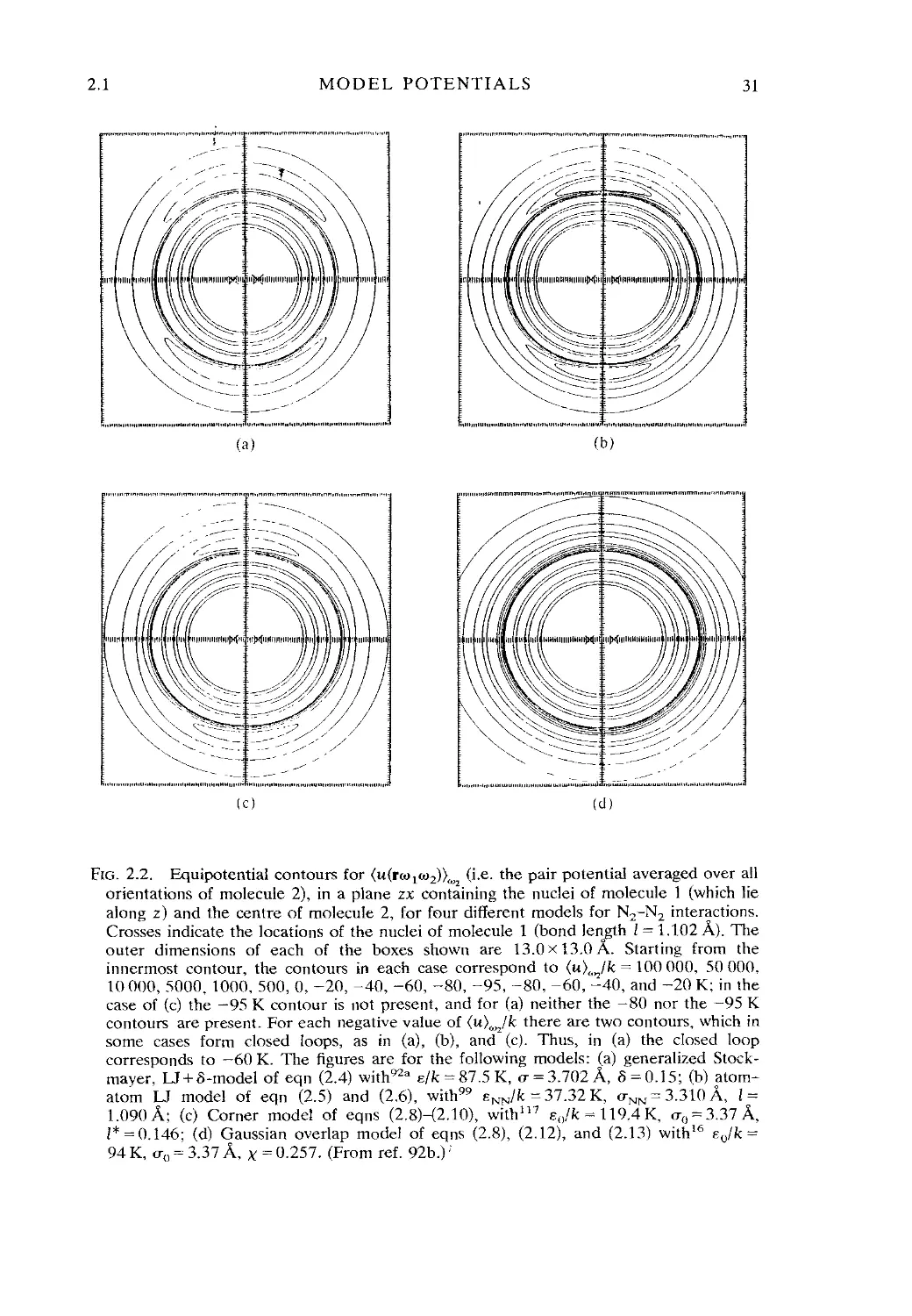
Текст
Oxford University Press, Walton Street, Oxford OX2 6DP
London New York Toronto Delhi
Bombay Calcutta Madras Karachi
Kuala Lumpur Singapore Hong Kong Tokyo
Nairobi Dar es Salaam Cape Town
Melbourne Auckland
and associated companies in
Beirut Berlin Ibadan Mexico City Nicosia
Oxford is a trade mark of Oxford University Press
Published in the United States
by Oxford University Press, New York
© C G. Gray and K.E. Gubbins 1984
All rights reserved. No part of this publication may be reproduced,
stored in a retrieval system, or transmitted, in any form or by any means,
electronic, mechanical, photocopying, recording, or otherwise, without
the prior permission of Oxford University Press
British Library Cataloguing in Publication Data
Gray, C. G.
Theory of molecular fluids. — (The international
series of monographs on chemistry; 9)
Vol 1: Fundamentals
1. Fluid dynamics
I. Title II. Gubbins, K. E. III. Series
532'.05 QC151
ISBN 0-19-855602-0
Library of Congress Cataloging in Publication Data
Gray, C. G.
Theory of molecular fluids.
(The International series of monographs on chemistry; 9)
Includes bibliographies and index.
Contents: v. 1. Fundamentals.
1. Molecular theory. 2. Fluids. I. Gubbins,
Keith E. II. Title. III. Series.
OD461.G7178 1984 541'.0422 83-23767
ISBN 0-19-855602-0 (t>. 1)
Filmset and printed in Northern Ireland by The Universities Press (Belfast) Ltd.
. PREFACE
The theory of molecular fluids (e.g. N2, H2O) must account for qualita-
qualitatively new effects that are not present for atomic fluids (e.g. Ar); for
example, the orientational correlations between molecules affect diffrac-
diffraction patterns, give rise to new types of phase changes and dielectric
effects, and cause alignment of molecules at liquid-gas and liquid-solid
interfaces. Statistical mechanical theories of molecular fluids have de-
developed rapidly in the last ten years. However, existing books cover the
theory of atomic, rather than molecular fluids. The present volumes were
written to fill this gap in the literature.
We restrict ourselves to equilibrium properties, both to keep the book
within reasonable bounds and because progress has been less rapid for
dynamic properties. We deal with gases and liquids, but the emphasis is
on liquids since some of the topics on gases are dealt with in other books.
An underlying theme is the role played by the various sorts of inter-
molecular forces in determining the different fluid properties. The scope
is restricted to small nearly rigid molecules, for example N2, HC1, CO2,
CH4, and H2O. The treatment is mainly classical, but we include lowest-
order quantum corrections where appropriate.
The books are aimed at beginning graduate students and research
workers in chemistry, physics, and engineering. We assume an under-
undergraduate knowledge of statistical mechanics, thermodynamics, elementary
electromagnetic theory, and vector analysis. A few sections require some
knowledge of quantum mechanics. Parts of the books have been used in
graduate courses at Cornell, Guelph, Berkeley, and Florida. The books
should be useful to experimentalists, as well as theorists, as we have
included detailed derivations, tables of numerical results, and (in Volume
2) comparisons of theory and experiment.
Volume 1 is devoted to the basic principles. In the introductory chapter
we discuss critically the basic assumptions underlying many of the later
calculations. In Chapter 2 we describe the various kinds of isotropic and
anisotropic intermolecular forces that are relevant for molecular fluids.
Our discussion of the isotropic forces is brief, since they have been
discussed in recent books on atomic fluids; we give a detailed discussion
of the anisotropic forces, however. In Chapter 3 we describe and relate
the various distribution functions and correlation functions which arise in
the statistical mechanics of molecular fluids. Chapters 4 and 5 contain
discussions of the perturbation and integral equation theories for the pair
correlation functions and thermodynamic properties used in later chapters
on applications. A number of technical points are relegated to appendices
following particular chapters. There are also some general appendices on
vi PREFACE
useful mathematical results, spherical tensor methods, multipole moments
and polarizabilities, and virial and hypervirial theorems. Volume 1 is
nearly self-contained; only in a few places do we utilize results derived in
Volume 2.
Volume 2 is devoted to applications such as thermodynamics of pure
(Chapter 6) and mixed (Chapter 7) fluids, surface properties (Chapter 8),
X-ray and neutron diffraction structure factors (Chapter 9), dielectric
properties (Chapter 10), and spectroscopic properties (Chapter 11).
Symmetry and invariance arguments play a key role throughout the
book. The reason is as follows. Intermolecular pair potentials and iso-
tropic fluid pair correlation functions depend on the mutual orientation of
two molecules, and are therefore invariant under coordinate rotations.
The description of molecular and fluid properties in terms of invariants
and other simply transforming quantities (tensors, e.g. dipole moments,
polarizabilities, etc.) thus arises naturally; in addition, calculations are
greatly simplified using tensor methods. Appendices A and B provide the
background information on Cartesian and spherical tensors needed for
these descriptions. Most of the existing books on these matters are
written largely from the point of view of the quantum theory of angular
momentum, so that in Appendix A we have recast some of the needed
results into the more generally useful language of tensors, focussing
particularly on their rotational transformation properties. ^
Guelph and Cornell C.G.G.
October 1982 K.E.G.
ACKNOWLEDGMENTS
Many friends and colleagues have read sections of the manuscript and
offered helpful advice; we are grateful to J. A. Barker, A.D. Buckingham,
P.T. Cummings, D. Henderson, C.G. Joslin, W.F. Murphy, B.G. Nickel,
B.J. Orr, M. Rigby, G. Stell, D.E. Sullivan, and B. Widom. We are
particularly indebted to J.S. Rowlinson for his help in planning the
project, for a critical reading of the entire manuscript, and for meticulous
editorial work. P.M. Gubbins exercised great care in drawing all of the
figures. We thank Demetra Dentes, Kathleen Harris, and Connie York
for their efficient and expert typing of the final manuscript. The financial
support of the Natural Sciences and Engineering Research Council of
Canada and the National Science Foundation is gratefully acknowledged.
Finally, it is a pleasure to thank Oxford University Press for their
patience and courtesy during the eight years the volumes were being
written.
TO
VIRGINIA AND PAULINE
CONTENTS
VOLUME 1: FUNDAMENTALS
COMMONLY OCCURRING ABBREVIATIONS xiii
NOTE ON UNITS xiv
1. INTRODUCTION 1
1.1 Theory of fluids in equilibrium 1
1.2 Molecular fluids 4
1.3 Scope of this book 16
References and notes 18
2. INTERMOLECULAR FORCES 27
2.1 Model potentials 30
2.2 Isotropic and anisotropic parts of the potential 38
2.3 Spherical harmonic expansion for the potential 39
2.4 Multipole expansions 45
2.5 Induction interactions 85
2.6 Dispersion interactions 91
2.7 Overlap interactions 100
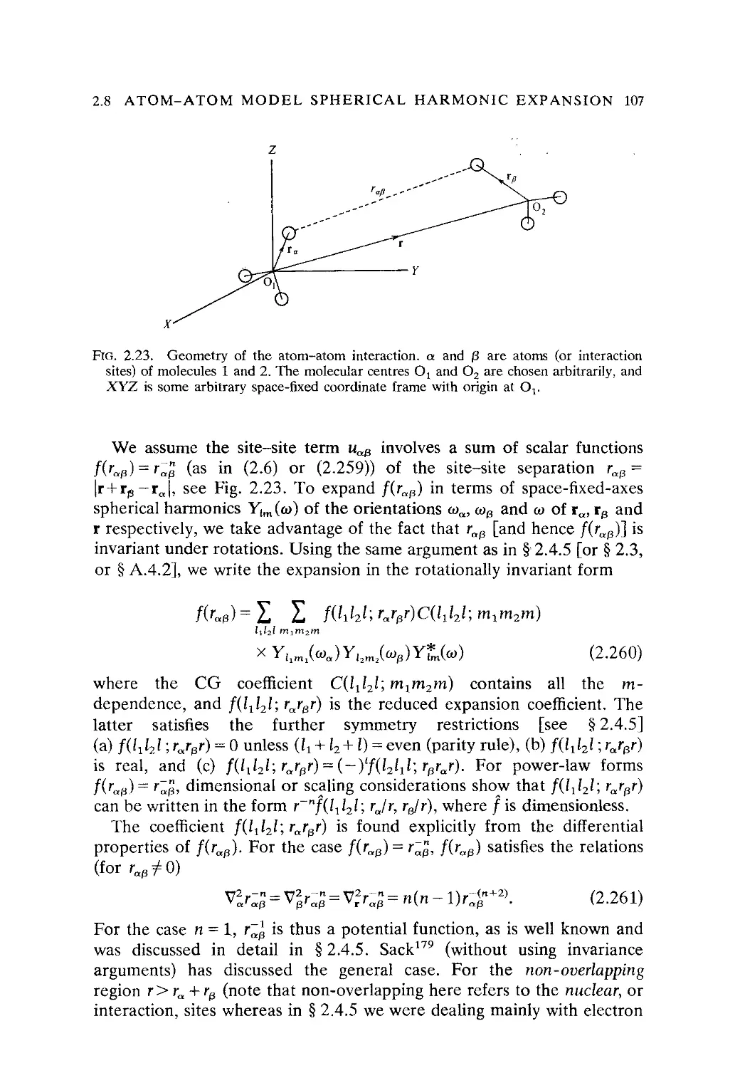
2.8 Spherical harmonic expansion of the atom-atom potential 106
2.9 Convergence of the inverse distance and spherical harmonic
expansions 114
2.10 Three-body interactions 123
2.11 Generalization to nonrigid molecules, etc. 130
References and notes 131
3. BASIC STATISTICAL MECHANICS 143
3.1 Distribution functions in the canonical ensemble 145
3.2 Spherical harmonic expansion of the pair correlation function 180
3.3 Distribution functions in the grand canonical ensemble 187
3.4 Hierarchies of equations for the distribution functions 192
3.5 Distribution functions for mixtures 204
3.6 Density expansions of the correlation functions and thermo-
dynamic properties 206
Appendix 3A Relation between the canonical and angular momenta 210
Appendix 3B Spherical harmonic form of the OZ equation 212
Appendix 3C Volume derivatives and the intensivity condition 219
Appendix 3D The classical limit and quantum corrections 224
Appendix 3E Direct correlation function expressions for some
thermodynamic and structural properties 237
References and notes 240
4. PERTURBATION THEORY 248
4.1 Brief historical outline , 248
4.2 A simple example: the u-expansion for free energy 254
4.3 General expansion for the angular pair correlation function 256
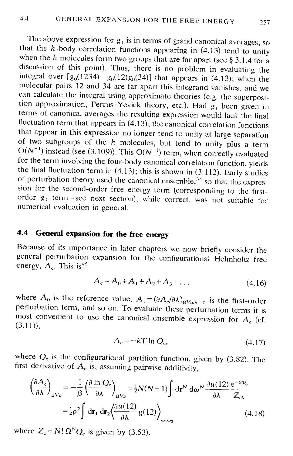
4.4 General expansion for the free energy 257
4.5 Further development of the u -expansion 258
x CONTENTS
4.6 The /-expansion 274
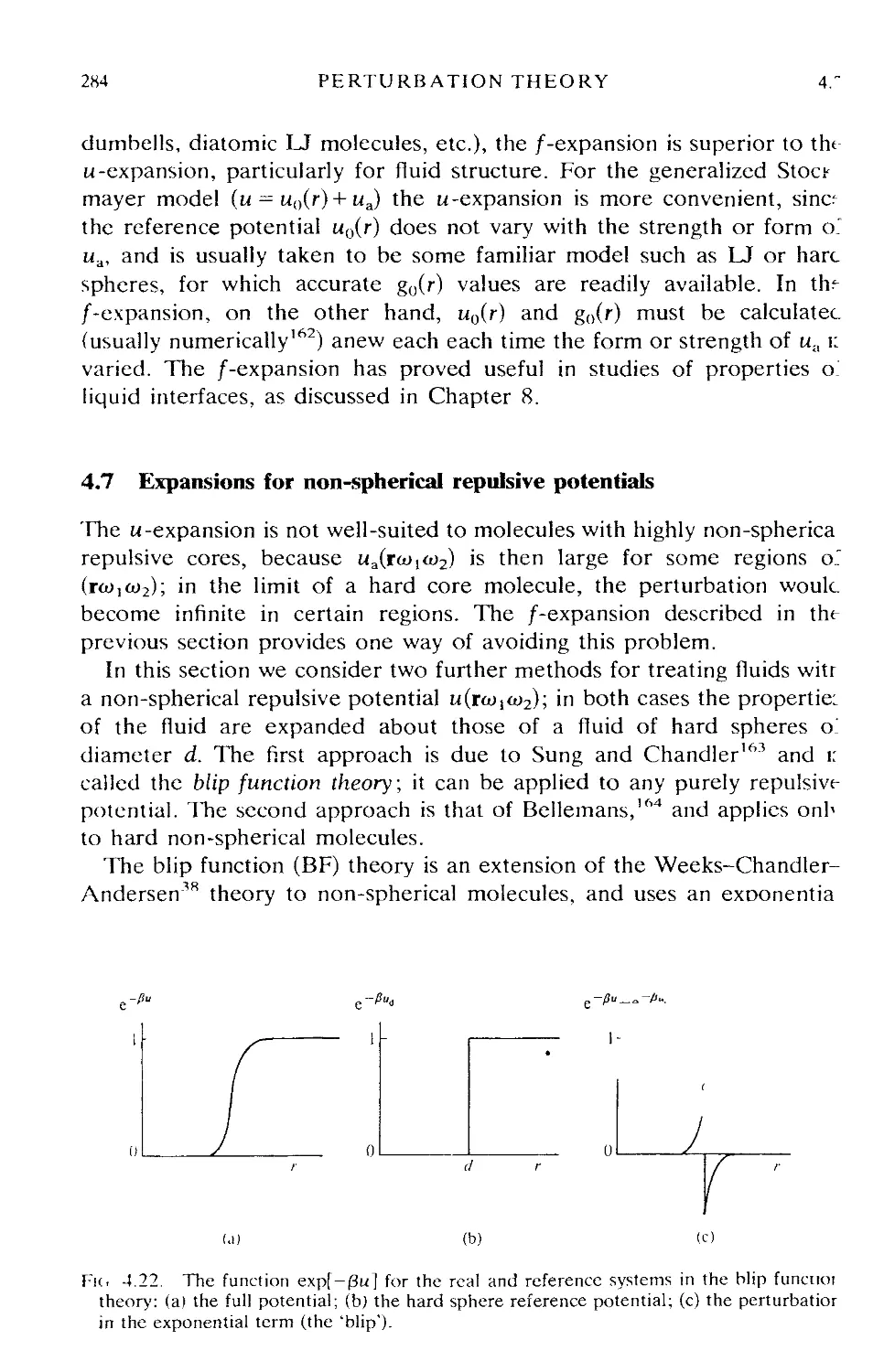
4.7 Expansions for non-spherical repulsive potentials 284
4.8 Non-spherical reference potentials 289
4.9 Effective central potentials 300
4.10 Perturbation theory for non-additive potentials 304
4.11 Conclusions 315
Appendix 4A Perturbation expansion for a general property (B) 317
References and notes 328
5. INTEGRAL EQUATION METHODS 341
5.1 The PY approximation for hard spheres 344
5.2 Spherical harmonic form of the OZ equation 348
5.3 Separation of the OZ equation into reference and perturbation
parts 350
5.4 Theories for the angular pair correlation function g(ra>io>2) 354
5.5 Theories for the site-site pair correlation functions g^gCr) 397
5.6 Conclusions 414
Appendix 5A Factorization method of solution of the OZ equation 415
Appendix 5B Thermodynamics of the HNC approximation 423
References and notes 426
APPENDIX A. SPHERICAL HARMONICS AND RELATED
QUANTITIES 441
A.I Spherical harmonics 442
Definition 442. List of P, and Plm 444. Other notations 444.
Eigenfunctions 445. Active and passive rotations 446. Rotation
operator 446. Commutation relations 447. Angular gradient
operator 448. Potential functions 448. Angular Laplacian 449.
Examples of rlYlm 449. Recurrence relation 450. Orthogonality
450. Completeness 450. Addition theorem 451. Product rule
452. Integrals 452. Transformation under rotations 452. Inversion
454. Gradient formula 454. Example, proof of special case of
gradient formula 455. Special cases of Y,m 456. List of Y,m 457.
A.2 Rotation matrices 458
Definition 458. Euler angles 459. Formula for Dlmn 460. Sym-
Symmetry properties of D'mn 460. Eigenfunctions 460. Dlmn as
generalized (four-dimensional) spherical harmonics 462. Angular
gradient and Laplacian 462. Rotation operator 462. Recurrence
relations 463. Orthogonality 463. Completeness 464. Unitarity
464. Product rule 464. Integrals 465. Group representation prop-
property 465. Transformation properties under rotations 466. Special
cases of DL 467. d'(8) and d\8) 467. Example, rotations about Z
468. Example, D\a(}y) 469. Direction cosine matrix 470.
A.3 Clebsch-Gordan coefficients 471
Definition 471. Selection rules 472. Symmetry properties 472. 3/
symbols 473. Orthogonality relations 473. Sum rules 473. Ab-
Abbreviated notation 475. Special values 475. Tables and formulae
476.
A.4 Tensors 476
Irreducible tensors 471. Irreducible spherical tensors 477. Exam-
Example, Y,,,, as irreducible tensors 478. Example, rank-one tensors
(vectors) 478. Example, rank-two tensor 478. Example, DLOT)* as
CONTENTS xi
irreducible tensop 478. Reduction and contraction 479. Example,
product of two vectors 479. Example, polarizability tensor 480.
Example, spherical harmonic addition theorem 481. Reduction of a
product of three irreducible spherical tensors 481. Example; An = 1,
B12-2, C|3«i 482. Rotational invariants 483. Example, rotational
invariants formed from products of three Dlmn and three Ylm 483.
Generalization to noninvariants 484. Cartesian tensor analogues
485. Integrals over products of direction cosine matrices 487.
Example, (QaeQys)n 487. Short-cut for last example 488. Transfor-
Transformation between Cartesian and spherical components 489. Definition
of Cartesian tensor 489. Reduction of second-rank Cartesian tensor
490. Reduction of third-rank Cartesian tensors, direct and spherical
methods 490 and 493. T,m in terms of the TaS 492. Example,
differential light scattering 493. Example, dipole-dipole interaction
496. Example, dispersion interaction 498.
A.5 The / symbols 500
The 6/ symbol 500. Definition 501. Racah coefficient 501. Selec-
Selection rules 502. Symmetry properties 502. Tables and formulae
503. Further sum rules 503. The 9/ symbol 504. Definition 504.
Selection rules 504. Symmetry properties 505. Further sum rules
505. Example, PY approximation 506. Example, A terms in induc-
induction interaction 509. Higher / symbols 510.
References and notes 511
APPENDIX B. SOME USEFUL MATHEMATICAL RESULTS 517
B.I Vector and tensor notation 517
B.2 Quantum notation 522
B.3 The delta function 524
B.4 The generalized Parseval theorem 526
B.5 The Rayleigh expansion 527
B.6 Pade approximants 530
B.7 Matrices 531
References and notes 536
APPENDIX C. MOLECULAR POLARIZABILITIES 538
C.I Introduction 538
C.2 Quantum calculation of polarizabilities 541
C.3 Dispersion and induction intermolecular forces 550
C.4 Glossary of polarizability symbols 560
References and notes 561
APPENDIX D. TABLE OF MULTIPOLE MOMENTS AND <-64
POLARIZABILITIES 564
D.I The multipole moments ^E9
D.2 The polarizabilities ^74
D.3 Units rg?
References and notes
APPENDIX E. VIRIAL AND HYPERVIRIAL THEOREMS 602
E.I The virial theorem 603
E.2 Hypervirial theorems 607
References and notes 611
INDEX 617
VOLUME 2: APPLICATIONS
Chapter 6 Thermodynamic properties of pure fluids
Appendix 6A Geometry of convex bodies
Appendix 6B Evaluation of perturbation theory averages
Chapter 7 Thermodynamic properties of mixtures
Chapter 8 Surface properties
Appendix 8A Functionals
Chapter 9
Chapter 10
Chapter 11
Structure factor
Dielectric properties
Appendix 10A Expressions for the dielectric constant
Appendix 10B Perturbation expansion for the angular cor-
correlation parameters G,
Appendix IOC Evaluation of G, and e in RISM
Appendix 10D DID approximation for collision-induced
polarizability
Appendix 10E Expressions for G[ in terms of g^eM
Spectroscopic properties
Appendix 11A Macroscopic relations for absorption
Appendix 11B Classical calculation of A(&>)
Appendix 11C Quantum calculation of A(&>)
Appendix 11D Kramers—Kronig relations
Appendix HE Quantum corrections to allowed moments
COMMONLY OCCURRING ABBREVIATIONS
Abbreviation
DID
BBGKY
CG
CIA
GMF (=LHNC = SSC)
GMSA
HNC
HS
LHNC (=GMF = SSC)
LJ
MC
MD
MSA
oz
PT
PY
QQ
RISM
SSC (= LHNC = GMF)
/x/x
Meaning
Dipole-induced-dipole
Bogoliubov, Born, Green,
Kirkwood, Yvon hierarchy of
equations
Clebsch-Gordan coefficient
Collision-induced absorption
Generalized mean field theory
Generalized mean spherical
approximation
Hypernetted chain theory
Hard sphere
Linearized hypernetted chain
theory
Lennard-Jones
Monte Carlo
Molecular dynamics
Mean spherical approximation
Ornstein-Zernike equation
Perturbation theory
Percus-Yevick theory
Quadrupole-quadrupole
interaction
Reference interaction site model
Single super chain theory
Dipole-dipole interaction
Introduced
p. 311
p. 203
p. 39
p. 567
p. 379
p. 355
p. 342
Fig. 3.5
p. 380
p. 30
Table 4.1
Table 4.4
p. 355
p. 184
Fig. 4.6
p. 342 ¦
Fig. 3.5
p. 398
p. 379
p. 375
NOTE ON UNITS
In dealing with molecular properties and intermolecular forces and their
effect on fluid properties we shall be concerned almost entirely with
electrostatics; electromagnetic forces and macroscopic circuit problems
play only a very minor role. We have therefore found it convenient to use
the electrostatic system of units rather than the rationalized Systeme
International (SI)t in our treatment of these topics (particularly in Chap-
Chapters 2 and 10, and in Appendices C and D). In Chapter 11 we use the
Gaussian system (which derives naturally from the esu system) when
dealing with light absorption and scattering. This makes for a more
compact notation, since the factors of Atre0 that occur in the SI system are
avoided. In Appendix D.3 the relations among the electrostatic (esu), SI,
and atomic units (au) systems are discussed in some detail.
t For a detailed discussion of various systems of units see: Jackson, J. D. A975), Classical
electrodynamics, 2nd edn Appendix, Wiley, New York; Marion, J. B. and Heald, M. A.
A980), Classical electromagnetic radiation, 2nd edn p. 2 and Appendix D, Academic, New
York; Danloux-Dumesnils, M A969), The metric system, University of London Athlone
Press.
1
INTRODUCTION
The first problem of molecular science is to derive
from the observed properties of bodies as accurate a notion
as possible of their molecular constitution. The knowledge
we may gain of their molecular constitution may then be
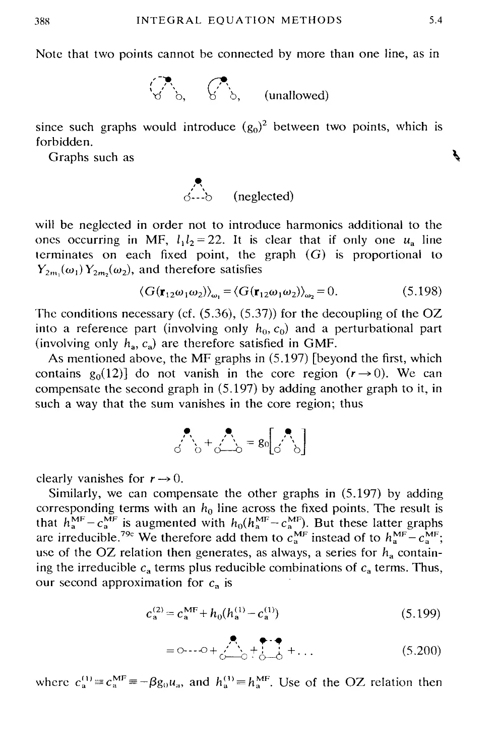
utilized in the search for formulas to represent their
observable properties. A most notable achievement in this
direction is that of van der Waals, in his celebrated memoir, . . .
J. Willard Gibbs, Proc. Am. Acad. 16, 458 A889).
1.1 Theory of fluids in equilibrium
The application of statistical mechanics to the study of fluids over the past
fifty yearst or so has progressed through a series of problems of gradually
increasing difficulty. The first and most elementary calculations were for
the thermodynamic functions (heat capacities, entropies, free energies,
etc.) of perfect gases. These properties are related to the molecular
energy levels, which for perfect gases can be determined theoretically (by
quantum calculations) or experimentally (by spectroscopic methods, for
example). For simple molecules (CO2, CH4, etc.) the energy levels, and
hence the thermodynamic properties, can be determined with great
accuracy, and even for quite complex organic molecules it is now possible
to obtain thermodynamic properties with satisfactory accuracy.1 With the
advent of digital computers it became possible to calculate ther-
thermodynamic properties for a wide variety of substances and temperatures,
and several useful tabulations of perfect gas properties now exist.2'3
Having successfully treated the perfect gas, it was natural to consider
gases of moderate density, where intermolecular forces begin to have an
effect, by expanding the thermodynamic functions in a power series (or
virial series) in density. Although the mathematical basis for a theoretical
treatment of this series was laid by Ursell4 in 1927, it was not exploited
until ten years later, when Mayer5 re-examined the problem.6 Since that
time a great deal of effort has been put into evaluating the virial
coefficients that appear in the series for a variety of intermolecular force
models.7 As the expressions for the virial coefficients are exact, they
provide a very useful means of checking such force models by comparison
of calculated and experimental coefficients.
tThe earlier history, including the classic work of van der Waals, is reviewed in the
historical references given at the end of the chapter.
2 INTRODUCTION 1.1
While the theory of dilute gases at equilibrium is essentially complete,11
this is far from being the case for all dense gases and liquids. The virial
series cannot be applied directly13 to liquids.20'3 As an alternative to the
'dense gas' approach to liquids, there were early attempts to treat liquids
as disordered solids by using cell or lattice theories;24^ these were popular
from the mid-1930s until the early 1960s. The problem of calculating the
partition function was simplified by assuming that the liquid was made up
of a series of cells. In the simplest of these models, due to Lennard-Jones
and Devonshire,27 the liquid volume was assumed to be spanned by a
lattice, and each molecule was confined to its cell by the repulsive forces
of its neighbours, Such models suffer from a number of defects, including
a large number of adjustable parameters and a failure to predict a
sufficiently large entropy. A variety of modifications have been intro-
introduced in an attempt to improve these models; none is entirely satisfac-
satisfactory, although they may provide a useful theory for special situa-
tions20-28-29 (e.g. melting).
An alternative and more fundamental approach to liquids is provided
by the integral equation methods20'30'31 (sometimes called distribution
function methods), initiated by Kirkwood and Yvon in the 1930s. One
starts by writing down an exact equation for the molecular distribution
function of interest, usually the pair function, and then introduces one or
more approximations to effect a solution. These approximations are often
motivated by considerations of mathematical simplicity, so that their
validity depends on a posteriori agreement with computer simulation or
experiment. The result is an integral equation which must be solved
numerically in most cases. The theories in question include those of YBG
(Yvon, Born, and Green), PY (Percus and Yevick), and the HNC (hyper-
netted chain) approximation. They provide the distribution functions
directly, and are thus applicable to a wide variety of properties.
A particularly successful approach to liquids has been provided by the
thermodynamic perturbation theories.20-31~3 In this approach the proper-
properties of the fluid of interest, in which the intermolecular potential energy is
°U say, are related to those for a reference fluid34 with potential °U0
through a suitable expansion. One attempts to choose a reference system
that is in some sense close to the real system, and whose properties are
well known (e.g. through computer simulation studies or an integral
equation theory). Although the statistical mechanical basis for these
theories was laid in papers published in the early 1950s,35~7 successful
forms of the theory were not developed until the late 1960s.38'39 They are
capable of giving excellent quantitative results for liquids and dense gases,
except in the vicinity of the critical point. For molecular liquids a number
of problems still remain to be worked out in detail, e.g. the calculation of
the liquid pair correlation function for strong anisotropic potentials (H2O,
etc.); see Chapters 4 and 5.
1.1 THEORY OF FLUIDS IN EQUILIBRIUM 3
Finally we mention the scaled-particle theory ,40~3 which was developed
about the same time as the Percus-Yevick theory. It gives good results for
the thermodynamic properties of hard molecules (spheres4041 or convex
molecules42-43). It is not a complete theory (in contrast to the integral
equation and perturbation theories) since it does not yield the molecular
distribution functions (although they can be obtained for some finite
range of intermolecular separations20-44). However, it does provide a
useful and quite accurate equation of state for hard convex molecules (see
Chapter 6).
This brief discussion of the theory of fluids would not be complete with-
without some mention of computer simulation studies,20'3 lA5~9 which
played an important role in the development of the theory. Simulations50
can be carried out by either the Monte Carlo or molecular dynamics
methods.5' In the Monte Carlo method one employs random numbers to
generate a sequence of molecular configurations distributed canonically
(for example), and then obtains property estimates by calculating the
arithmetic mean over these configurations. The Monte Carlo method is
suitable for treating static properties only, but has the advantage that a
variety of different ensembles can be used, e.g. the canonical (T, N, V
fixed), the grand canonical (T, jx, V fixed), or the isobaric (T, N, p fixed).
In the molecular dynamics method the Newton equations for the transla-
tional and rotational motions are solved for each molecule. Physical
properties are obtained by time-averaging the appropriate function of the
molecular positions, orientations, velocities, and angular velocities,
Molecular dynamics has the advantage that both static and time-
dependent properties are obtained, but its use is restricted (see, however,
ref. 51) to the microcanonical ensemble (E, N, V fixed). In certain
situations, e.g. the study of gas-liquid or liquid-liquid equilibria, where
one needs to calculate the free energy, this is a disadvantage, and it may
be easier to use the Monte Carlo method with the isobaric or grand
canonical ensembles. In both the Monte Carlo and molecular dynamics
methods the number of molecules used is usually in the range 100-1000.
However, this seems sufficient to provide an accurate estimate of fluid
properties, except perhaps for surface properties52 and properties in the
critical region.
Computer simulations play a role that is intermediate between theory
and experiment (see Fig. 1.1) By comparing theory with simulation
results it is possible to eliminate any uncertainties as to the form of the
intermolecular potential energy, which is the same in both theory and
simulation. In this role, the simulation provides 'experimental data' on a
precisely denned model fluid, against which the theory can be tested. (In
contrast, comparisons between theory and experiment test jointly the
theory and the intermolecular potential model, and therefore fail to
provide a conclusive test of the theory.) We shall frequently make use of
INTRODUCTION
1.2
Experiment
Theory and potential
Potential
Theory
Computer
simulation
Fig. 1.1. Methods for testing theoretical approximations and intermolecular potential
models.
simulation data for tests of theories throughout this book. A second use
of computer simulation data is in comparisons with experimental data for
real fluids, in order to test the intermolecular potential model.53 In this
role the simulation provides the 'theory' which is tested against experi-
experiment. By continually refining the potential and comparing the simulation
cesults with experiment, one hopes to end up with a realistic model for
the potential.
In addition to the above, computer simulations can be used to obtain
results which are difficult or impossible to obtain experimentally; exam-
examples54 are the static angular pair correlation function for molecular
liquids,47 and the density (and orientation) profile at liquid-vapour527172
and liquid-solid73 interfaces. Similarly, difficult theoretical questions can
be studied to advantage with simulation methods, e.g. ergodicity45 (by
comparing Monte Carlo and molecular dynamic results), the approach to*
equilibrium,5560 the N-dependence (where N is the number of molecules)
and ensemble dependence of thermal averages, and the dependence of
structural and thermodynamic properties on the long- and short-range
parts of the intermolecular potential.
1.2 Molecular fluids
Early work (before about 1970) on the theory of dense fluids dealt almost
exclusively with simple atomic fluids, in which the intermolecular forces
are between the centres of spherical molecules and depend only on the
separation distance r (Fig. 1.2(a)). Examples of such simple fluids are the
inert gases, the alkali metals, and certain molten salts. Throughout this
book we shall deal with fluids composed of relatively small but non-
spherical molecules. In such fluids the intermolecular forces depend on
the molecular orientations, vibrational coordinates, etc., in addition to r.
1.2
MOLECULAR FLUIDS
(a)
X x
Fig. 1.2. (a) The intermolecular potential u(r) between two spherical molecules depends
only on their separation r. (b) The intermolecular potential u(raIaJ) for two non
spherical molecules depends on their separation r and on their orientations ti, and u>2.
Here o>f represents the set of angles which give the orientation of the body-fixed axes
(x^Zj) relative to the space-fixed axes {XYZ). In the 'intermolecular frame' Z is chosen
to point along r.
The dependence of the intermolecular forces on the molecular orienta-
orientations leads to qualitatively new features in the liquid properties, when
compared to atomic liquids. The angular correlations between the
molecules are manifested in both the structural and thermodynamic
properties. For example, additional peaks occur in the X-ray and neutron
structure factors (Chapter 9), and the orientational energy and entropy
can influence strongly the phase diagrams of pure fluids and mixtures
(Chapters 6 and 7). For example, some binary mixtures exhibit a 'lower
critical mixing temperature', as well as the usual upper critical mixing
temperature. As further examples we mention the mean-squared torque
on a molecule, which vanishes for purely central forces (see Chapter 11),
and orientational polarization of molecules at surfaces (Chapter 8).
In most of the subsequent development we shall make use of three
basic approximations, and we discuss these briefly in what follows. These
approximations are (a) the rigid molecule assumption, (b) classical treat-
treatment of the translational and rotational motions, and (c) pairwise additiv-
ity of the intermolecular forces.
1.2.1 The rigid molecular approximation
In the 'rigid molecule approximation' it is assumed that the intermolecu-
intermolecular potential energy °U(rN<t>N) depends only on the positions of the centres
of mass rN=r,r2...rN for the N molecules and on their orientations
a>N = a>1aJ •• <^n- This implies that the vibrational coordinates of the
molecules are dynamically and statistically independent74 of the centre of
mass and orientation coordinates, and, that internal rotations75 are either
absent, or are independent of the rN and a)N coordinates. The molecules
are also assumed to be in their ground electronic states. The rigid
INTRODUCTION
1.2
molecule approximation eliminates from consideration long-chain
molecules having relatively free internal rotations, particularly polymers.
These assumptions should be quite realistic for many fluids composed
of small molecules such as N2, CO, CO2, Br2, CH4, C6H6, etc. The
assumption that vibrational states are independent of the rotational and
translational states should not lead to serious error for molecules in which
the separation between vibrational energy levels greatly exceeds both kT
and the separation between rotational levels; this is usually the case for
simple molecules.7677 The characteristic vibrational temperature 6V =
ha>/k = hv/k where v is the vibrational frequency in s, is given in Table
1.1 for some cases of interest; here h = h/2-ir, h is Planck's constant, and k
is the Boltzmann constant. When TS0v the population of the excited
vibrational energy levels will be appreciable. 0V is seen to be large in most
Table 1.1
Relevant quantities for estimating the importance of quantum effects in \
liquids at their normal boiling points t
Liquid
He
Ne
Ar
Xe
H2
HF
HCI
HBr
N2
CO
o2
Cl2
h
co2
H2O
CH4
CF4
NH,
N2O
CC14
SF6
QHf,
T/K
4.2
27.1
87.2
165.0
20.4
292.5
188.1
206.7
77.3
81.6
90.1
239
457.5
216.6§
373.1
111.6
145.1
239.7
184.7
349.9
222.3§
353.2
ejKt
—
—
—
6215
5960
4227
3814
3374
3100
2274
810
310
954
2290
1890
629
1360
850
310
523
582
A*t
2.67
0.593
0.186
0.063
1.73
0.199
0.144
0.081
0.226
0.220
0.201
0.067
0.024
0.011
0.021
0.239
0.080
0.186
0.105
0.033
0.046
0.045
A*/BttT*)'
1.708
0.271
0.087
0.029
0.930
0.074
0.058
0.035
0.100
0.097
0.092
0.033
0.010
0.004
0.006
0.110
0.033
0.093
0.042
0.013
0.017
0.020
0r/KH
—
85.3
30.2
15.02
12.02
2.88
2.77
2.07
0.351
0.054
0.561
40.1
7.54
0.275
13.6
0.603
0.0823
0.131
0.27
er/T
—
4.18
0.1032
0.0799
0.0582
0.0373
0.0339
0.0230
0.00147
0.00012
0.00259
0.108
0.0676
0.00189
0.0567
0.00326
0.00024
0.00059
0.00076
i Here T* = kT/e, A* = hl<j(me)\ 0V= hv/k where v is the vibrational frequency in s ', and
0, = hcBJk where Be is the usual rotational constant in cm.
+ fl^ values from refs. 26, 76-78. For the polyatomic molecules, which have more than one
vibrational mode, only the lowest 0V is listed.
§ Triple-point temperature.
H From refs. 8, 26, 76-78. For the symmetric and asymmetric top molecules, which have two
and three principal moments of inertia respectively, we have listed only the highest 8r.
1.2
MOLECULAR FLUIDS
'' Table 1.2
Shift in vibration frequency for various substances dissolved in
liquid argon at 90-100 K and in carbon tetrachloride at room
temperature (from ref. 91)t
Frequency shift
Substance
Mode
In At
In CC14
H2
CO
HC1
N7O
co2
cs2
CH4
CF4
C2H4
(CH3JO
vb(OCH)
4155.1
2143.3
2886.0
1284.9
588.8
2223.8
667.4
2349.2
1535.4
730.3
3288.4
3019.5
1306.2
1260.9
1282.6
949.3
947.9
614.5
1102
1179
-10
-5.3
-15
-1.4
-1.2
-3.3
-2.3
-6.2
-6.9
2.7
-4.4
-5.5
0
-2.9
-7.6
-0.7
-8.3
-0.8
-1.5
-6.0
-23
-8
-56
-3.6
-2.8
-7.8
-13
-14
-26
-12
-5
t Here v = v/c = 1/A = frequency in cm
is the wavelength in cm.
, where v is the frequency in s ', and A
cases; for these cases almost all molecules will be in their ground
vibrational states. Exceptions are I2, CC14, and SF6.
That the vibrational states are not completely unaffected by the transla-
tional or rotational states is shown by experimental studies of bond
vibrational frequencies,79'80 relaxation times,81 bond lengths,84 and con-
formational changes8
in dense fluids. However, these effects are
usually small for the molecules to be considered here. Tables 1.2 and 1.3
show typical results of spectroscopic studies of the effect of density on
bond vibrational frequencies; vibrational frequencies in the liquid are at
most only a few per cent different from those in the gas. Although small,
these vibrational perturbations can sometimes give rise to observable
thermodynamic effects, for example an 'inverse isotope effect' (see
§ 1.2.2). Bond lengths in the liquid or solid phase can be determined by
neutron or X-ray diffraction measurements carried out at large values of
momentum transfer. These liquid-phase bond lengths84 appear to be at
most only two or three per cent different from the vapour-phase values
8 INTRODUCTION 1.2
Table 1.3
Shift in vibration frequency for the a{ C-H vibration
for pure substances on going from the gas to the
liquid phase (from ref. 92)
Substance Frequency shiftt (j/h() —i>sas)/cm '
CHC13 -13.5
CH2C12 -12.0
CH2Br2 -18.0
CH3C1 -10.0
CH3I -22.0
cis C2H2C12 -10.0
cyclo C5HIC, -11.5
tThe value of v^ for the C-H bond is about 2980 cm, the
exact value depending on the molecule considered.
determined by electron diffraction. Thus, for liquid bromine neutron
diffraction84 yields bond lengths ranging from 2.26 to 2.32 A, while the
gas value is 2.28 A. Effects due to non-rigidity of the molecules can also
be studied theoretically808893~5 and by computer simulation. Such studies
have been made for H2O, NH3, HF, CH4, N2, CO, Br2 and alkanes94-9^100
(the case of H2O is discussed in § 5.5.4).
The rigid molecule approximation implies that the intermolecular po-
potential energy u(ro>1a>2) for a pair of molecules depends on the vector
r = (rQ4>) from the centre of molecule 1 to the centre of molecule 2, and
on the orientations o>i and <o2 of the molecules relative to some space-
fixed set of axes (Fig. 1.2(b)).un Here o>; =6^ for linear molecules (e.g.
CO2, N2, HC1) or <k0iXi for non-linear molecules (e.g. H2O, CC14). For
linear molecules 0( and 4>i are simply the polar angles (Figs 2.6 and A.I),
while for non-linear molecules the Euler angles (see Figs 2.5 and A.6) are
usually used. It is often convenient to adopt the 'intermolecular frame' or
'r-frame', in which the space-fixed Z-axis is chosen to point along r; thus
0 -0. We shall write the molecular orientations in this frame as co[ to
distinguish them from the orientations o>j for an arbitrary space-fixed
frame. In Fig. 2.9 the intermolecular frame is illustrated for the particular
case of two linear molecules.
1.2.2 The classical approximation
A second basic assumption made is that the fluids behave classically. For
rigid molecules one expects quantum effects in the translational and
rotational motions of the molecules to become important for light
molecules and/or at low temperatures. Thus some molecules containing
hydrogen (e.g. HF, HC1, HD, CH4, H2O, NH3, and particularly H2)
should exhibit quantum effects at sufficiently low temperatures.
1.2 MOLECULAR FLUIDS 9
Translatiohal quantum effects are of two types,8 (i) diffraction effects102
which result from the wave nature of the molecules, and (ii) symmetry
effects which result from the boson or fermion character of the molecules.
The symmetry effects arise for identical molecules, and are negligible for
all applications that we shall consider. In a perfect gas such symmetry
effects are negligible provided that the molecular thermal de Broglie
wavelength103 At is much smaller than the mean separation between
neighbouring molecules. The latter is of order p~\ where p is the fluid
number density, so that we have
A,«p-i A.1)
for a perfect gas when symmetry effects are negligible. Here A, is given by
where m is the molecular mass. However, the molecules of real gases and
liquids have hard cores which suppress104 the symmetry effects in almost
all cases of practical interest except108 for He. The hard cores prevent the
molecules from getting sufficiently close to 'notice' their ferinion or boson
character. For example,105 even in (gaseous) H2 the effect on the pair
correlation function is negligible until T=s5K. Rotational quantum
effects are also of two types, (i) kinetic energy effects due to the discrete
nature of the rotational energy levels of a molecule; closely related are
the intramolecular exchange effects (e.g. the ortho and para hydrogen
species), (ii) intermolecular potential energy effects which tend to quan-
quantize the motion of a hindered rotator.
A quantitative treatment of the quantum effects for equilibrium109
properties can be obtained by expanding the molecular distribution
functions and the partition function (and hence the thermodynamic
properties) in powers of ft (the Wigner-Kirkwood expansion8-31'78112). If
fermion-boson effects can be neglected, and if the repulsive core of the
intermolecular potential is not infinitely hard, the series contains only
even powers of ft.113 The partition function Q, for example, is given by112
Q = Qd[l + O(ft2)] A.3)
where Qd is the classical partition function and O(h2) is the order-ft2
fractional correction. For N linear molecules this is given by
°(ft)~ 24(kTKm
where I is the moment of inertia (with respect to the centre of mass), and
(F2) and (t2) are the classical mean-squared force and torque (about the
10 INTRODUCTION 1.2
centre of mass) on a molecule. Similar expressions can be derived for
spherical top, symmetric top and asymmetric top molecules (see Appen-
Appendix 3D and Chapter 6). The series A.3) is useful at not too low
temperatures; at low temperatures a full quantum treatment,781146 a
non-perturbative approximation method, or an ^-series acceleration
technique (see Chapter 6 for references) must be used.
The three terms on the right-hand side of A.4) correspond to the
translational diffraction effect, the rotational potential energy effect, and
the rotational kinetic energy effect, respectively. It is possible to give a
qualitative explanation of these three terms as follows. We first consider
the translational diffraction effect. For simplicity, we view the complicated
translational motion of the molecule in a dense liquid as having a large
vibrational component. The vibrational motion can be treated classically
if the vibrational energy level spacing heo (or the zero-point energy for
molecules in their ground state) is small compared to kT, where <o ~
(«/mM is the vibrational frequency and k~(V2<%) is the mean force
'constant'.117 Here °U is the total intermolecular potential energy, Vj the
gradient operator with respect to the position of a particular molecule,
and {. . .) denotes a classical thermal average. Using the classical hyper-
virial relation118
<V^) = (kT)-1((V1%J> A.5)
to eliminate the mean Laplacian of the potential, one can write the
classical condition ha>/kT« 1, or (ha>lkTJ« 1, as
A.6)
(kTfm
where (F2) = ((V^J) is the mean squared force on a typical molecule
(e.g. number 1). This condition corresponds119 to the first term on the
right-hand side of A.4), apart from numerical factors. An alternative
form of the condition A.6) is obtained by noting that diffraction effects
will be negligible if the de Broglie wavelength At is much less than the
molecular diameter <x, where A, is given by A.2). In terms of the
dimensionless de Broglie wavelength A* = /t/<x(me)' (the so-called de
Boer parameter8), where e is the well-depth of the isotropic part of the
intermolecular potential, the classical condition is
A* A.7)
B7TT*)i
where T* = kT/e is the reduced temperature. Using the estimate (F2)~
(s/(jJ in A.6), together with the fact that T*~l in liquids, we see that
A.6) reduces to A.7) apart from numerical factors. The ratio A*/BTrT*)i
1.2 MOLECULAR FLUIDS 11
is given in Table 1.1 for some liquids at their normal boiling points, and is
seen to be small (though not always negligible) in all cases except for He,
H2, and Ne.
Similar qualitative arguments can be used for the rotational potential
energy effect. For simplicity we view the complicated rotational motion of
the molecule in a dense liquid as having a large librational component.
The quantum effects in the librational motion should be small if the
librational energy level spacing h<o (alternatively, the zero-point energy)
is small compared to kT, where <o ~ (k/7I is the frequency, with I the
moment of inertia and k ~(Sl,fll) the mean torque constant. Here V<O] is
the angular gradient operator120 about the centre of mass of a typical
molecule. Using the classical hypervirial relation118
<V2v%) = (fcT)-1<(V<1)l%J) A.8)
we can eliminate the mean angular Laplacian of °U and write the classical
condition ha>lkT«l, or (ha>lkTJ«l, as
(kTKI
where (t2) = ((V^fllJ) is the mean squared torque on a molecule (about
the centre of mass). This condition corresponds to the second term119 on
the right-hand side of A.4). Using the estimate (see Chapter 11) (V^fli) —
ea, where ea is the strength of the anisotropic intermolecular potential for
r~~a, we can approximate A.9) as
(h2/IkT)(eJkT)«l. A.10)
The factor (h2/IkT) is usually small (see below), so that rotational
potential energy effects become important only for very strong aniso-
anisotropic forces.121 A case in point28122123 may be liquid H2O at room
temperature. The librational frequencies are of the order 500 cm, so
that hh)lkT« 1 is clearly not satisfied. Rotational quantum corrections are
also non-negligible for gaseous H2O and NH3 (see below).
Finally, rotational kinetic energy effects will become important when
kT is of the order of the spacing between low-lying rotational energy
levels, which are given by Ej =(h2/2I)J(J+l) for a linear or spherical
top molecule. The level spacing is thus of order h2/2I, so that the
classical condition ft2/2I« fcT can be written as
t,2
A.11)
2IkT
which corresponds to the third term on the right in A.4). The quantity124
6r=h2/2Ik is thus a characteristic rotational temperature and is listed in
12 INTRODUCTION 1.2
Table 1.1. The condition A.11) can be written as
0r/T«l, A.12)
and 6r/T is also listed in Table 1.1. The condition A.12) is satisfied at the
boiling point except for H2.
From Table 1.1 we have seen that quantum effects are usually expected
to be small for molecular liquids, but can be significant at low tempera-
temperatures. As a simple example,125 the h2 quantum correction to the Helm-
holtz free energy calculated from A.3) is 10 per cent for liquid Ne near
the triple point. The quantum correction given by A.3) is at constant
density. The corresponding corrections to the pressure, and the liquid-
vapour coexistence curves,125 can of course be larger than 10 per cent.
The traditional method of studying quantum effects in the thermodynamic
properties of liquids is by isotope substitution experiments,12*^8 e.g. for
vapour pressures, liquid volumes, heats of mixing, solubilities, and surface
tension. According to classical statistical mechanics, different isotopes,
which have the same intermolecular forces (neglecting (i) the difference
produced by averaging over slightly different vibrational motions, and (ii)
the extremely small non-adiabatic corrections to the electronic ground-
state energy), should have the same configurational properties, since the
mass and moment of inertia of the molecules do not appear in the
configurational partition function. Quantum mechanically, on the other
hand, the partition function does not factorize into kinetic and configura-
configurational parts, so that the mass and moment of inertia enter in a non-trivial
way. The results A.3) and A.4) show explicitly the dependence on m and
I in the 'high temperature approximation'. The quantum effects on
vapour pressure are the most studied.126128 Classically the composition of
a vapour of a binary isotope mixture would be the same as that of the
liquid with which it is in equilibrium. The configurational contribution to
the vapour/liquid equilibrium is unaffected by isotope substitution for the
reason discussed above; the kinetic contribution is also unaffected, since
the velocities of the molecules are affected equally on the vapour and
liquid sides of the interface. The isotope separation factor a,127 which is
essentially the ratio of the vapour composition to the liquid composition,
thus differs from unity entirely due to quantum effects (assuming rigid
molecules). For rigid molecules simple considerations of zero-point
energy lead one to expect the lighter isotope to be the more volatile.129
This is often found in practice; when an 'inverse isotope effect' is found, it
is attributed to perturbations of the vibrational motions of the molecules
due to intermolecular forces130 in the liquid. As a numerical example,127
a for 14N2/15N2 has been calculated at T = 70K using an atom-atom
potential, with the result a = 1 + 0.008 + 0.004-0.002, where the second
1.2 MOLECULAR FLUIDS 13
and third te^ms arise from the force and torque terms in A.4) respec-
respectively, and the last term, which has the opposite sign, arises from
vibrational perturbations.
For molecular gases, quantum corrections to the second virial coeffi-
coefficient B and to the second dielectric virial coefficient have been
calculated.131 For H2O and NH3 for example,132135 calculations using
Stockmayer potentials give quantum corrections to B of about 5-10 per
cent at room temperature. For these molecules the corrections are
predominantly rotational, due to the small moments of inertia.
We conclude that the quantum effects in the thermodynamic properties
are usually small, and can be calculated readily to first approximation (see
Chapter 6). For the structural properties (e.g. pair correlation function,
structure factors), no detailed estimates are presently available for
molecular liquids. For atomic liquids, and atomic and molecular gases, the
relevant theoretical expressions for the quantum corrections are available
in the literature.135"9 In later chapters we also discuss the quantum
corrections to the dielectric and spectroscopic properties.
1.2.3 The pairwise additivity approximation
The third basic approximation that we shall often introduce is that the
total intermolecular potential energy °11(tnojn) is simply the sum of the
intermolecular potentials for isolated pairs of molecules, i.e.
where M(ri)a)ia)J) is the potential140 for a pair of molecules i and j (isolated
from other molecules) with the centre of / at riy = r, — rf from i, and
orientations &>; and &>,. The sum over i runs from 1 to N~ 1, while that of
/ is from 2 to N, i always being kept less than j in order to avoid counting
any pair interaction twice. Fiquation A.13) is exact in the low density gas
limit, since configurations involving three or more molecules can be
ignored. It is not exact for dense fluids or solids, however, because the
presence of additional molecules nearby distorts the electron charge
distributions in molecules 1 and 2, and thus changes the intermolecular
interaction between this pair from the isolated pair value (Fig. 1.3). More
precisely, we should write <%i(tnojn) as a sum of isolated pair potentials, a
sum of three-body correction terms due to the addition of an interacting
t It is sometimes convenient to write this equation in the form
In this form each pair potential is included twice in the sum; the factor one-half corrects for
this.
14
INTRODUCTION
1.2
Fig. 1.3. The presence of molecule 3 nearby causes the charge clouds of molecules 1 and 2
to be distorted slightly (dashed lines) from their distributions for the isolated 12 pair (solid
lines), and thus changes the intermolecular potential between 1 and 2. Similarly the 13
and 23 potentials are influenced by the presence of the third molecule.
third molecule, a sum of four-body correction terms, etc. Thus
A.14)
where w(i/) = u(!•,•,&>;&>,¦), u(ijk) = u(itjiikijk<i)i<i)j<i)k), etc. The term u(ijk) is
the additional part of the potential not included in the sum of the isolated
pair terms u(ij) + u(ik)+u(jk), and so on. For inert gas fluids it seems
that the series in A.14) can be truncated at the triplet term,20 but the
situation is largely unknown for molecular fluids. For polar molecules
with large polarizability the higher D-body, etc.) terms in A.14) may be
important (see §§2.10 and 4.10).
The influence of the three-body terms on physical properties has been
studied in detail for atomic fluids;141'142 for these the long-range Axilrod-
Teller143 triple-dipole dispersion term seems to be the most important
part of the three-body interaction. Presumably this is because configura-
configurations where three molecules overlap are rare, due to the strongly repul-
repulsive nature of overlap potentials. The effect on the internal energy of the
liquid is small even at the triple point, being only a few per cent of the
total configurational energy; for less dense fluids the effect is smaller.
However, some properties are more sensitive to the three-body forces.
Figure 1.4 shows that the Axilrod-Teller three-body interaction has a
large effect on the third virial coefficient, B3, and at the lower tempera-
temperatures can have an influence equal to that of the two-body interaction. The
three-body interaction also has a marked effect on some other properties
for atomic liquids, for example the pressure and the surface tension.
Table 1.4 shows the influence of three-body forces on the surface tension
and surface energy for liquid argon, as calculated by Miyazaki et al.14S The
MOLECULAR FLUIDS
15
000 rr
:ooo h
000 -
; 1
-
-
1
1
1
1
t
i 1
-
1 1
100
200
300
Temperature/K
400
500
7IG. 1.4. Third virial coefficients of argon. The circles are experimental data (Michels et
al). The dashed curve is calculated with the Barker-Fisher-Watts144 potential alone; the
dotted curve includes also the Axilrod-Teller143 interactions; the dash-dotted curve adds
third-order dipole-quadrupole interactions, and the solid curve adds fourth-order dipole
interactions. Here B3 is denned by the virial series equation of state for gases—see
Chapter 3 (from ref. 20).
leglect of three-body forces is seen to'lead to a 25 per cent error in the
;urface tension and a 10 per cent error in surface energy.
Much less is known146 about the influence of three-body potentials in
nolecular fluids, because the two-body potentials are not yet accurately
cnown. (We note, however, that direct electrostatic potentials are exactly
additive.)
Table 1.4
Calculated and experimental surface properties for liquid argon at the triple
loint. The pair potential used is that of Barker, Fisher and Watts144 (BFW)
md the three-body potential is the Axilrod-Teller143 (AT) term (from
ref. 145)
Method
Potential
Surface tension
(erg cm)
Surface energy
(erg cm ~2)
Monte Carlo simulation
Monte Carlo simulation
Experiment
BFW
BFW + AT
17.7
14.1
13.35
38.3
34.7
34.8
16
INTRODUCTION
1.3
1,3 Scope of this book
Figure 1.5 shows the p-V projection of the phase diagram for a simple
pure substance, in which there is a single solid, liquid, and gas phase.
There is theoretical147 and experimental148 evidence that a clear distinc-
distinction exists between the solid and fluid states; such is not the case for gases
and liquids, since the two states become identical at the critical point C.
Thus, different theoretical approaches are applied to fluids and solids, and
we shall not treat the theory of solids1491 in this book. The theories to
be considered later are suitable for gases or liquids, with the exception of
the region immediately around the critical point.152 In the vicinity of the
critical point large-scale fluctuations occur, leading to correlations be-
between molecules which are much longer in range than the range of the
intermolecular forces. Because these correlations occur over regions
containing many molecules, the detailed nature of the intermolecular
forces has little effect on the property behaviour. Thus, critical phenomena
in widely varying types of fluids (inert gases, polar fluids, superfluids, etc.)
show a remarkable similarity (a situation known as universality). In fluids
away from the critical point, on the other hand, the intermolecular
correlations have a range similar to that of the intermolecular forces. The
fluid properties are then very markedly affected by the nature of these
forces.157 As a result, different theoretical methods are used for fluids
near and away from the critical point. We do not consider the theory of
p
Pr
\\\
\\\
ll 1
\»
11
ll
ll
ll
III
Solid (\
\|
I
I
L
\
\
\
\
\
\
\
\
I
\
—iLiquid/
N/
_ j/—
v^ C
f \
L-G
S-G
V Gas
~~ —rL
~— 7;
—
V
Fig. 1.5. p-V projection of the p-V-T diagram for a pure fluid. Solid lines are phase
boundaries, dashed lines are isotherms, horizontal dashed lines are tie-lines connecting
coexisting phases, pt and Tt are triple-point pressure and temperature, and C is the
gas-liquid critical point.
1.3 SCOPE OF THIS BOOK 17
the critical point region in this book, but refer the interested reader to the
substantial literature that exists.3'158'64
The preceding remarks and those in § 1.2 define the scope of the
present work, i.e. to non-critical fluid phases of small, nearly rigid
molecules, whose quantum effects are usually negligible or small. Exam-
Examples are given in Table 1.1. Since the theory of atomic fluids has been
reviewed in many other piaces20-31-32-78111165166 we do not discuss these
systems in detail except for particular problems such as PY theory for
hard spheres, mixtures such as HCl-Ar, etc. Also, we discuss mainly
molecular liquids, the discussion of molecular gases being brief because of
the extensive treatments given elsewhere.7'8 In addition to excluding from
discussion solids, freezing,20-31149167-168 nucleation,14 and critical
phenomena, we also exclude long-chain molecules,851692 glasses,173174
liquid crystals,175"82 electrolytes,78165-166183 plasmas,31163-165 molten
salts,165 liquid metals,166187188 reacting and dissociating liquids88-89171'190
and quantum liquids.111163196"9 Moreover, we shall not discuss dynam-
dynamical (non-equilibrium) properties.31-78-2001
In Chapter 2 the intermolecular potential models used for molecular
fluids are discussed. Relatively few ab initio quantum mechanical calcula-
calculations are available for polyatomic molecules, and these are not usually of
sufficient accuracy for property calculations. Two approximate potential
models have been especially widely used. These are the generalized
Stockmayer potential and the site-site potential. The generalized Stock-
mayer potential is a (truncated) sum of spherical harmonic terms repres-
representing the electrostatic, induction, dispersion, and overlap parts of the
potential. It is correct at long range, and is particularly convenient for
statistical mechanical calculations because angular integrations over the
harmonics are simple. However, the truncated spherical harmonic expan-
expansion may break down at short distances. The site-site potentials may give
a more realistic account of the molecular shape, are a convenient rep-
representation of highly anisotropic charge distributions, and are simple to
use in computer simulation studies, at least for small molecules. However,
they are incorrect at large intermolecular separations, and are difficult to
use in most analytic calculations.
We introduce in Chapter 3 the various molecular distribution functions,
and discuss their properties. Theories of these functions are taken up in
Chapters 4 and 5. The various forms of perturbation theories for molecu-
molecular fluids are described in detail in Chapter 4 while integral equation
methods are considered in Chapter 5. These chapters complete the
fundamental theory.
In Chapters 6-11 (Volume 2) we discuss applications of the theory to
several specific problems, including thermodynamics of pure and mixed
18 INTRODUCTION 1.3
fluids, interfacial properties, the structure factor (as determined by neut-
neutron and X-ray scattering), the dielectric constant, and the infrared,
Raman, and neutron spectral moments.
References and notes
Historical references
A. Partington, J. R. An advanced treatise on physical chemistry, Vol. 1 (Gases)
and Vol. 2 (Liquids), Longmans, London A949 and 1951).
B. Brush, S. G. The kind of motion we call heat, Books 1 and 2, in Studies in
statistical mechanics, Vol. 6 (ed. E. W. Montroll and J. L. Lebowitz) North-
Holland, Amsterdam A976).
General references
1. Frankiss, S. G. and Green, J. H. S. Chemical thermodynamics, Vol. 1,
Chapter 8 (ed. M. L. McGlashan) Specialist Periodical Report, Chemical
Society, London A973).
2. JANAF, Thermochemical tables, Nat. Standard Ref. Data Series, Nat. Bur.
Stand. (U.S.) 37, U.S. Department of Commerce A971).
3. Rossini, F. D. et al. Selected values of chemical thermodynamic properties,
Nat. Bur. Stand. Circular 500 A952).
4. Ursell, H. D. Proc. Camb. Phil. Soc. 23, 685 A927).
5. Mayer, J. E. J. chem. phys. 5, 67 A937).
6. The quantum virial series was also worked out later.7*10
7. Mason, E. A. and Spurting, T. H. The virial equation of state, Pergamosi,
Oxford A969); Maitland, G. C, Rigby, M., Smith, E. B., and Wakeham, W.
A. Intermolecular forces: their origin and determination, Clarendon Press,
Oxford A981).
8. Hirschfelder, J. O., Curtiss, C. F., and Bird, R. B. Molecular theory of gases
and liquids. Wiley, New York A954).
9. Kahn, B. and Uhlenbeck, G. Physica 5, 399 A938).
10. Lee, T. D. and Yang, C. N., Phys. Rev. 113, 1165 A959).
11. Practical difficulties12 still remain in evaluating the quantum virial coeffi-
coefficients for polyatomic molecules.
12. Larsen, S. Y. and Poll, J. D. Can. J. Phys. 52, 1914 A974).
13. However, the series has been utilized indirectly, through resummation
methods (see the discussion of integral equation methods below, and in
Chapter 5) and through models suggested by the series (e.g. the physical
cluster and droplet models146 for condensation and nucleation). The virial
coefficients have also been used to locate the critical point. 17~19
14. Abraham, F. F. Homogeneous nucleation theory, Academic Press, New York
A974).
15. Fisher, M. E. Physics 3, 255 A967).
16. Dorfman, J. R. J. Stat. Phys. 18, 415 A978); Lockett, A. M. X chem. Phys.
72, 4822 A980); Gibbs, J. H., Bagchi, B., and Mohanty, U. Phys. Rev. B24,
2893 A981).
17. Majumdar, C. K. and Rama Rao, I. Phys. Rev. A14, 1542 A976); Estevez,
G. A., Gould, H., and Cole, M. W. Phys. Rev. A18, 1222 A978).
18. Yang, C. N. and Lee, T. D. Phys. Rev. 87, 404, 410 A952).
REFERENCES AND NOTES 19
19. Kihara, V, Intermolecular forces, p. 44, Wiley, New York A978).
20. Barker, }'. A. and Henderson, D. Rev. mod. Phys. 48, 587 A976).
21. Barker, J. A. and1 Henderson, D. Can. J. Phys. 45, 3959 A967).
22. De Llano, M. and Nava-Jaimes, A. Mol. Phys. 32, 1163 A976).
23. Ruelle, D. Statistical mechanics: rigorous results, Benjamin, New York
A969).
24. Barker, J. A. Lattice theories of the liquid state, Pergamon, Oxford A963).
25. Levelt, J. M. H. and Cohen, E. G. D. Studies in statistical mechanics, Vol. 2
(ed. J. de Boer and G. E. Uhlenbeck) p. Ill, North-Holland, Amsterdam
A964).
26. Reed, T. M. and Gubbins, K. E. Applied statistical mechanics, McGraw-Hill,
New York A973).
27. Lennard-Jones, J. E. and Devonshire, A. F. Proc. Roy. Soc. A163, 53
A937).
28. Stillinger, F. H. Adv. chem. Phys. 31, 1 A975); J. stat. Phys. 23, 219 A980).
29. Wheeler, J. C. Ann. Rev. phys. Chem. 28, 434 A977).
30. Watts, R. O. Statistical mechanics, Vol. 1, p. 1 (ed. K. Singer) Specialist
Periodical Report, Chemical Society, London A973).
31. Hansen, J. P. and McDonald, I. R. Theory of simple liquids, Academic Press,
London A976).
32. Smith, W. R. Statistical mechanics, Vol. 1, p. 71 (ed. K. Singer) Specialist
Periodical Report, Chemical Society, London A973).
33. Boublik, T. Fluid Phase Equilibria 1, 37 A977).
34. As will be discussed in Chapter 4, the perturbation theory can in some cases
be based on hard spheres as reference, so that the zeroth approximation for
such liquids is a packing model for hard spheres (rather than a gas-like or
solid-like picture). The theory is then a quantitative version of the van der
Waals picture.
35. Longuet-Higgins, H. C. Proc. Roy. Soc. London A205, 247 A951).
36. Zwanzig, R. W. J. chem. Phys. 22, 1420 A954).
37. Pople, J. A. Proc. Roy. Soc. London A221, 498 A954).
38. Barker, J. A. and Henderson, D. J. chem. Phys. 47, 4714 A967).
39. Leland, T. W., Rowlinson, J. S., and Sather, G. A. Trans. Faraday Soc. 64,
1447 A968).
40. Reiss, H., Frisch, H. L., and Lebowitz, J. L. J. chem. Phys. 31, 369 A959).
41. Reiss, H. Adv. chem. Phys. 9, 1 A965).
42. Gibbons, R. M. Mol. Phys. 17, 81 A969); 18, 809 A970).
43. Boublik, T. Mol. Phys. 27, 1415 A974).
44. Reiss, H., in Statistical mechanics and statistical methods in theory and
application (ed. U. Landman) Plenum, New York A977).
45. Wood, W. W. and Erpenbeck, J. J. Ann. Rev. phys. Chem. 27, 319 A976).
46. Berne, B. (ed.) Modern theoretical chemistry, Vols. 5 and 6, Plenum, New
York A977); see reviews by Valleau and Whittington, Valleau and Torrie,
Erpenbeck and Wood, and Kushick and Berne.
47. Streett, W. B. and Gubbins, K. E. Ann. Rev. phys. Chem. 28, 373 A977).
48. Binder, K. (ed.) Monte Carlo methods, Springer-Verlag, New York A979).
49. Vesely, F. Computerexperimente an Flussigkeitsmodellen, Physik Verlag,
Weinheim A978).
50. Computer simulations are usually carried out classically. However a quan-
quantum version of the Monte Carlo method has been developed. See ref. 48 and
also Schmidt, K. E., Lee, M. A., Kalos, M. H., and Chester, G. V. Phys.
20 INTRODUCTION
Rev. Lett. 47, 807 A981). 'Semiclassical' Monte Carlo can be done easily by
adding the quantum corrections given by A.4) in terms of the classical
mean-squared force and torque. Approximate versions of quantum molecu-
molecular dynamics have been studied by Corbin, H. and Singer, K. Mol. Phys. 46,
671 A982). Modified molecular dynamics-type simulations for low density
(binary collision) gases have also been carried out for studies of collision-
induced absorption and collision-induced light scattering (Chapter 1 1); see
Birnbaum, G., Guillot, B., and Bratos, S. Adv. chem. Phys. 51, 49 A982)
and refs. therein.
51. Various 'intermediate' methods have been devised, e.g. 'Brownian
dynamics'; see J. M. Haile and G. A. Mansoori (ed.), Molecular-based study
of fluids, Advances in Chemistry Series, 204, American Chem. Soc,
Washington A983)-particularly the papers by Mansoori and Haile, Evans,
and Weber et al. See also H. C. Andersen [J. chem. Phys. 72, 2384 A980)]
for proposals for molecular dynamics at constant temperature or pressure.
For results see Haile, J. M. and Graben, H. W. J. chem. Phys. 73, 2412
A980); Abraham, F. F. Phys. Repts. 80, 340 A981).
52. Chapela, G. A., Saville, G., Thompson, S. M., and Rowlinson, J. S. J. Chem.
Soc, Faraday Trans. 11 73, 1133 A977) . There are also problems in
simulating dielectric properties for systems with long-range forces - see
Chapter 10.
53. This assumes quantum effects are negligible; otherwise we test the potential
model and the presence of quantum effects. As discussed in ref. 50,
quantum effects can sometimes be allowed for.
54. Other examples are the long-time tails on correlation functions,'5''6 new
transport coefficients (e.g. transverse current or shear wave correlation
functions,57 rotational viscosity coefficients58), Lorentz model fluid proper-
properties,ss properties of one- and two-dimensional fluids,55 hard sphere fluid
properties at varying density,55 finite frequency components of viscosity and
thermal conductivity,58 metastable and glass states of atomic liquids,59
higher-order and non-linear transport coefficients,60'61 cluster and nucleation
studies,62^ the triplet correlation function,66 fluid properties at extreme
state conditions,61'67'68 bulk viscosity,69 and non-local dielectric constants.7"
We also note that, combined with computer graphics techniques, computer
simulation gives us a vivid way of visualizing the complicated structures and
dynamical processes in condensed phases and at interfaces.
55. Wood, W. W. in Fundamental problems in statistical mechanics III (ed. E.
D. Cohen) North-Holland, Amsterdam A975).
56. Berne, B. J., Faraday Symposia of the Chemical Society, no. 11, 'Newer
Aspects of Molecular Relaxation Processes', p. 48 A977).
57. Jacucci, G. and McDonald, I. R. Mol. Phys. 39, 515 A980), and references
therein.
58. Evans, D. J. and Streett, W. B. Mol. Phys. 36, 161 A978). '
59. Rahman, A., Mandell, M. J., and McTague, J. P. J. chem. Phys. 64, 1564
A976).
60. Wood, W. W. and Erpenbeck, J. J. ref. 46.
61. Hoover, W. G. and Ashurst, W. T., in Theoretical chemistry, advances and
perspectives. Vol. 1, Academic Press, New York A975); see also Evans, D.
J., Phys. Rev. A23, 1988 A981).
62. Harrison, H. W. and Schieve, W. C. J. chem. Phys. 58, 3634 A972).
63. Lee, J. K., Barker, J. A., and Abraham, F. F. J. chem. Phys. 58, 3166
A973).
REFERENCES AND NOTES 21
64. Rao, M.,; Berne, B. J., and Kalos, M. H. J. chem. Phys. 68, 1325 A978).
65. Mandell, M. J., McTague, J. P., and Rahman, A. J. chem. Phys. 66, 3070
A977). '
66. Raveche, H. J. and Mountain, R. D., in Progress in liquid physics (ed. C.
Croxton) Chapter 12, Wiley, New York A978).
67. Pollock, E. C. and Alder, B. J. Phys. Rev. A15, 1263 A977).
68. Dewitt, H. E. and Hubbard, W. B. Ast. J. 205, 295 A976).
69. Hoover, W. G., Evans, D. J., Hickman, R. B., Ladd, A. J. C, Ashurst, W.
T., and Moran, B. Phys. Rev. All, 1690 A980).
70. Pollack, E. L. and Alder, B. J. Physica 102A, 1 A980).
71. Thompson, S. M. and Gubbins, K. E. J. chem. Phys. 74, 6467 A981).
72. A more complete list of references for both liquid-vapour and liquid-solid
interfaces is given in Chapter 8.
73. Sullivan, D. E., Barker, R., Gray, C. G., Streett, W. B., and Gubbins, K. E.
Mol. Phys. 44, 597 A981).
74. A special case is rigid molecules, having only rotational and translational
degrees of freedom; hence the somewhat inaccurate phrase 'rigid molecule
approximation'.
75. Internal rotations can occur in many molecules, for example about C-C
bonds in hydrocarbons. Thus in ethane, H3C-CH3, the second CH3 group
can rotate relative to the first about the C-C bond. Such rotations are
hindered in general, the degree of hindrance depending on the molecule
concerned. See, for examples: Orville-Thomas, W. J. (ed) Internal rotation
in molecules, Wiley, New York A974).
76. Herzberg, G. Spectra of diatomic molecules, 2nd edn, Van Nostrand, Prince-
Princeton A950).
77. Herzberg, G. Infrared and Raman spectra of polyatomic molecules, Van
Nostrand, Princeton A945).
78. McQuarrie, D. A. Statistical mechanics, Harper and Row, New York
A976).
79. For a review see e.g. Robin, M. B. Simple dense fluids (ed. H. L. Frisch and
Z. W. Salsburg) p. 215, Academic Press, New York A968), and ref. 80.
80. Gray, C. G. and Welsh, H. L. 'Intermolecular Force Effects in the Raman
Spectra of Gases', in Essays in structural chemistry (ed. A. J. Downs, D. A.
Long, and L. A. K. Staveley) MacMillan, London A971).
81. Kohler, F., Wilhelm, E., and Posch, H. Adv. mol. relaxation Proc. 8, 195
A976).
82. Lascombe, J. (ed.), Molecular motions in liquids, Reidel, Dordrecht A974).
83. Oxtoby, D. Adv. chem. Phys. 40, 1 A979); 47 (Pt. II), 487 A981); Ann.
Rev. phys. Chem. 32, 77 A981).
84. See for example: Stanton, G. W., Clarke, J. H., and Dore, J. C. Mol. Phys.
34, 823 A977); Walford, G., Clarke, J. H., and Dore, J. C. Mol. Phys. 33,
25 A977); Powles, J. G., Mol. Phys. 42, 757 A981); Sullivan, J. D. and
Egelstaff, P. A. Mol. Phys. 44, 287 A981); Sullivan, J. D. and Egelstaff, P.
A. J. chem. Phys., 76, 4631 A982).
85. Sinanoglu, O., in The world of quantum chemistry (ed. R. Daudel and B.
Pullman) p. 265, Reidel, Dordrecht A974).
86. Scott, R. A. and Scheraga, H. A., J. chem. Phys. 44, 3054 A966).
87. Ryckaert, J. P. and Bellemans, A. Chem. Phys. Lett. 30, 123 A975).
88. Jorgensen, W. L., J. phys. Chem. 87, 5304 A983).
89. Chandler, D. Farad. Disc. Chem. Soc. 66, 184 A978), and references cited
therein.
22 INTRODUCTION
90. Abraham, R. J. and Bretschneider, E. Chapter 13 of ref. 75.
91. Bulanin, M. O. J. molec. Structure 19, 59 A973).
92. Benson, A. M. and Drickamer, H. G. J. chem. Phys. 27, 1164 A957).
93. Buckingham, A. D. Proc. Roy. Soc. A248, 169 A958); A255, 32 A960).
94. Berne, B. J. and Harp, G. D. Adv. chem. Phys. 17, 63 A970).
95. Lemberg, H. L. and Stillinger, F. H. Mol. Phys. 32, 253 A976).
96. Rahman, A., Stillinger, F. H., and Lemberg, J. J. chem. Phys. 63, 5223
A975).
97. Ryckaert, J. P. and Bellemans, A. Farad. Disc. Chem. Soc. 66, 95 A978).
98. Stillinger, F. H. Israel J. Chem. 14, 130 A975).
99. McDonald, I. R. and Klein, M. Farad. Disc. Chem. Soc. 66, 48 A978), and
references cited therein.
100. Freasier, B. C, Jolly, D. C, Hamer, N. D., and Nordholm, S. Chem. Phys.
38, 293 A979); Herman, M. F. and Berne, B. J. Chem. Phys. Lett. 77, 163
A981).
101. Due to rotational invariance, u(rco!co2) in fact depends on fewer variables
than is indicated by its argument. This fact is exploited in Chapter 2.
102. Mason and Spurling7 argue that diffraction effects are really excluded
volume effects, at least for molecules with infinitely hard cores.
103. The quantity A, arises formally in C.78) in the evaluation of the partition
function.
104. Prigogine, I. Molecular theory of solutions, North-Holland, Amsterdam
A957).
105. Poll, J. D. and Miller, M. J. chem. Phys. 54, 2673 A971).
106. Kirkwood, J. G. J. chem. Phys. 1, 597 A933).
107. Larsen, S. Y., Kilpatrick, J. E., Lieb, E. H., and Jordan, H. F. Phys. Rev.
140, A129 A965).
108. Hynes, J. T., Deutch, J. M, Wang, C. H., and Oppenheim, I. J. chem. Phys.
48, 3085 A968).
109. For non-equilibrium properties an additional conditionlnR-""-111 must be
satisfied. For the time correlation function (A@)B(t)), the time t must
satisfy t»h/kT; stated alternatively in terms of the Fourier transform of
<-A@)B(f)>, the frequency a> must satisfy w«kT/h (see Chapter 11).
110. Schofield, P. Phys. Rev. Lett. 4, 239 A960).
111. Egelstaff, P. A. Introduction to the liquid state, Academic Press, London
A967).
112. The derivation and detailed references for this expansion are given in
Appendix 3D and Chapter 6.
113. For infinitely hard core potentials, odd powers of ft also occur. See Sinha, S.
K. and Singh, Y. J. math. Phys. 18, 367 A977) and references therein.
114. Van Kranendonk, J. Can. J. Phys. 39, 1563 A961).
115. Gray, C. G. and Taylor, D. W. Phys. Rev. 182, 235 A969).
116. Uhlenbeck, G. and Beth, E. Physica 3, 729 A936).
117. The reader will recall that for a one-dimensional harmonic oscillator the
potential energy is |kx2, and therefore the force constant k is the second
derivative of the potential.
118. This is derived in Appendix E.
119. We can ignore the factor of N (which is not small!) in A.4) since, as
explained in Appendix 3D, it is ultimately the free energy change per
molecule, (A - Acl)/N = -(feT/JV)ln(Q/QoI), which is of interest.
120. The operator Vm is related to the angular momentum operator I of (A.12)
and (A.70) by l = -i Vm.
REFERENCES AND NOTES 23
121. For most cases where A.10) is satisfied the classical rotational kinetic
condition, A.11^, is also satisfied. Liquid hydrogen is one of the few
exceptions.
122. Weares, O. and Rice, S. A. J. Am. Chan. Soc. 94, 8983 A972).
123. Shipman, L. L. and Scheraga, H. A. J. phys. Chem. 78, 909 A974).
124. eT is related to Ar of C.81) by Ar = 0r/T.
125. Hansen, J. P. and Weis, J. J. Phys. Rev. 188, 314 A969).
126. Jancso, G. and van Hook, W. A. Chem. Rev. 74, 689 A974).
127. Thompson, S. M, Tildesley, D. J., and Streett, W. B. Mol. Phys. 32, 711
A976).
128. Casanova, G. and Levi, A., in Physics of simple liquids (ed. H. N. V.
Temperley, J. S. Rowlinson, and G. S. Rushbrooke) p. 299, North-Holland,
Amsterdam A968).
129. The zero-point energy is inversely proportional to the square root of the
mass. The lighter component will have a greater zero-point energy, and
therefore a greater 'escaping tendency', in general.
130. The perturbation of the vibrational motions of a molecule due to interac-
interactions with its neighbours in the liquid often results in a mean frequency shift
to a lower value (cf. Tables 1.2 and 1.3). Further, the frequency of the
lighter isotope shifts more than that of the heavier one.93 Thus the lighter
isotope molecule can be vibrationally excited more easily by collisions, and
is therefore expected to take up less translational energy on collision; it can
therefore be 'kicked' into the vapour less easily.
An alternative view is to regard the larger negative intramolecular zero-
point energy shift (arising from the larger intramolecular mode negative
frequency shift) for the lighter isotope as a larger stabilization energy for the
lighter isotope liquid. For discussion of this alternative mechanism, see F. H.
Stillinger, in Theoretical chemistry: advances and perspectives (ed. H. Eyring
and D. Henderson) Vol. 3, p. 178, Academic Press, New York A978).
131. Wang Chang, C. S. Thesis, University of Michigan A944); reported in ref. 8,
p. 434.
132. McCarty, M. and Babu, S. V. K. J. phys. Chem. 74, 1113 A970).
133. Pompe, A. and Spurting, T. H. Aust. J. Chem. 26, 855 A973).
134. Singh, Y. and Datta, K. K. J. chem. Phys. 53, 1184 A970).
135. MacRury, T. B. and Steele, W. A. J. chem. Phys. 61, 3352, 3366 A974).
136. Nienhuis, G. J. math. Phys. 11, 239 A970).
137. Singh, Y. and Ram, J. Mol. Phys. 25, 145 A973); 28, 197 A974); Singh, Y.
and Sinha, S. K. Phys. Reports 79, 213 A981).
138. Gibson, W. G. Mol. Phys. 28, 793 A974); 30, 1 A975).
139. Jancovici, B. Mol. Phys. 32, 1177 A976).
140. We shall further make the usual assumption that ("(rijco.co,))^^, where
(¦ ' ¦)<„,<«, denotes an unweighted average over the orientations, decreases
faster than r~3. This is necessary for the thermodynamic properties to exist;
see, e.g. Miinster, A., Statistical thermodynamics, Vol. 1, p. 218, Springer-
Verlag, Berlin A969). We note that although the dipole-dipole potential u^
falls off only as r~3, the effective central potential (see Chapter 4)
-(uj»)»,»iftf falls off as r~S- I" Coulombic systems, where the electrostatic
potential decays as r~\ the effective potential is a screened one that falls off
faster than r~3.
141. Hirschfelder J. O. (ed.), 'Intermolecular forces', Adv. chem. Phys. 12
A967).
24 INTRODUCTION
142. Margenau, H. and Kestner, N. R., Theory of intermolecular forces, 2nd edn,
Chapter 5, Pergamon, Oxford A971).
143. Axilrod, B. M. and Teller, E. J. chem. Phys. 11, 299 A943).
144. Barker, J. A., Fisher, R. A., and Watts, R. O. Mol. Phys. 21, 657 A971).
145. Miyazaki, J., Barker, J. A. and Pound, G. M. J. chem. Phys. 64, 3364
A975).
146. See introduction to Chapter 2 and §§ 2.10 and 4.10.
147. Landau, L. and Lifshitz, E. M. Statistical physics, 2nd edn, p. 260, Addison-
Wesley, Reading, MA A969).
148. Rowlinson, J. S. Rep. Prog. Phys. 28, 169 A965).
149. Parsonage, N. G. and Staveley, L. A. K. Disorder in crystals, Clarendon
Press, Oxford A979).
150. Califano, S. (ed.) Lattice dynamics and intermolecular forces, Academic
Press, New York A975).
151. Kitaigorodsky, I. A. Molecular crystals and molecules, Academic Press, New
York A973).
152. Although critical behaviour can be studied1 " '' using the integral equation
methods of Chapter 5, one most often introduces totally different methods.
We do not consider in detail the theory of the gas-liquid critical point for
pure fluids in this book; however, we do discuss the location of gas-liquid
and liquid-liquid critical lines in binary mixtures in Chapter 7.
153. Stell, G. Phys. Rev. B 1, 2265 A970).
154. Luks, K. D. and Kozak, J. J. Adv. chem. Phys. 40, 139 A978); Green, K.
A., Luks, K. D., Jones, G. L., Lee, E., and Kozak, J. J. Phys. Rev. A 25,
1060 A982); Kumar, N., March, N. H., and Wasserman, A. Phys. Chem.
Liq. 11, 271 A982).
155. Fisher, M. E. and Fishman, S. Physica 108A, 1 A981); Phys. Rev. Lett. 47,
421 A981).
156. Foiles, S. M. and Ashcroft, N. W. Phys. Rev. A 24, 424 A981).
157. Although the property behaviour in the neighbourhood of the critical point
is similar for widely different types of fluids, we note that the location of the
critical point and extent of the critical region in the p-V-T diagram are
strongly affected by the nature of the intermolecular forces. The location of
the critical points of mixtures is discussed in Chapter 7.
158. Stanley, H. E. Introduction to phase transitions and critical phenomena,
Oxford, New York A971).
159. Domb, C. and Green, M. S., (ed.) Phase transitions and critical phenomena,
Vols 1-6, Academic Press, New York A972-1977).
160. Sengers, J. M. H., Hocken, R., and Sengers, J. V. Phys. Today 30, A2), 42
A977).
161. Wheeler, J. C. Ann. Rev. phys. Chem. 28, 411 A977).
162. Sengers, J. V. and Levelt Sengers, J. M. H. Chapter 4 of ref. 66.
163. March, N. H. and Tosi, M. P. Atomic liquid dynamics, MacMillan, London
A976).
164. Greer, S. C. and Moldover, M. R. Ann. Rev. phys. Chem. 32, 233 A981).
165. Watts, R. O. and McGee, I. J. Liquid state chemical physics, Wiley, New
York A976).
166. Miinster, A. Statistical thermodynamics, Vols. 1 and 2, Springer-Verlag,
Berlin A974).
167. Hoover, W. G. and Ross, M. Contemp. Phys. 12, 339 A971).
REFERENCES AND NOTES 25
168. Sherwood, J. N. (ed.) The plastically crystalline state, Wiley, New York
A979).
169. Flory, P. J. Statistical mechanics of chain molecules, Wiley, New York
A969).
170. Bixon, M. Ann. Rev. phys. Chem. 27, 65 A976).
171. Synek, M, Schieve, W. C. and Harrison, H. W. J. chem. Phys. 67, 2916
A977).
172. Chandler, D., in Studies in statistical mechanics, Vol. 8, p. 275 (ed. E. W.
Montroll and J. L. Lebowitz), North-Holland, Amsterdam A982).
173. Discussion of the Faraday Society 50, 'The Vitreous State', A970).
174. Goldstein, M. and Sinha, R. (ed.), Ann. N.Y. Acad. Sci. 279, 'The Glass
Transition and the Nature of the Glassy State', A976).
175. de Gennes, P. G. The physics of liquid crystals, Oxford University Press,
Oxford A974).
176. Stephen, M. J. and Straley, J. P. Rev. mod. Phys. 46, 617 A974).
177. Forster, D. Adv. chem. Phys. 31, 231 A975).
178. Chandrasekhar, S. Liquid crystals, Cambridge University Press, Cambridge
A977).
179. Brown, G. H. (ed.) Advances in liquid crystals, Vol. 1 A975-present)
Academic Press, New York. See in particular the reviews by Leslie (Vol. 4,
1979) and Ericksen (Vol. 2, 1976).
180. Chandrasekhar, S. and Madhusandana, N. V., in Progress in liquid physics,
(ed. C. Croxton) Chapter 4, Wiley, New York A978).
181. Luckhurst, G. R. and Gray, G. W. (ed.) The molecular physics of liquid
crystals, Academic Press, New York A979).
182. Gelbart, W. M. and Barboy, B. Ace. chem. Res. 13, 290 A980).
183. Enderby, J. E. and Neilson, G. W. Adv. Phys. 29, 323 A980).
184. Friedman, H. L. Ann. Rev. phys. Chem. 32, 179 A981).
185. Hafskjold, B. and Stell, G. Studies in statistical mechanics, Vol. 8, p. 175
(ed. J. L. Lebowitz and E. W. Montroll) North-Holland, Amsterdam A982).
186. Baus, M. and Hansen, J. P. Phys. Reports 59, 1 A980).
187. Ashcroft, N. W. and Stroud, D. Solid State Physics 33, 1 A978).
188. Shimoji, M. Liquid metals, Academic Press, London A977).
189. Moelwyn-Hughes, E. A. The chemical statics and kinetics of solutions,
Academic Press, New York A971).
190. Jolly, D. L., Freasier, B. C, and Nordholm, S. Chem. Phys. 25, 361 A977).
191. Eisenthal, K. B. Ace. chem. Res. 8, 118 A975).
192. Stillinger, F. H. Theoretical chemistry: advances and perspectives, (ed. H.
Eyring and D. Henderson) Vol. 3, p. 177, Wiley, New York A978).
193. Hamann, S. D., in High pressure physics and chemistry (ed. R. S. Bradley)
Vol. 2, p. 131, Academic Press, New York A963).
194. Entelic, S. G. and Toger, R. P. Reaction kinetics in the liquid phase, Wiley,
New York A976).
195. Coker, D. F. and Watts, R. O. Mol. Phys. 44, 1303 A981).
196. Huang, K. Statistical mechanics, Wiley, New York A963).
197. Pines, D. and Nozieres, P. The theory of quantum liquids, Benjamin, New
York A966).
198. Feenberg, E. Theory of quantum fluids, Academic Press, New York A969).
199. Campbell, C. E. Chapter 6 of ref. 6,6.
200. Gubbins, K. E., in Specialist Periodical Reports - Statistical Mechanics Vol.
26 INTRODUCTION
1, p. 194 (ed. K. Singer) Chem. Soc. London, A973).
201. Berne, B. J., in Physical chemistry, Vol. 8b (ed. H. Eyring, D. Henderson,
and W. Jost), Academic Press, New York A971).
202. Steele, W. A. Adv. chem. Phys. 34, 1 A976).
203. Marshall, W. and Lovesey, S. W., Theory of thermal neutron scattering,
Clarendon Press, Oxford A971).
204. Egelstaff, P. A., Gray, C. G., Gubbins, K. E., and Mo, K. C. J. stat. Phys.
13, 315 A975).
205. Berne, B. J. and Pecora, R. Dynamic light scattering, Wiley, New York
A976).
206. Hynes, J. T. Ann. Rev. phys. Chem. 28, 301 A977).
207. Bauer, D. R., Brauman, J. I., and Pecora, R. Ann. Rev. phys. Chem. 27, 443
A976).
208. Mountain, R. D. Adv. mol. relaxation Processes 9, 255 A976).
209. Hynes, J. T. and Deutch, J. M., in Physical chemistry: an advanced treatise,
Vol. 11B (ed. H. Eyring, D. Henderson, and W. Jost) Academic Press, New
York A975).
210. Dahler, J. S. and Theodosopulu, M. Adv. chem. Phys. 31, 155 A975).
211. Boon, J. P. and Yip, S. Molecular hydrodynamics, McGraw-Hill, New York
A980).
2
INTERMOLECULAR FORCES!
. . . for the whole burden of philosophy seems to consist
in this —from the phenomena of motions to investigate the
forces of nature, and then from these forces to demonstrate
the other phenomena;. . .
Issac Newton A686), Preface to Principia
Knowledge of the intermolecular potential for simple (i.e. monatomic)
molecules30 has increased greatly in recent years. For polyatomic
molecules,117 on the other hand, such knowledge is still rather meagre,
and much more is needed. One needs to know (i) what is the pair
potential? (ii) how important are the triplet and other multibody poten-
potentials in liquids? These multibody potentials have been studied very little
for polyatomic liquids (see refs. 28-35 and §§ 1.2.3, 2.10, and 4.10), and
are usually taken into account, if at all, by an effective pair potential.369
There have been, especially at short range, relatively few theoretical
evaluations of the pair potential for diatomic or polyatomic molecules
(see, e.g. refs. 21-7 and 40-55a). The most reliable existing knowledge
has been obtained from binary collision experiments, or, for the long-
range part of the potential, from measurements of properties of single
molecules. Examples include molecular beam scattering,26a-561 induced
birefringence,17'61" pressure and dielectric virial coefficients,6'62 and
collision-induced absorption62a (including gas dimer spectra,63 which
can also be studied by beam resonance spectroscopy66'67) which yield
values for the parameters (e.g. Lennard-Jones constants, polarizabilities,
dipole moments, quadrupole moments, octopole moments, etc. - see also
Appendix D) occurring in the expressions for the intermolecular poten-
potentials. The shape of the repulsive core of the potential can be inferred
approximately from the molecular structure and charge density as deter-
determined experimentally, for example68121 by electron and X-ray diffraction
or by quantum calculations.72"8
As an example of the last point we show in Fig. 2.1a contour map for
the theoretically calculated charge density of N2, the prototype molecule
for simple nonpolar molecular fluid studies. Over 95 per cent of the total
electronic charge is contained within the outermost @.002 au) contour,
and the dimensions of this contour are sometimes used to define a
theoretical size of the N2 molecule. The dimensions shown on Fig. 2.1
t The history of this subject is discussed in refs. 1 and 2.
28
INTERMOLECULAR FORCE:
-0.002
Fig. 2.1. Electron charge density contours in a plane containing the nuclei for the N
molecule, in atomic units A au = e/al, see Appendix D). (From refs. 14, 75.)
agree roughly with dimensions obtained experimentally from Lennard-
Jones diameters in gases (virial coefficients and viscosity) and so-callec
van der Waals radii79 from X-ray diffraction studies of solids. Of course
the charge density, as in Fig. 2.1, is simply related to the intermolecula-
potential79b only for a test charge (see § 2.4.1 or ref. 79a). For two rigk
interacting molecules, the electrostatic energy is related in a fairly compli-
complicated way to the charge densities of the two molecules, particularly a
short range (see §§ 2.4.5 and 2.8); formally the energy is just a Coulomr
integral over the two charge densities (see B.283)), but the explici
dependence on the separation and orientations of the charge densities i:
complicated. Nevertheless, one feels intuitively that in some sense tht
shape of the charge density contours should be qualitatively similar tc
intermolecular equipotential contours (cf. Figs 2.1, 2.2).
In addition to the methods mentioned above, several other experimen-
experimental methods on gases have some potential for determining anisotropk
intermolecular forces, e.g. transport coefficients,80 nuclear spin relaxa-
relaxation,81 pressure-broadening of infrared,82 Raman83-84 and microwave8
spectral lines, double resonance,61-86 infrared and Raman band spectra
moments,83-87 collision-induced light scattering,88 ion-molecule scatter-
scattering,89 neutron and X-ray diffraction,89" and others.80-803 Values of tht
intermolecular potential parameters obtained from some of thest
INTERMOLECULAR FORCES 29
methods may be subject to inaccuracies introduced by approximations
made in the theory, The same holds true for pair potential parameters
determined from fits to liquid and solid datas9b (see Fig. 1.1 and discus-
discussion), where there is the additional uncertainty introduced by multibody
potentials. A long-range objective is to obtain a single potential for a
given system which will fit all the gas, liquid, and solid data; such a
potential has been found for some monatomic systems.4>4a'10 A shorter
term objective may be to construct simple model potentials which explain
at least qualitatively, and perhaps semi-quantitatively, the various experi-
experimental data.
We consider molecules with no internal rotation, and which are in their
ground electronic and ground vibrational states.(see § 1.2.1). The pair
potential i^ra^o^) can thus be assumed to depend only on the inter-
molecular separation r and on the molecular orientations a)l and co2;
throughout we adopt the convention that r points from molecule 1 to
molecule 2. Here the vector r is r=rd4> and the orientations are
<u, = <f>,OiXi (Euler angles) and refer to some space-fixed coordinate frame.
(The Euler angles are defined precisely in § A.2.) If the orientations are
referred to r as polar axis, the notation u(r(o[oj2) is used. The potential
energy is expressed in terms of the intermolecular separation between
molecular centres, which can be chosen arbitrarily for each molecule. In
§3.1.2 in considering the kinetic energies, we introduce the centre of
mass in order to separate the translational and rotational kinetic energies.
One then often chooses the molecular centre for potential energy calcula-
calculations also as the centre of mass, so that all molecular parameters (mo-
(moments of inertia, multipole moments, etc.) relate to one origin. If one
chooses a different centre, it should be kept in mind that individual
intermolecular force parameters (e.g. multipole moments, polarizabilities)
can depend on the choice of centre (see § 2.4.3 and Appendix C),
although the total potential does not of course depend on this choice, and
some of the force parameters are in fact origin-independent.
In this chapter we first discuss some models and general aspects of the
pair potential (§§2.1-2.3). At long range the interaction energy is
classified^8 as multipolar (electrostatic), dispersion, and induction energy,
and at short range as overlap (electrostatic and exchange) energy. These
contributions to the pair potential are discussed in §§ 2.4-2.7. Expansions
of the atom-atom model potential are considered in § 2.8 and con-
convergence of the spherical harmonic expansion (particularly the multipole
series) is discussed in § 2.9. Finally we briefly discuss multibody interac-
interactions (§2.10).
It perhaps should be pointed out that magnetic129'32*149 multipolar,
dispersion, and induction intermolecular forces are usually negligible. The
molecule NO, for example, has a permanent magnetic dipole m due to
30 INTERMOLECULAR FORCES 2.1
electron orbital and spin motion, as well as a permanent electric dipole ijl.
The ratio of the magnetic to electric dipole-dipole interaction energy is
(see §2.4.5) umju^~(m2lr3)j{ix2lr3) = {mlixJ. The magnitudes of the
dipole moments are ix~eaa (i.e. 1 au, where ao = h2/mce2 is the Bohr
radius), and m~eh/2mcc (i.e. lau=lBohr magneton). Hence ml\i~
e2/hc = a (the dimensionless fine structure constant = 1/137). Thus the
ratio is umm/u^ ~ 1CT4. Other7 relativistic [i.e. O(a2), O(a4), etc.] terms
are also negligible; for exceptional cases see, e.g. discussions of dispersion
interactions in optically active molecules,89c and spin-orbit effects in
NO.89f (Retarded dispersion interactions, which are O(a~J) at large r, are
discussed in § 2.6.) The molecule O2 also has a magnetic dipole moment
by virtue of a non-zero electron spin (S = 1). For O2-O2 interactions8911 a
spin-dependent overlap (Heisenberg-type89e exchange) potential has been
invoked to explain the low temperature crystal structure and antifer-
romagnetism. This interaction is not a magnetic one, however, but a much
larger one of basically electrostatic origin (see also § 2.7) cast into the
form of an effective spin-spin interaction.
2.1 Model potentials
Because accurate theoretical potentials are few for polyatomic molecules,
statistical mechanical calculations are usually done with model potentials.
A particular model may be purely empirical [e.g. atom-atom], or semi-
empirical [e.g. generalized Stockmayer], where some of the terms have a
theoretical basis. In this section we briefly discuss in turn a number of
such models; further discussion of some of these and other models is
given by Mason and Spurling.6
2.1.1 Generalized Stockmayer model6-7¦1214-90~2a
This model consists of central and non-central terms. For the central part
one assumes a two-parameter central form u(r)
u(r) = sf(rla) B.1)
where e and u set the energy and distance scales respectively. The classic
example is the Lennard-Jones (LJ) A2, 6) form
where s and u are the well depth and diameter respectively. Occasionally
an (n, 6) potential is used in place of a A2,6), thereby introducing
another adjustable parameter. The long-range non-central part contains
in general a truncated sum of multipolar, induction and dispersion terms
2.1
MODEL POTENTIALS
31
Fig. 2.2. Equipotential contours for (ufrojjojj)),^ (i.e. the pair potential averaged over all
orientations of molecule 2), in a plane zx containing the nuclei of molecule 1 (which lie
along z) and the centre of molecule 2, for four different models for N2-N2 interactions.
Crosses indicate the locations of the nuclei of molecule 1 (bond length / = 1.102 A). The
outer dimensions of each of the boxes shown are 13.0x13.0 A. Starting from the
innermost contour, the contours in each case correspond to (u)<1Jk = 100 000, 50 000,
10 000, 5000, 1000, 500, 0, -20, -40, -60, -80, -95, -80, -60, -40, and -20 K; in the
case of (c) the —95 K contour is not present, and for (a) neither the -80 nor the -95 K
contours are present- For each negative value of (u^/fc there are two contours, which in
some cases form closed loops, as in (a), (b), and (c). Thus, in (a) the closed loop
corresponds to —60 K. The figures are for the following models: (a) generalized Stock-
mayer, U + S-model of eqn B.4) with928 e/k = 87.5K, a = 3.702 A, 8 = 0.15; (b) atom-
atom U model of eqn B.5) and B.6), with" 6NN/k =37.32 K, o-NN = 3.310A, 1 =
1.090 A; (c) Corner model of eqns B,8)-B.10), with117 en/k = 119.4 K, ero = 3.37A,
I* = 0.146; (d) Gaussian overlap model of eqns B.8), B.12), and B.13) with16 E0/k =
94 K, <r0 = 3.37 A.,x = 0-257. (From ref. 92b.)'
32
INTERMOLECULAR FORCES
(see §§ 2.4-2.6) so that the total potential is
u(ra),&>2) =
B.3
The short-range angle-dependent overlap part uov(ra>i&>2), representing
the shape or core of the potential, is modelled, for diatomics for examplt
by the leading (I = 1, 2) terms of the type (see § 2.7) Sr~12P,(cos 0[). Her^
P, is the Legendre polynomial, 6[ is the polar angle of molecule i relative
to the intermolecular axis r (see Fig. 2.9), and 8 is a strength coefficient
Figure 2.2(a) shows some equipotential contours for a LJ central term
plus / = 2 components of this overlap model
Ccos20I + 3 cos202-2)
B.4
for N2-N2, averaged over the orientations a>2 of molecule 2. For fluic
calculations there are at least three (e, cr, S) adjustable parameters, dt-
pending on whether the multipole moments and polarizabilities entering
«muii> "ind- and "dis are known from other sources. Further spherica
harmonic terms can easily be incorporated into uov, but this may lead U
an unwieldy number of adjustable parameters of the S-type. Of courst
for a given system, some of the terms in B.3) may be negligible.
The model is correct at sufficiently long range and is convenient for use
in analytic (see Volume 2) and computer simulation calculations. The
anisotropic part of the potential is oversimplified in neglecting othe"
terms at long and short range, and in assuming that simple additivit-
holds at intermediate range. (It is sometimes useful to introduce ar
Short |
6 7
r/au
Intermediate
Long
Fie;. 2.3. Approximate division of the He-He potential into snort, intermediate, am"
lonu-range parts A au of energy = e2la0). (From ref. 93.)
2.1
MODEL POTENTIALS
33
-40
-120
5 6
rlk
Fig. 2.4. Argon-argon pair potential. The solid curve is the potential of Barker, Fisher,
and Watts4 and the broken curve is the LJ A2,6) potential with elk = 119.8 K and
rr = 3.405 A. (From ref. 94.)
intermediate range, between the short and long ranges, which is indicated
roughly on Fig. 2.3 for He-He; theories for the intermediate range for
atoms are reviewed in refs. 1, 10, 27, 93; for calculations on molecules,
see, e.g. refs. 79d, 93a.) The central part B.2) is also undoubtedly
somewhat in error. Modern rare gas potentials are known to have a
greater well depth and to be shallower in the tail than the LJ potential, as
shown in Fig. 2.4.
2.1.2 Atom-atom and site-site models14-20-20*-20*3-26-95-103
In this model one assumes that the intermolecular potential is a sum of
interatomic potentials uafi between the atoms which constitute the two
molecules:
B.5)
where rafi is the separation between atoms a and j3 of molecules 1 and 2
respectively. Thus there are 4 atom-atom terms for N2-N2, 25 terms for
CH4-CH4, 144 terms for C6H6-C6H6, etc. The atomic potentials uafi are
usually taken of LJA2, 6) form,
B.6)
but other forms, e.g. r ", (exp, 6), .fused hard sphere, and Kihara15
(§2.1.4) have also been used. (For larger molecules, e.g. hydrocarbons,
one hopes15-20'102' to find parameters eafi, arafi that are transferable, so
34 INTERMOLECULAR FORCES 2.1
that predictions can be made for cases not used in the fitting.) When the
interaction sites a and /3 are taken as not coincident with the nuclei (and
often when they do coincide), the model is referred to as a site-site
potential. This lack of coincidence, of course, introduces more adjustable
parameters.
For small molecules the atom-atom model is convenient for use in
computer simulation studies.104 For larger molecules (e.g. C6H6) there are
too many terms uafi for it to be practical if the number of interaction sites
is taken equal to the number of atoms. As it stands, the dependence on
molecular orientations in B.5) is implicit, so that it is difficult to use in
analytic perturbation calculations of the type discussed in Chapter 4. The
latter two difficulties may be obviated in some cases by expanding B.4) in
spherical harmonics105 (see § 2.8). The model can be extended to non-
rigid and very large molecules (§ 2.11).
The atom-atom model may give a qualitatively correct short-range
shape or overlap potential. Figure 2.2(b) shows some equipotential contours
forNz-Nz.Themodelhas.however.anumberofdefects.14-15-20"-25-27-441051
The principal deficiency is the form of the potential at long range.
Due to the model's neglect of bonding charge density73 (i.e. the elec-
electronic charge which has shifted from the atoms to the bonds upon
molecule formation) the atom-atom model neglects entirely all the long-
range multipole and induction interactions, and treats incorrectly the
long-range anisotropic dispersion interactions. For example, the leading
long-range anisotropic term in the LJ atom-atom potential for N2-Ar
varies with r as r~8 (see § 2.8), whereas the correct London anisotropic
dispersion term varies as r~6 (see § 2.6). In some cases it also gives the
wrong angular dependence of the dispersion forces. This can lead107 to
predictions of incorrect dimer structures. There are also other deficien-
deficiencies, related to the assumed pairwise additivity109>109a of the model, to the
exact shape of the equipotential contours,44'110 and to the use of atom-
atom or bond-bond models when non-localized electrons26'111 (e.g. ir
electrons) are present in the molecule (as in C6H6). Some of these
deficiencies can be rectified (see below).
2.1.3 Point charge models5-40-51-79*-111-3-206
For H20-H20 interactions, many multipoles appear to be important, so
that the electrostatic part of the anisotropic potential has been rep-
represented by point charge models, both planar and non-planar. The
electrostatic potential is thus chosen to bet
«(ro,1a,2) = S^e B.7)
t Throughout this chapter and the rest of the book we use the esu system of units. See Note
on units, p. xiv, and Appendix D.
2.1 MODEL POTENTIALS 35
where a and J3 label charge sites in molecules 1 and 2 respectively. Such
models have also been used for other so-called hydrogen-bonded
fluids,112 e.g. HF and NH3, and for other cases as well.51 These models
can be thought of as site-site potentials of the charge-charge type, and
are suitable for computer simulation.104'112 Examples are given in § 2.9,
including the ST2 potential for H2O-H2O interactions.
All the above models can be refined and combined14-15-241023-114115 in
various ways. Thus one can add the leading multipole interaction to the
atom-atom potential.114115 For QH6-C6H6 bond-bond models have
been constructed,2013-116 involving multipolar, induction, dispersion, and
overlap interactions between the six CH bonds of each molecule. For
H2O-H2O5-47-116a and other cases,5012 theoretical potentials have been
fitted by a combination of atom-atom and charge-charge terms.
2.1.4 Pseudo-atomic models
In these models a pseudo-atomic expression of the type B.1) is used for
u(iaIw2) with either the potential parameters (Corner, Gaussian over-
overlap, or purely empirical models) or the distance variable (Kihara model)
replaced by a function of the orientations. Like the atom-atom and
site-site models their principal virtue is in providing a reasonable descrip-
description of the molecular shape. They usually have fewer adjustable parame-
parameters than the atom-atom models, especially for more complex molecules;
in addition, they are more convenient in computer simulations of complex
molecules such as benzene, for which 144 atom-atom terms might be
needed as opposed to one for the pseudo-atomic case. Apart from this,
the pseudo-atomic models suffer from the same defects as the atom-atom
models,.in that they fail to yield the correct long-range dispersion and
multipolar behaviour (although the dispersion part may be qualitatively
correct in some cases).
(i) Corner's four-site model6-8-117
Corner proposed modelling an intermolecular potential u(roIoJ) by a
pseudo-atomic form B.1), where e and a are assumed to be angle
dependent. Thus the LJ form B.2) would become
i \ a t ,|7o-(a>ifaJ2a))Y2 /cr(qIftJ(o)>\61
u(ra>1a>2) = 4e(a>1a>2a>)l I I -I I I B.8)
where <ou a>2 and a> denote the orientations of molecule 1, molecule 2,
and the intermolecular axis r respectively. For symmetric linear molecules
Corner assumed a LJ site-site potential with four sites per molecule, each
with site-site parameters ess and crss. By comparing the exact site-site
potential with B.8) he was able to find approximate empirical expressions
36 INTERMOLECULAR FORCES 2.1
for e(aIoJa)) and cr{aI(o2o))- These relations are
+ll*s[c[s'2c'2c'-ill*s'l2s?cnY, B.9)
s^2c;2c22c'2]' B.10)
where s'j = sin0';, c5 = cos0';, c' = cos($( —<?2) [see Fig. 2.9], eo=16ess,
cr0 = crss and I* = 2*(l/cr0), with I the intramolecular distance between the
first and fourth sites. The above expressions are valid for l*?? 1.5, and are
not necessarily unique or the simplest that could be found from the
numerical fitting. It is a three-parameter model (e0, cr0, I*), or perhaps a
two-parameter one if bond-length information is used to fix I*. It is
suitable for virial coefficient calculations6'8'117, and for computer simula-
simulation.
In Fig. 2.2(c) we show some contours of ("(rwjO)^),^ for N2-N2; the
parameters117 were obtained by fitting virial data.
(ii) Gaussian overlap model16AS-118
We consider an axially symmetric molecule whose charge density p(r) is
assumed to be Gaussian, p(r)~exp[—(jc2 + y2)/<r2 — z2/cr2] where x, y and
z refer to the principal axes, z being the symmetry axis. The contour
surfaces of p are ellipsoids of revolution, with cry and cr± the 'diameters'
of the distribution parallel and perpendicular respectively to the sym-
symmetry axis. If two such distributions, separated by r and having orienta-
orientations o>i and o>2, interact, the Coulomb energy is rigorously given by
M(ra>ia>2)= J dr! dr2p1(rI)p2(i2) ^ — rj. (Here a), = 6^ is the orientation
of the symmetry axis of distribution i.) Electron-electron exchange ener-
energies have a similar but more complicated two-centre integral form.8-27
One now assumes, as seems a reasonable first guess (see, however, refs.
93 and 121), that at short-range where the distributions overlap slightly, u
is approximately proportional to the overlap volume integral of the two
distributions, u(r<t>i<t>2) ~ J driPi(*i)P2(ii ~~')• This integral can be evaluated
exactly,118 and has a Gaussian form
uCrw^J = e(o»1w26)) e-r2M<">°vJ B.11)
where e(o)iW2w) and a-(aIaJw) are angle-dependent strength and range
parameters given by
e(a>io»2a») = eo(l - *2c?2)-*, B.12)
or(a»1a»2a») = cro(l - x2c?2)Kl - x(c? + c\) + *2BcjC2c12 - c?2))^
B.13)
2.1 MODEL POTENTIALS 37
where <70 = \/2crx and ^ = [1 - (cx/cr^^/tl + (cr±/cr||J] is an anisotropy
parameter. If ni, n2 and n denote unit vectors along cou <o2 and &>
respectively, then the three cosines in B.12) and B.13) are given by
c1 = n1.n, c2 = n2.n, c12 = n1.n2. Note that in this model e(oIaJa)) is
independent of w; as one expects, e(w1oJo)), which measures the overlap
at zero separation, is a maximum when the molecules are parallel, and a
minimum when they are perpendicular.
The model is constructed to give a reasonable angle dependence to
u(tct)iCt)-2), but the Gaussian r-dependence in B.11) is not realistic. One
then replaces the latter by a more realistic one, e.g. the LJ form B.8). If
the r-dependence is thus fixed, the model is a three-parameter one (e0,
a0, x), unless one reduces this number by using bond lengths and van der
Waals radii to estimate cr0 and/or x- It is valid for oblate as well as prolate
shapes of arbitrary anisotropy (whereas the Corner model discussed
above (which could be extended) is valid only for prolate molecules of
restricted anisotropy), and is convenient for use in computer simula-
simulation.119 It has been applied16-45 to H2, N2, CO2, and C6H6 interactions.
Figure 2.2(d) shows some equipotential contours for N2-N2, averaged
over molecule 2's orientations. The parameters were obtained by fitting
virial and solid state data. The shape of the molecular core is seen to be
modelled correctly, at least qualitatively. It is interesting that the attrac-
attractive dispersion potential for N2 is also given correctly, again at least
qualitatively, since the Gaussian model dispersion potential
—4e(aIa>2a>)[cr(a>1«2a>)/r]6 is most attractive, for a given separation r,
essentially where cr is largest (since e depends only on the angle between
Wj and cd2), i.e. in the end-to-end orientation. The true dispersion
potential is most attractive in this orientation since linear molecules are
more polarizable along their bonds than across it. Similarly, for two
oblate C6H6 molecules the model gives the largest attraction when the
two planar molecules are side-to-side, which is correct since benzene is
most polarizable for a direction in its plane.
It is a flexible model which can be extended in various directions, e.g.,
to (a) non-identical molecules,118>118a (b) asymmetric linear molecules120
(by incorporating odd-order spherical harmonics cu c\, etc. in B.12) and
B.13)), (c) general shape molecules,118 (d) better approximations1203-121
than the basic one of the model, that u is proportional to the overlap
integral of p1 and p2; this leads to a dependence of e on a>, as well as on
a), and w2.
(iii) Kihara core mode/6-8-15-16-24-121*
In this model the molecules are envisaged as convex hard cores (e.g.
spherocylinders, ellipsoids, etc.) which may or may not be surrounded by
longer range force fields. The pair potential M(roIoJ) is assumed to be a
2.2
function of p, where p = p(rco1w2) is the shortest distance between the
cores for the configuration (rw1co2)- F°r the case that force fields are
assumed to surround the cores, the LJ form is often employed,
where e0, cr0 are angle-independent parameters. Because of the difficulty
in calculating pOro)!^) f°r a given configuration of a pair of molecules,
the general model has not been used until recently122 for theories for
dense fluids; its use has been restricted to virial coefficient calcula-
tions.6'8'24-123 The pure hard core model has been used for computer
simulations123-124 and in scaled particle theory125-126 (Chapter 6).
The analytic work (virial coefficients, scaled particle theory) makes use
of the 'mean curvature' of the core, so that Kihara core potentials are
usually restricted to convex cases (see ref. 127 and Chapter 6). An
example of a useful non-convex core is the fused hard sphere model
discussed in Chapter 5 (which we have classified as an atom-atom
model).
2.2 Isotropic and anisotropic parts of the potential
For some applications it is convenient to separate the pair potential into
isotropic and anisotropic parts
M(roIoJ)=M0(r)+Ma(rftIco2) B.15)
where the isotropic potential m0 depends only on r. This decomposition is
obviously not unique, but the most convenient choice for u0 is the
unweighted orientational average of the full potential:
uo(r) = <u(r<o1<o2)>mi(a2 B.16)
If
=73
B.17)
where da) = sin 0 dO d(f> or sin 0 AO d<f> dx for linear or non-linear molecules
respectively; hence fl is 4ir for linear or 8tt2 for non-linear molecules
(see (A.28) and (A.81)). By a linear molecule we mean one where the
equilibrium positions of all the nuclei lie on a straight line, so that the
molecule has complete axial symmetry. In our definition, therefore,
molecules like ethylene and ammonia are non-linear. The choice B.16)
may not be optimal if u(r<t>i<t>2) contains a very hard anisotropic core (see
2.3 SPHERICAL HARMONIC EXPANSION FOR THE POTENTIAL 39
§§4.6, 4.9 and 5.4.9a). The anisotropic part ua in B.15) is, defined as
u — u0, and, for the choice B.16), has the important property
l<J2 = 0. B.18)
All anisotropic potentials defined by B.15) and B.16) satisfy B.18). As
we shall see for neutral molecules, multipolar and some terms of the
other potentials also satisfy the stronger condition
= 0 B.19)
and will be referred to as 'multipole-like' potentials.
2.3 Spherical harmonic expansion for the potential1273
As will be seen in later chapters it is extremely useful in theoretical
calculations to have a spherical harmonic expansion128 for the potential
M(ra)!aJ). For detailed discussion of the use of spherical harmonic
methods, together with the properties of the harmonics, the reader is
referred to Appendix A and § 3.2. Here we merely note that analytic
statistical mechanical calculations are easily carried out since the proper-
properties (integration, differentiation, rotation, etc.) of the spherical harmonics
are so well established. Also a given potential model will often contain
only a few harmonics (e.g. each multipole interaction contains only one
harmonic of the type lxlzl; see § 2.4.5). In the following sections we
expand in turn the multipolar, induction, dispersion and overlap interac-
interactions. Here we discuss the general properties of such expansions. For
molecules of general (non-linear) shape we write the expansion as
Ylm(cor B.20)
where C^iM; m1m2m) is a Clebsch-Gordan (CG) coefficient, Dlmn(co)* is
a generalized spherical harmonic, and Y|m(a>) is a spherical harmonic, all
in the conventions of Rose (see Appendix A). As explained! in Appendix
t The main point of the argument127" is that, for fixed IJ^ln^^ the unique (within a factor)
invariant combination of products
Dl&.D^n, is I C(l1l2l;m1m2rn)Dh*ntD'fin2Yfm.
m(s)
Similarly the unique invariant formed from products of three ordinary spherical harmonics
[used for linear molecules in B.23)] is Zm(si C(/,/2/; m,m2m) YlimiYhmiY^. These are
generalizations of the addition theorem tor products of two spherical harmonics,
Xm Ylm(aj)Yjl(o)') = invariant. For further discussion see notes 128a, 128b of this
chapter, and examples near (A.195), (A.196) of Appendix A. The simplest example
of these symmetry arguments occurs following eqn B.75).
40
INTERMOLECULAR FORCES
2.3
A (see argument following (A. 193)) the CG coefficient, which contains all
the m-dependence of the expansion coefficient, occurs in B.20) to ensure
that u is invariant under simultaneous rotation of Wj, o>2 and w> where
Wj = faOtXi (Euler angles), and to = 0<? (polar angles) refer to an arbitrary
space-fixed coordinate frame (Fig. 1.2b). The quantity u(lj2l; nxn2; r) is
referred to as the reduced expansion coefficient (as opposed to the
complete expansion coefficient uilJJ; nxn2; r)C{\x\2\; m1m2m)). As we
shall see, the sum ?m(s) CD*D*Y* is in general complex, so that
u(lil2l', W1W2; r) W'H in general be complex to ensure u(raIw2) is real. [In
the linear case B.23), however, it will turn out that ?m(s) CYYY* is real,
so that u(/1i2/; r) is real.]
For linear molecules, which are axially symmetric, the interaction
energy u must also be invariant under rotations of each molecule about
its symmetry axis. With the choice of the body-fixed frame JC^Zf with z,
along the symmetry axis of molecule i, this means that u must b^
independent of the third Euler angles Xi and Xi (see Fig- 2-5). Thus, since
D'mj,(j)8x)* depends on x as exp(m^) (see (A.64)), we must have
u(l1l2l;n1n2;r) =
Using (A.105),
B.21)
B.22)
\2l + V
we see that B.20) reduces to a sum over three ordinary spherical
z
Fig. 2.5. Geometric interpretation of the Euler angles: 6<f> are the polar angles of the
body-fixed z axis, and x is the 'twist' angle about z. (Cf. § A.2 and Fig. A.6 for a precise
definition of the Euler angles.)
2.3 SPHERICAL HARMONIC EXPANSION FOR THE POTENTIAL 41
Rg. 2.6. Geometry of interaction for two linear molecules. <o, = ().<?. denotes the orienta-
orientation of the symmetry axis of molecule i, and <o denotes the orientation of the intermolecu-
lar axis. All orientations refer to the space-fixed axes XYZ.
harmonics
u(l1l2l;r)C(l1l2l;m1m2m)
i>l>«) B-23)
where a>t = $,-0; now denotes the polar angles of molecule i (Fig. 2.6) and
?;00;r).
B.24)
The invariant ?m(s) CYYY* in B.23) must occur for linear molecules1283,
and is discussed in Appendix A (see (A.195a)). The expressions B.20)
and B.23) are sometimes referred to as 'invariant expansions' since they
hold in an arbitrary coordinate system (see also (A.195,195a)).
The expansion coefficients u(lj2l; n^; r) satisfy other general con-
constraints. Since u is real, we can put u - u* in B.20) and withthe help of
(A.66) and (A. 133) we find (A.^O ^ t^'4^ = 1)
where n = — n. If the molecules are identical, u is invariant under inter-
interchange of the molecules, i.e. under aI-^w2, o>2-* <ax, <o—*—<o (where
—a> = (tt — 6, it + 4>) is the inverted direction of «). This is illustrated in
Fig. 2.7 for the case of linear molecules. Using (A.47) and (A.134) we
42
INTERMOLECULAR FORCES
2.3
(a)
(b)
Fig. 2.7. The configurations of two identical linear molecules, (a) before, and (b) after
interchange (i.e. ojj->o>2, <*>2~*°>i> g>—*~g>)-
find
u(hl2l; nxn2; r) = (-)
^; r).
B.26)
The energy u is invariant under inversion of the axes. (Inversion
(x—> — x, y —* — y, z—> — z) is here done passively. It can also be done
actively (see Figs 2.8, and A.5, and also Figs A.2, A.3 for an analogous
discussion of active and passive rotations)). For molecules of general
shape this does not lead to a condition on u^-J^l; n^n-i, r), since under
inversion a right-handed (R) molecule changes into a left-handed (L) one,
and vice versa. One can then only derive a relation between the expan-
expansion coefficients for right- and left-handed molecules. (See ref. 128c for
an analogous discussion of wave functions, and also eqn (A.103)). In
cases where the R and L forms of a molecule are identical (i.e. congruent
or superposable), one can find an equivalent rotation for the inversion
operation, and thereby find a condition on the us. The simplest example
is the linear molecule where inversion F<j)) -* (it - 6, tt + <j>) can be
carried out by a rotation of ir about an axis perpendicular to the
symmetry axis. Using (A.47),
we see that inversion [i.e. «!—»¦— u>u&J~*~w2, a> —>— w] introduces a
Fig. 2.8. Right- and left-handed forms for the molecule Cabcd. The two forms are
obtained from each other by inversion in the origin. (An equivalent method is to reflect
one molecule in a vertical mirror through its origin and replace the second molecule with
this image; the two forms are then mirror images of each other, in a vertical mirror
midway between them.)
2.3 SPHERICAL HARMONIC EXPANSION FOR THE POTENTIAL 43
factor (-)'.+!*+l into B.23), so that w(?1/2/;00; r) = 0 unless/h + k+l is
even. From B.25) we also see that u(/i/2';00; r) 'S rea' f°r linear
molecules. Planar molecules also have identical R and L forms. In fact,
the simple molecules for which we give explicit calculations in this book
all have sufficient symmetry for the R and L forms to be identical. The
classic case of non-identical R and L forms is the molecule Cabcd, where
C = carbon. Lactic acid, for example, corresponds to the case a = COOH,
b = OH, c = H, d = CH3, (see Fig. 2.8). Parity conditions for other (sym-
(symmetrical) shapes can be derived from (A. 103). Because the intermolecular
forces129 are the same for pure fluids of R and L molecules, no differences
in thermodynamic properties can occur. Binary AR/AL mixtures,130 how-
however, will in general have properties differing from the pure AR and AL
fluids. (Here AR denotes a right-handed A-molecule.) Also, mixtures of
the type AR/BR will have different properties from the type AR/BL. The
pure R and L fluids do differ in their optical properties (optical activity
etc; see, e.g. Barron, ref. 11 of Appendix C).
For molecules of other symmetrical shapes (e.g. tetrahedral CH4,
octahedral SF6), rotational constraint conditions on the uil^l; nxn2; r)
can also be written down.12>13>10'5128d Examples are given in §§ 2.4.5, 2.7,
and 2.8.
In some applications (e.g. structure factor calculations, see Chapter 9)
space-fixed axes are important, whereas in others (e.g. thermodynamic
calculations) one can choose the polar axis along the intermolecular axis.
For example, for linear molecules, we use (A.55),
(or i
(
\rY8mo B-28)
to reduce B.23) to the formt
M(K»i»2= I u(.hhm\r)Yhm(a>[)Yhm{a>'2) B.29)
where w'j denotes the orientation of molecule i relative to the inter-
intermolecular axis (see Fig. 2.9), and
f mmOMhy-r). B.30)
Since Y[m@<?) depends on 4> as exp(im$) (see (A.2)), B.29) is seen to
t Note that some authors18-2791 use (it-62, -<!>i) rather than polar angles F'24>'2). Also note
that since CiJihh' mlm2m-3) = 0 unless each ImJsij, for fixed /]/2, m in B.29) runs over the
B^+1) values m = -l<,...,+l^, where i< is the smaller of lx and l2. Simple counting
shows that, as must be the case, this is the same (i.e. 21,- +1) as the number of / values in
B.23), for ( in the range 1 = |/, -12\, ...,lx + l2.
44 INTERMOLECULAR FORCE 2.3
Fig. 2.9. The intermolecular axis coordinate system (the 'r-frame'), with polar (Z') axis
along r.
depend only on D>[~- (f>2); this is to be expected since u is invariant under
rotation of the two molecule system about the intermolecular axis.
Since CG coefficients are real and uil^l; r) is real, we see from B.30)
that uilj^m; r) is real; it also satisfies
u(M2m ;/•) = «(*! !2m;r), B.31)
since C(ltl2l; mmO) = (-)i^'^'C(l1l2l; mmO) (see (A.133)), and lt + l2+l
is even. For identical molecules B.26) and B.30) (together with the
definition B.24) and the use of (A.133) and (A.134)) give
u(/1Z2rn;r) = (-I>+I*H(Mim;r). B.32)
Conversely, if the M(?1J2m;r) are known, we can solve B.30) for
"OiM; r)- Multiplying both sides of B.30) by C(lj2l'; mmO), summing
over m, and using the orthogonality relation (A.141) for the CG coeffi-
coefficients, gives
u(^f2m;r). B.33)
If molecule 2 is spherical (e.g. HCl/Ar) B.29) simplifies further since
u(r(i)[aJ) is independent of a>2 = 02$, and of (f>[. Hence we have 12= m =
0 so that using (A.2) and (A.56) we get
uirO'} — / u(l' t)P (cos 0') B 29a)
i
where u(l; r) = Dir)~1Bl + 1)'m(/00; r) and P, is the Legendre polyno-
polynomial. In terms of the space-fixed axes coefficients u(I1{2{; r) and
w(/1/2/;n1n2;r) we also have u(l; r) = DTr)~iBl + l)u(l0l; r) =
Dir)-l{2l+l)iu(lM;00;r).
In a similar way we can refer the general expansion B.20) to the
intermolecular axis frame. The expansion coefficients uil^l; nxn2; r) and*
u{lx\2m; n^n2; r) are again related by B.30) and B.33).
2,4 MULTIPOLE EXPANSIONS 45
The dependence of the coefficients w(Z1?2Z; tiin2', r) on the' choice of
molecular centre is discussed below separately for the multipolar, induc-
induction, dispersion and overlap interactions.
Finally we note that since the unweighted orientational average of a
spherical harmonic of order lj=0 vanishes (see (A.38), (A.92))
<DLFi)*>M=<Yht(«)>.=0, B.34)
the decomposition B.15) of the potential into isotropic and anisotropic
parts is accomplished automatically using a spherical harmonic expansion.
Thus the lj2l = 000 term gives the isotropic part u0,
uo(r) = Dtt)-*h@00; 00; r) B.35)
and the terms with ^^^000 constitute the anisotropic part ua. Those
terms with both Z1; /2^0 satisfy B.19) and are the multipole-like parts of
2.4 Multipole expansions
When two molecules are sufficiently far apart that the overlap of their
charge clouds is negligible, a part of the interaction energy can be
interpreted as being electrostatic and due to Coulomb forces between
the two charge clouds. This contribution to the interaction energy arises
even for rigid (non-polarizable) molecules, and can be evaluated classi-
classically by calculating the field acting on one molecule due to the other [see
§ 2.6 and Appendix C for a quantum discussion]. This field is usually
approximated by a multipole series, which is valid if the distance r between
the two molecular centres is greater than the dimensions of the molecular
charge clouds (see § 2.9). The multipole interactions can be attractive or
repulsive, depending on the relative orientations of the two molecules,
and angle-average to zero with the exception of the charge-charge term
(see B.19)).
We first briefly remind the reader of some basic electrostatics (§ 2.4.1).
In § 2.4.2 we then discuss the one-centre expansion problem, where the
field outside a charge cloud is decomposed into multipolar contributions.
In § 2.4.3 we deal with properties of the multipole moments and in
§ 2.4.4 consider the multipolar decomposition of the interaction energy of
a charge cloud with a given external field. The results of these preliminary
• sections serve to introduce the multipole moments, and also are used in
later sections of the book. In § 2.4.5 the two-centre expansion problem is
considered, where the electrostatic interaction energy between two charge
clouds is decomposed into multipole-multipole interactions. In refs 130a
the corresponding results in two-, four-, and d-dimensions are derived.
46 INTERMOLECULAR FORCES 2.4
2.4.1 Review of basic electrostatics
The force F2 exerted on a charge q2 due to charge qx is given by
Coulomb's law (in esu-see Appendix D and Note on units, p. xiv) as
B.36)
B.37)
where f = r/r is a unit vector along r, r = r2 — it is the vector from qx to q2
and E(r) is the field at r due to qt; the force Fj on q1 due to q2 is given by
Fi = —F2 (Fig. 2.10). When q1 and q2 have the same sign the forces are
repulsive; for charges of opposite sign the forces are attractive.
The force F2 can be expressed in terms of the electric field E(r), or the
potential field <j>(i). The electric field E at r (in this case due to a single
charge qx taken at the origin for simplicity) is defined as the force acting
on a unit positive test charge placed at the position r, and is given from
B.36) as
E(r) = ^f. B.38)
We can now calculate V. E and VxE from B.38); we get (proof below)
V.E = 4ttP, B.39)
VxE = 0 B.40)
where p(r) = q1S(T) is the charge density due to qu and 5(r) is the Dirac
delta function (see Appendix B). Equations B.39), B.40) are the funda^
mental Maxwell equations of electrostatics, and, together with the bound-
boundary condition E(r-»<»)-*0, are equivalent to Coulomb's law B.38).
Because the fields due to a number of source charges qlt q2, ¦ ¦ ¦ at
ri, r2,... are superposable, the relations B.39), B.40) are true in general.
To derive B.39) and B.40) we first rewrite B.38) as
B.41)
Fig. 2.10. Equal and opposite electrostatic forces Ft and F2 on two point charges
separated by r, for the case that qt and q2 have the same sign.
2.4 MULTIPOLE EXPANSIONS 47
Equation B.40) then follows immediately because of the identity Vx
V<E> = 0, where 4> is arbitrary (see (B.42)). [A direct calculation from
B.38) also quickly gives B.40)]. Equation B.39) follows from B.41)
when we use the relation (B.81), i.e.
V2 - =-47i-S(r), B.42)
(Refs. 131, 133 contain more detailed discussions.) Because E is curlless
(eqn. B.40)), a general theorem132 states that E(r) can be represented as
the gradient of a scalar potential 4>(i),
E = -V<fc B.43)
where the minus sign is included for convenience (see below). In general
one finds <j> from the general equations B.45) or B.49) given below. In
this case (f> is obvious by inspection of B.41) and is given by
*(r) = ^. B.44)
4>(t) quite generally has the physical significance133 of the potential energy
(relative to infinity) of a unit positive test charge at r. To see this we
calculate the work (w) done against the electric field in bringing a unit
positive test charge from infinity to point r,
w=-| E.dl B.45)
where dl is a line element of the path taken between infinity and r. Since
E is curlless (i.e. conservative), w is independent of which path is
chosen,132 a fact which we verify shortly. Substituting B.43) in B.45)
gives
w=\ V^.dl.
Using the fact that
V4>.dl dxAyA
v dx dy y dz
where d(f> is the total differential, we get
-['¦
as stated above. We have chosen <?(<») = 0. [For the point-source case
48 INTERMOLECULAR FORCES 2.4
B.38) one easily verifies explicitly that B.45) gives w = qjr. It is simplest
in this case to choose the straight path along the radius from infinity to r,
so that dl = f dr, where dr is the (negative) radius increment.] Of course
(f> + C, where C is a constant, is an equally good potential, since (f> and
(f> + C give rise to the same field E = — V(f>. The choice B.44) means we
assume for simplicity ^O30) = 0, as mentioned above.
From B.39) and B.43) we derive the Poisson equation for the potential
V2<? = -4irp B.46)
which reduces to Laplace's equation f
V2<? = 0 B.47) ^
in the source-free region of space. (The latter is r > 0 for a point source at
the origin.)
Using the relation (cf. B.42))
-rO, B.48)
one easily verifies that the solution of B.46) for a general source p(r) is
B.49)
If the source p consists of discrete charges qt at positions i;,
p(r) = ZqiS(r-ri), * B.50)
i
then B.49) reduces to
Equations B.49) and B.51) agree with what one would write down
intuitively using B.44) and the superposition principle.
One often works with the potential (f> rather than the field E, both
because of the physical significance of <\>, and because a scalar field is in
general simpler than a vector field.
[The analogous magnetic scalar potential due to a localized current
distribution, and its multipole expansion, can also be derived.132a]
2.4.2 Held outside a charge distribution13-18-19133'135
For simplicity we first consider a discrete charge distribution with charges
labelled! i = l, 2,... (see Fig. 2.11); the final results are easily
t In this section it is convenient to use r, as the position of charge i in some molecule,
whereas in other parts of the book we shall often use rf as the position of the centre of
molecule i. Similarly in § 2.4.5 rtj is the separation between qt and q,, and not the
intermolecular separation. This will not lead to confusion since in the final results the charge
positions r( do not appear explicitly.
2.4
MULTIPOLE EXPANSIONS
49
Rg. 2.11. The field point r and the source point Tt; other charges (not shown) q2, %... are
atr2>r3... .
generalized to continuous distributions by replacing the sum over discrete
charges by an integral over the charge density (cf. B.49) and B.51)). The
electrostatic potential 4>(i) at a point r=(r, 0<t>) = (r, w) due to source
charges qu q2 ... at r^ r2 ... is Y.i qj\t-ti\, (see B.51)), where the rt are
referred to some arbitrary space-fixed frame, with origin chosen some-
somewhere inside the distribution (Fig. 2.11). The multipole series involves an
expansion of |r—rj in powers of rjr. This expansion can be derived
using either Cartesian or spherical tensors.! Both approaches are useful.
The Cartesian method is elementary for the lower order (dipole and
quadrupole) terms and gives a simple physical picture of the lower order
multipole moments; however, the spherical tensor method is easier to use
both for the moments themselves and in statistical mechanical applica-
applications (see Chapters 4, 5 and Vol. 2) when higher moments and general
theorems must be considered. We first discuss the multipole expansion in
terms of Cartesian tensors, and follow this by the spherical tensor
derivation. The relations between the Cartesian and spherical multipole
tensors are given at the end of this section.
(i) Cartesian tensor derivation18-19-134*-1*5
The multipole expansion in terms of Cartesian tensors is obtained by
expanding |r—T;!" in a Taylor series in r,-, so that the electrostatic
potential is given by134b
t Cartesian and spherical tensors are introduced in Appendices B and A, respectively, and
the relations between them are also discussed in Appendix A.
50 INTERMOLECULAR FORCES 2.<t
or
4>(r) = qT<0)(r) — |x. T^'Or) +10 : TB)(r) -§O • T<3)(r) +... B.52)
where 7*" = 1/r, and
TA) = V(l/r), TB) = W(l/r), T(I) = V'(l/r) B.53)
with V' = VV ... V (/ factors). The contraction notation used in B.52) is
defined in § A.4.2 of Appendix A and in §B.l of Appendix B. The
multipole moments q, |a, 0, O, etc. are given by
B.54)
and so on. Here q is the charge, |a the dipole moment, 0 the quadrupole
moment, and O the octopole moment. These Cartesian tensors are
symmetric but not traceless (e.g. 0a3 = 6^, but ?a ^^O). The gradient
tensors T0', I*2' etc. can be written out explicitly,
TA)(r) = V(l/r) = f f A/r) = -ir2, B.55).
or
= V(-r/r3) = r3r-"r-lr-3 = Cfr- l)r3, B.56)
and so on, where f = r/r is a unit vector along r, and we have used (B.47),
Vr = l. The relation B.56) is valid for r^O, cf. B,42). The tensors T® for
l>2 are symmetric and traceless,1353 and therefore irreducible - see
§ A.4.3 - and vary with r as r~<l+1). The Cartesian quadrupole moment 6
has six independent components, but one of these is redundant. This
redundancy arises because we can add an arbitrary term of the type Al to
6, since
Al:W(l/r) = AV2(l/r) = 0, (r>0).
Thus, the term Al produces no r~3 field external to the distribution.
Conventionally we take
i
to make the quadrupole moment traceless. Thus, we can write the
2.4 MULTIPOLE EXPANSIONS 5
quadrupole term <j>2 in B.52) as135b "¦
4>2(r) = §e:T<2)(r)
= 11*^-^1) :T<2>(r)
i
= K>:T<2)(r) B.5"/
where Q is the traceless quadrupole moment, defined by
i-r?lI. B.58
i
The components of Q are
Q,e=5lqiCwip-'-2M> B-59
and in particular
= \ I*Cx2- r?), Qxy = 11 qtxiyi. B.60
i
For a continuous charge distribution the summation over qt in B.58) i
replaced by an integration over the charge density p(r),
Q = ||drp(r)Crr-r2l). B.61
If B.57) is used in B.52) the expression for the potential becomes
<t>(r) = qT<0)(r) -|a . TA)(r) +|Q: T<2)(r) +..., B.62
Successive terms in this expansion are approximately in the ratio a/i
where a is the size of the molecule, so that convergence is optimal fo
r»a (see §2.9). The corresponding expression for the electric field
E(r) = -qT^Or) + ji. T<2)(r) - |Q: T<3)(i) +.... B.63
The field line patterns1350""" produced by the charge, dipole, quadrupoli
and octopole are sketched in Fig. 2.12. The field line patterns are sucl
that the direction of the field at any point is given by the tangent to th<
field line through that point, and the magnitude of the field is equal to thi
flux density or number of lines passing through unit normal area. (Sei
refs. 131, 131a, 133, 135c, for detailed general discussions of field lines.
Equipotential surfaces, corresponding to the terms in B.62) can also bf
drawn; they are everywhere perpendicular to the field lines. At the smal
intermolecular separations occurring in liquids, the electric field terms it
52
INTERMOLECULAR FORCES
2.4
(a)
(b)
(c)
(d)
Fig. 2.12. Sketches illustrating field lines from (a) positive ion, (b) dipole, (c) axial
quadrupole, and (d) tetrahedral octopole. (From ref. 135e.)
B.63) can be large by normal laboratory standards, e.g. of order 10 J au,
where 1 au = e/ao = 51.3x 10⁸ V/cm, (see Appendix D for discussion of
atomic units), compared to 104-105 V/cm attainable in static macroscopic
experiments. (Dynamic fields due to focused giant-pulse laser beams135f\
can easily reach much higher values, e.g. 107V/cm.) The traceless oc-
octopole (ft) and hexadecapole (<&) moments are given explicitly by19-27 (we
assume a continuous charge density for simplicity of notation)
\ J drp(r)[5 V
g j drp(r)[35r
+ ry8ap)], B.64)
*,-5r2(rarp8yS
' rpfy8aS + rprs8ay + ryrs8ap)
B.65)
The general traceless symmetric (or irreducible) Cartesian multipole
2.4 MULTIPOLE EXPANSIONS
moment of order I is19'27
Q%... = ^f f drp(r)r2I+1 —^— (!) B.6(
I! J dra dre.-. \rJ
where there are I indices for Q<0. Equation B.66) is written moi
compactly in vector form as
drp(r)''2!+1T(I)(r). B.6'
The general term in the expansion B.62) is1927.135
^(r) = ^^Q<0.T<«(r) B.6*
where B1-1)!! = B/- l)BZ-3)... E)C)A), and the large dot indicates
full contraction (yielding a scalar) of the two rank-J tensor:
Q«)tiy...T%y...- The order of the contracted indices a, /3, etc. is immateri;
here since Q(!) and T*0 are symmetric tensors; see (B.14).
(ii) Spherical tensor derivation**'13'133
To obtain the desired result quickly we first give a short derivatio
based on the generating function for Legendre polynomials and th
addition theorem for spherical harmonics. We then give a derivation frot
first principles based on electrostatic arguments. The latter also intrc
duces symmetry arguments of a type which is useful generally (e.g. i
§§ 2.3, 2.8, 2.4.3, 2.4.5, A.I, and B.5.)
Short derivation. We start with the trigonometric cosine law for |r—r(| =
[(r-r,J]* (see Fig. 2.11),
(r-riJ = (r-ri). (r-r;) = r2+r?-2rr; cos yt
where y{ is the angle between r and rf. Thus we have
With the help of the generating function for Legendre polynomials
(A.9a),
(l-2cosyf+f2)^=? P,(cosTy, (M<1), B.70
1 = 0
where P, is the Legendre polynomial of order /, B.69) can be written as
B.71
54 INTERMOLECULAR FORCES 2.4
Using the spherical harmonic addition theorem, (A.33),
F,(cos Ti) = (^-) I Y,m(Wi) Ylm(a>)* B.72)
where m runs over the values —I,... ,+l, and o>j and a> are the directions
of rf and r, respectively, we see that B.71) becomes
QlmYfm(o>)/rl+1 B.73)
where Qim is the mth component of the spherical multipole moment
tensor of order /t of the charge distribution (in the space-fixed frame, see
Fig. 2.11), and is given by
Qm=Z*riyi«(«i)- B-74)
i
Properties of the Qlm are discussed below. They are complex quantities in
general (see definition (A.2) of the Y,m).
As we see from B.68) and B.73), in both the Cartesian and spherical^
tensor expressions, <f>(i) is a sum of multipolar constituents <fr(r), where
4>i(t) (being a scalar) is a contraction of two rank-/ tensors, the one a
property of the charge distribution (the multipole moments Q(l) or Q,),
the other characterizing the geometric dependence on the field point r
(i.e. the T<0(r) or Y,(a>)lrl+1). The corresponding tensors, Q(l) and Q, and
T^r) and Y,(&))/rl+1, can be simply related, either in general (using the
methods of Appendix A), or in particular cases (see end of this section).
First principles derivation. The electrostatic potential at a point r =
(r, 6<f>) = (r,o)) due to charge q1 at rt is qj\r—rjj. Choosing an arbitrary
coordinate frame with origin somewhere inside the distribution (Fig.
2.11), we expand |r—rjl in spherical harmonics
V1 V A"i,m/_ .\y /, . \ V I, *\* A 7C\
I — L-. L-m -<*1 I \M • / ¦* I m V^I/ ¦* ImV.^7 \^"'^J
1,1
where A™/?(rxr) is an expansion coefficient to be determined and the
complex conjugation is included for convenience (recall Yfm = (-)mY,E).
Since Ir-r^ is invariant under simultaneous rotation of r and r1; and
since the unique invariant combination of products of two spherical
harmonics is (see (A. 181))
? Y,Bl(o>1)Y,m(o>)*,
tWe note that some authors13-25-102"-133-136* include a factor of Dir/B/ + l))i (or other
factors7), and/or a complex conjugation in the definition B.74). For example refs. 12 and
134 use definition B.74) whereas ref. 13 defines QIm in terms of the Racah spherical
harmonics C,m (see (A.ll)).
2.4 MULTIPOLE EXPANSIONS 55
we see that A™1™ must vanish for /x / I and m1 / m, and is independent of
m. Hence we get
r^- = lA,(r1r)Y,m(ftJl)Yi*(o,) B.76)
where Afar) is independent of m. We also note that Afor) must be real
and symmetric in rx and r since jr—fij^1 is real and symmetric in i^ and r.
[The quantity Ir-rJ" is also invariant under translations (i.e. origin
shifts). The resulting conditions on the Afar) are complicated, but are
not needed here.]
For |r—Til/0, |r —r^ is a solution of Laplace's equation for the
variables r and rx: V2|r-r,| = V? Ir-r^^O, (see B.42)). We recall
(see (A.21), (A.23) or ref. 133) that the fundamental solutions of
Laplace's equation Vr<?(R) = 0 are of the two forms
RlYlm(O), Ylm(O)/R'+\ B.77)
Because of B.77) and the dependence on the product of Ys in B.76), the de-
dependence of Ai (rxr) on r1 and r must therefore be a linear combination of one
or more of the four types r[r~iUl\ r\r\ r7(l+1>r(l+1), and rx{l+1hl. How-
However, because of the boundary conditions that |r—I'll must remain finite
as the source point tx -> 0, and must also approach zero as the field point
r —> oo5 we can rule out all but the first type. Hence, the dependence of the
expansion coefficient Afar) on the radial variables must be of the form
A1(r1r) = (ri1/r'+1)Ai B.78)
where A, is a factor independent of rt and r.
The remaining numerical constants A, can be found by considering a
special case, e.g. when Tt and r are both parallel to the polar axis
(&)! = <o = 00). Using (A.55) we see that for this case B.76) with B.78)
becomes
On the other hand a direct binomial expansion yields
B-80)
Comparison of B.79) and B.80) gives
4tt
56 INTERMOLECULAR FORCES 2.4
Hence we get
|_ . I = L, L, J T^T Ylm(<°l) Y*m(<»)- B.82)
lr~rll Im V/l + 1/ T
This is valid for r>r1; for r< ra (not needed for the multipole expansion)
we interchange rt and r in B.82), because of the symmetry in r and rx
mentioned earlier.
The total electrostatic potential <?(r) at r due to all the charges qt of the
distribution is obtained by summing over i the terms like B.82), <f>(t) =
Ei <Ii/l*-*il- This again gives B.73) with the multipole moments defined by
B.74).
For a continuous distribution of charge the definition B.74) is replaced
Qim = jdrp(r)r'Y,m(a,) B.83)
where p(r) is the charge density at the source point r. [We note that Q,m
can also be expressed in terms of the spherical harmonic expansion
coefficients ftm(r) for the charge density, defined by p(r) =
lim Pim(r) Y?m(a>), according to Qlm = J r2 drr!plm(r).] For a molecule in the
ground electronic state, for example, the charge density is a sum of
nuclear pn and electronic pe contributions. If the nuclei are held at fixed
positions rn these charge densities are given by (we ignore electron spin133a
for notational simplicity)
B.84)
where 5(r) is the Dirac delta function, En denotes a sum over the nuclei,
Zne is the charge of nucleus n, t^e is the ground electronic state wave
function for the fixed nuclear configuration (rn), and dr^ indicates an
integration over (N— 1) of the N electron positions re. [These expressions
are intuitively obvious, and can also be derived from the expression (cf.
(B.54)) Qm =<LqirJYIm(o>i)>> where <.. .) = Jdrf^* ... ^ denotes the ex-
pectation value over the electronic state i^e.] If the molecule is in the
ground vibrational state, B.83) must be averaged over the nuclear
positions (rn) in the ground vibrational state, keeping the molecular
orientation (as defined, e.g., by the 'average' principal axes) fixed. This
gives the so-called permanent multipole moment.17 In this book we treat
the rotation of the molecule classically (cf. Appendix 3D, and § 1.2.2.). In
2.4 MULTIPOLE EXPANSIONS 57
a quantum treatment, if a linear molecule for example is in an angular
momentum eigenstate |JM) (see Appendix 3D for notation) for example,
one may wish to calculate the expectation value (JM\ Qlm |JM) (the
quantum permanent moment for state \JM)), or one of the off-diagonal
elements {JM\ Qlm \J'M'). The latter are the so-called transition multipole
moments, which describe transitions induced by collisions, or by radia-
radiation. There is a vast literature concerning molecules or processes where
such matrix elements are relevant. Typical examples occur in refs. 17, 56,
57, 61, 63, 65, 80-6, 140, 148.
The moments with I = 0,1,2,3,4 correspond to the monopole
(charge), dipole, quadrupole, octopole, and hexadecapole. There are
extensive tables of molecular dipole moments and quite a few quadrupole
moments are also known. A few experimental values of octopole and
hexadecapole moments have been obtained in recent years from, for
example, collision-induced absorption spectra. A short selection of mul-
multipole moments is given in Appendix D.
The spherical multipole moment tensor of order I has B1 + 1) indepen-
independent components Q!m (corresponding to m =—i to + 1). Thus the dipole
moment (I = 1) has three, the quadrupole moment A = 2) has five, the
octupole moment (I = 3) has seven, and so on. The correct number of
independent components thus emerges automatically for the Qims, in
contrast to the situation for the Cartesian moments. Other general
theorems will be seen to be proved easily with the Qms and they will be
found convenient for calculations for abritrary I; results are derived as
easily for the hexadecapole, say, as for the dipole. The reason is that
there are simple rules (Appendix A) for integrating, differentiating and
rotating arbitrary spherical harmonics. Of course the Cartesian compo-
components, particularly for I = 1 and I = 2, are easy to visualize, to list in tables
(being real), and to work with. The components Qlm are complex in
general (exceptions include Qlo and B.89)) and have no direct physical
significance in static problems in general (see, however, B.89)). In
dynamic problems,133'136 however, these components are responsible for
circularly polarized multipole radiation, just as the Cartesian components
are responsible for linearly polarized radiation. Also, in quantum radia-
radiation (and collision) problems, the matrix elements (JMj Qlm \J'M') of the
spherical multipole moment operators are very easily calculated using the
Wigner-Eckart theorem;136b for examples, see the references cited two
paragraphs above.
Relations between spherical and cartesian components. In order to find the
relations between the spherical multipole components Q,m and their
Cartesian counterparts, we write out the r|Y,m(&)j) in B.74) in terms of Xj,
yf and zt (see (A.62a) or (A.63)). This gives the following explicit
58 INTERMOLECULAR FORCES 2.4
relations 136a for the lower Qims:
; B.85)
B.86)
B.87)
and so on, where i = -s/-l. (For Qn, Q21, etc. where m<0, we can use
Oim=(-)mOL; see B.91).) The general"relations B.87) simplify in the
principal axes frame of the molecule as discussed in § 2.4.3.
2.4.3 Properties of the multipole moments
General properties
A number of properties are immediately evident from the definition
B.74). As we have discussed in §2.4.2 there are B1 + 1) independent
components in general (i.e. for a general shape molecule in a general
frame of reference). This number can be reduced by transforming to the
principal axes! frame xyz of the particular multipole. Thus for the dipole,
choosing z along ji leaves one independent component, /x2 = /x. The
three independent components then correspond to the three parameters
/x and 0<t>, the two angles giving the direction of the body-fixed z axis
relative to some space-fixed frame. For the quadrupole, choosing the
principal axes diagonalizes Q,
0
B.88I
and since Q is traceless only two independent body-fixed components
t Principal axes frames are discussed, e.g. in ref. 137 for the moment of inertia, in ref. 135b
for the quadrupole moment, and in Appendix C for the polarizability. If the molecule has
symmetry, the principal axes frames for the various multipoles can be taken as coincident
with a common set of symmetry axes.
2.4 MULTIPOLE EXPANSIONS 59
exist, Qxx and Qyv say; Qzz is then fixed as -(Qxx + Qyy)- In a general
frame XYZ, the five independent components correspond to the follow-
following five free parameters: Qxl, QTO, and the three Euler angles 4>Q\
specifying the orientation of xyz relative to XYZ. Similarly three of the
independent components for the octopole correspond to the orientation
of xyz with respect to XYZ, and so on. The number of independent
body-fixed components can be reduced13'17'19 if the molecule is of sym-
symmetrical shape as we shall see below.
To illustrate the simplifications that occur, we consider first in detail a
molecule having a quadrupole moment, and use the principal body-fixed
axes frame for the quadrupole moment, hereafter called simply 'the
principal axes frame'. Thus B.88) applies, with Q^, Qyy and Qzz all
different for a general (non-axial) molecule. For some polar non-axial
molecules, e.g. H2O, SO2 and H2S, the dipole moment |a lies along one of
the (quadrupole) principal axes. In these cases we call this the z-axis, so
that /x = /xz and /xx = /Xy = 0 (and also Qu = Qu = 0). For polar non-axial
molecules of more general shape (e.g. HCOOH), however, such a simp-
simplification will not usually occur, so that /xx, /Xy and /xz are all non-zero.
For the principal axes frame B.87) simplifies to
B.89)
We note in particular that in the principal axes frame Q2i and Q21 vanish,
while Q22 and Q22 are real. Thus, in the spherical tensor formalism Q20
and Q22 are the axial and non-axial parts of the quadrupole moment
respectively. [In using these terms we have in mind a molecule with some
axial symmetry (e.g. ethylene Q>H4 with z along the CC double bond).]
The corresponding axial (or prolateness) and non-axial Cartesian parts
of Q are Qzz =JdrP(r)[z2-i(x2 + y2)] and Q^-Qyy =§JdrP(r)U2-y2),
respectively. For non-polar, non-axial molecules142 (e.g. planar molecule
ethylene CJH^-see Appendix D or Fig. 3.1 for structure figure), where
the quadrupole-quadrupole term is the longest-range interaction, the
non-axial nature of the interaction may be of particular importance (see
Chapter 6).
For axial molecules, the x and y directions are equivalent so that
Qxx ~ Oyy, Q22 and O22 aH vanish, and we are left with the single spherical
component Q20, or the single independent Cartesian component Qzz
(with Qxx = Qyy — — \QZZ since Q is traceless). Further examples are given
Q-=fcJ Q*
60 INTERMOLECULAR FORCES 2.4
below of the reduction of the number of independent multipole compo-
components due to symmetry.
Using (A.47) in B.74) we see that under inversion of the coordinate
axes (r -> -r) we have
On - (-)!Qm- B-90)
Thus the dipole is odd under inversion, the quadrupole even, etc. From
(A.3) and B.74) we see
Q?m = (-)mQi2! B.91)
where m = -m.
From the definition B.74) it is clear that if the charge distribution is
rotated rigidly, the Qlm will transform as the Ylm((o) (see (A.41)). Thus,
using a passive (change of axes) rotation (see Figs. A.2, A.3 for active
versus passive) we have
B.92)
m
and conversely (see (A.43))
Qm=X?»mm,(O)*Qim, B.93)
m'
where Cl = <f>Ox denotes the Euler angles of the rotation carrying the old
frame XYZ into coincidence with the new frame X'Y'Z'. In particular, if
we introduce a frame X'Y'Z' = xyz fixed in the molecule (a so-called
body-fixed frame) we have
Qm=lDL(fi)*Qn B-94)
n
relating the body-fixed components Qtn to the space-fixed components
Q,m; fi in B.94) denotes the orientation of the molecule in the space-
fixed frame.
Spherical molecules
We note that for ground-state atoms, spherical ions, or other spherical
charge distributions, B.93) implies that the Qim for f >0 are all zero. This
is because for Z/0 B.93) gives a non-trivial transformation of Q,m under
rotations, whereas for a spherical distribution, p(r) and hence Q,m must
transform into itself. [An alternative proof is to use the definition B.83)
(p(r) = p(r) here),
Qim = Jr2drr'p(r)Jd<oY,m(f),
2.4 MULTIPOLE EXPANSIONS 61
and the property (A.38) of the Yim.] Thus the potential B.73) reduces to
the monopole term, <?(r) = qlr, i-e. the potential for a spherically symmet-
symmetric charge distribution is the same as that for a point charge at the origin.
Newton originally proved the same result for gravitational potentials.
For neutral atoms we thus have 4>(t) = 0. (We have assumed that p lies
entirely inside r; for real atoms, p(r) and <j>(i) decay exponentially at large
r (see § 2.9), but we ignore this contribution to <f> here.) Incidentally, we
also see that knowledge of all the multipole momwits Qm for a general
molecule is not equivalent to knowing the charge density p(r), since p(r)
and p(r) + po(r) [with p0 spherically symmetfic] have the same set of
multipole moments (for f>0). If, on the other hand, we expand the
exponential in the Fourier transform p(k) = j exp(ik • r)p(r) dr, i.e.
P(k) = J P(i) dr+ ik. jrp(r) dr-Jkk: Jrrp(r) dr+...,
we obtain the Taylor series for p(k), and therefore see that knowledge of
all the Cartesian moments B.54) (which have non-zero trace) is equival-
equivalent224 to knowledge of p(r).
The Q,m in general are thus a measure of the non-sphericity of the
charge distribution. We now examine molecular symmetries less than
spherical.
Linear molecules
One usually chooses the body-fixed axes to coincide with the principal
axes in order to obtain the simplest set of Qin. For example, for a linear
molecule we have Qln = 0 for n/ 0 if the principal axes are chosen with z
the molecular symmetry axis. This is because under a rotation of angle a
about the body-fixed z axis, Qln transforms as (see (A.64), or recall that
Yjm(^) depends on 4> as exp(<m^>))
Qln -> e-™QiB. B.95)
Thus only Qlo is completely invariant under rotations about z; the other
Qln must vanish since t properties of axially symmetric molecules must be
invariant under rotations about z. From B.74) and (A.2) the component
Qo is given explicitly by
t This is sometimes referred to as Neumann's principle1371"; the symmetry of a molecular
property (e.g. p, Qlm, a, etc.) must be at least as high as that of the molecule itself. (A
property symmetry can be higher than that of the molecule; e.g. for CH4, with tetrahedral
molecular symmetry,« has complete spherical symmetry (see next section and Appendix Q.)
62 INTERMOLECULAR FORCES 2.4
where
Q = I<J,r!P,(cosflt) B.97)
i
and P[ is the Legendre polynomial. \
Thus for axially symmetric molecules, there is only one independent
multipole moment for every order I, namely Qi0. The quantities Q in
B.97) are usually referred to as 'the' multipole moment of order I. For
1 = 0, 1, 2, 3, 4, one usually uses the notations Qo = q, Qx = n, Q2 = Q,
Thus for the quadrupole moment (discussed explicitly above) we have
Q = Q2 = T. <*r?P2(cos 6,) B.98)
i
or, in terms of Cartesian components,
Q = Qzz=lZqiCzf-rf). B.99)
i
Some authors8131-133135 omit the factor \ in B.99) or in B.58), but it
arises naturally and is to be preferred. We also note that B.99) can be
written Q =Y,i<li(zf~xf) when the equivalence of the x and y directions
is used. In a point-charge model with all the charges on the z axis this
further reduces to Q =Y,i<lizf-
From B.94), B.22) and B.96) we see that for linear molecules the
space-fixed components take the simple form134
Qb» = Qnn(a>) B-100)
where oi = 0<j> denotes the orientation of the symmetry axis of the
molecule. There is a simple alternative derivation134 of B.100). In general
QimWx) depends on the three Euler angles specifying the orientation of
the molecule (Fig. 2.5), but it is clearly independent of the third Euler
angle x f°r a linear molecule. Thus Qim(8<f>) is, for a linear molecule, a
function of the same variables as YlmF4>), and must therefore be propor-
proportional to Ylm(Q<$>) in order to transform as Yim@<?) under rotations.
(Recall that Qlm, being an irreducible spherical tensor, always transforms
as Y,m, i.e. according to the Dl law.) Putting Qm = Q,Y!m(&>), we find the
proportionality constant Q by comparing the m = 0 components of this
relation and B.74), in the body-fixed frame, giving again B.97). The
simplest proof of all is obtained on using the general theorem for tensors
given at the end of the second paragraph following.
For a symmetric linear molecule (e.g. H2, CO2) we have Q = 0 for odd
values of I, due to inversion symmetry (see B.90) or B.97)).
2.4 MULTIPOLE EXPANSIONS 63
For the dipole and quadrupole, the Cartesian analogues of B.100) are
ji = /xn, B.101)
Q=QCnn-l)/2 B.102)
where n is a unit vector in the positive direction of the symmetry axis z of
the molecule. Equation B.101) is obvious. To prove B.102) we can use
the transformation relation [(A.123), (A.216)] between the space-fixed
and body-fixed principal axes components of Q, and the expressions for
the latter components, Qzz = Q, Q^ = Qyy = -|Q. Alternatively, analog-
analogous to the simplified proof for spherical tensors given above, we can argue
that Q = Q(n) must be proportional to Cnn-1), since the latter is the only
(up to a factor) symmetric traceless second-rank tensor function of n that
we can construct. [Q clearly depends only on n for axial molecules.] To
find the proportionality constant A, we consider the body-fixed zz compo-
component of Q = A.Cnn—1), which gives A=§QZ2. A still simpler proof is
obtained by invoking the general tensor theorem that if a tensor relation
A.P = B«p holds in one coordinate system (XYZ say), it holds in all (e.g.
X'Y'Z'), so that Aa'P' = Ba,e: Equation B.102) is a tensor relation (i.e.
both sides are tensors), and is obviously valid in the principal axes, and is
therefore valid in all axes. [The general theorem used137de is valid for
tensors of any rank, and also for spherical components.] Analogous
relations hold for other traceless second-rank molecular properties; see
Appendix C for the polarizability anisotropy. Relations analogous to
B.101), B.102) for the higher order Cartesian multipole moments can be
derived27 (cf. preceding remark and (C.28)); in general we find1303
Q<!)= QP<0(n), where P<0(n) is a tensor Legendre polynomial35 (denoted
Y(l) on p. 493). For the octopole and hexadecapole moments we choose
fi = fi2ZZ = Q3 and <6 = <1>ZZZZ = Q4 as the independent body-fixed compo-
components.
Other molecular symmetries
For B.100) to hold, it is not necessary that the charge distribution have
complete axial symmetry; a p-fold axis will suffice, for example, if p > I.
For a p-fold axis of symmetry (the z axis say) the charge density, and
hence molecular properties like Qln, are invariant under a rotation of
angle Btt/p) about z. But (see B.95)) Qn transforms into
exp[—mBT7/p)]Qin under this rotation. The phase factor will be unity
only if n = 0, ±p, ±2p, etc. Hence, since \n\ =? I, if p > I only the n = 0 case
will have a unit phase factor, and hence only Qi0 can be non-zero. As an
example, there is only one independent quadrupole component for NH3,
which has a threefold axis. H2O, on the other hand, has only a twofold
axis, and therefore has two independent quadrupole components, con-
contrary to what is sometimes assumed. The proofs of the above results using
64
INTERMOLECULAR FORCES
2.4
Fig. 2.13. The allene molecule C3H4. The two CH2 groups lie in the two perpendicular
reflection symmetry planes crd (zx and zy). The three twofold symmetry axes are marked
Cj. The point group is D2d. (From ref. 137a.)
spherical components134 are much simpler than those using Cartesian
components.138
The molecules HC1 and NH3, which have one independent body-fixed
Q component, belong to the point symmetry groups Co^ and C3v respec-
respectively.1373 An example of a molecule where (wofold symmetry is suffi-
sufficient1383 to yield one independent Q component is allene (Fig. 2.13),
C3H4. Here there are three perpendicular twofold axes, and two perpen-
perpendicular reflection planes; the molecule belongs to the point group1373 D2d-
From the symmetry of Fig. 2.13 we see that the x and y directions are
equivalent, so that Qxx = Qyv, thus yielding one independent body-fixed
component of Q. This, therefore, is a case where p-fold symmetry, with
p = I, is sufficient to yield one independent multipole component of order.
I.
If the charge distribution has additional elements of symmetry besides a
p-fold axis, it may also be possible in some cases13'17'19138 to characterize
the multipole components of order / > p by a single scalar quantity. Thus
for a charge distribution with tetrahedral symmetry Td (e.g. CH4), which
has three twofold and four threefold rotation axes (Fig. 2.14), one finds
2.4
MULTIPOLE EXPANSIONS
65
Fig. 2.14. Body-fixed axes (xyz) for a molecule with tetrahedral (Td) symmetry.
the following non-vanishing Qln for I = 3 and 4:
B.103)
^-V<& B.104)
where i = V— 1 and 'the' octopole and hexadecapole moments are defined
by
fi = - I drp(r)xyz,
B.105)
B.106)
The quantity il is the same as that defined by Stogryn and Stogryn,138 and
is equal to the Cartesian flxvz (see B.64)); 4> is the same as the
hexadecapole defined in ref. 138, and is the Cartesian ^xyjix (see B.65)).
The body-fixed frame to be used in B.103)-B.106) is shown in Fig. 2.14.
To prove B.103) and B.104) one uses the group theoretical139 results
that the functions in the subspacest I which are invariant under the
symmetry operations of the tetrahedral group Td are:
B.107)
B.108)
B.109)
B.110)
tBasis functions in the subspace / are the Ylm, for m =—!... + !. Note that, therefore,
x2 + y2 + z2 (which is invariant under all rotations and therefore under Td) does not belong
to the 1 = 2 subspace, since x2 + y2+z2~r2Y00, and therefore belongs to 1 = 0.
(i) 1 = 1 subspace : no invariant function;
(ii) / = 2 subspace : no invariant function;
(iii) I = 3 subspace : one invariant function (>p3),
^3 = xyz ~ r3[ Y32(<o) - Y32M];
(iv) / = 4 subspace : one invariant function (</»4),
66 INTERMOLECULAR FORCES 2.4
There are various elementary methods89"-137" of deriving B.107)-B.110),
including simply verifying that t^3 and ifi4 are indeed invariant under the
24 symmetry operations of Td. The formal group theory methods (e.g.
those using projection operators896'139) are more systematic, and show as
well that B.107)-B.110) are unique and complete. [We note that ifj3 and
particularly i/»4 (because of its relevance to the octahedral or cubic group
Oh - see below), which are ubiquitous in solid state and molecular physics,
are often referred to as (particular) 'cubic (or Kubic) harmonics'.89e Just
as (see Appendix A) the spherical harmonics Y,m provide a basis for the
irreducible representations of the full rotation group RC), so the com-
complete set of cubic harmonics provide a basis for the irreducible represen-
representations of the cubic group Oh. Thus \p4 plays the role in Td in the I = 4
subspace (i.e. it is invariant) that Yoo plays in RC).] The results B.103)
and B.104) follows from B.109) and B.110) respectively when the
definition B.83) of Qln is used. Choosing polar coordinates (r, a>) to
evaluate the integral we have
Qln = Jdrp(r)r'Yln(a>) B.111a)
= fdrrV fd<oYb,(w)p(r,<o). B.111b)
The angular integral in B.111b) is the expansion coefficient in an expan-
expansion of the charge density p(r,(o) in spherical harmonics (see also remark
on this expansion on p. 56). Since the charge density is invariant under
Td, it can contain 1-3 harmonics only of the type tfe [eqn B.109)], and
1 = 4 harmonics only of the type ijj4 [eqn B.110)]. The relative value
Q32:032 thus follows from B.109), and the relative values
Q44: Q44: Q40 from B.110). The explicit values for Q32 and Q44 (i.e.
B.105) and B.106)) follow from B.111) when the rlYln(a>) in B.111) are
written out in terms of x, y, z (see (A.63)).
Thus, for tetrahedral molecules, from B.94) and B.103), B.104) one
can write down134 an analogue of the linear molecule relation B.100), for
the cases I = 3 and I = 4, e.g.
Q3m = i(^)i(|)in[D3n2(co)*-D3n3(w)*]. B.112)
An analogous relation can be written down168 for the third-rank polariza-
bility A of Appendix C; the Cartesian version (analogous to the linear
molecule relations B.101), B.102)) is given in refs. 18 and 19.
The octopole moment is the first non-vanishing multipole moment for
CH4, CF4 etc., and has been seen experimentally, for example in
collision-induced absorption (see ref. 140 and refs. in Chapter 11 and
2.4 MULTIPOLE EXPANSIONS ff)
Fig. 2.15. Body-fixed axes (xyz) for a molecule with octahedral (Oh) symmetry.
Appendix D). The group theory results B.95) and B.96) show that the
dipole and quadrupole moments vanish for tetrahedral molecules. These
results can also be seen intuitively from Fig. 2.14. Thus |a vanishes since
there is no single preferred direction for ft in which to point. The
quadrupole moment Qafj, or Q2m, is a measure of the non-sphericity of
the charge density, and vanishes for a spherical distribution (see earliei
argument). The ellipsoid Q:rr = L*p QopVp associated with137 the
second-rank tensor Q clearly degenerates to a sphere here, since the x, y
z axes in Fig. 2.14 are equivalent. Thus the charge density is spherical as
far as Q is concerned, so that Q = 0. [Alternatively, we have
Qxx — Oyy = Qzz from the equivalence of the x, y, and z directions in Fig
2.14. But Q is traceless, Qxx + Qyy + Qzz = 0, so that 3QXX = 0, or Qxx = 0
and therefore also Qyy = Q2Z = 0.]
For molecules with octahedral symmetry Oh (e.g. SF6), the first non-
vanishing moment is the hexadecapole A = 4). The dipole and octopole
vanish by inversion symmetry and the quadrupole moment vanishes foi
the same reason as it did for Td symmetry. The relations B.104) and B.106"
are valid for the hexadecapole moment, if the body-fixed axes are choser
as in Fig. 2.15. The hexadecapole moment of SF6 has been seen ir
collision induced absorption (ref. 140, Chapter 11 and Appendix D) anc
dielectric constant62 experiments on gases (see also Chapter 10).
There are tables17'19 showing the number of independent multipol*
components for other point groups.
Magnitude of the multipole moment
In considering induction interactions (§ 2.5) and in statistical mechani
cal calculations of thermodynamic properties142 (see Chapter 6), viria
coefficients142 (Chapter 6), and infrared absorption coefficients140'14
(Chapter 11), for example, there arises naturally the invariant combina-
combination Xm QfmQm = Sm |Oim|2- We therefore introduce the magnitude Q, o
68 INTERMOLECULAR FORCES 2.4
the multipole moment of order I, defined by
^l B.H3)
where Q[m are an arbitrary set of space-fixed components. Since B.113)
is an invariant (see (A.179)), we also have
B.H4)
where Qin are the body-fixed components.
For the dipole Qi^fi B.114) becomes, in the 'dipole principal axes
frame' (i.e. the frame where /x^ 0, /xx = /Lty = 0),
?o = /x2 B.115)
where /x2 = Ea/x2(=|Xz (principal axes); we have used B.86) and Qn =
For the quadrupole Q2^Q in its principal axes frame we have
Q2 (Q
y B.116)
since Q20 and Q2±2 are real and Q2i = 0 (see B.89)). O can also be
written in rotationally invariant Cartesian form
Q2 = §Q:Q, B.117)
or, in the principal axes frame,
Q2 = i(Qxx-QyyJ+Q2z B.H8)
= KQL+C&+QD. B.119)
To derive B.117) and B.118) one can use the general transformation
relation (A.230), or alternatively the specific relation B.89) to transform
B.116) into B.118). Equation B.119) is derived from B.118) using
Qxx + Qyy + Qzz = 0, or directly from B.117).
For axially symmetric (linear) molecules we have Oi = |Oi|, where Q is
'the' multipole moment denned by B.97). For general shape molecules
Q2 can sometimes be used142 as an 'effective axial quadrupole moment'
(see Chapter 6). For tetrahedral molecules we have Q3 = (^)i|n| and
Q4 = 0r)^ |4>|, where fl and 4> are the octopole and hexadecapole mo-
moments B.105), B.106). The relation Q4 = D^)i |<J>j is also valid for oc-
octahedral molecules.
2.4
MULTIPOLE EXPANSIONS
69
Origin dependence
We now discuss the transformation properties of the multipole mo-
moments under translation. As we did for rotations, we use the passive
(change of axes) point of view. (Active and passive rotations and inver-
inversions are discussed in Appendix A.) Consider (Fig. 2.16) a second,
parallel, space-fixed frame X'Y'Z' whose origin O' is shifted by a from
origin O of XYZ. Relative to X'Y'Z' the coordinates of a charge qt of the
distribution are rj, where
r; = ^-a. B.120)
The transformation B.120) can now be applied to the Cartesian or
spherical multipole moments. The former is simple17 for I = 1 and ( = 2 so
we discuss it first. If |a' denotes the dipole moment relative to X'Y'Z' we
have from B.54)
» V > V i \ V V
f* = Li *Jiri = 2-, QiW ~a) = Z. fli1' ~S Zi Qb
or
Similarly, from the definition B.58) of Q' and B.120) we get
Q' =Q-B(|ia + «|i)-(|i .a)l]+iqCaa-a2l)
B.121)
B.122)
Note that Q' is still symmetric and traceless, as it should be. We see that
the change in |a involves q, and the change in Q involves |a and q. If q = 0
and n / 0, then n' = n and Q' / Q, whereas if q = |a = 0 and Q / 0, then
|t' = 0 and Q' = Q. In general (see below) only the first non-vanishing
moment is independent of origin.
To discuss the general case we use the spherical tensor moments. We
denote the multipole moments relative to O and O' by Qim and Q'lm,
Fig. 2.16. Translation of the coordinate system by a.
0 INTERMOLECULAR FORCES 2.4
respectively. Then, using the notation Ylm(a>r)= Yim(r), we have
Q!m-X<F;lYlm(n)
i
= Z*|ri-a|'Ylm(ri-a). B.123)
i
Introducing the notation
/lm(r,a) = |r-a|!Ylm(r-a) B.124)
for the quantity in B.123), we expand /(m(r, a) in spherical harmonics,
/im(r,a) = X X fhijx, a)C(l1l2l;m1m2m)
xYlim»y,!B2(a) B.125)
where the CG coefficient in B.125) ensures that the right-hand side
transforms under rotations in the same way as the left-hand side, i.e.
according to Dl (see § A.4.1). The quantity r''YIm(rO is clearly a potential
function in r7 (see (A.21)), and therefore in r since V'2 = V2. From the
symmetry of r and a in r7 = r—a, r'!Y(m (rO is also a potential function in a.
Hence the radial dependence of fi^Jj, a) must be of the form rlla'2 (and
not, e.g. of the form r-(I.+ua-(!2+1) since flm is finite as r —* 0 or as a —* 0.)
We also must have lx +l2 = /, so that the dimensions are (length)' on both
sides of B.125). Thus for fixed I, the sum in B.125) runs over the finite
number of lx values lx = 0,1,..., I, where l2 = I — li'.
(*,«)= I I
B.126)
To find the remaining constants fhl in B.126) we consider a special
case: we put r and a parallel to the polar axis, and choose the m =0
component. Equation B.126) reduces to
;000)
B.127)
4tt I \ 4tt
Using the binomial expansion
B.127a)
2.4 MULTIPOLE
where I2=l-lu and the value (A. 162) for C(lj2l; 000), we get by
comparing B.127) and B.127a)
The derivation just given for B.126) is that of ref. 13, wherein references
to other derivations can also be found.
Substituting B.126) into B.123) we have
xQ,imiY,2m2(a) B.129)
where J2—'~'i- (The factors fi^CH^l; mlm2m) can also be expressed
explicitly143 in terms of binomial coefficients.)
From B.129) we see that the change in the multipole moment of order
/ in shifting origin from O to O' involves the lower order multipoles. In
particular, the first non-vanishing multipole moment is independent of
origin.
For the case of a linear molecule an origin translation through distance
a along the symmetry axis transforms the scalar moment B.97) into
Qi= Q + X(~)'~'1(n(I-l1)!)a'~'lQ>' B-l29a)
For example, the dipole Qt = fx. and quadrupole moment Q2^Q trans-
transform to
** ** aq' , B.130)
Q'=Q-2atx + a2q
where q = Qo is the net charge. The relations B.130) can also be derived
from the Cartesian definitions, ix = n,z, Q = QZZ, using B.121) and
B.122).
For a neutral polar molecule like HC1, there is no ambiguity when one
speaks of 'the' dipole moment, since it is independent of origin. The
quadrupole moment of HC1, on the other hand, depends on origin and
the origin corresponding to an experimental value will depend on the
particular experiment used to measure it. The latter origin is not neces-
necessarily the centre of mass, so that the conversion relation B.130) may have
to be used if one wants a centre of mass value. Thus in the induced
birefringence experiment144 (Chapter 10), the measured values of Q(HC1)
and Q(DC1) are the same, so that Q is definitely not referred to the centre
of mass. The actual origin in this experiment is not simply related tc
either the centre of mass or the centre of dipole (see Chapter 10 anc
72 INTERMOLECULAR FORCES 2.4
Appendix D). The origin where Q' = 0 is referred to17 as the 'centre of
dipole' by analogy with the centre of charge (the point in an ion where
lx' = 0). (For a general shape molecule it is not possible27 to find a point
where Q = 0.)
Another consequence of B.129) is that a single multipole at one origin
generates an infinite number when referred to a new origin. For example,
a charge q at O generates with respect to O', q' = q, ix' = -aq, Q' = a2q,
etc. and a dipole fi atO generates with respect to O'
and so on. The relations B.131) are useful in calculating higher molecular
moments from the 'bond-dipole' or 'atom-dipole' models (see Appendix
D).
Values of the multipole moments
If not zero for symmetry reasons, the values of the molecular multipole
moments for the small molecules listed in Appendix D are usually of
order one atomic unit, i.e. ea0 for dipoles, ea2, for quadrupoles, etc.,
where e is the proton charge and a0 the Bohr radius. In exceptional cases
the values may be somewhat smaller, either due to a near symmetry, or to
a near cancellation of nuclear and electronic contributions (e.g. jx(CO)
and Q(O2)).
2.4.4 Interaction energy of a charge distribution with a given external
field
In this section we derive the multipole expansion for the interaction
energy u of a non-polarizable charge cloud in a given external field,
characterized by a potential field <?(r),
« = I<Ji<K'.) B-132)
t
(see § 2.4.1). Such an expansion will be used in several applications later,
for example in deriving expressions for the multipole-multipole and
induction parts of the intermolecular pair potential (§§2.4.5, 2.5, 2.10),
and in the theories of the dielectric constant (Chapter 10), infrared
absorption (Chapter 11), and molecular polarizability (Appendix C).
(i) Cartesian tensor method18'19
We expand the potential <?(r) due to the external field in a Taylor series
about an origin within the charge cloud:
^... B.133)
B.134)
2.4 MULTIPOLE EXPANSIONS
where E = — Vcj> is the electric field and the subscript 0 indicates
at the origin. Substituting B.134) into B.132) we find the i
decomposition of the interaction energy in Cartesian form,
u = q<j>0-p. Eo-?8 : (VEH +....
We see from B.135) that the charge interacts with the pote
dipole with the electric field, the quadrupole with the ele<
gradient, and so on. As in § 2.4.2 we can replace 58 in B.135) I
B.58)) since
A1:(VEH = A(V.EH = 0,
there being no source charges in the region r~0. Thus we hav<
u = #0-(A. E0-^Q : (VEH+....
The general term in the expansion is19.27'135
where B/-l)!! = Bl-l)Bf-3).. .E)C)A), Q(" is defined b
E(D= -(V'0)o, and the large dot in B.137) indicates a full cc
(yielding a scalar), Q%y..E%y._.
The relation B.136) has been derived here for static fields. A
zation to dynamic fields can be given.145
Force and torque. In computer simulation studies of moleculj
with the molecular dynamics method, one needs the force F and
on a molecule due to the fields of the neighbouring molecules. r
and torque with respect to the molecular origin O are derh
F= — Vu and t = — Vmw, where V is the gradient operator for the
of O and Va is the angular gradient operator about O. The n
decompositions of F and t result from using B.136) for u. Altern
we can use the definitions
together with the Taylor expansion for E(r),
E(r) = E0 + r . (VEH + ^rr: (WEH+.
to give
74 INTERMOLECULAR FORCES 2.4
where, as before, we have introduced Q rather than 8. The mixed double
product T.xU in B.142) is defined by (B.25).
The reader can construct simple point-charge models to visualize
intuitively B.141) and B.142). For example, for a simple dipole (charges
+q and — q separated by 0 one can see why the torque |x.xE0 vanishes for
(I parallel to Eo, and why the force (a . (VEH vanishes if E is a uniform
field. Similarly a point-charge model of a quadrupolar molecule shows
why a quadrupole is oriented in a non-uniform field (see discussion
following A0.168)).
If the molecules are polarizable, additional terms must be added to
B.136), B.141), B.142), (see Appendix C).
(ii) Spherical tensor method
Choosing an origin inside the charge distribution we expand the field
4>(t) =<f>{r, to) in spherical harmonics,
*« = I<km(r)Y?,(a»). B.143)
lm
We have included the complex conjugate in B.143) to make manifest the
fact that <f> is a scalar (see (A.179)). Since <j>(i) satisfies Laplace's equation
with the boundary condition <?@) finite, the r-dependence in B.143) is r'
(see (A.21, 23)) so that we have
4>« = I 4v'YfJ") B.144)
lm
where the <?,m are constants.
The constants <?,m in B.144) are irreducible tensors (see § A.4.1)
characteristic of the field and must satisfy <fom = (-)"*<?&, since <?(r) is real.
If the field <?(r) has any symmetry propreties this must be reflected in the
4>tm. For example if <?(r0<?) is independent of angle <?, we have <f>lm = 0 for
The <plm are determined in the usual way by an angular integral over
4>(i) (see (A.30)). Alternatively,13'145" one can relate the <foms to the field
and its gradients at the origin by comparing B.144) with the Taylor
expansion of <f>(i) about the origin, B.133). We find (see below for proof)
<foo = D7r)tyo, B.145)
B.146)
^o B.147)
and so on, where Vm are the spherical components (A.48), (A. 167) of the
2.4 MULTIPOLE EXPANSIONS 75
gradient: VO = VZ, V±1= =F2~s(Vx±iVy). The relation B.145) is obvious
from B.144) and B.133). To derive B.146) we transform the Cartesian
scalar product r.(V<?H in B.133) to spherical component form using
(A.225):
a.,r.V4> = ?r*Vm4>. B.148)
m
With the help of (A. 165) this becomes
and comparison of B.149) and B.144) gives B.146). To derive B.147)
we transform rr: W<f> to reducible spherical components using (A.228),
and then to irreducible spherical components using (A.231),
rr:W4> = ?(rr)*m(VV4>Jm, B.150)
m
where
(rrJm =1 CA12; nvm)Vv, B.151)
v-v
1 rf. B.152)
In B.150) we have used the facts that (W<?H0 = (Wq)lm =0.
Using (A. 165) and (A.37) we write (rrJm as
(rrJm = (y)
B.153)
Substituting B.153) and B.152) in B.150), multiplying by one-half, and
comparing with B.144) gives B.147).
76 INTERMOLECULAR FORCES 2.4
The explicit values for the <?2m are
B.154)
where, for example, Vq<? = d2$/dz2 = -dEJdz.
In terms of the electric field Em = — Vm<?, we see that 4>i is essentially
the spherical tensor E,
B.155)
and 4>2 is essentially the / = 2 irreducible part of the spherical tensor V?,
J0. B.156)
Substituting B.144) into B.132) we find the multipolar decomposition
of the interaction energy u in spherical tensor form,
,mQ?m, B-157)
where the Q,m are the multipole moments B.74). Again we see that the
charge interacts with the potential, the dipole with the field, the quad-
rupole with the field gradient, etc.
If needed, spherical tensor expressions120 for the force F and torque t
on the molecule in the external field, analogous to the Cartesian expres-
expressions B.141), B.142), can be derived in one of three ways: (i) by
transforming B.141), B.142) to spherical tensor form using the methods
of § A.4.3, (ii) from F^ = -V^m and t^ = -(Vm)Am, with u given by
B.157), (iii) substituting the spherical harmonic expansion for E(r)
[obtained from E = — V<?, B.144), and the gradient formula (A.49)] into
B.138), B.139).
2.4.5 Multipole interaction energy between two charge distributions
The total electrostatic interaction energy of two rigid charge clouds (Fig.
2.17) is given by a sum of terms of the type q-^q^r^ (cf. B.44)), i.e.
u=l^ B.158)
2.4
MULTIPOLE EXPANSIONS
77
Fig. 2.17. Interaction geometry for charges qt and q2- XYZ is a set of arbitrary
space-fixed axes.
where i and / run over the charges of distributions 1 and 2 respectively,
and ri; is the separation between q{ and fy. If the two charge distributions
do not overlap, we can resolve B.158) into multipole-multipole con-
constituents m(i,2, in which the multipole of order lx of distribution 1 interacts
with the multipole of order l2 of distribution 2. We can derive these
multipole-multipole terms by two methods. In method (i), using the
results of § 2.4.2, we calculate the fields of the various multipoles of
molecule 1 at the position of molecule 2. Then, using the results of
§ 2.4.4, we calculate the interaction energy of the various multipoles of
molecule 2 in these fields. This method can be carried out using either
Cartesian or spherical tensors. In method (ii), we expand the quantity
ry1 = |r+r,- —Til, either in a double Taylor expansion in rf and r,- (thereby
generating a Cartesian tensor expression), or in a spherical harmonic
expansion in r( and f;- (thereby generating a spherical tensor expression).
We shall illustrate method (i) using Cartesian tensors, and method (ii)
using spherical tensors. Of.course, once one has derived a Cartesian
tensor expression for w(i,2, the spherical tensor expression can then be
derived by transforming the Cartesian tensors to spherical form, and vice
versa. We give one example of this below.
(i) Cartesian tensor expressions
We illustrate method (i) above by calculating uiu the dipole-dipole
interaction energy. According to B.63), the dipole ^ at the origin (Fig.
2.18) produces a field E(r) at the position r of dipole p^ equal to
E(r) = fix. T^Or). Hence wu = -^ • E (see B.136)) is given by
u^-^l^-.T^r) B.159)
where we have used the fact that T*2' is a symmetric tensor. Using B.56)
we can also write un in a form commonly employed,
»u =-(^i^2/'i3)[3(n1 .n)(n2.n)-n! .n2] B.159a)
78
INTERMOLECULAR FORCES
2.4
Fig. 2.18. Interaction geometry for the dipole-dipole interaction energy un.
where nf = ttJiM and n = r/r are unit vectors along |ij and r, respectively.
Other terms ulll2, ul2 (dipole-quadrapole), u22 (quadrupole-quadrupole),
etc. are derived similarly. For the total interaction energy u =Xi,i2 m(i,2 we
find
: T<2)(r)
+ .... B.160)
From B.68) and B.137) we derive the general term19-27-135 in the series
B.160),
B.161)
where Q(" is defined by B.67) and the large dots in B.161) indicate a full
contraction (yielding a scalar), Q^...'^:feI...e,2e™...Q?k^... • (We
can be somewhat cavalier about the order of the indices here, since the
tensors are all symmetric, cf. (B.14).)
(ii) Spherical tensor expressions
We select typical charges ql and q2 of the two charge clouds (Fig. 2.17),
having Coulomb energy qiq2/r12, and consider expanding r^ in spherical
harmonics. This is the simplest of the so-called two-centre expansion
problems, and was first solved by Carlson and Rushbrooke,146 who used r
in Fig. 2.17 as polar axis, and subsequently transformed to general axes.
There have been a number of rederivations.147 The derivation here13-134
uses general axes from the outset, and fully exploits the invariances and
2.4 MULTIPOLE EXPANSIONS 79
scaling properties of the interaction q\q^jr12. We use the invariance of
qtq2/r12 under rotations, inversion and complex conjugation. The interac-
interaction is also invariant under a number of other transformations not needed
here (e.g. charge conjugation qf —» — q{, charge interchange, and transla-
translations). Similar methods are useful in other two-centre expansion prob-
problems, e.g./overlap, induction, and dispersion interactions (ref. 148 and
§ 2.3), atom-atom interactions (§ 2.8) and magnetostatic interactions.149
We expand the function rj~2 = \t+t2—r1\~1 m terms of products of
spherical harmonics of the orientations (ou &>2 and to of iu r2, and r
respectively, referred to an arbitrary space-fixed coordinate frame (Fig.
2.17),
— =1 I AT/S'TOw)
'12 Ijl^l mim^m
xYllBlW^WY?M B.162)
where the * is included for convenience (see below, or (A.195a)). Because
r^l is invariant under simultaneous rotation of ri, r2 and r, the expansion
coefficient A in B.162) must contain a CG coefficient C(Zxy; mim2m),
A'E'fttw) = C(hl2l; mlm2rn)Aw(r1r2r) B.163)
where the factor A^^r^r) is independent of the ms. The reason for the
presence of the CG coefficient in B.163) is explained in detail in § 2.3,
and in Appendix A (see (A. 195a)), the essential point being that the
rotationally invariant combination of products of three spherical har-
harmonics is Xn« CYYY*. We also remember that the CG coefficient in
B.163) has built into it two constraints (A.130), (A.131) on the Is and
ms.
The quantity r12 is also invariant under simultaneous inversion of r1; r2
and r. Using B.27) we see that a factor (-)'>+^+I is introduced into the
expansion so that AlxlJj]T2r) must vanish unless (h + l2+l) is even.
Because ri\ and ?ms CYYY* (for l^ + ^+l even) are real, the coefficient
Aisijjir2r) must be real. Further, r72 is invariant under the interchange
of the points 1 and 2, i.e. under the transformation! tx —»r2, r2 —> rls
r —» —r. This gives
AuJjw) = (-)'Al2lll(r2r1r). B.164)
We now use the non-overlapping condition (r>rl + r2) and the fact that
t Four more results similar to B.164) can be derived from the invariance of rtl under the
transformations (r^r)—»(—rr2—O, (rjrrj). (~*i*t^), and (—n^rj. We do not give these
relations here as they correspond to configurations where the two charge clouds overlap.
(The overlapping region r^r1 + r2 is discussed in ref. 8).
80 INTERMOLECULAR FORCES 2.4
r\~l is a potential function to show that the non-vanishing A(ll2i corres-
correspond to l = lt + l2. For r12^0, the quantity ri2 =\t+i2 — ii\~1 is a solution
of the three Laplace equations in iu r2 and r. Since the fundamental
solutions of Laplace's equation Vr<? = 0 are of the forms B.77), and
because of the product of Ys in B.162), the dependence of Aw(rir2r) on
rlt r2 and r must be one or more of the eight types r\lrl?rl, r['r^r~u+1),
ri(ll+1)r22r\ etc. However, because of the boundary conditions for the
region r>ri + r2 that r^l must remain finite as tx or r2 tend to zero, and
must also approach zero as r—>°°, we can rule out all but the second type.
Hence the dependence of the expansion coefficient Ax^Jj-j^r) on the
radial variables must be of the form (cf. similar argument in § 2.4.2)
A,, yfory) = {rWflrM)Ahhx B.165)
where the remaining constants Alll2, are independent of all the rs. We
also see from B.165) that we must have l = lx+l2, in order that the
right-hand side of B.162) have the dimension of inverse length. [A
scaling argument gives the same result.] Putting A[lWl+,2 = AljB we there-
therefore get
I ll[2(}?) ? ihh
l<o2) Y* (a) B.166)
where I = lt +12.
The remaining constants A,ji2 can be found by considering the special
case where rx, r2 and r are all parallel to the polar axis. Using (A.55) we
see that for this case B.166) reduces to
= Z Alll2(r[^/rl+1)C(lJ2l; 000)
Comparison of B.167) with the direct binomial expansion
T2+r-rx
= I (- )'2 mi , (ri1r?/r''+1*+1) B.168)
gives
A _(-)'= r D7rKBi + l)!
hh~ 21+11B/,
2.4 MULTIPOLE EXPANSIONS 81
when (A.162) is used. (The unsymmetric phase ( —)'2 arises from the
choice of r as pointing from distribution 1 to distribution 2.)
The total interaction energy B.158) between the charge distributions is
thus given by w=L,i2 mm2 where
xQlim,Q,jm!Yf» B.170)
r '~
where the space-fixed multipole moments Qlm are defined by B.74). ullh
is the electrostatic interaction energy between the multipoles of orders lx
and l2 of charge distributions 1 and 2, respectively, un being the
dipole-dipole interaction, ul2 the dipole-quadrupole interaction, and so
on.
The fact that there occurs only the maximum value (lx + Z2) of I allowed
by the triangle relation among lly l2 and I is characteristic of the multipole
expansion of the Coulomb interaction.134 For other cases, such as the
induction, dispersion and overlap interactions, terms corresponding to
smaller values of I also occur148 (see §§ 2.5-2.8).
The dependence of ulih on the molecular orientations can be made
explicit by substituting in B.170) the relation B.94) between the space-
fixed axes components Qim and the body-fixed axes components Qlm
which gives for general shape molecules
«ia = A^ I (QliniQhJrl+1) I C(l1l2l;m1m2m)
o))* B.171)
where &>j = (p^Xi is the orientation of molecule 1. For linear molecules a
simpler expression results from using B.100),
«Ma = Alli2(Q,1Qi2/r1+1) ? C(l1l2l;m1m2m)
mi(Ti2m
X YlimiM YhmzM Y*lm (ay) B.172)
where now &>j = Ojfa denotes the orientation of the symmetry axis of
molecule i.
The expressions B.171) and B.172) have the standard rotationally
invariant forms B.20) and B.23) respectively. As discussed in § 2.3 these
expressions reduce still further in the intermolecular frame (i.e. the r-
frame (Fig. 2.9), with polar axis along r). For example B.172) takes the
standard form B-29),
m
iW B.173)
where w'j= 0/<?; denotes the orientation of molecule i in the r-frame.
82 INTERMOLECULAR FORCES 2.4
Standard expansion coefficents. As pointed out above the expression
B.171) has the standard spherical harmonic expansion form B.20), with
coefficient
umMJ; nin2; r) = Ahh(QhniQhJr'+1), B.174)
where Q,n is the body-fixed axes multipole component and Alih is the
constant B.169). Using B.96), B.103), and B.104) we write out explicitly
the lowest order terms in B.174) for pairs of identical molecules of linear,
tetrahedral, and octahedral shape:
linear:
MmultA12; 00; r)= -2F7r/5)^2/r3), B.175)
wmultA23; 00; r) = 2A5^/7)^01^), B.176)
MmultB24; 00; r) = (f)G07r)*( Q2/r5), B.177)
tetrahedral:
«multC36; 22; r) = -MmultC36; 22; r)
= A68/5)C3Tr/91)K^2/r7), B.178)
octahedral:
«mu,,D48; 00; r) = A4/5)*uraultD48; 40; r)
= 6A4307r/17)K4>2/r9). B.179)
The other non-vanishing coefficients for these cases, uB13; 00; r),
uC36; 22; r), and uD48; 04; r) can be obtained from those written down
together with the symmetry property B.26).
Explicit angle dependence. In analytic calculations (see Chapters 4, 5 and
Vol. 2) we use the spherical harmonic forms B.171) or B.172) for uhh,
since we can employ the integral relations for spherical harmonics and the
sum rules for CG coefficients (see Appendix A) to simplify the calcula-
calculations. Alternatively we can use the Cartesian form B.161) together with
the properties of Cartesian tensors given in Appendix A. For some
numerical calculations (e.g. computer simulations, exact virial coefficient
evaluations) we need the explicit angle dependence. This is obtained by
writing out either B.171) (or B.172)) or B.161) in terms of Euler angles
(or polar angles for linear molecules).
In space-fixed axes the dipole-dipole term uu is
Mh = -(nW^O^Ca- c12) B.180)
where c, is the cosine of the angle between (a,- and r, ci=ni.n =
cos 0j cos 0 + sin 0( sin 6 cos($j — <?), and c12 is the cosine of the angle
between m and ftj, c12 = nt. n2 = cos Ox cos 02 + sin 0t sin 02
2.4 MULTIPOLE EXPANSIONS 83
Here n1 = (A1/M.1, n2 = iju,/^, and n=r/r are unit vectors in the directions
of cox^O^i, <o2=024>2 and co = 6<p respectively. The direction of r is
chosen from molecule 1 to 2 in the intermolecular frame (Fig. 2.9) with
polar axis along r, so that B.180) reduces to
"u = -0*Wr3)Bc^-S;S2c') B.181)
where c'; = cos0j, Sj=5in0j, and c' = cos(<p[ — 02).
For axially symmetric molecules, (or molecules with at least threefold
symmetry axes) the dipole-quadrupole term u12 in space-fixed axes can
be obtained either from [B.160), B.102)] or B.172), with the result
«i2 = l()x1Q2/r4)(c1Ec|-l)-2c12c2). B.182)
In the r-frame (Fig. 2.9) this reduces to
u12^(fi1Q2/r4)(c'lCc22-l)-2s[s2c2c'). B.183)
The quadrupole-dipole term u21 is obtained from B.182) or B.183) by
interchanging the subscripts 1 and 2 and multiplying the complete expres-
expression by (—1).
For axial molecules the quadrupole-quadrupole interaction energy can
be derived similarly in space-fixed axes as
B.184)
which reduces in the r-frame to
B.185)
The minimum energy orientations are shown in Fig. 2.19 for the three
interactions un, u12, u22. Thus, for example, two linear quadrupoles
prefer a 'T' configuration, which can be understood intuitively using a
point charge model such as + = +. These minimum energy configurations
are of importance for orientational structures of gas dimers,107 liquids
(see Chapter 9) and solids.14>20b24>150 For specific molecules there are
often additional 'competing' interactions, such as shape and dispersion,
(a) (b) (c)
Fig. 2.19. The minimum energy orientations for (a) dipole-dipole interaction (assuming
H1H2>0), (b) dipole-quadrupole interaction (assuming m.1Q2>0), (c) quadrupole-
quadrupole interaction (assuming QiQ2>0).
84 INTERMOLECULAR FORCES 2.4
Fig. 2.20. 'Parallel-staggered' configuration for (CO2J dimer. (Simplified pictures of the
molecular shape and quadrupole (point-charge model) are shown.) Note the electrostati-
electrostatically favourable configuration.
which may lead to preferred orientations different from those favoured
purely electrostatically. For example,148 for N2-N2 the quadrupole-
quadrupole interaction is larger than the dispersion interaction, whereas
the opposite is true for O2-O2. For dispersion interactions the preferred
orientation at fixed r is end-to-end, as opposed to the T orientation for
quadrupole-quadrupole interactions.
The molecular shape influences the preferred orientations by control-
controlling the distance of closest approach.27-1493 For example, carbon dioxide
dimers (CO2J have been observed to be non-polar (|a = 0) in electric field
deflection experiments. This rules out a T-structure, which, being non-
symmetric, possesses a dipole moment induced by intermolecular forces
(see Chapter 11). Barton et af.151a postulate a 'parallel-staggered' struc-
structure, Fig. 2.20; the smaller centre-to-centre distance r compensates for
the fact that the QQ energy in this configuration is 25 per cent higher
than that for the T configuration for the same value of r. For further
examples, see refs. 51, 102b, and Figs. 2.27-2.29.
For condensed phases (liquids and solids), packing considerations also
play a role in deciding the preferred nearest neighbour orientations - see
comments in § 4.1 and Chapter 9.
For two non-linear molecules the explicit expressions become unwieldy.
For example, in the r-frame, u22 depends on five angles (<?i20i/Vi02,V2)
where <M2=<?j-<?2 (ref. 151b gives the explicit expression). It may be
advantageous in this case to program directly B.171) (in the r-frame),
with subprograms for CB24; m1m2m) and d^n@) based on (A.163) and
(A.115). However, as we have noted, for the calculation of quantities
like (u;,;,)^^, {ul2)aia,z, (Hl2)mi(Oj, etc. the explicit expressions are not
needed.
Transformation between Cartesian and spherical tensor expressions. The
pedestrian way to show that the Cartesian B.161) and spherical B.170)
tensor expressions for the multipole-multipole interaction energy are
equal is to write both out explicitly in terms of angles. This was done in
the preceding section for un, u12, u21 and u22. A more elegant way is to
transform one expression into the other using the transformation relations
of § A.4.3. We illustrate there the method (and an alternative simplified
version) with the dipole-dipole interaction mu (see (A.245), (A.247)).
2.5 INDUCTION INTERACTIONS 85
The general interaction uhh is discussed, using a more complicated
approach, in ref. 151.
2.5 Induction interactions
In § 2.4 the molecular charge distribution was assumed for simplicity to
be rigid (non-polarizable). In reality, the charge distribution will adjust in
response to an applied field, i.e. real molecules are polarizable.
When an arbitrary (non-uniform) external electrostatic field E(r) is
applied to a molecule, a dipole moment mnd is induced (see (C.I))
(%nd = «.E B.186)
where E = E@) is the field at the molecular centre and a is the molecular
polarizability tensor. (In Appendix C we discuss the properties of a, and
in Appendix D we list values of the principal components where these are
known.) There is an associated interaction energy uind (the induction
energy, see (C.2)), ^ = _^. E? B18?)
This interaction energy with the induced dipole moment is in addition to
the interaction energy of the field with the permanent moments discussed
in § 2.4.4. [In reality there are additional (non-linear) terms in B.186),
B.187) and additional induced moments involving the higher-order
polarizabilities (e.g. A) of the molecule. These are discussed briefly in
Appendix C, but are usually unimportant for induction intermolecular
forces (cf. §2.6 on A-type dispersion forces).]
The energy uind is negative, since" B.187) simplifies to uind =
—%[axxE* + ayyE* + azzEl) in the a principal axes where a is diagonal,
and the diagonal principal components axx, etc. are positive (see Appen-
Appendix C). If E is due to a neighbouring molecule, the relations uind<0 and
uind ~ r~" (see below) imply that the induction forces between molecules
are attractive, for all orientations.
Using B.186) or B.187) we can estimate the magnitude of inter-
intermolecular induction interactions. Consider for example two dipolar
molecules with dipole moments m and {Jl2 separated by r. The potential
field <t>(i) at molecule 2 due to fij is (see B.62) and B.55)) <?(r)~ m/r2, so
that the electric field E(i) = -V<f> is E(r)~ fijr3. The induced dipole
moment in molecule 2 is thus ixind~a2E~a2ii1lr3. The interaction
energy between jxj (the inducing dipole) and jxind (the induced dipole) is
(see B.159)) uM~ tx^^Jr3, or
«W ^i«2)x1r6 B.188)
where uiLav_ is the ((x1a2)x1) contribution to uind. (The minus sign follows
from the argument in the paragraph above.) We thus see that the ratio of
induction to permanent dipole-dipole energy is u^Ju^ ~ a/r3. (The
exact expression B.211) for u^^ differs from B.188) only by a geometric
86 INTERMOLECULAR FORCES 2.5
factor.) Similarly we can show that the OiaQv induction energy is of order
air3 times the Q,Qy permanent multipole-multipole interaction energy.
We show in Appendix C that a~(cr/2K, where a is the molecular
diameter, so that for r~cr, we expect a/r3—1CT1. More precise estimates
show that a/cr3 is in fact typically about 0.05. Thus the induction energy is
often small for isolated molecular pairs, and therefore for low density
gases. For liquids (see § 4.10) it turns out that induction interactions can
make a significant contribution to the free energy and pressure, .even
when the contribution to the internal energy is small. Multibody induction
interactions (see §§ 2.10 and 4.10) are also important in liquids, and can
enhance these effects. Also, for mixtures such as HCl-Ar (see Chapter 7),
there are no permanent multipole-multipole interactions for the unlike
pairs, so that the induction terms are relatively more important.
Explicit expressions for the induction interactions can be derived
classically from B.187) using either the Cartesian18-19-152 or spherical141
tensor methods. In Appendix C we find it convenient to use the spherical
tensor method, as this yields expressions in standard spherical harmonic
form B.20). (We also outline in Appendix C a quantum derivation, using
Cartesian tensors.) We summarize below the results of the calculations of
Appendix C. In § 2.10, on the other hand, we find it convenient to use
Cartesian tensors in discussing the multibody induction interactions.
We can decompose the total induction interaction energy into terms
like B.188) v , V M1OW
Mind = L UWaM'+ L "I,'*,!*" B.189)
li'li" Wh"
where M,i.a2,i» is the energy due to the multipole of order l[ of molecule 1
inducing a dipole in molecule 2 via a2, which in turn reacts back with the
multipole of order l'[ of molecule 1. The terms uWail2» arise similarly from
the polarization of molecule 1 by molecule 2. In §2.10 we derive a
Cartesian tensor expression for the dipolar term ulQ2l. In Appendix C we
derive the general term Mi,^,. in spherical tensor form.
Spherical harmonic expansion coefficients
In Appendix C we write the term u,ia2l!in standard spherical harmonic form
B.20), with coefficient
B.190)
2.5 INDUCTION INTERACTIONS 87
where {; j i} is a 9/ symbol (see Appendix A), Q[ini is the body-fixed (see
B.94)) multipole moment component of molecule 1, and cthrt2 is the
body-fixed irreducible polarizability component of molecule 2. As discus-
discussed in Appendix C (see also (A.229)), the (body-fixed) irreducible spheri-
spherical components aln (where I = 0 or 2) are derived from the (body-fixed)
reducible spherical components a^v by
oIb=2cA1I;/iwi)o|1V. B.191a)
The latter in turn are derived from the (body-fixed) Cartesian compo-
components aap by (see (A.227))
<V=I^otV*«0 B.191b)
where U^ is the unitary transformation matrix (A.220). The component
ain = aoo is proportional to the mean polarizability a,
a=l,(axx + ayy + azz) B.192a)
where axx, etc. are the principal components (see below, or (C.22),
(C.23)). For linear molecules, only the n = 0 component of a2n is non-
vanishing and a20 is proportional to the polarizability anisotropy y =
cx||— ax, where a||=azz, and aJ_ = axx = ayy (see (C.26), and note also
(C.27)). For linear molecules we thus have
a=i(au + 2aj, y = aira±. B.192b)
The energy uWaiV, arising from the polarization of molecule 1 by
molecule 2, can be written down from u^^* by inspection [(C.68)].
When we remember that r points from molecule 1 to 2, and the symmetry
property (A. 134) of CG coefficients, we see that the spherical harmonic
expansion coefficients Ui^^l^l; n^; r) are obtained from B.190) by
interchanging the subscripts 1 and 2, and multiplying by the phase (—)'1+l2 (or
simply by (-)'2 assuming Ii = 0,2).
Equation B.190) holds for two molecules of arbitrary shape and for
"arbitrary multipolar induction. We now consider some special cases in
detail.
(a) The isotropic term
For l'i=l'i, Uwa2h" contains an isotropic term. This is obtained from
B.190) with (lj2l) = @00). The polarizability «00 is given by B.191a),
B.193)
88 INTERMOLECULAR FORCES 2.5
The reducible spherical components a^v are given in terms of the
Cartesian aap by B.191b) so that, with the help of (A.221) and (A.226),
we find
= I<W B-194)
a
Hence from B.193) and B.194) we have
aoo=-C)*a B.195)
where a — Tr(a)/3 is the mean polarizability B.192a).
The 9/ symbol in B.190) has the value (see (A.297) and the 9/
symmetry properties)
ru i ii+n
\l[ 1 /I + l[ = [C)BII + l)BII + 3)]-*. B.196)
U 0 0 J
Substituting B.195) and B.196) in B.190) gives
«i,w,'@00; 00; r) = -(^(^j^a^r^4' B.197)
where Q, the magnitude of the multipole moment of order I, is defined
by B.114).
Equation B.197) shows that there is a non-vanishing isotropic part of
the l[al[ induction potential (see B.16) and B.35)), which is attractive,
t^r^'. B.198)
The total isotropic induction interaction between a pair of molecules will
be ^
) = I uJU^rH I u?w.(r). B.199)
For polar molecules the leading term will be the dipole-induced dipole
contribution {l[a2l[ = ^a2l and /i/' ll)
B.200)
while the quadrupole-induced dipole terms are
Hq-oM = -iQfaz^-iCW-8 B.201)
where Q is the magnitude of the quadrupole moment B.119).
2.5 INDUCTION INTERACTIONS 89
(b) One molecule is spherical ¦ ¦
For molecules with spherical, tetrahedral, or octahedral symmetry, a is
isotropic. Thus, if we consider the induction interaction for, say, H2O-Ar
or N2-CH4, the polarizabihty a2 of molecule 2 is isotropic, and therefore
contains only an 12= 0 part. The l2-0 term in B.190) can be reduced to
simpler form. The polarizability a00 is given by B.195).
For J2 = 0, the 9; symbol reduces to a 6; symbol (see (A.292)):
V'1 1 l'1+l\
L 0 I J
B.202)
+ 1 l'{
Substituting B.195) and B.202) in B.190) and using (A.155) gives
x r-('i'+ir+4)
x«2 I C(l[V[lx;n[n'[nl)Ql^Ql^- B.203)
(c) A linear and a spherical molecule
If molecule 1 is linear and molecule 2 is spherical (e.g. HCl-Ar), we
must have nI = ni = nx = 0 in B.190). Using B.203) this gives
;+3I
J
xC(i;+111+11; 000)
xQ,ja2Qirr-(i;+'i'+4) B.204)
We now specialize B.204) further to the dipolar and quadrupolar cases.
90 INTERMOLECULAR FORCES 2.5
The isotropic terms ule,2l@00;00; r) and u2o22@00;00; r) are given by
B.197). The coefficients of the anisotropic terms are:
6 > B-205)
ulaJ101; 00; r)'= -C7r)Hf)(M1a2Qi)'-7, B.206)
ula22C03; 00; r) = -(u/7)l(?)(mi«2Qi)^7, B-207)
u2a22B02; 00; r) = -E7r)Hi)(Q1a2Q1)r-8, B.208)
<,22D04; 00; r) = -(^(IXQ^QOr-8. B-209)
The coefficients for the interaction u2a2l are equal to the corresponding
terms in B.206) and B.207).
For computer simulation work one needs the complete potential, which
can be reassembled from the harmonics. Using the intermolecular axis
coordinate system (Fig. 2.9) we get
"ind=«ia2i + "ia22+«2i+M2a22 + (a2-* a1) + ... B.210)
where (a2 -* at) indicates four similar terms with a2 replaced by a,. The
four terms Uia2i, etc. are given by
ulail = -hix\a2{3c[2+l)r'6, B.211)
"ia22=-3Mi«2QiC;3r7, B.212)
«22=-lQ?«2Ec;4-2c;2+l)r8 B.213)
where c{ = cos0i, Q is defined by B.99), and w2<»2i = Mi<*22- The four
terms ulaii etc. are obtained from the corresponding terms B.211), etc.
by interchanging the subscripts 1 and 2, and multiplying the cos30 terms
by (-1).
For analytical calculations the spherical harmonic form of the potential
is the simplest to use.
(d) Two linear molecules
For two linear molecules all n^O terms in B.190) vanish, so that we
have
r(?;+i)a'1;+i)B;;+i)B^+i)B;;+3)B/';+3)B/1+i)B;2+i)l
L B1+1) J
B.214)
2.6 DISPERSION INTERACTIONS 91
with Qi defined by B.97), aOo ~ a and a2o ~ y (see (C.41) and Appendix
C glossary).
The explicit angular dependence can be obtained, if needed, from
B.23), B.24), and B.214) (see refs. 18 and 19 for the dipole and
quadrupole cases).
Origin dependence
The dependence of the interaction or the «(Zxy; n1n2; r) on the choice of
molecular centre is obtained simply from the dependence of the multipole
moments on origin (§ 2.4.3) and from the fact (Appendix C) that the
polarizability a is origin independent.
2.6 Dispersion interactions181819
In contrast to the multipole and induction interactions, the dispersion and
overlap interactions cannot be calculated completely classically. One must
solve the Schrodinger equation for the electronic ground-state energy
E(rn) for the molecular pair, for a fixed nuclear configuration (rn). The
intermolecular potential «(rn) is E(rn) minus the energies of the isolated
molecules. The concept of a continuous intermolecular potential «(rn) is
based on the adiabatic or Born-Oppenheimer approximation,1'8 in which
it is assumed that as the nuclei move, slowly compared to the electrons,
the electron cloud adjusts adiabatically, always remaining in the ground
state corresponding to the instantaneous nuclear configuration. Thus, the
nuclei move in the average field of the electrons, and the electrons follow
the motion of the nuclei adiabatically. As discussed in Appendix C, at
long range one neglects exchange effects, and expands the intermolecular
Coulomb interactions between the electrons and nuclei in powers of r
(the multipole expansion), where r is the intermolecular separation, and
then treats the multipole terms as a perturbation. The unperturbed
system is two isolated molecules. The final result is a series for the energy
in r~", with powers arising both from the multipole expansion and
the perturbation expansion. The first-order perturbation terms are the
interactions between the permanent multipole moments derived classi-
classically in §2.4.5. Part of the second-order terms involve the permanent
moments of one of the molecules and the polarizability of the other, and
correspond to the induction interactions derived classically in § 2.5. The
other second-order terms are called the 'dispersion energy', since they
involve the two molecular polarizabilities (polarizability also occurs in the
dispersion theory (refractive index) of light). The dispersion forces are
attractive1523 for all orientations, and are present whether or not the
molecules possess multipole moments. At short range, electron exchange
is important, and the multipole and perturbation expansions are invalid,
92 INTERMOLECULAR FORCES 2.6
so that one must solve the Schrodinger equation by a different method
(e.g. Hartree-Fock, variational, configuration interaction, electron gas
model, etc.) for the overlap interaction energy (see § 2.7).
Although the dispersion and overlap terms cannot be derived classi-
classically, they can be interpreted semi-classically in various ways. Thus, from
the Hellmann-Feynman theorem (see ref. 79a) one shows that the force
acting on a given nucleus when molecules interact can be obtained from
the classical electrostatic attraction of the total electron charge density of
the system and the electrostatic repulsion of the other nuclei; quantum
mechanics (including electron spin and exchange effects in general) is
needed only to furnish the electron charge density. Thus at long range,
attractive dispersion forces come about for Ar-Ar, for example, because
electronic charge shifts slightly into the internuclear, or 'bonding' region,
thereby pulling each nucleus electrostatically toward this region.
Another8-153 well known semi-classical picture of the dispersion in-
interactions is based on the ground-state fluctuations of the charge density.
Consider two s-state atoms for simplicity. From a classical, or from a
semi-classical Bohr-orbit point of view, the charge density in atom 1
fluctuates due to the orbital motion of its electrons. At any instant there is
a dipole moment fij say. This produces a field E ~ m/r3 at the position r
of atom 2. This field polarizes atom 2, giving an interaction energy
u12 ^a2E2. Hence u12 ^a2ii\r~6. We now average this instantane-
instantaneous interaction over a long time. The net energy udis = (u12) *s
"du—«2<M?>^6- B.215)
The expression B.215) has the same sign and r-dependence as the
properly derived dispersion interaction (see below and Appendix C). The
above argument also demonstrates that it is the correlated motion of m
and (*2 ~ a2(»Vr3) which is responsible for the dispersion interaction.
Hence a Hartree-Fock calculation of the energy, which neglects electron
correlation, will miss the dispersion energy. Further rough arguments
connect {(xi) to al4 First we replace (...) in B.215) by a quantum
mechanical expectation value over the ground electronic state. The
polarizability a for a spherical atom is given by (see (C.15))
B216)
Replacing the excitation energy En-E0 in B.216) by an average value E
gives
iZ .<n||i|0>. B.217)
The sum in B.217) can be extended over all states n now, since
2.6 DISPERSION INTERACTIONS 93
(O|ft|O) = O for a spherical atom. Using the completeness relation (B.53),
tn\n)(n\ = l, we get
«~|<M2> B-218)
where (.. .) = <0|... |0). [The relation a ~ (i*2)/E can also be obtained with
a more classical argument. Consider the simple classical model of the
atom of Fig. C.I, i.e. a positive nuclear charge +e surrounded by a
uniformly charged sphere of radius a and total charge -e. A simple
classical calculation (Appendix C) shows that the polarizability of this
model is a = a3. Since the nucleus-electron Coulomb energy E of this
electrostatic model of the isolated atom (Fig. C.I) is E~e2/a, we can also
write a ~ a2e2/E. If we now think of the electron as fluctuating over the
atomic volume to produce the long-time uniform charge density, then
(ae) is ofthe order of the instantaneous dipole moment /x, and hence
a~{jx2)/E, where (p2) is the mean fluctuation in the dipole moment.]
Note that both relations a~a3 and a~l/E (where E~ ionization
energy) are intuitively reasonable.
Combining B.218) and B.215) gives
B.219)
which resembles closely the exact London model expression (see below
and Appendix C)
B.220)
where El2 = E1E2/(E1 +E2), with Et the average excitation energy of
atom i. (Et is usually taken to be equal to the ionization energy for rough
estimates. For the rare gases24 this is accurate to 10-40 per cent. Note
that El2 = EJ2 for identical atoms.) A number of other approximate
expressions for udis have been proposed.6-27-102" We now discuss the
exact expression for udis.
We have taken a2 to be the static polarizability in the above qualitative
physical argument. In a more careful treatment154-24-161 we can decom-
decompose the fluctuating field E(t) into Fourier components E(o>), and then
use the corresponding dynamic polarizability a2(a>). The dynamic
polarizability can also be introduced via the exact second-order perturba-
perturbation theory method of calculation of dispersion forces, as we describe in
Appendix C. We find that for two atoms, the London static polarizability
expression B.220) gets replaced by the exact expression
¦f
dco"ai(Uo")a2(uo") B.221)
94 INTERMOLECULAR FORCES 2.6
where a(i<o") is the dynamic polarizability a(w) at the imaginary fre-
frequency a) = ico", defined by (C.47). a(f«u") is a real positive well-behaved
(monotonically decreasing) function of w". Precise theoretical and semi-
empirical estimates and bounds for the strength of the dispersion forces
for atoms have been made10-27 using B.221). For molecules, the complete
dynamical polarizability tensor a(iw") is involved (see (C.48)) which is not
known for many molecules, so that only in a few cases have precise
calculations been made.55?102b>155'155b It is thus necessary in most cases to
fall back on the static polarizability approximation. For CO2~rare gases,
for example,155 with ionization energies used to compute El2, the latter
gives a value for the harmonic coefficient udisB02; 00; r) [see below]
which is about 25 per cent too large as compared with the dynamic
polarizability result.
Retardation effects
In the above discussion we neglected retardation effects in the propaga-
propagation of the field; for large distances (i.e. r>A, where \=2ttcI<o is the
wavelength corresponding to the electronic frequency to), the induced
dipole gets out of phase with the inducing dipole, thereby weakening the
interaction. The detailed calculations156'157 show that for r» Ao, where Ao
is the wavelength corresponding to the characteristic electronic frequency
<oo of the molecule, the dispersion interaction energy u is of order
B.215) multiplied by (A0/r), so that the dispersion energy changes to a
u ~ r form at very large r. The factor (A0/r) can be understood in a
rough way by remembering133 that the static r~3 field of a dipole changes
to the form r~3 eikr in the dynamic case, where fc = B-jt/A) is the mag-
magnitude of the wave vector corresponding to the wavelength A of the field.
If we average the phase factor ei2kr (the factor of 2 arises since the
interaction energy is proportional to E2; alternatively, the field must
propagate from molecule 1 to 2 (a distance r), and then back again) over
all wave numbers up to a characteristic maximum fc0, using
: I (AVIV \ a'2kr
Jo
=| (dfc/fco)ei2
we get <ei2fcr)~(fcorr1~(Ao/r) if fcor»l. This argument is but slightly
better than a dimensional one but the actual calculation156157 is much
more complicated, due in part to the fact that the retarded dipolar field133
contains terms in r~~2 eikr and in r~x eikr, in addition to the term we have
considered.
For small molecules, Ao is typically of order 102-103 A, so that retarda-
retardation effects are of no importance since u is essentially zero anyway at
these large distances. Retardation effects are of importance for large (e.g.
2.6 DISPERSION INTERACTIONS 95
biological159'160) molecules, for macroscopic objects158-161-162 (e.g.
capacitor plates), and perhaps for colloids.161-163
Retardation effects associated with permanent multipole interactions
can also almost always be neglected, since the multipole moments vary in
time with the vibrational and rotational frequencies of the molecules. The
latter are in the infrared, so that retardation would not set in until
r~A~106A, where u is negligible.
Higher-order dispersion interactions
The dispersion interactions considered so far involve the dipole-dipole
polarizability0 a, and vary as r~6. Molecules also have higher-order
(dipole-quadrupole, etc.; see Appendix C) polarizabilities, and allowance
for these introduces intermolecular interactions varying as r~~'', r~8, etc.
The rigorous method of calculating these terms parallels that for the
ordinary ar~6 dispersion terms (see Appendix C). The qualitative physical
argument given above for the ar~6 terms can also be extended to include
these terms. Thus the Ar~7 dispersion term arises as follows (A is the
dipole-quadrupole polarizability, describing the dipole induced by a field
gradient-see Appendix C). The fluctuating dipole ix1 of molecule 1
produces a field (~/x1r) and therefore a field gradient (—/^r) at
molecule 2. The field gradient induces a dipole /u.2~Az(Mir~4) m
molecule 2, which reacts back with the original dipole with interaction
energy u~/u,1/u.2r~3~^2/lxir~7- Averaging over the Hi fluctuations and
using B.218) thus gives
u~E1a1A2r'7 B.222)
which has the correct form (see below). It turns out that this term can be
attractive or repulsive, depending on the orientation of molecule 2, and,
in fact, contains no isotropic part. We can similarly derive the form of the
r~8, etc. terms, as well as other intermolecular dispersion properties, e.g.
three-body potentials (§ 2.10), collision-induced dipole moments1363
(Chapter 11), and collision-induced polarizabilities (Appendix 10D).
For non-spherical molecules, the exact expressions indicated schemati-
schematically by B.219) and B.222) involve the polarizability tensors a and A.
For molecules with inversion symmetry (e.g. Ar, H2, SF6), A vanishes so
that the dispersion terms vary as r'6, r~8, etc. and the angle dependence
involves spherical harmonics with / even. For molecules lacking a centre
of inversion (e.g. HC1, CH4) A does not vanish, so that the dispersion
terms vary as r, r~7, r~8, etc. with both even and odd spherical
harmonics present. Since a is isotropic for CH4, the Ar term is the
longest-range anisotropic term for CH4-CH4 and CH4-Ar, and contains
spherical harmonics (see below) of order 1 = 3. This interaction has been
invoked to explain the mean squared torque (Chapter 11) derived from
96 INTERMOLECULAR FORCES 2.6
the pressure dependence of vibration-rotation bands167 of CH4. The A
tensor may also be responsible for at least some of the high-frequency
collision-induced rotational absorption and light scattering (Chapter 11)
seen in CH4 (see ref. 168 for a summary of these and other relevant
experiments; further references are given in Appendix D). Pressure
broadening of HC1 infrared169-169" and Raman169a lines in dilute HCl/Ar
is also sensitive to the Ar interaction. For NH3-Ar, the Ar~7 interac-
interaction is ^-dependent (where x 1S the third Euler angle for NH3) and is
therefore at least partially responsible (along with octopolar-induction
and overlap forces) for the An —±3 collision-induced rotational transi-
transitions of the symmetric top NH3 molecule, seen in double resonance
experiments.86 Here n is the quantum number corresponding to the
body-fixed z-axis component of angular momentum J (see CD.48) and
discussion there).
In contrast to a, A is origin dependent (see Appendix C), so that the
strength of the AT1 forces depends on the choice of molecular centre.
Except for centro-symmetric molecules, the Ar7 forces cannot be trans-
transformed away, but can be 'minimized' with the appropriate choice of
centre. For CH4, the obvious optimum choice is the geometric centre. For
HC1, choosing the centre such that A|| = |AX eliminates the 1 = 3 har-
harmonics, whereas the choice of centre such that A^= -2A± eliminates the
/ = 1 harmonics (see below). The latter origin has been termed169 the
'centre of dispersion force'. For HC1 it is about 0.1 A from the centre of
mass.toward the H atom.
Just as for the ar interactions, more accurate Ar'7 interaction
strengths are obtained by introducing the dynamic polarizability A(iw").
This has been considered explicitly1558 for CH4.
For interactions involving the octahedral SF6 molecule, such as SF6-SF6
or SF6-Ar, the leading anisotropic dispersion interaction1690 varies as
Cr~8 + Er~8 where C and E are the fourth-rank quadrupole-quadrupole
and dipole-octopole higher polarizabilities respectively (denoted by a22
and a13 in (C.36); see also (C.6), (C.7), Appendix C glossary, and
Appendix D).
Explicit expressions for molecules
The expressions B.220) and B.222) are valid for atoms. In §§ C.3.1 and
A.4.3 we derive some of the relevant expressions for the ar'6 and Ar'7
dispersion interactions for general shape molecules, in terms of the
Cartesian and spherical tensor components of a and A. The explicit angle
dependence is sometimes needed, so that we give it here for linear and
tetrahedral molecules.
For linear molecules the static polarizability approximation for the ar~6
dispersion energy was derived independently by London,170 using the
2.6 DISPERSION INTERACTIONS 97
Drude (harmonic oscillator) model,8 and by de Boer171 without the Drude
model. Buckingham18'27 (see also Kielich19), whose derivation we follow
in Appendix C, has generalized these results to molecules of arbitrary
shape, to include the Ar, etc. terms, and to include the proper dynamic
polarizabilities. Neglecting anisotropy in the ionization energy Ef (or
Drude model oscillator frequency - see Appendix C) we find in the static
polarizability approximation for linear molecules the ar terms
\r x.(s[s2c'-2c[c2J
] B.223)
where c'j = cos0'j, s'^sinfl';, c' = cos(<p'1-^J), 0'4>' refer to the inter-
molecular frame (Fig. 2.9) and a^ = azz, a± = axx^ayy are the principal
axes static polarizability components (see Appendix C). Et2 is defined
earlier. For the Ar terms we have the corresponding expression
-2a1A2|1c23-fa1A2xCc2-2c23)] B.224)
where a = f(a||+2ax) is the mean polarizability, and A^ = AZZZ, A±^AXXZ
are the two independent principal components of the third rank A tensor.
There are also171a terms of the type Aly2r'!> where y = a$ — a± is the
polarizability anisotropy, in addition to those in B.224). In principle E12
in B.224) could differ from E12 in B.223), but can be taken equal for
estimates of u?K. As noted above, and as will be seen again below when
we list the spherical harmonic components, «JS contains both isotropic
(attractive) and anisotropic parts, whereas u^s contains only an aniso-
tropic part. For a linear molecule-spherical molecule case (e.g. HCl-Ar)
one obtains the relevant expressions by setting a2§ = a2x and A2j = A2X =
0. For two tetrahedral molecules (e.g. CH4-CH4), or a tetrahedral-
spherical pair (e.g. CH4-Ar), «2is is given by the expression B.220) for
atoms, since a is isotropic. «^s, on the other hand, while vanishing for
two atoms, is given by
m?s = -|Ei2(8)r^7[A1a2 cos e'xl cos 0'yl cos 6'zl
- <*!A2 cos 6'x2 cos d'y2 cos 6'z2] B.225)
for two tetrahedral molecules. Here A = Axyz is the principal axes (Fig.
2.14) xyz component, and cos d'x is the direction cosine of the body-fixed
x-axis (Fig. 2.14) with respect to the z'-axis in the intermolecular frame
(Fig. 2.9). (A has one, e.g. Axyz, independent principal axes component
for tetrahedral symmetry.) Thus Q'xl is the angle between xl and z', B'x2 is
the angle between x2 and z', etc. The expression for CH4-Ar, say, is
98 INTERMOLECULAR FORCES 2.6
obtained from B.225) by setting A2 = 0. Again u?is is purely anisotropic,
<«&>.,., = 0.
As discussed earlier, more accurate strengths of wdls and «^s are
obtained by allowing for E\*2j=Ef2, E\2±E\2, or for dynamic
polarizabilities.
Spherical harmonic expansion
The above expressions B.223), etc. can easily be put148 in our standard
spherical harmonic forms B.20), B.23). Alternatively we can specialize
the general expression B.234) below to linear or tetrahedral molecules.
(a) Linear molecules
The isotropic term u(Ij!2{; nxn2; r) = «@00;00; r) is the same as for
two atoms (see B.35) and B.220)),
udis@00; 00; r) = -Dir)*| E12axa2r6. B.226)
The anisotropic {lj2l^000) harmonic coefficients are given by (we must
have n1 = n2 — 0 for linear molecules)
; 00; r) =
udisB02; 00; r) = - (f)*(§)§
«disC03;00; r)= -
udisB20; 00; r) = - (y)'(|)f
HdjsB22;00; r)= -(|f
3 - _7
2 12 1 2
!12Yl«2''~6,
E«r>,r',
E y1y2^6,
B.227)
B.228)
B.229)
B.230)
B.231)
udisB24; 00; r) = - (ff)*(f)f finYxYzr6 B.232)
where a = (a,, + 2a J/3, 7 = (a,, - ax), A = (A,, + 2Ax)/3, T = A,r |AX. The
OH coefficients are obtained from the 101 values B.227)-B.229) by inter-
interchanging the subscripts 1 and 2, and multiplying by (-)'. We see from
B.232) and B.177) that the 224 dispersion term has the same angle
dependence as the quadrupole-quadrupole interaction, but is of opposite
sign in the most common case that yxy2 has the same sign as QiQ2; see
also p. 84.
2.6 DISPERSION INTERACTIONS 99
(b) Tetrahedral molecules
The ar~6 term is purely isotropic with coefficient given by B.226). The
Ar~7 term is purely anisotropic with coefficients
MdisC03; 20; r) = - i(^f ¦— | E^A^r7 B.233)
and three other [C03; 20); @33; 02), @33; 02)] non-vanishing ones; the
C03; 20) coefficient is minus the value B.233), and the @33; 0±2)
coefficients are obtained from B.233) by interchanging the subscripts 1
and 2 and multiplying by (Tl).
The straightforward way to put the first term, u?s(l), of B.225) in
spherical harmonic form,168 and hence derive B.233), is to use the
r-frame (z' long r) and the cosine law (A.34) to transform variables
e'xe'yB'z -» 6'x', where 9' = 6'z. Here 6'x' are the last two of the three Euler
angles <j)'6'x'- (The interaction is independent of <j)' here since m^sA)
depends only on the orientation of molecule 1.) Alternatively one can
transform the Cartesian tensor expression18 involving AaPy into the
spherical tensor one involving Am (or a12Cm) in the notation of Appen-
Appendix C) using the methods of Appendix A. A simpler method here is to
note that for CH4-Ar, say, u^s(l) depends on orientation <j>'6'x' in the
same way that the octopole-charge multipole interaction does, since A
and 11 = Q3 are both third-rank tensors. Because «^s(l) is independent of
<f>', we need only the Q3m dependence for m = 0, which is given by
B.112). Thus we have
= (y)V«[Y32@'x')- YAd'x')] B.233a)
where f(r) is to be determined and we have used (A.106). We can
determine f(r) by comparing B.225) and B.233a) for a simple orientation
where m^sA) is non-zero, e.g. where molecule 2 (i.e. r) is in the A11)
direction relative to the body-fixed xyz axes of the CH4 molecule (see Fig.
2.14). Then using (A.62), the fact that the polar angles of r in xyz are
F', tt-x') [see p. 459, and Fig. A.6], and the relation uC03;20;r) =
Dir/7)*/(r) gives B.233).
(c) General shape molecules
In §A.4.3 we derive the general coefficient for the ar6 dispersion
interaction,
1(X) INTERMOLECULAR FORCES 2.7
where {...} is a 9/ symbol and a,n are the irreducible spherical compo-
components of a (see definition following B.190), or Appendix C glossary).
We note that the strength of the terms B.220), B.226), B.227), etc. is
sometimes estimated from the empirical Lennard-Jones (LJ) potential
g'Vmg §E12aia2 = 4eo-6. B.235)
However, the value 4e<r6 gives a strength coefficient C6 which is often
about a factor of 2 larger than the correct C6, since the long-range LJ
term -4e(<r/rN is being made to represent the complete series -C6r~6-
C8r~8+... (see also Fig. 2.4 and discussion).
2.7 Overlap interactions171b
As explained in the introduction to § 2.6, when two molecules overlap,
the intermolecular potential is found by solving the Schrodinger equation
for the electronic ground-state energy, for all possible nuclear configura-
configurations. In first approximation, the electronic energy, which we term the
'overlap energy', can be separated into electrostatic and exchange con-
contributions. The electrostatic part arises from the Coulomb interaction of
the two unperturbed charge clouds, including electron-electron, electron-
nucleus, and nucleus-nucleus contributions (see § 2.8 for an example).
The exchange part is of quantum origin, and arises because the electrons
must obey the Pauli exclusion principle; when two charge clouds overlap,
electrons with parallel spins must avoid each other, and do so by
distorting their motions such that they involve higher energy orbitals (the
lower ones are filled), at least for closed shell systems, thus giving a
molecule-molecule repulsion. The exchange energy is often larger than
the electrostatic energy, except for very short range (r —* 0) where the
nucleus-nucleus repulsion will usually dominate. Alternatively, on the
Hellmann-Feynman picture (see introduction to § 2.6) of the repulsive
forces, (for Ar-Ar, for example, at short range) the electrons are forced
out of the internuclear region (due to the electrostatic and exchange
effects just discussed) into the 'antibonding' region at the far sides of the
nuclei, thereby pulling each nucleus electrostatically in a direction away
from the other nucleus. The total overlap energy is a rapidly (exponen-
(exponentially) varying function of r, and can usefully be fitted by a simple
exponential or power law, at least over the small range of r relevant at
ordinary temperatures. The angle dependence reflects the molecular
shape, as discussed below. Because of electron exchange and possibly
charge transfer (see below), the molecules lose their identity upon in-
interaction, so that one cannot hope to express the overlap interaction
rigorously in terms of properties of the isolated molecules, in contrast to
the situation for the long-range multipolar, induction and dispersion
interactions (see, however, the atom-atom model of § 2.1.2). Thus there
2.7 OVERLAP INTERACTIONS 101
is no general theory at short range, and each pair must be treated
separately.
For a given configuration (rw,^) of two molecules, the overlap interac-
interaction energy wov(rw1w2) just described is usually repulsive. In some systems
(see below), charge transfer (chemical bonding) can occur, giving rise to
an attractive overlap energy (for not too small r). These charge transfer
effects are, of course, of great importance in some systems172 for reaction
and thermodynamic equilibria, and are sometimes referred to172 as
'specific' or 'chemical' interactions, to distinguish them from the 'univer-
'universal' or 'physical' interactions. 'Hydrogen bonding'21>2227172al72b and
other 'associations' or 'complexes', to the extent that these structures are
due to electrostatic, exchange, and polarization forces, are included
within the scope of the physical interactions. The relative importance of
charge transfer forces is not known with certainty in many cases of
interest,21-51 but is being actively studied in e.g. H2O-H2O,21'22'51C6H6-
I2,173174HC1-HF51'107 and halogen-halogen20"'51 systems. In the interests
of simplicity, we shall in this book neglect charge transfer interactions for
the systems studied unless there is compelling evidence to do otherwise.
Besides the standard perturbational and variational methods, the
methods used to compute the short-range overlap potentials include the
Hartree-Fock, configuration interaction, and electron gas methods (see
refs. 21-7 and 41-55). In a few cases42'175'175 (e.g. N2-Ar, N2-N2,
HF-HF) the angle dependence has been fitted by a spherical harmonic
expansion, thereby rendering the potentials convenient for statistical
mechanical perturbation theory calculations (see Chapter 6).
In other cases47112 (e.g. H2O-H2O, HF-HF) the potential has been
fitted by atom-atom and charge-charge terms, yielding potentials conve-
convenient for computer simulation. Since the accuracy of theoretical angle-
dependent overlap potentials is known in so few cases, one in general falls
back on model potentials, which contain adjustable parameters to be
obtained by fitting some data.
We discussed a number of model overlap potentials in § 2.1, including
the generalized Stockmayer, atom-atom, Corner and Gaussian models.
The equipotential contours were compared in Fig. 2.2 for the case of
N2-N2. In this section we discuss the spherical harmonic expansion of the
generalized Stockmayer model, and in § 2.8 we do the same for the
atom-atom model.
2.7.1 Generalized Stockmayer overlap model
As explained in § 2.3, we can always expand the overlap potential
"ov= «ovOrwiw2) in an infinite spherical harmonic series,
= wov@00)+uovA01)+wov@11) + ... B.236)
where
mOv('i'20= Z "ovCiM; n1n2;r)C(;i/2/;m1m2m)
x DiA.Jw.rDkJ^)* Y,m(")*. B.237)
The term /]/2( = 000 constitutes the isotropic part u°v of the overlap
potential (see §2.2) and the terms /^/^OOO constitute the anisotropic
part Mov The additional anisotropic terms in B.236) include lj2l = HO,
111, 112, 220, 221,... Because of the triangle condition (A.131) on the
CG coefficients, terms such as 100, 113, etc. are absent.
Pople91 suggested as a model the series B.236) truncated with a few
leading harmonics, the particular harmonics chosen depending on
molecular shape (see below). It is hoped that by so truncating the series
and force fitting the strength parameters one obtains a reasonable ap-
approximation to the shape, while retaining a model that is easy to work
with. We discuss a few simple shapes in turn.
Unsymmetrical linear molecules (HC1, CO, N2O, etc.)
The simplest thing one can try here is retaining just the 1^^1 = 000,
101, and Oil harmonics. In most cases,92b however, one needs to include
also at least the 202 and 022 harmonics, to obtain reasonable shapes. In
addition, to model the 4>' dependence (Fig. 2.9), one will need harmonics
/,/,/ with both /, and l2 non-zero.
For linear molecules we must have nx = n2 = 0 in B.237) (see § 2.3). In
the intermolecular coordinate frame (Fig. 2.9) the 101 term of B.237)
reduces to
wovA01) = uovA01;00; r)? CA01; mOm)
which, with the help of (A.55), (A.62), (A.107), (A.I 14), and (A.162),
reduces to
C N1
— 2uovA01;00;r)cose;. B.238)
4tt/
If the isotropic overlap term is taken to be of LJ r~12 model form, i.e.
, B.239)
then it is convenient to preserve the r~12 power-law form in the strength
coefficient uovA01; 00; r) of the anisotropic 101 term, and to write for the
first two factors in B.238)
; 00; r) = 4eS,(^), B.240)
thereby defining the anisotropic overlap (shape) parameter Sj. Thus we
have
movA01 ; 00; r) = (y^eS,^). B.241)
If molecule 1 is non-spherical and molecule 2 spherical (e.g. HCl/Xe),
the anisotropic term wov @11) will be absent, so that wovA01) alone is the
leading anisotropic term.
If both molecules are non-spherical, both A01) and @11) terms will be
present, where
wov@11) = (-^Mmov@11; 00; r)cos 6'2. B.242)
\4tj7
If the two molecules are identical we also have (see B.26))
uov@11;00;r) = -uovA01;00;r). B.243)
For the simplified A01) + @11) anistropic overlap model we then have
MSv(ra)ia)i)=«ovA01)+«O?@11)
(ci-ci) B.244)
where c-= cos 0\.
If the two molecules are non-identical, B.244) can be generalized to
(Slac;-Slbc^) B.245)
which allows the w[ and u>2 dependences to be of different strengths. A
particular case is Slh = 0, corresponding to a spherical molecule 2.
The angular function (cos 0J— cos 62) occurring in B.244) has the
extreme values 2 (for 01 = 0, 02 = rr) and -2 (for 6\ = it, 02 = 0). If we
assume the total overlap potential wov@00)+ uovA01) + uov@11) is posi-
positive (see remarks in the introduction to this section), we get two in-
inequalities, (l + 281)>0 and A —281)>0, corresponding to the extreme
values of the angular function. Hence 81 must be within the limits
-4<8,<i B.246)
For a diatomic AB molecule, for example, positive §j values correspond
to choosing the positive direction of the molecular symmetry axis in the
104 INTERMOLECULAR FORCES 2.7
(a) (b)
Fig. 2.21. Two identical AB molecules in their most repulsive orientation (the neighbour-
neighbouring B end configuration is assumed to be the most repulsive). Thus the anisotropic overlap
potential, uovA01) + uov@11), should have its maximum positive value in this orientation.
In case (a) the body-fixed z axis points from A to B so that (cos 8[—cos Oj) = 2, and 8,
should be positive so that this configuration is the most repulsive. In case (b) z points
from B to A, so that a negative 8, is needed.
direction A —> B, where the (B-end)-(B-end) configuration is taken to be
the most repulsive (see Fig. 2.21).
As mentioned previously, a more realistic overlap model is obtained by
including the 000, 101, Oil, 202, and 022 harmonics. Expressions for the
B02) and @22) potentials are included in B.4), and the spherical har-
harmonic coefficients are given by B.248) below. When the 202 or 022
harmonics are present, the constraint B.246) need not apply.
Similar expressions can be written down for the anisotropic model
potential for other molecular symmetries. For pairs of identical molecules
we find:
Symmetrical linear molecules (N2, CO2, etc.)
«ov = "ov@00) + wovB02) + uov@22) +..., B.247)
wovB02; 00; r) = uov@22; 00; r) = 2(yj5S24e(-Y2. B.248)
Tetrahedral molecules (CH4, CC14, etc.)
"ov = uov@00)+ wovC03) + wov@33)+..., B.249)
uovC03; 20; r) = i(ffis34efy, B.250)
u,,vC03; 20; r) = -uovC03; 02; r) = -movC03; 20; r) = uov@33; 02; r),
where i = V-l. B.251)
Octahedral molecules (SF6, etc.)
wovD04) + uov@44) +..., B.252)
movD04; 40; r) = (yj'MjQ B.253)
movD04: 40; r) = (^)iMovD04; 00; r) = (i)iMov@44; 00; r)
= wovD04; 40; r) = uov@44; 04; r)
= Mov@44;04;r). B.254)
2.7 OVERLAP INTERACTIONS 105
In these expressions the St are shape parameters, and n = —n. Assum-
Assuming the total overlap potential is repulsive yields the restrictions
-0.25<S2<0.5, B.255)
-0.474 <S3< 0.474, B.256)
-0.299<S4<0.448. B.257)
For linear molecules the body-fixed axes are chosen with origin in the
molecular centre, and z axis along the symmetry axis. In B.255) §2>0
arises for prolate (rod-like) and §2<0 for oblate (plate-like) molecules.
The limits' B.255)-B.257) and B.246) must be modified for pairs of
non-identical molecules, or if further harmonics are included in the
models. For example, for HCl/Xe, if only the 101 anisotropic term is
included we get
-1<8,<1. B.258)
For tetrahedral AB4 molecules we have chosen body-fixed axes as in
Fig. 2.14. Positive values of §3 indicate that the most repulsive orientation
occurs when AB bonds from the two molecules are colinear (Fig. 2.22).
For octahedral AB6 molecules we have chosen body-fixed axes as in
Fig. 2.15. Values §4>0 indicate that the most repulsive orientation
occurs when AB bonds from the two molecules are colinear.
As mentioned, the shape parameters 8 are usually treated as adjusta-
adjustable. One can also try to correlate 8 with the ratio of molecular dimensions
using, e.g. the atom-atom model spherical harmonic expansion (§ 2.8), or
using bond lengths and van der Waals radii directly. 175a'c For linear
molecules there is also a correlation17513 of molecular length/width ratio
obtained in a particular way from the 0.002 au contour (Fig. 2.1) and the
dimensionless polarizability anisotropy y/a. It is thus possible in some
cases to make a rough correlation between the anisotropies of the
dispersion r~6 and overlap r~12 potentials. Such a correlation is enforced
in some of the other model potentials, e.g. Gaussian overlap and atom-
atom, but the correlation may be incorrect in some cases.
o } ) o- ^
Fig. 2.22. The most repulsive orientation for two tetrahedral AB4 molecules occurs when
AB bonds from the two molecules are colinear and x'\ — X2, although the dependence on
x[ and X2 is probably weak.
106 INTERMOLECULAR FORCES 2.8
Origin dependence
The set of coefficients u{lvl2l; "i^; r) refers to particular origins O,
and O2 in the two molecules. We may wish to shift origins, due to, for
example, a shift in centre of mass position arising from an isotope
substitution in the molecules, or due to a need to shift to the centre of
mass from the geometric centre, etc. Shifting to new origins OJ and O2
will give rise to a new set of coefficients u'(J.[l'2l'; n[n.2, r'), where r' is the
separation between O[ and O2. For the multipolar, induction and disper-
dispersion interactions the relation between the two sets of coefficients simply
involves transforming the multipole moments and polarizabilities to the
new origins (see §§ 2.4.3, 2.5, 2.6). For the overlap models of this and the
next section, more general transformations of u(l-il2l; nrn2; r) can be
worked out, using spherical harmonic or Cartesian (Taylor series)
methods. The simplest example is a linear AB molecule with origin shift
along the symmetry axes. For AB/C interactions (or the lower order har-
harmonics of AB/CD interactions) the transformation of u(l0l; 00; r) [which
is equivalent to u(l;r) in B.29a)] has been worked out explicitly.1763
As a result of such a transformation the new parameters (e', cr', S[) can
be obtained directly from the old ones (e, cr, St), without a refitting of
data. The new model potential will, however, involve new powers of r
(e.g. r~13) not present in the old one.
2.8 Spherical harmonic expansion oi the atom-atom potential
The atom-atom model potential B.5) was discussed in §2.1.2. Here we
wish to derive explicitly the spherical harmonic expansion B.20) for this
potential. Such an expansion, where possible, is useful in making explicit
the dependence of u(T(a1<tJ) on the molecular orientations, and for
analytic and computer simulation calculations. The difficulty (see below)
is that for many cases of interest the convergence is too slow to be of
practical use.
It is always possible to find the expansion coefficients u(/,/2/; n,n2; r) in
B.20) by numerical integration.178 Sack179 and others180 have shown
that analytic expressions for the expansion coefficients can be derived for
many cases of interest (e.g. r~? and exp(-raP/aap)). We follow the
treatment of Downs et al.10S which utilizes the results of Sack.
We give explicit results for molecules of various shapes, where the'
atom-atom or site-site terms in B.5) have the LJ form B.6). The results
for the purely repulsive r~12 form
are also of interest as a model for the shape, or overlap forces, and are
easily obtained105 from the LJ result by omitting the r6 contributions.
2.8 ATOM-ATOM MODEL SPHERICAL HARMONIC EXPANSION 107
Fig. 2.23. Geometry of the atom-atom interaction, a and |3 are atoms (or interaction
sites) of molecules 1 and 2. The molecular centres Ol and O2 are chosen arbitrarily, and
XYZ is some arbitrary space-fixed coordinate frame with origin at O1.
We assume the site-site term uae involves a sum of scalar functions
f(rap)= rap (as in B.6) or B.259)) of the site-site separation raC =
|r + rp-ra|, see Fig. 2.23. To expand f(rap) in terms of space-fixed-axes
spherical harmonics Ylm(w) of the orientations <oa, we and w of ra, re and
r respectively, we take advantage of the fact that rap [and hence f(rap)] is
invariant under rotations. Using the same argument as in § 2.4.5 [or § 2.3,
or § A.4.2], we write the expansion in the rotationally invariant form
f(l1l2l;raV)C(lll2l;m1m2m)
B.260)
where the CG coefficient C(/1i2i; mlm2m) contains all the m-
dependence, and fil^l; rarsr) l% tne reduced expansion coefficient. The
latter satisfies the further symmetry restrictions [see § 2.4.5]
(a) fihh^W^^Q unless (I1 + I2+O = even (parity rule), (b) f(lil2l\rar&r)
is real, and (c) f(l\l2l',rarpr) = { — )lf{l2lll;rsirar). For power-law forms
/(raP)= Q", dimensional or scaling considerations show that f{lj2l; rarpr)
can be written in the form r~nf(lj2l; rjr, re/r), where / is dimensionless.
The coefficient f(lj2l; r^r) is found explicitly from the differential
properties of f(rap). For the case f(rap) = ra?, f(rap) satisfies the relations
(for r
y2 -n =
ap vr
_ 1 -v .-(n + 2)
B.261)
For the case n = 1, rap is thus a potential function, as is well known and
was discussed in detail in § 2.4.5. Sack179 (without using invariance
arguments) has discussed the general case. For the non-overlapping
region r> ra + r& (note that non-overlapping here refers to the nuclear, or
interaction, sites whereas in § 2.4.5 we were dealing mainly with electron
sites), j(lsl2l; rarpr) is given by
2'A+ 2 ''i + ^ + 2V'r2/'
), B.262)
where A = (/, + 12 + 1I2, A = A-/ = (/,+ /2-0/2 and the shifted factorial
(a)s is given by
(a)s=a(a + l)...(a + s-l) B.263)
with (aH = l; note that (l)s = s! The Appell function F (a kind of two
variable hypergeometric function1828) is defined as
We are interested in intermolecular separations r~cr (where <r is the
molecular, as opposed to the atom-atom, diameter). Hence the validity
condition r> ra + re for B.262) is approximately 2rmax< <r, or 2rmax/cr< 1,
where rmax is the largest intramolecular centre-to-site distance. (Sack179
has also derived results for the overlapping region r<ra + r0.) For a
homonuclear diatomic molecule, for example, with origin at the centre,
this condition becomes /*<1, where l* = l/cr with / the bond length.
For the two-term LJ form B.6), the expansion for M(rai]ai2) thus
becomes
u{r«ox«o2) =
y; mxm2m)
B.265)
x Ylimi(<O Ylimj(aK)Ylm(aj)*
where the expansion coefficient u^H^l; rarpr) is related to fil^l^l', V^r)
of B.262) by
"apCiM; rartir) = 4eali[allfl2(l1l2l; rarpr)-o-lpUihkl; rarpr)]
B.266)
where /12 and f6 are given by B.262) with n = 12 and n = 6, respectively.
For identical molecules the wafi(/i/2/; rarpr) satisfy the symmetry relation
l1l; rprar).
B.267)
The dependence of B.265) on the molecular orientations u, and a>2
can be made explicit by introducing body-fixed axes, which are fixed
relative to the molecule. The Ylm transform under rotation according to
(see (A.43))
Yi»(<O = I DU^f Yin{<) B.268)
where &>i = <l>\6iXi is the orientation of the body-fixed axes of molecule 1
relative to the space-fixed frame, a>'a is the orientation of ra in the
body-fixed frame, and D'mn((o)* is the generalized spherical harmonic.
Substituting B.268) and the analogous expression for Ylm(wp) in
B.265) gives the standard rotationally invariant form B.20), with coeffi-
coefficient w(/i/2'; ii^; r) given by
u(lxl2l; nxn2; r) = ? uap(lj2l; rarpr)Yhni(co?Yl2n2(co'p). B.269)
One easily checks that these coefficients obey the general reality and
identical molecule conditions B.25) and B.26); they are related to the
intermolecular frame (Fig. 2.9) expansion coefficients m(!1I2w; nxn2; r) by
B.30), B.33). For linear molecules u(rco1co2) cannot depend on the third
Euler angles xi and \2 so tnat "GiM; »i«2; r) vanishes unless nl = rc2 = 0;
in this case the expansion reduces to a sum over products of three
ordinary spherical harmonics, as in B.23).
The atom-atom potential u(ru>1aJ) contains an isotropic part uo(r),
corresponding to Z^^OOO in B.269), which is universally non-
vanishing, and an anisotropic part ujjra)iaJ) comprising the lj2lj= 000
harmonic terms.
Isotropic part
The isotropic part uo(r) is given by (see B.35))
Mo(r) = D7r)-iM@00; 00; r) = Dir)"* I ua/3@00; r^r). B.270)
We plot in Fig. 2.24 uo(r) for homonuclear diatomic AA molecules, for
various values of reduced bond length I* = l/cr, wheref I = 2rmax and <r is
the molecular diameter defined by wo(cr) = 0. For /*/0, wo(r) is steeper,
shallower, and has a larger diameter than for the LJ potential with /* = 0.
For the case Z* = 0.29 (corresponding to N2) u0 is close to a A5,6)
potential, and for I* = 0.49 (corresponding to Br2 and Cl2) it is close to a
B0,6) potential.
t Elsewhere (see § 2.1.4, and Chapters 3-5) we have used other definitions for the reduced
bond length /*.
110
INTERMOLECULAR FORCES
2.8
/*-0 0.2
0.34
0.44
Fig. 2.24. Isotropic part of the atom-atom LJ A2,6) potential for diatomic AA molecules,
for various reduced bond lengths 1*. (From ref. 105.)
Anisotropic Part
We list below the expressions for the leading non-vanishing anisotropic
coefficients u{lil2l; nxn2\ r) for pairs of identical molecules of simple
shapes.
(a) Homonuclear diatomic AA molecules. We choose the body-fixed
axes with origin at the geometric centre and such that z is along the
symmetry axis, so that we find
IT
B.271)
We note that u(lj2l; 00; r) = 0 if /, or l2 is odd.
(b) Heteronuclear diatomic AB molecules. We choose the body-fixed
axes such that z is along the symmetry axis with positive z in the
direction B to A. The origin can be in an arbitrary position between the
2.8 ATOM-ATOM MODEL SPHERICAL HARMONIC EXPANSION 111
sites. Then, using B.269) and B.267), we get
+ (-)'2uAB(lll2l; /ArBr) + (-)'=MAB(/2;,/; rArBr)
+ (-YuBB(hl2l\rBrBr)l B.272)
(c) Tetrahedral AB4 molecules. We choose the body-fixed axes to
coincide with the three twofold axes such that a B atom is in the A, 1, 1)
direction (see Fig. 2.14). The lowest non-vanishing coefficients are
B.273)
with the other non-vanishing / = 3 terms uC03;20;r) and u@33;02;r)
obtained using the general tetrahedral symmetry relations B.251), and
uD04;40; r)= ~(ffi KbD04; rBrBr) + |uBAD04; rB0r)],
B.274)
w@44;04;r)=uD04;40;r)
uD04;40;r) = uD04;40;r) B.275)
M@44; 04; r) = u@44; 04; r).
(d) Octahedral AB6 molecules. We choose the body-fixed axes to
coincide with the fourfold axes (Fig. 2.15). The leading non-vanishing
coefficients are
uD04;00; r) =^-[mbbD04; rBrBr)+ aMbaD04; rB0r)] B.276)
with the other non-vanishing 1 = 4 coefficients wD04;40;r),
MD04;40;r), u@44;00;r), u@44;04;r) and w@44;04;r) obtainable
from the general octahedral symmetry relations B.254). The odd / terms
vanish.
We now list the non-vanishing coefficients for two simple cases of a pair
of non-identical molecules:
(e) Atom A with homonuclear diatomic BB. Choosing the origin of
the body-fixed A axes to coincide with A itself and the body-fixed BB
axes as in (a), we find that the coefficients vanish unless /, =0, l2 is even
and / = l2. Then we have
u@l2l2; 00; r) = B'^+1> uAB@/2/2; 0rBr). B.277)
2tt
112
INTERMOLECULAR FORCES
2.8
(f) Atom A with hetemnuclear diatomic BC. Choosing the A origin as
in (e) and the BC body-fixed axes as in (b), we find that the coefficients
vanish unless /,=0 and I = l2. Then we have
u@/2/2;00;r) =
Bl2+\)\
477
B.278)
Applications
Downs et a/.105 studied the convergence of the spherical harmonic expan-
expansion for pairs of N2, F2, Br2, Cl2, HC1, CH4, SF6, and for simple unlike
pair cases. The full atom-atom LJA2,6) potential, as well as the atom-
atom r'2 repulsive potential, were studied. The atom-atom potential
parameters used are given in Table 2.1 and the reduced bond lengths in
Table 2.1
Atom-atom LJ parameters
c
H(HC
H(CH
Cl
S
F
a Ref.
bRef.
'Ref
C
51.2h
) —
*>
5, p. 22.
185.
186.
eo
H
23.81
20.0c
8.6h
B/fc/K
Cl
72.9C
258.5C
S
158.0a
F
—
93.1"
54.9a
C
3.35b
1 1 1
H
2.995h
2.735C
2.813b
a
3.044c
3.353C
S
—
3.700"
3
2
F
—
200"
700"
Table 2.2. In the calculations it was found that about 20-50 terms of the
type x"y" give 0.5 per cent accuracy for the Appell function series
B.264), for r ~ a and I* ~ 0.4. The latter is the largest value for which the
spherical harmonic series is rapidly convergent (we saw earlier that the
series converges for I*sl).
Table 2.2
Reduced bond lengths I* = 2rmaju, where rmax is the largest centre-to-site
distance, and <r is the molecular diameter defined by uo{cr) = 0. In all cases,
the molecular centre is taken as the geometric centre, (or bond midpoint for
HCl)
HCI
F2
Br2
Cl2
CH4
CBr4 CC14 CF4
0.29
0.32 0.42
0.49
0.49
0.52
0.58
0.58
0.59 0.63
:.8 ATOM-ATOM MODEL SPHERICAL HARMONIC EXPANSION 113
4
2
0
-2
-4
i
0.5
I
1
I
1
1 1.5
i 'K
j/
(b)
Convergence of the expansion for AA molecules in the parallel orientation
o, = o2 = ir/2; tf>' = 0, where the prime denotes the intermolecular frame), (a) N2 (i* =
).29); (b) (* = 0.42; full potential; second-order expansion (terms to (, = l2 =
1); fourth-order expansion; sixth-order Expansion. (From ref. 105.)
7or /* values up to 0.34 good convergence is obtained for homonuclear
liatomics by including harmonics up to Ii = l2 = 4 (the / values in
i(lj2l; nln2; r) are determined by the triangle, /= /, +l2,..., |/j — 12\, and
larity, (, + I2+/ = even, selection rules contained in C(lJ2l;000) in
2.262)). For /*s0.42 inclusion of up to /1 = /2 = 6 gives reasonable
¦onvergence. Figure 2.25 shows typical results for AA diatomic molecules
or I* = 0.29 (N2) and I* = 0.42. For /*>0.42 convergence is much
;iower.182b
Of the molecules of Table 2.2, convergence is thus rapid only for N2, F2
;nd HC1. Downs et al.10S point out that the convergence can be improved
¦>y shortening the bond length (i.e. going over to a site-site model),
ind/or perhaps increasing the atom-atom diameters. In some cases this
nay give a sensible model, since the neglect of bonding charge density73
n the atom-atom model tends to produce in some cases, too asymmetric
i charge distribution.
Finally we note some possible extensions and alternative expansions,
"he spherical harmonic expansion for an exponential atom-atom model,
¦xp(-ro(j/aop), which is also widely employed, has been derived. 179-I80a In
he present expansion we have assumed that the site-site interaction is a
;calar function of the site-site distances rafi only. The present results
114 INTERMOLECULAR FORCES 2.9
would need to be extended to deal with, for example, a bond-bond
model, if the bonds contain dipoles, quadrupoles, anisotropic polarizabil-
ity, etc., as has been employed for C6H6-C6H6.
Two alternative expansions have been proposed. The first1711*01"
involves a Cartesian tensor expansion, using a double Taylor series of r,',p,
generalizing the method mentioned in § 2.4.5 for ra^. The Cartesian
expansion can be transformed180 into the spherical harmonic expansion
using the methods of Appendix A. The second is a Gegenbauer polyno-
polynomial expansion.184 We have seen (see B.262)) that in general the expan-
expansion of r^p really involves two expansions, i.e. in spherical harmonics and
in powers of r~\ For a given order lj2l of spherical harmonics, various
powers of r arise. (The case r~p is exceptional (§ 2.4.5) in that a single
power of r~', i.e. r~(l+1), where l=l, + l2, accompanies each harmonic
/,/,/.) Alternatively one can expand from the beginning in powers of r'\
and a given power of /•"' involves a Gegenbauer polynomial of each
orientation, which correspond to various spherical harmonic orders l,l2l.
The Gegenbauer expansion can also'"' be transformed into the spherical
harmonic expansion.
2.9 Convergence of the inverse distance and spherical harmonic
expansions25-26-793-102"-135-146-175-187^2013
In the preceding sections we have for computational convenience usually
represented the r-dependence of the multipole, induction, dispersion and
overlap interactions u(raj1aj2) as a series expansion in r~\ and the angular
dependence as a spherical harmonic expansion. We comment here briefly
on the validity of such representations.
The multipole, induction and dispersion interactions are expansions in
r'\ and are believed202 to be asymptotic expansions for molecular charge
densities which do not cut off sufficiently rapidly. This means203 that for
every finite value of r, as one takes more and more terms in the series, the
result at first converges toward the correct energy, and then, after N{)
terms, begins to diverge from the correct energy. For a given system and
a definite r, one wants to know (a) what is the optimum number of terms
N,t, and (b) what is the error in using these No terms as an approximation
to the energy? Few discussions of these questions have been given for
non-spherical molecules.
A simpler, and in fact more useful question is: how many terms are
needed to represent the energy to, say, 1 per cent accuracy? The answer
will depend on r and on the values of the multipole moments and
polarizabilities. Usually only one or two multipole moments and
polarizabilities are known for the molecules of interest, so that one is
2.9 CONVERGENCE OF EXPANSIONS 115
Fig. 2.26. Discrete charge models for (a) symmetrical (quadrupolar), and (b) unsymmetri-
cal (polar) molecules.
forced to truncate the series with the known terms. The question then is:
after truncation with two terms, say, what is an error bound or estimate?
This question clearly deserves study because of its importance for liquids,
where the neighbouring molecules are in close proximity.
The simplest model for investigating the convergence of the multipole
expansion of the electrostatic energy is the point-charge model. The
multipole expansion for the known charge distribution can then be directly
compared with the exact electrostatic potential (i.e. with the sum of
Coulomb terms). Figure 2.26 shows such point charge models for (a) a
quadrupolar molecule and (b) a dipolar molecule; the exact potential in
both cases is
M(roIaJ) = I«^(rap) + I3i9' B.279)
where ulaJe is a Lennard-Jones (LJ) site-site potential between sites a and
|3; the aC sum is over all LJ sites, and the ij sum is over all charge sites.
The multipole moments of the linear distribution of point charges are
given by
/*= I <?,-*,, Q = !<?¦*?. fi = Iq.z?. B-280)
i i i
etc. where q, is the charge located at z{ from some centre. In Fig. 2.26 the
LJ sites are chosen to be on the positive charges in case (a), and on both
charges in case (b); it is, of course, easy to generalize to the case where
these two types of sites are all different. Figure 2.27 compares the exact
potential of B.279) with the multipole expansion terminated at the first
contributing (quadrupole-quadrupole) term. In spite of the large quad-
rupole moment the two results agree very well for the favourable T
orientation, and are quite good for other orientations; as expected, the
agreement gets better at larger r values. For the T orientation this good
agreement holds even when the charge separation is increased to /* = 0.8.
We conclude that for many property calculations for quadrupolar
molecules termination of the multipole series at the quadrupole-
quadrupole term can give good results. The next contributing multipole
116
INTERMOLECULAR FORCES
2.9
u/c
2
0
-2
-4
(,
\ +
\\
V
v
i — v\——
v?f
i _-——¦—
\\ \l ^
1.0
1.4
rla
Fric;. 2.27. Intermolecular potential curves for symmetrical linear molecules interacting
with a diatomic Lennard-Jones, atom-atom potential (with elongation. I* = Ha - 0.5471)
plus electrostatic interaction due to the charge distribution of Fig. 2.26(a). The charge
separation is /* = 0.5471, Q* = Q/(e<ts)' = 2, where f. and a are site-site LJ parameters,
and the molecular centre is taken to be the geometric centre. Full curves are for the LJ
atom-atom plus full electrostatic potential; dashed curves are for the U atom-atom plus
quadrupole-quadrupole potential. The curves are for + = crossed (B\ = 0'2 = <t>' = tt/2),
T = tcc(fl', =u/2, e'2 = <t>' = 0), and— = end-to-end (fl', = ft'2 = 4>' = 0). (From ref. 104.)
II/C
2
0
-2
-4
-6
L |\' \.- l\^
1^--' 1
1.0
1 4
rla
1.8
Fig. 2.28. Intermolecular potential curves for unsymmetrical molecules interacting with a
diatomic IJ. atom-atom potential (I* — 0.5471) plus electrostatic interaction due to (he
charge distribution of Fig. 2,26(b). The charges are at the LJ sites (reduced charge
separation - I* = 0.5471) and the molecular centre is chosen to be the bond midpoint; the
reduced multipole moments are jz* = ix/(e<r*)' = 2, Q* = 0. Full curves include the full
electrostatic potential, dashed curves include the dipole-dipole term only. Arrows repres-
represent dipole orientations. For the ^> and |—* orientations the electrostatic energy is zero.
CONVERGENCE OF EXPANSIONS
117
¦ki. z.zv. iniermolecular potential curves for unsymmetricai molecules (charge distribu-
distribution of Fig. 2.26(h)). The potential is the same as in Fig. 2.28, but now the molecular
centre is different from the bond midpoint, so that z/f = O.l, Q* = -0.864. Here full
curves are the exact potential, short dashes indicate the dipole-dipole term only, and long
dashes indicate all multipole terms up to quadrupole-quadrupole.
erm, should it be needed, would involve the hexadecapole moment, since
he octopole moment vanishes for this charge distribution. Figure 2.28
,nows a similar plot for a dipolar pair using the charge distribution of Fig.
I.26(b); the molecular centre is again taken to be the bond midpoint
z = //2), so that Q*= Q/(ecr5)' = 0. The agreement between the exact
-lectrostatic result and the multipole series truncated at the first con-
ributing term is still quite good, although not as good as for the
madrupolar case. The agreement becomes poorer, however, as (a) the
nolecular centre is moved away from the bond midpoint of the molecule,
;nd (b) the separation between the charges is increased. Figure 2.29
;nows the effect of choosing a molecular centre that is appreciably
lifferent B//= 0.1) from the midpoint (z//=0.5), so that now Q'* =
0.864. The convergence is seen to be much poorer; for the most
irobable orientation quite good results are obtained by including all
erms up to quadrupole-quadrupole, but the convergence is poor for the
ess likely orientations. It is known146 that for discrete charge distribu-
10ns, for convergence of the multipole series, the intermolecular separa-
lon must be at least as large as the sum of the radii of the two
-ncapsulating spheres for the distributions (see Fig. 2.30). From Fig. 2.30
1 is clear that the region of convergence is largest when the charge
listribution origins are taken as the geometric centres. It also seems
easonable, and one can show rigorously by straightforward calcula-
ion,204 that the bond midpoint gives the most rapid convergence of the
118
INTERMOLECULAR FORCES
2.9
Fig. 2.30. For convergence of the multipole expansion the condition is r > ra + rh, where ra,
rh are the radii of the encapsulating spheres of the charge distributions, for the particular
origins chosen, O[ and O2.
multipole series for the distribution of Fig. 2.26(b). For this simple
distribution, the multipole series converges when the intermolecular
separation r exceeds /. For other choices of molecular centre the sphere
inside which the series diverges is larger; thus if the centre is taken to be
one of the charges themselves the multipole series converges only for
r>2l. The above considerations show that the choice of molecular centre
is important, and, at least for linear molecules, the bond centre will often
be the best choice. Many experimental measurements of the multipole
moments are referred to the centre of mass. For a molecule such as HC1,
in which the centre of mass is very close to one of the nuclei, this is
probably not the best choice as far as,convergence is concerned, and it
may be preferable to convert the value of Q to some other choice of
centre using B.130) (see §2.4.3). (The origin with respect to which
Q'= 0, obtained from B.130), is termed the 'centre of dipole'.)
As a further example205 of the convergence of the multipole series, we
consider the ST2 point charge model206 for water (see Fig. 2.31). The
Fig. 2.31. ST2 model of water molecule for H,O-H2O interaction. Here q = 0.2357e,
<t = 3.10 A, 1,. = 1.0 A, /_ = 0.8A, flI = 2cos-'C~!) = 109° 28' is the tetrahedral angle. The
two +q charges model the two H's. and the two -q's correspond to the two lone pair
electrons. »
2.9
CONVERGENCE OF EXPANSIONS
119
potential is a LJ central potential plus a point-charge anisotropic poten-
potential:
u(ru>,a>2) = u, ,(/¦) +S(r) Y. -^ B.281)
.. r..
i) 'i;
where S(r) is a switching function which shuts off the electrostatic
potential for r<2.016 A, thereby preventing divergences,
S(r) = 0,
(r-r,JCru-r,-2r)
= 1,
r,<r<r.
r>r,,
B.282)
The LJ parameters are e/k =38.1 K, cr = 3.10 A, and the cut-off distances
in the switching function are r, = 2.0160 A, ru = 3.1287 A. Using the
body-fixed axes shown in Fig. 2.32 it is a straightforward matter to
calculate the moments Q,n from B.74) (see Table 2.3), and then to
compare the truncated multipole series with the exact ST2 potential (see
Figs. 2.33, 2.34). It is found that if multipole terms up to hexadecapole
(/, = /2 = 4) are included, the series reproduces the exact ST2 potential
within a few per cent for all orientations.
There have been a number of studies of the convergence of the
multipole expansion using a more realistic continuous molecular charge
density p(r). Examples102'-175-193-197'2013 studied include H2, HF, LiH, N2,
CO2, C2H4, pyridine, and H2O. Thus, Ng et al."s have considered the
'exact' (first-order) electrostatic interaction energy between pairs of
molecules of H2, HF, LiH, N2, and CO2. They have neglected overlap
exchange effects and polarization effects (induction and dispersion). The
Coulomb energy is then simply
Pi(ri)p2(r2)
u(rco
iw2)= I
dr. dr,
B.283)
Fig. 2.32. Body-fixed axes (xyz) for the ST2 H,O molecule.
120 INTERMOLECULAR FORCES 2.9
Table 2.3
Reduced spherical multipole moments
0,n = OJ(ec72l + 1)' /or the ST2 model t
!
n
1
i
2
2
2
3
3
3
3
4
4
4
4
4
5
S
5
S
5
S
6
6
6
6
6
6
6
7
7
7
7
7
7
7
7
n
0
0
1
0
1
2
0
1
2
3
0
1
2
3
4
0
1
2
3
4
5
0
1
2
3
4
5
6
0
1
2
3
4
5
6
7
o,n
0
2.903788
0
0
0
-0.77908.3
-0.258475
0
-0.114232
0
-0.037299
0
-0.080460
0
0.022291
-0.007402
0
0
0
0.030963
0
0.003331
0
0.007299
0
0.006232
0
-0.003609
0.002732
0
0.001772
0
0.001957
0
-0.001630
0
t From ref. 205.
where p,(r) is the charge density of an isolated molecule i. For H2 the
charge density p(r) for an isolated molecule is obtained by using B.84) for
a variety of approximate molecular wave functions for H2; one can then
apply stringent accuracy tests, by comparing with the known accurate
wave function of Kotos and Wolniewicz.207 The self-consistent field (SCF
or Hartree-Fock) wave function is found to be quite accurate. For HF,
-20
-40
-60 -
•id. z.jj. txact mz potential (solid line) and the spherical harmonic expansion up to
'i - '2 = 4 (dashed line) for all configurations (except no. 5, similar to no. 3) of Table 2.4.
Here u* = u/e and r* = rfa. For configuration 2 the two curves are indistinguishable at this
scale. (From ref. 205.)
-20
-30 \
-40 1'
-50
0.9
1.0
-60-
-70-
-90 L
tig. 2.34. Exact ST2 potential (solid line) and the spherical harmonic expansion up to
h = l2 = 4( "•¦ 5 ( ) and 6 (••¦•) for configuration 4 of Table 2.4. (From ref. 205.)
122 INTERMOLECULAR FORCES 2.9
Table 2.4
Configurations studied for the ST2 model @, = 109° 28'). Here 4>'6'x
refer to the intermolecular axis frame of reference
Number Configuration D>\,d\,x\) (<f>2> ^2, x'2)
@, 77, 0) @, 0, 0)
@,0,0) (i'°'°)
H
LiF, N2, and CO2 the SCF wave functions are used; it is felt by these
authors that the quadrupole and hexadecapole moments calculated from
p(r) are accurate to within a few per cent. In any case it is of interest by
itself to compare the exact energy B.283) with its multipole expansion.
The energy B.283) has been expanded in spherical harmonics and the
exact intermolecular (see B.29)) spherical harmonic expansion coeffi-
coefficients u(/,/2m; r) calculated as a function of r. There are two, somewhat
related, questions of interest:
(a) How rapid is the 'convergence' of the spherical harmonic expansion
series of B.283)?
(b) To what extent can one approximate the exact expansion coeffi-
coefficients u(lj2m; r) by the multipolar values urnuI,(/1/2m; r), which one gets
from B.283) in the manner of § 2.4.5 by neglecting the overlapping
regions of the two charge clouds?
Ng et a/.175 address mainly question (b). They calculate the exact coeffi-
coefficients u(/,/2m;r) for /,/2 = 00, 20, 02, 22. The '22' term, uB2m\ r),
corresponds to the angular dependence of the quadrupole-quadrupole
2.10 THREE-BODY INTERACTIONS 123
interaction; the multipole approximation umu]tB2m; r) varies as r~5, so
that a deviation of uB2m;r) from an r~5 dependence at short range
indicates the presence of an important charge overlap contribution.
The 00, 20, 02 coefficients are absent for pure multipole interactions,
so that their presence also indicates the importance of overlap.
The results show that for the tightly bound molecules H2 and HF the
two coefficients u{lxl2m; r) and wmu|t(/1/2m; r) are in good agreement (for
'i t4 0, '2/0), for the range of r of interest for property calculations, i.e.
r>a. For N2, LiH and CO2, on the other hand, the charge densities are
more diffuse (and prolate), as one expects from the negative values of the
quadrupole moment. This gives rise to appreciable overlap contributions
to the interaction energy for the range er<r<rmin, as well as at shorter
range, where rmin is the position of the LJ well-depth minimum.
Since these authors have neglected the short-range exchange effects in
the overlap energy, one cannot obtain a realistic model for the overlap
energy from their work (see, however, ref. 201a for N2), and one is forced
to fall back on the empirical models of § 2.7. Their work does emphasize,
however, that for some molecules, properties which derive a large con-
contribution from the region <y<r<rmin will be sensitive to the overlap
forces.
Finally we note that it has been shown128 that for prolate and oblate
shaped charge distributions, the speed and region of convergence of the
multipole series can be improved by employing 'ellipsoidal multipoles'.
There have been just a few similar studies of the convergence of the
non-spherical long-range induction and dispersion interaction
series,1026-2013 and the short-range overlap series.40'43176-2013 Thus for
CO2-Ar, for example,176 one needs overlap harmonics M(AB/;r) with
l\ =0, 2, 4, 6 to obtain about 1 per cent accuracy in the region r~@.9-
l.l)o\ The convergence of the overlap series in the atom-atom model was
discussed in § 2.8. Further work on the damping of non-spherical disper-
dispersion forces at short range is required.
2.10 Three-body interactions1 2835
The multipole interactions are pairwise additive, but the induction, dis-
dispersion and overlap interactions contain three-body (and higher multi-
body) terms.
Induction terms
We first consider the multi-body induction terms.28-35 For simplicity we
restrict ourselves to the case of permanent and induced dipoles (neglect-
(neglecting higher multipoles) and to only the a-type polarizability. The field at
molecule i due to all other molecules is given by B.63) for the purely
124 INTERMOLECULAR FORCES 2.10
dipolar case as
E^Z't^.A, B.284)
where the prime on the summation indicates ji=i, and
T,, -T^r,,-) = V,V,(-) = Or.r, -l)r,3 B.285)
where i = r/r, and A, is the total dipole moment of molecule /. The latter
consists of a permanent part |i,. plus an induced part a( . E,,
Ai=i*,-+o(.E/ B.286)
The total electrostatic energy is given by
t/clec = - i I' A. • T,,- . A, +11 E, . o, . Ef. B.287)
'J i
The first term on the right-hand side of B.287) is the energy of all of the
interacting dipoles Ai> while the second term is the work done to create
the induced dipoles (cf. B.159) for the first term and ref. 2 of Appendix C
for the second term). We wish to express Uelec in terms of the
polarizabilities a; and the permanent dipole moments p.,. We must first
solve B.284) and B.286) for Ef and Ai and then eliminate them from
B.287). Substituting B.286) in B.284) gives
Ei = I' T,7 • m, +1'T,, . a, . E,, B.288)
i i
Iterating B.288) we get
+ Z't,, .a, .Tjfc .afc .Tkl - |x, + B.289)
ikl
Similarly, (i, is obtained from B.286) and B.284) as
A, = m +1 «i • T(I- . ^ + Z'«, . T,, . a, . T,fc . im +.... B.290)
The primes on the summations in the above equations mean that the
indices on each T must be different. Substituting B.289) and B.290) in
2.10 THREE-BODY INTERACTIONS 125
B.287) and collecting terms of order a0, a, a2, etc. gives
"I ZVi • T,, . a, . Tjk . a,, . Tkl . |i, -.... B.291)
ijkl
In deriving this expression we have made use of the fact that T and a are
symmetric tensors, so that T.(i = (i.T, o.fi^fi.a, etc. An alternative
derivation of B.291) which gives an explicit form for the general term is
given in the following section.
The first term on the right-hand side of B.291) is the permanent
dipole-dipole interaction, while higher terms (of order a, a2, etc. in the
polarizability) are the induction contributions to C/eiec. The individual
induction terms in B.291) have an obvious physical interpretation. Thus
for the term of order a" a permanent dipole moment jl, produces a field
which induces a dipole moment of . E, in molecule /', the field of which in
turn induces a moment a.k . Ek in molecule k, etc., and the final induced
moment (in molecule r) in this chain (of n induced moments) interacts
with the permanent moment fis in molecule s; molecule s may or may not
be the original molecule i (Fig. 2.35).
The terms in B.291) can be subdivided into two-body,208 three-body,
etc. terms as shown in Fig. 2.36. Thus, the O(a) term will contain
two-body (i = fc) and three-body (i/fc) parts (Figs 2.36(a), (d)). The
two-body part of O(a) has been worked out in §2.5; it is of the form
(since T~r~3; we neglect numerical factors and the dependence on the
B.292)
Fig. 2.35. The general induction term of order a" in B.291). Solid and dashed arrows
represent permanent and induced dipoles, respectively; bonds represent the T tensor. The
two permanent dipoles M-, and |is interact via the chain of n induced dipoles in molecules
126
INTERMOLECULAR FORCES
2.10
:-body
(b)
3 -body
4-body
(g)
(h)
Fk. 2.36. The first few induction terms in B.291) for dipolar induction interactions,
showing the order in polarizability. Solid and dashed arrows represent permanent and
induced dipoles, respectively; bonds represent the T tensor.
with a corresponding term involving \i\axr\^. The three-body part con-
tains terms of the form
B.293)
The O(a2) term in B.291) will contain two-body (i = k, j = I), three-body
(i = k or i = l or j = l), and four-body (i^k,l;j^ I) terms; these are
shown in Figs 2.36(b), (e), (f), and (g), and contain terms of the forms
B.294)
B.295)
— 3—3—3 fO OQA\
Mjntj ~" fX i^2^3M'l'"l2 ^" 13 ^23 ' \^" ^*VO/
it — it m rv it r~3r~?>r~3 A 797^1
inci pl^2"'tr'4 12 23 14 \?*.?*y i )
together with similar terms obtained by permuting the indices.
2.10 THREE-BODY INTERACTIONS 127
It is possible to generalize the above results by (a) including higher
multipoles (by including extra terms in B.284), B.287)), and (b) including
higher polarizability terms in B.286), B.287), in the same way as was
done for the two-body case in § 2.5. Terms of the types B.292)-B.297)
have been included by McDonald31 in perturbation theory calculations of
the free energy. Singh3233 has generalized McDonald's calculation by
using the generalizations of B.292) and B.293) to arbitrary multipoles,
and then calculating the free energy by perturbation theory (see also
§4.10).
Dispersion terms
The three-body dispersion terms (due to Axilrod and Teller, and
Muto209) can be interpreted with the semi-classical model of § 2.6.
Consider three spherical molecules for simplicity. The fluctuating dipole
moment |x, of molecule 1 produces a field ~tiif[3 at molecule 2, and
therefore a dipole ~a2(n!rj2). which in turn produces a field
~(a2tiir723)''23 at molecule 3, and therefore a dipole ii3~ a3{a2ii-ir^r23).
The instantaneous interaction uX23~i*-i . (i3r73 is now averaged over the
fluctuations in |x, to give
uA23)~(/i2)a2a3rr23r733r233. B.298)
The relation B.218) is used to write B.298) as
B.299)
which apart from a geometric factor has the form of the correct Axilrod-
Teller expression1'24 for spherical molecules,
uA23) = %EX23<Xia2a3ri2ri3r23O cos d, cos d2cos d3 + 1)
B.300)
where Ev23 = EXE2E3(E^ + E2 + E3)I(EX + E2)(El + E3){E2 + E3), and d, is
the angle at molecule 1 of the triangle 123, etc.
The Axilrod-Teller form B.300) is based on the static polarizability
approximation. The generalization to include dynamic polarizability (cf.
analogous discussion of two-body dispersion in § 2.6) is7
mA23) = Cft/7r)r123r,33r23C cos d, cos d2 cos d3+ 1)
x j dw"a1(iw")a2(ia)")a3(iw"). B.301)
The expressions B.300) and B.301) can be derived by a rigorous applica-
application210 of the fluctuation argument sketched above, or by standard
third-order quantum perturbation theory (see Appendix C for second-
order dispersion energy calculations; dispersion energy is additive to
second order).
128 INTERMOLECULAR FORCES 2.10
For identical molecules, note that in the polarizability approximation
the coefficient of the three-body dispersion term B.300) is simply related
to the coefficient of the two-body dispersion term B.220) by E123/.Ei2 = j.
We also see that for the equilateral configuration for example, the ratio of
three-body to two-body energies is M3/u2~(a/r3), which is typically of
order 0.05 for r~a. The potential m3 can be attractive or repulsive,
depending on the geometry (e.g. u3/u2 Wr3 for an equilateral config-
configuration, and u3/u2—L-fealr3 for a linear configuration).
For non-spherical molecules a is anisotropic and B.300) has been
generalized by Kielich19-3"-35 to give
«A23) = - 2E123(«i . T,2 . o2): (T23 . a3 . Tl3) B.302)
where T^ is given by B.285) and E123 is the same as for the atomic case.
In the (very rough) Lennard-Jones approximation, where we replace the
two-body r~6 dispersion term by the LJ expression (see B.235)), we have
?,23 = 3E12/4 = 2ecr6/a2 for identical molecules. For non-identical
molecules El23 is given in the LJ approximation by
3a1a2a3 (s, + s2)(s\ + s3)(s:
where
11 1 1
st 4eucrfjak 4elfco-?ka/ 4e)kofkai
where i/fc = 123, 231 or 312.
B.302b)
Overlap terms
Three-body overlap forces for atoms are reviewed in refs. 1, 6, 53, and
211. For molecules, there are, for example,46206-212a Hartree-Fock
calculations and various models for (H2OK. The (CH4K trimer has also
been studied.214"
Three-body interactions are strongly suspected to be of importance for
the third virial coefficient of gases,94 thermodynamic properties of atomic
liquids,1'4 and structural and elasticity properties of atomic solids.1-2"
Hence, their study for molecular liquids is warranted (§4.10).
2.10.1 Alternative derivation of the induction energy B.291J'5~7
An alternative (matrix) derivation of B.291) is given here, which has
advantages in deriving the general form of the energy, and in extending
the result to include higher multipoles and polarizability, and/or an
external field (see § 10.1.5).
We first write out the tensor contractions in B.284), B.286) and
2.10 THREE-BODY INTERACTIONS 129
B.287) explicitly:
B.303)
B.304)
B.305)
ij a/3 i aC
where i,j=l,...,N are molecule indices, and a, |3 = x, y, z are the
tensor indices. We define Tu = 0 so that the sums over i and / are now
unrestricted.
The relations B.303)-B.305) are clearly in matrix multiplication form:
E = T/2, B.306)
(L = li+aE, B.307)
l^eiec= -l/iTTja+5ETaE. B.308)
Here T and a are 3Nx3N symmetric matrices with elements T**(:i and
S^af3 respectively, and E, fi, and /x are 3Nxl column matrices, with
elements Ef, fi.?, and /if, respectively. The notation A1 denotes the
transpose of A, so that fiT and ET are lx3N row matrices.
We wish to express the energy t/e]cc in terms of the molecular proper-
properties /i and a. Thus we must solve B.306) and B.307) for E and fi, and
eliminate them from B.308).
Substitution of B.307) in B.306) gives
B.309)
Iterating B.309) now gives
E=Tijl + TaTix + TaTaTfi + ...
= T(I+aT+aTaT+...)n
= TSix B.310)
where
S = I + aT+aTaT+... B.311)
and I is the unit matrix, with elements /^/3 = 8,;8Qp. We can also write
B.311) as an inverse matrix
S = (I-aT)'\ B.312)
We note for future use the identity
S = I+aT(I + aT+aTaT+...)
= I+aTS. B.313)
130 INTERMOLECULAR FORCES 2.11
From B.307) and B.310) we now have
ll = p. +
B.314)
where we have used B.313).
Substituting B.314) and B.310) in B.308) gives
B.315)
where we have used AT + BT = (A + B)T, (AB)T=BTAT, a = aT (since
?,,«"'' is symmetric in /', / and in a, /3), and the identity B.313).
The expression B.315) can be written out explicitly,
Uc^-kltfTfSfcul B.316)
Hk
--ilni.Ty.S,*.^. B.317)
ijk
Substituting the explicit expression B.311) for S in B.316) or B.317)
gives the desired relation B.291) for L7elec.
A somewhat briefer derivation is also possible.28 Since the local field at
a molecule is a linear function of the permanent dipoles (see B.310)), one
can write down B.315) immediately from B.310) by analogy with the
usual charging argument (Appendix C, ref. 2) for deriving u = -{aaEl =
-2«o V?nd. (with nind = a(,E0, or Eo = ao Vind) where u is the polarization
energy of an induced dipole p.ind = a,,E(, of a single (monatomic) molecule
in an applied field E() (see Appendix C).
2.11 Generalization to non-rigid molecules, etc.
This book is restricted in scope to a discussion of small rigid molecules
in their ground electronic states. We have written the pair potential
as u(ra),w2). One can generalize in a number of directions including:
(a) to non-rigid molecules214'21K2lg (b) to molecules with internal
rotation222'(c) to large (e.g. long chain) molecules, which may be
flexible,222 2:;' (d) to electronic excited state molecules, (e) to include
covalcncy, and charge transfer effects. The first two generalizations are
straightforward in principle; one lets u depend on coordinates describing
the additional degrees of freedom involved. For example, the multipole
moments Q( and polarizability a of a diatomic molecule are functions of
REFERENCES AND NOTES 131
the internuclear separation x. Similarly, the site-site model is simply
adapted to the non-rigid case. The last three generalizations are reviewed
in ref. 1. As for (c), for very large molecules the site-site plus charge-
charge model is at present the only viable one. Under (d) one encounters
the so-called long-range 'resonance' interactions.8
References and Notes
1. Margenau, H. and Kestner, N. R. Theory of intermolecular forces, 2nd edn,
Pergamon Press, Oxford, A971).
2. Ref. B, of Chapter 1.
3. Critical reviews of modern inert gas potentials are given in refs. 4, 4a and
10, and more briefly in refs. 5, 94. Useful general surveys are given in refs.
1 and 6-10.
4. Barker, J. A. in Rare gas solids, Vol. 1, pp. 212-64 (ed. M. L. Klein and J.
A. Venables) Academic Press, New York A976).
4a. Scoles, G. Ann. Rev. phys. Chem. 31, 81 A980). Aziz, R. in Inert gases:
potentials, dynamics and energy transfer (ed. M. L. Klein), Springer Series
in Chemical Physics, Springer-Verlag, Berlin A984), Chapter 2.
5. Watts, R. A. and McGee, I. J. Liquid state chemical physics, Wiley, New
York A976).
6. Mason, E. A. and Spurling, T. H. The virial equation of state, Pergamon
Press, Oxford A969).
7. Hirschfelder, J. O. (ed.), Intermolecular forces [Adv. chem. Phys. 12]
Wiley, New York A967).
8. Hirschfelder, J. O., Curtiss, C. F., and Bird, R. B. Molecular theory of gases
and liquids, Wiley, New York A954).
9. Buckingham, A. D. and Utting, B. D. Ann. Rev. phys. Chem. 21, 287
A970).
10. Maitland, G. C, Rigby, M., Smith, E. B., and Wakeham, W. A. Inter-
Intermolecular forces: their origin and determination, Clarendon Press, Oxford
A981).
11. There appears to be no comprehensive up-to-date review. Specific topics
are covered in refs. 12-27. Older general surveys are given in refs. 1 and
6-9.
12. Egelstaff, P. A., Gray, C. G., and Gubbins, K. E. International review of
science, physical chemistry, Series Two, Vol. 2 (ed. A. D. Buckingham) pp.
299-347, Butterworth, London A975).
13. Gray, C. G. Can. J. Phys. 54, 505 A976).
14. Scott, T. A. Phys. Reports 27, No. 3, pp. 89-157 A976). For more recent
work on N2 see Murthy, C. S., Singer, K., Klein, M. L., and McDonald, I.
R. Mol. Phys. 41, 1387 A980).
15. Raich, J. C. and Gillis, N. S. J. chem. Phys. 66, 846 A977).
16. MacRury, T. B., Steele, W. A., and Berne, B. J. J. chem. Phys. 64, 1288
A976).
17. Buckingham, A. D. in Physical chemistry, Vol. 4 (ed. H. Eyring, D.
Henderson, and W. Jost) pp. 349-86, Academic Press, New York A970).
18. Buckingham, A. D. ref. 7, pp. 107-42.
19. Kielich, S. in Specialist periodical reports, Dielectric and Related Molecular
Processes, (ed. M. Davies), Vol. 1, Chemical Society, London, pp. 192-387
A972).
20. Kitaigorodsky, A. I. Molecular crystals and molecules, Academic Press,
132 INTERMOLECULAR FORCES
New York A973).
2()a. Califano, S. (ed.) Lattice dynamics and intermolecular forces, Proc. Int.
School of Physics. Course LV, Academic Press, New York A975). See also
Neto. N.. Roghini, R., Califano, S., and Walmsley, S. H. Chem. Phys. 29,
167 A978).
20b. Mason, R. Perspectives struc. Chem. 3, 59 A970).
21. Morokuma, K. Ace. chem. Res. 10, 294 A977).
22. Kollman, P. in Modern theoretical chemistry, Vol. 4, Chapter 3, Plenum,
New York A978).
23. Faraday Discussions of the Chemical Society, No. 62, Potential Energy
Surfaces A977).
24. Kihara, T. Intermolecular forces, Wiley, New York A976).
25. Van der Waals systems, Topics in Current Chemistry 93 A980). See in
particular, the review of ab initio methods by A. van der Avoird, P. E. S.
Wormcr, F. Mulder and R. M. Berns, p. 1.
26. Amos, A. T. and Crispin, R. J. in Theoretical chemistry. Vol. 2 (ed. H.
Eyring and D. Henderson) Academic Press, New York A976), p. 1.
26a. Lawley, K. (ed.), Potential energy surfaces. Adv. chem. Phys. 42, A980).
See in particular the reviews of R. J. LeRoy and J. S. Carley on van der
Waals molecules, and H. Loesch on beam scattering.
27. Pullman, B. (ed.) Intermolecular interactions from diatomics to biopolymers,
Wile\ A978). A. D. Buckingham and P. Claverie present general theoreti-
theoretical reviews, and R. Rein and P. Schuster review specialized topics such as
hydrogen bonding and biomolecular interactions.
28. Barker. J. A. Proc. Roy. Soc. A219, 367 A953).
29. McDonald, I. R. and Woodcock, L. V. J. Phys. C3, 722 A970).
30. Stogryn, D. E. J. chem. Phys. 52, 3671 A970).
31. McDonald. I. R. J. Phys. C7, 1225 A974).
32. Singh, Y. Mol. Phys. 29, 155 A975).
33. Shukla, K. P., Ram, J., and Singh, Y. Mol. Phys. 31, 873 A976).
34. Singh, S. and Singh, Y. Physica 83A, 339 A976).
.35. Kielich, S. Physica 31, 444 A965).
36. Casanova. G., Dulla, R. J., Jonah, D. A., Rowlinson, J. S., and Saville, G.
Mol. Phys. 18, 589 A970).
37. Dulla, R. J., Rowlinson, J. S., and Smith, W. R. Mol. Phys. 21, 299 A971).
35. Sinanoglu, O. ref. 7, p. 283.
39. Sinha, S. K., Ram, J., and Singh, Y. J. chem. Phys. 66, 5013 A977).
40. Ref. 8, p. 1031.
4 1. Yarkony, D. R., O'Neill, S. V., Schaefer, H. F., Baskin, C. P., and Bender,
C. F. J.' chem. Phys. 60, 855 A974).
42. Alexander, M. H. and DcPristo, A. E. J. chem. Phys. 65, 5009 A976).
43. Gallup. G. A. Mol. Phys. 33, 443 A977). \
44. McMahon, A. K., Beck, H., and KrumhansI, J. A. Phys. Rev. A9, 1852
A974).
45. Raich. J. C, Anderson, A. B., and England, W. J. chem. Phys. 64, 5088
A976).
46. The extensive Hartree-Fock work for H2O-H2O by dementi and cowor-
kers is reviewed in ref. 47.
47. Clementi. E. Determination of liquid water structure, Springer-Verlag,
Berlin A976).
48. Meyer, W. Chem. Phys. 17, 27 A976).
REFERENCES AND NOTES 133
49. Thakkar, A. J. Chem. Phys. Lett. 46, 453 A977).
50. Wormer, P. E. S., Mulder, F., and van der Avoird, A. Int. J. quant. Chem.
11, 959 A977). and references therein.
50a. Jorgensen, W. L. J. chem. Phys. 70, 5888 A979) and references therein;
Jorgensen, W. L. and Ibrahim, M. J. Am. Chem. Soc. 102, 3309 A980).
51. Kollman, P. J. Am. Chem. Soc. 99, 4875 A977).
52. Magnasco, V. Mol. Phys. 37, 73 A979).
53. Clugston, M. J. Adv. Phys. 27, 893 A978). In addition to this review on
electron gas methods, see the papers of Kim and coworkers, J. chem. Phys.
68, 5001 A978); 70, 4856 A979).
54. Ng, K. C, Meath. W. J., and Allnatt, A. R. Mol. Phys. 37, 237 A979).
55. Mulder. F., van der Avoird, A. and Wormer, P. E. S. Mol. Phys. 37, 159
A979).
55a. Representative of more recent ab initio papers are: Ree F. H. and
Bender, J. J. chem. Phys. 73, 322, 4172 A980) [H2]; Ree, F. H. and Winter,
N. W. J. chem. Phys. 73, 322 A980) [N2]; Ko-Tos, W., Ranghino, G.
Clementi, E., and Novaro, O. Int. J. quant. Chem. 17, 429 A980) [CFLJ;
Meyer, W., Hariharan, P. C, and Kutzelnigg, W. J. chem. Phys. 73, 1880
A980) [H2/Ar, etc.]; Tang, K. T. and Toennies, J. P. J. chem. Phys. 74,
1148 A981) [H,/Ar, etc.J.Habitz, P.. Tang, K. T. and Toennies, J. P.
Chem. Phys. Lett. 85, 461 A982) [N2/He]; Burton, P. G. and Senff, W. E.
J. chem. Phys. 76, 6073 A982) [H2], See also ref. 25.
56. Buck. U. Adv. chem. Phys. 30, 303 A975).
57. Reuss, J. Adv. chem. Phys. 30, 389 A975); Stolte, S. and Reuss, J. in Atom
molecule collision theory (ed. R. B. Bernstein), Plenum, New York A979)
p. 201. Thuis, H., Stolte, S. and Reuss, J. Comments at. mol. Phys. 8, 123
A979).
58. Rulis, A. M. and Scoies, G. Chem. Phys. 25, 183 A977).
58a. Tsou, L., Auerbach, D. J., and Wharton, L. J. chem. Phys. 70, 5296
A979).
59. Zandee, L. and Reuss, J., Chem. Phys. 26, 345 A977).
60. Buck, U., Huisken, F., Schleusener, J., and Pauly, H. Phys. Rev. Lett. 38,
680 A977); Buck, U., Schleusener, J., Malik, D. J., and Secrest, D. J.
chem. Phys. 74, 1707 A981).
61. Faubel, M. and Toennies, J. P. Adv. at. mol. Phys 13, 229 A977);
Toennies, J. P. Ann. Rev. phys. Chem. 27, 225 A976).
61a. See also Chapter 10.
62. Sutter, H. Specialist periodical reports. Dielectric and Related Molecular
Processes (ed. M. Davies), Chemical Society London, Vol. 1 A972) p. 65;
see also Chapters 6 and 10 for pressure and dielectric virial coefficients.
62a. References lo collision-induced absorption are given in Chapter 11; see
also App. D.
63. LeRoy, R. J., Carley, J. S. and Grabenstetter, J. E. see ref. 23, and also
26a; Beswick, J. A. and Jortner, J. Adv. chem. Phys. 47, 363 A981).
64. Ewing, G. E. Can. J. Phys. 54, 487 A976); Blaney, B. L. and Ewing, G. E.
Ann. Rev. phys. Chem. 27, 553 A976); Levy, D. H., Adv. chem. Phys. 47,
323 A981).
65. Dunker, A. M. and Gordon, R. G. J. chem. Phys. 68, 700 A978).
66. Howard, B. J. International review of science, Physical Chemistry, Series 2,
Vol. 2 (ed. A. D. Buckingham) Butterworth, London, p. 93 A975). For
more recent work (e.g. Kr/HCI) see, e.g. Hutson, J. M., Barton, A. E.,
134 INTERMOLECULAR FORCES
Langridge-Smith, P. R. R., and Howard, B. J. Chem. Phys. Lett. 73, 218
A98A). For other recent work on dimers, see Faraday Discussions of the
Chemical Society 73, A982), 'Van der Waals Molecules'.
67. Klemperer, W. see refs. 23, 107.
68. Coppens, P. and Stevens, E. D. Adv. quant. Chem. 10, 1 A977).
69. Stevens, E. D. Mol. Phys. 37, 27 A979).
70. Specialist periodical reports, Molecular Structure by Diffraction Methods 1
A973) Chemical Society London.
71. Becker, P. Physica Scripta 15, 119 A977).
71a. Bonham, R. A., Lee, J. S., Kennerly, R., and St. John, W. Adv. quant.
Chem. 11, 1 A978).
72. Pople, J. A. in Modern theoretical chemistry 4 (ed. H. F. Schaefer) Plenum,
New York A978).
73. Coulson, C. A. The shape and structure of molecules, OUP, Oxford A973).
74. Bader, R. F. International review of science, Theoretical Chemistry, Vol. 1
(ed. C. A. Coulson and A. D. Buckingham) Butterworth, London A975) p.
43.
75. Bader, R. F. An introduction to the electronic structure of atoms and
molecules, Clarke, Irwin, Toronto A970).
76. Smith, V. H. Physica Scripta 15, 147 A977).
77. Streitwieser, A. and Owens, P. H. Orbital and electron density diagrams,
Macmillan, New York A973).
78. Van Wazer, J. R. and Absar, I. Electron densities in molecules and
molecular orbitals. Academic Press, New York A975).
79. Pauling, L. The nature of the chemical bond, 3rd edn, Cornell U.P., Ithaca,
N.Y. A960) p. 237.
79a. The forces acting on the nuclei of the interacting molecules can, however,
be calculated relatively more easily from the total charge density (after
allowing for charge distortion due to the interaction) using the usual
classical electrostatic relations; this is the statement of the Hellmann-
Feynman theorem7'8790 (see also Appendix E). The Hellmann-Feynman
route to intermoleeular forces appears, however, to be less accurate7'™
than the usual energy routes. [That the electronic ground-state energy (and
therefore the intermoleeular potential) are calculable in principle from the
total charge density seems clear from the Hellmann-Feynman theorem,
and is a corollary of the Hohenberg-Kohn7t>e theorem. Approximation
methods are needed to exploit this fact; see, e.g. §§ 2.4.5, 2.9, the electron
gas/' and other so-called density functional theories.79']
79b. Scrocco, E. and Tomasi, J. Topics in current Chemistry 42, 95 A973); Adv.
quant. Chem. 11, 116 A978).
79c. Deb, B. M. Rev. mod. Phys. 45, 22 A973); Bamzai, A. S. and Deb, B. M.,
Rev. mod. Phys. 53, 95 A981); Deb, B. M. (ed.) The force concept in
chemistry; Van Nostrand Reinhold, New York A981).
79d. van der Avoird, A. and Wormer, P. E. S. Mol. Phys. 33, 1367 A977).
79c. Hohenberg. P. and Kohn, W. Phys. Rev. B136, 864 A964); Mikolas, V.
and Tomasek. M. Phys. Lett. 64A, 109 A977); for reviews see refs. 74, 79b
and E. R. Davidson, Reduced density matrices in quantum chemistry,
Academic Press, New York A976) pp. 57, 92.
79f. Payne, P. W. J. chem. Phys. 68, 1242 A978) and references therein;
Harris. R. A. and Heller, D. F. J. chem. Phys. 62, 3601 A975).
80. Kestin, J. (ed.) AlP Conf. Proc. No. 11, Transport Phenomena, A973). See
REFERENCES AND NOTES 135
in particular the reviews by R. G. Gordon, and J. J. M. Beenakker, H. F.
P. Knaap, and B. C. Sanctuary.
80a. In a few cases a potential model has been constructed from a 'multiprop-
erty analysis' (i.e. fitting many data), as has been done for the rare
gases.410 See e.g., the O2-Ar potential model of Pirani, F. and Vecchiocat-
tivi, F. Chem. Phys. 59, 387 A981), and the H2O-H2O potential of
Reimers, J. R., Watts, R. O., and Klein, M. L. Chem. Phys. 64, 95 A982).
81. Bloom, M. International review of science, Physical Chemistry 4 (ed. C. A.
McDowell and A. D. Buckingham) Butterworth, London A973).
82. Rabitz, H. Ann. Rev. phys. Chem. 25, 155 A974).
83. Gray, C. G. and Welsh, H. L. in Essays in structural chemistry (ed. D. A.
Long, A. J. Downs and L. A. K. Staveley) Macmillan, London A971)
Chapter 7; see also Chapter 11 (Vol. 2 of this monograph).
84. Srivastava, R. P. and Zaidi, H. R. Topics in current physics 11, Springer-
Verlag, Berlin A979), Chapter 5.
85. Birnbaum, G., see ref. 7.
86. Oka, T. Adv. at. mol. Phys. 9, 127 A973).
87. Gray, C. G. J. chem. Phys. 50, 549 A969).
88. See Chapter 11, and also ref. 168 for a resume.
89. Budenholzer, F. E., Gilason, E. A., Jorgenson, A. D., and Sachs, J. G.
Chem. Phys. Lett. 47, 429 A977).
89a. Soper, A. K. and Egelstaff, P. A. Mol. Phys. 39, 1201 A980); Sullivan, J.
D., and Egelstaff, P. A. Mol. Phys. 44, 287 A981).
89b. The literature here is vast. Representative recent work is: Soper, A. K. and
Egelstaff, P. A. Mol. Phys. 42, 399 A981); Haymet, A. D. J., Morse, M.
D., and Rice, S. A. Mol. Phys. 43, 1451 A981); Morse, M. D. and Rice, S.
A. J. chem. Phys. 74, 6514 A981); Hinchliffe, A., Bounds, D. G., Klein,
M. L., McDonald, I. R., and Righini, R. J. chem. Phys. 74, 1211 A981);
Jorgensen, W. L. J. chem. Phys. 75,2026 A981); see also ref. 14 and Chapters
6, 7 and 9.
89c. Clugston, M. J. and Pyper, N. C. Chem. Phys. Lett. 63, 549 A979).
89d. English, C. A., Venables, J. A. and Salahab, D. R. Proc. Roy. Soc. A340,
81 A974). This interaction has recently been calculated ab initio: van
Hemert, M. C, Wormer, P. E. S. and van der Avoird, A. Phys. Rev. Lett.
51, 1167 A983).
89e. Callaway, J. Quantum theory of the solid state, Part A, Academic Press,
New York A974).
89f. Nielson, G. C, Parker, G. A. and Pack, R. T. J. chem. Phys. 64, 2055
A976).
90. Stockmayer, W. H. J. chem. Phys. 9, 398 A941).
91. Pople, J. A. Proc. Roy. Soc. A221, 498 A954).
91a. Eisenberg, D. and Kauzman, W. The structure and properties of water,
Oxford U.P., London A969).
92. Berne, B. J. and Harp, G. D. Adv. chem. Phys. 17, 63 A970).
92a. Spurling, T. H. and Mason, E. A. J. chem. Phys. 46, 322 A967).
92b. Thompson, S. M., Gray, C. G. and Gubbins, K. E., unpublished.
93. Murrell, J. N. in Rare gas solids, Vol. 1, (ed. M. L. Klein and J. A.
Venables) Academic Press, New York A976) Chapter 3.
93a. Geurts, P. J. M., Wormer, P. E. S., van der Avoird, A. Chem. Phys. Lett.
35, 444 A975).
94. Barker, J. A. and Henderson, D. Rev. mod. Phys. 48, 587 A976).
95. Sweet, J. R. and Steele, W. A. J. chem. Phys. 47, 3022, 3029 A967).
136 INTERMOLECULAR FORCES
95a. Eyring, H. J. Am. Chem. Soc. 54, 3191 A932).
95b. Miiller, A. Proc. Roy. Soc. A154, 624 A936).
96. Sandier, S. I., Das Gupta, A. and Steele, W. A. J. chem. Phys. 61, 1326
A974).
97. Barojas, J., Levesque, D., and Quentrec, B. Phys. Rev. 7, 1092 A973).
98. Powles, J. G. and Gubbins, K. E. Chem. Phys. Lett. 38, 841 A975).
99. Cheung, P. S. Y. and Powles, J. G. Mol. Phys. 30, 841 A975).
100. Singer, K., Taylor, A., and Singer, J. V. L. Mol. Phys. 32, 1757 A977).
101. Evans, D. J. Mol. Phys. 33, 979 A977).
102. MacRury, T. B. and Steele, W. A. J. chem. Phys. 66, 2262 A977).
102a. Mulder, F. and Huiszoon, C. Mol. Phys. 34, 1215 A977); Mulder, F., van
Hcmert, M., Wormer, P. E. S., and van der Avoird, A. Theoret. Chim.
Ada 46, 39 A977).
103. Hsu, C. S., Chandler, D., and Lowden, L. J. chem. Phys. 14, 213 A976).
104. Streett, W. B. and Gubbins, K. E. Ann. Rev. phys. Chem. 28, 373 A977).
105. Downs, J., Gray, C. G., Gubbins, K. E. and Murad, S. Mol. Phys. 37, 129
A979).
106. London, F. J. phys. Chem. 46, 305 A942).
107. Janda, K. C, Steed, J. M., Novick, S. E., and Klemperer, W. J. chem. Phys.
67, 5162 A977); Janda, K. C, Hemminger, J. C, Winn, J. S., Novick, S.
E.. Harris, S. J., and Klemperer, W. J. chem. Phys. 63, 1419 A975); Steed,
J. M., Dixon, T. A., and Klemperer, W. J. chem. Phys. 70, 4095 A979);
Holmgren, S. L., Waldman, M., and Klemperer, W. J. chem. Phys. 69,
1661 A978). See also Klemperer's review, ref. 23.
108. Morris. J. M. Mol. Phys. 28, 1167 A974); Aust. J. Chem. 26, 649 A973).
109. Zwanzig, R. W. J. chem. Phys. 39, 2251 A963).
109a. Longuet-Higgins, H. C. and Salem, L. Proc. Roy. Soc. A259, 433 A961).
110. Krauss, M. and Mies, F. H. J. chem. Phys. 42, 2703 A965); Roberts, C. S.
Phys. Rev. 131, 203 A963).
111. Coulson, C. A. and Davies, P. L. Trans. Farad. Soc. 48, 777 A952);
Eisenberg, D. and Kauzman, W. The structure and properties of water,
Oxford U.P., London A969).
112. McDonald, I. R. and Klein, M. L. Farad. Disc. chem. Soc. 66, 48 A978).
For more recent work on HF-HF, see Redington, R. L., J. Chem. Phys. 75,
4417 A981).
1 13. Julg, A. Topics in current Chemistry 58, 1, Springer-Verlag, Berlin (cf. 84)
A975).
114. Cheung, P. S. Y. and Powles, J. G. Mol. Phys. 32, 1383 A976).
1 15. Sweet, J. R. and Steele, W. A. J. chem. Phys. 50, 668 A968).
1 16. Evans, D. J. and Watts, R. O. Mol. Phys. 32, 93 A976).
1 Km. Schcraga. H. A. Ace. chem. Res. 12, 7 A979).
1 16b. Pack, R. T. Chem. Phys. Lett. 55, 197 A978); Rotzoll, G. Chem. Phys.
Lett. 88, 179 A982). These authors lit B.8) to beam scattering data, by
using truncated (at 1 = 2) spherical harmonic expansions to fit e(ti>tw2<^)
and <r(coico2(o).
117. Corner, J. Proc. Roy. Soc. A192, 275 A948).
118. Berne, B. J. and Pechukas, P. J. chem. Phys. 56, 4213 A972).
1 18a. Salacuse, J., Gray, C. G., and Gubbins, K. E., unpublished.
119. Kushick, J. and Berne, B. J. J. chem. Phys. 64, 1362 A976). See also
Modern theoretical chemistry, Vol. 6 (ed. B. J. Berne) Plenum, New York
A977), Chapter 2.
120. Stone, A. J. Mol. Phys. 35, 241 A978).
REFERENCES AND NOTES 137
120a Gay, J. G. and Berne, B. J. J. chem. Phys. 74, 3316 A981).
121. Walmsley, S. H. Chem. Phys. Lett. 49, 390 A977).
121a. Sakai, K.. Koide, A., and Kihara, T. Chem. Phys. Lett. 47, 416 A977).
122. Boublik, T. Mol. Phys. 32, 1737 A976); Nezbeda, I. and Leland, T. W. J.
Chem. Soc. Farad. Trans. II 2, 193 A979).
123. Monson, P. A. and Rigby, M. Chem. Phys. Lett. 58, 122 A978); Mol. Phys.
35, 1337 A978).
124. Rebertus, D. W. and Sands, K. M. J. chem. Phys. 67, 2585 A977).
125. Rigby, M Mol. Phys. 32, 575 A976).
126. Nezbeda, I. Chem. Phys. Lett. 41, 55 A976). See also Chapter 6.
127. Boublik, T. and Nezbeda, I. Chem. Phys. Lett. 46, 315 A977).
127a. We follow the method of refs. 134 and 148.
128. Stiles has suggested that an ellipsoidal harmonic expansion might be
superior for molecules with large non-sphericity. See Stiles, P. J. Mol. Phys.
38, 433 A979) and references therein; Chebyshev polynomial expansions
have been discussed by Monson, P. A. and Steele, W. A. Mol. Phys. 49,
251 A983). Gegenbauer polynomial expansions are discussed at the end of
§2.8.
128a. To see, e.g. that Jmim;m C(M2'; m,m2m) Yjimi Y|2m2 Yfn is a rotational in-
invariant, note that Zm,m2C(AB/; m1m2m) YlimiYi2m2 = Flm is a tensor of type
/, m (i.e. transforms under rotations like Ybn, by definition of the CG
coefficient), and that ?m FlmY^ is an invariant (addition theorem, or binary
invariant).
128b. Some readers may find it helpful to consider the Cartesian tensor versions
of the rotational invariants i//j (which occurs in ref. 128a, and in § 2.4.2)
and i/>i,i2i, formed from spherical tensors (Appendix A), where
•K.^ I C(ii;2!;m,m2m)Y,,,,,1(a)l)Y,2m2(aJ)Y^(a)).
Consider the questions: what are the rotational invariants formed from (a)
two vectors A and B, (b) three vectors A, B, and C? (Assume A, B and C
have directions &),, a>2 and u>, respectively). The answers are: (a) A.B =
YcAaBc and (b) A .BxC = ?ost Ee,s>AaB3Q. Thus (a) is proportional to
i/>i (i.e. tpi for / = 1), and (b) proportional to i/>ni- The Cartesian analysis is
cumbersome for (>1, however. Thus, for example, the Cartesian version
of i//,12 is AB:CCC-C21) [see (A.246) and discussion, and E.62) and
discussion]. Further Cartesian examples are discussed on pp. 485, 490,
and in references cited there. The advantage of the spherical tensor
formulation (as always-see p. 49) is generality, i.e. </'i,i2i is given in the
general case by Ims C( )YYY*.
128c. Wigner, E. P. Group theory and its application to the quantum mechanics of
atomic spectra, Academic Press, New York, p. 218 A959).
128d. Steele, W. A. Mol. Phys. 39, 1411 A980).
129. Craig, D. P. and Mellor, D. P. Topics in current Chemistry 63, 1, Springer-
Verlag, Berlin A976).
130. Scott, R. L. J. Chem. Soc. Farad. Trans. II, 73, 356 A977); Wheeler, J. C.
J. chem. Phys. 73, 5771 A980).
130a. Joslin, C. G. and Gray, C. G. Mol. Phys. 50, 329 A983); J. Phys. A. 17,
1313 A984).
131. Good, R. H. and Nelson, T. J. Classical theory of electric and magnetic
fields, Academic Press, New York A971), Chapter 1.
138 INTERMOLECULAR FORCES
131a. Coulson, C. A. and Boyd, T. J. M. Electricity, 2nd edn, Longman, London
A979).
132. Ref. 131, p. 51.
132a. Gray, C. G. Am. J. Phys. 46, 582 A978); 47, 457 A979).
133. Jackson, J. D. Classical electrodynamics, 2nd edn Wiley, New York
A975) p. 34.
133a. See, e.g., Schuster27, Coulson", and Bader74.
134. Gray, C. G. Can. J. Phys. 46, 135 A968).
134a. Frenkel, J. Z. Phys. 25, 1 A924); Lehrbuch der Electrodynamik, Springer-
Verlag, Berlin A926) vol. 1, p. 97.
134b. An alternative, but more cumbersome, way to obtain the Taylor series is to
write Ir-r.r^Kr-riMr-riXT* as |r-r(|^ = [r2-2r - r, + rf]"' =
r \\-2t .rjr2 + r2jr2~]'', and then to use the binomial expansion for A+
x) '. (Expressed in angle variables cos ¦/< = r . r,, this yields the generating
function expression B.70).)
135. Jansen, L. Phys. Rev. 110, 661 A958); Physica 23, 599 A957).
135a. T"'(r) is tracclcss for general I since the trace involves V2(l/r), which
vanishes for r>0 (see B.42)). (T*2)(r) is manifestly traceless from the
explicit expression B.56).)
135b. Alternatively we can use the language of irreducible tensors (A.218). We
decompose the 6 tensor into irreducible 1 = 0 and 2 parts, 6 = 6"" + 6'2'.
Only 0'2' will contribute to 0 : T12', since T*21 is symmetric and traceless, i.e.
pure I = 2 (see ref. 98a of Appendix A).
135c. Benedek, G. B. and Villars, F. M. H. Physics, Vol. 3, Electricity and
Magnetism, Addison-Wesley, Reading, MA A979).
135d. Buckingham, A. D. Quart. Rev. Chem. Soc. 13, 189 A959).
135e. Cole, R. H. Prog, in Dielectrics 3, 47 A961).
135f. Long, D. A. Raman spectroscopy, McGraw-Hill, New York A977) p. 19.
136. Gray, C. G. Am. J. Phys. 46, 169 A978); Gray, C. G. and Nickel, B. G.,
Am. J. Phys. 46, 735 A978).
136a. Gray, C. G. and Lo, B. W. N. Chem. Phys. 14, 73 A976); Chem. Phys.
Let;. 25, 55 A974).
136b. See, e.g. refs. 5, 8, 10, 12, 15 of Appendix A.
137. Goldstein, H. Classical mechanics, Addison-Wesley, Reading, MA A950)
p. 151 [2nd edn A980), p. 198].
137a. Herzberg, G. Infrared and Raman Spectra, Van Nostrand, New York
A945) p. 6.
137b. Nyc, J. F. Physical properties of crystals, Clarendon Press, Oxford A957) p.
20.
137c. Birss. R. R. Symmetry and magnetism, North-Holland, Amsterdam, 2nd
edn A966) p. 44.
137d. The theorem is self-evident geometrically (think of vectors A and B for
simplicity) and nearly so algebraically. An equivalent statement is that if
Tnl> = A,,,t - BaB vanishes in one coordinate system, it vanishes in all, and
conversely if Tll(, is non-vanishing in one coordinate system it is non-
vanishing in all. The latter statements are obvious from the transformation %
relation (A.216) for tensors. The method of proof is identical for spherical
components. The theorem is widely applicable in deriving tensor relations
for various quantities; simple examples are the higher Cartesian multipole
moment and polari/ability (cf. (C.29)) relations27 for molecules of symmet-
symmetrical shapes. It is this theorem which is at the root of the fundamental
REFERENCES AND NOTES 139
property (a) of tensors mentioned on p. 476, both for our restricted defi-
definition of tensors, and also in the more general cases mentioned on p. 477.
137e. For a discussion in the context of general tensor analysis, see, e.g. ref. 64 of
Appendix A, p. 65.
138. Stogryn, D. E. and Stogryn, A. D. Mol. Phys. 11, 371 A966).
138a. Allene has an S4 axis (i.e. a fourfold rotation-reflection axis along the CCC
bond-see ref. 137a), so the symmetry axis is four-fold in this sense.
139. Lax, M. Symmetry principles in solid state and molecular physics, Wiley,
New York A974) p. 101.
140. Gray, C. G. J. Phys. B4, 1661 A971).
141. Armstrong, R. L., Blumenfeld, S. M, and Gray, C. G. Can. J. Phys. 46,
1331 A968).
142. Gubbins, K. E., Gray, C. G., and Machado, J. R. S., Mol. Phys. 42, 817
A981).
143. Steinborn, E. O. and Ruedenberg, K. Adv. quant. Chem. 7, 1 A973).
Caola, M. J. J. Phys. All, L23 A978).
144. Buckingham, A. D. and Longuet-Higgins, H. C. Mol. Phys. 14, 63 A968).
145. Barron, L. D. and Gray, C. G. J. Phys. A6, 69 A973).
145a. Rowe, E. G. P. J. math. Phys. 19, 1962 A978).
146 Carlson, B. C. and Rushbrooke, G. S. Proc. Camb. Phil. Soc. 45, 626
A950).
147. References to other derivations can be found in ref. 134.
148. Gray, C. G. and Van Kranendonk, J. Can. J. Phys. 44, 2411 A966).
149. Gray, C. G. and Stiles, P. J. Can. J. Phys. 54, 513 A976).
149a. LeFevre, R. J. W. Dipole moments, Methuen, London, 3rd edn A953) p.
27.
150. Parsonage, N. G. and Staveley, L. A. K. Disorder in crystals, Clarendon
Press, Oxford A978).
151. Rose, M. E. J. Math, and Phys. (MIT) 37, 215 A958). See also Yamamoto,
T. J. chem. Phys. 48, 3193 A968).
151a. Barton, A. E., Chablo, A., and Howard, B. J. Chem. Phys. Lett. 60, 414
A979).
151b. Hosticka, C, Bose, T. K. and Sochanski, J. S. J. chem. Phys. 61, 2575
A974).
152. Evans, D. J. and Watts, R. O. Mol. Phys. 29, 777 A975).
152a. Dispersion forces are sometimes called van der Waals forces, since van der
Waals introduced a phenomonological attractive intermolecular force in
deriving his famous equation of state for dense fluids. Qualitatively, the
existence of universal attractive long-range forces was evident from, for
example, the very existence of low pressure liquids and from the
phenomena of capillarity. Similarly, the existence of short-range repulsive
forces, also discussed by van der Waals, was evident from the finite
densities of liquids and solids. The nomenclature is not standard since the
name 'van der Waals interactions' is also applied to the total long-range
part of the potential, and even to the total potential.
153. Graben, H. W. Am. J. Phys. 36, 267 A968).
154. McLachlan, A. D. Proc. Roy. Soc. A271, 387 A963).
155. Pack, R. T. J. chem. Phys. 64, 1659 A976).
155a. Lekkerkerker, H. N. W., Coulon, P., and Luyckz, R. J. Chem. Soc. Farad.
Trans. 73, 1328 A977).
155b. Langhoff, P. W., Gordon, R. G., and Karplus, M. J. chem. Phys. 55, 2126
140 INTERMOLECULAR FORCES
A971).
156. The original work of Casimir and Polder,'57 and others, is reviewed by E.
A. Power (see ref. 7, pp. 167-224).
157. Casimir, H. B. G. and Polder, D. Phys. Rev. 73, 360 A948).
158. Israelachvili, J. N. Contemp. Phys. 15, 159 A974).
159. Parsegian, V. A. Ann. Rev. Biophys. Bioeng. 2, 221 A973).
160. Gabler, R. Electrical interactions in molecular biophysics, Academic Press,
New York A978).
161. Mahanty. J. and Ninham, B. W. Dispersion forces, Academic Press, New
York A976).
162. Langbein, D. Theory of van der Waals attraction, Springer-Verlag, New
York A974).
163. Faraday discussion of the Chemical Society, No. 42 A966) Colloid Stability
in Aqueous and Non-aqueous Media; No. 65 A978) Colloid Stability.
164. Visser, J. Adv. in colloid and interface Sci. 3, 331 A972).
165. Van Olphcn, H. and Mysels, K. J. (ed.) Physical chemistry: enriching topics
from colloid and surface science, IUPAC Commission 1.6 (Theorex, La
Jolla, 1975).
166. Richmond, P. Specialist Peroidical Reports: Colloid science (ed. D. H.
Everett) 2, 130 A975) Chemical Society London.
167. Gray. C. G. J. chem. Phys. 50, 549 A969).
16S. Buckingham, A. D. and Tabisz, G. C. Mol. Phys. 36, 583 A978).
169. Herman, R. J. chem. Phys. 44, 1346 A966).
169a. Fabre, D., Widenlocher, G., Thiery, M. M, Vu, H., and Vodar, B.
Advances in Raman spectroscopy, Vol. 1 A973) (ed. J. P. Mathieu) Heyden
& Son. London, p. 497. Gray, C. G., Thesis, Toronto A967).
169b. Kircz, J. G., van der Peyl, G. U. Q., van der Elsken, J., and Frenkel, D. J.
chem. Phys. 69, 4606 A978). \
169c. Isnard, P., Robert, D., and Galatry, L. Mol. Phys. 39, 501 A980).
170. London, F., ref. 106. See also ref. 8, p. 969 and ref. 1, p. 39, (molecules).
The original London paper on atomic dispersion forces is: Z. Phys. Chem.
Bll, 222 A930); see also Trans. Farad. Soc. 33, 8 A937).
171. de Boer, J. Physica 9, 363 A942).
171a. Bonamy, J., Bonamy, L., and Robert, D. J. chem. Phys. 67, 4441 A977).
171b. In the literature overlap interactions are also referred to as shape, steric,
repulsive and exchange interactions.
172. Prausnitz, J. M. Molecular thermodynamics of fluid phase equilibria, Pren-
Prentice Hall, Englewood Cliffs, N.J. A969) pp. 75-85.
172a. Coulson, C. A. Research 10, 149 A957); see also his book Valence, OUP,
Oxford, 2nd edn A961) Chapter 13. [3rd edn by R. McWeeny, 1979].
172b. Schuster, P., Zundel, G., and Sandorfy, G. (ed.) The hydrogen bond, Vols.
1-3, North-Holland, Amsterdam A976).
173. Mulliken, R. S. and Person, W. B. Molecular complexes, Wiley, New York
A969). Person, W. B. in Spectroscopy and structure of molecular complexes
(ed. J. Yarwood) Plenum, New York A973) p. 1.
174. Hanna, M. W. and Lippert, J. L. in Molecular complexes, Vol. 1 (ed. R.
Foster) Crane, Russak, N.Y., A973).
175. Ng. K. C, Meath, W. J. and Allnatt, A. R. Mol. Phys. 32, 177 A976); 33,
699 A977); 38, 449 A979).
175a. Copeland, T. G. and Cole, R. H. J. chem. Phys. 64, 1741 A976).
175b. Winicur, D. G. J. chem. Phys. 68, 3734 A978).
REFERENCES AND NOTES 141
175c. Kong, C. L. J. chem. Phys. 53, 1516 A970).
176. Parker, G. A. Snow, R. L. and Pack, R. T. J. chem. Phys. 64, 1668 A976).
176a. Liu, W. K., Grabenstetter, J. E., LeRoy, R. J., and McCourt, F. R. J.
chem. Phys. 68, 5028 A978).
177. Thompson, S. M., Tildesley, D. J. and Streett, W. B. Mol Phys. 32, 711
A976).
178. Sweet, J. R. and Steele, W. A. J. chem. Phys. 47, 3022 A967).
179. Sack, R. A. J. Math. Phys. 5, 260 A964).
180. Yasuda, H. and Yamamoto, T. Prog, theor. Phys. 45, 1458 A971).
180a. Yasuda, H. J. chem. Phys. 73, 3722 A980); 74, 6531 A981); Briels, W. J.
J. chem. Phys. 73, 1850 A980).
181. van Rij, W. I. J. Phys. A8, 1164 A975).
182. Schroder, H. J. chem. Phys. 67, 1953 A977).
182a. Miller, W. M. Symmetry and separation of variables, Vol. 4 of Encyclopedia
of mathematics and its applications (ed. G. Rota) Addison-Wesley, Read-
Reading MA A977) Chapter 5.
182b. For the homonuclear diatomic case, similar conclusions were reached by
Watanabe, K., Allnatt, A. R., and Meath, W. J. Mol. Phys. 42, 165 A981).
183. Huiszoon, C. and Mulder, F. Mol. Phys. 38, 1497 A979); 40, 249 A980).
Dunkersloot, M. C. A. and Walmsley, S. H. Chem. Phys. Lett. 11, 105
A971).
184. Balescu, R. Physica 22, 224 A956); Prigogine, I. The molecular theory of
solutions, North-Holland, Amsterdam A957), p. 263; the errors in these
treatments are corrected in ref. 181.
185. Murad, S. and Gubbins, K. E. in Computer modeling of matter, (ed. P.
Lykos) ACS Symposium Series No. 86, 62 A978).
186. Powles, J. G., Evans, W. A. B., McGrath, E., Gubbins, K. E., and Murad,
S. Mol. Phys. 38, 893 A979).
187. Coulson, C. A. Proc. Roy. Soc. Edinburgh A61, 20 A941).
188. Brooks, F. C. Phys. Rev. 86, 92 A952).
189. Roe, G. M. Phys. Rev. 88, 659 A952).
190. Cusachs, L. D. Phys. Rev. 125, 561 A962); J. chem. Phys. 38, 2038
A963).
191. Dalgarno, A. and Lewis, J. T. Proc. Phys. Soc. A69, 57 A956).
192. Cohan, N. V. Mol. Phys. 17, 307 A969).
193. Pack, G. R., Wang, H., and Rein, R. Chem. Phys. Lett. 17, 381 A972).
194. Whitton, W. N. and Byers Brown, W. Int. J. quant. Chem. 10, 71 A976).
195. Young, R. H. Int. J. quant. Chem. 9, 47 A975).
196. Koide, A. J. Phys. B9, 3173 A976).
197. Mezei, M. and Campbell, E. S. Theor. Chim. Acta 43, 227 A977).
198. Kutzelnigg, W. ref. 23.
199. Ahlrichs, R. Theor. Chim. Acta 41, 7 A976).
200. Cole, R. H. Chem. Phys. Lett. 57, 139 A978).
200a. Brobjer, J. T. and Murrell, J. N. Chem. Phys. Lett. 77, 601 A981).
201. Jeziorski, B., Szalewicz, K. and Jaszunski, M. Chem. Phys. Lett. 61, 391
A979).
201a. Mulder F., van Dijk, G. and van der Avoird, A. Mol. Phys. 39, 107 A980);
Berns, R. M. and van der Avoird, A. J. chem. Phys. 72, 6107 A980).
202. The reason the expansions are thought to be asymptotic is that the exact
energy may contain terms which vanish faster than any power of r'1 (e.g.
exp(-Kr)).
142 INTERMOLECULAR FORCES
203. More formally, the series representation Y.n = i c^r"" of f(r) is convergent if
it approaches f(r) as N^>c° for given r, whereas it is asymptotic if it
approaches f(r) as r^°° for given N. See, e.g., Morse, P. M. and
Feshbach, H. Methods of theoretical physics, Vol. 1, p. 434, McGraw-Hill,
New York A953).
204. Evans, D. J. unpublished.
205. Nicolas, J. Thesis, Cornell Univ. A979).
206. Stillinger, F. H. Adv. chem. Phys. 31, 1 A975).
207. Ko/os, W. and Wolniewicz, L. J. chem. Phys. 43, 2429 A965).
208. The two-body series can be summed exactly for isotropic a; see Bucking-
Buckingham, A. D. and Pople, J. A. Trans. Farad. Soc. 51, 1173 A955), and
Appendix 10D.
209. Axilrod, B. M. and Teller, E. J. chem. Phys. 11, 299 A943); Axilrod, B.
M. J. chem. Phys. 19, 724 A951); Muto, Y. Proc. Phys. Math. Soc. Japan
17, 629 A943).
210. McLachlan, A. D. Mol. Phys. 6, 423 A963); McLachlan, A. D., Gregory,
R. D. and Ball, M. A. Mol. Phys. 7, 119 A964).
211. Jansen, L. Adv. quant, chem. 2, 119 A965).
212. Lie, G. C. and Clementi, E. J. chem. Phys. 60, 1275, 1288 A974).
213. Campbell, E. S. and Mezei, M. J. chem. Phys. 67, 2338 A977).
214. Stillinger, F. H. and David, C. W. J. chem. Phys. 69, 1473 A978);
Stillinger, F. H. Int. J. quant. Chem. 14, 649 A978).
214a. Clementi, E., Kotos, W., Lie, G. C, and Ranghino, G. Int. J. quant. Chem.
17, 377 A980).
214b. Novaro, O., Castillo, S., KoJos, W., and Les, A. Int. J. quant. Chem. 19,
637 A981).
215. Mandel, M. and Mazur, P. Physica 24, 116 A958).
216. Bottcher, C. J. F. Theory of electric polarization, 2nd edn, Elsevier, Amster-
Amsterdam A973).
217. Wertheim, M. S. Mol. Phys. 26, 1425 A973).
218. Rahman, A., Stillinger, F. H., and Lemberg, J. J. chem. Phys. 63, 5223
A976).
219. McDonald, I. R. and Klein, M. L. /. chem. Phys. 64, 4790 A976).
220. Ryckaert, J. P. and Bellemans, A. Farad. Disc. Chem. Soc. 66, 95 A978).
221. Rebertus, D. W., Berne, B. J., and Chandler, D. /. chem. Phys. 70, 3395
A979).
222. Weber, T. A. and Helfand, E. J. chem. Phys. 71, 4760 A979), and
references therein.
223. For a review of empirical site-site plus charge-charge potentials for large
flexible molecular systems, see Olie, T., Maggiora, G. M., Christoffersen,
R. E., and Duchamp, D. J., Int. J. quant, chem: Quantum Biology Symp. 8,
1 A981).
224. This statement should be qualified. See the corresponding discussion of
spectral moments in Chapter 11.
I HI
BASIC STATISTICAL MECHANICS
Such inquiries have been called by Maxwell statistical.
They belong to a branch of mechanics which owes its origin
to the desire to explain the laws of thermodynamics on
mechanical principles, and of which Clausius, Maxwell, and
Boltzmann are to be regarded as the principal founders ....
But although, as a matter of history, statistical mechanics
owes its origin to investigations in thermodynamics, it
seems eminently worthy of an independent development, both
on account of the elegance and simplicity of its principles,
and because it yields new results and places old truths in
a new light in departments quite outside of thermodynamics.
J. Willard Gibbs A902), Preface to Elementary principles
in statistical mechanics
In this chapter we introduce distribution functions for molecular
momenta and positions. All equilibrium properties of the system can be
calculated if both the intermolecular potential energy and the distribution
functions are known.
Throughout, we shall make use of the 'rigid molecule' and classical
approximations. In the rigid molecule approximation the system inter-
intermolecular potential energy cu^co™) depends only on the positions of the
centres of mass r^ = r1... rN for the N molecules and on their molecular
orientations <x>N = co1... coN; any dependence on vibrational or internal
rotational coordinates is neglected. In the classical approximation the
translational and rotational motions of the molecules are assumed to be
classical. These assumptions should be quite realistic for many fluids
composed of simple molecules, e.g. N2, CO, CO2, SO2 CF4, etc. They
are discussed in detail in §§ 1.2.1 and 1.2.2; quantum corrections to the
partition function are discussed in §§ 1.2.2 and 6.9, and in Appendix 3D.
In considering fluids in equilibrium we can distinguish three principal
cases: (a) isotropic, homogeneous fluids (e.g. liquid or compressed gas
states of N2, O2, etc. in the absence of an external field), (b) anisotropic,
homogeneous fluids (e.g. a polyatomic fluid in the presence of a uniform
electric field, nematic liquid crystals), and (c) inhomogeneous fluids (e.g.
the interfacial region). These fluid states have been listed in order of
increasing complexity; thus, more independent variables are involved in
cases (b) and (c), and consequently the evaluation of the necessary
distribution functions is more difficult (see, for example, Fig. 3.2).
144 BASIC STATISTICAL MECHANICS 3.1
For molecular fluids it is convenient to introduce several types of
distribution functions, correlation functions, and related quantities:
(a) The angular pair correlation function g(r1r2co1co2)- This gives com-
complete information about the pair of molecules, and arises in expressions
for the equilibrium properties for a general potential. It is proportional to
the probability density of finding two molecules with positions rx and r2
and orientations a^ and co2.
(b) The site-site correlation function ^3(^3) is proportional to the
probability density that sites a and C on different molecules are separated
by distance ra&, regardless of where the other sites are (i.e. regardless of
molecular orientations). These functions arise naturally in expressions for
certain properties, e.g. the structure factor S(k) as measured by neutron
diffraction. There the neutrons are scattered by the nuclear sites in the
molecule. In principle the g^p can be measured for nuclear sites by
neutron diffraction. The set of g^p always gives less information than
knowledge of g(r1r2oo1aJ) = gA2). One can calculate g^p from gA2) but
not vice versa.
(c) Spherical harmonic coefficients of g(r1r2co1co2)-the g(M2Z; ^1^2; r)
coefficients. If we have all the coefficients ({ — 0 to °°, ni=—li to 4-Z-) it is
equivalent to knowing gA2). There are three main uses of these: (i) the
harmonics have very convenient orthogonality properties in theoretical
calculations, (ii) the coefficients provide a useful way to test theories, and
(iii) some properties can be exactly expressed in terms of a single
harmonic. Examples are measurements of the dielectric constant, which
involves (P^cos y)), and measurements of the Kerr constant or de-
depolarized light scattering, which involve <P2(cos y)). For linear molecules
these involve the coefficients gA10;00;r) and gB20;00;r), respec-
respectively. Here y is the angle between the molecular axes of two linear
molecules and P{ is the Legendre polynomial of order I.
In §3.1 we consider the definitions and properties of distribution
functions in the canonical ensemble (fixed N, V, T). The spherical har-
harmonic expansion of pair correlation functions is carried out in § 3.2; such
expansions are often convenient in both theoretical and computer simula-
simulation studies. Distribution functions in the grand canonical ensemble (fixed
ia, V, T) are taken up in § 3.3; while the notation is more complex, this
ensemble is of more general usefulness than the canonical. In § 3.4 we
derive equations for the thermodynamic derivatives (with respect to ja, V,
and T) and position and orientation derivatives of the distribution func-
functions, using the grand canonical ensemble. In § 3.5 the most important
equations are extended to the case of mixtures. Finally, in § 3.6 we derive
expresssions for the distribution functions and equation of state that are
valid at low density.
3.1 DISTRIBUTION FUNCTIONS IN THE CANONICAL ENSEMBLE 145
3.1 Distribution functions in the canonical ensemble
3.1.1 Distribution law and the partition function
In this section we briefly discuss the probability distribution law, and the
relation between the partition function and the thermodynamic proper-
properties. For a detailed derivation and discussion of the expressions given
below the reader should consult standard texts on statistical mechanics
(see, for example, refs. 1-5).
We consider a system of N identical molecules in thermal equilibrium
in a volume V at temperature T. The probability Pn of finding the system
in quantum state n at any instant is given by1'2 (see also Appendix B.2)
Pn=Q~^/Q C.1)
where |8 = 1/fcT, k is Boltzmann's constant, T is the absolute tempera-
temperature, En is the energy for state n, and Q = Q(N, V, |8) is the canonical
partition function,
Q = I e-3E« C.2)
n
where the sum is over all quantum states. The Pn are normalized to unity,
i.e.
n = l. C-3)
The thermodynamic functions are directly related to the partition
function. The internal energy, U, is simply the average of En over all
possible states n, i.e.
or, using C.2),
a(^) C-4)
The relation between the Helmholtz free energy, A, and Q can be
obtained from the Gibbs-Helmholtz thermodynamic relation,
NV
Using C.4) for U in C.5) and integrating over T gives
• In Q
dT
146 BASIC STATISTICAL MECHANICS 3.1
where the constant C must be independent of temperature. We prove
rigorously in Appendix E that C must also be independent of the volume
in order that p = —EA/9V)NT yield the known virial equation of state.
That this statement is plausible is also made clear below (see discussion
below C.85)), where we show that it is only if C is independent of V that
C.6) yields the known equation of state, p = NkT/V, for a classical ideal
gas.
The expression for the entropy, S, is obtained from the definition
A = U-TS. Using C.4) and C.6) for A and U in this relation gives
S=l^j^ = ^+k\nQ-C. C.7)
The connection between entropy and the probability distribution law can
be obtained as follows. From C.1) we have
In Q C.8)
kT
where we have used C.3) and C.4). From C.7) and C.8) we have
S=-kYJPn\nPn-Q C.9)
n
which provides the connection between entropy and probability.
The probabilities Pn are independent of the energy zero used, as is
obvious from the fact that the Pn are physical quantities. To prove this we
introduce energies E'n = En~E' referred to a new energy zero E'; we
have from C.1)
' _ -(En-E')/JcT / V -(En-E')/kT
n c / Zj C
= Pn. C.10)
We define the so-called absolute entropy by choosing C = 0 in the above
equations. This choice6-7 of C makes S positive and extensive, and yields
a simple expression for T-^0 (see below). It also ensures (see C.9) and
C.10)) that S is independent of the energy zero used. In contrast, Q, U,
and A are not absolute quantities, since their values depend on the
energy zero. Although the choice C = 0 is universally used for the entropy
zero, there is no corresponding universal choice for the energy zero;
instead one chooses a zero based on convenience. In theoretical work on
dense fluids of rigid molecules, for example, the conventional choice for
3.1 DISTRIBUTION FUNCTIONS IN THE CANONICAL ENSEMBLE 147
the energy zero corresponds to the molecules being at an infinite distance
apart (^ = 0), with zero rotational and translational kinetic energy; this is
the choice generally adopted in this book. For the calculation of ideal gas
properties (see refs. 1-3 of Chapter 1), however, the energy of the
molecular ground state is usually used as the energy zero.
With C = 0, eqns C.6), C.7), and C.9) become
A = -kTIn Q, C.11)
C.12)
S = -fc][Pnln-pn C.13)
n
and the equation of state is obtained from p = —(dA/dV)NT as
Finally, we consider the entropy as the temperature approaches zero.
In general there will be g0 degenerate states having the lowest energy Eo.
From C.1) we see that as, T-^0 only these ground states can be
occupied; for these states C.1) gives Pn = (l/g0), while Pn=0 for other
states. Thus we have
limS = -fcgo(—ln-) = fclng0. C.15)
T^O \g0 go/
For non-degenerate ground states (e.g. a perfect crystal) we have g0 = 1
and S —* 0 as T —* 0. The entropy of most substances is of order Me,
where JV~ 1023, so that unless g0 is extremely large the entropy at
absolute zero is essentially zero.
The choice C = 0 in C.9) is thus consistent with the third law of
thermodynamics. Detailed discussions of the statistical mechanical basis
of the third law of thermodynamics are given, for example, by Fowler and
Guggenheim,8 Denbigh,9 Hill,3 and Wilks.10
The naive argument presented above is given in most textbooks, but is
unfortunately somewhat misleading. The argument suggests that for
C.15) to apply we must have T=sAe/fc, where Ae is the separation
between the ground and first excited levels. For macroscopic systems this
leads to T~ 10~15 K as the low temperature regime, for which the third
law is valid. However, this is far below the temperature (T~ 1 K) where
the lattice entropy is found to be vanishingly small in practice. The error
148 BASIC STATISTICAL MECHANICS 3.1
lies in neglecting the prodigious rate of increase of the number of states
with energy, which more than compensates for the decreasing Boltzmann
factor. A rigorous discussion11 requires consideration of the density of
states in the limit V—>°°} with V-^oo taken first and the limit T—>0
taken subsequently.
3.1.2 Factorization of the distribution function and partition function
Separation into classical and quantal parts.
Using the model outlined in the introduction, we now assume that the
Hamiltonian operator is separable into two independent parts,217
5if=^cl + ^qu C.16)
where $?cl corresponds to coordinates that can be treated classically (the
centre of mass and external rotational degrees of freedom) and $?qu to
those that must be treated quantally (vibrational and internal rotational
degrees of freedom). Equation C.16) implies that there are two indepen-
independent sets of quantum states, corresponding to $?cl and $?qu, respectively,
and obtained from the corresponding Schrodinger equations (B.56); i.e.,
the eigenstates \n) of %€ can be taken as products |rccl)|nqu) with corres-
corresponding energy E^ + E^u. (States of the system will be denoted by \A) in
Dirac notation, or by ijtA(x) in Schrodinger notation; see Appendix B.2.)
Thus Pn and Q each factorize:
Pn=P?PT, C.17)
Q = QciQqu C.18)
where
pel = e-3E
PT = e~3EQqu, Qqu = Z e-^s-. C.20)
- n
Equations C.16)-C.20) imply the neglect of interaction terms in the
Hamiltonian between the vibrations (and internal rotations) and transla-
tional and rotational motions. As discussed in § 1.2, such interaction
terms can usually be neglected in considering equilibrium structural and
thermodynamic properties. Because the intermolecular interactions are
assumed to have no effect on the qu states, E^u is simply a sum of the
individual molecular energies efu, and
Qqu = < C.21)
where qqu = Xt exp(— Csfu) is the corresponding molecular partition,func-
partition,function. The quantal partition function, and hence contributions to physical
3.1 DISTRIBUTION FUNCTIONS IN THE CANONICAL ENSEMBLE 149
properties from the qu coordinates, are independent of density, and are
the same for a liquid as for an ideal gas.1 We shall not consider these
contributions further, but shall turn our attention to distribution functions
for the cl coordinates.
In classical statistical mechanics the probability distribution for the
discrete states, P», is replaced by a continuous probability density
P(tNpN<oNp™) for the classical states in phase space (positions, orienta-
orientations, and the corresponding momenta of the molecules). We shall not
enter into the rigorous arguments by which these two probability distribu-
distributions are related. The derivations of the classical canonical distribution
function from the quantum Wigner distribution function, and of the
classical configurational distribution function from the quantum Slater
sum, are given, for example, in refs. 2, 18, and 19. The closely related
Wigner-Kirkwood expansion for the partition function is discussed in
Appendix 3D.
The probability density function is defined so that
P(r"pNG>Np?) dr" dpN d'a>N dp^ is the probability of finding molecule 1
in the element (dti dpx d'co! dp^) about the point (riPxtoxp^), molecule 2
in (dr2 dp2 d'co2 dp^) about (r2P2w2P<o2)> • • • > and molecule N in
(drN dpN d'wN dp^J about O^Pnovr^); more briefly, P(rNpNa)Np™) is
the probability density of finding the configuration (r^p^co^p"). Here
pN = PxP2 . . . pN are the momenta conjugate to the positions r" =
r^ .. . rN of the molecular centres, o>N = a>1oJ .. . coN are the Euler
angles (defined precisely in Appendix A; see also Figs 2.5, 2.6) giving the
molecular orientations (a^ = (p^Xi for non-linear, or co; = 6^ for linear
molecules, respectively), and p™=pOilp0>2... pO)N are the momenta conju-
conjugate to o)N. We use d'co = d0 d<f> dx, as opposed to the element
sin 6 d6 d</> d^, for which the symbol do> is used.
The probability density is given byf
C.22)
where Z is the phase integral,
Z = fdr^ dp" d'co" dp^ e-e^^'TO C.23)
and H is the Hamiltonian function (the same function of the dynamical
variables as is the operator $?cl),
H = Kt + KT+<sU(rN(oN). C.24)
~We could have introduced a classical rigid molecule model at the start, and therefore
begun with C.22); we chose to start with C.1) in order to show how one handles the
quantized internal and external motions of the molecules, and how one extends the theory
to non-rigid molecules.
150 BASIC STATISTICAL MECHANICS 3.1
Here %(rNwN) is the intermolecular potential energy, and the transla-
tional and rotational kinetic energies are given by
f/2m, C.25)
KT=t I JL/24 C.26)
t
? = 1 a=x,y,z
where Jict is the component of the angular momentum referred to the
body-fixed principal axis a for molecule i, Ia is the aa component of the
moment of inertia tensor at the vibrational equilibrium configuration of
the molecule (to a good approximation20'21), and m is the molecular mass.
The principal axes here are the ones that diagonalize the moment of
inertia tensor (the method of finding these axes is given, for example, in
refs. 21-4). For molecules with symmetry these axes coincide with the
multipolar and polarizability principal axes (see § 2.4.3 and Appendix C).
Equation C.26) expresses Kr in terms of the J; rather than the indepen-
independent canonical variables (co, pw). To obtain KT, and hence H, in terms of
the p^s one uses the J — p^ relations; for a single molecule these are23'24
(see Appendix 3A):
Jx = ~P<t> cosec 0 cos x + Pe sin x + Px cot 0 cos x,
Jy = p^ cosec 0 sin x + Pe cos x~Px cot 6 sin x>
h = Px- C-27)
The distribution function C.22) is normalized to unity,
f
I Qr dp Q CO Clp^ F(Y p CO p^j = 1. {j.Zo)
It should be noted that in writing C.24)-C.26) we have chosen the
molecular centre to be the centre of mass of the molecule. The molecular
symmetry Is often characterized in terms of the principal moments of
inertia. Thus linear molecules (N2, CO2, etc.) have Ix= Iy= I, where the
z-axis coincides with the molecular axis (for this case Iz is irrelevant since
J2J2IZ =0, as J is perpendicular to z). Spherical top molecules (CH4, CF4,
SF6, etc.) have all three moments of inertia equal, Ix =Iy=Iz=I. Sym-
Symmetric top molecules (CH3C1, CHC13, NH3, C6H6, etc.) have two moments
of inertia equal, Ix = Iyi= Iz. If all three moments of inertia are different
(H2O, C2H4, etc.) the molecule is called an asymmetric top.
The classical expression for the partition function Qd can be obtained
as the classical limit of C.19), and is17 (see Appendix 3D)
lZ C.29)
3.1 DISTRIBUTION FUNCTIONS IN THE CANONICAL ENSEMBLE 151
where h is Planck's constant and / is the number of classical degrees of
freedom per molecule; it is 5 for linear, and 6 for non-linear, molecules.
The factor (iV!) arises because the molecules are indistinguishable,
whereas the integrations in C.23) treat the molecules as distinguishable;
thus, there will be N\ possible permutations of the N molecules among
the N sets of phase coordinates, and each of these permutations will be
counted towards Z. The factor (hNf)~l in C.29) corrects for the fact that
the phase coordinates cannot in reality be precisely defined because of the
uncertainty principle (see also Appendix 3D). We note that Qcl is
dimensionless (as is the quantum expression CD.1)).
Factorization of the probability density
For many purposes only the configurational probability density P(rNa)N)
is required. Unfortunately, the probability density C.22) cannot be im-
immediately factored into kinetic and configurational parts, i.e.
because the Jts in C.26) depend on both the cos and p^s, as shown in
C.27). Two routes are available for obtaining P(rN(oN) from
(a) Integrate C.22) over the ps and p^s. Two variations on this
approach are possible: (i) write Kx in terms of the pw using C.26) and
C.27), and then integrate C.22) over the ps and p^s, or (ii) transform the
integration variables from pw to J, and then integrate over the Js.
Methods (i) and (ii) have been used by Mayer and Mayer,23 and by Van
Vleck,25 respectively, to evaluate the partition function for a polyatomic
ideal gas. Method (i) offers the advantage of working with the canonical
variables pM, although the integrations are a little more straightforward in
(ii). For the ideal gas °U = 0 in C.24), and P(rNpNa)Np^) and Z factorize in
a straightforward way; for example, P(i*pNc*NpZ) = P(rN)P(pN)P(coNp^).
For real fluids °U i= 0 and such a simple factorization is not possible.
(b) A new distribution function P'(rNpNa)N3N) can be introduced,
involving the JN in place of the p%. Although P' cannot be written down
straightaway as a canonical distribution function, since the JN are not
independent canonical variables (for example, there are Poisson bracket
relations among them26), it is simply derived from the canonical function
P(***pN<oNpS). This approach has the advantage that P'(rNpNwNJN) read-
readily factorizes into kinetic and configurational parts; it also provides a
more direct route to some results, e.g. the derivation of the mean
rotational kinetic energy (see C.73)).
In this section we adopt method (b). Before relating the distribution
functions P(rNpNa)Np^) and P'(rNpNtoNJN), we first consider the simpler
case of a distribution function P(x) for a single variable x. If a new
152
BASIC STATISTICAL MECHANICS
3.1
variable y is introduced, which is a function of x,
y = y(x),
then the distribution functions P(x) and P(y) are related by
P(y)dy=P(x)dx.
C.30)
C.31)
Equation C.31) states the obvious physical fact that the probability of
finding a value of x in the range x tox + dx equals the probability that y
lies in the corresponding range y to y+dy; here dy is found from C.30).
Thus C.31) can be written
P(y) = P(x)
dy
C.31a)
The magnitude sign in C.31a) is necessary because the probabilities must
be positive. This single variable result can be generalized to the many
variable case.27 Suppose that we wish to transform a set of variables
(xxx2 ... Xn) to another set (yxy2 ... yn), where each of the yt is a
continuous, single-valued function of all of the xs, and vice versa. We
further suppose that all of the ys are independent of each other, and that
there are no singularities in the range of values considered. The single-
variable relation dx = (dx/dy) dy is replaced by the following relation
between corresponding volume elements dx1... dx^ and dyx... dyn:
dxx... dx* = |j?(n)| dyx... dyn
where ^(n) is the Jacobian of the transformation, given by the determinant
<r(n,_a(x1x2...xn)^d(xn)
...yj 9(yn)
dx7
dy
dx1 dx2
dy2 dy2
C.32)
dx1 dx2
dyn dyn
and is assumed to be non-vanishing. Using
P(yi---yJdy1...dyn=P(x1...
we see that the generalization of C.31a) to the multiple variable case is
tn\ 'C.33)
3.1 DISTRIBUTION FUNCTIONS IN THE CANONICAL ENSEMBLE 153
The absolute value of the determinant is taken to ensure that the
transformed volume is always positive.
Applying these results to relate P(i?pN<oNpS) and P'(rNpNcoNJN) we
find
dpN d'<oN dJN =
N d'coN
or
where
C.34)
C.35)
C36)
is the Jacobian of the transformation JN —> p^. From C.27) Jf involves
ordy Po>(, and not the p^. for /# i. It follows that the determinant in C.32)
consists only of the single diagonal product, so that ^(N) factorises into a
product of single molecule terms
C.37)
where $i^$ is given by
sin 0 sin
cos 9
Solving C.27) for p^, pe and px gives CA.2); using this in C.38) gives
-sin 0 cos x sin x 0
cos^
0
C.39)
so that |^|= sin 0. Thus, from C.35)-C.39) we have
P'(rNpNcoNJN) = P(rV^NP^)sin 61 sin 62 .. . sin 0N. C.40)
From C.28) and C.34) we see that P' is normalized according to
I
dJ
N
C.41)
It is convenient to introduce a distribution function P(rNpNcoNJN), where
P(rNpNcoNJN) = P'(rNpNcoNJN)(sin 0X sin 02 . .. sin O^1 C.42)
which is normalized with respect to the dcos (doj =d<j> d6 sin 0 dx) rather
than the d'tos (d'co = d</> dO dx), i.e.
J
dr"
dco
N
= 1.
C.43)
154 BASIC STATISTICAL MECHANICS 3.1
From C.22), C.40), and C.42) we have explicitly
C.44)
It follows from C.43) and C.44) that Z, given by C.23), can also be
written in terms of the new variables,
Z = I dr^ dpN dcoN dJN e-PH^^»NIN) C.45)
where H(rNpNcoNJN) is given by C.24)-C.26). The physical interpreta-
interpretation of P(rNpNcoNJN) is that P(tNpN<oNJN) dr^ dpN d<oN dJN is the proba-
probability of finding molecule 1 in the element (dr: dpx do^ dJx) about
r1p1co1J1, molecule 2 in (dr2 dp2 dco2 dj2) about r2p2oJJ2, etc. It is a
geometrically appealing distribution function, since it involves the 'solid
angle' element dco = sin 6 dO d<f> dx, rather than the phase element d'oi =
d6d<]> dx-
From the decomposition C.24) of the Hamiltonian into translational,
rotational, and configurational parts, we can immediately factorize the
distribution function C.44) and the phase integral C.45):
P(rV^NJN) = P(pN)P(JN)P(rNcoN), C.46)
C.47)
where
P(pN) = e ^/2Zt, C.48).
C.49)
C.50)
and
C.51)
C.52)
Zc = | dr" dcoN e-3%(rN"N). C.53)
Each of the Ps in C.46) is a normalized probability distribution function
of its arguments. We see that the momenta pN and angular momenta JN
are uncorrelated with the positions and orientations rNcoN; the r^ and coN
are themselves correlated, however.
We can further factorize P(pN) and P(JN) into products of single-
molecule normalized distributions functions,
P(pN) = P(Pl)P(p2). .. P(pN), C.54)
P(JN) = P(JX)P(J2)... P(JN) C.55)
3.1 DISTRIBUTION FUNCTIONS IN THE CANONICAL ENSEMBLE 155
where
P(p) = ep2/2m/Ztl, C.56)
x \o) — C a oi <xj?^^y \D*D f)
and
Ztl=[dpe-3p2/2m, C.58)
rl — i uj c » a. yj.jy)
Hence the ps and Js of different molecules are uncorrelated.
A final factorization is possible into products corresponding to compo-
components,
P(p) = P(Px)P(Py)P(pz), C.60)
P(l) = P(Jx)P(Jy)P(Jz) C.61)
where
P(Px) = ep*/2m/Ztlx, C.62)
P(Jx) = e-^/2VZrlx C.63)
and
+
Ztlx=f dpxe-^/^ C.64)
Zrlx = f +~dJx eW. C.65)
Thus the components of p and J are uncorrelated. P(pxl), for example, is
the probability density for molecule 1 to have X-component of momen-
momentum pxl, irrespective of other molecules, etc. It should be noted that the
components of p in C.60) are space-fixed, whereas those of J in C.61) are
body-fixed.
We have assumed non-linear molecules in C.61). For linear molecules
(N2, HC1, CO2, etc.) the rotational Hamiltonian is J2/2I, and J is perpen-
perpendicular to the molecular symmetry axis z. Thus Jz is no longer a degree of
freedom, and C.61) is replaced by
P(J) = P(Jx)P(Jy) C.66)
where P(JX) and P(Jy) are given by C.63), with Ix=Iy=I. Similarly Zrl
becomes
Zri = ZrlxZrly C.67)
where Zrlx is given by C.65).
The explicit values of Ztlx and Zrlx are needed in deriving the
156 BASIC STATISTICAL MECHANICS 3.1
expressions for the partition function (see below), and are easily found
using the standard integral
)¦+°° / \i
dxe""^ -J. C.68)
W
We get
C.69)
C.70)
\ p /
Average molecular kinetic energy
As a simple example of the use of C.62) and C.63), we calculate the
single molecule average energies <px/2m> and <J2/2JX>. Thus, using
C.62) and C.64), we have
r +°° 2
> = dPx^(Px)—~
J-oo 2 m
a
Ztlx. C.71)
From C.69) we have Znx~B~K so that C.71) gives
<px/2m) = |fcT. C.72)
Similarly, using C.63), C.65), and C.70) we get
C.73)
The results C.72) and C.73) agree with the equipartition theorem,2*5 and
are equally valid for liquids or perfect gases. This is because of the
absence of correlation between the momenta and the coordinates in
classical statistical mechanics.
In quantum statistical mechanics the molecular coordinates and
momenta are correlated, due to the uncertainty principle, and the
equipartition theorem does not hold. For example, C.72) and C.73) are
replaced by (to order h2)
^> C.74)
C.75)
where <FX> and (t2.) are the classical mean squared x -components of force
and torque on a molecule, respectively. The proof of these relations is
3.1 DISTRIBUTION FUNCTIONS IN THE CANONICAL ENSEMBLE 157
given in Appendix 3D. A qualitative interpretation of the ft2 terms (in
terms of zero-point energy) is given in Chapter 1.
Similarly, in quantum statistical mechanics the pN and Is coordinates
are correlated, so that one no longer has, for example, (Kt(U) = (KI)(aU),
but
(Kt°U) = {KI)(°U) + O(h2). C.76)
The term of order h2 can be derived using the arguments of Appendix
3D, by writing K^=\{KtGUJrGllK^\{Ktall-GUK^. The first term gener-
generates the classical limit (i.e. the first term in C.76)), and the commutator
term generates O(h2) corrections using the methods of Appendix 3D.
Factorization of the partition function.
From the definition C.29) of the classical partition function Qcl, and
the factorization of Z described in C.46)-C.70), we immediately obtain a
factorization of Qcl into translational, rotational, and configurational
parts:
Qcl=QtQrQc C.77)
where
Qt = 7^7 dpN e-p ^ ^l2m = AtN C.78)
h J
with
At=(z f, C.79)
C.80)
with
2/ prl \j ,
(non-lmear)
8tt2I
and
1
(linear), C.81)
C-
In the above equations we have
Cl= idco = 87r2(non-linear)
= 4tt (linear).
158 BASIC STATISTICAL MECHANICS 3.1
The quantity At appearing in C.78) is the thermal de Broglie wavelength
of the molecules (see §1.2.2), and in C.80) A7x = qr is the rotational
partition function for a single molecule (see also CD.57) and CD.63); the
notation qf is used there). In C.82) Qc is the configurational partition
function. For spherical molecules it reduces to the usual expression,
C.84)
Moreover, C.80) and C.81) for Qr are the usual ideal gas expressions,
and are the classical limit of the usual quantum partition function (see
CD.40), CD.57), CD.63)).
The configurational partition function is the only part of Q that
depends on the intermolecular forces (and hence the only part that
depends on the volume). In the ideal gas case (°U = 0, or °ll negligible due
to infinite dilution) we have Qc= VN/Nl, and from C.14) the equation of
state is
p=NkT/V=pkT C.85)
where p = N/V is the fluid number density. This expression is known to
be true experimentally, and can be derived independently from the virial
theorem (see Appendix E) or kinetic theory. The above derivation of the
ideal gas equation of state therefore proves (classically) that the constant
C in C.6) must be independent of the volume in the ideal gas limit (a
more general proof of the volume independence of C is given in Appen-
Appendix E).
In writing C.24)-C.26) we chose the molecular centre to be the centre
of mass, and the body-fixed axes to be the principal axes; the variables
(r^, ojn) that appear in C.82) for Qc therefore correspond to this choice.
However, the integral in Qc is clearly unchanged if some other choice of
molecular centre or of body-fixed axes is used, since one integrates over
all possible values of the r^ and coN variables. (A rigorous proof is
possible28 by evaluating the Jacobian for an arbitrary change of integra-
integration variables from rV to t'n(o'n.)
Throughout this book we shall be primarily concerned with the relation
between intermolecular forces and macroscopic equilibrium properties. It
is therefore the configurational probability density C.50) and configura-
configurational partition function C.82) that will be of central importance.
The symmetry number
In the above classical treatment we have neglected any possible sym-
symmetry of the molecular state with respect to interchange of identical
nuclei in the molecule. A full understanding of this point requires a
quantum mechanical treatment, including a discussion of nuclear spin
3.1 DISTRIBUTION FUNCTIONS IN THE CANONICAL ENSEMBLE 159
)c - c
H H
(a) <b)
Fig. 3.1. The rotational symmetry number a: (a) for nitrogen a = 2, since an indistinguish-
indistinguishable orientation to that shown is obtained by a rotation of tt about an axis through the
centre c and perpendicular to the molecular axis; (b) for ethylene cr = 4, since two
equivalent orientations are available through a rotation of 77 of the molecule about z, and
a further two by rotation of it about y.
weights.29 However, a simple classical interpretation is as follows. For
symmetrical molecules there will, in general, be cr indistinguishable
molecular configurations obtained simply by rotating the molecule about
its centre; cr is called the symmetry number. For a homonuclear diatomic
molecule such as N2 we have a = 2, which is the number of congruent
configurations differing by a rotation (Fig. 3.1). Similarly cr = 2 for H2O, 3
for NH3, 4 for ethylene, and 12 for CH4 (where there is a threefold
symmetry about each of the four C-H bonds). In carrying out the
integrations over the orientations in C.23) ancWater equations such
identical molecular configurations have been treated as distinguishable,
and each has been counted separately in the integration. In the classical
treatment this can be corrected by inserting a factor cr in front of the
integration over the orientations for each molecule. When the partition
function is factorized, as in C.77), it is conventional to include these cr
factors in the rotational partition function, so that in general C.80) is
replaced by
The introduction of cr"N here is similar to the introduction of (N!) in
C.29) to account for the indistinguishability of identical molecules. The
presence of the cr term has no effect on equations C.46)-C.53) for the
probability densities.
3.1.3 Specific distribution functions30'31
The configurational probability density P(rNcoN) given by C.50) gives the
probability that a specific molecule A) is at (ii<oi), another specific
molecule B) is at (r2co2), etc. and is therefore termed a specific probability
density.
Properties can usually be expressed in terms of lower order or reduced
(-, 3, or 4 molecule) specific distribution functions. Thus P(rhcoh) is the
160 BASIC STATISTICAL MECHANICS 3.1
probability density for finding the configuration (rhcoh), irrespective of the
positions and orientations of the other (N—h) molecules. It is given by
P(r\oh) = f drN"h
C.87)
where drN~h dcoN~h = drh+1 drh+2 ... drN d<oh+1... dcoN. From C.53) and
C.87) it follows that P(rhcoh) satisfies the normalization condition
I
drhda>hP(rha)h) = l C.88)
where drh da>h = drx.. . drh dcox... dcoh.
If the molecules are uncorrelated, as in an ideal gas, then P(rhcoh) is a
product of one-particle distribution functions P(r1co1)P(r2co2) • • • P(tha>h).
It is convenient to define a specific correlation function of order h, gs(rhcoh),
by
P(r\oh) = P(rlWl)P(r2co2). . . P(rha>h)gs(rhooh). C.89)
For ideal gases gs(rhcoh) = 1; its departure from unity in other cases takes
account of correlations between the molecules. For the special case of an
isotropic and homogeneous fluid the probability density P(r1co1) is inde-
independent of both r1 and wx. From C.88) we obtain
C.90)
3.1.4 Generic distribution functions30'31
For most applications (particularly those involving identical molecules) it
is convenient to define a distribution function /(r^o^) so that
/(rNcoN) dr^ dcoN is the probability that some molecule (not necessarily
molecule 1) is in the element (di^ do^) about (i^cox), while at the same
time some other molecule is in (dr2dco2) about (r2w2), and so on. Since
there are N\ possible permutations of the molecules among a given set of
coordinates, we have
f(TNa>N) = N\ P(rNa)N) = N\ e-^^VZc C.91)
so that
f
= N\. C.92)
The function /(r^co^) is sometimes referred to as the generic distribution
function.
The reduced generic distribution function f(tho)h) is proportional to the
probability density for observing any set of h molecules in the configura-
configuration (rhwh), regardless of the positions or orientations of the others, and is
3.1 DISTRIBUTION FUNCTIONS IN THE CANONICAL ENSEMBLE 161
given by
/V
/(hh) '
/V f
' drN"h
-h)l J
The factor N\/(N-h)\ = N(N- l)(N-2) . . . (N- h + 1) is the number of
ways of choosing h molecules from the N molecules of the system. From
C.93) and C.92) we see that /(r^w^) is not normalized to unity, but
instead
f
C-94)
If the molecules are uncorrelated (e.g. an ideal gas) then /(rh<oh) is a
product of the one-particle distribution functions /(r1co1)/(r2(o2)...
/(rhcoh). It is therefore convenient to define a (generic) correlation
function of order h (sometimes called the angular correlation function),
g(r\oh) by
/(rV) = /(rlWl)/(r2co2). .. /(rhcoh)g(r\oh). C.95)
For ideal gases g(rhcoh) = 1, and its departure from unity in other cases is
a measure of the effect of intermolecular forces on the molecular distribu-
distribution. It is a simple matter to relate the generic correlation function
g(l... h) = g(rha)h) to the specific one, gs(l . .. h), defined by C.89).
From C.87), C.89), C.93), and C.95) we have
(N-h)\ PA)PB) • • • PW&A • • • fc) =7(l)/B) • • • /(H)g(l • • • h).
C.96)
From C.87) and C.93) we see that /(I) = NPA), and using this in C.96)
gives
1 N\
'" JNh(N-h)\
= gs(l... k)[1 + o(^)]' (h small). C.97)
For many purposes where h is small the O(l/N) term in C.97) can be
neglected.
It is sometimes useful to introduce a function y(rhcoh), which we shall
162 BASIC STATISTICAL MECHANICS 3.1
call the "y-function", denned by
C.98)
In particular, we have
^^ C.99)
where u(ro>1co2) is the pair potential. We note that exp(— fiu) is the pair
correlation function for an isolated pair of molecules (see § 3.6), i.e., it is
the direct correlation between 1 and 2. Thus y(ra>1(o2) can be thought of
as expressing the indirect correlation between 1 and 2, due to effects of
molecules 3, 4, etc. This function is especially useful in the theory of hard
core molecules, since for given orientations it is a continuous function of r
(even though u and g themselves are discontinuous).
The function y(rw1co2) can also be interpreted32 as the pair correlation
function for two 'cavities' (i.e. two molecules which interact with all the
other molecules of the fluid, but not with each other), and as such lends
itself to computer simulation,33 even for r values corresponding to the
core region (r:?cr) of the potential. The region r^cr is unphysical, in the
sense that the molecules never 'see' this region. However, the y values for
r<cr are of interest for two reasons. Firstly, some perturbation theories,
based on hard core potentials, require y(r<cr) (see ref. 34, and Chapter
4), and secondly, y(r = 0) and (dy/dr)r=0 can be related to thermodynamic
properties for hard core potentials.32
Distribution functions for molecular centres, irrespective of orienta-
orientations, are obtained by integrating the corresponding angular distribution
function over orientations. These functions are denned by
C.100)
C.101)
where an unweighted average over the orientations coi<o2 .. . coh is rep-
represented by
<¦ • .>«•. = <. • -U...^
jdcoh(.. .) C.102)
with fl given by C.83). The centres pair correlation function, g(r), where
C.103)
is of particular importance, and for isotropic, homogeneous fluids it is
function
3.1 DISTRIBUTION FUNCTIONS IN THE CANONICAL ENSEMBLE 163
Isotropic, homogeneous fluid.
We first consider the special case of an isotropic and homogeneous fluid
(Fig. 3.2); the probability density that a molecule has coordinates (i^cox) is
then independent of the values of both t1 and a>l. From C.94), therefore,
we have e r
drx dcoi/^xcox) = /(r^) drx d(ox = Vft/Cr^x) = N
C.104)
or
(a)
(b)
z=o
(c)
Fig. 3.2. The singlet and pair distribution functions for fluids that are (a) homogeneous
and isotropic, (b) homogeneous but anisotropic, due to the presence of a uniform electric
field E, and (c) both inhomogeneous and anisotropic, due to the presence of a plane
surface at Z = 0. For simplicity the molecules are assumed to be linear. In case (a) the
singlet distribution function /(l^/O^aii) is just p, the bulk number density (independent
of both rt and w,); in case (b) /(r^) depends on u>1 (through 6l only) but not r1; while
in case (c) /(r^) depends on both rl (through zx only) and o>1 (through 0t only).
Similarly, the pair distribution function, /A2) = /(r1r2W1&J)> involves fewer variables in
case (a) than in (b) or (c). Angles 0;, etc. are referred to Z as polar axis, while d\ and <?•
are referred to Z'; $'= \<t>[-<t>'^.
164 BASIC STATISTICAL MECHANICS 3.1
where Q is Air for linear and Stt2 for non-linear molecules, respectively.
For such isotropic, homogeneous fluids C.95) becomes
/(rV) = i?g(rV). C.105)
For isotropic homogeneous fluids the distribution functions /(rhcoh) are
unchanged under rotation and translation of the set of h molecules,
provided that the relative coordinates for the set remain fixed. We term
these properties of the f(rhojh) rotational and translational invariance.
Thus the two-particle distribution function /(r1oIr2w2) depends only on
the separation and orientation coordinates r and co relative to rx and cox,
and can be denoted by fitco^co^ or f(no).
The angular pair correlation function g(ToI(xJ) plays a central role in
the pairwise additivity theory of homogeneous fluids, i.e. where
is a good approximation (see Chapter 1). We shall frequently be in-
interested in some observable property (B) which is (experimentally) a time
average of a function of the phase variables, B(rN(oN); the latter is often a
sum of pair terms,
B(rV) = I fed^ci,-) C.106)
so that (B) is given by
C.107)
i.e. in terms of the pair correlation function gA2) = g(rco1co2). Examples
of such properties are the configurational contributions to energy, pres-
pressure, mean squared torque, and the mean squared force (see Chapters 6
and II).37 In C.107) (.. .L^ means an unweighted average over orienta-
orientations (see C.102)). The last form of this equation is obtained by using
C.93) and C.105). Here g(rcoxw2) is given by C.93) and C.105) as
f
dr3 . . . drN dco3 . . N ^c
C.108a)
= ^I <S(r;-ri) 6(r;-r2) S^-coJ S(a>;- <o2)> C.108b)
where ri2 = r2~*i> and is normalized to unity (neglecting terms of order
3.1 DISTRIBUTION FUNCTIONS IN THE CANONICAL ENSEMBLE 165
3 4
to
—
3
6 -
4 -
2 -
-
-
\ll
V
/ v
'?
5
T
i
=0.3
*=0.85
*=1.29
-4-
Fig. 3.3. Angular pair correlation function and intermolecular potential for two models of
the anisotropic overlap interaction for homonuclear diatomic molecules: (a) diatomic
Lennard-Jones potential, B.5); (b) isotropic Lennard-Jones plus first contributing spheri-
spherical harmonics B02 + 022 terms), eq. B.4). Here I* = 11 a, p* = pcr3, pj = pa3, T*==kT/e
and 8 are dimensionless bond length, density, temperature and overlap parameter,
respectively. In (a) cr and e are the site-site parameters, while ae is the diameter of a
sphere having the same volume as the hard diatomic molecule with each site of diameter
a; in (b) cr and e are the spherical Lennard-Jones parameters. The three orientations are:
|| = 'parallel', @'x = 6'2 = \-a, <f>' = 0), |— = 'tee' (Q\ = \ir, 6'2 = <f>' = 0), and — = 'end-to-end'
(d[ = 6'2 = <p' = 0). (From refs. 39, 40).
N x) at large r for all angles; the brackets (. ..) in C.108b) denote
ensemble averaging over the r- and <y •. The 8 function form is usually
used in the theory of radiation scattering;38 the function 8(a)' — co) is
denned in (A.32) and (A.85).
Molecular dynamics calculations of g(joIoJ) for homonuclear diatomic
molecules for several model potentials are shown in Figs 3.3 and 3.4.39>40
Two models for the anisotropic overlap (shape) forces (see Chapter 2) are
compared in Fig. 3.3. The first, shown in 3.3(a), is the atom-atom
diatomic Lennard-Jones model39 (see B.5) and B.6)). The second, shown
in 3.3(b), is a generalized Stockmayer or Pople model, i.e. Lennard-Jones
potential together with the first two spherical harmonic terms40 (see
B.4)). For both models at small separations the parallel orientation is the
most probable one, while the end-to-end orientation is least likely.
However, there are marked differences between the two models. In the
atom-atom model there is a strong differentiation of orientations accord-
according to the distances they are most likely to occur at. In the Stockmayer
model the distance of most probable occurrence is not much different for
3.1 DISTRIBUTION FUNCTIONS IN THE CANONICAL ENSEMBLE 167
1.3 r
0.5
(a)
2=
=1.666
Hard sphere
2.5
(b)
Fig. 3.5. The centres correlation function for a fluid interacting with a potential uHS + uQQ
consisting of hard spheres plus point quadrupole-quadrupole interaction as determined
by MCsimulation: (a) short-range behaviour; (b) long-range behaviour. Here Q2 = Q2/kTcr5.
Only a few representative points are shown on the graph. (From ref. 43.)
/(rh+1coh+!) when the molecular groups A, 2 . .. h) and (h + 1, h + 2 . .. I)
are widely separated is given for a homogeneous fluid by44'45
j3N\ap/3V
dfjtW)
p
j3N\ap/3Vp dp )\p dp
+ O(N~2) C.109)
where p = N/V is the bulk number density, and p is the pressure.
Equation C.109) is useful in evaluating integrals of the type
/¦
where B is some function of the rs and cos. Such integrals arise in
expressions for the thermodynamic derivatives of the distribution func-
functions, and in perturbation theory (Chapter 4). When integrated over the
rs and cos, the term O(N-1) in C.109) makes a non-zero contribution.
As an illustration of the use of C.109) we take the case of h = I = 1,
and consider the integral
I
dt1 dr2 dcox dco2[f(r1r2ojloJ) - fir^^fi^^)]. C.110)
Here / is the canonical distribution function defined by C.93), and from
C.94) it follows that the integral C.110) is equal to —N. We now replace
this canonical / for the finite N-molecule system by a function / which is
identical to / at short separation distances, but which satisfies
f(ih+lcoh+l)-+f(rha)h)f(iW) C.111)
for large separation of the groups h and I. We then write
fdl d2tfA2)-/(l)/B)]= f dl d2[/A2)-/(l)/B)]
f
•>r1
f
•>r12>R
where 1 means (i^cox), etc. If R is chosen so that for r12>
f
R [fA2)-/(l)/B)] is zero, but [fA2)-/(l)/B)] is given by C.109), we
have
Jdl d2[/A2)-/(l)/B)] = Jdl d2[/A2)-/(l)/B)]
(^) f(MWM?)\ C.n2)
p
dp JV dp
168 BASIC STATISTICAL MECHANICS 3.1
/(rh+lo)K+l) when the molecular groups A, 2 . .. h) and (h+ 1, h + 2 . .. I)
are widely separated is given for a homogeneous fluid by4445
J_/3p\ / #V)V 3/(r'o>')\
PN\dp)fAP dp )\P dp 1
) C.109)
where p = N/V is the bulk number density, and p is the pressure.
Equation C.109) is useful in evaluating integrals of the type
Jdrh+'do)h+l[f(r"+'a>h+l)-/(rtla>h)/(ria>1)]B(rh+1a>h+l)
where B is some function of the rs and a>s. Such integrals arise in
expressions for the thermodynamic derivatives of the distribution func-
functions, and in perturbation theory (Chapter 4). When integrated over the
rs and ws, the term O(N~') in C.109) makes a non-zero contribution.
As an illustration of the use of C.109) we take the case of h = 1 = 1,
and consider the integral
dr! dr2d<t)i daJ[/(r1r2(»IaJ)-/(r1aI)/(r2w2)]- C.110)
Here / is the canonical distribution function defined by C.93), and from
C.94) it follows that the integral C.110) is equal to — N. We now replace
this canonical / for the finite N-molecule system by a function / which is
identical to / at short separation distances, but which satisfies
/(r"^^1)-*/^")/^1) C.111)
for large separation of the groups h and /. We then write
fdld2[fA2)-/(l)/B)]= f
J Jr,2
,2-=
f
where 1 means (r,a),), etc. If R is chosen so that for r,2>
R [/A2)-/(l)/B)] is zero, but [fA2)-f(l)/B)] is given by C.109), we
have
|dld2[YA2W(l)fB)] = |dl
3.1 DISTRIBUTION FUNCTIONS IN THE CANONICAL ENSEMBLE 169
As explained above, the left-hand side of this equation is equal to -N,
and the right-hand side can be simplified by using C.104) for /(r^) and
/(!>>;), and C.105) together with C.101) for /(r^ai,^), to give
-l] C.113)
where g(r) is the centres pair correlation function corresponding to /A2)
and x = p~1(dp/dp)f5 is the isothermal compressibility. Equation C.133)
is known as the compressibility equation of state. It should be noted that
the g(r) appearing on the right-hand side of this equation approaches
unity exactly as r—>oo.
The grand canonical distribution function / defined in § 3.3 satisfies
C.111). Similarly, the grand canonical g(r) defined in § 3.3 is equal to the
g(r) that appears in C.113). In later parts of the book we shall usually use
the symbol / for distribution functions obeying either C.109) or C.111),
and distinguish between them only when integrals such as C.110) arise.
Anisotropic, homogeneous fluid
For such fluids the probability density that a molecule has coordinates
(rjoii) depends on wl, but not on r,. Distribution functions for molecular
orientations, irrespective of the location of molecular centres, play a
central role in the theory of anisotropic fluids, and have been discussed,
for example, by Buckingham.46 Of particular importance is the singlet
probability density P(oj), given by
P(oI) = -/(r1o>1). C.114)
P
(For an isotropic, homogeneous fluid P(a>i) = fr' from C.104).) Knowing
P(<x>i) one can obtain the quantities4748
F, = <P,(cos ©!)>= I do>iP,(cos OJPM C.115)
which are particularly relevant for linear molecules. (See Faber and
Luckhurst49 for the generalization of C.115) to the case of non-linear
molecules.) Ft is called the 'polarization' and F2 the 'alignment'. The F,
are also referred to as the order parameters. Here P( is the hh-order
Legendre polynomial, e.g., P,(jc) = jc, P2(x) = jCx2-1) (see Appendix A).
The quantity Ft is involved in the dielectric constant, and the Kerr
constant involves a linear combination of F, and F2 (see Chapter 10).50"M
Anisotropic, inhomogeneous fluid
In this case the probability density that a molecule has coordinates
depends on both rj and wl. Examples that will be considered in
170 BASIC STATISTICAL MECHANICS 3.1
Chapter 8 are the gas/liquid and fluid/solid interfacial region. If the
interface is parallel to the xy plane, then /(z,a>,) will be proportional to
the probability density of finding a molecule at Zj with orientation a>,;
similarly, the Fx{z) of C.115) will depend on z, and the pair distribution
function of interest will be /(z1r12aIaJ).
3.1.5 Total and direct correlation functions
The total correlation function h(x(i)i<o2) is defined by
h(r12oIw2) = g(r]2w1(o2)-l. C.116)
The total correlation function, like g(r,2«,a>2), measures the total effect
of a molecule 1 on a molecule 2, at separation r,2 and with orientations o>,
and a>2 (in contrast to the direct correlation function, defined below). It
differs from g(r12o>,«2) in that it approaches zero (to within a term
O(N ') in the canonical ensemble) in the limit ri2^"x>. Its deviation from
zero provides a measure of the total effect of molecule 1 on molecule 2.
In general, both h and g are of longer range than u (see Figs 3.3 and 3.4).
The so-called direct correlation function, c, was first introduced for
spherical molecules by Ornstein and Zernike.52 The total correlation
between molecules 1 and 2 can be separated into two parts: (a) a direct
effect of 1 on 2; this is short-ranged (having roughly the range of u) and is
characterized by c, and (b) an indirect effect,t in which 1 influences other
molecules 3, 4, etc. which in turn affect 2. The indirect effect is the sum of
all contributions from other molecules averaged over their configurations.
For non-spherical molecules c is a function of the variables (r]2w1oJ), and
is defined for an isotropic, homogeneous fluid by53i
= c(r12a>1&>2)+ p dr3<c(r13aIaK)fi(r32aKaJ))aK C.117)
which is the generalization of the Ornstein-Zernike (OZ) equation to
non-spherical molecules. The first term on the right of this equation gives
the direct part, and the second gives the indirect part of h. The physical
significance of this expression is most easily seen by eliminating h under
t Two measures of indirect correlations in g have now been introduced, (h — c) here and y in
S 3.1.4. These are not exactly equal in general, but are approximately related to each other
in various theories (e.g. Percus-Yevick and hypernetted chain theories-see introduction to
Chapter 5).
± For an inhomogeneous or anisotropic fluid, p in C.117) will depend on r3 or ai3 or both,
and cannot be taken outside the integral. Direct correlation functions corresponding to
other (e.g. singlet, triplet) correlation functions can also be introduced.54
3.1 DISTRIBUTION FUNCTIONS IN THE CANONICAL ENSEMBLE 171
(a) (b) (c)
Fig. 3.6. Direct (a) and indirect (b), (c) effects of molecule 1 on molecule 2. One part of
the indirect effect arises through molecule 3 and is given by cA3) cC2) averaged over the
position and orientation of 3. A second contribution arises from molecules 3 and 4, and is
given by cA3) cC4) cD2) averaged over positions and orientations of 3 and 4. The
complete series C.118) is the sum of ail possible such graphs, (a) + (b) + (c) + ... .
(O = fixed coordinate, • — integrated coordinate.)
the integral using C.117),
dr3
+ p2 dr3 dr4<c(r13w,0K)
+ .... C.118)
Thus, the second term on the right is the indirect contribution made up of
direct effects between 1 and 3, and 3 and 2, and so on (see Fig. 3.6). For a
dilute gas (binary collision region) all the indirect effects reduce to zero,
and h = c =exp(—Cu)— 1 (see §3.6).
Various authors5859 have discussed simplified physical pictures for
cA2) in terms of an 'effective potential' between molecules 1 and 2. The
name 'direct correlation function' cannot be interpreted too literally,
since this would lead to c =/ = exp(—j3a)— 1, which is only true at low
density; c is the direct correlation between 1 and 2 in the (average)
presence of other molecules (see refs. 60 and 61 for a detailed discus-
discussion). In any case the formal definition of cA2) is unambiguous, either in
terms of the OZ equation, C.117), or in terms of diagrams, where cA2)
is defined62 as (see Chapter 5) the irreducible part of h(l2).
For a wide range of fluids the asymptotic behaviour of cA2) has been
shown to be63
cA2)->-|3uA2) as ri2^°o C.119)
where c —> -j3u means c/(-j3u)—>• 1. In deriving C.119) it is assumed: (a)
that at large r,2 the potential uA2) vanishes faster than r\%, but no faster
than a power law; thus C.119) does not hold for hard spheres, for
example; (b) the state condition is not such that the compressibility
approaches infinity, i.e. the fluid is not at or near a critical point.
Equation C.119) can be made plausible by considering (a) low densities,
172
BASIC STATISTICAL MECHANICS
3.1
where cA2) = hA2)=/A2) = exp[-j3uA2)]-l, and (b) the Percus-
Yevick and hypernetted chain approximations of Chapter 5. Correspond-
Corresponding to C.119) one finds63 the asymptotic behaviour of h(\2) to be
h(\2)->-(pkTxJ(iu(.\2) as
C.120)
where x is the isothermal compressibility. Of course if *•—»°° (i.e. the
fluid approaches a critical point), the value of rJ2 where C.120) sets in
moves to larger and larger values, and approaches infinity.
For (rigid) polar fluids, where uA2) varies as r^i at large r12 (see
B.159a)), C.120) must be replaced by6465
y
/3uA2)/e
C.121)
where e is the fluid dielectric constant and y = D-7r/9)/3p(x2, with (x the
dipole moment of one of the molecules. In Chapter 10 and Appendix
10A we give plausibility arguments for C.119) and C.121) for rigid polar
fluids. The asymptotic behaviour of the site-site correlation functions
K,iArap) °f § 3.1.6 can also be derived;66 for polar fluids they are O(rap)
at large rn(i (see § 10.1).
The direct correlation function for molecular centres, c(r), is defined by
C.122)
2 -
1 -
0 -
h(r)
c(r)
Fig. 3.7. Comparison of h(r) and c(r) for a typical liquid. (From ref. 67.)
3.1 DISTRIBUTION FUNCTIONS IN THE CANONICAL ENSEMBLE 173
It is to be noted that h(r) = g(r) — 1 and c(r) do not satisfy a separate OZ
equation. It will be seen in § 3.2.2 that the spherical harmonic compo-
components of /i(ro>,a>2) and c(ra)lct>2), of which h(r) and c(r) represent the
isotropic, or !ty = 000, components, satisfy coupled OZ equations. We
also note that the compressibility equation, C.113), can be written in
terms of the direct correlation function as
[l-pjdrc(r)]
pkTx=[l-pJdrc(r)J . C.123)
This relation is derived in Appendix 3E. In Figure 3.7 c(r)
and h(r) are compared for a typical liquid; c(r) has both a shorter range and
simpler structure than h(r).
3.1.6 Site-site correlation functions
Correlation functions in r-space
It is sometimes useful to introduce correlation functions for sites within
molecules. These sites may be the nuclei themselves (as in the theory ef
neutron diffraction from molecular fluids -see Chapter 9), or may be sites
at arbitrary locations within the molecules (see § 2.1.2). The sites within a
particular molecule are labelled a, a', a" . . ., and are at positions
rc<«? 'ca' • • • from the molecular centre. Since the molecules are rigid, rm,
rcc(', etc. are constants, and rca, rcc/, etc. depend only on the molecular
orientation a>. The vector between sites a and C for different molecules is
given by (Fig. 3.8)
ra0 = r12 + rc20 - rcla C.124)
where r12 is the vector between molecular centres. The site-site pair
correlation function gc,p(ra0) is proportional to the probability density of
finding the C-site of some molecule at a distance raB from the a-site of
some different molecule. (Some authors, see e.g. Rao,68 and § 5.5.4,
define gcpC^) as proportional to the distribution of /3-sites about an
a-site, irrespective of whether the C- and a-sites are in the same
molecule or not; the distribution functions defined in this way are often
Fig. 3.8. Coordinates used to locate molecular sites a,
174 BASIC STATISTICAL MECHANICS 3.1
dominated by the intramolecular structure.) For a single-component fluid
Rap(r) is defined for molecules of general shape by3869
gaeOas) = — ( ? S(ria -rcj ~rciQ) S(r,0 -rcj -rc/0)> C.125)
P i#/
where rci and ija are the positions of the centre of molecule i and of site a
in molecule i, respectively, with respect to an arbitrary coordinate system,
and ia(i =im -ria, where i and / can be any pair of molecules, e.g. 1 and
2. The averaging in C.125) is over the rcis and rcjcts, the riO[s being fixed
parameters. By writing the sum over i=fij under the averaging in C.125),
we ensure that C.125) is also valid in the grand canonical ensemble of
§ 3.3. Carrying out the ensemble average in C.93) in terms of the angular
pair correlation function g(r12w1oJ) gives
go,0(''a0)=<g(rc<0+«-c,c,-rc20, a)iaJ)Ll(O2. C.126)
The physical interpretation of this equation is that gcptap) is obtained by
averaging g(r,2a>,a>2) over the orientations w, and o>2, keeping ra0 fixed.
For linear molecules the above simplifies, because rcia determines the
orientation a>j; thus rcja = rM(i)j where «; is a unit vector along the
symmetry axis. We note that the centres pair correlation function g(r),
defined by C.103), is a particular site-site pair correlation function.
For a molecule containing s sites there will in general be ^s(s + 1) of the
&tp(r<t(i) functions, because ^0a = gap; however, some of these functions
may be identical because of symmetry. For example N2 and CO each
have two nuclear sites; however, for N2 there is only one distinct site-site
function gNN, whereas for CO there are three (gcc, gco, and goo)-
It should be noted that g(rwjw2) contains more information than
contained in the set of g^tag) functions. Thus ^(r^) can be deter-
determined from g(rw!OJ) using C.126) above, but the converse is not true.
When the molecules are assumed to interact with a site-site model
intermolecular potential, some properties can be expressed in terms of
site-site correlation functions (see Chapters 6, 11). For more general
potential models only a few properties can be expressed in terms of the
g,,(J(r); these include the isothermal compressibility (see C.113)), the
structure factor38 (Chapter 9), the dielectric constant70 (Chapter 10), and
the Kerr constant71 (Chapter 10), and for mixtures (Chapter 7) the partial
molecular volumes and composition derivatives of the chemical potential.
Of course, once the compressibility is known from the gcpS, then other
thermodynamic properties can be obtained by appropriate ther-
modynamic integration and differentiation. However, this may not be
convenient; a given theory is usually accurate only over a finite region of
the phase diagram. Besides the practical advantages, g(rwjw2) has a
:.l DISTRIBUTION FUNCTIONS IN THE CANONICAL ENSEMBLE 175
¦onceptual advantage in that the orientational structure of nearest neigh-
neighbour molecular pairs, second-neighbour pairs, etc. can be easily vis-
lalized. In favour of the g^gS is the fact that they are clearly simpler,
leing functions of only one variable, and furthermore are more easily
generalized to non-rigid molecular fluids.
We have seen that g(rw1w2) = gA2) cannot be obtained rigorously from
he ga0(ra0)s; one can, however, derive approximate expressions for gA2)
n terms of the g^g, either as an additive superposition (see E.257)), or a
nuldplicative superposition72 - the so-called SSA, or site superposition
ipproximation. In SSA one writes
C.127)
vhere g(r) is the centres correlation function. The SSA has been tested
¦.gainst computer simulation results for (a) fused hard sphere site-site
potentials,74 (b) LJ diatomic site-site potentials,73 and (c) LJ +
juadrupole-quadrupole potentials.75 In (a) SSA appears to give reasona-
)le qualitative results for the G2 integrand (see E.245a)), while in (b)
easonable results are obtained for the harmonic coefficients of gA2)
leeded in calculating the pressure and mean squared torque.76 In (c), on
he other hand, SSA fails even qualitatively. It would also appear that
JSA is internally inconsistent in that, apart from the centre-centre g(r),
he site-site g^s obtained from g(rw!w2) using the definition C.126) do
lot agree with those used as input to C.127).
In Fig. 3.9 is shown the site-site correlation function for a homonuclear
uiatomic AA Lennard-Jones fluid.39 The main first peak at r~a is
rla
i>-j. j.y. oue-sue pair correlation function for homonuclear diatomic molecules interacting
with a diatomic Lennard-Jones potential, from molecular dynamics. Solid curve is for
molecules with no quadrupole moment (p* = 0.87, T* = 2.36, /* = 0.547); dashed curve
(pJ = 0.91, T* = 2.20, !* = 0.547) shows the effect of adding a quadrupole moment,
O* = O/(?iT5)' = 2.0. Reducing parameters defined as in Fig. 3.3. (From ref. 39.)
176
BASIC STATISTICAL MECHANICS
3.1
T
T
O
1
Flo. 3.10. The T-shaped orientation for diatomic Lennard-Jones molecules, for which
there are two site-site distances of r2~l + cr.
followed by a shoulder at a distance of approximately l + cr, where I is the
intermolecular AA separation. This structure can be explained as follows.
When two molecules touch, there is at least one atom-atom distance ~a,
and two others between a and l+a. Beyond l+a there is, therefore, a
sudden drop in probability, producing a shoulder at that distance. Adding
a point quadrupole to the diatomic Lennard-Jones model sharpens the
1.5
1.0
0.5
Fig. 3.11. Site-site pair correlation function for homonuclear diatomic moiecuies miciac-
ing with isotropic Lennard-Jones plus quadrupole-quadrupole potential, from molecula
dynamics;40 p* = 0.85, T*= 1.294, Q* = 1.0, l* = 0.329.
3.1 DISTRIBUTION FUNCTIONS IN THE CANONICAL ENSEMBLE 177
Fig. 3.12. Possible configuration of a molecule A with two (B and D) nearest neighbours
in quadrupole-preferred (T shaped) orientations. Molecule C is a second nearest neigh-
neighbour to A. There are two characteristic site-site distances, r, = 0.85cr and r2= 1.16ct. For
the cluster shown molecule A will have twelve site-site distances, of which four involve r,
('A.Di = 'A2Di = 'A2i)i = rA2B2) and five are approximately r2 (rAlo2 = rA1B1 = rA1B2 =
rA2i«~rA2ci)- 'ne separations r, and r2 correspond roughly to the locations
of the shoulder and peak in Fig. 3.11, while the ratio of the number of r2 to r, dis-
distances E/4 -- 1.2) roughly equals the ratio of peak to shoulder height in Fig. 3.11. (From
ref. 40).
first peak, and the shoulder is transformed into a second peak. This effect
is expected because of the increased probability of T orientations, for
which there are two site-site distances approximately equal to I + a (Fig.
3.10). In Fig. 3.11 is shown gAA(r) for molecules interacting with an
isotropic Lennard-Jones plus quadrupole-quadrupole potential. The site-
site correlation function is significantly different from that for the
diatomic Lennard-Jones case, showing a pronounced shoulder to the left
of the main peak. This behaviour may be due to molecular packing of the
type shown in Fig. 3.12.
One can also introduce a site-site OZ relation and a site-site direct
correlation function caB(rafi) which corresponds to ^(r^) (see §5.5).
Correlation functions in k-space.
For later discussions of the structure factor S(k) (Chapter 9), the
angular correlation parameters Gt (Chapter 10), and the site-site
Ornstein-Zernike relation (§5.5.2), it is convenient to transform C.125)
to k-space. We first rewrite C.125) as
- 1MA"! J S(r20 -ra0)>
where the ensemble averaging over the molecular positions and orienta-
orientations effectively averages over the site positions rlo, and r20; Ta(i is a fixed
178 BASIC STATISTICAL MECHANICS 3.1
parameter. Because of translational invariance of the fluid, the averaging
is also effectively over all relative site-site separations r,Q20 = r2p "'k, so
that C.125) can be written
&.3('«s) = \77 (N(N~ DS(ri«2P " r«B)>- C.125a)
P v
We now calculate the Fourier transform, gc0(fe), S
which, because of C.125a), becomes
^-l) e-'—>. C.129)
Since we have (see Fig. 3.8) r]a20 =ri2 + rc23 ~rcln, we obtain from
C.129)
&*(*) = "T^ (N(N- l)eik-'" e-ik-'- eik'-»>. C.130)
We now write out the average in C.130) with the help of the pair
correlation function g(r12w1w2) (see C.108)),
&,0(fc) = Jdr,2 eik-'.Kg(r12a,1a,2) e-ikjr- e1"--)^ C.131)
0 -'k-'-elk-'-)(Ui^. C.132)
If we subtract jdr,2 eik-r« = B-n-KS(k) from both sides of C.131) we can
also write C.132) as
Kp(k) = <h(ka>1a>2) e-""- e""™)^ C.133)
where fia0(r) = g»0(/-)-l and h(rw1aj2)=g(rw1w2)-1.
As will be seen in later chapters, the advantage of C.133) over C.126)
is that the integral over h(ka>,a>2) is unconstrained, whereas that over
g(ro),oJ) is constrained such that ra3 is fixed.
3.1.7 Uniqueness theorem for the pair correlation function77
We now establish a uniqueness theorem for the pair correlation function,
i.e. we show that different pair potentials give rise to different pair
correlation functions. There is, therefore, a one-to-one correspondence
between the pair potential uA2) and the pair correlation function gA2).
'Different pair potential' here means non-trivially different, i.e. differing
by more than a constant. Potentials differing only by a constant have the
3.1 DISTRIBUTION FUNCTIONS IN THE CANONICAL ENSEMBLE 179
same associated forces, and give rise to the same pair correlation func-
function.
We consider the intermolecular potential energy %A(rN«N),
%A =%0 + A(%-%0) C.134)
which is such that aUK=0 = aU0, aUx = l=aU.
We define
where
ZcA = Jdr" dwN e-3*\ C.136)
Differentiating C.135) we get
so that clearly
— <%-%0), <0. C.138)
If we integrate the quantity (d/dk)(aU~aU0)K between A =0 and A = 1 we
get
\-~(aU,-aU0)K C.139)
dA
so that from C.138) and C.139) we have
(%-%,,)<(%-%o)o C.140)
where (...) = (.. .)x = ,. From C.137) we see that the equality in C.140)
holds if and only if aU — aU0 = (aU — aU0)^ for all configurations, i.e., only if
cU-aU0 is a constant.
We consider now the case when °li and °U0 are pairwise additive
potentials, with pair potentials u and u(l, respectively. Then C.140)
becomes
or,
0 C.141)
180 BASIC STATISTICAL MECHANICS 3.2
where /A(ra>,a>2) is the pair distribution function corresponding to uK,
"a i = «,/a i=/, Au = u-u(), and A/ =/-/,,.
We consider the case where u and u() differ by more than a constant, so
that the inequality in C.141) holds. The inequality can only hold if A/^0,
i.e. if / differs from /„; Q.E.D.
Thus, if only pairwise potentials act, there is a one-to-one correspon-
correspondence between the pair potential and the pair correlation function. This is
obvious for low density gases, where gA2) = exp[-|3uA2)], but is not
obvious for dense fluids. The importance of this result is that if one knows
a priori that three-body forces are negligible, then a unique pair potential
corresponds to a given experimental pair correlation function.
Equation C.141) can be applied in particular to the case where
u(roIoJ) is a site-site model potential. For this case the theorem states
that a unique set of site-site interactions {uuli} corresponds to a given set
of site-site pair correlation functions {&,s}.
Left unanswered by the above are the questions: (a) how does one
actually find u given /? Closely related to this, how sensitive is / to
changes in m? For this one needs some specific theory relating u and /
(see Chapters 4, 5). (b) Given some experimental /, and no knowledge
about three-body forces, is there any pairwise u which will produce the
given /? (We only know that if there is one u, it is unique.)
If three-body forces are not negligible, the discussion following C.140)
must be generalized: if two- and three-body forces both operate, then the
set {/A2),/A23)} must differ in some way from the set {/,,A2), /OA23)}, if
u,,A2) differs from uA2) and uoA23) differs from uA23).
3.2 Spherical harmonic expansion of the pair correlation functions
It is sometimes convenient to expand the angular correlation functions in
spherical harmonics, using a procedure identical to that of § 2.3 for the
potential. A given physical property is often related simply to certain
spherical harmonics of the angular pair correlation function (see Chapters
6 and 10). Some theories are more easily given in terms of harmonics (see
Chapters 4 and 5). The harmonic expansions also offer a convenient
method for calculating correlation functions by computer simulation.3''"
3.2.1 The angular pair correlation function
For a homogeneous isotropic fluid the function g(rw,oJ) can be expanded
(cf. B.20) for the intermolecular pair potential u(koi(o2)) as
C.142)
3.2 SPHERICAL HARMONIC EXPANSION 181
where C(/jf2/; mim^m), D'mn, and Y!m are the Clebsch-Gordan coeffi-
coefficient, generalized spherical harmonic, and spherical harmonic, respec-
respectively (see Chapter 2 and Appendix A). liquation C.142) holds for
molecules of general shape with orientations referred to an arbitrary
space-fixed reference frame. For linear molecules the coefficients
g(/iM; nxn2\ r) vanish unless nl = nl=zQ (see § 2.3), and using B.22) we
reduce C.142) to
C.143)
where
r). C.144)
The centres correlation function g(r), defined by C.103), is related to
g@00; r) by
g(r) = Di7)"'g@00;r). C.145)
If the orientations are referred to the intermolecular frame, in which
the z-axis is parallel to r (i.e. a> = 04>), then it follows from C.143) and
B.28) thatt
g(ra)',w2)= ? g(/1/2m;r)Y1,m(a.;)Yl2J«2) C.146)
where the prime on <x>[ = f)[<p[ signifies the intermolecular frame
angles, m = — m, and
n i j- 1 \ J.
,l;r). C.147)
Equation C.147) relates the spherical harmonic coefficients in the inter-
intermolecular and space-fixed frames for linear molecules. This relation can
be inverted by multiplying each side of C.147) by C(l,l2l'; mmO) and
summing over m (cf. B.33)). After using (A.141) this gives
:(lll2l;mtn0)g(lll2m;r). C.148)
It is possible to derive general constraints (symmetry properties) for the
harmonic expansion coefficients that are identical to those of § 2.3 (see
B.24), B.25), B.31), and B.32)). The g(/1Brn;r) coefficients can be
•The intermolecular harmonic coefficients g!('m(r) used by Steele78 and by Streett and
Tildesley19 are related to ours by 4Trg,rm(r) = g{U'm; r). Their coefficient has the property
that g()(H(r) = g(r), where g(r) is the centres correlation function.
182
BASIC STATISTICAL MECHANICS
3.2
calculated from g(r«Ja>2)> e-g- in computer simulation studies,39-79RO by
using
g(lll2m;r) = 16^2(g(r(o'l(o'2)Y*im(<o'1)YfIJ<o'2)Uu>i, C.149)
which can be obtained from C.146) by using the orthogonality properties
of the YIms.
In computer simulations the intermolecular harmonics g((i/2m; r) have
usually been calculated (see, however, ref. 79). However, the expressions
for physical properties are particularly simple when space-fixed har-
harmonics, g(([/2(; r), are used, often involving only a single harmonic (see
¦2.36
0.87
0.547
(a)
(c)
r/a
Fig. 3.13. Spherical harmonic expansion coefficients of g(ru)[u>'2), referred to the inter-
intermolecular frame, for homonuclear diatomic molecules from molecular dynamics; (a)
diatomic Lennard-Jones potential, (b) diatomic Lennard-Jones plus point quadrupole,
and (c) spherical Lennard—Jones plus point quadrupole. Reducing parameters are defined
in captions to Figs. 3.3 and 3.4. (From refs. 39, 40.)
3.2
SPHERICAL HARMONIC EXPANSION
183
Chapters 6 and 10). The same properties require several intermolecular
harmonics.
Some of the lower order harmonic coefficients for homonuclear
diatomic molecules are shown in Fig. 3.13. From C.145) and C.148) it
follows that g@00; r) for the intermolecular frame is equal to 4irg(r),
where g(r) is the radial distribution function for molecular centres. Also,
the harmonic coefficients g(lxl2rn;r) for homonuclear diatomics vanish
unless lx and l2 are even. For the diatomic Lennard-Jones potential the
range and degree of angular ordering increases as the bond length I*
increases. The degree of angular ordering also increases with increasing
density. The effect of an added quadrupole is to make the B20) and B21)
harmonics more negative.
Molecular dynamics calculations of g(r<o[aJ) based on the series of
C.146) terminated after various numbers of terms are shown in Fig. 3.14.
Convergence is excellent for r*>l + /* (about 1.6 in this case), but is
slower for small separation distances. Harmonic coefficients with m j= 0 are
found to contribute little, indicating that g(r(o[<o2) is only weakly depen-
dependent on the azimuthal angle <p[2. It has been suggested81 that the
spherical harmonic expansion for y(roIoJ) may converge more rapidly
than that for gCra^o^) (see also ref. 82).
In a similar way one can expand other isotropic fluid distribution
functions - e.g., the Mayer function, the direct correlation function, or the
total correlation function. The expansion coefficients for a general quan-
quantity /(ra),aJ) for a general shape molecule in the space-fixed and inter-
intermolecular frames, f{l\l2l', n^n^; r) and f(lxl2m; nin2\ r) respectively, will
2.5
Fig. 3.14 The angular pair correlation function for a homonuclear diatomic fluid using
the LJ atom-atom plus quadrupole-quadrupole potential, calculated from C.146) using
various numbers of terms in the series. Based on molecular dynamics calculations (ref. 39)
for the T-shaped orientation, 7* = 2.20, p* = 0.911, (* = 0.5471, Q* = 2.0; these latter
symbols are defined in the captions for Figs. 3.3(a) and 3.4(a). (From ref. 39.)
184 BASIC STATISTICAL MECHANICS 3.2
be related by (cf. C.147) and C.148))
/((,Bm; n,n2; r) = ? ( J2C(/1B'; mmO)f(lll2l; «,n2; r),
C.150)
7(/!/2/; mmO)f(lJ2m; ntn2; r).
C.151)
Similarly, for linear molecules the generalization of C.147) and C.148)
are (cf. B.30) and B.33))
f(hl2m; r) = X (^^fcd^l; mmOmhhl; r), C.152)
C,153)
It has been suggested8384 that expansions in other complete sets of
orthogonal functions (e.g. ellipsoidal harmonics, Chebyshev poly-
polynomials) may improve the convergence and/or accuracy in some cases.
3.2.2 The Ornstein-Zernike equation
The Ornstein-Zernike (OZ) equation, C.117), is the starting point for
many of the theories of the pair correlation function (Percus-Yevick,
hypernetted chain, generalized mean field, etc.) considered in Chapter 5.
However, numerical solutions starting from C.117) are complicated by
the large number of variables involved (four even for linear molecules).
By expanding the direct and total correlation functions that appear in
C.117) in spherical harmonics, one obtains a set of algebraically coupled
equations relating the harmonic coefficients of h and c. These equations
involve only one variable (r or k) in place of the four or more in the
original OZ equation. The theories that are described later truncate the
infinite set of coupled equations into a finite set, thereby enabling a
reasonably simple solution to be carried out.
The harmonic expansion of the OZ equation was first derived by Blum
and Torruella.8'' We restrict our attention in this section to linear
molecules. Full details of the derivation, for both linear and non-linear
molecules, are given in Appendix 3B.
We first Fourier transform h(rwiOJ) and c{ru>xu>2) to k-space according
to
/(ra>,a>2)=(— j jdke~ik-7(koIaJ), C.154)
/(kw,ftJ) = jdr eik-'f(ia),aJ). C.155)
3.2 SPHERICAL HARMONIC EXPANSION 185
The convolution in r-space on the right-hand side of C.117) becomes a
product in k-space, exactly as in the monatomic case:
hikiOi^j = c(kwi«2) + p(c(k<o^(o3)h(k(o3<o2))^. C.156)
This simplification of the OZ equation is one of the advantages of
working in k-space. A second advantage is that some of the physical
properties can be more concisely expressed in terms of the k-space
harmonics h(l^l2l\ k)\ examples are the isothermal compressibility (Chap-
(Chapter 6), the structure factor (Chapter 9), and the angular correlation
parameters (Chapter 10).
We now expand the k-space quantities fi(ko>io>2) and c(k«,a>2) in
space-fixed spherical harmonics in the usual way:
=J]/ai/2!;fc) X C(lsl2l-mim2m)
x YIim,(a>,)Y^MY&fa) C.157)
where a>k is the direction of k. (The k-space harmonic coefficients
f(l^l2l; k) are related through a Hankel transform to the r-space coeffi-
coefficients; see Appendix 3B.) Substituting C.157) into C.156) and simplify-
simplifying (see Appendix 3B) gives the following harmonic component form of
the OZ equation,
h(lxl2i, k) = c(!,y; k) + Dirpp ? c(/,y; k)
< o X ) l\
where ( I and j \ are 3/ and 6/ symbols, respectively
(see Appendix A). Equation C.158) has the same structure as the original
OZ equation, and couples together the harmonics of h and c. An
important exception occurs in the limit k = 0 for short-range potentials.
Only the coefficients h^^OjO) and c(/,/,0;0) are then non-vanishing,
and these satisfy a decoupled OZ relation (see Appendix 3E). This does
not hold for dipolar potentials (see Chapter 10).
The OZ equation can also be written in terms of various other
harmonics (see refs 85, 122, Appendix 3B, and Chapter 5), e.g.,
fil-t^m; k), f(lxl2l;r), or f(l^l2m; r). The k-frame spherical harmonics
f(lil2m; k) lead to a particularly simple form of the OZ equation. In this
frame we take the polar axis along k. The k-frame harmonics are related
to the space-fixed harmonics used above by (cf. C.152))
B1 +1\-
——fCiUU; mmO)/(Z,Z2J; k) C.159)
417 /
186 BASIC STATISTICAL MECHANICS 3.2
Using C.159) to transform C.158) from (lj2l; k) to (lvl2m; k) we get (see
Appendix 3B for details)
h(/, J2m; k) = c(M2m; fc) + Dw)~V(-)™ I c(M3m; fc)h(y2m; k).
C.160)
This harmonic form of the OZ equation is remarkably simple, and quite
useful in practice (see Chapter 5).
3.2.3 Relation between g^r) and g(M2(; r)86
In discussing the fluid structure factor S(fc) (Chapter 9) and the angular
correlation parameters Gi (Chapter 10) it is useful to relate the site-site
correlation functions gogM of § 3.1.6 and the spherical harmonic expan-
expansion coefficients g(lj2l; r) °f the full pair correlation function g(roIoJ)-
It is easiest to work in k-space, and begin with C.133). We substitute
the spherical harmonic expansion CB.32) for ^(kcojb^) and the Rayleigh
expansion (B.89) for exp(—ik.rcla) and exp(i'k.rc20) into C.133), to get
ha(i(k) = X h(hl2l; n{n2; k)C(lJ2l; mlm2m)(-y<(.4m'<)Diri'i)
x Vllmik)Y,;m;K)Y,m(<ok)* C.161)
where the sum is over all the Is, ms, and ns, and where, for brevity,
ra = rcic» ar|d wlct =a>cla. To carry out the averages over ©j and a>2 in
C.161) we use the spherical harmonic transformation law (A.43)
YJi<ola) = I DL(a>i)*n.(a>iJ C.162)
M
where gj1c( and u>\a denote the orientation of rcla in the space-fixed
(XYZ) and body-fixed (xyz) frames respectively; w, denotes the orienta-
orientation of xyz with respect to XYZ (i.e. the orientation of molecule 1).
Substituting C.162) and the corresponding expression for Ylm(oJ&) into
C.161), we carry out the averages over o>, and o>2 using (A.80). We also
set <ok =00 in C.161) for convenience and use Y,m@0) = (B( + l)/4ir)iSm0;
this is allowed since hafi(k) is independent of the direction of k for an
isotropic fluid. We get
Equation C.163) is general. For linear molecules C.163) simplifies.
First we note that h(lj2l; nyn2; k) = 0 for nl, n2/0, and h(lxl2l; 00; k) is
given in terms of h(lxl2l; k) by a relation analogous to C.144). Also, for
3.3 GRAND CANONICAL DISTRIBUTION FUNCTIONS 187
linear molecules, we choose the body-fixed z-axis such that <o'a = F'a4>'a) is
either @4>') or (tt4>'), according as the a site is on the positive or negative
z axis. Since then Ym(<oa) = (±)l[Bl + l)/4ir)f (according as <o'a is parallel
or antiparallel to z), and since /((—x) = (—)'h(x), we can simplify C.163)
to
ha0(k) = Dir)-i ? i3I.+HBl1
x C{lyl2l; OOO)/,I(±kra)jl2(±fcr0)h(i1I2i; k) C.164)
where, in /;(±fcra), the positive or negative sign is chosen if the a-site is
on the positive or negative body-fixed z-axis respectively.
Because of the transformation law C.159), the relation C.164) can also
be expressed in terms of the k-frame harmonic coefficients h(lil2ni; k) of
x;I,(±krj7l2(±fcr0)h(;i/2m = 0; k). C.165)
The expressions C.163)-C.165) are useful in practice (see Chapters 9
and 10). Equation C.165) also sheds further light on why g(i(Oja>2)
contains more information than the set of g^pWs; the harmonics with
m/0 do not appear in C.165).
3.3 Distribution functions in the grand canonical ensemble
While the canonical ensemble (N, V, T, fixed) offers the advantage of
notational simplicity, there are many cases where the grand canonical
ensemble ((x, V, T fixed) is more convenient; this is true, for example, in
calculating properties which are related to fluctuations in the number
density (isothermal compressibility, partial molal volumes in mixtures,
etc.).
3.3.1 Distribution law and the grand partition function
Consider an open, single-component system of volume V, chemical
potential (x, and temperature T. In this section we assume that V is very
large, to avoid the necessity of writing the limit V^oo repeatedly. The
probability of observing the system at any instant with N molecules and in
quantum state k is given by1
PNk=e~B(B"^N)/B C.166)
where C = 1/fcT as before, H = H(/3jxV) is the grand partition function,
H = Z e^N X e~BEk = I e^NQN, C.167)
188 BASIC STATISTICAL MECHANICS 3.3
and ON is the canonical partition function for a N molecule system, given
by C.2). The probability that the system contains N molecules, irrespec-
irrespective of the quantum state, is
PN = I*W= = e3*NQN. C.168)
The PNk and PN are normalized to unity, i.e.
Nfc = l, C-169)
IPN = 1. C.170)
N
The thermodynamic functions are directly related to the grand partition
function. The average number of molecules (N) in the system is given by
X C.171)
Nk «- Nk
or, using C.167),
1(^=) C.172)
Similarly, by differentiating C.167) with respect to j3 at fixed (x and V,
and using G = (x(N) = U + pV— TS, we find
C.173)
The thermodynamic quantity pV is the characteristic function for the
variables C, (x, and V. Small changes in these quantities are related by the
thermodynamic expression
d(PV) = p dV+S dT+<N)d/x
which follows from writing d(pV) = p dV+ Vdp, and replacing Vdp
using the Gibbs-Duhem equation, Vdp = S dT + (iV)d(x. Thus, we have
the thermodynamic identities:
C.175) S
C.176)
C.177)
0V
3.3 GRAND CANONICAL DISTRIBUTION FUNCTIONS 189
From C.172) and C.177) we have, upon integrating over (x,
where the constant C" must be independent of chemical potential (x. Since
p is intensive, pV must be extensive, so that C, if it exists at all, must be
linear in V. Moreover, from C.175) and C.178), we have
(this also follows from C.178) and the intensivity of p). By the method
used in Appendix E to derive the analogous canonical ensemble result,
one can show that the term dC'/dV must vanish in order that C.179)
yield the known virial equation of state; i.e. C must be independent of V.
It therefore follows that C" must vanish if C.178) and C.179) are to be
consistent.
It is easy to show that the above results with C — 0 yield the known
equation of state for a classical ideal gas. We consider a gas in the limit
that V is large, so that the ideal gas equation of state should apply. For
such a gas the molecules do not interact, and the canonical partition
function QN has the form N
QN=^j C.180)
where q is the molecular partition function (c?, C.21) and § 3.1.2). With
A=exp(/3(x), C.167) gives
a= y Uq? = e*.=eP<PV-c-) C1
nTo Nl
where C.178) has been used to obtain the last form. From C.172) and
C.181) we have „
(^) =Aq = /3(pV-C)
0V
so that
PV = (N)kT+C C.182)
which is the known result provided that C' = 0.
With C' = 0 C.178) and C.179) become
pV = -lnB C.183)
1/8lnH^ C.184)
As noted earlier the pressure p is intensive, i.e. independent of volume.
190 BASIC STATISTICAL MECHANICS 3.3
Thus, from C.183) it follows that (l/V)lnH must be independent of
volume; i.e. In 5 is linear in V, so that
Hence dlnH/9V in C.184) can be replaced, if one wishes, by lnH/V.
An expression for the entropy is obtained from C.176) and C.183) as
C.186)
The connection between entropy and probability is obtained by noting
that we have, from C.166)
? Pm, In P^ = B ? PNfe(/j,N - Ek) - In H ? PNk
Nk Nk Nk
_lnS.
dB
From this result and C.186) we have
S = -fc I PNk In P^ C.187)
NIc
which is the analogue of C.13) in the canonical ensemble.
3.3.2 Configurational distribution functions
In classical statistical mechanics the probability distribution over states,
PNk, is replaced by a probability density for the coordinates in phase
space (see § 3.1.2). We shall confine ourselves to distribution functions for
the configurational coordinates (rNa>N) only. For an open system it is not
useful to define a specific distribution function as in §3.1.3, since
molecules enter and leave the system at will. For an open system the
generic distribution function f(rhwh) is defined to be proportional to the
probability density for finding a set of h molecules in the configuration
(rhoih), regardless of the total number of molecules N. It is given by
f(rha3h) = Y.PNfN(rh<oh). C.188)
N
Here fN(rh(oh) is the canonical distribution function for a system of N
molecules. We note that fN(rh(oh) vanishes for N<h in C.188). Using
C.168) for PN, together with C.18), C.21), C.77)-C.82) for QN and
3.3 GRAND CANONICAL DISTRIBUTION FUNCTIONS 191
C.93) for fN, we get
/(rVl) = h I tt^t; fdrN~h da>N~h e-e«^N> C.189)
and
uf I drN dpN d <oN dp™ <
= 1^7 fdrN d<oN e^%('N<uN) C.190)
which is the semi-classical limit of C.167). Here z is defined by
- C.191)
From C.189) and C.190) it is seen that
^) 0.192)
where the averaging in C.192) is over N. The angular correlation function
g(rhcoh) is defined as in C.95), and for isotropic, homogeneous fluids we
have
f(r^co1) = p/D,, C.193)
h
/(rfl<oh) = ^-g(rfl<ofl) C.194)
where p = (N)/V. Distribution functions for molecular centres, and the
total, direct and site-site correlation functions are defined as for the
canonical ensemble (§§3.1.4 to 3.1.6).
In the grand canonical ensemble the functions g(rKwh) approach unity
exactly in the limit as all of the r,, —> °° (in contrast to the canonical
correlation functions, where g —» 1 + O(N~1)).44'45'87 Similarly,
when the molecular groups A ... h) and (h + 1 . .. I) are widely separated
(cf. C.109)).
For the free rotation case, where %(rN) is independent of the orienta-
orientations, it should be noted that f(rhwh) defined by C.189) does not reduce
simply to the usual f(rh), but to f(rh)/flh, where
1 x - -- . . ,*_„ _„„„..*, C.196)
192 BASIC STATISTICAL MECHANICS 3.4
with
f
drNe^(W1.
C.197)
3.4 Hierarchies of equations for the distribunction functions
A number of useful equations can be obtained by considering derivatives V
of the distribution functions with respect to the independent variables on
which they depend. The resulting expressions involve fluctuations in
various observables, so that the equations depend in general on the
ensemble. We use the grand canonical ensemble, in which case the
variables are /u., j3, V, r,, w,, etc. For each derivative there is a hierarchy
of coupled equations, in which each member of the hierarchy relates
some distribution function, f{rhu>h) say, to distribution functions of higher
order. The equations given in this section are a natural generalization88 of
the work of Gibbs,89 Fowler,90 Yvon,91 Buff et al., Landau and Lif-
shitz,93 and Schofield.94 The extension to mixtures is given by Buff et al.92
3.4.1 Thermodynamic derivatives for a general property
It is convenient to first consider some dynamical variable B which is a
function of the coordinates (rNpN&>Np^). The average value of B (in the
grand canonical ensemble) is
= X f
drN dpN d'wN dpl.P(rNpNwNp^)B(rNpN(oNp^) C.198)
where d'u> = dd d<fi dx, and
P(rNpNa>Np") = g *^f e-fiH<r~p~"Nprf> C.199)
and H is given by C.190). Examples of (B) include the average number of
molecules, pressure, internal energy, or one of the distribution functions.
In most of the cases of interest later B will be a function of the variables
(rNtoN) only. In that case C.198) simplifies to (cf. §3.1.2)
(B) = ? fdrN d@NP(rNwN)B(rN<oN) C.200)
where
'N
P(rNwN) = -/s^e-C*(r%"N). C.201)
The quantity (B) depends on the thermodynamic variables |3, /x, and V
if (B) is extensive, or on j3 and (x if <B> is intensive. Considering the
3.4 HIERARCHIES OF EQUATIONS 193
tx-derivative, we have from C.198) and C.190)
) = » 2.—.— sp" M^e B(r)
-TTTT-^r dl e
where T = (rNpNojNp™) and dr = dr* dpN d' wN dp?. Using C.198), we get
=p[(BN)-(B)(N)]. C.203)
The j3-derivative of (B) is similarly derived from C.198) and C.190) as
finr) =^[<BN>-<B><N>]-[<BH)-<B><H>]. C.204)
When B is a function of the configuration coordinates (rN&>N) only, this
simplifies to
() C.205)
Va/3 /^v
The derivation of the expression for the V-derivative of an extensive
property (B) from C.198) and C.190) is longer, and is given in Appendix
3C. The resulting equation is
/am
C.206)
where 9 is the pressure dynamical variable,95 given by
^ = fiV~^V' C.207)
Equations C.203), C.204), and C.206) are the general results for the
thermodynamic derivatives of (B). Several modifications of these equa-
equations are of practical interest, and we briefly mention these in the
remainder of this section.
Experimental measurements are most readily carried out at constant
density, pressure, or temperature. The chemical potential derivative in
C.203) can be replaced by a density or pressure derivative by using
/d(B)\ _ /d(B)\ /dp\ =
\d^l /0V \ dp /pvW/sv V dp
2 (d(B)\ (d(B)\
) pIT) C.208)
dp /0V \ dp /nV
194 BASIC STATISTICAL MECHANICS 3.4
where the last two steps of C.208) follow because
dix=-sdT + -dp C.209)
P
with s being the entropy per molecule. Thus, from C.203) and C.208) we
have
P2x(^) = p(^) =Hl(BN)-(B)(N)] C.210)
\ dp /3V \ dp /0V
which provides a means of measuring the fluctuation in BN.
The derivative (diBy/dfi)^ that appears in eqn C.204) can be con-
converted to the experimentally accessible (a(B)/a/3)pV by using
=(d(B)\ /a<B>\ (dp
\ a/3 )pV \ a/3 )^ V aP
Using C.204) for 0<B>/3j3)M.v and (dpldft^v, and C.210) for (a<JB)/apHV,
and noting that [(N2)-<N>2] = Vp2xlfi from C.210), we find from C.211)
(~) =-?T-[{BN)-{BKN)][{NH)~(N){H)]-[(BH)-(B){H)]
V a/3 JpV Vp2x
C.212)
or
\ ap /pV Lvd/3/M. pj\ ap /0V
C.213)
Differentiating both sides of C.172) with respect to /3 at fixed /x, and
using p = (N)/V, we have
and using this in C.213), together with C.208), gives
(lr) ^(t) (t)
\ a/3 /pV pv v ap /0Vv dp /pv
which suggests a method for studying the fluctuation in BH experimen-
experimentally; here (H) is the observed internal energy of the system.
When (B) is an intensive quantity (e.g. one of the distribution func-
functions) it can only depend on two intensive properties (e.g. /3 and /x), so
that the volume derivative (diBy/dV)^ vanishes. It is also possible to
3.4 HIERARCHIES OF EQUATIONS 195
show that the condition
holds for an intensive (B) even when V is very large (V—»°°). (When (B)
is extensive this becomes V(d(B)/dV) = (B), since (B) is linear in V.)
Applying C.216) to C.206) leads to an 'intensivity condition',
O. C.217)
This equation can be applied to give a useful relation among the distribu-
distribution functions, as shown in the next section.
The methods given here are easily extended to higher derivatives such as
d2(B)/d,x2,33<B W,... ,a2(Q)/a/32,... ,d2(Q)/d V2,..., d2(Q)/dlx dp,...,.
We first introduce a more compact notation by rewriting C.203) and
C.204) in terms of correlations of fluctuations:
(—) = /3<ABAN>, C.218)
(^) =-<ABAH'> C.219)
where AB = B—{B) is the fluctuation in B, and H' = H — jjlN. The second
order /x and C derivatives can be written in a similar form,
= /32<(AB)(ANJ), C.220)
C.221)
^-) =<ABAiV>-/3<ABANAH'>. C.222)
The relations C.220)-C.222) can be derived by straightforward differen-
differentiation of C.203) and C.204), or by iteration of
(it) =C-)+^an>- C-223)
\ d)X /pv voju,/
(ABAH> C.224)
W
which generalizes C.218) and C.219) to the case that B can depend on fx
and C, in addition to the dependence on phase variables. (Note that AB
depends on ju, and j3, even if B does not. Also note that C.220)-C.222)
196 BASIC STATISTICAL MECHANICS 3.4
are given here only for the case of B independent of /x and j3; these are
easily generalized if further iterations are required.)
These equations can also be extended to mixtures, and are then
generalizations of the equations written down by Kirkwood, Buff and
others.92-96 Thus, C.203) and C.204) become, for mixtures
=t3[(BNj-(B){Na)l C.225)
=I*U<BNa>-<B><Na>]-[<BH>-<B><H>] C.226)
\ dp
while C.206) is unchanged. Here /x represents (ju,aju,b . . . ju,r), where r is the
number of components, and ju,' represents all /u.s except [xa. The chemical
potential derivative in C.225) can be converted to the experimentally
accessible derivative with respect to mole fraction (xa = (Na)l(N)) by
using standard thermodynamic transformations (see Chapter 7).
If one uses the canonical in place of the grand canonical ensemble the
above fluctuation theorems are, of course, modified. Thus, there is no
equation corresponding to C.203) for d(B)/dn, while the expressions
analogous to C.204) and C.206) are
C.227)
dj3
The expression for (B) analogous to C.198) does not contain a summa-
summation over N, and the canonical probability distribution function given by
C.22) is used in place of C.199).97
Some special cases of these fluctuation theorems have been written
down by others.89'9498 These cases include, for example, B = H, &, N,
AH, AN, etc. The three best-known relations involve fluctuations in
number density, energy, and pressure. The first is obtained by putting
B = N in C.203) and using C.208) to give
P2kTx = ^ <(ANJ> = V<(APJ) C.229)
where p=(N)/V and Ap = (N/V)-«N>/V). The second relation is ob-
obtained by putting B = H in C.227) and noting that (d(H}/dj3)NV =
— kT2Cv, where Cv is the heat capacity at constant volume:
kT2Cv = <(AHJ>. C.230)
3.4 HIERARCHIES OF EQUATIONS 197
The third results on putting B = *3> in C.228):
After some manipulation," this can be put in the form
0.232)
where xs is the adiabatic compressibility,
C-233)
Equations C.229), C.230), and C.232) relate the fluctuations in density,
energy, and pressure to the thermodynamic functions of isothermal com-
compressibility, heat capacity at constant volume, and adiabatic
compressibility, respectively.
Although the above derivations have been classical, an exactly parallel
argument can be given for the quantum case; in quantum mechanics B is
an operator. The equations are valid irrespective of whether B is a static
or time-dependent88 quantity.
3.4.2 Thermodynainic derivatives of the distribution functions
In this section we apply the general equations C.210), C.212), and
C.217) of the previous section to the special case where (B) is the generic
distribution function of order h. We choose B to be given by (cf.
C.108b))
Bh= X 8M-r1)8(w'i-a>l)8(ifi-T2)8(a)'i-aJ)...8(T'p-rh)8(w'p-a)h)
C.234)
where the r'h etc. are the dynamical variables here, i.e. Bh =Bh(r'Nw'N),
and the rhu>h are fixed parameters. From C.200) and C.189) we have
C.235)
Density derivative
The quantity (BN) is evaluated using C.200) to give
where use has been made of the symmetry of the integrand. Replacing N
198 BASIC STATISTICAL MECHANICS
by (N~h) + h we get
3.4
,=Iv.
»J
dr""
= drh+1 d«)h+,/(rh+1a>h+1) + ft/(r\oh). C.226)
Furthermore, we have (cf. C.94))
<N>= |drdft)/(ra>) C.237N
and substituting these two results into C.210), together with C.105,
gives
C.238
dp
0.12
0.08
0.04
0
-0.04
-0.08
-0.12
0.5
3 -
Pressure
Temperature
2.0
k/A
Fig 3.15. Pressure (dashed line) and temperature (full line) derivatives or me structurt
factor for liquid rubidium near its triple point. The lower part of the figure show:
S(k) for comparison. (From ref. 100.)
HIERARCHIES OF EQUATIONS
199
vhich holds for an isotropic, homogeneous fluid. This is a hierarchy of
oupled equations, the general member of which relates the distribution
unction of order h to its density derivative and to the next higher
listribution function. If C.238) is integrated over a^a^ . . . a>K, we obtain
he compressibility hierarchy in terms of the centres correlation functions
C.239)
Jor the special case of h = 1 this reduces to the compressibility equation,
3.113). A density hierarchy for the direct correlation functions can also
je derived.56
Comparisons of experimental diffraction data (neutron or X-ray) with
heoretical estimates of the integral term in C.238) or C.239) provides a
:l
iG. 3.16. The isothermal pressure derivative of the static structure factor for krypton at
218 K, 60 atm, on the gaseous side of the critical point. The solid curve is drawn through
the experimental data,102 the dashed curve represents the approximation103104 g(rr') =
l + h(r) + h(r') + h(|r-r'|) = A(rr'), and the dash-dot curve represents the approximation
g(rr') = A(n') + h(r)h(r')+ h(r')h(\i-Tr\) + h(\i-r'\)h(r) where h = g- 1 is the total correla-
correlation function. Here g(rr') = g@rr') is the triplet correlation function. (From ref. 102.)
200 BASIC STATISTICAL MECHANICS 3.4
sensitive test of liquid theories. Diffraction measurements (see Chapter 9)
yield the structure factor, S(k); for monatomic fluids (S(fc)— l)/p is the
Fourier transform of the total correlation function, h(r). In Fig. 3.15 is
shown the effect of temperature and pressure on the structure factor of a
dense monatomic liquid near its triple point. The pressure derivative
provides valuable information about the triplet correlation function, i.e.
about density-density-density correlations. Both the temperature and
pressure derivatives are needed to study the triplet density-density-
energy correlations, as seen from C.213). Egelstaff et a/.101102 have used
measurements of dS(k)/dp to test theories for the triplet correlation
function gtr^r,). In Fig. 3.16 we show a comparison of data for krypton
with an expansion of g^,^^) in terms of the pair correlation function.
Two terms in this expansion (dash-dot curve in Fig. 3.16) were needed
for qualitative agreement, while more than three terms were needed for
quantitative agreement.
Temperature derivative
The fluctuation terms appearing in C.212) are evaluated by methods
similar to those above, and are given by
di^ dr2d
+ - drT dr2 dr3 dco, do>2 doj3u
and
l(BhH) - (Bh) <H>] = [<Bh%> - (Bh
¦I
1
x[/(rh+2o.h+2)-/(rho»h)/(rh+1.h+2ojh + Iojh+2)]
where pairwise additivity has been assumed in the last two equations. (We
3.4 HIERARCHIES OF EQUATIONS 201
note that the term involving a sum over u(riJa>ia>,)/(rha>h) appearing on
the right-hand side of this equation vanishes if h = 1.) Substituting these
expressions into C.212) gives
I —g(rh«h)) = p2l dr1
\dp /p U
+ 2Pj dr12 dr13<u(r12aj1(o2)
r\oh)
x \ (i- phg(i*o»h)) - fi I u( W,)g(
+ I pfdrh+1<u(rl.h+Ia>1a>h+1)g(i'l+1a»H+1)>oll^
C.240)
Vo/ume derivative {intensivity condition)
The fluctuation terms in C.217) are evaluated in Appendix 3C for the
case where B is given by C.234). For an isotropic, homogeneous fluid this
yields the following intensivity condition for the correlation functions:94
3 12 \#~i Si,-
+ 5P2 drh+1 drh+2(rh+lh+2 iL+1-h+2
= pf drh+1
J
C.241)
(The first term on the left of this equation does not occur for h = 1.) This
equation is often useful in showing the compatibility of two different
expressions for the same quantity (e.g. in thermodynamic perturbation
theory). Thus, it can be used to show the compatibility94 of the (pairwise-
force) pressure equation, CC.17), and the compressibility equation,
C.113). For an isotropic, homogeneous fluid the pressure equation is,
202 BASIC STATISTICAL MECHANICS 3.4
from CC.17) and C.105),
P P2 \a
C 6 J
H 6 J "\ drl2
From this expression and C.238) we have
1 If / du(rl2oi1<o2) d
C.242)
fdr /
J 12V
fdr
6J 12V" ar12 flp
dr12< r12
f
J
, 2f, , / du(r12cQ|hJ) ,33., ,
+ p2 dr12 dr3( rl2 [g(r3co3) - g(r12w,w2)
However, using the consistency condition C.241) for h = 1, the last term
in brackets can be simplified, so that
(?) -
C-243>
which is the compressibility equation.
The extension of the above hierarchy of equations to the time-
dependent pair corrleation function is given in ref. 88.
3.4.3 Derivatives with respect to position or orientation coordinates
A useful hierarchy of coupled integro-differential equations is obtained \
by differentiating the function f(ihojh) with respect to one of the rs, say r^
Thus using C.189) and assuming pairwise additivity, we find
dr,
or
3jdrh+1
j=2 o'l
-/(rfl+1(ofl+1) = 0. C.244)
3.4 HIERARCHIES OF EQUATIONS 203
Assuming a homogeneous, isotropic fluid, and using C.105) and the
notation Vl=d/drl gives
J=2
+ pPJdr(l+1<V1u(r1,,+1«1coh+1)g(r('+laJfl+1))@^1 = 0. C.245)
Equations C.244) and C.245) each represent a hierarchy of coupled
equations, the BBGKY (Bogoliubov, Born, Green, Kirkwood, Yvon)
hierarchy.105 Equation C.244) for h = 1 provides a starting point for the
study of the singlet distribution function /(i^co,) in an inhomogeneous
system (see Chapter 8), while C.245) for h = 2 relates the pair and triplet
angular correlation functions. The simplest method of closing this equa-
equation is to assume the superposition approximation,
g^^r^o^co,) = g(r12(o1(o2)g(ri3(o,@3)g(r23(o2(o3). C.246)
This equation is exact at low densities, but may lead to errors at high
densities.106
A hierarchy similar to C.244) can be obtained by applying an angular
gradient operator, V^ say, to f(iho)h). This gives
1aJ'l41) = 0. C.247)
The operator Vo, used here is related to the angular momentum operator
L by (see Appendix A.2)
The component (V(u)x generates rotations about x, etc. For the
homogeneous, isotropic case C.247) becomes
1=2
h+1(VOJ,u(r1,(l+1col(oh+1)g(rfl+1aJh+1))OJh i = 0. C.248)
Similar hierarchies can be derived for the direct correlation functions.54
3.4.4 Derivatives with respect to a parameter A
In some cases the intermolecular potential energy is a function of some
additional 'potential parameter' A, i.e. 6U = 6Ux(rNojN). One example of
204 BASIC STATISTICAL MECHANICS 3.5
such a situation is in perturbation theory (Chapter 4), where the reference
system has a potential energy %A,-0 while the real system has aliK^i;
properties (B) of interest might be the thermodynamic functions or
g(r<o,<o2). In another example A might represent the strength of an
electric field applied to the system; properties (B) of interest would then
include the order parameters F, of C.115) (see Chapter 10). A third
example is the Kirkwood hierarchy equations for the correlation functions
(see ref. 19g of Chapter 5).
The A derivative of some general property (B)K is readily found from
C.200), C.201) and C.190) as
where (. . .)A denotes an ensemble average for the system with potential
aUx, and it is assumed that B is independent of A. When B depends on A a
term (c)B/dk)K must be added to the right-hand side of C.249).
Derivatives with respect to other (i.e. non-potential) sorts of parame-
parameters are also of interest. Thus, in non-equilibrium problems A = ( (time) is
of importance, and in quantum statistical mechanics A = h, A = m
(molecular mass), and A = / (moment of inertia) are of interest (see
Appendix 3D for examples). The case A = V (when we include a wall
potential in °U) arises in the virial theorem (Appendix E); the derivative
required is (dQ/dV)^ (grand canonical) or (OQ/dV)f3N (canonical), where
O is the partition function.
3.4.5 Quantum thermal averages
For the quantum thermal average (B) = Tr(PB) (see (B.59)), it is
straightforward to calculate the /x and C derivatives, and the results are
the same as in the classical case. The V derivative is less straightforward,
but the result is also the same as the classical one in many cases (see, e.g.
the virial theorem references of Appendix E). The A-derivative, on the
other hand, is more complicated107 due to the fact that H and dH/d\ do
not in general commute. The A derivative of the partition function can,
however, be calculated easily (see Appendix 3D).
3.5 Distribution functions for mixtures
The above equations arc readily extended to mixtures, and we mention
only the most important of these expressions here. We consider a mixture
containing NA,NB, . . ., NR molecules of components A, B,. . ., R at volume
V and temperature T; here ?« Na = N. The generalization of C.82) for
3.5 DISTRIBUTION FUNCTIONS FOR MIXTURES 205
the configurational partition function is
O= = n N\nK. |drN dwN e-^(^N) C.250)
where °U now depends not only on the set of coordinates (rNa>N), but also
on the assignment of molecules by species to these coordinates; i.e. °U is
no longer invariant under permutations of all the molecules among the
coordinates, but only under permutations involving molecules of the same
species. (Only in an ideal mixture is °U. independent of the assignment by
species to the various locations {r^}; see Chapter 7.)
For homogeneous, isotropic mixtures, C.104) becomes
C.251)
where pa = NJV, and ila is 4tt or 8tt2, depending on whether the type a
molecule is linear or non-linear. The canonical pair distribution function
for an aC pair is given by
- 8all) JdrN 2 dcoN-2 e^/Z,
C.252)
where 8ae is the Kronecker delta and Zc is given by C.53). Equation
C.252) is the generalization of C.93) and C.105) for the case h = 2. (The
function g^ in C.252) is the correlation function for two molecules of
species a and /3, and differs from the g^ used in § 3.1.6; there a and /3
referred to sites in different molecules.)
In the grand canonical ensemble the system is at V and T, with
chemical potentials /xA, /u.B, . .., /xR. The pair distribution function is given
by
C.253)
where the grand partition function is given by
NdcoNe^. C.254)
In these equations the sum is over NA, NB, . . ., NR, while the product is
over all components A, B,C,. . ., R.
Expressions for the derivatives of the mixture distribution function
fctay (*hu>h) with respect to /x and j3 have been worked out by Buff et
aj 92.108 ancj ^e jej-jvative with respect to a potential parameter is given
206 BASIC STATISTICAL MECHANICS 3.6
by Buff and Schindler.92 It is also possible to write some of these
expressions in terms of direct correlation functions.109
3.6 Density expansions of the correlation functions and
thermodynamic properties
In order to calculate observable properties from the expressions given in
subsequent chapters, a means of calculating the correlation functions
g(rha>h) must be available. For liquids one usually uses perturbation
theory (Chapter 4) or an integral equation method (Chapter 5). For gases
at low to moderate densities, however, it is more useful to expand the
correlation function in a power series in the number density. Detailed
derivations of such expansions are given in many places (see, for example,
refs. 110-5); in most cases such derivations are for simple atomic gases,
where the pair potential is a function only of r. These derivations are
easily generalized to molecular gases by replacing integrals over molecu-
molecular positions by integrals over position and orientation, i.e. by making the
transformation
r 1 r
r, d<o,. C.255)
We do not give a detailed derivation of such expansions here, but simply
outline a procedure for obtaining the first (two-body) term in the series
for the pair correlation function g(ra>,&>2)- Higher order terms are simply
quoted; they can be obtained by applying C.255) to the well-known
results for atomic gases.
Expansion of the pair correlation function g(ri2&>i&>2)S5gA2) about
p = 0 yields
gA2) = goA2) + PglA2) + p2g2A2) +.... C.256)
Several methods are available for deriving the terms g0, g1;.. . in this
expansion. The traditional method is that of Ursell116 and Mayer,117 who
write the Boltzmann factor exp[-j3%] as a sum of terms (see below). In
an alternative procedure, due to van Kampen,115 the factor exp[—j3%] is
written as a product of terms; this avoids the need to consider graphs,
reducible terms, etc.
To derive the expression for goA2) we first introduce the Mayer
/-function /((/)=/,¦, defined by
/«=expH3u(i/)]-l. C.257)
Assuming pairwise additivity, we then have
exp(-p%) =11 A +/«) = 1 + I h + I I fnfir+- ¦ ¦ ¦ C-258)
3.6
DENSITY EXPANSIONS
207
Substituting this result in C.108a), we get
IdxN
gA2) =
N(N-\)n2
C.259)
where dXj =dr; dco{. Noting that N(N-l)-N2 for large N and carrying
out the integrations in the usual way gives (see, e.g. eqn G.20) of ref. 4)
gA2)=-
/12 + O(P)
1 + O(p)
and on taking the low density limit we get
goA2) = limgA2)
C.260)
or
= exp[-puA2)].
C.261)
By considering higher order terms in C.259) it is possible to derive the
expressions for gl and g2 in the pairwise additivity approximation. In
writing down these higher order terms it is convenient to introduce a
graph notation (this notation will also be useful in discussing integral
equation theories in Chapter 5). In this notation open circles (O) are fixed
points (not integrated over), filled circles (•) are integrated points (i.e.
denotes integration over ri; and averaging over a>f), solid lines ( )
denote a Mayer /-function, and dotted lines (••••) denote 1+/ =
exp(-j3u). Thus
=/l
o---o =
= exp[-j3uA2)],
C.262)
C.263)
C.264)
etc. With this notation the expressions for g[ and g2
are
C.265)
C.266)
208 BASIC STATISTICAL MECHANICS 3.6
Equation C.256) can be used to derive density expansions for various
equilibrium properties. For example, substituting C.256) in C.242) yields
the virial equation of state,
^l+ZBnmr1 C.267)
where Bn is the nth pressure virial coefficient,
Bn = -k^drr(u'(xaIw2)gn^2(r<o1<o2))a,^ C.268)
where u'=du/dr. The additive contributions to the first few virial coeffi-
coefficients (B2 is given exactly in the pairwise approximation) are obtained
from C.261), C.265), and C.266) together with C.268). After an integ-
integration by parts, this gives
1 f
~0"<r''":'>- 1><U|U>2 dr, C.269)
C.270)
Although the region of convergence of C.256) is not known for a
general potential, qualitative discussions of the convergence of the virial
equation have been given by several authors, including Mason and
Spurling.114 It is generally agreed that below the critical temperature
C.267) converges for the saturated vapour (but not for the saturated
liquid), except near the critical point itself. Above the critical temperature
C.267) probably converges for densities up to the critical value (again this
statement excludes the critical region itself). These rough guidelines
presumably also apply to the expansion of g(r<a,«2). 3
The expressions given above are based on the three approximations
described in Chapter 1, namely rigid molecules, no quantum effects, and
pairwise additivity of the intermolecular potentials. An exception is the
equation C.261) for g()A2), the low density limit of gA2), which is valid
even when multibody potentials are present; similarly, C.269) for B2 is
not dependent on any assumption of pairwise additivity. Experimental
studies of low density gases (i.e. gases where C.261) applies) are there-
therefore an important source of information on intermolecular pair potentials.
Such studies include measurements of the structural (Chapter 9) and
dielectric (Chapter 10) second virial coefficients, as well as the pressure
second virial coefficient (Chapter 6). It is sometimes convenient to write
3.6 DENSITY EXPANSIONS 209
C.269) in the form
B2 = -^J[e-Su«w-l]dr C.272)
where ua(r) is a temperature-dependent central pseudopotential defined by
This potential uo(r) is also used in later chapters for liquid state calcula-
calculations (see §§ 4.6 and 5.4.9a).
The extension of the above results to include three-body potentials and
quantum corrections is straightforward. Thus, when three-body potentials
are present the expressions for giA2) and B3 become
C.274)
3 f 3 C.275)
where gidd and B3dd are the pairwise additive contributions given by
C.265) and C.270), respectively, and the non-additive contributions are
given by #
1
AB3 = -—- Jfc . C.277)
Here the shaded triangle indicates the three-body Mayer-function, fi]k =
exp[-(Bu(ijk)] — 1, where u{ijk) is the three-body potential. Thus
C.278)
etc. From C.276) and C.277) we see that the study of third virial
coefficients is an important source of information on three-body forces.
Expressions for the O(h2) quantum corrections to the pressure virial
coefficients can be derived from the expressions given in Chapter 6 for
the quantum correction to the Helmholtz free energy. The explicit
expressions arc obtained by substituting in these latter equations the
density expansion, C.256) for gA2), into the general expressions given in
Chapter 11 for the mean squared force (F2) and mean squared torque
(t2), and noting that the density expansion for Acl is
Acl = Ald + NkT ? Bnc] J-y C.279)
where A'd is the ideal gas value and Bnd is the classical value of Bn. For
210 BASIC STATISTICAL MECHANICS 3A
linear and spherical top molecules one finds that B2 is given by
to order h2, where B2ci 's the classical value of B2 given by C.269), and
<F2>0 = kT Jdr12<g0A2)V2uA2)>w C.281)
<t H = fcT jdr12(g0A2) V^d^L,^ C.282)
are the low density limits of (F2)/p and (r2)/p, and goA2) is the low
density limit of gA2) and is given by C.261). For asymmetric top
molecules the first two terms on the right-hand side of C.280) are
unchanged, but the last term on the right, (t2H/7, is replaced by
^ C.283)
where Ta is the principal (body-fixed) a-component of the torque, and Ia
is the principal cm -component of the moment of inertia tensor.
Appendix 3A Relation between the canonical and angular momenta
The straightforward method118 of relating the principal axes components
(Jx, Jv, Jz) of angular momentum to the canonical momenta (p^, pe, px) is
to relate both sets to the angular velocity components (flx, fly, flz). As a
result of the calculation one finds that the physical significance118 of the
canonical momenta is as follows: p^ is the component of angular momen-
momentum of the molecule along the space-fixed Z axis; p9 is the angular
momentum component along the line of nodes (i.e., ON of Fig. 3A.1); px
is the angular momentum component along the body-fixed z-axis. Such a
physical interpretation is plausible as seen from Fig. 3A.I.
With these results in hand, it is straightforward geometry (Fig. 3A.I) to
write the ps in terms of the is; e.g.
p^ = Jx cos(x, Z) + Jy cos(y, Z) + Jz cos(z, Z) C A. 1)
where (x, Z) is the angle between Ox and OZ, etc. From the geometry of
Fig. 3A.I or from the direction cosine matrix (A. 122) and (A. 123) we
have: cos(x, Z) = -sin 6 cos x, cos(y, Z) = sin 0 sin x, cos(z, Z) = cos 0. In
using (A. 122) and (A. 123) we note the following equivalences between
the particular axes and angles used here and the more general ones in
3A
CANONICAL AND ANGULAR MOMENTA
211
\ x'
\ X'
Z
A
t
s
Fig 3A. 1 The canonical momenta pl(l, pfl, px are the projections of the angular momen-
momentum vector J along the OZ, ON, and Oz axes respectively. Here XYZ are the space-
fixed axes, xyz are the body-fixed axes, tf>0\ are the Euler angles (sec Fig. A.6), and ON
is the line of nodes (i.e. the line where the XY and xy planes intersect).
Appendix A (see note on notation below eqn (A.71b)):
Appendix A: xyz x'y'z' afiy
Appendix 3A: XYZ xyz 4>QX-
In a similar way we calculate p8 and px. The result is
P<j. = Jx (^sin 0 cos x) + Jy s'i 6 sin x + K cos 6,
pa = Jx sin x + Jy cos x, CA.2)
px=J2.
The inverse relation is
Jx = p^i-cosec 6 cos x) + Pe sin \ + Px cot 6 cos x,
Jy = pj, cosec 6 sin \ + pg cos x + Px("Cot 0 sin x), CA.3)
Jz=PX
which is C.27).
[The reader will notice the identity of the transformations in CA.2) and
(A.70). This is due to the fact that the operator generators of rotations
correspond to angular momenta: i.e., corresponding to the angular
momenta Jx, Jy, Jz are the rotation generators Lx, Ly, Lz, and correspond-
corresponding to the angular momenta p^, pe, px are the rotation generators —id/d4>,
— id/d6, —id/dx- Readers familiar with quantum theory can phrase the
explanation slightly differently.]
212 BASIC STATISTICAL MECHANICS 3B
Three final points are worthy of mention. The relation between the
space-fixed components (Jx, JY, Jz) and the canonical momenta
(p<j» Po, Px) can also be worked out; the results take the form (A.69).
Secondly, the physical significance"9 of the body-fixed components
(Jx, Jv, Jz) should be kept in mind. These are the components of angular
momentum 'referred to' the xyz axes (i.e. the projections of J along the
instantaneous body-fixed axes). They are not the angular momentum
components 'in' the body-fixed frame, since the body is always at rest
with respect to this frame.
Finally, the above discussion assumes that the molecules are non-linear.
For linear molecules (N2, HC1, CO2, etc.) with the body-fixed z axis
chosen to lie along the molecular axis, only two Euler angles are neces-
necessary, and these are the polar angles @, 4>) for z relative to XYZ. The
angle x 'n Fig- 3A.I is not a variable, so that px and Jz do not arise. Thus
CA.2) and CA.3) are replaced by
P<b = ~JX sin 6,
^ x CA.4)
Pe=Jy
and
Jx = p<()(-cosec0),
CA.5)
Jv = Pa-
Appendix 3B Spherical harmonic form of the OZ equation85120 2
We consider in detail the case for linear molecules; in § 3B.3 we state
the corresponding results for general shape molecules.
3B.I Space-fixed axes form
The r-space form of the OZ equation for a pure fluid C.117) is
where the rs and o>s refer to some set of space-fixed axes.
We first Fourier transform h(ro>|O>2) and c(ra>io>2) to k-space according
to
f(rwlw2) = (~-^ jdk e-ik-7(kaj,oj2), CB.2)
/(kojjojz) = j dr eik-'f(Tw,oj2). CB.3)
The integral over r in CB.1), which is an r-space convolution, becomes
3B SPHERICAL HARMONIC FORM OF THE OZ EQUATION 213
a product in k-space, exactly as in the monatomic case:
h(kwloj2) = c(ka>1&>2) + p<c(kaj1aj3)h(kaj3«2))<O3. CB.4)
This step is reviewed in § 3B.4.
In § 3.2.1 (see also §§ 2.3 and A.4.2) it is explained why the spherical
harmonic expansion of rotationally invariant quantities such as h(ra>ia>2)
and c(t<oi<a^) takes the form
/(ro>lW2) = Y. fihW; r)<k,iA«>i«>2<»r) CB.5)
where wr denotes the orientation of r, and
*,y(wi«2«)= Z C(lJ2l;mlm2m)YUmi((ol)Yl2m7{(o2)Ylm((of
CB.6)
where C( ) is a Clebsch-Gordan (CG) coefficient.
Parity arguments show (§2.3) that for linear molecules f{lll2l;r) = Q
unless (ly + l2+l) is even, and the following symmetry properties can be
derived (cf. B.26), B.25)):
/;r), CB.7)
f(lj2l;r)=f(lll2l;r)* CB.8)
(i.e. /(Z,l2Z;r) is real).
We can similarly expand the Fourier transforms h(ko}i(o2) and
^y) CB.9)
where f(lj2l', k) are the expansion coefficients, wk denotes the orientation
of k, and ^jl^l(w\°}2(i}) is the same rotationally invariant function CB.6).
From CB.7), CB.8), and the Hankel transform relations between
f(ltl2l; r) and f(hl2l; k) given in § 3B.5 we find the symmetry properties
CB.10)
[Eqn CB.11) is derived alternatively from /(ka>1o>2)* = /(-kaIaJ), which
is the reality condition for /(rw,(iJ).] Note the difference between CB.8)
and CB.11).
We wish now to transform CB.4) into a relation between the harmonic
coefficients h(lj2l; k) and c(lxl2l; k). To this end consider the product
term in CB.4)
aj2)>^. CB.12)
Substituting the expansions CB.9) for c(ka)]oK) and h(ka>3o>2) and the
214 BASIC STATISTICAL MECHANICS 3B
explicit form CB.6) in CB.12) gives
'Z l'il'il"; k)C(l[l3V; m\m'3m')C(l'il'il"; m3m'im")
CB.13)
where the sum is over all Is and ms. Using (A.3) and (A.39) to evaluate
(. . .)„, and (A.36) to simplify Yrm.(a>k) Yr.m..(<wk) gives
F(kw1w2) = PDt7)~1 Zi-r-cWil'; k)h(l'3lW, k)
xC(l[l3l'; m[m'3m')C(l3W"; m'3m'2'm")Y,;m;(<o,)Yr.m»(a>2)
i";; m'm"m)Y*
(a.k)
CB.14)
where m= — m.
Consider now the sum over the ms of the three CG coefficients in
CB.14),
xC(ri"l;m'm"m) CB.15)
where V' denotes a sum over all ms except m[m'2'm. Converting the Cs in
CB.15) to 3/ symbols using (A.139), using the 3/ symmetry properties
and then applying the sum rule (A. 147) gives
' = [{21'
i m'2' m/U" I' l3l
Substituting CB.16) in CB.14) and again using the 3/-C relation
(A. 139) gives
~ ~~ c(l[l3l';k)h(r3l2r;k)
: X 'I ,!}
X ;; CB.17)
We see from CB.17) that F(kaj,aj2) has the standard form of expansion
CB.9), with coefficients ?{1^1; k) given by
c{lx\3V;k)h(l3U";k)
r 1} CB'18)
3B SPHERICAL HARMONIC FORM OF THE OZ EQUATION 215
Thus we see from CB.4), CB.12), and CB.18) that the OZ equation in
component form is
-ip ? c(hl3l';k)h(l3l2l";k)
Although this may seem complicated at first appearance, the simple OZ
structure in CB.19) is apparent, and the equation is not difficult to use in
practice (see ref. 122). A simpler form is derived in the next section.
3B.2 It-frame form
The original OZ equation CB.1) or CB.4) has been written in CB.19) in
terms of the k-space harmonics f(l\l2l; k). It is also possible to write it in
terms of various other harmonics, e.g. the 'k-frame' harmonics f(\x\2m\ k)
(to be defined below), the r-space harmonics f(lj2l; r) referred to space-
fixed axes, and the r-space harmonics f(lj2m;r) referred to the inter-
molecular axis r (i.e. the 'r-frame' harmonics). A detailed discussion of all
these cases is given in ref. 85. (See also Chapter 5.)
The 'k-frame' leads to a particularly simple form123 of OZ, so that we
discuss this case here. For functions /(k<u,a>2) the k-frame is defined by
choosing the polar axis along k. Referred to these axes the function
f(k(i)[o}2) can be expanded as (compare C.146))
f{kw[o)'2)= ? /(Z,l2m;fc)YlimK)YIl!5(a>2). CB.20)
The space-fixed and k-frame harmonic coefficients are related by (cf.
C.152), C.153))
ihU fc) = I (^yJC(/i'2'; m^0)^'i^m; k), CB.21)
f(hl2m;k) = y rC(/1/2/;mm0)/(/1/2/;fc). CB.22)
| \ 477 /
The /((i/2m; k) satisfy the symmetry relations
f(lil2m;k) = f(lil2rn;k), CB.22a)
which are derived from CB.22) and CB.10, 11), or from /(k<o,a>2)* =
/(-kft^ojj and CB.20).
Applying the transformation CB.22) to CB.19) and converting the C
216 BASIC STATISTICAL MECHANICS 3B
to a 3/ gives
m;k) CB.23)
where
F(hl2m;k) = D^r2p ? c(lJ3V; k)h(l3l2l"; k)
l!'!"l3
x(-)'K2l' + l)Bl"+l)Bl + l){^ j2 f} CB.24)
VO 0 O/Vm m 0/
Consider the sum in CB.24)
X
If we use the symmetry properties (A.283, 284) of the 6/ and the relation
(A.281) we get
( )( ). OB.26)
T \0 m ml\m 0 ml
Thus from CB.26) and CB.24) we have
F(/1l2m;/c) = D7r)-2p I c(lxl3l'; k)h(l3l2l"; k)
h h)(l2 l" lA CB.27)
m m/\m 0 m/
The sums over /' and I" in CB.27) can now be done with the help of
CB.22) and the symmetry properties of the 3/ symbols:
M3r;fc)(
VO m m
CB.28)
m 0 m i
CB.29)
Combining CB.27), CB.28), CB.29) gives
F(lil2m; k) = D-n-ylP(~)mYlc(lll3m; k)h(l3l2m; k). CB.30)
i3
3B SPHERICAL HARMONIC FORM OF THE OZ EQUATION 217
Thus, from CB.23) and CB.30) the OZ equation becomes
h(lxl2m; k) = c(lxl2m; k) + {4ttV p{-)m ? c(hl3m; k)h(l3l2m; k)
CB.31)
which is simple both in structure and appearance, and easy to use in
practice (see ref. 122 and Chapter 5).
3B.3 Non-linear molecules
The OZ forms analogous to CB.19) and CB.31) for non-linear molecules
are derived in the same way as for linear molecules. The space-fixed
harmonic expansion coefficients f(lxl2l; nxn2; k) are defined by writing
/(kwioj2) as (cf. C.142))
X I I f(lxl2l;nxn2;k)
CB.32)
The k-frame coefficients f(lxl2m; nxn2; k) are defined by writing f{k(i>[a)'2)
as (cf. C.146))
CB.33)
The coefficients f(lj2l; nxn2; k) and f(lvl2m; ntn2; k) are related as in
C.150), C.151). The symmetry properties of the space-fixed coefficients
arC f(lll2l;nln2;k) = (-)l'+'i(l2lll;n2n1;k), CB.34)
fihhU nin2; k) = {-)l'+l^n'+n-f{lxl2l\ nxn2; kf CB.35)
from which one can work out the symmetry properties of the k-frame
coefficients (cf. B.30), B.31)).
The space-fixed axes form of the OZ is
h(lj2l; nsn2; k) = c(lj2l; n{n2; k) + D77r1p
x I I c(lj3r; n.ny, k)h(l3l2l"; n3n2; k)
I,-., ,.,..
/r i" i\(i, u n
@ 0 oil/" r J CR36)
x(-y' B^i)@ 0 oil/" r J
and the k-frame form is
h{lil2m; nxn2\ k) = c(lxl2m; nxn2; k) + p(-)m
x Y. (-T^h+iy'ciUkm; nxn3;k)h(l3l2m; n3n2;k). CB.37)
218 BASIC STATISTICAL MECHANICS 3B
3B.4 Fourier transform of a convolution
In the OZ equation, or any many-body problem where chains of interac-
interactions are considered, there occur convolutions of the type
F(r12) = Jdr3c(r13)h(r32) CB.38)
where r^i^-iv Using CB.2) we substitute the Fourier transforms of
c(r,3) and h(r32) into CB.38) to get
Htl2) = b-) I dk dk' e'kr- e"lk'-'=c(k)/i(k') I dr3 e-'*"*'-''. CB.39)
From the relations (see (B.79), (B.80))
S(q) = S(-q) = (^-j Jdreiqj CB.40)
where 5(q) is the Dirac delta function, and
jdk'8(k-k')G(k') = G(k) CB.41)
we see that CB.39) becomes
/ 1 V f
F(r12)= — J dke"'k-'-c(k)h(k) CB.42)
which, comparing with CB.2), shows that the Fourier transform of the
convolution J dr3c(r13)h(r32) is c(k)h(k).
3B.5 The Hankel transform
The r-space and k-space harmonic expansion coefficients defined by
CB.5) and CB.9) are mutual Hankel transforms:
tfCMzZ;*-), CB.43)
CfcO/U.y; fc) CB.44)
7\
{Ztt) Jo
where jt is the spherical Bessel function.
To prove CB.43) we substitute CB.5) into CB.3) to get
JJ; r) fdwr e^^^aW. CB.45)
Substituting the Rayleigh expansion, (B.89),
eikr= I 477iLiL(kr)YLM(Wt)*YLM(a>r) CB.46)
3C VOLUME DERIVATIVES AND INTENSIVITY CONDITION 219
into CB.45) and using the explicit expression CB.6) for t//^, we get
x Jd<orYfm(<or) Yutto). CB.47)
Using the orthogonality relation (A.27) of the Y(ms we find that /(ka^a^)
has the form CB.9) with coefficients given by
/(Mai; fc) = 4ml^drr2jl(kr)f(lll2l; r),
which agrees with CB.43). The inverse relation CB.44) is proved in the
same way.
Appendix 3C Volume derivatives and the intensivity condition
In this appendix we derive an expression for the volume derivative of
some property (B), where B is a dynamical variable.94 We then consider
the special case where (B) is a distribution function of order h.
3C.1 Volume derivative of a general property (B)
To obtain the V-derivative of (B) we note that the r, integrations are
over the volume, so that from C.198) we have
where
1 = -77 f V • ¦ f VA'N e-*3"^"^'-»B(r'Vw'VS) CC.2)
d V Jo Jo
where JJ'dr denotes the integral JJ"dx J^'dy j^Tdz over the system
volume, assumed here to be cubic. This integral can be evaluated using
the method of Green and Bogoliubov,124 in which the following change to
dimensionless variables rj is made,
r,. = V*r,' (i = l,2,..., N) CC.3)
so that
dr, = V drj.
220 BASIC STATISTICAL MECHANICS 3C
Thus CC.2) becomes
I = —
where JJ dr/=J(,dx' Jody' Jjdz' and we note that H and B depend on V
through the rN coordinates. Transforming back to the original rN vari-
variables, we get
CC.4)
Combining CC.1) and CC.4), we find
By an exactly analogous argument to that used above to evaluate /, we
can show that
dlnH\ /N a
Moreover, in the grand canonical ensemble, this derivative is related to
the observed pressure p = (SP) by C.184). Here 0* is the dynamical
pressure given by125
SP = (N/l3V)-(dHIdV) CC.7)
Thus, from CC.4)-CC7), we get
O CC8)
To evaluate the quantity dH/dV that appears in these equations, we note
that H depends on the rf only through att(rNa>N). If we assume pairwise
additivity (eqn A.13)), we then have
av
3C VOLUME DERIVATIVES AND INTENSIVITY CONDITION 221
From CC.3) we have
^V~W^3V CC9)
so that we get
-lrr -\ A<i(* , * , * \
Ofl 1 \~< 0 Li \I:;OJ:OJ;)
Here ry = r^ — rb and we have used
Hence, since r . V = ra/3r, we have
Similarly, we have
8B 1 ^ dB
When (B) is intensive the volume derivative (d(B)/dV)l3llL vanishes.
Furthermore, we also have
(^).O CC.2,
which holds even when V-^°°. The proof of CC.12) is as follows.94 Any
property (B) (extensive or intensive) can be viewed as a function of the
variables /3, V, and (N), so that we have
^ av/3<N> la<N)/3v\ av,;
If <B> is intensive then we have (a(B)/apH<N> = (a<B)/apKV = (a(B)/apH,
since (B) depends only on C and p. Moreover, the derivatives
(d(B)/dVH(N} and (d(B)/d(N)HV that appear in CC.13) are then simply
222 BASIC STATISTICAL MECHANICS 3C
related to the density derivative by
\ dp J0 Va<N>/3V
= --{^) ¦ CC.14)
p \dV /3<N>
Also, from C.172) and C.184), together with C.209), we have
Hbr = tH =p- CC15)
Substituting CC.14) and CC.15) into CC.13) gives the desired condition
CC.12), provided that (d<B)/dpK is finite.
3C.2 Volume derivative of the distribution function of order h
We now derive the 'intensivity condition', C.241), for the case (B} =
f(rhojh). To do this we substitute C.234) for B into C.217). The quantity
(BhS?) is given by
~H n (N-h)l J* dw C aV
where z is given by C.191). Replacing N by (N-h) + h in the first term,
using CC.10) in the second term, and assuming pairwise additivity, we get
^77 1 drh+1dojh + 1r,.h+1 =-
J V j_i J ofi,h + i
If, , , , du
6VJ
6V h + i,h+2
xf(!>+2<0h+2). CC.16)
(The second term on the right hand side of this equation vanishes for
3C VOLUME DERIVATIVES AND INTENSIVITY CONDITION 223
h = 1.) The quantity {?P) is similarly evaluated,
P If,
H~7T? dr'
/3 6VJ
CC.17)
which is the pressure equation for a homogeneous, isotropic fluid. Equa-
Equation CC.17) can also be derived from the virial theorem (see Appendix
E).
From CC.11) and C.234) it follows that
where
I, = [dre-0*wr.-S(r-r,), CC.19)
J dr
with <%(r) = <%(r!r2 . .. r, = r ... rN). Writing r . d/Bt = xd/dx + yd/dy + za/3z,
we evaluate the xd/dx contribution to /, as
Ilx = [dx dy dz e-ecu(xyz)xS'(x - x,)8(y - y,)8(z - z,) CC.20)
where 8'(x) = dS(x)/dx. Using the standard relations (B.67) and (B.68) we
get
Ilx=-~(xe-^z>
Thus, /, is equal to
-0^'. CC.21)
Substituting this result in CC. 18) gives
Equations CC.16), CC.17), C.235), and CC.22) can now be substituted
into C.217) to give a consistency condition for f(rh<oh). For the isotropic,
homogeneous case, where C.105) applies, this gives C.241). A similar
224 BASIC STATISTICAL MECHANICS 3D
derivation of this consistency (or intensivity) condition has been given for
the spherical molecule case by Schofield.94
Appendix 3D The classical limit and quantum corrections
We derive here the classical limit and the leading (order ft2) quantum
corrections for the partition function (cf. A.3)). Expansions in powers of h
for the partition function and the distribution functions were first derived
by Wigner128 and Kirkwood,129 and have been reviewed in a number of
places. 130~4 Simplified derivations have also been given;135136 our deriva-
derivation is similar to that of ref. 136.
We give the derivation in detail for the case of spherical top molecules.
The results for other cases (linear, symmetric and asymmetric top
molecules) can be obtained similarly (see the remarks in § 3D.2) and are
given in Chapter 6. A qualitative interpretation of the results is given in
Chapter 1.
In § 3D.3 we discuss quantum corrections to the equipartition theorem
(see C.74), C.75)).
3D. I Spherical top molecules
The quantum partition function Q is given by (B.60),
Q=Tre 3H CD.1)
where Tr denotes the trace (over an arbitrary complete set of states-see
argument following (B.63)), and H = K + °U is the Hamiltonian for the N
interacting identical spherical top molecules, with al/. = °ll(rNwN) the inter-
molecular potential, and K = /ft + Kr the total (translational plus rota-
rotational) kinetic energy
K = Xp2/2m + Xj2/27 CD.2)
where the symbols p>, 3h etc. are standard and are denned in Chapter 3.
The Hamiltonian operator, denoted here by H for brevity, is denoted by
2ecl in C.16).
The derivation of the classical limit and quantum corrections to Q =
Trexp[-|3(K+%)] is based on the Baker-Hausdorff identity.137 We
recall that the proof of the exponential identity exp(A + B) =
exp(A)exp(B) for numbers A and B is based on the fact that A and B
commute. For example, if we expand all the exponentials, the second-
order term on the left-hand side is \{A + BJ = |(A2+ B2 + AB + BA),
whereas on the right-hand side it is {A2 + -2B2 + AB. These are equal only
if AB = BA. Hence, for non-commuting quantities (e.g. operators, mat-
matrices, etc.) we have
eA+B^eAeB. CD.3)
3D CLASSICAL LIMIT AND QUANTUM CORRECTIONS 225
We can, however, express exp(A + B) as exp(A)exp(B) plus an infinite
series of corrections involving the commutators [A,B] = AB~BA,
[A, [A, B]], etc. For the case at hand we get136137
4[K,°llT +...}. CD.4)
As we shall see, when the trace is taken the first term in CD.4),
exp(— /3K)exp(— p^ll), generates the classical limit plus the intramolecular
h2 quantum corrections (cf. A.4)), and the four commutator terms gener-
generate the intermolecular h2 corrections. The higher-order commutators and
powers in CD.4) would generate h4, etc. corrections, which we do not
consider here.
When we decompose K into translational plus rotational parts accord-
according to CD.2), we then get three additive comtributions to Q =
Trexp(—/3H): (i) Qj.- the classical limit plus intramolecular rotational
corrections (from Trexp(—CK)exp(—C%)), (ii) O2: intermolecular transla-
translational corrections (from the Kt commutators), (iii) Q3: intermolecular
rotational corrections (from the KT commutators). The cross terms involv-
involving [Kt, [Kr, %]] and [Kt, <%][Kr, <%] can easily be shown not to contribute
to the O(h2) corrections. We take up these three contributions separately.
(i) Classical limit plus intramolecular correction
To evaluate Q,, where
Q,=Tr(e SKe H, CD.5)
we write out the trace138 of the product in terms of two complete sets of
states, i.e. the coordinate eigenstates |rNa)N)=|r1a>1) |r2&>2) • • • I'm^n)
(where Ir,^)^^) \<oj), etc.) and the momentum-angular momentum
eigenstates
|pN(Jmn)N) = |p1(J1min1)).. . |pN(JNmNnN)>
(where \Pi(Jim1n1)) = \p1)\Jlminl), etc.),
Qi= I fdpNdrNdoJN<rNaJNje-fiK|pN(Jrwn)N)
(Jmn)" J
x(PN(Jmn)N|e-fi*!rNaJN>. CD.6)
(The state \Jtnn) is a common eigenstate of the commuting observables J2,
Jz (space-fixed Z-component of J), and Jz (body-fixed z-component); the
corresponding quantum numbers are J, m, and n respectively (see
226 BASIC STATISTICAL MECHANICS 3D
CD.48)).) Since |pN> and \(Jmn)N) are eigenstates of K, and Kr respec-
respectively, we have
e-«K|pN(Jmn)N) = exp(-^Xi
x exp(-0 X MJi + l)h2l2lj \pN(Jmn)N). CD.7)
Similarly |rNa>'v) is an eigenstate of exp(—/3%), since °U depends only on
the coordinates:
e |r oj / — e \t o) /. pu.oj
Using CD.7) and CD.8) with CD.6) and the relation (A | B) = {B | A)*
gives
V f N N N -PI.,
x e-fi 5:.-',<-',-i«2«' |(rN | pN)p |^n | (jmn)N)p. CD.9)
The normalized single-molecule momentum eigenfunctions t//p(r) = <r | p)
(see (B.50)) are given by139
p(^fl"-"h CD. 10)
so that we have
I</V(r)|2 = p. CD. 11)
The normalized single-molecule angular momentum eigenfunctions
ifcmn(d)) = (<i) | Jmn) are given by140
where Di,n(<w)* is the generalized spherical harmonic (see p. 460).
Because of the unitary property (A.86) of the Ds, the t//,,,m satisfy
IkJmnM|2 = n^. CD.13)
Using CD. 11) and CD. 13) in CD.9) gives
O -[yBJ+l^e-^»HN(^^-^^
Q^[L(.2J+1) e j j h3N {^2)N
xj-^pjnmj-sw.")^ CD. 14)
3D CLASSICAL LIMIT AND QUANTUM CORRECTIONS 227
In § 3D.2 below we show that the single-molecule rotational partition
function (the quantity inside the square brackets in CD. 14)) is given to
order fo2 by
qr= I B/+ IJ e-fW+lw'21 = qf f 1 +4^1 CD.15)
j L 81 J
where q,1 is the classical value [see also C.80) and C.81)],
,;' -11 <Sa dp. e"«""' - J5 Jdo, dJ e-«'
CD.16)
where d'co = d<f> dd dx, doj = d<? sin 0 d0 d^, and dpm = dp^, dpe dpx. From
CD.14H3D.16) and the relation (l+x)N = l + Nx (see also remarks
below CD.39)) we thus have to order h2
(^) CD.17)
where
Qcl =^ jda,N dJN d^ dpN e-^^^^
rN dpN e-0 s^/2( e^ z^/2m e^""^. CD. 18)
Comparing CD. 18) and C.77) we see that CD. 18) is the correct classical
limit, apart from the N! factor. To obtain this factor (and possibly
symmetry number factors, etc.-see C.86) and ref. 138) one must use
properly symmetrized states'292138 in evaluating the trace in CD.5).
(ii) Translational corrections
The translational contribution Q2 to Q is given by (see CD.2) and
CD.4))
Q2 = Tr e-0K e-0*{-il32[Kt, %]-^3[Kt, [Kt, %]]
+ kP3[% [% KJ]+hP*[Kt,'*lf} CD. 19)
where K"t = X,P?/2m is the translational part of K. (For atomic fluids
CD. 19) is the only h2 quantum correction term.)
We now evaluate the commutators in CD. 19). Using the identity141
[AB, C] = [A, C]B + A[B, C] CD.20)
228 BASIC STATISTICAL MECHANICS 3D
we get for the first commutator
Now the fundamental commutation relation of quantum mechanics is142
[Px>*] = ^'ft (with similar relations for [pv, y], etc. and [px, y] = 0, etc.).
From the fundamental commutation relation there follows143 for the
commutator of p with an arbitrary operator A = A(p, r, pot, a>)
CD.22)
where V = d/dr. Applying CD.22) to CD.21) gives
[*?„<%] = -— ?v,<%.p, + p, .Vj%. CD.23)
The second term in CD.23) can be replaced using pi.Vi(% =
V,<% .p, +[p( ., V,<%]. Using CD.22) again to evaluate [pf ., V^] thus
gives
[/Cl,<tt] = --5]Vi<tt.pi--J-5;v?«fc. CD.24)
m j 2m i
The first term in CD.24) is O(ft); we anticipate the result that this term
will not contribute to CD. 19) since (to O(ft2)) the trace arising from it is
imaginary, whereas d is real. (The formal proof involves noting that
Vt°ll .p, is linear in pf, so that the subsequent thermal average arising
from Tr will annul this term to O(h2).) It is the second term141" in CD.24)
which gives a non-vanishing O(h2) contribution to CD.19).
The double commutators [Kt, [Kt, <%]] and [<%, [% Kj] can now be
calculated from CD.24) employing similar methods. Using [pif p,] = 0 we
find
t, [Kt, %]] = --h— Z V,V,%: PjPi + O(ft3), CD.25)
m (j
X(V%J
— /,vW\ CD.26) .
m ; ^
where the tensor notation of §B.l is used. From CD.24) we also have
h2 ^
The leading term in CD.27) arises from the square of the first term in
CD.24); there is an O(h3) correction to this term due to the fact that
(V,<&.p,)(V1<%.pj)/(Vj<%)(Vi%):pipi (cf. argument below CD.23)), but
we do not need any terms of higher order than h2 for what follows.
3D CLASSICAL LIMIT AND QUANTUM CORRECTIONS 229
Since the four commutator terms in CD. 19) are O(ft2), we can replace
the thermal average Tr(e~3K e~B°"A)/QC| by a classical thermal average
(A)c] (see (B.59)), since the corrections will generate terms of higher
order than h2. Thus we have to order h2
q2/q , = ^— Y <V2%) + —— ? (ViV,%: p,-Pi)
4m ; 6m „
where in CD.28) (...) denote classical thermal averages for brevity.
Classically the momenta are uncorrelated with the positions (§3.1.2) so
that, for example we have
(Vf V,-% : p,.p,.) = <VfVj<U): <p,-Pi). CD.29)
Since the momenta of different molecules are uncorrelated, we have
(PiPj) = 0 for ii= j. Also, from the equipartition theorem, we have (p2x) =
(pfy)= (pfz)= tnkT, and since the momentum components of a single
molecule are uncorrelated we have (pixply) = 0, etc. All this information is
summarized by
(PiP,-) = mfcTSyl. CD.30)
Using the results CD.29) and CD.30) in CD.28) together with the
hypervirial relation (see (E.31))
CD.31)
gives
Q2lQc\= Z<(V^J)[4 + 6~3^8J. CD.32)
III I
The force on molecule i due to the other molecules is Ff = — V^. Since all
the N molecules are equivalent we can write CD.32) as
CD.33)
where (F2) is the mean squared force on molecule 1.
(iii) Rotational corrections
The rotational contribution Q3 to Q is given by (see CD.2) and CD.4))
Q3 = Tr e~3K e ^{-|/32[/<:r, °U]-^C3[Kr, [Kr, <%]]
+ 5/33['%, [°U, KT]] + l(i4[Kr, °U]2} CD.34)
where Kr = Vf I2121 is the rotational part of K.
230 BASIC STATISTICAL MECHANICS 3D
The evaluation of the four terms in CD.34) exactly parallels the
evaluation of the corresponding translation terms in CD.19). Replacing
the commutation relation CD.22) is
CD.35)
where Vu> is the angular gradient operator.144 The analogue of CD.30) is
(J,J,) = //cT8i,l, CD.36)
and the angular hypervirial relation which replaces CD.31) is (see (E.32))
2 J) CD.37)
where Vf, is the angular Laplacian (see (A.71) and ref. 144). We can thus
write down the result for Q3 by inspection of CD.33),
,m38)
where t, -~Vo1i°U is the torque on molecule 1.
Adding together CD. 17), CD.33), and CD.38) gives for Q =
O, + Q2 + Q3 the result
. CD.3*
One can worry about the validity of the derivation of the series »
CD.39), and the corresponding series for the free energy A—Acl =
-/cTln(Q/Qcl) (cf. §6.9), since N is usually of order 1023, so that the
terms of the series are usually not small. However, the series is valid for
small N, and because A~AC] turns out to be proportional to N (i.e.
extensive as it should be), and because the series is unique, it must be
valid for large N also. Similar arguments are used to justify derivations of
the virial series145 and the perturbation series (cf. §4.2).
It is cumbersome to work out the higher-order (h4, etc.) terms of the
series. The series is presumably an asymptotic one.
3D.2 Single-molecule rotational partition functions for general shape
molecules
It remains to derive CD. 15) for the single-molecule rotational partition
function of a spherical top molecule. We shall formulate the problem a
little more generally in order to include a brief discussion of the other
cases of interest (symmetric top, asymmetric top, and linear molecules).
The evaluation of the intermolecular quantum correction terms for
these cases, involving the mean squared force and torque components,
proceeds exactly as for spherical tops; the results are given in § 6.9.
The rotational partition function for a single rigid molecule of arbitrary
3D CLASSICAL LIMIT AND QUANTUM CORRECTIONS 231
shape is
qt = Tr e~3K" CD.40)
where Krl is the rotational kinetic energy of a single molecule
Ktl = aJl+bf$+cJl CD.41)
where Jx, Jy, Jz are body-fixed principal axes components of J, and
a = l/2/xx, etc. For a non-linear molecule there are three cases, (i)
spherical top (a = b = c), (ii) symmetric top (a = b^c), (iii) asymmetric
top (a, b, c unequal). For a linear molecule the term cJ\ is absent (i.e.
KTl = a32, with a = 1/21).
(a) Linear molecules
The simplest example is the linear molecule. Since this case is discussed
in many places131132146 we can run through the derivation fairly quickly.
We write out the trace in CD.40) in terms of the eigenstates of the
Hamiltonian Krl = a32, which are clearly also eigenstates of J2. These
states can therefore be taken as \Jm), which are common eigenstates of
the complete set of commuting observables J2 and Jz (where Jz is the
space-fixed Z component):
Jz\Jm) = mh\Jm).
(The Schrodinger wave function forms of these relations are given in
(A. 14).)
Since m can take the values m = —J,..., +J, the energy levels are
BJ+l)-fold degenerate, so that CD.40) becomes
m2, CD.43)
j
since exp(-/3aJ2) |Jm> = exp(-/3aJ(J+ l)h2) \Jm) (see (B.58)) and
(Jm\Jm)=\.
The sum CD.43) cannot be done exactly, but can be evaluated approx-
approximately with the help of the Euler-Maclaurin summation formula,147 148
? f(n)= \ f(n)dn+Ma)+f(b)]-T2[f'(a)-f'(b)-] + ...
CD.44)
where the sum is from n = a to n = b in integer steps. Thus we have in
this case - r-
I f(J) = f(J) dJ + i/@) - hf @) +. ¦. CD.45)
J=0 JO
232 BASIC STATISTICAL MECHANICS 3D
where /(J) = BJ+l)exp(-aJ(J+1)), with
a = /3aft2. CD.46)
The integral in CD.45) can be done exactly (since BJ+l)dJ is the
difTerential of J(J+1)) and gives rise to the classical value, qf = a~x. The
leading [O(a) = O(h2)] correction arises from the terms f@) and /'@). The
result is
qr = a-'[l + |a + ...] CD.47)
(b) Non-linear molecules
For arbitrary non-linear molecules with rotational Hamiltonian CD.41)
a complete set of commuting observables is149 {J2, Jz, Jz}, where Jz is the
space-fixed Z-component and Jz the body-fixed 2-component of J.
Because they commute this set of observables possesses a common set of
eigenstates149 \Jmn),
J2 \Jmn) = J(J+l)h2 \Jmn),
Jz \Jmn) = mh \Jmn), CD.48)
Jz \Jmn) = nh \Jmn).
The complete set of states \Jmn) (with J = 0, 1, 2,. . . ; m = -J,. . . , +J;
n = —J, . . . , +/) furnishes us with a basis for writing out the trace in
CD.40). We take up separately the case of the spherical, symmetric, and
asymmetric tops.
(i) Spherical top molecules
For spherical tops (a = b = c) the rotational Hamiltonian CD.41) is
simply Kr, = aS2, with a = 1/2/. Hence the states \Jmn) defined by
CD.48) are automatically eigenstates of Krl. Writing out the trace
CD.40) in terms of these states thus gives (cf. CD.15))
qT= ?<Jmn|e-pa*|Jmn>
Jmn
= Y.BJ+lJcliaJa+>)fl2 CD.49)
where we use the fact that the energy levels are BJ+ lJ-fold degenerate
(cf. CD.43) and following remarks). The partition function is thus qT =
Y.'j -o BJ + lJexp(-oJ(J+ 1)), with a again given by CD.46). Noting the
identity J(J+ 1) = (J + ^J~k, we rewrite qr as
X 2e-"<J+JJ. CD.50)
3D CLASSICAL LIMIT AND QUANTUM CORRECTIONS 233
Changing summation variable to j = J + h we have qr =
4 exp(a/4) Xr~' I2 exP(~a/2)' or because the summand is even in j,
qr = 2e°'4 ? j2e-'. CD.51)
/—— °°
The sum in CD.51) can be evaluated approximately using the Euler-
Maclaurin summation formula CD.44). Since the summand and all its
derivatives vanish at / = ±o° we have150
CD.52)
If we now expand the exponential in CD.52) as exp(a/4) = 1 + a/4, we
obtain to O(ft2)
CD.53)
which establishes CD. 15).
(ii) Symmetric top molecules
By adding and subtracting a term aJ2, the symmetric top (a=b=/=c)
Hamiltonian CD.41) can be rewritten as
Krl = a32+(c~a)J2z, CD.54)
where J2 = Jl + J2 + J2z. Thus, the states \Jmn) defined by CD.48) are
again automatically eigenstates of KTl. The corresponding eigenvalues are
obviously EJn = aJ(J+ \)h2 + (c - a)n2h2. Writing out the trace in CD.40)
in the \Jmn) representation thus gives
Qr= ie^(It" t e-^-O CD.55)
where aa = (ih2a, etc. The sums in CD.55) can again be evaluated approxi-
approximately using the Euler-Maclaurin relation CD.44). A straightforward but
tedious calculation151153 gives to order h2
CD.56)
Note that CD.56) reduces to CD.53) for the case of the spherical top
234 BASIC STATISTICAL MECHANICS 3D
(iii) Asymmetric top molecules
The energy eigenstates and corresponding energy eigenvalues are un-
unknown in genera!154 for the asymmetric top (a, b, c unequal) Hamiltonian
CD.41). We are thus forced to try to evaluate the partition function trace
CD.40) without knowing the energy levels. The ft-expansion has been
derived155 as an application of Kirkwood's general method12y (i.e. solving
the Bloch equation with an h series expansion.) The result is (to order h2)
() CD.57)
cyclic V " /J
where aa = Ch2a, etc. Note that CD.57) is symmetric in the moments of
inertia (a = 1/2/^, etc.), as it should be, and reduces to CD.56) in the
symmetric top case. The derivation in ref. 155 is fairly involved, so that
we restrict ourselves to a heuristic argument.
Starting with the Hamiltonian CD.41), we write qr using the Baker-
Hausdorff formula (see discussion following CD.2)) as
qT = Tr C-paJ- e-0W? e'^l + <€} CD.58)
w
here <€ denotes a series of commutators involving Jx, Jv, and Jz, e.g.
[_J\, Jy], [Jj, [Jy, Jf]], etc. These commutators can easily be evaluated
using CD.20) and the fundamental commutation relation
[Jx,Jy] = -!frJz CD.59)
(and cyclic permutations thereof). Note the minus sign in the body-fixed
commutation relation CD.59); the space-fixed components obey the
relation [Jx, JY]= + ihJz (see also p. 461, ref. 154 and discussion of
analogous classical Poisson bracket relations in ref. 26).
Just as in § 3D.1 one expects the 1 in {1 +c€} to give rise to the classical
limit if? = Tr'2(aaabac)~l and *# to generate the quantum corrections. The
first part proves difficult to prove rigorously simply, and it is here we
invoke a plausibility argument. We wish to establish157
q ? = Tr e'paJ2' e~pbJ' c'^. CD.60)
We use the fact that, at high temperatures where the classical limit is
valid, many high J values are thermally populated. For the large (classi-
(classical) J-values, we assume the BJ+1J states \Jmn), for m and n =
- J,. . . , +J, are uniformly distributed in J-space. Thus, in a spherical shell
of thickness (J+ \)h-Jh = h, there are approximately 4J2 states, so that
the density of states is approximately 4J2/4ir(JtiJh= I/tt^3. We write out
the trace in qt = Tr[exp(—/3K"r,)] in the \Jmn) representation, assuming
3D CLASSICAL LIMIT AND QUANTUM CORRECTIONS 235
that at large J (classical limit) the non-commutative nature of Jx, Jy, and
Jz can be ignored, so that \Jmn) is approximately an eigenstate of KrX,
e~pK-> |Jmn> = e-3<aJ*+w'+CJ? \Jmn) CD.61)
where J2., etc. in CD.61) are classical numerical values. Approximating
the trace sum by an integral, with the density of states l/-n-ft3 as deter-
determined above, thus gives
f^<^+M5+CJ5) CD.62)
J Tin
where dJ = dJx dJy dJz. The result CD.62) is equal to the classical1
value (cf. transformation C.23) —> C.45))
K- CD.63)
where d'co = d<p dO dx, do) = dc/> sin 0 dd dx, and dpw = dp^ dp0 dpx.
It is straightforward but tedious to work out the h2 quantum corrections
by evaluation of all the commutators ^ in CD.58). Fortunately a short
cut is available, analogous to that used by Stripp and Kirkwood.155 By
studying the dependence on the inertia parameters a, b, and c of the
commutators and thermal averages (using (aJ2) = \kT, etc.) in CD.58) we
find h2 corrections proportional to a and be/a, (with similar terms
involving b and c). Thus, because of the symmetry in a, b, and c we must
have
qjq? = I + \(a + b + c) + n(bc/a + ca/b + able) CD.64)
where A and /^ are constants to be determined. We determine these by
requiring that CD.64) reduce to the symmetric top result CD.56) for
a = b. This quickly gives the desired result CD.57).
3D. 3 Quantum corrections to equipartition theorem
The O(ft2) quantum corrections to the classical equipartition theorem
results are given in C.74) and C.75). Here we give a simple derivation156
based on the ft expansion of the partition function and free-energy given
in §§3D.l and 6.9.
We start with the general quantum relation158 for the A derivative of
the free-energy A, where A is any parameter upon which the Hamiltonian
236 BASIC STATISTICAL MECHANICS 3D
H depends:
8^n CD.65)
dA W/
where {...) denotes a quantum thermal average (see (B.55) or (B.59)).
Here H = K, + Kr + aU(rN(j}N) is the total Hamiltonian, where, as always,
Kt = I, Ku =T.i pf/2mt and KT = L Kri =!,„ Jfj2Iia are the kinetic parts.
Equation CD.65) is also valid classically; classical special cases were
derived in §§4.4 and 6.4 (see also §§3.4.4 and 3.4.5).
We first apply CD.65) with A = m,, the mass of molecule 1. Noting that
dH/Cm, =rKp?/2m,)/r)m1 = — m'{lKa where KtI = p?/2m, is the transla-
tional kinetic energy of molecule 1, we get
</Ctl> = -m,—A. CD.66)
Similarly, choosing A =/,x, we get
<KrU> = -/u-^-A CD.67)
where KTix = J\J2l{x is the rotational kinetic energy of molecule 1 about
the body-fixed x axis.
From CD.66) and CD.67) we can obtain the h series for (K,,) and
(KTlK) from the Wigner-Kirkwood series for A. As discussed in §§ 3D.1
and 6.9, the latter series is
A=Acl + ^f XI^^ + ^^I—II^-^T-I + O^)
CD.68)
where Fla and ria are the body-fixed principal a-axis components of the
force F, and torque t( on molecule i, Iia is the aa principal component of
the moment of inertia I;, (. . ,)c, denotes a classical thermal average, and
/,,//d/v is a cyclic permutation of IJIyIz; i.e. IJIeIy = IJIyIz, IV/IJX, or
/z//x/v for a = x, y, or z, respectively. Carrying out the differentiations in
CD.66) and CD.67) gives to O(h2)
CD.69)
CD.70)
Equation CD.70) agrees with C.75). Equation CD.69) yields C.74)
3E DIRECT CORRELATION FUNCTION EXPRESSIONS 237
when we note that, by symmetry, (Ktl) = 3(Ktlx) and (F^) = 3(Ffx)- For
brevity, in C.74) and C.75) we have dropped the subscripts 'cl' on (.. .)cl,
and '1' on m,, lu (Knx), (Kr]x), {t\), and {F\) since these are the same
for all N (identical) molecules. The relation CD.70) is valid for an
arbitrary asymmetric top. For symmetric and spherical tops, and for linear
molecules, it simplifies (cf. § 6.9). In the latter case, for example, we get
cI+
.
Appendix 3E Direct correlation function expressions for some
thermodynamic and structural properties159^61
Many of the properties considered in this book can be expressed in terms
of either the total or the direct correlation functions. In this appendix we
derive the direct correlation function expressions for the quantities h(;
these are defined below (see CE.6)). The best known of these quantities
is hQ, which is simply related to the compressibility, but hx and h2 are also
measurable, and are angular correlation parameters arising in the theory
of the dielectric and Kerr constants (see Chapter 10). Other property
expressions in terms of the molecular direct correlation function c(ro),w2)
will be considered in later chapters, for example in the Kirkwood-Buff
theory of mixtures (Chapter 7) and in surface properties (Chapter 8).
There are also expressions for some properties in terms of the site-site
direct correlation functions cali(r), e.g. the expression for isothermal
compressibility in Chapter 6.
For atomic fluids the isothermal compressibility x can be written in
terms of h(r) = g(r)-l (see C.113) and following remarks):
= l + p\drh(r)
= l + ph@) CE.2)
where f(k) is the Fourier transform CB.3) of f(r),
CE.3)
Jdreik-7(r).
[We use the notation /(k) here, rather than /(k), in order that /@) be
unambiguous]. Because of the OZ relation CB.4) we have l + ph@) =
[1 —pc(O)], so that we can also write x m terms of the direct correlation
function c(r),
CE.4)
= [l-pc@)]-\ CE.5)
238 BASIC STATISTICAL MECHANICS 3E
For molecular fluids composed of linear molecules the quantities ht all
have physical significance where
s712))o,ia>2 CE.6)
= p(h(Oa>1a>2)P,(cosy12)L,a>2 CE.7)
and 7,2 is the angle between the symmetry axes of the pair of linear
molecules (see Fig. A.4). As noted above, hih hl, and h2 are related to the
compressibility A + h0 = pkT\), dielectric, and Kerr constants, respec-
respectively.
Below we shall prove that hL can be written in terms of the direct
correlation function c(ra>,o>2),
l+hl=(l-c,)-1 CE.8)
where
c,=p\ dr<c(ra>iaJ)P|(cos
= p(c@oJlaJ)P1(cos 7.2)>oW CE.9)
Alternatively, CE.8) can be written as
(l + h,)(l-c,)=l CE.10)
or
h^d + cA CE.11)
or
1-c,
CE.12)
As discussed below (see ref. 162) the relations CE.8) and CE.10)-
CE.12) are not valid for / = 1 in the presence of dipolar interactions. The
various forms CE.8), CE.10)-CE. 12) correspond to the various possible
structures of the OZ relation (see Chapter 5).
We also note that h( can be expressed in terms of the space-fixed
spherical harmonic coefficients (h(ljl2l;r) or /i(/,/2(;/c) for linear
molecules) of h(ra>io>2) or h(k(x>l(x>2), respectively (see C.143), C.157));
for linear molecules we have
h = (~I{4ttT\21 + l)-ip f drh(»0; r) CE.13)
= (-)ID7r)-'B/+l)-5ph(H0;0) CE.14)
with identical relations between c, and c(U0; r) and c(U0; 0). The relation
3E DIRECT CORRELATION FUNCTION EXPRESSIONS 239
CE.13) is derived by substituting the expansion corresponding to C.143)
for h(ra)!a>2), and the spherical harmonic addition theorem (A.33)
4t7
P,(cos 7l2) =—— Y YIm(oI)*Ylm(o>2) CE.15)
into CE.6) and using the orthogonality relation (A.27) together with
(A.38) for the Y,m, the sum rule (A.145), and the relation (A.139)
between the CG coefficient and the 3/ symbol. The relation CE.14) is
then obtained using CB.43) and the fact that /0@) = 1.
The simplest method of deriving CE.11) is to consider the limit k —»0
of the harmonic form C.158) of the OZ equation. In the limit k —» 0, the
quantity f(k(x>1a>2) must be independent of cok (the direction of k), so that
the expansion coefficient f(lil2l; k = 0) in C.157) must vanish162 unless
/ = 0. We then must also have („ = l2 in order that /@a>jOJ) be invariant
under rotations (i.e. depend only on the angle between o)t and aJ).163 As
a result, we find that the OZ relation C.158) decouples in this limit,
h(U0; 0) = c(«0; 0) + D-n-)^p(-)!B/+ l)^c(//0; 0)h(U0; 0)
CE.16)
where (A.285) has been used to evaluate the 6/ symbol in C.158). In
view of CE.14), we see that CE.11) follows immediately.
The relation CE.8) can also be derived directly from the form C.156)
of the OZ equation, rather than from the harmonic form C.158). We
rewrite the result to be proved, CE.8) or CE.10), as
)=l CE.17)
where for brevity we put hA2) = h(k = 0, w1a>2), (•••);—(¦••)„,, and
P,A2) = Pi(cos 712). Equation CE.17) can be multiplied out and rear-
rearranged to give
<hA2)P1A2)>12 = <cA2)PIA2)>12 + p<cA2)P1A2)>12<hA2)P1A2))I2.
CE.18)
We compare CE.18) to
<fiA2)P,A2)>12 = <cA2)P,A2)>12 + p<cA3)P,A2)hC2)>12,
CE.19)
which we obtain directly from the OZ equation C.156).
To show the identity of CE.18) and CE.19) we use CE.15) to rewrite
the last term in CE.19) as
^ cA3) Yfm(l)>,<fiC2)YImB)>2>3 CE.20)
where yIm(l) = y[m(w1), etc. After averaging over aI; for an isotropic
240 BASIC STATISTICAL MECHANICS
fluid (c(\3)Y*m(\))x is independent of the direction aK. Similarly
(hC2)Y|mB)J is independent of o>3. Thus, we can drop the redundant
averaging over co3 in CE.20). Also, choosing the polar axis Z along co3 in
(c(\3)Y*m{l))i, we see that this quantity vanishes for m/0, since cA3)
depends only on the polar angle 6X between u>x and oK (and not on the
azimuth angle c/>,), and (exP("r'c/I))rf)] =0 for m/0. Using (A.2),
we see that CE.20) and CE.19) give
(hA2)P1A2)>12 = <cA2)PIA2)>12 + p<cA3)P,A3)>,<hC2)P1C2)>2.
CE.21)
Comparing CE.21) and CE.18), we see they are identical when we
remember that the fluid isotropy enables us to apply an orientational
averaging over co3 to each member of the product term in CE.21). This
completes the derivation, which is seen to be based directly on the
isotropy of the fluid.
References and notes
1. Hill, T. L. Statistical mechanics, Chapters 2, 3, McGraw-Hill, New York
A956).
2. Hirschfelder, J. O., Curtiss, C. F., and Bird. R. B. Molecular theory of gases
and liquids. Chapter 2, Wiley, New York A954).
3. Hill. T. L. Introduction to statistical thermodynamics, Chapters 1, 2,
Addison-Wesley, Reading, Massachusetts (I960).
4. Reed. T. M. and Gubbins, K. E. Applied statistical mechanics, Chapter 2,
Appendix B, McGraw-Hill, New York A973).
5. McQuarrie, D. A. Statistical mechanics, Harper and Row, New York
A973).
6. Uhlenbeck, G. E. and Ford, G. W. Lectures in statistical mechanics, p. 21,
23. American Mathematical Society, Providence, Rhode Island A963).
7. Schroclingcr. E. Statistical thermodynamics, 2nd edn, p. 15, Cambridge
University Press A952).
S. fowler, R. and Guggenheim, E. A. Statistical thermodynamics, p. 191,
Cambridge University Press, Cambridge A939).
9. Denbigh. K. G. Chemical equilibrium, 4th edn, Chapter 13, Cambridge
University Press. Cambridge A981).
1A. Wilks, J. The third law of thermodynamics, Clarendon Press, Oxford
A961); also in Physical chemistry, an advanced treatise, Vol. 1 (ed. W.
Jost) p. 437, Academic Press, New York A971).
1 1. Stuart, E. B., Brainard, A. J., and Gal-Or, B. (ed.) A critical review of ther-
thermodynamics. Mono Book Corp., Baltimore A970). See the articles by R.
B. Griffiths and P. M. Quay.
12. Callen, H. B., in Modern developments in thermodynamics (ed. B. Gal-Or),
p. 201, Wiley, New York A974).
REFERENCES AND NOTES 241
f3. Klein, M. J. Scuolo Internazionale di Fisica "Enrico Fermi", Corso X,
Varenna, Italy, p. 1 A959).
14. Casimir, H. B. G. Z. Phys. 171, 246 A963).
15. ter Haar, D. Elements of thermostatics, 2nd edn, p. 291, Holt, Rinehard &
Winston, New York A966).
16. Huang, K. Statistical mechanics, p. 191, Wiley, New York A963).
17. Hill, T. L., ref. 1, p. 91.
18. Mori, H., Oppenheim, I., and Ross, J. Studies in statistical mechanics, (ed.
J. de Boer and G. E. Uhlenbeck) Vol. 1, pp. 235-4, North-Holland,
Amsterdam A962).
19. Hill, T. L., ref. 1, p. 56.
20. Herzberg, G. Spectra of diatomic molecules, 2nd edn. Van Nostrand,
Princeton, New Jersey A950).
21. Herzberg, G. Infrared and Raman spectra of polyatomic molecules, Van
Nostrand, Princeton, New Jersey A945).
22. Goldstein, H. Classical mechanics, 2nd edn, p. 201 ff, Addison-Wesley,
Reading, Massachusetts A980).
23. Mayer, J. E. and Mayer, M. G. Statistical mechanics, 2nd edn, pp. 198,
199, Wiley, New York A977).
24. Wilson, E. B., Decius, J. C, and Cross, P. C. Molecular vibrations, pp. 281,
282, McGraw-Hill, New York A955) [Dover edn 1980]
25. Van Vieck, J. H. The theory of electric and magnetic susceptibilities, p. 34,
Oxford University Press, Oxford A932).
26. See ref. 18 of Appendix A. The relations are {Jx, Jy}= -Jz, and cyclic
permutations, where { , } denotes the Poisson bracket. This relation is
sometimes called 'anomalous' (see Van Vleck, J. H., Rev. mod. Phys. 23,
213 A951)), since the sign is changed from the relation satisfied by
space-fixed components, {JX,JY} = J7. The physical interpretation is, in
fact, straightforward (see (A. 18) and discussion there, where the corres-
corresponding commutation relations for the angular momentum operators are
discussed). The 'mixed' Poisson bracket relations are {Jx, Jx} = \JX, /y}etc. = 0.
27. See, for example: Parzen, E. Modern probability theory and its applications,
p. 330, Wiley, New York A960); Hildebrand, F. B. Advanced calculus for
applications, p. 340, Prentice-Hall, Englewood Cliffs A962); Jeffreys, H.
and Jeffreys, B. S. Methods of mathematical physics, 3rd edn, p. 182,
Cambridge University Press, Cambridge A956). The two variable case
is discussed in detail in Hildebrand and Jeffreys and Jeffreys for a general
function, and from the point of view of probability distribution functions in
Rice. O. K. Statistical mechanics, thermodynamics and kinetics, p. 19,
Freeman, San Francisco A966).
28. Bearman, R. J. Mol. Phys. 34, 1687 A977).
29. McQuarrie, D. A., ref. 5, pp. 100-8, 135.
30. Hill. T. L., ref. 1, Chapter 6.
31. de Boer, J. Rep. Prog. Phys. 12, 305 A949).
32. Meeron, E. and Siegert, A. J. F. J. chem. Phys. 48, 3139 A968). See also
Dcvore. J. A. and Mayer, J. E. J. chem. Phys. 70, 1821 A979).
33. Torric. G. and Patey, G. N. Mol. Phys. 34, 1623 A977).
34. Grundke, E. W. and Henderson, D. Mol. Phys. 24, 269 A972).
35. Hoover, W. G. and Poirier, J. C. J. chem. Phys. 37, 1041 A962).
36. Barboy, B. and Tenne, R. Mol. Phys. 31, 1749 A976).
37. Properties which cannot be expressed simply in terms of gA2), even for
pairwise forces, include: (i) the entropy and free energy (see Chapter 6 for
242 BASIC STATISTICAL MECHANICS
a coupling constant expression, or Morita, T. and Hiroike, K. Prog, theor.
Phys. 25, 537 A961) for an expression involving an infinite series of
integrals over g(l2)), (ii) the specific heat and thermal expansion coefficient
(Egelstaff, P. A. Ann. Rev. phys. Chem. 24, 159 A973)), (iii) infrared and
Raman spectral moments in the presence of collision-induced dipole
moments and polarizabilities (Chapter 11).
38. Gubbins, K. E., Gray, C. G., Egelstaff, P. A., and Ananth, M. S. Mol.
Phys. 25, 1353 A973).
39. Streett, W. B. and Tildesley, D. J. Proc. Roy. Soc. Lond. A355, 239 A977).
40. Haile, J. M., Gubbins, K. E., Streett, W. B., and Gray, C. G., un-
unpublished data.
41. Wang, S. S., Gray, C. G., Egelstaff, P. A., and Gubbins, K. E. Chem. Phys.
Lett. 21, 123 A973).
42. Patey, G. N. and Valleau, J. P. J. chem. Phys. 61, 534 A974).
43. Patey. G. N. and Valleau, J. P. J. chem. Phys. 64, 170 A976).
44. Lebowitz. J. L. and Percus, J. K. Phys. Rev. 122, 1675 A961).
45. Hiroike. K. J. Phys. Soc. Japan 32, 904 A972).
46. Buckingham, A. D. Disc. Faraday Soc. 43, 205 A967).
47. Buckingham, A. D. and Graham, C. Mol. Phys. 22, 335 A971).
48. Ramshaw, J. D., Schaefer, D. W., Waugh, J. S., and Deutch, J. M. J. chem.
Phys. 54, 1239 A971).
49. Faber, T. E. and Luckhurst, G. R. Ann. Rept. Chem. Soc. 72, 31 A975).
50. We do not make the relation explicit in Chapter 10. For this see ref. 48.
51. Values of F4 have been obtained for liquid crystals from Raman and
fluorescence polarization spectroscopies; see Pershan, P. S. in The molecu-
molecular physics of liquid crystals (ed. G. R. Luckhurst and G. W. Gray),
Academic Press, New York A981), and Kooyman, R. P. H., Levine, Y. K.
and van der Meer, B. W. Chem. Phys. 60, 317 A981).
52. Ornstcin. L. S. and Zcrnike, F. Proc. Sect. Sci. K. ned. Akad. Wet. 17, 793
A914); reprinted in ref. 62.
53. Workman, H. and Fixman, M. J. chem. Phys. 58, 5024 A973).
54. Wertheim, M. S. J. chem. Phys. 65, 2377 A976).
55. Wertheim. M. S. J. math. Phys. 8, 927 A967).
56. Baxter, R. J., in Physical chemistry, an advanced treatise, Vol. 8A (ed. H.
Eyring, D. Henderson, and W. Jost), Academic Press, New York A971).
57. Sullivan. D. E. and Stell, G. J. chem. Phys. 69, 5450 A978).
58. March, N. H. Liquid metals, Pergamon, Oxford A968); see also Enderby,
J.. Gaskell, T., and March, N. H. Proc. Phys. Soc. 85, 217 A965).
59. Nelkin, M. and Ranganathan, S. Phys. Rev. 164, 222 A967); see also
J. K. Percus in ref. 62.
60. Henderson, D. and Davison, S. G., in Physical chemistry, an advanced
treatise, Vol. 2 (ed. H. Eyring, D. Henderson and W. Jost), p. 372.
Academic Press, New York A967).
61. Rice. O. K., ref. 27, p. 349.
62. Frisch. H. L. and Lebowitz, J. L. (ed.), The equilibrium theory of classical
fluids, Benjamin, New York A964).
63. Stell. G.. in Modern theoretical chemistry, Vol. 5. Statistical mechanics, Part
A. Equilibrium techniques (ed. B. Berne), Plenum, New York A977).
64. Kuni. F. M. Phys. Lett. 26A, 305 A968).
65. Nienhuis. G. and Deutch, J. M. J. chem. Phys. 55, 4213 A971).
66. Chandler, D. J. chem. Phys. 67, 1113 A977); H0ye, J. S. and Stell, G. J.
chem. Phys. 65, 18 A976).
REFERENCES AND NOTES 243
67. Henderson, D. Latin American School of Physics Lectures, Puerto Rico
A978).
68. Rao, K. R. J. chem. Phys. 48, 2395 A968).
69. Chandler, D. and Andersen, H. C. J. chem. Phys. 57, 1930 A972).
70. H0ye, J. S. and Stell, G. X chem. Phys. 65, 18 A976).
71. H0ye, J. S. and Stell, G. J. chem. Phys. 66, 795 A977).
72. Hsu, C. S., Chandler, D. and Lowden, L. J. Chem. Phys. 14, 213 A976).
73. Quirke, N. and Tildesley, D. J. Mol. Phys. 45, 811 A982).
74. Ladanyi, B. M., Keyes, T., Tildesley, D. J., and Streett, W. B. Mol. Phys.
39, 645 A980).
75. Haile, J. M. Farad. Disc. Chem. Soc. 66, 75 A978).
76. Quirke and Tildesley73 have considered various modifications of SSA.
These SSA modifications have only been tested for a few harmonic
coefficients of gA2)~ those needed in calculating pressure and mean-
squared torque-and only for diatomic LJ site-site potentials.
77. Henderson, R. L. Phys. Lett. 49A, 197 A974).
78. Steele, W. A. J. chem. Phys. 39, 3197 A963).
79. Hailc, J. M. and Gray, C. G. Chem. Phys. Lett. 76, 583 A980).
80. Monson, P. A. and Rigby, M. Mol. Phys. 38, 1699 A979).
81. Steele, W. A. Faraday Disc. Chem. Soc. 66, 138 A979).
82. Wang. S. S., EgelstafT, P. A., Gray, C. G., and Gubbins, K. E. Chem. Phys.
Lett. 24, 453 0974).
83. Stiles, P. J. Chem. Phys. Lett. 30, 126 A975); Perram, J. W. and Stiles, P.
J. Proc. Roy. Soc. Lond. A349, 125 A976).
84. Monson, P. A. and Steele, W. A. Mol. Phys. 49, 251 A983).
85. Blum, L. and Toruella, A. J. J. chem. Phys. 56, 303 A972); Blum, L. J.
chem. Phys. 57, 1862 A972); 58, 3295 A973). We use a different notation
from theirs for the /s, /s, ms, and ns. Our expansion coefficient (f) is related
to theirs (/BT) by
f(l,l2l- n,n2; k) = (-)''">+'D7r)'B/ + 1)-TUM; ntn2; kf.
86. Equations C.163)-C.165) have been derived independently by J. S. H0ye
and G. Stell [J. chem. Phys. 66, 795 A977)] and by C. G. Gray [unpub-
[unpublished, 1978; see also ref. 11 of EgelstafT, P. A. Farad. Disc. Chem. Soc.
66, 7 A978)], and probably by others [see, e.g., the various expressions
derived for the closely related structure factor S(k) by Gubbins. K. E.,
Gray, C. G., EgelstafT, P. A., and Ananth, M. S. Mol. Phys. 25, 1353
A973)].
87. Hill, T. L., ref. 1, Appendix 7.
88. Gubbins, K. E., Gray, C. G. and Egelstaff, P. A. Mol. Phys. 35, 315 A978).
89. Gibbs, J. W. Elementary principles in statistical mechanics, p. 201, Yale
University Press, New Haven A902) (reprinted by Dover, 1960).
90. Fowler, R. H. Statistical mechanics, Chapter 20, Cambridge University
Press, Cambridge A929).
91. Yvon. J. Actualites scientifiques et industrielles. No. 543, Hermann, Paris
A937); Correlations and entropy in classical statistical mechanics, Pergamon
Press. Cambridge A929).
92. Buff. F. P. and Brout, R. J. chem. Phys. 23, 458 A955); 33, 1417 A960);
Buff. F. P. J. chem. Phys. 23, 419 A955); Buff, F. P. and Schindler, F. M.
J. chem. Phys. 29, 1075 A958).
93. Landau. L. D. and Lifshitz, E. M. Statistical physics, 2nd edn, Chapter 12.
Pergamon, Oxford A969). The quasi-thermodynamic approach to fluctuation
244 BASIC STATISTICAL MECHANICS
theory used by Landau and Lifshitz is due to Einstein (A. Einstein, Ann.
Physik, 33, 1275 A910)).
94. Schofield, P. Proc. Phys. Soc. 88, 149 A966).
95. In Appendix E we discuss another dynamical variable, 9' = — BH'h'IV,
where H' contains a wall potential.
96. Kirkwood, J. G. and Buff, F. P. J. chem. Phys. 19, 774 A951).
97. Fluctuation relations in other ensembles (e.g. microcanonical, constant
pressure, etc.) are given by: Ray, J. R. and Graben, H. W. Mol. Phys. 43,
1293 A981): Ray. J. R., Graben, H. W., and Haile, J. M. J. chem. Phys.
75, 4077 A981); Lado, F. J. chem. Phys. 75, 5461 A981).
9S. Hill, T. L., ref. 1., Chapter 4.
99. Klein, M. J. Physica, 26, 1073 (I960). There has been some controversy
over the derivation of C.232) from C.231), as discussed by Klein. In part
this controversy revolves around the question of whether the pressure
fluctuations are a system property, like <(ApJ) or the pressure itself (as is
implied by C.232)), or whether they depend on the nature of the forces
between the molecules and the wall. The fluctuations in &' (see Appendix
E and ref. 95 of this chapter) are given by
kT
) [' ']
) [x,x ],
i.e. by the first term of C.232). The quantities <(AS?J> and <(AS?'J> can
both be measured in computer simulation. These fluctuations are both
O(l//V) and arc therefore impossible to measure directly in real experi-
experiments. The question of whether ((Ag^'J) is proportional to the fluctuation
of the force on a wall is a subtle one (see Klein and also remarks in ref.
17 of Appendix E).
100. HgelstafF, P. A. The properties of liquid metals, p. 13, Proc. 2nd Int. Conf.,
Tokyo. 1972 (cd. S. Takcuchi), Taylor and Francis, London A973).
101. HgelstafF, P. A., Page, D. I., and Heard, C. R. T. J. Phys. C4, 1453 A971);
Tcitsma. A. and Egelstaff, P. A. Phys. Rev. A21, 367 A980); EgelstafT, P.
A., Teitsma, A., and Wang, S. S. Phys. Rev. A22, 1702 A980).
102. Winficld. D. J. and Egelstaff, P. A. Can. J. Phys. 51, 1965 A973).
103. Abe, R. Prog. Theor. Phys. 21, 421 A959).
104. Stell. G. Physica 29, 517 A963).
105. Yvon, J. La theorie statistique des fluides et Vequation d'etat, Act. Sci. et
Indust. No. 203. Hermann, Paris A935); Born, M. and Green, H. S. Proc.
Roy. Soc. A188, 10 A946); Bogoliubov, N. N. J. Phys. USSR 10, 256, 265
A946); sec also Bogoliubov, N. N. in Studies in statistical mechanics (cd. .1.
deBoer and G. H. Uhlenbeck), Vol. 1, Part A, North-Holland, Amsterdam
A962); both the earlier 1946 papers of Bogoliubov and the 1962 review
are English translations of an earlier Russian work. The Kirkwood hierar-
hierarchy [Kirkwood, J. G. J. chem. Phys. 3, 300 A935)] is equivalent, but not
identical to C.245): see ref. 19g of Chapter 5.
106. Raveche, H. J. and Mountain, R. D., in Progress in liquid physics (cd. C.
A. Croxton), p. 469, Wiley, New York A978).
107. Wilcox, R. M. J. math. Phys. 8, 962 A967).
108. Buff, F. P. J. chem. Phys. 23, 419 A955).
109. O'Connell, J. P. Mol. Phys. 20, 27 A971).
1 1A. Ref. 23. Chapter 13.
111. Hill, T. L. ref. 1, Chapter 5.
1 12. Hirschfelder, J. O., Curtiss, C. F., and Bird, R. B. ref. 2, Chapter 3.
1 13. Reed. T. M. and Gubbins, K. E. ref. 4, Chapter 7.
REFERENCES AND NOTES 245
114. Mason, E. A. and Spurling, T. H. The virial equation of state, Pergamon,
Oxford A969).
115. van Kampen. N. G. Physica 27, 783 A961).
116. Ursell, H. D. Proc. Camb. Phil. Soc. 23, 635 A927).
117. Mayer, J. E. J. chem. Phys. 5, 67 A937).
118. Born, M. The mechanics of the atom, F. Ungar, New York A960).
119. Van Vleck, J. H. Rev. mod. Phys. 23, 213 A951).
120. Jepsen, D. W. and Friedman, H. L. J. chem. Phys. 38, 846 A963).
121. Wertheim, M. S. J. chem. Phys. 55, 4291 A971).
122. Gray, C. G. and Henderson, R. L. Can. J. Phys. 56, 571 A978); 57,
1605 A979).
123. The k-frame form of the OZ equation is identical to what is termed the
"irreducible representation" in ref. 85.
124. Green, H. S. Proc. Roy. Soc. A189, 103 A947); see also Green, H. S. The
molecular theory of fluids, p. 51, North-Holland, Amsterdam A952). This
method was also derived independently by Bogoliiibov; see ref. 105.
125. The pressure dynamical variable is often written126127 as Sf>'=-dH'/dV,
rather than as in CC.7). However, H' then includes a wall potential,
whereas here the wall is handled through the integration limits (see
Appendix E).
126. Reed, T. M. and Gubbins, K. E., ref. 4, p. 43.
127. Uhlenbeck, G. and Ford, G. W., ref. 6, p. 21.
128. Wigner, E. P., Phys. Rev. 40, 749 A932).
129. Kirkwood, J. G., J. chem. Phys. 1, 597 A933).
130. Ref. 93, p. 96.
131. Ref. 23, p. 444.
132. Ref. 5, p. 185 and references therein.
133. Friedmann, H., Adv. chem. Phys. 4, 225 A962); Physica 30, 921 A964).
134. St. Pierre, A. G. and Steele, W. A., Ann. Phys. (N.Y.) 52, 251 A969).
135. Hill, R. N., J. math. Phys. 9, 1534 A968); see also ref. 31 of Chapter 1,
and Nienhuis, G., /. math. Phys. 11, 239 A970).
136. Powles, J. G. and Rickayzen, G., Mol. Phys. 38, 1875 A979).
137. One form of the Baker-Hausdorff identity is
For a review of elegant methods of derivation, see ref. 107. A straightfor-
straightforward if tedious method is to introduce a parameter A by
and determine the coefficients C,, C2, ... by equating successive A deriva-
derivatives of both sides at A = 0.
138. We note that Tr(AB) = ?„,<«! A \s){s\ B \a} in terms of the complete sets
{\a)} and {|s)}, which follows by inserting unity A =?, \s)(s\, see the
completeness relation (B.53)) between A and B in Tr( AB) =
X« (a| AB \a). Note also that the product states |rN<wN>, etc. are used for
convenience (see below CD.1)); we do not assume non-interacting
molecules. We do ignore for now (see remark below CD. 18)) symmetriza-
tion of the states arising from the boson/fermion character of the identical
molecules, and also any possible intramolecule exchange effects (nuclear
spin weights, etc.-see Fig. 3.1 and discussion).
139. Messiah, A. M., Quantum mechanics, Vol. 1, p. 306, Wiley, New York
A961).
140. See refs. 2, 6, 18 of Appendix A, and also eqn (A.68).
246 BASIC STATISTICAL MECHANICS
141. Rcf. 139, p. 207. The identity is established trivially by writing out
explicitly both sides.
142. Ref. 139, p. 206.
143. Ref. 139, pp. 207, 208.
143a. Alternatively, if we replace the first term in CD.23) giving
2m i
in place of CD.24), a more detailed argument (e.g. writing out the trace
explicitly in the momentum representation) is then needed to obtain the
contribution ~(/r/2m) ?, V2(9/ to the O(h2) correction.
144. See (A.70). The differential operator L of (A.69), (A.70) is related to V,,,
by L= -iV^,. We thus also have L2 =-V,2,, where L2 is given explicitly by
(A.71).
145. Ref. 93, A958 edn) p. 219.
146. Mulholland, H. P., Proc. Camb. Phil. Soc. 24, 280 A928).
147. See the first edn of ref. 23, p. 153 and p. 431.
148. Jeffreys. H. and Jeffreys, B. S., Methods of mathematical physics, Cam-
Cambridge University Press, Cambridge A946), p. 255; Wilf, H. S., Mathema-
Mathematics for the physical sciences, Wiley, New York, A962) (Dover reprint,
1978) p. 119; Knopp, K., Theory and application of infinite series, Blackie,
London, 2nd edn A951), p. 518.
149. See Landau, L. D. and Lifshitz, B. M., Quantum Mechanics, p. 373,
Pergamon, Oxford A958) or refs. 17, 18, 20 of Appendix A, or Kroto
(ref. 154 below). (A brief discussion is given on p. 461.)
150. it should perhaps be noted that, despite the fact that correction terms to
the integral in CD.44) vanish in this case, the sum CD.51) is not exactly
equal to CD.52). This is because the Euler-Maclaurin series CD.44) is an
asymptotic expansion,MR which in this case misses (non-analytic) terms
which vanish faster than powers of a = O(h2), e.g. exp(—a"'). To obtain the
latter type of terms'^' (which do not concern us here) one can use the
Poisson summation formula152
t f(n)= ? fB7rm)
where /(k) = f, <ixc'kxf(x) is the Fourier transform of f(x). Non-analytic
intramolecular exchange terms, if present,'" can be handled by similar
methods.1'"
151. Kayser. R. and Kilpatrick, J. E., J. chem. Phys. 68, 1511 A978); 63, 5216
A975).
152. Courant, R. and Hilbert, D., Methods of mathematical physics, Vol. 1,
Wiley, New York A953), p. 76. Morse, P. M. and Feshbach, H., Methods
of theoretical physics, Vol. 1, McGraw-Hill, New York A963) p. 466.
153. Viney, I. E., Proc. Camb. Phil. Soc, 29, 142, 407 A933); Kassel, L. S., J.
chem. Phys. 1, 576 A933).
154. See ref. 21, or Kroto, H. W., Molecular rotation spectra, Wiley, New York
A974).
155. Stripp, K. F. and Kirkwood, J. G., J. chem. Phys. 19, 1131 A951). See also
ref. 134.
REFERENCES AND NOTES 247
156. Byrns, F. L. and Mazo, R. M., J. chem. Phys. 47, 2007 A967); Gordon, R.
G.. J. chem. Phys. 41, 1819 A964).
157. An alternative heuristic derivation of Tr e'1""—* J(d'o) dpjh*) e~pK" is to
simply note the general one-particle result Tre~BH-H>
J(d3p d3q/h3) e""CH<p''), where (p, q) are the canonical variables (see, e.g.,
Balescu, R., Equilibrium and non-equilibrium statistical mechanics, Wiley,
New York A975), p. 120).
158. Equation CD.65) is sometimes referred to as the quantum statistical
Hellmann-Feynman theorem, as it can be derived from the quantum
dynamical Hellmann-Feynman theorem [ref. 7 of Appendix C]
d{n\ H\n)/dk ={n\ dH/dk \n) by averaging this relation with Boltzmann
weight Pn sexp(-KE,,)/O (see (B.55)). Alternatively, CD.65) can be de-
derived more simply and directly by differentiating the partition function
O=Trexp(-|3H). This gives dQ/dk = -13 Tr[exp(-CH) dH/dk]. Hence we
have Q dQ/dk =-C 7r[PdH/dk] = -p{dH/dk), where P = exp(-|3H)/Q
(see (B.59)). Since A = ~kT\n Q, we get dA/dk =(dH/dk). [Although the
operators dH/dk and H (and therefore exp(-j3H)) do not commute in
general, this causes no problems here (i.e. we need not worry whether to
write d exp(-|3H)/flA as -|3 exp(-pH)(dH/dk) or as -j3OH/3A)exp(-j3H))
since the product exp(-j3H) dH/dk occurs under the trace, and Tr(AB) =
Tr(BA) in general (see (B.63)). Compare remarks in § 3.4.5.]
159. Ramshaw, J. D. J. chem. Phys. 57, 2684 A972).
160. H0ye, J. S. and Stell, G. J. chem. Phys. 61, 562 A974).
161. Ramshaw, J. D. J. chem. Phys. 66, 3134 A977).
162. This vanishing for k —¦ 0 can also be seen formally since (see CB.43))
f(lJ7U;k)« j d^hikrmitUir)
Jo
and j,(kr)-^- O(fcr)', which vanishes for k —»0, except for ( = 0. An excep-
exception occurs if f(l,l2l; r) is long-ranged, since the integral may then diverge,
and /(/,J2/; fc —»U) may remain finite. This is the case for dipole-dipole
interaction, where h(\\2; r) and cA12;r) vary at large r as r~3, so that
?A12; 0) and cA12;0)^0. As a result, the relation CE.8) is not valid for
/ = 1 for polar fluids. The correct relation for this case is derived in Chapter
10.
163. Alternatively, we can note that the CG coefficient C{lll2Q;m-im2Q) that
appears in C.157) is zero unless (, = l2.
4
PERTURBATION THEORY
It will thus be seen that I have never been able
to consider that the last word had been said about
the equation of state, and I have continually returned
to it during other studies.
Johannes D. van der Waals A910), Nobel Prize Lecture
In perturbation theory1 one relates the properties (e.g. the distribution
functions or free energy) of the real system, for which the intermolecular
potential energy is aU(rNwN), to those of a reference system where the
potential is %0(rNo)N), usually by an expansion in powers of the perturba-
perturbation potential aU.-l=aU-°U.{). The first-order, second-order, etc. perturba-
perturbation terms then involve both %! and the distribution functions for the
reference system.
In the sections that follow we first briefly discuss the historical back-
background of perturbation theory (§4.1). As a simple example we then
derive the u-expansion for the free energy (§ 4.2). This is followed by
general expansions for the angular pair correlation function (§ 4.3) and
the free energy (§ 4.4). The expansions developed in these latter sections
are for an arbitrary reference system and arbitrary perturbation parame-
parameter. We next consider some particular choices of reference system and
perturbation parameter. We first consider the u-expansion (§ 4.5) further,
for a potential having both attractive and repulsive parts, and also the
/-expansion (§ 4.6) which uses a different reference fluid. This is followed
by a description of methods for expanding the system properties for an
anisotropic repulsive potential about those for a hard sphere potential
(§ 4.7), and then the expansion for a general potential (attractive and
repulsive parts) about a non-spherical reference potential (§ 4.8). We also
discuss two approximation methods based on perturbation theory, the
effective central potential method (§ 4.9), and generalized van der Waals
models (§4.11). Non-additive potential effects are discussed in §4.10.
Perturbation theories have been the subject of reviews for both atomic2
and molecular82 liquids.
4.1 Brief historical outline
Perturbation expansions are closely related to inverse temperature expan-
expansions, which have been a standard technique since the earliest days of
statistical mechanics. As examples, we mention some early work on gases
4.1 BRIEF HISTORICAL OUTLINE 249
(virial coefficients,13"9 dielectric20'21 and Kerr22 constants), and solids
(lattice phonon specific heat,23 polar lattice thermodynamics, electric and
magnetic susceptibility properties,2425 alloy order-disorder transitions,26
ferromagnetism,27"9 and diamagnetism30).
In considering perturbation theory for liquids it is convenient first to
discuss the historical development for atomic liquids. The parallel de-
development for molecular liquids is discussed below. The first use of
perturbation theory for liquids appears to have been by Longuet-
Higgins31 in 1951, who related the free energy of a non-ideal solution to
that for an ideal one; all molecular pairs were assumed to be conformal,
i.e., to obey the same two-parameter intermolecular potential law. The
free energy was expanded in powers of <&,, the potential difference
between the real and the ideal solution. The resulting theory worked well
only for weakly non-ideal solutions.32 A few years later, Zwanzig34
showed how the free energy of a dense atomic fluid interacting with some
isotropic pair potential u(r) could be related to that of a hard sphere fluid
(with potential h0) by writing the potential as u — u^+u^, and expanding
in powers of {uJkT). This was used to calculate the equation of state for
a Lennard-Jones A2, 6) fluid. Good results were obtained at high temper-
temperatures, although the calculations were sensitive to the choice of the
hard-sphere diameter. The Zwanzig method does not take proper account
of the "softness" of the repulsive part of the intermolecular potential
(thus the perturbation will become infinite in magnitude for sufficiently
small r). An improved method of doing this was proposed by Rowlin-
son,35 who used an expansion in powers of a softness parameter, n~\
about n'1 = 0 (corresponding to a hard-sphere fluid) for a potential of the
form u(r) = /(/¦""). This method gives good results for the repulsive, but
not for the attractive, part of the potential. Subsequently, several
workers3*^8 attempted to combine the strong points of the Zwanzig and
Rowlinson approaches. The first successful approach for liquids was that
of Barker and Henderson (BHK7 who showed that a second-order theory
gave quantitative results for the thermodynamic properties of a Lennard-
Jones (LJ) liquid. Even more rapidly convergent results were later ob-
obtained by Weeks, Chandler and Andersen (WCAK8 by using a somewhat
different reference system; in this case first-order theory gives good
results for the dense liquid.39 The BH and WCA choices for the reference
potential are compared in Fig. 4.1. The WCA choice corresponds to the
repulsive part of the full potential. In both the BH and WCA theories the
reference fluid properties are related to those of a fluid of hard spheres of
diameter d, the prescriptions for d being somewhat different in the two
cases.40
The development of perturbation expansions for the distribution func-
functions has followed along similar lines to those described above for the free
250
PERTURBATION THEORY
(b)
(c)
He 4.1. (a) The full potential for a pair of spherical molecules; (b) the Barker-Henuersor
reference potential, ut)~u for r<cr, u(( —0 for r>cr; (c) the Weeks—Chandler-Anderset,
reference potential, uo=u + e, for r<rm, uo = 0 for r>rm.
energy. Kirkwood et al.41 applied perturbation theory to solve the ap-
approximate Born-Green integral equation for the pair correlation function
g(r). An exact expression for the first-order perturbation term in the
expansion of the distribution function of order h was first derived by Buff
and Schindler.42 Subsequently, Weeks et al.3S presented a theory of g(r)
for fluids with purely repulsive forces, and suggested that the effect of
attractive forces was negligible at high densities. Perturbation expansions
for g(r) for a fluid having both attractive and repulsive potentials have
been studied by Smith et al.43 and by Gubbins et al.44 Perturbation theory
has also been used to calculate quantum corrections (see references given
at the end of § 1.2.2) and the effect of three-body forces on the distribu-
distribution functions (see §4.10).
The pair correlation functions for the LJ potential and for various
reference potentials used for atomic fluids are compared in Figs 4.2 to
4.4. For many atomic liquids near the triple point (see Fig. 4.2) the liquid
structure is largely determined by the repulsive part of the intermolecular
forces.45 From Fig 4.2 it is seen that g(r) for the dense LJ fluid, in which
both attractive and repulsive forces are present, is very similar to g(r) for
the WCA potential, where only the repulsive part of the forces is
included; it is because of this similarity that the first-order WCA pertur-
perturbation theory is successful (for a more precise discussion see ref. 96). Also
included in Fig. 4.2 are the g(r) curves for the BH and McQuarrie-Katz36
reference systems; the latter consists of just the r~12 term from the LJ
potential. These are appreciably different from the LJ g(r), and conse-
consequently perturbation expansions about the BH and McQuarrie-Katz
reference systems are less rapidly convergent for dense liquids than for
the WCA reference.60 Although the attractive forces have little effect on
4.1
BRIEF HISTORICAL OUTLINE
251
3.0
2.0 -
1.0
U
1.0
2.0
3.0
Fig. 4.2. Comparison of pair correlation functions for a liquid state condition near the
triple point (p* = pa* = 0.80, T* = kT/e = 0.720), from molecular dynamics (MD) simula-
simulation: Lennard-Jones (LJ) fluid; Barker-Henderson (BH)reference;—•—¦—
Weeks-Chandler-Andersen (WCA) reference; McQuarrie-Katz (MK) reference.
Here r* = rla.
g(r) at high densities,61 they do make large contributions to the ther-
modynamic functions and dynamical properties; for example, the attrac-
attractive forces are entirely62 responsible for fluid-fluid (gas-liquid, liquid-
liquid, or "gas-gas") phase transitions, which are absent when the forces
are purely repulsive.
For less dense liquids (e.g. near the critical point), and particularly for
gases, the attractive forces have a larger effect on g(r); since the
molecules are no longer tightly packed, the attractive forces can cause
significant structural effects. This is shown for a state condition near the
gas-liquid critical point in Fig. 4.3, and for the dilute gas in Fig. 4.4. For
gases at low temperatures none of the reference potentials proposed for
liquids yields dilute gas g(r)s bearing any resemblance to that for the full
potential.
The brief historical outline given above is concerned with the develop-
development of perturbation theory for atomic fluids. The first rigorous applica-
application of perturbation theory to molecular fluids seems to have been made
in 1951 by Barker,6364 who expanded the partition function for a polar
252
PERTURBATION THEORY
4.1
2.0 ¦
i 1.0 -
3.0
I-Ki 4 ?>. Comparison of pair correlation functions for a state condition near the critical
point (p* = 0.35. T* = 1 350) from molecular dynamics. Key as in Fig. 4.2.
fluid about that for a fluid of isotropic molecules. The first-order pertur-
perturbation term vanishes in this series (neglecting induction interactions);
Barker derived the second-order free energy term for the dipole-dipole
interaction, and showed that it can be expressed in terms of ther-
modynamic properties of the reference fluid. This was followed by a
treatment of polar liquids by Pople65 in which perturbation terms were
4 ¦
0
0.8 1.0 1.2 1.4 1.6 1.8 2.0
r*
]:i<i. 4.4. The pair correlation function in the low density limit, where g — e tiu, for the
and various reference potentials at T* = 0.719. Key as in Fig. 4.2.
4.1 BRIEF HISTORICAL OUTLINE 253
evaluated within the framework of the cell theory; expressions for the
second-order perturbation terms were also worked out for multipole
interactions up to quadrupole terms. Barker66 extended this work to
include polarizable dipoles, again using lattice theory to evaluate pertur-
perturbation terms to second order. The expression for A2, the second-order
contribution to the Helmholtz free energy, was first written in terms of
reference fluid distribution functions for multipole-like potentials by
Pople67 in 1953. This paper was the direct forerunner of Pople's much-
quoted 1954 paper,19'68 in which he gave the rigorous expression for A2
for an intermolecular potential of general form. This involves two- and
three-body integrals over reference system distribution functions; the
three-body term vanishes for multipole-like potentials. In parallel with
these developments, Cook and Rowlinson69 in 1953 pointed out that for
certain types of orientation-dependent potential (e.g. dipole-dipole and
certain other dispersion and overlap potentials) the free energy can be
equated, to lowest order in the perturbation, to that of a fluid of isotropic
molecules in which the molecules interact with a temperature-dependent
effective potential. Extensive comparisons with experiment were
made.6970
The choice of the isotropic potential used in the Barker-Pople expan-
expansion (which we shall refer to as the u-expansion later in this chapter)
causes the first-order term to vanish, and also results in simplification of
the higher order terms. Comparisons with experimental data were limited
to second virial coefficient calculations, because of the lack of any
satisfactory theory or simulation results for dense fluids of isotropic
molecules at that time. Later, using an approach similar to Pople's,
perturbation theory for the angular pair correlation function g(raI&J) was
initiated by Gubbins and Gray.71 The Barker-Pople approach for the free
energy has also been extended, and detailed comparisons have been made
with both computer simulations and experiment911; a Pade approximant
to the free energy series proposed by Stell et al.72 is particularly success-
successful. Further details of this approach are given in §4.5.
Several other approaches have been suggested for molecular fluids.
Some of these retain the use of an isotropic reference potential aU{), but
adopt either a different choice of <%o3'74 or °f the expansion proce-
procedure.7576 An alternative approach is to expand about some non-spherical
reference potential.7778783 Such an expansion is often more rapidly
convergent than the Barker-Pople series, but the perturbation terms are
more difficult to evaluate numerically. For simplified model intermolecu-
intermolecular potentials of the atom-atom or site-site form (see § 2.1.2), perturba-
perturbation theory for the site-site pair correlation functions ga0(r) can be
developed79 along similar lines to those described above for atomic fluids.
Details of these various approaches, and references to more recent work
on them, are given in §§ 4.6-4.8.
254 PERTURBATION THEORY 4.2
Although the evidence that the repulsive forces largely determine the
structure of dense atomic liquids of the inert-gas type seems conclusive39
(as shown in Fig. 4.2), the situation is less clear-cut for the case of
molecular liquids. Molecular liquids have an orientational structure, as
well as a positional one, and in general these two structures are corre-
correlated. Computer simulation results1180"82 suggest that both the repulsive
and attractive anisotropic forces affect the orientational structure, at least for
simple model fluids; for real fluids the relative importance of the long-
range and short-range forces may differ from case to case.83 (See Figs
3.3(a) and 3.4(a), where the effects of both molecular shape and quad-
rupolar forces on g(ru>lu>2) are shown.) Attempts to understand experi-
experimental data for the structure factor S(fc) of molecular liquids8084"90 in
terms of long-range versus short-range forces have been hampered by the
difficulty in obtaining sufficiently precise data, and the lack of a successful
theory that accounts for both the long-range and short-range forces. This
is discussed in more detail in Chapter 9. As is also the case for atomic
fluids, the thermodynamic properties are, of course, extremely sensitive to
the long-range forces.
4.2 A simple example: the u-expansion for free energy
As an example of perturbation theory we first give a simplified91 deriva-
derivation of the Barker-Pople1963 expansion of the free energy. This series is
considered in more detail in § 4.5.
The configurational Helmholtz free energy is given by Ac = -/cTln Qc,
with Qc given by C.82). We consider a total intermolecular potential
energy °UX,
<%x(rNWN)=<%0(rN) + A<%a(rNWN) D.1)
where %, is the unweighted average of aU = aU.K = 1 over the orientations
(see C.102)),
N))<uN D.2)
so that
<%a(rNwN))<u~ = 0. D.3)
We consider the ratio QcJQc(, of canonical partition functions,
D.4)
Ocx/Oco =.-<e-)o
J drN do>N e-0*.<
where Qc0 is the value corresponding to %, and (.. .H denotes a reference
4.2 THE u-EXPANSION FOR FREE ENERGY 255
system ensemble average. Hence AcK —Ac0 = —kTln(QcJQc0) is given by
3 ] D.5)
where we have used D.3) to eliminate the linear term. Since the series
[1 + O(A2) + O(A3) + ...] in D.5) contains no linear term, we have
D.6)
to third order in A. Hence, on substituting D.6) in D.5) and putting A = 1
to regain the real system (potential <%), we have
... D.7)
where
A2 = 4/3(<%2H, D.8)
A3=l(i2(tUlH. D.9)
We note that in the approximation D.6) we assume the quantity
[O(A2) + O(A3)] is less than unity, and D.6) is, therefore, only valid for
small values of A. Since A is extensive, the quantities (<%2H and (<%3H wiU
be proportional to N, so that [O(A2) + O(A3)] will be small compared to
unity only for very small A. However, because the Taylor series in A for
ln(exp(-/3A<%a)H is unique, the result D.7) we have derived will be valid
for larger values of A.
If we now express <%a as a sum of pair potentials, and identify (as pair
terms, triplet terms, etc.) the various possible types of terms in <%2 and
°Ul, we can write D.8) and D.9) in terms of reference fluid distribution
functions (see § 4.5). We note that the ensemble averages that appear in
D.8) and D.9) are canonical ones for a system of N molecules in volume
V, but they are unchanged on taking the thermodynamic limit. For higher
order terms (A4, etc.) taking the thermodynamic limit is less straightfor-
straightforward,91 and it is preferable to use the grand canonical ensemble (see
Appendix 4A).
256 PERTURBATION THEORY 4.3
4.3 General expansion for the angular pair correlation function
We consider a uniform fluid in which the potential energy is °UK, where A
is some perturbation parameter (to be precisely defined later) such that
<Uk =,> = %>, D.10)
aUx = i=aU. D.11)
Here %, and °U are the potentials in the reference and real systems,
respectively. We now expand the angular pair correlation function
g(r<O|O>2) in a Taylor series92 about A = 0 at fixed temperature and
density94 (cf. Appendix 4A),
g (tw i u>2) = go(rw2to2) + g i (rw! <u2) + g2(rw, «2) +... D.12)
where g0 is the function for the reference system, g, = (dg/dAHpX=o is the
first-order perturbation term,95 etc. The expression for g, is derived in
Appendix 4A.4, and for the pairwise additive case it is
-!/3p2 f
dr3 dr4(P~^) [goA234)- goA2)goC4)])
\\ 3A /o 'o
+ ipfdr14dr4,((^4i)[g()C45)-g0C4)]) ] D.13)
J W dA. /o I u,^u<oj
where g,A2) = g,(r12a)i<u2), g()A2) = go(ri2WiW2), etc., and (du(ij)/d\H is
the value of du(ij)/d\ at A = 0. Here (.. .)„, denotes an unweighted
average over the orientations shown (see C.102)), and g0 is a correlation
function for the reference system.
An alternative perturbation expansion is obtained by expanding the
indirect correlation function y(r,2&Ito2) defined by C.99). In place of
D.12) one obtains
- • •] D.14)
where
/3(———1 goGrwiw^ + g^rw!^)
L \ 3A /o J
D.15)
with g, given by D.13). Perturbation theory for the direct correlation
function c{tw-iCL>2) is discussed in §5.3.1.
4.4 GENERAL EXPANSION FOR THE FREE ENERGY 257
The above expression for g! is in terms of grand canonical averages, so
that the /i-body correlation functions appearing in D.13) tend to unity
when the h molecules form two groups that are far apart (see § 3.1.4 for a
discussion of this point). Thus, there is no problem in evaluating the
integral over [goA234)-goA2)goC4)] that appears in D.13); when the
molecular pairs 12 and 34 are far apart this integrand vanishes, and we
can calculate the integral using approximate theories (e.g. the superposi-
superposition approximation, Percus-Yevick theory, etc.). Had g! been given in
terms of canonical averages the resulting expression would lack the final
fluctuation term that appears in D.13); the canonical correlation functions
that appear in this expression no longer tend to unity at large separation
of two subgroups of the h molecules, but tend to unity plus a term
O(N~') instead (see C.109)). This O(N-1) term, when correctly evaluated
for the term involving the four-body canonical correlation function, yields
the final fluctuation term in D.13); this is shown in C.112). Early studies
of perturbation theory used the canonical ensemble,34 so that the expres-
expression for the second-order free energy term (corresponding to the first-
order g[ term-see next section), while correct, was not suitable for
numerical evaluation in general.
4.4 General expansion for the free energy
Because of its importance in later chapters we now briefly consider the
general perturbation expansion for the configurational Helmholtz free
energy, Ac. This is96
Ac = A0 + Al+A2 + A3 + ... D.16)
where Ao is the reference value, Ax = CAc/3AHVpjA=o is the first-order
perturbation term, and so on. To evaluate these perturbation terms it is
most convenient to use the canonical ensemble expression for Ac (cf.
C.11)),
Ac = -fcTlnQc, D.17)
where Qc is the configurational partition function, given by C.82). The
first derivative of Ac is, assuming pairwise additivity,
D.18)
where Zc = N!flNQc is given by C.53).
258 PERTURBATION THEORY 4.5
Thus we have96
A1 = ip2fdr1dr2((^)g0A2)) . D.19)
J W dA /o ' <ol0>2
By further differentiating D.18) and taking the A —»0 limit it is easy to
show that
D-20)
)g2A2)) . D.21)
Jo ' o,,o>2
Thus, the term of order fc in D.16) involves all orders of g(r<Hi<o2) up to
(fc-1) in D.12). Explicit expressions for A2, A3, etc. are obtained by
substituting the expressions for g,, g2, etc. in the above equations. This is
done for particular choices of reference systems in some of the sections
that follow.
4.5 Further development of the u-expansion
Barker,6366 Pople,19-65-67-68 and Cook and Rowlinson69 were the first to
propose a perturbation expansion for molecular fluids. They considered
the free energy, and expanded in powers of the anisotropic potential
energy, <%a. For the pairwise additive case the expansion corresponds to
the parameterization
D.22)
and Pople defines the isotropic reference potential u0 to be97
u0(r) = (u(rwi0J))o,^2 = -x2 I doyldto2u(T(o1oJ) D.23)
where Cl is Air for linear or 8-n-2 for non-linear molecules, respectively.
This same parameterization and reference system were first used for the
angular pair correlation function by Gubbins and Gray.71 We refer to this
expansion scheme as the u-expansion. From D.22) and D.23) it follows
4.5 FURTHER DEVELOPMENT OF THE u-EXPANSION 259
(^^)) D.24)
and it is this property, together with the fact that the second and higher
order derivatives of u with respect to A vanish, that leads to great
simplification of the general expressions obtained in §§ 4.3 and 4.4. Thus,
the most complicated terms in the expression D.13) for gi vanish, and the
first-order contribution to the angular pair correlation function becomes
3 D.25)
while the first three perturbation terms for the Helmholtz free energy are
obtained from D.19)-D.21) as
AX=Q, D.26)
= 3P J dr1dr2<u
D.27)
dr, dr2(Ma(«-i2WiM2)g2(iri2«i«2))u)i<O2. D.28)
Pople19-67 evaluated the A2 term for a general potential, while the A3
term was worked out more recently.7198 Substituting D.25) into D.27)
gives for the A2 term
^ dr, dr2g0A2)(uaA2J)lt)itt,2
dr, dr2 dr3g0A23)(MaA2)uaA3))lo,o>2(U3 D.29)
where «a(y') = ^(r^w,) and go(y) = goir^), etc. The expression for g2 is
worked out in Appendix 4A.5. From D.28) and DA.45) the third-order
contribution to the free energy is
A3 = A3A + A3B+A3C + A3D+A3E D.30)
where .
A3A = t^/3VJ drx dr2g0A2)<uaA2KLitO2, D.31)
A3B = i/32p31 dn dr2 dr3goA23)<MaA2)uaA3)uaB3))a)iOJ2ltK, D.32)
A3C = ^/32P3J drt dr2 dr3goA23)(uaA2JuaA3))OJ,<020K, D.33)
A3D =s|32p4j drx dr2 dr3 dr4g0A234)<uaA2)uaA3)uaA4))a)]<U2(U3(ll4, D.34)
A3E = ^2p4j df! dr2 dr3 dr4g0A234)<uaA2)MaB3)uaC4))(Ui<O2<U3<O4. D.35)
260 PERTURBATION THEORY 4.5
Equations D.25), D.29) and D.30) are valid for a general anisotropic
potential ua. If wa consists of a sum of spherical harmonic terms u(f,!2/) in
which /,, l2 and / are all non-zero, then these equations simplify considei-
ably; we refer to such potentials as multipole-like (all multipolar poten-
potentials are of this type, but dispersion, overlap and induction potentials
usually are not). For such cases we have (see B.19))
(Ma(ri2Mi<D2))., = <"a0ri2«l«2>a>2 = 0, D.36)
which follows from the property B.34) of spherical harmonics. Thus for
multipole-like ua, D.25), D.28) and D.30) simplify to
D.37)
dr, dr2g0A2)<uaA2J>Ui<-2> D.38)
^/3 V J dr, dr2 dr3goA23)<MaA2)uaA3)uaB3)LlUia>1.
D.39)
Other simplifications can occur in special cases. Thus when Ma is the
dipole-dipole interaction A3A vanishes since (waA2K)<j)|CO2 = 0 due to the
odd parity of the dipole-dipole interaction; hence we have Ai = At,b for
this case.
The above expansions have been tested against computer simulation
results for potentials of the type u = u()+ua, where u() is either the
hard-sphere or the Lennard-Jones A2,6) model, and wa is either a
multipolar potential (dipole-dipole, dipole-quadrupole, or quadrupole-
quadrupole) or an anisotropic overlap model. A test of the series for
g(roj,oi>2) is shown in Fig. 4.5 for the case of a LJ central potential with
the addition of a quadrupole-quadrupole potential, B.185). To first order
the series for g is obtained from D.12) and D.37) as
g(rw, a>2) = g,,(r)[l - /3ua(rw, «2)]. D.40)
Also shown in Figure 4.5 is an alternative series obtained by expanding
the function yA2) = exp[/3uA2)]gA2) in place of gA2) itself (see D.14));
for the Pople reference system D.14) and D.15) give, to first order
e-Bu-(~-^)g()(r). D.41)
It is seen that these two expressions for gA2) give similar results at small
values of the quadrupole moment. Both expressions fail for Q* values
greater than about 0.4 (the values of Q* for F2, N2 and CO2 are roughly
0.3, 0.5 and 0.9, respectively).99-100
'.5
FURTHER DEVELOPMENT OF THE u-EXPANSION
261
rla
-hi. t.3. lest of perturbation expansion equations D.40) and D.41) for IJ plus
quadrupolc-quadrupolc potential for Q* = Q/(Ecrs)' = 1 (lower set of curves) and Q* = \
(upper set of curves), for the T orientation. Solid lines are cqn D.40), dashed lines are
D.41), and points are Monte Carlo results. (From ref. 81.)
The series D.12) for g has also been tested to second order101'102 for a
nultipole-like ua. The second-order term is given by DA.45) in general,
)ut this expression simplifies for multipole-like ua.103 Nevertheless, the
~esulting equation contains fluctuation terms involving three- and four-
)ody correlation functions for the reference fluid, which are difficult to
evaluate numerically. The difficult terms all occur in the centres correla-
ton function part, so that this difficulty can be circumvented by consider-
ng only the anisotropic or non-central part gnc(rttIw2) = g(rw,ttJ)-g(r),
vhere g(r) = (g(ra),ttJ))o)<i,2 is the centres correlation function. To second
>rder we therefore find
gncA2) = gnclA2) + gnc2A2)
vhere, for multipole-like uaA2), we have
gnclA2) = glA2) - gl(r) = -/3goA2)MaA2),
= g2A2) - g2(r) = |/32g0A2)[uaA2J- <M
goA23)<[uaA3)+ MaB3)]2>w, dr3
D.42)
D.43)
D.44)
262
PERTURBATION THEORY
4.5
O.81
1.0
rla
1.2
1.4
1.6
-4 -
-12 -
-16
-20
Flo. 4.6. The harmonic coefficient gB24; r) for a LJ plus quadrupole-quadrupole poten-
potential, at p* = 0.75, 7'*= 1.154, O*2 = 0.5. Points are molecular dynamics results [J. M.
Hailc, private communication, 1980], and the lines are theoretical calculations;
second-order PT; first-order PT; —¦ — — LHNC/SSC/GMF; QHNC;
these last two theories are discussed in Chapter 5. (From ref. 101.)
In Figs 4.6 and 4.7 are shown results calculated from D.42) for a liquid
in which u0 is the LJ model and ua is the quadrupole-quadrupole
potential. For the 224 harmonic (and hence the thermodynamic proper-
properties) the theory gives excellent results, while the predictions are poorer
but still reasonable for the 220 harmonic. For this potential the second-
order theory yields the first 18 harmonics of gnc in contrast to the
first-order theory, which just yields the harmonics present in ua. The
theory has also been tested for other quadrupole strengths,104 for polar
fluids,1021 and for non-axial quadrupole fluids.102 It should be noted
that D.42) cannot be used to calculate the centres correlation function
g(r). However, other theories give this function accurately, as described
below.
Several authors758'-8298105 have compared the u-expansion for the
free energy with computer simulation results. Such a comparison is shown
in Fig. 4.8 for the case where u0 is a LJ potential and ua is either a
dipole-dipole potential, B.181), or a quadrupole-quadrupole potential,
FURTHER DEVELOPMENT OF THE u-EXPANSION
263
-io. 4. i. me narmonic coefficient gB20; r). Key as in Fig. 4.6. First-order PT gives
gB20; r) = 0. (From ref. 101.)
Nc
-10 -
-12 -
-14 L
Quadrupole
;ig. 4.8. Comparison of the u-expansion with computer simulation data for the configura-
tional energy for LJ plus dipole-dipole and LJ plus quadrupole-quadrupole potentials.
Dotted lines are the second-order theory, D.45), dashed lines are the third-order theory,
D.46), solid lines are the Pade approximant, D.47), and points are computer simulation
data.105 Here p* = per3, T* = kT/e, fi* = ^/(ea3^ and Q* = Q/(e<r5)i.
264 PERTURBATION THEORY 4.5
B.185). Included in the figure are the configurational energies corres-
corresponding to the second-order theory,
D.45)
the third-order theory,
AC = AO+A2+A3, D.46)
and a Pade approximant proposed by Stell et a/.,72108
A=A() + A?{ ). D.47)
c ° 2\l-A3/A27
For these two potentials A2 and A3 are negative and positive, respec-
respectively, so that the second term in D.47) is always finite; the A2 term is
always negative, regardless of the potential model, as shown in Chapter 6.
The configurational energies in Fig. 4.8 are obtained from these expres-
expressions for Ac by applying the thermodynamic relation
D.48)
The second-order theory is seen to fail at quite modest values of jx* and
Q*. The addition of the third-order term extends the theory somewhat,
but this approximation also fails at large values of the moments. The Pade
approximation gives good agreement over the whole range of values of jx*
and O* studied, however. Verlet and Weis75 have made a similar test for
dipoles of strengths up to jx* = 2.3, and find that agreement between the
Pade approximation and computer simulation results is still good.
The success of the Pade109 is remarkable in view of the small number of
terms and the poor series convergence at high strengths; D.47) is clearly
just a guess that the complete series A2 + A3 + . . . is geometric,
A2A + A3/A2+.. .). However, one can give a rough argument82-3
indicating why D.47) should be at least qualitatively reasonable. We note
that for small values of the dimensionless parameter A' = |3 |ua| (i.e. high
temperature or weak anisotropic forces), where |wa|«A is a measure of
the strength of ua,114D.47) reduces to
D.49)
N N
where O(A'2) = ((S/N)A2, as it should, and for large A' (low temperature or
strong anisotropic forces), to
4.5 FURTHER DEVELOPMENT OF THE u-EXPANSION 265
where
O(A') = (/3/N)(-A!/A3). D.51)
The linear dependence on A' at large A' agrees with what one expects
intuitively, since in dense fluids the strong anisotropic forces cause the
molecules to become locked into preferred orientations (e.g. T shapes for
quadrupoles), and increasing A' now causes no further alignment (i.e.
there is "saturation")- There is merely a scaling of the interaction energy
with A' once saturation has been reached.115 (If one considers just the A2
and A3 terms in the series, D.47) is the only Pade that preserves this
saturation effect.)
Although this saturation argument suggests that D.47) is qualitatively
reasonable, it is nevertheless surprising that the term O(A') =
/3(-A|/A3)/N is quantitatively correct in many cases. In addition to the
tests for polar and quadrupolar liquids discussed in this section, On-
sager116 and Sullivan et al.U2 have studied classical, rigid polar lattices,
for which it is possible to calculate the higher order terms An in the free
energy expansion exactly, and also the limiting form of A as A' -^™ (for
this case A' in D.49)-D.51) is /3pfi2/3).117 Sullivan et al. find that: (a) the
large A' limit given by the Pade agrees remarkably well with the exact
results. Thus, for a simple cubic lattice the exact value of the O(A') term
in D.50) is 8.028A', whereas the Pade gives 8.040A'; (b) the simple 0/1
Pade of D.47) gives better results than the next higher 1/2 Pade (thus the
latter gives O(A') = 7.274A' for the simple cubic lattice). At the present
time, then, one regards the Pade as a kind of interpolation formula
between the small and large A' limits, eqns D.49) and D.50).
In Fig. 4.9 is shown a case where the Pade breaks down at sufficiently
large values of A'. The potential is the LJ plus 5-model of B.4); here 8 is
an anisotropic strength parameter which determines the non-sphericity of
the molecule. When 8 > 0 the molecules are prolate, whereas 8 < 0
corresponds to oblate molecules. In this case the third-order and Pade
theories give similar results, and both fail for 8 a 0.35. However, the
range —0.2<S<0.35 includes such small molecules as N2, Br2, HC1,
CO2, C2H6, etc.
In connection with Figs 4.8 and 4.9 we note that there are two ways of
constructing a Pade approximant for Uc. The first is to apply D.48) to
D.47), which gives
Alternatively, we can form a Pade approximant from the series for Uc
itself,
)
Uc=U0+U2[-———) (U-route). D.53)
\1 U3/U2
266
PERTURBATION THEORY
4.5
F-'io. 4.9. Comparison of second-order theory (dashed line), D.45), third-order theory
(dotted line), D.46), Pade approximation (solid line), D.47), and computer simulation
results' (points) for a liquid in which the intermolecular potential is the LJ plus
anisotropic overlap model of B.4). (From ref. 98.)
Since D.52) and D.53) disagree, the Pade method is 'thermodynamically
inconsistent'.120 Comparisons with computer simulation data show that
D.52) is more accurate, and it is this expression that is shown in Figs 4.8
and 4.9.
Similar comparisons of the perturbation theory with Monte Carlo
results for thermodynamic properties have been carried out for hard
spheres with embedded dipoles or quadrupoles, by Verlet and Weis75 and
Patey and Valleau82-1. Tables 4.1-4.3 show some of the results of Patey
and Valleau. From Table 4.1 it is seen that for dipolar hard spheres the
Pade gives good, though not exact, results for the thermodynamic func-
functions. For the internal energy the equation derived from the Pade for A is
somewhat better than the Pade for U itself. Tables 4.2 and 4.3 show
similar results for hard spheres with embedded quadrupoles (where ua is
given by B.185)). It is again seen that the perturbation series to A3 is
Table 4.1
Comparison of Fade approximation and mean spherical approximation (MSA) with Monte Carlo (MC) results for hard
spheres with added dipolei' at pa3 = 0.8344 (from ref. 107). The MSA results are discussed in Chapter 5
0.056
0.506
1.406
2.755
Pade
0.00304
0.204
1.168
3.24
-AAJMcT
(MSA)A§
0.0018
0.124
0.732
2.12
MC
0.0035
±0.0003
0.210
±0.016
1.14
±0.085
3.19
±0 23
(Pade),jl-
0.0060
0.372
1.95
5.04
-AUJNkT
(Pade)A t
0.0060
0.368
1.87
4.64
(MSA)u§
0.0036
0.226
1.20
3.21
MC
0.0064
±0.0004
0.348
±0.006
1.79
±0.01
4.80
±0.04
(Pade) A t
0.0030
0.164
0.70
1.40
-ASJNk
(MSA)A§
0.0018
0.102
0.468
1.09
MC
0.0029
±0.0005
0.138
±0.017
0.65
±0.09
1.61
±0.23
(Pade)At
0.0045
0.265
1.26
2.92
-Ap/pfeT
(MSA)P§
0.0036
0.226
1.20
3.21
(MSA)A§
0.0018
0.102
0.468
1.09
MC
-0.03
0.58
1.35
3.08
t Here U d
§ Here subsc
Au, AUL= U,-Uth ASC = SC-S(), Ap-p-pn.
notes value derived from Pade for U, D.53), while A denotes value derived by differentiating Pade for A, D.52).
ripts U, p, A denote the U-, p- and A-routes, respectively (see Chapter 5).
Table 4.2
Comparison of u-expansion and Pade approximation with MC results for the free energy of hard spheres with added
quadrupole at per3 = 0.8344 (from ref. 82)
62 = Q2/fc7V
0.02
0.1
0.2
0.4
0.58824
0.71429
0.83333
1.0
1.25
1.66666
-AJNkT
0.00100
0.0249
0.0998
0.0399
0.863
1.273
1.732
2.495
3.898
6.930
-A3/NkT
-0.0000061
-0.00076
-0.0061
-0.049
-0.155
-0.277
-0.440
-0.760
-1.484
-3.517
Thermodynamic perturbation theory
-(A2+AJINkT
0.00099
0.0242
0.0937
0.351
0.709
0.996
1.293
1.735
2.414
3.413
-(AAc/McT)At
0.00099
0.0242
0.0941
0.356
0.732
1.045
1.382
1.912
2.823
4.597
-(A2 + A3 + A4)/NkTi
0.00099
0.0242
0.0939
0.354
0.723
1.027
1.350
1.853
2.702
4.324
MC
-AAJNkT
0.00100±0.00001
0.0242±0.0003
0.0935±0.0011
0.350± 0.004
0.714±0.009
1.014±0.012
1.334±0.016
1.835±0.022
2.687±0.032
4.324±0.052
'From D.47). AAC = AC-AO.
: Here A. is fitted from MC data. See text.
lalc ».J
Comparison of u-expansion and Pade approximation with MC re*^.,* /< A; -. . .
added quadrupole, per3 = 0.8344 {from ref. 82).
t From D.52). Al/C= [/„- [/,,.
itFrom D.53).
§ Here [/„ is fitted from MC data. See text.
hxll
zi ;j llh
62
0.02
0.1
0.2
0.4
0.58824
0.71429
0.83333
1.0
1.25
1.66666
-Ui/NkT
0.00200
0.0499
0.200
0.798
1.726
2.546
3.465
4.989
7.796
13.859
-U3/NkT
-0.000018
-0.0023
-0.018
-0.146
-0.464
-0.831
-1.319
-2.279
-4.451
-10.551
Thermodynamic perturbation
-(U2+U3)IMT
0.00198
0.0476
0.181
0.652
1.263
1.715
2.146
2.710
3.345
3.308
-(AUJNkT)Ai
0.00198
0.0477
0.183
0.673
1.353
1.904
2.484
3.378
4.868
7.645
theory
-(AUJNkT)PU±
0.00198
0.0477
0.183
0.675
1.361
1.919
2.510
3.425
4.962
7.869
u2+u3+u4ymn
0.00198
0.0476
0.182
0.664
1.319
1.838
2.374
3.182
4.497
6.950
MC
-AUJNkT
0.00201 ±0.00012
0.0464±0.0009
0.181 ±0.002
0.655 ±0.003
1.301±0.010
1.801 ±0.012
2.333±0.016
3.182±0.014
4.754±0.017
6.987 ±0.027
270 PERTURBATION THEORY 4.5
only valid for moderate Q values, although the convergence is not as
poor as in the dipole case; here Q = Q/(kT(r5)*. The Pade again gives
good results, although it is somewhat in error at large Q values; for C/c
the Pade formed from the Uc series, D.53), is again somewhat worse than
that derived from the Pade for A, D.52). Also included in Tables 4.2 and
4.3 are estimates of the sum (A2 + A3 + A4) of the first three non-
vanishing terms in the Pople series. For quadrupolar hard spheres this is
(at p* = 0.8344)
AA
—-- = -2.495Q4 + 0.760Q6 + a4Q8+... D.54)
NkT
where the first two terms are obtained from perturbation theory. If the
convergence of D.54) were sufficiently rapid, one additional term, that is
Q8, would be sufficient for good results at the values of Q studied. Patey
and Valleau82 have therefore studied the function (AAJNkT + 2.495Q4 -
0.760Q6) by computer simulation, and find that it is linear in Q8 within
the accuracy of their calculation; from this linear relation they obtain a
value for a4. It is also possible to estimate a4 from the Monte Carlo (MC)
results for the internal energy, by comparison with the fourth-order
series. Both the AAC and AC/C results yield essentially the same values for
a4, namely 0.118. It is seen from Tables 4.2 and 4.3 that the fourth-order
series obtained in this way gives excellent agreement with the MC results,
and that this agreement is better than that of the Pade result. Patey and
Valleau82 have also examined dipolar hard spheres in the same way, and
find that the A4 term (a4fl8) is again sufficient to give good results, at
least up to fI2~2.
Most comparisons of the Pade theory with simulation results have been
for the internal energy and pressure, since these are the thermodynamic
properties most readily calculated in conventional simulation methods.
However, Monte Carlo (MC) values of the free energy have been
calculated for dipolar hard spheres121 and for LJ plus quadrupole122
models, using the umbrella sampling MC technique. Since the MC studies
cover a wide range of temperature and density it is possible to calculate
the vapour-liquid coexistence curve, and to compare the MC curve thus
generated with theoretical results. Such comparisons123 are shown in Figs
4.10 and 4.11. As seen in Fig. 4.10, for dipolar hard spheres the Pade
and MSA theories give coexistence curves that are much broader than the
MC result (the MSA theory is discussed in Chapter 5). For the Pade
theory the predicted critical density is about 45% too low, while the
critical temperature is about 12% too high. Part of this discrepancy
between theory and experiment could arise from the use of a hard sphere
potential, for which there is no corresponding vapour-liquid region. This
supposition is supported by the results for the quadrupolar LJ fluid shown
FURTHER DEVELOPMENT OF THE u-EXPANSION
271
1.28
1.26
0.24
0.22
cnn
L '
-
1
V
/
-i— ¦ i ¦ i ¦
^ o -
\ ;
i . i . i i
V
•iij. t. iu. Liquia-vapour coexistence curves for the dipolar hard sphere fluid from Monte
Carlo simulations ( ), the Pade form of perturbation theory ( ), and the MSA
(mean spherical approximation) theory ( ). Open circles indicate the critical point,
f =feTo-1/|M2, and V= V/Na\ (From ref. 121.)
n Fig. 4.11. The coexistence curve is there found to again He above the
vIC result and to be too broad, but the differences are much smaller. In
his case the predicted critical density and critical temperature are each
oo high by 2%. The Pade theory is in better overall agreement with the
vIC results than the GMF/LHNC/SSC theory; this latter theory is discus-
,ed in Chapter 5. It should be noted that the Pade theory is in poor
2.5
2.0 -
1.5 -
1.0
TP-
0.5
0.2
0.4
p*
0.6
0.8
7io. 4.It. Liquid-vapour coexistence curves (upper set) for the quadrupolar LJ fluid from
MC simulations for 32 and 108 molecule systems ( ), the Pade form of perturbation
theory ( ), and the GMF/LHNC/SSC theory ( ). Here T* = kT!r, and p* =
pa'. Also shown for comparison is the coexistence curve for the LJ fluid calculated from
the equation of state of Nicolas el al.124 (From ref. 122.)
272
PERTURBATION THEORY
4..
agreement with the MC results at low density, as seen from Fig. 4.10 (the
poor agreement is less obvious in Fig. 4.11 because of the scale).125 Fo
dipolar hard spheres, for example,121 the value of the excess second viria
coefficient (relative to hard spheres) predicted by the Pade theory is ir
error by 9% at f = 0.67 and by 46% at f = 0.286. These poor results fcr
the low-density gas were anticipated earlier (see ref. 115) and are furthe-
discussed in Chapter 6.
Although the series convergence for the angular pair correlation fum -
tion is slow (see Fig. 4.5), considerably better results are obtained for the
centres pair correlation function g(r) defined by C.103). The terrr_
g^rw,^) in D.12) vanishes on averaging over the orientations, so tha
„,+... D.55
The functions g(r) and go(r) are compared for three different potentia
models in Fig. 4.12 (see also Fig. 3.5). The dipolar and quadrupola-
forces are seen to have little effect on the correlation of molecula~
centres, despite their large effect on correlation of molecular orientation;
(see Fig. 3.4b). Anisotropic overlap forces have a large effect on g(r,
however. Madden et af.126'127 have used the Percus-Yevick (PY) anc
hypernetted chain (HNC) forms of integral equation theory (see Chapte:
5 for a discussion of these) to estimate the higher order terms g2 and g3 ir_
D.55). They find that a simple Pade approximant for g(r),
L g?(r) J
D.56
then gives good results. (The modulus sign on the right-hand side o
D.56) ensures that g(r) always remains finite). In Fig. 4.13 is shown l
comparison of the exact values of g2 with those calculated in the HNC
1 . 3
(a) (b) (c)
I;K.. 4.12. Effect of anisotropic intermolecular forces on the centres correlation function
Kir) for a fluid of linear molecules with potential u = uo + ua, where u0 is the IJ model, at
fKT^ =0.800, kTle. =0.719. Dashed line is for the fluid of isotropic molecules, full line is
for the fluid of anisotropic molecules: (a) ua = dipole-dipole interaction B.181), with
(j.*2 = (i2/f<t1= 1.4; (b) ua = quadrupole-quadrupole interaction, B.185), with Q*2 =
Oz/f<t*= 1; (c) ua = anisotropic overlap model B.4). (From ref. 105.)
4.5
FURTHER DEVELOPMENT OF THE ((-EXPANSION
273
Fig. 4.13. A comparison of the exact and HNC approximation values for g2M, the
second-order perturbation term in the expansion of the centres correlation function g(r),
for the quadrupolar hard sphere fluid. Here per3 = 0.8344, Q = Q/(fcTcr5)i= 1.291. The
solid line gives the exact values of g2, the dashed line gives the HNC approximation to g2,
and the points are computer simulation results for (g — gHS), where gIIS is the hard sphere
correlation function. (From ref. 127.)
approximation for a quadrupolar hard sphere fluid having a large quad-
rupole moment. The agreement is not exact, but is quite good, especially
at small r values where the perturbation is large. Also shown in this figure
are the values of g(r) —gn(r); it is seen that g2(r) alone is not sufficient,
and higher order perturbation terms are needed. A test of the Pade
approximant D.56) is shown in Fig. 4.14, again for quadrupolar hard
1.4
Fig. 4.14. The difference [g(r)-gIIS(r)J for quadrupolar hard spheres, pa3- 0.8344,
O = QI(kTa5)i = 1.291. Points are Monte Carlo results;82 eqn D.55) to g3; —¦ — ¦ —
/-expansion D.68); Pade approximant D.56). The Pade approximant is also in
good agreement with the MC results at larger r/a values. (From ref. 127.)
274 PERTURBATION THEORY 4.6
spheres with g2 and g3 calculated in the HNC approximation. The
agreement with computer simulation results is excellent. Similar results to
those shown in Figs 4.13 and 4.14 are obtained for dipolar hard
spheres.'26127 Agrafonov et a!.128 have calculated the full angular pair
correlation function g(ra),aJ) to second order for dipolar hard spheres,
using the HNC approximation to evaluate the perturbation terms.
The Pade method described in this section is most useful for the free
energy, although we have seen101102111127 that corresponding results
for g(ra),(o2) and g(r) can be obtained. It should be noted that it is not
required that the Pade yield an accurate g(ro)loJ) in order to yield an
accurate A. Since A is more sensitive to particular ws and rs (depending
on the nature of u(ru>loj2)), it suffices that g(roIoJ) be accurate in these
sensitive regions. Alternatively, it is sufficient that the spherical harmonic
coefficients g(/]/20 of g(rajl(iJ) of the same order (M2O as those contained
in uitojiCDj) be accurate for the sensitive regions of r. Thus, it is possible
for a theory to give a good A and a poor g. The converse can also
happen; it is possible for a theory to give a good g but a poor A. An
example is the RISM theory for the site-site g^p discussed in § 5.5.1. The
reason is essentially the same; when one quantity (A) is an integral over
another (g), small changes in the integrand can produce large changes in
the integral.
4.6 The /-expansion
The u-expansion described in the previous section has the attraction of
simplicity, but suffers from several drawbacks. First, all of the anisotropy
of the intermolecular potential is included as a perturbation, leading to
slow convergence for strongly anisotropic molecules. Second, the u-
expansion is not well suited to potentials having a hard non-spherical
core. Third, it does not yield the correct expression for the low density
limit (e.g. the second virial coefficient). The expansion described in this
section, which we call the f-expansionyi29 removes the third objection and
goes some way to removing the other two, while still preserving the
simplicity of a reference system of spherical molecules. The /-expansion
uses a reference potential that includes a contribution from the aniso-
anisotropic intermolecular forces, and takes the Mayer /-function as the expan-
expansion functional. It was first presented for the free energy by Barker73 in
1957, although he only applied it to fluids of spherical molecules. The
expansion for the pair correlation function and applications to molecular
liquids are more recent.130
In the /-expansion the reference potential uo(r) is defined by131
exp[-/3uo(r)] = (exp[~(iu(rojioj2)])COiUl7. D.57)
4.6 THE /-EXPANSION 275
This is equivalent to writing
uo(r) = <u(rw1a>2)>MlOJ+ Ma(r) D.58)
where the first term on the right-hand side of D.58) is the reference
potential used in the u-expansion, and 0a is given by
exp[-/3ua(r)] = (exp[-/3Ma(rwiaJ)])WlOJ D.59)
where ua(roIaJ) is defined as in the u-expansion (see D.22) and D.23)).
It should be stressed that the /-expansion uo(r) defined by D.57) differs
from the u-expansion uu(r) defined by D.23). We see from D.57) and
C.269) that with this definition of u0 the pressure second virial coefficient
is the same in both the real and reference systems. We now introduce a
potential uxA2) = ux(roIw2) defined by
D.60)
or, equivalently,
U,A2) = u0A2)-^ln[l + A/aA2)] D.61)
where HA2) = u(ro)]<o2), woA2) = uo(r), /aA2)=/a(roIoJ), with
= exp{-?S[uA2)- uoA2)]}- 1
= exp{-|3[uaA2)-MaA2)]}-l D.62)
and uaA2) = Ma(roIaJ), uaA2) = 0a(r). From D.57) and D.62) it follows
that
</aA2)Liaj2 = 0. D.63)
Thus, on using D.61)-D.63) in D.13) we obtain the first-order expan-
expansion of the pair correlation function, gA2) = goA2)+ g^l.2), as
, D.64)
whereas the y-expansion to first order, yA2) = yoA2)+yjA2), obtained
from D.14) and D.15), givest
gA2) = [1 +/aA2)]{g0A2) + PJ dr3g0A23)</aA3) + /a
D.65)
tWe note that the term y,A2) in the first-order expansion of yA2) is linear in /a, as it
should be. The expression for gA2) = exp[—puA2)]yA2) that corresponds to this is D.65);
it is second order in /a due to the presence of the exp[—CuA2)] term. To avoid confusion we
shall refer to D.65) and equations derived from it as the first-order f theory.
276 PERTURBATION THEORY 4.6
We shall refer to D.64) and D.65) as the fK and /y expansions for gA2),
respectively, in what follows. We note that the /, and /v expansions give
different expressions for g(ro)ito2) even at zeroth order; the zeroth-order
/,, theory gives gA2) = go(r), whereas from fy theory we have yA2) =
y,,(r) or gA2) = A +/a)g,,. From D.19) and D.20) the first two terms in
the free energy expansion are±
A, = 0, D.66)
A2 = -^~ P3} dr, dr2 dr3g0A23)(/aA2)/aA3))OJiaJ2aj,. D.67) x
The /-expansion has been tested against computer simulation results
for fluids of dipolar132 and quadrupolar127 hard spheres, dipolar135 and
quadrupolar135136139 LJ molecules, LJ + S-overlap model of B.4),135
homonuclear diatomic LJ molecules,13JI ">~41) diatomic LJ with embedded
quadrupole,13313X repulsive WCA-type reference potentials derived from
the diatomic LJ model,1392 homonuclear136139140142"x and heteronuc-
lear139142 hard dumbells, linear triatomic BAB models composed of three
fused hard spheres,139142 hard spherocylinders,149 and a four-centre
tetrahedral LJ model of carbon tetrachloride.150 Several theories have
also been proposed151152 which are closely related to the /-expansion.
We first briefly consider the results for the structure, and then those for
the thermodynamic properties.§
For the centres pair correlation function defined by C.103) the results
are generally good, and superior to those from the w-expansion. Both the
fK and fy expansions give the simple result
g(r) = go(r) D.68)
to zeroth order, where g,,(r) is the pair correlation function for the fluid
with potential «0(r) given by D.57). At first order the fg expansion,
D.64), still yields D.68) since the first-order term in D.64) vanishes on
averaging over orientations by virtue of D.63). The first-order fy expan-
expansion, D.65), gives
g(r) = g«,(r) + 2p J dr3g()A23)</aA2)/aA3))a),^1 D.69)
.;: liquation D.67) gives the first non-zero term in the fK expansion for A. The fv expansion
for the thermodynamic properties can be obtained by using the f,, expansion for
sA2) in the free energy equation for A (see §6.4 and ref. 149), or in the appropriate
equations for U or p (see SS6.1, 6.2).
§ Almost all calculations in which the fii-st order g- or y-expansion, or the second order free
energy expansion is used, have used the superposition approximation to evaluate go( 123).
I"his is now known to be a poor approximation, and the theory gives better results when
computer simulation values of j>(lA23) are used. See: Breitenfeldcr-Manske, H. Mol Phys.
48, 209 A983).
4.6
THE /-EXPANSION
277
For dipolar and quadrupolar hard spheresl27-1S2~4 the zeroth-order theory
D.68) gives good agreement with computer simulation studies; a typical
result is shown in Fig. 4.14. It should be noted that the u-expansion
result, g = gHS, where gHS is the hard sphere function, is in substantial
error for these potentials. The zeroth-order /-expansion also gives good
results135136 for g(r) for dipolar (up to <x* = fx/(eo-3)i = 1.4) and quad-
quadrupolar (up to Q* = Q/(eo-s)i = 0.8) LJ molecules, as well as for the
2.0
1.0
0
-
- /
\
I \
/*=0.4
p* = 0.S
1 i 1 .
1.5
2.0
(a)
2.0
1.0
0
/
~f \ \ 1
/*-0.6
p*«0.4
I
1.0
2.0
(b)
Fig. 4.15. The centres pair correlation function for the hard dumbell fluid from Monte
Carlo simulation151 (solid line), zeroth-order /-expansion, D.68) (dashed line), and the
zeroth-order blip function theory (dash-dot line), D.75). described in §4.7. The pair
correlation functions needed for the /-expansion and blip-function results are also
obtained from computer simulation. Here r* = r/cr, l* = l/cr, p* = po-\ where / is the
intersite distance and a is the hard sphere diameter. (From ref. 145.)
278
PERTURBATION THEORY
i 1.0
0.5
2.0
Fig. 4.16. The centres pair correlation function for a fluid of hard prolate spnerocynner.
from Monte Carlo simulation1'''1'55 (points) and from zeroth-order /-expansion, (solic
line); the function g,,(r) needed in D.68) was also obtained by computer simulation. Her;
r* — r/a, I* = l/rr where / is the spherocyliner length (excluding the hemispherical caps), r
is the diameter, and r\ = pvm where vm is the molecular volume. (From ref. 149.)
LJ + S-overlap model (for -0.2 <S=? 0.25); the results are again ar
improvement over the u-expansion, particularly in the case of the LJ+<
model (see Fig. 4.12). For molecules with shape anisotropy the g(r
results are best for moderate elongations and densities; they becomt
poorer for very elongated molecules and for high densities. Results fcr
dumbells, spherocylinders and diatomic LJ molecules are shown in Fig.
4.15-4.17. For spherocylinders (Fig. 4.16) the results became poor at the
highest elongations, particularly at high density. For the diatomic LJ fiuic
(Fig. 4.17) the /-expansion curve shows a main peak which is somewha
to the left of that for the simulation results; this is because the reference
potential used in the /-expansion overemphasizes156 the effect of attrac-
attractive orientations on gA2). Also shown in Fig. 4.17 is the g(r) curvt
calculated from the first-order /y expansion, which is worse than the
zero-order result. The first-order fy expansion is also worse than the
zeroth-order result for g(r) for spherocylinders,149 indicating that tht
/-expansion is slowly convergent for molecules with significant anise
tropy. This conclusion is supported by the results for the orientationa
structure, which we discuss below. The superposition approximation,
g(ri2)g(rI3)g(r23)
D.70
THE /-EXPANSION
279
10 h
-10 -
L
<
/)
w
\X
—^
7
\
\
\
220)
)
T*=2.26
P*=0 524
/*=0.547
i i
1.0
1.2
1.4
1.6
1.8
2.0
7ig. 4.17. Spherical harmonic expansion coefficients of g(r&>i&>2), referred to the inter-
molecular frame (see C.146)), for diatomic LJ molecules. Results are from computer
simulation ( ), zero-order fy expansion ( ), first-order /B expansion (—¦—), and
first-order fy expansion (¦ • ¦). The latter is shown for g@00; r) only. The superposition
approximation is used to estimate the first-order terms in the /e and fy expansions. For
both g@00; r) and gB20; r) the zeroth- and first-order g-expansion results are identical.
The coefficient g@00; r) is related to the centres pair correlation function g(r) by
g@00; r) = 4irg(r), as shown in §3.2.1. Here r* = r/a, I* = I/a, T* = fcT/e, p* = per3 with a
and e the site parameters. (From ref. 138.)
s used for goA23) in the first-order term in the /-expansion in these
alculations, and also in the calculations discussed below.
Orientational structure can be discussed in terms of the spherical
larmonic expansion coefficients of g(raIa>2), the site-site correlation
unctions gc,s(r), or the full pair correlation function g(roIoJ). The
expressions for the harmonic coefficients are obtained by a harmonic
malysis of D.64) and D.65), and are given by Quirke et a/.'33-138 and by
^mith et a(.146149 Typical results for these coefficients157 are shown in Figs
J-.17 and 4.18. The zeroth order fy theory reproduces qualitative features
)f the harmonics, but is not quantitative. The first-order /R and fy
expansions do not offer any significant improvement, again pointing to
:iow convergence. In both cases the theory gives harmonics that are too
.nort-ranged; for r greater than the range of the angular-dependent part
)f wA2) the /g and /y results become identical. Similar results to those
;nown in Fig. 4.18 have been found for spherocylinders.149 The theoreti-
:al predictions can be improved146149 by calculating the so-called 're-
luced harmonics', g((l/2'r'; r) = g(lil2m; r)/g@00; r). However, this is
280
PERTURBATION THEORY
4.6
/•-0.2
/•-0.4
/•-0.6
5
o
A
1.0
1.2
1.0
1.5
2.0 1.0 1.5
2.0
2.5
F-ifi. 4. IX. Spherical harmonic expansion coefficients for a hard dumbell fluid at p* = 0.5,
referred to the intermolecular frame (see C.146)). Results are from computer simula-
simulation'51 (points), zeroth-order /v Iheory ( ), first-order fK theory (— ¦ —), first-order
/v theory ( ), and first-order blip function (BF) theory ( ). The expression used for
the first-order BF term g, is approximate (see text). For gB20;r) the zeroth and first
order fe results are identical. At l* = 0.2, the fy and f% first-order results are almost thcS
same. At I* = 0.2 and 0.4 the BF results are very similar to those from the first-order fy
theory, and so are not shown. At (* = 0.6 representative BF results are shown for
gB00;r) and gD00; r). Here r* = r/<r, l* = lla and p* = pcr\ with cr the site diameter.
(From ref. 146.)
only useful if a theory more accurate than the /-expansion is available for
the centres pair correlation function, g(r) = D7r)~' g@00; r).
The /y expansion is to be preferred to the /K in general,'46149 because
the latter gives unphysical behaviour at small r values. Thus, for r values
inside the molecular core g(ra),w2) should be zero, whereas the /s
expansion, D.64), usually produces non-zero values. Any attempt to
calculate thermodynamic properties from such functions is, of course,
doomed to failure. Qualitatively correct behaviour at small r is ensured in
the /v expansion by the factor A +/a) that appears on the right-hand side
of D.65).
Tests of the /-expansion for the full pair correlation function g(ro),aJ)
have been carried out,136-'38-'46-149 but the results are usually rather poor
4.6
THE /-EXPANSION
281
2.0
Fig. 4.19. The pair correlation function g(r<o,&>2) = gA2) for hard dumbells in the T-
orientation for p* = 0.5. Points are Monte Carlo results: O = sum of first 14 spherical
harmonic terms,153 A = direct calculation of gA2) in the simulation.1<i8 Other results are
from first-order fv theory ( ), first-order /R theory (— ¦ —), and first-order BF theory
( )¦ The expression used for the first-order BF term g, is approximate (see text,
§4.7). At 1* = 0.2 and 0.4 the BF results are almost the same as those from the first-order
fy theory. Reducing parameters as in Fig. 4.18. (From ref. 146.)
when the molecules are appreciably anisotropic. Results for hard dum-
dumbells in the T orientation are shown in Fig. 4.19. The comparison here is
somewhat uncertain because the simulation results shown as circles were
obtained by summing the first 14 harmonic coefficients obtained in the
Monte Carlo (MC) run, and this series is poorly convergent. Nevertheless,
a direct MC calculation of gA2) in the simulation for I* =0.6 (triangles in
the figure) confirms that the /-expansion is in serious error near contact at
the larger elongations. As expected, the first-order /s theory gives un-
physical positive values inside the core. The /-expansion has also been
used to calculate site-site correlation functions1380147 for a variety of
282
PERTURBATION THEORY
4.6
1.0
Fig. 4.20. The site-site pair correlation function for diatomic LJ molecules, I* = 0.5471,
p* —0.524, T* = 2.26. Results are from molecular dynamics simulation (points), 7eroth-
order /v theory- ( ), and the non-spherical reference perturbation theory of Tildes-
ley"*" ( ) which is discussed in §4.8. Here r* = r/tr, /* = I/a, p* - fxr\ T* = kTle, where
f and a are site parameters. (From ref. 140.)
11
10
9
P
pkT 8
7
6
5
¦c.
O.I
0.2 0.3
po>
i
0.4
0.5
Fie;. 4.21. The pressure for hard dumbells, /* = //<r = 0.6. The results are from computer
simulation161 (points), zeroth-order/^ theory ( ), first-order/K theory D.67) (— • —),
zeroth-order BF theory ( ), and zeroth-order Bellemans theory, A = Ad ( ).
The BF curve is for the u,> reference fluid used in the /-expansion. (From ref. 143.)
4.6 THE /-EXPANSION 283
diatomic and triatomic molecules. A typical result for the diatomic LJ
model is shown in Fig. 4.20. The /-expansion gives a first peak that is
somewhat too low and is displaced to too large an r* value, it fails to give
the shoulder at r*~ 1 + I*, and the range of correlation is too short. The
results become worse when the first-order fy term is included. For
repulsive potentials such as hard dumbells and repulsive WCA-type
reference potentials derived from the diatomic LJ model the results are
poorer140 than those shown in Fig. 4.20. For such repulsive potentials a
site frame159 /-expansion has been proposed,147139140 and seems to give
better results for the site-site correlation functions.
The /-expansion usually gives rather poor results for thermodynamic
properties, particularly at the higher densities.14(U43'149 Comparisons with
simulation data are shown in Fig. 4.21 and Table 4.4 for hard dumbells
and diatomic LJ fluids, respectively. For both fluids the predicted pres-
pressures are too low, as has also been found to be the case for spherocylin-
ders.149 The first-order theory shows a small improvement over zeroth
order in the case of the dumbell fluid (Fig. 4.21) and usually makes
matters somewhat worse for the diatomic LJ fluid, again indicating poor
convergence.
In summary, the /-expansion gives a qualitative account of the struc-
structure of a variety of fluids composed of anisotropic molecules, while
preserving the simplicity of a reference fluid of spherical molecules. For
small anisotropy and/or low densities the structural predictions are quan-
quantitatively accurate (they are exact in the low density limit), but as
molecular anisotropy or density increase the results become poorer. The
series is then poorly convergent, and results for the thermodynamic
properties become poor. For molecules of non-spherical shape (hard
Table 4.4
Configurational energy and pressure for a diatomic LJ fluid (from ref,
140)t
(* = 0.329 p* = 0.66 !* = 0.547, p* = 0.524 I* = 0.793, p* = 0.422
Calculation T* = 1.791 T* = 2.26 T*= 1.345
method U* p* U* p* U* p*
Zeroth-order/yt -17.9 -3.0 -13.0 -0.1 -10.8 -1.8
First-order /vt -16.6 -3.7 -11.5 -0.8 -9.2 -1.8
NRPT -17.1 +3.1 -12.4 +3.6 -10.5 -0.0
MD -17.64 -0.06 -12.5 +3.31 -10.54 +0.14
+ /* = Her, p* = per3, T* = fcT/e, U* = UJNe, p* = per3Is, where e and a are site parameters.
% The /v theory results are obtained by using the /v expansion for gA2) in the equations that
relate U^ and p to the site-site correlation functions; these equations are given in § 6.7. The
NRPT results are from the nonspherical reference perturbation theory of Tildesley'fi" (see
§4.8), and MD are the molecular dynamics results.140
284
PERTURBATION THEORY
dumbells, diatomic LJ molecules, etc.), the /-expansion is superior to the
w-expansion, particularly for fluid structure. For the generalized Stoc."
mayer model (u = u,,(r) + wa) the w-expansion is more convenient, sine?
the reference potential uo(r) does not vary with the strength or form o"
wa, and is usually taken to be some familiar model such as LJ or hart
spheres, for which accurate g,,(r) values are readily available. In th^
/-expansion, on the other hand, uo(r) and go(r) must be calculatec
(usually numerically162) anew each each time the form or strength of ua 1:
varied. The /-expansion has proved useful in studies of properties o_
liquid interfaces, as discussed in Chapter 8.
4.7 Expansions for non-spherical repulsive potentials
The M-expansion is not well-suited to molecules with highly non-spherica
repulsive cores, because ua(rw,oJ) is then large for some regions o"
(ra),aJ); in the limit of a hard core molecule, the perturbation woulc
become infinite in certain regions. The /-expansion described in the
previous section provides one way of avoiding this problem.
In this section we consider two further methods for treating fluids witr
a non-spherical repulsive potential w(raIaJ); in both cases the propertiei
of the fluid are expanded about those of a fluid of hard spheres ol
diameter d. The first approach is due to Sung and Chandler163 and i:
called the blip function theory; it can be applied to any purely repulsive-
potential. The second approach is that of Bellemans,164 and applies onb
to hard non-spherical molecules.
The blip function (BF) theory is an extension of the Weeks-Chandler-
Andersen18 theory to non-spherical molecules, and uses an exDonentia
(j) (b) (c)
Fk. 4.22. The function expf-Cu] for the real and reference systems in the blip funcuot
theory: (a) the full potential; (b) the hard sphere reference potential; (c) the perturbatior
in the exponential term (the 'blip').
4.7 NON-SPHERICAL REPULSIVE POTENTIALS 285
expansion. The parameterization of uxA2) is that of D.60), i.e.
exp[-/3^A2)] = exp[-/3udA2)] + A{exp[-0uA2)]--exp[>/3udA2)]}
D.71)
where ud = ud{r) is the hard sphere potential. The perturbation in
exp[-j3n] will often be small even when (u —ud) is large (see Fig. 4.22).
The hard sphere diameter d is chosen so as to annul the first-order term
in the free energy series
Ac = Ad + A, +... D.72)
where, assuming pairwise additivity, we have
A, = (dAJd\)x=0 = lim ¦?- {-fcT In —^ f dr" do^FI ^"M
= lim (-kT)\N{N-1) f drt dr2 dWl dw2
x C- e"^A2)) ePu»A2) f d^-2 dwN-2?^
= -27rNpfeTrdrr2yd(r)<[e^"A2)-e^"-(r)]L,m2. D.73)
Thus, if we choose d to satisfy
d(r)([e-0"a2)-e-p"..(^]LiUJ = O, D.74)
then we have Al = 0, and Ac = Ad+O(A2). The y-expansion D.14) is
used for the pair correlation function. In practice this is often truncated at
the zeroth-order term, so that
g(ra)!aJ) = exp[-/3w(roj1aJ)]yd(r). D.75)
The first-order term in the y-expansion can be readily obtained from
D.15) together with D.13) and D.71); the resulting expression is more
complicated than the /-expansion result, and contains 3- and 4-body
terms.165
The BF theory, like the /-expansion, is exact in the low density limit.
This can be seen from D.74) and D.75) by noting that yd(r) —> 1 as p —> 0.
The BF theory uses the same parameterization (see D.71)) as the /-
expansion, but differs from it in the choice of reference potential. The
different reference potentials lead to differences in the expressions for the
higher order perturbation terms, since D.63) holds for the /-expansion,
but not for the BF theory.
Extensive tests of BF theory against Monte Carlo data have been made
286 PERTURBATION THEORY 4.7
2 -
1.0 1.4 1.8
rlo
Fit;. 4.23. Comparison of the centres correlation function calculated from BF theory
fzeroth order), D.75), with Monte Carlo results for hard homonuclear diatomic molecules,
[* = ;/„- = 0.6, p* = pa3 = 0.5: BF theory; —•— Monte Carlo. (From ref. 153.)
for hard dumbells,143145146153165 and some of these results are shown in
Figs 4.15, 4.18, 4.19, 4.21, and 4.23. The results are good at small
elongations (e.g. I* = 0.2), but become increasingly poorer as /* increases.
Moreover, this deterioration is more rapid than for the /-expansion, so
that the latter is superior at the longer bond lengths typical of Br2 or Cl2
(see Figs 4.15, 4.18, 4.19, and 4.21). For the centres pair correlation
function (Figs 4.15, 4.23) the zeroth-order BF theory overestimates the
first peak, and fails to reproduce the shoulder that occurs to the left of the
main peak at high densities and elongations (see Fig. 4.23). The inclusion
of the first-order perturbation term (see Figs 4.18 and 4.19) offers little
improvement; thus it improves the results for the harmonic coefficient
gB00;r), but makes gB20; r) worse.153165 It should be noted that the
calculation of the first-order correction is only approximate, since it omits
the difficult four-body and fluctuation terms in g, (see ref. 165). At
/* = 0.6 the BF expansion gives unphysical negative values for g(r) at
small r* values, and also for g(r<o!<o2) in some orientations.146 The BF
theory has also been used to study mixtures of hard dumbells166 (with
similar results), the repulsive part of the diatomic LJ model163'165167 (i.e.
the sum of the site-site terms «"p, where u°p denotes the repulsive part of
H,,,,, the site-site LJ potential-see D.100), and a fluid of spherical
molecules whose pair potential uo(r) is the reference potential for the
/-expansion,137138 D.57). The theory gives poor results in this last case, a
consequence of the softness of the u0 potential. The BF theory has also
been used to calculate site-site correlation functions for model potentials
of the site-site type (see Fig. 5.14 and discussion), and to interpret
neutron and X-ray diffraction data for real molecular liquids168 (see
Chapter 9).
Bellemans164 has considered fluids composed of hard non-spherical
molecules. The expansion is made in terms of the anisotropy of the hard
core, rather than in terms of a perturbation potential (which would be
infinite for some regions), and the reference system is one of hard spheres
4.7 NON-SPHERICAL REPULSIVE POTENTIALS 287
Fig. 4.24. For two hard non-spherical molecules in contact the distance (ftnij^M^) equals
the distance between centres, OiO2.
of diameter d. The pair potential is
= oo, r12<dxA2)
= 0, r12>dx A2) D.76)
where dK(l2) = dK(wiOJo)l2) is the distance between molecular centres
when the molecules touch, their orientations being fixed at a^ and w2 and
the orientation of rl2 being fixed at o>12 (Fig. 4.24). When A = 1 D.76)
gives the full potential, while A = 0 gives the reference potential. The
following parameterization is now introduced:
D.77)
where the hard sphere diameter d is defined by
d-(dA2))MiaJ D.78)
where dA2) = dx = 1A2). Thus 7A2) = [dA2)/d]-l and
D.79)
To calculate the lowest order terms in the perturbation expansion for
g(roIoJ) and Ac we need an expression for the first derivative of uxA2)
with respect to A. Noting that uK{\2) is a function of (r12 — dk), we get for
the first derivative
duK{\2) JuK{\2) ddK{\2) 3
0A 04A2) dk ~ dr dk
= -TA2)e^«2)-e-^A2)
C dr
| ^A2) 8(r - dxA2)) D.80)
where r = rl2, 8(r~dk(\2)) is the Dirac delta function, and we have used
288 PERTURBATION THEORY 4.7
(B.70). Thus we have
^)=^7A2)e^S(r-d). D.81)
dA /op
From D.79) and D.81) we have
where f(r) is some function of r that remains finite at r = d. From D.13),
D.81) and D.82) we see that
+ 8(r23-d)<7B3)>,J D.83)
is the first-order term in the expansion of g(r12a)iaJ). This expression is
unsatisfactory because of the singularity at r,2 = d. For spherical
molecules with purely repulsive forces the expansion of y(r) gives good
results, and one might therefore expect the expansion of y(r12a>,aJ) to
give better results than the g(ri2oIoJ) expansion for rigid non-spherical
molecules. From D.14), D.15) and D.83), the expansion of y(rl2o>,aJ)
gives, to first order
]• D.84)
The first-order contribution to the free energy vanishes, as can be seen
from D.19) and D.79). The second-order contribution A2 is most easily.
obtained by taking the A-derivative of D.18). After using D.81) this gives
_ l (a2A\ _ itPN<i2
A2 —— | _.tI —
2\0A2/o C
+ ^|dr128(r12-d)<7A2)y1A2)>UiA,2 D.85)
where the standard property (B.68) of S-functions has been used to
obtain the first term on the right-hand side of this equation, and ytA2) is
the first-order term in the y-expansion, D.14). The y! term is obtained
4.8 NON-SPHERICAL REFERENCE POTENTIALS 289
from D.13) and D.15), together with D.81), with the result that
irpNd2
A2 =
p2Nd2
x 5(r13 ~ d)<7(w1w2O(«iw.OL,^. D.86)
Bellemans164 has used D.86) to make calculations for prolate ellipsoids.
He obtained gd(r12) and g^r^is^) by Monte Carlo simulation for two
densities in the dense fluid region and one in the solid region. The
second-order perturbation term was found to be
Ai 7 = 0.21 ±0.03 for p* = 0.7725 (fluid)
NkTe
= 0.38±0.08 p* = 0.8369 (fluid)
= 4.56 ± 0.09 p* = 1.0000 (solid).
Here e = (a — b)/b, where a and b are the principal axes of the ellipsoid
{a>b), and p* = per3 is the reduced density. Thus for small e, e.g. e = 0.1,
the perturbation term A2/NkT is very small (of the order 0.002) in the
fluid region, and can probably be ignored; Ac = Ad is then a good
approximation. The perturbation term is larger for solids, however.
The zeroth-order Bellemans expansion has also been used to calculate
the thermodynamic properties and centres pair correlation function g(r)
for hard dumbells.'43 The results for the pressure are very good for
Z*=//cr = 0.6 (see Fig. 4.21) and 1.0-much superior to the /-expansion
or BF theories. The results for the structure are very poor, however.
Thus, the Bellemans expansion at zeroth order, y(r)= yd(r), gives a first
peak in g(r) that is much too high (by about 50% at p* = 0.5), and
oscillations at larger r that are also much too large; these results are
worse than those from the /-expansion or BF theories.143 Thus, the
Bellemans expansion apparently gives good results for the ther-
thermodynamic properties, but is poor for the structure.
The thermodynamic properties of fluids composed of hard convex
bodies have also been studied by a perturbation expansion in which the
reference system is a hard sphere fluid.169 This expansion is related to
that of Bellemans, and makes use of the simplified geometry of convex
bodies (see §6.13 and Appendix 6A for a discussion of fluids of convex
bodies).
4.8 Non-spherical reference potentials
For strongly anisotropic pair potentials it is unlikely that any choice of
spherically symmetric reference potential will give good convergence,
290 PERTURBATION THEORY 4.8
because molecular packing will depend strongly on the relative orienta-
orientations of neighbouring molecules (see, for example, Figs 3.3 and 3.4). In
this section we consider the use of a non-spherical reference potential as a
method for obtaining improved convergence.170 We adopt the
parameterization
ux(r&I&J) = uo(r&),&J) + Au1(raIaJ) D.87)
so that the free energy expansion is obtained from D.19) as
drr2<u1(r«1«2)g0(r«1«2))u),aJ + ... D.88)
\
The expression for gtA2) is obtained by using D.87) in D.13).
The reference system should be chosen so that it has a structure similar
to that of the real system; accurate methods must also be available for
calculating its properties. In view of the success of the WCA theory for
atomic fluids (see §4.1), Mo and Gubbins78 proposed a similar method
for the molecular case. The intermolecular frame is chosen, and for each
set of molecular orientiations (coi<i>2) the potential is divided into repulsive
and attractive parts,
= 0 , r>rm(cjl(o2), D.89)
= —e(co1co2) , r ^rm(co1co2) \
r >/•„,(«! co2) D.90)
where eiw^-^ and rm{<olw2) are the magnitude of u(ru>lu>2) and the
separation distance, respectively, both evaluated at the minimum of the
pair potential (for fixed <olt &>2).
The remaining problem is to evaluate Ao and gotrcoto^). There are
several possible procedures.78140'141144171 The simplest is to relate these
quantities to the corresponding properties for hard spheres, using one of
the theories for non-spherical repulsive potentials described in the previ-
previous section. Three such procedures might be considered: (a) a single blip
function expansion about hard spheres, (b) a blip expansion about hard
non-spherical molecules (the potential of eq. D.76)) followed by a second
blip expansion about hard spheres, and (c) a blip expansion about hard
non-spherical molecules followed by a Bellemans expansion about hard
spheres. Method (c) gives the best results for dipolar LJ spheres.78 The
blip function expansion about hard non-spherical molecules is carried out
as in D.72)-D.75) to give
Ao = Ad + second-order terms, D.91)
= exp[-/3uo(rco1co2)]yd(rco,w2) + . . . D.92)
4.8 NON-SPHERICAL REFERENCE POTENTIALS 291
where A,, and yd are not the quantities corresponding to hard spheres,
but to the system with the non-spherical potential D.76), and d(coico2) has
been chosen to satisfy (cf. D.74))
P dir2y<1A2)[e-Bu«<12) -e-B"-(I2)] = 0. D.93)
Thus, from D.88), D.91) and D.92) we have, to first order
Ac = Ad +27-piVJ d/r2(u1(rcoico2)exp[-/3u0(rw1co2)]yd(rco1co2))<0l<U2.
D.94)
The quantities Ad and yd =exp[/3ud(rco1co2)]g(r&I&J) can be calculated
from the Bellemans theory using D.86) and D.84), respectively.
Calculations based on D.94) have been carried out78 for potentials of
the type M0(r) + ua(rco1co2), where u0 is the LJ model and ua is either the
dipole-dipole, quadrupole-quadrupole, or anisotropic overlap potential
(eqns B.181), B.185), and B.4), respectively). For a liquid of dipolar LJ
spheres at the reduced conditions per3 = 0.85, fcT/e = 1.15, jx* =
fi/(eo-3M= 1.072, D.94) gives (Ac-A0)/NfcT = 0.55, in good agreement
with the Monte Carlo value75 of 0.535±0.01. A further test for dipolar
LJ spheres is shown in Table 4.5. Similar results are obtained when ua is a
quadrupole-quadrupole or anisotropic overlap potential. For very strong
dipoles or quadrupoles the Bellemans expansion used to calculate Ad and
yd in D.94) is likely to give poor results. Thus, if we define a dimension-
less 'eccentricity' e by , , , ,,, ,. „_,
e^{dmax-dmin)/dmin D.95)
Table 4.5
Comparison of non-spherical reference perturba-
perturbation theory with Monte Carlo resu/rs106 for the
anisotropic contribution to the internal energy of
a dipolar LJ fluid with |x* = f/,(eo-3)^= 1 for
various p* = per3 and T* — kT/e values. The
estimated accuracy of the Monte Carlo values
is ±0.03 (from ref. 78)
p*
0.5
0.6
0.7
0.8
0.8
0.8
T*
1.35
1.35
1.35
2.74
1.35
1.15
UJNe
Theory
-0.50
-0.58
-0.71
-0.61
-0.80
-0.83
MC
-0.53
-0.60
-0.70
-0.57
-0.82
-0.86
292 PERTURBATION THEORY 4.8
where dmax and <imin are, respectively, the maximum and minimum values
of d(toito2) as a function of the orientations, we find that for dipolar LJ
spheres e=0.1 at jx* = 1 but e = 1.44 at fx* = 2.14 (a value used by
Verlet and Weis in Monte Carlo studies); in the case of quadrupolar LJ
liquids we find e = 0.66 at Q* = Q/(ea5)^= 1. For large values of e
(probably above about 0.3) the Bellemans expansion breaks down.
Several variations on the above procedure are possible. For many fluids
the fy expansion at zeroth order is likely to give better results144 than the
BF theory for goA2), as seen from Figs 4.15, 4.18, 4.19, 4.21, and 4.23.
The pair correlation function goA2) is then given by D.92), but with
YdA2) replaced by yref(r12), the function for a fluid of spherical molecules
with pair potential uref(r12) given by (cf. D.57))
exp[-/3uref(r12)] = <exp[-/3uoA2)]Ll(U2. D.96)
For molecules with non-spherical shape the results can also be improved
by expanding about hard non-spherical molecules of appropriate shape,
and avoiding the final expansion about hard spheres that was used to
obtain D.94). An accurate equation of state is then needed for the free
energy of the reference system of hard non-spherical molecules. Such an
approach has been shown144141140171 to be successful for diatomic LJ
liquids. The fy expansion is used for goA2), and BF theory is used to
expand Ao about Adb, the free energy for a fluid of hard dumbells. The
bond length I is kept constant in this expansion, and the diameter cr of
the fused hard spheres is adjusted to annul the first-order term in the BF
expansion. Thus we have
A0 = Adb +second-order terms D.97)
with cr determined by the condition (cf. D.74))
f drr2(ydbA2){exp[-/3M0A2)]-exp[-/3udbA2)]})lUl^ = 0. D.98)
Thus, the final expression for the configurational free energy is, to first
order
drr2yref(r)<u1(rco1co2)exp[-/3u()A2)]XOl<U2.
D.99)
In calculations based on D.99) an equation of state for hard dumbells due
to Boublik and Nezbeda172 has been used (see § 6.13 for a discussion of
equations of state for hard non-spherical molecules), and yref(r) has been
calculated from PY theory143; the function ydbA2) that appears in D.98)
has been calculated by the zeroth-order /y expansion.173 Some typical
4.8 NON-SPHERICAL REFERENCE POTENTIALS 293
Table 4.6
The configurational free energy of a diatomic LJ fluid correspond-
corresponding to N2 (I* = l/cr — 0.329) from non-spherical reference perturba-
perturbation theory and from computer simulation;174 all dimensionless
quantities are reduced with site parameters e and cr {from ref. 140)
p*
0.6
0.7
0.7
0.7
T*
3.0
3.0
2.0
1.55
Eqn D.99)t
-3.53
-3.06
-6.03
-8.75
AJNkT
Eqn D.102)*
-3.57
-3.11
-6.02
-8.70
Simulation
-3.53
-3.07
-6.02
-8.71
t Based on a WCA division of the full molecular potential u(r<o,<o2)-see D.89)
and D.90).
* Based on a WCA division of the site-site potential uaB(raB)-see D100) and
D.101).
results of this method are shown in Table 4.6 and Fig. 4.25. Agreement is
good except at the lowest temperatures and highest densities.
Perturbation expansions based on the splitting of the potential shown in
D.89) and D.90) have been studied for fluids interacting with a Kihara
potential, B.14), by Boublik and collaborators.783175"8 In this model the
molecules contain a hard convex core, and the intermolecular pair poten-
potential depends on the shortest distance p = p(ro>ico2) between molecular
cores rather than on the distance between molecular centres; for p<0 we
have u = °°, while for p > 0 the potential is of LJ form. For such molecules
it is possible to use the simple geometry of convex bodies (see Appendix
6A) to simplify the integral that appears in the A! term on the right-hand
side of D.88). The resulting expression for Aj involves a correlation
function go(p) that depends only on the shortest distance p between cores
and is proportional to the probability of finding a molecular pair with
distance p between cores, irrespective of molecular orientations or
centres positions. The reference properties Ao and go(p) are related to
the corresponding values for a fluid of hard convex bodies by expansions
of the Barker-Henderson37 or BF types. Quite accurate expressions are
available for the free energy of simple hard convex bodies (see §6.13);
for the correlation function ghCb(p) approximate expressions have been
proposed,175"8 but their accuracy has been tested only for a few simple
shapes. This theory has not been tested against computer simulation
results,179 but extensive comparisons have been made with
experiment783'175"8 for both pure and mixed liquids. These calculations are
further discussed in Chapters 6 and 7. An approximate expression has also
been given177178 for the second-order term, A2.
294
PERTURBATION THEORY
o. 6
T*-2.0
r*—1.5-
T*-U
t*-o.t
0.4
0.5
P*
0.6
Fig. 4.25. Pressure isotherms for the diatomic LJ fluid, bond length (/<r = 0.63 corres-
corresponding to Br2), from the non-spherical reference perturbation theory of D.99) (lines), anc
from MD simulation (points). Here p* = pcr'/e, p* = pa3, T* = kT/e, cr and e are the silt
parameters, and p, is the triple-point density; the triple and critical temperatures are, ir
reduced units, T*~ 1.00, T*~2.20. The MD points shown were obtained by smoothing
and interpolating the original data along isochores. (From ref. 141.)
For the special case of site-site model fluids a somewhat differen
approach to that described above can be used. It is then possible to dividt
the site-site potential uaB(r) into reference (u"p) and perturbation (u}aB
parts, rather than dividing the full intermolecular potential u(rco1co2). Ir
place of D.89) and D.90) we then have
= 0
/•>/•„
, r>rc
C.m
D.100
D.101
4.8 NON-SPHERICAL REFERENCE POTENTIALS 295
where eaB and raBm are the magnitude of uaB and the separation distance,
respectively, both evaluated at the minimum of the site-site potential.
With this choice the free energy expansion is obtained to first order by
using D.19) as180
[ drr2g°aB(r)uiB(r). D.102)
Such an approach was first proposed in 1972,79 but numerical calculations
have only been carried out more recently.160 The reference fluid proper-
properties Ao and g°,e are calculated160 by a BF expansion about hard dumbells
having the same bond length I as the diatomic LJ molecules. The dumbell
hard sphere diameter daB is obtained by solving the equation
f
drr2yf3(r){exp[-/3uos(r)]-exp[-/3u*(r)]} = 0 D.103)
where
yaB(r) = eeu">(r)gaB(r) D.104)
and db signifies the function for dumbells. In the usual BF treatment
g°p(r) in D.102) would be calculated from the expression
y» = y». D.105)
However, y^g has a cusp at r = <jafS +1, which should not be present in y°3.
To overcome this difficulty Tildesley160 has introduced a 'smooth' y-
function, y^g = yae — y^g, where y^B is the part of yaS that gives rise to
cusps. This latter function can be calculated in the approximation of
RISM theory (see Chapter 5 for a discussion of this theory). Equation
D.105) is therefore replaced by
y>) = y»- D-106)
Tests of D.102) against computer simulation results are shown in Tables
4.4, 4.6, and 4.7; the free energy of the fluid of hard dumbells is
obtained from computer simulation data,181 and g°,g is calculated from
D.106) with the aid of RISM theory. Agreement between theory and
simulation is generally good, particularly at the higher temperatures;
there are errors in the calculated pressures at low temperatures and high
densities, however (see Table 4.7). This theory can also be used to make
approximate calculations of the site-site correlation function ^(r); if the
effect of attractive forces is neglected we have
and gap(r) can be calculated from D.106). This procedure gives quite
good results at high densities for moderate and long bond lengths (see
296 PERTURBATION THEORY 4.8
Table 4.7
Reduced pressures (p* = pcr3/e, where
a and e are site parameters) versus
reduced density p* = per3 calculated
from the non-spherical reference per-
perturbation theory based on the reference
fluid of eqn D.100), compared with
molecular dynamics results,™2 for a
diatomic LJ fluid with Her = 0.608. All
calculations are at T* = fcT/e = 1.5
{from ref. 160)
p*
0.541
0.520
0.512
0.495
0.485
Theory
2.82
1.61
1.21
0.47
0.096
MD
2.51
1.37
1.02
0.40
0.096
Fig. 4.20). The approximation of D.107) is expected to be poor except at
high densities, and will be very poor at low densities (cf. Figs 4.2-4.4 for
atomic fluids). Moreover, the RISM theory used in calculating g^r) is
itself poor at low densities and small elongations.
A slightly different approach to site-site model fluids183184 involves the
use of a Barker-Henderson potential splitting in place of the WCA
splitting of D.100) and D.101),
= 0 , r>era&, D.108)
= uaB{r\ r>aafi D.109)
(see Fig. 4.1 for the corresponding reference potentials in the atomic fluid
case). The free energy is again given by D.102), but a somewhat different
expansion of Au and g"p about the corresponding dumbell fluid is used.
The prescription for the site diameter dafi for the hard dumbells is now
{1—exp[— (iuafi (r)]} dr D.110)
so that daB depends on temperature but not on density. Equation D.110)
gives a much simpler prescription for da& than D.103), which must be
4.8 NON-SPHERICAL REFERENCE POTENTIALS 297
solved by iteration. Moreover, the dafi given by D.103) depends on
density as well as temperature. This approach seems to give good results
for thermodynanic properties,183184 although tests have so far been
limited to rather small bond lengths.
So far we have only discussed applications of non-spherical reference
perturbation theory to models in which the anisotropy of the intermolecu-
lar forces is due primarily to non-spherical shape or to multipolar forces.
The situation is more complex when both non-spherical shape and
multipolar forces are present. The multipolar forces cannot be easily
treated within the framework of the theories that split the site-site
potential,160183184 since one must then know the full pair correlation
function go('«i«2) for the reference system; the site-site correlation
functions g°p(r) are no longer sufficient. The first attempt to tackle this
problem was by Sandier;77 he used a potential of the form D.87) with u0
being a hard dumbell model and u, being either a dipole-dipole or
quadrupole-quadrupole interaction. The reference properties Ao and
goA2) are calculated from the blip function theory (using A0 = Ad
and D.75), respectively, with d given by D.74)). Table 4.8 shows calcula-
calculations of Ao and Ax for approximate models of nitrogen, chlorine and
hydrogen chloride. For N2 and CI2 the perturbation potential is the
quadrupole-quadrupole term, while for HC1 it is the dipole-dipole term.
The state conditions chosen correspond to the critical, boiling, and
freezing points of the fluid. Although the contribution from the multipo-
multipolar term is small for N2, it is large for Cl2 and HC1, particularly in the
dense liquid region. These conclusions are supported by more recent
calculations.185186 Perturbation theory for the pair correlation function
g(rco,co2) and its (intermolecular frame) harmonic coefficients g(l,/2m; r)
has also been studied'87 for the case where ua is a diatomic LJ model and
Uj is a quadrupole-quadrupole interaction. In these calculations exact
Monte Carlo values153188 were used for the go(M2m; r) coefficients of the
diatomic LJ reference fluid, so that the calculations are 'exact' to first
order. The first-order theory is found to give good results for weak
quadrupolar forces, but for larger quadrupoles the results are rather poor
(see Fig. 4.26), indicating slow convergence.
The principal difficulty in the use of non-spherical reference potentials is
the evaluation of Ao and particularly gotrcojo^) in D.88). If u0 is a hard
diatomic potential and u, includes all attractive forces77186 one may also
have to consider higher order perturbation terms in D.88), which are
even more difficult to evaluate than the A] term. For such cases a Pade
approximant for the A2 and A3 terms has been suggested189 (cf. D.47)),
i.e.
D.111)
298
PERTURBATION THEORY
4.8
Table 4.8
Values of the perturbation terms in D.88) for the case where u0 is a hard
diatomic model and u, is the lowest non-vanishing multipolar term: here I
is the bond length (from ref. 77)
Species
Parameterst
State
A'0/NkTt A,/N»cT§
I* = 0.367
Q = -1.52xl(T26esu
A) pm = 0.311 gem 0.7?43 -0.0018
T= 126.1 K
B) Pm = 0.8084gem-3 3.0277 +0.0297
T = 77.4K
C) pm = 0.868 gem 3.4469 +0.0446
T = 63.2K
Cl2 <rcl = 3.6 A
I* = 0.556
O = +6.14xl06esu
A) pm = 0.573 gem
T = 417.2K
B) pm = 1.557gem-3
T = 238.6 K
C) Pm= 1.707gem-3
T=171.6K
1.2982 -0.0078
6.956 +0.825
8.513 1.887
HCI
(Ta = 3.6 A
/* = 0.5333
u. = 1.07xl0~18esu
A) Pm = 0.42gem
T = 324.6 K
B) Pm= 1.193gem-3
T= 188.2 K
C) Pm= 1.276gem
T= 162.2 K
0.973 +0.0053
4.917 +0.319
5.585 +0.490
t Here a is the site parameter, I* = f/cr, and pm = mass density. For HCI, I* = l/<xH.
+ Af, = residual part of A,, = A0(iWT)~ Aj,d(iWT), where Aj,d is the ideal gas value; from
Sandier,77 using BF theory.
§ A, = first-order term in D.88), using BF theory for goA2).77
Although the A2 and A3 terms are numerically intractable in general, a
rough estimate of their magnitude can be obtained by replacing the true
reference correlation functions (g0(rco1co2), etc.) by some effective angle-
averaged functions. The simplest approach is to replace the true (angular)
reference correlation functions by the corresponding spherically symmet-
symmetric functions for hard spheres,186189 using a suitable prescription for the
hard sphere diameter. One such prescription186 is to equate the isother-
isothermal compressibility of the non-spherical reference system, \0, to that for
the effective hard sphere fluid, Xd,
Xo = Xd-
D.112)
Fig. 4.26. Spherical harmonic expansion coefficients of gA2), referred to the intermolecular frame (see C.146)), for a fluid with potential uQ+ult
where u0 is the diatomic LJ model and U[ is a quadrupole-quadrupole term. In these calculations T* = fcT/e = 2.361, p* = per3 — 0.520,
(* = l/(T =0.540 (corresponding to Cl2), Q* = Q/(ea5)?= 1.716, and a = 3.679 A, where s and a are site parameters and / is the bond length.
Results are from Monte Carlo (MC) simulation for the full system with potential uo+ul (—•—), MC for the reference system with potential
u()(A), and first-order perturbation theory with the Ug system as reference ( ). Beyond r = 6-8 A the results for the perturbation theory and
reference system are very close, so that only one of them has been drawn. Note that the values shown in (a) are related to the centres correlation
function by g@00; r) = 4irg(r). (From ref. 187.)
300
PERTURBATION THEORY
1.0
0.5
0-
-0.5
-1.0
1 /
/
-
'v.
\ ^
'\
\
\
\
\
\
I
^-417K
^172
I —
-
-
417K
•N 238.6
0.2
0.3 0.4
n
0.5
Fir,. 4.27. Contributions of the various terms in D.111) to the configurational iree energ'
for a model of C\2 in which the pair potential is of the form u0 4- u,, where un is a hare
dumbell term and u, is the quadrupole-quadrupole interaction; here <r = 3.6A, O =
6.14 x 10~26 esu, and I* = l/cr = 0.6 (cf. Table 4.8, where all parameters are the same excep
/*, which is there 0.556). The results shown are for A'JNkT ( ), AJNkT ( ,
and [A2A-A.1/A2)~l]/NkT (—• )¦ Here A,r, is the residual free energy for tht
reference system, -n = pvm is the reduced density, and um is the volume of the diatomi-
moleculcs with site diameter a and bond length /. (From ref. 186.)
For the hard dumbell reference fluid the Nezbeda equation of state185 car
be used for Xo (sec § 6.13), while for Xd the PY compressibility equatior
is a good approximation. Values of the various terms in D.111) are showr
in Fig. 4.27 for the model of Cl2 given in Table 4.8. The higher orde-
pcrturbation terms make a substantial contribution at all densities, anc
are larger in magnitude than the A, term.
4.9 Effective central potentialst
When the intermolecular forces are only weakly orientation-dependen.
the free energy Ac and centres pair correlation function g(r) can each bt
+ See also Note added in Proof on p. 340.
4.9 EFFECTIVE CENTRAL POTENTIALS 301
set equal to the corresponding properties for a fluid of spherical
molecules with an effective central potential ucn(r). This latter quantity
depends on temperature, and so is not a true potential. The use of such
effective potentials simplifies calculations, since one can then make use of
the simple and accurate theories that have been developed for atomic
fluids. The first clear discussion of the use of effective potentials for
thermodynamic properties seems to be that by Cook and Rowlinson59 in
1953.190 Here we generalize their derivation191 to encompass arbitrary
anisotropic potentials; we also give a treatment of the centres pair
correlation function, in addition to the thermodynamic functions.
We consider a molecular fluid in which the intermolecular potential is
u(r&I&J) = uo(r)+ ua(r&>1 co2) where u0 is the Barker-Pople reference po-
potential of D.23) and ua(to)i(o2) is a multipole-like potential. The expan-
expansions for the free energy and the centres correlation function are
..., D.113)
r) + ... D.114)
where A2 is given by D.38) and g2(r) is obtained by averaging DA.45)
over the orientations and using the multipole-like property D.36) of ua.
Thus, we have
dr3g0A23)([uaA3J + MaB3J])(OiW2UK
dr3 dr4[g0A234) - g()A2)g0C4)](MaC4J)<UilO4
~ [p2goA2)][ J dr34g0C4)(MaC4JL3(O4
dr34dr45[g()C45)-goC4)](uaC4J)u),^]} D.H5)
where uaA2) = ua(rI2<m,co2), goA2) = go(r,2), etc.
We compare these molecular fluid results with those for a fluid of
isotropic molecules in which the pair potential is uats(r) = uo(r) + ui"(r),
where u0 is again the Barker-Pople reference potential. The free energy
and pair correlation function for this central-force system are given by
+..., D.116)
(r) + ... D.117)
with Af and gf* given by D.19) and D.13), respectively; in these
expressions (du(r)/5AH = u1"(r). If we now make the choice
uf (r12) =^<Ma(r12co1co2J)a,,0J, D.118)
302 PERTURBATION THEORY 4.9
then we see that (a) Af in D.116) is equal to A2 in D.113), and (b) gf
in D.117) is equal to g2 in D.114). Thus, to first non-vanishing order in
the perturbation, the thermodynamic properties and the centres pair
correlation function for the molecular fluid are equivalent to those for the
system with the effective isotropic potential, provided that ua is
multipole-like. Thus, for molecules with weakly anisotropic forces, per-
perturbation methods that are well developed for atomic fluids (e.g. the BH
or WCA theories) can be used to estimate these properties.
This approach is particularly convenient when the r-dependence of
(uaA2J)tOllO2 is the same as that of u0 (or part thereof); with the Lennard-
Jones (LJ) model for u0, examples are the dipole-dipole interaction
((ua(l2J)o>i<t>2 oc r~6) and the anisotropic London dispersion interaction
((uaA2J)tOl<U2 <x r~12). In such cases it is possible to rearrange the effective
potential into the LJ form, and to calculate properties of the molecular
fluid from the corresponding states principle applied to the LJ fluid. For
example, if ua is the dipolar interaction, we have
\ ^<
?-
Combining the coefficients of r~6, we can write this as
D.120)
where the potential parameters are now temperature-dependent and are
given by
16 D.121)
ecn = e(l + xJ D.122)
where
k D-123)
The equation of state for such a molecular fluid will be
P* = p?j(T*,p*) D.124)
where p* = pcreff/eeff, T* = kT/ect,, p* = perl,,, and p^iT*, p*) is the func-
function for the LJ fluid. Extensive use has been made of such corresponding
states correlations.69072192~4 It should be remembered, however, that
the above methods are only valid for cases where the u-expansion can be
truncated at the first non-vanishing term. From the discussion in § 4.5
4.9 EFFECTIVE CENTRAL POTENTIALS 303
(see also Fig. 4.8) it is clear that such a truncation can only be made for
weakly anisotropic molecules; in the case of dipolar molecules, there will
be significant discrepancies if n* = n/iecr3)^ is greater than about 0.5.
Nevertheless, the effective potential idea has led to useful empirical
equations of state, in which the parameter x that appears in D.120) is
replaced by an empirical, state-dependent shape parameter.195
The effective potential method can be generalized72 by writing the
configurational phase integral, C.53), as
D.125)
where <Uen(^) is an N-body effective isotropic potential given by
~. D.126)
Clearly, a fluid of central-force molecules with potential energy %eff will
have the same free energy and centres correlation function as the molecu-
molecular fluid. We can decompose %efl uniquely into a sum of two-body,
three-body, etc., terms:
%eff= I Weff(r,r,-)+ I ueff(ririrk) + .... D.127)
l=si<j==N l<i</<ksN
Thus, for an anisotropic potential of the type u(r12co1co2) =
Uo(ri2) + ujr12w1w2), the pair term ueff(r12) is (cf. D.57) and D.61))
ue«(rl2)=Ven(i1T2)=u0(r12)~^\n(e-^^))lOi0l2. D.128)
Expanding the exponential and then the logarithm in D.128) gives
iU'12) = «o(''i2)-^<uaA2J)ll>l@2
). D.129)
The term ueffA23) can be obtained by similar methods as
ueff(r1r2r3) = %eff(r!r2r3) - ueffA2) - ue(fA3) - ueffB3)
= /32<uaA2)uaA3KB3)L1<1JUK + O(i4). D.130)
When these expressions are truncated at the O(u2) terms they reduce
to the effective potential of D.118), which reproduces the u-expansion to
A2. Including the O(ul) terms will reproduce the series to A3. This gives
improved results72'75 but the simplicity of the O(u2) result is lost.
304 PERTURBATION THEORY 4.10
4.10 Perturbation theory for non-additive potentials
If the series for the potential energy,
? ..., D.131)
can be cut off after the three-body term u(Gfc) = u(rjr,rkcoia)jco|c) it is
straightforward66196^8 to extend the earlier results for g(rco1&J) and Ac. In
general the three-body potential will be a sum of contributions from
dispersion, induction and overlap terms. The three-body overlap con-
contribution to thermodynamic properties is poorly understood and is often
neglected; for atomic fluids this contribution is claimed to be small.199
This is presumably because the triplet correlation function is small for the
short-range configurations where uovA23)^0. The three-body dispersion
and induction terms are known to be significant for some molecular fluids,
however (see below and §6.11).
These three-body potential terms can be included as part of the
perturbing potential. For simplicity we consider the u-expansion. When
induction forces are present it is convenient to write the potential as *
%JrNcuN) = I uo(ri,) + a[*? «?„>„•) + I ua07)+ ? u(ijk)].
D.132)
We note that uo(rif) here is not the Barker-Pople reference potential
defined by D.23), but is the isotropic potential in the absence of induction
interactions; ufncl(rjj) is the isotropic two-body part of the induction
interaction and u^=u — u0— u°nd is the anisotropic part of the pair poten-
potential. The first-order term in the expansion for Ac no longer vanishes in
this case, and is given by (cf. D.18) and D.19))
A,=2P2J dr1dr2go(r12)ufnd(/-12)
+ |p3 J dri dr2 dr3go(r12rI3r23)<uA23)><1>1<<>2Ml. D.133)
The three-body induction term uimlA23) makes no contribution to A,.
Thus, for the three-body dipole-induced dipole interaction (cf.
B.291)),200
uind(lBK) = -m . T12 . a2 . T23 . m, D.134)
the term (Mind(lBK))u>]U2CO3 contains <|x;>^ (for i = 1 and 3) as a factor,
which vanishes; the B) in uind(lBK) indicates the molecule that is
polarized. The three-body dispersion potential, B.302), will contribute to
A\, however. The explicit equation for the dispersion contribution to A,
is given in Appendix 6B.
4.10 THEORY FOR NON-ADDITIVE POTENTIALS 305
It is also straightforward, though tedious, to work out the expression
for A2 in the presence of three-body forces.196 It will involve integrals
over the square of the perturbing potential, and will include terms of the
types (we note that terms of the type M°,dua do not contribute by virtue of
D.24)):
(a) u°nd(ij)u°nd(fc0,
(b) uld{ij)u(klm),
(c) ua(i/)ua(kl),
(d) uJLij)u(klm),
(e) u(ijk)u(lmn).
Terms of type (c) will be large in general, and have already been included
in the A2 expression given in D.29). Of the remaining terms we might
expect those of type (d) to be most significant,201 especially when uz(ij) is
a multipolar term and u(klm) is the three-body induction term of type
D.134). Numerical calculations confirm this expectation (see § 6.11). The
expression for the multipolar three-body induction contribution to A2 is
readily evaluated by the methods of §§ 4.4 and 4.5 and is
ABnon. ¦nuL-ind) = .1^3 J ^ ^ dr3g0A23)(MmultA2)uindA23))OJ,uJM3.
D.135)
When uindA23) is the dipole-induced dipole interaction,
uindA23) = uind((lJ3) + uind(lBK) + uindA2C)), D.136)
with the terms uind((lJ3), etc. being of the type D.134), A2 simplifies to
A2non-mu"-ind) = -^p3Jdr1dr2dr3g0A23)(MmultA2)uindA2C))><U|(,J(Ui
D.137)
since the other two terms in D.136) will contain (ni)^ as a factor. The
term in D.137) will be appreciable for polar fluids, particularly if ix
and/or a are large. Numerical calculations106-197-202-203 for this and other
contributions to A2 are discussed in Chapter 6.
The influence of induction forces on the thermodynamic properties of
molecular liquids has been studied by perturbation theory.66106197202"9 In
such studies one must consider, in addition to the two-body dipolar
induction term of order a, the effects of (a) higher order terms in a (e.g.
the terms in Fig. 2.36(b), (c), (e), (f), etc.), (b) the multibody terms (e.g.
the terms in Fig. 2.36(d), (e), (f), (g), etc.), (c) higher order multipole
terms, and (d) the anisotropy of the polarizability. In one approximation
scheme,106-204 proposed by McDonald,106 one neglects higher order mul-
tipoles and higher order terms in a (including multibody terms higher
306 PERTURBATION THEORY 4.10
than three-body), and retains terms in the perturbation series up to A2;
thus the two- and three-body induction terms (a) and (d) in Fig. 2.36 are
included in this treatment. Since the perturbation series for the O(a)%
induction terms converges slowly, a Pade approximant is suggested,
= Ac-Au+Ii 1 ^
j D.138)
Here Ac = ALJ+(i+a = AU + AA^ +AAa is the total configurational
energy, AA^ is the contribution from the rigid dipoles (in the absence of
polarizability), AA^ is the additional part arising from the polarizability,
A',intl) is the two-body induction part of A, in D.133), and A2mulMnd" =
^ta.n.muii,-inci) arises from the three-body induction potential and is given
by D.137). Equation D.138) predicts that the induction contributions are
large.62 For a fluid of polarizable dipoles with a central LJ potential at
fcT/e = 1.15, f/,/(?<73M= 1, a/<x3 = 0.05, and liquid densities, we find
ALV-0.10-0.15, AAJAA^-0.30, and ApJAp^-0.30, where
AC/Q, etc. correspond to AA^ and AAa. We shall see below that
D.138) in fact underestimates the magnitude of the induction contribu-
contributions, so that they are an even larger fraction of the rigid dipole contribu-
contributions. The large induction effect may be somewhat surprising at first sight,
since the ratio of the induction pair potential energy to the corresponding
multipole-multipole energy is of order a/cr3 (see § 2.5) or about 5 per
cent in this case. However, this neglects effects due to the angular
dependence of the induction and multipolar potentials, and also due to
three-body (and higher multi-body) terms. The effect of induction forces
on A represents a combination of the effects on internal energy and
entropy, since A = U—TS. The induction forces will affect the molecular
structure (and hence S) as well as the energy, and these two effects
combine to produce an enhanced effect on the free energy.
The perturbation calculation based on D.138) omits terms O(a2) and
higher (and hence all four-body and higher multi-body induction terms),
and does not contain any dependence on the anisotropy of the polariza-
polarizability. In order to study these additional aspects of the problem computer
simulations have been carried out for polarizable molecules; potentials
studied include polarizable dipolar LJ,207 hard sphere,205208 and site-site
interaction209 models. Such simulations are time consuming, because of
the many-body nature of the induction contribution. The total electrosta-
electrostatic energy (for purely dipolar molecules) is given by B.287),
%cec = -iI fc • Tf/ . A/ + IIE,. a,. E, D.139)
4.10 THEORY FOR NON-ADDITIVE POTENTIALS 307
where p., =|A; -t-otj . E; (see B.286)) is the total dipole moment, consisting
of a permanent and an induced part, T(j is the dipole field tensor given by
B.285), and E, is the field at molecule i due to all the other molecules
and is given by B.284),
E, = lT, .?, D.140)
i
where ?'/ denotes a sum excluding / = i.
The electrostatic energy must be calculated from D.139) and D.140),
using an iterative process to obtain E,. In the first step of the iteration the
total dipole moment ?.,- on the right-hand side of D.140) is approximated
by p,,- = fiy, the permanent moment. The resulting field, E[0), is used to
calculate ^l> = Hi+«i -Ei0), which is then used in D.140) to obtain a
second approximation, E-n, to the field. For physically realistic a values
only a few iterations (typically205-208 3-10) are needed to obtain con-
convergence; the electrostatic energy is then calculated by using E|"~n and
p.- in D.139). Patey et a/.208 have made such calculations by the Monte
Carlo method for polarizable dipolar hard spheres at a reduced density
p* = per3 = 0.8344 and a reduced dipole moment (I2 = ix/kTcr3 = 1. Two
different choices were made for the polarizabililty. In the first a*x =
a*y = a*z = 0.03 (isotropic polarizability, y* = 0) was chosen, while in the
second a*x = a*y =0.03, a*z=0.06 (anisotropic polarizability,
7* = a*2 - a*x = 0.03) was used; here z is chosen to lie in the direction of
M- and a* = a/cr3. Results for the contribution of the induction forces to
the free energy and internal energy are shown in Table 4.9. Even though
the polarizability values studied (a* = 0.03 and 0.04) are quite modest,
the induction contribution is large, AA^/AA^— 0.29-0.53 and210
A UJAU^ ~ 0.22-0.46. The Pade approximant of D.138) seriously under-
underestimates the magnitude of the induction effect, by almost a factor of two
for AAa at a* = 0.03, y* = 0. The effect of polarizability is to lower both
the free and internal energies. The major contribution to the decrease in
the internal energy is seen to arise directly from the average induction
energy (%]„<]), but there is also a significant contribution from changes in
the average permanent dipole energy (%li); this latter change indicates
that the induction forces have a substantial effect on the fluid structure. A
direct measure of such structural effects is provided by the changes in the
magnitude and direction of the total dipole moment jl associated with a
single molecule relative to the permanent moment n. It is useful to
introduce a mean total dipole moment n' = (|l)'0, where ( )™ denotes an
ensemble average with the molecular orientation w held fixed. Equival-
ently, we can obtain n' by choosing the body-fixed axes x, y and z and
computing the components (/lx), (/ly), and (jl2), where ( > now denotes an
unconditional average. This quantity can be obtained in computer simula-
simulations, and some values for the magnitude of \i, (x' = |(i'|, are shown in
Table 4.9
Effects of polarizability on properties for polarizable dipolar hard spheres at per3 = 0.8344, /x2/fcTo-3=l, a^ = a*y =0.03.
The free energy and internal energy for the rigid dipole fluid (a = 0) at these conditions are AA(i/NfcT= -0.638±0.005 and
M!JNkT= -1.056±0.007, respectively {from ref. 208)i
0.03
0.06
a*
0.03
0.04
7*
0
0.03
-(A,-A,,s)/NfcT
0.820 ±0.007
0.977 ±0.01
MC
0.182 ±0.01
0.339 ±0.01
-^AJNkT
MC"
0.173±0.006
0.310±0.0U
RT
0.195
0.370
P;
0.
ade
104
-<*.VNkT
1.101 ±0.01
1.175±0.01
MC
0.192±0.003
0.370 ±0.004
0.
0.
IkT
MC"
173±0.006
310±0.011
MC
1.077 ±0.001
1.183±0.002
a-
MC
1.074±0.002
1.164 ±0.004
RT
1.083
1.203
+ Here a* = altr^, 7* = 7/a3 = a*. — a*x, (I'2 = (i'2/kTcr:\ ja'= magnitude of the average total dipole moment, AAa = AHSt „ —AHS+(ip, where
AHS+U<.<> = Ac is the free energy for the system of polarizable dipoles and AHSt;1 is that for the system of rigid dipoles with ot = 0, AA^ = AHS+ll — AHS,
where AHS is the value for hard spheres, (AL/^ is defined similarly), (aU^) is the average permanent dipole contribution to the configurational energy, and
<%jnd) is the average induction energy; in these latter two quantities the averaging is carried out in the system of polarizable molecules. Note that CUJ) will
vary with ot, since the induction forces will influence the fluid structure. Values listed for (Ac— AHS) and (91^) are Monte Carlo (MC) values.
MC° = reference fluid MC, eqn D.142); RT = renormalization theory of Wertheim;206 Pade=eqn D.138).
4.10
THEORY FOR NON-ADDITIVE POTENTIALS
309
0.8 1.2
0/radians
Fig. 4.28. The probability density f(d) for the angle 8 between the permanent and induced
dipole moments for polarizable dipolar hard spheres at per3 = 0.8344, n2/fcT«T3=l,
«*x =«*, =0.03. The solid line is for the case a*z =0.06 G* = 0.03), the dashed line is
for a*2=0.03 (y* = 0), and the dotted line shows the uncorrelated case, /o@) = jsin0.
(From ref. 208.)
Table 4.9. It is seen that fx' increases significantly over the permanent
dipole moment due to polarizability (further calculations of j/,' are discus-
discussed in § 10.1.6). The instantaneous angle 0 between the permanent and
induced dipole moments n and Hind gives a measure of the influence of
polarizability on orientational structure, and the probability density func-
function fF) for this angle is shown in Fig. 4.28. The most probable
orientation of the induced dipole is close to that of the permanent one,
the values of 0 being about 27° and 10° for the a* = 0.03 and 0.04 cases,
respectively. These results do not imply that (tx.;n(i)'° is not parallel to ia; on
the contrary, since the molecules considered in Fig. 4.28 are axial, all
azimuth angles of |Xj,,d about n are equally likely, so that (Hind)" will be
parallel to p..
The computer simulation studies described above are very time con-
consuming. When the induction forces are not too large it is possible to use a
simpler perturbation approach, which substantially reduces the time
needed for simulation (by a factor of about 20, typically). This method
has been applied to polarizable, dipolar hard spheres by Patey and
Valleau.205208 The potential is written
%=^HS+li+^ind D.141)
310
PERTURBATION THEORY
4.10
where %Hs+n 's a sum of the hard sphere and dipole-dipole potentials for
all molecular pairs, and °Uina is the induction energy (i.e. all terms in
B.291) except the initial dipole-dipole term). Expanding Ac about the
value for dipolar hard spheres gives
A=A
HS-t
./HS+p
D.142)
where (.. .)Hs+n means an ensemble average over the reference system of
dipolar hard spheres. The first-order perturbation term (%ir,d)HS+lt w'"
involve g(ra),aJ) and higher order distribution functions for the reference
system, all of which are unknown. Patey and Valleau therefore evaluate
the first-order term by Monte Carlo simulation; we shall refer to the
values obtained by the first two terms in D.142) as MC° (reference fluid
MC). From Table 4.9 it is seen that the MC" values lie a little above the
exact MC values for AAa but are in good agreement for a*<0.04
G* ?—0.03); this includes most real molecules (see Appendix D). We
note that2'1 (cf. §6.8)
Ac-AHS+li?(%ind)Hs+^ D.143)
so that the MC° values must be an upper bound on the induction free
energy; since (%jnd)Hs+M. 's negative, the MC° values are a lower bound on
the magnitude of AAa. Results from MC° for the effect of anisotropy of
the polarizability on the free energy are shown in Fig. 4.29. It is seen that
the induction contribution to the free energy depends strongly on the
0.4
0.2
0.04
0.08
Fig. 4.29. Effect of the anisotropy of the polarizability, 7* = a* — a*, on the free energy
for polarizable, dipolar hard spheres, pxr3 = 0.8344, \x2lkT(T^— 1.0, a* = a/<r1 = 0.03,
«u = azz, ax = axx = ayy (z along dipoie); AAa is defined in the footnote to Table 4.9. The
point at 7* = 0 is from a rigorous MC calculation,208 and the lines are from various
approximations: from MC", D.142), including all multi-b.ody terms.to first order in
the perturbation (this gives a rigorous lower bound to -AAJNkT); from MC",
D.142), but including only the two-body induction terms; from the Pade approxi-
mant of D.138); — the renormalization theory (RT) of Wertheim206 (from refs.
205 and 206.)
4.10 THEORY FOR NON-ADDITIVE POTENTIALS 311
anisotropy of the polarizability when multi-body induction potential
terms are included, but that this effect is absent in the pairwise additive
approximation and also in the Pade approximant of D.138). The pairwise
additive approximation is clearly poor except when the polarizability is
nearly isotropic. From both Table 4.9 and Fig. 4.29 we see that the Pade
approximant of D.138) seriously violates the condition D.143). In view of
D.143) the exact values of —AAJNkT are expected to lie somewhat
above the MC° values (solid curve) in Fig. 4.29. However, the compari-
comparisons of MC° and MC values shown in Table 4.9 suggest that MC° is not in
serious error, at least for y* values up to about 0.03.
The MC° has been used209 to estimate the contribution of induction
interactions to the internal energy of HF and HC1; these calculations are
shown in Table 4.10. The potentials used for these molecules consist of
atom-atom models with the addition of dipolar and quadrupolar interac-
interactions.212 The MC° calculations are based on D.142) with HS+/x now
replaced by HS + /X + Q. The induction interaction now contains both
dipole-induced-dipole (DID) and quadrupole-induced-dipole (QID) con-
contributions. The values shown for —(aUmdH/ NkT provide a lower bound on
the magnitude of the polarizability contribution to the free energy,
AAJNkT, for these models. For HF the induction contribution is particu-
particularly large, approximately 23 per cent of (%H, the total energy of the
non-polarizable system, and about half of this amount is contributed by
the multi-body forces. The average total dipole moment is about 20 per
cent larger in magnitude than the permanent dipole moment.
These calculations indicate that a large number of multibody induction
Table 4.10
Effect of polarizability on properties of models of HF and HCl from MC".
Here (%H and (%eiec)o a^ the average total and electrostatic energy,
respectively, for the reference fluid in which a = 0, while (%nd)o *s f^e
induction energy averaged over the reference system and is, to first order, an
estimate of AAa (from ref. 209)t
System
HF
HCl
T/K
278
201
V/cm1 mol '
19.96
30.74
_mjNkT
9.71
9.89
10.57
3.08
-
DID
1.76
A.07)
0.61
@.42)
QID
0.50
@.06)
0.24
@.03)
kT
Total
2.26
A.13)
0.85
@.45)
M-7D
2.15
1.29
tFor HF: |i=1.82D, O = 2.6x 10 2<sesu, a, = 0.96A\ a±=0.72A3. For HCl: m. = 1.04D, Q =
3.37x lO^esu, a, = 3.13A', a±=2.39A\ The estimated uncertainties in the calculated values of
("U^Ja/NkT and (%lnd)o/NkT are ±0.15 and ±0.10, respectively. The quantities in brackets are obtained
in the pairwise additive approximation.
312 PERTURBATION THEORY 4.10
terms in D.131) may be needed to obtain accurate results. This is
impractical using straightforward perturbation theory because reference
fluid correlation functions of high order are needed. In order to overcome
this problem Wertheim206'2 has developed a form of perturbation theory
based on a graphical resummation (renormalization), which accounts for
both multibody induction terms and for anisotropy of the polarizability.
We refer to this as the renormalization theory (RT); it is further discussed
in Chapter 10 in connection with the dielectric constant. In RT the
isolated molecule dipole moment |i is replaced by a renormalized value213 ,
I*' which accounts for multibody induction effects. This renormalized
dipole moment depends on the state condition, polarizability and poten-
potential parameters. Physically, |i' is simply the mean total dipole moment
(ix}u> for fixed orientation u> of the molecule. The effect of polarizability is
to make n' larger in magnitude than the permanent dipole moment ji,
often by 20 per cent or more (see Tables 4.9 and 4.10 and Chapter 10).
In terms of this renormalized dipole moment, the perturbation terms in
the expansion of the free energy up to O(/x'6) involve only g()A2) and
goA23), and are no more complex than the A2 and A3 terms in the
u-expansion.
Although the graph-theoretical analysis used in RT is complex, the
final results are quite simple and straightforward to use, and we therefore
give them here. (In Chapter 7 (Vol. 2) we give a simple non-graphical
plausibility argument for the basic equations.) We consider the case of
molecules which interact with some central isotropic pair potential uo(r),
and possess a permanent dipole moment |i, (and no higher multipoles)
and polarizability a. The perturbation terms in the expansion for the free
energy are found to involve one or other of two dimensionless state-
dependent variables xx and x2, which are given by
x2 = pa D.144)
where C = 1/fcT, p is the number density, /x' is the magnitude of (*', and a
is the mean polarizability. Wertheim chooses to form two separate Pade
approximants, P(x,) and P(x2), for these two types of perturbation terms;
each Pade is of similar form to the Pade successfully used to resum the
u-expansion (see D.47)). The resulting equation for the Helmholtz free
energy is206-214
+ ^ D.145)
where Ao is the free energy of the reference system of spherical
molecules with pair potential uo(r). The first term on the right-hand side
4.10 THEORY FOR NON-ADDITIVE POTENTIALS 313
of D.145) gives the contribution to (A — A0)/NkT from the effects of
permanent and induced dipolar forces, and the second can be considered
to represent the contribution from the polarization of all dipoles from n
to the mean moment (*'. (In a mean-field theory, up would in fact be the
mean polarization energy per molecule). The Pade approximant P(x) is
given by
bu <4I46)
where I2 and I3 are two- and three-body integrals over correlation
functions for the reference system given by215
J2 = jdr12go(r12)T12:T12
= 6jdr12g0(r12K26 D.147)
and
\ : T23 . T13
, = I dr12 dr,3g0(r12ri3r2;
= -24tt2 dr12r7| dr13rr32 dr23r232g0(r12r13r23)
J0 J0 J|r12-r13[
x(l + 3 cos al cos a2cos a3). D.148)
Here T,, is the dipole field tensor given by B.285), go(r12) and
go('"i2'"i3'3) are the pair and triplet correlation functions for the reference
system of spherical molecules, and a,, a2 and a3 are the internal angles of
the triangle formed by molecules 1, 2 and 3. Note that P(x), 12 and 13
have dimensions of inverse volume. In the limit of rigid dipoles (a = 0) it
is easy to show that D.145)-D.148) reduce to the usual Pade approxi-
mant of D.47), Ac — Ao = A2(l — A3/A2), where A2 and A3 are the usual
perturbation terms for dipoles.216 The mean polarization energy per
molecule that appears in D.145) is given rigorously by a mean-field-like
expression
up = 2-E'.a.E' D.149)
where E' is the sum of a particular set of graphs, and is given in RT by
E' = |P'(x,)|*' D.150)
where
dx,
314 PERTURBATION THEORY 4.10
The physical significance of E' is seen from the expression206 EJ = <E,)<ui,
i.e. EJ is equal to the mean electric field at molecule 1, which has fixed
orientation «,. It remains to determine the renormalized moment ft'. This
is given in RT by
a] = |i D.152)
where 1 is the unit tensor and n is the permanent dipole moment.
Equation D.152) follows immediately from \i.[ = p.x + o^ . E',; the latter
relation is obtained by averaging the corresponding microscopic relation
(see below D.139)).
The procedure for numerical calculations based on D.145) is as follows.
Equation D.152) is first solved for |i' by iteration, making use of D.151)
for P'(xi) and D.144) for x,; in carrying out this solution it is usually true
that /x'>/x. Equations D.150) and D.149) are then used to calculate up,
and D.146)-D.148) are used for P(x,) and P(x2). The calculations are
only slightly more time consuming than for the usual Pade approximant
of D.47).
The RT has been applied to fluids of polarizable, dipolar hard spheres.
The z-direction is chosen to coincide with the direction of ft, and a is
taken to be diagonal in the xyz axes,217
D.153)
For such molecules D.152) becomes
/Xz[l-!P'(*i)azz] = M.z D.154)
with /x; = |xv = 0, while D.149) and D.150) together give
up = |P'(x1J/x;2a2Z. D.155)
We note that although only the zz component of a appears explicitly in
D.154), P'(x,) depends on both /x2 and the mean polarizability a, so that
/xz itself will depend also on the values of axx and ayy. However, one
might expect from D.154) that n' will depend strongly on a2Z, the
component in the direction of n, and this is confirmed by the calculations.
Some of these RT calculations are shown in Tables 4.9, 4.11, and Fig.
4.29. From Table 4.9 we see that RT is within about 10 per cent of the
Monte Carlo value of AAa for the anisotropic polarizability case G* =
0.03), and is even better for the isotropic case. Moreover, the RT values
for the mean dipole moment n' are also close to the MC values, providing
strong support for the validity of the theory. In Fig. 4.29 is shown the
effect of anisotropy of the polarizability on the free energy as calculated
by RT, and the various terms that appear in D.145) for (Ac-A0) are
4.11
CONCLUSIONS
315
Table 4.11
Effect of the anisotropy of the polarizability on the free energy of polariza-
ble, dipolar hard spheres as calculated from renormalization theory. Here
pa3 = 0.8344, /x2/fcT(T3 = 1.0, a* = a/a3 = 0.03, a,, = azz, aL = axx = ayy (z
along /x) (from ref. 206)t
(Ac-A0)INkT
0
0.03
0.045
0.06
0.075
0.09
<
0.045
0.03
0.0225
0.015
0.0075
0
1
1.0830
1.1362
1.2009
1.2818
1.3864
-P(x,)/p
-0.7792
-0.9921
-1.1464
-1.3523
-1.6399
-2.0607
P(x2)/p
0.0077
0.0077
0.0077
0.0077
0.0077
0.0077
0
0.1148
0.2061
0.3363
0.5294
0.8295
RT
-0.7715
-0.8696
-0.9326
-1.0083
-1.1028
-1.2235
MC"
-0.726
-0.811
-0.860
-0.912
-0.971
-1.035
^ = AHS+li — AHS is —0.638±0.004 from MC simulation and —0.675 from perturbation
theory. The values of AAa from RT and MC° are therefore in somewhat better agreement
than the corresponding values of (Ac —A^) shown here (see Fig. 4.29).
given in Table 4.11. We note that /x' = ^'z, and hence Xi, depend strongly
on a1] = a2z through D.154), and this causes the terms —Pix^/p and f3up
to be strongly dependent on a^. These two terms make the major
contribution to (Ac-Au). The term P(x2)/p is a constant, independent of
a|[. The RT values of AAa lie somewhat below the MC° values, which
provide an upper bound. However, the two sets of values agree moder-
moderately well, particularly at the smaller values of the anisotropy y.
Several other approaches218 to many-body induction effects have been
used, in addition to perturbation theory, and some of these are described
in other chapters (see particularly § 10.1).
4.11 Conclusions
Although no fully satisfactory perturbation theory yet exists for the pair
correlation function g(t(olaJ) for molecules with strongly anisotropic
forces, several useful approaches are available for the thermodynamic
properties. For long-range anisotropic (e.g. multipolar) potentials the
Pade resummation of the u-expansion, eqn D.47), gives good results and
is simple to use. It has been tested against computer simulation results for
dipole-dipole and quadrupole-quadrupole potentials, and has also been
compared with experiment for a variety of molecular liquids (see § 6.11).
A similar expansion is possible for ionic systems; again, a Pade approxi-
mant to the series gives good results when tested against simulation
data.111113204 For short-range anisotropic potentials (e.g. overlap) the
u-expansion is less satisfactory; it also gives rather poor results for the
fluid structure, even for multipolar potentials. At the cost of some
316 PERTURBATION THEORY 4.11
additional numerical work, the /-expansion gives better results for struc-
structural properties, and is usually better for molecules that have non-
spherical shape forces. However, both the u- and /-expansions rely on a
reference fluid of spherical molecules, and this is the main restriction on
their range of validity. For highly anisotropic molecules a non-spherical
reference potential is called for. Some progress has been made in this
direction, particularly in dealing with non-spherical shape forces, but the
reference correlation functions that appear in the perturbation terms are
now themselves dependent on orientation, so that numerical calculations
are usually tedious. Fluids in which the molecules have both short- and
long-range forces that are strongly orientation-dependent (e.g. non-
spherical shape with strong multipolar forces) are difficult to treat, and no
fully satisfactory method is yet available. The effects of multibody forces
can often be conveniently treated by perturbation theory. Multibody
dispersion forces often have a rather small, though not negligible, effect.
For polar fluids multibody induction forces usually have a much larger
clfect, typically amounting to 20-40 per cent of the electrostatic contribu-
contribution to internal or free energies of simple model polar fluids. Not only
must one consider higher n-body induction terms, but the anisotropy of
the polarizability also plays an important role. The RT theory is an
important step forward in our understanding of these complex effects, and
the final equations are simple to use.
The discussion of perturbation theory given here is by no means
exhaustive. Thus we have omitted any mention of the cluster series
approach.75111-219 This method in its various forms (often referred to as
LEXP, LIN, L3, QUAD, and LIN + SQ) is a partial resummation of a
cluster expansion for the pair correlation function. This apparently gives '
quite good results for dipole-dipole interactions,75220 but may be less
accurate for other potentials.221222
We have also omitted any discussion of the van der Waals model,223
which has been extensively used to interpret thermodynamic properties.
This model can be derived from perturbation theory by replacing the
reference correlation functions g()A2), goA23), etc. by constants-i.e. we
assume that terms involving the fluctuations of the g0 functions can be
neglected in comparison with those involving the mean value of g0. This
should be more accurate the longer the range of the potential. As an
example, consider the first-order expression for the free energy using a
non-spherical reference potential, D.88). If UiA2) vanishes for r12<
cr(aIaJ), corresponding to separations for which go^O, and if we replace
go by unity for rJ>cr(aIaJ), then we have
A=A() + aNp D.156)
and p = -dA/dV is
2 D.157)
4A EXPANSION FOR A GENERAL PROPERTY (B) 317
where a is a constant which depends only on the perturbation potential.
When the reference system is a hard sphere fluid, D.157) is the van der
Waals equation of state. For non-spherical cores D.157) is a generaliza-
generalization of the usual formula, and apparently gives the correct qualitative
behaviour for simple molecular liquids.224 Higher terms in the expansion
have also been studied by this approach,978 as well as other equations of
state.225
Appendix 4A Perturbation expansion for a general property (B)
In this appendix we derive general expressions for the first- (§4A.I) and
second-order (§ 4A.2) perturbation terms (B)j and (BJ in the expansion
of some property (B); both the reference system and method of
parameterization are arbitrary at this stage. In §§ 4A.3-4A.5 we consider
several applications of these genera! expressions. We use the grand
canonical ensemble throughout, since the expressions obtained are then
easier to use for calculations than those derived using the canonical
ensemble (see ref. 91).
We consider a uniform fluid in which the potential energy is allx, where
°U^ obeys D.10) and D.11). Any property (B) can now be expanded in a
Taylor series about A = 0. This is usually done94 at fixed temperature,
density and volume, so that
5@)
pVp.A.=0 -i V OA /pVp,A.=0
Taking A = 1 gives (B) for the real system,
(B) = {BH + (BI + (BJ + ... DA.2)
where (B)o is the reference system value (at the same |3Vp as the real
system), (B)i = (a<B)/flA)fJVp.\=o is the first-order perturbation term, etc.
4A.1 The first-order perturbation term(B)i
We have already obtained an expression for the grand canonical deriva-
derivative (d(B)/dAHVM. in Chapter 3, and this is related to the canonical one (at
fixed pVp) by
= MB>\ +/a<B>\ MA
V
= +
\ 3A /gvp ^ dk /eV(l V / eV\ pvp
The derivatives C<B)/aA)fJVlt and (d<B)/d/x)Pvx are given by C.249) and
C.203), respectively. To evaluate (a/x/dAHVp we note that at fixed C and
(^) M dA
V3A
318 PERTURBATION THEORY 4A
and hence we have
VdA/0Vp
From C.208) we find
P X, DA.5)
while from C.172) we get
(dp\ 1 /d2lnH\ /Aass
[—) = I ) • DA.6)
Using the definition C.190) of H we have
—) DA.7)
where ML/d\=d°UJ\. Thus, combining DA.6) and DA.7) gives
Using DA.4), DA.5), DA.8) and C.203) we have
where, for brevity, {...) = {.. .)K is a grand canonical average and %=%x
here.
Combining DA.3) with C.249), C.208) and DA.9), gives for the
first-order term (we consider the most general case, where B may depend
on A):
The expression for the first-order term (B)i for any specific case can be
obtained from DA.10) by taking226 the limit A —»0. We then get
4A EXPANSION FOR A GENERAL PROPERTY <B) 319
where (.. .H indicates a grand canonical average over the reference
system.
4A.2 The second-order perturbation term (BJ
Differentiating DA.3) gives,
/d2(B)\ = /3_/3<B>\ \ J±(d(B)\ \ /V
\ dA2 /0Vp VdA \ dk IpVJ0Vp VdA V d/x /pvi'svp^
The first two terms on the right-hand side of this equation can be put in a
more useful form by the use of DA.3), with (B) there set equal to
(d(B)/dAHVM. and (d(B>/d/xHVX respectively. The result is
9A /QVo \ dk /f)V,, VM
evp N OA ' 3Vn w/v O/X ' 3V WA ' 3Vp
3)\ /^/x\2 /3(B)\ /32/x\ . . _.
2") I—) +( ) \—2) • DA.12)
The second derivatives (d2(B)/dA2HVlU {d2{B)/dk 3/xHV and
(a2<B>/a/x2Kvx can be evaluated by iteration of C.249) and C.203). This
gives
DA.15)
320 PERTURBATION THEORY 4A
The derivative (d/x/dAHVp has already been evaluated in §4A.l. It is
The second derivative of /x with respect to A is obtained from DA.16) as
=~vw) w)BV
) w)BVJ w N)
3VP w/v 1<"v ' ' 3Vp
DA.17)
The various terms in DA.17) can be evaluated with the aid of DA.10)
and C.203). The result is
The complete expression for the second derivative of (B) with respect
to A is given for the general case by substituting DA.13)-DA.18) in
DA.12). The second-order perturbation term is then obtained by taking
the A —» 0 limit of this equation and multiplying by one half. This will be a
long and complicated expression in general. However, considerable sim-
simplification occurs in certain special cases, as shown below.
4A EXPANSION FOR A GENERAL PROPERTY <B) 321
4A.3 (B)! and (BJ with the Barker-Pople reference system
With the choice of parameterization and reference potential used in the
u-expansion (see D.1) and D.2)), the equations given above simplify
considerably. In that case we have
and
2 O DA.19)
= 0 DA.20)
where z = exp(/3/x)qqu/AfAr (see §3.3.2). Similarly we have
0, DA.21)
lim/iV2 — \ = 0. DA.22)
It follows from DA.11) that the first-order perturbation term is given by
<BI = -p(B%aH + (^). DA.23)
\oa/o
From DA.4) and DA.8) we see that
(-) =0
and DA.12) simplifies to
/d2(B)\ ^ /d2(B)\ | /3<B)\ /3V\
Using the properties DA.19M4A.22) in DA.13), C.203) and DA.18)
gives
where (.. .}0 denotes an average over the reference system ensemble.
322 PERTURBATION THEORY 4A
4A.4 First-order perturbation contribution to the pair correlation function
As a further example of the use of the general expression for (Bt), cq.
DA.11), we consider the expansion of the pair correlation function
g(ra>,a>2), defined by C.108). We make no specific choice of the reference
potential or expansion parameter, and derive the general expression for
the first order term gl(ta>1aJ) of D.12).
To find the expression for g we use DA.11) with (cf. C.108))
B = I «(r, -O Sfo -Wl) d{i, -r2) 8(a>, -<o2) DA.25)
so that from C.198) and C.194) we have
g(ro>,a>2). DA.26)
We assume pairwise additivity,
<MrN<uN) = I u,(riJa,,a,j) DA.27)
so that we have
Examination of this equation shows that there will be terms of four types:
(a) N(N-l) terms with i = k and j = I, (b) N(N-l)(N-2) terms with
i = fc, /^l, (c) N(N-l)(N-2) terms with / = fc, iV, and (d)
]MN-l)(N-2)(N-3) terms with i/ fc, ' and /V k, /. Thus, using
C.189), we find
OTA 3mA2) f pMA3) 3mB3)
/A2)+J drdL+
f
J dr3
^4) DA.28)
+Mdr3dr4dw3dw4
2 J dA
where MA2) = Mx(ri2w1w2), /A2) = /A(r12a>ia>2), etc. By similar methods
4A EXPANSION FOR A GENERAL PROPERTY <B) 323
we get
DA.29)
/3/A2)\ 3mA2)
I-—— =-p
\ 3A /3p dA
0 f
J
d^^
dA
+^ f dr, dr2 dr3 dWl d«2 dw3 ^^/A23). DA.30)
Z J dA
The final form of DA.30) is arrived at by replacing N2 in the first line by
N[(N-2) + 2]. Finally, (N) can be written
(N)=Jdr1dw1/(l). DA.31)
Substituting DA.26) and DA.28)-DA.31) into DA.10) gives
f puA3) duB3)l
J L dA dA J
dr3 dr4 d«3 d«4 ^^ [fA234) - /A2)/C
^ p /a/(i2)\ f f a«C4)
+ — —— 1 dr3 d»4 dw3 doj4 fC4)
V \ dp /3xU dA
+ \( dr3 dr4 dr5 dw3 d«4 dw5 ^^ [fC45) -
2 J OA
DA.32)
Taking the A^O limit of DA.32), and using C.194) gives the desired
expression, D.13) for g!.
4A.5 The u-expansion for the pair correlation function71221
As a final example of the use of the equations given in §§ 4A.1 and 4A.2,
we consider the u-expansion for gA2). In this case B is given by DA.25)
and %a(rNa>N) is defined by D.1) and D.2) and is assumed to be a sum of
pair potentials ua(riJa>ia),). We have, from D.24), the simplifying feature
that the unweighted average of ujjf) over orientations vanishes.
Moreover, the correlation functions for the reference system are indepen-
independent of orientations for this choice of reference, so that from D.24) and
D.13) the expression for the first-order term g! simplifies to D.25), as
shown in §4.5.
2 V V dp /oL
where f2 is the second order contribution to /(ra),aJ) and
324 PERTURBATION THEORY 4A
In this section we obtain the second-order term g2A2) for this series,
from the general expression for (BJ. With the present choice of B both
dB/dk and d2B/dA2 are zero, so that DA.24) simplifies to
DA.33)
D A. 34)
it
Assuming pairwise additivity,
%a= I Ua(kl),
we have
<= Z Z ua(fc/)ua(mn) DA.35)
and
B%a=Z Z Z b(v)M.(fcOM,(mn) DA.36)
where
b(ij) = 8(rj — Tj) 8(o)j — o>i) 8(r; — r2) 8(wj — <u2). DA.37)
Examination of DA.35) and DA.36) shows that °U2 and B°Ul each
involve terms of several types. These are summarized in Table 4A.1.
Thus we have
= 2p2jdr1dr2goA2)(uaA2J)<ui^
+ P3J dr, dr2 dr3goA23)<MaA2)MaA3)Li(U2<U3 DA.38)
where we note that the ensemble average of uaA2)uaC4) vanishes
because of the property
and we have used
lim f,A2 ... h) = ^r go(l ...h). DA.39)
A
4A EXPANSION FOR A GENERAL PROPERTY <B> 325
Similarly, we get
+ <N(N-l)(N-2)(N-3 + 3)uaA2)uaA3)>0
= p2 J drx dr2g0A2)<MaA2J>Mia>1
+ ip3j dd dr2 dr3g0A23)(uaA2J)CO|<U2
+ 3P3J dr, dr2dr3goA23)(uaA2)uaA3)Li(U2a,3
+ p4J dr, dr2 dr3 dr4g0A234)<uaA2)uaA3)>u),(O2(O, DA.40)
From DA.34), DA.38), and DA.40), together with
<N>0 = <N) = pV = pJdri, DA.41)
we obtain the second term in DA.33) as
[2goC4) + pJ dr5[g0C45)-g0C4)]]
dr3 dr4 dr5<MaC4)MaC5)>o>3^lU5
x [3goC45) + PJ dr6[g0C456)-g0C45)]]}.
+ p3
This expression can be put in a more compact form by using the
compressibility hierarchy equation, C.238),
drh+1[go(l • • •
dp
326 PERTURBATION THEORY 4A
Thus, we have
1 P2 (d{B)\ UNq.2^ _/xn /O.2V -1
~o 77 I ,w ) LV^^a/O VVo\ «aA)J
2 V \ov /0
f dr3 dr4<uaC4J>MVU4 /- [p2g0C4)]
2 J op
+ Jdr3 dr4 drs<uaC4)uaC5)LjM4M5 ^ [p3g0C45)]} DA.42)
where Xo~ P l(dp/dpH is the isothermal compressibility of the reference
fluid.
The term (B1llH is evaluated by summing the averages of the various
terms in Table 4A.1. Thus we get
+ 2puaA2)Jdr3g0A23)<[uaA3) +1*3
+ 2pJ dr3g0A23)<MBA3)MaB3)>^
dr3g0A23)([MaA3J+ uaB3J]L3
y2^ dr3 dr4[g0A234)- g0A2)g0C4)](uaC4JL3OL
+ P2 J dr3dr4g()A234)<[MaA3)MaA4)+uaB3)uaB4)])<UiOL
+ 2p2 J dr3 dr4g,)(l234)<[u11A3)uaB4)+ uaA3)uaC4)
+ uaB3)uaC4)]L3OL
+ P3J dr3 dr4 dr5[g0A2345)- goA2)goC45)]<MaC4)uaC5)L,W4U>5}.
DA.43)
Combining DA.42) and DA.43) and noting that
4A
EXPANSION FOR A GENERAL PROPERTY <B>
Table 4A.1
Classification of terms in "III and Bill
327
Type of term
uaA2J
uaA2)uaA3)
uaA2)uaC4)
ftA2)uaA2J
feA2)uaA3J
feA2)uaB3J
feA2)uaA2)uaA3)
feA2)uaA2)uaB3)
feA2)uaA3)uaB3)
feA2)uaC4J
feA2)uaA2)uaC4)
bA2)uaA3)uaA4)
ftA2)uaA3)uaB4)
feA2)uaA3)uaC4)
feA2)uaB3)uaB4)
feA2)uaB3)uaC4)
feA2)uaA3)uaD5)
bA2)uaB3)uaD5)
feA2)uaC4)uaC5)
feA2)uaC4)uaE6)
Number of terms
|N(iV-l)
N(N-l)(N-2)
|N(N-l)(iV-2)(iV-3)
N(N-l)
N(N-l)(N-2)
N(N-\)(N-2)
2N(iV-l)(N-2)
2N(N-l)(iV-2)
2N(N-l)(N-2)
^N(N-\)(N-2)(N-3)
N(N-l)(N-2)(N-3)
N(N~\)(N~2){N-3)
2N(N-l)(JV-2)(N-3)
2N(N-l)(JV-2)(N-3)
N(N-l)(iV-2)(iV-3)
2JV(N-l)(JV-2)(N-3)
N(N - 1 )(N - 2)(N - 3)(JV - 4)
JV(N -1 )(N - 2)(N - 3)(N - 4)
N(JV - 1)(N - 2)(N - 3)(N - 4)
]jN(N -l)(N- 2)(N - 3)(iV - 4)(N - 5)
we have for the second-order perturbation contribution to g(ro>1oJ):
+ 2pua( 12) J dr3g0( 123)<[mb( 13) + uaB3)]>M,
+ 2PJ dr3goA23)<MaA3)MaB3)>(U3
+ pJdr3g0A23)<[uaA3J+uaB3J]><U3
|P2J dr3 dr4[g0A234)-g0A2)g0C4)](uaC4JL
328 PERTURBATION THEORY
+ p2Jdr3dr4g(,A234)<[MaA3)MaA4)+MaB3)uaB4)]Ll(U4
+ 2p2Jdr3dr4g0A234)<[uaA3)uaB4) + uaA3)uaC4)
+ uaB3)uaC4)]>(u,oL
+ P3| dr3dr4dr5[g0A2345)-g0A2)g0C45)]<uaC4)uaC5)L3UL(U5
[p3goC45)])(MaC4)MaC5)L3W4UM]. DA.45)
References and notes
1. Here we use the terms 'perturbation theory' or 'thermodynamic perturba-
perturbation theory' for the case where °U.U represents a non-trivial reference system.
The virial expansion (§ 3.6) and integral equation (Chapter 5) results can be
obtained from resummcd perturbation expansions based on the ideal gas
(%„ = 0) as reference.
2. Smith, W. R. in Statistical mechanics (ed. K. Singer), Vol. 1, p. 71, Specialist
Periodical Reports, Chemical Society, London A973).
3. Gubbins, K. E. AIChE Journal 19, 684 A973).
4. Barker, J. A. and Henderson, D. Rev. mod. Phys. 48, 587 A976).
5. Andersen, H. C, Chandler, D., and Weeks, J. D. Adv. chem. Phys. 34, 105
A976).
6. Ailawadi, N. K. Phys. Rept. 57, 241 A980).
7. Stell, G. and Weis, J. J. Phys. Rev. A21, 645 A980).
8. Boublik, T. Fluid Phase Equilibria 1, 37 A977).
9. Egclstaff, P. A., Gray, C. G., and Gubbins, K. E., in Physical chemistry,
series 2, Vol. 2, p. 299 (cd. A. D. Buckingham), MTP international review of
science, Buttcrworths, London A975).
10. Gray, C. G., in Statistical mechanics (ed. K. Singer), Vol. 2, p. 300,
Specialist Periodical Reports, Chemical Society, London A975).
1 1. Streett, W. B. and Gubbins, K. E. Ann. Rev. phys. Chem. 28, 373 A977).
12. Werthcim. M. S. Ann. Rev. phvs. Chem. 30, 471 A979).
13. van der Waals, J. D. Verslag K. Akad. Wetens Amsterdam 17, 130, 391
A908); Ann. Phys. Beibl. 33, 48, 446 A909).
14. Ornstein, L. S. Proc. K. Akad. Wetens. Amsterdam 11, 116, 526 A908,
1909).
15. Kcesom, W. H., Commun. Phys. Lab. Leiden, Supp. 24b, §6 A912); see
REFERENCES AND NOTES 329
also Hirschfelder, J. O., Curtiss, C. F., and Bird, R. B., Molecular theory of
gases and liquids, p. 210, Wiley, New York A954).
16. Falkenhagen, H. Zeit. Phys. 23, 87 A922).
17. Lennard-Jones, J. E. Proc. Roy. Soc. A106, 463 A924).
18. Corner, J. Proc. Roy. Soc. A192, 275 A948).
19. Pople, J. A. Proc. Roy. Soc. A211, 498, 508 A954).
20. Debye, P. Polar molecules, Chemical Catalog Co., New York A929).
21. Van Vleck, J. H. The theory of electric and magnetic susceptibilities, Oxford
University Press, Oxford A932).
22. Serber, R. Phys. Rev. 43, 1011 A933).
23. Thin-ing, H. Zeit. Phys. 14, 867 A913); 15, 127, 180 A914). See also
Maradudin, A. A., Montroll, E. W., and Weiss, G. H. Theory of lattice
dynamics in the harmonic approximation, Academic Press, New York
A963).
24. Van Vleck, J. H. J. chem. Phys. 5, 320, 556 A937).
25. Waller, I. Zeit. Phys. 104, 132 A936).
26. Kirkwood, J. J. chem. Phys. 6, 70 A938).
27. Opechowski, W. Physica 4, 181 A937).
28. Kramers, H. and Wannier, G. Phys. Rev. 60, 263 A941).
29. Domb, C. Adv. Phys. 9, 49 A960).
30. Peierls, R. Zeit. Phys. 80, 763 A933); see also Landau, L. D. and Lifschitz,
E. M. Statistical physics, 2nd edn, p. 90, Addison-Wesley, Reading A969).
31. Longuet-Higgins, H. C. Proc. Roy. Soc. A205, 247 A951).
32. Leland et al.33 have developed an improved form of conformal solution
theory, usually referred to as van der Waals 1 theory, by using different
expansion parameters from those of Longuet-Higgins. This gives good
results even for quite non-ideal solutions, and is discussed in Chapter 7.
33. Leland, T. W., Rowlinson, J. S., and Sather, G. A. Trans. Faraday Soc. 64,
1447 A968).
34. Zwanzig, R. W. J. chem. Phys. 22, 1420 A954).
35. Rowlinson, J. S. Mol. Phys. 8, 107 A964).
36. McQuarrie, D. A. and Katz, J. L. J. chem. Phys. 44, 2393 A966).
37. Barker, J. A. and Henderson, D. J. chem. Phys. 47, 4714 A967).
38. Weeks, J. D. and Chandler, D. Phys. Rev. Lett. 25, 149 A970); Weeks, J.
D., Chandler, D., and Andersen, H. C. J. chem. Phys. 54, 5237 A971).
39. We refer here primarily to LJ and similar rare-gas-like liquids, where the
short-range repulsive forces largely determine the structure. [Even in this
case the attractive forces have a significant effect on S(k) at small k; see
Evans, R. and Sluckin, T. J. J. Phys. C14, 2569 A981).] There are a number
of exceptions, particularly for other types of atomic liquids and mixtures,
where the attractive forces give rise to important structural effects. Exam-
Examples where Coulombic forces are involved include electrolyte solutions (see,
e.g. Enderby, J. E. in Microscopic structure and dynamics of liquids, ed. J.
Dupuy and A. J. Dianoux, p. 301, Plenum, New York A978)), and liquid
metals (where the effective potential has a much softer core: see pp. 262,
263 of ref. 6; Shimoji, M. Liquid metals, p. 72, Academic Press, London,
A977); Ashcroft, N. W. and Stroud, D. Sol. St. Phys. 33, 1 A978),
especially p. 73). Other exceptions include binary mixtures near liquid/liquid
phase separations, in which the strengths of the attractive forces are appreci-
appreciably different for the various components (see Sung, S. H., Chandler, D.,
and Alder, B. J. J. chem. Phys. 61, 932 A974); Henderson, R. L. and
Ashcroft, N. W. Phys. Rev. A13, 859 A976)), and structure at interfaces,
330 PERTURBATION THEORY
which is generally more sensitive to attractive forces (see Chapter 8 and
references therein).
40. The BH d depends only on temperature, whereas the WCA d depends on
both density and temperature. At low densities (per3<—0.45) dWCA>dml,
whereas for high densities (pa3 > —0.45) dWCA<dim- Both the BH and
WCA theories have difficulties in describing liquids at densities above that
of the triple point (see, e.g. Ross, M. J. chem. Phys. 71, 1567 A979)).
41. Kirkwood, J. G., Lewinson, V. A., and Alder, B. J. J. chem. Phys. 20, 929
A952).
42. Buff, F. P. and Schindler, F. M. J. chem. Phys. 29, 1075 A958).
43. Smith, W. R., Henderson, D., and Barker, J. A. J. chem. Phys. 55, 4027
A971).
44. Gubbins, K. E., Smith, W. R., Tham, M. K., and Tiepel, E. W. Mol. Phys.
22, 1089 A971).
45. The idea that the structure of a dense atomic fluid is determined mainly by
the hard core part of the potential probably originated with van der Waals,
although he applied the idea also to the critical point where the approxima-
approximation is, in fact, a poor one (see Widom46). Certainly van der Waals' thesis47
seems to be the first clear recognition of the different roles played by the
short-range repulsive and long-range attractive forces; the significance of
van der Waals' work in the light of modern developments has been
. discussed by several authors.4H~^' The idea had been followed up extensively
by various workers, without being made precise using perturbation theory
(cf., e.g. the ball bearing''2 and gelatin ball" packing models, hard sphere fits
to experimental structure factors,54'55 scaled-particle theory results,56'57 im-
improved van der Waals type equations of state used in theories of freezing,58 :
and computer simulation studies of hard spheres59).
46. Widom, B. Science 157, 375 A967).
47. van der Waals, J. D. Over de Continuiteit van den Gas- en Vloeistoftoes-
tand, thesis, Univ. Leiden A873); the English translation is given by
Threlfall, R. and Adair, J. F. Phys. Mem. 1, 333 A890).
48. Rigby, M. Rev. Chem. Soc. 24, 416 A970).
49. Rowlinson, J. S. Nature 244, 414 A973).
50. de Boer, J. Physica 73, 1 A974).
51. Lebowitz, J. L. and Waisman, E. M. Physics Today, March 1980, p. 24.
52. Bernal, J. D. Trans Faraday Soc. 33, 27 A937); Nature 183, 147 A959);
with S. V. King in Physics of simple liquids, Chapter 6, (ed. H. N. V.
Temperley, J. S. Rowlinson, and G. A. Rushbrooke), Wiley, New York
A968).
53. Morrell, W. II. and Hildebrand, J. H. Science 80, 125 A934); cf. also
Regular solutions, by J. H. Hildebrand and R. L. Scott, Prentice Hall,
Englewood Cliffs A962).
54. Ashcroft, N. W. and Lekner, J. Phys. Rev. 145, 83 A966); Ashcroft, N. W.
Physica 35, 148 A967).
55. Verlet, L. Phys. Rev. 165, 201 A968).
56. Reiss, H. Adv. chem. Phys. 9, 1 A965).
57. Frisch, H. L. Adv. chem. Phys. 6, 229 A964).
58. Longuet-Higgins, H. C. and Widom, B. Mol. Phys. 8, 549 A964).
59. Alder, B. J. and Wainwright, T. E. J. chem. Phys. 27, 1208 A957). See also
the early theoretical work of J. G. Kirkwood and E. M. Boggs [J. chem.
Phys. 6, 394 A942); also J. G. Kirkwood, J. chem. Phys. 1, 919 A939)] and
O. K. Rice [J. chem. Phys. 12, 1 A944)].
60. Verlet, L. and Weis, J. J. Phys. Rev. A5, 939 A972).
REFERENCES AND NOTES 331
61. It should be noted that the dispersion forces themselves have a significant
effect on the structure, through their role in determining the net repulsive
force in the region rsrm (cf. LJ and MK curves in Fig. 4.2).
62. An exception is the 'penetrable hard sphere' model in which the spheres
have non-additive diameters; see, for example, Widom, B. and Rowlinson,
J. S. J. chem. Phys. 52, 1670 A970); Lebowitz, J. L. and Lieb, E. H. P/iys.
Lett. 39A, 98 A972); Ahn, S. and Lebowitz, J. L. J. chem. Phys. 60, 523
A974). For non-spherical molecules the isotropic/nematic liquid crystal
transition may be an exception; see Luckhurst, G. R. and Zannoni, C.
Nature 267, 412 A977); Boehm, R. E. and Martire, D. E. Mol. Phys. 36, 1
A978).
63. Barker, J. A. J. chem. Phys. 19, 1430 A951).
64. Longuet-Higgins recognized that his conformal solutions theory applied to
non-spherical molecules, but only for the rather trivial case in which the
molecules of various species were of the same size and shape.
65. Pople, J. A. Proc. Roy. Soc. A215, 67 A952).
66. Barker, J. A. Proc. Roy. Soc. A219, 367 A953).
67. Pople, J. A. Disc. Faraday Soc. 15, 35 A953).
68. See also: Zwanzig, R. W. J. chem. Phys. 23, 1915 A955). In this paper
Zwanzig derives the second-order perturbation term for the dipole-dipole
interaction. The expression, which is for the pressure, is equivalent to
Pople's. Zwanzig appears to have been unaware of Pople's 195367 and
1954|l> papers at the time.
69. Cook, D. and Rowlinson, J. S. Proc. Roy. Soc. A219, 405 A953); this work
was extended to mixtures in Sutton, J. R. and Rowlinson, J. S., Proc. Roy.
Soc. A229, 271, 396 A955).
70. Rowlinson, J. S. Trans. Faraday Soc. 50, 647 A954); 51, 1317 A955).
71. Gubbins, K. E. and Gray, C. G. Mol. Phys. 23, 187 A972).
72. Stell, G., Rasaiah, J. C, and Narang, H. Mol. Phys. 27, 1393 A974).
Pople65 had earlier constructed a Pade-like approximation of this series,
based on a cell model.
73. Barker, J. A. Proc. Roy. Soc. A241, 547 A957).
74. Perram, J. W. and White, L. R. Mol. Phys. 28, 527 A974).
75. See, e.g. Verlet, L. and Weis, J. J. Mol. Phys. 28, 665 A974).
76. An infinite order perturbation theory for the direct correlation function, pair
correlation function, and thermodynamic properties has also been de-
developed. See Wertheim, M. S. Mol. Phys. 26, 1425 A975), and Henderson,
R. L. and Gray, C. G., Can. J. Phys. 56, 571 A978). This is more
conveniently discussed in the next chapter on integral equations.
77. Sandier, S. I. Mol. Phys. 28, 1207 A974).
78. Mo, K. C. and Gubbins, K. E. Chem. Phys. Lett. 27, 144 A974); J. chem.
Phys. 63, 1490 A975).
78a. Boublik, T.Coll. Czech, chem. Commun. 39, 2333 A974).
79. Chandler, D. and Andersen, H. C. J. chem. Phys. 57, 1930 A972); see also
ref. 88.
80. Streett, W. B. and Tildesley, D. J. Proc. Roy. Soc. A355, 239 A977).
81. Wang, S. S., Egelstaff, P. A., Gray, C. G., and Gubbins, K. E. Chem. Phys.
Lett. 24, 453 A974).
82. Patey, G. N. and Valleau, J. P. J. chem. Phys. 64, 170 A976).
83. For molecular liquids the situation is complicated by the presence of
torques, in addition to forces. Although the force can be divided into
attractive and repulsive parts, a similar division of the torque is not possible.
Thus, if a WCA reference potential is used, the potential and force each go
332 PERTURBATION THEORY
smoothly to zero at r = rm, but the torque has a discontinuity at this point.
This difficulty does not arise if one uses a site-site LJ potential and a WCA
reference potential for each site-site interaction separately (see § 4.8).
84. Gubbins, K. E., Gray, C. G., Egelstaff, P. A., and Ananth, M. S. Mol. Phys.
25, 1353 A973).
85. Lowden, L. J. and Chandler, D. J. chem. Phys. 59, 6587 A973).
86. Lowden, L. J. and Chandler, D. J. chem. Phys. 61, 5228 A974).
87. Ladanyi, B. M. and Chandler, D. J. chem. Phys. 62, 4308 A975).
88. Hsu, C. S., Chandler, D. and Lowden, L. J. Chem. Phys. 14, 213 A976).
89. Sandier, S. I. and Narten, A. H. Mol. Phys. 32, 1543 A976).
90. Agrawal, R., Sandier, S. I. and Narten, A. H. Mol. Phys. 35, 1087 A978).
91. Trie derivation given in §4.2 uses the canonical ensemble for simplicity.
Provided that the thermodynamic limit (N, V^=o, N/V fixed) is taken
carefully in evaluating the perturbation terms, no difficulty is encountered. In
the u-expansion with the Barker-Pople reference system the expressions for
A,, A2 and A3 are unchanged on taking this limit, because they do not
involve fluctuations. Taking the limit for higher-order perturbation terms is
less straightforward because fluctuation quantities occur; thus, in the canoni-
canonical ensemble derivation of the u-expansion we find A4 =
"(l/24)C3[<%a)o~3<%a)i'i], whereas the grand canonical expression for A4
has additional fluctuation terms. In general it is better to use the grand
canonical ensemble to derive perturbation theory, as is done in Appendix
4A and later sections, since the thermodynamic limit has in effect already
been taken in that case. For a more detailed discussion of this point see
§ 3.1.4 and Smith, W. R., ref. 2, pp. 85-8.
92. It is also possible to use a functional Taylor expansion to derive perturbation
theory expressions for a general reference system and parameterization.
This approach has been developed by Smith93 for the free energy and the
pair correlation function.
93. Smith, W. R. Can. J. Phys. 52, 2022 A974).
94. We can also contemplate grand canonical (constant fx; see Kumar, B. and
Penrose, O. Mol. Phys. 30, 849 A975)) and constant pressure perturbation
theory.
95. In the absence of long-range dipole-dipole forces (see Chapter 10) g is
intensive so that (dg/dA.KVo can be written (dg/<5A.)Bp.
96. The series D.16) is expected to converge rapidly if the structure of the real
and reference fluids are similar. That this is so can be seen from the free
energy equation (see §6.4); when uxA2) = uoA2) + XuiA2) this is
0= f dA-^ = 2plv[ dA[dr
Jo OA Jo J
Ac-A0= f dA-^ = 2plv[ dA[dr12<u,A2)gxA2)>
J A J J
If gxA2)~g0A2) for all 0<A<l (which implies the structure of the real
and reference fluids are approximately the same) the right-hand side of this
equation becomes equal to A, as given by D.19). The first-order perturba-
perturbation theory is then very accurate.
97. For polarizable molecules u0 will contain a contribution from induction
forces. See §§2.5 and 4.10.
98. For a general anisotropic potential ua the A, term has been evaluated by
Gray, C. G., Gubbins, K. E., and Twu, C. H. J. chem. Phys. 69, 182 A978).
For "multipole-like" ua the A3 term had previously been evaluated by Stell,
G., Rasaiah, J. C, and Narang, H. Mol. Phys. 23, 393 A972); Rasaiah, J. C.
and Stell, G. Chem. Phys. Lett. 25, 519 A974); Flytzani-Stephanopoulos,
REFERENCES AND NOTES 333
M., Gubbins, K. E., and Gray, C. G. Mol. Phys. 30, 1649 A975). For the
case of non-axial molecules explicit equations have been given for multipo-
lar contributions (up to quadrupole-quadrupole) to A2 and A3 by Gubbins,
K. E., Gray, C. G., and Machado, J. R. S. Mol. Phys. 42, 817 A981), and
for dispersion contributions to A2 by Lobo, L. Q., Staveley, L. A. K.,
Clancy, P., Gubbins, K. E., and Machado, J. R. S. J. Chem. Soc, Faraday
Trans. 2 79, 1399 A983).
99. Equation D.40) suffers from three obvious deficiencies. Firstly, g will
become negative for some orientations and r values for sufficiently strong ua.
(Such a deficiency is common to many theories for g, and one often tries to
modify the theory so that g remains positive everywhere - see Chapter 5).
Secondly, D.40) fails to yield the correct low density results, g = exp[— fiu].
Equation D.41), while not suffering from these two deficiencies, usually
predicts g values that are in serious error when Cua is large. Thirdly,
g(ra),co2) will contain only those spherical harmonics (besides the isotropic
term) that are contained in ua(ra>ico2).
100. For large r we note from D.40) that g,A2) —* -CuaA2), provided we
assume that go(r)-^l faster than the r~" dependence in uaA2). For polar
fluids this result ostensibly does not agree with C.121), hA2)-^>
~(CuaA2)/e)[(e - l)/3y]2; however, it should be noted that in this latter
expression e depends on the dipole moment, and hence on ua. If we assume
(e — 1)—»3y (see the Debye result E.163)) for small y, we do get consis-
consistency between D.40) and C.121).
101. Murad, S., Gubbins, K. E., and Gray, C. G. Chem. Phys. Lett. 65, 187
A979); Chem. Phys. 81, 87 A983).
102. Murad, S. Chem. Phys. Lett. 84, 114 A981); see also Murad, S. Chem. Phys.
Lett. 11, 194 A980).
103. The expression for g2 for multipole-like ua is given by Gubbins and Gray.71
104. Murad, S., PhD. dissertation, Cornell University A979).
105. Wang, S. S., Gray, C. G., EgelstafT, P. A., and Gubbins, K. E. Chem. Phys.
Lett. 21, 123 A973). Further comparison of the u-expansion with simulation
results for the LJ + 8 model are given in Cummings et al., ref. 135.
106. McDonald, I. R. J. Phys. C7, 1225 A974).
107. Patey, G. N. and Valleau, J. P. Chem. Phys. Lett. 21, 297 A973); J. chem.
Phys. 61, 534 A974).
108. The Pade approximant n/d = Pn(x)IQd(x) to a function f{x) is the ratio of
two polynomials of degrees n and d such that / and PJQd have the same
series expansion to order x"+d, i.e. f(x) - Pn(x)IQd(x) + O(xn*d + v). A more
detailed discussion of Pade approximants is given in Appendix B. (In the
literature the notation [d, n] or [n, d] is often used, rather than the more
natural n/d.)
109. H0ye and Stell"" have proposed an expression for g(rco,co2) for dipolar
fluids which reproduces the Pade equation for the free energy. This expres-
expression requires the dielectric constant as input, and is called the "Pade
producing approximation" (PPA).
110. H0ye, J. S. and Stell, G. J". chem. Phys. 63, 5342 A975).
111. Stell, G., in Modern theoretical chemistry, vol. 5. Statistical mechanics, part
A. Equilibrium techniques (ed. B. J. Berne), Plenum, New York A977).
112. Sullivan, D. E., Deutch, J. M., and Stell, G. Mol. Phys. 28, 1359 A974).
113. Stell, G. and Wu, K. C. J. chem. Phys. 63, 491 A975).
114. For example, for dipolar fluids or solids one can take A' = 0|x2/cr3 or A' =
2
334 PERTURBATION THEORY
115. It should be noted that this saturation argument (and hence the Pade) will
break down for lower densities, and particularly for gases; thus lowering the
temperature for a gas then lowers the free energy exponentially as more and
more molecules form bound pairs (see §6.10). Computer simulation studies
of quadrupolar LJ fluids (J. M. Haile, private communication, 1980) show
that the free energy seems to be approaching the saturation limit of eq.
D.50) at large Q*2 values (O*2>2 at T* = 1.23, p* = 0.85); however,
solidification usually occurs before the saturation limit is reached.
116. Onsager, L. J. phys. Chem. 43, 189 A939).
117. There appears to be no general study of rigid quadrupolar lattices available,
although Felsteiner'18 has discussed the special case of a face-centred cubic
lattice.
118. Felsteiner, J. Phys. Rev. Lett. 15, 1025 A965).
119. Haile, J. M., private communication A978).
120. A theory is said to be thermodynamically consistent if all possible routes to
the calculation of a given property (e.g. pressure or energy) give identical
results. Thus thermodynamic perturbation theory to some order k is ther-
thermodynamically consistent, but the Pade discussed here is not. The integral
equation methods given in Chapter 5 are also inconsistent; for example, the
pressure calculated from the virial and compressibility equations of state
give different results in PY theory.
121. Ng. K. C, Valleau, J. P., Torrie, G. M, and Patey, G. N. Mol. Phys. 38,
781 A979).
122. Shing, K. S. and Gubbins, K. E. Mol. Phys. 45, 129 A982).
123. The question of whether the perturbation series D.46) or the Pade D.47) for
Ak encompass phase transitions of various types is difficult to answer in
general. Fluid-fluid phase transitions are known to occur (see Figs 4.10,
4.11, and Chapter 7), which is not surprising for a van der Waals-type
theory. On the other hand, fluid-solid and orientational transitions in
solids apparently do not occur.
124. Nicolas, J. J., Gubbins, K. E., Streett, W. B., and Tildesley, D. J. Mol. Phys.
37, 1429 A979).
125. To correct the Pade at low density, one can add terms which make A
correct to the second virial level —see the similar approximation of Larsen,
B., Stell, G., and Wu, K. C. J. chem. Phys. 67, 530 A977), which has been
applied to ionic systems.
126. Madden, W. G. and Fitts, D. D. Chem. Phys. Lett. 28, 427 A974); Mol.
Phys. 31, 1923 A976).
127. Madden, W. G., Fitts, D. D., and Smith, W. R. Mol. Phys. 35, 1017 A978).
128. Agrafonov, Y. V., Martinov, G. A., and Sarkisov, G. N. Mol. Phys. 39, 963
A980).
129. This expansion has also been referred to as the RAM (for 'reference-
averaged Mayer-function') expansion.
130. The /-expansion for molecular fluids as given here was put forward indepen-
independently by Perram and White74 and by Smith93 in 1974.
131. The use of un(r) defined by D.57) as an effective central potential in the
statistical mechanics of polar and other molecular liquids has a long history.
The first clear discussion seems to be that of Cook and Rowlinson69, who
started from the assumption that the properties of the molecular liquid
with potential u(raIaJ) can be approximated by that of the reference fluid
with potential u,,(r) - i.e. a zeroth order /-expansion. However, these au-
authors expand the exponential term on the right-hand side of D.57), thus
obtaining a u-expansion, and only keep terms to O(CuaJ. A more general
REFERENCES AND NOTES 335
discussion of the use of temperature-dependent effective potentials in statis-
statistical mechanics is given by G. S. Rushbrooke [Trans. Faraday Soc. 36, 1055
A940)].
The effective isotropic potential defined by D.57) has the virtue that it
gives the pressure second virial coefficient exactly (see C.272)), while for
dense fluids it provides a zeroth-order approximation to thermodynamic
properties that is useful if the intermolecular forces are only weakly depen-
dependent on orientation (see § 4.9 for a detailed discussion of effective isotropic
potentials). Some early workers [e.g. Hirschfelder, J. O., Curtiss, C. F., and
Bird, R. B. Molecular theory of gases and liquids, pp. 985-8. Wiley, New
York A954); Balescu, R. Bull. Acad. Belg. Classe Sci. 41, 1242 A955); also
Prigogine, I. Molecular theory of solutions, Chapter 14. North-Holland,
Amsterdam A957)] used a different effective isotropic potential, obtained
by averaging the pair potential uA2) weighted by the Boltzmann factor
exp[-CuA2)] over orientations. This isotropic potential does not give the
pressure second virial coefficient correctly, nor does it provide a useful
starting point for a perturbation theory of dense fluids, and it has therefore
been criticised (see Rowlinson, J. S. Mol. Phys. 1, 414 A958)).t
132. Smith, W. R., Madden, W. G., and Fitts, D. D. Chem. Phys. Lett. 36, 195
A975).
133. Quirke, N. Faraday Disc. Chem. Soc. 66, 166 A978).
134. de Leeuw, S. W., Perram, J. W., Quirke, N., and Smith, E. R. Mol. Phys. 42,
1197 A981).
135. Smith, W. R. Chem. Phys. Lett. 40, 313 A976). The /-expansion for the
LJ + S-overlap model of B.4) has also been tested for the harmonic coeffi-
coefficients of gA2), in addition to g for molecular centres [Cummings, P. T.,
Ram, J., Barker, R., Gray, C. G., and Wertheim, M. S. Mol. Phys. 48, 1177
A983)], and the results have been compared with those from the
SSC/LHNC, SSCF, and PY integral equation theories; see Chapter 5 for a
discussion of these latter theories, especially § 5.4.9a. The /-expansion and
SSCF theories are of about equal quality except for the harmonics contained
in uaA2), i.e. (, l2l — 202 and 022; for the latter harmonics SSCF is superior.
136. Smith, W. R. Faraday Disc. Chem. Soc. 66, 130, 165 A978).
137. Fischer, J. and Quirke, N. Mol. Phys. 38, 1703 A979).
138. Quirke, N., Perram, J. W. and Jacucci, G. Mol. Phys. 39, 1311 A980).
139. Nezbeda, I. and Smith, W. R. Mol. Phys. 45, 681 A982); Melnyk, T. W.,
Smith, W. R., and Nezbeda, I. Mol. Phys. 46, 629 A982).
140. Quirke, N. and Tildesley, D. J. J. phys. Chem., 87, 1972 A983).
141. Fischer, J. J. chem. Phys. 72, 5371 A980).
142. Nezbeda, I. and Smith, W. R. J. chem. Phys. 75, 4060 A981).
143. Kohler, F., Marius, W., Quirke, N., Perram, J. W., Hoheisel, C, and
Breitenfelder-Manske, H. Mol. Phys. 38, 2057 A979).
144. Kohler, F., Quirke, N., and Perram, J. W. J. chem. Phys. 71, 4128 A979).
145. Nezbeda, I. and Smith, W. R. Chem. Phys. Lett. 64, 146 A979).
146. Melnyk, T. W. and Smith, W. R. Mol. Phys. 40, 317 A980).
147. Nezbeda, I. and Smith, W. R. Chem. Phys. Lett. 81, 79 A981).
148. Smith, W. R. and Nezbeda, I. Chem. Phys. Lett. 82, 96 A981).
149. Smith, W. R. and Nezbeda, I. Mol. Phys. 44, 347 A981).
150. Steinhauser, O. and Bertagnolli, H. Zeit. physikal. Chem., neue Folge 124,
S33 A981).
151. Lee, L. L., Assad, E., Kwong, H. A., Chung, T. H., and Haile, J. M.
t See also Note Added in Proof, p. 340.
336 PERTURBATION THEORY
Physica 110A, 235 A982); Lee, L. L. and Chung, T. H. J. chem. Phys. 78,
4712 A983).
152. Wertheim, M. S. J. chem. Phys., 78, 4619 A983). The approach used here
bears some similarity to the /-expansion, but involves graphical and ulti-
ultimately integral equation methods for the case of hard dumbells.
153. Streett, W. B. and Tildesley, D. J. Proc. Roy. Soc. A348, 485 A976).
154. Monson, P. A. and Rigby, M. Chem. Phys. Lett. 58, 122 A978).
155. Nezbeda, I. Czech. J. Phys. B30, 601 A980).
156. Better results for g(r) can be obtained by neglecting the attractive forces in
the full potential uA2) when calculating ufi(r) and go(r), as shown in ref.
137.
157. Many authors138146'49 have reported calculations for intcrmolecular har-
harmonic coefficients gir,,,(r); these are related to those used here by girm(r) =
4irg(//'m; r).
158. Streett, W. B. and Tildesley, D. J., private communication A979).
159. In the usual centre frame /-expansion the averaging over orientations in
D.57) is carried out at fixed centre-centre distance r, whereas in the site
frame /-expansion the orientational averaging is at constant site-site dis-
distance roB (see ref. 94f of Chapter 5). The remaining equations used in
deriving the /-expansion are formally the same in the two frames.13gl447
For the diatomic LJ fluid the two frames seem to give similar results, but for
hard dumbells the site frame gives better results13914"; at low densities these
results are superior to the RISM theory (see Chapter 5).
160. Tildesley, D. J. Mol. Phys. 41, 341 A980).
161. Freasier, B. C. Chem. Phys. Lett. 35, 280 A975).
162. Several integral equation theories have been used to calculate the reference
fluid pair correlation function go(r) needed in the /-expansion theory.141148
Both the py""-I4K and various modifications of the HNC theory148 have
proved successful.
163. Sung, S. and Chandler, D. J. chem. Phys. 56, 4989 A972).
164. Bellemans, A. Phys. Rev. Lett. 21, 527 A968).
165. Steele, W. A. and Sandier, S. I. J. chem. Phys. 61, 1315 A974). These
authors given an approximate expression for g,A2), the first-order term in
the expansion of gA2) in the blip function theory, which consists of the
3-body term only (the second term on the right-hand side of D.13)). They
ignore the other 3- and 4-body terms present in D.13).
166. Aviram, I. and Tildesley, D. J. Mol. Phys. 35, 365 A978).
167. The BF results for this model have not been compared with simulation
results for the same model, but instead with results for the full diatomic LJ
model.'63165 The agreement is rather poor. Such tests are therefore ambigu-
ambiguous, since they implicitly assume that the attractive forces have a negligible
effect on the liquid structure. Such comparisons test both this assumption
and the BF theory itself.
168. Das Gupta, A., Sandier, S. I., and Steele, W. A. J. chem. Phys. 62, 1769
A975).
169. Nezbeda, I. and Leland, T. W. J. Chem. Soc, Faraday Trans. II 75, 193
A979).
170. The first perturbation theory calculations to employ a non-spherical refer-
reference potential were made independently by Sandier,77 Mo and Gubbins,78
and by Boublik783 in 1974. At that time the use of such expansions was
hampered by the lack of accurate equations of state for suitable reference
REFERENCES AND NOTES 337
fluids. For the special case of molecules interacting with site-site inter-
molecular potentials, Chandler and Andersen79 suggested a non-spherical
reference perturbation scheme in 1972, but no numerical calculations were
made until much later, by Tildesley160. Non-spherical reference perturbation
theory has been applied to liquid crystals by Singh and Singh (Singh, S. and
Singh, Y. Mol. Cryst. Liq. Cryst. 87, 211 A982).
171. Kohler, F. and Quirke, N., in Molecular-based study of fluids (ed. J. M.
Haile and G. A. Mansoori), A. C. S. Adv. Chem. Series 204, Amer. Chem.
Soc. Washington, D.C., A983), p. 209.
172. Boublik, T. and Nezbeda, I. Chem. phys. Lett. 46, 315 A977).
173. Kohler et al.144 use the zeroth-order /s expansion for ydbA2), whereas
Fischer141 replaces ydbA2) by yref(r), where yref(r) is the function for the fluid
with potential uTQf(r) given by D.96). The two methods give essentially the
same results.171
174. Quirke, N. and Jacucci, G. Mol. Phys. 45, 823 A982).
175. Boublik, T. Mol. Phys. 32, 1737 A976).
176. Boublik, T. Fluid Phase Equilibria, 3, 85 A979).
177. Boublik, T. Coll. Czech, chem. Commun. 46, 1355 A981).
178. Boublik, T. Fluid Phase Equilibria 7, 1, 15 A981).
179. Although convenient for theoretical calculations, the Kihara model does not
easily lend itself to computer simulation studies except for very simple
shapes, because the distance p between cores cannot be expressed as a
simple analytic function of (ra>ico2) >n general.
180. The derivation of D.102) is similar to that of the internal energy equation in
§6.7.
181. Tildesley, D. J. and Streett, W. B. Mol. Phys. 41, 85 A980).
182. Singer, K., Taylor, A., and Singer, J. V. L. Mol. Phys. 33, 1757 A977).
183. Lombardero, J., Abascal, L. F., and Lago, S. Mol. Phys. 42, 999 A981).
This work is extended to multicomponent fluids in: Enciso, E. and Lombar-
Lombardero, M. Mol. Phys. 44, 725 A981).
184. Lombardero, M. and Abascal, J. L. F. Chem. Phys. Lett. 85, 117 A982).
185. Martina et al.™6 have calculated Ao and A, for the models of N2 and Cl2 of
Table 4.8 using methods that should be more accurate than the BF theory
used by Sandier.77 For Ao Martina et al. use the accurate Nezbeda equation
of state for convex bodies (Nezbeda, I. Mol. Phys. 33, 1287 A977)), with the
shape factor determined by equating the second virial coefficient for dum-
bells to the B2 expression for convex bodies (see § 6.13 for a discussion of
this equation of state and its application to dumbells). This is known to be in
good agreement with computer simulation data except at the higher den-
densities, and is more accurate than BF theory. However, the differences in the
A(, values from the two methods do not change the qualitative conclusions
to be drawn from Table 4.8. Martina et al. calculate A, using Monte Carlo
data153 for the harmonic coefficients g,,m(r) of g(roI(o2). They obtain A,
values that are of similar order of magnitude of the BF values given in Table
4.8, but the values so obtained are highly sensitive to errors in the gt(•„, (for
example, glrm from computer simulations for 256 and 500 molecules give
A, values that differ in sign for /* = 0.4 and p* = 0.6).
186. Martina, E. Stell, G., and Deutch, J. M. J. chem. Phys. 70, 5751 A979). For
errata to the equations and numerical calculations in this paper see J. chem.
Phys. 74, 3636 A981). In addition to errors listed there, note also that the
values listed in Table III for y, eq. B.7) and blip are incorrect, as are the
numerical results shown in Fig. 1 for Ao and A^
338 PERTURBATION THEORY
187. Valderrama, J. O., Sandier, S. I., and Fligner, M. Mol. Phys. 42, 1041
A981); 49, 925 A983).
188. Fligner, M, M.Ch.E. Thesis, Univ. of Delaware A979).
189. Rasaiah, J. C, Larsen, B., and Stell, G. J. chem. Phys. 63, 722 A975).
190. Barker's'11 1951 paper on perturbation theory for polar liquids implies that
an effective spherical potential can be used to calculate the free energy,
although this is not brought out explicitly.
191. The treatment of Cook and Rowlinson69 starts from a zeroth-order /-
expansion, as discussed in ref. 131, but is equivalent to the derivation given
here.
192. Leland, T. W. and Chappelear, P. S. Ind. Eng. Chem. 60, 17 A968).
193. Rowlinson, J. S. and Swinton, F. L. Liquids and liquid mixtures, 3rd edn, *
pp. 230-43. Butterworth, London A982).
194. Reed, T. M. and Gubbins, K. E. Applied statistical mechanics, pp. 157-62
and 323-7, McGraw-Hill, New York A973).
195. See, for example, Leach, J. W., Chappelear, P. S., and Leland, T. W. Proc.
Am. Petrol. Inst. 46, 223 A966); Rowlinson, J. S. and Watson, I. D. Chem.
Eng. Sci. 24, 1565 A969); Watson, I. D. and Rowlinson, J. S. Chem. Eng.
Sci. 24, 1575 A969); Gunning, A. J. and Rowlinson, J. S. Chem. Eng. Sci.
28, 521 A973); Teja, A. S. and Rowlinson, J. S. Chem. Eng. Sci. 28, 529
A973); Murad, S. and Gubbins, K. E. Chem. Eng. Sci. 32, 499 A977).
196. Singh, Y. Mol. Phys. 29, 155 A975).
197. Shukla, K. P., Ram, J., and Singh, Y. Mol. Phys. 31, 873 A976).
198. Clancy, P. and Gubbins, K. E. Mol. Phys. 44, 581 A976).
199. Barker, J. A. in Rare gas solids, Vol. 1, pp. 212-64, (ed. M. L. Klein and J.
A. Venables), Academic Press, New York A976).
200. The term uindA23) in D.134) is the sum of the two equal terms,
-j[l«.i .T12 .ct2-T23 .iit + ii.3 .Ti2-c^'T2i .Hi] which occur in the O(a)
term in B.291). Note that the total uindA23) for the 123 molecular triplet is
u,ndA23) = u,nd(lBK) + u,nd((lJ3) + uindA2C)), where u,nd(lBK) is the term
given in D.134) and (i) indicates the molecule that is polarized.
201. Terms of type (a) should be small since they are O(a2); type (b) terms also
involve higher orders of a and should be small; terms of type (e) should be
small since they involve a product of two three-body terms. An early
treatment of the dipole-induction term of type (d) was given by Barker66 in
1953.
202. Shukla, K. P., Pandey, L., and Singh, Y. J. Phys. C12, 4151 A979).
203. Shukla, K. P., Singh, S., and Singh, Y. J. chem. Phys. 70, 3086 A979);
Shukla, K. P. and Singh, Y. J. chem. Phys. 72, 2719 A980).
204. Larsen, B., Rasaiah, J. C. and Stell, G. Mol. Phys. 33, 987 A977).
205. Patey, G. N. and Valleau, J. P. Chem. Phys. Lett. 42, 407 A976); erratum,
58, 157 A978).
206. Wertheim, M. S. Mol. Phys. 37, 83 A979).
207. Vesely, F. J. Chem. Phys. Lett. 56, 390 A978). In this paper the pressure
and configurational energy (but not the free energy) are calculated for
molecules with isotropic polarizability.
208. Patey, G. N., Torrie, G. M. and Valleau, J. P. J. chem. Phys. 71, 96 A979).
209. Patey, G. N., Klein, M. L., and McDonald, I. R. Chem. Phys. Lett. 73, 375
A980).
210. Note that AUa = ?/HS+ll+et- C/Hs+m- contains a contribution from <%ind) and
also one from <%u), due to the effect of induction on the fluid structure.
REFERENCES AND NOTES 339
Thus AUa =[(aUja-(aU^)n,0] + (%„<,), where <...)„ and <...>„_<, mean av-
averaging over the real system of polarizable molecules and over the system of
rigid dipolcs (with « = 0), respectively.
211. Isihara, A. J. Phys. A, Ser. 2, 1, 539 A968).
212. Klein, M. L. and McDonald, I. R. J. chem. Phys. 71, 298 A979); McDonald,
I. R., O'Shea, S. F., Bounds, D. G., and Klein, M. L., J. chem. Phys. 72,
5170 A980). The potentials proposed for HCl and HF in these papers use
point charges to represent the electrostatic interactions. In the calculations
of Patey et al209 shown in Table 4.10 these point charge interactions are
replaced by the leading dipolar and quadrupolar terms.
213. The theory here referred to as RT is Wertheim's 1-R theory. Wertheim2
considers several successive levels of renormalization, which he calls 0-R,
1-R and 2-R. At the 0-R level the parameters ft and « remain simply the
single molecule parameters; the 0-R level.corresponds closely to the treat-
treatment of induction effects by McDonald106-see D.138). At the 1-R level |j. is
replaced by the renormalized moment (j.' but a is unchanged. At the 2-R
level |j. is replaced by |j.', and a is replaced by either «' or a", depending on
the class of graphs considered; here a' and a" are two different renormalized
polarizabilities, for which explicit equations are given by the theory (see also
§ 10.1.5). The 2-R results for the free energy are only slightly different from
the 1-R results, and the latter are a little closer to the simulation results.2"8
The extension of RT to mixtures is given by Venkatasubramanian, V.,
Gubbins, K. E., Gray, C. G., and Joslin, C. G. Mol. Phys. in press A984).
For an extension to include quadrupoles see Gray, C. G., Joslin, C. G.,
Gubbins, K. E., and Venkatasubramian, V. Mol. Phys. submitted A984).
These papers also give a simplified, non-graphical derivation of RT.
214. Wertheim, M. S. Mol. Phys. 34, 1109 A977).
215. The integrals I2 and J3 are simply related to the integrals /„ and
K(/!'/"; nn'n") that arise in the u-expansion for polar fluids (see Flytzani-
Stephanopoulos et al.9S and Appendix 6B), The relations are
where
J6=J dr*r*~4g0(r*),
f.rt,2 f " "
J|r?2-r?,l
x go(r*2rtV*3)(l +3 cos d, cos d2 cos a3)
where r* = rjcr.
216. When a = 0 we have up = 0, x, =pfrx2/3, x2 = Q, and's
A
(Jp/V?iVcr-3KB22; 333)
where J6 and 1CB22; 333) are defined in note 215 above.
340 PERTURBATION THEORY
217. The simpler equations D.154) and D.155) will hold whenever a takes the
form D.153), with z being the direction of ij., and so will include linear and
other molecules with axial symmetry (e.g. H2O-like symmetrical molecules,
etc.), where n lies along one of the principal a directions. We see from
D.154) that in these cases |j.' will lie in the same direction as ft.
218. We mention in particular the 'polarization models' [see Stillinger, F. H. J.
chetn. Phys. 71, 1647 A979)], which, like RT, introduce effective pairwise
potentials and correlation functions which include the multibody effects.
One can also include polarizability via the SSC integral equation (Chapter
5). For numerical results see Carnie, S. L. and Patey, G. N. Mol. Phys. 47,
1129 A982) and Stell, G., Patey, G. N., and H0ye, J. S. Adv. chem. Phys.
48, 183 A981).
219. Stell, G. in Phase transitions and critical phenomena, Vol. 5B (ed. C. Domb
and M. S. Green). Academic Press, London A976).
220. Stell, G. and Weis, J. J. Phys. Rev. A16, 757 A977).
221. Martina, E. and Deutch, J. M. Chem. Phys. 27, 183 A978).
222. Patey, G. N. Mol. Phys. 35, 1413 A978).
223. This idea goes back to van der Waals' thesis.47 He understood that his
equation of state rested on the separation of effects of long-range attractive
and short-range repulsive forces. The idea that the attractive forces must be
weak but long-range was understood more clearly by Rayleigh [Lord
Rayleigh, Nature 45, 80 A891); Sci. Papers 3, 469 A902)] and Boltzmann
[Boltzmann, L. Lectures on gas theory, trans, by S. G. Brush, pp.220, 375.
Berkeley, 1964]. For the modern statistical mechanical derivation of the van
der Waals equation of state see Kac and Uhlenbeck [Kac, M. Phys. Fluids 2,
8 A959); Kac, M., Uhlenbeck, G. E., and Hemmer, P. C. J. math. Phys. 4,
216, 229 A963); 5, 60 A964); Lebowitz, J. L. and Penrose, O. J. Math.
Phys. 7, 98 A966)], The historical development of such van der Waals
models (or 'mean-field theories' in modern parlance) is described in more
detail by Rowlinson49 and others.48'""
224. Rigby, M. J. phys. Chem. 76, 2014 A972).
225. Henderson, D., in Equations of state in engineering and research, (ed. K. C.
Chao and R. L. Robinson, Jr.), Adv. in Chem. Ser., No. 182, p. 1 A979).
226. The term (&(B)ldp)BVK can be written in terms of dynamical quantities by
using C.210). However, in the applications to follow it is often convenient
to leave this term as a density derivative.
227. Gray, C. G., Gubbins, K. E., and Twu, C. H. J. chem. Phys 69, 182 A978).
Note added in proof. Recently a temperature-independent effective central potential un,cd(r)
lias been proposed, where uInc,j(r) is the median potential al fixed r, as contrasted with the
mean potential D.23); see Shaw. M S., Johnson, J. D. and Holian. B. 1.., Phys. Rev. Lett.
50, 1141 A983), and Lebowitz, J. L. and Percus, J. K., J. diem. Phys. 79, 443 A983).
Accurate results are obtained for the thermodynamic properties at high densities for
repul
see G
qualit
i(incJ
ive site-site type potentials (I.e.), and also at low densities (second virial coefficients);
ay. C. G. and Joslin, C. G., Chem. Phys. Lett., 101, 248 A983), where also a simple
tive explanation for the .success of unKii(r) is given. For muhipole potentials, however,
) fails completely (Gray and Joslin, I.e.). For structural properties, e.g. the centres
m,|('l is less accurate even for site-site potentials; see Joslin, C. G., Gray, C. G.,
and Wojcik. M, submitted A984).
5
INTEGRAL EQUATION METHODS
Two functions are introduced, one relating to
the direct interaction of molecules, the other to the
mutual influence of two elements of volume. An integral
equation gives the relation between the two functions.
Leonard S. Ornstein and Fritz Zernike, Proc. Akad. Sci.
(Amst.) 17, 793 A914).
In this chapter we describe some of the integral equation methods which
have been devised for calculating the angular pair correlation function
g(r&>i&>2) and the site-site pair correlation function gcpM for molecular
liquids. These methods are in the main natural extensions of methods
devised for calculating the pair correlation function g(r) for atomic
liquids.1013 They can be derived from infinite-order perturbation theory
(an example is given in § 5.4.8), whereby one partially sums the perturba-
perturbation series of Chapter 4 to infinite order10c usually with the help of
diagrams, or graphs, but alternative methods of derivation are also
available, e.g. functional expansions.
The original integral equation theories are in a certain sense more
complete than perturbation theories, in that the full correlation function g
(°r gap) 's calculated, whereas in perturbation theory one calculates the
correction g — g0 to the reference fluid value gA. On the other hand the
perturbation theory approximations are controlled; one can estimate the
error by calculating the next term. It is extremely difficultrod to estimate a
priori the error in integral equation approximations, since certain terms
are neglected almost ad hoc. Their validity must therefore be a posteriori,
according to agreement with computer simulation results (or, less satisfac-
satisfactorily (cf. Fig. 1.1), with experiment). Of particular interest are theories
which are a combination^'¦'•13-13b-15 of perturbation theory and an integral
equation, which tend to have some of the advantages'53 of both ap-
approaches (see also §5.3.1). An example41 is the GMF/SSC theory of
§5.4.7.
The structure of the integral equation approach for calculating
g(rft),ftJ) is as follows. One starts with the Ornstein-Zernike (OZ) in-
integral equation C.117) between the total correlation function h — g— 1 and
the direct correlation function c, which we write here schematically1511 as
h = c + pch E.1)
342 INTEGRAL EQUATION METHODS
or, even more schematically, as
h --= h[c], (OZ) E.2)
where h[c] denotes a functional of c. The relation E.2) is exact. The
second relation is the so-called closure relation
c=c[h], (closure) E.3)
and is an approximation. We now have two equations in two unknowns.
The various integral equation theories to be described below (PY, HNC,
MSA, GMF) differ in their closure relations E.3). From E.2) h depends
on c, and from E.3) c depends on h; thus the unknown h depends on
itself and must be determined self-consistently. This (self-consistency
requiring, or integral equation) structure is characteristic of all many-
body problems. n-1^19b
We note that E.2) and E.3) can be rewritten as a non-linear integral
equation for h, so that solving for h will be difficult in general. The
solution is usually carried out by iteration of E.2) and E.3), although other
methods4'l9c e.g. variational,lyce perturbational (see § 5.3.1), factorization
(Appendix 5A), etc. have also been devised, and analytic solutions exist
in a few cases (see §§ 5.1 and 5.4.2). Thus, beginning with an initial guess
/i(" for h, one calculates the corresponding cA> from E.3), cm = c[hm],
and then the new value of h, hm = h[cn)] from E.2). One then repeats
the cycle and continues until h(n + i) = h(n) to the desired accuracy.19' In
practice one often uses standard tricks419c to speed up the convergence,
such as using some average of h(n) and h<n~x) as input to calculate c<rl)
from E.3). Two19" of the classic integral equation approximations for
atomic liquids are the PY (Percus-Yevick1013-20-21) and the HNC (hyper-
netted chain 1~10b-22~6) approximations
h-c = y-l, (PY) E.4)
h-c = )ny, (HNC) E.5)
where y is the indirect correlation function (see C.99)), defined by
kA2) = cxp(—/3wA2))y(l2), with wA2) the pair potential. We assume
pairwise additivity throughout this chapter; see refs. 1, 77, 79 for exten-
extensions to multibody potentials. The closures E.4) and E.5) can be written
in the form E.3)
c = g(l-e<3"), (PY) E.6)
c = ft-|3u-lng, (HNC) E.7)
which also display explicitly how the pair potential wA2) enters the
problem.263
Since the derivations of E.4) and E.5) are somewhat lengthy and are
INTEGRAL EQUATION METHODS 343
given in many other places, 1~lob we give here26b a heuristic argument. We
have introduced (see Chapter 3) two measures of indirect correlation
between molecules 1 and 2, viz. yA2), the indirect part of gA2), and
h(\2)~cA2), the indirect part of h(\2). Assuming the indirect part of
h = g — 1 is y — 1, we equate these two measures of indirect correlation in
h to obtain the PY approximation E.4). If y is close to unity,26c we can
write In y = y — 1. In the HNC approximation one employs In y as in E.5)
rather than y — 1, even if y is not close to unity.
As mentioned above (see ref. 10c), the PY and HNC approximations
can be derived by partially summing the density series26d for c,101Oa
cA2) =
Here O denotes a fixed point A or 2), • denotes an integrated point
C, 4,...) [i.e. • denotes multiplication by p, integration over r3, and
averaging over co3], and denotes a Mayer /-bond, /A2) =
exp(-|3wA2))- 1, where /A2)=/(ri2<<>i<<>2)- For example we have
pJdr
=/A2)pJdr3(/A3)/C2))u,
etc. where (.. .)„ = J (dw/H)... (see B.17)). In E.8) the two-body term is
independent of density p, the three-body term linear in p, etc. The PY
and HNC approximations both keep the first two rows of E.8), but drop
terms313 from the third and succeeding rows. Thus, for the four-body
terms (third row), one drops the last term in the HNC approximation, and
the last four terms in the PY approximation:
+ 2
In spite of the fact that the HNC theory sums more diagrams, it is not
necessarily a superior theory, since there can be cancellation among the
last four diagrams in E.8) for certain potentials. Thus, for atomic li-
liquids513131'27 the PY theory does better for steep repulsive pair poten-
potentials, e.g. hard spheres, whereas the HNC theory does better when
344 INTEGRAL EQUATION METHODS 5.1
attractive forces are present, e.g. Lennard-Jones, square well, and
Coulomb potentials. One expects that the same situation might hold true
for molecular liquids, although there have as yet been very few tests of
this hypothesis.31b
We discuss below the theories for g(raIa>2) and for the site-site g^r)
that have been developed and applied for molecular liquids. For simplic-
simplicity we discuss only pure liquids. Three sections containing background
material precede this discussion. The reader who is mainly interested in
results, and not in the details of the derivations, should read only §§ 5.4.1,
5.4.2, 5.4.7, 5.5.1, and 5.5.4. In fact, many other readers might want to
start with these sections.
5.1 The PY approximation for hard spheres
We briefly discuss the solution to the PY approximation for the hard
sphere atomic fluid. Besides its historical interest as an analytical solu-
solution3233'35 to a classical many-body problem, it also forms a basis for
other theories, e.g., in molecular fluids the MSA and RISM theories to be
discussed below, and the non-spherical reference perturbation theory
(§§ 4.7, 4.8). The importance of the hard sphere fluid as a proper
reference for atomic fluids was discussed in §4.1.
For atomic fluids the OZ equation C.117) simplifies to
h{rl2) - c(rl2) + pjdr.1c(r,3)h(r32). E.9)
Choosing the origin at molecule 1 one can also rewrite E.9) as
h(r) = c(r) + pjdr'c(r')h(|r-r'|) E.10)
or, in k-space since the convolution term factorizes, (see C.156) or
8 3B.4)
= c(k) + pc(k)h(k). E.11)
We note for future reference two alternative forms of E.11):
T—rr, E.12)
l-pc(fc)
l. E.13)
For hard spheres one obviously has g(r) = 0 for r<a, where a is the
hard sphere diameter, since there is zero probability of overlap for two
hard spheres. Thus we have the exact condition
h(r) = -l, r<a. E.14)
5.1
THE PY APPROXIMATION FOR HARD SPHERES
345
The PY approximate condition E.6) reduces to
c(r)=0, r>a
E.15)
for hard spheres.
The problem is thus35a to solve the OZ equation E.10) for c{r) for
r<a and h(r) for r>a, given h(r) for r<a and c(r) for r>a. The
simplest method of solution is based on the Wiener-Hopf factorization
technique (see Appendix 5A). The result for c(r) is a cubic polynomial
(see EA.29))
= co + c,(r/cr) + c3(r/crK
= 0
where the (dimensionless) constants cx = Cj(t|) are given by
with c3 = 2f)C0. Here
= (tt/6)po-3
E.16)
E.17)
E.18)
is the 'packing fraction',35b which is proportional to the reduced density
per3. Because of the discontinuity in c(r) at r = a, the result13 for h(r) is
only piecewise analytic for the regions @, a), {a, 2a), etc.35c However, as
we shall see, E.16) is sufficient to obtain the equation of state.
In Fig. 5.1 we compare the theoretical results for g(r) with Monte
— PY
• Monte Carlo
V..
1.5 2
(r/o)
2.5
Fig. 5.1. Comparison of the 'exact' Monte Carlo and PY theory results for the pair
correlation function g(r) for hard spheres at density tj =0.49. (From ref. 5.)
346 INTEGRAL EQUATION METHODS 5.1
Carlo values, for the high density tj = 0.49, which is close to freezing. The
PY results are seen to be qualitatively good, but there are two principal
deficiencies: (a) the first peak height, at contact, r = a, is about 20
percent too low-this is important since (cf. E.24)) the pressure depends
on g at contact; (b) for larger r values, not shown in Fig. 5.1, the PY g(r)
peaks are slightly too high and out of phase-this gives rise to a principal
peak height in the structure factor S(k) (see Chapter 9) which is about 5
per cent too high.
The hard sphere system solidifies in reality5 for r\ S 0.49. PY theory, on
the other hand, continues to predict fluid phase g(r)s for 0.49 Stj <0.62.
For tj>0.62 PY theory gives unphysical results, g(r)<0.
The PY results for c(r) and y(r) for r<cr are reviewed and assessed in
refs. 13, 13a. (They are related by E.25) in PY.) The y(r) for r<a is of
interest since in perturbation theories for liquids based on a hard sphere
reference fluid (see Chapter 4) one needs ynsM f°r r<a, where yHs(r) "s
the indirect correlation function for the hard sphere fluid. It turns out
that, for dense fluids, the PY c(r) is quite good, but the y(r) is poor.
Better theories for y(r<cr) are discussed in refs. 13 and 35c'.
The equation of state can be obtained in two ways. The first method is
based on the compressibility relations [see C.113), C.123), or Appendix
3E]
E.19)
= [l-pjdrc(r)] E.20)
where x = P~'(dp/3p)T is the isothermal compressibility. From E.16) and
E.20) we get35d
fcT- = ^^. E.21)
Integration of E.21) with respect to density, with boundary condition
(p/pfcT)p_0 —> 1, gives the 'compressibility equation of state'35e
(x-route). E.22)
For the second route to the equation of state one uses the virial relation
[see Appendix E],
J) E.23)
5.1
THE PY APPROXIMATION FOR HARD SPHERES
347
which for hard spheres reduces to35f
P/pkT=l+§7rpcr3g(o-+)
E.24)
where g(cr+) denotes the limit of g(r) as r approaches a from above.
Using the fact that y(r) is a continuous function513 at r = a, and is given
in PY theory (cf. E.4)) by
() g(r), r>a •
= -c(r), r<a E.25)
we see that g(cr+) = — c(a~). Using this result together with E.24) and
E.16) gives the 'pressure equation of state'
(p-route).
E.26)
A-T,J
We first note that the results E.22) and E.26) differ, so that the PY
theory is 'thermodynamically inconsistent' (cf. ref. 120 of Ch. 4). In Fig.
5.2 the two PY equations of state are compared with computer simulation
data (and also with the HNC theory results, which are seen to be in worse
agreement with the data and to have errors of opposite sign from PY).
The two PY curves bracket the correct one, with the compressibility curve
being closer to the correct one. One expects the compressibility equation
of state to be better than the pressure equation of state, since the latter
12
10
CS
• • Monte Carlo
Fig. 5.2. Equation of state for the hard sphere fluid according to the PY and HNC
theories; \ and p denote the compressibility and pressure equations of state respectively.
The points are the computer simulation data and the dashed line is the Carnahan-Starling
(CS) equation of state. (Adapted from refs. 5, 13.)
348 INTEGRAL EQUATION METHODS 5.2
depends on only g(r) at contact (cf. E.24)) which is considerably in error
in PY theory (Fig. 5.1), whereas the former depends on the integral E.19)
over the whole g(r) curve.
From E.22) and E.26) we see that the pressure is predicted to be
continuous and analytic up to the singularity at tj = 1 (where space is
completely filled). Thus, the theory fails to predict the freezing transition
which is known from computer simulation513 to occur at -rjr-0.49. This
failure is perhaps not surprising since p and g in the OZ equation have
been assumed homogeneous and isotropic.
If we average the two PY equations of state, p = (§)p(x-route) + (g)p(p-
route), we obtain the phenomenological Carnahan-Starling (CS) equation
of state,51338
^X7^3' (cs) E-27)
which is seen (Fig. 5.2) to agree well with the simulation data for the
stable fluid density range (tj =30.49); for the metastable range small
discrepancies occur.36 Phenomenological fits to the simulation g(r) also
exist,3Aa and improved closures3* have been devised, based on ther-
modynamic consistency, which agree with the simulation g(r) to within 1
per cent. From E.22), E.26), or E.27) we can also obtain closed-form
expressions for the free-energy and chemical potential (ref. 13 and
Chapter 6). The theory is readily extended to mixtures (see ref. 13,
Appendix 5A and Chapter 6).
5.2 Spherical harmonic form of the OZ equation
In practice the integral equations for g(io>1o}2) are almost always solved
using spherical harmonic expansions. This is because the basic form
C.117) of the OZ relation contains too many variables to be handled
efficiently. We remind the reader (§ 3.2.2 and Appendix 3B) of the
spherical harmonic form of the OZ equation for linear and general shape
molecules; we restrict ourselves here to linear molecules. We have seen
(Chapters 2, 3, and Appendix A) that a rotationally invariant pair
quantity /(ro>,<x>2) such as the pair potential u(ra>,<x>2), pair correlation
functions g(raI<o2), h(T(ii^u>2), c(iu>loJ), Mayer /-bond f(ru>iu>2), etc. can
be expanded in terms of products of three spherical harmonics with
respect to space-fixed axes as
/(rco,oJ)= Y. fiW; r)<Pw(oi0J<*>r) E.28)
I,!2I
where ^ + B+! = even (from parity; see argument following B.27)), and
5.2
SPHERICAL HARMONIC FORM OF THE OZ EQUATION
349
ill2i is the rotational invariant
= Z C(lll2l;m1m2m)YUmi(o}l)Y,2m2((o2)Ylm(<o)*
E.29)
with C( ) a Clebsch-Gordan (CG) coefficient. The space-fixed axes
expansion coefficients filial', r) are related to the intermolecular axes (the
'r-frame') expansion coefficients f{lj2m;r), defined by C.146), by the
CG relations C.147), C.148).
The quantity f(iu>xo>2) can be Fourier transformed to k-space using
C.154) and C.155) and is denoted by f(ka)xw2). We can similarly expand
/(kft>i&>2) in spherical harmonics
= Z
E.30)
where i//(|,2,(oj1aJa)k) is the same rotational invariant E.29) with <o = ojk.
The two sets of space-fixed coefficients, f(lj2l; r) and f(Ul2l', k), are
mutual /( Hankel transforms, CB.43) and CB.44). Finally, /(ka>ja>2) can
be referred to the 'k-frame', i.e. polar axis along k (cf. CB.20)), with
corresponding expansion coefficients f(lil2m; k). The k-space coefficients
f(lj2l; k) and f(lil2m; k) are related in the same way as are f(lj2l; r) and
f{lxl2rn;r), i.e. by the CG relations CB.21), CB.22). In Fig. 5.3 we
summarize the Clebsch-Gordan (C) and Hankel (jt) relations between
the four expansion coefficients f(lj2l;r), f{lxl2m;r), f(lj2l;k),
f(lj2m; k). (Also shown are two auxiliary coefficients introduced in
§5.4.3.)
r-space k-space
Fig. 5.3. The spherical harmonic expansion coefficients (in boxes) in r-space and k-space
showing the Clebsch-Gordan (C) and Hankel transform (/i) relations between them.
[Also shown are two auxiliary coefficients /""(/,l2l', r) and /""(f^m; r) introduced in
§5.4.3, eqns E.77), E.78).] The transformation relations f(l,Bm; r)-»f(l,!2l; r)->
/(I, I2l; fc) -»/(*! l2m; k) are defined precisely by C.148), CB.43), and CB.22), respectively.
[The inverse relations f(;,!2m; fc)-*/((,B/; fc)->/((,B/; r)-^/(!,/2m; r) are given by
CB.21), CB.44), and C.147), respectively.]
35A INTEGRAL EQUATION METHODS 5.3
It is most convenient (see §§5.4.1, 5.4.2, 5.4.7, 5.4.9a, and Appendix
5B) to employ the OZ equation in terms of the k-space harmonic
coefficients f(/,/2/;fc) and f(ltl2rn;k), see C.160) and C.158). (The
factorized form analogous to E.13) is EB.12).)
In the PY, MSA, and GMF theories discussed below in terms of the
harmonics of g^a^a^), the expansions E.28) and E.30) are truncated
after a finite number of terms. The validity of the truncations rests on the
rate of convergence of the harmonic series, which depends in turn on the
degree of anisotropy in the intermolecular potential (see Chapter 3, and
also Chapter 2 for comments on the convergence of the harmonic series
for g(roIo>2) and for the potential M(ro>1o>2)). If we truncate the harmonic
series for g^a^a^) too soon, the rigorous condition g(rai|(iJJ0 may be
violated. For example,41 consider a fluid with Lennard-Jones (LJ) iso-
tropic potential and quadrupole-quadrupole (QQ) anisotropic potential,
and let us truncate the g(ra>io>2) series E.28) keeping only the /,/2/ = 000,
220, 222, and 224 harmonics; we assume these are the dominant har-
harmonics in g, since the potential contains only 000 and 224 harmonics. We
put g(ro>,oJ) = g(r) + ga(ro>1oJ), where g(r) is essentially (see C.145)) the
000 term, and ga comprises the 220, 222, and 224 terms. With only these
three harmonics in ga, it is easy to show that ga(—) = -2ga(T), where —
and T denote the 'end-to-end' and 'T' configurations of the two
molecules, respectively. The 'T' configuration is the most probable for
QQ interactions, and the first peak in g(T) becomes larger and larger41 as
the quadrupole moment Q increases. Hence for large Q the truncated
series383 will give g(—) = g(r) + ga(—) < 0 in the region of the main peak
in g(T).
Thus, even if the theory gives accurate values for the four harmonics
000, 220, 222, and 224 of g(ro),aJ), the sum will not be a good
representation of g for large Q. On the other hand certain properties of
the fluid depend only on the lower-order harmonics. For the fluid in
question (LJ + QQ) the energy can be determined from g@00; r) and
gB24; r) (cf. Chapter 6), and the Kerr constant angular correlation
parameter depends on gB20; r) (cf. Chapter 11). If the theory yields
accurate values for these harmonics it will still be useful. Computer
simulation yields directly the individual harmonics of g (§ 3.2.1), so that it
is easy to test the theoretical values.
5.3 Separation of the OZ equation into reference and perturbation
parts
One often divides the intermolecular pair potential uA2) into two parts,
e.g. reference and perturbation parts, isotropic and anisotropic parts,
long- and short-range parts, etc. It is then of interest to derive the
5.3 SEPARATION OF THE OZ EQUATION 351
corresponding decomposition of the OZ equation.18a'3441'4344 For defin-
itehcss we consider our standard decomposition [B.15), D.22)] of the
pair potential into reference and perturbation parts,
ub(t<o1<x}2), E.31)
where M0(r) = {M(ra>1aJ))u,l<U2 is isotropic, and the anisotropic perturbation
Ma(roIa>2) satisfies
(uB{iwl<o2))atai = 0. E.32)
We have defined multipole-like potentials, cf. B.19), D.36), as those
satisfying the stronger condition
<Ma(ro),aJ))Ml = («a(iwi&J))^ = 0. E.33)
Corresponding to E.31) we now decompose h and c into reference and
perturbation, or correction, parts
E.34)
E.35)
At this stage we do not assume that ha and ca are small; in §§ 5.3.1 and
5.4.7 we develop /ia and ca in perturbation series in wa.
The real fluid pair h, c satisfy the 'molecular' OZ C.117), and the
reference fluid pair h0, c,, satisfy the 'atomic' OZ E.9). It must be possible
to combine the real and reference fluid OZs to obtain an equation for the
correction terms ha, ca. Now in general h.d and ca do not satisfy an angular
condition of the type E.32), let alone the stronger condition E.33).
Therefore, in general the centre-to-centre pair correlation function h(r) =
(/i(raIco2))<ul<o2 differs from the reference fluid value ho(r). In Fig. 4.12 are
compared Monte Carlo results42 for h(r) and ho(r), for (i) LJ plus
multipolar, and (ii) LJ plus overlap potentials. In case (i) the shift of h(r)
from h()(r) is small, whereas in case (ii) it is large. A similar result is
shown in Fig. 5.11 for a quadrupolar hard sphere fluid. In the MSA and
GMF theories discussed below, and applied to multipolar fluids, the
difference between h(r) and ho(r) is neglected. It will be seen that in these
theories the strong angular condition
<ca(ra)l0J)>o)i =<ca(raIa>2)>^ = 0. E.36)
is satisfied if the potential ua satisfies E.33). It then follows from iteration
of the OZ C.117) and the use of E.34) that in MSA and GMF /ia also
satisfies the strong angular condition,
(K(rwlw2))oll = <ha(ra>,a>2)>^ = 0. E.37)
352 INTEGRAL EQUATION METHODS 5.3
It now follows from substitution of E.34) and E.35) into the OZ C.117)
the use of E.36) and E.37), and the removal of the reference OZ that ha
and ca satisfy38b an OZ equation:
J E.38)
Thus, when E.36) holds a decoupling occurs; the reference fluid values
h(), c() and corrections ha, ca satisfy independent OZs. In the more general
case one gets
Ur^w^J = ca(T12wl(o2) + P\ dt3c0{rx2){hjj32oj3oj2))^
4- pi dr3<ca(r13a),aK)>(U3/i0(r32)
+ pi dr3<ca(r13aIa»3)fia(r32a»3toJ)L,, E.39)
so that the reference fluid values h0, c0 appear explicitly. Since h0, c0
satisfy the reference OZ, it must be possible to eliminate c0, say, from
E.39). This can be done in a systematic way4344 as follows. We use the
symbolic, operator, or matrix notation E.1),
E.40)
which, in coordinate space,44" stands for (cf. C.117))
Jdr3<cA3)hC2)L,
E.41)
where h{\2) = h{ti<x)x, r2a>2) = /i(r,2a),aJ) for homogeneous fluids. Simi-
Similarly, a multiple product like D = ABC, which occurs below, stands for
DA2) =|dr3 dr4<AA3)BC4)CD2)>UlWl, E.42)
etc. Corresponding to E.38) the reference fluid values h0, c0 satisfy the
OZ
E.43)
The OZ E.40) can be rewritten (compare E.13)) as
(l-pc)(l + ph) = l E.44)
5.3 SEPARATION OF THE OZ EQATION 353
where 1 is the unit operator, with 'matrix elements' IA2) = fi8A2) =
ftS(r, -r2)S(o), - (o2), so that 1 . A = A according to the multiplication rule
of E.40), E.41). Multiplying E.44) from the left with (l-pc) gives44"
(l-pc)-1. E.45)
We now introduce the obvious (operator) identity440
A1 = B1 + B\B-A)A~1 E.46)
and put A = 1 — pc and B = 1 — pc0. This gives
A - pc)^ = A - pee) + A - pcT Wl - pc)-\ E.47)
or, using E.45) and the corresponding relation between h0, c0,
A + ph) = A + pfc0) + A + pfto)pca(l + ph). E.48)
Putting h = ho+ha in E.48) finally gives
K = A + P^o)Ca(l + pho) + P(l + P^o)Ca^a- E.49)
The relation E.49L40 is the desired result; it is the symbolic version of
E.39) with c0 eliminated.
Using E.42) we see that E.49) reduces to E.38) when Jdoj!CaA2) = 0
(cf. E.36)). The relation E.49) will be needed whenever441
Jda>jCaA2) ^0. In particular, it is valid for a non-spherical reference
potential (§4.8). Equation E.49) has been applied43 to the calculation of
the dielectric constant of rigid polar fluids, and is also useful for deriving
the GMF approximation for general anisotropic potentials (§ 5.4.9), and
for deriving the RISM equation in a simple way (ref. 83h).
5.3.1 Perturbation theory solution of integral equations134145
In 'grafting together' perturbation theory and an integral equation theory,
the object may either be to (i) use perturbation theory to solve the
integral equation, or (ii) use the integral equation to sum the perturbation
series. We are concerned with use (i) here; an example of (ii) is given
§ 5.4.7.
To solve the OZ equation E.40) with the help of perturbation theory,
we expand h and c in powers of the perturbation potential wa in E.31):
h = ho + h1 + h2 + ..., E.50)
c=co + c1 + c2 + ... E.51)
where h0, c0 are the reference fluid values corresponding to m0 in E.31).
Here h, is linear in wa, h2 is quadratic, etc.
Substituting E.50) and E.51) in E.40), and equating terms of the same
354 INTEGRAL EQUATION METHODS 5.4
order in ua gives
h() = co+pcohit, E.52)
hl=cl + p{clh() + cohx), E.53)
h2 = c2+p(coh2 + clhl + c2ho), E.54)
etc. Equation E.52) is just the reference fluid OZ E.43), and E.53),
E.54), etc. relate hn to cn and the lower order h{ and c{. If the set {cn} is
known, E.53), etc. then determine the {hn}, and conversely. In Chapter 4
we have worked out hx and h2 explicitly, so that c^ and c2 can be
obtained from E.53) and E.54). For the special case where E.36) (or
E.37)) holds, E.53) and E.54) reduce to
fc,=c,, E.55)
1 E.56)
since c() and h0 are assumed to be isotropic. The result C] = hx is used in
§ 5.4.7.
5.4 Theories for the angular pair correlation function g(ro>1o>2)
We discuss now the PY, MSA, and GMF/SSC/LHNC approximations for
the angular pair correlation function g(ro>1o>2) for molecular fluids.
5.4.1 The Percus-Yevick (PY) approximation
As discussed earlier (see introduction and § 5.1) the PY theory is based
on the OZ equation C.117) together with the closure relation E.6).
Because of the large number of variables in h(ro>,a>2) ar|d c(ra),a>2), the
solution is most easily carried out using the spherical harmonic form
C.160) of the OZ relation. The PY closure E.6) can also be written
directly in terms of spherical harmonic components (see Appendix A,
eqns (A.305) and (A.306c)). We thus have two algebraic relations for the
harmonic coefficients of h and c. In practice4647'4711 the harmonic series
for h and c must be truncated (somewhat arbitrarily), so that the two
algebraic relations referred to become finite sets of coupled equations.
Chen and Steele46 applied the theory to a relatively low density
symmetric diatomic fused-hard-sphere fluid (sphere diameter a, bond
length /), for reduced bond lengths I* = I/a = 0.3 and 0.6. The harmonics
/,/2 = 00, 20, 02 were kept. The results for the harmonic coefficients
g(/,/2/; r) and the pressure are in good agreement with computer simula-
simulation482 and the virial series.46 One expects good results at low densities
for the exact PY theory (see Chapter 5, introduction). The good agree-
agreement found here suggests that truncation of the harmonic series for
can give reasonable results.
5.4 ANGULAR PAIR CORRELATION FUNCTION 355
Morrison47 applied the PY theory to calculate the structure factor S(k)
for liquid Cl2. He used an atom-atom LJ potential, and kept the har-
harmonics /,/2 = 00, 20, 02, 22, 40, 04. Because of the usual473 difficulties in
comparing theoretical and experimental S(k) curves, and also because of
the lack of accurate data for liquid Cl2, no conclusions could be drawn
from this study about the validity of the theory.
Cummings et al.41h have tested the theory at high density against
computer simulation; their method of solution takes full advantage of the
harmonic forms C.160) and (A.306c) of the OZ and closure relations
discussed above. They employed a LJ central potential, with 5-model
B.248) short-range anisotropic overlap forces, with S2 ranging from 0 to
0.3. Solution is by iteration, and is extremely slow to converge. The
theoretical and simulated harmonics, for lj2l = 000, 202, 022, 220,
222, 224, are in reasonable qualitative agreement, but with some quan-
quantitative discrepancies. Because the harmonics of c and h were truncated
at (, l2 = 22, it is not possible to ascribe the discrepancies totally to the PY
approximation.
These preliminary results show that the PY approximation appears to
be potentially useful for short-range anisotropic forces, and methods of
improving it have been proposed-see ref. 79d' of §5.4.9.
5.4.2 The mean spherical approximation (MSA)
The MSA theory for fluids originated48 as the extension to continuum
fluids of the spherical model for lattice gases. Besides its intrinsic interest
for the qualitative insights and simple results it provides, and its historical
interest as an analytic solution50 to an approximation scheme for a
semi-realistic49a molecular liquid model (dipolar hard spheres), it is a
basis for later improved theories, e.g. GMF (§ 5.4.7), GMSA
('generalized' MSA),1334 CMSA15 = ORPA ('corrected' MSA =
'optimized random phase approximation'), and others.65 Also many
of the techniques introduced in MSA such as the form E.75) for
the OZ equation, and the transformation E.85) to short-range functions,
are useful in other theories. For molecular liquids with non-central
intermolecular forces the MSA does not, with a few exceptions, yield
quantitatively accurate structural and thermodynamic properties.
The MSA is usually applied to potentials with spherical hard cores,
although extensions to soft core1313b53a and non-spherical core13c poten-
potentials have been discussed. We adopt a simplified model and assume the
pair potential u(iwi<o2) = M0(r) + Ma(roIa>2) has a spherical hard core part
uo(r) = uHs(r) of diameter cr:
r>a E.57)
35fi INTEGRAL EQUATION METHODS 5.4
where ua(ra>,to2) is the longer-range part of the potential which is
assumed anisotropic.52" We shall discuss explicitly the case of a pure52b
fluid with wa the dipole-dipole potential B.159a), and indicate briefly the
extensions to other uas.57~9 We summarize the results in this section, and
defer the technical details to §§5.4.3-5.4.6.
The MSA theory is based on the OZ relation C.117) together with the
closure
-1, r<a, E.58)
c(rw](xJ) = — /3Ma(ra>i<x>2)» r>a. E.59)
The condition E.58) is exact for hard core potentials E.57), since
g(rto,a>2) = 0 for r<cr. The condition E.59) is the approximation. We
recall (see C.119) and Appendix 10A) that asymptotically (large r)
c(rto,co2) is equal to -|3Ma(ro>1aJ); in MSA one assumes E.59) for all r
(r>cr). We thus expect the approximation to be worst near the hard core.
We also note that the theory is not exact at low density (except for a pure
hard sphere potential, where MSA = PY, see below), where c = h=f =
exp(-|3u)—1. This is not too important since good theories exist for low
densities, and we are therefore mainly interested here in high densities.
For Ma = () or C-> 0 the MSA E.59) reduces to the hard sphere PY
approximation. For a = 0 the MSA reduces to an RPA or Debye-Hiickel
type approximation.n-4S-49-52
The solution is most easily accomplished using the spherical harmonic
components /(/,/2/;r) [defined by E.28)], of h and c. For dipolar fluids
the alternative Cartesian tensor expressions50 for some of the lower-order
harmonic invariants in E.28) are often employed:593
. E.60)
where
A(to,to2a>) = n, . n2 E.61)
(and is in fact independent of to) where n( is a unit vector along o>;, the
direction591' of molecule (', and D(a>,a>2a>) is the angular dependence of
the dipole-dipole interaction wa (cf. B.159a))
D(o>1o>2o)) = 3(n:. n)(n2 .n)-n! .n2 E.62)
with n = rlr a unit vector in the direction to. Comparison of E.28) and
E.60) gives (cf. (A.246), (A.248))
A(o>!to2to) = -D7rM(gJi^no(a>ia>2to),
= D<n\)i(t|)i(//112(to1to2to)
5.4 ANGULAR PAIR CORRELATION FUNCTION 357
so that we have
h(r) = -Dir)-iC)i/A10; r), E.64)
/D(r) = Dir)-S(?)l/(l 12; r).
As we shall see shortly only the three harmonics lj2l = 000,110,112
enter in MSA for dipolar hard spheres.
We now consider the case where wa is a dipole-dipole interaction. The
pair potential E.57) contains an isotropic (/1/2( = 000) term, and an
anisotropic term (dipole-dipole) with just one non-vanishing harmonic,
ltl2l = 112 (see B.172) or (A.247)); the coefficient of the latter is
uaA12; r) = -Dir)'(?)*(fA2/r3). E-65)
Since c(ra>ia>2) is proportional to ua(ro>ia>2) for r>cr (cf. E.57)), we see
that for r>cr, c(ro>1co2) (ar>d therefore h(ro>1a»2)-see E.37)) satisfies the
strong angular condition E.36) characteristic of multipole interactions (cf.
E.33)). Because of this fact and the fact that the hard core boundary is
spherically symmetric, we know from the discussion of § 5.3 that the OZ
equation [C.117) or C.158)] decouples into an OZ equation for the
isotropic parts (l\l2l =000) of c and h, and an equation for the anisotropic
parts (^y/000) of c and h. The isotropic OZ equation, involving c0, h0,
is just that corresponding to the reference590 (hard sphere) fluid. With the
closure ho(r) = -l, r<a, and co(r) = 0, r>cr, (cf. E.58), E.59)) we see
that c0, h0 are just the solutions to the PY hard sphere problem, discussed
in § 5.1. The isotropic harmonic coefficients /s(r) are thus given by
cs(r) = CpyOO, hs(r) = hPY(r) E.66)
where fPY is an abbreviation for /PYhs> the PY hard sphere value.
We also see immediately from E.59), E.65) and the harmonic form of
the OZ equation [C.160) or C.158)] that only the ^y = 112 and 110
anisotropic harmonics of c and h will be non-vanishing. As we show in
§ 5.4.3, these two harmonics can also be expressed in terms of the PYHS
functions. We find59dc for c±(r)
ca(/-) = 2k[ci>y('';2kp)-c,>y('", ~Kp)] E.66)
where CpY(rlP) iS the PYHS c(r) at density p, and k is a scaling
parameter defined by
qPYB/<T})~qPY(-KT}) = 3y E.67)
with t} the packing fraction E.18), y the dimensionless combination of
density, temperature, and dipole moment,
y = D7r/9)Cpfx2 E.68)
358
INTEGRAL EQUATION METHODS
and qt>y(ri) = (pkTxPY) ' the dimensionless PYHS inverse compressibilit1
defined by E.21), i.e.
. A + 2-nJ
QpyKV ) = ~7l ^3" ¦ (J .09
A-T)L
The harmonic coefficient cD(r) contains a long-range59' r~3 component
- 3r~3 f'drW^V)
Jo
cD(r) = cg>(r)
where c?JV) is a short-range function. The value of the latter is
E.70
E.71
(so that, in fact,59* cJSV) = 0 for r>a). Expressions of the forms E.66
and E.70) also hold for hA(r) and hu(r).
Thus, all the harmonic coefficients (/s, fA, ft3) of c and h are given ir
terms of the known PYHS values. The cA, cD results are therefore
analytic (see E.16)) and the hA, hD results piecewise analytic. In Fig. 5.^
we compare the MSA harmonic coefficients hs (=gs-l), hD, and hA witr
computer simulation results13'60 at density p* = pa3 = 0.9, and dipole
strength (I2 = Cju,2/o-3 = 1. As expected, the MSA coefficients are reasona-
reasonable at long range, but poor near contact. From the three MSA harmonic:
one can reconstruct the complete g(rco1oJ);61 however, one should not^
the precaution given in § 5.2 regarding theories containing a finite
number of harmonics.
As discussed in §5.4.3 the MSA can also be solved for quadruDola-
4 -
2 -
MSA
oand» Computer
simulation
1.0
1.2
1.0
F-Ki. 5.4. Comparison of the theoretical MSA harmonic coefficients tor uipoiar *,,.._
wilh computer simulation values, for (I2= 1 (O) and jI2 = 0 (¦). The density is p*-(
(F-Yom ref. 13.)
5.4
ANGULAR PAIR CORRELATION FUNCTION
359
1.0
0.4
0.3
0.2
0.1
0
0.1
_
i
" \\
r \\
\\
2
1
i i
\
- v
.0
\
\\
\\
\
¦^.__
1
—^^
•
vx
l
MSA
LHNC-GMF
QHNC
Monte Carlo
1.2 1.3
1
1.5
2.0
2.5
3.0
(rlo)
Fig. 5.5. Comparison of theoretical MSA and Monte Carlo _results for the harmonic
coefficient hp B24; r) for quadrupolar spheres at p* = 0.83, Q2= 1.25. Also shown are
the LHNC and QHNC theoretical curves. [hpB24; r) is proportional to hB24; r), sec ref.
61a.] (From ref. 62.)
spheres,58 although the results are less explicit. The pair potential u =
mHs+uoq contains lj2l = 000 and 224 harmonics. This leads, in MSA, to
000, 224, 222, 220 harmonics in h and c. In Fig. 5.5 are compared613 the
MSA and the computer simulation values of hB24; r) for p* = 0.83 and
Q2 = (iQ2/a5= 1.25. The MSA value is seen to be inaccurate. (The
LHNC = GMF and QHNC values (see § 5.4.7) are seen to be much more
accurate.)
The MSA thermodynamics is worked out in § 5.4.4, and the results are
also analytic. For dipolar spheres the anisotropic potential contribution to
the thermodynamics is determined by the g(Zj/2Z; r) = gA12; r), or go(rX
component of the pair correlation function, since Ma(ro>1o>2) contains only
a 112 harmonic (see E.131)). Since the MSA goM is inaccurate (Fig.
5.4), especially near contact, we expect to obtain inaccurate ther-
modynamic results. As an example,63 we compare in Fig. 5.6 the MSA
and Monte Carlo values for A A = A — Ao, the additional free energy due
to the dipole-dipole potential. The dipole strength is /I2 = 0.5. The value
obtained from the Pade approximant to the Pople series, D.47), is also
shown and is again seen to be accurate. As expected, the MSA value is
360
INTEGRAL EQUATION METHODS
-0.05
-0.1
-0.15
-0.2
-0.2S
-0.3 -
MSA
PADE
• Monle Carlo
0.2
0.4
0.6
0.8
F[(i. 5.6. Comparison of MSA, Monte Carlo and Padc values for the dipolar irec cnerg1
(AA/NfcT) as a function of density p*, for (I2 = 0.5. (From refs. 5, 63.)
not in good agreement with the 'exact' Monte Carlo values. MS/
pressures (Ap), energies (At/), and free energies (AA) are compared U
Monte Carlo values for dipolar spheres in Table 4.1, for various dipok
strengths, and again the MSA values are seen to be inaccurate althougr
they do follow the correct trend with dipole strength. The MSA is alst
seen (Table 4.1) to be thermodynamically inconsistent; the Ap = p —p(
values calculated from the pressure and free-energy routes are seen tt
disagree (see also § 5.4.4). Detailed phase diagrams for dipolar hare
spheres according to MSA have also been plotted.6170 Numerical result:
for mixtures have also been worked out.70 Similar results are obtained fcr
quadrupolar spheres (cf. Table 5.2).
The MSA theory of the dielectric constant e (for rigid dipolar spheres
is worked out in § 5.4.5. The result is again analytic for e = e(y):
e =-
where ? = ktj is determined by y using E.67), i.e.
= 3y.
E.72)
E.73)
ANGULAR PAIR CORRELATION FUNCTION
361
MSA
Onsager
• Monte Carlo
200
160
120
40
2.0
2.5
3.0
•ig. ,V7. Comparison of theoretical and Monte Carlo values of the dielectric constant s for
p* = 0.8 and various dipole strengths /I. (From refs. 63, 64, 65a'.)
\s we shall see e is determined by an integral over the harmonic
:oefficient h(\\0; r) or hA(r). In contrast to the thermodynamic properties
his integral receives significant contributions from the large r values, e.g.
lp to6464a r~10cr for /I2 = 2.0, and the MSA e is thus aacurate to
ibout 10 per cent for jl2ssl (cf. Fig. 5.7). In Fig. 5.763-64 we give the
vlSA e, and also the values for the Debye, Onsager (§ 5.4.5) and
^MF^LHNC (§ 5.4.7) theories for p* = 0.8; it is convenient to compare
vlSA with the other theories here, but the reader may wish to postpone a
;erious study of the results of the other theories until later. (In GMF e
lepends on p as well as y.) Based on the limited and somewhat uncertain
lirect Monte Carlo data that is available64-64'653' (i.e. 3 points in Fig. 5.7),
;nd also on indirect Monte Carlo values of e inferred from the SCOZA65
self-consistent OZ approximation), it appears that the GMF values of e
ire the most accurate of the theories shown in Fig. 5.7 for small /I;
lowever, GMF appears to be seriously in error at large /I. More recent
ind more extensive simulation tests65" for dipolar spheres and dipolar LJ
nolecules confirm that the GMF e is accurate for small dipole strengths,
)ut seriously overestimates e at large dipole strengths. This work is
liscussed in detail in Chapter 10.
This completes the discussion of results for the MSA theory. Generally,
or multipolar fluids, it is not a quantitatively accurate theory. For central
"(otentials, including electrolyte solutions, it has been more success-
uj_i3.i3b,34,53.s3a Nevertheless, as mentioned in the introduction, the de-
ails of the solution are of interest in their own right, as well as being
362 INTEGRAL EQUATION METHODS 5.4
useful in suggesting improved approximation schemes and introducing
general theoretical techniques. The reader not interested in the technical
details can skip §§5.4.3-5.4.6.
5.4.3 Solution of the MSA
In this section we derive E.66) and E.70) of the preceding section. The
procedure will be to carry out the transformations f(lil2l; r)—*
fmdil2l; r)->/@)(/,Bm; r) on c and h, which are illustrated in Fig. 5.3.
In terms of the /<0)('i'2m; 0s (which will be introduced shortly in E.77))
we shall see that the MSA problem reduces to the PYHS problem, and is
therefore trivially soluble in terms of the solutions of the latter problem.
As discussed in the preceding section, because ua contains only an
/,B' = 112 harmonic E.65), the only non-vanishing harmonics of c and h
correspond to lrl2l = 000, 110, 112, (i.e. the s, A, and D harmonics of the
other notation). The OZ C.158) (or C.160)) decouples. The c and h
solutions for the /,/2'-000 harmonics are just the PYHS values E.66).
To find the 110 and 112 harmonics, it is easiest to use the k-frame
harmonics /(llm; fc), (m =0, ±1), and corresponding OZ C.160). Since
(see CB.22a))
;fc) E.74)
(where m =— m) we focus attention on the 110 and 111 harmonics.
Since the non-vanishing harmonics of c and h correspond to IJ2 — OO and
11, the OZ C.160) also decouples. For the lll2 = \\ case, since coeffi-
coefficients such as cA0m; k), etc. vanish in the product term, we have
h(llm; fc) = c(llm; k) + Dir)-'P(-)mc(llm; k)h(Um; k).
E.75)
We note that the equations for the l^m —110 and 111 harmonics are
themselves uncoupled in E.75) (whereas the 11[2! = 112 and 110 har-
harmonics are coupled in C.158)). Thus E.75) is of the same form as for
atomic liquids, and can be solved immediately for h(\\m; k) in terms of
c(llm;/c), (cf. E.12)).
We must now transform E.75) directly to r-space, since the closure
relations for c and h will be given in terms of the f(lll; r)s (see E.92)).
(We do not use the other possible route to r-space, f(llm; k)—»
f(l\l;k)-*f(\ll;r), (see Fig. 5.3), since the OZ equations become
coupled by this set of transformations (cf. C.158)). The r-space form of
E.75) is (cf. E.11) and E.10))
E.76)
where65b /<0)(llm;r) [which differs from /(llm;r), see Fig. 5.3] is the
5.4 ANGULAR PAIR CORRELATION FUNCTION 363
Fourier transform (see C.154), C.155))
-*-Tf{lxl2m;k) E.77')
;/0(/cr)/(ii;2m;/c) E.77)
where jo(x) = sin(x)/x is a spherical Bessel function; the angular integral
in E.77') is simply done since f(.lj2l;k) depends only on fc = |k|. We
similarly define a Fourier transform of the space-fixed k-space harmonic
coefficients f(lil2l; k),
4tt
BttK
The inverse transformation to E.78) is
Jfc2dfcj0(fcr)/(M2J;fc). E.78)
drj0(kr)f°\lll2l;r) E.79)
and similarly the inverse of E.77) can be written down.
The harmonic coefficients f(l\l2l; k) and f{lj2m; k) are related by the
Clebsch-Gordan relations CB.21), CB.22). Because of E.77) and E.78)
the same relations hold between fm(lil2l; r) and fi0\lil2m; r):
rihhh r) = I t^fcdJJ; mmO)f@\lJ2m; r), E.80)
fm{lj2m; r) = I (^-^felxy; mipO/^dWjI; r). E.81)
\ 4tt /
i 4tt
To relate the auxiliary quantities fm(l}l2l;r) to the space-fixed har-
harmonic coefficients f(lj2l; r) of interest, we substitute the Hankel transform
CB.43) for f(lj2l; k) into the Fourier transform relation E.78). This gives
{Ztt)
where the kernel Kt(r, r') is given by
\r'2dr'Kt(r, r')/(i,BI; r') E.82)
J
Kt(r, r') = i'|/c2 d/c/0(/cr)/,(/cr'). E.83)
364 INTEGRAL EQUATION METHODS 5.4
Similarly, we find the inverse relation from E.79) and CB.44)
f{Uhl;r) = {-)l~~ fr'2dr'K1(r',r)/@)(M2Z;r'). E.84)
Btt)- J
The kernel K,(r, r') is evaluated in §5.4.6, and is given by eqn E.179).
Using this result in E.83) and E.84) gives for / even65c the explicit *¦-
relations
l;r)-- f dr'PJ(r/r')/(/1l2I;r'), E.85)
'dr'P\(r'lr)f@\l1l2l;r'), E.86)
where P\(x) = (d/dx)P[(x), and Pt(x) is the Legendre polynomial.
In addition to the original four spherical harmonic expansion coeffi-
coefficients f(lj2l;r), f(l\lzm;r), f(Ul2l; k), f(lj2m;k), we have now intro-
introduced two auxiliary6'" coefficients, fia\lxl2l; r) and fm{lxl2m; r). To assist
the reader in keeping track of these coefficients and the various relations
between them we have listed the coefficients and their relations in Fig.
5.3. It turns out that the f(m(lj2m; r) have two remarkable properties:650
(i) they decouple the OZ equation (we have seen this already, eqn E.76)),
(ii) the MSA closure reduces to a PY closure in terms of these coeffi-
coefficients. As a result of these two properties we can immediately (and
analytically) solve the MSA problem in terms of the known solution to
the PY problem.
A preliminary result, needed to prove assertion (ii) above, is that the
transformation E.85) annuls functions of the type r~(i+1); i.e. we have
if f(hl2l;r) = Ar-"+l\ { '
This is proved for general I in § 5.4.6. For the dipole case, we have
cA10;r) = 0 and c(l 12; r) = Ar^ (see E.59), E.65)) for r>a. Using
P',,(x) = 0, and P'2(x) = 3x in E.85) and E.86), we get the explicit relations
E.88)
;r)- f ^-/A12;r'), E.89a)
12;r)-^ [ r'2 dr'/@)A12; r'). E.89b)
r Jo
A simple calculation now gives c<0)A12; r) = 0 for r>a. In essence, then,
5.4 ANGULAR PAIR CORRELATION FUNCTION 365
the transformation E.85) transforms awayt the interaction outside the
core. Hence because of the relation E.81), we see that the c@)(fi/2m; r)s
satisfy the closure property (ii) mentioned in the preceding paragraph.
We now fill in the details. The explicit forms of E.80), E.81) for the
dipole-dipole case are needed. The /@)(ll(; r)s are given by (note E.74))
; r) = D7r)KM/@)Ull; r) + /@)A10; r)],
)]
Conversely65* the /<0)(llm; r)s are given by
; r) = (^-f{lfu(O)(n0; r) + (§)^0)(H2; r)],
/ i\viv
; r) = (^JEJ[-/<0)A10; r) + A0)*/<0>A12; r)]
The OZ E.76) is in terms of the /<0)(llm; r)s. To formulate the closure
relations in terms of these quantities we carry out the transformations
f(.ni;r)^f°Xni;r)^>fm(Um;r), (see Fig. 5.3). In terms of the
/A11; r)s the closure relations are (see E.58), E.59), E.65))
h(U0;r) = 0, r<a, E.92a)
cA10;r) = 0, rXr, E.92b)
r<a, E.92c)
r><r. E.92d)
Transforming to the /(O)A1Z; r)s via E.89a) gives (note E.87))
h@)(HO;r)=0, r<(T, E.93a)
c(o)A10;r) = 0, r>a, E.93b)
h@)A12;r) =-3D71)^)^^ r<(T, E.93c)
c(mA12;r) = 0, r>a, E.93d)
where k is a dimensionless constant,
¦r). E.94)
t Because the transformation E.85) annuls the long-range multipole interactions, the
coefficient /@1((,BJ; r) can be read as 'the short-range part of /((,B'; r)\ or. f°r ' even (see
E.77)) as 'the ;,, transform of /(I,I2I; k)\ or more simply as (see E.77) or E.168), E.169))
'the Fourier transform of f(I,l2i;fc)'. The quantity f(lxl2l;r), on the other hand, is (see
CB.44)) 'the (/,) Hankel transform of fil^k)'.
36<S INTEGRAL EQUATION METHODS 5.4
Transforming to the /""(llm; r)s via E.91) gives finally
r<<r, E.95a)
r>a; E.95b)
, r<a, E.95c)
c(o)A10;r) = 0, r><7. E.95d)
The relations E.95) are essentially PYHS closures h(r) = -\ for r<a,
c(r) = 0 for r>o-. Consider, for example, the OZ E.75) for m = 1,
E.96)
or schematically,
h = c + Dir)-\-p)ch, E.97)
with closure E.95a,b). We denote the PYHS solutions at density p by
/iPY(r;p) and cPY(r; p). The (schematicN5* OZ for these quantities is
hPY(p) = cPY(p) + pcpY(p)hPY(p). E.98)
Multiplying E.98) by 4ttk, i.e.
E.99)
shows that 47TKhpY(p), 4-7rKCPY(p) are solutions of an OZ-like equation;
the closures are 4ttk/ipy = -Attk for r<cr, 4ttkcpy = 0 for r>a. Scaling
the density p by —k in E.99) then gives
E.100)
The quantities 47r«hpY(-Kp) and 4-7rKCPY(-xp) in E.100) satisfy the same
OZ-like equation as the quantities in E.97), and the same closure
relations. Hence the solutions of E.97) (or E.96)) are
/@)(lll;r) = 47n</pY(r;-/<p) E.101)
where /"" denotes c(m or h<0\ with /PY the corresponding PY value of c
or h. Similarly, for m =0 we get
f'"A10; r) = 47rBK)/PY(r; 2Kp) E.102)
We must now carry out the reverse transformations
/A11; r) ^/<0)(li;; r) «-/@)(llm; r) E.103)
to obtain the space-fixed harmonics of interest. From E.90) and E.101),
5.4 ANGULAR PAIR CORRELATION FUNCTION 367
E.102) we obtain the /<O)A1Z; r)s
/(n)(H0; r) = D-7rMCM2K[/PY(r;-/<p)-/pY(r;2Kp)], E.104)
Finally, using E.89b) we get the /(Hi; r)s
/A10; r) = D7r)^2«[/pY(r;-Kp)-/pY(r;2Kp)], E.106)
/A12;r) = /@)A12;r)-3r-3f r'2dr'/@)A12; r') E.107)
Jo
with the /@)(lli;r)s given by65h E.104) and E.105). The relations
E.106), E.107) were given in the preceding section (cf. E.66), E.70)) in
the other notation E.64).
There remains only to evaluate the scaling parameter k, which is
defined implicitly65' by E.94). A more explicit expression can be obtained
by equating the two expressions E.92d) and E.107) for cA12; r) for
r>a; since c<0)A12; r) = 0 for r>cr we have
DirM(AIPfA2r3 = -3r-3 {"radr1 c<0\\\2; r'). E.108)
Jo
Substituting E.105) in E.108) gives
4-7T 2 f f
— Cpju, = —Kp|drcpY(r; —«p) — 2«p JdrcPY(r; 2kp)
or
4-7T
-—Cpfx =qPYBKT)) —qPY(—ktj) E.109)
where
f
•cPY(r;p) E.110)
is the dimensionless inverse PYHS compressibility E.20), which is ex-
explicitly given by E.69). The relation E.109) gives k as a function of y
E.68) and tj E.18).
From E.69) one shows that qPYB?) — qPY(— ?) is a monotonic function
of ? in the interval 0 <?<i so that from E.109) as y =Dtt/9)Cpju,2 varies
from 0 to oo, ? varies from 0 to \.
Solution for other multipoles
We briefly indicate the solution to the MSA for quadrupoles and other
multipoles.58 For the pair potential u(t(xIw2) = MHS(r) + MQO(ro>1a>2), in
MSA the non-vanishing harmonics of c and h are lxl2l = 000, 224, 222,
V,,S INTEGRAL EQUATION METHODS 5.4
220 since the only non-vanishing harmonic in the anisotropic potential is
i(,,B24; r) (cf. B.172); we consider linear molecules),
E.111)
Since for r>cr we have in MSA c(rwiw2) = — CMa(ra),aJ), the only non-
vahishing lxl2l harmonic of c outside the core is cB24; r), analogous to
E.92). To carry out the transformations (and inverses) fB2l;r)—*
/""B2/;r)^/'O)B2m;r), we need the analogues of E.88), E.89) and
E.90), E.91). Analogous to E.88), E.89) we find
/(<"B20;r)=/B20;r),
/""B22;r) = /B22;r)-3| -4/B22; r'), E.112a)
35 ~,f°°dr' 15 f°°dr'
/@>B24;r) = /B24;r) r2 — /B24;r')+— — /B24; r')
2 Jr r'3 2 Jr r'
and conversely
/B20;r) = /<mB20;r),
/B22; r) =/(A)B22; r)-\ [ r'2 dr'/@)B22; r'),
E.112b)
/B24; r) = /(n)B24; r) 5 r'4 dr'f())B24; r')
Jo
p)B24; r').
Analogous to E.90) we have for the /(O)B2/;r)s in terms of the
/""B2m; r)s
/(O)B24; r)= (|^J[/(o)B20; r) + |/(O)B21; r) + ^/(O)B22; r)],
/"l>B22; r) = (—J[-/(n)B20; r) + /@'B21; r) + 2/@)B22; r)], E.113)
/""B20; r) = (yV[f(O)B20; r)-2/A1)B21; r) + 2/@)B22; r)].
5.4 ANGULAR PAIR CORRELATION FUNCTION 369
Conversely, analogous to E.91) we have for the /<0>B2m; r)s
r>B22; ^)= (^)'[/(mB20; r) + 5 (~fr B22;
x/@)B24;r)],
x/'0)B24;
; r) = (^[ ^f ^f
x/(wB24;r)l.
From E.112a) we obtain the closure relations in terms of the fmB2l; r)s,
analogous to E.93):
h@)B20;r) = 0, r<a, E.115a)
c<0)B20;r) = 0, r>a, E.115b)
h@)B22;r) = -3J %-h{222;r'), r<a, E.115c)
c(o'B22;r) = 0, r>a, E.115d)
h<0)B24; r) = ~ r2 f^ hB24; r') + ^ f"^ hB24; r'),
E.115e)
C@)B24;r) = 0, r>o-. E.115f)
The first non-trivial difference from the dipolar case appears here; in
E.115e) there occurs the form a + br2 on the right-hand side, rather
than a constant as occurs in E.93c). In transforming E.115) to the
hmB2m; r)s (analogous to E.93) -> E.94)) using E.114), there will occur
closures of the type
h@)B2m; r) = polynomial in r, r<cr, E.116a)
c@)B2m;r) = 0, r>a. E.116b)
The OZ equation analogous to E.76) for the /<0)B2m; r)s together with
the closure E.116) can be solved58 using the Wiener-Hopf factorization
method of Appendix 5A (see ref. 119). The final results are not as explicit
as in the dipole case, owing to the fact that three constants of the type
E.94) occur in E.115) and must be determined self-consistently.
370 INTEGRAL EQUATION METHODS 5.4
A further complication57"9 arises for some unlike multipole interac-
interactions (e.g. dipole-quadrupole, charge-dipole), and for induction, disper-
dispersion, and overlap potentials, due to the presence of harmonics f(l\l2l', r)
with / odd. The transforms E.77), E.78) must be replaced by cosine
transforms (see § 5.4.6), and as a result the OZ E.76) takes a more
complicated form. A relatively simple example involving the charge-
dipole interaction, which occurs for electrolyte solutions with polar sol-
solvents, has been worked out explicitly.4357'57"
Finally, we mention that a variational method of solution of the MSA
equations has also been developed.55
5.4.4 Thermodynamics of the MSA63-610
From the MSA pair correlation function and the theoretical expressions
for the thermodynamic quantities given in Chapter 6 we can calculate A
(free energy), U (internal energy), p (pressure) and x (isothermal com-
compressibility). The numerical results have been discussed in § 5.4.2. The
results can all be obtained in closed form, and also illustrate nicely the
problem of 'thermodynamic inconsistency'; i.e. different routes to the
thermodynamic quantities give rise to different results, because the theory
is approximate.
For a pair potential of the form uK = uQ + Aua (where here uQ = uHS and
ua = u^), the additional free energy AA = A — Ao due to the anisotropic
potential ua is given by (see § 6.4O0a
=4pj3f
Jo
j3AA//V=4pj3f dA fdrd^rco^M™,^))^ E.117)
where hK = ho + ha is the total correlation function for the fluid with pair
potential uK. In terms of the spherical harmonic components of ua and hx
E.117) becomes (see §6.4)
J3AA/N = !p/3D7r)-3 f dA fdr ? B1 + l)ua(M2l; r)hk(hl2l; r).
Jo J i,i2i
E.118)
Here only uaA12;r) is non-vanishing, and is given by E.65). Thus, we.
have
^j3p,i,(^VD7rrf dA f -hAA12;r). E.119)
2 \15/ J J
f dA f -
But from E.94) we see that the r-integral in E.119) is proportional to
) E.120)
5.4 ANGULAR PAIR CORRELATION FUNCTION 371
where kk is determined from (cf. E.109))
4*77
y Kx-n). E.121)
Hence, from E.119) and E.120) we have
j3AA/N = -3y[ dkxK E.122)
[
Jo
l2
where y = Dtt/9)j3p/ll2. Changing integration variable in E.122) to y' =
Ay, and introducing ?' = KKr\, we have
j3AA/N = --/(y) E.123)
where
fV E.124)
df E.125)
where we have integrated by parts, and introduced ? = ktj. The quantity
y' is determined by ?' from E.121), i.e.
E-126)
Substituting y' from E.126) in E.125) and carrying out the integration
gives
where ? is determined by y in the same way E.126) as ?' is determined
by y' (see E.73)).
The (dimensionless) free energy change is thus given70b in the closed
form E.123). For future use we note the relation obtained by differentiat-
differentiating E.124)
~Ky) = 4- E.128)
The internal energy change700 AU=U-U0 will be calculated here in
two of the four possible ways. First, by differentiating the free energy
E.123) according to j3At//N = j3O/3j3)(j3AA/JV) we get
. E.129)
dy
372 INTEGRAL EQUATION METHODS 5.4
Because of E.128), E.129) gives
j3A[//N = -3/<y, (A-route), E.130)
where (A-route) indicates the value derived from the free energy route.
In the second method we use the relation for Uc in terms of gA2) and
mA2), or rather the spherical harmonic form (see §§6.1, 6.6). Since only
uA12; r)^0 for r>a, and since in MSA E.33) and E.37) are satisfied
we therefore have
J3AL//N = ij3pD77-r3jdrh(l 12; r)u(l 12; r). E.131)
Again using E.65) and E.94) we find E.131) becomes
t3Mf/N =-3xy, ([/-route), E.132)
which agrees70" with E.130).
We now calculate the pressure in four ways. First, by differentiating the
free energy E.123) according to |3Ap/p = p(d/dp)(KAA/iV), using again
E.128), we get
CAp/p=-/(y)-3i<y. E.133)
V
Comparing E.133), E.123), and E.130) we see that
C\p!p=(iAUIN-CAA/N E.134)
which, in view of the thermodynamic relation A = U — TS, where S is the
entropy, can also be written as
j3Ap/p = AS/Nk, (A-route). E.135)
In the second method of calculating p, we use the virial relation [see § 6.2
or Appendix E] between p and gA2). Because the dipole-dipole poten-
potential varies as r 3, it satisfies
where u^ttu.Jrlr, so that by comparison with the energy equation and
the use of E.33) and E.37) we see
0Ap/p = /3A[//N, (p-route) E.136)
where A.U is given by E.132). In the third route to the pressure we use
the compressibility relation C.13)
-l] E.137)
where g(r) = gs(r) is the centres pair correlation function. Since in MSA
5.4 ANGULAR PAIR CORRELATION FUNCTION 373
gs(r) = goM. the PY hard sphere value, we have x — Xo- Since this is true
for all values of the density p, integration of the inverse of x — P~' dp/dp
with respect to density will give p = p0, or Ap = p - p0 = 0. Thus, from the
compressibility route we get
j3Ap/p = 0, (x-route). E.138)
The fourth route to the pressure is based on the energy equation (§ 6.1)
[or see C.107) and discussion]. We integrate the thermodynamic relation
CAU/N = j3C/3j3)@AA/iV) with respect to |3 to obtain j3AA/N, and then
differentiate with respect to density using {ih.plp = pC/dp)(j3AA/N) to
obtain Ap. However, because of the equality of E.130) and E.132), the
result of this route will be the same as that of the A-route, E.135), so
that we have
j3Ap/p = AS/Nk, ([/-route). E.139)
Finally we discuss the compressibility. If we use the compressibility
equation E.137) to calculate x, we get
pAx/j3=0, (x-route) E.140)
for the reasons already discussed following E.137). This is equivalent to
E.138). Non-vanishing, and therefore inconsistent, expressions for Ax
can also be derived from the A-, p-, and [/-routes (equivalent to E.135),
E.136), and E.139), respectively).
We have listed above the incremental quantities Ap, A[/, etc. To obtain
the total quantity, we simply add the PYHS value, which can be obtained
from §5.1.
We have seen that in MSA there is inconsistency in the thermodynamic
quantities. These inconsistencies are substantial in practice. For example,
at p* = per3 = 0.59 the two values E.135) and E.136) of Ap can differ by
a factor of 2 or more (see Table 4.1). This thermodynamic inconsistency
can be made the basis of an improved theory,13'34 GMSA (generalized
MSA), wherein one introduces additional tail terms in c(roj1aj2) which
contain adjustable parameters, and then fixes the values of the parame-
parameters by forcing agreement700 between the inconsistent quantities.
5.4.5 Dielectric constant of the MSA5063-67-71
Here we give the derivation of the dielectric constant e for rigid dipolar
spheres in MSA, eq. E.72). The relation E.72) for e = e(y) can also be
written as
e=qPYB!)/qPY(-?) E.141)
as we see from the explicit relation E.69) for qPY(T|). Here ? = ?(y) is
determined by E.73), with y = Dtt/9)|3pil<,2.
374 INTEGRAL EQUATION METHODS 5.4
As discussed in Chapter 10, there are various routes from g(ra>|i<j2) to
the dielectric constant. As we shall see, these routes all give rise to the
same expression E.141), so that the MSA theory is 'dielectrically consis-
consistent', in contrast to the 'thermodynamic inconsistency' found in the
preceding section. In two of the routes we shall obtain e directly from
g(rw1aJ) [in fact from the harmonic coefficients gA(r) and gD(r)] and in
the third route from c{io}lo}2) [using cA(r)].
The dielectric constant is a system property which is believed to be
intensive, independent713 of the size and shape of the sample. Due to the
long-range (r~3) nature of the dipolar field, however, the relation between
e and gOra^o^) does depend on sample size and shape, which compen-
compensates for the fact that gOra^o^) for dipolar systems depends on size and
shape (see Chapter 10). In what follows we write down expressions for e
which are valid for an infinite sample.7
The first expression we use is the famous Kirkwood exact relation710
(see § 10.1.4),
(e - l)Be + U = l+ [drfliOraMtoJcos YizL,^ E.142)
9ey J
where y12 is the angle between the two dipoles of molecules 1 and 2.
Since we shall consider only linear molecules, y12 is also the angle
between the two symmetry axes of the molecules. The relation E.142)
can be re-expressed (eq. A0.41)) in terms of the l^l k-space harmonic
coefficient 6A10; fc), or hA(k),t for k = 0:
— =l+|p6A@). E.143)
The y0 Hankel transformation7" CB.43) then gives
(e-l)Be
= l+?p drhA(r). E.144)
9ey
Substituting the analogous relation to E.66) for hA(r) in E.144) gives
(e-:
9ey 3
3
+ ?[l + (-Kp)Jdr/iPY(r;-KP)j. E.145)
Noting the compressibility relations E.69) and E.19) we get71e
+§qPY(-gr1. E.146)
We use f(k) for a k-space quantity here so that f@) will be unambiguous.
5.4 ANGULAR PAIR CORRELATION FUNCTION 375
Using the relation E.67)
3y = q+-q_ E.147)
where q+ = qPYB?) and q- = qPY(~?), we rewrite E.146) as
), E.148)
or alternatively as
(e - l)(e + 2) = (q+/q_ - l)(q_/q+ + 2) E.149)
from which we derive the desired relation E.141), e =q+/q_.
The second route to e from g{iwloJ) is based on the formally exact
asymptotic relation (see C.121), and for derivation (§ 10A))
E.150)
which in turn follows from the formally exact relation
E.151)
where ullLIL(toilw2) is the anisotropic r 3 dipole-dipole potential. Since u^
contains only an lxl2l = 112 or D harmonic (see E.65)), h(r<uioj2) will fall
off at large r as r~3, and contain only a D harmonic. The relation E.150)
can be re-expressed (see § 10.1.4) in terms of this D harmonic in H0ye-
Stell form
O-1J
^-^ = -pM0). E.152)
3ey
Using the Fourier7" transform relation E.79) we write E.152) as
^-=^ = -pfdrhg)(r) E.153)
3ey J
where /iSV) is the Fourier transform of hD(k). Substituting the h{o
analogue of E.71) in E.153) and again using the compressibility relations
E.69) and E.19) gives
^^-^ E.154)
3ey
which we rewrite using E.147) as
(e - l)(e-1 - 1) = (qjq_ - l)(qJq+ - 1). E.155)
We see again from E.155) that e =q+/q_.
In the third route to e we make use of the exact Ramshaw expression
376 INTEGRAL EQUATION METHODS 5.4
(§ 10.1.4)
^= I l-pjd'<c(raIaJ)cos712>o)lW2J E.156)
which is derived from E.151). We transform this expression in the same
way E.142) was transformed to E.143) and E.144):
^ = [1-^@)]-' E.157)
y e +2
[J] . E.158)
Substituting E.66) in E.158) and using the compressibility relations
E.69) and E.20) gives
= 3(q+ + 2q_)~1 E.159)
or, using E.147),
e~l ' w . _ ,_, E.160)
= I +r E-161)
From E.161) we see again71' e =q+/q_.
Thus, all three routes lead to the same expression E.141) for e in
MSA.71s We note that e depends only on ? and therefore only on
y « j3p)x2, and is independent7111 of o\ For small711 y, ? is given by
? = sy-256y +•••¦ E.162)
It is interesting to compare the MSA result for e with the results of the
early theories of Debye72 (D) and Onsager73 (O):
"~1=v, (D) E.163)
= y. (O) E.164)
e+2
(e -1X26 + 1)
9e
The Debye and Onsager approximations arise from mean field theories in
which the angular correlations between the molecules [represented by
h(raj,a>2) in E.142)] are neglected (see Chapter 10). The unphysical
singularity in the Debye theory (e—»c° for y —* 1) is avoided in t|je
Onsager theory by the use of an average 'reaction field'.
5.4 ANGULAR PAIR CORRELATION FUNCTION 377
It is convenient to compare the Clausius-Mossotti function (e - l)/(e +
2) for the three theories. If this function is expanded in powers of y, for
small y, the nearly exact result is74
?Zi=y-iiy3 + -.. • (Jepsen) E.165)
e + 2
The Debye theory gives the linear term E.163) for the Clausius-Mossotti
function, whereas the Onsager approximation E.164) gives
?zi=y_2y2+... (O) E.166)
e +2
and the MSA E.160) gives
e — 1 ,, ,
e+2
(MSA) E.167)
Thus the MSA theory is nearly correct to the first two orders in y, which
is an improvement over the Debye and Onsager theories.
The values of e for larger values of y = Dtt/9)p*jI2 are given for all
three theories in Fig. 5.7, and are also compared to the available Monte
Carlo data. Also shown is the GMF^LHNC theory (§5.4.7) result.
Discussion of these results was given in § 5.4.2; further results are given
in Chapter 10.
In conclusion, MSA for the dielectric constant is quantitatively correct
for small y, and gives an analytical result for larger y which has at least a
qualitatively correct trend. Further insight into the reasons for the relative
success of MSA as regards the dielectric constant can be found in the
papers of Stell and coworkers.13c65-74a
5.4.6 Evaluation of the kernel K{(r, r')
The kernel K,(r, r') defined by E.83) leads to a simple explicit expression
only5658 for even /. For odd /, we therefore modify the transform E.78)
(and E.77)) in such a way as to lead to a more convenient kernel K,. For
even I we use E.78) and E.79)
(/even). E.168)
For odd I, we can either58 replace jQ(kr) in E.78) and E.79) by ji(kr), or57
replace sin kr in E.168) by cos kr. Since the latter procedure gives rise to
378 INTEGRAL EQUATION METHODS 5.4
a simpler result we follow it here. We therefore use
I odd). E.169)
The kernel E.83) then becomes
K,(r, r') = i'J fc2 d/c^-/,(fcr'), I even
E.170)
c2dfcC°,S rh(kr'),
kr
and can now be evaluated.56'57
We write E.170) as
E.171)
which is valid for all /. Using the integral representation75
duetauP,(u) E.172)
where P[(u) is the Legendre polynomial, and introducing a convergence
factor _
lim e
into the k integral in E.171), we obtain for E.171)
K,(r, r') = Re— duP,(u) k dfc eilc(ur'r+ie) E.173)
2r J J
where it is understood that the limit e —* 0 is to be taken after the
integrations are carried out. We can write E.173) as
K,(r, /•') = Re(—) — fdMP,(u) [dfc eilt("r"r+i<!) E.174)
\2rI drJ J
and then do the fc integral in E.174). This gives
K,(r,r') = Re(^i)f fdnP,(n) , \. . E.175)
\2r / dr J ur-r + ie
Using the relation76 (see (B.73))
()iTr8(x) E.176)
5.4 ANGULAR PAIR CORRELATION FUNCTION 379
where P( ) denotes the principal value, we get
J
= (r')~1
E.177)
Using 8(ur'-r) = (r')~18(u -r/r') (see (B.71)) and then doing the u in-
integral in E.177) gives
Kt(r, r') = - (~) f [P,(/-//H(r'" r)] E.178)
\Zrr I or
where Q(r' — r) is the unit step function, 0 or 1 according as r'<r or r'>r,
respectively. Carrying out the differentiation in E.178), using
(d/dxH(x) = 8(x) (see (B.70)) gives finally
] E.179)
where P[(u) = (d/du)P[(w). The result E.179) is valid for both even and
odd I.
Substitution of E.179) in E.82) leads to the explicit transformation
E.85). To prove the property E.87) of this transformation, we first
integrate E.85) by parts,
f°\r) = -\\ r' dr'P((r/r')[2/(/) + r'/'(r')] E.180)
where we have used the facts that Pj(l) = 1 and /(<») = 0; we also use for
brevity the notation f(lll2l; r)=f(r) here. Putting/(/•) = Ar~('+1) in E.180)
now gives
Changing integration variable to x = r/r' in E.181), we get
^2. E.182)
But x'~2 can be written as a linear combination of Legendre polynomials
Pj(x), where I' runs over 1 — 2,1 — 4,.... Because of this fact, the even-
evenness of the integrand, and the orthogonality relation (A.9b) for Legendre
polynomials, the integral E.182) vanishes.
5.4.7 Generalized mean field (GMF) approximation
The GMF (generalized mean fieldO63 approximation was originally de-
derived77 in the general context of polar and polarizable fluids, where it was
christened773 the SSC (single superchain) approximation. A simplified
380 INTEGRAL EQUATION METHODS 5.4
diagrammatic rederivation41 (see § 5.4.8) was later given in which
molecular polarizability is assumed absent; the approximation can be
applied for arbitrary anisotropic pair potentials (see §5.4.9). Another
rederivation64 has been given based on the HNC approximation E.7),
wherein the approximation was called LHNC (linearized HNC-see
§ 5.4.9). For purposes of derivation we shall refer to the GMF approxi-
approximation. Later we shall often refer to the SSC, LHNC, SSC/LHNC, etc.
approximation.
We assume7715 the pair potential u(xtx>l<iJ) has the decomposition E.31)
into an isotropic reference part uQ(r) and an anisotropic perturbation
ujx<ti1o}2) satisfying E.32). For simplicity we shall also consider here only
multipole-like potentials satisfying E.33), although the theory can be
applied for general was (see §5.4.9, and ref. 47b for application to
anisotropic overlap forces). The theory is based on the OZ equation
together with the closure E.191), where ca and ha are defined by E.34)
and E.35). Since in the GMF theory ca will be seen to satisfy the strong
angular condition E.36), the correction terms ha and ca themselves satisfy
an OZ relation E.38) which is not coupled to h0 and c0.
GMF is an extension and improvement upon MSA in the following
ways: (i) the theory is applicable to soft core (e.g. LJ) potentials, (ii) the
exact values of h0 and c0 are used, rather than PY approximations to
these quantities, (iii) the GMF ca contains the correct first-order term in
ua (for multipole-like ua), and also contains higher order terms (whereas
MSA has neither of these attributes), and (iv) extensions of the theory can
be given to account for the difference between g(r) and go(r) (see
§§5.4.9, 5.4.9a, and discussion p. 351). Because of (ii) and (iii) GMF is
expected to be more accurate than MSA. The disadvantage is that (so far)
the results have not been worked out analytically, although as we shall
see, some analytic steps can be carried out. In common with MSA, in
GMF, g(r<u,oJ) automatically contains only a finite number of harmonics
(if ua does), which simplifies the theory,77c and satisfies the core condition
g(roj]&J) —» 0 as r —* 0. The theory also gives the correct asymptotic (large
r) results for c and g. It does not, however, become exact at low densities;
cf. § 5.4.2 for comments concerning why this defect is relatively unimpor-
unimportant.
We start with the perturbation theory solution of the OZ equation
derived in §5.3.1. The perturbation corrections hx in E.50) have been
worked out in Chapter 4. In particular, for multipole-like ua, ht is given
byD'37) h,(rw1«U2) = -pg0(r)iia(rw1<a2), E.183)
and clearly satisfies the strong angular condition E.37). Hence, from
E.55), C] is given by
E.184)
5.4 ANGULAR PAIR CORRELATION FUNCTION 381
The approximation ca = cu
= -/3go(r)u11(wB1<a2) E.185)
or, c = co + cu
cMF(rwlto2) = Co(r)-pgo(r)M.(r<a1<a2), E.186)
is designated the mean field (MF) approximation,77 by analogy with
mean field and RPA theories of linear response.51116
We wish to solve the OZ E.38) for h^*, with c™? given explicitly by
E.185). For concreteness we take an LJ + QQ pair potential
uo(r) = Mu(r), Ma(roIoJ) = Moq^oj,^). E.187)
The anisotropic potential WqqOnuiwJ contains a single lj2l space-fixed
harmonic coefficient uaB24; r), given by E.111). From E.185) we see
that c™f(to}1o}2) will also contain a single harmonic, with coefficient
; r) = -D7r)iA4/45)igo(r)(j3Q2/r5). E.188)
For the reasons discussed in §5.4.2 (p. 357, 367) this leads to three
non-vanishing harmonics ha, corresponding to lxl2l = 224, 222, and 220.
The coupled OZ equation C.158) for these harmonics reduces to a 3x3
system in this case, and is readily solved explicitly41 for the hJ22l; r)s, in
terms of the known caB24; r). Alternatively,41 and even more simply, we
can use the OZ C.160) in terms of the k-frame harmonics, /B2m; fc),
where m=2,1,0, (with /B2m; fc) = /B2m; fc)-see CB.22a)). In this
frame, the OZ relation decouples,
haB2m; fc) = caB2m; k) + D7r)-\-)mpcaB2m; k)KB2m; fc),
E.189)
and so is easily solved,
^g^ and GMF7-).
h.B2m;fc) [4^g^w;fc),
E.190)
Transformation of this result using CB.21) [which is explicitly written out
in E.113) for the IJ2 = 22 case] gives the h™FB2l;k)s. Either of the
methods just described for solving the OZ equation thus yields a closed
form for the k-space harmonic coefficients h™F{22l; fc). Hankel transfor-
transformation77^778 of these coefficients using CB.44) yields the desired r-space
coefficients h%iFB2l; r). The reference fluid go(r) values for a LJ fluid,
needed in E.188), are known over a wide range of density and tempera-
temperature from computer simulation studies.7711
For small Q (Q*<i where Q* = Q/(ecr5)J) the results41 of the MF
382 INTEGRAL EQUATION METHODS 5.4
theory are found to be only marginally better than the results of first-
order perturbation theory (§4.5), based on ha = -pgo(r)Ma(raj1&J). For
larger Q values the theory fails completely, in that the harmonic coeffi-
coefficients haAFB2l; r) do not vanish in the core region. This will lead to
unphysical values of the thermodynamic properties. Although of no
intrinsic interest then, the MF theory is of value in being a direct
antecedent of a useful generalization, the GMF (generalized MF) approx-
approximation. The closure E.185) is replaced by E.191)
Ca = -j3go"a + ho(ha-ea), (GMF). E.191)
This result is derived in § 5.4.8, by summing the perturbation series E.51)
for ca, ca = Ci + c2 + ..., selectively to infinite order. Two properties of
E.191), which are in fact built into the derivation, are evident. First, for
small r where ho = — 1, E.191) reduces to ha = 0, so that g = go+ga(=ha)
vanishes in the core region. Second, because the anisotropic quantities
(ua, ca, Jia) occur linearly in E.191), only the IJ2 harmonics which occur
in ua will arise in ca and ha. Thus, for QQ interaction, only i1J2 = 22
occurs in ua so that in GMF ca and ha will contain only IJ2 = 22
harmonics. In more detail, ua contains only ^y = 224; the coupling in
the OZ equation C.158) [for ca, ha; see also E.38)] results in the three
specific harmonics I J2l = 224, 222, 220 for ca and ha.
Expressed equivalently, the lxl2m =222, 221, 220 harmonics of ca and
ha arise in C.160), just as in the MF E.189). Since E.189) is uncoupled
for the different ms, the solution is again E.190). In terms of harmonic
coefficients, then, the GMF theory consists771 of the OZ E.190) in terms
of the /B2m; fc)s, together with the closure E.191) which can be written
in terms of the /B2Z; r)s,
caB2f ;/•) = -(igo(r)uaB2l; r) + ho(r)[haB2l; r) - ca{22l; r)]
E.192)
where uaB2l; r)^0 only for 1 = 4 (see E.111)). This relation can be
solved explicitly for caB2i; r) in terms of fiaB2Z; r) so that E.191) and
E.192) become a harmonic version of the standard forms E.2) and E.3).
The solution is by iteration (cf. ref. I9f, or ref. 41, for a rapid method).
The results for the harmonics haB2l; r) are shown in Figs 5.8-5.10 for
the LJ + QQ interaction, at density p* = per3 = 0.75, temperature T* =
fcT/e = 1.07 and quadrupole strength Q*2 = Q2/ecr5 = 0.5. Also shown in
the figures are Monte Carlo values and, for haB24; r), the first-order
u-expansion perturbation theory (FT) result (cf. Chapter 4, eqn D.37)).
GMF represents a significant improvement over first-order PT for
haB24; r); for the other two harmonics, GMF is seen to be in qualitative
agreement with the data (first-order FT gives zero for these harmonics).
Comparisons with second -order PT have been made for Q*2 = 0.5 (see ,
5.4
ANGULAR PAIR CORRELATION FUNCTION
383
Or
-4
-12
-16
-20
— GMF
... PT
• Monte Carlo
1.0
1.2
1.4
1.6
(rlo)
Fig. 5.8. The harmonic coefficient fia B24; r) for a quadrupolar LJ fluid with p* = 0.75,
T*= 1.07, Q*2 = 0.5. The values shown correspond to Monte Carlo, generalized mean
field (GMF), and first-order perturbation theory (PT). (From ref. 41.)
0.8 1.0 1.2 1.4 1.6 1.8 2.0 2.2
Fig. 5.9. The harmonic coefficient Ha B22; r) for a quadrupolar LJ fluid. (From ref. 41.)
384
INTEGRAL EQUATION METHODS
5.4
-2
C2 -4
-6
— GMF
• Monte Carlo
1.0 1.2 1.4 1.6 1.8 2.0 2.2
(r/a)
Fig. 5.10. The harmonic coefficient ha B20; r) for a quadrupolar LJ fluid. (From ref. 41.)
Figs 4.6, 4.7, and ref. 77j). Somewhat surprisingly, second-order FT does
better than GMF for gB24; r) and gB20; r); it does less well for
gB22; r). Tests at larger Q* and other state conditions are obviously
needed. Similar results have been found for dipolar hard spheres.77k
Comparisons of a modified form of the /-expansion PT (PTF) with a
modified GMF approximation have also been carried out,47c as well as
comparisons47b of PTF with LHNCF (see below).
Similar calculations have been carried out for dipolar64 and quadrupo-
quadrupolar62 hard spheres, with similar results. An example for the latter case was
shown in Fig. 5.5.
The GMF = SSC = LHNC theory can be applied to non-multipole
potentials as discussed in § 5.4.9. When applied47*5 to the short-range
anisotropic overlap S-model B.248), the theory does poorly, as antici-\
pated for HNC-type theories. Also, convergence of the iteration method
of solution is very slow for these short-range potentials, whereas it is fast
for the long-range multipole potentials. A modified version LHNCF =
SSCF (i.e. SSC based on an /-expansion -see §5.4.9) is much more
accurate,4711 and is only slightly less accurate than the PY theory (§ 5.4.1).
As mentioned earlier, and as will be discussed in § 5.4.9, the GMF
approximation is equivalent to the LHNC approximation E.210), ob-
obtained by linearizing the HNC closure E.7). A natural extension of the
GMF = LHNC approximation is the QHNC approximation E.211), in
which one keeps the linear and quadratic terms from HNC. As seen from
the example in Fig. 5.5, QHNC represents a further improvement.
Another feature771 of QHNC is that g(r) = <g(raIaJ)><Ol^^ go(r), i.e. the
difference between the centres and reference correlation functions is
accounted for (which is not so in LHNC = GMF). The quadratic terms
5.4
ANGULAR PAIR CORRELATION FUNCTION
385
2.5
fe 1.5
05
i
- V
6
4
2
IT
, I , ,
l.i
/
, i
Hard sphere
QHNC
Monte Carlo
1
1.0
2.0
2.5
(rlo)
Fig. 5.11. The centres pair correlation function g(r) = (g(rtu,tu2))o)|<(>2 for a quadrupolar
hard sphere fluid at density p* = 0.834 and Q2 = 1.25. The dashed line gives the reference
fluid (hard sphere) value. (From ref. 62.)
give rise to coupling between the lj2l = 000 and the lJ2l^000 har-
harmonics. One must return to the general (coupled) OZ relations C.117),
C.158), C.160); the decoupled E.38), and harmonic versions thereof,
cannot be used in QHNC. An example77 of the results for quadrupolar
hard spheres is shown in Fig. 5.11, for Q2 = Q2/(kT)a5 = 1.25, p* =
0.834. It is seen that QHNC accounts nicely for the observed shift of g(r)
from go(r). QHNC and second-order PT have been compared,77' for
the LJ + QQ potential with Q*2 = 0.5, and appear equally accurate on
balance, with particular harmonics given better in the one or other theory.
GMF thermodynamics is derived in § 5.4.9. In common with other
integral equation approximations, the theory is thermodynamically incon-
inconsistent (see also Table 5.1). As an example,78 for the LJ + QQ case
discussed earlier, we show in Table 5.1 the values of AA (=A — Ao), At/,
and Ap compared with values from molecular dynamics (MD) and from
the Pade approximant to the free energy perturbation series (Chapter 4).
The thermodynamic quantities are determined mainly by hB24; r) (see
§ 5.4.9), which is given reasonably accurately in GMF (see Fig. 5.8), so
Table 5.1
Thermodynamic quantities for a quadrupolar LJ fluid
GMFt
PADE
MD
pAAIN
PAU/N
pAp/p
-0.419 (A)
-0.676 (A)
-0.798A7)
-0.670 (A)
-1.32 (p)
-0.379
-0.692
-0.678
—
-0.637 ±0.03
—
t Here (A), (U) and (p) indicate that the quantity is determined by
the A-, U- or p-route, respectively (see §5.4.9).
386 INTEGRAL EQUATION METHODS 5.4
Table 5.2
Energy -j3AL//iV of a quadrupolar hard sphere fluid, calculated by the
energy route E.212), for p* = 0.834 (from ref. 62)
Q2 MSA Pade LHNC QHNC MC
0.4
1.0
1.25
1.6666
0.320
1.811
2.703
4.450
0.673
3.378
4.868
7.645
0.697
3.396
4.830
7.464
0.663
3.228
4.629
7.272
0.655 ±0.003
3.182±0.014
4.574 ±0.017
6.987 ±0.027
that we expect the GMF thermodynamic quantities to be given fairly
accurately. This is borne out in the table. For the quadrupolar hard
sphere fluid (Table 5.2) the LHNC = GMF approximation does about as
well as the Pade; QHNC does even better. (The density and temperature
derivatives of go(r) needed for the A-route values of Ap and At/ were
obtained78 by numerical differentiation of the simulated go(r) values./
Liquid-vapour coexistence curves and critical points obtained from GMF
have been obtained (Fig. 4.11).
The Kerr constant and depolarized light scattering angular correlation
parameter G2 (see E.245a) or Appendix 3E and Chapter 10) is given by
G2 = Dir)-iE)-lpJ r2drhB20;r) E.193)
and has the value G2 = —0.11 for the quadrupolar LJ fluid in GMF at the
state condition given above. As G2 is notoriously difficult to simulate
there are no simulation data with which to compare this value. In view of
Fig. 5.10, the GMF values is not expected to be accurate.
The dielectric constant for dipolar systems is given by E.144), and the
results for dipolar spheres were discussed in § 5.4.2; further results are
given in Chapter 10. GMF appears to give accurate values for the
dielectric constant for not too large dipole strengths. The reason that
GMF (and, to a lesser extent, MSA) give good values for e is presumably
that the angular correlations between the molecules occurring at longer
range783 contribute significantly [through h(\ 10; r)~hA(r) in E.144)] to
the effect. The GMF closure E.191) is accurate at longer range (as is
MSA).
Finally we note that GMF = SSC can also be generalized to include
multi-body induction potentials,7779 non-electrolyte and electrolyte mix-
mixtures,78*' and non-axial multipole effects.780
5.4 ANGULAR PAIR CORRELATION FUNCTION 387
5.4.8 Derivation of the GMF approximation
We saw in the preceding section that the mean field (MF) approximation
E.185) failed in that g(r<u1oj2) did not vanish in the core region. We now
modify the theory to remedy this defect. We also want to retain the
simplicity of MF, in that only79a IJ2 = 22 harmonics of ca and ha are
non-vanishing, so that the OZ C.160) automatically reduces to a finite
system of equations. We use a graphical argument here; an alternative
derivation based on HNC theory is given in the next section.
In the standard graphical treatment103183-3940 (see introduction to this
chapter) one expands h (and c) in powers of / = exp(— j3m)-1. Corres-
Corresponding to the decomposition u = M0+"a of the potential into reference
and perturbation terms, we have
/ = /0 + /a+/0/a E.194)
where /0 = exp(-/3M0)-l and /a = exp(-j3ua)-1. If we substitute E.194)
into the h expansion just mentioned, a complicated expression results in
general.34'44 We shall consider here only a simpler case where (i) /a is
linearized to — j3ua (cf. § 5.4.9 where /a is kept), and (ii) the f0 bonds are
resummed79b everywhere to ho= go~ 1. Our simplified graphical rules are
then taken to be:
1. O, fixed point A or 2),
2. •, integrated point C,4,...) [see eqn E.197) for exact prescrip-
prescription],
3. = h0,
4. = "|3go«a
where we have included a g0 in for convenience. The MF approxi-
approximation E.185) is thus
cmf=o_-_o E.195)
= -j3go(r12)"a('l2WiOJ). E.196)
Iteration of the OZ E.38) then yields the MF value of ha,
h^FA2) = o—-o+/*\ +?""¦? + ...
o o o 6
E.197)
- c^A2) + PJd3crFA3)ca4FC2) +...
where A2) = (r12ii>ii<J2) and d3 = dr3 daj3/fl.
We wish now to go beyond MF E.197) and make a selection from the
other graphs which are allowed in ha, such as
388 INTEGRAL EQUATION METHODS 5.4
Note that two points cannot be connected by more than one line, as in
Xi b, b b, (unallowed)
since such graphs would introduce (g0J between two points, which is
forbidden.
Graphs such as \
d'---b (neglected)
will be neglected in order not to introduce harmonics additional to the
ones occurring in MF, Z,/2 = 22. It is clear that if only one ua line
terminates on each fixed point, the graph (G) is proportional to
^2m,(<jJi)^'2m2('t'2)» and therefore satisfies
(G(ri2(Oico2))OJl — \G(ri2(O](o2))(U2 = 0. E.198)
The conditions necessary (cf. E.36), E.37)) for the decoupling of the OZ
into a reference part (involving only h0, c0) and a perturbational part
(involving only ha, ca) are therefore satisfied in GMF.
As mentioned above, the MF graphs in E.197) [beyond the first, which
contains goA2)] do not vanish in the core region (r^>0). We can
compensate the second graph in E.197) by adding another graph to it, in
such a way that the sum vanishes in the core region; thus
d
* * r .• i
¦ \ + / \ = go ,' \
o o—o L° oj
clearly vanishes for r —* 0.
Similarly, we can compensate the other graphs in E.197) by adding
corresponding terms with an h0 line across the fixed points. The result is
that h™F-c™F is augmented with ho(h™F-c™F). But these latter graphs
are irreducible.790 We therefore add them to c™F instead of to h™F-c™F;
use of the OZ relation then generates, as always, a series for ha contain-
containing the irreducible ca terms plus reducible combinations of ca terms. Thus,
our second approximation for ca is
cL2) = cr+MhLn-O E.199)
E.200)
where ca" = c!^F = -j3goua, and h*,1) = h^F. Use of the OZ relation then
5.4 ANGULAR PAIR CORRELATION FUNCTION 389
generates from E.200)
, ,21
ha = 0---
a
/ \ + • : +...
O O 6 O
o—b 6—A
+ .... E.201)
The graphs of the last line in E.201) do not vanish in the core region,
so that we add the set
<?>)] E.202)
where the last equality follows from inspection of E.201) and E.197).
Since the graphs E.202) are irreducible we add them to ca, giving as our
next approximation
c? = c?+hQ(h™-c?)-K{h^-c?)
= caMF+ho(hi2)-c<2)) E.203)
where we have used E.199).
We can continue this procedure. The general term will be
c(rl) = -j3gowa+ K{h^-c^) E.204)
where h^ and c^ are related by the OZ equation. Evidently the limit of
this iterative process is achieved with functions ca and ha which satisfy the
OZ and the closure
c. = -pgou.+ ho(ha-cj E.205)
which is the GMF approximation.
From the above iterative scheme for constructing ca, ca is given by
in which in each term an h0 line connects the two fixed points, the ua lines
appear only in a single chain,79d and the remaining h0 lines do not cross.
Although derived above for multipole-like ua, we show in the next
section that the closure E.205) is in fact valid for arbitrary ua. In the most
general case (where ua is such that E.206) is not satisfied), the general
form E.39) (or E.49)) of the OZ relation must be used. (Alternatively,
one can return to the complete OZ; see also next section).
390 INTEGRAL EQUATION METHODS 5.4
5.4.9 Equivalence of the GMF and LHNC approximations15-78
If we put u = uo+Ma, c = co + ca, h = ho+ha, and g = go+ga in the HNC
closure E.7), and rearrange, we get
c(, + ca = (h0-j3M0-lngo)-i3Ma+^-ln(l + ga/g0). E.207)
If the reference fluid is also treated in HNC approximation, then E.207)
glVCS co=ho-|3Ko-Ingo, E-208)
c, = -/3«a+ha-ln(l + ga/g0). (HNC) E.209)
If we now expand the logarithm in E.209), and retain only the linear
term, we get
ca = -?ua+Mo/go, (LHNC) E.210)
where we have used the relation ga = ha. This is the LHNC (linearized
HNC) approximation.54
If we retain two terms in the expansion of the logarithm, we get
ca = -?Ma+h>o/go + ^a/goJ, (QHNC) E.211)
which is the QHNC (quadratic HNC) approximation.62
We can improve E.209) by using the exact reference fluid values hu, c0,
instead of the HNC values E.208). If we use these exact values in
E.209), we get a 'corrected' HNC (i.e. CHNC) theory,1215 (also called
RHNC-renormalized or reference HNC). 'Corrected' PY theories can
be derived similarly.79d
In order for E.210) to be equivalent to GMF E.205), we first must use
the exact h0 and g0 values in E.210) (not the HNC values). Then, if we
write E.205) as
ca = -j3gnWa+ KK- Kca,
put ho= g0— 1 in the last term, and divide by g0, we obtain E,210). Thus
GMF is really equivalent to a CLHNC (corrected LHNC) theory. We
shall, however, continue to use the briefer designation LHNC.
Earlier we derived the GMF closure E.205) only for multipole-like was
and spherical reference potentials uu, whereas LHNC E.210) is valid
without these restrictions. The derivation of GMF can be extended78 to
remove both these restrictions; we use the form E.49) of the OZ
relation, and graph theory similar to that used above. This derivation
shows that the graphs in caA2) now include the following types in
addition to those in E.206):
Hence LHNC and GMF/SSC can be regarded as equivalent in general.
5.4 ANGULAR PAIR CORRELATION FUNCTION 391
We should note two small provisos for the equivalence of GMF/SSC
and LHNC. First, in deriving E.210) we have divided by g0, thus tacitly
assuming go^0. Thus E.210) is not valid in the core region of the
potential where go = 0. Thus, in LHNC for hard sphere u0 for example,
one would use E.210) outside the core, and augment this with the
condition ga = 0 inside the core. This is equivalent to using GMF E.205)
everywhere; the validity of E.205) in the core region was in fact built into
the derivation. Second, we could set gA2) = gc(rj2) + gncA2) in the HNC
closure and linearize in gncA2). Here gc(r12) is the central (or centres) and
gncA2) the non-central (or anisotropic) part of gA2). In terms of spheri-
spherical harmonics, they comprise the lxl2l = 000 and IJ^l^ 000 terms, respec-
respectively. This version of LHNC would thus in general differ from one based
on gA2) = go(r12) + gaA2), where g0 is the reference fluid g and ga the
correction. For multipole-like ua, however, we saw that in
LHNC (gaXu,^ = 0, so that in this case gc = g0 and gnc = ga. We also remind
the reader that in GMF for non-multipole potentials we cannot use the
simple decoupled form E.38) of OZ equation for ca and /ia; we must use
one of the more complicated forms E.39) or E.49), or the complete OZ
equation E.40). Equivalently, the (j^I = 000 and ^y^OOO harmonics
are coupled in general. In most theories (PY, QHNC, LHNCF) this is
the case. Only for MSA and GMF with multipolar forces do we get a
decoupling.
There are still other ways47bc to linearize the HNC equation, as we now
discuss.
5.4.9a Beyond GMF (=SSC = LHNCL7b
We recall the identity E.194), which we rewrite as
l+/=(l+/0)(l+/a) E.211a)
which is obviously equivalent to e = eoea, with e = exp(—|3h), e0 =
exp(—(lu0), ea = exp(— (luj, where M = uo + ua and e = l+/, eo=l+/o,
We keep the reference (u0) and perturbation (ua) parts of u arbitrary
for the time being. If we replace (—fiu) in the HNC closure E.7) by
ln(l+/), and use E.211a), c = co + ca, and g = go+ga, we have
-)¦
?o/
f— . E.211b)
go/
If we assume the reference parts c0, f0, hQ obey the HNC relation for the
reference fluid and subtract this from E.211b) we have
go
392 INTEGRAL EQUATION METHODS 5.4
Linearizing in /a and hjho we get
c* = L+ha-hJg0 E.211c)
or, rearranging,
c. = /.go+ho(h.-c.). (LHNCF-SSCF) E.211d)
As in LHNC above, we replace the HNC values g0, h0 in E.21 Id) by the
exact values. Equation E.21 Id) is then really a 'corrected' SSCF approxi-
approximation. Comparing E.21 Id) with E.205), we see that LHNC is obtained
from LHNCF by linearizing /a = exp(— (iua) — 1 to (—0ua). At short range,
where ua is not necessarily small compared to u0, it can happen47b that /a
is small compared to /0, so that LHNCF may be more reasonable in some
cases than LHNC.
Various choices for «„ and it,, and the corresponding gn and /io=go— 1,
are possible. Consider for concreteness the total potential wA2) =
Mu(ri2) + MooA2). Choosing u0 = uu and Ma=MoQ gives a version of
LHNCF analogous to u-expansion PT (§ 4.5). On the other hand, choos-
choosing «0(r,2) defined by exp(-«,,(r12)) =(exp(-j3MA2)>A)](O2 and ua=u-u0
gives a version of LHNCF analogous to /-expansion perturbation theory
(i.e. PTF). [Advantages of PTF are discussed generally in § 4.6. Here we
simply recall that defining u0 by exp(-/3M0) = (exp(—0u))<U|a>2 builds some
of the anisotropy of uA2) into uo(rl2), and that the isotropic part of /A2)
is the reference value fo(r12) (equivalently /a is purely anisotropic,
</aA2))o)]O>2 = 0), so that solution of the integral equation by spherical
harmonic analysis is simplified a bit; we have /a@00; r) = 0.] Tests47b of
the latter version for the potential uA2)= uLJ(r,2) + usA2), where usA2)
is the short-range anisotropic overlap model B.247), shows that LHNCF
is superior to LHNC for anisotropic short-range perturbations. As men-
mentioned, this is expected since /a remains relatively small even when wa is
large. The PY approximation (§ 5.4.1), however, seems to be even better
than LHNCF for these short-range Mas.
We note that to derive E.2lid) graphically in the spirit of § 5.4.8, and
which we would then denote as GMFF (=SSCF), we merely replace
(-(iuj everywhere by /a; i.e. we let now denote /ag0 instead of
(-j3«a)g0 as in rule 4, p. 387.
We have already noted in the preceeding section the extension of
LHNC to (truncated - see below) QHNC; applications to the calculation
of the dielectric constant are discussed in Chapter 10. Solution of the full
HNC E.7) seems prohibitive at this time, even by spherical harmonic
methods, since one would need to do spherical harmonic analysis inte-
integrals of In g at each iteration (in contrast to PY E.6), for example, where
harmonic analysis of A —expOu)) is done once at the beginning). An
5.4 ANGULAR PAIR CORRELATION FUNCTION 393
approximate solution of a truncated CHNC (see below E.211)) approxi-
approximation (in which harmonics up to / = 4 only are kept) has, however, been
carried out79' for fused hard spheres for various values of bond length (
and equivalent diameter d (see E.245)). The harmonic coefficients
g(/i/2w;r) are in qualitative agreement with simulation, and the ther-
modynamic properties agree within a few per cent if /* = I/a is not too
large (I*<0.6). Just as for MSA and LHNC/SSC/GMF, the A-integration
in the A-route E.117) can be carried out analytically in HNC (see
Appendix 5B); it can be carried out approximately79'' in CHNC.
5.4.10 Thermodynamics of the GMF approximation7879
From the GMF pair correlation function g(i(Oi(o2) we can evaluate the
thermodynamic quantities using the relations of Chapter 6. There are
four routes linking g(rcolco2) to the thermodynamic quantities (the A-, U-,
p-, ^-routes), and, as with MSA, the theory is found to be thermodynam-
ically inconsistent.
For concreteness we again take wa(raIaJ) to be a quadrupole-
quadrupole (QQ) interaction. Then, in terms of the harmonic coefficients
of ua and h (see § 6.6) we have for the incremental energy AU = U- Uo
(since (hX,^ = 0 in GMF)
PAU/N = ^PDtt)~3 (drhB24; r)uB24; r), (G-route)
1 E.212)
with uB24; r)= uaB24; r) given by E.111).
We can also calculate At/ from the A-route,
/3AL//N = ?—OAA/N). E.213)
dp
We show later that this gives
dgoto
PAUIN=(I3AUIN)U -|Dt7)Pp ? B1 +1) fdr-
x[hB2l;r)-cB2l;r)-l3uB2l;r)Y, (A-route) E.214)
where (pAU/N)^, denotes the value E.212) obtained by the L/-route.
We can calculate the pressure from the p-route (virial relation) [see
§ 6.2 or Appendix E], and since for the QQ interaction (which varies as
r~5) we have rwa = —5wa, we find (since in GMF (hj^^ = (ga)OJlQ,2 = 0)
(p-route) E.215)
Calculated by the A-route,
-^03AA/N), E.216)
dp
394 INTEGRAL EQUATION METHODS 5.4
we show later that Ap is given by
PAp/p = OALT/AOu - OAA/N)-iDir)-3p2 I B1 + 1) fdr ^~
x[hB2/;r)-cB2/;r)-?uB2/;r)]2, (A-route) E.217)
where AA is given by E.228).
From the compressibility route we get for Ap
?Ap/p = 0, (x-route) E.218)
since g(r) = go(r) for all values of p in GMF theory (see E.137) and .
discussion following). We could also obtain Ap from the t/-route using
E.213) and E.216).
To calculate the free energy increment AA = A — Ao, we start with
E.117). As we now show, it is possible to do the A-integration analyti-
analytically. Furthermore,790 the result can be analytically differentiated using
E.213) and E.216), leading to E.214) and E.217), which contain only
reference fluid go(r) derivatives. Thus we do not have to solve the GMF
equations over a range of state conditions to obtain Ap and At/ at a given
state condition.
In E.117) hk can be replaced by ha, since h0 is assumed isotropic. We
now manipulate the GMF closure
Ca = -?go(A-«a) + ho(ha-Ca) E.219)
to find a more convenient form for uaha in E.117). We write the last term
in E.219) as ho/ta — hoc^, put ho = go— 1 in hoc^, and obtain
go(ca + 0Aua)= hoha. E.220)
Differentiation with respect to A gives
°f ¦ ¦<522I)
Cross-multiplying E.220) and E.221), and dividing79f by goho gives
^(^ + e«a)=^(c^Aua). E.222)
\9A / dA
We rearrange E.222)
2 dA dA
and integrate between A = 0 and A = 1 to give
f1 t1 dcK
j3 dAh>a = i/ta(ca + ?ua)- d\K-f E.223)
Jo Jo "A
where ha = h^ = 1.
5.4 ANGULAR PAIR CORRELATION FUNCTION 395
We now substitute E.223) into E.117) (with hx replaced by h$) to give
= \p\ di(ha(iw1w2)[ca{iw1w2) + ?ua(r«1«2)])<Oia>2
^ . E.224)
The integrals in E.224) can be transformed using the generalized Parse-
val theorem (B.88) to a form involving the harmonic coefficients
f(lj2m; fc) [=/B2m; fc) here] used in § 5.4.7. The second term in E.224)
gives
(j3AA/NJ = -2-p [ dAB-rr)-3 [dk ? Dir)~2h*B2m ;fc) — c*B2m; k)
Jo J d\
E.225)
where we have used the fact that the harmonic coefficients /B2m; k) are
real (cf. CB.22a)). In GMF we have (cf. E.190))
E-226)
From E.226) we can do the A integration in E.225):
E.227)
Combining E.227), E.225), and E.224) we get the final result for AA:
j3AA/N = —^— X fc2 dfchaB2m; fc)[caB2m; fc) + ?uaB2m; fc)]
o(ZiT) m Jo
+^T Z } fc2 dfc[D7r)^(-)mpcaB2m; fc)
+ ln(l-D7r)-1(-)mpcaB2m; fc))]. E.228)
To calculate the pressure E.216) and energy E.213), we need the
396 INTEGRAL EQUATION METHODS
^-derivative of E.228), where v = p or v = fi. We get
4tt p „ J 9v L 1-Dtt) (-) pc,
E.229)
where we have used the abbreviation fa = /aB2m; fc). The last term in
E.229) can be transformed using the OZ relation E.190) to
so that, with (dldv)(pca) = 8vpca+ p(dcjdv), and E.228), we have
f (dAA/N) = -f- I f e dfcff (ha(ca + (iua)) - 2ha ^
flv 8Btt) m J l3i^ 9i^
E.230)
We can now transform E.230) back to r-space expressions using the
generalized Parseval theorem (B.88),
f (fSAA/N) = ^ fdr(^ [ha(ca + ?ua)] - 2ha ^)
UeL E.231)
where here ha = /ia(ro),oJ), etc. and (. . .)„ =(. . .)<Ol<O2.
The GMF closure E.205) can now be manipulated as follows to
eliminate the ^-derivative of ha and ca in E.231). With A = 1 in E.220),
we differentiate with respect to v giving
<3g<), . q \. aCa. d (r, X , dll*,L ag° /com
—- (ca + j3«J + g() — + g0 — (j3ua) = h0 — + ha — . E.232)
c)v ov dv ov ov
5.5 THE SITE-SITE PAIR CORRELATION FUNCTION 397
Cross-multiplying E.220) [A = 1] with (.5.232) and rearranging gives
¦ a a 9i-> J a dv a 9^
E.233)
An inconvenient expression for the first term in E.231) would result from
E.233) since hogo would occur in the denominator. We invoke the
closure again to re-express the last term in E.233). For A = 1 we
substitute go=ho+l in E.220) to get
ca+0ua=ho(ha-ca-0ua) E.234)
whereas substituting ho = go—1 in E.220) gives
ha= go(^a~Ca~ PUa)- E.235)
Substituting E.234) and E.235) in E.233), and cancelling hogo, gives
dv a a dv dv a a "ftp
E.236)
When we substitute E.236) in E.231) we obtain the final result
l Jdr<haua)<u. E.237)
The working expressions E.214) and E.217) are obtained by putting
v = f3 and v = p, and transforming E.237) to space-fixed harmonic com-
components fB2l; r) using the generalized Parseval theorem (B.84).
5.5 Theories for the site-site pair correlation function
The site-site pair correlation functions ga0(ra0) have been introduced in
§ 3.1.6. Since they depend only on the radial variables rae (between sites),
they are naturally simpler than gfj-o^a^). They contain less information
than g(ra>iOJ) but sufficient to calculate the compressibility x-> the struc-
structure factor S(fc) (Chapter 9), and the dielectric constant and angular
correlation parameters G, (Chapter 10) quite generally. For site-site
model potentials, other thermodynamic properties (i.e. U, A, but not p)
can also be expressed in terms of the ga0s (Chapter 6). The theories for
ga0 fall naturally into two categories, based on site-site or particle-
particle OZ equations, and are discussed in §§5.5.1 and 5.5.4, respec-
respectively. Various closures can be used with either category. By analogy with
398 INTEGRAL EQUATION METHODS 5.5
the atomic liquid case (cf. introduction) one expects PY-type closures to
work better for short-range repulsive potentials, and HNC-type closures
to be more accurate for the longer-range part of the potential. As we
shall see, on the limited available evidence this naive expectation appears
to be valid for the short-range structure, but the simple PY and HNC-
type closures both have serious defects as regards the long-range (or
long-wavelength) structure.
5.5.1 Site-site OZ equation methods (RISM)
The 'reference interaction site model', or RISM,79e is a theory designed
to calculate the site-site correlation functions ga^ir^) for the case that
the intermolecular pair potential u(r<wi«2) is modelled by the site-site
form B.5), (see §§2.12 and 2.8). The original intuitive derivation80 of
RISM is based on exploring the possibility of decomposing g(r«i«2) a'so
in the form B.5), i.e. as a sum of site-site gaB(r)s. Functional expansion81
and graphical82'83 derivations were subsequently given. (Among the
graphs summed in RISM are some unallowed ones83" - see below.) In this
section we state the RISM approximation, and give some results. A
derivation along the original lines is given in § 5.5.2, and in § 5.5.3 a
simplified derivation based on atomic (or particle) fluid mixture theory is
given for the diatomic case, which sheds further light on the nature of the
approximation.
The RISM theory consists of (i) an OZ-like relation between the set
{fiaB}83c (where hal3(r) = ga0(r)— 1) and corresponding set {ca&} of direct
correlation functions, and (ii) a PY-type or other type of closure. The
OZ-like relation is a matrix one; in k-space it readst (see E.265))
h = wc(x> + pojch, E.238)
or,83f in full,
E.239)
Here a)aa-(k) is an intramolecular correlation function which, for rigid83*
molecules, is given by
«w« = ^~ E.240)
act'
where /„„¦ is the intramolecular site-site distance between sites a and a'
in a single molecule. The self-terms (a = a') in E.240) are simply
a)m(k)=l. E.241)
t We use the notation cscin this section (see §5.5.2).
5.5 THE SITE-SITE PAIR CORRELATION FUNCTION 399
The r-space form of E.240) is (cf. CB.2), CB.3))
,rl8(r- laa.) E.242)
and is proportional to the probability density of finding the a site at
position r from the a site. Equation E.238) can be regarded as a
definition of the {c^} and is therefore exact. The approximation enters
later with the closure.
The equation E.238) (or E.239)) can be interpreted physically in the
usual way, i.e. by iteration. A typical p2 term found is (note that both self
{a = a') and distinct (a^a1) <w terms arise)
2
which we represent pictorially in Fig. 5.12. We show a diatomic fluid for
simplicity. The correlation between sites a and (i of molecules 1 and 2
occurs via first an intramolecular correlation from site a of molecule 1 to
site a' of molecule 1, then an intermolecular correlation to y' of 3, then
an intermolecular correlation to 5' of 4, then an intramolecular correla-
correlation to 5" of 4, and finally an intermolecular correlation to site fi of
molecule 2. The complete series obtained from E.239) is a sum over all
possible such chains of intra- and intermolecular correlations.
For the special case of a homonuclear diatomic AA fluid, which has
only one distinct li^ and Caa, E.238) can be solved explicitly8311
hAA(k) = -—^ ,..r'"AA —-. E.243)
1 — 2pcAA(fc)U + Waa'WJ
where (oAA.(k) = sin(fcJAA.)/fc/AA., with ZAA. the bond length. For /AA. —* 0,
E.243) reduces to the atomic case E.12), apart from a factor of 4 in the
definition of Caa.
For general site-site potentials wa0(r) one begins by trying8081831
standard atomic fluid type closures (e.g. MSA (co0 = -j3ua(i), PY83i' (cafi =
/apVcp) or HNC (cf. §5.5.4)). Applications have largely focussed on the
fused hard sphere model (wc>e(r)=<» for r<crafi, uafi(r) = 0 for r>o-a(i),
2
Fig. 5.12. Correlation of site a of molecule 1 with site fi of molecule 2, via the sites a', 7',
8' and 8". The solid lines denote intramolecular correlation functions (w), and the dashed
lines intermolecular correlation functions (c).
400 INTEGRAL EQUATION METHODS 5.5
using a PY-type closure (E.14), E.15))
ha(s(r) = -l, r<<rafi, E.244a)
c«0(r) = O, r>aa0. E.244b)
Equation E.244a) is exact, and expresses the obvious fact that gc,0(r) = O
for r<<ja&. Equation E.244b) is the approximation. We shall see that
RISM [E.238) and E.244)] gives similar results to those of hard sphere
PY theory, although quantitatively worse. There are some qualitative
differences also (e.g. RISM is not exact8284 at low densities, whereas PY
is exact; see also below and § 5.5.3a). Applications have also been carried
out for a variety of other potentials, with various closures.83l~" Also, soft
core and attractive tails of the potential have been treated by modifying*
the hard core RISM results with 'blip-function-type' (§ 4.7) perturbation
theory.8290 Attempts have been made to incorporate non-site-site poten-
potentials.88 The extensions to mixtures,83" fluid/solid interfaces83" (Chapter
8), and non-rigid molecules (see ref. 172 of Chapter 1) have also been
given. We shall restrict our quantitative discussion mainly to the case of
hard sphere sites with PY closure E.244).
To solve the RISM, one seeks functions ca0 (r) for r < cra& such that when
substituted into the OZ relation they yield the result haP(r) = —l for
r<o-a0. Having found the ca0(r)s, one then finds the hal3(r)s from the OZ
relation. In practice a variational method,84'85 Gillan's method,86cl9c and
the factorization method (Appendix 5A.)83p-86-86a give rapid solutions for
the hard sphere site potentials. For more general potentials, the latter two
methods and iteration methods (both ordinary83 and 'chain recur-
recurrence'8611 types) have all been employed, with Gillan's method perhaps the
most rapid.
In Fig. 5.13 we show the results89 of the RISM approximation for a
homonuclear AA diatomic fluid, at density pd3 = 0.9 and l/cr = 0.6. Here
d is the diameter of the sphere having the same volume as that of the
molecule,
d[ll(/)i(//K] (l) E.245)
Also shown is the result for gAA when an 'auxiliary site' is placed at the
centre of the molecule. This site has a diameter small enough so that it is
enveloped by the two fused A spheres, and therefore contributes nothing
to the intermolecular potential. If RISM were an exact theory, no effect
would result in gAA due to the auxiliary site.89'89c The fact that the effect
is observable in Fig. 5.13 shows that RISM is not internally consistent;
some measure of the error inherent in RISM is given by the discrepancy
between the two RISM curves of Fig. 5.13. (The authors of ref. 89 do not
specify the diameter chosen for the auxiliary site; presumably it is chosen
to give best agreement with simulation - see ref. 89c.)
5.5
THE SITE-SITE PAIR CORRELATION FUNCTION
401
3.0
1.0 -
RISM (no auxiliary site)
RISM (auxiliary site at center)
o o o Monte Carlo
0.5
1.0
1.5 2.0
{rla)
2.5
3.0
Fig. 5.13. Comparison of the RISM and Monte Carlo site-site pair correlation functions
SaaW- (From ref. 89.)
The RISM gAAs are in qualitative agreement with the Monte Carlo
data. As with hard sphere PY theory, there is a large error at contact. An
interesting feature is the ability of RISM to give the cusp at r = cr+l =
1.6a. One intuitively expects91 such a cusp since r = cr-f- I is a characteris-
characteristic site-site distance; when site A is at distance o- from site a (i.e. two
spheres are at contact), another intermolecular site must be within cr+l
from a due to the bonding of a third site to C.
In Fig. 5.14 we show the results90 for a LJ site-site model92 of liquid
N2. The hard core RISM results of the type shown in Fig. 5.13 have been
'softened' using the 'blip function' method (cf. § 4.7). The agreement with
molecular dynamics results92 is again qualitatively correct. Similar re-
results83' are obtained by solving RISM for the complete LJ potential.
Results have also been obtained for heteronuclear diatomic89 and
polyatomic89a-b86c molecules (see also Chapter 9). In Fig. 5.15 are com-
compared the RISM and Mont© Carlo results for the triatomic BAB liquid
(with parameters chosen to model CS2). Again the gross qualitative
features are given correctly by RISM. However, we note that the RISM
value of gBB at contact is 20 per cent too high (it was too low in the
diatomic case of Fig. 5.13) and that RISM fails to predict the small
secondary peaks on the small r side of the main peaks of gAB and gAA-
Qualitative (and quantitative) errors are similarly found for tetrahedral
molecules ;R6c RISM with PY closure gives a second peak height lower
402
INTEGRAL EQUATION METHODS
Fir,. 5.14. The NN pair correlation function for the diatomic LJ model determined d>
RISM and by molecular dynamics (MD) at pa-3 = 0.696 and fcT/s = 1.83. (From ref. 90.)
than the first, opposite to the behaviour observed in simulation (Fi<_
5.15A).
Short-range structural results from RISM will be discussed further lr
Chapter 9 on the structure factor S(k). We simply note here that it i:
difficult to draw conclusions about the validity of a theory by comparisons
with experimental structure factors, since S(k) is fairly insensitive to tht
theory used, and also intermolecular potential parameters are often fittec
The pressure p/pkT can be obtained from the compressibility (x) routt
(§6.7.1), or by the free-energy (A) route (§6.7.4). The results for tht
AA diatomic fused hard sphere fluid at I* = I/a = 0.3 and 0.6 are showr
in Fig. 5.16. The results are somewhat similar to the hard sphere PY result:
(Fig. 5.2), but with a larger discrepancy with simulation, and between tht
X- and A-route values here than occur between the x~ and p-routt
values there.93 Also there is a qualitative feature13 which is incorrect. "Wt
see that for a given molecular volume (~d3), the x-route value of r
increases with increasing I/a (as one expects intuitively, and from viria
coefficients,13 scaled particle theory,13 and simulation data13-9187 (Fij.
5.16)-see also §6.13), but the A-route value of p decreases witr
increasing l/cr. In ref. 87 the RISM equation of state is compared with t
number of other, superior, 'hard-object' equations of state. The latter art
discussed in §6.13.2. Since RISM is primarily a qualitative theory o~
short-range structure, it is not too surprising that the thermodynamk
properties are not given accurately. For LJ sites, the RISM pressure \i
similarly poor, but the internal energy is given accurately.860 This u
5.5
THE SITE-SITE PAIR CORRELATION FUNCTION
403
RISM
Monte Carlo
(rlan)
Fig 5.15. The site-site correlation functions g^M for the triatomic BAB fused hard
sphere model, according to RISM and Monte Carlo simulation, for l/crH = 0.897, p* =
F/7r)pD111 = 0.897 (where u,n is the molecular volume), and orA/o-B = 0.857. D indicates a
discontinuity and C a cusp. (From ref. 89a.)
similar to PY for LJ atomic liquids, where the energy route gives the best
thermodynamics.l3
The most serious deficiencies of RISM arise when we calculate the
angular correlation and dielectric properties. This is discussed in detail in
Chapter 10 and we give only a brief summary here.
404
INTEGRAL EQUATION METHODS
RISM
MD simulation
~~= 0.90 -
Fk;. 5.ISA. Site-site pair correlation function gB8(r) for tetrahedral B4 (four-site) fluic
with U sites, at pa^ = 0.2453, kT/eBB = 2.54 and IbbAtbb = 0.85. (From ref. 86c.)
We consider linear molecules for simplicity. The angular correlatior
parameters Gi are defined by
G, = N<P,(cos 7J)> = PJdr12<gA2)P,(cos y12)L1&J E.245a
where yl2 is the angle between the symmetry axes of molecules 1 and 1
16 -
8 -
4 -
RISM (/*-0.3)
RISM (/*=0.6)
Monte Carlo (/*-0.3)
Monte Carlo (/*-0.6)
F"i(i. 5.16. The equation of state for the fused hard sphere fluid for I* = 0.3 and l* = 0.6.
The RISM values are obtained from the compressibility (x) and free-energy (A) routes.
(From refs. 84, 87 (Tildesley and Streett).)
5.5 THE SITE-SITE PAIR CORRELATION FUNCTION 405
G, « (cos -y12) is important for the dielectric constant (see also E.142) and
ref. 71e) and G2 a C cos2-y12— 1) arises in the theory of the Kerr constant
(Chapter 10) and depolarized light scattering (Chapter 11). The G|S can
be expressed in terms of the hal3s or ca0s in either r- or k-space (see refs.
93a, 93b, Appendix 10E). For example, Gt is related to the second
moment of the ha0(r)s, or equivalently to the k-space second-power
expansion coefficients (d2/ia3(fc)/dk2)|C=0. When G; is evaluated using the
RISM approximation for the ha0s, one obtains zero,93c instead of a
correct non-zero value arising from angular correlations between
molecules. This is true for the usual fused hard sphere PY-type RISM,
and more generally for any closure and intermolecular potential which
has the asymptotic (large r) property93d caC(r)-^ — Pua0(r) built in, e.g.
PY, MSA, and HNC closures.
Similarly, for charged sites (together with any shorter-range site in-
interactions), when we express the dielectric constant e in terms of the
hafss [see § 10.1.4] and evaluate e using RISM hafis we find93e the
trivial ideal gas-type result e = l+3y, where y is defined in E.68). This
holds for molecules of arbitrary symmetry, arbitrary site-site forces and
arbitrary closures which have the asymptotic behaviour cal3(r)-^
-pn,B(r).
The RISM theory is thus inadequate for the calculation of these long-
range93' structural properties. Suggestions for modifying the theory are
discussed in § 5.5.3a. Useful theories for calculating e and G, are dis-
discussed briefly in § 5.4.2 and in detail in Chapter 10.
5.5.2 Derivation of the site-site OZ equation
We wish to derive the RISM site-site OZ relation E.238). We follow
here more or less the original argument;80 in the next section a simplified
derivation is given for the case of an AB diatomic liquid.
The site-site correlation function hctB(raB) = ^(r^) —1 is defined in
r-space by C.126), and is given alternatively in k-space as C.133),
hal3(k) = (Ji(kWla>2) e~ik-r- e'k-r«»><1>lW2 E.246)
where rcla is the position of the site a with respect to the centre of
molecule 1. We define cal3(ral3) in terms of c(raI<w2) analogously to
C.126)
Ccptae) = (c(rci« +ra0 -rc20, w,^)),^ E.247)
or, equivalently, in k-space as
ca0(k) = (c(kWlw2)e-ik-'- eik*->MlM2. E.248)
We now explore the possibility of decomposing c(r<W!<w2) into a sum of
406 INTEGRAL EQUATION METHODS 5.5
site-site terms ca0(rafj),
c(ra>lM2) = Y,cal3(rali), E.249)
where we expect cal3^cal3 in general. The expression E.249) seems
plausible at first sight. For example, if the potential M(ra),aJ) is of
short-range site-site form B.5) [e.g. fused hard spheres], then E.249)
satisfies the approximate PY relation943
c(raIoJ) = 0 (no overlap) E.250)
if the caB(ra0)s satisfy a PY relation caB(raB) = 0 for rae>acc&. The
relation E.249) can also be written in k-space form; Fourier transforming
E.249) according to CB.3) we have
= X [dreik-rc«B(r,,B). E.251)
c<0 J
The left-hand side of E.251) is c(k<w1oJ). The integral on the right-hand
side is for fixed a^ and co2, i.e. fixed icla and rC20- Transforming the
integration variable to taB using (cf. Fig. 3.8) ra0 = r + rC2B ~'ci<*, we get
dr = dra0 so that
c(koIoJ) = ? caP(k) eik-r- e-k-'-» E.252)
where cal3(k) is the Fourier transform of ca0(ra0).
We now work out the relation between the two types of site-site cs, ca0
and 4,0. Substituting E.252) in E.248) we get
ca0(k)= Z 4-e-(k)<e'k-(r--r-)L1<e-|k-('--'^)>M2. E.253)
a'0'
We define the real and symmetric matrix waa(k) by
«««(fe) = <eiM'--r-))lUl E.254)
which for rigid molecules is easily evaluated9415 as
sin kla.a
o>a-a(k)=— E.255)
where /„.„ =|rcla--rcla| is the intramolecular aa' separation. Thus, from
E.253) and E.254) we have
or, in matrix notation
E.256)
5.5 THE SITE-SITE PAIR CORRELATION FUNCTION 407
Next we show from the OZ relation that if c(r<w1<w2) possesses the
site-site decomposition E.249), so does h(ioIoJ), i-e.
fi(t«#2) = Z^(^) E-257)
or equivalents (cf. E.249) and E.252))
= ? hae(k) dk-r-e-'k-*-». E.258)
We substitute E.252) into the iterated form of the molecular OZ equa-
equation C.118),
to get
= I caP(k) e'k-r- e-ik-r-3
a/3
+ P Z <c^(fc)eik-'-e
yp(fc) eik*~. e^^L, + • • • • E.259)
Carrying out the averaging over <w3 in E.259) using E.254) gives
E.26
We see that indeed ^(kwiwj has a site-site decomposition E.258), with
or, in matrix notation
h = c + pcwc + ... E.261)
or
h=c+pcwh E.262)
where iteration of E.262) generates E.261).
Corresponding to E.256), we find the relation between the two types of
site-site hs,
h=wha). E.263)
We now have two sets of site-site cs, and two sets of site-site /is. The
relation E.262) is an OZ-like relation between the pair (h, c). We can
derive three more such relations [between (h, c), (h, c), and (h, c)] by
eliminating from E.262) c, h, or both. Thus multiplying E.262) from the
408 INTEGRAL EQUATION METHODS 5.5
left and from the right with <w, and using E.263) and E.256), we get94c
h E.264)
where co1 is the inverse matrix to <w. If we eliminate c from E.264) using
E.256) we get
h + h (RISM) E.265)
where we use the designation (RISM) to indicate that this is the RISM
OZ relation actually used in practice (see remarks below). Finally,
eliminating h from E.264) using E.263) gives, for completeness
/^w-W+poT'c/t. E.266)
The quantities of experimental interest are the haBs, so that we focus
attention on E.264) and E.265). As mentioned above (cf. E.250) and
discussion) the ca0s have desirable physical properties, so that E.265)
appears the best candidate for a site-site OZ relation. Further arguments
for choosing E.265) are given in the next section. There is, however, a
fundamental difficulty. The relation E.257) (and therefore E.249) on
which it is based) is in fact invalid, since it violates the fundamental
physical requirement94*1 (see Fig. 5.17)
h(rw1w2) = -l, overlap. E.267)
We can now adopt one of two points of view. In the first, we regard
E.265) as an approximation, based on the inexact relations E.257) and
E.249). In the second viewpoint, we divorce ourselves from the invalid
relations E.257) and E.249), and define cafi by E.265). The relation
E.265) is then exact. Whether this procedure is useful then depends on
whether we can invent approximate closures which generate accurate
ha0s from E.265).
Finally we note that E.265) can be solved formally,
E.268)
or, since a>c commutes with a function of <wc,
h = o)c(l-po}c)-lo), E.269)
which should be compared to the atomic liquid case E.12). The form of
Fig. 5.17. Two overlapping fused hard spheres. Of the four site-site terms (ac, ad, be, bd)
in E.257), the last three give rise to a violation of E.267).
5.5 THE SITE-SITE PAIR CORRELATION FUNCTION 409
E.265) corresponding to E.13) or E.44) is
/ E.270)
where I is the unit matrix.
5.5.3 Simplified derivation of the site-site OZ equation79*1'831
To shed further light on E.265) we give a simplified derivation from
atomic mixture theory for the special case of a diatomic AB liquid.946 As
a by-product the intermediate results are useful in § 5.5.4.
We consider a 50-50 mixture of A atoms and B atoms (pA = pB). We
shall eventually fuse together each A with one B, so that we end up with
a diatomic AB liquid of number density p = pA = pB.
The mixture OZ equation in k-space is95-95a
Hae(k) = CaB(k) + pY,Cay(k)HyB(k) E.271)
y
where p = pa = Pb- Here a and (i label the species (A or B). We use
capital letters since later h and c will be needed for the site-site
functions. The {H^} are explicitly {Haa, Hbb, Hab}. In matrix notation
E.271) is
H=C + pCH E.272)
which can be rewritten as (cf. E.13) or E.44))
(I-pC)(I + Pm = I E.273)
where I is the unit matrix.
After fusing together the As with the Bs, we shall now show that the
following relations are valid for the two factors in E.273):
I + pH = o) + ph, E.274)
I-pC = w~l-pc E.275)
where <oaa'(k) is the intramolecular correlation function E.240). Once
E.274) and E.275) are established, we have then proved E.270), and
therefore the desired relation E.265).
The validity of E.274) is clear from the following physical argument.
The total pair correlation function of the mixture, consisting of a self-
term [a delta-function in r-space, or the 'constant' I in k-space] plus a
distinct interatomic term pH, is decomposed into an intra molecular part a>
plus an intermolecular part ph, thereby defining h. (On the right-hand
side of E.274) the self-term is included in <w (see E.241).)
The relation E.275) has a similar interpretation: I — pC consists of an
intramolecular plus an intermolecular part. To show that these parts
410 INTEGRAL EQUATION METHODS 5.5
correspond to the two terms on the right-hand side of E.275), we let
J-pc = cin(ra+cinler
^QMra-pc, E.276)
thereby defining c.
To find Cintra in E.276) we substitute E.276) and E.274) in E.273),
(C,ntTa-pc)(w + ph) = I. E.277)
Since95b this must be true for all values of the density p, we take the case
p —¦> 0. This gives Cintra = aT1, thereby establishing E.275), and hence the
relation to be proved.
5.5.3a Beyond RISM
Despite some qualitative successes, some failures of RISM have been
noted, so that amendments are required. The three deficiencies which are
most helpful in pointing the way to improved theories are: (i) the trivial
values predicted for e and Gh (ii) the dependence of physical properties
(e.g. the 'real' site g^s) on 'auxiliary' (non-interacting) sites, and (iii) the
theory is graphically unsound;95b the RISM OZ equation will generate
unallowed graphs in h if c is assumed to consist only of the subset of
irreducible h graphs.
Defect (i) can be traced to the property of standard RISM closures that
asymptotically the site-site c obeys caB(r)-^> — /3ua0(r) for r—»°°. This
appears reasonable at first sight by analogy with the formally exact result
C.119) for the molecular cA2). The trivial results for e and Gu which
depend on moments of the ha0{r), or k —»0 behaviour of haa{k), suggest
that ca0{r) does not in fact approach ~j3uctB(r) asymptotically. We can, of »,
course, work backwards7911 (see Chapter 10), and obtain the asymptotic
behaviour of cati(r) by demanding that RISM yield correct Gt and e
values. Alternatively, we can critically re-examine the derivation of the
preceding sections to see more directly where the flaw in RISM lies. For
cxample,79h in defining C,,ncr^-pc by E.276), with C^^^oj'1, there is
no guarantee that Cinter or c is, in fact, a normal type of direct correlation
function, with the usual properties of being short-range (see Fig. 3.7) and
asymptotically equal to the potential. In fact, if we solve the RISM OZ
equation E.270) for the defined c(fc),
pc(fc) = co(fc)^1-[a;(k) + ph(fc)r1, E.277a)
we can evaluate the k -»0 behaviour of cae(k) from the known95c
behaviours of coa0(k) and hae(k). Due to the inverse matrices in E.277a)
it is plausible that c{k) will contain singular [O(&T")] fc-space behaviour,
since <o(k) and h(k) are regular95d (at least up to k2) at small fc, and
5.5 THE SITE-SITE PAIR CORRELATION FUNCTION 411
therefore long-range behaviour in r-space. As examples ,79h>95d for non-
polar (uncharged sites) AB diatomics we find for small k, coie(k)«-
[G1;/A + Gi)]fc~2; for polar (charged sites) diatomics Gt is replaced by a
function of e. This corresponds to the large-r behaviour ca0 (r)«
[G1/A + G1)]r~l. For polar and non-polar ACB linear triatomics, the
corresponding asymptotic results are caS(fc) <x[G2/(l + G2)]fc~4 and
coib(>'HC[G2/A + G2)>. Thus, we see that cae(k) is singular956 at k=0,
(except for the AA diatomic case, where Gx = 0) and this corresponds to
long-range r-space behaviour, even for short-range (e.g. hard-sphere)
ua&(r)- It is therefore not surprising that short-range-type closure approx-
approximations (e.g. E.244b)) will lead to inconsistent and erroneous results for
the long-wavelength (k —> 0) properties.
Defect (ii), the dependence on auxiliary sites, is also manifest in the
above examples. If we take site C in the ACB molecule to be auxiliary,
and the AB distance the same for both, then the gAB, g^, and gBB
should be the same in the two cases. They are, in fact, quite different
asymptotically. This difference is particularly great in the symmetric cases
of AA and ACA. Here cAA(r) is short-ranged (since G1 = 0) for the AA
fluid, but varies as r at large r for the ACA fluid. These considerations
also demonstrate that the RISM ca0(r), unlike ha0(r), is not an intrinsi-
intrinsically intermolecular quantity.
Two possible ways of remedying the situation suggest themselves: (i)
modify the usual RISM closures, and (ii) modify the usual RISM OZ
equation. The simplest way95' to accomplish (i) is to add terms to ca0(r)
such that the rigorous asymptotic result for cat3(r) is satisfied. Another
method is to invoke closures in terms of the modified direct correlation
function c' = u>cu>, where c is the RISM direct correlation function (cf.
E.256) and note the notational change c-^c, c—>c'). However, in the
applications9569511 to date where PY-, HNC-, and MSA-type closures
were applied to c', results worse than RISM were obtained for the
hap(r)s, even though a priori there appeared to be reasons8194 for
expecting better results! More work along these lines might be worth-
worthwhile. In inventing new closures generally, it may be necessary to treat
the real and auxiliary sites on different footings.
In the second basic approach to improving RISM, modifying the RISM
OZ equation, various possibilities suggest themselves. For example, one
might try one of the three other site-site OZ equations derived in § 5.5.2.
For example, using the modified OZ E.264) and a PY-type closure on c'
(denoted as c in E.264)) is equivalent to the procedure of using the old
(RISM) OZ equation and the PY closure for c' discussed in the preceding
paragraph. The latter was unsuccessful, but other possibilities can be
explored. Another proposal94' is to derive a site-site /-expansion refer-
reference potential (§4.6) u°B(r) from the full potential uA2), and use this in
412 INTEGRAL EQUATION METHODS 5.5
standard atomic liquid integral equations and closures, thereby yielding
directly a site-site g(r). This avoids using u> (and the RISM OZ equation).
The above methods are all admittedly somewhat ad hoc. A more sys-
systematic approach, based on defect (iii) above, is to derive a new site-site
OZ equation which is graphically sound, i.e. c defined by the OZ
equation is obtained by topological reduction, and has the usual property
of consisting of the subset of irreducible h-graphs. This has been done83d
but the result is more complicated than in the original RISM; one is
forced to introduce four new topologically distinct cs which are related to
each other and to h through four coupled OZ-like equations. Closures
can now be introduced in the usual way of omitting graphs. Numerical
results using this approach are beginning to be explored.95'
Finally, it is possible to return to the particle-particle approach, as we *
discuss in the next section.
5.5.4 Particle-particle OZ equation methods (central force model)
For longer-range site-site model potentials, theories of the HNC type for
the site-site g«g(r)s are expected to be more accurate than those of the
PY type (§5.5.1), at least for the short-range structure. Thus one can
use83k the exact site-site OZ relation E.265) together with an HNC-type
closure E.7) between ha0(r) and cae(r). For H2O, for example, three-site
(H, H, and O) RISM/HNC calculations831* give results which capture
some of the qualitative features of gHH> 8oh> ar|d goo seen in simulation.
Alternatively, we can return to the particle-particle approach96963 of
§ 5.5.3; the molecular liquid is envisioned as an atomic liquid mixture, of
species A, B, C,.... Then we use the atomic mixture OZ relation E.271)
[generalized to a general mixture95'953] for the Hae(k), Ca0(k),
l,yyyek) E.278)
y
together with the closure (cf. E.7))
ff(r)-ln Gae(r) E.279)
where Uae(r) is the total particle-particle potential (including the in-
infra molecular bonding contribution; the molecules are allowed to be
non-rigid and dissociatable, and chemical saturation arises automatically
from the force model) and Ga& =Ha0 + l. The Hat3s (and Ca0s) contain
both the infra and intermolecular contributions (cf. §5.5.3).
Equations E.278) and E.279) have been applied to liquid H2O for a
particular atom-atom plus charge-charge model96 for the Uaes (i.e. Uoo,
UHH, and UOh)- The results for the three H»3(r)s (i.e. Hoo, Whh, HOH)
.5 THE SITE-SITE PAIR CORRELATION FUNCTION 413
.vj. _,. iu. ¦ aniLit-particle correlation functions Ga^(r) = Ha0(r) + 1 for H2O according to
the HNC approximation (at mass density 0.32 g/cm3, T= 1900 K). (From ref. 96.)
;re shown in Fig. 5.18. Equations E.278) and E.279) were solved by
teration96b (see the introduction to this chapter). Due to numerical
:onvergence difficulties96" the solution was obtained only for low density,
ligh temperature state conditions (Fig. 5.18 corresponds to a mass
lensity of 0.32 g/cm3, and a temperature T= 1900 K).
There are significant intramolecular contributions in Fig. 5.18. Thus, as
¦xpected, GOH(r) is dominated by the intramolecular peak at r = 0.98 A,
he OH bond length. The intramolecular peak in GHH(r) occurs at
¦= 1.46 A, which compares with 1.52 A found in the free molecule. This
;hift of about 4 per cent agrees with that found from computer simula-
ion.97 The intermolecular peak in GHH(r) at r = 2.32 A is consistent with
he usual linear hydrogen bond model of liquid H2O.
An interesting feature of the HNC solutions is that they satisfy the
lgorous zeroth and second moment conditions98'9811 for charged fluids.
414 INTEGRAL EQUATION METHODS 5.6
For the H2O case we have
Po|dr[GOH(r) - G00W] = 1, E.280)
(r)-GHH(r)]=l, E-281)
Jdrr2[2GOH(r) - Goo(r) - GHH(r)] = CkT/8Trp2oq2), E-282)
where po = jpH = p, and q is the charge on the H particles. These
conditions express the overall neutrality of the charged-particle system,
and the local neutrality around each ion due to screening by ions of
opposite sign.
The areas under the first peaks in GOH(r) and GHH(r) are also consis-
consistent with the facts that in each H2O molecule two Hs surround each O,
and another H is near each H.
5.6 Conclusions
For general intermolecular potentials u(rw1w2) where one needs the
complete angular pair correlation function g(r<o1a>2) the theories MSA—*
GMF (=LHNC = SSC)-*QHNC or LHNCF-»HNC or PY represent a
natural progression toward increasing complexity and accuracy. The re-
results seem potentially more accurate for g(rw1w2) than the various
perturbation series of Chapter 4, but in practice98b47b it is still an open
question for a general potential whether a particular perturbation theory
or integral equation theory is the more accurate for the structure. The
elementary perturbation theory (with Pade) has a definite advantage in its
simplicity and accuracy for thermodynamic properties.
Because of the mathematical complexity of these integral equations,
spherical harmonic decomposition is necessary in order to obtain a
solution. For a potential ujl^l) containing a single anisotropic harmonic
each of these theories yields only a finite number of harmonic coefficients
g(/,/2/), either because of approximations used in the closure of the OZ
equation or because of truncation (by necessity) of the harmonic series;
for example, if ua(/,/2/) = uaB24) then the MSA and GMF theories yield
the ga(/i/20 for lj2l =220, 222, and 224 only. In most applications these
three harmonics are sufficient; in others (e.g. S(k) calculations) more of
the harmonics of the full pair correlation function g(rco,a;2) may be
needed. In theories where the harmonic series has been truncated arbit-
arbitrarily (by necessity), e.g., PY, HNC, QHNC, LHNCF, the harmonics
retained have some error due to truncation. In principle this error can be
estimated by retaining a few more harmonics, and observing if the
lower-order ones change. Tests of this sort should be carried out.
5A FACTORIZATION METHOD FOR OZ EQUATION 415
For site-site models of the intermolecular potential, the site-site
(RISM) and particle-particle (central force model) integral equation
theories for the site-site correlation functions g«B(raB) appear to be at
least qualitatively accurate for the short-range structure. For the long-
wavelength angular correlation structure, further developments of the
theories are needed.
As pointed out in Chapters 3, 4, 9, and 10, but not discussed explicitly
here, the short- and long-range orientational and site-site structures
found in many of the cited references depend on both the long-range and
short-range forces, in contrast to dense Ar-type atomic fluids where only
the centres correlation function g(r) exists and which usually depends
mainly on the short-range forces, at least for pure fluids.
On the limited available evidence, one can hypothesize that the PY-
type theories for gA2) or g«B(r) are generally speaking the most success-
successful of present theories in handling the short-range anisotropic potentials,
whereas the HNC-type theories are the best for dealing with the longer-
range anisotropic potentials, in agreement with the overall picture in
atomic fluids.13 Further tests of this hypothesis are certainly required.
As yet, quantum effects" have not been taken into account for molecu-
molecular liquid gA2)s or g»p(r)s.
Appendix 5Af Factorization method of solution of the OZ equation
The equations for radiation equilibrium in the
stars belong to a type now known by Eberhard Hopf s name and
mine. They are closely related to other equations which arise
when two different physical regimes are joined across a sharp
edge or a boundary ....
Norbert Wiener, I am a mathematician A956)
The use of the Wiener-Hopf factorization method100 for solving the OZ
equation was introduced by Wertheim32'35 via Laplace transformation of
the OZ equation. Baxter subsequently introduced two new derivations
and reformulations, the first101 also based on Laplace transforms (and
which gives a more complicated factorized form), and the second102 based
on Fourier transforms. Wertheim113 has also derived the factorized form
of the OZ equation using combined Fourier-Laplace methods, and has
extended the result in various ways (see below). We shall follow Baxter's
second derivation since it is pedagogically simple. Both the Fourier and
t In preparing this appendix the authors are indebted to Dr. D. Henderson for the use of his
unpublished notes.
416 INTEGRAL EQUATION METHODS 5A
Laplace transform versions have been applied widely and extended in
various ways. Here we can only note a few highlights,103 develop the basic
equations for pure atomic fluids, and then apply the factorization method
to the PY problem for hard spheres (§ 5.1), originally solved analytically
and in closed form by Wertheim32 and Thiele33 by other methods.
The method has been used primarily to obtain analytic104* solutions to
the OZ equation, but there have been a few purely numerical410411105
applications. The original pure atomic fluid theory has been extended to
atomic fluid mixtures,10*"9 fluids at walls,11011 and to the triplet correla-
correlation function.112 For molecular fluids, the factorization method has been
applied to the angular pair correlation function, with58 (see E.116)) and
without spherical harmonic expansions, both in bulk and at walls,
and also to the site-site863-114 and particle-particle79h correlation func-
functions, again both in bulk and at walls83p (see Chapter 8). We restrict
ourselves here to a discussion of the simplest case, pure atomic fluids; this
illustrates the method and is adequate for the purpose at hand, to solve
the hard sphere PY problem. We shall see that the factorization method
solves analytically the hard sphere PY problem extremely simply.
We begin by noting three equivalent forms for the Fourier transform
CB.3) of a spherically symmetric function f(r), (e.g. h(r) or c(r)),
r/(r) E A.I)
dr^f(r) EA.2)
= 4tt[ dr cos(fcr)F(r), EA.3)
where
F(r)= dr'r'f(r'). EA.4)
liquation EA.2) is derived by choosing the polar axis along k in EA.I)
and then doing the angular integrations, or alternatively by using the
Rayleigh expansion (B.89), the fact that JdtorY,m(wr) = 0 for (^0, and the
relation /0(x) = sin(x)/x. Equation EA.3) is obtained from EA.2) by
integration by parts. The advantage of EA.3) is that it is a simple
one-dimensional Fourier transform.
The OZ relation E.13) for an atomic fluid can be written as
= tl-pc(Jk)]-1. EA.5)
It is well known (see Chapter 9 or ref. 5) that l + ph(k) in EA.5) is the
5A FACTORIZATION METHOD FOR OZ EQUATION 417
structure factor S(fc) for the fluid, and is real and positive definite with no
singularities.115 Hence 1 — pc(k) must be real and positive definite with no
zeros. It is then plausible116 that l-pc(fc) can be written as the absolute
square of some function,
l-pc(k) = \q(k)\2^q(k)q(kT = q(k)q(-k) EA.6)
where q(fc) has no zeros, and corresponds to some real r-space function
q(r).
The relation EA.6) is referred to as a Wiener-Hopf factorization.100 A
rigorous proof that the factorization EA.6) is possible has been given by
Baxter,102 who also shows using complex variable analysis that q(k) can
be defined in such a way as to have the following properties.
A) q(k) — 1 possesses a Fourier transform q(r), defined by
q(fc) = l-2npf dreikrq(r), EA.7)
Jo
where q(r) is a real function, so that
q(k)* = q(-k). EA.8)
B) For the case that c{r) satisfies117
c(r) = 0, r>R EA.9)
q(k) can be analytically continued in such a way that
q(r) = 0, r<0, EA.10a)
q(r) = 0, r>R. EA.10b)
(The upper limit in EA.7) can therefore be taken as R, cf. EA.47).)
C) q(k) is analytic and has no zeros in the upper half complex k plane.
A simplified proof of properties (l)-C) of q(k) is given in § 5A.2.
We wish now to transform EA.6) to r-space. Using EA.3) and EA.8)
and the fact that C(r) = 0 for r>R (cf. EA.4) and EA.9)) we rewrite
EA.6) in the form
•r
1-4ttP\ dr cos fcrC(r) = q(fc)q(-fc). EA.11)
We now invert the transforms in EA.11) to relate C(r) and q(r).
Substituting EA.7) in EA.11), operating on both sides with
J!L dk e~'kr..., using 2 cos kr = eikr + e-'kr, and (see (B.72))
S(r)=-^- [ dke-ikr, EA.12)
418 INTEGRAL EQUATION METHODS 5A
and the relations EA. 10), we find
\ dr'q(r')q(r'-r) EA.13)
for 0<r<R. We note from EA. 13) that q(i?) = 0 (since C(R) = 0), so
that from EA. 10b) we see that q{r) is continuous at r = R. The relation
EA. 13) is the r-space version of the factorization EA.6).
We can also relate q(r) to h(r) through the OZ relation EA.5), which
we rewrite using EA.6) as
or
q(k)[l + ph(k)]-l=q(-k)-1-l. EA.14)
The relation EA. 14) can be converted to r-space by operating on both
sides with JT^ dk e~ikr.... We evaluate the resulting integral on the
right-hand side of EA.14) by contour integration, closing the contour
with a large semicircle in the lower half k plane. There is no contribution
from this semicircle since (cf. EA.7)) q{—k)—* 1 for Im(fc)—* —<=°, so that
the integrand e~lkr[q(—k) — 1] vanishes for Im(fc) —» —co. Since q(—k)~l
has no poles in the lower half plane (see property 3 above for q(k)), the
integral on the right-hand side of EA.14) therefore vanishes by the
pole-residue theorem. On the left-hand side, before integrating over k, we
substitute EA.7) for q{k), and EA.3) for h{k), which since H{\r\) is an
even function of r we can rewrite as
dr eikrH(|r|). EA.15)
Integrating now with respect to k and using EA. 10b) and EA. 12) again
we find
[ dr'q(r')H(\r~r'\) EA.16)
for all r>0. This is the OZ relation with c(r) eliminated in favour of q(r).
By differentiating EA.13) and EA.16) with respect to r, and using
q(R) = 0, we can write these relations directly in terms of c(r) and h(r):
R
dr'q'(r')q(r'-r) EA.17)
for Ossrssi?, where q'(r) = (d/dr)q(r), and
rh(r) = -q'(r) + 27rp\ dr'q{r'){r~r')h(\r-r'\) EA.18)
Jo
for all r>0.
5A FACTORIZATION METHOD FOR OZ EQUATION 419
The relations EA.17) and EA.18) are the desired reformulation118 of
the OZ equation. The great advantage of EA.17) and EA.18) over the
original OZ E.10), is that the one-dimensional convolution-type integrals
in EA.17), EA.18) are over the reduced range @, i?), whereas in the
original three-dimensional equation the convolution integral involves the
r range @, 2R). As we discuss in detail in the next section, this reduction
of range35.101102113 property of the transformation reduces the solution of
the hard sphere PY problem for c(r) for r<R to simple quadratures,
because h(r) is known119 in the range @, R).
Also noteworthy (cf. E.20) and EA.6)) is the fact that the compressi-
compressibility x (and hence the equation of state) can be obtained from q using
EA.19)
where q@) = q(k =0) is real and given in terms of q(r) by EA.7).
5A. 1 Solution of the PY approximation for hard spheres
We begin with the factorized form EA.17), EA.18) of the OZ relation,
together with the closure E.14), E.15). Putting ^=0- in EA.17) and
EA.18), and introducing the dimensionless quantities x = r/cr and q(x) =
q(r)/<r2, we have
xc(x) = -q'(x) + 12tj [ dx'q'(x')q{x' - x) EA.20)
for 0<x<l, where r\ = (tt/6)pct3, and
dx'q(x')(x-x')h(\x-x'\) EA.21)
for all x>0, where q'(x)^(d/dx)q(x). We also have the closure E.14),
E.15)
h{x) = -\, x<l,
c(x) = O, x>l.
Setting h(x) = -\ for x<l in EA.21) gives
q'(x) = ax + b, (x<l),
EA.22a)
EA.22b)
EA.23)
where
a = 1 - 12tjj dxq(x), EA.24)
| dxq(x)x. EA.25)
o
420 INTEGRAL EQUATION METHODS 5A
The linear relation EA.23) is easily solved for q(x),
q{x) = \a{x2-l) + b{x-\), x=sl
EA.26)
= 0, I>1,
where we have used the boundary condition q(l) = 0 (cf. discussion
following EA. 13)).
The parameters a and b are found (self-consistently) by substituting
EA.26) in EA.24) and EA.25). This gives the two equations
a = l+4va + 6rib,
' EA.27)
b = — 5-rja—2t)?>
with solution
1+2t)
a =
A-T)J'
EA.28)
3
b 2A-t,J-
Having determined q(x), we now obtain c(x) by substituting EA.26) in
EA.20). After a number of elementary integrations and the use of
EA.28) we get
3, x<\,
EA.29)
= 0, x>\.
Equation EA.29) can be rewritten in the form E.16).
An analytic solution EA.29) has thus been found for c(x), from which
one can obtain the thermodynamic functions in closed form (see §5.1).
The correlation function h(x) for x>l can be obtained from EA.21) but
the result13'32'33120 is only piecewise analytic over the x ranges A,2),
B, 3), etc.
5A.2 Properties of q(k)
The properties of q(k) given on p. 417 have been proved rigorously by
Baxter.102 We give here a heuristic argument due to Sullivan.1"
Because of the OZ relation EA.5) the structure factor S(fc) = 1 + ph(k)
of the fluid is related to c(fc) by
EA.30)
so that the relation to be proved EA.6) is
S(fe)-1=|q(fc)|2 EA.31)
where q(k) has the three properties given on p. 417.
5A FACTORIZATION METHOD FOR OZ EQUATION 421
The relation EA.31) defines the modulus |q(fc)|. We show that the
phase of q(k) can be chosen in such a way that properties (l)-C) hold. If
S(fc) is to have a product form EA.31), its logarithm will be a sum. We
therefore introduce In S(k) and its Fourier transform121 L{r),
In Siky1 ={ dr eilcrL(r) EA.32)
where
L f dke~ikr In S(k)-1. EA.33)
2 tt .Lo
The physical values of fc are real and positive. We define S(fc)~! for
real negative k by EA.30) and EA.3), so that S(fc) is a real and even
function of k. Since S(k)~l is also positive definite, In S(fc) is a real even
function of fc. From EA.33) it follows that L(r) is a real and even
function of r. The transforms EA.32) and EA.33) can therefore be
reduced to one-sided ones
lnS(fcr1=2| dr cos(fcr)L(r), EA.34)
L{r) = - I dfc cos(kr)ln S(fc)-1. EA.35)
IX Jo
Since 2 cos kr = exp(ifcr) + exp(—ikr), we get from EA.34)
In S(fc) = !(fc) + /(fc)* EA.36)
where
l(k)=\ dreckrL(r). EA.37)
As expected In S in EA.36) is a sum of two terms, so that we have
j(k) — (,e )(c ) ¦ pa.js)
We now adopt as our definition of q(fc)
e1(@ EA.39)
so that S(fc) takes the desired form EA.31).
Since /(fc) is completely defined in terms of S{k) (or c(fc)) by EA.37)
and EA.35), EA.39) defines completely (modulus and phase) q(k). We
now show that with this definition q{k) has the desired properties.
Up to now fc has been real. It is useful to define the functions c(fc),
S(fc), /(fc), and qik) for complex fc. We define c(fc), and hence S(fc)^1
422 INTEGRAL EQUATION METHODS 5A
EA.30) for complex fc by EA.3),
dr cos(fcr)C(r) EA.40)
where we have used EA.9). Since the integral EA.40) is over a finite
interval, c(k), and hence S(fc), is analytic throughout the complex fc
plane.
The function /(fc) defined by EA.37) is clearly analytic in the upper
half plane (UHP). Hence q(k) defined by EA.39) is analytic in the UHP,
and also (because of the exponential) has no zeros there. For y = Im(fc) —*
o°, we have /(fc)—*0 and therefore q(k)—>1. In the lower half plane
(LHP) /(fc) and q(k) are analytic for finite fc, but will diverge for y —* — °°.
The exact behaviour can be obtained from (cf. EA.31))
q(-fc)-1 EA.41)
which extends to complex fc the real fc relation based on q(k)* = q(—k).
Since for y -» -oo we have q(-k) -> 1 and (cf. EA.30), EA.40)) S(fc) ->
l + O(elv|R), we therefore have
q(fc)-^l+O(elv|R), (y->-oo). EA.42)
Since (cf. EA.39), EA.37)) for real fc-»°°wehave q(k)-*l, q(fc)-l
will possess a Fourier transform
q(k)- 1 = -27rp[ dr eikrq(r) EA.43)
where
-2irpq(r)=-M dfc e-'kr[q(fc)- 1]. EA.44)
2tt J_«,
For r<0 the integrand in EA.44) is analytic in the UHP and vanishes
for Im(fc) = y—>o°. Closing the contour integral by a large semicircle in
the UHP we therefore have
q(r) = 0, r<0. EA.45)
For r>i? we close the contour in EA.44) by a large semicircle in the
LHP. The integrand is analytic in the LHP, and for y —»—oo
e"lkr decays as O(eHvlr)whereasq(fc)~l grows as (cf.EA.42))O(elvlR).Thus
for r>R the integrand vanishes exponentially on the semicircle.
Hence, because there is no contribution from the semicircle and because
of the absence of poles in the LHP we have
q(r) = 0, r>R EA.46)
which is EA. 10). Because of EA.45) and EA.46) one can rewrite
5B THERMODYNAMICS OF THE HNC APPROXIMATION 423
EA.43) as
r
2Tpl
Jo
R
drelhrq(r). EA.47)
Appendix 5B Thermodynamics of the HNC approximation
From the harmonic coefficients h{lxl2l; r) of hA2) we can calculate the
thermodynamic quantities from the U-, p-, and ^-routes in the usual
straightforward ways (cf. §§5.4.10 and 5.4.4) in HNC. The A-route
E.118) would appear to present problems because of the A-integration,
but just as in MSA and LHNC/SSC/GMF, we can carry out the A-
integration analytically121 in HNC. Also analogous to MSA and LHNC,
we can analytically differentiate the resulting AA expression with respect
to density and temperature to obtain the pressure and energy in HNC. In
contrast, the LHNCF/SSCF and PY closures do not possess these proper-
properties.
5B. 1 Free-energy
We begin by rewriting the free-energy equation E.117) as
where uA2) = u(rw1w2) is the complete potential, so that AA is the
residual free energy, i.e. the excess over the ideal gas value, gxA2), is the
pair correlation function corresponding to the fluid pair potential Am (('/),
(all i,j), and A is integrated from 0 to 1.
The HNC closure E.7) for pair potential Am can be rewritten as
gx=e-»u+(hK-cM EB2)
so that we have
^ + g^(^-Cx). EB.3)
3A dA
For the quantity j3ugx occurring in EB.1) we therefore have
?+ g(hc)
oA dA
= ^[-gx + gx(^-cx)]-~(^~cA). EB.4)
dA dA
The last quantity in EB.4) can be rewritten as ~(l/2)(d/dA)(hxJ +
(dgx/3A)c\ so that we have
?"gx=-^-Q(kxJ+hx-gx0xx-<:x)] + c^ EB.5)
5A 5A
where we have replaced the term gx in EB.4) following (d/dA) by h\
424 INTEGRAL EQUATION METHODS 5B
If we substitute EB.5) in EB.1) we get
(j3AA/NJ, where the first term arises from the d/dA term in EB.5). The
A-integration in EB.1) can be carried out immediately for this term
giving
OAA/N), = -ip|dr<ihA2J+hA2)-gA2)[hA2)-cA2)])MlUj
EB.6)
where h = hx = 1, etc. The expression h2l2+h can be written a bit more
simply as (g2—l)/2. This term can be expressed immediately in terms of
r- or k-space harmonic coefficients of hA2) and cA2) using the
generalized Parseval relations of Appendix B (§ B.4).
The second term (?SAA/NJ is given by
^^) EB.7)
where we have used dgxld\ =dhKld\. We express this in terms of the
k-frame harmonic coefficients f(lJ2m\k) using the generalized Parseval
relation (B.88),
dA
EB.8) \
Using the symmetry properties CB.22a) we rewrite the last part of this
expression as
v f , a/, , ,, dhx(/iBm; k) v f f . , dhx(m;k)]
1 dAc^/^mjk) = 2. dATr cx(m;k)
i,i2m J 5A m J L 5A J
EB.9)
where we have introduced matrix notation (Appendix B); the matrices
cK(m; k) and hx(m; fc) have elements c^il^m; k) and hx(?iBm; k), and
Tr[AB] denotes the trace of the matrix product AB. Thus, we have
ipB7r)-3|dkDw)-2 I jdA
EB.10)
The k-frame OZ equation C.160) can be written in matrix notation as
or equivalent^ as (cf. E.13) and E.270))
-1p(~)mhx(m; k)] = [/~D7r)-'pHmcx(m; k)V
EB.12)
5B THERMODYNAMICS OF THE HNC APPROXIMATION 425
where I is the unit matrix. We note the identity122
I
EB.13)
where A is any non-singular matrix which depends on a parameter A.
From EB.13) and EB.12) we have
^ In det[/ + Dtt)-VR-V] - Tr{[/ D7r)pHc]D7rr V() ^
5A I dA
where hK = hK(m; k), etc. Hence the expression Tr[cx d?ix/dA] in EB.10)
is given by
]}. EB.14)
With the help of this expression the A integration in EB.10) can now be
carried out immediately. We get
(/3AA/NJ = --!- B77-r3 I dk X {In det[I + D-ir)-1 p(-)mh(m; k)]
2p J
EB.15)
With this expression and EB.6) we achieve our objective, to express AA
directly in terms of the harmonic coefficients of hA2) and cA2). Whereas
in EB.6) we can use any of the four types of harmonic coefficients
discussed in § B.4, in EB.15) we must use the k-frame harmonic coeffi-
coefficients f{lxl2m; k). In terms of the latter harmonics we can write EB.6) as
(/3AA/N), = -^B77)-3JdkD77) ?TrSh(m; kf
+ h(m; k)B7rKD-77-)S(k)S,il2m,O0O
-g(m;fc)(fi(m;fc)-c(m;fc))] EB.16)
where e>lli2m?Ooo = 1 for lj2m = 000, and zero otherwise. In principle det[ ]
and Tr[ ] in EB.15) and EB.16) are to be evaluated for infinite dimen-
dimensional matrices. In practice we truncate the ltl2 harmonic series, usually
with lu /2<4 or Z1; B<2, so that det and Tr are evaluated for finite
dimensional matrices. If h and c are assumed diagonal in IJ2 (i.e. we
neglect coupling between different harmonics (, and l2) EB.6) plus
EB.15) reduces to the form E.228) derived previously for
LHNC/SSC/GMF. The superficial differences between [EB.6) + EB.15)]
and E.228) arise from the fact that in EB.5) we expressed |3ugx in terms
426 INTEGRAL EQUATION METHODS
of cA dgx/dA =cx dhx/5A; we could just as easily have expressed /3ugx in
terms of hx dcx/d\, and this would lead to a final expression involving
Tr[c] and In det[/-D7r)-1pHmc], as in E.228). (We also took /,/2 = 22
for purposes of illustration in E.228).)
For atomic fluids EB.6) and EB.15) reduce to
-c(r))], EB.17)
(/3AA/NJ = ~ B77-r3 fdk[ln(l + ph(k)) - ph(k)] EB.18)
2p J
where h(k) is the Fourier transform of h{r) (see CB.3) or EA.1)).
Equation EB.18) follows from EB.15) on noting that the only non-
vanishing element of h(!,/2m; k) for atomic fluids occurs in the m=0
matrix, and is /i@00; k) = 4irh(k).
5B.2 Pressure and energy
The A-route residual (or configurational) energy (CAU/N) and pressure
(/3Ap/p) are obtained from (/3AA/N) using E.213) and E.216). Hence we
must calculate the ^-derivative of [EB.6) + EB.15)], where v = |3 or
v = p. The calculation is tedious but fortunately can be avoided by
recalling the result26 established by functional methods for atomic fluids
(and which presumably readily extends to molecular fluids) that the
free-energy, pressure and energy are thermodynamically consistent in
HNC theory. Hence the A-route energy (/3AL///V) will equal that calcu-
calculated from the [/-route, and the A-route pressure (|3Ap/p) will equal that
calculated by the p-route (virial expression). Thus, of the four traditional
routes, the only inconsistency in HNC theory arises from the x-route as
compared to the other three routes. We note the contrast with LHNC
theory (§ 5.4.10), where all four routes are generally inconsistent.
References and notes
1. Rushbrooke, G. S. in Physics of simple liquids (ed. H. N. V. Temperley,
J. S. Rowlinson, G. S. Rushbrooke), p. 25, North-Holland, Amsterdam
A968).
2. Henderson, D. and Davison, S. G. in Physical chemistry, an advanced
treatise, (ed. H. Eyring, D. Henderson, W. Jost), p. 339, Vol. 2, Academic
Press, New York A967).
3. Rowlinson, J. S. and Swinton, F. L. Liquids and liquid mixtures, 3rd edn,
pp. 251-253, Butterworth, London A982); see also Rept. Prog. Phys. 28,
169 A965); Physics of simple liquids (ed. H. N. V. Temperley, J. S.
Rowlinson, G. S. Rushbrooke), p. 59, North-Holland, Amsterdam A968).
4. Watts, R. O. Statistical mechanics, Specialist Periodical Report (ed. K.
Singer), Vol. 1, p. 1, Chem. Soc. London A973)
5. Hansen, J. P. and McDonald, I. R. Theory of simple liquids, Academic
Press, New York A976).
REFERENCES AND NOTES 427
6. Stell, G. in Equilibrium theory of classical fluids (ed. H. L. Frisch and J. L.
Lebowitz), pp. II, 171-266, Benjamin, New York A964).
7. Rice, S. A. and Gray, P. G. The statistical mechanics of simple liquids,
Wiley, New York A965).
8. Baxter, R. J. in Physical chemistry, an advanced treatise, (ed. H. Eyring, D.
Henderson, W. Jost), Vol. 8A, p. 268, Academic Press, New York A971).
9. Cole, G. H. A. The statistical theory of classical dense fluids, Pergamon,
New York A967).
10. Croxton, C. A. Liquid state physics, a statistical mechanical introduction,
Cambridge University Press, Cambridge A974); cf. also Liquid state physics,
Wiley, New York A975).
10a. McQuarrie, D. A. Statistical mechanics, Harper and Row, New York
A976).
10b. March, N. H. and Tosi, M. P. Atomic dynamics in liquids, Macmillan,
London A976).
10c. The orthodox approach, in fact, is to sum partially the density expansion
(cf. E.7)); however, the density expansion can be derived" as a rear-
rearranged perturbation expansion, with the ideal gas as reference, and the full
pair potential as perturbation.
lOd. Correction terms can be calculated4 in principle from the so-called PY II
and HNC II approximations. For more recent work based on HNC, see
Rosenfeld, Y. and Ashcroft, N. W., Phys. Rev. A20, 1208 A979) (cf. refs.
12). For some of the simpler integral equations, corrections can be worked
out more readily (see §§5.4.2, 5.4.9a, 5.6).
11. Brout, R. and Carruthers, P., Lectures on the many-electron problem,
Gordon & Breach, New York A963).
12. Lado, F. J. chem. Phys. 60, 1686 A974); Phys. Rev. A8, 2548 A973);
A125, 135, 1013 A964); Phys. Lett. 89A, 196 A982). For alternative
derivations of CHNC [§ 5.4.9] see refs. lOd, 15, and McGowan, D. Phys.
Lett. 76A, 264 A980).
13. Barker, J. A. and Henderson, D. Rev. mod. Phys. 48, 587 A976).
13a. Torrie, G. and Patey, G. N. Mol. Phys. 34, 1623 A977).
13b. Andersen, H. C. Ann. Rev. phys. Chem. 24, 145 A975).
13c. H0ye, J. S. and Stell, G. J. chem. Phys. 64, 1952 A976).
14. Madden, W. G. and Fitts, D. D. Mol. Phys. 31, 1923 A976).
14a. Madden, W. G., Fitts, D. D., and Smith, W. R. Mol. Phys. 35, 1017
A978).
15. Smith, W. R. and Henderson, D. J. chem. Phys. 69, 319 A978).
15 a. The advantage of perturbation theory is its simplicity. The integral equa-
equations are more powerful in that they go to infinitely high order in the
pertrubation potential.
15b. For atomic liquids ch is a convolution in r-space, or a simple product in
k-space [see E.10), E.11)]. For molecular liquids, ch can be written in
terms of radial and angular convolution (see C.117)), or as a matrix
product (using spherical harmonic indices see C.158), C.160)), EB.11)
(see also § 5.3).
16. Brout, R. Phase transitions, Benjamin, New York A965).
17. Abrikosov, A. A., Gorkov, 1,. P., and Dzyaloshinskii, I. Ye. Quantum field
theoretical methods in statistical physics, Pergamon, New York A965).
18. Fetter, A. L. and Walecka, J. D. Quantum theory of many-particle systems,
McGraw-Hill, New York A971).
428 INTEGRAL EQUATION METHODS
18a. Stell, G. in Phase transitions and critical phenomena, (ed. C. Domb and M.
S. Green), Vol. 5B, p. 205, Academic Press, London A976).
19. Mattuck, R. D. A guide to Feynman diagrams in the many-body problem,
2nd edn, McGraw-Hill, New York A975).
19a. The structure of the OZ equation E.1) is, in fact, similar to that of the
Dys*on equation179 of many-body theory (cf. also § 5.3). The structure of
the Lippmann-Schwinger integral equation of scattering theory'*' is also
similar.
19b. Other examples of this many-body structure are given in §§ 2.10 and 10.1.
19c. Dale, W. D. T. and Friedman, H. L. J. chem. Phys. 68, 3391 A978).
Other methods devised to speed up convergence of the iteration method
include: Rossky, P. J. and Dale, W. D. T. J. chem. Phys. 73, 2457 A980)
['chain recurrence', cf. § 5.4.8]; Gillan, M. J. Mol. Phys. 38, 1781 A979)
[Newton-Raphson aspect incorporated]; Ceperley, D. M. and Chester, G.
V. Phys. Rev. A15, 755 A977) [recast as eigenvalue problem to optimize
the mixing of iterates]; Leribaux, H. R. and Miller, L. F. J. chem. Phys.
61, 3327 A974) [optimized mixing]; Larsen, B. J. chem. Phys. 68, 4511
A978) [solves for the small and smooth difference c-cGMSA]; Hall, D. S.
and Conkie, W. R. Mol. Phys. 40, 907 A980) [iterates on G, c) pair,
where y = h~c; and utilizes various numerical methods techniques]. See
also refs. 19f, 96b, and 104b. Other methods are reviewed by Watts.4
19d. Rodberg, L. S. and Thaler, R. M. Introduction to quantum theory of
scattering, Academic Press, New York A967).
19e. Olivares, W. and McQuarrie, D. A. J. chem. Phys. 65, 3604 A976);
Vicsek, T. Physica A102, 523 A980); MacCarthy, J. E., Kozak, J. J.,
Green, K. A., and Luks, K. D. Mol. Phys. 44, 17 A981).
19f. In some cases convergence is faster by starting with c<n, calculating hm
from E.2), then c<2) from E.3), etc. and stopping when C(" + 1) = C(>1) (see
§5.4.7).
19g. The third classic method1'*'13 has a somewhat different basis. One uses
the BBGKY28~31 hierarchy C.245) to relate the pair correlation function
gA2) to the triplet function gA23), and then 'closes' with the superposi-
superposition approximation gA23) = gA2)gA3)gB3). This theory is generally less
successful for atomic liquids,513 and has not been applied to molecular
liquids. Closely related is the theory based on the Kirkwood
hierarchy410313
where A is a potential parameter, such that A = 0 decouples molecule 1
from the system, and A = 1 corresponds to the full interaction of all N
molecules, i.e.
The MSA (and closely related ORPA - optimized random phase approxi-
approximation) theory has also been applied to atomic liquids.'313hl5'53a
20. Percus, J. K. and Yevick, G. J. Phys. Rev. 110, 1 A958).
21. Percus, J. K. in Equilibrium theory of classical fluids, (ed. H. L. Frisch and
J. L. Lebowitz) p. 11-33, Benjamin, New York A964).
22. Rushbrooke, G. S. Physica 26, 259 A960).
REFERENCES AND NOTES 429
23. Verlet, L. Nuovo Cimento 18, 77 A960).
23a. Green, M. S., Hughes Aircraft Rept. (Sept. 1959); J. chem. Phys. 33, 1403
A960); Percus, J. K., ONR Rept. A956), also published in App. B. of ref.
21.
24. Meeron, E. J. math. Phys. 1, 192 A960).
25. van Leeuwen, J. M. J., Groeneveld, J., and de Boer, J. Physica 25, 792
A959).
25a. Abe, R. Prog, theoret. Phys. 19, 57, 407 A958).
26. Morita, T. Prog, theoret. Phys. 23, 829 (I960); Morita, T. and Hiroike, K.
Prog, theoret. Phys. 23, 1003 A960).
26a. It is also seen that the PY and HNC approximations satisfy the formally
exact asymptotic condition cA2)-»—/3uA2), (r12-»«) (see C.119)).
26b. A linearized version of the HNC theory is derived in § 5.4.9.
26c. We recall that y = 1 at low densities (binary collision regime) where
26d. Note that cA2) contains only irreducible diagrams, whereas the corres-
corresponding hA2) series103 contains also reducible diagrams. A reducible
diagram is one which contains one or more integrated points such that
when cut at such a point the diagram falls into disconnected pieces,
thereby separating the fixed points. An example is I I . See refs.
l-10a, 18a, 39, 40, 40a for a precise classification of diagrams.
27. Madden, W. G. and Fitts, D. D. J. chem. Phys. 61, 5475 A974).
28. Bogoliubov, N. N. in Studies in statistical mechanics, (ed. J. de Boer and
G. E. Uhlenbeck), Vol. 1, p. 1, North-Holland, Amsterdam A962).
29. Born, M. and Green, H. S. Proc. Roy. Soc. A188, 10 A946).
30. Kirkwood, J. G. J. chem. Phys. 3, 300 A935).
31. Yvon, J., La theorie statistique des fluides et Vequation d'etat, Act. Sci. et
Indust. No. 203, Hermann et Cie, Paris A935).
31a. The PY and HNC cA2) functions thus err in the p2 terms (and above),
which leads to errors in (p/p/cT) at the p3 terms; i.e. the PY and HNC
theories give the correct second and third virial coefficients, but err in the
higher coefficients (see ref. 5, p. 118).
31b. So far only linearized and/or truncated (finite spherical harmonic expan-
expansions) versions of the PY and HNC approximations have been solved.
32. Wertheim, M. S. Phys. Rev. Lett. 10, 321 A963).
33. Thiele, E. J. chem. Phys. 39, 474 A963).
34. Stell, G., in Modern theoretical chemistry (ed. B. Berne), Statistical
mechanics, Vol. 5, Chapter 2, Plenum, New York A977).
35. Wertheim, M. S. J. math. Phys. 5, 643 A964).
35a. One can show34 quite generally that the OZ equation together with h(r)
for r<r0 and c(r) for r>r0 are sufficient to determine h(r) and c(r) for all
r. The result is proved most simply using the factorized form of the OZ
equation given in Appendix 5A; see ref. 119.
35b. This is the fraction of space occupied by the spheres. The value t) =
(tt/6)V2 = 0.74 corresponds to a close-packed crystal, t) ~ 0.64 corres-
corresponds to random close packing (glass; metastable), t) —0.545 corres-
corresponds to the melting density, and tj ~ (tt/6JV2/3 = 0.49 corresponds to
the freezing density.5'36:'6a
35c. The structure factor (see Appendix 5A and Chapter 9) S(k) = A - pc(fc))~'
430 INTEGRAL EQUATION METHODS
can, however, be written in closed form since the Fourier transform of
E.16) is easily carried out (N. W. Ashcroft and J. Lekner, Phys. Rev.
145, 83 A966)); setting fccr = fc* we have
) = -24T)fc*-2[c0(sinfc*-fc*cosfc*) + c1fc*"'Bfc*sinfc*
-(fc*2-2)cos fc*-2) + c3fc*-3(Dfc*3-24fc*)sin fc*
-(fc*4-12fc*2 + 24)cosfc*
where the q are defined in E.17).
35c'. Stell, G. Physica 29, 517 A963).
35d. Ekiuation E.21) is also easily obtained from EA.19).
35e. The result E.22) was obtained earlier37 from scaled particle theory (SPT),
see Ch. 6; however, the SPT and PY theories are not13 in general
equivalent.
35f. To derive E.24) we substitute g(r) = exp(—pu(r))y(r) into E.23), note the
relations -f}u' exp(-Cn) = (<)/dr)e.xp(-(}u(r)) = 8(r — a), and use the fact
that y(r) is continuous5 at r = a (see also Chapter 6).
36. Reed, T. M. and Gubbins, K. E. Applied statistical mechanics, Chapter 8,
McGraw-Hill, New York A973); de Llano, M. J. chem. Phys. 65, 501
A976).
36a. Verlet, L. and Weis, J. J. Phys. Rev. 5, 939 A972); for the hard sphere
solid g(r), see Kincaid, J. M. and Weis, J. J. Mol. Phys. 34, 931 A977).
For a review of random close-packing of spheres, see R. Zallen, in Studies
in statistical mechanics (ed. E. W. Montroll and J. L. Lebowitz), North-
Holland, Amsterdam 7, 177 A979).
36b. See Verlet, L. Mol. Phys. 41, 183 A980); 42, 1291 A981), and references
therein.
37. Reiss, H., Frisch, H. L., and Lebowitz, J. L. J. chem. Phys. 31, 369 A959).
38. Carnahan, N. F. and Starling, K. E. J. chem. Phys. 51, 635 A969); 53, 600
A970).
38a. Similar problems will arise, for example, for a dipolar fluid if one truncates
the harmonic series with (,B/ = 000, 110, 112.
38b. Because E.38) has the OZ form C.117), the OZ relations C.158) and
C.160) for the harmonic coefficients, ha(lil2l; fc), c,(lil2l; fc) and
/ia(/,f2m; fc), cJJxl2m; fc), respectively, will also be valid. In terms of the
complete harmonics h(lxl2l; fc), c(Ul2l; fc) this means that [when E.36)
and E.37) hold] the OZ C.158) decouples into two relations, one for the
harmonic /,/2( =000 and another for the harmonics U l2l^ 000. In general,
however, this decoupling does not occur.
39. Uhlenbeck, G. E. and Ford, G. W. Studies in statistical mechanics, (ed. J.
de Boer and G. E. Uhlenbeck), North-Holland, Amsterdam Vol. 1, p. 119
A962).
40. Andersen, H. C. in Modern theoretical chemistry, Vol. 5, (ed. B. Berne),
Statistical mechanics, Chapter 1, Plenum, New York A977).
4()a. McDonald, I. R. and O'Gorman, S. P. Phys. Chem. Liq. 8, 57 A978).
41. Henderson, R. L. and Gray, C. G. Can. J. Phys. 56, 571 A978).
42. Wang, S. S., Gray, C. G., Egelstaff, P. A., and Gubbins, K. E. Chem. Phys.
Lett. 21, 123 A973); 24, 453 A974).
43. Adelman, S. A. and Deutch, J. M. Adv. chem. Phys. 31, 103 A975).
44. Lebowitz, J. L., Stell, G., and Baer, J. J. math. Phys. 6, 1282 A964).
44a. See also note 15b relevant to E.1).
44b. If need be the matrix elements of (l-pc)~' can be found explicitly from
REFERENCES AND NOTES 431
the series representation (l-pc) = l + pc + p2c2+... together with the
multiplication rules E.41), E.42).
44c. The use of such identities is common in scattering theory.44'3
44d. See ref. 19d, p. 178.
44e. The relations E.48) and E.49) also have the simple Dyson equation
structure (cf. ref. 19a).
44f. The relation Jda>,cA2) = 0 is only satisfied in simple theories (cf. discus-
discussion following E.35)).
45. Kirkwood, J. G., Lewinson, V. A., and Alder, B. G. J. chem. Phys., 20,
929 A952).
46. Chen, Y. D. and Steele, W. A. J. chem. Phys. 50, 1428 A969); 52, 5284
A970).
47. Morrison, P. F., Ph.D. thesis, University of California A972). See also
Morrison, P. F. and Pings, C. J. J. chem. Phys. 60, 2323 A974).
47a. Comparison of theory and experiment tests jointly the potential model and
the theory. Also S(fc) is relatively insensitive to the type of theory used (cf.
also remarks in Chapters 1, 4, and 9).
47b. Cummings, P. T., Ram, J., Barker, R., Gray, C. G., and Wertheim, M. S.
Mol. Phys. 48, 1177 A983).
47c. Lee, L. L. and Chung, T. H., J. chem. Phys. 78, 4712 A983). These authors
further approximate ca in E.210) by a PY-type approximation, and term
the resulting approximation MLHNC (modified LHNC).
48. Lebowitz, J. L. and Percus, J. K. Phys. Rev. 144, 251 A966).
48a. Streett, W. B. and Tildesley, D. J. Proc. Roy. Soc. A348, 485 A976).
49. Jepsen, D. W. and Friedman, H. L. J. chem. Phys. 38, 846 A963).
49a. The 'dipolar Debye-Huckel approximation', or dipolar random phase
approximation (RPA),11 in which one sets c(ra)]OJ) = -fiu^fra),^) for all
r (where m^ is the dipole-dipole potential), was solved somewhat
earlier,491, (as was the MSA for charged hard spheres52).
50. Wertheim, M. S. /. chem. Phys. 55, 4291 A971).
51. Ramshaw, J. D. J. chem. Phys. 64, 3666 A976).
52. Waisman, E. and Lebowitz, J. L. J. chem. Phys. 52, 4307 A970); 56,
3086, 3093 A972).
52a. Assessment of the MSA for monatomic potentials (Coulomb, square well,
Yukawa, LJ) is given elsewhere.311-34-53-53"
52b. The MSA for dipolar hard sphere mixtures has also been solved.547
53. Smith, W. R., Henderson, D., and Tago, Y. J. chem. Phys. 67, 5308
A977).
53a. Rosenfeld, Y. and Ashcroft, N. W. Phys. Rev. A20, 2162 A979); Madden,
W. G. and Rice, S. A. J. chem. Phys. 72, 4208 A979).
54. Isbister, D. and Bearman, R. J. Mol. Phys. 28, 1297 A974); Freasier, B.
C. and Isbister, D. J. Mol. Phys. 38, 81 A979).
55. Martina, E. and Deutch, J. M. Chem. Phys. 27, 183 A978).
56. Adelman, S. A. and Deutch, J. M. J. chem. Phys. 59, 3971 A973).
57. Adelman, S. A. and Deutch, J. M. J. chem. Phys. 60, 3935 A974).
57a. Blum, L. J. chem. Phys. 61, 2129 A974); Chem. Phys. Lett. 26, 200
A974); Perez-Hernandez, W. and Blum, L. J. stat. Phys. 24, 451 A981).
58. Blum, L. J. chem. Phys. 57, 1862 A972); 58, 3295 A973).
59. Maclnnes, D. A. and Farquhar, I. E. Mol. Phys. 30, 457, 889 A975).
59a. Here . .. indicates the remaining harmonics in E.28), i.e. lj2l = 101, 011,
202, 022, 220, etc. In simple theories (e.g. MSA, GMF) the harmonic
series is truncated (cf. §5.2). In particular, for u = «(ref.) + «(dipole-
432 INTEGRAL EQUATION METHODS
dipole), the MSA and GMF theories keep only the three harmonics
written explicitly in E.60).
59b. We take co, to be defined by n-,, the dipole of molecule ('.
59c. It is perhaps worth pointing out again that in general the following two
decompositions of h (or c) do not coincide: (a) h =
h (reference)-!- h (correction), (b) h = h(isotropic) + h(anisotropic). How-
However, when h(correction) [or c(correction)] satisfies the strong E.33) or
weak E.32) angular condition, (a) and (b) do coincide. (We assume the
reference fluid potential uo(r) is isotropic; see also the discussion in § 5.3.)
59d. There is no difficulty with the negative density term, see E.16).
59e. It is plausible that cs(r), cA(r), cD(r) are expressible in terms of cPY(r), since
apart from an r~3 tail in cD(r), E.57) is a PY closure for cs, ca, cD.
59f. The 112 or D harmonic of the potential is long-ranged (cf. E.65)), so one
expects cD(r) and hD(r) to depend on r asymptotically as r 3.
59g. The analogous quantity h'o(r) is also a short-range function (i.e. contains
no r term at large r), but does not vanish for r>cr, since hPY(r)^0 for
r>cr.
60. Verlet, L. and Weis, J. J. Mol. Phys. 28, 665 A974).
61. Quirke, N. and Perram, J. W. Chem. Phys. 26, 191 A977).
61a. The quantity plotted hPB24; r) is in Patey's convention,52 and is related to
our coefficient by h"B24; r) = Dir)-iG)(n)'hB24; r).
62. Patey, G. N. Mol. Phys. 35, 1413 A978).
63. Rushbrooke, G. S., Stell, G., and H0ye, J. S. Mol. Phys. 26, 1199 A973).
64. Patey, G. N. Mol. Phys. 34, 427 A977).
64a. The reason for such a large range is not clear intuitively. It may be that
this is simply analogous to calculating the compressibility from h(r) using
E.19); the latter is always difficult because of cancellations arising from
the oscillating integrand. Alternatively the system may be approaching an
orientational phase transition analogous to a liquid crystal. A third possi-
possibility is that it is an artifact of the theory.
64b. Levesque, D., Patey, G. N., and Weis, J. J. Mol. Phys. 34, 1077 A977).
65. Stell, G. and Weis, J. J. Phys. Ret;. A16, 757 A977).
65a. Pollack, E. L. and Alder, B. J. Physica 102A, 1 A980); de Leeuw, S. W.,
Perram, J. W., and Smith, E. R. Proc. Roy. Soc. A273, 27 A980); and
further references in Chapter 10.
65a'. Adams, D. J. Mol. Phys. 40, 1261 A980).
65b. We give E.77) for general l^lj. The result E.76) is also valid for, for
example, quadrupole-quadrupole interaction if (,/2 = 22 is used in place of
11; The quadrupole case is discussed briefly later. For cross multipole
interactions (e.g. IJ2= 12; dipole-quadrupole) the transformation E.77) is
not useful and is replaced by another one (see ref. 65c).
65c. It turns out that E.83) can be put in useful form only for even I. For odd I
(which arises when (some) unlike multipole interactions are present, e.g.
dipole—quadrupole, dipole-charge, and also for some non-multipolar in-
interactions) the definition E.83) is modified in such a way that the results
E.87), E.85), and E.86) are in fact valid for all I (see § 5.4.6).
65d. These two quantities are not expansion coefficients.
65e. It would be useful to have further insight into the reasons these properties
hold.
65f. Since m takes the values m = 1, 0, and ( the values / = 2, 0, the meaning of
/""A10; r) will be clear from the context, i.e. whether it is a member of
the set {/""A12; r),/""A10; r)} or of {/""A11; r), /""A10; r)}.
REFERENCES AND NOTES 433
65g. See E.1) or E.40).
65h. As expected (see ref. 59f) the /A12; r)s contain a long-range r~3 part for
r—*co. The /l<))A12; r)s are the short-range parts (see footnote p. 365) of
the /A12;r)s, and are quite generally given by E.89a). In MSA the
c(m(ll/;r)s in fact vanish for r>a (see E.104), E.105)).
65i. It will be seen in § 5.4.4 (eqn E.132)) that k is proportional to the
(dimensionless) energy per molecule of the fluid.
66. Andersen, H. C. and Chandler, D. J. chem. Phys. 57, 1918 A972).
67. Nienhuis, G. and Deutch, J. M. J. chem. Phys. 56, 5511 A972).
68. H0ye, J. S., Lebowitz, J. L. and Stell, G. J. chem. Phys. 61, 3253 A974).
69. H0ye, J. S. and Stell, G. J. chem. Phys. 67, 439 A977).
70. Sutherland, J. W. H., Nienhuis, G., and Deutch, J. M. Mol. Phys. 27, 721
A974).
70a. Note that gx in E.117) can be replaced by hK since ua satisfies E.32).
70b. Alternative expressions for AA can be obtained by integrating the ther-
modynamic relations for Ap, A U, and Ax, which are in turn given in terms
of gA2) later. Since the corresponding inconsistent expressions are given
for Ap later, we do not give these alternative expressions.
70c. For hard spheres Uo = (|)NfcT is entirely kinetic.
70d. The A- and l/-routes for AU in MSA do not always agree for central
potentials.69 For the dipolar case, inequivalent expressions for AJJ derived
from the p- and x-routes can also be written down (see ref. 70b).
70e. Similar self-consistency requirements can be imposed on other13b (e.g. PY
and HNC) theories.
71. Ramshaw, J. D. J. chem. Phys. 57, 2684 A972).
71a. References to the extensive literature on this point are given in Chapter
10.
71b. MSA finite volume corrections (i.e. allowing for V<c°) are discussed in
ref. 50.
71c. h or g can be used in E.142), since (cos 7i2)«w = 0.
71d. The Fourier transformation E.79) gives the same result, since these
transformations coincide for I = 0.
71e. The result E.142) is often written (e - 1)Be + 1)/9e = g,y, where g, is the
Kirkwood angular correlation parameter. Equation E.146) then yields the
MSA result for g,, gl = &(qV + 2qZl).
71f. The j2 Hankel transform CB.43) cannot be directly utilized for fc —» 0 (see
ref. 43 of Chapter 10).
71f. Other routes discussed in Chapter 10, e.g. the Wertheim exact relation
A0.48), also give e =q4/q_.
71g. The reason is that the MSA cA2) satisfies the formally exact asymptotic
condition C.119).
71h. e will depend indirectly on a through p if p is taken as an independent
thermodynamic variable rather than p.
71i. From the numerical examples63 (a) ? = 0.2, e = 144, y = 8.275, and (b)
f = 0.25, e = 625, y =21.299, we see that, in MSA, the physically interest-
interesting ranges of f and y are ?Sy, y<8; the complete ranges allowed by the
MSA solution (?:=j, y<co) are not utilized.
72. Debye, P. Polar molecules, Chemical Catalog Co., New York A929) (Dover
reprint).
73. Onsager, L. J. Am. Chem. Soc. 58, 1486 A936).
74. Jepsen, D. W. J. chem. Phys. 44, 774 A966); 45, 709 A966); see also
Rushbrooke, G. S. Mol. Phys. 37, 761 A979). The coefficient a3 of y3
434 INTEGRAL EQUATION METHODS
differs from -15/16 by a few per cent; the exact result is a3(p*) =
~15/16 + 0.0314p* + .... In GMF the coefficient is a^(p*) =
-15/16-0.0181p* + . . ., again nearly equal to -15/16. Here p* = jxr\
74a. Martina, E. and Stell, G. J. chem. Phys. 69, 931 A978).
75. Morse, P. M. and Feshbach, H., Methods of theoretical physics, p. 622,
McGraw Hill, New York A953).
76. Merzbacher, E. Quantum mechanics, 2 edn, Wiley, New York A970) p.
85.
76a. The reason for this name will be apparent following E.185) and E.191).
77. Wertheim, M. S. Mol. Phys. 26, 1425 A973).
77a. The aptness of this name will be seen in § 5.4.8.
77b. Some of the results of §§ 5.3 and 5.3.1 will be used in this section.
77c. See also the cautionary remarks on p. 350 concerning theories with a finite
number of harmonics.
77d. Equation E.186) reduces to the usual mean field result c-~pu for an
ideal gas reference system (ref. 16, p. 16). For a hard core reference
potential, MF E.186) (and also the GMF E.191)) reduces to MSA E.59)
outside the core if c0 is neglected and g0 is approximated by its low
density limit (a step function).
77e. For future use, we anticipate in E.190) that /ta and ca also satisfy this
relation in the GMF theory. The extension41 of E.190) to arbitrary
like-multipole (/i = B) potentials is immediate.
77f. The jo, j2, and /4 transforms are readily assembled from separate sine and
cosine transform routines, making use of the power law form of ;'i(x) at
small x. As a check on the numerical routines caB24; fe) can be calculated
from caB24; r) in the approximation where go(r) in E.188) is replaced by
a step function, using ? r2 drj,(kr)r'" + l) = k'^i^k^KkaI''. (For ct ^ 0
the right-hand side becomes fc'~2/Bf -1)!! where x!!=x(x—2)
(x —4) . . . A).) Another check on the numerical Hankel transform routines
is provided by transforming a given test function, and then back-
transforming the result.
77g. It may be useful numerically in some cases62 to carry out the Hankel
transformation by the indirect route f(lj2l; k)-* f(a\lj2l;r)-~^f(l]l2l;r),
which uses a Fourier transform in the first step (cf. Fig. 5.3 and § 5.4.3).
77h. Verlet, L. Phys. Rev. 165, 201 A968). More extensive LJ g,,(r)s from
computer simulation are given by Nicolas, J. J., Gubbins, K. E., Streett,
W. B., and Tildesley, D. J. Mol. Phys. 37, 1429 A979). An empirical fit to
these results is given in Goldman, S. J. phys. Chem. 83, 3033 A979).
77i. The closure E.191) is derived first only for multipole-Iike «as. We can,
however, extend the derivation to general uas (see § 5.4.9). In the most
general case one needs the more general form E.39) (or E.49)) of the OZ
relation.
77j. Murad, S., Gubbins, K. E., and Gray, C. G. Chem. Phys. Lett. 65, 187
A979); Chem. Phys. 81, 87 A983).
77k. Agrofonov, Yu. V., Martinov, G. A., and Sarkisov, G. N. Mol. Phys. 39,
963 A980).
771. Alternative methods of calculating the shift, based on the effective central
potential method (§ 4.9) and using HNC theory to evaluate the perturba-
perturbation series for g(r) (Chapter 4), have also been developed.14"
77m. Actually the full QHNC was not solved in ref. 62; the harmonic expan-
expansions of c and h were truncated, keeping only the l,l2l = 000, 224, 222,%
220 terms (i.e. the ones that occur naturally in LHNC).
78. Gray, C. G. and Henderson, R. L. Can. J. Phys. 57, 1605 A979).
REFERENCES AND NOTES 435
78a. There is no r~3 weighting of the integrand in E.144), as occurs for the
thermodynamics (cf. E.131)).
78b. Levesque, D., Weis, J. J., andPatey, G. N. Mol. Phys. 38, 535 A979);
72, 1887 A980); Carnie, S. L., Chan, D. Y. C, and Walker, G. R. Mol.
Phys. 43, 1115 A981).
78c. Carnie et a!;78b Carnie, S. L. and Patey, G. N. Mol. Phys. 47, 1129 A982).
79. Wertheim, M. S. Mol. Phys. 33, 95 A977).
79a. For concreteness the discussion is given for QQ interactions, where the
three specific harmonics of ca and ha correspond to ltl2l — 224, 222, 220.
The extension to arbitrary multipole interactions is obvious. The extension
to general «a is discussed at the end of this section.
79b. As a result, only reference pair functions goA2) occur in GMF. This is
equivalent to using the superposition approximation for goA23), etc.
which occur in the exact perturbation series for g (see Chapter 4).
79c. See Chapter 5 introduction, ref. 26d; note that c contains only irreducible
graphs, whereas h contains both irreducible and reducible graphs because
of the OZ relation.
79d. The origin of the name SSC (single super chain) approximation [§ 5.4.7] is
now apparent. The name is less apt for non-multipole potentials, however;
see E.211a').
79d'. The 'corrected' PY closure1215
ca = /a[go + (l+/oHia-';a)] + /o(ha-ca), (CPY)
is obtained by substituting c^Cq + c^, / = /o + /a(l+/o), and y = yo+ya in
the PY closure c = fy, and then using the forms c0 = foyo and ya = ha - ca of
the PY closure. We also use the exact g0 in the final expression.
A similar closure47b PYX (i.e. PY 'excess')
c» = /a[go + god, - c,)] + ho(ha - ca), (PYX)
can be derived graphically. CPY can be obtained from PYX by approx-
approximating h0 by /0 in the two (ha-cj terms. LHNCF/SSCF E.211d) is
obtained from PYX by dropping the term go/,(ha~ca). Linearized versions
of CPY and PYX, where /„ is approximated by — CMa> can also t>e
contemplated by analogy with LHNC.
The CPY and PYX approximations have been tested for the S-model
anisotropic overlap model potential B.247), and found to be about equally
good, with both somewhat better than PY and SSCF; see Cummings, P.
T., Ram, J., Gray, C. G., and Wertheim, M. S. Mol. Phys. 50, 1183
A983).
79e. These remarkable properties of GMF were first pointed out by Wer-
Wertheim,79 (see also ref. 78). Similar properties arise in MSA (§ 5.4.4) and in
HNC (Appendix 5B).
79f. It is not difficult to show that E.222) also gives correct results [of the form
0 = 0] for small r (where gu = 0) and large r (where ho = 0).
79/'. Lado, F. Mol. Phys. 47, 283, 299 A982).
79g. We have followed the historical nomenclature but note that Cummings
and Stell7911 have suggested the following sensible changes: A) ISM (in-
(interaction site model) to denote any site-site model potential (see §2.1.2).
B) RISM (reference ISM) to denote the fused-hard-sphere site-site model
potential, where uafl(r) = 0 for r>craB. C) ISA (interaction site approxima-
approximation), where one assumes caB(r) = -fiuali(r) for r>aaS (with uaB forr>aoS
the tail of the potential outside a hard core). D) RISA (reference ISA),
where one assumes caS(r) = 0 for r>craB. Thus new RISA = old RISM.
436 INTEGRAL EQUATION METHODS
79h. Cummings, P. T. and Stell, G. Mol. Phys. 46, 383 A982).
80. Chandler, D. and Andersen, H. C. J. chem. Phys. 57, 1930 A972).
81. Chandler, D. J. chem. Phys. 59, 2742 A973).
82. Ladanyi, B. M. and Chandler, D. J. chem. Phys. 62, 4308 A975).
83. Chandler, D. Mol. Phys. 31, 1213 A976).
83a. This statement refers to the RISM OZ equation. When an approximate
closure is introduced (e.g. PY-like), some graphs are then dropped, as is
usual for closures. See refs. 83, 83b, 83c, 83d.
83b. Cummings, P. T., Gray, C. G., and Sullivan, D. E. /. Phys. A14, 1483
A981).
83c. Pratt, L. R. Mol. Phys. 43, 1163 A981).
83d. Chandler, D., Silbey, R., and Ladanyi, B. M, Mol. Phys. 46, 1335 A982);
Chandler, D., Joslin, C. G., and Deutch, J. M. Mol. Phys. 47, 871 A982).
The latter authors verify explicitly that this theory can yield a non-trivial e
using non-Coulomb parts of their new direct correlation functions which
are short-ranged. However, to date, just as in amended RISM-type
theories7911 which have the correct asymptotic behavior of c built in,
non-trivial es have not been truly predicted; rather, closures have been
written down with a prescribed e essentially incorporated into the closure.
83e. For an AB diatomic fluid for example, {haii} = {hAA, hlils, /tAE1}.
83f. Naturally E.238) or E.239) can also be written in r-space as convolutions
(cf. E.10), E.11)).
83g. For extensions to non-rigid molecules, see ref. 172 of Chapter 1.
83h. The scalar RISM OZ equation E.243) can be written in various alterna-
alternative forms, analogous to the general RISM OZ equation, e.g.
G))ch, (A)
l (B)
where h=hAA(k), ai = oiaa^/c), c=cAA(k). A scalar (non-matrix) equation
can be derived7911 whenever all sites are equivalent.
The form (A) closely resembles the general form E.49)-with good
reason. Equation E.49) results whenever h and c are divided into two
pieces in any manner, corresponding to the division of the potential u intoi
two pieces. Here the original atomic fluid atom-atom potential can be
regarded as separated into an intra (bonding) piece plus an inter (site—site)
piece. (There arc subtleties connected with this division of the potential -
see ref. 79h).
The form (B) is the natural one to which to apply the factorization
method of solution-see ref. 86a and Appendix 5A.
83i. H0yc, J. S. and Stell, G. SUNY CEAS Report 307 (Dec. 1977); See also
Stcll, G., Patey, G. N., and H0ye, J. S. Adv. chem. Phys. 48, 183 A981).
83i'. The PY closure E.6) can be written alternatively as c = fy.
83j. Kojima, K. and Arakawa, K. Bull. Chem. Soc. Japan 51, 1977 A978);
Johnson, E. and Hazoume, R. P. J. chem. Phys. 70, 1599 A979);
Steinhauser, O. and Bertagnolli, H. Zeit. f. phys. Chem. neue Folge 124,
33 A981). [LJ sites, PY and HNC closures].
83k. Hirata, F. and Rossky, P. J. Chem. Phys. Lett. 83, 329 A981); Hirata, F.,
Pettitt, M., and Rossky, P. J. J. chem. Phys 77, 509 A982). [LJ plus
charged sites, PY and HNC closures; renormalization (topological reduc-
reduction) techniques used to treat the long-range Coulomb tail.] Pettitt, B. M.
Rossky, P. J. J. chem. Phys. 77, 1451 A982). [RISM with HNC closure,
applied to H2O-Iike case].
REFERENCES AND NOTES 437
831. Cummings, P. T., Morriss, G. P., and Wright, C. C. Mol. Phys. 43, 1299
A981) [hard sphere sites, GMSA (Yukawa) closure].
83m. Thompson, S. M, Gubbins, K. E., Sullivan, D. E., and Gray, C. G., Mol.
Phys., 51, 21 A984) [full LJ and repulsive-only LJ sites, PY closure; for
bulk fluid and fluid/wall interface].
83n. Cummings, P. T., Morriss, G. P., and Stell, G. J. phys. Chem. 86, 1696
A982) [central HS + charged sites, modified MSA-type closure]; Morriss,
G. P. and Perram, J. W. Mol. Phys. 43, 669 A981) [hard sphere plus
charged sites, MSA closure].
83o. Lombardero, M. and Enciso, E. J. chem. Phys. 74, 1357 A981); Pratt, L.
R., Hsu, C. S., and Chandler, D. J. chem. Phys. 68, 4202 A978); see also
ref. 83p.
83p. Sullivan, D. E., Barker, R., Gray, C. G., Streett, W. B., and Gubbins, K.
E. Mol. Phys. 44, 597 A981).
84. Lowden, L. J. and Chandler, D. J. chem. Phys. 59, 6587 A973), erratum
62, 4246 A975).
85. Lowden, L. J. and Chandler, D. J. chem. Phys. 61, 5228 A974).
86. Maclnnes, D. A. and Farquhar, I. E. /. chem. Phys. 64, 1481 A976).
86a. Morriss, G. P., Perram, J. W., and Smith, E. R. Mol. Phys. 38, 465 A979);
see also ref. 79h and refs. therein.
86b. See ref. 83k and also Pratt, L. R., Rosenberg, R. O., Berne, B. J., and
Chandler, D. /. chem. Phys. 73, 1U02 A980); the general method is
described in ref. 19c.
86c. Monson, P. A., Mol. Phys. 47, 435 A982) [LJ sites].
87. Freasier, B. C. Chem. Phys. Lett. 35, 280 A975); Jolly, D., Freasier, B. C,
and Bearman, R. J. Chem. Phys. Lett. 46, 75 A977); Freasier, B. C. Mol.
Phys. 39, 1273 A980); Tildesley, D. J. and Streett, W. B. Mol. Phys. 41,
85 A980).
88. Johnson, E. J. chem. Phys. 67, 3194 A977).
89. Chandler, D., Hsu, C. S., and Streett, W. B., J. chem. Phys. 66, 5231
A977).
89a. Streett, W. B. and Tildesley, D. J. Faraday Disc. Chem. Soc. 66, 27 A978).
89b. Narten, A. H., Sandier, S. I., and Rensi, T. Faraday Disc. 66, 39 A978).
89c. Ref. 83b studies in detail the dependence on the size and position of the
auxiliary site. It is found, for example, that if the auxiliary site C is placed
at the centre of an AA molecule, no effect in gAA occurs if the diameter <rc
of site C is small enough to be contained in the overlapping volume
(co-sphere) of the two A spheres. Also, the effect on gcc is considerable;
unphysical (gCc(r)<0) gccS result unless <rcc is sufficiently large.
These defects are not surprising, since auxiliary and real (interacting)
sites are treated on the same footing in RISM.
90. Hsu, C. S., Chandler, D., and Lowden, L. J. Chem. Phys. 14, 213 A976).
91. Streett, W. B. and Tildesley, D. J. J. chem. Phys. 68, 1275 A978).
92. Barojas, J., Levesque, D., and Quentrec, B. Phys. Rev. A7, 1092 A973).
93. The p-route cannot be used here since RISM does not yield the full
g(ro)ioJ), which is needed in the p-equation (see §6.7.3) to calculate
<ri2cos YaeXw However, for (atomic) hard spheres, the A-route (§6.7.4)
gives the same value as the p-route. The L/-route (§ 6.7.2) gives trivial
results of course for hard spheres.
93a. Sullivan, D. E. and Gray, C. G. Mol. Phys. 42, 443 A981).
93b. H0ye, J. S. and Stell, G. J. chem. Phys. 66, 795 A977).
93c. This was stated without proof by D. Chandler [Farad. Disc. Chem. Soc.
438 INTEGRAL EQUATION METHODS
66, 74 A978)] for the case of G2 for a symmetric (ACA) linear triatomic.
General proofs for G, and G2 are given in ref. 93a. See also App. IOC.
93d. This might appear to be correct by analogy with the formally exact result
C.119) for the molecular cA2). However, as we discuss later, this relation
is in fact incorrect.
93e. See ref. 93a; other references and derivation are given in Chapter 10.
93f. Since d and e depend on integrals over all r of haB(r), we should perhaps
refer to them as 'long-wavelength' (fc —» 0) properties.
94. Topol, R. and Claverie, P. Mol. Phys. 35, 1753 A978).
94a. Equation E.249) leads to unphysical results in the overlap region, how-
however, as shown later in this section.
94b. See for example, the Rayleigh expansion (B.89); alternatively choose the Z
axis in E.254) along k.
94c. The relation E.264) and others below containing a> ' are somewhat
formal, since oj~' does not exist for fc = 0. (The nature of the divergence of
a) ' can be found, and exploited; see § 5.5.3a.)
94d. Equation E.257) is also invalid on other grounds. For a homonuclear AA
diatomic liquid, for example, E.257) implies that a function of four
variables fi(ra>iCiJ) is determined by a single function hAA(r) of one
variable, which seems unreasonable. Equation E.257) is an additive SSA
(site superposition approximation); multiplicative SSAs have also been
proposed (see C.127)).
94e. For the diatomic AA case, the result follows simply from the remarks in
ref. 83h.
94f. Nezbeda, I. and Smith, W. R. Chem. Phys. Lett. 82, 96 A981); Naumann,
K.-H. and Lippert, E. Ber. Bunsenges. phys. Chem. 85, 650 A981);
Naumann, K.-H. Ber. Bunsenges. phys. Chem. 86, 519 A982). (Related
methods are also discussed in the last two references.) The site-site
/¦-expansion reference potential u"B(r) is defined by exp[-Cu^B(rnS)] =
(exp[-CuA2)]X,,loB, where (. . .)„,„,, is done with fixed ap distance r,>B; i.e.
the two molecular centres are shifted to the two sites, and {. . .)am is then
carried out. We can also define a site-site u'lB(r) as in u-expansion
perturbation theory, uaB(rae) = (,u(\2)),,,lO>2; however, the former procedure
would be expected to be superior for strongly anisotropic cores.
95. Ref. 5, eqn E.106).
95a. Pearson, F. J. and Rushbrooke, G. S. Proc. Roy. Soc. Edin. A64, 305
A957); Munster, A. Statistical mechanics, Vol. 2, Springer, Berlin, p. 716
A974).
95b. Alternatively,7911 we can decompose the particle-particle potential in the
atomic fluid UaB into intra (bonding) and inter (site-site) parts, UnB(r) =
U"a(r) + Uaij(r). Instead of varying the density, we can vary the strength of
K,p(r) (cf. ref. 83h).
95b'. This defect is not on the same footing as the other two, in that an orthodox
graphical expansion (or any graphical expansion for c for that matter) is
not a rigorous requirement. However, it is convenient to have such an
expansion.
95c. See eqn A0.69) for the asymptotic behaviour of haB(r).
95d. Cummings, P. T. and Sullivan, D. E. Mol. Phys. 46, 665 A982).
95e. For charged sites, on the naive assumption caB(r) —> ~(iuaB(r), we expect
cal3(k) to contain a term proportional to qaqBk~2. The result in the text
shows that, for diatomics for example, the coefficient of fc is different
from the naive expectation qa%.
REFERENCES AND NOTES 439
95f. See Cummings, Morriss, and Stell83" and ref. 79h.
95g. Kojima, K. and Arakawa, K. Bull. Chem. Soc. Japan. 53, 1795 A980).
95h. In ref. 83p the wall-RISM analogue of c' is introduced, and closures
worked out.
95i. For fluid/solid interfaces, the new theory with PY-type closure gives
results for the short-range structure of about the same overall quality as in
RISM83p for a hard diatomic A A fluid at a hard wall (see Chapter 8). Also,
for an AB diatomic fluid there are no difficulties in solving the equations
analogous to those found in RISM;83p Sullivan, D. E., Thurtell, J., and
Gray, C. G. unpublished.
96. Lemberg, H. L. and Stillinger, F. H. Mol. Phys. 32, 353 A976). This is
also called the 'central force mod".!'.
96a. The relation between the particle-particle and site-site approaches is
explored graphically in ref. 83c.
96b. To assist in the solution, the transformation to short-range components
Or), fQr) [cf. E.85)], and variational methods, are available.96
96c. More recently the solution has been obtained at 1 g/cm3 and 302 K; see
Thuraisingham, R. A. and Friedman, H. L., /. chem. Phys. 78, 5772
A983).
97. Rahman, A., Stillinger, F. H., and Lemberg, H. L. J. chem. Phys. 63, 5223
A978).
98. Stillinger, F. H. and Lovett, R. J. chem. Phys. 48, 3858 A968); Mitchell,
D. J., McQuarrie, D. A., Szabo, A., and Groeneveld, J. J. stat. Phys. 17,
15 A977); van Beijeren, H. and Felderhof, B. U. Mol. Phys. 38, 1179
A979).
98a. The relations between these particle-particle moment conditions for
GaB(r) of non-rigid molecules and the moment conditions for the site-site
hae,{r) of rigid molecules (the latter are mentioned briefly in the last
section and discussed in detail in Chapter 10) are discussed by H0ye, J. S.
and Stell, G. J. chem. Phys. 67, 1776 A977).
98b. Murad, S., Gubbins, K. E., and Gray, C. G., Chem. Phys., 81, 87 A983).
99. In principle one can apply 'quantum corrections' to the gs calculated by
classical integral equations. Alternatively, one can devise quantum ver-
versions of the integral equations - see ref. 137 in Chapter 1, ref. 4 of this
chapter and Ripka, G. Phys. Reports 56, 1 A979).
100. Noble, B. Methods based on the Wiener-Hopf technique for the solution of
partial differential equations, Pergamon, New York A958); Roos, B. W.
Analytic functions and distributions in physics and engineering, Wiley, New
York A969).
101. Baxter, R. J. Phys. Rev. 154, 170 A967).
102. Baxter, R. J. Aust. J. Phys. 21, 563 A968).
103. For reviews of applications to various atomic fluid problems, see ref. 4,
and Cummings, P. T., Ph.D. Thesis, University of Melbourne A979). For
representative recent work see, e.g. H0ye, J. S. and Blum, L. J. stat. Phys.
16, 399 A977); Cummings, P. T. and Smith, E. R. Chem. Phys. 42, 241
A979); Niizek, K. Mol. Phys. 43, 251 A981).
104a. By this we mean the problem is reduced to algebraic equations and
quadratures. In some special cases (e.g. PY for hard spheres) the solution
, can be reduced to a closed form expression.
104b. Kohler, F., Perram, J. W., and White, L. R. Chem. Phys. Lett. 32, 42
A975) [iterative/perturbationa! solution of factorized OZ equation].
440 INTEGRAL EQUATION METHODS
105. Dixon, M. and Hutchinson, P. Mol. Phys. 33, 1663 A977); Jolly, D.,
Freasier, B. C, and Bearman, R. J. Chem. Phys. 15, 237 A976) [used to
extend simulation data for h(r)].
106. Lebowitz, J. L. Phys. Rev. A133, 1 A964).
107. Wertheim, M. S. ref. 6, p. 11-282.
108. Baxter, R. J. J. chem. Phys. 52, 4559 A970).
109. Hiroike, K. and Fujui, Y. Prog, theoret. Phys. 43, 660 A970); Hiroike, K. J.
Phys. Soc. Japan 27, 1415 A969); Prog, theoret. Phys. 62, 91 A979).
110. Blum, L. and Stell, G. J. stat. Phys. 15, 439 A976).
111. Sullivan, D. E., Levesque, D., and Weis, J. J. J. chem. Phys. 72, 1170
A980).
112. Parrinello, M. and Giaquinta, P. V. J. chem. Phys. 74, 1990 A981).
113. Wertheim, M. S. J. chem. Phys. 73, 1398 A980); 74, 2466 A981).
114. Maclnnes, D. A. and Farquhar, I. E. J. chem. Phys. 64, 1481 A976).
1 15. We assume that the fluid is not at the critical point.
1 16. In stochastic theory, for example, the (real) power spectrum of a random
variable is essentially the square of the Fourier component of the (real)
random variable.
1 17. For potentials u(r) of finite range R, EA.9) is satisfied in PY and MSA
approximations. In general one expects c(r) to be of short range if u(r) is
(cf. § 3.1.5). In any case, by taking R sufficiently large, the error in c(r)
(and h(r)) can be made arbitrarily small. [It therefore seems plausible that
the final results EA.17), EA.18) can be generalized to the case that
EA.9) is replaced by a weaker requirement,'"9 that c(r) fall off 'suffi-
'sufficiently fast' at large r.]
118. If q(r) is eliminated between EA.17) and EA.18) the original form E.10)
of the OZ relation can be recovered.109 This shows that the OZ E.10)
and EA.17), EA.18) are equivalent. [Those readers who do not wish to
follow the details of the derivation of EA.17), EA.18) can therefore
justify these relations by eliminating q(r).] From either10'9 E.10) or2
EA.17), EA.18) one can also derive the alternative1"' but more compli-
complicated Baxter 'factorized' or 'reduced range' form of the OZ relation.
119. The method is a general one; whenever h{r) is known for r<R, EA.18)
gives q(r) for r<R, and EA.17) then gives c(r) for r<R. An application to
the molecular MSA for higher multipoles is mentioned following E.116).
These remarks apply to the case c(r) = 0 for r>R. More generally (e.g.,
atomic MSA with Yukawa tail) if c(r) is known for r>r0 and h(r) is
known for r<r0, EA.18) and EA.17) (with R—*°°) determine q(r) and
then c(r) and h(r) for all r [G. Stell and P. T. Cummings, personal
communications].
120. Smith, W. R. and Henderson, D. Mol. Phys. 19, 411 A970); Perram, J. W.
Mol. Phys. 30, 1505 A975).
121. Since for large fc, In S(k)'1 =ln[l-pc(k)] =-pc(k), the integral EA.33) is
well defined.
121 a. See ref. 79f; this generalizes the atomic fluid results of M. S. Green23" and
T. Morita and K. Hiroike,26 and the LHNC results of § 5.4.10.
122. The identity EB.13) follows from differentiating the identity lndet(A) =
Trln(A). The latter identity is easily proved using the representation in
which A is diagonal, with eigenvalues A,, A2 . . . along the diagonal. The
LHS is then !n(A,A2 . . .), and the RHS In A,+ ln A2+. . . (since/(A) has
eigenvalues /(A)). The two sides are obviously equal.
APPENDIX A
SPHERICAL HARMONICS AND RELATED
QUANTITIES
... in the early days .. . there was much resistance to the
adoption of invariance principles as everyday working tools.
This resistance disappeared in the course of the years and
is not even understood by the new generation of physicists.
Eugene P. Wigner, Rev. mod. Phys. 37, 595 A965).
The theory of spherical harmonics can be approached from various
viewpoints,25 e.g. special function theory,273 potential theory,346 quan-
quantum theory of angular momentum,13'5"8105 or the representation theory
of the rotation group.216926 The rotation group approach is perhaps
most relevant in fluid theory because we are constantly dealing with
physical quantities (tensors) which are either invariant under rotations37
(e.g. intermolecular potentials, pair correlation functions, Mayer /-bonds,
etc.), or transform under rotations in some other simple way (e.g. dipole
moments, quadrupole moments, polarizabilities, etc.).
Invariance or symmetry properties lead to two important simplifications
in the theoretical work:
(a) They assist in deriving (spherical harmonic) expressions for various
physical quantities, e.g. the pair potential (§ 2.3,2.4), the multipole
moments (§ 2.4.3), the polarizabilities (Appendix C), the pair correlation
function (Chapter 3), etc.
(b) They assist in the calculation of various statistical mechanical
averages, e.g. thermodynamic (Chapter 6), polarization and alignment
(Chapter 10), etc. by means of standard properties available for the
spherical harmonics. These properties are derived in the representation
theory itself, and lead to useful and well documented5"8 auxiliary quan-
quantities such as the Clebsch-Gordan coefficient (§ A.3), the rotation matrix
(§ A.2), and the / symbols (§ A.5).
Sectionst A.1-A.3 give a compendium of properties for the spherical
harmonics, the rotation matrices, and the Clebsch-Gordan coefficients.
For proofs of these relations we refer for the most part to the standard
sources listed at the end of this Appendix. A discussion of the / symbols,
which is to a large extent self-contained, is given in § A.5 from the point
of view most relevant to irreducible spherical tensors. Irreducible spheri-
spherical tensors themselves, which are physical quantities transforming under
rotations like spherical harmonics, are discussed in § A.4. This section
also considers reducible spherical tensors, and Cartesian tensors (both
t A detailed Table of Contents for this Appendix is given on p. x.
442
APPENDIX A
A.I
reducible and irreducible), together with the relations between Cartesian
and spherical tensors.
A.I Spherical harmonics
Definition
We consider a right-handed coordinate system (Fig. A.I) and the stan-
standard polar angles (x> = 6(t> [where O<0<7r, 0<<?<2tt] defined by
x = r sin 6 cos 4>,
y = r sin 6 sin <p, (A.I)
z = r cos d.
""> (xyz) or (re<f>)
Fig. A.I. Polar coordinates rd<f>.
For m>0 the complex spherical harmonics Ylm(d4>)= Ylm(<i>)
[/ = 0, 1, 2, ...; m = -/,...,+/] are defined by
\ 4tt 7 \(l + m)\J
xP|m(cos0)eim<(', (m>0)
where i=-J~ 1, and for m<0 one uses
(A.2)
(A.3)
where m=—m. For a definite / there are 21 + 1 independent functions.
We note the phase (—)m in (A.2), which is the standard3510 Condon
and Shortley phase convention.! A consistent set of phases for the
t'rhe phase (—)'" holds for positive m only. The phase factor can be written i*1^ which
because of (A.3), is valid for all m.
A.I SPHERICAL HARMONICS 443
spherical harmonics, rotation matrices and Clebsch-Gordan (CG) coeffi-
coefficients must be followed; the Condon and Shortley convention is the most
commonly used. Ref. 38 (p. 17) lists other conventions used in the
literature.
In (A.2) Plm(cos 6) is the associated Legendre function
,(x) (A.4)
where P((x) is the Legendre polynomial, defined for x in the range
(—1,1), and is given by
^()' (A5)
B1-1)!!
n L B)B/-i)
|x- + ...] (A.7)
where {21- 1)!! = B0!/2'i! = {21- l)Bi - 3)... C)A). In (A.6) the sum
over fc runs over the integers fc = 0, 1, 2,. .. . The upper limit in (A.6) can
be put equal to [112] where [Q] denotes the integer part of Q (e.g. [§] = 2,
[3] = 3), since (? —2fc)!=c° for larger values of k. The polynomial (A.7)
contains even powers for / even (and therefore ends with x°), and odd
powers for I odd (and then ends with x1). P((x) is a polynomial of degree
/, parity (—)' (i.e. even function for I even, odd function for I odd), and
has I zeros in the range (— 1,+1).
The explicit values of the lowest order polynomials are
P0(x)=l,
Pi(x) = x,
P2(x) = K3x2-l), (A.8)
and so on. Higher order polynomials can be obtained from (A.7), or from
the recurrence relation
. (A.9)
444 APPENDIX A A.I
The generating function for the P|S is
(l-2rCos0 + r2)-2= ? p,(Cos0)f(, (|r|<l), (A.9a)
1 = 0
and they satisfy the orthogonality relation
I d(cos 0)P,(cos 0)Pr(cos 0) = 2B1 + I) 5,r. (A.9b)
J-i
From (A.4) and (A.8) we find
Poo(cos0) = l,
P,(,(cos 0) = cos 0,
P,, (cos 0) = sin0,
P20(cos 0) = 1C cos20 - 1),
P2i(cos 0) = 3 sin 0 cos d,
P22(cos 0) = 3 sin20,
P30(cos 6) = |E cos30 - 3 cos 0), (A. 10)
P31(cos 0) = | sin 0E cos2 0 - 1),
P32(cos 0) = 15 sin20 cos 6,
P33(cos 0) = 15 sin30,
P40(cos 0) = |C5 cos40 - 30 cos20 + 3),
P41(cos 0) = | sin 0G cos30 - 3 cos 0),
P42(cos 0) = ^ sin2eG cos2e -1),
P43(cos 0) = 105 sin30 cos 0,
P44(cos 0) = 105 sin40
etc. Also, we have
P,[(cos0) = B/~l)!!sin'0
Pl[_!(cOS 0) =COt 0P,,(COS 0).
In the subsections below we summarize some of the properties of the
spherical harmonics. For a detailed treatment the reader should consult
Rose5 or Edmonds,6 for example.
Other notations
Ylm(d<t>) = YIm(o>) = Y,m(r) = Y,m(r)
where f = r/r is a unit vector in the direction of r.
A.I SPHERICAL HARMONICS 445
The Racah spherical harmonics C|m@<?) are defined by4'8
Ylm(e<t>) = (^^fclm{e<t>). (A.ii)
The Y|m(co) are normalized to unity with respect to the argument u> (i.e.
Jdco | Y,m(co)|2= 1), and unnormalized with respect to index m
(Sm l^im('t))|2 = B1 + 1)/4tt). C|m(co) has the opposite properties.
Eigenfunctions5'10
The Ylm(d4>) are simultaneous eigenfunctions of the differential operators
lz and I2, where I = —i(rxV) [the angular momentum operator, or
generator of rotations]. The factor of —i is included to agree with
quantum theory (apart from an h factor used there); it makes I hermitian
(i.e. Jdtt)A*lB =Jdco(lA)*B). The operators I2 and lz commute, so that
simultaneous eigenfunctions are possible.10 The operator I is given in
polar coordinates by
L = i( sin d> hcot d cos
/ =
—),
=i(-cos<? — + cote sin 4>—), (A. 12)
\ dd d4>/
so that f = ll+ly + ll is given by
sinfl
We have
(A. 14)
Operators of the form exp(—ian.l), where n is a unit vector in an
arbitrary direction, are called rotation operators,510 and n. 1 the
generator of rotations about n. For example, note that
exp(-ialz)f(<t>) = A - ialz +. . .)/(<?) = /(<?-«) (A. 15)
where (A. 12) and Taylor's expansion are used. Putting exp(—ia^)/ = /',
and <p + a = <p', we can write this as
which has the obvious interpretation that the value of the new function at
446
APPENDIX A
A.I
Fig. A.2a. Active rotation through angle a.
Fig. A.2b. Passive rotation through angle a.
the new point equals the value of the old function at the old point. This
defines the (active) rotation of the function / into /'. (The rotation is
called active since the space points (or body) are rotated, keeping the
coordinate system fixed (see Fig. A.2a)). Thus lz generates rotations
about z, etc. In a passivet rotation, on the other hand, the space points
(or body) remain fixed and the axes are rotated (Fig. A.2b). In a passive
rotation (A. 16) is valid, with <?' = <?-a (cf. Fig. A.2b). Thus a clockwise
passive rotation is equivalent to a counter clockwise active rotation, as is
also clear geometrically.
In the general case, where exp(-jan .1) performs the rotation of angle
a about axis n, the resulting relation between a> = 04> (or 4>6x) and
a>' = d'4>' (or 4>'d'x') is more complicated. Since we shall usually consider
rotations about one (or more) of the axes (X, Y, or Z) we do not discuss
+ Throughout this book we use passive transformations (rotations, inversion, translations).
A.I
SPHERICAL HARMONICS
447
the general case37a explicitly here. The relation between w and u>' can
also be expressed in terms of the Euler angles characterizing the rotation,
but again we shall need only the existence of the relation [see (A.45) and
discussion] and not the explicit relation.
For small angles a of rotation, the small change 5/ of a function f(a>) is
given by the leading term of the Taylor expansion of exp(—ian . 1)/, i.e.
8f = f'-f=-Uxn.lf=-an.VJ (A. 16a)
where in the last step we have introduced the angular gradient operator
V<u = A (see next section).
One may also need the transformation law for the Cartesian compo-
components (x, y), instead of for the polar coordinates (r, 4>) of point P in Fig.
A.2b. (We later consider the three-dimensional case.) The components in
the rotated frame, (x1, y'), are given by
x' = (cos a)x + (sin a)y,
y' = —(sin a)x + (cos a)y. (A.17)
The transformation (A.17) is passive for a >0 (counterclockwise). An
active clockwise rotation of (x, y) gives the same formal result as (A. 17).
In Fig. A.3 we illustrate schematically active and passive rotations in
three dimensions. Later (see Fig. A.6) we discuss three-dimensional (pas-
(passive) rotations quantitatively.
We also note the commutation relations among the la
[(„/,] = ilz (andcycl.) (A. 18)
where [A, B] = AB —BA denotes the commutator. These follow algebrai-
algebraically from (A. 12), or geometrically391 from the fact that the product of
Z'
(a)
Y
(b)
Fig. A.3. Active (a) and passive (b) rotations in three dimensions. In (b), a rotation
fi = <f>0x (see Sec. A.2 for precise definition of Euler angles) brings the old coordinate
system XYZ into coincidence with the new one X'Y'Z'. The point r has orientation to
with respect to XYZ and o>' with respect to X'Y'Z'.
448 APPENDIX A A.I
the four infinitesimal rotations in the order (a), +e about X, (b), +e about
Y, (c), -e about X, (d), ~e about Y, is a second-order rotation of -e2
about Z, i.e.
Ry(-e)Rx(-e)Ry(e)Rx(e) = Rz(~e2).
Using jRx(e) = exp(-i8/x) = (l-ie/x-382/2), etc. and equating coefficients
of g2 gives (A. 18).
Angular gradient operator
We introduce here the angular gradient operator for a point, or a linear
molecule (with rotational degrees of freedom d<p). On p. 462 we
generalize to a rigid-body of general shape (with rotational degrees of
freedom 4>6x)-
The gradient operator V = id/dx+j d/dy + kd/dz can be decomposed
into radial and tangential parts,
V = f -fxl
dr r
AIALA (A.18a)
dr rdd rsin0d<?
The angular gradient operator V^ is denned by
l = -iVO) = -irxV (A. 18b)
so that Vu = rxV. Hence we have
1*1 ¦*.
^ = -6 + <{> — . (A.18c)
sin 6d<t> 90
The § and 4> components of VM are given by (A.18c); the space-fixed
X, Y and Z components are given by Vu = i\ and (A.12).
We also have
Vl = -l2. (A.18d)
Note in particular that V^ is not equal to the tangential part of V given in
(A. 18a). However, Vf, is essentially equal to the angular part of V2 (see
next section).
Potential functions34
The operator I2 is essentially the angular part of the Laplacian V2 =
A.I SPHERICAL HARMONICS 449
where
r2 dr dr
_<?_ 2d_
~2
" rdr2'
(A.19)
\dr r i
and V2 = —I2 is given by
V2=-^— — sin0" + -r^—^-5, (A.20)
The functions
designated solid harmonics, are homogeneous harmonic polynomials38 in
x, y, z; i.e. B/lm satisfies Laplace's equation V2B/jm =0, and each term in
¦2/^ is of degree I.
Examples:
f\azxy).
tJ 2
(Further examples are given by (A.63)).
The second set34 of fundamental solutions of Laplace's equation is
YlmF<t>)lr'+\ (r^O). (A.23)
The solutions (A.21) and (A.23) are often referred to as the regular and
irregular solutions respectively.
It is easy to verify (A.21) and (A.23) satisfy Laplace's equation. Thus
450 APPENDIX A A.I
from (A.19), (A.18d) and (A.14) we get
V2[r" Ylm] = (V2r") YIm + rn~2(VlYlm)
= [n(n+l)~l(l+l)]r"~2Ylm (A.23a)
which clearly vanishes for n = ( and n = — (!+ 1).
An arbitrary solution of Laplace's equation can be written32 as a linear
combination of the fundamental solutions (A.21) and (A.23).
Recurrence relation
LYlm=[l(l+l)-m(m±l)$Ylm±l (A.24)
where l±= lx±it,. (The positive square root is to be taken in (A.24) which
is consistent with the Condon and Shortley phase convention.) From
(A.12)weget
() (A.25)
The quantities (± are step up and step down operators, respectively. The
relations (A. 14b) and (A.24) can also be combined into the single
relation5
lYlm = (-y[l(l+l)fC(lll; m + vvm) YIm+v (A.26)
where {„ denotes the spherical components (see (A. 167)) of I:
lo=lz,l±x = ^2'Kl±ily),,
and C denotes a Clebsch-Gordan coefficient (§A.3).
Orthogonality
Jdco YIm(a))* Yrm.(a>) = 5,rSmm. (A.27)
where Sn- is the Kronecker delta, and
jdco^j d<t>\ d(cose) = J d<t>\ d0sin0 = 47r. (A.28)
Completeness
One can expand an arbitrary function of the angles f(a>) in spherical
harmonics "
/M = I/lmYlm(o,), (A.29)
lm
where the expansion coefficients are given by
flm = | dtuYIm(«)*/(*)). (A.30)
A.I
SPHERICAL HARMONICS
451
Substituting (A.30) in (A.29) we see that we must have
(A.31)
where
(A.32)
is the angular Dirac delta function. Equation (A.31) is the completeness
relation. In this book we often write the expansion (A.29) as /(w) =
Zim/im^tm(w)> which is then in manifestly rotationally invariant form-
(see § A.4.2).
Addition theorem5
Ylm(a,)* Y!m(co') =
7)
(A.33)
where y is the angle between u> and co' (Fig. A.4). Equation (A.33) is
proved later (see (A. 181)).
For the case / = 1 (A.33) becomes
cos 7 = cos 6 cos 6' + sin d sin 6' cos(<? — <
i.e. the law of cosines of spherical trigonometry.
For w' = co (A.33) becomes
v-, , >,-, 21+1
m +/^"
which is sometimes referred to as Unsold's theorem.
z
(A.34)
(A.35)
Fig. A.4. The angle y between the directions cu =
(A.34)).
and w' = 8'4>' (see (A.33) and
452 APPENDIX A A.I
Product rule5
x C(!,/2I; OOOJCd^al; m1m2m)Ylm(a)) (A.36)
where C(lil2l', mlm2m) is a Clebsch-Gordan coefficient (see § A.3). The
inverse of (A.36) is obtained using (A. 141) to be
rBf1 + DBi2+i)i|
I D^B1+1) JC«.M;000)YIm(a,)
D^B1+1)
= I C(M2l;m1m2m)YllMl(a,)YIjm2(a,). (A.37)
mim2
Note that the arguments of the spherical harmonics in (A.36) and (A.37)
are all the same.
Integrals
J dco Ylm (co) = Dir)l 8,o Sm0, (A.38)
* Ylim,(co) = S,,,2 Smim2, (A.39)
Jda>Yl,m»*Ylim»YIimi(a>)
" hhl3; mim2m3) (A.40)
The relation (A.40) is sometimes referred to as Gaunt's formula.
Integrals over products of more than three spherical harmonics can be
evaluated using the product rule (A.36) and (A.39).
5^0
Transformation under rotations
and the inverse transformation
YIm(o)) = Z D'm,m(n~l) Y,m.(o)') (A.42)
where a> and a>' are the orientation of r with respect to XYZ and X'Y'Z',
respectively, and ?1 denotes the rotation carrying XYZ into coincidence
with X'Y'Z'-see Fig. A.3(b) and § A.2 (we use the passive interpre-
interpretation (see p. 446) of rotations here). Here D'mm<(?l) is the rotation matrix
A.I SPHERICAL HARMONICS 453
(§ A.2) exactly as definedt by Rose or Messiah (see (A.64)). Using
D(fT!) = D\Q) = DT(fi)* [see p. 464 and eqn (A.99)], where DT is
the transpose of D, we write (A.42) as
VImM = lDL,.(n)*Ylm.(o>) (A.43)
The interpretation of (A.41) is that under rotations the Ylm of the same
I transform among themselves. The precise meaning of this statement is
as follows. We recall (eqn (A. 16)) that a function /(o>) is rotated into a
new function f'(u>') using
/(co) = /V) (A.44)
where a>' is a definite function of co
co' = co'((o) (A.45)
and conversely
co = w(co') (A.46)
The transformation relation (A.46) also depends on the particular rota-
rotation Cl, and a more precise notation is &> = co(co'; Cl). We substitute114 this
value of co into Yim(w), thereby generating a function of co' (and f2). The
result can be put in the form (A.43), where the D'mm.(Ci)* are the
coefficients of the Y,m-(co').
In the language of vector spaces, one says that the B1 + 1) functions Ylm
span a space which is invariant under rotations. This space has the further
important property that it is irreducible (i.e. it contains no invariant
subspace). Thus, no subset of Yims, or linear combinations, can be found
which transform under rotations only among themselves.
The rotational transformation relation for spherical harmonics can also
be pictured geometrically. For example, consider the (active) rotation of
Yoo. This spherically symmetric function obviously transforms into itself
under rotations. As another example, consider the three / = 1 functions
Yn, Y10, Yli. These are equivalent (by linear combinations) to the
functions x/r, y/r, z/r, which are figure-eight-like lobes along the X, Y,
and Z axes, respectively (i.e. the familiar px, py, pz orbitals). If one of the
lobes is rotated in some arbitrary way, the result is intuitively seen to be a
linear combination of the three original lobes: no higher or lower har-
harmonics are mixed in. The / — 1 space is therefore invariant under rota-
rotations. The irreducibility property (with respect to arbitrary rotations) is
t One must be careful to note the differences in the D-matrices of various authors. Brink
and Satchler8 give a number of comparisons. We repeat that, in our convention for (A.41)
and (A.43) we use the passive interpretation of rotations, and the explicit D-matrices of
Rose5 and Messiah10 (see eqn (A.64)).
454
APPENDIX A
A.I
also clear intuitively in the latter case since an arbitrary rotation of one
lobe will be a linear combination of all three original lobes. (By contrast,
the / = 1 space is reducible with respect to rotations about the Z-axis,
since z/r is invariant under these rotations, and (jc/r, y/r) transform among
themselves; thus the three-dimensional / = 1 space is reducible into two
invariant subspaces with respect to these restricted rotations).
Inversion (parity)
Inversion in the origin is defined actively and passively in Figs. A.5(a) and
A.5(b), respectively. The polar coordinates ((o) = F4>) of a point trans-
transform into (-w) = (tt-6, 4> + tt). We have
Ylm(-a,) = (-)'Y,mM. (A.47)
Thus, even (odd) order spherical harmonics have even (odd) parity.
(a)
-Z
(b)
Fig. A.5. (a) Active inversion: the point r transforms into r' = — r. Thus the Cartesian
coordinates of the new point are (x'y'z') = {—x, -y, — z). (b) Passive inversion: the axes
transform into X' = —X, Y' = — Y, Z' = —Z. Thus the new Cartesian coordinates of a point
are (x'y'z') = (-x, -y, -z).
The gradient formula57'8
We denote by V,, the spherical components (see (A.167)) of the gradient
operator V;V,, = V2, V±1 = =F2^(VX ±iVy). Then
V,,(/(r)Y,m(w)) = C(lll + l; mvm + v)
- <->
x/(r)Y,_lm+v(a>)
where f(r) is an arbitrary function of r.
(A.48)
A.I SPHERICAL HARMONICS 455
Corollaries
>'Y,mM) =-C(/l(-1; mwn + k)
l-lY^m+A<o\ (A.49)
,,(YlmM/rI+1) = -C(lll + 1; mwn + v)Bl +1)
(A.50)
Example: Proof of (A. 50)
This relation is used a few times (see, e.g., Appendix C and Chapter 11)
so that a short derivation is perhaps of interest.
We expand Vv(Ylm(co)/r1+1) in spherical harmonics
where AIT'lM are the unknown expansion coefficients. Since Vv trans-
transforms as D\ and Y,m as D1, the left-hand side (of (A.51)) transforms
under rotations according to D^D1, and therefore the expansion coeffi-
coefficient must contain the Clebsch-Gordan coefficient C(llL; vmM) (cf.
(A.182), and analogous arguments in §§2.3, 2.4.3, and 2.4.5):
Arrtf(r) = CA1L; vmM)AUL(r) (A.52)
where the factor AUL{r) is independent of the ms. Since V2 commutes
with V the quantity Vv(Yim(co)/r'+1) is a potential function (cf. (A.21),
(A.23)) and the r-dependence of A\T™(r) must be /-~<L+1); no terms in r1'
are allowed as V^(Y(m(o))/rl+1) vanishes for r—»oo. Also the dimension of
Vv(V,m/rl+1) is (inverse length)i+2, so that only L = l+1 contributes.
Hence (A.51) becomes
V,(Ylm(co)/r'+1) = A,C(lll + 1; vmv + m)
xYl+lv,+m(co)/r1+2 (A.53)
where M=v+m is used, and A, is some remaining constant. To find A,,
take the special case v = m = 0, and a> = @0). Since r is along z, we can
put V0 = d/dz =d/dr, so that we have
l;000)
x Y1+10@0)/r1+2.
The values of Y,o@0) and CAH + 1;OOO) are given by (A.55) and
456 APPENDIX A A.I
(A. 162). Hence we find
which completes the derivation of (A.50).
Special cases
For co = 0<? we have
For raaO we have
f, o) . M>"
2 /
(A.55)
(A.55a)
m
= 0, f + modd (A.55b)
with jc!!=jc(jc-2) ... D)B) for x even, and
) (A.55c)
(A.56)
P,,(cos0) = B/-l)!!sin'0, (A.57)
Pu-iicos 6) = B1- l)V. cos 6 sin'^tf (A.58)
where B/ —1)!! is defined on p. 443.
Pim(l) = Plm(-l) = 0, m^O, (A.58a)
P,()(l) = l, P10(-l) = (-)', (A.58b)
= 0, /-m = 2s + l, (A.58c)
P,(D = 1, (A.59)
Pi(-l) = (-)', (A.60)
P,@) = 0, I odd
A.I SPHERICAL HARMONICS 457
The lower order harmonics are given explicitly by
loo =
(A-62)
G \i i
— 2-Ecos30-3cos0),
Air; 2
Y40 = {-^-f - C5 cos40 - 30 cos2© + 3).
\4ijv 8
In terms of the Cartesian coordinates (A.I) the above relations can be
written, using
r cos 0 = z, r sin 6 e'* = x + iy, (A.62a)
458 APPENDIX A A.2
as
(A.63)
V
30z V
A.2 Rotation matrices510
Definition
The rotation matrices (also called the representation coefficients of the
rotation group) D'mn(Cl) [where I = 0, 1, 2,. . . ; m, « = -(,...,+/] have
been defined in eqn (A.41) as the transformation law for the spherical
harmonics Ylm(w) under rotations. The Ds are functions of the rotation Cl
which carries the initial frame XYZ into coincidence with the final frame
xyz. One usually choosest to represent ft by the three Euler angles <j>dx
(see Fig. A.6).
+ Other choices of three parameters to label a rotation are possible, e.g. Caley-Klein
parameters (or quaternion parameters - see footnote p. 463), axis of rotation42 (two
parameters) together with angle of rotation, direction cosines (see (A.122); because of
(A. 125) only three of the nine direction cosines are independent), etc.
A.2
ROTATION MATRICES
459
Fig. A.6. The Euler angles <p8x- The space-fixed axes are OXYZ and the body-fixed axes
are Oxyz. Hie line OV (the intersection of the XY and xy planes) is called the line of
nodes. Note that x = X'", V = Y", y = Y'", z = Z" = Z'", Z = Z', Z. YOY' = <?, LX'OX" =
Euler angles
The rotation fl = <?#\- can be carried out in two equivalent ways: Method
I (i) rotate positively by <f> @<<?<2it) about the Z axis, thereby bringing
XYZ into position X'Y'Z', (ii) rotate by 0(O<0<it) about Y', thereby
bringing X'Y'Z' into position X"Y"Z", (iii) rotate by x@<x<27r) about
Z", thereby bringing X"Y"Z" into the final position X'"Y'"Z'"=xyz. A
positive rotation about an axis is one such that the positive direction of
the axis advances in the direction in which a right-handed screw advances.
In the above method the rotations are carried out in the body-fixed or
moving frame of reference; in applications discussed in this book, the xyz
frame will be attached in some definite way to a rigid body (molecule).
On can show,5 algebraically or geometrically, that the same overall
rotation is effected by carrying out all three rotations in the original
space-fixed axes XYZ, provided they are carried out in reverse order, i.e.
(i) rotate by x about Z, (ii) rotate by 6 about Y, (iii) rotate by <f> about Z.
We note in passing (Fig. A.6) that the polar coordinates of z in XYZ
are F, 4>) and the polar coordinates of Z in xyz are F, tt-x)- We also
note that the inverse of ?l = (<f>,6,x) is H = {-y, -6, ~<t>) =
(tt — x, 6, Tr — <f>), where the first form is strictly speaking incorrect, as we
have defined <j>, 0, x to be positive.
For the special case of linear molecules (N2, HC1, CO2, C2H2, etc.),
460 APPENDIX A A.2
with the z axis along the line of molecular symmetry, only two angles
@, <f>) arc necessary; in this case the third Euler angle x >s redundant and
can be put equal to zero.
For an intuitive picture of the Euler angles, see Fig. 2.5
The notation a(iy=<f>dx is also used for the Euler angles (see, e.g.,
(A.120, 123)).
Definition of Dlmn
The D'mnD>dx) are given explicitly by
D'mnD>dX) = e-'"">-d'mn(d) e-*, (A.64)
where the real function dlmnF) = D'm,,@d0), which represents a rotation of
6 about Y, is given byt
(-)fc(cos0/2J'+m-"-2fc(sin0/2Jk~m+" . , .
(A.65)
f (/ + m - k)\ (I- n - k)\ kl (k - m + n)\
The ds can also be expressed in terms of hypergeometric functions or
Jacobi polynomials.6-7-27
Symmetries5
Dllnn(<fNx) = {~~)m+"Dlmn(<fNx)* (A.66)
where m=—m.
<*!„„(») = (-)m+BdL@). ,AA^
(A.67)
'(e) dl(e)
Eigenfunctions2''8
The functions Dlmn(<f>6x)* are simultaneous eigenfunctions of the differen-
differential operators Lz, Lz and L2
LzD'mn(Q,)* = mD'mn(Q,)*, (A.68)
f In (A.65) the sum over k can be taken over values such that the arguments of the
factorials in the denominator are positive, since (—x)!=°°. Hence d'mn(8) contains a finite
number of terms (see (A.114), (A.115) for the 1=1 and \ = 2 cases).
A.2 ROTATION MATRICES 461
where43 L has the following space-fixed and body-fixed axes components
respectively:
/ d d d\
Lx = —i\ -cos d> cot d sin d> hcos d> cosec d— I,
\ dd> dd dx/
I d d d\
LY = —i\ —sin d> cot d hcos<? 1-sm d> cosec d— , (A.69)
\ dd> dd dx'
d
and
/ a a d\
Lx = — ilcos x cot d hsin y cos y cosec 6— ,
\ dx dd dd>)
Ly =-((-sinxcot 6 hcosx~: +sin x cosec 0—-), (A.70)
\ 9x 9^ dd>J
so that L2 = LX+Ly+L| = L2 + L2 + Lj is given by
L2 r i a5inQa , i (d2 , d2
Lsin 6 dd dd sin2 d \dd>2 dx2
(A.71)
The operators (Lx, LY, Lz) are the generators of rotations of a rigid
body about the space-fixed axes X, Y, Z respectively. They satisfy the
usual (cf. (A. 18), valid for a point or particle) commutation relations
[Lx, LY]= iLz, etc. The operators (Lx, Ly, Lz) are the generators of rota-
rotations about the body-fixed axes x, y, z. They satisfy the 'anomalous'
commutation relations [Lx, !*,,] =—iLz, etc. [One can derive the 'anomal-
'anomalous' commutation relations algebraically44^7 from (A.70), or geometri-
geometrically from the fact that the product of the four rotations in the order
(i), +s about x, (ii), +s about y, (iii), —e about x, (iv), —e about y, is a net
rotation of +s2 about z (cf. analogous derivation of (A.18)).] Since
rotations about the space-fixed axes commute with those about body-
fixed axes, one also has [Lx, L,,] = 0, etc.
The eigenvalue problem (A.68) arises in quantum mechanics for the
spherical top.21843 For a freely rotating top the Hamiltonian is H =
L2/2J, where I is the moment of inertia. Hence (A.68) provides an
immediate solution to the Schrodinger equation (see CD.48) and follow-
following discussion). Similarly, the Ylm(8<t>) are the solutions of the
462 APPENDIX A A.2
Schrodinger equation for a freely rotating dumbell in three dimensions
(cf. CD.42)), and the functions eim<* are the solutions of the Schrodinger
equation for a freely rotating dumbell in two dimensions.
Just as for a point or linear molecule (cf. p. 448) one defines an angular
gradient operator Vn and angular Laplacian V^ by
L = -iVn, L2 = -V^ (A.71a)
with L and L2 defined by (A.69) and (A.71).
Equations (A.69) and (A.70) together with Vn = i'L, give the Cartesian
components of Vn, analogous to (A. 12) in the linear (or point) case. It is
not possible to introduce in a simple way an analogue of (A. 18c), the
angular components in the linear case, since «j> and 0 vary from point to
point in a rigid body.
As for the linear, or point, case the operator exp(— ian.L.) rotates a
function f(w) = fD>6x)- In particular, for small angles a of rotation (about
axis n), the change 8f = f'~ f in a function /(co) is given by (cf. (A. 16a))
8f=-ian-Lf=-an-Vnf, (A.71b)
Note on notation
The alternative notation J is often used for L and/or I (see, e.g.
Appendix 3D). Also, when no confusion can arise (i.e. when body-fixed
components (lx, /y), A^, Ly, Lz) etc. are not usually being considered), the
notation (lx, ly, lz), and (Lx,Ly,Lz), (Ax,Ay,Az), and (Txx, Txy,...), etc.
are usually used for simplicity for the space-fixed components (/x, lY, lz),
(Lx, Ly, Lz), (Ax, Ay, Az), (Txx, TXY,. ..) [see, e.g. earlier in the appen-
appendix, and also Appendix B, Chapters 2, 10 etc.]. [The body-fixed (usually
principal axes) components are then denoted by (ix., Jy-), (Lx-, Lv., Lz.),
(Ax., Ay-,AZ), (Tx-X., TyV,. . .) if they need be introduced (see, e.g.
Chapter 2 and (A.213b)) at all.]
Generalized (four-dimensional) spherical harmonics1*8"
The functions D'mn(<f>dx)* furnish a set of spherical harmonics in four
dimensions; hence it is not surprising the Ds and Ys have analogous
properties. For fixed /, the B1+ IJ functions Dlmn(<f>dx)* form an or-
orthogonal set of spherical harmonics of order 21.
To prove the above assertions one transforms from the four-
dimensional Cartesian coordinates (xix2x3xA) to the polar coordinates
A.2 ROTATION MATRICES 463
usingt
x2 = rsin@/2)cos[D>-x)/2],
x3 = r cos@/2)sin[(<? + x)/2], (A.72)
x4 = r cos@/2)cos[D> + *)/2].
The Laplacian V2 = ?¦ 32/3x? becomes
7 4 ,
V2 = V2 + -V^ (A.73)
where
la a l / a2 a2 „ a2 \
sin 0— + —y~ —5H 5-2cos d
sin 6 86 86 sin26 \8<t>2 dx 3<A &x'
so that Vn = —L2, where L2 is the operator defined in (A.71). Hence, from
(A.68) we have
^DL(n)* = -i(i+i)DL(nr (a.76)
showing that the Dlmn(Sl)* are indeed four-dimensional spherical har-
harmonics. The four-dimensional potential functions are
r2lDlmn(nr, DL(fl)*/r2l+2 (A.77)
which are analogous to (A.21) and (A.23). In (A.76, 77) we have 1=0,
5, 1, §,...; nowhere else in this book do we require half-integral ( values.
In particular the expansion (A.82) given below, when applied to a rigid
body in three dimensions, requires only 1 = 0,1,2,....
Recurrence relations
(Lx ± iLv)DL(n)* = W + 1) - '"(m ± l)$Dlm±Un(Cl)*, (A.78)
(I, ±i^D'^Q.)* = [Id + 1)- n(n =F l)fD^nT1(nr. (A.79)
Orthogonality
| (^) 8h. Smm. 8m. (A.80)
t Various other transformations to polar coordinates are possible in four dimensions, and in
fact more common. Biedenharn51 discusses the more common cases, and the corresponding
forms of the spherical harmonics which arise. The x<s (with r= 1) are the usual quaternion
parameters.1R-54
464 APPENDIX A A.2
where
dfl=| d^l d(cos0)l dx=] d^>| dflsinrjl dx=8-n-2.
(A.81)
Note that the D's are not normalized to unity.
Completeness
The functionst Dlmn(fi) (or Dlmn(Cl)*) form a complete orthogonal set, so
that an arbitrary function f(Cl) can be expanded as
/(ft)=I/ImnDL(ft) (A-82)
Imn
where the sum over integer I is from 0 to <x>, and the sums over m and n
are from —! to +/. The expansion coefficients are given by
r)J
(A.83)
Substituting (A.83) in (A.82) we see that
I (^)DL(afDL(n') = s(fi-n'), (a.84)
where
(A.85)
is the Dirac delta function in fi-space. f
Unitarity (D~l = D1'*)
lDL(fi)*DL-(ft) = Snr,., (A.86)
I DLn(H)*DL.n(n) = Smm.. (A.87)
Product rule2*
(A.88)
+ In this book we expand quantities in the D|,m(fi)*s, rather than in the D[nn(fi)s, since, with
our definition (A.64), the former quantities have properties exactly parallelling the Y,m(io)s,
and in fact reduce to a Ylm(8<p) for n=0 (see (A.105)).
A.2 ROTATION MATRICES 465
The inverse relation is
D'mn(il)= I C(I1/2I;m1m2m)C(I1/2I;n1«2«)
where the I value on the LHS must satisfy the triangle relation with lx and
l2. Note that the arguments of all the Ds in (A.88) and (A.89) are the
same. The relation (A.88) is called the Clebsch-Gordan series. An
immediate corollary is found from the unitarity-orthogonality properties
(A.86) and (A.141) of the Cs and Ds:
I ii^2(nr = C(hl2l;
mlm2m
(A.90)
or, in terms of the 3/ symbols (A. 139)
ni()^()L() (
m2 ml l \nx n2 n
(A.91)
Equation (A.91) is given an interpretation in § A.4.2.
Integrals''
| L (f) 0 sn0, (A.92)
M2 Sm,m2 Snin2, (A.93)
{hl2h\ m1m2m3)C(J1I2I3; MjUjMs). (A.94)
Integrals involving four or more Ds can be evaluated using (A.88) and
(A.93).
Group representation property2
A group is a set that (i) is closed under multiplication, (ii) possesses a unit
element, (iii) possesses an inverse element for every element, (iv) obeys the
associative law of multiplication. A group representation is another set in
correspondence with the original set such that its elements multiply in the
same way the group elements do. Thus given three rotations Slu Cl2, Cll2,
466 APPENDIX A A.2
such that
nl2 = n]n2 (a.95)
where Cllfl2 means" the rotation "first fl,, then fl2", then the Ds for
every ( form a representation
(A.96)
or, equivalently,
D(n1n2) = D(n1)D(a2). (a.97)
(The relation (A.96) is found by applying (A.41) twice in succession.) The
interpretation of (A.97) is that the representative of the product is the
product of the representatives. Immediate corollaries are
D(n = 0) = J (A.98)
where / is the unit matrix, and
D(fT') = D-'0ft) (A.99)
in an obvious notation. Since the Ds are unitary, we also have D\Cl) =
DT(f2)*, where DT is the transpose of D.
Transformation properties of the Ds
In four dimensions the Ds transform under rotations as four-dimensional
spherical harmonics (see p. 462).
Of more interest to us here are the three-dimensional transformation
properties under rotations, inversion and conjugation. The conjugation
property is given by (A.66). The following relations follow from the group
property (A.97):
Z ^n)*, (A. 100)
where R and Cl denote rotations. Putting RCl = Cl and fl= R~lCl = Cl' in
(A.100) gives
DL,(A)* = I Dl.jR^D'^idT (A.102)
m'
and comparison with (A.42) shows that the columns of the D*s transform
like Yims under rotations of the space-fixed axes. (Similarly from (A. 101)
one shows that the rows of the D*s transform inversely to the Yins under
rotations of the body-fixed axes.)
The configuration space of a rigid body of given shape consists of all
A.2
ROTATION MATRICES
467
possible orientations CL of its body-fixed frame xyz relative to a space-
fixed frame XYZ. Hence, for a given shape, inversion is not contemplated
since inversion will change a given shape into its optical isomer shape. We
may, however, be interested in the orientation Qf = PCl assumed by the
isomer shape obtained by inverting the original shape (here P denotes the
parity or inversion operation). One can find PCI explicitly and then show
that53
D'mn(PO,) = (-I+nDL(f2). (A.103)
For symmetrical bodies the two isomers will have identical shape, so that
P can be replaced by an equivalent rotation (cf. § 2.3).
Special cases
Dlmn@00) = Smn,
dU(<Wx)* = I
Yln(ex),
2
s
2
1-c
\ 2
V2
2
s
s 1 + c
"V2 1~
(A. 104)
(A. 105)
(A. 106)
(A. 107)
(A. 108)
(A. 109)
(A. 110)
(A. Ill)
(A.112)
(A.113)
(A. 114)
468
id+cJ
(l + c)Bc
V6
APPENDIX
) ^
-1) f,c i
: K3c*-1)
A
i<>
V6
2
-c)
:i +
sc
A.2
¦\
V6
V
A-cJ
id+cJ
(A. 115)
where s =sin 6, c =cos 6, and where m, n increase from —J, — i starting in
the upper left-hand corner. Thus, for example, djo = sin 0/V2. Extensive
tables of the dlmnF) exist.533
The explicit relations (A.104)-(A.H5) are based on a number of
conventions510 (e.g. right-handed coordinate system, Condon and Short-
ley phases, the 6 rotation done about y (not x), use of passive rotations,
summing over the first index in D in (A.41) rather than the second, use of
the notation 4>&x ^ opposed to x6<fr, etc.). General properties of the Ds
(e.g. orthogonality, completeness, unitarity) hold for all conventions. In
problems where one needs explicitly the values such as (A.104)-(A.H5),
it is advisable to have consistency checks. Two such checks follow. We
use (~l = <x(ly in these examples to avoid confusion with a> = dip-
Example: Rotations about Z
We must have for this case (using the inverse of (A. 17))
c\ /cos a — sin a\/x'\
;/ Vsin a cos a/\v'/'
(A. 116)
V,y/ \sin a cos a.1 \y' '
where a is defined in Fig. A.7. We want to verify that (A.43) with I = 1
¦ tx,y) or f.v'j'')
Fig. A.7. Transformation of the Cartesian coordinates (x, y, z) into (x\ y', z') under a
passive rotation of a about Z.
A.2
ROTATION MATRICES
469
and with a Z-rotation,
Ylm(w) = X D^iafiy)* Ylm.(w'), (A.117)
reduces to (A.116). Substituting a07 = aOO in (A.117) and using (A.108)
For m = 1 (A.118) gives (using (A.63))
Equating corresponding real and imaginary parts of (A.119) gives
(A.116).
For m = 0 in (A.118), one gets z = z', as also is required for a rotation
about Z.
Example: The D^(a(iy) matrix.
We want to verify that the transformation law for the Ylm for a full
afiy transformation
Vlm(o>) = 2 Dlm.(a(iy)* Ylm,(co') (A. 120)
m'
is equivalent to the usual transformation law54 for the coordinates ra =
(x, y, z)
r« = lDaa.ro. (A. 121)
where Daa, = cos(aa') is the direction-cosine matrix (Fig. A.8):
/cos(jcjc') cos(xy') cos(xz')\
D = lcos(yx') cos(yy') cos(yz')), (A. 122)
Vcos(zx') cos(zy') cos(zz')/
Z'
\
,-r
i--''
Fio. A.8. Direction cosines between the new {X'Y'Z') and old (XYZ) axes. The angle
(zyr) is illustrated: cos(zy') = D2y., etc.
470 APPENDIX A A.2
To find D in terms of the a/37, we can use the geometry of Fig. A.8, or
we can apply the three successive rotations [note the order of the matrices
in (A.122a); one derives this by successive application of (A.121)]:
D(a/3y) = D(a)D(/3)D(y) (A.122a)
where the individual Ds in (A. 122a) are of the two-dimensional type in
(A. 116):
(ca —sot 0\
so. ca 01,
0 0 1/
/ c/3 0 s|3V
D(/3)=f 0 10),
V-s/3 0 c/3/
(cy —sy 0\
sy cy Oj
0 0 1/
where ca = cos a, sa = sin a, so thatt
0/cacjicy — sasy —cac/3sy —sacy cas/3\ /x'\
= I sacjicy + easy -sac/3sy + cacy sas/3jly'|. (A.123)
\-~sf3cy sCsy cB/\z'l
D(apy)
Using (A.63) and (A. 114) we write out the m =0 term in (A. 120). This
gives
2 = (-s/3cy)x' + (s/3sy) y' + (c/3)z'
which is equivalent to the last row of (A.123). Similarly the m = 1 term in
(A. 120) gives
+ (-e'"s/3)z' + (e** -~- e-*J(x' - iy'). (A. 124)
Equating corresponding real and imaginary parts in (A. 124) gives rise to
the first and second rows of (A.123) respectively.
t Note that Goldstein54 (first edn) uses a different convention for his Euler angles and uses
the inverse of (A. 121) to define his Daa,, so that his direction cosine matrix differs from
(A.123). In his second edition he compares various conventions.
A.3 CLEBSCH-GORDAN COEFFICIENTS 471
Hence D is equivalent to D1, the first being the transformation law for
(x, y, z), the second that for (-(x + iy)/V2, + (x-iy)/V2, z).
For reference purposes we list the unitarity (orthogonality) relations for
the D_.:
(A.125)
which are analogous to (A.86) and (A.87). In § A.4.2 we point out
further analogous relations. We also note that
det(D) = l (A. 126)
for a rotation matrix (whereas det(D) = —1 if D represents the inversion
transformation x' = —x, y' = — y, z' = —z).
A.3 Clebsch-Gordan (CG) coefficients510
The spherical harmonics Ylm(a>) transform under rotations according to
Dl (see (A.41)). Hence products Yiimi(<oj)Yl2m2(ft>2) will transform ac-
according to Dl'DlK
Uih2 (A.127)
For fixed lu l2, we are interested in finding linear combinations Flm of
products
Fim= I C(l1l2l;m1rn2m)YlimiYltmi (A.128)
m1m2
such that Fbn transforms according to a single Dl:
FlmW^2) = I D!nm.(fl)F!m(to1w2). (A.129)
The coefficients C(lxl2l; mlm2m) defined in (A.128) are the Clebsch-
Gordan (CG) coefficients.
In the language of vector spaces, the direct product space l^®l2,
spanned by the BZ1 + l)B/2+l) functions Y1]miYi2m2, is invariant under
rotations (see (A.127)). It is, however, reducible (contains invariant
subspaces), and we wish to decompose it into a direct sum of irreducible
subspaces. The basis functions for these irreducible subspaces are those
denned by (A.128).
472 APPENDIX A A.3
The general result is that lt®l2 contains irreducible parts l = lx + l2,
f, + l2— 1,... |/, —12\, (which we write symbolically as Ci + '2)ffi
(/, + /2- 1)©...). Thus, for example, 302 = 5©4©3©2©1. Also, since
both sides of (A. 129) must transform in the same way under rotations
about Z, one finds (recall (A. 118)) C = 0 unless m = mx + m2. These two
results are summarized in the selection rules:
C(lxl2l; mim2m) = 0 unless
(i) m = mx + m2 (A.130)
(ii) A^y) (i.e. the three /s can form a triangle; thus,
for example, / must obey |/, — 12\ </<(!, + l2), with
similar relations for /, and !2.) (A.131)
For definite lu l2, there are B/, + 1)BB+ 1) F,ms which are orthogonal
for differing / or m.
One conventionally normalizes the Flms to unity, so that C in (A. 128)
is a unitary transformation. It also turns out to be real. Since C is unitary
and real, the inverse transformation to (A. 128) is
YIim,Yl2m, = I C{lxl2l; mim2m)Fim. (A.132)
lm
Note that in general F[m(o>Ia>2) is not a spherical harmonic (it depends on
too many variables; F,m does, of course, transform like a spherical
harmonic. Only for oi2~(ii>l is Flm essentially a Ylm (see (A.37)).
Thus the CG coefficient constructs simply transforming objects (F,m)
from objects (Y,imiY,2m2) that transform in a more complicated way. In
particular we shall make extensive use of the construction of rotational
invariants Foo (see discussions near (A. 181), B.20) and B.75)). We shall
later extend the argument to construct rotational invariants from triple
products Y|,mi Yl2m2Y,3,ni (see discussions near (A.196) and B.20)).
Symmetry properties (integer I, m)
(A.133)
(A. 134)
(A. 135)
(A. 136)
(A. 137)
(A. 138)
\2/,
where m = —m.
A.3 CLEBSCH-GORDAN COEFFICIENTS 473
3j symbols104
1 2 ) = (-)l'+'^mBl+l)~^C(l1l2l;m1m2m). (A.139)
ml m2 ml
The 3/ symbol is more symmetrical than the CG coefficient, and is easier
to use in applications involving sums of products of three or more CG
coefficients (see (A.147)-(A.15O)). The 3/ symbol has the following
symmetry properties. It is
(i) invariant under cyclic permutation of the columns,
(ii) multiplied by (—)'<+'i+l under a permutation of any two columns,
(iii) multiplied by (—)'>+'2+l when the three ms are simultaneously
reversed in sign.
Examples:
D 1 4\_/l 4 4\
\2 1 3/ \1 3 21
_ /4 1 4\
~ V3 1 2/
= /4 1 4N
\3 1 21
We note that the selection rule (A. 130) in terms of the 3/ is
( ' z ) = 0 unless m1 + m2+m=0. (A.140)
Wj m2 ml
Orthogonality (unitarity) relations
2_, C(lll2l;mlm2m)C(lll2l';m1m2m') = 8ll-8mm; (A.141)
I C(hl2i, m1m2m)C(lll2l; m[m2m) = 8m,mi. 6m2m2.. (A.142)
In terms of the 3/ symbols we have
h l)=(~-7)Su8mm; (A. 143)
m, m2 ml
m2 m/lmi m2
(A. 144)
Sum ru/es8-10-11-1314
Sums over the ms of CG coefficients or 3/ symbols arise repeatedly in
applications. We give the results likely to arise in practice. Again, the
results are given only for integer / and m.
474 APPENDIX A A.3
When encountering a sum over CG coefficients, the reader is advised to
switch the sum to one over 3/ symbols using (A. 139), and then use the 3/
sum rules, rather than try to use directly the corresponding CG sum rules.
Because of the higher symmetry of the 3/ symbols, 3/ sums are much
easier to put in the standard forms (A.145)-(A.15O). Examples of the use
of such sums are given later.
5iboSmbO, (A. 145)
ma ma mb/ \llb + l/ "
II , ) = BJC + 1) 8Kl/8mcmc., (A.146)
\ma mb mc/\ma mb mj
\ma mb m'J\mb mc m'a)\mc ma m'J
\ , (A.147)
mcnla lh l)
V /_»tnbtmt['« lb I'c V 'b ^c 'a\
>omhmc Vwa mb m'J\mb mc m'J
m""'bJlc L 'iVC U i"\
\mc ma m'b/\m'a m'b m"J
(A. 149)
(A.150)
A.3 CLEBSCH-GORDAN COEFFICIENTS 475
In (A.145)-(A.15O), we have m= — m, and the quantities
. -, Gi 72 jY|
/l ]2 ]3[ J . . -I
. I, \ ]a 15 ]6t
456 U? /s /J
are 6/ and 9/ symbols, respectively (see § A.5.1, A.5.2).
Abbreviated notation
The sums (A.145)-(A.15O), and similar ones arising in practice, are
somewhat cumbersome to manipulate when written out in full. We
therefore introduce the abbreviated notation
ma mb mcl \ma mb mc
(ab,ab) = \ , A2,12) =(
\ma mb mab) xm^ m2 mi;
(A. 152)
etc. In terms of this notation (A. 146) and (A. 147) read
~ =Bc + iyl8cc.8mm; (A.153)
? (-)m«+m>-+m<(abc'){bca'){cab')
mambmc
= (-r+b+%a'b'c')\a' b' C'\
la b c)
(A.154)
Special values
C{lj2l; 000) = 0 unless (i1 + ;2 + 0
(parity selection rule), (A.155)
CW\mQm') = 8a.8mm., (A.156)
C(H'O; mm'O) = (-)'+mB/ +1)~^ S,,. 5m2,., (A.157)
(-)l+mm8mm.
\(A 158)
m 0 m'l [/B/ + l)a+l)]i' ^ J
m 0 m/ 1B1 —1)(B( + 1)(/ + l)B( + 3)_p
C(!1I2I1+f2;I1f2I1 + I2)=l, (A.160)
(A. 161)
476 APPENDIX A A.4
Equation (A.161) is valid for i, + 12 +1 = even. For / = l{ + l2 this becomes
Tables and formulae
The values of the 3; symbols have been tabulated14 in the form of square
roots of rational fractions for the Is in the range @-8). There are also
algebraic tables3 available for Z2=l,2. For problems requiring a large
number of values, recurrence relations and general formulae exist5'6
which are suitable for programming.55 Racah's general formula is
C(/,/2/; miin2m)
(A. 163)
where z runs over those positive integer values such that none of the
factorials in the denominator is negative. (The last two factorials in
(A. 163) are in the denominator).
A.4 Tensorst
Besides their obvious importance arising from the fact that physical
quantities are tensors of various sorts, tensors are generally of importance
in physics since physical laws expressed in tensor form are (a) invariant
(true in different coordinate systems; in many cases of interest, coordinate
systems differing by a rotation-see Chapter 2, p. 63 and ref. 137d), and
(b) expressed in a compact form.
For our purposes a tensor is any physical quantity which depends in a
definite way on the orientation of the system of interest. Equivalently, a
tensor of a certain type is a physical quantity which transforms (or whose
components:]: transform) under rotations in a specified way. Tensors are
+ The notation for Cartesian tensors is introduced in §B.l.
±Since we shall usually use the passive (i.e. change of basis of coordinates - cf. Figs. A.2,
A.3 for rotations) view of coordinate transformations, to be consistent we should perhaps
refer to the Cartesian and spherical components of a given tensor (regarded as a fixed
geometric object). The components transform according to definite laws (see (A. 164) and
(A.216) for examples).
A.4 TENSORS 477
therefore generalized vectors. Cartesian tensors56"9 arise by considering
Cartesian coordinate rotational transformations (xyz)-^(x'y'z'). In an
analogous way spherical tensors, t4"8 arise from rotational transformations
of so-called spherical coordinates, (x + iy, x-iy, 2)—»(x' + iy', x'—iy', z').
[In certain areas of physics and mathematics one profitably introduces
more general tensors16'3160 by considering more general transforma-
transformations of more general coordinates in more general spaces.]
Tensors in general have a number of components, which transform
among themselves under rotations. The tensor is said to be irreducible if
no smaller set, formed by linear combinations of the original set of
components, can be formed whose members transform just among them-
themselves (see also § A.4.1). These irreducible tensors play a privileged role
both from the mathematical and the physical points of view. Mathemati-
Mathematically, irreducible tensors comprise smaller sets with simpler transforma-
transformation properties. Physically, if a tensor contains irreducible parts of more
than one type (e.g. the polarizability tensor contains isotropic and aniso-
anisotropic types-see Appendix C), the different parts will often be responsi-
responsible for different physical effects. If more than one part contributes to an
effect, the result is often additive. For example,65 for an isotropic fluid the
isotropic and anisotropic parts of the polarizability tensor (Appendix C)
contribute additively to the polarized light scattering; the depolarized
light scattering, on the other hand, arises solely from the anisotropic part
(see Chapter 11).
Irreducible tensors occur throughout this book. Thus the pair potential,
pair correlation function, dipole moment, quadrupole moment, octopole
moment, etc. are all irreducible tensors of various sorts.
A.4.1 Irreducible spherical tensors4**
A quantity T, is called an irreducible spherical tensor66 of rank I if its
components Tlm transform under rotations in the same way as the
spherical harmonics Y(m (i.e. in accordance with (A.41)). Thus if T,m and
T|m- denote the components in the old and new coordinate frames XYZ
and X'Y'Z', respectively, then
^¦ = lDL.(fl)Tta (A. 164)
m
where O, denotes the rotation carrying XYZ into coincidence with
X'Y'Z'. (We use the passive interpretation of rotations (Figs. A.2, A.3,
and discussion); if the active interpretation is used, the notation T'lm.
should be used for the new components of the new tensor; however, no
ambiguity would ensue from using an abbreviated notation such as T,m. or
T'lm.) Tensors of ranks 1 = 0,1,2,... are referred to as scalars, vectors,
rank-two tensors,....
478 APPENDIX A A.4
Example 1: Spherical harmonics as tensors
The V,ms arc the prototype of all irreducible spherical tensors (cf.
(A.41) and (A.164)).
Example 2: Rank-one tensors (vectors)
The quantities
rm = rClm(i) = (yMrYlm(f) (A. 165)
where m=0, ±1 are called the spherical components of the position
vector r. They clearly transform according to Dl. The spherical compo-
components r0 and r±1 are easily related to the Cartesian components of r by
writing out Ylo and Yt±, in (A.165) using (A.63). This gives
r" = Z' 4 (A. 166)
r±1==F(i)i(*±iy).
The inverse relations are
x=&(r1-r1), \
y=&Hrl + rl), (A. 166a)
z = r0.
Similarly, for any vector E (e.g. the electric field), the spherical compo-
components Em are denned by
?o = ? (A. 167)
(Ex±iEy)
and will transform according to Dl.
The dipole Qlm (see B.74)) is another example of an irreducible
spherical tensor with l = \.
Example 3: Rank-two tensor
The quadrupole moment components Q2m (see B.74)) constitute a
rank-two tensor.
Example 4: The rotation matrices D'mn(?l)* as irreducible tensors
From (A. 102) we see that the columns of the D*s transform like Y,ms,
and therefore can be interpreted as irreducible tensors.
The inverse relation to (A.164) (cf. (A.43)) is
TIm=lD|Bm.(ft)*Tlm., (A. 168)
A.4 TENSORS 479
A common application of (A. 168) is to relate the components Tlm in a
space-fixed frame XYZ to the components Tln in a frame xyz fixed to the
system (the so-called body-fixed frame)
Tlm = I Dlmn(n)*Tln, (A. 169)
n
The body-fixed frame itself is often chosen to coincide with a principal
axes frame.
A.4.2 Reduction and contraction
Consider two irreducible tensors A(| and Bl2. The products Aiim|Bl2m2
transform under rotations according to DllDl2 and are therefore reduci-
reducible, in general. Just as for spherical harmonics (see (A.128)) the linear
combinations (AB)tm, where
(AB)lm= ? C(lll2l;mlm2m)Alim,Bhm2 (A. 170)
transform according to D\ and are therefore irreducible. (In (A. 170)
C(lj2l\ mlm2m) is the CG coefficient of § A.3. In particular C = 0 unless
Example 1: Product of two vectors
If A^ and Bv denote the spherical components of two vectors A and B
(see (A. 167)), then A,Jiv is a (second-rank) reducible spherical tensor.
[We could use the notation A1|x, but prefer A^ for brevity.] The irreduci-
irreducible parts (AB)lm correspond to / = 0, 1,2. Explicitly,
is the rank I = 0 (scalar) part,
(AB)lm = ?c(lll;n.wn)A|1B, (A.172)
is the rank I! = 1 (vector) part, and
(ABJm = X CA12; ii.vm)AvBv (A.173)
is the rank / = 2 part.
If the explicit values are needed, they are easily written down. Thus,
from (see (A. 157))
( 1l
we find
= -©JA.B (A. 174)
480 APPENDIX A A.4
i.e. (AB)m is proportional to A. B, (cf. also (A.177) and (A.225)). From
CA11;±1=F1O) = ±G)SCA11;OOO) = O
and (A. 167) we get
(AB)m = i{\)KAxBy -\BX) (A. 175)
with similar results for the other (AB)lm; i.e. the (AB)im arc propor-
proportional to the spherical components of AxB. Similarly we get
(ABJj = (|)*(A0B, + A.B,,), (A.176)
where the (AB)lm for negative m can be written down using (AB)|m =
(-)'(-)m(AB)tm, (see (A.180)).
Example 2
The polarizability components af," (cf. (C.32)) transform according to
D'D\ and therefore form a reducible tensor. The irreducible compo-
components aH(/m), where !=(), 1,2, arc discussed in Appendix C.
In forming the irreducible tensors (AB)lm from AtiBl2 using (A.170),
we see from the triangle condition A(/,/2y that a rank-zero (invariant, or
scalar) tensor cannot be formed unless /, = l2. For /, = l2, we use (see
(A.157))
to get
? (-)mAlmBlm = X (-)mAlmBlm = invariant. (A. 177)
The form (A. 177) is also called a contraction of the tensors A, and B,.
If the components of A, and B, satisfy the spherical harmonic conjuga-
conjugation property (A.3)
Afm = (-)"'Alm, (A. 178)
then
X AfmBlm = X AlmB*m = real invariant. (A. 179)
m m
The multipole moments Olm, for example, satisfy (A.178). The real
invariant ?m |O|,,,|2 is discussed in §2.4.3.
Not all tensors satisfy (A. 178). In particular, if Au and B,2 satisfy
A.4 TENSORS 481
(A.178), then (AB)lm (cf. (A. 170)) satisfies
(AB)fm =(-)l'+l'+l(-)m(AB)l3P (A.180)
so that (A.178) is satisfied only for (/i + Zj+O even.
Example: The spherical harmonic addition theorem (A.33)
Because of (A. 179), we see
? y,m(w1)*Y,m(w2) = invariant. (A.181)
m
(The value of the invariant, ([2/+ 1]/4tt) P,(cos 7), where 7 is the angle
between to, and io2, is easily found by choosing the polar axis along o>l or
io2, and then using (A.55).)
Because the CG coefficient is unitary and real (see (A.141)), the inverse
of (A. 170) reads
Aiim,B,2m2= Z C(lj2l; m1m2rn)(AB)im. (A.182)
lm
The interpretation of (A.182) is that the tensor AhBh has been decom-
decomposed into a sum of irreducible constituents (AB)t; these constituents are
formed by coupling A(] and Bh according to (A. 170). (An equivalent
terminology is to say that the direct product space lx®l2 has been
decomposed into a direct sum of irreducible subspaces / given by the
triangle condition: lx®l2 = (lx + I2)®(h + l2- 1H.. .© \h~ 12\- Thus, for
example, the product of a rank-two and a rank-one tensor can be
decomposed into irreducible parts 1 = 3,2, 1; 201 = 3©2©1.)
We also note that the unitary property of Cilxl2l; mim2m) implies
I i2J ] (a.183)
i.e. the normalization of the tensor AltBl2 is preserved. Similarly one
shows _ _,
I (AlimBl2m2)*(Clsmpl2m7) = Yd(AB)?m(CD)lm, (A.184)
jyi \ vn-2 tvn
i.e. the scalar product of (AB) with (CD) is preserved.
To reduce a product of three irreducible tensors A|imiB,2m,C|,mj we
proceed in two stages. First we form the tensor (AB)Kk,
(AB)Kk= ? ca1J2A;m1m2K)AlimiB,2m2, (A.185)
m|m2
and then (ABC)Klm
(ABC)Klm= X C(\l3l; Km3m)(AB)KKChm2
= 2- C{lxl2\\ mlm2K)C(\l3l; Km3m)
m|Hi2m3K
xAIimiBl2miCIjmj. (A.186)
482 APPENDIX A A.4
The label A in (ABC)K{ serves to distinguish among tensors of the same
rank /; when three (or more) tensors are coupled, the irreducible parts /
can occur more than once. For example, if A1(l, Blv and Clo) are vectors,
we have A = 2, 1,0 and the irreducible parts ( are 1 = 3 (once: A =2), 2
(twice: A =2, 1), 1 C times: A = 2, 1, 0), 0 (once: A = 1).
In the reduction of Ii®12®13, the irreducible parts / are unique, but
different labels A are possible, depending on the order of coupling. In
(A.186) we coupled in the order first AB, then (AB)C. An alternative
order is first BC, then A(BC):
(ABC)x.Im= I C(l2l3k';m2m3K')
tn | m2fTt3K'
x C(A'M; K'm,m)AlliniBIimiCljmj (A.187)
The third possibility is (ABC)V., = ((AC)V.B)|.
Example: /, = 1, l2 = 2, l3 = 1
Consider the tensors A(l, Bh, Q3 where /[ = 1, 12 = 2, 13 = 1. The first
coupling (AB)K produces tensors of types A = 3, 2, 1; i.e.
(AB)K=(ABK,(ABJ,(AB)U (A.188)
The second coupling ((AB)KC)i=(ABC)Kl produces tensors of the types
1 = 4, 3, 2, 1, 0: i.e.
(ABC)Kl = (ABCK4, (ABCK3, (ABCK2
(ABCJ3,(ABCJ2,(ABCJ1 (A.189)
(ABCI2,(ABC)lu(ABC)w.
Note that the types / = 3, 2, 1 occur more than once, and are distin-
distinguished by the A label.
An alternative coupling order consists of first coupling (AC) to a
resultant (AC)X~ where A" = 2, 1,0,
(AC)K.. = (ACJ, (AC)U (AC)o (A.190)
and then coupling B to (AC) according to ((AC)yB)l=(ABC)K~l, where
1=4,3, 2, 1, 0:
(ABC)k~, = (ABCJ4, (ABCJ3, (ABCJ2, (ABCJl, (ABC)
20
(ABCH2
Comparing the two sets of resultant tensors (ABC)b we see that the same
irreducible types / are produced, with the same multiplicities, no matter
which order of coupling is carried out [i.e. I = 4 (once), 3 (twice), 2 (three
A.4 TENSORS 483
times), 1 (twice), 0 (once)] but that those irreducible types occurring more
than once can be distinguished by either of the intermediate coupling
labels A or A".
The irreducible spherical tensors (ABC)lx, (ABC)Ki and (ABC)^ are
related by a 6/ symbol (see §A.5.1).
The J = 0 part, (ABC)Kl=0, is the rotationally invariant part, and is
unique. Using (see (A. 157))
C(\13O; Km30) = H''+m'bl 7) Sxt3 SK!D3 (A. 192)
in (A.186), we see
? (-T^Cil!^; m1m2m3)A,imiB,2m2q32!3 = invariant.
(A.193)
(One can also see directly that (A.193) is an invariant, since
transforms as D'1 and
is the binary invariant (A. 177)).
The invariant (A. 193) can also be written in terms of the 3; symbol
using (A. 139):
I ('' h '3WmiBl2m2Cl3m3 = invariant. (A.194)
Example
The spherical harmonics Y^w) and the rotation matrices Dlmn(a>)* can
be regarded as irreducible tensors (see p. 478) so that the quantities
? C(/1I2I;m1m2m)DjAini(n1)*D|SlK2(n2)*Y,m(«)* (A.195)
and
? C(lll2l;mlm2m)Ylimi(tol)Ylim2(w2)Ylm(<a)* (A.195a)
ml^n^^Tt
are rotational invariants.
Rotationally invariant physical quantities involving three directions
Wj^O^i can be expressed in terms of the form (A. 195a). Specific
examples from the literature include intermolecular forces (refs. 68-70
484 APPENDIX A A.4
and §§ 2.3-2.9), the pair correlation function and Mayer /-bond (refs.
71-73 and § 3.2), three-body interactions for atoms,74 three-body angular
integrals in statistical mechanics7576 (Appendix 6B), and radiation angu-
angular correlation problems.7778 Thus consider a two-molecule quantity
/(r<xI<x>2) [e.g. pair potential u(rw,a>2), pair correlation function g(rw,to2),
etc.]. For linear molecules we can always expand such a quantity as
f{tu>loJ)= Z Z f(l\y;m1m2m;r)
o,)*. (A.195b)
But since / is rotationally invariant, and the unique (up to a factor)
rotational invariants constructed from products of three Y,ms are
(A. 195a), we see that the expansion coefficients must take the form68'69
fiUhl; m,m2m; r) = C(/,/2(; mxm2rn)f{Ul2l; r), (A.195c)
where the reduced expansion coefficients f{l\l2l; r) are independent of
the ms. Thus we have
f(r<ol<o2)='?f(lll2l;r) ? C(/,I2J; m,m2m)
(A.195d)
The form (A.195d) has a number of obvious advantages: (a) the expan-
expansion coefficients have been partially determined due solely to the rota-
rotational invariance; i.e. the m -dependence is known, and the CG coeffi-
coefficient has built into it the usual constraints on the ms (m = in, + m2) and /s
(A(/,B/)), (b) the expansion has a manifestly rotationally invariant form,
i.e. the equation is valid in all axes systems, (c) The CG coefficients satisfy
a number of orthogonality, normalization, and sum-rule relations, which
in practice enable us to ultimately eliminate the CG coefficient and
express various system properties directly in terms of the reduced expan-
expansion coefficients f(l]lil\r). The latter depend on fewer variables, are
invariant, and can be tabulated.
For non-linear molecules, using (A.195), we generalize (A.195d) to5"
/(roj,(o2)=X Z /X'1'2'; "i; r)
(A.195e)
Example: Generalization of (A.195), (A.195a)
Rotational invariants (scalars) of a two-molecule system (e.g. the pair
potential u(rft>1ft>2)) are expressible in terms of the forms (A.195) [general
shape molecules] or (A.195a) [linear molecules]; see Chapter 2.
A.4 TENSORS 485
Vector properties (e.g. the force79 F(ro>ift>2) or torque T(rw,w2) on one
of the interacting molecules, or the collision-induced dipole moment80
[Chapters 10 and 11] n.(rti>,a>2)) of a two-molecule system are expressible
in terms of the basis forms (for linear molecules, for example)
|/'i,'i2\i= Ti C(/,/2A; mxm2K)C(kl\; Kinv)
m ,m2f"K
x Ylim,(«,)Yl2m>>2)Yim(«), (A.196)
A second-rank tensorial property (e.g. the collision-induced polariza-
bility anisotropy otB)(rti>ia>2)) of a two-linear-molecules system [Chapters
10 and 11] can be expressed in terms of the forms
</'?1'Ui== Z C(/,/2A; m1m2«)C(A/2;
x Ylim,(wi)Y,2m2(<o2)Y,m(<o) (A. 196a)
Yutsis et alV point out the analogy of (A. 194) to the Cartesiant triple
scalar product
A.BxC= ? ea^AaB0Cy (A. 197)
where eQfjT is the alternating tensor: exyz = +1, with each permutation of
indices introducing a minus sign, so that gyxz = -1, etc; also eaf3y = 0 if any
two indices are equal. (We recall [see § B.I] that the cross product AxB
is defined by
(AxBL=^soPTAsBY (A. 198)
so that (A.197) follows from D . C = ?« DaCa and (A.198)). The analogy
between eafiy and the 3/ symbol can be made precise by choosing three
vectors in (A. 194):
V v
)A.B,.QO= invariant. (A.199)
Hence, apart from a possible factor, I I is the spherical compo-
VfJ, V <J)/
nent form of eaey. We find by comparing (A.197) and (A.199) [after
writing out explicitly both I.aPyeaeyAaBfiCy='Zvl.vaeILVO,Av,Bl,Ca, and
(A.199) in terms of Cartesian components]
?„.«. = 'FM • (A.200)
V v
t Cartesian tensors are introduced in Appendix B.
486 APPENDIX A A.4
(The relation (A.200) can also be derived from the transformation
relation between spherical and Cartesian components, see § A.4.3). The
quantity I I, or more generally I 2 ), is a special kind
\/x v o)J xirij m2 m3/
of spherical tensor, i.e. an isotropic one, in the same sense that 8afi and
eu0T are isotropic Cartesian tensors57 (see also p. 488); the components
of these tensors have the same values in all coordinate systems (see
(A.91)).
We have discussed the spherical tensor forms for A. B X C (see
(A.199)) and A .B (see (A.174)). The cross product in spherical compo-
components is (see (A.172), (A. 175))
ZA l ^^- (A.201)
The triple cross product Ax(BxC) is discussed by Fano and Racah.4
We conclude this section with a list of some standard Cartesian tensor
identities involving the Kronecker delta 8ali, the Levi-Civita symbol ea&y,
and the Cartesian rotation matrix Daa.(il) (see (A. 122) and (A. 123)). The
reader may find it instructive to identify corresponding spherical tensor
identities. Two basic identities are81
_i_sfs s _s ? "i (A 909s!
Zc r> co~\r) ("o"\r) /n\ = c (a ?n^
from which one derives various corollaries:
Z e«3,ea3V = S00.STy-S0yST3., (A.204)
IeaP,eoPy = 2«TY., (A.205)
a3
Z eaB,eap, = 6, (A.206)
Z Eah.Eap.,eo.ff, = e(I.3V, (A.207)
Z sa.0.y.Daa. = Z e^g^Dpg.D^., (A.208)
a' /3-y
D33.DYV-D^.D3y= Z e«p7E<,'BVD«a', (A.209)
<x<x'
a3T
a'0V
A.4 TENSORS 487
The following integrals5965'84"8 are analogous to (A.92)-(A.94):
dilDaa,(n) = 0, (A.211)
J
J
a.e., (A.212)
ffYea.pv. (A.213)
Integrals over four and more Ds can also be evaluated.84"8 Thus, using
the notation (. . .)n=J (dfl/8r2) ... we have
(Dn^'Dpg'D^'Dgg^n = is SafJ SyS 8a-e. Sy-S- — is 8ai3 8yS Sa.y S06-
~30 Oaf3 8yS Oa-S. Sfj-y-
3
(A.213a)
The statistical mechanical calculations in this book are often carried out
using spherical tensors, but with some Cartesian examples in later chap-
chapters. For examples of statistical mechanical calculations using Cartesian
tensors we refer to refs. 67, 84, 89-93 and Chapters 10 and 11. Inter-
molecular forces are considered from both points of view in Chapter 2,
and polarizabilities from both viewpoints in Appendix C. The advantage
of using the spherical tensors for calculations becomes particularly appar-
apparent for the higher rank (l>2) tensors (see also §2.4.2). Also, general
theorems are often simpler to prove using spherical tensors.
Example: Evaluation of (QafiQys)n
In second-order thermodynamic perturbation theory involving quad-
rupoles, there arises the average (QQ)n, with components (QafiQys}n,
where Q is the molecule quadrupole moment, and (. . .)a denotes an
average over all molecular orientations. The same type of average arises
in light scattering with Q replaced by a. (the polarizability), and in
collision-induced absorption (see Chapter 11).
The space-fixed (Qal3) and body-fixed (Qa-e') components are related
by the usual second-rank transformation relation
0 Mp. (A.213b)
where ?l = <f>6x denotes the orientation of the molecule (i.e. the rotation
488 APPENDIX A A.4
needed to carry the space-fixed XYZ into coincidence with the body-
fixed X'Y'Z'), and we use the summation convention (repeated indices
summed) for brevity.
From (A.213a) and (A.213b) we get
= TS
~ 36 8<xy SesQaa'QVY + T5 Say SggOa'fi'Oa'fi'
+ ftSa5S0>Oa.0.O0.c,.. (A.213c)
Because Q is traceless we have Qa-a- (summation) = 0, so that the first,
fourth and seventh terms of (A.213c) vanish. Also, Qa'3. is symmetric, so
that we have
Oo,-B-Oa-B-=Qa'B'C?p.«- = Q:Q. (A.213d)
Thus, we get
(Q-flQ*),, = -TisQ •• Q Sae 5yR + ^Q : Q SaT 53S
+ irjQ:QSQ5S0T (A.213e)
S/ior(-cu(:87a We can avoid the cumbersome relation (A.213a) as
follows. The quantity (OafiQys)a is an example of a fourth rank isotropic
tensor;57 i.e. the components are the same in all coordinate systems, since
after the averaging there is no preferred axes system. Second-rank
isotropic tensors are, fairly obviously,57 multiples of Saf3. We are not too
surprised to find" that fourth rank isotropic tensors are multiples of
5,,o 5Yfi, 8ay Spg or Sa8 53t (or combinations thereof). Hence (QaiiQyS)n
must be a linear combination of these three basic isotropic tensors.
Because (Q<,jiQys)i> is invariant under the interchange a ^> E, we see that
it must have the form
(O^Q^)n = A5UT Sws + \8aS Sey + p,5Q0 6Tfi (A.2130
where A, p, arc constants to be determined (note this agrees with
(A.213e) obtained the other way). [The form (A.213f) is also plausible
from elementary considerations.93"]
We find A and p, from any two convenient conditions, e.g., from the
traces of Q and Q2.
A) Q is traceless. Put (J = a and 8 = 7, and sum over a in (A.213f):
A.4 TENSORS 489
or
Ji=-|A. (A.213g)
B) Calculate Tr(Q2) = Q : Q. We get (since Q: Q is a scalar, indepen-
independent of fl)
(A.213h)
From (A.213g) and (A.213h) we get
A=tIjQ:Q, /x = -AQ:Q (A.2131)
and from (A.213i) and (A.213f) we obtain again (A.213e).
A.4.3 Transformation between Cartesian^ and spherical
components4-59'94-6
In accordance with the general definition (p. 477) of an irreducible
tensor, an irreducible Cartesian tensor is one whose components trans-
transform among themselves under rotations, and such that no subset of
components can be found which transform just among themselves.
A Cartesian tensor is reducible if one can find, by taking a subset of
components or appropriate linear combinations of components, a smaller
set of components which transform just among themselves. Cartesian
tensors can be reduced directly, or by first converting to spherical
components and then reducing the latter components. We sketch briefly
these two methods.
To define Cartesian tensors we recall (see (A. 121)) that under rotations
of the coordinate system the Cartesian components ra of a point trans-
transform according to
ra=lDaAtl)ra. (A.214)
ol'
where D(Cl) is the direction cosine matrix (Fig. A.8). corresponding to the
particular rotation il. Quantities aa which transform according to
(A.214),
aa = I Daa.(O)aa; (A.215)
are defined as rank-one Cartesian tensors (vectors). Rank-one tensors are
tCartcsian tensors and their elementary properties are introduced in §B.l; eqns (A.215),
(A.216), etc. give their proper definitions in terms of rotational transformation properties of
their components (cf. footnote p. 476).
490 APPENDIX A A.4
irreducible; this is clear geometrically, or from the fact that Daa' is
equivalent to Dlm.m (cf. (A.120, 121)).
The product of two vectors T = ab, with components Ta0 = aab0, will
transform according to
TaB = ? Daa.D00.Ta.0.. (A.216)
Quantities that transform according to (A.216) are by definition second-
rank tensors. The nine-component tensor T = ab is reducible since the
linear combination XaO^^a.b is a scalar, (one component), and the
three components X^-, e^^agfe., =(axb)a form a vector. The remaining
five components cannot be further reduced. We can similarly decompose
an arbitrary second-rank T into / = 0,1,2 irreducible parts using the
self-evident identity (see also (B.4))
+TB) (A.217)
where
TJiHfe.-TpJ, (A.218)
n2e = 5(^3 + 7^)-4 Tr(T)SQC.
are the trace, antisymmetric, and traceless-symmetric parts of T, respec-
respectively. T*01 is the scalar part (one independent component), T*1' being
antisymmetric has three independent components, and is equivalent to a
vector, and T*2' is traceless-symmetric, with five independent components.
The third rank tensor Ta0y = aab&cy has 3 x 3 x 3 = 27 components, and
is reducible into (=0,1,2,3 parts (see § A.4.2). The invariant part is
(axb). c, and the vector parts are (a . b)c, (a . c)b and (b . c)a (or, alterna-
alternatively, ax(bxc), bx(cxa), and (b . c)a). The ( = 2 and / = 3 parts are not
as obvious (see refs. 59, 95a, 97; ref 97a discusses reduction of fourth
rank). This process of reducing directly Cartesian tensors thus becomes
cumbersome for third and higher rank tensors.
The second procedure is to first convert the Cartesian to spherical
components, and then reduce the latter. The conversion of first-rank
Cartesian component tensors aa, (a = x, y, z), to spherical components a^,
(jz = 1,0,-1), has been carried out in §A.4.1, example 2. We rewrite
(A. 167) as
<V = ? LUa« (A.219)
a
or
ao =
a,/
1/1,
l/o,
UoA
uj
(a,
U
A.4
where
TENSORS
491
y z
(A.220)
We note that U satisfies
I* =(—}*! I
|xa V > «-Vc<>
The equations (A. 167) can be inverted to give (see (A.166a))
(A.221)
(A.222)
where
a\fi=-l 0 1
y \n °
i
o/
(A.223)
From (A.220) and (A.223) we see that (U)^ = ?/*», i.e. U is unitary,
so that t/~1 = C7+=C7*T, where T denotes the transposed matrix and +
the hermitian conjugate. The unitary property ensures that the length of a
is preserved:
Similarly one has
The unitarity conditions C7C7t= C7+C7= 1 give explicitly
(A.224)
(A.225)
(A.226)
TJ* TJ ,
492 APPENDIX A A.4
For a second-rank tensor Tafl the (reducible) spherical components T^v
are formed by
T^ = lLUCVr«,,B- (A.227)
afi
This is obvious if Tafi is of the simple product type a^b^, as then
'I'ilv = <ip.bv> where a^ and bv are given by (A.219). Equation {A.221)
extends the definition to non-product Ts. The unitarity of the transforma-
transformation ensures, for example,
ZstT^ = XSaeTQ0, (A.228)
which is easily proved using (A.226). To reduce the second-rank T^ into
irreducible parts T(m, we simply apply (A.170)
Zl (A.229)
The unitary nature of U and C ensure98
(A.230)
lm
98"
or, more generally,98"
Z ALBlm = Z AtJB^ = Z AaliBafs. (A.231)
lm i^v tx(S
Because the CG coefficient is unitary and real, the inverse of (A.229) is
J^ (A.229a)
Explicit expressions for the T,m
We write out explicitly the Tlms obtained from the Tafss using the
transformations (A.227) and (A.229):
(A.231a)
!)> (A.231b)
= 2). (A.231c)
The explicit expressions (A.231a)-(A.231c) are occasionally of use, but
often only the general properties (e.g. (A.231)) are needed. These expres-
expressions can be guessed (to within a factor) by examining how Ylm is
constructed from x, y, z (cf. (A.63)). For symmetric tensors Ta0 (cf.
A.4
TENSORS
493
B.85)-B.87) for the quadrupole moment, and Appendix C for the
polarizability), the relations (A.231a)-(A.231c) simplify. A Cartesian
rank-/ symmetric-traceless tensor equivalent to Ylm(?) is (cf. B.67),
B.83) and p.63) Y@(f) = ((-On)rl+1V'(l/r), where V1 = W.. .V ((factors).
Y@ has B1 + 1) independent components Y%y__, and is irreducible. The
Ylm are formed by taking (complex) linear combinations of the real
..(see, e.g., B.85)-B.87)).
YLV
To reduce a third-rank TafSy, one first forms the reducible spherical
components
-y * a
(A.232)
and then the irreducible spherical components TKlm (or 7\.(m, see § A.4.2)
Txlm=
(A.233)
As before, invariants are formed by contraction of the Cartesian or
spherical indices:
I Aa(iyBally = ? A*lmBKlm.
ct(iy \lm
(A.234)
We conclude this section with three examples taken from the literature.
In each case the proofs have been simplified somewhat.
Example 1: Differential light scattering"
The two-group model of an optically active molecule consists of two
axially symmetric units separated by r. The units have orientations
oI = d1<f>1 and <jL>2=02<f>2 relative to space-fixed axes (Fig. A.9) and have
polarizabilities a, and a2. The difference in scattering intensities for right
and left circularly polarized light depends on the rotational invariant100
(A.235)
ag-yS
Fig. A.9. The two-group model for optical activity.
494 APPENDIX A A.4
The expression (A.235) can be transformed into spherical component
form using the transformation relations (A.232) and (A.233), together
with the standard recoupling methods of this appendix." Alternatively,
we note that each a in (A.235) can be decomposed into / = 0 and I = 2
parts ((A.218), (C.21)), a = a@) + aB), and that only the 1 = 2 part will
contribute to A, since only [a(,2)a22)] contains an / = 1 part needed to
combine with r to produce an invariant. Hence we have
A= I e^r.fit^a^. (A.236)
For axial units, «<2) is given by (see (C.27))
«S = G/3)CnQn0~SQ0) (A.237)
where n is a unit vector in the direction co of the molecular unit. The
spherical components of (A.237) are proportional to yY2m(co), (see
B.100), B.102) for the analogous second-rank Q), where 7 is the polariza-
bility anisotropy, and the spherical components of r are proportional to
rYlm (see (A. 165)). Hence the invariant (A.236) is equal to (cf. (A. 194))
JmtlJm2(lm (A.238)
\U2 ml
where a> denotes the direction of r, and C is a constant to be determined.
Substituting (A.237) in (A.236) we find the alternative Cartesian form
A = Gi72'')(ni . n2)(n . n, xn2) (A.239)
where n = t/r is a unit vector along r.
Since (A.238) and (A.239) are valid in all coordinate systems, we can
choose a convenient system to evaluate these expressions, and hence
obtain C. Choosing the coordinate system with Z along r, we get from
(A.239)
A ()(ni • n2)(nlxn2y - nlyn2x)
(ni • n2)sin 0x sin 02 sin(^>1 — <f>2), (A.240)
To evaluate (A.238) we use
and
12 2
Vo o
B 2 l\/2 2 1\_ / 1 \2
\1 10/ \1 1 0/ \2x3x5/
B 2 l\/2 2 \\J23.
\2 2 0/ \2 2 0/ \15/
A.4
TENSORS
495
to get
— I I - I Ci)cos 7 sin 0t sin d7
— <f>2) (A.241)
where (cf. (A.34))
cos 7 = ii! .n2 = cos 61 cos
sin
with 7 the angle between
gives
and u>2. Comparison of (A.240) and (A.241)
(A.242)
C = -Dtt)M-
which completes the derivation of (A.238).
Two possible variations on the above derivation will be mentioned
briefly. One possibility is to use the spherical tensor forms for A. B and
A.BxC (see (A.174) and (A.199)), and the standard coupling relations
of this appendix, to convert (A.239) to spherical form. Another approach
is to use a simple configuration to evaluate (A.238) and (A.239), and
thereby obtain C. The simplest configuration giving a non-zero A is where
iix and n2 are in parallel planes (Fig. A. 10), with relative twist <p2, so that
io{ = (it/2, 0), «2 = (it/2, <f>2), <a = @,0) From (A.239) we get
A = GiY2r)(cos <?2)(sin <fi2)
(A.243)
and from (A.238)
Comparison of (A.243) and (A.244) again gives (A.242).
Fig. A. 10. The simplest configuration giving a non-zero value of A.
496 APPENDIX A A.4
Example 2: The dipole-dipole interaction""
The dipole-dipole interaction in Cartesian form is given by (see
B.159))
1 f 3(|*. . r)(|*2 . r)
(A.245)
r
where
i/» = 3(n1 .n)(n2 .n) —ii! .n2 (A.246)
with fij =Hi/(j.j a unit vector along dipole i, and n = r/r a unit vector along
the intermolecular axis. In spherical form the dipole-dipole interaction is
(sec B.172))
, (A.247)
where
~ CA12;m,m2m)
,M (A.248)
where ^ is the orientation of nh and co the direction of n. We wish to
show that the angular factors (A.246) and (A.248) are identical.
We write i// as a contraction
^ = n1n2:Cnn-l). (A.249)
The tensor T = Cnn — 1), being symmetric and traceless, can have only an
/ = 2 irreducible part (see (A.218)). Furthermore, the irreducible spherical
components T2m must be proportional to Y2m, since both depend on the
same variable a> and transform identically, (see § 2.4.3 for other methods
of proof). We therefore put
T2m=\Y2m(w) (A.250)
where A is to be determined. The components T2m are given explicitly
from (A.227) and (A.229) as
T2m = 2 ( ; ^)^
IEtVr«p. (A.251)
The relations (A.250) and (A.251) are valid in all coordinate systems. We
A.4 TENSORS 497
now compare (A.250) and (A.251) for the m =0 component in the frame
where Z is along n, so that the only non-vanishing Tafi are Txx = Tyy =
-1, T22=2. Equating (A.250) and (A.251), and using (A.55), (A.220),
and (A.221) we get
= CA12;000)(t/0;:JT22
-4CA12;H0)|C7lx|2Txx (A.252)
so that, with14 CA12; 000) = B/3)* and CA12; 110) = A/6)' we get
A = |—]
and hence
T2m = (—VF)* Y2mM. (A.253)
The contraction (A.249) can be written in terms of spherical components
as (see (A.231))
i/» = ?(n1n2JmT|m (A.254)
m
where the irreducible spherical tensor {nxn2)-z is given by (A.229) as
~ u«2,, (A.255)
Using (A. 165)
"*=(t)' Yv (a-256)
and substituting (A.253), (A.255) and (A.256) in (A.254) gives
which is identical to (A.248). This completes the proof.
A variation of the above approach is to recognize from (A. 195a) that \\i
must be of the form
? ,(aJ,)Ylm>2)Yfm(w) (A.257)
m im2m
where c is a constant. The relation (A.257) is valid since t// is an invariant
498 APPENDIX A A.4
formed from the tensors n,, n2 and T. Recognizing that the irreducible
spherical components of these tensors are proportional to YUn, Ylm, Y2m
respectively, we can write down (A.257) because of the (unique) way (cf.
(A. 195a)) that one forms an invariant from three spherical tensors. The
value of c can be obtained by comparing (A.257) and (A.249) for the
case that n1; n2 and n are parallel to the polar axis. This gives the result in
(A.248) immediately.
Example 3: The dispersion interaction^02
The dispersion interaction between two molecules of arbitrary shape is
given in the London static polarizability approximation (see (C.51) or ref.
103) by
U=~^T I a.^a^.gT^.TBp. (A.258)
4
where El2 is defined in § 2.6, a; is the polarizability tensor of molecule i,
and T is the dipole-dipole tensor of (A.249) and B.285):
T=Cnn-l)r3, (A.259)
with n = r/r a unit vector along the intermolecular axis r.
We first transform the a and T tensors to reducible spherical compo-
components. From the unitarity of the transformation (i.e. scalar products are
preserved-cf., e.g., (A.228)) we get for (A.258)
" = -^T I at^^v-T^T^. (A.260)
Next we transform to irreducible spherical components using (A. 182).
Since T is symmetric and traceless it will contain only an / = 2 part (see
(A.218)), whereas a contains both an / = 2 and an ( = 0 part. Thus we have
(see (A.229a))
Z (A.261)
T^ = I C(l 12; /xvm)T2m. (A.262)
m
Substituting (A.261) and (A.262) into (A.260) we get
x C(Uh; nvmJCilllz; |u.Vm2)
x CA12; ju.ju.V")CA12; vv v") (A.263)
where the sum is over the !s and ms (including the fxs and i/s). The
A.4 TENSORS 499
product tensors alimial2in2 and T2lL«T2v« can be decomposed into irreduci-
irreducible parts using (A. 182). We get
x C(M2/; m1m2rn)CB2/"; fx'V'm")
xCA12; ^V")CA12; w'v"). (A.264)
The sum over the ms in the six CG coefficients can be carried out using
(A. 139) and (A. 150)
(I 1 Q
X CCCCCC= 5B1, + l)iBl2+l)Ml 1 l2UH.8mm. (A.265)
U 2 ij
where ?' indicates a sum over all ms except m and m", and {...} denotes
a 9/ symbol. From (A.264) and (A.265) we therefore have
l,l2 Im
x(ahah)fm(T2T2)lm (A.266)
The (atial:)lm components are given explicitly by (A. 170) as
(ahah)lm = X C(lll2l;mlm2m)al<m:ahm2. (A.267)
m,m2
The dependence in (A.267) on the orientations of the molecules can be
made explicit using (A. 169),
(a(io:i2)lm = 2, C(J]BI; mlm2m)
*,„(*,„ (A.268)
where aln are the body-fixed irreducible components.
It remains to evaluate the components (T2T2)lm. The symmetric trace-
less tensor T has irreducible spherical components T2m which are clearly
proportional to Y2m(a>), so that we can write
T2m=Ar-3Y2m(co) (A.269)
where A is a constant to be determined. We can find the magnitude of A
from the normalization condition (see (A.230))
Z!T2m|2=Z(ToeJ-T:T. (A.270)
SIX) APPENDIX A A.5
This becomes
AV6X|V2J2 = r~6Cnn-l):Cnn-l). (A.271)
m
When we use (A.35), (A.271) gives A2E/4tt-) = 6, i.e.
(A.272)
From (A.269) and (A. 170) we see that the components (T2T2)i,n occur-
occurring in (A.266) are given explicitly by
(T2T2),m=AV6 I CB2;;m,m2m)Y2m»Y2m». (A.273)
=AV6
When we use (A.37) and (A.272) this becomes
(T2T2),m = 6(^jJ CB21; 000)r Ylm(«). (A.274)
Substituting (A.268) and (A.274) into (A.266), and taking the complex
conjugate gives
Ii
J
B1 + 1)
fl 1 1,1
xCB2/;000Kl 1 f2f a,,n,a,2,,2
B21)
x C(lil2l', mim2m)Dln!1]fl](aI)Dl^2n2(aJ) Y*,(a)). (A.275)
This has the standard form B.20), with expansion coefficients
]'f
B1+1)
n i m
xCB2/;000)jl 1 l2 \ «,„„«,,„,. (A.276)
B 2 I J
A.5 The j symbols
The / symbols are invariants104 arising in the first instance105 in the
rccoupling of the products of three or more irreducible tensors.
A.5.1 The 6; symbol
In reducing the product of three irreducible spherical tensors A^B^C^,
we have seen (see (A.I86) and (A. 187)) that the irreducible constituents
A.5 THE ; SYMBOLS 501
{ABC)l of a definite / occur generally more than once, and can therefore
be labelled (ABC)Kh (ABC)K,, or (ABC)yt according to whether the first
coupling carried out is (AB), (BC) or (AC) respectively. There must be
linear relations between the components of the irreducible tensors
(ABC)Kl, (ABC)x-i, (ABC)K.; so that for example we have
(ABC)Klm= ? «lil2lj(Alm | ATm')(ABC)XTm. (A.277)
X'l'm'
The coefficient *€ must be diagonal in I and in m, and must be indepen-
independent of m, in order that both sides of (A.277) transform under rotations in
the same (irreducible) way, i.e. according to Dlmn. We therefore rewrite
(A.277) as
K 3 ( A J
x(ABC\.lm, (A.278)
thereby defining the so-called 6/ symbol {...}, or recoupling coefficient.t
By substituting (A.186) into the left-hand side of (A.278), and (A. 187)
into the right-hand side, and then equating coefficients of the linearly
independent terms A|imiB|2m2Ciim3, we get the following relation between
the 6/ and CG coefficients:
? C(!i/2a; m1m2K)C(\l3l; Km3m)
xC(l2l3\'; m2m3Kl)C(\'lll; K'm.m). (A.280)
Using (A.139) to introduce the 3/ symbols in place of the CG coefficients
in (A.280), changing the notation, and rearranging slightly gives
{r
(A.281)
U e f]
It is to be stressed that the 6j symbol is a geometric quantity which depends only on the Is:
it is independent of ms, and of the physical nature of the tensors A(i, B,2, C,v
tThe 6/ symbol is equal to the Racah coefficient W up to a sign:
fa I) c]
502 APPENDIX A A.5
where we have introduced the abbreviated notation of § A.3:
A23) = (h h /3YA23)-(yi h h
From (A.281), the relations (A.147) and (A.148) are derived using the
orthogonality relation (A. 143) of the 3/ symbols. The latter sum rules are
important in practice.
The 6/ symbols \ \ defined by (A.281) can be seen to obey the
Id e f)
four triangle relations A(abc), A(dec), A(dbf), A(ae/). These can be
pictured as follows:13
(A.282)
Thus one triad consists of the three elements of the top row, and the
other triads contain two elements from the bottom row and one from the
top row such that one element is chosen from each column. The triangle
selection rules are also neatly summarized by means of a tetrahedron
figure (Fig. A.11), where the three lines entering any vertex satisfy the
triangle condition. References 8, 11 and 24 discuss quantitative usage of
figures such as A. 11 in /-symbol theory.
Fig. A. 11. Tetrahedron showing the four triangle conditions for the 6/ symbol: the j's
corresponding to the three lines entering any vertex satisfy a triangle condition.
The 6/ symbol has the following symmetry properties.t It is invariant
under
(i) permutations of the columns
fa b c\ (b a c\
e.g. \ \ = \ ,\, (A.283)
Id e f) ie d fi
(ii) interchange of two corresponding elements of the top and bottom
rows
fa b c] (d e c*\ . „„ x
e.g. \ \=\ \. A.284
Id e f) [a b f)
+ These are the most useful symmetry properties in practice. More subtle symmetry
properties for the 6/ (and also for the 3j) symbols, due to Regge, have also been
discovered.1-14-20-106
A.5 THE I SYMBOLS 503
If a zero occurs in one of the six positions in the 6/ symbol, it can be
brought to the upper right-hand corner using the symmetry properties,
and the symbol then evaluated using
] ()[Ba + l)Bd + l)]SabSde (A.285)
(where it is understood that A(dbf) is satisfied).
The 6/ are tabulated as square roots of rational fractions in ref. 14.
Algebraic tables, recurrence relations, computer programs and a general
formula (due to Racah) also exist. 1-5~8-55 The latter is
l2 '3
where
and
Ur h l
x O'l + A> + h + h~ 2)! O2 + /3+ '2 + h~ z)\ 0*3 + A + '3+ '1 ~ 2)!
(A.285a)
where the sum is over all positive integer values of z such that no
factorial in the denominator has a negative argument. (The last three
factorials are in the denominator).
We list a few sum rules which can be used, for example, to check
numerical values obtained from the tables (integer is are assumed as
always in this Appendix):
(A.287)
(A.288)
d f'Y
(A.289)
504
APPENDIX A
A.5
d p
f q
=(-y
Ap q r]fp q 0
le a dilf b c\
(A.290)
where S is the sum of the nine distinct elements on the right-hand side.
Equation (A.288) is a kind of orthogonality relation, (A.289) is due to
Racah (variously known as the back-coupling rule, associative property,
group property), and (A.290) is referred to as the Biedenharn-Elliott
identity. (Equation (A.290) can be depicted geometrically106107 in terms
of Desargues' theorem from projective geometry.108)
The 6/ symbols can also be expressed106 in the manifestly invariant
form of integrals over the rotation group characters x'(Q)~, here x'(fl) =
Tr[D'(fl)], where Tr denotes the (invariant) trace.
A.5.2 The 9/symbol8-10-11-13
The 9j symbol arises in the recoupling of four irreducible tensors,
analogous to the appearance of the 6; in recoupling three irreducible
tensors (see § A.5.1); it is defined by (A.149) or (A.150). The 9/ symbol
vanishes unless the six triangle conditions for the rows and columns are
satisfied: A(abc), A(def), A(ghi), A(adg), A(fceh), A(c/i). These triangle
selection rules can be summarized by Fig. A.12(a), which can be vis-
visualized as a twisted (Mobius) strip. [The untwisted strip (Fig. A.12(b) and
(A.290)) gives rise to a so-called '9/ symbol of the second kind',1'11 which
is a degenerate case613 (it reduces to the product of two 6/ symbols in
(A.290)].
Using (A.281) the definition (A.150) can be reduced to the symmetrical
form (as always in this book, the relations given here and in the following
h
a
(a) (b)
Fir.. A. 12. (a) The 9/ symbol of the first kind (twisted), corresponding to definition
(A.291). (b) The 9/ symbol of the second kind (untwisted), corresponding to the
ISicdenharn-Elliot identity (A.290).
A.5 THE j SYMBOLS 505
are valid for integer Is)
\d I /l = ZBx + l){r ' X)\hf 1 X)\f b X\ (A.291)
, . x lh d g) If b e)la i c)
Lg h i)
The sum rule (A. 150) is important in practice.
The 9/ symbol has the following symmetry properties. It is
(i) invariant under reflection in either diagonal;
(ii) multiplied by (—)s under interchange of two rows or two columns,
where S is the sum of the elements in the 9/ symbol.
As a consequence of (ii), if two rows or two columns are identical, the
symbol vanishes unless the third has an even sum.
When one of the /s is zero, the 9/ reduces to a 6/:
(a b c\ f /, 1
d e /[ = Hb+d+c+BtBc + l)Bg+l)rM" d CjSc/5g(l. (A.292)
The 9/ are tabulated for integer / values in ref. 109. Ferguson110 gives the
following corrections to this set of tables:
ii i H^- (i I h
Most of the 9/ values needed in the'numerical calculations of this book
were obtained from these tables. For the occasional value not in the
tables, we used (A.291) to compute it, using the 6/ tables of ref. 14. (Note
that since the summation variable x in (A.291) must satisfy six triangle
relations, the number of terms in the sum is very small in practice.)
Three general sum rules are
Bc+l)B/+l)'
(A.293)
I c b\ P
= (-)f+f'\e d f\, (A.294)
(A.295)
506 APPENDIX A A.5
If, as often happens in applications, two rows (or two columns) are
identical, we have
(a b c\2
a b c\ =J
g h i]
x [1 + Ba + I) +Bb + I)'1 + Bc + I)] (A.296)
where Y! denotes a sum over even values of g, h, i.
Further relations between 6/ and 9/ symbols are given in refs. 8 and 13.
The following special cases arise often in practice:111
(A.297)
(A.298)
where A = [a(a + 1)-b(b + l)]-[a'(a'+ 1)-b'(b'+ 1)], and the right-hand
side of (A.298) is evaluated using (A.292) and the symmetry properties.
Example 1: The PY approximation
As an example of a problem using the 9/ symbol we consider the PY
approximation (see § 5.4.1) for molecular liquids. [Further examples of the
use of the 9/ are given in ex. 3 (p. 498), ex. 2 (p. 509), and Appendix
6B]. In the PY approximation the direct correlation function c(ra),aJ) is
given by
= fc(rw,aJ)g(ra)iaJ) (A.299)
where b = 1 — exp(/3u), and g is the pair correlation function. We consider
linear molecules for simplicity and expand c, b and g in spherical
harmonics according to the general scheme B.23). The problem is to
determine the expansion coefficients for c, c(lil2l; r), in terms of those for
b and g, b(l1l2l',r) and gCi^';''). respectively.
Substituting the expansions B.23) for b and g into (A.299) gives
x C(l,y;
x Y,,m,(Wl) ?,,.„,,.(«,) Yhm2(co2) Yl2.mi.(«o2)
xY,*(«)Yr*m.(ai) (A.300)
A.5 THE j SYMBOLS 507
where the sum is over all the (s and ms. Using the relation (A.36) three
times in (A.300) gives
[B1, + l)Bi 1 + 1)BI2 + l)Bl2 + l)Bl + 1)B/' + 1) 1
X L DttKB1'[ + l)Bi? + 1)BJ" + 1) J
x C(lj2l; mlm2tn)C(l'il2l'; m[m2m')
xCiWl; m1m[m'{)C(l2Wi; m2m2rn2)C(ll'I"; mm'm")
x C(lJ[r[; 000)C(l2l2l'i; 000)C(HT; 000)
x Yl.,m,.(Ml)Yl.,m,,(co2)Y^.(w) (A.301)
The sums over the five m-dependent CG coefficients in (A.301) can be
carried out by converting to 3/ symbols with (A. 139);
X CCCCC = (-)',"+'2"+'» ."+•«,"
x [B1 + 1)BI' + l)Bl'{ + 1)B^ + 1)B!" + 1)]^
x X A2/)(l'2T)(ll'l")B2'2")(M'j")
(m]"tn2"m")
(A.302)
where X<...> indicates a sum over all ms except those in {...), and we have
used the abbreviated notation (A.151). Using the sum rule (A.149), we
get
X CCCCC = [B1 + l)Bl' + l)Bl'l + l)Bl'2' + l)f
(nii"m2"yn")
xC(r[l'il";m'lm'im")U[ l2 l'\ (A.303)
[l'i I'i I") ¦
From (A.301) and (A.303) we have (interchanging dummy summation
indices)
2+1x2/2+
J.
x C(VXV[\X; Q00)C(l2ril2; 000)C(l'l"l; 000)
xll'l l'i l"\b(l[l2l';r)g(V[l'il";r)
Ui I2 U
xCdWal; m1m2m)Y,]mi(co1)Yl2m>2)Y1mM. (A.304)
508 APPENDIX A A.5
Equation (A.304) has the standard spherical harmonic expansion form
B.23), so that the coefficients are given by
c(l,!2!;r)= ? B1 + \)Bl" + I)
1,'12T
U2i[ + i)Br;+i)Bi^+i)Bi'i+m
L DttKB/ + 1) J
DttKB/ +
x C(l\l'[U; 000)C(l2l2l2; 000)C(l'l"l; 000)
n; n i']
Ml" H l"\b(l[l^;rMl'[lH";r). (A.305)
The expansion (A.305) is applicable to linear molecules. For non-linear
molecules, one expands c, b, g in generalized spherical harmonics (see
B.20)), with coefficients c(lj2l; nxn2; r), b{lxl2l; «in2; r) and
g(/,/2/; «iH2; r)» respectively. A calculation parallelling that above gives
(l[ I2 I'}
xC(l'l"l;000)\l'{ I'i l"
u, B /J
n 1 n,
n2'n2"
';^/"; n'^J; r). (A.306)
The relation (A.299) holds in any space-fixed coordinate system. If
instead one uses the intermolecular system with r as polar axis (cf. Fig.
2.9 and eqn B.29)), (A.299) becomes
c(no[w2) = b(no[(o2)g(rio[io2) (A.299a)
where wj refers to r as polar axis. To transform (A.299a) into a relation
between the harmonic coefficients c(lil2m; r), b(l\l2m;r), g(/(Bw;r),
which are defined by (we consider linear molecules for simplicity)
/(ro>;«i)= Z f(lAm;r)Ylim(io[)Yl2m(co[), (A.306a)
l,!2m
we can use (A.305) and the transformation relation B.30) between
/(?,Bm;r) and f(Ul2l;r). It is simpler, however, to proceed directly by
A.5 THE ; SYMBOLS 509
substituting the expansions (A.306a) for b and g into (A.299a). This gives
X l\l^m"; r)
x Y,^(oj1)Yl..m..(<o1)Yl.m.(oj2)Yl..m..(io2). (A.306b)
Using the product rule (A.36) we find the form (A.306a) for c(ro)I<u2)>
and hence the expansion coefficients
2Jvl)]2
x C{l[l'[lx; 000)Ca^; 000)
x ^ C(l[l'{ll;m'm"m)C(r2l'il2;m'm"m)
m'm"
x b(l[Iim'; r)g(/i'/2m"; r) (A.306c)
Example 2: The A terms in the induction interaction
In § C.3.2(b) we are faced with the following sum over seven 3;
symbols:
I' = I'\-T*+m'{abp){cad)(efb){geh)
x(hf[)(cgq)(djr) (A.307)
where X' denotes a sum over all ms except mp, mq, mr, and (abc) =
a b c\ .
I, etc.
I (geh)(hfj) (A.308)
Consider the term
mn mb mc_
in (A.307). Using the symmetry properties of the 3/ symbols and the
relation (A.281) we have
(geb)(hfi)=
(A309)
Substitution of (A.309) in (A.307) and the use of the 3/ orthogonality
relation (see (A. 143) and the 3/ symmetry properties),
510
APPENDIX A
A.
gives
(A.310
x (gjb)(cad)(abp)(cgq)(djr).
Using the symmetry properties of the 3/ symbols and the relatior
(A. 149) in (A.310) gives the final result
Z' _ /\h+e+f+d+j+r+c+a+d\ 8 g I
"( ' \f / b\
(A.311
A.5.3 Higher j symbols11'3-20-112
The 12/ symbol of the first kind arises in the recoupling of five irreducible
tensors. It is defined by a sum over the ms of eight 3/ symbols, and can b?
represented as in Fig. A.13(a). This figure can be visualized as a twistec
(Mobius) strip, analogous to the 9/ symbol (Fig. A.12(a)).
Also analogous113 to the case of the 9/ symbols, there arises a seconc
invariant 12/ symbol, independent of the first, defined in terms of l
different sum over the ms of eight 3/ symbols. This 12/ symbol of the
second kind corresponds to an 'untwisted strip', Fig. A.13(b).
Since 12/ symbols have not yet been needed for intermolecular force o
fluid calculations, we shall not give a summary of their properties here
(see refs. 11, 13, 112). Still higher / symbols A5/, 18/, etc.) have also beer
defined.11
1
/
f k~
(a)
(b)
Fk;. A. 13. (a) 12/ symbol of the first (twisted) kind, (b) \1\ symbol of the second
(untwisted) kind.
REFERENCES AND NOTES 511
References and notes
A. General references
1. Biedenharn, L. C. and Van Dam, H. (ed.), Quantum theory of angular
momentum, Academic Press, New York A965). [A collection of reprints of
articles by Wigner, Racah and others, and which also contains an extensive
bibliography.]
2. Wigner, E. P., Group theory and its application to the quantum mechanics of
atomic spectra, Academic Press, New York A959). [Translation and new
edition of classic 1931 German text.]
3. Condon, E. U. and Shortley, G. H. The theory of atomic spectra, Cam-
Cambridge University Press, London A935). [The standard phase conventions
for spherical harmonics and Clebsch-Gordan coefficients are introduced
here; see also Rose.5]
4. Fano, U. and Racah, G. Irreducible tensorial sets, Academic Press, New
York A959).
5. Rose, M. E. Elementary theory of angular momentum, Wiley, New York
A957). [We use Rose's conventions in this book.]
6. Edmonds, A. R. Angular momentum in quantum mechanics, Princeton
University Press, Princeton A960).
7. Sharp, W. T. The quantum theory of angular momentum, AECL Report
CRL-43, Chalk River, Ontario A957).
8. Brink, D. M. and Satchler, G. R. Angular momentum, Oxford University
Press, Oxford, 2nd edn A968).
9. Gelfand, I. M., Minlos, R. A., and Shapiro, Z. Y. Representations of the
rotation and Lorentz groups, Macmillan, New York A963).
10. Messiah, A. Quantum mechanics, Vols. 1 and 2, North-Holland, New
York A963). [Messiah's conventions agree with Rose's, and are the ones
we follow.]
11. Yutsis, A. P., Levinson, I. B., and Vanagas, V. V. Mathematical apparatus
of the theory of angular momentum, Israel Program for Scientific Transla-
Translations, Jerusalem A962).
12. De Shalit, A. and Talmi, I. Nuclear shell theory, Academic Press, New
York A963).
13. Judd, B. R. Operator techniques in atomic spectroscopy, McGraw-Hill, New
York A963), and Angular momentum theory for diatomic molecules,
Academic Press, New York A975).
14. Rotenberg, M., Metropolis, N., Bivens, R., and Wooten, J. K., Jr. The 3/
and 6/ symbols, M.I.T. Press, Cambridge, Massachussetts A959). [Very
useful tables.]
15. Shore, B. W. and Menzel, D. H. Principles of atomic spectra, Wiley, New
York A968).
16. Hamermesh, M. Group theory, Addison-Wesley, Reading, Massachusetts
A962).
17. Tinkham, M., Group theory and quantum mechanics, McGraw-Hill, New
York A964).
18. Casimir, H. B. G. Rotation of a rigid body in quantum mechanics, Thesis,
Leyden A931).
19. van der Waerden, B. L. Group theory and quantum mechanics, Springer-
Verlag, New York A974), [New edition of the i932 classic German text.]
20. Biedenharn, L. C. and Louck, J. D. Angular momentum in quantum
512 APPENDIX A
physics, and The Racah-Wigner algebra in quantum theory, Addison-
Wcslcy, Reading, Massachusetts A980). [Modern scholarly treatises.]
21. Chisholm, C. D. H. Group theory techniques in quantum chemistry,
Academic Press, New York A976).
22. Gilmore, R. Lie groups, Lie algebras and some of their applications, Wiley,
New York A975).
23. Burns, G. Introduction to group theory with applications, Academic Press,
New York A977).
24. El Baz and Castel, B. Graphical methods of spin algebra in atomic, nuclear
and particle physics, Marcel Dekker, New York A972).
24a. Elliott, J. P. and Dawber, P. G. Symmetry in physics, Vols. 1 and 2, Oxford
University Press, Oxford A979).
24b. Normand, J. M. A Lie group: rotations in quantum mechanics, North-
Holland, Amsterdam A980).
24c. Shorle, J. I. Resource Letter CM-1 on The teaching of angular momentum
and rigid body motion, Am. J. Phys. 33, 1 A965).
24d. Rosen, J., Resource Letter SP-2: Symmetry and group theory in physics,
Am. J. Phys. 49, 304 A981). {Refs. 24c and 24d contain extensive
bibliographies],
24e. Cohcn-Tannoudji, C, Din, B., and Laloc, F. Quantum mechanics, Vols. 1
and 2, Wiley, New York A977).
B. Specific references
25. These viewpoints are of course related. Thus, from the mathematical point
of view, the last two focus attention on the representations of the Lie
algebra of the group, and of the Lie group itself, respectively.
26. A group is a set whose chief characteristic is that it is closed under
multiplication (a complete definition is given on p. 465). Rotations form a
group since two successive rotations equal some net rotation. A represen-
representation of a group is a set of elements (e.g., matrices, operators, etc.) in
correspondence with the group elements such that the representation
elements multiply in the same way as the group elements do. Examples of
matrix representations of the rotation group are given in (A.95) and
(A.96).
27. Talman, J. D. Special functions, a group theoretic approach, (based on
lectures by E. P. Wigncr), Benjamin, New York A968).
28. Hobson, E. W. The theory of spherical and ellipsoidal harmonics, Cam-
Cambridge University Press, Cambridge A931). [Reprinted by Chelsea Publish-
Publishing Company, 1955.]
29. Byron, F. W. and Fuller, R. W. Mathematics of classical and quantum
physics. Vol. 1, Addison-Wesley, Reading, Massachusetts A969).
30. Hylleraas, E. A. Mathematical and theoretical physics, Vol. 1, Wiley, New
York A970).
31. Arfken, G. Mathematical methods for physics, Academic Press, New York
A970).
32. Wyld, H. W. Mathematical methods for physics, Benjamin, New York A976).
33. Miller, W. H. Lie groups and special functions, Academic Press, New York
A968); Symmetry groups and their applications, Academic Press, New York
A972); Symmetry and separation of variables, Addison-Wesley, Reading,
MA A977).
34. Jackson, J. D. Classical electrodynamics, 2nd edn, Wiley, New York
A975).
REFERENCES AND NOTES 513
35. Sternberg, W. J. and Smith, T. L. The theory of potential and spherical
harmonics, University of Toronto Press, Toronto A944).
36. Ramsey, A. S. An introduction to the theory of Newtonian attraction,
Cambridge University Press, Cambridge A964).
37. We also make extensive use of other fluid invariances such as translational,
inversion, permutations arising from identical molecules, time reversal
(complex conjugation, reality), time translations (stationarity) and point
group operations arising from symmetry of molecular shape. Thus, for
example, translational symmetry leads to the introduction of plane waves
exp(ik . r) [Fourier transforms] in the same way that rotational symmetry
introduces the spherical harmonics Ylm@<f>), and cubic point group sym-
symmetry leads to the cubic harmonics (see B.109), B.110)).
37a. One can, e.g. use (A. 123), the relation between (x, y, z) and (rd<$>), and the
explicit expression for exp(—ian .I)r. For the last result, see, e.g. ref. 20, p.
8, or C. Leubner, Am. J. Phys. 47, 727 A979) and references therein. The
result may originate with Gibbs (Chapter 6 of ref. 3, Appendix B).
38. Steinborn, E. O. and Ruedenberg, K. Adv. quant. Chem. 7, 1 A973).
39. Ref. 4, p. 126.
40. Ref. 15, p. 260, or ref. 24e, p. 692.
41. Feynman, R. P. Theory of fundamental processes, Benjamin, New York,
p. 14 A961).
42. Leubner, C. Am. J. Phys. 47, 727 A979) and references therein.
43. Schutte, C. J. H. The theory of molecular spectroscopy, Vol. 1, p. 226,
North-Holland, Amsterdam A976). The relations (A.69), (A.70) can be
derived from the classical angular momentum relations of Appendix 3A,
together with P<b = (ft/i)d/3<f>, po={hli)d/de, Pv = (hli)d/dX.
44. Klein, O. Z. Phys. 58, 730 A929).
45. Ref. 17, p. 250.
46. Ref. 18, p. 44.
47. Van Vleck, Rev. mod. Phys. 23, 213 A951).
48. Hund, F. Z. Phys. 51, 1 A928,.
49. Courant, R. and Hilbert, D. Methods of mathematical physics, Vol. 1,
Wiley, New York, p. 544 A953).
50. Armstrong, R. L., Blumenfeld, S. M., and Gray, C. G. Can. J. Phys. 46,
1331 A968). Joslin, C. G. and Gray, C. G., J. Phys. A. 17, 1313 A984).
51. Biedenharn, L. C. J. math. Phys. 2, 433 A960).
52. Varshalovich, D. A., Moskalev, A. N., and Hersonskii, V. K. Kvantovaia
Teoria Uglovogo Momento, Leningrad A975), p. 77.
53. Ref. 2, p. 218.
53a. Behkami, A. N. Nucl. Data Tables 10, No. 1 A971), pp. 1-48; Buckmas-
ter, H. A. Can. J. Phys. 42, 386 A964); Wolters, G. F. Nucl. Phys. B18,
625 A970); Fox, K. J. comp. Phys. 24, 455 A977).
54. Goldstein, H. Classical mechanics, Addison-Wesley, Reading, Mas-
Massachusetts, p. 95, 109 A950). [Second edn, 1980]. To derive (A.121),
expand r as r = X<(rniQ and as r = ?„¦ ra\a>, where {!„} and {ia) are unit
vector sets along XYZ and X'Y'Z', respectively. Multiplying these rela-
relations with iQ .gives (A.121), where Daa=(i,, .!„•).
The inverse transformation rn=Y.a (D^1)nc,ra is derived similarly. We
find D = D1, where D1 is the transpose of D. Hence D is an orthogonal
matrix.
55. Wills, J. G. Comp. Phys. Comm. 2, 381 A971). Shapiro, J. Comp. Phys.
Comm. 1, 207 A969). Schulten, K. and Gordon, R. G. Comp. Phys.
514 APPENDIX A
Comm. 11, 269 A976). Rao, K. S. and Venkatesh, V. Comp. Phys. Comm.
15, 227 A978); Galvan, D. H., Saha, S. K. and Henneberger, W. C. Am. J.
Phys. 51, 953 A983).
56. See S B. 1 and references there, and also ref. 29, p. 33, and ref. 31, p. 122.
57. Jeffreys, H. Cartesian tensors, Cambridge University Press A931); Temple,
G. Cartesian tensors, Methuen, London A960)
58. Aris, R. Vectors, tensors and the basic equations of fluid mechanics,
Prentice-Hall, Englewood Cliffs, New Jersey, p. 21 A962); Nye, J. F.
Physical properties of crystals, Oxford University Press, London, p. 3
A957).
59. Coope, J. A. R., Snider, R. F., and McCourt, F. R. J. chem. Phys. 43, 2269
A965); Coope, J. A. R. and Snider, R. F. J. math. Phys. 11, 1003 A970);
Coope. .1. A. R. J. math. Phys. 11, 1591 A970).
60. Adler, R., Bazin, M., and Schiffer, M. Introduction to general relativity, 2nd
edn, McGraw-Hill, New York A975).
61. Lichnerowicz, A. Elements of tensor calculus, Methuen, London A962).
62. Schouten, J. A. Ricci-calculus, 2nd edn, Springer-Verlag, New York
A954).
62a. Bishop, R. L. and Goldberg, S. I. Tensor analysis on manifolds, Macmillan,
New York A968), (Dover edn 1980), and references therein to further
tensor analysis and differential geometry texts.
63. Brillouin, L. Tensors in mechanics and elasticity, Academic Press, New
York A964).
64. Sokolnikoff, I. S. Tensor analysis, theory and applications to geometry and
mechanics of continua, Wiley, New York A964).
65. Wilson, E. G., Decius, J. C, and Cross, P. C. Molecular vibrations,
McGraw-Hill, New York, p. 47 A955). [Dover edn 1980.]
66. Racah^ has given an alternative and equivalent definition in terms of the
commutation properties with the angular momentum operator (A.69):
7'i = T|(f2) is an irreducible tensor if its components Tlm satisfy
[L,,, T,,,,] = (-)"[/(!+ l)]'C(lU;m + ppm)Tlmhv (A.164a)
Because L» is a differential operator (see (A.69)), we can replace
[L,., Tj,,,] by L,,T[,n in (A.164a). Cartesian analogues of (A.164a) are given,
for example, in refs. 67 (see also Chapter 11). Here Lv are spherical
components.
67. Buckingham, A. D. and Ladd, A. J. C. Can. J. Phys. 54, 611 A976); Gray,
C. G. and Gubbins, K. E. Mol. Phys. 42, 843 A981).
68. Gray, C. G. and Van Kranendonk, J. Can. J. Phys. 44, 2411 A966).
69. Gray, C. G. Can. J. Phys. 46, 135 A968).
70. Egelstaff, P. A., Gray, C. G., and Gubbins, K. E. International review of
science, Series Two, Vol. 2, (ed. A. D. Buckingham), pp. 299-347,
Butterworth, London A975).
71. Jepsen, D. W. and Friedman, H. L. J. chem. Phys. 38, 846 A963).
72. Blum, L. and Torruella, A. J. J. chem. Phys. 56, 303 A972).
73. Gray, C. G. and Gubbins, K. E. Mol. Phys. 30, 179 A975).
74. Bell, R. J. J. Phys. B3, 751 A970).
75. Flytzani-Stephanopoulos, M., Gubbins, K. E., and Gray, C. G. Mol. Phys.
30, 1649 A975).
76. Twu, C. H., Gubbins, K. E. and Gray, C. G. Mol Phys. 29, 713 A975).
77. Biedenharn, L. C, in Nuclear spectroscopy, part B (ed. F. Azjenberg-
Selove), Academic Press, New York, p. 732 A960).
REFERENCES AND NOTES 515
78. Case, D. A. and Herschbach, D. R. Mol. Phys. 30, 1537 A975).
79. Stone, A. J. Mol. Phys. 35, 241 A978).
80. Poll, J. D. and Van Kranendonk, J. Can. J. Phys. 39, 189 A961).
81. Equation (A.202) is derived in ref. 82 and eqn (A.203) in ref. 83. Note
that (A.202) can also be written compactly as a determinant, having three
rows (Sm'SaBSny'), (SSc<SBB.SB,'), (S^.S-^^y).
82. Moss, R. E. Advanced molecular quantum mechanics, Chapman and
Hall, London A973), p. 19; Good, R. H. and Nelson, T. J. Classical theory
of electric and magnetic fields, Academic Press, New York A971), p. 76.
83. Marion, J. B. Principles of vector analysis, Academic Press, New York,
p. 42 A965).
84. Kielich, S. in Dielectric and related molecular processes, Specialist periodical
reports, Vol. 1 (ed. M. Davies), Chem. Soc. London, p. 265 A972).
85. Andrews, D. L. and Thirunamachandran, T. J. chem. Phys. 67, 5026
A977); Power, E. A. and Thirunamachandran, T. J. chem. Phys. 60, 3695
A974). Andrews, D. L. and Ghoul, W. A. J. Phys. A14, 1281 A981).
86. Cyvin, S. J., Rauch, J. E., and Decius, J. C. J. chem. Phys. 43, 4083 A965).
87. Healy, W. P. J. Phys. B7, 1633 A974). Wagniere, G. J. chem. Phys. 76,
473 A982).
87a. Carrington, A. and McLachlan, A. D. Introduction to magnetic resonance,
Harper and Row, New York A967), App. I.
88. Boyle, L. and Mathews, P. Int. J. quant. Chem. 5, 381 A971).
89. McCourt, F. R. and Snider, R. F. J. chem. Phys. 41, 3185 A964).
90. Kagan, Y. and Maksimov, L. JETP (Sov. Phys.) 14, 604 A962).
91. Jansen, L. Physica 20, 1215 A954).
92. Buckingham, A. D. and Pople, J. A. Trans. Farad. Soc. 51, 1029 A955).
93. Kielich, S. Mol. Phys. 9, 549 A965); Ada Phys. Polon 27, 395 A964).
93a. We can see that (QaeQ^)n has just two independent components as
follows. By inspection the independent non-vanishing types of components
are (QxyQxy)n, <QxyQyx)n and <QxxQyy)n- Other components such as
(QxiQxz)n and <QxxQxx>!i are expressible in terms of the above three (e.g.
(Qxz)n = (Qxy)n by symmetry, and note the relation (Q:Q)« =
Q : Q = 3(Qxx)n + 6(Qxv)n, which determines (Qxx>n]- Also, because of the
symmetry Qyx = Qxy the second of the above three components is equal to
the first, so that there are just two independent components, (QxyQxv>n and
(QxxQvy)n say.
94. Stone, A. J. Mol. Phys. 29, 1461 A975); Stone, A. J. J. Phys. A9, 485
A976).
94a. Gray, C. G. and Lo, B. W. N. Chem. Phys. 14, 73 A976).
95. Kumar, K. Ann. of Phys. 37, 113 A966); Robson, R. E. Ann. of Phys. 60,
46 A970).
95a. Jerphagnon, J., Chemla, D., and Bonneville, R. Adv. Phys. 27, 609
A978).
96. See Appendix C for the explicit transformation relations between the
Cartesian and spherical components of polarizability.
97. Andrews, D. L. and Thirunamachandran, T. J. chem. Phys. 68, 2941
A978).
97a. Andrews, D. L. and Ghoul, W. A. Phys. Rev. A25, 2647 A982).
98. If f defined by f2 = ?„<, (TaBJ denotes the magnitude of T, and f, defined
by tf = l,n |T,m|2 the magnitude of T,, then (A.230) shows f2 = ?,f2.
98a. Also useful is
A : B = A<1>): B<11) +A(" : Blu +A121: Bl2)^ ? A'" : B("
516 APPENDIX A
where A(l) is defined by (A.218). The cross terms (e.g. AO):B<2) are
easily shown to vanish (e.g. using (B.13)). The scalar product thus consists
additively of irreducible component scalar products, in agreement with the
LHS of (A.231), (cf. ref. 98 above).
99. Barron. L. D. and Buckingham, A. D. J. Am. Chem. Soc. 96, 4769 A974);
Stone, A. J. Mol. Phys. 33, 293 A977).
100. A changes sign under inversion and is therefore called a pseudoscalar,
rather than a true scalar. In general pseudotensors transform under rota-
rotations in the same way as true tensors, but transform oppositely under
inversion.
101. Ref. 4, p. 163.
102. Luckhurst, G. R., Zannoni, C, Nordia, P. L., and Segre, U. Mol. Phys. 30,
1345 A975).
103. Ref. 18, Chapter 2.
104. We are considering here the 6/, 9/, 12/... symbols; the so-called 3/ symbol
depends on ms, as well as /s, and is not one of the invariant / symbols. It is
not even analogous to the / symbols. The 3/ symbol is a coupling
coefficient, which forms the irreducible tensor parts from the product of
two irreducible tensors. The 6/ symbol, on the other hand, is a recoupling
coefficient, which relates the irreducible tensor parts arising from two
alternative couplings of three irreducible tensors. (The coupling coefficient
for products of three irreducible tensors, analogous to the 3/ for products
of two irreducible tensors, is simply a product of two 3/ symbols; see e.g.,
ref. 11.) It would be better to designate the coupling coefficients and
recoupling coefficients as jm symbols and / symbols respectively. (The
general definition of a jm -coefficient of Yutsis et a/.11 contains ours as a
special case.)
105. It has not been proved that all possible invariant j symbols" are interpret-
able as recoupling coefficients.
106. Sharp, W. T. Racah algebra and the contraction of groups, Chalk River
Report, CRT-935 A960); Lockwood, L. A. J. math. Phys. 17, 1671
A976); 18, 45 A977); Shelepin, L. A. Proc. Lebedev Phys. Insl. 70, 1
A973).
107. Ref. 4, p. 160.
108. Coxeter, H. S. M., The real projectwe plane, McGraw-Hill, New York
A949).
109. Kennedy, J. M, Sears, B. J., and Sharp, W. T. Tables of X coefficients,
Chalk River Report, CRT-569 A954).
110. Ferguson, A. J., Angular correlation methods in gamma-ray spectroscopy,
North-Holland, Amsterdam A965).
111. Stassis, C. and Williams, S. A. J. math. Phys. 17, 480 A976). These
authors point out that (A.298) is given incorrectly in refs. 12 and 14.
112. Sharp, W. T. Some formal properties of 12/ symbols, Chalk River Report,
TPI-81 A955).
113. For the 9/, the untwisted symbol is a degenerate case, reducing to a
product of two 6/s (cf. § A.5.2 and refs. 6, 13).
114. A simpler method is to transform Ylm(x, y, z) (see (A.63)) using (A.123).
APPENDIX B
SOME USEFUL MATHEMATICAL RESULTS
B.I Vector and tensor notation1
Even Prof. Willard Gibbs must be ranked as one of the
retarders of quaternion progress, in virtue of his pamphlet
on 'Vector Analysis', a sort of hermaphrodite monster, compounded
of the notations of Hamilton and of Grassmann.
Peter Guthrie Tait, Quaternions, preface to 3rd edn A890)
Prof. Tait has spoken of the calculus of quaternions as throwing
off in the course of years its early Cartesian trammels. I
wonder that he does not see how well the progress in which he
has led may be described as throwing off the yoke of the
quaternion.
J. Willard Gibbs, Nature 47, 463 A893)
We follow the standard notation and conventions of Milne1 and Chap-
Chapman.2 Vectors (e.g. A) and higher rank tensors (e.g. T, C, etc.) are
denoted by boldface type. Their Cartesian components are denoted by
<t> —> 4> (zeroth rank, or scalar),
A —> Aa (first rank, or vector),
T —> Tae (second rank),
C -> Cafiy (third rank),
etc., where a, /3, 7, etc. can assume the values x, y, or z. Thus, explicitly,
for example, A has the three components Aa = (Ax, Ay, Az) and T has the
nine components Tafi which can be conveniently displayed in matrix form
(B.I)
Analogous to the basis vector decomposition A= Axi +Ayj + A2k for
vectors, an alternative3 to the representation (B.I) for tensors is T =
TXJtii+Txyij + .. . + Tzzkk (nine terms). For example, the unit tensor (B.3)
can be written 1 = ii +jj + kk. Certain tensors are a direct product of lower
518 APPENDIX B B.I
rank tensors, e.g.
AB -> (ABU = AaB6,
etc.
More general tensors consist of linear combinations of these simple direct
product tensors, e.g. T = AB + CD. Note the non-commutative nature of
these products, in particular
AB + BA. (B.2)
A (second-rank) tensor equation T = U denotes nine component equa-
equations Ta0 = Ua&{oi, (} =x, y, z), so that to prove (B.2) it is sufficient to
note, for example, that the xy component of AB does not equal the xy
component of BA.
The unit tensor 1 has components la0 = SaC, where 5a0 is the
Kronecker delta, which has the value 1 or 0 according as a = C or a i= C.
Thus in detail we have
(B.3)
The symmetric Ts and antisymmetric TA parts of a second-rank tensor
= TS + TA are defined by writing
(B.4)
Ts satisfies Tfe = 1% and TA satisfies T?3 = -T?a.
The dot (scalar) product is defined for vectors as
A.B = AaBa (B.5)
where we use the Einstein repeated index summation convention,
AaBa = Y, AaBa = AXBX + AyBv + AZBZ. (B.6)
The process exemplified by (B.5), whereby from a tensor (the second-
rank AB here) one derives a lower rank tensor (the scalar A .B here) by
summing over a common index, is referred to as contraction. The contrac-
contraction of the indices of a second rank tensor is called the trace
Tr (T) = Taa. (B.7)
B.I VECTOR AND TENSOR NOTATION 519
In particular we have
Tr A) = 8aa (summation) = 3.
Contractions involving higher rank tensors are defined similarly, e.g.
(A.T)a=AftTea, (B.8)
(T.AL^TVV (B.9)
Note the convention employed here, that the contracted indices are the
neighbouring ones. If more than one contraction is involved, one first
contracts the nearest neighbour indices, then the next nearest, etc. As
examples we havet
T:V=TaliUfia, (B.ll)
etc. We note that T:U = U:T (whereas in general TU^UT and
T.U^U.T). If S is a symmetric tensor (Sa0 = S0a) and A an antisym-
antisymmetric one (Aa0 =— A^), it is easy to show that
S:A=0. (B.13)
Also, if one of the tensors (call it S) in (B.ll) is symmetric, the order of
the indices can be changed at will
S : U = &ap Upa = Jpa Upa = bap L/a3 = iSpa Uali — L'3ct'->a3 ~ U ! S.
(B.14)
The above contraction rules lead immediately to identities such as
We also note the
and therefore 1.
(AB). C =
AB: CD =
relations
1./
1.1
1:1
AB
1 = 1. 1:1
A(B.
AC:
L = A
r=T
r = T:
: 1 =
• C),
BD = (B.C)(A
1 — A
. x — .tv,
1 — T
:l = Tr(D,
1:AB = A.B
.D)
= 3. The inverse tensor T"
(B.15)
(B.16)
(B.17)
(B.18)
(B.19)
(B.19a)
1 to a second-rank
tensor T, if it exists, satisfies T. T = 1, T: T = 3 (see Appendix B.7 for
existence condition for T"!).
t Gibbs3 used the opposite convention to that of Milne and Chapman, viz T: V = TaBUali.
520 APPENDIX B B.I
The cross(vector) product A x B of two vectors is defined by
= EaeyAeBy (B.20)
where the completely antisymmetric tensor (also called the alternating
tensor, and the Levi-Civita symbol) eaPy is defined by exyz = 1, with each
permutation of the indices introducing a minus sign; all other values (e.g.
e^y) are zero. Thus for example ey3tz = —1, eyzx = 1, exzy = —1. Expressed
equivalently, we have
?apT = 1 if «Cy is a cyclic permutation of xyz
= — 1 if afiy is a non-cyclic permutation of xyz
= 0 otherwise (B.21)
Written out explicitly, (B.20) gives the usual relations (AxB)x =
AyBz - AzBy, etc., which are easily remembered from the cyclic order of
the indices.
A key relation in proving vector and tensor identities is
e<»f3T<8a3v = Spp-dyy — 50T.5T0. (B.22)
To prove, for example, the vector triple product identity
Ax(BxC) = B(A.C)-C(A.B) (B.23)
we note that the a component of the left-hand side (LHS) of (B.23) is
given by
Cyclicly permuting the indices of the first ? symbol according to eaPy =
e^p and then using (B.22) gives
(LHS)a = AeBaCe - A3B3Q
= (RHS)a
where RHS denotes the right-hand side, thereby establishing (B.23).
Cross products involving tensors are similarly defined, e.g.,
(T X A)a0 = T^A.e^. (B.24)
The mixed double product is defined by
(TxlD^T^Up^. (B.25)
The double dot product is defined in (B.ll), and we can also define
B.I VECTOR AND TENSOR NOTATION 521
further multiple products such as TxU and TxU, but these will not be
needed here.
The gradient operator V (with components Va =d/dra, (a =x, y, z)) can
be applied to scalar <?(r), vector A(r) and tensor T(r) fields in the usual
way. As examples we have
(B.26)
(B.27)
(B.28)
(B.29)
py, (B.30)
(V.T)<,=VBTpn. (B.31)
As exercises, the reader can prove the following identities and rela-
relations. The proofs are often simplest using components, cf. proof of (B.23).
TxA.B = T.AxB, (B.32)
T.(lxA)=TxA, (B.33)
(Axl):(Axl) = 2A2, (B.33a)
(AxB)xC=C.(AB-BA), (B.34)
A.BxC = B.CxA = C.AxB, (B.34a)
Ax(BC) = (AxB)C, (B.35)
Vx(AxB) = V.(BA-AB), (B.36)
W:(AT-TA)=Vx(V.TxA), (B.37)
V . (T . A) = (V . T). A + TT:VA, (B.38)
= Ax(VxA) + A.VA, (B.39)
l.VA = VA, (B.40)
1:VA = V.A, (B.41)
Vx(V<^) = 0, (B.42)
V.(VxA) = 0, (B.43)
= V(V.A)-V2A, (B.44)
V(r.T)=T, (T = const), (B.45)
V.(r.T)=Tr(T), (T = const), (B.46)
Vr = l, (B.47)
Vf = (l-rf)r-1, (B.48)
. (B.48a)
522 APPENDIX B B.2
In the above equations A, B and C are vectors and T is a second-rank
tensor. In (B.38) TT denotes the transpose tensor, with elements T^0 =
T^, in (B.45) and (B.46) T = const indicates that T is independent of r,
and in (B.48) f — r/r is a unit vector along r.
Further properties of Cartesian tensors, including their proper definition
in terms of rotational transformation properties [see (A.215, 216)], and
the relations with spherical tensors, are given in Appendix A.
B.2 Quantum notation
Dirac, in several papers, as well as in his recently
published book, has given a representation of quantum mechanics
which is scarcely to be surpassed in brevity and elegance, and
which is at the same time of invariant character.
John von Neumann, Mathematical foundations of quantum
mechanics A955), (German edn 1932).
We shall now see that there exists a corresponding density [P]
in quantum mechanics, having properties analogous to the [classical
probability density]. It was first introduced by von Neumann.
Paul A. M. Dirac, The principles of quantum mechanics, 4th edn A958)
Throughout the book we employ the standard Dirac notation5 for quan-
quantum mechanical quantities. The physical states of the system form a
vector space, often called the Hilbert space, and are denoted by |), the
'kef vectors. Particular vectors are labelled |A), \B), \n), etc. The conju-
conjugate, or 'bra', vectors (which form the dual space) are denoted by (|. The
scalar product is denoted by (A | B), [The names 'bra' and 'ket' originate
from the bracket symbol (|)].
There is a one-to-one correspondence between this abstract Dirac
vector space and the more concrete Schrodinger vector space of wave
functions ij/, \A) «-> 4*a(x), such that corresponding scalar products are
equal,
(A | B)= Jdjc«Mjc)*«te(jc). (B.49)
(In the case of a system of N rigid molecules, x symbolizes the complete
set of coordinates rN«jN.) |A) and ipA(x) are related by5-8
<Mx) = <x|A> (B.50)
where |x) is an eigenstate of the coordinate operator.
One often expands58 an arbitrary state \A) in terms of some complete
B.2 QUANTUM NOTATION 523
set of basis states {\a}},
where the expansion coefficients (a | A) are the scalar products of |A>
with the |a)s. The states |a) are assumed to be orthogonal and normalized
to unity,
{a I a') — Saa' (B.52)
where 8aa' is the Kronecker delta. Because |A) in (B.51) is arbitrary we
have
I|a)<a| = l (B.53)
a
which is the 'completeness relation'8 for the states \a). (The quantity
|a)(a| is the projection operator6 onto state \a), and operates according
to (\a)(a\)\A) = \a)(a\A).)
Observables of the system are represented by operators, denoted by F,
G, etc. in Dirac space, and F, G, etc. in Schrodinger space. (We shall omit
the " when there is no possibility of error). 'Matrix elements' of operators,
denoted by (a| F\a') or Jdxi/^Fi/v in a particular basis in their respective
spaces, are particular scalar products and because of (B.49) we have
x). (B.54)
The diagonal element (a\ F\a) is the expectation value of the observable
F in state \a).
Quantum mechanically, a statistical mechanical canonical ensemble
average (B) is given by7
{B) = YdPn{n\B\n) (B.55)
n
where Pn = exp(-CEn)/Q is the normalized Boltzmann factor for the state
\n) (i.e. the probability of finding the system in state \n)), with E,x the
energy corresponding to the energy eigenstate \n),
H\n) = En\n) (B.56)
and Q is the partition function,
Q = Z e~3E» (B.57)
In (B.56) H is the Hamiltonian operator for the system.
If we expand exp(-CH) as \ — (HH+. .. and use (B.56) we get
(B.58)
524 APPENDIX B B.3
Using (B.58) we can write (B.55) and (B.57) as invariant traces
<B) = Tr(PB), (B.59)
O = Tr(e^0H) (B.60)
where P = exp(~CH)/Q is the canonical density operator, and Tr(...)
denotes the trace of an operator,
To derive (B.60), we use (B.57) and the fact that (n \ n)= 1 to write
where we have used (B.58). To prove (B.59), we again use (B.58), to get
= YJ{n\BP\n). (B.62)
Because of the identity9
Tr(AB) = Tr(BA) (B.63)
(B.62) yields (B.59).
The trace (B.61) of an operator is invariant5 under arbitrary unitary
transformation of basis vectors \n)-^\a), i.e. ?„ (n\ F\n) = Y.a(<*\ F \a).
This is easily proved from the completeness relation (B.53) for the states
In) and la), since
X<|F|) Z<|)<|F|)
B.3 The delta function1" 13
S(x) is not a function of x according to the usual
mathematical definition of a function, which requires a
function to have a definite value for each point in its domain,
but is something more general, which we may call an 'improper
function' to show up its difference from a function defined by
the usual definition.
Paul A. M. Dirac, The principles of quantum mechanics,
4th edn A958).
The Dirac delta 'function' 8(x) in one dimension can be visualized12
intuitively as the limit of a function sharply peaked at x =0 and with unit
B.3 DELTA FUNCTION 525
arCa: 6W = 0' **°
Jdx5(x) = l (B.65)
In (B.65) the integration range can be written !"„, or any other range
which includes the singularity at x = 0. The following properties are easily
proved:103
Jdx/(x)S(x) = /@), (B.66)
J dx/(xM(x - a) = /(a), (B.67)
Jdx/(xM'(x) = ~f@), (B.68)
S(-x) = 6(x), (B.69)
8(x)=—6(x), (B.70)
dx
(B.71)
5(x) = — dke-"", (B.72)
2 77 .)_«,
(B.73)
In (B.68), we have 8'(x) = (d/dx) 5(x), and in (B.70) 0(x) is the unit step
function
e(x) = o, x<o
= 1, x>0
In (B.73I4 the limit e —»0 is to be understood and P(l/x) denotes the
principal value of the integral in which A/x) occurs in the integrand, i.e.
The delta function S(r) in three dimensions is defined similarly:
8(r)-0, r^O (B ?5)
= oo, r=0,
|dr5(r)=l (B.76)
526 APPENDIX B B.4
where df is the volume element (e.g. dr = dxdydz in Cartesian coordi-
coordinates), and the integral is over all space. The following relations can be
derived:103
5(r) = 5(x)8(yM(z), (B.77)
Jdr/(rM(r)=/@), (B.78)
S(r) = S(-r), (B.79)
Equation (B.81) is used in Chapters 2 and 10, and is derived, for
example, in ref. 21.
B.4 The generalized Parseval theorem
We restrict ourselves for simplicity to linear molecules and consider
integrals / of the form
/ = J dr(A(roj1oj2)B(,Tojl(o2)H>ia>2 (B.82)
where A(ioj1w2) and B(rw}a>2) are real quantities. We expand A and B
in terms of spherical harmonics referred to space-fixed axes [as in CB.5),
CB.6)], so that (AB)oliOJ2 = (A*B)iO]Ul2 is equal to
xC(lll2l;mim2m)C(l'1l2l';m[m2m')Ylm(oj)Y*,m,(oj)
where the sum is over all Is and ms. Using the orthogonality relation
(A.27) of the Y,ms to evaluate the angular averages, the orthogonality
relation (A. 141) of the Cs and the relation (A.35), we get
o<oi = D7r)-3 2, B1 + 1)A(IJ21; r)*B(lJ2l; r).
(B.83)
Substituting (B.83) in (B.82) gives
/= dr > D-n-)B/ + l)A(/1/2(;r)*B(/l/2;;r) (B.84)
B.4 GENERALIZED PARSEVAL THEOREM 527
We can also express I in terms of the intermolecular frame expansion
coefficients for A and B
J= fdf I I
J l,I2m
(B.85)
which can be derived from (B.84) using the transformation relation B.33)
and the orthogonality relation (A. 142) for the Clebsch-Gordan coeffi-
coefficients.
It is also possible to express / in terms of k-space quantities. Thus,
Fourier transforming A(ra>i<x>2) and B(raIoJ) in (B.82) according to
CB.2), using the reality of A and B and then using (cf. (B.80))
B77-r3 Jdrei(k-k')-'=S(k-k')
we get
j (B.86)
Using the same methods as employed above for the r-space versions,
we can express (B.86) in terms of space-fixed harmonic coefficients
/(/,/2l; k) (see CB.9)), or k-frame coefficients /(M2m; k) (see CB.20))
I = Btt) [dk X Dtt)-3B! + l)A(/1i2(; k)*B{lxl2l; k) (B.87)
J !,I21
= BttT3 [dk Y, D-n-)-2A(;l/2m;fc)*B(A/2m;k). (B.88)
The result (B.86) for I is Parseval's theorem,15 and (B.84), (B.85),
(B.87), (B.88) are forms of the generalized Parseval theorem.16 We note
that because A(/,!2/; r) and A(lil2m; r) are in fact real we can omit the
asterisk in (B.84) and (B.85), (see CB.8) and CB.11)). The results are
easily extended to non-linear molecules using C.142) and CB.32). For
example, in place of (B.83) we find
•) (B.83a)
B.5 The Rayleigh expansion179
Of great utility is the so-called17 Rayleigh expansion of a plane wave
exp(ik . r) in terms of spherical harmonics
eik-' = 47r]r ;'/,(k/-)Ylm(a)k)*Y,m(Wr) (B.89)
lm
528 APPENDIX B B.5
where wk and u>r denote the orientations of k and r with respect to an
aribtrary space-fixed frame, and j,(x) is a spherical Bessel function.21
Because of the addition theorem (A.33) for spherical harmonics, (B.89)
can also be written as
eik™' = I B1 + l)i'/,(kr)P,(cos y) (B.90)
i
where y is the angle between k and r.
To derive (B.89) we expand exp(ik.r) in spherical harmonics
eik-r=I/,(fcr)Y,m(WJ*Ylm(a)r) (B.91)
lm
where the expansion coefficients ft(kr) are independent of m due to the
rotational invariance of exp(ik .r) (cf. § 2.4.2). Also, the expansion coeffi-
coefficients fi(kr) depend on k and r only through the product kr since the
product form occurs on the left-hand side (see left-hand side of (B.90)).
We now use the fact that the plane wave exp(ik .r) satisfies the wave
equation (V2 + k2)ip = 0. [Here ip is an arbitrary harmonic wave form of
wave number k; for the case at hand ijj = exp(ik . r).] When we recall that
the fundamental solutions of the wave equation in polar coordinates (r, a>)
which are finite everywhere (as exp(ik.r) is) are of the form21
h(kr)Ylm{w), (B.92)
we see that the expansion coefficients must take the form fi(kr) = fljl(kr),
where /, is a numerical constant. Thus the expansion becomes
eik-' = lfiii(kr)Ylm(wk)*Yim(wr) (B.93)
lm
where the /,s remain to be determined.
We note that exp(ik. r) is invariant under simultaneous inversion of k
(i.e. k —> ~k) and application of the complex conjugation. Application of
these operations to the right-hand side of (B.93), and using the relation
Y,m(-w) = (-)'YlmM and the fact that XmYlm(<ok)*Y,m(ojr) is real (see
(B.90)), gives
eik-= I (-)'/!/,(kr) Y(m(oJk)*Y,m(aJr). (B.94)
lm
Comparison with (B.93) shows that /, satisfies
/! = (-)'/,, (B.95)
i.e. /, is real for even / and imaginary for odd /. We satisfy this
requirement by putting /, = i'/,, where /( is real, so that we have
i(fcr) Ylm(wk)* Ylm(wr). (B.96)
B.5 RAYLEIGH EXPANSION 529
We now show that /, is independent of I. We use the fact that exp(ik . r)
is an eigenfunction of the operator V. It is simplest to apply this condition
to the case where k and r are both in the direction of the polar axis. Using
(A.55) we see that in this case (B.96) becomes
(B.97)
We apply d/dr to both sides of (B.97). The left-hand side (LHS) gives
— (LHS) = ik (LHS). (B.98)
dr
Using the recurrence relation20
(B.99)
where /'1(x) = (a/3x)/,(x), we obtain for the right-hand side (RHS) of
(B.97)
f (RHS) = ikI fr'-Vh^-d + 1)/1+1]~ • (B.100)
For (B.98) and (B.100) to be identical, we must have
or, changing summation indices on the left-hand side,
The left-hand side of this relation will reduce to the right-hand side only
if /, is independent of I. Hence our expansion becomes
eik-r = /Z iI;((fcr)Y,m(aJk)*Y,m(aJr). (B.lOl)
To determine the single constant / in (B.lOl), we again take the special
case where k and r are along the polar axis. We also take the limit of
kr-^0. Using the relation2021
Ji@) = S,o (B.102)
we get
so that / = 4tt. This completes the derivation of (B.89).
530
APPENDIX B
B.6
B.6 Pade approximants22 5
The method of Pade approximants provides a means of approximating a
function, represented by a convergent or divergent power series, by a
ratio of two polynomials. We consider some function f(x) which is
represented by its series expansion
(B.103)
The nld Pade approximant to this series has the form
d+1) (B.104)
where Pn and Qd are polynomials of degree n and d, respectively,
Pn(x) = p0 + Plx + ... + pnxn, (B.105)
-qdxd (B.106)
and with no loss in generality we choose qo=l in (B.106). The polyno-
polynomials Pn and Qd are determined from the identity obtained by substitut-
substituting (B.105) and (B.106) into (B.104),
=O
Equating terms of equal power of x in this identity leads to n + d+\
linear equations (one of which is qft = 1), from which the values p0 . . . p,,
and qf) . . . qd can be determined. The result is
fn-d+l
fn
fn-d+2
fn + \
2^ fk-dx 2^ /fc-d-l
k=0 k=0
fn+d
, (B.108)
FQd (x) =
/n-d+l /pt-df2 • • • /n t I
/„
/n+d
1
(B.109)
In these two equations fk =0 if fc<0, and F is the minor obtained by
omitting the last row and the last column from these determinants. Thus
the nld Pade approximant to f(x) is simply the ratio of the determinants
on the right-hand side of (B.108) and (B.109); it reproduces the expan-
expansion in (B.103) to order (n + d), and also provides an estimate of the
PADE APPROXIMANTS
531
Exacl value
ig. B.I. Approximations for cosx. Here P2/Q2 = (l-0.456x2 + 0.021x4)/(l + 0.044x2
+ 0.00086x4). (From ref. 25.)
-emainder of the series. As an example the 0/1 Pade approximant to f(x)
s
/(*) =
f2 / f
¦ to _f I, 7i
7o hx v Jo
(B.110)
he Pade approximant to the free energy proposed by Stell et a!.26 (see
4.47)) is a 0/1 Pade for the function f=(A - A0)/A2, with fo = A2/X2, and
1=A3/A3, where x = \ is the perturbation parameter. Alternatively,
4.47) can be regarded as the 2/1 Pade for the free energy A (i.e. / = A,
0 = A0, /1 = A1/A=0, etc.).
Figure B.I shows the use of a 2/2 Pade approximant to calculate cos x
rom the first four terms in the series
The 2/2 Pade is superior to the series to five terms.
B.7 Matrices27'28
Vlatrices are used explicitly in S8 2.10.1, 5.5, 6.7.1, Chapter 7, and
Appendices A, 5B and IOC. In addition, various matrix properties of
ensors (e.g. eigenvalues, trace) are used throughout the book.
A matrix A of order (m x n) is a set of mn quantities (the matrix
dements Ay) arranged in a rectangular array of m rows and n columns,
A =
(B.lll)
VAml A
532 APPENDIX B B.7
Matrices, like tensors (§ B.I), arc arrays, not single numbers (in contrast
to determinants). In certain situations it is useful to interpret some of
them as linear operators acting on row or column arrays. Matrices differ
from tensors; second rank Cartesian tensors are matrices with particular
transformation properties.
The operations of matrix addition, subtraction and multiplication are
defined as follows:
Addition and subtraction. Two matrices A and B can be added (sub-
(subtracted) to form a new matrix C only if they are of the same order. The
elements of the new matrix are the sum (difference) of the corresponding
elements of A and B, i.e. Ci( = Aif + B,( (addition) or Q = A,, - Biy (sub-
(subtraction). Addition and subtraction are both associative and commuta-
commutative, i.e.
A + B = B + A, (B.112)
(A + B) + C = A+(B + C). (B.113)
Multiplication. Two matrices A and B can be multiplied to form a new
matrix C = AB only if the number of columns of A equals the number of
rows of B. If A is of order (m x p) and B is of order (p x n), then C will be
or order (m x n) with elements Q defined by
Q = X AikBkl, (B.114) S
k
For example, if
A i2 A13I
= /Au
\A21
A = , .
A22 A23
Then
/cn c12\
\c21 cj
21 c22
AuBl2 + A}2B22 + Ai3B3
Clearly matrix multiplication is non-commutative in general, AB^BA.
Matrix multiplication is associative and distributive, however,
(AB)C = A(BC), (B.115)
(A + B)C = AC+BC. . (B.116)
Multiplication by a constant. Multiplication of matrix A by a number k
produces a new matrix B = kA of the same order as A, with elements
B.7 MATRICES 533
given by Bit = kAir Multiplication by a constant is both commutative,
kA = Ak, and distributive k(A + B) = kA+ kB.
We now consider several particular types of matrices:
A) Null matrix. A matrix whose elements are all zero.
B) Square matrix. An nxu matrix is a square matrix of order n. The
trace of a square matrix is the sum of its diagonal elements,
TrA=?Au (B.I 17)
i
From (B.114) and (B.117) it is easy to show that
Tr(AB)=Tr(BA). (B.I 18)
C) Diagonal matrix. A square matrix A in which all the non-diagonal
elements are zero, i.e. Aik =0 for ;'/ k.
D) Row matrix. A matrix of order A x n), i.e. A = (AtA2 ... An)
E) Column matrix. A matrix of order (m x 1), i.e.
A =
F) Unit matrix. The unit matrix I is a diagonal matrix whose diagonal
elements are all unity. Thus the elements of the unit tensor given in (B.3)
form a unit matrix of order C x 3), with elements Zi(- = SfJ, where 8ti is the
Kronecker delta.
G) Determinant and singular matrix. The determinant of a square
matrix A is the determinant of its elements, and is denoted by det A. The
determinant is conveniently defined in terms of the expansion down the
first column of A,
detA=?{-)i+xAilaii (B.120)
i = l
where an (the minor of Aa) is the determinant of order (« — 1) obtained
by deleting the row and column in A containing An. The determinant of
A can be evaluated by further expanding the <xn in terms of their minors,
and so on. The cofactor |A|i( of matrix element Ai(- is defined as the minor
of Aj, with the correct sign attached, i.e.
Where the matrix A contains only one element then |A|jj = l (see, for
example, the simplification of the Kirkwood-Buff equations for mixtures
to the pure fluid case, as treated in Chapter 7). For a product of two
534 APPENDIX B B.7
matrices A and B we can show that
det(AB) = det A det B = det(BA). (B.122)
If det A is zero the matrix A is said to be singular.
(8) Transposed matrix. The transposed matrix AT is obtained from A
by interchanging the rows and columns,
A2
The transpose of a matrix product is related to the individual transposed
matrices by
(AB)T=BTAT. (B.124)
(9) Complex conjugate matrix. The complex conjugate A* of A is
defined as the matrix formed by taking the complex conjugate of all the
elements Aiy,
t, A*2 ... A?
) (B.125)
A0) Hermitian matrix. The hermitian conjugate A+ is defined as the
transpose of the complex conjugate matrix,
A* = A*T. (B.126)
A square matrix A is hermitian if A=Af. We note that
(ABV = BfA\ (B.127)
A1) Symmetric matrix. A square matrix is symmetric if it satisfies
Ao = A,j for all i, j.
A2) Adjoint matrix. If A is a square matrix then its adjoint matrix,
adj A, is defined to be the transpose of the matrix of its cofactors |A|j,-.
Thus we have
(|n |A|21 ... |A|ml\
|A|12 |A|22 ... |A|m2
|ln |A|2n ... \A\m
B.7 MATRICES
From the properties of determinants29 we have that
t Aiy|A|ik=0, (j?k),
i = l
? Al/|A|ly=detA, (i fixed).
535
(B.129)
(B.130)
It follows from these two relations and the matrix multiplication property
that
/detA 0 0 ... 0 \
0 det A 0 ... 0
A adj A =
0 0 detA ... 0
\ 0 0 0 ... detA/
= (detA)Z
(B.131)
where I is the unit matrix.
A3) Inverse matrix, the inverse of A is defined by
A-1-^ (B.132)
detA
and has elements (adj Aydet A =|A|,j/det A. From (B.131) it follows
that
AAl = I. (B.133)
Clearly A can only exist if A is non-singular, i.e. provided det A ^ 0.
Also we can show that
AA~1=A~lA = Z, (B.134)
(ABYl = B~lA-\ (B.135)
As an example, consider the matrix equation
AB = I. (B.136)
Multiplying both sides of B~' = B'"' from the left by AB gives
ABU —IB (B.137)
or, using (B.133),
Thus we get
detB
536 APPENDIX B
and
A,=|^ (B.138)
This relation is used in §7.2 (note that there B is symmetric, so |B|fj =
|B|.,)-
Eigenvalues of A. The product of a square matrix A (of order nxn)
and a column matrix X is, in general, distinct from X. However, there can
be certain non-zero column matrices for which the product AX is just X
multiplied by a constant A, i.e.
AX = AX (B.139)
or
(A-A/)X = 0 (B.140)
where / is the unit matrix of order n. Non-trivial solutions (i.e. solutions
other than X = 0) to (B.140) will exist if (cf. above discussion of the
inverse matrix)
det(A-AJ) = 0. (B.141)
Equation (B.141) is the characteristic equation of the matrix A; it will
have n roots A,, A2 . . . An, which are called the eigenvalues of A. To each
eigenvalue there will be a corresponding solution X of (B.139); these
solutions for X are termed the eigenvectors of A. The eigenvalues are
invariants of the matrix, as are the trace and the determinant.30 The latter
can be shown to be related to the eigenvalues by:3031
TrA=?A,, (B.142)
i
detA=n*i- (B.143)
i
The eigenvalues are also often called the principal values in the case of
the C x 3) tensorial-type matrices, for example the polarizability aa3 and
the quadrupole moment QaB (see Chapter 2 and Appendix C).
References and notes
1. Milne, E. A. Vectorial mechanics, Methuen, London A948).
2. Chapman, S. and Cowling, T. G. The mathematical theory of non-uniform
Rases, Cambridge University Press, Cambridge A939; 3rd edn 1970).
3. Wilson, E. B. (based on the lectures of J. W. Gibbs), Vector analysis, Bnd
edn) Scribner A909) (Dover reprint 1960).
4. Portis, A. M. Electromagnetic fields. Appendices A, B, C and references
therein, Wiley, New York A978). Additional references for Cartesian tensors
are given in our Appendix A.
5. Messiah, A. Quantum mechanics, Vol. 1, North-Holland, Amsterdam A961),
Chapter 7.
REFERENCES AND NOTES 537
6. Ref. 5, p. 262.
7. Ref. 5, p. 331 and p. 204.
8. Merzbacher, E. Quantum mechanics Bnd edn), Wiley, New York A970), p.
319.
9. Ref. 8, p. 322.
10. Ref. 8, p. 82.
11. Ref. 5, Appendix A.
12. Lighthill, M. J. Introduction to Fourier analysis and generalized functions,
Cambridge University Press, Cambridge A958).
13. Arfken, G. Mathematical methods for physicists, Academic Press, New York,
A970), p. 413.
14. Ref. 8, p. 85.
15. Papoulis, A. The Fourier integral and its applications, McGraw-Hill, New
York, A962) p. 27.
16. Gray, C. G. and Henderson, R. L. Can. J. Phys. 57, 1605 A979).
17. Watson, G. N. A treatise on the theory of Bessel functions Bnd edn),
Cambridge University Press, Cambridge A941), p. 128. Watson attributes
(B.89) to Bauer A859).
18. Ref. 5, p. 357.
19. Ref. 8, p. 197.
20. Ref. 5, p. 488.
21. Jackson, J. D. Classical electrodynamics Bnd edn), Wiley, New York A975),
p. 739.
22. Baker, G. A. in The Pade approximant in theoretical physics, (ed. G. A. Baker
and J. L. Gammel), Academic Press, New York A970).
23. Graves-Morris, P. R. (ed.) Pade approximants and their applications,
Academic Press, New York A973).
24. Baker, G. A. Essentials of Pade aovroximants, Academic Press, New York
A975); Baker G. A. and Graves-Morris, P. R. Pade approximants, Part I and
Part II, Addison-Wesley, Reading, MA A981).
25. Cabannes, H. (ed.) Pade approximants method and its applications to
mechanics, Springer-Verlag, Berlin A976).
26. Stell, G., Rasaiah, J. C, and Narang, H. Mol. Phys. 27, 1393 A974).
27. Stephenson, G. Mathematical methods for science students Bnd edn), Long-
Longman, London A973), Chapter 17.
28. Ayres, F. Matrices, Schaum Outline Series, McGraw-Hill, New York A962).
29. Ref. 27, p. 286.
30. Properties of A which are invariant under the similarity transformation31
SAS~' of A are said to be invariants. Here S is any non-singular square
matrix. The invariance of the trace is proved using the cyclic invariance
property Tr(ABC) = Tr(BCA), etc. [see (B.118)] to give Tr(SAS~') =
Tr(ASS~') = Tr(A). Similarly we use det(ABC) = det(BCA) [see (B.122)] to
prove det(SAS') = det(A). Choosing S to be the matrix which diagonalizes
A then gives immediately (B.142) and (B.143), because the diagonal ele-
elements are the eigenvalues. A sufficient condition for A to be diagonalizable is
that it be hermitian; for real A it is therefore sufficient that A be symmetric
(examples are aaB and Qals, the polarizability and quadrupole moment).
31. Kreyszig, E. Advanced engineering mathematics Dth edn), Wiley, New York
A979), pp. 358-9, has a discussion of the relations (B.118), (B.122), (B.142)
and (B.143). This book also has a useful summary of the other properties
given here. See also: Mathews, J. and Walker, R. L. Mathematical methods of
physics Bnd edn), Benjamin, New York A970), p. 154.
APPENDIX C
MOLECULAR POLARIZABILITIES
. . . The immediate problem to be solved is what relation
exists between a and other molecular properties. The oldest
model for determining the behavior of a molecule in an electric
field, already used by Clausius and by Mossotti, was that of a
conductive sphere of radius a ...
Pieter J. W. Debye, Polar molecules A929)
C.I Introduction
In the presence of a weak uniform applied electrostatic field E, a
molecule acquires, due to distortion of its charge distribution, an induced
dipole moment jiind given by1
l*ind = a.E (C.I)
where a is the polarizability tensor. For strong and/or non-uniform fields
there are additional terms in jilnd, and also an induced quadrupole
moment, etc. to be discussed below. The molecule may also have a
permanent dipole moment, which would add with (C.I) to give the total
dipole moment in the presence of the field (see (C.19) below). Corres-
Corresponding to (C.I) there is an interaction energy (induction energy) U,nd
given by2
(Jind=-i«:EE. (C.2)
In general a. is anisotropic, i.e. depends on the orientation of the
molecule, so that jiind and E are in different directions, and there is a
torque on the molecule. For spherical atoms, a is isotropic, a = al, and
(C.I) and (C.2) reduce to jiind = aE and [7jnd = -(l/2)aE2.
Before showing how to calculate a. quantum mechanically, we give a
brief classical discussion which brings out many of the salient points.
One can always assume a. in (C.2) (and hence in (C.I)) to be a
symmetric tensor, aafi = aBa. This follows, assuming a. is not necessarily
symmetric, on decomposing a. into symmetric and antisymmetric parts,
a = tts + aA (see (B.4)), and noting that aA does not contribute to (C.2)
since EE is a symmetric tensor (see (B.13)). Thus, if not already symmet-
symmetric, a. can be replaced by as (a in (C.I) should then be replaced by as).
We also note that Uind is real. Assuming a. is symmetric in (C.2), this
means a is also real. The possibility of always being able to choose a static
« to be real and symmetric can also be verified from the explicit quantum
expression (C.15) given below for a. Of course, one can also choose an «
C.I INTRODUCTION 539
without these properties (as can also be verified from (C.15)), but this
would be needlessly complicated. For dynamic polarizability a(co), the
situation changes, as we discuss below (see (C.4) and (C.20)). Due to
magnetic effects and/or resonance absorption effects, «(w) is necessarily
non-symmetric and/or complex. It can only be chosen real and symmetric
for frequencies away from resonances and in the absence of magnetic
effects (e.g. intramolecular spin-orbit coupling). The complex polarizabil-
polarizability a.(o)) = a.'(u)) + ia!'(ci)) gives the in-phase (a!) and out-of-phase («")
response of a molecule to a dynamic field of frequency o>; the analogous
complex susceptibility tensor \(o)) for a macroscopic system is defined
precisely and discussed in detail in Appendix 11D.
We can estimate the size of a from a number of classical models.3 The
simplest is the (one-dimensional) harmonic oscillator (Drude) model. If
the oscillator of charge q and force constant k is in a field E, the
displacement x is given by x = qE/k, so that the dipole moment induced is
P-ind = qx = (q2/k)E, and hence the polarizability a = jj,ind/E is
a = q2/k = q1lm<al (C.3)
where m and w0 are the oscillator mass and natural frequency, respec-
respectively. This model is rather crude for the electronic part of the
polarizability - it is somewhat better for the nuclear (also called the
vibrational, ionic, or 'atomic' part4) contribution - but is simple, and
easily generalized to include, e.g., anisotropy (we let k be different for the
x, y, and z directions) and dynamic polarizability. For the latter case
(C.3) generalizes to
«(co) = 4^ (C4)
which closely resembles the correct quantum expression (see (C.20) below
and ref. 1). In general the dynamic polarizability tensor aa0(o)) of a
molecule need not be symmetric or real; away from resonances it is
hermitian, aa0(o)) = aSc((a>)*, so that the real and imaginary parts a! and
a", defined by a = a' + ia", are symmetric and antisymmetric respectively,
«a3 = as<r, a-'L[i = ~a-'{ia- The complex polarizability a(co) also satisfies1
a.(—o}) = <x(o})*, and therefore «'("<o) = a'(o>), a"(—w) = — ol'(u>). (The
situation near resonances is more complex-see ref. 10).
Another simple model for estimating polarizability classically is shown
in Fig. C.I, i.e. a positive nuclear charge +q surrounded by a sphere of
radius a and total charge —q uniformly spread throughout its volume. In
the presence of the field E, the nucleus is displaced a distance ( relative to
the centre of the sphere such that the force on it qE due to the applied
field is balanced by the force due to the electron cloud. By Gauss'
theorem the latter force is (q'/l2)q, where q' = (UaKq is the charge inside
540 APPENDIX C C.I
(a) (b)
Fie;. C.I. Simple classical model for estimating the polarizability of an atom.
the sphere of radius /. Hence we have qE = lq2la3, or l = (a3/q)E. The
induced dipole moment jj,ind = q/ is thus nind = aE, where
a. = a3~vm (C.5)
where we have introduced the molecular volume um = DTr/3)<r3. We see
that a has dimension of (lengthK, and is of the order of magnitude of the
volume of the molecule. This seems reasonable intuitively, as the larger
the molecule, the more loosely bound are the outer electrons. The simple
relation (C.5) is sometimes borne out even quantitatively in practice for
atoms and ions;3 more complicated quantitative relations between a and
molecular size have been proposed for molecules.5 For the hydrogen
atom, evaluation of the exact quantum expression (C.15) derived below
gives a = (9/2)aC, where au is the Bohr radius.
If the applied field E(r) is non-uniform and/or strong, (C.I) and (C.2)
must be augmented1 by terms in the field gradients, and non-linear terms
in the higher powers of the field and its gradients. Thus (C.I) becomes18
jUnd = «. E + ^p: EE + h '- EEE +... + gB : VEE +...
+ ^A:VE + T5E:WE+... (C-6)
where E = E0 and VE = (VEH, etc. are the field and field gradient at the
molecular origin (chosen arbitrarily), (ial3y is the first hyperpolarizability,
which describes the dipole induced by a field squared, yaiiyS is the second
hyperpolarizability, etc., Aafiy the first higher polarizability, etc. A de-
describes the dipole induced by a field gradient (and we shall see below that
it also describes the quadrupole induced by a field). A and P vanish for
centrosymmetric molecules (e.g., N2, SF6) as can be seen by simple
arguments. For p for example, reversal of E should reverse |xillti for a
centrosymmetric molecule, whereas (i:EE remains unchanged; hence p
must vanish. Alternatively p, being a third-rank tensor, is odd under
coordinate inversion, whereas inversion leaves a centrosymmetric
molecule and hence p invariant; hence p must vanish. For the latter
reason A also vanishes. A and P are non-vanishing for molecules like
HC1 and CH4, which lack inversion symmetry.
C.2 QUANTUM POLARIZABILITY CALCULATIONS 541
The induction energy corresponding to (C.6) is12
E
JJ||.. (C.7)
We show how to derive (C.6) and (C.7) below quantum mechanically. We
could also give, but omit for brevity, classical discussions of A, (J, etc. and
the corresponding fjtjnd and Uind parallelling that given for a above. Of the
various higher terms in (C.6) and (C.7), only A seems at present to be
unambiguously relevant for intermolecular forces in a few systems (see
Chapter 2). The other terms are, however, relevant for the dielectric
constant (Chapter 10), the Kerr effect (Chapter 10), field gradient induced
birefringence (Chapter 10), collision-induced absorption (Chapter 11) and
collision-induced light scattering (Chapter 11).
In Appendix D we tabulate a for a number of molecules, and list A for
the few cases where it is known.
We now give the quantum derivations of (C.6) and (C.7); we give the
result first in Cartesian, and then in spherical tensor form.
C.2 Quantum calculation of polarizabilities
C.2.1 Cartesian tensor derivation
The Hamiltonian for the nuclei and electrons of a molecule in a static
inhomogeneous electric field E(r) is H = H0+ V, where Ho is the Hamil-
Hamiltonian in the absence of the field, and (see B.136))
V = -ji.E-K>:VE+... (C.8)
where E and VE are the field and field gradient at the molecular origin,
and p. and Q are the electric dipole and quadrupole moments of the nuclei
and electrons of the molecule. We consider the molecule with fixed origin
and fixed orientation, and we wish to solve the Schrodinger equation
H\4j) = E\i{<) (C.9)
for the energy E = Eo + U of the ground electronic-vibrational state |t/>),
where Eo is the unperturbed energy. To second-order in the perturbation
V, the interaction energy U is given by6
V'0> (CIO)
where |0), \n) are the ground and excited states of the isolated molecule,
and the notation ?n>o indicates a sum over all excited states (including
the continuum), which have En>E0.
542 APPENDIX C C.2
Substituting (C.8) in (CIO) we see that U= Umuh+Uin<i, where
Umui, = V0) . E-|Q@): VE +... (C.ll)
is the interaction energy with the permanent multipole moments (e.g.
n"" = @| n|0), which is denoted by simply ja in the main text), and
is the induction energy. The terms (C.ll) and (C.12) generate a power
series for U in terms of the field and its gradients. The total induction
energy, and the EE, (VE)(VE), etc. terms are negative, since in (CIO)
<0| V|n)<n| V|0) = |<0| V|n)|2 because V is hermitian. The induction
energy (C.12) was derived classically in §C.l by calculating the energy
of the induced multipoles in the field, together with the energy required to
create the multipoles. The contractions in (C.12) are explicitly given by
(see Appendix B for details of tensor notation)
a: EE = ccaeEeEa, (C.13)
where the summation convention for repeated indices is used. The
polarizability aa3 is given by
y <0[ ^ |n><n| up 10)
=2 2, F F (C15)
n>0 Cn ^
The operator ja is hermitian, n = nt, so that
with the result that a is a hermitian matrix, aae =a|a. This result is in
fact a necessary and sufficient condition for the « term in the energy
(C.12) to be real. In the absence of magnetic effects (e.g. applied
magnetic field, strong spin-orbit coupling) the wave functions <f>n used in
calculating the matrix elements
can be chosen to be real, so that (n| n |n') is real since ja is a real function
of the coordinates. Thus « is usually real, and hence symmetric. Even if
not real, the real symmetric part a^3 = (l/2)(o^B + a0a) of aa3 can be used
in place of aali as discussed in §C.l.
The higher polarizability A is given by
. v @1 na \n)(n\ QgT JO) v <Q| Qey \n)(n\ na \0)
^a&y ~ L p. p + L p. _ p • (.<-• AOJ
C.2 QUANTUM POLARIZABILITY CALCULATIONS 543
Since the matrix elements (n\ O \ri) in (C.16) are usually real (cf. preced-
preceding paragraph), we can rewrite (C.16) as
We note that Aaey is symmetric in /3y since Q3t = QtB. We also note that
A is odd under inversion, in contrast to a which is even. As a result, A is
non-vanishing only for molecules lacking a centre of inversion (e.g. HO,
CH4).
The physical significance of a. and A is found with the help of the
Hellmann-Feynman theorem7
Denoting by ja(E) the dipole moment of the molecule in the presence of
the field, we have8
= -dE/dE
= -d(E0+U)ldE
Similarly we find
E + .... (C.19a)
From (C.19) and (C.I9a) we see that a. describes the dipole induced by a
uniform field, and A describes the dipole induced by a field gradient, and
the quadrupole induced by a field. Because of (C.15) and (C.17), a and A
are also referred to as the dipole-dipole and dipole-quadrupole
polarizabilities respectively. A depends on the distribution of polarizabil-
ity in the molecule. It is in general origin dependent1 (whereas a. is not).
Equation (C.15) and (C.17) can be generalized to the dynamic cases,
a(a>) and A(a>). As discussed in §C.l, these dynamic, or frequency
dependent, polarizabilities are in general complex. For example, <x =
a! + ia" is given by910
KoRe«0|n|n)<n|nl0»
(C.20)
544 APPENDIX C C.2
where o)nU = (En - E0)/h, and Re( ) and Im( ) denote real and imaginary
parts. The real part a'(co) satisfies a'aSi = a'0oc, reduces to the real part of
(C. 15) for o>=0, and has the frequency dependence similar to that
predicted by the simple classical (one-resonance) model (C.4). The imagi-
imaginary part a"(w) satisfies 0^3= — ajo, vanishes at zero frequency, as it
should, and also requires (off resonance10) complex wave functions (i.e.
magnetic effects, or time-reversal non-invariance of the Hamiltonian) to
yield a non-vanishing value (cf. argument following (C.15)). It is responsi-
responsible for enhanced depolarized light scattering11 from atoms with non-zero
spin or orbital angular momentum. Near resonances, a." (when damping is
introduced) is also responsible for absorption.10 These dynamic
polarizabilities arise in the rigorous theory of dispersion intermolecular
forces (see below and §2.6).
The tensors a and A are both linear response functions (cf. (C.I9) and
(C. 19a)). Higher order polarizabilities, including the non-linear ones (see
(C.6), (C.7)) are derived1 by considering the higher order terms in (C.8)
and (CIO).
Irreducible parts and principal axes. The tensor a, being of second rank,
can be decomposed into irreducible parts ( = 0, 1, 2 (see (A.217)). The
/ = 1 part vanishes since a. is symmetric. The / = 0 part (the isotropic part)
and the / = 2 part (the anisotropic, or traceless-symmetric part) are given
explicitly by
where 1 is the unit tensor (lafi=8ali), and a=Tr(a)/3, where Tr(a) =
Za aaa denotes the trace. The isotropic part a(m contains one independent
component, and the anisotropic part a<2) contains five, for a total of six as
in the original a.
In the principal axes12 coordinate system « = a<0) + a<2) is diagonal
(C.22)
«B)= 0 avv~a 0 (C.23)
where axx, etc. are the principal components, and a, being one third the
trace, which is invariant under rotations, is equal to (l/3)(axx + ayy + azz).
A second trace-invariant which is often introduced13 is the anisotropy of
B) „
a(O)
/«xx"
0
\ 0
a
= °
\0
-a
a
0
a
0
0
yy ~
0
o\
o1
a)
-a
f
0
0
a,, —a
C.2 QUANTUM POLARIZABILITY CALCULATIONS 545
the polarizability 7, defined by14
72 = (l/2)[3Tr(a2)-(TraJ] (C.24)
where Tr(a2)=Tr(a .oL) = a.:oi = aa(iaea. Writing out the traces in (C.24)
in the principal axes coordinate system gives
T2 = 5[(«xx ~ «yvJ + (axx - azzf + (avy -azzJ] (C.25)
which shows explicitly that 7 is a measure of anisotropy since it clearly
vanishes for a spherical molecule.
For linear molecules, there are only two independent principal compo-
components, a\\ = azz, and a± = axx=ayy. Introducing (C.25), the anistropy of
the polarizability, which reduces to y = ±(a^ — ax) for linear molecules,
and choosing the plus sign we can write a<2) in the principal axes as
/-7/3 0 0 \
oP=l 0 -7/3 0 j (C.26)
V 0 0 27/3/
The components in arbitrary axes are (cf. proof of B.102) for the Q
tensor)
a<2> = B7/3)(l/2)Cnn-l) (C.27)
where n is a unit vector along the symmetry axis.
For tetrahedral molecules a is isotropic and therefore contains only an
I =0 part.
A general third rank tensor Ta0y contains 3x3x3 = 27 components.
The tensor AaS^, being symmetric and traceless in (iy, contains only
3x5 = 15 independent components in general. The reduction of A into
1=3 A independent components), 2 E components), 1 C components)
irreducible parts is carried out in the next section.
For linear molecules A can be written1 in space-fixed axes as
nBSQT + ny8afi - 2nan0ny) (C.28)
and is therefore characterized by two independent principal axes compo-
components, A[{ = AZZZ, and A± = AXXZ = Ayy2; for a simple proof see p. 63 and
ref. 137d of Chapter 2.
For tetrahedral molecules, there is one independent principal axes
component A = Axyz. The space-fixed components are then given by1 (see
p. 63 and ref. 137d of Chapter 2)
A = A(i'j'k' + ...) (C.29)
where i', j', k' lie along the body-fixed principal axes (cf. Fig. 2.14) and
... indicates the terms corresponding to the five other permutations of
546 APPENDIX C C.2
i'j'k'. For tetrahedral molecules A is the leading anisotropic polarizability
since a. is isotropic. Because of this the longest-range anisotropic poten-
potential in CH4-Ar involves A (see §2.6).
Buckingham1 has tabulated the number of independent components of
a. and A for other point groups.
C.2.2. Spherical tensor derivation
The Cartesian tensors Ta3T... in (C. 12) can be transformed in a
straightforward way first to the reducible spherical form T^vm.. . using
(A.232) and then to irreducible spherical form Txlm using (A.233). This is
not difficult in practice for aaS since there are relatively few components.
For AaBy, the least cumbersome method is arrived at by noting that Aaey
is traceless and symmetric in (iy and is therefore already reduced with
respect to these indices (i.e. there are only five independent fjy compo-
components, not nine). Thus the reduction scheme (A. 187) of Appendix A is to
be preferred. The method of Gray and Lo,1 to be outlined here, automati-
automatically achieves this order of reduction.
We return to the basic Hamiltonian and write it in spherical tensor
form B.157),
V=ZO,X + IO2,I*l (C30)
where the field 4>y and field gradient 4>2 components are defined by
B.155), B.156), and the multipole moments Q,^ defined by B.74).
Substituting (C.30) into (C.IO) we see that the induction energy is given
where
(x f i — 2 /
and
^ v (Ql Qlt»(rcl Q2 JO)
«'12= Z- F _ F
+ y @1 Q2. \n){n\ Qltt JO) 33)
n >0 ^n ^0
With similar arguments as those used in reducing (C.16) to (C.17) we find
v <0l Oi \n)(n\ Q2 |0)
«it2=2 2- ^ c (C.34)
The components a"," are essentially the reducible spherical components
alxl, obtainable from anli by the transformation (A.227) (see Appendix C
C.2 QUANTUM POLARIZABILITY CALCULATIONS 547
glossary)
«M?K- (c35)
The general polarizability alll2 is given by1
g|?lg, = 2Z<o|Q...n,l»><n|Qhmjo> (C36)
and describes the multipole of order lx induced by a field gradient of
order l2. Thus we have the correspondence with the Cartesian tensors
an^>a and a.l2^>-A. The explicit relations are discussed in the next
section (see also glossary).
The components a™'™2 transform under rotations according to (A. 127),
(and are therefore reducible). In particular, choosing body-fixed axes to
coincide with the principal axes, we have
«iT'Ej= I DiA.jo.rD^MX1;;2 (c.37)
ntn2
where u> = <j>dx denotes the orientation of the body-fixed axes with
respect to the space-fixed axes, and a are the body-fixed (principal)
components.
The translational transformation properties of al|i2 (i.e. the dependence
on the choice of molecular origin) are derived in the same way as for the
multipole moments (cf. § 2.4.3, and refs. 1). One finds au independent of
origin, but that a change in a12 occurs which depends linearly on the
change in origin position and on au,
The reducible tensor alil2 can be decomposed into irreducible parts
a,,,2(I), where (cf. (A.170)) *
a(,i2(/m)= X C(lj2l; m1m2rn)a,7'^. (C.38)
From the selection rule A(Z, J2Z) in (C.38) we see that Z == 2, 1,0 parts are
allowed for au (although the 1 = 1 part is found to vanish for static a.
since it involves a^-a^), and / = 3, 2, 1 parts are allowed for al2.
The space-fixed irreducible components a,L,2(/m) are related to corres-
corresponding body-fixed components a,il2(Zn) by (see (A.169))
auittm) = I D»*Q,it(In). (C.39)
n
The Im and In components are found from the mlm2 and n%n2 compo-
components respectively, using (C.38).
For linear molecules we have alii2(/n) = 0 for n/0, since alii2(lm)
cannot depend on the third Euler angle \ in u> = <f>6x- Using (A. 105) in
54X APPENDIX C C.2
(C.39) we thus have
(^^M M (C.40)
where a> = <f>d denotes the orientation of the symmetry axis. (Equation
(C.40) should be compared to B.100)). We note that the / = 2 component
of a,2 must vanish for linear molecules, because a12 is odd under
inversion, whereas Y2m is even.
The spherical principal components alll2(ln) are related to the Car-
Cartesian principal components using (C.38) and the results of § C.2.3. For
example, for linear molecules we find
where a = (a^ + 2a±)l3, y = al] — aL, and Att and A± arc defined in the
preceding section.
For tetrahedral molecules, an is isotropic, and the ( = 0 component is
given by the same relation as the first of (C.41). The non-vanishing
body-fixed irreducible components of a12(/ = 3) are (cf. analogous oc-
topole components Q3n, eqn B.103)) a12C2) and a12C2) = — a,2C2).
From (C.38) we see that the non-vanishing body-fixed a"' must there-
therefore be af21*1 and a"f2, which are given in terms of the body-fixed
Axvz =A in the next section. We find
a,2C2) = -a12C2) = '(^)(y)^. (C.42)
Example
To derive the third relation in (C.41), we start with (C.38), applied to
the body-fixed principal components ai2(ln),
C.2 QUANTUM POLARIZABILITY CALCULATIONS 549
From tables15 we find CA21; 110) = CA21; 110) = C/10)* and
CA21;000) = -B/5)i, and using the a"j from the next section we get
a12A0) = 2CA21; 110)a^ + CA21; 000)a?|
4ir\2
where we have used the relations for the body-fixed principal components
for linear molecules Axzx = AXX2 = AVV2 =AX, Axyz = Ayzx =0, A222 =A||.
C.2.3 Transformation relations between Cartesian and spherical
components
In § A.4.3 we discuss generally how to transform a reducible Cartesian
tensor TQ0T to reducible spherical components Tvvul , and then to
irreducible spherical components TKlm. Here we shall give the first step
for a and A, i.e. establish the relations aali oaf[ and Aa0y*-*a^2- ln the
preceding section we took the second step and established the relations
aa0-<^an(/m), Aa0T-^-> a12(!m) for the special case of the body-fixed
principal axes, for molecules of linear and tetrahedral shapes. The general
relations a.aB<^a.u(lm) are given in (A.231) etc. [See also § C.4.]
To establish the general anp«>oin and A,^ <-» a f2 relations, we can
use the general transformation relations of § A.4.3. Alternatively, we can
express the spherical multipole components in the definitions (C.32) and
(C.34) in terms of the Cartesian components using B.86, 87), and
compare the results with the Cartesian definitions (C.15) and (C.17). This
gives16:
dipole-dipole polarizability:
l/_3_
550 APPENDIX C C.3
dipole-quadrupole polarizability:
2 4-tt \3
(l)
2 Atx \6/ (A—-A2yy±2(A2xy),
-a
zx -^
4tt
a + ;a + ;a
mi
\3/
i(i5)Ji mi
ai2 = ^2 47,. 2 \3/ xxx ~yy yy
=F2iAxxy±iAyxxTiAyyy).
C.3 Dispersion and induction intermoiecular forces
Here we give some of the technical details omitted from the text in §§ 2.5
and 2.6. We use the methods of the preceding sections.
C.3.1 Dispersion forces^
We consider two molecules, separated by r and sufficiently far apart that
A) electron exchange can be neglected, B) the electrostatic interaction V
between the nuclei and electrons of molecule 1 with the nuclei and
electrons of molecule 2 can be treated as a perturbation, and C) V can be
expanded in a multipole series. The molecules are assumed to have fixed
positions and orientations (or fixed nuclear coordinates if we wish to
obtain the dependence of u on vibrational coordinates) and we wish to
find the electronic-vibrational ground-state energy E = E0+u, where
E(, = Ej/' + Hfj2' is the ground-state energy of the non-interacting
molecules, and the perturbation or interaction energy u is given by (cf.
(CIO))
C.3 INTERMOLECULAR FORCES 551
where Y! denotes a sum over all nx and n2 except the single term
n{ = n2 = O, and |00) = |0)|0) and \nln2) = \ni)\n2) are the ground and
excited states of the non-interacting molecules, with energies (E'/' H*2^
and (Eni + En2), respectively. The interaction V is (see B.159))
¦(I) . „ ..
0 /
(C.44)
where T = W(l/r), and i^ is the dipole moment (operator) of the nuclei
and electrons of molecule i; we shall do the calculation explicitly for the
dipole-dipole term in (C.44), and state the corresponding results for the
dipole-quadrupole etc. other terms.
When (C.44) is substituted in (C.43), the first-order term <00| V |00>
gives rise to the multipole-multipole interaction terms between permanent
multipoles that was discussed classically in § 2.4.5. The second-order
terms can be classified into types with A) nl = 0, n2>0, B) nl>0, n2 = 0,
and C) «!>(), n2>0. The first two types involve virtual excitations of
only one of the molecules and therefore depend on the polarizability of
one molecule and the permanent multipoles of the other, and are identi-
identical to the induction interaction terms discussed classically below, and in
§2.5. The third class of terms involve virtual excitations of both
molecules, and are the so-called dispersion interaction terms, denoted by
uJs for V given by the first term in (C.44),
iT^2s 100) ,„.<-,
where fta>ni0 = Eni — E(q\ etc.
We would like to write the sum Xn,n2 as a product (?„,... )(Xn2 • • •) of
separate isolated molecule terms. The numerator readily factors because
of the relations <00| m.1c,m.2s |ni> = @| nla |ni)@| 1H23 \n2) etc. The de-
denominator, being a sum, cannot be factored directly. We make use of the
identity
k>",_2. »2aL, ,^. (a,b>0) (C.46)
to express (a + b) 1 as an integral over a product. We also recall the
expression (C.20) for the dynamic polarizability. We assume for simplicity
that aay(a>) is real [the imaginary part is easily included but normally
gives only a small contribution-see Buckingham, ref. 1], and note that
for imaginary frequency a> = iu>" we then have
,. „, 2 y a)n0@| ia, |n)<n| ^ ]0)
aay(iu )=- 2, 2 lh • (C.47)
552 APPENDIX C C.3
From (C.45), (C.46) and (C.47) we thus have
5ls = -— Ta0Ty5 J
(C.48)
where am is the polarizability of molecule 1, etc.
For spherical polarizability, a(a>) = al, (C.48) reduces to
f a)"aA)(iw")aB)(ift)") (C.49)
77 Jo
since T: T = 6r~6.
The expressions (C.48) and (C.49) are rigorous (apart from small a"
terms') and achieve the objective of involving individual molecule pro-
properties, but at the expense of introducing an integral over the dynamic
polarizabilities.
For estimates of u°Jis, we approximate aae(ia>") by a one-term expres-
expression (cf. (C.4))
aaB(ia>") = aa0 _2 ll2 . (C.50)
Equation (C.50) satisfies aa(i{iu>") —* aa& (static value) for a)"—>0, and
approaches zero monotonically as a>"—*<», as required by the rigorous
expression (C.47). In (C.50) u> is some mean excitation frequency. If we
use (C.50) in (C.48) and carry out the integral using (C.46) we get the
London approximate result17
where E12 = E1E2/(E1 + E2), E;=fta>; is an average excitation energy for
molecule i, and a(l> is the static polarizability of molecule i. This expres-
expression is discussed in § 2.6, and transformed into spherical tensor form in
Appendix A (see (A.258)).
If we include the higher multipole terms in (C.44), we get higher-order
dispersion energies, which involve the higher polarizabilities of the
molecules. For example, including the dipole-quadrupole and
quadrupole-dipole terms in (C.44) leads to terms proportional to Ar~7. In
the London-type static polarizability approximation these are (Bucking-
(Buckingham1)
where TySe = VyTSr =VTV8VE(l/r). These terms are discussed in §2.6.
C.3.2 Induction forces
The induction forces can be derived quantum mechanically, as described
above, or classically as we show here (see § 2.5 for a qualitative discus-
discussion, and §2.10 for Cartesian tensor derivation of the dipolar a terms).
C.3 INTERMOLECULAR FORCES 553
We use the spherical tensor approach in this section since we wish
ultimately to express the interaction in terms of the spherical harmonics
of the orientations of the molecules. We shall include the terms in the A
(field gradient) polarizability, as well as in the usual a (field) polarizabil-
ity. Because the fields near molecules in liquids can be strong and highly
non-uniform, one suspects the higher terms in (C.6) can be of importance.
However, in many cases the induction energies are small compared to the
electrostatic and other intermolecular interaction energies, so that, if any
induction terms are included at all, they are usually the a terms. We do,
however, include a brief discussion of the A terms for pedagogical
reasons (i.e. to illustrate the use of 9/ symbols, and how they can arise in
intermolecular force expressions).
We consider two molecules separated by r. The field, field-gradient,
etc. produced by the multipole moments of molecule 1 polarize molecule
2; the induced moments in molecule 2 react back with the inducing
moments, giving an induction interaction energy wind. (There are similar
effects originating in the moments of molecule 2.) In terms of the field E
(or <?>[) and field gradient VE (or 4>2) at molecule 2 due to molecule 1, the
energy is given by (C.12) or (C.31). Because uind is real, we can rewrite
(C.31) as
"ind= -kYj°Lti*<l>\n<l>\v~Y.a-\2 4>w<fov (C.53)
where an (equivalent to a) and al2 (equivalent to A) are the polarizabil-
polarizability and field-gradient polarizability, respectively, of molecule 2. The
tensors a,r and 4>i4>r are reducible (see §§ A.4.2 and C.2.2). The irreduci-
irreducible components are (see (A. 170))
X w'm)a?f, (C.54)
wx'm)<hu<fov. (C.55)
In terms of the irreducible components the energy (C.53) becomes (see
(A.231))
M>i4>2W (C.56)
im \m
To apply (C.56) to calculate the induction interaction energy of two
molecules, we first consider the field at molecule 2 due to molecule 1.
After deriving the form of this interaction energy, we write down by
inspection the corresponding term arising from the field of molecule 2 at
molecule 1. It is convenient to discuss separately the ot(an) and A(a12)
terms in (C.56).
554 APPENDIX C C.3
\
(a) The a terms in the induction energy
The terms involving a. in (C.56) arc
M?nd= I «ll«2»»2)*(<Ml)Iim2 (C57)
l2m2
where an(/2) is the l2 part of the polarizability of molecule 2, and <?>, is
the electric field at molecule 2 due to molecule 1. The electric field 4>1 is
derived using B.146) from the potential field <? which we wrote down in
B.73) as a sum of multipolar contributions:
<Hr)= I (x^Wm,ylim,(co)//-'.+1 (C.58)
l,m, XZ'l + [/
where Oi, is the multipole moment of order /, of molecule 1, and r is the
position of the origin of molecule 2. From B.146) and (C.58) we have
(^l)C^V, (C59)
Application of the gradient formula (A.50) to (C.59) gives
l,m,M
x Yh+,M(w)lrl'+2 (C.60)
where we have included a summation over M for convenience. Substitut-
Substituting (C.60) into (C.55), and the result into (C.57) gives
xC(llB;
where the sum in (C.61) is over all Is and ms.
The product Qi,m,Q|,~m,» can be resolved into spherical harmonics in
oj,, the orientation of molecule 1, by using B.94) and (A.88):
l.m.n,
(C.62)
Similarly Yl]+1M(co)Y(]..+ ]M.(o)) can be resolved into spherical harmonics
C.3 INTERMOLECULAR FORCES 555
of a) using (A.36):
I J
x Y(m(a>). (C.63)
Substituting (C.62) and (C.63) into (C.61) gives
M.M.'m2). (C.64)
Using the notation X' to denote a sum over all ms except (m1m2m), we
write the sum over the last 5Cs in (C.64) in terms of 3; symbols (cf.
(A.139)):
?' CCCCC = (-)V+V+m.+
m[ fx M Am" fx' M' J\m[ m"
M M m)\[x ju, m2
where m=~m. With the help of the symmetry properties (p. 473) of the
3js, changing some dummy ms to ms, and using the relation (A.149), we
get
X' CCCCC = (-)I+m.+m*[Bi; + 3X2/',' + 3)B/, +1)
xf'1 h l )\V[ 1 l'[+\) (C.66)
\m, m2 m)\
"i B i
where {¦} is a 9/ symbol.
We now substitute (C.66) into (C.64). We also make explicit the
556 APPENDIX C C.3
dependence on the orientation o>2 of molecule 2 by using (C.39)
«n(/2m2) = I D|Sin2(w2)*a11(/2n2) (C.67)
Sin2(
where au(/2n2) are the body-fixed components. Substituting these two
relations into (C.64), taking the complex conjugate (u°d is real), and
using (A.133) and (A.139), we get
_ v [ I)Bt2
¦„„ = L[
/i i r.+n
d i2 ( J
n,(aI)*D^rt2(aJ)* Ylm(a))*. (C.68)
We assume a symmetric polarizability aQ0 (cf. §C.l) so that /2 is even
(zero or two). The interaction (C.68) has the form B.20) of our general
expansion. We write (C.68) as
Wajl.,
(C.69)
where U|,¦<,,!,» gives the energy due to the multipole of order l\ of
molecule 1 inducing a dipole in molecule 2 via a2, which in turn reacts
back with the multipole of order I" of molecule 1. The spherical harmonic
decomposition iitl'a2i;.{l^l2l) can be read from (C.68), and the coefficients
are
L B( + l) J
B1 + 1)
xc(/j + ir,'+ii;ooo)j/'; 1 /','+
u, u i
n;
i('2n2) I C(/[J'1''i;n;n'i'ni)Qi1-n,-Qi,»n,»- (C.70)
C.3 INTERMOLECULAR FORCES 557
In transcribing (C.70) to the text (see B.190)) we replace a11(l2n2) by the
equivalent a,2tl2 using the relation (see § C.4) an(lm) = C/47r)a(m.
Equation (C.69) gives the energy due to the dipole induced in molecule
2 only. The energy W|2aij2» arising from the polarization of molecule 1 by
molecule 2 can be written down by inspection. When we remember that r
points from molecule 1 to 2, and the symmetry property (A. 134) of the
CG coefficients, we see that the spherical harmonic expansion coefficients
"iva.i/CiM; NiH2; r) are obtained from (C.70) by interchanging the sub-
subscripts 1 and 2, and multiplying by the phase (-)'1+'2 (or simply (-)'*
assuming l^ =0 or 2). The total a-type induction energy is then
(b) The A terms in the induction energy
We discuss the field-gradient polarizability (A or al2) terms in order to
illustrate the use of 9; symbols in intermolecular force calculations. The
A terms in (C.56) are
<d= ~ I a^WtoKfc)!,™, (C72)
l2m2
where a12('2) is the l2 part of the field gradient polarizability of molecule
2, and <?, and <f>2 are the electric field and field-gradient at molecule 2
due to molecule 1. The field 4>± is given by (C.60) and the field-gradient
<t>2, from B.73) and B.147) as
Applying the gradient formula (A.50) twice to (C.73) gives
4>2V = Dtt>Co> ^L^ [ B/1 + 5) J
xQ^m,y,,+2M'Mr('.+3). (C.74)
From (C.55), (C.60) and (C.74) we get
xCA2;2;
xCA12; ix'ix"v)C(r{U'l + \; m'[^'M')C{l'[ + 111'/ + 2;
x Q*m,'Q*»m,»V,,'+1M(a)) YV.+2M-M (C.75)
558 APPENDIX C C.3
where the sum in (C.75) is over all /s and ms except l2m2. Resolving
Oirm,'Qi,"m,- and Vi,'+im^i,-+2M" mto spherical harmonics using (C.62)
and (C.63) we get
*\ Ua WM
>i<t>2)i2mi= - 3Dtt)Hto)
B1 + 1)
ll(',' + 2; M'ix"M")C(l;/','(,; m[m'[mx)
xC(!| + llr; + 2l;MM"m) (C.76)
Using the notation X' to denote a sum over all ms except mlm2m, we
write the sum over the last seven Cs in (C.76) in terms of 3/ symbols (cf.
(A.139)):
X' CCCCCCC = [B/2
k)jl v tn2
r,
X\m
i ii + n/i i 2vr; i rl + v
; fi M A/u.' ji" v/Vm" fi' M' ,
i r;+2\/;; r; /,\/n + i r;+2 /
I. M i (C.77)
M' ix" M" )\m\ m'[ mj\ M M" ml
The sum over the seven 3/s in (C.77) is given by the relations (A.307),
(A.311), with (\2l2) = (abp), (l\ll[ + l) = (cad), (U2) = (efb), (fj'ltj'+l)^
(geh), (I'[ + 11 /j' + 2) = (hfj),(l'iI'iU) = (egg), (fi + 1 *i + 21) = (d/r), where (cf.
(A. 151) and following)
(afec)^l
\mambmcj
Replacing the 3/ in (A.311) by a CG coefficient and substituting the result
C.3 INTERMOLECULAR FORCES 559
in (C.77), and this result in (C.76) gives
,„., JU1 +1H"+ i)(r;+2)Bi1 + i)B«;+3)Br1'+5)Bi1 +i)H
x B1" + 3) ~———-— ;
L B1 + 1) J
ilco). (C.78)
The interaction energy (C.72), which is real, can be written
— — 2j DyaJ a\2\'2l^2)\<l)l<n)t2m^ (C.79)
where we have used (C.39) to make explicit the dependence on the
orientation a>2 of molecule 2. Substituting (C.78) in (C.79) gives
l + mr{ + 2)Bl2 + m2l[ + 3)Bri + 5)Bl1 + l)^
B1 + 1) J
B/l
J_2
x C(l[l'{lu n[n'{n1)Q,.n.Ql..n,,a12(l2n2)
2 l" l"+2
ini(co1)*D^n2(aJ)*y,m(a))* (C.80)
The interaction (C.80) has the standard spherical harmonic form B.20).
We write it as
«?d= Z W..-AJ,- (C81)
where Mi/AjI,- can be interpreted as the energy due to Q(l. of molecule 1
inducing a dipole in molecule 2 via A2, which in turn reacts back with
560 APPENDIX C C.4
O(]" of molecule 1. The spherical harmonic decomposition of this interac-
interaction energy can be read from (C.80), and the coefficients are
B1-
xa,2(l2n2) X C(!!i;!1;nin7nl)Ol.B.Qll.n.. (C.82)
Equations (C.81) and (C.82) give the A-part of the pair induction
energy due to the dipole induced in molecule 2 only. The spherical
harmonic expansion coefficients Ui2-Alt2«(lil2l; ntn2; r) for the interaction
"i;A,i,- can be written down by inspection. Remembering that r points
from molecule 1 to 2, and using B.27), we obtain this coefficient from
(C.82) by interchanging the subscripts 1 and 2, and multiplying by the
phase (-)'1*'2. The total A-part of the induction energy is then given by
"md= Z u,.A2l..+ ? u,2.Ai,2... (C.83)
In contrast to ufnd, there are no isotropic terms in u?d. We recall also
that molecule 2 must lack a center of inversion for A to be non-zero, so
that M[,a2i," is absent for cases such as HCl-Ar, N2-Ar, CH4-Ar. It is
present for example in HC1-HC1, N2-CH4 and CH4-CH4.
For the cases we consider in the book the induction A terms are
negligible. There are dispersion A terms (cf. § 2.6) which we find it
necessary to include in the HCl-Xe mixture thermodynamic calculations
(Chapter 7).
The angular dependence of the A-type induction interactions can be
made more explicit, if need be, using (C.80) (see ref. 1 for the dipole
case).
C.4 Glossary of polarizability symbols
(a) dipole-dipole polarizability a.
aafi Cartesian components (a, j3 = x, y, z); defined in
(C.I) and (C.15).
a"Jj ( = 0 irreducible Cartesian components; defined in
(C.21).
C.4 GLOSSARY 561
a^l 1 = 2 irreducible Cartesian components; defined in
(C.21).
a(a>) = a'(a)) + iot"(a>) dynamic polarizability; defined in (C.20).
ot(ia)") dynamic polarizability at imaginary frequency; real
part defined in (C.47).
at\ I reducible spherical components (/u,, v = 0, ±1);
«„„ J defined by (C.32) and B.191b); related by «?," =
C/477)^,
an('"i)l irreducible spherical components (l = 0,2;m =
alm J -1... + 1); defined in (C.38) and B.191a); related
by au(lm) = C/47r)alm.
(b) dipole-quadrupole polarizability A
Aa0T Cartesian components; defined in (C.6) and (C.17).
A^lw reducible spherical components; defined in (A.232)
in terms of Aa0y.
AKlm irreducible spherical components derived from
A(l» by (A.233)
a.^2 (partially) reducible spherical components; defined
in (C.34); related to AQ0T in § C.2.3.
al2(lm) irreducible spherical components derived from a^2
by (C.38).
(c) higher polarizabilities: defined in (C.6, 7) and (C.36) [see also refs. 1].
P ~ C! n (dipole-dipole-dipole)
y ~ y a 11 (dipole-dipole-dipole-dipole)
B ~ 02 n (quadrupole-dipole-dipole)
C ~ a22 (quadrupole-quadrupole)
E ~ a 13 (dipole-octopole)
References and notes
1. Discussions of a, A, etc. based on Cartesian tensors are given by Buckingham
and Kielich in refs. 18, 19 and 27 of Chapter 2; for the corresponding
spherical tensor discussion see Gray and Lo, ref. 136a of Chapter 2.
2. The relations (C.I) and (C.2) [and more generally (C.6) and (C.7)] can be
derived from each other using nind= —d(/ind/dE, or C/ind= -jH(xind.dE. [In
the more general case (C.6), (C.7) we ignore for now the pure field gradient,
second gradient, etc. terms (i.e. all non-E terms such as that involving C in
(C.7)); when present an integration constant must be added to the last
expression which takes account of the non-E terms]. A quantum derivation of
these relations is given § C.2. To derive them classically, consider a simple
case of a point charge model dipole ;x = qx induced parallel to E, where x is
the separation between charges ±q. The work done dW in increasing x to
x + dx is dW = (qE) dx = E d;x. From d(fxE) = d/nE + /n dE, we write dW as
dW = d((xE) — fx dE. The total work done in creating the dipole is therefore
562 APPENDIX C
W = fxE-$ ijl dE. The energy of interaction Uimt is thus the sum of W plus
the energy (-fiE) (sec B.136)) of the dipolc in the field. This gives Uml =
-J/n dE, as required. (For atoms, and considering only a, the two terms in
C/,,,d are thus +(\/2)aE2 and ~aE2, which add up to -A/2)aE2, as is also
obtained directly from -J fi dE.)
3. For a discussion of a number of classical models, see, e.g., Coelho, R. Physics
of dielectrics for the engineer, Elsevier, Amsterdam A979). The various
classical models all lead to (C.5).
4. The 'atomic' part is due to the distortion by the field of the relative nuclear
positions in the molecule. It vanishes for atoms and homonuclear diatomic
molecules (since these are infrared inactive), and is also inoperative if (a) the
nuclei are held in fixed positions, or (b) a dynamic field is applied at a
frequency to high compared to the nuclear vibration frequencies <oo (cf. Fig.
10.1). For small molecules the 'atomic' part of the polarizability is usually of
the order of 1 per cent of the total, but may be larger (—30 per cent) in larger
molecules like SF6 and CF4; see, e.g., Gislason, E. A., Budenholzer, F. E., and
Jorgcnscn, A. D. Chem. Phys. Lett. 47, 434 A977), and refs. therein, and
further refs. in Appendix D (see Table D.2).
5. Cohen, A. Chem. Phys. Lett. 68, 166 A979); Charney, E. Chem. Phys. Lett.
75, 599 A980).
6. See any book on quantum theory, e.g. SchifT, L. I., Quantum mechanics, 3rd
edn, McGraw-Hill, New York A968).
7. This theorem is easily proved (see also Appendices 3D and E for generali-
generalizations and historical refs.) If H depends on some parameter A, then |i//) will
also depend on A because of (C.9). Thus we have
The first and third terms add to zero, since, because of (C.9) and the fact that
H is hermitean, their sum is E(ri/riA)(i//1 i//>, which vanishes since |i//> is
assumed normalized to unity «i//1 ijj) = 1) for all A.
8. More generally (cf. §C.l) if ot contains both symmetric and antisymmetric
parts, a = ots + aA, we find |J.(E) = |J.@) + as-E + . . . ; since as is real, we see
explicitly (as must be the case) that |jl(E) is real.
9. We note the following differences in notation between our a = a'+ iat" and
Buckingham's (ref. 1) a = aIS — ia^. A) Our a' and a." denote the real and
imaginary parts respectively, whereas Buckingham's aB and «n denote the
symmetric and antisymmetric parts respectively. B) Away from resonance we
have ot' = ot,, and at" = -«J. C) Near resonance (see ref. 10) we have a'^a,]
and ot" i= -a/, since the symmetric and antisymmetric (if present) parts each
become complex.
10. We assume oi is away from any resonance (<ona) frequencies. At resonances,,
a'^a(<o) for a = (i is indeterminate from (C.20) (a'^a(<o) = 0 off resonance),^
and one must introduce damping (finite, or infinitesimal - see below) to obtain
a'^(w) and hence absorption from a light wave (Chapter 11) in general (i.e.
even when the off-diagonal a'^B(oj) = 0). Formally the complex polarizability
valid for all frequencies can be obtained by replacing the denominators
(wn,,±<x))~' in (C.20) by (<<>„„ T ie ±<x>y' = P(a>,,0±a>r' ±i-irS(wn0±w) where e
is infinitesimal and P denotes the principal value (see (B.73)). Near resonance
a(&)) is no longer hermitian, but it does still satisfy a(-to) = a(<w)*. In practice
for isolated molecules the sharp 8-function absorption lines are broadened
REFERENCES AND NOTES 563
due to various effects, such as radiation damping and the Doppler effect. (For
interacting atoms in gases etc. there arc also collision broadening effects, cf.
Chapter 11.) See Buckingham (refs. 1) or Born, M. and Huang, K. Dynami-
Dynamical theory of crystal lattices, Oxford UP, Oxford A954), p. 194.
11. Penney, C. M. J. Op. Soc. Am. 59, 34 A969); Barron, L. D., Spec. Periodical
Repts./Molec. Spec. 4, 96 A976); Hamaguchi, H., Buckingham, A. D., and
Kakimoto, M. Optics Lett. 5, 114 A980); Barron, L. D. and Svendsen, E. N.,
Adv. in Infared and Raman Spectrosc. 8, 322 A981).
12. For a molecule with symmetry (e.g. C2H4) the principal axes for a are the
same as those for the moment of inertia I and the quadrupole moment Q (see
§ 2.4.3). For an unsymmetrical molecule, the three sets of axes differ in
general.
13. See, e.g., Wilson, E. B., Decius, J. C, and Cross, P. C. Molecular vibrations,
McGraw-Hill, New York A955) (Dover edn 1980); Long, D. A., Raman
spectroscopy, McGraw-Hill, New York A977).
14. An equivalent definition is y2 = C/2)ot<2>: otB) = C/2)Tr(otBJ). In terms of the
irreducible spherical components a™ = a2m, we can also write y2 =
C/2) Lu K«f (see (A.230)).
15. See, e.g., ref. 14 of Appendix A.
16. See Gray and Lo, ref. 1; note that because of the use of Racah spherical
harmonics (eq. (A.ll)) and symmetrized polarizabilities in this reference, the
tensors af" and afj given there are related to our af," and a^ by «u =
iC/47r)an and <*12 = ?(A5)'/4tt)<*12.
17. Equation (C.51) can also be derived1 from (C.45) by approximating the
energy denominator as
1 . E12
where E,2 = E,E2/(E, + E2), with E, an average excitation energy.
18. The 3, 7, B, etc. terms in the first line of (C.6) are hyper-polarizabilities (i.e.
non-linear response functions), and the A, E, etc. terms of the second line are
higher-polarizabilities (i.e. linear response functions).
APPENDIX D
TABLE OF MULTIPOLE MOMENTS
AND POLARIZABILITIES
D.I The multipole moments
. . . the value of the electric moment alone does not
enable one to determine the exact dimensions and
geometry of the molecule, but it does disclose whether
or not the atoms are arranged in a symmetrical way.
The absence of an electric moment, of course, means a
high degree of symmetry . . .
John H. Van Vleck, The theory of electric and
magnetic susceptibilities, A932)
Values of the multipole moments can be obtained by theoretical or
experimental methods. Theoretically, the electric charge density distribu-
distribution p(r), and hence the multipole moments (see B.61), B.67), or B.83))
can be obtained once the wave function is known for the free molecule
(sec B.84)). The theoretical approach can be used for any of the moments
and for any choice of molecular centre, and yields both the sign and the
magnitude of the components of the moments. However, accurate quan-
quantum mechanical calculations are available for only a few small molecules,
principally diatomics. For larger molecules the quantum mechanical cal-
calculations are subject to significant error; it is not unusual for good SCF
(self-consistent field) wave functions to give dipole moments that are in
error by 10-20 per cent, with correspondingly larger errors for the higher
moments. This is because the multipole moments depend on the outer
reaches of the wave function. SCF wave functions can be accurate at
small r, thereby yielding a good value for the energy, but may not be
accurate at large r.
The importance of non-SCF effects (i.e. electron correlation,' as
calculated by, for example, CI (configuration interaction) methods) is
currently being investigated, as is the well known 'basis set problem'1 (i.e.
the dependence of the calculated multipole moments and polarizabilities
on the size of the molecular orbital basis set used). A final difficulty in
calculating accurate multipole moments is that the nuclear (calculated
from pn(r)-see B.84a)) and electronic (calculated from pc(r)-see
B.84b)) contributions are usually of opposite sign. For example, for the
quadrupole moment Q = QZZ of axial molecules, we have Qn>0 and
Oc<0 for prolate (cigar-shaped) molecules, and Qn<0 and Qc>0 for
D.I MULTIPOLE MOMENTS 565
Table D.I
Nuclear (Qn) and electronic (Qe) contributions
to Q/B for some oblate benzene-type molecules
(see Table D.3 for molecular structures). Q is an
experimental value (Table D.3), Qn is calculated
from equilibrium bond lengths and angles, and
Qe is the difference Q — Qn. (From refs. 5,6.)
Molecule Q,, Qe Q
C6H6 -257.5 +248.8 -8.7
C6H3F3 -692.81 +693.75 +0.94
C6F6 -1128.1 +1137.6 +9.5
oblate (plate-shaped) molecules, where Qn and Qe are the nuclear and
electronic contributions respectively to Q = Qn+Qe. As specific prolate
molecule examples, for H2 Poll and Wolniewicz4 calculate Qn =+1.321,
Qe =-0.7055, and hence Q = +0.616B (for units, see § D.3), and for N2
Amos3 calculates Qn =+20.25, Qe =-21.89 and hence Q = -1.64B.
Some specific examples for oblate molecules are given in Table D.I. We
see that to obtain two or three figure accuracy in Q sometimes requires
five figure accuracy in the separate contributions Qn and Qe. A well
known example of these difficulties is the small dipole moment for CO,
m(C O+) = 0.112D (see Table D.3); even the sign is given incorrectly in
SCF calculations. Another difficult case is the small quadrupole moment
for O2, Q(O2) = 0.4B (see Table D.3).
A variety of experimental methods76 exist for measuring moments
(see also refs. in Chapter 2). These can be divided into direct and indirect
methods. Direct methods involve measurements on isolated molecules (in
gases or beams), and are not dependent on any assumed form for the
intermolecular potential. The dipole moment /u, can be obtained directly
by measurements of the dielectric constant1415 (see Chapter 10 for the
theory) or of the Stark effect16 (splitting or shift of spectral lines due to an
electric field), for example. Stark effect measurements are capable of
giving ju, = fiz (z axis along n) with an accuracy of 1 per cent or better in
favourable cases; such measurements are usually carried out in the
microwave region, or at radio frequencies, on molecular beams.17 The
experimental dipole moments are more accurate than the theoretical
ones. Nevertheless we have listed in Table D.3 a few theoretical values, in
order to give some independent indication of the reliability of the theory
in calculating higher moments, particularly the next odd one, the octopole
moment. Also, the sign of the dipole moment, although obtainable
experimentally by various methods,1012 is often easily obtained from
simple electronegativity or other theoretical considerations. We also note
566 APPENDIX D D.I
that for unsymmetrical molecules n will not lie along one of the principal
axes for the quadrupole moment Q or polarizability a (e.g. HCOOH-
Table D.3).
The quadrupole moment can be obtained directly18 by measurements
of induced birefringence (IB) (anisotropy in the refractive index produced
by a nonuniform electric field) in dilute gases, or of magnetizability (also
called magnetic susceptibility) anisotropy (MA) measured by Zeeman
effect microwave spectroscopy or by beam resonance methods; the mag-
magnetizability anisotropy can also be obtained by Cotton-Mouton (CM)
measurements - see § D.2 and Table D.3. These two methods (IB and
MA) yield both the sign and magnitude of the quadrupole moment, and
are expected to have an accuracy of 5-10 per cent in many cases. MA
measurements yield the quadrupole moment referred to the centre of
mass as origin. Quadrupole moments obtained by IB are referred to the
'effective quadrupole centre' as origin; this is the point at which the
polarizability anisotropy of the molecule can be considered to be located
(sec also p. 71 and Chapter 10). It coincides with the centre of mass for
nonpolar molecules.
IB theory is discussed in Chapter 10. In gases the observable is
essentially a :Q = aa0QCa= axxQxx +ayyQyy + azzQzz (Q principal axes),
where a is the polarizability tensor. If a is known, IB measurements thus
in general give one relation for the two independent principal axes
components (see below). For axial molecules a :Q reduces to yQ, where
Y = a|| —aj_ is the polarizability anisotropy (see next section) and Q = QZZ,
so that Q is determined by the measurement.
In MA measurements, the observables are x (magnetizability tensor)
and g (dimensionless gyromagnetic tensor, defined by m = (e/2mpc)g . J,
where m is the molecular magnetic dipole moment due to molecular
rotation, J the molecular rotational angular momentum, e the proton
charge, and mp the proton mass), from, respectively, second- and first-
order Zeeman (magnetic field) effects on a rotational line in the case of
polar molecules; for nonpolar molecules (and also for polar molecules),
beam resonance methods (MBER and MBMR-see footnote to Table D.3
for notation) have been used in a few cases. From these observables the
Q tensor is determined from19'20
Q = -Fmcc2/e)XB)-Ce/2mp)(g. l)a) (D.I)
where I is the moment of inertia tensor, A<2) the traceless part of A (see
(A.218)) and mc the electron mass. The diagonal components of x, g and
I are measured, in the I principal axes coordinate system, thus yielding
the diagonal elements of Q in this system. For molecules with symmetry,
the Q and I principal axes coincide, so that the principal components
(Qxx, Qyy, Qzz) of Q are determined. For unsymmetrical molecules Q has
off-diagonal elements in the I-axes, as well as diagonal elements, but only
D.I MULT1POLE MOMENTS 567
the diagonal elements are determined (see, e.g. formic acid in Table D.3).
For linear molecules, with Izz = g2z =0, (D.I) reduces to
Q = -Dmec2/e)Ax + (e/mp)gl (D.2)
where Q = QZZ, ^X = X\rX± = X,z~X^, g = gi = gxx = gyy
Jxx = Jyy For symmetric top molecules gl in (D.2) is replaced by g±l± —
gl|/||. The two terms in (D.2) are usually of opposite sign and often of the
same order of magnitude, which then leads to large experimental errors in
Q. A particularly severe case is CH3F, where the two terms give Q =
+9.627-9.588 =+0.039±1.0B (see Table D.3).
A number of indirect methods are available for the experimental
determination of quadrupole and higher moments, including measure-
measurements of pressure and dielectric second virial coefficients, heats of subli-
sublimation and other crystal properties, pressure-broadening in microwave,
infrared and Raman spectra, collision-induced vibrational, rotational and
translational absorption spectra, ion-molecule scattering in gases, non-
nonlinear light scattering,21 and molecular beam scattering. All of these
methods have the disadvantage that the values of the moments depend on
the assumed form of the intermolecular pair potential. In addition they
yield only the magnitude, and not the sign, of the moment. For the
octopole and higher moments, only the indirect methods have been used.
Of the indirect methods, collision-induced infrared absorption (CIA)
measurements on low density (binary collision) gases are among the most
reliable. CIA theory is given in Chapter 11. For symmetrical non-axial
molecules (e.g. C2H4), where the Q, a and I principal axes coincide, CIA
gas spectra determine both2223 independent principal Qaa components
(apart from signs), by measurement of two spectral moments. For axial
molecules |Q| = |QZZ| is determined. For determinations of Q, CIA is most
accurate for nonpolar molecules, where one does not have the problem of
separating the induced spectrum from the allowed one. (Similarly the
octopole moment is most accurately measured when n = Q = 0 (e.g. CH4),
etc.). There are also practical limitations to symmetrical (as defined
above) molecules if the complete Q tensor is desired. For critical assess-
assessments of some of the indirect methods (CIA, DSV, PB - see Table D.3
footnote for abbreviations used), see Birnbaum's reviews.24
For molecules for which no theoretical or experimental values of the
moments are known, rough estimation methods are available. These are
based on the idea that the moments can be approximated by a sum over
localized group, bond or atomic values.10'257 For example, one can
assign a charge or dipole to each atom in the molecule, and then perform
the summation of B.58) to estimate the quadrupole moment. A table of
atom dipoles is given by Gierke et al.26 for this purpose.
In Table D.3 are shown some values of multipole moments that have
568 APPENDIX D D.I
been reported for various molecules. Where only indirect experimental
measurements have been made of quadrupole and higher moments, the
values are usually subject to substantial uncertainty. For some molecules
neither experimental nor theoretical values have been reported; in such
cases values can be estimated by semiempirical methods26 (based on atom
or bond dipoles). The body-fixed coordinate axes have been chosen as
follows. If the molecule has at least a threefold symmetry axis and is not
of tetrahedral Td or octahedral Oh symmetry, the z axis is the axis of
greatest rotational symmetry, while the x and y axes are two other
perpendicular axes. For molecules of tetrahedral or octahedral symmetry
the axes are as shown in Figs 2.14 and 2.15, respectively. For other
molecules the axes are as shown in Table D.3.
In the quadrupole principal axes coordinate system (see B.88) and
following discussion) the quadrupole moment Q has three non-vanishing
components, Qxx, Qyy and Qzz. However, Q is also traceless, as shown in
B-58)'S° that Q, + Qvy+Q2Z=0. (D.3)
(As mentioned earlier, for a molecule without symmetry, the principal
axes for Q, a, and I do not coincide. In non-principal axes, Q has of
course three more independent QaP components - see p. 59.) Thus, for
a general asymmetric top molecule (H2O, SO2, H2S, C2H4, H2CO,
CH3OH, C2H5OH, CH3OCH3, etc.) two independent principal compo-
components (e.g. Qxx, Qyy) are required to specify the quadrupole moment.
These have been measured for only a few molecules, mainly by the MA
method; tabulations are given in the reviews by Flygare and co-
workers,113 and some of these results are included in Table D.3. Some
authors have reported a single scalar 'effective quadrupole moment' for
asymmetric molecules,725'28 but such an approach cannot be expected to
give generally useful results unless the non-axial components of Q are
small; such is not the case for many molecules of interest (see e.g. H2O,
SO2, C2H4 in Table D.3). These points are discussed further on p. 68,
in Chapter 6, and by Gubbins et al. in ref. 28.
Molecules having at least a threefold symmetry axis, but not having
tetrahedral or octahedral symmetry, have quadrupole moments described
by a single scalar Q^Q^z (§2.4.3). These include the linear molecules
and symmetric top molecules such as ammonia, benzene, and CH3X
where X = F, Cl, Br, I.
The number of independent components (see Chapter 2) of the oc-
topole moment il is one for linear and tetrahedral molecules; it is
denoted by Cl, where Cl = Clzzz (linear) or Cl = Clxyz (tetrahedral); similarly,
there is only one independent hexadecapole component (t) = (t)zz22 for
linear, tetrahedral and octahedral molecules. For other molecular sym-
symmetries consult §2.4.3 or Buckingham.10 As an example, ethane C3H6,
D.2 THE POLARIZABILITIES 569
with D3d symmetry, has two independent hexadecapole components,
which can be chosen as <t>xxxx and <t>zzzz (see Table D.3). The octopole
and hexadecapole are the lowest non-vanishing moments for tetrahedral
and octahedral molecules, respectively.29 The most reliable experimental
values in these cases have been obtained from CIA.
For molecules possessing a dipole moment, the quadrupole moment
will depend on the choice of molecular centre. Similarly, higher moments
will depend on this choice unless all lower moments are zero (see § 2.4.3).
The multipole moment values listed in Table D.3 are the Cartesian
components, and are referred to the centre of mass unless otherwise
stated. The spherical tensor components (Q(n) can be calculated in
general from the Cartesian components by using B.86), B.87). For linear
molecules (and for certain classes of axial molecules - see § 2.4.3) we have
f^ = Qi, Qzz = Q2, ^zzz = Q3 and <t>zzzz = Q4, where Q, is defined by
B.97). For tetrahedral and octahedral molecules fl and <t> are related to
the nonvanishing Qln using B.103, 104).
There have been a few calculations of moments for />4, but no
reliable measurements.
Normally, the reported theoretical moments correspond to the equilib-
equilibrium nuclear positions, whereas the experimental values are averages in
the ground vibrational state. These can differ by a few per cent.7303
Readers desiring high accuracy should check the original references, since
authors sometimes 'correct' their original values.
D.2 The polarizabilities
... by suitable experiments we can also determine the
anisotropy of the polarizability, and so also form for ourselves
a picture of the anisotropy of the electron cloud....
Max Born, Atomic physics, 8th edn, 1969 (German edn 1933)
Polarizabilities, higher polarizabilities and hyperpolarizabilities (see Ap-
Appendix C for definitions) can be evaluated by theoretical or experimental
methods.140 Some of the remarks and references of §D.l on the
theoretical calculations of the multipole moments are also applicable to
calculations of the various polarizabilities. For the polarizability a a
variety of direct experimental methods are available, including measure-
measurements on gases of refractive index (Chapter 10), dielectric constant
(Chapter 10), Rayleigh and Raman scattering (Chapter 11), the Kerr
effect (Chapter 10), absorption coefficients41'42 using Kramers-Kronig
transform and sum-rule techniques (Appendix 11D), the quadratic Stark
effect,16 and non-linear optical phenomena.'°-34~35 Indirect experimental
570 APPENDIX D D.2
methods, such as collision-induced light scattering (CIL), also exist (see
below).
As discussed in Appendix C, the polarizability a. has three distinct
principal axes components axx, ayy, azz in general. The mean polarizabil-
polarizability a is
a=|Tr(ot), (general axes) (D.4a)
= 3(axx+Ovv +azz)> (principal axes) (D.4b)
where x, y, z denote principal axes (and X, Y, Z general space-fixed
axes). For linear or symmetric top molecules, with z chosen as the main
symmetry axis, (D.4b) reduces to
a=5(a|| + 2a±) (D.5)
where ay = azz, ax = axx = ayv. The mean polarizability can be determined
experimentally from the refractive index n using the Lorentz-Lorenz
relation (see Chapter 10). For low density gases this relation is
n -1 = 27rpa . (D.6)
where p is the number density. The accuracy3943 of as so determined is
usually in the range 0.5-5 per cent, the uncertainty being greater for
larger molecules.
The polarizability anisotropy can be determined from depolarized
Rayleigh scattering,43 the Kerr effect, the Stark effect using molecular5
beam electric resonance methods, the Cotton-Mouton effect44 (magnetic
field-induced bifrefringence), rotational Raman line intensities, and non-
nonlinear refractive index35 studies. The overall anisotropy 7 is defined by
(C.24), (C.25),
y2 = |[3a : a.- 9a2], (general axes) (D.7a)
= s[(axx ~avyJ + (axx — azzJ + (ayy — azzJ], (principal axes). (D.7b)
Some authors3438 employ a dimensionless polarizability anisotropy k
defined by
k = y/3a. (D.8)
For linear or symmetric top molecules y2 reduces to (ay — axJ. Choosing
the positive square root we have
7 = «i-«i. (D.9)
The depolarization ratio pv for Rayleigh scattered light is39'45 pv =
IVH/IVV, where (see Chapter 11) 7^ and /w are the depolarized
D.2 THE POLARIZABILITIES 571
and polarized scattered intensities, i.e. the horizontally and vertically
polarized scattered intensities when the incident light is vertically
polarized. Here V and H refer to the 'scattering plane', defined by the
incident and scattered beam directions. In terms of y2 or k2, pv is given
classically, for scattering at an angle of 90°, by
-j 2 -j 2
P = = !T^ (D10)
Measurement of y2 using (D.10) is relatively straightforward provided the
anisotropy is not too small. For pvSl0~2, care must be taken462 to
subtract the unwanted vibrational Raman scattering (Chapter 11) in order
to obtain the desired Rayleigh plus rotational Raman integrated inten-
intensities. If the total scattered light is observed, the contribution of the
vibrational bands to the depolarization ratio is typically OA0~4).
For axial molecules the sign of (ot\\~~aj is obviously not determined
from pv measurements. It can be determined from the Kerr effect for
polar molecules in favourable cases (see Chapter 10); alternatively the
sign can be determined from theoretical considerations.
For asymmetric top molecules axx, ayv and azz all differ, so that results
from three different experiments must be combined to yield all three
components. Thus refractive index, depolarization ratio, and rotational
Raman spectral data have been used to obtain the complete a accurately
for QH4,53H2O,54SO2,138H2S,55'56 and other molecules.46 The determina-
determination is not quite unique (two possible sets (axx, ayy, azz) are determined),
but is usually pinned down with the help of theoretical considerations, or
by invoking further data (e.g. Kerr data in the case of polar molecules).
Other combinations of data have also been employed474857-58 to obtain
the complete a. (see Table D.3). We also note again that for unsymmetri-
cal molecules the a principal axes will not coincide with those for I or Q
for example, so that off-diagonal elements aaC are required if a is
referred to nonprincipal axes.
Finally we note two effects on a due to molecular non-rigidity.2'32'33
First, for frequencies below the vibrational resonance frequencies,194 in
particular at zero frequency, there is a direct nuclear contribution to
ex-the so-called 'atomic' part.59 Secondly,31'60'61 the electronic part of a
corresponds in reality to the ground vibrational state average value,
rather than to fixed equilibrium configuration of the nuclei. (A third small
effect arises from centrifugal distortion, due to the rotational motion.)
These two effects can each affect ct by a few per cent typically. Experi-
Experimentally, ot is often determined at optical frequencies, so that the 'atomic'
part of ot is absent. Theoretically, if ot is calculated for a fixed (equilib-
(equilibrium) nuclear configuration, both of the above effects are absent.
572
APPENDIX D
D.2
Whether these effects are included or not thus should be clear from the
method used to obtain a, but the reader who is interested in high
accuracy should consult the original papers to check precisely which
effects are included in the tabulated values given here. Along the same
lines, small corrections234 for dispersion will need to be made to the
electronic part, obtained from experimental dynamic polarizabilities a(a>)
(Appendix C), if highly accurate static as are required. (Theoretical as
are generally less accurate than experimental ones, but the discrepancies
between theory and experiment are usually reduced by taking account of
these three effects. See ref. 2 for examples of accurate calculations). Table
D.2 illustrates the difference between the static and dynamic as as
determined experimentally by various means (see Table D.3). In most
cases there is just a few per cent difference between a and a(&>), and
between y and y(«). Exceptions occur for CF4 and SF6, for example,
where the 'atomic' contribution to a is large. Similar remarks apply to A
etc. discussed below.
Table D.2
Static and dynamic (o>) mean polarizabilities [a and
a(&>)] and polarizability anisotropies [7 and 7@))] in A3.
Here &> is an optical frequency corresponding to a
wavelength A = 6328 A (values selected from Table D.3).
Molecule
Xe
N2
CO
co2
N2O
ocs
HC1
C2H2
C2H4
CH4
CF4
CC14
SF6
QH6
CH3CI
CH2C12
CHCI3
(CH,J
Mean
a
4.02
1.740
1.98
2.913
3.03
5.21
2.61
3.49
4.30
2.593
3.84
11.2
6.558
10.6
4.7
7.9
9.5
4.44
polarizabilities
a(a>)
4.11
1.768
1.980
2.639
2.93
5.20
2.60
3.36
4.21
2.607
2.85
10.51
4.498
10.39
4.55
6.6
8.5
4.50
Anisotropies
y
0
0.696
2.36
3.222
4.67
0.23
1.27
1.62
0
0
0
0
1.62
3,03
-3.36
0.80
y{<o)
0
0.696
0.53
2.10
2.96
4.12
0.311
1.86
1.81
0
0
0
0
-5.62
1.55
2.64
-2.67
0.770
D.2 THE POLARIZABILITIES 573
Higher and Hyper-polarizabilities62
The higher (e.g. dipole-quadrupole A) and hyper- (e.g. dipole-dipole-
dipole P) polarizabilities are discussed in Appendix C. A is origin
dependent, in contrast to a., and is usually referred to the centre of mass.
It is non-vanishing for molecules lacking inversion symmetry (e.g. HC1,
CH4). Only a few values have been reported. For CH4, the principal
component A = Axyz (see Fig. 2.14 for axes) has been obtained from CIL
experiments63 as |A| = 1.0±0.1 A4, and theoretically3364 one finds A =
0.82 A4, a value which has been used to interpret CIA experiments.65
[Early estimates from a combination of data (CIA, virial, infrared band
moments) gave66 |A|~2.4 A4; this value is now believed to be too high].
For CF4, CIL gives63 |A|<2.2A4, CIA gives146 |A|~4.5A4, and a
bond polarizability estimate63 yields A— 2.2 A4. For CC14, bond and atom
models suggest67 A ~ 5-10 A4. Theoretical estimates have also been
made for larger68 (hydrocarbon) molecules. For a few axial molecules the
two independent principal axes components A^ = AZZZ and A±=AXXZ
have been calculated32 (see also refs. 192, 69), giving in A4 (Aj, A±) =
(-0.882,-1.06), @.310,0.055), A.07,0.194) and A.55,2.49) for CO,
HF, HC1 and CH3F respectively. The positive z directions used are:
C^O, F-h>H, Cl-^H and F^C. For H2O calculations give64 for the
two independent principal components (see Table D.3 for axes) Azzz =
0.172 A4, Axxz = 0.529 A4, and for H2CO Fowler175 calculates Azzz =
0.934 A4 and Axxz =0.646 A4; for C3H6 calculations give69 Axxx =
—2.00 A4, where x is a twofold axis perpendicular to the threefold z
axis (Table D.3). There are also earlier semi-empirical estimates.70
For centrosymmetric molecules (e.g. N2, SF6) A vanishes, and the first
non-vanishing higher62 polarizability is E (denoted by E in (C.6) for
obvious reasons). Even less is known about E than for A. It has been
invoked to explain (partially) high frequency wings in CIL63 and CIA,71
and Er 8 type anisotropic dispersion forces have been discussed (see p.
96). E (as well as A, B, C, p - see (C.6, 7)) has been calculated for
CH4,33 benzene-type molecules,72 C2H4,73 N2,74 and H2O.64 For calcula-
calculations of C for H2, HF, CO and N2, see ref. 192; for the rare gases see refs
193.
The hyperpolarizabilities p, y etc. in (C.6) have been discussed briefly
in Appendix C. They are relevant for the Kerr effect (Chapter 10), IB
(Chapter 10), CIA (Chapter 11) and CIL (Chapter 11). For critical
assessments of their experimental determinations, see the reviews of
Bogaard and Orr.3436
As in the case of multipole moments, rough estimation methods for the
molecular polarizabilities a, A, etc. are available, based on sums over
localized group, bond or atomic values.34>40>63>757
574 APPENDIX D D.3
D.3 Units2"
It seems absurd that there should be two different units of
electricity.
Silvanus P. Thompson, Elementary lessons in electricity
and magnetism A884)
Since the first printing of the book I have observed
to my great surprise that in spite of what seemed to me a
lucid and convincing exposition there are still differences
in fundamental points of view, so that the subject cannot
yet be regarded as entirely removed from the realm of
controversy. . ..
Percy W. Bridgman, Dimensional analysis, 2nd edn, A931)
Throughout this book we use mainly electrostatic units (esu) (see Note on
Units, p. xiv). The electrostatic unit of charge is defined so that when two
unit charges q^ and q2 are separated by a distance r of one centimetre, the
magnitude of the force F between them, given by Coulomb's law in the
form F = qtq2lr2, is one dyne; thus we have
1 esu of charge = 1 (dyn cm2)" = l(erg cra)^
Other systems of units include atomic units (au) and SI units. In au the
unit of charge is the proton charge, e = 4.803 x 10~10 esu, and the unit of
length is the Bohr radius, ao = 0.5292 x 1(T8 cm = 0.5292 A. In the SI
system the charge is expressed in Coulombs AC = 0.29979 x 1O10 esu) and
distance is in metres. In SI Coulomb's law becomes
with F in Newtons, q in Coulombs, and r in metres; 4Treo =
1.11265 x 10"loC2N~1m^2 is a dimensional constant, with en the permit-
permittivity of free space. In SI the multipole moment of order I has units C m',
corresponding to esu in the esu system. (The esu units are often written
instead as esu cm', but the cm1 is redundant.) The SI units for
polarizabilities are complicated by the e() factor. Thus the esu unit for a
or y is cm3, whereas the SI unit is m3x(unit of e0), i.e. C2m2J~'; one
often finds instead a/4ire0 given in m3. Similarly, the esu and SI units for
A are cm4 and C2m3JI, respectively.
The units of the multipole moments for 1 = 1, 2, 3, 4 and of the
D.3 UNITS 575
polarizabilities a and A in the various systems are summarized below:
Dipole moment |l (/ = 1);
(a) Electrostatic units: esu
(b) Atomic units: ea0
1 au = 2.5418 x 1(T18 esu = 2.5418D
= 8.478xlO0 Cm.
(c) SI: C m
1 C m = 0.29979 x 10¹² esu = 0.29979 x 1030D
= 0.11795 xl030au.
(d) Debyes: D
lD=1018esu.
Quadrupole moment Q A = 2):
(a) Electrostatic units: esu
(b) Atomic units: ea2,
1 au = 1.3450 x 10⁶ esu = 4.487 x 100 C m2.
(c) SI: Cm2
1 C m2 = 0.29979 x 10¹⁴ esu = 0.22289 x 1040 au.
(d) Buckinghams: B
lB = lDA=106esu.
Octopole moment il(Z = 3):
(a) Electrostatic units: esu
(b) Atomic units: ea30
1 au = 0.7118 x 10~34 esu = 2.374 x lO0 C m3.
(c) SI: Cm3
1 C m3 = 0.29979 x 10¹⁶ esu = 0.4212 x 1O50 au.
Hexadecapole moment 4>(/ = 4):
(a) Electrostatic units: esu
(b) Atomic units: ea4,
1 au = 0.3767 x 10~42 esu = 1.256 x lO0 C m4.
(c) SI: Cm4
1 C m4 = 0.29979 x 10¹⁸ esu = 0.7959 x 1O60 au.
576 APPENDIX D D.3
Polarizability ot:
(a) Electrostatic units: cm3
(b) Atomic units: a3,
1 au = 0.148185 x 1(T24 cm3
= 0.16488 x\Q-40C2m2rl.
(c) SI:C2m2r'
1 C2 m2 r1 = 0.8988 x 1016 cm3
= 6.065 x 1040 au.
(d) Angstrom units: A3
1 A3 = 104 cm3.
Higher polarizability A:
(a) Electrostatic units: cm4
(b) Atomic units: a4
1 au = 0.07842 x 10~32 cm4
= 8.725 xl0-52C2m3J~'.
(c) SI:C2m3r'
1 C2 m3J~'= 0.8988xlO18 cm4
= 0.11461 xl052au.
(d) Angstrom units: A4
lA4=10-32cm4.
i\ioltMlar properties tt
Principal
Molecule axes (i-/10"l8esu Q/lCT26esu a/104esu <t>/10~42esu a/10"
He
Ne
Ar
Kr
Xe
H2
0
0
0
0
0
0
0
0
0
0
0
+0.637*0.046" MA
+0.61574QM
0
0
0
0
0
0
0
0
0
0
0
<0.2279 CIA
~0.1579CIA
+0.118oQM
0.20634 DC
0.20495678 QM
0.39634DC
1.64234DC
2.48434 DC
4.0234 DC
4.1134RI
0.80634 DC
0
0
0
0
0
0.31443DLS
0.3016±0.000581 MBMR
0.30±0.0149DLS
t The multipole moments are for the electronic ground state and are referred to the center of mass as origin (except for IB polar molecule Q values as
noted in the text). The value of jx listed is jxz (including the sign). The sign of the quadrupole moment is given, where this is known; in other cases only
the magnitude of the moment is given. Definitions of the moments are as given here, in Chapter 2, and in Stogryn and Stogryn7 and Buckingham10. For
linear and symmetric top molecules the Q value given is Qzz, where z is the symmetry axis. DC and theoretical as and 7s are static polarizabilities;
experimental RI and DLS values are dynamic ones as noted in the references; 7 is given by (D.9) for linear and symmetric top molecules, and by (D.7)
for asymmetric top molecules (H2O, SO2, H2S, C6H5F, C5H5N, QH^, CH2O, CH3OH, CftOH, CH3OCH3). For spherical top molecules 7 = 0. If no
sign is given explicitly, 7 = a|| — ax is positive for linear and symmetric top molecules.
I The following abbreviations indicate the methods used to obtain the moments and polarizabilifies: CIA = collision-induced absorption; CM = Cotton-
Mouton effect measurement; DC = dielectric constant measurement; DLS = depolarized light scattering; DSV = dielectric second virial coefficient;
IB = (field-gradient) induced birefringence; IMS = ion-molecule scattering; IR = infrared spectrum; KE = Kerr effect measurement; KK = Kramers-Kronig
transformation of absorption data; MA = magnetizability anisotropy; MBER= molecular-beam electric-resonance spectrometry; MBMR = molecular-
beam magnetic-resonance spectrometry; PB = pressure-broadening of spectral lines; PSV = pressure second virial coefficient; QM = quantum mechanical
calculation; RI = refractive index measurement; RR = rotational Raman spectra; SE = semi-empirical calculation; SES = Stark effect spectroscopy.
Table D.3 (Contd)
Molecule
Principal
axes
fl/IO 14esu
<Wl<r42esu
a/10 "cm1
7/10 "cm1
HD
D,
5.85 x 10~4 IR +0.642±0.024"' MA
+0.649' QM
0.79534 DC
0.80943 RI
0.29943 DLS
0.2917 ±0.000481 MBMR
0.29 ±0.014'DLS
N,
-1.4±0.1"MA
1.5 ±0.6"" IMS
1.5*5CIA
-1.47±0.09IB
1.5±0.r"CIA
-1.474QM
-1.63QM
2.787 CIA
3.9 ±0.3"* CIA
-2.9374QM
-2.823QM
1.740" DC
1.7433' RI
1.693QM(SCF)
1.73'QM (CD
0.69643 DLS
0.663" DLS
0.7953QM (SCF1
0.6563 QM (CI)
0.704"" DLS
0.713 ±0.01"" RR
-0.41" IB
~0.487 CIA
4.387 CIA
1.58034DC
1.6034RI
1.09943DLS
1.13 ±0.02"" RR
~1.5°"PSV
+0.887 QM
+0.56"' QM
+0.45 QM
0.75PSV + DSV
1.38QM
l.W»5QM
1.30QM
1.40"
1.25"
QM
SE
Br2
+4.78"' QM
6.43097 RI
7.0'*RI
6.06°" QM
5.61'1" QM
+ 3.38" QM
+5.0±0.5"" IB
+3.571O2QM
+ 3.23±0.1686IB
4.25 mQM
3.83" QM
2.712QM
2.84" QM
+ 5.61" QM
12.3MRI
9.31" QM
10IO3SE
6.69±0.33lo3MBMR
8.55" QM
HF
(hydrogen
fluoride)
1.8268
1.9232QM
1.931O4QM
+2.6'-10QM
+2.36±0.03losMBER
+2.3632 QM
+2.11" QM
+2.31104QM
+ 1.83:
+ 1.79
2QM
04 QM
H.8632QM
H.87IO4QM
0.7232 QM
0.822 QM
0.832 RI
0.2475 SE
0.22 ±O.O2106 MBER
O.236'07 QM
0.21332QM
0.213"-QM
HC1
(hydrogen
chloride)
1.109s
1.10'QM
1.00ul4QM
+ 3.87l0QM, PB
+ 3.74±0.121O5MBER
5.8±1.510<i»CIA
+ 3.41" QM
+ 3.68'02QM
+ 3.45""*QM
+4.5™ SE
+2.6103 QM
+2.4104QM
f3.97 IR
(solid)
M.9"'2QM
f4.7I04QM
2.6043RI
2.311O2QM
3.01'" DC
2.61'53KK
0.31143 DLS
0.23±0.3'o8MBER
0.29±1.0'°9MBER
0.344'n2QM
HBr
(hydrogen
bromide)
0.828* ~4'-"> PB
+ 4.14±0.13IIOMBER
5.5±1.51MaCIA
+ 3.78 QM
3.6175RI
3.5407 DC
3.611!3KK
0.91073 KE
0.37 ±0.09'"" MBER
0.58±0.14UOMBER
HI
(hydrogen
iodide)
0.4488
~67 "PB
4 4.27'" QM
5.447! RI
5.58s7 DC
5.44l53KK
1.697' KE
Table D.3 (Contd)
Molecule
Principal
axes
n/10'
Ol 10-
n/io-
al 10 ""cm1
CO
(carbon
monoxide)
0.1127-1"
0.1096"'
MBER
-0.258" QM
(SCF)
0.3102QM
-2.0±l.0" MA
-2.27 QM
2.0±0.5K4IMS
-2.5±0.3IB
1.9±0.1113CIA
-1.9"'MBER
-2.02" QM
+ 3.14" QM -3.98" QM
1.98""RI
1.97734DC
1.9462QM
0.532"" DLS
0.5802 QM
NO
(nitric
oxide)
0.159s -0,9'QM
0.214QM -1.23QM
~0.87PB
~2.4""PB,PSV
+0.779ll4QM -0.260QM
1.7443RI
1.91" DC
0.84441 DLS
CO2
(carbon
dioxide)
0
-4.37'"IB
-4.3±0.2"MA
-4.57±0.3Il6QM
4.4±0.884IMS
4.5C1A
4.3"* DSV
-4.5"* QM
-4.49±0.1512oIB
-1.64'2' QM
-4.07'2' QM
2.91334DC
2.5939RI
2.639±0.008'22RI
2.1043DLS
2.033»DLS
2.054' DLS
2.114SDLS
OCS
(carbonyl
sulphide)
0.7152s
-0.88±0.15'2MA
-0.3±0.1IB
-1.026SE
-1.36±0.6Il6QM
-0.79±0.01123MBER
-0.86±0.02123MBER
5.20"8RI
4.59" QM
4.1234DLS
3.893« DLS
4.63"p QM
4.67±0.1614SES
(carbon
disulphide)
I 5' to
6.8'24PSV
+2.10±0.9-12oQM
+ 2.8 ±0.7" "MA/CM
+ 3.33'25QM
+4.26±0.3126IB
+ 3.60±0.212oQM
8.723" DC
8.6949 RI
8.6748 RI
8.0125 QM
9.43734 DLS
9.6±0.549DLS
9.46448 DLS
8.36125QM
CSe2
(carbon
diselenide)
+4.62±0.9127IB
10.8128RI
10.8±0.2127KE
C2H2
(acetylene)
~3.07PB
+ 5.426SE
4.2100PSV
+ 8.4129MA
+7.35129QM
+7.6±0.1129» CM/MA
f21.8129QM
3.36" RI
3.4934 DC
3.34130QM
3.42IMQM
1.75MDLS
2.0013OQM
1.841MQM
1.83±0.0849DLS
1.8648 DLS
NNO
(nitrous
oxide)
0.161s
-3.65±0.25'2MA
-3.51±0.351I2IB
3.4'31 DSV, PSV
~3.3132PB
4.1133 CIA
-3.36±0.18s6IB
~6132PB
3.0334 DC
2.9339 RI
2.9643 DLS
2.8339DLS
3.222 ±0.04634SES
HCN
(hydrogen
cyanide)
2.9849
3.32134QM
+ 3.1±0.612MA
~4.47PB
+2.03134 QM
+6.37134QM
(,A7"* QM
2.5975 RI
2.33QM
2.73'"KK
2.007s KE
1.32'34QM
Table D.3 (Contd)
Molecule
Principal
axes
n/10
Q/10 ~*esu
n/IO '4esu
a/10'24 cm3
¦ 7/10 cm'
(water)
x
1.855"
1.875"'QM
2.00" QM
O« = +2.63±0.02
Ovv = -2.50±0.02
O« = -0.13±0.03"'j
Q^ = + 1.97'3'QM
O,, = -1.89"'QM
Q« =-0.0815"'QM
O« = + 1.903"QM
Ovy =-1.79™QM
Q« = -0.1043oQM
QXI=+2.71"QM
'-ma ni;
'-MA flD
¦'-MA flI:
= -1.10'"QM *„
= + 1.8613'QM *„
= -1.24"QM *„
= +2.18QM 4>,,
4>__
-1.28"'QM
+ 1.55"'QM
-0.49713sQM
-1.10"QM
+ 1.31"QM
-0.467" QM
Qyv = -2.61*
O.^-O.IO6
'QM
'QM
a^ = 1.528±0.0135''
RI + RR + DLS
avv= 1.415 ±0.01354
RI + RR+DLS
a« = 1.468±0.003'4
RI + RR + DLS
a^ = 1.502QM
avv = 1.432QM
aI2 =1.452QM
(sulphur
dioxide)
1.634s
-4.91±0.10136MA
+3.86±0.06""MA
+ 1.02±0.03'3*MA
-6.88'37QM
+ 5.17'37QM
+ 1.71'37QM
a=4.2834CD
a = 3.8948 RI
a« = 5.317±0.011'3l!
RR+RI + DLS
a,v= 3.007 ± 0.03513S
RR + RI + DLS
a« = 3.511 ±0.045138
RR + RI+DLS
2.04048 DLS
H
(hydrogen
sulphide)
0.974'
a = 3.678 DC
a=3.788RI
«„ = 3.735 ±0.020ss'36
RR+RI + DLS+KE
a,v= 3.841 ±0.020"'36
RR+RI + DLS+KE
a,,=3.749±0.010"-56
RR+RI + DLS+KE
aXI=3.4213'QM
ayv=3.50""QM
a,,=3.41139QM
0.098213dDLS
(methane)
CH3F
(fluoro-
methane,
methyl
fluoride)
H, F
C
ri r
CH2F2
(difluoro-
methane)
2 <—
(see ref.
32)
X
T
z<—I
1.847s
2.0532 QM
1.9850
2.82121 QM
-0.4±1.0'3MA
+0.04±1.0'43MA
2.31MPSV, DSV
-0.50232 QM
Qxx = -4.1 ±0.4' 'MA
Qyv=+2.2±0.6"MA
OIZ = +1.9±0.3"MA
On = -7.33'21 QM
OVV = +1.2112'QM
Oll=+6.12'2!QM
2.3"" CIA 4.8"
2.22'42CIA -2.79
+ 1.7333QM
nzII=-1.2732QM *,«
n^=+0.63532QM tm
Ji'2'QM *121
"CIA
33 QM
« = -0.97932 QM
x = -0.36732 QM
QM
2.60±0.02=uRI
2.3933 QM
2.3532QM 0.14332QM
3.0±0.15ODC 0.203±0.0305OKE
2.61±0.03suRI 0.23±0.02!oDLS
0.29±0.0349DLS
a = 3.2±0.13oSE(DC)
a=2.73±0.05soSE(RI)
^ 'I 0046.50.51
Otj^c — Z.J5O
RR + DLS + KE+SE
ovv=2.5946-50sl
RR+DLS+KE+SE
a — 2 7246-50-51
RR+DLS+KE+SE
CHF,
(trifluoro-
methane,
fluoro-
form)
z <- 1.6550
2.2412' QM
4.5"" PSV, DSV
+4.87±0.02145MBER
+7.13121QM
n121 qm
1 QM
3.6±0.1SODC
2.80±0.035ORI
-0.218±0.045SOKE
-0.173±0.0104"°DLS
-0.28±0.0449DLS
CF4
(carbon
tetra-
fluoride)
Fig. 2.14 0
4.814OCIA
3.31s7 CIA
2.7146 CIA
-6.61121QM
15.187 CIA
4.7146CIA
+ 3.83121QM
3.84±0.01SODC
2.85±0.02SORI
CF3C1
(chloro-
trifluoro-
methane)
-z 0.505'
5.6±0.1SODC
4.8±0.1MSE(RI)
4.43±0.03147RI
±1.21±0.10MDLS
Table D.3 (Contd)
Molecule
Principal
axes
n/10"
Q/10~26esu fI/10 14esu */10 " esu
a/lCT
T/KT^cm3
CF2C12
(dichloro-
difluoro-
methane)
-Cl
Cl
0.5 r
a=8.0±0.55"DC
a=6.7±0.2!"SE(RI)
a=6.58±0.04147RI
a = 7.49^ RI
aIZ -a=-0.17±0.103oKE
7=2.4154SDLS
a« =7.8148KE + DLS+RI
avv=5.5l4iiKE+DLS + RI
aI2 = 6.2014" KE+ DLS+ RI
CFCU
(fluoro-
trichloro-
methane
>• z 0.46'"
9.4±0.55oDC
8.6±0.25°SE(RI)
8.52±0.05'47RI
-0.77 ±0.30s" KE
ecu
(carbon
tetra-
chloride)
Fig. 2.14 0
-IS14" CIA
11.2±0.2!oDC
10.5±0.1'°RI
CC1,H
(chloroform,
trichloro-
methane)
>z 1.04'°
9.5±0.55oDC
8.5±0.1SORI
8.9815OQM
-3.0±0.6!oKE
-2.67±0.093oDLS
-2.7±0.149DLS
-3.32'SOQM
-3.361!lKK
a
CCI2H2
(methylene
chloride,
dichloro-
methane)
U
CCIH3
(methyl
chloride,
chloro-
methane)
1.90"
1.23±0.82"MA
CH3Br
(bromo-
methane,
methyl
bromide)
1.8110
2.43I52QM
+ 3.6±0.812MA
+4.23'52QM
CH3I
(iodo-
methane,
methyl
iodide)
1.6210
+ 5.4±0.9'-MA
CH3CN
(methyl
cyanide,
aceto-
nitrile)
3.9138
4.19X21QM
-1.8±1.212MA
-4.58'2lQM
6.6±0.2SORI
7=2.64" DLS
aI2 -a =—0.61x
4.7±0.1SODC
4.55±0.055oRI
4.71ISOQM
1.9±0.3SOKE
1.55±0.055oDLS
1.54±0.08-*9DLS
1.2415OQM
1.6215'KK
5.61'"aRI
5.5948RI
5.671S3KK
5.87±0.621S4DC
1.95'S5KE
2.03"8DLS
7.591!3"RI
7.564S RI
7.611MKK
2.65"" DLS
1 QM
' QM
4.4648 RI
4.5149 RI
2.2448 DLS
2.23±0.149DLS
Table D.3 (Contd)
Principal
Molecule axes M-/10~'8esu
if>/10~42esu
a/10-"cm1
7/10 "cm1
CBr4
(carbon
tetra-
bromide)
Fig. 2.14
-24'-">CIA
14""SE
18.8"*SE
SiH4
(silane)
Fig. 2.14
2.6±0.3'"CIA 5.9±1.91S7CIA
+6.67QM -16.67QM
5.44" DC
SF6 Fig. 2.15 0
(sulphur
hexafluoride)
7.2-15l4MCIA
5.4'" CIA
6.558 ±0.007121 DC
4.498±0.008'22RI
(ammonia)
-»z 1.4710
(see ref. 1.512QM
135) 1.6111SQM
-2.32±0.07"MA fLzl = -1.20'35 QM *„„
~1.37PB n,v,=-1.83135QM *„„
-2.11IMQM
= +0.214QM 2.22J3RI 0.28843 DLS
= -1.49135QM 2.182QM 0.3542 QM
2.81±0.41DC
(benzene)
-8.69±0.50'IB
-9.98 ±0.70" IB
-8.78"'aQM
-9.56"° QM
-9.717IQM
-8.5±1.4l61MA+SE
+76.172QM
10.614 DC
10.03' RI
10.39*" RI
-5.62s4' DLS
-5.19MDLS
il t
H F
C6H3F3
A,3,5 tri-
fluoro-
benzene)
t
1—>x
H M
0
M
H M
O,H3M3,
Me=CH3
A,3,5 tri-
methyl-
benzene)
M _M
M(( )\M
M M
+9.5±0.7sIB
-9.6±0.86IB
-7.2 ±0.6" IB
M=CH3
(hexamethyl-
benzene)
-12162KK
10.4748 RI
11.461;i3KK
-6.35! DLS
15.5163RI
-17'62KK
-4.73±0.3*KE +
20.7163RI
~23KK
-6.51±0.36KE +
Table D.3 (Contd)
Principal
Molecule axes
n/10~'Hesu
Q/lO^esu
n/104esu
<t>/10~43 esu
7/10 "
M M
M M
C6H2M,, Ms=CH3
A.2,4,5 tetramethyl-
benzene)
a^ = 19.0'" KE+CM+RI
avy = 18.6'" KE+CM + RI
a«= 13.3164 KE+CM + RI
H H
H H
QH4C12
A,4 dichloro-
benzene)
On = 18.6'" KE + CM + RI
avv = 13.1164 KE+CM+RI
a^= 9.4164 KE+CM + RI
C6HSF
(fluoro-
benzene)
1.60"
xx = -5.82±0.6216'MA
yy =+7.34±0.48l6lMA
OSI = -1.52±0.36'6'MA
X1 = -5.63'6'QM
VV = +7.49'61QM
Qt, = -1.86161QM
^ = -6.30±0.30'65IB
», = +6.75 ± 0.70'" SE
O« = -0.45±0.9016!SE
a=10.2"*RI
a^ = 7.111MRI+KE+SE
avv = ll.l'MRI+KE+SE
7=5.68a8DLS
a^ = 7.73 ±0.30165 RI+ KE+ CM
a,, = 11.4±0.45'65 RI+KE + CM
a« = ll.6i0.20'65 RI+KE+CM
Or
C5H5N
(pyridine)
N—N
(O)
N—N
2.7972 QM
Oyv = +8.0±0.4'3MA
Q« = -2.6±0.4l3MA
Oxx = -5.8672 QM
Qyy = +9.2972 QM
O«=-3.4372QM
OXX = -17.172QM
OVV = + 12.372QM
OII=+4.872QM
(s-tetrazine)
So C4HUN2
(pyrazine)
I—»y
x= + 14.8372QM
y = -12.8972QM
I = -1.9472QM
Osv = -10.67167QM
QZI=-8.96167QM
C,0H8
(naph-
(naphthalene)
OII=-13.5±0.1358IB
On = +6.89167° QM
Ovs=+8.71° QM
Q« =-15.6"'7'' QM
QXI = +6.15'MQM
O,V = +7.17">OQM
O«=-13.316<]QM
Cuft,,,
(anthracene)
Qx> = +7.94"° QM
Qvy=+10.4!6oQM
ct,, = 11.9"* RI+DLS+KE
a« = 10.8166 RI+ DLS + KE
a« = 6.1972QM
avy = U.O72QM
a^ = 10.872 QM
«„ = 9.2272 QM
a,, = 9.2972 QM
a«=5.1272QM
*72QM
a = 8.8072 QM
a = 8.9872 Rl
a^ = 10.6472 QM
a,y = 10.0372QM
aiI=5.7372QM
a«= 24.0s8
RI + KE+CM
^,=22.158
RI+KE+CM
^ = 12.758
RI+KE+CM
avv = 14.3l69QM
=35.2'" RI+KE+CM «„ =39.01MQM
v =25.6'" RI+KE+CM a,, =22.4169 QM
= 15.21*4 RI+KE + CM
3
s
c- ,.
(N
II
?-
5
3
o
d
II
?-
rj
o
c
-H
o
(N
II
a
s
•i-i
II
d*
Q
+
+
«
II
•<
S
ITi
_|
Q
4-
5
4-
a
a
3
a
4-
5
+
0!
0!
aospprooo
ii ii ii n I'
o o o
^ -H -H
</-. r-i f*^
. 00
, oo? : -H
O oc *~ trt
O) OC O O . _ . _ .__._..
_ . rn—3 (N H *-* —lr0--'~'r0--(N
|| |! II II II !i I! II ll II I! II II 1 I !l
o 6o dodood dodoodd
3! i
/\ t
« B
d Q ° O
5
do'6 6
? 3.
3 °
VI VI
. I, «
fa
M M kV
o: a *
ON — ^~
DO
o
2 pj <
° « D
+ + V
590
A
t,
(CH2K
(cyclopropane)
Q«=+2.52*9QM
QII = + 1.6±0.2698'>IB
= +5.726" *„„= - 14.7s" QM
QM
5.6448 RI
5.03™ QM
5.74'" KK
-0.825" DLS
-0.791±0.0632RR
-0.6656'QM
M ^M
MCOM,
(acetone, 2-
propanone)
a=6.424SRI
a^=7.1440-"'3
RI+KE + DLS
ayv=4.884°'163
RI + KE + DLS
a«=7.1640-163
RI + KE+DLS
a^ = 7.13"° SE
asy=5.024°SE
aZI=7.1740SE
y = 1.8248 DLS
alx=7.48l74QM
avv=5.86'74QM
aZI =6.26174QM
S H%
(formal-
(formaldehyde)
y 2.33'°
t 3.11121QM
2.67I7SQM
2.24176 QM
Q
--0.1±0.512MA
= +0.2±0.2t2MA
= -0.1±0.312MA
= +0.20175QM
= +0.17'7"QM
= -0.37175QM
= +0.473176QM
!vv = +0.430176QM
J«=-0.903176QM
ni
: = + 1.3177 *„
QM 4>s>
» = -2.3177 (p^
QM
21 QM
21 QM
21 QM
a=2.45178RI
a = 2.51153KK
a« = 1.69'79QM
avv=2.36I79QM
ctII=3.03179QM
a^ = 1.09175QM
avv = 1.72175QM
a« = 2.6417sQM
7=0.9318°DLS
avy=2.20181QM
a^=2.88181QM
H
CH3OH
(methanol)
1.70"
refs. 40,
121
Q111.M.,76QM
Q25 SE
QelI~5.728PSV
V21 QM
<I>121 QM
a = 3.3143RI
a=3.2375RI
0.8743 DLS
«40182SE
a174 QM
TableD.3 (Contd)
Molecule
Principal
axes
Q/ll) ;"esu
n/10 "esu
al 10 24cm'
7/11) :4cm'
H---C—C---H
H (X
ref. 40
1.441"
«=5.U""RI
a4"""SE
1.10'KE
aQM
Q,H,OH
(ethano!)
O
1.30"
« = + 3.3±0.612MA
yv = -1.3±1.0'-MA
ZI = -2.0±0.512MA
a=5.2248RI
a = 5.70±0.30154DC
1.204"DLS
(dimethyl
ether)
RI+KE+DLS
ayv=4.91±0.10'8s
RI+KE + DLS
a« =4.75±0.10'*5
RI + KE+DLS
CH3
(dimethyl
mercaptan or
sulphide)
2.33*-
1—*Z
Q^=+3.2±0.512MA
Qvv = -1.7±0.812MA
Q« = -1.5±0.5'2MA
7.554"RI
2.114*DLS
H—C
^°
o
(see
n, = 0.269s
m = 1.38s
ns =0s
,, 1 11
QIlx-+5.2±0.6"MA
Qvv=-5.3±0.6"MA
QII= + 0.1±0.6" MA
Q^ = +6.5""QM
Q,, = -7.1'"QM
Q« = +0.6'"''QM
1 *-<«¦ '»¦ nil
n121 qm
<t'21 QM
= 3.32188RI
= 3.2818oSE
= 3.4710OSE
alx~2.U1»'QM
avv~3.79'"QM
a«~0.75'"QM
REFERENCES AND NOTES 593
References and notes
1. McCullough, E. A. Mol. Phys. 42, 943 A981); Maksic, Z. B. Int. J. quant.
Chem. 18, 1483 A980); Sanhueza, J. E. Theoret. Chim. Ada 60, 143
A981); Green, S. Adv. chem. Phys. 25, 179 A974).
2. Werner, H. J. and Meyer, W. Mol. Phys. 31, 855 A976). We have
tabulated their equilibrium values. These authors have also calculated
vibrational corrections.
3. Amos, R. D. Mol. Phys. 39, 1 A980).
4. Poll, J. D. and Wolniewicz, L. J. chem. Phys. 68, 3053 A978).
5. Battaglia, M. R., Buckingham, A. D., and Williams, J. H. Chem. Phys.
Lett. 78, 421 A981).
6. Vrbancich, J. and Ritchie, G. L. D. J. Chem. Soc. Farad. Trans. II 76, 648
A980) (dilute solution measurements). For IB values of Q(C6H3X3), with
X = C1, Br, and I, see Ritchie, G. L. D. Chem. Phys. Lett. 93, 410 A982).
Ritchie also gives SE estimates for the corresponding Q(C6X6)s.
7. Stogryn, D. E. and Stogryn, A. P. Mol. Phys. 11, 371 A966).
8. Landolt-Bornstein, Numerical data and functional relationships in science
and technology, New Series, Group II: Atomic and molecular physics, Vol.
6: Molecular constants, (ed. K. H. Hellwege and A. M. Hellwege), Springer-
Verlag, Berlin A974), §§2.6, 2.9, 6.
9. Nelson, R. D. Lide, D. R., and Maryott, A. A. Nat. std. ref. Data
Series-Nat. Bur. Stand. 10 A967); McClellan, A. L. Tables of experimental
dipole moments, Freeman, San Francisco A963); Vol. 2, Rahara Enter-
Enterprises, El Cerrito A974); Lovas, F. J. and Tiemann, E. J. phys. Chem. ref.
Data 3, 609 A974) [ji for diatomics]; Lovas, F. J. J. phys. Chem. ref.
Data 7, 1445 A978) [\i for triatomics].
10. Buckingham, A. D. Adv. chem. Phys. 12, 107 A967); Buckingham, A. D.
Physical chemistry. An advanced treatise, Vol. 4, Molecular properties, (ed.
H. Eyring, D. Henderson, and W. Jost). Academic Press, New York
A970), Chapter 8; Buckingham, A. D. in Critical evaluation of chemical
and physical structural information, p. 509, (ed. D. R. Lide and M. A.
Paul), National Academy of Sciences, Washington A974). See also ref. 27
of Chapter 2.
11. Flygare, W. H. and Benson, R. C. Mol. Phys. 20, 225 A971). For early
MA work see Ramsey, N. F. Molecular beams, OUP, Oxford A956), p.
229, and references therein.
12. Flygare, W. H. Chem. Rev. 74, 653 A974); Flygare, W. H. in Critical
evaluation of chemical and physical structural information, p. 449, (ed. D.
R. Lide and M. A. Paul), National Academy of Sciences, Washington
A974).
13. Sutter, D. H. and Flygare, W. H. in Bonding and structure, topics in current
chemistry, Springer-Verlag, Berlin A976). Vol. 63, 89.
14. Bottcher, C. J. F. Theory of electric polarization, 2nd edn, Vol. 1 (with O. C.
van Belle, P. Bordewijk and A. Rip) A973), and Vol. 2 (with P. Bor-
dewijk) A978), Elsevier, Amsterdam.
15. Exner, O. Dipole moments in organic chemistry, G. Thieme, Stuttgart
A975); Minkin, V. I., Osipov, O. A., and Zhdanov, Y. A. Dipole moments
in organic chemistry, Plenum, New York A970); Hill, N. E., Vaughan, W.
E., Price, A. H., and Davies, M. Dielectric properties and molecular
behaviour, Van Nostrand Reinhold, London A969). Price (p. 203) discusses
594 APPENDIX D
seven methods of determining \i experimentally. Further references to
dielectric theory are given in our Chapter 10.
16. Buckingham, A. D. International Reviews of Science, Physical Chemistry,
Series 2, Vol. 3. Spectroscopy (ed. D. A. Ramsey), p. 73. Butterworths,
London A972).
17. For a review of molecular-beam electric-resonance spectrometry (MBER),
see Muenter, J. S. and Dyke, T. R. MTP International Review of Science,
Physical Chemistry, Series Two Vol. 2 (ed. A. D. Buckingham), Butter-
worths. London, p. 27 A975).
18. Strictly speaking, even the 'direct' methods involve competing effects. In
IB there is always a (usually) small hyperpolarizability term (see refs. 10,
Chapter 10, and Amos, R. D. Chem. Phys. Lett. 85, 123 A982)), and
A-type terms for polar molecules (not necessarily small32), and in MA an
extra term (not always small) arises for polar symmetric top molecules (see
Engelbrecht, L. and Sutter, D. H. Z. Naturforsch. 30a, 1265 A975)) due
to a 'translational Stark effect' (an electric dipole moving in a magnetic
field 'sees' an electric field); see, e.g. CH3F in Table D.3.
In principle, a third direct method to measure Q is infrared rotational
line quadrupole absorption. In practice, the spectrum is too weak to
observe except in hydrogen; see Reid, J. and McKellar, A. R. W. Phys.
Rev. A18, 224 A978). A fourth direct method, the effect of non-
uniformity of the applied field on the static dielectric constant, has also
been proposed: Logan, D. E. Mol Phys. 46, 271 A982).
19. For discussion of the usually small corrections to (D.I) and (D.2) due to
molecular non-rigidity, see Buckingham, A. D. and Cordle, J. E. Mol.
Phys. 28, 1037 A974). For molecules with internal rotation, see Engel-
Engelbrecht, L. and Sutter, D. H. Z. Naturforsch. 33a, 1525 A978).
20. A more detailed discussion of units and conversion factors is given in:
Flygare, W. H. Molecular structure and dynamics, Appendix A, Prentice-
Hall, Englewood Cliffs, New Jersey A978). See also Note on Units, p. xiv.
21. Kielich, S., in Intermolecular spectroscopy and dynamical properties of dense
systems (ed. J. Van Kranedonk), North-Holland, Amsterdam A980), p.
146.
22. Gray, C. G. and Gubbins, K. E. Mol. Phys. 42, 843 A981).
23. Gray, C. G., Gubbins, K. E., Dagg, I. R., and Read, L. A. A. Chem. Phys.
Lett. 73, 278 A980).
24. Birnbaum, G., in Intermolecular spectroscopy and dynamical properties of
dense systems (ed. J. Van Kranendonk), North-Holland, Amsterdam A980)
[CIA and DSV methods]; Adv. chem. Phys. 12, 487 A967) [PB method],
25. Eubank, P. T. A.I.Ch.E. Journal 18, 454 A972); Johnson, J. R. and
Eubank, P. T. l.E.C Fund. 12, 156 A973).
26. Gierke, T. D., Tigelaar, H. L., and Flygare, W. H. J. Amer. Chem. Soc. 94,
330 A972).
27. Other papers on localized bond and atomic summation methods include:
Miller, C. K., Orr, B. J., and Ward, J. F. J. chem. Phys. 67, 2109 A977);
Applequist, J. Ace. chem. Res. 10, 79 A977); Sundberg, K. R. J. chem.
Phys. 66, 114 A977); Olson, M. L. and Sundberg, K. R. J. chem. Phys. 69,
5400 A978); Amos, A. T. and Crispin, R. J. in Theoretical chemistry,
advances and perspectives, Vol. 2 (ed. H. Eyring and D. Henderson),
Academic Press A976), and also refs. 77.
28. Singh, S. and Singh, Y. J. Phys. B7, 980 A974). Qcfr listed for CH3OH is »
an effective axial moment defined in terms of (Q:Q)* and jiji : Q//n.2; see '
REFERENCES AND NOTES 595
Gubbins, K. E., Gray, C. G., and Machado, J. R. S. Mol. Phys. 42, 817
A981), and Chapter 6.
29. Strictly speaking, the dipole and quadrupole moments vanish only for
non-rotating molecules. However, the moments induced in a rotating
molecule by centrifugal distortion are extremely small (e.g. (n.(CH4)~
1CTSD); see, e.g. Oka, T. in Molecular spectroscopy, modern research, Vol.
2 (ed. K. H. Rao), Academic, New York A976). The induced polarizabil-
ity anisotropy is also similarly extremely small; Verlan, E. M. Opt. and
Spec. 35, 627 A974), Rosenberg, A. and Chen, K. M. J. chem. Phys. 64,
5304 A976).
30. Fowler, P. W. and Raynes, W. T. Mol. Phys. 43, 65 A981) and references
therein; 45, 49 A982).
31. Morrison, M. A. and Hay, P. J. J. chem. Phys. 70, 4034 A979).
32. Amos, R. D. Mol. Phys. 35, 1765 A978); Chem. Phys. Lett. 88, 89 A982);
87, 23 A982). We are indebted to Dr. Amos for sending us Qxxz and *„„
for CH3F. For the latter quantities the xy axes are oriented such that an H
atom is in the zx plane.
33. Amos, R. D. Mol. Phys. 38, 33 A979).
34. Bogaard, M. P. and Orr, B. J. MTP International Review of Science,
Physical Chemistry, Series Two, Vol. 2. Molecular structure and properties
(ed. A. D. Buckingham), Chapter 5, Butterworths, London A975).
35. Elliott, D. S. and Ward, J. F. Phys. Rev. Lett. 46, 317 A981).
36. Orr, B. J. in Nonlinear behaviour of molecules, atoms and ions in electric,
magnetic or electromagnetic fields (ed. L. Neel), Elsevier, Amsterdam
A979) [critical survey of hyperpolarizability determinations].
37. Polarizability anisotropies obtained from some of the older (pre-
hyperpolarizability; see Chapter 11) Kerr effect studies (e.g. refs. 75, 155,
163, 184) may not be very reliable.
38. Bridge, N. J. and Buckingham, A. D., ref. 43.
39. Alms, G. R., Burnham, A. K., and Flygare, W. H. J. chem. Phys. 63, 3321
A975).
40. Applequist, J., Carl, J. R., and Fung, K.-K. J. Amer. Chem. Soc. 94, 2952
A972).
41. Zeiss, G. D. and Meath, W. J. Mol. Phys. 33, 1155 A977), and references
therein.
42. Buckingham, A. D., Bogaard, M. P., Dunmur, D. A., Hobbs, C. P., and
Orr, B. J. Trans. Farad. Soc. 66, 1548 A970). The static as and 7s were
obtained by adding the 'atomic' contribution to the optical values. The
'atomic' contributions were obtained by summing contributions from the
infrared absorption bands. This is equivalent to a Kramers-Kronig (KK)
transformation of the absorption to obtain the dispersion; see Fig. 10.1 and
Appendix 11D, and Whiffen, D. H. Trans. Farad. Soc. 54, 327 A958),
Illinger, K. H. and Smyth, C. P. J. chem. Phys. 32, 787 A960); Bishop, D.
M. and Cheung, L. M. J. phys. Chem. ref. Data 11, 119 A982).
43. Bridge, N. J. and Buckingham, A. D. Proc. Roy. Soc. A295, 334 A966).
The dynamic polarizabilities given here correspond to a wavelength A =
6328 A.
44. Battaglia, M. R. and Ritchie, G. L. D. J. Chem. Soc. Farad. Trans. II 73,
209 A977) (dilute solution measurement).
45. Wilson, E. B., Decius, J. C, and Cross, P. C. Molecular vibrations,
McGraw-Hill, New York A955) (Dover edn 1980).
596 APPENDIX D
46. Orr, B. J. and Murphy, W. F., private communications. See also refs. 50
and 51.
47. Burnham, A. K., Buxton, L. W., and Flygare, W. H. J. chem. Phys. 67,
4990 A977).
48. Bogaard, M. P., Buckingham, A. D., Pierens, R. K., and White, A. H. J.
Chem. Soc. Farad. Trans. I 74, 3008 A978) (a values corresponding to
A = 6328 A given in Table D.3). These authors also determine a at
A =5145 A and A = 4880 A.
49. Baas, F. and van den Hout, K. D. Physica 95A, 597 A979) [dynamic
values at A = 6328 A].
50. Miller, C. K., Orr, B. J. and Ward, J. F., ref. 77. See this critical evaluation
and compilation of recommended values for the original data sources. The
designations SE(DC) and SE(RI) in Table D.3 indicate semi-empirical
calculations of static and dynamic a, respectively.
51. Bogaard, M. P., Orr, B. J., Murphy, W. F., Srinivasan, K., and Bucking-
Buckingham, A. D.. to be published.
52. Monan, M., Bribes, J., and Gaufres, R. J. Raman Spec. 12, 190 A982)
(A =4880 A).
53. Hills, G. W. and Jones, W. J. J. Chem. Soc. Farad. Trans. II, 71, 812
A975) [A = 5145 A used],
54. Murphy, W. F. J. chem. Phys. 67, 5877 A977) [A = 5145 A used].
55. Bogaard, M. P., Buckingham, A. D., and Ritchie, G. L. D. Chem. Phys.
Lett. 90, 183 A982).
56. Bogaard, M. P., Buckingham, A. D., and Ritchie, G. L. D. ref. 55; Monan,
M.', Bribes, J., and Gaufres, R. C.R. Acad. Sc. Paris 290B, 521 A980), J.
chim. Phys. 78, 781 A981).
57. Calvert, R. L. and Ritchie, G. L. D. ref. 58.
58. Calvert, R. L. and Ritchie, G. L. D. J. Chem. Soc. Farad. Trans. II, 76,
1249 A980) (dilute solution measurements). Qlz is obtained approximately
by assuming Ov,/O« lies in the range 0.5-1.5.
59. See Appendix C ref. 4, and remarks below (C.3), and also refs. 42, 60, 61,
164.
60. Bishop, D. M. Mol. Phys. 42, 1219 A981); Bishop, D. M. and Cheung, L.
M. J. chem. Phys. 72, 5125 A980); Bishop, D., Cheung, L. M., and
Buckingham, A. D. Mol. Phys. 41, 1225 A980).
61. Pandey, P. K. K. and Santry, D. P. J. chem. Phys. 73, 2899 A980).
62. The linear response functions in (C.6) are referred to as 'higher'
polarizabilities and the nonlinear response functions as 'hyper'
polarizabilities.
63. Buckingham, A. D. and Tabisz, G. C. Mol. Phys. 36, 583 A978); Shelton,
D. P. and Tabisz, G. C. Mol. Phys. 40, 299 A980).
64. John, I. G., Bacskay, G. B., and Hush, N. S. Chem. Phys. 51, 49 A980).
65. Birnbaum, G., Frommhold, L., Nencini, L., and Suttcr, H. Chem. Phys.
Lett. 100, 392 A983).
66. Isnard, P., Robert, D., and Galatry, L. Mol. Phys. 31, 1789 A976). See
also Gray, C. G. J. chem. Phys. 50, 549 A969).
67. Posch, H. A. Mol. Phys. 40, 1137 A980).
68. Schweig, A. Mol. Phys. 14, 533 A968); Espinoza, L. L., Toro, A., and
Fuentealba, P. Int. J. quant. Chem. 16, 939 A979).
69. Amos, R. D. and Williams, J. H. Chem. Phys. Lett. 84, 104 A981). The
point group for C^H,, is D,,, (see Herzberg, G. Molecular spectra and
REFERENCES AND NOTES 597
molecular structure II: Infrared and raman spectra, Van Nostrand, New
York A949), p. 6). For the experimental Qtz listed in Table D.3 no
correction was applied for hyperpolarizability effects.
70. Girardet, C, Robert, D. and Galatry, L. Compt. Rend. B270, 798 A970).
71. Moon, M. and Oxtoby, D. W. J. chem. Phys. 75, 2674 A981).
72. Mulder, F., van Dijk, G. and Huiszoon, C. Mol. Phys. 38, 577 A979). Q
refers to the centre of mass in all cases in this paper. For C6H6 there is a
misprint in the sign of <t> (= (Q40) in their notation) [F. Mulder, private
communication].
73. Mulder, F., van Hemert, M., Wormer, P. E. S. and van der Avoird, A. D.
Theoret. Chim. Ada 46, 39 A977).
74. Mulder, F., van Dijk, G. and van der Avoird, A. Mol. Phys. 39, 407
A980).
75. Hirschfelder, J. O., Curtiss, C. F., and Bird, R. B. Molecular theory of gases
and liquids, p. 950, Wiley, New York A954).
76. Amos, A. T. and Crispin, R. J. J. chem. Phys. 63, 1890 A975).
77. Birge, R. R. J. chem. Phys. 72, 5312 A980); Miller, C. K., Orr, B. J., and
Ward, J. F. J. chem. Phys. 74, 4853 A981); Miller, K. J. and Savchik, J. A.
J. Am. Chem. Soc. 101, 7206 A979); Metzger, R. M. J. chem. Phys. 74,
3444 A981); Thole, B. T. Chem. Phys. 59, 341 A981); Kang, Y. K. and
Jhon, M. S. Theoret. Chim. Acta 61, 41 A982); Rhee, C. H., Metzger, R.
M. and Wiygul, F. M. J. chem. Phys. 77, 899 A982).
78. Buckingham, A. D. and Hibbard, P. G. Farad. Symp. 2, 41 A968).
79. Gibbs, P. W., Gray, C. G., Hunt, J. L., Reddy, S. P., Tipping, R. H., and
Chang, K. S. Phys. Rev. Lett. 33, 256 A974).
80. Ng, K. C, Meath, W. J., and Allnatt, A. R. Mol. Phys. 32, 177 A976).
81. MacAdam, K. B. and Ramsey, N. F. Phys. Rev. A6, 6 A972).
82. Trefler, M. and Gush, H. P. Phys. Rev. Lett. 20, 703 A968). For theoreti-
theoretical discussion see, e.g. Bunker, P. R. J. molec. Spectrosc. 46, 119 A973).
H arises from small non-adiabatic (electron slippage) effect in electron
motion, due to vibration in ground state.
83. Quinn, W. E., Baker, J. M., La Tourrette, J. T., and Ramsey, N. F. Phys.
Rev. 112, 1929 A958); Ramsey, N. F. and Lewis, H. R. Phys. Rev. 108,
1246 A957).
84. Budenholzer, F. E., Gislason, E. A., Jorgensen, A. D., and Sachs, J. G.
Chem. Phys. Lett. 47, 429 A977).
85. Poll, J. D. Phys. Lett. 7, 32 A963); Ketelaar, J. A. and Rettschnick, R. P. H.
Mol. Phys. 7, 191 A963).
86. Buckingham, A. D., Graham, C, and Williams, J. H. Mol. Phys. 49, 703
A983).
87. Birnbaum, G. and Cohen, E. R. Mol. Phys. 32, 161 A976).
88. Poll, J. D. and Hunt, J. L. Can. J. Phys. 59, 1448 A981). The <l> value is an
'effective' hexadecapole moment. References to further theoretical values
for O(N2) and <t>(N2) can be found here.
89. Buldakov, M. A., Matrosov, I. I., and Popova, T. N. Opt. and Spectrosc.
46, 488 A979).
90. Spurling, T. H. and Mason, E. A. J. chem. Phys. 46, 322 A967).
91. Straub, P. A. and McLean, A. D. Theoret. Chim. Acta. 32, 227 A974).
92. Huber, H. Mol. Phys. 41, 239 A981).
93. Ely, J. F., Hanley, H. J. M., and Straty, G. C. J. chem. Phys. 59, 842
A973).
94. O'Hare, J. M. and Hurst, R. P. J. chem. Phys. 46, 2356 A967).
598 APPENDIX D
95. Sadiej, A. J. Theoret. Chitn. Ada 47, 205 A978).
96. Winicur, O. H. J. chem. Phys. 68, 3734 A978).
97. Moelwyn-Hughes, E. A. Physical chemistry Bnd edn), p. 383, Pergamon
Press, Oxford A961). c*(a>) for Br2 and other molecules have been ex-
extrapolated to zero frequency; see comments in §D.3.
98. David, J. G. and Person, W. B. J. chem. Phys. 48, 510 A968) (solid state
measurements).
99. Seger, G. and Kochanski, E. Int. J. quant. Chem. 17, 955 A980).
UK). King, A. D. J. chem. Phys. 51, 1262 A969).
101. Emrich, R. J. and Steele, W. Mol. Phys. 40, 469 A980).
102. Williams, J. H. and Amos, R. D. Chem. Phys. Lett. 70, 162 A980).
10.3. Callahan, D. W., Yokozeki, A., and Muenter, J. S. X chem. Phys. 72, 4791
A980).
104. Maillard, D. and Silvi, B. Mol. Phys. 40, 933 A980).
105. de Leeuw, F. H. and Dymanus, A. J. molec. Spec. 48, 427 A973).
106. Muenter, J. S. J. chem. Phys. 56, 5409 A972).
106a. Weiss, S. and Cole, R. H. J. chem. Phys. 46, 644 A967).
107. Stevens, R. M. and Lipscomb, W. N. J. chem. Phys. 41, 184 A964).
108. Johnson, D. W. and Ramsey, N. F. J. chem. Phys. 67, 941 A977).
109. Kaiser, E. W. J. chem. Phys. 53, 1686 A970).
1 10. Dabbousi, O. B., Meerts, W. L., de Leeuw, F. H., and Dymanus, A. Chem.
Phys. 2, 473 A973).
111. Meerts, W. L., de Leeuw, F. H., and Dymanus, A. Chem. Phys. 22, 319
A977).
1 12. Buckingham, A. D., Disch, R. L., and Dunmur, D. A. J. Amer. Chem. Soc.
90, 3104 A968). These values refer to 'effective quadrupole centre' as
origin, which differs from the centre of mass for unsymmetrical molecules
(see text and Chapter 2). For C2H4 Ql2 is estimated assuming axx ~«vy. For
C2Hf) we have not included the hyperpolarizability correction, which may
be significant (see also ref. 18).
113. Buontempo, V., Cunsolo, S., and Jacucci, G. J. chem. Phys. 59, 3750
A973).
1 14. Ferguson, W. I. Mol. Phys. 42, 371 A981).
1 15. Tejwani, G. D. T., Golden, B. M. and Yeung, E. S. J. chem. Phys. 65,
5110 A976).
1 16. Amos, R. D. and Battaglia, M. R. Mol. Phys. 36, 1517 A978).
117. Harries, J. E. J. Phys. B3, 704, LI50 A970); Ho, W., Birnbaum, G., and
Rosenberg, A. J. chem. Phys. 55, 1028. 1039 A971).
1 18. Bose, T. K. and Cole, R. H. J. chem. Phys. 54, 3829 A971).
1 19. England, W. B., Rosenberg, B. J., Fortune, P. J. and Wahl, A. C. J. chem.
Phys. 65, 684 A976).
120. Battaglia, M. R., Buckingham, A. D., Neumark, D., Pierens, R. K., and
Williams, J. H. Mol. Phys. 43, 1015 A981).
121. Snyder, L. C. and Basch, H. Molecular wave functions and properties,
Wiley, New York A972). The multipole moments calculated by these
authors do not always refer to the centre of mass. For CHF,, CH2F2, and
CH3CN we have converted their Q values to centre of mass values using
B.122).
122. St. Arnaud, J. M. and Bose, T. K. J. chem. Phys. 68, 2129 A978); 71,
4951 A979).
123. de Leeuw, F. H. and Dymanus, A. Chem. Phys. Lett. 7, 288 A970).
124. Hung, H. P. and Spurting, T. H. Aust. J. Chem. 23, 377 A970).
REFERENCES AND NOTES 599
125. Williams, J. H. and Amos, R. D. Chem. Phys. Lett. 66, 370 A979).
126. Ritchie, G. L. D. and Vrbancich, J. J. Chem. Soc. Farad. Trans. II 76,
1245 A980) (dilute solution measurement).
127. Brereton, M. P., Cooper, M. K., Dennis, G. R., and Ritchie, G. L. D. Aust.
J. Chem. 34, 2253 A981) (dilute solution measurements).
128. c*(CSe2) determined from liquid state refractive index data (refs. 14, 15 of
Brereton et a/.127). We are indebted to Dr. G. L. D. Ritchie for these
results.
129. Amos, R. D. and Williams, J. H. Chem. Phys. Lett. 66, 471 A979). The
point group for C2H6 is DM (Herzberg69). We are indebted to Dr. Amos
for sending us <t>xxxx. For <i>xxxx the xy axes are oriented such that an H atom
is in the zy plane.
129a. Kling, H., Geschka, H., and Huttner, W. Chem. Phys. Lett. 96, 631
A983). Q obtained using (D.2), with A^; from CM and g values from
MBER.
130. Sadlej, A. J. Mol Phys. 36, 1701 A978).
131. Kirouac, S. and Bose, T. K. J. chem. Phys. 59, 3043 A973); Launier, R.
and Bose, T. K. Can. J. Phys. 59, 639 A981).
132. Boulet, C, Lacombe, N., and Isnard, P. Can. J. Phys. 51, 605 A973).
133. Copeland, T. G. and Cole, R. H. Chem. Phys. Lett. 21, 289 A973).
134. Gready, J. E., Bacskay, G. B., and Hush, N. S. Chem. Phys. 31, 467
A978).
135. Cipriani, J. and Silvi, B. Mol. Phys. 45, 259 A982). For ftw and *xys2 of
NH3 the xy axes are oriented such that an H atom is in the xz plane.
136. Ellenbroek, A. W. and Dymanus, A. Chem. Phys. Lett. 42, 303 A976).
137. Rothenberg, S. and Schaefer, H. F. J. chem. Phys. 53, 3014 A970).
138. Murphy, W. F. J. Raman Spec. 11, 339 A981) (A =5145 A).
139. Martin, R. L., Davidson, E. R., and Eggers, D. F. Chem. Phys. 38, 341
A979).
140. Gray, C. G. J. Phys. B4, 1661 A971).
141. Isnard, P., Robert, D., and Galatry, L. Mol. Phys. 31, 1789 A976).
142. Birnbaum, G. and Cohen, E. R. J. chem. Phys. 62, 3807 A975); 66, 2443
A977); see also Akhmedzhanov, R., Gransky, P. V., and Bulanin, M. O.
Can. J. Phys. 54, 519 A976) for study of sensitivity to intermolecular
potential model.
143. This value is obtained by applying the correction discussed in note 18; see
refs. 13 and 18.
144. Copeland, T. G. and Cole, R. H. X chem. Phys. 64, 1741 A976).
145. Ellenbroek, A. W. and Dymanus, A. Chem. Phys. 35, 227 A978).
146. Afanasev, A. D. and Tonkov, M. V. Opt. and Spec. 46, 141 A979).
147. Yoshihara, A., Anderson, A., Aziz, R. A., and Lim, C. C. Chem. Phys. 51,
141 A980) (liquid state measurements).
148. Denis, A. Mol. Phys. 41, 629 A980) (liquid state measurement).
149. Ewool, K. M. and Strauss, H. L. J. chem. Phys. 58, 5835 A973) (liquid
measurement). The (very rough) values of Cl given for CC14 and CBr4 are
based on a comparison with CF4, and assume ft(CF4) = 4.5 x 10'34 esu.
150. Dewar, M. J. S., Yamaguchi, Y., and Suck, S. H. Chem. Phys. Lett. 59, 541
A978).
151. Bogaard, M. P., Orr, B. J., Buckingham, A. D., and Ritchie, G. L. D. J.
Chem. Soc. Farad. Trans. II 74, 1573 A978). The method of obtaining
static as is as in ref. 42.
152. Del Conde, P. G., Bagus, P. S. and Bauschlicher, C. W. Theoret. Chim.
600 APPENDIX D
Ada 45, 121 A977). We have converted their Q = 5.77 with respect to the
Br atom to the centre of mass value using B.122).
153. Static a obtained approximately from optical value by method of ref. 42,
using 'atomic' contribution of Bishop and Cheung.42 This neglects the
(usually) small dispersion in the electronic contribution.
153a. Ramaswamy, K. L. Proc. Ind. Acad. Sci., Sect. A4, 675 A936)
(A = 5893 A used).
154. Barnes, A. N. M., Turner, D. J., and Sutton, L. E. Trans. Faraday Soc. 67,
2902 A971).
155. Stuart, H. A. and Volkmann, H. Ann. d. Phys. 18, 121 A933) (A = 5893 A
used).
156. Rhee et al., ref. 77.
157. Rosenberg, A. and Ozier, I. J. chem. Phys. 65, 418 A976).
158. Rosenberg, A. and Birnbaum, G. J. chem. Phys. 52, 683 A970).
159. Birnbaum, G. and Sutter, H. Mol. Phys. 42, 21 A981).
159a. Ha, T. Chem. Phys. Leu. 79, 313 A981).
160. Chablo, A., Cruickshank, D. W. J., Hinchliffe, A., and Munn, R. W. Chem.
Phys. Leu. 78, 424 A981).
161. Stolze, W. H., Stolze, M., Hiibner, D., and Sutter, D. Z. Naturforsch. 37a,
1165 A982).
162. Static a obtained very approximately by method of ref. 42 using rough
'atomic' values of Ritchie and Vrbancich.1A4
163. Le Fevre, C. G. and Le Fevre, R. J. W. Rev. pure and appl. Chem. 5, 261
A956).
164. Cheng, C. L., Murthy, D. S. N., and Ritchie, G. L. D. Aust. J. Chem. 25,
1301 A972). For determinations of a for other tri- and hexa-substituted
benzenes using KE + CM+ RI data, see Ritchie, G. L. D. and Vrbancich, J.
Aust. J. Chem. 35, 869 A982). These authors also estimate the 'atomic'
contributions to a for these substituted benzenes.
165. Dennis, G. R., Gentle, I. R., and Ritchie, G. L. D. J. Chem. Soc, Faraday
Trans. 2 79, 529 A983). Dilute solution IB measurement of Qxx; all
components listed in Table refer to centre of mass. Qxx obtained using
avv=azz, and Qsy, Qzz from C6H6 IB values with SE method, a values
correspond to A = 6328 A, and to some extent are effective values for CC14
solvent, since Lorentz (spherical cavity) local field used.
166. Stuart, H. A. Molekulstruktur, 3rd edn, Springer-Verlag, Berlin A967), p.
416.
167. Case, D. A., Cook, M., and Karplus, M. J. chem. Phys. 73, 3294 A980).
167a. Califano, S., Righini, R. and Walmsley, S. H. Chem. Phys. Lett. 64, 491
A979).
168. Mathics, R. and Albrecht, A. C. J. chem. Phys. 60, 2500 A974).
169. Zamani-Khamiri, O. and Hameka, H. F. J. chem. Phys. 71, 1607 A979).
170. Dagg, I. R., Read, L. A. A., and Smith, W. Can. J. Phys. 60, 1431 A982).
Errors quoted arc experimental uncertainties only. Approximations in the
theory make the overall uncertainty about 25 per cent (see ref. 23).
170a. Kukolich, S. G., Aldrich, P. D., Read, W. G., and Campbell, E. J. J. chem.
Phys. 79, 1105 A983). MA/Zeeman measurements done on C2H4 + HC1
complex; C2H4 values obtained by subtraction of HC1 values.
171. Mulder, F. and Huiszoon, C. Mol. Phys. 34, 1215 A977).
1 72. Dagg, I. R., Smith, W., and Read, L. A. A. Can. J. Phys. 60, 16 A982). By
estimating the CIA rotational-translational band shape, these authors also
give more quantitative estimates for Q.
REFERENCES AND NOTES 601
173. Dagg, I. R., Read, L. A. A., and Anderson, A. Can. J. Phys. 61, 633
A983).
174. Rinaldi, D. and Rivail, J. Theoret. Chim. Acta 32, 243 A974).
175. Ahlstrom, M., Jonsson, B., and Karlstrom, G. Mol. Phys. 38, 1051 A979).
For more recent calculations on H2CO, see Fowler, P. W. Mol. Phys. 47,
355 A982).
176. Spangler, D. and Christoffersen, R. E. Int. J. quant. Chem. 17, 1075
A980); Kapuy, E., Kozmutza, C, and Daudel, R. Theoret. Chim. Ada 56,
259 A980).
177. Neumann, D. and Moskowitz, J. W. J. chem. Phys. 50, 2216 A969).
178. Timmermans, J. The physico-chemical constants of binary systems in con-
concentrated solutions, Interscience, New York, New York A960), p. 20
(A = 5893 A used).
179. Jaquet, R., Kutzelnigg, W., and Staemmler, V. Theoret. Chim. Acta 54,
205 A980).
180. Parthasarathy, S. Indian J. Phys. 7, 139 A932) (A = 5893 A used).
181. Hudis, J. A. and Ditchfield, R. Chem. Phys. Lett. 77, 202 A981).
182. Birge, ref. 77.
183. Vogel, A. I. J. Chem. Soc. 1814 A948) (A = 5893 A used).
184. Le Fevre, C. G., Le Fevre, R. J. W., Rao, B. P. and Williams, A. J. J.
Chem. Soc. 123 (I960) (A =5893 A used).
185. Bogaard, M. P., Buckingham, A. D., and Ritchie, G. L. D. J. Chem. Soc.
Farad. Trans. II 77, 1547 A981) (A = 6328 A).
186. Smit, P. H., Derissen, J. L., and van Duijneveldt, F. B. J. chem. Phys. 67,
274 A977).
187. These are the principal axes of I (not Q or a)-see ref. 186 for details.
Because formic acid is planar the z axis is a principal one and hence Qxz
and Qvz vanish.
188. Batsanov, S. S. Refractometry and chemical structure, Consultants Bureau,
New York A961).
189. Kang and Jhon, ref. 77.
190. Miller and Savchik, ref. 77.
191. Marchese, F. T. and Jaffe, H. H. Theoret. Chim. Acta 45, 241 A977). The
axes are unspecified here, so the a listed in Table D.3 is an estimate.
192. Cartier, A. Theoret. Chim. Acta 59, 181 A981).
193. Reinsch, E. A. and Meyer, W. Phys. Rev. A18, 1793 A978); Doran, M. B.
X Phys. B7, 558 A974); Lyons, J. D., Langhoff, P. W., and Hurst, R. P.
Phys. Rev. 151, 60 A966).
194. Above far infrared (rotational) frequencies the dispersion in c*(a>) is similar
to that in the dielectric constant e(a>) of gases; see (D.6) and recall
r,(w) = n2. See Fig. 10.1 for a schematic illustration of the complete
dispersion curve for e(o>). (The real part is there denoted by e'(to); recall
(Appendix C and Chapter 10) that in absorbing regions a(w) and e(o))
become complex). In Fig. 10.1 optical frequencies are denoted by u>L
195. Pringle, W. C, Jacobs, S. M., and Rosenblatt, D. H. Mol. Phys. 50, 205
A983).
APPENDIX E
VIRIAL AND HYPERVIRIAL THEOREMS
A very valuable contribution to molecular science is the
conception of the virial, defined in his [Clausius] paper
A870), . . .where he shows that in any case of stationary
motion the mean vis viva of the system is equal to its virial.
J. Willard Gibbs, Proc. Amer. Acad. 16, 458 A889).
The original virial theorem' 3 is a classical dynamical one, relating the
time average translational kinetic energy of a stationary dynamical system
of particles to the time average of the so-called virial (Xi^i .Fj) of the
forces F, acting on the particles. We are interested here in the statistical
mechanical virial theorem, which is obtained from the dynamical one by
replacing time averages by equilibrium ensemble averages in the usual
way, or by direct derivation in terms of ensemble averages, as we do here.
As discussed below, the theorem has been generalized to apply quantum
mechanically, and to relate other quantities besides the virial (hypervirial
theorems). We do not discuss the further possible generalization to
non-stationary systems.
Our system of interest is a fluid of non-spherical molecules in thermal
equilibrium at temperature T. In this appendix the walls of the system
container are taken into account by a 'wall potential', rather than through
configurational integration limits as done in Chapter 3. We thus consider
the Hamiltonian of the system to be3a
(E.I)
where K, =Y.i P?/2m and Kr = Y.i<*Jfj2Ia are the usual (Chapter 3) trans-
translational and rotational kinetic energies, %(rNcoN) the intermolecular po-
potential energy, and °U' the wall potential. In reality the 'wall' is also a
dynamical system, the molecules of which may have complicated (e.g.
non-additive, non-spherical, etc.) interactions with the molecules of the
system of interest. We make the physically reasonable assumption that,
for the purpose of calculation of the system bulk properties, we can
represent the wall by a static potential, whose precise nature is irrelevant.
We therefore choose a simple isotropic hard-wall model:
°U'(rN) = 0, all r( inside V,
= co, any rf outside V, (E.2)
E.I VIRIAL THEOREM 603
where V denotes the system volume. When discussing surface properties
in Chapter 8, we represent the particle-wall interactions by various
models, including somewhat more realistic ones.
E.I The virial theorem
A number of derivations of the virial theorem are possible. We first give a
simple one (both classical and quantal) based on Newton's equation of
motion. Two other derivations will emerge as by-products in §§ E. 1.3 and
E.2.1, based on scaling the Hamiltonian, and on the hypervirial theorem
respectively. (See also ref. 24 for reference to other methods of deriva-
derivation.) In the scaling argument, we scale both the positions and momenta
of the molecules, thus generalizing the Green [ref. 11] scaling argument
used elsewhere (Appendix 3C and Chapter 6), which is based on scaling
only the positions. The joint scaling approach enables us to derive a
simple expression &' = — dH'/dV (see (E.18)) for the pressure dynamical
variable 0>', and to give a derivation of the virial theorem which is valid
quantally as well as classically.
E.I.I Classical23
Newton's equation for the translational motion of molecule i is32
mif^Fr (E.3)
where F!ot is the total force on molecule i due to the other molecules and
the walls, and A = dA/dt. Multiplying (E.3) by rf. and ensemble averaging
the result gives
m(rj.ifi) = <ri.Fr>. (E.4)
Using the relation4
(AB) = -(AB), (E.5)
we rewrite the left-hand side of (E.4) as — m(jf) = —(pf/m), where p< =
mrt is the momentum. Thus, we have
-(p?/m) = (ri.F'ot). (E.6)
Summing over all the molecules gives
) (E.7)
We write F,tot as a sum Fjot = F, + F/ of internal Ff =~ViaU and external
F[ = — Vj%' contributions, due to the other molecules and the walls,
respectively. A short calculation gives for the external contribution to the
604 APPENDIX E E.I
average virial
(lr,.Fi)=-3PV (E.8)
where p is the pressure of the fluid. To derive (E.8) note that the average
force exerted by the wall element dS on the molecules is equal and
opposite to the (average) pressure force p dS exerted by the molecules on
dS; the surface element dS is assumed, as always, to point outwards.
When averaging over the rf to obtain the contribution of dS to the
average (?.> Ti • F[X note also that F- is short-ranged, so that we must have
r, = r, where r is the position of dS, when rt . F- is non-vanishing. Thus,
the contribution of dS to the average (?i r; . FJ) is r . (—p dS). Integrating
over the surface therefore gives (Y.iri.F'i) = -pjsr.dS = —pSvV.rdV =
— 3pV, where we have assumed p is uniform and have used Gauss'
theorem and the relation V.r = Vara =3. Note that the container shape
has not been specified in this argument, so that (E.8) is valid for
containers of any shape.
Hence, we find from (E.7) and (E.8)
^ ^ (E.9)
We can also write this as
where 0>' is the pressure dynamical variable defined by (cf. ref. 125 of
Appendix 3C)
0>'= B/3 V)Kt - A/3 V) ?*.?,%. (E.ll)
Equation (E.9) or (E.10) is the general form of the virial theorem. At this
stage we can evaluate (...) in (E.9) either with Hamiltonian H' and
infinite integration limits on the r( or with Hamiltonian H and finite
integration limits. The first term in (E.9) can be evaluated using the
equipartition theorem,5 (Kt) - C/2)NkT, giving
The second term can be simplified if the forces are pairwise additive.
Using the arguments of Appendix 3C gives
where u(ij) = ufa^a),-) is the pair potential and u'(r<oi(o2) = du/dr. Sub-
E.I VIRIAL THEOREM 605
stituting (E.13) in (E.12) we find in the usual way (cf. C.107) or § 6.2)
p = pkT-^ Jdr12r12<n'A2)gA2)>Ml<^ (E.14)
where gA2) is the pair correlation function. Equation (E.14) is the
classical virial theorem for pairwise additive forces. For atomic fluids
(E.14) reduces to p = pfcT~(p2/6) j drru'(r)g(r).
E.1.2 Quantum367
The result (E.9) is also valid quantum mechanically, if we interpret (...)
as a quantum thermal average (see (B.55) or (B.59)). The derivation
exactly parallels the classical one once we have derived Newton's law
(E.3) from the Heisenberg equation of motion7 for an operator observa-
observable A, A =(ih)~l[A,H'], where [A, B] = AB-BA is the commutator.
Thus using rf = (ifrT'fr;, H'] and the commutation relations given in
Appendix 3D [see CD.20) and below CD.21), where [p;,re] = -ifcl is
derived] gives
so that mri=Pi. Again, using pf = (ifrT'tP;, H'] and the commutation
relation CD.22) gives
p^-V^'^FT" (E.16)
where %tot = % + %'. Hence we obtain33 mf; = F*°l, as in the classical starting
point. The virial theorem (E.9) follows immediately.
If the intermolecular forces are pairwise additive we can reduce (E.9)
as in the classical case to8
d-j Jdr12r12<u'A2)gA2)>Ml<^ (E.17)
where gA2) is the quantum pair correlation function. The kinetic term
B/3V)(Kt) cannot be reduced to pkT since the equipartition theorem is
not valid quantum mechanically (see Appendix 3D). It can be reduced9 to
an integral over the quantum single-molecule momentum distribution
function F(pi). If the system is nearly classical10 we can expand (Kt) (see
Appendix 3D) and gA2) (see references in Chapter 1 for the cases of
atomic fluids and molecular gases) in powers of h.
Finally we note that the above derivations have not been restricted to
any particular equilibrium ensemble; the virial theorem is valid in all
equilibrium ensembles.
606 APPENDIX E E.I
E.I.3 Application: thermo dynamic consistency of statistical mechanics"
In Chapter 3 (see argument following C.6)) we argued, in essence, that
the free energy A defined in (canonical ensemble) statistical mechanics by
A =— fcTln O gives the correct internal energy U = {H) using the ther-
modynamic relation12 U = 3(j3A)/3j3, and the correct virial pressure p =
(B/3V)K,-(l/3V)Lri.Vill/) using the thermodynamic relation p =
-3A/3V; i.e. that the energy and pressure calculated from the postulated
statistical mechanical free energy (i.e. from U = 3(j3A)/3j3 and p =
—dA/dV, with A=-fcTlnQ) agree with their (statistical) mechanical
definitions. In brief, statistical mechanics is thermodynamically consis-
consistent.1212a The first relation, 3(j3A)/3j3 =<H), is established quickly (either
quantally or classically) since 3(|3A)/3|3 = -C/30)ln Q = -Q'1 30/3C =
-Q 1C/3i3)Trexp(-pH) = OTr[exp(-i3H)H] = <H), where we have
used the definitions (B.60) and (B.59). (Note that (H) = {H') (see (E.I)
and (E.2)), so that it does not matter whether we use H or H' here). The
second relation, -3A/3V ~{0>l), is established in the following paragraph.
The proof we give is valid both classically and quantum mechanically.
We calculate p = -3A/3V= kT d In Q/dV, where Q =Trexp(-j3H'),
using the statistical mechanical Hellmann-Feynman theorem13 14 CD.65),
or directly, giving (cf. ref. 125 of Appendix 3C)
(E.18)
which is valid both quantally and classically; (.. .) is the appropriate
quantum or classical thermal average. To evaluate dH'/dV, which appears
difficult'4" because of the singular wall potential (E.2), we scale15 the
positions and momenta using the canonical transformation216
where L= V1. The new variables rJ,Pj are canonical, with r- dimension-
less. For simplicity we assume V is cubic, so that L is a cube side; the
argument can easily be extended to other shapes. The Hamiltonian (E.I)
becomes
H' = L~2 X p[2/2m +°U{Lr[, ..., Lr'N; coN)+ . . . (E.20)
i
where . . . indicates terms independent of V. The wall potential (E.2), for
example, is now
°ll'= 0, all r'i inside the unit cube,
= 0°, any r; outside the unit cube
E.2 HYPERVIRIAL THEOREMS 607
which is independent of V. Thus, using dH'/dV = (dH'/dL)(dL/dV) =
0H'/dL)(l/3L2), we get (cf. Appendix 3C, near CC.9))
^ = -§L-5?^—+ 5L-2?I/-Vli% (E.22a)
or, in terms of the original variables,
dH'
= B/3V)Ipf/2m-(l/3VJ]ri .V,<U. (E.22b)
Comparing (E.22b) and (E.ll) gives 9>' = -dH'/dV, as we set out to
prove.17
As mentioned already, the above derivation goes through both classi-
classically and quantum mechanically. In the latter case, all quantum effects
(rotational, diffraction and symmetry-see §1.2.2) are included. The
results of this section can be interpreted as an alternative derivation (by
scaling and using the canonical ensemble) of the virial theorem, if one has
accepted the validity of the canonical ensemble relation A=-fcTlnQ
from other arguments. Similar results can be derived in the other
ensembles (see, e.g., C.179) and CC.17) for the grand canonical ensem-
ensemble, and ref. 18a for the microcanonical ensemble).
E.2 Hypervirial theorems19
Hypervirial theorems are generalized virial relations (or virial-like rela-
relations), e.g. (Ff)= fcT(V2%), which are used extensively in Chapters 1 and
11, and Appendix 3D. Some of them (e.g. the one just given) are valid
only classically, as we discuss below.
E.2.1 Classical
For a system in thermal equilibrium we have
(A> = 0 (E.23)
where A is any dynamical variable and A = dA/dt. Equation (E.23) is
physically evident, since A is as often negative as positive for a system in
equilibrium; it was discussed formally earlier in connection with (E.5).
We can express A as a function of the system canonical variables
(paqa). Assuming A depends on t through the (paqa) only, and not also
explicitly, we have2" A={A,H'} (E.24)
where {A, B} denotes the Poisson bracket
(E.25)
E.2 HYPERVIRIAL THEOREMS 609
To derive (E.31) we can choose A =pi.Fi in (E.23), (E.26), or (E.27).
The first choice gives
Fi) = 0. (E.33)
Using Newton's law p( = F,-, the relation26 Ff =?,- v,-. V^+X, O,. V^.F;,
where H, is the angular velocity of molecule j, the fact that the p( are
uncorrelated with the H, and with the positions, and the relation (fl,) = 0,
gives
I(piP,)</,) (E.34)
m j
Using the equipartition relation CD.30) and F; = -Vj% in (E.34) yields
the desired relation (E.31).
Another simple method of derivation of (E.31) is to write out (...) in
(E.31) explicitly as integrals, and then to integrate either side by parts
with respect to iv As we shall see below (see also ref. 5), this method of
deriving hypervirial relations is also quite useful, but is less systematic for
generating new relations, and cannot be used quantally.
To derive (E.32) we choose A =3t . tj; where Jf is the angular momen-
momentum of molecule ('. Since J, is not a canonical variable, we find it easiest to
use the form (E.23) of the general hypervirial relation. This gives
Using the equation of motion Jf = t*, and the same type of arguments
used to reduce (E.33) to (E.34) gives
<Tf>=-I<J,.(J,.IT1.V<Ul)Tj> (E.35)
j
where we have introduced the reciprocal moment of inertia tensor I
through 11 = J.I \ which follows from2 J = 1.0 = 11.1. When we aver-
average over the Js for fixed configuration rNo>N, the average (J;Jj) vanishes
for i//, due to lack of correlation between the Js for different molecules.
Writing out the contractions in (E.35) (see Appendix B.I for tensor
notation), we thus have
<T?> = -«J«JB>l/^(VJTTa> (E.36)
where (.. .)' denotes an average over J; for fixed position and orientation
of molecule i, and for brevity we have dropped the subscript i on the
other symbols. The remaining (outer) average in (E.36) is over all
positions and orientations. From the equipartition theorem we have
<JfCri)i = lfcT = |r1:(JJ>i (E.37)
608 APPENDIX E E.2
From (E.23ME.25) we find
<{A,H'}> = 0 (E.26)
or
( 2)
Equations (E.23), (E.26), and (E.27) are three forms of the hypervirial
theorem. We can choose A arbitrarily, and thereby obtain an infinite
number of relations. We give a few examples.
Choosing A = ?, r* . pf, we have
aA/ap^Fj
m
where aU'"'=aU + aU' (see (E.I)). We also have aA/aco, = dA/dp^ =0. From
(E.28) and (E.27) we get
) () (E.29)
which is just the preliminary form (E.7) of the virial theorem (E.9).
By choosing A = ?¦ r(p, we obtain21213 an expression for the pressure
tensor p (i.e. minus the stress tensor)
^(l/V)^5;riV1'W^ (E.30)
which is needed for fluid surface22 regions, and some other inhomogene-
ous and/or anisotropic fluids (e.g. polarized ones-see Fig. 3.2 and p. 169,
and ref. 23), where p is anisotropic. It is also required in non-equilibrium
(transport theory) problems.24 In (E.30) vi=ri=pi/m is the molecular
velocity. Equation (E.30) reduces to (E.9) for isotropic bulk fluids, p = pi,
where p =Tr(p)/3.
We shall often use the following hypervirial relations involving the
mean squared force <Ff) = <(V;%J> and torque (t2) = ((Vci)'%J) on a par-
particular molecule (here molecule i) due to the other molecules,
%) (E.32)
where V^ and V2 are the angular gradient and angular Laplacian respec-
respectively (see (A. 18b) and (A.18d) for linear molecules, and (A.71a) for
non-linear molecules). The relations (E.31), (E.32) are valid in the ther-
modynamic limit (N, V—>oo)) where we can neglect25 the wall forces on a
particular molecule. The Hamiltonian in (E.27) can therefore be taken
equal to H = K + <U (see (E.I)).
REFERENCES AND NOTES 611
The first integral in (E.45) vanishes, as we find when we write out the
Poisson brackets explicitly and integrate by parts. Using the identity
{B, A} = —{A, B} in the second integral establishes the desired relation
(E.41).
As simple examples, choosing A=ii. and B = P; in (E.41), and using
{r., p} = 3 which follows from {r, p} = 1, yields the equipartition theorem
for translational kinetic energy (cf. ref. 5), and choosing A = P;. and B = rf
yields the virial theorem (E.6). The choice A = Xt, B = pXi, where x, Px are
the canonical variables corresponding to the third Euler angle x, yields31
the equipartition theorem (Jl/2Iz)=kT/2 for rotational kinetic energy.
E.2.2 Quantum
The relation (E.23) is also valid quantally. From the Heisenberg equation
of motion A = (ih)~\A, H'], where [A, B] = AB - BA is the commutator,
we get
<[A,H']> = 0 (E.46)
analogous to (E.26).
Choosing various As in (E.46) will generate a host of quantum hyper-
virial relations.19 As a simple example, choosing A=Xiri.pi (or the
hermitian observable Y.i (ri • Ps +P; •ri)/2) will generate the quantum vir-
virial theorem, just as in the classical case (E.29).
We note in particular that (E.31) and (E.32) are not valid quantally, as,
among other things, we have used the equipartition theorem in the
derivation. Equation (E.41) is not valid quantally either, but the quantum
analogue has been derived.29 Since we are concerned in this book
primarily with classical theory, it is beyond our needs to give specific
quantum examples. The interested reader can generate them easily from
(E.46) and the commutation relations given in § E.I.2 and Appendix 3D.
References and notes
1. For historial references to the early work of Clausius A870) and others, see
Brush, S. G. Am. J. Phys. 29, 593 A961). The dynamical theorem appears
to originate with Lagrange and Jacobi. Clausius considered both the dynam-
dynamical and statistical mechanical virial theorems.
The range of applications of the dynamical theorem is remarkable,
spanning the submolecular (refs. 14) to the astrophysical scales (Collins, G.
W. The virial theorem in stellar astrophysics, Pachart Publishing House,
Tucson, Arizona A978)).
2. Goldstein, H. Classical mechanics, 2nd edn, Addison-Wesley, Reading,
MA, A980), p. 82.
3. Hirschfelder, J. O., Curtiss, C. F., and Bird, R. B. Molecular theory of gases
and liquids, pp. 42, 68, 134, 399, Wiley, New York A954). Applications of
the quantum dynamical theorem are reviewed on p. 930.
610 APPENDIX E E.2
where Kri=E)I"' : JJ is the rotational kinetic energy of molecule i ex-
expressed in general axes;2 the usual additional averaging over oih etc. in
(H.37) can be omitted since I~':(JJ)' is a scalar. Comparison of (E.37)
with I ' : I = 3 gives27
<Jjy = kTl. (E.38)
From (E.36) and (E.38) we find
r^VoiyTa). (E.39)
Using LtiInl = 8ny and the relation t = -V(U% in (E.39) establishes the
desired relation (E.32). An alternative derivation28 is given by integrating
either side of (E.32) by parts with respect to oj,. Equation (E.32) has been
proved here explicitly for non-linear molecules, but similar proofs (with
cither method) can be given for linear molecules.
The importance of (E.31) and (E.32) will become apparent in Chapter
11 where we calculate (F2) and (t2). If °U is pairwise additive, use of
(E.31), (E.32) requires only the pair correlation function gA2) in
evaluating (V2%) and (V2%), whereas direct evaluation of <(V;%J) and
((V^/%J) would require the triplet correlation function gA23).
Finally we note the relation29
/3<AB> = <{A,B}> (E.41)
which will prove useful in Chapter 11 (see Appendix 11C) in deriving
alternative expressions for the system absorption coefficient. It is also
useful for deriving alternative expressions for surface tension22 (see
Chapter 8). To establish (E.41) we first note the relation
PPA={P,A} (E.42)
where P = exp(-/3 H')/Q, which follows immediately from the definitions
(E.24) and (E.25). Adopting the usual notation dr = rL,dpadqQ we
therefore have
= Jdr{P, A}B. (E.43)
Using the identity30
{XY, Z} = X{ Y, Z} + {X, Z} Y (E.44)
we rewrite (E.43) as
/3<AB>= jdr{PB, A}- jdrP{B, A}. (E.45)
612 APPENDIX E
3a. The quantity H' introduced here should not be confused with H' = H-^N
introduced in C.219). We do not use the latter quantity in this appendix.
4. This relation follows by putting C(l) = A(t)B(t) in the relation (C) = 0; here
C is an arbitrary dynamical variable. The latter relation follows from the
fact that <C(()> is clearly time-independent for a system in equilibrium (often
called the stationarity property) so that d(C)/dr = (dC/df) = 0.
5. It is amusing to note that the equipartition theorem for translational kinetic
energy can also be derived from the form (E.7) of the virial theorem. We set
F;w = -Vj*"" = -VjH', where <&'"' = <& + <&', note the relation
exp(-CH')V,H' = —j3~'Vi exp(-CJ-T), and integrate by parts with respect to
r,, in evaluating the average (Z, r*. V(H').
Alternatively, setting A = x, and B = pix in the hypervirial relation (E.41)
below, and using the fundamental Poisson bracket relation {x,px}=\ (cf.
quantum analogue above CD.22)), also immediately generates the equipar-
equipartition theorem.
The equipartition theorem can thus be regarded as a corollary of the virial
theorem.
6. Born, M, Heisenberg, W., and Jordan, P. Z. Phys. 35, 557 A926); Finkel-
stein, B. W. Z. Phys. 50, 293 A928); Fock, V. Z. Phys. 63, 855 A930);
Slater, J. C. J. chem. Phys. 1, 687 A933).
7. Merzbacher, E. Quantum mechanics, 2nd edn, p. 168, Wiley, New York
A970); Cohen-Tannoudji, C, Diu, B., and Laloe, F. Quantum mechanics,
Vol. 2, p. 1191, Wiley, New York A977). These authors discuss the
quantum dynamical virial theorem, and some applications.
8. The quantity (E.13) is a two-particle coordinate type, B =Zi<i ?>('/)¦ To
evaluate the average (B) = Tr(PB), we write out the trace in the coordinate
representation |rN<oN) (see below CD.5)), where B is diagonal, giving
<B> = JdrN da)N<rN<oN| P \rNcoN)B(tNcoN). Defining the pair correlation func-
function g(r,2<o,oJ) as in C.89) by PA2) = (Vfl)gA2), where PA2) is the
two-particle specific configurational distribution function, PA2) =
P(rloiuT2oi2)^P(Tl2<ol<o2) = idiN~2dwN'2P(tN<oN), where P(rNcoN) =
<rNa)N| P |rNa)N) is the probability distribution for configuration rNoiN, we get
<B) = 2pN jdr,2<gA2)t>A2))a,w, as in C.107). [Here and in ref. 9 we ignore
for simplicity the possibly required symmetrization of the states in defining
the distribution functions-cf. ref. 138 of Chapter 3].
9. We write out the trace in (K,) = Tr(PK,) in the momentum representation
lpvp™> (see below CD.5)) where K, = ?, p2/2m is diagonal. This gives (K,) =
(N/2m)Jdp1P(p,)p2) where P(p,) = J dpN~'dp"P(pNp") with P(pNp") =
(P P-l P Ip P<u) the full momentum distribution function.
10. The h series for p can also be obtained (more simply) using p = — SA/SV and
the h series for A (see Appendix 3D and § 6.9).
11. de Boer, J. Rep. Prog. Phys. 12, 305 A949); Green, H. S. Proc. Roy. Soc.
A189, 103 A947).
12. To complete the bridge between statistical mechanics and thermodynamics,
we must also establish (i = 1/fcT. We do this by comparing the statistical
mechanical relation 1/ = d(|3A)/r)|3 with the thermodynamic relation U =
-T2 ;>(AIT)ldT. This immediately shows C * 1/T, since fl(l/T) = (-1/T2) flT.
The constant k is identified as the gas constant per molecule (Boltzmann's
constant) by comparing (E. 14) for the case of a classical ideal gas (p = pkT)
with experiment. The constant k is universal (the same for all systems) since
any system (within our class of models defined by H = K + cjll) becomes a
classical ideal gas at sufficiently low p and high T, and it is known
experimentally that p = pk'f holds independent of the nature of the gas.
REFERENCES AND NOTES 613
More general arguments, valid also for spin systems etc., can be given (e.g.
McQuarrie20, p. 43) by showing that two systems in equilibrium with each
other have the same C value; since j3 = (kTY1 and the T values are equal, k
must be the same for the two systems.
12a. More precisely, the arguments of this appendix show that A =
— fcT In Q + CT, where C is a constant independent of T and V. We dispose
of this constant in § 3.1.1.
13. The dynamical Hellmann-Feynman theorem (see ref. 158 of Appendix 3D)
was derived by H. Hellmann (Einfiihrung in die Quantenchemie, Deuticke,
Vienna A937)) and R. P. Feynman (Phys. Rev. 56, 340 A939)) who applied
the theorem to the problem of intra- and intermolecular forces on nuclei;
see ref. 79a of Chapter 2 and ref. 3 of this appendix. The theorem was also
derived earlier by Pauli, Van Vleck and others (see Musher, J. I. Am. J.
Phys. 34, 267 A966) for the history).
14. We thus see that the Hellmann-Feynman and virial theorems are closely
related. For discussions of this relation see Cohen-Tannoudji et al.7 and:
Epstein, S. T. The variation method in quantum chemistry, Academic Press,
New York A974); Davidson, E. R. Reduced density matrices in quantum
chemistry, Academic Press, New York A976).
14a. If we take the wall potential (E.2) to be the limit of a large but finite step
function, then the form (E.8) for p can be derived directly. See Massignon,
D. Mecanique Statistique des Fluides, p. 131, Dunod, Paris A957).
15. For discussions of scaling transformations in relation to the virial theorem,
see Epstein;14 Davidson;14 Feynman, R. P. Statistical mechanics, p. 56,
Benjamin, Reading, MA A972); Jhon, M. S., Dahler, J. S., and Desai, R. C.
Adv. chem. Phys. 46, 279 A981); Byers Brown, W. J. chem. Phys. 28, 522
A958); McLellan, A. G. Am. J. Phys. 42, 239 A974); Gersch, H. A. Am. J.
Phys. 47, 555 A979); Kleban, P. Am. J. Phys. 47, 883 A979); Ray, J. R.
Am. J. Phys. 50, 1035 A982); Slater, J. C. Quantum theory of molecules and
solids, Vol. 1, p. 29, McGraw-Hill, New York A963); Fock, V. Fundamen-
Fundamentals of quantum mechanics, 2nd edn, p. 226, Mir, Moscow A978); de
Boer;11 Hirschfelder et al.;3 Zubarev.18"
16. Note that, classically, (E.19) leaves the phase volume element
drN dpN d'<oN dp^ invariant, since drN dpN = dr'N dp'N; the fact that drN dpN
is independent of V is tacitly assumed in the classical derivation of (E. 18)
since d/c)V has been commuted with drN dpN. Quantally, an analogous
assumption underlies (E.18), i.e. that the normalization of the states used to
evaluate the trace in (. . ,) = Tr(P. . .) is independent of V.
17. If we differentiate (E.22a) again we get [MassignonMa (pp. 112, 132),
Rowlinson,18 Ray15]
av2/ 3vLp + W+w\ir^:V-
which yields a molecular expression for the pressure fluctuations, in view of
the relation [cf. C.228)] dp/aV = d<3P')/0V = <aS?7aV>+J3((A3P'J> =
(-a2H7dV2)+ C<(ASP'J>- Here (^9'f) = (S/)-(9'f is the fluctuation in 9'.
The fluctuation ((ASP1J) can also be expressed in terms of thermodynamic
quantities by using the relation [Klein - ref. 99 of Chapter 3] (d2H'/dV2) =
-(ap/aV)s. This relation is established in the same way as (i)H'/dV) =
(f)(J/aV)s = — p is established; the latter relation is a familiar one for the
pressure itself. We thus find, formally at least, that the pressure fluctuations
are A) O(l/N), B) expressible in terms of bulk thermodynamic quantities,
C) independent of the nature of the wall forces. For clear physical discus-
614 APPENDIX E
sions of the subtle tacit assumptions involved here, see Klein (loc. cit.)and
Baierlein, R. Physica 67, 367 A973). These authors and Ray15 also give
references to the work of Gibbs, Fowler, Wergeland, and Miinster. [The
reason for C) is that we have in fact calculated the internal pressure
fluctuations, (i.e. normal stress fluctuations across an imaginary surface in
the bulk fluid); the external pressure fluctuations (where the imaginary
surface is taken against a wall) do depend on the wall forces.]
18. Rowlinson, J. S. Liquids and liquid mixtures, Chapter 8, Butterworths,
London A959).
18a. Zubarev, D. N. Non-equilibrium statistical thermodynamics, Consultants
Bureau, New York A974).
19. The seminal paper on quantum dynamical hypervirial relations was written
by Hirschfelder, J. O. J. chem. Phys. 33, 1462 A960), who also discussed
classical dynamical and statistical mechanical hypervirial relations. Classical
hypervirial relations had previously been derived by various authors: see,
e.g. Rayleigh, J. W. Phil. Mag. 50, 210 A900); Yvon, J. Cahiers de Physique
14 A943); Parker, E. N. Phys. Rev. 96, 1686 A954); Eisenschitz, R. Phys.
Rev. 99, 1059 A955); Kubo (see ref. 29 for (E.41) and its quantum
generalization); Lebowitz, J. L. Phys. Rev. 109, 1464 A958); Landau and
Lifschitz, 1958 edn [ref. 93 of Chapter 3], p. 100. For reviews and
extensions, see Chandrasekhar, S. Boulder Lectures in theoretical Physics 6,
1 A964) (ed. W. E. Brittain and W. R. Chappell) Univ. of Colorado Press;
Morgan, D. J. and Landsberg, P. T. Proc. Phys. Soc. (London) 86, 261
A965); Kobussen, J. A. Helv. Phys. Ada 53, 483 A980); Epstein;14
Fernandez, F. M. and Castro, E. A. Phys. Rev. A24, 2344 A981).
20. See ref. 2, p. 408, or McQuarrie, D. A. Statistical mechanics, p. 508. Harper
and Row, New York A973).
21. See, e.g. McLellan1'' and Eisenschitz.'9
21a. To evaluate the wall contribution (?, r,FJ) to the tensorial virial, we use an
argument parallelling that used to derive (E.8). The contribution of
the surface element dS to the average (?, rfF!) is rdS.(-p), since, by
definition of the pressure tensor (see McQuarrie,2" or any text on continuum
mechanics), dS . (-p) is the force on the fluid element dS due to the wall.
Thus, we have <?, i-F,') = $s r dS. (-p) = -Jv dV[V. (pr)]r = -jv d V[r(V. p) +
p. (Vr)] = -JV dVp, where we have used: (i) Gauss' theorem; (ii) the
hydrostatic equilibrium condition (cf., e.g. McQuarrie,20 eqn A7-21))
V. p = 0 for the pressure tensor; and (iii) the relations Vr = 1 and p . 1 = p (see
(B.47) and (B.18)). We distinguish two cases, (a) If p is constant throughout
the system volume we then get (Y.i r;F|) = - Vp, thereby yielding (E.30). (b)
If p is not constant (e.g. in a vapour/liquid interface region p differs from its
bulk value), a relation for the integral JvdVp is thereby derived. This
integral, or rather its anisotropy Jv dVAp, where Ap = pzz — pxx (where z is
the direction perpendicular to the interface, assumed planar), is proportional
to the surface tension.22 An expression for p itself in the nonuniform case
can be derived by making a different choice of variable A in the hypervirial
relation (cf. refs. 22 and 24 for various methods of derivation).
22. See Jhon et a/.;15 Rowlinson, J. S. and Widom, B. Molecular theory of
capillarity. OUP, Oxford A982); Davis, H. T. and Scriven, L. E. Adv. chem.
Phys. 49, 357 A982); Evans, R. Adv. in Phys. 28, 143 A979); Navascues,
G. Rep. Prog. Phys. 42, 1131 A979); and Chapter 8.
23. Suttorp. L. G. and de Groot, S. R. Physica 108A, 361 A981).
24. If the stress/pressure varies rapidly spatially (strongly inhomogeneous fluid),
REFERENCES AND NOTES 615
more complicated expressions may arise; see Evans, D. J. Mol. Phys. 42,
1355 A981) and references therein. Molecular expressions for the pressure
tensor were derived by: Yvon, J. Actualites scientifiques et industrielles 203,
Hermann, Paris A935); Kirkwood, J. G. J. chem. Phys. 14, 180 A946);
Irving, J. H. and Kirkwood, J. G. J. chem. Phys. 18, 817 A950); Born, M.
and Green, H. S. Proc. Roy. Soc. A190, 455 A947), [non-equilibrium]; and
by Kirkwood, J. G. and Buff, F. P. J. chem. Phys. 17, 3 A949) [equilibrium,
liquid/vapour interface region]. There were also some precursors (e.g.
Rayleigh"). For macroscopic discussions of the pressure tensor, see any text
on continuum mechanics, or McQuarrie.20
The stress/pressure tensor can also be derived by the methods of §E.l.
Still another method of deriving the pressure tensor expression and there-
therefore also the pressure expression, is to calculate the average stress which two
molecules, through their mutual interaction, exert across an imaginary
surface element internal to the fluid. Alternatively and equivalently, the
average momentum transport or flux across the surface element (kinetic plus
potential contributions) can be calculated (Yvon (loc. cit.), Irving and
Kirkwood (loc. cit.), Rowlinson and Widom22).
25. We can derive general relations involving the wall forces also.
26. This follows from the chain rule F:=L;(dF/drf). (dr,/d() + Ij (dFi/do>,).
(dtOj/d() = Zi (v, • V,+H, . V^JFj, since F, depends only on the configura-
tional variables tNcoN.
27. An alternative derivation of (E.38) is to note that it is obviously true in the
principal axes (since <ij>= fcT7xx, etc. by equipartition) and is therefore true
in all axes from a general tensor theorem (see p. 63).
28. Friedmann, H. Adv. chem. Phys. 4, 225 A962).
29. Kubo, R. J. Phys. Soc. Japan 12, 570 A957); Rep. Prog. Phys. 29, 255
A966); McQuarrie,20 p. 509.
30. This follows immediately from the definition (E.25). The quantum analogue
was given in CD.20).
31. We use the relations {*, pv}=l, pY = J2=/2ft2 (see CA.2)), y =
(cot 6 cos x)fix - (cot e sinx)fiv +fiz (see ref. 24 of Chapter 3), and the
statistical independence of the body-fixed principal axes components ?!„ (or
Ja)-
32. In writing (E.3) and the corresponding rotational equation of motion J, = t,
(see above (E.35)) we assume the molecular centre is chosen as the centre of
mass.
33. We have derived mr, (f) = F,tot@ for ( = 0 since this suffices for our needs, but
it is easy to show (e.g. by applying the time evolution operator7) that this
relation holds for arbitrary t, just as in the classical case.
INDEX
ab initio calculations
of potentials 27
of multipole moments and polarizabilities
564-5, 569, 572-3
absorption coefficients 569
adiabatic approximation 91
adiabatic compressibility 197
alignment function 169
allene 64, 590
ammonia 35, 63, 586
angular correlation parameters G, 169, 238-
40, 386, 397, 403-5
angular gradient operator 448, 462
angular momentum
and kinetic energy 150
relation to canonical momenta 150, 210-
12
angular momentum operator 445, 461
angular velocity 210, 609, 615
anisotropic fluid 143, 163, 169
Appell function 108
argon 6, 15, 17, 33, 415, 577
associated Legendre function 443-4, 456
association 101
asymmetric top molecule, definition 150
asymptotic expansions 114, 230
atom-atom interactions 79, 106-14
atom-dipole model 72
atom dipoles 567
average
molecular kinetic energy 156
statistical mechanical 164, 188, 192, 523
time 164, 602
axially symmetric molecules 61, 63
Axilrod-Teller dispersion potential 14, 15,
127-8
Baker-Hausdorff identity 224, 234, 245
Barker-Pople reference system 254, 258, 321
basis set problem 564
benzene 6, 7, 33, 35, 37, 565, 572, 586
Bessel function 218, 528
Biedenharn-EUiott identity 504
biological molecules 95
body-fixed axes 40, 60, 459, 568
Bogoliubov-Born-Green-Kirkwood-Yvon
(BBGKY) hierarchy 202-3, 428
Bohr magneton 30, 574
Bohr radius 30, 574
Boltzmann factor 523
bond-dipole model 72
bond length 7, 8, 36, 399
reduced 36, 112, 277, 279, 400, 403
bond polarizability 573
bond vibration 7
Born-Oppenheimer approximation 91
Bosons 9, 245
Buckingham unit for quadrupole moment
575
canonical ensemble 3, 144
canonical momenta 149, 210-12
cell theory 2
central force model 412-14
centre of charge 72
centre of dipole 72, 118
centre of mass 9, 29, 71, 150, 615
centre of molecule, choice of 29, 150, 158,
615
charge 50
charge density
definition 46
electron 28
electronic contribution 56
for isolated molecule 120
nuclear contribution 56
charge transfer (chemical bonding) 100-1
Chebyshev polynomial expansions 137
chemical interactions 101
chemical potential 187
classical approximation 8-13, 143
classical limit of partition function 9, 224-37
Clausius-Mossotti function 377
Clebsch-Gordan coefficients 39, 441, 471-6
abbreviated notation 475
and 3/ symbols 473
orthogonality (unitarity) 473
selection rules 472
special values 475-6
sum rules 473-4
symmetry properties 472
tables and formulae 476
collision-induced absorption 96, 541, 567,
573
collision-induced light scattering 541, 570,
573
colloids 95
commutator 157, 225, 605, 611
618
INDEX
commutation relations 228, 230, 605, 611
for angular momentum operators 234, 447,
461
complete set
of spherical harmonics 450
of states 523
of generalized spherical harmonics 464
complexes 101
compressibility equation of state 169, 199,
202, 237
compressibility hierarchy 199
compressibility
adiabatic 197
isothermal 169, 174, 298
computer simulation 3
Condon and Shortley phase convention 442
configuration interaction method 92, 101,
564
configurational energy 164, 372
contour plots
for charge density 28
for intermolecular potentials 31
convex bodies 289
convolution, Fourier transform of 185, 218,
. 344
corrected hypernetted chain approximation
390
corrected linearized hypernetted chain
approximation 390, 393, 431
corrected mean spherical approximation
(CMSA) 355
corrected Percus-Yevick theory 390, 435
correlation function
angular pair 144, 164-6
centres 162, 166-7, 272-4, 277-9, 286, 289
density expansion 206-9
direct 170-3, 237-40
direct, density expansion of 343
direct in k-space 177-8
intramolecular 398-9, 409
limiting (large r) behaviour 166-9, 171-2,
191
of order h 160-1, 191, 257
site-site 144, 173-8, 397-414
spherical harmonic coefficients of 144,
180-4
total 170-3
uniqueness theorem for pair 178-80
corresponding states correlations 302-3
corresponding states correlations, shape
parameter 303
cosine law 451
Cotton-Mouton effect 566, 570
Coulomb's law 46, 574
critical point 16
cubic harmonics 66
deBoer parameter 10
deBroglie wavelength 9, 158
Debye
theory for dielectric constant 376-7
units for dipole moment 575
degeneracy 147
delta function, see Dirac delta function
density expansion
of correlation functions 206-9
of thermodynamic properties 208-10
density operator (or matrix) 524
depolarization ratio 570-1
depolarized light scattering 144, 405, 477,
544, 570-1
determinant 533
diagrams, see graph notation
dielectric constant 144, 169, 174, 237, 249,
397, 405, 541, 565, 569
measurements 565, 569
theory 360-1, 374-7, 405, 410
differential light scattering 493-5
diffraction measurements, see structure
factor
dimers, gas 83-4
dipole-dipole interaction 78, 82-3, 496
dipole field tensor T 51, 124-5, 306-7, 313
dipole moment
induced 85
mean total 307
methods of measurement 565-6
sign of 565
total 124, 306-7
units for 574-5
values of 577-92
dipole-quadrupole interaction 78, 83
Dirac delta function 524-6
Dirac notation 148, 522
direct correlation function
density hierachy for 199
equations for structural properties 237-40
equations for thermodynamic properties
237-40
see also correlation function, direct
direction cosines 469-70
dispersion and frequency dependence of
polarizability 572
dispersion interactions, three-body 127-8
see also intermolecular interactions, dis-
dispersion
distribution function
in canonical ensemble 145-80
centres 162
configurational 154, 190, 192
density derivative of 197-200, 204
factorization of 148-56
generic 160-70, 190-2
INDEX
619
distribution function (contd.)
in grand canonical ensemble 187-92
hierarchy equations for 192-204
for mixtures 204-6
r derivative of 202-3, 204
radial 162
reduced 159-61
separation into classical and quantal parts
148-9
single molecule 154-6
specific 159-60
temperature derivative of 200-1, 204
thermodynamic derivatives of 197-202,
204, 222-4
volume derivative of 201-2, 204, 222-4
ai derivative of 202-3, 204
A derivative of 203-4
distribution law
canonical ensemble 145
grand canonical ensemble 187-8
Drude harmonic oscillator model 97, 539
dumbells, hard 33-4, 276-84, 286
dynamic fields 52, 57
electric field 46, 51
dynamic 73
interaction with charge cloud 72-6
outside a charge distribution (multipole
expansion) 51
electron exchange 30, 91
electron gas model 92, 101
electrostatic energy, total 124
electrostatics, review of 46-8
ellipsoids, hard prolate 289
entropy
absolute 146
at absolute zero 147
equation of state 267, 283, 294, 296
p-route 346, 372, 393
t/-route 373, 394
A -route 372, 393
X-route 346, 372, 394
canonical expression 147
generalized van der Waals 317
grand canonical expression 190
equipartition theorem 156, 611, 612
quantum corrections to 156, 235-7
equipotential surfaces 31, 51
ethylene 7, 59, 159, 572, 590
Euler angles 29, 40, 459-60
Euler-Maclaurin formula 231
excitation energy 92
excitation energy, average 92-3
factorial, double 73, 443, 456
factorial, shifted 108
Fermions 9, 245
field due to charge distribution 48-58
field gradient induced birefringence 541
field lines 51, 52
fine structure constant 30
fluctuation
density 196
energy 196
pressure 197
fluctuation formulae 192-204
force on molecule due to electric field 73-4
Fourier transform 212, 416
of a convolution 218
fused hard sphere
fluid 399
potential 38
gases
moderate density 1
perfect 1
see also viriai coefficients
Gaunt's formula 452
generalized mean field theory (GMF) 341,
354, 359, 377, 379-97
corrections 391-3
derivation 387-90
electrolytes 386
equivalence to LHNC 390-1
mixtures 386
and multi-body induction 386
non-axial multipole effects 386
thermodynamics 393-7
see also linearized hypernetted chain
theory and single superchain theory
generalized mean spherical approximations
(GMSA) 355, 373
generalized Parseval theorem 395-7, 526-7
generalized spherical harmonics 39
invariant combinations of 39, 483
generating function, Legendre polynomials
53
Gibbs-Duhem equation 188
Gibbs-Helmholtz equation 145
gradient operator 448, 521
angular 448, 462
grand canonical ensemble 3, 144, 187-92
grand partition function 187
graph notation 207, 343, 387
group 465, 512
group representation 465
gyromagnetic tensor 566
Hamiltonian function 149
Hamiltonian operator 148, 224, 523
Hankel transform 185, 218-19
hard sphere fluid 249, 344, 419
620
INDEX
Hartrcc-Fock method 92, 101, 120, 128,
564
see also self-consistent field method
heat capacity 196
heat of sublimation 567
Heisenberg equation of motion 605, 611
Heisenberg uncertainty principle 151, 156
Hellmann-Feynman theorem
dynamical 92, 100, 134, 543, 562
statistical mechanical 236, 247, 606, 613
Helmholtz free energy 145, 147, 606
in terms of pair correlation function 370
Hermitian operator 445, 562
hexadecapole moment 52, 57, 65-7
methods of measurement 567, 569
units for 574-5
values of 577-92
higher polarizabilities 540-1, 561, 573
see also polarizability, A tensor
Hilbert space 522
Hohenberg-Kohn theorem 134
homogeneous fluid 143, 163
hydrogen bonding 35, 101
hydrogen chloride 6, 7, 17, 71, 112, 298,
572, 579
hypernetted chain theory 2, 342-4, 347, 392-
3, 405
heuristic derivation 343
thermodynamics for 423-6
use in perturbation theory 272-4
see also corrected hypernetted chain
theory
hyperpolarizability 540-1
methods of measurement 573
values of 573
hypervirial theorems 10, 11, 230, 607-11
angular 230, 608
classical 607-11
quantum 611, 614
ideal gas 158, 189
ideal mixture 205
indirect correlation between molecules 170,
343
induced birefringence 566, 573
induction energy 538, 541-2
induction interactions 85-91, 304-15, 509-
10, 550-60
field-gradient terms 540-1
non-linear terms 540-1
inhomogeneous fluid 143, 163, 169-70
integral equation theory 2, 341-440
closure 342
comparison of 414-5
perturbation theory solution 353-4
.sec also generalized mean field, hypernet-
hypernetted chain, mean spherical approxima-
intcgral equation theory (could.)
tion, Percus-Yevick, and reference in-
interaction site model theories
intensivity condition
for correlation functions 201-2, 222-4
for a general property 195, 219-22
intermolecular frame 5, 8, 43-4
intermolecular potential
A terms in induction 557-60
a terms in induction 554-7
anisotropic part 38-9, 45
atom-atom 33-4, 165-6, 175-7, 289, 292-
300, 354-5
atom-atom, potential parameters 112
atom-atom, spherical harmonic expan-
expansion of 106-14
Barker-Fisher-Watts 33
Corner's model 35-6
covalency, charge transfer 130-1
dipole-dipole 78, 82-3, 356, 496-8
dispersion 91-100, 304, 550-2
dispersion, general shape molecules 99-
100, 498-500
dispersion, linear molecules 98
dispersion, semiclassical model 92-3
dispersion, tetrahedral molecules 99
effective 27
effective central 300-3
electron exchange 30, 91-2
electronic excited state molecules 130-1
equipotential contours 31
from physical properties 27-9
from theoretical calculations 27
Gaussian overlap model 36-7
higher order dispersion 95
induction 85-91, 304, 509-10, 552-60
linear and spherical molecules 89-90
many-body 123-7, 128-30
one molecule spherical 89
origin dependence 91
two linear molecules 90-1
isotropic part 38, 45 '
Kihara core model 37-8, 293
large molecules 130-1
Lennard-Jones A2,6) 30
Lennard-Jones (n, 6) 30
magnetic 29-30
models 30-8
multibody27, 123-30, 304-15
multipole 45, 48-85, 496-8
multipole-like 39, 260
non-rigid molecules 130-1
overlap 100-6
overlap, generalized Stockmayer 101-5
overlap, origin dependence 106
point charge model 34-5, 115-23
pseudo-atomic models 35-8
INDEX
621
intermolecular potential (conld.)
relativistic 30
resonance interactions 131
retardation effects 94-5
retarded dispersion 30
site-site 33-4, 399
spherical harmonic expansion, converg-
convergence 114-23
spherical harmonic expansion of 39-45
spin-dependent overlap 30
Stockmayer, generalized 30-3,101-5,165-
7, 176-7, 260-74, 276-78, 284, 290-2,
350, 355, 358-61, 382-6
ST2 model 35, 118-22
three-body 123-30, 304-15
see also atom-atom
internal energy 145
invariant vector space 453
ion-molecule scattering 567
ionic fluids, moment conditions for 413-14
ionization energy 93, 97
irreducible graphs 171, 410, 412, 429
irreducible vector space 453, 471
isobaric ensemble 3
isotope separation factor 12
isotope substitution experiments 12
isotropic fluid 143, 163
iteration method of solution of integral
equations 342, 355, 382, 400, 413, 428
Jacobian 152-3
/-symbols 441, 473-5, 500-10
6/ 500-4
9/504-10
12/ 510
Kerr constant 144, 169, 174, 236, 249, 386,
405, 541
Kerr effect 569-71, 573
kinetic energy
average molecule 156-7
rotational 150
translational 150
Kirkwood-Buff theory 237
Kirkwood integral equation 428
Kramers-Kronig transform 569
Laplacian 448
angular 448, 462
Laplace's equation 48, 449
solutions of 55, 449
lattice theory 2
Legendre function, associated, see associ-
associated Legendre function
Legendre polynomial, 443-4, 456
expressions for 443
generating function 444
Legendre polynomial, (contd.)
orthogonality condition 444
Levi-Civita symbol, see tensor, alternating
light scattering, see depolarized light scatter-
scattering, differential light scattering, Raman
scattering, Rayleigh scattering
line of nodes 459
linear molecule, definition 38, 150
linearized hypernetted chain theory 271,
354, 359, 380, 384,390-1, 423
see also generalized mean field theory,
single superchain theory, corrected
linearized hypernetted chain theory
London dispersion interaction 93, 96
see also intermolecular potential, disper-
dispersion
Lorentz-Lorenz relation 570
magnetic dipole moment 29, 566
magnetic scalar potential 48
magnetic susceptibility, see susceptibility
and magnetizability
magnetizability anisotropy 566
magnetizability tensor 566
magnetostatic interactions 29, 79
matrices 531-6
characteristic equation of 536
Maxwell equations 46-7
Mayer /-function 206, 209
mean field approximation 381-2
mean spherical approximation (MSA) 267,
270-1, 355-80, 391, 405, 423
dielectric constant 373-7
higher multipoles 367-70
results 358-62
solution of 362-70
thermodynamics 370-3
see also corrected MSA
mean squared force 9, 10, 229, 608
mean squared torque 9, 11, 95-6, 230, 608
methane 6, 7, 33, 64, 66, 112, 572, 583
microcanonical ensemble 3, 607
Mobius strip 504, 510
molecular beam resonance methods 566,
577
molecular beam scattering 567
molecular centre, see centre of molecule
molecular dynamics method 3
moment conditions, for site-site correlation
functions 405, 414
moment of inertia 150
monopole (charge) 57
Monte Carlo method 3
multibody interactions, induction 86
multipole expansion 45-85
Cartesian tensor method 49-53, 72-4, 77-
622
INDEX
multipolc expansion (contd.)
charge distribution with electric field 72-6
dynamic 57
interaction of two charge distributions
76-85
magnetic 48
spherical tensor method 53-7, 74-6, 78-
81
in two and four dimensions 45
multipole-like potential 260
multipole moments 50-3, 58-72
approximation estimation methods
(group, bond, atomic contributions)
567
body-fixed frame 60, 87
change under inversion 60
change under rotation 60, 62
general properties 58-60
magnitude 67-8, 88
methods for determining 564-9
non-rigidity effects 569
nuclear and electronic contributions 564-
5
number of body-fixed components 63
origin dependence 69-72
in principal axes frame 58-9
permanent 56
properties, linear molecules 61-3
properties, spherical molecules 60-1
properties, other symmetries 63-7
relation between spherical and Cartesian
57-8
spherical tensor form 54, 56, 57
transition 57
units for 574-5
values for various molecules 72, 577-92
see also transformation, properties of ten-
tensors
Neumann's principle 61
nine-/ symbols, see /' symbols
nitrogen 6, 27-8, 31, 112, 119, 159, 298,
565, 572, 573, 578
non-linear light scattering 567
non-linear optical phenomena 569
non-linear refractive index 570
non-rigid molecules 8, 130
nuclear spin 158-9
oblate shape 105
octahedral symmetry 67
octopole moment 50, 57, 65-7
methods of measurements 567, 569
number of components 568-9
traceless 52
units for 574-5
values of 577-92
Onsager theory for dielectric constant 376-7
optically active molecules 42-3
optimized random phase approximation
(ORPA) 355
order parameters 169
Ornstein-Zcrnikc equation 170-1
factorization method of solution 415-23
mixtures 409
particle-particle 412-14
separation into reference and perturba-
perturbation parts 350-3
spherical harmonic expansion of 184-7,
212-9, 348-50
spherical harmonic expansion of k frame
form 215-7
Ornstein-Zernike equation, site-site form
398
derivation 405-9
HNC closure 412
simplified derivation 409-12
overlap energy \
electrostatic 100
exchange 100
overlap interaction 100-6
origin dependence 106
three body 128
packing fraction 345
Pad6 approximants 264, 312, 333, 530
pairwise additivity approximation 13-15,
164
parity
condition for spherical harmonic expan-
expansions 43, 107, 213
of generalized spherical harmonics 467
inversion operation 454
of Legendre polynomials 443
selection rule for Clebsch-Gordan coef-
coefficients 475
of spherical harmonics 454
Parseval theorem, see generalized Parseval
theorem
partition function 9
canonical 145, 148, 150, 157-9
classical 148, 150-1
configurational 157-8
factorization 148, 157-9
grand 187
ideal gas 158, 189
molecular 148, 157-8, 189
quantum corrections 224-37
rotational 157
separation into classical and quantal parts
148-9
and thermodynamic properties 145-8
translational 157
Pauli exclusion principle 100
INDEX
623
Percus-Yevick (PY) theory 2, 300, 342-8,
345-5, 391, 398, 403, 405, 506-9
for hard spheres 344-8, 419-20
heuristic derivation of 342-3
use in perturbation expansion 272
see also corrected Percus-Yevick theory
permittivity 574
perturbation theory (thermodynamic) 2,248-
340
angular pair correlation function, general
expansion 256-7
atomic fluids 249-52
Barker-Henderson 249, 293, 296-7, 302
Bellemans expansion 282, 284, 286-9,290-
2
blip-function expansion 280-2, 284-6,
290-1, 293, 295, 297-8, 400-1
for centres correlation function 272-4
cluster series approach 316
and effective central potentials 300-3
/-expansion 274-284, 289, 292
free energy, general expansion 257-8
general property (B) 317-23
history of 248-54
ionic systems 315
nonadditive potentials 304-15
nonspherical reference system 282-3, 289-
300
for nonspherical repulsive potentials 284-
9
Pad6 approximant 264, 297-300, 385-6
quantum 541
u-expansion 253-5, 258-274, 301-3, 321-
8, 382-4
u-expansion, Pade approximant 264, 272
van der Waals model 316-17
Weeks-Chandler-Andersen 249, 284,
294-6, 302
phase diagram 16
phase integral 149
physical interactions 101
point charge models 34-5, 115-23
Poisson brackets 151, 607
Poisson equation 48
Poisson summation formula 246
polarizability 85, 307-15, 538-61
A tensor 95-9, 540-3, 545-6
A tensor, values of 573
anisotropy 87, 308, 310, 545, 570
antisymmetric part 538-9, 544
atomic part 539, 562, 571
body-fixed components 87, 570
classical models for 539-40
complex 539, 543
dispersion corrections 572
dynamic 93-4, 96-7, 539, 543-4, 572
glossary of symbols for 560-1
polarizability (contd.)
hermitian 542
higher order tensors 96, 540-1
higher order tensor, values of 573
hyper, see hyperpolarizability
irreducible parts 544-6
isotropic 89
mean 87, 570
methods of measurement 569-72
non-rigidity effects 571-2
and principal axes 544
quantum calculation of 541-50
real 538
sign of anisotropy 571
as a spherical tensor 480, 546-50
static 93, 538
symmetric part 538-9, 544
units for 574, 576
values for various molecules 572, 577-92
polarization energy 313
polarization function 169
potential field 46, 51
potential functions 441, 448-50, 463
see also Laplace's equation
pressure 147, 189
pressure-broadening of spectral lines 96, 567
pressure dynamical variable 193, 604
pressure equation of state 201-2, 223
pressure tensor 608, 614
principal axes 58, 150, 544
principal value of an integral 525
probability density 149-56
probability distribution law 145-56
prolate shape 105
pseudo-atomic potentials 35-8
pseudopotential 209
quadratic hypernetted chain theory 359, 384-
6, 390-1
quadrupole moment 50, 57, 62
axial and nonaxial 59, 568
effective 68, 568
magnitude of 68
methods of measurement 566-9
and molecular centre 566
origin dependence 71-2, 566
traceless 51
units for 574-5
values of 577-92
quadrupole-quadrupole interaction 78, 83,
368, 381
quantum effects 6, 8-13, 224-37
diffraction 9, 10
equipartition theorem 235-7
magnitude 12, 13
rotational 9, 11, 229-35
symmetry 9
624
INDEX
quantum effects (could.)
translational 9, 10, 227-9
quantum notation 522-4
quaternion parameters 458, 463
Racah coefficient W501
Racah spherical harmonics 445, 563
radial distribution function, see distribution
function, radial
Raman line intensities 570
Raman scattering 569-71
vibrational contribution 571
random close packing 429
Rayleigh expansion 218, 527-9
Raylcigh scattering 569-71
reduced (dimcnsionless) thermodynamic
variables 279, 283, 345
reference interaction site model (RISM)
274. 295-6, 398-412
corrections to 410-12
solution methods 400
refractive index 569-71
renormalization (reference) hypernetted
chain theory 390
renormalization theory for induction effects
308, 310, 312-15
retardation effects 94-5
right-handed
coordinate system 442, 468
molecular shape 42-3, 467
rigid molecule
approximation 5, 143
rotational energy eigenstates 226, 231,
232, 461
rotation matrices 441, 458-71
completeness 464
definition 458, 460
as eigenfunctions 460-2
as generalized spherical harmonics 462-3
group representation property 465
integrals 465
as irreducible tensors 478
orthogonality 463
potential functions and 463
product rule 464-5
recurrence relations for 463
special cases 467
symmetries 460
us tensors 478
transformation properties 466-7
unitarity 464
rotation
active 446-8
generator 445
operators 445-8, 460-2
passive 446-8
rotational invariance vi, 39, 54, 79, 107, 164,
180, 441, 483-5
rotational temperature 6, 11
scalars, see tensors
scaled particle theory 3, 430
Schrodinger equation 148, 174, 541
Schrodinger notation 148, 522
second virial coefficient
dielectric 13
pressure 13
see also virial coefficients
self-consistent field method 120-2, 564-5
see also Hartree-Fock
semi-empirical calculations of molecular
properties 577
shape parameters 103-5
single superchain (SSC) theory 354, 379,
384, 391-3
see also generalized mean field theory,
linearized hypernetted chain theory
site superposition approximation 175
six-/ symbols, see j symbols
Slater sum 149
solid harmonics 449
space-fixed frame 5, 41, 459
specific interactions 101
spherical harmonics 39, 441-58
addition theorem 451, 481
completeness 450-1
definition 442-3
as eigenfunctions 445
expressions for lower order 457-8
generalized or four-dimensional 462-3
gradient formula 454-6
integrals over 452
invariant combinations of 39, 481, 483
inversion (parity) 454
orthogonality 450
potential functions and 448-50
product rule 452
recurrence relation 450
special cases 456-8
as tensors 478
transformation under rotation 452-4
spherical harmonic expansion
atom-atom potential 106-14
coefficients, multipolar potentials 82
for dispersion potentials 98, 498-500
for induction potentials 86, 552-60
for pair correlation function 180
for potential 39-45
for potential, convergence 114-23
for rotational invariants 483-4
for vector and tensor properties 485
truncated, for potential 30, 102, 113, 117-
22
truncated, for pair correlation function
183,355,356, 380, 414
see also Ornstein-Zernike equation
INDEX
625
spherical top molecule, definition 150
spherocylinders 278
Stark effect 565, 569
ST2 model for water 35, 118-22
multipole moments for 120
stress tensor, see pressure tensor
structure factor 144, 198-200
pressure derivative of 198-200
temperature derivative of 198-200
sulphur hexafluoride 6, 67, 112, 572, 586
susceptibility 539, 566
superposition approximation 203, 276, 278,
428
superposition of electric fields 46
symmetric top molecule, definition 150
symmetry number 158-9
T-tensors 50
tensor, alternating (Levi-Civita symbol) 485-
6,520
tensors 476-500, 517-22
Cartesian 489-91, 517-22
contraction of 479, 518
direct product of 517-8
irreducible 476
irreducible spherical 476-9
reduction and contraction of spherical 479
repeated index convention 518
spherical 476-500
symmetric and antisymmetric 518
trace 518-9
transformation between Cartesian and
spherical 489-500
transformation properties, conjugation 60
transformation properties, inversion 60
transformation properties, rotational 60,
477, 489-90
transformation properties, translational
69, 72
tetrahedral symmetry 65-6
thermodynamic consistency 266, 334, 347,
606
thermodynamic derivatives of a general
property 192-7, 219-222
thermodynamic properties
density expansion of 208-10
from integral equations Chapter 5
from perturbation theory Chapter 4
quantum corrections to 9-13, 224-36
third law of thermodynamics 147-8
three-body interactions 123-130
three-body potential 14, 15
effect on internal energy 14
effect on surface tension 14, 15
effect on third virial coefficient 14, 15
three-/ symbols 473
see also Clebsch-Gordan coefficients
torque on molecule due to electric field
73-4
trace
of a tensor 518
of a matrix 536
traceless
tensors 490
multipole moments 50, 52-3, 568
polarizability 544
T-tensors 50
transformation, Cartesian to spherical ten-
tensor forms 57-8, 76, 84-5
translational invariance 164
triangle selection rule, see Clebsch-Gordan
coefficients selection rules
triplet correlation function 200, 203, 256,
276, 278, 428
two-centre expansion 78-81
uncertainty principle, see Heisenberg uncer-
uncertainty principle
unit matrix 533
unit step function 525
unit tensor 518
units xiv, 574-6
atomic 574-6
electrostatic 574-6
SI 574-6
universality 16
Unsold's theorem 451
van der Waals forces 139
van der Waals models 316-17
van der Waals radius 28
variational method 92, 342, 370, 400
vectors, see tensors
vibrational frequency shifts 7, 8
vibrational temperature 6
virial coefficients
dielectric 208, 567
perturbation theory for 249
pressure 208-10, 567
quantum corrections 209-10
structural 208
three-body effect 209
virial equation of state 208
virial series 1
virial theorem 158, 602-7, 611
classical 603-5
quantum 605
used to prove thermodynamic consistency
606-7
volume derivative
of distribution function 222-4
of general property 219-22
wall potential 602-3
626 . INDEX
water 6, 11, 13, 34, 63, 118-22, 412-14, y-function 161-2
573,582 Yvon-Born-Green theory 2
Wiener-Hopf factorization 369, 415-19 see also BBGKY hierarchy
Wigner distribution function 149
Wigner-Eckart theorem 57
Wigner-Kirkwood expansion 9, 149, 224,
236 Zeeman effect 566