/


Автор: Hubbard J. H.
Теги: mathematics higher mathematics differential equations linear algebra prentice hall vector calculus
Год: 1998


Текст
Vector Calculus, Linear Algebra,
And Differential Forms
A Unified Approach
John Hamal Hubbard Barbara Burke Hubbard
Cornell University
PRENTICE HALL
Upper Saddle River, New Jersey 07458
Contents
PREFACE xi
CHAPTER 0 Preliminaries 1
0.0 Introduction 1
0.1 Reading Mathematics 1
0.2 How to Negate Mathematical Statements 4
0.3 Set Theory 5
0.4 Real Numbers 6
0.5 Infinite Sets and Russell's Paradox 12
0.6 Complex Numbers 14
0.7 Exercises for Chapter 0 20
CHAPTER 1 Vectors, Matrices, and Derivatives
1.0 Introduction 27
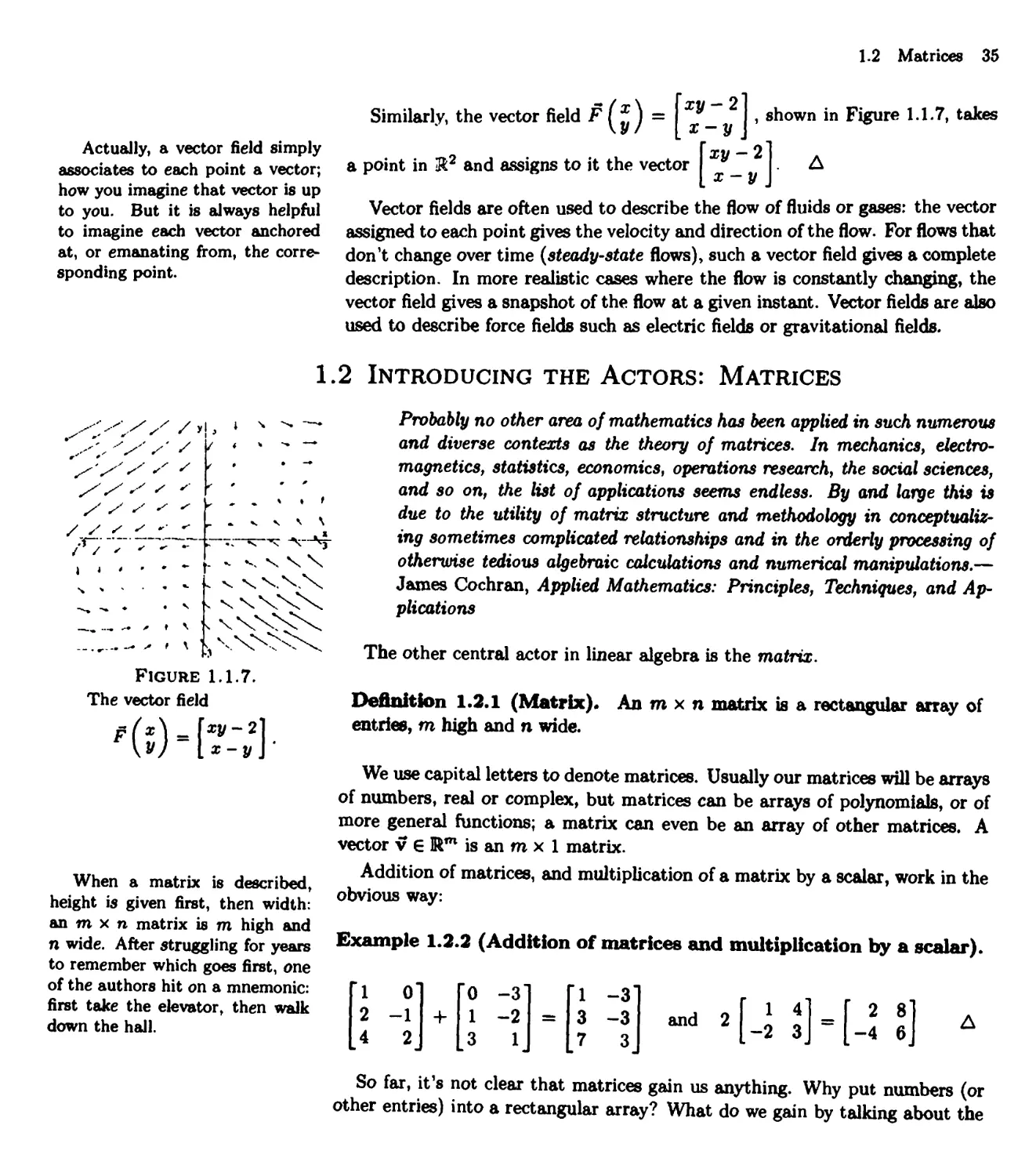
1.1 Introducing the Actors: Vectors 28
1.2 Introducing the Actors: Matrices 35
1.3 A Matrix as a Transformation 46
1.4 The Geometry of Kn 58
1.5 Convergence and Limits 72
1.6 Four Big Theorems 89
1.7 Differential Calculus 100
1.8 Rules for Computing Derivatives 115
1.9 Criteria for Differentiability 120
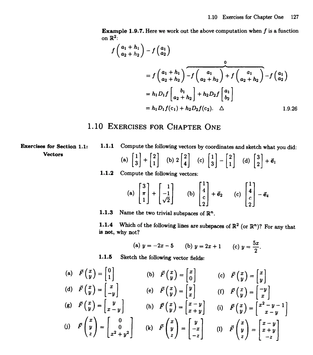
1.10 Exercises for Chapter 1 127
CHAPTER 2 Solving Equations
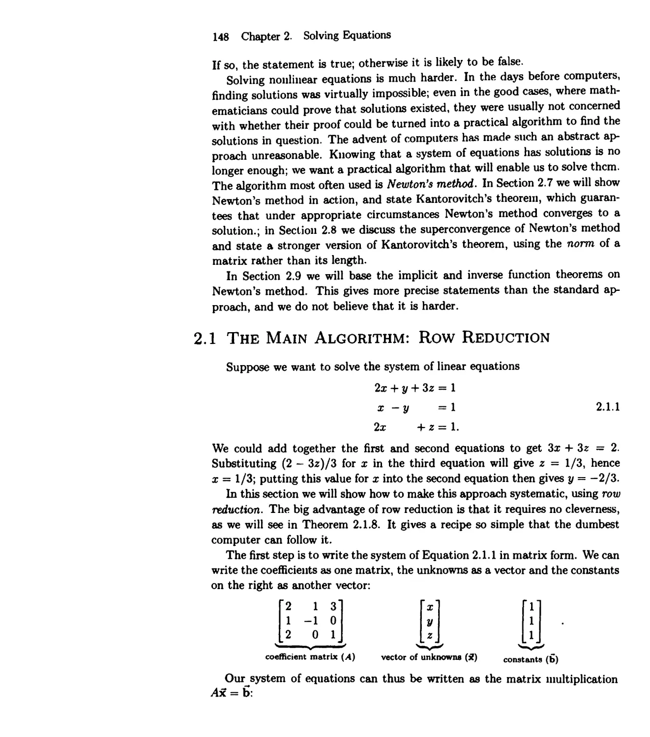
2.0 Introduction 147
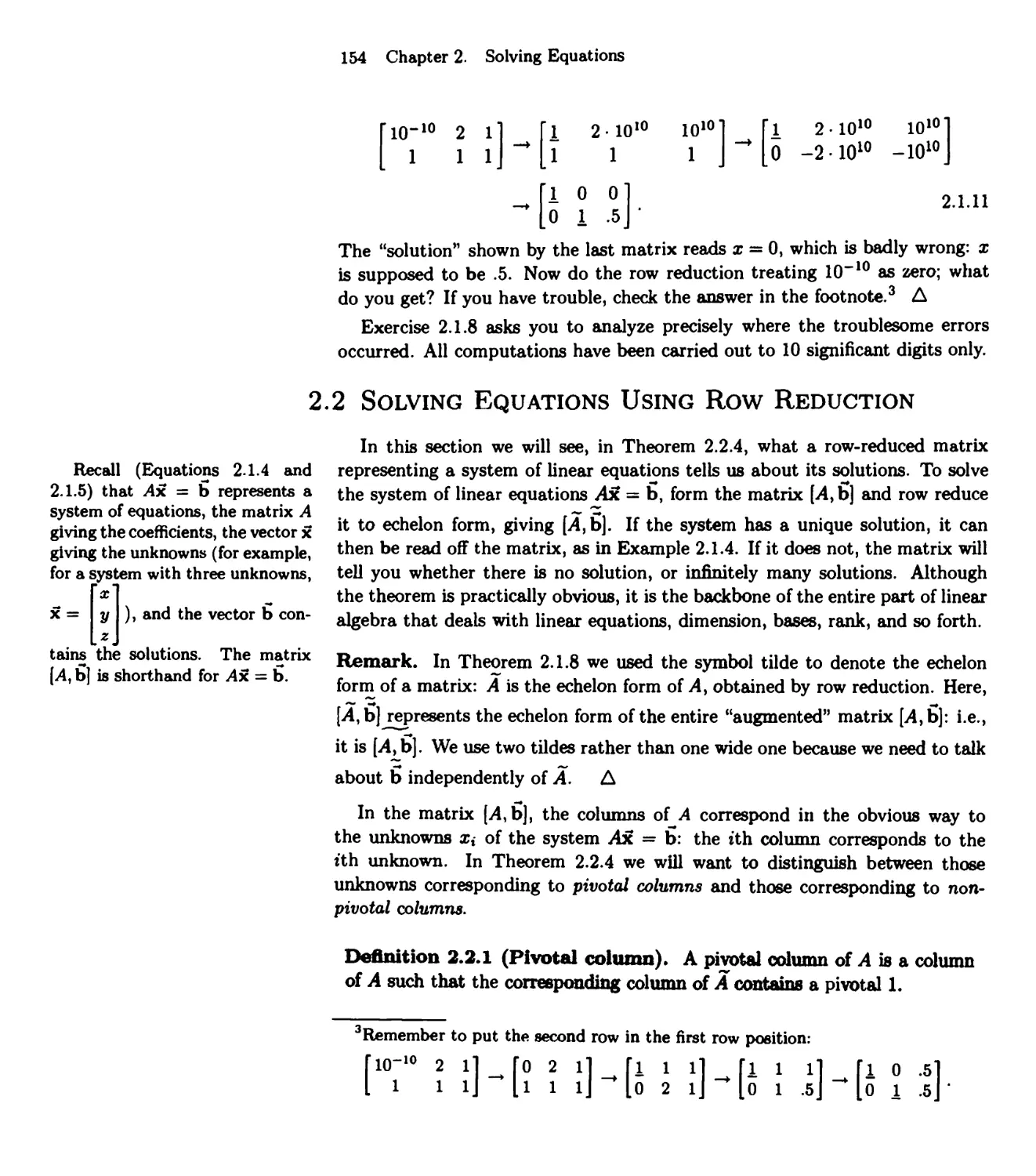
2.1 The Main Algorithm: Row Reduction 148
2.2 Solving Equations Using Row Reduction 154
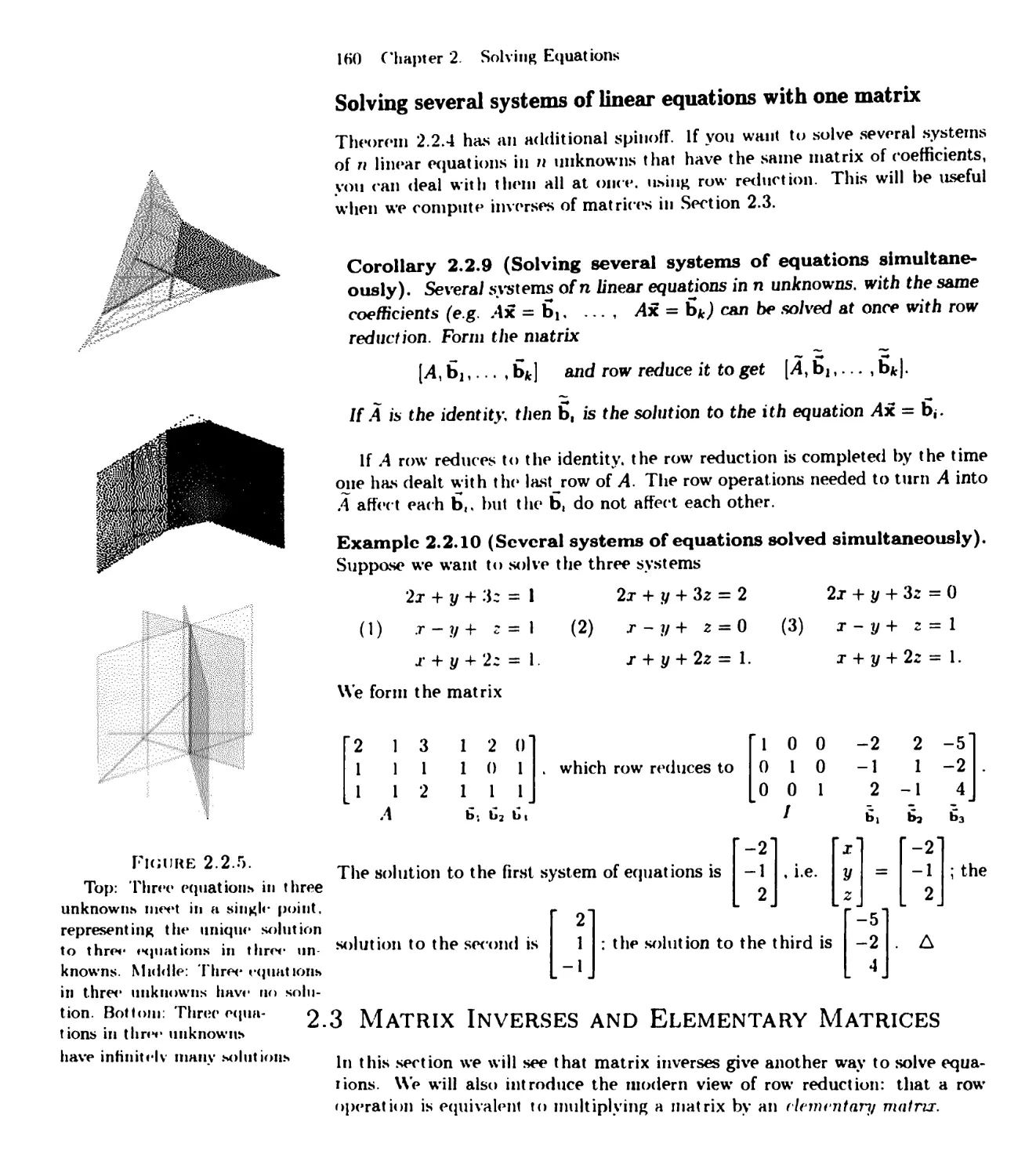
2.3 Matrix Inverses and Elementary Matrices 160
2.4 Linear Combinations, Span, and Linear Independence 165
2.5 Kernels and Images 177
2.6 Abstract Vector Spaces 189
2.7 Newton's Method 197
viii Contents
2.8 Superconvergence 211
2.9 The Inverse and Implicit Function Theorems 217
2.10 Exercises for Chapter 2 231
CHAPTER 3 Higher Partial Derivatives, Quadratic Forms,
and Manifolds
3.0 Introduction 249
3.1 Curves and Surfaces 250
3.2 Manifolds 266
3.3 Taylor Polynomials in Several Variables 275
3.4 Rules for Computing Taylor Polynomials 285
3.5 Quadratic Forms 290
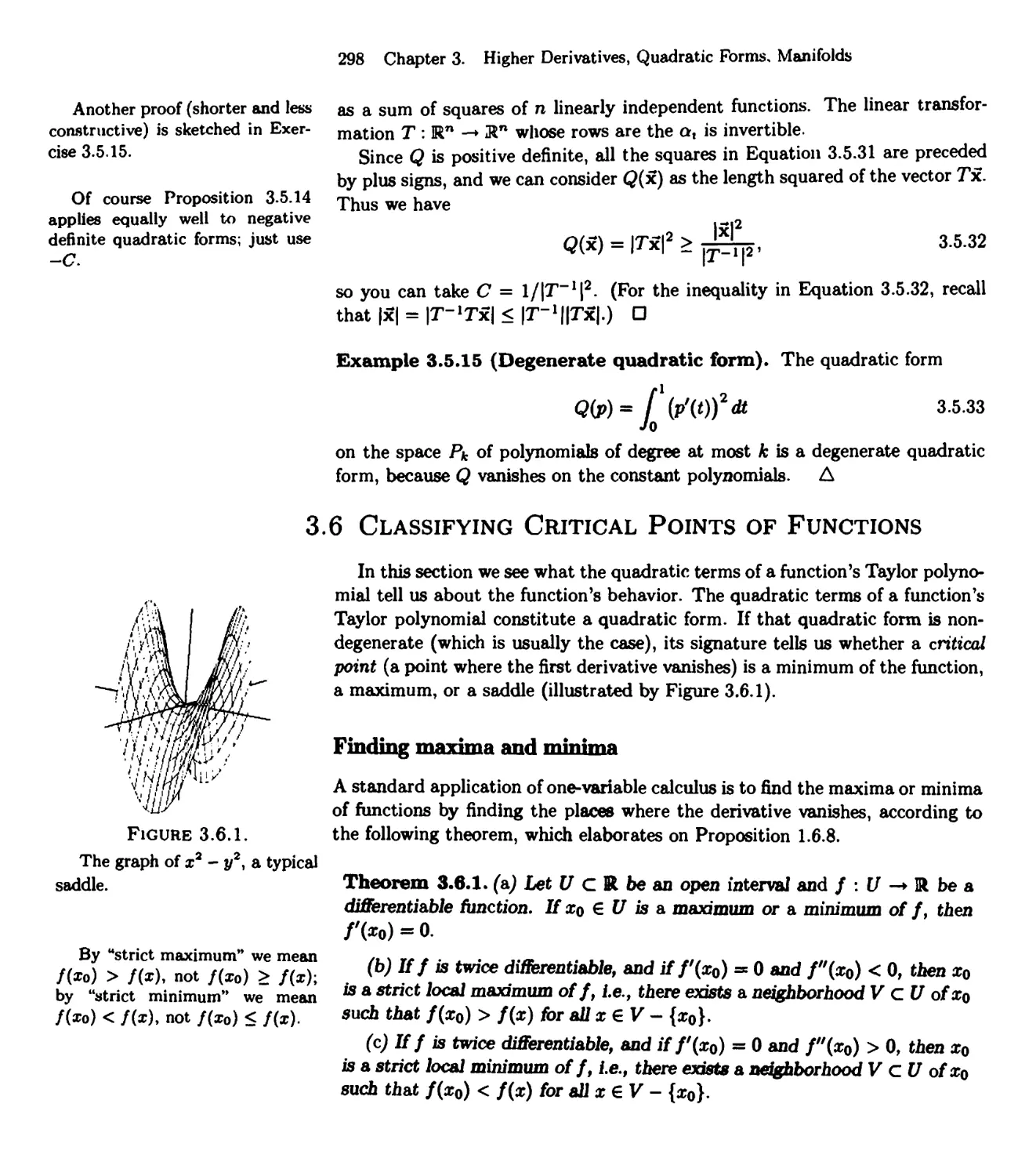
3.6 Classifying Critical Points of Functions 298
3.7 Constrained Critical Points and Lagrange Multipliers 304
3.8 Geometry of Curves and Surfaces 316
3.9 Exercises for Chapter 3 332
CHAPTER 4 Integration
4.0 Introduction 351
4.1 Defining the Integral 352
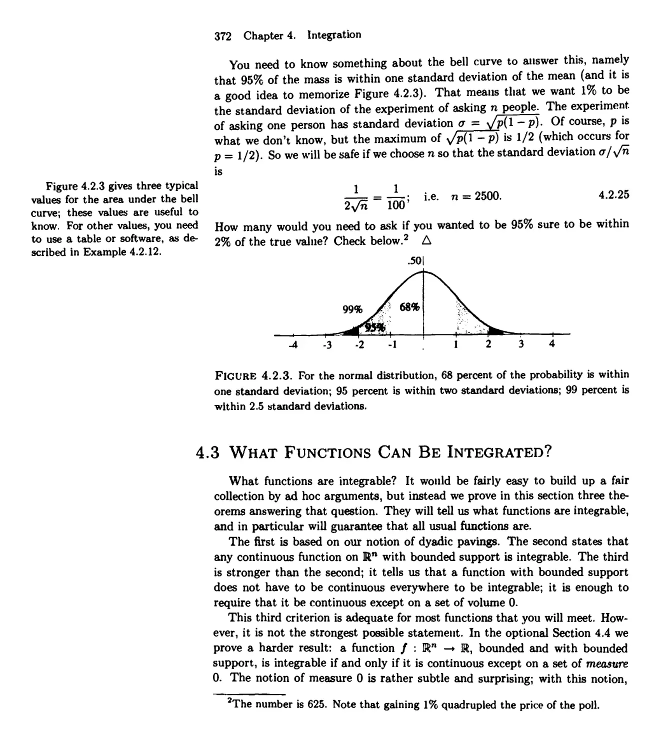
4.2 Probability and Integrals 362
4.3 What Functions Can Be Integrated? 372
4.4 Integration and Measure Zero (Optional) 380
4.5 Fubini's Theorem and Iterated Integrals 387
4.6 Numerical Methods of Integration 395
4.7 Other Pavings 404
4.8 Determinants 405
4.9 Volumes and Determinants 420
4.10 The Change of Variables Formula 426
4.11 Improper Integrals 436
4.12 Exercises for Chapter 4 449
CHAPTER 5 Lengths of Curves, Areas of Surfaces, ...
6.0 Introduction 469
5.1 Parallelograms and their Volumes 470
5.2 Parametrizations 473
5.3 Arc Length 479
5.4 Surface Area 482
5.5 Volume of Manifolds 488
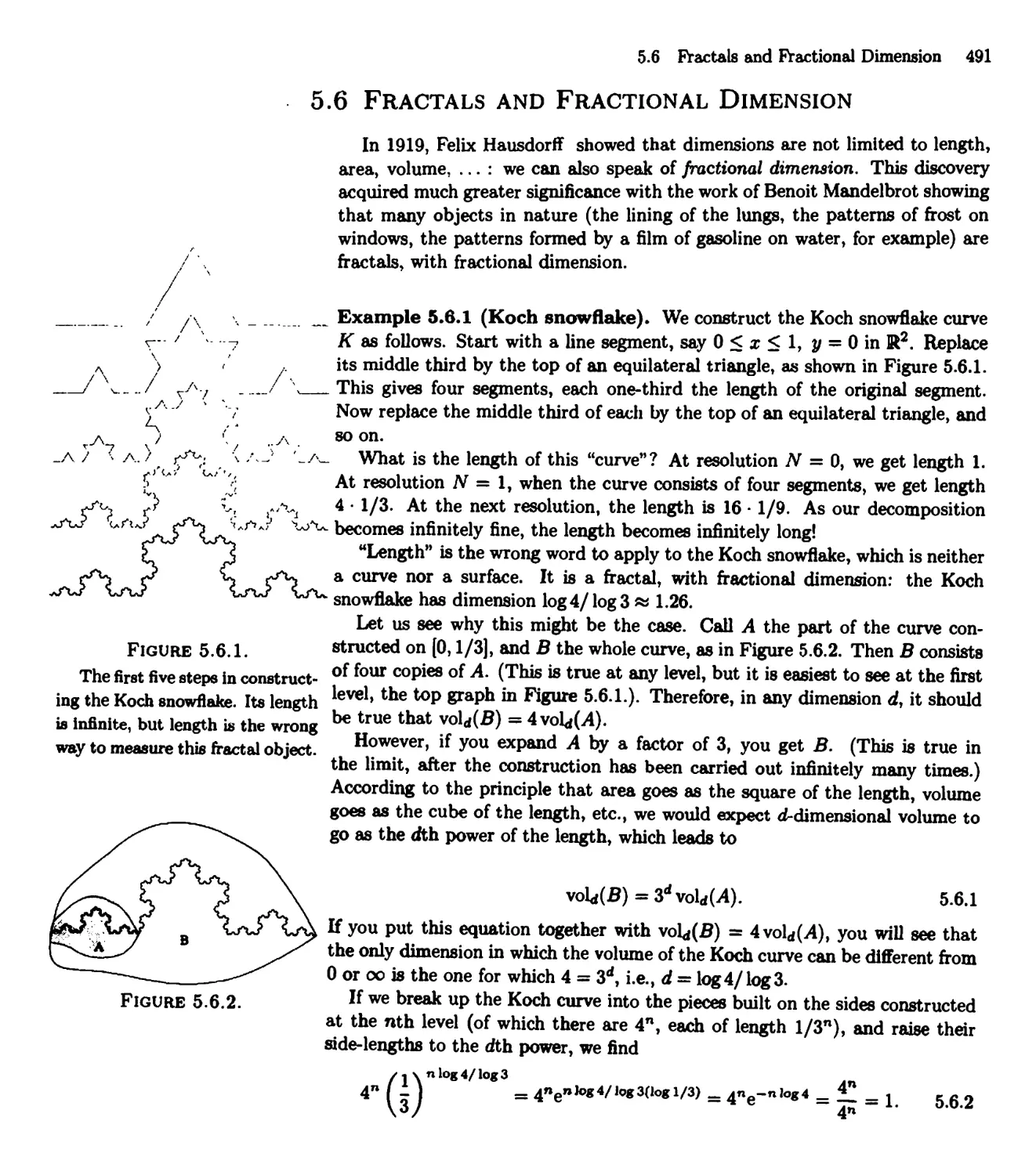
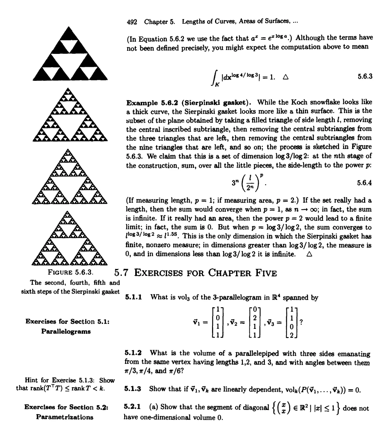
5.6 Fractals and Fractional Dimension 491
Contents ix
5.7 Exercises for Chapter 5 492
CHAPTER 6 Forms and Vector Calculus
6.0 Introduction 499
6.1 Forms as Integrands over Oriented Domains 500
6.2 Forms on W1 501
6.3 Integrating Form Fields over Parametrized Domains 512
6.4 Forms and Vector Calculus 516
6.5 Orientation and Integration of Form Fields 525
6.6 Boundary Orientation 536
6.7 The Exterior Derivative 544
6.8 The Exterior Derivative in the Language of Vector Calculus 550
6.9 Generalized Stokes's Theorem 556
6.10 The Integral Theorems of Vector Calculus 563
6.11 Potentials 568
6.12 Exercises for Chapter 6 573
APPENDIX A: Some Harder Proofs
A.O Introduction 589
A. 1 Proof of the Chain Rule 589
A.2 Proof of KantorovitcrTs theorem 592
A.3 Proof of Lemma 2.8.4 (Superconvergence) 597
A.4 Proof of Differentiability of the Inverse Function 598
A.5 Proof of the Implicit Function Theorem 602
A.6 Proof of Theorem 3.3.9: Equality of Crossed Partials 605
A.7 Proof of Proposition 3.3.19 606
A.8 Proof of Rules for Taylor Polynomials 609
A.9 Taylor's Theorem with Remainder 613
A. 10 Proof of Theorem 3.5.3 (Completing Squares) 617
A. 11 Proof of Propositions 3.8.12 and 3.8.13 (Frenet Formulas) 619
A. 12 Proof of the Central Limit Theorem 622
A. 13 Proof of Fubini's Theorem 626
A. 14 Justifying the Use of Other Pavings 629
A. 15 Existence and Uniqueness of the Determinant 632
A. 16 Rigorous Proof of the Change of Variables Formula 635
A. 17 A Few Extra Results in Topology 643
A. 18 Proof of the Dominated Convergence Theorem 643
A. 19 Justifying the Change of Parametrization 648
A.20 Proof of Theorem 6.7.3 (Computing the Exterior Derivative) 652
x Contents
A.21 The Pullback 656
A.22 Proof of Stokes' Theorem 661
A.23 Exercises 665
APPENDIX B: Programs
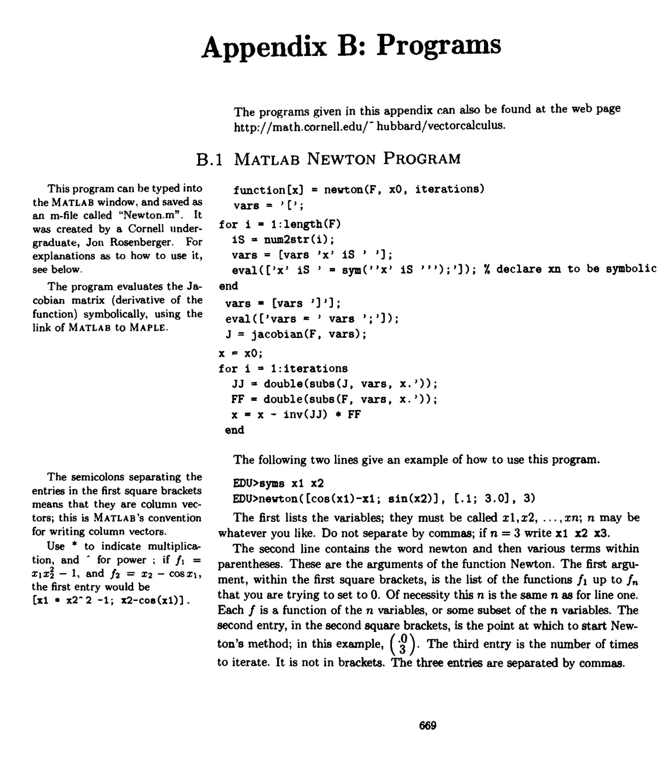
B.l Matlab Newton Program 669
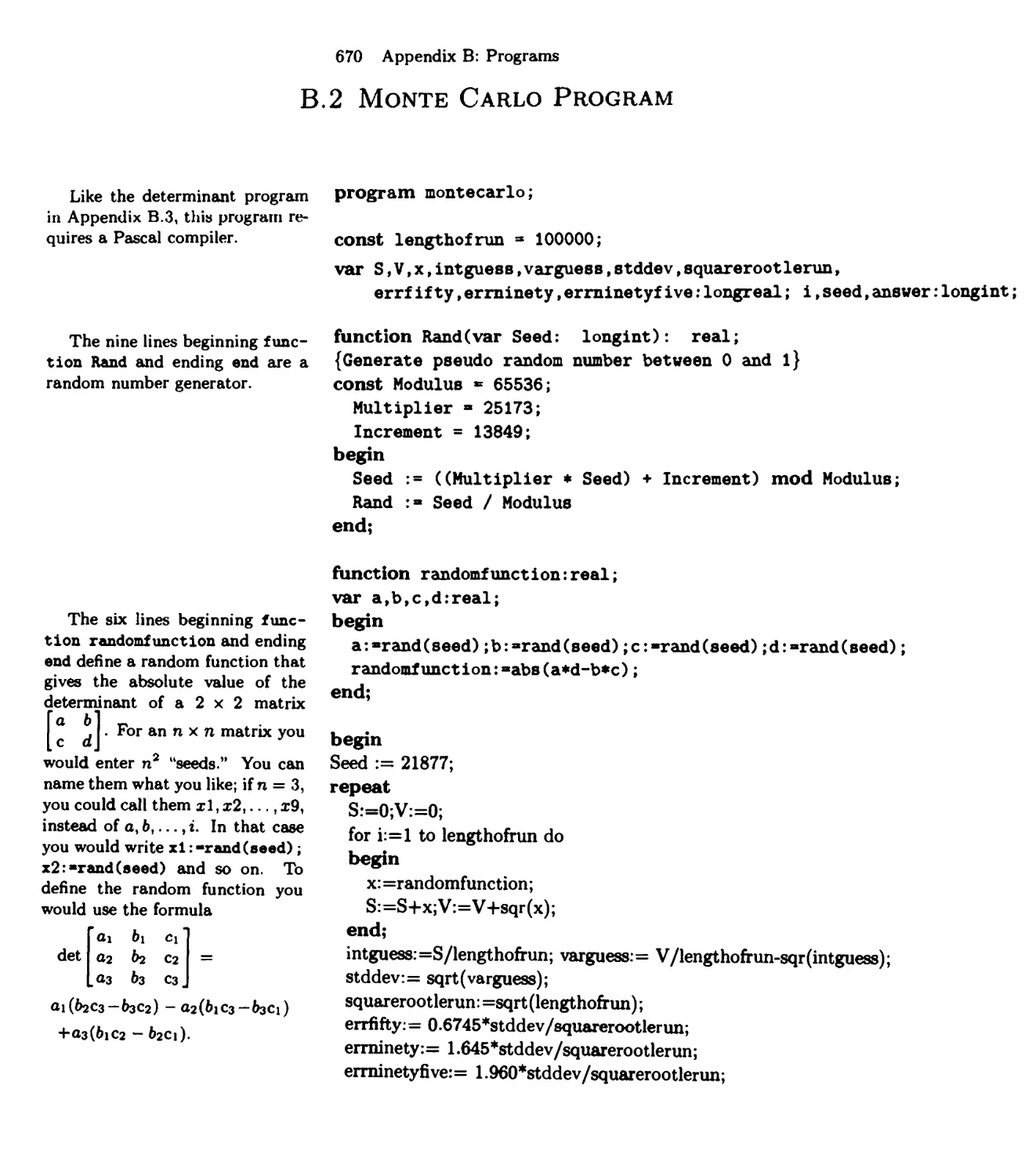
B.2 Monte Carlo Program 670
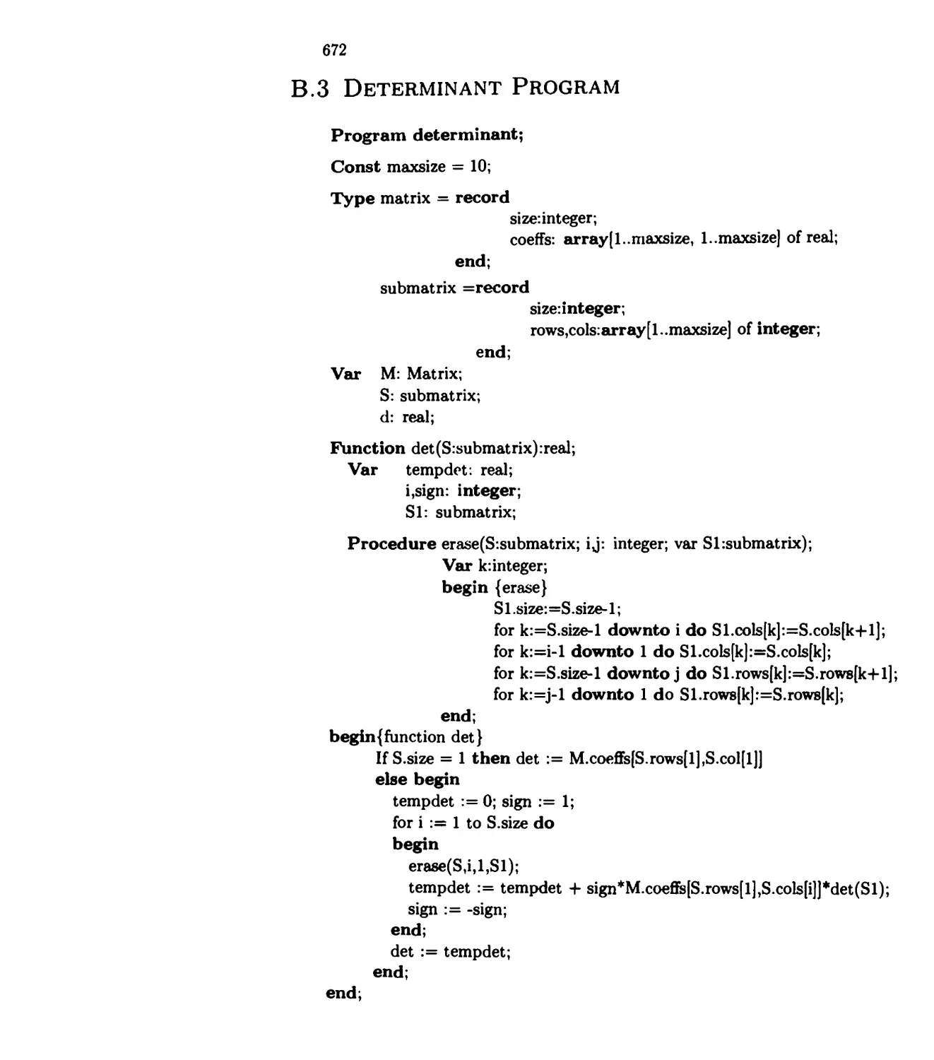
B.3 Determinant Program 672
BIBLIOGRAPHY 675
INDEX 677
Preface
... The numerical interpretation ...is however necessary. ...So long
as it is not obtained, the solutions may be said to remain incomplete and
useless, and the truth which it is proposed to discover is no less hidden
in the formulae of analysis than it was in the physical problem itself.
-Joseph Fourier, The Analytic Theory of Heat
This book covers most of the standard topics in multivariate calculus, and a
substantial part of a standard first course in linear algebra. The teacher may
find the organization rather less standard.
There are three guiding principles which led to our organizing the material
as we did. One is that at this level linear algebra should be more a convenient
setting and language for multivariate calculus than a subject in its own right.
We begin most chapters with a treatment of a topic in linear algebra and then
show how the methods apply to corresponding nonlinear problems. In each
chapter, enough linear algebra is developed to provide the tools we need in
teaching multivariate calculus (in fact, somewhat more: the spectral theorem
for symmetric matrices is proved in Section 3.7). We discuss abstract vector
spaces in Section 2.6, but the emphasis is on Kn, as we believe that most
students find it easiest to move from the concrete to the abstract.
Another guiding principle is that one should emphasize computationally
effective algorithms, and prove theorems by showing that those algorithms really
work: to marry theory and applications by using practical algorithms as
theoretical tools. We feel this better reflects the way this mathematics is used
today, in both applied and in pure mathematics. Moreover, it can be done with
no loss of rigor.
For linear equations, row reduction (the practical algorithm) is the central
tool from which everything else follows, and we use row reduction to prove all
the standard results about dimension and rank. For nonlinear equations, the
cornerstone is Newton's method, the best and most widely used method for
solving nonlinear equations. We use Newton's method both as a computational
tool and as the basis for proving the inverse and implicit function theorem,
rather than basing those proofs on Picard iteration, which converges too slowly
to be of practical interest.
xi
xii Preface
Jean Dieudonne\ for many
years a leader of Bourbaki, is the
very personification of rigor in
mathematics. In his book
Infinitesimal Calculus, he put the
harder proofs in small type,
saying "... a beginner will do well
to accept plausible results without
taxing his mind with subtle proofs
n
Following this philosophy, we
have put many of the more
difficult proofs in the appendix, and
feel that for a first course, these
proofs should be omitted.
Students should learn how to drive
before they learn how to take the car
apart.
In keeping with our emphasis on computations, we include a section on
numerical methods of integration, and we encourage the use of computers to
both to reduce tedious calculations (row reduction in particular) and as an
aid in visualizing curves and surfaces. We have also included a section on
probability and integrals, as this seems to us too important a use of integration
to be ignored.
A third principle is that differential forms are the right way to approach the
various forms of Stokes's theorem. We say this with some trepidation,
especially after some of our most distinguished colleagues told us they had never
really understood what differential forms were about. We believe that
differential forms can be taught to freshmen and sophomores, if forms are presented
geometrically, as integrands that take an oriented piece of a curve, surface, or
manifold, and return a number. We are aware that students taking courses
in other fields need to master the language of vector calculus, and we devote
three sections of Chapter 6 to integrating the standard vector calculus into the
language of forms.
The great conceptual simplifications gained by doing electromagnetism in
the language of forms is a central motivation for using forms, and we will apply
the language of forms to electromagnetism in a subsequent volume.
Although most long proofs have been put in Appendix A, we made an
exception for the material in Section 1.6. These theorems in topology are often not
taught, but we feel we would be doing the beginning student a disservice not
to include them, particularly the mean value theorem and the theorems
concerning convergent subsequences in compact sets and the existence of minima
and maxima of functions. In our experience, students do not find this material
particularly hard, and systematically avoiding it leaves them with an uneasy
feeling that the foundations of the subject are shaky.
Different ways to use the book
This book can be used either as a textbook in multivariate calculus or as an
accessible textbook for a course in analysis.
We see calculus as analogous to learning how to drive, while analysis is
analogous to learning how and why a car works. To use this book to "learn
how to drive," the proofs in Appendix A should be omitted. To use it to "learn
how a car works," the emphasis should be on those proofs. For most students,
this will be best attempted when they already have some familiarity with the
material in the main text.
Students who have studied first year calculus only
(1) For a one-semester course taken by students have studied neither linear
algebra nor multivariate calculus, we suggest covering only the first four
chapters, omitting the sections marked "optional," which, in the analogy of learning
Preface xiii
to drive rather than learning how a car is built, correspond rather to learning
how to drive on ice. (These sections include the part of Section 2.8 concerning
a stronger version of the Kantorovitch theorem, and Section 4.4 on measure
0). Other topics that can be omitted in a first course include the proof of the
fundamental theorem of algebra in Section 1.6, the discussion of criteria for
differentiability in Section 1.9, Section 3.2 on manifolds, and Section 3.8 on
the geometry of curves and surfaces. (In our experience, beginning students
do have trouble with the proof of the fundamental theorem of algebra, while
manifolds do not pose much of a problem.)
(2) The entire book could also be used for a full year's course. This could be
done at different levels of difficulty, depending on the students' sophistication
and the pace of the class. Some students may need to review the material
in Sections 0.3 and 0.5; others may be able to include some of the proofs in
the appendix, such as those of the central limit theorem and the Kantorovitch
theorem.
(3) With a year at one's disposal (and excluding the proofs in the appendix),
one could also cover more than the present material, and a second volume is
planned, covering
applications of differential forms;
abstract vector spaces, inner product spaces, and Fourier series;
electromagnetism;
differential equations;
eigenvalues, eigenvectors, and differential equations.
We favor this third approach; in particular, we feel that the last two topics
above are of central importance. Indeed, we feel that three semesters would
not be too much to devote to linear algebra, multivariate calculus, differential
forms, differential equations, and an introduction to Fourier series and partial
differential equations. This is more or less what the engineering and physics
departments expect students to learn in second year calculus, although we feel
this is unrealistic.
Students who have studied some linear algebra or multivariate
calculus
The book can also be used for students who have some exposure to either
linear algebra or multivariate calculus, but who are not ready for a course in
analysis. We used an earlier version of this text with students who had taken
a course in linear algebra, and feel they gained a great deal from seeing how
linear algebra and multivariate calculus mesh. Such students could be expected
to cover Chapters 1-6, possibly omitting some of the optional material discussed
I
xiv Preface
above. For a less fast-paced course, the book could also be covered in an entire
year, possibly including some proofs from the appendix.
Students ready for a course in analysis
We view Chapter 0 primarily
as a resource for students, rather
than as part of the material to be
covered in class. An exception is
Section 0.4, which might well be
covered in a class on analysis.
If the book is used as a text for an analysis course, then in one semester one
could hope to cover all six chapters and some or most of the proofs in Appendix
A. This could be done at varying levels of difficulty; students might be expected
to follow the proofs, for example, or they might be expected to understand them
well enough to construct similar proofs. Several exercises in Appendix A and
in Section 0.4 are of this nature.
Mathematical notation is not
always uniform. For example, \A\
can mean the length of a matrix
A (the meaning in this book) or
it can mean the determinant of
A. Different notations for partial
derivatives also exist. This should
not pose a problem for readers
who begin at the beginning and
end at the end, but for those who
are using only selected chapters,
it could be confusing. Notations
used in the book are listed on the
front inside cover, along with an
indication of where they are first
introduced.
Numbering of theorems, examples, and equations
Theorems, lemmas, propositions, corollaries, and examples share the same
numbering system. For example, Proposition 2.3.8 is not the eighth proposition of
Section 2.3; it is the eighth numbered item of that section, and the first
numbered item following Example 2.3.7. We often refer back to theorems, examples,
and so on, and hope this numbering will make them easier to find.
Figures are numbered independently; Figure 3.2.3 is the third figure of
Section 3.2. All displayed equations are numbered, with the numbers given at
right; Equation 4.2.3 is the third equation of Section 4.2. When an equation
is displayed a second time, it keeps its original number, but the number is in
parentheses.
We use the symbol A to mark the end of an example or remark, and the
symbol D to mark the end of a proof.
Exercises
Exercises are given at the end of each chapter, grouped by section. They range
from very easy exercises intended to make the student familiar with vocabulary,
to quite difficult exercises. The hardest exercises are marked with a star (or, in
rare cases, two stars). On occasion, figures and equations are numbered in the
exercises. In this case, they are given the number of the exercise to which they
pertain.
In addition, there are occasional "mini-exercises" incorporated in the text,
with answers given in footnotes. These are straightforward questions
containing no tricks or subtleties, and are intended to let the student test his or her
understanding (or be reassured that he or she has understood). We hope that
even the student who finds them too easy will answer them; working with pen
and paper helps vocabulary and techniques sink in.
Preface xv
Web page
Errata will be posted on the web page
http://math.comell.edu/~hubbard/vectorcalculus.
The three programs given in Appendix B will also be available there. We plan
to expand the web page, making the programs available on more platforms, and
adding new programs and examples of their uses.
Readers are encouraged to write the authors at jhh8@cornell.edu to signal
errors, or to suggest new exercises, which will then be shared with other readers
via the web page.
Acknowledgments
Many people contributed to this book. We would in particular like to express
our gratitude to Robert Terrell of Cornell University, for his many invaluable
suggestions, including ideas for examples and exercises, and advice on notation;
Adrien Douady of the University of Paris at Orsay, whose insights shaped our
presentation of integrals in Chapter 4; and R6gine Douady of the University
of Paris-VII, who inspired us to distinguish between points and vectors. We
would also like to thank Allen Back, Harriet Hubbard, Peter Papadopol, Birgit
Speh, and Vladimir Veselov, for their many contributions.
Cornell undergraduates in Math 221, 223, and 224 showed exemplary
patience in dealing with the inevitable shortcomings of an unfinished text in
photocopied form. They pointed out numerous errors, and they made the course a
pleasure to teach. We would like to thank in particular Allegra Angus, Daniel
Bauer, Vadim Grinshpun, Michael Henderson, Tomohiko Ishigami, Victor Kam,
Paul Kautz, Kevin Knox, Mikhail Kobyakov, Jie Li, Surachate Limkumnerd,
Mon-Jed Liu, Karl Papadantonakis, Marc Ratkovic, Susan Rushmer, Samuel
Scarano, Warren Scott, Timothy Slate, and Chan-ho Suh. Another Cornell
student, Jon Rosenberger, produced the Newton program in Appendix B.l. Karl
Papadantonakis helped produce the picture used on the cover.
For insights concerning the history of linear algebra, we are indebted to the
essay by J.-L. Dorier in L'Enseignement de I'alg&bre lineaire en question. Other
books that were influential include Infinitesimal Calculus by Jean Dieudonne\
Advanced Calculus by Lynn Loomis and Shlomo Sternberg, and Calculus on
Manifolds by Michael Spivak.
Ben Salzberg of Blue Sky Research saved us from despair when a new
computer refused to print files in Textures. Barbara Beeton of American
Mathematical Society's Technical Support gave prompt and helpful answers to technical
questions.
We would also like to thank George Lobell at Prentice Hall, who
encouraged us to write this book; Nicholas Romanelli for his editing and advice, and
xvi Preface
Gale Epps, as well as the mathematicians who served as reviewers for Prentice-
Hall and made many helpful suggestions and criticisms: Robert Boyer, Drexel
University; Ashwani Kapila, Rensselaer Polytechnic Institute; Krystyna Kuper-
berg, Auburn University; Ralph Oberste-Vorth, University of South Florida;
and Ernest Stitzinger, North Carolina State University. We are of course
responsible for any remaining errors, as well as for all our editorial choices.
We are indebted to our son, Alexander, for his suggestions, for writing
numerous solutions, and for writing a program to help with the indexing. We
thank our oldest daughter, Eleanor, for the goat figure of Section 3.8, and for
earning part of her first-year college tuition by reading through the text and
pointing out both places where it was not clear and passages she liked—the first
invaluable for the text, the second for our morale. With her sisters, Judith and
Diana, she also put food on the table when we were to busy to do so. Finally, we
thank Diana for discovering errors in the page numbers in the table of contents.
John H. Hubbard
Barbara Burke Hubbard
Ithaca, N.Y.
jhh8@coraell.edu
John H. Hubbard is a professor of mathematics at Cornell University and the author of
several books on differential equations. His research mainly concerns complex analysis,
differential equations, and dynamical systems. He believes that mathematics research
and teaching are activities that enrich each other and should not be separated.
Barbara Burke Hubbard is the author of The World According to Wavelets, which
was awarded the prix d'Alembert by the French Mathematical Society in 1996.
0
Preliminaries
0.0 Introduction
This chapter is intended as a resource, providing some background for those
who may need it. In Section 0.1 we share some guidelines that in our
experience make reading mathematics easier, and discuss a few specific issues like
sum notation. Section 0.2 analyzes the rather tricky business of negating
mathematical statements. (To a mathematician, the statement "All seven-legged
alligators are orange with blue spots" is an obviously true statement, not an
obviously meaningless one.) Section 0.3 reviews set theory notation; Section
0.4 discusses the real numbers; Section 0.5 discusses countable and uncountable
sets and Russell's paradox; and Section 0.6 discusses complex numbers.
0.1 Reading Mathematics
The most efficient logical order for a subject is usually different from the
best psychological order in which to learn it. Much mathematical writing
is based too closely on the logical order of deduction in a subject, with too
many definitions without, or before, the examples which motivate them,
and too many answers before, or without, the questions they address.—
William Thurston
Reading mathematics is different from other reading. We think the following
guidelines can make it easier. First, keep in mind that there are two parts to
understanding a theorem: understanding the statement, and understanding the
proof. The first is more important than the second.
What if you don't understand the statement? If there's a symbol in the
formula you don't understand, perhaps a 5, look to see whether the next line
continues, "where 8 is such-and-such." In other words, read the whole sentence
before you decide you can't understand it. In this book we have tried to define
all terms before giving formulas, but we may not have succeeded everywhere.
If you're still having trouble, skip ahead to examples. This may contradict
what you have been told—that mathematics is sequential, and that you must
understand each sentence before going on to the next. In reality, although
mathematical writing is necessarily sequential, mathematical understanding is
not: you (and the experts) never understand perfectly up to some point and
We recommend not spending
much time on Chapter 0. In
particular, if you are studying
multivariate calculus for the first time
you should definitely skip certain
parts of Section 0.4 (Definition
0.4.4 and Proposition 0.4.6).
However, Section 0.4 contains a
discussion of sequences and series which
you may wish to consult when we
come to Section 1.5 about
convergence and limits, if you find you
don't remember the convergence
criteria for sequences and series
from first year calculus.
1
2 Chapter 0. Preliminaries
The Greek Alphabet
Greek letters that look like
Roman letters are not used as
mathematical symbols; for example, A is
capital a, not capital a. The letter
X is pronounced "kye," to rhyme
with "sky"; y>, ty and £ may rhyme
with either "sky" or "tea."
0
7
6
X
v
o
X
A alpha
B beta
gamma
delta
epsilon
zeta
eta
theta
iota
K kappa
A lambda
M mu
N nu
r
A
E
Z
H
e
i
O omicron
II pi
P rho
£ sigma
T tau
T upsilon
$ phi
X chi
* psi
Q omega
In Equation 0.1.3, the symbol
£2=1 oay8 tnat tne 8Um will have
n terms. Since the expression
being summed is at,kbk,J} each of
those n terms will have the form
ab.
not at all beyond. The "beyond," where understanding is only partial, is an
essential part of the motivation and the conceptual background of the "here and
now." You may often (perhaps usually) find that when you return to something
you left half-understood, it will have become clear in the light of the further
things you have studied, even though the further things are themselves obscure.
Many students are very uncomfortable in this state of partial understanding,
like a beginning rock climber who wants to be in stable equilibrium at all times.
To learn effectively one must be willing to leave the cocoon of equilibrium. So
if you don't understand something perfectly, go on ahead and then circle back.
In particular, an example will often be easier to follow than a general
statement; you can then go back and reconstitute the meaning of the statement in
light of the example. Even if you still have trouble with the general statement,
you will be ahead of the game if you understand the examples. We feel so
strongly about this that we have sometimes flouted mathematical tradition and
given examples before the proper definition.
Read with pencil and paper in hand, making up little examples for yourself
as you go on.
Some of the difficulty in reading mathematics is notational. A pianist who
has to stop and think whether a given note on the staff is A or F will not be
able to sight-read a Bach prelude or Schubert sonata. The temptation, when
faced with a long, involved equation, may be to give up. You need to take the
time to identify the "notes."
Learn the names of Greek letters—not just the obvious ones like alpha, beta,
and pi, but the more obscure psi, xi, tau, omega. The authors know a
mathematician who calls all Greek letters "xi," (£) except for omega (a;), which he
calls "w." This leads to confusion. Learn not just to recognize these letters, but
how to pronounce them. Even if you are not reading mathematics out loud, it
is hard to think about formulas if £, ^, t,lj, <p are all "squiggles" to you.
Sum and product notation
Sum notation can be confusing at first; we are accustomed to reading in one
dimension, from left to right, but something like
53 a«.*6*.J
0.1.1
requires what we might call two-dimensional (or even three-dimensional)
thinking. It may help at first to translate a sum into a linear expression:
0.1.2
^2* = 2° + 21+22...
t=0
n
°*d = 5Za».*6*.J = aU&ij + a«,2&2,j + • • • + attnbnij. 0.1.3
0.1 Reading Mathematics 3
Ep- B-S-
E±3—-E*3-—-EO---
Two £ placed side by side do not denote the product of two sums; one sum
is used to talk about one index, the other about another. The same thing could
be written with one £, with information about both indices underneath. For
example,
t'=l j—2 i from 1 to 3,
j from 2 to 4
1
= (U + 2) + (l + 3) + (l + 4))
+ ((2 + 2) + (2 + 3) + (2 + 4))
+ ((3 + 2) + (3 + 3) + (3 + 4));
this double sum is illustrated in Figure 0.1.1.
Rules for product notation are analogous to those for sum notation:
0.1.4
Figure 0.1.1.
In the double sum of Equation
0.1.4, each sum has three terms, so
the double sum has nine terms. Proofs
J7 Oj = oi • 02 • • a„; for example, JJ i — n\.
When Jacobi complained that
Gauss's proofs appeared
unmotivated, Gauss is said to have
answered, You build the building and
remove the scaffolding. Our
sympathy is with Jacobi*s reply: he
likened Gauss to the fox who
erases his tracks in the sand with
his tail.
We said earlier that it is more important to understand a mathematical
statement than to understand its proof. We have put some of the harder proofe in
the appendix; these can safely be skipped by a student studying multivariate
calculus for the first time. We urge you, however, to read the proofe in the main
text. By reading many proofe you will learn what a proof is, so that (for one
thing) you will know when you have proved something and when you have not.
In addition, a good proof doesn't just convince you that something is true;
it tells you why it is true. You presumably don't lie awake at night worrying
about the truth of the statements in this or any other math textbook. (This
is known as "proof by eminent authority*'; you assume the authors know what
they are talking about.) But reading the proofe will help you understand the
material.
If you get discouraged, keep in mind that the content of this book represents
a cleaned-up version of many false starts. For example, John Hubbard started
by trying to prove FVibini's theorem in the form presented in Equation 4.5.1.
When he failed, he realized (something he had known and forgotten) that the
statement was in fact false. He then went through a stack of scrap paper before
coming up with a correct proof. Other statements in the book represent the
efforts of some of the world's best mathematicians over many years.
4 Chapter 0. Preliminaries
0.2 HOW TO NEGATE MATHEMATICAL STATEMENTS
Even professional mathematicians have to be careful not to get confused
when negating a complicated mathematical statement. The rules to follow are:
(1) The opposite of
[For all x, P(x) is true]
is [There exists x for which P(x) is not true].
0.2.1
Above, P stands for "property." Symbolically the same sentence is written:
The opposite of Vx,P(x) is 3x| not P(x). 0.2.2
Instead of using the bar | to mean "such that" we could write the last line
(3x)(not P(x)). Sometimes (not in this book) the symbols ~ and -■ are used
to mean "not."
(2) The opposite of
[There exists x for which R(x) is true]
is (For all xy R(x) is not true].
0.2.3
Statements that to the
ordinary mortal are false or
meaningless are thus accepted as true by
mathematicians; if you object, the
mathematician will retort, "find
me a counter-example."
Symbolically the same sentence is written:
The opposite of (3x)(P(x)) is (Vx) not P(x). 0.2.4
These rules may seem reasonable and simple. Clearly the opposite of the
(false) statement, "All rational numbers equal 1," is the statement, "There
exists a rational number that does not equal 1."
However, by the same rules, the statement, "All seven-legged alligators are
orange with blue spots" is true, since if it were false, then there would exist a
seven-legged alligator that is not orange with blue spots. The statement, "All
seven-legged alligators are black with white stripes" is equally true.
In addition, mathematical statements are rarely as simple as "All rational
numbers equal 1." Often there are many quantifiers and even the experts have
to watch out. At a lecture attended by one of the authors, it was not clear to
the audience in what order the lecturer was taking the quantifiers; when he was
forced to write down a precise statement, he discovered that he didn't know
what he meant and the lecture fell apart.
Here is an example where the order of quantifiers really counts: in the
definitions of continuity and uniform continuity. A function / is continuous if for
all x, and for all c> 0, there exists S > 0 such that for all y, if |x - y\ < <5, then
\f(x) ~ f(y)\ < c- That is, / is continuous if
(Vx)(Vc > 0)(3(5 > 0)(Vy) (|x - y\ < S =* |/(x) - f(y)\ < c). 0.2.5
0.3 Set Theory 5
A function / is uniformly continuous if for all e > 0, there exists 6 > 0 for
all x and all y such that if \x - y\ < <5, then \f(x) - f(y)\ < e. That is, / is
uniformly continuous if
(Ve > 0)(3<5 > 0)(Vs)(Vy) (\x - y\ < 6 ==> \f(x) - f(y)\ < e). 0.2.6
For the continuous function, we can choose different 6 for different x; for the
uniformly continuous function, we start with € and have to find a single 6 that
works for all x.
For example, the function f{x) = x2 is continuous but not uniformly
continuous: as you choose bigger and bigger x, you will need a smaller <5 if you
want the statement \x - y\ < 6 to imply \f(x) - f(y)\ < e, because the function
keeps climbing more and more steeply. But sins is uniformly continuous; you
can find one S that works for all x and all y.
0.3 Set Theory
There is nothing new about
the concept of "set" denoted by
{a\p(a)}. Euclid spoke of
geometric loci, a locus being the set
of points defined by some
property. (The Latin word locus means
"place"; its plural is loci.)
At the level at which we are working, set theory is a language, with a
vocabulary consisting of seven words. In the late 1960's and early 1970's, under the
sway of the "New Math," they were a standard part of the elementary school
curriculum, and set theory was taught as a subject in its own right. This was a
resounding failure, possibly because many teachers, understandably not
knowing why set theory was being taught at all, made mountains out of molehills. As
a result the schools (elementary, middle, high) have often gone to the opposite
extreme, and some have dropped the subject altogether.
The seven vocabulary words are
€ "is an element oP
{o |p(o)} "the set of o such that p(o) is true"
C "is a subset of (or equals, when Ac A)
n "intersect": A C\ B is the set of elements of both A and B.
U "union": A U B is the set of elements of either A or B
or both,
x "cross": A x B is the set of pairs (o, b) with a e A and
beB.
- "complement": A - B is the set of elements in A that
are not in B.
One set has a standard name: the empty set <#, which has no elements.
There are also sets of numbers that have standard names; they are written in
black-board bold, a font we use only for these sets. Throughout this book and
most other mathematics books (with the exception of N, as noted in the margin
below), they have exactly the same meaning:
6 Chapter 0. Preliminaries
N is for "natural," 7L is for
"Zahl," the German for number,
Q is for "quotient," R is for "real,"
and C is for "complex."
Mathematical notation is not quite
standard: some authors do not include
OinN.
When writing with chalk on a
black board, it's hard to
distinguish between normal letters and
bold letters. Black-board bold
font is characterized by double
lines, as in N and R.
Although it may seem a bit
pedantic, you should notice that
[jln and {ln\neZ}
n€Z
are not the same thing: the first
is a subset of the plane; an
element of it is a point on one of
the lines. The second is a set of
lines, not a set of points. This
is similar to one of the molehills
which became mountains in the
new-math days: telling the
difference between <f> and {<#}, the set
whose only element is the empty
set.
o
Showing that all such
constructions lead to the same numbers is
a fastidious exercise, which we will
not pursue.
N "the natural numbers" {0,1,2,...}
Z "the integers," i.e., signed whole numbers {...,-1,0,1,...}
Q "the rational numbers" p/q, with p,q € Z, q ^ 0
R "the real numbers," which we will think of as infinite decimals
C "the complex numbers" {a + ib\ a, b € R}
Often we use slight variants of the notation above: {3,5,7} is the set
consisting of 3,5, and 7, and more generally, the set consisting of some list of elements
is denoted by that list, enclosed in curly brackets, as in
{n j n e N and n is even} = {0,2,4,... }, 0.3.1
where again the vertical line | means "such that."
The symbols are sometimes used backwards; for example, A D B means
B C j4, as yon probably guessed. Expressions are sometimes condensed:
{x e R | x is a square } means {x \ x € R and x is a square } , 0.3.2
i.e., the set of non-negative real numbers.
A slightly more elaborate variation is indexed unions and intersections: if
SQ is a collection of sets indexed by a 6 A, then
p| Sq denotes the intersection of all the 5Q, and
a€A
M Sa denotes their union.
a£A
For instance, if Zn C R2 is the line of equation y = n, then Unez 'n is the set
of points in the plane whose y-coordinate is an integer.
We will use exponents to denote multiple products of sets; A x A x • • • x A
with n terms is denoted An: the set of n-tuples of elements of A.
If this is all there is to set theory, what is the fuss about? For one thing,
historically, mathematicians apparently did not think in terms of sets, and
the introduction of set theory was part of a revolution at the end of the 19th
century that included topology and measure theory. We explore another reason
in Section 0.5, concerning infinite sets and Russell's paradox.
,4 Real Numbers
All of calculus, and to a lesser extent linear algebra, is about real numbers.
In this introduction, we will present real numbers, and establish some of their
most useful properties. Our approach privileges the writing of numbers in base
10; as such it is a bit unnatural, but we hope you will like our real numbers
being exactly the numbers you are used to. Also, addition and multiplication
will be denned in terms of finite decimals.
0.4 Real Numbers 7
There are more elegant
approaches to defining real
numbers, (Dedekind cuts, for instance
(see, for example, Michael Spivak,
Calculus, second edition, 1980, pp.
554-572), or Cauchy sequences of
rational numbers; one could also
mirror the present approach,
writing numbers in any base, for
instance 2. Since this section is
partially motivated by the treatment
of floating-point numbers on
computers, base 2 would seem very
natural.
The least upper bound
property of the reals is often taken as
an axiom; indeed, it characterizes
the real numbers, and it sits at
the foundation of every theorem in
calculus. However, at least with
the description above of the reals,
it is a theorem, not an axiom.
The least upper bound supX
is sometimes denoted l.u.b.X; the
notation max X is also sometimes
used, but suggests to some people
that max X € X.
Numbers and their ordering
By definition, the set of real numbers is the set of infinite decimals: expressions
like 2.95765392045756..., preceded by a plus or a minus sign (in practice the
plus sign is usually omitted). The number that you usually think of as 3 is the
infinite decimal 3.0000..., ending in all zeroes.
The following identification is absolutely vital: a number ending in all 9's is
equal to the "rounded up" number ending in all 0's:
0.34999999 • • = 0.350000.
0.4.1
Also, +.0000 • • • = -.0000 Other than these exceptions, there is only one
way of writing a real number.
Numbers that start with a + sign, except +0.000..., are positive; those
that start with a - sign, except -0.00..., are negative. If x is a real number,
then —x has the same string of digits, but with the opposite sign in front. For
k > 0, we will denote by [a;]* the truncated finite decimal consisting of all the
digits of x before the decimal, and exactly k digits after the decimal. To avoid
ambiguity, if x is a real number with two decimal expressions, [x]k will be the
finite decimal built from the infinite decimal ending in 0's; for the number in
Equation 0.4.1, \x]3 = 0.350.
Given any two different numbers x and y, one is always bigger than the other.
This is defined as follows: if x is positive and y is non-positive, then x > y. If
both are positive, then in their decimal expansions there is a first digit in which
they differ; whichever has the larger digit in that position is larger. If both are
negative, then x > y if -y > -x.
The least upper bound property
Definition 0.4.1 (Upper bound; least upper bound). A number a is
an upper bound for a subset X C R if for every x 6 X we have x < a. A
least upper bound is an upper bound b such that for any other upper bound
o, we have b < a. The least upper bound is denoted sup.
Theorem 0.4.2. Every non-empty subset ^CK that has an upper bound
lias a least upper bound sup A".
Proof. We will construct successive decimals of sup A". Let us suppose that
x 6 X is an element (which we know exists, since X ^ <£) and that o is an
upper bound. We will assume that x > 0 (the case x < 0 is slightly different).
If x = o, we are done: the least upper bound is a.
8 Chapter 0. Preliminaries
Recall that [a]7 denotes the
finite decimal consisting of all the
digits of a before the decimal, and
j digits after the decimal.
We use the symbol D to mark
the end of a proof, and the symbol
A to denote the end of an example
or a remark.
Because you learned to add,
subtract, divide, and multiply in
elementary school, the algorithms
used may seem obvious. But
understanding how computers
simulate real numbers is not nearly
as routine as you might imagine.
A real number involves an infinite
amount of information, and
computers cannot handle such things:
they compute with finite decimals.
This inevitably involves rounding
off, and writing arithmetic
subroutines that minimize round-off
errors is a whole art in itself. In
particular, computer addition and
multiplication are not
commutative or associative. Anyone who
really wants to understand
numerical problems has to take a serious
interest in "computer arithmetic."
If x ^ a. there is a first j such that the jth digit of x is smaller than the jfth
digit of a. Consider all the numbers in [x, a] that can be written using only j
digits after the decimal, then all zeroes. This is a finite non-empty set; in fact
it has at most 10 elements, and \a]j is one of them. Let b3 be the largest which
is not an upper bound. Now consider the set of numbers in (&,, a] that have
only j + 1 digits after the decimal point, then all zeroes. Again this is a finite
non-empty set, so you can choose the largest which is not an upper bound; call
it bj+i. It should be clear that fy+i is obtained by adding one digit to bj. Keep
going this way, defining numbers 6j+2,&j+3, • • •» eacn ^me adding one digit to
the previous number. We can let b be the number whose kth decimal digit is
the same as that of &*; we claim that b = sup A".
Indeed, if there exists y € X with y > 6, then there is a first digit k of y
which differs from the kth digit of 6, and then bk was not the largest, number
with k digits which is not an upper bound, since using the kth digit of y would
give a bigger one. So b is an upper bound.
Now suppose that b' < b is also an upper bound. Again there is a first digit
k of b which is different from that of b'. This contradicts the fact that bk was
not an upper bound, since then 6a- > &'• D
Arithmetic of real numbers
The next task is to make arithmetic work for the reals: defining addition,
multiplication, subtraction, and division, and to show that the usual rules of
arithmetic hold. This is harder than one might think: addition and multiplication
always start at the right, and for reals there is no right.
The underlying idea is to show that if you take two reals, truncate (cut) them
further and further to the right and add them (or multiply them, or subtract
them, etc.) and look only at the digits to the left of any fixed position, the
digits we see will not be affected by where the truncation takes place, once it is
well beyond where we are looking. The problem with this is that it isn't quite
true.
Example 0.4.3 (Addition). Consider adding the following two numbers:
.222222... 222...
.777777...778...
The sum of the truncated numbers will be .9999... 9 if we truncate before the
position of the 8, and 1.0000.. .0 if we truncate after the 8. So there cannot
be any rule which says: the 100th digit will stay the same if you truncate after
the Nth digit, however large N is. The carry can come from arbitrarily far to
the right.
If you insist on defining everything in terms of digits, it can be done but
is quite involved: even showing that addition is associative involves at least
0.4 Real Numbers 9
six different cases, and although none is hard, keeping straight what yon are
doing is quite delicate. Exercise 0.4.1 should give you enough of a taste of
this approach. Proposition 0.4.6 allows a general treatment; the development
is quite abstract, and you should definitely not think you need to understand
this in order to proceed.
Let us denote by ID the set of finite decimals.
ID1 stands for "finite decimal."
Definition 0.4.4 (Finite decimal continuity). A mapping / : lDn -> ID
will be called finite decimal continuous (0-continnous) if for all integers N
and k, there exists / such that if (xx,..., x„) and (yx, •.., yn) are two elements
of &>n with all |x,|, \yi\ < N, and if \xt - yt\ < 10~J for all t = 1,..., n, then
|/(xi,..-,Xn)-/(yi,...,yn)l<10-*. 0.4.2
We us*« A for addition, M for
multiplication, and S for
subtraction; the function Assoc is needed
to prove associativity of addition.
Since we don't yet have a
notion of subtraction in £.. we can't
write \x-y\ < f, much less 52(jti -
y,)2 < c'J. which involves addition
and multiplication besides. Our
definition of fr-close uses only
subtraction of finite decimals.
The notion of fc-closc is the
correct way of saying that two
numbers agree to k digits after the
decimal point. It takes into account
the convention by which a
number ending in all 9's is equal to the
rounded up number ending in all
0's: the numbers .9998 and 1.0001
are 3-close.
Exercise 0.4.3 asks you to show that the functions A(x, y) = x + y, M(ar, y) =
xy, S(x, y) = x - ,y, j4ssoc(ar, y) = (x + y) + z are D-continuous, and that l/x
is not.
To see why Definition 0.4.4 is the right definition, we need to define what it
means for two points x, y 6 Rn to be close.
Definition 0.4.5 (fc-close). Two points x,y 6 Rn are fc-close if for each
i = 0,... ,n, then \[xt]k - {y{]k\ < 10"*.
Notice that if two numbers are fc-close for all k, then they are equal (see
Exercise 0.4.2).
If / : lj'n ~-► Z is ^'-continuous, then define f :Rn -> K by the formula
/(x)=sup iiif/([xiji,...,[*„]/).
k !>k
0.4.3
Proposition 0.4.6. The function f : W1 -> R is the unique function that
coincides with f on !Dn and which satisfies that the continuity condition for
all k 6 N, for all iVeN, there exists I 6 N such that when x, y €jRn are
l-close and all coordinates xx ofx satisfy \xi\ < N, then /(x) and /(y) are
k-close.
The functions A and M
satisfy the conditions of Proposition
0.4.6; thus they apply to the real
numbers, while A and A/ without
tildes apply to finite decimals.
The proof of Proposition 0.4.6 is the object of Exercise 0.4.4.
With this proposition, setting up arithmetic for the reals is plain sailing.
Consider the EP-continuous functions A(x, y) = x + y and M(ar, y) = xy\ then
we define addition of reals by setting
x + y = A(x.y) and xy = M(x, y).
It isn't harder to show that the basic laws of arithmetic hold:
0.4.4
10 Chapter 0. Preliminaries
x + y = y + x Addition is commutative.
(x + y) + z - x + (y + 2) Addition is associative.
x + (_x) = 0 Existence of additive inverse.
xy = 2/x Multiplication is commutative.
(xy)z = x(yz) Multiplication is associative.
x(y + z) = xy + xz Multiplication is distributive over addition.
These are all proved the same way: let us prove the last. Consider the
function D3 —> D given by
It is one of the basic irritants
of elementary school math that
division is not defined in the world
of finite decimals.
All of calculus is based on this
definition, and the closely related
definition of limits of functions.
If a series converges, then the
same list of numbers viewed as a
sequence must converge to 0. The
converse is not true. For example,
the harmonic series
1+H+...
docs not converge, although the
terms tend to 0.
F(x, 2/, z) = M(x, A(y, z)) - A(M(x,3/), M(x, z)).
We leave it to you to check that F is ID-continuous, and that
F(x, 2/, z) = M(x, A(y, z)) - A(M(x, y), A/(x, z)).
0.4.5
0.4.6
But F is identically 0 on D3, and the identically 0 function on R3 is a function
which coincides with 0 on P3 and satisfies the continuity condition of
Proposition 0.4.6, so F vanishes identically by the uniqueness part of Proposition 0.4.6.
That is what was to be proved.
This sets up almost all of arithmetic; the missing piece is division. Exercise
0.4.5 asks you to define division in the reals.
Sequences and series
A sequence is an infinite list (of numbers or vectors or matrices ... ).
Definition 0.4.7 (Convergent sequence). A sequence an of real numbers
is said to converge to the limit a if for all c > 0, there exists N such that for
all n > N, we have \a - an\ < t.
Many important sequences appear as partial sums of series. A series is a
sequence where the terms are to be added. If 01,02,... is a series of numbers,
then the associated sequence of partial sums is the sequence *lf s2y..., where
«A/ = 5^on. 0.4.7
For example, if 01 = 1, o2 = 2,03 = 3, and so on, then «4 = lH-2-h3-+-4.
0.4 Real Numbers 11
Definition 0.4.8 (Convergent series). If the sequence of partial suras of
a series has a limit 5, we say that the series converges, and its limit is
an = 5.
0.4.8
Example of geometric series:
2.020202 =
2 + 2(.01) + 2(.01)2 + ...
2
" 1 (.01)
= 200
99 '
Example 0.4.9 (Geometric series). If \r\ < 1, then
oo
Indeed, the following subtraction shows that S„(l - r) = a - arn+1:
Sn = a + ar + ar2 + ar3 + • • • + arn
Snr = ar + ar2 + ar3+-- + arn + arn+*
0.4.9
0.4.10
5„(l-r) = o -arn+1
But limn—oc arn+l = 0 when \r\ < 1, so we can forget about the -arn+1: as
n -+ oo, we have 5n —► o/(l - r). A
It is hard to overstate the
importance of this problem:
proving that a limit exists without
knowing ahead of time what it
is. It was a watershed in the
history of mathematics, and remains
a critical dividing point between
first year calculus and
multivariate calculus, and more generally,
between elementary mathematics
and advanced mathematics.
Proving convergence
The weakness of the definition of a convergent sequence is that it involves the
limit value. At first, it is hard to see how you will ever be able to prove that a
sequence has a limit if you don't know the limit ahead of time.
The first result along these lines is the following theorem.
Theorem 0.4.10.
it is bounded.
A non-decreasing sequence on converges if and only if
Proof. Since the sequence on is bounded, it has a least upper bound A. We
claim that A is the limit. This means that for any e > 0, there exists N such
that if n > JV, then |o„ - A\ < e. Choose e > 0; if A - o„ > e for all n, then
A - e is an upper bound for the sequence, contradicting the definition of A. So
there is a first N with A - o^ < e, and it will do, since when n > Ar, we must
have A - o„ < A - o/v < e. D
Theorem 0.4.10 has the following consequence:
Theorem 0.4.11. Ifoniaa series such that the series of absolute values
oo oo
^2 la»l converges, then so does the series ]P on.
12 Chapter 0. Preliminaries
One unsuccessful 19th century
definition of continuity stated that
a function / is continuous if it
satisfies the intermediate value
theorem: if, for all a < 6, / takes
on all values between f(a) and
f(b) at some c € (a, 6]. You are
asked in Exercise 0.4.7 to show
that this does not coincide with
the usual definition (and
presumably not with anyone's intuition of
what continuity should mean).
Proof. The series £~=1 an + |o„| is a series of non-negative numbers, and
so the partial sums bm = £™=i(a* + lanl) are non-decreasing. They are also
bounded:
m m m oo
6m = £(a„ + K|)<£2|an| = 2£|a„|<2 5>n|. 0.4.11
n=l n=l n»l n«l
So (by Theorem 0.4.10) the bm form a convergent sequence, and finally
f>n = £;(an + M) + (-£l«n|) 0412
n=l n=l n=l
represents the series ££Li an as the sum of two numbers, each one the sum of
a convergent series. D
The intermediate value theorem
The intermediate value theorem is a result which appears to be obviously true,
and which is often useful. Moreover, it follows easily from Theorem 0.4.2 and
the definition of continuity.
Theorem 0.4.12 (Intermediate value theorem). If f : [a, b] -► M is
a continuous /unction such that /(a) < 0 and /(&) > 0, then there exists
c € [a, b] such that /(c) = 0.
Proof. Let X be the set of x € [a, b] such that f(x) < 0. Note that X is
non-empty (o is in it) and it has an upper bound, namely b, so that it has a
least upper bound, which we call c. We claim /(c) = 0.
Since / is continuous, for any e > 0, there exists 6 > 0 such that when
\x - c| < <5, then |/(x) - /(c)| < e. Therefore, if /(c) > 0, we can set e = /(c),
and there exists 6 > 0 such that if \x - c| < <5, then \f(x) - /(c) | < /(c). In
particular, we see that if x > c - 6/2, f(x) > 0, so c - 6/2 is also an upper
bound for X, which is a contradiction.
If /(c) < 0, a similar argument shows that there exists 6 > 0 such that
/(c -I- 6/2) < 0, contradicting the assumption that c is an upper bound for X,
The only choice left is /(c) = 0. D
0.5 Infinite Sets and Russell's Paradox
One reason set theory is accorded so much importance is that Georg Cantor
(1845-1918) discovered that two infinite sets need not have the same "number"
of elements; there isn't just one infinity. You might think this is just obvious,
for instance because there are more whole numbers than even whole numbers.
But with the definition Cantor gave, two sets A and B have the same number of
0.5 Infinite Sets and Russell's Paradox 13
elements (the same cardinality) if you can set up a one-to-one correspondence
between them. For instance
2 3
4 6
5
10
6
12
0.5.1
establishes a one to one correspondence between the natural numbers and the
even natural numbers. More generally, any set whose elements you can list has
the same cardinality as N. But Cantor discovered that R does not have the
same cardinality as H: it has a bigger infinity of elements. Indeed, imagine
making any infinite list of real numbers, say between 0 and 1, so that written
as decimals, your list might look like
.154362786453429823763490652367347548757...
.987354621943756598673562940657349327658...
.229573521903564355423035465523390080742...
.104752018746267653209365723689076565787...
.026328560082356835654432879897652377327...
0.5.2
This argument simply
flabbergasted the mathematical world;
after thousands of years of
philosophical speculation about the
infinite, Cantor found a
fundamental notion that had been
completely overlooked.
It would seem likely that R and
R2 have different infinities of
elements, but that is not the case (see
Exercise 0.4.5).
Now consider the decimal formed by the elements of the diagonal digits (in bold
above) .18972..., and modify it (almost any way you want) so that every digit
is changed, for instance according to the rule "change 7's to 5's and change
anything that is not a 7 to a 7": in this case, your number becomes .77757
Clearly this last number does not appear in your list: it is not the nth element
of the list, because it doesn't have the same nth decimal. t
Sets that can be put in one-to-one correspondence with the integers are called
countable, other infinite sets are called uncountable., the set R of real numbers
is uncountable.
All sorts of questions naturally arise from this proof: are there other infinities
besides those of N and R? (There are: Cantor showed that there are infinitely
many of them.) Are there infinite subsets of R that cannot be put into one to
one correspondence with either R or Z? This statement is called the continuum
hypothesis, and has been shown to be unsolvable: it is consistent with the other
axioms of set theory to assume it is true (Godel, 1938) or false (Cohen, 1965).
This means that if there is a contradiction in set theory assuming the continuum
hypothesis, then there is a contradiction without assuming it, and if there is
a contradiction in set theory assuming that the continuum hypothesis is false,
then again there is a contradiction without assuming it is false.
Russell's paradox
Soon after Cantor published his work on set theory, Bertrand Russell (1872-
1970) wrote him a letter containing the following argument:
14 Chapter 0. Preliminaries
This paradox has a long
history, in various guises: the Greeks
knew it as the paradox of the
barber, who lived on the island of Mi-
los, and decided to shave all the
men of the island who did not
shave themselves. Does the
barber shave himself?
Consider the set X of all sets that do not contain themselves. If X 6 X,
then X does contain itself, so X i X. But if X i X, then X is a set which
does not contain itself, so X 6 X.
Russell's paradox was (and remains) extremely perplexing: Cantor's reaction
was to answer that Russell had completely destroyed his work, showing that
there is an inconsistency in set theory right at the foundation of the subject.
History has been kinder, but Russell's paradox has never been quite "resolved."
The "solution," such as it is, is to say that the naive idea that any property
defines a set is untenable, and that sets must be built up, allowing you to take
subsets, unions, products, ... of sets already defined; moreover, to make the
theory interesting, you must assume the existence of an infinite set. Set theory
(still an active subject of research) consists of describing exactly the allowed
construction procedures, and seeing what consequences can be derived.
0.6 Complex Numbers
Complex numbers (long
considered "impossible" numbers) were
first used in 16th century Italy,
as a crutch that made it
possible to find real roots of real cubic
polynomials. But they turned out
to have immense significance in
many fields of mathematics,
leading John Stillwell to write in his
Mathematics and Its History that
"this resolution of the paradox of
v7-! was so powerful, unexpected
and beautiful that only the word
'miracle' seems adequate to
describe it."
Complex numbers are written a + 6z, where o and b are real numbers, and
addition and multiplication are defined in Equations 0.6.1 and 0.6.2. It follows
from those rules that i = yf^\.
The complex number a + ib is often plotted as the point ( ? J e K2. The
real number a is called the real part of o + ib, denoted Re (a + ib), and the real
number b is called the imaginary part, denoted Im (o + ib). The reals & can be
considered as a subset of the complex numbers C, by identifying a € K with
a + iO 6 C; such complex numbers are called "real," as you might imagine.
Real numbers are systematically identified with the real complex numbers, and
a + iO is usually denoted simply o.
Numbers of the form 0 + ib are called purely imaginary. What complex
numbers, if any, are both real and purely imaginary?1 If we plot a + ib as the
point (g) eR2, what do the purely real numbers correspond to? The purely
imaginary numbers?2
Arithmetic in C
Complex numbers are added in the obvious way:
(oi + ibi) -r (o2 +162) = (01 +02) + i(bi + 62). 0.6.1
Thus the identification with K2 preserves the operation of addition.
The only complex number which is both real and purely imaginary is 0 = 0 + Oi.
2The purely real numbers are all found on the x-axis, the purely imaginary numbers
on the y-axis.
0.6 Complex Numbers 15
Equation 0.6.2 is not the only
definition of multiplication one
can imagine. For instance, we
could define (d +i&i)*(a2 + *&2) =
{aia?) + 1(6162). But in that case,
there would be lots of elements
by which one could not divide,
since the product of any purely
real number and any purely
imaginary number would be 0:
(d + tO) * (0 + 162) = 0.
If the product of any two non-zero
numbers a and (3 is 0: aft = 0,
then division by either is
impossible; if we try to divide by a, we
arrive at the contradiction 0 = 0:
5=^=^ = 0=0.
These four properties,
concerning addition, don't depend on the
special nature of complex
numbers; we can similarly define
addition for n-tuples of real numbers,
and these rules will still be true.
The multiplication in these five
properties is of conrse the special
multiplication of complex
numbers, defined in Equation 0.6.2.
Multiplication can only be defined
for pairs of real numbers. If we
were to define a new kind of
number as the 3-tuple (a,b,c) there
would be no way to multiply two
such 3-tuples that satisfies these
five requirements.
There is a way to define
multiplication for 4-tuples that
satisfies all but commutativity, called
Hamilton's quaternions.
What makes C interesting is that complex numbers can also be multiplied:
(<*i + ibi)(a2 + 162) = (ai<*2 - 6162) + i(axb2 + a2bi). 0.6.2
This formula consists of multiplying a\ + ib\ and a2 +1&2 (treating i like the
variable x of a polynomial) to find
{a\ + ib\)(a2 + ib2) = ai«2 + i(ai&2 + «2&i) + i2(b\b2) 0.6.3
and then setting i2 = -1.
Example 0.6.1 (Multiplying complex numbers).
(a) (2 + i)(l-3i) = (2 + 3) + i(l-6) = 5-5i (b) (1 + i)2 = 2i. A 0.6.4
Addition and multiplication of reals viewed as complex numbers coincides
with ordinary addition and multiplication:
(a + iO) + {b + iO) = (a + b) + zO (a + i0)(b + iO) = (ab) + iO. 0.6.5
Exercise 0.6.1 asks you to check the following nine rules, for z\, z2 e C:
(1) {z\ +z2)+23 = z\ +(22+23) Addition is associative.
(2) zi + z2 = z2 + zx
(3) z + 0 = z
(4) (a + i&) + (-a-i&)=0
Addition is commutative.
0 (i.e., the complex number 0 + Oi)
is an additive identity.
(-a - ib) is the additive inverse
of a + ib.
(5) (zi22)23 = 21(2223)
(6) Zl22 = Z0Z1
(7) \z = z
Multiplication is associative.
Multiplication is commutative.
1 (i.e., the complex number 1 + Oi)
is a multiplicative identity.
(8) (o + ib) (ai%yi - iai+ip ) = 1 If 2 ^ 0, then z has a multiplicative
inverse.
Multiplication is distributive over
addition.
(9) Zl(22 + 23) = 2i22 + Z1Z3
The complex conjugate
Definition 0.6.2 (Complex conjugate). The complex conjugate of the
complex number z = a + ib is the number 2 = a - ib.
Complex conjugation preserves all of arithmetic:
2 + w = z + w and z~w = 2 w.
0.6.6
16 Chapter 0. Preliminaries
The real numbers are the complex numbers z which are equal to their complex
conjugates: 1 — z, and the purely imaginary complex numbers are those which
are the opposites of their complex conjugates: z = -z.
There is a very useful way of writing the length of a complex number in
terms of complex conjugates: If z = a + ib, then zl = a2 + b2. The number
Figure 0.6.1.
\z\ = ,/a2 + P = y/zJ 0.6.7
is called the absolute value (or the modulus) of z. Clearly, |o-f ib\ is the distance
from the origin to ( £ J.
Complex numbers in polar coordinates
Let z = a+ib ^ 0 be a complex number. Then the point ( ? J can be represented
in polar coordinates as f £2^$ )» where
0.6.8
When multiplying two complex
numbers, the absolute values are and tf is an angle such that
multiplied and the arguments
(polar angles) are added.
r= y/a2 + b2 = \z\%
cos0 = - and
r
sin0 = ■
so that
0.6.9
0.6.10
z = r(cos0 + isintf).
The polar angle 0, called the argument of 2, is determined by Equation 0.6.9
up to addition of a multiple of 2ir.
The marvelous thing about this polar representation is that it gives a
geometric representation of multiplication, as shown in Figure 0.6.1.
Proposition 0.6.3 (Geometrical representation of multiplication of
complex numbers). The modulus of the product ziz? is the product of
the moduli \zi\\z2\.
The polar angle of the product is the sum of the polar angles 0X, $2:
(ri(cos0i+tsm0i))(r2(cos0^
Proof. Multiply out, and apply the addition rules of trigonometry:
cos(0i + $2) = cos0i cos $2 - sin 0i sin02
sin(0i + $2) = sin$X cos02 + cos0i sin62. D
The following formula, known as de Moivre 's formula, follows immediately:
0.6 Complex Numbers 17
Corollary 0.6.4 (De Moivre's formula). If z = r(cos0 -Msintf), then
zn = rn(cosn0 + isin?i0). 0.6.12
ve/5
De Moivre's formula itself has a very important consequence, showing that in
the process of adding a square root of -1 to the real numbers, we have actually
added all the roots of complex numbers one might hope for.
Proposition 0.6.5. Every complex number z = r(cos0 + isin0) with r ^ 0
has n distinct complex nth roots, which are the numbers
r»" (.
0 + 2kic . . 0
cos V t sin —
+ 2kir\
fc = 0,
,n-l.
0.6.13.
u5
Note that rUn stands for the positive real nth root of the positive number
r. Figure 0.6.2 illustrates Proposition 0.6.5 for n - b.
r"4
Figure 0.6.2.
The fifth roots of z form a reg- Proof. All that needs to be checked is that
ular pentagon, with one vertex at
polar angle 0/5, and the others
rotated from that one by multiples of
2*/5.
(1) (r""
(2)
= r, which is true by definition;
Immense psychological
difficulties had to be overcome before
complex numbers were accepted
as an integral part of
mathematics; when Gauss came up with
his proof of the fundamental
theorem of algebra, complex
numbers were still not sufficiently
respectable that he could use them
in his statement of the theorem
(although the proof depends on
them).
e + 2kit $ + 2kn
cost? =cos0 and sinn =sni0, 0.6.14
n n
which is true since n^ffi* = 6 + 2A:7r, and sin and cos are periodic with
period 27r; and
(3) The numbers in Equation 0.6.13 are distinct, which is true since the
polar angles do not differ by a multiple of 27r. D
A great deal more is true: all polynomial equations with complex coefficients
have all the roots one might hope for. This is the content of the
fundamental theorem of algebra, Theorem 1.6.10, proved by d'Alembert in 1746 and by
Gauss around 1799. This milestone of mathematics followed by some 200 years
the first introduction of complex numbers, about 1550, by several Italian
mathematicians who were trying to solve cubic equations. Their work represented
the rebirth of mathematics in Europe after a long sleep, of over 15 centuries.
Historical background: solving the cubic equation
We will show that a cubic equation can be solved using formulas analogous to
the formula
-b ± v/62 - 4oc
2a
0.6.15
for the quadratic equation ax2 + bx -f c
18 Chapter 0. Preliminaries
Let us start with two examples; the explanation of the tricks will follow.
Example 0.6.6 (Solving a cubic equation). Let us solve the equation
x3 + x + 1 = 0. First substitute x = u - l/3tx, to get
("-i)3+(U-y + 1=u3-U+i-2^ + U-i + 1 = 00-616
After simplification and multiplication by u3 this becomes
u6 + u3- — = 0. 0.6.17
27
This is a quadratic equation for u3, which can be solved by formula 0.6.15, to
yield
u3 = ^-l±yfn*0.0358..., -1.0358....
0.6.18
Both of these numbers have real cube roots: approximately u\ « 0.3295 and
u2 « -1.0118.
This allows us to find x = u - l/3tx:
x = u, - -i- = tta - -i- « -0.6823. A 0.6.19
3txi 3tt2
Example 0.6.7. Let us solve the equation x3 - 3x + 1 = 0. As we will explain
below, the right substitution to make in this case is x = u + 1/tx, which leads
to
Here we see something bizarre:
in Example 0.6.6, the polynomial (u+!\ .3/^+1^ + 1 = 0. 0.6.20
has only one real root and we can \ u) \ u)
find it using only real numbers, A p . . . .. ,,.,.,-*,.. , ,
but in Example 0.6.7 there are After multiplying out, canceling and multiplying by tr\ this gives the quadratic
three real roots, and we can't find equation
any of them using only real num- _i -i_ • /q o o
bers. We will see below that it is u6 + u3 + 1 = 0 with solutions Vi,2 = ~— = cos -£- ± i sin -^-. 0.6.21
always true that when Cardano's '2 3 3
formula is used, then if a real poly- The cube roots of V\ (with positive imaginary part) are
nomial has one real root, we can
always find it using only real num- cos JL + ; sill * cos -^ + i sin —, cos — + i sin —. 0.6.22
bers, but if it has three real roots, 9 9 9 9 9 9
we never can find any of them us- ln all three cases, we have l/u = IZ, so that u + l/u = 2Retx, leading to the
ing real numbers. three roots
x, = 2 cos -^ » 1.532088, x2 = 2 cos — » -1.879385,
14* °'6-23
x3 = 2 cos — « 0.347296. A
0.6 Complex Numbers 19
The substitutions x = u - I/3u
in Example 0.6.6 and x = u +
1/u in Example 0.6.7 were special
Eliminating the term in x2
means changing the roots so that
their sum is 0: If the roots of a
cubic polynomial are ai,a-2. and a3l
then we can write the polynomial
as
p = (x - ai){x - a2){x - a3)
= x3 - (ai +a2 + aa)x2
+ (ai<J2 + a»a3 + a2<i3)x
— a \ 0,2(13-
Thus eliminating the term in x2
means that a\ + a* + a3 =0. We
will use this to prove Proposition
0.6.9.
Derivation of Cardano's formulas
If we start with the equation x3 -+- ax2 -f bx + c = 0, we can eliminate the term
in x2 by setting x-y- a/3: the equation becomes
„2
a* a& 2a3
where p = b- — and g = c - y + —.
Now set y = u - £; the equation y3 + py + o = 0 then becomes
which is a quadratic equation for tx3.
Let v\ and t>2 be the two solutions of the quadratic equation v2 + qv -
and let itt,iiUi.2iUi,3 be the three cubic roots oft;* for i = 1,2. We now have
apparently six roots for the equation x3 + px + q = 0: the numbers
0.6.24
0.6.25
27'
ViJ = «ij "
3w,.j'
i = 1,2; j = 1.2,3.
0.6.26
Exercise 0.6.2 asks you to show that -p/(3u\j) is a cubic root of V2, and
that we can renumber the cube roots of vi so that -p/(3u\ j) = U2,j. If that is
done, we find that j/ij = j/2,j for j = 1,2,3; this explains why the apparently
six roots are really only three.
The discriminant of the cubic
Definition 0.6.8 (Discriminant of cubic equation). The number A
27^ + 4p3 is called the discriminant of the cubic equation x3 + px + q.
Proposition 0.6.9. The discriminant A vanishes exactly when x^+px+g = 0
has a double root
Proof. If there is a double root, then the roots are necessarily {a,ay -2a} for
some number a, since the sum of the roots is 0. Multiply out
(x - a)2(x + 2a) = x3 - 3a2x + 2a3, so p = -3a2 and q = 2a3,
and indeed 4p3 + 27a2 = -4 • 27a6 + 4 • 27a6 = 0.
Now we need to show that if the discriminant is 0, the polynomial has a
double root. Suppose A = 0, and call a the square root of -p/3 such that
2a3 = q\ such a square root exists since 4a6 = 4(-p/3)3 = -4p3/27 = q2. Now
multiply out
(x - a)2(x + 2a) = x3 4- x(-4a2 + a2) + 2a3 = x3 + px + a,
and we see that a is a double root of our cubic polynomial. D
20 Chapter 0. Preliminaries
Cardano's formula for real polynomials
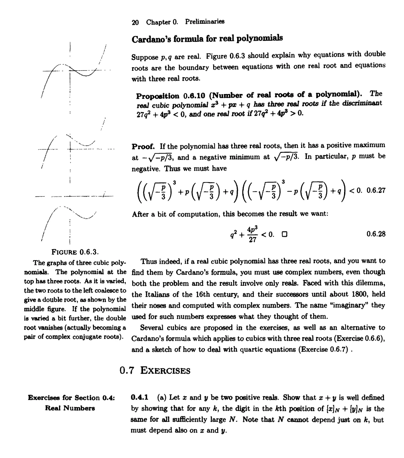
Suppose p>q are real. Figure 0.6.3 should explain why equations with double
roots are the boundary between equations with one real root and equations
with three real roots.
Proposition 0.6.10 (Number of real roots of a polynomial). The
real cubic poiynomiai a?3 + px + q has three real roots if the discriminant
27q2 + 4p3 < 0, and one real root if 11<? 4- V > 0.
/ .]_. .r:r.:'. _. ... Proof. If the polynomial has three real roots, then it has a positive maximum
/ at - v^-p/3, and a negative minimum at \J-pj%- In particular, p must be
! negative. Thus we must have
After a bit of computation, this becomes the result we want:
<0. 0.6.27
/ ! 92 + ^<0. D 0.6.28
/ I 27
Figure 0.6.3.
The graphs of three cubic poly- Thus indeed, if a real cubic polynomial has three real roots, and you want to
nomials. The polynomial at the find them by Cardano's formula, you must use complex numbers, even though
top has three roots. As it is varied, both the problem and the result involve only reals. Faced with this dilemma,
the two roots to the left coalesce to x. .... r lL 1tfJ. A , . . ..... ««™ , ,j
. .. . , A. the Italians of the 16th century, and their successors until about 1800, held
give a double root, as shown by the
middle figure. If the polynomial tneir noses and comPuted witn complex numbers. The name "imaginary" they
is varied a bit further, the double used for such numbers expresses what they thought of them,
root vanishes (actually becoming a Several cubics are proposed in the exercises, as well as an alternative to
pair of complex conjugate roots). Cardano's formula which applies to cubics with three real roots (Exercise 0.6.6),
and a sketch of how to deal with quartic equations (Exercise 0.6.7) .
0.7 Exercises
Exercises for Section 0.4: 0.4.1 (a) Let x and y be two positive reals. Show that x 4- y is well defined
Real Numbers by showing that for any k, the digit in the Arth position of {x]N 4- [j/Jat is the
same for all sufficiently large N. Note that N cannot depend just on &, but
must depend also on x and y.
0.7 Exercises 21
Stars (*) denote difficult
exercises. Two stars indicate a
particularly challenging exercise.
Many of the exercises for
Chapter 0 are quite theoretical, and
too difficult for students taking
multivariate calculus for the first
time. They are intended for use
when the book is being used for a
first analysis class. Exceptions
include Exercises 0.5.1 and part (a)
of 05.2.
digit
1 position
even
Odd
0
left
right
1
right j
left
Table 0.4.6
*(b) Now drop the hypothesis that, the numbers are positive, and try to
define addition. You will find that this is quite a bit harder than part (a).
*(c) Show that addition is commutative. Again, this is a lot easier when the
numbers are positive.
**(d) Show that addition is associative, i.e., x + (y + z) = (x + y) + z. This
is much harder, and requires separate consideration of the cases where each of
x, y and z is positive and negative.
0.4.2 Show that if two numbers are fc-close for all k, then they are equal.
*0.4.3 Show that the functions A(x,y) = x + y, M(x,y) = xy, S(x,y) -
x-y, (x + y) + z are ID-continuous, and that 1/x is not. Notice that for A and
S. the I of Definition 0.4.4 does not depend on JV, but that it does for M.
**0.4.4 Prove Proposition 0.4.6. This can be broken into the following steps.
(a) Show that supfc infi>fc /([*i)/> • • •, [xn]i) is well defined, i.e., that the sets
of numbers involved are bounded. Looking at the function S from Exercise
0.4.3, explain why both the sup and the inf are there.
(b) Show that the function / has the required continuity properties.
(c) Show the uniqueness.
*0.4.5 Define division of reals, using the following steps.
(a) Show that the algorithm of long division of a positive finite decimal a by
a positive finite decimal b defines a repeating decimal a/6, and that b(a/b) = o.
(b) Show that the function inv(x) defined for x > 0 by the formula
inv(x)
:infl/[x]fc
satisfies xinv(x) = 1 for all x > 0.
(c) Now define the inverse for any x ^ 0, and show that x inv(x) =
x^0.
1 for all
**0.4.6 In this exercise we will construct a continuous mapping 7 : [0,1] —»
K2. the image of which is a (full) triangle T. We will write our numbers in [0,1]
in base 2, so such a number might be something like .0011101000011..., and
we will use Table 0.4.6.
Take a right triangle T. We will associate to a string s = si, S2,... of digits
0 and 1 a sequence of points xo, Xi, X2,... of T by starting at the right angle
xo(i), dropping the perpendicular to the opposite side, landing at Xi(s), and
deciding to turn left or right according to the digit si, as interpreted by the
bottom line of the table, since this digit is the first digit (and therefore in an
odd position): on 0 turn right and on 1 turn left.
Now drop tiie perpendicular to the opposite side, landing at x2(s), and turn
right or left according to the digit S2, as interpreted by the top line of the table,
etc.
22 Chapter 0. Preliminaries
\
Figure 0.4.6.
This sequence corresponds to
the string of digits
00100010010....
Exercises for Section 0.5
Infinite Sets
and Russell's Paradox
This construction is illustrated in Figure 0.4.6.
(a) Show that for any string of digits (s), the sequence Xn(s) converges.
(b) Suppose a number t € [0, l] can be written in base 2 in two different
ways (one ending in O's and the other in l's), and call (s), (§!) the two strings
of digits. Show that
lim xn(s) = lim Xn(s').
n-»oo n~*oo
Hint: Construct the sequences associated to .1000... and .0111 —
This allows us to define i(t) = lim„_*oo xn(s).
(c) Show that 7 is continuous.
(d) Show that every point in T is in the image of 7- What is the maximum
number of distinct numbers ti,...,t* such that 7(^1) = ••• =* 7(**)? Hint:
Choose a point in T, and draw a path of the sort above which leads to it.
0.4.7 (a) Show that the function
ifx^O
ifx = 0
is not continuous.
(b) Show that / satisfies the conclusion of the intermediate value theorem:
if f(x\) — a\ and ffa) = 02, then for any number o between a\ and 02, there
exists a number x between x\ and £2 such that f(x) = a.
0.5.1 (a) Show that the set of rational numbers is countable, i.e., that you
can list all rational numbers.
(b) Show that the set D of finite decimals is countable.
0.5.2 (a) Show that the open interval (-1,1) has the same infinity of points
as the reals. Hint: Consider the function g(x) = tan(irx/2).
*(b) Show that the closed interval [-1, lj has the same infinity of points as
the reals. For some reason, this is much trickier than (a). Hint: Choose two
sequences, (1) do = 1,01,02,...; and (2) 60 = -1,61,62,... and consider the
map
g(x) -x if x is not in either sequence.
0(On)=On+l.
0(6„) = 6n+i.
*(c) Show that the points of the circle
{(£)€R*|x* + J,' = l}
have the same infinity of elements as M. Hint: Again, try to choose an
appropriate sequence.
0.7 Exercises 23
*(d) Show that K2 has the same infinity of elements as ift.
Exercise 0.5.4, part (h): This
proof, due to Cantor, proves that
transcendental numbers exist
without exhibiting a single one.
Many contemporaries of Cantor
were scandalized, largely for this
reason.
Exercise 0.5.5 is the
one-dimensional case of the celebrated Drou-
wer fixed point theorem, to be
discussed in a subsequent volume. In
dimension one it is an easy eon-
sequence of the intermediate value
theorem, hut in higher dimensions
(even two) it is quite a delicate
result.
Exercises for Section 0.6:
Complex Numbers
For Exercise 0.6.2, see the
subsection on the derivation of Car-
dano's formulas (Equation 0.6 26
in particular).
*0.5.3 Is it possible to make a list of the rationals in [0.1], written as
decimals, so that the entries on the diagonal also give a rational number?
*0.5.4 An algebraic number is a root of a polynomial equation with integer
coefficients: for instance, the rational number p/q is algebraic, since it is a
solution of qx -p — 0, and so is \/2. since it is a root of x2 -2 = 0. A number
that is not algebraic is called transcendental. It isn't obvious that there are any
transcendental numbers; the following exercise gives a (highly unsatisfactory)
proof for their existence.
(a) Show that the set of all algebraic numbers is countable^ Hint: List the
finite collection of all roots of linear polynomials with coefficients with absolute
value < 1. Then list the roots of all quadratic equations with coefficients < 2
(>\hich will include the linear equations, for instance ().r2 + 2x - 1 =0), then
all roots of cubic equation with coefficients < 3. etc.
(b) Derive from part (a) that there exist transcendental numbers, in fact
unconntably many of them.
0.5.5 Show that if / : \a.b] —» [a.b] is continuous, there exists c G (a,b] with
m = c
0.5.6 Show that if p{.r) is a polynomial of odd degree with real coefficients,
then there is a real number c such that f(c) = 0.
0.6.1 Verify the nine rules for addition and multiplication of complex
numbers. Statements (5) and (9) are the only ones that are not immediate.
0.6.2 Show that -p/(3u\j) is a cubic root of i'2. and that we can renumber
the cube roots of i'2 so that -p/(3«i.,) = «2.j-
0.6.3 (a) Find all the cubic roots of 1.
(b) Find all the 4th roots of 1.
*(c) Find all the 5th roots of 1. Use your formula to construct a regular
pentagon using ruler and compass construction.
(d) Find all the 6th roots of 1.
0.6.4 Show that the following cubics have exactly one real root, and find it.
(a) j3- 18\r + 35 = 0
(b) x3 + 3j2 + x + 2 = 0
0.6.5 Show that the polynomial x3 - 7x + 6 has three real roots, and find
them.
24 Chapter 0. Preliminaries
In Exercise 0.6.6. part (a), use
de Moivre's formula:
cosn0 + /sinn0 = (cos0 + isin0)".
Exercise 0.6.7 uses results from
Section 3.1.
0.6.6 There is a way of finding the roots of real cubics with three real roots,
using only real numbers and a bit of trigonometry.
(a) Prove the formula 4cos30 - 3cos0— cos 30 = 0 .
(b) Set y - ax in the equation x3 + px• + q = 0, and show that there is a
value of a for which the equation becomes 4y%i - 3y - q\ =0; find the value of
a arid of q\.
(c) Show that there exists an angle 0 such that 30 = qx precisely when
27(/2-f 4p3 < 0, i.e.. precisely when the original polynomial has three real roots.
(d) Find a formula (involving arccos) for all three roots of a real cubic
polynomial with three real roots.
*0.6.7 In this exercise, we will find formulas for the solution of 4th degiee
polynomials, known as quartics. Let w4 + air3 4- bvr + cw 4- </ be a quartic
polynomial.
(a) Show that if we set w = .t - a/4, the quartic equation becomes
x4 + px2 + qx + r — 0.
and compute p, q and r in terms of a. b. c. d.
(b) Now set y — x2 + p/2, and show that solving the quartic is equivalent to
finding the intersections of the parabolas V\ and f2 of equation
Figure 0.6.7(a).
The two parabolas of Equation
0.7.1: note that their axes are
respectively the y-axis and the x-
axis.
</
--V
Ska.
Figure 0.6.7(b).
The three pairs of lines that
go through the intersections of the
two parabolas.
' - y + p/2 = 0 and y + qx + r - ~ = 0
respectively, pictured in*Figure 0.6.7(A).
The parabolas Ti and T2 intersect (usually) in four points, and the curves
of equation
„2N
fm (*) ~ar2-y + p/2 + mU* + gar + r
■?)
:()
0.7.1
are exactly the curves given by quadratic equations which pass through those
four points; some of these curves are shown in Figure 0.6.7(C).
(c) What can you say about the curve given by Equation 0.7.1 when m - 1?
When m is negative? When m is positive?
(d) The assertion in (b) is not quite correct: there .is one curve that passes
through those four points, and which is given by a quadratic equation, that is
missing from the family given by Equation 0.7.1. Find it.
(e) The next step is the really clever part of t he solution. Among t hese curves,
there are three, shown in Figure 0.6.7(B), that consist of a pair of lines, i.e.,
each such "degenerate" curve consists of a pair of diagonals of the quadrilateral
formed by the intersection points of the parabolas. Since there are three of
these, we may hope that the corresponding values of m are solutions of a cubic
equation, and this is indeed the case. Using Ihe fact that a pair of lines is not
0.7 Exercises 25
a smooth curve near the point where they intersect, show that the numbers
m for which the equation /„, = 0 defines a pair of lines, a/id the coordinates
x,y of the point where they intersect, are the solutions ofcthe system of three
equations in three unknowns^
P2
y2 + qx + r - ^- + m(x2 -y- p/2) = 0
1y - m = 0
q + 2mx = 0.
(f) Expressing x and y in* terms of m using the last two equations, show that
m satisfies the equation
m3 - 2pm2 + (p2 - 4r)m + q2 = 0
for m; this equation is called the resolvent cubic of the original quarLio equation.
FIGURE 0.6.7 (3). The curves /,„ ( x J = x2 - y + p/2 + m (y2 + q:t■ + r - ^) = °
for seven different values of m.
Let mi,m2 and rri3 be the roots of the equation, and let ( ?* ) i ( »? ) and
f J3 j be the corresponding points of intersection of the diagonals. This doesn't
quite give the equations of the lines forming the two diagonals. The next part
gives a way of finding them.
26 Chapter 0. Preliminaries
(g) Let f J1 J be one of the points of intersection, as above, and consider the
line Ik through the point ( J1 ) with slope Ar, of equation
2/ — 2/i = k(x- x{).
Show that the values of A: for which /* is a diagonal are also the values for which
the restrictions of the two quadratic functions y2 + qj■ + r - £- and x2 - y - p/2
to Ik are proportional. Show that this gives the equations
J_ _ -k _ kxi - yi + p/2
A:2 ~~ 2A:(-A::r1 + y1) + <? ~ (kxx - y,)2 -p2/4 + r'
which can be reduced to the single quadratic equation
*2(*i - 2/i + a/2) =y2 + bxi- a2/4 + c.
Now the full solution is at hand: compute (m\.X\*y\) and (7712,22,3/2); vou
can igrtore the third root of the resolvent cubic or use it to check your
answers. Then for each of these compute the slopes Ar,.i and A:,,2 = -kt>i from the
equation above. You now have four lines, two through A and two through B.
Intersect them in pairs to find the four intersections of the parabolas.
(h) Solve the quartic equations
jl - Ax2 + x + 1 = 0 and x* + 4x3 -I- x - 1 = 0.
1
Vectors, Matrices, and Derivatives
It is sometimes said that the great discovery of the nineteenth century was
that the equations of nature were linear, and the great discovery of the
twentieth century is that they are not—-Tom Kdrner, Fourier Analysis
1.0 Introduction
In this chapter, we introduce the principal actors of linear algebra and multi-
variable calculus.
By and large, first year calculus deals with functions / that associate one
number f(x) to one number x. In most realistic situations, this is inadequate:
the description of most systems depends on many functions of many variables.
In physics, a gas might be described by pressure and temperature as a
function of position and time, two functions of four variables. In biology, one might
be interested in numbers of sharks and sardines as functions of position and
time; a famous study of sharks and sardines in the Adriatic, described in The
Mathematics of the Struggle for Life by Vito Volterra, founded the subject of
mathematical ecology.
In micro-economics, a company might be interested in production as a
function of input, where that function has as many coordinates as the number of
products the company makes, each depending on as many inputs as the
company uses. Even thinking of the variables needed to describe a macro-economic
model is daunting (although economists and the government base many
decisions on such models). The examples are endless and found in every branch of
science and social science.
Mathematically, all such things are represented by functions f that take n
numbers and return m numbers; such functions are denoted f : Rn -► Rm. In
that generality, there isn't much to say; we must impose restrictions on the
functions we will consider before any theory can be elaborated.
The strongest requirement one can make is that f should be linear, roughly
speaking, a function is linear if when you double the input, you double the
output. Such linear functions are fairly easy to describe completely, and a
thorough understanding of their behavior is the foundation for everything else.
The first four sections of this chapter are devoted to laying the foundations of
linear algebra. We will introduce the main actors, vectors and matrices, relate
them to the notion of function (which we will call transformation), and develop
the geometrical language (length of a vector, length of a matrix, ... ) that we
27
28 Chapter 1. Vectors, Matrices, and Derivatives
will need in multi-variable calculus. In Section 1.5 we will discuss sequences,
subsequences, limits and convergence. In Section 1.6 we will expand on that
discussion, developing the topology needed for a rigorous treatment of calculus.
Most functions are not linear, but very often they are well approximated by
linear functions, at least for some values of the variables. For instance, as long
as there are few hares, their number may well double every year, but as soon
as they become numerous, they will compete with each other, and their rate of
increase (or decrease) will become more complex. In the last three sections of
this chapter we will begin exploring how to approximate a nonlinear function
by a linear function—specifically, by its higher-dimensional derivative.
1.1 Introducing the Actors: Vectors
The notion that one can think
about and manipulate higher
dimensional spaces by considering a
point in n-dimensional space as a
list of its n "coordinates" did not
always appear as obvious to
mathematicians as it does today. In
1846, the English mathematician
Arthur Cayley pointed out that a
point with four coordinates can be
interpreted geometrically without
recourse to "any metaphysical
notion concerning the possibility of
four-dimensional space."
"Vol" denotes the number of
shares traded, "High" and "Low,"
the highest and lowest price paid
per share, "Close," the price when
trading stopped at the end of the
day, and "dig," the difference
between the closing price and the
closing price on the previous day.
Much of linear algebra and multivariate calculus takes place within Kn. This
is the space of ordered lists of n real numbers.
You are probably used to thinking of a point in the plane in terms of its two
coordinates: the familiar Cartesian plane with its x,y axes is U2. Similarly, a
point in space (after choosing axes) is specified by its three coordinates:
Cartesian space is K3. Analogously, a point in Rn is specified by its n coordinates;
it is a list of n real numbers. Such ordered lists occur everywhere, from grades
on a transcript to prices on the stock exchange.
Seen this way, higher dimensions are no more complicated than R2 and R3;
the lists of coordinates just get longer. But it is not obvious how to think about
such spaces geometrically. Even the experts understand such objects only by
educated analogy to objects in K2 or K3; the authors cannot "visualize K4" and
we believe that no one really can. The object of linear algebra is at least in part
to extend to higher dimensions the geometric language and intuition we have
concerning the plane and space, familiar to us all from everyday experience. It
will enable us to speak for instance of the "space of solutions" of a particular
system of equations as being a four-dimensional subspace of R7.
Example 1.1.1 (The stock market).
Journal, Dec. 14, 1996.
The following data is from the Ithaca
Local Nyse Stocks
Airgas
AT&T
Borg Warner
Corning
Dow Jones
Eastman Kodak
Emerson Elec.
Federal Express
Vol High Low Close Chg
193 24V2 23V8 235/s
36606 391/4 383/8 39
74 383/8 38 38
4575 443/4 43 441/4
1606 331/4 321/2 331/4
7774 80Vs 791/4 793/8
3335 973/8 955/8 955/s •
5828 421/2 41 415/s
-3/s
3/8
-3/s
"A
Vs
-3A
■lVs
1V2
1.1 Vectors 29
Each of these lists of eight
numbers is an element of K8; if we were
listing the full New York Stock
Exchange, they would be elements of
1T&3356
The Swiss mathematician Leon-
hard Euler (1707-1783) touched on
all aspects of the mathematics and
physics of his time. He wrote
textbooks on algebra, trigonometry,
and infinitesimal calculus; all texts
in these fields are in some sense
rewrites of Euler's. He set the
notation we use from high school on:
sin, cos, and tan for the
trigonometric functions, f(x) to indicate
a function of the variable x are
all due to him. Euler's complete
works fill 85 large volumes—more
than the number of mystery
novels published by Agatha Christie;
some were written after he became
completely blind in 1771. Euler
spent much of his professional life
in St. Petersburg. He and his
wife had thirteen children, five of
whom survived to adulthood.
We
can think of this table as five columns, (
Vol =
■ 193 "
36606
74
4575
1606
7774
3335
. 5828 J
/24Vfe>
High =
39i/4
383/s
443/4
331/4
805/8
973/8
\42i/2>
/23Vs\
Close =
39
38
441/4
331/4
793/s
955/8
\415/8/
Chg =
iach an
element of K8
v /231/s\
Low =
383/s
38
43
321/2
791/4
955/s
' \ 41 /
r -3/s 1
3/8
"3/8
V2
Vs
-3A
-17s
- IV2J
A
Note that we write elements of Rn as columns, not rows. The reason for
preferring columns will become clear later: we want the order of terms in matrix
multiplication to be consistent with the notation /(x), where the function is
placed before the variable—notation established by the famous mathematician
Euler. Note also that we use parentheses for "positional" data and brackets for
"incremental" data; the distinction is discussed below.
Points and vectors: positional data versus incremental data
An element of W1 is simply an ordered list of n numbers, but such a list can
be interpreted in two ways: as a point representing a position or as a vector
representing a displacement or increment.
Definition 1.1.2 (Point, vector, and coordinates). The element of Rn
with coordinates £1,£2, • • • »£n can be interpreted in two ways: as the point
■-G)
or as the vector St =
, which represents an increment.
Example 1.1.3 (An element of K2 as a point and as a vector). The
element of R2 with coordinates x = 2, y = 3 can be interpreted as the point
( J in the plane, as shown in Figure 1.1.1. But it can also be interpreted as
the instructions "start anywhere and go two units right and three units up,"
rather like instructions for a treasure hunt: "take two giant steps to the east,
Figure 1.1.1.
The point (% J.
/ /
/
/
Figure 1.1.2
All the arrows represent the
same vector,
IS]-
As shown in Figure 1.1.2, in the
plane (and in three-dimensional
space) a vector can be depicted as
an arrow pointing in the direction
of the displacement. The amount
of displacement is the length of the
arrow. This does not extend well
to higher dimensions. How are we
to picture the "arrow" in R3356
representing the change in prices
on the stock market? How long is
it, and in what "direction" does it
point? We will show how to
compute these magnitudes and
directions for vectors in Rn in Section
1.4.
30 Chapter 1. Vectors, Matrices, and Derivatives
and three to the north"; this is shown in Figure 1.1.2. Here we are interested in
the displacement: if we start at any point and travel L , how far will we have
gone, in what direction? When we interpret an element of Rn as a position, we
call it a point; when we interpret it as a displacement, or increment, we call it
a vector. A
Example 1.1.4 (A point as a state of a system). It is easy to think of a
point in R2 or R3 as a position; in higher dimensions, it can be more helpful to
think of a point as a "state" of a system. If 3356 stocks are listed on the New
York Stock Exchange, the list of closing prices for those stocks is an element
of R3356, and every element of R3356 is one theoretically possible state of the
stock market. This corresponds to thinking of an element of R3356 as a point.
The list telling how much each stock gained or lost compared with the
previous day is also an element of R3356, but this corresponds to thinking of the
element as a vector, with direction and magnitude: did the price of each stock
go up or down? How much? A
Remark. In physics textbooks and some first year calculus books, vectors are
often said to represent quantities (velocity, forces) that have both "magnitude"
and "direction," while other quantities (length, mass, volume, temperature)
have only "magnitude" and are represented by numbers (scalars). We think
this focuses on the wrong distinction, suggesting that some quantities are always
represented by vectors while others never are, and that it takes more information
to specify a quantity with direction than one without.
The volume of a balloon is a single number, but so is the vector expressing
the difference in volume between an inflated balloon and one that has popped.
The first is a number in R, while the second is a vector in R. The height of
a child is a single number, but so is the vector expressing how much he has
grown since his last birthday. A temperature can be a "magnitude," as in "It
got down to -20 last night," but it can also have "magnitude and direction," as
in "It is 10 degrees colder today than yesterday." Nor can "static" information
always be expressed by a single number: the state of the Stock Market at a
given instant requires as many numbers as there are stocks listed—as does the
vector describing the change in the Stock Market from one day to the next.
A
Points can't be added; vectors can
As a rule, it doesn't make sense to add points together, any more than it makes
sense to "add" the positions "Boston" and "New York" or the temperatures 50
degrees Fahrenheit and 70 degrees Fahrenheit. (If you opened a door between
two rooms at those temperatures, the result would not be two rooms at 120
1.1 Vectors 31
We will not consistently use
different notation for the point
zero and the zero vector, although
philosophically the two are quite
different. The zero vector, i.e., the
"zero increment," has a universal
meaning, the same regardless of
the frame of reference. The point
zero is arbitrary, just as "zero
degrees" is arbitrary, and has a
different meaning in the Centigrade
system and in Fahrenheit.
Sometimes, often at a key point
in the proof of a hard theorem,
we will suddenly start thinking of
points as vectors, or vice versa;
this happens in the proof of Kan-
toroviten's theorem in Appendix
A.2, for example.
a2-t>2
s»-b
aj^L
"a-b
degrees!) But it does make sense to measure the difference between points (i.e.,
to subtract them): you can talk about the distance between Boston and New
York, or about the difference in temperature between two rooms. The result
of subtracting one point from another is thus a vector specifying the increment
you need to add to get from one point to another.
You can also add increments (vectors) together, giving another increment.
For instance the vectors "advance five meters east then take two giant steps
south" and "take three giant steps north and go seven meters west" can be
added, to get "advance 2 meters west and one giant step north."
Similarly, in the NYSE table in Example 1.1.1, adding the Close columns on
two successive days does not produce a meaningful answer. But adding the Chg
columns for each day of a week produces a perfectly meaningful increment: the
change in the market over that week. It is also meaningful to add increments
to points (giving a point): adding a Chg column to the previous day's Close
column produces the current day's Close—the new state of the system.
To help distinguish these two kinds of elements of Rn, we will denote them
differently: points will be denoted by boldface lower case letters, and vectors
will be lower case boldface letters with arrows above them. Thus x is a point
in R2, while x is a vector in K2. We do not distinguish between entries of
points and entries of vectors; they are all written in plain type, with subscripts.
However, when we write elements of Rn as columns, we will use parentheses for
a point x and square brackets for a vector x: in K2, x
-(s)
and x =
Remark. An element of Kn is an element of Rn—i.e., an ordered list of
numbers—whether it is interpreted as a point or as a vector. But we have very
different images of points and vectors, and we hope that sharing them with you
explicitly will help you build a sound intuition. In linear algebra, you should
just think of elements of Kn as vectors. However, differential calculus is all
about increments to points. It is because the increments are vectors that linear
algebra is a prerequisite for multivariate calculus: it provides the right language
and tools for discussing these increments.
Subtraction and addition of vectors and points
Figure 1.1.3.
The difference between point a and point b is the vector a - b, as shown in
The difference a^b between Fi*Ure LL3*
point a and point b is the vector Vect0rS are added ** addin« the corresponding coordinates:
joining them. The difference can
be computed by subtracting the
coordinates of b from those of a. I : I "^ I : I = I l» 111
1V1'
V2
lVn-
+
'W\'
U>2
.Wn-
=
'Vi+Wi~
V2 + W2
. Vn + Wn J
v + w
32 Chapter 1. Vectors, Matrices, and Derivatives
the result is a vector. Similarly, vectors are subtracted by subtracting the
corresponding coordinates to get a new vector. A point and a vector are added
by adding the corresponding coordinates; the result is a point.
In the plane, the sum v + w is the diagonal of the parallelogram of which
two adjacent sides are v and w, as shown in Figure 1.1.4 (left). We can also
add vectors by placing the beginning of one vector at the end of the other, as
shown in Figure 1.1.4 (right).
If we were working with
complex vector spaces, our scalars
would be complex numbers; in
number theory, scalars might be
the rational numbers; in coding
theory, they might be elements of
a finite field. (You may have run
into such things under the name of
"clock arithmetic") We use the
word "scalar'' rather than "real
number" because most theorems
in linear algebra are just as true
for complex vector spaces or
rational vector spaces as for real ones,
and we don't want to restrict the
validity of the statements
unnecessarily.
FIGURE 1.1.4. In the plane, the sum v -I- w is the diagonal of the parallelogram at
left. We can also add them by putting them head to tail.
Multiplying vectors by scalars
Multiplication of a vector by a scalar is straightforward:
X]
ax i
for example, n/3
r 3i
-i
2
=
r 3^1
-l\/3
2\/3j
1.1.2
In this book, our vectors will be lists of real numbers, so that our scalars—
the kinds of numbers we are allowed to multiply vectors or matrices by—are
real numbers.
The symbol € means "element
of." Out loud, one says "in." The
expression "x, y € V" means "x €
V and y € V\n If you are
unfamiliar with the notation of set theory,
set? the discussion in Section 0.3.
Subspaces of w
A subspace of E" is a subset of Kn that is closed under addition and
multiplication by scalars.1 (This Rn should be thought of as made up of vectors, not
points.)
'In Section 2.6 we will discuss abstract vector spaces. These are sets in which
one can add and multiply by scalars, and where these operations satisfy rules (ten of
them) that make them clones of Kn. Subspaces of Rn will be our main examples of
vector spaces.
1.1 Vectors 33
Definition 1.1.5 (Subspace of Rn). A non-empty subset V e Rn is called
a subspace if it is closed under addition and closed under multiplication by
scalars; i.e., V is a subspace if when
x,yeV, and a e R, then x + y e V and ax* e V.
To be closed under
multiplication a subspace must contain the
zero vector, so that
0 v = 6.
For example, a straight line through the origin is a subspace of R2 and of R3.
A plane through the origin is a subspace of R3. The sot consisting of just the
zero vector {6} is a subspace of any Kn, and Rn is a subspace of itself. These
last two, {6} and Rn, are considered trivial subspaces.
Intuitively, it is clear that a line that is a subspace has dimension 1, and
a plane that is a subspace has dimension 2. Being precise about what this
means requires some "machinery" (mainly the notions of linear independence
and span), introduced in Section 2.4.
The notation for the standard
basis vectors is ambiguous; at
right we have three different
vectors, all denoted ei. The subscript
tells us which entry is 1 but does
not say how many entries the
vector has- i.e., whether it is a vector
in F.2, IP;3 or what.
The standard basis
vectors in
R2 and R3 are often denoted i, ],
and k:
^^■=[l0]or
-r - roi
j - e2 = L or
A: = g3 =
0'
0
1
0
.0.
0"
1
.0.
We do not use this notation but
mention it in case you encounter
it elsewhere.
The standard basis vectors
We will meet one particular family of vectors in Rn often: the standard basis
vectors. In .W2 there are two standard basis vectors, e*i and e^; in R3, there are
three:
in R2 : e,
-(;]•
e2 =
in ir
1
0
0
.e2 =
0
1
0
,e3 =
0
0
1
Similarly, in !ft5 there are five standard basis vectors:
ei =
ri'
0
0
p
Lo.
. e2 =
-o-
1
0
0
.0^
e5 =
Definition 1.1.6 (Standard basis vectors). The standard basis vectors
in Rn are the vectors e,- with n entries, the jth entry 1 and the others zero.
Geometrically, there is a close connection between the standard basis vectors
in R2 and a choice of axes in the Euclidean plane. When in school you drew
an x-axis and y-axis on a piece of paper and marked off units so that you could
plot a point, you were identifying the plane with R2: each point on the plane
corresponded to a pair of real numbers—its coordinates with respect to those
axes. A set of axes providing such an identification must have an origin, and
each axis must have a direction (so you know what is positive and what is
34 Chapter 1. Vectors, Matrices, and Derivatives
Figure 1.1.5.
The point marked with a
circle is the point ( g 1 in this non-
orthogonal coordinate system.
Figure 1.1.6.
negative) and it must have units (so you know, for example, where x = 3 or
V = 2 is).
Such axes need not be at right angles, and the units on one axis need not
be the same as those on the other, as shown in Figure 1.1.5. However, the
identification is more useful if we choose the axes at right angles (orthogonal)
and the units equal; the plane with such axes, generally labeled x and y, is
known as the Cartesian plane. We can think that e\ measures one unit along
the x-axis, going to the right, and §2 measures one unit along the y-axis, going
;iup."
Vector fields
Virtually all of physics deals with fields. The electric and magnetic fields of
electromagnetism, the gravitational and other force fields of mechanics, the
velocity fields of fluid flow, the wave function of quantum mechanics, are all
"fields." Fields are also used in other subjects, epidemiology and population
studies, for instance.
By "field" we mean data that varies from point to point. Some fields, like
temperature or pressure distribution, are scalar fields: they associate a number
to every point. Some fields, like the Newtonian gravitation field, are best
modeled by vector fields, which associate a vector to every point. Others, like the
electromagnetic field and charge distributions, are best modeled by form fields,
discussed in Chapter 6. Still others, like the Einstein field of general relativity
(a field of pseudo inner products), are none of the above.
Definition 1.1.7 (Vector field). A vector field on Rn is a function whose
input is a point in W1 and whose output is a vector (also in Mn) emanating
from that point.
We will distinguish between functions and vector fields by putting arrows on
vector fields, as in F in Example 1.1.8.
A vector field associates a vec- Example 1.1.8 (Vector fields in l2). The identity function in R2
tor to each point. Here we show
the radial vector field f [) ~ [)
F\y)~[y\' takes a P°int in r2 and returns the same point. But the vector field
Vector fields generally are easier to
depict when one scales the vectors
down, as we have done above and takes a po|nt ,n R2 and .^ to it the yector correSDOnding to that ^ M
ln gUFe " shown in Figure 1.1.6. To the point with coordinates (1,1) it assigns the vector
L ; to the point with coordinates (4,2) it assigns the vector .
■«)-[:]
1.1.3
1.1.4
1.2 Matrices 35
Actually, a vector field simply
associates to each point a vector;
how you imagine that vector is up
to you. But it is always helpful
to imagine each vector anchored
at, or emanating from, the
corresponding point.
Similarly, the vector field F (*) = Ky_ 2 , shown in Figure 1.1.7, takes
a point in U2 and assigns to it the vector _ . A
Vector fields are often used to describe the flow of fluids or gases: the vector
assigned to each point gives the velocity and direction of the flow. For flows that
don't change over time (steady-state flows), such a vector field gives a complete
description. In more realistic cases where the flow is constantly changing, the
vector field gives a snapshot of the flow at a given instant. Vector fields are also
used to describe force fields such as electric fields or gravitational fields.
y">yyy /*
* y.'/ y /
yyy y '
y' y y / '
/ / s s *• *
, ... , t \ '
-., ' ' ^ '
, .. v V V \
_____ __ __ _»»
. - v v v X
< S\\\\
Figure 1.1.7.
The vector field
'(5)-(
*V -2]
x-V i'
When a matrix is described,
height is given first, then width:
an m x n matrix is m high and
n wide. After struggling for years
to remember which goes first, one
of the authors hit on a mnemonic:
first take the elevator, then walk
down the hall.
1.2 Introducing the Actors: Matrices
Probably no other area of mathematics has been applied in such numerous
and diverse contexts as the theory of matrices. In mechanics,
electromagnetics, statistics, economics, operations research, the social sciences,
and so on, the list of applications seems endless. By and large this is
due to the utility of matrix structure and methodology in
conceptualizing sometimes complicated relationships and in the orderly processing of
otherwise tedious algebraic calculations and numerical manipulations.—
James Cochran, Applied Mathematics: Principles, Techniques, and
Applications
The other central actor in linear algebra is the matrix.
Definition 1.2.1 (Matrix). Anmxn matrix is a rectangular array of
entries, m high and n wide.
We use capital letters to denote matrices. Usually our matrices will be arrays
of numbers, real or complex, but matrices can be arrays of polynomials, or of
more general functions; a matrix can even be an array of other matrices. A
vector v e Bfcm is an m x 1 matrix.
Addition of matrices, and multiplication of a matrix by a scalar, work in the
obvious way:
Example 1.2.2 (Addition of matrices and multiplication by a scalar).
("1
2
L4
0"
-1
2
+
"0
1
3
-3"
-2
1
=
"1
3
7
-3"
-3
3J
- !U5]-[-"J
So far, it's not clear that matrices gain us anything. Why put numbers (or
other entries) into a rectangular array? What do we gain by talking about the
36 Chapter 1. Vectors, Matrices, and Derivatives
How would you add the
matrices
[I I I] - [i I] ?
You can't: matrices can be added
only if they have the same height
and same width.
Matrices were introduced by
Arthur Cayley, a lawyer who
became a mathematician, in A
Memoir on the Theory of Matrices,
published in 1858. He denoted the
multiplication of a 3 x 3 matrix by
the vector
(a,
K'
a",
X
y
z
6,
6'
b"
using the format
c ()xty,z)
c' 1
, c" '
"... when Werner Heisenberg
discovered 'matrix' mechanics in
1925, he didn't know what a
matrix was (Max Bom had to tell
him), and neither Heisenberg nor
Born knew what to make of the
appearance of matrices in the
context of the atom."—Manfred R.
Schroeder, "Number Theory and
the Real World," Mathematical
Intelligencer, Vol. 7, No. 4
2x2 matrix
rather than the point
e IR4? The answer is that the
matrix format allows another operation to be performed: matrix multiplication.
We will see in Section 1.3 that every linear transformation corresponds to
multiplication by a matrix. This is one reason matrix multiplication is a natural
and important operation; other important applications of matrix multiplication
are found in probability theory and graph theory.
Matrix multiplication is best learned by example. The simplest way to
multiply A times B is to write B above and to the right of A. Then the product
AB fits in the space to the right of A and below £, the t,jth entry of AB
being the intersection of the ith row of A and the jth column of B, as shown in
Example 1.2.3. Note that for AB to exist, the width of A must equal the height
of B. The resulting matrix then has the height of A and the width of B.
Example 1.2.3 (Matrix multiplication). The first entry of the product
AB is obtained by multiplying, one by one, the entries of the first row of A by
those of the first column of B, and adding these products together: in Equation
1.2.1, (2xl) + (-1 x 3) = -1. The second entry is obtained by multiplying
the first row of A by the second column of B: (2x4) + (-1 x 0) = 8. After
multiplying the first row of A by all the columns of B, the process is repeated
with the second row of A: (3 x 1) + (2 x 3) = 9, and so on.
[A][B] = [AB)
Given the matrices
A =
N
4 -2
0 2
HM li-i)[-ii
l\
A
1.2.1
;:] *-[2il c-{\~i-i\
D =
\\ 0]
2 2
1 1
what are the products AB, AC and CD? Check your answers below.2 Now
compute BA. What do you notice? What if you try to compute CA?3
•"-[.°i]< AC-■[i:«-.,l= -=fo0:l]-
3Matrix multiplication is not commutative; BA = ^ jj , which is nc
AB = L g . Although the product AC exists, you cannot compute CA
1.2 Matrices 37
Definition 1.2.4 says nothing
new, but it provides some
practice moving between the concrete
(multiplying two particular
matrices) and the symbolic
(expressing this operation so that it
applies to any two matrices of
appropriate dimensions, even if the
entries are complex numbers or even
functions, rather than real
numbers.) In linear algebra one is
constantly moving from one form
of representation (one "language")
to another. For example, as we
have seen, a point in IK" can be
considered as a single entity, b, or
as the ordered list of its
coordinates; matrix A can be thought of
as a single entity or as a
rectangular array of its entries.
In Example 1.2.3. A is a 2 x 2
matrix and B is a 2 x 3 matrix, so
that n = 2, m = 2 and p = 3; the
product C is then a 2 x 3 matrix.
If we set i = 2 and j = 3, we see
that the entry C2.3 of the matrix C
is
C2.3 = «2,1^1.3 + «2,2&2.3
= (3--2) + (2-2)
= -6 + 4 = -2.
Using the format for matrix
multiplication shown in Example
1.2.3, the i, jth entry is the entry
at the intersection of the ith row
and jth column.
Below we state the formal definition of the process we've just, described. If
the indices bother you, do refer to Figure 1.2.1.
Definition 1.2.4 (Matrix multiplication). If A is an 77? x n matrix whose
(t,j)th entry is Oij, and B is an n x p matrix whose (i, j)th entry is bi.j.
then C = AB is the m x p matrix with entries
1.2.2
hi
■hL
' \^k) fo| I ^
ilh
row
jth
col.
FIGURE 1.2.1. The entry CitJ of the matrix C = AB is the sum of the products of
the entries of the a,,* of the matrix A and the corresponding entry 6*., of the matrix
B. The entries a*,* are all in the ith row of A\ the first index i is constant., and the
second index k varies. The eutries bk,3 are all in the jth column of B\ the first index
k varies, and the second index j is constant. Since the width of A equals the height
of B, the entries of A and those of B can be paired up exactly.
Remark. Often people write a problem in matrix multiplication in a row:
[A][B] = [AB]. The format shown in Example 1.2.3 avoids confusion: the
product of the tth row of A and the jth column of B lies at the. intersection of
that row and column. It also avoids rccopying matrices when doing repeated
38 Chapter 1. Vectors, Matrices, and Derivatives
multiplications, for example A times B times C times D:
[""
AB
l] [(>IB)] \{AB)C
D
(ABC)D
1.2.3
| Multiplying a matrix by a standard basis vector
Observe that multiplying a matrix A by the standard basis vector e, selects out
the tth column of A, as shown in the following example. We will use this fact
often.
Example 1.2.5 (The tth column of A is A$i). Below, we show that the
second column of A is i4e2:
Figure 1.2.2.
The tth column of the product
AB depends on all the entries of
A but only the tth column of B.
r3
2
0
LI
-2
1
4
0
°1
2
3
2\
?2
i
L°J
-2-|
1
4
. OJ
multiplies the 2nd column by 1:
■-2
1
4
. OJ
xl =
2
1
4
L o
AB
f
A AG*
A 1.2.4
Similarly, the tth column of AB is Abi} where b* is the tth column of B, as
shown in Example 1.2.6 and represented in Figure 1.2.2. The jth row of AB is
the product of the jth row of A and the matrix B, as shown in Example 1.2.7
and Figure 1.2.3.
Example 1.2.6. The second column of the product AB is the same as the
product of the second column of A and the matrix B:
Figure 1.2.3.
The jth row of the product AB
depends on all the entries of B but
only the jth row of A.
[ 1 4-21
[ 3 0 2J
[2 -ii r-i s -el r
[3 2j [ 9 12 -2j [
[J]
1 Ii]
1.2.5
Ab2
Example 1.2.7. The second row of the product j4B is the same as the product
of the second row of A and the matrix B:
1.2 Matrices 39
In his 1858 article on matrices,
Cayley stated that matrix
multiplication is associative but gave no
proof. The impression one gets is
that he played around with
matrices (mostly 2x2 and 3x3)
to get some feeling for how they
behave, without worrying about
rigor. Concerning another matrix
result (the Cay ley-Hamilton
theorem) he verifies it for 3 x 3
matrices, adding / have not thought it
necessary to undertake the labour
of a formal proof of the theorem in
the general case of a matrix of any
degree.
m
m
A J
P
B
[ah
q
lei
W
U
n A
r i 4-2]
[ 3 0 2j
[2 -1] [-1 8 -6]
[3 2j [ 9 12 -2j
1 4
3 0
1.2.6
(3 2] ( 9 12 -2]
Matrix multiplication is associative
When multiplying the matrices A,B, and C, we could set up the repeated
multiplication as we did in Equation 1.2.3, which corresponds to the product
(AB)C. We can use another format to get the product A(BC):
1
M
B
L :
1 AB
C
: '.
(AB)C
1
ox
_
B
L J
A
C
\ (BC)
J.
A(BC
1.2.7
J
Figure 1.2.4.
This way of writing the
matrices corresponds to calculating
(AB)C.
Is (AB)C the same as (AB)C1 In Section 1.3 we give a conceptual reason why
they are; here we give a computational proof.
Proposition 1.2.8 (Matrix multiplication is associative). If A is an
nxm matrix, B isanmxp matrix and C isapxq matrix, so that (AB)C
and A(BC) are both defined, then they are equal:
(AB)C = A{BC). 1.2.8
Proof. Figures 1.2.4 and 1.2.5 show that the ijth entry of both A(BC) and
(AB)C depend only on the ith line of A and the jth column of C (but on all the
entries of B), and that without loss of generality we can assume that A is a line
matrix and that C is a column matrix, i.e., that n = q = 1, so that both (AB)C
and A(BC) are numbers. The proof is now an application of associativity of
multiplication of numbers:
Figure 1.2.5.
This way of writing the
matrices corresponds to calculating
A(BC).
(AB)C
2=1 \*=1 /
Zth entry of AB
P m m / p \
= E E a*6*.<c<=E aM E6*^ = A(BC)-
i=i *=i *=i \i=i /
1.2.9
fcth entry of BC
40 Chapter 1. Vectors, Matrices, and Derivatives
Exercise 1.2.2 provides
practice on matrix multiplication. At
the end of this section, Example
1.2.22, involving graphs, shows a
setting where matrix
multiplication is a natural and powerful tool.
Non-commutativity of matrix multiplication
As we saw earlier, matrix multiplication is most definitely not commutative. It
may well be possible to multiply A by B but not B by A. Even if both matrices
have the same number of rows and columns, AB will usually not equal BA, as
shown in Example 1.2.9.
Example 1.2.9 (Matrix multiplication is not commutative). If you
by the matrix Q , the answer you get will
multiply the matrix
depend on which one you put first:
[0 11
.1 ij
o r
1 0
1 01
i i_
is not equal to
ro i
[l 0
0 f
1 1
1 I]
0 lj
A 1.2.10
The main diagonal is also called
the diagonal. The diagonal from
bottom left to top right is the anti-
diagonal.
Multiplication by the identity
matrix / does not change the
matrix being multiplied.
The columns of the identity
matrix /„ are of course the
standard basis vectors e*i,..., en:
U =
1
0
0
0
ei
0
1
0
0
e2
0
0
1
0
63
0"
0
0
1.
e4
The identity matrix
The identity matrix / plays the same role in matrix multiplication as the number
1 does in multiplication of numbers: IA = A = AI.
Definition 1.2.10 (Identity matrix). The identity matrix /„ is the n x n-
matrix with l's along the main diagonal (the diagonal from top left to bottom
right) and 0's elsewhere.
For example,
/2 =
1 0
0 1
and IA
If A is an n x m-matrix, then
IA = AI = Ay or, more precisely,
rl
0
0
.0
0 0 0"
1 0 0
0 1 0
0 0 1.
■»n" == Aim
= A,
1.2.11
1.2.12
since if n ^ m one must change the size of the identity matrix to match the
size of A. When the context is clear, we will omit the index.
Matrix inverses
The inverse A'1 of a matrix A plays the same role in matrix multiplication as
the inverse \/a does for the number a. We will see in Section 2.3 that we can
use the inverse of a matrix to solve systems of linear equations.
1.2 Matrices 41
We will see in Section 2.3 that
only square matrices can have a
two-sided inverse, i.e., an inverse.
Furthermore, if a square matrix
has a left inverse then that left
inverse is necessarily also a right
inverse; similarly, if it has a right
inverse, that right inverse is
necessarily a left inverse.
It is possible for a non-square
matrix to have lots of left inverses
and no right inverse, or Jots of
right inverses and no left inverse,
as explored in Exercise 1.2.20.
While we can write the inverse
of a number x either as x~l or as
1/rc, giving xx~l = x(l/x) = 1,
the inverse of a matrix A is only
written A'1. We cannot divide
by a matrix. If for two matrices
A and B you were to write A/By
it would be unclear whether this
meant
B~lA or AB'1.
The only number that does not have an inverse is 0, but many matrices do
not have inverses. In addition, the non-commutativity of matrix multiplication
makes the definition more complicated.
Definition 1.2.11 (Left and right inverses of matrices). Let A be a
matrix. If there is another matrix B such that
BA = I,
then B is called a left inverse of A. If there is another matrix C such that
AC = I,
then C is called a right inverse of A.
It is possible for a nonzero matrix to have neither a right nor a left inverse.
Example 1.2.12 (A matrix with neither right nor left inverse). The
matrix _ n does not have a right or a left inverse. To see this, assume it
has a right inverse. Then there exists a matrix , such that
[J Slti] ■[!?]•
But that product is , i.e., in the bottom right-hand corner, 0 = 1. A
similar computation shows that there is no left inverse. A
Definition 1.2.13 (Inveriible matrix). An invertible matrix is a matrix
that has both a left inverse and a right inverse.
Associativity of matrix multiplication gives us the following result:
Proposition and Definition 1.2.14. If a matrix A has both a left and a
right inverse, then it has only one left inverse and (me right inverse, and they
are identical; such a matrix is called the inverse of A and is denoted A~l.
Proof. If a matrix A has a right inverse B> then AB = /. If it has a left
inverse C, then CA =* /. So
C(AB) = CI = C and (CA)B = IB = £, so C = B. D 1.2.14
We discuss how to find inverses of matrices in Section 2.3. A formula exists
for 2 x 2 matrices: the inverse of
A =
: 2] - '--aM-.' i]- "»
42 Chapter 1. Vectors, Matrices, and Derivatives
as Exercise 1.2.12 asks you to confirm by matrix multiplication of AA~l and
A~XA. (Exercise 1.4.12 discusses the formula for the inverse of a 3 x 3 matrix.)
Notice that a 2 x 2 matrix is invertible if ad - be ^ 0. The converse is also
true: if ad - be — 0, the matrix is not invertible, as you arc asked to show in
Exercise 1.2.13.
Associativity of matrix multiplication is also used to prove that the inverse
of the product of two invertible matrices is the product of their inverses, in
reverse order:
We are indebted to Robert Ter- Proposition 1.2.15 (The inverse of the product of matrices). If A
rell for the mnemonic, "socks on, an(j Q ajg invertible matrices, then AB is invertible, and the inverse is given
shoes on; shoes off, socks off." To ^v the formula,
undo a process, you undo first the
last thing you did. {AB)~l = B_li4~!. 1.2.16
Ifv:
. then its transpose
= (1 0 1).
Do not confuse a matrix with
its transpose, and in particular,
never write a vector horizontally.
If you write a vector written
horizontally you have actually
written its transpose; confusion
between a vector (or matrix) and its
transpose leads to endless
difficulties with the order in which things
should be multiplied, as you can
see from Theorem 1.2.17.
Proof. The computation
(AB)(B"1 A~l) = A{BB~l)A~l = AA~l = /
1.2.17
and a similar one for (B lA'l){AB) prove the result. D
Where was associativity used in the proof? Check your answer below.4
The transpose
The transpose is an operation on matrices that will be useful when we come to
the dot product, and in many other places.
Definition 1.2.16 (Transpose). The transpose AT of a matrix A is formed
by interchanging all the rows and columns of A> reading the rows from left
to right, and columns from top to bottom.
For example, if A = , then AT -
r i
! 4
-2
3]
0
2J
The transpose of a single row of a matrix is a vector; we will use this in
Section 1.4.
4 Associativity is used for the first two equalities below:
D iEF) (DE) F
(ABlfjrlA-ll = ^(^(F^T7)) = A({BB^)^) = A(IA'1) = /.
(AB)
(BC)
1.2 Matrices 43
The proof of Theorem 1.2.17
is straightforward and is left as
Exercise 1.2.14.
Theorem 1.2.17 (The transpose of a product). The transpose of a
product is the product of the transposes in reverse order:
(AB)T=BTAT. 1.2.18
[1
11
L°
i
0
3
0]
3
0J
A symmetric matrix
0 1 2
-10 3
-2 -3 0
An anti-symmetric matrix
Some special kinds of matrices
Definition 1.2.18 (Symmetric matrix). A symmetric matrix is equal to
its transpose. An anti-symmetric matrix is equal to minus its transpose.
Definition 1.2.19 (Triangular matrix). An upper triangular matrix is a
square matrix with nonzero entries only on or above the main diagonal. A
lower triangular matrix is a square matrix with nonzero entries only on or
below the main diagonal.
110 3
0 2 0 0
0 0 10
0 0 0 0
An upper triangular matrix
Definition 1.2.20 (Diagonal matrix). A diagonal matrix is a square
matrix with nonzero entries (if any) only on the main diagonal.
What happens if you square the diagonal matrix 0 ? If you cube it?5
2 0
0 2
0 0
0 0
A diagonal matrix
Exercise 1.2.10 asks you to show
that if A and B are upper
triangular n x n matrices, then so is
AB.
Applications of matrix multiplication: probabilities and graphs
While from the perspective of this book matrices are most important because
they represent linear transformations, discussed in the next section, there are
other important applications of matrix multiplication. Two good examples are
probability theory and graph theory.
Example 1.2.21 (Matrices and probabilities). Suppose you have three
reference books on a shelf: a thesaurus, a French dictionary, and an English
dictionary. Each time you consult one of these books, you put it back on the
shelf at the far left. When you need a reference, we denote the probability that
it will be the thesaurus Plt the French dictionary P2 and the English dictionary
P3. There are six possible arrangements on the shelf: 123 (thesaurus, French
dictionary, English dictionary), 132, and so on.
Ja or _Ta2 0 1 [a 0l3 _ [a3 Ol
lo a J "lo a2J4o aJ "lo a3]"
44 Chapter 1. Vectors. Matrices, and Derivatives
For example, the move from
(2 1 3) to (32 1) has probability P3
(associated with the English
dictionary), since if you start with
the order (213) (French
dictionary, thesaurus, English
dictionary), consult the English
dictionary, and put ii back lo the far
left, you will then have the order
(321). So the entry at the 3rd
row, 6th column is P:j. The move
from (2 1 3) to (3 1 2) has
probability 0, since moving the English
dictionary won't change the
position of the other books. So the
entry at the 3rd row, 5th column
isO.
A situation like this one, where
each outcome depends only on the
one just before it, it called a
Markov chain.
Sometimes easy access isn't
the goal. In Zola's novel Au Bon-
heur des Dames, the epic story of
the growth of the first big
department store in Paris, the hero has
an inspiration: he places his
merchandise in the most inconvenient
arrangement possible, forcing his
customers to pass through parts
of the store where they otherwise
wouldn't set foot, and which are
mined with temptations for
impulse shopping.
We can then write the following 6x6 transition matrix, indicating the
probability of going from one arrangement to another:
(1,2,3)
(1.3,2)
(2,1,3)
(2,3,1)
(3,1,2)
(3,2,1)
(1,2,3)
Pi
O
Pi
Pi
0
0
(1,3,2)
0
Pi
0
0
Pi
Pi
(2,1,3)
P2
P2
P2
0
0
0
(2,3,1)
0
0
0
P2
P2
P2
(3,1,2)
P3
P3
0
0
P3
0
(3,2,1)
0
0
P3
P3
0
P3
Now say you start with the fourth arrangement, (2,3,1). Multiplying the line
matrix (0,0,0,1,0; 0) (probability 1 for the fourth choice, 0 for the others) by the
transition matrix T gives the probabilities Pi,0,0,P2,0, P3. This is of course
just the 4th row of the matrix. The interesting point here is to explore the
long-term probabilities. At the second step, we would multiply the line matrix
Pi,0,0, P2,0, P3 by T\ at the third we would multiply that product by T\ ... .
If we know actual values for Plt P2, and P3 we can compute the probabilities
for the various configurations after a great many iterations. If we don't know
the probabilities, we can use this system to deduce them from the configuration
of the bookshelf after different numbers of iterations.
This kind of approach is useful in determining efficient storage. How should a
lumber yard store different sizes and types of woods, so as little time as possible
is lost digging out a particular plank from under others? For computers, what
applications should be easier to access than others? Based on the way you use
your computer, how should its operating system store data most efficiently? A
Example 1.2.22 is important for many applications. It introduces no new
theory and can be skipped if time is at a premium, but it provides an
entertaining setting for practice at matrix multiplication, while showing some of its
power.
Example 1.2.22 (Matrices and graphs). We are going to take walks on
the edges of a unit cube; if in going from a vertex Vi to another vertex V* we
walk along n edges, we will say that our walk is of length n. For example, in
Figure 1.2.6. if we go from vertex V\ to Vfe, passing by V4 and Vfc, the total
length of our walk is 3. We will stipulate that each segment of the walk has to
take us from one vertex to a different vertex; the shortest possible walk from a
vertex to itself is of length 2.
How many walks of length n are there that go from a vertex to itself, or, more
generally, from a given vertex to a second vertex? As we will see in Proposition
1.2.23, we answer that question by raising to the nth power the adjacency
matrix of the graph. The adjacency matrix for our cube is the 8x8 matrix
1.2 Matrices 45
whose rows and columns are labeled by the vertices Vi,..., Vs, and such that
the i, jth entry is 1 if there is an edge joining V* to Vj, and 0 if not, as shown in
Figure 1.2.6. For example, the entry 4,1 is 1 (underlined in the matrix) because
there is an edge joining V4 to Vi; the entry 4,6 is 0 (also underlined) because
there is no edge joining V4 to V$.
v*;\
I
V4l
V6
Vl
v*
v3
\
\
\
V, V2 V3 V* Vs V6 V? Vs
Vi
V2
V3
A= V4
V6
v7
Vs
V5 0
FIGURE 1.2.6. Left: The graph of a cube. Right: Its adjacency matrix A. If two
vertices V% and Vj are joined by a single edge, the (i, j)th and (j, i)th entries of the
matrix are 1; otherwise they are 0.
The reason this matrix is important is the following.
You may appreciate this result
more if you try to make a rough
estimate of the number of walks
of length 4 from a vertex to itself.
The authors did and discovered
later that they had missed quite
a few possible walks.
Proposition 1.2.23. JFbr any graph formed of vertices connected by edges,
the number of possible walks of length n torn vertex Vi to vertex Vj is given
by the *, jth entry of the matrix An formed by taking the nth power of the
graph's adjacency matrix A.
For example, there are 20 different walks of length 4 from V5 to V7 (or vice
versa), but no walks of length 4 from V4 to V3 because
As you would expect, all the l's
in the adjacency matrix A have
turned into 0's in <44; if two
vertices are connected by a single
edge, then when n is even there
will be no walks of length n
between them.
Of course we used a computer
to compute this matrix. For all
but simple problems involving
matrix multiplication, tise Matlab or
an equivalent.
•21
0
20
0
20
0
20
.0
0
21
0
20
0
20
0
20
20
0
21
0
20
0
20
0
0
20
0
21
0
20
0
20
20
0
20
0
21
0
20
0
0
20
0
20
0
21
0
20
20
0
20
0
20
0
21
0
0-
20
0
20 .
0
20
0
21J
yl4 =
Proof. This will be proved by induction, in the context of the graph above;
the general case is the same. Let Bn be the 8 x 8 matrix whose i, jth entry is
the number of walks from Vi to Vj of length w, for a graph with eight vertices;
46 Chapter 1. Vectors, Matrices, and Derivatives
we must prove Bn = An. First notice that £, = A1 = A: the number AtJ is
exactly the number of walks of length 1 from vt to vr
Next, suppose it is true for n, and let us see it for n + 1. A walk of length
n + 1 from Vt to V3 must be at some vertex Vk at time n. The number of such
walks is the sum, over all such V*, of the number of ways of getting from Vt to
Vfc in n steps, times the number of ways of getting from V* to Vj in one step.
This will be 1 if Vk is next to V,. and 0 otherwise. In symbols, this becomes
Like the transition matrices of
probability theory, matrices
representing the length of walks from
one vertex of a graph to another
have important applications for
computers and multiprocessing.
No. of ways ^^^ No. ways t to No. ways k to
t to j in n + 1 steps |.or ajj k in n steps j in 1 step
vertices k
1.2.19
~ inductive def. Pf \
hypothesis of A ' z*
which is precisely the definition of An+l. D
Above, what do we mean by An? If you look at the proof, you will see that
what we used was
A»=((...(A)A)a)a.
1.2.20
Exercise 1.2.15 asks you to
construct the adjacency matrix for a
triangle and for a square. We
can also make a matrix that
allows for one-way streets (one-way
edges), as Exercise 1.2.18 asks you
to show.
Matrix multiplication is associative, so you can also put the parentheses any
way you want; for example,
,4*= (,4(,4(,4)...)).
1.2.21
In this case, we can see that it is true, and simultaneously make the associativity
less abstract: with the definition above, BnBm = Bn+m. Indeed, a walk of
length n + m from V* to Vj is a walk of length n from V* to some Vjt, followed
by a walk of length m from Vjt to Vj. In formulas, this gives
1.3
(Bn+m)ij = 7 S^n)i,k(Bm)k,j'
What the Actors Do: A Matrix
as a Transformation
1.2.22
In Section 2.2 we will see how matrices are used to solve systems of linear
equations, but first let us consider a different view of matrices. In that view,
multiplication of a matrix by a vector is seen as a linear transformation, a
special kind of mapping. This is the central notion of linear algebra, which
1.3 Transformations 47
The words mapping (or map)
and function are synonyms,
generally used in different contexts.
A function normally takes a point
and gives a number. Mapping is a
more recent word; it was first used
in topology and geometry and has
spread to all parts of
mathematics. In higher dimensions, we tend
to use the word mapping rather
than function, but there is
nothing wrong with calling a mapping
from R* — P.5 a function.
Figure 1.3.1.
A mapping: every point on the
left goes to only one point on the
right
Figure 1.3.2.
Not a mapping: not well
defined at a, not defined at b.
The domain of our
mathematical "final grade function" isKn; its
range is IR. In practice this
function has a "socially acceptable"
domain of the realistic grade
vectors (no negative numbers, for
example) and also a "socially
acceptable" range, the set of possible
final grades. Often a
mathematical function modeling a real
system has domain and range
considerably larger than the realistic
values.
allows us to put matrices in context and to see them as something other than
"pushing numbers around."
Mappings
A mapping associates elements of one set to elements of another. In common
speech, we deal with mappings all the time. Like the character in Moliere's play
Le Bourgeois Gentilhomme, who discovered that he had been speaking prose
all his life without knowing it, we use mappings from early childhood, typically
with the word "of or its equivalent: "the price of a book" goes from books to
money; "the capital of a country'* goes from countries to cities.
This is not an analogy intended to ease you into the subject. "The father of"
is a mapping, not "sort of like" a mapping. We could write it with symbols:
f(x) = y where x — a person and y = that person's father: /(John Jr.) =
John. (Of course in English it would be more natural to say, "John Jr.'s father"
rather than "the father of John Jr." A school of algebraists exists that uses
this notation: they write (x)f rather than f(x).)
The difference between expressions like "the father of in everyday speech
and mathematical mappings is that in mathematics one must be explicit about
things that are taken for granted in speech.
Rigorous mathematical terminology requires specifying three things about a
mapping:
(1) the set of departure (the domain),
(2) the set of arrival (the range),
(3) a rule going from one to the other.
If the domain of a mapping M is the real numbers IR and its range is the
rational numbers <Q>, we denote it M : IR —► Q, which we read "Af from K to
Q." Such a mapping takes a real number as input and gives a rational number
as output.
What about a mapping T : Rn -» Km? Its input is a vector with n entries;
its output is a vector with m entries: for example, the mapping from Kn to IR
that takes n grades on homework, tests, and the final exam and gives you a
final grade in a course.
The rule for the "final grade" mapping above consists of giving weights to
homework, tests, and the final exam. But the rule for a mapping does not
have to be something that can be stated in a neat mathematical formula. For
example, the mapping M : K -»IR that changes every digit 3 and turns it into
a 5 is a valid mapping. When you invent a mapping you enjoy the rights of an
absolute dictator; you don't have to justify your mapping by saying that "look,
if you square a number x, then multiply it by the cosine of 2tt, subtract 7 and
then raise the whole thing to the power 3/2, and finally do such-and-such, then
48 Chapter I. Vectors, Matrices, and Derivatives
Note, that in correct
mathematical usage, "the father of" as a
mapping from people to people is
not the same mapping as "the
father of" as a mapping from
people to men. A mapping includes a
domain, a range, and a rule going
from the first to the second.
if x contains a 3, that 3 will turn into a 5. and everything else will remain
unchanged." There isn't any such sequence of operations that will "carry out"
your mapping for you. and you don't need one.6
A mapping going "from" \kn "to" ?/" is said to be defined on its domain K".
A mapping in the mathematical sense must be well defined: it must be defined
at every point of the domain, and for each, must return a unique element of
the range. A mapping takes you, unambiguously, from one element of the set
of departure to one element of the set of arrival, as shown in Figures 1.3.1 and
1.3.2. (This does not mean that yon can go unambiguously (or at all) in the
reverse direction; in Figure 1.3.1, going backwards from the point d in the range
will take you to either a or 6 in the domain, and there is no path from c. in the
range to any point in the domain.)
Not all expressions "the this of the that'' are true mappings in this sense.
"The daughter of." as a mapping from people to girls and women, is not
everywhere defined, because not everyone has a daughter; it. is not well defined
because some people have more than one daughter. It is not a mapping. But
"the number of daughters of," as a mapping from women to numbers, is
everywhere defined and well defined, at a particular time. And "the father of," as
a mapping from people to men, is everywhere defined, and well defined; every
person has a father, and only one. (We speak here of biological fathers.)
Remark. We use the word "range" to mean the space of arrival, or "target
space"; some authors use it to mean those elements of the arrival space that are
actually reached. In that usage, the range of the squaring function F : R -+ P.
given by F(x) = .r2 is the non-negative real numbers, while in our usage the
range is R. We will see in Section 2.5 that what these authors call the range,
we call the image. As far as we know, those authors who use the word range to
denote the image either have no word for the space of arrival, or use the word
interchangeably to mean both space of arrival and image. We find it useful to
have two distinct words to denote these two distinct objects. A
Here's another "pathological" but perfectly valid mapping: the mapping M : R -»
IP. that takes every number in the interval [0, lj that can be written in base 3 without
using l's, changes every 2 to a 1, and then considers the result as a number in base 2.
If the number has a 1, it changes all the digits after the first 1 into 0's and considers
the result as a number in base 2. Cantor proposed this mapping to point out the need
for greater precision in a number of theorems, in particular the fundamental theorem
of calculus. At the time it was viewed as pathological but it turns out to be important
for understanding Newton's method for cubic polynomials in the complex. Mappings
just like it occur everywhere in complex dynamics—a surprising discovery of the early
1980's.
1.3 Transformations 49
Figure 1.3.3.
An onto mapping, not 1-1,
and 6 go to the same point.
Figure 1.3.4.
A mapping: 1-1, not onto, no
points go to a or to 6.
Existence and uniqueness of solutions
Given a mapping 7\ is there a solution to the equation T(x) = 6, for every 6 in
the range (set of arrival)? If so, the mapping is said to be onto, or surjective.
"Onto" is thus a way to talk about the existence of solutions. The mapping
"the father of as a mapping from people to men is not onto, because not all
men are fathers. There is no solution to the equation "The father of x is Mr.
Childless." An onto mapping is shown in Figure 1.3.3.
A second question of interest concerns uniqueness of solutions. Is there at
most one solution to the equation T(x) = 6, for every 6 in the set of arrival, or
might there be many? If there is at most one solution to the equation T(x) — b,
the mapping T is said to be one to one, or injective. The mapping "the father
oP is not one to one. There are, in fact, four solutions to the equation "The
father of x is John Hubbard." But the mapping "the twin sibling of," as a
mapping from twins to twins, is one to one: the equation "the twin sibling of x
— y" has a unique solution for each y. "One to one" is thus a way to talk about
the uniqueness of solutions. A one to one mapping is shown in Figure 1.3.4.
A mapping T that is both onto and one to one (also called bijective) has
an inverse mapping T~l that undoes it. Because T is onto, T-1 is everywhere
defined; because T is one to one, T"1 is well defined. So T~x qualifies as a
mapping. To summarize:
Definition 1.3.1 (Onto). A mapping is onto (or surjective) if every element
of the set of arrival corresponds to at least one element of the set of departure.
"Onto" is a way to talk about
the existence of solutions: a
mapping T is onto if there is a solution
to the equation T(x) = 6, for every
6 in the set of arrival (the range
of T). "One to one" is a way to
talk about the uniqueness of
solutions: T is one to one if for every
6 there is at most one solution to
the equation T(x) = 6.
Definition 1.3.2 (One to one). A mapping is one to one (or injective) if
every element of the set of arrival corresponds to at most one element of the
set of departure.
Definition 1.3.3 (Bijective). A mapping is bijective if it is both onto and
one to one. A bijective mapping is invertible.
Example 1.3.4 (One to one and onto). The mapping "the Social Security
number of as a mapping from Americans to numbers is not onto because there
exist numbers that aren't Social Security numbers. But it is one to one: no two
Americans have the same Social Security number.
The mapping f(x) = x2 from real numbers to real positive numbers is onto
because every real positive number has a real square root, but it is not one
to one because every real positive number has both a positive and a negative
square root. A
A composition is written from
left to right but computed from
right to left: you apply the
mapping g to the argument x and
then apply the mapping / to the
result. Exercise 1.3.12 provides
some practice.
When computers do
compositions it is not quite true that
composition is associative. One way uf
doing the calculation may be more
computationally effective than
another; because of round-off errors,
the computer may even come up
with different answers,
depending on where the parentheses are
placed.
Although composition is
associative, in many settings,
{{fog) oh) and (fo(goh))
correspond to different ways of
thinking. Already, the "father
of the maternal grandfather" and
"the paternal grandfather of the
mother" are two ways of thinking
of the same person; the author of a
biography might use the first term
when focusing on the relationship
between the subject's grandfather
and that grandfather's father, and
use the other when focusing on the
relationship between the subject's
mother and her grandfather.
50 Chapter 1. Vectors, Matrices, and Derivatives
Composition of mappings
Often one wishes to apply, consecutively, more than one mapping. This is
known as composition.
Definition 1.3.5 (Composition). The composition fog of two mapping,
/ and g, is
(fog)(x) = f(g(x)). 1-3.1
Example 1.3.6 (Composition of "the father oP and "the mother of").
Consider the following two mappings from the set of persons to the set of persons
(alive or dead): F, "the father of," and M, "the mother of." Composing these
gives:
FoM (the father of the mother of = maternal grandfather of)
M oF (the mother of the father of = paternal grandmother of).
It is clear in this case that composition is associative:
Fo(FoM) = (FoF)oM. 1.3.2
The father of David's maternal grandfather is the same person as the paternal
grandfather of David's mother. Of course it is not commutative: the "father of
the mother" is not the "mother of the father.") A
Example 1.3.7 (Composition of two functions). If f(x) = x - 1, and
g(x) = x2, then
(/o(/)W = /to)=x2-l. A
1.33
Proposition 1.3.8 (Composition is associative). Composition is
associative:
fogoh=(fog)oh = fo(goh). 1.3.4
Proof. This is simply the computation
((/ og) o h)(x) = (/ og)(h(x)) = f(g(h(x))) whereas
(fo(goh))(x) = f((goh)(x))=f(g(h(x))). D 1.3.5
You may find this "proof" devoid of content. Composition of mappings is
part of our basic thought processes: you use a composition any time you speak
of "the this of the that of the other."
1.3 Transformations 51
The words transformation and
mapping are synonyms, so we
could call the matrix A of Figure
1.3.5 a mapping. But in linear
algebra the word transformation is
more common. In fact, the matrix
A is a linear transformation, but
we haven't formally defined that
term yet.
Mathematicians usually denote
a linear transformation by its
associated matrix; rather than
saying that the "dinners to shopping
list" transformation is the
multiplication Ah = c, they would call
this transformation A.
Matrices and transformations
A special class of mappings consists of those mappings that are encoded by
matrices. By "encoded" we mean that multiplication by a matrix is the rule
that turns an input vector into an output vector: just as f(x) — y takes a
number x and gives y, Av = w takes a vector v and gives a vector w.
Such mappings, called linear transformations, are of central importance in
linear algebra (and every place else in mathematics). Throughout
mathematics, the constructs of central interest are the mappings that preserve whatever
structure is at hand. In linear algebra, "preserve structure" means that you can
first add, then map, or first map, then add, and get the same answer; similarly,
first multiplying by a scalar and then mapping gives the same result as first
mapping and then multiplying by a scalar.) One of the great discoveries at the
end of the 19th century was that the natural way to do mathematics is to look
at sets with structure, such as Kn, with addition and multiplication by scalars,
and to consider the mappings that preserve that structure.
We give a mathematical definition of linear transformations in Definition
1.3.11, but first let's see an example.
Example 1.3.9 (Frozen dinners). In a food processing plant making three
types of frozen dinners, one might associate the number of dinners of various
sorts produced to the total ingredients needed (beef, chicken, noodles, cream,
salt,... ). As shown in Figure 1.3.5, this mapping is given by multiplication (on
the left) by the matrix A> which gives the amount of each ingredient needed for
each dinner: A tells how to go from b, which tells how many dinners of each kind
are produced, to the product c, which tells the total ingredients needed. For
example, 21 pounds of beef are needed, because (.25x60)+(.20x30)+(0x40) =
21. For chicken, (0 x 60) + (0 x 30) + (.45 x 40) = 18.
lbs. of beef—*
lbs. of chicken —>
lbs. of noodles —►
lbs. of rice —>
liters of cream —>
V.
.25
0
beef stroganoff
.20
0
ravioli
o ■
.45
fried chicken
, N-
6 Dinners
produced
[ 60 stroganoff 1
30 ravioli
[40 fried chicken J
" 21 lb of beef 1
18 lb of chicken
• lb of noodles
• • • lb of rice
•liters of cream J
1 v~ '
A Ingredients per dinner <? Total needed
FIGURE 1.3.5. The matrix A is the transformation associating the number of dinners
of various sorts produced to the total ingredients needed. A
52 Chapter 1. Vectors, Matrices, and Derivatives
Notice that matrix
multiplication emphatically does not allow
for feedback. For instance, it does
not allow for the possibility that
if you buy more you will get a
discount for quantity, or that if
you buy even more you might
create scarcity and drive prices up.
This is a key feature of linearity,
and is the fundamental weakness
of all models that linearize
mappings and interactions.
r,
T(2x)=2T(x)
Figure 1.3.6.
For any linear transformation
T(ax) = aT(x).
Example 1.3.10 (Frozen foods: composition). For the food plant of
Example 1.3.9, one might make a matrix Dy 1 high and n wide (n being the
total number of ingredients), that would list the price of each ingredient, per
pound or liter. The product DA would then tell the cost of each ingredient in
each dinner, since A tells how much of each ingredient is in each dinner. The
product (DA)b would give the total cost of the ingredients for all b dinners.
We could also compose these transformations in a different order, firstjiguring
how much of each ingredient we need for all b dinners—the product Ah. Then,
using Dy we could figure the total cost: Z)(Ab). Clearly, (DA)b = D(Ab),
although the two correspond to slightly different perspectives. A
Real-life matrices
We kept Example 1.3.9 simple, but you can easily see how this works in a more
realistic situation. In real life—modeling the economy, designing buildings,
modeling airflow over the wing of an airplane—vectors of input data contain
tens of thousands of entries, or more, and the matrix giving the transformation
has millions of entries.
We hope you can begin to see that a matrix might be a very useful way of
mapping from Wl to Rm. To go from 1R3, where vectors all have three entries,
to IR4, where vectors have four entries, w
multiply v on the left by a 4 x 3 matrix:
U>2
W4^
you would
1.3.6
V\
v2
Wi
W2
Wz
w4J
One can imagine doing the same thing when the n and m of IRn and Km are
arbitrarily large. One can somewhat less easily imagine extending the same idea
to iniinite-dimensional spaces, but making sense of the notion of multiplication
of infinite matrices gets into some deep water, beyond the scope of this book.
Our matrices are finite: rectangular arrays, m high and n wide.
Linearity
The assumption that a transformation is linear is the main simplifying
assumption that scientists and social scientists (especially economists) make to
understand their models of the world. Roughly speaking, linearity means that if you
double the input, you double the output; triple the input, triple the output....
1.3 Transformations 53
The Italian mathematician Sal-
vatore Pincherle, one of the early
pioneers of linear algebra, called
a linear transformation a
distributive transformation (operazioni
distributive), a name that is
perhaps more suggestive of the
formulas than is "linear."
Every linear transformation is
given by a matrix. The matrix can
be found by seeing how the
transformation acts on the standard
basis vectors
ei =
In Example 1.3.9, the transformation A is linear: each frozen beef stroganoff
dinner will require the same amount of beef, whether one is making one dinner
or 10,000. We treated the price function D in Example 1.3.10 as linear, but in
real life it is cheaper per pound to buy 10,000 pounds of beef than one. Many,
perhaps most, real-life problems are nonlinear. It is always easier to treat them
as if they were linear; knowing when it is safe to do so is a central issue of
applied mathematics.
Definition 1.3.11 (Linear transformation). A linear transformation
T : Rn -* Rm is a mapping such that for all scalars a and all v\# € Rn,
T(v* + w)=r(v*) + T(w) and T(o$) «aT(v*).
1.3.7
The two formulas can be combined into one (where b is also a scalar):
T(av + bw) = aT(v) + 6T(w). 1.3.8
Example 1.3.12 (Linearity at the checkout counter). Suppose you need
to buy three gallons of cider and six packages of doughnuts for a Halloween
party. The transformation T is performed by the scanner at the checkout
counter, reading the UPC code to determine the price. Equation 1.3.7 is
nothing but the obvious statement that if you do your shopping all at once, it will
cost you exactly the same amount as it will if you go through the checkout line
nine times, once for each item:
T(3gal.cider-f6pkg. doughnuts) = 3(T(lgal.cider))+6(T(lpkg. doughnuts)),
unless the supermarket introduces nonlinearities such as "buy two, get one free."
Example 1.3.13 (A matrix gives a linear transformation). Let A be an
to x n matrix. Then A defines a linear transformation T : Rn —► Km by matrix
multiplication:
T(v) = Av.
1.3.9
Such mappings are indeed linear, because A(v+w) — Av + Aw and A(cv) =
cAv*, as you are asked to check in Exercise 1.3.14. A
The crucial result of Theorem 1.3.14 below is that every linear transformation
r* _► Rm ^ given by a matrix, which one can construct by seeing how the
transformation acts on the standard basis vectors. This is rather remarkable. A
priori the notion of a transformation from Rn to Rm is quite vague and abstract;
one might not think that merely by imposing the condition of linearity one could
say something so precise about this shapeless set of mappings as saying that
each is given by a matrix.
54 Chapter 1. Vectors, Matrices, and Derivatives
Theorem 1.3.14 (Linear transformations given by matrices). Every
linear transformation T iW1 ->W" is given by multiplication by themxn
matrix [T\, the ith column of which is T(e\).
Putting the columns together, this gives T(v*) = (T]v\ This means that
Example 1.3.13 is "the general" linear transformation in Kn.
Proof. Start with a linear transformation T : Rn -► Rm, and manufacture the
trix, just ask: what does the trans- matrix [T] according to the rule given immediately above: the ith column of
formation do to e,? [T] is T(ei). We may write any vector v 6 Kn in terms of the standard basis
vectors:
To find the matrix for a linear
transformation, ask: what is the
result of applying that
transformation to the standard basis vectors?
The ith column of the matrix for
a linear transformation T is T(e,);
to get the t'th column of the ma-
rvr
v2
-Vn.
= Vi
"1"
0
.0.
+V2
-oi
1
0
.oJ
• + Vn
1.3.10
We can write this more succinctly:
The orthogonal projection of
the point I \ J onto the x-axis v = Viex + v2e2 + ■ • • + v„e„, or, with sum notation, v = Y^ v^i. 1.3.11
is the point (j). "Projection" Then by ^^^
means we draw a line from the
point to the x-axis. "Orthogonal"
means we make that line
perpendicular to the x-axis.
Figure 1.3.7.
W = rE,*sE«'T(*)»
1.3.12
which is precisely the column vector [T]v. D
If this isn't apparent, try translating it out of sum notation:
T(9X)
Tfr)
W = 5>r«)«Vl N +x>2 [1
2nd ml
of [T]
T(9n)
l«*.col
LV„J
in*
-II
nth col.
o([T]
1.3.13
Figure 1.3.8.
Every point on one face is
reflected to the corresponding point Example 1.3.15 (Finding the matrix of a iinear transformation). What
is the matrix for tne transformation that takes any point in K2 and gives its
of the other.
1.3 TYansformations 55
orthogonal (perpendicular) projection on the x-axis, as illustrated in Figure
1.3.7? You should assume this transformation is linear. Check your answer in
the footnote below.7
What is the orthogonal projection on the line of equation x = y of the point
(_?)? Again, assume this is a linear transformation, and check below.s
Example 1.3.16 (Reflection with respect to a line through the origin).
Let us show that the transformation that reflects a point through a line through
the origin is linear. This is the transformation that takes a point on one side
of the line and moves it perpendicular to the line, crosses it, and continues the
same distance away from the line, as shown in Figure 1.3.8.
We will first assume that the transformation T is linear, and thus given by a
matrix whose zth column is T(e<). Again, all we have to do is figure out what
the T does to e*i and eV We can then apply that transformation to any point
we like, by multiplying it by the matrix. There's no need to do an elaborate
computation for each point.
To obtain the first column of our matrix we thus consider where e*i is mapped
to. Suppose that our line makes an angle 0 (theta) with the x-axis, as shown
T cos IB1
in Figure 1.3.9. Then e*i is mapped to . „ . To get the second column, we
1 0]
0 oJ'
which you will note is consistent with Figure 1.3.7, since
7The matrix is
n I I 1 I I n I' If vou na<* trouble with this question, you are making life too
hard for yourself. The power of Theorem 1.3.14 is that you don't need to look for the
transformation itielf to construct its matrix. Just ask: what is the result of applying
that transformation to the standard basis vectors? The tth column of the matrix for
a linear transformation T is T(e»). So to get the first column of the matrix, ask, what,
does the transformation do to ei? Since e"i lies on the x-axis, it is projected onto
itself. The first column of the transformation matrix is thus ej = . The second
standard basis vector, e*2, lies on the y-axis and is projected onto the origin, so the
second column of the matrix is .
8The matrix for this linear transformation is '. '. , since the perpendicular
line from to the line of equation x = y intersects that line at ( Vjl J, as does
the perpendicular line from . To determine the orthogonal projection of the point
yj{ J, we multiply I j^ j^l Ml = | jl. Note that we have to consider the
point I i J as a vector in order to carry out the multiplication; we can't multiply a
matrix and a point.
56 Chapter 1. Vectors, Matrices, and Derivatives
see that e2 is mapped to
[cos(20-9O°)
I sin (20 -90°)
sin 20 1
-cos 20
So the "reflection" matrix is
i^2
,T(C,):
J™26]
(sin 20 J
[cos 20 sin 20]
[sin20 -cos20j '
1.3.14
1.3.15
For example, we can compute that the point with coordinates x = 2,j/ = 1
n . . .u • . r2cos20 + sin20l .
reflects to the point 0 . nD _ nQ , since
^ [ 2 sin 20 - cos 20 J
and
T(e2:
Figure 1.3.9.
The reflection maps
*-[?]-[-*a-
J sin 20]
H-cos 2eJ
[cos 20
sin 20
sin 20
-cos20
1 f2l _ f2cc
J [lj " [2sL
cos 20 +sin 20
sin 20-cos 20
1.3.16
The transformation is indeed linear because given two vectors v and w, we
have T(v + w) = T(v) + T(w), as shown in Figure 1.3.10. It is also apparent
from the figure that T(cv) = cT(v). A
Example 1.3.17 (Rotation by an angle 0). The matrix giving the
transformation R ("rotation by 0 around the origin") is
[*(*,), *(%)]-
cos 0 - sin 0
sin 0 cos 0
The transformation is linear, as shown in Figure 1.3.11: rather than thinking
of rotating just the vectors v and w, we can rotate the whole parallelogram
P(v,w) that they span. Then i?(P(v,w)) is the parallelogram spanned by
R(v)} -ft(w), and in particular the diagonal of i?(P(v, w)) is R(v + w). A
Exercise 1.3.15 asks you to use
composition of the transformation
in Example 1.3.17 to derive the
fundamental theorems of
trigonometry.
FIGURE 1.3.10. Reflection is linear: the sum of the reflections is the reflection of
the sum.
1.3 Transformations 57
Exercise 1.3.13 asks you to find the matrix for the transformation R3 -h
that rotates by 30° around the j/-axis.
Now we will see that composition corresponds to matrix multiplication.
K3
R(v)+R(w)
\R(v)
R(w)\
/ y
%J^
Theorem 1.3.18 (Composition corresponds to matrix
multiplication). Suppose 5 : Rn -» Rm and T : Rm -► R1 are iinear transformations
given by the matrices [S] and [T] respectively. Then the matrix of the
composition ToS equals the product [T][$\ of the matrices ofS and T:
[ToS\ = [T\[S]. 1.3.17
Proof. This is a statement about matrix multiplication and cannot be proved
without explicit reference to how matrices are multiplied. Our only references
to the multiplication algorithm will be the following facts, both discussed in
Section 1.1.
(1) Aei is the ith column of A (as illustrated by Example 1.2.5);
(2) the ith column of AB is Abi, where b, is the ith column of B (as
illustrated by Example 1.2.6).
Figure 1.3.11.
Now to prove the theorem; to make it unambiguous when we are applying
Rotation is linear: the sum of a transformation to a variable and when we are multiplying matrices, we will
the rotations is the rotation of the write matrix multiplication with a star *.
sum- The composition (7" o S) is itself a linear transformation and thus can be
given by a matrix, which we will call [T o 5], accounting for the first equality
below. The definition of composition gives the second equality. Next we replace
S by its matrix [5], and finally we replace T by its matrix:
Many mathematicians would
say that Theorem 1.3.18 justifies
the definition of matrix
multiplication. This may seem odd to the
novice, who probably feels that
composition of linear mappings is
more baroque than matrix
multiplication.
Exercise 1.3.16 asks you to
confirm by matrix multiplication that
reflecting a point across the line,
and then back again, lands yoti
back at the original point.
[To S\ * e, = (To S)(8t) = T(S(e{)) = T([S) * e{) = [T] * [\S] * et). 1.3.18
So the first term in this sequence, [To S] * e», which is the tth column of
\T o 5) by fact (1), is equal to
[T\ * the ith column of [5), 1.3.19
which is the ith column of [T] * [5] by fact (2).
Each column of \T o 5] is equal to the corresponding column of \T] * [5], so
the two matrices are equal. D
We gave a computational proof of the associativity of matrix multiplication
in Proposition 1.2.8; this associativity is also an immediate consequence of
Theorem 1.3.18.
Corollary 1.3.19. Matrix muitip/ication is associative: if A, B, C are
matrices such that the matrix multiplication (AB) C is allowed, then so is A (BC),
and they are equal.
Proof. Composition of mappings is associative. D
58 Chapter 1. Vectors, Matrices, and Derivatives
1.4 Geometry of r«
... To acquire the feeling for calculus that is indispensable even in the
most abstract speculations, one must have learned to distinguish that
which is ''big" from that which is "little," that which is "preponderant"
and that which is "negligible. "—Jean Dieudonne, Calcul infinitesimal
Whereas algebra is all about equalities, calculus is about inequalities: about
things being arbitrarily small or large, about some terms being dominant or
negligible compared to others. Rather than saying that things are exactly true,
we need to be able to say that they are almost true, so they "become true in
the limit."
For example, (5 + h)3 ^ 125 -f 75/i + .... so if h - .01, we could use the
approximation
(5.01)3 « 125 -f (75 • .01) = 125.75. 1.4.1
The issue then is to quantify the error.
Such notions cannot be discussed in the language about Kn that has been
developed so far: we need lengths of vectors to say that vectors are small, or
that points are close to each other. We will also need lengths of matrices to say
that linear transformations are "close" to each other. Having a notion of
distance between transformations will be crucial in proving that under appropriate
circumstances Newton's method converges to a solution (Section 2.7).
In this section we introduce these notions. The formulas are all more or
less immediate generalizations of the Pythagorean theorem and the cosine law,
but they acquire a whole new meaning in higher dimensions (and more yet in
infinitely many dimensions).
The dot product
The dot product in Rn is the basic construct that gives rise to all the geometric
notions of lengths and angles.
Definition 1.4.1 (Dot product). The dot product x • y of two vectors
x, ? € Rn is:
The dot product is also known
the standard inner product.
x y =
■*r
X2
.Xn-
"i/ii
V2
For example,
"l"
2
3
rr
0
i
=
(lx
= xij/i + X2V2 + -• + xnyn.
= (1 x 1) + (2 x 0) + (3 x 1) = 4.
1.4.2
1.4 Geometry of Rn 59
What we call the length of a
vector is often called the Euclidean
norm.
Some texts use double lines to
denote the length of a vector: ||v*||
rather than |v*|. We reserve double
lines to denote the norm of a
matrix, defined in Section 2.8. Please
do not confuse the length of a
vector with the absolute value of a
number. In one dimension, the
two are the same; the "length" of
the one-entry vector v* = (-2] is
vy2* = 2.
The dot product is obviously commutative:
x • y = y • x,
and it is not much harder to check that it is distributive, i.e., that
x • (?i + y2) = (x • yi) + (x • y2), and
(x1+x2)-y = (x, .y) + (x2.y).
The dot product of two vectors can be written as the matrix product of the
transpose of one vector by the other: x • y = $Ty = yTx.
2/1
2/2
1.4.3
1.4.4
rxr
! x2
lxn.
[2/1]
2/2
-2/nJ
is the same as
2/n
[X\ X2-- Xn] [Xiyi + S23/2 + • • • + XnVn j[■
*-9
transpose £T
*T?
1.4.5
Conversely, the i, jth entry of the matrix product AB is the dot product of
the jfth column of B and the transpose of the ith row of A. For example, the
entry 1,2 of AB below is 5, which is the dot product of the transpose of the
first row of A and the second column of B:
B
[l 2] [3 5'
[3 4J [7 13
'- [!]
1.4.6
transpose, 2nd col.
1st row of A ofB
Definition 1.4.2 (Length of a vector). The length |x| of a vector x* is
|*| = v/*n=v/a3 + a3 + ... + a£.
1.4.7
What is the length |v*| of v" =
?9
Length and dot product: geometric interpretation in l2 and R3
In the plane and in space, the length of a vector has a geometric interpretation:
|x| is then the ordinary distance between 0 and x. As indicated by Figure 1.4.1,
60 Chapter 1. Vectors, Matrices, and Derivatives
Definition 1.4.2 is a version of
the Pythagorean theorem: in two
dimensions, the vector x = I * I
is the hypotenuse of a right
triangle of which the other two sides
have lengths xi and x2:
x2 = xi2 + x22.
this is exactly what the Pythagorean theorem says in the case of the plane; in
space, this it is still true, since OAB is still a right triangle.
Figure 1.4.2.
The cosine law gives
\Z-9\2 = \*\2+\9\*-2)x\\9\co8a.
FIGURE 1.4.1. In the plane, the length of the vector with coordinates (a, 6) is the
ordinary distance between 0 and the point LI. In space, the length of the vector with
coordinates (a, 6, c) is the ordinary distance between 0 and the point with coordinates
(a,6,c).
The dot product, also has an interpretation in ordinary geometry:
Proposition 1.4.3 (Geometric interpretation of the dot product).
IfZyfare two vectors in R2 or R3, then
2-?«|*l Plena,
where a is the angle between x" and y.
1.4.8
Remark. Proposition 1.4.3 says that the dot product is independent of the
coordinate system we use. You can rotate a pair of vectors in the plane, or in
space, without changing the dot product, as long as you don't change the angle
between them. A
Proof. This is an application of the cosine law from trigonometry, which says
that if you know all of a triangle's sides, or two sides and the angle between
them, or two angles and a side, then you can determine the others. Let a
triangle have sides of length a, 6, c, and let 7 be the angle opposite the side with
length c. Then
r2 = /*2
a2 + b2 -2abcosy.
Cosine Law 1.4.9
Consider the triangle formed by the three vectors x\y and x - y, and let a be
the angle between x and y, as shown in Figure 1.4.2.
1.4 Geometry of Rn 61
If you don't see how we got
the numerator in Equation 1.4.12,
note that the dot product of a
standard basis vector e, and any
vector v is the ith entry of v. For
example, in IK3,
v"-e2 =
\v\'
V2
[v3
'0'
1
0,
= 0 + V2 +0 = V2-
<^.-'T
Applying the cosine law, we find
|x - y|2 = |x|2 + |y|2 - 2|x||y| cosa. 1.4.10
But we can also write (remembering that the dot product is distributive):
|x-y|2 = (x-y)-(^-y) = ((x-y)-x)-((^-y)-y)
= (*.*)-(?-*)-(*-y) + (y-y) 1-4.11
= (x'x) + (9'9)-2*.9= |x|2 + |y|2 - 2x-y.
This leads to
x-y = |x||y|cosa, (1.4.8)
which is the formula we want. D
Example 1.4.4 (Finding an angle). What is the angle between the diagonal
of a cube and any side? Let us assume our cube is the unit cube 0 < x, y, z < 1,
so that the standard basis vectors e*i,§2,e3 are sides, and the vector 3=11
is a diagonal. The length of the diagonal is |<3| = \/3, so the required angle a
satisfies
d e, 1
cosa = - „ = -7=.
|d||e«| y/S
1.4.12
^ Thus a = arccos V5/3 « 54.7°. A
Corollary 1.4.5 restates Proposition 1.4.3 in terms of projections; it is
illustrated by Figure 1.4.3.
Figure 1.4.3.
The projection of y onto the
line spanned by x* is z. This gives
x-^= |x||^|cosa
=i*iw m=ixw
Corollary 1.4.5 (The dot product in terms of projection*). If* and
f are two vectors in fit2 or R3, then * • ? is the product of |*| and the signed
length of the projection off onto the line spanned by *. The signed length
of the projection is positive if it points in the direction of it; it is negative if
it points in the opposite direction.
Defining angles between vectors in Rn
We want to use Equation 1.4.8 backwards, to provide a definition of angles in
Rn, where we can't invoke elementary geometry when n > 3. Thus, we want to
define
v-w
a = arccos p^TT,
|v||w|
i.e., define a so that cosa =
mm'
1.4.13
62 Chapter 1. Vectors, Matrices, and Derivatives
But there's a problem: how do we know that
-1 < *'* < l, 1.4.14
" 1*11*1 " x'
so that the arccosine exists? Schwarz's inequality provides the answer.10 It is
an absolutely fundamental result regarding dot products.
Theorem 1.4.6 (Schwarz's inequality). For any two vectors V and w,
|?-w|<|v||w|. 1.4.15
The two sides are equal if and only if v or w is a multiple of the other by a
scalar.
Proof. Consider the function |v*+tw|2 as a function of t. It is a second degree
polynomial of the form at2 + bt + c; in fact,
|v + tw|2 = |tw + vf = |w|2*2 + 2(v • w)t + |v|2. 1.4.16
All its values are > 0, since it is the left-hand term squared; therefore, the
graph of the polynomial must not cross the t-axis. But remember the quadratic
formula you learned in high school: for an equation of the form at2 + bt + c = 0,
. -b±VP-4ac
r* , a a t = ^ • 1.4.17
Figure 1.4.4. la
Left to right: a positive dis- if the discriminant (the quantity 62 -4ac under the square root sign) is positive,
criminant gives two roots; a zero the equation will have two distinct solutions, and its graph will cross the t-axis
discriminant gives one root; a neg- twice, as shown in the left-most graph in Figure 1.4.4.
ative discriminant gives no roots. Substituting |w|2 for o, 2v-w for 6 and |v|2 for c, we see that the discriminant
of Equation 1.4.16 is
4(?-w)2-4|v|2|w|2. 1.4.18
All the values of Equation 1.4.16 are > 0, so its discriminant can't be positive:
4(v • w)2 - 4|v|2|w|2 < 0, and therefore |v • w| < |v||w|,
which is what we wanted to show.
The second part of Schwarz's inequality, that |v • w| = |v| |w| if and only
if v or w is a multiple of the other by a scalar, has two directions. If w is a
multiple of v*, say w = tv, then
\9 ■ w| = |«||v|2 = (PDfltlPI) = |v||w|, 1.4.19
A more abstract form of Schwarz's inequality concerns inner products of vectors
in possibly infinite-dimensional vector spaces, not just the standard dot product in
Rn. The general case Is no more difficult to prove: the definition of an abstract inner
product is precisely what is required to make this proof work.
1.4 Geometry of Rn 63
The proof of Schwarz's
inequality is clever; you can follow it
line by line, like any proof which
is written out in detail, but you
won't find it by simply following
your nose! There is considerable
contention for the credit: Cauchy
and Bunyakovski are often
considered the inventors, particularly in
Prance and in Russia.
We see that the dot product of
two vectors is positive if the angle
between them is less than tt/2, and
negative if it is bigger than ir/2.
We prefer the word orthogonal
to its synonym perpendicular for
etymological reasons. Orthogonal
comes from the Greek for "right
angle," while perpendicular comes
from the Latin for "plumb line,"
which suggests a vertical line. The
word normal is also used, both
as a noun and as an adjective, to
express a right angle.
Figure 1.4.5.
The triangle inequality:
Ix + y|<|*| + |y|.
so that Schwarz's inequality is satisfied as an equality.
Conversely, if |v ■ w| = |v||wj, then the discriminant in Equation 1.4.18 is
zero, so the polynomial has a single root to:
|v< + tow|2 = 0, i.e., v = -t0w 1.4.20
and v is a multiple of w. D
Schwarz's inequality allows us to define the angle between two vectors, since
we are now assured that
a b
-l < ^r4 < i,
~ MM
(1.4.14)
Definition 1.4.7 (The angle between two vectors). The angle between
two vectors v and w in Kn is that angle a satisfying 0 < a < n such that
cc«a = £n?) 1.4.21
W |w|
Corollary 1.4.8. Two vectors are orthogonal if their dot product is zero.
Schwarz's inequality also gives us the triangle inequality: when traveling
from London to Paris, it is shorter to go across the English Channel than by
way of Moscow.
Theorem 1.4.9 (The triangle inequality). For any vectors it and y in
|x + y|<|x| + |y|.
1.4.22
Proof. This inequality is proved by the following computation:
|x+y|2 = |x|2+2x.y+|jf < |xl2+2|x||y|+|y|2 = (|x|+|y|) , 1.4.23
Schwarz
so that |x + ?|<|x| + |?|. D
This is called the triangle inequality because it can be interpreted (in the
case of strict inequality, not <) as the statement that the length of one side of
a triangle is less than the sum of the lengths of the other two sides. If a triangle
has vertices 0, x and x+?, then the lengths of the sides are |x|, \Z+f-x\ = |y|
and |x + y|, as shown in Figure 1.4.5.
64 Chapter 1. Vectors, Matrices, and Derivatives
Measuring matrices
The dot product gives a way to measure the length of vectors. We will also
need a way to measure the "length" of a matrix (not to be confused with either
its height or its width). There is an obvious way to do this: consider anmxn
matrix as a point in Knm, and use the ordinary dot product.
In some texts, \A\ denotes the
determinant of the matrix .4. We
use detj4 to denote the
determinant.
The length |>1| is also called
the Minkowski norm (pronounced
MinKOVski). We find it simpler
to call it the length, generalizing
the notion of length of a vector.
Indeed, the length of an n x 1
matrix is identical to the length
of the vector in Kn with the same
entries.
You shouldn't take the word
"length" too literally; it's just a
name for one way to measure
matrices. (A more sophisticated
measure, considerably harder to
compute, is discussed in Section 2.8.)
Thinking of an m x n matrix
as a point in Knrn, we can see
that two matrices A and B (and
therefore, the corresponding linear
transformations) are close if the
length of their difference is small;
i.e., if \A - B\ is small.
Definition 1.4.10 (The length of a matrix). If A is an n x m matrix,
its length \A\ is the square root of the sum of the squares of all its entries:
w2 = ££<,-
=i j=i
For example, the leugth |>4| of the matrix A =
1.4.24
1 2
0 1
1 2 1
1 0 3
is v/6, since 1 -h 4 H-
0+1 = 6. What is the length of the matrix B =
If you find double sum notation confusing, Equation 1.4.24 can be rewritten
as a single sum:
\A\2 = Y^ a Jj : we sum all a*j for i from 1 to n and j from 1 to m.
t=l....,n
j = l,...,»n
As in the case of the length of a vector, do not confuse the length \A\ of a
matrix with the absolute value of a number. (But the length of the 1 x 1 matrix
consisting of the single entry [n] is indeed the absolute value of n.)
Length and matrix multiplication
We said earlier that the point of writing the entries of lRmn as matrices is
to allow matrix multiplication, yet it isn't clear that this notion of length, in
which a matrix is considered simply as a list of numbers, is in any way related
to matrix multiplication. The following proposition says that it is.
Proposition 1.4.11. (&) If A is an n x m matrix, and b is a vector in Km,
then
Mb| < |4||S|.
1.4.25
(b) If A is an n x m matrix, and B is a m x k matrix, then
\AB\<\A\\B\.
1.4.26
n\B\ = 4, since 1 + 4 + 0 + 1 + 1 + 9 = 16.
1.4 Geometry of Rn 65
Proposition 1.4.11 will soon
become an old friend; it is a very
useful tool in a number of proofs.
Of course, part (a) is the
special case of part (b) (where k = 1),
but the intuitive content is
sufficiently different that we state the
two parts separately. In any case,
the proof of the second part
follows from the first.
Remark 1.4.12. It follows from
Proposition 1.4.11 that a linear
transformation is continuous.
Saying that a linear transformation A
is continuous means that for every
£ and every x € Rn, there exists
a 6 such that if |x - y*| < 6t then
\Ax - Ay\ < e. By Proposition
1.4.11,
\Ax-Ay\=\A(x-y)\<\A\\x-y\.
So, set
'T
Then if we have fx - y\ < 6,
-9]<m
and
\Ax-Ay\<^=e.
We have actually proved more:
the 6 we found did not depend on
x; this means that a linear
transformation Kn -* Kn is always
uniformly continuous. The definition
of uniform continuity was given in
Equation 0.2.6. A
Proof. First note that if the matrix A consists of a single row, i.e., if A = aT
is the transpose of a vector a, the assertion of the theorem is exactly Schwarz's
inequality:
|>lb| = |a-b|<|a||b| = |>l||b|.
1.4.27
|aS| |a UN
The idea of the proof is to consider that the rows of A are the transposes of
vectors a*i,... a„, as shown in Figure 1.4.6, and to apply the argument above
to each row separately. Remember that since the ith row of A is a*7, the ith
entry (Ab)x of Ab is precisely the dot product at • b. (This accounts for the
equal sign marked (1) in Equation 1.4.28.)
: ST 1
aj
« 1
matrix A
| a", .£ = (i4b)i
a2 • b = (i4b)2
1 a; b = (Ab)n
vector i4b
FIGURE 1.4.6. Think of the rows of A as the transposes of the vectors ai,a*2,. • • ,an.
Then the product a, b is the same as the dot product a~* b. Note that Ab is a vector,
not a matrix.
This leads to
\Ab\2
t=l Kl) i=l
1.4.28
Now use Schwarz's inequality (2); factor out |b|2 (step 3), and consider (step
4) the length squared of A to be the sum of the squares of the lengths of aV
(Of course, |a,|2 = |a,T|2). Thus,
£(*-b)2 < £w2l6l2 =
t=l (2) i=l (3)
(£*■)
ibp = i/jp|bp.
This gives us the result we wanted:
l^b|2 < |^|2|b|2.
1.4.29
66 Chapter 1. Vectors. Matrices, and Derivatives
When solving big systems of
linear questions was in any case
out of tbe question, determinants
were a reasonable approach to the
theory of linear equations. With
the advent of computers they lost
importance, as systems of linear
equations can be solved far more
effectively with row reduction (to
be discussed in Sections 2.1 and
2.2). However, determinants have
an interesting geometric
interpretation; in Chapters 4, 5 and
especially 6, we use determinants
constantly.
Recall that the formula for the
inverse of a 2 x 2 matrix A -
[:s]"
a-'.-±t-{ ' -»].
ad- be [ -c a\
So a 2 x 2 matrix A is invertible if
and only if det A ^ 0.
In this section we limit our
discussion to determinants of 2 x 2
and 3x3 matrices; we discuss
determinants in higher dimensions in
Section 4.8.
For the second, we decompose the matrix B into its columns and proceed as
above. Let bi,...,b* be the columns of B. Then
\AB\2 = £ \Abj\2 < £ \A\2\b3\2 = \A\2 £ |b/ = \A\*\B\\ 1.4.30
which proves the second part. D
Determinants in U2
The determinant is a function of square matrices: it takes a square matrix as
input and gives a number as output.
Definition 1.4.13 (Determinant in IR2). The determinant of a 2 x 2
matrix j1 .!
[02 02}
detl"1 V | =a162-o26i. 1.4.31
[a, 6,1
The determinant is an interesting number to associate to a matrix because
if we think of the determinant as a function of the vectors a and b in K2, then
it has a geometric interpretation, illustrated by Figure 1.4.7:
Proposition 1.4.14 (Geometric interpretation of the determinant in
R2). (a) The area of the parallelogram spanned by the vectors
■-[:] -MS]
is |det[a,b]|
(b) The determinant det[a, b] is positive if and only if b lies
counterclockwise from &; it is negative if and only if\> lies clockwise from a.
Proof, (a) The area of the parallelogram is its height times its base. Its base
is |b| = y/b2 + b\. Its height h is
h = sin0|a| = sm0Ja\ + a%.
We can compute costf by using Equation 1.4.8:
o>\b\ + a,2b>2
/> a b
cos 6 = _ „ =
|a||b| y/a(T%y/bT+bJ'
1.4.32
1.4.33
1.4 Geometry of Rn 67
So we get sin 6 as follows:
• . Pi 22 /(«i+«2)(ft? + *3)-(«!»! +
fl2^2)2
af 6f + a?6% + affi + a^ - affi - 2ai6ia2fr2 - affi* l 4 34
Figure 1.4.7.
The area of the parallelogram
spanned by a and b is | det[a,b]|.
Using this value for sin 6 in the equation for the area of a parallelogram gives
Area = |b| |a|sin0
base height
height
(b) The vector c obtained by rotating a counterclockwise by n/2 is £ =
' 2 , and we see that cf • b = det[a, b]:
Figure 1.4.8.
In the two cases at the top, the
angle between b and c is less than
n/2, so det(fi,6) > 0; this
corresponds to b being
counterclockwise from a. At the bottom, the
angle between b and c* is more
than 7r/2; in this case, b is
clockwise from fi, and det(a> b) is
negative.
[r]-[y—*+--*fc y-
1.4.36
Since (Proposition 1.4.3) the dot product of two vectors is positive if the angle
between them is less than 7r/2, the determinant is positive if the angle between
b and c is less than 7r/2. So b lies counterclockwise from a, as shown in Figure
1.4.8. D
Exercise 1.4.6 gives a more geometric proof of Proposition 1.4.14.
Determinants in R3
Definition 1.4.19 (Determinant in R3). The determinant of a 3 x 3
matrix is
&2 &2 Ca
as 63 C3
* aifacs - 63C2) - 02(6103 - 63C1) + 03(6102 - 62C1).
Chapter 1. Vectors, Matrices, and Derivatives
Exercise 1.4.12 shows that a
3x3 matrix is invertible if its
determinant is not 0,
For larger matrices, the
formulas rapidly get out of hand; we will
see in Section 4.8 that such
determinants can be computed much
more reasonably by row (or
column) reduction.
Each entry of the first column of the original matrix serves as the coefficient
for the determinant of a 2 x 2 matrix; the first and third (ai and a3) are positive,
the middle one is negative. To remember which 2x2 matrix goes with which
coefficient, cross out the row and column the coefficient is in; what is left is the
matrix you want. To get the 2 x 2 matrix for the coefficient ar.
6i c2
62 e2
ak 63 C3
61 ci
63 c3
1.4.37
The determinant can also be
computed using the entries of the
first row, rather than of the first
column, as coefficients.
Example 1.4.16 (Determinant of a 3 x 3 matrix).
det
3
1
2
1
2
0
-2
4
1
= 3 det
Pi]
ldet
-2
1
]+2drf[j
:3(2-0)-(l + 0) + 2(4 + 4) = 21
1.4.38
The cross product of two vectors
Although the determinant is a number, as is the dot product, the cross product
is a vector:
Definition 1.4.17 (Cross product in R3). The cross product axbin
R3 is
1*01"
02
[03 _
X
V
62
63
=
det
-det
det
02 62
03 63
01 bi
03 63
a\ b\
[02 62 J
0263 — ^362
—0163 + 0361
I. ^162 - 0261J
1.4.39
The cross product exists only in
3 (and to some extent in R7).
Think of your vectors as a 3 x 2 matrix; first cover up the first row and take
the determinant of what's left. That gives the first entry of the cross product.
Then cover up the second row and take minus the determinant of what's left,
giving the second entry of the cross product. The third entry is obtained by
covering up the third row and taking the determinant of what's left.
1.4 Geometry of Rn 69
Example 1.4.18 (Cross product of two vectors in K3).
3
0
1
X
2
1
4
__
det
-det
det
ro ii
1 4
3 2
1 4
3 2
0 1
—
-1
-10
3
1.4.40
Like the determinant, the cross
product has a geometric
interpretation.
The right-hand rule: if you
put the thumb of your right hand
on a and your index finger on b,
while bending your third finger,
then your third finger points in the
direction of a X b. (Alternatively,
curl the fingers of your right hand
from a to b; then your right thumb
will point in the direction of axb.)
Proposition 1.4.19 (Geometric interpretation of the cross product).
The cross product a x b is the vector satisfying three properties:
(1) It is orthogonal to the plane spanned by a and b; i.e.,
a-(axb) = 0 and b-(axb) = 0.
1.4.41
(2) Its length |a x b| is the area of the parallelogram spanned by a and
(3) The three vectors a, b and axb satisfy the right-hand rule.
Proof. For the first part, it is not difficult to check that the cross product
axb is orthogonal to both a and b: we check that the dot product in each
case is zero (Corollary 1.4.8). Thus axbis orthogonal to a because
Definition 1.4.17 of axb
a • (a x b) =
Oi"
0-2
O3
/•
02^3 — O362 |
—O163 + O361
O162 — O261 J
1.4.42
= 01O263 — 010362 — 010263 + 02O3&1 + 010362 — 02O361 = 0.
For the second part, the area of the parallelogram spanned by a and b is
|a| • |b|sin0, where 6 is the angle between a and b. Wc know (Equation 1.4.8)
that
cos0 =
a-b _ 0161 + 0262 + 0363
so we have
i*-*/T"7^25- /1 (0161+Q262 + 0363)2
j(a\ + a* + o§)(6f + 6j + 6j) - (ol6I + 0262 + Q363)2
(o2 + o22+o2)(6?+6i + 632)
1.4.43
1.4.44
70 Chapter 1. Vectors, Matrices, and Derivatives
The last equality in Equation
1.4.47 comes of course from
Definition 1.4.17.
You may object that the middle
term of the square root looks
different than the middle entry of the
cross product as given in
Definition 1.4.17, but since we are
squaring it,
(-0163+0361)2 = (0163 -a36i)2.
so that
|a||b| sin0 = yj{a\ + a\ + a|)(6? 4- b\ + 6§) - (a,6, + a262 4- a363)2. 1.4.45
Carrying out the multiplication results in a formula for the area that looks
worse than it is: a long string of terms too big to fit on this page under one
square root sign. That's a good excuse for omitting it here. But if you do the
computations you'll see that after cancellations we have for the right-hand side:
i
'o?6£+ c%b\ - 2ai6ia2&2+a2&3 + a\b\ - 20161O363 + a262 + a\b\ - 202620363,
(0163-0261)2 (0163-0361)3 (0263-0362)3
1.4.46
which conveniently gives us
Area
|a||b|sin0 =
\J(a>\b2 ■
|a x b|.
0261 )2 + (0163 - 0361)2 + (0263 - 0362)2
1.4.47
So^far, then, we have seen that the cross product a x b is orthogonal to a
and b, and that its length is the area of the parallelogram spanned by a and b.
What about the right-hand rule? Equation 1.4.39 for the cross product cannot
actually specify that the three vectors obey the right-hand rule, because your
right hand is not an object of mathematics.
What we can show is that if one of your hands fits ei, e2, e3, then it will also
fit a,b,a^x b. Suppose a and b are not collinear. You have one hand that fits
a, b, a x b; i.e., you can put the thumb in the direction of a, your index finger in
the direction of b and the middle finger in the direction of ax b without bending
your knuckles backwards. You can move a to point in the same direction as
ei, for instance, by rotating all of space (in particular b, a x b and your hand)
around the line perpendicular to the plane containing a and e2. Now rotate all
of space (in particular a x b and your hand) around the x-axis, until b is in the
ane, with the y-coordinate positive. These movements simply rotated
your hand, so it still fits the vectors.
Now we see that our vectors have become
a
0
0
and
b =
61
62
0
a x b =
0
0
062
1.4.48
Thus, your thumb is in the direction of the positive x-axis, your index finger
is horizontal, pointing into the part of the (x, j/)-plane where y is positive, and
since both a and 62 are positive, your middle ringer points straight up. So
the same hand will fit the vectors as will fit the standard basis vectors: the
right hand if you draw them the standard way (x-axis coming out of the paper
straight at you, y-axis pointing to the right, z-axis up.) A
1.4 Geometry of Rn 71
The word parallelepiped seems
to have fallen into disuse; we've
met students who got a 5 on the
Calculus BC exam who don't
know what the term means. It is
simply a possibly slanted box: a
box with six faces, each of which
is a parallelogram; opposite faces
are equal.
Geometric interpretation of the determinant in R3
The determinant of three vectors a, b and c can also be thought of as the dot
product of one vector with the cross product of the other two, a • (b x d):
Oi
0-2
L<*3
\i>2 c2l _
[&3 C3J
[h c3J
-detI J1 Cl j =o,det
L&3 C3J
det J1 Cl
[02 C2 J J
As such it has a geometric interpretation:
02det
&2 c2
h c3
+ o3 det
&i ci
62 c2
1.4.49
Proposition 1.4.20. (a) The absolute value of the determinant of three
vectors £, b, c forming a 3 x 3 matrix gives the volume of the parallelepiped
they span.
(b) The determinant is positive if the vectors satisfy the right-hand rule,
and negative otherwise.
The determinant is 0 if the
three vectors are co-planar.
Figure 1.4.9.
The determinant of a, b, c gives
the volume of the parallelepiped
spanned by those vectors.
Proof, (a) The volume is height times the area of the base, the base shown
in Figure 1.4.9 as the parallelogram spanned by b and c. That area is given
by the length of the cross product, |b x c|. The height h is the projection of a
onto a line orthogonal to the base. Let's choose the line spanned by the cross
product b x c—that is, the line in the same direction as that vector. Then
h = |a| cos0, where 9 is the angle between a and bxc, and we have
Volume of parallelepiped = |b x c| |a| cos0 = | a • (b x c) |. 1.4.50
base height determinant
(b) The determinant is positive if cos0 > 0 (i.e., if the angle between a and
b x c is less than tt/2). Put your right hand to fit b x c,b,c; since b x c is
perpendicular to the plane spanned by b and c, you can move your thumb in
any direction by any angle less than 7r/2, in particular, in the direction of a.
(This requires a mathematically correct, very supple thumb.) A
Remark. The correspondence between algebra and geometry is a constant
theme of mathematics. Figure 1.4.10 summarizes the relationships discussed in
this section. A
72 Chapter 1. Vectors, Matrices, and Derivatives
T Correspondence of Algebra and Geometry
Operation
dot product
determinant of
2x2 matrix
cross product
determinant
of 3 x 3 matrix
Algebra
vw = J>jU/,
det.
«3
det
01 b\
0.2 i>2
X
bx 1
63 \
— (i\b2 — fl-a^i
=
a\ bx cx
02 &2 C2
. 03 *>3 C3 J
a2bs - 6203
feia.3 — 0163
01&2 — 02^1
= a • (b x c)
Geometry
v • w = |v||w|cos0
det
02 &2J
= Area of parallelogram
(axb)la, (axb)lb
Length = area of parallelogram
Right-hand rule
|det[a, b,c]| = Volume of parallelepiped
FIGURE 1.4.10. Mathematical "objects" often have two interpretations: algebraic
and geometric.
The inventors of calculus in the
17th century did not have
rigorous definitions of limits and
continuity; these were achieved only
in the 1870s. Rigor is ultimately
necessary in mathematics, but it
does not always come first, as
Archimedes acknowledged about
his own work, in a manuscript
discovered in 1906. In it
Archimedes reveals that his deepest
results were found using dubious in-
finitary arguments, and only later
proved rigorously, because "it is of
course easier to supply the proof
when we have previously acquired
some knowledge of the questions
by the method, than it is to find it
without any previous knowledge."
(We found this story in John Still-
well's Mathematics and Its
History.)
1.5 Convergence and Limits
In this section, we collect the relevant definitions of limits and continuity.
Integrals, derivatives, series, approximations: calculus is all about convergence
and limits. It could easily be argued that these notions are the hardest and
deepest of all of mathematics. They give students a lot of trouble, and
historically, mathematicians struggled to come up with correct definitions for two
hundred years. Fortunately, these notions do not become more difficult in
several variables than they are in one variable.
More students have foundered on these definitions than on anything else in
calculus: the combination of Greek letters, precise order of quantifiers, and
inequalities is a hefty obstacle. Working through a few examples will help you
understand what the definitions mean, but a proper appreciation can probably
only come from use; we hope you have already started on this path in one-
variable calculus.
Open and closed sets
In mathematics we often need to speak of an open set U\ whenever we want to
approach points of a set U from every side. U must be open.
Think of a set or subset as your property, surrounded by a fence. The set is
open (Figure 1.5.1) if the entire fence belongs to your neighbor. As long as yon
stay on your property, you can get closer and closer to the fence, but you can
1.5 Convergence and Limits 73
©
never reach it. No matter how close you are to your neighbor's property, there
is always an epsilon-thin buffer zone of your property between you and it—just
as no matter how close a non zero point on the real number line is to 0, you
can always find points that are closer.
The set is closed (Figure 1.5.2) if you own the fence. Now, if you sit on your
fence, there is nothing between you and your neighbor's property. If you move
even an epsilon further, you will be trespassing.
What if some of the fence belongs to you and some belongs to your neighbors?
An open set includes none of Then the set is neither open nor closed.
the fence; no matter how close a . »,»,.*•*..
Remark 1.5.1. Even very good students often don t see the point of specifying
that a set is open. But it is absolutely essential, for example in computing
derivatives. If a function / is defined on a set that is not open, and thus contains
at least one point x that is part of the fence, then talking of the derivative of /
at x is meaningless. To compute f'(x) we need to compute
Figure 1.5.1.
point in the open set is to the
fence, you can always surround it
with a ball of other points in the
open set.
Figure 1.5.2.
A closed set includes its fence.
rw = kj(/(i+fc)-/(i)),
1.5.1
but f(x + h) won't necessarily exist for h arbitrarily small, since x + h may be
outside the fence and thus not in the domain of /. This situation gets much
worse in IRn.12 A
In order to define open and closed sets in proper mathematical language, we
first need to define an open ball. Imagine a balloon of radius r, centered around
a point x. The open ball of radius r around x consists of all points y inside
the balloon, but not the skin of the balloon itself: whatever y you choose, the
distance between x and y is always less than the radius r.
Definition 1.5.2 (Open ball). For any x € Rn and any r > 0, the open
ball of radius r around x is the subset
Note that |x - y| must be less
than r for the ball to be open; it
cannot be = r.
The symbol C used in
Definition 1.5.3 means "subset of." If
you are not familiar with the
symbols used in set theory, you may
wish to read the discussion of set
theoretic notation in Section 0.3.
5r(x) = {y € Rn such that |x - y| < r}.
1.5.2
We use a subscript to indicate the radius of a ball B; the argument gives the
center of the ball: a ball of radius 2 centered at the point y would be written
*2(y).
A subset is open if every point in it is contained in an open ball that itself
is contained in the subset:
Definition 1.5.3 (Open set of Kft). A subset U c Rn is open in Rn if for
every point x € U, there exists r > 0 such that Br(x) C U.
12It is possible to make sense of the notion of derivatives in closed sets, but these
results, due to the great American mathematician Hassler Whitney, are extremely
difficult, well beyond the scope of this book.
74 Chapter 1. Vectors, Matrices, and Derivatives
Note that parentheses denote
an open set: (a, 6), while brackets
denote a closed set: \a,b).
Sometimes, especially in France,
backwards brackets are used to denote
an open set: ]a,6[= (a, 6).
However close a point in the open subset U is to the "fence" of the set, by
choosing r small enough, you can surround it with an open ball in Rn that is
entirely in the open set, not touching the fence.
A set that is not open is not necessarily closed: an open set owns none of its
fence. A closed set owns all of its fence:
Definition 1.5.4 (Closed set of Rn). A closed set of Rn, C C Rn, is a set
whose complement Rn - C is open.
The use of the word domain in
Example 1.5.6 is not really
mathematically correct: a function is the
triple of
(1) a set X: the domain;
(2) a set Y: the range;
(3) a rule / that associates an
element f(x) G Y to each
element x € X.
Strictly speaking, the formula
1/(3/ - z2) isn't a function until
we have specified the domain and
the range, and nobody says that
the domain must be the
complement of the parabola of equation
y = x2: it could be any subset of
this set. Mathematicians usually
disregard this, and think of a
formula as defining a function, whose
domain is the natural domain of
the formula, i.e., those arguments
for which the formula is defined.
Example 1.5.5 (Open sets).
(1) If o < 6, then the interval
(o,6) = {x€R|o<x<6} 1.5.3
is open. Indeed, if x e (0,6), set r = min{x - 0,6 - x}. Both these
numbers are strictly positive, since a <r < 6, and so is their minimum.
Then the ball {y\ y - x < r } is a subset of (a,b).
(2) The infinite intervals (0,00), (-00,6) are also open, but the intervals
(o,6] = {i6K|o<i<6} and [0,6] = {x G R | a<x<b} 1.5.4
are not.
(3) The rectangle
(0,6) x (c,d) = {(*) GR2|o<x<6, c<y<d\ 1.5.5
is also open. A
Natural domains of functions
We will often be interested in whether the domain of definition of a function—
what we will call its natural domain—is open or closed, or neither.
Example 1.5.6 (Checking whether the domain of a function is open
or closed). The natural domain of the function l/(y - x2) is the subset of R2
where the denominator is not 0, i.e., the natural domain is the complement of
the parabola P of equation y — x2. This is more or less obviously an open set,
as suggested by Figure 1.5.3.
We can see it rigorously as follows. Suppose (?) £ P, so that \b - a2\ =
C > 0, for some constant C. Then if
M.M<min{l,|,^|} = r,
1.5.6
1.5 Convergence and Limits 75
we have13
|(6 + V) - (a + u)2\ = \b - a2 + v - 2au - u2\ > C - (|v| + 2|a||u| + \u\2)
Therefore, (jt Jj) is not on the parabola. This means that we can draw
a square of side length 2r around the point ( £ J and know that any point in
that open square will not be on the parabola. (We used that since |u| < 1, we
have \u\2 < |u|.)
If we had defined an open set in terms of squares around points rather than
balls around points, we would now be finished: we would have shown that the
complement of the parabola P is open. But to be complete we now need to point
out the obvious fact that there is an open ball that fits in that open square.
We do this by saying that if \(lXv) ~ (*)| < r (ie" if {b + v) fa m the
, . ' circle of radius r around ( ? |) then Id, \v\ < r (i.e., it is also in the square
It seems obvious that given a V o )
point off the parabola P, you can of side length 2r around (5))- Therefore the complement of the parabola is
draw a disk around the point that Q n ^
avoids the parabola. Actually
finding a formula for the radius of T^8 ^ms like a lot of work to prove something that was obvious to begin
such a disk is more tedious than with. However, now we can actually compute the radius of an open disk around
you might expect. any point off the parabola. For the point (i), what is the radius of such a
disk? Check your answer below.14 The answer you get will not be sharp: there
are points between that disk and the parabola. Exercise 1.5.6 asks you to find
a sharper result; Exercise 1.5.7 asks you to find the exact result. A
Example 1.5.7 (Natural domain).
function
What is the natural domain of the
f(v) = vf-
1.5.8
i.e., those arguments for which the formula is defined? If the argument of the
square root is non-negative, the square root can be evaluated, so the first and
the third quadrants are in the natural domain. The a;-axis is not (since y = 0
there), but the j/-axis with the origin removed is in the natural domain, since
13How did we make up this proof? We fiddled, starting at the end and seeing what
r should be in order for the computation to come out. Note that if a = 0, then C/(6|o|
is infinite, but this does not affect the choice of r since we are choosing a minimum.
uForx = 2,2/ = 3 we have C = jy - z2| = |3-4| = 1, so r = min/l, |,gj^} =
1/12. The open disk of radius 1/12 around f ^ J does not intersect the parabola.
76 Chapter 1. Vectors, Matrices, and Derivatives
Figure 1.5.4.
The natural domain of the
function
■(;)-£
is neither open nor closed.
Infinite decimals are actually
limits of convergent sequences. If
oo = 3,ai = 3.1, a2 = 3.14,
...,a„ = ir to n decimal places,
how large does M have to be so
that if n > A/, then \an - n\ <
10"3? The answer is M = 3: n -
3.141 = .0005926.... The same
argument holds for any real
number.
x/y is zero there. So the natural domain is the region drawn in Figure 1.5.4.
A
Several similar examples are suggested in Exercise 1.5.8.
Convergence
Unless we state explicitly that a sequence is finite, sequences will be infinite.
A sequence of points ai, a2 • •. converges to a if, by choosing a point &m far
enough out in the sequence, you can make the distance between all subsequent
points in the sequence and a as small as you like:
Definition 1.5.8 (Convergent sequence). A sequence of points ai,a2 • •.
in Rn converges to a € Kn if for all e > 0 there exists M such that when
m> M, then |am - a| < e. We then call a the limit of the sequence.
Exactly the same definition applies to a sequence of vectors: just replace a
in Definition 1.5.8 by a, and substitute the word "vector" for "point.*
Convergence in Rn is just n separate convergences in K:
Proposition 1.5.9.A sequence (a™) = a!,a2,... with a* € Rn converges
to a if and only if each coordinate converges; i.e., if for all j with l<j<n
the coordinate (am)j converges to ajy the jth coordinate of the limit a.
The proof is a good setting for understanding how the e - M game is played
(where M is the M of Definition 1.5.8). You should imagine that your opponent
gives you an epsilon and challenges you to find an M that works, i.e., an M
such that when m> M, then |(am)7 - clj\ < e. You get extra points for style
for finding a small M, but it is not necessary in order to win the game.
Proof. Let us first see the easy direction: the statement that a™ =
(Om)l
(Om)n
converges implies that for each j = l,...,n, the sequence of numbers (am)j
converges. The challenger hands you an epsilon. Fortunately you have a
teammate who knows how to play the game for the sequence am, and you hand her
the epsilon you just got. She promptly hands you back an M with the
guarantee that when m > M, then la^ -a| < e (since the sequence am is convergent).
The length of the vector a™ - a is
1.5 Convergence and Limits 77
This is typical of all proofs
involving convergence and limits:
you are given an e and challenged
to come up with a 6 (or M or
whatever) such that a certain
quantity is less than (..
Your "challenger" can give you
any e > 0 he likes; statements
concerning limits and continuity
arc of the form "for all epsilon,
there exists ... ."
so you give that M to your challenger, with the argument that
l(«m)j-«jl <|am-a|<€.
1.5.9
He promptly concedes defeat.
Now let us try the opposite direction: the convergence of the coordinate
sequences (am)j implies the convergence of the sequence am. Again the challenger
hands you an e > 0. This time you have n teammates, each of whom knows how
the play the game for a single convergent coordinate sequence (am)j. After a
bit of thought and scribbling on a piece of paper, you pass along e/y/n to each
of them. They dutifully return to you cards containing numbers M\...Mn,
with the guarantee that
|(flm)j - fljl < -7= when m > M3.
1.5.10
You sort through the cards arid choose the one with the largest number,
M = max{Mi...A/n}, 1.5.11
which you pass on to the challenger with the following message:
if m > M, then m > Mj for each j = 1 • • • = n, so \(am)j — <ij\ < e/y/n, so
la™ - a| = y ((om)i - <n)2 + • • • + ((om)n - o„)2
<v(£),+-+(£),-i/?-e-
1.5.12
The scribbling you did was to figure out that handing e/y/n to your
teammates would work. What if you can't figure out how to "slice up" e so that the
final answer will be precisely e? In that case, just work directly with e and see
where it takes you. If you use e instead ofe/^/n in Equations 1.5.10 and 1.5.12,
you will end up with
| <ey/n.
1.5.13
You can then see that to land on the exact answer, you should have chosen
e/v/n.
In fact, the answer in Equation 1.5.13 is good enough and you don't really
need to go back and fiddle. Intuitively, "less than epsilon" for any e > 0 and
"less than some quantity that goes to 0 when epsilon goes to 0" achieve the
same goal: showing that you can make some quantity arbitrarily small. The
following theorem states this precisely; you are asked to prove it in Exercise
1.5.12.
78 Chapter 1. Vectors, Matrices, and Derivatives
Theorem 1.5.10 (Elegance is not required). Let u(e), with e > 0, be
a /unction such that u(e) -> 0 as e -+ 0. Then the following two statements
are equivaJent:
(1) For all e > 0, there exists a 6 > 0 such that when fx - Xo| < 6, then
|/(X)-/(X0)| <«(€).
(2) For all e > 0, there exists a <* > 0 such that when |x - xo| < 6, then
|/(x)-/(xo)|<£.
In practice, the first statement is the one mathematicians use most often.
The following result is of great importance, saying that the notion of limit
is well defined: if the limit is something, then it isn't something else. It could
be reduced to the one-dimensional case as above, but we will use it as an
opportunity to play the c, M game in more sober fashion.
Proposition 1.5.11. If the sequence of points ai,a2 • • - in Kn converges to
a and to b, then a = b.
Proof. Suppose a ^ b, and set eo = (|a - b|)/4; our assumption a ^ b implies
that co > 0. Thus, by the definition of the limit, there exists M\ such that
|an - a| < €0 when n > M\, and A/2 such that \&n - b| < e0 when n > A/2.
Set M = max{Afi, Af2}. If n > M, then by the triangle inequality (Theorem
1.4.9),
|a - b| = |(a - a„) + (a„ - b)| < |a - a„| + K - b| < 2e0 = |a - b|/2. 1.5.14
<CO <€o
This is a contradiction, so a = b. D
Theorem 1.5.13 states rules concerning limits. First, we need to define a
bounded set.
Definition 1.5.12 (Bounded set). A subset X c Rn is bounded if it is
contained in a ball in Rn centered at the origin:
Recall that Br denotes a ball of
radius R; the ball Br(0) is a ball
of radius R centered at the origin.
X c BR{0) for some R < 00. 1.5.15
The ball containing the bounded set can be very big, but its radius must be
finite.
1.5 Convergence and Limits 79
Illustration for part (d): Let
cm = l/m and am = f ^J .
Then Cm converges to 0, but
lim (cmam) ^ 0.
m-*oo
Why is the limit not 0 as in part
(d)? Because a™ is not bounded.
Theorem 1.5.13 (Limits). Let a™, bm be two sequences of points in Rn
and Cm be a sequence of numbers. Then
(a) If am and bm both converge, then so does am + bm, and
lim (am + bm) = lim a™ + lim bm.
m—»oo m—»oo m—»oo
(b) If am and Cm both converge, then so does Cmam, and
lim (cm^m) = ( lim Cm) ( lim am) •
m—»oo \m—»oo / \m—»oo /
(c) If am and bm both converge, then so does am • bm, and
lim (am • bm) = ( lim aj) • ( lim bm).
m-»oo \m-»oo / \m-»oo /
(d) If am is bounded and Cm converges to 0, then
lim (Cm^m) = 0.
Exercise 1.5.13 asks you to
prove the converse: if every
convergent sequence in a set C C IRn
converges to a point in C, then C
is closed.
We will not prove Theorem 1.5.13, since Proposition 1.5.9 reduces it to the
one-dimensional case; the proof is left as Exercise 1.5.16.
There is an intimate relationship between limits of sequences and closed sets:
closed sets are "closed under limits."
Proposition 1.5.14. If xi,X2,... is a convergent sequence in a closed set
Ccltt, converging to a point xo € Kn, then xo € C.
Intuitively, this is not hard to see: a convergent sequence in a closed set can't
approach a point outside the set without leaving the set. (But a sequence in a
set that is not closed can converge to a point of the fence that is not in the set.)
Proof. Indeed, if xo £ C, then xo € (Kn - C), which is open, so there exists
r > 0 such that Br(xo) C (Rn - C). Then for all m we have |xm - xo| > r.
On the other hand, by the definition of convergence, we must have that for any
c > 0 we have |xm - xo| < e for m sufficiently large. Taking e — r/2, we see
that this is a contradiction. D
Subsequences
Subsequences are a useful tool, as we will see in Section 1.6. They are not
particularly difficult, but they require somewhat complicated indices, which are
scary on the page and tedious to type.
80 Chapter 1. Vectors, Matrices, and Derivatives
Sometimes the subsequence
at<i),at(2)>---
is denoted atl,at71 —
The proof of Proposition 1.5.16
is left as Exercise 1.5.17, largely
to provide practice with the
language.
Definition 1.5.15 (Subsequence). A subsequence of a sequence a\, 02, • • •
is a sequence formed by taking first some element of the original sequence,
then another element further on, and yet another, yet further along .... It
is denoted aj(i),a,(2), • ■, where i(k) > i(j) when k > j.
You might take all the even terms, or all the odd terms, or all those whose
index is a prime, etc. Of course, any sequence is a subsequence of itself. The
index i is the function that associates to the position in the subsequence the
position of the same entry in the original sequence. For example, if the original
sequence is
1
r
<*i
1
2'
<*2
1
3'
<*3
1
4'
«u
1
5'
<*5
1
6
a6
and the subsequence is
we see that i(l) = 2, since 1/2 is the second entry of the original sequence.
Similarly, i(2) = 4, i(3) = 6, (In specific cases, figuring out what i(l), i(2),
etc. correspond to can be a major challenge.)
Proposition 1.5.16. If a sequence a* converges to a, then any subsequence
of a* converges to the same limit.
The closure of A is thus A plus
its fence. If A is closed, then
A = A.
Limits of functions
Limits like limx_>Xo /(x) can only be defined if you can approach xo by points
where / can be evaluated. The notion of closure of a set is designed to make
this precise.
Definition 1.5.17 (Closure). If A C Rn is a subset, the closure of A,
denoted >I, is the set of all limits of sequences in A that converge in Kn.
For example, if A - (0,1) then A = [0,1]; the point 0 is the limit of the
sequence 1/ra, which is a sequence in A and converges to a point in R.
When xo is in the closure of the domain of /, we can define the limit of
a function, limx_Xo /(x). Of course, this includes the case when xo is in the
domain of /, but the really interesting case is when it is in the boundary of the
domain.
Example 1.5.18. (a) If A = (0,1) then A = [0,1], so that 0 and 1 are in A.
Thus, it makes sense to talk about
lim(l+ x)1/x
1.5.16
because although you cannot evaluate the function at 0, the natural domain of
the function contains 0 in its closure.
1.5 Convergence and Limits 81
Figure 1.5.5.
The region in example 1.5.18,
(c). You can approach the origin
from this region, but only in rather
special ways.
Definition 1.5.19 is not
standard in the United States but is
quite common in France. The
standard version substitutes 0 <
|x - xo| < 6 for our |x - xo| < 6.
The definition we have adopted
makes little difference in
applications, but has the advantage that
allowing for the case where x = xo
makes limits better behaved
under composition. With the
standard version, Theorem 1.5.22 is
not true.
(b) The point (q) is in the closure of
U = {(x) e R2 | 0 < x2 + J/2 <l} (the unit disk with the origin removed)
(c) The point ( q ) is also in the closure of U (the region between two
parabolas touching at the origin, shown in Figure 1.5.5):
U = {(xy)e®?\ \y\<x2} D
A mapping f : W1 -> Rm is
an "Rm-valued" mapping; its
argument is in Rn and its values are
in Rm. Often such mappings are
called "vector-valued" mappings
(or functions), but usually we are
thinking of its values as points
rather than vectors. Note that
we denote an Rm-valued mapping
whose values are points in Km
with a boldface letter without
arrow: f. Sometimes we do want to
think of the values of a mapping
Rn -♦ Rft as vectors: when we are
thinking of vector fields. We
denote a vector field with an arrow:
Forf.
Deanltion 1.5.19 (Limit of a function). A function / : U -► »m has
the limit a at Xo:
Hmf(x) = a 1.5.17
X—»X0
if xo € U and if for all c > 0, there exists 6 > 0 such that when |x - xo| < 6,
and x € tf, then |f (x) - a| < c.
That is, as / is evaluated at a point x arbitrarily close to Xo, then /(xo) will
be arbitrarily close to a.
Since we are not requiring that x<> e Uy /(xo) is not necessarily denned, but
if it is defined, then for the limit to exist we must have
lim f(x) = f(xo).
X—»Xo
1.5.18
Limits of mappings with values in Km
As is the case for sequences (Proposition 1.5.9), it is the same thing to claim
that an Mm-valued mapping f: Kn -*• Rm has a limit, and that its components
have limits, as shown in Proposition 1.5.20. Such a mapping is sometimes
written in terms of the "sub-functions" (coordinate functions) that define each
new coordinate. For example, the mapping f : R2 —► K3,
'(y) * ( x2y ) can be written f = ( h I,
1.5.19
where /i(x) = xy, f2(x) = x2y, and /3(x) = x - y.
82 Chapter 1. Vectors, Matrices, and Derivatives
//.(x)\
Proposition 1.5.20. Let f (x) = be a function defined on a do
V/«(x)/ _
main U C Kn, and let xn € Rn be a point in tf. Then limx-,xo f = a ex*8*8
if and only if each of limx-»xo /< — °i exists, and
Recall (Definition 1.5.17) that
17 denotes the closure of (/: the
subset of Rn made up of the set of
all limits of sequences in U which
converge in W1.
If you gave e/y/m to your
teammates, as in the proof of
Proposition 1.5.9, you would end up with
|f (x) - a|< £,
rather than (f(x) - a| < e^/m. In
some sense this is more "elegant."
But Theorem 1.5.10 says that it is
mathematically just as good to
arrive at less than or equal to epsilon
times some fixed number or, more
generally, anything that goes to 0
when £ goes to 0.
lim f =
X—»Xn
(limx_x. /, \ / a, \
; 1*. «= : I
limx-oco fm ) \«m/
1.5.20
Proof. Let's go through the picturesque description again. The proof has an
"if part and an "only if part.
For the "if part, the challenger hands you an e > 0. You pass it on to a
teammate who returns a 6 with the guarantee that when |x — xn| < 6, and
f(x) is defined, then |f(x) - a| < e. You pass on the same 6y and a*, to the
challenger, with the explanation:
|/i(x)-ai|<|f(x)-a|<€.
1.5.21
For the "only if part, the challenger hands you an e > 0. You pass this e to
your teammates, who know how to deal with the coordinate functions. They
hand you back 6i,... ,6m. You look through these, and select the smallest one,
which you call <5, and pass on to the challenger, with the message
"If |x - xo| < <5, then \Xi - (a?o)*| <<$<<$», so that |/,(x) - Oj| < e, so that
l/(x) -a| = V/(/,(x)-a1)2+.-+(/m(x)-am)2 < ye2 + ... + e2 = €y^
m terms
1.5.22
which goes to 0 as e goes to 0. You win!
Theorem 1.5.21 (Limits of functions). Let f and g be functions from
U -► Km, and h a function from U-+R.
(a) If limx_x0 f (x) and linix^ g(x) exist, then limx_xo(f+g)(x) exists,
and
lim f(x) + lim g(x) = lim(f + g)(x).
1.5.23
(b) If limx-^xo f (x) and limx-xo /i(x) exist, then limx-»Xo hf(x) exists,
and
lim /i(x) lim f(x) = lim /if(x).
X—Xo 'x-OCo V ' X-»Xn V '
1.5.24
1.5 Convergence and Limits 83
We could substitute
2(|g(xo)| + €)
in Equation 1.5-29, and
for t
for £
2(|f(Xo)|+€)
in Equation 1.5.30. This would
give
|f(x).g(x)-f(xo)-g(xo)|
c|g(x)[
g|f(xo)|
-2(|g(xo)|+€)T2(|f(xo)| + €)
Again, if you want to land exactly
on epsilon, fine, but
mathematically it is completely unnecessary.
(c) If limx^xo f M exists, and limx-x* h(x) exists and is different from 0,
tlien limx-x0(£)(x) exists, and
limx^x
limx
(d) If limx-»xo f(x) and limx-.xo g(x) exist, tlien so does lim^^f • g),
and
"5===^. !,»(') (x)
1.5.25
lim f(x)- lim g(x)= Urn (f-g)(x).
X-»Xo X-»Xo X-»Xo
(e) Iff is bounded and limx-^ /i(x) = 0, then
lim (/if)(x) = 0.
X—»Xo
(f) If timx-xo f(x) = 0 and /i(x) is bounded, then
lim (/if)(x)« 0.
X—»Xo
1.5.26
1.5.27
1.5.28
Proof. The proofs of all these statements are very similar; we will do only (d),
which is the hardest. Choose e (think of the challenger giving it to you). Then
(1) Find a <5i such that when |x - xo| < <5i, then
|g(x) - g(xo| < e. 1.5.29
(2) Next find a 62 such that when |x - xo| < £2, then
|f(x) - f(xo)| < e. 1.5.30
Now set S to be the smallest of <5i and 62, and consider the sequence of
inequalities
|f(x)-g(x)-f(xo)-g(xo)|
= |f(x) • g(x)-f(x„)-g(x) + f(xo)g(x)-f(xo) • gfo)|
=0
< |f(x) • g(x) - f(xo) • g(x)| + |f(xo) ■ g(x) - f(xo) • g(xo)| 1.5.31
= |(f(x) - f(xo)) • g(x)| + |f(x«) ■ (g(x) - g(xo))|
< |(f(x) - f(xo))| |g(x)| + |f(xo)| |(g(x) - g(x«))|
< e|g(x)| + e|f(x,)| = e(|g(x)| + |f(xo)|).
Now g(x) is a function, not a point, so we might worry that it could get big faster
than c gets small. But we know that when |x-xo| < <5, then |g(x) -g(xo)| < £,
which gives
|g(x)| < e + |g(xo)|.
1.5.32
84 Chapter 1. Vectors, Matrices, and Derivatives
lira gof(x)= lim g(y). 1.5.34
x-xo y-»yo
So continuing Equation 1.5.31, we get
e(|g(x)| + |f(Xo)|) < e{c + |g(xo)|) 4- e|f(x0)|, 1.5.33
which goes to 0 as e goes to 0. □
Limits also behave well with respect to compositions.
Theorem 1.5.22 (Limit of a composition). If U C Rn, V C Rm are
subsets, and f : U -* V and g : V -► R* are mappings, so that g o f
is defined, and ify0 =f limx^xo f(x), and limy_yo g(y) both exist, then
limx_xo 6 ° f (x)> ««sto, and
There is no natural condition
that will guarantee that
f(x) * f(xo);
if we had required x ^ xo in our Proof. For all e > 0 there exists 6\ such that if |y - y0| < 6\> then |g(y) -
definition of limit, this argument g(yo)| < e. Next, there exists 6 such that if |x-xo| < <5, then |f(x)-f(xo)| < 6\.
would not work. Hence
|g(f(x))-g(f(xo))|<e when |x - xo| < & □ 1.5.35
Theorems 1.5.21 and 1.5.22 show that if you have a function / : W1 -► R
given by a formula involving addition, multiplication, division and composition
of continuous functions, and which is defined at a point xo, then limx_Xo /(x)
exists, and is equal to /(xo).
Example 1.5.23 (Limit of a function). We have
lim x2sin(xy) = 32sin(-3) ~ -1.27.... 1.5.36
(;)-«
In fact, the function x2 s'm(xy) has limits at all points of the plane, and the
limit is always precisely the value of the function at the point. Indeed, xy is the
product of two continuous functions, as is x2, and sine is continuous at every
point, so sin(xj/) is continuous everywhere; hence also x2sm(xy). A
In Example 1.5.23 we just have multiplication and sines, which are pretty
straightforward. But whenever there is a division we need to worry: are we
dividing by 0? We also need to worry whenever we see tan: what happens
if the argument of tan is tt/2 + kn? Similarly, log, cot, sec, esc all introduce
complications.
In one dimension, these problems are often addressed using 1'HdpitaTs rule
(although Taylor expansions often work better).
Much of the subtlety of limits in higher dimensions is that there are lots
of different ways of approaching a point, and different approaches may yield
1.5 Convergence and Limits 85
different limits, in which case the limit may not exist. The following example
illustrates some of the difficulties.
Example 1.5.24 (A case where different approaches give different
limits). Consider the function
Vy/ [0 ifx = 0,
shown in Figure 1.5.6. Does lim/ \ /0\ /(«) cm8*7
WW
A first idea is to approach the origin along straight lines. Set y = mx. When
m = 0, the limit is obviously 0, and when m ^ 0, the limit becomes
HmH.-l*l;
x-*0 I X I
this limit exists and is always 0, for all values of m. Indeed,
1.5.38
lim ie_I/t = lim — = 0.
1.5.3
Figure 1.5.6.
The function of Example 1.5.24
is continuous except at the
origin. Its value is 1/e along the
"crest line" y = ±x2, but
vanishes on both axes, forming a very
deep canyon along the x-axis. If
you approach the origin along any
straight line y = mx with m ^
0, the path will get to the broad
valley along the y-axis before it
reaches the origin, so along any
such path the limit of / exists and
isO.
t-»o t «-*oo e*
So however you approach the origin along straight lines, the limit always exists,
and is always 0. But if you set y — kx2 and let x —► 0, approaching 0 along a
parabola, you find something quite different:
Bjm|*|e-I*l = |jfe|e-W,
1.5.40
which is some number that varies between 0 and 1/e (see Exercise 1.5.18). Thus
if you approach the origin in different ways, the limits may be different. A
Continuous functions
Continuity is the fundamental notion of topology, and it arises throughout
calculus also. It took mathematicians 200 years to arrive at a correct definition.
(Historically, we have our presentation out of order: it was the search for a
usable definition of continuity that led to the correct definition of limits.)
Definition 1.5.25 (Continuous function). Let X C Rn. Then a mapping
f: X -+ lRm is continuous at Xo € X if
lim f(x)-f(xb); 1.5,41
X—♦Xo
f is continuous on A" if it is continuous at every point of X.
86 Chapter 1. Vectors, Matrices, and Derivatives
There is a reformulation in terms of epsilons and deltas:
A map f is continuous at xo if
you can make the difference
between f(x) and f(xo) arbitrarily
small by choosing x sufficiently
close to xo. Note that |f(x) -
f(xo)| must be small for all x
"sufficiently close" to x0. It is not
enough to find a S such that for
one particular value of x the
statement is true. However, the
"sufficiently close" (i.e., the choice of S)
can be different for different
values of x. (If a single S works for all
x, then the mapping is uniformly
continuous.)
We started by trying to write
this in one simple sentence, and
found it was impossible to do so
and avoid mistakes. If
definitions of continuity sound stilted,
it is because any attempt to stray
from the "for all this, there exists
that..." inevitably leads to
ambiguity.
Note that with the definition of
limit we have given, it would be
the same to say that a function
f : U —♦ IRm is continuous at
x0 € U if and only if limx^Xo f (x)
exists.
Proposition 1.5.26 (Criterion for continuity). The map f : X -► Km
is continuous at Xo if and only if for every e > 0, there exists 6>0 such that
when |x - xol < 6, then |f(x) - /(xo)| < e.
Proof. Suppose the e>6 condition is satisfied, and let xt, i = 1,2,... be a
sequence in X that converges to xo G X. We must show that the sequence
f(xt), i = l,2,... converges to f(xo), i.e., that for any e > 0, there exists N
such that when n > N we have |f(x) - f(xo)| < c. To find this AT, first find
the 6 such that |x - Xol < 6 implies that |f (x) - f(xo)| < e. Next apply the
definition of a convergence sequence to the sequence x*: there exists N such
that if n > Ny then |xn - Xol < 6. Clearly this N works.
For the converse, remember how to negate sequences of quantifiers (Section
0.2). Suppose the e,6 condition is not satisfied; then there exists e0 > 0 such
that for all 6, there exists xe X such that |x - Xo| < 6 but |f (x) - f (xo)| > e0.
Let Sn = 1/n, and let xn G X be such a point; i.e.,
|xn-x<>|<i and |f(xn) - f(xo)| > €0. 1-5.42
n
The first part shows that the sequence xn converges to Xo, and the second part
shows that f (xn) does not converge to f (xo). □
The following theorem is a reformulation of Theorem 1.5.21; the proof is left
as Exercise 1.5.19.
Theorem 1.5.27 (Combining continuous mappings). Let U be a
subset ofW1, f and g mappings U -+ Rm, and h a function U -+ R.
(&) Iff and g are continuous at Xo, then so is f + g.
(b) Iff and h are continuous at Xo, tiien so is hi'.
(c) Iff and h are continuous at Xo, and ft(x<>) # °» tn*n then so is £.
(d) Iff and g are continuous at xo, then so is f ■ g
(e)Iffis bounded and h is continuous at Xo, with h(xo) = 0, tiien hf is
continuous at Xq.
We can now write down a fairly large collection of continuous functions on
Kn: polynomials and rational functions.
A monomial function on Mn is an expression of the form xfl... x*n with
integer exponents kly... ,fc„ > 0. For instance, x2yz5 is a monomial on K3,
and x\x2xl is a monomial on M4 (or perhaps Kn with n > 4). A polynomial
function is a finite sum of monomials with real coefficients, like x2y + Zyz. A
rational function is a ratio of two polynomials, like x+v2.
1.5 Convergence and Limits 87
,A
^4
s3
Corollary 1.5.28 (Continuity of polynomials and rational functions).
(a) Any polynomial function Kn -► K is continuous on all of W.
(b) Any rational function is continuous on the subset of Rn where the
denominator does not vanish.
Series of vectors
As is the case for numbers (Section 0.4), many of the most interesting sequences
arise as partial sums of series.
Definition 1.5.29 (Convergent series of vectors). A series ££i % is
convergent if the sequence of partial sums
8n=5>
1.5.43
Figure 1.5.7.
A convergent series of vectors.
The fcth partial sum is gotten by
putting the first k vectors nose to
tail.
Absolute convergence means
that the absolute values converge.
is a convergent sequence of vectors. In that case the infinite sum is
oo
ESi = lim Sn. 1.5.44
n-»oo
*=1
Proposition 1.5.80 (Absolute convergence implies convergence).
oo oo
If y^|aj| converges, then 22^* converge8-
Proposition 1.5.30 is very
important; we use it in particular
to prove that Newton's method's
converges.
Proof. Proposition 1.5.9 says that it is enough to check this component by
component; in one variable, it is a standard statement of elementary calculus
(Theorem 0.4.11). D
Geometric series of matrices
When he introduced matrices, Cayley remarked that square matrices "comport
themselves as single quantities." In many ways, one can think of a square
matrix as a generalized number; many constructions possible with numbers are
also possible with matrices. Here we will see that a standard result about the
sum of a geometric series applies to matrices as well; we will need this result
when we discuss Newton's method for solving nonlinear equations, in Section
2.7. In the exercises we will explore other series of matrices.
Definitions 1.5.8 and 1.5.29 apply just as well to matrices as to vectors, since
when distances are concerned, if we denote by Mat (n, m) the set ofnxm
88 Chapter 1. Vectors, Matrices, and Derivatives
Example: Let
Then
A2 = 0 (surprise!), so that the
infinite series of Equation 1.5.48
becomes a finite sum:
{I-A)~
■I + A,
and
[j-'iT-is1?]-
We will see in Section 2.3 that if
a square matrix has either a right
or a left inverse, that inverse is
necessarily a true inverse;
checking both directions is not actually
necessary.
matrices, then Mat (n,m) is the same as Mnm. In particular. Proposition 1.5.9
applies: a series
E»*
1.5.45
of n x m matrices converges if for each position (i, j) of the matrix, the series
of the entries (j4n)(»,j) converges.
Recall (Example 0.4.9) that the geometric series S = a + ar + ar2 -f • • •
converges if \r\ < 1, and that the sum is a/(I - r). We want to generalize this
to matrices:
Proposition 1.5.31. Let A be & square matrix. If\A\ < 1, the series
S = I + A + A2 + --- 1.5.48
converges to (I - A)"1.
Proof. We use the same trick used in the scalar case of Example 0.4.9. Denote
by Sk the sum of the first k terms of the series, and subtract from Sk the product
SkA, to get 5|(/ -A) = I- Ak+l:
Sk = I + A + A2 + A6 + -.. + i4*
SkA = A + A2 + A3 + -.- + Ak + Ak+l L5.49
Sk(I-A) = / -i4*+I.
We know (Proposition 1.4.11 b) that
Ii4*+I|<|i4|*|i4| = |i4|*+I, 1.5.50
so Hindoo Ak+l = 0 when \A\ < 1, which gives us
S(I -A)= lim Sk(I - A) = lim (/ - Ak+l) = / - lim Ak+l = /. 1.5.51
0
Since 5(7 - A) - I, S is a left inverse of (I - A). If in Equation 1.5.49 we
had written ASk instead of SkA, the same computation would have given us
(7 - A)S = 7, showing that 5 is a right inverse. So by Proposition 1.2.14, S is
the inverse of (1 - A). D
Corollary 1.5.32. If\A\ < 1, then (7 - 4) is invertible.
Corollary 1.5.33. The set of invertible nxn matrices is open.
Proof. Suppose B is invertible, and \H\ < \/\B~l\. Then | - B~lH\ < 1, so
7 + B~lH is invertible (by Corollary 1.5.32), and
(7 + B-lH)-*B-1 = (£(J + B-'H))-1 - (B + T/)"1. 1.5.52
1.6 Four Big Theorems 89
Thus if \H\ < 1/IB"1!, the matrix B + H is invertible, giving an explicit
neighborhood of B made up of invertible matrices. □
1.6 Four Big Theorems
When they were discovered, the
examples of Peano and Cantor
were thought of as aherrations. "I
turn with terror and horror from
this lamentable scourge of
continuous functions with no derivatives
... ." wrote Charles Hermite in
1893. Six years later, the French
mathematician Henri Poincare
lamented the rise of "a rahhle of
functions ... whose only job. it
seems, is to look as little as
possible like decent and useful
functions."
"What will the poor student
think?" Poincare worried. "He
will think that mathematical
science is just an arbitrary heap of
useless subtleties; either he will
turn from it in aversion, or he will
treat it like an amusing game."
Ironically, although Poincare
wrote that these functions,
"specially invented only to show up the
arguments of our fathers," would
never have any other use, he was
ultimately responsible for
showing that seemingly "pathological"
functions are essential in
describing nature, leading to such fields
as chaos and fractals.
In this section we describe a number of results, most only about 100 years
old or so. They are not especially hard, and were mainly discovered after
various mathematicians (Peano, Weierstrass, Cantor) found that many statements
earlier thought to be obvious were in fact false.
For example, the statement a curve in the plane has area 0 may seem
obvious. Yet it is possible to construct a continuous curve that completely fills up a
triangle, visiting every point at least once! The discovery of this kind of thing
forced mathematicians to rethink their definitions and statements, putting
calculus on a rigorous basis.
These results are usually avoided in first and second year calculus. Two
key statements typically glossed over are the mean value theorem and the inte-
grability of continuous functions. These are used—indeed, they are absolutely
central—but often they are not proved.15 In fact they are not so hard to prove
when one knows a bit of topology: notions like open and closed sets, and
maxima and minima of functions, for example.
In Section 1.5 we introduced some basic notions of topology. Now we will
use them to prove Theorem 1.6.2, a remarkable non-constructive result that will
enable us to prove the existence of a convergent subsequence without knowing
where it is. We will use this theorem in crucial ways to prove the mean value
theorem and the fundamental theorem of algebra (this section), to prove the
spectral theorem for symmetric matrices (Theorem 3.7.12) and to see what
functions can be integrated (Section 4.3).
In Definition 1.6.1 below, recall that a subset X C ffin is bounded if it is
contained in a ball centered at the origin (Definition 1.5.12).
Definition 1.6.1 (Compact set).
closed and bounded.
A subset Ccln is compact if it is
The following theorem is as important as the definition, if not more so.
Definition 1.6.1 is amazingly
important, invading whole
chapters of mathematics; it is the hasic
"finiteness criterion" for spaces.
Something like half of
mathematics consists of showing that some
space is compact.
Theorem 1.6.2 (Convergent subsequence in a compact set), if a
compact set C c Rn contains a sequence xi, X2,..., then that sequence has
a convergent subsequence xi(i), x,(2),... whose limit is in C.
Note that Theorem 1.6.2 says nothing about what the convergent
subsequence converges to; it just says that a convergent subsequence exists.
15One exception is Michael Spivak's Calculus.
90 Chapter 1. Vectors, Matrices, and Derivatives
Figure 1.6.1.
If the large box contains an
infinite sequence, then one of the four
quadrants must contain a
convergent subsequence. If that
quadrant is divided into four smaller
boxes, one of those small boxes
must contain a convergent
subsequence, and so on.
Several more properties of
compact sets are stated and proved in
Appendix A. 17.
Proof. The set C is contained in a box -10* < x* < 10" for some AT.
Decompose this box into boxes of side 1 in the obvious way. Then at least one
of these boxes, which we'll call B0} must contain infinitely many terms of the
sequence, since the sequence is infinite and we have a finite number of boxes.
Choose some term xt(0) in Bq, and cut up B0 into 10n boxes of side 1/10 (in
the plane, 100 boxes; in K3, 1,000 boxes). At least one of these smaller boxes
must contain infinitely many terms of the sequence. Call this box B\, choose
x,(i) € B\ with i(l) > i(0). Now keep going: cut up B\ into 10n boxes of
side 1/102; again, one of these boxes must contain infinitely many terms of
the sequence; call one such box B2 and choose an element x^2) € B2 with
t(2)>t(l)...
Think of the first box Bq as giving the coordinates, up to the decimal point,
of all the points in Bq. (Because it is hard to illustrate many levels for a decimal
system, Figure 1.6.1 illustrates the process for a binary system.) The next box,
B\% gives the first digit after the decimal point.16 Suppose, for example, that
Bo has vertices (1,2), (2,2), (1,3) and (2,3); i.e., the point (1,2) has coordinates
isl,y = 2, and so on. Suppose further that B\ is the small square at the top
right-hand corner. Then all the points in B\ have coordinates (x = 1.9..., y =
2.9...). When you divide B\ into 102 smaller boxes, the choice of B2 will
determine the next digit; if B2 is at the bottom right-hand corner, then all
points in B2 will have coordinates (x = 1.99..., y = 2.90...), and so on.
Of course you don't actually know what the coordinates of your points are,
because you don't know that B\ is the small square at the top right-hand corner,
or that B2 is at the bottom right-hand corner. All you know is that there exists
a first box Bq of side 1 that contains infinitely many terms of the original
sequence, a second box B\ 6 Bq of side 1/10 that also contains infinitely many
terms of the original sequence, and so on.
Construct in this way a sequence of nested boxes
Bq D Bi d B2 d .
1.6.1
with Bm of side 10"m, and each containing infinitely many terms of the
sequence; further choose x,(m) 6 Bm with i(m + 1) > i(m).
Clearly the sequence x*(m) converges; in fact the mth term beyond the
decimal point never changes after the mth choice. The limit is in C since C is
closed. D
You may think "what's the big deal?" To see the troubling implications of
the proof, consider Example 1.6.3.
Example 1.6.3 (Convergent subsequence). Consider the sequence
xm = sin I0m. 1.6.2
To ensure that all points in the same box have the same decimal expansion, we
should say that our boxes are all open on the top and on the right.
1.6 Four Big Theorems 91
Remember (Section 0.3) that U
means "union": AuB is the set of
elements of either A or B or both.
This is certainly a sequence in the compact set C = [-1,1], so tt 4£>fl|ailfc-
a convergent subsequence. But how do you find it? The first step o\ the
construction above is to divide the interval [-1,1] into three sub-intervals^****
"boxes"), writing
[-1,1] = [- 1,0) U (0,1) U {1}.
Now how do we choose which of the three "boxes" above shouiH^e J& first1
box Bo? We know that xm will never be in the box {1}, since sinfl ^1 ifjnrt"
only if $ = 7r/2 + 2kn for some integer k and (since n is irrational) 10m cannot
be n/2 + 2kn. But how do we choose between (-1,0) and [0,1)? If we want
to choose (0,1), we must be sure that, we have infinitely many positive xm. So,
when is xm = sin 10m positive?
Since sin0 is positive for 0 < 0 < n> then xm is positive when the fractional
part of 10m/(27r) is greater than 0 and less than 1/2. ( By "fractional part"
we mean the part after the decimal; for example 5/3 = 1 + 2/3 = 1.666... ;
the fractional part is .666 ) If you don't see this, consider that (as shown in
Figure 1.6.2) sin27ra depends only on the fractional part of a:
(=0 if a is an integer or half-integer
> 0 if the fractional part of a is < 1/2
< 0 if the fractional part of a is > 1/2
If instead of writing xm = sin 10m we write
10m 10m
xm =sin27r-—, i.e. a =-r—,
2n 2n
we see, as stated above, that xm is positive when the fractional part of 10"1
is less than 1/2.
So if a convergent subsequence of xm is contained in the box [0,1), an infinite
1.6.4
1.6.5
7(2")
FIGURE 1.6.2.
Graph of sin27rx. If the
fractional part of a number x is be- number of 10m/(27r) must have a fractional part that is less than 1/2. This will
tween 0 and 1/2, then sin27rx > 0; ensure that we have infinitely many xm = sin 10m in the box [0,1).
For any single xm, it is enough to know that the first digit of the fractional
part of 10m/(27r) is 0, 1, 2, 3 or 4: knowing the first digit after the decimal
point tells you whether the fractional part is less than or greater than 1/2. Since
multiplying by 10m just moves the decimal point to the right by m, knowing
whether the fractional part of every 10m/(27r) starts this way is really a question
about the decimal expansion of £: do the digits 0,1,2,3 or 4 appear infinitely
many times in the decimal expansion of
if it is between 1/2 and 1, then
sin 2irx < 0.
^- = .1591549...?
2n
1.6.6
Note that we are not saying that all the 10m/(27r) must have the decimal
point followed by 0,1,2,3, or 4! Clearly they don't. We are not interested in
all the xm\ we just want to know that we can find a subsequence of xm that
92 Chapter 1. Vectors. Matrices, and Derivatives
The point is that although the
sequence xm = sin 10m is a
sequence in a compact set, and
therefore (by Theorem 1.6.2)
contains a convergent subsequence,
we can't begin to "locate"' that
subsequence. We can't even say
whether it is in (-1,0) or [U, 1).
converges to something inside the box [0,1). For example. :ti is not in the box
[0,1), since 10 x .1591549... = 1.591549...: the fractional part starts with 5.
Nor is x2, since 102 x .1591549... = 15.91549...: the fractional part starts wit h
9. But x3 is in the box [0.1), since the fractional pari of 103 x .1591549.. =
159.1549... starts with a. 1.
Everyone believes that the digits 0,1.2,3 or 4 appear infinitely many times in
the decimal expansion of 2*_: it is widely believed that n is a normal number.
i.e., where every digit appears roughly l/10th of the time, every pair of digits
appears roughly l/100th of the time, etc.. The first 4 billion digits of ?r have
been computed and appear to bear out this conjecture. Still, no one knows how
to prove it; as far as we know it is conceivable that all the digits after the 10
billionth are 6!s, 7rs and 8's.
Thus, even choosing the first "box" £0 requires some god-like ability to "see"
this whole infinite sequence, when there is simply no obvious way to do it. A
Theorem 1.6.2 is non-constructive: it proves that something exists but gives
not the slightest hint of how to find it. Many mathematicians of the end of
the 19th century were deeply disturbed hy this type of proof; even today, a
school of mathematicians called the intuitionists reject this sort of thinking.
They demand that in order for a number to be determined, one give a rule
which allows the computation of the successive decimals. Intuitionists are pretty
scarce these days: we have never met one. But we have a certain sympathy
with their views, and much prefer proofs that involve effectively computable
algorithms, at least implicitly.
Recall that compact means
closed and bounded.
Although the use of the words
least upper bound and sup is
completely standard, some people use
maximum as another synonym for
least upper bound, not a least
upper bound that is achieved, as
we have defined it. Similarly,
some people use t he words greatest
lower bound and minimum
interchangeably; we do not.
Continuous functions on compact sets
We can now explore some of the consequences of Theorem 1.6.2.
One is that a continuous function defined on a compact subset has both a
maximum and a minimum. Recall from first year calculus and from Section
0.4 the difference between a least, upper bound and a maximum (similarly, the
difference between a greatest lower bound and a minimum).
Definition 1.6.4 (Least upper bound). A number x is the least upper
bound of a function / defined on a set C if x is the smallest number such
that f(a) < x for all a 6 C. It is also called supremum, abbreviated sup.
Definition 1.6.5 (Maximum). A number x is the maximum of a function
/ defined on a set C if it is the least upper bound of / and there exists b € C
such that f(b) = x.
1.6 Four Big Theorems 93
On the open set (0, 1) the
greatest lower bound of f{x) = x2 is
0. and / has no minimum. On
the closed set [0,1]. 0 is both the
greatest lower bound and the
minimum of /.
Recall that "compact" means
closed and bounded.
For example, on the open set (0,1) the least upper bound of /(a) = x2 is
1, and / has no maximum. On the closed set [0,1], 1 is both the least upper
bound and the maximum of /.
Definition 1.6.6 (Greatest lower bound, minimum). A number y is
the greatest lower bound of a function / defined on a set C if y is the largest
number such that f(a) > x for all a e C. The word infimum, abbreviated
inf, is a synonym for greatest lower bound. The number y is the minimum
of / if there exists b e C such that /(&) = y.
Theorem 1.6.7 (Existence of minima and maxima). Let C C Kn be a
compact subset, and / : C —> K be a continuous function. Then there exists
a point a e C such that /(a) > /(x) for all x e C, and a point b G C such
that /(b) < /(x) for aii x e C.
/(*)
■{\
1.6.7
Here are some examples to show that the conditions in the theorem are
necessary. Consider the function
when x = 0
otherwise,
defined on the compact set [0,1]. As x —► 0, we see that f(x) blows up to
infinity: the function does not have a maximum (it is not bounded). This
function is not continuous, so Theorem 1.6.7 does not apply to it.
The function f(x) = 1/x, defined on (0,1], is continuous but it has no
maximum either: this time the problem is that (0,1) is not closed, hence not
compact. And the function f(x) = x, defined on all of K, is not bounded cither;
this time the problem is that K is not bounded, hence not compact. Exercise
1.6.1 asks you to show that if A C Mn is any non-compact subset, then there
always is a continuous unbounded function on A.
Proof. The proof is by contradiction. Assume / is unbounded. Then for
any integer Ny no matter how large, there exists a point xjv € C such that
|/(xiv)| > N. By Theorem 1.6.2, the sequence x# must contain a convergent
subsequence Xjv(j)i which converges to some point b G C. Since / is continuous
at b, then for any e, there exists a 6 > 0 such that when |x - b| < 6, then
|/(x)-/(b)|<f;i.e.f|/(x)|<|/(b)| + £.
Since the xjV(j) converge to b, we will have Ix^) - b| < 6 for j sufficiently
large. But as soon as N(j) > |/(b)| + e, we have
\f(xN(j))\>N(j)>\nb)\ + *> 1-6.8
a contradiction.
Therefore, the set of values of / is bounded, which means that / has a least
upper bound M. What we now want to show is that / has a maximum: that
there exists a point a G C such that /(a) = M.
1.6.9
94 Chapter 1. Vectors, Matrices, and Derivatives
There is a sequence x. such that
lim /(x,) = M.
t—oo
We can again extract a convergent subsequence xi(m) that converges to some
point a e C. Then, since a = lim™-^ xt(m),
/(a) = mlimo/(xt(m)) = M. 1.6.10
The proof for the minimum works the same way. D
We will have several occasions to use Theorem 1.6.7. First, we need the
following proposition, which you no doubt proved in first year calculus.
Proposition 1.6.8. If a function g defined and differentiable on an open
interval in R has a maximum (respectively a mftrfmwm) at c, then its derivative
at c i8 0.
Stated in terms of cars, the
mean value theorem may seem
obvious. But notice that the
theorem does not require that the
derivative be continuous: even if it were
possible for a car to jump from
going 59 mph to going 61 mph,
without ever passing through 60 mph,
it would still be true that a car
that traveled 60 miles in an hour
would have at some instant to be
going 60 mph.
Proof. We will prove it only for the maximum. If g has a maximum at c, then
0(c) - g(c + h) > 0, so
g(c)-g(c + h) ( ><
h \ <(
i.e.,
: 0 if h > 0
: 0 if h< 0;
is simultaneously < 0 and > 0, so it is 0. D
lim
h-»0
g(c) - g(c -r h)
1.6.11
An essential application of Theorem 1.6.7 and Proposition 1.6.8 is the mean
value theorem, without which practically nothing in differential calculus can be
proved. The mean value theorem says that you can't drive 60 miles in an hour
without going exactly 60 mph at one instant at least: the average change in /
over the interval (a, 6) is the derivative of / at some point c € (o,6).
Theorem 1.6.9 (Mean value theorem). If f : [a,6] -► R is continuous,
and f is differentiable on (a, b), then there exists c € (a, 6) such that
o — a
1.6.12
Note that / is defined on the closed and bounded interval [a, 6], but we must
specify the open interval (a, 6) when we talk about where / is differentiable.17
If we think that / measures position as a function of time, then the right-hand
side of Equation 1.6.12 measures average speed over the time interval b-a.
,7One could have a left-hand and right-hand derivative at the endpoints, but we
are not assuming that such one-sided derivatives exist.
1.6 Four Big Theorems 95
Proof. Think of a function / as representing distance traveled (by a car or, as
in Figure 1.6.3, by a hare). The distance the hare travels in the time interval
6 - o is /(&) - /(a), so its average speed is
m=iHM. 1.6.13
b — a
The function g represents the steady progress of a tortoise starting at f(a) and
constantly maintaining that average speed (alternatively, a car set on cruise
control):
g(x) = /(a) + m(x - a).
The function h measures the distance between / and g:
h(x) = f(x) - g(x) = /(*) - (f(a) + m(x - a)). 1.6.14
It is a continuous function on [a, 6], and h(a) = h(b) = 0. (The hare and the
tortoise start together and finish in a dead heat.)
If h is 0 everywhere, then f(x) = g(x) = /(a) + m(x - a) has derivative m
everywhere, so the theorem is true.
If h is not 0 everywhere, then it must take on positive values or negative
values somewhere, so it must have a positive maximum or a negative minimum,
or both. Let c be a point where it has such an extremum; then c 6 (o,6), so h
Pin fi ** k (m^erent*able at ci and by Proposition 1.6.8, h'(c) = 0.
This gives 0 = /i'(c) = /'(c) - m. (In Equation 1.6.14, x appears only twice;
A race between hare and tor- the /(x) contributes //(c) Qnd the .^ contributes -m.) D
toise ends in a dead heat. The
function / represents the progress
of the hare, starting at time a and The fundamental theorem of algebra
ending at time 6. He speeds ahead, _, . , x . . . . , , iU x . ^ A . .
. x , , , The fundamental theorem of algebra is one of the most important results of
overshoots the mark, and returns. „ , _ . A . . , , ,n , , « , i .
o1 . . , . _, . . all mathematics, with a history gomg back to the Greeks and Babylonians. It
Slow-and-steady tortoise is repre- , . , .. ., . ,rtrt„ m ,
a. j u / \ *i \ / x was not proved satisfactorily until about 1830. The theorem asserts that every
sented by g(x) = /(a) + m(x - a). . \ . , x J J
polynomial has roots.
Theorem 1.6.10 (Fundamental theorem of algebra). Let
p(z) s=zk+ ak-izk~l + • • • + flo 1.6.15
be a polynomial of degree k > 0 with complex coefficients. Then p has a
Even if the coefficients o„ are j^; tbere ejdst8 a co^pfe* BUmber 2b such tAat p(zo) = 0.
real, the fundamental theorem of
algebra does not guarantee that
the polynomial has any real roots; When k = 1, this is clear: the unique root is zq = —oq.
the roots may be complex. When k — 2, the famous quadratic formula tells you that the roots are
—y—-• 1-6.16
96 Chapter 1. Vectors, Matrices, and Derivatives
Niels Henrik Abel, born in
1802, assumed responsibility for a
younger brother and sister after
the death of their alcoholic father
in 1820. For years he struggled
against poverty and illness, trying
to obtain a position that would
allow him to marry his fiancee; he
died from tuberculosis at the age
of 26, without learning that he
had been appointed professor in
Berlin.
Evariste Galois, born in 1811,
twice failed to win admittance to
Ecole Polytechnique in Paris, the
second time shortly after his
father's suicide. Ill 1831 he was
imprisoned for making an implied
threat against the king at a
republican banquet; he was acquitted
and released about a month later.
He was 20 years old when he died
from wounds received in a duel.
At the time Gauss gave his
proof of Theorem 1.6.10, complex
numbers were not sufficiently
respectable that they could be
mentioned in a rigorous paper: Gauss
stated his theorem in terms of real
polynomials. For a discussion of
complex numbers, see Section 0.6.
The absolute value of a
complex number z — x + iy is
1*1 = \A2 + y2-
(Recall above that the coefficient of z2 is 1.) This was known to the Greeks
and Babylonians.
The cases k = 3 and k = 4 were solved in the 16th century by Cardano and
others; their solutions are presented in Section 0.6.
For the next two centuries, an intense search failed to find anything analogous
for equations of higher degree. Finally, around 1830, two young mathematicians
with tragic personal histories, the Norwegian Hans Erik Abel and the
Frenchman Evariste Galois, proved that no analogous formulas exist in degrees 5 and
higher. Again, these discoveries opened new fields in mathematics.
Several mathematicians (Laplace, d'Alembert, Gauss) had earlier come to
suspect that the fundamental theorem was true, and tried their hands at proving
it. In the absence of topological tools, their proofs were necessarily short on
rigor, and the criticism each heaped on his competitors does not reflect well on
any of them. Although the first correct proof is usually attributed to Gauss
(1799), we will present a modern version of d'Alembert's argument (1746).
Unlike the quadratic formula and Cardano's formulas, our proof does not
provide a recipe to find a root (Indeed, as we mentioned above, Abel and
Galois proved that no recipes analogous to Equation 1.6.16 exist.) This is a
serious problem: one very often needs to solve polynomials, and to this day
there is no really satisfactory way to do it; the picture on the cover of this
text is an attempt to solve a polynomial of degree 256. There is an enormous
literature on the subject.
Proof of 1.6.10. We want to show that there exists a number z such that
p(z) = 0. The strategy of the proof is first to establish that \p(z)\ has a
minimum, and next to establish that its minimum is in fact 0. To establish
that \p(z)\ has a minimum, we will show that there is a disk around the origin
such that every z outside the disk gives a value \p(z)\ that is greater than |p(0)|.
The disk we create is closed and bounded, and \p(z)\ is a continuous function,
so by Theorem 1.6.7 there is a point zq inside the disk such that |p(^o)l is the
minimum of the function on the disk. It is also the minimum of the function
everywhere, by the preceding argument. Finally—and this will be the main
part of the argument—we will show that p(zq) = 0.
We shall create our disk in a rather crude fashion; the radius of the disk we
establish will be greater than we really need. First, \p(z)\ can be at least as
small as \oq\, since when z = 0, Equation 1.6.15 gives p(0) = ao- So we want to
show that for \z\ big enough, \p(z)\ > \a0\. The "big enough" will be the radius
of our disk; we will then know that the minimum inside the disk is the global
minimum for the function.
It it is clear that for \z\ large, \zk\ is much larger. What we have to ascertain
is that when \z\ is very big, \p(z)\ > \ao\: the size of the other terms,
,k-
\ak-iz" + ... + aiz + a0l
will not compensate enough to make \p(z)\ < |a0|.
1.6.17
1.6 Four Big Theorems 97
First, choose the largest of the coefficients |ofc-i|, • • •, Kl ^d <»M lt A:
i4 = 8up{|afc_,|,...,|ao|}. 1-6.18
Then if \z\ - R, and R > 1, we have
lofc-12*"1 + • ■ • + 012 + ool < ARk~l + ■ ■ ■ + AR + A
< AR*-1 + • • • + ARk~l + AR*-1 = kARk~\
1.6.19
To get from the first to the second line of Equation 1.6.19 we multiplied all
the terms on the right-hand side, except the first, by R1, R2 ... up to Rk~Y in
order to get an #fc_1 in all A; terms, giving kARk~l in all. (We don't need to
make this term so very big; we're being extravagant in order to get a relatively
simple expression for the sum. This is not a case where one has be dehcate
with inequalities.)
Now, when \z\ = R} we have
IpWI = lsg^+5»fc-i**~1 + -" + flo|» 1.6.20
Rk abs. value <kAR"~l
so using the triangle inequality,
IpWI > l**| - kb-i**-1 + • • • + alZ + ool 1621
>Rk- kARk~l = &-l(R - kA).
FIGURE 1.6.4. Any z outside the disk of radius R will give \p(z)\ > \ao\.
Of course Rk~l\R - kA] > \a0\ when R = max{ifei4 + |ao|, 1}. So now we
know that any z chosen outside the disk of radius R will give |p(z)| > |o0|, as
shown in Figure 1.6.4. If the function has a minimum, that minimum has to
be inside the disk. Moreover, we know by Theorem 1.6.7 that it does have a
minimum inside the disk. We will denote by Zq a point inside the disk at which
the function achieves its minimum.
The notation
sup{|afc_i|,...,|ao|}
means the largest of
|ofc_i|,...,|ao|.
The triangle inequality can also
be stated as
|v*|-|w|<|v* + w|,
since
|?| = |tf + w - w|
< Jv + w| + | - w|
= |v + w| + |w|.
98 Chapter 1. Vectors, Matrices, and Derivatives
You might object, what
happens to the middle terms, for
example, the 2a2Zou in a2(«o + «)2 =
a2«o +2a2«o« +a2tx2? But that is
a term in u with coefficient ailz^,
so the coefficient a22zo just gets
added to b\, the coefficient of u.
The big question is: is zq a root of the polynomial? Is it true that \p(zq)\ = 0?
Earlier we used the fact that for \z\ large, \zk\ is very large. Now we will use the
fact that for \z\ small, \zk\ is very small. We will also take into account that we
are dealing with complex numbers. The preceding argument works just as well
with real numbers, but now we will need the fact that when a complex number
is written in terms of its length r and polar angle 0, taking its power has the
following effect:
(r(cos0 + isin 0))k = r*(cos0 + i sin0). 1.6.22
As you choose different values of 6 then z — r(cos 6 + i sin 6) travels on a circle
of radius r. If you raise that number to the fcth power, then it travels around a
much smaller circle (for r small), going much faster—A; times around for every
one time around the original circle.
The formulas in this last part of the proof may be hard to follow, so first we
will outline what we are going to do. We are going to argue by contradiction,
saying that p(zo) ^ 0, and seeing that we land on an impossibility. We will
then see that p(zq) is not the minimum, because there exists a point z such that
\p(z)\ < |p(2o)|- Since we have already proved that \p(zq)\ is the minimum, our
assumption that p(zo) ^ 0 is false.
We start with a change of variables; it will be easier to consider numbers in
a circle around zq if we treat zq as the origin. So set z = zq + u> and consider
the function
p(z) = zk + ak-izk l + • • • + oo = (zq + u)k + ofc_i(2o + u)k~l + • • • +
ao
= „*
where
= uk + frfc-itx*-1 + • ■ • + bo = q(u),
bo = Zq + afc-i^o ! + • • • + ao = p(zq).
1.6.23
1.6.24
This is a polynomial of degree A; in u. We have grouped together all the terms
that don't contain u and called them b$.
Now, looking at our function q(u) of Equation 1.6.23, we choose the term
with the smallest power j > 0 that has a nonzero coefficient. (For example, if
we had q(u) = u4 + 2u2 + 3tx + 10, that term, which we call bjv?, would be 3tx;
if we had q(u) = u5 + 2u4 + 5tx3 + 1, that term would be 5tx3.) We rewrite our
function as follows
q(u) = bo + b3;v*' + (bj+iuj+l + • • ■ + uk).
v '
abe.val. smaller than |6^u^| for small u
1.6.25
Exercise 1.6.2 asks you to justify that |(6j+1tx>+1 + ■ • ■ + uk)\ < \bjU>\ for small
u. The construction is illustrated in Figure 1.6.5.
1.6 Four Big Theorems 99
Because there may be lots of
little terms bj+iuj+* +• • +ufc, you
might imagine that the first dog
holds a shorter leash for a smaller
dog who is running around him,
that smaller dog holding a yet
shorter leash for a yet smaller dog
who is running around him ...
FIGURE 1.6.5. The point p(zo) = bo (the flagpole) is the closest that p(z) ever comes
to the origin, for all z. The assumption that the flagpole is different from the origin
(feo ^ 0) leads to a contradiction: if |u| is small, then as z = zo + u takes a walk
around zq (shown at left), p(z) (the dog) goes around the flagpole and will at some
Exercise 1.6.6 asks you to prove p^ ^ closer to the origin tnan ^ tne flagpole itself (shown at right).
that every polynomial over the
complex numbers can be factored
into linear factors, and that every
polynomial over the real numbers Now consider our number u written in terms of length p and polar angle 0:
can be factored into linear factors
and quadratic factors with com- u = p(cos$+ ism$). 1.6.26
plex roots.
The numbers z = z$ + u then turn in a circle of radius p around zq as we
Recall that p is pronounced change the angle 6. What about the numbers p(z)7 If we were to forget about
"rho." the small terms grouped in parentheses on the right-hand side of Equation
1.6.25, we would say that these points travel in a circle of radius p* (smaller
than p for p < 1) around the point &o = p{zo)- We would then see that, as
shown in Figure 1.6.5, that if p? < |&ol» some of these points are between &o and
0; i.e., they are smaller than V If we ignore the small terms, this would mean
that there exists a number z such that \p(z)\ < \p(zo)\, contradicting the fact,
which we have proved that \p(zo)\ is the minimum of the function.
Of course we can't quite ignore the small terms, but we can show that they
don't affect our conclusion. Think of bo as a flagpole and &o + bjU*t with \u\ = p
as a man walking on a circle of radius \bj\p* around that flagpole. He is walking
a dog that is running circles around him, restrained by a leash of radius less than
Ifyl^, for p sufficiently small. The leash represents the small terms. So when
the man is between 0 and the flagpole, the dog, which represents the point p(z)),
is closer to 0 than is the flagpole. That is, \p(z)\ is less than |6o| = \p(zo)\. This
is impossible, because we proved that \p{zo)\ is the minimum of our function.
Therefore, our assumption that p(zo) ^ 0 is false. D
The proof of the fundamental theorem of calculus illustrates the kind of thing
we meant when we said, in the beginning of Section 1.4, that calculus is about
"some terms being dominant or negligible compared to other terms."
-0
100 Chapter 1. Vectors, Matrices, and Derivatives
The object of differential
calculus is to study nonlinear
mappings by replacing them with linear
transformations; we replace
nonlinear equations with linear
equations, curved surfaces by their
tangent planes, and so on.
1.7 Differential Calculus: Replacing nonlinear
Transformations by Linear Transformations
Born: / should like to put to Herr Einstein a question, namely, how
quickly the action of gravitation is propagated in your theory ....
Einstein: It is extremely simple to write down the equations for the case
when the perturbations that one introduces in the field are infinitely small.
... The perturbations then propagate with the same velocity as light.
Born: But for great perturbations things are surely very complicated?
Einstein: Yes, it is a mathematically complicated problem. It is especially
difficult to find exact solutions of the equations, as the equations are
nonlinear.—Discussion after lecture by Einstein in 1913
As mentioned in Section 1.3, in real life (and in pure mathematics as well) a
great many problems of interest are not linear; one must consider the effects of
feedback. A pendulum is an obvious example: if you push it so that it moves
away from you, eventually it will swing back. Second-order effects in other
problems may be less obvious. If one company cuts costs by firing workers, it
will probably increase profits; if all its competitors do the same, no one company
will gain a competitive advantage; if enough workers lose jobs, who will buy
the company's products? Modeling the economy is notoriously difficult, but
second-order effects also complicate behavior of mechanical systems.
The object of differential calculus is to study nonlinear mappings by replacing
them with linear transformations. Of course, this linearization is useful only if
you understand linear objects reasonably well. Also, this replacement is only
more or less justified. Locally, near the point of tangency, a curved surface may
be very similar to its tangent plane, but further away it isn't. The hardest part
of differential calculus is determining when replacing a nonlinear object by a
linear one is justified.
In Section 1.3 we studied linear transformations in W1. Now we will see
what this study contributes to the study of nonlinear transformations, more
commonly called mappings.
This isn't actually a reasonable description: nonlinear is much too broad a
class to consider. Dividing mappings into linear and nonlinear is like dividing
people into left-handed cello players and everyone else. We will study a limited
subset of nonlinear mappings: those that are, in a sense we will study with care,
"well approximated by linear transformations."
Derivatives and linear approximation in one dimension
In one dimension, the derivative is the main tool used to linearize a function.
Recall from one variable calculus the definition of the derivative:
1.7 Differential Calculus 101
Limiting the domain as we do
in Definition 1.7.1 is necessary,
because many interesting functions
are not defined on all of R, but
they are defined on an appropriate
open subset V C R. Such
functions as log x, tan x and 1/x are
not defined on all of R; for
example, 1/x is not defined at 0. So if
we used Equation 1.7.1 as our
definition, tan x or log x or 1/x would
not be differentiable.
We discussed in Remark 1.5.1
why it is necessary to specify an
open set when talking about
derivatives.
Exercises 1.7.1, 1.7.2, 1.7.3,
and 1.7.4 provide some review of
tangents and derivatives.
The derivative of a function / : M -> R, evaluated at o, is
/»=limi(/(a + /i)-/(a)).
n—0 n
Although it sounds less friendly, we really should say:
1.7.1
Definition 1.7.1 (Derivative). Let U be an open subset of R, and /
[/-»Ra function. Then / is differentiable at a € U if the limit
f'(a) - Urn i (f(a + h)- /(a)) exists.
1.7.2
Students often find talk about open sets t/6K and domains of definition
pointless; what does it mean when we talk about a function / : U —► R? This
is the same as saying / : R -> R, except that f(x) is only defined if x is in U.
Example 1.7.2 (Derivative of a function from R -► R). If f(x) = x2,
then f'(x) = 2x. This is proved by writing
fix) = lim i((x + h)2 - x2) = lim \(2xh + h2) = 2x + lim h = 2x. 1.7.3
The derivative 2x of the function /(or) = x2 is the slope of the line tangent
to / at x\ one also says that 2x is the slope of the graph of f at x. In higher
dimensions, this idea of the slope of the tangent to a function still holds,
although already in two dimensions, picturing a plane tangent to a surface is
considerably more difficult than picturing a line tangent to a curve. A
Partial derivatives
One kind of derivative of a function of several variables works just like a
derivative of a function of one variable: take the derivative with respect to one
variable, treating all the others as constants.
Definition 1.7.3 (Partial derivative). Let U be an open subset of Rn
and /:l/->la function. The partial derivative of / with respect to the
ith variable, and evaluated at a, is the limit
A/(a)=lim-
h-*0 h
if the limit exists, of course.
( ( 0l \
Ot + h
/a>\
\aj)
1.7.4
102 Chapter 1. Vectors, Matrices, and Derivatives
The partial derivative D\f
measures change in the direction
of the vector €i; the partial
derivative Dif measures change in the
direction of the vector €2; and so
on.
Different notations for the
partial derivative exist:
df
D,/ =
dxi
A notation often used in partial
differential equations is
/*, = DJ.
We can rewrite Equation 1.7.4, using standard basis vectors:
/(a + /teQ-/(a)
DJ(b
■ lim ;
1.7.5
since all the entries of et are 0 except for the ith entry, which is 1, so that
/ a, \
& + h€i ■■
at-\-ht
\
1.7.6
The partial derivative Dtf(a) answers the question, how fast does the
function change when you vary the ith variable, keeping the other variables
constant? It is computed exactly the same way as derivatives are computed in first
year calculus. To take the partial derivative with respect to the first variable
of the function f I 1 = xy, one considers y to be a constant and computes
Dif = y.
What isDif\if(Xj =x3 + x2y + y2? What is D2f? Check your answers
below.1S
Remark. There are at least four commonly used notations for partial
derivatives, the most common being
dx\' dx2' ' dxx
for the partial derivative with respect to the first, second, ... ,ith variable. We
prefer the notation Dif, because it focuses on the important information: with
respect to which variable the partial derivative is being taken. (In problems
in economics, for example, where there may be no logical order to the
variables, one might assign letters rather than numbers: Dwf for the "wages"
variable, Dpf for the "prime rate," etc.) It is also simpler to write and looks
better in matrices. But we will occasionally use the other notation in examples
and exercises, so that you will be familiar with it. A
1.7.7
Pitfalls of partial derivatives
One eminent French mathematician, Adrien Douady, complains that the
notation for the partial derivative omits the most important information: which
variables are being kept constant.
*Dtf = 3i2 + 2xy and D2f = x2 + 2y.
1.7 Differential Calculus 103
All notations for the partial
derivative omit crucial
information: which variables are being
kept constant. In modeling real
phenomena, it can be difficult even
to know what all the variables are.
But if you don't, your partial
derivatives may be meaningless.
For instance, consider the very real question: does increasing the minimum
wage increase or decrease the number of minimum wage jobs? This is a question
about the sign of
■k'minimum wage/*
where x is the economy and f(x) = number of minimum wage jobs.
But this partial derivative is meaningless until you state what is being held
constant, and it isn't at all easy to see what this means. Is public investment to
be held constant, or the discount rate, or is the discount rate to be adjusted to
keep total unemployment constant, as appears to be the present policy? There
are many other variables to consider, who knows how many. You can see here
why economists disagree about the sign of this partial derivative: it is hard if
not impossible to say what the partial derivative is, never mind evaluating it.
Similarly, if you are studying pressure of a gas as a function of temperature,
it makes a big difference whether the volume of gas is kept constant or whether
the gas is allowed to expand, for instance because it fills a balloon.
Note that the partial derivative
of a vector-valued function is a
vector.
We use the standard
expression, "vector-valued function,"
but note that the values of such
a function could be points rather
than vectors; the difference in
Equation 1.7.8 would still be a
vector.
We give two versions of
Equation 1.7.10 to illustrate the two
notations and to emphasize the fact
that although we used x and y to
define the function, we can
evaluate it at variables that look
different.
Partial derivatives of vector-valued functions
The definition of a partial derivative makes just as good sense for a vector-
valued function (a function from R" to Rm). In such a case, we evaluate the
limit for each component of f, defining
I ( ^
Dtt(a) = Urn i-
V
at+h
V On /
~f
fai\
V0n/
A/i(a)
Difm(m).
1.7.8
Example 1.7.4. Let f : K2 -+ K3 be given by
h f J = sin (x + j/), written more simply f ( x ) = [ sin (x + y) | .
xy
x2-y2
The partial derivative of f with respect to the first variable is
*(:)-
y
cos (x -I- y)
2x
— (*)-
cos (a + 6)
2o
1.7.9
1.7.10
104 Chapter 1. Vectors, Matrices, and Derivatives
What is the partial derivative with respect to the second variable?19 What
are the partial derivatives at ( £ J of the function
\ y ) \ cos y )
How would you rewrite the answer, using the notation of Equation 1.7.7?20
Partial derivatives measure the
rate at which f varies as the
variable moves in the direction of the
standard basis vectors.
Directional derivatives measure the rate at
which f varies when the variable
moves in any direction.
Some authors consider that
only vectors v of length 1 can be
used in the definition of directional
derivatives. We feel this is an
undesirable restriction, as it loses the
essential linear character of the
directional derivative as a function
of v.
Directional derivatives
The partial derivative
lim
f(a + /ie,)~f(a)
1.7.11
measures the rate at which f varies as the variable x moves from a in the
direction of the standard basis vector e,. It is natural to want to know how f
varies when the. variable moves in any direction v:
Definition 1.7.5 (Directional derivative). The directional derivative of
f at a in the direction v,
,. f(a + /iv)-f(a)
lim : .
h-*o h
1.7.12
measures the rate at which f varies when x moves from a in the direction v*.
Example 1.7.6 (Computing a directional derivative). Let us compute
~r
2|
1
the derivative in the direction v —
evaluated at the point a —
of the function / [ y | = xysinz,
Equation 1.7.12 becomes
1
1
7T/2
f(a+/»v)
We have hv = h
f(«)
rr
2
i
=
r h]
2/i
h
ir
Umo-(l + /i)(l + 2/l)sin(-+/i)-(llsin5).
1.7.13
cos(x + y)
2ab] pr.
0
J* M_[2a6l at (a\ _ f a' 1
1.7 Differential Calculus 105
Using the formula sin(o + b) = sin a cos b + cos a sin 6, this becomes
= i =o
lim | (((1 + /i)(l + 2/i)(sin J cos/* + cos ~ sin/i)) - sin £)
fc-o/i\ 2 * z/
= limif((l + 3/i + 2/i2)(cos/0)-l) 1714
= lim i(cos/i-l)+limr3/ic(>s/i+limi2/i2cos/i = 0 + 3 + 0 = 3. A
The derivative in several variables
Often we will want to see how a system changes when all the variables are
allowed to vary; we want to compute the whole derivative of the function. We
will see that this derivative consists of a matrix, called the Jacobian matrix,
whose entries are the partial derivatives of the function. We will also see that
if a function is differentiable, we can extrapolate all its directional derivatives
from the Jacobian matrix.
Definition 1.7.1 from first year calculus defines the derivative as the limit
change in / f(a + h) - f(a)
— : , i.e., , 1.7.15
change in x h
as h (the increment to the variable x) approaches 0. This does not generalize
well to higher dimensions. When / is a function of several variables, then an
increment to the variable will be a vector, and we can't divide by vectors.
It is tempting just to divide by |/i|, the length of h:
/'(a) = lim 4-(/(• + £) - /(«))• 1-7.16
h-»o |n|
This would allow us to rewrite Definition 1.7.1 in higher dimensions, since we
can divide by the length of a vector, which is a number. But this wouldn't
work even in dimension 1, because the limit changes sign when h approaches
0 from the left and from the right. In higher dimensions it's much worse. All
the different directions from which h could approach 0 give different limits. By
dividing by |h| in Equation 1.7.16 we are canceling the magnitude but not the
direction.
We will rewrite it in a form that does generalize well. This definition will
emphasize the idea that a function / is differentiable at a point o if the increment
Af to the function is well approximated by a linear function of the increment
h to the variable. This linear function is f'(a)h.
106 Chapter 1. Vectors, Matrices, and Derivatives
When we call f'{a)h a linear
function, we mean the linear
function that takes the variable h and
multiplies it by f'(a)—i.e., the
function h *— f'(a) h (to be read,
uh maps to /'(a)/i"). Usually the
derivative of / at a is not a linear
function of a. If f(x) = sin x or
f(x) = x3, or just about anything
except f(x) — x2, then f'(a) is not
a linear function of a. But h *-*
f'(a)h is a linear function of h.
For example, h »-» (sin x)h is a
linear function of h, since (sin x)(/ii +
/i2) = (sinx)/ii -I- (sinx)/i2-
Note the difference between *-*
("maps to") and —» ("to"). The
first has a "pusher."
Figure 1.7.1.
The mapping
Definition 1.7.7 (Alternate definition of the derivative). A function
/ is differentiable at o, with derivative m, if and only if
linear function
(mh) ) = 0.
A/
lim
1.7.17
The letter A, named "delta," denotes "change in"; A/ is the change in
the function; Ax = h is the change in the variable x. The function m/i that
multiplies h by the derivative m is thus a linear function of the change in x.
We are taking the limit as h —► 0, so h is small, and dividing by it makes
things big; the numerator—the difference between the increment to the function
and the approximation of that increment—must be very small when h is near
0 for the limit to be zero anyway (see Exercise 1.7.11).
The following computation shows that Definition 1.7.7 is just a way of
restating Definition 1.7.1:
/'(a) by Equation 1.7.2
Hmi((/(a + ft)-/(a))-[/'(a)]ft) = Um^±^
-/(a) f'{a)h
1.7.18
= /'(a)-/'(a) = 0.
Moreover, the linear function h h-» f'(a)h is the only linear function satisfying
Equation 1.7.17. Indeed, any linear function of one variable can be written
h h-» mhy and
0 = lirni((/^
1.7.19
so f'(a) = m.
The derivative in several variables: the Jacobian matrix
The point of rewriting the definition of the derivative is that with Definition
1.7.7, we can divide by \h\ rather than h;m = f'(a) is also the unique number
such that
A/ linear function of h
fi?oiS[(f/(a+*>-/(aJ)- (^"W )=a
1.7.20
It doesn't matter if the limit changes sign, since the limit is 0; a number close
takes the shaded square in the to 0 is close to 0 whether it is positive or negative.
square at top to the shaded area Therefore we can generalize Equation 1.7.20 to mappings in higher dimen-
at bottom. sions, like the one in Figure 1.7.1. As in the case of functions of one variable, the
1.7 Differential Calculus 107
key to understanding derivatives of functions of several variables is to think that
the increment to the function (the output) is approximately a linear function
of the increment to the variable (the input): i.e., that the increment
Af = f(a + h)-f(a)
1.7.21
is approximately a linear function of the increment h.
In the one-dimensional case, A/ is well approximated by the linear function
h *-*■ f'(a)h. We saw in Section 1.3 that every linear transformation is given by
a matrix; the linear transformation h *-* f'(a)h is given by multiplication by
the 1 x 1 matrix [/'(a)].
For a mapping from Kn -♦ Km, the role of this lxl matrix is played by a
m x n matrix composed of the partial derivatives of the mapping at a. This
matrix is called the Jacobian matrix of the mapping f; we denote it [Jf (a)]:
Definition 1.7.8 (Jacobian matrix). The Jacobian matrix of a function
f is the m x n matrix composed of the partial derivatives of f evaluated at
a:
^,/,(a) ... Ai/iW
[Jf (a)] =
LA/m(B)
AJm(a)
1.7.22
Note that in the Jacobian
matrix we write the components of f
from top to bottom, and the
variables from left to right. The first
column gives the partial
derivatives with respect to the first
variable; the second column gives the
partial derivatives with respect to
the second variable, and so on.
Example 1.7.9. The Jacobian matrix of the function in Example 1.7.4 is
[»(:)]-
y x
cos (x + y) cos (x + y)
2x -2y
1.7.23
The first column of the Jacobian matrix gives D\ f, the partial derivative with
respect to the first variable, x\ the second column gives D2f, the partial
derivative with respect to the second variable, y. A
What is the Jacobian matrix of the function f
your answer below.21
ft) - (A)
? Check
"K;)j
The first column is Dif (the partial derivatives
[3x2y x3
4xy2 4x2y \
L V
with respect to the first variable); the second is D2f. The first row gives the partial
derivatives for / ( * J = x3y; the second row gives the partial derivatives for / ( x ) =
2x2y2, and the third gives the partial derivatives for / ( x ) = xy.
108 Chapter 1. Vectors, Matrices, and Derivatives
The fact that the derivative of
a function in several variables is
represented by the Jacobian
matrix is the reason why linear
algebra is a prerequisite to multivari-
able calculus.
We will examine the issue of
such pathological functions in
Section 1.9.
When is the Jacobian matrix of a function its derivative?
We would like to say that if the Jacobian matrix exists, then it is the derivative
of f. That is, we would like to say that the increment f(a + h) - f(a) is
approximately [Jf (a)]h, in the sense that
lim -4- ((f (a + h) - f(a)) - [J/(a)]fi) = 0.
h-o |h| \ /
1.7.24
This is the higher-dimensional analog of Equation 1.7.17, which we proved
in one dimension. Usually it is true in higher dimensions: you can calculate
the derivative of a function with several variables by computing its partial
derivatives, using techniques you already know, and putting them in a matrix.
Unfortunately, it isn't always true: it is possible for all partial derivatives of
a function f to exist, and yet for f not to be differentiable! The best we can do
without extra hypotheses is the following statement.
Theorem 1.7.10 (The Jacobian matrix and the derivative). If there
is any linear transformation L such that
lim i- f(f (a + h) - f (a)) - (£(£))) = (
h—o n V /
1.7.25
then all partial derivatives of f at a. exist, and the matrix representing L is
[Jf(a)J. In particular, such a linear transformation is unique.
Definition 1.7.11 (Derivative). If the linear transformation of Theorem
1.7.10 exists, f is differentiable at a, and the linear transformation represented
by [Jf(a)] is its derivative [Df(a)]: the derivative of f at a.
Remark. It is essential to remember that the derivative [Df(a)] is a matrix
(in the case of a function / : K -+ R, a 1 x 1 matrix, i.e., a number). It is
convenient to write [Df(a)J rather than writing the Jacobian matrix in full:
(Df(a)] = [Jf(a)] =
DiMm)
Djm(a)
A./i(a)
Dnfm(8L)
1.7.26
But when you see (Df(a)], you should always be aware of its dimensions. Given
a function f : K3 -> K2, what are the dimensions of its derivative at a, [Df(a)J?
Check your answer below.22 A
"Since f : R3 — R2 takes a point in R3 and gives a point in R2, similarly, [Df(a)j
takes a vector in R3 and gives a vector in ."R2. Therefore [Df(a)] is a 2 x 3 matrix.
1.7 Differential Calculus 109
We will prove Theorem 1.7.10 after some further discussion of directional
derivatives, and a couple of extended examples of the Jacobian matrix as
derivative.
In Equation 1.7.27 for the
directional derivative, we use the h>
crement vector hv rather than h
because we are measuring the
derivative only in the direction of a
particular vector v.
Example: You are standing at
the origin on a hill with height
Extrapolating directional derivatives from partial derivatives
If a function is differentiable, we can extrapolate all its directional derivatives
from its partial derivatives—i.e., from its derivative:
Proposition 1.7.12 (Computing directional derivatives from the
derivative). If f is differentiable at a, then all directional derivatives off at
a exist; the directional derivative in the direction v is given by the formula
f(a + /tv*)-f(a)
lim •
k-o h
■ = \Of (a)]v.
1.7.27
•(;)-
3x + 8y.
Example 1.7.13 (Computing a directional derivative from the
Jacobian matrix). Let us use Proposition 1.7.12 to compute the directional de-
(x\
rivative of Example 1.7.6. The partial derivatives of / I y J = xysinz are
Dif = ysin z.Dif — xsinz and D^f = xycosz, so its derivative evaluated
When you step in direction v =
2 I, your rate of ascent is
[D/(8)]*-|3.K|[;]=19.
at the point
int 1
W2
is the one-row matrix [1, 1, 0]. (The commas may be
misleading but omitting them might lead to confusion with multiplication.)
does indeed give the answer 3, which
Multiplying this by the vector v =
is what we got before. A
Proof of Proposition 1.7.12. The expression
r (h) - (f(a + h) - f(a)) - [Df(a)]h 1.7.28
defines the "remainder" r(h)—the difference between the increment to the
function and its linear approximation—as a function of the increment h. The
hypothesis that f is differentiable at a says that
h^o |h|
Substituting hv for h in Equation 1.7.28, we find
r(/iv) = f (a + hv) - f (a) - [Df (a)]/*v,
1.7.29
1.7.30
110 Chapter 1. Vectors, Matrices, and Derivatives
and dividing by h gives
.r(hv) _ f (a + hv) - f (a)
|v|:
h\v\
[Df(a)]v,
To follow Equation 1.7.32, re- where we have used the linearity of the derivative to write
call that for any linear transforma-
tion T, we have [Df(a)]/iv = h[Bf(a)\v = [Df (a)]^
T(av) = aT(v). h h
The derivative [Df (a)] gives a lin- The term
ear transformation, so r(/tv)
/*|v|
[Df(a)]/iv- = /i[Df(a)]v.
1.7.31
1.7.32
1.7.33
on the left side of Equation 1.7.31 has limit 0 as h -> 0 by Equation 1.7.29, so
Once we know the partial
derivatives of f, which measure rate of
change in the direction of the
standard basis vectors, we can
compute the derivatives in any
direction.
This should not come as a
surprise. As we saw in Example
1.3.15, the matrix for any linear
transformation is formed by
seeing what the transformation does
to the standard basis vectors: The
ith column of the matrix [T] is
T(e,),. One can then see what T
does to any vector V by
multiplying [T\V. The Jacobian matrix is
the matrix for the "rate of change"
transformation, formed by seeing
what that transformation does to
the standard basis vectors.
|imf(a + W)-f(a)_
/i-o h l J
1.7.34
Example 1.7.14 (The Jacobian matrix of a function f : K2 -► R2). Let's
see, for a fairly simple nonlinear mapping from K2 to R2, that the Jacobian
matrix does indeed provide the desired approximation of the change in the
mapping. The Jacobian matrix of the mapping
f(;)-C^0 * [jf(;)H
y x
2x -2y
1.7.35
since the partial derivative of xy with regard to x is y, the partial derivative of
T/il
xy with regard to y is x, and so on. Our increment vector will be
Plugging this vector, and the Jacobian matrix of Equation 1.7.35, into
Equation 1.7.24, we get
lim
[:]-[:]
3CT(('(::.*)-'(:))-([ii][J]))^
f(a+fi)
f(a)
Jacobian matrix
1.7.36
The V7i2 + k2 at left is |h|, the length of the increment vector (as defined in
Equation 1.4.7). Evaluating f at ( ** fc J and at ( £ Y we have
1.7.37
For example, at(*!) = (i)'
the function
f(;)=Uv)
of Equation 1.7.35 gives / ( M =
L and we are asking whether
'aw m
/l + /i + fc\
V 2/i - 2k J
is a good approximation to
/ 1 + /i + fc + /ifc \
'\2h-2k + h2-k2J-
(That is, we are asking whether
the difference is smaller than
linear. In this case, it clearly is: the
first entry differs by the quadratic
term hk, the second entry by the
quadratic term h2 - k2.)
1.7 Differential Calculus 111
After some computations the left-hand side becomes
1 I" ab + ak + bh + hk-ab-bh-ak 1
r|imri y/WTV W + 2a/i + £ - 62 - 26* - *! - a2 + 62 - 2ah + 2bk\ '
L J L J 1.7.38
which looks forbidding. But all the terms of the vector cancel out except those
that are underlined, giving us
lim
[*]-[:]
y/h2 + k2
hk 1 I fO]
tf-k2J " [Oj
1.7.39
Indeed, the hypotenuse of a triangle is longer than either of its other sides,
0 < \h\ < y/h2 + k2 and 0 < \k\ < y/h2 + *2, so
0<
hk
Vh2 + k21
v^TF
W < 1*1,
and we have
squeezed between
OandO
hk
0< lim I '"* . I < lim 1*1=0.
Similarly,
0<
h2-k2
y/h2 + k2
<\h\
h
Vh2 + k2
+ 1*1
k
vW+F
1.7.40
1.7.41
< |/i| + |fc|, 1.7.42
squeezed between
OandO
I h2-k2 I
0< _lim_ .L,, .. < lim (|/i| +1*|) = 0 + 0 = 0. 1.7.43
hi rollv/^TFl
W-[:]
W-[:]
112 Chapter 1. Vectors, Matrices, and Derivatives
When we speak of Mat(n, n)
as the space of n x n matrices
we mean that we can identify an
n x n matrix with an element of
Kn3. In Section 2.6 we will see
that Mat (n,n) is an example of
an abstract vector space, and we
will be more precise about what
it means to identify such a space
with an appropriate RN.
If you wonder how we found the
result of Equation 1.7.45, look at
the comment accompanying
Equation 1.7.48.
We could express the
derivative of the function f(x) = x2 as
f'(x) : h ~ 2xh.
Equation 1.7.48 shows that
AH + HA
is exactly the linear terms in H of
the increment to the function, so
that subtracting them leaves only
higher degree terms; i.e., AH+HA
is the derivative.
Example 1.7.15 (The derivative of a matrix squared). In most serious
calculus texts, the first example of a derivative is that if f(x) = x2, then
f'(x) = 2x, as shown in Equation 1.7.3. Let us compute the same thing when
a matrix, not a number, is being squared. This could be written as a function
K»2 _► $»*} and you are asked to spell this out for n = 2 and n = 3 in Exercise
1.7.15. But the expression that you get is very unwieldy as soon as n > 2, as
you will see if you try to solve the exercise. This is one time when a linear
transformation is easier to deal with than the corresponding matrix. It is much
easier to denote by Mat (n, n) the space ofnxn matrices, and to consider the
mapping S : Mat (n, n) —► Mat (rc, n) given by
S(A) = A2. 1.7.44
(The S stands for "square.")
In this case we will be able to compute the derivative without computing the
Jacobian matrix. We shall see that S is differentiable and that its derivative
[D5(i4)J is the linear transformation that maps H to AH + HA:
[VS(A)]H ^AH + HA, also written \DS(A)] : H ~ AH + HA. 1.7.45
Since the increment is a matrix, we denote it H. Note that if matrix
multiplication were commutative, we could denote this derivative 2AH or 2HA—very
much like the derivative /' = 2x for the function f(x) = x2.
To make sense of Equation 1.7.45, a first thing to realize is that the map
[VS(A)] : Mat (n, n) -♦ Mat (n, n), H>-> AH + HA 1.7.46
is a linear transformation. Exercise 2.6.4 asks you to check this, along with
some extensions.
Now, how do we prove Equation 1.7.45?
Well, the assertion is that
Bm jly|(5(i* + Jf)-5(i4)) - (AH + HA) | = 0. 1.7.47
increment
to mapping
linear function of
increment to variable
Since S(A) = A2,
\S(A + H)- S(A) - (AH + HA)\ - |(^ + H)2 - A2 - AH - HA\
= \A2 + AH + HA + H2-A2-AH-
= \H2\.
So the object is to show that
hm Vttt = 0.
H-o \H\
HA\
1.7.48
1.7.49
1.7 Differential Calculus 113
Exercise 1.7.20 asks you to
compute the Jacobian matrix and
verify Proposition 1.7.16 in the
case of 2 x 2 matrices. It should
be clear from the exercise that
using this approach even for 3 x 3
matrices would be extremely
unpleasant.
Since H -» 0 in Equation 1.7.51,
we can assume that l-A""1/!'! < 1,
so treating (/ + A"1 if)-1 as the
sum of the series is justified.
Since \H2\ < \H\'2 (by Proposition 1.4.11), this is true. A
Exercise 1.7.18 asks you to prove that the derivative AH-{-HA is the "same"
as the Jacobian matrix computed with partial derivatives, for 2 x 2 matrices.
Much of the difficulty is in understanding 5 as a mapping from K4 -► K4.
Here is another example of the same kind of thing. Recall that if f(x) = 1/x,
then f'(a) = -l/o2. Proposition 1.7.16 generalizes this to matrices.
Proposition 1.7.16. The set of invertible matrices is open in Mat(n,n),
and if f(A) = A~l, then f is differentiable, and
{Df{A)]H = -A"1 HA-1. 1.7.50
Note the interesting way in which this reduces to f'(a)h = -h/a2 in one
dimension.
Proof. (Optional) We proved that the set of invertible matrices is open in
Corollary 1.5.33. Now we need to show that
■™^(V+*);'->>-' - za-^£, )=o.
1.7.51
linear function of H
increment to mapping
Our strategy (as in the proof of Corollary 1.5.33) will be to use Proposition
1.5.31, which says that if B is a square matrix such that \B\ < 1, then the
series I + B + B2 -\ converges to (/ - B)~l. (We restated the proposition
here changing the A's to B's to avoid confusion with our current A's.) We also
use Proposition 1.2.15 concerning the inverse of a product of invertible matrices.
This gives the following computation:
Prop. 1.2.16
(A + H)-1 = (AV + A-tH))"1 = (I + A-XH)-'A-*
= (l-(-A-lH))-\ A->
sum of series in line below
1.7.52
= (i + (-A~lH) + (-J4-1//-)2 + • •) A'1
series I+B+B*+..., where B=-A~»H
(Now we consider the first term, second terms,
and remaining terms:)
= A'1- A-lHA-\ + ((-A~lH)2 + (-A~lH? + ... )A'1
1st 2nd others
It may not be immediately obvious why we did the computations above. The
point is that subtracting (A'1 - A~lHA~l) from both sides of Equation 1.7.52
Switching from matrices to
lengths of matrices in Equation
1.7.54 has several important
consequences. First, it allows us, via
Proposition 1.4.11, to establish an
inequality. Next, it explains why
we could multiply the |i4~l|2 and
\A~l| to get lA'1]*: matrix
multiplication isn't commutative, but
multiplication of matrix lengths is,
since the length of a matrix is a
number. Finally, it explains why
the sum of the series is a fraction
rather than a matrix inverse.
Recall (Exercise 1.5.3) that the
triangle inequality applies to
convergent infinite sums.
114 Chapter 1. Vectors, Matrices, and Derivatives
gives us, on the left, the quantity that really interests us: the difference between
the increment of the function and its approximation by the linear function of
the increment to the variable:
((A + H)-l-A~l) - (-A-'HA-1)
^ V i.— —.^ i- ■ ^
increment to function . linear function of
increment to variable
= ((-A^H)2 + {-A^H)3 + ■ • ■ M~! 1-7.53
= (a~1h)2(i + (-a~1h) + {-a~1h)2 + • • • )*~l-
Now applying Proposition 1.4.11 to the right-hand side gives us
\{A + H)~l-A-1 + A-lHA~l\
< \A~lH\2 |l + (-A~lH) + (-A~lH)2 + • • • jl^"1!,
and the triangle inequality gives
convergent geometric series
1.7.54
< \A'lH\2\A~l\(l + | - A~lH\ + | - A'lH\2 + • • )
<\H\2\A->\>
1
\-\A-iH\-
Now suppose H so small that \A~lH\ < 1/2, so that
1
<2.
We see that
l-\A~*H\
1.7.55
D 1.7.56
Proving Theorem 1.7.10 about the Jacobian matrix
Now it's time that we proved Theorem 1.7.10. We restate it here:
Theorem 1.7.10 (The Jacobian matrix as derivative). If there is any
linear transformation L such that
lim
fi-o
(f(a + g)-f(a))-L(S)
= 0,
(1.7.25)
then all partial derivatives of f at a exist, and the matrix representing L i
[Jf(a)].
This proof proves that if there
is a derivative, it is unique, since a
linear transformation has just one
matrix.
1.8 Rules for computing derivatives 115
Proof. We know (Theorem 1.3.14) that the linear transformation L is
represented by the matrix whose ith column is Let, so we need to show that
Le, = Dtf,
1.7.57
lim
1.7.58
Df being by definition the ith column of the Jacobian matrix (Jf(a)].
Equation 1725 is true for any vector h, including te\, where t is a number:
(f(a-MeQ-/(a))-L(tet)
\tSi\
We want to get rid of the absolute value signs in the denominator. Since
\tei\ = \t\\ex\ (remember t is a number) and |e«| = 1, we can replace |tej| by \t\.
The limit in Equation 1.7.58 is 0 for t small, whether t is positive or negative,
so we can replace \t\ by t:
f(a + tei)-f(sL)-L(tex)
lim
t
= 0.
Using the linearity of the derivative, we see that
L(tex) = tL(ex),
so we can rewrite Equation 1.7.59 as
f(a + tet)-f(a)
lim
t
- L(Si) = 0.
1.7.59
1.7.60
1.7.61
The first term is precisely Definition 1.7.5 of the partial derivative. So L(ex) —
Djf(a): the ith column of the matrix corresponding to the linear transformation
L is indeed Dxf. In other words, the matrix corresponding to L is the Jacobian
matrix. D
1.8 Rules for computing derivatives
In this section we state rules for computing derivatives. Some are grouped in
Theorem 1.8.1 below; the chain rule is discussed separately, in Theorem 1.8.2.
These rules allow you to differentiate any function that is given by a formula.
Theorem 1.8.1 (Rules for computing derivatives). Let U C Rn be an
open set.
(1) If f: U -+ Rm is a constant function, then f is differentiable, and its
derivative is [0] (i.e., it is the zero linear transformation Rn -► Rm, represented
by them xn matrix Oiled with zeroes)
(2) If t: Rn -► Rm is linear, then it is differentiable everywhere, and its
derivative at all points a is f:
(Df(a)]? = f(*).
1.8.1
Note that the terms on the
right of Equation 1.8.4 belong to
the indicated spaces, and therefore
the whole expression makes sense;
it is the sum of two vectors in Km,
each of which is the product of a
vector in Km and a number. Note
that [Dg(a)]v is the product of a
line matrix and a vector, hence it
is a number.
The expression f, g : U -» Rm
in (4) and (6) is shorthand for
f : U — R"1 and g : V — Rm.
We discussed in Remark 1.5.1 the
importance of limiting the domain
to an open subset.
(5) Example of /g: if
/(*)=*'and g(x) = («»*),
(6) Example of f • g: if
fw-(ii).«w=(Sl).
then their dot product is
(f-g)(x) — xsince -+■ x2cosx.
116 Chapter 1. Vectors, Matrices, and Derivatives
(3) K fi > • • •»fm '■ V -»R are m scalar-valued functions diiferentiabie at a,
then the vector- valued mapping
(fi\
f _ 1 ; • u _>jRm is differentiable at a, with derivative
\fmJ „ , n 1.8.2
(Df (*)]*«
LP/m«]*J
(4) If f, g : U -» Rm are diiferentiabie at a, then so is f + g, and
P(f + g)(a)] = [Df (a)] + [Dg(a)]. 1.8.3
(5) Iff:U-*R and g : U -+ Rm are diiferentiabie at a, then so is /g, and
the derivative is given by
ii™ ii™
(6) If f, g : U -* Rm are both di/Ferentiabie at a, then so is the dot product
f • g : U —► R, and fas in one dimension)
(D(f • g)(a)]V = [Df (a)]* - g(a) + f (a) • [Dg(a)]v. 1.8.5
As shown in the proof below, the rules are either immediate, or they are
straightforward applications of the corresponding one-dimensional statements.
However, we hesitate to call them (or any other proof) easy; when we are
struggling to learn a new piece on the piano, we do not enjoy seeing that it has
been labeled an "easy piece for beginners."
Proof of 1.8.1. (1) If f is a constant function, then f(a + fi) = f(a), so the
derivative [Df (a)) is the zero linear transformation:
Urn -=r (f (a + h) - f (a) - 0 h ) = lim —0 = 0. 1.8.6
fi-o |h|v ^ / h-*o |h|
([Df(»)]h
(2) Suppose f(a) is linear. Then [Df(a)] = f:
lim -1 (f(a + fi) - f(a) - f(fi)) = 0, 1.8.7
h-»o |n|
sincef(a + fi) = f(a) + f(fi).
1.8 Rules for computing derivatives 117
According to a contemporary,
the FVench mathematician Laplace
(1749-1827) used the formula it
est aisi a voir ("it's easy to see")
whenever he himself couldn't
remember the details of how his
reasoning went, hut was sure his
conclusions were correct. "I never
come across one of Laplace's l Thus
it plainly appears' without feeling
sure that I have hours of hard work
before me to fill up the chasm
and find out and show how it
plainly appears," wrote the nine-
teenth century mathematician N.
Bowditch.
(3) Just write everything out:
7,(a + h)\ //,(■)'
lim -^
h >o h
v/m(a + h)/ \/m(a);
[D/,(a)]h
|_[D/m(a)]hJ
1.8.8
= 0.
h
limh-^o £ (/•»(» + fi) " -Ma) " P/m(a)l£)
h
(4) Functions are added point by point, so we can separate out f and g:
(f + g)(a + h) - (f + g)(a) - ([D/(a)] 4- [D^(a)])h 1.8.9
= (f(a + h) - f(a) - [D/(a)]h) + (g(a + h) - g(a) - [D^(a)]h).
Now divide by |h|, and take the limit as |h| —> 0. The right-hand side gives
0 -f 0 = 0, so the left-hand side does too.
(5) By part (3), we may assume that m = 1, i.e., that g = g is scalar valued.
Then
Jacobian matrix of fg
[D/,(a)]h = fti),/,)(•),..".,(!>,/,)(•)[£ 1.8.10
= [/(a)(Z)lg)(a) + (Z)1/)(a)g(a),..., /(a)(Z?nS)(a) + (£>„/)(a)g(a)] h
in one variable. (/tf)'=/o'+/'tf
= /(a)[(£>,g)(a),...,(Z>ng)(a)Jh + [(A/Xa),..., (Z>„/)(a)Jg(a)h
Jacobian matrix ofg
Jacobian matrix of/
= /(a)([D,(a)]h) + ([D/(a)]h),(a).
(6) Again, write everything out:
ddtef' °h <«> n
(D(f •■)(•))£ ° =° [D(£/iS,)(a)]h = £[D(/ift)(a)]h
(5) »
= £(|D/,(a)]h)s<(a) + /j(a)([D*(a)]h) 1811
t=l
def. of
dot£r°d([Df(a)]h).g(a) + f(a).([Dg(a)]h).
The second equality uses rule (4) above: f • g is the sum of the figit so the
derivative of the sum is the sum of the derivatives. The third equality uses rule
(5). A more conceptual proof of (5) and (6) is sketched in Exercise 1.8.1. D
118 Chapter 1. Vectors, Matrices, and Derivatives
The chain rule
One rule for differentiation is so fundamental that it deserves a subsection of
its own: the chain rule, which states that the derivative of a composition is the
composition of the derivatives, as shown in Figure 1.8.1.
Some physicists claim that the
chain rule is the most important Theorem 1.8.2 (Chain rule). Let U C Rn,V C Rm be open seta, let
theorem in all of all mathematics. ^ : u -> V and f : V -+W> be mappings and let a be a point of U. If g is
differentiable at a and f is differentiable at g(a), then the composition fog
is differenti&ble at a, and its derivative is given by
The chain rule is proved in Ap-
pendix A.i. [D(f og)(a)J = [Df(g(a))Jo[Dg(a)]. 1.8.12
In practice, when we use the chain rule, most often these linear
transformations will be represented by their matrices, and we will compute the right-hand
side of Equation 1.8.12 by multiplying the matrices together:
P(f o g)(a)J = [Df (g(a))J[Dg(a)J. 1.8.13
[Dg(a)][Df(b)]w«
[Dg(a)][Df(b)]v=
[D(f g)(a)]7
Figure 1.8.1. The function g maps a point a € U to a point g(a) 6 V. The function
f maps the point g(a) = b to the point f (b). The derivative of g maps the vector v
to (Dg(a)](v) = w\ The derivative of f o g maps v* to [Df(b)](w).
Remark. One motivation for discussing matrices, matrix multiplication, linear
transformations and the relation of composition of linear transformations to
matrix multiplication at the beginning of this chapter was to have these tools
available now. In coordinates, and using matrix multiplication, the chain rule
states that
, m
D,V ogWa) = 5^X>fc/i(g(a))D^fc(a). 1.8.14
fc-i
1.8 Rules for computing derivatives 119
In Example 1.8.3, R3 plays the
role of V in Theorem 1.8.2.
You can see why the range of
g and the domain of / must be
the same (i.e., V in the theorem;
K3 in this example): the width of
(D/(g(0)] must equal the height
of [Dg(0] for the multiplication to
be possible.
Equation 1.7.45 says that the
derivative of the "squaring
function" / is
[Df(A)]H = AH + HA.
In the second line of Equation
1.8.19, g(A) = A-1 plays the role
of A above, and -A~lHA"1 plays
the role of H.
Notice the interesting way this
result is related to the one-variable
computation: if f(x) = z~2, then
f'(x) = -2x~3. Notice also how
much easier this computation is,
using the chain rule, than the
proof of Proposition 1.7.16,
without the chain rule.
We will need this form of the chain rule often, but as a statement, it is a disaster:
it makes a fundamental and transparent statement into a messy formula, the
proof of which seems to be a computational miracle. A
Example 1.8.3 (The derivative of a composition). Suppose g : R — K3
and / : K3 -+ K are the functions
■(;)-
1(0 ■
■o
1.8.15
The derivatives (Jacobian matrices) of these functions are computed by
computing separately the partial derivatives, giving, for /,
D/l y
[2x,2y,2z].
1.8.16
(The derivative of / is a one-row matrix.) The derivative of / evaluated at g(t)
is thus [2*, 2*2,2t3]. The derivative of g at t is
fDg(O) :
So the derivative at t of the composition / o g is
P(/og)WI = [D/(g(t))]o[Dg(0] = [2*,2*2,2*3]
v v '
[D/(g(«))l
1
2t
|Dg(t)l
1.8.17
= 2t + At3 + 6f\
A 1.8.18
Example 1.8.4 (Composition of linear transformations). Here is a case
where it is easier to think of the derivative as a linear transformation than as
a matrix, and of the chain rule as speaking of a composition of linear
transformations rather than a product of matrices. If A and H are n x n matrices, and
f(A) = A2yg(A) = j4~1, then (fog)(A) = A'2. To compute the derivative of
fog we use the chain rule in the first line, Proposition 1.7.16 in the second and
Equation 1.7.45 in the third:
Pfog(A))H = ID f(g(A)))[Dg(A)]H
= lDf(9(A))](-A-lHA-1)
= A-\-A-xHA-1) + (-A-*HA-l)A~l
= -(a-2ha-v+a-1ha-2).
Exercise 1.8.7 asks you to compute the derivatives of the maps A h-> A~3
and A *-> A~n.
1.8.19
120 Chapter 1. Vectors, Matrices, and Derivatives
1.9 The Mean Value Theorem and Criteria for
Differentiability
/ turn with terror and horror from this lamentable, scourge of
continuous functions with no derivatives.—Charles Hermite, in a letter to
Thomas Stieltjes, 1893
In this section we discuss two applications of the mean value theorem
(Theorem 1.6.9). The first extends that theorem to functions of several variables,
and the second gives a criterion for when a function is differentiable.
The mean value theorem for functions of several variables
The derivative measures the difference of the values of functions at different
points. For functions of one variable, the mean value theorem says that if
/:[ai|-»R is continuous, and / is differentiable on (a.b), then there exists
c € (a. b) such that
m-f(a) = f'(c)(b-a). 1.9.1
The analogous statement in several variables is the following.
Theorem 1.9.1 (Mean value theorem for functions of several
variables). Let U C Rn be open, / : U -► R be differentiable, and the segment
[a, b] joining a to b be contained in U. Then there exists c € [a, b] such that
/(b)-/(a) = [D/(c)](b-a). 1.9.2
Corollary 1.9.2. If f is a function as defined in Theorem 1.9.1, then
l/(b) - /(a)| < ( sup I [D/(c)] I)|b - a|. 1.9.3
\c€[a.b] ' '/
Proof of Corollary 1.9.2. This follows immediately from Theorem 1.9.1 and
Proposition 1.4.11. D
Proof of Theorem 1.9.1. Note that as t varies from 0 to 1, the point
(l-t)a+tb moves from a to b. Consider the mapping g(t) - f((l-t)a+tb). By
the chain rule, g is differentiable, and by the one-variable mean value theorem,
there exists to such that
9(1) ~ 9(0) = g'(t0)(l - 0) = g'(t0). 1.9.4
1.9 Criteria for Differentiability 121
Set c = (1 - *o)*+ *ob. By Proposition 1.7.12, we can express g'(t0) in terms
of the derivative of /:
g.(to) . lin. ^o + s)-gM = /(c + s(b-a))-/(c) = (D/(c)](b _ a)
5-0 s * 1.9.5
So Equation 1.9.4 reads
/(b)-/(a) = [D/(c)](b-a). D 1.9.6
The graph of / is made up of
straight lines through the origin,
so if you leave the origin in any
direction, the directional
derivative in that direction certainly
exists. Both axes are among the lines
making up the graph, so the
directional derivatives in those
directions are 0. But clearly there is
no tangent plane to the graph at
the origin.
Criterion for differentiability
Most often, the Jacobian matrix of a function is its derivative. But as we
mentioned in Section 1.7, this isn't always true. It is perfectly possible for all
partial derivatives of / to exist, and even all directional derivatives, and yet
for / not to be differentiate! In such a case the Jacobian matrix exists but
does not represent the derivative. This happens even for the innocent-looking
function
Actually, we should write this function
x2y
"Vanish" means to equal 0.
"Identically" means "at every
point."
x2 + j/2'
■CM!)
1.9.7
shown in Figure 1.9.1. You have probably learned to be suspicious of functions
that are defined by different formulas for different values of the variable. In this
case, the value at ( q J is really natural, in the sense that as (J J approaches
( q J, the function / approaches 0. This is not one of those functions whose
value takes a sudden jump; indeed, / is continuous everywhere. Away from the
origin, this is obvious; / is then defined by an algebraic formula, and we can
compute both its partial derivatives at any point (J J ^ ( 2 ).
That / is continuous at the origin requires a little checking, as follows. If
x2 + y2 = r2, then |x| < r and \y\ < r so \x2y\ < r3. Therefore,
\f{y)\^£=r> -d Hm /(5)«0. 1.9.8
So / is continuous at the origin. Moreover, / vanishes identically on both axes,
so both partial derivatives of / vanish at the origin.
122 Chapter 1. Vectors, Matrices, and Derivatives
If we change our function,
replacing the x2y in the
numerator of the algebraic formula by xy,
then the resulting function, which
we'll call g, will not be
continuous at the origin. If x = j/, then
g = 1/2 no matter how close I * 1
gets to the origin: we then have
9(x)==|? = i
So far, / looks perfectly civilized: it is continuous, and both partial
derivatives exist everywhere. But consider the derivative in the direction of the vector
: , i.e., the directional derivative
uvea
lim
■(«)"lil)-'«) . - ■
lim r-= = ■ .
t-o 2t3 2
1.9.9
This is not what we get when we compute the same directional derivative by
multiplying the Jacobian matrix of / by the vector L as in the right-hand
side of Equation 1.7.27:
M8).M8)][:]-M[:]-a
1.9.10
Jacobian matrix (J/(0)]
Thus, by Proposition 1.7.12, / is not differentiable.
In fact, things can get worse. The function we just discussed is continuous,
but it is possible for all directional derivatives of a function to exist, and yet
for the function not to be continuous, or even bounded in a neighborhood of 0,
as we saw in Example 1.5.24; Exercise 1.9.2 provides another example.
Continuously differentiable functions
The lesson so far is that knowing a function's partial derivatives or directional
derivatives does not tell you either that the function is differentiable or that it
is continuous. Even in one variable, derivatives alone reveal much less than you
might expect; we will see in Example 1.9.4 that a function / : M -♦ K can have
a positive derivative at x although it does not increase in a neighborhood of x!
Of course we don't claim that derivatives are worthless. The problem in
these pathological cases is that the function is not continuously differentiable: its
derivative is not continuous. As long as a function is continuously differentiable,
things behave nicely.
Example 1.9.3 (A function that has partial derivatives but is not
differentiable). Let us go back to the function of Equation 1.9.7, which we
just saw is not differentiable:
'(;)-
x2y
FT?
-CK)
■(;)-©•
*'(;)-
1.9 Criteria for Differentiability 123
and reconsider its partial derivatives. We find that both partials are 0 at the
origin, and that away from the origin—i.e., if(y)^(o) then
(x2 4- y2)(2xy) - x2y(2x) _ 2xy3_
(x2 + y2)2 (x2+y2)2 i9n
^ ,(x\ (x2+y2)(x2)-x2y(2y) x* - x 2y2
U2f\y)~ (x2 + y2)2 ~~(x2 + y2)2'
These partial derivatives are not continuous at the origin, as you will see if
you approach the origin from any direction other than one of the axes. For
example, if you compute the first partial derivative at the point f ^ J of the
diagonal, you find the limit
)LmoMe) = (|^4 1JU2
which is not the value of
w (8)-
0. A 1.9.13
Example 1.9.4 (A differentiable yet pathological function in one
variable). Consider the function
f(x) = X-+X2sm-, 1.9.14
2 x
a variant of which is shown in Figure 1.9.2. To be precise, one should add
/(0) = 0, since sin l/x is not defined there, but this was the only reasonable
value, since
lim x2 sin - = 0. 1.9.15
x-»0 X
Moreover, we will see that the function / is differentiable at the origin, with
derivative
/'(0) = \. 1.9.16
This is one case where you must use the definition of the derivative as a limit;
you cannot use the rules for computing derivatives blindly. In fact, let's try.
We find
Figure 1.9.2.
figure i.y.z. i i / 1\ / 1 \ l i i
Graph of the function /(*) = /'(*) = 2 + 2xsin x + ** \C0S x) {'x2) = 2 + 2*Sin x ~ C0S x' L9"17
§ +6x2 sin £. The derivative of / ,_..„,.
does not have a limit at the origin, TbaB formula n ^^y «««* for x ± 0, but /'(*) doesn't have a limit when
but the curve still has slope 1/2 X ™* °' Indeed'
there' nmj+2*sin± = ± 1.9.18
x—0 2 x 2
124 Chapter 1. Vectors, Matrices, and Derivatives
The moral of the story is: only
study continuously differentiable
functions.
does exist, but cos l/x oscillates infinitely many times between -1 and 1. So /'
will oscillate from a value near -1/2 to a value near 3/2. This does not mean
that f isn't differentiable atO. We can compute the derivative at 0 using the
definition of the derivative:
f'^-^ol^^^^^^^i^^l)
lim
h
= - + lim h sin r = -,
2 h-o h 2
1.9.19
since (by Theorem 1.5.21, part (f)) lim^o^ sin £ exists, and indeed vanishes.
Finally, we can see that although the derivative at 0 is positive, the function
is not increasing in any neighborhood of 0, since in any interval arbitrarily close
to 0 the derivative takes negative values; as we saw above, it oscillates from a
value near -1/2 to a value near 3/2. A
This is very bad. Our whole point is that the function should behave like its
best linear approximation, and in this case it emphatically doesn't. We could
easily make up examples in several variables where the same occurs: where the
function is differentiable, so that the Jacobian matrix represents the derivative,
but where that derivative doesn't tell you much.
Determining whether a function is continuously differentiable
Fortunately, you can do a great deal of mathematics without ever dealing with
such pathological functions. Moreover, there is a nice criterion that allows us
to check whether a function in several variables is continuously differentiable:
A function that is continuously
differentiable—i.e., whose
derivative is continuous—is known as a
C1 function.
If you come across a function
that is not continuously
differentiable (and you may find such
functions particularly interesting)
you should be aware that none of
the usual tools of calculus can be
relied upon. Each such function
is an outlaw, oheying none of the
standard theorems.
Theorem 1.9.5 (Criterion for differentiability). IfU is an open subset
of Rn, and f : U -» Rm is a mapping such that all partial derivatives off
exist and are continuous on U, then f is differentiable on U, and its derivative
is given by its Jacobian matrix.
Definition 1.9.6 (Continuously differentiable function). A function
is continuously differentiable on U C Rn if all its partial derivatives exist and
are continuous on U.
Most often, when checking that a function is differentiable, the criterion of
Theorem 1.9.5 is the tool used. Note that the last part, "... and its derivative is
given by its Jacobian matrix," is obvious; if a function is differentiable, Theorem
1.7.10 tells us that its derivative is given by its Jacobian matrix. So the point
is to prove that the function is differentiable. Since we are told that the partial
derivatives of f are continuous, if we prove that f is differentiable, we will have
proved that it is continuously differentiable.
1.9 Criteria for Differentiability 125
In Equation 1.9.20 we use the
interval {a, a + /i), rather than
(a, b)y making the statement
r(c)s/c« + *w(«>t
hf'(c) = f(a + h) - /(a).
(What are the dimensions of the derivative of the function f described in
Theorem 1.9.5? Check your answer below.23)
Proof. This is an application of Theorem 1.6.9, the mean value theorem. What
we need to show is that
lim 4-f(a + h) - f(a) - [Jf(a)]h = 0.
h-o |h|
1.9.20
It will become clearer in
Chapter 2 why we emphasize the
dimensions of the derivative [Df(a)j.
The object of differential calculus
is to study nonlinear mappings by
studying their linear
approximations, using the derivative. We
will want to have at our disposal
the techniques of linear algebra.
Many will involve knowing the
dimensions of a matrix.
First, note (Theorem 1.8.1, part (3)), that it is enough to prove it when
m = 1 (i.e., / : 17 -♦ R).
Next write
(oi + hx \
0.2 +h,2 I
: -/.
On + hnJ
in expanded form, subtracting and adding inner terms:
/or
a2
/(a + h)-/(a) =
fax+hx \
O2 + /l2
-f
I ai \
&2 + /l2
\an + hn/
1.9.21
1.9.22
^The function f goes from a subset of Kn to Rm, so its derivative takes a vector
in Rn and gives a vector in Rm. Therefore it is an m x n matrix, m tall and n wide.
126 Chapter 1. Vectors, Matrices, and Derivatives
By the mean value theorem, the ith term above is
/
\
ot + /*,
V an + hn I
\
Ot+l +hi+l
V On + /ln /
= hiDtf
bt
Ot+l + ^i+l
1.9.23
tth term
for some b{ € [at, a, + /*»): there is some point 6, in the interval [a*, Oj + /i*] such
that the partial derivative Dtf at bt gives the average change of the function /
over that interval, when all variables except the ith are kept constant.
Since / has n variables, we need to find such a point for every i from 1 to n.
We will call these points c»:
/
C; =
ai
o2
bt
Oj+i + /lt+i
\
this gives /(a + h) - /(a) = £ hiDJ(a).
\ On + /ln /
Thus we find that
The inequality in the second
line of Equation 1.9.25 comes from
the fact that |/i,|/|h| < 1.
/(a + hj-ZW-X^/W/ij = ^/i,(A/(Ci) - A/(a)). 1.9.24
So far we haven't used the hypothesis that the partial derivatives Dif are
continuous. Now we do. Since Dif is continuous, and since ct tends to a as
h —► 0, we see that the theorem is true:
lim
h-0
E,n=, Dtf(m)h.
|/(a + h)-/(a)- [J/(a)]h |
= lim£^|A/(Ci)-A/(a)|
h-°£T )h|
< Hm^lA/CcO-A/WI = 0.
h-*0 i=1
O 1.9.25
1.10 Exercises for Chapter One 127
Example 1.9.7. Here we work out the above computation when / is a function
on R2:
\a2 + h2) J \a2J
~f{a2 + h2) f{a2 + h2)+f\a2 + h2) f\<*)
[:]
= /llZ>l/(Ci) + /l2^2/(C2). A
1.10 Exercises for Chapter One
1.9.26
Exercises for Section 1.1:
Vectors
1.1.1 Compute the following vectors by coordinates and sketch what you did:
WiH!] HI «[!]
1.1.2 Compute the following vectors:
(d)
+ e.
(»)
|"3"
7T
[l_
+
r
-i
.A
(b)
•i-
4
c
.2J
+ e2
(c)
-e4
1.1.3 Name the two trivial subspaces of Rn.
1.1.4 Which of the following lines are subspaces of R2 (or Kn)? For any that
is not, why not?
(a)
(d)
(g)
*(;)-
>(;)-
0) /
(•)■
(a) y = -2x - 5 (b) y = 2x + 1
1.1.5 Sketch the following vector fields:
(e) /(J)
(h) /
(c)y = T.
y
x-y
0
0
x2 + y2
(k) F
(x\ = \*-y]
\yj [x + y\
(•)■
(1)
'(:)■
[-"}
x'-y-U
x-y J
x + y
—z
128 Chapter 1. Vectors, Matrices, and Derivatives
Exercises for Section 1.2:
Matrices
In Exercise 1.2.2, remember to
use the format:
1.1.6 Suppose that in a circular pipe of radius o, water is flowing in the
direction of the pipe, with speed a2 -r2, where r is the distance to the axis of
the pipe.
(a) Write the vector field describing the flow if the pipe is in the direction of
the 2-axis.
(b) Write the vector field describing the flow if the axis of the pipe is the
unit circle in the (x, y)-plane.
1.2.1 (a) What are the dimensions of the following matrices?
(a)
(d)
10 0 1
0 10 1
10 10
«[:
(e)
l"
2
© © »—
(c)
0 Ol
1 0
0 lj
\n l"
0 1
[l 0
(b) Which of the above matrices can be multiplied together?
1.2.2 Perform the following matrix multiplications when it is possible.
(a)
(c)
(e)
1
4
1
-1
-1
(b)
N
1 -1
1 2
0 -2
(d)
1 4
-l :
-2 i
r 7
-l
w
1 4] [ 0 1]
-1 3j [-1 3j '
(0
0 2 1
1 3 2
A =
B =
Matrices for Exercise 1.2.4
-a
1.2.3 Compute the following without doing any arithmetic,
ro
1
10
(a)
2
8
„2
(b)
2 3a2
2v/o 2
12 3
e2 (c)
[2 i 8
ells 2 v/3 4jC3
1.2.4 Given the matrices A and B in the margin at left,
(a) Compute the third column of AB without computing the entire matrix
AB.
(b) Compute the second row of AB, again without computing the entire
matrix AB.
1.2.5 For what values of a do the matrices
[l ll
1 0
and B-
[1 01
[a lj
satisfy AB = BA?
1.10 Exercises for Chapter One 129
= [12 il
B
C =
Matrices for Exercise 1.2.9
[1
1
[l
1
0
1
0]
1
OJ
Recall that Mat (n, m) denotes
the set of n x m matrices.
1.2.6 For what values of o and 6 do the matrices
0
■-[::] - -H'
satisfy AB = BA?
1.2.7 From the matrices below, find those that are transposes of each other.
(a)
(d)
1 2
x 0
1 x2
3 y/Z
2 0
1 x
3 n
y/S
2
2 "
X2
1
(b)
(e)
1 2
2 0
3 T
2
x 1
0 2
y/3 3
(c)
(0
2
y/i
3
2 3
0 x2
\/3 2
'-[:;] -»-[{!:]■
1.2.8 Given the two matrices A ■
(a) What are their transposes?
(b) Without computing AB what is (AB)T?
(c) Confirm your result by computing AB.
(d) What happens if you do part (b) using the incorrect formula (AB)T =
ATBT?
1.2.9 Given the matrices A, B, and C at left, which of the following
expressions make no sense?
(a) AB (b) BA (c) A + B (d) AC
(e)BC (t)CB (g)4^ (h)BTA (i) BTC
1.2.10 Show that if A and B are upper-triangular n x n matrices, then so is
AB.
1.2.11 (a) What is the inverse of the matrix A =
\a b]
[o a\
for a £ 0?
(b) If we identify Mat (2,2) with R4 in the standard way, what is the angle
between A and A'1? Under what condition are A and A~l orthogonal?
1.2.12 Confirm by matrix multiplication that the inverse of
d -6]
1.2.13 Prove that a matrix
[:si-
not invertible if ad - be — 0.
1.2.14 Prove Theorem 1.2.17: that the transpose of a product is the product
of the transposes in reverse order:
(AB)T = B^AT.
130 Chapter 1. Vectors, Matrices, and Derivatives
"Stars" indicate difficult
exercises.
Graphs for Exercise 1.2.18
1.2.15 Recall from Proposition 1.2.23, and the discussion preceding it, what
the adjacency graph of a matrix is.
(a) Compute the adjacency matrix AT for a triangle and As for a square.
(b) For each of these, compute the powers up to 5, and explain the meaning
of the diagonal entries.
(c) For the triangle, you should observe that the diagonal terms differ by 1
from the off-diagonal terms. Can you prove that this will be true for all powers
of Ar?
(d) For the square, you should observe that half the terms are 0 for even
powers, and the other half are 0 for odd powers. Can you prove that this will
be true for all powers of As?
*(e) Show that half the terms of the powers of an adjacency matrix will be 0
for even powers, and the other half are 0 for odd powers, if and only if you can
color the vertices in two colors, so that every edge joins a vertex of one color to
a vertex of the other.
1.2.16 (a) For the adjacency matrix A corresponding to the cube (shown in
Figure 1.2.6), compute A2, A3 and A4. Check directly that (A2)(A2) = (A3)A.
(b) The diagonal entries of A4 should all be 21; count the number of walks
of length 4 from a vertex to itself directly.
(c) For this same matrix At some entries of An are always 0 when n is even,
and others (the diagonal entries for instance) are always 0 when n is odd. Can
you explain why? Think of coloring the vertices of the cube in two colors, so
that each edge connects vertices of opposite colors.
(d) Is this phenomenon true for At, -45? Explain why, or why not.
1.2.17 Suppose we redefined a walk on the cube to allow stops: in one time
unit you may either go to an adjacent vertex, or stay where you are.
(a) Find a matrix B such that B^ counts the walks from V{ to Vj of length
n.
(b) Compute B2, B3 and explain the diagonal entries of B3.
1.2.18 Suppose all the edges of a graph are oriented by an arrow on them.
We allow multiple edges joining vertices, so that there might be many (a
superhighway) joining two vertices, or two going in opposite directions (a 2-way
street). Define the oriented adjacency matrix to be the square matrix with both
rows and columns labeled by the vertices, where the (ij) entry is m if there
are m oriented edges leading from vertex i to vertex j.
What are the oriented adjacency matrices of the graphs at left?
1.10 Exercises for Chapter One 131
"Stars" indicate difficult exer-
1.2.19 An oriented walk of length n on an oriented graph consists of a
sequence of vertices V0, Vi,..., Vn such that ViyVi+l are, respectively, the
beginning and the end of an oriented edge.
(a) Show that if A is the oriented adjacency matrix of an oriented graph,
then the (i, j) entry of An is the number of oriented walks of length n going
from vertex i to vertex j.
(b) What does it mean for the oriented adjacency matrix of an oriented graph
to be upper triangular? lower triangular? diagonal?
1.2.20 (a) Show that
(b) Show that the matrix
a 1
L 01
6 0 lj
rix
'0 0
1 0
0 1
is a left inverse of
has no right inverse.
(c) Find a matrix that has infinitely many right inverses. (TVy transposing.)
1.2.21 Show that
and find it.
"l a
0 1
0 0
6
c
1
has an inverse of the form
[1
0
o
X
1
0
yl
z
IJ
Exercises for Section 1.3:
A Matrix as a Transformation
♦1.2.22 What 2x2 matrices A satisfy
A2 = 0, A2 = /, A2 » -/?
1.3.1 Are the following true functions? That is, are they both everywhere
defined and well defined?
(a) The aunt of," from people to people.
(b) f(x) = j, from real numbers to real numbers.
(c) "The capital of," from countries to cities (careful—at least two countries,
the Netherlands and Bolivia, have two capitals.)
1.3.2 (a) Give one example of a linear transformation T : R4 -»R2.
(b) What is the matrix of the linear transformation S\ : R3 -» R3
corresponding to reflection in the plane of equation x = y? What is the matrix
corresponding to reflection S2 : R3 -» R3 in the plane y = z? What is the
matrix of Si o £2?
1.3.3 Of the functions in Exercise 1.3.1, which are onto? One to one?
1.3.4 (a) Make up a non-mathematical transformation that is bijective (both
onto and one to one), (b) Make up a mathematical transformation that is
bijective.
132 Chapter 1. Vectors, Matrices, and Derivatives
1.3.5 (a) Make up a non-mathematical transformation that is onto but not
one to one. (b) Make up a mathematical transformation that is onto but not
one to one.
1.3.6 (a) Make up a non-mathematical transformation that is one to one but
not onto, (b) Make up a mathematical transformation that is one to one but
not onto.
1.3.7 The transformation f(x) = x2 from real numbers to real positive
numbers is onto but not one to one.
(a) Can you make it 1-1 by changing its domain? By changing its range?
(b) Can you make it not onto by changing its domain? By changing its
range?
1.3.8 Which of the following are characterized by linearity? Justify your
answer.
(a) The increase in height of a child from birth to age 18.
(b) "You get what you pay for."
(c) The value of a bank account at 5 percent interest, compounded daily, as
a function of time.
(d) "Two can live as cheaply as one."
(e) "Cheaper by the dozen"
1.3.9 For each of the following linear transformations, what must be the
dimensions of the corresponding matrix?
(a) T : K2 - K3 (b) T : BS3 - M3
(c) T : K4 — R2 (d) T : R4 -> R
1.3.10 For the matrices at left, what is the domain and range of the
corresponding transformation?
1.3.11 For a class of 150 students, grades on a mid-term exam, 10 homework
assignments, and the final were entered in matrix form, each row corresponding
to a student, the first column corresponding to the grade on the mid-term, the
next 10 columns corresponding to grades on the homeworks and the last column
corresponding to the grade on the final. The final counts for 50 percent, the
mid-term counts for 25 percent, and each homework for 1.5 percent of the final
grade. What is the transformation T : R12 -► R that assigns to each student
his or her final grade?
1.3.12 Perform the composition fogoh for the following functions and values
of x.
(a) f(x) = x2 - 1, g(x) = 3x, h(x) = -i + 2, for x = 2.
In Exercise 1.3.9, remember
that the height of a matrix is given
first: a 3 x 2 matrix is 3 tall and 2
wide.
(aM«
(b)B =
1 3 C
0 3 1
Ll 2 C
aA 64
a5 65.
r
5
1
wo-fc-i,0?]
D=[l 0 -2 5].
Matrices
for Exerc
ise 1
.3.10
1.10 Exercises for Chapter One 133
In Exercise 1.3.18 note that the
symbol ■-► (to be read, "maps to")
is different from the symbol —* (to
be read "to"). While -» describes
the relationship between the
domain and range of a mapping, as
in T : Ka -♦ K, the symbol ■->
describes what a mapping does to a
particular input. One could write
f(x) = x2 as / : x ■-» x2.
«[;] <»>[$
(c)
Vectors for Exercise 1.4.2
Exercises for Section 1.4:
Geometry in Kn
r r
-i
i.
(d)
r
-2
2J
(b) f(x) = x2, g(x) = x - 3, h(x) = x - 3, for x = 1.
1.3.13 Find the matrix for the transformation from K3 -► R3 that rotates by
30° around the y-axis.
1.3.14 Show that the mapping from Rn to Rm described by the product Av
is indeed linear.
1.3.15 Use composition of transformations to derive from the transformation
in Example 1.3.17 the fundamental theorems of trigonometry:
cos(0i + $2) = cos0i cos02 - sin 0i sin 02
sin(0i + 02) = sin 0i cos02 + cos0i sin 02-
1.3.16 Confirm (Example 1.3.16) by matrix multiplication that reflecting a
point across the line, and then back again, lands you back at the original point.
1.3.17 If A and B are n x n matrices, their Jordan product is
AB + BA
2
Show that this product is commutative but not associative.
1.3.18 Consider K2 as identified to C by identifying ( g ) to z - a + ib.
Show that the following mappings C —► C are linear transformations, and
give their matrices:
(a) 3? : z h-» ^(2) (the real part of 2);
(b) Of: z •-> S(z) (the imaginary part of 2);
(c) c : z »-♦ 2 (the complex conjugate of 2, i.e., 1~ a — ik if z = a + ib);
(d) mw : 2 »-> wz, where w = u + iv is a fixed complex number.
1.3.19 Show that the set of complex numbers {z\ &(wz) = 0} with fixed
w € C is a subspace of K2 = C. Describe this subspace.
1.4.1 If v and w are vectors, and A is a matrix, which of the following are
numbers? Which are vectors?
v x w; v • w; |v|; \A\\ det A\ Aw.
1.4.2 What are the lengths of the vectors in the margin?
1.4.3 (a) What is the angle between the vectors (a) and (b) in Exercise 1.4.2?
(b) What is the angle between the vectors (c) and (d) in Exercise 1.4.2?
1.4.4 Calculate the angles between the following pairs of vectors:
134 Chapter 1. Vectors, Matrices, and Derivatives
rr
0
I.0
,
r
i
i
(b)
- 1-
0
~i
. 0.
,
•1-
l
l
.1.
(a)
(c) lim„_3c (angle between
rr
0
0
1°
„ I .
T
1
1
1
. • j
as vectors in Rn).
Figure 1.4.6.
(When figures and equations
are numbered in the exercises,
they are given the number of the
exercise to which they pertain.)
(a)
[!!]
(c)
(d)
(b)
© to •-
-2 5 3"
-13 4
-2 3 7m
"1 2 -6'
0 1 -3
1 0
-2.
0 2"
4 1 j
1 3J
Matrices for Exercise 1.4.9
(a)
r i 2
i -i i
[ 2 2
To 6
0 d
[o o
To 6
c d
U f
3"
1
2j
cl
e 1
/J
0]
0
9}
(b)
(c)
Matrices for Exercise 1.4.11
1.4.5 Let P be the parallelepiped 0<x<o, 0<y<bt 0 < z < c.
(a) What angle does a diagonal make with the sides? What relation is there
between the length of a side and the corresponding angle?
(b) What are the angles between the diagonal and the faces of the
parallelepiped? What relation is there between the area of a face and the
corresponding angle?
1.4.6 (a) Prove Proposition 1.4.14 in the case where the coordinates a and b
are positive, by subtracting pieces 1-6 from (oi + &i)(a2 -f 62), as suggested by
Figure 1.4.6.
(b) Repeat for the case where b\ is negative.
1.4.7 (a) Find the equation of the line in the plane through the origin and
perpendicular to the vector , •
(b) Find the equation of the line in the plane through the point f 0 J and
perpendicular to the vector I . .
1.4.8 (a) What is the length of v„ = Si + • • • + en € Rn?
(b) What is the angle an between v„ and S\? What is lim„—ooan?
1.4.9 Compute the determinants of the matrices at left.
1.4.10 Compute the determinants of the matrices
« [? "J] v [! !] <«> [0 i]
1.4.11 Compute the determinants of the matrices in the margin at left.
1.4.12 Confirm the following formula for the inverse of a 3 x 3 matrix:
2 J &2C3 - &3C2 &3C1 - b\ C3 61C2 - &2C1
O3C2 - 02C-3 O1C3 — O3C1 O2C1 - O1C2
[0263 — O3&2 G3&1 — G1&3 Gl&2 — 0,2^1
Q>\ b\ ci
O2 &2 C2
0.3 &3 C3
deM
1.10 Exercises for Chapter One 135
In part (c) of Exercise 1.4.18
think of the geometric definition of
the cross product, and the
definition of the determinant of a 3 x 3
matrix in terms of cross products.
r 2x*
-y
L 3z.
X
" X '
21/
0
(b)
"l"
2
5
X
'2
0
3
(c)
2"
-1
-6
X
"3l
0
2J
1.4.13 (a) What is the area of the parallelogram with vertices at
(8). GM?).(¥)'
(b) What is the area of the parallelogram with vertices at
(8). G). (-5M!)'
1.4.14 Compute the following cross products:
1.4.15 Show that the cross product of two vectors pointing in the same
direction is zero.
1.4.16 Given the vectors H =
(a) Compute u x (v x w) and (0 x v) x w.
(b) Confirm that v • (v x w) = 0. What is the geometrical relationship of v
and v x w?
1.4.17 Given two vectors, V and w, show that (V x w) = -(w x V).
1.4.18 Let A be a 3 x 3 matrix with columns a, b, c, and let Qa be the 3 x 3
matrix with rows
rr
2
11
, v =
"2"
0
1
, w =
ll
0
-lj
(bxc)T,(cxa)T,(axb)T.
(a) Compute Qa when
A =
1 2 0
0 -1 1
1 1 -1
(b) What is the product Qa A in the case of (a) above?
(c) What is Qa A for any 3 x 3 matrix A?
(d) Can you relate this problem to Exercise 1.4.12?
1.4.19 (a) What is the length of
n
#„ = ei + 2e2 + • • • + n€„ = £«e, ?
(b) What is the angle antk between wn and ek ?
*(c) What are the limits
lim an,fc , lim an>n
n1^0'"-^]
Exercises for Section 1.5:
Convergence and Limits
B =
Matrix for Exercise 1.5.1
[1
0
.0
e
1
0
el
£
lj
-U T]-
Matrix for Exercise 1.5.2
136 Chapter 1. Vectors, Matrices, and Derivatives
where [n/2] stands for the largest integer not. greater than n/2?
1.4.20 For the two matrices and the vector
'l 0
1 2
D [2 0l
D=[o ij' c:
(a) compute |4|,|£|."jc|;
(b) confirm that: \AB\ < \A\\B\, \Ac\ < \A\\c\, and \Bc\ < \B\\c\.
1.4.21 Use direct computation to prove Schwarz's inequality (Theorem 1.4.6)
in K2 for the standard inner product (dot product); i.e., show that for any
numbers x\, 3*2. J/11 2/2 > we have
kij/i + x2y2\ < y/x(+ A yi/? + vl
1.5.1 Find the inverse of the matrix B at left, by finding the matrix A such
that B — I — A and computing the value of the series S = I + A + A2 + A,i + —
This is easier than you might fear!
1.5.2 Following the procedure in Exercise 1.5.1, compute the inverse of the
matrix B at left, where \e\ < 1, using a geometric series.
1.5.3 Suppose Yl%i x* *s a convergent series in Rn. Show that the triangle
inequality applies:
5>
i = l
1.5.4 Let A be a square n x n matrix, and define
00 1
I + A+1-A* + ±iA3 + ....
(1)
(a) Show that the series converges for all A} and find a bound for \eA\ in
terms of \A\ and n.
(b) Compute explicitly eA for the following values of A:
[ao:]. (2)[o° oj. c>[_° sj.
For the third above, you might look up the power series for sins and cosx.
(c) Prove the following, or find counterexamples:
(1) Do you think that eA+B = aAeB for aU A and B? What if AB = BA?
(2) Do you think that e2A = (aAf for all A?
1.5.5 For each of the following subsets X of R and R2, state whether it is
open or closed (or both or neither), and prove it.
1.10 Exercises for Chapter One 137
(a) {x 6 IK | (X x < 1} (b) { ( * ) € K2 | 1< *2 + y2 < 2 }
(c){(Xy)e^\xy^0) (d){(^€R2|j, = 0}
*(e) {QcM} (the rational numbers)
1.5.6 (a) Show that the expression
l(*)-(S)f
is a polynomial p(x) of degree 4, and compute it.
(b) Use a computer to plot it: observe that it has two minima and a
maximum. Evaluate approximately the absolute minimum: you should find
something like .0663333....
(c) What does this say about the radius of the largest disk centered at I 3 J
which does not intersect the parabola of equation y — x2. Is the number 1/12
found in Example 1.5.6 sharp?
(d) Can you explain the meaning of the other local maxima and minima?
1.5.7 Find a formula for the radius r of the largest disk centered at ( « ) tnat
doesn't intersect the parabola of equation y = x2, using the following steps:
(a) Find the distance squared ( 3 ) ~ ( 3 ) asa 4tn degree polynomial in
(b) Find the zeroes of the derivative by the method of Exercise 0.6.6.
(c) Find r.
1.5.8 For each of the following formulas, find its natural domain, and show
whether it is open, closed or neither.
(a) sin ^ (b) log yjx2-y (c) log log x
(d) arcsin ^ (e) V^H (f) £
1.5.9 What is the natural domain of the function
Hm(l + x)1/x of Example 1.5.18?
1.5.10 (a) Show that if U C Rn is open, and V is an open subset of U, then
V is an open subset of Rn.
(b) Show that if A is a closed subset of Kn and B is closed in A, then B is
closed in Rn.
1.5.11 Show that if X is a subset of Rn, then ~X is closed.
138 Chapter 1. Vectors, Matrices, and Derivatives
1.6.12 Suppose that <f>: (0, oo) -> (0, oo) is a function such that lime^o <t>(e) =
0.
(a) Let ai,a2,... be a sequence in Rn. Show that this sequence converges
to a if and only if for any e > 0, there exists N such that for n > N, we have
|an - a| < <t>(e).
(b) Find an analogous statement for limits of functions.
1.6.13 Prove the converse of Proposition 1.5.14: i.e., prove that if every
convergent sequence in a set C C Kn converges to a point in C, then C is closed.
1.6.14 State whether the following limits exist, and prove it.
(.) Urn -i- (b) to jffl&
(:H0"+r (i)-C) +'
(c) Urn -4J2L (d) lim x2+j,3-3
(;)-(:)^ (:)-(0
* (g) lim (x2 + y2)(log \xy\)y defined when xy ^ 0.
(h) lim (x2 + S,2)log(x2 + J,2)
1.6.16 (a) Let D' C R2 be the region 0 < x2 + y2 < 1, and let / : D* -► K
be a function. What does the following assertion mean?
lim
(:)-(:)
'(;)-
(b) For the two functions below, either show that the limit exists and find
it, or show that the limit does not exist:
f(y) = W0 • (;)-<m+w)i-*»+/>
1.6.16 Prove Theorem 1.5.13.
1.6.17 Prove Proposition 1.5.16: If a sequence a* converges to a, then any
subsequence converges to the same limit.
1.10 Exercises for Chapter One 139
a _ f cosmfl sinmfll
m~[-sinm0 cosmflj
Sequence for Exercise L5.20
1.5.18 (a) Show that the function f(x) = |x|e",x| has an absolute maximum
at some x > 0.
(b) What is the maximum of the function?
(c) Show that the image of / is [0, l/e].
1.5.19 Prove Theorem 1.5.27.
1.5.20 For what numbers 6 does the sequence of matrices Am (shown at left)
converge? When does it have a convergent subsequence?
1.5.21 (a) Let Mat (n, m) denote the space ofnxm matrices, which we will
identify with j£nm. For what numbers a G R does the sequence of matrices
a a
a a
? What is the limit?
An e Mat (2,2) converge as n —► oo. when A =
(b) What about 3x3 matrices filled with o's, or n x n matrices?
1.5.22 Let V C Mat (2,2) be the set of matrices A such that I—A is invertible.
(a) Show that U is open, and find a sequence in U that converges to /.
(b) Consider the mapping f :U —> Mat (2,2) given by
f(A) = (A2-I)(A-I)-1.
Does lim^_/ f(A) exist? If so, what is the limit?
*(c) Let B = L _j , and let V C Mat (2,2) be the set of matrices A
such that A - B is invertible. Again, show that V is open, and that B can be
approximated by elements of V.
*(d) Consider the mapping g : V -» Mat (2,2) given by
g(A) = (A2-B2)(A-B)-\
Does \imA-+B g(A) exist? If so, what is the limit?
1.5.23 (a) Show that the matrix A = jj 2\
ping R2 -► R2.
*(b) Find an explicit 6 in terms of e.
(c) Now show that the mapping
represents a continuous map-
[:]-[: J] [:
is continuous for any o, 6, d, c.
1.5.24 Let a„ = o 78 r *'e*' tne two ent"es are n an^ e> to n places.
How large does M have to be so that *»*-*< 10"3? How large does M
have to be so that
a„-
< 1(T4?
140 Chapter 1. Vectors, Matrices, and Derivatives
1.5.25 Which of the following functions are continuous at [qJ?
w(£K-7FTT w/(;)->/n^F
(c) / ( * ) = (x2 + 3/2) log \x + j/l (d) / ( * ) = (i2 + J/2) log(x2 + 2j/2)
Exercises for Section 1.6: 1*6.1 Let A c 1" be a subset that is not compact. Show that there exists a
Four Big Theorems continuous unbounded function on A.
Hint: If A is not bounded, then consider /(x) = |x|. If A is not closed, then
consider /(x) = l/|x - a| for an appropriate a.
1.6.2 In the proof of the fundamental theorem of algebra (Theorem 1.6.10),
justify the statement (Equation 1.6.25) that
\(bJ+luj+1 + • • • + uk)\ < \bjUj\ for smalJ u.
1.6.3 Set z = x -f iy% where x,y £R. Show that the polynomial
P(2) = 1+XV
has no roots. Why doesn't this contradict Theorem 1.6.10?
1.6.4 Find, with justification, a number R such that there is a root of p(z) =
z5 + 4z3 + Ziz - 3 in the disk \z\ < R. (You may use that a minimum of \p\ is
a root of p.)
1.6.5 Consider the polynomial
p(z) = z6 + 4z4 + z + 2 = z6 + q(z).
(a) Find R such that |z6| > \q(z)\ when \z\ > R.
(b) Find a number Ri such that you are sure that the minimum of \p(z)\
occurs for \z\ < Rx.
1.6.6 Prove that:
(a) Every polynomial over the complex numbers can be factored into linear
factors.
(b) Every polynomial over the real numbers can be factored into linear factors
and quadratic factors with complex roots.
1.6.7 Find a number R for which you can prove that the polynomial
p(z) = z10 + 2*9 + 32s + • • • + 10* + 11
has a root for \z\ < R. Explain your reasoning.
1.10 Exercises for Chapter One 141
Exercises for Section 1.7:
Differential Calculus
You really must learn the
notation for partial derivatives used in
Exercise 1.7.7, as it is used
practically everywhere, but we much
prefer Dif, etc.
1.7.1 Find the equation of the line tangent to the graph of /(x) at ( j^ J
for the following functions:
(a) /(x) = sinx , a = 0 (b) /(x) = cosx , a = tt/3
(c) f{x) = cosx , a = 0 (d) f(x) = l/x , a = 1/2.
1.7.2 For what a is the tangent to the graph of f(x) = e~x at ye-a) a line
of the form y = mi?
1.7.3 Example 1.7.2 may lead you to expect that if / is differentiable at a,
then /(a 4- h) - f(a) - f'(a)h has something to do with h2. It is not true that
once you get rid of the linear term you always have a term that includes h2.
TVy computing the derivative of
(a) f(x) = |x|3/2 at 0 (b) f(x) = xlog |x| at 0 (c) f(x) = x/ log |x|, also
atO
1.7.4 Find f'(x) for the following functions /.
(a) f(x) = sin3(x2 + cosx) (b) f(x) = cos2((x + sinx)2)
(c) /(x) - (cos x)4 sin x (d) /(x) = (x + sin4 x)3
\sinx /
1.7.5 Using Definition 1.7.1, show that y/x2 and v^x2 are not differentiable
at 0, but that y/x* is.
1.7.6 What are the partiaJ derivatives D\f and D2f of the following
functions, at the points ( * J and ( _i ):
(e)/(x) = S^^
(a) / (*) - V^T~y;
(c) f[y) =cosxy + ycosy;
Wf(xy)=xiy + y*,
w/(J)-
1.7.7 Calculate the partiaJ derivatives
dxy dy
y/x + y2
for the vector-valued functions:
. . / cosx \ / Jx2 + y2\
(a)f(*)= xW -d (b)f(j)- Xy .
\sin(x2-j/)/ *' \ sm2xy )
1.7.8 Write the answers to Exercise 1.7.7 in the form of the Jacobian matrix.
142 Chapter 1. Vectors, Matrices, and Derivatives
1.7.9 (a) Given a vector-valued function
,/r\ /fi\ .iL , .. „ • \2xcos{x2 + y) cos(x2 + j/)1
(y) = V h J ' W 3acobian matnx I j/ex« xeIV J '
what is Dt of the function /i? £>2 of the function /i? I>2 of /2?
(b) What are the dimensions of the Jacobiaii matrix of a vector-valued func-
'(•H!)7
1.7.10 What is the derivative of the function / : Kn -► Kn given by the
formula /(x) = |x|2x?
1.7.11 Show that if f(x) = |x|, then for any number m,
lim (/(0 + h) - /(0) - m/i) = 0,
but that
lim r (/(0 + *) - /(0) - m/i) = 0
never exists: there is no number m such that mh is a "good approximation" to
f(h) - /(0) in the sense of Definition 17.7.
1.7.12 (a) Show that the mapping
Mat (n, n) -► Mat (n, n), 4 h-> 43
is difFerentiable, and compute its derivative,
(b) Compute the derivative of the mapping
Mat (n, n) —► Mat (n, n)} A>-> Ak for any integer A: > 1.
1.7.13 (a) Define what it means for a mapping F : Mat(rc,m) -> Mat (A:, J)
to be differentiable at a point A € Mat (n,m).
(b) Consider the function F : Mat (n, m) —► Mat (rc, n) given by
F(A) = >L4T.
Show that F is difFerentiable, and compute the derivative (DF{A)\.
1.7.14 Compute the derivative of the mapping A »-> AAr.
1.7.15 Let A =
a 6]
c d\
and i42 =
ci di
1.10 Exercises for Chapter One 143
The function of Exercise 1.7.15
Hint for 1.7.20 (a): Think of
ca
as the element
of R4. Use the formula for
computing the inverse of a 2 x 2 matrix
(Equation 1.2.15).
(a) Write the formula for the function S : R4 -> R4 defined at left.
(b) Find the Jacobian matrix of S.
(c) Check that your answer agrees with Example 1.7.15.
(d) (For the courageous): Do the same for 3 x 3 matrices.
1.7.16 Which of the following functions are differentiable at ^p
^H ii(x)*(°)
«/(*)--*-> M/ft)-'3** W W
x* + y*
0
x2y
(c)f{*y)=i*+v\ a)/{;)-■
T7
■0-0
-0-0
'0-0
1.7.17 Find the Jacobian matrices of the following mappings:
(•)/(J)-*!(*,) b)/(£)=e<*a+v3>
(«)'(;)■(,?,) o'(5)-(;sJ)
1.7.18 In Example 1.7.15, prove that the derivative AH + HA is the "same"
as the Jacobian matrix computed with partial derivatives.
1.7.19 (a) Let U C Rn be open and f : U -► Rm be a mapping. When is f
differentiable at a 6 17? What is its derivative?
(b) Is the mapping f : Rn -* Rn given by
f(x) = |x|x
differentiable at the origin? If so, what is its derivative?
1.7.20 (a) Compute the derivative (Jacobian matrix) for the function f(A) =
A'1 described in Proposition 1.7.16, when A is a 2 x 2 matrix.
(b) Show that your result agrees with the result of Proposition 1.7.16.
1.7.21 Considering the determinant as a function only of 2 x 2 matrices, i.e.,
det: Mat (2,2) >-+ R, show that
[Ddet(/)]/f = /ll>1+/i2>2,
where I of course is the identity and H is the increment matrix
H =
[f*2,l /l2,2j
144 Chapter 1. Vectors, Matrices, and Derivatives
Exercises for Section 1.8: 1-8.1 (a) Prove Leibnitz's rule (part (5) of Theorem 1.8.1) directly when
Rule, for Computing Derivatives / : V - * and g : U -. R- are differentiable at a, by writing
|/(a + h)g(a + £)- /(a)g(a)- /(a) ([Dg(a)]h) - (|D/(a)]h) g(a)|
lim J -g-± J—+ L 1 = 0,
h-o |h|
and then developing the term under the limit:
g(a + h)-g(a) ^ flmA /g(a + h)-g(a)-[Dg(a)]h^
(/(a + h)-/(a))^ + g-^+/(a)(l
+ /7(a + fi)-/(a)-[D/(a)|h\ g(a)
(b) Prove the rule for differentiating dot products (part (6) of Theorem 1.8.1)
by a similar decomposition.
(c) Show by a similar argument that if f, g : U —► R3 are both differentiable
at a, then so is the cross product fxg:C/-»R3. Find the formula for this
derivative.
1.8.2 (a) What is the derivative of the function
,.v.«~ *.„.„. v„U.~ ^ .2
the composition of f(t) = / fla defined for s > 1?
/ v Jt s + sin .s
Hint for Exercise 1.8.2: think of
and
\VJ Jx s + sins'
both of which you should know , I . \ \-> , .. m mn . , .^
how to differentiate. 'I = J=L,I*I<+> and the curve 7 : R - R" given by 7(«) =
(b) When is / increasing or decreasing?
1.8.3 Consider the function
xn
What is the derivative of the function t •-> /(7(0)?
1.8.4 True or false? Justify your answer. If f : R2 -> R2 is a differentiable
function with
f(8)-(!) and [Df(0)] = [; [J,
there is no smooth mapping g : R2 -> R2 with
«(})-(o°) - '•«(;)-(2).
1.8.5 Let ip : R -> R be any differentiable function. Show that the function
1.10 Exercises for Chapter One 145
satisfies the equation
1.8.6 (a) Show that if a function f : R2 -> R2 can be written <p(x2 + y2) for
some function <p : R -♦ R, then it satisfies
xD^f - yDif = 0.
Hint for part (b): What is the -§/ v t r —• —•_ _ ,
"partial derivative of / with re- *(b) show the converse: every function satisfying xD2t - yDxt = 0 can be
spect to the polar angle 0"? written *p(x2 + y2) for some function \p : R -> R.
1.8.7 Referring to Example 1.8.4: (a) Compute the derivative of the map
A ~ A~\
(b) Compute the derivative of the map A •-» j4~n.
1.8.8 If / ( * ) = <p (|4-^) for some differentiate function <p : R -► R, show
that
1.8.9 TVue or false? Explain your answers, (a) If f : R2 -> R2 is differentiate,
and [Df(0)] is not invertible, then there is no function g : R2 —► R2 such that
gof(x) = x.
(b) Differentiable functions have continuous partial derivatives.
Exercises for Section 1.9: 1*9*1 Show that the function
Criteria for Differentiability
/ f + x2sin± ifx^O
/(X) = \0 lfx-0
is differentiable at 0, with derivative /'(0) = 1/2.
1.9.2 (a) Show that for
3x2i/ -1
all directional derivatives exist, but that / is not differentiable at the origin.
(b) Show that there exists a function which has directional derivatives
everywhere and isn't continuous, or even bounded. (Hint: Consider Example
1.5.24.)
146 Chapter 1. Vectors, Matrices, and Derivatives
un» •(:)■(:)
Function for Exercise 1.9.3
Hint for Exercise 1.9.4, part
(c): You may find the following
fact useful: |sinx| < x for all
1.9.3 Consider the function defined on K2 given by the formula at left.
(a) Show that both partial derivatives exist everywhere.
(b) Where is / differentiable?
1.9.4 Consider the function / : U2 -► 2R given by
sin(x2y2)
p+f
(a) What does it mean to say that / is differentiable at ( q J ?
(b) Show that both partial derivatives D\f (£) and D2/ (S) exist, and
compute them.
(c) Is / differentiable at (Jj)?
1.9.5 Consider the function defined on K3 defined by the formulas
xyz
(a) Show that all partial derivatives exist everywhere.
(b) Where is / differentiable?
2
Solving Equations
Some years ago, John Hubbard was asked to testify before a subcommittee
of the U.S. House of Representatives concerned with science and
technology. He was preceded by a chemist from DuPont who spoke of modeling
molecules, and by an official from the geophysics institute of California,
who spoke of exploring for oil and attempting to predict tsunamis.
When it was his turn, he explained that when chemists model
molecules, they are solving Schrodinger's equation, that exploring for oil
requires solving the Gelfand-Levitan equation, and that predicting tsunamis
means solving the Navier-Stokes equation. Astounded, the chairman of
the committee interrupted him and turned to the previous speakers. "Is
that true, what Professor Hubbard says?" he demanded. "Is it true that
what you do is solve equations?"
2.0 Introduction
All readers of this book will have solved systems of simultaneous linear
equations. Such problems arise throughout mathematics and its applications, so a
thorough understanding of the problem is essential.
What most students encounter in high school is systems of n equations in n
unknowns, where n might be general or might be restricted ton = 2 and n = 3.
Such a system usually has a unique solution, but sometimes something goes
wrong: some equations are "consequences of others," and have infinitely many
solutions; other systems of equations are "incompatible," and have no solutions.
This chapter is largely concerned with making these notions systematic.
A language has evolved to deal with these concepts, using the words
"linear transformation," "linear combination," "linear independence," "kernel,"
"span," "basis," and "dimension." These words may sound unfriendly, but
they correspond to notions which are unavoidable and actually quite
transparent if thought of in terms of linear equations. They are needed to answer
questions like: "how many equations are consequences of the others?"
The relationship of these words to linear equations goes further. Theorems
in linear algebra can be proved with abstract induction proofe, but students
generally prefer the following method, which we discuss in this chapter:
Reduce the statement to a statement about linear equations, row reduce
the resulting matrix, and see whether the statement becomes obmous.
In every subject, language is
intimately related to understanding.
"It is impossible to dissociate
language from science or science
from language, because every
natural science always involves three
things: the sequence of
phenomena on which the science is based;
the abstract concepts which call
these phenomena to mind; and the
words in which the concepts are
expressed. To call forth a
concept a word is needed; to portray a
phenomenon, a concept is needed.
All three mirror one and the same
reality."—Antoine Lavoisier, 1789.
"Professor Hubbard, you
always underestimate the difficulty
of vocabulary."—Helen Chigirin-
skaya, Cornell University, 1997.
147
148 Chapter 2. Solving Equations
If so, the statement is true; otherwise it is likely to be false.
Solving nonlinear equations is much harder. In the days before computers,
finding solutions was virtually impossible; even in the good cases, where
mathematicians could prove that solutions existed, they were usually not concerned
with whether their proof could be turned into a practical algorithm to find the
solutions in question. The advent of computers has made such an abstract
approach unreasonable. Knowing that a system of equations has solutions is no
longer enough; we want a practical algorithm that will enable us to solve them.
The algorithm most often used is Newton's method. In Section 2.7 we will show
Newton's method in action, and state Kantorovitch's theorem, which
guarantees that under appropriate circumstances Newton's method converges to a
solution.; in Section 2.8 we discuss the superconvergence of Newton's method
and state a stronger version of Kantorovitch's theorem, using the norm of a
matrix rather than its length.
In Section 2.9 we will base the implicit and inverse function theorems on
Newton's method. This gives more precise statements than the standard
approach, and we do not believe that it is harder.
2.1 The Main Algorithm: Row Reduction
Suppose we want to solve the system of linear equations
2x + y + Zz = 1
x -y =1
2x +2 = 1.
2.1.1
We could add together the first and second equations to get 3x + 3z = 2.
Substituting (2 - 3z)/3 for x in the third equation will give z = 1/3, hence
x = 1/3; putting this value for x into the second equation then gives y = -2/3.
In this section we will show how to make this approach systematic, using row
reduction. The big advantage of row reduction is that it requires no cleverness,
as we will see in Theorem 2.1.8. It gives a recipe so simple that the dumbest
computer can follow it.
The first step is to write the system of Equation 2.1.1 in matrix form. We can
write the coefficients as one matrix, the unknowns as a vector and the constants
on the right as another vector:
[2
1
I2
1 3]
-1 0
0 lj
X
V
z
coefficient matrix (A) vector of unknowns (St)
constants (b)
Our system of equations can thus be written as the matrix multiplication
2.1 The Main Algorithm: Row Reduction 149
The matrix A uses position to
impart information, as do Arabic
numbers; in both cases, 0 plays
a crucial role as place holder. In
the number 4 084, the two 4's have
very different meanings, as do the
l's in the matrix: the 1 in the first
column is the coefficient of x, the
l's in the second column are the
coefficients of y, and that in the
third column is the coefficient of
z.
Using position to impart
information allows for concision; in
Roman numerals, 4 084 is
MMMMLXXXIIII.
(To some extent, we use position
when writing Roman numerals, as
in IV = 4 and VI = 6, but the
Romans themselves were quite happy
writing their numbers in any
order, MMXXM for 3020, for
example.)
The tth column of the matrix A
corresponds to the ith unknown.
[2
1
L2
1 3'
-1 0
0 1
• N,
xl
y
"l]
1
1J
2.1.2
We now use a shorthand notation, omitting the vector x, and writing A and b
as a single matrix, with b the last column of the new matrix:
2.1.3
r2
l
L2
1
-1
0
3 1 '
0 1
1 1 J
More generally, we see that a system of equations
01,1X1 H + oi,nxn = 6i
2.1.4
am,ixi + 1- om,nx„ = bni
is the same as Ax = b:
The first subscript in a pair of
subscripts refers to vertical
position, and the second to horizontal
position: ai,n is the coefficient for
the top row, nth column: first take
the elevator, then walk down the
hall
The matrix [A>b] is shorthand
for the equation Ax = b.
0i,l
«l,n
Xi
, i.e.,
ai,i • •' a>i,n bi
L^m.l * ' Q>m,n Vm
. 2.1.5
Ii4.bJ
We denote by [A, b], with a comma, the matrix obtained by putting side-by-
side the matrix A of coefficients and the vector b, as in the right-hand side of
Equation 2.1.5. The comma is intended to avoid confusion with multiplication;
we are not multiplying A and b.
How would you write in matrix form the system of equations
x -I- 3z = 2
2x -I- y + z = 0
2y + z = ll
150 Chapter 2. Solving Equations
Check your answer below.1
Row operations
We can solve a system of linear equations by row reducing the corresponding
matrix, using row operations.
Definition 2.1.1 (Row operations). A row operation on a matrix is one
of three operations:
(1) Multiplying a row by a nonzero number,
(2) Adding a multiple of a row onto another row,
(3) Exchanging two rows.
Remark 2.1.2. We could just as
well talk about column operations,
substituting the word column for
the word row in Definition 2.1.1.
We will use column operations in
Section 4.8.
Exercise 2.1.3 asks you to show that the third operation is not necessary;
one can exchange rows using operations (1) and (2).
There are two good reasons why row operations are important. The first
is that they require only arithmetic: addition, subtraction, multiplication and
division. This is what computers do well; in some sense it is all they can do.
And they spend a lot of time doing it: row operations are fundamental to most
other mathematical algorithms.
The other reason is that they will enable us to solve systems of linear
equations:
Theorem 2.J..3. If the matrix [A, bj representing a system of linear
equations j4x = b can be turned intoJj4',b/] by a sequence of row operations,
then the set of solutions of AH «= b and set of solutions ofA'ii = b' coincide.
Proof. Row operations consist of multiplying one equation by a nonzero
number, adding a multiple of one equation to another and exchanging two equations.
Any solution of Ax = b is thus a solution of A'SL = b'. In the other direction,
any row operation can be undone by another row operation (Exercise 2.1.4), so
any solution A'x = b' is also a solution of ASL = b. D
Theorem 2.1.3 suggests that we solve A5L = 6 by using row operations to
bring the system of equations to the most convenient form. In Example 2.1.4
we apply this technique to Equation 2.1.1. For now, don't worry about how
the row reduction was achieved; this will be discussed soon, in the proof of
Theorem 2.1.8. Concentrate instead on what the row reduced matrix tells us
about solutions to the system of equations.
10 3 2
2 110
0 2 11
; i.e.,
"1 0 3'
2 1 1
0 2 1
X
V
z m
=
"21
0
_lj
2.1 The Main Algorithm: Row Reduction 151
We said not to worry about
how we did the row reduction in
Equation 2.1.7. But if you do
worry, here are the steps: To get
(1), divide Row 1 by 2, and add
--1/2 Row 1 to Row 2, and
subtract Row 1 from Row 3. To get
from (1) to (2), multiply Row 2 by
-2/3, and then add that result to
Row 3. From (2) to (3), subtract
half of Row 2 from Row 1. For (4),
subtract Row 3 from Row 1. For
(5), subtract Row 3 from Row 2.
(1)
(2)
1 1/2 3/2 1/2
0 -3/2 -3/2 1/2
0-1 -2 0
1 1/2 3/2 1/2
0 1 1 -1/3
0 0-1 -1/3
(3)
(4)
(5)
1 0 1 2/3
0 1 1 -1/3
0 0 1 1/3
1 0 0 1/3
0 1 1 -1/3
0 0 1 1/3,
1 0 0 1/3
0 1 0 -2/3
0 0 1 1/3
Echelon form is generally
considered best for solving systems of
linear equations. (But it is not
quite best for all purposes. See
Exercise 2.1.9.)
Example 2.1.4 (Solving a system of equations with row operations).
To solve
2x + y + 32 = 1
x-y=l 2.1.6
2x + z = 1,
we can use row operations to bring the matrix
1 0 0 1/3 1
2.1.7
2
1
2
1 3 f
-1 0 1
0 1 1
to the form
■10 0 1/3"
0 1 0 -2/3.
.0 0 1 1/3 .
(To distinguish the new A and b from the old, we put a "tilde" on top: A, b.) In
this case, the solution can just be read off the matrix. If we put the unknowns
back in the matrix, we get
1/3
-2/3
1/3.
x = 1/3
V = -2/3
2= 1/3
2.1.8
Echelon form
Of course some systems of linear equations may have no solutions, and others
may have infinitely many. But if a system has solutions, they can be found by
an appropriate sequence of row operations, called row reduction, bringing the
matrix to echelon form, as in the second matrix of Equation 2.1.7.
Definition 2.1.5 (Echelon form). A matrix is in echelon form if:
(1) In every row, the first nonzero entry is 1, ceiled a pivotal 1.
(2) The pivotal 1 of a lower row is always to the right of the pivotal 1 of
a higher row;
(3) In every column that contains a pivotal 1, ail other entries are 0.
(4) Any rows consisting entirely of 0's are at the bottom.
Clearly, the identity matrix is in echelon form.
Example 2.1.6 (Matrices in echelon form). The following matrices are in
echelon form; the pivotal l's are underlined:
10 0
oio
0 0 1
3"
-2
1
f i
110 0*
ooio
0 0 0 1
>
0 13 0
oooi
0 0 0 0
0 3 0-4
-2 10 1
0 0 1 2
152 Chapter 2. Solving Equations
Example 2.1.7 Matrices not in echelon form). The following matrices
are not in echelon form. Can you say why not?2
Row reduction to echelon form
is really a systematic form of
elimination of variables. The goal is to
arrive, if possible, at a situation
where each row of the row-reduced
matrix corresponds to just one
variable. Then, as in Equation
2.1.8, the solution can be just be
read off the matrix.
Essentially every result in the
first six sections of this chapter is
an elaboration of Theorem 2.1.8.
In MaTLAB, the command
rref ("row reduce echelon form")
brings a matrix to echelon form.
Once you've gotten the hang
of row reduction you'll see that it
is perfectly simple (although we
find it astonishingly easy to make
mistakes). There's no need to look
for tricks; you just trudge through
the calculations.
Computers use algorithms that
are somewhat faster than the one
we have outlined. Exercise 2.1.9
explores the computational cost of
solving a system of n equations in
n unknowns. Partial row
reduction with back-substitution,
defined in the exercise, is roughly a
third cheaper than full row
reduction. You may want to take
shortcuts too; for example, if the first
row of your matrix starts with a
3, and the third row starts with
a 1, you might want to make the
third row the first one, rather than
dividing through by 3.
10 0 2
0 0 1-1
0 10 1
110 1'
0 0 2 0
0 0 0 1
,
"0 0 0'
1 0 0
0 1 0
,
0 1
0 0
0 0
0 3
-1 1
0 0
Exercise 2.1.5 asks you to bring them to echelon form.
How to row reduce a matrix
The following result and its proof are absolutely fundamental:
Theorem 2.1.8. Given any matrix A, there exists a unique matrix A in
echelon form that can be obtained torn A by row operations.
Proof. The proof of this theorem is more important than the result: it is an
explicit algorithm for computing A. Called row-reduction or Gaussian
elimination (or several other names), it is the main tool for solving linear equations.
Row reduction: the algorithm. To bring a matrix to echelon form:
(1) Look down the first column until you find a nonzero entry, called a pivot.
If there is none, look down the second column, etc.
(2) Put the row containing the pivot in the first row position, and then divide
it by the pivot to make its first entry a pivotal 1, as defined above.
(3) Add appropriate multiples of this row onto the other rows to cancel the
entries in the first column of each of the other rows.
Now look down the next column over, (and then the next column if necessary,
etc.) starting beneath the row you just worked with, and look for a nonzero
entry (the next pivot). As above, exchange its row with the second row, divide
through, etc.
This proves existence of a matrix in echelon form that can be obtained from
a given matrix. Uniqueness is more subtle and will have to wait; it uses the
notion of linear independence, and is proved in Exercise 2.4.10. D
Example 2.1.9 (Row reduction). Here we row reduce a matrix. The R's
refer in each case to the rows of the immediately preceding matrix. For example,
the second row of the second matrix is labeled R\ + #2. because that row is
obtained by adding the first and second rows of the preceding matrix.
The first matrix violates rule (2); the second violates rules (1) and (3); the third
violates rule (4), and the fourth violates rule (3).
2.1 The Main Algorithm: Row Reduction 153
Just as you should know how
to add and multiply, you should
know how to row reduce, but the
goal is not to compete with a
computer, or even a scientific
calculator; that's a losing proposition.
This is not a small issue.
Computers spend most of their time
solving linear equations by row
reduction. Keeping loss of precision
due to round-off errors from
getting out of hand is critical.
Entire professional journals are
devoted to this topic; at a university
like Cornell perhaps half a dozen
mathematicians and computer
scientists spend their lives trying to
understand it.
12 3 1
-110 2
10 12
Rz — R\
Ri - 2R2
R3 + 2R2
I 2
0 3
0 -2
3 r
3 3
2 1
-»i?2/3
-1
1
3
Ka/3
'I 2
0 I
0 -2
1 0 1
0 I 1
0 0 0
3
1
-2
-l"
1
I
1
1
1
Note that in the fourth matrix we were unable to find a nonzero entry in the
third column, third row, so we had to look in the next column over, where there
is a 3. A
Exercise 2.1.7 provides practice in row reducing matrices. It should serve also
to convince you that it is indeed possible to bring any matrix to echelon form.
When computers row reduce: avoiding loss of precision
Matrices generated by computer operations often have entries that are really
zero but are made nonzero by round-off error: for example, a number may be
subtracted from a number that in theory is the same, but in practice is off by,
say, 10""50, because it has been rounded off. Such an entry is a poor choice
for a pivot, because you will need to divide its row through by it, and the row
will then contain very large entries. When you then add multiples of that row
onto another row, you will be committing the 6<wtc sin of computation: adding
numbers of very different sizes, which leads to loss of precision. So, what do
you do? You skip over that almost-zero entry and choose another pivot. There
is, in fact, no reason to choose the first nonzero entry in a given column; in
practice, when computers row reduce matrices, they always choose the largest.
Example 2.1.10 (Thresholding to avoid round-off errors). If you are
computing to 10 significant digits, then 1 + 10-10 = 1.0000000001 = 1. So
consider the system of equations
l<rl0x + 2y = l
2.1.9
x + y= 1,
the solution of which is
1
2-10-10'
2/= ;
1-HT10
2.1.10
2-10"10'
If you are computing to 10 significant digits, this is x = y = .5. If you actually
use 10-10 as a pivot, the row reduction, to 10 significant digits, goes as follows:
154 Chapter 2. Solving Equations
Recall (Equations 2.1.4 and
2.1.5) that Ax = b represents a
system of equations, the matrix A
giving the coefficients, the vector x
giving the unknowns (for example,
for a system with three unknowns,
), and the vector b
contains the solutions. The matrix
[j4, b] is shorthand for Ax = b.
r10-10 2 1
1 1 ]
'1-
1 2 1010
1 1
1 0 0]
0 I .5 1'
1010"
1
—♦
21010
-21010
1010
-1010
2.1.11
The "solution" shown by the last matrix reads x = 0, which is badly wrong: x
is supposed to be .5. Now do the row reduction treating 10"10 as zero; what
do you get? If you have trouble, check the answer in the footnote.3 A
Exercise 2.1.8 asks you to analyze precisely where the troublesome errors
occurred. All computations have been carried out to 10 significant digits only.
2.2 Solving Equations Using Row Reduction
In this section we will see, in Theorem 2.2.4, what a row-reduced matrix
representing a system of linear equations tells us about its solutions. To solve
the system of linear equations Ax = b, form the matrix [Ay b] and row reduce
it to echelon form, giving [A}b\. If the system has a unique solution, it can
then be read off the matrix, as in Example 2.1.4. If it does not, the matrix will
tell you whether there is no solution, or infinitely many solutions. Although
the theorem is practically obvious, it is the backbone of the entire part of linear
algebra that deals with linear equations, dimension, bases, rank, and so forth.
Remark. In Theorem 2.1.8 we used the symbol tilde to denote the echelon
form of a matrix: A is the echelon form of A, obtained by row reduction. Here,
[i4,b] represents the echelon form of the entire "augmented" matrix [A>b]: i.e.,
it is [Ay b]. We use two tildes rather than one wide one because we need to talk
about b independently of A. A
In the matrix [j4,b], the columns of A correspond in the obvious way to
the unknowns x, of the system Ax = b: the ith column corresponds to the
ith unknown. In Theorem 2.2.4 we will want to distinguish between those
unknowns corresponding to pivotal columns and those corresponding to non-
pivotal columns.
Definition 2.2.1 (Pivotal column). A pivotal column of A is a column
of A such that the corresponding column of A contains a pivotal 1.
3Ftemember to put the second row in the first row position:
flO"10 2 1] [0 2 1] [1 1 ll [1 1 ll [i o .51
I 1 1 1J Ll 1 lj [O 2 lj -*[() 1 .5j "lo 1 .5j'
2.2 Solving Equations Using Row Reduction 155
The terms "pivotal" and "non-
pivotal" do not describe some
intrinsic quality of a particular
unknown. If a system of equations
has both pivotal and non-pivotal
unknowns, which are pivotal and
which are not may depend on the
order in which you order the
unknowns, as illustrated by Exercise
2.2.1.
The row reduction in Example
2.2.3 is unusually simple in the
sense that it involves no fractions;
this is the exception rather than
the rule. Don't be alarmed if your
calculations look a lot messier.
In Example 2.2.3 the non-
pivotal unknown z corresponds to
the third entry of x; the system of
equations
2x + y -f 3z = 1
x-y = 1
x + y + 1z = 1
corresponds to the multiplication
2
1
1
1
-1
1
3 "
0
2
X
y
z
:1
1
1
A non-pivotal column is a column of A such that the corresponding column
of A does not contain a pivotal 1.
Definition 2.2.2 (Pivotal unknown). A^pivotal unknown (or pivotal
variable) of a system of linear equations Ax = b is an unknown corresponding
to a pivotal column of A: Xi is a pivotal unknown if the ith column of A
contains a pivotal 1. A non-pivotal unknown corresponds to a non-pivotal
column of A: Xj is a non-pivotal unknown if the jth column of A does not
contain a pivotal 1.
Example 2.2.3 (Pivotal and non-pivotal unknowns). The matrix
[A,b) =
2
1
1
1
-1
I
3
0
2
1
1
1
corresponding to the system of equations
2x + y + 32 = 1
x — y = 1 row reduces to
x + y + 2z = 1
\l
0
[o
0
I
0
1
1
0
0]
0
l\
(-4.6]
so x and y are pivotal unknowns, and z is a non-pivotal unknown. A
Here is what Theorems 2.1.3 and 2.1.8 do for us:
Theorem 2.2.4 (Solutions to linear equations). Represent the system
Ax — b, involving m linear equations in n unknowns, by the m x (n -I- 1)
matrix [A,b], which row reduces to [A,b]. Then
(1) If the row-reduced vector b contains a pivotal 1, the system has no
solutions.
(2) If b does not contain a pivotal 1, then:
(a) if there are no non-pivotal unknowns (i.e., each column of A
contains a pivotal 1), the system has a unique soiution;
(b) if at least one unknown is non-pivotai, there are infinitely many
solutions; you can choose freely the values of the non-pivotal
unknowns, and these values will determine the values of the
pivotal unknowns.
There is one case where this is of such importance that we isolate it as a
separate theorem, even though it is a special case of part (2a).
156 Chapter 2. Solving Equations
The nonlinear versions of these
two theorems are the inverse
function theorem and the implicit
function theorem, discussed in
Section 2.9. In the nonlinear case,
we define the pivotal and non-
pivotal unknowns as being those
of the linearized problems; as in
the linear case, the pivotal
unknowns are implicit functions of
the non-pivotal unknowns. But
those implicit functions will be
defined only in a small region, and
which variables are pivotal and
which are not depends on where
we compute our linearization.
Note, as illustrated by
Equation 2.2.2, that if b (i.e., the last
column in the row-reduced matrix
(4,b]) contains a pivotal 1, then
necessarily all the entries to the
left of the pivotal 1 are zero, by
definition.
In this case, the solutions form
a family that depends on tfie single
non-pivotal variable, z\ A has one
column that does not contain a
pivotal 1.
Theorem 2.2.5. A system A5L = b has a unique solution for every b if and
oniy if A row reduces to the identity (For this to occur, there must be as
many equations as unknowns, i.e., A must be square.)
We will prove Theorem 2.2.4 after looking at some examples. Let us consider
the case where the results are most intuitive, where n = m. The case where the
system of equations has a unique solution is illustrated by Example 2.1.4. The
other two—no solution and infinitely many solutions—are illustrated below.
Example 2.2.6 (A system with no solutions). Let us solve
2x + y + 32 = 1
x-y=l 2.2.1
x + y + 22 = 1.
2.2.2
so the equations are incompatible and there are no solutions; the last row tells
us that 0 = 1. A
Example 2.2.7 (A system with infinitely many solutions). Let us solve
2x + y + 32 = 1
x - y =1 2.2.3
x + y + 22 = 1/3.
The matrix
'2
1
1
1
-1
1
3
0
2
r
1
1
row reduces to
"I
0
0
0
1
0
1
1
0
0
0
1
The matrix
"2 1
1 -1
1 1
3
0
2
1
1
1/3.
row reduces to
I 0 1
0 1 1
0 0 0
2/3
-1/3
0
2.2.4
The first row of the matrix says that x + z = 2/3; the second that y + z =
-1/3. You can choose z arbitrarily, giving the solutions
2/3 -2
-1/3-z
z
2.2.5
there are as many solutions as there are possible values of z—an infinite number.
In this system of equations, the third equation provides no new information; it
is a consequence of the first two. If we denote the three equations Ri, R2 and
Rz respectively, then R3 = \/Z(2Rl - R2):
2.2 Solving Equations Using Row Reduction 157
2#i 4x + 2y + 62 = 2
-R2 -x + y =-1
2^,-^2 = 3^3 3x + 3y + 6z = 1. A
In the examples we have seen so far, b was a vector with numbers as entries.
What if its entries are symbolic? Depending on the values of the symbols,
different cases of Theorem 2.2.4 may apply.
Example 2.2.8 (Equations with symbolic coefficients). Suppose we want
to know what solutions, if any, exist for the system of equations
If we had arranged the columns
differently, a different variable
would be non-pivotal; the four
variables here play completely
symmetrical roles.
[10 10
[-4,6]= Oil 0
[0 0 0 im
6
Figure 2.2.1.
Case 1: No solution.^
The row-reduced column 6
contains a pivotal 1; the third line
reads 0=1. (The left-hand side
of that line must contain all 0's;
if the third entry were not 0, it
would be a pivotal 1, and then 6
would contain no pivotal 1.)
(A 6] =
I 0 0 61
0 I 0 A*
0 0 I 63
0 0 0 0
Figure 2.2.2.
Case 2a: Unigue solution.
Each column of A contains a
pivotal 1, giving
x\ = b\; X2 — ^2; £3 =63.
x\ + X2 = a>\
X2 + £3 = a2
£3 + £4 = <*>z
£4 + X\ = O4.
Row operations bring the matrix
2.2.6
1 1 0 0 ox
0 1 1 0 o2
0 0 1 1 o3
1 0 0 1 o4J
to
10 0 1 01 + 03 - o2
0 10-1 o2-03
0 0 11 03
0 0 0 0 02 + 04-01-03
2.2.7
so a first thing to notice is that there are no solutions if 02+04 - ot — o3 ^ 0: we
are then in case (1) of Theorem 2.2.4. Solutions exist only if 02+04-0!-03 = 0.
If that condition is met, we are in case (2b) of Theorem 2.2.4: there is no pivotal
1 in the last column, so the system has infinitely many solutions, depending
on the value of the single non-pivotal variable, x4, corresponding to the fourth
column. A
Proof of Theorem 2.2.4. Case (1). If the row-reduced vector b contains a
pivotal 1, the system has no solutions.
Proof: The set of solutions of Ax = b is the same as that of Ax* = 6 by
Theorem 2.1.3. If bj is a pivotal 1, then the jth equation of Ax* = 6 reads 0 = 1
(as illustrated by the matrix in Figure 2.2.1), so the system is inconsistent.
Case (2a). If b does not contain a pivotal 1, and each column of A contains
a pivotal 1, the system has a unique solution.
Proof: This occurs only if there are at least as many equations as unknowns
(there may be more, as shown in Figure 2.2.2). If each column of A contains
a pivotal 1, and b has no pivotal 1, then for each variable x^ there is a unique
solution n — bi\ all other entries in the ith row will be 0, by the rules of row
reduction. If there are more equations than unknowns, the extra equations
do not make the system incompatible, since by the rules of row reduction,
158 Chapter 2. Solving Equations
the corresponding rows will contain all O's, giving the correct if uninformative
equation 0 = 0.
Case (2b) If b does not contain a pivotai 1, and at least one coiumn of A
contains no pivotai 1, there are infinitely many solutions: you can choose freely
the values of the non-pivotal unknowns, and these values will determine the
values of the pivotal unknowns.
Proof: A pivotal 1 in the ith column corresponds to the pivotal variable x,.
The row containing this pivotal 1 (which is often the ith row but may not be,
as shown in Figure 2.2.3, matrix B) contains no other pivotal 1 's: all other
nonzero entries in that row correspond to non-pivotal unknowns. (For example, in
the row-reduced matrix A of Figure 2.2.3, the -1 in the first row, and the 2 in
the second row, both correspond to the non-pivotal variable £3.)
Thus if there is a pivotal 1 in the jth row, corresponding to the pivotal
unknown Xj, then xx equals bj minus the sum of the products of the non-pivotal
unknowns x* and their (row-reduced) coefficients in the jth row:
xt = bj- Yl^kXk D 228
sum of products of the
non-pivotal unknowns in
jth row and their coefficients
For the matrix A of Figure 2.2.3 we get
xi = 61 + £3 and x2 = 62 - 2x3;
we can make X3 equal anything we like; our choice will determine the values of
the pivotal^yariables xi and x2. What are the equations for the pivotal variables
of matrix B in Figure 2.2.3?4
How many equations in how many unknowns?
In most cases, the outcomes given by Theorem 2.2.4 can be predicted by
considering how many equations you have for how many unknowns. If you have n
equations for n unknowns, most often there will be a unique solution. In terms
of row reduction, A will be square, andjnost often row reduction will result in
every row of A having a pivotal 1; i.e., A will be the identity. This is not always
the case, however, as we saw in Examples 2.2.6 and 2.2.7.
4The pivotal variables xi,xa and x4 depend on our choice of values for the non-
pivotal variables x3 and 15:
xi = 61 - 3x3 - 2x5
X2 = 62 — X3
X4 = 63 — X5.
M,b|>
lB.fi) =
I 0
0 I
0 0
0 3
1 1
0 0
-1 61"
2 I2
0 0.
0 2 61"
0 0 62
1 1 i
>3 J
Figure 2.2.3.
Case 2b: Infinitely many
solutions (one for each value of non-
pivotal variables).
2.2 Solving Equations Using Row Reduction 159
Figure 2.2.4.
Top: Two lines meet in a
single point, representing the unique
solution to two equations in two
unknowns. Middle: A case where
two equations in two unknowns
have no solution. Bottom: Two
lines are colinear, representing a
case where two equations in two
unknowns have infinitely many
solutions.
If you have more equations than unknowns, as in Exercise 2.1.7(b), you would
expect there to be no solutions; only in very special cases can n - 1 unknowns
satisfy n equations. In terms of row reduction, in this case A will have more
rows than columns, and at least one row of A will not have a pivotal 1. A row
of A without a pivotal 1 will consist of O's; if the adjacent entry of b is non-zero
(as is likely), then the solution will have no solutions.
If you have fewer equations than unknowns, as in Exercise 2.2.2(e), you would
expect infinitely many solutions. In terms of row reduction, A will have fewer
rows than columns, so at least one column of A will contain no pivotal 1: there
will be at least one non-pivotal unknown. In most cases, b will not contain a
pivotal 1. (If it does, then that pivotal 1 is preceded by a row of O's.)
Geometric interpretation of solutions
These examples have a geometric interpretation. The top graph in Figure 2.2.4
shows the case where two equations in two unknowns have a unique solution.
As you surely know, two equations in two unknowns,
aix + 6ij/ = ci
CL2X + 62I/ = C2,
2.2.9
are incompatible if and only if the lines £\ and £2 in R2 with equations a\x +
b\y = ci and 02a; + &2I/ = C2 are parallel (middle graph, Figure 2.2.4). The
equations have infinitely many solutions if and only if £\ = £2 (bottom graph,
Figure 2.2.4).
When you have three equations in three unknowns, each equation describes
a plane in R3. The top graph of Figure 2.2.5 shows three planes meeting in a
single point, the case where three equations in three unknowns have a unique
solution.
There are two ways for the equations in R3 to be incompatible, which means
that the planes do not intersect. One way is that two of the planes are parallel,
but this is not the only, or even the usual way: they will also be incompatible
if no two are parallel, but the line of intersection of any two is parallel to the
third, as shown by the middle graph of Figure 2.2.5. This latter possibility
occurs in Example 2.2.6.
There are also two ways for equations in R3 to have infinitely many solutions.
The three planes may coincide, but again this is not necessary or usual. The
equations will also have infinitely many solutions if the planes intersect in a
common line, as shown by the bottom graph of Figure 2.2.5. (This second
possibility occurs in Example 2.2.7.)
ItiO Chapter 2. Solving Equations
Solving several systems of linear equations with one matrix
Theorem 2.2.4 has an additional spinoff. If you want to solve several systems
of n linear equations in »i unknowns that have the same matrix of coefficients,
you can deal with them all at twice, iimiik row reduction. This will be useful
when we compute inverses of matrices in Section 2.3.
Corollary 2.2.9 (Solving several systems of equations
simultaneously). Several systems ofn linear equations in n unknowns, with the same
coefficients (e.g. Ax = Si, ... , Ax = bk) can be solved at once with row
reduction. Form the matrix
[i4,bi,... ,bfc] and row reduce it to get [Atbi,... ,6*].
If A is the identity, then S, is the solution to the ith equation Ax = bj.
If A row reduces to the identity, the row reduction is completed by the time
que has dealt with the last row of A. The row operations needed to turn A into
A affect each b,, hut the b, do not affect each other.
Example 2.2.10 (Several systems of equations solved simultaneously).
Suppose we want to solve the three systems
2x + y + 3c = 1 2x + y + 3z = 2 2x + y + 32 = 0
(1) T-J/+ 2=1 (2) T-y+ 2 = 0 (3) x-y + 2 = 1
x + y + 2z = \. x + y + 2z=l. x + y + 2z=\.
We form the matrix
Fic;ijre 2.2.5.
Top: Three equations in three
unknowns meet in a single point,
representing the unique solution
to three equations in three un
knowns. Middle: Three equations
in three unknowns have no
solution. Bottom: Three
equations in thn*e unknowns
have infinitely manv solutions
2 0
0 1
1 1
which row reduces to
The solution to the first system of equations is
-2
-1
2
2 -5
1 -2
-1 4
"-2"
; the
solution to the second is
the solution to the third is
2.3 Matrix Inverses and Elementary Matrices
In this section we will see that matrix inverses give another way to solve
equations. We will also introduce the modern view of row reduction: that a row
operation is equivalent to multiplying a matrix by an vlemrntary matrix.
2.3 Matrix Inverses and Elementary Matrices 161
Only square matrices can have
inverses: Exercise 2.3.1 asks you
to (1) derive this from Theorem
2.2.4, and (2) show an example
where AB = /, but BA ^ 1.
Such a B would be only a
"onesided inverse" for A, not a real
inverse; a "one-sided inverse" can
give uniqueness or existence of
solutions to Ax = b, but not both.
Solving equations with matrix inverses
Recall from Section 1.2 that the inverse of a matrix A is another matrix A '
such that AA~l = A'1 A = /, the identity. In that section we discussed two
results involving inverses, Propositions 1.2.14 and 1.2.15. The first says that if
a matrix lias both a left and a right inverse, then those inverses are identical.
The second says that the product of two invertible matrices is invert ible. and
that the inverse of the product is the product of the inverses, in reverse order.
Inverses give another way to solve equations. If a matrix A has an inverse
A~}, then for any b the equation Ax = b has a unique solution, namely x =
A-Xb.
One can verify that ,4-1b is a solution by plugging it into the equation
Ax = b:
A{A~lb) = {AA~l)b = lb = b. 2.3.1
This makes use of the associativity of matrix multiplication.
The following computation proves uniqueness:
Ax = b, so A~ lAx = A~lb; since A'1 Ax = x, we have x — ,4~lb.
2.3.2
Again we use the associativity of matrix multiplication. Note that in Equation
2.3.1 the inverse of A is on the right; in Equation 2.3.2 it is on the left.
The above argument, plus Theorem 2.2.5, proves the following proposition.
Proposition 2.3.1. A matrix A is invertible if and only if it row reduces to
the identity.
To construct the matrix [A\I] of
Theorem 2.3.2, you put A to the
left of the corresponding identity
matrix. By 'corresponding" we
mean that if A is n x n, then ihe
identity matrix / must be n x n.
In particular, to be invertible a matrix must be square.
Computing matrix inverses
Computing matrix inverses is rarely a good way to solve linear equations, but
it is nevertheless a very important construction. Equation 1.2.15 shows how-
to compute the inverse of a 2 x 2 matrix. Analogous formulas exist for larger
matrices, but they rapidly get out of hand. The effective way to compute matrix
inverses for larger matrices is by row reduction:
Theorem 2.3.2 (Computing a matrix inverse). If A is a n x n matrix,
and you construct the nx2n augmented matrix [A\I] and row reduce it, then
either:
(1) The first n columns row reduce to the identity, in which case the last
n columns of the row-reduced matrix are the inverse of A, or
(2) The first n columns do not row reduce to the identity, in which case
A does not have an inverse.
162 Chapter 2. Solving Equations
Example 2.3.3 (Computing a matrix inverse).
We haven't row reduced the
matrix to echelon form; as soon
we see that the first three columns
are not the identity matrix, there's
no point in continuing; we already
know that A has no inverse.
A =
"2
1
1
because
[2 1 3
1-11
|_1 1 2
1 3]
-1 1
1 2\
1 0 0"
0 1 0
0 0 1
has inverse A l
row reduces to
«
"1
0
0
3
1
-2
0 0
1 0
0 1
-1 -4"
-1 -1
1 3
3 -1
1 -1
-2 1
>
-4"
-1
3J
2.3.3
2.3.4
Exercise 2.3.3 asks you to confirm that you can use this inverse matrix to
solve the system of Example 2.2.10. A
Example 2.3.4 (A matrix with no inverse). Consider the matrix of
Examples 2.2.6 and 2.2.7, for two systems of linear equations, neither of which has
a unique solution:
This matrix has no inverse A~
*2 1 3 10 0"
1-10 0 10
1 12 0 0 1 I
Proof of Theorem 2.3.2. Suppose \A\l\ row reduces to \l\B\. Since A row
reduced to the identity, the tth column of B is the solution xt to the equation
Axi =e\.
This uses Corollary 2.2.9. In Example 2.2.10 illustrating that corollary, AB
row reduced to IB, so the tth column of B (i.e., b*) is the solution to the
equation Ax, = b». We repeat the row reduction of that example here:
A =
2 1 3
1 -1 0
1 1 2
I-1 because
row
reduces to
"1
0
0
0 1
1 1
0 0
2.3.5
1 0 -f
-10 2
-2 1 3
2.3.6
2 13 12 0
1-11 10 1
1 12 111.
A b| 62 63
row reduces to
10 0 -2 2-5
0 10 -1 1-2
0 0 1 2-14
1 6, §3 63
so Abi = bt.
Similarly, when AI row reduces to IB, the tth column of B (i.e., bt) is the
solution to the equation Ax\ = e»:
T2 13 10 0"|
row reduces to|0 1 0 1 -1 -1 1, 2.3.7
-1 1
1 2
A
0 1 0
0 0 1
ei 62 S3
1 0
0 1
0 0
/
0
0
1
3
1
-2
b,
-1
-1
1
ba
-4
-1
3
63
2.3 Matrix Inverses and Elementary Matrices 163
1 0
0 1
0 0
0 0... 0 ... 1
Type 1: Ei (i, i)
10 0 0
0 10 0
0 0 2 0
0 0 0 1
Example type 1: Ei(3,2)
Recall (Figure 1.2.3) that the
ith row of E\ A depends on all the
entries of A but only the ith row
of Ei.
ri
0
0
Lo
... 0 ... 0 ... 0-
... 1 ... x ... 0
... 0 ... 1 ... 0
... 0 ... 0 ... lJ
Type 2: E2(iJ,x)
\1
0
0
0
1
0
-3]
0)
lj
Example type 2: £2(1,3, -3)
so Abi = e,. So we have:
j4[bi,b2,.
• bn] = [ei,e2,...en
2.3.8
This tells us that B is a right inverse of A: that AB = I.
We already know by Proposition 2.3.1 that if A row reduces to the identity it
is invertible, so by Proposition 1.2.14, B is also a left inverse, hence the inverse
of A. (At the end of this section we give a slightly different proof in terms of
elementary matrices.) □
Elementary matrices
After introducing matrix multiplication in Chapter 1, we may appear to have
dropped it. We haven't really. The modern view of row reduction is that any
row operation can be performed on a matrix by multiplying A on the left by an
elementary matrix. Elementary matrices will simplify a number of arguments
further on in the book.
There are three types of elementary matrices, all square^ corresponding to the
three kinds of row operations. They are defined in terms of the main diagonal,
from top left to bottom right. We refer to them as "type 1," "type 2,"and "type
3," but there is no standard numbering; we have listed them in the same order
that we listed the corresponding row operations in Definition 2.1.1.
Definition 2.3.5 (Elementary matrices).
(1) The type 1 elementary matrix E\ (i, x) is the square matrix where every
entry on the main diagonal is 1 except for the (i, i)th entry, which is x ^ 0,
and in which all other entries are zero.
(2) The type 2 elementary matrix ^2(1', j',x), for i ^ j, is the matrix where
all the entries on the main diagonal are 1, and all other entries are 0 except
for the (i, j)th, which is x. (Remember that the first index,i, refers to which
row, and the second, j, refers to which column. While the (i, j)th entry is x,
the (,7,«)th entry is 0.)
(3) The type 3 elementary matrix Ez(i,j)y i ^ j, is the matrix where the
entries i,j and j,i are 1, as are all entries on the main diagonal except «,i
and j>j> which are 0. All the others are 0.
• Multiplying A on the left by Ex multiplies the ith row of A by x: E\ A is
identical to A except that every entry of the ith row has been multiplied by x.
• Multiplying A on the left by £? adds (x times the jth row) to the ith row.
• The matrix E3A is the matrix A with the ith and the jth rows exchanged.
164 Chapter 2. Solving Equations
The type 3 elementary matrix
Eiihj) is shown at right. It is the
matrix where tho entries iyj and
j, i are 1, as are all entries on the
main diagonal except i,i and j,j.
which are 0. All the others are 0.
fl 0]
0 2
2 1 1
1 lj
1 °1
0 2
4 2
1 lj
elementary matrix
Multiplying A by this elementary
matrix multiplies the third row of
,4 by 2.
1 0 0
0 0 1
0 1 0
0 0 0
0 0 0
0 1
Type 3: E3(iJ)
Example type 3
£s(2,3)
The proof is left as Exercise
2.3.13.
Example 2.3.6 (Multiplication by an elementary matrix). We can
multiply by 2 the third row of the matrix A, by multiplying it on the left by
the type 1 elementary matrix E\ (3,2) shown at left. A
Exercise 2.3.8 asks you to confirm that multiplying a matrix A by the other
types of elementary matrices is equivalent to performing the corresponding row
operation. Exercise 2.1.3 asked you to show that it is possible to exchange rows
using only the first two row operations. Exercise 2.3.14 asks you to show this
in terms of elementary matrices. Exercise 2.3.12 asks you to check that column
operations can be achieved by multiplication on the right by an elementary
matrix of types 1,2, and 3 respectively.
Elementary matrices are invertible
One very important property of elementary matrices is that they are invertible,
and that their inverses are also elementary matrices. This is another way of
saying that any row operation can be undone by another elementary operation.
It follows from Proposition 1.2.15 that any product of elementary matrices is
also invertible.
Proposition 2.3.7. Any elementary matrix is invertible. More precisely
(1) (Ei(iyx))~ - Ei(iy £): the inverse is formed by replacing the x in
the (i, i)th position by l/x. This undoes multiplication of the ith row
by x.
(2) (E2(i, j,x))~ = Ea(iJy -x): the inverse is formed by replacing the
x in the (ij)th position by -x. This subtracts x times the jth row
from the ith row.
(3) (£3(1,./))-* = E3(iJ): multiplication by the inverse exchanges rows
i and j a second time, undoing the first change.
2.4 Linear Independence 165
Of course in ordinary
arithmetic you can't conclude from 4 x
6 = 3x8 that 4 = 3 and 6 -
8, but in matrix multiplication if
[E)[A\I] = [I\B], then [E][A] = /
and [E] [I] = B, since the
multiplication of each column of A and of
/ by [E] occurs independently of
all other columns:
w\
[E] \EA\EI}.
Equation 2.3.10 shows that
when row reducing a matrix of the
form [A\I}> the right-hand side of
that augmented matrix serves to
keep track of the row operations
needed to reduce the matrix to
echelon form; at the end of the
procedure, / has been row reduced
to Ek ... E\ = By which is
precisely (in elementary matrix form)
the series of row operations used.
Proving Theorem 2.3.2 with elementary matrices
We can now give a slightly different proof of Theorem 2.3.2 using elementary
matrices.
(1) Suppose that [A\I] row reduces to [I\B]. This can be expressed as
multiplication on the left by elementary matrices:
Ek...E1{A\I] = {I\B). 2.3.9
The left and right halves of Equation 2.3.9 give
Ek...EtA = I and Ek...ElI = B. 2.3.10
Thus B is a product of elementary matrices, which are invertible, so (by
Proposition 1.2.15) B is invertible: B~l = E^1... E^1. Moreover, substituting the
right equation of 2.3.10 into the left equation gives BA - /, so B is a left
inverse of A. We don't need to check that it is also a right inverse, but doing so
is straightforward: multiplying BA = I by B~l on the left and B on the right
gives
/ = B~lIB = B~1(BA)B = (B~1B)AB = AB.
2.3.11
So B is also a right inverse of A.
(2) If row reducing [A\I] row reduces to [A'|,4"], where A' is not the identity,
then (by Theorem 2.2.5), the equation Ax, = e< either has no solution or has
infinitely many solutions for each i = l,...n. In either case, A is noninvert-
ible. D
2.4 Linear Combinations, Span, and Linear
Independence
In 1750, questioning the general assumption that every system ofn linear
equations in n unknowns has a unique solution, the great mathematician
Leonhard Euler pointed out the case of the two equations 3x - 2y = 5 and
4y = 6x — 10. "We will see that it is not possible to determine the two
unknowns x and y," he wrote, "since when one is eliminated, the other
disappears by itself, and we are left with an identity from which we can
determine nothing. The reason for this accident is immediately obvious,
since the second equation can be changed to 6x — 4y = 10, which, being
just the double of the first, is in no way different from it"
Euler concluded by noting that when claiming that n equations are sufficient
to determine n unknowns, "one must add the restriction that all the equations
be different from each other, and that none of them is included in the others."
Euler's "descriptive and qualitative approach" represented the beginning of a
166 Chapter 2. Solving Equations
More generally, these ideas
apply in all linear settings, such as
function spaces and integral and
differential equations. Any time
the notion of linear combination
makes sense one can talk about
linear independence, span,
kernels, and so forth.
Example 2.4.1 (Linear
combination). The vector is a
linear combination of the standard
basis vectors e*i and e2, since
RHIiHItl-
new way of thinking.5 At the time, mathematicians were interested in solving
individual systems of equations, not in analyzing them. Even Euler began his
argument by pointing out that attempts to solve the system fail; only then did
he explain this failure by the obvious fact that 3x - 2y = 5 and 4y - 6x - 10
are really the same equation.
Today, linear algebra provides a systematic approach to both analyzing and
solving systems of linear equations, which was completely unknown in Euler's
time. We have already seen something of its power. Row reduction to echelon
form puts a system of linear equations in a form where it is easy to analyze.
Theorem 2.2.4 then tells us how to read that matrix, to find out whether the
system has no solution, infinitely many solutions, or a unique solution (and, in
the latter case, what it is).
Now we will introduce vocabulary that describes concepts implicit in what
what we have done so far. The notions linear combinations, span and linear
independence give a precise way to answer the questions, given a collection of
linear equations, how many genuinely different equations do we have? How
many can be derived from the others?
Definition 2.4.2 (Linear combinations). If vlt... , tffc is a collection of
vectors in Rn, then a linear combination of the ^ is a vector # of the form
But the vector
combine
ei =
tio
"l"
0
.0
3'
4
is not a linear
L i j
n of the vectors
a
nd
e2 =
"0"
1
0
for any scalars a{
In other words,
>-5>*«.
2.4.1
In other words, the vector w is the sum of the vectors Vi,... ,v**, each
multiplied by a coefficient.
The notion of span is a way of talking about the existence of solutions to
linear equations.
Definition 2.4.3 (Span). The span of v*i,...,?* is the set of linear
combinations oivi + • • • + Ofc^. It is denoted Sp(v*i,...,?k).
The word span is also used as a verb. For instance, the standard basis vectors
e*i and e*2 span K2 but not K3. They span the plane, because any vector in the
plane is a linear combination a\ e*i -I- o2 eY
Geometrically, this means that any point in the x, y plane can be written in
terms of its x and y coordinates. The vectors u and v shown in Figure 2.4.1
also span the plane.
5Jean-Luc Dorier, ed., L'Enseignement de I'algebre liniaire en question, La Pensee
Sauvage, Editions, 1997. Euler's description, which we have roughly translated,
is from "Sur une Contradiction Apparente dans la Doctrine des Lignes Courbes,"
Memoires de VAcadimie des Sciences de Berlin 4 (1750).
2.4 Linear Independence 167
You are asked to show in Exercise 2.4.1 that Sp(vi,..., vfc) is a subspace of
Rn and is the smallest subspace containing vi,..., v*.
Examples 2.4.4 (Span: two easy cases). In simple cases it is possible to
see immediately whether a given vector is in the span of a set of vectors.
|"2"
in the span of w =
Figure 2.4.1.
The vectors u and v span the
plane: any vector, such as a, can
be expressed as the sum of
components in the directions u* and v,
i.e., multiples of u and v.
Like the word onto, the word
span is a way to talk about the
existence of solutions.
We used Matlab to row reduce
the matrix in Equation 2.4.5, as
we don't enjoy row reduction and
tend to make mistakes.
(1) Is the vector u* =
? Clearly not; no
multiple of 0 will give the 1 in the second position of u.
(2) Given the vectors
r *i r~2i r *i r°i
*» = 2 • *> = "\ • *= -I • f4= i • 2A-2
L-iJ L oJ L iJ LoJ
is v4 in the span of {vi,v2, v3}? Check your answer below.6
Example 2.4.5 (Row reducing to check span). When it's not immediately
obvious whether a vector is in the span of other vectors, row reduction gives
the answer. Given the vectors
Wi
2"
1
1
, w2 =
r
-1
1
> w3 =
"3"
0
2
, v =
"3
3
1
2.4.3
is v in the span of the other three? Here the answer is not apparent, so we
can take a more systematic approach. If v is in the span of {wi, w2, W3}, then
X1W1 +X2W2 + X3W3 = v; i.e., (writing wi, w2 and W3 in terms of their entries)
there is a solution to the set of equations
2xi +*2 + 3x3 = 3
x\-x2 =3 2.4.4
x\ +x2 + 2x3 = 1.
Theorem 2.2.4 tells us how to solve this system; we make a matrix and row
reduce it:
2 13 3
1-10 3
1 12 1
row reduces to
10 1 2
0 11-1
0 0 0 0
2.4.5
No. It is impossible to write V4 as a linear combination of the other three vectors.
Since the second and third entries of vi are 0, if v*4 were in the span of {v*i, v*2,v3},
its second and third entries would depend only on v*2 and v3. To achieve the 0 of the
second position, we must give equal weights to v*2 and V3, but then we would also
have a 0 in the third position, whereas we need a 1.
168 Chapter 2. Solving Equations
Since the last column of the row reduced matrix contains no pivotal 1, there
is a solution: v is in the span of the other three vectors. But the solution
is not unique: A has a column with no pivotal 1, so there are infinitely many
ways to express v as a linear combination of {wi,w2,w3}. For example,
v = 2wi - w2 = Wj - 2w2 + W3- A
Is the vector v =
in the span of the vectors
, and
? Is
in the span of
and
? Check your answers below.7
The vectors e*i and e*2 are
linearly independent. There is only
one way to write in terms of
ei and ©2:
•[J]«[:]-[3-
But if we give ourselves a third
vector, say v = I 2 I, then we can
also write
The three vectors e*i, ej and v are
not linearly independent.
Linear independence
Linear independence is a way to talk about uniqueness of solutions to linear
equations.
Definition 2.4.6 (Linear independence). The vectors Vi,... yvk are
linearly independent if there is at most one way of writing a vector w as a
linear combination of v*i,... ,?fc, i.e., if
k k
w = ^s»v, = J^i/tVi implies xx = yu x2 = 1/2, • • ,x* = Vk- 2.4.6
(Note that the unknowns in Definition 2.4.6 are the coefficients x*.) In other
words, if Vi,..., vfc are linearly independent, then if the system of equations
W = X1V1 + X2V2 + • • • + XfcVfc
has a solution, the solution is unique.
2.4.7
7Yes, v* is in the span of the others: V = 3
12 10] fl 0 0 3
0 13 1 row reduces to 0 1 0 -2
1 1 0 lj [0011
2
others (as you might have suspected, since I 2
0
1
0
.1
-2
2
1
1
+
1
3
°J
, since the matrix
. No, w is not in the span of the
is a multiple of
). If we row
reduce the appropriate matrix we get
no solution.
10 1/2 0
0 10 0
0 0 0 1
the system of equations has
2.4 Linear Independence 169
Like the term one to one, the
term linear independence is a way
to talk about uniqueness of
solutions.
The pivotal columns of a
matrix are linearly independent.
Non-pivotal is another way of
saying linearly dependent.
Saying that v is in the span of
the vectors wi,w2,w3,W4 means
that the system of equations has
a solution; since the four vectors
are not linearly independent, the
solution is not unique.
In the case of three linearly
independent vectors in R3, there is a
unique solution for every b € R3,
but uniqueness is irrelevant to the
question of whether the vectors
span R3; span is concerned only
with existence of solutions.
Example 2.4.7 (Linearly independent vectors). Are the vectors
ll
2
3
, w2 =
-2
1
2
, w3 =
Wi =
linearly independent? Theorem 2.2.5 says that ajjystem Ax = b of n equations
in n unknowns has a unique solution for every b if and only if A row reduces
to the identity. The matrix
'1
row reduces to
1
2
3
W!
-2
1
2
w2
-1
1
-1
#s
so the vectors are linearly independent: there is only one way to write a vector
v, in R3 as the linear combination o,Wi + 6iw2 + ciw3. These three vectors
also span R3, since we know from Theorem 2.2.5 that any vector in R3 can be
written as a linear combination of them. A
Example 2.4.8 (Linearly dependent vectors). If we make the collection
of vectors in Example 2.4.7 linearly dependent, by adding a vector that is a
linear combination of some of them, say W4 = 2^2 + W3:
* 1 =
1
2
3
, w2 =
-2
1
2
, w3 =
-1
1
-1
, w4 =
-5
3
3
and use them to express some arbitrary vector8 in R3, say v* =
2.4.8
, we get
1 -2 -1 -5 -7
2 113-2
3 2-131
which row reduces to
0 0-2
0 2 3
1 1 -1
2.4.9
Since the fourth column is non-pivotal and the last column has no pivotal 1, the
system has infinitely many solutions: there are infinitely many ways to write v"
as a linear combination of the vectors Wi, #2* W3, W4. The vector v is in the
span of those vectors, but they are not linearly independent. A
It is clear from Theorem 2.2.5 that three linearly independent vectors in R3
span R3: three linearly independent vectors in R3 row reduce to the identity,
8Actually, not quite arbitrary. The first choice was
, but that resulted in
messy fractions, so we looked for a vector that gave a neater answer.
170 Chapter 2. Solving Equations
which means that (considering the three vectors as the matrix A) there will be
a unique solution for Ax = b for every beK3.
But linear independence does not guarantee the existence of a solution, as
we see below.
Calling a single vector linearly
independent may seem bizarre;
the word independence seems to
imply that there is something to
be independent from. But one can
easily verify that the case of one
vector is simply Definition 2.4.6
with k = 1; excluding that case
from the definition would create
all sorts of difficulties.
Linear independence is not
restricted to vectors in Rn: it also
applies to matrices (and more
generally, to elements of arbitrary
vector spaces). The matrices A, B
and C are linearly independent if
the only solution to
aii4 + or2B + a3C = 0 is
ai = oi2 = Qf3 = 0.
Example 2.4.9. Let us modify the vectors of Example 2.4.7 to get
r-7i
-2
1 '
lj
di =
TV
2
3
Lo.
, 1*2 =
-2-
1
2
.-1.
, "3 =
-11
1
-1
. lJ
V =
2.4.10
The vectors iii,u2,u3 e R4 are linearly independent, but v is not in their span:
the matrix
ri
2
3
.0
-2
1
2
-1
-1
1
-1
1
-71
-2
1
lJ
row reduces to
1
0
0
0
0
1
0
0
0
0
1
0
o-
0
0
1.
2.4.11
The pivotal 1 in the last column tells us that the system of equations has no
solution, as you would expect: it is rare that four equations in three unknowns
will be compatible. A
Example 2.4.10 (Geometrical interpretation of linear independence).
(1) One vector is linearly independent if it isn't the zero vector.
(2) Two vectors are linearly independent if they do not both lie on the same
line.
(3) Three vectors are linearly independent if they do not all lie in the same
plane.
These are not separate definitions; they are all examples of Definition 2.4.6.
Alternative definitions of linear independence
Many books define linear independence as follows, then prove the equivalence
of our definition:
Definition 2.4.11 (Alternative definition of linear independence).
A set of k vectors v*i,... , v** is linearly independent if and only if the only
solution to
O1V1 + 02V*2 + • • • + a*?* » 8 is
ax-.
= a*=0. 2.4.12
2.4 Linear Independence 171
In one direction, we know that Ov^ +0v2 + • • • + 0vfc = 6, so if the coefficients
do not all equal 0, there will be two ways of writing the zero vector as a linear
combination, which contradicts Definition 2.4.6. In the other direction, if
6iVi + ...6fcVfc and CiVi + ...cfcvfc 2.4.13
are two ways of writing a vector u as a linear combination of Vi,..., v**, then
(6,-ci)*i+ ...(&*-Cfc)**=0. 2.4.14
But if the only solution to that equation is 61 - ci = 0,..., 6* = c* = 0, then
there is only one way of writing fl as a linear combination of the vV
Yet another equivalent statement (as you are asked to show in Exercise 2.4.2)
is to say that vt are linearly independent if none of the v» is a linear combination
of the others.
More generally, more than n
vectors in Rn are never linearly
independent, and fewer than n
vectors never span.
The matrix of Equation 2.4.16
could have fewer than four pivotal
columns, and if it has four, they
need not be the first four. All that
matters for the proof is to know
that at least one of the first five
columns must be non-pivotal.
The matrix of Equation 2.4.18,
A 6
corresponds to the equation
ai
02
a3
o4
tfl.l Vl,2 Vl,3 Vl.4] [Wl
V2.1 V2.2 V2.3 1/2,4 ti/2
t/3.1 V3,2 V3.3 1/3.4 W3
V4.1 1/4,2 1/4,3 1/4.4 WA
1/5,1 t/5,2 V5(3 1/5,4] [WS
How many vectors that span Rn can be linearly independent?
The following theorem is basic to the entire theory:
Theorem 2.4.12. In Rn, n + 1 vectors are never linearly independent, and
n - 1 vectors never span.
Proof. First, we will show that in K4, five vectors are never linearly
independent; the general case is exactly the same, and a bit messier to write.
If we express a vector w 6 R4 using the five vectors
vi,v2,v3,v4,u,
2.4.15
at least one column is non-pivotal, since there can be at most four pivotal l's:
u2
S3
u4
Wi
W2
w3
Wil
2.4.16
(The tilde indicates the row reduced entry: row reduction turns t*i into ui.)
So there are infinitely many solutions: infinitely many ways that w can be
expressed as a linear combination of the vectors Vi, V2, v3, v4, u.
Next, we need to prove that n - 1 vectors never span Rn. We will show that
four vectors never span R5; the general case is the same.
Saying that four vectors do not span R5 means that there exists a vector
w 6 R5 such that the equation
aiV*l + 02V2 + CL3V3 + «4^4 = W
has no solutions. Indeed, if we row reduce the matrix
2.4.17
2.4.18
172 Chapter 2. Solving Equations
What gives us the right to set
ws to 1 and set the other entries of
w to 0? To prove that four vectors
never span Rr\ we need to find
just one vector w for which the
equations arc incompatible. Since
any row operation can be undone,
we can assign any values we like to
our w, and then bring the echelon
matrix back to where it started,
[vi, V2, V3, v*4, w). The vector w
that we get by starting with
0
0
0
0
1
and undoing the row operations
is a vector that makes the system
incompatible.
1
0
0
0
0
0
1
0
0
0
0
0
1
0
0
0
0
0
1
0
m'
w2
W3
U?4
wb.
we end up with at least one row with at least four zeroes: any row of 4 must
either contain a pivotal 1 or be all 0's, and we have five rows but at most four
pivotal l's:
2.4.19
Set u>5 = 1, and set the other entries of w to 0; then w$ is a pivotal 1, and the
system has no solutions; w is outside the span of our four vectors. (See the box
in the margin if you don't see why we were allowed to set w$ = 1.) D
We can look at the same thing in terms of multiplication by elementary
matrices; here we will treat the general case of n - 1 vectors in Rn. Suppose
that the row reduction of [vi,..., vn-ij is achieved by multiplying on the left
by the product of elementary matrices E = E^ ... E\, so that
E([*i,....*„-i]) = K 2.4.20
is in echelon form; hence its bottom row is all zeroes.
Thus, to show that our n— 1 vectors do not span Rn, we want the last column
of the augmented, row-reduced matrix to be
"01
0
2.4.21
we will then have a system of equations with no solution. We can achieve that
by taking w = £~!e„: the system of linear equations 01V1 + • • • +an_ivn_! =
E len has no solutions.
A set of vectors as a basis
Choosing a basis for a subspace of Kn, or for Kn itself, is like choosing axes
(with units marked) in the plane or in space. This allows us to pass from
non-coordinate geometry (synthetic geometry) to coordinate geometry (analytic
geometry). Bases provide a "frame of reference" for vectors in a subspace.
Definition 2.4.13 (Basis). Let V C Mn be a subspace. An ordered set of
vectors vS,... , vk 6 V is called a basis of V if it satisfies one of the three
equivalent conditions.
(1) The set is a maximal linearly independent set: it is independent, and
if you add one more vector, the set will no longer be linearly independent.
2.4 Linear Independence 173
The direction of basis vectors
gives the direction of the axes; the
length of the basis vectors provides
units for those axes.
Recall (Definition 1.1.5) that
a subspace of IRn is a subset of
Rn that is closed under addition
and closed under multiplication by
scalars. Requiring that the vectors
be ordered is just a convenience.
ei ;
• •, e„ :
LOJ L1J
The standard basis vectors
(2) The set is a minimal spanning set: it spans V, and if you drop one
vector, it will no longer span V.
(3) The set is a linearly independent set spanning V.
Before proving that these conditions are indeed equivalent, let's see some
examples.
Example 2.4.14 (Standard basis). The fundamental example of a basis is
the standard basis of Rn; our vectors are already lists of numbers, written with
respect to the "standard basis" of standard basis vectors, e*i,... ,en.
Clearly every vector in Rn is in the span of ei,... , e„:
ai
■a\e\ -\ ha„en;
2.4.22
and it is equally clear that e*i,... ,eM are linearly independent (Exercise 2.4.3).
Figure 2.4.2.
The standard basis would not
be convenient when surveying this
yard. Use a basis suited to the job.
Example 2.4.15 (Basis formed of n vectors in Rn).
is not the only one. For instance.
The standard basis
!]•[-!] *™ a basis in K*, as do [J] , [«] (but not [»],[«].)
In general, if you choose at random n vectors in Kn, they will form a basis.
In R2, the odds are completely against picking two vectors on the same line; in
K3 the odds are completely against picking three vectors in the same plane
You might think that the standard basis should be enough. But there are
times when a problem becomes much more straightforward in a different basis.
The best examples of this are beyond the scope of this chapter (eigenvectors,
orthogonal polynomials), but a simple case is illustrated by Figure 2.4.2. (Think
also of decimals and fractions. It is a great deal simpler to write 1/7 than
0.142857142857..., yet at other times computing with decimals is easier.)
In addition, for a subspace V C Un it is usually inefficient to describe vectors
using all n numbers:
Example 2.4.16 (Using two basis vectors in a subspace of R3). In the
subspace V C R3 of equation x + y + z = 0, rather than writing a vector by
giving its three entries, we could write them using only two coefficients, a and
6, and the vectors wi =
and W2 =
1
0
-1
v = awi +6w2.
For instance,
2.4.23
174 Chapter 2. Solving Equations
What other two vectors might you choose as a basis for V?9
One student asked, "When n >
3, how can vectors be orthogonal,
or is that some weird math thing
you just can't visualize?"
Precisely! Two vectors are orthogonal
if their dot product is 0. In R2 and
R3, this corresponds to the vectors
being perpendicular to each other.
The geometrical relation in higher
dimensions is analogous to that in
R2 and R3, but you shouldn't
expect to be able to visualize 4 (or
17, or 98) vectors all
perpendicular to each other.
For a long time, the
impossibility of visualizing higher
dimensions hobbled mathematicians. In
1827, August Moebius wrote that
if two fiat figures can be moved in
space so that they coincide at
every point, they are "equal and
similar." To speak of equal and
similar objects in three dimensions,
he continued, one would have to
be able to move them in four-
dimensional space, to make them
coincide. "But since such space
cannot be imagined, coincidence
in this case is impossible."
Orthonormal bases
When doing geometry, it is almost always best to work with an orthonormal
basis. Below, recall that two vectors are orthogonal if their dot product is zero
(Corollary 1.4.80).
Definition 2.4.17 (Orthonormal basis). A basis v*i, v2 . • • v\ of a sub-
space V C Mn is orthonormal if each vector in the basis is orthogonal to
every other vector in the basis, and if all basis vectors have length 1:
^•Vj=0 for i^j and |v<| = 1 for all i < k.
The standard basis is of course orthonormal.
The reason orthonormal bases are interesting is that the length squared of
a vector is the sum of the squares of its coordinates, with respect to any
orthonormal basis. If vi,... Vfc and Wi,... w* are two orthonormal bases, and
then
! + - + «2 = 6? + .
ax vi + • • • + OfcVit = 6^! + • • • + 6fcwfc,
The proof is left as Exercise 2.4.4.
If all vectors in the basis are orthogonal to each other, but they don't all have
length 1, then the basis is orthogonal. Is either of the two bases of Example
2.4.15 orthogonal? orthonormal?10
Proposition 2.4.18. An orthogonal set of nonzero vectors Vi,..., v** is
linearly independent
Proof. Suppose 01V1 + • • • + akvk = 6. Take the dot product of both sides
with v»:
(01V1 +--- + afcvfc)-vi =0-v\ = 0.
2.4.24
9The vectors
are a basis for K, as are
r-1/2'
-1/2
i
,
ii
-i
oj
; the vectors
-1
0
_ 1_
just need to be linearly independent and the sum of the" entries ofeach vector must
be 0 (satisfying x + y + z - 0). Part of the "structure" of the subspace V is thus built
into the basis vectors.
10The first is orthogonal, since [}]'[_}]
= 1-1=0; the second is not, since
|oj[-3]1+0 = 1' Neitner " orthonormal; tbe vectors of the first basis each
have length v/2, and those of the second have lengths 2 and \/9^25.
2.4 Linear Independence 17")
The surprising thing about
Proposition 2.4.18 is that it
allows us to assert that a set of
vectors is linearly independent
looking only at pairs of vectors. It
is of course not true that if you
have a set of vectors and every pair
is linearly independent, the whole
set is linearly independent;
consider, for instance, the three vec-
By "nontrivial." we mean a
solution other than
rtj = d2 = • • ■ = On
-b = 0.
So
oi(vi • Vi) + • • • + ai(vi • vj + • • • + Ofc(vfc • v,) = 0. 2.4.25
Since the Vj form an orthogonal set, all the dot products on the loft are zero
except for the 2th. so a*(v\ • v») = 0. Since the vectors are assumed to be
nonzero, this says that a* = 0. D
Equivalence of the three conditions for a basis
We need to show that the three conditions for a basis given in Definition 2.4.13
are indeed equivalent.
We will show that (1) implies (2): that if a set of vectors is a maximal linearly
independent set, it is a minimal spanning set. Let V C K" be a subspace. If
an ordered set of vectors v*i , v* 6 V is a maximal linearly independent set.
then for any other vector weK, the set {vi,... , v>, w} is linearly dependent,
and (by Definition 2.4.11) there exists a nontrivial relation
2.4.26
OiVi -I- h akvk + 6w = 0.
The coefficient b is not zero, because if it were, the relation would then involve
only the vs, which are linearly independent by hypothesis. Therefore we can
divide through by 6, expressing w as a linear combination of the v's:
2.4.27
?*
Since w 6 V can be any vector in V, we see that the v's do span V.
Moreover, v*i,... ,v*fc is a minimal spanning set: if one of the v^'s is
omitted, the set no longer spans, since the omitted v* is linearly independent
of the others and hence cannot be in the span of the others.
This shows that. (1) implies (2); the other implications are similar and left
as Exercise 2.4.7.
Now we can restate Theorem 2.4.12:
Corollary 2.4.19. Every basis ofW1 has exactly n elements.
Indeed a set of vectors in W1 never spans 3Rn if it has fewer than n elements,
and it is never linearly independent if it has more than n elements (see Theorem
2.4.12).
The notion of the dimension of a subspace will allow us to talk about such
things as the size of the space of solutions to a set of equations, or the number
of genuinely different equations.
Proposition and Definition 2.4.20 (Dimension). Every subspace E C
Mn has a basis, and any two bases of a subspace E have the same number of
elements, called the dimension of E.
176 Chapter 2. Solving Equations
We can express any w;asa
linear combination of the v» because
the v*i span E.
It might seem more natural to
express the w's as linear
combinations of the v"s in the following
way:
wi =ai,ivi H +ai,fcvfc
Proof. First we construct a basis of E. If E = {0}, the empty set is a basis of
E. Otherwise, choose a sequence of vectors Vi, v2, • • • in E as follows: choose
v2 ^ 0, then v2 i Sp(?i), then v3 <£. Sp(v!,v2), etc. Vectors chosen this
way are clearly linearly independent. Therefore we can choose at most n such
vectors, and for some m < n, v*i,..., vfc will span E. (If they don't span, we
can choose another.) Since these vectors are linearly independent, they form a
basis of E.
Now to see that any two bases have the same number of elements. Suppose
vi,..., v/b and Wi,..., wp are two bases of E. Then there exists an k xp matrix
A with entries aij such that
wj = XX^-
2.4.28
i.e., that Wj can be expressed as a linear combination of the v*. There also
exists apxfc matrix B with entries fr/,, such that
* = £>Mw,.
2.4.29
wp = ap,iV*i H +ap,k?k.
The a's then form the transpose of
matrix A we have written. We use
A because it is the change of basis
matrix, which we will see again in
Section 2.6 (Theorem 2.6.16).
The sum in Equation 2.4.28 is
not a matrix multiplication. For
one thing it is the sum of products
of numbers with vectors; for
another, the indices are in the wrong
order.
.30
Substituting the value for v< of Equation 2.4.29 into Equation 2.4.28 gives
k p p / k \
Wj = ^2 aitj ^2 6Mw, = ^2 I H 6MaM I *'• 2A-
i=l 1=1 1=1 \i=l /
/,jth entry of BA
This expresses Wj as a linear combination of the w's, but since the w's are
linearly independent, Equation 2.4.30 must read
Wj = Owi + 0w2 + • • • + lwj + • • • + 0wp. 2.4.31
So Q2i btti&i,j) is 0, unless / = j, in which case it is 1. In other words, BA = /.
The same argument, exchanging the roles of the tf's and the w's, shows that
AB = /. Thus A is invertible, hence square, and k = p. D
Corollary 2.4.21. Tlie onfr n-dimensional subepace ofW1 is Rn itself.
Remark. We said earlier that the terms linear combinations, span, and linear
independence give a precise way to answer the questions, given a collection of
linear equations, how many genuinely different equations do we have. We have
seen that row reduction provides a systematic way to determine how many of
the columns of a matrix are linearly independent. But the equations correspond
to the rows of a matrix, not to its columns. In the next section we will see that
the number of linearly independent equations in the system ASL = b is the same
as the number of linearly independent columns in A.
2.5 Kernels and Images 177
2.5 Kernels and Images
The kernel is sometimes called
the "null-space." In Definition
2.5.1, the linear transformation T
is represented by a matrix [T].
The vector
nel
-U J :]•
is in the ker-
because
1 M
-i i
[:]■
It is the same to say that b is
in the image of A and to say that
b is in the span of the columns of
A. We can rewrite A5L = b as
aixi + S2X2 H hanxn = b.
If Ax - b, then b is in the span of
a*i,... a„, since it can be written
as a linear combination of those
vectors.
The kernel and the image of a linear transformation are important but rather
abstract concepts. They are best understood in terms of linear equations.
Kernels are related to uniqueness of solutions of linear equations, whereas images
are related to their existence.
Definition 2.5.1 (Kernel). The kernel of a linear transformation 7\
denoted kerT, is the set of vectors x such that T(x) = 0. When T is
represented by a matrix [T\, the kernel is the set of solutions to the system of
linear equations (T]x = 0.
Kernels are a way to talk about uniqueness of solutions of linear equations.
Proposition 2.5.2. The system of linear equations T(x) = b has at most
one solution for every b if and only if kerT = {6} (that is} if the only vector
in the kernel is the zero vector).
Proof. If the kernel of T is not 0, then there is more than one solution to
T(x) = 0 (the other one being of course x = 0).
In the other direction, if there exists a b for which T(x) = b has more than
one solution, i.e.,
T(x,) = T(x2) = b and x2 ^ x2, then
r(x, - x2) = T(x,) - T(x2) = b - b - 0.
So (x*i - x2) is a nonzero element of the kernel. D
2.5.1
The image of a transformation is a way to talk about existence of solutions.
Definition 2.5.3 (Image). The image of T, denoted Img T, is the set of
vectors b for which there exists a solution of T(x*) = b.
For example, is in the image of , si]
[{.*] [JHI]-
2.5.2
Remark. The word image is not restricted to linear algebra; for example, the
image of f(x) = x2 is the set of positive reals. A
178 Chapter 2. Solving Equations
The image is sometimes called
the "range"; this usage is a source
of confusion since many authors,
including ourselves, use "range"
to mean the entire set of arrival:
the range of a transformation T :
Kn -> lm is Rm.
The image of T is sometimes
denoted im T, but we will stick to
ImgT to avoid confusion with "the
imaginary part." which is also
denoted im. For any complex
matrix, both "image1' and "imaginary
part" make sense.
The following statements are
equivalent:
(1) the kernel of A is 0;
(2) the only solution to the
equation Ax. = 6 is x = 0:
(3) the columns a, making up
A are linearly independent;
(4) the transformation given by
A is one to one;
(5) the transformation given by
A is injective;
(6) if the equation Ax = b has
a solution, it is unique.
Given the matrix and vectors below,
which if any vectors are in the kernel
of A? Check your answer below.11
A =
'10 11'
2 113
10 2 2
, Vi =
■ o-
2
1
.-1.
, v2 =
•1-
0
1
.0.
, v3 =
■ o-
4
?
.-2.
The image and kernel of a linear transformation provide a third language
for talking about existence and uniqueness of solutions to linear equations, as
summarized in Figure 2.5.1. It is important to master all three and understand
their equivalence. We may think of the first language as computational: does a
system of linear equations have a solution? Is it unique? The second language,
that of span and linear independence of vectors, is more algebraic.
The third language, that of image and kernel, is more geometric, concerning
subspaces. The kernel is a subspace of the domain (set of departure) of a linear
transformation; the image is a subspace of its range (set of arrival).
Algorithms
Row reduction
Existence of solutions
Uniqueness of solutions
Algebra
Inverses of matrices
Solving linear equations
Span
Linear independence
Geometry
Subspaces
Images
Kernels
FIGURE 2.5.1. Three languages for discussing solutions to linear equations:
algorithms, algebra, geometry
This may be clearer if we write our definitions more precisely, specifying
the domain and range of our transformation. Let T :
transformation given by the m x n matrix \T\. Then:
(1) The kernel of T is the set of all vectors v e
0. (Note that the vectors in the kernel are in
transformation.)
R" -► Rm be a linear
Rn such that [T]v =
Kn, the domain of the
(2) The image of T is the set of vectors w G Km such that there is a vector
V G Kn with [T]v = w. (Note that the vectors in the image are in Km,
the range of T.)
11 The vectors vi and v3 are in the kernel of A, since A\\ - 0 and 4v*3 = 0. But
v2 is not, since Av2 ~
. The vector
is in the image of A.
2.5 Kernels and Images 179
Proposition 2.5.4 means that
the kernel and the image are closed
under addition and under
multiplication by scalars; if you add two
elements of the kernel you get an
element of the kernel, and so on.
Thus by definition, the kernel of a transformation is a subset of its domain,
and the image is a subset of its range. In fact, they are also subspaces of the
domain and range respectively.
Proposition 2.5.4. If T : Kn -► Km is a linear transformation given by the
mxn matrix A, then the kernel of A is a subspace of Rn, and the image of
A is & subspace of Km.
The proof is left as Exercise 2.5.1.
Given the vectors and the matrix T below:
, w2 =
2
1
2
-13 2 1
0 13 0
-110 1
,Wi =
1
2
3
, w3 =
, w4 =
which vectors have the right height to be in the kernel of T? To be in its image?
Can you find an element of its kernel? Check your answer below.12
Finding bases for the image and kernel
Suppose A is the matrix of T. If we row reduce A to echelon form A, we can
find a basis for the image, using the following theorem. Recall (Definition 2.2.1)
that a pivotal column of A is one whose corresponding column in A contains a
pivotal 1.
Theorem 2.5.5 (A basis for the image). The pivotal columns of A form
a basis for Img A
We will prove this theorem, and the analogous theorem for the kernel, after
giving some examples.
Example 2.5.6 (Finding a basis for the image). Consider the matrix A
below, which describes a linear transformation from K5 to K4:
The matrix T represents a transformation from K5 to R3; it takes a vector in
K5 and gives a vector in R3. Therefore #4 has the right height to be in the kernel
(although it isn't), and Wi and #3 have the right height to be in its image. Since the
fol
sum of the second and fifth columns of T is 0, one element of the kernel is
180 Chapter 2. Solving Equations
The vectors of Equation 2.5.3
are not the only basis for the
image.
Note that while the pivotal
columns of the original matrix A
form a basis for the image, it is
not necessarily the case that the
columns of the row reduced matrix
A containing pivotal l's form such
a basis. For example, the matrix
21
a u*
row reduces to
The vector
[i]
C U1CM.IIA
[;!]■
forms a basis for
the image, but
[i]
does not.
ri o i 3 o
0 112 0
112 5 1
LO 0 0 0 0.
which row reduces to A ■
ri o i 3 o
0 112 0
0 0 0 0 1
0 0 0 0 0
The pivotal l's of the row-reduced matrix A are in columns 1, 2 and 5, so
columns 1, 2 and 5 of the original matrix A are a basis for the image:
rOi
1 |
1
oJ
and
2.5.3
For example, the w below, which is in the image of A, can be expressed
uniquely as a linear combination of the image basis vectors:
w = 2ai + a2 - S3 + 2S4 - 3a5 :
rr
4
8
.0.
= 7
■1-
0
1
.0.
+ 4
0i
1
1
.0.
-3
-0-
0
1
.oJ
2.5.4
Note that each vector in the basis for the image has four entries, as it must,
since the image is a subspace of R4. (The image is not of course R4 itself; a
basis for R4 must have four elements.) A
A basis for the kernel
Finding a basis for the kernel is more complicated; you may find it helpful to
refer to Example 2.5.8 to understand the statement of Theorem 2.5.7.
A basis for the kernel is of course a set of vectors such that any vector
in the kernel (any vector w satisfying Aw = 0) can be expressed as a linear
combination of those basis vectors. The basis vectors must themselves be in
the kernel, and they must be linearly independent.
Theorem 2.2.4 says that if a system of linear equations has a solution, then
it has a unique solution for any value you choose of the non-pivotal unknowns.
Clearly Aw = 0 has a solution, namely w = 0. So the tactic is to choose
the values of the non-pivotal unknowns in a convenient way. We take our
inspiration from the standard basis vectors, which each have one entry equal to
1, and the others 0. We construct one vector for each non-pivotal column, by
setting the entry corresponding to that non-pivotal unknown to be 1, and the
entries corresponding to the other non-pivotal unknowns to be 0. (The entries
corresponding to the pivotal unknowns will be whatever they have to be to
satisfy the equation Av{ — 0.)
2.5 Kernels and Images 181
In Example 2.5.6, the matrix A
has two non-pivotal columns, so
p = 2; those two columns are the
third and fourth columns of A% so
k\ = 3 and fo = 4.
Theorem 2.5.7 (A basis for the kernel). Let p be the Dumber of non-
pivotal coiumns of A> and k\,...,kpbe their positions. For each aon-pivotal
column form the vector tf< satisfying Avt = 0, and such that its kith entry
is 1, and its kjth entries are all 0, for j £ i. The vectors ?i,...,tfp form a
basis ofker A.
An equation Ax = 0 (i.e., Ax. =
b where b = 6) is called homoge-
These two vectors are clearly
linearly independent; no "linear
combination" of Vi could produce
the 1 in the fourth entry of ^2,
and no "linear combination" of v*2
could produce the 1 in the third
entry of Vi. Basis vectors found
using the technique given in
Theorem 2.5.7 will always be linearly
independent, since for each entry
corresponding to a non-pivotal
unknown, one basis vector will have
1 and all the others will have 0.
Note that each vector in the
basis for the kernel has five entries,
as it must, since the domain of the
transformation is R5.
We prove Theorem 2.5.7 below. First, an example.
Example 2.5.8 (Finding a basis for the kernel). The third and fourth
columns of A in Example 2.5.6 above are non-pivotal, so the system has a
unique solution for any values we choose of the third and fourth unknowns. In
particular, there is a unique vector Vi whose third entry is 1 and fourth entry
is 0, such that A\\ — 0. There is another, V2, whose fourth entry is 1 and third
entry is 0, such that Av2 = 0:
vi =
v2 =
2.5.5
Now we need to fill in the blanks, finding the first, second, and fifth entries of
these vectors, which correspond to the pivotal unknowns. We read these values
from the first three rows of [A,0] (remembering that a solution for Ax = 0 is
also a solution for Ax = 0):
[A,0] =
which gives
ri 0 1 3 0 0
0 112 0 0
0 0 0 0 I 0
0 0 0 0 0 0.
i.e.,
xi + £3 + 3x4 = 0
X2 + X3 + 2X4 = 0
X5 =0,
2.5.6
Xi = —X3 — 3X4
X2 = —X3 — 2X4
X5=0.
2.5.7
So for v1} where x3 = 1 and x4 = 0, the first entry is xi = -1, the second is
-1 and the fifth is 0; the corresponding entries for $2 are -3, -2 and 0:
Vi =
-r
-1
1
0
0.
; *2 =
--3'
-2
0
1
. 0.
2.5.8
182 Chapter 2. Solving Equations
These two vectors form a basis of the kernel of A. For example, the vector
r on
is in the kernel of A, since A? = 0, so it should be possible to
express v as a linear combination of the vectors of the basis for the kernel.
Indeed it is: v = 3vi - v2. A
Now find a basis for the image and kernel of the following matrix:
2 13 1
1-10 1
1 12 1
, which row reduces to
10 10
0 110
0 0 0 1
2.5.9
checking your answer below.13
Proof of Theorem 2.5.5 (A basis for the image). Let A = [a*i.. .aVn].
To prove that the pivotal columns of A form a basis for the image of A we need
to prove: (1) that the pivotal columns of A are in the image, (2) that they are
linearly independent and (3) that they span the image.
(1) The pivotal columns of A (in fact, all columns of A) are in the image,
since Aex — at.
(2) The vectors are linearly independent, since when all non-pivotal entries
of x are 0, the only solution of Ax = 0 is x = 0. (If the pivotal
unknowns are also 0, i.e., if x = 0, then clearly A5L = 0. This is the only
such solution, because the system has a unique solution for each value
we choose of the non-pivotal unknowns.)
(3) They span the image, since each non-pivotal vector v* is a linear
combination of the preceding pivotal ones (Equation 2.2.8). D
Proof of Theorem 2.5.7 (A basb for the kernel). Similarly, to prove
that the vectors v, = Vi,..., vp form a basis for the kernel of A, we must show
13The vectors
1 Land
[i]
form a basis for the image; the vector
is a basis for the kernel. The row-reduced matrix [,4,0] is
1 0 01 xi+x3=0
, i.e., X2 4- X3 = 0
xA =0.
I 0
0 110 0
0 0 0 10
The third column of the original matrix is non-pivotal, so for the vector of the basis
of the kernel we set x$ = 1, which gives xi = -1,X2 = -1.
2.5 Kernels and Images 183
For a transformation T : Rn -»
Rm the following statements are
equivalent:
(1) the columns of [T] span Rm;
(2) the image of T is Mm;
(3) the transformation T is onto;
(4) the transformation T is surjec-
tive;
(5) the rank of T is m;
(6) the dimension of Img(T) is m.
(7) the row reduced matrix T has
no row containing all zeroes.
(8) the row reduced matrix T has
a pivotal 1 in every row.
For a transformation from Kn
to Rn, if ker(T) = 0, then the
image is all of Rn.
Recall (Definition 2.4.20) that
the dimension of a subspace of Rn
is the number of basis vectors of
the subspace. It is denoted dim.
The dimension formula says
there is a conservation law
concerning the kernel and the image:
saying something about
uniqueness says something about
existence.
The rank of a matrix is the
most important number to
associate to it.
that they are in the kernel, that they are linearly independent, and that they
span the kernel.
(1) By definition, Avt = 0, so v, € ker A.
(2) As pointed out in Example 2.5.8, the vt are linearly independent, since
exactly one has a nonzero number in each position corresponding to
non-pivotal unknown.
(3) Saying that the v, span the kernel means that any x such that Ax = 0
can be written as a linear combination of the vt. Indeed, suppose that
Ax = 0. We can construct a vector w = £*, Vi + £fc3v2 -\ + £fcpvp
that has the same entry x^ in the non-pivotal column fc* as does x.
Since Av{ = 0, we have Aw = 0. But for each value of the non-
pivotal variables, there is a unique vector x such that Ax = 0. Therefore
x = w. D
Uniqueness and existence: the dimension formula
Much of the power of linear algebra comes from the following theorem, known
as the dimension formula.
Theorem 2.5.9 (Dimension formula). Let T : Kn -* Rm be a linear
transformation. Then
dim (ker T) + dim (Img T) = n, the dimension of the domain. 2.5.10
Definition 2.5.10 (Rank and Nullity). The dimension of the image of
a linear transformation is called its rank, and the dimension of its kernel is
called its nullity.
Thus the dimension formula says that for any linear transformation, the rank
plus the nullity is equal to the dimension of the domain.
Proof. Suppose T is given by the matrix A. Then, by Theorems 2.5.5 and
2.5.7 above, the image has one basis vector for each pivotal column of A> and
the kernel has one basis vector for each non-pivotal column, so in all we find
dim (ker T) + dim (Img T) = number of columns of A = n. D
Given a transformation T represented by a 3 x 4 matrix [T] with rank 2, what
is the domain and its range of the transformation? What is the dimension of
its kernel? Is it onto? Check your answers below.14
l4The domain of T is K4 and its range is K3. The dimension of its kernel is 2, since
the dimension of the kernel and that of the image equal the dimension of the domain.
The transformation is not onto, since a basis for R3 must have three basis elements.
184 Chapter 2. Solving Equations
The power of linear algebra
comes from Corollary 2.5.11. See
Example 2.5.14, and Exercises
2.5.10, 2.5.16 and 2.5.17. These
exercises deduce major
mathematical results from this corollary.
The most important case of the dimension formula is when the domain and
range have the same dimension. In this case, one can deduce existence of
solutions from uniqueness, and vice versa. Most often, the first approach is
most useful; it is often easier to prove that T(x) = 0 has a unique solution
than it is to construct a solution of 7'(x) = b. It is quite remarkable that
knowing that T{x) = 0 has a unique solution guarantees existence of solutions
for all 7\x) = b. This is, of course, an elaboration of Theorem 2.2.4. But
that theorem depends on knowing a matrix. Corollary 2.5.11 can be applied
when there is no matrix to write down, as we will see in Example 2.5.14, and
in exercises mentioned at left.
Since Corollary 2.5.11 is an "if
and only if" statement, it can also
be used to deduce uniqueness from
existence: in practice this is not
quite so useful.
Corollary 2.5.11 (Deducing existence from uniqueness). IfT:Rn->
Kn is a linear transformation, then the equation !T(x*) = b has a solution for
any b6ln if and oniy if the only solution to the equation T(x*) = 0 is x* = 0,
(i.e., if the kernel is zero).
Proof. Saying that T(x) = b has a solution for any beK" means that W1 is
the image of 7\ so dim Img T = n, which is equivalent to dim ker(r) = 0. D
The following result is really quite surprising: it says that the number of
linearly independent columns and the number of linearly independent rows of
a matrix are equal.
Proposition 2.5.12. Let A be a matrix. Then the span of the columns of
A and the span of the tows of A have the same dimension.
One way to understand this result is to think of constraints on the kernel of
A. Think of A as the mx n matrix made up of its rows:
~-A2--
A =
--A„
2.5.11
Then the kernel of A is made up of the vectors x satisfying the linear constraints
j4]X = 0,..., Amx = 0. Think of adding in these constraints one at a time.
Before any constraints are present, the kernel is all of ln. Each time you add
one constraint, you cut down the dimension of the kernel by 1. But this is only
true if the new constraint is genuinely new, not a consequence of the previous
ones, i.e., if At is linearly independent from Aiy..., Ax-\.
Let us call the number of linearly independent rows A{ the row rank of A.
The argument above leads to the formula
dimker/l = n - row rank(/l).
2.5 Kernels and Images 185
We defined linear combinations
in terms of linear combinations of
vectors, but (as we will sec in
Section 2.6) the same definition can
apply to linear combinations of
other objects, such as matrices,
functions. In this proof we arc
applying it to row matrices.
The rise of the computer, with
emphasis on computationally
effective schemes, has refocused
attention on row reduction as a way
to solve linear equations.
Gauss is a notable exception;
when he needed to solve linear
equations, he used row reduction.
In fact, row reduction is also called
Gaussian elimination.
The dimension formula says exactly that
dim ker A — n - rank(/l),
so the rank of A and the row rank of A should be equal.
The argument above isn't quite rigorous: it used the intuitively plausible but
unjustified "Each time you add one constraint, you cut down the dimension of
the kernel by 1." This is true and not hard to prove, but the following argument
is shorter (and interesting too).
Proof. Given a matrix, we will call the span of the columns the column space
of A and the span of the rows the row space of A. Indeed, the rows of A
are linear combinations of the rows of A, and vice versa since row operations
are reversible. In particular, the row space of A and of A coincide, where A
row-reduces to A. _
The rows of A that contain pivotal l's are a basis of the row space of A: the
other rows are zero so they definitely don't contribute to the row space, and
the pivotal rows of A are linearly independent, since all the other entries in a
column containing a pivotal 1 are 0. So the dimension of the row space of A
is the number of pivotal l's of A, which we have seen is the dimension of the
column space of A. D
Corollary 2.5.13. A matrix A and its transpose AT have the same rank.
Remark. Proposition 2.5.12 gives us the statement we wanted in Section 2.4:
the number of linearly independent equations in a system of linear equations
AH = b is the number of pivotal columns of A. Basing linear algebra on row
reduction can be seen as a return to Euler's way of thinking. It is, as Euler said,
immediately apparent why you can't determine x and y from the two equations
3x - 2y = 5 and 4y = 6x - 10. (In the original, uLa raison de cet accident
saute d'abord aux yeux": the reason for this accident leaps to the eyes). In
that case, it is obvious that the second equation is twice the first. When the
linear dependence of a system of linear equations no longer leaps to the eyes,
row reduction provides a way to make it obvious.
Unfortunately for the history of mathematics, in the same year 1750 that Euler
wrote his analysis, Gabriel Cramer published a treatment of linear equations
based on determinants, which rapidly took hold, and the more qualitative
approach begun by Euler was forgotten. As Jean-Luc Dorier writes in his essay
on the history of linear algebra,15
... even if determinants proved themselves a valuable tool for
studying linear equations, it must be admitted that they introduced a certain
complexity, linked to the technical skill their use requires. This fact had
the undeniable effect of masking certain intuitive aspects of the nature of
linear equations ... A
15J.-L. Dorier, ed., L'Enseignement de I'alg&bre lintaire en question, La Pensee
Sauvage, Editions, 1997.
Note that by the
fundamental theorem of algebra (Theorem
1.6.10), every polynomial can be
written as a product of powers
of degree 1 polynomials
(Equation 2.5.12). Of course rinding the
at means finding the roots of the
polynomial, which may be very
difficult.
186 Chapter 2. Solving Equations
Now let us see an example of the power of Corollary 2.5.11.
Example 2.5.14 (Partial fractions). Let
p(x) = (x-a1)n'--(x-a*)n* 2.5.12
be a polynomial of degree n = n\ + ■ ■ • + nk> with the ot distinct; for example,
x2 - 1 = (x-f \)(x- 1), withoi = -l,o2 = l;ni =n2 = 1, so thatn = 2
x3 - 2x2 + x = x(x - l)2, withoi = 0,a2 = l;ni = l,n2 =2, so thatn = 3.
The claim of partial fractions is the following:
Proposition 2.5.15 (Partial fractions). For any such polynomial p of
degree n, and any polynomial q of degree < n, the rational function q/p can
be written uniquely as a sum of simpler terms, called partial fractions:
q(x) _ qi(x) , , qk(x)
p(x) (x-a^
with each qi a poiynomiai of degree < rij.
(x - ak)n" '
2.5.13
For example, when q(x) — 2x + 3 and p(x) = x2 - 1, Proposition 2.5.15
says that there exist polynomials q\ and g2 of degree less than 1 (i.e., numbers,
which we will call Aq and Bo, the subscript indicating that they are coefficients
of the term of degree 0) such that
2x + 3
Aq Bo
x + 1 x-l'
2.5.14
x2-l
If q(x) = x3 - 1 and p(x) = (x -I- l)2(x - l)2, then the proposition says that
there exist two polynomials of degree 1, q\ = A\x + Aq and g2 = B\X + Bo,
such that
1
Axx + Ao Bix + Bo
2.5.15
(x + l)2(x-l)2 (x+1)2 ' (x-l)2
In simple cases, it's clear how to find these terms. In the first case above, to
find the numerators Ao and Bo, we multiply out to get a common denominator:
2s+ 3 Aq Bo ^ A0(x - 1) + B0(x + 1) {A0 + B0)x + (B0 - A0)
x2 - 1 x + 1 x - 1 x2 - 1 x2 - 1
so that we get two linear equations in two unknowns:
-Aq + Bo = 3
A0 + Bo = 2,
5 1
i.e., the constants Bq = -, Aq = --. 2.5.16
We can think of the system of linear equations on the left-hand side of Equation
2.5.16 as the matrix multiplication
[-: J][S]-[s]-
2.5.17
2.5 Kernels and Images 187
What is the analogous matrix multiplication for Equation 2.5.15?16
What about the general case? If we put the right-hand side of Equation
2.5.13 on a common denominator we see that q(x)/p(x) is equal to
ft(s)(s -a2)n2.. .(x -ak)nk + ta(x)(x -ai)n'(x - a3)n3... (x - ak)nk + • • • Wk(x)(x -en)"* ... (x -Ofc-Q"*-1
(x-ai)n» (x-o2)na.. .(x - ofc)n*
2.5.18
As we did in our simpler cases, we could write this as a system of linear
equations for the coefficients of the ft and solve by row reduction. But except
in the simplest cases, computing the matrix would be a big job. Worse, how
do we know that the system of equations we get has solutions? We might
worry about investing a lot of work only to discover that the equations were
incompatible.
Proposition 2.5.15 assures us that there will always be a solution, and
Corollary 2.5.11 provides the key.
Proof of Proposition 2.5.15 (Partial fractions). Note that the matrix we
would get following the above procedure would necessarily be an n x n matrix.
This matrix gives a linear transformation that has as its input a vector whose
entries are the coefficients of ft,...ftt- There are n such coefficients in all.
(Each polynomial ft has n* coefficients, for terms of degree 0 through (n» — 1),
and the sum of the n» equals n.) It has as its output a vector giving the n
coefficients of q (since q is of degree < n, it has n coefficients, 0... n - 1.)
Thus the matrix can be thought of a linear transformation T : Kn -» Kn, and
by Corollary 2.5.11, Proposition 2.5.15 is true if and only if the only solution
of T(q\,..., qk) = 0 is q\ = • • • = qk = 0. This will follow from Lemma 2.5.16:
Corollary 2.5.11: if T : Rn —
Rn is a linear transformation, the
equation T(x) = b has a solution
for any b 6 ln if and only if
the only solution to the equation
T(&) = 0 is x = 0.
We are thinking of the
transformation T both as the matrix that
takes the coefficients of the qt and
returns the coefficients of q, and
as the linear function that takes
ft,..., qk and returns the
polynomial q.
6Multiplying out, we get
x3(Ai +Bi) + x2(-2Ai +Ao + 1B\ + B0) + x(Ai - 2A0 + Bi + 2Bp) + A0 + B0
(x+l)»(x-l)»
A0 + Bo = -l
Ai - 2A0 + Bi+2B0= 0
-2Ai + A0 + 2Bi + Bo = 0
Ai + Bi = 1
(coefficient of term of degree 0)
(coefficient of term of degree 1)
(coefficient of term of degree 2)
(coefficient of term of degree 3);
0
1
2
1
1 0 1]
-2 12
12 1
0 1 OJ
\Ai'
Ao
Bx
Bo
\-\
0
0
1
188 Chapter 2. Solving Equations
The numerator in Equation 2.5.21
is of degree < n», while the
denominator is of degree n».
This example really put linear
algebra to work. Even after
translating the problem into linear
algebra, via the linear transformation
T, the answer was not clear; only
after using the dimension formula
is the result apparent. The
dimension formula (or rather, Corollary
2.5.11, the dimension formula
applied to transformations from Kn
to Un) tells us that if T : Rn -»
Rn is one to one (solutions are
unique), then it is onto (solutions
exist).
Still, all of this is nothing more
than the intuitively obvious
statement that either n equations in
n unknowns are independent, the
good case, or everything goes
wrong at once-the transformation
is not one to one and therefore not
onto.
Lemma 2.5.16. Ifqi^O is a polynomial of degree < nif then
2.5.19
That is, if qt ^ 0, then qi(x)/(x - ot)n> blows up to infinity.
Proof. It is clear that for values of x very close to a*, the denominator (x—di)nx
will get very small; if all goes well the entire term will then get very big. But
we have to work a bit to make sure both that the numerator does not get small
equally fast, and that the other terms of the polynomial don't compensate.
Let us make the change of variables u — x — Oj, so that
Qi(x) = qi(u + at), which we will denote qt(u).
Then we have
lim
ti-0
\qM\
:oo if qi ^ 0.
2.5.20
2.5.21
Indeed, if qi ± 0, then qi ^ 0, and there exists a number m <rii such that
q^u) = amum + • • • +ani_itxn»_1 2.5.22
with am j=- 0. (This om is the first nonzero coefficient; as u -* 0, the term amum
is bigger than all the other terms.) Dividing by un% we can write
5(«) I
ytli Uni~
where the dots ... represent terms containing u to a positive power, since
m < rii. In particular,
r(Om + ...)f
2.5.23
as u -* 0,
un*~
-* oo and (om + ...)-
2.5.24
2.5.25
We see that as x -* aiy the term qi(x)/(x - a;)n» blows up to infinity: the
denominator gets smaller and smaller while the numerator tends to om ^ 0.
This ends the proof of Lemma 2.5.16.
Proof of Proposition 2.5.15, continued. Suppose qi ^ 0. For all the other
terms qj,j ^ i, the rational functions
ft to
(x - a,-)"'
have the finite limits qj(ai)/(ai - Oj)n> as x -* a<, and therefore the sum
^. *feL + ...+ *M 2.5>26
has infinite limit as x -* a,i and q cannot vanish identically. So T(q\,... , qk) ^ 0
if some qt ^ 0, and we can conclude— without having to compute any matrices
2.6 Abstract Vector Spaces 189
We have already used vector
spaces that are not 3£n: in Section
1.4 we considered anmxn matrix
as a point in IRnm, and in Example
1.7.15 we spoke of the "space" Pk
of polynomials of degree at most
k. In each case we "identified" the
space with IRN for some
appropriate N: we identified the space of
mxn matrices with ]Rnm, and we
identified Pk with Rk+1. But just
what "identifying" means is not
quite clear, and difficulties with
such identifications become more
and more cumbersome.
or solve any systems of equations—that Proposition 2.5.15 is correct: for any
polynomial p of degree n, and any polynomial q of degree < n, the rational
function q/p can be written uniquely as a sum of partial fractions. D
2.6 An Introduction to Abstract Vector Spaces
In this section we give a very brief introduction to abstract vector spaces,
introducing vocabulary that will be useful later in the book, particularly in
Chapter 6 on forms.
As we will see in a moment, a vector space is a set in which elements can
be added and multiplied by numbers. We need to decide what numbers we
are using, and for our purposes there are only two interesting choices: real
or complex numbers. Mainly to keep the psychological load lighter, we will
restrict our discussion to real numbers, and consider only real vector spaces,
to be called simply "vector spaces" from now on. (Virtually everything to be
discussed would work just as well for complex numbers.)
We will denote a vector in an abstract vector space by an underlined bold
letter, to distinguish it from a vector in Rn: v 6 V as opposed to v 6 in.
A vector space is anything that satisfies the following rules.
You may think of these eight
rules as the "essence of Rn"
abstracting from the vector space
Rn all its most important
properties, except its distinguished
standard basis. This allows us to work
with other vector spaces, whose
elements are not naturally defined
in terms of lists of numbers.
Definition 2.6.1 (Vector space). A vector space is a set V of vectors
such that two vectors can be added to form another vector, and a vector can
be multiplied by a scalar in R to form another vector. This addition and
multiplication must satisfy the following eight rules:
(1) Additive identity. There exists a vector 0 6 V such that for any
v 6 V, 0 + v = v.
(2) Additive inverse. For any v 6 V, there exists a vector -v 6 V such
that v + (-v) = 0.
(3) Commutative law for addition. For all y, w 6 V, we have v + w =
w + v.
(4) Associative law for addition. For all v^ Vg, V3 € V, we have Vj +
(v2+Y3) = (x1+X3) + V3.
(5) Multiplicative identity. For all y € V we have lv = y.
(6) Associative law for multiplication. For all a, /? € R and all v € V,
we have a(0y) = (a#)x-
(7) Distributive law for scalar addition. For all scalars a, & € M and all
v € V, we have (a + 0)v = av + #£.
(8) Distributive law for vector addition. For all scalars a € M and
X» w 6 V, we have o(y + w) = av + as.
190 Chapter 2. Solving Equations
Note that in Example 2.6.2 our
assumption that addition is well
defined in C(0, lj uses the fact that
the sum of two continuous
functions is continuous. Similarly,
multiplication by scalars is well
defined, because the product of a
continuous function by a constant
is continuous.
In some sense, this space
R2, by identifying fa>b with
R2; this was not obvious from the
definition.
; is
:]■
The primordial example of a vector space is of course Rn itself. More
generally, a subset of Rn (endowed with the same addition and multiplication by
scalars as R" itself) is a vector space in its own right if and only if it is a
subspace of Rn (Definition 1.1.5).
Other examples that are fairly easy to understand are the space Mat (n, m)
of n x to matrices, with addition and multiplication defined in Section 1.2, and
the space P* of polynomials of degree at most k. In fact, these are easy to
"identify with Rn."
But other vector spaces have a different flavor: they are somehow much too
big.
Example 2.6.2 (An infinite-dimensional vector space). Consider the
space C(0,1) of continuous real-valued functions f(x) defined for 0 < x < 1.
The "vectors" of this space are functions / : (0,1) -♦ R, with addition defined as
usual by (/ + g)(x) = f(x) + g(x) and multiplication by (af)(x) =■ a f(x). A
Exercise 2.6.1 asks you to show that this space satisfies all eight requirements
for a vector space.
The vector space C(0,1) cannot be identified with R"; there is no linear
transformation from any Rn to this space that is onto, as we will see in detail in
Example 2.6.20. But it has subspaces that can be identified with appropriate
Rn's, as seen in Example 2.6.3, and also subspaces that cannot.
Example 2.6.3 (A finite-dimensional subspace of C(0,1)). Consider the
space of twice differentiable functions / : R -♦ R such that D2f = 0 (i.e.,
functions of one variable whose second derivatives are 0; we could also write
this /" = 0). This is a subspace of the vector space of Example 2.6.2, and is
a vector space itself. But since a function has a vanishing second derivative if
and only if it is a polynomial of degree at most 1, we see that this space is the
set of functions
fayb(x) =a + bx.
2.6.1
Precisely two numbers are needed to specify each element of this vector space;
we could choose as our basis 1 and x.
On the other hand, the subspace C*(0,1) C C(0,1) of once continuously
differentiate functions on (0,1) also cannot be identified with any RN; the
elements are more restricted than those of C(0,1), but not enough so that an
element can be specified by finitely many numbers.
Linear transformations
In Sections 1.2 and 1.3 we investigated linear transformations Rn -» Rm. Now
we wish to define linear transformations from one (abstract) vector space to
another.
2.6 Abstract Vector Spaces 191
Equation 2.6.2 is a shorter way
of writing both
T(Xi+Y3) = T(v1)+r(v3)
and
r(av1) = aT(v1).
In order to write a linear
transformation from one abstract
vector space to another as a
matrix, you have to choose bases:
one in the domain, one in the
range. As long as you are in finite-
dimensional vector spaces, you can
do this. In infinite-dimensional
vector spaces, bases usually do not
exist.
Definition 2.6.4 (Linear transformation). If V and W are vector spaces,
a linear transformation T : V -+ W is a mapping satisfying
T(avx + 0v2) = aTivJ + pT(v2)
for all scalars a, (3 € K and all v^ v2 € V.
2.6.2
In Section 1.3 we saw that every linear transformation T : Km -* W1 is given
by the matrix in Mat (nym) whose ith column is Tfe.) (Theorem 1.3.14). This
provides a complete understanding of linear transformations from Km to Kn.
In the setting of more abstract vector spaces, linear transformations don't
have this wonderful concreteness. In finite-dimensional vector spaces, it is still
possible to understand a linear transformation as a matrix but you have to work
at it; in particular, you must choose a basis for the domain and a basis for the
range. (For infinite-dimensional vector spaces, bases usually do not exist, and
matrices and their analogs are usually not available.)
Even when it is possible to write a linear transformation as a matrix, it may
not be the easiest way to deal with things, as shown in Example 2.6.5.
In Example 2.6.6, C[0,1] is the
space of continuous real-valued
functions f(x) defined for 0 < x <
1.
The function g in Example 2.6.6
is very much like a matrix, and
the formula for Tg looks a lot like
Efft.i/?- This is the kind of thing
we meant above when we referred
to "analogs" of matrices; it is as
much like a matrix as you can hope
to get in this particular infinite
dimensional setting. But it is not
true that all transformations from
C[0,1] to C[0,1] are of this sort;
even the identity cannot be
written in the form Tg.
Example 2.6.5 (A linear transformation difficult to write as a matrix).
If A € Mat (n,n), then the transformation Mat (n,n) —* Mat (n,n) given by
H *-+ AH + HA is a linear transformation, which we encountered in Example
1.7.15 as the derivative of the mapping S : A •-» A2:
{DS(A))H = AH + HA.
2.6.3
Even in the case n = 3 it would be difficult, although possible, to write this
transformation as a 9 x 9 matrix; the language of abstract linear transformations
is more appropriate. A
Example 2.6.6 (Showing that a transformation is linear). Let us show
that if g ( J J is a continuous function on [0, l] x [0, l], then the transformation
Tg : C[0,1] - C[0,1] given by
(Tg(f))(x) = j\(xy)f(y)dy
2.6.4
is a linear transformation. For example, ifp(j) = |s - j/|, then we would have
the linear transformation {Tg(f))(x) = J* \x - y\f(y)dy.
To show that Equation 2.6.4 is a linear transformation, we first show that
rf(/i+/2) = rf(/l) + rf(/2),
2.6.5
which we do as follows:
192 Chapter 2. Solving Equations
definition of addition
in vector space
(T9(h+h))(x) = j\(*)Ui + f2Hv)dy = fo »(*) (/i(v) + /2(»)) dy
= £{9{*)Mv) + 9{xy)My))<iv
= l9{xy)My)dy + j\(xy)Mv)<iy
= (r,(/,))(x) + (r,(/,))(x) = (r,(/,) + r,(/»))(«). 2.6.6
Next we show that Tg{af)(x) = aTg(f)(x):
rf(a/)(x) = fa(*) («/)(»)* = «/'»(*) /W* = «rf(/)W- 2-6-7
Example 2.6.7 (A linear differential operator). The transformation T :
C2(K) -► C(R) given by the formula
(r(/))(«) = (x2 + 1)/"(*) - xf'(x) + 2/(x) 2.6.8
is a linear transformation, as Exercise 2.6.2 asks you to show.
Linear independence, span and bases
In Section 2.4 we discussed linear independence, span and bases for Kn and
subspaces of Kn. Extending these notions to arbitrary real vector spaces
requires somewhat more work. However, we will be able to tap into what we have
already done.
Let V be a vector space and let {v} = V!,..., vm be a finite collection of
vectors in V.
Definition 2.6.8 (Linear combination). A linear combination of the
vectors vt,..., vm is a vector v of the form
m
v = ^Taivi, with o1,...,aro€K. 2.6.9
Definition 2.6.9 (Span). The collection of vectors \y) = wx,..., vm spans
V if and only if all vectors of V are linear combinations of v,,..., v_.
The linear transformation in
Example 2.6.7 is a special kind of
linear transformation, called a
linear differential operator. Solving
a differential equation is same as
looking for the kernel of such a
linear transformation. The
coefficients could be any functions of x,
so it's an example of an important
class.
2.6 Abstract Vector Spaces 193
Definition 2.6.10 (Linear independence). The vectors v^..., vm are
linearly independent if and only if any one (hence all) of the following three
equivalent conditions are met:
(1) There is only one way of writing a given linear combination; i.e., if
m m
5^fliVt = ^6ivi implies a\ = b\, &i = 62,..., Om = bm. 2.6.10
(2) The only solution to
aiv1+a2v2+-+amvm =0 is ai =02 = • •• = am =0. 2.6.11
(3) None of the v{ is a linear combination of the others.
Definition 2.6.11 (Basis). A set of vectors vlt..., vm 6 V is a basis of V
if and only if it is linearly independent and spans V.
The concrete to abstract
function *{v} ("Phi v") takes a
column vector a 6 Km and gives an
abstract vector v 6 V.
The following definition is central. It enables us to move from the concrete
world of Rn to the abstract world of a vector space V.
Definition 2.6.12 ("Concrete to abstract" function ${v})- Let V be
a vector space, and let {v} = Xi» • • •»X«n ** a fi^te collection of vectors in
V. The "concrete to abstract" function ${v} is the linear transformation
^{y} : Km -► V given the formula
(\aiW
VLomJ/
• + amv„
2.6.12
Example 2.6.13 (Concrete to abstract function). Let P2 be the space of
polynomials of degree at most 2, and consider its basis .y.1 = 1> 2L2 = x» ¥3 = x2-
= a\ + a2x + o3x2 identifies P2 with R3. A
Then *{y}
Example 2.6.14 (Tb interpret a column vector, the basis matters). If
V = K2 and e is the standard basis, then
(If V = Rny and {e} is the standard basis, then ${5} is always the identity.)
194 Chapter 2. Solving Equations
Choosing a basis is analogous
to choosing a language. A
language gives names to an object or
an idea; a basis gives a name to
a vector living in an abstract
vector space. A vector has many
embodiments, just as the words book,
livre, Buch ... all mean the same
thing, in different languages.
in this case, both the
In Example 2.6.14, the
function *{v} is given by the matrix
domain and the range are K2.
You were asked to prove
Proposition 2.6.15 in the context of sub-
spaces of Rn, in Exercise 2.4.9.
Why study abstract vector
spaces? Why not just stick to Kn?
One reason is that Rn comes with
the standard basis, which may not
be the best basis for the problem
at hand. Another is that when
you prove something about Rn,
you then need to check that your
proof was "basis independent"
before you can extend it to an
arbitrary vector space.
Exercise 2.4.9 asked you to
prove Proposition 2.6.15 when V
is a subspaceof Rm.
If instead we used the basis v*i = L , v2 = _, • then
2.6.14
in the new basis equals
in the standard basis.
Proposition 2.6.15 says that if {v} is a basis of V, then the linear
transformation ${v} : Rm -♦ V allows us to identify Kn with V, and replace questions
about V with questions about the coefficients in Rn; any vector space with a
basis is "just like" Kn. A look at the proof should convince you that this is just
a change of language, without mathematical content.
Proposition 2.6.15 (Linear independence, span, basis).
vector space, and {v} = vx,..., v^ are vectors in V, then:
If V is a
(1) The set {v} is linearly independent if and only if${v} *s one to one.
(2) The set {v} spans V if and only if ${xj is onto.
(3) The set {v} is a basis ofV if and only if${v] is one to one and onto
(i.e., invertible).
When {v} is a basis, then $7V\ is the "abstract to concrete" transformation.
It takes an element in V and gives the ordered list of its coordinates, with
regard to the basis {v}. While ${x} synthesizes, $7^ decomposes: taking the
function of Example 2.6.13, we have
p{v}
= oi -f a2x + a-ixl
*{v}(ai + a2* + a3x2) =
2.6.15
Proof. (1) Definition 2.6.10 says that v,,..., vn are linearly independent if
m m
53 a» 2i = H bix« imPlies a>\ = &i. «2 = &2, • ■ •, am = bm. 2.6.16
That is exactly saying that ${v}(a) = ${v}(b) if and only if a = b, i.e., that
${v} is one to one.
2.6 Abstract Vector Spaces 195
The use of *{v) and its
inverse to identify an abstract vector
space with Rn is very effective but
is generally considered ugly;
working directly in the world of
abstract vector spaces is seen as more
aesthetically pleasing. We have
some sympathy with this view.
Exercise 2.6.3 asks you to show
that in a vector space of
dimension n, more than n vectors are
never linearly independent, and
fewer than n vectors never span.
*[v!} exist? By Proposition 2.6.15,
the" fact that {v} and {w} are
bases means that *{v> and <b^
are invertible.
It is often easier to understand
a composition if one writes it in
diagram form, as in
r* - v - rp,
in Equation 2.6.18. When writing
this diagram, one reverses the
order, following the order in which
the computations are done.
Equation 2.6.18 is the general
case of Equation 2.4.30, where we
showed that any two bases of a
subspace of Rn have the same
numher of elements.
(2) Definition 2.6.9 says that {v} = y,,
vectors of V are linear combinations of y!,.
be written
,.,vm span V if and only if all
• > Ym; i.e., any vector y € V can
v = axy_x + ■ • • + dnY.n = ${y_}(a).
2.6.17
In other words, ${x} is onto.
(3) Putting these together, y!,
,yn is a basis if and only if it is linearly
independent and spans V, i.e., if ${x} is one to one and onto. D
The dimension of a vector space
The most important result about bases is the following statement.
Theorem 2.6.16. Any two bases of a vector space have the same number of
The number of elements in a basis of a vector space V is called the dimension
of V', denoted dim:
Definition 2.6.17 (Dimension of a vector space). The dimension of a
vector space is the number of elements of a basis of that space.
Proof of Theorem 2.6.16. Let {y} and {w} be two bases of a vector space
V: {y} the set of k vectors y^... jV*, so that ${v} is a linear transformation
from Rfc to V, and {w} the set of p vectors w,,...,wp, so that ${Hj is a linear
transformation W to V. Then the linear transformation
*(i)0*(r)
R* -4 RP (i.e.
- V
change of basis matrix
2.6.18
is invertible. (Indeed, we can undo the transformation, using $#v!» ° $/-,}•) ^ut
it is given by an p x k matrix (since it takes us from R* to Rp), and we know
that a matrix can be invertible only if it is square. Thus k — p. D
Remark. There is something a bit miraculous about this proof; we are able
to prove an important result about abstract vector spaces, using a matrix that
seemed to drop out of the sky. Without the material developed earlier in this
chapter, this result would be quite difficult to prove. The realization that the
dimension of a vector space needed to be well defined was a turning point in
the development of linear algebra. Dedekind's proof of this theorem in 1893
was a variant of row reduction. A
196 Chapter 2. Solving Equations
With our definition (Definition
2.6.11), a basis is necessarily finite,
but we could have allowed infinite
bases. We stick to finite bases
because in infinite-dimensional
vector spaces, bases tend to be
useless. The interesting notion for
infinite-dimensional vector spaces
is not expressing an element of
the space as a linear combination
of a finite number of basis
elements, but expressing it as a
linear combination that uses
infinitely many basis vectors i.e., as an
infinite series 5Z^oa»Y-t (for
example, power series or Fourier
series). This introduces questions of
convergence, which are interesting
indeed, but a bit foreign to the
spirit of linear algebra.
It is quite surprising that there
is a one to one and onto map from
R to C[0, lj; the infinities of
elements they have are not different
infinities. But this map is not
linear. Actually, it is already
surprising that the infinities of points in
R and in M2 are equal; this is
illustrated by the existence of Peano
curves, described in Exercise 0.4.5.
Analogs of Peano curves can be
constructed in C[0,1].
Example 2.6.18 (Change of basis). Let us see that the matrix A in the
proof of Proposition and Definition 2.4.20 (Equation 2.4.28) is indeed the change
of basis matrix
*ii°*<«>::*p-"Rfc'
2.6.19
expressing the new vectors (the w's) in terms of the old (the v's.)
Like any linear transformation Rp -» Rfc, the transformation $jT^ °${w} has
& k x p matrix A whose jth column
ak,j
is A(ej). This means
«i.j
«fc,J
: M%) = *ii °*{H>«) = *u>(*i>. 2-6-20
or, multiplying the first and last term above by ${v}»
$
{v}
dkyj]
■■ oij-vi + • • • + OfcjVfc = Wj. A
2.6.21
Example 2.6.19 (Dimension of vector spaces). The space Mat (71,771) is a
vector space of dimension nm. The space P* of polynomials of degree at most
A: is a vector space of dimension k + 1 . A
Earlier we talked a bit loosely of "finite-dimensional" and
"infinite-dimensional" vector spaces. Now we can be precise: a vector space is finite
dimensional if it has a finite basis, and it is infinite dimensional if it does not.
Example 2.6.20 (An infinite-dimensional vector space). The vector
space C[0,1] of continuous functions on [0, l], which we saw in Example 2.6.2,
is infinite dimensional. Intuitively it is not hard to see that there are too many
such functions to be expressed with any finite number of basis vectors. We can
pin it down as follows.
Assume functions f\,..., fn are a basis, and pick n + 1 distinct points 0 =
x\ < X2- •• < i„+i = 1 in [0,1]. Then given any values Ci,...,cn+i, there
certainly exists a continuous function f(x) with f(x{) - c,, for instance, the
piecewise linear one whose graph consists of the line segments joining up the
points (£).
If we can write / = J2k=i akfk, then evaluating at the xi, we get
/(x?) = a = Y^akfk(xi),
k=l
ii = 1 n+ 1.
2.6.22
2.7 Newton's Method 197
Recall that the derivative
(Df (ao)} is a matrix, the Jacobian
matrix, whose entries are the
partial derivatives of f at ao- The
increment to the variable, x — ao, is
a vector.
We put an arrow over f to
indicate that elements of the range
of f are vectors; ao is a point and
f(ao) is a vector. In this way f is
like a vector field, taking a point
and giving a vector. But whereas
a vector field P takes a point in
one space and turns it into a vector
in the same space, the domain and
range of f can be different spaces,
with different units. The only
requirement is that there must be as
many equations as unknowns: the
dimensions of the two spaces must
be equal. Newton's method has
such wide applicability that being
more precise is impossible.
This, for given c,'s is a system of n +1 equations for the n unknowns a\,... ,0^;
we know by Theorem 2.2.4 that for appropriate c,'s the equations will be
incompatible. Therefore there are functions that are not linear combinations of
/i,...,/„, so /i,..., /n do not span C[0,1].
2.7 Newton's Method
When John Hubbard was teaching first year calculus in France in 1976,
he wanted to include some numerical content in the curriculum. Those
were the early days of programmable calculators; computers for
undergraduates did not then exist. Newton's method to solve cubic polynomials
just about fit into the 50 steps of program and eight memory registers
available, so he used that as his main example. Writing the program was
already a problem, but then came the question of the place to start: what
should the initial guess be?
At the time he assumed that even though he didn't know where to start,
the experts surely did; after all, Newton's method was in practical use all
over the place. It took some time to discover that no one knew anything
about the global behavior of Newton's method. A natural thing to do was
to color each point of the complex plane according to what root (if any)
starting at that point led to. (But this was before the time of color screens
and color printers: what he actually did was to print some character at
every point of some grid: x 's and 0 's, for example.)
The resulting printouts were the first pictures of fractals arising from
complex dynamical systems, with its archetype the Mandelbrot set.
Theorem 2.2.4 gives a quite complete understanding of linear equations. In
practice, one often wants to solve nonlinear equations. This is a genuinely hard
problem, and when confronted with such equations, the usual response is: apply
Newton's method and hope for the best.
Let f be a differentiable function from Rn (or from an open subset of IR")
to Kn. Newton's method consists of starting with some guess ao for a solution
of f(x) = 0. Then linearize the equation at ao: replace the increment to the
function, f(x) - f(ao), by a linear function of the increment, [Df(ao)](x - ao).
Now solve the corresponding linear equation:
f(ao) + [Df(ao)](x - ao) = 0. 2.7.1
This is a system of n linear equations in n unknowns. We can rewrite it
[Df(ao)](x_-ao) = -f(ao). 2.7.2
198 Chapter 2. Solving Equations
Note that Newton's method
requires inverting a matrix, which is
a lot harder than inverting a
number; this is why Newton's method
is so much harder in higher
dimensions than in one dimension.
In practice, rather than find
the inverse of (Df(ao)), one solves
Equation 2.7.1 by row reduction,
or better, by partial row reduction
and back substitution, discussed
in Exercise 2.1.9. When applying
Newton's method, the vast
majority of the computational time is
spent doing row operations.
How do you come by your
initial guess ao? You might have a
good reason to think that nearby
there isji solution, for instance
because |f(ao)| is small; we will see
many examples of this later: in
good cases you can then prove that
the scheme works. Or it might
be wishful thinking: you know
roughly what solution you want.
Or you might pull your guess out
of thin air, and start with a
collection of initial guesses ao, hoping
that you will be lucky and that at
least one will converge. In some
cases, this is just a hope.
Remember that if a matrix A has an inverse A"1, then for any b the equation
Ax = b has the unique solution A~ 1b, as discussed in Section 2.3. So if [Df (ao)]
is invertible, which will usually be the case, then
- [DfCao)]-1?^);
= ao - [Df(ao)pr(ao); 2.7.3
Call this solution ai, use it as your new "guess," and solve
[D?(a,)](x-a,) = -f(ai), 2.7.4
calling the solution a2, and so on. The hope is that ai is a better approximation
to a root than ao, and that the sequence ao.ai,... converges to a root of the
equation. This hope is sometimes justified on theoretical grounds, and actually
works much more often than any theory explains.
Example 2.7.1 (Finding a square root). How do calculators compute
the square root of a positive number 6? They apply Newton's method to the
equation /(x) = x2 - 6 = 0. In this case, this means the following: choose
ao and plug it into Equation 2.7.2. Our equation is in one variable, so we can
replace [Df(ao)] by /'(ao) = 2a0, as shown in Equation 2.7.5.
This method is sometimes introduced in middle school, under the name divide
and average.
a\
= ao__L(a2_6)= I(ao+£)
2.7.5
Newton's method divide and average
(Exercise 2.7.3 asks you to find the corresponding formula for nth roots.)
The motivation for divide and average is the following: let a be a first guess
at Vb. If your guess is too big, i.e., if a > y/b, then b/a will be too small, and the
average of the two will be better than the original guess. This seemingly naive
explanation is quite solid and can easily be turned into a proof that Newton's
method works in this case.
Suppose first that a0 > \/b\ then we want to show that y/b < a\ < Oq. Since
ai = \(&o + b/a0). this comes down to showing
b< l*(ao + ~ )) <a2n, 2.7.6
te)'
or, if you develop, 46 < a2, -I- 26 + £ < 4a2,. To see the left-hand inequality,
subtract 46 from each side:
a2+ 26+^-46 = a2-26+~= (*> ~ M > °-
ao ao \ aoj
2.7.7
2.7 Newton's Method 199
The right-hand inequality follows immediately from 6 < ag, hence 62/ao < ao:
O t>2 M o
Cq+ 26 + -J <4a5-
<a2
2.7.8
Two theorems from first
year calculus.
(1) If a decreasing sequence is
bounded below, it converges (see
Theorem 0.4.10).
(2) If an is a convergent
sequence, and / is a continuous
function in a neighborhood of the
limit of the an, then
lim/(an) = /(liman).
Recall from first year calculus (or from Theorem 0.4.10) that if a decreasing
sequence is bounded below, it converges. Hence the a* converge. The limit a
must satisfy
a = lim ai+i = lim - \<ii + — J = - \a + - J , i.e., a = Vb. 2.7.9
What if you choose 0 < Oq < Vb? In this case as well, a\ > y/b:
2 o b2
4a5 < 46 < Oq + 26 + -J .
a0
2.7.10
We get the right-hand inequality using the same argument used in Equation
2.7.7: 26 < aj + Jy, since subtracting 26 from both sides gives 0 < (oq - jM .
Then the same argument as above applies to show that ai < ax.
This "divide and average" method can be interpreted geometrically in terms
of Newton's method: Each time we calculate a„+i from On we are calculating
the intersection with the x-axis of the line tangent to the parabola y = x2 - 6
at a„, as shown in Figure 2.7.1.
There aren't many cases where Newton's method is really well understood
far away from the roots; Example 2.7.2 shows one of the problems that can
arise, and there are many others.
Example 2.7.2 (A case where Newton's method doesn't work). Let's
apply Newton's method to the equation
3 v/2 n
x3-x+ — =0,
2.7.11
starting at x = 0 (i.e., our "guess" oq is 0). The derivative f'(x) = 3x2 - 1, so
Figure 2.7.1. /'(0) = -1, and /(0) = v/2/2, giving
Newton's method: each time 3 /j /^ _
we calculate a„+i from an we are <n = Oo - . . . f(ao) = Oo - °° "" f° + 2 =0+1 = -
/ (oo) 3ag - 1 1 2
calculating the intersection with
the x-axis of the line tangent to Since ax = v/2/2, we have f'(ax) = 1/2, and
the parabola y - x2 - b at an.
2.7.12
-$-($-$*$)-*
2.7.13
200 Chapter 2. Solving Equations
We're back to where we started, at o0 = 0. If we continue, we'll bounce back
and forth between ^ and 0, never converging to any root:
Don't be too discouraged by
this example. Most of the time
Newton's method does work. It
is the best method available for
solving nonlinear equations.
This uses Equation 0.4.9 the
sum of a geometric series: If \r\ <
1, then
2
2.7.14
Now let's try starting at some small e > 0. We have /'(f) = 3e2 - 1, and
/(e) = e3 - f + \/2/2, giving us
Now we can treat
1
En <*>
_n 1-r"
l-3e2
This gives us
We can substitute 3«2 for r in that
equation because e2 is small.
Remember that we said in the
introduction to Section 1.4, that
calculus is about "... about some
terms being dominant or
negligible compared to other terms.''
Just because a computation is
there doesn't mean we have to do
it to the bitter end.
If we continue, we'll bounce
between a region around ^ and a
region around 0, getting closer and
closer to these points each time.
as the sum of the geometric series (1 + 3f2 + 9c4 + ...).
a, = € + f€3 - €+^Vl +3c2 + 9c4+ ...).
2.7.16
Now we just ignore terms that are smaller than e2, getting
ax = e + (— - e\(l + 3c2) + remainder
y/2 3\/2€2
2.7.17
2 +" 2
+ remainder.
2.7.18
Ignoring the remainder, and repeating the process, we get
This looks unpleasant; let's throw out all the terms with e2. We get
rt — w, so that
T, -- ~ 2 22
02 = 0 + ce2, where c is a constant.
2.7.19
We started at 0 + e and we've been sent back to 0 4- cc2!
We're not getting anywhere; does that mean there are no roots? Not at all.17
Let's try once more, with ao = -1. We have
2~ 2 3($)»-l 2 1*«'
Oi = On x — = —- —
1 °° ^T1 1 3a2 -1 '
2.7,20
l7Of course not. All odd-degree polynomials have real roots by the intermediate
value theorem, Theorem 0.4.12
2.7 Newton's Method 201
As we said earlier, the reason
Newton's method has become so
important is that people no longer
have to carry out the
computations by hand.
Any statement that guarantees
that you can find solutions to
nonlinear equations in any generality
at all is bound to be tremendously
important. In addition to the
immediate applicability of Newton's
method to solutions of all sorts
of nonlinear equations, it gives a
practical algorithm for finding
implicit and inverse functions.
Kantorovitch's theorem then gives a
proof that these algorithms
actually work.
A computer or programmable calculator can be programmed to keep iterating
this formula. It's slightly more tedious with a simple scientific calculator; with
the one the authors have at hand, we enter "1 +/- Min" to put -1 in the
memory ("MR") and then:
(2 x MR x MR x MR - 2v/div2)div(3 x MR xMR- 1).
We get a\ = -1.35355...; entering that in memory by pushing on the "Min"
(or "memory in") key we repeat the process to get:
a2 =-1.26032... a4 = -1.25107...
a3 = -1.25116... a5 =-1-25107....
It's then simple to confirm that a5 is indeed a root, to the limits of precision of
the calculator or computer. A
Does Newton's method depend on starting with a lucky guess? Luck
sometimes enters into it; with a fast computer one can afford to try out several
guesses and see if one converges. But, you may ask, how do we really know
that solutions are converging? Checking by plugging in a root into the
equation isn't entirely convincing, because of round-off errors. We shall see that
we can say something more precise. Kantorovitch's theorem guarantees that
under appropriate circumstances Newton's method converges. Even stating the
theorem is difficult. But the effort will pay off.
Lipschitz conditions
Imagine an airplane beginning its approach to its destination, its altitude
represented by /. If it loses altitude gradually, the derivative /' allows one to
approximate the function very well; if you know how high the airplane is at the
moment I, and what its derivative is at t, you can get a good idea of how high
the airplane will be at the moment t 4- h:
f(t + h)*f(t) + f'(t)h.
2.7.22
But if the airplane suddenly loses power and starts plummeting to earth, the
derivative changes abruptly: the derivative of / at t will no longer be a reliable
gauge of the airplane's altitude a few seconds later.
The natural way to limit how fast the derivative can change is to bound the
second derivative; you probably ran into this when studying Taylor's theorem
with remainder. In one variable this is a good idea. If you put an appropriate
limit to /" at t, then the airplane will not suddenly change altitude.
Bounding the second derivative of an airplane's altitude function is indeed a pilot's
primary goal, except in rare emergencies.
To guarantee that Newton's method starting at a certain point will converge
to a root, we will need an explicit bound on how good an approximation
[Df(xo)]h is to f(xo + h) - f(xo).
2.7.23
202 Chapter 2. Solving Equations
In Definition 2.7.3, U can be
a subset of K"; the domain and
the range of f do not need to have
the same dimension. But when
we use this definition in the Kan-
torovitch theorem, those
dimensions will have to be the same.
As in the case of the airplane, to do this we will need some assumption on how
fast the derivative of f changes.
But in several variables there are lots of second derivatives, so bounding the
second derivative doesn't work so_ well. We will adopt a different approach:
demanding that the derivative of f satisfy a Lipschitz condition.
Definition 2.7.3 (Lipschitz condition). Let f : U — Rm be a differen-
tiable mapping. The derivative [Df(x)j satisfies a Lipschitz condition on a
subset V C V with Lipschitz ratio M if for all x, y € V
|[Df(x)]-[Df(y)]| <M |x-y|
2.7.24
distance
between deriv.
distance
between points
A Lipschitz ratio tells us
something about how fast the
derivative of a function changes.
It is often called a Lipschitz
constant. But M is not a true
constant; it depends on the problem
at hand; in addition, a mapping
will almost always have different
M at different points or on
different regions. When there is a
single Lipschitz ratio that works on
all of Rn, we will call it a global
Lipschitz ratio.
Example 2.7.4 is misleading:
there is usually no Lipschitz ratio
valid on the entire space.
Note that a function whose derivative satisfies a Lipschitz condition is
certainly continuously differentiable. Having the derivative Lipschitz is a
requirement that the derivative is especially nicely continuous (it is actually close to
demanding that the function be twice continuously differentiable).
Example 2.7.4 (Lipschitz ratio: a simple case). Consider the mapping
f : R2 - R2
Given two points x and y,
MsM-KsM-k0^, -2V2)]-
Calculating the length of the matrix above gives
so
||Df(x)]-[Df(y)]| = 2|x-y|;
in this case M = 2 is a Lipschitz ratio for [DfJ.
2.7.25
2.7.26
"J/2 I
2.7.27
Example 2.7.5 (Lipschitz ratio: a more complicated case). Consider
the mapping f: R2 -♦ R2 given by
f(xi) = C;;:;). withderivative[Df(-)] = [3;? "M]. „28
Given two points x and y we have
0
Ms)]-Ms)]-[^°.rf) -n-*].
2.7.29
2.7 Newton's Method 203
and taking the length gives
IMS)]-MS)]I
FIGURE 2.7.2.
Equations 2.7.31 and 2.7.32 say
that when (*J J and ( & j are
in the shaded region above, then
3/1 is a Lipschitz ratio for [Df(x)j.
It is not immediately obvious how
to translate this statement into a
condition on the points
*-(2) - *-(s)-
By sup{(n + yi)2, (x2 + s&) }
we mean "the greater of (xi +yi )2
and (X2 + Ste)2." In this
computation, we are using the fact that
for any two numbers a and b, we
always have
(a + 6)2<2(a2+62),
since 0< (a-6)2.
2.7.30
= 3^(xi - j/i)2(x, + j/,)2 + (x2 - 2/2)2(x2 + V2)'2-
2.7.31
2.7.32
Therefore, when
(xi + j/i)2 < A2 and (x2 + y2)2 < A2,
as shown in Figure 2.7.2, we have
IKs)]-MS)lNHfe)-(S)l-
i.e., 3A is a Lipschitz ratio for [Df(x)J.
When is the condition of Equation 2.7.31 satisfied? It isn't really clear that
we need to ask this question: why can't we just say that it is satisfied when it
is satisfied; in what sense can we be more explicit? There isn't anything wrong
with this view, but the requirement in Equation 2.7.31 describes some more or
less unimaginable region in R4. (Keep in mind that Equation 2.7.32 concerns
points x with coordinates x\, x2 and y with coordinates j/i, j/2, not the points of
Figure 2.7.2, which have coordinates £1,3/1 and x2,j/2 respectively.) Moreover,
in many settings, what we really want is a ball of radius R such that when two
points are in the ball, the Lipschitz condition is satisfied:
|(Df(x)]-(Df(y)]|<3i4|x-y| when |x| < R and |y| < R. 2.7.33
If we require that |x|2 = x\ + x\ < A2/4 and |y|2 = y2 + y\ < A2/Ay then
suptt*! +yi)2y(X2+y2)2} < 2(s2+2/2+s2 + 2/2) = 2(|x|2 + |y|2) < A2. 2.7.34
Thus we can assert that if
A
2
|x|,|y|<|, then |[Df(x)| - [Df(y)]| < 3^|x - y|. A 2.7.35
Computing Lipschitz ratios using higher partial derivatives
Most students can probably follow the computation in Example 2.7.5 line by
line, but even well above average students will probably feel that the tricks
used are way beyond anything they can be expected to come up with on their
own. Finding ratios M as we did above is a delicate art, and finding M's
that are as small as possible is harder yet. The manipulation of inequalities is
a hard skill to acquire, and no one seems to know how to teach it very well.
Fortunately, there is a systematic way to compute Lipschitz ratios, using higher
partial derivatives.
Higher partial derivatives are essential throughout mathematics and in
science. Mathematical physics is essentially the theory of partial differential
equations. Electromagnetism is based on Maxwell's equations, general relativity
204 Chapter 2. Solving Equations
Originally we introduced higher
partial derivatives in a separate
section in Chapter 3. They are so
important in all scientific
applications of mathematics that it seems
mildly scandalous to slip them in
here, just to solve a
computational problem. But in our
experience students have such trouble
computing Lipschitz ratios—each
problem seeming to demand a new
trick—that we feel it worthwhile
to give a "recipe."
Different notations for partial
derivatives exist:
Dj(DJ)(a
d2f
dijdx,
= /x,Xj(a).
(a)
As usual, we specify the point a at
which the derivative is evaluated.
In Example 2.7.7 we evaluated
the partial derivatives of / at both
(i)""-!!)
to emphasize
the fact that although we used x, y
and z to define /, we can evaluate
it on variables that look different.
Recall that a function is C2
if it is twice continuously differ-
entiable, i.e., if its second partial
derivatives exist and are
continuous.
on Einstein's equation, fluid dynamics on the Navier-Stokes equation,
quantum mechanics on Schrodinger's equation. Understanding partial differential
equations is an prerequisite for any serious study of these phenomena. Here,
however, we will use them as a computational tool.
Definition 2.7.6 (Second partial derivative). Let U C Kn be open,
and / : U -* R be a differentiate function. If the function A/ is itself
differentiable, then its partial derivative with respect to the jth variable,
is called a second partial derivative of /.
Example 2.7.7 (Second partial derivative). Let / be the function
/ [ y | =2x + xy3 + 2yz2.
Then D2(DJ) | 6
= £>2(2 + 63) = 362.
Similarly, D3(D2f) [ y I = D3 (Sxy2 + 2z2) = 4*. A
We can denote £>,(£>,/) by £>?/, D2(D2f) by D2f, .... For the function
/ (*) = xy2 + sinx, what are D2f,DlfyDx(D2f), and D2(Dxf) ?18
Proposition 2.7.8 says that the derivative of f is Lipschitz if f is of class C2.
Proposition 2.7.8 (Derivative of a C2 mapping is Lipschitz). Let
UcW1 be open, and f : U - Rn be a C2 mapping. If \DkDjfi(x)\ < aJtk
for all triples of indices 1 < t, jy k<n, then
|[Df(u)]-[Df(v)J|<( £ (djrf) |u-v|.
\l<t,j,fc<n /
2.7.36
Proof. Each of the DjU is a scalar-valued function, and Corollary 1.9.2 tells
us that
sDif - y2 + cosx and D2f - 2xy, so
D\f = Dx (y2 + cos x) = - sin x, D\j = D2(2xy) = 2x,
Di(D2f) = Di(2xy) = 2y, and D2{Dxf) = D2(y2 + cosx) = 2y.
2.7 Newton's Method 205
Equation 2.7.37 uses the fact
that for any function g (in our n . 1/2
that for any function g [\n our .1/2
case'D'/i)' iD,/i(.+fi)-j>,/.wi< £(^*)2 i£i- 2-7-37
Ua + h)~s(a)| V*-> '
< (suplp0(a + eh)]f)|h|;
Vlo.i)1 '/ / n
|[Df(a + £)] - [Df(a)]| = I £ (^(a + h) - Djft(a))2
|y(a-♦-h) - y(a) _
By definition
Mi^ai-nijji jinii
remember that
iP*(a + *h)|(
2\ !/2
x 5Z(D*^B+tfi)) ( n ((n V
N *-» So |[Df(a + £)] - [Df(a)]| < £ I (£(« J.*)2J
- f £ ^A
/2
1*1
2.7.39
1/2
|h|.
The proposition follows by setting u = a + h, and v = a. D
Example 2.7.9 (Redoing Example 2.7.5 the easy way). Let's see how
much easier it is to find a Lipschitz ratio in Example 2.7.5 using higher partial
derivataives. First we compute the first and second derivatives, for fi = x\ -x\
and f2 = £1 + x2:
£>,f = 1; D2fx = -Zxl; £>,f2 = 3x?; £>2f2 = 1. 2.7.40
In Equation 2.7.41 we use the This gives
fact that crossed partials of f are ^ ^ ,. n ~ ^ «. ~ ~ «. ~ ^ ^ *
equal (Theorem 3 3.9). A^fi = 0; DXD2U = D2Dxtx = 0; Z^f, =-6s2 27A1
DxDif2 = 6xu DiD2f2 = D2Dif2 = 0; D2D2f2 =0.
So our Lipschitz ratio is y36xf + 36xj = 6^? + x2- again we can assert that
if
|x|,|y|<£, then |pf(x)] - pf(y)]| < 6£|x-y|. A 2.7.42
Using higher partial derivatives, recompute the Lipchitz ratio of Example 2.7.4.
Do you get the same answer we did?19
10The higher partial derivative method gives 2v/3; earlier we got 2, a better result.
A blunderbuss method guaranteed to work in all cases is unlikely to give results as
good as techniques adapted to the problem at hand. But the higher partial derivative
method gives results that are good enough.
206 Chapter 2. Solving Equations
By fiddling with the
trigonometry, one can get the \/86 down to
\/78 « 8.8, but the advantage of
Proposition 2.7.8 is that it gives
a systematic way to compute
Lipschitz ratios; you don't have to
worry about being clever.
To go from the first to the
second line of Equation 2.7.44 we use
the fact that | sin | and | cos | are
bounded by 1.
The Kantorovitch theorem says
that if certain conditions are met,
the equation
f (X) = 0
has a unique root in a
neighborhood U0. In our airplane analogy,
where is the neighborhood
mentioned? It is implicit in the
Lipschitz condition: the derivative is
Lipschitz with Lipschitz ratio M
in the neighborhood U0.
Remember that acceleration
need not be a change in speed—it
can also be a change in direction.
Example 2.7.10 (Finding a Lipschitz ratio using second derivatives: a
second example). Let us find a Lipschitz ratio for the derivative of F [ J =
/sin(x 4- y) \ for ^ < 2 ( ( < 2 We compute
y cos(xy) J
DxDxFx - -sin(x + y), D2D\FX = DXD2FX = -sin(xj/),
D2D2FX = -sin(x + y)\
DXDXF2 = -y2cos(xy), D2D\F2 = DXD2F2 = -(sin(xj/) + yxcos{xy))y
D2D2F2 = x2co8xy. 2.7 AZ
This gives
y/4 sin2 (a; + y) + y4 cos2 xy + x4 cos2 xy + 2(sin xy + xy cos xy)2
< v/4 + j/4+x4 + 2(1 + |xj/|)2.
: 2, we have a Lipschitz :
|[Df(u)]-[Df(v)]|<9.3|u-v|. A
44
So for \x\ < 2, \y\ < 2, we have a Lipschitz ratio M < y/4 +16 + 16 + 50 =
v/86 < 9.3; i.e.,
2.7.45
Kantorovitch's theorem
Now we are ready to tackle Kantorovitch's theorem. It says that if the product
of three quantities is < 1/2, then the equation f (x) = 0 has a unique root in
a neighborhood Uo, and if you start with initial guess ao in that neighborhood,
Newton's method will converge to that root.
The basic idea is simple. The first of the three quantities that must be small
is the value of the function at ao- If you are in an airplane flying close to
the ground, you are more likely to crash (find a root) than if you are several
kilometers up. The second quantity is the square of the inverse of the derivative
of the function at ao. In one dimension, we can think that the derivative must
be big.20 If your plane is approaching the ground steeply, it is much more likely
to crash than if it is flying almost parallel to the ground.
The third quantity is the Lipschitz ratio Af, measuring the change in the
derivative (i.e., acceleration). If at the last minute the pilot pulls the plane out
of a nose dive, some passengers or flight attendants may be thrown to the floor
as the derivative changes sharply, but a crash will be avoided.
Why the theorem stipulates the square of the inverse of the derivative is more
subtle. We think of it this waj: the theorem should remain true if one changes the
scale. Since the "numerator" f(ao)M in Equation 2.7.48 contains two terms, scaling
up will change it by the scale factor squared. So the "denominator" |[Df(a0)]"1|2
must also contain a square.
2.7 Newton's Method 207
Note that the domain and the
range of the mapping f have the
same dimension. In other words,
setting f(x) = 6, we get the same
number of equations as unknowns.
This is a reasonable requirement.
If we had fewer equations than
unknowns we wouldn't expect tbem
to specify a unique solution, and
if we had more equations than
unknowns it would be unlikely that
there will be any solutions at all.
In addition, if n / m, tben
[Df(a0)] would not be a square
matrix, so it would not be invert-
ible.
The Kantorovitcb theorem is
proved in Appendix A.2.
But it is not each quantity individually that must be small: the product
must be small. If the airplane starts its nose dive too close to the ground, even
a sudden change in derivative may not save it. If it starts its nose dive from
an altitude of several kilometers, it will still crash if it falls straight down. And
if it loses altitude progressively, rather than plummeting to earth, it will still
crash (or at least land) if the derivative never changes.
Theorem 2.7.11 (Kantorovitch's theorem). Let ao be a point in IR", U
an open neighborhood of ao in IRn and f:[/->Fa differentiate mapping,
with its derivative [Df(an)] invertible. Define
ho = -[Df(a0)]-,f(a0) , ai=ao + ho , U0 = {x\ |x - a,| < |h0| } .
2.7.46
If the derivative [Df (x)J satisfies the Lipschitz condition
|[Df(ui)]-[Df(u2)]| < M|u! -u2| for all points ul,u2eU0, 2.7.47
and if the inequality
\i(ao)\\\pi(ao)]-l\2M<-
2.7.48
is satisfied, the equation f(x) = 6 has a unique soiufcion in Uq, and Newton's
method with initial guess ao converges to it.
If Inequality 2.7.48 is satisfied, then at each iteration we create a new ball
inside the previous ball, and with at most half the radius of the previous: Ui is
in Uq, l/2 is in U\ , as shown to the right of Figure 2.7.3. In particular, the
Lipschitz condition that is valid for Uq is valid for all subsequent balls. As the
radius of the balls goes to zero, the sequence ao,ai,... converges to a. which
we will see is a root.
FIGURE 2.7.3. Equation 2.7.46 defines the neighborhood U0 for which Newton's
method is guaranteed to work when the inequality of Equation 2.7.48 is satisfied.
Left: the neighborhood Uq is the ball of radius |h*o| = [ai - ao| around ai. so a() is on
tbe border of Uq. Rigbt: a blow-up of t/o, showing the neighborhood U\.
208 Chapter 2. Solving Equations
Equation 2.7.48:
|f(ao))|(DF(ao)r
M < ■
A good way to check whether
some equation makes sense is to
make sure that both sides have
the same units. In physics this is
essential.
We "happened to notice" that
sin2 - 1 = -.0907 with the help
of a calculator. Finding an initial
condition for Newton's method is
always the delicate part.
The Kantorovitch theorem
does not say that the system of
equations has a unique solution; it
may have many. But it has one
unique solution in the
neighborhood l/o, and if you start with the
initial guess ao, Newton's method
will find it for you.
Recall that the inverse of
A-
■-[: i)
ad-bc [ -
d -b
]•
The right units. Note that the right-hand side of Equation 2.7.48 is the
unitless number 1/2:
1
|f(ao)[|[Df(a0)]-ir^<2
2.7.49
All the units of the left-hand side cancel. This is fortunate, because there is
no reason to think that the domain U will have the same units as the range;
although both spaces have the same dimension, they can be very different. For
example, the units of U might be temperature and the units of the range might
be volume, with f measuring volume as a function of temperature. (In this
one-dimensional case, f would be /.)
Let us see that the units on the left-hand side of Equation 2.7.48 cancel. We'll
denote by u the units of the domain, I/, and by r the units of the range, K". The
term jf(ao)| has units r. A derivative has units range/domain (typically,
distance divided by time), so the inverse of the derivative has units domain/range
= ti/r, and the term |[Df(ao)]~!|2 has units u2/r2. The Lipschitz ratio M is the
distance between derivatives divided by a distance in the domain, so its units
are r/u divided by u. This gives the following units:
„2
2.7.50
both the r's and the ti's cancel out.
Example 2.7.12 (Using Newton's method). Suppose we want to solve
the two equations
cos(x-y) = s, j?(x\_\cos(x-y)-y]_[0]
sin(x + j,) = x, \y) lsin(x + j,)-xj-[oJ- ZJbl
We just happen to notice that the equation is close to being satisfied at ( ? ):
cos(l-l)-l=0 and sin(l + 1) - 1 = -.0907.... 2.7.52
Let us check that starting Newton's method at ao = (?) works. To do this
we must see that the inequality of Equation 2.7.48 is satisfied. We just saw that
\F{ao)\ ~ .0907 < .1. The derivative at ao isn't much worse:
id^>i=U0-i c;12]--fD^)]-i=^rT[1:Mi2 j].
and
2.7.53
pF(ao)]
■M «.
1
(cos2-l)2
as you will see if you put it in your calculator.
((cos2)2 + 1 + (1 - cos2)2) - 1.1727 < 2,
\{D?(Xy\)]-lDF(%
The Kantorovitch theorem
does not say that if Inequality
2.7.48 is not satisfied, the equation
has no solutions; it does not even
say that if the inequality is not
satisfied, there are no solutions in the
neighborhood Uo. In Section 2.8
we will see that if we use a different
way to measure (Df(ao)], which is
harder to compute, then
inequality 2.7.48 is easier to satisfy. That
version of Kantorovitch's theorem
thus guarantees convergence for
some equations about which this
somewhat weaker version of the
theorem is silent.
The Matlab program
"Newton, m" is found in Appendix B.l.
2.7 Newton's Method 209
Rather than compute the Lipschitz ratio for the derivative using higher
partial derivatives, we will do it directly, taking advantage of the helpful formulas
| sin a-sin 6| < |a-6|, |cosa-cos6| < |a-6|.21 These make the computation
manageable:
- sin(xi - 2/i ) + sinfe - 2/2)
cos(xi + j/i) - cos(x2 - 2/2)
|-(*i -2/i) + (*2 -2/2)1 |(*i -2/i)
|(*1 + 2/l) "0*2-2/2)1 |(X1 +2/l)
= V/4((x,-x2)2 + (2/,-2/2)2) = 2|(^)-(^)|. 2.7.54
Thus M = 2 is a Lipschitz constant for [DF]. Putting these together, we see
that
sin(xi - 2/1) - sin(x2 - 2/2)
cos(xi + 2/1) - cos(x2 - 2/2)
-(*2-2/2)1
-(*2-2/2)1
\F(ao)\\lBF(Bo)}-l\2 M <
12-2 = .4<
2.7.55
so the equation has a solution, and Newton's method starting at f ^ j will
converge to it. Moreover,
ho:
1
cos2-l
cos 2
l-cos2
0j[sin2-lJ [ 0 J
-.064
0
2.7.56
so Kantorovitch's theorem guarantees that the solution is within .064 of ryj° \
The computer says that the solution is actually ( ggg J, correct to three decimal
places. A
Example 2.7.13 (Newton's method, using a computer). Now we will
use the Matlab program to solve the equations
x2 - y + 8in(x - y) — 2 and y2 - x = 3,
starting at ( ^ ) ^d at ( 0 ) *
The equation we are solving is
s(vH
x2 - y + sin(x — y) -
y2 - x - 3
-[!]•
2.7.57
2.7.58
21 By the mean value theorem, there exists a c between a and b such that
I sin a - sin fc| = | cos c||a - 6|;
since | cos c| < 1, we have | sin a - sin fc| < |o - fc|.
210 Chapter 2. Solving Equations
In fact, it super-converges: the
number of correct decimals
roughly doubles at each iteration; we
see 1, then 3, then 8, then 14
correct decimals. We will discuss su-
perconvergence in detail in Section
2.8.
Starting at (2)' the Matlab Newton program gives the following values:
(2\ f2.I\ „ / 2.10131373055664^
f 2.10125829294805 \
1.25859653168689/'
2.7.59
1.25868946388913 J'
/2.10125829441818\ v _ (2.1
X3 = (, 2.25859653392414 )> x< ~ U-2
and the first 14 decimals don't change after that. Newton's method certainly
does appear to converge.
But are the conditions of Kantorovitch's theorem satisfied? The MATLAB
program prints out a "condition number," cond, at each iteration, which is
|F(x,)| [DF(x,))~! . Kantorovitch's Theorem says that Newton's method
will converge if cond • M < 1/2, where M is a Lipschitz constant for [DF] on
Ui.
We first computed this Lipschitz constant without higher partial derivatives,
and found it quite tricky. It's considerably easier with higher partial derivatives:
DiDifi = 2 - sin(x - 3/); DxD2fi = sin(x - y); D2D2fi = - sin(x - y)
DaD1f2 = -l; DiD2f2=0; D2D2f2 = 2y 2.7.60
^(DiDj/k)2 = (2 - sin(x - j,))2 + 2(sin(x - y))2 + (sin(x - y))2 + 4;
E(D>D>f*Y
<9 + 2+l + 4 = 16;
2.7.61
M = 4 is a Lipschitz constant for F on all of K2.
Let us see what we get when cond • M < 1/2. At the first iteration, cond
= 0.1419753 (the exact value is \/26/18), and 4 x 0.1419753 > .5. So
Kantorovitch's theorem does not assert convergence, but it isn't far off. At the next
iteration, we find cond = 0.00874714275069, and this works with a lot to spare.
What happens if we start at ( 2r The comPuter gives
^^(-2^ Xi _ (-1.78554433070248 \ v _ /-l.82221637692367\
*° { 2 ) > Xl - (, 1.30361391732438 ) > X2 - [ 1.10354485721642 ) »
x3
/ -1.82152790765992 \ „ / -1.82151878937233 \
~ ^ 1.08572086062422 )' ** ~ [ 1.08557875385529 ) »
Ve_ (-1.82151878872556 \
**~\ 1.08557874485200 /'
and again the numbers do not change if we iterate the process further. It
certainly converges fast. The condition numbers are
0.3337, 0.1036, 0.01045, ....
2.7.62
2.8 Superconvergence 211
The computation we had made for the Lipschitz constant of the derivative is
still valid, so we see that the condition of Kantorovitch's theorem fails rather
badly at the first step (and indeed, the first step is rather large), but succeeds
(just barely) at the second. A
Remark. Although both the domain and the range of Newton's method are
n-dimensional, you should think of them as different spaces. As we mentioned,
in many practical applications they have different units. It is further a good
idea to think of the domain as made up of points, and the range as made up of
vectors. Thus f(a*) is a vector, and h* = -[Df(aO)~lf(at) is an increment in
the domain, i.e., a vector. The next point a^+i = a* + h» is really a point: the
sum of a point and an increment.
Remark. You may not find Newton's method entirely satisfactory; what if you
don't know an initial "seed" ao? Newton's method is guaranteed to work only
when you know something to start out If you don't, you have to guess and hope
for the best. Actually, this isn't quite true. In the nineteenth century, Cay ley
showed that for any quadratic equation, Newton's method essentially always
works. But quadratic equations form the only case where Newton's method
does not exhibit chaotic behavior.22
2.8 Superconvergence
Kantorovitch's theorem is in some sense optimal: you cannot do better than
the given inequalities unless you strengthen the hypotheses.
Example 2.8.1 (Slow convergence). Consider solving f(x) = (x - l)2 = 0
by Newton's method, starting at o0 = 0. Exercise 2.8.1 asks you to show that
the best Lipschitz ratio for /' is 2, so the product
I/Ml |(//(a0))-,|2A' = 1 - (-02 • 2 = i, 2.8.1
and Theorem 2.7.11 guarantees that Newton's method will work, and will
converge to the unique root o = 1. The exercise further asks you to check that
hn — l/2n+1 so on = 1 - l/2n+1, exactly the rate of convergence advertised. A
Example 2.8.1 is both true and squarely misleading. If at each step Newton's
method only halved the distance between guess and root, a number of simpler
algorithms (bisection, for example) would work just as well.
22For a precise description of how Newton's method works for quadratic equations,
and for a description of how things can go wrong in other cases, see J. Hubbard and
B. West, Differential Equations, A Dynamical Systems Approach, Part /, Texts in
Applied Mathematics No. 5, Springer-Verlag, N.Y., 1991, pp. 227-235.
"ST -(Df(ao)r1 f(ao)
point minua vector equals point
212 Chapter 2. Solving Equations
As a rule of thumb, if Newton's
method hasn't converged to a root
in 20 steps, you've chosen a poor
initial condition
The 1/2 in x0 = 1/2 is
unrelated to the 1/2 of Equation 2.8.2.
If we were to define superconver-
gence using digits in base 10, then
the same sequence would super-
converge starting at £3 < 1/10.
For it to start superconverging at
£0, we would have to have Xo <
1/10.
|f(ao)||[Df(a0)]-1!'2A/ = A:<
2.8.2
Newton's method is the favorite scheme for solving equations because usually
it converges much, much faster than in Example 2.8.1. If, instead of allowing
the product in Inequality 2.7.48 to be < 1/2, we insist that it be strictly less
than 1/2:
]_
2'
then Newton's method superconverges.
How soon Newton's method starts superconverging depends on the problem
at hand. But once it starts, it is so fast that within four more steps you will
have computed your answer to as many digits as a computer can handle. In
practice, when Newton's method works at all, it starts superconverging soon.
What do we mean when we say that a sequence ao,ai, • • • superconverges?
Our definition is the following:
Definition 2.8.2 (Supercoavergence). Set x» = |ai+1 -<n\; i.e., x»
represents the difference between two successive entries of the sequence. We will
say that the sequence ao,ai,... superconverges if, when the x, are written
in base 2, then each number x< starts with 2* - 1 « 2* zeroes.
For example, the sequence xn+i = x£, starting with x0 = 1/2 (written
.1 in base 2), superconverges to zero, as shown hi the left-hand side of Figure
2.8.1. By comparison, the right-hand side of Figure 2.8.1 shows the convergence
achieved in Example 2.8.1, again starting with xq = 1/2.
xo = 1
xi = .01
x2 = .0001
x3 = .00000001
x4 = .0000000000000001.
x0 = .1
xi = .01
x2 = .001
x3 = .0001
x4 = .00001.
Figure 2.8.1. Left: superconvergence. Right: the convergence guaranteed by Kan-
torovitch's theorem. In both cases, numbers are written in base 2: .1 = 1/2, .01 =
l/4,.001 = l/8,....
We will see that what goes wrong for Example 2.8.1 is that at the root a = 1,
/'(a) = 0, so the derivative of / is not invertible at the limit point: 1//'(1)
does not exist. Whenever the derivative is invertible at the limit point, we do
have superconvergence. This occurs as soon as Equation 2.8.2 is satisfied: as
soon as the product in the Kantorovitch inequality is strictly less than 1/2.
2.8 Superconvergence 213
Theorem 2.8.3 (Newton's method superconverges). Let the
conditions of the Kantorovitch theorem 2.7.11 be satisfied, but with the stronger
assumption that
|f(ao)| |{Df(.o)]-,|2M - * < J- (2-8-2)
Set c=if±|[Dr(a0)]-1|y. 2.8.3
• \ 2m
If |hn|<i, then |£„+m|<i-Qj . 2.8.4
Equation 2.8.4 means superconvergence. Since hn = |an+i -an|, starting at
step n and using Newton's method for m iterations causes the distance between
an and an+m to shrink to practically nothing before our eyes. For example, if
m = 10:
Even if k is almost 1/2, so that
c is large, the factor (1/2)2"* will \U \ <? ^ l^\ OS*
soon predominate. |nn+m| -c'^j
The proof requires the following lemma, proved in Appendix A.3.
Lemma 2.8.4. If the conditions of Theorem 2.8.3 are satisfied, then for all i,
|fii+i|<c|hi|2. 2.8.6
Proof of Theorem 2.8.3. Let n = c|hj|. Then
Xi+x = cft+i I < c*|fi,|2 = x\. 2.8.7
Our assumption that |h„| < ^ tells us that xn < 1/2. So
1 /A2*
Xn+2 < (Xn+i)2 < Xn < — = t - \ , 2.8.8
Xn+m < xlm < (-J .
Since |h„| < ^, we have the result we want, Equation 2.8.4:
if |£»l<^, then |£n+m|<i-Q) • D 2.8.9
214 Chapter 2. Solving Equations
Kantorovitch's theorem: a stronger version (optional)
We have seen that Newton's method converges much faster than guaranteed
by Kantorovitch's theorem. In this subsection we show that it is possible to
state Kantorovitch's theorem in such a way that it will apply to a larger class
of functions. We do this by using a different way to measure linear mappings:
the norm \\A\\ of a matrix A.
Definition 2.8.5 (The norm of a matrix). The norm ||j4|| of a matrix A
141 s sup M&l, when Ifl = 1.
2.8.10
Multiplication by the matrix A
of Example 2.8.6 can at most
double the length of a vector; it does
not always do so; the product Ah,
where A = \ n , and b =
is I 1 , with
[J :]-«-[?]■
length 1.
This means that ||j4|| is the maximum amount by which multiplication by A
will stretch a vector.
Example 2.8.6 (Norm of a matrix). Take
A=z lo ll and^== M' sothat>bc= I
Since by definition |x| = \Jx2 + y2 = 1, we have
iU|| = sup \Ax\ = sup y/Ax2 + j/2 = 2. A
|x|=i ' „ ——'
setting x=l,y=0
2.8.11
There are many equations for
which convergence is guaranteed if
one uses the norm, but not if one
uses the length.
In Example 2.8.6, note that ||j4|| = 2, while \A\ = \/5. It is always true that
\\A\\ < \A\\ 2.8.12
this follows from Proposition 1.4.11, as you are asked to show in Exercise 2.8.2.
This is why using the norm ||i4|| rather than the length \A\ makes
Kantorovitch's theorem stronger: the theorem applies equally as well when we use
the norm rather than the length to measure the derivative [Df (x)] and its
inverse, and the key inequality of that theorem, Equation 2.7.48, is easier to
satisfy using the norm.
Theorem 2.8.7 (Kantorovitch's Theorem: a stronger version). Kan-
torovitcb 's theorem 2.7.11 still holds if you replace all lengths of matrices by
norms of matrices.
Proof. In the proof of Theorem 2.7.11 we only used the triangle inequality
and Proposition 1.4.11, and these hold for the norm ||^4[| of a matrix A as well
as for its length |j4|, as Exercises 2.8.3 and 2.8.4 ask you to show. D
2.8 Superconvergence 215
Figure 2.8.2.
The diagram of the trigonomet-
circle for Example 2.8.8.
Unfortunately, the norm is usually much harder to compute than the length.
In Equation 2.8.11 above, it is not difficult to see that 2 is the largest value of
y/4x2 + y2 compatible with the requirement that \/x2 + y2 = 1, obtained by
setting x = 1 and y — 0. Computing the norm is not often that easy.
Example 2.8.8 (Norm is harder to compute). The length of the matrix
Vl2 + l2 + l2 = v^, or about 1.732. The norm is ±^, or
about 1.618; arriving at that figure takes some work, as follows. A vector
with length 1 can be written , and the product of A and that vector is
cos t + sin t
sint
, so the object is to find
sup y (cos t + sin t)2 + sin21 .
2.8.13
At its maximum and minimum, the derivative of a function is 0, so we need
to see where the derivative of (cos t + sin t)2 + sin21 vanishes. That derivative
is sin 2* + 2cos2£, which vanishes for It — arctan(-2). We have two possible
angles to look for, t\ and ^> as shown in Figure 2.8.2; they can be computed
with a calculator or with a bit of trigonometry, and we can choose the one that
gives the biggest value for Equation 2.8.13. Since the entries of the matrix A
are all positive, we choose t\, in the first quadrant, as being the best bet.
By similar triangles, we find that
C0S2*! = ■=.
and sin 2*i = -p
Using the formula cos2*i = 2cos2 *i - 1 = 1 - 2sin2 ty we find that
cost,=vK^)'and sinWKi+7i)'
which, after some computation, gives
costi +sin*i
sin£i
3+n/5
and finally ||>1||
-■[j i]>=^
1 + v^
2.8.14
2.8.15
2.8.16
2.8.17
Remark. We could have used the following formula for computing the norm
of a 2 x 2 matrix from its length and its determinant:
Ml
. /|jtp + ypp-4(dBtity>
2.8.18
216 Chapter 2. Solving Equations
In higher dimensions things are much worse. It was to avoid this kind of
complication that wc used the length rather than the norm when we proved Kan-
torovitch's theorem in Section 2.7. A
In some cases, however, the norm is easier to use than the length, as in the
following example. In particular, norms of multiples of the identity matrix are
easy to compute: such a norm is just the absolute value of the multiple.
"Mat" of course stands for
"matrix"; Mat(2,2) is the space
of 2 x 2 matrices.
You might think that
something like would be even
better, but squaring that gives
_6 a I ■ '" Edition, starting
with a diagonal matrix makes our
computations easier.
You may recognize the AB +
BA in Equation 2.8.22 from
Equation 1.7.45, Example 1.7.15.
Example 2.8.9 (Using the norm in Newton's method). Suppose we
want to find a 2 x 2 matrix A such that A2 = I 1 . . So we define F :
Mat (2,2) — Mat (2.2) by
F(A)-.
[-; ii-
2.8.19
and try to solve it by Newton's method. First we choose an initial point Aq. A
logical place to start would seem to be the matrix
A0 =
3 0
0 3
9 0
0 9
2.8.20
, so that Aq =
We want to see whether the Kantorovitch inequality 2.7.48 is satisfied, i.e., that
2.8.21
\F(Ao)\-Ml\DF(Ao)]-ll2<l
First, compute the derivative:
[DF(A)]B = AB + BA.
2.8.22
The following computation shows that A >-► [DF(A)] is Lipschitz with
respect to the norm, with Lipschitz ratio 2 on all of Mat (2,2):
\\{DF(A,)]-{DF(A2)]\\ = sup |([DF(^)]-[DF(A,)))£l
|S|=1 ' v ' '
= sup \AXB + BAX - A2B - BA2\ = sup |(,4i - A2)B + B(A{ - A2)\
|S| = 1 |B|=1
< sup \(AX - A2)B\ + \B(AX - A2)\ < sup \AX - A2\\B\ + )B||i4, - A2\
1*1=1 |B|=1
< sup 2|B||i4i - A2\ = 2|4, - A2\.
1*1-1
Now we insert A0 into Equation 2.8.19, getting
«*-[:!]-[-! i]-[! :!]■
so that |F(i40)| = v/4 = 2.
2.8.23
2.8.24
2.9 The Inverse and Implicit Function Theorems 217
Now we need to compute lUDFf/to)]"1!!2- UsinS Equation 2.8.22 and the
fact that A0 is three times the identity, we get
[DF(A0)]B = A0B + BA0 = 3B + W = 6B. 2.8.25
TVying to solve Equation 2.8.19
without Newton's method would
be unpleasant. In a draft of this
book we proposed a different
example, finding a 2 x 2 matrix A
such that
So we have
B
[DF(/lo)r1B = -,
|B|
A2 + A-
[::]■
IHDF^o)]"1!! = sup |B/6| = sup J-ri = 1/6,
|£J| = 1 |B|=1 °
2.8.26
ll[DF(,4o)r
A friend pointed out that this
problem can be solved explicitly
(and more easily) without
Newton's method, as Exercise 2.8.5
asks you to do.
_1_
36
The left-hand side of Equation 2.8.21 is 2 • 2 • 1/36 = 1/9, and we see that
[3 Ol
I and use
r <,
Newton's method, we can compute the square root of
8 1
-1 10
2.9 The Inverse and Implicit Function
Theorems
In Section 2.2 we completely analyzed systems of linear equations. Given
a system of nonlinear equations, what solutions do we have? What variables
depend on others? Our tools for answering these questions are the implicit
function theorem and its special case, the inverse function theorem. These two
theorems are the backbone of differential calculus, just as their linear analogs,
Theorem 2.2.4 and its special case, Theorem 2.2.5, are the backbone of linear
algebra. We will start with inverse functions, and then move to the more general
case.
The inverse and implicit
function theorems are a lot harder
than the corresponding linear
theorems, but most of the hard work
is contained in the proof of Kan-
torovitch's theorem concerning
the convergence of Newton's
method.
"Implicit" means "implied."
The statement 2i - 8 = 0 implies
that x — 4; it does not say it
explicitly (directly).
Inverse functions in one dimension
An inverse function is a function that "undoes" the original function. If f(x) =
2x, clearly there is a function g(f(x)) = x, mainly, g(y) — y/2. Usually finding
an inverse isn't so straightforward. But the basic condition for a continuous
function in one variable to have an inverse is simple: the function must be
monotone.
Definition 2.9.1 (Monotone function). A function is monotone if its
graph always goes up or always goes down: if x < y always implies f(x) <
f(y)y the function is monotone increasing; if x < y always implies f(x) >
f(y), the function is monotone decreasing.
218 Chapter 2. Solving Equations
Figure 2.9.1.
The function f(x) = 2x + sin x
is monotone increasing; it has an
inverse function g{2x + sin x) = x,
but finding it requires solving the
equation 2x + sinx = y, with x the
unknown and y known. This can
be done, but it requires an
approximation technique; you can't find
a formula for the solution using
algebra, trigonometry or even more
advanced techniques.
Part (c) justifies the use of
implicit differentiation: such
statements as
1
If a function / that expresses x in terms of y is monotone, then its inverse
function g exists expressing y in terms of x. In addition you can find g(y) by a
series of guesses that converge to the solution, and knowing the derivative of /
tells you how to compute the derivative of p.
More precisely:
Theorem 2.9.2 (Inverse function theorem in one dimension). Let
f : [a, b] -> [c, d\ be a continuous function with f(a) = c , /(&) = d and with
f increasing (or decreasing) on [a, b] . Then:
(a) There exists a unique continuous /unction g : [c, <f] —► [a, b] such that
f(9(y)) =y, for all y€ [c, d\, and 2.9.1
g(f(x)) = x,forallx€ [a, 6]. 2.9.2
(b) You can find g(y) by solving the equation y - f(x) = 0 for x by bisection
(described below).
(c) If f is differentiate at x € (a, b), and f'(x) £ 0, tiien g is differentiable
at f(x), and its derivative satisfies gf(f(x)) = l/f'(x) .
arcsin'(x) =
vT
You are asked to prove Theorem 2.9.2 in Exercise 2.9.1.
Example 2.9.3 (An inverse function in one dimension). Take f(x) —
2x + sin x, shown in Figure 2.9.1, and choose [a, b] = [-kn, kn] for some positive
integer k . Then
/(a) = f(-kw) = ~2for + sin(-fc;r) and f(b) = f(kn) = 2kir + sin(for); 2.9.3
= o =o
i.e., /(a) = 2a and f(b) = 26, and since f'(x) = 2 + cosx, which is > 1, we
see that / is strictly increasing. Thus Theorem 2.9.2 says that y = 2x + sinx
expresses x implicitly as a function of y for y e [-2fc7r, 2kn}: there is a function
g : [-2fc7r, 2kn] -> [-knf kn] such that g(f(x)) - g(2x + sin a;) = x.
But if you take a hardnosed attitude and say, "Okay, so what is <?(1)?", you
will see that this question is not so easy to answer. The equation 1 = 2x + sinx,
is not a particularly hard equation to "solve," but you can't find a formula for
the solution using algebra, trigonometry or even more advanced techniques.
Instead you must apply some approximation technique. A
In several variables the approximation technique we will use is Newton's
method; in one dimension, we can use bisection. Suppose you want to solve
f(x) = V> and you know o and b such that /(a) < y and f(b) > y. First try the
x in the middle of [o, 6], computing /(^). If the answer is too small, try the
midpoint of the right half-interval; if the answer is too big, try the midpoint of
the left half-interval. Next choose the midpoint of the quarter-interval to the
2.9 The Inverse and Implicit Function Theorems 219
Figure 2.9.2.
The function graphed above is
not monotone and has no global
inverse; the same value of y gives
both x = B and x = C. Similarly,
the same value of y gives x — A
and x = D. But it has many local
inverses; the arc AB and the arc
CD both represent x as a function
of y.
The inverse function theorem is
really the "local" inverse function
theorem, carefully specifying the
domain and the image of the
inverse function.
As in Section 1.7, we are using
the derivative to linearize a
nonlinear problem.
Fortunately, proving this con-
structivist version of the inverse
function theorem is no harder than
proving the standard version
right (if your answer was too small) or to the left (if your answer was too big).
The sequence of xn chosen this way will converge to g{y).
Note, as shown in Figure 2.9.2, that if a function is not monotone, we cannot
expect to find a global inverse function, but there will usually be monotone
stretches of the function for which local inverse functions exist.
Inverse functions in higher dimensions
In one dimension, monotonicity of a function is a sufficient (and necessary)
criterion for an inverse function to exist, and bisection can be used to solve the
equations. The point of the inverse function theorem is to show that inverse
functions exist in higher dimensions, even though monotonicity and bisection
do not generalize. In higher dimensions, we can't speak of a mapping always
increasing or always decreasing. The requirement of monotonicity is replaced
by the requirement that the derivative of the mapping be invertible. Bisection
is replaced by Newton's method. The theorem is a great deal harder in higher
dimensions, and you should not expect to breeze through it.
The inverse function theorem deals with the case where we have as many
equations as unknowns: f maps U to W, where U and W are both subsets of
Kn. By definition, f is invertible if the equation f(x) = y has a unique solution
x e U for every y G W.
But generally we must be satisfied with asking, if f(xo) = yot in what
neighborhood of y0 does there exist a local inverse? The name "inverse function
theorem" is somewhat misleading. We said in Definition 1.3.3 that a
transformation has an inverse if it is both onto and one to one. Such an inverse is
global. Very often a mapping will not have a global inverse but it will have a
local inverse (or several local inverses): there will be a neighborhood V C W of
y0 and a mapping g : V -» U such that (f o g)(y) = y for all y G V.
The statement of Theorem 2.9.4 is involved. The key message to retain is:
If the derivative is invertible, the mapping is locally invertible.
More precisely:
If the derivative of a mapping f is invertible at some point xo, the mapping
is locally invertible in some neighborhood of the point f (xo)
All the rest is spelling out just what we mean by "locally" and
"neighborhood." The standard statement of the inverse function theorem doesn't spell
that out; it guarantees the existence of an inverse, in the abstract: the theorem
is shorter, but also less useful. If you ever want to use Newton's method to
220 Chapter 2. Solving Equations
We saw an example of local
vs. global inverses in Figure 2.9.2;
another example is f(x) = x2.
First, any inverse function of / can
only be denned on the image of
/, the positive real numbers.
Second, there are two such "inverses,"
9\{y) = +y/V and g2(y) = ->/£,
and they both satisfy f(g(y)) =
y, but they do not satisfy
*(/(*)) :
However, g\ is an inverse if the
domain of / is restricted to x > 0,
and <ft is an inverse if the domain
of / is restricted to x < 0.
The statement "suppose that
the derivative L = (Df(xo)] is
invertible" is the key condition of
the theorem.
We could write f (g(y)J = y as
the composition
(f°g)(y)=y-
On first reading, skip the last
sentence concerning the little ball
with radius R\, centered at xo.
It is a minor point, and we will
discuss it later. Do notice that we
have two main balls, Wo centered
at xo and V centered at yo =
f(xo), as shown in Figure 2.9.3.
The ball V gives a lower bound
for the domain of g; the actual
domain may be bigger.
compute an inverse function, you'll need to know in what neighborhood such a
function exists.23
Theorem 2.9.4 (The inverse function theorem). Let W C Km be an
open neighborhood of Xo, and f : W -* Km be a continuousiy differentiable
function. Set yo = f(xo), and suppose that the derivative L = [Df(xo)] is
invertible.
Let R > 0 be a number satisfying the following hypotheses:
(1) The ball W0 of radius 2R\L~l\ and centered at xo is contained in W.
(2) In W0, the derivative satisfies the Lipechitz condition
Lipechita ratio
|[Df(u)]-[Df(v)]|< ^^ |u-v|.
2.9.4
There then exists a unique continuously differentiable mapping g from the
ball of radius R centered at yo (which we will denote V) to the ball Wq:
g : V -* W0, such that
2.9.5
f(g(y))=y and [Dg(y)] - [Df(g(y))]-1. 2.9.6
Moreover, the image of g contains the ball of radius Ri around xo, where
Rt = 2rt|L-'|2 U\L\2 + -L-- |I|J . 2.9.7
The theorem tells us that if certain conditions are satisfied, then f has a
local inverse function g. The function f maps every point in the lumpy-shaped
region g(V") to a point in V, and the inverse function g will undo that mapping,
sending every point in V to a point in g(Vr).
Note that not every point f (x) is in the domain of g; as shown in Figure
2.9.3, f maps some points in W to points outside of V. For this reason we had
to write f (g(y)) = y in Equation 2.9.6, rather than g(f(x)) = x. In addition,
the function f may map more than one point to the same point in V, but only
one can come from Wo (and any point from Wq must come from the subset
g(V)). But g maps a point in V to only one point. (Indeed, if g mapped the
same point in V to more than one point, then g would not be a well-defined
But once your exams are over, you can safely forget the details of how to compute
that neighborhood, as long as you remember (1) if the derivative is invertible, the
mapping is locally invertible, and (2) that you can look up statements that spell out
what "locally" means.
2.9 The Inverse and Implicit Function Theorems 221
mapping, as discussed in Section 1.3.) Moreover, that point is in W0. This may
appear obvious from Figure 2.9.3; after all, g(V) is the image of g and we can
see that g(V) is in W0. But the picture is illustrating what we have to prove,
not what is given; the punch line of the theorem is precisely that M ... then
there exists a unique continuously difFerentiable mapping from ... V to the ball
Wo"
Br(Xo>
FIGURE 2.9.3. The function f : W — Rm maps every point in g(V) to a point in
V; in particular, it sends xo to yo. Its inverse function g : V —♦ Wo sends every point
in V to a point in g(V). Note that f can well map other points outside Wq into V.
Do you still remember the main point of the theorem? Where is the mapping
guaranteed by the inverse function theorem to be locally invertible?24
24 You're not being asked to spell out how big a neighborhood "locally" refers to, so
you can forget about /?, V, etc. Remember, if the derivative of a mapping is invertible,
the mapping is locally invertibie. The derivative is
The formula for the inverse of a 2 x 2 matrix
and here ad - be = -2(x2 + y2), which is 0 only if x = 0 and y = 0. The function
is locally invertible near every point except f ( * J = f[}j. To determine whether
a larger matrix is invertible, use Theorem 2.3.2. Exercise 1.4.12 shows that a 3 x 3
matrices is invertible if its determinant is not 0.
222 Chapter 2. Solving Equations
Figure 2.9.4.
The graph of "best Lipschitz
constant" Mr for [Df ] on the ball
of radius 2R\L~X\ increases with
R, and the function
1
2i?JI-1|2
decreases. The inverse function
theorem only guarantees an
inverse on a neighborhood V of
radius R when
1
2R\L~
<MR.
In emphasizing the "main point" we don't mean to suggest that the details
are unimportant. They are crucial if you want to compute an inverse function,
since they provide an effective algorithm for computing the inverse: Newton's
method. This requires knowing a lower bound for the natural domain of the
inverse: where it is defined. To come to terms with the details, it may help to
imagine different quantities as being big or little, and see how that affects the
statement. First, in an ideal situation, would we want R to be big or little?
We'd like it to be big, because then V will be big (remember R is the radius
of V") and that will mean that the inverse function g is defined in a bigger
neighborhood. What might keep R from being big? First, look at condition (1)
of the theorem. We need W0 to be in W, the domain of f. Since the radius of
Wo is 2R\L"l\y if R is too big, Wo may no longer fit in W.
That constraint is pretty clear. Condition (2) of the theorem is more delicate.
Suppose that on W the derivative (Df (x)] is locally Lipschitz. It will then be
Lipschitz on each Wo C W, but with a best Lipschitz constant Mr which starts
out at some probably non-zero value when Wo is just a point (i.e., when R = 0),
and gets bigger and bigger as R increases (it's harder to satisfy a Lipschitz
ratio over a large area than a small one). On the other hand, the quantity
1/(2#|L-1|2) starts at infinity when R = 0, and decreases as R increases (see
Figure 2.9.4). So Inequality 2.9.4 will be satisfied when R is small; but usually
the graphs of MR and \/(2R\L~1\2) will cross for some Ro, and the inverse
function theorem does not guarantee the existence of an inverse in any V with
radius larger than Rq.
The conditions imposed on R may look complicated; do we need to worry
that maybe no suitable R exists? The answer is no. If f is differentiable, and
the derivative is Lipschitz (with any Lipschitz ratio) in some neighborhood of
xo, then the function MR exists, so the hypotheses on R will be satisfied as
soon as R < Rq- Thus a differentiable map with Lipschitz derivative has a local
inverse near any point where the derivative is invertible: if L~x exists, we can
find an R that works.
The main difficulty in
applying these principles is that Mr
is usually very hard to compute,
and |L~x |, although usually easier,
may be unpleasant too.
Do we really have to check that the derivative of a function is Lipschitz?
The answer is no: as we will see in Corollary 2.7.8, if the second partial
derivatives off are continuous, then the derivative is automatically Lipschitz
in some neighborhood oJxq. Often this is enough.
Remark. The standard statement of the inverse function theorem, which
guarantees the existence of an inverse function in the abstract, doesn't require
the derivative to be Lipschitz, just continuous.25 Because we want a lower
Requiring that tbe derivative be continuous is necessary, as you can see by looking
at Example 1.9.3, in which we described a function whose partial derivatives are not
continuous at the origin; see Exercise 2.9.2
2.9 The Inverse and Implicit Function Theorems 223
\ w0
Figure 2.9.5.
Newton's method applied to the
equation /y(x) = 0 starting at Xo
converges to a root in Uq.
Kantorovitch's theorem tells us this is
the unique root in Vo\ the inverse
function theorem tells us that it is
the unique root in all of Wq.
We get the first equality in
Equation 2.9.10 by plugging in
appropriate values to the definition
of ho given in the statement of
Kantorovitch's theorem (Equation
2.7.46):
ho = -[Df(ao)]-,f(a0).
Recall that in Equation 2.9.10
we write ho(y) rather than ho
because our problem depends on y:
we are solving fy = 0.
bound for R (to know how big V is), we must impose some condition about how
the derivative is continuous. We chose the Lipschitz condition because we want
to use Newton's method to compute the inverse function, and Kantorovitch's
theorem requires the Lipschitz condition.
Proof of the inverse function theorem
We show below that if the conditions of the inverse function theorem are
satisfied, then Kantorovitch's theorem applies, and Newton's method can be used
to find the inverse function.
Given y € V, we want to find x such that f(x) = y. Since we wish to use
Newton's method, we will restate the problem: Define
fy(x)d^f(x)-y = 0.
2.9.8
We wish to solve the equation fy(x) = 0 for y € V, using Newton's method
with initial point x0.
We will use the notation of Theorem 2.7.11, but since the problem depends
on y, we will write ho(y),C/o(y)» etc. Note that
(Dfy(xo)] = [Df(x<>)] = L, and fy(x0) = f(x0) -y = y0 - y, 2.9.9
so that
h0(y) = - [Dfy^cojr^xo) = -L-l(yo - y).
L
2.9.10
This implies that |ho(y)| < \L~l\Ry since y0 is the center of V, y is in V,
and the radius of V is R, giving |y0 -y\ <_R. Now we compute X! = x0 + h0(y)
(as in Equation 2.7.46, where ai = ao + ho). Since |ho(y)| is at most half the
radius of W0 (i.e., half 2R\L~l\), we see that U0(y) (the ball of radius |h0(y)|
centered at X!) is contained in W0i as suggested by Figure 2.9.5.
Now we see that the Kantorovitch inequality (Equation 2.7.48) is satisfied:
|fy(x0)||[Df(x0)]-1|2M<^|L-1|2^7irT^ = i. 2.9.11
|yo-y|<*
\L-i\'
2R\L~
Thus Newton's method applied to the equation fy(x) = 0 starting at x0
converges; denote the limit by g(y). Certainly on V, f o g is the identity: as
we have just shown, f (g(y)) = y. O
We now have our inverse function g. A complete proof requires showing that
g is continuously differentiable. This is shown in Appendix A.4.
Example 2.9.5 (Where is f invertible?). Where is the function
224 Chapter 2. Solving Equations
-2.2'
fc
Itf' i
Ik i
Figure 2.9.6.
Top: The square -.6 < x <
.6, -2.2 < y < 1. Bottom: Its
image under the mapping f of
Example 2.9.5. Note that the square
is folded over itself along the line
x + y - -n/2 (the line from B to
D); f is not invertible in the
neighborhood of the square.
r(x\ _ /sin(x + y)\
\y)-{ x2-y2 )
locally invertible? The derivative is
Dfi
(x\] _ [cos(x + y) cos(x + y)
VWJ~| 2x -2y
2.9.12
2.9.13
which is invertible if -2ycos(x + y) - 2xcos(x + y) ^ 0. (Remember the formula
for the inverse of a 2 x 2 matrix.26) So f is locally invertible at all points f ( ?j J
that satisfy -y ^ x and cos(x + y) ^ 0 (i.e., x + y ^ 7r/2 + A;7t). A
Remark. We strongly recommend using a computer to understand the
mapping f : R2 -» K2 of Example 2.9.5and, more generally, any mapping from R2 to
K2. (One thing we can say without a computer's help is that the first coordinate
of every point in the image of f cannot be bigger than 1 or less than -1, since
the sine function oscillates between -1 and 1. So if we graph the image using
x,y coordinates, it will be contained in a band between x = -1 and x = 1.)
Figures 2.9.6 and 2.9.7 show just two examples of regions of the domain of f
and the corresponding region of the image. Figure 2.9.6 shows a region of the
image that is folded over; in that region the function has no inverse. A
FIGURE 2.9.7. The function f of Example 2.95 maps the region at left to the region
at right. In this region, f is invertible.
Example 2.9.6. Let C\ be the circle of radius 3 centered at the origin in R2,
and C2 be the circle of radius 1 centered at (1q\ What is the loci of centers
of line segments drawn from a point of C\ to a point of C2?
2.9 The Inverse and Implicit Function Theorems 225
It follows from the formula for
the inverse of a 2 x 2 matrix that
the matrix is not invertible if its
determinant is 0; Exercise 1.4.12
shows that the same is true of
3x3 matrices. Theorem 4.8.6
generalizes this tonxn matrices.
Does Example 2.9.6 seem
artificial? It's not. Problems like this
come up all the time in robotics;
the question of knowing where a
robot arm can reach is a question
just like this.
The center of the segment joining
/ 3 cos 6 \ ~ n
^ (COSsU10)^ 2914
is the point
t(0\ - I /3cos0 + cosy>+lO\
\<p)~2\ 3sin0 + smy? J'
2.9.15
We want to find the image of F. A point (^) where [df(£)] is invertible
will certainly be in the interior of the image (since points in the neighborhood
of that point are also in the image), so the candidates to be in the boundary of
the image are those points F (\\ where [D^(^)] is not invertible. Since
det[DF(£)]=idet
-3sin0
3cos0
-sin
cos
J]
2.9.16
-3,
= — (sin 6 cos <p - cos 6 sin <p) =
— sin(0 - <p),
which vanishes when 6 = </? and when 6 = <p + 7r, we see that the candidates for
the boundary of the image are the points
^) = (2<S5) - *(•*.)-("3ft5). 2.9.17
i.e., the circles of radius 2 and 1 centered at p = ( q J. The only regions whose
boundaries are subsets of these sets are the whole disk of radius 2 and the
annular region between the two circles. We claim that the image of F is the
annular region, since the symmetric of C2 with respect to p is the circle of
radius 1 centered at the origin, which does not intersect Ci, so p is not in the
image of F. A
We say "guaranteed to exist"
because the actual domain of the
inverse function may be larger
than the ball V.
Example 2.9.7 (Quantifying "locally"). Now let's return to the function
f of Example 2.9.5; let's choose a point xo where the derivative is invertible and
see in how big a neighborhood of f (xo) an inverse function is guaranteed to exist.
We know from Example 2.9.5 that the derivative is invertible at xo = (®\
This gives *=[Df(2)]-[-J :2llso
~l = — f"27r
2tt [ 0
. and \L~
4tt2 + 2
4tt2 '
2.9.18
For the first inequality of
Equation 2.9.19, remember that
| cos a — cos 6| < \a — 6|,
and set o = ui -f 112 and 6 = vi +V2-
In going from the first square
root to the second, we use
(a + 6)2<2(a2 + 62),
setting a = ui — t»i and 6 = ti2-i>2-
Since the domain W of f is
R2, the value of R in Equation
2.9.20 clearly satisfies the
requirement that the ball Wo with radius
2R\L~l\ be in W.
226 Chapter 2. Solving Equations
Next we need to compute the Lipschitz ratio M (Equation 2.9.23). We have
|[Df(u)] - [Df(v)]|
_ I |"cos(ui + u2) - cos(vi + v2) cos(ui + u2) - cos(vi + v2) 11
"II 2(u1-t/1) 2(t*-t/i) JI
I [ Ui + U2 - V\ - V2 Ui + U2 - Vi - V2 1
-|[ 2(t*i - «i) 2(v2-u2) J
= ^2((tti - wi) + (ua - v2))2 + 4((tt| - vi)2 + (u2 - v2)2)
= i/4((wi " v02 + ("2 - v2Y) + 4((t*i - vi)2 + (w2 - v2)2)
= >/8|u-v|. 2.9.19
Our Lipschitz ratio M is thus \/8 = 2\/2, allowing us to compute R:
o 01 r 119= 2v/2, so R=—-F-^— wO.l
2flL-M2 4v/2(47r2 + 2)
The minimum domain V of our inverse function is a ball with radius » 0.17.
What does this say about actually computing an inverse? For example, since
'(?)-(J£0. and(_0(J)iswithin.17of(_02),
then the inverse function theorem tells us that by using Newton's method we
can solve for x the equation f (x) = ( _9vJ ). A
(.16825.
2.9.20
The implicit function theorem
We have seen that the inverse function theorem deals with the case where we
have n equations in n unknowns. Forgetting the detail, it says that if U C JKn
is open, f : U -* Kn is differentiablc, f(xo) = y0 and [Df(x0)J is invertible,
then there exists a neighborhood V of y0 and an inverse function g : V -+ Kn
with g(y0) = xo, and f o g(y) = y. Near (*j), the equation f(x) = y (or
equivalently, f(x) - y = 0) expresses x implicitly as a function of y.
Stated this way, there is no reason why the dimensions of the variables x and
y should be the same.
Example 2.9.8 (Three variables, one equation). The equation x2 + y2 +
z1 - 1 = 0 expresses z as an implicit function of (*\ near [ 0 J. This implicit
function can be made explicit: z = y/l - x2 - y2\ you can solve for z as a
function of x and y. A
2.9 The Inverse and Implicit Function Theorems 227
Recall that C means
continuously differentiable: differentiable
with continuous derivative. We
saw (Theorem 1.9.5) that this is
equivalent to requiring that all
the partial derivatives be
continuous. As in the case of the
inverse function theorem, Theorem
2.9.9 would not be true if we did
not require (DF(x)] to be
continuous with respect to x. Exercise
2.9.2 shows what goes wrong in
that case. But such functions are
pathological; in practice you are
unlikely to run into any.
Theorem 2.9.9 is true as stated,
but the proof we give requires that
the derivative be Lipschitz.
More generally, if we have n equations inn + m variables, we can think of
m variables as "known," leaving n equations in the n "unknown" variables,
and try to solve them. If a solution exists, then we will have expressed the n
unknown variables in terms of the m known variables. In this case, the original
equation expresses the n unknown variables implicitly in terms of the others.
If all we want to know is that an implicit function exists on some unspecified
neighborhood, then we can streamline the statement of the implicit function
theorem; the important question to ask is, "is the derivative onto?"
Theorem 2.9.9 (Stripped-down version of the implicit function
theorem). Let U be an open subset ofRn+m. Let F : U -» Kn be a C1 mapping
such that F(c) = 0, and such that its derivative, the linear transformation
[DF(c)], is onto. Then the system of linear equations [DF(c)](x) = 0 has
n pivotal variables and m non-pivotal variables, and there exists a
neighborhood ofc for which F = 0 implicitly defines the n pivotal variables in terms
of the m non-pivofcaJ variables.
The implicit function theorem thus says that locally, the mapping behaves
like its derivative—i.e., like its linearization. Since F goes from a subset of
Kn+m to IRnf its derivative goes from Kn+m to Kn. The derivative (DF(c)]
being onto means that it spans IRn. Therefore [DF(c)j has n pivotal columns
and m non-pivotal columns. We are then in the case (2b) of Theorem 2.2.4;
we can choose freely the values of the m non-pivotal variables; those values will
determine the values of the n pivotal variables. The theorem says that locally,
what is true of the derivative of F is true of F.
The full statement of the implicit function theorem
In Sections 3.1 and 3.2, we will see that the stripped-down version of the implicit
function theorem is enough to tell us when an equation defines a smooth curve,
surface or higher dimensional analog. But in these days of computations, we
often need to compute implicit functions; for those, having a precise bound on
the domain is essential. For this we need the full statement.
Note that in the long version of the theorem, we replace the condition that
the derivative be continuous by a more demanding condition, requiring that the
derivative be Lipschitz. Both conditions are ways of ensuring that the derivative
not change too quickly. In exchange for the more demanding hypothesis, we
get an explicit domain for the implicit function.
The theorem is long and involved, so we'll give some commentary.
228 Chapter 2. Solving Equations
The assumption that we are
trying to express the first n
variables in terms of the last m is a
convenience; in practice the
question of what to express in terms of
what will depend on the context.
We represent by a the first n
coordinates of c and by b the last
m coordinates. For example, if
n = 2 and m = 1, the point eel3
might be I 0 J, with a = ( J J €
R2, and b = 2 € R.
If it isn't clear why L is
invertible, see Exercise 2.3.6.
The 0 stands for the mxn zero
matrix; Im is the m x. m identity
matrix. So L is (n + m) x (n 4- m).
If it weren't square, it would not
be invertible.
First line, through the line immediately following Equation 2.9.21: Not only is
(DF(c)] is onto, but also the first n columns of [DF(c)] are pivotal. (Since
F goes from a subset of Rn+m to Rn, so does [DF(c)]. Since the matrix of
Equation 2.9.21, formed by the first n columns of that matrix, is invertible, the
first n columns of [DF(c)] are linearly independent, i.e., pivotal, and [DF(c)J
is onto.)
The next sentence: We need the matrix L to be invertible because we will use
its inverse in the Lipschitz condition.
Definition of W0: Here we get precise about neighborhoods.
Equation 2.9.23: This Lipschitz condition replaces the requirement in the
stripped-down version that the derivative be continuous.
Equation 2.9.24- Here we define the implicit function g.
Theorem 2.9.10 (The implicit function theorem). Let W bean open
neighborhood of c = ({j) 6 Rn+m, and F : W -> Rn be differentiable, with
F(c) = 0. Suppose that thenxn matrix
[DiF(c),...iDnF(c)J, 2.9.21
representing the first n columns of the derivative of F, is invertible.
Then the following matrix, which we denote L, is invertible also:
L = [ PiF(c)f..., DnF(c)] [Z>n+1F(c),..., DmF(c)\ 1 ^^
Let W0 = £2fl|L-i|(c) C »n+m be the ball of radius 2R\L~1\ centered at
c. Suppose that R>0 satisfies the following hypotheses:
(1) It is small enough so that WqCW.
(2) In W0, the derivative satisfies the Lipschitz condition
1
[DF(u)]-[DF(v)] <
2R\L~
2.9.23
Then there exists a unique continuously differentiable mapping
Equation 2.9.25, which tells us g : BR(b) -> B2R{L-*\(&) such that F (gl^) =0 for all y 6 BR(b),
how to compute the derivative of 2.9.24
an implicit function, is important; and the derivative of the implicit function g at b is
we will use it often. What would
we do with an implicit function if
we didn't know how to differentiate
it?
[Dg(b)] = -piF(c),..., DnFlc)]-l[Dn+iF(c),..., Dn+mF(c)l 2.9.25
partial deriv. for
pivotal variables
partial deriv. for
non-pivotal variables
2.9 The Inverse and Implicit Function Theorems 229
Since the range of F is 3£n,
saying that [DF(c)J is onto is the
same as saying that it has rank
n. Many authors state the implicit
function theorem in terms of the
rank.
The inverse function theorem
is the special case of the implicit
function theorem where we have
In variables: the unknown n-
dimensional variable x and the
known n-dimensional variable y,
and where our original equation is
f (x) - y = 0; it is the case where
we can separate out the y from
PI
■(*)■
There is a sneaky way of
making the implicit function theorem
be a special case of the inverse
function theorem; we use this in
our proof.
Equation 2.9.28: In the lower
right-hand corner of L we have the
number 1, not the identity matrix
/ ; our function F goes from 3£2 to
R, so n = m = 1, and the 1 x 1
identity matrix is the number 1.
Summary. We assume that we have an n-dimensional (unknown) variable
x, an m-dimensional (known) variable y, an equation F : Rn+m — Kn, and a
point (g) such that F (g) =0. We ask whether the equation F (*) = 0
expresses x implicitly in terms of y near (gj. The implicit function theorem
asserts that this is true if the linearized equation
ns)][:H
2.9.26
expresses u implicitly in terms of v, which we know is true if the first n columns
of DF(g) are linearly independent. A
The theorem is proved in Appendix A.5.
Example 2.9.11 (The unit circle and the implicit function theorem).
The unit circle is the set of points c = ( J J such that F(c) = 0 when F is the
function F f J J = x2 + y2 — 1. The function is differentiable, with derivative
DF(t) =[2a, 26]. 2.9.27
In this case, the matrix of Equation 2.9.21 is the 1 x 1 matrix [2a], so requiring
it to be invertible simply means requiring a ^ 0.
Therefore, if a ^ 0, the stripped-down version guarantees that in some
neighborhood of ( £ J, the equation x2 + y2 - 1 =0 implicitly expresses x as &
function of y. (Similarly, if 6 ^ 0, then in some neighborhood of ( ? J the equation
x2 + y2 — 1 = 0 expresses implicitly y as a function of x.)
Let's see what the strong version of the implicit function theorem says about
the domain of this implicit function.
The matrix L of Equation 2.9.22 is
[2a 261 . ._, 1 [1
-[o l]' and L =2o-[o
-26
0 2a
So we have
Il-I-^VTmS+^-vJ.
2.9.28
2.9.29
The derivative of F is Lipschitz with Lipschitz ratio 2:
IN«i)]-[DF(S)]l=it2u'-2u"2^-2^
= 2\\ux - v\, u2 - v2)\ < 2|u - vf,
so (by Equation 2.9.23) we can satisfy condition (2) by choosing an R such that
2.9.30
230 Chapter 2. Solving Equations
Equation 2.9.31: Note the way
the radius R of the interval around
6 shrinks, without ever
disappearing, as a —► 0. At the point
( ±1 )' tne e<iluation
does not express x in terms of y,
but it does express x in terms of y
when a is arbitrarily close to 0.
Of course there are two possible
x's. One will be found by starting
Newton's method at a, the other
by starting at -a.
In Equation 2.9.33 we write
1/DiF rather than (DiF)'1
because DiF is a a x 1 matrix.
2 =
/? =
4|L"
~5~
2.9.31
2/?|Zr1| =
_,, 2a^v/5
2.9.32
2fl|L-1|2'
We then see that W0 is the ball of radius
Z_w.
5 2\a\ v/5'
since W is all of K2, condition (1) is satisfied.
Therefore, for all ( g ) when a ^ 0, the equation x2 + y2 - 1 = 0 expresses
x (in the interval of radius \a\/y/b around a) as a function of y (in the interval
of radius a2/5 around 6).
Of course we don't need the implicit function theorem to understand the unit
circle; we already knew that we could write x = ±\J\ -y2- But let's pretend
we don't, and go further. The implicit function theorem says that if we know
that a point I 9 J is a root of the equation x2 + y2 — 1 =0, then for any y within
a2/5 of 6, we can find the corresponding x by starting with the guess xq = a
and applying Newton's method, iterating
xn+i — xn ■
•ft)
x2+y2-l
2x„
2.9.33
Example 2.9.12 (An implicit function in several variables). In what
neighborhood of ( q ) do the equations
x"-y =a
y2~z=b
z2-x=0
determine
ine J y J as an implicit function g (%Y with g (|j) = j 0 ]'
n = 3, m = 2; the relevant function is F : K5 -* R3, given by
the derivative of F is
Df
y
z
a
\bJ
/X\
y
z
I a I I
\b)\
(x2-y-a\
2x
0
-1
-1 0
2y -1
0 2z
2.9.34
Here,
2.9.35
2.9.36
2.10 Exercises for Chapter Two 231
The
w-
this discussion Ls
the y of Equation 2.9.24, and the
origin here is the b of that
equation.
and M = 2 is a global Lipschitz constant for this derivative:
2x,
0
-1
-1
2yi
0
0
-1
2*i
1
0
0
°1
-1
0
-
2x2
0
-1
-1
2y2
0
0
-1
2*2
-1
0
0
= 2v/(x, -x2)2 + (yi -V2)2 + (*i -*2)2 < 2
/x,\
yi
z\
(X2\
*2
t fl2 ,
w
2.9.37
Setting x = y = z - 0 and adding the appropriate two bottom lines, we find
that
""-10]] r 0 0 -1 0 On
0-1 -1 0 0-1 o|
0 oj , I"1* 0 -1 0 0-1
10] 0 0 0 1 01
0 ll J L 0 0 0 0 K
2.9.38
Since the function F is defined on all of R5, the first restriction on R is
vacuous. The second restriction requires that
L =
0
0
1
0
0
-1
0
0
0
0
0
-1
0
0
0
1
2R\L-l\*
>2,
- 28
2.9.39
Thus we can be sure that for any f £) in the ball of radius 1/28 around the
origin (i.e., satisfying \/a2 + b2 < 1/28), there will be a unique solution to
Equation 2.9.34 with
(0
2y/7
28
1
2v/7'
2.9.40
2.10 Exercises for Chapter Two
Exercises for Section 2.1:
Row Reduction
2.1.1 (a) Write the following system of linear equations as the multiplication
of a matrix by a vector, using the format of Exercise 1.2.2.
3x + y - Az = 0
2y + z = 4
x - 3y = 1.
(b) Write the same system as a single matrix, using the shorthand notation
discussed in Section 2.1.
232 Chapter 2. Solving Equations
In Exercise 2.1.9 we use the
following rules: a single addition,
multiplication, or division has unit
cost; administration (i.e.,
relabeling entries when switching rows,
and comparisons) is free.
(c) Write the following system of equations as a single matrix:
H-7X2 + 2x3= 1
xi - 3x2 = 2
2xi -2x2 = -1-
2.1.2 Write each of the following systems of equations as a single matrix:
3y - z = 0 2xi + 3x2 - x3 = 1
(a) -2x + y + 2* = 0; (b) -2x2+x3= 2
x-5z = 0 xi-2x3 = -l.
2.1.3 Show that the row operation that consists of exchanging two rows is
not necessary; one can exchange rows using the other two row operations: (1)
multiplying a row by a nonzero number, and (2) adding a multiple of a row
onto another row.
2.1.4 Show that any row operation can be undone by another row operation.
Note the importance of the word "nonzero" in the algorithm for row reduction.
2.1.5 For each of the four matrices in Example 2.1.7, find (and label) row
operations that will bring them to echelon form.
2.1.6 Show that if A is square, and A is what you get after row reducing A
to echelon form, then either A is the identity, or the last row is a row of zeroes.
2.1.7 Bring the following matrices to echelon form, using row operations.
(»)
[i
1 2 3
4 5 6
1 3 -
1 2
3 7
(b)
1 41
1 2
1 9
1
-1
-1
(e)
-1 f
0 2
1 1
'1 1
2 -3
1 -4
(c)
i r
3 3
2 2
1
2
0
2 3
3 0
1 2
5
-1
3
(d)
2.1.8 For Example 2.1.10, analyze precisely where the troublesome errors
occur.
2.1.9 In this exercise, we will estimate how expensive it is to solve a system
Ax = b of n equations in n unknowns, assuming that there is a unique solution,
i.e., that A row reduces to the identity. In particular, we will see that partial
row reduction and back substitution (to be defined below) is roughly a third
cheaper than full row reduction.
In the first part, we will show that the number of operations required to row
reduce the augmented matrix [i4|b] is
R(n) = n3 -f n2/2 - n/2.
2.10 Exercises for Chapter Two 233
(a) Compute R{1), /?(2), and show that this formula is correct when n = 1
and 2.
Hint: There will be n - k + (b) Suppose that columns 1 A: - 1 each contain a pivotal 1, and that
1 divisions, (n - l)(n - A + l) all other entries in those columns are 0. Show that you will require another
multiplications and (n- l)(n-k+ (2n — l)(n — k + 1) operations for the same to be true of A:.
l) addi,ions' (c) Show that
£(2n-l)(n-* + l) = n3 + y-|.
*=1
1 *
0 1
* 62
000
1 6„
Now we will consider an alternative approach, in which wc will do all the steps
of row reduction, except that we do not make the entries above pivotal l's be
0. We end up with a matrix of the form at left, where * stands for terms which
are whatever they are, usually nonzero. Putting the variables back in, when
n = 3, our system of equations might be
x + 2y - z = 2
y-3z = -l
z = 5, which can be solved by bacA: substitution as follows:
2 = 5, y = -1 + 32 =14, z = 2-2y + 2 = 2-28 + 5 = -21.
We will show that partial row reduction and back substitution takes
<?(«) = fn' + §n»- \n -1
operations.
(d) Compute C?(1),C?(2),C?(3). Show that Q(n) < R{n) when n > 3.
(e) Following the same steps as in part (b), show that the number of
operations needed to go from the (A: - l)th step to the A:th step of partial row
reduction is (n - A: + l)(2n - 2A: + 1).
(f) Show that
V(n - A: + l)(2n - 2A: + 1) = \nz + in2 - -n.
k^\ 3 2 6
(g) Show that the number of operations required by back substitution is
Exercises for Section 2.2:
Solving Equations
with Row Reduction
(h) Compute Q(n).
2.2.1 Rewrite the system of equations in Example 2.2.3 so that y is the first
variable, z the second. Now what are the pivotal unknowns?
2.2.2 Predict whether each of the following systems of equations will have
a unique solution, no solution, or infinitely many solutions. Solve, using row
234 Chapter 2. Solving Equations
operations. If your results do not confirm your predictions, can you suggest an
explanation for the discrepancy?
(a) 2x + 13y - 3z = -7 (b) x - 2y - \2z = 12 (c) x + y + z = 5
x + y = 1
x + 7z= 22
2x + 2y + 2z= 4
2z + 32/ + 42:= 3
x-y-z— 4
2x + 6y + 6z = 12
(d) (e) x + 2y + z - Aw + v = 0
x + 3y + z= 4 z + 22/-2: + 2u;-t; = 0
-x~y + 2: = -l 2a? + 4y + 2:-5w; + t; = 0
2x + 4y = 0 x + 2y + 3z - lOw + 2v = 0
2.2.3 Confirm the solution for 2.2.2 (e), without using row reduction.
2.2.4 Compose a system of (n - 1) equations in n unknowns, in which b
contains a pivotal 1.
2.2.5 On how many parameters does the family of solutions for Exercise
2.2.2 (e) depend?
2.2.6 Symbolically row reduce the system of linear equations
x + y + 2z = 1
x — y + az = 6
2x - bz = 0.
(a) For what values of a, 6 does the system have a unique solution? Infinitely
many solutions? No solutions?
(b) Which of the possibilities above correspond to open subsets of the (a, 6)-
plane? Closed subsets? Neither?
For example, for k = 2 we are
asking about the system of equa- 2.2.7 (a) Row reduce the matrix
tions
r 1 -1 3 0-2l
loo a
\ 1
-2
0
. 2
-1
2
2
-6
M-
uj-
3"
-6 1
5
__4J
-2
0
L 2
2
2
-6
-6
5
-4
0
-1
2
4
0
-4.
(b) Let V*, A; = 1,... 5 be the columns of A. What can you say about the
systems of equations
[vi,...,v*]
xx
Xkl
= v*+1
for A: = 1,2,3,4.
2.10 Exercises for Chapter Two 235
Exercises for Section 2.3:
Inverses and
Elementary Matrices
A =
1 3 a
-1 1 6
1 2 c
r2
1
1
1 3"
-1 1 1
1 2j
Matrices for Exercise 2.3.2
C =
-2 4
5 -5
a b
Matrix for Exercise 2.3.5
[0 0 0]
[o o oj
Example of a u0 matrix."
A^
-6
-7
-12
Matrix for Exercise 2.3.7
2.2.8 Given the system of equations
X\ - X2 - £3 — 3X4 + £5 = 1
£1 + x-i - 5x3 - £4 + 7x5 = 2
-xi + 2x2 + 2x3 + 2x4 + x5 = 0
-2xi 4- 5x2 - 4x3 + 9x4 + 7x5 = /?,
for what values of (5 does the system have solutions? When solutions exist, give
values of the pivotal variables in terms of the non-pivotal variables.
2.3.1 (a) Derive from Theorem 2.2.4 the fact that only square matrices can
have inverses, (b) Construct an example where AB = J, but BA ^ I.
2.3.2 (a) Row reduce symbolically the matrix A at left.
(b) Compute the inverse of the matrix B at left.
(c) What is the relation between the answers in parts (a) and (b)?
2.3.3 Use A~l to solve the system of Example 2.2.10.
2.3.4 Find the inverse, or show it does not exist, for each of the following
matrices:
(a)
(e)
[i ?]■ »[!!]•
(c)
\l 2 3"
2 3 0
0 1 2
; (d)
'1 2"
0 3|
1 oj
3 2
0 1
8 3
-f
1
9
; (0
'1 0
2 1
1 1
1
-1
-1
(g)
1111
12 3 4
1 3 6 10
Ll 4 10 20.
2.3.5 (a) For what values of a and 6 is the matrix C at left invertible?
(b) For those values, compute the inverse.
2.3.6 (a) Show that if A is an invertible nxn matrix, B is an invertible mxm
matrix, and C is any n x m matrix, then the (n + m) x (n + m) matrix
\A C]
0 B
where 0 stands for the m x n 0 matrix, is invertible.
(b) Find a formula for the inverse.
2.3.7 For the matrix A at left, (a) Compute the matrix product AA.
(b) Use the result in (a) to solve the system of equations
x -6y + 3z = 5
2x -7y + 3z = 7
4x-12y + 5z= 11.
236 Chapter 2. Solving Equations
In both cases, remember that
the elementary matrix goes on the
left of the matrix to be multiplied.
2.3.8 (a) Confirm that multiplying a matrix by a type 2 elementary matrix as
described in Definition 2.3.5 is equivalent to adding rows or multiples of rows.
(b) Confirm that multiplying a matrix by a type 3 elementary matrix is
equivalent to switching rows.
[1 0 -1]
2.3.9 (a) Predict the effect of multiplying the matrix 2 1 1 | by each
[0 1 2
of the elementary matrices, with the elementary matrix on the left.
"1 0 0"
0 3 0
0 0 1
(2)
"1 0 0"
0 0 1
0 1 0
(3)
"1 0 0"
0 1 0
2 0 1
12 0 1
113 3
0 10 1
2 113
The matrix A of Exercise 2.3.10
(1)
(b) Confirm your answer by carrying out the multiplication.
(c) Redo part (a) and part (b) placing the elementary matrix on the right.
2.3.10 When A is the matrix at left, multiplication by what elementary
matrix corresponds to:
(a) Exchanging the first and second rows of A?
(b) Multiplying the fourth row of A by 3?
(c) Adding 2 times the third row of A to the first row of A?
2.3.11 (a) Predict the effect of multiplying the matrix B at left by each of
the matrices. (The matrices below will be on the left.)
1 3
0 2
1 0
(1)
1 0
0 1
0 0
-3"
0
1
(2)
"l 0 0'
0 2 0
0 0 1
(3)
"l 0 0"
0 0 1
0 1 Oj
The matrix B of Exercise 2.3.11 (b) Verify your prediction by carrying out the multiplication.
2.3.12 Show that column operations (Definition 2.1.11) can be achieved by
multiplication on the right by an elementary matrix of type 1,2 and 3
respectively.
2.3.13 Prove Proposition 2.3.7.
2.3.14 Show that it is possible to switch rows using multiplication by only
the first two types of elementary matrices, as described in Definition 2.3.5.
2.3.15 Row reduce the matrices in Exercise 2.1.7, using elementary matrices.
2.4.1 Show that Sp(vi,...,vfc) is a subspace of Kn and is the smallest
subspace containing vi,..., vfc.
2.4.2 Show that the following two statements are equivalent to saying that a
set of vectors vi,... , vk is linearly independent:
Exercises for Section 2.4:
Linear Independence
2.10 Exercises for Chapter Two 237
Recall that Mat (n, m) denotes
the set ofnxm matrices.
(a) The only way to write the zero vector 6 as a linear combination of the
v, is to use only zero coefficients.
(b) None of the v\ is a linear combination of the others.
2.4.3 Show that the standard basis vectors e*i,... .e* are linearly
independent.
2.4.4 (a) For vectors in K2, prove that the length squared of a vector is the
sum of the squares of its coordinates, with respect to any orthonormal basis:
i.e.. that if vi vM and wi,... w„ are two orthonormal bases, and
aivi + ---+onvn =6iwi +•• +6r,w„, then a2 + • • +a2 = 6* + • ••+ 62.
(b) Prove the same thing for vectors in R3.
(c) Repeat for Rn.
2.4.5 Consider the following vectors:
1
1
0
1
2
1
. and
0
1 1
a
(a) For what values of a are these three vectors linearly dependent?
(b) Show that for each such a the three vectors lie in the same plane, and
give an equation of the plane.
2.4.6 (a) Let vi,...,?* be vectors in lRn. What does it mean to say that
they are linearly independent? That they span Kn? That they form a basis of
Ifl>n?
(b) Let A
I2 iJ
Are the elements I, A, A2, A3 linearly independent in
Mat (2,2)? What is the dimension of the subspace V C Mat (2,2) that they
span?
(c) Show that the set W of matrices B € Mat (2,2) that satisfy AB = BA
is a subspace of Mat (2,2). What is its dimension?
(d) Show that V CW. Are they equal?
2.4.7 Finish the proof that the three conditions in Definition 2.4.13 are
equivalent: show that (2) implies (3) and (3) implies (1).
2.4.8 Let v,
[!]
and v2 =
L . Let x and y be the coordinates with
respect to the standard basis {ei,e2} and let u and v be the coordinates with
respect to {vi, v2}- Write the equations to translate from (x,y) to (u,v) and
back. Use these equations to write the vector in terms of vi and v2.
238 Chapter 2. Solving Equations
Hint for Exercise 2.4.10, part
(b): Work by induction on the
number m of columns. First check
that it is true if m = 1. Next,
suppose it is true for m — 1, and view
annxm matrix as an augmented
matrix, designed to solve n
equations in m - 1 unknowns.
After row reduction there is a
pivotal 1 in the last column
exactly if am is not in the span of
ai,...,am_i, and otherwise the
entries of the last column satisfy
Equation 2.4.10.
(When figures and equations
are numbered in the exercises,
they are given the number of the
exercise to which they pertain.)
Exercise 2.4.12 says that any
linearly independent set can be
extended to form a basis. In FVench
treatments of linear algebra, this
is called the theorem of the
incomplete basis; it plus induction can
be used to prove all the theorems
of linear algebra in Chapter 2.
2.4.9 Let V!,... , vn be vectors in IRm, and let P{?}: W1 — Km be given by
*,Q)-s>*.
(a) Show that vi,... , vn are linearly independent if and only if the map
F(v} is one to one.
(b) Show that vi,... , vn span Em if and only if P{v} is onto.
(c) Show that v2,... , v„ is a basis of lm if and only if P{v} is one to one
and onto.
2.4.10 The object of this exercise is to show that a matrix A has a unique
row echelon form A: i.e., that all sequences of row operations that turn A into
a matrix in row echelon form produce the same matrix, A. This is the harder
part of Theorem 2.1.8.
We will do this by saying explicitly what this matrix is^ Let AJ>e annxm
matrix with columns a*i,..., am. Make the matrix A = [aj , am] as follows:
Let i\ < • • • < ik be the indices of the columns that are not linear
combinations of^the earlier columns; we will refer to these as the unmarked columns.
Set atj = e,; this defines the marked columns of A.
If a*j is a linear combination of the earlier columns, let j(l) be the largest
unmarked index such that j(l) < /, and write
m
a-' = £Q>a\>'
setting
a* =
o
2.4.10
This defines the unmarked columns of A.
(a) Show that .4 is in row echelon form.
(b) Show that if you row reduce A, you get A.
2.4.11 Let vi,..., vfc be vectors in Kn, and set V = [i?i,..., vfc].
(a) Show that the set v2,..., vfc is orthogonal if and only if VT V is diagonal.
(b) Show that the set Vly..., $k is orthonormal if and only if VTV = J*.
2.4.12 (a) Let V be a finite-dimensional vector space, and vi,...Vfc € V
linearly independent vectors. Show that there exist vfc+1?...?vn such that
vi,.. •, v„ € V is a basis of V.
(b) Let V be a finite-dimensional vector space, and vlf.. .v* € V be a
set of vectors that spans V. Show that there exists a subset ii,t2>---iim of
{1,2 /c} such that vM, vtr?i is a basis of V.
2.10 Exercises for Chapter Two 239
Exercises for Section 2.5:
Kernels and Images
(a)
[1 1 3]
[2 2 6J
(6)
(c)
1 2 3]
-1 1 1
-1 4 5j
[1 1 ll
12 3
[2 3 4J
Matrices for Exercise 2.5.2.
■-[: .1
1 2 a
aba
b b a
Matrices for Exercise 2.5.6.
A =
1 13 6 2
2-104 1
4 1 6 16 5
-[
13 6 2
-10 4
J)
Matrices for Exercise 2.5.7
2.5.1 Prove that if T : Rn -+ IRm is a linear transformation, then the kernel
of T is a subspace of Rn, and the image of T is a subspace of W1.
2.5.2 For each of the matrices at left, find a basis for the kernel and a basis
for the image, using Theorems 2.5.5 and 2.5.7.
2.5.3 TVue or false? (Justify your answer). Let / : Rm — K* and g : W1 —
IRm be linear transformations. Then
/ og = 0 implies Imgg - ker /.
2.5.4 Let P2 be the space of polynomials of degree < 2, identified with R3 by
identifying a + bx + ex2 <
'-(I)-
(a) Write the matrix of the linear transformation T : P2 —» Pi given by
(T(p))(x)=xp'(x) + x2p"(x).
(b) Find a basis for the image and the kernel of T.
2.5.5 (a) Let Pk be the space of polynomials of degree < k. Suppose T : P* —►
Rk+1 is a linear transformation. What relation is there between the dimension
of the image of T and the dimension of the kernel of T?
(b) Consider the mapping Tk : Pk -► Rk+1 given by Tk(p) =
P(l)
P(k)l
. What
is the matrix of T2, where P2 is identified to K3 by identifying a + bx + ex2 to
(c) What is the kernel of Tkl
(i)
(d) Show that there exist numbers Co,..., c* such that
p(t)dt = ^ ap(i) for all polynomials p€ Pk.
F
Jo
2.5.6 Make a sketch, in the (a, 6)-plane, of the sets where the kernels of
the matrices at left have kernels of dimension 0,1,2, Indicate on the same
sketch the dimensions of the images.
2.5.7 For the matrices A and B at left, find a basis for the image and the
kernel, and verify that the dimension formula is true.
240 Chapter 2. Solving Equations
2.5.8 Let P be the space of polynomials of degree at most 2 in the two
variables x,y, which we will identify to P.6 by identifying
[ai
a\ + a2x + a3y + a4x2 + a$xy + a$y2 with \
La6J
(a) What are the matrices of the linear transformations S,T : P -» P given
by
S(P)(y)=*Dip{y) and T(p) (*) = yD2p (*)?
(b) What are the kernel and the image of of the linear transformation
p ~ 2p - S(p) - T{p)7
2.5.9 Let ai,..., ajt, 6i,..., 6jt be any 2k numbers. Show that there exists a
unique polynomial p of degree at most 2k — 1 such
p(i) = aiy p'{i) = bt
for all integers i with 1 < i < k. In other words, show that the values of p and
p' at 1,..., A: determine p. Hint: you should use the fact that a polynomial p of
degree d such that p(i) = p'(i) = 0 can be written p(x) = (x - i)2q(x) for some
polynomial q of degree d — 2.
2.5.10 Decompose the following into partial fractions, as requested, being
explicit in each case about the system of linear equations involved and showing
that its matrix is invertible:
(a) Write
x + x2 A B
■ + ^ + •
(x + l)(x + 2)(x + 3) x + 1 x + 2 x + 3'
(b) Write
x + x3 Ax + B Cx2 + Dx + F
(x + l)2(x-l)3 ■* (x + l)2+ (x - l)3 '
2.5.11 (a) For what value of a can you not write
s-1 = ^o Bxx + Bq 0
(x + l)(x2 + ax + 5) x+1 x2 + ax + 5*
(b) Why does this not contradict Proposition 2.5.15?
2.5.12 (a) Let f(x) = x+Ar2 + £x3. Find a polynomial g(x) = x+ax2+0x2
such that g(f(x)) - x is a polynomial starting with terms of degree 4.
(b) Show that if
2.10 Exercises for Chapter Two 241
f(x) = x + yZdiX1 is a polynomial, then there exists a unique polynomial
7=2
k
g(x) - x + ^2 k*' witn 9 ° fW = x + zk+lp(x) for some polynomial p.
The polynomial p which
Exercise 2.5.16 constructs is called
the Lagrange interpolation
polynomial, which "interpolates"
between the assigned values.
Hint for Exercise 2.5.16:
Consider the map from the space of
Pn of polynomials of degree n to
Kn+1 given by
[p(*o)1
P I
LP(Zn)J
You need to show that this map
is onto; by Corollary 2.5.11 it is
enough to show that its kernel is
{0}.
2.5.13 A square nxn matrix P such that P2 = P is called a projector.
(a) Show that P is a projector if and only if / - P is a projector. Show that
if P is invertible. then P is the identity.
(b) Let V\ = ImgP and V2 = ker P. Show that any vector v € $rt can
be written uniquely v = vi + v2 with v^ € V\ and v*2 € V*. Hint: v ■=
P(v) + (v-P(v).
(c) Show that there exists a basis Vi , v„ of Kn and a number k <n such
that P(vi) = vi...., P(vit) = va-, P{vk+i) - 0,..., P(vn) = 0.
(d) Show that, if Pi and P2 are projectors such that P1P2 = 0, then Q =
Pi + P7. - (P2P1) is a projector, ker Q = ker Pi D ker P2, and the image of Q is
the space spanned by the image of Pi and the image of P2.
2.5.14 Show that if A and B are nxn matrices, and AB is invertible, then
A and B are invertible.
♦2.5.15 Let Ti,T2 : Kn -► Un be linear transformations.
(a) Show that there exists S : Rn -+ Rn such that T\ = S o T2 if and only if
kerT2 CkerTi.
(b) Show that there exists S : Rn — ln such that Tx = T2 o S if and only if
ImgTi ClmgT2.
*2.5.16 (a) Find a polynomial p(x) - a + bx + ex2 of degree 2 such that
p(0) = 1, p(l) = 4. and p(3) = -2.
(b) Show that if if xo,. • •, xn are n-f 1 distinct points in K. and a0,..., an are
any numbers, there exists a unique polynomial of degree n such that p{xt) ~ a,
for each i =(),... ,n.
(c) Let the xt and a, be as above, and let 60,..., 6T, be some further set of
numbers. Find a number k such that there exists a unique polynomial of degree
k with
p(xx) = a{ and p'(xt) = bt for alii = 0,..., n.
*2.5.17 This exercise gives a proof of BezouVs Theorem. Let px and P2 be
polynomials of degree k\ and k2 respectively, and consider the mapping
T-(qi,q2) -+Piqi +/>2?2,
242 Chapter 2. Solving Equations
where qv and q2 are polynomials of degrees k2 - 1 and kt - 1 respectively, so
that piqi 4- P2Q2 >s of degree< ky + k2 - 1.
Note that the space of such (qi,q2)is of dimension fci + k2, and the space of
polynomials of degree k\ \- k2 - 1 is also of dimension k\ + k2.
(a) Show that ker T = {0} if and only if pi and p2 are relatively prime (have
no common factors).
(b) Use Corollary 2.5.11 to show that if pi, p2 are relatively prime, then
there exist unique q\ and q2 as above such that
PiQi +P2Q2 = 1- (Bezout's Theorem)
Exercises for Section 2.6: 2.6.1 Show that the space C(0,1) of continuous real-valued functions /(x)
Abstract Vector Spaces defined for 0 < x < 1 (Example 2.6.2) satisfies all eight requirements for a
vector space.
2.6.2 Show that the transformation T : C2(R) -► C(R) given by the formula
(T(/))(x) = (x2 4- l)/"(x) - x/'(x) + 2/(x)
of Example 2.6.7 is a linear transformation.
2.6.3 Show that in a vector space of dimension n, more than n vectors are
never linearly independent, and fewer than n vectors never span.
2.6.4 Denote by £(Mat (n, n), Mat (n, n)) the space of linear transformations
from Mat (n, n) to Mat (n, n).
(a) Show that £(Mat (n, n), Mat (n, n)) is a vector space, and that it is finite
dimensional. What is its dimension?
(b) Prove that for any A € Mat (n,n), the transformations
La, Ra : Mat (n,n) —* Mat (n,n) given by
LA(B) = AB, RA(B) = BA
are linear transformations.
(c) What is the dimension of the subspace of transformations of the form
(d) Show that there are linear transformations T : Mat (2,2) -+ Mat (2,2)
that cannot be written as LA + Rb- Can you find an explicit one?
2.6.5 (a) Let V be a vector space. When is a subset W cV & subspace of V?
Note: To show that a space is (b) Let V be the vector space of C1 functions on (0,1). Which of the following
not a vector space, you will need m bubs of y,
to show that it ,s not (0}. i) {f *V\ f(x) = /'(*) + 1};
ii){/€V|/(x)=x/'(x)};
i"){/€V|/(x) = (/'(x))2}.
2.10 Exercises for Chapter Two 243
2.6.6 Let V, W C W1 be two subspaces.
(a) Show that V D W is a subspare of !Rn.
(b) Show that if V U W is a subspace of Rn, then either V ^W oxW CV.
2.6.7 Let P2 be the space of polynomials of degree at most two, identified to
K3 via the coefficients; i.e.,
(a
p(x) = a + bx + ex2 € P2 is identified to I 6
\c
Consider the mapping T : P2 -» P2 given by
T{p)(x) = (x2 + l)p"(x) - xp'(x) + 2p(x).
(a) Verify that T is linear, i.e., that T(apx + 6p2) = aT(px) + 6T(p2).
(b) Choose the basis of P2 consisting of the polynomials pi(x) = l,p-i{x) =
^iP3(x) == £2- Denote ${pj : R3 —* P2 the corresponding concrete-to-abstract
linear transformation. Show that the matrix of
*<-p>oTo*<P>
(c) Using the basis l,x,x2,... xn, compute the matrices of the same
differential operator T, viewed as an operator from P3 to P3, from P4 to P4, ... , Pn
to Pn (polynomials of degree at most 3, 4, and n).
2.6.8 Suppose we use the same operator T : P2 -> P2 as in Exercise 2.6.7,
but choose instead to work with the basis
qi(x) = x2, <fc(z) = x2 + x, q3(x) - x2 + x + 1.
Now what is the matrix $r\ 0T0$^j ?
Exercises for Section 2.7: 2.7.1 (a) What happens if you compute y/b by Newton's method, i.e., by
Newton's Method setting
r2
'0
0
0
1
0
2"
0
2j
-K-i)
an+i = r ( °n + — j » startmg with Oo < 0?
(b) What happens if you compute v^ by Newton's method, with 6 > 0,
starting with ao < 0?
2.7.2 Show (a) that the function |x| is Lipschitz with Lipschitz ratio 1 and
(b) that the function y/\x~\ is not Lipschitz.
2.7.3 (a) Find the formula On+i = g(an) to compute the fcth root of a number
by Newton's method.
244 Chapter 2. Solving Equations
(b) Interpret this formula as a weighted average.
2.7.4 (a) Compute by hand the number 91/3 to six decimals, using Newton's
method, starting at a« — 2.
(b) Find the relevant quantities /i0,ai,M of Kantorovitch's theorem in this
case.
(c) Prove that Newton's method does converge. (You are allowed to use
Kantorovitch's theorem, of course.)
2.7.5 (a) Find a global Lipschitz ratio for the derivative of the mapping F :
IR2 -> R2 given by
'(;)-(?-s=i?)-
(b) Do one step of Newton's method to solve F (*) = ( q )' starting at
«)■
(c) Find a disk which you are sure contains a root.
2.7.6 (a) Find a global Lipschitz ratio for the derivative of the mapping F :
K2 -* K2 given by
In Exercise 2.7.7 we advocate
using a program like Matlab p (* \ _ (sin(x - y)+ y2 \
(Newton.m), but it is not too cum- V 2/ / V cos(x + V) ~ x J '
bersome for a calculator.
(b) Do one step of Newton's method to solve
"(;)"(o)-(8) -ting at (°).
(c) Can you be sure that Newton's method converges?
2.7.7 Consider the system of equations
cosx + y = 1.1
x + cos(:r + y) = .9
(a) Carry out four steps of Newton's method, starting at ( 2 ). How many
decimals change between the third and the fourth step?
(b) Are the conditions of Kantorovitch's theorem satisfied at the first step?
At the second step?
2.10 Exercises for Chapter Two 245
For Exercise 2.7,8, note that
[2/13 = [8/J, i.e.,
"2 0 0"
0 2 0
10 0 2
3
=
"8 0 0|
0 8 0
0 0 8j
Hint for Exercise 2.7.14 b: This
is a bit harder than for Newton's
method. Consider the intervals
bounded by an and 6/aJ"1, and
show that they are nested.
A drawing is recommended for
part (c), as computing cube roots
is considerably harder than
computing square roots.
2.7.8 Using Newton's method, solve the equation
A3 =
"9
0
0
0
7
2
ll
0
8j
2.7.9 Use the Matlab program Newton.m (or the equivalent) to solve the
systems of equations:
(a)
0>)
x2 - y + sin(x - y) = 2
y - x = 3
x3 - y + sin(x - y) = 5
starting at f ^ J , f tA
y2 - x = 3
starting at f ^ ) i ( 2 ) '
(a) Does Newton's method appear to superconverge?
(b) In all cases, determine the numbers which appear in Kantorovitch's
theorem, and check whether the theorem guarantees convergence.
2.7.10 Find a number c > 0 such that the set of equations
x + y2 = a
y + z2 = b has a unique solution near 0 when |a|, |6|, |c| < c.
z + x2 =- c
-11 = 0 /o\
starting at ao = ( X J.
2.7.11 Do one step of Newton's method to solve the system of equations
x + cosy- 1.1 = 0
x2 - sin y -
2.7.12 (a) Write one step of Newton's method to solve x5 -x-6 = 0, starting
at xo = 2.
(b) Prove that this Newton's method converges.
2.7.13 Does a 2 x 2 matrix of the form I + tB have a square root A near
\f
1 0
0 -1
2.7.14 (a) Prove that if you compute Vb by Newton's method, as in Exercise
2.7.3, choosing ao > 0, then the sequence a„ converges to the positive nth root.
(b) Show that this would still be true if you simply applied a divide and
average algorithm:
°"+1 = Ka" + *F)
246 Chapter 2. Solving Equations
Exercises for Section 2.8:
Superconvergence
Hint for Exercise 2.8.5: TVy
a matrix all of whose entries are
equal.
(c) Use Newton's method and "divide and average" (and a calculator or
computer, of course) to compute v^, starting at ao = 2. What can you say
about the speeds of convergence?
2.8.1 Show (Example 2.8.1) that when solving f(x) = (x - l)2 = 0 by
Newton's method, starting at a0 = 0, the best Lipschitz ratio for /' is 2, so
l/(ao)l|(/,(ao))"1|2^ = l(-y '2=5
and Theorem 2.7.11 guarantees that Newton's method will work, and will
converge to the unique root a = 1. Check that hn = l/2n+1 so an = 1 - l/2n+1,
on the nose the rate of convergence advertised.
2.8.2 (a) Prove (Equation 2.8.12) that the norm of a matrix is at most its
length: ||i4|| < |i4|.
(b) When are they equal?
2.8.3 Prove that Proposition 1.4.11 is true for the norm ||i4|| of a matrix A
as well as for its length |j4|: i.e., prove:
(a) If A is an n x m matrix, and b is a vector in Rm, then
ll>»b||<p||||b||.
(b) If A is an n x m matrix, and Bisamxfc matrix, then
Infill < Ml ||B||.
2.8.4 Prove that the triangle inequality (Theorem 1.4.9) holds for the norm
||i4|j of a matrix /U.e., that for any matrices A and B in Kn,
M + B||< ||,4||+ ||B||.
2.8.5 (a) Find a 2 x 2 matrix A such that
A2 + A-.
[::]■
(b) Show that when Newton's method is used to solve the equation above,
starting at the identity, it converges.
2.8.6 For what matrices C can you be sure that the equation A2 + A = C in
Mat (2,2) has a solution which can be found starting at 0? At /?
2.8.7 There are other plausible ways to measure matrices other than the
length and the norm; for example, we could declare the si2e |i4| of a matrix A
to be the absolute value of its largest element. In this case, \A + B\ < \A\ + |B|,
but the statement \Ax\ < \A\\x\ is false. Find an t so that it is false for
A =
1 1 1+e"
0 0 0
0 0 0
, and x =
"l"
1 1
0
2.10 Exercises for Chapter Two 247
Starred exercises are difficult;
exercises with two stars are
particularly challenging.
Exercises for Section 2.9:
Inverse and Implicit
Function Theorems
*2.8.8
Mil
_(\A?+y/\Ar-4D\'"^
is a 2 x 2 real matrix, show that
/2
where D = ad - be = det A.
2.9.1 Prove Theorem 2.9.2 (the inverse function theorem in 1 dimension).
2.9.2 Consider the function
/(X) = \0 ifx = 0,
discussed in Example 1.9.4. (a) Show that / is differentiable at 0 and that the
derivative is 1/2.
(b) Show that / does not have an inverse on any neighborhood of 0.
(c) Why doesn't this contradict the inverse function theorem, Theorem 2.9.2?
2.9.3 (a) See by direct calculation where the equation y2 + y + 3z + 1 =0
defines y implicitly as a function of x.
(b) Check that your answer agrees with the answer given by the implicit
function theorem.
2.9.4 Consider the mapping f:R2-(g)-K2 given by
Does f have a local inverse at every point of K2?
2.9.5 Let y(x) be defined implicitly by
x2 + y3 + ev = 0.
Compute y'(x) in terms of x and y.
2.9.6 (a) TYue or false? The equation s'm(xyz) = z expresses x implicitly as
a differentiable function of y and z near the point
(•)
tt/2
(b) TYue or false? The equation sin(xyz) = z expresses z implicitly as a
differentiable function of x and y near the same point.
2.9.7 Does the system of equations
x + y 4- sin(xy) = a
sin(x2 + y) = 2a
248 Chapter 2. Solving Equations
have a solution for sufficiently small a?
2.9.8 Consider the mapping 5 : Mat (2,2) -> Mat (2,2) given by S(A) - A2.
Observe that S(-I) = I. Does there exist an inverse mapping g. i.e., a mapping
such that S(g(A)) = A, defined in a neighborhood of /. such that g(I) - -/?
2.9.9 True or false? (Explain your answer.) There exists r > 0 and a
different iable map
9:Bri['30 _3])-Mat(2,2)suchthat,([-03 jj) = [_} j]
tmd (g(A))2 = A (ot z\\ A £ Br (I"* j]Y
2.9.10 lYue or false? If / : IR3 -♦ R is continuously differentiate, and
D2J (6/0 , D3f 6/0, then there exists
(h(y)
a function h of ( yz \, defined near ( M, such that / I y | = 0.
2.9.11 (a) Show that the mapping
F ( V ) ~ (ex + e~y ) is locallv invertible at every point (* ) € $L2.
(b) If F(a) = b. what is the derivative of F'1 at b?
2.9.12 lYue or false: There exists a neighborhood U C Mat (2,2) of [!?
and a C1 mapping F :U — Mat (2,2) with
""([!:])-[!-*.]■-
(2) (F(A))2 = A.
You may use the fact that if 5 : Mat (2,2) — Mat (2,2) denotes the squaring
map S(A) = A2, then [D5(i4)]B = ,4£ + BA.
3
Higher Partial Derivatives,
Quadratic Forms, and Manifolds
Thomson [Lord Kelvin/ had predicted the problems of the first
[transatlantic] cable by mathematics. On the basis of the same mathematics he
now promised the company a rate of eight or even 12 words a minute.
Half a million pounds was being staked on the correctness of a partial
differential equation. —T.W. Korner, Fourier Analysis
0 Introduction
This chapter is something of a grab bag. The various themes are related, but
the relationship is not immediately apparent. We begin with two sections on
geometry. In Section 3.1 we use the implicit function theorem to define just what
we mean by a smooth curve and a smooth surface. Section 3.2 extends these
definitions to more general /^-dimensional "surfaces'* in R". called manifolds:
surfaces in space (possibly, higher-dimensional space) that locally are graphs of
different iable mappings.
We switch gears in Section 3.3, where we use higher partial derivatives to
construct the Taylor polynomial of a function in several variables. We saw in
Section 1.7 how to approximate a nonlinear function by its derivative; here we
will see that, as in one dimension, we can make higher-degree approximations
using a function's Taylor polynomial. This is a useful fact, since polynomials,
unlike sines, cosines, exponentials, square roots, logarithms, ... can actually
be computed using arithmetic. Computing Taylor polynomials by calculating
higher partial derivatives can be quite unpleasant; in Section 3.4 we give some
rules for computing them by combining the Taylor polynomials of simpler
functions.
In Section 3.5 we take a brief detour, introducing quadratic forms, and seeing
how to classify them according to their "signature." In Section 3.6 we see
that if we consider the second degree terms of a function's Taylor polynomial
as a quadratic form, the signature of that form usually tells us whether at a
particular point the function is a minimum, a maximum or some kind of saddle.
Tn Section 3.7 we look at cxtrema of a function / when / is restricted to some
manifold M C &n.
Finally, in Section 3.8 we give a brief introduction to the vast and important
subject of the geometry of curves and surfaces. To define curves and surfaces in
3.i
When a computer calculates
sines, it is not looking up the
answer in some mammoth table of
sines; stored in the computer is a
polynomial that very well
approximates sin a- for x in some
particular range. Specifically, it uses the
formula
sin i = x -f a3X3 -f chjt5 + <nx7
+ ayx9 +aiix" +e(x),
where the coefficients are
a3 = -.1666666664
a* = .0083333315
a7 = -.0001984090
a9 = .0000027526
an = -.0000000239.
When \x\ < tt/2, the error is
guaranteed to be less than 2 x 10"9,
good enough for a calculator which
computes to eight significant
digits.
249
250 Chapter 3. Higher Derivatives, Quadratic Forms, Manifolds
the beginning of the chapter, we did not need the higher-degree approximations
provided by Taylor polynomials. To discuss the geometry of curves and surfaces,
we do need Taylor polynomials: the curvature of a curve or surface depends on
the quadratic terms of the functions defining it.
3.1 Curves and Surfaces
Everyone knows what a curve is, until he has studied enough mathematics
to become confused through the countless number of possible exceptions—
F. Klein
As familiar as these objects are,
the mathematical definitions of
smooth curves and smooth
surfaces exclude some objects that we
ordinarily think of as smooth: a
figure eight, for example. Nor are
these familiar objects simple:
already, the theory of soap bubbles
is a difficult topic, with a
complicated partial differential equation
controlling the shape of the film.
We are all familiar with smooth curves and surfaces. Curves are idealizations
of things like telephone wires or a tangled garden hose. Beautiful surfaces are
produced when you blow soap bubbles, especially big ones that wobble and
slowly vibrate as they drift through the air, almost but not quite spherical.
More prosaic surfaces can be imagined as an infinitely thin inflated inner tube
(forget the valve), or for that matter the surface of any smooth object.
In this section we will see how to define these objects mathematically, and
how to tell whether the locus defined by an equation or set of equations is a
smooth curve or smooth surface. Wc will cover the same material three times,
once for curves in the plane (also known as plane curves), once for surfaces in
space and once for curves in space. The entire material will be repeated once
more in Section 3.2 for more general A>dimensional "surfaces" in Rn.
Recall that the graph T(/) of a
function / : Rn -♦ R:
r(/) C K,l+I
is the set of pairs (x, y) € Rn x IR
such that /(x) = y.
Remember from the discussion
of set theory notation that / x J
is the set of pairs (x, y) with x €
/ and y e J: e.g., the shaded
rectangle of Figure 3.1.1.
Smooth curves in the plane
When is a subset X C R2 a smooth curve? There are many possible answers,
but today there seems to be a consensus that the objects defined below are the
right curves to study. Our form of the definition, which depends on the chosen
coordinates, might not achieve the same consensus: with this definition, it isn't
obvious that if you rotate a smooth curve it is still smooth. (We will see in
Theorem 3.2.8 that it is.)
Definition 3.1.1 looks more elaborate than it is. It says that a subset X € R2
is a smooth curve if X is locally the graph of a differentiable function, either of
x in terms of y or of y in terms of x; the detail below simply spells out what
the word "locally" means. Actually, this is the definition of a uCl curve"; as
discussed in the remark following the definition, for our purposes here we will
consider C1 curves to be "smooth."
Definition 3.1.1 (Smooth curve in the plane). A subset X C R2 is a
Cl curve if for every point ( £ J € X, there exist open neighborhoods I of a
and J of 6, and either a Cl mapping / : / -» J or a C1 mapping g : J -* I
(or both) such that X n (J x J) is the graph of / or of g.
3.1 Curves and Surfaces 251
Note that we do not require
that the same differentiabie
mapping work for every point: we can
switch horses in mid-stream, and
often we will need to, as in Figure
3.1.1.
A function is C2 ("twice
continuously differentiabie") if its first
and second partial derivatives
exist and are continuous. It is C3 if
its first, second, and third partial
derivatives exist and are
continuous.
Some authors use "smooth" to
mean "infinitely many times
differentiabie" ; for our purposes, this
is overkill.
Exercise 3.1.4 asks you to show
that every straight line in the
plane is a smooth curve.
FIGURE 3.1.1. Above, / and I\ are intervals on the x-axis, while J and J\ are
intervals on the y-axis. The darkened part of the curve in the shaded rectangle / x J
is the graph of a function expressing x € / as a function of y € J, and the darkened
part of the curve in I\ x J\ is the graph of a function expressing y € J\ as a function
of a: € I\. Note that the curve in I\ x J\ can also be thought of as the graph of
a function expressing x € h as a function of y € J\. But we cannot think of the
darkened part of the curve in / x J as the graph of a function expressing y € J as a
function of x € /; there are values of x that would give two different values of y, so
such a "function" is not well defined.
Remark 3.1.2 (Fuzzy definition of "smooth"). For the purposes of this
section, "smooth" means "of class C1." We don't want to give a precise
definition of smooth; its meaning depends on context and means "as many times
differentiabie as is relevant to the problem at hand." In this and the next
section, only the first derivatives matter, but later, in Section 3.7 on constrained
extrema, the curves, surfaces, etc. will need to be twice continuously
differentiabie (of class C2), and the curves of Section 3.8 will need to be three times
continuously differentiabie (of class C3). In the section about Taylor
polynomials, it will really matter exactly how many derivatives exist, and there we
won't use the word smooth at all. When objects are labeled smooth, we will
compute derivatives without worrying about whether the derivatives exist.
Example 3.1.3 (Graph of any smooth function). The graph of any
smooth function is a smooth curve: for example, the curve of equation y = x2,
which is the graph of y as a function of x, or the curve of equation x = y2,
which is the graph of x as a function of y.
For the first, for every point f J J with y = x2, we can take / = R, J = R
and /(x) = x2. A
252 Chapter 3. Higher Derivatives, Quadratic Forms, Manifolds
Think of / = (-1,1) as an
interval on the ar-axis, and J —
(0,2) as an interval on the y-axis.
Note that for the upper half circle
we could not have taken J = R.
Of course, / does map (-1,1) -»
R, but the intersection
sn((-i,i)xR)
(where IR is the y-axis) is the
whole circle with the two points
(I) - ("5)
removed, and not just the graph of
/, which is just the top half of the
circle.
Figure 3.1.2.
The graph of f{x) = |x| is not
a smooth curve.
Figure 3.1.3.
The graph of f{x) = x,/3 is
a smooth curve: although / is
not differentiable at the origin, the
function g(y) = y3 is.
Example 3.1.4 (Unit circle). A more representative example is the unit
circle of equation x2 + y2 = 1, which we denote S. Here we need the graphs of
four functions to cover the entire circle: the unit circle is only locally the graph
of a function. For the upper half of the circle, made up of points y^j with
y > 0, we can take
/ = (-1,1), J = (0,2) and / : / -> ./ given by f(x) = y/\ - x2. 3.1.1
We could also take J = (0,oo), or J = (0,1.2), but J - (0,1) will not do, as
then J will not contain 1, so the point ( J J, which is in the circle, will not be
in the graph. Remember that / and J are open.
Near the point ( q J, S is not the graph of any function / expressing y as
a function of x, but it is the graph of a function g expressing x as a function
of y, for example, the function g : (-1,1) -> (0,2) given by x = \/\ - y2. (In
this case, J = (-1,1) and / = (0,2).) Similarly, near the point ( q J, S is the
graph of the function g : (-1,1) —» (-2,0) given by x = -y/l - y2.
For the lower half of the circle, when y < 0, we can choose I = (-1,1), J =
(0, -12), and the function / : / -» J given byf(x) = —y/\- x2. A
Above, we expressed all but two points of the unit circle as the graph of
functions of y in terms of x\ we divided the circle into top and bottom. When
we analyzed the unit circle in Example 2.9.11 we divided the circle into right-
hand and left-hand sides, expressing all but two (different) points as the graph
of functions expressing x in terms of y. In both cases we use the same four
functions and we can use the same choices of / and J.
Example 3.1.5 (Graphs that are not smooth curves). The graph of the
function /:R-»R, f(x) = |x|, shown in Figure 3.1.2, is not a smooth curve; it
is the graph of the function / expressing y as a function of x, of course, but / is
not differentiable. Nor is it the graph of a function g expressing x as a function
of y, since in a neighborhood of ( q J the same value of y gives two values of x.
The set X C IR2 of equation xy = 0 (i.e., the union of the two axes) is also
not a smooth curve; in any neighborhood of ( q J, there are infinitely many y's
corresponding to x — 0, and infinitely many x's corresponding to y = 0, so it
isn't a graph of a function either way.
In contrast, the graph of the function f(x) = x1/3, shown in Figure 3.1.3, is
a smooth curve; / is not differentiable at the origin, but the curve is the graph
of the function x = y3, which is differentiable.
Example 3.1.6 (A smooth curve can be disconnected). The union X of
the x and y axes, shown on the left in Figure 3.1.4, is not a smooth curve, but
^~{(o)} *sa smooth curve—even though it consists of four distinct pieces.
3.1 Curves and Surfaces 253
Tangent lines and tangent space
Definition 3.1.7 (Tangent line to a smooth plane curve). The tangent
line to a smooth plane curve C at a point ( y?fl\ J is the line of equation
y _ /(a) = f'(d)(x - a). The tangent line to C at a point ( 9y ) is the line
of equation x - g(b) = tf(b)(y - b).
You should recognize this as saying that the slope of the graph of / is given
by/'.
Figure 3.1.4. At a point where the curve is neither vertical nor horizontal, it can be thought
Left: The graph of the x and y of locally as either a graph of x as a function of y or as a graph of y as a function
axes is not a smooth curve. Right: Qf x. Will this give us two different tangent lines? No. If we have a point
The graph of the axes minus the . ( . / (k\\
origin is a smooth curve. \&J = (/(«)/ = \ 0 ) € ^ Z.l.2
where C is a graph of / : / —* J and g : J —► /, then g o f(x) = x (i.e.,
g(f(x)) = x). In particular, g'(b)f'(a) = 1 by the chain rule, so the line of
equation y-f(a) = f'(a)(x—a) is also the line of equation x-g(b) = g'(b)(y-b),
and our definition of the tangent line is consistent.1
Very often the interesting thing to consider is not the tangent line but the
tangent vectors at a point. Imagine that the curve is a hill down which you are
skiing or sledding. At any particular moment, you would be interested in the
slope of the tangent line to the curve: how steep is the hill? But you would also
be interested in how fast you are going. Mathematically, we would represent
your speed at a point a by a velocity vector lying on the tangent line to the
curve at a. The arrow of the velocity vector would indicate what direction you
, are skiing, and its length would say how fast. If you are going very fast, the
y velocity vector will be long; if you have come to a halt while trying to get up
/.--...^ nerve to proceed, the velocity vector will be the zero vector.
„. The tangent space to a smooth curve at a is the collection of vectors of all
possible lengths, anchored at a and lying on the tangent line, as shown at the
middle of Figure 3.1.5.
A
A
/ x
/
/
Figure 3.1.5.
Top: The tangent line. Middle:
the tangent space. Bottom: The
tangent space at the tangent point
and translated to the origin.
Definition 3.1.8 (Tangent space to a smooth curve). The tangent
space to C at a, denoted TmC, is the set of vectors tangent to C at a: i.e.,
vectors from the point of tangency to a point of the tangent line.
^ince g'(b)f'(a) ■•
written
y-6 =
1, we have f'(a) = 1/^(6), so y - f(a) = f'(a)(x - a) can be
x-p(6)=^(6)(y-6).
x-a x - g(b)
g'(b) g'(b) *'
254 Chapter 3. Higher Derivatives, Quadratic Forms, Manifolds
Figure 3.1.6.
The unit circle with tangent
spaces at ( J J and at ( ~J ) •
The two tangent spaces are the
same; they consist of vectors such
that the increment in the x
direction is 0. They can be denoted
x = 0, where x denotes the first
entry of the vector . I; it is not
a coordinate of a point in the
tangent line.
The tangent space will be
sential in the discussion of
constrained extrema, in Section 3.7,
and in the discussion of
orientation, in Section 6.5.
Note that a function of the
form f(*) =cisofa different
species than the functions / and
g used to define a smooth curve;
it is a function of two variables,
while / and g are functions of one
variable. If / is a function of one
variable, its graph is the smooth
curve of equation f(x) - y = 0.
Then the curve is also given by
the equation F ( * J =0, where
r(xy)=f(*)-v-
The vectors making up the tangent space represent increments to the point a;
they include the zero vector representing a zero increment. The tangent space
can be freely translated, as shown at the bottom of Figure 3.1.5: an increment
has meaning independent of its location in the plane, or in space. Often we
make use of such translations when describing a tangent space by an equation.
In Figure 3.1.6, the tangent space to the circle at the point where x = 1 is
the same as the tangent space to the circle where x = -1; this tangent space
consists of vectors with no increment in the x direction. (But the equation for
the tangent line at the point where x = 1 is x — 1, and the equation for the
tangent line at the point where x = -1 is x = -1; the tangent line is made
of points, not vectors, and points have a definite location.) To distinguish the
tangent space from the line x = 0, we will say that the equation for the tangent
space in Figure 3.1.6 is x — 0. (This use of a dot above a variable is consistent
with the use of dots by physicists to denote increments.)
Level sets as smooth curves
Graphs of smooth functions are the "obvious" examples of smooth curves. Very
often, the locus (set of points) we are asked to consider is not the graph of any
function we can write down explicitly. We can still determine whether such a
locus is a smooth curve.
Suppose a locus is defined by an equation of the form F ( x J = c, such as
e8" x2 - .2x4 - y2 = -2. One way to imagine this locus is to think of cutting the
graph of F ( * J = x2 - .2x4 - y2 by the plane z = -2. The intersection of the
graph and the plane is called a level curve; three such intersections, for different
values of z, are shown in Figure 3.1.7. How can we tell whether such a level set
is a smooth curve? We will see that the implicit function theorem is the right
tool to handle this question.
Theorem 3.1.9 (Equations for a smooth curve in R2). (a) UU is open
in R2, F : £/ -► R is a diSerentiable function with Lipechitz derivative, and
Xc={x€U\ F(x) = c}, then Xc is a smooth curve in Ik2 if [DF(a)] isonto
for all a € Xc; i.e., if
[df(*)]*0 for all a=(g)€Xc.
(b) If Equation 3.1.3 is satisfied, then the tangent space to Xc at a is
ker[DF(a)];
TmXe = ker\DF(a)].
3.1.3
3.1 Curves and Surfaces 255
The condition that (DF(a)] be
onto is the crucial condition of the
implicit function theorem.
Because (DF(a)] is a 1 x 2
matrix (a transformation from St2 to
R), the following statements mean
the same thing:
for all
-(0
exc,
(1) lDF(a)] is onto.
(2)[DF(a)]*0.
(3) At least one of D\ F(a) or
D2F(a) is not 0.
Note that
[DF(a)) = [D,F(a),D2F(a));
saying that [DF(a)] is onto is
saying that any real number can be
expressed as a linear combination
DiF(a)a + D2F(a)/? for some
eR2.
[;]
Part (b) of Theorem 3.1.9
relates the algebraic notion of
ker[DF(a)| to the geometrical
notion of a tangent space
Saying that ker(DF(a)] is the
tangent space to Xc at a says that
every vector v tangent to Xc at a
satisfies the equation
[DF(a)]v = 0.
This puzzled one student, who
argued that for this equation to be
true, either (DF(a)J or v must be
0, yet Equation 3.1.3 says that
(DF(a)) # 0. This is forgetting
that [DF(a)J is a matrix. For
example: if (DF(a)] is the line
matrix (2, -2), then (2, -2] [ j ] = 0.
FIGURE 3.1.7. The surface F ( * j = x2 - .2x4 - y2 sliced horizontally by setting
z equal to three different constants. The intersection of the surface and the plane
z = c used to slice it is known as a level set. (This intersection is of course the same
as the locus of equation F ( J J = c.) The three level sets shown above are smooth
curves. If we were to "slice" the surface at a maximum of F, we would get a point,
not a smooth curve. If we were to slice it at a saddle point (also a point where the
derivative of F is 0), we would get a figure eight, not a smooth curve.
Example 3.1.10 (Finding the tangent space). We have no idea what the
locus Xc defined by x9 + 2x3 + y + y5 = c looks like, but the derivative of the
function F (* ) = x9 + 2x3 + y + y5 is
[df(J)] =[9x8 + 6x2,l^Vj, 3.1.4
DiF D2F
which is never 0, so Xe is a smooth curve for all c. At the point (J J € Xs, the
derivative [DFf * J is [15, 6J, so the equation of the tangent space to X& at
that point is 15x + 6y = 0. A
Proof of Theorem 3.1.9. (a) Choose a = (fy € X. The hypothesis
[DF(a)] ^ 0 implies that at least one of DXF (%\ or D2F ( g) is not 0; let
us suppose DiF ( g J ^ 0 (i.e., the second variable, y, is the pivotal variable,
which will be expressed as a function of the non-pivotal variable x).
256 Chapter 3. Higher Derivatives, Quadratic Forms, Manifolds
Note that the derivative of the
implicit function, in this case /', is
evaluated at a, not at a = (?).
If you know a curve as a graph,
this procedure will give you the
tangent space as a graph. If you
know it as an equation, it will
give you ail equation for the
tangent space. If you know it by a
parametrizatioti, it will give you
a parametrization for the tangent
space.
The same rule applies to
surfaces and higher-dimensional
manifolds.
This is what is needed in order to apply the short version of the implicit
function theorem (Theorem 2.9.9): F (* ) -= 0 then expresses y implicitly as a
function of xina neighborhood of a.
More precisely, there exists a neighborhood U of a in 1R. a neighborhood V of
6, and a continuously differentiable mapping f : U —* V such that F ( r/x\ J =
0 for all x € U. The implicit function theorem also guarantees that we can
choose U and V so that when x is chosen in (/, then f(x) is the only y e V
such that F ( J ) =0- In other words, X n {U x V) is exactly the graph of /,
which is our definition of a curve.
(b) Now we need to prove that the tangent space TAXC is ker[DF(a)]. For
this we need the formula for the derivative of the implicit function, in Theorem
2.9.10 (the long version of the implicit function theorem). Let us suppose that
Z?2F(a) 7^ 0, so that, as above, the curve has the equation y = f(x) near
a = ( ?) > and its tangent space has equation y = f'(a)x.
The implicit function theorem (Equation 2.9.25) says that the derivative of
the implicit function / is
f'(a) = [D/(a)] = -D2F(a)-iDlF(a).
Substituting this value for f'(a) in the equation y = f'(a)xy we get
y = -D2F{a)-1DlF{a)x.
Multiplying through by D2F(a) gives ZW(a)y = -DiF(a)x, so
0 = DtF(a)x + D2F(a)y = [DiF(a)t D2F(a)]
(DF(a)j
3.1.5
3.1.6
3.1.7
Remark. Part (b) is one instance of the golden rule: to find the tangent space
to a curve, do unto the increment
with the derivative whatever you did to
points with the function to get your curve. For instance:
• If the curve is the graph of /, i.e, has equation y = f(x), the tangent space
at ( jfy J is the graph of /'(a), i.e. has equation y = f'(a)x.
• If the curve has equation F (* ) =0, then the tangent space at (x° ) has
equation [DF(^)]f?l=0.
3.1 Curves and Surfaces 257
Figure 3.1.8.
The locus of equation x4 + y4 +
x2 - y2 = -1/4 consists of the two
points at ±l/\/2 on the y-axis; it
is not a smooth curve. Nor is the
figure eight, which is the locus of
equation x4+y4+x2-y2 = 0. The
other curves are smooth curves.
The arrows on the lines are an
artifact of the drawing program.
Why? The result of "do unto the increment ..." will be the best linear
approximation to the locus defined by "whatever you did to points ... ." A
Example 3.1.11 (When is a level set a smooth curve?). Consider the
function F (* ) = x4 + y4 + x2 - y2. We have
[DF(J)] = [4x^+j2x,V-2^ = [2x(2x2 + 1), 2y{2y2 - 1)]. 3.1.8
D\F D2F
There are no real solutions to 2x2 + 1=0; the only places where both partials
vanish are
(8M*M.
3.1.9
where F takes on the value 0 and -1/4. Thus for any number c ^ 0 and
c ^ -1/4, the locus of equation c = x4 + y4 + x2 - y2 is a smooth curve.
Some examples are plotted in Figure 3.1.8. Indeed, the locus of equation
x4 + y4 + x2 - y2 = -1/4 consists of precisely two points, and is nothing you
would want to call a curve, while the locus of equation x4 4- y4 + x2 - y2 = 0 is
a figure eight, and near the origin looks like two intersecting lines; to make it
a smooth curve we would have to take out the point where the lines intersect.
The others really are things one would want to call smooth curves.
"Smooth curve" means
something different in mathematics and
in common speech: a figure eight
is not a smooth curve, while the
four separate straight lines of
Example 3.1.6 form a smooth curve.
In addition, by our definition the
empty set (which arises in
Example 3.1.11 if c < -1/4) is also a
smooth curve! Allowing the empty
set to be a smooth curve makes a
number of statements simpler.
Smooth surfaces in M3
Our definition of a smooth surface in R3 is a clone of the definition of a curve.
Definition 3.1.12 (Smooth surface). A subset S C ft3 is a smooth
surface if for every point a = | b | € 5, there are neighborhoods I of a, J
.-(:).*,
of b and K of c, and either a differentiate mapping
• f : I x J -► K, i.e., z as a function of (x, y) or
• g: I x K -> J, i.e., y as a function of (x, z) or
• h:J xK -+ I, i.e., x as a function of (y, z),
such that X n (/ x J x K) is the graph of /,$, or h.
258 Chapter 3. Higher Derivatives, Quadratic Forms, Manifolds
We will see in Proposition 3.2.8
that the choice of coordinates
doesn't matter; if you rotate a
smooth surface in any way, it is
still a smooth surface.
If at a point xo the surface is
simultaneously the graph of 2 as a
function of x and y, y as a function
of x and z, and rasa function
of y and z, then the corresponding
equations for the tangent planes to
the surface at Xo denote the same
plane, as you are asked to show in
Exercise 3.1.9.
As before, x denotes an
increment in the x direction, y an
increment in the y direction, and so
on. When the tangent space is an-
chored at a, the vector i
increment from the point
Definition 3.1.13 (Tangent plane to a smooth surface). The tangent
(a\
plane to a smooth surface S at I 6 | is the plane of the equations
*-c=[D/(?)]
V->=Mc)]
x - a
y-b
x- a
z — c
= Z51/(?)(i-a) + D2/(?)(»-6)
= Dig(°)(x-a) + D29(ac)(z-c) 3.1.10
in the three cases above.
As in the case of curves, we will distinguish between the tangent plane, given
above, and the tangent space.
Definition 3.1.14 (Tangent space to a smooth surface). The tangent
space to a smooth surface S at a is the plane composed of the vectors tangent
to the surface at a, i.e., vectors going from the point of tangency a to a point
of the tangent plane. It is denoted T&S.
The equation for the tangent space to a surface is:
*-Ms)l
HMc)]
-0,/(5)±+ft/(;)*
= Dig(ac)i + D2g(ac)z
[!j-w(!)*+w(!)*-
3.1.11
Example 3.1.15 (Sphere in M3). Consider the unit sphere: the set
This is a smooth surface. Let
-{(•)
rface. Let
such that x2 + y2 + z'
such that x2 + y2 < 1, z
4
3.1.12
3.1.13
3.1 Curves and Surfaces 259
Many students find it very hard
to call the sphere of equation
two-dimensional. But when we
say that Chicago is "at" x latitude
and y longitude, we are treating
the surface of the earth as two-
dimensional.
be the unit disk in the (x, j/)-planet and R+ the positive part of the z-axis.
Then
S2 n (£/*.„ xR+) 3.1.14
is the graph of the function Ux<y -» R± given by y/l - x2 - y2.
This shows that S2 is a surface near every point where z > 0, and considering
- y/l - x2 - y2 should convince you that S2 is also a smooth surface near any
point where z < 0.
In the case where z = 0, we can consider
(1) UXmt and Uy>z\
(2) the half-axes Rj and R+; and
(3) the mappings ±\/l - x2 - z2 and ±>/l - y2 - z2,
as Exercise 3.1.5 asks you to do. A
Most often, surfaces are defined by an equation like x2 + y2 + z2 = 1, which
is probably familiar, or sin (x + yz) = 0, which is surely not. That the first is a
surface won't surprise anyone, but what about the second? Again, the implicit
function theorem comes to the rescue, showing how to determine whether a
given locus is a smooth surface.
In Theorem 3.1.16 we could say
"if [DF(a)j is onto, then A" is a
smooth surface." Since F goes
from U C R3 to R, the derivative
[DF(a)j is a row matrix with three
entries, DiF,D2F, and D3F. The
only way it can fail to be onto is if
all three entries are 0.
You should be impressed by
Example 3.1.17. The implicit
function theorem is hard to prove,
but the work pays off.
Without having any idea what the set
defined by Equation 3.1.16 might
look like, we were able to
determine, with hardly any effort, that
it is a smooth surface. Figuring
out what the surface looks like—
or even whether the set is empty—
is another matter. Exercise 3.1.15
outlines what it looks like in this
case, but usually this kind of thing
can be quite hard indeed.
Theorem 3.1.16 (Smooth surface in R3). (a) Let U be an open subset
o/R3, F : U —► R a differentiable /unction with Lipschitz derivative and
X = l U) €R3| F(x) = oi.
3.1.15
If at every a € AT we have [DF(a)] ^ 0, tAen X is a smooth surface,
(b) The tangent space TmX to the smooth surface is ker[DF(a)].
Example 3.1.17 (Smooth surface in R3). Consider the set X defined by
the equation
■(!)-
sin(x + yz) = 0.
The derivative is
DF
(:)]
= [cos(q + 6c),ccos(q + 6c),6cos(a + 6c)].
DiF D2F D3F
3.1.16
3.1.17
On A*, by definition, sin(a + 6c) = 0, so cos(a + 6c) ^ 0, so X is a smooth
surface. A
260 Chapter 3. Higher Derivatives. Quadratic Forms. Manifolds
Proof of Theorem 3.1.16. Again, this is an application of the implicit
function theorem. If for instance DiF(a) ^ 0 at some point a € X, then the
condition F(x) - 0 locally expresses x as a function h of y and z (see Definition
3.1.12). This proves (a).
For part (b), recall Definition 3.1.11, which says that in this case the tangent
space T&X has equation
*-K»)][}].
But the implicit function theorem says that
[Dft(J)] = -[D,F(«)]-'[i?,F(a),fl,F(«)]. 3.1.19
(Can you explain how Equation 3.1.19 follows from the implicit funct
theorem? Check your answer below.2)
Substituting this value for D/if Q J in Equation 3.1.18 gives
j* -[D1F(a)]-,[D2F(a),D3F(a)j j^l ,
and multiplying through by DiF(a), we get
[D,F(a)].t = - [Z?1F(a)][D1F(a)]"1[D2F(a),D3F(a)J f*l , so 3.1.21
ion
3.1.20
[D2F(a),D3F(a)]
y
+ [DiF(a)]x = 0; i.e.,
= 0, or |DF(a)]
[D1F(a)tD2F(a)tD3F(a)]
[DF(a)]
So the tangent space is the kernel of [DF(a)]. D
Til
y
3.1.22
= 0
2RecalI Equation 2.9.25 for the derivative of the implicit function:
[Dg(b)] = -[P>(c), ■ . . t DnF(c))-llpn+lF(ch ■ . . , Dn+mF(c)).
partial deriv. for
pivotal variables
partial deriv. for
non-pivotal variables
Our assumption was that at some point a € X the equation F(x) = 0 locally expresses
x as a function of y and z. In Equation 3.1.19 D,F(a) is the partial derivative with
respect to the pivotal variable, while D2F(a) and D3F(a) are the partial derivatives
with respect to the non-pivotal variables.
3.1 Curves and Surfaces 261
For smooth curves in IR2 or
smooth surfaces in IR3, we always
had one variable expressed as a
function of the other variable or
variables. Now we have two
variables expressed as a function of the
other variable.
This means that curves in space
have two degrees of freedom, as
opposed to one for curves in the
plane and surfaces in space; they
have more freedom to wiggle and
get tangled. A sheet can get a
little tangled in a washing machine,
but if you put a ball of string in
the washing machine you will have
a fantastic mess. Think too of
tangled hair. That is the natural state
of curves in R3.
Note that our functions f,g,
and k are bold. The function f,
for example, is
f(x):
U(*)]~ W"
Smooth curves in K3
A subset X C I3 is a smooth curve if it is locally the graph of either
• y and z as functions of x or
• x and z as functions of y or
• x and y as functions of z.
Let us spell out the meaning of "locally."
Definition 3.1.18 (Smooth curve in K3). A subset X C R3 is a smooth
curve if for every a = I 6 ] € X, there exist neighborhoods J of a, J of 6
,.(:).*■
and K of c, and a differentiable mapping
• f : I —► J x K, i.e., y, z as a function of x or
• g : J -* I x K, i.e., x, z as a function of y or
• k : K —► J x J, i.e., x,y as a function of z,
such that X D (J x J x K) is the graph of f,g or k respectively.
If y and z are functions of x, then the tangent line to X at ( 6 | is the line
intersection of the two planes
y - b — f[(a) (x -a) and z - c = /2(a)(x - a).
3.1.23
What are the equations if x and z are functions of y? If x and y are functions
of z? Check your answers below.3
The tangent space is the subspace given by the same equations, where the
increment x - a is written x and similarly y - b = y, and z - c = z. What are
the relevant equations?4
3lf x and z are functions of y, the tangent line is the intersection of the planes
x-a = g'l(b)(y-b) and z - c = g2{b){y - b).
If x and y are functions of z, it is the intersection of the planes
x - a = k[ (c) (z - c) and y -b = k'2(c)(z - c).
4The tangent space can be written as
\i] = \9i(b)(y)]
UJ [92(b)(y)\
\v] m f/jWW] 01
,r r*i = r*i(*>(*)
UJ [k'2(c)(z)
262 Chapter 3. Higher Derivatives, Quadratic Forms, Manifolds
Since the range of (DF(a)j is
X2, saying that it has rank 2 is
the same as saying that it is onto;
both are ways of saying that its
columns span IR2.
In Equation 3.1.24, the partial
derivatives on the right-hand side
are evaluated at a
The
derivative of the implicit function
k is evaluated at c; it is a
function of one variable, z, and is not
defined at a.
Here (DF(a)] is a 2 x 3 matrix,
so the partial derivatives are
vectors, not numbers; because they
are vectors we^write them with
arrows, as in DiF(a).
Once again, we distinguish
between the tangent line and the
tangent space, which is the set of
vectors from the point of tangency
to a point of the tangent line.
Proposition 3.1.19 says that another natural way to think of a smooth curve
in R3 is as the intersection of two surfaces. If the surfaces S} and S2 are given
by equations /1 (x) = 0 and /2(x) = 0. then C = 5, H52 is given by the equation
F(x) = 0. where F(x) = (^(xj) is a maPPin6 from R* ~* K*-
Below wc speak of the derivative having rank 2 instead of the derivative
being onto; as the margin note explains, in this case the two mean the same
thing.
Proposition 3.1.19 (Smooth curves in R3). (a) Let U CM3 be open,
F : U -> K2 be differentiable with Lipscbitz derivative, and let C be the set
of equation F(x) = 0. If [DF(a)] has rank 2 for every a € C, then C is a
smooth curve in R3.
(b) The tangent vector space to X at a. is ker[DF(a)].
Proof. Once more, this is the implicit function theorem. Let a be a point of
C. Since [DF(a)] is a 2 x 3 matrix with rank 2, it has two columns that are
linearly independent. By changing the names of the variables, we may assume
that they are the first two. Then the implicit function theorem asserts that near
a, x and y are expressed implicitly as functions of z by the relation F(x) = 0.
The implicit function theorem further tells us (Equation 2.9.25) that the
derivative of the implicit function k is
(Dk(c)| = -[D,F(a), D2F(a))->lD3F(a)}.
3.1.24
partial deriv. for
pivotal variables
for non-
pivotal
variable
We saw (footnote 4) that the tangent space is the subspace of equation
[Dk(c))i, 3.1.25
~ [*2(c)i
where once more x,y and z are increments to x,y and z. Inserting the value
of [Dk(c)] from Equation 3.1.24 and multiplying through by [£>iF(a), D2F(a)]
gives
This should look familiar: we
did the same thing in Equations
3.1.20-3.1.22.
-[dTfW, £>>(a)] [£>7F(a), Z^F(a)]"1 [D7F(a)Ji = [DTF(a),D>(a)][ij,
so 0 = [D,F(a), D2F(a), £>3F(a)]
[DF(a)l
i.e., [DF(a)J
= 0. □
3.1.26
3.1 Curves and Surfaces 263
In Equation 3.1.27 we
parametrize the surface by the variables
x and y. But another part of the
surface may be the graph of a
function expressing x as a function of
y and z; we would then be locally
parametrizing the surface by the
variables y and z.
Figure 3.1.9.
A curve in the plane, known by
the parametrization
/»-» ( t2-smt \
1 \68intcostJ'
Parametrizations of curves and surfaces
We can think of curves and surfaces as being defined by equations, but there
is another way to think of them (and of the higher-dimensional analogs we
will encounter in Section 3.2): parametrizations. Actually, local
parametrizations have been built into our definitions of curves and surfaces. Locally, as
we have defined them, smooth curves and surfaces come provided both with
equations and parametrizations. The graph of / ( J J is both the locus of
equation z = f (X)(expressing z as a function of x and y) and the image of the
parametrization
3.1.27
How would you interpret Example 3.1.4 (the unit circle) in terms of local
parametrizations?5
Global parametrizations really represent a different way of thinking.
The first thing to know about parametrizations is that practically any
mapping is a "parametrizatton" of something.
The second thing to know about parametrizations is that trying to find
a global parametrization for a curve or surface that you know by equations
(or even worse, by a picture on a computer monitor) is very hard, and often
impossible. There is no general rule for solving such problems.
By the first statement we mean that if you fill in the blanks of t *-> ( ~ ),
where - represents a function of t (t3, sin t, whatever) and ask a computer
to plot it, it will draw you something that looks like a curve in the plane. If
you happen to choose t >-> (%falr Jt ^ c^raw vou a circle; t ►"♦ (Cw)
parametrizes the circle. If you choose t ■-► (fofa'cost)' you wil1 get the curve
shown in Figure 3.1.9.
5In Example 3.1.4, where the unit circle x2 + y2 = 1 is composed of points ( x ),
we parametrized the top and bottom of the unit circle (y > 0 and y < 0) by x: we
expressed the pivotal variable y as a function of the non-pivotal variable x, using
the functions y = /(x) = v^l - s2 and y = /(x) = -y/t^x5. In the neighborhood
of the points ( J J and I "J J we parametrized the circle by y: we expressed the
pivotal variable x as a function of the non-pivotal variable y, using the functions
^ = f(y) = y/l-y2 and x = /(y) = -JT^tf.
264 Chapter 3. Higher Derivatives, Quadratic Forms, Manifolds
If vou choose three functions of t, the computer will draw something that
/casA
looks like a curve in space; if you happen to choose f •-♦ I sin M , you'll get
\ «« /
the helix shown in Figure 3.1.10.
Figure 3.1.10.
A Curve in space, known by the
parametrization t
Figure 3.1.11.
In Definition 3.1.20 we could
write "(D7(01 is one to one"
instead of "y'(t) # 0" ; y'(t) and
[D7(i)j are the same column
matrix, and the linear transformation
given by the matrix [D7(*)l is one
to one exactly when y*(t) ^ 0.
Recall that 7 is pronounced
"gamma."
We could replace "one to one
and onto" by "bijective."
If you fill in the blanks of ( * ) •— I - I, where - represents a function of
u and v (for example, sin2 u cos u, for some such thing) the computer will draw
you a surface in .r.3. The most famous parametrization of surfaces parametrizes
the unit sphere in !R3 by latitude u and longitude, v:
(")~(
cos u cos v
cos u sin v
sinu
3.1.28
But virtually whatever you type in, the computer will draw you something. For
/ u3 cos v \
example, if you type in ( |J j >-> | u2 + v2 I, you will get the surface shown in
\ v2 cos u J
Figure 3.1.11.
How does the computer do it? It plugs some numbers into the formulas to
find points of the curve or surface, and then it connects up the dots. Finding
points on a curve or surface that you know by a parametrization is easy.
But the curves or surfaces we get by such "parametrizations" are not
necessarily smooth curves or surfaces. If you typed random parametrizations into
a computer (as we hope you did), you will have noticed that often what you
get is not a smooth curve or surface; the curve or surface may intersect itself,
as shown in Figures 3.1.9 and 3.1.11. If we want to define parametrizations of
smooth curves and surfaces, we must be more demanding.
Definition 3.1.20 (Parametrization of a curve). A parametrization of
a smooth curve C € Kn is a mapping 7 : / -► C satisfying the following
conditions:
(1) / is an open interval of R.
(2) 7 is Cl, one to one, and onto
(3) f(t) ^ 0 for every t € /.
Think of / as an interval of time; if you are traveling along the curve, the
parametrization tells you where you are on the curve at a given time, as shown
in Figure 3.1.12.
3.1 Curves and Surfaces 265
Op/
In the case of surfaces, saying
that [D7(u)j is one to one is the
same as saying that the two partial
derivatives I>i7, #27 are linearly
independent. (Recall that the
kernel of a linear transformation
represented by a matrix is 0 if and
only if its columns are linearly
independent.-, it takes two linearly
independent vectors to span a plane,
in this case the tangent plane.
In the case of the
parametrization of a curve (Definition 3.1.20),
the requirement that y{t) ^ 0
could also be stated in these terms:
for one vector, being linearly
independent means not being 0.
FIGURE 3.1.12. We imagine a parametrized curve as an ant taking a walk in the
plane or in space. The parametrization tells where the ant is at any particular time.
Definition 3.1.21 (Parametrization of a surface). A parametrization
of a surface S € M3 is a smooth mapping 7 : U —► S such that
(1) U C K2 is open.
(2) 7 is one to one and onto.
(3) [D7(u)] is one to one for every u € U.
The parametrization
JSt\
ntj'
t _ (cost
1 \ sin t
which parametrizes the circle, is
of course not one to one, but its
restriction to (0,2n) is;
unfortunately, this restriction misses the
point
(»)■
It is generally far easier to get
a picture of a curve or surface if
you know it by a parametrization
than if you know it by equations.
In the case of the curve whose
parametrization is given in
Equation 3.1.29, it will take a computer
milliseconds to compute the
coordinates of enough points to give
you a good picture of the curve.
It is rare to find a mapping 7 that meets the criteria for a parametrization
given by Definitions 3.1.20 and 3.1.21, and which parametrizes the entire curve
or surface. A circle is not like an open interval: if you bend a strip of tubing
into a circle, the two endpoints become a single point. A cylinder is not like an
open subspace of the plane: if you roll up a piece of paper into a cylinder, two
edges become a single line. Neither parametrization is one to one.
The sphere is similar. The parametrization by latitude and longitude
(Equation 3.1.28) satisfies our definition only if we remove the curve going from the
North Pole to the South Pole through Greenwich (for example).
Example 3.1.22 (Parametrizations vs. equations). If you know a curve
by a global parametrization, it is easy to find points of the curve, but difficult
to check whether a given point is on the curve. The opposite is true if you
know the curve by an equation: then it may well be difficult to find points of
the curve, but checking whether a point is on the curve is straightforward. For
example, given the parametrization
7 : ty
(cos31 - 3sintcost\
t>-t* J'
3.1.29
you can find a point by substituting some value of t, like t = 0 or t = 1. But
checking whether some particular point (?) is on the curve would be very
266 Chapter 3. Higher Derivatives, Quadratic Forms, Manifolds
difficult. That would require showing that the set of nonlinear equations
a = cos31 - 3sin t cos t
b = t2- t5
3.1.30
has a solution.
Now suppose you are given the equation
y + sin xy + cos(ar + y) = 0, 3.1.31
which defines a different curve. It's not clear how you would go about finding a
point of the curve. But you could check whether a given point is on the curve
simply by inserting the values for x and y in the equation.6 A
Remark. It is not true that if 7 : / -» C is a smooth mapping satisfying
*y'(t) £ 0 for every t, then C is necessarily a smooth curve. Nor is it true
that if 7 : U -» S is a smooth mapping such that [D7(u)] is one to one, then
necessarily 5 is a smooth surface. This is true only locally: if / and U are
small enough, then the image of the corresponding 7 will be a smooth curve or
smooth surface. A sketch of how to prove this is given in Exercise 3.1.20. A
3.2 Manifolds
A mathematician trying to
picture a manifold is rather like a
blindfolded person who has never
met or seen a picture of an
elephant seeking to identify one by
patting first an ear, then the trunk
or a leg.
In Section 3.1 we explored smooth curves and surfaces. We saw that a subset
X € M2 is a smooth curve if X is locally the graph of a difTereiitiable function,
either of x in terms of y or of y in terms of x. We saw that S C K3 is a smooth
surface if it is locally the graph of a differentiable function of one coordinate
in terms of the other two. Often, we saw, a patchwork of graphs of function is
required to express a curve or a surface.
This generalizes nicely to higher dimensions. You may not be able to visualize
a five-dimensional manifold (we can't either), but you should be able to guess
how we will determine whether some five-dimensional subset of W1 is a manifold:
given a subset of Rn defined by equations, we use the implicit function theorem
You might think, why not use Newton's method to find a point of the curve given
by Equation 3.1.31? But Newton's method requires that you know a point of the
curve to start out. What we could do is wonder whether the curve crosses the y-axis.
That means setting x = 0, which gives y + cosy - 0. This certainly has a solution by
the intermediate value theorem: y + cosy is positive when y > 1, and negative when
y < -1. So you might think that using Newton's method starting at y = 0 should
converge to a root. In fact, the inequality of Kantorovitch's theorem (Equation 2.7.48)
is not satisfied, so that convergence isn't guaranteed. But starting at y = -n/4 is
guaranteed to work: this gives
M\f(yo)\
(/'(yo))2
< 0.027 <i.
3.2 Manifolds 267
Making some kind of global
sense of such a patchwork of
graphs of functions can be quite
challenging indeed, especially in
higher dimensions. It is a
subject full of open questions, some
fully as interesting and demanding
as, for example, Fermat's last
theorem, whose solution after more
than three centuries aroused such
passionate interest. Of particular
interest are four-dimensional
manifolds (4-manifolds), in part
because of applications in
representing spacetime.
This description is remarkably
concise and remarkably
uninformative. It isn't even clear how
many dimensions A2 and A3 have;
this is typical when you know a set
by equations.
/
V
7"3
L
X4
*1
Figure 3.2.1.
One possihle position of four
linked rods, of lengths I1J2J3,
and {4, restricted to a plane.
to determine whether every point of the subset has a neighborhood in which the
subset is the graph of a function of several variables in terms of the others. If
so, the set is a smooth manifold: manifolds are loci which are locally the graphs
of functions expressing some of the standard coordinate functions in terms of
others. Again, it is rare that a manifold is the graph of a single function.
Example 3.2.1 (Linked rods). Linkages of rods are everywhere, in
mechanics (consider a railway bridge or the Eiffel tower), in biology (the skeleton), in
robotics, in chemistry. One of the simplest examples is formed of four rigid
rods, with assigned lengths Ji,/2,J3,*4 > 0, connected by universal joints that
can achieve any position, to form a quadrilateral, as shown in Figure 3.2.1.
In order to guarantee that our sets are not empty, we will require that each
rod be shorter than the sum of the other three.
What is the set X2 of positions the linkage can achieve if the points are
restricted to a plane? Or the set A"3 of positions the linkage can achieve if
the points are allowed to move in space? These sets are easy to describe by
equations. For X2 we have
X2 = the set (x1,X2,x3,x4) € (K2)4 such that 3.2.1
|xi-x2|=/i, |x2-x3|=/2, |x3-x4| = /3, \x4-xi\=l4.
Thus X2 is a subset of Ks. Another way of saying this is that X2 is the subset
defined by the equation f (x) = 0, where f : (K2)4 —► 3£4 is the mapping
[>2-*i)2 + (ife-yi)2-/?l
f(&M5M2M2))-
3.2.2
(x3 - x2)2 + (y3 - y2)2 - l\
(x4 - x3)2 + (j/4 - ys)2 - ll
(xi-xA)2 + (yi-yA)2-l2\
Similarly, the set A"3 of positions in space is also described by Equation
3.2.1, if we take Xj € R3; X3 is a subset of K12. (Of course, to make equations
corresponding to Equation 3.2.2 we would have to add a third entry to the
Xi, and instead of writing (x2 - xx)2 + (jfc - y\)2 - I2 we would need to write
(x2 - xO2 + (y2 - yi)2 + (z2 - Zl)2 - l2.)
Can we express some of the x, as functions of the others? You should feel,
on physical grounds, that if the linkage is sitting on the floor, you can move
two opposite connectors any way you like, and that the linkage will follow in a
unique way. This is not quite to say that x2 and X4 are a function of xi and x3
(or that Xi and x3 are a function of x2 and X4). This isn't true, as is suggested
by Figure 3.2.2.
In fact, usually knowing Xi and x3 determines either no positions of the
linkage (if the xi and x3 are farther apart than lY +12 or /3 + /4) or exactly
four (if a few other conditions are met; see Exercise 3.2.3). But x2 and X4 are
locally functions of xi,x3. It is true that for a given Xi and x3, four positions
268 Chapter 3. Higher Derivatives, Quadratic Forms, Manifolds
You could experiment with this
system of linked rods by cutting
straws into four pieces of
different lengths and stringing them
together. For a more complex
system, try five pieces.
If you object that, you cannot
visualize what this manifold looks,
like, you have our sympathy;
neither can we. Precisely for this
reason, it gives a good idea of the kind
of problem that comes up: you
have a collection of equations
defining some set but you have
no idea what the set looks like.
For example, as of this writing we
don't know precisely when X2 is
connected—that is, whether we
can move continuously from any
point in X2 to any other point in
X-2> (A manifold can be
disconnected, as we saw already in the
case of smooth curves, in
Example 3.1.6.) It would take a bit
of thought to figure out for what
lengths of bars Xj is, or isn't,
connected.
are possible in all, but if you move xi and x3 a small amount from a given
position, only one position of x2 and x4 is near the old position of x2 and x4.
Locally, knowing Xi and x3 uniquely determines x2 and x4.
FIGURE 3.2.2. Two of the possible positions of a linkage with the same Xi and X3
are shown in solid and dotted lines. The other two are xi, X2, Xi, X4 and xi, X2, Xj, X4.
Even this isn't always true: if any three are aligned, or if one rod is folded
back against another, as shown in Figure 3.2.3, then the endpoints cannot be
used as parameters (as the variables that determine the values of the other
variables). For example, if xi,x2 and X3 are aligned, then you cannot move xi
and X3 arbitrarily, as the rods cannot be stretched. But it is still true that the
position is a locally a function of x2 and x4.
There are many other possibilities: for instance, we could choose x2 and x4
as the variables that locally determine Xi and X3, again making X2 locally a
graph. Or we could use the coordinates of xi (two numbers), the polar angle
of the first rod with the horizontal line passing through xi (one number), and
the angle between the first and the second (one number): four numbers in all,
the same number we get using the coordinates of Xi and x3.7 We said above
that usually knowing Xi and x3 determines either no positions of the linkage or
exactly four positions. Exercise 3.2.4 asks you to determine how many positions
are possible using xi and the two angles above—again, except in a few cases.
Exercise 3.2.5 asks you to describe X2 and X3 when h = Z2 + Z3 + Z4. A
A manifold: locally the graph of a function
Figure 3.2.3.
If three vertices are aligned, the
end-vertices cannot move freely: The set X2 of Example 3.2.1 is a four-dimensional manifold in K8; locally, it is
for instance, they can't moved in the graph of a function expressing four variables (two coordinates each for two
the directions of the arrows with- points) in terms of four other variables (the coordinates of the other two points
out stretching the rods.
Such a system is said to have four degrees of freedom.
3.2 Manifolds 269
or some other choice). It doesn't have to be the same function everywhere. In
most neighborhoods, X2 is the graph of a function of xi and x3, but we saw
that this is not true when xi, x2 and x3 axe aligned; near such points, X2 is the
graph of a function expressing Xi and x3 in terms of x2 and x4.s
Now it's time to define a manifold more precisely.
Definition 3.2.2 is not friendly.
Unfortunately, it is difficult to be
precise about what it means to be
"locally the graph of a function"
without getting involved. But
we have seen examples of just
what this means in the case of
1-manifolds (curves) and 2-mani-
folds (surfaces), in Section 3.1.
A fc-manifold in P." is locally
the graph of a mapping expressing
n—k variables in terms of the other
k variables.
Definition 3.2.2 (Manifold). A subset M C Kn is a fc-dimensional
manifold embedded in Kn if it is locally the graph of a Cl mapping expressing
n-k variables as functions of the other k variables. More precisely, for every
x € M, we can find
(1) A; standard basis vectors e^,..., etfc corresponding to the A; variables
that, near x, will determine the values of the other variables. Denote
by Ei the span of these, and by E2 the span of the remaining n-k
standard basis vectors; let xi be the projection of x onto E\, and x2
its projection onto £2;
(2) a neighborhood U of x in Kn;
(3) a neighborhood U\ of Xi in E\;
(4) a mapping f : U\ -* E2\
such that M O U is the graph of f.
If U C M.n is open, the U is a
manifold. This corresponds to the
case where Ex = Kn, E2 = {0}.
Figure 3.2.4 reinterprets Figure
3.1.1 (illustrating a smooth curve)
in the language of Definition 3.2.2.
FIGURE 3.2.4. In the neighborhood of x, the curve is the graph of a function
expressing x in terms of y. The point xi is the projection of x onto E\ (i.e., the y-axis);
the point x2 is its projection onto E2 (i.e., the x-axis). In the neighborhood of a, we
can consider the curve the graph of a function expressing y in terms of x. For this
point, E\ is the x-axis, and E2 is the y-axis.
For some lengths, X2 is no longer a manifold in a neighborhood of some positions:
if all four lengths are equal, then X2 is not a manifold near the position where it is
folded flat.
270 Chapter 3. Higher Derivatives, Quadratic Forms, Manifolds
A curve in K2 is a 1-manifold
in K2; a surface in K3 is a 2-
manifold in IR3; a curve in IR3 is
a 1-manifold in IR3.
Recall that for both curves in M2 and surfaces in IR3, we had n-k = 1 variable
expressed as a function of the other A; variables. For curves in IR3, there are
n - k = 2 variables expressed as a function of one variable; in Example 3.2.1
we saw that for X2, we had four variables expressed as a function of four other
variables: X2 is a 4-manifold in IR8.
Of course, once manifolds get a bit more complicated it is impossible to draw
them or even visualize them. So it's not obvious how to use Definition 3.2.2 to
see whether a set is a manifold. Fortunately, Theorem 3.2.3 will give us a more
useful criterion.
Since f : U — Rn~\ saying
that [Df(x)j is onto is the same
as saying that it has n-k linearly
independent columns, which is the
same as saying that those n-k
columns span Kn~fc: the equation
[Df(x)]v = b
has a solution for every b € Iftn~*.
(This is the crucial hypothesis of
the stripped-down version of the
implicit function theorem,
Theorem 2.9.9.)
In the proof of Theorem 3.2.3
we would prefer to write
rU))=°
rather than
f(u + g(u)) =0,
but that's not quite right because
Z?i may not be spanned by the
first k basis vectors. We have
ue E\ and g(u) e E2\ since both
E\ and E2 are subspaces of Rn,
it makes sense to add them, and
u + g(u) is a point of the graph
of u. This is a fiddly point; if you
find it easier to think off
go ahead; just pretend that Ey is
spanned by e*i,..., e\, and E2 by
efc+i,...,e*.
USo)'
Manifolds known by equations
How do we know that our linkage spaces X2 and X$ of Example 3.2.1 are
manifolds? Our argument used some sort of intuition about how the linkage
would move if we moved various points on it, and although we could prove
this using a bit of trigonometry, we want to see directly that it is a manifold
from Equation 3.2.1. This is a matter of saying that f(x) = 0 expresses some
variables implicitly as functions of others, and this is exactly what the implicit
function theorem is for.
Theorem 3.2.3 (Knowing a manifold by equations). Let U CRn be
an open subset, and f : U —> Rn~k be a differenti&ble mapping with Lipschitz
derivative (for instance a C2 mapping). Let M C U be the set of solutions
to the equation f (x) = 0.
//■(Df(x)J is onto, then M is a k-dimensional manifold embedded in Kn.
This theorem is a generalization of part (a) of Theorems 3.1.9 (for curves)
and 3.1.16 (for surfaces). Note that we cannot say—as we did for surfaces in
Theorem 3.1.16—that M is a A>manifold if [Df(x)J ^ 0. Here [Df(x)J is a
matrix n-k high and n wide; it could be nonzero and still fail to be onto.
Note also that A:, the dimension of M, is n - (n - k), i.e., the dimension of the
domain of f minus the dimension of its range.
Proof. This is very close to the statement of the implicit function theorem,
Theorem 2.9.10. Choose n-k of the basis vectors et such that the
corresponding columns of [Df (x)] are linearly independent (corresponding to pivotal
variables). Denote by E2 the subspace of Kn spanned by these vectors, and by
E\ the subspace spanned by the remaining A: standard basis vectors. Clearly
dim E2 = n ~ k and dim Ei = A:.
Let Xi be the projection of x onto E\, and x2 be its projection onto E2.
The implicit function theorem then says that there exists a ball U\ around
Xi, a ball U2 around x-2 and a differentiable mapping g : U\ -► U2 such that
f (u + g(u)) = 0, so that the graph of g is a subset of M. Moreover, if U is
3.2 Manifolds 271
Bach partial derivative at right
is a vector with four entries: e.g.,
["0i/i(x)l
Dif(x) =
0i/a(x)
[DiMx)\
and so on.
Unfortunately we had to put
the matrix on two lines to make it
fit. The second line contains the
last four columns of the matrix.
^_. J j
Xj X2 X3
Figure 3.2.5.
If the points xi, x2, and x» are
aligned, then the first two columns
of Equation 3.2.5 cannot be
linearly independent: j/i — J/2 is
necessarily a multiple of Xi - x2, and
Jte — J/3 is a multiple of X2 - X3.
the set of points with £1 -coordinates in U\ and ^-coordinates in t/2, then the
implicit function theorem guarantees that the graph of g is MMJ. This proves
the theorem. D
Example 3.2.4 (Using Theorem 3.2.3 to check that the linkage space
X2 is a manifold). In Example 3.2.1, X2 is given by the equation
t/1
X2
V2
X3
V3
X4
W
=
(x2-x1)2 + (y2-yi)2-li
(x3-x2)2 + (y3-y2)2-l22
(*4-*3)2 + (V4-V3)2-*§
(x1-x4)2 + (y1-y4)2-/42
3.2.3
The derivative is composed of the eight partial derivatives (in the second line
we label the partial derivatives explicitly by the names of the variables):
[Df (x)] = [Dtt (x), D2i (x), D3f (x), D4t (x), D5f (x), D6f (x), D7f (x), ftf (x)]
= [iC, f (x), P^i * (*). ^2f (x), i^f (x), D*XJ (x), P^f (x), l£f (x), l£f (x)J.
Computing the partial derivatives gives
[Df (x)] =
[ 2(x! - x2) 2(yi - y2) -2(xi - x2) -2(y! - y2)
0 0 2(x2-x3) 2(y2-y3)
0 0 0 0
2(x4-x0 -2(y4-yi) 0 0
3.2.4
0
-2(x2 - x3)
(x3 - x4)
0
0
-2(jfc - Vs)
2(y3 - y4)
0
0
0
-2(x3 - x4)
2(x4-xi)
0
0
-2(y3 - y4)
2(y4-yi)
Since f is a mapping from R8 to R4, so that E2 has dimension n - k — 4, four
standard basis vectors can be used to span E2 if the four corresponding column
vectors are linearly independent. For instance, here you can never use the first
four, or the last four, because in both cases there is a row of zeroes. How about
the third, fourth, seventh, and eighth, i.e., the points x2 = (X2 Vx^ = (x* )?
m, \ V2 / V y4 /
These work as long as the corresponding columns of the matrix
-2(xi - x2)
2(x2 - x3)
0
0
D*2f(x)
-2(yi - y2)
2(y2 - ya)
0
0
DV2f(x)
0
0
-2(x3 - x4)
2(x4 - xi)
o,4f(x)
0
0
-2(y3 - y4)
2(y4-yi)J
DV4f(x)
3.2.5
272 Chapter 3. Higher Derivatives, Quadratic Forms, Manifolds
are linearly independent. The first two columns are linearly independent
precisely when xi,x2, and x3 are not aligned as they are in Figure 3.2.5, and the
last two are linearly independent when x;J, x4, and Xi are not aligned. The same
argument holds for the first, second, fifth, and sixth columns, corresponding to
Xi and X3. Thus you can use the positions of opposite points to locally
parametrize X2, as long as the other two points are aligned with neither of the two
opposite points. The points are never all four in line, unless either one length
is the sum of the other three, or l\ + h = h + U, or l2 + k = U +1\. In all
other cases, X2 is a manifold, and even in these last two cases, it is a manifold
except perhaps at the positions where all four rods are aligned.
Equations versus parametrizations
As in the case of curves and surfaces, there are two different ways of knowing
a manifold: equations and parametrizations. Usually we start with a set of
equations. Technically, such a set of equations gives us a complete description
of the manifold. In practice (as we saw in Example 3.1.22 and Equation 3.2.2)
such a description is not satisfying; the information is not in a form that can be
understood as a global picture of the manifold. Ideally, we also want to know
the manifold by a global parametrization; indeed, we would like to be able to
move freely between these two representations. This duality repeats a theme of
linear algebra, as suggested by Figure 3.2.6.
Linear
Algebra
Differential
Calculus
Algorithms
Row reduction
Newton's method
Algebra
Inverses of matrices
Solving linear equations
Inverse function theorem
Implicit function theorem
Geometry
Subspaces
Kernels and images
Manifolds
Defining manifolds
by equations and parametrizations
FIGURE 3.2.6. Correspondences: algorithms, algebra, geometry
The definition of a parametrization of a manifold is simply a generalization
of our definitions of a parametrization of a curve and of a surface:
Definition 3.2.5 (Parametrization of a manifold). A parametrization
of a fc-dimensional manifold M C Kn is a mapping 7 : U -> M satisfying the
following conditions:
(1) U is an open subset of Rn.
(2) 7 is C1, one to one, and onto;
(3) [I>7(u)] is one to one for every u € U.
William Thurston, arguably
the best geometer of the 20th
century, says that the right way to
know a A>dimensional manifold
embedded in n-dimensional space
is neither by equations nor by
parametrizations but from the
inside: imagine yourself inside the
manifold, walking in the dark,
aiming a flashlight first at one
spot, then another. If you point
the flashlight straight ahead, will
you see anything? Will anything
be reflected back? Or will you see
the light to your side? ...
Mappings that meet these
criteria, and which parametrize the
entire manifold, are rare.
Choosing even a local parametrization
that is well adapted to the
problem at hand is a difficult and
important skill, and exceedingly
difficult to teach.
3.2 Manifolds 273
In this sense, a manifold is a
surface in space (possibly, higher-
dimensional space) that looks flat
if you look closely at a small
region.
As mentioned in Section 3.1.
the tangent space will be essential
in the discussion of constrained
extrema, in Section 'i.7. and in
the discussion of orientation, in
Section 6.5.
The tangent space to a manifold
The essence of a Ar-diinensioiial differentiate manifold is that it is well
approximated, near every point, by a fr-dimeiisiotial subspace of?.". Everyone has an
intuition of what this means: a curve is approximated by its tangent line at a
point, a surface by its tangent plane.
Just as in the cases of curves and surfaces, we want to distinguish the tangent
vector space TXM to a manifold M at a point x € A/ from the tangent line,
plane ... to the manifold at x. The tangent space TXM is the set of vectors
tangent to M at x.
Definition 3.2.6 (Tangent space of a manifold). Let M C Rn be a
A>dimensional manifold and let x € A/, so that
• A: standard basis vectors span E\;
• the remaining n - k standard basis vectors span E2;
• U\ C E,, U C Rn are open sets, and
• g : V\ —► Ez is a C1 mapping,
such that x € U and M D U is the graph of g. Then the tangent vector
space to the manifold at x, denoted TXM, is the graph of [Dg(x)J: the linear
approximation to the graph is the graph of the linear approximation.
Part (b) of Theorems 3.1.9 (for
curves) and 3.1.16 (for surfaces)
are special cases of Theorem 3.2.7.
If we know a manifold by the equation f = 0, then the tangent space to the
manifold is the kernel of the derivative of f.
Theorem 3.2.7 (Tangent space to a manifold). If f = 0 describes a
manifold, under the same conditions as in Theorem 32.3, then the tangent
space TXM is the kernel of [Df(x)].
Proof. Let g be the function of which M is locally the graph, as discussed in
the proof of Theorem 3.2.3. The implicit function theorem gives not only the
existence of g but also its derivative (Equation 2.9.25): the matrix
[Dg(x«)| = -(Z^f(x), ..., Djn_kf(x)]-l{Duf(x), ..., Dlkf(x)\ 3.2.6
partial deriv. for
pivotal variables
partial deriv. for
non-pivotal variables
where Dix ... Din_k are the partial derivatives with respect to the n-k pivotal
variables, and Dti ... Dik are the partial derivatives with respect to the A: non-
pivotal variables.
By definition, the tangent space to M at x is the graph of the derivative of
g. Thus the tangetit space is the space of equation
w= ~[DjJ(x), ..., ZV^Wr'lA^x) A,f(x))v, 3.2.7
274 Chapter 3. Higher Derivatives, Quadratic Forms, Manifolds
One thing needs checking: if
the same manifold can be
represented as a graph in two
different ways, then the tangent spaces
should be the same. This should
be clear from Theorem 3.2.7.
Indeed, if an equation f(x) expresses
some variables in terms of others
in several different ways, then in
all cases, the tangent .space is the
kernel of the derivative of f and
does not depend on the choice of
pivotal variables.
In Theorem 3.2.8, T~l is not
an inverse mapping; indeed, since
T goes from Rn to IKm, such an
inverse mapping does not exist when
n ^ m. By T"'(;V/) we denote
the inverse image: the set of points
x € Un such that T(x) is in M.
A graph is automatically given
by an equation. For instance, the
graph of / : R —- IS is the curve of
equation y - f(x) — 0.
Corollary 3.2.9 follows
immediately from Theorem 3.2.8, as
applied to T'1:
T(M) = {T-l)"*(M).
where v is a variable in E\% and w is a variable in E2- This can be rewritten
\DjJ(x) Djn_J(x)]w + [A,f(x), . • •, Dikf(x)]v = 0, 3.2.8
which is simply saying [Df (v 4- w)) = 0. D
Manifolds are independent of coordinates
We defined smooth curves, surfaces and higher-dimensional manifolds in terms
of coordinate systems, but these objects are independent of coordinates; it
doesn't matter if you translate a curve in the plane, or rotate a surface in
space. In fact Theorem 3.2.8 says a great deal more.
Theorem 3.2.8. Let T : Mrt -> Rm be a linear transformation which is
onto. If M C IRm is a smooth k-dimensional manifold, then T~l(M) is a
smooth manifold, of dimension k + n-m.
Proof. Choose a point a 6 T~l(M), and set b = T(a). Using the notation of
Definition 3.2.2, there exists a neighborhood U of b such that the subset MC\U
is defined by the equation F(x) = 0, where F: U -* E2 is given by
^(%)=/(xi)-x2 = 0.
3.2.9
Moreover, [DF(b)] is certainly onto, since the columns corresponding to the
variables in E2 make up the identity matrix.
The set T~l(MnU) = T-lMnT~l(U) is defined by the equation FoT(y) =
0. Moreover,
[DF o T(a)] = [DF(T(a))] o |0T(a)] = [DF(b)] o T
3.2.10
is also onto, since it is a composition of two mappings which are both onto. So
T~lM is a manifold by Theorem 3.2.3.
For the dimension of the smooth manifold T~l(M), we use Theorem 3.2.3
to say that it is n (the dimension of the domain of F o T) minus m- k (the
dimension of the range of F o T), i.e., n - m + k. □
Corollary 3.2.9 (Manifolds are independent of coordinates). If
T : Rm -> Mm is an invertible linear transformation, and M C Mm is a
fc-dimensionai manifoJd, then T(M) is also a k-dimensional manifold.
Corollary 3.2.9 says in particular that if you rotate a manifold the result is
still a manifold, and our definition, which appeared to be tied to the coordinate
system, is in fact coordinate-independent.
3.3 Taylor Polynomials in Several Variables 275
3.3 Taylor Polynomials in Several Variables
Almost the only functions that
can be computed are
polynomials, or rather piecewise polynomial
functions, also known as splines:
functions formed by stringing
together bits of different
polynomials. Splines can be computed,
since you can put if statements in
the program that computes your
function, allowing you to
compute different polynomials for
different values of the variables.
(Approximation by rational functions,
which involves division, is also
important in practical applications.)
One proof, sketched ill Exercise
3.3.8, consists of using I'Hopital's
rule A; times. The theorem is also
a special case of Taylor's theorem
in several variables.
In Sections 3.1 and 3.2 we used first-degree approximations (derivatives) to
discuss curves, surfaces and higher-dimensional manifolds. Now we will discuss
higher-degree approximations, using Taylor polynomials.
Approximation of functions by polynomials is a central issue in calculus
in one and several variables. It is also of great importance in such fields as
interpolation and curve fitting, computer graphics and computer aided design;
when a computer graphs a function, most often it is approximating it with cubic
piecewise polynomial functions. In Section 3.8 we will apply these notions to
the geometry of curves and surfaces. (The geometry of manifolds is quite a bit
harder.)
Taylor's theorem in one variable
In one variable, you learned that at a point x near a, a function is well
approximated by its Taylor polynomial at a. Below, recall that /{n) denotes the
nth derivative of /.
Theorem 3.3.1 (Taylor's theorem without remainder, one variable).
If U C R is an open subset and / :U -* K is k times continuously differen-
tiable on U, then the polynomial
P/> + h) = /(o) + f'{a)h + ^/"(a)/i2 + ... + ±f{k)(a)hk 3.3.1
Taylor polynomial
is the best approximation to f at a in the sense that it is the unique
polynomial of degree < k such that
f(a + h)-pkfJq + h)
lim ,.
h-o hk
= 0.
3.3.2
We will see that there is a polynomial in n variables that in the same sense
best approximates functions of n variables.
Multi-exponent notation for polynomials in higher dimensions
roduce some notation. In one variable, it
ial" of degree k as
k
Oq + a\x + d2X2 H \-akxk = y^atx{
First we must introduce some notation. In one variable, it is easy to write the
"general polynomial" of degree k as
For example,
3 + 2x-x2 + 4t4 = 3x° + 2x1-lx2-|-0x3 + 4x4
3.3.3
3.3.4
276 Chapter 3. Higher Derivatives, Quadratic Forms, Manifolds
can be written as
4
]5T atx\ where a0 = 3, a\ = 2, o2 = -1. a3 = 0. a4 = 4. 3.3.5
But it isn't obvious how to find a "general notation" for expressions like
1 + x + yz + x2 + xyz+y2z- x2y2. 3.3.6
One effective if cumbersome notation uses multi-exponents. A
multi-exponent is a way of denoting one term of an expression like Equation 3.3.6.
Definition 3.3.2 (Multi-exponent). A multi-exponent J is an ordered
finite sequence of non-negative whole numbers, which definitely may include
0:
/ = (*i,...t»). 3.3.7
Example 3.3.3 (Multi-exponents). In the following polynomial with n - 3
variables:
\ + x + yz + x2 + xyz + y2z - x2y2, (3.3.6)
each multi-exponent J can be used to describe one term:
1 = x°y°z° corresponds to J = (0,0,0)
x = xly°z° corresponds to J = (1,0,0) 3.3.8
yz = x°ylzl corresponds to J — (0,1,1). A
What multi-exponents describe the terms x2,xyz,y2z, and x2y2?9
The set of multi-exponents with n entries is denoted J„:
Z"n = {(<!,... in)} 3.3.9
The set J3 includes the seven multi-exponents of Equation 3.3.8, but many
others as well, for example J - (0,1,0), which corresponds to the term y,
and J = (2,2,2). which corresponds to the term x2y2z2. (In the case of the
polynomial of Equation 3.3.6, these terms have coefficient 0.)
We can group together elements of In according to their degree:
9
x2 = x2y°z° corresponds to / = (2,0,0).
xyz = xlylzl corrasponds to / = (1,1.1).
y2z = x°y2zl corresponds to / = (0,2,1).
x2y2 = xiy2z° corresponds to / = (2,2.0).
Polynomials in several
variables really are a lot more
complicated than in one variable: even
the first questions involving
factoring, division, etc. lead rapidly
to difficult problems in algebraic
geometry.
3.3 Taylor Polynomials in Several Variables 277
For example, the set l| of
multi-exponents with three entries
and total degree 2 consists of
(0,1,1), (1,1,0), (1,0,1), (2,0,0),
(0,2,0), and (0,0,2).
Recall that 0! = 1, not 0.
For example, if / - (2,0,3),
then /! = 2!0!3! = 12.
The monomial x\x\ is of degree
5; it can be written
xl = x(0.2.0.3)
In Equation 3.3.12, m is just
a placeholder indicating the
degree. To write a polynomial with
n variables, first we consider the
single multi-exponent / of degree
to = 0, and determine its
coefficient. Next we consider the set l\
(multi-exponents of degree to = 1)
and for each we determine its
coefficient. Then we consider the
set 7% (multi-exponents of degree
m = 2), and so on. Note that we
could use the multi-exponent
notation without grouping by degree,
expressing a polynomial as
But it is often useful to group
together terms of a polynomial
by degree, constant term,
linear terms, quadratic terms, cubic
terms, etc.
Definition 3.3.4 (Degree of a multi-exponent). For any multi-exponent
J € X„, the total degree of / is deg J = i\ + • • • + in-
The degree of xyz is 3, since 1 f 1 + 1 = 3; the degree of y2z is also 3.
Definition 3.3.5 (I!). For any multi-exponent / € 2n>
7! = ii!-...•»»!.
3.3.10
Definition 3.3.6 (I*). We denote by I* the set of multi-exponents with n
entries and of total degree k.
What are the elements of the set Ij? Of Zf? Check your answers below.10
Using multi-exponents, we can break up a polynomial into a sum of
monomials (as we already did in Equation 3.3.8).
Definition 3.3.7 (Monomial). For any / € In, the function
x7 = x\l... xj^ on Kn will be called a monomial of degree deg /.
Here ii gives the power of xi, while Z2 gives the power of X2, and so on. If
I = (2,3,1), then x7 is a monomial of degree 6:
x/ = X<2,3,1) = X2X3X1
3.3.11
We can now write the general polynomial of degree A; as a sum of monomials,
each with its own coefficient a/:
3.3.12
3.3.13
m=0 /€7£»
Example 3.3.8 (Multi-exponent notation). To apply this notation to the
polynomial
2 + xi — X2X3 + 4x1X2X3 + 1x\x\,
we break it up into the terms:
2 = 2x\x\x% I = (0,0,0), degree 0, with coefficient 2
/ = (1,0,0), degree 1, with coefficient 1
J = (0,1,1), degree 2, with coefficient -1
J = (1,1,1), degree 3, with coefficient 4
/ = (2,2,0), degree 4, with coefficient 2.
Xi — IX1X2X3
-X2X3 = - \x\x\x\
4x1X2X3 = 4x|x2x3
ZX^X<2 ==- lX 1X2X0
10J| = {(1,2),(2,1),(0,3),(3,0); J33 = {(1,1,1), (2,1,0), (2,0,1), (1,2,0),
(1,0,2), (0,2,1), (0,1,2), (3,0,0), (0,3,0), (0,0,3).
We write I e I? under the
second sum in Equation 3.3.14
because the multi-exponents / that
we are summing are sequences of
three numbers, X\,x<2 and x:t, and
have total degree m.
Exercise 3.3.6 provides more
practice with multi-exponent
notation.
278 Chapter 3. Higher Derivatives, Quadratic Forms, Manifolds
Thus we can write the polynomial as
t £ "*'
m=0/€2T
where
3.3.14
3.3.15
«(o.o.o) = 2» a(i,o.o) = 1, a(o,i,i) - _1»
G<1.1.1) = 4» a(2,2,0) = 2»
and all other aj = 0, for / € X™, with m < 4. (There are 30 such terms.) A
What is the polynomial
J2 £ fl'x/> 3-316
m=0 lei?
where a(0.o) = 3, a(i,o) = ~1» a(i,2) = 3, a(2,i) = 2, and all the other
coefficients a/ are 0? Check your answer below.11
Recall that different notations
for partial derivatives exist:
Of course Djf is only defined if
all partials up to order deg / exist,
and it is also a good idea to
assume that they are all continuous,
so that the order in which the
partials are calculated doesn't matter
(Theorem 3.3.9).
Multi-exponent notation and equality of crossed partial
derivatives
Multi-exponent notation also provides a concise way to describe the higher
partial derivatives in Taylor polynomials in higher dimensions. Recall (Definition
2.7.6) that if the function Dif is differentiable, then its partial derivative with
respect to the jth variable, Dj(Dtf), exists12; it is is called a second partial
derivative of /.
To apply multi-exponent notation to higher partial derivatives, let
Dtf = D\lD?...Dirf. 3.3.17
For example, for a function / in three variables,
D1(D1(D2(D2/)))=Df(D|/) can be written D2(D|(D?/)), 3.3.18
which can be written £>(2>2,o)/, ie., £>//, where / = (ii,i2,h) = (2,2,0).
What is D( 1,0,2)/, written in our standard notation for higher partial
derivatives? What is -0(0,1,1)/? Check your answer below.13
uIt is 3 - xi + 3xix! + 2xfx2.
12This assumes, of course, that / : U —► R is a differentiable function, and 1/cK"
is open.
I3The first is D\(Dlf), which can also be written D\ (d3(D3/)V The second is
D2(D3f).
3.3 Taylor Polynomials in Several Variables 279
We will see when we define
Taylor polynomials in higher
dimensions (Definition 33.15) that
a major benefit of multi-exponent
notation is that it takes advantage
of the equality of crossed partials,
writing them only once; for
instance, Di(D2f) and D2{D\f) are
written D(\,\).
Theorem 3.3.9 is a surprisingly
difficult result, proved in
Appendix A.6. In Exercise 4.5.11 we give
a very simple proof that uses Fu-
bini's theorem.
Recall, however, that a multi-exponent / is an ordered finite sequence of
non-negative whole numbers. Using multi-exponent notation, how can we
distinguish between Dx(D3f) and D:i(Dif)? Both are written D{Uhi). Similarly,
DM could denote Di(D2f) or D2(Dif). Is this a problem?
No. If you compute the second partials Di(D3f) and D6(Dif) of the
function x2 + xy3 + xz, you will see that they are equal:
Di(D3f)
= DsiDJ)
= 1.
3.3.19
Similarly, £>i(£>2/) = D2(Dlf)> and D2(D3f) = D3(D2f).
Normally, crossed partials are equal. They can fail to be equal only if the
second partials are not continuous; you are asked in Exercise 3.3.1 to verify that
this is the case in Example 3.3.11. (Of course the second partials do not exist
unless the first partials exist and are continuous, in fact, differentiable.)
Theorem 3.3.9 (Crossed partials equal). Let f : U -> M be a function
such that all second partial derivatives exist and are continuous. Then for
every pair of variables xiyXj, the crossed partials are equal:
Z)i(A/)(a) = Di(Djf)(a). 3.3.20
Corollary 3.3.10. If f :U -> R is a function all of whose partial derivatives
up to order k are continuous, then the partial derivatives of order up to k do
not depend on the order in which they are computed.
For example, Dl(DJ(Dit/))(a) = Dfc(^(A/))(a), and so on.
The requirement that the partial derivatives be continuous is essential, as
shown by Example 3.3.11
Don't take this example too
seriously. The function / here is
pathological; such things do not
show up unless you go looking
for them. You should think that
crossed partials are equal.
Example 3.3.11 (A case where crossed partials aren't equal). Consider
the function
/(;)
xy
7T?
Then
*/(;)-
4xV + xAy - y5
(x2 + y2)2
•0-0'
3.3.21
and D2
'(v)
- 4xV
(x2 + y2)2
■xy
280 Chapter 3. Higher Derivatives, Quadratic Forms, Manifolds
when (x) ^ (Jj). and both partial* vanish at the origin. So
My) = { o ify = o=-y and M°Mo
ifx = 0
giving D2(D1/)(2)-D2(-y) = -l and D,(D2/) (g) = D,(t) = 1,
the first for any value of y and the second for any value of x: at the origin, the
crossed partials D2{Dif) and Di(D2f) are not equal. A
For example, take the
polynomial x -*- 2x2 + 3x'5 (i.e.. a\ —
\.a-2 = 2,<i3 -3.) Then
f'(x) - 1 + 4r+ 9j*. so
/'(0) - 1: indeed. I'm = 1.
/"(x) = 4 + 18r. so
/"(0) = 4: indeed. 2! o2-4
/f3)(i) = 18;
indeed, 3!a:, = 6-3= 18.
Evaluating the derivatives at 0
gets rid of terms that coine from
higher-degree terms. For example,
in f"{x) = 4 - 18x. the 18.r comes
from the original 3x\
In Proposition 3.3.12 we use J
to denote the multi-exponents we
sum over to express a polynomial,
and / to denote a particular multi-
exponent .
The coefficients of polynomials as derivatives
We can express the coefficients of a polynomial in one variable in terms of
the derivatives of the polynomial at 0. If p is a polynomial of degree k with
coefficients qq ... a*., i.e..
p(x) = o0 4- a\X -f a2x2 -I + Ofcx
then, denoting by pU) the itli derivative of p, we have
i\at =p{i)(Q)\ i.e..
a,
Pl,)(0).
3.3.23
3.3.24
Evaluating the itli derivative of a polynomial at 0 isolates the coefficient of
x': the ith derivative of lower terms vanishes, and the tth derivative of higher
degree terms contains positive powers of x, and vanishes (is 0) when evaluated
atO.
We will want to translate this to the case of several variables. Yon may
wonder why. Our goal is to approximate difFerentiable functions by polynomials.
We will sec in Proposition 3.3.19 that if, at a point a, all derivatives up to
order A: of a function vanish, then the function is small in a neighborhood of
that point (small in a sense that depends on k). If we can manufacture a
polynomial with the same derivatives up to order k as the function we want to
approximate, then the function representing the difference between the function
being approximated and the polynomial approximating it will have vanishing
derivatives up to order k: hence it will be small.
So. how does Equation 3.3.23 translate to the case of several variables?
As in one variable, the coefficients of a polynomial in several variables can
expressed in terms of the partial derivatives of the polynomial at 0.
Proposition 3.3.12 (Coefficients expressed in terms of partial
derivatives at 0). Let p be the polynomial
Then for any particular I el, we have /! a/ = D/p(0).
3.3.25
3.3 Taylor Polynomials in Several Variables 281
For example, if /(.*) ^ x2. then
Proof. First, note that it is sufficient to show that
D/x7(0) = /! and D/xJ(0) = 0 for all J ^ I.
We can see that this is enough by writing:
3.3.26
p written in
mniti-uxpon«nt form
D,p(0) = D, £ E °VJ(0)
\m=0 Jel^1
3.3.27
If you find it hard lo focus jf we prove tjie statements in Equation 3.3.26, then all the terms ajDixJ(0)
on this proof written in miilti- for j ^ j drop out? leaving D/p(0) = I\ah
exponeni notation, look at Exam- ,, . r,
pie 3.3.13. ^° Prove tnat Dlx (°) = "- wnte
1 3.3.28
= f,!.....iB! = /!•
To prove D/x;(0) = 0 for all J ^ J, write similarly
D7xJ = Dj1 ... D%x[l •... • x{n = DJ'x^ •... • Dlnnxi;\ 3.3.29
At least one jm must be different from im, either bigger or smaller. If it is
smaller, then we see a higher derivative than the power, and the derivative is 0.
If it is bigger, then there is a positive power of xm left over after the derivative,
and evaluated at 0, we get 0 again. D
Multi-exponent notation takes
some getting used to: Example
3.3.13 translates multi-exponent
notation into more standard (and
less concise) notation.
Example 3.3.13 (Coefficients of a polynomial in terms of its partial
derivatives at 0). What is D^D$p, where p = 3a^xp We have D2p = 9x2xf,
Dip = 18x2*i, alld s° on» ending with D1D1D2D2D2P = 36.
In multi-exponent notation, p = 3x5x2 is written 3x(23\ i.e., a/x7, where
J = (2,3) and a(2,3) = 3. The higher partial derivative D*D$p is written
£>(2,3)P. By definition (Equation 3.3.10), when / = (2,3), I\ = 2!3! = 12.
Proposition 3.3.12 says
a, = ^Dip(O);
1 36
here, — D<2.3)P(0) = tz = 3, which is indeed a(2.3).
What if the multi-exponent J for the higher partial derivatives is not the same
as the multi-exponent J for x? As mentioned in the proof of Proposition 3.3.12,
the result is 0. For example, if we take D\D\ of the polynomial p = 3xfx|, so
that / = (2,2) and J = (2,3), we get 36x2; evaluated at p - 0, this becomes
0. If J > J, the result is also 0; for example, what is Dip(0) when J = (2,3),
p = a./x-7, aj = 3, and J = (2,2)?14 A
,4This corresponds to D?D?(3j:?j-|): already, D%(3xUl) = 0.
Although the polynomial in
Equation 3.3.30 is called the
Taylor polynomial of / at a, it is
evaluated at a + h, and its value there
depends on h. the increment to a.
In Equation 3.3-30. remember
that / is a multi-exponent; if you
want to write the polynomial out
in particular cases, it can get
complicated, especially if A* or n is big.
Example 3.3.Hi illustrates
notation; it ha* no mathematical
content.
The first term -the term of
degree m=0- -corresponds to the 0th
derivative, i.e., the function /
itself.
Remember (Definition 3.3.7)
that x7 = x\l...x\l': similarly,
h7 = h\l ... h\ll. For instance, if
/ = (1,1) we have
h7 = h{M, = /z1^;
if / = (2,0,3) we have
h7 = h{20-3> = tfhl
Since the crossed partials of /
are equal,
D(i.1)f{a)hlh2 =
\DxD2f{^)hlhi
+ ±D2Dlf(a)h1h2.
The term 1/7! in the formula for
the Taylor polynomial gives
appropriate weights to the various
terms to take into account the
existence of crossed part ials.
This is the big advantage of
multi-exponent notation, which is
increasingly useful as n gets big:
it takes advantage of the existence
of crossed partials.
282 Chapter 3. Higher Derivatives, Quadratic Forms, Manifolds
Taylor polynomials in higher dimensions
Now we are ready to define Taylor polynomials in higher dimensions, and to
see in what sense they can be used to approximate functions in n variables.
Definition 3.3.14 (Ck function). A Ck function on U C Kn is a function
that is A:-times continuously different iable—i.e., all of its partial derivatives
up to order A: exist and are continuous on U.
Definition 3.3.15 (Taylor polynomial in higher dimensions). Let
U C K" be an open subset and / : U —► K be a Ck function. Then the
polynomial of degree A:,
* 1
P*a(a + h) = £ £ -D//(a)h', 3.3.30
is called the Taylor polynomial of degree A: of / at a.
Example 3.3.16 (Multi-exponent notation for a Taylor polynomial of
a function in two variables). Suppose / is a function in two variables. The
formula for the Taylor polynomial of degree 2 of / at a is then
2
P,2a(a + h)=£ £ ^//(a)h'
3.3.31
J_
our
0<o.o)/(a)A?A8 + ±D{lja)f(a)h\h% + ^- 0(o.i)/(a)A?Aj
1!0!
0!1!
/(a)
t«rm» of degree 1: first derivatives
+ jjftgftw/Wfciftg + IjftP<i,i)/Mfcifta + o^<0,2,/(a)ft?h22,
terms of degree 2: second derivatives
which we can write more simply as
3.3.32
^/.a(a + h) = /(a) + D(l%0)f(a)hi + D{0A)f(a)h2
+ 2D(2,o)/(a)/i? + 0(i,i,/(a)M2 + \D{0t2)f(a)hl A
Remember that D(lo)f corresponds to the partial derivative with respect to
the first variable, Z^/, while £>(0,i)/ corresponds to the partial derivative with
respect to the second variable, D2f. Similarly, Z>(U)/ corresponds to DiD2f =
D2Dif, and Di20)f corresponds to DyDif. A
3.3 Taylor Polynomials in Several Variables 283
What are the terms of degree 2 (second derivatives) of the Taylor polynomial
at a, of degree 2, of a function with three variables?15
Example 3.3.17 (Computing a Taylor polynomial). What is the Taylor
polynomial of degree 2 of the function / f f, J = sin(x + y2), at ( q J ? The first
term, of degree 0, is / ( q J - sin 0 = 0. For the terms of degree 1 we have
0(i,o)/(*) =cos(x + y2) and D{0>l)f (*) = 2j/cos(x + y2), 3.3.33
so 0(i,o)/ (o ) = 1 ^d 0(o,i)/ (o) = °- For tne ^rms of degree 2, we have
0(2,o)/(*) = -sin(x + j/2)
0(1,1)/ (y) = -2j/sin(x + J/2) 3.3.34
0(0,2)/ ( y ) = 2cos(x + j/2) - 4j/2sin(x + j/2);
ho^J^i^^^Z ******* (8),thesegiveO,0,and2respectively. So the Taylor polynomial
two lines, using rules we will give °f degree 2 is
for computing Taylor polynomials. /["/> 1\ 9
^m([EJ)"0+*i+0+0+0+5**8- 3335
What would we have to add to make this the Taylor polynomial of degree 3
of / at ( q J ? The third partial derivatives are
0(3,o)/(^)=0i0?/(^)=0i(-sin(x + j/2)) = -cOS(x + j/2)
0(0,3)/ (*) = 020|/ (*) = 02(2cos(x + j/2) - 4j/2sin(x + y2))
= Ay sin(x + y2) - 8j/sin(x + y2) - Sy3 cos(x + y2)
5The third term of P/,.(a + h) = £ £ I0//(a)h'
m=0/€lj»
°1^2 Oli?3 D2D:
is 0(i,i.o)/(a)/ii/i2 +0(i,o.i)/(a)/ii/i3 + '0<o,i,i)/(a)/i2/i3
*>1 Dl D\
+ 2 D(2.o.o)/(a)/i? + 20(o.2.o)/(a)^ + |0(o,o.2)/(a)/il.
284 Chapter 3. Higher Derivatives, Quadratic Forms. Manifolds
D{2J)f(l)=Dl(DlD2)f(*) = Dl(-2ysin(x + y2)) = -2ycos(x + y2)
D(li2)/(*) = D,D2f[xy) = D,{2cos(x + y2)-Ay2sm{x + y2))
= -2sin(x + j/2) - Ay2 cos(x + y2).
3.3.36
At (2) all are 0 except £>(3,0), which is -1. So the term of degree 3 is
(-1 \)h\ = -£&?, and the Taylor polynomial of degree 3 of / at (Q J is
;.(•)(&])"
*i+*i-i*?.
A 3.3.37
Taylor's theorem with remain- Ta lor>s the0rem without remainder in higher dimensions
der is discussed in Appendix A.9. *
Note that since we are dividing
by a high power of |hj, the limit
being 0 means that the numerator
is very small.
Theorem 3.3.18 (Taylor's theorem without remainder in higher
dimensions), (a) The polynomial PftB(& + h) is the unique polynomial of
total degree k which has the same partial derivatives up to order k at a as
/•
(b) The polynomial P*ia(a + h) is the unique polynomial of degree < k
that best approximates f when h —► 0, in the sense that it is the unique
polynomial of degree < k such that
lim/(a + h)-^,(a + h)=o
h-0 |h|fc
3.3.38
We must require that the
partial derivatives be continuous;
if the aren't, the statement isn't
true even when k = 1, as you
will see if you go back to
Equation 1.9.9, where / is the function
of Example 1.9.3, a function whose
partial derivatives are not
continuous.
To prove Theorem 3.3.18 we need the following proposition, which says that
if all the partial derivatives of / up to some order A; equal 0 at a point a, then
the function is small in a neighborhood of a.
Proposition 3.3.19 (Size of a function with many vanishing partial
derivatives). Let U be an open subset oi*Rn and / : U -♦ R be a Ck
function. If at a 6 U all partial derivatives up to order k vanish (including
the 0th partial derivative, i.e., /(a)), then
h-0 |h|*
:0.
3.3.39
3.4 Rules for Computing Taylor Polynomials 285
The. expression in Equation
3.3.41 is D/p(0), where p = QkfM.
We get the equality of Equation
3.3.41 by the same argument as
in the proof of Proposition 3.3.12:
all partial derivatives where / ^ J
vanish.
Proof of Theorem 3.3.18. Part (a) follows_from Proposition 3.3.12.
Consider the polynomial Q) a that, evaluated at h, gives the same result as the
Taylor polynomial P*a evaluated at a + h:
P*.(a + h) = (#,(£) = £ £ jDjfto*- 3-340
m=0 Jtl™
Now consider the 7th derivative of that polynomial, at 0:
v=Q)..
//(a)h'(O). 3.3.41
coefficient of p
D,p(0)
Proposition 3.3.12 says that for a polynomial p, we have 7!a/ = £>/p(0),
where the a/ are the coefficients. This gives
/th coeff. of
7!l(D//(a))=DiQ^(0);
I\a, D'P(°)
i.e., D//(a) = D/C#,a(0).
3.3.42
Now, when h = 0, then P£a(a + h) becomes P*a(a), so
DiQ),M = DiPftm(*)t so D/P?,a(a) = D//(a); 3.3.43
the partial derivatives of P*a, up to order k, are the same as the partial
derivatives of /, up to order £. Therefore all the partials of order at most A; of the
difference /(a + h) - P£a(a + h) vanish.
Part (b) then follows from Proposition 3.3.19. To lighten the notation, denote
by g(a 4- h) the difference between /(a 4- h) and the Taylor polynomial of / at
a. Since all the partials of g up to order A; vanish, Proposition 3.3.19 says that
Um£(^)=o.
fi-o |h|*
3.3.44
3.4 Rules for Computing Taylor Polynomials
Computing Taylor polynomials is very much like computing derivatives; in
fact, when the degree is 1, they are essentially the same. Just as we have rules for
differentiating sums, products, compositions, etc., there are rules for
computing Taylor polynomials of functions obtained by combining simpler functions.
Since computing partial derivatives rapidly becomes unpleasant, we strongly
recommend making use of these rules.
286 Chapter 3. Higher Derivatives, Quadratic Forms, Manifolds
"Since the computation of
successive derivatives is always
painful, we recommend (when it is
possible) considering the function as
being obtained from simpler
functions by elementary operations
(sum, product, power, etc.). ...
Taylor polynomials are most
often a theoretical, not a
practical, tool." Jean Dieudonne, Cal-
cul Infinitesimal
To write down the Taylor polynomials of some standard functions, we will
use notation invented by Landau to express the idea that one is computing "up
to terms of degree k"\ the notation o, or "little o." While in the equations of
Proposition 3.4.2 the "little o" term may look like a remainder, such terms do
not give a precise, computable remainder. Little o provides a way to bound
one function by another function, in an unspecified neighborhood of the point
at which you are computing the Taylor polynomial.
Definition 3.4.1 (Little o). Little o, denoted o, means "smaller than," in
the following sense: if h(x) > 0 in some neighborhood of 0, then / € o{h) if
for all € > 0, there exists 6 > 0 such that if \x\ < 6, then
\f(x)\<eh(x).
3.4.1
A famous example of an
asymptotic development is the prime
number theorem, which states that
if 7r(x) represents the number of
prime numbers smaller than x,
then, for x near oc,
/r(x) =
°\Jogx/ '
log a:
(Here n has nothing to do with
7r fa 3.1415.) This was proved
independently in 1898 by Hadamard
and de la Valle-Poussin, after
being conjectured a century earlier
by Gauss.
Anyone who proves the
stronger statement,
*<*>-/* E^ + 'O*'1*')-
for all c > 0 will have proved
the Riemann hypothesis, one of
the two most famous
outstanding problems of mathematics, the
other being the Poincare'
conjecture.
Alternatively, we can say that / 6 o{h) if
lim^=0;
3.4.2
x-o h(x)
in some unspecified neighborhood, |/| is smaller than h: as x —► 0, |/(x)|
becomes infinitely smaller than h(x).
Very often Taylor polynomials written in terms of bounds with little o are
good enough. But in settings where you want to know the error for some
particular x, something stronger is required: Taylor's theorem with remainder,
discussed in Appendix A.9.
Remark. In the setting of functions that can be approximated by Taylor
polynomials, the only functions h(x) of interest are the functions |x|* for k > 0.
In other settings, it is interesting to compare nastier functions (not of class Ck)
to a broader class of functions, for instance, one might be interested in bounding
functions by functions h(x) such as y/\x\ or |x| log |x|... . (An example of what
we mean by "nastier functions" is Equation 5.3.10.) The art of making such
comparisons is called the theory of asymptotic developments. But any place
that a function is Ck it has to look like an positive integer power of x. A
In Proposition 3.4.2 we list the functions whose Taylor polynomials we expect
you to know from first year calculus. We will write them only near 0, but
by translation they can be written anywhere. Note that in the equations of
Proposition 3.4.2, the Taylor polynomial is the expression on the right-hand
side excluding the little o term, which indicates how good an approximation
the Taylor polynomial is to the corresponding function, without giving any
precision.
3.4 Rules for Computing Taylor Polynomials 287
Equation 3.4.7 is the binomial
formtda.
Propositions 3.4.3 and 3.4.4 are
stated for scalar-valued functions,
largely because we only defined
Taylor polynomials for scalar-
valued functions. However, they
are true for vector-valued
functions, at least whenever the
latter make sense. For instance, the
product should be replaced by a
dot product (or the product of a
scalar with a vector-valued
function). When composing functions,
of course we can consider only
compositions where the range of
one function is the domain of the
other. The proofs of all these
variants are practically identical to the
proofs given here.
Proposition 3.4.2 (Taylor polynomials of some standard functions).
The following formulas give the Taylor polynomials of the corresponding
functions:
e* = l + x+!r + - .• + ^T+o(x")
n!
3.4.3
~2n+\
suite) = x - — + - + (-Dn— 77 + o(x2n+1) 3.4.4
suuxj - x 3f + 5J -r ^ i; (2n + 1)f v /
cos(x) = 1 - g + £ - - - - + (-1)^ + o(x*>) 3.4.5
log(l +x) = X-y+.+ ("1)n+1^ + ^^^ 3'4'6
+ m(m"1)^,m"(n"1))x- + o(x«). 3.4.7
nl
The proof is left as Exercise 3.4.1. Note that the Taylor polynomial for sine
contains only odd terms, with alternating signs, while the Taylor polynomial for
cosine contains only even terms, again with alternating signs. All odd functions
(functions / such that /(-x) = -/(x)) have Taylor polynomials with only odd
terms, and all even functions (functions / such that f(-x) = f(x)) have Taylor
polynomials with only even terms. Note also that in the Taylor polynomial of
log(l + x), there are no factorials in the denominators.
Now let us see how to combine these Taylor polynomials.
Proposition 3.4.3 (Sums and products of Taylor polynomials). Let
U c Mn be open, and f,g:U ->MbeCk functions. Then f + g and fg are
also of class Ck, and thek Taylor polynomials are computed as follows.
(a) The Taylor polynomial of the sum is the sum of the Taylor polynomials:
Pf+g,*(* + fi) = PfJ* + ft + 3!.(a + h). 3.4.8
(b) The Taylor polynomial of the product fg is obtained by taking the
product
J$.(a+ £)•/*.<■ + £)
and discarding the terms of degree > k.
3.4.9
288 Chapter 3 Higher Derivatives. Quadratic Forms. Manifolds
Please notice that the
composition of two polynomials is a
polynomial.
Why does the composition in
Proposition 3.4.4 make sense?
/'/Jfc- m) is a Rood
approximation to f(b i a) only when \u\ is
small. But our requirement that
<y(a) — b guarantees precisely that
/^a(a— h) = b -\ something small
when h is small. So it is
reasonable to substitute that
"something small" for the increment u
when evaluating the polynomial
Proposition 3.4.4 (Chain rule for Taylor polynomials). Let U C Rn
and V C^bc open, and g : U -> V and f : V - R be of class C Then
fog:U->s. is of class Ck, and if g(a) = 6, then the Taylor polynomial
pk a(a + h) is obtained by considering the polynomial
^(^.a(a + h))
and discarding the terms of degree > k.
Example 3.4.5 (Computing a Taylor polynomial: an easy example).
Let's nse these rules to compute the Taylor polynomial of degree 3 of the
function /(*) = sin(a; + J/2), at ({j), which we already saw in Example
3.3.17. According to Proposition 3.4.4, we simply substitute x + y2 for u in
sin ?/-?/- ?/3/6 + o(u:i), and omit all the terms of degree > 3:
sin(.r + ,2) ^ (x + /) - ^^ + o ((z2 + y2)*2)
= x + y'-
6
o((*2 + lf)3'2).
3.4.10
Taylor polynomial
Presto: half a page becomes two lines.
Whenever von are trying to
compute the Taylor polynomial of
a quotient, a good tactic is to
factor out the constant terms (here.
/(«) + f(b))i and apply Equation
'iA.7 to what remains.
r, ( a + a \ _
Example 3.4.6 (Computing a Taylor polynomial: a harder example).
Let U C Lu. be open, and /:{/-» 7. be of class C2. Let V C U x U be the
subset of?.2 where f(x) + f(y) ^ 0. Compute the Taylor polynomial of degree
2 of the function F : V > P.. at a point (%\ €V.
it)
/(*) + /(*}"
3.4.11
Choose (J)€V. and set (j)«(UH> Then
1
(/(a)+ /'(a)ti + f"(a)u2/2 + o(u2)) + (/(6) + f'(b)v + /"(fc)t'2/2 + o(v*))
a constant (1+x)"1, where i is the fraction in the denominator
^ /(a) +
1
/(*)
1 +
/'(a)u + /"(a)ti2/2 + /'(6)t;
/(a) + fW
+ r^)+o(uW
3.4.12
The fact that
{1 + x.y1 = 1 - x + xJ ~ ...
is a special case of Equation 'V4.7.
where m = -1. We already saw
this case in Example 0.4.9. where
we had
1 - r'
3.4 Rules for Computing Taylor Polynomials 289
The point of this is that the second factor is something of the form (1+x)"1 =
1 - x + x2 - — leading to
= J /, _ /'(q)« + /"(a)«2/2 + f'(b)v + f"(b)v2/2
/(«) + /(») ^ /(<•) + /(*)
. {f'(a)u + f"(a)u2/2 + f'(b)v + f"(b)vy2\2 \
V /(«)+/w J y
In this expression, we should discard the terms of degree > 2, to find
3.4.13
F2 (a + u \ ^ 1 f'(a)u + f(b)v f"(a)u2 + /"(6)t<2 (/'(a)ti + /'(6)u)2
,.(;;) U + r; /(«) + /(» (/(a) + /(6))2 2(/(a) + /(6))2 + (/(a) + /(6))3 '
3.4.14
Taylor polynomials of implicit functions
Among the functions whase Taylor polynomials we are particularly interested
in are those furnished by the inverse and implicit function theorems. Although
these functions are only known via some limit process like Newton's method,
their Taylor polynomials can be computed algebraically.
Assume we are in the setting of the implicit function theorem (Theorem
2.9.10), where we have an implicit function g such that
F ( y ) = ° for aI1 y in some neighborhood of b.
It follows from Theorem 3.4.7
that if you write the Taylor
polynomial of the implicit function
with undetermined coefficients,
insert it into the equation specifying
the implicit function, and identify
like terms, you will be able to
determine the coefficients.
Theorem 3.4.7 (Taylor polynomials of implicit functions). If F is of
class Ck for some k>l, then g is also of class Ck, and its Taylor poiynomiai
of degree k is the unique polynomial mapping p : Kn -> Rm of degree at
most k such that
•^(^"Hm,.
3.4.15
Example 3.4.8 (Taylor polynomial of an implicit function. The
equation F I y 1 = x2 + y3 + xyz3 -3 = 0 determines z as a function of x and y i
a neighborhood of [ 1 1, since D$F I 1
.1/ ' u
3^0. Let compute the Taylor
290 Chapter 3. Higher Derivatives, Quadratic Forms, Manifolds
polynomial of this implicit function g to degree 2. . We will set
9(^)=s(i:^=i+a'u+a2''+^"2+a''2uv+£fi'2+o(tt2+3.26
Inserting this expression for z into x2 + y3 + xyz3 -3 = 0 leads to
(l+u)2+(l+v)3 + (l+tz)(l+r) (l + aiu + a2v + ^V + ah2uv + ^*>2) "3 € o{u2+v2).
Now it is a matter of multiplying out and identifying like terms. We get:
The linear terms could have Constant terms: 3-3 = 0.
been derived from Equation
2.9.25, which gives in this case Linear terms:
4
(DeffO)! = -f3r!f3 41 2tA + 3u + u + t' + 3aitA + 3a2V = 0, i.e., a\ = -1, a2 = —z.
= —[l/3][3,4] Quadratic terms:
= [-1, -4/3]. u2(l+3ai+3af+5ai,i)+v2(3+3a2+3ai+-a2>2)+^(l+3ai+3a2+6aia2+3ai>2).
Identifying the coefficients to 0, and using a\ = -1 and a2 = -4/3 now gives
ai.i = -2/3, a2,2 = -26/9, aU2 = 10/9. 3.4.17
Finally, this gives the Taylor polynomial of g:
g(l) = i-(x-l)-|(»-l)-|(«-I)»-§(»-l)»+^(x-l)(»-I)+o((x - l)2 + (y- l)2).
3.4.18
3.5 Quadratic Forms
A quadratic form is a polynomial all of whose terms are of degree 2. For
instance, x2 + y2 and xy are quadratic forms in two variables, as is 4x2+xy- y2.
The polynomial xz is also a quadratic form (probably in three variables). But
xyz is not a quadratic form; it is a cubic form in three variables.
Exercises 35.1 and 3.5.2 give a
more intrinsic definition of a qua- Definition 3.5.1 (Quadratic form). A quadratic form Q : Rn - K is a
dratic form on an abstract vector , . , . ., . , . „ . , . .
polynomial m the variables «i,..., x„, all of whose terms are of degree 2.
Although we will spend much of this section working on quadratic forms that
look like x2 + y2 or 4x2+xy- j/2, the following is a more realistic example. Most
often, the quadratic forms one encounters in practice are integrals of functions,
often functions in higher dimensions.
Example 3.5.2 (An integral as a quadratic form). The integral
Q(P)= f {p(t))2dU 3.5.1
3.5 Quadratic Forms 291
The quadratic form of
Example 3.5.2 is absolutely fundamental
in physics. The energy of an
electromagnetic field is the integral of
the square of the field, so if p is
the electromagnetic field, the
quadratic form Q(p) gives the amount
of energy between 0 and 1.
A famous theorem due to Fer-
mat (Fermat's little theorem)
asserts that a prime number p ^ 2
can be written as a sum of two
squares if and only if the
remainder after dividing p by 4 is 1. The
proof of this and a world of
analogous results (due to Fermat, Eu-
ler, Lagrange, Legendre, Gauss,
Dirichlet, Kronecker, ... ) led to
algebraic number theory and the
development of abstract algebra.
In contrast, no one knows
anything about cubic forms. This has
ramifications for the
understanding of manifolds. The abstract,
algebraic, view of a four-dimensional
manifold is that it is a quadratic
form over the integers; because
integral quadratic forms are so
well understood, a great deal of
progress has been made in
understanding 4-manifolds. But even
the foremost researchers don't
know how to approach
six-dimensional manifolds; that would
require knowing something about
cubic forms.
where p is the polynomial p(t) = a0 + a\t + a2«2, is a quadratic form, as we can
confirm by computing the integral:
Q(p)= f {ao + axt + a2t2)2dt
Jo
= / (a? + <*?*2 + <%t4 + 2aoM + 2aoa2*2 + 2aia2t3) dt
-«**♦[¥]:♦[¥]
2aoaiV
"2a0a2t3'
3
i
+
0
'2aj.a2t41
4 I
o a? a\ 2aoa2 , aia2
5flo2 + f + f+ floai + —+ — •
3.5.2
Above, p is a quadratic polynomial, but Q(p) is a quadratic form if p is a
polynomial of any degree, not just quadratic. This is obvious if p is linear: if
a2 = 0, Equation 3.5.2 becomes Q(jp) = ag 4- a\/Z + aQa\. Exercise 3.5.3 asks
you to show that Q is a quadratic form if p is a cubic polynomial. A
In various guises, quadratic forms have been an important part of
mathematics since the ancient Greeks. The quadratic formula, always the centerpiece
of high school math, is one aspect.
A much deeper problem is the question: what whole numbers a can be
written in the form x2+y2? Of course any number a can be written \fa +02, but
suppose you impose that x and y be whole numbers. For instance, 22 +12 = 5,
so that 5 can be written as a sum of two squares, but 3 and 7 cannot.
The classification of quadratic forms over the integers is thus a deep and
difficult problem, though now reasonably well understood. But the classification
over the reals, where we are allowed to extract square roots of positive numbers,
is relatively easy. We will be discussing quadratic forms over the reals. In
particular, we will be interested in classifying such quadratic forms by associating
to each quadratic form two integers, together called its signature.
In Section 3.6 we will see that quadratic forms can be used to analyze the
behavior of a function at a critical point: the signature of a quadratic form will
enable us to determine whether the critical point is a maximum, a minimum or
some flavor of saddle, where the function goes up in some directions and down
in others, as in a mountain pass.
Quadratic forms as sums of squares
Essentially everything there is to say about real quadratic forms is summed up
by Theorem 3.5.3, which says that a quadratic form can be represented as a
sum of squares of linearly independent linear functions of the variables.
292 Chapter 3. Higher Derivatives, Quadratic Forms, Manifolds
We know that w < n. since
there can't bo more than n
linearly independent linear functions
on i*n (Exercise 2.0.3).
The term "sum of squares" is
traditional; it would perhaps be
more accurate to call it a
combination of squares, since some
squares may he subtracted rather
than added.
Of course more than one
quadratic form can have the same
signature. The quadratic forms in
Examples 3.5.6 and 3.5.7 hclow
both have signature (2. I).
The key point is that ax2 + Bx
can be rewritten
ax2 + Bx +
(&)'-(-"
2vV
(We have written a lower case and
B upper case hecause in our
applications, a will be a number, but B
will he a linear function.)which
Theorem 3.5.3 (Quadratic forms as sums of squares), (a) For any
quadratic form Q{x) on W1, there exist m linearly independent linear
functions ai(x),... , Qfm(x) such that
Q(x) = (a,(x))2 + • • • + (Mx))2 - (ttfc+1 (x))2 (<Wx))2. 3.5.3
(b) The number k of plus signs and the number 1 of minus signs in a
decomposition like that of Equation 3.5.3 depends only on Q and not on the
specific linear functions chosen.
Definition 3.5.4 (Signature). The signature of a quadratic form is the
pair of integers (kj).
The word suggests, correctly, that the signature remains unchanged
regardless of how the quadratic form is decomposed into a sum of linearly independent
linear functions: it suggests, incorrectly, that the signature identifies a quadratic
form.
Before giving a proof, or even a precise definition of the terms involved, we
want to give some examples of the main technique used in the proof; a careful
look at these examples should make the proof almost redundant.
Completing squares to prove the quadratic formula
The proof is provided by an algorithm for finding the linearly independent
functions nt: "completing squares/' This technique is used in high school to
prove the quadratic formula.
Indeed, to solve ax2 + bx + c = 0. write
a** + 6x + c = ax'+6I+(JL)2-(^)2 + c = 0, 3.5.4
( r b \2 b2
Taking square roots gives
gives
3.5.5
r , 6 lb2 - Aac , ,.
X 2~T = V —4 ' Ieadl,16 to tne famous formula 3.5.6
-6 ± s/b2 - 4ac
2a
3.5.7
Clearly the functions
-(:)
■•*!■
(:)-
3.5.8
3.5.9
are linearly independent: no
multiple of j//2 can give x + y/2. If
we like, we can be systematic and
write these functions as rows of a
matrix:
fl 1/2]
[o 1/2J
It is not necessary to row reduce
this matrix to see that the rows
are linearly independent.
This decomposition of Q(x) is
not the only possible one. For
example, Exercise 3.5.7 asks you to
derive two alternative
decompositions.
3.5 Quadratic Forms 293
Example 3.5.5 (Quadratic form as a sum of squares).
x2 + xy = x2 + xy + -y2--y2 = (* + |) -(f)
In this case, the linear functions are
Express the quadratic form x2 + xy - y'2 as a sum of squares, checking your
answer below.16
Example 3.5.6 (Completing squares: a more complicated example).
Consider the quadratic form
Q(x) = x2 + 2xy - Axz -I- 2yz - Az2. 3.5.10
We take all the terms in which x appears, which gives us x2 + (2y - Az)x; we see
that B — y - 2z will allow us to complete the square; adding and subtracting
(y - 2z)2 yields
Q(x) = (x + y- 2z)2 - (y2 - Ayz + Az2) + 2yz - Az2
3.5.11
= (x + y - 2z)2 - y2 + 6yz - 8z2.
Collecting all remaining terms in which y appears and completing the square
gives:
Q(x) = (x + y - 2z)2 -(y- Zz)2 + (z)'2.
In this case, the linear functions are
(x\ (x\ (x\
cti I V I = 3- + y - 2z, a2 I y I = y - 3z, and a2 I y \
and a2 [ y \ = z.
If we write each function as the row of a matrix and row reduce:
row reduces to
3.5.12
3.5.13
fl
0
0
0
1
0
0]
0
lj
1 1 -2
0 1 -3 I row reduces to | 0 1 0 [ . 35.14
0 0 1
we see that the functions are linearly independent. A
The algorithm for completing squares should be pretty clear: as long as the
square of some coordinate function actually figures in the expression, every
.+iy-/=I»+2V+^^^(l+^/^)
V 2 /
There wasn't anything magical
about the choice of u, as Exercise
3.5.8 asks yon to show; almost
anything would have done.
There is another meaning one
can imagine for linear
independence, which applies to any
functions ai,...ttm, not necessarily
linear: one can interpret the
equation
CiQci + ■
■ + cmam = 0
as meaning that (nidi + • • +
CmQm) is the zero function: i.e.,
that
(cia, + --- + cmam)(x,) = 0
for any x € Rn, and say that
ai,...am are linearly
independent if ci =••• = cm = 0. In
fact, these two meanings coincide:
for a matrix to represent the
linear transformation 0, it must be
the 0 matrix (of whatever size is
relevant, here 1 x n).
294 Chapter 3. Higher Derivatives. Quadratic Forms, Manifolds
appearance of that variable can be incorporated into a perfect square; by
subtracting off that perfect square, you are left with a quadratic form in precisely
one fewer variable. (The "precisely one fewer variable" guarantees linear
independence.) This works when there is at least one square, but what should you
do with something like the following?
Example 3.5.7 (Quadratic form with no squares). Consider the
quadratic form
Q(x) = xy - xz + yz. 3.5.15
One possibility is to introduce the new variable u = x - y, so that we can trade
x for u + y, getting
(u + y)y - (u + y)z + yz = y2 + uy - uz
u\ 2 u2
( U\z IT 2 2
= (*+f)2-G+2)2+*2
= (H)2-(H-)2-2
3.5.16
Again, to check that the functions
' x
«i | y
2 + yr Q2(^)=f-f + *' *3
are linearly independent, we can write them as rows of a matrix:
1/2 1/2 0
1/2 -1/2 1
0 0 1
row reduces to
[l
0
0
0
1
0
°1
0
lj
3.5.17
3.5.18
Theorem 3.5.3 says that a quadratic form can be expressed as a sum of
linearly independent functions of its variables, but it does not say that whenever
a quadratic form is expressed as a sum of squares, those squares are necessarily
linearly independent.
Example 3.5.8 (Squares that are not linearly independent). We can
write
2x2 + 2y2 + 2xy = x2 + y2 + (x + y)2
or
2*2 + 2y2 + 2*y = (v^+X)2+^|y
3.5.19
3.5.20
3.5 Quadratic Forms 295
Only the second decomposition reflects Theorem 3.5.3. In the first, the linear
functions z, y and x + y are not linearly independent, since x + y is a linear
combination of x and y.
Definition 3.5.9 is equivalent to
saying that a quadratic form is
positive definite if its signature
is (n,0) and negative definite if
its signature is (0,n), as Exercise
3.5.14 asks you to show.
The fact that the quadratic
form of Example 3.5.10 is negative
definite means that the Laplacian
in one dimension (i.e., the
transformation that takes p to p") is
negative. This has important
ramifications; for example, it leads to
stable equilibria in elasticity.
When we write Q(p) we mean
that Q is a function of the
coefficients of p. For example, if p =
x2+ 2x+l, then Q(p) = Q I 2 I .
Proof of Theorem 3.5.3
All the essential ideas for the proof of Theorem 3.5.3, part (a) are contained in
the examples; a formal proof is in Appendix A. 10.
Before proving part (b), which says that the signature (kj) of a quadratic
form does not depend on the specific linear functions chosen for its
decomposition, we need to introduce some new vocabulary.
Definition 3.5.9 (Positive and negative definite). A quadratic form
Q(x) is positive definite if and only if Q(x) > 0 when x / 0. It is negative
definite if and only if Q(x) < 0 when x* / 0.
The fundamental example of a positive definite quadratic form is Q(x) — |x|2.
The quadratic form of Example 3.5.2,
f1 2
Q(p) - I (p(0) dt, is ^s0 positive definite. (3.5.1)
Jo
Here is an important example of a negative definite quadratic form.
Example 3.5.10 (Negative definite quadratic form). Let Pk be the space
of polynomials of degree < A:, and V0,& C Pk the space of polynomials p that
vanish at a and 6 for some a < b. Consider the quadratic form Q : V^ —► K
given by
Q(P)= f V(t)p"{t)dt. 3.5.21
Ja
Using integration by parts,
<%>)= / P(t)p"(t)dt = p(b)p'(b)-p(a)p'(a)- f {p'(t))2dt < 0. 3.5.22
= 0 by def.
Since p € Vatb, p(a) = p(b) = 0 by definition; the integral is negative unless
p' = 0 (i.e., unless p is constant); the only constant in Va,b is 0. A
Proof of Theorem 3.5.3 (b)
Now to prove that the signature (A:, /) of a quadratic form Q on Kn depends
only on Q and not on how Q is decomposed. This follows from Proposition
3.5.11.
296 Chapter 3. Higher Derivatives. Quadratic Forms. Manifolds
Recall that when a quadratic
form is written as a "sum" of
squares of linearly independent
functions, A: is the number of
squares preceded by a plus sign,
and / is the number squares
preceded by a minus sign.
Proposition 3.5.11. The number k is the largest dimension of a subspace of
Rn on which Q is positive definite and the number I is the largest dimension
of a subspace on which Q is negative definite.
Proof. First let us show that Q cannot be positive definite on any subspace
of dimension > A\ Suppose
Q(x) = (ai(x)2+-+a*(x)2) - (afr+i(x)2 + • • • + ak+i{*)\) 3.5.
23
"Non-trivial" kernel means the
kernel is not 0.
is a decomposition of Q into squares of linearly independent linear functions,
and that W c ?.n is a subspace of dimension fci > A:. Consider the linear
transformation W —* S£* given by
["qi(w)1
«fc(w)J
3.5.24
Since the domain has dimension k\. which is greater than the dimension k of
the range, this mapping has a non-trivial kernel. Let w ^ 0 be an element of
this kernel. Then, since the terms fti(w)2 H 4- a*(w)2 vanish, we have
Q(w) = -(afc+,(w)2 + • ■ • + a*+i(w)2) < 0. 3.5.25
So Q cannot be positive definite on any subspace of dimension > k.
Now we need to exhibit a subspace of dimension k on which Q is positive
definite. So far we have k + l linearly independent linear functions Q] , o*+j.
Add to this set linear functions Qk+i+i <xn such that. f>i,...,a„ form a
maximal family of linearly independent linear functions, i.e., a basis of the
space of 1 xn row matrices (see Exercise 2.4.12).
Consider the linear transformation T : P.n —» Kn"*
T:xk
C*A- + l(x)
Mx)
3.5.26
The rows of the matrix corresponding to T are thus the linearly independent
row matrices a*+i,... ,a„; like Q, they are defined on 3." so the matrix T is n
wide. It is n - k tall.
Let us see that kerT has dimension k, and is thus a subspace of dimension
A: on which Q is positive definite. The rank of T is equal to the number of its
linearly independent rows (Theorem 2.5.13), i.e., dimlmgT = n - A-, so by the
dimension formula,
dimkerr + dimlmgr = n. i.e., dimkerT = A:.
3.5.27
3.5 Quadratic Forms 297
For any v € ker T, the terms ak+1(v)...., ak+l(v) of Q(v) vanish, so
g(v) = fti (v)2 + • • • + **(v)2 > 0. 3.5.28
If g(v) = 0, this means that every term is zero, so
Ql(v) = ..- = Qn(v) = 0, 3.5.29
which implies that v = 0. So we see that if v ^ 0, Q is strictly positive.
The argument for / is identical. D
Proof of Theorem 3.5.3(b). Since the proof of Proposition 3.5.11 says
nothing about any particular choice of decomposition, we see that k and /
depend only on the quadratic form, not on the particular linearly independent
functions we use to represent it as a sum of squares. □
Classification of quadratic forms
Definition 3.5.12 (Rank of a quadratic form). The rank of a quadratic
The quadratic form of Example form on Kn is the number of linearly independent squares that appear when
3.5.5 has rank 2; the quadratic the quadratic form is represented as a sum of linearly independent squares,
form of Example 3.5.6 has rank 3.
Definition 3.5.13 (Degenerate and nondegenerate quadratic forms).
It follows from Exercise 3.5.14 A qua<iratic form on Mn with rank m is nondegenerate if m = n. It is
that only nondegenerate forms can degenerate if m < n.
he positive definite or negative
definite.
The examples we have seen so far in this section are all nondegenerate; a
degenerate one is shown in Example 3.5.15.
The following proposition is important; we will use it to prove Theorem 3.6.6
about using quadratic forms to classify critical points of functions.
Proposition 3.5.14. If Q : Mn -» R is a positive definite quadratic form,
then there exists a constant C > 0 such that
0® > CM2
3.5.30
foraiix€Mn.
Proof. Since Q has rank n, we can write
Q(x) = (Ql(x))2 + ... + (Qn(x))2
3.5.31
298 Chapter 3. Higher Derivatives, Quadratic Forms, Manifolds
Another proof (shorter and less as a sum of squares of n linearly independent functions. The linear
transformation T : W1 -» 3*n whose rows are the a, is invertible.
Since Q is positive definite, all the squares in Equation 3.5.31 are preceded
by plus signs, and we can consider Q(x) as the length squared of the vector Tx.
Thus we have
constructive) is sketched in
Exercise 3.5.15.
Of course Proposition 3.5.14
applies equally well to negative
definite quadratic forms; just use
-C.
Q(x) = |7x|2 > J^_,
3.5.32
Figure 3.6.1.
The graph of x2 - y2, a typical
saddle.
By ustrict maximum" we mean
/(x0) > /(*), not /(x0) > f{x)-
by "strict minimum" we mean
/(xo) < f{x), not /(x0) < fix).
so you can take C = 1/|T_1|2- (For the inequality in Equation 3.5.32, recall
thaHX\ = \T-lTiH<\T-l\\rX\.) D
Example 3.5.15 (Degenerate quadratic form). The quadratic form
Q(P)= f (V'(t)f& 3.5.33
Jo
on the space Pk of polynomials of degree at most A; is a degenerate quadratic
form, because Q vanishes on the constant polynomials. A
3.6 Classifying Critical Points of Functions
In this section we see what the quadratic terms of a function's Taylor
polynomial tell us about the function's behavior. The quadratic terms of a function's
Taylor polynomial constitute a quadratic form. If that quadratic form is non-
degenerate (which is usually the case), its signature tells us whether a critical
point (a point where the first derivative vanishes) is a minimum of the function,
a maximum, or a saddle (illustrated by Figure 3.6.1).
Finding maxima and minima
A standard application of one-variable calculus is to find the maxima or minima
of functions by finding the places where the derivative vanishes, according to
the following theorem, which elaborates on Proposition 1.6.8.
Theorem 3.6.1. (a) Let U C R be an open interval and f \ U -+ R be a
differentiable function. If xq e U is & maximum or a minimum of /, then
/,(^o) = 0.
(b)Iffis twice differentiable, and iff'(x0) = 0 and f"(x0) < 0, then x0
is a strict local maximum off, i.e., there exists a neighborhood V c U ofx0
such that f(x0) > f(x) for all x € V - {x0}.
(c)Iffis twice differentiable, and iff'(x0) = 0 and f"(x0) > 0, then x0
is a strict local minimum off, i.e., there exists a neighborhood VcUofx0
such that f(x0) < f(x) forallxtV- {x0}.
3.6 Classifying Critical Points of Functions 299
The plural of extremum is ex-
trema.
Note that the equation
(D/(x)] = 0
is really n equations in n variables,
just the kind of thing Newton's
method is suited to. Indeed, one
important use of Newton's method
is finding maxima and minima of
functions.
Part (a) of Theorem 3.6.1 generalizes in the most obvious way. So as not
to privilege maxima over minima, we define an extremum of a function to be
either a maximum or a minimum.
Theorem 3.6.2 (Derivative zero at an extremum). Let U C Mn be
an open subset and f : U —► 1R be a differentiabie function. If xq € U is an
extremum of/, then [D/(xo)] = 0.
Proof. The derivative is given by the Jacobian matrix, so it is enough to show
that if xo is an extremum of /, then A/(xo) - 0 for all i = 1,... ,n. But
Dtf(xo) = p'(0), where g is the function of one variable g(t) = /(xo + tet), and
our hypothesis also implies that g has an extremum at t = 0, so g'(0) = 0 by
Theorem 3.6.1. D
In Definition 3.6.3, saying that
the derivative vanishes means that
all the partial derivatives vanish.
Finding a place where all partial
derivatives vanish means solving n
equations in n unknowns.
Usually there is no better approach
than applying Newton's method,
and finding critical points is an
important application of Newton's
method.
It is not true that every point at which the derivative vanishes is an
extremum. When we find such a point (called a critical point), we will have to
work harder to determine whether it is indeed a maximum or minimum.
Definition 3.6.3 (Critical point). Let U C W1 be open, and / : U -» K be
a differentiable function. A critical point of / is a point where the derivative
vanishes.
Example 3.6.4 (Finding critical points). What are the critical points of
the function
/(*) = x + x2 + xy + y3?
The partial derivatives are
Dif(*) = l + 2x + y, D2f(*)=x + 3y2.
In this case we don't need Newton's method, since the system can be solved
explicitly: substitute x - -3y2 from the second equation into the first, to find
3.6.1
3.6.2
1+2,-6^ = 0; i.e., y « i±jg±E « J or - J. 3.6.3
Substituting this into x = -(1 + y)/2 (or into x = -3y2) gives two critical
points:
— (-$) and *=(:$)• A
3.6.4
Remark 3.6.5 (Maxima on closed sets). Just as in the case of one variable,
a major problem in using Theorem 3.6.2 is the hypothesis that U is open.
Often wc want to find an extremum of a function on a closed set, for instance
the maximum of x2 on [0,2]. The maximum, which is 4, occurs when x = 2,
300 Chapter 3. Higher Derivatives. Quadratic Forms, Manifolds
In Section 3.7, we will see that
sometimes we can analyze the
behavior of the function restricted to
the boundary, and use the variant
of critical point theory developed
there.
In evaluating the second
derivative, remember that £>if/{a)
means the second partial
derivative DiDif. evaluated at a. It
does not mean D"\ times /(a). In
this case we have D*f = 2 and
D\Dif — 1; these are constants,
so where we evaluate the
derivative doesn't matter. But />!(/) =■
6y, evaluated at a this gives 3.
which is not a point where the derivative of x2 vanishes. Especially when
we have used Theorem 1.6.7 to assert that a maximum exists in a compact
subset, we need to check that this maximum occurs in the interior of the region
under consideration, not on the boundary, before we can say that. it. is a critical
point. A
The second derivative criterion
Is either of the critical points given by Equation 3.6.4 an extremum? In one
variable, we would answer this question by looking at the sign of the second
derivative. The right generalization of "the second derivative" to higher
dimensions is "the quadratic form given by the quadratic terms of the Taylor
polynomial." It seems reasonable to hope that since (like every sufficiently dif-
ferentiable function) the function is well approximated near these points by its
Taylor polynomial, the function should behave like its Taylor polynomial.
Let us apply this to the function in Example 3.6.4, /(x) = x + x2 + xy + y3.
Evaluating its Taylor polynomial at ai — f ~\i\ )> w© g«t
Pj?ai(a,+fi) = -
16
+ ±2h2l+hlh2+l-3h22.
3.6.5
second derivative
The second derivative is a positive definite quadratic form:
3
2
h\ + hih2 + ^/i|
-(,♦*)■
+ 5h2
with signature (2,0). 3.6.6
What happens at the critical point a2 = ( \'/\ )? Check your answer below.17
How should we interpret these results? If we believe that the function behaves
near a critical point like its second degree Taylor polynomial, then the critical
point ai is a minimum; as the increment vector h —► 0, the quadratic form
goes to 0 as well, and as h gets bigger (i.e., we move further from ai), the
quadratic form gets bigger. Similarly, if at a critical point the second derivative
is a negative definite quadratic form, we would expect it to be a maximum. But
what about a critical point like a2> where the second derivative is a quadratic
form with signature (1,1)?
You may recall that even in one variable, a critical point is not necessarily an
extremum: if the second derivative vanishes also, there are other possibilities
^/.a2(aa + h) = -— + -2/i? + /i,/i2 + -(-2)/& with quadratic form
(h \ 2 *»
hi + -T- J - -h\, which has signature (1.1).
3.6 Classifying Critical Points of Functions 301
The quadratic form in
Equation 3.6.7 is the second degree
term of the Taylor polynomial of
/ at a.
We state the theorem as we
do, rather than saying simply that
the quadratic form is not positive
definite, or that it is not
negative definite, because if a quadratic
form on P." is degenerate (i.e.,
k + l < n), then if its signature is
(fc,0), it is positive, but not
positive definite, and the signature
does not tell you that there is a
local minimum. Similarly, if the
signature is (0, A;), it does not tell
you that there is a local maximum.
We will say that a critical point
has signature (fc,/) if the
corresponding quadratic form has
signature (kj). For example, x2 +
y2 — z2 has a saddle of signature
(2,1) at the origin.
The origin is a saddle for the
function x2 - y2.
(the point of inflection of f(x) = r3. for instance). However, such points are
exceptional: zeroes of the first and second derivative do not usually coincide.
Ordinarily, for functions of one variable, critical points are extrema.
This is not the case in higher dimensions. The right generalization of "the
second derivative of / does not vanish" is "the quadratic terms of the Taylor
polynomial are a non-degenerate quadratic form." A critical point at which this
happens is called a non-degenerate critical point. This is the ordinary course of
events (degeneracy requires coincidences). But a non-degenerate critical point
need not be an extreinum. Even in two variables, there are three signatures
of non-degenerate quadratic forms: (2,0), (1,1) and (0,2). The first and third
correspond to extrema, but signature (1,1) corresponds to a saddle, point.
The following theorems confirm that the above idea really works.
Theorem 3.6.6 (Quadratic forms and extrema). Let U C M.n be an
open set, / : U —*■ K be twice continuously differentiate (i.e., of class C2),
and let a € U be a critical point of f, i.e., [D/(a)] = 0.
(a) If the quadratic form
<?(h)= £^(£>//(a))h'
3.6.7
iei*
is positive definite (i.e., has signature (n, 0)), then a is a strict local minimum
off. If the signature of the quadratic form is (k, I) with I > 0, then the critical
point is not a local minimum.
(b) If the quadratic form is negative definite, (i.e., has signature (0,n)),
then a is a strict local maximum off. If the signature of the quadratic form
is (k, I) with k > 0, then the critical point is not a maximum.
Definition 3.6.7 (Saddle). If the quadratic form has signature (kj) with
k > 0 and / > 0, then the critical point is a saddle.
Theorem 3.6.8 (Behavior of functions near saddle points). Let U C
Rn be an open set, and let f :U -► R be aC2 function. If f has a saddle at
aeU, then in every neighborhood of a there are points b with /(b) > /(a),
and points c with /(c) < /(a).
Proof of 3.6.6 (Quadratic forms and extrema). We will treat case (a)
only; case (b) can be derived from it by considering -/ rather than /.
We can write
/(a + h) = /(a) + Q(h) + r(h),
3.6.8
302 Chapter 3. Higher Derivatives, Quadratic Forms, Manifolds
Equation 3.6.10 uses
Proposition 3.5.14.
The constant C depends on Q,
not on the vector on which Q is
evaluated, so Q(h) > C\h\2: i.e.,
Q(h) > C|h|2 = c
|h> - |h|2
A similar argument about W
shows that there are also points
c where /(c) < /(a). Exercise
3.6.3 asks you to spell out this
argument.
where the remainder r(h) satisfies
lir
h^o |h|2
Thus if Q is positive definite,
IimOfi-0.
/(a + h)-/(a) = Q(h) t r(h) r(h)
|h|2 [h|2 Jh|2 |h|21
3.6.9
3.6.10
where C is the constant of Proposition 3.5.14—the constant C > 0 such that
Q(x) > C\x\2 for all x € Rn, when Q is a positive definite.
The right-hand side is positive for h sufficiently small (see Equation 3.6.9),
so the left-hand side is also, i.e., /(a+ h) > /(a) for h sufficiently small; i.e., a
is a strict local minimum of /.
If Q has signature (k,l) with / > 0, then there is a subspace V C Rn of
dimension / on which Q is negative definite. Suppose that Q is given by the
quadratic terms of the Taylor polynomial of / at a critical point a of /. Then
the same argument as above shows that if h € V and |x| is sufficiently small,
then the increment /(a+h) -/(a) will be negative, certainly preventing a from
being a minimum of /. Q
Proof of 3.6.8 (Behavior of functions near saddle points). Write
- r(h)
/(a + h) = /(a) + Q(h) + r(h) and lim 4r-^ = 0.
h-o |h|2
as in Equations 3.6.8 and 3.6.9.
By Theorem 3.5.11 there exist subspaces V and W of W1 such that Q is
positive definite on V and negative definite on W.
If h € V, and t > 0, there exists C> 0 such that
/(a + th)-/(a) _ t*Q(h) + r(th) r(th)
^2 = £2 >/(a) + C+-^-, 3.6.11
and since
lim -ijs-i = 0,
t—o t2
3.6.12
it follows that /(ath) > /(a for t> 0 sufficiently small.
Degenerate critical points
When /(x) has a critical point at a, such that the quadratic terms of the
Taylor polynomial of / at a are a nondegenerate quadratic form, the function
near a behaves just like that quadratic form. We have just proved this when the
quadratic form is positive or negative definite, and the only thing preventing
3.6 Classifying Critical Points of Functions 303
us from proving it for any signature of a nondegenerate form is an accurate
definition of "hehave just like its quadratic terms."1S
But if the quadratic is degenerate, there are many possibilities; we will not
attempt to classify them (it is a big job), but simply give some examples.
FIGURE 3.6.2. The upper left-hand figure is the surface of equation z = x2+y3, and
the upper right-hand figure is the surface of equation z = x2 -k-y*. The lower left-hand
figure is the surface of equation z = x2 - y*. Although the three graphs look very
different, all three functions have the same degenerate quadratic form for the Taylor
polynomial of degree 2. The lower right-hand figure shows the monkey saddle; it is
the graph of z = x3 - 2xy2, whose quadratic form is 0.
Example 3.6.9 (Degenerate critical points). The three functions x2 + y3,
x2 + y4, x2 -y4, and all have the same degenerate quadratic form for the Taylor
polynomial of degree 2: x2. But they behave very differently, as shown in Figure
3.6.2 (upper left, upper right and lower left). The second one has a minimum,
the other two do not. A
Example 3.6.10 (Monkey saddle). The function f (x) = x3 - 2xy2 has
a critical point that goes up in three directions and down in three also (to
accommodate the tail). Its graph is shown in Figure 3.6.2, lower right. A
18A precise statement is called the Morse lemma; it can be found (Lemma 2.2) on
p. 6 of J. Milnor, Morse Theory, Princeton University Press, 1963.
Yet another example occurs in
the optional subsection of Section
2.8: the norm of a matrix A is
sup |i4x|.
fx| = l
What is sup|i4x| when we require
that x have length 1?
304 Chapter 3. Higher Derivatives. Quadratic Forms. Manifolds
3.7 Constrained Critical Points and Lagrange
Multipliers
The shortest path between two points is a straight line. But what is the shortest
path if yon are restricted to paths that lie on a sphere (for example, because
you are flying from New York to Paris)9 This example is intuitively clear but
actually quite difficult to address. In this section we will look at problems in
the same spirit, but easier. We will be interested in cxtrenia of a function /
when / is restricted to some manifold X C lRn.
In the case of the set IcM8 describing the position of a link of four rods in
the plane (Example 3.2.1) we might imagine that the origin is attracting, and
that each vertex x, has a "potential" |x,|2, perhaps realized by rubber bands
connecting the origin to the joints. Then what is the equilibrium position,
where the link realizes the minimum of the potential energy? Of course, all
four vertices try to be at the origin, but they can't. WThere will they go?
In this section we provide tools to answer this sort, of question.
Recall (Definition 3.2.6) that
T*X is the tangent space to a
manifold X at a.
Geometrically, Theorem 3.7.1
means that a critical point of *p
restricted to A" is a point a such
that the tangent space to the
constraint, TmX, is a subspace of
ker[D</?(a)J, the tangent space to
a level set of ^>.
Finding constrained critical points using derivatives
A characterization of extrema in terms of derivatives should say that in some
sense the derivative vanishes at an extremum. But when we take a function
defined on IRn and consider its restriction to a manifold of'?", we cannot assert
that an extremum of the restricted function is a point at which the derivative of
the function vanishes. The derivative of the function may vanish at points not
in the manifold (the shortest "unrestricted" path from New York to Paris would
require tunneling under the Atlantic Ocean). In addition, only very seldom will
a constrained maximum be an unconstrained maximum (the tallest child in
kindergarten is unlikely to be the tallest child in the entire elementary school).
So only very seldom will the derivative of the function vanish at a critical point
of the restricted function.
What we can say is that at an extremum of the function restricted to a
manifold, the derivative of the function vanishes on all tangent vectors to the
manifold: i.e., on the tangent space to the manifold.
Theorem 3.7.1. If X C Un is a manifold, U CW1 is open, <p : U -► R is a
C1 function and a € X 0 U is a local extremum of<p restricted to X, then
TaX C ker[D<,p(a)].
3.7.1
Definition 3.7.2 (Constrained critical point). A point a such that
T&X C ker[Dy?(a)l is called a critical point of <p constrained to X.
3.7 Constrained Critical Points and Lagrange Multipliers 305
A level set of a function </? is
those points such that *? = v.
where c is some constant. We used
level sets in .Section 3.1.
Example 3.7.3 (Constrained critical point: a simple example).
Suppose we wish to maximize the function ^ ( ») =xyon\ he first quadrant of the
circle a2 + y2 - I. As shown in Figure 3.7.1T some level sets of that function do
not intersect the circle, and some intersect it in two points, but one. xy = 1/2.
intersects it at the point a = (\'/ffi)- That point is the critical point of ^
constrained to ihe circle. The tangent space to the constrain! (i.e.. to the circle)
consists of the vectors . where x = -y. This tangent space is a subspace of
the tangent space to the level set xy = 1/2. In fact, the two are the same.
Example 3.7.4 (Constrained critical point in higher dimensions). Sup-
pose we wish to find the minimum of the function \p I y I = ,t2 + ?/2 + z2. when
it is constrained to the ellipse (denoted X) that is the intersection of the cylinder
x2 + y2 = 1. and the plane of equation x — z. shown in Figure 3.7.2.
Figure 3.7.1.
The unit circle and several level
curves of the function xy. The
level curve xy = 1/2, which
realizes the maximum of xy restricted
to the circle, is tangent to the
circle at the point ( ' - J, where
the maximum is realized.
Since y? measures the square
of the distance from the origin,
we wish to find the points on the
ellipse X that are closest to the
origin.
FIGURE 3.7.2. At the point -a
-(-9-
the distance to the origin has a minimum
on the ellipse; at this point, the tangent, space to the ellipse ie a subspace of the tangent
space to the sphere.
306 Chapter 3. Higher Derivatives, Quadratic Forms, Manifolds
In keeping with the notation
introduced in Section 3.1, y = 0
indicates the plane where there is
zero increment in the direction of
the y-axis; thus y = 0 denotes the
plane tangent to the sphere (and
to the cylinder) at a
- H>
it also denotes the plane tangent
to the sphere (and the cylinder) at
a = [ 1 I. It is the plane y = 0
w
translated from the origin.
0^
The points on the ellipse nearest the origin are a = I 1 I and -a = I -1
W V °J
they are the minima of <p constrained to X. In this case
ker[D^(a)] = ker[0,2,0] and ker[D<^(-a)] = ker[0 ,-2,0),
i.e., at these critical points, ker[D<^] is the space y = 0. The tangent space
to the ellipse at the points a and -a is the intersection of the planes of
equation y = 0 (the tangent space to the cylinder) and x = z (which is both the
plane and the tangent space to the plane). Certainly this is a subspace of
'0> "
ker | Dv? | 1 | |. A
The proof of Theorem 3.7.1 is
easier to understand if you think
in terms of parametrizations.
Suppose we want to find a maximum
of a function <p ( J 1 on the unit
circle in K2. One approach is
to parametrize the circle by t >-»
(sin*)' and l°°k f°r th6 Un"
constrained maximum of the new
function of one variable, <p\ (t) =
^fsinO" We did JUSt thiS in
Example 2.8.8. In this way, the
restriction is incorporated in the
parametrization.
FIGURE 3.7.3. The composition </>og: the parametrization g takes a point in R2 to
the constraint manifold X; <p takes it to K. An extremum of the composition, at ai,
corresponds to an extremum of <p restricted to X, at a; the constraint is incorporated
into the parametrization.
Proof of Theorem 3.7.1. Since X is a manifold, near a, X is the graph
of a map g from some subset U\ of the space E\ spanned by k standard basis
vectors, to the space Ei spanned by the other n — k standard basis vectors.
Call ai and a2 the projections of a onto E\ and Ei respectively.
Then the mapping g(xi) = xi +g(xi) is a parametrization of X near a, and
X, which is locally the graph of g, is locally the image of g. Similarly, T&X,
which is locally the graph of [Dg(ai)], is also locally the image of [Dg(ai)].
Then saying that <p on X has a local extremum at a is the same as saying
that the composition </?og has an (unconstrained) extremum at ai, as sketched
in Figure 3.7.3. Thus [D(y?og)(ai)j = 0. This means exactly that [Dy(a)]
vanishes on the image of [Dg(ai)j, which is the tangent space TBX. D
This proof provides a straightforward approach to finding constrained critical
points, provided you know the "constraint manifold" by a parametrization.
3.7 Constrained Critical Points and Lagrange Multipliers 307
Example 3.7.5 (Finding constrained critical points using a parametri-
zation). Say we want to find local critical points of the function
(x\
on the surface parametrized bv g : ( " ) l-M u + v
sin uv + u y
shown in Figure 3.7.4 (left). Instead of looking for constrained critical points
Exercise 3.7.1 asks you to show of (p, we will look for (ordinary) critical points of ip o g. We have
that g really is a parametrization.
We could have substituted v =
2ti into £>2(<?og) instead.
ip o g — sin uv + u + (u + v) + uv, so
A(<^og) = vcosuv + 2 + v
D2(<pog) = ucosuv + 1 + u\
setting these both to 0 and solving them gives 2u - v — 0. In the parameter
space, the critical points lie on this line, so the actual constrained critical points
lie on the image of that line by the parametrization. Plugging v = 2u into
Di(^og) gives
ucos2u2 + u+ 1 = 0,
whose graph is shown in Figure 3.7.4 (right).
3.7.2
Left:
Figure 3.7.4.
The surface X parametrized
The
/ \ / sin uv + u \
byW~( ur )•
critical point where the white
tangent plane is tangent to the surface
corresponds to u = -1.48.
Right: The graph of ucos2u2 +
u + 1 =0. The roots of that
equation, marked with black dots,
give values of the first coordinates
of critical points of <p(x) = x+y+z
restricted to X.
ucos^ + u* 1 . S
*t\ ' i *■
This function has infinitely many zeroes, each one the first coordinate of a
critical point; the seven visible in Figure 3.7.4 are approximately u = -2.878,
-2.722, -2.28, -2.048, -1.48 - .822, -.548. The image of the line v = 2u is
308 Chapter 3. Higher Derivatives, Quadratic Forms, Manifolds
represented as a dark curve on the surface in Figure 3.7.4, together with the
tangent plane at the point corresponding to u = -1.48.
Solving that equation (not necessarily easy, of course) will give us the values
of the first coordinate (and because 2u = v, of the second coordinate) of the
points that are critical points of <p constrained to X.
Notice that the same computation works if instead of g we use
Figure 3.7.5.
Left: The "surface" X\ is the
image of
gi
(N /sin tit; \
0- ■:■)'
it is a subset of the surface Y of
equation x = sin z, which
resembles a curved bench.
Right: The graph of u cos u2 + u 4-
1 = 0. The roots of that equation,
marked with black dots, give
values of the parameter u such that
¥>(x) = x + y + z restricted to X\
has "critical points" at gi ( JJ 1.
These are not true critical points,
because we have no definition of
a critical point of a function
restricted to an object like X\.
gj:[uJM I a + v ] , which gives the "surface" X\ shown in Figure 3.7.5,
\ uv )
but this time the mapping gi is emphatically not a parametrization.
Since for any point
I V I € Xi, x = sin2,
we see that X\ is contained in the
surface Y of equation x = sin z, which is a graph of x as a function of z. But X\
covers only part of Y, since y2-Az = (u+v)2-4uv = (u-v)2 > 0; it only covers
the part where y2 - 4z > 0,19 and it covers it twice, since gi fM =gi f JM.
The mapping gi folds the (u, u)-plane over along the diagonal, and pastes the
resulting half-plane onto the graph Y. Since gi is not one to one, it does not
qualify as parametrization (see Definition 3.1.21; it also fails to qualify because
its derivative is not one to one. Can you justify this last statement?20)
Exercise 3.7.2 asks you to show that the function <p has no critical points
on Y: the plane of equation x + y-l-z = cis never tangent to Y. But if you
follow the same procedure as above, you will find that critical points of <p ogj
occur when u — v, and ucosu2 + u + 1 = 0. What has happened? The critical
I9We realized that y2 - 4z = (u + v)2 - 4uv = (u - v)2 > 0 while trying to
understand the shape of X\, which led to trying to understand the constraint imposed
by the relationship of the second and third variables,
fcosttv costtv"]
1 1
1 The derivative of gi is
this matrix are not linearly independent.
; at points where u-v, the columns of
3.7 Constrained Critical Points and Lagrange Multipliers 309
points of v>°gi Jiow correspond to "fold points/' where the plane x + y + z = a
is tangent not to the surface Y, nor to the "surface" X\, whatever that would
mean, but to the curve that is the image of u = v by gi. A
Lagrange multipliers
The proof of Theorem 3.7.1 relies on the parametrization g of X. What if you
know a manifold only by equations? In this case, we can restate the theorem.
Suppose we are trying to maximize a function ^ona manifold X. Suppose
further that we know X not by a parametrization but by a vector-valued equa-
goes from an open subset U of Kn to Km,
tion, F(x) = 0, where F =
Fmi
and [DF(x)| is onto for every x € X.
Then, as stated by Theorem 3.2.7, for any a € A", the tangent space TAX is
the kernel of [DF(a)|:
TaX = ker|DF(a)j
3.7.3
So Theorem 3.7.1 asserts that for a mapping (p : U —► K, at a critical point of
ip on X, we have
ker[DF(a)] c ker[Dy>(a)]. 3.7.4
This can be reinterpreted as follows.
Recall that the Greek A is
pronounced "lambda."
We call Fi,..., Fm constraint
functions because they define the
manifold to which <p is restricted.
Theorem 3.7.6 (Lagrange multipliers). Let X be a manifold known by
a vector-vaiued function F. If<p restricted to X has a critical point at a € X,
then there exist numbers Ai,..., Am such that the derivative of <p at a is a
linear combination of derivatives of the constraint functions:
[D*>(a)] = A^Di^a)] + - + Am[DFm(a)].
3.7.5
The numbers Ai,..., Am are called Lagrange multipliers.
In our three examples of
Lagrange multipliers, our constraint « . „ - - /T ... .. , . * „
manifold is defined by a scalar- ExamPte 3-7-7 (Lagrange multipliers: a simple example). Suppose -
valued function F, not by a vector- want to maximize y? ( ? J = x + y on the ellipse x2 + 2y2 = 1. We have
valued function F =
F(£)=x2 + 2j/2-l, and [df(*)] = [2*, 4y), 3.7.6
Zfv^XjSSZ While H*)] = P. »!• S° at a «——• ^ere wi.l exist A such that
vector-valued function.
(1, 1] = A[2x, 4j,]; i.e., x = JL; „ = -L.
3.7.7
310 Chapter 3. Higher Derivatives, Quadratic Forms, Manifolds
Inserting these values into the equation for the ellipse gives
= 1; i.e.,
So the maximum of the function on the ellipse is
-L + 2-L
4A2 16A2
wr
yhlvhvl
3.7.8
A 3.7.9
Disjointly means having
nothing in common.
Example 3.7.8 (Lagrange multipliers: a somewhat harder example).
What is the smallest number A such that any two squares Si, 52 of total area
1 can be put disjointly into a rectangle of area A?
Let us call a and 6 the lengths of the sides of S\ and 52, and we may assume
that a > 6 > 0. Then the smallest rectangle that will contain the two squares
disjointly has sides a and a + 6, and area a(a + 6), as shown in Figure 3.7.6. The
problem is to maximize the area a2 + ab, subject to the constraints a2 + 6* = 1,
and a > b > 0.
The Lagrange multiplier theorem tells us that at a critical point of the
constrained function there exists a number A such that
[2a+ 6, a] = A (2a, 26]
3.7.10
deriv. of
constraint func.
Figure 3.7.6.
The combined area of the two
shaded squares is 1; we wish to
find the smallest rectangle that Substituting the value of a from the second equation into the first, we find
will contain them both.
So we need to solve the system of three simultaneous nonlinear equations
2a + 6 = 2aA, a = 26A, a2 + 62 = l. 3.7.11
46A2 - 46A - 6 = 0.
3.7.12
This has one solution 6 = 0, but then we get a = 0, which is incompatible with
a2 + 62 = 1. The other solution is
If we use
we end up with
4A2-4A-1 = 0; i.e., A =
liv/2
Our remaining equations are now
\/4-2n/2
<0.
£=2A = l±v/2 and a2 + 62 = l,
o
which, if we require a, 6 > 0, have the unique solution
1 'l + v/2^
(:)■
;\ 1 )'
n/4 + 2v/2
This satisfies the constraint a > 6 > 0, and leads to
4 + 3v/2
A = a(a + 6) =
4 + 2v/2*
3.7.13
3.7.14
3.7.15
3.7.16
3.7 Constrained Critical Points and Lagrange Multipliers 311
The two endpoints correspond
to the two extremes: all the area in
one square and none in the other,
or both squares with the same
area: at f J J, the larger square
has area 1, and the smaller
rectangle has area 0; at ( J J, the
two squares are identical.
Note that Equation 3.7.18 is a
system of four equations in four
unknowns: x, y, 2, A. This is
typical of what comes out of Lagrange
multipliers except in the very
simplest cases: you land on a system
of nonlinear equations.
But this problem isn't quite
typical, because there are tricks
available for solving those
equations. Often there are none, and
the only thing to do is to use
Newton's method.
You are asked in Exercise 3.7.3
to show that the other critical
points are saddles.
We must check (see Remark 3.6.5) that the maximum is not achieved at the
endpoints of the constraint region, i.e., at the point with coordinates a= 1,6 =
0 and the point with coordinates a - b = n/2/2 It is easy to see that (a +
b)a = 1 at both of these endpoints, and since *±|^I > 1, this is the nnique
maximum. A
Example 3.7.9 (Lagrange multipliers: a third example). Find the
critical points of the function xyz on the plane of equation
■(;)-
x + 2y + 3z - 1 = 0.
3.7.17
Theorem 3.7.6 asserts that a critical point is a solution to
(1) \yz, xz, xy) = A (1, 2, 3]
dcriv. of function xyz
(2) x + 2y + Sz = 1
yz = A
xz = 2X
xy = 3\
1 = x + 2y + 3z.
3.7.18
constraint equation
In this case, there are tricks available. It is not hard to derive xz = 2yz and
xy — 3yz, so if z ^ 0 and y ^ 0, then y = x/2 and z = x/3. Substituting these
values into the last equation gives x = 1/3, hence y = 1/6 and z = 1/9. At this
point, the function has the value 1/162.
Now we need to examine the cases where z = 0 or y = 0. If z = 0, then our
Lagrange multiplier equation reads
[0, 0, xy] = A[l, 2, 3] 3.7.19
which says that A = 0, so one of x or y must also vanish. Suppose y = 0, then
x = 1, and the value of the function is 0. There are two other similar points.
Let us summarize: there are four critical points,
'l/3>
1/6 I ; 3.7.20
at the first three our function is 0 and at the last it is 1/162.
Is our last point a maximum? The answer is yes (at least, it is a local
maximum), and you can see it as follows. The part of the plane of equation
ar+2y+3z = 1 that lies in the first octant ar, y, z > 0 is compact, as |ar|, |y|, \z\ < 1
there; otherwise the equation of the plane cannot be satisfied. So our function
does have a maximum in that octant. In order to be sure that this maximum
is a critical point, we need to check that it isn't on the edge of the octant
(see Remark 3.6.5). That is straightforward, since the function vanishes on the
boundary, while it is positive at the fourth point. So this maximum is a critical
point, hence it must be our fourth point.
(:)• (*)■ (a)- (i
312 Chapter 3. Higher Derivatives, Quadratic Forms. Manifolds
A space with more constraints
is smaller than a space with fewer
constraints: more people belong to
the set of musicians than belong to
the set of red-headed. left-handed
cello players with last names
beginning with W. Here. /4x = 0
imposes m constraints, and .ix — 0
imposes only one.
This is simply saving that the
only linear consequences one can
draw from a system of linear
equations are the linear combinations
of those equations.
We don't know anything about
the relationship of n and m. but
we know that k < w, since n + 1
vectors in IP." cannot be linearly
independent.
Proof of Theorem 3.7.6. Since THX = ker[DF(a)]. the theorem follows
from Theorem 3.7.1 and from the following lemma from linear algebra, using
A = [DF(a)] and ,i = (D^(a)].
Lemma 3.7.10. Let A =
: ?" — *.m he a linear Transformation (i.e..
air m x n matrix), and J : Rn —► £ be a 7inear /"unction (a row matrix n wide).
Then
ker A C ker (3
if and only if there exist numbers Ai,..., Am such that
3 = AjOri + ••• + Amam.
Proof of Lemma 3.7.10.
In one direction, if
3.7.21
3.7.22
3.7.23
6 = A^! -\ + Amam.
and v € ker A, then v € ker a, for i = 1 m, so v € ker ,i.
Unfortunately, this isn't the important direction, and the other is a bit
harder. Choose a maximal linearly independent subset of the at; by
ordering we can suppose that these are oi, —a*. Denote the set A'. Then
ker
r ai "
A'
= ker
s.
al 1
. (*m J
3.7.24
(Anything in the kernel of ai,..., a* is also in the kernel of their linear
combinations.)
If 0 is not a linear combination of the ai,... ,am, then it is not a linear
combination of ai— ,ak. This means that the (A: + 1) x n matrix
£ =
Ofl.l
OtkA
01
<*!,>
0n J
3.7.25
has k + 1 linearly independent rows, hence A: + 1 linearly independent columns:
the linear transformation B : Rn — iftAr+I is onto. Then the set of equations
'Qfi.i
ajfc.i
«l.n
VnJ
3.7.26
3.7 Constrained Critical Points and Lagrange Multipliers 313
Generalizing the spectral
theorem to infinitely many dimensions
is one of the central problems of
functional analysis.
For example.
\r>
•2*2
, J":i
r i « f
0 1 2
1 2 !>
J-i'
•r-z
X:\
= x\ + x\ + 2x i x:t + 4x-2xmi + ftej .
quadratic form
Square matrices exist that have
no eigenvectors, or only one.
Symmetric matrices are a very
special class of square matrices, whose
eigenvectors are guaranteed not
only to exist but also to form an
orthonormal basis.
The theory of eigenvalues and
eigenvectors is the most exciting
chapter in linear algebra, with
close connections to differential
equations, Fourier series
"...when Werner Heisenberg
discovered 'matrix' mechanics in
1925, he didn't know what a
matrix was (Max Born had to tell
him), and neither Heisenberg nor
Born knew what to make of the
appearance of matrices in the
context of the atom. (David Hilbert
is reported to have told them to
go look for a differential
equation with the same eigenvalues, if
that would make them happier.
They did not follow Hilbert's well-
meant advice and thereby may
have missed discovering the
Schrodinger wave equation.)'1
—M. R. Schroeder, Mathematical
Intelligencer. Vol. 7. No. 4
has a nonzero solution. The first A' lines say that v is in ker 4', which is equal
to ker A, but the last line says that it is not in ker 3. D
The spectral theorem for symmetric matrices
In this subsection we will prove what is probably the most important theorem
of linear algebra. It goes under many names: the spectral theorem, the principle
axis theorem. Sylvester's principle of inertia. The theorem is a statement about
symmetric matrices; recall (Definition 1.2.18) that a symmetric matrix is a
matrix that is equal to its transpose. For us, the importance of symmetric
matrices is that they represent quadratic forms:
Proposition 3.7.11 (Quadratic forms and symmetric matrices). For
any symmetric matrix A, the function
QA(x)=xAx 3.7.27
is a quadratic form; conversely, every quadratic form
Q(x) = J^ a'*7 S'72S
is of the form Qa for a unique symmetric matrix A.
Actually, for any square matrix A/ the function Qm(x) = x-Ax is a quadratic
form, but there is a unique symmetric matrix A for which a quadratic form can
be expressed as Q/\. This symmetric matrix is constructed as follows: each
entry A}.t on the main diagonal is the coefficient of the corresponding variable
squared in the quadratic form (i.e., the coefficient of x'f) while each entry Aij
is one-half the coefficient of the term XiXj. For example, for the matrix at left,
j4i.i = 1 because in the corresponding quadratic form the coefficient of x\ is
1, while A2.\ = A\2 = 0 because the coefficient of x-2X\ — x\X2 = 0. Exercise
3.7.4 asks you to turn this into a formal proof.
Theorem 3.7.12 (Spectral theorem). Let A be a symmetric n x n
matrix with real entries. Then there exists an orthonormal basis vi...., vn
of Kn and numbers Aj,..., A„ such that
Avt — Atv*j.
3.7.29
Definition 3.7.13 (Eigenvector, eigenvalue). For any square matrix
A, a nonzero vector v* such that Av = Av for some number A is called an
eigenvector of A. The number A is the corresponding eigenvalue.
314 Chapter 3. Higher Derivatives, Quadratic Forms, Manifolds
Exercise 3.7.5 asks you to
justify the derivative in Equation
3.7.32, using the definition of a
derivative as limit and the fact that
A is symmetric.
In Equation 3.7.34 we take the
transpose of both sides,
remembering that
(AB)r = BTAT.
As often happens in the middle
of an important proof, the point
a at which we are evaluating the
derivative has turned into a
vector, so that we can perform vector
operations on it.
We use A to denote both Lagrange multipliers and eigenvalues; we will see
that eigenvalues are in fact Lagrange multipliers.
Example 3.7.14 (Eigenvectors). Let A = L Q . You can easily check
that
• 1 + %/5
" i
l + \/5
[ i ]
and A
[f ]. l^|^|,3,30
m-
and that the two vectors are orthogonal since their dot product is 0:
r l+^-j r i-ys -\
[THT
= 0.
3.7.31
The matrix A is symmetric; why do the eigenvectors v2 and v*2 not form the
basis referred to in the spectral theorem ?21
Proof of Theorem 3.7.12 (Spectral theorem). We will construct our
basis one vector at a time. Consider the function Qa(*) '■ Kn —> R = x • Ax.
This function has a maximum (and a minimum) on the (n - l)-sphere S of
equation Fi(x) = |x|2 = 1. We know a maximum (and a minimum) exists,
because a sphere is a compact subset of Kn; see Theorem 1.6.7. We have
[DQA(S)]h = a • (Ah) + h • (AS) = &TAh + hrA& = 2aT,4h, 3.7.32
whereas
[DF!(a)]h = 2aTh. 3.7.33
So 2aTi4 is the derivative of the quadratic form Qa, and 2aT is the derivative
of the constraint function. Theorem 3.7.6 tells us that if the restriction of Qa
to the unit sphere has a maximum at v*i, then there exists Ai such that
2vJ",4 = A^vJ", so >lTv1=A1^1.
Since A is symmetric,
,4 V! = AivV
3.7.34
3.7.35
This gives us our first eigenvector. Now let us continue by considering the
maximum at v2 of QA restricted to the space Sfl (vi)1 (where, as above, 5 is
the unit sphere in Kn, and (Vi)1 is the space of vectors perpendicular to vi).
21 They don't have unit length; if we normalize them by dividing each vector by its
length, we find that
■"V^sffi *"d *°
= vS(^l dothejob-
3.7 Constrained Critical Points and Lagrange Multipliers 315
The first equality of Equation
3.7.39 uses the symmetry of A: if
A is symmetric,
v • (,4w) = vT(ylw) = (vTyl)w
= (vT,4T)w = (ylv)Tw
= (i4v) • w.
The second uses Equation 3.7.35,
and the third the fact that v2 €
Snfv,)1*.
If you've ever tried to find
eigenvectors, you'll be impressed
by how easily their existence
dropped out of Lagrange
multipliers. Of course we could not
have done this without the
existence of the maximum and
minimum of the function Qa,
guaranteed by the non-constructive
Theorem 1.6.7. In addition, we've
only proved existence: there is
no obvious way to find these
constrained maxima of Qa ■
Exercise 3.7.6 characterizes the
norm in terms of eigenvalues.
That is, we add a second constraint, F2, maximizing Qa subject to the two
constraints
Fj (x) = 1 and F2(x) = x • vi = 0. 3.7.36
Since [DF2(v2)| = vi, Equations 3.7.32 and 3.7.33 and Theorem 3.7.6 tell us
that there exist numbers A2 and //2,i such that
Av-2 = A*2,iVi + A2V2. 3.7.37
Take dot products of both sides of this equation with v*i, to find
(Av2) • vi = A2v2 • vi + A*2,ivi • vi.
Using
(Av2) • vi = v2 • (Aw\) = v2 • (A1V1) = 0,
Equation 3.7.38 becomes
0 = A*2,l|Vi|2+ A2V2-V! =//2,l,
= 0 since ^2X^1
so Equation 3.7.37 becomes
Av2 = A2v2. 3.7.41
We have found our second eigenvector.
It should be clear how to continue, but let us spell it out for one further step.
Suppose that the restriction of Qa to S C\ vj- D v^ has a maximum at v3, i.e.,
maximize Qa subject to the three constraints
F,(x) = l, F2(x) = x •?, =0, and F3(x) = x • v2 = 0. 3.7.42
The same argument as above says that there then exist numbers A3,//3,i and
//3,2 such that
3.7.38
3.7.39
3.7.40
^V3 = //3,1V! + //3i2V2 + A3V3.
3.7.43
Dot this entire equation with v*i (resp. v2); you will find //3,i = //3i2 = 0, and
we find Av3 = A3v3. D
The spectral theorem gives us an alternative approach to quadratic forms,
geometrically more appealing than the completing of squares used in Section
3.5.
Theorem 3.7.15. If the quadratic form QA has signature (k> /), then A has
k positive eigenvalues and I negative eigenvalues.
316 Chapter 3. Higher Derivatives, Quadratic Forms, Manifolds
3.8 Geometry of Curves and Surfaces
Curvature in geometry
manifests itself as gravitation.—C. Mis-
ner, K. S. Thome, J. Wheeler,
Gravitation
Recall (Remark 3.1.2) the fuzzy
definition of "smooth" as meaning
"as many times differentiable as is
relevant to the problem at hand."
In Sections 3.1 and 3.2, once
continuously differentiable was
sufficient; here it is not.
In which we return to curves and surfaces, applying what we have learned
about Taylor polynomials, quadratic forms, and extrema to discussing their
geometry: in particular, their curvature.
A curve acquires its geometry from the space in which it is embedded.
Without that embedding, a curve is boring: geometrically it is a straight line. A
one-dimensional worm living inside a smooth curve cannot tell whether the
curve is straight or curvy; at most (if allowed to leave a trace behind him) it
can tell whether the curve is closed or not.
This is not true of surfaces and higher-dimensional manifolds. Given a long-
enough tape measure you could prove that the earth is spherical without any
recourse to ambient space; Exercise 3.8.1 asks you to compute how long a tape
measure you would need.
The central notion used to explore these issues is curvature, which comes in
many flavors. Its importance cannot be overstated: gravitation is the curvature
of spacetime; the electromagnetic field is the curvature of the electromagnetic
potential. Indeed, the geometry of curves and surfaces is an immense field, with
many hundreds of books devoted to it; our treatment cannot be more than the
barest overview.22
We will briefly discuss curvature as it applies to curves in the plane, curves
in space and surfaces in space. Our approach is the same in all cases: we write
our curve or surface as the graph of a mapping in the coordinates best adapted
to the situation, and read the curvature (and other quantities of interest) from
quadratic terms of the Taylor polynomial for that mapping. Differential
geometry only exists for functions that are twice continuously differentiable; without
that hypothesis, everything becomes a million times harder. Thus the functions
we discuss all have Taylor polynomials of degree at least 2. (For curves in space,
we will need our functions to be three times continuously differentiable, with
Taylor polynomials of degree 3.)
The geometry of plane curves
For a smooth curve in the plane, the "best coordinate system" X, Y at a point
a = ( £ J is the system centered at a, with the X-axis in the direction of the
tangent line, and the Y axis normal to the tangent at that point, as shown in
Figure 3.8.1.
For further reading, we recommend Riemannian Geometry, A Beginner's Guide,
by Frank Morgan (A K Peters, Ltd., Wellesley, MA, second edition 1998) or
Differential Geometry of Curves and Surfaces, by Manfredo P. do Carmo (Prentice-Hall, Inc.,
1976).
3.8 Geometry of Curves and Surfaces 317
In these X, Y coordinates, the curve is locally the graph of a function Y =
g(X), which can be approximated by its Taylor polynomial. This Taylor
polynomial contains only quadratic and higher terms23:
V=Pm = ^X2+^3 + ..., 3.8.1
where A2 is the second derivative of g (see Equation 3.3.1). All the coefficients
* of this polynomial are invariants of the curve: numbers associated to a point
of the curve that do not change if you translate or rotate the curve.
The curvature of plane curves
Figure 3.8.1.
To study a smooth curve at
a = ( £ 1, we make a the origin
of our new coordinates, and place
the X-axis in the direction of the
tangent to the curve at a. Within
the shaded region, the curve is the
graph of a function Y = g(X) that
starts with quadratic terms.
The Greek letter k is "kappa."
We could avoid the absolute value
by defining the signed curvature of
an oriented curve, but we won't do
so here, to avoid complications.
When X = 0, both g(X) and
g'(0) vanish, while g"(0) = -1;
the quadratic term for the Taylor
polynomial is \g".
The coefficient that will interest us is A2, the second derivative of g.
Definition 3.8.1 (Curvature of a curve in M2). Let a curve in M2 be
locally the graph of a function g(X), with Taylor polynomial
g(X) = ±X* + ^X* + ....
Then the curvature k of the curve at 0 is I.A2I.
The curvature is normalized so that the unit circle has curvature 1. Indeed,
near the point f j V the "best coordinates" for the unit circle are X = x, Y =
y - 1, so the equation of the circle y = \/l - x2 becomes
g(X) = Y = y - 1 = s/\-X2 - 1 3.8.2
with the Taylor polynomial24
p(z) = -i*2 + ...,
3.8.3
the dots representing higher degree terms. So the unit circle has curvature
1-11 = 1.
Proposition 3.8.2 tells how to compute the curvature of a smooth plane curve
that is locally the graph of the function f(x). Note that when we use small
letters, x and j/, we are using the standard coordinate system.
23The point a has coordinates X = 0, Y - 0, so the constant term is 0; the linear
term is 0 because the curve is tangent to the X-axis at a.
24We avoided computing the derivatives for g(X) by using the formula for the
Taylor series of a binomial (Equation 3.4.7):
(l+0r = l + ma + ^il02 + m<m-^m-2V + „,,
In this case, m is 1/2 and a = -X2.
318 Chapter 3. Higher Derivatives, Quadratic Forms, Manifolds
Proposition 3.8.2 (Computing the curvature of a plane curve known
as a graph). The curvature k of the curve y = f(x) at ( jfy ) is
(i + /'(«)2)
3/2*
3.8.4
The rotation matrix of
Example 1.3.17:
1cos0 -sinflj
sin0 cosflj
is the inverse of the one we are
using now; there we were rotating
points, while here we are rotating
coordinates.
Recall (Definition 3.8.1) that
curvature is defined for a curve
locally the graph of a function g(X)
whose Taylor polynomial starts
with quadratic terms.
Alternatively, we could say that
X is a function of Y if D\F is
invertible.
Here,
D2F= -f'{a)smO-cosO
corresponds to Equation 2.9.21 in
the implicit function theorem; it
represents the "pivotal columns"
of the derivative of F. Since that
derivative is a line matrix, D^F
is a number, heing nonzero and
being invertible are the same.
Proof. We express f(x) as its Taylor polynomial, ignoring the constant term,
since we can eliminate it by translating the coordinates, without changing any
of the derivatives. This gives us
/(x) = /'(a)i+^x2 + ....
Now rotate the coordinates by 0, using the rotation matrix
cos 9 sin 91
- sin 9 cos 9
3.8.5
3.8.6
Then
X = x cos 9 + y sin 9
XcosS - Ysin$ = x(cos20 + sin20) = x
giving
Y = -xsinO + ycosO X sin 9 + Y cos 0 = y(cos2 $ + sin2 9) = y.
3.8.7
Substituting these into Equation 3.8.5 leads to
Xsin9 + Ycos0 = f'(a) (Xcos9- Ysin9) +■
V x
f"-^-(Xcos9-Ysin9)2 + ..
2 < /
3.8.8
We want to choose 9 so that this equation expresses Y as a function of X, with
derivative 0, so that its Taylor polynomial starts with the quadratic term:
A2,
Y = g(X):
2-X2 + ....
3.8.9
If we subtract X sin 9 + Y cos 9 from both sides of Equation 3.8.8, we can write
the equation for the curve in terms of the X, Y coordinates:
F(£) =0= -Xsin0-ycc«0 + //(a)(Xcos0-ysin0) + .
with derivative
[DF(o)] = [/'Wcosfl - sin9,-f'(a)sing - cosflj.
3.8.10
3.8.11
dxf
D3F
The implicit function theorem says that Y is a function g(X) if D2F is
invertible, i.e., if -f'(a)sm9 - cos9 ^ 0. In that case, Equation 2.9.25 for the
derivative of an implicit function tells us that in order to have p'(0) = 0 (so that
g(X) starts with quadratic terms) we must have D\F = f'(a)cos9 - sin0 - 0,
i.e., tan0 = /'(a):
3.8 Geometry of Curves and Surfaces 319
Setting tan0 = /'(a) is simply
saying that /'(a) is the slope of the
<*£
f'(a)
p'(0) = 0 = -[D2F(0)}~1 (DiF(O)] 3.8.12
#) must be 0
If we make this choice of 0, then indeed
-f (a) sinO - cos0 = —^ 0, 3-8.13
cosy
so the implicit function theorem does apply. We can replace Y in Equation
3.8.10 by g(X):
F (g(x)) = 0 = -Xsin0 - g(X)cos$ + f'(a)(Xcos0 -g(X)smO)
^e_
+ ^~Y^(X cos9 - g(X) sin0)2 +...,
3.8.14
1
Figure 3.8.2.
This right triangle justifies
Equation 3.8.18.
additional term; see Eq.3.8.8
If we group the linear terms in g(X) on the left, and put the linear terms in X
on the right, we get
= o
(f'(a)sm0 + cosO)g(X) = (f'(a)cos$-sin$)X
+
_ f"(a)
f"(a)
(cos$X-sm$g(X))2 + .
3.8.15
Since g'(0) = 0, g(X) starts
with quadratic terms. Moreover,
by Theorem 3.4.7, the function g
is as differentiate as F, hence as
/. So the term Xg(X) is of degree
3, and the term g(X)2 is of <
4.
- '-(cosOX-sinOgiX)) +....
We divide by /'(a)sin0 + cos0 to obtain
^VM^ + c^H'*
- 2 cos $ sin OXg(X) + sin2 0(g(X)2) + ....
these are of degree 3 or higher
Now express the coefficient of X2 as A2/2, getting
A /"(a) cos2 0
2 J'(a) sin 0 + cos 0'
Since f'(a) = tan0, we have the right triangle of Figure 3.8.2, and
/'(*) . . 1
sin0 =
^i + (/'(«))2
and cos0 =
^2 ~ ' ^Timf
Substituting these values in Equation 3.8.17 we have
A2 =
3.8.16
3.8.17
3.8.18
/»
(l + C/'W)2)"
(i + /'W2)3
320 Chapter 3. Higher Derivatives. Quadratic Forms, Manifolds
There is no reasonable
generalization of this approach to
surfaces, which <lo have intrinsic
geometry.
Geometry of curves parametrized by arc length
There is an alternative approach to the geometry of curves, both in the plane
and in space: parametrization by arc length. The existence of this method
reflects the fact that curves have no interesting intrinsic geometry: if you were
a one-dimensional bug living on a curve, you could not make any measurements
that would tell whether your universe was a straight line, or all tangled up.
Recall (Definition 3.1.20) that a parametrized curve is a mapping 7 : / -► Rn,
where / is an interval in E. You can think of / as an interval of time; if you are
traveling along the curve, the parametrization tells you where you are on the
curve at a given time.
The vector V is the velocity
vector of the parametrization 7.
Definition 3.8.3 (Arc length). The arc length of the segment y([a,b}) of
a curve parametrized by gamma is given by the integral
f.
\Y(t)\dL
3.8.20
If the odometer says you have
traveled 50 miles, then you have
traveled 50 miles on your curve.
Computing the integral in
Equation 3.8.22 is painful, and
computing the inverse function
t{s) is even more so, so
parametrization by arc length is more
attractive in theory than in practice.
Later we will see how to compute
the curvature of curves known by
arbitrary parametrizations.
Proposition 3.8.4 follows from
Proposition 3.8.13.
A more intuitive definition to consider is the lengths of straight line segments
("inscribed polygonal curves") joining points 7(£n)> 7(*i) ,7(*m), where ty =
a and tm = 6, as shown in Figure 3.8.3. Then take the limit as the line segments
become shorter and shorter.
In formulas, this means to consider
m-1 m-1
£ b(t1+l) - 7(tt)|, which is almost £ IVftW.+i - *.)• 3.8.21
1=0 1=0
(If you have any doubts about the "which is almost," Exercise 3.8.2 should
remove them when 7 is twice continuously differentiate.) This last expression
is a Riemann sum for fQ \Y(t)\ dt.
If you select an origin 7(^0), then you can define s(t) by the formula
5(0
odometer
reading
at time t
f
\l'(u)\ du;
3.8.22
s(t) gives the odometer reading as a function of time: "how far have you gone
since time t^). It is a monotonically increasing function, so (Theorem 2.9.2)
it has an inverse function t(s) (at what time had you gone distance s on the
curve?) Composing this function with 7 : / -» R2 or 7 : / -» K3 now says
where you are in the plane, or in space, when you have gone a distance s along
the curve (or, if 7 : / — Mn, where you are in Kn). The curve
S(s) = j(t(s)) 3.8.23
is now parametrized by arc length: distances along the curve are exactly the
same as they are in the parameter domain where s lives.
3.8 Geometry of Curves and Surfaces 321
Proposition 3.8.4 (Curvature of a plane curve parametrized by arc
length). The curvature * of a piane curve S(s) parametrized by arc length
is given by the formuia
K(S(8)) = |<$7'(s)|. 3.8.24
Figure 3.8.3.
A curve approximated by an
inscribed polygon. While you may
be more familiar with closed
polygons, such as the hexagon and
pentagon, a polygon does not need
to be closed.
In Equation 3.8.25, the first
index for the coefficient. A refers to
X and the second to Y, so A i. i is
the coefficient for XY, and so on.
The best coordinates for surfaces
Let S be a surface in K3, and let a be a point in 5. Then an adapted coordinate
system for S at a is a system where X and Y are coordinates with respect to an
orthonormal basis of the tangent plane, and the Z-axis is the normal direction,
as shown in Figure 3.8.4. In such a coordinate system, the surface S is locally
the graph of a function
Z = / ($ ) = -{A2t0X2 + 2AitiXY + Aq>2Y2) + higher degree terms.
quadratic term of Taylor polynomial
3.8.25
Many interesting things can be read off from the numbers ^2,0» j4i,i and
Aq.2'. in particular, the mean curvature and the Gaussian curvature, both
generalizations of the single curvature of smooth curves.
Figure 3.8.4.
In an adapted coordinate
system, a surface is represented as
the graph of a function from the
tangent plane to the normal line.
In those coordinates, the function
starts with quadratic terms.
Definition 3.8.5 (Mean curvature of a surface).
H of a surface at a point a is
1
The mean curvature
H=-(A2,o + Ao>2).
The mean curvature measures how far a surface is from being minimal. A
minimal surface is one that locally minimizes surface area among surfaces with
the same boundary.
Definition 3.8.6 (Gaussian curvature of a surface).
curvature K of a surface at a point a is
K = ^2,0Au -A*tl.
The Gaussian
3.8.26
The Gaussian curvature measures how big or small a surface is compared to
a flat surface. The precise statement, which we will not prove in this book, is
that the area of the disk Dr(x) of radius r around a point x of a surface has
the 4th degree Taylor polynomial
Area(Z)r(x)) % irr2 --
12
3.8.27
area of curved disk
322 Chapter 3. Higher Derivatives, Quadratic Forms, Manifolds
Sewing is something of a dying
art, but the mathematician Bill
Thurston, whose geometric vision
is legendary, maintains that it is
an excellent way to acquire some
feeling for the geometry of
surfaces.
If the curvature is positive, the curved disk is smaller than a flat disk, and
if the curvature is negative, it is larger. The disks have to be measured with
a tape measure contained in the surface; in other words, Dr{x) is the set of
points which can be connected to x by a curve contained in the surface and of
length at most r.
An obvious example of a surface with positive Gaussian curvature is the
surface of a ball. Take a basketball and wrap a napkin around it; you will have
extra fabric that won't lie smooth. This is why maps of the earth always distort
areas: the extra "fabric" won't lie smooth otherwise.
An example of a surface with negative Gaussian curvature is a mountain
pass. Another example is an armpit. If you have ever sewed a set-in sleeve on a
shirt or dress, you know that when you pin the under part of the sleeve to the
main part of the garment, you have extra fabric that doesn't lie flat; sewing the
two parts together without puckers or gathers is tricky, and involves distorting
the fabric.
^'-v.
The Gaussian curvature is the
prototype of all the really
interesting things in differential geometry.
It measures to what extent pieces
of a surface can be made flat,
without stretching or deformation—as
is possible for a cone or cylinder
but not for a sphere.
FIGURE 3.8.5. Did you ever wonder why the three Billy Goats Gruff were the sizes
they were? The answer is Gaussian curvature. The first goat gets just the right
amount of grass to eat; he lives on a flat surface, with Gaussian curvature zero. The
second goat is thin. He lives on the top of a hill, with positive Gaussian curvature.
Since the chain is heavy, and lies on the surface, he can reach less grass. The third
goat is fat. His surface has negative Gaussian curvature; with the same length chain,
he can get at more grass.
3.8 Geometry of Curves and Surfaces 323
Computing curvature of surfaces
Proposition 3.8.2 tells how to compute the curvature of a plane curve known
as a graph. The analog for surfaces is a pretty frightful computation. Suppose
we have a surface 5, given as the graph of a function / ( * J, of which we have
written the Taylor polynomial to degree 2:
' = / (*) = alX + a2y + -(a2,o*2 + 2aMxj/ + oo,2J/2) + • • • • 3.8
28
(There is no constant term because we translate the surface so that the point
we are interested in is the origin.)
A coordinate system adapted to S at the origin is the following system, where
we set c = y/af + a| to lighten the notation:
*=-*>* +
ai
Y+-
fli
cvTTc* vTTc*
a2
y= 2i* + -=_
c cn/TTc5
Y +
<*2
■Y--
l
y/lT? vfT?
z.
3.8.29
That is, the new coordinates are taken with respect to the three basis vectors
r_a2
c
9±
c
0
i
r fll i
o/TT"?
a2
cv^TT?
c
ly/TT^l
'
r ai -,
«2
LvTT?J
3.8.30
The first vector is a horizontal unit vector in the tangent plane. The second is
a unit vector orthogonal to the first, in the tangent plane. The third is a unit
vector orthogonal to the previous two. It takes a bit of geometry to find them,
but the proof of Proposition 3.8.7 will show that these coordinates are indeed
adapted to the surface.
324 Chapter 3. Higher Derivatives, Quadratic Forms, Manifolds
Remember that we set
- \fa'i + <*2-
Note that Equations 3.8.33 and
3.8.34 are somehow related to
Equation 3.8.4: in each case the
numerator contains second
derivatives (02.0, Qo,2, etc., are
coefficients for the second degree terms
of the Taylor polynomial) and the
denominator contains something
like 1 + \Df\2_ (the a\ and a2 of
c = \fa1 + a^ are coefficients of
the first degree term). A more
precise relation can l>e seen if you
consider the surface of equation
z — /(*)> V arbitrary, and the
plane curve, z = f(x). In that case
the mean curvature of the surface
is half the curvature of the plane
curve. Exercise 3.8.3 asks you to
check this.
We prove Proposition 3.8.7
after giving a few examples.
Proposition 3.8.7 (Computing curvature of surfaces), (a) Let S be
the surface of Equation 3.8.28, and X, Y, Z be the coordinates with respect
to the orthonormal basis given by Equation 3.8.30. With respect to these
coordinates, S is the graph of Z as a function F of X and Y:
F ( * ) = ±(A2,0X2 + 2i4,,,XY + A0,2Y2) + ..., 3.8.31
which starts v/ith quadratic terms.
(b) Setting c = \fa\ + a?>, the coefficients for the quadratic terms ofF are
A2,o = --—== (a2,oa2 ~ 2«i,iaifl2 + 00,20?)
j4i,i = c2(l , ^(0102(02,0 - 00,2) + 01,1(02 - a?))
^°-2 = "^2/1 +^3/2 C02-00? + 2aUaifl2 + 00,20!) •
(c) The Gaussian curvature of S is
Q2,qQo,2 - Qiti
(1 + c2)2 '
and the mean curvature is
H = 2(1 -fc2)3/2^2,0^1 + °® ~ 2aifl2fl1'1 + a°-2(1 + a^)*
3.8.32
3.8.33
3.8.34
Example 3.8.8 (Computing the Gaussian and mean curvature of a
surface). Suppose we want to measure the Gaussian curvature at a point
( £ J of the surface given by the equation z = x2 - y2 (the saddle shown in
Figure 3.6.1). We make that point our new origin; i.e., we use new translated
coordinates, u,v,?/•, where
x = a + u
y = 6 + v
z - a2 - b2 + w.
3.8.35
(The u-axis replaces the original x-axis, the v-axis replaces the y-axis, and the
w-axis replaces the 2-axis.) Now we rewrite the equation z = x2 - y2 as
■b2 + w = (a + u)2-(b + v)2
= a2 + 2au + u2 - bi2 - 2bv - v2,
3.8.36
3.8 Geometry of Curves and Surfaces 325
which gives
- = 2au - 2bv + u2 - v2 » ^u + ^v + \^^u2 +^V^' 3'8'37
Remember that we set
c = \fa2i + <*?■
The first two rows of the right-
hand side of Equation 3-8.40 are
the rotation matrix we already
saw in Equation 3-8.6. The
mapping simultaneously rotates by a
in the (x, y)-plane and lowers by a
in the z direction.
Figure 3.8.6.
The helicoid is swept out by a
horizontal line, which rotates as it
is lifted.
Now we have an equation of the form of Equation 3.8.28, and we can read off
the Gaussian curvature, using the values we have found for a\, a2, a2,o and oqX-
K =
(2 • -2) - 0
-4
(l + 4a2 + 462)2 (1 + 4a2+ 462)2 •
3.8.38
<l+c*)»
Looking at this formula for K, what can you say about the surface away from
the origin?25
Similarly, we can compute the mean curvature:
4(62 - a2)
H =
(l+4a2 + 462)3/2'
3.8.39
Example 3.8.9 (Computing the Gaussian and mean curvature of the
helicoid). The helicoid is the surface of equation ycosz = xsinz. You can
imagine it as swept out by a horizontal line going through the z-axis, and which
turns steadily as the z-coordinate changes, making an angle z with the parallel
to the x-axis through the same point, as shown in Figure 3.8.6.
A first thing to observe is that the mapping
G)
x \ I x cos a + y sin a
y | t-* I -x sin a + y cos a
3.8.40
is a rigid motion of R3 that sends the helicoid to itself. In particular, setting
a = z, this rigid motion sends any point to a point of the form I 0 I, and it is
W
enough to compute the Gaussian curvature K(r) at such a point.
We don't know the helicoid as a graph, but by the implicit function theorem,
the equation of the helicoid determines z as a function gr ( J ) near I 0 I when
V2/y \oJ
r ^ 0. What we need then is the Taylor polynomial of gr. Introduce the new
coordinate u such that r + u = x, and write
9r (jj) = z = a2y + aitiuy + -a0,2y2 + •...
3.8.41
The Gaussian curvature of this surface is always negative, but the further you
go from the origin, the smaller it is, so the flatter the surface.
In rewriting
y cos z = (r + u) sin z
as Equation 3.8.42, we replace
cosz by its Taylor polynomial,
zl z4
2! 4!
keeping only the first term. (The
term z2/2\ is quadratic, but. y
times 22/2! is cubic). We replace
sin z by its Taylor polynomial,
sin(z) =
keeping only the first term.
3! + 5! "
You should expect (Equation
3.8.43) that the coefficients <i2 and
a\,\ will blow up as r —♦ 0, since
at the origin the helicoid does not
represent z as a function of x and
y. But the helicoid is a smooth
surface at the origin.
We were glad to see that the
linear terms in X and Y cancel,
showing that we had indeed
chosen adapted coordinates. Clearly,
the linear terms in X do cancel.
For the linear terms in V,
remember that c = >Ja2 + <*% So the
linear terms on the right are
ajY__ | a\Y c2Y
Cy/1 + C2 Cn/1 + c2 Cy/\ + C2
and on the left we have
cY
326 Chapter 3. Higher Derivatives, Quadratic Forms, Manifolds
Exercise 3.8.4 asks you to justify our omitting the terms cnu and a2#u2.
Introducing this into the equation ycosz = (r + u)siii2 and keeping only
quadratic terms gives
y = (r + u) (a2y + auluy + -00,2V2) +
z from Equation 3.S.41
Identifying linear and quadratic terms gives
ai = 0 , a2 = - , ai 1 = —o ' gov = 0 » a2.o = 0.
r rz
We can now read off the Gaussian and mean curvatures:
*w =-4/1 rL™ = /i ~\™ and *m =°-
Gaussian
curvature
r4(l + l/r2)2 (l + r2)2
3.8.42
3.8.43
3.8.44
We see from the first equation that the Gaussian curvature is always negative
and does not blow up as r -► 0: as r —► 0, K(r) —► -1. This is what we should
expect, since the helicoid is a smooth surface. The second equation is more
interesting yet. It says that the helicoid is a minimal surface: every patch of
the helicoid minimizes area among surfaces with the same boundary. A
Proof of Proposition 3.8.7. In the coordinates X, Y, Z (i.e., using the values
for x, y and z given in Equation 3.8.29) the Equation 3.8.28 for S becomes
z from Equation 3.S.29
x from Equation 3.S.29
1
n/TT? vTTc2"'
+ a0t2(^-X
: = ai(-7*
ai
ai
cv/1 + c2
Y +
o/TTc2"
7rhz)
y +
ai
VTT?
a2
Y + -
a2
cvTT? y/T+1?
, ^Y + _
cv/TTc2 v/T
«2
cvTTc2
<*2
cv/TTc2
r + -
02
v/iT? 7
3.8.45
We observe that all the linear terms in X and Y cancel, showing that this is
an adapted system. The only remaining linear term is -\/\ +c2Z and the
coefficient of Z is not 0, so D3F ^ 0, so the implicit function theorem applies.
Thus in these coordinates, Equation 3.8.45 expresses Z as a function of X and
Y which starts with quadratic terms. This proves part (a).
To prove part (b), we need to multiply out the right-hand side. Remember
that the linear terms in X and Y have canceled, and that we are interested
3.8 Geometry of Curves and Surfaces 327
Since the expression of Z in
terms of X and Y starts with
quadratic terms, a term that is linear
in Z is actually quadratic in X and
Y.
Equation 3.8.47 says
Z=±(A2.oX2 + 2AiAXY
+ AQ,2Y2) + ....
This involves some quite
miraculous cancellations. The mean
curvature computation is similar,
and left as Exercise 3.8.10; it also
involves some miraculous
cancellations.
Knot theory Ls a very active
field of research today, with
remarkable connections to physics
(especially the latest darling of
theoretical physicists: string
theory).
3.8.46
only in terms up to degree 2; the terms in Z in the quadratic terms on the right
now contribute terms of degree at least 3, so we can ignore them. We can thus
rewrite Equation 3.8.45 as
»-(-?**;5ftj*)(?x*aft7,')+
If we multiply out, collect terms, and divide by -Vl + c2, this becomes
Z=-M - -—-g a2,0al- 2aUiala2 + Qo,2Q? JX2
+ 2 ( ^ 1 ^v - 02,00102 - Ol,l02 + aUfll + 00,20102 J XY
(-C2(1+c2)3/2fl2.oo? + 2a1|1a1a2 + aQ>2aYjY2\ +...
This proves part (b).
To see part (c), we just compute the Gaussian curvature, K = A2$A§y2-A\x\
3.8.47
^2,0^0.2 - A\A =
[ ov2 f (02,002 ~ 2oi,iai02 + ao,202) (02,0a2 + 2ai,iai02 + oo,2o|)
- (02,00102 + 01,1a2, — fli.iai - 00,20102) ]
C4(l-
Q2,qOo,2 - Qi.i
(1 + c2)2
. D
3.8.48
Coordinates adapted to space curves
Curves in K3 have considerably simpler local geometry than do surfaces:
essentially everything about them is in Propositions 3.8.12 and 3.8.13 below. Their
global geometry is quite a different matter: they can tangle, knot, link, etc. in
the most fantastic ways.
Suppose C C R3 is a smooth curve, and a 6 C is a point. What new
coordinate system X, Y, Z is well adapted to C at a? Of course, we will take
the origin of the new system at a, and if we demand that the X-axis be tangent
328 Chapter 3. Higher Derivatives. Quadratic Forms. Manifolds
We again use the rotation
matrix of Equation 3.8.6:
[cos 9 sin 91
-sin0 cosflj '
Remember that s = sin 9 and
= cos0, so c2 + s'2 = 1.
A2 = yjal + 6^,
B3 =
to C at a, and call the other two coordinates U and V, then near a the curve
C will have an equation of the form
V = f(X) = l-a2X2 + ]-a:iX:i + •
V = 9(X) = \b2X2 + h3X3 + .
3.8.49
where both coordinates start with quadratic terms. But it l urns out that we can
do better, at least when C is at least three times differentiable, and (i\ + b\± 0.
Suppose we rotate the coordinate system around the X-axis by an angle 0. and
call X. Y, Z the new (final) coordinates. Let c — cos#, s = sin 6: this means
setting
U = cY + sZ and V = -sY + cZ.
Substituting these expressions into Equation 3.8.49 leads to
cY + sZ = \a2X2 + la3X3 + ...
2 o
-sY + cZ= \b2X2 + lb3X'3 + ....
2 6
3.8.50
3.8.51
We solve these equations for Y by multiplying the first through by c and the
second by -s and adding the results:
Y(c2 + s2) = Y = -(co2 - sb2)X2 + -(co3 - *&3)X3.
A similar computation gives
Z = \{sa2 + c62)X2 + g(sa3 + c&3)X3.
3.8.52
3.8.53
The point of all this is that we want to choose the angle 0 (the angle by which
we rotate the coordinate system around the A"-axis) so that the Z-component
of the curve begins with cubic terms. We achieve this by setting
b-2 . b2
, , ., so that tan 9 = ;
<sja\ + bl fl2
3.8.54
c = cos 9 ■
a2
and s = sin 0 ■
\/a\ + b\
this gives
y = 5v^2+*§*2 + Tin*3 = t*2 + t*3 +
z y Gy/aZ -\ b\ 2 6
z _ -Ma + a2b3 3 B3 3
3.8.55
3.8 Geometry of Curves and Surfaces 329
The word osculating comes
from the Latin osculari, "to kiss."
Note that the torsion is defined
only when the curvature is not
zero. The osculating plane is the
plane that the curve is most nearly
in, and the torsion measures how
fast the curve pulls away from it.
It measures the "non-planarity" of
the curvp.
A curve in R" can be
parametrized by arc length because curves
have no intrinsic geometry; you
could represent the Amazon River
as a straight line without
distorting its length. Surfaces and other
manifolds of higher dimension
cannot be parametrized by anything
analogous to arc length; any
attempt to represent the surface of
the globe as a flat map
necessarily distorts sizes and shapes of the
continents. Gaussian curvature is
the obstruction.
Imagine that you are driving in
the dark, and that the first unit
vector is the shaft of light
produced by your headlights.
We know the acceleration must
be orthogonal to the curve because
your speed is constant; there is no
component of acceleration in the
direction you are going.
Alternatively, you can derive
26' ■ 6" = 0
The Z-component measures the distance of the curve from the (A\ K)-plane;
since Z is small, then the curve stays mainly in that plane. The (X, K)-plane
is called the osculating plane to C at a.
This is our best adapted coordinate system for the curve at a, which exists
and is unique unless a2 = h = 0. The number k = A2 > 0 is called the
curvature of C at a, and the number r = B3/A2 is called the torsion of C at a.
Definition 3.8.10 (Curvature of a space curve). The curvature of a
space curve C at a is
K = A2 > 0.
Definition 3.8.11 (Torsion of a space curve). The torsion of a space
curve C at a is
r = B3/A2.
Parametrization of space curves by arc length: the Frenet frame
Usually, the geometry of space curves is developed using parametrizations by
arc length rather than by adapted coordinates. Above, we emphasized adapted
coordinates because they generalize to manifolds of higher dimension, while
parametrizations by arc length do not.
The main ingredient of the approach using parametrization by arc length
is the Frenet frame. Imagine driving at unit speed along the curve, perhaps
by turning on cruise control. Then (at least if the curve is really curvy, not
straight) at each instant you have a distinguished basis of R3. The first unit
vector is the velocity vector, pointing in the direction of the curve. The second
vector is the acceleration vector, normalized to have length 1. It is orthogonal
to the curve, and points in the direction in which the force is being applied—
i.e., in the opposite direction of the centrifugal force you feel. The third basis
vector is the binomial, orthogonal to the other two vectors.
So, if S : K -» R3 is the parametrization by arc length of the curve, the three
vectors are:
ft., _,(.,, ^^Ig.^, jfr)-fr)x«(.),.
3.8.56
velocity vector
normalized
acceleration vector
from |<P|2 - 1.
The propositions below relate the Frenet frame to the adapted coordinates;
they provide another description of curvature and torsion, and show that the
two approaches coincide. The same computations prove both; they are proved
in Appendix All.
330 Chapter 3. Higher Derivatives, Quadratic Forms, Manifolds
Proposition 3.8.12 (Frenet frame). The point with coordinates X, K, Z
(as in Equation 3.8.55) is the point
a + Xt(0) + rn(0) + Zh(0). 3.8.57
Equivaientiy, the vectors t(0),n(0),b(0) form the orthonormal basis (Frenet
framej with respect to which our adapted coordinates are computed.
Equation 3-8.58 corresponds to
the antisymmetric matrix
Exercise 3.8.9 asks you to
explain where this antisymmetry
comes from.
Propositions 3.8.14 and 3.8.15
make the computation of
curvature and torsion straightforward
for any parametrized curve in K3.
Proposition 3.8.13 (Curvature and torsion of a space curve). The
Frenet frame satisfies the following equations, where k is the curvature of the
curve at a and r is its torsion:
t'(0) = kH(0)
n'(0) = -Kt(0) +rb(0) 3.8.58
b'(0) = - rn(0).
Computing curvature and torsion of parametrized curves
We now have two equations that in principle should allow us to compute
curvature and torsion of a space curve: Equations 3.8.55 and 3.8.58. Unfortunately,
these equations are hard to use. Equation 3.8.55 requires knowing an adapted
coordinate system, which leads to very cumbersome formulas, whereas
Equation 3.8.58 requires a parametrization by arc length. Such a parametrization
is only known as the inverse of a function which is itself an indefinite integral
that can rarely be computed in closed form. However, the Frenet formulas can
be adapted to any parametrized curve:
Proposition 3.8.14 (Curvature of a parametrized curve).
vature k of a curve parametrized by 7 : K3 —♦ M is
«m«
lVffl x 77/(0l
IY(0l3
The cur-
3.8.59
Proposition 3.8.15 (Torsion of a parametrized curve). The torsion r
of a parametrized curve is
T(<) =
(7'(Qx77/(0)-77//(0 (^(Q)6
Or-(O)6 tf(t) x y'(0|2
iv (t) x 77/mi2
3.8.60
3.8 Geometry of Curves and Surfaces 331
Since 7(0
!)•
Y = X2
and z = X , so Equation 3.8.55
says that Y = X2 = §X2, so
42 = 2 ... .
To go from the first to the
second line of Equation 3.8.66 we
use Proposition 3.8.13, which says
that t' = kA.
Note in the second line of
Equation 3.8.66 that we are adding
vectors to get a vector:
+ s"(0t(s(*))
Example 3.8.16 (Computing curvature and torsion of a parametrized
curve). Let 7(0= ( <2 )• Then
7'(0 '
So we find
and
(l+4*2+9*4)3/2
( 2t) , 77,(0 = ( 2
2t \ x 2
U2) \6tJ
T(t) =
6*2
-6t
7"'(0 = ( ° I • 38'61
;6>
(l+9t»+ **)'"
"2(1 +4*+ *«)»/' 3-8-62
3.8.63
4(l+9<2 + 9<4) I 2 I 16) l+9<2 + 9*4'
At the origin, the standard coordinates are adapted to the curve, so from
Equation 3.8.55 we find A2 = 2, £3 = 6; hence k = A2 = 2 and r = £3/^2 = 3.
This agrees with the formulas above when t = 0. A
Proof of Proposition 3.8.14 (curvature of a parametrized curve). We
will assume that we have a parametrized curve 7 : R —» K3; you should
imagine that you are driving along some winding mountain road, and that 7(0 is
the position of your car at time t. Since our computation will use Equation
3.8.58, we will also use parametrization by arc length; we will denote by 6(s)
the position of the car when the odometer is s, while 7 denotes an arbitrary
parametrization. These are related by the formula
7(0 = <*(s(0), where s(t)
Jto
)\du,
3.8.64
and to is the time when the odometer was set to 0. The function s(t) gives you
the odometer reading as a function of time. The unit vectors t, n and b will
be considered as functions of s, as will the curvature k and the torsion r.
We now use the chain rule to compute three successive derivatives of 7. In
Equation 3.8.65, recall (Equation 3.8.56) that 6' = t; in the second line of
Equation 3.8.66, recall (Equation 3.8.58) that t'(0) = kH(0):
(1) 7>(«) = (<f'(s(0K(0 = s'(t)t(a(t))t
(2) 77'(0 = t'(*(0) {At))2 + t>(0K'(0
\2-
= «W0)(s'(0) n(S(0)+s"(0t>(0),
3.8.65
3.8.66
332 Chapter 3. Higher Derivatives, Quadratic Forms, Manifolds
(3) 77,,(0 = /c'(s(0)n(s(0)(s'(0)3 + 2K.(s(0)n(s(0)(s/(0)3+
K(5(0)i«W0)(*/(0)(«'/(0)t>(»W)(«'(0)K(0)
Equation 3.8.69: by Equations / 2 w \- m 3.8.67
3.8.65 and 3.8.66, = ((*(*«))) + « (0JtW)) +
7"*'(0, * ?'(0 (k'MWM)3 + Ms(t))(s,(t))(s',(t)))n(s(t)) +
= s (t)t(s(t)) V '
x [*c(3(«))(*'(0)2fl(*(0) (*(*(0M*(0))i>-
+ »"(t)t(»(t))\. Smce £ has length 2 Equation 3 8 65 gives us
Since for any vector t, t x t = 0, s'^ = \yt(t)\, 3.8.68
and since (Equation 3.8.56)
t x n = b this gives which we already knew from the definition of s. Equations 3.8.65 and 3.8.66
give
7~*'W x J'W Y(t) x Y'(t) = *(*(*)) (a'W^WO). 3.8.69
= s(t)t(s(t)) _
since t x n = b. Since b has length 1,
x [*(«(0)(*'(0)2ff(«(0)]
= K(s{t))(s'(t)fb(S(t)).
h'(t)xf'(t)\=K{s(t)){s'(t))\ 3.8.70
Using Equation 3.8.68, this gives the formula for the curvature of Proposition
3.8.14. D
Proof of Proposition 3.8.15 (Torsion of a parametrized curve). Since
77 X7" points in the direction of b, dotting it with Y' will pick out the coefficient
of b for 77". This leads to
(Y(t) x 77,(0) • 77"(0 = r(s(t)) (n(s(t)))2(s'(t)f , 3.8.71
square of Equation 3.S.70
which gives us the formula for torsion found in Proposition 3.8.15. □
3.9 Exercises for Chapter Three
Exercises for Section 3.1: 3.1.1 (a) For what values of the constant c is the locus of equation sin(x+j/) =
Curves and Surfaces c a smooth curve?
(b) What is the equation for the tangent line to such a curve at a point ( u \ ?
3.1.2 (a) For what values of c is the set of equation Xr = x2 + y3 = c a
smooth curve?
(b) Give the equation of the tangent line at a point ( ^ ) of such a curve Xc.
We strongly advocate using
Matlab or similar software.
Hint for Exercise 3.1.7 (a): This
does not require the implicit
function theorem.
3.9 Exercises for Chapter Three 333
(c) Sketch this curve for a representative sample of values of c.
3.1.3 (a) For what, values of c is the set of equation Yc - x2 + y3 + z4 = c a
smooth surface?
(b) Give the equation of the tangent plane at a point | v I of the surface
(c) Sketch this surface for a representative sample of values of c.
3.1.4 Show that every straight line in the plane is a smooth curve.
3.1.5 In Example 3.1.15, show that S2 is a smooth surface, using £>XiJ/, DTU
and Dyz; the half-axes Kf, iRj and R+; and the mappings
±y/x2 + y2-h ±y/x2 + z2-l and ± y/y2 + z2 - 1.
3.1.6 (a) Show that the set M*) € K2 | x + x2 + y2 - 2} is a smooth
curve.
(b) What is an equation for the tangent line to this curve at a point I q J?
3.1.7 (a) Show that for all a and 6. the sets Xa and Yb of equation
x2 + j/3 + z — a and x + y + z = 6
respectively are smooth surfaces in R3.
(b) For what values of a and 6 is the intersection Xa O Kb a smooth curve?
What geometric relation is there between Xa and Yb for the other values of a
and 6?
3.1.8 (a) For what values of a and 6 are the sets Xa and VJ, of equation
x-y2 = a and x2 + y2 + z2 = 6
respectively smooth surfaces in M3?
(b) For what values of a and 6 is the intersection Xa D Yb a smooth curve?
What geometric relation is there between Xa and Yb for the other values of a
and 6?
3.1.9 Show that if at a particular point xo a surface is simultaneously the
graph of z as a function of x and y, and y as a function of x and 2, and x as
a function of y and z (see Definition 3.1.13), then the corresponding equations
for the tangent planes to the surface at xo denote the same plane.
You are encouraged to use a
computer, although it is not
absolutely necessary.
Hint for Exercise 3.1.12,
part (b): write that x - 7(0 is
a multiple of i'{,t), which leads to
two equations in x, y, z and t. Now
eliminate t among these equations;
it takes a bit of fiddling with the
algebra.
Hint for part (c): show that
the only common zeroes of / and
[Df] are the points of C; again this
requires a bit of fiddling with the
algebra.
Part (b): A parametrization of
this curve is not too hard to find,
but a computer will certainly help
in describing the curve.
334 Chapter 3. Higher Derivatives, Quadratic Forms, Manifolds
3.1.10 For each of the following functions / (*) and points (gj: (a) State
whether there is a tangent plane to the graph of / at the point [ A \ I ■
(b) If there is, find its equation, and compute the intersection of the tangent
plane with the graph.
(a) /(*)=x2-j/2 at the point (})
(b) / (*) = y/x^Ttf at the point (g)
(c) /(*) = y/x2 + J/2 at the point (__})
(d) / (*) = cos(x2 + y) at the point (g)
3.1.11 Find quadratic polynomials p and q for which the function
F (x ) = x4 + y4 + x2 - y2 of Example 3.1.11 can be written
F(Xy)=p(x)2 + q(y)2
1
Sketch the graphs of p, q,p2 and q2, and describe the connection between your
graph and Figure 3.1.8.
3.1.12 Let C C l3 be the curve parametrized by 7(0 = I t2 | . Let X be
the union of all the lines tangent to C.
(a) Find a parametrization of X.
(b) Find an equation /(x) = 0 for X.
(c) Show that X - C is a smooth surface.
(d) Find the equation of the curve which is the intersection of X with the
plane x = 0.
/cost
3.1.13 Let C be a helicoid parametrized by y(t) = I sin*
V *
(a) Find a parametrization for the union X of all the tangent lines to C. Use
a computer program to visualize this surface.
(b) What is the intersection of X with the (x, z)-plane?
(c) Show that X contains infinitely many curves of double points, where X
intersects itself; these curves are helicoids on cylinders x2 + y2 = r2. Find an
equation for the numbers ru and use Newton's method to compute r1,r2,r3.
3.9 Exercises for Chapter Three 335
3.1.14 (a) What is the equation of the plane containing the point a
perpendicular to the vector v?
(b) Let ->(*) = I t2 I. and Pt be the plane through the point 7(0 and
-(*)■
perpendicular to f'(t). What is the equation of Pt?
(c) Show that if t\ ^ t2, the planes Ptl and Ptj always intersect in a line.
What are the equations of the line P\ D Pt?
(d) What is the limiting position of the line Pi n Pi+h as h tends to 0?
3.1.15 In Example 3.1.17, what does the surface of equation
Hint: Think that sin a = 0
if and only if a = far for some / X \ . ... 0
integer fa / I V I = 8in(* + Vz) = ° look llke?
3.1.16 (a) Show that the set X C K3 of equation
x3 + xy2 + yz2 + z3 = 4 is a smooth surface,
(b) What is the equation of the tangent plane to X at the point Ixl?
3.1.17 Let f[y) = 0 be the equation of a curve X C R2, and suppose
[D/(£)]*0foral.(£)e*.
(a) Find an equation for the cone CX C K3 over X, i.e., the union of all the
lines through the origin and a point
Qwith(*)e*.
(b) If X has the equation y = x3, what is the equation of CX?
(c) Show that CX - {0} is a smooth surface.
(d) What is the equation of the tangent plane to CX at any x 6 CX?
3.1.18 (a) Find a parametrization for the union X of the lines through the
origin and a point of the parametrized curve 11
"•(£)■
(b) Find an equation for the closure ~X of X. Is ~X exactly X?
(c) Show that ~X - {0} is a smooth surface.
(d) Show that
/r(l+sin*)\
V 7 \r(l-sm$)J
336 Chapter 3. Higher Derivatives. Quadratic Forms, Manifolds
Exercises for Section 3.2:
Manifolds
The "unit sphere" has radius
1; unless otherwise stated, it is
always centered at the origin.
is another parametrization of A*. In this form you should have no trouble giving
a name to the surface X.
(e) Relate ~X to the set of non-invertible 2x2 matrices.
3.1.19 (a) What is the equation of the tangent plane to the surface 5 of
(x\ U\
equation / I y — 0 at the point I b I G 5?
(b) Write the equations of the tangent planes P1.P2.Pi to the surface of
equation z = Ax2 + By2 at the points pi, p2, P3 with ^-coordinates (qJ,
(o)' (b)' and find thePoint q = ^inp2np3.
(c) What is the volume of the tetrahedron with vertices at Pi,P2,P3 and q?
♦3.1.20 Suppose U C 1R2 is open. x0 € V is a point and f : U -* R3 is a
differentiable mapping with Lipschitz derivative. Suppose that [Df(xo)j is 1-1.
(a) Show that there are two basis vectors of IR3 spanning a plane E\ such
that if P : IR3 —> E\ denotes the projection onto the plane spanned by these
vectors, then [D(Pof)(x0)J is invertible.
(b) Show that there exists a neighborhood V C E\ of P o f)(xo) and a
mapping g : V -► P.2 such that (Pofog)(y) = y for all y G V.
(c) Let W = g{V). Show that f(W) is the graph of fog : V -> E2, where E2
is the line spanned by the third basis vector. Conclude that f(W) is a smooth
surface.
3.2.1 Consider the space Xi of positions of a rod of length / in IR3, where one
endpoint is constrained to be on the x-axis, and the other is constrained to be
on the unit sphere centered at the origin.
(a) Give equations for Xi as a subset of K4, where the coordinates in K4 are
the x-coordinate of the end of the rod on the x-axis (call it t), and the three
coordinates of the other end of the rod.
(b) Show that near the point I n , the set Xi is a manifold, and give
\ 0 /
the equation of its tangent space.
(c) Show that for / ^ 1, Xi is a manifold.
3.2.2 Consider the space X of positions of a rod of length 2 in IR3, where one
endpoint is constrained to be on the sphere of equation (x -
and the other on the sphere of equation (x + l)2 + y2
l)2 + y2 + z2 = h
: 1.
3.9 Exercises for Chapter Three 337
/*l\
yi
2]
X2
2/2
w
( \\
1
0
-1
1
^ 0/
Point for Exercise 3.2.2, part
(b).
When we say "parametrize'' by
0i, 02, and the coordinates of Xi.
we mean consider the positions of
the linkage as being determined by
those variables.
Hint for Exercise 3.2.6, part
(a): This is the space of
matrices A t£ 0 such that det A — 0
Hint for Exercise 3.2.6, part (b):
If A € M2(3,3), then det ,4^0.
Recall (Definition 1.2.18) that
a symmetric matrix is a matrix
that is equal to its transpose. An
antisymmetric matrix A is a
matrix A such that A — -AT.
(a) Give equations for AT as a subset of R6, where the coordinates in Rb are
the coordinates | t/i | of the end of the rod on the first sphere, and the three
coordinates
(:)"
the other end of the rod.
(b) Show that near the point in P.6 shown in the margin,
the set X is a manifold, and give the equation of its tangent space. What is
the dimension of X near this point?
(c) Find the two points of X near which X is not a manifold.
3.2.3 In Example 3.2.1. show that knowing Xi and x3 determines exactly four
positions of the linkage if the distance from Xi to x3 is smaller than both l\ -h/2
and h + U and greater than |/| - /3I and \l2 - U\-
3.2.4 (a) Parametrize the positions of the linkage of Example 3.2.1 by the
coordinates of Xi, the polar angle 0\ of the first rod with the horizontal line
passing through xi, and the angle 62 between the first and the second: four
numbers in all. For each value of 62 such that
('3 - Uf <l] + l22- 2/l/2 CGS02 < (*3 + M2.
how many positions of the linkage are there?
(b) What happens if either of the inequalities in Equation 3.2.4 above is an
equality?
3.2.5 In Example 3.2.1, describe X2 and X3 when l\ = h + I3 + U-
3.2.6 In Example 3.2.1, let M*(n, m) be the space ofnxm matrices of rank
Ar.
(a) Show that the space M\ (2.2) of 2 x 2 matrices of rank 1 is a manifold
embedded in Mat (2,2).
(b) Show that the space M2(3,3) of 3 x 3 matrices of rank 2 is a manifold
embedded in Mat (3,3). Show (by explicit computation) that [Ddet(;4)] = 0 if
and only if A has rank < 2.
*3.2.7 If l\ + I2 = h + h, show that X2 is not a manifold near the position
where all four points are aligned with x2 and x4 between xx and x3.
*3.2.8 Let O(n) C Mat (n, n) be the set of orthogonal matrices, i.e., matrices
whose columns form an orthonormal basis of Kn. Let S(n,n) be the space of
symmetric n x n matrices, and A(n,n) be the space of antisymmetric n x n
matrices.
Exercises for Section 3.3:
Taylor Polynomials
338 Chapter 3. Higher Derivatives, Quadratic Forms, Manifolds
(a) Show that A € 0(n) if and only if AT A = /.
(b) Show that if A, Be 0(n), then AB € 0(n) and A'1 € 0(n).
(c) Show that AT A - I € S{n,n).
(d) Define F : Mat (n, n) — 5(n, n) to be F(A) = AAT - /, so that 0(n) =
F_1(0). Show that if A is invertible, then [df(a)] : Mat (n,n) -> S(n,n) is
onto.
(e) Show that 0(n) is a manifold embedded in Mat (n, n) and that TiO(n) =
A(n,n).
*3.2.9 Let MA,(n,m) be the space ofnxm matrices of rank k.
(a) Show that Mi(n,m) is a manifold embedded in Mat (n,m) for all n,m>
1. Hint: It is rather difficult to write equations for Afi(n,m), but it isn't too
hard to show that Mi (n, m) is locally the graph of a mapping representing some
variables as functions of others. For instance, suppose
4 = [ai,...,am] €Mi(n,m),
and that ai,i ^0. Show that all the entries of
fl2,2
fl2,m
lan<2 ... an,mJ
are functions of the others, for instance 02,2 = 01,202,1/01,1-
(b) What is the dimension of Mi(n,m)?
♦3.2.10 (a) Show that the mapping <px : (Rm - {0}) x K""1 given by
rA2-
^1 I a> I : I I ^ Ia. ^a,..., Ana]
HID
is a parametrization of the subset Ui C Mi (m, n) of those matrices whose first
column is not 0.
(b) Show that Mi(m,n) - Ui is a manifold embedded in Mi(m,n). What is
its dimension?
(c) How many parametrizations like y^i do you need to cover every point of
Mi(m,n)?
3.3.1 For the function / of Example 3.3.11, show that all first and second
partial derivatives exist everywhere, that the first partial derivatives are
continuous, and that the second partial derivatives are not.
3.9 Exercises for Chapter Three 339
3.3.2 Compute
Didhf), D2(D3f), D3(DJ), and Dx(D2{D-if))
for the function / I y ) = x2y + xy2 + yz2.
3.3.3 Consider the function
'(;)-
■(:)-(:)•
(a) Compute Di/ and D2/. Is / of class C1?
(b) Show that all second partial derivatives of / exist everywhere.
(c) Show that
MMg^MMg)).
(d) Why doesn't this contradict Proposition 3.3.11?
3.3.4 TVue or false? Suppose / is a function on K2 that satisfies Laplace's
equation D2f + D\j = 0. Then the function
0 ( J ) = / ( // 2 i 2\ ) ^^ satisfies Laplace's equation.
3.3.5 If / I f, J = (p (x — y) for some twice continuously differentiable function
<p : K -» R, show that D2/ - Pf / = 0.
3.3.6 (a) Write out the polynomial
5
} } a/x7, where
m=0 /elj*
a(o,o,o) = 4, a(o,i,o) = 3, a(i,o,2) = 4, a(i,i,2) = 2,
a(2,2,0) = 1> a(3,0,2) = 2, 0(5,0,0) = 3,
and all other a/ = 0, for / € 2J* for m < 5.
(b) Use multi-exponent notation to write the polynomial
2x2 + xix2 - X1X2X3 + x2 4- 5x3X3.
(c) Use multi-exponent notation to write the polynomial
3x!X2 - x2x3x4 + 2x3X3 + x\x\ + x^.
340 Chapter 3. Higher Derivatives, Quadratic Forms, Manifolds
The object of this exercise is
to illustrate how long successive
derivatives become.
Exercise 3.3.13 uses Taylor's
theorem with remainder in one
dimension. Theorem A9.1, stated
and proved in Appendix A9.
3.3.7 (a) Compute the derivatives of (l + /(x))m, up to and including the
fourth derivative.
(b) Guess how many terms the fiRh derivative will have.
(c) Guess how many terms the n derivative will have.
3.3.8 Prove Theorem 3.3.1. Hint: Compute
f(a + h) - (f(a) + f'(a)h + --- + &?lhk)
te j?
by differentiating, k times, the top and bottom with respect to /i, and checking
each time that the hypotheses of l'Hopital's rule are satisfied.
3.3.9 (a) Redo Example 3.3.16, finding the Taylor polynomial of degree 3.
(b) Repeat, for degree 4.
3.3.10 Following the format of Example 3.3.16, write the terms of the Taylor
polynomial of degree 2, of a function / with three variables, at a.
3.3.11 Find the Taylor polynomial of degree 3 of the function
/ I y I = sin(a; + y + z) at the point
tt/6
tt/4
jt/3
3.3.12 Find the Taylor polynomial of degree 2 of the function
/ ( y ) = \/x + V + W at the point ( I3 ) •
3.3.13 Let f(x) = ex, so that /(0) = e. Use Corollary A9.3 (a bound for the
remainder of a Taylor polynomial in one dimension) to show that
1
e = 5Z"7T+r*-H' where |r*+i| <
(* + !)*
(b) Prove that e is irrational: if e = a/6 for some integers a and 6, deduce from
part (a) that
36 Jfc! Jfc' Jfc' jfc'
\k\a - bm\ < — , where m is the integer Xf + Tf + ^+' + T7-
Conclude that if k is large enough, then k\a-bm is an integer that is arbitrarily
small, and therefore 0.
(c) Finally, observe that k does not divide m evenly, since it does divide
every summand but the last one. Since k may be freely chosen, provided only
that it is sufficiently large, take A: to be a prime number larger than 6. Then
3.9 Exercises for Chapter Three 341
in k\a = bm we have that k divides the left side, but does not divide m. What
conclusion do you reach?
3.3.14 Let / be the function
/(a-W^P
Note: Part (a) is almost
obvious except when y — 0,x > 0,
where y changes sign. Ft may help
to show that this mapping can be
written (r, 9) >- y/rs\n(9/2) in
polar coordinates.
A homogeneous polynomial is a
polynomial in which all terms have
the same degree.
where sgn(j/) is the sign of j/, i.e., +1 when y > 0, 0 when y = 0 and -1 when
y<0.
(a) Show that / is continuously differentiate on the complement of the half-
line y — 0, x < 0.
(b) Show that if a = (z\) a™1 ** = o ' then a^*1011^ both a and a + **
are in the domain of definition of /, Taylor's theorem with remainder (Theorem
A9.5) is not true.
(c) What part of the statement is violated? Where does the proof fail?
3.3.15 Show that if / G Z™, then (xh)7 = xmh7.
*3.3.16 A homogeneous polynomial in two variables of degree four is an
expression of the form
p(x, y) = ax4 + bx3y + cx2y2 + dxy3 + ey4.
Consider the function
•{',)-
&* •(.■)-(:)
where p is a homogeneous polynomial of degree 4. What condition must the
coefficients of / satisfy in order for the crossed partials D\ (I>2(/)) and I>2(D\(/))
to be equal at the origin?
Exercises for Section 3.4: 3.4.1 Prove the formulas of Proposition 3.4.2.
Rules for Computing
Taylor Polynomials
Hint for Exercise 3.4.2, part
(a): Ft is easier to substitute x +
y2 in the Taylor polynomial for
sinu than to compute the
partial derivatives. Hint for part (b):
Same as above, except that you
should use the Taylor polynomial
of 1/(1+ti).
3.4.2 (a) What is the Taylor polynomial of degree 3 of sin(x + y2) at the
origin?
(b) What is the Taylor polynomial of degree 4 of l/(l+x2 + j/2) at the origin?
3.4.3 Write, to degree 2, the Taylor polynomial of
/ ( y ) = \/l + sin(x -I- y) at the origin.
Hint for Exercise 3.4.5, part
(a): this is easier if you use sin(ct +
3) = sin a cos /i + cos a sin 3.
Exercises for Section 3.5:
Quadratic Forms
Exercise 3.5.4: by "represents
the quadratic form" we mean that
Q can be written as x ■ Ax (see
Proposition 3.7.11).
342 Chapter 3. Higher Derivatives, Quadratic Forms, Manifolds
3.4.4 Write, to degree 3, the Taylor polynomial P'fQ of
/ (x \ = cos(l 4- sin(x2 + y)) at the origin.
3.4.5 (a) What is the Taylor polynomial of degree 2 of the function f [y) =
sin(2x + y) at the point (j^)?
(b) Show that
'(;K(-'-t)-(~J)'
has a critical point at
iV/V)' What kind of critical P°int is it?
3.5.1 Let V be a vector space. A symmetric bilinear function on V is a
mapping B :V xV —>M such that
(1) BiaVi + 6v2,w) = ai^Vj.w) + &£(v2,w) for all v1,v2,w € V and
a,&€R:
(2) £(v, w) = B(w,y) for all v, w € V.
(a) Show that if A is a symmetric n x n matrix, the mapping B^(vt w) =
vT/4w is a symmetric bilinear function.
(b) Show that every symmetric bilinear function on IRn is of the form Ba for
a unique symmetric matrix A.
(c) Let Fit be the space of polynomials of degree at most k. Show that the
function B : P* x Pk -♦ R given by B(p, q) = J* p(t)q(t) dt is a symmetric
bilinear function.
(d) Denote by p\(t) = 1,P2(0 = t,... ,Pk+i(t) = tk the usual basis of Fit, and
by $p the corresponding "concrete to abstract" linear transformation. Show
that £($p(a, b) is a symmetric bilinear function on Rn, and find its matrix.
3.5.2 If £ is a symmetric bilinear function, denote by Qb ■ V —► R the
function Q(v) = £(v, v). Show that every quadratic form on Un is of the form
Qb for some bilinear function £.
3.5.3 Show that
Qip)
= /W
./o
dt
(see Example 3.5.2) is a quadratic form if p is a cubic polynomial, i.e., if p(t) =
ao + cut + a2t2 + a3t3.
3.5.4 Confirm that the symmetric matrix A =
sents the quadratic form Q = x2 + xz - yz - z2.
1
0
/2
0
0
-1/2
1/2
-1/2
-1
repre-
3.9 Exercises for Chapter Three 343
3.5.5 (a) Let Pk be the space of polynomials of degree at most k. Show that
the function
Q(p) = J (p(t))2 - (p'(t))2 is a quadratic form on Pk-
Jo
(b) What is the signature of Q when A: = 2?
3.5.6 Let Pk be the space of polynomials of degree at most A:.
(a) Show that the function 6a ' Pk -* K given by 6a(p) = p(a) is a linear
function.
(b) Show that <50, •.. ,Sk are linearly independent. First say what it means,
being careful with the quantifiers. It may help to think of the polynomial
x{x-\)...(x-j- l)(x - j + 1)... (x - *),
which vanishes at 0,1,..., j - l,j + 1, A: but not at j.
(c) Show that the function
Q(p) - (p(0))2 - (p(1))2 + • ■ ■ + (-D*(p(*))2
is a quadratic form on Pk. When A: = 3, write it in terms of the coefficients of
p(x) = ax3 + bx2 + cx + d.
(d) What is the signature of Q when k = 3? There is the smart way, and
then there is the plodding way ...
3.5.7 For the quadratic form of Example 3.5.6,
Q(x) = x2 + 2xy - Axz + 2yz - 4z2,
(a) What decomposition into a sum of squares do you find if you start by
eliminating the z terms, then the y terms, and finally the x terms?
(b) Complete the square starting with the x terms, then the y terms, and
finally the z terms.
3.5.8 Consider the quadratic form of Example 3.5.7:
Q(Z) = xy-xz + yz.
(a) Verify that the decomposition
(x/2 + y/2)2 - (x/2 - y/2 + zf + z2
is indeed composed of linearly independent functions.
(b) Decompose Q(H) with a different choice of u, to support the statement
that u = x -y was not a magical choice.
3.5.9 Are the following quadratic forms degenerate or nondegenerate?
(a) x2 + Axy + Ay2 on R2.
(b) x2 + 2xy + 2y2 + 2yz + z2 on R3.
344 Chapter 3. Higher Derivatives. Quadratic Forms. Manifolds
(c) 2x2 + 2j/2 + z2 + w2 + 4xy + 2^2 - 2xw - 2yw on ~l.
3.5.10 Decompose each of the following quadratic forms by completing
squares, and determine its signature.
(a) x2 + xy - 3y2 (b) x2 + 2xy - y2 (c) x2 + xy + yz (d) xy + y*
3.5.11 What is the signature of the following quadratic forms?
(a) x2 + xy on P.2 (b) xj/ + yz on K3
on ?.4 *(d) xix2 + X2X3 + ■ • ■ + xn-\xn on #"
<«)*.[« J
3.5.12 On F:4 as described by A/ =
Q(A/) = det M. What is its signature?
a c
6 <Z
, consider the quadratic form
3.5.13 Consider again Q(M) = tr(A/2), operating 011 the space of upper
"a 61
0 d
triangular matrices described by M =
(a) What kind of surface in K3 do you get by setting Q(M2) = 1?
(b) What kind of surface in R3 do you get by setting Q(MMl) = 1?
Hint for Exorcises 3.5.14: The
main point is i<> prove that if the 3.5.14 Show that a quadratic form on iftrt is positive definite if and only if its
quadratic form Q has signature signature is (n.O).
(A:,0) with k < u, there is a
vector v 5* 6 such that Q{\) - 0. 3.5.15 Here is an alternative proof of Proposition 3.5.14. Let Q : ifc" -> P.
You can find .such a vector using be a positive definite quadratic form. Show that there exists a constant C > 0
the transformation T of Equation sucj1 tmit
3.5.26.
Q(x) > C\x\2 3.5.30
for all x € £", as follows.
(a) Let Sn~l = {x € Kn||x| = 1}. Show that S""1 is compact, so there
exists x0 € 5n_1 with Q(x\)) < Q{x) for all x € Sn~l.
(b) Show that Q(xo) > 0.
(c) Use the formula Q(x) = |x|2Q(x/|x|) to prove Proposition 3.5.14.
Exercise 3.5.16: See margin
note for Exercise- 3.5.4. 3>5>16 ghow that a 2 x 2 symmetric matrix G = [ J * 1 represents a positive
definite quadratic form if and only if det G > 0, a + d > 0.
3.5.17 Consider the vector space of Hermitian 2x2 matrices:
H\b-ic d I" What te the siSnature of tne quadratic form Q(H)=det H'l
3.5.18 Identify and sketch the conic sections and quadratic surfaces
represented by the quadratic forms defined by the following matrices:
Exercises for Section 3.6:
Classifying Critical Points
3.5.19 Determine the signature of each of the following quadratic forms.
Where possible, sketch the curve or surface represented by the equation.
(a) x2 + xy - y2 = 1 (b) x2 + 2xy-y2 = l
(c) x2 + xy + yz = 1 (d) xy + yz = 1
(a)
(d)
"-
'2 1
1 3
1 0]
1 4 J
1 (b)
(c)
[2 1 0'
12 1
L° l 2.
2 4-
4 1
-3 3-
3'
3
1
(c)
(0
[2 0
0 0
3 0
1 2"
2 4
3.6.1 (a) Show that the function /
(•)■
x2 + xy + z2 - cos j/ has a critical
point at the origin.
(b) What kind of critical point does it have?
3.6.2 Find all the critical points of the following functions:
(a) sinxcosy (b) 2x3 - 24xy + 16j/3
(c)zj/+* + ± *(d) sin z + sin j/+ sin(x + y)
For each function, find the second degree approximation at the critical points,
and classify the critical point.
3.6.3 Complete the proof of Theorem 3.6.8 (behavior of functions near saddle
points), showing that if / has a saddle at a € 17, then in every neighborhood of
a there are points c with /(c) < /(a).
3.6.4 (a) Find the critical points of the function / ("J } = a-3 - I2xy + 8y3.
(b) Determine the nature of each of the critical points.
3.6.5 Use Newton's method (preferably by computer) to find the critical
points of -x3 + j/3 + xy + Ax - by. Classify them, still using the computer.
3.6.6 (a) Find the critical points of the function / j y I = xy+yz-xz+xyz.
(b) Determine the nature of each of the critical points.
3.6.7 (a) Find the critical points of the function / ( x J = 3x2 - 6xy + 2j/3
(b) What kind of critical points are these?
346 Chapter 3. Higher Derivatives, Quadratic Forms, Manifolds
Exercises for Section 3.7:
Constrained Extrema
and Lagrange Multipliers
Hint for Exercise 3.7.2, part
(b): The tangent plane to Y at
any point is always parallel to the
y-axis.
3.7.1 Show that the mapping
«:(:)~
sin uv + u
u + v
uv
is a parametrization of a smooth surface.
(a) Show that the image of g is contained in the locus 5 of equation
z = (x - sin z)(sin z - x + y).
(b) Show that 5 is a smooth surface.
(c) Show that g maps 1R2 onto 5.
(d) Show that g is one to one, and that [Dg(^)] is one to one for every
„(;)-
3.7.2 (a) Show that the function y>|j/| = x + y + z constrained to the
surface Y of equation x = sin z has no critical point,
(b) Explain geometrically why this is so.
3.7.3 (a) Show that the function xyz has four critical points on the plane of
equation
,(;)-
ax + cy + dz -1=0
when a, 6, c > 0. (Use the equation of the plane to write z in terms of x and
y;i.e., parametrize the plane by x and y.)
(b) Show that of these four critical points, three are saddles and one is a
maximum.
3.7.4 Let Q(x) be a quadratic form. Construct a symmetric matrix A as
follows: each entry AtA on the diagonal is the coefficient of x2, while each entry
AltJ is one-half the coefficient of the term xtXj.
a) Show that Q(x) = x Ax.
b) Show that A is the unique symmetric matrix with this property. Hint:
consider Q(et), and Q(aei +tej).
3.7.5 Justify Equation 3.7.32, using the definition of the derivative and the
fact that A is symmetric.
3.7.6 Let A be any matrix (not necessarily square).
3.9 Exercises for Chapter Three 347
Part (c) of Exercise 3.7.6 uses
the norm ||i4|| of a matrix A. The
norm is defined (Definition 2.8.5)
in an optional subsection of
Section 2.8.
(a) Show that AAT is symmetric.
(b) Show that all eigenvalues A of AAT are non-negative, and that they are
all positive if and only if the kernel of A is {0}.
(c) Show that
||4|| = sup y/\.
A eigenvalue of AAT
3.7.7 Find the minimum of the function x3 + y3 + z3 on the intersection of
the planes of equation x + y + z = 2 and x + y - z = 3.
3.7.8 Find all the critical points of the function
/
(:)■
2xy + 2yz - 2x2 - 2y2 - 2z2 on the unit sphere of K3
3.7.9 What is the volume of the largest rectangular parallelepiped contained
in the ellipsoid
x2 + 4y2 + 9z2<9?
3.7.10 Let i4, B, C, D be a convex quadrilateral in the plane, with the vertices
free to move but with a the length of AB, b the length of BC, c the length of
CD and d the length of DA all assigned. Let (p be the angle at A and ty be the
angle at C.
(a) Show that the angles <p and ip satisfy the constraint
a2 + d2 -2dcos<p = b2 + c2 -2bccosrp.
(b) Find a formula for the area of the quadrilateral in terms of <p, rp and
a, 6, c, d.
(c) Show that the area is maximum if the quadrilateral can be inscribed in
a circle. You may use the fact that a quadrilateral can be inscribed in a circle
if the opposite angles add to ir.
3.7.11 Find the minimum of the function x3 + y3 + z3 on the intersection of
the planes of equation
x + y + z = 2 and x + y - z = 3.
3.7.12 What is the maximum volume of a box of surface area 10, for which
one side is exactly twice as long as another?
3.7.13 What is the maximum of xyz, if x, y, z belong to the surface of
equation x + y + z2 = 16?
3.7.14 (a) If / (*) = a + bx + q/, what are
££'(*')*«and i'f ('(^w
348 Chapter 3. Higher Derivatives, Quadratic Forms, Manifolds
Figure 3.7.16.
(b) Let / be as above. What is the minimum of /J /<* (/ (y )) \dxdy\
among all functions / such that
3.7.15 (a) Show that the set X C Mat (2,2) of matrices with determinant 1
is a smooth submanifold. What is its dimension?
To ll
(b) Find a matrix in X which is closest to the matrix -
**3.7.16 Let D be the closed domain bounded by the line of equation x+y =
0 and the circle of equation x2 + y2 = 1, whose points satisfy x > -y, as shaded
in Figure 3.7.16.
(a) Find the maximum and minimum of the function / ( ? ) = xy on D.
(b) TVy it again with /(*) = x + 5xy.
Exercises for Section 3.8:
Geometry of Curves
and Surfaces
Useful fact for Exercise 3.8.1
The arctic circle is those points
that are 2607.5 kilometers south
of the north pole.
3.8.1 (a) How long is the arctic circle? How long would a circle of that radius
be if the earth were flat?
(b) How big a circle around the pole would you need to measure in order
for the difference of its length and the corresponding length in a plane to be
one kilometer?
3.8.2 Suppose 7(0
'MtV
<7n(t),
is twice continuously differentiate on a
neighborhood of [a, 6].
(a) Use Taylor's theorem with remainder (or argue directly from the mean
value theorem) to show that for any s\ < s2 in [a, 6], we have
|7(s2) - 7(«i) - 7;(«i)(s2 - «i)| < C\s2 - si|2, where
C = y/n sup supt€[aM\^{t)l
(b) Use this to show that
KmJT|7&+i-7(«l= / IVWIA.
where a = t0 < t\ • • • < tm = 6, and we take the limit as the distances ti+i - U
tend to 0.
3.8.3 Check that if you consider the surface of equation z = /(x), y arbitrary,
and the plane curve z = /(x), the mean curvature of the surface is half the
curvature of the plane curve.
3.9 Exercises for Chapter Three 349
Hint for Exercise *3.8.9: The
curve
F:t~[t(t)Mt)Mt)]=T(t)
is a mapping / ►— 5(9(3), so t >-*
T-l{t0)T(t) is a curve in 50(3)
passing through the identity at to.
3.8.4 (a) Show that the equation y cos z = x sin z expresses z implicitly as a
function z = gr[y) near the point (^°) = (o) when r * °-
(b) Show that Digr = D2gr = 0. (Hint: The x-axis is contained in the
surface)
3.8.5 Compute the curvature of the surface of equation z = y/x2 + y2 at
Explain your result.
\zj \VZTV)
3.8.6 (a) Draw the cycloid, given parametrically by
(x\ = f a(t-8int) \
\y) \a(l-cost))'
■ cos t) J
(b) Can you relate the name "cycloid" to "bicycle"?
(c) Find the length of one arc of the cycloid.
3.8.7 Do the same for the hypocycloid
(x\ __ (acoslt\
\y) \asin3tj-
3.8.8 (a) Let / : [a, 6] -» K be a smooth function satisfying f(x) > 0, and
consider the surface obtained by rotating its graph around the x-axis. Show
that the Gaussian curvature K and the mean curvature H of this surface depend
only on the x-coordinate.
(b) Show that
KM = -/"(*)
Ai ' /(x)(l + /'(x))*'
(c) Find a formula for the mean curvature in terms of / and its derivatives.
*3.8.9 Use Exercise *3.2.8 to explain why the FVenet formulas give an
antisymmetric matrix.
*3.8.10 Using the notation and the computations in the proof of Proposition
3.8.7, show that the mean curvature is given by the formula
H = 2(1 + c2)3/2(fl2'o(1 + °® " 2aifl2fl11 + °°*(l + a»))- 3834
4
Integration
When you can measure what you are speaking about, and express it in
numbers, you know something about it; but when you cannot measure
it, when you cannot express it in numbers, your knowledge is of a
meager and unsatisfactory kind: it may be the beginning of knowledge, but
you have scarcely, in your thoughts, advanced to the stage of science.—
William Thomson, Lord Kelvin
4.0 Introduction
Chapters 1 and 2 began with algebra, then moved on to calculus. Here, as in
Chapter 3, we dive right into calculus. We introduce the relevant linear algebra
(determinants) later in the chapter, where we need it.
When students first meet integrals, integrals come in two very different
flavors: Riemann sums (the idea) and anti-derivatives (the recipe), rather as
derivatives arise as limits, and as something to be computed using Leibnitz's
rule, the chain rule, etc.
Since integrals can be systematically computed (by hand) only as anti-
derivatives, students often take this to be the definition. This is misleading:
the definition of an integral is given by a Riemann sum (or by "area under the
graph"; Riemann sums are just a way of making the notion of "area" precise).
Section 4.1 is devoted to generalizing Riemann sums to functions of several
variables. Rather than slice up the domain of a function / : R -♦ R into little
intervals and computing the "area under the graph" corresponding to each
interval, we will slice up the "n-dimensional domain" of a function in / : Rn -► K
into little r&-dimensional cubes.
Computing n-dimensional volume is an important application of multiple
integrals. Another is probability theory; in fact probability has become such
an important part of integration that integration has almost become a part of
probability. Even such a mundane problem as quantifying how heavy a child
is for his or her height requires multiple integrals. Fancier yet are the uses of
probability that arise when physicists study turbulent flows, or engineers try
to improve the internal combustion engine. They cannot hope to deal with one
molecule at a time; any picture they get of reality at a macroscopic level is
necessarily based on a probabilistic picture of what is going on at a microscopic
level. We give a brief introduction to this important field in Section 4.2.
An actuary deciding what
premium to charge for a life insurance
policy needs integrals. So does
a bank deciding what to charge
for stock options. Black and Sc-
holes received a Nobel prize for
this work, which involves a very
fancy stochastic integral.
351
352 Chapter 4. Integration
Section 4.3 discusses what functions are integrable; in the optional Section
4.4. we use the notion of measure to give a sharper criterion for integrability (a
criterion that applies to more functions than the criteria of Section 4.3).
In Section 4.5 we discuss Pubini's theorem, which reduces computing the
integral of a function of n variables to computing n ordinary integrals. This is an
important theoretical tool. Moreover, whenever an integral can be computed in
elementary terms, Fubini's theorem is the key tool. Unfortunately, it is usually
impossible to compute anti-derivatives in elementary terms even for functions
of one variable, and this tends to be truer yet of functions of several variables.
In practice, multiple integrals are most often computed using numerical
methods, which we discuss in Section 4.6. We will see that although the theory
is much the same in U2 or R10 , the computational issues are quite different.
We will encounter some entertaining uses of Newton's method when looking for
optimal points at which to evaluate a function, and some fairly deep probability
in understanding why the Monte Carlo methods work in higher dimensions.
Defining volume using dyadic pavings, as we do in Section 4.1, makes most
theorems easiest to prove, but such pavings are rigid; often we will want to
have more "paving stones" where the function varies rapidly, and bigger ones
elsewhere. Having some flexibility in choosing pavings is also important for the
proof of the change of variables formula. Section 4.7 discusses more general
pavings.
In Section 4.8 we return to linear algebra to discuss higher-dimensional
determinants. In Section 4.9 we show that in all dimensions the determinant
measures volumes: we use this fact in Section 4.10, where we discuss the change
of variables formula.
Many of the most interesting integrals, such as those in Laplace and Fourier
transforms, are not integrals of bounded functions over bounded domains. We
will discuss these improper integrals in Section 4.11. Such integrals cannot be
defined as Riemann sums, and require understanding the behavior of integrals
under limits. The dominated convergence theorem is the key tool for this.
4.1 Defining the Integral
Integration is a summation procedure; it answers the question: how much is
there in all? In one dimension, p(x) might be the density at point x of a bar
parametrized by [a,6J; in that case
/ p{x)dx 4.1.1
is the total mass of the bar.
If instead we have a rectangular plate parametrized by a < x < 6. c < y < d,
and with density p ( * J, then the total mass will be given by the double integral
jf p(*)cbrdy< 4.1.2
[a.6]xMJ
The Greek letter /?, or "rho," is
pronounced "row."
4.1 Defining the Integral 353
We will see in Section 4.5 that
the double integral of Equation
4.1.2 can be written
jfOf'GO*)*-
We arc not presupposing this
equivalence in this section. One
difference worth noting is that Jn
specifics a direction: from a to
b. (You will recall that direction
makes a difference: Jn = -/6°.)
Equation 4.1.2 specifies a domain,
but says nothing about direction.
Figure 4.1.1.
The function that is rainfall
over Britain and 0 elsewhere is
discontinuous at the coast.
where [a, b] x [c,d], i.e., the plate, is the domain of the entire double integral
//•
We will define such multiple integrals in this chapter. But you should always
remember that the example above is too simple. One might want to understand
the total rainfall in Britain, whose coastline is a very complicated boundary. (A
celebrated article analyzes that coastline as a fractal, with infinite length.) Or
one might want to understand the total potential energy stored in the surface
tension of a foam; physics tells us that a foam assumes the shape that minimizes
this energy.
Thus we want to define integration for rather bizarre domains and functions.
Our approach will not work for truly bizarre functions, such as the function
that equals 1 at all rational numbers and 0 at all irrational numbers; for that
one needs Lebesgue integration, not treated in this book. But we still have to
specify carefully what domains and functions we want to allow.
Our task will be somewhat easier if we keep the domain of integration simple,
putting all the complication into the function to be integrated. If we wanted
to sum rainfall over Britain, we would use K2, not Britain (with its fractal
coastline!) as the domain of integration; we would then define our function to
be rainfall over Britain, and 0 elsewhere.
Thus, for a function / : W1 —* R, we will define the multiple integral
L
/(x)|eTx|,
4.1.3
with W1 the domain of integration.
We emphatically do not want to assume that / is continuous, because most
often it is not: if for example / is defined to be total rainfall for October over
Britain, and 0 elsewhere, it will be discontinuous over most of the border of
Britain, as shown in Figure 4.1.1. What we actually have is a function g (e.g.,
rainfall) defined on some subset of Kn larger than Britain. We then consider
that function only over Britain, by setting
f p(x) if x e Britain
I 0 otherwise.
We can express this another way, using the characteristic function X.
The characteristic function Xa
is pronounced "kye sub A," the
symbol X being the Greek letter
chi.
Definition 4.1.1 (Characteristic function). For any bounded subset
A C Kn, the characteristic function Xa is:
if x€i4
0 ifxgA
X*(x)
-{'.
4.1.5
Equation 4.1.4 can then be rewritten
/M=0(x)XBntain(x).
4.1.6
354 Chapter 4. Integration
We tried several notations
before choosing \dnx\. First we used
dx\ ... dxn- That seemed clumsy,
so we switched to dV'. But it failed
to distinguish between |d2x| and
|<i3x|, and when changing
variables we had to tack on subscripts
to keep the variables straight.
But dV had the advantage of
suggesting, correctly, that we are
not concerned with direction
(unlike integration in first year
calculus, where /fl6 da; ^ /6a dx). We
hesitated at first to convey the
same message with absolute value
signs, for fear the notation would
seem forbidding, but decided that
the distinction between oriented
and unoriented domains is so
important (it is a central theme of
Chapter 6) that our notation
should reflect that distinction.
The notation Supp (support)
should not be confused with sup
(least upper bound).
Recall that "least upper bound"
and "supremum" are synonymous,
as are "greatest lower bound" and
"infimum" (Definitions 1.6.4 and
1.6.6).
This doesn't get rid of difficulties like the coastline of Britain—indeed, such
a function / will usually have discontinuities on the coastline- -but putting all
the difficulties on the side of the function will make our definitions easier (or at
least shorter).
So while we really want to integrate g (i.e., rainfall) over Britain, we define
that integral in terms of the integral of / over Mn, setting
/ g\dnx\ = / /|<Tx|.
•/Britain Jlftn
More generally, when integrating over a subset i4cKn,
/ p(x)|<f»x|=- / p(x)^(x)|rf"x|.
Some preliminary definitions and notation
Before defining the Riemann integral, we need a few definitions.
Definition 4.1.2 (Support of a function: Supp(/)). The support of a
function / : Rn — K is
4.1.7
4.1.8
Supp(/) = {x€Br|/(x)/0}.
4.1.9
Definition 4.1.3 (MA(f) and mA(f))- If A C Rn is an arbitrary subset,
we will denote by
Ma(/) = supx€>4 /(x), the supremum of /(x) for x € A
™>a(!) = infx(zA /(x), the infimum of /(x) for x € A. 4.1.10
Definition 4.1.4 (Oscillation). The oscillation of / over A, denoted
osc^(/), is the difference between its least upper bound and greatest lower
bound:
<xcA(f) = MA(f)-mA(f).
4.1.11
Definition of the Riemann integral: dyadic pavings
In Sections 4.1-4.9 we will discuss only integrals of functions / satisfying
(1) |/| is bounded, and
(2) / has bounded support, i.e., there exits R such that /(x) = 0 when
|x| > R.
With these restrictions on /, and for any subset A C Rn, each quantity
Ma(/)> rnA(f), and oscA(f), is a well-defined finite number. This is not true
4.1 Defining the Integral 355
In Section 4.7 wc will see thai
much more general pavings can bo
used.
Wo call our pavings dyadic
because each time, we divide by a
factor of 2; "dyadic" come* from
the Crook dyiis, meaning two. We
could use decimal pavings instead,
cutting each side into fen parts
each time, but dyadic pavings are
easier to draw.
for a function like f(r) = 1/r. defined on the open interval (0.1). In that case
|/| is not bounded, and s\\\)f{j) = x.
There is quite a bit of choice as to how to define the integral; we will first
use the most restrictive definition: dyadic pavings of £:".
To compute an integral in one dimension, we decompose the domain into
little intervals, and construct on each the tallest rectangle which fits under the
graph and the shortest rectangle which contains it. as shown in Figure 4.1.2.
<*■■
3*
Figure 4.1.3.
A dyadic decomposition in R2.
The entire figure is a "cube" in R2
at level N - 0, with side length
1/2° = 1. At level 1 (upper left
quadrant), cubes have side length
1/2'^ 1/2; at level 2 (upper right
quadrant), they have side length
1/22 = 1/4; and soon.
FlGl'RE 4.1.2. Left: Lower Riemann sum for J* f(x)dx. Right: Upper Riemann
sum. If the two sums converge to a common limit, that limit is the integral of the
function.
The dyadic upper and lower sums correspond to decomposing the domain
first at the integers, then at the half-integers, then at the quarter-integers, etc.
If, as we make the rectangles skinnier and skinnier, the sum of the area of
the upper rectangles approaches that of the lower rectangles, the function is
integrable. We can then compute the integral by adding areas of rectangles—
either the lower rectangles, the upper rectangles, or rectangles constructed some
other way, for example by using the value of the function at the middle of each
column as the height of the rectangle. The choice of the point at which to
measure the height doesn't matter since the areas of the lower rectangles and
the upper rectangles can be made arbitrarily close.
To use dyadic pavings in Rn we do essentially the same thing. We cut up
Rn into cubes with sides 1 long, like the big square of Figure 4.1.3. (By "cube"
we mean an interval in R, a square in R2. a cube in R3, and analogs of cubes in
higher dimensions.) Next we cut each side of a cube in half, cutting an interval
in half, a square into four equal squares, a cube into eight equal cubes .... At
the next level we cut each side of those in half, and so on.
To define dyadic pavings in R" precisely, we must first say what we mean by
an n-dimensioual "cube.'* For every
r*v
€ Z". where Z represents the integers, 4.1.12
356 Chapter 4. Integration
we define the cube
CkJv = {xeir|^
< Xi < -^j- for 1
< i <n>.
4.1.13
" ■ "7
l
L
0
1 1 r
• —
r
^
._L. I
Figure
%2
,
"lT" rf
■
n
i
11
4.1.2
T
j+
i
1
.
1 r ''
hft-J-J
TT
nrr
1
"5
+1
X!
tI
■-
1
1
i i
1
Each cube C has two indices. The first index, k, locates each cube: it gives
the numerators of the coordinates of the cube's lower left-hand corner, when the
denominator is 2V. The second index, N, tells which "level" we are considering,
starting with 0: you may think of N as the "fineness" of the cube. The length
of a side of a cube is 1/2^, so when N = 0, each side of a cube is length 1;
when N = 1, each side is length 1/2; when N = 2, each side is length 1/4. The
bigger N is, the finer the decomposition and the smaller the cubes.
Example 4.1.5 (Dyadic cubes). The small shaded cube in the lower right-
-j hand quadrant of Figure 4.1.3 (repeated at left) is
J
i
In Equation 4.1.13, we chose
the inequalities < to the left of x,
and < to the right so that at
every level, every point of IPln is in
exactly one cube. We could just
as easily put them in the opposite
order; allowing the edges to
overlap wouldn't be a problem either.
1.1
dim*
sists of the x = I y I
= < x € K2
9 10 6 ^ 7
16 " 16* 16 " y 16
4.1.14
width of cube height of cube
For a three-dimensional cube, k has three entries, and each cube Cu,n
consists of the x = | y | € K3 such that
kl ^ ^ *' + 1 k* ^ ^ k* + l ** . ^ k3 + 1
^<x< -^j-; 27v <2/< -^-\ ^ < z < -^j-
2N -'
2N
A
4.1.15
width of cube length of cube height of cube
The collection of all these cubes paves Kn:
Definition 4.1.6 (Dyadic pavings). The collection of cubes Ck,N at a
single level JV, denoted 2V(Rn), is the 7Vth dyadic paving of Kn.
We use vol„ to denote n-dimen-
sional volume.
You are asked to prove
Equation 4.1.17 in Exercise 4.1.5.
The n-dimensional volume of a cube C is the product of the lengths of its
sides. Since the length of one side is 1/2^, the n-dimensional volume is
vol-C=(2^) J *•«*•■ ^nC^-pX-
4.1.16
Note that all C € T>N (all cubes at a given resolution) have the same n-
dimensional volume.
The distance between two points x, y in a cube C € V^ is
Ix-y|<^,
4.1.17
4.1 Defining the Integral 357
As in Definition 4.1.3, Mc{f)
denotes the least upper bound,
and mcU) denotes the greatest
lower bound.
Since we are assuming that /
has bounded support, these sums
have only finitely many terms.
Each term is finite, since / itself
is bounded.
Thus two points in the same cube C are close if N is large.
Upper and lower sums using dyadic pavings
With a Riemann sum in one dimension we sum the areas of the upper rectangles
and the areas of the lower rectangles, and say that a function is integrable if the
upper and lower sums approach a common limit as the decomposition becomes
finer and finer. The common limit is the integral.
We will do the same thing here. We define the Nth upper and lower sums
UN{f) = ^ Mc(/)volnC, L^if) = V mcMvolnC. 4.1.18
upper sum C€VN
LnU) = £ mc(/)volnC.
lower sum C€7?iV
For the Nth upper sum we compute, for each cube C at level TV, the product
of the least upper bound of the function over the cube and the volume of the
cube, and we add the products together. For the lower sum we do the same
thing, using the greatest lower bound. Since for these pavings all the cubes
have the same volume, it can be factored out:
"»(/)= 4n £ M^(/), M/)= A? £"*</)• 4.1
19
CZDN
C€VN
We invite you to turn this
argument into a formal proof.
Proposition 4.1.7. As N increases, the sequence Un(J) decreases, and the
sequence Ln(J) increases.
Think of a two-dimensional function, whose graph is a surface with
mountains and valleys. At a coarse level, where each cube (i.e., square) covers a lot
of area, a square containing both a mountain peak and a valley will contribute
a lot to the upper sum; the mountain peak will be the least upper bound for
the entire large square. As TV increases, the peak is the least upper bound for
a much smaller square; other small squares that were part of the original big
square will have a much smaller least upper bound.
The same argument holds, in reverse, for the lower sum; if a large square
contains a deep valley, the entire square will have a low greatest lower bound,
contributing to a small lower sum. As N increases and the squares get smaller,
the valley will have less of an impact, and the lower sum will increase.
We are now ready to define the multiple integral. First we will define upper
and lower integrals.
Definition 4.1.8 (Upper and lower integrals). We call
U(f) = Jim UN(f)
the upper and lower integrals of /
U(f) = lim UN(f) and L(f) = Jim LN(f)
/V—»oo N-*oo
4.1.20
358 Chapter 4. Integration
Definition 4.1.9 (Integrable function). A function / : Kn -> K is
integrable if its upper and lower integrals are equal; its multiple integral is then
denoted
/ f\dnx\ = U(f) = L(f). 4.1.21
It is rather hard to find integrals that can be computed directly from the
definition; here is one.
Example 4.1.10 (Computing an integral). Let
{x if 0 < x < 1
4.1.22
0 otherwise,
which we could express (using the characteristic function) as the product
/(x)=xX(o,i](z). 4.1.23
First, note that / is bounded with bounded support. Unless 0 < k/2N < 1,
we have
Of course, we are simply
computing mCfci„(/) = MCfc.„(/) = 0. 4.1.24
.21 l
fo f(x)\dx\ = [yj^ = I. If 0 < k/2N < 1, then
?C ^TAv th!S eX.aT,e I' k° ™c>.sU) = ^ and MCkN(f) = ^ • 4.1.25
show that this integral, almost the l™ M 2;v a
easiest that calculus provides, Can greatest lower bound of / over Ck.N lowest upper bound of / over Ck.N
be evaluated by dyadic sums. i8 the beginning of the interval is the beginning of the next interval
Since we are in dimension 1, Thus
our cubes are intervals:
2 -,1 k ' 2
c,„ = |*/2»,*/2-,. Ln(j) _ i E * ^ Un(}) i E * 4X26
2iv Z-> 2^ wn\j) — ^n JL^t 2N'
In particular, £/*(/) - LN(f) = 2"/22iV = 1/2", which tends to 0 as N
tends to oo, so / is integrable. Evaluating the integral requires the formula
1 + 2 + • ■ • + m = m(m + l)/2. Using this formula, we find
LnU) - 2N 2-2^ = 2(1 " 2")
Al M 4127
, ._ ... 1 2JV(2" + 1) 1. 1 x
Clearly both sums converge to 1/2 as N tends to oo. A
4.1 Defining the Integral 359
Warning! Before doing this
you must know that your function
is integrable: that the upper and
lower sums converge to a common
limit It is perfectly possible for
a Riemann sum to converge
without the function being integrable
(see Exercise 4.1.6). In that case,
the limit doesn't mean much, and
should be viewed with distrust.
In computing a Riemann sum,
any point will do, but some are
better than others. The sum will
converge faster if you use the
center point rather than a corner.
When the dimension gets
really large, like 1024, as happens in
quantum field theory and
statistical mechanics, even in
straightforward cases no one knows how to
evaluate such integrals, and their
behavior is a central problem in
the mathematics of the field. We
give an introduction to Riemann
sums as they are used in practice
in Section 4.6.
Riemann sums
Computing the upper integral U(f) and the lower integral L(f) may be difficult.
Suppose we know that / is integrable. Then, just as for Riemann sums in one
dimension, we can choose any point Xk./sr € Ck.Ar we like, such as the center of
each cube, or the lower left-hand corner, and consider the Riemann sum
"width" "height"
*(/,*) = L wi(Q3o7^)- 4.1.28
k€Z"
Then since the value of the function at some arbitrary point Xk„/v is bounded
above by the least upper bound, and below by the greatest lower bound,
mck,Nf < /(xmt) < MCkiNf, 4.1.29
the Riemann sums /?(/, N) will converge to the integral.
Computing multiple integrals by Riemann sums is conceptually no harder
than computing one-dimensional integrals; it simply takes longer. Even when
the dimension is only moderately large (for instance 3 or 4) this is a serious
problem. It becomes much more serious when the dimension is 9 or 10; even in
those dimensions, getting a numerical integral correct to six significant digits
may be unrealistic.
Some rules for computing multiple integrals
A certain number of results are more or less obvious:
Proposition 4.1.11 (Rules for computing multiple integrals).
(a) If two functions fyg : IRn -► K are both integrable, then f + g is also
integrable, and the integral of f + g equals the sum of the integral off and
the integral of g:
f (f + g)\<Tx\ = f /|<Tx| + / g\<Tx\. 4.1.
Me function, and a € R, then
f (af)\<Tx\ = af /|<Tx|
?fe functions with f <g (i
less than or equal to the i
/ /I^X|< / g\,Tx\.
(b)Iff is an integrable function, and a € R, then the integral ofaf equals
a times the integral off:
4.1.31
(c) Iffyg are integrable functions with f <g (i.e., f(x) < g(x) for all x),
then the integral of f is less than or equal to the integral ofg:
4.1.32
360 Chapter 4. Integration
An example of Equation 4.1.33:
if / and g are functions of
census tracts, / assigning to each per
capita income for April through
September, and g per capita
income for October through March,
then the sum of the maximum
value for / and the maximum
value for g must be at least the
maximum value of f+g, and very likely
more: a community dependent on
the construction industry might
have the highest per capita income
in the summer months, while a ski
resort might have the highest per
capita income in the winter.
Proof, (a) For any subset A C If:", we have
MA(f) + MA(g)>MA(f + g) and mA(f) + mA(g) < mA(f + g). 4.1.33
Applying this to each cube C 6 T>N(?.n) we get
UN(f) + U,x(g) > UN(f + g) > LN(f + g) > L,v(/) + LN(g). 4.1.34
Since the outer terms have a common limit as N —► oo, the inner ones have the
same limit, giving
LN(f + g) = LN(f) + LN(g).
UN{f) + UN{g\ = UN(f + g)
f*n (/) I^XJ + Z^ (9)\dnx\ fmn (f + 9) |<Tx,
4.1.35
(b) If a > 0, then Ux(af) = aU^(f) and LN(af) = aLn(f) for any TV, so
the integral of af is a times the integral of /.
If a < 0. then U^(af) = aLjv(/) and Liv(af) = aUsU)- so tne result is also
true: multiplying by a negative number turns the upper limit into a lower limit
and vice versa.
(c) This is clear: VN(f) < VN(g) for every N. □
The following statement follows immediately from Fubini's theorem, which
is discussed in Section 4.5. but it fits in nicely here.
Proposition 4.1.12. If /,(x) is integrMe on Kn and /2(y) is integrMe on
Rm, then the function
You can read Equation 4.1.37
to mean "the integral of the
product /i (x)/2(y) equals the product
of the integrals," but please note
that we are not saying, and it is
not true, that for two functions
with the same variable, the
integral of the product is the product
of the integrals. There is no
formula for //i(x)/2(x). The two
functions of Proposition 4.1.37
have different variables.
<?(x,y) = /i(x)/2(y)
on Rn+m is integrMe, and
jf^ g\<rx\\<ry\ = U h |<Tx|J U h l<ry|Y
4.1.36
4.1.37
Proof. For any Ax c Rn, and ^ C Km. we have
MAlxA2{g) = MAx(f\)MA2(f2) and mAlXA2(g) = rnAl(fi)mA2(f2).
4.1.38
Since any C € Z>v(Rn+m) is of the form Cx x C2 with Cx € Z>Ar(iRn) and
C2 € VN(Rm), applying Equation 4.1.38 to each cube separately gives
UN(g) = UN(fx)UN(f2) and LN(g) = LN(fx)LN{f2). 4.1.39
The result follows immediately. Q
4.1 Defining the Integral 361
Volume defined more generally
The computation of volumes, historically the main motivation for integrals,
remains an important application. We used the volume of cubes to define the
integral; we now use integrals to define volume more generally.
Definition 4.1.13 (n-dimensional volume). When Xa is integrable, the
n-dimensional volume of A is
vo\nA= f X*|cTx|.
4.1.40
Some texts refer to pavable sets
as "contented" sets: sets with
content.
Thus vol i is length of subsets of R, vol2 is area of subsets of R2, and so on.
We already defined the volume of dyadic cubes in Equation 4.1.16. In
Proposition 4.1.16 we will see that these definitions are consistent.
Definition 4.1.14 (Pavable set: a set with well-defined volume). A
set is pavable if it has a well-defined volume, i.e., if its characteristic function
is integrable.
The volume of a cube i
but here n = 1.
n = l.
Lemma 4.1.15 (Length of interval). An interval I = [a, b] has volume (i.e.,
length) |6-a|.
Proof. Of the cubes (i.e., intervals) C € ZV(IR), at most two contain one of
the endpoints a or 6. All the others are either entirely in / or entirely outside,
so on those
Mc(Xi) - mc(Xi)
-{l
ifCc/
ifCn/ =
■&
4.1.41
Recall from Section 0.3 that
p = /ix-x/„cr.
means
P = {x 6 Rn | xt € /, } ;
thus P is a rectangle if n = 2. a 4.1.13.
box if n = 3, and an interval if
where <fr denotes the empty set. Therefore the difference between upper and
lower sums is at most two times the volume of a single cube:
UN(Xj) - LN(Xj) < 2^,
4.1.42
which tends to 0 as TV -+ oo, so the upper and lower sums converge to the same
limit: Xj is integrable, and / has volume. We leave its computation as Exercise
D
Similarly, parallelepipeds with sides parallel to the axes have the volume one
expects, namely, the product of the lengths of the sides. Consider
P = Ii x-- x/ncKn.
4.1.43
362 Chapter 4. Integration
Proposition 4.1.16 (Volume of parallelepiped). The parallelepiped
Pr^x-x^Cf 4.1.44
formed by the product of intervals /, = [at,6t] has volume
voln(P) =* l&i - ai| |fc - aal • ■ • \b* ~ °»l- 4L45
In particular, the n-dimensional voiume of a cube C € P^(Kn) is
vo!„C=^r. 4.1.46
Proof. This follows immediately from Proposition 4.1.12, applied to
XF(x) = X/1(x1)X/2(x2)...X/rl(xn). D 4.1.47
The following elementary result has powerful consequences (though these
will only become clear later).
Disjoint means having no Theorem 4.1.17 (Sum of volumes). If two disjoint sets A, B in Kn are
points in common. pavabJe, then so is their union, and the volume of the union is the sum of
the volumes:
vol„(i4UB) « vol„ A + vol„ B. 4.1.48
Proof. Since Xakjb = Xa + Xb> this follows from Proposition 4.1.11, (a). D
Proposition 4.1.18 (Set with volume 0). A set X C Kn has volume 0
You are asked to prove Propo- ifand only tf for every c > ° there exists N ^^ tb&t
53 vol„(C)<c 4.1.49
C € VN(lkn)
cnx^4>
Unfortunately, at the moment there are very few functions we can integrate;
we will have to wait until Section 4.5 before we can compute any really
interesting examples.
4.2 Probability and Integrals
Computing areas and volumes is one important application of multiple
integrals. There are many others, coming from a wide range of different fields:
geometry, mechanics, probability, .... Here we touch on a couple: computing
centers of gravity and computing probabilities. They sound quite different, but
the formulas are so similar that we think each helps in understanding the other.
sition 4.1.18 in Exercise 4.1.4.
4.2 Probability arid Integrals 363
Integrating density gives mass.
Here fx (mu) is a function
from A to M; to a point of A it
associates a number giving the
density of A at that point.
In physical situations fx will be
non-negative.
Definition 4.2.1 (Center of gravity of a body), (a) If a body i4cF
(i.e., a pavable set) is made of some homogeneous material, then the center
of gravity of A is the point x whose «th coordinate is
* = ^
J x<|<r:
x|
L*
4.2.1
*|
(b) More generally, if a body A (not necessarily made of a homogeneous
material) has density p, then the mass M of such a body is
M
= ^M(x)|<Tx|,
and the center of gravity x is the point whose ith coordinate is
fAXjn(x)\<rx\
M
Xi = -
4.2.2
4.2.3
We will see that in many problems in probability there is a similar function
/i, giving the "density of probability."
A brief introduction to probability theory
In probability there is at the outset an experiment, which has a sample space
S and a probability measure Prob. The sample space consists of all possible
outcomes of the experiment. For example, if the experiment consists of throwing
a six-sided die, then S = {1,2,3,4,5,6}. The probability measure Prob takes
a subset A C S, called an event, and returns a number Prob(i4) € [0,1], which
corresponds to the probability of an outcome of the experiment being in A.
Thus the probability can range from 0 (it is certain that the outcome will not
be in A) to 1 (it is certain that it will be in A). We could restate the latter
statement as Prob(S) = 1.
When the probability space S consists of a finite number of outcomes, then
Prob is completely determined by knowing the probabilities of the individual
outcomes. When the outcomes are all equally likely, the probability assigned
any one outcome is 1 divided by the number of outcomes; 1/6 in the case of the
die. But often the outcomes are not equally likely. If the die is loaded so that
it lands on 4 half the time, while the other outcomes are equally likely, then
the Prob{4} = 1/2, while the probability of each of the other five outcomes is
1/10.
When an event A consists of several outcomes, Prob(i4) is computed by
adding together the weights corresponding to the elements of A. If the
experiment consists of throwing the loaded die described above, and A = {3,4}, then
364 Chapter 4. Integration
Prob(4) = 1/10+1/2 = 3/5. Since Prob(S) = 1. the sum of all the weights for
a given experiment always equals 1.
Integrals come into play when a probability space is infinite. We might
consider the experiment of measuring how late (or early) a train is; the sample
space is then some interval of time. Or we might play v'spin the wheel," in
which case the sample space is the circle, and if the game is fair, the wheel has
an equal probability of pointing in any direction.
A third example, of enormous theoretical interest, consists of choosing a
number x € [0.1] by choosing its successive digits at random. For instance, you
might write x in base 2, and choose the successive digits by tossing a fair coin.
If you have a ten-sided die, with writing 1 if the toss comes up heads, and 0 if it comes up tails.
e si es mar e .... you cou these cases, the probability measure cannot be understood in terms of
write your number in base 10 in- r j
stead. the probabilities of the individual outcomes, because each individual outcome
has probability 0. Any particular infinite sequence of coin tosses is infinitely
unlikely. Some other scheme is needed. Let us see how to understand
probabilities in the last example above. It is true that the probability of any particular
number, like {1/3} or {n/2/2}, is 0. But there are some subsets whose
probabilities are easy to compute. For instance Prob([0,1/2)) = 1/2. Why? Because
x € [0,1/2), which in base 2 is written x € [0, .1), means exactly that the first
digit of x is 0. More generally, any dyadic interval / € VN{U) has probability
1/2^, since it corresponds to x starting with a particular sequence of N digits,
and then makes no further requirement about the others. (Again, remember
that our numbers are in base 2.)
So for every dyadic interval, its probability is exactly its length. In fact,
since length (i.e., voli) is defined in terms of dyadic intervals, we see that the
probability of any pavable subset of A C [0,1] is precisely
Prob(,4)= J XA\dx\- 4.2.4
A similar description is probably possible in the case of late trains: there
is likely a function g(t) such that the probability of a train arriving in some
time interval [a, 6) is given by Jja 6] g(t) dt. One might imagine that the function
looks like a bell curve, perhaps centered at the scheduled time to, but perhaps
several minutes later if the train is systematically late. It might also happen
that the curve is not bell-shaped, but camel-backed, reflecting the fact that if
the train misses a certain light then it will be set back by some definite amount
of time.
In many cases where the sample space is Kfc, something of the same sort is
true: there is a function fi(x) such that
Prob(,4) = J fi(x)\dkx\. 4.2.5
4.2 Probability and Integrals 365
Of course some heights are
impossible. Clearly, the height of
such a girl will not fall in the range
10-12 inches, or 15-20 feet.
Including such impossible outcomes
in a sample space is standard
practice. As William Feller points out
in An Introduction to Probability
Theory and Its Applications, vol.
1 (PP- 7 8)» "According to
formulas on which modern
mortality tables are based, the
proportion of men surviving 1000 years
is of the order of magnitude of
one in 1010 .... This statement
does not make sense from a
biological or sociological point of view,
but considered exclusively from a
statistical standpoint it certainly
does not contradict any experience
.... Moreover, if we were
seriously to discard the possibility of
living 1000 years, we should have
to accept the existence of a
maximum age, and the assumption that
it should be possible to live x years
and impossible to live x years and
two seconds is as unappealing as
the idea of unlimited life."
In this case, ^ is called a probability density: to be a probability density the
function ft must satisfy
4.2.6
fi(x)>0 and / p(x)\dkx\ = l.
We will first look at an example in one variable; later we will build on this
example to explore a use of multiple integrals (which are, after all, the reason
we have written this section).
Example 4.2.2 (Height of 10-year-old girls). Consider the experiment
consisting of choosing a 10-year-old girl at random in the U.S., and measuring
her height. Onr sample space is R. As in the case of choosing a real number
from 0 to 10, it makes no sense to talk about the probability of landing on any
one particular point in K. (No theoretical sense, at least; in practice, we are
limited in our measurements, so this could be treated as a finite probability
space.) What we can do is determine a "density of probability" function that
will enable us to compute the probability of landing in some region of IK, for
example, height between 54 and 55 inches.
Every pediatrician has growth charts furnished by the Department of Health,
Education, and Welfare, which graph height and weight as a function of age, for
girls from 2 to 18 years old; each consists of seven curves, representing the 5th,
10th, 25th, 50th, 75th, 90th, and 95th percentiles, as shown in Figure 4.2.1.
6 8 10 12 14 16 18
Age (years)
6 8 10 12 14 16 18
Age (years)
FIGURE 4.2.1. Charts graphing height and weight as a function of age, for girls from
2 to 18 years old.
Looking at the height chart and extrapolating (connecting the dots) we can
construct the bell-shaped curve shown in Figure 4.2.2, with a maximum at x =
366 Chapter 4. Integration
54.5, since a 10-year-old girl who is 54.5 inches tall falls in the 50th percentile
for height. This curve is the graph of a function that we will call /z^; it gives
the "density of probability" for height for 10-year-old girls. For each particular
range of heights, it gives the probability that a 10-year-old girl chosen at random
will be that tall:
Prob{/i! < h < h2] = f 2 Hh(h) \dh\.
Jhi
of probal
ing weigl
rW2
Prob{u>i <w<w2} = Hw(w) \dw\.
Jwi
4.2.7
70 80 90 100 ■ 10 Similarly, ive can construct a. "density of probability" function ^tw for iveisht,
Figure 4.2.2. sucn that the probability of a child having weight w satisfying wi < w < w2 is
Top: graph of fxn, giving the
"density of probability" for height Prob{u>i < w < w2] = / Hw(w) \dw\. 4.2.8
for 10-year-old girls.
Bottom: graph of /iw, giving The integrals ^tih{h)\dh\ and fRnw(w)\dw\ must of course equal 1.
'density of probability" for
Remark. Sometimes, as in the case of unloaded dice, we can figure out the
appropriate probability measure on the basis of pure thought. More often, as in
the "height experiment," it is constructed from real data. A major part of the
work of statisticians is finding probability density functions that fit available
data. A
the
weight
It is not always possible to find
a function /i that fits the available
data; in that case there is still
a probability measure, but it is
not given by a density probability
function.
The name random function is
more accurate, but nonstandard.
The same experiment (i.e.,
same sample space and
probability measure) can have more than
one random variable.
The words expectation, expected
value, mean, and average are all
synonymous.
Since an expectation E
corresponds not just to a random
variable / but also to an experiment
with density of probability /t*, it
would be more precise to denote
it by something like £„(/).
Once we know an experiment's probability measure, we can compute the
expectation of a random variable associated with the experiment.
Definition 4.2.3 (Random variable). Let S be the sample space of
outcomes of an experiment. A random variable is a function / : S -* R.
If the experiment consists of throwing two dice, we might choose as our
random variable the function that gives the total obtained. For the height
experiment, we might choose the function fH that gives the height; in that
case, /h(x) = x.
For each random variable, we can compute its expectation.
Definition 4.2.4 (Expectation). The expectation B(f) of a random
variable / is the value one would expect to get if one did the experiment a great
many times and took the average of the results. If the sample space S is
finite, E(f) is computed by adding up all the outcomes s (elements of 5),
each weighted by its probability of occurrence. If S is continuous, and /z is
the density of probability function, then
W)»jf/WM«)W.
Example 4.2.5 (Expectation). The experiment consisting of throwing two
unloaded dice has 36 outcomes, each equally likely: for any 5 G 5, Prob(s) = i.
4.2 Probability and Integrals 367
In the dice example, the weight
for the total 3 is 2/36, since there
are two ways of achieving the total
3: (2,1) and (1,2).
If you throw two dice 500 times
and figure the average total, it
should be close to 7; if not, you
would be justified in suspecting
that the dice are loaded.
Equation 4.2.9: As in the finite
case, we compute the expectation
by "adding up" the various
possible outcomes, each weighted by its
probability.
Let / be the random variable that gives the total obtained (i.e., the integers 2
through 12). To determine the expectation, we add up the possible totals, each
weighted by its probability:
%+4+4<<<+>&<+<*''k^--'-
36
For the "height experiment" and "weight experiment" the expectations are
£(///)= / hnh(h)\dh\ and E(fw) = f' wfiw{w)\dw\. A 4.2.9
Jz Jm
Note that an expectation does not need to be a realizable number; if our
experiment consists of rolling a single die, and / consists of seeing what number
we get, then E(f) =£+§+f+§+§+§= 3.5. Similarly, the average family
may be said to have 2.2 children ....
Since Var (/) is defined in terms
of the expectation of /, and
computing the expectation requires
knowing a probability measure,
Var (/) is associated to a
particular probability measure. The same
is true of the definitions of
standard deviation, covariance, and
correlation coefficient.
Variance and standard deviation
The expectation of a random variable is useful, but it can be misleading.
Suppose the random variable / assigns income to an element of the sample
space S, and S consists of 1000 supermarket cashiers and Bill Gates (or, indeed,
1000 school teachers or university professors and Bill Gates); if all you knew
was the average income, you might draw very erroneous conclusions. For a less
extreme example, if a child's weight is different from average, her parents may
well want to know whether it falls within "normal" limits. The variance and
the standard deviation address the question of how spread out a function is
from its mean.
Definition 4.2.6 (Variance). The variance of a random variable /,
denoted Var(/), is given by the formula
Var (/) = E((f - E(f))2) = jf (/(x) - E(f))2\dkx\.
4.2.10
Why the squared term in this formula? What we want to compute is how
far / is, on average, from its average. But of course / will be less than the
average just as much as it will be more than the average, so E(f - E(f)) is
0. We could solve this problem by computing the mean absolute deviation,
E\f - E(f)\. But this quantity is difficult to compute. In addition, squaring
/ - E(f) emphasizes the deviations that are far from the mean (the income
of Bill Gates, for example), so in some sense it gives a better picture of the
"spread" than does the absolute mean deviation.
But of course squaring / - E(f) results in the variance having different units
than /. The standard deviation corrects for this:
368 Chapter 4. Integration
The name for the Greek letter
a is "sigma."
The mean absolute deviation
for the "total obtained" random
variable is approximately 1.94.
significantly less than the standard
deviation. Because of the square
in the formula for the variance, the
standard deviation weights more
heavily values that are far from
the expectation than those that
are close, whereas the mean
absolute deviation treats all deviations
equally.
Indeed, a very important
application of probability theory is
to determine whether phenomena
are related or not. Is a person
subjected to second-hand smoke
more likely to get lung cancer than
someone who is not? Is total fat
consumption related to the
incidence of heart disease? Does
participating in Head Start increase
the chances that a child from a
poor family will graduate from
high school?
Definition 4.2.7 (Standard deviation). The standard deviation of a
random variable /, denoted <r(/), is given by
*(/) = v/VarTT).
4.2.11
Example 4.2.8 (Variance and standard deviation). If the experiment is
throwing two dice, and the random variable gives the total obtained, then the
variance is
36
36
G '- -^2_,_ i__?_Ml_7\2_i_J_M9_7^2=5.g33....,
4.2.12
JL(2-7)*+£(3-7)*+- • -+£(7-7)2 + . • .+-(11 -7)^(12-7)
36
36v
36v
and the standard deviation is \/5.833... « 2.415.
Probabilities and multiple integrals
Earlier we discussed the functions \iu and tiw, the first giving probabilities for
height of a 10-year-old girl chosen at random, the second giving probabilities
for weight. Can these functions answer the question: what is the probability
that a 10-year-old girl chosen at random will have height between 54 and 55
inches, and weight between 70 and 71 pounds? The answer is no. Computing a
"joint" probability as the product of "single" probabilities only works when the
probabilities under study are independent. We certainly can't expect weight to
be independent of height.
To construct a probability density function /z in two variables, height and
weight, one needs more information than the information needed to construct
\ih and \xw separately. One can imagine collecting thousands of file cards, each
one giving the height and weight of a 10-year-old girl, and distributing them
over a big grid; the region of the grid corresponding to 54-55 inches tall, 74-75
pounds, would have a very tall stack of cards, while the region corresponding
to 50-51 inches and 100-101 pounds would have a much smaller stack; the
region corresponding to 50-51 inches and 10-11 pounds would have none. The
distribution of these cards corresponds to the density probability function \i.
Its graph will probably look like a mountain, but with a ridge along some curve
of the form w = c/i3, since roughly you would expect the weight to scale like
the volume, which should be roughly proportional to the cube of the height.
We can compute fj.h and /j.w from \i\
M«0 =//'(£) \dh\.
4.2.13
4.2 Probability and Integrals 369
You might expect that
'I'
This is true, and a form of Fubinis
theorem to be developed in
Section 4.5. If we have thrown away
information about height-weight
distribution, we can still figure out
height expectation from the cards
on the height-axis (and weight
expectation from the cards on the
weight-axis). We've just lost all
information about the correlation
of height and weight.
If two random variables are
independent, their covariance is 0, as
is their correlation coefficient. The
converse is not true.
By "independent," we mean
that the corresponding probability
measures are independent: if / is
associated with fxt, and g is
associated with /Hum then / and g are
independent, and ph and fxw are
independent, if
l*h(x)tiw(y)
■•(:)■
where fx is the density probability
function corresponding to the
variable I
■(;)■
But the converse is not true. If we have our file cards neatly distributed over
the height-weight grid, we could cut each file card in half and put the half giving
height on the corresponding interval of the /i-axis and the half giving weight
on the corresponding interval of the ir-axis, which results in fih and /*„.. (This
corresponds to Equation 4.2.13). In the process we throw away information:
from our stacks on the h and w axes we would not know how to distribute the
cards on the height-weight grid.1
Computing the expectation for a random variable associated to the height-
weight experiment requires a double integral. If you were interested in the
average weight for 10-year-old girls whose height is close to average, yon might
compute the expectation of the random variable / satisfying
if(*-^
0 otherwise.
The expectation of this function would be
■(«■{.
)<h<(h + 2p)
4.2.14
*</>=j£/(£M£)i^
'w\.
4.2.15
A double integral would also be necessary to compute the covariance of the
random variables /// and fw-
Definition 4.2.9 (Covariance). Let S\ be the sample space of one
experiment, and 52 be the sample space for another, If / : 5i -* R and g : 52 —► R
are random variables, their covariance, denoted Cov(/,p), is:
Cov(f,g) = £((/ - EU))(9 - E(g)j). 4.2.16
The product (/ - E(f))(g - E(g)) is positive when both / and a are on the
same side of their mean (both less than average, or both more than average),
and negative when they are on opposite sides, so the covariance is positive when
/ and g vary "together," and negative when they vary "opposite."
Finally, we have the correlation coefficient of / and g:
Definition 4.2.10 (Correlation coefficient). The correlation coefficient
of two random variables / and g, denoted corr(/,p), is given by the formula
Cov(/,g)
corr (/,$) =
°{f)°i9) '
4.2.17
The correlation is always a number between -1 and 1, and has no units.
lU fih and /.i,,, were independent, then we could compute fx from fxh and fxw; in
that case, we would have fx = fihfXw
370 Chapter 4. Integration
Exercise 4.2.2 explores these
analogies.
You should notice the similarities between these definitions and
the length squared of vectors, analogous to the variance;
the length of vectors, analogous to the standard deviation;
the dot product, analogous to the covariance;
the cosine of the angle
between two vectors, analogous to the correlation.
In particular, "correlation 0"
corresponds to "orthogonal."
The graph of the normal
distribution is a bell curve.
As n grows, all the detail of the
original experiment gets ironed
out, leaving only the normal
distribution.
The standard deviation of the
new experiment (the "repeat the
experiment n times and take the
average" experiment) is the
standard deviation of the initial
experiment divided by y/n.
Equation 4.2.20 puts the
complication in the exponent;
Equation 4.2.21 puts it in the domain
of integration.
The exponent for e. in Equation
4.2.20 is hard to read; it is
_n (x-E\2
2 V * )
Central limit theorem
One probability density is ubiquitous in probability theory: the normal
distribution given by
/i(i) = -^et2/2. 4.2.18
V27T
The object of this subsection is to explain why.
The theorem that makes the normal distribution important is the central
limit theorem. Suppose you have an experiment and a random variable, with
expected value E and standard deviation a. Suppose that you repeat the
experiment n times, with results xi,... ,xn. Then the central limit theorem asserts
that the average
x = -(xi + •
n
•+*n)
4.2.19
There are a great many
improvements on and extensions of
the central limit theorem; we
cannot hope to touch upon them here.
is approximately distributed according to the normal distribution with mean E
and standard deviation a/y/n, the approximation getting better and better as
n —► oo. Whatever experiment you perform, if you repeat it and average, the
normal distribution will describe the results.
Below we will justify this statement in the case of coin tosses. First let us
see how to translate the statement above into formulas. There are two ways
of doing it. One is to say that the probability that x is between A and B is
approximately
^fBe-H^)2dx. 4.2.20
We will use the other in our formal statement of the theorem. For this we make
the change of variables A = E -f aajy/n, B = E + ab/y/n.
Theorem 4.2.11 (The central limit theorem). If an experiment and a
random variable have expectation value E and standard deviation at then
if the experiment is repeated n times, with average result It, the probability
that x is between E + -£-a and E + -fob is approximately
-VV2
dy.
4.2.21
4.2 Probability and Integrals 371
Recall the binomial coefficient:
(:)-
W(n-fc)!'
One way to get the answer in
Equation 4.2.24 is to look up a
table giving values for the ''standard
normal distribution function."
Another is to use some
software. With Matlab, we use .5
erf to get:
EDU> a= .5*erf(20/sqrt(2000))
EDU> a = 0.236455371567231
EDU> b= .5*erf(40/sqrt(2000))
EDU> b = 0.397048394633966
EDU> b-a
ans = 0.160593023066735
The "error function" erf is
related to the "standard normal
distribution function" as follows:
We prove a special case of the central limit theorem in Appendix A. 12. The
proof uses Stirling's formula, a very useful result showing how the factorial n\
behaves as n becomes large. We recommend reading it if time permits, as it
makes interesting use of some of the notions we have studied so far (Taylor
polynomials and Riemann sums) as well as some you should remember from
high school (logarithms and exponentials).
Example 4.2.12 (Coin toss). As a first example, let us see how the central
limit theorem answers the question: what is the probability that a fair coin
tossed 1000 times will come up heads between 510 and 520 times?
In principle, this is straightforward: just compute the sum
1
2iooo
£(T)-
4.2.22
In practice, computing these numbers would be extremely cumbersome; it is
much easier to use the central limit theorem. Our individual experiment consists
of throwing a coin, and our random variable returns 1 for "heads" and 0 for
"tails." This random variable has expectation E = .5 and standard deviation
a = .5 also, and we are interested in the probability of the average being between
.51 and .52. Using the version of the central limit theorem in Equation 4.2.20,
we see that the probability is approximately
Now we set
1000
VSFA J.si
( ^—r- J = t2, so that 2y/To66dx = dt.
4.2.23
Substituting t2 and dt in Equation 4.2.23 we get
j /.40/vTooo 2
-%= / e'1 /2dt& 0.1606.
V27T 720/v/ToOO
Does this seem large to you? It does to most people. A
4.2.24
Computations like this are used
everywhere: when drug companies
figure out how large a population
to try out a new drug on, when
industries figure out how long a
product can be expected to last,
etc.
Example 4.2.13 (Political poll). How many people need to be polled to call
an election, with a probability of 95% of being within 1% of the "true value"?
A mathematical model of this is tossing a biased coin, which falls heads with
unknown probability p and tails with probability I - p. If we toss this coin
n times (i.e., sample n people) and return 1 for heads and 0 for tails (1 for
candidate A and 0 for candidate B), the question is: how large does n need to
be in order to achieve 95% probability that the average we get is within 1% of
p?
372 Chapter 4. Integration
You need to know something about the bell curve to answer this, namely
that 95% of the mass is within one standard deviation of the mean (and it is
a good idea to memorize Figure 4.2.3). That means that we want 1% to be
the standard deviation of the experiment of asking n people. The experiment
of asking one person has standard deviations = \/p(l-p)- Of course, p is
what we don't know, but the maximum of y/p(\ - p) is 1/2 (which occurs for
p = 1/2). So we will be safe if we choose n so that the standard deviation (r/y/n
is
-L = -I-; i.e. n = 2500. 4.2.25
2y/n 100'
How many would you need to ask if you wanted to be 95% sure to be within
2% of the true value? Check below.2 A
.501
99% / 68% fv
1 ■! adT^^H | 1*'- ' -'^ ,
-4 -3 -2 -I . 1 2 3 4
FIGURE 4.2.3. For the normal distribution, 68 percent of the probability is within
one standard deviation; 95 percent is within two standard deviations; 99 percent is
within 2.5 standard deviations.
4.3 What Functions Can Be Integrated?
What functions are integrable? It would be fairly easy to build up a fair
collection by ad hoc arguments, but instead we prove in this section three
theorems answering that question. They will tell us what functions are integrable,
and in particular will guarantee that all usual functions are.
The first is based on our notion of dyadic pavings. The second states that
any continuous function on Un with bounded support is integrable. The third
is stronger than the second; it tells us that a function with bounded support
does not have to be continuous everywhere to be integrable; it is enough to
require that it be continuous except on a set of volume 0.
This third criterion is adequate for most functions that you will meet.
However, it is not the strongest possible statement. In the optional Section 4.4 we
prove a harder result: a function / : Kn -> R, bounded and with bounded
support, is integrable if and only if it is continuous except on a set of measure
0. The notion of measure 0 is rather subtle and surprising; with this notion,
2The number is 625. Note that gaining 1% quadrupled the price of the poll.
Figure 4.2.3 gives three typical
values for the area under the bell
curve; these values are useful to
know. For other values, you need
to use a table or software, as
described in Example 4.2.12.
4.3 What Functions Can Be Integrated? 373
This follows the rule that there
is no free lunch: we don't work
very hard, so we don't get much
for our work.
Recall that VN denotes the
collection of all cubes at a single
level JV, and that oscc(/) denotes
the oscillation of / over C: the
difference between its least upper
bound and greatest lower bound,
over C
Epsilon has the units of vol n. If
n = 2, epsilon is measured in
centimeters (or meters ... ) squared;
if n = 3 it is measured in
centimeters (or whatever) cubed.
Figure 4.3.1.
The graph of the characteristic
function of the unit disk, Xd-
we see that some very strange functions are integrable. Such functions actually
arise in statistical mechanics.
First, the theorem based on dyadic pavings. Although the index under the
sum sign may look unfriendly, the proof is reasonably easy, which doesn't mean
that the criterion for integrability that it gives is easy to verify in practice. We
don't want to suggest that this theorem is not useful; on the contrary, it is the
foundation of the whole subject. But if you want to use it directly, proving
that your function satisfies the hypotheses is usually a difficult theorem in its
own right. The other theorems state that entire classes of functions satisfy the
hypotheses, so that verifying integrability becomes a matter of seeing whether
a function belongs to a particular class.
Theorem 4.3.1 (Criterion for integrability). A function / : Rn — R,
bounded and with bounded support, is integrabie if and only if for ail c > 0,
there exists N such that
volume of all cubes for which
the oscillation of / over the cube is >«
]T VOlnC <€.
[CeVN\ oscc(/)>«)
4.3.1
In Equation 4.3.1 we sum the volume of only those cubes for which the
oscillation of the function is more than epsilon. If, by making the cubes very small
(choosing TV sufficiently large) the sum of their volumes is less than epsilon,
then the function is integrable: we can make the difference between the upper
sum and the lower sum arbitrarily small; the two have a common limit. (The
other cubes, with small oscillation, contribute arbitrarily little to the difference
between the upper and the lower sum.)
You may object that there will be a whole lot of cubes, so how can their
volume be less than epsilon? The point is that as N gets bigger, there are more
and more cubes, but they are smaller and smaller, and (if / is integrable) the
total volume of those where oscc > € tends to 0.
Example 4.3.2 (Integrable functions). Consider the characteristic
function Xd that is 1 on a disk and 0 outside, shown in Figure 4.3.1. Cubes C
that are completely inside or completely outside the disk have oscc(Xd) = 0.
Cubes straddling the border have oscilJation equal to 1. (Actually, these cubes
are squares, since n = 2.) By choosing N sufficiently large (i.e., by making
the squares small enough), you can make the area of those that straddle the
boundary arbitrarily small. Therefore Xd is integrable.
Of course, when we make the squares small, we need more of them to cover
the border, so that the sum of areas won't necessarily be less than e. But
as we divide the original border squares into smaller ones, some of them no
374 Chapter 4. Integration
Figure 4.3.2.
The function sin i is integrable
over any bounded interval. The
dyadic intervals sufficiently near 0
will always have oscillation 2, but
they have small length when the
dyadic paving is fine.
longer straddle the border. This is not quite a proof; it is intended to help you
understand the meaning of the statement of Theorem 4.3.1.
Figure 4.3.2 shows another integrable function, sin ^. Near 0, we see that a
small change in x produces a big change in /(*), leading to a large oscillation.
But we can still make the difference between upper and lower sums arbitrarily
small by choosing N sufficiently large, and thus the intervals sufficiently small.
Theorem 4.3.10 justifies our statement that this function is integrable.
Example 4.3.3 (A nonintegrable function). The function that is 1 at
rational numbers in [0,1] and 0 elsewhere is not integrable. No matter how
small you make the cubes (intervals in this case), choosing N larger and larger,
each cube will still contain both rational and irrational numbers, and will have
osc=l. A
Proof of Theorem 4.3.1. First we will prove that the existence of such an N
implies integrability: i.e., that the lower sum Un(/) and the upper sum L^(f)
converge to a common limit. Choose any e > 0, and let JV satisfy Equation
4.3.1. Then
contribution from cubes with osc>e contribution from cubes with osc<e
UN(f)-LN(f) <
2sup|/|volnC +
evolnC
The center region of Figure
4.3.2 is black because there are
infinitely many oscillations in that
region.
Note again the surprising but
absolutely standard way in which
we prove that something (here, the
difference between upper and
lower sums) is zero: we prove that it
is smaller than an arbitrary e >0.
(Or equivalently, that it is smaller
than ti(e), when u is a function
such that it(e) —» 0 as c -♦ 0.
Theorem 1.5.10 states that these
conditions are equivalent.)
{C€P,vl oscc(/)>e>
<c(2sup|/| + volnCsUpp),
{C^T>N I«m*c(/)£c
and COSupp(/)/ <£>}
4.3.2
where sup|/| is the supremum of |/|, and Csupp is a cube that contains the
support of / (see Definition 4.1.2).
The first sum on the right-hand side of Equation 4.3.2 concerns only those
cubes for which osc> e. Each such cube contributes at most 2 sup |/| voln C to
the maximum difference between upper and lower sums. (It is 2 sup |/| rather
than sup |/| because the value of / over a single cube might swing from a
positive number to a negative one. We could also express this difference as
sup/- inf/.)
The second sum concerns the cubes for which osc < c. We must specify that
we count only those cubes for which / has, at least somewhere in the cube, a
nonzero value; that is why we say {C \ C n Supp(/) ^ <#}. Since by definition
the oscillation for each of those cubes is at most e, each contributes at most
c vol„ C to the difference between upper and lower sums.
We have assumed that it is possible to choose N such that the cubes for
which osc > e have total volume less than e, so we replace the first sum by
2c sup |/|. Factoring out c, we see that by choosing JV sufficiently large, the
upper and lower sums can be made arbitrarily close. Therefore, the function is
integrable. This takes care of the "if part of Theorem 4.3.1.
4.3 What Functions Can Be Integrated? 375
To review how to negate
statements, see Section 0.2.
You might object that in
Equation 4.3.2 we argued that by
making the c in the last line small,
we could get the upper and lower
sums to converge to a common
limit. Now in Equation 4.3.4 we
argue that the el in the last line
means the sums don't converge;
yet the square of a small number
is smaller yet. The crucial
difference is that Equation 4.3.4
concerns one particular Co > 0, which
is fixed and won't get any smaller,
while Equation 4.3.2 concerns any
c > 0, which we can choose
arbitrarily Small.
For the "only if part we must prove that if the function is integrable, then
there exists an appropriate N. Suppose not. Then there exists one epsilon,
c0 > 0, such that for all N we have
£ volnC>c0. 4.3.3
{CeVN\ OSCC(/)>€0}
Now for any N we will have
VnU) - Mf) = £ oscc(/)vol„C
cevN
>e0 >€o 4.3.4
> Y, oscc(/)^UC > el
{CeVN\ o»cc;(/)>eo}
The sum of volnC is at least c0, by Equation 4.3.3, so the upper and the
lower integrals will differ by at least cj, and will not tend to a common limit.
But we started with the assumption that the function is integrable. D
Theorem 4.3.1 has several important corollaries. Sometimes it is easier to
deal with non-negative functions than with functions that can take on both
positive and negative values; Corollary 4.3.5 shows how to deal with this.
Definition 4.3.4 (/+ and /*"). If / . Rn
/(x) if/(x)>0
/+(x)
-{;
*/(*)< 0
and / (x)
R is any function, then set
-/(x) if/(x)<0
0 if/(x)>0.
-{
Clearly both /+ and / are non-negative functions, and / = /+ - /".
Corollary 4.3.5. A bounded function with bounded support f is integrable
if and only if both f+ and f are integrable.
Proof. If /+ and /" are both integrable, then so is / by Proposition 4.1.11.
For the converse, suppose that / is integrable. Consider a dyadic cube C 6
2>Ar(Kn). If / is non-negative on C, then oscc(f) = oscc(/+) and oscc(f~) =
0. Similarly, if/ is non-positive on C, then oscc(f) = oscc(/~) and oscc(/+) =
0. Finally, if / takes both positive and negative values, then oscc(f+) <
oscc(/), oscc(/~) < oscc(/). Then Theorem 4.3.1 says that both /+ and f~
are integrable. D
Proposition 4.3.6 tells us why the characteristic function of the disk discussed
in Example 4.3.2 is integrable. We argued in that example that we can make
the area of cubes straddling the boundary arbitrarily small. Now we justify that
argument. The boundary of the disk is the union of two graphs of functions;
The graph of a function / :
j*/' —» Pi is n-diniensional but it
lives in F.,,+l, just as thegraph
of a function / : ft — .£ is a
curve drawn in the (j\ y)-plane.
The graph V(f) can't inicrsect the
cube Co because V(f) is in ft"4"
and Co is in ft:". We have to add
a dimension by using Co x ft.
^ If
! 7T
; 4
Figure 4.3.3.
The graph of a function from
K — P.. Over the interval A
the function lias osc < c; over
the interval B, it has osc > (.
Above A, we keep the two cubes
that intersect the graph: above B,
we keep the entire tower of cubes,
including the basement.
376 Chapter 4. Integration
Proposition 4.3.6" says that any bounded part of the graph of an integrable
function has volume 0.3
Proposition 4.3.6 (Bounded part of graph has volume 0). Let f :
T£n _ R ^ an integrable function with graph T(/), and let C0 C Kn be any
dyadic cube. Then
voUi ( r(/)n(C0xIR) ) = 0 4.3.5
bounded part of graph
Proof. The proof is not so very hard, but we have two types of dyadic cubes
that we need to keep straight: the (n + l)-dimensional cubes that intersect the
graph of the function, and the n-dimensional cubes over which the function itself
is evaluated. Figure 4.3.3 illustrates the proof with the graph of a function from
R -» M; in that figure, the x-axis plays the role of Rn in the theorem, and the
(x, 2/)-plane plays the role of Kn+1. In this case we have squares that intersect
the graph, and intervals over which the function is evaluated. In keeping with
that figure, let us denote the cubes in Kn+l by S (for squares) and the cubes
in Rn by / (for intervals).
We need to show that the total volume of the cubes S € I>^(Rn+1) that
intersect T(f) fl (Co x R) is small when N is large. Let us choose c, and TV
satisfying the requirement of Equation 4.3.1 for that c: we decompose Co into
n-dimensional cubes / small enough so that the total n-dimensional volume of
the cubes over which osc(/) > e is less than c.
Now we count the (n + l)-dimensional cubes S that intersect the graph.
There are two kinds of these: those whose projection on lRn are cubes / with
osc(/) > c, and the others. In Figure 4.3.3, B is an example of an interval with
osc(f) > c. while A is an example of an interval with osc(/) < c.
For the first sort (large oscillation), think of each n-dimensional cube / over
which osc(/) > c as the ground floor of a tower of (n + l)-dimensional cubes S
that is at most sup |/| high and goes down (into the basement) at most - sup |/|.
To be sure we have enough, we add an extra cube S at top and bottom. Each
3It would be simpler if we could just write voln+i(r(/)J = 0. The problem is
that our definition for integrability requires that an integrable function have bounded
support. Although the function is bounded with bounded support, it is defined on
all of Rn. So even though it has value 0 outside of some fixed big cube, its graph
still exists outside the fixed cube, and the characteristic function of its graph does
not have bounded support. We fix this problem by speaking of the volume of the
intersection of the graph with the (n + I)-dimensional bounded region Cn x JR. You
should imagine that Co is big enough to contain the support of /, though the proof
works in any case. In Section 4.11, where we define integrability of functions that are
not bounded with bounded support, we will be able to say (Corollary 4.11.8) that a
graph has volume 0.
4.3 What Functions Can Be Integrated? 377
In Equation 4.3.7 we are
counting more cubes than necessary: we
are using the entire n-dimensional
volume of Co, rather than
subtracting the parts over which
osc(/) > e.
tower then contains 2(sup |/| + 1) • 2V such cubes. (We multiply by 2;V because
that is the inverse of the height of a cube 5. At N = 0, the height of a cube
is 1: at N = 2, the height is 1/2. so we need twice as many cubes to make the
same height tower.) You will see from Figure 4.3.3 that we are counting more
squares than we actually need.
How many such towers of cubes will we need? We chose N large enough so
that the total u-diniensional volume of all cubes / with osc > c is less than c.
The inverse of the volume of a cube / is 2nN, so there are 2nNe intervals for
which we need towers. So to cover the region of large oscillation, we need in all
e2n
2(sup|/| + l)2Ar
4.3.6
no-.?£ «Hj*f,7 no. of cubes 5
with oscx for one j with osc(/)>,
(n + l)-dimeitsioiial cubes 5.
For the second sort (small oscillation), for each cube / we require at most
2^6 + 2 cubes S , giving in all
2nNvo\n(C0) (2*6 + 2)
4.3.7
no. of cubes /
to cover Cn
no. of cubes 5
for one / with osc(/}<<
Adding these numbers, we find that the bounded part of the graph is covered
by
2(n+u,v /2c(sup |/| + l) + (e + JL) voln(C0)] cubes 5. 4.3.8
enormous number, but recall that ea
l/2(n+1,N, so the total volume is
2«(sup|/| + !) + (« + J^) voln(Co),
This is of course an enormous number, but recall that each cube has (n + 1)-
dimensional volume l/2<n+1,N, so the total volume is
4.3.9
which can be made arbitrarily small. □
As you would expect, a curve in the plane has area 0, a surface in R3 has
volume 0, and so on. Below we must stipulate that such manifolds be compact,
since we have denned volume only for bounded subsets of Kn.
Proposition 4.3.7. If M C Kn is a manifoid embedded in Kn, of dimension
k < n, then any compact subset X C M satisfies voln(A") = 0. In particular,
any bounded part of a subspace of dimension k <n has n-dimensional volume
0.
In Section 4.11 (Proposition ^
4.11.7) we will bo able to drop the Proof- ™e can choose for each x € X a neighborhood V C Rn of x such
requirement that M be compact. tnat M n U is a graph of a function expressing n- k coordinates in terms of
the other k. Since X is compact, a finite number of these neighborhoods cover
378 Chapter 4. Integration
The equation g(x) = 0 that
defines M n U is n - k equations in
n unknowns. Any point x
satisfying g(x) — 0 necessarily satisfies
gi (x) = 0, so M n U C Mi ■
The second part of the proof is
just spelling out the obvious fact
that since (for example) a surface
in K3 has three-dimensional
volume 0, so does a curve on that
surface.
X, so it is enough to prove vol„(M O U) = 0 for such a neighborhood. In the
case k = n - 1. this follows from Proposition 4.3.6. Otherwise, there exists a
[ 9\ 1
mapping g = : U — IRn~* such that M n U is defined by the equation
\_9n-k J
g(x) = 0, and such that [Dg(x)j is onto Rn~k for every x € M H U. Then the
locus M\ given by just the first of these equations, gi(x) = 0, is a manifold of
dimension n - 1 embedded in Ut so it has n-dimensional volume 0, and since
M n U C Mi, we also have vol„(M n U) = 0. □
What functions satisfy the hypothesis of Theorem 4.3.1? One important
class is the class of continuous functions with bounded support. To prove that
such functions are integrable we will need a result from topology—Theorem
1.6.2 about convergent subsequences.
Theorem 4.3.8. Any continuous function on Rn with bounded support is
integrable.
The terms compact support and
bounded support mean the same
thing.
Our proof of Theorem 4.3.8
actually proves a famous and much
stronger theorem: every
continuous function with bounded
support is uniformly continuous (see
Section 0.2 for a discussion of
uniform continuity).
This is stronger than Theorem
4.3.8 because it shows that the
oscillation of a continuous function
is small everywhere, whereas inte-
grability requires only that it be
small except on a small set. (For
example, the characteristic
function of the disk in Example 4.3.2
is integrable, although the
oscillation is not small on the cubes that
straddle the boundary.)
Our previous criterion for integrability, Theorem 4.3.1, defines integrability in
terms of dyadic decompositions. It might appear that whether or not a function
is integrable could depend on where the function fits on the grid of dyadic cubes;
if you nudge the function a bit, might you get different results? Theorem 4.3.8
says nothing about dyadic decompositions, so we see that integrability does not
depend on how the function is nudged; in mathematical language, integrability
is translation invariant.
Proof. Suppose the theorem is false; then there certainly exists an €o > 0 such
that for every Ny the total volume of all cubes Cn € T>n with osc > Co is at
least c0- In particular, a cube Cn € P/v must exist such that oscc(f) > Co- We
can restate this in terms of distance between points: Cn contains two points
XAr,yAr such that
l/(xAr)-/(yAr)|>€0. 4.3.10
These points are in the support of /, so they form two bounded sequences:
the infinite sequence composed of the points x# for all N> and the infinite
sequence composed of the points y# for all N. By Theorem 1.6.2 we can extract
a convergent subsequence x^ that converges to some point a. By Equation
4.1.17,
|xN,.-y^|<^,
4.3.11
> we see that y^t also converges to a.
4.3 What Functions Can Be Integrated? 379
Since / is continuous at a, then for any c there exists 6 such that if |x -a| < S
then |/(x) - /(a)| < e; in particular we can choose e = c0/4, so |/(x) - /(a)| <
co/4.
For N sufficiently large, \xNj - a| < S and |yAr. - a| < 6. Thus (using the
triangle inequality, Theorem 1.4.9),
■ ;
' ! Ll.l
J L
1 1 I
! ' r
~TL
1 1 ■ ■ i • 1 ■ 1
i|-| ^rrrij j ■
k§\ 1 II ' ' '
[ 1 WJ ' 1 i KM 1 1
i
1 H 1 : FjUl i i
| tf-ii , mBI ' | : j-
T^ 1 i i i , 1
1 1 i
distance as crow flics
crow tnkea scenic route
eo < \f(xNi) - f(yNi)\ < \f(xNi) - /(a)| + |/(«) - f(yNi
'<|. 4.3.12
Figure 4.3.4.
The black curve represents A;
the darkly shaded region consists
of the cubes at some level that
intersect A. The lightly shaded
region consists of the cubes at the
same depth that border at least
one of the previous cubes.
Equation 4.3.10
But Co < co/2 is false, so our hypothesis is faulty: / is integrable. D
Corollary 4.3.9. Any bounded part of the graph of a continuous function
has volume 0.
A function need not be continuous everywhere to be integrable. as our third
theorem shows. This theorem is much harder to prove than the first two, bin
the criterion for integrability is much more useful.
Theorem 4.3.10. A function f :Wl —> K, bounded with bounded support,
is integrable if it is continuous except on a set of voiume 0.
Note that Theorem 4.3.10, like Theorem 4.3.8 but unlike Theorem 4.3.1, is
not an "if and only if" statement. As will be seen in the optional Section 4.4, it
is possible to find functions that are discontinuous at all the rationals. yet still
are integrable.
—^ Proof. Denote by A ("delta") the set of points where / is discontinuous:
"X.' ' O
Figure 4.3.5.
In 1R2,32 - 1 = 8 cubes are
enough to completely surround a
cube C,. In K3,33 - I = 26 cubes
are enough to completely surround
a cube C,. If we include the cube
C, then 32 cubes are enough in
K2, and 33 in R3.
A = {x € Rn | /is not continuous at x }.
4.3.13
Choose some c > 0. Since / is continuous except on a set of volume 0, we
have voln A = 0. So (by Definition 4.1.18) there exists N and some finite union
of cubes Ci,..., Ck € T>N(Rn) such that
AcCiU-UCit and ^vol^C,
- 3"
4.3.14
Now we create a "buffer zone" around the discontinuities: let L be the union
of the Ci and all the surrounding cubes at level 7V\ as shown in Figure 1.3.4. As
illustrated by Figure 4.3.5, we can completely surround each C,, using 3" - 1
cubes (3n including itself). Since the total volume of all the C, is less than
c/3"f
vol„(L)<t.
4.3.15
380 Chapter 4. Integration
Moreover, since the length of a side of a cube is 1/2*, every point of iRn - L
is at least 1/2* away from A.
All that remains is to show that there exists M > N such that if C € VM
and C <£ L, then oscc(f) < «• If we can do that, we will have shown that a
decomposition exists at which the total volume of all cubes over which osc(/) >
e is less than c, which is the criterion for integrability given by Theorem 4.3.1.
Suppose no such M exists. Then for every M >N> there is a cube C € T>m
and points xM,y\t € C with \f(xM) - /(yw)! > «•
The xjw are a bounded sequence in Kn, so we can extract a subsequence x\jx
that converges to some point a. Since (again using the triangle inequality)
|/(xWl) - /(a)| + |/(a) - /(yMf )| > |/(xMl) - /(yWl)| > €, 4.3.16
we see that at least one of |/(xa/< ) - /(a)| and \f(yM,) - /(a)| does not converge
to 0, so / is not continuous at a, i.e., a € A. But this contradicts the fact that
a is a limit of points outside of L. Since all xm, are at least 1/2* away from
points of A, a is also at least 1/2* away from points of A. D
Corollary 4.3.11. If $ is an integrable function on Kn, and g is another
bounded function such that f = g except on a set of volume 0, then g is
integrable, and
f /|«Tx| = / g\<Tx\. 4.3.17
Corollary 4.3.12 says that vir-
tually all examples that occur in Corollary 4.3.12. Let A C K» be a region bounded by a finite union of
Vector calculus examples are in- t,rx« ^ i • * * * n* • . «,,
tearable graphs of^ontmuous functions, and let f : A -* K be continuous. Then the
function / : Mn -+ K that is f(x) forxeA and 0 outside A is integrable.
tegrable.
In particular, the characteristic function of the disk is integrable, since the
Exercise 4.3.1 asks you to give disk is bounded by the &aphs of the two functions
an explicit bound for^ the num- = +V/^TT and y = -v/^^T. 4.3.18
ber of cubes of Vn(R2) needed to
cover the unit circle.
4.4 Integration and Measure Zero (optional)
There is measure in all things.—Horace
We mentioned in Section 4.3 that the criterion for integrability given by
Theorem 4.3.10 is not sharp. It is not necessary that a function (bounded
and with bounded support) be continuous except on a set of volume 0 to be
integrable: it is sufficient that it be continuous except on a set of measure 0.
4.4 Integration and Measure Zero (optional) 381
The measure theory approach
to integration. Lebemjur inttegm-
Hon, is superior to Niemann
integration from scvoral points of
view. It makes it possible to
integrate otherwise nnintegrahle
functions, and it is better behaved
than Niemann integration with
respect to limits / = lini/„.
However, the theory takes much longer
to develop and is poorly adapter!
to computation. l"or the kinds
of problems treated in this book.
Rieniann integration is adequate.
Our boxes B, are open cubes.
But the theory applies to boxes
Bt that have o(her shapes:
Definition 4.4.1 works with the B, as
arbitrary sets with well-defined
volume. Exercise 4.4.2 asks you to
show that you can use balls, and
Exercise 4.4.3 asks you to show
that you can Use arbitrary pavable
sets.
Figure 4.4.1.
The set A*, shown as a heavy
line, is covered by boxes that
overlap.
Measure theory is a big topic, beyond the scope of this book. Fortunately,
the notion of measure i) is much more accessible. "Measure ()'' is a subtle notion
with some bizarre consequences; it gives us a way. for example, of saying that the
rational numbers "don't count." Thus it. allows us to use Rieniann integration to
integrate some quite interesting functions, including one we explore in Example
4.4.3 as a reasonable model for space averages in statistical mechanics.
In the definition below, a box B in ¥" of side 6 > 0 will be a cube of the
form
{x € P " | «f < ./", <at+6. i = \ n }. 4.4.1
There is do requirement that the a, or 6 be dyadic.
Definition 4.4.1 (Measure 0)
,. A set X e R" has measure 0 if and only
if for every e > 0, there exists an infinite sequence of open boxes B{ such that
X e U Di and £^ vol,, (#,) < e.
4.4.2
That is. the set can be contained in a possibly infinite sequence of boxes
(intervals in !?.. squares in P.2. ... ) whose total volume is < epsilon. The crucial
difference between measure and volume is the word infinite in Definition 4.4.1.
A set with volume 0 can be contained in a finite sequence of cubes whose total
volume is arbitrary small. A set with volume 0 necessarily has measure 0, but
it is possible for a set to have measure 0 but not. to have a defined volume, as
shown in Example 4.4.2.
We speak of boxes rather than cubes to avoid confusion with the cubes of our
dyadic pavings. In dyadic pavings, we considered ''families'* of cubes all of the
same size: the cubes at. a particular resolution A", and fitting the dyadic grid.
The boxes Bx of Definition 4.4.1 get small as i increases, since their total volume
is less than e. but it is not necessarily the case that any particular box is smaller
than the one immediately preceding it. The boxes can overlap, as illustrated in
Figure 4.4.1. and they are not required to square with any particular grid.
Finally, you may have noticed that the boxes in Definition 4.4.2 are open,
while the dyadic cubes of our paving are semi-open. In both cases, this is jnst
for convenience: the theory could be built, just as well with closed cubes and
boxes (see Exercise 4.4.1).
We say that the sum of the
lengths is less than t because) some
of the intervals overlap.
The set {/, is iiKcrest ing in i<s
own right; Exercise AlJS. I explores
some of its bizarre properties.
Example 4.4.2 (A set with measure 0, undefined volume). The set.
of rational numbers in the interval [0,1] has measure 0. You can list, them
in order 1.1/2.1/3,2/3. 1/4.2/4.3/4, l/r> (The list is infinite and includes
some number* more than once.) Center an open interval of length e/2 at 1, an
open interval of length e/4 at 1/2. an open interval of length e/8 at 1/3, and
so on. Call V, the union of these intervals. The sum of the lengths of these
intervals (i.e.. £ volj) will be less than e(1/2 + 1/4 + 1/8 + ...) = c.
382 Chapter 4. Integration
The set of Example 4.4.2 is a
good one to keep in mind while
trying to picture the boxes B,,
because it helps us to see that
while the sequence Bx is made of
f?i,f?2,..., in order, these boxes
may skip around. The "boxes"
here are the intervals; if B\ is
centered at 1/2, then B2 is centered
at 1/3, B3 at 2/3, BA at 1/4, and
so on. We also see that some boxes
may be contained in others: for
example, depending on the choice
of e, the interval centered at 17/32
may be contained in the interval
centered at 1/2.
Statistical mechanics is an
attempt to apply probability theory
to large systems of particles, to
estimate average quantities, like
temperature, pressure, etc., from
the laws of mechanics.
Thermodynamics, on the other hand, is
a completely macroscopic theory,
trying to relate the same
macroscopic quantities (temperature,
pressure, etc.) on a phenomeno-
Iogical level. Clearly, one hopes to
explain thermodynamics by
statistical mechanics.
You can place all the rationals in [0,1] in intervals that are infinite in number
but whose total length is arbitrarily small! The set thus has measure 0. However
it does not have a defined volume: if you were to try to measure the volume,
you would fail because you could never divide the interval [0,1] into intervals
so small that they contain only rational numbers.
We already ran across this set in Example 4.3.3, when we found that we could
not integrate the function that is 1 at rational numbers in the interval [0,1] and
0 elsewhere. This function is discontinuous everywhere; in every interval, no
matter how small, it jumps from 0 to 1 and from 1 to 0. A
In Example 4.4.3 we see a function that looks similar but is very different.
This function is continuous except over a set of measure 0, and thus is
integrable. It arises in real life (statistical mechanics, at least).
Example 4.4.3 (An integrable function with discontinuities on a set
of measure 0). The function
/(*)
■{
if x: = ? is rational, Ixl < 1 and written in lowest terms
q 4.4.3
if x is irrational, or \x\ > 1
is integrable. The function is discontinuous at values of x for which f(x) ^ 0.
For instance, /(3/4) = 1/4, while arbitrarily close to 3/4 we have irrational
numbers such that f(x) = 0. But such values form a set of measure 0. The
function is continuous at the irrationals: arbitrarily close to any irrational
number x you will find rational numbers p/q, but you can choose a neighborhood
of x that includes only rational numbers with arbitrarily large denominators q,
so that f(y) will be arbitrarily small. A
The function of Example 4.4.3 is important because it is a model for functions
that show up in an essential way in statistical mechanics (unlike the function
of Example 4.4.2, which, as far as we know, is only a pathological example,
devised to test the limits of mathematical statements).
In statistical mechanics, one tries to describe a system, typically a gas
enclosed in a box, made up of perhaps 1025 molecules. Quantities of interest might
be temperature, pressure, concentrations of various chemical compounds, etc.
A state of the system is a specification of the position and velocity of each
molecule (and rotational velocity, vibrational energy, etc., if the molecules have
inner structure); to encode this information one might use a point in some
gadzillion dimensional space.
Mechanics tells us that at the beginning of our experiment, the system is in
some state that evolves according to the laws of physics, "exploring" as time
proceeds some part of the total state space (and exploring it quite fast relative to
our time scale: particles in a gas at room temperature typically travel at several
hundred meters per second, and undergo millions of collisions per second.)
4.4 Integration and Measure Zero (optional) 383
We discussed Example 4.4.3 to
show that such bizarre functions
can have physical meaning.
However, we do not mean to suggest,
that because the rational numbers
have measure 0, trajectories with
rational slopes are never
important for understanding the
evolution of dynamical systems. On the
contrary: questions of rational vs.
irrational numhers are central to
understanding the intricate
interplay of chaotic and stable
behavior exhibited, for example, by the
taken of Wada. (For more on this
topic, see J.H. Hubbard, What it
Means to Understand a
Differential Equation, The College
Mathematics Journal, Vol. 25, (Nov. 5.
1994), 372-384.)
The guess underlying thermodynamics is that the quantity one measures,
which is really a time average of the quantity as measured along the trajectory
of the system, should be nearly equal in the long run to the average over all
possible states, called the apace average, (Of course the "long run" is quite a
short run by our clocks.)
This equality of time averages and space averages is called Boltzmann's er-
godic hypothesis. There aren't many mechanical systems where it is
mathematically proved to be true, but physicists believe that it holds in great generality,
and it is the key hypothesis that connects statistical mechanics to
thermodynamics.
Now what does this have to do with our function / above? Even if you believe
that a generic time evolution will explore state space fairly evenly, there will
always be some trajectories that don't. Consider the (considerably simplified)
model of a single particle, moving without friction on a square billiard table,
with ordinary bouncing when it hits ail edge (the angle of incidence equal to the
angle of reflection). Then most trajectories will evenly fill up the table, in fact
precisely those that start with irrational slope. But those with rational slopes
emphatically will not: they will form closed trajectories, which will go over and
over the same clased path. Still, as shown in Figure 4.4.2. these closed patlis
will visit more and more of the table as the denominator of the slope becomes
large.
■:x:<;
... • V-y.>:' •
FIGURE 4.4.2. The trajectory with slope 2/5. at center, visits more of the square
than the trajectory with slope 1/2, at left. The slope of the trajectory at right closely
approximates an irrational number; if allowed to continue, this trajectory would visit
every part of the square.
Suppose further that the quantity to be observed is some function / on the
table with average 0, which is positive near the center and very negative near
the corners. Moreover, suppose we start our particle at the center of the table
but don't specify its direction. This is some caricature of reality, where in the
laboratory we set up the system in some macroscopic configuration, like having
one gas in half a box and another in another half, and remove the partition.
This corresponds to knowing something about the initial state, but is a very
long way from knowing it exactly.
384 Chapter 4. Integration
Theorem 4.4.4 is stronger than
Theorem 4.3.10, since any set of
volume 0 also has measure 0, and
not conversely. It is also stronger
than Theorem 4.3.8.
But it is not stronger than
Theorem 4.3.1. Theorems 4.4.4 and
4.3.1 both give an "if and only if
condition for integrability; they
are exactly equivalent. But it is
often easier to verify that a function
is integrahle using Theorem 4.4.4.
It also makes it clear that whether
or not a function is integrahle does
not depend on where a function is
placed on some arhitrary grid.
We prune the list of hoxes by
throwing away any box that is
contained in an earlier one. We could
prove our result without pruning
the list, but it would make the
argument more cumhersome.
Recall (Definition 4.1.4) that
oscb, (/) is the oscillation of / over
Bi', the difference hetween the
least upper hound of / over B, and
the greatest lower hound of / over
Bx.
Trajectories through the center of the table, and with slope 0, will have
positive time averages, as will trajectories with slope oc. Similarly, we believe
that the average, over time, of each trajectory with rational slope will also be
positive: the trajectory will miss the corners. But trajectories with irrational
slope will have 0 time averages: given enough time these trajectories will visit
each part of the table equally. And trajectories with rational slopes with large
denominators will have time averages close to 0.
Because the rational numbers have measure 0, their contribution to the
average does not matter; in this case, at least, Boltzmann's ergodic hypothesis
seems correct. A
Integrability of "almost" continuous functions
We are now ready to prove Theorem 4.4.4:
Theorem 4.4.4. A function / : Kn -> K, bounded and with bounded
support, is integrable if and only if it is continuous except on a set of measure
0.
Proof. Since this is an "if and only if': statement, we must prove both
directions. We will start with the harder one: if a function / ; Mn —» M, bounded
and with bounded support, is continuous except on a set of measure 0, then it
is integrable. We will use the criterion for integrability given by Theorem 4.3.1;
thus we want to prove that for all c > 0 there exists N such that the cubes
C € Vs over which osc(/) > c have a combined volume less than c.
We will denote by A the set of points where / is not continuous, and we will
choose some c > 0 (which will remain fixed for the duration of the proof). By
Definition 4.4.1 of measure 0, there exists a sequence of boxes Bx such that
£volnB,
<€,
4.4.4
AeiiBi and
and no box is contained in any other.
The proof is fairly involved. First, we want to get rid of infinity.
Lemma 4.4.5. There are oniy finitely many boxes B, on which osc/j.(/) > c.
We will denote such boxes Bi}, and denote by L the union of the Bi .
Proof of Lemma 4.4.5. We will prove Lemma 4.4.5 by contradiction. Assume
it is false. Then there exist an infinite subsequence of boxes Bi}, and two infinite
sequences of points, Xj,yj € Bijt such that \f(xj) - f(yj)\ > f.
The sequence x; is bounded, since the support of / is bounded and Xj is
in the support of /. So (by Theorem 1.6.2) it has a convergent subsequence
xJk converging to some point p. Since \f(xj) - f(yj)\ — 0 as j -► oo, the
subsequence yJk also converges to p.
4.4 Integration and Measure Zero (optional) 385
Figure 4.4.3.
The collection of boxes
covering A is lightly shaded; those with
osc > e are shaded slightly darker.
A convergent subsequence of those
is shaded darker yet: the point p
to which they converge must
belong to some box.
You may ask, how do we know
they converge to the same point?
Because x^y^, and z^{ are all
in the same cube, which is
shrinking to a point as N —► oo.
The boxes Bi making up L are
in Mn, so the complement of L is
Kn - L. Recall (Definition 1.5.4)
that a closed set C C Kn is a set
whose complement Rn -C is open.
The point p has to be in a particular box, which we will call Bp. (Since the
boxes can overlap, it could be in more than one, but we just need one.) Since
Xjk and yjk converge to p, and since the Bi3 get small as j gets big (their total
volume being less than e), then all Bijk after a certain point will be contained
in Bp. But this contradicts our assumption that we had pruned our list of
Bi so that no one box was contained in any other. Therefore Lemma 4.4.5 is
correct: there are only finitely many B{ on which oscj^ f > *• (Our indices
have proliferated in an unpleasant fashion. As illustrated in Figure 4.4.3, Bi
are the sequences of boxes that cover A, i.e., the set of discontinuities; B^
are those Bj's where osc > e; and Bijk are those £,/s that form a convergent
subsequence.)
Now we assert that if we use dyadic pavings to pave the support of our
function /, then:
Lemma 4.4.6. There exists N such that ifC € T>N(Rn) and oscc / > c, then
CcL.
That is, we assert that / can have osc > c only over C's that are in L.
If we prove this, we will be finished, because by Theorem 4.3.1, a bounded
function with bounded support is integrable if there exists an N at which the
total volume of cubes with osc > c is less than 6. We know that L is a finite
set of Bi, and (Equation 4.4.4) that the Bi have total volume < e.
To prove Lemma 4.4.6, we will again argue by contradiction. Suppose the
lemma is false. Then for every N, there exists a Cn not a subset of L such that
osccn f > c- IR other words,
3 points xN,yNtzN in CN, with zN $ L, and ]f(xN) - /(vat)| > c. 4.4.5
Since xN,yN, and t.n are infinite sequences (for N = 1,2,...), then there
exist convergent subsequences x^y^ and z^v all converging to the same
point, which we will call q.
What do we know about q?
• q € A: i.e., it is a discontinuity of /. (No matter how close xN{ and yN.
get to q, \f(xNi) - f(yNi)\ > c) Therefore (since all the discontinuities of the
function are contained in the Bj.), it is in some box Bif which we'll call Bq.
• q £ L. (The set L is open, so its complement is closed; since no point of
the sequence zN. is in L, its limit, q, is not in L either.)
Since q € Bqy and q g Z,, we know that Bq is not one of the boxes with
osc > e. But that isn't true, because xN. and yN{ are in Bq for Ni large
enough, so that osca, / < € contradicts \f(xN.) - f(yNi)\ > e.
Therefore, we have proved Lemma 4.4.6, which, as we mentioned above,
means that we have proved Theorem 4.4.4 in one direction: if a bounded
function with bounded support is continuous except on a set of measure 0, then it
is integrable.
386 Chapter 4. Integration
o.„
!
..; —
!
Figure 4.4.4.
The function that is identically
1 on the indicated dyadic cube and
0 elsewhere is discontinuous on
the boundary of the dyadic cube.
For instance, the function is 0 on
one of the indicated sequences of
points, but its value at the limit
is 1. This point is in the interior
of the shaded cube of the dotted
grid.
Definition 4.4.1 specifies that
the boxes Dt are open.
Equation 4.1.13 defining dyadic cubes
shows that they are half-open: x,
is greater than or equal to one
amount, but strictly less than
another:
*L<It<*L±I
Now we need to prove the other direction: if a function / ; W1 —► lRt bounded
and with bounded support, is integrable, then it is continuous except on a set of
measure 0. This is easier, but the fact that we chose our dyadic cubes half-open,
and our boxes open, introduces a little complication.
Since / is integrable, we know (Theorem 4.3.1) that for any c > 0, there
exists N such that the finite union of cubes
{C€VN(ULn)\oscc(f)>e} 4.4.6
has total volume less than c.
Apply Equation 4.4.6, setting ei = (5/4, with 5 > 0. Let C^ be the finite
collection of cubes C € V^^W1) with oscc/ > (5/4. These cubes have total
volume less than (5/4. Now we set e2 = <5/8, and let Cn2 be the finite collection
of cubes C € Vn2(IRn) with oscc/ > <5/8; these cubes have total volume less
than (5/8. Continue with c3 = (5/16, ....
Finally, consider the infinite sequence of open boxes B\, £2,... obtained by
listing first the interiors of the elements of Cnx , then those of the elements of
Cn2 , etc.
This almost solves our problem: the total volume of our sequence of boxes
is at most (5/4 + (5/8 + • • • = (5/2. The problem is that discontinuities on the
boundary of dyadic cubes may go undetected by oscillation on dyadic cubes:
as shown in Figure 4.4.4, the value of the function over one cube could be 0,
and the value over an adjacent cube could be 1; in each case the oscillation over
the cube would be 0, but the function would be discontinuous at points on the
border between the two cubes.
To deal with this, we simply shift our cubes by an irrational amount, as
shown to the right of Figure 4.4.4, and repeat the above process.
To do this, we set
/(x) = /(x - a), where a =
y/i
V2]
4.4.7
(We could translate x by any number with irrational entries, or indeed by a
rational like 1/3.) Repeat the argument, to find a sequence £i, £2,
Now translate these back: set
£t' = {x-aJ x€£i}. 4.4.8
Now we claim that the sequence BuB[,B2iB2i... solves our problem. We
have
voln(£i) + voln(£2) + ... < j+ ! + ..- = j, 4.4.9
so the total of volume of the sequence Bx, B[, B2, B2,... is less than 6.
Now we need to show that / is continuous on the complement of
Bi U B[ U B2 U £2, U..., 4.4.10
4.5 Fubini's Theorem and Iterated Integrals 387
The expression on the left-hand
side of Equation 4.5.1 doesn't
specify the order in which the
variables are taken, so the iterated
integral on the right could be
written in any order: we could
integrate first with respect to xn> or
any other variable, rather than x\.
This is important for both
theoretical and computational uses of
Fubini's theorem.
i.e., on Rn minus the union of the B{ and B\. Indeed, if x is a point where /
is not continuous, then at least one of x and x = x + a is in the interior of a
dyadic cube.
Suppose that the first is the case. Then there exists Nk and a sequence x,
converging to x so that |/(x,) - /(x)| > S/2l+Nk for all i; in particular, that
cube will be in the set Csk, and x will be in one of the Bi.
If x is not in the interior of a dyadic cube, then x is a point of discontinuity
of /, and the same argument applies. D
4.5 Fubini's Theorem and Iterated Integrals
We now know—in principle, at least—how to determine whether a function is
integrable. Assuming it is, how do we go about integrating it? Fubini's theorem
allows us to compute multiple integrals by hand, or at least reduce them to the
computation of one-dimensional integrals. It asserts that if / : Kn -> K is
integrable, then
jL'™-£(-"(£41W"')*
4.5.1
That is, first we hold the variables X2>.>xn constant and integrate with
respect to x\; then we integrate the resulting (no doubt complicated) function
with respect to X2, and so on.
Remark. The above statement is not quite correct, because some of the
functions in parentheses on the right-hand side of Equation 4.5.1 may not be
integrable; this problem is discussed (Example A 13.1) in Appendix. A13. We state
Ribini's theorem correctly at the end of this section. For now, just assume that
we are in the (common) situation where the above statement works. A
In practice, the main difficulty in setting up a multiple integral as an iterated
one-dimensional integral is dealing with the "boundary" of the region over which
we wish to integrate the function. We tried to sweep difficulties like the fractal
coastline of Britain under the rug by choosing to integrate over all of Rn, but of
course those difficulties are still there. This is where we have to come to terms
with them: we have to figure out the upper and lower limits of the integrals.
If the domain of integration looks like the coastline of Britain, it is not
at all obvious how to go about this. For domains of integration bounded by
smooth curves and surfaces, formulas exist in many cases that are of interest
(particularly during calculus exams), but this is still the part that gives students
the most trouble.
Before computing any multiple integrals, let's see how to set them up. While
a multiple integral is computed from inside out— first with respect to the
variable in the inner parentheses—we recommend setting up the problem from
outside in, as shown in Examples 4.5.1 and 4.5.2.
388 Chapter 4. Integration
By "integrate over the triangle"
we mean that we imagine that the
function / is defined by some
formula inside the triangle, and
outside the triangle / = 0.
Example 4.5.1 (Setting up multiple integrals: an easy example).
Suppose we want to integrate a function I (Z) over the triangle
T~{(y) eR2\°^2x^y^2}
4.5.2
shown in Figure 4.5.1. This triangle is the intersection of the three regions (in
this case, half-planes) defined by the three inequalities 0 < x, 2x < j/, and y <
2.
Say we want to integrate first with respect to y. We set up the integral as
follows, temporarily omitting the limits of integration:
JJf(*)dxdy = J(Jfdjjdx.
R2
4.5.3
(We just write / for the function, as we don't want to complicate issues by
specifying a particular function.) Starting with the outer integral—thinking
first about x—we hold a pencil parallel to the y-axis and roll it over the triangle
from left to right. We see that the triangle (the domain of integration) starts
at x = 0 and ends at x = 1, so we write in those limits:
Figure 4.5.1.
The triangle defined by
Equation 4.5.2.
jf(/'*)
dx.
4.5.4
Once more we roll the pencil from x = 0 to x = 1, this time asking ourselves
what are the upper and lower values of y for each value of x? The upper value
is always y = 2. The lower value is given by the intersection of the pencil with
the hypotenuse of the triangle, which lies on the line y — 2x. Therefore the
lower value is y = 2x, and we have
IXJlfdyh
If we want to start by integrating / with respect to x, we write
J jf{Xy)dxdy = j(J f^dy,
4.5.5
4.5.6
and, again starting with the outer integral, we hold our pencil parallel to the
x-axis and roll it from the bottom of the triangle to the top, from y = 0 to
y = 2. As we roll the pencil, we ask what are the lower and upper values of x
for each value of y. The lower value is always x = 0, and the upper value is set
by the hypotenuse, but we express it now in terms of x, getting x = j//2. This
gives us
JXl!fdx)dy-
4.5.7
4.5 Pubini's Theorem and Iterated Integrals 389
Figure 4.5.2.
The shaded area represents a
truncated part of the triangle of
Figure 4.5.1
Now suppose we are integrating over only part of the triangle, as shown in
Figure 4.5.2. What limits do we put in the expression /(/ fdy)dx? Try it
yourself before checking the answer in the footnote.4 A
Example 4.5.2 (Setting up multiple integrals: a somewhat harder
example). Now let's integrate an unspecified function / (y) over tne ****
bordered on the top by the parabolas y = x2 and y = (x - 2)2 and on the
bottom by the straight lines y = -x and y - x - 2, as shown in Figure 4.5.3.
Let's start again by sweeping our pencil from left to right, which corresponds
to the outer integral being with respect to x. The limits for the outer integral
are clearly x = 0 and x = 2, giving
jf (//*)*■ 4.5.8
As we sweep our pencil from left, to right, we see that the lower limit for y
is set by the straight line y — -x, and the upper limit by the parabola y = x2,
so we are tempted to write
■2 / fx2 \
fdy)dx. 4.5.9
a/»
But once our pencil arrives at x = 1, we have a problem. The lower limit
is now set by the straight line y = x - 2, and the upper limit by the parabola
y = (x - 2)2. How can we express this? Try it yourself before looking at the
answer in the footnote below.5 A
Exercise 4.5.2 asks you to set up the multiple integral for Example 4.5.2 when
the outer integral is with respect to y. Exercise 4.5.3 asks you to set up the
multiple integral /(/ fdx)dy for the truncated triangle shown in Figure 4.5.2.
In both cases the answer will be a sum of integrals.
Figure 4.5.3.
Example 4.5.3 (A multiple integral in R3). As you might imagine, already
The region of integration for in R3 this kind of visuaiization becomes much harder. Here is an unrealistically
Example 4.5.2.
4When the domain of integration is the truncated triangle in Figure 4.5.2, the
integral is written
/.*(/»*•
In the other direction writing the integral is harder; we will return to it in Exercise
4.5.3.
6We need to break up this integral into a sum of integrals:
£{£'+)*+£{£*'*)
dx.
Exercise 4.5.1 asks you to justify our ignoring that we have counted the line x = 1
twice.
390 Chapter 4. Integration
simple example. Suppose we want to integrate a function over the pyramid P
shown in the top of Figure 4.5.4, and given by the formula
Figure 4.5.4.
Tbp: The pyramid over which we
are integrating in Example 4.5.3.
Middle: The same pyramid,
truncated at height z. Bottom: The
plane at height z shown in the
middle figure, put flat.
{
j|0<x;0<j/;0<z;x + j/ + z<1
}
4.5.10
We want to figure out the limits of integration for the multiple integral
f[[f(\yndxdydz = J([(Jfdx)dy\dz.
4.5.11
There are six ways of applying Fubini's theorem, which in this case because of
the symmetries will result in the same expressions with the variables permuted.
Let us think of varying z first, for instance by lifting a piece of paper and
seeing how it intersects the pyramid at various heights. Clearly the paper will
only intersect the pyramid when its height is between 0 and 1. This leads to
y writing
r<
)dz
4.5.12
where the space needs be filled in by the double integral of / over the part of
the pyramid P at height z, pictured in the middle of Figure 4.5.4, and again at
the bottom, this time drawn flat.
This time we are integrating over a triangle (which depends on z), just as in
Example 4.5.1. Let us think of varying y next (it could just as well have been
x), (rolling a horizontal pencil up); clearly the relevant y-values are between 0
and 1 - z, which leads us to write
jf(f <
)dy J dz
4.5.13
where now the space represents the integral over part of the horizontal line
segment at height z and "depth" y (if depth is the name of the y coordinate).
These x-values are those between 0 and 1 - z - y, so finally the integral is
i"(r(r-'([;]H
dy I dz A
4.5.14
Now let's actually compute a few multiple integrals.
Example 4.5.4 (Computing a multiple integral). Suppose we have a
function fly) = xy defined on the unit square, as shown in Figure 4.5.5.
Then
4.5 Fubini's Theorem and Iterated Integrals 391
In Equation 4.5.15, recall that
to compute
ic:
//'(;) **•/'(/-fc)*
we evaluate x2y/2 at both x = 1
and x = 0, subtracting the second
from the first.
Jo I 2 J_
4.5.15
*-jfl*-I-
In Example 4.5.4 it is clear that we could have taken the integral in the
opposite order and found the same result, since our function is / (*) = xy,
and xy = yx. Fubini's theorem says that this is always true as long as the
functions involved are integrable. This fact can be useful; sometimes a multiple
integral can be computed in elementary terms when written in one direction,
but not in the other, as you will see in Example 4.5.5. It may also be easier
to determine the limits of integration if the problem is set up in one direction
rather than another, as we already saw in the case of the truncated triangle
shown in Figure 4.5.2.
Example 4.5.5 (Choose the easy direction). Let us integrate the function
Figure 4.5.5. e-va over the triangle shown in Figure 4.5.6:
The integral in Equation 4.5.15
is 1/4: the volume under the sur- T={(*j€M2|0<x<y<lJ. 4.5.16
ace en y S yyJ - xy, an Yubim's theorem gives us two ways of writing this integral as an iterated one-
above the unit square, is 1/4. dimensional integral:
(1)
J (J e-y3dy\dx and (2) f ( Te'V3dx\ dy. 4.5.17
The first cannot be computed in elementary terms, since e"v does not have
an elementary anti-derivative.
But the second can:
Figure 4.5.6.
. Older textbooks contain many examples of this sort of computational mira-
nang e o amp e cje ^e ^ nQt gure the phenomenon was ever very important, but today it is
sounder to take a serious interest in the numerical theory, and go lightly over
computational tricks, which do not work in any great generality in any case.
Example 4.5.6 (Volume of a ball in Rn). Let B%(0) be the ball of radius
R in Rn, centered at 0, and let bn(R) be its volume. Clearly bn(R) = JT6n(l).
We will denote 6n(l) = 0n the volume of the unit ball.
You should learn how to
handle simple examples using Fubini's
theorem, and you should learn
some of the standard tricks that,
work in some more complicated
situations; these will be handy on
exams, particularly in physics and
engineering classes. But in real life
you are likely to come across
nastier problems, which even a
professional mathematician would have
trouble solving "by hand", most
often you will want to use a
computer to compute integrals for you.
We discuss numerical methods of
computing integrals in Section 4.6.
The ball B?{0) is the ball of
radius 1 in R'\ centered at the
origin;
is the ball of radius \/\ - x£ in
K""1, still centered at the origin.
In the first line of Equation
4.5.19 we imagine slicing the n-
dimensional ball horizontally and
computing the n - l)-dimensional
volume of each slice.
392 Chapter 4. Integration
By Fubini's theorem,
(;»- I )-dimen.sional vol
of one .slice of B"{0)
Pn =/ Kx|=/! 1/ , |rf—X| IrfXn
-V JB?(0) J-l \Jl3n-±-~W ]
vol. _.
unit ball in X"
vol. ball of radius
vol. ball of
radius 1
= tfn-1 / (I - xl)^ dxn.
vol. of unit
ball in Sn_l
This reduces the computation of 6n to computing the integral
cn = J (\ - t2)^ dt.
4.5.19
4.5.20
This is a standard tricky problem from one-variable calculus: Exercise 4.5.4,
(a) asks you to show that
n - 1
cn = c„_2, forn > 2. 4.5.21
n
So if we can compute cq and c\t we ran compute all the other cn. Exercise
4.5.4, (b) asks you to show that Co = ir and c,\ = 2 (the second is pretty easy).
n
0
1
2
3
4
5
r — n~lr o
Cn - —C"-2
IT
2
2
4
3
3tt
8
16
15
Volume of ball
Pn =CnPn-l
2
7T
4tt
3
*2
2
8*2
15
FIGURE 4.5.7. Computing the volume of a ball in IR1 through P.5.
4.5 Fubini's Theorem and Iterated Integrals 393
L v\ V2 J
x2y\.
We have d2x and d2y because
x and y have two coordinates:
d2x = dx\dx2 and d2y = dy\dy?.
Saying that we are choosing our
points at random in the square
means that our density of
probability for each dart is the
characteristic function of the square.
An integrand is what comes
after an integral sign: for Jxdx,
the integrand is x dx. In Equation
4.5.24, the integrand for the
innermost integral is \x\y2 — X2J/i | rfj/2;
the integrand for the integral
immediately to the left of the
innermost integral is
[J \x1y2~x2y1\dy2j dx2.
This allows us to make the table of Figure 4.5.7. It is easy to continue the
table (what is tf6? Check below.6) If you enjoy inductive proofs, you might try
Exercise 4.5.5, which asks you to show that
7T* _, a 7Tfc*!22fc+1
&fc = ¥ and /W= {2k+iy •
4.5.22
Figure 4.5.8.
Choosing a random
parallelogram: one dart lands at I J1 )»
the other at ( *2 J .
Remember that in K2, the
determinant is
det
Computing probabilities using integrals
As we mentioned in Section 4.1, an important use of integrals is in computing
probabilities.
Example 4.5.7 (Using Fubini to compute a probability). Choose at
random two pairs of positive numbers between 0 and 1 and use those numbers
as the coordinates (xi,yi), (12,2/2) of two vectors anchored at the origin, as
shown in Figure 4.5.8. (You might imagine throwing a dart at the unit square.)
What is the expected (average) area of the parallelogram spanned by those
vectors? In other words, what is the expected value of the absolute value of the
determinant?
This average is
L
|a:iy2-yiX2||rf2x||rf2y|,
4.5.23
where C is the unit cube in M4. (Each possible parallelogram corresponds
to two points in the unit square, each with two coordinates, so each point in
C € K4 corresponds to one parallelogram.) Our computation will be simpler if
we consider only the cases xi > y\; i.e., we assume that our first dart lands below
the diagonal of the square. Since the diagonal divides the square symmetrically,
the cases where the first dart lands below the diagonal and the cases where it
lands above contribute the same amount to the integral. Thus we want to
compute twice the quadruple integral
iTff
Jo Jo Jo Jo
|xi Jfe -x2y\ I dy2 dx2 dyi dxx.
4.5.24
(Note that the integral f*1 goes with dy\: the innermost integral goes with the
innermost integrand, and so on. The second integral is f*1 because yi < x\.)
Now we would like to get rid of the absolute values, by considering separately
the case where det = x^ - x2yi is negative, and the case where it is positive.
Observe that when y2 < Vix2/xi, the determinant is negative, whereas when
V2 > yiX2/xi it is positive. Another way to say this is that on one side of the
*,sofc = *ft = £.
394 Chapter 4. Integration
*2
Figure 4.5.9.
The arrow represents the first
dart. If the second dart (with
coordinates Z2,2ft) lands in the
shaded area, the determinant will
be negative. Otherwise it will be
positive.
x2 x2
Figure 4.5.10.
If we had not restricted the first
dart to below the diagonal, then
for values of x2 to the left of the
vertical dotted line, the sign of the
determinant would depend on the
value of y2. For values of X2 to the
right of the vertical dotted line,
the determinant would be negative
for all values of y2.
line j/2 = ^x2 (the shaded side in Figure 4.5.9) the determinant is negative,
and on the other side it is positive.
Since we have assumed that the first dart lands below the diagonal of the
square, then whatever the value of x2j when we integrate with respect to y2»
we will have two choices: if y2 is in the shaded part, the determinant will be
negative; otherwise it will be positive. So we break up the innermost integral
into two parts:
- det + det
yl r*i [if r(V\xi)/*i r1 ^
/ / /(/ (x2yi-xiy2)dy2+ (xiy2-x2yi)dy2 )<ix2dyi dzi.
J0 J0 Jo WO J(ViXi)/xi J
4.5.25
(If we had not restricted the first dart to below the diagonal, we would have
the situation of Figure 4.5.10, and our integral would be a bit more
complicated.7)
The rest of the computation is a matter of carefully computing four ordinary
integrals, keeping straight what is constant and what is the variable of
integration at each step. First we compute the inner integral, with respect to y2. The
first term gives
eval. at
ya=Vi*2/xi
U2yiy2-a;i^-
The second gives
,2"| Vi*a/Xi
0
X2\
yix2
X\
1 y\x\ ,
eval. at ya=0
= 1 2/1*2
2 xi
eval. at ya=l
eval. at ya=yi*2/*i
\xiyZ ] TxT
\-z--X2yiy2\ =fy-
xhH
1 -I
Continuing with Equation 4.5.25, we get
*22/i
ViX2\
x\ )
4.5.26
X\
= T-l2!" + '2x1
7In that case we would write
f1 f1 I fXl/yi I /("»Xa^xi r1 \
/ / / / (X2yi-xiy2)dy2+ (xiy2-x2yi)dy2
Jo Jo \Jo \Jo Awi»a)/xi J
+ j II (xiyi-x^d&Jdxi]
idyidxi.
The first integral with respect to x2 corresponds to values of x2 to the left of the
vertical dotted line in Figure 4.5.10; the second corresponds to values of x2 to the
right of that line. Exercise 4.5.7 asks you to compute the integral this way.
4.6 Numerical Methods of Integration 395
What if we choose at random
three vectors in the unit cube?
Then we would be integrating over
a nine-dimensional cube. Daunted
by such an integral, we might be
tempted to use a Riemann sum.
But even if we used a rather coarse
decomposition the computation is
forbidding. Say we divide each
side into 10, choosing (for
example) the midpoint of each mini-
cube. We turn the nine
coordinates of that point into a 3 x 3
matrix and compute its
determinant. That gives 109
determinants to compute—a billion
determinants, each requiring 18
multiplications and five additions.
Go up one more dimension and
the computation is really out of
hand. Yet physicists like Nobel
laureate Kenneth Wilson routinely
work with integrals in dimensions
of thousands or more. Actually
carrying out the computations is
clearly impossible. The technique
most often used is a sophisticated
version of throwing dice, known as
Monte Carlo integration. It is
discussed in Section 4.6.
/ / /(/ (x2yi~xly2)dy2+ (xly2-x2yi)dy21 dx2dyi dxu
Jo Jo Jo \Jo AynaJ/xi /
-jff/,(¥-~»¥h»«-
[3 -IVi=*i
- h fl ia -i5 r^v i3
"36/0 Xl 1"36[3J0"" 108-
So the expected area is twice 13/108, i.e., 13/54, or slightly less than 1/4.
4.5.27
Stating Fubini's theorem more precisely
We will now give a precise statement of Pubini's theorem. The statement is
not as strong as what we prove in Appendix A. 13, but it keeps the statement
simpler.
Theorem 4.5.8 (Fubini's theorem). Let f be an integrable function on
Rn x Mm, and suppose that for each x € Rn, the function y *-» /(x,y) is
integrable. Then the function
x~ / /(x,y)|<Ty|
is integrable, and
[ /(x,y)|d»x||<ry|=/ (/ /<x,y)|<ry|Wx|.
4.6 Numerical Methods of Integration
In a great many cases, Fubini's theorem does not lead to expressions that can
be calculated in closed form, and integrals must be computed numerically.
In one dimension, this subject has been extensively investigated, and there is
an enormous literature on the subject. In higher dimensions, the literature is
still extensive but the field is not nearly so well known. We will begin with a
reminder about the one-dimensional case.
396 Chapter 4. Integration
Our late colleague Milton
Abramowitz used to
say—somewhat in jest—that 95 percent of all
practical work in numerical
analysts boiled down to applications of
Simpson's rule and linear
interpolation.
-Philip J. Davis and Philip Ra-
binowitz, Methods of Numerical
Integration, p. 45
One-dimensional integrals
In first year calculus you probably heard of the trapezoidal rule and of Simpson's
rule for computing ordinary integrals (and quite likely you've forgotten them
too). The trapezoidal rule is not of much practical interest, but Simpson's
rule is probably good enough for anything you will need unless you become an
engineer or physicist. In it, the function is sampled at regular intervals and
different "weights'" are assigned the samples.
Definition 4.6.1 (Simpson's rule). Let / be a function on [a, 6], choose an
integer n, and sample / at 2n + 1 equally distributed points, xo, Xi,..., X2n»
where x0 — a and x2n = 6. Then Simpson's approximation to
fb
f(x) dx in n steps is
f
Here in speaking of weights
starting and ending with 1, and so
forth, we are omitting the factor
of (6 - a)/6n.
Why do we multiply by (6 —
a)/6n? Think of the integral as
the sum of the area of n
"rectangles," each with width (6 - a)/n—
i.e., the total length divided by the
number of "rectangles".
Multiplying by (6 - a)/n gives the width
of each rectangle. The height of
each "rectangle" should be some
sort of average of the value of the
function over the interval, but in
fact we have weighted that value
by 6. Dividing by 6 corrects for
that weight.
*M!</>!
b-a
6n
(/(xo)+4/(x1)+2/(X2)+4/(x3)+--+4/(X2n-l)+/(X2„)).
For example, if n ~ 3, a = -1 and 6=1, then we divide the interval [-1,1]
into six equal parts and compute
I (/(-I) + 4/(-2/3) + 2/(-l/3) + 4/(0) + 2/(1/3) + 4/(2/3) + /(l)). 4.6.1
Why do the weights start and end with 1, and alternate between 4 and 2 for
the intermediate samples? As shown in Figure 4.6.1, the pattern of weights is
not 1,4,2,..., 4.1 but 1,4,1: each 1 that is not an endpoint is counted twice,
so it becomes the number 2. We are actually breaking up the interval into n
subintervals, and integrating the function over each subpiece
i'b pX2 rX4
/ f(x)dx = /(x)dx+/ /(x)dx + .... 4.6.2
J a J a Jt2
Each of these n sub-integrals is computed by sampling the function at the
beginning point and endpoint of the subpiece (with weight 1) and at the center
of the subpiece (with weight 4), giving a total of 6.
Theorem 4.6.2 (Simpson's rule), (a) Iff is a piecewise cubic function,
exactly equal to a cubic polynomial on the intervals [x2», x2i+2], then
Simpson 's rule computes the integral exactly.
(b) If a function / is four times continuously differentiable, then there
exists c € (a, 6) such that
S[".n(/)
Ja
f(x) dx
_(fc-q)5
2880n4
/(4>(c
4.6.3
4.6 Numerical Methods of Integration 397
Theorem 4.6.2 tells when
Simpson's rule computes the integral
exactly, and when it gives an
approximation.
Simpson's rule is a fourth-order
method\ the error (if / is
sufficiently differentiable) is of order
hA, where h is the step size.
A/V
b
-G
nth piece
FIGURE 4.6.1. To compute the integral of a function / over [a,6), Simpson's rule
breaks the interval into n pieces. Within each piece, the function is evaluated at
the beginning, the midpoint, and the endpoint, with weight 1 for the beginning and
endpoint, and weight 4 for the midpoint. The endpoint of one interval is the beginning
point of the next, so it is counted twice and gets weight 2. At the end, the result is
multiplied by (6 - a)/6n.
Proof. Figure 4.6.2 proves part (a); in it, we compute the integral for constant,
linear, quadratic, and cubic functions, over the interval [—1,1], with n = 1.
Simpson's rule gives the same result as computing the integral directly.
By cubic polynomial we mean
polynomials of degree up to and
including 3: constant functions,
linear functions, quadratic
polynomials and cubic polynomials.
If we can split the domain of
integration into smaller intervals
such that a function / is exactly
equivalent to a cubic polynomial
over each interval, then Simpson's
rule will compute the integral of /
exactly.
Function
/(*) = !
/(x) = x
/(*) = X2
/(x) = x3
Simpson's rule
l/3(/(-l) + 4(/(0)) + /(l))
1/3(1+ 4 + 1) = 2
0
l/3(l+0+l) = 2/3
0
Integration
/-i/(*)«**
2
0
f!_lx2dx = 2/3
0
FIGURE 4.6.2. Using Simpson's rule to integrate a cubic function gives the exact
A proof of part (b) is sketched in Exercise 4.6.8.
Of course, you don't often encounter in real life a piecewise cubic polynomial
(the exception being computer graphics). Usually, Simpson's method is used
to approximate integrals, not to compute them exactly.
Example 4.6.3 (Approximating integrals with Simpson's rule). Use
Simpson's rule with n = 100 to compute
j:
-dr = log4 = 21og2,
4.6.4
398 Chapter 4. Integration
In the world of computer
graphics, piecewise cubic
polynomials are everywhere. When you
construct a smooth curve using a
drawing program, what the
computer is actually making is a piece-
wise cubic curve, usually using the
Bezier algorithm for cubic
interpolation. The curves drawn this way
are known as cubic splines.
When first drawing curves with
such a program it comes as a
surprise how few control points are
needed.
By "normalize" we mean that
we choose a definite domain of
integration rather than an interval
[a, 6]; the domain [-1, lj allows us
to take advantage of even and odd
properties.
In Equation 4.6.7 we are
integrating Jlx xn dx for n from 0 to
3, using
/'.•*-{°, ifnis
odd
which is infinitely differentiable. Since /<4> = 24/x5, which is largest at x = 1,
Theorem 4.6.2 asserts that the result will be correct to within
24-35
2880 • 1004
so at least seven decimals will be correct
= 2.025 • 10"s
A
4.6.5
The integral of Example 4.6.3 can be approximated to the same precision
with far fewer evaluations, using Gaussian rules.
Gaussian rules
Simpson's rule integrates cubic polynomials exactly. Gaussian rules are
designed to integrate higher degree polynomials exactly with the smallest number
of function evaluations possible. Let us normalize the problem as follows,
integrating from -1 to 1:
Find points X\ , xm and weights W\,..., wm with m as small as possible
so that, for all polynomials p of degree < d,
p(x)dx = ^Wip(xi).
■i .—i
4.6.6
We will require that the points xt satisfy -1 < x, < 1 and that wt > 0 for all i.
Think first of how many unknowns we have, and how many equations: the
requirement of Equation 4.6.6 for each of the polynomials 1, x,..., xd give d+ 1
equations for the 2m unknowns Xi,...xmiwi,...,wmt so we can reasonably
hope that the equations might have a solution when 2m > d + 1.
Example 4.6.4 (Gaussian rules). The simplest case (already interesting) is
when d = 3 and m = 2. Showing that this integral is exact for polynomials of
degree < 3 amounts to the four equations
fcir / = 1
for f(x) = x
for f(x) = x2
for f(x) = x3
W\ + W>2 = 2
ItflXi +IU2Z2 = 0
wix2 + w2x\ = §
W\ xf -I- IU2Z3} = 0
4.6.7
This is a system of four nonlinear equations in four unknowns, and it looks
intractable, but in this case it is fairly easy to solve by hand: first, observe that
if we set X\ = -x2 — x > 0 and W\ = u>2 = w, making the formula
symmetric around the origin, then the second and fourth equations are automatically
satisfied, and the other two become
2w = 2
i.e., w = 1 and x = l/\/3. A
and 2wx2 = 2/3,
4.6.8
4.6 Numerical Methods of Integration 399
Exercises 4.6.4 and 4.6.5 invite
you to explore how Gaussian
integration can be adapted to such
integrals.
Remark. This means that whenever we have a piecewise cubic polynomial
function, we can integrate it exactly by sampling it at two points per piece.
For a piece corresponding to the interval [-1,1], the samples should be taken
at —1/%/3 and l/y/l, with equal weights. Exercise 4.6.3 asks you to say where
the samples should be taken for a piece corresponding to an arbitrary interval
[a, 6]. A
If m = 2k is even, we can do something similar, making the formula
symmetric about the origin and considering only the integral from 0 to 1. This allows
us to cut the number of variables in half; instead of 4k variables (2A: iu's and
2k x's), we have 2k variables. We then consider the system of 2k equations
W\ + W2 + • • • + U)k = 1
w\x\ + W2x\ 4- ■
• + WkXk = ;
1
4.6.9
We say that Newton's method
works "reasonably" well because
you need to start with a fairly
good initial guess in order for the
procedure to converge; some
experiments are suggested in
Exercise 4.6.2.
wixf'2 + W2x\k~
2 + --- + u**f-2 =
1
4A:-1
If this system has a solution, then the corresponding integration rule gives
the approximation
k
/;
and this formula will be exact for all polynomials of degree < 2k - 1.
A lot is known about solving the system of Equation 4.6.9. The principal
theorem states that there is a unique solution to the equations with 0 < x\ <
• • • < Xk < 1, and that then all the Wi are positive. The main tool is the theory
of orthogonal polynomials, which we don't discuss in this volume. Another
approach is to use Newton's method, which works reasonably well for k < 6 (as
far as we have looked).
Gaussian rules are well adapted to problems where we need to integrate
functions with a particular weight, such as
Jo
x)e~* dx or
/;
-tdx.
4.6.11
Exercises 4.6.4 and 4.6.5 explore how to choose the sampling points and the
weights in such settings.
Product rules
Every one-dimensional integration rule has a higher-dimensional counterpart,
called a product rule. If the rule in one dimension is
/ f(x)dx*J2wif(Pi),
J a
4.6.12
400 Chapter 4. Integration
then the corresponding rule in n dimensions is
f /|<rx|* £ wu...wlnf\ ;
JWMn i<u....in<k \Pt„ J
4.6.13
The following proposition shows why product rules are a useful way of
adapting one-dimensional integration rules to several variables.
Proposition 4.6.5 (Product rules). If /i, ..., /„ are functions that are
integrated exactly by an integration rule:
fj(x)dx = ^2 wifj(xi) for j = 1,..., n, 4.6.14
then the product
/(x)d=/i(xi)/2(2:2).../n(xn) 4.6.15
is integrated exactly by the corresponding product rule over [a,b]n.
Proof. This follows immediately from Proposition 4.1.12. Indeed,
4 16 8 16 ... 16 4
1 4 2 4 ... 4 1
Figure 4.6.3. r ( rb \ / rb \
Weights for approximating the J fc n /(x) l^l = I J /i(*i)^i I • • • I ^ /»(*»)<**»)
integral over a square, using the la' ' ^ / \ a /
two-dimensional Simpson's rule. _ (\^ ,t u- \ (S*w f lr>\\
Each weight is multiplied by " \2^w^^dx') ' • \2^w^^) 4.6.16
(6 - a)7(36n2).
1 4
4 16
2 8
4 16
2 4 .
8 16 .
4 8 .
8 16 ..
4
. 16
8
. 16
1
4
2
4
Example 4.6.6 (Simpson's rule in two dimensions). The
two-dimensional form of Simpson's rule will approximate the integral over a square, using
the weights shown in Figure 4.6.3 (each multiplied by (6 - a)2/(36n2)).
In the very simple case where we divide the square into only four subsquares,
and sample the function at each vertex, we have nine samples in all, as shown
in Figure 4.6.4. If we do this with the square of side length 2 centered at 0,
Equation 4.6.13 then becomes
4.6 Numerical Methods of Integration 401
Here b - a — 2 (since we are
integrating from -1 to 1), and
n = 1 (this square corresponds,
in the one-dimensional case, to the
first piece Out of n pieces, as shown
in Figure 4.6.1). So
Each two-dimensional weight is
the product of two of the one-
dimensional Simpson weights, u>i,
iU2, and IU3, where iui = W2 = 1/3-
1 = 1/3, and w2 = 1/3 • -4 = 4/3.
/;
f(x)\dnx\ =wiwi
f( I1)
1/9 -1/9 1/9
+ U>2U>l/(_?) + ^2^2/(o) +J^JS^(l) 4'617
4/9 16/9 4/9
+ w3mf(_\) + ^3^2/(0) + J^3/(i);
1/9 4/9 1/9
Theorem 4.6.2 and Proposition 4.6.5 tell us that this two-dimensional
Simpson's method will integrate exactly the polynomials
1, x, y, x2, xy, y2,x3, x2y, xy2, y3, 4.6.18
and many others (for instance, x2y3), but not x4. They will also integrate
functions which are piecewise polynomials of degree at most three on each of
the unit squares, as in Figure 4.6.4. A
Gaussian rules also lead to product rules for integrating functions in several
variables, which will very effectively integrate polynomials in several variables
of high degree.
V*
'16/9
1/9.
Problems with higher dimensional Riemann sums
Both Simpson's rule and Gaussian rules are versions of Riemann sums. There
are at least two serious difficulties with Riemann sums in higher dimensions.
One is that the fancier the method, the smoother the function to be integrated
needs to be in order for the method to work according to specs. In one dimension
this usually isn't serious; if there are discontinuities, you break up the interval
into several intervals at the points where the function has singularities. But
in several dimensions, especially if you are trying to evaluate a volume by
integrating a characteristic function, you will only be able to maneuver around
the discontinuity if you already know the answer. For integrals of this sort, it
isn't clear that delicate, high-order methods like Gaussians with many points
are better than plain midpoint Riemann sums.
The other problem has to do with the magnitude of the computation. In one
dimension, there is nothing unusual in using 100 or 1000 points for Simpson's
thod in two dimensions gives the method or Gaussian rules, in order to gain the desired accuracy (which might be
weights above. 10 significant digits). As the dimension goes up, this sort of thing becomes first
alarmingly expensive, and then utterly impossible. In dimension 4, a Simpson
approximation using 100 points to a side involves 100000000 function
evaluations, within reason for today's computers if you are willing to wait a while;
with 1000 points to a side it involves 1012 function evaluations, which would
tie up the biggest computers for several days. By the time you get to
dimension 9, this sort of thing becomes totally unreasonable unless you decrease your
Figure 4.6.4.
If we divide a square into only
four subsquares, Simpson's me-
402 Chapter 4. Integration
A random number generatoi
can be used to construct a code:
you ran add a random sequence
of bits to your message, bit by bit
(with no carrier, so that 1 +1 — 0);
to decode, subtract it again. If
your message (encoded as bits) is
the first line below, and the
second line is generated by a random
number generator, then the sum
of the two will appear random as
well, and thus undecipherable:
10 11 10 10 1111 01 01
01 01 10 10 0000 11 01
11 10 00 00 1111 10 00
The points in A referred to in
Definition 4.6.7 will no doubt be
chosen using some pseudo-random
number generator. If this is
biased, the bias will affect both the
expected value and the expected
variance, so the entire scheme
becomes unreliable. On the other
hand, off-the-shelf random
number generators come with the
guarantee that if you can detect
a bias, you can use that
information to factor large numbers and,
in particular, crack most
commercial encoding schemes. This could
be a quick way of getting rich (or
landing in jail).
The Monte Carlo program is
found in Appendix B2, and at the
website given in the preface.
desired accuracy: 1009 = 101S function evaluations would take more than a
billion seconds (about 32 years) even on the very fastest computers, but 109 is
within reason, and should give a couple of significant digits.
When the dimension gets higher than 10. Simpson's method and all similar
methods become totally impossible, even if you are satisfied with one significant
digit, just to give an order of magnitude. These situations call for the
probabilistic methods described below. They very quickly give a couple of significant
digits (with high probability: you are never sure), but we will see that it is next
to impossible to get really good accuracy (say six significant digits).
Monte Carlo methods
Suppose that we want to to find the average of | det A\ for all n x n matrices with
all entries chosen at random in the unit interval. We computed this integral
in Example 4.5.7 when n = 2, and found 13/54. The thought of computing
the integral exactly for 3 x 3 matrices is awe-inspiring. How about numerical
integration? If we want to use Simpson's rule, even with just 10 points on
the side of the cube, we will need to evaluate 109 determinants, each a sum
of six products of three numbers. This is not out of the question with today's
computers, but a pretty massive computation. Even then, we still will probably
know only two significant digits, because the integrand isn't difFerentiable.
In this situation, there is a much better approach. Simply pick numbers at
random in the nine-dimensional cube, evaluate the determinant of the 3x3
matrix that you make from these numbers, and take the average. A similar method
will allow you to evaluate (with some precision) integrals even of domains of
dimension 20, or 100, or perhaps more.
The theorem that describes Monte Carlo methods is the cental limit theorem
from probability, stated (as Theorem 4.2.11) in Section 4.2 on probability.
When trying to approximate fAf(x)\dnx\, the individual experiment is to
choose a point in A at random, and evaluate / there. This experiment has a
certain expected value £", which is what we are trying to discover, and a certain
standard deviation a.
Unfortunately, both are unknown, but running the Monte Carlo algorithm
gives you an approximation of both. It is wiser to compute both at once, as the
approximation you get for the standard deviation gives an idea of how accurate
the approximation to the expected value is.
Definition 4.6.7 (Monte Carlo method). The Monte Carlo algorithm
for computing integrals consists of
(1) Choosing points Xi,i = 1,... ,N in A at random, equidistributed in
A.
(2) Evaluating a, = /(Xi) and b> = (/(x<))2.
(3) Computing a = £ ££i <n and a2 - j, ££, a, - a2.
4.6 Numerical Methods of Integration 403
Probabilistic methods of
integration are like political polls. You
don't pay much (if anything) for
going to higher dimensions, just as
you don't need to poll more people
about a Presidential race than for
a Senate race.
The real difficulty with Monte
Carlo methods is making a good
random number generator, just as
in polling the real problem is
making sure your sample is not
biased. In the 1936 presidential
election, the Literary Digest
predicted that Alf Landon would beat
Franklin D. Roosevelt, on the
basis of two million mock ballots
returned from a mass mailing. The
mailing list was composed of
people who owned cars or telephones,
which during the Depression was
hardly a random sampling.
Pollsters then began polling far
fewer people (typically, about 10
thousand), paying more attention
to getting representative samples.
Still, in 1948 the Tribune in
Chicago went to press with the
headline, "Dewey Defeats TYuman";
polls had unanimously predicted a
crushing defeat for TYuman. One
problem was that some
interviewers avoided low-income
neighborhoods. Another was calling the
election too early: Gallup stopped
polling two weeks before the
election.
Why l^xl in Equation 4.6.23?
To each point x € R9, with
coordinates xi,..., X9, we can associate
the determinant of the 3x3 matrix
A =
X\ X4 £7
X2 X*> X&
[xz x$ £9
The number a is our approximation to the integral, and the number s is our
approximation to the standard deviation a.
The central limit theorem asserts that the probability that a is between
E + aa/y/N and E + ba/y/N 4.6.19
is approximately
^ Ja
y/2n
.2
4.6.20
In principle, everything can be derived from this formula: let us see how this
allows us to see how many times the experiment needs to be repeated in order
to know an integral with a certain precision and a certain confidence.
For instance, suppose we want to compute an integral to within one part in a
thousand. We can't do that by Monte Carlo: we can never be sure of anything.
But we can say that with probability 98%, the estimate a is correct to one part
in a thousand, i.e., that
E-a
<.001.
4.6.21
This requires knowing something about the bell curve: with probability 98%
the result is within 2.36 standard deviations of the mean. So to arrange our
desired relative error, we need
5.56 • 106 ■ a2
\[NE
< .001, i.e., N >
E2
4.6.22
Example 4.6.8 (Monte Carlo). In Example 4.5.7 we computed the expected
value for the determinant of a 2 x 2 matrix. Now let us run the program Monte
Carlo to approximate
L
|deM||dPx|,
4.6.23
i.e., to evaluate the average absolute value of the determinant of a 3 x 3 matrix
with entries chosen at random in [0,1J.
Several runs of length 10000 (essentially instantaneous)8 gave values of .127,
.129, .129, .128 as values for ? (guesses for the standard deviation a). For these
same runs, the computer the following estimates of the integral:
.13625, .133150, .135197,. 13473. 4.6.24
It seems safe to guess that a < .13, and also E « .13; this last guess is not
as precise as we would like, neither do we have the confidence in it that is
On a 1998 computer, a run of 5000000 repetitions of the experiment took about
16 seconds. This involves about 3.5 billion arithmetic operations (additions,
multiplications, divisions), about 3/4 of which are the calls to the random number generator.
404 Chapter 4. Integration
Note that when estimating how
many times we need to repeat an
experiment, we don't need several
digits of a\ only the order of
magnitude matters.
required. Using these numbers to estimate how many times the experiment
should be repeated so that with probability 98%, the result has a relative error
at most .001, we use Equation 4.6.22 which says that we need about 5 000 000
repetitions to achieve this precision and confidence. This time the computation
is not instantaneous, and yields E - 0.134712, with probability 98% that the
absolute error is at most 0.000130. This is good enough: surely the digits 134
are right, but the fourth digit, 7, might be off by 1. A
4.7 Other Pavings
The dyadic paving is the most rigid and restrictive we can think of, making
most theorems easiest to prove. But in many settings the rigidity of the dyadic
paving T>x is not necessary or best. Often we will want to have more ''paving
tiles', where the function varies rapidly, and bigger ones elsewhere, shaped to
fit our domain of integration. In some situations, a particular paving is more
or less imposed.
To measure the standard
deviation of the income of
Americans, you would want to subdivide
the U.S. by census tracts, not by
closely spaced latitudes and
longitudes, because that is how the
data is provided.
The set of all P € V
completely paves Un, and two "tiles"
can overlap only in a set of volume
0.
Example 4.7.1 (Measuring rainfall). Imagine that you wish to measure
rainfall in liters per square kilometer that fell over South America during
October, 1996. One possibility would be to use dyadic cubes (squares in this case),
measuring the rainfall at the center of each cube and seeing what happens as
the decomposition gets finer and finer. One problem with this approach, which
we discuss in Chapter 5, is that the dyadic squares lie in a plane, and the surface
of South America does not.
Another problem is that using dyadic cubes would complicate the collection
of data. In practice, you might break South America up into countries, and
assign to each the product of its area and the rainfall that fell at a particular
point in the country, perhaps its capital; you would then add these products
together. To get a more accurate estimate of the integral you would use a finer
decomposition, like provinces or counties. A
Here we will show that very general pavings can be used to compute integrals.
Definition 4.7.2 (A paving of X C Kn). A paving of a subset X C Kn is
a collection V of subsets P C X such that
UP€VP = X, and voln(Fi nP2) = 0 (when Pu P2 € V and P1 ^ P2). 4.7.1
Definition 4.7.3 (The boundary of a paving of X C R"). The
boundary &P of V is the set of x € Rn such that every neighborhood of x intersects
at least two elements P € V. It includes of course the overlaps of pairs of
tiles.
4.8 Determinants 405
In contrast to the upper and
lower sums of the dyadic
decompositions (Equation 4.1.18), where
voU C is the same for any cube C
at a given resolution TV, in
Equation 4.7.3, voln P is not
necessarily the same for all "paving tiles"
PeVN.
Recall that Mp(f) is the
maximum value of /(x) for x € P;
similarly, mp(f) is the minimum.
What we called UN(f) in
Section 4.1 would be called Ut>N(f)
using this notation. We will often
omit the subscript T>n (which you
will recall denotes the collection of
cubes C at a single level N) when
referring to the dyadic
decompositions, both to lighten the notation
and to avoid confusion between V
and V, which, set in small
subscript type, can look similar.
If you think of the P € V as tiles, then the boundary dV is like the grout
lines between the tiles—exceedingly thin grout lines, since we will usually be
interested in pavings such that vol dV = 0.
Definition 4.7.4 (Nested partition). A sequence VN of pavings of X C
Kn is called a nested partition of X if
(1) Vn+\ refines Vn'. every piece of Vn+i is contained in a piece of Vn-
(2) All the boundaries have volume 0: volw(#fy) = 0 for every N.
(3) The pieces of Vn shrink to points as N -» oo:
lim sup diam P = 0.
N-+oo P£pN
4.7.2
For example, paving the United States by counties refines the paving by
states: no county lies partly in one state and partly in another. A further
refinement is provided by census tracts. (But this is not a nested partition,
because the third requirement isn't met.)
We can define an upper sum Up^ (/) and a lower sum Lj>N (/) with respect
to any paving:
Uvs(f)= £ MP(f)vo\nP and LpN(f) = £ mP(f)vo\nP. 4.7.3
P€VN P€VN
Theorem 4.7.5. Let X C Rn be a bounded subset, and Vn be a nested
partition ofX. If the boundary OX satisfies vo\n(dX) = 0, and / : W1 -♦ R
is integrable, then the limits
lim UVs(f)
and
Jto.W/)
both exist, and are equal to
I,
/(x)|(Tx|.
4.7.4
4.7.5
The theorem is proved in Appendix A. 14.
4.8 Determinants
In higher dimensions the
determinant is important because it has
a geometric interpretation, as a
signed volume.
The determinant is a function of square matrices. In Section 1.4 we introduced
determinants of 2 x 2 and 3x3 matrices, and saw that they have a geometric
interpretation: the first gives the area of the parallelogram spanned by two
vectors; the second gives the volume of the parallelepiped spanned by three vectors.
In higher dimensions the determinant also has a geometric interpretation, as a
signed volume; it is this that makes the determinant important.
406 Chapter 4. Integration
We will use determinants
heavily throughout the remainder of
the book: forms, to be discussed
in Chapter 6, are built, on the
determinant.
As we did for the determinant
of a 2 x 2 or 3 x 3 matrix, we
will think of the determinant as a
function of n vectors rather than
as a function of a matrix. This
is a minor point, since whenever
you have n vectors in Rn. you can
always place them side by side to
make annxn matrix.
The properties of multilinearity
and antisymmetry will come up
often in Chapter 6.
More generally, normalization
means "setting the scale." For
example, physicists may
normalize units to make the speed of
light 1. Normalizing the
determinant means setting the scale for n-
dimensiona) volume: deciding that
the unit "n-cube" has volume 1.
Once matrices are bigger than 3x3, the formulas for computing the
determinant are far too messy for hand computation—too time-consuming even
for computers, once a matrix is even moderately large. We will see (Equation
4.8.21) that the determinant can be computed much more reasonably by row
(or column) reduction.
In order to obtain the volume interpretation most readily, we shall define the
determinant by the three properties that characterize it.
Definition 4.8.1 (The determinant). The determinant
det A = det
= det(ai,a2,... ,an) 4.8.1
| ai, a2, ... , an |
i i i
is the unique real-valued function of n vectors in Mn with the following
properties:
(1) Multilinearity: det A is linear with respect to each of its arguments.
That is, if one of the arguments (one of the vectors) can be written
&i=avi + 0w, 4.8.2
then
det(a*i,... ,a\_i,(au + /?w),aVH,--- ,«*„)
= adet(ai,... ,£,'-1,1!,£,-+!,... ,£,») 4.8.3
+ /?det(ai,... ,aV-i,tf,aVn,... ,£,»).
(2) Antisymmetry: det A is antisymmetric. Exchanging any two
arguments changes its sign:
det(al5... ,a\,... ,a*j,... ,£„) = -det^,... ,ajV.. ,5*,... ,an). 4.8.4
(3) Normalization: the determinant of the identity matrix is 1, i.e.,
det / = det (^,€2, ...,§„) = 1, 4.8.5
where e*i... en are the standard basis vectors.
Example 4.8.2 (Properties of the determinant). (1) Multilinearity: if
a = -1, (5-2, and
rr
0
1
, w =
'2
2
3
, so that au + /?w =
-1
0
-1
+
4
4
6
=
3
4
5j
4.8 Determinants 407
then
det
fl 3 3*
2 4 1
0 5 1
= -ldet
"1 1 3"
2 0 1
0 1 1
+ 2 det
"1 2 3]
2 2 1
0 3 lj
23 -lx3=-3
as you can check using Definition 1.4.15.
(2) Antisymmetry:
det I
[1 3 3]
2 4 1
[0 5 1
= - det
'1 3 3]
2 1 4
0 1 b\
4.8.6
4.8.7
Remark 4.8.3. Exercise 4.8.4
explores some immediate
consequences of Definition 4.8.1: if a
matrix has a column of zeroes, or
if it has two identical columns, its
determinant is 0.
(3) Normalization:
det
fl
0
[o
0
1
0
0]
0
lj
= l((lxl)-0) = l.
4.8.8
Our examples are limited to 3 x 3 matrices because we haven't shown yet
how to compute larger ones. A
In order to see that Definition 4.8.1 is reasonable, we will want the following
theorem:
Theorem 4.8.4 (Existence and uniqueness of the determinant).
There exists a function det A satisfying the three properties of the
determinant, and it is unique.
The proofs of existence and uniqueness are quite different, with a somewhat
lengthy but necessary construction for each. The outline for the proof is as
follows:
First we shall use a computer program to construct a function D(A)
by a process called "development according to the first column." Of
course this could be developed differently, e.g., according to the first
row, but you can show in Exercise 4.8.13 that the result is equivalent
to this definition. Then (in Appendix A. 15) we shall prove that D(A)
satisfies the properties of det A, thus establishing existence of a function
that satisfies the definition of determinant.
Finally we shall proceed by "column operations" to evaluate this
function D(A) and show that it is unique, which will prove uniqueness of the
determinant. This will simultaneously give an effective algorithm for
computing determinants.
408 Chapter 4. Integration
Development according to the first column. Consider the function
For this to work we must say
that the D of a 1 x 1 "inalrix."
i.e., a number, is the number itself.
For example. det(7] — 7.
D(4) = ^(-l),+'a,1^(^.
•1.8.9
where A is an n x n matrix and A,,j is the (n - 1) x (n - 1) matrix obtained
from A by erasing the ith row and the jth column, as illustrated by Example
4.8.5. The formula may look unfriendly, but it's not really complicated. As
shown in Equation 4.8.10, each term of the sum is the product of the entry alA
and D of the new. smaller matrix obtained from A by erasing the 2th row and
the first column: the (-l)l+l simply assigns a sign to the term.
alAD{AlA)
4.8.10
tells whether product of a, i nn<\
+ or— D of smaller matrix
Our candidate determinant D is thus recursive: D of an n x n matrix is the
sum of 7i terms, each involving D's of (n - 1) x (n - 1) matrices; in turn, the
D of each {n - 1) x (n - 1) matrix is the sum of (n - 1) terms, each involving
D's of (n - 2) x (n - 2) matrices .... (Of course, when one deletes the first
column of the (n - 1) x (n - I) matrix, it is the second column of the original
matrix, and so on.)
Example 4.8.5 (The function D{A)). If
\l 3 4]
A= 0 1 1 , then A2A =
[1 2 Oj
and Equation 4.8.9 corresponds to
3 4
t 2 0
-[::]■
°«>-'°([;;])-»([; ;])♦■»([;:])
4.8.11
4.8.12
The first term is positive because when I = 1, then 1 + / = 2 and we have
(-1)2 = 1; the second is negative, because (-1)3 = -1. and so on.
Applying Equation 4.8.9 to each of these 2x2 matrices gives:
1 l ' l lD(0)-2D(l) = 0-2= -2:
2 0
3 4
2 0
)
J = 3D(0) - 2D(4) = -8;
* j])=3D(1)-1D(4) = -1,
4.8.13
so that D of our original 3x3 matrix is l(-2) - 0 + 1(-1) = -;i.
4.8 Determinants 409
This program emhodies the
recursive nature of the determinant
as defined above: the key point is
that the function D calls itself. It
would be quite a bit more difficult
to write this program in Fortran
or Basic, which do not allow that
sort of thing.
The Pascal program Determinant, in Appendix B.3. implements the
development of the determinant according to the first column. It will compute D(A)
for any square matrix of side at most 10; it will run on a personal computer and
in 1998 would compute the determinant of a 10 x 10 matrix in half a second.9
Please note that this program is very time consuming.Suppose that the
function D takes time T(k) to compute the determinant of a A: x A: matrix. Then,
since it makes A: "calls" of D for a (A: - 1) x (k - 1) matrix, as well as k
multiplications, A: - 1 additions, and k calls of the subroutine "erase," we see that
T(k)>kT(k-l), 4.8.14
so that T(k) > A:!T(1). In 1998, on a fast personal computer, one floating point
operation took about 2 x 10~9 second. The time to compute determinants by
this method is at least the factorial of the size of the matrix. For a 15 x 15 matrix,
this means 15! « 1.3 x 10¹² calls or operations, which translates into roughly
45 minutes. And 15 x 15 is not a big matrix: engineers modeling bridges or
airplanes and economists modeling a large company routinely use matrices that
are more than 1 000 x 1000. So if this program were the only way to compute
determinants, they would be of theoretical interest only. But as we shall soon
show, determinants can also be computed by row or column reduction, which
is immensely more efficient when the matrix is even moderately large.
However, the construction of the function D(A) is most convenient in proving
existence in Theorem 4.8.4.
The number of operations that
would be needed to compute the
determinant of a 40 x 40 matrix
using development by the first
column is bigger than the number of
seconds that have elapsed since the.
beginning of the universe. In fact,
bigger than the number of bil-
lionths of seconds that have
elapsed: if you had set a computer
computing the determinant back
in the days of the dinosaurs, it
would have barely begun
The effective way to compute
determinants is by column
operations.
Proving the existence and uniqueness of the determinant
We prove existence by verifying that the function D(A) does indeed satisfy
properties (1), (2), and (3) for the determinant det A. This is a messy and
uninspiring exercise in the use of induction, and we have relegated it to
Appendix A. 15.
Of course, there might be other functions satisfying those properties, but we
will now show that in the course of row reducing (or rather column reducing)
a matrix, we simultaneously compute the determinant. Column reduction of
annxn matrix takes about n3 operations. For a 40 x 40 matrix, this means
64 000 operations, which would take a reasonably fast computer much less than
one second.
At the same time this algorithm proves uniqueness, since, by Theorem 2.1.8,
given any matrix A, there exists a unique matrix A in echelon form that can
be obtained from A by row operations. Our discussion will use only properties
(1), (2), and (3), without the function D(A).
We saw in Section 2.1 that a column operation is equivalent to multiplying
a matrix on the right by an elementary matrix.
'In about 1990, the same computation took about an hour; in 1996, about a minute.
410 Chapter 4. Integration
As mentioned earlier, we will
use column operations (Definition
2.1.11) rather than row operations
in our construction, because we
defined the determinant as a
function of the n column vectors. This
convention makes the
interpretation in terms of volumes simpler,
and in any case you will be able to
show in Exercise 4.8.13 that row
operations could have been used
just as well.
Let us check how each of the three column operations affect the determinant.
It turns out that each multiplies the determinant by an appropriate factor p:
(1) Multiply a column through by a number m ^ 0 (multiplying by a type
1 elementary matrix). Clearly, by multilinearity (property (1) above),
this has the effect of multiplying the determinant by the same number,
fi = m.
4.8.15
(2) Add a multiple of one column onto another (multiplying by a type 2
elementary matrix). By property (1), this does not change the determinant,
because
det (a\— .a^,
— det (ai,.
,(5,+/?^),... ,an) 4.8.16
a,,... ,a,-,... ,an) + /?det(ai,... ,a,,... ,5i,... ,Sn).
= 0 because 2 identical terms a,
The second term on the right is zero: two columns are equal (Exercise
4.8.4 b). Therefore
0=1.
4.8.17
(3) Exchange two columns (multiplying by a type 3 elementary matrix). By
antisymmetry, this changes the sign of the determinant, so
fi = ~\.
4.8.18
Any square matrix can be column reduced until at the end, you either get the
identity, or you get a matrix with a column of zeroes. A sequence of matrices
resulting from column operations can be denoted as follows, with the multipliers
Hi of the corresponding determinants on top of arrows for each operation:
A -Si. A, -S. A2 -£. ... *=.' An.t .2=. An, 4.8.19
with An in column echelon form. Then, working backwards,
det An~i - — det An;
det i4„_2 =
/^n-l/in
- det An;
det A ■-
1
PlPl • ■ - l*n-\ Hn
det An.
4.8.20
4.8 Determinants 411
Equation 4.8.21 is the formula
that is really used to compute
determinants.
Therefore:
(1) If An = /, then by property (3) we have det An = 1, so by Equation
4.8.20,
1
det A =
4.8.21
A*lAt2-..Atn-l/*n
(2) If An ^ /, then by property (1) we have det An = 0 (see Exercise 4.8.4),
det A = 0.
4.8.22
You may object that a
different sequence of column operations
might lead to a different sequence
of /i's, with a different product. If
that were the case, it would show
that the axioms for the
determinant were inconsistent; we know
they are consistent because of the
existence part of Theorem 4.8.4,
proved in Appendix A. 15.
Proof of uniqueness of determinant. Suppose we have another function,
Di(A), which obeys properties (1), (2), and (3). Then for any matrix A,
DX(A) =
1
/*l/*2 -Hn
- det An -D(A)\
4.8.23
i.e., DX=D. □
Theorems relating matrices and determinants
In this subsection we group several useful theorems that relate matrices and
their determinants.
Theorem 4.8.6. A matrix A is invertible if and only if its determinant is
not zero.
Proof. This follows immediately from the column-reduction algorithm and
the uniqueness proof, since along the way we showed, in Equations 4.8.21 and
4.8.22, that a square matrix has a nonzero determinant if and only if it can be
column-reduced to the identity. We know from Theorem 2.3.2 that a matrix is
invertible if and only if it can be row reduced to the identity; the same argument
applies to column reduction. □
A definition that defines an
object or operation by its properties
is called an axiomatic definition.
The proof of Theorem 4.8.7 should
convince you that this can be a
fruitful approach. Imagine trying
to prove
D{A)D(B) = D(AB)
from the recursive definition.
Now we come to a key property of the determinant, for which we will see a
geometric interpretation later. It was in order to prove this theorem that we
defined the determinant by its properties.
Theorem 4.8.7. If A and B arenxn matrices, then
det A det B = det(AB).
4.8.24
Proof, (a) The serious case is the one in which A is invertible. If A is invertible,
consider the function
det (AB)
f{B)-^-A-
4.8.25
412 Chapter 4. Integration
1
0
0
0
0
1
0
0
0
0
2
0
0
0
0
1
The determinant of this type 1
elementary matrix is 2.
As you can readily check (Exercise 4.8.5), it has the properties (1), (2), and (3),
which characterize the determinant function. Since the determinant is uniquely
characterized by those properties, then f(B) = det B.
(b) The case where A is not invertible is easy, using what we know about
images and dimensions of linear transformations. If A is not invertible, det A
is zero (Theorem 4.8.6), so the left-hand side of the theorem is zero. The right-
hand side must be zero also: since A is not invertible, rank>4 < n. Since
\mg(AB) C Img.4, then rank(j4£) < rank ,4 < n, so AB is not invertible
either, and det AB = 0. □
Theorem 4.8.7, combined with Equations 4.8.15, 4.8.18, and 4.8.17, give the
following determinants for elementary matrices.
Theorem 4.8.8. The determinant of an elementary matrix equals the
determinant of its transpose:
detE = detET. 4.8.26
1 0 -3
0 1 0
0 0 1
The determinant of all type 2
elementary matrices is 1.
ro
l
0
l
0
0
ol
0
lj
The determinant of all type 3
elementary matrices is -1.
Corollary 4.8.9 (Determinants of elementary matrices). The
determinant of a type 1 elementary matrix is m, where m ^ 0 is the entry on
the diagonal not required to be 1. The determinant of a type 2 elementary
matrix is 1, and that of a type 3 elementary matrix is -1:
det Ei (i, m) = m
det E2(i J, x) = 1
det E3(iJ) =-I.
Proof. The three types of elementary matrices are described in Definition
2.3.5. For the first type and the third types, E = ET, so there is nothing to
prove. For the second type, all the entries on the main diagonal are 1, and all
other entries are 0 except for one, which is nonzero. Call that nonzero entry,
in the ith row and jth column, a. We can get rid of a by multiplying the ith
column by -a and adding the result to the jth column, creating a new matrix
E1 = /, as shown in the example below, where i = 2 and j = 3.
Tl 0 0 0]
0 1 a 0
10 0 1 0
L0 0 0 lj
H E =
then
4.8.27
r°i
i
o
Lo.
=
■ o-
-a
0
. 0.
; and
-0"
a
1
.0.
+
- o-
-a
0
. 0.
=
rOi
0
1
.oJ
ith
column
jth
column
4.8.28
4.8 Determinants 413
One easy consequence of
Theorem 4.8.10 is that a matrix with a
row of zeroes has determinant 0.
We know (Equation 4.8.16) that adding a multiple of one column onto another
does not change the determinant, so detE = det/. By property (3) of the
determinant (Equation 4.8.5), det I = 1, so det E = det /. The transpose ET is
identical to E except that instead of aitj we have aJyi\ by the argument above,
det ET = det I. □
We are finally in a position to prove the following result.
Theorem 4.8.10. For any n x n matrix A,
det A = deti4T.
4.8.29
The fact that determinants are
numbers, and that therefore
multiplication of determinants is
commutative, is much of the point
of determinants; essentially
everything having to do with
matrices that does not involve non-
commuta-
tivity can be done using
determinants.
Recall Corollary 2.5.13: A
matrix A and its transpose AT have
the same rank.
Proof. Column reducing a matrix A to echelon form A is the same as
multiplying it on the right by a succession of elementary matrices Ei... E*:
A^A(Ei...Ek). 4.8.30
By Theorem 1.2.17, (AB)T = BTAT, so
AT = (El...Ek)TAT. 4.8.31
We need to consider two cases.
First, suppose A = /, the identity. Then AT = I, and
i4 = £?i"1...£?I-1 and AT = (E*1.. .E;1)1' = (Ef1)1"... (E£l)T, 4.8.32
so
det A = det (E^1... E{l) = det Efc_1... det Ej"1;
detAT=det((ETy...(E;l)T) ^^
= det(E-1)J*...det(E-1)J ^ detEf1 ...detE^1.
Theorem
4.8.8
A determinant is a number, not a matrix, so multiplication of determinants is
commutative: det Ej~l... det E^1 = det E^*1... det Efl. This gives us det A =
detAT.
If A t£ /, then rank A < n, so rank AT < n, so det A = det AT = 0. □
One important consequence of Theorem 4.8.10 is that throughout this text,
whenever we spoke of column operations, we could just as well have spoken of
row operations.
Some matrices have a determinant that is easy to compute: the triangular
matrices (See Definition 1.2.19).
Theorem 4.8.11. If a matrix is triangular, then its determinant is the
product of the entries along the diagonal.
414 Chapter 4. Integration
An alternative proof is sketched
in Exercise 4.8.6.
Proof. We will prove the result for upper triangular matrices; the result for
lower triangular matrices then follows from Theorem 4.8.10. The proof is by
induction. Theorem 4.8.11 is clearly true for a 1 x 1 triangular matrix (note
that any 1 x 1 matrix is triangular). If A is triangular of size n x n with
n > 1, the submatrix AiA (A with its first row and first column removed) is
also triangular, of size (n - 1) x (n - 1), so we may assume by induction that
det Ai,i = a2.2 • ■ • an.n • 4.8.34
Since ou is the only nonzero entry in the first column, development according
to the first column gives:
deti4 = (-l)2oi,ideti4i,i = aua2.2- • •<*„.„. D 4.8.35
Theorem 4.8.12. If a matrix A is invertible, then
Here are some more character- _ l _ 1 4 ft qfl
izations of invertible matrices. ~~ det~i4
Proof. This is a simple consequence of Theorem 4.8.7:
det A det A'1 = det(AA"1) = det/ = 1. D 4.8.37
The following theorem acquires its real significance in the context of abstract
vector spaces, but we will find it useful in proving Corollary 4.8.22.
Theorem 4.8.13. The determinant function is basis independent: ifP is the
cbange-of-basis matrix, then
det A = det(P~lAP). 4.8.38
Proof. This follows immediately from Theorems 4.8.7 and 4.8.12. D
Theorem 4.8.14. If A is an n x n matrix and B is an m x m matrix, then
for the (n + m) x (n + m) matrix formed with these as diagonal elements,
The proof of Theorem 4.8.14 is
left to the reader as Exercise 4,8.7.
■\i! 21-
det L D = det A det B. 4.8.39
The signature of a permutation
Some treatments of the determinant start out with the signature of a
permutation, and proceed to define the determinant by Equation 4.8.46. We approached
the problem differently because we wanted to emphasize the effect of row
operations on the determinant, which is easier using our approach.
4.8 Determinants 415
Recall that a permutation of
{l,...,n} is a one to one map
a : {l,...,n} — {l,...,n}. One
permutation of {1,2,3} is {2,1,3};
another is {2,3,1}. There are
several ways of denoting a
permutation; the permutation that maps
1 to 2, 2 to 3, and 3 to 1 can be
denoted
■f
2
.3.
■-»
'21
3
lj
-[J I'}
Permutations can be composed: if
and
[Y
2
Ia
rr
2
.3
•-»
y-
"2|
1 j
m3m
21
3
jj
then we have
rr
2
L3.
rr
2
L3.
»-+
H->
'3"
2
.lj
"ll
3
2J
and
We see that a permutation
matrix acts on any element of Rn by
permuting its coordinates.
In the language of group
theory, the transformation that
associates to a permutation its matrix
is called a group homomorphism.
There are a great many possible definitions of the signature of a permutation,
all a bit unsatisfactory.
One definition is to write the permutation as a product of transpositions, a
transposition being a permutation in which exactly two elements are exchanged.
Then the signature is +1 if the number of transpositions is even, and -1 if it is
odd. The problem with this definition is that there are a great many different
ways to write a permutation as a product of transpositions, and it isn't clear
that they all give the same signature.
Indeed, showing that different ways of writing a permutation as a product of
transpositions all give the same signature involves something like the existence
part of Theorem 4.8.4; that proof, in Appendix A.15, is distinctly unpleasant.
But armed with this result, we can get the signature almost for free.
First, observe that we can associate to any permutation a of {1,... ,n} its
permutation matrix May by the rule
(M.)* = ea{i). 4.8.40
Example 4.8.15 (Permutation matrix). Suppose we have a permutation
a such that a{\) — 2,<r(2) = 3, and <r(3) = 1, which we may write
or simply (2,3,1).
This permutation puts the first coordinate in second place, the second in third
place, and the third in first place, not the first coordinate in third place, the
second in first place, and the third in second place.
The first column of the permutation matrix is M9$\ = e«r(i) = ©2- Similarly,
the second column is e3 and the third column is e*i:
rr
2
[3
1—►
'2"
3
ml\
Ma =
0 0 1
1 0 0
0 1 0
4.8.41
You can easily confirm that this matrix puts the first coordinate of a vector
in R3 into second position, the second coordinate into third position, and the
third coordinate into first position:
M0
[a"[ Tel
6 - a
[cj [b\
4.8.42
Exercise 4.8.9 asks you to check that the transformation a *-> M„ that
associates to a permutation its matrix satisfies MaOT - MaMr.
The determinant of such a permutation matrix is obviously ±1, since by
exchanging rows repeatedly it can be turned into the identity matrix; each time
two rows are exchanged, the sign of the determinant changes.
416 Chapter 4. Integration
Some authors denote the
signature (-IT-
Remember that by
^ = (3,1.2)
we mean the permutation such
that 2 •—
rr
2
3
i—
":}"
1
2_
'1
0
0
0
1
0
0"
ol
1J
Definition 4.8.16 (Signature of a permutation).
permutation a. denoted sgn(<7), is defined by
sgn(cr) — det M„.
The signature of a
4.8.43
Permutations of signature +1 are called even permutations, and
permutations of signature -1 are called odd permutations. Almost all properties of the
signature follow immediately from the properties of the determinant; we will
explore thein at some length in the exercises.
Example 4.8.17 (Signatures of permutations). There are six
permutations of the numbers 1, 2, 3:
<r, = (1.2,3), <72 = (2.3.1), (j3 = (3.1.2)
<t, = (1.3,2), <75 = (2.1.3), <t6 = (3,2.1).
4.8.44
The first three permutations are even; the last three are odd. We gave the
permutation matrix for cr2 in Example 4.8.15; its determinant is +1. Here are
three more:
det Ma, - det
"l
0
0
0
1
0
0"
0
1^
= +1.
det A/^3
= det
"0 1 0"
0 0 1 .
1 0 0
= +1.
4.8.45
= -1.
det M9A = det
Exercise 4.8.10 asks you to verify the signature of 0$ and cr6.
1 0 0
0 0 1
0 1 0
Remark. In practice signatures aren't computed by computing the
permutation matrix. If a signature is a composition of k transpositions, then the
signature is positive if k is even and negative if k is odd, since each
transposition corresponds to exchanging two columns of the permutation matrix,
and hence changes the sign of the determinant. The second permutation of
Example 4.8.17 has positive signature because two transpositions are required:
exchanging 1 and 3, then exchanging 3 and 2 (or first exchanging 3 and 2, and
then exchanging 1 and 3). A
We can now state one more formula for the determinant.
Theorem 4.8.18. Let A be an n x n matrix with entries denoted (aij). Then
det ,4= ]T sg[i(a)QlMl)...anMn). 4.8.46
ff€Perm(l n)
4.8 Determinants 417
Each term of the sum in
Equation 4.8.46 is the product of n
entries of the matrix A, chosen so
that there is exactly one from each
row and one from each column; no
two are from the same column or
the same row. These products are
then added together, with an
appropriate sign.
In Equation 4.8.46 we are summing over each permutation a of the numbers
1 f n. If n = 3, there will be six such permutations, as shown in Example
4.8.17. For each permutation a, we see what a does to the numbers 1,..., n,
and use the result as the second index of the matrix entries. For instance, if
<r(l) = 2, then ai)<r(i) is the entry al>2 of the matrix A.
Example 4.8.19 (Computing the determinant by permutations).
n = 3, and let A be the matrix
Let
A =
1 2 3
4 5 6
7 8 9
Then we have
! ax = (123)
(72 = (231)
(73 = (312)
<74 = (132)
(75 = (213)
(76 = (321)
+
+
+
-
-
-
01,102,203,3 = 1 • 5-9 = 45
01,202,303,1 = 2*6-7 = 84
01,302,103,2 = 3 • 4 • 8 = 96
01,102,303,2 = 1*6*8= 48
01,202.103,3 = 2*4-9= 72
01,302,203,1 =3-5*7= 105
4.8.47
So det ,4 = 45+84+96-
had to be 0?10 A
42 - 72 -105 = 0. Can you see why this determinant
In Example 4.8.19 it would be quicker to compute the determinant directly,
using Definition 1.4.15. Theorem 4.8.18 does not provide an effective algorithm
for computing determinants; for 2 x 2 and 3x3 matrices, which are standard in
the classroom (but not anywhere else), we have explicit and manageable
formulas. When they are large, column reduction (Equation 4.8.21) is immeasurably
faster: for a 30 x 30 matrix, roughly the difference between one second and the
age of the universe.
Proof of Theorem 4.8.18. So as not to prejudice the issue, let us temporarily
call the function of Theorem 4.8.18 D(A):
D(A) = $3 sgnWoi^i)- -On.^n)* 4.8.48
<r€Perm(l,...,n)
We will show that the function D has the three properties that characterize the
determinant. Normalization is satisfied: £>(/) = 1, since if a is not the
identity, the corresponding product is 0, so the sum above amounts to multiplying
10Denote by a-, a*2, S3 the columns of A. Then S3 - a*2 =
and a*2 - ai =
So a- -2a2+a3 = 0; the columns are linearly dependent, so the matrix is not invertible,
and its determinant is 0.
418 Chapter 4. Integration
The trace of
1 0
1 2
0 1 -
; 1+2 + (-!) = 2.
Using sum notation, Equation
4.8.51 is
trA = 5Z °
together the entries on the diagonal, which are all 1, and assigning the product
the signature of the identity, which is +1. Multilincarity is straightforward:
each term a1(T(1).. .<*„.„(„) is multilinear as a function of the columns, so any
linear combination of such terms is also multilinear.
Now let's discuss antisymmetry. Let i ^ j be the indices of two columns of
annxn matrix A, and let r be the permutation of {1 n} that exchanges
them and leaves all the others where they are. Further, denote by A' the matrix
formed by exchanging the ith and jth columns of A. Then Equation 4.8.46,
applied to the matrix A'', gives
D(A')= ]T sgii(<7)a'lf„n).
<r€Pt-nn(l....,n)
•anMn)
]C Sgn(<7)ai.TO«r(l)---fln.To«r(n).
<r€Perm(l n)
4.8.49
since the entry of A' in position (A:, I) is the same as the entry of A in position
(*,t(D).
As a runs through all permutations, a' — roa does too, so we might as well
write
<r'€Perm(I n)
4.8.50
and the result follows from sgn(r ! oa') = sgn(r !)(sgn(<r)) = -sgn(cr), since
sgn(r) = sgn(r"1) = -1. □
The trace and the derivative of the determinant
Another interesting function of a square matrix is its trace, denoted tr.
Definition 4.8.20 (The trace of a matrix). The trace ofanxn matrix
A is the sum of its diagonal elements:
tri4 = aifi+a2|2 + ---+an,n. 4.8.51
The trace is easy to compute, much easier than the determinant, and it is a
linear function of A:
tr(aA + bB) = a tr A + 6 tr B.
4.8.52
The trace doesn't look as if it has anything to do with the determinant, but
Theorem 4.8.21 shows that they are closely related.
4.8 Determinants 419
Note that in Equation 4.8.53,
[Ddet(/)| is the derivative of the
determinant function evaluated at
/. (It should not be read as the
derivative of det(/), which is 0,
since det(/) = 1).) In other words,
(Ddet(/)] is a linear
transformation from Mat (n, n) to K.
Part (b) is a special case of part
(c), but it is interesting in its own
right. We will prove it first, so we
state it separately. Computing the
derivative when A is not invertible
is a bit trickier, and is explored in
Exercise 4.8.14.
Try the 2 x 2 case of Equation
4.8.55:
det ( / + h
f 1 + ha hb 1
[ he l+hd\
= (1 + ha){\ + hd) - h2bc
= l+h(a + d) + h2(ad-bc).
Theorem 4.8.21 (Derivative of the determinant), (a) The determinant
function det: Mat (n, n) -» R is duferentiable.
(b) The derivative of the determinant at the identity is given by
(Ddet(J)]£ = tr£. 4.8.53
(c) If det A # 0, then \Ddet(A)]B = det>4 tr^B).
Proof, (a) By Theorem 4.8.18, the determinant is a polynomial in the entries
of the matrix, hence certainly differentiate. (For instance, the formula ad-be
is a polynomial in the variables a, 6, c, d.)
(b) It is enough to compute directional derivatives, i.e., to evaluate the limit
det(I + hB)-detI
lim •
or put another way, to find the terms of
rl 4- hbi^i hb\t2
\ hbiA 1
det( J + hB) = det
hb2,\ 1 + ^62,2
hbhn
hb2,n
l+hbntnl
4.8.54
4.8.55
L hbUti hbny2
which are linear in h. Equation 4.8.46 shows that if a term has one factor off
the diagonal, then it must have at least two (as illustrated for the 2x2 case in
the margin): a permutation that permutes all symbols but one to themselves
must take the last symbol to itself also, as it has no other place to go. But all
terms off the diagonal contain a factor of h, so only the term corresponding to
the identity permutation can contribute any linear terms in h.
The term corresponding to the identity permutation, which has signature
+1, is
(l + /i6lil)(l + /i62,2)...(l+/i6n,n)
= 1 + h(bhl + 62,2 + ■' + bnin) + ■ • ■ + hnbltlb2,2 • • • bntni
and we see that the linear term is exactly 61,1 + 62,2 + •• + bntU = tr£
(c) Again, take directional derivatives:
lim det(i4 + /iB)-deti4 = det(A(I + hA^B)) - det A
4.8.56
h-0 h
_ lim deti4det(7 + hA~lB) - det A
h-*o h
= det^limdet(/ + ftf'g)-1
*-o h
= deti4 tr(i4_1B). D
4.8.57
420 Chapter 4. Integration
Equation 4.8.58 looks like
Equation 4.8.38 from Theorem
4.8.13, but it is not true for the
same reason. Theorem 4.8.13
follows immediately from Theorem
4.8.7:
det{AB) = detAdetB.
This is not true for the trace:
the trace of a product is not the
product of the traces. Corollary
4.8.22 is usually proved by
showing first that tr AB = tr BA.
Exercise 4.8.11 asks you to prove
tr AB = trBA algebraically;
Exercise 4.8.12 asks you to prove it
using 4.8.22.
Theorem 4.8.21 allows easy proofs of many properties of the trace which are
not at all obvious from the definition.
Corollary 4.8.22. If P is invertible, then for any matrix A we have
tr(P-lAP) = trA. 4.8.58
Proof. This follows from the corresponding result for the determinant (The
orem 4.8.13):
tr(P"UP) = lim
det(I + hP-1AP)-detI
.. det(P-'(J + M)P)-detJ
= lim r
h—o h
,. det(P"l) det(J + hA) det P) - det /
= lim — i r—-
h-»o h
,. det(J + hA) - det / . _
= lim * r1 = tr A. □
h—o h
4.8.59
4.9 Volumes and determinants
Recall that "pavabie" means
"having a well-defined volume," as *n ^s section, we will show that in all dimensions the determinant measures
stated in Definition 4.1.14. volumes. This generalizes Propositions 1.4.14 and 1.4.20, which concern the
determinant in 3*2 and R3.
2-
T(A)
1 2
Figure 4.9.1.
The transformation given by
n 9 turns the square with side
length 1 into the square with side
length 2. The area of the first is 1;
the area of the second is |det[T]|
times 1; i.e., 4.
Theorem 4.9.1 (The determinant measures volume). Let T : Kn -♦
Rn be a linear transformation given by the matrix [T). Then for any pavaWe
set Ac W1, its image T(A) is payable, and
volnT(,4) = |det[T]|volnA
4.9.1
The determinant |det[T]| scales the volume of A up or down to get the
volume of T(A)\ it measures the ratio of the volume of T(A) to the volume of
A.
Remark. A linear transformation T corresponds to multiplication by the
matrix [TJ. If A is a pavable set, then what does T(A) correspond to in terms
of matrix multiplication? It can't be \T\A\ a matrix can only multiply a matrix
or a vector. Applying T to A corresponds to multiplying each point of A by
[T\. (To do this of course we write points as vectors.) If for example A is the
unit square with lower left-hand corner at the origin and T(A) is the square
with same left-hand corner but side length 2, as shown in Figure 4.9.1, then [T]
4.9 Volumes and determinants 421
is the matrix
In Definition 4.9.2, the business
with t% is a precise way of saying
that a ^-parallelogram is the
object spanned by vi,... vit,
including its boundary and its inside.
A A> dimensional
parallelogram, or A>parallelogram, is an
interval when k = 1, a parallelogram
when k = 2, a parallelepiped when
k = 3, and higher dimensional
analogs when k > 3. (We first
used the term A:-parallelepiped; we
dropped it when one of our
daughters said "piped" made her think
of a creature with 3.1415 ... legs.)
Anchoring Q at the origin is
just a convenience; if we cut it
from its moorings and let it float
freely in n-dimensional space, it
will still have n-dimensional
volume 1, which is what we are
interested in.
Note that for T{VN) to be a
paving of Rn (Definition 4.7.2),
T must be invertible. The first
requirement for a paving, that
Ucev„T(C) = Rn,
is satisfied because T is onto, and
the second, that no two tiles
overlap, is satisfied because T is one to
one.
by [T] gives
L J; multiplying I
multiplying
and so on. A
by [T] gives
, multiplying
ffl
For this section and for Chapter 5 we need to define what we mean by a
ik-dimensional parallelogram, also called a fc-parallelogram.
Definition 4.9.2 (ib-parallelogram). The fc-parallelogram spanned by
vi,... V** is the set of all ti v*i -f • • -f tfcv/t with 0 < U < 1 for i from 1 to k.
It is denoted P(v*i,... vfc).
In the proof of Theorem 4.9.1 we will make use of a special case of the k-
parallelogram: the n-dimensional unit cube. While the unit disk is traditionally
centered at the origin, our unit cube has one corner anchored at the origin:
Definition 4.9.3 (Unit n-dimensional cube). The unit n-dimensional
cube is the n-dimensional parallelogram spanned by e*i,... en. We will denote
it Qm or, when there is no ambiguity, Q.
Note that if we apply a linear transformation T to Qf the resulting T(Q) is
the n-dimensional parallelogram spanned by the columns of [T]. This is nothing
more than the fact, illustrated in Example 1.2.5, that the ith column of a matrix
[T] is [T]e*i; if the vectors making up [T] are vl5... vn, this gives v,- = [T]et,
and we can write T(Q) = P(\\,... v„).
Proof of Theorem 4.9.1 (The determinant measures volume). If [T] is
not invertible, the theorem is true because both sides of Equation 4.9.1 vanish:
volnT04) = |det[T]|voln,4.
(4.9.1)
The right side vanishes because det[T| = 0 when [T] is not invertible (Theorem
4.8.6). The left side vanishes because if [T] is not invertible, then T(Kn) is a
subspace of Rn of dimension less than n, and T(A) is a bounded subset of this
subspace, so (by Proposition 4.3.7) it has n-dimensional volume 0.
This leaves the case where [T] is invertible. This proof is much more involved.
We will start by denoting by T{VN) the paving of W1 whose blocks are all the
T(C) for C € VN(Mn). We will need to prove the following statements:
(1) The sequence of pavings T(T>n) is a nested partition.
(2) IfC€ZV(Rn), then
volnT(C) = volnT(Q)volnC.
(3) If A is pavable, then its image T(A) is pavable, and
vol„ T(A) = voln T(Q) vol„ A.
422 Chapter 4. Integration
r
Ficjiire 4.9.2.
The potato-shaped area at top
is the set A: it is mapped by T to
its image T(A), at bottom. If C is
the small black square in the top
figure, T(C) is the small hlark
parallelogram in the bottom figure.
The ensemble of all the T(C) for
C in Pa-(IF.") is denoted T{Vs).
The volume of T(A) is the limit
of the sum of the volumes of the
T(C), where C 6 P/v(&") and
C C A. Each of these has the
same volume
vol„ T(C) = voln Cvol„ T{Q).
(4) volM:T(Q) = |det[7l|.
We will take them in order.
Lemma 4.9.4. The sec/neiice of pavings T(V^) is a nested partition.
Proof of Lemma 4.9.4. We must rlieck the three conditions of Definition
4.7.4 of a nested partition. The first condition is that small paving pieces must
fit inside big paving pieces: if we pave R" with blocks T(C), then if
C, 6 2>iV( (&"). C2 e 2>/v2(r>T), and C, C C2. 4.9.2
we have
T(CX)CT(C2). 4.9.3
This is clearly met: for example, if you divide the square A of Figure 4.9.1 into
four smaller squares, the image of each small square will fit inside T(A).
We use the linearity of T in meeting the second and third conditions. The
second condition is that the boundary of the sequence of pavings must have
//-dimensional volume 0. The boundary c/D,\(]P.n) is a union of snbspaces of
dimension 7? — 1. hence #T(Z>;v(IR")) is also. Moreover, only finitely many
intersect any bounded subset of K", so (by Corollary 4.3.7) the second condition
is satisfied.
The third condition is that the pieces T(C) shrink to points as N —* oo.
This is also met: since
diam(C) = -^ when C G VN{VU). we have diam(T(C)) < \T\^. 4.9.4
So diani(T(C)) - 0 as AT — oo.11
Proof of Theorem 4.9.1: second statement.
Now for the second statement. Recall that Q is the unit (n-dimensional)
cube, with n-dhneiisional volume 1. We will now show that T(Q) is pavable,
as are all T(C) for C e VN. Since C is Q scaled up or down by 2* in all
directions, and T(C) is T(Q) scaled by the same factor, we have
volw T(C) _ vol,, C _ volwC
voln T(Q) ~ voln Q ~ 1 r
which we can write
4.9.5
volMT(C) = volnr(Q)volfJ(C).
4.9.6
1' If this is not clear, consider that for any points a and b in C (which we can think
«»f as joined by the vector v"),
|T(a) - T(b)| = |T(a - b)' = \[T\l\ ^ \[T\\\v\.
Prop 1.4.11
So the diameter of T[C) can be at most \\T]\ times the length of the longest vector
joining two points of C: i.e. y/u/2N.
4.9 Volumes and determinants 423
In reading Equation 4.9.7, it's
important to pay attention to
which Cs one is summing over:
C n A # (f> = Cs in A or
straddling A
C C A = C*s entirely
in A
Subtracting the second from the
first gives Cs straddling A.
You may recall that in K2 and
especially R3 the proof that the
determinant measures volume was
a difficult computation. In Rn,
such a computational proof is out
of the question.
Exercise 4.9.1 suggests a
different proof: showing that voln T(Q)
satisfies the axiomatic definition of
the absolute value of determinant,
Definition 4.8.1.
What does E(A) mean when
the set A is defined in
geometric terms, as above? If you find
this puzzling, look again at Figure
4.9.1. We think of E as a
transformation; applying that
transformation to A means multiplying each
point of A by E to obtain the
corresponding point of E(A).
Proof of Theorem 4.9.1: third statement. We know that A is pavable;
as illustrated in Figure 4.9.2, we can compute its volume by taking the limit of
the lower sum (the cubes C el> that are entirely inside A) or the limit of the
upper sum (the cubes either entirely inside A or straddling A).
Since T(VN) is a nested partition, we can use it as a paving to measure the
volume of T(A), with upper and lower sums:
upper sum for *T(A)
= vol„ T(C) by Bq. 4.9.6
£ volnr(C)=]T voln (C) vol„ T(Q) = voln T(Q) £ volnC;
T(C)nr(A)* <t> Cc\A± <& cnA? <b
limit is vol„ T(A)
lower sum for Xt(A)
limit is voln (.4)
limit ia voln(A)
£ voln T(C) =£ voln(C) voln T(Q) = voln T(Q) 53 voln C. 4.9.7
T(C)CT(A) CCA CCA
Subtracting the lower sum from the upper sum, we get
Un(X-t(A)) ~ Ln(Xt(a)) '•
volnT(C)
C straddles
boundary of A
= volnT(0)
vol„C.
C straddles
boundary of A
Since A is pavable, the right-hand side can be made arbitrarily small, so T(A)
is also pavable, and
Voln T(A)= VOln T(Q) VOln A.
4.9.8
Proof of Theorem 4.9.1: fourth statement. This leaves (4): why is
voln T(Q) the same as | det[T]|? There is no obvious relation between volumes
and the immensely complicated formula for the determinant. Our strategy will
be to reduce the theorem to the case where T is given by an elementary matrix,
since the determinant of elementary matrices is straightforward.
The following lemma is the key to reducing the problem to the case of
elementary matrices.
Lemma 4.9.5. IfS,T: Mn -> Mn are linear tranafonnations, then
voln(5 o T)(Q) = voln S(Q) voln T(Q).
4.9.9
Proof of Lemma 4.9.5. This follows from Equation 4.9.8, substituting S for
T and T(Q) for A:
vol„ (5 o T)(Q) = voln S(T(Q)) = voln S(Q) voln T{Q). Q 4.9.10
424 Chapter 4. Integration
/E(Q)
Figure 4.9.3.
The second type of elementary
matrix, in R2, simply takes the
unit square Q to a parallelogram
with base 1 and height 1.
Any invertible linear transformation 7", identified to its matrix, can be
written as the product of elementary matrices,
{T] = EkEk.l...El, 4.9.11
since [T] row reduces to the identity. So by Lemma 4.9.5, it is enough to prove
(4) for elementary matrices: i.e., to prove
voln£(Q) = |det£|. 4.9.12
Elementary matrices come in three kinds, as described in Definition 2.3.5.
(Here we discuss them in terms of columns, as we did in Section 4.8, not in
terms of rows.)
(1) If E is a type 1 elementary matrix, multiplying a column by a nonzero
number to, then detE = to (Corollary 4.8.9), and Equation 4.9.12
becomes volT, E(Q) = \m\. This result was proved in Proposition 4.1.16,
because E(Q) is then a parallelepiped all of whose sides are 1 except one
side, whose length is |to|.
(2) The case where E is type 2, adding a multiple of one column onto
another, is a bit more complicated. Without loss of generality, we may
assume that a multiple of the first is being added to the second.
First let us verify it for the case n = 2 , where E is the matrix
I1;]
'-& •]■
with det£ = l.
4.9.13
As shown in Figure 4.9.3, the image of the unit cube, E(Q), is then a
parallelogram still with base 1 and height 1, so vo\(E(Q)) = |det£| =
l.12
If n > 2, write Rn = M2 x Rn"2. Correspondingly, we can write
Q = Q\ x Qi, and E = Ei x E2, where £? is the identity, as shown in
Figure 4.9.4.
Then by Proposition 4.1.12,
Figure 4.9.4.
Here n = 7; from the 7 x 7
matrix E we created the 2 x 2
matrix Ei a= I * I and the 5 x 5
identity matrix Ei.
vo\n(E(Q)) = vol2(E1(g1))voln_2(g2) = 1-1 = 1.
4.9.14
(3) If E is type 3, then |det£| = 1, so that Equation 4.9.12 becomes
vo\nE(Q) = 1. Indeed, since E(Q) is just Q with vertices relabeled,
its volume is 1. D
But is this a proof? Are we using our definition of volume (area in this case)
using pavings, or some "geometric intuition," which is right but difficult to justify
precisely? One rigorous justification uses Fubini's theorem:
E{Q) = L (/^ dx)dy=1'
Another possibility is suggested in Exercise 4.9.2.
4.9 Volumes and determinants 425
Note that after knowing vo\nT(Q) = |det[T]|, Equation 4.9.9 becomes
| det[5]| | det[T]| = | det[5T]|. 4.9.15
Of course, this was clear from Theorem 4.8.7. But that result did not have a
very transparent proof, whereas Equation 4.9.9 has a clear geometric meaning.
Thus this interpretation of the determinant as a volume gives a reason why
Theorem 4.8.7 should be true.
Linear change of variables
It is always more or less equivalent to speak about volumes or to speak about
integrals; translating Theorem 4.9.1 ("the determinant measures volume") into
the language of integrals gives the following theorem.
Theorem 4.9.6 (Linear change of variables). Let T : Rn -* Rn be
an invertible linear transformation, and f : Rn -+ R an integr&ble function.
Then foT is integrable, and
j /(y) kTy|, = |detT| [^ f(T(x)) \<Tx\ 4.9.16
corrects for _ f(v\
stretching by T JK"
where x is the variable of the first Rn and y is the variable of the second Rn.
In Equation 4.9.16, |detT| corrects for the distortion induced by T.
takes the unit circle to the ellipse
shown above. Example 4.9.7 (Linear change of variables). The linear transformation
given by T = transforms the unit circle into an ellipse, as shown in
Figure 4.9.5. The area of the ellipse is then given by
Area of ellipse =y |d2y| = Idet f* £]l / |d2x| = \ab\ir. 4.9.17
ab ir=ar©A of circle
If we had integrated some function / : R2 -> R over the unit circle and
wanted to know what the same function would give when integrated over the
ellipse, we would use the formula
/ f(y)\d2y\ = \ab\[ f(Zl)\<?x\ A 4.9.18
-/ellipse ./circle ^\ to2 /
T(x)
Figure 4.9.5.
The linear transformation
-I::]
426 Chapter 4. Integration
Proof of Theorem 4.9.6.
Figure 4.9.6.
The vectors a, b span a
parallelogram of positive area; the
vectors b and a span a parallelogram
of negative area.
Alternatively, we can say that
just as the volume of T(Q) is
J det T\, the signed volume of T(Q)
is detT.
Of course, "counterclockwise"
is not a mathematical term;
finding that the determinant of some
2x2 matrix is positive cannot tell
you in which direction the arms of
your clock move. What this
really means is that the smallest
angle from vi to v*2 should be in the
same direction as the smallest
angle from ei to 62.
/ /(T(x))|detr||<rx| = lim £ Mc((foT)\itetT\) voln(C)
C€P*(Kn)
= lim y Mc(foT) vol„(r(C))
4.9.19
C€7?N(Bn)
=|detT|vol„(C)
= lim T M/>(/)voln(P)= / f(y)\<ry\. D
Signed volumes
The fact that the absolute value of the determinant is the volume of the image
of the unit cube allows us to define the notion of signed volume.
Definition 4.9.8 (Signed volume). The signed ^-dimensional volume of
the parallelepiped spanned by v*i,..., v** € R* is the determinant
... |
... v*fc|
det
4.9.20
Thus the determinant not only measures volume; it also attributes a sign to
the volume. In JR2, two vectors vt and v*2, in that order, span a parallelogram of
positive area if and only if the smallest angle from v*i to v*2 is counterclockwise,
as shown in Figure 4.9.6.
In R3, three vectors, vi,^, and v3, in that order, span a parallelepiped of
positive signed volume if and only if they form a right-handed coordinate
system. Again, what we really mean is that the same hand that fits v1} v*2, and v3
will fit ei,e*2, and £3; it is by convention that they are drawn counterclockwise,
to accommodate the right hand.
4.10 The Change op Variables Formula
We discussed linear changes of variables in higher dimensions in Section
4.9. This section is devoted to nonlinear changes of variables in higher
dimensions. You will no doubt have run into changes of variables in one-dimensional
integrals, perhaps under the name of the substitution method in methods of
integration theory.
4.10 The Change of Variahles Formula 427
Example 4.10.1 (Change of variables in one dimension: substitution
method). To compute
F
Jo
4.10.1
TYaditionally, one says: set
u = cos x, so that du = - sin x dx. 4.10.2
Then when x = 0, we have u = cos 0 = 1, and when x = 7r, we have u - cos7r =
-1, so
fn sin xecosxdx = / -eudu = /
eudu = e-i. A
4.10.3
The meaning of expressions like
du is explored in Chapter 6. We
will see that we can use the change
of variahles formula in higher
dimensions without requiring exact
correspondence of domains, hut
for this we will have to develop the
language of forms. You will then
find that this is what you were
using (more or less hlindly) in one
dimension.
In this section we want to generalize this sort of computation to several
variables. There are two parts to this: transforming the integrand, and
transforming the domain of integration. In Example 4.10.1 we transformed the integrand
by setting u — cosx, so that du — -smxdx (whatever du means), and we
transformed the domain of integration by noting that x = 0 corresponds to
u = cosO = 1, and x = ir corresponds to u = co8 7r = -1.
Both parts are harder in several variables, especially the second. In one
dimension, the domain of integration is usually an interval, and it is not too
hard to see how intervals correspond. Domains of integration in Rn, even in the
traditional cases of disks, sectors, balls, cylinders, etc., are quite a bit harder
to handle. Much of our treatment will be concerned with making precise the
"correspondences of domains" under change of variables.
There is another difference between the way you probably learned the change
of variables formula in one dimension, and the way we will present it now in
higher dimensions. The way it is typically presented in one dimension makes the
conceptual basis harder but the computations easier. In particular, you didn't
have to make the domains correspond exactly; it was enough if the endpoints
matched. Now we will have to make sure our domains correspond precisely,
which will complicate our computations.
Three important changes of variables
Before stating the change of variahles formula in general, we will first explore
what it says for polar coordinates in the plane, and spherical and cylindrical
coordinates in space. This will help you understand the general case. In
addition, many real systems (encountered for instance in physics courses) have a
central symmetry in the plane or in space, or an axis of symmetry in space,
and in all those cases, these particular changes of variables are the useful ones.
Finally, a great many of the standard multiple integrals are computed using
these changes of variables.
In Equation 4.10.5, the r in
rdrdB plays the role of | detT| in
the linear change of variables
formula (Theorem 4.9.6): it corrects
for the distortion induced by the
polar coordinate map P. We could
put ] det T\ in front of the integral
in the linear formula because it is
a constant. Here, we cannot put
r in front of the integral: since P
is nonlinear, the amount of
distortion is not constant but depends
on the point at which P is applied.
In Equation 4.10.5, we could
replace
by
/ f(rcos0\
]Bl\rsm0)
which is the format we used in
Theorem 4.9.6 concerning the lin-
428 Chapter 4. Integration
Polar coordinates
Definition 4.10.2 (Polar coordinates map). The polar coordinate map
P maps a point in the (r,0)-plane to a point in the (x,y)-plane:
4.10.4
P--(l)»tiZrr%t).
where r measures distance from the origin along the spokes, and the polar
angle $ measures the angle (in radians) formed by a spoke and the positive
x axis.
Thus, as shown in Figure 4.10.1, a rectangle in the domain of P becomes a
curvilinear "rectangle" in the image of P.
FIGURE 4.10.1. The polar coordinate map P maps the rectangle at left, with
dimensions Ar and A0, to the curvilinear box at right, with two straight sides of length
Ar and two curved sides measuring rA0 (for different values of r).
Proposition 4.10.3 (Change of variables for polar coordinates).
Suppose / is an integrabie function defined on 1ft2, and suppose that the
polar coordinate map P maps a region B C (0, oo) x [0,2ir) of the (r, 0)-
plane to a region A in the (x, y)-plane. Then
jA/ft) l**l = jBKm)rl**l- <•">•»
Note that the mapping P : B —* A is necessarily bijective (one to one and
onto), since we required $ € [0,27r). Moreover, to every A there corresponds
such a By except that 0 should not belong to A (since there is no well-defined
polar angle at the origin). This restriction does not matter: the behavior of
an integrable function on a set of volume 0 does not affect integrals (Theorem
4.3.10). Requiring that $ belong to [0,27r) is essentially arbitrary; the interval
4.10 The Change of Variables Formula 429
This was originally computed by
Archimedes, who invented a lot of
the integral calculus in the
process. No one understood what he
was doing for about 2 000 years.
[-7T, 7r) would have done just as well. Moreover, there is no need to worry about
what happens when 9 - 0 or $ = 27r, since those are also sets of volume 0.
We will postpone the discussion of where Equation 4.10.5 comes from, and
proceed to some examples.
Example 4.10.4 (Volume beneath a paraboloid of revolution).
Consider the paraboloid of Figure 4.10.2, given by
if x2 + y2<R2
Figure 4.10.2.
In Example 4.10.4 we are
measuring the region inside the
cylinder and outside the paraboloid.
Figure 4.10.3.
The lemniscate of equation
r2 = cos 20.
■-'(;)-{:+'
Usually one would write the integral
\{x2+y2>R2.
where
/ f(l) \dxdy\ as / (x2 + y2)dxdy,
j&* v y * Jdr
DR = {(xy)eR2\x2 + y2<R2}
4.10.6
4.10.7
4.10.8
is the disk of radius R centered at the origin.
This integral is fairly complicated to compute using Fubini's theorem;
Exercise 4.10.1 asks you to do this. Using the change of variables formula 4.10.5, it
is straightforward:
X./(5) **-jfjf'(rS»-*-
= (^ f (r2)(cos20 + sin29)rdrd$
Jo Jo
4.10.9
Most often, polar coordinates are used when the domain of integration is a
disk or a sector of a disk, but they are also useful in many cases where the
equation of the boundary is well suited to polar coordinates, as in Example
4.10.5.
Example 4.10.5 (Area of a lemniscate). The lemniscate looks like a figure
eight; the name comes from the Latin word for ribbon. We will compute the area
of the right-hand lobe A of the lemniscate given by the equation r2 = cos 20,
i.e., the area bounded by the right loop of the figure eight shown in Figure
4.10.3. (Exercise 4.10.2 asks you to write the equation of the lemniscate in
complex notation.)
430 Chapter 4. Integration
The formula for change of
variables for polar coordinates,
Equation 4.10.5, has a function / on
both sides of the equation. Since
we are computing area here, the
function is simply 1.
Of course this area can be written fA dxdy, which could be computed by
Riemann sums, but the expressions you get applying Fubini's theorem are
dismayingly complicated. Using polar coordinates simplifies the computations.
The region A (the right lobe) corresponds to the region B in the (r,0)-plane
where
B-{($)|-J<«<5,0<r<vOT}.
Thus in polar coordinates, the integral becomes
4.10.10
/w/4 / rVcoe2$
■n/4 \Jo
■*)*mCM
_ fn/4 cos 2$
J-n/4
2
-ir/4
dB
4.10.11
Spherical coordinates
Spherical coordinates are important whenever you have a center of symmetry
inK3.
Definition 4.10.6 (Spherical coordinates map). The spherical
coordinate map S maps a point in space (e.g., a point inside the earth) known by
its distance r from the center, its longitude 0, and its latitude <p. to a point
to (x, y, z)-apace:
Figure 4.10.4.
In spherical coordinates, a
point is specified by its distance
from the origin (r), its longtitude
(0), and its longitude (<p)\
longitude and latitude are measured in
radians, not in degrees.
The r2 cos tp corrects for
distortion induced by the mapping.
S
(r\ /x = rcoB0CQ8<p\
& J *"* I V — r8in$co8(p J
y>/ \ z=*rsiny> /
4.10.12
This is illustrated by Figure 4.10.4.
Proposition 4.10.7 (Change of variables for spherical coordinates).
Suppose f is an integrable function defined on R3, and suppose that the
spherical coordinate map S maps a region B of the (r, 0, (p)-space to a
region A in the (xiy,z)-space. Farther, suppose that B C (0,oo) x [0,2*r) x
(-*/2,*/2). Then
//
0)
dxdydz
> /rcosflcosyA
'- I f [ rsinOcoBip ) r*coB(pdrd$d(p. 4.10.13
rsunp
Again, we will postpone the justification for this formula.
4.10 The Change of Variables Formula 431
For spherical coordinates, many
authors use the angle from the
North Pole rather than latitude.
Mainly because most people are
comfortable with the standard
latitude, we prefer this form. The
formulas using the North Pole are
given in Exercise 4.10.10.
As shown in Figure 4.10.4, r
goes from 0 to 1, v> from 0 to tt/2
(from the Equator to the North
Pole), and 6 from 0 to 2tt.
At 0 = -tt/4 and 6 = tt/4,
r = 0.
\
-*■
I
Example 4.10.8 (Spherical coordinates). Integrate the function z over
the upper half of the unit ball:
/ z dxdydz,
4.10.14
where A is the upper half of the unit ball, i.e., the region
A=l I y J €D*3|x2 + y2 + z2<l, z>0\. 4.10.15
The region B corresponding to this region under S is
i,oo) x [0,2tt) x (-7r/2,7r/2) I r < 1,
B
-{(•)•*■
i, v>ol.
4.10.16
Thus our integral becomes
/ (rsin<p)(r2cos<p)drd0dtp = III (/ r3siny>c
= 2tt / — dr = -. A
Jo 2 4
e)d(p\dr
4.10.17
Figure 4.10.5.
In cylindrical coordinates, a
point is specified by its distance
r from the z-axis, the polar angle
9 shown above, and the z
coordinate.
Cylindrical coordinates
Cylindrical coordinates are important whenever you have an axis of
symmetry. They correspond to describing a point in space by its altitude (i.e., its
z-coordinate), and the polar coordinates r,0 of the projection in the (x,y)-
plane, as shown in Figure 4.10.5.
Definition 4.10.9 (Cylindrical coordinates map). The cylindrical
coordinates map C maps a point in space known by its altitude z and by and
the polar coordinates r, 0 of the projection in the (x, y)-plane, to a point in
(x, y, z)-space:
"(•)~(rl
4.10.18
432 Chapter 4. Integration
In Equation 4.10.19, the r in
rdrdBdz corrects for distortion
induced by the cylindrical
coordinate map C.
Exercise 4.10.3 asks you to
derive the change of variable
formula for cylindrical coordinates
from the polar formula and Fu-
bini's theorem.
Proposition 4.10.10 (Change of variables for cylindrical
coordinates). Suppose / is an integr&bh function defined on R3, and suppose that
the cylindrical coordinate map C maps a region B C (0, oo) x [0,2n) x M of
the (r, $, z)-space to a region A in the (x, j/, z)-space. Then
f flv) dxdydz = j fl rsinO J
rdrdB dz.
4.10.19
Figure 4.10.6.
The region we are integrating
over is bounded by this cone, with
a flat top on it.
Since the integrand r3z doesn't
depend on 6, the integral with
respect to 6 just multiplies the
result by 2n, which we did at the
end of the second line of Equation
4.10.20.
"Injective" and "one to one"
are synonyms.
We denote by u a point in U
and by v a point in V.
Example 4.10.11 (Integrating a function over a cone). Let us integrate
(x2 + y2)z over the region A C R3 that is the part of the inverted cone z2 >
x2 4- y2 where 0 < z < 1, as shown in Figure 4.10.6. This corresponds under C
to the region B where r < z < 1. Thus our integral becomes
=i
[(x2 + y2)zdxdydz= I r2z(cos26 + sin2$)rdrd$dz = I (r2z)rdrdBdz
J A Jb Jb
-jf*G-?)*-*[$-s]:
=2*(i-nH-
Note that it would have been unpleasant to express the flat top of the cone in
spherical coordinates. A
General change of variables formula
Now let's consider the general change of variables formula.
Theorem 4.10.12 (General change of variables formula). Let X be
a compact subset of Rn, with boundary of volume 0, and U an open
neighborhood ofX. Let $ : U -> Rn be a C1 mapping with Lipschitz derivative,
that is injective on (X - dX)t and such that [D*(x)J is invertible at every
x€(X-dX). SetY = *(X).
Then iff:Y->Ris integrablet (f o $) |det[D$]| is integrate on X, and
f /(v) |<Tv| = / (/ o S)(u) |det[DS(u)]| |<Tu|
jy j x
4.10.21
4.10 The Change of Variables Formula 433
Once we have introduced
improper integrals, in Section 4.11,
we will be able to give a cleaner
version (Theorem 4.11.16) of the
change of variables theorem.
Let us see how our examples are special cases of this formula. Let us consider
polar coordinates
pfr\ _ (rcos0\
4.10.22
and let / : IR2 -» K be an integrable function. Suppose that the support of / is
contained in the disk of radius R. Then set
X = U^)\0<r<R, O<0<2tt}. 4.10.23
and take V to be any bounded neighborhood of A", for instance the disk centered
at the origin in the (r, 0)-plane of radius R + 2*. We claim all the requirements
are satisfied: here P, which plays the role of $, is of class Cl in U with Lipschitz
derivative, and it is injective (one to one) on X-dX (but not on the boundary).
Moreover, [DP] is invertible in X - dX, since det[Z>$] = r which is only zero
on the boundary of X.
The case of spherical coordinates
r\ /rcoS(pcos$\
0 J = I rcosv?sin0 4.10.24
(p J \ rsin<^> J
is very similar. If as before the function / to be integrated has its support in
the ball of radius R around the origin, take
X = \ I 0 j | 0 < r < R, ~ < <p < ^,0 < 0 < 2ir 1,
4.10.25
and U any bounded open neighborhood of X. Then indeed S is Cl on U with
Lipschitz derivative; it is injective on X - dX, and its derivative is invertible
there, since the determinant of the derivative is r2cos<^, which only vanishes
on the boundary.
Remark 4.10.13. The requirement that * be injective (one to one)
often creates great difficulties. In first year calculus, you didn't have to worry
about the mapping being injective. This was because the integrand dx of one-
dimensional calculus is actually a form field, integrated over an oriented domain:
Cfdx^~Jbafdx.
For instance, consider ff dx. If we set x = u2, so that dx = 2udu, then
x = 4 corresponds tou = ±2, while x = 1 corresponds to u = ±1. If we choose
u = -2 for the first and u = 1 for the second, then the change of variable
formula gives
,=/w
2udw = [u2]f2=4-l =3,
4.10.26
434 Chapter 4. Integration
even though the change of variables was not injective. We will discuss forms in
Chapter 6. The best statement of the change of variables formula makes use of
forms, but it is beyond the scope of this book. A
Theorem 4.10.12 is proved in Appendix A. 16; below we give an argument
that is reasonably convincing without being rigorous.
Figure 4.10.7.
The paving P{Vjfw) of U2
corresponding to polar coordinates;
the dimension of each block in the
angular direction (the direction of
the spokes) is n/2N.
A heuristic derivation of the change of variables formulas
It is not hard to see why the change of variables formulas above are correct,
and even the general formula. For each of the coordinate systems above, the
standard paving T>n in the new space induces a paving in the original space.
Actually, when using polar, spherical, or cylindrical coordinates, you will
be better off if you use paving blocks with side length ir/2N in the angular
directions, rather than the 1/2^ of standard dyadic cubes. (Since ir is irrational,
dyadic fractions of radians do not fill up the circle exactly, but dyadic pieces of
turns do.) We will call this paving 7>^w, partly to specify these dimensions,
but mainly to remember what space is being paved.
The paving of K2 corresponding to polar coordinates is shown in Figure
4.10.7; the paving of K3 corresponding to spherical coordinates is shown in
Figure 4.10.8.
In the case of polar, spherical, and cylindrical coordinates, the paving T}™w
clearly forms a nested partition. (When we make more general changes of
variables $, we will need to impose requirements that will make this true.)
Thus given a change of variables mapping $ with respect to the paving V^fw
we have
x
/Id-vl = ^ £ M*(C)(/)voln*(C)
~*t3° C€T>tfw
= lim Y, Mc(fo*)
J\ —*00 _ ' *
VOln*(C)
volnC
4.10.27
volnC.
This looks like the integral over U of the product of / o $ and the limit of the
ratio
voln$(C)
volnC
as N -* oo, so that C becomes small. This would give
voln $(<?)>
X^'-jU1
(/o$) lim
N—oo
volnC
|rf"u|.
4.10.28
4.10.29
This isn't meaningful because the product of / o * and the ratio of Equation
4.10.28 isn't a function, so it can't be integrated.
But recall (Equation 4.9.1) that the determinant is precisely designed to
measure ratios of volumes under linear transformations. Of course our change
4.10 The Change of Variables Formula 435
of variable map $ isn't linear, but if it is diflferentiable, then it is almost linear
on small cubes, so we would expect
^~WD*(u),|
4.10.30
when C € Vffw(Mn) is small (i.e., N is large), and u € C. So we might expect
our integral fA f to be equal to
[ f\d"v\ = /(/o*)(x)||(Tu|.
Jv Ju
4.10.31
We find the above argument completely convincing; however, it is not a
proof. Turning it into proof is an unpleasant but basically straightforward
exercise, found in Appendix A. 16.
Example 4.10.14 (Ratio of areas for polar coordinates). Consider the
ratio of Equation 4.10.30 in the case of polar coordinates, when $ = P, the
polar coordinates map. If a rectangle C in the (r, 6) plane, containing the point
( J° J, has sides of length Ar and A0, then the corresponding piece P(C) of
the (x, y) plane is approximately a rectangle with sides roA0, Ar. Thus its area
is approximately ro ArA0, and the ratio of areas is approximately r0. Thus we
would expect that
//|(f»v|= f(foP)rdrd$,
Jv Ju
4.10.32
Figure 4.10.8.
Ms)]-[£-£:]. »** hMsMI-'. «•*»
where the r on the right is the ratio of the volumes of infinitesimal paving
blocks.
Indeed, for polar coordinates we find
0080 -rsinfll
_sin0 rcostf
Under the spherical coordinate ... . .. , _ . .. , » „ , „,*.
map St a box with dimensions plaining the r in the change of variables formula, Equation 4.10.5. A
Ar, A0, and Atp, and anchored at
Example 4.10.15 (Ratio of volumes for spherical coordinates). In
the case of spherical coordinates, where $ = 5, the image S(C) of a box
C € DfiF^R3) with sides Ar,A0, Aip is approximately a box with sides Ar,
rAy>, and rcos y>A0, so the ratio of the volumes is approximately r2cosy>.
Indeed, for spherical coordinates, we have
ar,M
(:)
(top) is mapped to a
curvilinear "box" with dimensions
Ar, r cos <pA0, and rAtp.
DS
(:)
cos$cos(p -rsw$CQ6<p -rcos0siny>
sm$co8(p rcos$cos<p -rsin0siny>
sin^ 0 rcos^
4.10.34
436 Chapter 4. Integration
so that
Idet
K:)l
= T COS <f.
4.10.35
Example 4.10.16 (A less standard change of variables). The region T
tetrahedron pictu
7:[0,27r]x[0,l]
/0\ /t(l-2)cos0\
I t J = J t(l + z)sin0 J
l<z< 1
4.10.36
looks like the curvy-sided tetrahedron pictured in Figure 4.10.9. We will
compute its volume. The map 7 : [0,2n) x [0,1] x [-1,1] -> K3 given by
Figure 4.10.9.
The region T resembles a
cylinder flattened at the ends.
Horizontal sections of T are ellipses, which
degenerate to lines when z = ±1. parametrizes X. The determinant of [D7] is
r-*(l-z)sin0 (l-*)cos0 -tcos0
det t(l + z)cos0 (l + z)sin0 tsin0
[0 01
Thus the volume is given by the integral
= -*(i-22).
Exercise 4.5.18 asks you to
solve a problem of the same sort.
J9 I J \-t(l-Z2)\dzdtd$= y. A
4.10.37
4.10.38
4.10.39
4.11 Improper Integrals
So far all our work has involved the integrals of bounded functions with bounded
support. In this section we will relax both of these conditions, studying improper
There are many reasons to integrals: integrals of functions that are not bounded or do not have bounded
study improper integrals. An es- 3,™^ or both.
sential one is the Fourier
transform, the fundamental tool of
engineering and signal processing Improper integrals in one dimension
(not to mention harmonic
analysis). Improper integrals are also In one variable, you probably already encountered improper integrals: integrals
ubiquitous in probability theory. like
I
L
I'.
-^1 + x2
xne~xdx = n\
1
dx = [arctan 2]^ = 7r
-= dx = [2v^)i = 2.
0 Vx
4.11.1
4.11.2
4.11.3
4.11 Improper Integrals 437
In the cases above, even though the domain is unbounded, or the function is
unbounded (or both), the function can be integrated, although you have to work
a bit to define the integral: upper and lower sums do not exist. For the first two
examples above, one can imagine writing upper and lower sums with respect to
a dyadic partition; instead of being finite, these sums are infinite series whose
convergence needs to be checked. For the third example, any upper sum will
be infinite, since the maximum of the function over the cube containing 0 is
infinity.
We will see below how to define such integrals, and will see that there are
analogous multiple integrals, like
L
£n 1 + \x]n + l '
4.11.4
There are other improper integrals, like
r^rfs, 4.11.5
Jo x
which are much more troublesome. You can define this integral as
Urn / dx 4.11.6
>4—oo J0 X
and show that the limit exists, for instance, by saying that the series
Tf —dx 4.11.7
.. f \sinx
hm /
*~"x> Jo I £
dx 4.11.8
is an decreasing alternating series whose terms go to 0 as k —► oo. But this
works only because positive and negative terms cancel: the area between the
graph of sin x/x and the x axis is infinite, and the limit
rA |
lim
A^ooj0
does not exist. Improper integrals like this, whose existence depends on
cancellations, do not generalize at all well to the framework of multiple integrals.
In particular, no version of Fubini's theorem or the change of variables formula
is true for such integrals, and we will carefully avoid them.
Defining improper integrals
It is harder to define improper integrals—integrals of functions that are
unbounded, or have unbounded support, or both—than to define "proper"
integrals. It is not enough to come up with a coherent definition: without Fubini's
theorem and the change of variables formula, integrals aren't of much
interest, so we need a definition for which these theorems are true, in appropriately
modified form.
438 Chapter 4. Integration
Using 1 = Ru {+00,-00}
rather than R is purely a matter
of convenience: it avoids speaking
of functions defined except on a set
of volume 0. Allowing infinite
values does not affect our results in
any substantial way; if a function
were ever going to be infinite on
a set that didn't have volume 0,
none of our theorems would apply
in any case.
For example, if we truncate by
R = 1, then
|7(x)if|x|<l,/(x)<l
(/h(x)={l if |x| <l,/(x)>l
lO if|x|>l.
We will use the term I-integral
to mean "improper integral," and
I-integrable to mean "improperly
integrable."
In Equation 4.11.13 we could
write limft_oo rather than sup^.
The condition for I-integrability
says that the integral in
Equation 4.11.13 must be finite, for any
choice of R.
We will proceed in two steps: first we will define improper integrals of non-
negative functions; then we will deal with the general case. Our basic approach
will be to cut off a function so that it is bounded with bounded support,
integrate the truncated function, and then let the cut-off go to infinity, and see
what happens in the limit.
Let / : Kn -» K U {oo} be a function satisfying /(x) > 0 everywhere. We
allow the value f oo, because we want to integrate functions like
/(*) =
<M
4.11.9
setting this function equal to +00 at the origin avoids having to say that the
function is undefined at the origin. We will denote by R the real numbers
extended to include +00 and -00:
K = KU{+oo,-oo}.
4.11.10
In order to define the improper integral, or I-integral, of a function / that is
not bounded with bounded support, we will use truncated versions of /, which
are bounded with bounded support, as shown in Figure 4.11.1.
Definition 4.11.1 (/{-truncation). The ^-truncation [f]R is given the
formula
(/(x) if |x| < R and /(x) < R,
R if |x| < R and /(x) > R;
0 if |x| > R.
4.11.11
Note that if Rx < R2, then [f]Rl < [f]R2. In particular, if all [f]R are
integrable, then
/ [/K(x)|(Tx|< / [/]*2(x)|(Tx|.
4.11.12
Definition 4.11.2 (Improper integral). If the function / : Rn -+ R is
non-negative (i.e., satisfies f(x) > 0), it is improperly integrable if all [f]R
are integrable, and
sup / [f]R(x)\<Tx\ < 00. 4.11.13
The supremum is then called the improper integral, or I-integral, of /.
4.11 Improper Integrals 439
Figure 4.11.1.
Graph of a function /,
truncated at R to form [/]«; unlike /,
the function [/]* is bounded with
bounded support.
If / has both positive and negative values, write / = /+ - /"", where both
/+ and /" are non-negative (Definition 4.3.4). Then / is I-integrable if and
only if both /+ and /" are I-integrable, and
/ f(x)\<Tx\= f /+(x)|<Tx|-/ r(x)|(Tx|.
yRn 7ln J*n
4.11.14
Note that since /+ and /" are both I-integrable, the I-integrability of / does
not depend on positive and negative terms canceling each other.
A function that is not I-integrable may qualify for a weaker form of integra-
bility, local integrability:
Definition 4.11.3 (Local integrability). A function / : Mn -
integrable if all the functions [/]r are integrable.
► R is locally
For example, the function 1 is locally integrable but not I-integrable.
Of course a function that is I-integrable is also locally integrable, but
improper integmbility and local integrability address two very different concerns.
Local integrability, as its name suggests, concerns local behavior; the only way
a bounded function with bounded support, like [/]r, can fail to be integrable
is if it has "local nonsense," like the function which is 1 on the rationals and
0 on the irrationals. This is usually not the question of interest when we are
discussing improper integrals; there the real issue is how the function grows at
infinity: knowing whether the integral is finite.
Generalities about improper integrals
Remember that R denotes the
real numbers extended to include
+oo and -oo.
Proposition 4.11.4 (Linearity of improper integrals). Iff,g: Rn -> m
are I-integrable, and a, b € R, then af + bghs I-integrable, and
f (a/(x) + &0(x))|(Tx| - a / /(x)|<Tx| + 6 / g(x)\<Tx\. 4.11.15
Proof. It is enough to prove the result when / and g are non-negative. In
that case, the proposition follows from the computation:
a f f(x)\<Tx\ + bf g(x)\<rx\
J*n Jin
= asup/ [/]k(x)|<Tx|+&suP/ fo)n(x)|<rx|
r , " 4.11.16
= suP/in (a[/Jn(x) + %]k(x)) |<Tx|
= / (a/ + to)(x)|d*x|. □
440 Chapter 4. Integration
Proposition 4.11.5 (Criterion for improper integrals). A function
f : Kn -+ I is J-integra6/e if and only if it is locally integrabie and |/| is
I-integrable.
Proof. If / is locally integrabie, so are /+ and /", and since
/ l/lSWKxl < / [|/|]ji(x)|<Tx| < / |/(x)|Kx| 4.11.17
7R" J*n J*n
Proposition 4.11.5 gives a crite- is bounded, we see that /+ (and analogously/") are both I-integrable. Con-
rion for integrability. versely, if / is 1-integrable, then |/| = /++/" is also. □
Volume of unbounded sets
In Section 4.1 we defined the n-dimensional volume of a bounded subset i4cKn.
Now we can define the volume of any subset.
Definition 4.11.6 (Volume of a subset of Rn). The volume of any subset
AcW1 is
voln,4= / |<Tx| = / ^(x)Kx|=sup/ [x*]jt(x)|<Tx|.
When we spoke of the volume
of graphs in Section 4.3, the best
we could do (Corollary 4.3.6) was
to say that any bounded part of the
graph of an integrabie function has
volume 0. Now we can drop that
annoying qualification.
A curve has length but no area
(its two-dimensional volume is 0).
A plane has area, but its three-
dimensional volume is 0 ... .
Thus a subset A has volume 0 if its characteristic function Xa is I-integrable,
with I-integral 0.
With this definition, several earlier statements where we had to insert "any
bounded part of" become true without that restriction:
Proposition 4.11.7 (Manifold has volume 0). (a) Any closed manifold
M € Rn of dimension less than n has n-dimensional volume 0.
(b) In particular, any subspace E c Rn with dim E <n has n-dimensional
volume 0.
Corollary 4.11.8 (Graph has volume 0). If f : Kn -♦ K is an integrabie
/unction, then its graph T(f) c Mn+1 has (n + l)-dimensionai voiuine 0.
Integrals and limits
The presence of sup in Definition 4.11.2 tells us that we are going to need to
know something about how integrals of limits of functions behave if we are
going to prove anything about improper integrals.
What we would like to be able to say is that if /* is a convergent sequence
of functions, then, as k -» oo, the integral of the limit of the fk is the same
4.11 Improper Integrals 441
The key condition is that given
, the same N works for all x.
Exercise 4.11.1 asks you to
verify these statements.
Instead of writing "the
sequence PkXAn we could write "pk
restricted to A" We use PkXA
because we will use such restrictions
in integration, and we use X to
define the integral over a subset A:
f p(x) = / p(x)XA(x)
Ja /r»
(see Equation 4.1.5 concerning the
coastline of Britain).
Equation 4.11.20: if you
picture this as Riemann sums in one
variable, e is the difference
between the height of the lower
rectangles for /, and the height of the
lower rectangles for fk, while the
total width of all the rectangles is
voln(f?R), since Br is the support
for A.
The behavior of integrals under
limits is a big topic; the main rat-
son d'etre for the Lebesgue
integral is that it is better behaved
under limits than the Riemann
integral. We will not introduce the
Lebesgue integral in this book, but
in this subsection we will give the
strongest statement that is
possible using the Riemann integral.
as the limit of the integral of fk. There is one setting where this is true and
straightforward: uniformly convergent sequences of integrable functions, all
with support, in the same bounded set.
Definition 4.11.9 (Uniform convergence). A sequence of functions fk :
Mfc -» M converges uniformly to a function / if for every e > 0, there exists
K such that when k> K, then |A(x) - /(x)| < c.
The three sequences of functions in Example 4.11.11 below provide typical
examples of non-uniform convergence. Uniform convergence on all of Rn isn't a
very common phenomenon, unless something is done to cut down the domain.
For instance, suppose that
Pk(x) = ao.it + aukx + • • • + amtkxm 4.11.18
is a sequence of polynomials all of degree < m, and that this sequence
"converges" in the "obvious" sense that for each degree i, the sequence of coefficients
fli,o»ttiii1aji2,... converges. Then pk does not converge uniformly on K. But
for any bounded set A, the sequence pkXA does converge uniformly.
Theorem 4.11.10 (When the limit of an integral equals the integral
of the limit). If fk is a sequence of bounded integrable functions, all with
support in a fixed ball Br C Rn, and converging uniformly to a /unction /,
then / is integrable, and
lim / A(x)|«Tx|= / /(x)|d"x|.
4.11.19
Proof. Choose e > 0 and K so large that supx€E„ |/(x) - fk(x)\ < e when
k> K. Then
LN(f)>LN(fk)-cvo\n(BR) and UN(f) < UN(fk) + evo\n(BR) 4.11.20
when k> K. Now choose N so large that £/#(/*) ~ ^N(fk) < c; we get
UN(f) " LnU) < UN(fk) - MA)+2cvol«(Bn)f 4.11.21
yielding U(f) - L(f) < e(l + 2vo\n(BR)). Since c is arbitrary, this gives the
result. □
In many cases Theorem 4.11.10 is good enough, but it cannot deal with
unbounded functions, or functions with unbounded support. Example 4.11.11
shows some of the things that can go wrong.
Example 4.11.11 (Cases where the mass of an integral gets lost). Here
are three sequences of functions where the limit of the integral is not the integral
of the limit.
The dominated convergence
theorem avoids the problem of
non-integrability illustrated by
Equation 4.11.26, by making the
local integrability of / part of the
hypothesis.
The dominated convergence
theorem is one of the
fundamental results of Lebesgue
integration theory. The difference
between our presentation, which uses
Riemann integration, and the
Lebesgue version is that we have to
assume that / is locally integrable,
whereas this is part of the
conclusion in the Lebesgue theory. It is
hard to overstate the importance
of this difference.
The "dominated" in the title
refers to the |/jt| being dominated
by p.
442 Chapter 4. Integration
(1) When fk is defined by
M if Jfc < x < A; + 1
~ \ 0 otherwise,
the mass of the integral is contained in a square 1 high and 1 wide; as A; -» oo
this mass drifts off to infinity and gets lost:
4.11.22
lim r°A(z)dx = l, but (°° lim fk(x)dx = f Odx = 0. 4.11.23
—ooy0 Jo fc—oo j0
/*(*) = { 0
4.11.24
(2) For the function
k if 0 < x < J
otherwise,
the mass is contained in a rectangle A; high and 1/k wide; as A; -♦ oo, the height
of the box approaches oo and its width approaches 0:
lim / /fc(x)dx = l,but / \imfk(x)dx= f 0dx = 0. 4.11.25
fc-ooJo Jo fc-"°° Jo
(3) The third example is less serious, but still a nasty irritant. Let us make
a list ai,a2, • • • of the rational numbers between 0 and 1. Now define
1 ifx€ {ai,...,ajb}
0 otherwise,
i
A(x)dx = 0 for all*, 4.11.27
fk(x) = { (
Then / j
JO
4.11.26
but lim*—oo fk is the function which is 1 on the rationals and 0 on the irrationals
between 0 and 1, and hence not integrable. A
Our treatment of integrals and limits will be based on the dominated
convergence theorem, which avoids the pitfalls of disappearing mass. This theorem
is the strongest statement that can be made concerning integrals and limits if
one is restricted to the Riemann integral.
Theorem 4.11.12 (Dominated convergenGe theorem for Riemann
integrals). let fk : Rn -♦ R be a sequence of /-integrable /unctions, let
/ : Kn -♦ R be a locally integrable function, and Jet g : Rn -♦ 5 be I-
integrable. Suppose that all fk satisfy |A| < g, and
Hm/fc(x) = /(x)
except perhaps for x in a set B of volume 0. Then
lim / A(x)|<Tx|= / lim fk(x)\<rx\ = / /(x)|<Tx|. 4.11.2S
K—*00 J^n Jjjn fc—»<X> J^n
4.11 Improper Integrals 443
Saying fi < fa means that for
any x, /i(x) < /2(x).
The conclusions of the
dominated convergence theorem and
the monotone convergence
theorem are not identical; the integrals
in Equation 4.11.28 are finite while
those in Equation 4.11.29 may be
infinite.
Unlike limits, sups can always
be exchanged, so in Equation
4.11.32 we can rewrite sup^sup*
as 8upfcSupR.
Equation 4.11.33 is the
definition of I-integrability, applied to /;
Equation 4.11.34 is the same
definition, applied to A*.
The crucial condition above is that all the |A| are bounded by the I-integrable
function g; this prevents the mass of the integral of the A from escaping to
infinity, as in the first two functions of Example 4.11.22. The requirement that
/ be locally integrable prevents the kind of "local nonsense" we saw in the third
function of Example 4.11.22.
The proof, in Appendix A. 18, is quite difficult and very tricky.
Before rolling out the consequences, let us state another result, which is often
easier to use.
Theorem 4.11.13 (Monotone convergence theorem). Let A : Rn -> S
be a sequence of I-integraMe functions, and / : Mn -» R be a locally integrable
function, such that
0</i</2<..., *nd supA(x) = /(x)
fc—oo
4.11.29
4.11.30
except perhaps for x in a set B of volume 0. Then
sup/ A(x)|<Tx|=/ /(x) |<Tx|,
•ttPj»A(x)
in the sense that they are either both infinite, or they are both finite and
equal.
Note that the requirement in the dominated convergence theorem that |AI <
g is replaced in the monotone convergence theorem by the requirement that the
A be monotone increasing: 0 < A < A <
Proof. By the dominated convergence theorem,
sup / [AU(x)|dnx| = / [/ln(x)|<Tx|. 4.11.31
since all the [A]n are bounded by [f]R, which is I-integrable (i.e., [f]R plays the
role of g in the dominated convergence theorem). Taking the sup as R —> oo of
both sides gives
sup/ [/]u(x)|<Tx| = supsup/ lfk]R(x)\(Px\ = sxxpsup f \fk]R(x)\(Fx\,
4.11.32
and either both sides are infinite, or they are both finite and equal. But
sup/ [/ln(x)|«Tx| = / /(x)|<Tx| 4.11.33
R At" Jl"
and supsup/ [A]*(x) |<Tx| = sup / A(x)|<Tx|. D 4.11.34
k R J*n k J*n
There is one function
y~{/Wx,y)
for each value of x.
444 Chapter 4. Integration
Fubini's theorem and improper integrals
We will now show that if you state it carefully, Fubini's theorem is true for
improper integrals.
Theorem 4.11.14 (Fubini's theorem for improper integrals). Let
f : Kn x Km -► 1 be a function such that
(1) The functions y »-> [/]rt(x,y) are integrable;
(2) The function h(x) = /Em /(x,y) l^fyl is locally integrable as a
function ofx;
(3) The function f is locally integrable.
Then f is I-integrable if and only if h is I-integrable, and if both are
Here, x represents n entries of I-integrable, then
a point in Rn+TO, and y represents * f / f \
the remaining m entries. / /(x.yJI^xHcTyl = / (/ f(x,y)\<Fy\) \<JFx\. 4.11.35
Proof. To lighten notation, let us denote by hR the function
Mx)=f [/In(x1y)|dwy|; note that lim hR(x) = h(x). 4.11.36
Applying Fubini's theorem (Theorem 4.5.8) gives
f [/U(x,y)|^x||(ry|= / (f [/Mx,y)|(Ty|>) |<Tx|
= [ hfl(x)|rf"x|.
4.11.37
Taking the sup of both sides as R —► oo and (for the second equality) applying
the monotone convergence theorem to hR, which we can do because h is locally
integrable and the hR are increasing as R increases, gives
sup / [/)*(x, y) |<Tx| |<Ty| = sup f hR(x) \dnx\
= / supM>OI<*nx|.
4.11.38
Thus we have
4.11 Improper Integrals 445
The terms connected by | are
equal. On the left-hand side of
Equation 4.11.39, the first line is
simply the definition of the
improper integral of / on the third
line. On the right-hand side, to
go from the first to the second line
we use the monotone convergence
theorem, applied to [J)r.
/»k(x)
sup / [/]i?(x,y)|rfnx||(ry| = / sup / [/]*(x,y)|<ry| |«Tx|
1 i
= L(jimSUP[/lH(X'y)l<ryl)|dnX|
1 1
/ /(x,y))<rx||<ry|= / (f /(x,y)|<ry|) |d»x|. D
4.11.39
It's not immediately apparent
that 1/(1 + i2 -f y2) is not
integrable; it looks very similar to the
function in one variable, 1/(1 +x2)
of Equation 4.11.1, which is
integrable.
Example 4.11.15 (Using Fubini to discover that a function is not I-
integrable). Let us try to compute
Ittto"^1'
4.11.40
According to Theorem 4.11.14, this integral will be finite (i.e., the function
i+aj+yi is I-integrable) if
is finite, and in that case they are equal. In this case the function
can be computed by setting y2 = (1 + x2)u2, leading to
h(x) = L TTTO5 '*' = i d+^u')|du| = TOT'
But h(x) is not integrable, since l/\/l +x2 > l/2x when x > 1, and
fA 1 1
/, Txdx=2X°gA'
which tends to infinity as A —* oo. A
4.11.41
4.11.42
4.11.43
4.11.44
446 Chapter 4. Integration
Note how much cleaner this
statement is than our previous
change of variables theorem,
Theorem 4.10.12. In particular, it
makes no reference to any
particular behavior of $ on the boundary
of U. This will be a key to
setting up surface integrals and
similar things in Chapters 5 and 6.
Recall that a Cl mapping is
once continuously differentiable:
its first derivatives exist and are
continuous. A diffeomorphvtm is a
differentiable mapping & :U —*V
that is bijective (one to one and
onto), and such that S>-1 : V -> U
is also differentiable.
_ Recall (Definition 1.5.17) that
C is the closure of C: the subset of
Rn made up of the set of all limits
of sequences in C which converge
inRn.
The change of variables formula for improper integrals
Theorem 4.11.16 (Change of variables for improper integrals). Let
U and V be open subsets of W1 whose boundaries have volume 0, and ^
U -*V aCl diffeomorphism, with locally Lipechitz derivative. Iff:V—>R
is an integrable function, then (fo<p)\ det[D$\\ is also Integra We, and
/ /(v)|<Pv| = /(/o*)(u)|det(DS(u|)]|<ru|. 4.11.45
Jv Jv
Proof. As usual, by considering / = /+ - f~, it is enough to prove the result
if / is non-negative. Choose R > 0, and let Ur be the points x € U such that
|x| < R. Choose N so that
C€P*(Kn),
1
which is possible since the boundary of U has volume 0. Set
XR= (J C.
4.11.46
4.11.47
C€Piv(En),
ecu
and finally YR = *(XR).
Note that XR is compact, and has boundary of volume 0, since it is a union
of finitely many cubes. The set Yr is also compact, and its boundary also has
volume 0. Moreover, if / is an I-integrable function on V, then in particular
[I]r is integrable on YR. Thus Theorem 4.10.12 applies, and gives
/ [/]«o^(x)|det[D^(x)]||^x|= / [/]*(y)|<Ty|. 4.11.48
JxR Jyr
Now take the supremum of both sides as R —> oo. By the monotone convergence
theorem (Theorem 4.11.13), the left side and right side converge respectively to
/*/o$(x)|det[D$(x)]||<rx| and / f(y)\dTy\, 4.11.49
Ju Jv
in the sense that they are either both infinite, or both finite and equal. Since
Jv /(yJl^yl < °°» tney are finite and equal. D
The Gaussian integral
The integral of the Gaussian bell curve is one of the most important integrals
in all of mathematics. The central limit theorem (see Section 4.6) asserts that
4.11 Improper Integrals 447
if you repeat the same experiment over and over, independently each time, and
make some measurement each time, then the probability that the average of
the measurements will lie in an interval (a, b] is
1 (g-g)2
1 e~ 2^rfx, 4.11.50
J a
\/27r(7
where x is the expected value of x, and a represents the standard deviation.
Since most of probability is concerned with repeating experiments, the Gaussian
integral is of the greatest importance.
Example 4.11.17 (Gaussian integral). An integral of immense importance,
which underlies all of probability theory, is
r
J-c
e~x dx = y/n. 4.11.51
But the function e~x doesn't have an anti-derivative that can be computed in
elementary terms.13
One way to compute the integral is to use improper integrals in two
dimensions. Indeed, let us set
/
e~xdx = A. 4.11.52
-oo
Then
^2 = (/°°e~x2rf*) (j~ e~v2dy)=jve~{x2+v2)^- 41L53
Note that we have used Fubini, and we now use the change of variables formula,
passing to polar coordinates:
The polar coordinates map 2
(Equation 4.10.4): I *-<***> \#x\ - ( J( e-2rdrd0. 4.IL54
\6J \ rsinfl J • The factor of r which comes from the change of variables makes this straight-
Here, forward to evaluate:
xl + y2 = r2(cos2 6 + sin2 6) = r2.
>2ir /.oo
f / re-
o Jo
So A = v/tF. A
e
2
= tt. 4.11.55
o
I3This is a fairly difficult result; see Integration in Finite Terms by R. Ritt,
Columbia University Press, New York, 1948. Of course, it depends on your
definition of elementary; the anti-derivative J*^ e~*2dt is a tabulated function, called
the error function.
448 Chapter 4. Integration
When does the integral of a derivative equal the derivative of an
integral?
Very often we will need to differentiate a function which is itself an integral.
This is particularly the case for Laplace transforms and Fourier transforms,
as we will see below. Given a function that we will integrate with respect to
one variable, and differentiate with respect to a different integral, under what
circumstances does first integrating and then differentiating give the same result
as first differentiating, then integrating? Using the dominated convergence
theorem, we get the following very general result.
Theorem 4.11.18 (Exchanging derivatives and integrals). Let
This theorem is a major result /(t, x): Mn+1 -+ R be a function such that for each Bxed t, the integral
with far-reaching consequences. *
F(t)= / /(t,x)|(Tx| 4.11.56
J*n
exists. Suppose moreover that Dtf exists for all x except perhaps a set of x
of volume 0, and that there exists an integrable function g(x) such that
|/(g,x)-/(*,x)|
s-t
<P(x)
4.11.57
for all s^t Then F(t) is differentiate, and its derivative is
DF(t)= f A/(«,x)|cTx|.
Proof. Just compute:
DF(t) = iim nt + h)-F(t) = Um r /(t + fc,x)-/(t,x)kr»i
h—o h fc—ojjgn h
moving the limit inside the integral sign is justified by the dominated
convergence theorem. D
4.11.58
4.11.59
Applications to the Fourier and Laplace transforms
Recall (Equation 0-6.7) that Fourier transforms and Laplace transforms give important example of differen-
the length, or absolute value, of a Nation under the integral sign. If / is an integrable function on K, then so is
complex number a+ib is \/a* + 62. f(x)e*x for each (€K, since
Since e" = cos* + isin t, we have |/(l)e>fI| = |/(i)| 4 n 6Q
|et4j = \/cos2 t + sin2 t = 1.
So we can consider the function
ho = J
f(x)e*Tdx.
4.11.61
4.12 Exercises for Chapter Four 449
Passing from / to / is one of the central constructions of mathematical
analysis; many entire books are written about it. We want to use it as an
example of differentiation under the integral sign.
According to Theorem 4.11.18, we will have
Df(t) = J Dt (e^f(x)) dx = ixf^f(x)dx = tf/fc), 4.11,
62
provided that the difference quotients
I eHt+h)x _ eitx
/(*) =
l/W
4.11.63
are all bounded by a single integrable function. Since |e*o - 1| = 2|sin(o/2)| <
\a\ for any real number o, we see that this will be satisfied if \xf(x) is an
integrable function.
Thus the Fourier transform turns differentiation into multiplication, and
correspondingly integration into division. This is a central idea in the theory of
partial differential equations.
4.12 Exercises for Chapter Four
Exercises for Section 4.1:
Defining the Integral
4.1.1 (a) What is the two-dimensional volume (i.e., area) of a dyadic cube
C € Z>3(K2)? of C € Z>4(R2)? of C € X>5(R2)?
(b) What is the volume of a dyadic cube C € Z>3(IR3)? of C € Z>4(K3)? of
C € Z>5(R3)?
4.1.2 In each group of dyadic cubes below, which has the smallest volume?
the largest?
(a)Cfll ;Cm ;Cm (b) C € Z>2(R3); C € V^U3); C € Z>s(K3)
W4 W-2 uJ-6
4.1.3 What is the volume of each of the following dyadic cubes? What
dimension is the volume (i.e., are the cubes two-dimensional, three-dimensional
or what)? What information is given below that you don't need to answer those
two questions?
(a)Cm
13-
[01
1
.3
(c)C
.2
ro-
1
1
.1.
(d)C
,3
r°i
1
4.1.4 Prove Proposition 4.1.18.
4.1.5 Prove that the distance between two points x,y in the same cube C €
Z>Ar(Rn) is
450 Chapter 4. Integration
4.1.6 Consider the function
{0 if |x| > 1, or x is rational
1 if |x| < 1, and x is irrational,
(a) What value do you get for the "left-hand Riemann sum," where for the
interval
[ \ k ^ *+l1
you choose the left endpoint k/2N? The right-hand Riemann sum? The
midpoint Riemann sum?
(b) What value do you get for the "geometric mean" Riemann sum, where
the point you choose in each Cjt,/v is the geometric mean of the two endpoints,
If k \(k + T\ _ y/k(k+\)t
\\2N)\ 2N )~ 2*
1 4.1.7 (a) Calculate £JU*•
Ficure 4 18
(b) Calculate directly from the definition the integrals
The heavy line is the graph of
the function xX[0,a)(x) / xX[M(x)\dx\, f xX{0tl](x)\dxl / xX(0li](x)|dx|, f xXi0,i)(x)\dx\.
In particular show that they all exist, and that they are equal.
4.1.8 (a) Calculate £2U *•
(b) Choose a > 0, and calculate directly from the definition the integrals
J x*[o,*)(x)\dx\, J xX[0,a](x)\dxl J xX(0,a](x)|<te|, J xx(0,a)(x)|dx|.
(The first is shown in Figure 4.1.8.) In particular show that they all exist, and
that they are equal.
(c) If a < 6, show that xX[0|6], xX[a,&)> xX(0>&j, xX(a,b) ^e all integrable and
compute their integrals, which are all equal.
In Exercises 4.1.8 and 4.1.9,
you need to distinguish between 4.1.9 (a) Calculate Ya^o*2-
«dyad^i.e^endp^intTof dyadic (b) ChoOSe a > °» ^ ^^ *Tectly from the definition the integrals
intervals, and the cases where they / 2* / m. . f ? ,*,., to , .. . , f o
are not. J^ ^XpU)(*) W» J^ x2X[Q,a](x)\dx\, J x2X(0,a)(x)|cix|, J x2X(0,a)(x) \dx.\
In particular show that they all exist, and that they are equal.
(c) If a < b, show that x2XM), x2X(a,6)> x2X(a,6j, x2X(a,6) are all integrable
and compute their integrals, which are all equal.
4.12 Exercises for Chapter Four 451
4.1.10 Let Q C K2 be the unit square 0 < x, y < 1. Show that the function
is integrable by providing an explicit bound for Un(!) - ^n(I) which tends to
0 as N -> oo.
4.1.11 (a) Let i4 = [ai, 6i] x • • • x [an, 6n] be a box in W1, of constant density
ix—I. Show that the center of gravity is the center of the box, i.e., the point
c with coordinates Ci = (ai + b{)/2.
(b) Let A and B be two disjoint bodies, with densities ii\ and /12, and set
C = A U B. Show that
_ M(A)x(A) + M(B)x(B)
XiW~ (A) + M(B)
4.1.12 Define the dilation of a function by a of a function / : Rn -+ R by the
formula
Daf(x) = f(—). Show that if / is integrable, then so is D2Nf} and
/ D2sf(x)\<rx\ = 2N f /(x)|«Tx|.
Jin ./l»
(b) Recall that the canonical cubes are half open, half closed. (You should
have used this in part (a)). Show that the closed cubes also have the same
volume. (This is remarkably harder to carry out than you might expect.)
4.1.13 Complete the proof of Lemma 4.1.15.
4.1.14 Evaluate the limit
t N 2N
4.1.15 (a) What are the upper and lower sums U\(f) and L\(f) for the
function
f(x\fx2 + y2 if 0 < x,2/ < ]
^' I 0 otherwise
i.e., the upper and lower sums for the partition 2>i(R2), shown in Figure 4.1.15?
(b) Compute the integral of the function / and show that it is between the
upper and lower sum.
4.1.16 (a) Does a set with volume 0 have volume?
(b) Show that if X and Y have volume 0, then X n Y, X x Y, and X U Y
have volume 0.
452 Chapter 4. Integration
Exercise 4.1.17 shows that the
behavior of an integrable function
/ : Kn — R on the boundaries of
the cubes of Vn does not affect the
integral.
Starred exercises are difficult;
exercises with two stars are more
difficult yet.
Hint: You may assume that
the support of / is contained in
Q, and that. |/| < 1. Choose
e > 0, then choose N\ to make
Uv(f)-LN(f) < e/2, then choose
N2 > Ni to make vo\{Xa<D„2 <
e/2. Now show that for N > N2,
UN{f)-lN(f)<e and
UN(f)-LN(f)<(.
Exercises for Section 4.2:
Probability
(c) Show that jY^1 ) 6 K2|o < xl < l} has volume 0 (i.e., vol2 = 0).
(d) Show that I I x2 J € M3 0 < xi,x2 < 1 > has volume 0 (i.e., vol3 = 0).
♦4.1.17 (a) Let S be the unit cube in ]Rn, and choose a € [0,1). Show that
the subset {x € 51 x, = a} has n-dimensional volume 0.
(b) Let dVN be the set made up of the boundaries of all the cubes C € VN.
Show that voln(XN n S) = 0.
(c) For each
C={x€K»||r<x,<^L}, set
These are called the interior and the closure of C respectively.
Show that if / : Kn -► K is integrable, then
UN(f) = Jim Y, AM/JvoWC)
C€7?N(ln)
!*(/)« lim YL ^(f)^ln(C)
~*°°C€VsWn)
UN(f) = Jim
Y, A%(/)voln(C)
LN(f) = Jim £ m^(/)voln(C)
W—»oo *—'
all exist, and are all equal to /Rn f(x)\dnx\.
(d) Suppose / : Un -> R is integrable, and that /(-x) = -f(x). Show that
/Rn/|d»x|=0.
4.2.1 (a) Suppose an experiment consists of throwing two dice, each of which
is loaded so that it lands on 4 half the time, while the other outcomes are
equally likely. The random variable / gives the total obtained on each throw.
What are the probability weights for each outcome?
(b) Repeat part (a), but this time one die is loaded as above, and the other
falls on 3 half the time, with the other outcomes equally likely.
4.2.2 Suppose a probability space X consists of n outcomes, {1,2,... ,n},
each with probability 1/n. Then a random function / on X can be identified
with an element /*€ Rn.
4.12 Exercises for Chapter Four 453
1
- . 1
(a) Show that E(f) = l/n(/ • 1), where 1 =
(b) Show that
Var(/) = l-\f-E{f)l\\
a(f) = ±\f-E(f)l\.
(c) Show that
Exercises for Section 4.3:
What Functions
Can Be Integrated
Hint for Exercise 4.3.1 (a):
imitate the proof of Theorem 4.3.6,
writing the unit circle as the union
of four graphs of functions: y =
y/x2 - 1 for |x| < v/2/2, and the
three other curves obtained by
rotating this curve around the origin
by multiples of ir/2.
Cov(/,p) = !(/- E(f)T) • (g - E(g)T);
corr(/,0) = cos0, _
where 6 is the angle between the vectors / - E(f)l and g - E(g)l.
4.3.1 (a) Give an explicit upper bound for the number of squares C € Z>n(R2)
needed to cover the unit circle in 3£2.
(b) Now try the same exercise for the unit sphere 52 C i3.
4.3.2 For any real numbers a < 6, let
Q2,b = {* € Mn | a < Xi < b for all 1 < i < n} ,
and let P£b C Q^b be the subset where a < x\ < x^ • • • < xn < b.
Let / : Rn —> R be an integrable function that is symmetric in the sense that
for any permutation a of the symbols 1,2,..., n.
*(n)>
(a) Show that
Jonu Jp*
(b) Let / : [a, 6] —> K be an integrable function. Show that
We will give further
applications of this result in Exercise
4.5.17.
/ l^xl = n! / |d»x|.
e an integrable function. Sh
jpn fMf(X2)..J(Xn)\<rx\ = ^u'f(x)\dx\j .
4.3.3 Prove Corollary 4.3.11.
4.3.4 Let P be the region x2 < y < 1. Prove that the integral
/ smy2\dxdy\
exists. You may either apply theorems or prove the result directly. If you use
theorems, you must show that they actually apply.
454 Chapter 4. Integration
Exercises for Section 4.4: 4.4.1 Show that the same sets have measure 0 regardless of whether you define
Integration and Measure Zero measure 0 using open or closed boxes. Use Definition 4.1.13 of n-dimensional
volume to prove this equivalence.
4.4.2 Show that X € Kn has measure 0 if and only if there exists an infinite
sequence of balls
oo
Bt = {x € Rn | |x - Hj| < r, } with ]TV,n < e
isl
such that XcUf=1Bj.
4.4.3 Show that if X is a subset of Kn such that for any e > 0, there exists
a sequence of pavable sets B,-, i = 1,2,... satisfying
Xc\jBt and ^voln(Bi)<C
Exercises for Section 4.5:
Fubini's Theorem
and Iterated Integrals
then X has measure 0.
4.4.4 (a) Show that Qcl has measure 0. More generally, show that any
countable subset of R has measure 0.
(b) Show that a countable union of sets of measure 0 has measure 0.
**4.4.5 Consider the subset U C [0,1] which is the union of the open
intervals
for all rational numbers p/q € (0,1]. Show that for C > 0 sufficiently small,
U is not pavable. What would happen if the 3 were replaced by a 2? (This is
really hard.)
4.5.1 In Example 4.5.2, why can you ignore the fact that the line x = 1 is
counted twice?
4.5.2 (a) Set up the multiple integral for Example 4.5.2, where the outer
integral is with respect to y rather than x. Be careful about which square root
you are using.
(b) If in (a) you replace +^/y by -^/y and vice versa, what would be the
corresponding region of integration?
4.5.3 Set up the multiple integral /(/ fdx)dy for the truncated triangle
shown in Figure 4.5.2.
4.12 Exercises for Chapter Four 455
4.5.4 (a) Show that if
Cn= f (l-t2)(n~l)/2dt, then c„ = ^-cn-2, for n > 2.
(b) Show that cq = it and ci = 2.
4.5.5 Again for Example 4.5.6, show that
„* . , irkk\22k+>
&fc = ¥ and /%„.,--_—.
4.5.6 Write each of the following double integrals as iterated integrals in two
ways, and compute them:
(a) The integral of sin(x + y) over the region x2 < y < 2.
(b) The integral of x2 + y2 over the region 1 < |x|, |y| < 2.
4.5.7 In Example 4.5.7, compute the integral without assuming that the first
dart falls below the diagonal (see the footnote after Equation 4.5.25).
4.5.8 Write as an iterated integral, and in three different ways, the triple
integral of xyz over the region x, y, z > 0, x + 2y + 3z < 1.
4.5.9 (a) Use Fubini's theorem to express
III dxjdy as a double integral.
(b) Write the integral as an iterated integral in the other order.
(c) Compute the integral.
4.5.10 (a) Represent the iterated integral
f (/" ^e~y,dy] **
as the integral of yjye v over a region of the plane which you should sketch.
(b) Use Fubini's theorem to make this integral into an iterated integral, first
with respect to x and then with respect to y.
(c) Evaluate the integral.
4.5.11 You may recall that the proof of Theorem 3.3.9, that
Di(D2(f)) = D2{D1(f))
was surprisingly difficult, and only true if the second partials are continuous.
There is an easier proof that uses Fubini's theorem.
456 Chapter 4. Integration
(a) Show that if U C K2 is an open set, and / : V — 1 is a function such
that
D2{Dl(f)) and D,{D2U))
both exist and are continuous, and if Di{D2{f)) (?) ^ D2{Di(f)) (£ J for
some point ( £ Y then there exists a square 5 C U such that either
D2{DXU)) > Dy(D2(f)) on 5 or D1(D2(f)) > D2(D,(/)) on S.
(b) Apply Fubini's theorem to the double integral
D2(D1(/))-D1(D2(/)))^rfj/
//.e
Js
to derive a contradiction
(c) The function
.(a-/-** •(;)-(:)
I 0 otherwise,
is the standard example of a function where D\(D2f)) ^ D2(D\(f)). What
happens to the proof above?
4.5.12 (a) Set up in two different ways the integral of siny over the region
0<x<cosj/,0<j/< 7r/6 as an iterated integral.
(b) Write the integral
/•2 r3y3 j
J\ Jy3
-dxdy
x
as an integral, first integrating with respect to y, then with respect to x.
4.5.13 Set up the iterated integral to find the volume of the slice of cylinder
x2 + y2 < 1 between the planes
2 = 0, 2 = 2, y= ^ V = ~2-
4.5.14 Compute the integral of the function z over the region R described
by the inequalities x > 0, y > 0, z > 0, x + 2y + 3z < 1.
4.5.15 Compute the integral of the function \y - x2\ over the unit square
0<x,2/< 1.
4.5.16 Find the volume of the region bounded by the surfaces
z = x2 + y2 and z - 10 - x2 - y2.
4.12 Exercises for Chapter Four 457
4.5.17 Recall from Exercise 4.3.2 the definitions of P£b C Q2)b. Apply the
result of Exercise 4.3.2 to compute the following integrals.14
(a) Let Mr(x) be the rth largest of the coordinates xi,... ,xn of x. Then
f Mr(x)|(Tx| =-^-.
JQo.i n + l
(b) Let n > 2 and 0 < b < 1. Then
/ min 1, —,..., — |(Tx| = ——r.
Jq01 \ zi *nj n-1
Figure 4.5.18.
The region
_E + H <i
(z* - l)2 (*3 + l)2 - '
-1 <z< 1,
which looks like a peculiar pillow.
Exercises for Section 4.6:
Numerical Methods
of Integration
4.5.18 What is the volume of the region
:<1, -!<*<!,
(*3 - l)2 * (*3 + l)2
shown in Figure 4.5.18?
4.5.19 What is the z-coordinate of the center of gravity of the region
4.6.1 (a) Write out the sum given by Simpson's method with 1 step, for the
integral
/ /(x)|d"x|
JQ
when Q is the unit square in K2 and the unit cube in K3. There should be 9
and 27 terms respectively.
(b) Evaluate these sums when
/(*) = I
J\yJ i + x + y'
and compare to the exact value of the integral.
4.6.2 Find the weights and control points for the Gaussian integration scheme
by solving the system of equations 4.6.9, for k = 2,3,4,5. Hint: Entering the
equations is fairly easy. The hard part is finding good initial conditions. The
following work:
W\ = .6 x\ = .3
A; = 1 wi = 17 xi = .57 k = 2 1
W2 = .4 X2 = .8
14This exercise is borrowed from Tiberiu Trif, "Multiple integrals of symmetric
functions," American Mathematical Monthly, Vol. 104, No. 7 (1997), pp. 605-608).
k=l
458 Chapter 4. Integration
w\ = .35 x\ = .2
w\ — .5 x\ — .2
ltf2 = .3 X2 = O
k = 3 w2 = .3 x2 = .7 A: = 4
u>3 = .2 x3 = .8
u>3 = -2 x3 = .9
ltf4 = .1 X4 — .95
The pattern should be fairly clear; experiment to find initial conditions when
A: = 5.
4.6.3 Find the formula relating the weights Wi and the sampling points Xi
needed to compute /a6 f(x) dx to the weights u>< and the points xi appropriate
for /_, f(x)dx.
4.6.4 (a) Find the equations that must be satisfied by points x\ < • • - < xp
and weights w\ < • • • < wp so that the equation
/ p(x)e~xdx =
Jo
is true for all polynomials p of degree < d.
(b) For what number d does this lead to as many equations as unknowns?
(c) Solve the system of equations when p = 1.
(d) Use Newton's method to solve the system for p = 2,..., 5.
(e) For each of the degrees above, approximate
/ e~4sinxdx and / e~4logxdx.
Jo Jo
and compare the approximations with the exact values.
4.6.5 Repeat the problem above, but this time for the weight e'*3, i.e., find
points Xi and Wi such that
/oo k
p(x)e"2 =^Wip(xi)
00 t=o
is true for all polynomials of degree < 2k - 1.
4.6.6 (a) Show that if
/ f(x)dx = ]T *f(xi) and / g(x)dx = T c#fa),
J[a.b\x[a,b\ i=\j=\
then
4.12 Exercises for Chapter Four 459
Exercise 4.6.8 was largely
inspired by a corresponding
exercises in Michael Spivak's Calculus.
Hint for Exercise 4.6.8(c):
Show that the function g[t) —
q(x)(f(t-p(t))-q(t)(f(x)-p(x))
vanishes n + 2 times; and recall
that the n + 1st derivative of a
polynomial of degree n is zero.
(b) What is the Simpson approximation with one step of the integral
x2y3\dxdy\.
Jio,
/(0.1]x(0.1]
4.6.7 Show that there exist c and u such that
dx
L
/(*)
v/i"
= c(/(«)+ /(-«))
when / is a polynomial of degree d < 3.
*4.6.8 In this exercise we will sketch a proof of Equation 4.6.3. There are
many parts to the proof, and many of the intermediate steps are of independent
interest.
(a) Show that if the function / is continuous on [ao, an] and n times differen-
tiable on (ao, an), and / vanishes at the n+1 distinct points a® <a\ < -- <ani
then there exists c € (ao,a„) such that /^(c) = 0.
(b) Now prove the same thing if the function vanishes with multiplicities.
The function / vanishes with multiplicity k + 1 at a if f(a) = f'(a) = • • • =
/(fc)(a) = 0. Then if / vanishes with multiplicity kt + 1 at a», and if / is
N = n + £"=0fct times differentiable, then there exists c € (ao,an) such that
/W(c)=0.
(c) Let f be n times differentiable on [ao,an]> and let p be a polynomial of
degree n (in fact the unique one, by Exercise 2.5.16) such that /(a*) = p(ai),
and let
n
*=o
Show that there exists c 6 (ao,an) such that
/(x)-p(x) = ^rn^,(x).
(d) Let / be 4 times continuously differentiable on (a, 6], and p be the
polynomial of degree 3 such that
a.)-*.), /(i±J) =P(±±-ft), r (s±») -•(**-*). ,(»>.*».
Show that
jrv(I)dx=*_£(/(a)+4/(^)+/(6))_(^!/W(c)
for some cG [a,b].
(e) Prove Formula 4.6.3: If / is four times continuously differentiable, then
there exists c € (a, b) such that
rb
*£,
*W-jf/M*-fe£/«M-
460 Chapter 4. Integration
Exercises for Section 4.7:
Other Pavings
Hint for Exercise 4.7.1: This
is a fairly obvious Riemann sum.
You are allowed (and encouraged)
to use all the theorems of Section
4.3.
Exercises for Section 4.8:
Determinants
-nm/N*
exists.
4.7.1 (a) Show that the limit
lim -rrr 5Z me
(b) Compute the limit above.
4.7.2 (a) Let A(R) be the number of points with integer entries in the disk
x2 + y2 < R2. Show that the limit
r MR)
hm —^
R-ic R2
exists, and evaluate it.
(b) Now do the same for the function B(R) which counts how many points
of the triangular grid
{" (o) +m\V3/2) | n,m € Z| are in the disc.
4.8.1 Compute the determinants of the following matrices, using development
by the first row:
(a)
1 -2 3 01
4 0 12
5-121
3 2 1 0J
(b)
i i 2 n
0 3 4 1
12 3 1
2 10 4
(c)
12 3 4
0 1-13
3 0 11
1 2 -2 0J
Hint: think of multiplying the
column through by 2, or by -4.
4.8.2 (a) What is the determinant of the matrix
[-& a 0 0
0 b a 0
0 0 6a
a 0 0 b.
(b) What is the determinant of the corresponding n x n matrix, with 6's on
the diagonal and a's on the slanted line above the diagonal and in the lower
left-hand corner?
(c) For each n, what are the values of a and b for which the matrix in (h) is
not invertible? Hint: remember complex numbers.
4.8.3 Spell out exactly what the three conditions defining the determinant
(Definition 4.8.1) mean for 2 x 2 matrices, and prove them.
4.8.4 (a) Show that if a square matrix has a column of zeroes, its determinant
must be zero, using the multilinearity property (property (1)).
(b) Show that if two columns of a square matrix are equal, the determinant
must be zero.
4.12 Exercises for Chapter Four 461
4.8.5 If A and B are n x n matrices, and A is invertible, show that the
function
_ det (AB)
/(B)-^eT^'
has properties (1), (2), and (3) (multilinearity, antisymmetry, normalization)
and that therefore f(B) = det B.
4.8.6 Give an alternative proof of Theorem 4.8.11, by showing that
(a) If all the entries on the diagonal are nonzero, you can use column
operations (of type 2) to make the matrix diagonal, without changing the entries on
the main diagonal.
(b) If some entry on the main diagonal is zero, row operations can be used
to get a column of zeroes.
4.8.7 Prove Theorem 4.8.14: If A is an n x n matrix and B is an m x m
matrix, then for the (n + m) x (n + m) matrix formed with these as diagonal
elements,
\A 0"
det|0 B
= det A det B.
4.8.8 What elementary matrices are permutation matrices? Describe the
corresponding permutation.
4.8.9 Given two permutations, o and r, show that the transformation that
associates to each its matrix (Ma and MT respectively) is a group homomor-
phism: it satisfies Maor = MaMT.
4.8.10 In Example 4.8.17, verify that the signature of <r5 and a6 is -1.
4.8.11 Show by direct computation that if A and B are 2 x 2 matrices, then
tr(AB) = tr(BA).
4.8.12 Show that if A and B are n x n matrices, then tr(AB) = tr(BA).
Start with Corollary 4.8.22, and set C = P, D = AP"1. This proves the
formula when C is invertible; complete the proof by showing that if Cn is a
sequence of matrices converging to C, and ti(CnD) = tr(DCn) for all n, then
tr(CD) = ti(DC).
♦4.8.13 For a matrix A, we defined the determinant D(A) recursively by
development according to the first column. Show that it could have equally
well been defined, with the same result, as development according to the first
row. Think of using Theorem 4.8.10. It can also be proved, with more work,
by induction on the size of the matrix.
462 Chapter 4. Integration
Exercises for Section 4.9:
VoJumes and Determinants
♦4.8.14 (a) Show that if A is an n x n matrix of rank n -1, then [D det(4)] :
Mat (n, n) —► E is not the zero transformation.
(b) Show that if A is an n x n matrix with rank(>l) < n- 2, then [D det(y4)] :
Mat (n, n) —► IR is the zero transformation.
4.9.1 Prove Theorem 4.9.1 by showing that voln T(Q) satisfies the axiomatic
definition of the absolute value of determinant (see Definition 4.8.1).
4.9.2 Prove Equation 4.9.13 by "dissection," as suggested in Figure 4.9.2.
4.9.3 (a) What is the volume of the tetrahedron T\ with vertices
Figure 4.9.2.
Exercise 4.9.3, part (a): Yes, do
use Fubini
Exercise 4.9.3, part (b): No,
do not use Fubini. Find a
linear transformation S such that
S(Ti) = T2.
0
0
0
»
1
0
0
,
0
1
0
,
0
0
lj
(b) What is the volume of the tetrahedron T* with vertices
0
0
0
,
2
1
1
y
-1
3
1
>
-2
-5
2,
4.9.4 What is the n-dimensional volume of the region
{x € ln I Xi > 0 for all t = 1,..., n and xx + • • • + xn < 1}?
4.9.5 Let T : ln -► Rn be given by the matrix
fl 0 0 ... 0
2 2 0
3 3 3
in n n ... n\
and let A C Rn be given by the region given by
|Zl| + |Z2|2 + |z3|3 + --- + |xnr<l.
What is voln(T(>l))/voln(i4)?
4.9.6 What is the n-dimensional volume of the region
{x € AT I xt > 0 for all t = 1,..., n and xx + 2x2 • • • + nxn < n }?
4.9.7
Let q(x) be a continuous function on R, and suppose that f(x) and g(x)
satisfy the differential equation
/"(*)=«(*)/(*), g"(x) = q(x)g(x).
Exercises for Section 4.10:
Change of Variables
Hint for Exercise 4.10.4 (a): use
the variables u — x/a, t; = y/b.
4.12 Exercises for Chapter Four 463
Express the area A(x) of the parallelogram spanned by
|7(*)1 [SMI
[/'(*) J' [g'(x)\
in terms of A(0). Hint: you may want to differentiate A(x).
4.9.8 (a) Find an expression for the area of the parallelogram spanned by
vi and v2, in terms of |vi|, |tf2|> and |vi - v2|.
(b) Prove Heron's formula: the area of a triangle with sides of length a, 6,
and c, is
y/p(p-a)(p-b)(p-c) , where p = - .
4.9.9 Compute the area of the parallelograms spanned by the two vectors in
(a) and (b), and the volume of the parallelepipeds spanned by the three vectors
in (c) and (d).
(c)
(d)
1
1
3
[~la
2
3
UJ
,
, 1
1 2
-1
[-1
-11
2
3J
,
,
|3
6
L°J
oi
i
2J
4.10.1 Using Fubini, compute the integral of Example 4.10.4:
(x2 + y2)dxdy, where
Jd,
DR = {(xy)€R2\x2 + y2<R2}.
4.10.2 Show that in complex notation, with z = x + iy, the equation of the
lemniscate can be written \z2 + 1| = 1.
4.10.3 Derive the change of variables formula for cylindrical coordinates from
the polar formula and Fubini's theorem.
4.10.4 (a) What is the area of the ellipse
x2 y2
a2 o*
(b) What is the volume of the ellipsoid
x2 v2 z2
4.10.5 (a) Sketch the curve in the plane given in polar coordinates by the
equation
r = 1 + sin 0, 0<#<2ir.
Hint for Exercise 4.10.7: You
may want to use Theorem 3.7.12.
Hint: First transform it into
a multiple integral, then pass to
spherical coordinates.
464 Chapter 4. Integration
(b) Find the area that it encloses.
4.10.6 A semi-circle of radius R has density p(t) - m(x2+y2) proportional
to the square of the distance to the center. What is its mass?
4.10.7 Let A be an 72 x 72 symmetric matrix, such that the quadratic form
Qa(x) = x- Ax is positive definite. What is the volume of the region Q(x) < 1?
4.10.8 Let
V
■{(
er
x > 0, y > 0, z > 0,
^ + £ + ^<ll
a2 + fc2 + C2 * 7
Compute
L
xyz\dxdydz\.
4.10.9 (a) What is the analog of spherical coordinates in four dimensions.
What does the change of variables formula say in that case,
(b) What is the integral of |x| over the ball of radius R in K4.
4.10.10 Show that the mapping
S
fr\ frsimpcc
I ^ I *""* I rsin</?si
\<fij \ rcosy
COS0
sin0
with 0 < r < oo,0 < 6 < 2ir, and 0 < <p < tt, parametrizes space by the
distance from the origin r, the polar angle 0, and the angle from the north pole,
9-
4.10.11 Justify that the volume of the sphere of radius R is %nR3.
4.10.12 Evaluate the iterated integral
py/4—x2 fy/4-x2 — y
2 .A) Jo
(x2 + y2 + z2)3'2dzdydx.
4.10.13 Find the volume of the region between the cone of equation z2 =
x2 + y2 and the paraboloid of equation z - x2 + y2.
4.10.14 (a) Let Q be the part of the unit ball x2+y2+z2 < 1 where x,y,z> 0.
Using spherical coordinates, set up the integral
/ (x + y + z) \<Px\ as an iterated integral.
Jq
4.12 Exercises for Chapter Four 465
Hint for Exercise 4.10.15: You
may wish to use the trigonometric
formulas
4cos30 = cos30 + 3cos0
2cosv?cos0 = cos(0 + <p)
+ cos(0 - yfi).
(b) Compute the integral.
4.10.15 (a) Sketch the curve given in polar coordinates by r = cos 20, \9\ <
tt/4.
(b) Where is the center of gravity of the region 0 < r < cos 20, |0| < ?r/4.
4.10.16 What is the center of gravity of the region A defined by the
inequalities x2 + y2 < z<l,x>0,y>0?
4.10.17 Let Qa = [0,a] x [0,a] C M2 be the square of side a in the first
quadrant, with two sides on the axes, $ : R2 -> K2 be given by
•CO-kw).
and A = $(Q«).
(a) Sketch A, by computing the image of each of the sides of Qa (it might help
to begin by drawing carefully the curves of equation y = ex + l and y = e~x +1).
(b) Show that $ : Qa —* A is one to one.
(c) What is JAy\dxdy\?
4.10.18 WThat is the volume of the part of the ball .r2 + y2 + z2 < 4 where
z2 >x2 + y2, 2>0?
4.10.19 Let Q = [0,1] x [0,1] be the unit square in IP:2, and let $ : K2 -► I2
be given by
♦(?)-(&"+"«) ** A=*(«)•
(a) Sketch A, by computing the image of each of the sides of Q (they are all
arcs of parabolas).
(b) Show that $ : Q -► A is 1-1.
(c) What is }Ax\dxdy\?
4.10.20 The moment of inertia of a body X C R3 around an axis is the
integral
/.
(r(x))2|d3x|,
where r(x) is the distance from x to the axis.
(b) Let / be a positive continuous function of x € [a, b]. What is the moment
of inertia around the x-axis of the body obtained by rotating the region 0 <
V < f(x), a < x <b around the x-axis.
(c) What number does this give when
/(x) = cosx. a= -~, 6= |?
466 Chapter 4. Integration
Exercises for Section 4.11: 4.11.1 (a) Show that the three sequences of functions in Example 4.11.11 do
Improper Integrals not converSe ^iformly.
*(b) Show that the sequence of polynomials of degree < m
Pk(x) = ao,* + ai%kx + • • • + am>kxm
does not converge uniformly on R, unless the sequence alfk is eventually constant
for all i > 0 and the sequence ao,* converges.
(c) Show that if the sequences Oitk converge for each i < m, and A is a
bounded set, then the sequence pkXA converges uniformly.
4.11.2 Letan = m^.
(a) Show thai the series J2 an is convergent.
*(b) Show that £~=1 fln = log2.
(c) Explain how to rearrange the terms of the series so that it converges to
5.
(d) Explain how to rearrange the terms of the series so that it diverges.
4.11.3 For the first two sequences of functions in Example 4.11.11, show that
lim lim / [fk(x)]Rdx ? lim lim [ [fk(x)]Rdx.
4.11.4 In this exercise we will show that
f°° sin x , 7T
I —^=2- 4114
This function is not integrable in the sense of Section 4.11, and the integral
should be understood as
/,°°sinxJ ,. fasmxJ
J ax = hm / dx.
JO X a-ooyo x
(a) Show that
J I I e-pxsinxdx)dp= J I / e~pxsinxdp] dx.
for all 0 < a < b < oo.
(b) Use (a) to show
* a ♦ fb(e-ax -€-bx)sinxJ
arctan b - arctan a = I dx.
Ja x
(c) Why does Theorem 4.11.12 not imply that
r((e--e^)sinx(fa= j"***^
a-+0b-*ooJQ X Jq X
4.12 Exercises for Chapter Four 467
(d) As it turns out, the equation in part (c) is true anyway; prove it. The
following lemma is the key: If c„(t) > 0 are monotone increasing functions of
t, with \imt-+cx> Cn(t) = C„, and decreasing as a function of n for each fixed L
tending to 0, then
Hmf;(-irCn(t) = £(-ircn.
n=l n=l
Remember that the next omitted term is a bound for the error for each partial
sum.
(e) Write
/~ ((e-«*-e-»*)sins ~ yW>« .((e—- e-^)|sinx|
and use (d) to prove Equation 4.11.4.
4.11.5 (a) Show that the integral /0°° ^ dx of Equation 4.11.5 is equal to
the sum of the series
Hint for Exercise 4.11.6: you m=1 ^ m" '
will need the dominated conver-
Sn°r^e^r (The°rem 41112) 4116 ^t P* be the space of polynomials of degree at most it. Consider the
P C l8' function F : Pk -► R given by p ■-* /J \p(x)\dx.
(a) Show that F is differentiable except at 0, and compute the derivative.
*(b) Show that if p has only simple roots between 0 and 1, then F is twice
differentiable at p.
5
Lengths of Curves, Areas of Surfaces, ...
5.0 Introduction
In Chapter 4 we saw how to integrate over subsets of Rn, first using dyadic
pavings, and then more general pavings. But these subsets are flat. What
if we want to integrate over a (curvy) surface in M3, or more generally, a A:-
manifold in Kn? There are many situations of obvious interest, like the area
of a surface, or the total energy stored in the surface tension of a soap bubble,
or the amount of fluid flowing through a pipe, which clearly are some sort of
surface integral. In a physics course, for example, you may have learned that
the electric flux through a closed surface is proportional to the electric charge
inside that surface.
A first thing to realize is that you can't just consider a surface 5 as a subset of
M3 and integrate a function in M3 over S. The surface S has three-dimensional
volume 0, so such an integral will certainly vanish. Instead, we need to rethink
the whole process of integration.
At heart, integration is always the same:
Break up the domain into little pieces, assign a little number to each little
piece, and finally add together all the numbers. Then break the domain
into littler pieces and repeat, taking the limit as the decomposition
becomes infinitely fine. The integrand is the thing that assigns the number
to the little piece of the domain.
In this chapter we will show how to compute things like arc length (already
discussed in Section 3.8), surface area and higher dimensional analogs, including
fractals. We will be integrating expressions like f(x)\dkx\ over A>dimensional
manifolds, where \dkx\ assigns to a A>dimensional manifold its area. Later, in
Chapter 6, we will study a different kind of integrand, which assigns numbers
to oriented manifolds.
What does "little piece" mean?
The words "little piece" in the heuristic description above needs to be pinned
down to something more precise before we can do anything useful. There is quite
a bit of leeway here; choosing a decomposition of a surface into little pieces is
469
470 Chapter 5. Lengths of Curves, Areas of Surfaces, ...
analogous to choosing a paving, and as we saw in Section 4.7, there were many
possible choices besides the dyadic paving. We will choose to approximate
curves, surfaces, and more general A:-manifolds by ^-parallelograms. These are
described, and their volumes computed, in the next section.
We can only integrate over parametrized domains, and if we stick with the
definition of parametrizations introduced in Chapter 3, we will not be able to
parametrize even such simple objects as the circle and the sphere. Fortunately,
for the purposes of integration, a looser definition of parametrization will suffice;
we discuss this in Section 5.2.
5.1 Parallelograms and their Volumes
We specify a A:-parallelogram in Kn by the point x where it is anchored, and
the k vectors which span it. More precisely:
It follows from Definition 5.1.1
that the order in which we take the
vectors doesn't matter:
Px(v2,V2) = Px(V2,V,),
Px(v*l, V"2, V3) = PX(V1, V3, V2),
and so on.
Definition 5.1.1 (^parallelogram in Btn). A ^-parallelogram in W1 is
the subset of W1
P*(*u--.,**) = {x + *i*i+--- + t**fc|0 <«!,...,**<1},
where x € Mn is a point and v*i,... ,tf* are k vectors. The corner x is part
of the data, but the order in which the vectors are listed is not.
Notice that if the
^parallelogram in (3) is in R2, it must be
squashed flat, and it can perfectly
well be squashed flat even if n > 2:
this will happen if Vi,v2,v*3 are
linearly dependent.
For example,
(1) /x(v) is the line segment joining xtox + v.
(2) Px(vi, v2) is the (ordinary) parallelogram with its four vertices at x,x +
v*i,x + v2,x + vi + v2.
(3) Px(vi,v2, v3) is the (ordinary) parallelepiped with its eight vertices at
X, X + V!, X + V2, X + V3, X + V^+VV
X + V! + V*3, X + V*2 + V3, X + Vi + V2 + V3.
The volume of A>parallelograms
Clearly the fc-dimensional volume of a fc-parallelogram Px(vi,..., v*) does not
depend on the position of x in Mn. But it isn't obvious how to compute this
volume. Already the area of a parallelogram in M3 is the length of the cross
product of the two vectors spanning it (Proposition 1.4.19), and the formula is
quite messy. How will we compute the area of a parallelogram in K4, where the
cross product does not exist, never mind a 3-parallelogram in M5?
It comes as a nice surprise that there is a very pretty formula that covers all
cases. The following proposition, which seems so innocent, is the key.
5.1 Parallelograms and their Volumes 471
Proposition 5.1.2 (Volume of a A>parallelogram in Mfc). Let v\,..., v*fc
be k vectors in Rfc, so that T = [v*!...., 1k] is a square A: x A: matrix. Then
volfcP(v1,...vfc) = ydet(TTT).
5.1.1
Proof. We have
In the proof of Proposition 5.1.2
we use Theorems 4.8.7 and 4.8.10:
detv4detB = det(v4B)
and (for square matrices)
detv4 = detv4T.
We follow the common
convention according to which the square
root symbol of a positive number
denotes the positive square root:
y/a — +a, not dba.
Note that one consequence of
the proof of Theorem 5.1.2 is that
if T is any matrix, TTT always has
a non-negative determinant:
det(TTT) > 0.
Recall (Proposition (1.4.3) that
*? = |x| Oleosa,
where a is the angle between X* and
9-
y/det(TTT) = v/(detT)(detT) = y/&aT)* = |detT|. □ 5.1.2
Proposition 5.1.2 is obviously true, but why is it interesting? The product
TTT works out to be
T
Vl
v2
r... <? ...i
... vj ...
1::: *j :::.
s
r Ivil2 vi-v2 .
vi-v2 |v2|2 .
-V^Vfc VVVfc .
• V2 ' Vife
• |Vn|2J
Vik
5.1.3
T' TTT
(We follow the format for matrix multiplication introduced in Example 1.2.3.)
The point of this is that the entries of TTT are all dot products of the vectors
v\. In particular, they are computable from the lengths of the vectors v*i,..., v*
and angles between these vectors; no further information about the vectors is
needed.
Example 5.1.3 (Computing the volume of parallelograms in R2 and
R3). When A: = 2, we have
det(TTT) = det [J*£ ^*2] = |*|W - (*i ■ *2)2.
If you write V! • v2 = |vi||v*2| cos0, this becomes
det(TTT) = |v*i|2|v2|2(l -cos2*) = |v^|2|v2|2sin20,
so that the area of the parallelogram spanned by v*! f v2 is
vo\2P(vuv*2) = y/detiirr) = IvJIvaHsin^l.
5.1.4
5.1.5
5.1.6
Of course, this should come as no surprise; we got the same thing in Equation
1.4.35. But exactly the same computation in the case n = 3 leads to a much less
472 Chapter 5. Lengths of Curves, Areas of Surfaces, ...
This would not be easy to
compute directly from det T. since we
don't actually know the vectors.
familiar formula. Suppose T = [vj, v2. v3], and let us call 0{ the angle between
v2 and v3, 02 the angle between v*i and v3, and 03 the angle between v, and
v2. Then
TTT= vi-v2 |v2|2 v2v3 5.1.7
!vi|2
Vi V2
Vi V3
Vi V2
|V2|2
v2 • v3
V] • V3
v2 • v3
|v3|2
and det TTT is given by
|vi|2|v2|2|v3|2 + 2(vi • v2)(v2 • v3)(vi • v3) 5.1.8
- |*l|2(*2 • Is)2 - |v2r2(V! • V3)2 - |V3|2(V! . V2)2
= |vi|2|v2|2|v3|2(l + 2cos01cos02cos03 - (cos20! + cos202 + cos203)).
For instance, the volume of a parallelepiped spanned by three unit vectors,
each making an angle of tt/4 with the others, is
/
l + 2cos3T-3cos2
4
?■/■
y/2-\
5.1.9
Thus we have a formula for the volume of a parallelogram that depends only
on the lengths and angles of the vectors that span it; we do not need to know
what or where the vectors actually are. In particular, this formula is just as
good for a k-parallelogram in any Rn, even (and especially) if n > k.
This leads to the following theorem.
Theorem 5.1.4 (Volume of a ^-parallelogram in Rn). Let vi,..., vfc be
k vectors in lRn, and T be the n x k matrix with these vectors as its coiumns:
T = [vi,..., vfc]. Then the fc-c/imensionai volume of Px(vi,..., v\.) is
vol* Px(vx,..., Vfc) = y/det (TTT).
5.1.10
Exercise 5.1.3 asks you to show
that if Vi,v*r are linearly
dependent, voU(P(v,,..., v/b)) = 0. In
particular, this shows that if k >
n, voljfc(P(vi vfc)) = 0
Proof. If we compute TTT, we find
TTT-
1*1 P
vi -v2
Vi V2
LV!-Vn Vi.Vn
v2v„
|Vnj2 J
5.1.11
which is precisely our formula for the fc-dimensional volume of a fc-parallelograin
in terms of lengths and angles. D
Example 5.1.5 (Volume of a 3-parallelogram in R4). What is the volume
of the 3-parallelogram in flk4 spanned by V\ =
m
lo
0
LI.
,v2 =
roi
l
0
.i.
,v3 =
r°i
0
11
.u
5.2 Parainetrizations 473
Set T = (v1.v2.v3]; then
[2 1 ll
TTT =12 1 and det(TTT) = 4.
[1 1 2j
so the volume is 2. A
5.2 Parametrizations
In this section we are going to relax our definition of a parametrization. In
Chapter 3 (Definition 3.2.5) we said that a parametrization of a manifold M is
a Cl mapping >p from an open subset U C Mn to M, which is one to one and
onto, and whose derivative is also one to one.
The problem with this definition is that most manifolds do not admit a
parametrization. Even the circle does not; neither does the sphere, nor the
torus. On the other hand, our entire theory of integration over manifolds is
going to depend on parametrizations, and we cannot simply give up on most
examples.
Let us examine what goes wrong for the circle and the sphere. The most
obvious parametrization of the circle is 7 : t *-* ( ^-J^ J. The problem is
choosing a domain: If we choose (0, 2tt), then 7 is not onto. If we choose [0, 2tt),
the domain is not open, and 7 is not one to one. If we choose [0,2ir), the domain
is not open.
For the sphere, spherical coordinates
/B\ (COS(Pcose\
'■■ UJ-M cos*>sin0
\ sin (fi )
5.2.1
present the same sort of problem. If we use as domain (-tt/2, tt/2) x (0, 2tt),
then 7 is not onto; if we use [-n/2,n/2] x [0,2tt], then the map is not one to
one, and the derivative is not one to one at points where <p = ±n/2, ....
The key point for both these examples is that the trouble occurs on sets
of volume 0, and therefore it should not matter when we integrate. Our new
definition of a parametrization will be exactly the old one, except that we allow
things to go wrong on sets of fc-dimensional volume 0 when parametrizing k-
dimensional manifolds.
Sets of ^-dimensional volume 0 in Rn
Let A" be a subset of Kn. We need to know when X is negligible as far as
fc-dimensional integrals are concerned. Intuitively it should be fairly clear what
this means: points are negligible for 1-dimensional integrals or higher, points
and curves are negligible for 2-dimensional integrals, etc.
474 Chapter 5. Lengths of Curves, Areas of Surfaces, ...
The cubes in Equation 5.2.2
have side length \/2N. We are
summing over cubes that intersect
X.
Proposition A 19.1 in the
Appendix explains why this is a
reasonable definition: if X has k-
dimensional volume 0, then its
projection onto k coordinates has
fc-dimensional volume 0.
Typically, U will be closed, and
X will be its boundary. But there
are many cases where this isn't
quite the case, including many
which come up in practice like
5.2.3 below, where it is desirable
to allow X to be larger.
The mapping 7 is a strict
parametrization on U — X, i.e., on U
minus the boundary and any other
trouble spots of ^-dimensional
volume 0.
It is possible to define the Jfc-dimensional volume of an arbitrary subset X C
IRn, and we will touch on this in Section 5.6 on fractals. That definition is quite
elaborate; it is considerably simpler to say when such a subset has fc-dimensional
volume 0.
Definition 5.2.1 (fc-dimensional volume 0 of a subset of Kn).
A bounded subset of W1 has fc-dimensional volume 0 if
lim
N-*oo
5.2.2
cnx*<t>
An arbitrary subset X has ^-dimensional volume 0 if for all R, the bounded
set X n Br(Q) has ^-dimensional volume 0.
New definition of parametrization
Prom now on when we use the word "parametrization" we will mean the
following; if we wish to refer to the more demanding definition of Chapter 3, we
will call it a "strict parametrization."
Definition 5.2.2 (Parametrization of a manifold). Let M C Kn be
a ^-dimensional manifold and U be a subset of R* with boundary of k-
dimensional volume 0; let X C U have ^-dimensional volume 0, and let
U — X be open. Then a continuous mapping 7: U —>Rn parametrizes M if
(1) 7(tf) 3 A/;
(2) y(U - X) c M;
(3) *y(U - X) -¥ M is one to one, of class Cl, with locally Lipschitz
derivative;
(4) the derivative [i>y(u)] is one to one for all u in U - X;
(5) -f(X) has ^-dimensional volume 0.
Often condition (1) will be an equality; for example, if M is a sphere and U
a closed rectangle mapped to M by spherical coordinates, then y(U) = M. In
that case, X is the boundary of Uy and 7(A") consists of the poles and half a
great circle (the international date line, for example), giving j(U -X) c M for
„ condition (2).
Figure 5.2.1.
The subset of K3 of equation Example 5.2.3 (Parametrization of a cone). The subset of IR3 of equation
x2 +y2 - z2 is not a manifold at x2 +y2 - z2, shown in Figure 5.2.1, is not a manifold in the neighborhood of
the vertex. tne vertex, which is at the origin. However, the subset
M
■Hi)!
x2 + y2 - z2 = 0, 0 < z < 1
5.2.3
5.2 Parametrizations 475
Figure 5.2.2.
The surface of equation x2 +
y3 + z* = 1. Top: The surface
seen as a graph of x as a function
of y and z (i.e., parametrized by y
and z). The graph consists of two
pieces: the positive square root
and the negative square root.
Middle: Parametrizing by x and
z. Bottom: Parametrizing by x
and y. Note in the bottom two
graphs that the lines are drawn
differently: different
parametrizations give different resolutions to
different areas.
is a manifold. Consider the map 7 : [0,1] x [0, 2tt] - M3 given by
frcosO
' ' ( 0 ) *""* ' r sm ^
5.2.4
If we let U - [0,1] x [0,2tt], and X - dU, then 7 is a parametrization of M.
Indeed, 7([0,1] x [0,2n]) D M (it contains the vertex and the circle of radius 1
in the plane z = 1, in addition to M), and 7 does map (0,1) x (0,2tt) into M
(this time, it omits the line segment x - z,y = 0). The map is one to one on
(0,1) x (0,2tt), and so is its derivative. A
A small catalog of parametrizations
As we will see below, essentially all manifolds admit parametrizations with the
new definition. But it is one thing to construct such a parametrization using the
implicit function theorem, and another to write down a parametrization
explicitly. Below we give a few examples, which frequently show up in applications
and exam problems.
Graphs. If U is an open subset of Mfc with boundary dU of fc-dimensional
volume 0, and f : U —» Rn_fc is a C1 mapping, then the graph of f is a manifold
in Rn, and the map
'"[f(:
5.2.5
is a parametrization.
There are many cases where the idea of parametrizing as a graph still works,
even though the conditions above are not satisfied: those where you can "solve"
the defining equation for n - k of the variables in terms of the other k.
Example 5.2.4 (Parametrizing as a graph). Consider the surface in !R3
of equation x2 + y3 -I- z5 — 1. In this case you can "solve" for x as a function
of y and z:
x = ±y/l-y*-z5. 5.2.6
You could also solve for y or for z, as a function of the other variables, and
the three approaches give different views of the surface, as shown in Figure
5.2.2. Of course, before you can call any of these a parametrization, you have
to specify exactly what the domain is. When the equation is solved for x, the
domain is the subset of the (yt *)-plane where 1 - y3 - z5 > 0. When solving
for y, remember that every number has a unique cube root, so the function
y = (l - x2 - z5) is defined at every point, but it is not differentiate when
476 Chapter 5. Lengths of Curves, Areas of Surfaces, ...
x2 + z5 = 1, so this curve must be included in the set X of trouble points that
can be ignored (using the notation of Definition 5.2.2.) A
Surfaces of revolution. The graph of a function f(x) is the curve C of
equation y = f(x). Let us suppose that / takes only positive values, and rotate
C around the x-axis, to get the surface of revolution of equation
y2 + z2 = (f(x))2. 5.2.7
This surface can be parametrized by
i:(xe)~\Hx)cos0).
K°J \f(x)smO/
5.2.8
Again, to be precise one must specify the domain of 7. Suppose that / :
(a, b) —► M is defined and continuously differentiate on (a, b). Then the domain
of 7 is (a, b) x [0,2?r], and 7 is one to one, with derivative also one to one on
(a,6)x(0,27r).
If C is a parametrized curve, (not necessarily a graph), say parametrized by
t »-> (JJ|*| J, the surface obtained by rotating C can still be parametrized by
(»~
U(t)
v(t)cos$
v{t)s\n$
5.2.9
Spherical coordinates on the sphere of radius R are a special case of this
construction: If C is the semi-circle of radius R in the (x, z)-plane, parametrized
by
/ x = R cos tp \
V z — R sin (p J '
-tt/2 < 4> < tt/2,
5.2.10
then the surface obtained by rotating this circle is precisely the sphere of radius
R centered at the origin in M3, parametrized by
/ Rcos<f>cos0^
( 0 ) *~* I ^cos<£sm0
\ Rsin<f>
the parametrization of the sphere by latitude and longitude.
5.2.11
Figure 5.2.3.
The surface obtained by rotat
ing the curve of equation
(\-xf = z2
Example 5.2.5 (Surface obtained by rotating a curve). Consider the
around the *-axis. The surface surface obtained by rotating the curve of equation (1 - xf = z2 in the (x, z)-
drawn corresponds to the region / v 3
where \z\ < 1, rotated only three plane around the z~^s- This surface has the equation fl - y/x2 + y2) = z2.
quarters of a full turn. The curve can be Parametrized by
so the surface can be parametrized by
t2z = t\
5.2.12
5.2 Parametrizations 477
The exercises contain further
examples of parametrizations.
Exercise 5.2.6 explores a
manifold that cannot be parametrized.
But such manifolds are
pathological; you won't run into them
unless you go out of your way to look
for them. We do not believe that
there is a reasonable way to
integrate over such manifolds using
Riemann integrals.
2)cos0
t2)sin0
5.2.13
Figure 5.2.3 represents the image of the parametrization |t| < 1, 0 < 0 <
3tt/2. It can be guessed from the picture (and proved from the formula) that the
subset of [-1,1] x [0,3tt/2] where t - ±1 are trouble points (they correspond to
the top and bottom "cone points"), and so is the subset {0} x [0, 3tt/2], which
corresponds to a "curve of cusps." A
The existence of parametrizations
Since our entire theory of integrals will be based on parametrizations, it would
be nice to know that manifolds, or at least some fairly large class of manifolds,
actually can be parametrized.
Remark. There is here some ambiguity as to what "actually" means. In the
above examples, we came up with a formula for the parametrizing map, and
that is what you would always like, especially if you want to evaluate an integral.
Unfortunately, when a manifold is given by equations (the usual situation), it
is usually impossible to find formulas for parametrizations; the parametrizing
mappings only exist in the sense that the implicit function theorem guarantees
their existence. If you really want to know the value of the mapping at a
point, you will need to solve a system of nonlinear equations, presumably using
Newton's method; you will not be able to find a formula. A
Theorem 5.2.6 (What manifolds can be parametrized)* Let M C
Rn be a manifold, such that there are finitely many open subsets U{ C
M covering M, corresponding subsets v\ C R* all with boundaries of k-
dimeDskmai volume 0, and continuous mappings n :Vi->T£ which are one
to one on Viy with derivatives which are also one to one. Then M can be
It is rather hard to think of any manifold that does not satisfy the hypotheses
of the theorem, hence be parametrized. Any compact manifold satisfies the
hypotheses, as does any open subset of a manifold with compact closure. We
will assume that our manifolds can all be parametrized. The proof of this
theorem is technical and not very interesting; we do not give it in this book.
Change of parametrization
Our theory of integration over manifolds will be set up in terms of
parametrizations, but of course we want the quantities computed (arc length, surface area,
478 Chapter 5. Lengths of Curves, Areas of Surfaces, ...
Recall that Theorem 4.11.16,
the change of variables for
improper integrals, says nothing
about the behavior of the change
of variables map on the
boundary of its domain. This is
important since often, as shown in
Example 5.2.7, the mapping is not
defined on the boundary. If we
had only our earlier version of the
change of variables formula
(Theorem 4.10.12), we would not be able
to use it to justify our claim that
integration does not depend on the
choice of parametrization.
Figure 5.2.4.
The black dot in the left
rectangle is mapped by 71 to a point
in the hemisphere that is a pole
for the parametrization 72; the
inverse mapping 7^! then maps that
point to an entire line segment,
lb avoid this kind of problem, we
must define our change of
variables mapping carefully.
fluxes of vector fields, etc.), to depend only on the manifold and the integrand,
not the chosen parametrization. In the next three sections we show that the
length of a curve, the area of a surface and, more generally, the volume of a
manifold, are independent of the parametrization used in computing the length,
area or volume. In all three cases, the tool we use is the change of variables
formula for improper integrals, Theorem 4.11.16: we set up a change of variables
mapping and apply the change of variables formula to it. We need to justify
this procedure, by showing that our change of variables mapping is something
to which the change of variables formula can be applied: i.e., that satisfies the
hypotheses of Theorem 4.11.16.
Suppose we have a fc-dimensional manifold M and two parametrizations
71 : U\ -> M and 72 : U2 -► A/,
5.2.14
where U\ and U2 are subsets of R*. Our candidate for the change of variables
mapping is $ = 73" * o 7^ i.e.,
Ui - M - U2.
71 l2l
5.2.15
But this mapping can have serious difficulties, as shown by the following
example.
Example 5.2.7 (Problems when changing parametrizations). Let 71
and 72 be two parametrizations of S2 by spherical coordinates, but with
different poles. Call Pi, P[ the poles for 71 and P2» Pi tne poles for 72. Then 7J1071
is not defined at 7i~1({J>2,Pj})- Indeed, some one point in the domain of 71
maps to P21 But as shown in Figure 5.2.4, 72 maps a whole segment to P2, so
that 72-1 ° 7i maps a point to a line segment, which is nonsense. The only way
to deal with this is to remove 7f1({P2t^2}) from the domain of $, and hope
that the boundary still has A>volume 0. In this case this is no problem: we just
removed two points from the domain, and two points certainly have area 0.
Definition 5.2.2 of a parametrization was carefully calculated to make the
analogous statement true in general.
Let us set up our change of variables with a bit more precision. Let U\ and
U2 be subsets of R*. Following the notation of Definition 5.2.2, denote by XY
the negligible "trouble spots" of 71, and by X2 the trouble spots of 72. In
Example 5.2.7, X\ and X2 consist of the points that are mapped to the poles
(i.e., the lines marked in bold in Figure 5.2.4).
If P2 happens to be on the date line with respect to 71, two points map to
P2: in Figure 5.2.4, a point on the right-hand boundary of the rectangle, and the
corresponding point on the left-hand boundary.
5.3 Arc Length 479
Theorem 4.11.16 (change of
variables for improper integrals):
Let U and V be open subsets of
Mn whose boundaries have volume
0, and O : U — V a Cl diffeo-
morphism, with locally Lipschitz
derivative. If / : V —► 1R is
an integrable function, then (/ o
<p)\ det[DOj| is also integrable, and
/ /(v)|<Tv| =
Jv
/(/oO)(u)|det[D<I»(u)]|dnu|.
Jv
Call
Yx = fri"1 °7l)(*i). and Y2 = frf1 ol2){X2Y 5.2.16
In Figure 5.2.4, the dark dot in the rectangle at left is Y2, which is mapped by
7i to a pole of 72 and then by y2 l to the dark line at right; Yx is the (unmarked)
dot in the right rectangle that maps to the pole of 71.
Set
U?k = U1-(XlL)Y2) and U? = U2 - (X2 UYX); 5.2.17
i.e., we use the superscript uok" to denote the domain or range of a change of
mapping with any trouble spots of volume 0 removed.
Theorem 5.2.8. Both U°k and U2k are open subsets ofUk with boundaries
of k-dimensional volume 0, and
$:£/1ofc^£/2ofc = 72"lo7i
is a C1 diffeomorphism with locally Lipschitz inverse.
Theorem 5.2.8 says that $ is something to which the change of variables
formula applies. It is proved in Appendix A. 19.
5.3 Arc Length
Sometimes the element of arc
length is denoted dl or ds.
Note that
|v| = ^(^v),
so that Equation 5.3.1 is a special
case of Equation 5.1.10.
Archimedes (287-212 BC) used
this process to prove that
223/71 < 7T < 22/7.
In his famous paper The
Measurement of the Circle, he
approximated the circle by an inscribed
and a circumscribed 96-sided
regular polygon. That was the
beginning of integral calculus.
The integrand |rf1x|, called the element of arc length, is an integrand to be
integrated over curves. As such, it should take a 1-parallelogram Px(v) in Kn
(i.e., a line segment) and return a number, and that is what it does:
Id'xK^v)) = |v|. 5.3.1
More generally, if / is a function on R", then the integrand /|d'x| is defined
by the formula
f\dix\(Px(*) = f(-x.)\a\.
If C c Rn is a smooth curve, the integral
1**1
h
5.3.2
5.3.3
is the number obtained by the following process: approximate C by little line
segments as in Figure 5.3.1, apply \dlx\ to each to get its length, and add.
Then let the approximation become infinitely fine; the limit is by definition the
length of C.
In Section 3.8, we carried out this computation when / is the interval [a, 6],
and C C R3 is a smooth curve parametrized by 7 : / -► R3, and showed that
the limit is given by
jt Uxip^wm dt=\ |7-«)i i<«|.
5.3.4
480 Chapter 5. Lengths of Curves, Areas of Surfaces, ...
In particular, the integral
J\l'(t)\\dt\ 5.3.5
depends only on C and not on the parametrization.
/
Example 5.3.1 (Graph of function). The graph of a Cl function /(x), for
a < x < 6, is parametrized by
_J. *"(/(*))• ***
* v. and hence its arc length is given by the integral
Figure 5.3.1. XJ[/i)]|l<fa| = /v/l + (/'(x))2'fa' S'3'7
A curve approximated by an .
inscribed polygon, shown already Because of the ^uare r00t'these mteSrab tend to be unpleasant or impossible
* St' 3 8 t0 ca^cu^ate in elementary terms. The following example, already pretty hard,
is still one of the simplest. The length of the arc of parabola y = ax2 for
0 < x < A is given by
rA
f y/\ + 4a2x2 dx. 5.3.8
Jo
A table of integrals will tell you that
/ \/\ + u2du = |\/u2 + l + i log|u + \/l + u2|. 5.3.9
Setting 2ax = u, this leads to
/ v/l + 4a2x2 dx = J- [2ax\/l + 4a2x2 + log|2ax + y/\ + 4a2x2 |] *
= — (2a>l>/l +4aM2 + log|2a>l+ v/l +4a2A2|).
5.3.10
Moral: if you want to compute arc length, brush up on your techniques of
integration and dust off the table of integrals. A
Curves in Rn have lengths even when n > 3, as the following example
illustrates.
Example 5.3.2 (Length of a curve in M4). Let pyq be two integers, and
consider the curve in R4 parametrized by
fcospty
sin pt
cosqt
< sin qt /
*>-;;. o<«<2,.
Its length is given by
5.3 Arc Length 481
The curve of Example 5.3.2 is
important in mechanics, as well as
in geometry. It is contained in the
unit sphere S3 cl4, and in this
sphere is knotted when p and q are
coprime and both are greater than
1.
Integrating the length of the
velocity vector, |7'(t)|, gives us
distance along the curve. Proposition
5.3.3 says that if you take the same
route (the same curve) from New
York to Boston two times, making
good time the first, and caught in
a traffic jam the second, you will
go the same distance both times.
r
Jo
^/(-psmpt)2 + (pcospt)2 + (-<? sin qt)2 + (q cos qt)2 dt
5.3.12
= 2ny/p2 + q2. A
We can also measure data other than pure arc length, using the integral
j f(x)\dlx\^ J^iyWtfmdtl 5.3.13
for instance if /(x) gives the density of a wire of variable density, the integral
above would give the mass of the wire.
In other contexts (particularly surface area), it will be much harder to define
the analogs of "arc length" independently of a parametrization. So here we give
a direct proof that the arc length given by Equation 5.3.5 does not depend on
the chosen parametrization; later we will adapt this proof to harder problems.
Proposition 5.3.3 (Arc length independent of parametrization).
Suppose 71 : /i -* R3 and 7i : I2 -* R3 are two parametrizations of the
same curve C € 1R3. Then
/|t!(<i)II«*iI= / hg(fe)ll<tb|.
Jli JU
5.3.14
Example 5.3.4 (Parametrizing a half-circle). We can parametrize the
upper half of the unit circle by
In Equation 5.3.16 we write x„( *_ ] f _j < x < 1§ or by «~ («') ,0 < « < *. 5-3.15
J(-i,i) rather than J_x because we \\/\ - x2 J Vs>1"l'
1 both
are not concerned with
orientation: it doesn't matter whether we In both cases we get length tt. With the first parametrization we get
go from -1 to 1, or from 1 to -1.
For the same reason we write \dx\
not dx.
1
—X
5.3.16
J[-i,i) V 1 - xz
= /.,.,, vrb?I<te| = tarcsinx)Ll = i " (-5) - *•
The second gives
= f \dt\ = tt. A
J[0,n)
5.3.17
482 Chapter 5. Lengths of Curves, Areas of Surfaces, ...
This map $ goes from an open
subset of 11 to an open subset of
/2, with both boundaries of one-
dimensional volume 0. In fact, the
boundaries consist of finitely many
points. This is an easy case of the
harder general case discussed in
Section 5.2: defining $ so that the
change of variables formula applies
to it.
Recall the change of variables
formula:
I
J.
/(v)|<Tv| =
(/o<I>)(u)|det[D<I>(u)]|dnu|.
In Equation 5.3.23, |t£[ plays
the role of /. Since [D<I>(*i)] is a
number,
det(D<D(*i)] = [D<D(*,)].
The second equality is Equation
5.3.22, and the third is Equation
5.3.21.
Proof of Proposition 5.3.3. Denote by $ = 72-1 ° 7i : Jik -> J2k the
"change of parameters map" such that $(*i) = t2. This map $ goes from an
open subset of h to an open subset of I2 by way of the curve; 71 takes a point
of I\ to the curve, and then 7^ takes it "backwards" from the curve to I2.
Substituting 72 for f, $ for g and Ti for a in Equation 1.8.12 of the chain
rule gives
[D(72o *)(*,)] = |D72(*(«i))]o[D*(*i)].
Since
*
72 0$ = 72 o 72~lo7i = 7i.
we can substitute 71 for (72 o $) in Equation 5.3.18 to get
[D7i(«i)l=[D72Wi))]jD^i)].
lo7l)'
5.3.18
5.3.19
5.3.20
i[{t\)
tJ<«2>
W
Note that the matrices
P7i(*i)] = 7l(*i) and (D72W1))] = t£(*(«i)) = V2fe) 5.3.21
are really column vectors (they gp from K to K3) and that [D$(*i)], which goes
from K to M, is a 1 x 1 matrix, i.e., really a number. So when we take absolute
values, Proposition 1.4.11 gives an equality, not an inequality:
|(D7i(«i)]| = |Pbs(*(«i))]| |[D*(«1)]|- 5.3.22
We now apply the change of variables formula (Theorem 4.10.12), to get
det[D*(t,)l
/ \l2(t2)\\dt2\ = f |[D(72o*)(*!)]! I [D$(01 I |4i|
Jh Jh
5.3.23
= / ||D7i(ei)!ll*il= / l7l(ei)l|d*i|. a
Jh Jh
5.4 Surface Area
Exercise 5.4.1 asks you to show Tne integrand \<Px\ takes a parallelogram Px(vi, v2) and returns its area. In
that Equation 5.4.1 is another way K3, this means
of stating Equation 5.4.2.
tk u 1 . e .. u- u I^K^Vi,^)) = |vi x v2|; 5.4.1
The "element of area, which v ' '
we denote |d2x|, is often denoted the general formula, which works in all dimensions, and which is a special case
dA. of Theorem 5.1.4, is
M2x|(Px(v,,v2)) = ^([vi.van^.va]).
5.4.2
5.4 Surface Area 483
We speak of triangles rather
than parallelograms for the same
reason that you would want a
three-legged stool rather than a
chair if your floor were uneven.
You can make all three vertices of
a triangle touch a curved surface,
which you can't do for the four
vertices of a parallelogram.
To integrate |d*x| over a surface, we wish to break up the surface into little
parallelograms, add their areas, and take the limit as the decomposition
becomes fine. Similarly, to integrate f\d?x\ over a surface, we go through the same
process, except that instead of adding areas we add /(x) xarea of parallelogram.
But while it is quite easy to define arc length as the limit of the length of
inscribed polygons, and not much harder to prove that Equation 5.3.5 computes
it, it is much harder to define surface area. In particular, the obvious idea of
taking the limit of the area of inscribed triangles as the triangles become smaller
and smaller only works if we are careful to prevent the triangles from becoming
skinny as they get small, and then it isn't obvious that such inscribed polyhedra
exist at all (see Exercise 5.4.13). The difficulties are not insurmountable, but
they are daunting.
Instead, we will use Equation 5.4.3 as our definition of surface area. Since
this depends on a parametrization, Proposition 5.4.4, the analog of Proposition
5.3.3, becomes not a luxury but an essential step in making surface area well
defined.
Definition 5.4.1 (Surface area). Let S C K3 be a smooth surface
parametrized by 7 : U -» 5, where U is an open subset of M2. Then the
area of S is
jv \**\(*,(«)(^7(u),ft7(u)))kPu| = J ^det([D7(u)]T[D7(u)])|(i2u|.
5.4.3
Figure 5.4.1.
A surface approximated by
parallelograms. The point x0
corresponds to 7(u), and the vectors V*i
and V2 correspond to the vectors
^n(u)
and 2^27(u).
Let us see why this ought to be right. The area should be
lim ^ Areaof7(Cntf). 5.4.4
That is, we make a dyadic decomposition of R2 and see how 7 maps to S
the dyadic squares C that are in U or straddle it. We then sum the areas of
y(C n U), which, for C C U, is the same as 7(C); for C that straddle U, we
add to the sum the area of the part of C that is in U.
The side length of a square C is 1/2N, so at least when C C U} the set
l(CC\ U) is, as shown in Figure 5.4.1, approximately the parallelogram
^(u)(^IVKu), -LzVy(u)),
where u is the lower left hand corner of C.
That parallelogram has area
^^detlDiWnD-Ku)).
So it seems reasonable to expect that the error we make by replacing
5.4.5
5.4.6
Area of 7(C C\U) by vol2(C) ^detp7(u)]T [D7(u)J 5.4.7
484 Chapter 5. Lengths of Curves, Areas of Surfaces, ...
will disappear in the limit as N -* oc. And the area given by Equation 5.4.7 is
precisely a Riemann sum for the integral giving surface area:
^ £ vol2 Cv/det[D7(u)]T[D7(u)] = j ^det[D7(u)]T[D7(u)] |d2u|.
Figure 5.4.2.
The torus with the u and v
coordinates drawn. You should
imagine the straight lines as curved.
By "torus" we mean the surface
of the object. The solid object is
called a solid torus.
We write \dudv\ in Equation
5.4.10 to avoid having to put
subscripts on our variables; we could
have used U\ and 112 rather than u
and vy and then used the integrand
l<*2u|.
In the final, double integral, we
are integrating over an oriented
interval, from 0 to 2ir} so we write
dudv rather than \dudv\.
Note that the answer has the
right units: r and R have units of
length so Air2rR has units length
squared.
In Example 5.4.2 the square
root that inevitably shows up
(since we are computing the length
of a vector) was simply y/l. It is
exceptional that the square root of
any function can be integrated in
elementary terms. Example 5.4.3
is more typical.
C€XMR2)
area of surface by Eq. 5.4.3
5.4.8
Unfortunately, this argument isn't entirely convincing. The parallelograms
above can be imagined as some sort of tiling of the surface, gluing small flat
tiles at the corners of a grid drawn on the surface, a bit like using ceramic
tiles to cover a curved counter. It is true that we get a better and better fit
by choosing smaller and smaller tiles, but is it good enough? Our definition
involves a parametrization 7; only when we have shown that surface area is
independent of parametrization can we be sure that Definition 5.4.1 is correct.
We will verify this after computing a couple of examples of surface integrals.
Example 5.4.2 (Area of a torus). Choose R > r > 0. We obtain the torus
shown in Figure 5.4.2 by taking the circle of radius r in the (x, z)-plane that is
centered at x = Ry z — 0, and rotating it around the z-axis.
This surface is parametrized by
/ (R + r cos u) cos v \
\v) = I (^ + rcosu)smu ) 1
\ rsinu /
5.4.9
as Exercise 5.4.2 asks you to verify.
Then the surface area of the torus is given by the integral
J\o
[0,2ir)x[0,2irJ
-rsinucosv
-rsinusinv
rcosu
D21
-(R + rcosu) sin v
(R + rcosu) cos v
0
\dudv\
= / r(R + r cos u) \/(sin u)2 + (cos u sin v)2 + (cos u cosv)2 \du dv\
y[0,2«Jx(0,2irj
/•2tt i.2ir
= r/ / (R + r cos u) du dv = 4ir2rR. A
Jo Jo
5.4.10
Example 5.4.3 (Surface area: a harder problem). What is the area of
the graph of the function x2 + yz above the unit square Q c K2?
Applying Equation 5.2.5, we parametrize the surface by
'<Hl>)
and apply Equation 5.4.3:
5.4 Surface Area 485
Dn
Dil
Again, on the right-hand side of
Equation 5.4.11 we drop the
absolute value signs, writing dxdy,
because we now have an oriented
interval, from 0 to 1: /0 .
Even Example 5.4.3 is
computationally nicer than is standard:
we were able to integrate with
respect to x. If we had asked for
the area of the graph of x3 + y4,
we couldn't have integrated in
elementary terms with respect to
either variable, and would have
needed the computer to evaluate
the double integral.
And what's wrong with that?
Integrals exist whether or not they
can be computed in elementary
terms, and a fear of numerical
integrals is inappropriate in this age
of computers. If you restrict
yourself to surfaces whose areas can
be computed in elementary terms,
you are restricting yourself to a
minute class of surfaces.
L
\ l
0
|_2x
X
i
,3y2\
\dxdy\
Jo Jo
+ 4x2 + 9y4 dx dy.
5.4.11
The integral with respect to x is one we can calculate (just barely in our case,
checking our result with a table of integrals). First we get
/
r-z 5j uVu2 + a2 , a2 log(tt + y/u2 + a2)
V« +azdu = + 5 "
5.4.12
This leads to the integral
/ / >/l+4x2 + 9^ dxdy
Jo Jo
xy/Ax2 + 1 +V 1 + 9y4 log(2x + y/4x2 + 1 + 9y4
2 4
-i:
5.4.13
It is hopeless to try to integrate this mess in elementary terms: the first
term requires elliptic functions, and we don't know of any class of special
functions in which the second term could be expressed. But numerically, this
is no big problem; Simpson's method with 20 steps gives the approximation
1.93224957.... A
Surface area is independent of the choice of parametrization
As shown by Exercise 5.4.13, it is quite difficult to give a rigorous definition
of surface area that does not rely on a parametrization. In Definition 5.4.1
we defined surface area using a parametrization; now we need to show that
two different parametrizations of the same surface give the same area. Like
Proposition 5.3.3 (the analogous statement for curves), this is an application of
the change of variables formula.
Proposition 5.4.4 (Surface area independent of parametrization).
Let S be a smooth surface in M3 and 71 : U -» M3, 72 : V -♦ R3 be two
parametrizations. Then
J ^det([D7i(u)nD7l(u)]) |<Ai| = / ^det([D72(v)P[D72(v)]) |d:
Jv Jv
v|.
5.4.14
Proof. We begin as we did with the proof of Proposition 5.3.3. Define $ =
72"lo7i : Uok -* Vok to be the "change of parameters" map such that v = $(u).
486 Chapter 5. Lengths of Curves, Areas of Surfaces, ...
To go from line one to line
two of Equation 5.4.16 we use the
change of variables formula. To go
from line two to line three we use
the fact that [D$(u)| is a square
matrix, and that for a square
matrix A, det A = detA~. To go
from line three to four first replace
det AB by det B det A and then
remember that each of these dets is a
number, so they can be multiplied
in any order. To go from line four
to line five we use the chain rule.
Notice that the chain rule applied to the equation 7i = 72 ° 72 * ° 7i = 72 ° $
gives
[D(72 °$)(u)] = (D7i(u)] - [D72(*(u)l(D$(u)]. 5.4.15
If we apply the change of variables formula, we find
j v/det[D72(v)])T[D72(v)])|d2v|
= J yjdet ([D(72 o $)(u)]T[D(72 o *)(u)]) |det[D*(u)]| |d2u|
= | x/det([D72Wu))]T[D72(^(u))]) ^det ((D*(u)]T[D*(u)]) |d2u|
= J V/det([D$(u)]-r[D72($(u))]-r[D72($(u))][D$(u)]) l^ul
= j yjdet ([D(72 o *)(u)]T[D(72 o *)(u)]) \<Pu\
= J ^/detlD^MinD^u)]) \<Pu\. D 5.4.16
Areas of surfaces in Mn, n > 3
A surface (i.e., a two-dimensional manifold) embedded in Rn should have an
area for any n, not just for n = 3.
A first difficulty is that it is hard to imagine such surfaces, and perhaps
impossible to visualize them. But it isn't particularly hard to describe them
mathematically.
For instance, the subset of K4 given by the two equations x\ + x\ = r2, x\ +
x\ = **2, is a surface; it corresponds to two equations in four unknowns. This
surface is discussed in Example 5.4.5. More generally, we saw in Section 3.2
that the set X c W1 defined by the n - k equations in n variables
(2)- '"(l)=o
5.4.17
defines a ^-dimensional manifold if [Df (x)] : Rn -* Rm is onto for each x £ X.
Example 5.4.5 (Area of a surface in K4). The surface described above,
the subset of K4 given by the two equations
; + x\ = r2 and x\ + x\ ■■
5.4.18
5.4 Surface Area 487
is parametrized by
and since
M(:))1X(:))]
■[
,0 < u,v < 2?r,
5.4.19
-rism« ricosti
0 0
-r2Sinv r2cosv
-ri sinu
T\ COSW
0
0
0
—T2 sin v
r2cosv.
" 0 r?
Equation 5.4.3 tells us that its area is given by
tHo^HW^1^"1
•Ao,:
5.4.20
5.4.21
\r\r\ \dudv\ = An2r\r2. A
./[0,2irJx[0,2irJ
Another class of surfaces in R4 which is important in many applications, and
which leads to remarkably simpler computations that one might expect, uses
complex variables. Consider for instance the graph of the function f(z) = z2,
where z is complex. This graph has the equation z? = z\ in C2, or
x2 = x\ - y2, j/2 = 2xiyi, in R4. 5.4.22
Equation 5.4.3 tells us how to compute the areas of such surfaces, if we manage
to parametrize them. If S c Rn is a surface, U c R2 is an open subset, and
7 : U -* Rn is is a parametrization of 5, then the area of S is given by
js M2x| - j ^((07(0)1^107(0)1) |*u|.
5.4.23
Example 5.4.6 (Area of a surface in C2). Let us tackle the surface in C2
of Equation 5.4.22. More precisely, let us compute the area of the part of the
surface of equation z2 = z2, where |zi| < 1. Polar coordinates for zx give a nice
way to parametrize the surface:
'(5) =
' rcostf >
rsin0
r2cos 20
^ r2 sin 20 )
0 < r < 1, 0 < 0 < 2?r.
t v ^: ' Ji
5.4.24
Notice (last line of Equation
5.4.26) that the determinant ends
up being a perfect square; the
square root that created such
trouble in Example 5.3.1, which deals
with the real curve of equation
y = x2 causes none for the
complex surface with the same
equation z-i = z\.
This "miracle" happens for all
manifolds in Cn given by
"complex equations," such as
polynomials in complex variables.
Several examples are presented in the
exercises.
488 Chapter 5. Lengths of Curves, Areas of Surfaces, ...
Again we need to compute the area of the parallelogram spanned by the two
partial derivatives. Since
Ms)]TMi)]
= r cos0
— [-rsinfl
sin0 2rcos20 2rsin20 1
rcosfl -2r2sin20 2r2 cos 20 J
1 +4r2
0 r2(l+4r2)
Equation 5.4.3 says that the area is
COS0
sin#
2rcos20
2rsin0
= / v/r2(l+4r2)2 \dudv\ = 2tt
J [o,\] x(o,
-rsinfl ~\
rcosO
-2r2sin20
2r2cos20
5.4.25
5.4.26
square root
of a perfect square
(h:=
3tt. A
5.5 Volume of Manifolds
Everything we have done so far in this chapter works for a manifold M of
any dimension k, embedded in any R". The A>dimensional volume of such a
manifold is written
The argument why this should
correspond to the heuristic
description is exactly the same as the
one in Section 5.4, and we won't
repeat it.
Jm
where |dfcx| is the integrand that takes a Ar-parallelogram and returns its k-
dimensional volume. Heuristically, this integral is defined by cutting up the
manifold into little A> parallelograms, adding their fc-dimensional volumes and
taking the limits of the sums as the decomposition becomes infinitely fine.
The way to do this precisely is to parametrize M. That is, we find a subset
f/cKfc and a mapping 7 : U -* M which is differentiate, one to one and onto,
with a derivative which is also one to one.
Then the A>dimensional volume is defined to be
j v/det([D7(u)jT[D7(u)]) |dfcu|.
5.5.1
The independence of this integral from the chosen parametrization also goes
through without any change at all.
5.5 Volume of Manifolds 489
The proof of Proposition 5.5.1
is identical to the case of surfaces,
given in Equation 5.4.16. The
difference is the width of the matrix
[D72(v)j. In the case of surfaces,
[D72(v)] is n x 2; here it. is n x k.
(Of course the transpose is also
different; now it is k x n.)
Proposition 5.5.1 (Volume of manifold independent of parametriza-
tion). UUX,U2 are subsets of Uk and 71 : U -♦ M, 72 : V -* M are two
parametrizations of M, then
J ^detaD^uJHD^u)]) \dku\ = jf ^ctot(|DTa(v)np7i(v)]) |(ffcv|.
Example 5.5.2 (Volume of a three-dimensional manifold in K4). Let
(/ C K3 be an open set, and / : U -* M be a C1 function. Then the graph
of / is a three-dimensional manifold in M4, and it comes with the natural
parametrization
/ x \
y
5.5.2
We then have
= det
= det
0
0
1
D3fi
l + (^i/)2 (DJ)(D2f) DYf)(Dzf)
\(Dlf)(D2f) \ + (D2f)2 D2f)(D3f)
.DJ)(D3f) (D2f)(D3f) 1 + (D3/)2
^\ + (Dlf)2 + (D2f)2 + (D2f)\
So the three-dimensional volume of the graph of / is
5.5.3
fv v/1 + (A/)2 + (D2f)2 + (D2f)*\d3x\.
5.5.4
It is a challenge to find any function for which this can be integrated in
elementary terms. Let us try to find the area of the graph of
■(:)-*
above the ball BR(Q) of radius R centered at the origin.
5.5.5
Again, this is an integral which
will stretch you ability with
techniques of integration. You are
asked in Exercise 5.5.5 to justify
the last step of this computation.
490 Chapter 5. Lengths of Curves, Areas of Surfaces, ...
Using spherical coordinates, this leads to
r2* rn/2 pR
5.5.6
r2it rn/2 [R
/ J\+x* + tf + z*\#x\ = / / / vU^2 cos <pdrd<pd0
JBo(R) J° J-«/2J°
rR
= 47r/ y/l + r2r2dr
Jo
= *(*(! + R2)3/2 - 5log(*+ V^Ttf) - jWl+/P). A
Example 5.5.3 (Volume of an n-dimensional sphere in Rn+1). For a final
example, iet us compute voln 5n, where Sn C Rn+1 is the unit sphere. It would
be possible to do this using some generalization of spherical coordinates, and
you are asked to do so for the 3-sphere in Exercise 5.5.7. These computations
become quite cumbersome, and there is an easier method. It relates voln 5n to
the (n + l)-dimen8ional volume of an(n + l)-dimensional sphere, voln+i Bn+1.
First, how might we relate the area of a disk (i.e., a two-dimensional ball,
B2) to the length of circles (i.e., one-dimensional spheres, S1)? We could
fill up the disk with concentric rings, and add together their areas, each
approximately the length of the corresponding circle times some 8r
representing the spacing of the circles. The length of the circle of radius r is r x
the length of the circle of radius 1. More generally, this approach gives
vol„
HBn+1= / vo\nSn(r)dr= f rnvoln5n^r=-i-voln(5n). 5.5.7
Jo Jo n + l
The part of Bn+1 between r and r + Ar should have volume Ar(voln(5n(r)));
This allows us to add one more column to Table 4.5.7:
n
0
1
2
3
4
5
Cn =
n
2
2
4
3
3ir
S
16
15
Volume of ball
2
n
4ir
3
n2
2
S*2
15
*n = (n+l)A»+i
2
2tt
4tt
2n2
Sn2
3
7T3
5.6 Fractals and Fractional Dimension 491
5.6 Fractals and Fractional Dimension
In 1919, Felix Hausdorff showed that dimensions are not limited to length,
area, volume, ... : we can also speak of fractional dimension. This discovery
acquired much greater significance with the work of Benoit Mandelbrot showing
that many objects in nature (the lining of the lungs, the patterns of frost on
windows, the patterns formed by a film of gasoline on water, for example) are
fractals, with fractional dimension.
A
' A
\
-/ Av
VA./ *
A. / t^:
_ Example 5.6.1 (Koch snowflake). We construct the Koch snowflake curve
K as follows. Start with a line segment, say 0 < x < 1, y = 0 in R2. Replace
its middle third by the top of an equilateral triangle, as shown in Figure 5.6.1.
_/ \ This gives four segments, each one-third the length of the original segment.
Now replace the middle third of each by the top of an equilateral triangle, and
A so on.
J '_a_ What is the length of this "curve"? At resolution N = 0, we get length 1.
At resolution N = 1, when the curve consists of four segments, we get length
.a, 4 • 1/3. At the next resolution, the length is 16 • 1/9. As our decomposition
J \>*u becomes infinitely fine, the length becomes infinitely long!
"Length" is the wrong word to apply to the Koch snowflake, which is neither
a curve nor a surface. It is a fractal, with fractional dimension: the Koch
- snowflake has dimension log 4/ log 3 « 1.26.
Let us see why this might be the case. Call A the part of the curve con-
Figure 5.6.1. structed on [0,1/3], and B the whole curve, as in Figure 5.6.2. Then B consists
The first five steps in construct- of four copies of A' (This te true at "^ leve1' but !t is easiest to ^ at the ***
ing the Koch snowflake. Its length leve1' the ^ &&*>h m ^^^ 5'61)- Therefore, in any dimension d, it should
is infinite, but length is the wrong ** true that vol*(B) = 4
Midway to meastire this fraxrtal object. However, if you expand A by a factor of 3, you get B. (This is true in
the limit, after the construction has been carried out infinitely many times.)
According to the principle that area goes as the square of the length, volume
goes as the cube of the length, etc., we would expect ^-dimensional volume to
go as the dth power of the length, which leads to
5.6.1
Figure 5.6.2.
vold(B) = 3dvo\d(A).
If you put this equation together with voU(B) = 4 vold(>4), you will see that
the only dimension in which the volume of the Koch curve can be different from
0 or oo is the one for which 4 = 3d, i.e., d = log4/log3.
If we break up the Koch curve into the pieces built on the sides constructed
at the nth level (of which there are 4n, each of length l/3n), and raise their
side-lengths to the dth power, we find
/,\ nlog4/log3
4n ( - I — 4*»enJog4/Jog3(logl/3) _. ^ne~n}og4 _ JL _ j 5 g 2
\3/ 4n
Figure 5.6.3.
492 Chapter 5. Lengths of Curves, Areas of Surfaces, ...
(In Equation 5.6.2 we use the fact that ax - exlo*a.) Although the terms have
not been defined precisely, you might expect the computation above to mean
/ |dxlog4/,og3| = 1.
JK
5.6.3
Example 5.6.2 (Sierpinski gasket). While the Koch snowflake looks like
a thick curve, the Sierpinski gasket looks more like a thin surface. This is the
subset of the plane obtained by taking a filled triangle of side length /, removing
the central inscribed subtriangle, then removing the central subtriangles from
the three triangles that are left, then removing the central subtriangles from
the nine triangles that are left, and so on; the process is sketched in Figure
5.6.3. We claim that this is a set of dimension log 3/log 2: at the nth stage of
the construction, sum, over all the little pieces, the side-length to the power p:
■(«'
5.6.4
(If measuring length, p = 1; if measuring area, p = 2.) If the set really had a
length, then the sum would converge when p = 1, as n —♦ oo; in fact, the sum
is infinite. If it really had an area, then the power p — 2 would lead to a finite
limit; in fact, the sum is 0. But when p = log 3/log 2, the sum converges to
flog3/log2 ^ ji.5s Tnis is the only dimension in which the Sierpinski gasket has
finite, nonzero measure; in dimensions greater than log 3/log 2, the measure is
0, and in dimensions less than log 3/log 2 it is infinite. A
5.7 Exercises for Chapter Five
The second, fourth, fifth and
sixth steps of the Sierpinski gasket
Exercises for Section 5.1:
Parallelograms
5.1.1 What is vol3 of the 3-parallelogram in M4 spanned by
Vl =
rli
0
l
LiJ
,v2 =
r°i
2
1
LlJ
,v3 =
rl-i
11
01
L2J
5.1.2 What is the volume of a parallelepiped with three sides emanating
from the same vertex having lengths 1,2, and 3, and with angles between them
7r/3,7r/4, and?r/6?
Hint for Exercise 5.1.3: Show
that rank(TTT) < rankT < k. 5.1.3 Show that if vi, v* are linearly dependent, vo\k(P(vu.. .,?*)) = 0.
Exercises for Section 5.2: 5.2.1 (a) Show that the segment of diagonal {(%) € K2 | \x\ < 1 j does not
Parametrizations have one-dimensional volume 0.
Exercises for Section 5.3:
5.7 Exercises for Chapter Five 493
/cos A
(b) Show that the curve in K3 parametrized by t >-* I cosM does have
\ sin t J
two-dimensional volume 0, but does not have one-dimensional volume 0.
5.2.2 Show that Proposition A19.1 is not true if X is unbounded. For
instance, produce an unbounded subset of K2 of length 0, whose projection onto
the x-axis does not have length 0.
5.2.3 Choose numbers 0 < r < R, and consider the circle in the (x, z)-plane
of radius r centered at ( x Z. q ) • Let 5 be the surface obtained by rotating
this circle.
(a) Write an equation for 5, and check that it is a smooth surface.
(b) Write a parametrization for 5, paying close attention to the sets U and
X used.
(c) Now parametrize the part of S where
i) z > 0;
ii) x > 0, y > 0;
iii) z > x + y. This is much harder, and even after finding an equation
for the curve bounding the parametrizing region, you may need a computer to
visualize it.
5.2.4 Let / : [a, b] —► R be a smooth positive function. Find a parametrization
for the surface of equation
S + f-(/«)2-
5.2.5 Show that if M C Kn has dimension less than k, then vo\k(M) = 0.
*5.2.6 Consider the open subset of IR constructed in Example 4.4.2: list the
rationals between 0 and 1, say ai,a2,a3,... and take the union
for some integer k > 1. Show that U is a one-dimensional manifold, and that
it cannot be parametrized according to Definition 5.2.2.
e 5.3.1 (a) Let ( Jkj J be a parametrization of a curve in polar coordinates.
Show that the length of the piece of curve between t = a and t = b is given by
the integral
/
Ja
V(r'(t))2 + (r(t))2mt))2dt. 5.3.1
Exercises for Section 5.4:
Surface Area
494 Chapter 5. Lengths of Curves, Areas of Surfaces, ...
(b) What is the length of the spiral given in polar coordinates by
(*l)-C7V>o
between t = 0 and t = a? What is the limit of this length as a — 0?
(c) Show that the spiral turns infinitely many times around the origin as
t -* oo. Does the length tend to oo as t -> oo?
5.3.2 Use Equation 5.3.1 of Exercise 5.3.1 to give the length of the curve
between t = 1 and t = a. Is the limit of the length finite as a —► oo?
5.3.3 For what values of a does the spiral
between t — 1 and t — oo have finite length?
(r(t)\
5.3.4 (a) Suppose now that I <p(t) I is a parametrization of a curve in 1R3,
\m)
written in spherical coordinates. Find the formula analogous to Equation 5.3.1
of Exercise 5.3.1 for the length of the arc between t = a and t = 6.
(b) What is the length of the curve parametrized by r(t) = cos*,y?(£) —
ty 0(t) = tan t between t = 0 and t = a, where 0 < a < tt/2?
5.4.1 Show that Equation 5.4.1 is another way of stating Equation 5.4.2, i.e.,
show that
vi x v2| = Jdet([vi,v2lT[vi,?2]) .
In Exercise 5.4.5, part (b), a
computer and appropriate
software will help.
5.4.2 Verify that Equation 5.4.9 does indeed parametrize the torus obtained
by taking the circle of radius r in the (x, z)-plane that is centered at x = R, z —
0, and rotating it around the z-axis.
5.4.3
of revolution ;
Compute JJx2 + y2 + Zz2) l^xl, where S is the part of the paraboloid
Jtion z = x* + y2 where z < 9.
5.4.4 What is the surface area of the part of the paraboloid of revolution
z = x2 + y2 where z < 1?
5.4.5 (a) Set up an integral to compute the integral fs(x+y+z) \d*x\, where
S is the part of the graph of x3 -I- yA above the unit circle.
(b) Can you evaluate it numerically?
5.7 Exercises for Chapter Five 495
For Exercise 5.4.6, part (b) :
the earth's diameter is 40 000
kilometers, and the earth's axis is
tilted by 23°.
5.4.6 (a) Ut Si be the part of the cylinder of equation x2 + y2 = 1 with
-1 < z < 1, and let S2 be the unit sphere. Show that the horizontal radial
projection Si —> S2 is area-preserving.
(b) What is the area of the polar cap on earth? The tropics?
(c) Find a formula for the area AR(r) of a disk of radius r on a sphere of
radius R (the radius is measured on the sphere, not inside the ball). What is
the Taylor polynomial of A(r) to degree 4?
5.4.7 Compute the area of the graph of the function / ( y ) = §(z3/2 + 2/3/2)
above the region 0 < x, y < 1.
5.4.8 (a) Give a parametrization of the surface of the ellipsoid
x2 y2 z2
-7T + ?=- + -=• = 1 analogous to spherical coordinates.
a2 b2 c2
(b) Set up an integral to compute the surface area of the ellipsoid.
5.4.9 (a) Set up an integral to compute the surface area of the unit sphere.
(b) Compute the surface area (if you know the formula, as we certainly hope
you do, simply giving it is not good enough).
5.4.10 Let f(x) be a positive Cl function of x 6 [a, b].
(a) Find a parametrization of the surface in IR3 obtained by rotating the
graph of / around the x-axis.
(b) What is the area of this surface? (The answer should be in the form of
a one-dimensional integral.)
5.4.11 Let X C C2 be the graph of the function w = zk, where both z —
x + iy = re*9 and w = u + iv are complex variables.
(a) Parametrize X in terms of the polar coordinates r, $ for z.
(b) What is the area of the part of X where \z\ < Rl
5.4.12 The total curvature K(S) of a surface S C JR3 is given by
AT(5)=^|A:(x)||d2x|.
(a) What is the total curvature of the sphere S^ C K3 of radius R?
(b) What is the total curvature of the graph of the function f (x) =x2~y2?
(See Example 3.8.8.)
(c) What is the total curvature of the part of the helicoid of equation y cos z =
x sin z (see Example 3.8.9) with 0 < z < a?
496 Chapter 5. Lengths of Curves, Areas of Surfaces, ...
*5.4.13 Let f (M = I u2 J be a parametrization of a parabolic cylinder.
If T is a triangle with vertices a,b.c € R2, the image triangle will be by
definition the triangle in R3 with vertices f(a),f(b),f(c). Show that there
exists a triangulation of the unit square in the (u, v)-plane such that the sum
of the areas of the image triangles is arbitrarily large.
Exercises for Section 5.5: 5.5.1 Let Mi(n,m) be the space of n x m matrices of rank 1. What is the
Volume of Manifolds three-dimensional volume of the part of Afi(2,2) made up of matrices A with
\A\ < 1?
5.5.2 A gas has density C/r, where r = y/x2 + y2 + z2. If 0 < a < 6, what
is the mass of the gas between the concentric spheres r = a and r = 6?
5.5.3 What is the center of gravity of a uniform wire, whose position is the
parabola of equation y = x2, where 0 < x < a?
5.5.4 Let X C C2 be the graph of the function w = ez + e~z, where both
z = x + iy and w = u + iv are complex variables. What is the area of the part
of X where -1 < x, y < 1?
5.5.5 Justify the result in Equation 5.5.6 by computing the integral.
5.5.6 The function cosz of the complex variable z is by definition
eiz + e~iz
C06Z = _ .
(a) If z = x + iy, write the real and imaginary parts of cos z in terms of x
and y.
(b) What is the area of the part of the graph of cosz where -n < x <
fl-,-1 < y< 1?
5.5.7 (a) Show that the mapping
f cos i> cosy? cos 0\
cosVcos^sinfl |
cos^sin^ I
sin^ /
parametrizes the unit sphere S3 in K4 when -n/2 <<p,i/>< ir/2,0 < 0 < 2n.
(b) Use this parametrization to compute vol3(53).
5.5.8 What is the area of the surface in C3 parametrized by
fzPs
7W = I *« I , z £ C, |z| < 1 ?
5.7 Exercises for Chapter Five 497
5.6.1 Consider the set C obtained by by taking [0,1], and removing first the
open middle third (1/3,2/3), then the open middle third of each of the segments
left, then the open middle third of each of the segments left, etc., as shown in
Figure 5.6.1.
(a) Show that an alternative description of C is that it is the set of points
that can be written in base 3 without using the digit 1. Use this to show that
C is an uncountable set. (Hint: For instance, the number written in base 3 as
.02220000022202002222... is in it.)
(b) Show that C is a pavable set, with one-dimensional volume 0.
(c) Show that the only dimension in which C could have volume different
from 0 or infinity is log 2/ log 3.
5.6.2 Now let the set C be obtained from the unit interval by omitting the
middle l/5th, then the middle fifth of each of the remaining intervals, then the
middle fifth of the remaining intervals, etc.
(a) Show that an alternative description of C is that it is the set of points
which can be written in base 5 without using the digit 2. Use this to show that
C is an uncountable set.
(b) Show that C is a pavable set, with one-dimensional volume 0.
(c) What is the only dimension in which C could have volume different from
0 or infinity?
5.6.3 This time let the set C be obtained from the unit interval by omitting
the middle 1/nth, then the middle 1/n of each of the remaining intervals, then
the middle fifth of the remaining intervals, etc.
(a) Show that C is a pavable set, with one-dimensional volume 0.
(b) What is the only dimension in which C could have volume different from
0 or infinity? What is this dimension when n = 2?
Exercises for Section 5.6:
Fractals
Figure 5.6.1.
6
Forms and Vector Calculus
Gradient a 1-form? How so? Hasn't one always known the gradient
as a vector? Yes, indeed, but only because one was not familiar with the
more appropriate 1-form concept.—C. Misner, K. S. Thorne, J. Wheeler,
Gravitation
6.0 Introduction
What really makes calculus work is the fundamental theorem of calculus:
that differentiation, having to do with speeds, and integration, having to do
with areas, are somehow inverse operations.
Obviously, we will want to generalize the fundamental theorem of calculus
to higher dimensions. Unfortunately, we cannot do so using the techniques
of Chapter 4 and Chapter 5, where we integrated using Itfxl. The reason is
that |d"x| always returns a positive number; it does not concern itself with
the orientation of the subset over which it is integrating, unlike the dx of one-
dimensional calculus, which does:
/ f(x)dx = - T f(x)dx.
lb get a fundamental theorem of calculus in higher dimensions, we need to
introduce new tools. If we were willing to restrict ourselves to M2 and M3 we
could use the techniques of vector calculus. We will use a different approach,
forms, which work in any Rn. Forms are integrands over oriented domains;
they provide the theory of expressions containing dx or dxdy ... .
Because forms work in any dimension, they are the natural way to approach
two towering subjects that are inherently four-dimensional: electromagnetism
and the theory of relativity. They also provide a unified treatment of
differentiation and of the fundamental theorem of calculus: one operator (the exterior
derivative) works in all dimensions, and one short, elegant statement (the
generalized Stokes's theorem) generalizes the fundamental theorem of calculus to
all dimensions. In contrast, vector calculus requires special formulas, operators,
and theorems for each dimension where it works.
On the other hand, the language of vector calculus is used in many science
courses, particularly at the undergraduate level. So while in theory we could
provide a unified treatment of higher dimensional calculus using only forms,
You have in fact been using
forms without realizing it. When
you write d(t2) = 2tdt you are
saying something about forms, 1-
forms to be precise.
499
500 Chapter 6. Forms and Vector Calculus
-^4
~*l
y
Figure 6.0.1.
The radial vector field
'(:)-[:]■
Figure 6.1.1.
The Moebius strip was
discovered in 1858 by August Moebius,
a German mathematician and
astronomer. Game for a rainy day:
Make a big Moebius strip out of
paper. Give one young child a
yellow crayon, another a blue crayon,
and start them coloring on
opposite sides of the strip.
this would probably not mesh well with other courses. If you are studying
physics, for example, you definitely need to know vector calculus. In addition,
the functions and vector fields of vector calculus are more intuitive than forms.
A vector field is an object that one can picture, as in Figure 6.0.1. Coming to
terms with forms requires more effort. We can't draw you a picture of a form.
A it-form is, as we shall see, something like the determinant: it takes k vectors,
fiddles with them until it has a square matrix, and then takes its determinant.
We said at the beginning of this book that the object of linear algebra uis at
least in part to extend to higher dimensions the geometric language and
intuition we have concerning the plane and space, familiar to us all from everyday
experience." Here too we want to extend to higher dimensions the geometric
language and intuition we have concerning the plane and space. We hope that
translating forms into the language of vector calculus will help you do that.
Section 6.1 gives a brief discussion of integrands over oriented domains. In
Section 6.2 we introduce A:-forms: integrands that take a little piece of oriented
domain and return a number. In Section 6.3 we define oriented A>parallelograms
and show how to integrate form fields—functions that assign a form at each
point—over parametrized domains. Section 6.4 translates the language of forms
on R3 into the language of vector calculus. Section 6.5 gives the definitions
of orientation necessary to integrate form fields over oriented domains, while
Section 6.6 discusses boundary orientation. Section 6.7 introduces the exterior
derivative, which Section 6.8 relates to vector calculus via the grad, div, and
curl. Sections 6.9 and 6.10 discuss the generalized Stokes's theorem and its four
different embodiments in the language of vector calculus. Section 6.11 addresses
the question, important in both physics and geometry, of when a vector field is
the gradient of a function.
6.1 Forms as Integrands over Oriented Domains.
In Chapter 4 we studied the integrand |cT*x|, which takes a subset A C Rn
and returns its n-dimensional volume, voln A. In Chapter 5 we showed how
to integrate the integrand l^x] (the element of arc length) over a curve, to
determine its length, and how to integrate the integrand l^xl over a surface,
to determine its area. More generally, we saw how to integrate \dkx\ over a
fc-dimensional manifold in Kn, to determine its fc-dimensional volume.
Such integrands take a little piece (of curve, surface, or higher-dimensional
manifold) and return a number. They require no mention of the orientation of
the piece; non-orientable surfaces like the Moebius strip shown in Figure 6.1.1
have a perfectly well-defined area, obtained by integrating l^xl over them.
The integrands above are thus fundamentally different from the integrand
dx of one variable calculus, which requires oriented intervals. In one variable
calculus, the standard integrand f(x)dx takes a piece [xlyxt+l] of the domain,
and returns the number f(xi)(xi+i - Xi): the area of a rectangle with height
6.2 Forms on Rn 501
/(a) and width xl+i -x{. Note that dx returns xt+i -z„ not \xi+i -Xi\\ that
is why
While it is easy to show that
a Moebius strip has only one side
and therefore can't be oriented, it
is less easy to define orientation
with precision. How might a flat
worm living inside a Moebius strip
be able to tell that it was in a
surface with only one side? We
will discuss orientation further in
Section 6.5.
Analogs to the Moebius strip
exist in all higher dimensions, but
all curves are orientable.
The important difference
between determinants and A:-forms is
that a A:-form on IRn is a function
of k vectors, while the determinant
on W1 is a function of n vectors;
determinants are only defined for
square matrices.
The words antisymmetric and
alternating are synonymous.
Antisymmetry
If you exchange any two of the
arguments of </>> you change the
sign of <p:
^(vl,...,Vt,...,\?j,...,Vifc)
= -y?(vi,...,Vj,...,vt,...,v;fe).
Multilinearity
If v? is a fc-form and v» = au +
frw, then
V>(vi,.
ay(vi,..
bp(v\,..
.., (au + 6w),...
.,vt_i,u\v1+1,.
,.,v,_i,w,v\+i,
.*)-
• -Vfc) +
,..v*).
J f(x)dx = -£ f(x)dx.
6.1.1
In order to generalize the fundamental theorem of calculus to higher
dimensions, we need integrands over oriented objects. Forms are such integrands.
Example 6.1.1 (Flux form of a vector field: $g). Suppose we are given a
vector field F on some open subset 17 of K3. It may help to imagine this vector
field as the velocity vector field of some fluid with a steady flow (not changing
with time). Then the integrand $p associates to a little piece of surface the
flux of F through that piece; if you imagine the vector field as the flow of a
fluid, then $p associates to a little piece of surface the amount of fluid that
flows through it in unit time.
But there's a catch: to define the flux of a vector field through a surface, you
must orient the surface, for instance by coloring the sides yellow and blue, and
counting how much flows from the blue side to the yellow side (counting the
flow negative if the fluid flows in the opposite direction). It obviously does not
make sense to calculate the flow of a vector field through a Moebius strip. A
6.2 Forms on Rn
You should think of this section as a continuation of Section 4.8. There we
saw that there is a unique antisymmetric and multilinear function of n vectors
in W1 that gives 1 if evaluated on the standard basis vectors: the determinant.
Because of the connection between the determinants and volumes described in
Section 4.9, the determinant is fundamental to multiple integrals, as we saw in
Section 4.10.
Here we will study the multilinear antisymmetric functions of k vectors in
Mn, where k > 0 may be any integer, though we will soon see that the only
interesting case is when k < n. Again there is a close relation to volumes, and
in fact these objects, called forms, are the right integrands for integrating over
oriented domains.
Definition 6.2.1 (fc-form on Rn). A fc-fonn on Rn is a function y> that
takes k vectors in Rn and returns a number, such that y>(v*i ,...,?*) is
multilinear and antisymmetric.
That is, a fc-form if is linear with respect to each of its arguments, and
changes sign if two of the arguments are exchanged.
It is rather hard to imagine forms, so we start with an example, which will
turn out to be the fundamental example.
502 Chapter 6. Forms and Vector Calculus
The entire expression
dxu A • • • A dxXk
is just the name for this fc-form;
for now think of it as a single
item without worrying about the
component parts. The reason for
the wedge A will be explained at
the end of this section, where we
discuss the wedge product., we will
see that the use of A in the wedge
product is consistent with its use
here. In Section 6.8 we will see
that the use of d in our notation
here is consistent with its use to
denote the exterior derivative.
Note (Equation 6.2.4) that to
give an example of a 3- form we had
to add a third vector. You cannot
evaluate a 3-form on two vectors
(or on four); a fc-form is a
function of A: vectors. If you have more
than A: vectors, or fewer, then you
will end up with a matrix that is
not square, which will not have a
determinant. But you can
evaluate a 2-form on two vectors in M4,
as we did above, or in K16. This is
not the case for the determinant,
which is a function of n vectors in
In the top line of Equation 6.2.5
we could write
M!x|(*) = t/det(vTv),
in keeping with the other
formulas, since det of a number equals
that number.
Example 6.2.2 (fc-form). Let iu... ,ifc be any k integers between 1 and n.
Then dxil A • • • Adxik is that function of k vectors vi,..., vfc in Rn that puts
these vectors side by side, making the n x k matrix
Vl,k
6.2.1
v„,i ... v„,jtj
and selects first the iith row, then the i2 row, etc, and finally the ifcth row,
making the square k x k matrix
"Vil.l ••• Vii.fc |
and finally takes its determinant. For instance,
= det
r *!
2
! -i
L iJ
*
r 3i
-2
1
L 2J
[!-S]
= -8.
6.2.2
6.2.3
1st and 2nd rows
of original matrix
dX\ A dX2 A dX4
3-form
/
V
r *i
2
-1
L iJ
.
r 3i
-2
1
L 2J
>
r°i
1
2
LlJ
\ 1
= det
/ 1
3 0
-2 1
2 1
= -7 A 6.2.4
Remark. The integrand \dkx\ of Chapter 5 also takes A: vectors in Mn and
gives a number:
l^xKv) = |v| = v^?,
I^x|(^i,^2) = ^det^i.vaF^i,^])
6.2.5
|dfcx|(v1,...,vO = ydet([v1,...,vfc]|T[^li...,Srfc]).
Unlike forms, these are not multilinear and not antisymmetric. A
Geometric meaning of A>forms
Evaluating the 2-form dx\ A dx2 on the vectors a and b, we have:
dXi A dx2 I \a2 , 62 I I = det *l M = axb2 - a2bu
6.2.6
6.2 Forms on Rn 503
Rather than imagining
projecting a and b onto the plane to get
the vectors of Equation 6.2.7, we
could imagine projecting the
parallelogram spanned by a and b
onto the plane to get the
parallelogram spanned by the vectors of
Equation 6.2.7.
which can be understood geometrically. If we project a and b onto the (xi, x2)-
plane, we get the vectors
[:] - ft]-
6.2.7
the determinant in Equation 6.2.6 gives the signed area of the parallelogram
that they span, as described in Proposition 1.4.14.
Thus dxi A dx2 deserves to be called the (xux2) component of signed
area. Similarly, dx2 A dx3 and dx\ A dx3 deserve to be called the (x2, x3)
and the (x1}x3) components of signed area.
We can now interpret Equations 6.2.3 and 6.2.4 geometrically. The 2-form
form dxi A dx2 tells us that the (x1}X2) component of signed area of the
parallelogram spanned by the two vectors in Equation 6.2.3 is -8. The 3-form
ctei A dx2 A dx4 tells us that the (dx\, dx2, dx4) component of signed volume of
the parallelepiped spanned by the three vectors in Equation 6.2.4 is -7.
Similarly, the 1-form dx gives the x component of signed length of a vector,
while dy gives its y component:
(\ 2]\ (\ 2]\
dx ( -3 II = det2 = 2 and rfy I J —3 I 1
= det(-3) = 3.
More generally (and an advantage of fc-forms is that they generalize so easily
to higher dimensions), we see that
*([!])
= det[vi] — Vi
6.2.8
is the ith component of the signed length of tf, and that dxix A • • • A rfx»fc,
evaluated on (v!,... Vfc), gives the (xix,... xih) component of signed fc-dimensional
volume of the ^-parallelogram spanned by ?i,... v*.
Elementary forms
There is a great deal of redundancy in the expressions dxix, A • • • Adxik. Consider
for instance dx\ A rfx3 A dxi. This 3-form takes three vectors in Mn, stacks them
side by side to make an n x 3 matrix, selects the first row, then the third, then
the first again, to make a 3 x 3 and takes its determinant. So far, so good; but
observe that the determinant in question is always 0, independent of what the
vectors were; we have taken the determinant of a 3 x 3 matrix for which the
third row is the same as the first; such a determinant is always 0. (Do you see
504 Chapter 6. Forms and Vector Calculus
why?1) So
dx\ Adx3 Adxi = 0;
6.2.9
it takes three vectors and returns 0.
But that is of course not the only way to write the form that takes three
vectors and returns the number 0; both dxv A dx\ A dx3 and dx2 A dx3 A dx$
do so as well, and there are others. More generally, if any two of the indices
ii,..., ik are equal, we have dxu A • • • A dxik = 0: the Morm dxix A • • A dxik,
where two indices are equal, is the Morm which takes A: vectors and returns 0.
Next, consider dx\ A dx3 and dx$ A dxi. Evaluated on
an r&i*
and b= ; I > we find
Recall (Definition 4.8.16) that
the signature of a permutation
<r, denoted sgn(<r), is sgn(<r) =
det M„, where Ma is the
permutation matrix of a. Theorem 4.8.18
gives a formula for the
determinant using the signature.
A3 &3
dx\ A dx3(a, b) = det
dx3A(tT1(a,b) = detfa3 b.3
= O163 - G3&1
= 0361 - 0163.
6.2.10
Clearly dx\ A dx3 = -dx3 A dx\\ these two 2-forms, evaluated on the same two
vectors, always return opposite numbers.
More generally, if the integers ti,..., ik and ji, •. •, jfc are the same integers,
just taken in a different order, so that ji = ia(i)>h = *a(2)» • • • * jfc = M*) *°r
some permutation <7of{l,...,A:}, then
dxjx A • • A dxjk = sgn(o")da;tl A • • • A dxik. 6.2.11
Indeed, dxix A • • • A dxjk computes the determinant of the same matrix as
dx{x A • • Adxiky only with the rows permuted by a. For instance, dx\ Adx2 =
-dx2 Adxi, and
dx\ A dx2 A dx$ = dx2 A dx$ A dx\ = dx3 A dx\ A dx2-
6.2.12
To eliminate this redundancy, we make the following definition: an
elementary k-form is of the form
dx^ A • • • A dxtk with 1 < ti < i2 - ■ ■ < ik < n;
6.2.13
putting the indices in increasing order selects one particular permutation for
any set of distinct integers j\,..., j*.
The determinant of a square matrix containing two identical columns is always
0, since exchanging them reverses the sign of the determinant, while keeping it the
same. Since (Theorem 4.8.10), det A = det AT, the determinant of a matrix is also 0
if two of its rows are identical.
6.2 Forms on »n 505
That there are no elementary
fc-forms when k > n is an example
of the "pigeon hole" principle: if
you have more than n pigeons in
n holes one hole must contain at
least two pigeons. Here we would
need to select more than n distinct
integers between 1 and n.
Definition 6.2.3 (Elementary A>forms on Rn)
W1 is an expression of the form
• A dxlk,
A elementary Ar-form on
6.2.14
dxix A •
where 1 < i\ < • • • < ik < n (and 0 < k < n). Evaluated on the vectors
vi,..., Vfc, it gives the determinant of the A: x A: matrix obtained by selecting
the ii,..., ik rows of the matrix whose columns are the vectors ?i,..., vfc.
The only elementary 0-form is the form, denoted 1, which evaluated on zero
vectors returns 1.
Note that there are no elementary A: forms on Kn when k > n; indeed, there
are no nonzero forms at all when A: > n: there is no function <p that takes k > n
vectors in Un and returns a number, such that ^(vi,..., v*) is multilinear and
antisymmetric. If v1}..., vfc are vectors in Rn and k > n, then the vectors are
not linearly independent, and at least one of them is a linear combination of
the others, say
vk = Y,aii'i-
i=l
Then if ^ is a A:-form on Kn, evaluation on the vectors vi,..., vfc gives
it-i
,vJk) = ^(v1,...,^aivi)
6.2.15
Y>(vi
»=i
= 5^a»^(vi,...,vi,.
»=i
6.2.16
,v,).
Each term in this last sum will compute the determinant of a matrix, two
columns of which coincide, and will give 0.
In terms of the geometric description, this should come as no surprise: you
would expect any kind of three-dimensional volume in IR2 to be zero, and more
generally any Avdimensional volume in IRn to be 0 when A: > n.
What elementary A:-forms exist on K4?2
2 On M4 there exist
(1) one elementary 0-form, the number 1.
(2) four elementary l-forms: dx\,dx2,dxz and di4.
(3) six elementary 2-forms: dx\ A dx2,dx\ A dxz,dx\ A dxA,dx2 Adx3,dx2 Adx4,
and dx3 A dx*.
(4) four elementary 3-forms: dx\ A dx2 A dx$, dx\ A dx2 A dx4, dx\ A dx3 A dx4,
dx2 A dxz A dx*.
(5) one elementary 4-form: dxx A dx2 A dx$ A dx^.
506 Chapter 6. Forms and Vector Calculus
All forms are linear combinations of elementary forms
We said above that dxix A • • A dxik is the fundamental example of a fc-form.
Now we will justify this statement, by showing that any fc-form is a linear
combination of elementary fc-forms.
The following definitions say that speaking of such linear combinations makes
sense: we can add it-forms and multiply them by scalars in the obvious way.
Definition 6.2.4 (Addition of fc-forms). Let <p and $ be two fc-forms.
The Greek letter $ is pro- T°en
Definition 6.2.5 (Multiplication of fc-forms by scalars). If <p is a
fc-form and a is a scalar, then
M(?u.. •, vfc) = a(^i,..., vfc)).
Using these definitions of addition and multiplication by scalars, the space of
fc-forms in Kn is a vector space. We will now show that the elementary fc-forms
form a basis of this space.
Definition 6.2.6 (i4fc(Kn)). The space of fc-forms in Rn is denoted i4fc(Mn).
Theorem 6.2.7. The elementary k-forms form a basis for Ak(Rn).
In other words, every multilinear and antisymmetric function \p of fc vectors
in Kn can be uniquely written
<P= Yl at"i-..i*«te«i A--- Adxik, 6.2.17
l<ii< —<i*<n
and in fact the coefficients are given by
a»i.~i* =?($!,...,$ J. 6.2.18
Proof. Most of the work is already done, in the proof of Theorem 4.8.4, showing
that the determinant exists and is uniquely characterized by its properties of
multilinearity, antisymmetry, and normalization. (In fact, Theorem 6.2.7 is
Theorem 4.8.4 when fc = n.) We will illustrate it for the particular case of
2-forms on K3; this contains the idea of the proof while avoiding hopelessly
complicated notation. Let \p be such a 2-form. Then, using multilinearity,
we get the following computation. Forget about the coefficients, and notice
Adding fc-forms
ZdxAdy + ldxAdy = bdxAdy.
Multiplying fc-forms by scalars
5(dxAdy + 2dx Adz)
= 5 dx A dy + 10 dx A dz.
6.2 Forms on P" 507
that this equation says that <p is completely determined by what it does to (he
standard basis vectors:
<P I \V2 , U'2 J
\ V3 W3 '
= ^(t'iei + v2e2 + t'3e3. ii>iei 4- w2e2 + wb^O
= ^(Vl©!, U>iei -4- W2e2 + ^3^3) + ^(V2©2« Wl«?i + w2e*2 + M'3C;Q
w w
+ ¥?(v3e3, wiei + w2e2 + tt>3e3)
0.2.19
When reading Theorem 6.2.8,
remember that 0! = I.
Note that
since
(n-k)
(n-Ar)»(n-(n-*;))!
fc!(n-fc)!'
In particular, for a given n,
there are equal numbers of
elementary A;-forms and elementary (n -
fc)-'forms: Ak(Ru) and .4n-fc(IRn)
have the same dimension. Thus, in
S3, there is one elementary 0-form
and one elementary 3-form, so the
spaces A°(R3) and 43(IR3) can be
identified with numbers. There
are three elementary 1-forms and
three elementary 2-forms, so the
spaces ^!(R3) and A2(R*) can be
identified with vectors.
= (p(vi€\,wi€\) +<p(vleuW2e2) + <p(viS\. w3e3) + ...
= (viw2-v2ini)(p(^i,e2) + (vlw3-v3wl)<f(€l ,e-6) + (vzw-.i-v-swy)^^^)-
An analogous but messier computation will show the same for any k and tr.
ip is determined by its values on sequences e,:,,... ,e,-fc, with ascending indices.
(The coefficients will be complicated expressions that give determinants, as in
the case above, but you don't need to know that.) So any fc-form that gives
the same result when evaluated on every sequence e,,,... ,e.jk with ascending
indices coincides with <p. Thus it is enough to check that
]T oll...<fcdiil A • • • A dxtk(€Jt,... ,e,,) = o^...,,. (i.2.20
1<H< -<ijc<n
This is fairly easy to see. If ii*...Ak ^ ji ,jk* then there is at least one
i that does not appear among the j's, so the corresponding rfx,-. acting on the
matrix e"j,,..., eJk, selects a row of zeroes. Thus
<&m «»(5j, ejk) 6.2.21
is the determinant of a matrix with a row of zeroes, so it vanishes. But
df/i Jk(eJ1,...,e,J = l, 6.2.22
since it is the determinant of the identity matrix. □
Theorem 6.2.8 (Dimension of Afc(Kn)). The space Ak(Rn) has
dimension equal to the binomial coefficient
\kj k\(n-k)V
6.2.23
Proof. Tins is just a matter of counting the elements of the basis: i.e.. the
number of elementary A:-forms on lRn. Not for nothing is the binomial coefficient
called "n choose fc". D
508 Chapter 6. Forms and Vector Calculus
Remember that although an
element of an (abstract) vector
space is called a vector, it need not
be a column vector. But we will
concentrate on subspaces EcMn,
whose elements are column
vectors.
Some texts use the notation
Qk(E) rather than Ak{E)\ yet
others use Ak(E*).
In Definition 6.2.10 we do not
require that E be a subset of Rn:
a vector in E need not be
something we can write as a column
vector. But until we assign E a
basis we don't know how to write
down such a fc-form.
Just as when E = Mn, the
space Ak(E) is a vector space
using the obvious addition and
multiplication by scalars.
Example 6.2.9 (Dimension of 4fc(R3)). The dimension of 4°(R3) and of
A3(R3) is 1, and the dimension of Al(U3) and of A2(R3) is 3, because on R3
we have
(* \ = J** = i elementary 0-form; ( J J = yj^-y = 3 elementary 1-forms;
( 2 ) = 2»7IV = 3 elementary 2-forms' ( 3 ) = 3j75j? = l elementary 3-form.
Forms on vector spaces
So far we have been studying k forms on W1. When defining orientation, we
will make vital use of ife-forms on a subspace E cW1. It is no harder to write
the definition when E is an abstract vector space.
Definition 6.2.10 (The space Ak(E)). Let E be a vector space. Then
Ak(E) is the set of functions that take k vectors m E and return a number,
and which are multilinear and anti-symmetric.
The main result we will need is the following:
Proposition 6.2.11 (Dimension of Ak(E)). IfE has dimension m, then
Ak(E) has dimension (™Y
Proof. We already know the result when E = Mm, and we will use a basis
to translate from the concrete world of IRm to the abstract world of E. Let
t>!,..., bm be a basis of E.
Then the transformation $,
{b}
<*i
Om
\ Mm -► E given by
aib! 4- • • • 4- ambm
6.2.24
is an invertible linear transformation, which performs the translation "concrete
-> abstract." (See Definition 2.6.12.) We will use the inverse dictionary $7J}.
We claim that the forms <plu...,lk, 1 < ii> < • • • < i* < m, defined by
Vix ufei,. • •. Vfc) = d*,! A • • • A ^(^(Vi),... ,^{"b}(vfc)) 6.2.25
form a basis of Ak(E). There is not much to prove: all the properties follow
immediately from the corresponding properties m Mm. One needs to check that
the \pix ik are multilinear and antisymmetric, that they are linearly
independent, and that they span Ak(E).
6.2 Forms on R" 509
Checking the other properties
is similar, and left as Exercise
6.2.1.
Let us see for instance that the ftl,.. ik are linearly independent. Suppose
that
^T <itl. ,uytl...,u =0.
1<M< •■<*k<*n
Then applied to the particular vectors
b,,, ■.. ,kjk = *{b)(e,:)...., *{b}(eJJk.)
we will still get 0. But
Yl a«' '*p'i «*(*(w(«ji) ^{b)^,))
5Z flu ikdxtl A-- Adxih{ejn...,ejk)
l<ii.<-"<ik<in
= aji...Jfc=0-
So all the coefficients are 0, and the forms arc linearly independent. D
6.2.26
6.2.27
6.2.28
The last equality of Equation
6.2.28 is Equation 6.2.20. The case of greatest interest to us is the case when m = k:
Corollary 6.2.12 follows
immediately from Proposition 6.2.11.
Regarding Corollary 6.2.12,
there is one "trivial case" when the
argument above doesn't quite
apply: when E — {6}. But it is easy
to see the result directly: an
element of Au({6}) is simply a real
number: it takes zero vectors and
returns a number. So .4°({6}) is
not just one-dimensional: it is in
fact _r\.
The wedge product is a messy
thing: a complicated summation,
over various shuffles of vectors, of
the product of two A>forms, each
given the sign — or - according to
the rule for permutations.
Figure 62.1 explains the use of
the word "shuffle" to describe the
a over which we arc summing.
Corollary 6.2.12. If E is a fc-dimensionai vector space, then Ak(E) is a
vector space of dimension J.
The wedge product
We have used the wedge A to write down forms; now we will see what it means:
it denotes the wedge product, also known as the exteiior product.
Definition 6.2.13 (Wedge product). Let <p be a /r-form and tl> be a
/-form, both on IRrt. Then their wedge product <p A ii> is a {k + /)-form
that acts on k + I vectors. It is defined by the following sum, where the
summation is over all permutations a of the numbers 1,2,3 k + I such
that <7(1) < a(2) < < <r(k) and <r{k + 1) < • • • < a(k + /):
wedge product evaluated
on fc+f vectors
¥?A^(v1,V2,...,Vfc+|)
}H sgn(a)<p(va(1),...,^(k))^fyoik+ih
»vff(Jt+0.
shuffles
a€Perm(Jt>0
We start on the left with a (k -f /)-form evaluated on k + I vectors. On the
right we have a somewhat complicated expression involving a A*-forin >p acting
510 Chapter 6. Forms and Vector Calculus
Figure 6.2.1.
Take a pack of k + 1 cards, cut
it to produce subpacks of k cards
and / cards, and shuffle them.
The permutation you obtain is one
where the order of the cards in the
subpacks remains unchanged.
More simply, we note that the
first permutation involves an even
number (0) of exchanges, or
transpositions, so the signature is
positive, while the second involves an
odd number (1), so the signature
is negative.
on k vectors, and a /-form ij; acting on I vectors. To understand the right-hand
side, first consider all possible permutations of the k +1 vectors vx, v2,..., Vfc+j f
dividing each permutation with a bar line | so that there are k vectors to the
left and I vectors to the right, since \p acts on k vectors and rp acts on I vectors.
(For example, if k = 2 and / = 1, one permutation would be written viv2|v3f
another would be written v2v3|vi, and a third v3v2|v!.)
Next, chose only those permutations where the indices for the fc-form (to the
left of the dividing bar) and the indices for the /-form (to the right of the bar)
are each, separately and independently, in ascending order, as illustrated by
Figure 6.2.1. (For k = 2 and / = 1, the only allowable choice is viv2|v3.) We
assign each chosen permutation its sign, according to the rule given in Definition
4.8.16, and finally, take the sum.
Example 6.2.14 (The wedge product of two 1-forms). If tp and ip are
both 1-forms, we have two permutations, vi|v2 and v2|vi, both allowable under
our "ascending order" rule. The sign for the first is positive, since
V2
V2
gives the permutation matrix n 1 ,
with determinant +1. The sign for the second is negative, since
-1 —» -2 gives the permutation matrix L . ,
with determinant -1. So in this case the equation of Definition 6.2.13 becomes
(v?A^)(v1,v2) = ^(v1)^(v2)-(^(v2)^(v1). 6.2.29
We see that the 2-form dx\ A dx2
dxi A dx2 (a,b) = det fll * = cub - a2bu 6.2.
30
The wedge product of a 0-form
a with a fc-form ip is a fc-form,
a A ip — aip. In this case, the
wedge product coincides with
multiplication by numbers.
is indeed equal to the wedge product of the 1-forms dx\ and cte2, which,
evaluated on the same two vectors, gives
dxi Acte2(a,b) = dxi(£)dx2(b) - dxi(b)dx2(S) =0162 - a2bx. 6.2.31
So our use of the wedge in naming the elementary forms is coherent with its
use to denote this special kind of multiplication.
Example 6.2.15 (The wedge product of a 2-form and a 1-form). If>
is a 2-form and ip is a 1-form, then we have the six permutations
viv2|v3, vi?3|v2, v2v3|?i, ^V!^, v2vi\v3, and vav^vj. 6.2.32
The first three are in ascending order, so we have three permutations to sum,
+(viv2|v3), -(viv3|v2), +(v2v3|vi), 6.2.33
6.2 Forms on K" 511
The wedge product y? A tp
satisfies a) and b) of Definition 6.2.1
for a form (multilinearity and
antisymmetry). Multilinearity is not
hard to see; antisymmetry is
harder (as was the proof of
antisymmetry for the determinant).
giving the wedge product
V?A^(v1?v2>V3) = ^(v1,v2)^(v3)-^(v1?v3)i/;(v2)+^(v2;v;{)t,'(vi). 6.2.34
Again, let's compare this result with what we get using Definition (i.2.3.
setting (f = dx\ Adx2 and V = dx$ ; to avoid double indices we will rename the
vectors Vi,v2,v3, calling them u, v, and w. Using Definition 6.2.3 we get
(dx\ A dx2) A dxz (u, v, w) = det
= u\V2Wa - U\VaW2
«2 t'2 W2
W3 *'3 ^3
6.2.35
' U2ViW3 + U2V3W1 -f U3ViW2 - U-AViW\.
If instead we use Equation 6.2.34 for the wedge product, we get.
(dx\/\dx2) Adx3(u,v,w) = (dx\ A dx2)(u,v)dx^(w)
- (dx\ A dx2){u, w) dx:i(v)
4- (dx\ A da:2)(v, w) dxz(u)
= det[Ul "'l^-deth ""1^ +det
[U2 V2J l«2 U}2 J
= U1V2W3 - U1V3W2 - U2V1W3 + U2V3W1 + W3V1W2
l'l ll'i
y2 U'2
Ma
U3/'2«?l-
6.2.36
A
You are asked to prove
Proposition 6.2.16 in Exercise 6.2.4. Part
(2) is quite a bit harder than the
other two. Exercise 6.2.5 asks you
to verify that Example 6.2.14 does
not commute, and that Example
6.2.15 does.
Part {2) justifies the omission
of parentheses in the fr-form
dxn A dx,3 A • • • A dnk;
all the ways of putting parentheses
in the expression give the same
result.
Properties of the wedge product
The wedge product behaves much like ordinary multiplication; except that one
needs to be careful about the sign, because of skew commutativity:
Proposition 6.2.16 (Properties of the wedge product). The wedge
product has the following properties:
(1) distributivity: p A (fa +^2) = ¥>A^1+^A^2- 6.2.37
(2) associativity: (y>\ A <p2) A^3 = ^A (<p2 A <^3). 6.2.38
(3) skew commutativity: If<p is a k-form and 4> is an l-form. then
<pAi> = (-l)klipA<j>. 6.2.39
Note that in Equation 6.2.39 the y> and ty change positions. For example, if
<p = dx\ A dx2 and ip = dx3, skew commutativity says that
(dxi A dx2) A dxz = (-l)2dx3 A (dx\ A dx2), i.e.,
det
U\
U2
«3
V\
v2
V3
W\'
U>2
U>3
= det
«3 V3 W-s
U2 V2 W2
6.2.40
512 Chapter 6. Forms and Vector Calculus
When k = 2, a direct basis
vi, V2 is one where V2 lies
counterclockwise from Vi, if e*i and e*2
are drawn in the standard way. In
M3, a basis Vi, V2, v3 is direct if it
is right-handed, again if e*i. e-j and
e3 are drawn in the standard right-
handed way. (The right-hand rule
is described in Section 1.4.)
which you can confirm either by observing that the two matrices differ by two
exchanges of rows (changing the sign twice) or by carrying out the computation.
6.3 Integrating Form Fields over Parametrized
Domains
The objective of this chapter is to define integration and differentiation over
oriented domains. We now make our first stab at defining integration of forms;
we will translate these results into the language of vector calculus in Section
6.4 and will return to orientation and integration of form fields in Section 6.5.
We say that k linearly independent vectors v*!,..., vfc in Rk form a direct
basis of Uk if det[v1?..., vfc] > 0, otherwise an indirect basis. Of course, this
depends on the order in which the vectors v*i,..., v* are taken. We want to
think of things like the fc-parallelogram Px(vit..., vfc) in Rfc (which is simply
a subset of Kfc) plus the information that the spanning vectors form a direct or
an indirect basis.
The situation when there are k vectors in Kn and k ^ n is a little different.
Consider a parallelogram in M3 spanned by two vectors, for instance
In P°(vi,. ••,?*), the little 0
is there to remind you that this
is an oriented parallelogram: an
oriented subset of Kn.
vi =
1"
1
1
and
v2 =
1
-1
1
6.3.1
This parallelogram has two orientations, but neither is more "direct" than the
other. Below we define orientation for such objects.
An oriented k- parallelogram in Kn, denoted ±P£(\i,..., v*), is a Jfc-parallel-
ogram as defined in Definition 5.1.1, except that this time all the symbols
written are part of the data: the anchor point, the vectors vit and the sign. As
usual, the sign is usually omitted when it is positive.
Definition 6.3.1 (Oriented ^-parallelogram). An oriented fc-parallelo-
gram db/£(?i,..., ?*) is a fc-parallelogram in which the sign and the order
of the vectors are part of the data. The oriented ^parallelograms
Wi,...,**) and -/;(*!,...,**)
have opposite orientations, as do two oriented A>parallelograms
<F£(vi,...,vfc) if two of the vectors are exchanged.
Two oriented fc-parallelograms are opposite if the data for the two is the
same, except that either (1) the sign is changed, or (2) two of the vectors are
exchanged (or, more generally, there is an odd number of transpositions of
vectors). They are equal if the data is the same except that (1) the order of
the vectors differs by an even number of transpositions, or (2) the order differs
by an odd number of transpositions, and the sign is changed. For example,
6.3 Form Fields and Parametrized Domains 513
Another way of saying this is
that if a permutation a is applied
to the vectors, the parallelogram is
multiplied by the signature of <r:
^x(v„n) vff(Jk))
= Sf;n(<7)Px(vi V*).
J?(vi.v2)
/?(V!.V2)
f?(vi.v2!v3)
/?(vi.v2lv3)
/?(vi.v2,v3)
and
and
and
and
and
Px"(v2.v,)
-fj(v2.vi)
f?(v2.vi,v3)
-Pj(v2.v3lvi)
/?(V2.V3,V!)
are opposite;
are equal;
are opposite:
are opposite;
are equal.
Are P^(v1,v3,v2),P;J(v3Jv1,v2),-P^(v2,v,,V3) equal or opposite?3
The word "field" means data
that varies from point to point.
The number a form field gives
depends on the point at which it
is evaluated. A fc-form field is
also called a "differential form."
We find "differential" a
mystifying word: it is almost impossible to
make sense of the word
"differential" as it is used in first year
calculus. We know a professor who
claims that he has been teaching
"differentials" for 20 years and still
doesn't know what they are.
Form fields
Most often, rather than integrate a /r-form, we will integrate a k-fonn field. A
fc-form field <p on an open subset U of Rn assigns a /r-fonn p(x) to every point
x in U. While the number returned by a A*-form depends only on k vectors,
the number returned by a fc-form field depends also on the point at which is
evaluated: a fc-form is a function of k vectors, but a fc-form field is a function
of an oriented ^-parallelogram P£(v\ v*), which is anchored at x.
Definition 6.3.2 (fc-forni field). A fc-form field on an open subset U C Rn
is a function that takes k vectors vx,..., v*. anchored at a point x € &n, and
which returns a number. It is multilinear and antisymmetric as a function
of the v's.
We already know how to write fc-form fields: it is any expression of the form
<p = 22 ail ik('x.)dxil A •• • Adxik, 6.3.2
i<t1<--<tfc<«
where the a,-, u are real-valued functions of x € U.
Example 6.3.3 (A 2-form field on R3). The form field cos(.tc) dx A dy is a
2-form field on K3. Below it is evaluated twice, each time on the same vectors,
but at different points:
cos(.T2) dx A dy
cos(a:2) dx A dy
(!)
«T)
( ° • 2 ) =(«*(lf))det[j l}=-*-
I
'\
0
1
|"2l
2
3
\
)\
- (cos(l/2- ?r))det
= 0.
/
3Px(v3,v'i,v2) = -P^(v2, vl5 v3). Both are opposite to P^{y\. v.j, v2)
514 Chapter 6. Forms and Vector Calculus
A singularity is a point where a
subset fails to meet the criteria for
a smooth manifold; for a curve, for
example, it could be a point where
the curve intersects itself. But
a singularity can be much worse
than that; for example, the curve
could go through itself infinitely
many times at such a point.
The ^-parallelogram in
Equation 6.3.3 is oriented: it comes
with the spanning vectors in a
particular order, which depends on
the order in which we took our
variables in R*.
We hope that this discussion
convinces you that Definition
6.3.4 corresponds to the heuristic
description of how the integral of
a form should work.
Integrating form fields over parametrized domains
Before we can integrate form fields over oriented domains, we must define the
orientation of domains; we will do this in Section 6.5. Here, as an introduction,
we will show how to integrate form fields over domains that come naturally
equipped with orientation-preserving parametrizations: parametrized domains.
A parametrized A:-dimensional domain in Kn is the image 7(A) of a C1
mapping 7 that goes from a pavable subset A of Rk to W1. Such a domain
-y(A) may well not be a smooth manifold; a mapping 7 always parametrizes
something or other in Mn, but 7(A) may have horrible singularities (although
it is more likely to be mainly a A:-dimensional manifold with some bad points).
If we had to assign orientation to 7(A) this would be a problem; we will see in
Section 6.5 how to assign orientation to a manifold, but we don't know how to
assign orientation to something that is "mainly a A:-dimensional manifold with
some bad points."
Fortunately, for our purposes here it doesn't matter how nasty the image is.
We don't need to know what 7(A) looks like, and we don't have to determine
its orientation. We are not thinking of y(A) in its own right, but as "the result
of 7 acting on A" A parametrization by a mapping 7 automatically carries an
orientation: 7 maps an oriented A:-parallelogram P£(\i,..., v*) to a curvilinear
parallelogram that can be approximated by P°(x)(0i7(x),... Dky(x))\ the
order of the vectors in this fc-parallelogram depends on the order of the variables
in Uk. To the extent that 7(A) has an orientation, it is oriented by this order
of vectors.
The image 7(A) comes with a natural decomposition into little pieces: take
some N, and decompose 7(A) into the little pieces 7(CflA), where C € VN(Rn).
Such a piece y(C n A) is naturally well approximated by a it-parallelogram: if
u £ Rk is the lower left-hand corner of C, the parallelogram
p°(u) (^^(u),..., ^r^(u)) 6.3.3
is the image of C by the linear approximation
w •-► 7(u) + [D7(u)](w~^u) to 7 at u. 6.3.4
So if y is a fc-form field on Mn (or at least on a neighborhood of 7(A)), an
approximation to
should be
voU(C) Y, *>(^(u)(^7(u),...,Dr-r(u))).
ceo,
6.3.5
6.3.6
Anc#<2)
6.3 Form Fields and Parametrized Domains 515
Since k = 1, in the first line of
Equation 6.3.9, we have the single
rather than the
. r-flsinul ]
[ J? cost* J
£>i7(u),..., Dkl(u) of Definition
6.3.4.
In the second line of Equation
6.3.9, the first ft cos u is x, while
the second is the number given
by dy evaluated on the
parallelogram. Similarly, ft sin u is y, and
(-Rsmv) is the number given by
dx evaluated on the parallelogram.
Remember that v? is the
integrand on the left side of Equation
6.3.8, just as \dh\i\ is the integrand
on the right. We use y? to avoid
writing
5^ at, ik{x)dxixf\..AdxXk.
l<ti<.. .<ik<n
Why must we choose the
positive orientation? The interval
[a, 0] is a subset of R, so the
orientation is determined by the
orientation of M. The standard
orientation of K is from negative to
positive.
Similarly, 1R2 and E3 also have
a standard orientation: that in
which the standard basis vectors
are written in the normal way,
giving det(ei,e2) = 1 > 0 and
det[ei,e2,e3J = 1 > 0. For R3,
this is equivalent to the right-hand
rule (see Proposition 1.4.20). This
will be discussed further in Section
6.5.
But this last sum is a Riemann sum for the integral
j vfau) (OT-Ku),.. •. Drfu)j) |d*u|. 6.3.7
To be rigorous, we define J^(A) <p to be the above integral:
Definition 6.3.4 (Integrating a fc-form field over a parametrized
domain). Let A C R* be a payable set and 7 : A-> Rn be & Cl mapping.
Then the integral of the Worm field <p over i(A) is
/ <P = / *(/?(«) (Dtf{u)%..., Drt*))) 1*4 6-3.8
This is a function of u.
Example 6.3.5 (Integrating a 1-form field over a parametrized curve).
Consider a case where k = l,n = 2. We will use 7(w) = (#2^) and will
take A to be the interval [0,a], for some a > 0. If we integrate the 1-form field
xdy -ydx over i(A) using the above definition, we find
/ (xdy-ydx) = f (xdy-ydx)\P°, A *s{liU\ I \du\
= / (RcosuRcosu-(Rsinu)(-Rsinu))\du\ = / R2\du\
6.3.9
= / R2du = R2a.
Jo
What would we have gotten if a < 0? Until the bottom line, everything is the
same. But then we have to decide how to interpret [0, a]. Should we write
/ R2du or / R2du? 6.3.10
We have to choose the second, because we are now integrating over an oriented
interval, and we must choose the positive orientation. So the answer is still
R2a, which is now negative. A
Example 6.3.6 (Another parametrized curve). In Example 6.3.5, you
probably saw that 7 was parametrizing an arc of circle. To carry out the sort
of computation we are discussing, the image need not be a smooth curve. For
that matter, we don't need to have any idea what *y(A) looks like.
In Equation 6.3.13, 0 < s, t < 1
means
0 < s < 1 and 0 < t < 1.
516 Chapter 6. Forms and Vector Calculus
Take for instance 7(0 = (arctan*)' Set A = '°'a' f°r S°me a > ° and
tp = xdy. Then
!l*l
6.3.11
Example 6.3.7 (Integrating a 2-form field over a parametrized surface
in K3). Let us compute
/ dx A dy + y dx A dz
A(C)
over the parametrized domain 7(C) where
7(o-(T)' c-{(oio^'^}-
6.3.12
6.3.13
Applying Definition 6.3.4, we find
/ dx Ady + ydx A dz
\dsdt\
6.3.14
= (dxAdy + ydxAdz)\ P, .A 2a , 0
= / / (-2« + «2(2t))|d«A|
Vo Jo
6.4 Forms and Vector Calculus
The real difficulty with forms is imagining what they are. What "is" dx\ A
dx2 + dxz A cte4? We have seen that it is the function that takes two vectors
in R4, projects them first onto the (xi,x2)-plane and takes the signed area of
the resulting parallelogram, then projects them onto the (£3,2:4)-plane, takes
the signed area of that parallelogram, and finally adds the two signed volumes.
6.4 Forms and Vector Calculus 517
Acquiring an intuitive
understanding of what sort of
information a fc-form encodes really is
difficult. In some sense, a first course
in electromagnetism is largely a
matter of understanding what sort
of beast the electromagnetic field
is, namely a 2-form field on IR4.
But that description is extremely convoluted, and although it isn't too hard to
use it in computations, it hardly expresses understanding.
However, in K3, it really is possible to visualize all forms and form fields,
because they can be described in terms of functions and vector fields. There
are four kinds of forms on M3: 0-forms, l-forms, 2-forms, and 3-forms. Each
has its own personality.
0-form fields. In IR3 and in any Rn, a 0-form is simply a number, and a 0-form
field is simply a function. If / is a function on an open subset U C Kn and
/ : U -► IR is a function, then the rule f(P£) = /(x) makes / into a 0-form
field. The requirement of antisymmetry then says that f(-P£) = — /(x).
1-form fields. Let F be a vector field on an open subset U C Kn. We can
then associate to F a 1-form field Wf, which we call the work form field:
The 1-form field xdx\ + ydy +
z dz is the work form field of the
vector field F
G) = [l
, the
radial vector field shown (in K2)
in Figure 1.1.6:
{xdx + ydy + zdz)(pZ{v)) =
x • det v\ + y • det V2 + x • det v$
' X
y
z
V\~
V2
y*\
Definition 6.4.1 (Work form field). The work form field Wp of a vector
fiV
field F =
Fn
is the 1-form field defined by
6.4.1
This can also be written in coordinates: the work form field Wp of a vector
field F =
Fn]
is the 1-form field Fxdxi + ■ ■ ■ + Fndxn. Indeed,
(FidXi + ■ ■. + FndXn) (/?(v)) = (Fi(x)<te! + • • • + Fn(x)dxn)
= Fx (x)vi + ■ ■ ■ + Fn(x)t;n = F(x) • v.
In this form, it is clear from Theorem 6.2.7 that every 1-form on U is the work
of some vector field.
What have we gained by saying that that a 1-form field is the work form field
of a vector field? Mainly that it is quite easy to visualize Wp and to understand
what it measures: if F is a force field, its work form field associates to a little
line segment the work that the force field does along the line segment. To really
understand this you need a little bit of physics, but even without it you can see
what it means. Suppose for instance that F is the force field of gravity. In the
absence of friction, it requires no work to push a wagon of mass m horizontally
from a to b; the vector b - a and the constant vector field representing gravity
518 Chapter 6. Forms and Vector Calculus
In Equation 6.4.2, g represents
the acceleration of gravity at the
surface of the earth, and m is
mass; — gm is weight, a force; it is
negative because it points down.
The unit of a force field such as
the gravitation field is energy per
length. It's the per length that
tells us that the integrand to
associate to a force field should be
something to be integrated over
curves. Since direction makes a
difference—it takes work to push
a wagon uphill but the wagon rolls
down by itself—the appropriate
integrand is a 1-form field, which
is integrated over oriented curves.
The * in the flux form field
Qp is of course unrelated to the
$ of the "concrete to abstract"
function ${v} introduced in
Section 2.6.
It may be easier to remember
the coordinate definition of Qp if
it is written
FidyAdz + F2dzAdx + F3dxAdy
(changing the order and sign of
the middle term). Then (for x -
l,y = 2,z = 3) you can think
that the first term goes (1,2,3),
the second (2,3,1), and the third
(3,1,2). For instance,
*(i)
x dy A dz+y dz A dx + z dx A dy.
are orthogonal to each other, with dot product zero:
= 0.
0 "
0
-gm
h -ai'
b2-a2
0 J
6.4.2
But if the wagon rolls down an inclined plane, the force field of gravity does
"work" on the wagon equal to the dot product of gravity and the displacement
vector of the wagon:
r o "
1 o
-gm
'bi -ai"]
&2 - <*2
63-^3]
= -gm(b3 - 03),
6.4.3
which is positive, since 63 - 0,3 is negative. If you want to push the wagon back
up the inclined plane, you will need to furnish the work, and the force field of
gravity will do negative work.
For what vector field F can the 1-form field X2 dx\ + X2X4 dx2 + x\ dx4 be
written as Wp?4
2-forms. If F is a vector field on an open subset U C M3, then we can associate
to it a 2-form field on U called its flux form field $p, which we first saw in
Example 6.1.1.
Definition 6.4.2 (Flux form field). The flux form field $p is the 2-form
field defined by
**(*?(*.*)) = det[j?(x), *, w]. 6.4.4
In coordinates, this becomes $jt = FidyAdz-F2dxAdz + F3dxA dy:
(Fi dy A dz - F2dx A dz + F3dx A dy) P° I
I I2 I 2 J
6.4.5
= Fi(x)(v2W3 - V3W2) - F2(x)(ViW3 - V3WX) + F3(x)(ViW2 - V2Wi)
= det[F(x), v*, w].
In this form, it is clear, again from Theorem 6.2.7, that all 2-form fields on R3
are flux form fields of a vector field: the flux form field is a linear combination of
all the elementary 2-forms on R3, so it is just a question of using the coefficients
of the elementary forms to make a vector field.
4It is the work form field of the vector field f
(*l\
X2
X3
\x4/
=
X2 1
X2X4
. X? j
6.4 Forms and Vector Calculus 519
If a vector field represents the
flow of a fluid, what units will
it have? Clearly the vector field
measures how much fluid flows
through a unit surface
perpendicular to the direction of flow in
unit time: the units should be
mass/(length2). The length2 in
the denominator tips us off that
the appropriate integrand to
associate to this vector field is a 2-
form, or at least an integrand to
be integrated over a surface. You
might go one step further, and
say it is a 3-form on space-time:
the result of integrating it over a
surface in space and an interval
in time is the total mass flowing
through that region of spacetime.
In general, any n - I-form field in
Rn can be considered a flux form
field.
Once more, what we have gained is an ability to visualize, as suggested by
Figure 6.4.1: the flux form field of a vector field associates to a parallelogram
the flow of the vector field through the parallelogram.
P.%.
FIGURE 6.4.1, The flow of F through a surface depends on the angle between F
and the surface. Left: F is orthogonal to the surface, providing maximum flow. This
corresponds to F(x) being perpendicular to the parallelogram spanned by v*, w. (The
volume of the parallelepiped is det|/\v,w] = F • (v x w), which is greatest when
the angle 6 between P and v x w is 0, since X* • y = Ix'HIj'l cos0.) Middle: F is not
orthogonal to the surface, allowing less flow. Right: F is parallel to the surface; the
flow is 0. In this case Px(/*(x), v, w) is flat. This corresponds to F- (v x w) = 0. i.e.,
F is perpendicular tovxw and therefore parallel to the parallelogram spanned by v
and w.
Recall that p is the Greek letter
urho.M
The 3-form dx Ady Adz is
another name for the determinant:
dxAdy A dz{v\, v*2, V3)
= det[^ltV2,V3].
The characteristic of functions
which really should be considered
as densities is that they have units
something/cubic length, such as
ordinary density (kg/m3) or
charge density (coulombs/m3).
If F is the velocity vector field of a fluid, the integral of its flux form Held
over a surface measures the amount of fluid flowing through the surface. Indeed,
the fluid which flows through the parallelogram /?(v,w) in unit time will fill
the parallelepiped P£(F(x),v,w): the particle which at time 0 was at the
corner x is now at x + F(x). The sign is positive if F is on the same side of
the parallelogram as v x w, otherwise negative (and 0 if F is parallel to the
parallelogram; indeed, nothing flows through it then).
3-forms. Any 3-form on an open subset of R3 is the 3-form dxAdyA dz (alias
the determinant) multiplied by a function: we will denote by p/ the 3-form
fdx Ady Adz, and call it the density of f.
Definition 6.4.3 (Density form of a function). Let U C I3 be open.
The density form pf of a function / : U -+ R is the 3-form defined by
^VJJ?(*i,*2,v3)) = /(x) det[v! v2lv3] . 6.4.6
density
SF7
signed volume of P
520 Chapter 6. Forms and Vector Calculus
Summary: work, flux, and density forms on K3
Let / be a function on K3 and F = F2
lFK
be a vector field. Then
To keep straight the order of
the elementary 2-forms in
Equation 6.4.8, think that the first one
omits dx, the second omits dy and
the third omits dz.
Recall that the work form field
Wp of a vector field f is the 1-
form field
H>(/2(v-))=F(x)-v.
Note that the vectors v,vi,va.
and v*3 of the definitions for the
work form, flux form, and
density form, are replaced in the
integration formulas by derivatives
of the parametrizations: i.e., by
i{t), Dtf, ZVy, and [D7(u)].
Wf = Fidx + F2dy + F3dz 6.4.7
$f = FidyAdz- F2dx Adz + F3dx A dy 6.4.8
Pf = fdx AdyA dz. 6.4.9
Integrating work, flux and density form fields over parametrized
domains
Now let us translate Definition 6.3.4 (integrating a fc-form field over a
parametrized domain) into the language of vector calculus.
Example 6.4.4 (Integrating a work form field over a parametrized
curve). When integrating the work form field over a parametrized curve
7(A) = C, the equation of Definition 6.3.4:
j *mj K^C)&*")>■■■'*Vrtu»)l<**u| (6.3.8)
I * = f»>K,)(AiW)W = /fdWl-fWW 6.4
becomes
10
?'(«)
This integral measures the work of the force field F along the curve. A
Example 6.4.5 (Integrating a work form field over a helix). What is
the work of the vector field
F\y) =
over the helix parametrized by
7(0-
cost
sint
t
0 < t < 4?r?
6.4.11
6.4.12
l
By Equation 6.4.10 this is
An
1" sin t
-cost
L °
- sin t "1
cost
1 J
,4*
*-/ (~
Jo
sin21 - cos21) dt - -4tt. A 6.4.13
6.4 Forms and Vector Calculus 521
The flux form field $? of a
vector field F is the 2-form field
^(Px (vi, v2)) = det[F(x), v, w].
If F is the velocity vector field of
a fluid, the integral of a flux form
field measures the amount of fluid
flowing through a surface.
The density form field pf is the
3-form
P/(j?(vi,v2,v3))
= /(x)det[vi,v2,v3|.
In coordinates, pf is written
f(x)dx Ady A dz.
Example 6.4.6 (Integrating a flux form field over a parametrized
surface). Let U be a subset of IR2, 7 : U -* K3 be a parametrized domain, and F
a vector field defined on a neighborhood of 5. Then
f *p = f ^(P7%)(D17(u),D27(u)))|d2u|
= /det[F(7(u)),DT7,iVy]|rf2u|.
Ju
6.4.14
If F is the velocity vector field of a fluid, this integral measures the amount of
fluid flowing through the surface 5. A
Example 6.4.7. The flux of the vector field F
parametrized domain
(:)■[
through the
Jo Jo
det
(;)■
2u 0
0 2v
uv I , 0 < u, v < 1
„2
dudv= I I (2uV - 4u3v3 + 2u2v2) du dv
Jo Jo
=l![r3v2-^Ld-Io(lv2-v3)dv=-i A 6415
Example 6.4.8 (Integrating a density form field over a parametrized
piece of K3). Let U,V Cl&3 be open sets, and 7 : U -> V be a C1 mapping.
If / : V —► R is a function then
luPf = X^^(u)(Dl7(u),D27(u),jD37(u)))|d3u|
= jT/(7(u))det[D7(u)]|rf3u|.
6.4.16
There is a particularly important special case of such a mapping 7 : U —► V:
the case where V - U and 7(x) = x is the identity. In that case, the formula
for integrating a density form field becomes
/ Pf= [ f(u)\d3ul
J-t(U) Ju
6.4.17
i.e., the integral of pf is simply what we had called the integral of / in Section
4.2. If / is the density of some object, then this integral measures its mass.
A
522 Chapter 6. Forms and Vector Calculus
When computing integrals by
hand, the choice of parametrizar
tion can make a big difference in
how hard it is. It's always a good
idea to choose a parameterization
that reflects the symmetries of the
problem. Here the torus is
symmetrical around the z-axis;
Equation 6.4.19 reflects that symmetry.
Example 6.4.9 (Integrating a density form). Let / be the function
(•)-
x2 + y\
6.4.18
Figure 6.4.2.
This torus was discussed in
Example 5.4.2. This time we are
interested in the solid torus.
and for r < R, let Tr,R be the torus obtained by rotating the circle of radius r
centered at ( q ) in the (x, *)-plane around the *-axis, shown in Figure 6.4.2.
Compute the integral of pf over the region bounded by TrtR (i.e., the inside
of the torus). Here, using the identity parametrization would lead to quite a
clumsy integral. The following parametrization, with 0 < u < r, 0 < v, w < 2tt,
is better adapted:
/ u\ /(R + ucosv)
I v I = I (R + ucosv)
\w J \ usinv
)cosw
) sin w
6.4.19
The integral becomes
r2* r2n
III - (R + u cos v)2u(R + u cos v)dudvdw
Jo Jo Jo
= 2n / (R3u + ZR2u2 cos v + ZRu3 cosu +ix4 cos3 v) du dv
Jo
=_2„jr2*(^!+flvcoSt,+?«^+^)
6.4.20
dv
You might wonder whether this has anything to do with the integral we would
have obtained if we had used the identity parametrization. A priori, it doesn't,
but actually if you look carefully, you will see that there is a computation
of det[Z>y], and therefore that the change of variables formula might well say
that the integrals are equal, and this is true. But the absolute value that
appears in the change of variables formula isn't present here (or needed, since
the determinant is positive). Really figuring out whether the absolute value is
needed will be a lengthy story, involving a precise definition of orientation.
Work, flux and density in Rn
In all dimensions,
(1) 0-form fields are functions.
(2) Every 1-form field is the work form field of a vector field.
(3) Every (n - l)-form field is the flux form field of a vector field
(4) Every n-form is the density form field of a function.
6.4 Forms and Vector Calculus 523
We've already seen this for 0-form fields and 1-form fields. In IR3, the flux
form field is of course a 2 = (n - l)-form field; its definition can be generalized:
Definition 6.4.10 (Flux form field on Rn). If U C Kn is an open subset
and F is a vector field on U, then the flux form field $? is the (n - l)-form
field defined by the formula
^^(^i,-.-,vn_1) = det[F(x),v1,...,vn_1]. 6.4.21
Exercise 6.4.8 asks you to verify
that det[F(x),v\,...,vn~i) is an
(n - l)-form field.
In the first term, where i = 1,
we omit dx\\ in the second term,
where i = 2, we omit dx2, and so
on.
In dimensions higher than IR3,
some form fields cannot be
expressed in terms of vector fields
and functions; in particular, 2-
forms on IR4, which are of great
interest in physics, since the
electromagnetic field is such a 2-form on
spacetime. The language of vector
calculus is not suited to describing
integrands over surfaces in higher
dimensions, while the language of
forms is.
In coordinates, this becomes
n
$^ = ^(-l)*-1^^! A • • • A dXi A • • • A dxn
»=l
= F\dx2 A • • • A dxn - F2dx\ A dx2 A • • • A dxn + ...
+ (-l)n-lFndxi Adx2 A —Adx„_i,
where the term under the hat is omitted.
6.4.22
For instance, the flux of the radial vector field F
0=
xi
$^ = (xidx2 A •••Adx„)-(x2dxi Adx3 A--Adxn)H ±xndxi A-- Adxn_i,
6.4.23
where the last term is positive if n is odd, and negative if it is even.
In any dimension n, n-form fields are multiples of the determinant, so all
n-form fields are densities of functions:
Definition 6.4.11 (Density form field on Rn). Let U C Kn be open.
The density form field pj of a function / : U —» M is given by
pj = fdx\ A • • • A dxn.
The correspondences between form fields, functions and vectors, summarized
in Table 6.4.3, explain why vector calculus works in IR3—and why it doesn't
work in higher dimensions than 3. For A:-forms on IRn, when k is anything
other than 0,1, n - 1, or n, there is no interpretation of form fields in terms of
functions or vector fields.
A particularly important example is the electromagnetic field, which is a
6-component object, and thus cannot be represented either as a function (a
1-component object) or a vector field (in IR4, a 4-component object).
The standard way of dealing with the problem is to choose coordinates
x,y,z,t, in particular choosing a specific space-like subspace and a specific
time-like subspace, quite likely those of your laboratory. Experiment indicates
the following force law: there are two vector fields, E (the electric field) and
524 Chapter 6. Forms and Vector Calculus
The "c" in Equations 6.4.25
and 6.4.25 represents the speed of
light. It is necessary to put it in
so that Wg A cdt and Qs have
the same units: force/(charge x
length2). We are using the cgs
system of units (centimeter, gram,
second). In this system the unit of
charge is the slatcoulomb, which is
designed to remove constants from
Coulomb's law. (The mks system,
based on meters, kilograms and
seconds, uses a different unit of
charge, the coulomb, which results
in constants //« and *o that clutter
up the equations). We could go
one step further and use the
mathematicians' privilege of choosing
units arbitrarily, setting c = 1, but
that offends intuition.
Exercise 6.8,8 asks you to use
form fields to write Maxwell's
laws.
B (the magnetic field), with the property that a charge q at (x, 0 and with
velocity v (in the laboratory coordinates) is subject to the force
9(£(x) + -x£(x)).
6.4.24
But E and B are not really vector fields. A true vector field keeps its
individuality when you change coordinates. In particular, if a vector field is 0 in one
coordinate system, it will be 6 in every coordinate system. This is not true of
the electric and magnetic fields. If in one coordinate system the charge is at
rest and the electric field is 0, then the particle will not be accelerated in those
coordinates. In another system moving at constant velocity with respect to the
first (on a train rolling through the laboratory, for instance) it will still not be
accelerated. But it now feels a force from the magnetic field, which must be
compensated for by an electric field, which cannot now be zero.
Is there something natural that the electric field and the magnetic field
together represent? The answer is yes: there is a 2-form field on 3£4, namely
Exdx A cdt + Eydy A cdt+E^dz A cdt + Bxdy Adz + Bydz A dx + Bzdx A dy
=W$/\cdt + $§. 6.4.25
This 2-form field, which the distinguished physicists Charles Misner, Kip
Thome, and J. Archibald Wheeler call the Faraday (in their book
Gravitation, the bible of general relativity), is really a natural object, the same in
every inertial frame. Thus form fields are really the natural language in which
to write Maxwell's equations.
1 Form Fields
0-form field
1-form field
(n - 2)-form field
(n - l)-form field
n-form field
Vector Calculus
K3
Function
Vector field (via work form field)
Same as 1-form
Vector field (via flux form field)
Function (via density form field)
Rn
Function
Vector field .
No Equivalent
Vector field
Function
FIGURE 6.4.3. Correspondence between forms and vector calculus. In all dimensions,
0-form fields, 1-form fields, (n - l)-form fields, and n-form fields can be identified to
a vector field or a function. Other form fields have no equivalence in vector calculus.
6.5 Orientation and Integration 525
6.5 Orientation and Integration of Form Fields
"... the great thing in this world is not so much where we stand, as
in what direction we. are moving." -Oliver Wendell Holmes
We found this argument by
working through the proof of the
statement that integrals of manifolds
with respect to \dkx\ are
independent of parametrization
(Proposition 5,5.1, proved for surfaces in
Equation 5.4.16) and noting the
differences. You may find it
instructive to compare the two
arguments. Superficially, the
equations may seem very different, but
note the similarities. The first line
of Equation 5.4.16 corresponds to
the right-hand side of the first line
of Equation 6.5.1; in both we have
/ (—)\dkv\.
Jv
In the second lines of both
equations, we have
b
-) |det[D*(u)j
Compatible orientations of parametrized manifolds
We have discussed how to integrate fc-form fields over fc-dimensional
parametrized domains. We have seen that where integrands like Id^xl are concerned,
the integral does not depend on the parametrization. Is this still true for form
fields? The answer is "not quite": for two parametrizations to give the same
result, they have to induce the same orientation on the image.
Let us see this by trying to prove the (false) statement that the integral does
not depend on the parametrization, and discovering where we go wrong. Let
M C Rn be a fc-dimensional manifold, U, V be subsets of Kfc, and 7! : U —►
M, 72 : V —» M be two parametrizations, each inducing its own orientation.
Let tp be a fc-form on a neighborhood of M.
Define as in Theorem 5.2.8 the "change of parameters" map $ = 7J1 o 71 :
fjok _> yok
Then Definition 6.3.4 (integrating a fc-form field over a parametrized domain)
and the change of variables formula, give
/ <p= f ^(P72(v)(Dl72(v) £>*72(v)))|d*v|
A2(v) Jv v /
6.5.1
= jf *(P^#(u)(0i72^
We want to express everything in terms of 71. There is no trouble with the
point (72 o$)(u) = 7i(u) where the parallelogram is anchored, but the vectors
which span it are more troublesome, and will require the following lemma.
Lemma 6.5.1. If w1}..., w* are any k vectors in Kfc, then
^(P72(v)(A72(v),..., Dfc72(v))) det[wlt...,\vk]
/ x 652
= ^(^(v)([D72(v)]^i,..., [D72(v))w*))-
Proof. Since the vectors [D72(v)]wi,..., [D72(v)]wjt in the second line of
Equation 6.5.2 depend on Wi,..., wk, we can consider the entire right-hand side
of that line as a function of v and wh..., wfc, multilinear and antisymmetric
with respect to the w. The latter are k vectors in Mfc, so the right-hand side
can be written as a multiple of the determinant: a(v) det[wi,..., w*] for some
function a(v).
526 Chapter 6. Forms and Vector Calculus
The first line of Equation 6.5.5
is the function being integrated on
the second line of Equation 6.5.1:
everything between the /y and the
|dfcu|, with the important
difference that here the det[D*(u)] is
not between absolute value signs.
The second line is identical to
the first, except that det[D*(u)]
has been rewritten in terms of the
partial derivatives.
6.5.4
To find a(v), we set wl5..., wfc = ei,... ,efc. Since [D72(v)]ei = A72(v),
substituting e*i,..., ek for Wi,..., wk in the second line of Equation 6.5.2 gives
<p(P72{v)([D72(v)]e1,..., [D72(v)]efc)) = </>(P72(v)(/VtoM,..., 2Vfc(v)))
= a(v)detfa,...ek] = a(v). 6.5.3
So
^(P72(v)([D72(v)]w1,..., [D72(v)]wfc)) = a(v)det[w!,..., wfc]
•= ^(^2(v)(A72(v), ■.., iVy2(v))) det[wlt..., wfc). D
Now we write down the function being integrated on the second line of
Equation 6.5.1, except that we take det[D$(u)] out of absolute value signs, so that
we will be able to apply Lemma 6.5.1 to go from the second to the third line:
¥>(JWu) (d772(*(u)), ..., ZVy2(*(u))) ) det[D$(u)]
= ^(^o»(u)(/Vy2Wu)), •.., ZVy2(*(u)))) det[Dr^(u),...,Z^(u)j
Wl,...,*fc
= *>(*y2o*(u) ((D72(*(u))1(dT*(u)), • • • , (D72($(U))](dT^(u))))
*i
**
= *>(P7i(u)(A7i(u),.,., Dfc7i(u))).
6.5.5
To pass from the second to the third line of Equation 6.5.5 we use Lemma
6.5.1, setting w^ = Dj$(u) and v = $(u). (We have marked some of these
correspondences with underbraces.) We use the chain rule to go from the third
to the fourth line.
Now we come to the key point. The second line of Equation 6.5.1 has
|det[D$(u)]|, while the first line of Equation 6.5.5 has det[D$(u)]. Therefore
the integral
/ ¥>(P7l(u)(A7i(u), • • •, -CVhM) |dfcu| 6.5.6
Ju
6.5.7
obtained using 7l and the integral
jf vK^2(v)(^72(v), • • •, aT72(v)) \dkv\
obtained using 72 will be the same only if |det[D$(u)]| = det[D$(u)]. That
is, they will be identical if det[D$] > 0 for all u € U> and otherwise probably
not. If det[D$] < 0 for all u € U then
6.5.8
6.5 Orientation and Integration 527
If det(D$(u)] is positive in some regions of U and negative in others, then the
integrals are probably unrelated.
If det[D$] > 0, we say that the two parametrizations of M induce compatible
orientations of M.
Definition 6.5.2 (Compatible orientation). Let 71 and 72 be two
parametrizations, with the "change of parameters" map $ = 7J1 07^ The
two parametrizations 7! and 72 are compatible if det[D$] > 0.
This leads to the following theorem.
Theorem 6.5.3 (Integral independent of compatible
parametrizations). Let M C W1 be a A:-dimensionaJ oriented manifold, U, V open
subsets ofRk, and 71 : U -> W1 and 72 : V -► Rn be two parametrizations of
M that induce compatible orientations of M. Then for any k-form (p defined
on a neighborhood of A/,
/ tp = / <p. 6.5.9
Orientation of manifolds
When using a parametrization to integrate a A:-form field over an oriented
domain, clearly we must take into account the orientation induced by the
parametrization. We would like to be able to relate this to some
characteristic of the domain of integration itself. What kind of structure can we bestow
on an oriented curve, surface, or higher-dimensional manifold that would enable
us to decide how to check whether a parametrization is appropriate?
There are two ways to approach the somewhat challenging topic of
orientation. One is the ad hoc approach: to limit the discussion to points, curves,
surfaces, and three-dimensional objects. This has the advantage of being more
concrete, and the disadvantage that the various definitions appear to have
nothing to do with each other. The other is the unified approach: to discuss
orientation of A:-dimensional manifolds, showing how orientation of points, curves,
surfaces, etc., are embodiments of a general definition. This has the
disadvantage of being abstract. We will present the ad hoc approach first, followed by
the unified theory.
The ad hoc world: orienting the objects
We will treat orientations of the objects first, followed by orientation-preserving
parametrizations.
In Definition 6.5.2, recall that
when 71 goes from U to M, and
72 from KtoM, $ = 72"l°7i «s
only defined on U"k.
528 Chapter 6. Forms and Vector Calculus
/
4 \
Definition 6.5.4 (Orientation of a point). An orientation of a point is
a choice of ±: an oriented point is "plus the point" or "minus the point."
It is easy to understand orientations of curves (in any Rn): give a direction
to go along the curve. The following definition is a more formal way of saying
the same thing; it is illustrated in Figure 6.5.1. By "unit tangent vector field"
we mean a field of vectors tangent to the curve and of length 1.
Definition 6.5.5 (Orientation of a curve in Rn). An orientation of a
curve C C R3 is the choice of a unit tangent vector field f that depends
continuously on x.
Figure 6.5.1.
A curve is oriented by the
choice of a unit tangent vector
field that depends continuously on
x. We could give this curve the
opposite orientation by choosing
tangent vectors pointing in the
opposite direction.
We orient a surface S C R3 by choosing a normal vector at every point, as
shown in Figure 6.5.2 and defined more formally below.
Definition 6.5.6 (Orientation of a surface in R3). To orient a surface
in R3, choose a unit vector field N orthogonal to the surface. At each point
x there are two vectore </V*(x); choose one at each point, so that the vector
field N depends continuously on the point.
This is possible for an orientable surface like a sphere or a torus: choose either
the outer-pointing normal or the inward-pointing normal. But it is impossible
on a Moebius strip. This definition does not extend at all easily to a surface in
R4: at every point there is a whole normal plane, and choosing a normal vector
field does not provide an orientation.
Definition 6.5.7 (Orientation of open subsets of R3). One orientation
of an open subset X of R8 is given by det; the opposite orientation is given
by - det. The standard orientation is by det.
We will use orientations to say whether three vectors vi, v*2, v3 form a direct
basis of R3; with the standard orientation, v*i, v2,^3 being direct means that
det[vi,v*2,v*3] > 0. If we have drawn Sue2ySs in the standard way, so that
they fit the right hand, then v*i, v*2, v3 will be direct precisely if those vectors
also satisfy the right-hand rule.
Figure 6.5.2.
Tb orient a surface, we choose
a normal vector field that depends
continuously on x. (RecaU that AU three notions of orientation are reasonably intuitive, but they do not appear
"normal" means "orthogonal.") to have anything in common. Signs of points, directions on curves, normals
to surfaces, right hands: how can we make aU four be examples of a single
construction?
The unified approach: orienting the objects
6.5 Orientation and Integration 529
Recall (part (b) of Proposition
1.4.20) that the determinant of
three vectors is positive if they
satisfy the right-hand rule, and
negative otherwise.
Unlike the ad hoc definition of
orientation, which does not work
for a surface in IR4. the unified
definition applies in all dimensions.
We will see that orienting manifolds means orienting their tangent spaces, so
before orienting manifolds we need to see how to orient vector spaces. We saw
in Section 6.2 (Corollary 6.2.12) that for any Ar-diiiieiisiciiial vector space E, the
space Ak{E) of fc-fonns in E has dimension one. Nuw we will use this space
to show that the different definitions of orientation we gave at the beginning of
this section are all special cases of a general definition.
Definition 6.5.8 (Orienting the space Ak(E)). The one-dimensional
space Ak(E) is oriented by choosing a nonzero element cj of Ak(E). An
element auj, with a > 0, gives the same orientation as a;, while bus, with
b < 0, gives the opposite orientation.
Definition 6.5.9 (Orienting a finite-dimensional vector space). An
orientation of a /e-dimensional vector space E is specified by a nonzero
element of Ak(E). Two nonzero elements specify the same orientation if one is
a multiple of the other by a positive number.
Definition 6.5.9 makes it clear that every finite-dimensional vector space (in
particular every snbspace of Rn) has two orientations.
Equivalence of the ad hoc and the unified approaches for sub-
spaces of R3
Let E C Mk be a line, oriented in the ad hoc sense by a nonzero vector v € E,
and oriented in the unified sense by a nonzero element u; £ Al{E). Then these
two orientations coincide precisely if u;(v) > 0.
For instance, if E c R2 is the line of equation x -f y - 0, then the vector
i defines an ad hoc orientation, whereas dx provides a unified orientation.
They do coincide: dx I = 1 > 0. The element of Al(E) corresponding to
dy also defines an orientation of E, in fact the opposite orientation. Why does
dx + dy not define an orientation of this line?5
Now suppose that E C K3 is a plane, oriented "ad hoc" by a normal n, and
oriented "unified* by u> € A2(E). Then the orientations coincide if for any two
vectors Vi, v2 € E, the number w(vi, v2) is a positive multiple of det(n, vx, v2].
For instance, suppose E is the plane of equation x + y + z = 0, oriented "ad
"l]
, and oriented "unified" by dx A dy. Any two vectors in E can be
hoc" by
5Because any vector in Ecan be written _° , and (dx+dy) f _a 1 =0, sodx+dy
corresponds to 0 € Al(E).
530 Chapter 6. Forms and Vector Calculus
written
so we have
unified approach : dx Ady
ad hoc approach : dct
a
b
-a- b
,
c
d
-c-d\
\ a i r ° i
b I • I d
! —a — 6 J |_— c - d]
6.5.10
= ad-bc, 0.5.11
a c
b d
-a - b —c-d,
■ 3(ad - be)
6.5.12
These orientations coincide, since 3 > 0. What if we had chosen dy A dz or
dx A dz as our nonzero element of A2(£)?6
We see that in most cases the choice of orientation is arbitrary: the choice
of one nonzero element of Ak{E) will give one orientation, while the choice of
another may well give the opposite orientation. But IRTl itself and {0} (the
zero subspace of P."), are exceptions: these two trivial subspaces of P." do have
a standard orientation. For {0}, we have A°({6\) = 1R, so one orientation is
specified by +1, the other by -1; the positive orientation is standard. The
trivial subspace R" is oriented by a; = dct; and det > 0 is standard.
Orienting manifolds
Most often we will be integrating a form over a curve, surface, or higher-
dimensional manifold, not simply over a line, plane, or 1R3. A fc-manifold is
oriented by orienting TXM, the tangent space to the manifold at x, for each
x € M: we orient the manifold M by choosing a nonzero element of Ak'(TxM).
Definition 6.5.10 (Orientation of a ^-dimensional manifold). An
orientation of a fc-dimensional manifold M C Rn is an orientation of the
tangent space TXM at every point x € M, so that the orientation varies
continuously with x. To orient the tangent space, we choose a nonzero element
of Ak{TxM).
bThe first gives the same orientation as dx Ady, and the second gives the opposite
orientation: evaluated on the vectors of Equation 6.5.10, which we'll call v*i and v2.
they give
dy A dz(\i, v2) - del I
dx f\dz{\\. v2) — det
[ —a — o
d
-c-d
-c — d
— —be - bd + ad + bd — ad - be,
I =-lad-be).
6.5 Orientation and Integration 531
Recall (Section 3.1) that the
tangent space to a smooth curve,
surface or manifold is the set of
vectors tangent to the curve,
surface or manifold, at the point of
tangency. The tangent space to
a curve C at x is denoted TXC
and is one-dimensional; the
tangent space to a surface 5 at x is
denoted T*S and is two-dimensional,
and so on.
Figure 6.5.3.
Top: y'(t) (the velocity vector
of the parametrization) points in
the same direction as the vector
orienting the curve; the
parametrization 7 preserves orientation.
Below: y(t) points in the opposite
direction of the orientation; 7 is
orientation reversing.
Once again, we use a linearization (the tangent space) in order to deal with
nonlinear objects (curves, surfaces, and higher-dimensional manifolds).
What does it mean to say that the "orientation varies continuously with x"?
This is best understood by considering a case where you cannot choose such an
orientation, a Moebius strip. If you imagine yourself walking along the surface
of a Moebius strip, planting a forest of normal vectors, one at each point, all
pointing "up" (in the direction of your head), then when you get back to where
yon started there will be vectors arbitrarily close to each other, pointing in
opposite directions.
The ad hoc world: when does a parametrization preserve
orientation?
We can now define what it means for a parametrization to preserve orientation.
For a curve, this means that the parameter increases in the specified direction:
a parametrization 7 : [a, 6] »-► C preserves orientation if C is oriented from 7(a)
to 7(6). The following definition spells this out; it is illustrated by Figure 6.5.3.
Definition 6.5.11 (Orientation-preserving parametrization of a
curve). Let C c Rn be a curve oriented by the choice of unit tangent
vector field f. Then the parametrization 7 : (a, 6) -» C is orientation
preserving if at every t 6 (o, 6), we have
yWT(7(0)>o.
6.5.13
Equation 6.5.13 says that the velocity vector of the parametrization points
in the same direction as the vector orienting the curve. Remember that
?i-v2 = (0080)1*! I |v2|, 6.5.14
where $ is the angle between the two vectors. So the angle between y(r-) and
T(7(t)) is less than 90°. Since the angle must be either 0 or 180°, it is 0.
It is harder to understand what it means for a parametrization of an oriented
surface to preserve orientation. In Definition 6.5.12, Di7(u) and JVKti) are
two vectors tangent to the surface at 7(u).
Definition 6.5.12 (Orientation-preserving parametrization of a
surface). Let S c R3 be a surface oriented by a choice of normal vector field
H. Let U C K2 be open and 7 : U -► S be a parametrization. Then 7 is
orientation preserving if at every ueU,
detftf (7(u)),i^7(u),^li)] > 0.
6.5.15
532 Chapter 6. Forms and Vector Calculus
Definition 6.5.13 (Orientation-preserving parametrization of an
open subset of M3). An open subset U of ffi3 carries a standard
orientation, denned by the determinant. If V is another open subset of R3, and
^ . y _> [J is ft parametrization (i.e., a change of variables), then 7 is
orientation preserving if det[D7(v)] > 0 for all v € V.
The unified approach: when does a parametrization
preserve orientation?
First let us define what it means for a linear transformation to be orientation
preserving.
In Definition 6.5.14, Rk is
oriented in the standard way, by det,
and
det(ei ...efc) = 1 > 0.
If the orientation of V by w also
gives a positive number when
applied to T(ei)... T(e/k), then T is
orientation preserving.
Exercise 6.5.2 asks you to prove
that if a linear transformation T is
not one to one, then it is not
orientation preserving or reversing.
In Definition 6.5.15, the
derivative [r>y(u)J is of course a
linear transformation; we use
Definition 6.5.14 to determine whether it
preserves orientation. Since U C
Rk is open, it is necessarily k-
dimensional.
Definition 6.5.14 (Orientation-preserving linear transformation). If
V C Km is a fc-dimensional subspace oriented by u £ Ak(V), and T : Uk — V
is a linear transformation, T is orientation-preserving if
w(r(*i)f...1r(gfc))>o.
It is orientation reversing if
u;(T(e1),...,T(efc))<0.
6.5.16
6.5.17
Note that for a linear transformation to preserve orientation, the domain and
the range must have the same dimension, and they must be oriented.
As usual, faced with a nonlinear problem, we linearize it: a (nonlinear)
parametrization of a manifold is orientation preserving if the derivative of the
parametrization is orientation preserving.
Definition 6.5.15 (Orientation-preserving parametrization of a
manifold). Let M be an oriented fc-dimensional manifold, U C Uk be
an open set, and 7 : U —► M be a parametrization. Then 7 is
orientation preserving if [I>y(u)] : Rk —► T~,(uyM is orientation preserving for every
u £ U, i.e., if
u;([D7(u)](e1),..., \Py{u)](Sk)) = u/(D?y(u)f..., Dtf(u)) > 0.
Example 6.5.16 (Orientation-preserving parametrization). Consider
the surface S in C3 parametrized by
(s)
1*1 < i,
6.5.18
6.5 Orientation and Integration 533
In this parametrization we are
writing the complex number z in
terms of polar coordinates:
2 = r(cos0 + isin0).
(See Equation 0.6.10).
We will denote points in C3 by
x\ +iy\
= | x2 + iyi
x3 + iyz
Orient 5, using u; = dx\ A dj/i -
If we parametrize the surface by
(i)~
/ x\ — rcosO
j/i = rsinfl
X2 = r2 cos 20
j/2 = r2 sin 20
x3 = r3 cos 30
\y3=r3Sin30/
6.5.19
does that parametrization preserve orientation? It does, since
-rsin0
dx\ A dy\ (£>i7(u), £>27(u)) = dx\ A dj/i
cos 6
sin0
6.5.20
= detfCOS^ -rsin/]=rcos2^ + rsin^ = r>0. A
Exercise 6.5.4 asks you to show that our three ad hoc definitions of
orientation-preserving parametrizations are special cases of Definition 6.5.15.
Recall (Definition 6.5.2) that
two parametrizations 71 and 72
with the "change of parameters"
map $ = ^2 l ° "ri are compatible
if det{D<I>] > 0.
Compatibility of orientation-preserving parametrizations
Theorem 6.5.3 said the result of integrating a Ac-form over an oriented manifold
does not depend on the choice of parametrization, as long as the
parametrizations induce compatible orientations. Now we show that the integral is
independent of parametrization if the parametrization is orientation preserving.
Most of the work was done in proving Theorem 6.5.3. The only thing we need
to show is that two orientation-preserving parametrizations define compatible
orientations.
Theorem 6.5.17 (Orientation-preserving parametrizations define
compatible orientations). If M is an oriented k-manifold, U\ and U2
are open subsets of Rfc, and ^x : Ui -* M, 72 : U2 -» M are orientation-
preserving parametrizations, then they define compatible orientations.
Proof. Consider two points Ui € Ui,u2 € U2 such that 71 (ui) = 72(112) =
x £ M. The derivatives then give us maps
Rfc ID^Oj-M TjtA# IP^t-,)) Rfc
6.5.2J
534 Chapter 6. Forms and Vector Calculus
where both derivatives are one to one linear transformations. Moreover, we
have w(x) ^ 0 in the one-dimensional vector space Ak(TxM). What we must
show is that if
fa/(x)(DpKi(ui)f...f^T7i(»i))>0 and u/(x) (A^M,... ,£>*72(u2)) > 0,
then det([D72(u2)])'-1[I>7i(ui)) > 0.
Note that
«(x)flD7i(ui)](^i)f..., PTl(iii)IWk)) = odetp,,... , *fc| fi ^
u;(x)([D72(u2)](w1),..., [D72(u2)](wfc)) = /?det[wlt..., wfc].
for some positive numbers a and /?. Indeed, both left-hand sides are nonzero
elements of the one-dimensional vector space Ak(Rk), hence nonzero multiples
of the determinant, and they return positive values if evaluated on the standard
basis vectors. Now write
a = ui(x)(Di7,(ui),..., ZVn (ui)=u;(x)([D7i(u1)]e1,...,[D7i(u1)Jefc)
= u,(x)([D72(u2)] ([D72(u2)])-1 [D7i(ui)]*if...,
[D72(u2))([D72(u2)])-1 (D7i(u,)]ft)
=/?det[([D72(u2)])"1 [D7i(u1)]e1,...,([D72(u2)])-1 [D7i(ui)]efc)
= £det (([D72(u2)])"1 pD7i(u,))) det[elt... ,efc] 6.5.23
= /?det(([D72(u2)])-1[D7i(u1)j). D
Corollary 6.5.18 (Integral independent of orientation-preserving
parametrizations). Let M be an oriented k-numifoid, U and V be open
subsets o/Rfc, and 71 : U -♦ A/, 72 : V -» M be orientation-preserving
parametrizations of M. Then for any k-form <p denned on a neighborhood
ofMf we have
f <p= f <p. 6.5.24
Integrating form fields over oriented manifolds
Now we know everything we need to know in order to integrate form fields over
oriented manifolds. We saw in Section 5.4 how to integrate form fields over
parametrized domains. Corollary 6.5.18 says that we can use the same formula
to integrate over oriented manifolds, as long as we use an orientation-preserving
parametrizations. This gives the following:
Remember that
7i (uj) =72(112) =x;
in the first line of Equation 65.22,
x = 7i(ui); in the second line,
x = 72(112).
6-5 Orientation and Integration 535
Definition 6.5.19 (Integral of a form field over an oriented
manifold). Let M be a fc-dimensional oriented manifold, <p be a fc-form field
on a neighborhood of A/, and 7 : U -» M be any orientation-preserving
parametrization of A/. Then
JM J<r(U) Ju K J
This is an example of the first
class of parametrizations listed in
Section 5.2, parametrizations as
graphs; see Equation 5.2.5.
At right we check that 7
preserves orientation.
Now we compute the integral.
Note that the formula for
integrating a flux form over a surface
in M3 enahles us to transform an
integral over a surface in K3 into
a integral over a piece of R2, as
studied in Chapter 4.
Example 6.5.20 (Integrating a flux form over an oriented surface)
What is the flux of the vector field F ( y =
y
—x
through the piece of the
plane P defined by x + y + z — 1 where x, y, z > 0, and which is oriented by
"l"
the normal
This surface is the graph of z = 1 - x - y, so that
6.5.25
x
y
1 -x-j/y
is a parametrization, if x and y are in the triangle TcM2 given by x, y > 0, x+
y < 1. Moreover, this parametrization preserves orientation (see Definition
6.5.12), since det[7V(7(u)),Dr7(u),^7(u)] is
det
By Definition 6.4.6, the flux is
rrr
1
LL1
f
r
0
-1
y
r oil
1
-1Jj
= 1>0.
6.5.26
Dtf
Dii
is\i\ =iA
\ y
1 —x
Ll - x - y
>
1
0
-1
,
0
11
-lj
\dxdy\
= J (I - 2x) \dxdy\ = j (j\\ - 2x) dx\ dy
6.5.27
A
Example 6.5.21 (Integrating a 2-form field over a parametrized
surface in C3 = &6). Consider again the surface S in C3 of Example 6.5.16.
536 Chapter 6. Forms and Vector Calculus
What is
/.
dxi A dy\ + dx2 A dy2 + dxs A dys 1
As in Example 6.5.16, parametrize the surface by
/ rcosfl \
rsinfl
r2 cos 20
r2 sin 20
r3cos 30
\r3sin3$J
which we know from that example preserves orientation. Then
■(e)'
6.5.28
(6.5.19)
{dx\ Adyi + dx2 Ady2
= det
COS0
sin0
-rsin0
rcosfl
+ dx,Ady3)ip%, (/?i7(5),Ai7(5))
I + det I
2rcos20 -2r2sin20l
2rsin20 2r2cos20|
= r + 4r* + 9r5
3r2cos30 -3r3sin30l
3r2sin30 3r3 cos 30 J
6.5.29
Note that in both cases in
Example 6.5.23 we are integrating
over the .same oriented point, x =
+2. We use curly brackets to
avoid confusion between
integrating over the point -4-2 with
negative orientation, and integrating
over the point —2.
6.5.30
Finally, we find for our integral:
2tt / (r + 4r3 4- 9r*) dr = 7n. A
Jo
For completeness, we show the case where tp is a 0-form field:
Example 6.5.22 (Integrating a 0-form over an oriented point). Let
x be an oriented point, and / a function (i.e., a O-form field) defined in some
neighborhood of x. Then
/ / = +/(x) and / / = -/(x). A
Example 6.5.23 (Integrating over an oriented point).
/ x2 = 4 and /
^+{4-2} J~{
We need orientation of domains
and their boundaries so that we
can integrate and differentiate
forms, but orientation is
important for other reasons. Homology
theory, one of the big branches of
algebraic topology, is an enormous
abstraction of the constructions in
our discussion of the unified ap-
proach to orientation. g^g BOUNDARY ORIENTATION
-4. A
6.5.31
6.5.32
-{+2}
Stokes's theorem, the generalization of the fundamental theorem of calculus, is
all about comparing integrals over manifolds and integrals over their boundaries.
Here we will define exactly what a "manifold with boundary" is; we will see
moreover that if a "manifold with boundary" is oriented, its boundary carries
a natural orientation, called, naturally enough, the boundary orientation.
6.0 Boundary Orientation 537
E4 Mm
'W
-^ -v-'-v-..-----^'/
Figure 6.6.1.
This figure illustrates our
definition of a piece-with-bonndary of
a manifold; above. M is a manifold
and X a piece-with-boundary of
that manifold. Locally, the
manifold M is a graph; every point
x € M has a neighborhood where
M CI U is the graph of a
mapping. The part of that
neighborhood within X lies above the
region Gt > 0 in the domain.
In Definition 6.6.1, part (1)
deals with the parts of the "piece-
with-boundary" that are inside
the piece; part (2) deals with the
boundary.
A diffeomorphism is a
differentiable mapping with differentiable
inverse.
You may think of a "piece-with-boundary1' of a fc-dirnensional manifold as a
piece one can carve out of the manifold, such that the boundary of the piece
is part of it (the piece is thus closed). However, the boundary can'l have
any arbitrary shape. In many treatments the boundaries are restricted to being
smooth. In such a treatment, if the manifold is three-dimensional, the boiuidary
of a piece of the manifold must be a smooth surface; if it is two-dimensional,
the boundary must be a smooth curve.
We will be less restrictive, and will allow our boundaries to have corners.
There are two reasons for this. First, in many cases, we wish to apply Stokes's
theorem to things like the region in the sphere where in spherical coordinates.
0 < 0 < n/2, and such a region has corners (at the poles). Secoud. we would like
^-parallelograms to be manifolds with boundary, and they mast definitely have
corners. Fortunately, allowing our boundaries to have corners doesn't make any
of the proofs more difficult.
However, we won't allow the boundaries to be just anything: the boundary
can't be fractal, like the Koch snowflake we saw in Section 5.6; neither ran it
contain cusps. (Fractals would really cause problems: cusps would be
acceptable, but would make our definitions too involved.) Yon should think that a
region of the boundary either is smooth or contains a corner. Being smooth
means being a manifold: locally the graph of a function of some variables in
terms of others. What do we mean by comer? Roughly (we will be painfully
rigorous below) if you should think of the kind of curvilinear "angles" you can
get if you drew the (x,y)-plane on a piece of rubber and stretched it, or if yon
squashed a cube made of foam rubber.
Definition 6.6.1 is illustrated by Figure 6.6.1.
Definition 6.6.1 (Piece-with-boundary of a manifold). Let A/ c !R"
be a fc-dimensional manifold. A subset X c M will be called a piece-with-
boundary if for every x 6 X, there exist
(1) Open subsets U\ C Ex and U C Mn with x € U and f : U{ -» E<2 a
C1 mapping such that M O U is the graph of f. (This is Definition
3.2.2 of a manifold.)
(2) A diffeomorphism G =
<-(D<«-*.
such that X O U is /(A'i), where Xi C U\ is the subset where G\ >
0,...,Gfc>0.
Example 6.6.2 (A ^-parallelogram seen as a piece-with-boundary of a
manifold). A Ar-paiallelograui f^(v\ v*) in Rn is a piece-with-boundary
538 Chapter 6. Forms and Vector Calculus
Definition 6.6.3 distinguishes
between the smooth boundary and
the rest (with corners).
of an oriented it-dimensional submanifold of Kn when the vectors \i,
linearly independent. Indeed, if M C W1 is the set parametrized by
(!)
i->x + *ivi + ••• + **?*,
,vjt are
6.6.1
then M is a it-dimensional manifold in Kn. It is the translation by x of the
subspace spanned by vi,..., v* (it is not itself a subspace because it doesn't
contain the origin). For every a € A/, the tangent space TaM is the space
spanned by v*i,..., vfc. The manifold M is oriented by the choice of a nonzero
element u; € Ak(TBM), and uj gives the standard orientation if
w(v!,...,vfc)>0. 6.6.2
The it-parallelogram P^i, • • •, v*fc) is a piece-with-boundary of A/, and thus it
carries the orientation of M. A
Definition 6.6.3 (Boundary of a piece-with-boundary of a manifold).
If X is a piece-with-boundary of a manifold M, its boundary dX is the set
of points where at least one of the Gt = 0; the smooth boundary is the set
where exactly one of the G{ vanishes.
The d should be thought of
as coordinate functions. Think of
(x, y, z)-space, i.e., k = 3. The
(x, z)-plane is the set where y
vanishes, the (y, 2)-plane is the set
where x vanishes, and the (x, y)-
plane is the set where z vanishes.
This corresponds to the m = 2
dimensional stratum, where k - m
(i.e., 3 - 2 = 1) of the Gx
vanish. Similarly, the x axis is the set
where the y and z vanish; this
corresponds to part of the m = 1
dimensional stratum, where k — m
(i.e., 3 - 1 = 2) of the G, vanish.
We will be interested only in
the inside (the Ac-dimensional
stratum) and the smooth boundary
(the {k- 1)-dimensional stratum),
since Stokes's theorem relates the
integrals of fc-forms and k - 1
forms.
Remark. We can think of a piece-with-boundary of a A:-dimensional
manifold as composed of strata of various dimensions: the interior of the piece and
the various strata of the boundary, just as a cube is stratified into its interior
and its two-dimensional faces, one-dimensional edges, and O-dimensional
vertices. When integrating a A>form over a piece-with-boundary of a ^-dimensional
manifold, we can disregard the boundary; similarly, when integrating a (A: - 1)-
form over the boundary, we can ignore strata of dimension less than k — \. More
precisely, the m-dimensional stratum of the boundary is the set where exactly
A: - m of the Gi of Definitions 6.6.1 and 6.6.3 vanish, so the inside of the piece
is the A>dimensional stratum, the smooth boundary is the (A: - l)-dimensional
stratum, etc. The m-dimensional stratum is an m-dimensional manifold in Mn,
hence has m'-dimensional volume 0 for any m' > m (see Exercise 5.2.5); it can
be ignored when integrating m'-fonns. A
Boundary orientation: the ad hoc world
The faces of a cube are oriented by the outward-pointing normal, but the other
strata of the boundary carry no distinguished orientation at all: there is no
particularly natural way to draw an arrow on the edges. More generally, we
will only be able to orient the smooth boundary of a piece-with-boundary.
The oriented boundary of a piece-with-boundary of an oriented curve is
simply its endpoint minus its beginning point:
6.6 Boundary Orientation 539
Definition 6.6.4 (Oriented boundary of a piece-with-boundary of
an oriented curve). Let C be a curve oriented by the unit tangent vector
field 7\ and let P C C be a piece-with-boundary of C. Then the oriented
boundary of P consists of the two endpoints of P, taken with sign +1 if the
tangent vector points out of P at that point, and with sign -1 if it points in.
Figure 6.6.2.
The boundary of the shaded
region of R2 consists of the three
curves drawn, with the indicated
orientations. If you walk along
those curves, the region will
always be to your left.
In Definition 6.6.6, the question
whether N should be put first or
last, or whether one should use
vectors that point inward or
outward, is entirely a matter of
convention. The order we use is
standard, but not universal.
If the piece-with-boundary consists of several such Pt, its oriented boundary
is the sum of all the endpoints, each taken with the appropriate sign.
Definition 6.6.5 (Oriented boundary of a piece-with-boundary of
R2). If U C R2 is a two-dimensional piece-with-boundary, then its boundary
is a union of smooth curves C\. We orient all the Ci so that if you walk along
them in that direction, U will be to your left, as shown in Figure 6.6.2.
When R2 is given its standard orientation by + det, Definition 6.6.5 says
that when you walk on the curves, your head is pointing in the direction of the
z-axis. With this definition, the boundary of the unit disk {x2 + y2 < 1} is the
unit circle oriented counterclockwise.
For a surface in R3 oriented by a unit normal, the normal vector field tells
you on which side of the surface to walk. Let 5 C K3 be a surface oriented by
a normal vector field N, and let U be a piece-with-boundary of 5, bounded by
some union of curves C,. An obvious example is the upper hemisphere bounded
by the equator. If you walk along the boundary so that your head points in
the direction of N, and U is to your left, you are walking in the direction
of the boundary orientation. Translating this into mathematically meaningful
language gives the following, illustrated by Figure 6.6.3.
Definition 6.6.6 (Oriented boundary of a piece-with-boundary of an
oriented surface). Let S C R3 be a surface oriented by a normal vector
field ffy and let S\ be a piece-with-boundary of S, bounded by some union
of closed curves Q. At a point x € C*, let ^wt be a vector tangent to S
and pointing out of Si. Then the boundary orientation is defined by the unit
vector ? tangent to d> chosen so that
det[iV(x),vout,*]>0.
6.6.3
Since the system composed of your head, your right arm, and your left arm
also satisfies the right-hand rule, this means that to walk in the direction of
dSi, you should walk with your head in the direction of N, and the surface to
your left.
Finally let's consider the three-dimensional case:
540 Chapter 6. Forms and Vector Calculus
Figure 6.6.3.
The shaded area is the piece-
with-boundary Si of the surface
S. The vector v"oui Is tangent to
S at a point in the boundary C, of
5, and points out of Si. The unit
vector v is tangent to C,. Since
det[^(x),S?out,v] >0t
the boundary orientation is
defined by v". If we rotated v" by
180°, then the vectors would obey
the left-hand rule instead of the
right-hand rule, and the
orientation would be reversed.
For a 2-manifold, i.e., a surface,
the "outward-pointing vector
tangent to Af" is illustrated by Figure
6.6.3.
In Definition 6.6.9, w is a it-
form and vo is a (k — l)-form, so
the two can't be equal; Equation
6.6.5 says not that the forms are
equal, but that evaluated on the
appropriate vectors, they return
the same number.
Definition 6.6.7 (Oriented boundary of a piece-with-boundary of
R3). Let U C R3 be piece-with-boundary of R3, whose smooth boundary
is a union of surfaces Sj. We will suppose that U is given the standard
orientation of R3. Then the orientation of the boundary of U (i.e., the
orientation of the surfaces) is specified by the outward-pointing normal.
Boundary orientation: the unified approach
Now we will see that our ad hoc definitions of oriented boundaries of curves,
surfaces, and open subsets of R3 are all special cases of a general definition.
We need first to define outward-pointing vectors.
Let M C R" be a manifold, X C M a piece-with-boundary, and x 6 dX
a point of the smooth boundary of X. At x, the tangent space Tx(dX) is a
subspace of TXX whose dimension is one less than the dimension of TXX, and
which subdivides the tangent space into the outward-pointing vectors and the
inward-pointing vectors.
Definition 6.6.8 (Outward-pointing and inward-pointing vectors).
Let v* 6 Tx(dXi) and write
v =
8]
with V*! €£i,V*2€^2.
6.6.4
Then v is
outward pointing if [Dg{x.i)]\i > 0, and
mward pointing if [Dp(xi )J^i < 0.
If v is outward pointing, we denote it vout.
Definition 6.6.9 (Oriented boundary of piece-with-boundary of an
oriented manifold). Let M be a ^-dimensional manifold oriented by u>,
and P be a piece-with-boundary of M. Let x be in dP, and vout € TXM be
an outward-pointing vector tangent to M. Then, at x, the boundary dP of
P is oriented by va, where
orienting boundary
orienting manifold
<*>a( vi,.,. vk-1) = w(vout, v*i,... v**_ i),
6.6.5
Example 6.6.10 (Oriented boundary of a piece-with-boundary of an
oriented curve). If C is a curve oriented by u;, and P is a piece-with-boundary
of C, then at an endpoint x of P (i.e., a point in dP)y with an outward-pointing
vector Vout anchored at x, the boundary point x is oriented by the nonzero
6.6 Boundary Orientation 541
If we think of IR2 as the
horizontal plane in R3, then a piece-
with-boundary of R? is a special
case of a piece-with-boundary of
an oriented surface. Our
definitions in the two cases coincide; in
the ad hoc language, this means
that the orientation of R7 by det
is the orientation denned by the
normal pointing upward.
Equation 6.6.9 is justified in the
subsection, "Equivalence of the ad
hoc and the unified approaches for
subs paces of IR3."
number uq = ^(vout). Thus it has the sign 4-1 if ujd is positive, and the sign
-1 if u)d is negative. (In this case, u; takes only one vector.)
This is consistent with the ad hoc definition (Definition 6.6.4). If u;(v) = tv,
then the condition u)d > 0 means exactly that t(x) points out of P. A
Example 6.6.11 (Oriented boundary of a piece-with-boundary of K2).
Let the smooth curve C be the smooth boundary of a piece-with-boundary S of
R2. If M2 is oriented in the standard way (i.e., by det), then at a point x € C,
the boundary C is oriented by
u>d(v) = det(vout, v). 6.6.6
Suppose we have drawn the standard basis vectors in the plane in the standard
way, with e*2 counterclockwise from e*i. Then
i e*2 counterclockwise from e*i. Then
det(vout,v) >0
6.6.7
if, when you look in the direction of v, the vector vout is on your right. In this
case S is on your left, as was already shown in Figure 6.6.2. A
Example 6.6.12 (Oriented boundary of a piece-with-boundary of an
oriented surface in M3). Let Si C S be a piece-with-boundary of an oriented
surface S. Suppose that at x € dSi, S is oriented by cj 6 A2(TX(S)), and that
vout £ TXS is tangent to S at x but points out of Si. Then the curve dSi is
oriented by
cja(v) =cj(vout,v).
6.6.8
This is consistent with the ad hoc definition, illustrated by Figure 6.6.3. In
the ad hoc definition, where S is oriented by a normal vector field Ny the
corresponding u) is
so that
u>(vi,v2) = det.(tf(x),v1,v2)),
u>a(v) = det(7V(x),vout,v)).
6.6.9
6.6.10
Thus if the vectors e*i,e2,e3 are drawn in the standard way, satisfying the
right-hand rule, then v defines the orientation of dSi if iV(x), vout, v* satisfy the
right-hand rule also. A
Example 6.6.13 (Oriented boundary of a piece-with-boundary of K3).
Suppose U is a piece-with-boundary of M3 with boundary dU = S, and U is
oriented in the standard way, by det. Then S is oriented by
^a(vi,v2) = det(vout, vx, v2). 6.6.11
542 Chapter 6. Forms and Vector Calculus
c/
If we wish to think of orientating S in the ad hoc language, i.e., by a field
of normals N, this means exactly that for any x 6 S and any two vectors
vi,v2 € TXS, the two numbers
dct(/Vi(x),v1,V2) and det(vout,vltv2) 6.6.12
should have the same sign, i.e., N(x) should point out of U. A
Figure 6.6.4.
The cube spanned by the
vectors v\,v2, and v3, anchored at
x. To lighten notation we set
a = x + vi,b = x -4- V2, and
c = x + v3. The original three
vectors are drawn in dark lines;
the translates in lighter or dotted
lines. The cube's boundary is its
six faces:
/2(*i,v2)
/?(v2,v\3)
/2(*i, v3)
P«(V2,V3)
Pb(V!,V3)
Pc(vi,v2)
the bottom
the left side
the front
the right side
the back
the top
If i is odd, the expression
fj2+*,(vi,...,$t,...,vfc)
-/S(v,,...,£,,...,vfc))
is preceded by a plus sign; if i is
even, it is preceded by a minus
sign.
Did you expect the right-hand
side of Equation 6.6.14 to be
*2+*(v) - Px°(v)?
Remember that v is precisely the
v, that is being omitted.
The oriented boundary of an oriented ^-parallelogram
We saw above that an oriented fc-parallelogram /?(vi, • •., v*) is a piece-with-
boundary of an oriented manifold if the vectors Vi,..., v* are linearly
independent (i.e., the parallelogram is not squished flat). As such its boundary carries
an orientation.
Proposition 6.6.14 (Oriented boundary of an oriented fc-parallelo-
gram).
The oriented boundary of an oriented k-parallelogram PJ(v*i,... , v**) is
given by
0J?(*i,...,v*) =
* . %i ^ N 6.6.13
where a hat over a term indicates that it is being omitted.
This business of hats indicating an omitted term may seem complicated.
Recall that the boundary of an object always has one dimension less than the
object itself: the boundary of a disk is a curve, the boundary of a box
consists of the six rectangles making up its sides, and so on. The boundary of
a fc-dimensional parallelogram is made up of (k - l)-parallelograms, so
omitting a vector gives the right number of vectors. For the faces of the form
^x(vi,..., V*,..., Vfc), each of the k vectors has a turn at being omitted. (In
Figure 6.6.4, these faces are the three faces that include the point x.) For
the faces of the type /*J+^. (vi,...,v, v*), the omitted vector is the vector
added to the point x.
Before the proof, let us give some examples, which should make the formula
easier to read.
Example 6.6.15 (The boundary of an oriented 1-parallelogram). The
boundary of P£(v) is
dnW = Pi**-Pi- 6.6.14
So the boundary of an oriented line segment is its end minus its beginning, as
you probably expect.
6.6 Boundary Orientation 543
W
Example 6.6.16 (The boundary of an oriented 2-parallelogram). A
look at Figure 6.6.5 will probably lead you to guess that the boundary of an
oriented parallelogram is
x+v,+ v2
<M»(v„v2) =%Wl+P^v,(v2)-2l^l2~SlS' 6'6'15
,„ x boundary 1st side 2nd side 3rd side 4*b side
which agrees with Proposition 6.6.14. A
Example 6.6.17 (Boundary of a cube). For the faces of a cube shown in
Figure 6.6.4 we have:
Figure 6.6.5.
If you start at x in the direction
of vi and keep going around the
boundary of the parallelogram,
you will find the sum in Equation
6.6.15. The last two edges of that
sum are negative because you are
traveling against the direction of
the vectors in question.
(i = l so (-l)^1 = 1);
(i = 2 so (-1)*"1 =-1);
(t = 3 so (-l)i_1= 1);
+ (Px°+v,(v2,v3) -/?(v2,v3))
right side left side
back front
+(^W*>>^)-;£i(*12))- A
6.6.16
top
The important consequence of
preceding each term by (—1),_1 is
that the boundary of the
boundary is 0. The boundary of the
boundary of a cube consists of the
edges of each face, each edge
appearing twice, once positively and
once negatively, so that the two
cancel.
How many "faces" make up the boundary of a 4-parallelogram? What is each
face? How would you describe the boundary following the format used for the
cube in Figure 6.6.4? Check your answer below.7
Proof of Proposition 6.6.14. As in Example 6.6.2, denote by M the
manifold of which P£(vi,... ,vjt) is a piece-with-boundary. The boundary
dP%(\i,..., vjt) is composed of its 2k faces (four for a parallelogram, six for a
cube ... ), each of the form
^(vi fi vfc), or f?(v, i...,vt), 6.6.17
where a hat over a term indicates that it is being omitted. The problem is to
show that the orientation of this boundary is consistent with Definition 6.6.9
of the oriented boundary of a piece-with-boundary.
7 A 4-parallelogram has eight "faces," each of which is a 3-parallelogram (i.e., a
parallelepiped, for example a cube). A 4-parallelogram spanned by the vectors vi, v2, V3,
and v4, anchored at x, is denoted P£{i?i, v2) V3, v4). The eight "faces" of its boundary
are
^(V1,V2,V3), P°(V2>V3,V*4), P?(Vi,V*3,V*4), Px{vU V2, V4),
P2+*! (V2, V*3, V4 ), P$+*2 (VI, V3, V4 ),
fx+*3(vi,V*2,V4), /^+V4(V1,V2,V3).
544 Chapter 6. Forms and Vector Calculus
Let u/ € Ak(M) define the orientation of M, so that cj(vi, ..., v*) > 0. At a
point of P°+^ (V!..... 5,-,..., Vfc), the vector v, is outward pointing, whereas at
a point of f£(vi v\ vfc), the vector -v\ is outward pointing, as shown
in Figure 6.6.6. Thus the standard orientation of P£+^ (vi,..., v*,..., v*) is
consistent with the boundary orientation of P*(v],..., v,-,..., vfc) precisely if
w(Vi,Vi,...,Vi....,Vfc)>0,
i.e.. precisely if the permutation a{ on k symbols which consists of taking the
+ 2 ith element and putting it in first position is a positive permutation. But the
x+v2* * signature of <Ti is (-1)'"1, because you can obtain ax by switching the ith
symbol first with the (t - l)th, then the (i - 2)th, etc., and finally the first,
doing / - 1 transpositions. This explains why /£+*,(vi,..M^n-"iV*) occurs
v2 with sign (-1)'"1.
A similar argument holds for /?(vi,..., v„..., vjt). This oriented
parallelogram has orientation compatible with the boundary orientation precisely if
w(-v,, V!,..., \{ Vk\j> 0, which occurs if the permutation ax is odd. This
x v * explains why P°(vj t v,,..., v*) occurs in the sum with sign (-1)1. □
/v* 6.7 The Exterior Derivative
Figure 6.6.6. , ,. , ..- .. . ,
In which we differentiate forms.
The vector vt anchored at x
is identical to f£(vi,v2). On Now we come tQ the construction that gives the theory of forms its power,
this segment of the^boundary of making possible a fundamental theorem of calculus in higher dimensions. We
the parallelogram Px°(vi,V2). the have already discussed integrals for forms. A derivative for forms also exists,
outward-pointing vector is -v2. Thig derivative, often called the egterior derivative, generalizes the derivative
The^top edgeof the parallelogram of ordinary functions. We will first discuss the exterior derivative in general;
>s ^x+*2(vj, v2); on this edge, the ,ater we wiH ^ that the three differentia] operators of vector calculus (div,
outward-point.ng vector ,s +v2. curlj ^ grad) are embodiments of the exterior derivative.
(We have shortened the outward
and inward pointing vectors for
the purpose of the drawing.) Reinterpreting the derivative
What is the ordinary derivative? Of course, you know that
/*(*)-Km i(/(* + *)-/(*)), 6.7.1
*—oh
but we will reinterpret this formula as
Equations 6.7.1 and 6.7.2 say
the same thing in different words. fUx\ = Hm A / /. 6 7 2
In the first wo arc evaluating / at *- »0 h Jqpo/m
the two points x + h and x. In 1X7U . , . . _ „_ . .._. , „
the second we are integrating / . What does tms mean? We m J"8* """^ Afferent words and different nota-
over the boundary of the segment tion t0 describe tne same operation. Instead of saying that we are evaluating
P'r{h). f at the two points x + h and x, we say that we are integrating the 0-form /
6.7 The Exterior Derivative 545
over the boundary of the oriented segment [x,x + h] = P?{ti). This boundary
consists of the two oriented points +P?+h and ~Px- Thc first Point is the
endpoint of P£(h), and the second its beginning point; the beginning point is
taken with a minus sign, to indicate the orientation of the segment. Integrating
thc 0-forni / over these two oriented points means evaluating / on those points
(Definition 6.5.22). So Equations 6.7.1 and 6.7.2 say exactly the same thing.
It may seem absurd to take Equation 6.7.1, which everyone understands
perfectly well, and turn it into Equation 6.7.2, which is apparently just a more
complicated way of saying exactly the same thing. But the language generalizes
nicely to forms.
Defining the exterior derivative
The exterior derivative d is an operator that takes a fc-form \p and gives a
(k 4- l)-form, dp. Since a (k + l)-form takes an oriented (k + l)-dimensional
parallelogram and gives a number, to define the exterior derivative of a fc-form
<p, wc must say what number it gives when evaluated on an oriented (k + 1)-
parallelogram.
Compare the definition of the
exterior derivative and Equation
6.7.2 for the ordinary derivative:
/'(x)=limi/ /.
One thing that makes Equation
6.7.3 hard to read is that the
expression for the boundary is so
long that one might almost miss
the v? at the end. We are
integrating the fc-form <p over the
boundary, just as in Equation 6.7.2 we
are integrating / over the
boundary.
Definition 6.7.1 (Exterior derivative). The exterior derivative d of a
fc-form <p, denoted dip, takes a k + 1-parallelogram and returns a number, as
follows:
integrating <p over boundary
(k+1 )-parailelograzn
& (WL-.l^-jtojjLJ
(fc+D-
form
0/5(*vlf...,*vfc+1)
boundary of fc+1 -parallelogram,
smaller and smaller as h-*0
6.7.3
This isn't a formula that you just look at and say—"got it." We will work
quite hard to see what the exterior derivative gives in particular cases, and to see
how to compute it. That the limit exists at all isn't obvious. Nor is it obvious
that the exterior derivative is a (k + l)-form: we can see that dip is a function
of k + 1 vectors, but it's not obvious that it is multilinear and alternating. Two
of Maxwell's equations say that a certain 2-form on R4 has exterior derivative
zero; a course in electromagnetism might well spend six months trying to really
understand what this means. But observe that the definition makes sense;
/J(vi,..., vjk+i) is (k + l)-dimensional, its boundary is fc-dimensional, so it is
something over which we can integrate the fc-form <p.
Notice also that when k = 0, this boils down to Equation 6.7.1, as restated
in Equation 6.7.2.
Remark 6.7.2. Here we see why we had to define the boundary of a piece-with-
boundary as we did in Definition 6.6.9. The faces of the (k + t)-parallelogram
oriented domains. This is why.
546 Chapter 6. Forms and Vector Calculus
P^(vl5..., Vfc+i) are fc-dimensional. Multiplying the edges of these faces by h
should multiply the integral over each face by hk. So it may seem that the limit
above should not exist, because the individual terms behave like hk/hk+l =
\/h. But the limit does exist, because the faces come in pairs with opposite
We said earlier that to gener- orientation, according to Equation 6.6.13, and the terms in hk from each pair
alize the fundamental theorem of cancel leaving something of order hk+l.
calculus to higher dimensions we
needed a theory of integration over This cancellation is absolutely essential for a derivative to exist, that is why
we have put so much emphasis on orientation. A
Computing the exterior derivative
Theorem 6.7.3 shows how to take the exterior derivative of any A:-form. This
is a big theorem, one of the major results of the subject.
Theorem 6.7.3 (Computing the exterior derivative of a A>form).
(a) If the coefficients a of the k-form
</>= JZ a*i.-*fc<&ti A-<- Adxik 6.7.4
1<»1<- -<»*<n
are C2 functions on U c Mn, then the timit in Equation 6.7.3 exists, and
defines a(k+ l)-form.
(b) The exterior derivative is linear over K; if <p and ip are k-forms on
U c Kn, and a and b are numbers (not functions), then
d(cup + bif>) = adip + bdil>. 6.7.5
(c) The exterior derivative of a constant form is 0.
(d) The exterior derivative of the Q-form (i.e.} function) f is given by the
formula
# = [D/] = £(A/)<&v 6.7.6
t=i
(e) If f is a function, then
d(/^,A-A dxik) = df A dxix A . •. A dxik. 6.7.7
Theorem 6.7.3 is proved in Appendix A.20.
These rules allow you to compute the exterior derivative of any fc-form, as
shown below for any fc-form and as illustrated in the margin:
6.7 The Exterior Derivative 547
writing v? in full
The first line of Equation 6.7.8
just says that d<p = dy?; for
example, if <p = f(dxAdy) + g(dyhdz),
then
dip = d(f(dx A dy) + g(dy A dz)).
The second line says that the
exterior derivative of the sum is the
sum of the exterior derivatives.
For example:
d(f(dx A dy) + g(dy A d*)) =
d(/(dx A dy)) + d[g{dy A dz)).
The third line says that
d(f{dx A dy)) = df A dx A dy
d(g(dy A dz)) = dg A dy A dz.
The first term in the second line
of Equation 6.7.11 is 0 because it
contains two dx's; the second
because it contains two dy's. Since
exchanging two terms changes the
sign of the wedge product,
exchanging two identical terms
changes the sign while leaving it
unchanged, so the product must
be 0. With a bit of practice
computing exterior derivatives you will
learn to ignore wedge products
that contain two identical terms.
You will usually want to put
the dxt in ascending order, which
may change the sign, as in the
third line of Equation 6.7.12. The
sign is not changed in the last line
of Equation 6.7.11, because two
exchanges are required.
dtp = d ^2 a'i i.dx^ A--Adxik
l<ii<--<ik<n
^ £ d((aix ik)(dxuA--Adxik))
(b) i<*i< <**<" 6.7.8
exterior derivative of sum equals sum of exterior derivatives;
^ ]T (ddi, ih)AdxuA--Adxik
(e) l<*i<--<*k<n f
' „ '
problem reduced to computing ext. deriv. of function
Going from the first to the second line reduces the computation to computing
exterior derivatives of elementary forms; going from the second to the third
line reduces the computation to computing exterior derivatives of functions. In
applying (e) we think of the coefficients a^ ik as the function /.
We compute the exterior derivative of the function / = a^,... »k from part
(d):
n
daix ik =^Djaix ikdXj. 6.7.9
For example, if / and g are functions in the three variables x, y and z, then
df = DJdx + D2fdy + D3f dzy 6.7.10
so
df A dx A dy = (Difdx + D2fdy + D3f dz) AdxAdy
= Dif dx A dx A dy+D2fdyAdx A dy+D3fdz AdxAdy
y v / > v '
0 0
= D3fdz AdxAdy = D3fdx A dy Adz. 6.7.11
Example 6.7.4 (Computing the exterior derivative of an elementary
2-form on K4). Computing the exterior derivative of x\x3(dx2 A dx*) gives
d{x2x3) A dx2 A dx4
o o
= (Pi(x2x3) dxi + D2(x2x3) dx2 + £3(222:3) dx3 + D4(x2x3) dx4)Adx2Adx4
d(x2x3)
= (x3 dx2 + x2 dx3) Adx2Adx4 = (x3 dx2 A dx2 A dx4) + (x2 dx3Adx2A dx4)
= x2 (dx3 Adx2 Adx4) = -x2 (dx2 AdxAAdx4). A 6.7.12
dx'a out of order
sign changes as
order is corrected
548 Chapter 6. Forms and Vector Calculus
Figure 6.7.1.
The origin is your eye; the
"solid angle" with which you see
the surface 5 is the cone shown
above. The intersection of the
cone and the sphere of radius 1
around your eye is the region P.
The integral of the 2-form 4>«
over S is the same as its integral
over P, as you are asked to prove
in Exercise 6.9.8, in the case where
5 is a parallelogram.
What is the exterior derivative of the 2-form on !R3 x\X%dx\ A d2? Check
your answer below.8
Example 6-7.5 (Computing the exterior derivative of a 2-form).
Compute the exterior derivative of the 2-form on K4,
\}> = x\X2<lx2 Adx4 - x\dxz Adx4, 6.7.13
which is the sum of two elementary 2-forms. We have
d(p — d(xiX2 dx2 A dx4) - d(x\ dx$ A dx4)
- (D\(xix2) dxi+D2(xix2) dx2^-D3(xiX2) dx3+D4(xix2)dx4) Adx2 Adx4
- (^1(^2) dx\ + D2(x\) dx2 + Dz(x\) dx3 + D4(x%) dx4) A dx3 A dx4
= (i2 dx\ + x\ dX2) A dx2 A dx4 - (2x2 dx2 A dx3 A dx4)
- X2 dxi A dx2 Adx4 + xi dX2 A dx2 A dx4 -2x2 dx2 Adx3Adx4 6.7.14
= o
= X2 dx\ A dx2 A dx4 — 2x2 dx2 A dxz A dx4. A
Example 6.7.6 (Element of angle). The vector fields
x2 + y2 [ x
and F3 =
1
(x2 + J,2 + z2)3/2
6.7.15
'
s
■ ,-<•
' . /
%':'-•
'■ Xs' ' '
' ' \
'\
satisfy the property that dWp2 - 0 and d$p^ = 0. The forms Wp2 and $^ can
be called respectively the "element of polar angle" and the "clement of solid
angle"; the latter is depicted in Figure 6.7.1.
We will now find the analogs in any dimension. Using again a hat to denote
a term that is omitted in the product, our candidate is the (n - l)-form on Rn:
n
^(-l)*"1^ dxi A .. • A dxi A • • • A dxni 6.7.16
(*? + ... + *2)»/'£j
Figure 6.7.2.
The vector field F2 of Example
6.7.6 points straight out from the
origin. The flux of this through
the unit circle is positive.
which can also be thought of as the flux of the vector field
Fn =
1
(x\ + • • . + Xj )n/2
which can be written
6.7.17
d(xtxjdx\ Adx2) - d{x\xl) AdxiAdx2
= Di(xixj)cbiAcb:iAdx2 + !h(xixl)dx2AdxiAdx2 + D3(xiX3)dx3Adxi Adx2
= 2xiX3<te3 Adx\ Adx2 — 2x\x$dx\ Adx2 Adx3.
6.7 The Exterior Derivative 549
In going from the first to the
second line we omitted the
partial derivatives with respect to the
variables that appear among the
dx's to the right; i.e., we compute
only the partial derivative with
respect to xt, since dxx is the only dx
that doesn't appear on the right.
Going from the second to the
third line is just putting the dx, in
its proper position, which also gets
rid of the(-l),_l; moving da:, into
its proper position requires i - 1
transpositions.
The fourth equal sign is merely
calculating the partial derivative
and the fifth involves factoring out
(x? + ■ ■ ■ + x2n)n/2~x from the
numerator and canceling with the
same factor in the denominator.
It is clear from the second description that the integral of the flux of this vector
field over the unit sphere 5n_1 is positive; at every point, this vector field points
outwards, as shown for n = 2 in Figure 6.7.2. In fact, the flux is equal to the
(n - l)-dimensional volume of 5""1.
The computation in Equation 6.7.18 below shows that du)n - 0:
-D-ir'p.^ ..g;ga)n/2<te'A<teiA-Ag'A-A<fae"
SfV (*? + ■■■ + *;)« J
We get the last equality because the sum of the numerators cancel. For
instance, when n = 2we have x\ + x\ - 2x\ + x\ + x\ - 2x\ = 0. A
In the double sum in Equation
6.7.19, the terms corresponding to
i — j vanish, since they are
followed by dxt A dxt. If i / j, the
pair of terms
DjDifdXj Adxx
and DiDjfdxtAdXj
cancel, since the crossed partials
are equal, and dx3 A dxx - -da:, A
dx3.
The second equality in the
second line of Equation 6.7.19 is part
(d) of Theorem 6.7.3. Here Dtf
plays the role of / in part (d),
giving
d{DJ) = YdDJDxfdxJ-%
we have j in the subscript rather
than i, since i is already taken.
Taking the exterior derivative twice
The exterior derivative of a fc-fonn is a (k + l)-form; the exterior derivative of
that (k -f l)-form is a (k + 2)-form. One remarkable property of the exterior
derivative is that if you take it twice, you always get 0. (To be precise, we must
specify that ^ be twice continuously diflerentiable.)
Theorem 6.7.7. JFbr any k-form on U C Rn of class C2, we have d(d<p) = 0.
Proof. This can just be computed out. Let us see it first for 0-forms:
n n
ddf = dfeDJdxi") = J2d(Difdxl)
6.7.19
= £ dDif A dxx = Y, J2 D>D>fdx> A dx> = 0.
t=i i=ij=i
If k > 0, it is enough to make the following computation:
d(d(fdxtl A • • • A dzlfc)) = d(df A dxtl A • • • A dxtk)
= (ddf)AdxuA--AdxXk=0. D 6.7.20
-o
550 Chapter 6. Forms and Vector Calculus
There is also a conceptual proof of Theorem 6.7.7. Suppose p is a A>form
and you want to evaluate d(<hp) on k + 2 vectors. We get d(d<p) by integrating
dtp over the boundary of the oriented (k + 2)-parallelogram spanned by the
vectors, i.e., by integrating <p over the boundary of the boundary. But what
is the boundary of the boundary? It is empty! One way of saying this is that
each face of the {k + 2)-parallelogram is a (k + l)-dimensional parallelogram,
and each edge of the (k + l)-parallelogram is also the edge of another (k + 1)-
parallelogram, but with opposite orientation, as Figure 6.7.3 suggests for k = 1,
and as Exercise 6.7.8 asks you to prove.
6.8 The Exterior Derivative in the Language of
Figure 6.7.3. VECTOR CALCULUS
Each edge of the cube is an
edge of two faces of the cube, and The operators grad, div, and curl are the workhorses of vector calculus. We
is taken twice, with opposite ori- will see that they are three diflFerent incarnations of the exterior derivative,
entations.
The gradient associates a
vector field to a function. The curl
associates a vector field to a
vector field, and the divergence
associates a function to a vector field.
We denote by the symbol V
(unabla ") the operator
tf =
Some authors call V "del."
Note that both the grad of a
function, and the curl of a vector
field, are vector fields, while the
div of a vector field is a function.
Mnemonic: Both "curl" and
"cross product" start with "c";
both "divergence" and "dot
product" start with "d".
Definition 6.8.1 (Grad, curl and div). Let f :U ^>Rbe &Cl function
on an open set U C Rn, and let F be a Cl vector field on U. Then the grad
of a function, the curl of a vector field, and the div of a vector field, are given
by the formulas below:
grad/ =
D2f
D3f
= V/
curl F = curl
div F = div
= tf xf =
= VF =
\D2
D3
X
F2
F3
s
D2F3-D3F2]
D3F1 - DYFZ
DiF2 - D2Fi J
I"D»1
\D2
LA>J
[>il
F2
L*3j
croes product of $ and P
= DxFt + D2F2 + D3F3.
dot product of ^ and P
These operators all look kind of similar, some combination of partial
derivatives. (Thus they are called differential operators.) We use the symbol V to
make it easier to remember the above formulas, which we can summarize:
grad/ = V/
curl ? = ?xF
divF = V-F.
6.8.1
6.8 The Exterior Derivative and Vector Calculus 551
We will use the words "grad,"
"curl," and "div" and the
corresponding formulas of Equation
6.8.1 interchangeably, both in text
and in equations. This may seem
confusing at first, but it is
important to learn both to see the name
and think the formula, and to see
the formula and think the name.
To compute the exterior
derivative of a function / one can
compute grad /. To compute the
exterior derivative of the work form
field of P one can compute curl P.
To compute the exterior derivative
of the flux form field of F one can
compute div F.
Example 6.8.2 (Curl and div). Let F be the vector field
'(•)-
-z
xz2
x + y
Fi = -z , F2 = xz2, F3 = x + y.
The partial derivative D2F3 is the derivative with respect to the second variable
of the function F3, i.e., D2(x + y) = l. Continuing in this fashion we get
D2(x + y)-Dz(xz2)}
Dz(-z)-Dl(x + y)
Dx(xz*)-D2(-z)
curl! xz2 J
VI x + y\)
\-2xz
-2
*2
6.8.2
The divergence of the vector field F [ y I =
x + y
yz
is 1 + x2z + y.
What is the grad of the function / = x2y + z? What are the curl and div of
the vector field F = x ? Check your answers below.9
Vxz J
The following theorem relates the exterior derivative to the work, flux and
density form fields.
Theorem 6.8.3 (Exterior derivative of form fields on R3). Let f be a
Auction on R3 and let P be a vector Geld. Then we have the following three
formulas:
(a) df = W$p i-e-, df is the work form field of grad f,
(b) dWpi = *$xp\ i.e., dWp is the Bux form field of curl F,
(c) d$p = p$.p) i.e., d$p is the density form Geld of div P.
Example 6.8.4 (Equivalence of df and WV9Af). In the language of forms,
to compute the exterior derivative of a function in R3, we can use part (d) of
Theorem 6.7.3 to compute d of the O-form /:
' = Difdxi + D2fdx2 + D3fdx3.
6.8.3
grad/ =
2xy
x2
1
; curl F =
\Dl
\d2
\d3
X
-y
X
xz
=
0
—z j
2
; div F =
rDii
]D2
.^
-y'
x \
xz
552 Chapter 6. Forms and Vector Calculus
Evaluated on t he vector v =
this 1-form gives
Note that writing
df = DJdxi + D2fdx2 4- D3fdx3
is exactly the same as writing
4f«(D/) = [D«/fZk/.03/)-
Both are linear transformations
from R3 -» R, and evaluated on
a vector v, they give the same
result:
(D\fdxi + D2fdx2 + D3fdx3)(v)
= D\fv\ + D2fv2 + D3fv3,
and
d/(v) = DJvi + D2fv2 + D3/U3. 6-8-4
In the language of vector calculus, we can compute Wgraci/ - W$f = Vv'r D f
which evaluated on v gives
r^i/i
£>2/
L^3/J
"vi"
*>2
.V3.
= Di/ui+D2/v2 + D3V3. A 6.8.5
[Dif,D2f,D3f]
Example 6.8.5 (Equivalence of dW^ and $^xf)' Let us compute the
exterior derivative of the 1-form in R3
xydx + zdy + yzdz, i.e., Wp, when F =
fusion with our vector field
F =
xy
y*J
Exercise 6.8.3 asks you to work
out a similar example showing the
equivalence of d$p and p^.p-
In the language of forms,
d(xy dx + zdy + yz dz) — d(xy) A dx + d(z) Ady + d(yz) A dz
= (Dyxydx 4- D2xydy 4- D3xydz) A dx + {D\zdx + D2zdy + D$zdz) a dj/
+ (Di2/2dx 4- D2yzdy + D3yzdz) Adz
=-x(dxAdy)±(z-\)(dyAdz). 6.8.6
Since any 2-form in 1R3 can be written $£ = G\ dyAdz — G2 dxAdz+G3 dxAdy,
>~l1
the last line of Equation 6.8.6 can be written $^ for G =
This vector field is precisely the curl of F:
VxF=|D2|x|z| = | -D^yz + D3xy 1 = 1 0 I . A
Proof of Theorem 6.8.3. The proof simply consists of using symbolic entries
rather than the specific ones of Examples 6.8.4 and 6.8.5 and Exercise 6.8.3.
For part (a), we find
\Di
\D2
D3
X
xy
z
yz
~
D2yz - D3z
-Diyz + D3xy
Dxz - D2xy
=
~z~ 1]
0
-x \
df = D, fdx + D2fdy + D3fdz = W
Ld3/J
= Wi
Vf
6.8.7
6.8 The Exterior Derivative and Vector Calculus 553
For part (b), a similar computation gives
The workjorm field VV> of a
vector field F is the l-form field
^>(Px(v))=F(x)v.
So Theorem 6.8.3 part (a) says
df{K{v))=Wtf(K{v))
= V/(x) • v.
The flits form field <Pp of a
vector field F is the 2-form field
**(/£( vi,va))
= dct[F(x),vi,v-2).
So part (b) says
^(Pxw(v,.v2))
-dctj(V x F)(x),vi,v2].
The density form field p/ of a
function / is the 3-form field
P/(^x(V|;V-2,V.3))
= /(x)det[vi.v2.v3).
So part (c) of Theorem 6.8.3
says
^(f*(vi,v2,v3))
= (V-F)(x)det[v,,V2.v3].
The diagram of Figure 6.8.1
commutes; if you start anywhere
on the left, and go down and right,
you will get the same answer as
you get going first right and then
down.
dWi
; = d{Fidx + F2dy + F3dz) = dFx Adx + dF2 Ady + dF3 A dz
= {DxFxdx + D2F\dy + D3F}dz) A dx
+ {Dx F2dx + D2F2dy + D3F2dz) A dy
+ (DiF3dx + D2F3dy + D3F3dz) A dz
= (D,F2 - D2Fi)dx Ady + (DXF3 - D3Fx)dx A dz
+ (D2F3 - D3F2)dy A dz
6.8.8
= $
D2K3-D3F2
DzFi-DiFs
lDiF2-D2F\ J
1 = ^xr
6.8.9
For part (c), the computation gives
d$j? = d(Fidy Adz + F2dz A dx + F3dx A dy)
= (Z^Fjdz + D2Fxdy + D3Fxdz) AdyAdz
+ (DYF2dx + D2F2dy + D3F2dz) AdzAdx
+ (£>iF3dz + D2F3dy 4- £>3^3<k) AdxAdy
= (D^! 4- D2F2 4- D3F3)dx AdyAdz = ptJ?. D
Theorem 6.8.3 says that the three incarnations of the exterior derivative in
R3 are precisely grad, curl, and div. Grad goes from 0-form fields to l-form
fields, curl goes from l-form fields to 2-form fields, and div goes from 2-form
fields to 3-forni fields. This is summarized by the diagram in Figure 6.8.1, which
you should learn.
1 Vector Calculus in M3
Form fields in R3
functions =
i gradient
vector fields ™&*w
i curl
1 vector fields fl^*
Idiv
functions den-^ >
0-form fields
Id
l-form fields
±d
2-form fields
id 1
3-form fields |
FIGURE 6.8.1. In R3, 0-form fields and 3-form fields can be identified with functions,
and l-form fields and 2-form fields can be identified with vector fields. The operators
grad, curl, and div are three incarnations of the exterior derivative d, which takes a
Ar-form field and gives a (A; + l)-form field.
554 Chapter 6. Forms and Vector Calculus
Geometric interpretation of the exterior derivative in K3
We already knew how to compute the exterior derivative of any fc-form, and
we had an interpretation of the exterior derivative of a fc-form <p as integrating
tp over the oriented boundary of a (k + l)-parallelogram. Why did we bring in
grad, curl and div?
One reason is that being familiar with grad, curl, and div is essential in
many physics and engineering courses. Another is that they give a different
perspective on the exterior derivative in R3, with which many people are more
comfortable.
Geometric interpretation of the gradient
The gradient of a function, abbreviated grad, looks a lot like the Jacobian
matrix. Clearly grad/(x) = [D/(x)]T; the gradient is gotten simply by putting
the entries of the line matrix [D/(xj] in a column instead of a row. In particular,
grad/(x) • v = [D/(x))v*; 6.8.10
the dot product of v with the gradient is the directional derivative in the
direction v.
If 6 is the angle between grad /(x) and v, we can write
grad/(x) • v = |grad/(x)| |v|cos0, 6.8.11
which becomes | grad /(x)| cos 6 if v is constrained to have length 1. This is
maximal when 9 = 0, giving grad /(x) • v = | grad /(x)|. So we see that
The gradient of a function f at x points in the direction in which f
increases the fastest, and has a length equal to its rate of increase in that
direction.
Remark. Some people find it easier to think of the gradient, which is a vector,
and thus an element of Mn, than to think of the derivative, which is a line
matrix, and thus a linear function Mn -♦ K. They also find it easier to think
that the gradient is orthogonal to the curve (or surface, or higher-dimensional
manifold) of equation /(x) - c = 0 than to think that ker[D/(x)] is the tangent
space to the curve (or surface or manifold).
Since the derivative is the transpose of the gradient, and vice versa, it may
not seem to make any difference which perspective one chooses. But the
derivative has an advantage that the gradient lacks: as Equation 6.8.10 makes clear,
the derivative needs no extra geometric structure on Kn, whereas the gradient
requires the dot product. Sometimes (in fact usually) there is no natural dot
product available. Thus the derivative of a function is the natural thing to
consider.
But there is a place where gradients of functions really matter: in physics,
gradients of potential energy functions are force fields, and we really want to
6.8 The Exterior Derivative and Vector Calculus 555
By conservative we mean that
the integral on a closer! path is
zero: i.e., the total energy
expended is zero. The gravity force
field is conservative, but any force
field involving friction is not: the
potential energy yon lose going
down a hill on a hicycle is never
quite recouped when you roll up
the other side.
In French the curl is known as
the rotationnel, and originally in
English it was called the rotation
of the vector field. It was to avoid
the abbreviation rot that the word
curl was substituted.
Figure 6.8.2,
Curl prohe: put the paddle
wheels at some spot of the fluid;
the speed at which it rotates will
be proportional to the component
of the curl in the direction of the
axle.
The flow is out if the hox has
the standard orientation. If not,
the flow is in.
think of force fields as vectors. For example, the gravitational force field is the
0
which we saw in Equation 6.4.2: this is the gradient of the
vector
0
-gm
height function (or rather, minus the gradient of the height function).
As it turns out, force fields are conservative exactly when they are
gradients of functions, called potentials (discussed in Section 6.11). However, the
potential is not observable, and discovering whether it exists from examining
the force field is a big chapter in mathematical physics. A
Geometric interpretation of the curl
The peculiar mixture of partials that go into the curl seems impenetrable. We
aim to justify the following description.
The curl probe. Consider an axis, free to rotate in a bearing that you hold,
and having paddles attached, as in Figure 6.8.2.
We will assume that the bearing is packed with a viscous fluid, so that its
angular speed (not acceleration) is proportional to the torque exerted by the
paddles. If a fluid is in constant motion with velocity vector field F, then the
curl of the velocity vector field at x, (V x /*)(x), is measured as follows:
The curl of a vector field at a point x points in the direction such that
if you insert the paddle of the curl prohe vrith its uxis in that direction,
it will spin the fastest. The speed at which it spins is proportional to the
magnitude of the curl.
Why should this be the case? Using Theorem 6.8.3(b) and Definition 6.7.1
of the exterior derivative, we see that
^(^(v,,v2)) = lim^/s
dP°(h*i,h*2)
W>
6.8.12
measures the work of F around the parallelogram spanned by Vi and V2 (i.e.,
over its oriented boundary). If Vi and v2 are unit vectors orthogonal to the
axis of the probe and to each other, this work is approximately proportional to
the torque to which the probe will be subjected.
Theorems 6.7.7 and 6.8.3 have the following important consequence in K3:
If f ii a C2 function on an open subset U C R3, then curlgrad/ = 0.
Therefore, in order for a vector field to be the gradient of a function, its curl
must be zero. This may seem obvious in terms of a falling apple; gravity does
not exert any torque and cause the apple to spin. In more complicated settmgs,
it is less obvious; if yon observed the motions of stars in a galaxy, you might be
tempted to think there was some curl, but there isn't. (We will see in Section
556 Chapter 6. Forms and Vector Calculus
6.11 that having curl zero does not quite guarantee that a vector field is the
gradient of a function.)
The Laplacian is arguably the
most important differential
operator in existence. In R3 it is
D? + D\ + Dh
it measures to what extent a graph
is "tight." It shows up in elec-
tromagnetism, relativity,
elasticity, complex analysis ....
Geometric interpretation of the divergence
The divergence is easier to interpret than the curl. If you put together the
formula of Theorem 6.8.3(c) and Definition 6.7.1 of the exterior derivative,
we see that the divergence of F at a point x is proportional to the flux of F
through the boundary of a small box around x, i.e., the net flow out of the box.
In particular, if the fluid is incompressible, the divergence of its velocity vector
field is 0: exactly as much must flow in as out. Thus, the divergence measures
the extent to which flow along the vector field changes the density.
Again, Theorems 6.7.7 and 6.8.3 have the following consequence:
// F is a C2 vector field on an open subset l/Cl3, then divcurl F = 0.
Remark. Theorem 6.7.7 says nothing about
div grad /, grad div F, or curl curl F,
which are also of interest (and which are not 0); they are three incarnations of
the Laplacian. A
6.9 The Generalized Stokes's Theorem
This theorem is also known as
the generalized Stokes's theorem,
to distinguish it from the special
case (surfaces in U?3) discussed in
Section 6-10.
Names associated with the
generalized Stokes's theorem include
Poincare (1895), Volterra (1889),
Brower (1906), and Elie Cartan,
who formalized the theory of
differential forms in the early 20th
century.
We worked pretty hard to define the exterior derivative, and now we are going
to reap some rewards for our labor: we are going to see that there is a higher-
dimensional analog of the fundamental theorem of calculus, Stokes's theorem.
It covers in one statement the four integral theorems of vector calculus, which
are explored in detail in Section 6.10.
Recall the fundamental theorem of calculus:
Theorem 6.9.1 (Fundamental theorem of calculus). If f is a. Cl
/unction on a neighborhood of[a,b], then
' f'(t)dt = f(b)-f(a). 6.9.1
r
Restate this as
J[a.b) Jdlcb]
6.9.2
i.e., the integral of df over an oriented interval is equal to the integral of / over
the oriented boundary of the interval. In this form, the statement generalizes
to higher dimensions:
6.9 The Generalized Stokes's Theorem 557
Note that the dimensions in
Equation 6.9.3 make sense: if X
is (k + l)-dimensional. dX is k-
dimensional, and if v? is a k form,
dip is a (k + l)-form, so d<p can be
integrated over X, and <p can be
integrated over OX.
This is a wonderful theorem; it
is probably the best tool
mathematicians have for deducing global
properties from local properties.
The square S has side length 2,
so its area is 4.
Theorem 6.9.2 (Generalized Stokes's theorem). Let X be a compact
piece-with-boundary of a (k + l)-dimensional oriented m&nifold M C Rn.
Give the boundary dX of X the boundary orientation, and let <pbea. k-form
defined on a neighborhood of X. Then
I *~I
Jax Jx
<hp.
6.9.3
This beautiful, short statement is the main result of the theory of forms.
Example 6.9.3 (Integrating over the boundary of a square). You apply
Stokes's theorem every time you use anti-derivatives to compute an integral: to
compute the integral of the 1-form f(x) dx over the oriented line segment [a, 6],
you begin by finding a function g(x) such that dg(x) = f(x) dx, and then say
f f(x)dx= f dg= [ g = g(b)-g(a).
Ja J[a,b) Jd[a,b]
6.9.4
This isn't quite the way it is usually used in higher dimensions, where
"looking for anti-derivatives" has a different flavor.
For instance, to compute the integral fcxdy-ydx, where C is the boundary
of the square S described by the inequalities \x\,\y\ < 1, with the boundary
orientation, one possibility is to parametrize the four sides of the square (being
careful to get the orientations right), then to integrate xdy-ydx over all four
sides and add. Another possibility is to apply Stokes's theorem:
xdy-ydx= (dx Ady - dy Adx) = 2dxAdy = S. A 6.9.5
What is the integral over C of x dy + y dx? Check below.10
Example 6.9.4 (Integrating over the boundary of a cube). Let us
integrate the 2-form
V? = (x - y2 + z3) (dy A dz + dx A dz + dx A dy) 6.9.6
over the boundary of the cube Ca given by 0 < x, y, z < a. It is quite possible
to do this directly, parametrizing all six faces of the cube, but Stokes's theorem
simplifies things substantially.
Computing the exterior derivative of <p gives
dip-dxAdyAdz-2ydyAdxAdz + 3z2dzAdxAdy
= (1 + 2y + 3z2) dxAdyA dz, 6'9*7
d{xdy + y dx - dx A dy + dy A dx - 0, so the integral is 0.
558 Chapter 6. Forms and Vector Calculus
J ^p= / (l-h22/-*- 3z2) dxAdyA dz
Jdca Jc0
= f f f (l + 22/ + 3z2)dzdj/dz
Jo Jo Jo
« a'2([*]°o + [y2)ao + MS) = a2(« + «2 + «3)- A
6.9.8
Computing this exterior
derivative is less daunting if you are alert
for terms that can be discarded.
Denote (x\ -x%+x%- •- ± x„)
by /. Then D,/ = dxlt D2f =
-2x2dx2,D3f = 3x1 dx3 and so
on, ending with ±nx£"*1 dxn. For
the first, the only term of
5>,
• A dxt A • • • A da?n
that survives is that in which i =
1, giving
dx\ Adx2 A • • Adxn-
For D2/, the only term of the sum
that survives is dxiAdx3A- • Adxn,
giving -2x2Adx2AdxiAdx3A- -A
din; when the order is corrected
this gives
2x2 A dx\ A dx2 A • • • A dxn.
In the end, all the terms are
followed simply by dx\ A • • • A dxn,
and any minus signs have become
plus.
This parametrization is
"obvious" because x and y parametrize
the top of the cube, and at the top,
z = l.
Example 6.9.5 (Stokes's theorem: a harder example). Now let's try
something similar to Example 6.9.4, but harder, integrating
if = (Xi - x\ + X% ■
±Xn) [ 5Z <iXl A " ' A dXi A ' " A dXn ) 6'9'9
over the boundary of the cube Ca given by 0 < Xj < a,j: — 1,..., n.
This time, the idea of computing the integral directly is pretty awesome:
parametrizing all 2n faces of the cube, etc. Doing it using Stokes's theorem is
also pretty awesome, but much more manageable.
We know how to compute dtp, and it comes out to
dtp = (1 + 2x2 + 3x1 + ••• + nx;_1)dxi A ••• Adxn- 6.9.10
The integral of jxJ,~l dxx A • • • A dxn over Ca is
[■[^
6.9.11
1|cTx| = «'+n-1-
/o ./o
so the whole integral is an(l + a + V an~l). A
The examples above bring out one unpleasant feature of Stokes's theorem: it
only relates the integral of a k - 1 form to the integral of a A-form if the former
is integrated over a boundary. It is often possible to skirt this difficulty, as in
the example below.
Example 6.9.6 (Integrating over faces of a cube). Let 5 be the union of
the faces of the cube C given by -1 < x, y, z < 1 except the top face, oriented
fxl
by the outward pointing normal. What is /s $^, where F =
The integral of $,? over the^whole boundary dC is by Stokes's theorem the
integral over C of dip = div F dx A dy A dz — 3 dx A dy A dz, so
/ $p= div Fdx A dy Adz = 3 dx A dy Adz = 24. 6.9.12
Jdc Jc Jc
Now we must subtract from that the integral over the top. Using the obvious
parametrization
ization ( ? ) ■
t ] gives
6.9 The Generalized Stokes's Theorem 559
The matrix in Equation 6.9.13
/:/;
det
s 1 0
t 0 1
1 0 0
\dsdt\ = 4.
6.9.13
[/?(7(0),jD,7(0,jD27 vOJ' So the whole integral is 24 - 4 = 20. A
You could also argue that all
faces must contribute the same Proof of the generalized Stokes's theorem.
amount to the flux, so the top
must contribute 24/6 = 4. Before starting the proof of the generalized Stokes's theorem, we want to sketch
two proofs of the fundamental theorem of calculus, Theorem 6.9.1. You
probably saw the first in first-year calculus, but it is the other that will generalize to
prove Stokes's theorem.
r\ First proof of the fundamental theorem of calculus
Set F(x) = J* f(t) dt. We will show that
as Figure 6.9.1 suggests. Indeed,
6.9.14
Figure 6.9.1.
Computing the derivative of F.
F\x) = Um I (J'*" fit) dt - £ f(t) dtj
6.9.15
«/l/(x)
(The last integral is approximately hf(x)\ the error disappears in the limit.)
Now consider the function
Ja
6.9.16
-*o t, t213
with deriv. /'(x)
— ^ The argument above shows that its derivative is zero, so it is constant;
evaluating the function at x = a, we see that the constant is /(a). Thus
Figure 6.9.2. fb
A Riemann sum as an
approximation to the integral in Equation
Second proof of the fundamental theorem of calculus.
fW- fbf'(t)dt = f(a). D
Ja
6.9.17
Here the appropriate drawing is the Riemann sum drawing of Figure 6.9.2.
By the very definition of the integral.
560 Chapter 6. Forms and Vector Calculus
/%(*)dr*£/(*,)(*,+ i-*.), 6.9.18
• • < xm decompose ja, b] into m little pieces, with a - x0
where x0 < X\
and b- xm-
By Taylor's theorem,
/(xt+1)«/(T,) + /,(x,)(xJ+1-xJ).
You may take your pick as to
which proof you prefer in the one-
dimensional case but only the sec- f(x.j.\) « fix A -f f'(xt)(xt+\ - £,). 6.9.19
ond proof generalizes well to a
proof of the generalized Stokes's These two statements together give
theorem. In fact, the proofs are ^
almost identical. / f'(x) dx « ]T /'(*.)(*« + ! " *«) * X] /(*t+i) " /(*■')■ 6-9'20
In the far right-hand term all the interior x»'s cancel:
Y, f{Xi+i) - /(*.) = /(*i) - /(*o) + /to) - /(*i) + ■ • • + f(xn) - /(xm_,),
t=0
6.9.21
leaving f(xm) - f(x0), i.e., /(6) - /(a).
Let us analyze a little more closely the errors we are making at each step;
we are adding more and more terms together as the partition becomes finer, so
the errors had better be getting smaller faster, or they will not disappear in the
limit. Suppose we have decomposed the interval into m pieces. Then when we
replace the integral in Equation 6.9.20 by the first sum, we are making m errors,
each bounded as follows. The first equality uses the fact that A(b - a) = f A.
Figure 6.9.3.
Although the staircase is very
close to the curve, its length is not
close to the length of the curve,
i.e., the curve does not fit well with
a dyadic decomposition. In this
case the informal proof of Stokes's
theorem is not enough.
We get the last equality in
Equation 6.9.22 because the
length of a little interval x,+i - i,
is precisely the original interval
6-0 divided into m pieces.
/ " /'(*) dx- f\xt)(x~^Z)\ = / ,+1 (/'(*) " /'(*<)) dx\
sup |/"|(a: - Xi)dx
<-f
= sup|/"| / l+\x-Xi)dx
„ (xt+i -a:,)2
6.9.22
= sup|/"
sup |/"
(b-a)2
2m2
We also need to remember the error term from Taylor's theorem, Equation
6.9.19, which turns out to be about the same. So all in all. we made m errors,
each of which is < Ci/m2, where C\ is a constant that does not depend on m.
Multiplying that maximal error for each piece by the number m of pieces leaves
an m in the denominator, and a constant in the numerator, so the error tends
to 0 as the decompositions becomes finer and finer. D
6.9 The Generalized Stokes's Theorem 561
An informal proof of Stokes's theorem
Suppose you decompose X into little pieces that are approximated by oriented
(A: + l)-parallelograms P?:
We find this argument
convincing, but it is not quite rigorous.
For a rigorous proof, see Appendix
A.22. The problem with this
informal argument is that the
boundary of X does not necessarily fit
well with the boundaries of the
little cubes, as illustrated by Figure
6.9.3.
Then
^ = ^(vUtv2,,...,vfc+1)l).
f d<p » £<M/?) * W <p * /
Jx . . JdPP Jd
6.9.23
6.9.24
dx
■—
- J
u.
R*
^
-
-J
«
T^s.
kE
u\
J *i
\ J
support
of <p
Figure 6.9.4.
The integral of dtp over U-
equals the integral of <p over the
boundary of U-; we will see in
Equation 6.9.34 that this is equal
to the integral of <p over E.
In this case, the easy proof
works because the boundary of X
fits perfectly with the boundary of
the dyadic cubes.
The first approximate sign is just the definition of the integral; the « becomes
an equality in the limit as the decomposition becomes infinitely fine. The second
approximate sign comes from our definition of the exterior derivative
When we add over all the P?t all the internal boundaries cancel, leaving
fax*-
As in the case of Riemann sums, we need to understand the errors that are
signaled by our « signs. If our parallelograms P° have side c, then there are
approximately e~(fc+1) such parallelograms. The errors in the first and second
replacements are of order efc+2. For the first, it is our definition of the integral,
and the error becomes small as the decomposition becomes infinitely fine. For
the second, from the definition of the exterior derivative
d<p(P?) = J p + terms of order (k + 2), 6.9.25
JdP?
so indeed the errors disappear in the limit. □
A situation where the easy proof works
We will now describe a situation where the proof in Section 6.9 really does work.
In this simple case, we have a (A: - l)-form in Rfc, and the boundary of the piece
we will integrate over is simply the subspace E C Uk of equation xi = 0. There
are no manifolds; nothing curvy. Figure 6.9.4 illustrates Proposition 6.9.7.
Proposition 6.9.7. Let U be a bounded open subset of Rk, and let U- be
the subset ofU where the first coordinate is non-positive (i.e., x\ < 0). Give
U the standard orientation ofRk (by det,), and give the boundary orientation
to dU- =UC)E. Let </? be a (k - l)-form on Kfc of class C2, which vanishes
identically outside U. Then
J *-l
JdU- Ju.
dtp.
6.9.26
Proof. We will repeat the informal proof above, being a bit more careful about
the bounds. Choose e > 0, and denote by R* the subset of ]Rfc where x\ > 0.
562 Chapter 6. Forms and Vector Calculus
When we evaluate dip on C
in Equation 6.9.28, we are
thinking of C as an oriented
parallelogram, anchored at its lower left-
hand corner.
One important advantage of
allowing boundaries to have corners,
rather than requiring that they be
smooth, is that cubes have
corners. Thus they are assumed
under the general theory, and do not
require separate treatment.
Recall from the proof of Theorem 6.7.3 (Equation A20.15) that there exists11
a constant K and 6 > 0 such that when \h\ < 6,
JdF
<Khk+1.
6.9.27
JdP^{hS1 h$k)
That is why we required (p to be of class C2, so that the second derivatives
of the coefficients of (p are bounded. Take the dyadic decomposition V^(Uk),
where h = 2~N. By taking N sufficiently large, we can guarantee that the
difference between the integral of dtp over U- and the Riemann sum is less than
e/2:
\jv <*>- £ MC)\<
6.9.28
C€X>*(**)
Now we replace the fc-parallelograms of Equation 6.9.27 by dyadic cubes,
and evaluate the total difference between the exterior derivative of </? over the
cubes C, and <p over the boundaries of the C. The number of cubes of Vn{^L)
that intersect the support of <p is at most L2kN for some constant L, and since
h = 2~N, the bound for each error is now K2~N(>k+1\ so
C€D*(Ii) C€X>n(I*) ^
L2kN K2-N(M) = LK2~N.
No. of cubee bound for
each error
6.9.29
This can also be made < e/2 by taking N sufficiently large—to be precise,
by taking
log 2
Putting these inequalities together, we get
<e/2
<e/2
C€X>N (■* ) C€X>N (Kl) C€X>N (R* ) JdC
6.9.31
so in particular, when N is sufficiently large we have
II*-
C€I>w(I!L)
Finally, all the internal boundaries in the sum
6.9.32
6.9.33
csv N (ml)
11 The constant in Equation A20.15 (there called C, not K)y comes from Tfylor's
theorem with remainder, and involves the suprema of the second derivatives.
6.10 The Integral Theorems of Vector Calculus 563
Of course forms can be
integrated only over oriented domains,
so the E in the third term of
Equation 6.9.34 must be oriented. But
E is really R*"1, with coordinates
£2,... xn, and the boundary
orientation of Rl is the standard
orientation of Rk~l. In Figure 6.9.4, it
is shown as the line oriented from
bottom to top.
cancel, since each appears twice with opposite orientations. The only
boundaries that count are those in R*'1. So (using C" to denote cubes of the dyadic
composition of R*'1)
y* [ v= yi [ v= I <p= v- 6
t'miJ'c v<n'v Je Jdu'
9.34
C€P*(K*)
C'€Vh(B)
(We get the last equality because ip vanishes identically outside U, and therefore
outside U\.) So
1/ *-I
\Ju- Jeu
</? < c.
6.9.35
Since c is arbitrary, the proposition follows. D
6.10 The Integral Theorems of Vector Calculus
The four forms of the generalized Stokes's theorem that make sense in R2
and R3 don't say anything that is not contained in that theorem, but each is
of great importance in many applications; these theorems should all become
personal friends, or at least acquaintances. They are used everywhere in elec-
tromagnetism, fluid mechanics, and many other fields.
Using a parametrization,
Theorem 6.10.1 can easily be reduced
to the ordinary fundamental
theorem of calculus, Theorem 6.9.1,
which it is if n = 1.
We could also call this the
fundamental theorem for integrals
over curves; "line integrals" is
more traditional.
Yes, we do need both bounded's
in Theorem 6.10.2. The exterior
of the unit disk is bounded by the
unit circle, but is not bounded.
Theorem 6.10.1 (Fundamental theorem for line integrals). Let C
be an oriented curve in R2 or R3 (or for that m&tter any Rn), with oriented
boundary (Pg - P£), and let f be a /unction defined on a neighborhood of
C. Then
L
4f«/(b)-/(•).
6.10.1
Green's theorem and Stokes's theorem
Green's theorem is the special case of Stokes's theorem for surface integrals
when the surface is flat.
Theorem 6.10.2 (Green's theorem). Let S be a bounded region of
R2, bounded by a curve C (or several curves Q), carrying the boundary
orientation as described in Definition 6.6.12. Let P be a vector field defined
on a neighborhood ofS. Then
Ja*rp-loW» or fa-Ef^
6.10.2
564 Chapter 6. Forms and Vector Calculus
This is traditionally written
There is a good deal of
contention as to who should get credit for
these important results. The
Russians attribute them to Michael
Ostrogradski, who presented them
to the St. Petersburg Academy of
Sciences in 1828. Green published
his paper, privately, in 1828, but
his result was largely overlooked
until Lord Kelvin rediscovered it
in 1846. Stokes proved Stokes's
theorem, which he asked on an
examination in Cambridge in 1854.
Gauss proved the divergence
theorem, also known as Gauss's
theorem.
The curve C in Theorem 6.10.4
may well consist of several pieces
f(Dig-D2f)dxdy = J fdx + gdy.
6.10.3
To see that the two versions are the same, write Wj? = / f J J dx + g [*) dy
and use Theorem 6.7.3 to compute its exterior derivative:
dW? = d(f dx + gdy) = df Adx + dg A dy
= (DJdx + D2fdy) Adx + (D^gdx + D2gdy) A dy.
= D2fdy Adx + Digdx Ady = (Dig - D2f) dx A dy.
Example 6.10.3 (Green's theorem). What is the integral
6.10.4
JdL
2xy dy + x2 dxy
6.10.5
where U is the part of the disk of radius R centered at the origin where y > 0,
with the standard orientation?
This corresponds to Green's theorem, with fit) — x2 and g (J J = 2xy,
so that Dig = 2y and D2f = 0. Green's theorem says
/ 2xydy + x2dx= (DYg - D2f) dx dy = f 2ydxdy
JdU JU JV
fir fR rt/?3 fir
= 11 (2rsine)rdrdB=^- sin0d$ =
Jo Jo 3 Jo
What happens if we integrate over the boundary of the entire disk?12
6.10.6
4fl3
3
Theorem 6.10.4 (Stokes's theorem). Let S be an oriented surface in
K3, bounded by a curve C that is given the boundary orientation. Let <p be
a i-/orm Geld defined on a neighborhood of S. Then
fs^-fc"'
6.10.7
Again, let's translate this into classical notation. First, and without loss of
generality, we can write ip = Wp, so that Theorem 6.10.4 becomes
/,*•>-/,•-'-?/«
6.10.8
It is 0, by symmetry: the integral of 2y over the top semi-disk cancels the integral
over the bottom semi-disk.
6.10 The Integral Theorems of Vector Calculus 565
The N\d2x\ in the left-hand
side of Equation 6.10.9 takes the
parallelogram Px(v,w) and
returns the vector
N(x)\v x w|,
since the integrand |<i2x| is the
element of area; given a
parallelogram, it returns its area, i.e.,
the length of the cross-product
of its sides. When integrating
over 5, the only parallelograms
•Px(v, w) we will evaluate the
integrand on are tangent to S at x,
and with compatible orientation,
so that v x w is a multiple of N(x),
in fact
v x w = |v x w|/V(x),
since N(x) is a vector of unit
length and perpendicular to the
surface. So
curlF(x) • N(x) \d2x\
= curl/*(x)) • (v, x v*2)
= det[curlF(x),Vi,v*2],
i.e., the flux of a vector field F
acting on vi and v2.
Exercise 6.5.1 shows that for
appropriate curves, orienting by
decreasing polar angle means that
the curve is oriented clockwise.
This still isn't the classical notation. Let N be the normal unit vector field
on S defining the orientation, and f be the unit vector field on the Ct defining
the orientation there. Then
//(curl F(x)) • N(x) \d2x\ = E /, FW' f <x>^
6.10.9
The left-hand side of Equation 6.10.9 is discussed in the margin. Here let's
compare the right-hand sides of Equations 6.10.8 and 6.10.9. Let us set F =
"Fll
F2 • In the right-hand side of Equation 6.10.8, the integrand is Wp = Fi dx+
_F3J
Fi dy + F3 dz\ given a vector v, it returns the number F\V\ + F2v2 + F3V3.
In Equation 6.10.9, f (x) |d!x| is a complicated way of expressing the identity:
given a vector v, it returns f (x) times the length of v. Since T(x) is a unit
vector, the result is a vector with length |v|, tangent to the curve. When
integrating, we are only going to evaluate the integrand on vectors tangent to
the curve and pointing in the direction of T, so this process just takes such a
vector and returns precisely the same vector. So F(x)T(x) |d!x| takes a vector
v and returns the number
(F(x)f(x)|d1x|)(v) =
rF»i
F2
if*\
*>r
v2
.V3j
= Flvl+F2v2 + F3V3 = W>(v). 6.10.10
Example 6.10.5 (Stokes's theorem). Let C be the intersection of the
cylinder of equation x2 + y2 = 1 with the surface of equation z = sin xy + 2.
Orient C so that the polar angle decreases along C. What is the work over C
of the vector field
\ \y3l
F I y I = \ x ? 6.10.11
It's not so obvious how to visualize C, much less integrate over it. Stokes's
theorem says there is an easier approach: compute the integral over the subsurface
S consisting of the cylinder x2 + y2 - 1 bounded at the top by C and at the
bottom by the unit circle Ci in the (x, j/)-plane, oriented counterclockwise.
By Stokes's theorem, the integral over C plus the integral over C\ equals
the integral over 5, so rather than integrate over the irregular curve C, we will
integrate over S and then subtract the integral over C\. First we integrate over
S:
Lw'*L ">-/.♦-"-/,
= 0.
6.10.12
566 Chapter 6. Forms and Vector Calculus
Since C is oriented clockwise,
and C\ is oriented
counterclockwise, C + Ci form the oriented
boundary of S. If you walk on
S along C, in the clockwise
direction, with your head pointing
away from the z-ax'is, the surface
is to your left; if you do the same
along Ci, counterclockwise, the
surface is still to your left.
What if both curves were
oriented clockwise? Denote by these
curves by C+ and C*, and denote
by C and Cf the curves oriented
counterclockwise. Then (leaving
out. the integrands to simplify
notation) we would have
/ +<-/ >-/•
Jc+ Jet Js
but
Jc* Jc-'
so /c+ Wp remains unchanged.
If both were oriented
counterclockwise, so that C did not have
the boundary orientation of 5, we
would have
Jc- Jci- Js
instead of
/ »> = -/
Jc+ Jc,
we have
/ ">-/
Jc- Jci
W* =
w? = r
This last equality comes from the fact that the vector field is vertical, and has
no flow through the vertical cylinder. Finally parametrize C\ in the obvious
way:
*~[cos'l, 6.10.13
[sin* J
which is compatible with the counterclockwise orientation of Ci, and compute
x,»>=r['»f] ■[-::]•
fr 3 7
= / (-sint)4 + cos21dt = -n + n = -n.
Jo 4 4
So the work over C is
L
W*
7
6.10.14
6.10.15
The divergence theorem
The divergence theorem is also known as Gauss's theorem.
Theorem 6.10.6 (The divergence theorem). Let M be a bounded
domain in K3 with the standard orientation of space, and let its boundary
dM be a union of surfaces Si, each oriented by the outward normal. Let y>
be a 2-form Geld deGned on a neighborhood ofM. Then
I fy = £ / ¥>•
Jm i J Si
6.10.16
Again, let's make this look a bit more classical. Write <p = $;=?, so that
dtp = d$j? = pdiv p, and let N be the unit outward-pointing vector field on the
St; then Equation 6.10.16 can be rewritten
fffdivFdxdydz = '22[[i?- N\d2x\.
6.10.17
When we discussed Stokes's theorem, we saw that F • N, evaluated on a
parallelogram tangent to the surface, is the same thing as the flux of F evaluated
on the same parallelogram. So indeed Equation 6.10.17 is the same as
Jm Jm iJst
6.10.18
Remark. We think Equations 6.10.9 and 6.10.17 are a good reason to avoid
the classical notation. For one thing, they bring in N, which will usually involve
6.10 The Integral Theorems of Vector Calculus 567
dividing by the square root of the length; this is messy, and also unnecessary,
since the l^xl term will cancel with the denominator. More seriously, the
classical notation hides the resemblance of this special Stokes's theorem and
the divergence theorem to the general one, Theorem 6.9.2. On the other hand,
the classical notation has a geometric immediacy that really speaks to people
who are used to it. A
Example 6.10.7 (Divergence theorem). Let Q be the unit cube. What is
the flux of the vector field
-2yz
through the boundary of Q if Q carries
the standard orientation of R3 and the boundary has the boundary orientation?
The divergence theorem asserts that
This can readily be computed by Pubini's theorem:
f [ f (2xy-2z)dxdydz=±-l = -±. A 6.10.:
20
Example 6.10.8 (The principle of Archimedes). Archimedes is said to
have been asked by Creon, the tyrant of Syracuse, to determine whether his
crown was really made of gold. Archimedes discovered that by weighing the
crown when suspended in water, he could determine whether or not it was
counterfeit. According to legend, he made the discovery in the bath, and proceeded
to run naked through the streets, crying "Eureka" ("/ have found it").
The principle he claimed is the following: A body immersed in a fluid receives
a buoyant force equal to the weight of the displaced fluid.
We do not understand how he came to this conclusion, and the derivation
we will give of the result uses mathematics that was certainly not available to
Archimedes.
The force the fluid exerts on the immersed body is due to pressure. Suppose
that the body is M, with boundary dM made up of little oriented parallelograms
P?. The fluid exerts a force approximately
p(x,-)Area(lf)fii, 6.10.21
where n is an inner pointing unit vector perpendicular to Pf and x* is a point
of P?\ this becomes a better and better approximation as Pf becomes small
so that the pressure on it becomes approximately constant. The total force
exerted by the fluid is the sum of the forces exerted on all the little pieces of
the boundary.
Thus the force is naturally a surface integral, and in fact is really an integral
of a 2-form field, since the orientation of dM matters. But we can't think of it
568 Chapter 6. Forms and Vector Calculus
How did Archimedes find this
result without the divergence
theorem? He may have thought of
the body as made up of little
cubes, perhaps separated by little
sheets of water. Then the force
exerted on the body is the sum of
the forces exerted on all the little
cubes. Archimedes's law is easy to
see for one enhe of side a, where
the vertical component of top of
the cube is z, which is a negative
number {z = 0 is the surface of the
water).
The lateral forces obviously
cancel, and force on the top is
vertical, of magnitude s2gpz, and the
force on the hottom is also
vertical, of magnitude — s2gfi(z - s), so
the total force is s'^ng, which is
precisely the weight of a cube of
the fluid of side s.
If a body is made of lots of little
cubes separated by sheets of
water, all the. forces on the interior
walls cancel, so it doesn't matter
whether the sheets of water are
there or not, and the total force
on the body is buoyant, of
magnitude equal to the weight of the
displaced fluid. Note how similar this
ad hoc argument is to the proof of
Stokes's theorem.
as a single 2-form field: the force has three components, and we have to think
of each of them as a 2-form field. In fact, the force is
JdM P**3
(Px°(v1,v2))=p(x)
det[ei}vi,v2
det[e2,vi,v2
det[e3,vi,v2]j
6.10.22
6.10.23
= p(x)(v! x v2) =p(x)Area(/*?(vi,v2))fi.
In an incompressible fluid on the surface of the earth, the pressure is of the form
p(x) = -figz, where /z is the density, and g is the gravitational constant. Thus
the divergence theorem tells us that if dM is oriented in the standard way, i.e.,
by the outward normal, then
Total force =
Ism Wz*Si
JdM /****»
JdM W****
Um^-(m9**3>J
The divergences are:
V (fjigzei) = V<(/*pze2) = 0 and V • (ngze3) = MP- 6.10.25
Thus the total force is
0 1
0 , 6.10.26
ImP^I
and the third component is the weight of the displaced fluid; the force is oriented
upwards.
This proves the Archimedes principle. A
6.11 Potentials
A very important question that constantly comes up in physics is: when is a
vector field conservative? The gravitational vector field is conservative: if you
climb from sea level to an altitude of 500 meters by bicycle and then return to
your starting point, the total work against gravity is zero, whatever your actual
path. FViction is not conservative, which is why you actually get tired during
such a trip.
A very important question that constantly comes up in geometry is: when
does a space have a "hole" in it?
We will see in this section that these two questions are closely related.
6.11 Potentials 569
Another way of stating
independence of path is to require that
the work around any closed path
be zero; if 71 and 72 are two paths
from x to y, then 71 -72 is a closed
loop. Requiring that the integral
around it be zero is the same as
requiring that the works along 71
and 72 be equal. It should be clear
why under these conditions the
vector field is called conservative.
Why obvious? We are trying to
undo a gradient, i.e., a derivative,
so it is natural to integrate.
Remember, if / is a function on
R3 and F is a vector field, then
df = W$r So if we show that
df
We, we will have shown
= w &
that F = V/, i.e., that F is the
gradient of the function /.
Conservative vector fields and their potentials
Asking whether a vector field is conservative is equivalent to asking whether it
is the gradient of a function.
Theorem 6.11.1. A vector Held is the gradient of a. function if and only if
it is conservative: i.e., if and only if the work of the vector field along any
path depends only on the endpoints, and not on the oriented path joining
them.
Proof. Suppose F is the gradient of a function f:F = V/. Then by Theorem
6.9.2, for any parametrized path
7:M]-IRn 6.11.1
we have (Theorem 6.10.1)
/ W*, = /(7(&))-/(7(<0).
Ada ,61)
6.11.2
Clearly, the work of a vector field that is the gradient of a function depends
only on the endpoints: the path taken between those points doesn't matter.
It is a bit harder to show that path independence implies that the vector
field is the gradient of a function. First we need to find a candidate for the
function /, and there is an obvious dioice: choose any point xo in the domain
of F, and define
/(:
A(x)
W*%
6.11.3
where 7 (x) is an arbitrary path from Xo to x: our independence of path
condition guarantees that the choice does not matter.
Now we have to see that F = V/, or alternatively that Wp = df. We know
that
4r(/?W) = Bin-(/(x + *v)-/(x))l
6.11.4
and (remembering the definition of / in Equation 6.11.3) /(x 4- hv) - /(x) is
the work of F first from x back to xo, then from Xo to x + hv. By independence
of path, we may replace this by the work from x to x + hv along the straight
line. Parametrize the segment in the obvious way (by 7 : t •-» x + tv, with
0 < t < h) to get
<V{PZW) = Wm i(j F(x + tv) • v dt) = F(x) • v,
6.11.5
F(7(0)V(0
i.e., df = IV{
570 Chapter 6. Forms and Vector Calculus
Theorem 6.11.1 provides one
answer, but it isn't clear how to
use it; it would mean checking the
integral along all closed paths. (Of
course you definitely can use it to
show that a vector field is not a
gradient: if you can find one closed
path along which the work of a
vector field is not 0, then the
vector field is definitely not a
gradient.
Definition 6.11.2 (Potential). A function / such that grad / = F is called
a potential of F.
A vector field has more than one potential, but pretty clearly, two such
potentials / and g differ by a constant, since
grad(/ - g) = grad/ - gradp = F - F = 0; 6.11.6
the only functions with gradient 0 are the constants.
So when does a vector field have a potential, and how do we find it? The
first question turns out to be less straightforward than might appear. There
is a necessary condition: in order for a vector field F to be the gradient of a
function, it must satisfy
curl F = 0.
6.11.7
This follows immediately from Theorem 6.7.7: ddf = 0. Since df = W^,, then
if p = V/,
^F = ^cur,F = ^ = 0;
6.11.8
the flux of the curl of F can be 0 only if the curl is 0.
Some textbooks declare this condition to be sufficient also, but this is not
true, as the following example shows.
Example 6.11.3 (Necessary but not sufficient). Consider the vector field
F =
x* + y*
-y
x
0
on R3 with the z-axis removed. Then
curlF=
'DlJ*l*2 ~D*„'2^.2
L x' + y*
x" + y* J
6.11.9
6.11.10
and the third entry gives
(x* + yi)-2x* (x* + y*)-2y*
(x' + j,*)' + (x^ + y2)2 =°- «•»•»
But F cannot be written V/ for any function / : (K3 - z-axis) -» K. Indeed,
using the standard parametrization
l(t)-
(COS A
sin£ I
6.11.12
6.11 Potentials 571
Recall (Equation 5.6.1) that the work of F around the unit circle oriented counterclockwise gives
the formula for integrating a work
form over an oriented surface is
L w>=II *(7(°) ■V(0 dt Lw?=f
i
cos2 t 4- sin2 t
The unit circle is often denoted
" - sin t
cost
0
— S\nt
cost ,
0 J
dt = 2tt.
6.11.13
Sl.
A pond is convex if you can
swim in a straight line from any
point of the pond to any other.
A pond with an island is never
convex.
This cannot occur for work of a conservative vector field: we started at one
point and returned to the same point, so if the vector field were conservative,
the work would be zero.
We will now play devil's advocate. We claim
P = V (arctan -) ;
6.1114
and will leave the checking to you as Exercise 6.11.1. Why doesn't this
contradict the statement above, that F cannot be written f/? The answer is
that
arctan -
6.11.15
is not a function, or at least, it cannot be defined as a continuous function on
M3 minus the z-axis. Indeed, it really is the polar angle 0, and the polar angle
cannot be defined on K3 minus the z-axis; if you take a walk counterclockwise
on a closed path around the origin, taking your polar angle with you, when you
get back where you started your angle will have increased by 2n. A
Example 6.11.3 shows exactly what is going wrong. There isn't any problem
with F, the problem is with the domain. We can expect trouble any time we
have a domain with holes in it (the hole in this case being the z-axis, since P
is not defined there). The function / such that v/ = P is determined only up
to an additive constant, and if you go around the hole, there is no reason to
think that you will not add on a constant in the process. So to get a converse
to Equation 6.11.7, we need to restrict our domains to domains without holes.
This is a bit complicated to define, so instead we will restrict them to convex
domains.
Definition 6.11.4 (Convex domain). A domain U C MR is convex if for
any two points x and y of 17, the straight line segment [x,y] joining x to y
lies entirely in U.
Theorem 6.11.5. IfUcJSPb convex, and P is a vector held on U, then
P is the gradient of a function f defined on U if and only if curl P = 0.
572 Chapter 6. Forms and Vector Calculus
We have been considering the
question, when is a l-form (vector
field) the exterior derivative
(gradient) of a 0-form (function)? The
Poincari lemma addresses the
general question, when is a Ac-form
the exterior derivative of a (k - 1)-
form? In the case of a 2-form on
M4, this question is of central
importance for understanding
electromagnet ism. The 2-form
We f\cdt + $£,
where E is the electric field and B
is the magnetic field, is the force
field of electromagnetism, known
as the Faraday.
The statement that the
Faraday is the exterior derivative of
a l-form ensures that the
electromagnetic potential exists; it is the
l-form whose exterior derivative is
the Faraday.
Unlike the gravitational
potential, the electromagnetic potential
is not unique up to an additive
constant. Different l-forms exist
such that their exterior derivative
is the Faraday. The choice of 1-
form is called the choice of gauge;
gauge theory is one of the
dominant ideas of modern physics.
Proof. The proof is very similar to the proof of Theorem 6.11.1. First we need
to find a candidate for a function /, and there is again an "obvious" choice.
Choose a point Xo € U, and set
A(x)
W>,
6.11.16
where this time 7(x) is specifically the straight line joining xo to x. Note that
this is possible because U is convex; if U were a pond with an island, the straight
line might go through the island (where the vector field is undefined).
Now we need to show that V/ = F. Again,
V/(x) • v = lim -(/(x + hv) - /(x)),
n—»o n
6.11.17
and /(x 4- hv) - f(x) is the work of F along the path that goes straight from
xtoxo and then straight on to x 4- hv. We wish to replace this by the path
that goes straight from x to x 4- hv. We don't have path independence to allow
this, but we can do it by Stokes's theorem. Indeed, the three oriented segments
[x,xo], [x0, x 4- hv], and (x 4- /iv, x] together bound a triangle T, so the work of
F around the triangle is equal to zero:
JdT JT
We can now rewrite Equation 6.11.17:
V/(x)-v
curl^
= 0.
6.11.18
/ *-° h J[x,X+h*}
/(x+fc*)
The proof finishes as above (Equation 6.11.5). D
6.11.19
Example 6.11.6 (Finding the potential of a vector field). Let us carry
out the computation in the proof above in one specific case. Consider the vector
field
6.11.20
>se curl is indeed 0:
VxF =
D2
D3
X
'(•)
=
y2/2 + yz'
x(y 4- z)
xy
'y2/2 + yz
x(y 4- z)
xy
=
r x — :
-y +
c
y
' + *).
o o o
6.11.21
Since F is defined on all of R3, which is certainly convex, Theorem 6.11.5 asserts
that F = V/, where
/(a)
-i,
W>, for 7a(0 = ta, 0 < t < 1,
6.11.22
6.12 Exercises for Chapter Six 573
i.e., 7« is a parametrization of the segment joining 0 to a. If we set a = ( b
this leads to
/ >
(tb)2/2 + t2bc'
{tb -}- tc)ta
t2ab
a
b
cj
= fl 1 (tab2/2 + 3ab) = ab2/2 + abc.
This means that
, 1 *y2
f I 2/ I = -y- + ^2/^i
and it is easy to check that V/ = F.
6.12 Exercises for Chapter Six
6.11.23
6.11.24
6.1.1 An integrand should take a piece of the domain, and return a number,
in such a way that if we decompose a domain into little pieces, evaluate the
integrand on the pieces and add, the sums should have a limit as the
decomposition becomes infinitely fine. What will happen if we break up [0,1] into
intervals [xi,xi+i], for i = 0,1,..., n — 1, with 0 = xq < %\ < • • • < a?n = 1»
(h)7/7s~a c1 finctionon a neigh- and assi8n one of the numbers below to each of the [x*, xi+1j?
borhood of (0, lj.
Exercises for Section 6.1:
Forms as Integrands
Over Oriented Domains
In Exercise 6.1.1, parts (f), (g),
(a) \xi+i-Xi\2
(d) \(xi+1)2~(Xi)2\
(g) |/((*,+1)2)-/(*?)|
(b) sinlx!-x<+1| (c) y/\xi -xi+i\
(e) |(xi+1)3-(xt)3| (f) |/(*i+i)-/(*i)|
(h) |(/(*<+i))2-(/(zt))2| (i) l*t+i-Zi|log|z,+1-*»l
6.1.2 Same exercise as 6.1.1 but in K2, the integrand to be integrated over
[0, l]2; the integrand takes a rectangle a<x<bjc<y<d and returns the
number
Exercises for Section 6.2:
Forms on IRn
(a) \b-a\2y/\cTd\ (b) |oc-6d| (c) (ad-be)2
6.2.1 Complete the proof of Proposition 6.2.11.
6.2.2 Compute the following numbers:
(a) dx3 A dx2 Pg I
rn
2
13
L4J
1
r °i
11
-1
L iJ
(b)e*
dy{pfo (S))
574 Chapter 6. Forms and Vector Calculus
/
L (
h
oT
v w
•v
2
3
.4.
•
- o-
1
-1
. 1.
'
- r
-l
-l
. 0.
\
i
i
/
ll(
■r
2
3
.4.
■
■ o-
1
-1
. 1.
\
\
)
(b)e^U,(3)
rl-
2
3
.4.
1
- o-
1
-1
. 1.
1
" 1-
-1
-1
. 0.
\
1
/
/
Exercises for Section 6.3:
Integration Over
Parametrized Domains
(c) x\ dx3 Adx2Adxi
6.2.3 Compute the following functions:
(a) sin(x4) dx$ A dx2
(c) x\eX2 dxz A di2 A dx\
6.2.4 Prove Proposition 6.2.16.
6.2.5 Verify that Example 6.2.14 does not commute, and that Example 6.2.15
does.
6.3.1 Set up each of the following integrals of form fields over parametrized
domains as an ordinary multiple integral, and compute it.
/sin^
(a) /7(/) xdy + ydz, where / = [-1,1], and i(t) = j cos*
(b) /7(i/) x*V A dz, where U = [-1,1) x [-1,1], and 7 ( *) = ( u + v J.
(c) fy(U)xidx2Kdx3 + x2dx3Adx4, where U = i (M 0 < w,v; u + v <2|,
\log(u + v+l)/
(d)
A(i/)X2 dxi Adx3 Adx4, where ^ = \ I v O^u.v.u;; u + v + u)<3>,
6.12 Exercises for Chapter Six 575
and 7
(:)-(*)•
6.3.2 Set up each of the following integrals of form fields over parametrized
domains as an ordinary multiple integral.
(a) fy{J) y2dy + x2dz, where / = [0, a) and 7(0 = M2 + 1
(b) /7(|/) siny2dxA dz, where U = (0, a] x [0, b], and 7 (J)) = I w J.
(c) /7(i;)(xi +x4)(te2 Arfx3, where £/ = {(*)IM < w < l},
\ sin v /
(d) / (l/) x2x4 dx\ A dxz A dx4, where
'-{(:)!
(w-1)2 >u2 + v2, 0<?u< 1 I, and 7 I v I =
1 /'
>,and 7 I ?
J \*
Exercises for Section 6.4: 6.4.1 (a) Write in coordinate form the work form field and the flux form field
Form Fields and Vector Calculus ^ T x2 "• r -2 "•
of the vector fields F =
and F =
(b) For what vector field F is each of the following 1-form fields in K3 the
work form field Wp.1
(i) xydx -y2dz\ (ii) ydx+ 2dy-3xdz.
(c) For what vector field F is each of the following 2-form fields in R3 the
flux form field $p?
(i) 2z4 dx A dy + 3y dy A dz - x2z dx A dz\ (ii) x2x3 dx Adz- x2x3 dy A dz.
6.4.2 What is the work form field Wp{P^(^)) of the vector field
/\ tot /~\
(x\ r J, l /o\
UJ = [x-7j'ata=UJ'
evaluated on the vector u =
576 Chapter 6. Forms and Vector Calculus
6.4.3 What is the flux form field $f of the vector field F [ y
at the point x
-x
y2
xy
evaluated on P°
"1"
0
1
"0"
1
°J
(-:)'
6.4.4 Evaluate the work of each the following vector fields F on the given
1-parallelograms:
^2
(a)F =
(c)F =
on P*
C)
OH P"
(i)
[5] w =
(d)F =
sinxj/
on P'
sin j/
cos(x + z)
on P'
6.4.5 What is the density form of the function / [ y ) = xy + z2, evaluated
k z j
at the point x = [ 2 | on the vectors
1
'f
0
1
,
'2
1
1
, and
"0"
1
1
6.4.6 Given the vector field F j y | =
x + z
xz
a
zy, the point x = [ 1 ), and the vectors vi =
,-1
what
(1) the work form W>(/?(vi))?
(2) the flux form ^^(P^(v!,v2))?
(3) the density form pf(PZ(vx, v2, v3))?
, the function / [ y ] = xz+
z i
,v2 -
,V3 =
6.4.7 Evaluate the flux of each the following vector fields F on the given
2-parallelograms:
(a)F =
onP?
(!)
/
V
r
i
0
f
0"
oi
-IJ
])•
6.12 Exercises for Chapter Six 577
Exercises for Section 6.5:
Orientation
")
c)
m
Figure 6.5.7.
Surfaces for Exercise 6.5.7:
which are orientable?
(b)F =
smy
cos(x + z)
ex
on P?
(.!)
r°i
i
0
,
t
2
oj
cm
6.4.8 Verify that det[F(x),V! vn_i) is an (n - l)-form field, so that
Definition 6.4.10 of the flux form on W makes sense.
6.5.1 (a) Let C C K2 be the circle of equation x2 + y2 = 1. Find the unit
vector field f describing the orientation "increasing polar angle."
(b) Now do the same for the circle of equation (x - l)2 + y2 = 4.
(c) Explain carefully why the phrase "increasing polar angle" does not
describe an orientation of the circle of equation (x - 2)2 + y2 = 1.
6.5.2 Prove that if a linear transformation T is not one to one, then it is not
orientation preserving or reversing.
6.5.3 In Example 6.5.16, does dx\ A dy2 define an orientation of 5? Is it the
same as the orientation given by dx\ A dyi?
6.5.4 Show that the ad hoc definitions of orientation-preserving parametriza-
tions (Definitions 6.5.11 and 6.5.12) are special cases of Definition 6.5.15.
6.5.5 Let z\ - x\ + iy\,z2 = x2 + iy2 be coordinates in C2. Consider the
surface S in C2 parametrized by
7 : z •"•" f ee_z J , z = x + iy, \x\ < 1, \y\ < 1
which we will orient by requiring that C be given the standard orientation, and
that 7 be orientation preserving. What is
x
dx\ A dy\ + dyi A dx2 + dx2 A dy2 ?
6.5.6 Let z\ — x\ + ij/i, z2 — x2 + iy2 be coordinates in C2.
Compute the integral of dxx A dy\ + dy\ A dx2 over the part of the locus of
equation z2 = zf where l^l < 1.
6.5.7 Which of the surfaces in Figure 6.5.7 are orientable?
6.5.8 (a) Let X C Rn be a manifold of the form X = /"l (0) where / : iRn -»
K is a C1 function and [D/(x)] ^ 0 for all x € X. Let vlt... vn_, be elements
of TX{X). Show that
u;(v1,...vn_1) = det(v/(x),v1,...vri_,)
defines an orientation of X.
578 Chapter 6. Forms and Vector Calculus
(b) What is the relation of this definition and the definition of the boundary
orientation?
(c) Let X C I" be an (n - m)-dimensional manifold of the form X = f_1(0)
where f : Kn -> Sm is a Cl function and [Df(x)] is onto for all x € X. Let
V!,... vn_! be elements of TX(X). Show that
u;(v1,...vn_m) = det(v/i(x),...,V/m(x),v1,...vn_m),
defines an orientation of X.
6.5.9 Consider the map IR2 -» K3 given by spherical coordinates
(COS(£COS0\
cos</?sin0 1 .
siny? J
The image of this mapping is the unit sphere, which we will orient by the
outward-pointing normal. In what part of IR2 is this mapping orientation
preserving? In what part is it orientation reversing?
6.5.10 (a) Find a 2-form <p on the plane of equation x + y + z = 0so that
if the projection [ y I »-+ ( ^ J is oriented by y>, the projection is orientation-
preserving.
(b) Repeat, but this time find a 2-form a so that if the projection is oriented
by a, it is orientation reversing.
6.5.11 Let S be the part of the surface of equation z = sinxy + 2 where
x2 + y2 < 1 and x > 0, oriented by the upward-pointing normal. What is the
" 0 "
' through 5?
flux of the vector field
6.5.12 Is the map
0
x + y
[;]
p~
cosipcosd
cos (p sin 9
simp
, O<0,y><
flan orientation preserving parametrization of the unit sphere oriented by the
outward-pointing normal? the inward-pointing normal?
6.5.13 What is the integral
/
£3 dx\ A dx.2 A dx4
where S is the part of the three-dimensional manifold of equation x4 = Xix2x3
where 0 < xux2,x3 < 1, oriented by dxx A dx2 A dx3. Hint: this surface is a
graph, so it is easy to parametrize it.
6.12 Exercises for Chapter Six 579
In Exercises 6.5.16 and 6.5.17,
part of the problem is finding
parametrizations of S that
preserve orientation.
Hint for Exercise 6.5.19, part
(b): Show that you cannot choose
an orientation for M\ (2,3) so that
both (pi and y>2, as defined in
Exercise 3.2.10, are both orientation
preserving.
Hint for Exercise 6.5.19, part
(c): Use the same method as in
(b); this time you can find an
orientation of A/i(3,3) such that all
three of y?i,<p2» and <p3 are
orientation preserving.
6.5.14 Find the work of the vector field F ( * ) = ( *J£ ) around the
boundary of the rectangle with vertices (o)'(2)'(a)»(o)» oriented ^ that these
vertices appear in that order.
6.5.15 Find the work of the vector field
■(s)
over the arc of helix parametrized by t »-►
with 0 < t < q, and oriented by increasing t.
6.5.16 Find the flux of the vector field F
fcosP
sin*
l at i
where r =
y/x2 + z2 + z2, and a is a number, through the surface S, where S is the sphere
of radius R oriented by the outward-pointing normal. The answer should be
some function of a and R.
6.5.17 Find the flux of the vector field F
(!)-(=)•
through 5, where
S is the part of the cone z — y/x2 -I- y2 where x, y > 0, x2 + y2 < R, and it
is oriented by the upward pointing normal (i.e., the flux measures the amount
flowing into the cone).
6.5.18 What is the flux of the vector field
V I =
through the surface z = \Jx2 + y2, x2 -I- y2 < 1,
oriented by the outward normal?
6.5.19 This exercise has Exercise 3.2.10 as a prerequisite. Let Afi(n,m) be
the space ofnxm matrices of rank 1. (a) Show that Mi (2,2) is orientable.
(This follows from Exercise 3.2.6 (a) and 6.5.8(a).)
(*b) Show that Mi (2,3) is not orientable.
(*c) Show that Mi (3,3) is orientable.
6.5.20 Consider the surface S in C3 parametrized by
W<i
7:z
~(5)
Exercises for Section 6.6:
Boundary Orientation
Exercises for Section 6.7:
The Exterior Derivative
580 Chapter 6. Forms and Vector Calculus
which we will orient by requiring that C be given the standard orientation, and
that 7 be orientation-preserving. What is
x
dx\ A dy\ + dxz A dy2 + dx$ A dyz ?
6.6.1 Consider the curve S of equation x2 + y2 = 1, oriented by the tangent
vector at the point (q J.
(a) Show that the subset X where x > 0 is a piece-with-boundary of S.
What is its oriented boundary?
(b) Show that the subset Y where |x| < 1/2 is a piece-with-boundary of S.
What is its oriented boundary?
(c) Is the subset Z where x > 0 a piece-with-boundary? If so, what is its
boundary?
6.6.2 Consider the region X = PC) B C IR3, where P is the plane of equation
x -f y + z = 0, and B is the ball x2 + y2 + z2 < 1. We will orient P by the normal
111, and the sphere x2 -f y2 + z2 = 1 by the outward-pointing normal.
W
(a) Which of the forms dxAdy, dxAdz, dyAdz define the given orientation
ofP?
(b) Show that X is a piece-with-boundary of P, and that the mapping
t~
/ cos* sin* \
cos* _ sin*
"72 75*
osin* ,
, 0 < * < 2?r
is a parametrization of dX.
(c) Is the parametrization compatible with the boundary orientation of dX.
(d) Do any of the 1-forms dx, dy, dz define its orientation at every point?
(e) Do any of the 1-forms xdy - ydx, xdz - zdx, ydz - zdy define its
orientation at every point?
6.7.1 What is the exterior derivative of
(a) sin(xyz) dx in K3; (b) x\x3 dx2 A dx4 in R4;
(c) E?=i A <tei A • • • A dXi A • • • A dxn in W1.
6.7.2 (a) Is there a function / on K3 such that
(1) df = cos(x + yz) dx + y cos(x + yz) dy + z cos(x + yz) dz?
(2) df = cos(x + yz)dx + z cos(x 4- yz) dy + y cos(a* 4- yz) dz ?
6.12 Exercises for Chapter Six 581
(b) Find the function when it exists.
6.7.3 Find all the 1-forms u = p(y, z)dx + q(x, z) dy such that
dw = xdy Adz + ydx Adz.
6.7.4 (a) Let ip = xyz dy. Compute from the definition the number
( )
(b) What is d<p? Use your result to check the computation in (a).
6.7.5 (a) Let y? = x\X$dx2 Adx4. Compute from the definition the number
dv?(F001(e2,e3,e4)).
(b) What is dip? Use your result to check the computation in (a).
6.7.6 (a) Let <p = x\ <jx3. Compute from the definition the number
<V(^-e2(g2,S3)).
(b) What is d<p? Use your result to check the computation in (b).
6.7.7 (a) There is an exponent m such that
V.(x2 + y2 + z2Y
= 0; find it.
(b*) More generally, there is an exponent m (depending on n) such that the
(n - l)-form $rmF has exterior derivative 0, when f is the vector field
and r = |f|. Can you find it? (Start with n = 1,2.)
6.7.8 Show that each face of a (k + 2)-parallelogram is a (k + 1)-dimensional
parallelogram, and that each edge of the (k + l)-parallelogram is also the edge
„ , „ ^ of another (k + l)-parallelogram, but with opposite orientation.
Exercises for Section 6.8:
The Exterior Derivative in R3 fcfcl Ontnmite the gradients of the following functions:
W /(£)»* (« f(Xy)=V2 W f(Xy)=*2+V2
(d) f{Xy)=*2-V2 (e) /(*)-«ta(x + v) (f) /(*)=log(*2+s,2)
582 Chapter 6. Forms and Vector Calculus
y)=xyz (k) fly J = \og\x + y + z\ (1) fly
6.8.2 (a) For what vector field F is the 1-form on R3
x2 dx + y2z dy + xy dz
the work form field Wfl
(b) Compute the exterior derivative of x2 dx + y2z dy + xy dz using Theorem
6.7.3 (computing the exterior derivative of a fc-form), and show that it is the
same as $vxf-
6.8.3 (a) For what vector field F is the 2-form on M3
(xy) dx /\dy + (x) dy A dz + (xy) dx A dz the flux form field $j??
(b) Compute the exterior derivative of (xy) dxAdy-\-(x) dyAdz + (xy) dxAdz
using Theorem 6.7.3, and show that it is the same as the density form field of
divF.
6.8.4 (a) Show that if F = i £* j
is the gradient of a C2 function, then D2F\ = D\F2.
(b) Show that this is not true if / is only of class Cl.
= grad / is a vector field in the plane which
6.8.5 Which of the vector fields of Exercise 1.1.5 are gradients of functions?
6.8.6 Prove the equations
curl (grad /) = 0 and div(curl F) = 0
for any function / and any vector field F (at least of class C2) using the formulas
of Theorem 6.8.3.
6.8.7 (a) What is dWrol ? What Is dWrnl (P° (eue3))7
o
[•]
(b) Compute dWrQ, (P° (ei,e3)) directly from the definition.
W [;J
6.8.8 (a) Find a book on electromagnetism (or a tee-shirt) and write
Maxwell's laws.
Let E and B be two vector fields on R4, parametrized by x, j/, z, t.
(b) Compute d(Wg Acdt + Qg).
(c) Compute d(Ws A cdt - $g).
(d) Show that two of Maxwell's equations can be condensed into
d(Wg A cdt + *s) = 0.
Exercises for Section 6.9:
Stokes's Theorem in Mn
6.12 Exercises for Chapter Six 583
(e) How can you write the other two Maxwell's equations using forms?
, ,? (b) Of$
6.8.9 (a) What is the exterior derivative of W,
6.8.10 Compute the divergence and curl of the vector fields
(a)
-2yz
and (b)
6.8.11 (a) What is the divergence of F [ y
(b) Use part (a) to compute
sinxz
cosyz
xyz J
d$PP°, ^ (ei,e2,e3)
(c) Compute it again, directly from the definition.
6.9.1 Let U be a compact piece-with-boundary of R3. Show that the volume
of U is given by
/ - (z dx A dy + y dz A dx + x dy A dz).
Jau 3
6.9.2 (a) Find the unique polynomial p such that p(l) = 1 and such that if
u; = x dy A dz - 2zp(y) dx Ady-j- yp(y) dz A dx,
then dw = dx Ady Adz.
(b) For this polynomial p, find the integral fs u>, where 5 is that part of the
sphere x2 + y2 + z2 = 1 where z > \/2/2, oriented by the outward-pointing
normal.
6.9.3 What is the integral
xdy Adz + ydz Adx + zdx Ady
L
over the part of the cone of equation z = a- y/x2 + y2 where z > 0, oriented by
the upwards-pointing normal. (The volume of a cone is 5 • height area of base.)
6.9.4 Compute the integral of xx dx2 A dx3 A dx4 over the part of the three-
dimensional manifold of equation
x\ + x2 + X3 + £4 = a, Xi, X2, £3, £4 > 0,
584 Chapter 6. Forms and Vector Calculus
oriented so that the projection to the (.r^a;-^ ^-coordinate 3-space is
orientation preserving.
6.9.5 (a) Compute the exterior derivative of the 2-forni
_ xdy Adz + ydz Adx + zdx Ady
*~ (x2 + y2 + z2)*!2
(b) Compute the integral of tp over the unit sphere x2 + y2 + z2 = 1, oriented
by the outward-pointing normal.
(c) Compute the integral of </? over the boundary of the cube of side 4,
centered at the origin, and oriented by the outward-pointing normal.
(d) Can <p be written dip for some 1-form ^ on 3£3 - {0}.
6.9.6 What is the integral of
xdy Adz + ydz Adx + zdx Ady
over the part S of the ellipsoid
^ + ^ = 1
a2 P <?
where x, j/, z > 0, oriented by the outward-pointing normal? (You may use
Stokes's theorem, or parametrize the surface.)
6.9.7 (a) Parametrize the surface in 4-space given by the equations
x2 + x%= a2, xj + x\ = b2.
(b) Integrate the 2-form xxxi dx-i A rfx3 over this surface.
(c) Compute d(x.\X2 di2 A dx^).
(d) Represent the surface as the boundary of a three-dimensional manifold
in R4, and verify that Stokes's theorem is true in this case.
6.9.8 Use Stokes's theorem to prove the statement in the caption of Figure
6.7.1, in the special case where the surface 5 is a parallelogram: i.e., prove that
the integral of the "element of solid angle" $p over a parallelogram S is the
same as its integral over the corresponding P.
Exercises for Section 6.10: 6.10.1 Suppose U C K3 is open, F is a vector field on U, and a is a point of
The Integral Theorems U. Let Sy(a) be the sphere of radius r centered at a, oriented by the outward
of Vector Calculus pointing normal. Compute
lim -^ / $£,.
6.12 Exercises for Chapter Six 585
Hint for Exercise 6.10.2: use
cylindrical coordinates.
hi Exercise 6.9.6, 5 is a box
without a top.
This is a "shaggy dog" exercise,
with lots of irrelevant detail!
6.10.2 (a) Let X be a bounded region in the (x,z)-plane where x > 0. and
call Za the part of E3 swept out by rotating X around the z-axis by an angle
a. Find a formula for the volume of ZQ, in terms of an integral over X.
(b) Let X be the circle of radius 1 in the (x, z)-plane, centered at the point
x = 2, z = 0. What is the volume of the torus obtained by rotating it around
the z-axis by a full circle?
(c) What is the flux of the vector field
through the part of the boundary
of this torus where y > 0, oriented by the normal pointing out of the torus?
6.10.3 Let F be the vector field F = V (^^Y What is the work of F
along the parametrized curve
7(0 =
*COS7T*
t
t
0 < t < 1, oriented so that 7 is orientation preserving?
6.10.4 What is the integral of
around the boundary of the 11-sided regular polygon inscribed in the unit circle,
with a vertex at f A J, oriented as the boundary of the polygon?
6.10.5 Let S be the surface of equation z = 9 - j/2, oriented by the upward-
pointing normal.
(a) Sketch the piece X C S where x > 0, z > 0 and y > x, indicating
carefully the boundary orientation.
(b) Give a parametrization of X, being careful about the domain of the
parametrizing map, and whether it is orientation preserving.
(c) Find the work of the vector field F
oiX.
(x\ f°l
\y = \xz\
w L°J
around the boundary
6.10.6 Let C be a closed curve in the plane. Show that the two vector fields
0 and do opposite work around C.
6.10.7 Suppose U C K3 is open, F is a vector field on U, a is a point of U,
and v ^ 0 is a vector in M3. Let Ur be the disk of radius R in the plane of
equation (x - a) • v = 0, centered at a, oriented by the normal vector field v,
and let dUR be its boundary, with the boundary orientation.
586 Chapter 6. Forms and Vector Calculus
Compute
imn^/ WF
^o & JduR
lim
R- '
6.10.8 Let 17 C R3 be a subset bounded by a surface S, which we will give
the boundary orientation. What relation is there between the volume of U and
the flux /5$|-x-|?
6.10.9 Compute the integral fc Wp, where F (*) =
xy
Hint for Exercise 6.10.9: the the upper half-circle x2 + y2 = 1, y > 0, oriented clockwise,
first step is to find a closed curve
^2
y+i
, and C is
of which C is a piece.
Hint: think of integrating x dy
around the triangle.
6.10.10 Find the flux of the vector field | y2 through the surface of the
z2\
unit sphere, oriented by the outward-pointing normal.
6.10.11 Use Green's theorem to calculate the area of the triangle with vertices
ft] •ft]-
A3
6.10.12 What is the work of the vector field
y2 = 1, z — 3 oriented by the tangent vector
-3y
3x
1
around the circle x2 4-
r o'
-i
0
at
V
0
3J
6.10.13 What is the flux of the vector field
x\ [x +
y I = \y +
z) [z +
-yz
-xz
-xy
through the boundary of the region in the first octant
x, j/, z > 0 where z < 4 and x2 + y2 < 4, oriented by the outward-pointing
normal?
Exercises for Section 6.11: 6.11.1 For the vector field of Example 6.11.3, show (Equation 6.11.14) that
Potentials ^
F = V farctan -J .
6.12 Exercises for Chapter Six 587
6.11.2 A charge of c coulombs per meter on a vertical wire x = a,y = b
creates an electric potential
V\ V I = c\og((x-a)2 + (y-b)2).
Several such wires produce a potential which is the sum of the potentials due
to the individual wires.
(a) What is the electric field due to a single wire going through the point
( 2 ), with charge per length r. = 1 coul/m, where coul is the unit for charge.
(b) Sketch the potential due to two wires, both charged with 1 coul/m, one
going through the point ( A J, and the other through ( q J.
(c) Do the same if the first wire is charged with 1 coul/m and the other with
-1 coul/m.
the gradient of a function on M2 -
6.11.3 (a) Is the vector field
{0}?
(b) Is the vector field
X
y
z
r x
_y
l^Ty2
on R3 the
6.11.4 Find a 1-form ip such that dip = ydx Adz - xdy Adz.
6.11.5 Let F be the vector field on R3
(x\ \Fi{x,y)
\y\ = F2(x,y)
Suppose D2jFi = DiF2. Show that there exists a function / : R3 -♦ K such
that F = V/.
♦6.11.6 (a) Show that a 1-form y> on IR2 - 0 can be written df exactly when
ckp = Q and /51 </? = 0, where S1 is the unit circle, oriented counterclockwise.
(b) Show that a 1-form <p on R2 - U^ V f jOl can be written df exactly
when d<p = 0 and both JSi (p = 0, /5j <p = 0 where Si is the circle of radius 1/2
centered at the origin, and S2 is the circle of radius 1/2 centered at (V), both
oriented counterclockwise.
Appendix A: Some Harder Proofs
A.O Introduction
... a beginner will do well
to accept plausible restilts without
taxing his mind with subtle proofs,
so that he can concentrate on
assimilating new notions, which are
not "evident".—Jean Dieudonne\
Calcul Infinitesimal
When this book was first used in manuscript form as a textbook for the
standard first course in multivariate calculus at Cornell University, all proofe
were included in the main text and some students became anxious, feeling,
despite assurances to the contrary, that because a proof was in the text, they
were expected to understand it. We have thus moved to this appendix certain
more difficult proofe. They are intended for students using this book for a
class in analysis, and for the occasional student in a beginning course who has
mastered the statement of the theorem and wishes to delve further.
In addition to proofe of theorems stated in the main text, the appendix
includes material not covered in the main text, in particular rules for arithmetic
involving o and O (Appendix A.8), Taylor's theorem with remainder (Appendix
A.9), two theorems concerning compact sets (Appendix A. 17), and a discussion
of the pullback (Appendix A.21).
A.l Proof of the Chain Rule
Theorem 1.8.2 (Chain rule). Let U C Rn, V C Mm be open sets, let
g : U -* V and f : V -* Rp be mappings, and let a be a point ofU. If g is
differenti&ble at a and f is differenti&ble at g(a), then the composition fog
is differenti&ble at a, and its derivative is given by
P(fog)(a)] = [Df(g(a))]o[Dg(a)].
1.8.12
Proof. To prove the chain rule, you must set about it the right way; this
is already the case in one-variable calculus. The right approach ^at least, one
that works), is to define two "remainder" functions, r(h) and s(k). The
function r(h) gives the difference between the increment to the function g and its
linear approximation at a. The function s(k) gives the difference between the
increment to f and its linear approximation at g(a):
g(a + h)-g(a) - [Dg(a)]h = r(h)
increment to function linear approx.
f (g(a) + k) - f (g(a)) - [Df(g(a))]k = s(k).
A\.\
41.2
increment to f
linear approx.
589
590 Appendix A: Some Harder Proofs
In the first line, we are just
evaluating f at g(a + h), plugging
in the value for g(a + h) given
by the right-hand side of Equation
AL4. We then see that [Dg(a)]h+
r(h) plays the role of k in the
left side of Equation A 1.5. In the
second line we plug this value for
k into the right side of Equation
A1.5.
To go from the second to the
third line we use the linearity of
[Df(g(a))].<
[Df(g(a))]([Dg(a)]h + p(fi))
= [Df(g(a))][Dg(a))h
+ (Df(g(a))]r(h).
The hypotheses that g is difFerentiable at a and that f is differentiable at g(a)
say exactly that
lim^ = 0 and lim *M = 0.
- - ' k-^o |k|
41.3
h-o |h|
Now we rewrite Equations A 1.1 and A 1.2 in a form that will be more convenient:
g(a + h) = g(a) + [Dg(a)]h + r(h)
f (g(a) + k) = f (g(a)) 4- [Df(g(a))]k + s(k),
and then write:
from Equation A 1.4
41.4
41.5
41.6
f(g(a + h))=f(g(a)+ [Dg(a)]h + r(h) )
V Sr-
k, left-hand aide Fq. A 1.5
= f(g(a)) + (Df(g(a))] ([Dg(a)]fi + r(h)) +s ([Dg(a)]fi + r(h))
= f(g(a)) + [Df(g(a))j([Dg(a)]fi)+ |Df(g(a))](r(h)) + s([Dg(a)lh-+ r(h)).
remainder
We can subtract f (g(a)) from both sides of Equation A 1.6, to get
linear approx. linear approx.
to f at g(a) to g at a
f(g(a + £)) - f (g(a)) « [Df(g(a))f ([Dg(a)] h) + remainder. 41.7
N " ■ ' v ■ < ' N " v f
increment to composition composition of linear approximations
The "composition of linear approximations" is the linear approximation of the
increment to f at g(a) 05 evaluated on the linear approximation of the increment
to g at h.
What we want to prove is that the linear approximation above is in fact the
derivative of fog as evaluated on the increment h. To do this we need to prove
that the limit of the remainder divided by Jh| is 0 as h —♦ 0:
Hm [Df(g(a))](r(h)) + s([Dg(a)]h + r(h)) ^
fi-o |h|
41.8
Let us look at the two terms in this limit separately. The first is
straightforward. Since (Proposition 1.4.11)
|[Df(g(a))]r(h)| < |[Df(g(a))]| |r(h)|, A1.9
A.l Proof of the Chain Rule 591
we have
m "Df(6(!))lr(fi)l < |(Df(g(a))]| jfm m = 0. ,11.10
h-o |h| h-o |h|
= 0by Eq. A1.3
The second term is harder. We want to show that
iims([Dg(.))h + r(h))=0 Mn
h-o |h|
First note that there exists 5 > 0 such that |r(h)| < |h| when |h| < 6 (by
Equation A 1.3).^
Thus, when |h| < S, we have
|[Dg(a)]h + r(h)| < |[Dg(a)]h| + |h| = (|[Dg(a)]| 4- l)|h|. Al.12
<|h|
Now Equation Al.3 also tells us that for any e > 0, there exists 0 < 8' < 6
such that when |k[ < 6', then |s(k)| < e|k|. If you don't see this right away,
consider that for |k| sufficiently small,
|s(k)|
M
< c; i.e., |s(k)| < e|k|. ^41-13
Otherwise the limit as k —► 0 would not be 0. We specify "|k| sufficiently small"
by |k| < 6'.
Now, when
|fi|$ltD«Wl)| + l; '*• (I(D*(«0]I + 1)N<<>'. >U.14
then Equation Al.12 gives
|[Dg(a)jh + r(h)|<<J',
so we can substitute the expression |[Dg(a)]h + r(h)| for |k| in the equation
|s(k)| < c|k|, which is true when |kj < 6'. This gives
|s([Dg(a)]h-f r(h))| < 5l[Dg(a)]h + r(h)| ^ e(|[Dg(a)]| + l) |h|.
= |s(k)| =e|k| Eq. Al.12
41.15
Dividing by |h| gives
|s([Dg(a))h + r(h))|^(|[Dg(a)1| + i)[
lhl
^In fact^by choosing a smaller 6, we could make |r(fi)| as small as we like, getting
Jr(fi)| < e|h| for any e > 0, but this will not be necessary; taking c = 1 is good enough
(see Theorem 1.5.10).
592 Appendix A: Some Harder Proofs
and since this is true for every t > U. we have proved that the limit in Equation
AMI isO:
iims([Dg(a)]h^r(h))=o Q {Alu)
h^o |h|
A.2 Proof of Kantorovitch's Theorem
Facts (1), (2) and (3)
guarantee that the hypotheses about ao
of our theorem are also true of
ai. We need (1) in order to
define hi and a* and U\.
Statement (2) guarantees that U\ C Uo,
hence [Df(x)] satisfies the same
Lipschitz condition on U\ as on
Uo. Statement (3) is needed to
show that Inequality A2.3 is
satisfied at ai. (Remember that the
ratio M has not changed.)
Theorem 2.7.11 (Kantorovitch's theorem). Let ao 6e a point in Mn, U
an open neighborhood of ao in Mn and f : U -► Mn a di/ferentiabJe mapping,
with its derivative [Df (ao)] invertibie. Define
ho^-IDftao)]-1^) , a^ao + ho , U0 = {x| |x- ai| < |ho| } .
A2.1
If the derivative [Df (x)] satisfies the Lipschitz condition
|[Df(ui))-[Df(u2)]| < M\ui -u2| for all points uuu2 € U0, A2.2
and if the inequality
IfMlKDfWrfM^i 42.3
is satisfied, the equation f (x) = 0 has a unique solution in Uo, and Newton's
method with initial guess ao converges to it.
Proof. The proof is fairly involved, so we will first outline our approach. We
will show the following four facts:
(1) [Df(ai)] is invertibie, allowing us to define hi = -(Dffaijp^aj);
(2) |hi|<
Ihol.
(3) IffaOHlDffaiM-M^lffaoJUlDffao)]-
(4) |f(aOI < ylhol2-
-H2.
A2A
If (1), (2), (3) are true we can define sequences h,,ai,£/t:
ht = -\Df(ai)]-lf{at), *=*-, + £,_!, and^ = {x| |x-ai+1| < |h,|}t
and at each stage all the hypotheses of Theorem 2.7.11 are true.
Statement (2), together with Proposition 1.5.30, also proves that the a;
converge; let us call the limit a. Statement (4) will then say that a satisfies f (a) = 0.
Indeed, by (2),
i*i <f
42.5
A.2 Proof of Kanlorovitch's Theorem 593
so by part (4).
|/(a.)|< ylfi-il
;<£ih„f.
42.6
and in the limit as i —♦ oo, we have |f(a)| = 0.
First we need to prove Proposition A2.1 and Lemma A2.3.
Proposition A2.1. IfU C Mn is a ball and f : U — lftm is a diflerentiabie
mapping whose derivative satisfies the Lipschitz condition
|[Df(x)j-[Df(y)]|<A/|x-y|, A2.7
then
|f(x + h)-f(x)
increment to f
■ [DfWjh |<y|h|2.
linear approx.
of increment to f
42.8
In Example A2.2 we have no
guarantee that the difference
between the increment to / and its
approximation by f'(x)h behaves
like h2.
Before embarking on the proof, let us see why this statement is reasonable.
The term [Df (x))h is the linear approximation of the increment to the function
in terms of the increment h to the variable. You would expect the error term
to be of second degree, i.e., some multiple of |h|2, which thus gets very small
as h —» 0. That is what Proposition A2.1 says, and it identifies the Lipschitz
ratio M as the main ingredient of the coefficient of |h|2.
The coefficient A//2 on the right is the smallest coefficient that will work
for all functions f : U —♦ P.m, although it is possible to find functions where
an inequality with a smaller coefficient is satisfied. Equality is achieved for the
function f(x) = x2: we have
[D/(z)| = /'(*) = 2*, so |[D/(x)] - p>/(y)]| = 2|x - y|
and the best Lipschitz ratio is M =■ 2:
\/(x + h)- f(x) - 2xh\ = \{x + h)2 - x
42.9
2xh\ = h2 = \h2 = ^.h2. 42.10
1 2 2
If the derivative of / is not Lipschitz (as in Example A2.2) then it may be
the case that there exists no C such that
|f (x + h) - f (x) - [Df (x)]h| < C\h\2. 42.11
Example A2.2 (A derivative that is not Lipschitz). Let f(x) = x4/3, so
[*>/(*)] = /'(*) = |*1/3. In particular /'(0) = 0, so
1/(0 + h) - /(0) - /'(0)/i| = hA*\ 42.12
But /14/3 is not < C\h\2 for any C. since h4^/h2 = 1/h'2?3 - oc as h -* 0.
594 Appendix A: Some Harder Proofs
Proof of Proposition A2.1. Consider the function g(t) = f(x + th). Each
coordinate of g is a differentiate function of the single variable t, so the
fundamental theorem of calculus says
f(x + fi) - f(x) = g(l) - g(0) = / g'(*) dt.
Jo
,42.13
,42.14
,42.15
To go from the first to the
second line of Equation A2.17 we iisp
Equation A2.7.
Proving Lemma A2.3 is the
hardest part of proving Theorem
2.7.11. At the level of this book,
we don't know much about
inverses of matrices, so we have to
use "bare hands" techniques
involving geometric series of
matrices.
Using the chain rule, we see that
g'(0 = [Df(x-Mh)]h,
which we will write as
«-(«) = [Df(x)]h + ([Df(x + th))h - |Df(x)]h).
This leads to
f(x + h)-f(x)= J [Df(x)]hd* + / ([Df(x-Mh)]h-[Df(x)]h)d*. ,42.16
The first term is the integral from 0 to 1 of a constant, so it is simply that
constant, so we can rewrite Equation A2.16 as
|f(x + h) - f(x) - [Df(x))h| = \jl ([Df(x + *h)]h - [Df(x)]h) dt\
< f A/|x-Mh-x||h|d*
Jo
A/t|h||h|dt = T|h|2.
,42.17
,42.18
Lemma A2.3. The matrix [Df(ai)] is invertible , and
ipffaOl-^^^pffao)]-'!.
Proof. We have required (Equation A2.2) that the derivative matrix not vary
too fast, so it is reasonable to hope that
[Df(a„))-,[Df(a1)]
is not too far from the identity. Indeed, set
A = /-([DfMrMDfCa,)]) = (DfCaoTIPDfWJ-CIDfKJj-MDfCa,)])
= [Df(a0)j-1(fDf(a„)]-[Df(a1)]).
(
\A\ < IfDffaor1) Ifiol^-
,42.19
By Equation A2.2 we know that |IDf(ao)] - [Dffa!)]! < Af|ao - ai), and by
definition we know |ho| = |ai - ao|. So
,42.20
A.2 Proof of Kantorovitch's Theorem 595
Note that in Equation A2.27 we
use the number 1, not the identity
matrix: 1 + \A\ + \A\2 ..., not
/ + A + A2 This is crucial
because since |i4| < 1/2, we have
\A\ + \A\2 + \A\3 + ---<1.
When we first wrote this proof,
adapting a proof using the norm
of a matrix rather than the length,
we factored before using the
triangle inequality, and ended up with
I+A+A2 This was disastrous,
because |/| = y/n, not 1. The
discovery that this could be fixed by
factoring after using the triangle
inequality was most welcome.
By definition,
ho^-lDffaor^ao), so |h0| < |[Df(ao)]-!||f(ao)l ,42.21
(Proposition 1.4.11, once more). This gives us
\A\ < KDffaor^llDffao)!-1!^^)!^. ,42.22
^ ^
left-hand side of Inequality A2.3
Now Inequality A2.3 guarantees
W < 2-
,42.23
which we can use to show that (Df(ai)] is invertible, as follows. We know from
Proposition 1.5.31 that if |,4| < 1, then the geometric series
/ + A + A2 + A3 f ... = B A2.24
converges, and that B(I - A) = I; i.e., that B and (/ - A) are inverses of each
other. This tells us that [Df(ai)] is invertible: from Equation A2.19 we know
that / - A = (Df(ao)|"1[Df(a1)]; and if the product of two square matrices is
invertible, then they both are invertible. (See Exercise 2.5.14.)
In fact, (by Proposition 1.2.15: (AB)~l = B~lA~l) we have
B = (/ - A)~l = [DffaOj-^Dffao)!, so ,42.25
[DffaO]-1 = B[Df(ao)]~l
= (/ + ,4 + ,42 + -..)[Df(a()))-'1
= [Df(a0)]-1 + >l[Df(ao)]-1+--,
hence (by the triangle inequality and Proposition 1.4.11)
KDffaOr^lWaojn + MlllDffao)]-1^...
= |[Df(a0)r1|(l + M| + M|2 + ...)
<|[Df(ao)]-1|(l4-l/2 + l/4+...) = 2|[Df(a0)rl|.
,42.26
,42.27
since [A\<l/2, Eq. A2.23
D Lemma A2.3
So far we have proved (1). This enables us to define the next step of Newton's
method:
h\ = -[Df(a,)]-1f(a1), a2=a1+fi0, and^1 = |x| |x-a2| < |fii|}.
A2.28
Now we will prove (4), which we will call Lemma A2.4:
Lemma A2.4. We have the inequaJity
|f(a,)l < ylfiol2.
.42.29
596 Appendix A: Some Harder Proofs
Proposition A2.1 gives
Figure A2.1.
The terms that cancel are
exactly the value of the linearization
to f at ao, evaluated at ai.
The first inequality in
Equation A2.33 uses the definition of
hi (Equation A2.28) and
Proposition 1.4.11. The second inequality
uses Lemmas A2.3 and A2.4.
Note that the middle term of
Equation A2.33 has ai, while the
right-hand term has ao-
M-
|f(ai) - f(ao) - [Df(ao)]ho| < T|ho|
,42.30
Proof. This is a straightforward application of Proposition A2.1; but a miracle
happens during the computation. Remembering that h0 = -[Df(ao))~1f(a0),
we see that the third term in the sum on the left,
-[Df (ao))ho = [Df (ao)][Df (ao)]" ^ (ao) = f (ao), ,42.31
cancels with the second term (that is the miracle). So we get
,42.32
M -
|f(ai)| < -Hhol2 as required. □ Lemma A2.4
Figure A2.1 explains the miracle: why the cancellation occurred.
Proof of Theorem 2.7.11 (Kantorovitch theorem) continued. Now we
just string together _the inequalities. We have proved (1) and (4). To prove
statement (2), i.e., |hi| < |ho|/2, we consider
|£,| < |f(a,)||[Df(ai)]-l| < ^M2|[Df(ao)j-'|. -42.33
Now cancel the 2's and write |ho|2 as two factors:
|hi| < |ho|M|[Df(ao)]-l||h0|. ,42.34
Next, replace one of the |ho|, using the definition ho = -(Df(ao)]-1f(ao),
to get
>|hof
Sil < In^lfMIIDftaoJl-Vlf^llfDftao)]-1)) < ^-. ,42.35
< 1/2 by Inequality A2.3
Now to prove part (3), i.e.:
WaOHlDf^)]-1!2 < |f(a0)||(Df(a0)]-1|2. A2.36
Using Lemma A2.4 to get a bound for ^(a^l, and Equation A2.18 to get a
bound for |[Df(ai)]~!|, we write
IffaOllpffa,)!-'!2 < ^^(^(Dffao)]"1!2)
>(ho|2
< KDffao)]"1!2 IffaoJ^lffaoJIKDfCao)]-1!2^
,42.37
at most 1/2 by A2.3
<|[Df(ao)]-T|f(a0)|. □ Theorem 2.7.11
A.3 Proof of Lemma 2.8.4 (Superconvergence) 597
A.3 Proof of Lemma 2.8.4 (Superconvergence)
Here we prove Lemma 2.8.4, used in proving that Newton's method supercon-
verges. Recall that
c = ^|[Df(a0)rI|f- (2.8.3)
Lemma 2.8.4. If the conditions of Theorem 2.8.3 are satisfied, then for all i,
|hi+1|<c|h<|2. A3.1
Proof. Look back at Lemma A2.4 (rewritten for a*):
IfMIS^lfi,-,!8. >»3.2
The definition
h\ = -[DffaO]-1^*) A3.3
gives
Al < |[Df(a,)]-'| |f(a,)| < y KDffmJl-'llfii-.l2. -43.4
This is an equation almost of the form [h«| < c|ht-i|2:
Ihil^yKDfCa,)]"'!^.,!2. ,43.5
C,
If we have such a bound, sooner
or later superconvergence will oc- ^he difference is that c* is not a constant but depends on a*. So the h* will
cur. superconverge if we can find a bound on |[Df(ai)]|~! valid for all t. (The
term Af/2 is not a problem because it is a constant.) We cannot find such
a bound if the derivative [Df(a)] is not invertible at the limit point a. (We
saw this in one dimension in Example 2.8.1, where /'(l) = 0.) In such a case
|[Df(at)]-1| -> oo as a* -♦ a. But Lemma A3.1 says that if the product of the
Kantorovitch inequality is strictly less than 1/2, we have such a bound.
Lemma A3.1 (A bound on HDffaOJr1)- If
|f(ao||[Df(a0)]-1|2M = A:, where A: < 1/2, A3.6
then all [Df(at)]-1 exist and satisfy
ipfMr'IsHDfM-'I^L. A3.7
Proof of Lemma A3.1. Note that the ai in Lemma A2.3 is replaced here
by an. Note also that Equation A2.35 now reads |h*i| < Jfc|h*o| (and therefore
|hR| < *|fi„_i|), so that
598 Appendix A: Some Harder Proofs
The proof of this lemma is a
rerun of proof of Lemma A2.3; you
may find it helpful to refer to that
proof, as we are more concise here.
The An in Equation A3.9
(where we have aT») corresponds to
the A in Lemma A23 (where we
had ai).
The second inequality of
Equation A3.10 uses Equation A3.8-
The third uses the inequality
||hol<|[Df(ao)]-l||f(ao)|;
see Equation A2.21.
K -ao| =
£ h\ < £ it I < |h0|(l 4 * 4 ■ ■ ■ + fc""1) < Ihol YZ%
triangle
,43.8
inequality
Next write
An~I- [Df(ao)]- '[Df(a»)l = [Df(«o)]-' (pf(«o)] - (!*(*.))). A3.9
<A/|ao-»n|by
Lipschitz cond.
> that
|ho|
\Ani<\fpt(Bo)]'l\M\Bo-Bnl < llDf^)]-1 [Mf^j-
l[Df(ao)]-'|2M|f(ao)l k
\-k - 1-fc'
,43.10
We are assuming k < 1/2, so / - An is invertible (by Proposition 1.5.31),
and the same argument that led to Equation A2.27 here gives
llDffa.)]"1! < l[Df(a0)]-1l(l + |>ln| + Mn|2 + ...)< 1=± |[Df(ao)r'|
1
1 - |i4„|
a asm
A.4 Proof of Differentiability of the
Inverse Function
In Section 2.9 we proved the
existence of an inverse function g.
As we mentioned there, a
complete proof requires showing that g
is continuously differentiabie, and
that g really is an inverse, not just
a right inverse. We do this here.
Theorem 2.9.4 (The inverse function theorem). Let W cRm bean
open neighborhood of xo, and f : W -» Rm be a continuously differentiabie
function. Set y0 = f (xo), and suppose that the derivative L = [Df (xo)] is
invertible.
Let R > 0 be a number satisfying the following hypotheses:
(1) The bail W0 of radius 2J*|L~11 and centered at xo is contained in W.
(2) In W0> the derivative satisfies the Lipschitz condition
|[Df(u)]-{Df(v)]|<
1
2/*|L~
2.9.4
A.4 Proof of Differentiability of the Inverse Function 599
There then exists a unique continuously diiferentiabJe mapping g from the
ball of radius R centered at y0 (which we will denote V) to the ball W0:
2.9.5
g : V - Wb,
such that
f(g(y))=y and (Dg(y)] = [Df(g(y)))-'. 2.9.6
Moreover, the image of g contains the bail of radius R\ around Xo, where
Rt = 2R\L~l\2 fv/w2 + ^T[2-w) •
2.9.7
Recall (Equation 2.9.8) that
/y(x)d^f/(x)-y = 0.
The first inequality on the
second line of Equation A4.2 comes
from the triangle inequality. We
get the second inequality because
at each step of Newton's method,
hi is at most half of the
previous. The last inequality comes
from the fact (Equation 2.9.10 and
Proposition 1.4.11) that ho(y) <
lOlyo-yl-
(1) Proving that g is continuous at yo
Let us show first that g is continuous at yo: that for all e > 0, there exists
6 > 0 such that when |y - yo| < 6, then |g(y) - g(yo)| < c. Since g(y) is the
limit of Newton's method for the equation /y(x) = 0, starting at xo, it can be
expressed as xq plus the sum of all the steps (ho(y), hi(y),...):
g(y) = *o + ]Cfii(y)'
So
lg(y) - g(yo) I =
xo + £My)-xo
£My)
44.1
44.2
<f;|h;-(y)| < |fio(y)|(l + i + ...) < 2|L-1||y-y0|.
If we set
6 =
2\L~
44.3
then when |y — yol < <5, we have |g(y) - g(y0)| < c
(2) Proving that g is differentiable at y0
Next we must show that g is differentiable at y0, with derivative [Dg(y0)] =
L~l\ i.e., that
Hm (g(yo + k)-g(y0))-L-1k =
fi-o |k|
44.4
When |y0 + k| £ V} define r(k) to be the increment to x0 that under f gives
the increment k to yo:
f (x0 + r(k)) = y0 + k,
44.5
600 Appendix A: Some Harder Proofs
To get the second line we just
factor out. L~x.
or, equivalently.
g(yo + k) = x0 + r(k), i44.6
Substituting the right-hand side of Equation A4.6 for g(y„ + k) in the left-hand
side of Equation A4.4, remembering that g(y0) = x0, we find
W0
Figure A4.1.
Top: The Kaiitorovitch
theorem guarantees that if we start at
xo, there is a unique solution in
Uo\ it does not guarantee a unique
solution in any neighborhood of
xo- (In Section 2.7 we use ao and
ai rather than x0 and x\.)
Bottom: The inverse function
theorem guarantees a unique solution
in the neighborhood Wo of x0.
lim
k-o
xo + r(k) - xp
|k|
= lim = =—
k^o |k| |f(k)|
k by Eq. A4.5
A4.7
— lim
k-0
I-'(lf(k)-(f(xo + r(k))-f(xo))) |f(t)|
We know that f is differentiable at xo, so the term
Lr(k)-f(xo + r(k)) + f(xo)
44.8
has limit 0 as r(k) -♦ 0. So we need to show that r(k) ~* 0 when k -» 0. Using
Equations A4.6 for the equality and A4.2 for the inequality, we have
?(k) = g(y0 + k) - g(y0) < 2|Z,"1|(yo + k - y0),
,44.9
i.e., r(k) < 2|L"1|k. ,44.10
So the limit is 0 as k —* 0. In addition, the term |r(k)|/|k| is bounded:
■^<2|L-1|, v44.ll
|k| "
so Theorem 1.5.21, part (e) says that A4.4 is true.
(3) Proving that g is an inverse, not a just right inverse
We have already proved that f is onto the neighborhood V of yo; we want to
show that it is injective (one to one), in the sense that g(y) is the only solution
x of fy(x) = 0 with x € Wq. As illustrated by Figure A4.1, this is a stronger
result than the one we already have from Kantorovitch's theorem, which tells
us that fy(x) = 0 has a unique solution in Uq. Of course there is no free lunch;
what did we pay to get the stronger statement?2
We will suppose that x is a solution, and show that x = g(y). First, we will
express fy(x) as the sum of (1) fy(xo), (2) a linear function L of the increment
to Xo, and (3) a remainder r:
0 = fy(x) = fy(x0) + L(x - xo) + f, ,44.12
2We are requiring the Lipschitz condition to be satisfied on all of W0, not just on
U0.
A.4 Proof of Differentiability of the Inverse Function 601
The smaller the set in which
one can guarantee existence, the
better: it is a stronger statement
to say that there exists a William
Ardvark in the town of Nowhere,
NY, population 523, than to say
there exists a William Ardvark
in New York State. The larger
the set in which one can
guarantee uniqueness, the better: it is
a stronger statement to say there
exists a unique John W. Smith
in the state of California than to
say there exists a unique John W.
Smith in Tinytown, CA.
Here, to complete our proof of
Theorem 2.9.4, we show that g
really is an inverse, not just a
right inverse: i.e., that g(f(x)J =
x. Thus our situation is not like
f{x) = x'2 and g(y) = -r^.
In that case f(g(yn = y, but
9 (/(*)) ^ * when x < 0. The
function f(x) — x2 is neither in-
jective in any neighborhood of 0
in the domain, or surjective (onto)
in any neighborhood of 0 in the
range.
Equation A4.20: the first is
from Equation 2.9.4, and the
second because x is in Wi,, a ball
centered at xo with radius 2R\L~X\.
This shows in particular that
g o f(x) = xon the image of g,
and the image of g contains those
points in x € W„ such that f(x) €
V.
where r is the remainder necessary to make the equality true. If we think of x
as Xo plus an increment if:
44.13
x = x0 + s.
we can express r as
r = fy(xo+s)-fy(x0)-£s.
44.14
We will use Proposition A2.1, which says that if the derivative of a differentiabie
mapping is Lipschitz, with Lipschitz ratio M, then
|/(x + fi)-f(x)-[Df(x))h|<^|h|2.
44.15
We know that L satisfies the Lipschitz condition of Equation 2.9.4, so we have
44.16
|rl<y|SI2, i.e., |f|<^|x-x„|2.
Multiplying Equation A4.12 by L l, we find
x - xo = -L lfy(xo) - L~lr.
44.17
Remembering from the Kantorovitch theorem (Theorem 2.7.11) that ao =
&i +[Df(ao)]"lf(ao), which, with our present notation, is xo = Xi + L~lfy(xo),
and substituting this value for xo in Equation A4.17, we see that
x- xi = ~L~lr.
We use the value for r in Equation A4.16 to get
Ix-xJ^MIL^IIx-xol2.
Remember that
M =
1
and |x-x0|2<4H2|L-1p.
2R\L~l\2
Substituting these values in Equation A4.19, we get
'*~Xl1 " ^2^^|jL"1|4^2|L"112 * |L"1|R
i.e., |x-x,| < I2T1!*.
44.18
44.19
44.20
44.21
44.22
So x is in a ball of radius 2\L~l\R around xo, and in a ball of radius \L~*\R
around Xi, and (continuing the argument) in a ball of radius \L~l\R/2 around
x2 Thus it is the limit of the x„, i.e., x = g(y). □
602 Appendix A: Some Harder Proofs
A.5 Proof of the Implicit Function Theorem
It would be possible, and in
some sense more natural, to prove
the theorem directly, using the
Kantorovitch theorem. But this
approach will avoid our having to
go through all the work of proving
that the implicit function is
continuously differentiable.
When we add a tilde to F,
creating the function F of Equation
A5.6, we use F as the first
■(;)
n coordinates of F and stick on y
(m coordinates) at the bottom; y
just goes along for the ride. We
do this to fix the dimensions: F :
verse function, while F can't.
Theorem 2.9.10 (The implicit function theorem). Let W be an open
neighborhood of c - ({j) € Mn+m, and F ; W -> Kn be differentiate, with
F(c) = 0. Suppose that thenxn matrix
[DiF(c),...lD„F(c))l A5.1
representing the first n columns of the derivative of F, is invertible.
Then the following matrix, which we denote L, is invertible also:
•,A»F(c)]l
L =
(D1F(c)f...lD„F(c)) (D„+1F(c),..
0 In
45.2
Let W0 = B2R\L~i\(c) C Rn+m be the ball of radius 2R\L~l\ centered at
c. Suppose that R > 0 satisfies the following hypotheses:
(1) It is small enough so that Wq C W.
(2) In Wq, the derivative satisfies the Lipschitz condition
1
|[DF(u)]-[DF(v)]|<;
45.3
2R\L~l\*i ''
Let BR(b) € Mm be the ball of radius R centered at b.
There then exists a unique continuously differentiable mapping
g:£fl(b)->£2H,L-M(a) such that f(*^))=0 for ally € Bji(b),
45.4
and the derivative of the implicit function g at b is
[Dg(b)] = -p1F(c),...,DnF(c)]-1pn+iF(c),...,Dn+mF(c)]. ,45.5
Proof. The inverse function theorem is obviously a special case of the implicit
function theorem: the special case where F f x J = f (x)-y; i.e., we can separate
out the y from F ( * J. There is a sneaky way of making the implicit function
theorem be a special case of the inverse function theorem. We will create a new
function F to which we can apply the inverse function theorem. Then we will
show how the inverse of F^will give us our implicit function g.
Consider the function F:^-»RnxKm, defined by
■v-m
45.6
where x are n variables, which we have put as the first variables, and y the
remaining m variables, which we have put last. Whereas F goes from the high-
dimensional space, W C JKn+m, to the lower-dimensional space, Kn, and thus
A.5 Proof of the Implicit Function Theorem 603
had no hope of having an inverse, the domain and range of F have the same
dimension: n + m, as illustrated by Figure A5.1.
FIGURE A5.1. The mapping F is designed to add dimensions to the image of F so
that the image has the same dimension as the domain.
Exercise 2.3.6 addresses the
question why L is invertible if
(£>iF(c),..., DnF{c)\ is invertible.
The derivative
|DF(u),= [<°7f]
is an (n + ra) x (n + ra) matrix;
the entry [DF(u)j is a matrix n
tall and n + m wide ; the 0 matrix
is ra high and n wide; the identity
matrix is m x m.
We denote by Br f g J the ball
of radius R centered at ( {J 1.
While G is defined on all of
Sr ( b )' we wil1 only be inter"
ested in points G f J J.
So now we will find an inverse of F, and we will show that the first coordinates
of that inverse are precisely the implicit function g.
The derivative of F at c is
[DF(c)) =
[D,F(c),...,DnF(c)]
0
[Dn+1F(c),...,Dn+mF(c)]
= L, 45.7
showing that it is invertible at c precisely when [£>iF(c),..., £>nF(c)] is
invertible, i.e., the hypothesis of the inverse function theorem (Theorem 2.9.4).
Note that the conditions (1) and (2) above look the same as the conditions
(1) and (2) of the inverse function theorem applied to F (modulo a change of
notation). Condition (1) is obviously met: F is defined wherever F is. There
is though a slight problem with condition (2): our hypothesis of Equation A5.3
refers to the derivative of F being Lipschitz; now we need the derivative of F to
be Lipschitz in order to show that it has an inverse. Since the derivative of F
is [DF(u)] =
f [DF(u)J
I 0 | /
matrices cancel, giving
when we compute |[DF(u)] - [DF(v)]|, the identity
|[DF(u)] - [DF(v)]| = |[DF(u)] - [DF(v)]|.
Ab.8
Thus F is locally invertible; there exists a unique inverse G : BR (?) -► WQ.
In particular, when |y - b| < R,
;(«(y)) = (y)-
Ab.9
604 Appendix A: Some Harder Proofs
Now let's denote by G the first n coordinates of G:
'(;)-('
»)•
Equation A5.10: The function
G has exactly the same
relationship to G as F does to F; to go
from G to G we stick on y at the
bottom. Since F does not change
the second coordinate, its inverse
cannot change it either.
Since F is the inverse of G,
By the definition of G we have
f(G(°))-f(G{h\, so F
W$))-*(°«))-
Now set g(y) = G ( ® J. This gives
(■«>)-«)■
A5.10
A5.ll
A5.12
Exercise A5.1 asks you to show
that the implicit function found
this way is unique.
In Equation A5.13 £>g(b) is an
n x m matrix, / is m x m, and
0 is the n x m zero matrix. In
this equation we are using the fact
that g is differentiable; otherwise
we could not apply the chain rule.
p/g(y)
j-^D-ff).-'(?)-«
Remember that c
- (■&>)•
g is the required "implicit function": F I * J implicitly defines x in terms of y,
and g makes this relationship explicit.
Now we need to prove Equation A5.5 for the derivative of the implicit
function g. This follows from the chain rule. Since F f &y') = 0, the derivative
of the left side with respect to y is also 0, which gives (by the chain rule),
[DF(gib))][Dg/b)]=a A5'13
So
II II
D!F(c)... D„F(c), Dn+iF(c),... Dn+mF(c)
Dg(b)
I
= 0, A5.14
If A denotes the first n columns of [DF(c)| and B the last m columns, we have
A[Dg(b)] + B = 0, so A[Dg(b)] = -B, so [Dg(b)J = -A~lB. A5.15
Substituting back, this is exactly what we wanted to prove:
[Dg(b)] = r[DiF(c)t.... DnF(c)]-1 [Dn+1F(c),..., Dn+mF(c)]. □
A.6 Proof of Theorem 3.3.9: Equality of Crossed Partials 605
A.6 Proof of Theorem 3.3.9: Equality of Crossed
Partials
Theorem 3.3.9. Let f : U -» K be a function such that all second partial
Of course the second partials derivatives exist and are continuous. Then for every pair of variables Xi,Xj,
do not exist unless the first par- tbe crossed partials && equal:
tials exist and are continuous, in
fact, different iable
3.3.20
D,(Dif)(m) = A(iV)(a).
As we saw in Equation 1.7.5,
the partial derivative can be writ- proof4 pir8tj iet yg expand the definition of the second partial derivative. In
the first line of Equation A6.1 we express the first partial derivative £>t as a
limit, treating Djf as nothing more than the function to which Di applies. In
the second line we rewrite Djf as a limit:
ten in terms of the standard basis
vectors:
/(a + /ie,)-/(a)
A/(a)
: lim : ,
Please observe that the part
in parentheses in the last line of
Equation A6.1 is completely
symmetric with respect to e, and e,;
after all, /(a + /ie, + ke}) = /(a +
fce, + /ie,). So it may seem that
the result is simply obvious. The
problem is the order of the limits:
you have to take them in the
order in which they are written. For
instance,
I\(0,-/)(«) = lim T(D,f{* + hSt) - £,/(•))
= UmV Km±(/(a + hSi +1*,)- /(a + M,)) - Hm ±(/(a + kg,) -/(a)))
Djf(&+hSi)
Djf (a)
46.1
,. ,. x* - y*
lim hm ——^ = 1,
x—o v-.o x2 + y2
but
lim lim
—Ox—0 x2 + y2
V __
= i!?0 i\$3> I (/(a + h*{ + k*j)~ /(a+ **)) - Wa+*%) - /W))
* £?o*5o }£ (/(a + ^ + *^) " /(a + ^) " /(a + *%) + /(a)).
We now define the function
u(t) = /(a + te{ + Are,) - /(a + te<), so that A6.2
u(h) = /(a + /ie< + kej) - /(a + he.) and u(0) = /(a + Are,) - /(a). A6.3
This allows us to rewrite Equation A6.1 as
1
A6.4
A(D,/)(a) = lim lim _(*(*) - u(0)).
Since w is a differentiate function, the mean value theorem (Theorem 1.6.9)
asserts that for every h > 0, there exists hi between 0 and h satisfying
u(h)-u(0) =t/(/li)> 80that w(/l)-.w(0) = W(/ll). X6.5
This allows us to rewrite Equation A6.4 as
ZMDi/Ha) = lim to ^hAhi).
A6.6
Since
606 Appendix A: Some Harder Proofs
This is a surprisingly difficult
result. In Exercise 4.5.11 we give
a very simple (but less obvious)
proof using Fubini's theorem.
Here, with fewer tools, we must
work harder: we apply the mean
value theorem twice, to carefully
chosen functions. Even having
said this, the proof isn't obvious.
Once more we use the mean
value theorem.
«(M = /(a + M» + kej) - /(a + M,), A&7
the derivative of u(hi) is the sum of the derivatives of its two terms:
u'(hx) = D,/(a + Mt + ke3) - DJ(a + M,), so ,46.8
Di(Djf)(a) = lim lim i (D,/(a + M* + kSj) - DJ(a + Ms)) • 46.9
h—*Q k—*0 K V f^
tt'(fci)
Now we create a new function so we can apply the mean value theorem again.
We replace the part in brackets on the right-hand side of Equation A6.9 by the
difference v(k) - v(0), where v is the function defined by
v(k) = Dif(a + M» + kej). 46.10
This allows us to rewrite Equation A6.9 as
DADjfX*) = lim lim-(«(*) -v(0)).
Again v is differentiable, so there exists fci between 0 and k such that
v(k) - v(0) « kv'fa) = Ar(^(A(/))(a + h^ + Mj))-
Substituting this in Equation A6.ll gives
A(^/)(a)=limlimiA:i;,(A:1)
n—»0 k—♦O K
esis that the second partial derivatives ax
o do h\ and k\, so
Di(Djf)(*) = Km limfD^A/fa + /i^ + Ane,))
46.11
46.12
46.13
Now we use the hypothesis that the second partial derivatives are continuous.
As h and k tend to 0, so do h\ and kx, so
= D;(A/)(a). □
A.7 Proof of Proposition 3.3.19
46.14
Proposition 3.3.19 (Size of a function with many vanishing partial
derivatives). Let U be an open subset ofW1 and f : U -♦ R be a Ck
function. IfataeUalipartials up to orderk vanish (including the0th
partial derivative, i.e., f(a)), then
fi-0 |h|*
3.3.39
A.7 Proof of Proposition 3.3.19 607
The case k = 1 is the case
where / is a C1 function, once
continuously differentiable.
Proof. The proof is by induction on ky starting with k = 1. The case k =
1 follows from Theorem 1.9.5: if / vanishes at a, and its first partials are
continuous and vanish at a, then / is differentiable at a, with derivative 0. So
0= lim /C + h)-/W-P/(»)lh = lim Zfe+M.
h-o |h| h-o |h|
= 0 since / is differentiable
A7.1
This proves the case k = 1.
Now we write /(a + h) in a form that separates out the entries of the
increment vector h, so that we can apply the mean value theorem.
Write /(a + h) = /(a + h) - /(a) =
This equation is simpler than
it looks. At each step, we allow
just one entry of the variable h to
vary. We first subtract, then add,
identical terms, which cancel.
/
\
+f
s_
changing only hi
' ax+hi \
a2 + ^2 1
&3 + hi I
<*n~l +/*n-l 1
CLn + hn J
-f
N-
changing only h3
a2
1 (Lz + /I3
1 a„_! +/i„-i
V an + hn ,
\
/
plU8
/ a, \
Q>2 + h,2
0,3 + hz
On-i +/ln-l
V CLn+hn J
minus
... ■■■ + j
/
= /
V
+/
'<-
changing only hi
( ^ \
a2 + ^2 I
^3 + ^3 1
On-l + ^n-l
V an + /in >
plus
changing only h
1 °2 1
1 <*n-l J
\an + hn/
1
-f\
V
y^" <"
plus
aY +hx
Ct2 + h,2
a>3 + /*3
fln-1 +^n-l
a>n + hn >
-/
/
a2
03 + /13 1
On-! + /ln-l 1
\ an+hn/
minus
Ol \
02
03
a„ /
/ a, ^
J <*2
<*3
1 an_
V On
/
,47.2
608 Appendix A: Some Harder Proofs
Proposition 3.3.19 is a useful
tool, but it does not provide an
explicit bound on how much the
function can change, given a
specific change to the variable: a
statement that allows us to say.
for example. "All partial
derivatives of / up to order k = 3 vanish,
therefore, if we increase the
variable by h = 1/4, the increment
to / will be < 1/64. or < rl/64,
where r is a constant which we
can evaluate.'' Taylor's theorem
with remainder (Theorem A9.5)
will provide such a statement.
The mean value theorem: If
/ : [aya + h] —► P. is continuous,
and / is differentiable on (a. a+/i),
then there exists 6 6 (a, a+/i) such
that
fl{b) = /(fl-f/Q ••/(«).
/(o + /i)-/(a) = /»/'(6).
In Equation A7.8 we are
substituting Dtf for / and c, for h in
Equation 3.3.39. You may object
that in the denominator we now
have A; - 1 instead of k. But
Equation 3.3.39 is true when / is a Ck
function, and if / is a C* function,
then D,f is a Ck x function.
By the mean value theorem, the ith term in Equation A7.2 is
at + h,
al4i + /il+i
V (In + h„ I
( ^ \
a,
\ an + hn I
,47.3
f(a+h)-f(a)
hf'ib.)
for some bt € (a,.a, + h,). Then the ith term of /(a + h) is /i^/fbi). This
allows us to rewrite Equation A7.2 as
/(a+ h) = /(a+ h) - /(a) = YfhtDtf(bt).
Now we can restate our problem; we want to prove that
limZ<a±fi> = limf^) m £lira * A/(M = 0.
h-o |h|* h^olhUhl*-1 fr?h-o|h| |h|*"1
Since |/i,|/|h| < 1, this comes down to proving that
h-0 \h\k~l
Now set bt = a + cf; i.e., c, is the increment to a that produces bt. If we
substitute this value for bt in Equation A7.6, we now need to prove
A1A
Al.b
A7.6
,imA/(. + c-,)=a
All
h-.o |h|*-
By definition, all partial derivatives of / to order k exist, are continuous on U
and vanish at a. By induction we may asstime that Proposition 3.3.19 is true
for Dify so that
Thus we can assert that.
Ito^^-O.
h-o |h|*-
A1.8
A7.9
A.8 Proof of Rules for Taylor Polynomials 609
You may object to switching the c, to h. But we know that |c,| < |h|:
0
c» =
0
d
hi+i
and c, is between 0 and /i».
47.10
hn J
So Equation A7.8 is a stronger statement than Equation A7.9. Equation A7.9
tells us that for any 6, there exists a 6 such that if |h| < <5, then
A/(a + h)
|fi|*->
<€.
-47.11
If |h| < <J, then |c,| < 6. And putting the bigger number |h|fc_1 in the
denominator just makes that quantity smaller. So we're done:
A.8 Proof of Rules for Taylor Polynomials
Proposition 3.4.3 (Stuns and products of Taylor polynomials). Let
U C Un be open, and f,g:U -+RbeCk functions. Then f + g and fg are
also of class Ck, and their Taylor polynomials are computed as follows.
(a) The Taylor polynomial of the sum is the sum of the Taylor polynomials:
*?+,> + h) = P/fca(a + h) + /*> + h). 3.4.8
(b) The Taylor polynomial of the product fg is obtained by taking the
product
and discarding the terms of degree > k.
3.4.9
Proposition 3.4.4 (Chain rule for Taylor polynomials). Let U cRn
and V c K be open, and g : U -♦ V, f : V -* R be of class Ck. Then
f o g : U -+ M is of class Ck, and if g(a) = 6, then the Taylor polynomial
Pk0gt&(& 4- h) is obtained by considering the polynomial
*W,.(»+fi))
and discarding the terms of degree > k.
610 Appendix A: Some Harder Proofs
Big O has an implied constant,
while little o does not: big O
provides more information.
Notation with big O "signfi-
cantly simplifies calculations
because it allows us to be sloppy—
but in a satisfactorily controlled
way."—Donald Knuth, Stanford
University (Notices of the A MS,
Vol. 45, No. 6, p. 688).
These results follow from some rules for doing arithmetic with little o and
big O. Little o was denned in Definition 3.4.1.
Definition A8.1 (Big 0). If h(x) > 0 in some neighborhood of 0, then
a function / is in 0(h) if there exist a constant C and 6 > 0 such that
|/(x)| < Ch(x) when 0 < |x| < 6; this should be read uf is at most of order
h(xy
Below, to lighten the notation, we write 0(|x|fc) + 0(\x\l) = 0(|x|fc) to mean
that if / € 0(\x\k) and g € 0(\x\l), then f + g G 0(\x\k); we use similar
notation for products and compositions.
Proposition A8.2 (Addition and multiplication rules for o and 0).
Suppose that 0 < k < I are two integers. Then
For example, if / e 0(|x|2)
and g € 0(|x|3), then / + # is
in 0(|x|2) (the least restrictive of
the O, since big O is defined in
a neighborhood of zero).
However, the constants C for the two
Oflx|2) may differ.
Similarly, if / € o(|x|2) and g €
o(|x|3), then f+g is in o(|x|2), but
for a given f, the S for / e c(|xj2)
may not be the same as the S for
/ + <?€o(|x|2).
In Equation A8.2, note that the
terms to the left and right of the
second inequality are identical
except that the C2W on the left
becomes C2M* on the right.
All these proofs are essentially
identical; they are exercises in fine
shades of meaning.
1.0(|x|*) + 0(|x|')-0(|x|»)
2.o(|x|*) + o(|x|') = o(|x|*)
3. o(|x|fc) + 0(|x|') = o(|x|*) ifk<l
4. 0(|x|*) 0(|x|') = 0(|x|*+')
5.o(|x|*)0(|x|') = o(|xr')
formulas for addition
formulas for multiplication
Proof. The formulas for addition and multiplication are more or less obvious;
half the work is figuring out exactly what they mean.
Addition formulas. For the first of the addition formulas, the hypothesis is
that we have functions /(x) and g(x), and that there exist 6 > 0 and constants
C\ and C2 such that when 0 < |x| < <5,
l/(x)|<C,|x|* and |p(x)| < C2\x\\
If Si = inf{<5,1}, and C = C\ + C2, then
/(x) 4- y(x) < Cx\x\k + C2\x\l < d\x\k + C2\x\k = C|x|fc.
For the second, the hypothesis is that
AS.l
A8.2
lim (W=0 ^ iim^)=0.
W-0 |x|* |xH0 |x|'
Since / > k, we have limixi_0 %&J- = 0 also, 1
1 ■ |x|"
lim/M+£(x)=a
M-o |x|fc
,48.3
A8A
A. 8 Proof of Rules for Taylor Polynomials 611
For the statements concerning
composition, recall that / goes
from U, a subset of Rn, to V, a
subset of K, while g goes from V
to K, so 3 o / goes from a subset
of Kn to JR. Since g goes from a
subset of IR to K, the variable for
the first term is x, not x.
To prove the first and third
statements about composition, the
requirement that / > 0 is
essential. When / = 0, saying that.
/ € 0(\x\l) = 0(1) is just saying
that / is bounded in a
neighborhood of 0; that does not
guarantee that its values can be the input
for <7, or be in the region where we
know anything about g.
In the second statement about
composition, saying / € o(l)
precisely says that for all c, there
exists 6 such that when x < 6, then
/(x) < c; i.e.
lim f(x) = 0.
So the values of / are in the
domain of g for Jx| sufficiently small.
The third follows from the second, since g € 0(\x\l) implies that g € o(|x|fc)
when / > k. (Can you justify that statement?3)
Multiplication formulas. The multiplication formulas are similar. For the
first, the hypothesis is again that we have functions /(x) and p(x), and that
there exist S > 0 and constants C\ and C2 such that when |x| < 6,
|/(x)|<C,|x|fc, |p(x)|<C2|x|'. AS.5
Then f(x)g(x) < C1C2|x|fc+/.
For the second, the hypothesis is the same for /, and for g we know that for
every c, there exists r; such that if |x| < 77, then |p(x)| < c|x|f. When |x| < 77,
|/(x)p(x)|<C,e|x|fc+', AS.6
talWUo.
A8.7
IxHo \x\k+l
To speak of Taylor polynomials of compositions , we need to be sure that
the compositions are defined. Let U be a neighborhood of 0 in Mn, and V be
a neighborhood of 0 in R. We will write Taylor polynomials for compositions
g o /, where / : U - {0} -* K and g : V -> M:
U-{0] M
u
v JU
A8.8
We must insist that g be defined at 0, since no reasonable condition will prevent
0 from being a value of /. In particular, when we require g € 0(xk), we need
to specify k > 0. Moreover, /(x) must be in V when |x| is sufficiently small; so
if f € 0(1x1') we must have / > 0, and if f £ oflxf) we must have / > 0. This
explains the restrictions on the exponents in Proposition A8.3.
Proposition A8.3 (Composition rules for o and 0). Let f : U - {0} ->
JR and g : V -► R be functions, where U is a neighborhood of 0 in Rn, and
VcRisa neighborhood of 0. We will assume throughout that k>0.
1. If 9 € 0(|x|fc) and / € Oflxl1), then go f <= 0(|x|w), if I > 0.
2. Ifg € OQx\k) andfe oQxf), then go / € ofM*1), if I > 0.
S.Ifge o(\x\k) andfe 0(\x\l), then gofe o(\x\kl)t if I > 0.
Proof. For the formula 1, the hypothesis is that we have functions /(x) and
g(x), and that there exist 61 > 0, S2 > 0, and constants d and C2 such that
when |x| < Si and |x| < 62,
IpWI^C.W*. |/(x)| < C2|x|'. A8.9
3Let's set / = 3 and k = 2. Then in an appropriate neighborhood, ^(x) < Cjx|3 =
C|x||x|2; by taking |x| sufficiently small, we can make C\x\ < e.
612 Appendix A: Some Harder Proofs
Since / > 0, /(x) is small when |x| is small, so the composition g(f(x)) is
defined for |x| sufficiently small: i.e., we may suppose that 77 > 0 is chosen so
that 77 < 62, and that |/(x)| < <5i when |x| < 77. Then
|p(/(x))| < C,|/(x)|fc < C, (C2\x\l)k = C,Ck\x\kl. ,48.10
For formula 2, we know as above that there exist C and <5i > 0 such that
\g(x)\ < C\x\k when |x( < <5i. Choose e > 0; for / we know that there exists
62 > 0 such that |/(x)| < e|x|' when |x| < 62. Taking S2 smaller if necessary,
we may also suppose e|<52|' < <$i- Then when |x| < <52, we have
|p(/(x))| < C|/(x)|* < C(e\x\l)k = C£ \x\kl. i48.ll
an arbitrarily
small (
For formula 3, our hypothesis g G o(|x|fc) asserts that for any e > 0 there
exists <5i > 0 such that \g(x)\ < e\x\k when |x| < <5i.
Now our hypothesis on / says that there exist C and 62 > 0 such that |/(x)| <
C\x\l when |x| < 82\ taking S2 smaller if necessary, we may further assume that
CM <&i. Then if |x| < <52,
|p(/(x))| < e\f(x)\k < e\C\x\'\k = eCk\x\lk. D A8.12
Proving Propositions 3*4.3 and 3.4.4
We are ready now to use Propositions A8.2 and A8.3 to prove Propositions
3.4.3 and 3.4.4. There are two parts to each of these propositions: one asserts
that sums, products and compositions of Ck functions are of class Ck\ the other
tells how to compute their Taylor polynomials.
The first part is proved by induction on k, using the second part. The rules
for computing Taylor polynomials say that the (k — Impartial derivatives of a
sum, product, or composition are themselves complicated sums of products and
compositions of derivatives, of order at most k — 1, of the given Ck functions.
As such, they are themselves continuously differentiable, by Theorems 1.8.1 and
1.8.2. So the sums, products and compositions are of class Ck.
Computing sums and products of Taylor polynomials. The case of sums
follows immediately from the second statement of Proposition A8.2. For
products, suppose
/M=Pfc(x)+rfc(x) and p(x) = qk(x) + sfc(x), 48.13
with rfc,sfc G o(|x|fc). Multiply
/(x)p(x) = (pfc(x) + rk(x))(qk(x) + sfc(x)) = Pk(x) + Rk(x), 48.14
where Pk(x) is obtained by multiplying pk(x)qk(x) and keeping the terms of
degree between 1 and k. The remainder Rk(x) contains the higher-degree terms
We may have /(x) = 0, but we
have required that p(0) = 0 and
that k > 0, so the composition is
defined even at such values of x.
This is where we are using the
fact that / > 0. If I = 0, then
making 62 small would not make
C|<52|' small.
A.9 Taylor's Theorem with Remainder 613
of the product Pfc(x)<?fc(x), which of course are in o(|x|fc). It also contains the
products rfc(x)sfc(x),rfc(x)<7fc(x), and pk(x)ak(x), which are of the following
forms:
0(lK(x) e o(|x|*);
r*(x)0(l) 6 o(|x|*); ^8.15
rk(x)sk(x) 6 o(|x|2*).
Computing compositions of Taylor polynomials. Finally we come to the
compositions. Let us denote
/(a + h)= ^ + Q*.(h) +r^(h), 48.16
term polynomial terms remainder
1< degree <k
separating out the constant term; the polynomial terms of degree between^ and
k, so that \Qkftt(h)\ € 0(|h|); and the remainder satisfying r£a(h) 6 o(|h|fc).
Then
Among the terms in the sum above, there are the terms of P*6(6 + Q*a(h)) of
degree at most k in h; we must show that all the others are in o(|h|fc).
Most prominent of these is
rj)6(6 + ^>a(h) + r*a(h)) €o(|0(|h|)+o(|h|*|fc) = o(|0(|h|)|fc) = o(|h|fc),
48.18
using part (3) of Proposition A8.3.
Note that m is an integer, not The other terms are of the form
a multi-index, since g is a function ^ ^ _ x m
of a single variable. —:Dmg(b)(b + Qkfti(h) +r) a(h)j . A8.19
If we multiply out the power, we find some terms of degree at most k in the
In Landau's notation, Equation coordinates ht of h, and no factors rkf >a(h): these are precisely the terms we are
A9.1 says that if / is of class Ck+1 keeping in our candidate Taylor polynomial for the composition. Then there are
near a, then not only is those of degree greater than k in the /i» and still have no factors rja(h), which
/(a + h) - P/,a(a + h) are evidently in o(|h|fc), and those which contain at least one factor rja(h).
ino(|h|fc); itisinfactinO(|h|fc+1); These last are in 0(l)o(|h|fc) = o(|h|fc). D
Theorem A9.7 gives a formula for
the constant implicit in the O. A.9 TAYLOR'S THEOREM WITH REMAINDER
It is all very well to claim (Theorem 3.3.18, part (b)) that
~J5f
,. /(a + h)--P/a(a + h)
Hm - ''aV = 0; A9.1
614 Appendix A: Some Harder Proofs
that doesn't tell you how small the difference /(a + h) - P£a(a 4- h) is for any
particular h ^ 0.
Taylor's theorem with remainder gives such a bound, in the form of a multiple
of |h|fc+1. You cannot get such a result without requiring a bit more about the
function /; we will assume that all derivatives up to order k + 1 exist and are
continuous.
Recall Taylor's theorem with remainder in one dimension:
When k = 0, Equation A9.2 is
the fundamental theorem of
calculus:
g{a + h) = g{a) + f g'{a + t)dt.
Jo
Theorem A9.1 (Taylor's theorem with remainder in one
dimension). If g is (k + 1)-times continuously differentiable on (a — /?,a + R),
then, for \h\ < R,
(Taylor polynomial of g at a, of
*)
g(a + h) = g(a) + </(a)ft + • • • + l/k)(a)kk
A9.2
+ ^Jo(h-t)k9^\a + t)dt.
We made the change of
variables s = a + t, so that as t goes
from 0 to h, s goes from a to x.
Proof. The standard proof is by repeated integration by parts; you are asked
to use that approach in Exercise A9.3. Here is an alternative proof (slicker and
less natural). First, rewrite Equation A9.2 setting x = a + h:
g(x) = g(a) + g'(a)(x - a) + • • • + -p(fc)(a)(x - a)k
u>-
A9.3
fcn(fc+D
SJP
(s)dt.
Now think of both sides as functions of a, with x held constant. The two
sides are equal when a = x: all the terms on the right-hand side vanish except
the first, giving g(x) = g(x). If we can show that as a varies and x stays fixed,
the right-hand side stays constant, then we will know that the two sides are
always equal. So we compute the derivative of the right-hand side:
9'(a) + (-p'(a) + (x - a)g"(a)) + (-(* - a)g"(a) + (£zf£ffi) + ...
(a-p)*-y*>(p) (s-a)y*+0(a)
(k-l)\ + k\
(x-a)Vfc+1)(a)
k\
derivative of the remainder
A9A
where the last term is the derivative of the integral, computed by the
fundamental theorem of calculus. A careful look shows that everything drops out. □
A.9 Taylor's Theorem with Remainder 615
Another approach to Corollary
A9.3 is to say that there exists c
between a and x such that
hf>~*
^(x-a)(x-c)Vfc+,)(e).
Evaluating the remainder: in one dimension
To use Taylor's theorem with remainder, you must "evaluate" the remainder.
It is not useful to compute the integral; if you do this, by repeated integrals by
parts, you get exactly the other terms in the formula.
Theorem A9.2. There exists c between a and x such th&t
Corollary A9.3. If |/<*+1>(<J +1)| < C for t between 0 and h, then
l/fa + AJ-P/.Ja + ftJlS^jyjft^1
A calculator that computes to
eight places can store Equation
A9.5, and spit it out when you
evaluate sines; even hand
calculation isn't out of the question. This
is how the original trigonometric
tables were computed.
Computing large factorials is
quicker if you know that 6! = 620.
It isn't often that high
derivatives of functions can be so easily
bounded; usually using the
Taylor's theorem with remainder is
much messier.
A9.S
Example A9.4 (Finding a bound for the remainder in one dimension).
A standard example of this sort of thing is to compute sin 0 to eight decimals
when \9\ < n/6. Since the successive derivatives of sin 9 are all sines and cosines,
they are all bounded by 1, so the remainder after taking k terms of the Taylor
polynomial is at most
1 (*\k+l
(fc+l)!UJ
for |0| < tt/6. Take k = 8 (found by trial and error); 1/9! = 3.2002048 x 10⁻⁶
and (tt/6)9 « 2.76349 x 10⁻³; the error is then at most 8.8438 x 10⁻⁹. Thus we
can be sure that
5! 7!
to eight decimals when |0| < tt/6. A
sin0 = 0- — +
+ 9!
49.6
Taylor's theorem with remainder in higher dimensions
Theorem A9.5 (Taylor's theorem with remainder in higher
dimensions). Let U C Kn be open, let / : V -> R a /unction of class C*+1,
and suppose th&t the interval [a, a + h] is contained in U. Then there exists
c € [a, a + h] such that
/(a + fi) = /$a(a + fi)+ £ Dif(c)&.
A9.7
616 Appendix A: Some Harder Proofs
We call Lemma A9.6 the
polynomial formula because it
generalizes the binomial formula to
polynomials. This result is rather nice
in its own right, and shows how
multi-index notation can simplify
complicated formulas-
Proof. Define j>{t) = a + £h, and consider the scalar-valued function of one
variable g(t) = fMt)). Theorem A9.2 applied to g when h = 1 and a = 0 says
that there exists c with 0 < c < 1 such that
p(l)=p(0) + --- +
9(k)(0)
k\
+ »9'
,<*+»)
(c).
49.8
Taylor polynomial remainder
We need to show that the various terms of Equation A9.8 are the same as the
corresponding terms of Equation A9.7^ That the two left-hand sides are equal
is obvious; by definition, g(l) = /(a + h). That the Taylor polynomials and the
remainders are the same follows from the chain rule for Taylor polynomials.
To show that the Taylor polynomials are the same, we write
^o(«) = rMP») = E E 7j0'/«(«fi)'
= E ( E T^/wtf)')«"
m=0 \/€l™ " /
This shows that
P(0) + • ■ • +
p(A)(Q)
= P£a(a + h).
49.9
49.10
For the remainder, set c = p(c). Again the chain rule for Taylor polynomials
gives
psk.t'(t) = p£«(/*+>(«)) = E E jf^/wefi)'
m=0 ItX™
A9.ll
m=0 \/€l^
Looking at the terms of degree k + 1 on both sides gives the desired result:
Ip(*+»(c)= £ ±D,/(c)(h)'. D 49.12
There are many different ways of turning this into a bound on the remainder;
they yield somewhat different results. We will use the following lemma.
Lemma A9.6 (Polynomial formula).
49.13
/€l£
Proof. We will prove this by induction on n. When n = 1, there is nothing
to prove: the lemma simply asserts hm = h'n.
A.10 Completing Squares 617
The last step is the binomial
theorem.
Suppose the formula is true for n, and let us prove it for n + 1. Now h =
r /m
U„
, and we will denote h' =
hn J
Let us simply compute:
fc—m
n+1
l€l*
m=0 ,/€l™
fc
= £>*. + -+M"
1
by induction on n
(A: - m)!
i.fc-m
"n+1
,49.14
fc-m
n+1
^',"> (fc - ™)•m•
=^(/ll+•••+/^n+/^n+l)m. O
This, together with Theorem A9.5, immediately give the following result.
Theorem A9.7 (An explicit formula for the Taylor remainder). Let
U CKn be open, /:^-»Ra /unction of class Ck+l and suppose that the
interval [a, a + h] is contained inU. If
then
sup sup |Z>//(c)| < Cy
/€l£+x c€[a,a+h]
/ n \ *+l
|/(a + h)-P;> + h)|<cf^Nj .
,49.15
i49.16
A. 10 Proof of Theorem 3.5.3 (Procedure for
Completing Squares)
Theorem 3.5.3 (Quadratic forms as sums of squares), (a) Fbr any
quadratic form Q(x) on Rn, there exist linearly independent linear functions
ai(x*),..., Qm(x) such that
Q(*) = (ttl(x))2 + ... + (a*(x))2 - (afc+1(*))2
■ (a*+,(*))2. 3.5.3
(b) The number k of plus signs and the number I of minus signs in such
a decomposition depends only on Q and not on the specific linear functions
chosen.
618 Appendix A: Some Harder Proofs
Recall that fi is a function of
the variables other than xt; thus
when those variables are 0, so is
0(9) (asareai(e\) am(ft))-
Proof. Part (b) is proved in Section 3.5. To prove part (a) we need to formalize
the completion of squares procedure; we will argue by induction on the number
of variables appearing in Q.
Let Q : Kn -»IK be a quadratic form. Clearly, if only one variable x» appears,
then Q(x) = ±ax2i with a > 0, so Q(x) = ±(y/axi)2, and the theorem is true.
So suppose it is true for all quadratic forms in which at most k - 1 variables
appear, and suppose k variables appear in the expression of Q. Let x» be such a
variable; there are then two possibilities: either (1), a term ±ax2 appears with
a > 0, or (2), it doesn't.
(1) If a term ±ax2 appears with a > 0, we can then write
Q(x) = ±{ax2 + /?(*)*, + ^§~) + «i(*) = ± (v^i + f^|)2 + Qi(x)
410.1
where f3 is a linear function of the k — 1 variables appearing in Q other than £j,
and Qi is a quadratic form in the same variables. By induction, we can write
Q^x) = ±{al(x))2 ± • • • ± (am(*))2 410.2
for some linearly independent linear functions aj(x) of the k - 1 variables
appearing in Q other than xt.
We must check the linear independence of the linear functions ao, cti,
where by definition
ao(*)-,/5x4+|G|.
Suppose
,<*„
410.3
then
coa0 + • • • + cmam = 0;
(Coa0 + • • • + CmOtmKx) = 0
410.4
410.5
for every x\ in particular, X* = §», when x^ = 1 and all the other variables are
0. This leads to
coy/a = 0, so co = 0,
410.6
so Equation A 10.4 and the linear independence of ai,..., am imply Ci = • • • =
Cm=0.
(2) If no term ±ax2 appears, then there must be a term of the form ±aXiXj
with a > 0. Make the substitution Xj = x» + u; we can now write
<?C
x) -«? + /?(«,«)zt+ (/?(*-'"))2 +(?,(*,„;
4a
= (^ + ^), + 9.ft.,.
410.7
A. 11 Proof of Frenet Formulas 619
where (3 and Q\ are functions (linear and quadratic respectively) of u and of
the variables that appear in Q other than x, and x3. Now argue exactly as
above; the only subtle point is that in order to prove Co = 0 you need to set
u — 0, i.e.. to set xt = Xj = 1. D
A. 11 Proof of Propositions 3.8.12 and 3.8.13
(Frenet Formulas)
Proposition 3.8.12 (Frenet frame). The point with coordinates XyY,Z
(as in Equation 3.S.55) is the point
a+Xt(0) + yn(0) + Zb(0).
EquivaJently, the vectors f(0),n(0),b(0) form the orthonormal basis (Frenet
frame) with respect to which our adapted coordinates are computed.
Proposition 3.8.13 (Frenet frame related to curvature and torsion).
The Frenet frame satisfies the following equations, where n is the curvature
of the curve at a and r is its torsion:
t'(0) = /cfi(O)
n"(0) = -«t(0) + rb(0)
b'(0) = - rfi(O).
When Equation 3.8.55 first
appeared we used dots (...) to
denote the terms that can be
ignored; here we are more specific,
denoting these terms by o(X3).
Proof. We may assume that C is written in its adapted coordinates, i.e., as
in Equation 3.8.55, which we repeat here:
This means that we know (locally) the parametrization as a graph
X
A\\.\
6:X*->
whose derivative at X is
*'(*) =
X2 + %X* + o(X3)
%X* + o(X3)
A2X + ^ + ...
B3X3 ,
,411.2
,411.3
620 Appendix A: Some Harder Proofs
Parametrizing C by arc length means calculating X as a function of arc
length s, or rather calculating the Taylor polynomial of X(s) to degree 3.
Equation 3.8.22 tells us how to compute s(X)\ we will then need to invert this to
find X(s).
Lemma All.l. (a.) The function
s(X) = j* Wl + (A2t + ^y + (Y«2)2 + o('2) dt -411.4
length of 8'{t)
has the Taylor polynomial
s(X) = X + \a22X3 + o(X3). 411.5
6
(b) The inverse function X(s) has the Taylor polynomial
X(s) = s - -zAh3 + o(s3) to degree 3. 411.6
o
Proof of Lemma All.l. (a) Using the binomial formula (Equation 3.4.7),
we have
y 1 + (A2t + ^pf + (f^)" + o«2) = 1 + X-A\? + o«2) AU.7
to degree 2, and integrating this gives
'W=f U + \A22t2 + o(t2)\dt = X+l-A2X3 + o(X3) 411.8
to degree 3. This proves part (a).
(b) The inverse function X(s) has a Taylor polynomial; write it as X(s) =
as + 0s2 + 7s3 + o(s3), and use the equation s(X(s)) = s and Equation A11.8
to write
s(X(s)) = X(s)+l-A2X(s)3 + o(83)
= {as + 0s2 + -ys3 + o(s3)) + l-A2(as + 0s2 + <ys3 + o(s3))3 + o(s3)
= 5- 411.9
Develop the cube and identify the coefficients of like powers to find
A2
a=l , 0 = 0 , 7 = -^*-,
6
which is the desired result, proving part (b) of Lemma All.l.
a=l , 0 = 0 , 7 = -^, 411.10
A. 11 Proof of Frenet Formulas 621
Proof of Propositions 3.8.12 and 3.8.13, continued. Inserting the value
of X(s) given in Equation A 11.6 into Equation A11.2 for the curve, we see that
up to degree 3, the parametrization of our curve by arc length is given by
X(s) = s - l-A\s2 + o(s3)
Y(s) = \a2(s-~A22sA +l-A3s3 + o(s3) = l-A2s2+l-A3s3 + o(s3)
Z(s) = -B3s3 + o(s3).
Differentiating these functions gives us the velocity vector
A2
t(s) =
l-^ + o(s2)
A2s + ~A3s2 + o(s2)
^.S2 + 0(32)
to degree 2, hence t(0) =
Now we want to compute ii(s). We have:
_ . t'(s) 1
It'WI It'Wi
We need to evaluate |t'(s)|:
-A\s + o(s)
A2 + A3s + o(s)
B3s + o(s)
It'WI = y/A42s2 + A2 + A3s2 + 2A2A3s + B2s* + o(s2)
= yfA\ + 2A2A3s + o(s).
Therefore,
i^rW + M^. + o(.))-^.(^(l + ^)+oW)
1 / 2A3s\-W
Again using the binomial theorem,
i411.11
411.12
411.13
411.14
-1/2
So
nW =
[ "(i-^5)(^) + o(5)) J
r-A2s + o(s)
1 + o(s)
I £' + *>.
411.15
411.16
411.17
622 Appendix A: Some Harder Proofs
Hence
roi
to degree 1, and b(0) = t(0) x n(0) =
Figure A 12.1.
The sum log l+log2+- • -flogn
is a midpoint Rjemann sum for the
integral
fn+l/2
gxdx.
rn+l/2
/ log a
Jl/2
ii(0) =
Moreover,
^(0) =
-A2
0
= -«t(0) + rb(0), and t'(0) = «n(0).
A11.18
,411.19
Now all that remains is to prove that b'(0) = -rrl(O), i.e., b'(0) = -^
Ignoring higher degree terms,
b(s) = t(s) x n(s) as
The fcth rectangle has the same
area as the trapezoid whose top ~
edge is tangent to the graph of
logx at log n, as illustrated when
fe = 2.
1
A2s
0
b'(0) =
r-A2s'
l
o 1
*
0 .
.
«
a
r °
-ft
i
411.20
411.21
A. 12 Proof of the Central Limit Theorem
To explain why the central limit theorem is true, we will need to understand
how the factorial n! behaves as n becomes large. How big is 100! ? How many
digits does it have? Stirling's formula gives a very useful approximation.
Proposition A12.1 (Stirling's formula). The number n! is
approximately
Figure A12.2.
The difference between the
areas of the trapezoids and the area
under the graph of the logarithm
is the shaded region. It has finite
total area, as shown in Equation
A12.2.
n! « v/2ir (-} y/nt
in the sense that the ratio of the two sides tends tol asn tends to oo.
For instance,
v/2^(100/e)loov/i00« 9.3248-10157 and 100? « 9.3326 • 10157, A12.1
for a ratio of about 1.0008.
Proof. Define the number Rn by the formula
A. 12 Proof of the Central Limit Theorem 623
412.2
The second equality in
Equation A 12.3 comes from setting x =
n + t and writing
x = n + t = n(l + -J .
so
logx = logfn(l + t/n))
= logn + log(l +t/n)
and
/.
/*
\ogndt = logn.
J-l/2
The next is justified by
r
J-l/2
1*.
The last is Taylor's theorem with
remainder:
log(1+,0 = ft+|(__L_)ft=
for some c with \c\ < \h\\ in our
case, h ~ t/n with t e (-1/2,1/2]
and c = -1/2 is the worst value.
Equation A 12.5 comes from:
log(n + i) = log(n(l + -L))
= logn + log(l + i-)
= logn + ^+0(±).
412.3
rn+l/2
logn! = log 1 + log2 + • • • + logn = / logxdx + Rn-
' * ' J\/2
midpoint Riemann sum
(As illustrated by Figures 12.1 and 12.2, the left-hand side is a midpoint Rie-
mann sum.) This formula is justified by the following computation, which shows
that the Rn form a convergent sequence:
I rn+l/2 l I rl/2 / t\ \
|iT»--R„-i|= logn- / \ogxdx\ = \ log (1 + -J dt\
J Jn-l/2 I \J-l/2 V nJ I
-|/>KKH
I fl/2 ft\2 I 1
| J-\/2 W | 6n2
so the series formed by the Rn-Rn-i is convergent, and the sequence converges
to some limit R. Thus we can rewrite Equation A12.2 as follows:
rn + l/2
logn!= / \ogxdx + R + €i(n) = [x\ogx-x]"tl/2 + R + ci(n)
J1/2
-((» + i)log(n+i)-(»+i))-(ilogi-J)+li + e1(»)>
412.4
where ci(n) tends to 0 as n tends to oo. Now notice that
(n + iJ log (n + i J = (n + ^J logn + i + €2(n), 412.5
where e2(n) includes all the terms that tend to 0 as n -» oo. Putting all this
together, we see that there is a constant
-«-(M-{)
412.6
such that
The epsilons €i(n) and €2(n)
are unrelated, but both go to 0 as
n —» oo, as does e(n) = €i(n) +
e2(n).
logn! = nlogn + - logn - n + c + c(n),
412.7
where c(n) -+ 0 as n -> oo. Exponentiating this gives exactly Stirling's formula,
except for the determination of the constant C:
n\ = Cnne-ny/n e'(n) , 412.8
-»1 as n—»oo
where C = ec. There isn't any obvious reason why it should be possible to
evaluate C exactly, but it turns out that C = v^tt; we will derive this at the
624 Appendix A: Some Harder Proofs
— t
end of this subsection, using a result from Section 4.11 and a result developed
below. Another way of deriving this is presented in Exercise 12.1. □
Proving the central limit theorem
We now prove the following version of the central limit theorem.
Theorem A12.2. //"a /air coin is tossed In times, the probability that the
number of heads is between n + ay/n and n + by/n tends to
-^fbe-t2dt 412.9
as n tends to oo.
Proof. The probability of having between n + ay/n and n + by/n heads is
exactly
i b^ t b^ /-O^M
J_ V ( 2n \ = — V (2w)! 412 10
22r. 2^ \n + k) 22n ^ (n + k)\(n-k)\'
k=a-Jti k=a-Jn
The idea is to rewrite the sum on the right, using Stirling's formula, cancel
everything we can, and see that what is left is a Riemann sum for the integral
in Equation A12.9 (more precisely, 1/y/n times that Riemann sum).
Let us begin by writing k = ty/n, so that the sum is over those values of t
between a and b such that ty/n is an integer; we will denote this set by T}a6].
These points are regularly spaced, l/y/n apart, between a and 6, and hence are
good candidates for the points at which to evaluate a function when forming a
Riemann sum. With this notation, our sum becomes
(2n)»
12.11
22* t^h](n + ty/n)\(n-tyfr)\
_J_ y. C(2n)2ner2ny/^t
~ ^ «€t£6, (C(n + ty/Ti)^ t^)e-(n+t^)^n + tyfl^ (C(n _ ty/n){n-t^)G-(n-t^)yJn _ tyfi^ '
Now for some of the cancellations: (2n)2n = 22nn2n, and the powers of 2
cancel with the fraction in front of the sum. Also, all the exponential terms
cancel, since e-(«+*>/") e-(*-*>/**) = e~2n. Also, one power of C cancels. This
leaves
■hT.
C t^\lb Vn2 - t2n (n + ty/n)("+*y/*)(n - ty/r2)("-*>ffi '
412.12
Next, write (n + iv/n)<n+t^ = nln+t^(l + t/y/n)(n+t^\ and similarly
for the term in n - ty/n, note that the powers of n cancel with the n2n in the
A. 12 Proof of the Central Limit Theorem 625
numerator, to find
We denote by At the spacing of
the points J, i.e., l/y/n.
In the third line of Equation
A12.15, the denominator of the
first term tends to e"' as n —»
oo, by Equation A12.14. By the
same equation, the numerator of
the second term tends to e~l ,
and the denominator of the second
term tends to e} .
"^h ? v*
2n
2 -faj] + t/y/n)<n+t>W(l ~ t/y/n)^-*^^'
height of rectangles for Riemann sum
412.13
The term under the square root converges to y/2/n — \/2A*, so it is the
length of the base of the rectangles we need for our Riemann sum. For the
other, remember that
lira (l + -)X = ea
412.14
We use Equation A12.14 repeatedly in the following calculation:
1
(1 + t/y/n)(n+l^)(\ - t/yfii)(»-iytt
1
~ (1 + t/y/n)n{\ + t/y/n)^! - t/y/n)n(\ - t/y/n)-'^
l-^/n)»(i + ^)^
1 e~t2 *
412.15
Putting this together, we see that
1 V / 2n
ci.>2-<2Mi+^:
i
*/v^)<n+«>^>(l - tjy/n)^^^)
412.16
t€T[ob]
converges to
C y/n J* C '
which is the desired Riemann sum. Thus as n —* oo,
k=n+a^i Ja
We finally need to invoke a fact justified in Section 4.11 (Equation 4.11.51)
(^ e-t2dt = y/t.
J—oo
Now since when a = -oo and b = +oo we must have
\/2 n y/2
412.17
412.18
412.19
y/2 r V2 f°° _
1 dt = \y
412.20
626 Appendix A: Some Harder Proofs
we see that C = v^r, and finally
n+by/n - rb
A. 13 Proof of Fubini's Theorem
Theorem 4.5.8 (Fubini's theorem). Let f be an integrable function on
Mn x Rm, and suppose that for each x € Rn, the function y ►-► /(x,y) is
integrable. Then the function
x~ / /(x,y)|cry|
is integrable, and
/ /(x,y)|d-x||(ry|=/ (f /(x,y)|d*"y|) |rf*x|.
In fact, we will prove a stronger theorem: it turns out that the assumption
"that for each x £ Mn, the function y »-♦ /(x,y) is integrable" is not really
necessary. But we need to be careful; it is not quite true that just because / is
integrable, the function y *-* /(x,y) is integrable, and we can't simply remove
that hypothesis. The following example illustrates the difficulty.
Example A13.1 (A case where the rough statement of Fubini's theo-
mean rem does not work). Consider the function / ( ? ) that equals 0 outside the
unit square, and 1 both inside the square and on its boundary, except for the
boundary where x — 1. On that boundary, / = 1 when y is rational, and / = 0
when y is irrational:
• Adxn
(1 ifO<x<landO<y<l
1 if x = 1 and y is rational
0 otherwise.
A13.1
Following the procedure we used in Section 4.5, we write the double integral
///({|)**-jf(jf/(;)*)*- A™
However, the inner integral /o / (i) dy do«s not make sense. Our function /
is integrable on Ra, but / ( M is not an integrable function of y. A
A. 13 Fubini's Theorem 627
In fact, the function F could be
undefined on a much more
complicated set than a single point, but
this set will necessarily have
volume 0, so it doesn't affect the
integral /R F(x) dx.
For example, if we have an
integrate function /
(:)•
think of it as a function on R2 x ft,
where we consider xi and x? as the
horizontal variables and y as the
vertical variable.
Fortunately, the fact that F(l) is not defined is not a serious problem: since
a point has one-dimensional volume 0, you could define F(l) to be anything
you want, without affecting the integral J* F{x) dx. This always happens: if
/ : Rn+m -> R is integrable, then y •-> /(x: y) is always integrable except for
a set of x of volume 0, which doesn't matter. We deal with this problem by
using upper integrals and lower integrals for the inner integral.
Suppose we have a function / : Kn+m — R, and that x £ Rn denotes the
first n variables of the domain and y 6 Km denotes the last m variables. We
will think of the x variables as "horizontal" and the y variables as "vertical."
We denote by /x the restriction of / to the vertical subset where the horizontal
coordinate is fixed to be x, and by fy the restriction of the function to horizontal
subset where the vertical coordinate is fixed at y. With /x(y) we hold the
"horizontal'1 variables constant and look at the values of the vertical variables.
You may imagine a bin filled with infinitely thin vertical sticks. At each point
x there is a stick representing all the values of y.
With fy we hold the "vertical" variables constant, and look at the values
of the horizontal variables. Here we imagine the bin filled with infinitely thin
sheets of paper; for each value of y there is a single sheet, representing the
values of x. Either way, the entire bin is filled:
/x(y) = /y(*) = /(x,y). ,413.3
Alternatively, as shown in Figure A13.1, we can imagine slicing a potato
vertically into FVench fries, or horizontally into potato chips.
As we saw in Example A13.1, it is unfortunately not true that if / is
integrable, then /x and fy are also integrable for every x and y. But the following
is true:
Theorem A13.2 (Fubini's theorem).
Kn x Km Tben tbe fQur factious
Let f bean integrable function on
Figure A13.1.
Here we imagine that the x
and y variables are horizontal and
the z variable is vertical. Fixing
a value of the horizontal variable
picks out a FVench fry, and
choosing a value of the vertical variable
chooses a flat potato chip.
"(/«). W«), VW), L(f)
are all integrable, and
adding upper sums for all columns
,413.4
for all columns
/ */(/x)|<Tx| = / Uf*)\d?x\
adding upper sums for all rows adding lowwr sums for all rows
= / </(/*) |<Ty| = / liP)\Ty\
,413.5
integral of /
-/
/|<rx||<Ty|.
628 Appendix A: Some Harder Proofs
Of course, the same idea holds
in IR3: integrating over all the
French fries and adding them up
gives the same result as
integrating over all the potato chips and
adding them.
Equation A13.7: The first line
is just the definition of an upper
sum.
To go from the first to the
second line, note that the
decomposition of Kn x IRm into C\ x C2 with
Ci € 2MRn) and C2 € 2V(3*m)
is finer than 2>*(Rn+m).
For the third line, consider
what wc are doing: for each C\ €
T>n (Mn) we choose a point x € CK,
and for each C2 € 2>*'(Km) we
find the y € C2 such that /(x, y)
is maximal, and add these
maxima. These maxima are restricted
to all have the same x-coordinate,
so they are at most Mcx xc2/, and
even if we now maximize over all
x € Ci, we will still find less than
if we had added the maxima
independently; equality will occur only
if all the maxima are above each
other (i.e., all have the same x-
coordinate).
Corollary A13.3. The set o/x such that U(fx) £ L{fx) has volume 0.
The set of y such that U(P) £ L(fy) has volume 0.
In particular, the set of x such that fx is not integrable has n-dimensional
volume 0, and similarly, the set of y where fy is not integrahle has
Tridimensional volume 0.
Proof of Corollary A13.3. If these volumes were not 0, the first and third
equalities of Equation A13.5 would not be true. □
Proof of Theorem A13.2. The underlying idea is straightforward. Consider
a double integral over some bounded domain in IR2. For every N, we have to sum
over all the squares of some dyadic decomposition of the plane. These squares
can be taken in any order, since only finitely many contribute a nonzero term
(because the domain is bounded). Adding together the entries of each column
and then adding the totals is like integrating /x; adding together the entries of
each row and then adding the totals together is like integrating /y, as illustrated
in Figure A 13.2.
1 5
2 6
3 7
+ 4 +8
10 + 26 =36
1 + 5= 6
2 + 6= 8
gives the same result as 3 + 7 = 10
4 + 8= 12
36
FIGURE A13.2. To the left, we sum entries of each column and add the totals;
this is like integrating /x. To the right, we sum entries of each row and add the
totals; this is like integrating fy.
Putting this in practice requires a little attention to limits. The inequality
that makes things work is that for any N' > N, we have (Lemma 4.1.7)
UN(f)>UN(UN,UJ).
413.6
Indeed,
Un(/)= £ Mc(/)voln+mC
C€D<v(lnxE"»)
- £ £ MClxC3(/)volnC1volmC2
Ci€Z>jv(In)C2€ZV(Em)
^ £ MCx ( £ Mc, (fx) volm C2 J voln d.
413.7
A. 14 Justifying the Use of Other Pavings 629
In Equations A13.8 and Al39,
expressions like Un(UN'(/x)) and
Ln(£(/x)) may seem strange, but
note that UN>(fx) and L(/x) are
just functions of x, bounded with
bounded support, so we can take
Nth upper or lower sums of them.
We don't know which is
bigger, Un(L(U)) or LN(U(fn)), but
that doesn't matter. We know
they are between the first and last
terms of Equation A 13.9, which
themselves have a common limit
as N —> oo.
An analogous argument about lower sums gives
UN{f) > UN{UN<(fx)) > LN(LN,(fx)) > M/)-
,413.8
Since / is integrable, we can make UN(f) and LN(f) arbitrarily close, by
choosing N sufficiently large; we can squeeze the two ends of Equation A13.8
together, squeezing everything inside in the process. This is what we are going
to do.
The limits as N' -* oo of UN>(fx) and LN>(fx) are the upper and lower
integrals U(fx) and L(fx) (by Definition 4.1.9), so we can rewrite Equation
A13.8:
UN(f) > UN(U(fx)) > LN(L(fx)) > LN(f\
413.9
Given a function /, U(f) > L(f)\ in addition, if / > p, then UN(f) > UN(g).
So we see that Uw(L(fx)) and L^{U(fx)) are between the inner values of
Equation A 13.9:
U„{U(fx)) > UN(L(fx)) > LN(L(fx))
UN{U(fx)) > LN{U(fx)) > LN{L(fx)).
413.10
So Un(L(Jx)) and Ln(L{/x)) have a common limit, as do Us(U(fx)) and
£n(^(/x))> showing that both L(fx) and U(fx) are integrable, and their
integrals are equal, since they are both equal to
/
413.11
The argument about the functions fy is similar. D
A. 14 Justifying the Use of Other Pavings
Here we prove Theorem, which says that we are not restricted to dyadic pavings
when computing integrals.
Theorem 4.7.5. Let X c Rn be a bounded subset, and VN be a nested
partition ofX. If the boundary 8X satisfies vol^&Y) = 0, and /: Rn -* K
is integrable, then the UmHa
lim AM/) and Km IrpN(f)
both exist, and are equal to
j^/(x)|(Tx|.
4.7.4
4.7.5
630 Appendix A: Some Harder Proofs
Why the 8 in the
denominator? Because it will give us the
result we want: the ends justify the
means.
This is where we use the fact
that the diameters of the tiles go
toO.
Proof. Since the boundary of X has volume 0, the characteristic function Xx
is integrable, and we may replace / by XxL and suppose that the support of
/ is in X. We need to prove that for any c, we can find M such that
UvM(f)-Lv„(f)<e. >U4.1
Since we know that the analogous statement for dyadic pavings is true, the idea
of the proof is to use "other pavings" small enough so that each paving piece
P will either be entirely inside a dyadic cube, or (if it touches or intersects
a boundary between dyadic cubes) will contribute a negligible amount to the
upper and lower sums.
First, using the fact that / is integrable, find N such that the difference
between upper and lower sums of dyadic decompositions is less than f/2:
UN(f) - M/) <
414.2
Next, find N' > N such that if L is the union of the cubes C € V^> whose
closures intersect dT>w, then the contribution of voln L to the integral of / is
negligible. We do this by finding N' such that
voln L <
8 sup |/|'
414.3
Now, find N" such that every P € Vn» either is entirely contained in L, or is
entirely contained in some C € Z>at, or both.
We claim that this N" works, in the sense that
UvN„(f)-LvN„(f)<t, 414.4
but it takes a bit of doing to prove it.
Every x is contained in some dyadic cube C. Let CW(x) be the cube at
level N that contains x. Now define the function J that assigns to each x the
maximum of the function over its cube:
7(x) = A/c„(x)(/). 414.5
Similarly, every x is in some paving tile P. Let Pa/(x) be the paving tile at
level M that contains x, and define the function g that assigns to each x the
maximum of the function over its paving tile P if P is entirely within a dyadic
cube at level AT, and minus the sup of / if P intersects the boundary of a dyadic
cube:
MpM„ix)(f)
-sup |/|
if PN"(x)C)&DN= <b
otherwise.
.(x) = {^
Then g < /; hence
/ g\d»x\ < f 7|<Tx| = UN(f)
Now we compute the upper sum UvN„ (/), as follows:
414.6
414.7
A. 14 Justifying the Use of Other Pavings 631
UvHM)= E MP(f)vo\nP *14.8
PevN„
On the far right of the sec- canCels out
ond line of Equation A 14.8 we add , * ■■ .
- sup |/| + sup |/|=0 to MP(f). = Y MP(/)volnP+ Y (Mp(/)-sup|/| + sup|/|)volnP.
P£VNu, P£VN»,
pnavN= <t> pndvN? <&
contribution from P contribution from P that intersect
entirely in dyadic cubes the boundary of dyadic cubc9
Now we make two sums out of the single sum on the far right:
£ (-sup|/|)vol„P + £ (MP(f)+sup \f\)vo\nP, 414.9
P£VN„, PCPN»,
PndVN? <£> Pr\&D»£ <fr
and add the first sum to the sum giving the contribution from P entirely in
dyadic cubes, to get the integral of g:
10
P£VN,,t P£VN»,
pnavN= <b pndVN* <b
\
Since Mp(f) is the least upper _
. j • ^ r, ... i„ <2sup/ (see note in margin)
bound just over P while sup|/|
£ A/p(/)volnP+ £ (-sup|/|)volr,P= / g\<Tx\. AU.
£VN„, P£Vr- En
)VS= <b PndVf,
We can rewrite Equation A14.8 as:
is least upper bound over all of UvN„(f) = I SK*! + V (MP(f) + sup|/|) volTlP v4l4.ll
Rn, we have MP(f) + sup |/| < ^in P%VN„>
28up|/|. pndVN? '<&
Using Equation A 14.3 to give an upper bound on the volume of the paving
pieces P that intersect the boundary, we get
\uvNM)- f SKx||<2sup|/|volnL<2sup|/|—^—- = f 414.12
I /*« I 8 sup |/| 4
Equation A14.7 then gives us
<vN{f)
\UvNM)- j^9\<rx\\<*-, so UVn„U)<VnU) + \- 14.13
An exactly analogous argument leads to
LvN„(f) > LN(f) ~ j, i.e., - LvN„(f) < -LN(f) + I. 414.14
Adding these together and using Equation A14.2, we get
UVn„ (f) - LVn„ (f) < UN(f) - LN(f) + \ < c. D 414.15
632 Appendix A: Some Harder Proofs
A. 15 Existence and Uniqueness of the Determinant
This is a messy and
uninspiring exercise in the use of
induction; students willing to accept the
theorem on faith may wish to skip
the proof, or save it for a rainy day.
The three n x n matrices of
Equation AI f>. I are identical
except for the kth column, which are
respectively a*, b and c.
We can see from Equation 4.8.9
that exchanging the columns of a
2x2 matrix changes the sign of D.
We can restrict ourselves to k =
2 because if k > 2, say, k = 5,
then we could switch j — 1 and
k with a total of three exchanges:
one to exchange the Arth and the
second position, one to exchange
positions 1 and 2, and a third
to exchange position 2 and the
fifth position again. By our
argument above we know that the first
and third exchanges would each
change the sign of the
determinant, resulting in no net change;
the only exchange that "counts" is
the change of the first and second
positions.
In the next-to-last line of
Equation A15.4, Ax,\ = £,.j = C\.i
because the matrices A, B, and C are
identical except for the first
column, which is erased to produce
/4u,£«.j, andC.i.
Theorem 4.8.4 (Existence and uniqueness of determinants). There
exists a function det A satisfying the three properties of the determinant,
and it is unique.
Uniqueness is proved in Section 4.8; here we prove existence. We will verify
that the function D{A), the development along the first column, does indeed
satisfy properties (1), (2), and (3) for the determinant det A.
(1) Multilinearity
Let b,c € !Rn, and suppose a* = /?b -f- 7c Set
4 = [ai,... ,afc,... ,a„],
,afc,.
B = [au... ,b,... ,a„
C = [a!,... ,c,... ,a„;
The object is to show that
D(A) = 0D(B) + 1D(C)i
415.1
415.2
We need to distinguish two cases: k = 1 (i.e., k is the first column) and k > 1.
The case k > 1 is proved by induction. Clearly multilinearity is true for £)'s
of 1 x 1 matrices, which are just numbers. We will suppose multilinearity is
true for £>'s of (n - 1) x (n - 1) matrices, such as 4^. Just write:
n
D{A) = '£(-l)l+i attlD(Au) (Equation 4.8.9)
n
= ]£(-l)l+,"a,-ti(0D(Blti) +-yD(d,i)) (Inductive assumption)
t=i
= /3X;(-l)1+io,,,D(B,,1)+7^(-l)1+<a,,1D(C,,l)
t-1 1=1
= 0D{B)+iD(C). 415.3
This proves the case k > 1. Now for the case k = 1:
D(4) = ^(~l)1^a,1D(4u) = £(-l)1+t W6u+7Q-,i) 0(4,1)
t=i t=i N v '
= <*»,i by definition
= 0Jt,{-l)l+%tiD (4^) + 7£(-l)l+1"ci.iD(i4iil)
= 0D(B) + >yD(O. 415.4
A. 15 Existence and Uniqueness of the Determinant 633
This proves multilinearity of our function D.
The matrix A is tin* same as
A with the jftli and Ath columns
exchanged.
(2) Antisymmetry
We want to prove D(A) = -P(A). where A is formed by excluuiging the _/th
and A-th cohumis of .4.
Again, we have two cases to consider. The first, where both j and A- are
greater than 1. is proved by induction: we assume the function D is
antisymmetric for (n - 1) x (n - 1) matrices, so that in particular D{A\,t) = -D{A\tl)
for each ?',, and we will show that if so. it is true for n x n matrices.
L'J J 1 1 ' 1 1 1
n '
H "i- i'i4'!-lj-!|f!J'r'T' i "" •* "i
H i M >
f ll i 1 1 1 I 1 !
r 1 i i I 1 I 1
[Jill
Figiwk A 15.1.
The black square is in the jth
row of the matrix (in this case the
6th). But. after removing the first
column a)id ith row, h is in ).liu 5th
row of the new matrix. So when
we exchange the first and
second columns, the determinant of
the unshaded matrix will multiply
Ot.ittj.2 in both cases, but will
contribute to the determinant with
opposite sign.
D(yl) = ^(-l),+1a,,DKi
1 = 1
= -D(A).
by *=1
induction
.£(-irVi£>04u)
415.5
The case where either j or A* equals 1 is more unpleasant. Let's assume
j = l.A: = 2. Our approach will be to go one level deeper into our recursive
formula, expressing D(A) not just in terms of (w — 1) x (n - 1) matrices, but in
tenns of (n - 2) x (n - 2) matrices: the matrix Mi.,,,.1.2). formed by removing
the first and second columns and the ith and mth rows of A.
In the second line of Equation A 15.6 below, the entire expression within big
parentheses gives D{Alti), in terms of D(i4fim:i.2):
D(A) = TT(-iy+]a,,lD(AiA)
415.G
=^(-ir+,«u(^(-i)m+iani,2D(^-m:1,2)+ £(-ir«,„,2£U,m:i.2)).
t \m=l m-< + l /
lerms where m<i
terms* wlicr*'ni>»
="(^(.i).«n term* of D of Mi,,„, 1.2). considered in two parts
There are two sums within the term in parentheses, because in going from the
matrix A to the matrix Ai^, the >th row was removed, as shown in Figure A 15.1.
Then, in creating At.m.):2 from A)ti. we remove the mth row (and the second
column) of A. When we write D(AlA), we must thus remember that the ith row
is missing, and hence am%2 is jn the (m -1) row of Aui when m > i. We do that
by summing separately, for each value of t, the terras with m from 1 to i - 1
and those with m from * + 1 to n, carefully using the sign (-l)n,-,+1 = (-l)m
for the second batch. (For i - 4, how many terms are there with m from 1 to
i - 1? With m from i + I to n?4)
'As shown in Figure A 15.1. there are three terms in the first sum. m = 1.2.3. and
- 4 terms in the second.
634 Appendix A: Some Harder Proofs
Exactly the same computation for 4 leads to
D(A) = f2(-iy+ldjAD(Aj>l)
415.7
3=\
=D-i)i+la,.ifB-i)p+,ap.2^Mi*i.2)+ E (-1)pv%p;i12) •
J=l \p=l P=j+1 /
{
415.8
415.9
Let us look at one particular term of the double sum of Equation A15.7,
corresponding to some j and p:
(-i)J+p ^.1^.2^(^1.2) "fp<i
(_l)i+p+i ~ajl Op,2 D(AjyP;l<2) if p > j-
Remember that fij.i = ajt2y aPt2 = aP(i, and 4yiP;i,2 = 4p,J;i>2- Thus we can
rewrite Equation A 15.8 as
r (-1)>+" o^ap,! D(i4pJ.,i2) if V < 3
{ (_i)i+P+i a. 2flpit D(4PJ;li2) if p > J-
This is the term corresponding to i = p and m = j in Equation A15.6, but with
the opposite sign, n
Let us illustrate this in a particular example. Focus on the 2 and the 8:
415.10
D
[15--
2 6 - -
3 7 - -
L4 8 - -
A
r5 1 - -1
6 2 - -
7 3--
L8 4 — —J
A
=1D
("6 -
7 -
[8 -
+3D
=5D
[5 -
6 -
[8 -
'2 -
3 -
4 -
+7D
1 -
2 -
4 -
-
-2D
[5 - -"
7 - -
[fi - -j
-
-
-
-1
-4D
-6D
[5 - -1
6 - -
[7 - -J
1 " "1
3 - -
4 - -
U J
_1
-
-J
-§D
1 - -]
2 - -
3 - -
415.11
Expanding the second term on the right-]
■hand side of Equation A15.10 gives
A. 16 Rigorous Proof of the Change of Variables Formula 635
-z(5D\z z]-7D\- -]+SD[- _]);
v415.12
What about the other terms
in Equations A15.12 and A15.13? expanding the fourth term on the right-hand side of of Equation A15.ll gives
Each term from the expansion of
A corresponds to a term of the ex- —8 f 1 D I ~ ~ I - 2 D I ~~ ~ I + 3 D I I I . v4l5.13
pansion of At identical but with
opposite sign. For example, the
term -2(5 £> ~ ~ ) of
Equation A15.12 corresponds to the
first term gotten by expanding the
first term on the right-hand side of
Equation A15.ll.
The first gives
§(lD[- _]-2D[_ _]+3D[_ _])•
-16D|~
The two blank
I, the second +16D _
matrices here axe identical, so the terms axe identical, with opposite signs.
Why does this happen? In the matrix A, the 8 in the second column is below
the 2 in the first column, so when the second row (with the 2) is removed, the 8
is in the third row, not the fourth. Therefore, 8 D
comes with positive
sign: (-1)J+1 = (-1)4 = + L In the matrix A, the 2 in the second column is
above the 8 in the first column, so when the fourth row (with the 8) is removed,
the 2 is still in the second row. Therefore, 2D _ comes with negative
sign: (-l)t+l = (-l)3 = -l.
We chose our 2 and 8 arbitrarily, so the same argument is true for any pair
consisting of one entry from the first column and one from the second. (What
would happen if we chose two entries from the same row, e.g., the 2 and 6
above?5 What happens if the first two columns axe identical?6)
(3) Normalization
The normalization condition is much simpler. If A = (ei,... ,en], then in
the first column, only the first entry aM = 1 is nonzero, and Aiyi is the identity
matrix one size smaller, so that D of it is 1 by induction. So
D(A) = altlD(Altl) = lt
415.14
and we have also proved property (3). This completes the proof of existence;
uniqueness is proved in Section 4.8. D
A. 16 Rigorous Proof of the Change of Variables
Formula
Here we prove the change of variables formula, Theorem 4.10.12. The proof is
just a (lengthy) matter of dotting the i's of the sketch in Section 4.10.
This is impossible, since when we go one level deeper, that row is erased.
The determinant is 0, since each term has a term that is identical to it but with
opposite sign.
636 Appendix A: Some Harder Proofs
The second line of Equation
A 16.1 is a Riemann sum; Xc is the
point in C where $ is evaluated:
midpoint, lower left-hand corner,
or some other choice.
Theorem 4.10.12 (Change of variables formula). Let X be a compact
subset ofW1 with boundary dX of volume 0, and U an open neighborhood of
X. Let$\U -* W1 be a Cl mapping with Lipschitz derivative, that is one to
one on (X - dX), and such that (D$(x)] is invertible at every xe(X- dX).
SetY = *(*)■
Then iff:Y-*Ris integrabie, then (/ o $) | det [D$] | is integr&ble on X,
and
J^ /(v)|d"v| = Jx(f° •)(»)! det[D*(u)]| |d»u|.
Proof. As shown in Figure A 16.1, we will use the dyadic decomposition of X,
and the image decomposition for Y, whose paving blocks are the $(CC)X), C €
ZV(IRn). We will call this partition $(T>N(X)). The outline of the proof is as
follows:
sup / over curvy cube
times vol. of curvy cube
/ /|<Tx|« £ M*(C)/voln*(C)
JY C€Pn(E«)
* Z Mc(/o*)(vol„C|det[D*(xc)ll)
C€PW(Rn)
416.1
« / (/o*)x|det[D*(x)]|)|<Tx|,
Jx
where the xc in the second line is some x in C The « become equalities in
the limit.
A cube C € VN(Rn) has side-
length 1/2*, and (see Exercise
4.1.5) the distance between two
points x, y in the same cube C is
|x-y|<
2"'
So the maximum distance between
two points of <p(C) is ^^, i.e.,
<p(C) is contained in the box C"
centered at <p(zc) with side-length
Ky/n/2N.
(1) To justify the first «, we need to show that the image decomposition of
y, $(Dn(X)), is a nested partition.
(2) To justify the second (this is the hard part) we need to show that
as N —► oo, the volume of a curvy cube of the image decomposition
equals the volume of a cube of the original dyadic decomposition times
|det[D$(xc)]|.
(3) The third is simply the definition of the integral as the limit of a Riemann
We need Proposition A 16.1 (which is of interest in its own right) for (1): to
show that (p(VN(X)) is a nested partition. It will also be used at the end of
the proof of the Change of Variables Formula.
A. 16 Rigorous Proof of the Change of Variables Formula 637
T
i x r
Proposition A16.1 (Volume of the image by a Cl map ). Let Z C Rn
be a compact pavabie subset of Mn, U an open neighborhood of Z and $ :
U -* Kn a Cl mapping with bounded derivative. Set K = supx€t/ |[D$(x)]|.
Then
voln$(Z) < (Ky/n)nwo\nZ.
In particular, if vol„ Z = 0, then vol„ $(Z) = 0.
Proof. Choose c > 0 and N > 0 so large that
A= |J CCtf and vol„ A < vol„ Z + c
A16.2
C€X>w(ln),
cnz^tf>
(Recall that C denotes the closure of C.) Let zc be the center of one of the
cubes C above. Then by Corollary 1.9.2, when z € C we have
|$(zc) - *(z)| < tf|zc - z|. 416.3
(The distance between the two points in the image is at most K times the
distance between the corresponding points of the domain.) Therefore $(C) is
contained in the box C' centered at $(zc) with side-length Ky/n/2N.
Finally,
$(Z)C |J C\ 416.4
C€D„(Rn),
CC\Z±<b
SO
Figure A16.1.
The Cl mapping * maps X to
Y. We will use in the proof the
fact that $ is defined on U, not
just on X.
VOlnV?(Z) < £ VOlnC" =
mn
ratio vol« C to vol« C ^
= (AVn)nvol„i4 < (A-^)n(volnZ + c). D
C€X>w(*n)>
cnz*tf>
£ VOlnC
C€Pjv(«n).
416.5
Corollary A16.2. The partition <p(VN(X)) is a nested partition ofY.
Proof. The three conditions to be verified are that the pieces are nested, that
the diameters tend to 0 as N tends to infinity, and that the boundaries of the
pieces have volume 0. The first is clear: if C\ C C2, then <p(Ci) C <p(C2). The
second is the same as Equation A16.3, and the third follows from the second
part of Proposition A16.1. D
Our next proposition contains the real substance of the change of variables
theorem. It says exactly why we can replace the volume of the little curvy
parallelogram $(C) by its approximate volume | det(D$(x)]| vol„ C.
638 Appendix A: Some Harder Proofs
Proposition A16.4 is the main
tool for proving Theorem 4.10.12.
It says that for a change of
variables mapping $, the image <I>(C)
of a cube C centered at 0 is
arbitrarily close to the image of C by
the derivative of $ at 0, as shown
in Figures A16.2 and A16.3.
Recall that "bijective" means
one to one and onto.
Why does Equation A16.9
prove the right-hand inclusion?
We want to know that if x € C,
then
*(x) € (1 4- €)(D»(0)J(C)f
or equivalently,
Since
(D<I>(0))-1<I>(x) = x+
^•^-^•(xJ-ID^OMCx)),
[D*(0)]-l*(x) is distance
IfD^OJJ-^^CxJ-fD^O^x))!
from x. But the ball of radius
e\x\/y/n around any point x € C is
completely contained in (1 + e)C,
by Lemma A16.3
Every time yon want to compare balls and cubes in Kn, there is a pesky y/n
which complicates the formulas. We will need to do this several times in the
proof of A 16.4, and the following lemma isolates what we need.
Lemma A16.3. Choose 0 < a < b, and iet Ca and Cb be the cubes centered
at the origin of side length 2a and lb respectively, i.e., the cubes defined by
\x,\ < a (respectively \xt\ < b), i = 1,... ,n. Then the ball of radius
i^W ,116.6
Qy/n
around any point of Ca is contained in C<>.
Proof. First note that if x € Ca, then |x| < ax/n. Let x 4- h be a point of the
ball. Then
KM < n < ■=— < 7=— =b-a.
ay/n ay/n
Thus \xt -I-hi\ < \xt\ + \ht\ <a + b-a = b. D
416.7
Proposition A 16.4. Let U, V be open subsets in Mn with 0 € U and 0 € V.
Let$ :U -+V be& differentiate mapping with $(0) = 0. Suppose that $ is
bijective, [D$] is Lipschitz, and that $~1 :V -+U is also differentiable with
Lipschitz derivative. Let M be a Lipschitz constant for [D$] and [D$]~J.
Then
(a) For any e > 0, there exists 5 > 0 such that if C is a cube centered at
0 of side < 26, then
(1 - e) [D$(0)]C C $(C) C (1 + €) [D*(0))C.
416.8
squeezed between
right and left sides
as <-»0
(b) We can choose S to depend only on e, |[D$(0)]|, ((D^O))"1!, and the
Lipschitz constant M, but no other information about $.
Proof. The right-hand and the left-hand inclusions of Equation A 16.8 require
slightly different treatments. They are both consequences of Proposition A2.1,
and you should remember that the largest n-dimensional cube contained in a
ball of radius r has side-length 2r/y/n.
The right-hand inclusion, illustrated by Figure A16.2, is gotten by finding a
5 such that if the side-length of C is less than 25, and x € C, then
ItD^OJl-^^xJ-lD^OJKx)))^
e|x|
y/n
416.9
A. 16 Rigorous Proof of the Change of Variables Formula 639
Again, it isn't immediately
obvious why the left-hand inclusion
of Proposition A16.8 follows from
the inequality A1613. We need to
show that if x € (1 - c)C, then
[D*(0)]x € *(C).
Apply $_1 to both sides to get
^((DfcfOJJx) € C. Inequality
A16.13 asserts that
$~!((D$(0))x) is within
|x| ofx,
y/n(l-e)
but the ball of that radius around
any point of (1 — €)C is contained
in C, again by Lemma A16.3.
FIGURE A16.2. The cube C is mapped to $(C), which is almost [D$(0)](C), and
definitely inside (l + e)(D$(0)](C). As e -* 0, the image $(C) becomes more and
more exactly the parallelepiped [D$(0)]C
According to Proposition A2.1,
|[D*(0)]-' (*(x) - [D*(0)](x))| < "D^(0)1I'|M|X|2,
v4l610
2c
v416.11
so it is enough to require that when x € C,
|[D4>(0)l-|M|xl2 e|x|
2 ~ y/n' 'e- |X|- v^|[D*(0)|-'Mr
Since x € C and C has side-length 26, we have |x| < 6y/n, so the right-hand
inclusion will be satisfied if
2c
6 = -
416.12
MnllD^O)]-1!'
For the left-hand inclusion, illustrated by Figure A16.3, we need to find 6
such that when C has side-length < 26, then
(^([D^lx) -x| < ^--(1C_e)lx| 416.13
when x e (1 - e)C. Again this follows from A2.1. Set y = [D$(0)]x. Then we
find
l^flD^OjJx) - x| = \*-ly - [D^-HO)]^
M
M
M,
i\y\2 < tIP^WW < tIP*^! H ■
Our inequality will be satisfied if
M
2^°)H2W2^(l-c)
|x|, i.e. |X| S (1 _ f)v^ •
416.14
A1615
640 Appendix A: Some Harder Proofs
Remember that x € (1 - e)C, so |x| < (1 - €)Sy/n, and the left-hand inclusion
is satisfied if we take
<S = 5. 416.16
(i-«H[D#(o)ir
r j __. Choose the smaller of the two deltas. D
fr-^o-cltPSflttKCji) _ Proof of the change of variables formula, continued
t '; Proposition A16.4 goes a long way to towards proving the change of variables
L— • » J formula; still, the integral is defined in terms of upper and lower sums, and we
must translate the statement into that language.
(l+e)C
1
: <l-e)lD*(0)]<C)/
Proposition A16.5. Let U and V be bounded subsets in Rn and let
$ : U —► V be a differentiable mapping with Lipschitz derivative, that is
byective, and such that $-1 : V —> U is also differentiable with Lipschitz
derivative.
Then for any rj > 0, there exists N such that ifC € VN(Un) and C C U,
then,
(1 - 77) A/c(|det[D$]|) volC < vol$(C)
,, 416.17
// ! /. ^ (D<D(0))(C) <(! + *?)mc(\det[D$J|) volC.
/. '""' (1+€)|CKIH0)J(C)
Proof of Proposition A16.5. Choose 77 > 0, and find e> 0 so that
F.OUREA16.3. (1+«)*»<1+, and (1-«)-•> 1 -„.
The parallelepiped For this c, find NY such that Proposition A 16.4 is true for every cube C €
(1 - e)[D*(0))(C) X>at, (Rn) such that C C U.
, , __, , A Next find N2 such that for every cube C € Z>Ar2(Mn) with C C U, we have
is mapped by * almost, to 2V ' '
(1 -e)C, and definitely inside C. Mc|det[D$]| mc|det[D$]|
Therefore, the image of C covers mc|det[D$]| <l+€ and A/c|det[D$]| > C* 416.18
_C'1 ^ '' Actually the second inequality follows from the first, since 1/(1 + c) > 1 - c.
If N is the larger of N\ and N2t together these give
voln *(C) < (1 + e)n|det[D$(0)J|, 416.19
and we get
voln *(C) < (1 + c)n+1mc(|det[D$|). 416.20
An exactly similar argument leads to
voU$(C)>(l-*)n+IMc|det[D$]|. D 416.21
A. 16 Rigorous Proof of the Change of Variables Formula 641
We can now prove the change of variables theorem. First, we may assume
that the function / to be integrated is positive. Call M the Lipschitz constant
of [D$], and set
AT=sup|[D$(x)]| and L = sup |/(x)|. 416.22
x€X x<=X
Choose 7) > 0. First choose Ni sufficiently large that the union of the cubes
C £ VNx(X) whose closures intersect the boundary of X have total volume
< r). We will denote by Z the union of these cubes; it is a thickening of dX,
the boundary of X.
Lemma A16.6. The ciosure of X - Z is compact, and contains no poin* of
dX.
Proof. For the first part, X is bounded, so X — Z is bounded, so its closure is
closed and bounded. For the second, notice that for every point a 6 Kn, there
is an r > 0 such that the ball £r(a) is contained in the union of the cubes of
P/v,(IRn) with a in their closure. So no sequence in X - Z can converge to a
point a € dX. □
In particular, [D$]-1 is bounded on X-Z, say by K\ and it is also Lipschitz.
This is seen by writing
Recall that if M is the Lipschitz
constant of (D*|, then <M|y-x|
|[D*(x)J - [D*(y)]| < M|x - y| U^MP1 - [D*(y)]-'| = |[D#(x)]-' «D*(y)] - [D#(x)])[D»(y))-»|
forallx,ye£/. <(K')*M\x-y\. 416.23
Since K' = sup|[D<I>(x))|~1, it ^° we can cnoose N2 > N\ so that Proposition A16.5 is true for all cubes in
is also sup|[D*(y)]r', account- Vn7 contained in X - Z. We will call the cubes of VNi in Z boundary cubes,
ing for the K2 in the second line and the others interior cubes.
of Equation A 16.23. Then we have
Un2 ((/ o *)| dct[D*H) = £ Mc((f o *)| det[D*]|) voln C
C€2>*2(1»)
£ AM(/o*)|det[M]|)vol„C
interior cubes C
+ 5Z Mc((/o*)|det[D*]|)vol„C
boundary cubes C
£ J2 ^c((/o*)|det[D*J|) voln C + nL(Ky/n)n
interior cubes C
^ TT7 £ M*(C)(f)vol„ *(C) + nL(Kjn)n
416.24
642 Appendix A: Some Harder Proofs
A similar argument about lower sums leads to
M(/o*)|det[D*]|) > 7~^*<iM«-))(/) -^v^)n- >*16.
25
Proposition A 16.1 explains the Putting these together leads to
(Ky/n)n in Equation A 16.25.
(,„„(/) -r;L(A:v^)n < Lw((/o*)|det[D*]|)
1 + ^ 416.26
< M(/o*)|det[D*J|) < ^U*(Vs(**))U) + r)L(Ky/n)n.
We can choose N2 larger yet so that the difference between upper and lower
sums
"♦(z>*a(««»(/) " £*<z>*a(i-))(/) < »?• ^-27
since / is integrable and $(2>(Rn)) is a nested paving.
If a, 6, c are positive numbers such that \a - b\ < r;, then
(i^^)-(i^-^)-(1+?:,g-,,)>^<^^^
416.28
which will be arbitrarily small when 77 is arbitrarily small, so
Un2 ((/ o *)| det[D*]|) - Ln2 ((/ o ft)| det[D*]|) 416.29
can be made arbitrarily small by choosing tj sufficiently small (and the
corresponding N2 sufficiently large). This proves that (/o$)|det[D$]| is integrable,
and that the integral is equal to the integral of /. D
A. 17 A Few Extra Results in Topology
In this section, we will give two more properties of compact subsets of Mn, which
we will need for proofs in Appendices A. 18 and A.22. They are not particularly
harder than the ones in Section 1.6, but it seemed a bad idea to load down that
section with results which we did not need immediately.
Theorem A17.1 (Decreasing Intersection of nested compact sets). If
Xk C ffin is a sequence of non-empty compact seta, such that X\ D X2 D ...,
then
H ** *tf- -417.1
Note that the hypothesis that the Xk are compact is essential. For instance,
the intervals (0,1/n) form a decreasing intersection of non-empty sets, but their
intersection is empty; similarly, the sequence of unbounded intervals [it, 00) is
A. 18 Dominated Convergence Theorem 643
a decreasing sequence of non-empty closed subsets, but its intersection is also
empty.
Proof. For each k, choose xjt €■ Xk (using the hypothesis that Xk^<b)- Since
this is in particular a sequence in Xx, choose a convergent subsequence xjtt • The
limit of this sequence is a point of the intersection ngi^*, since the sequence
beyond xjt,A: > m is contained in Xm, hence the limit also since each Xm is
closed. D
The next proposition constitutes the definition of "compact" in general
topology; all other properties of compact sets can be derived from it. It will not play
such a central role for us, but we will need it in the proof of the general Stokes's
theorem in Appendix A.22.
Theorem A17.2 (Heine-Borel theorem). If X C Un is compact, and
Ui C Mn is a family of open subsets such that X C HUif then there exist
finitely many of the open sets, say U\,...,Un, such that
XcUiU---UUN. 417.2
Proof. This is very similar to Theorem 1.6.2. We argue by contradiction:
suppose it requires infinitely many of the Ui to cover X.
The set X is contained in a box -10^ < xx < 10^ for some N. Decompose
this box into finitely many closed boxes of side 1 in the obvious way. If each
of these boxes is covered by finitely many of the Ui, then all of X is also, so at
least one of the boxes Bo requires infinitely many of the Ui to cover it.
Now cut up B0 into 10n closed boxes of side 1/10 (in the plane, 100 boxes;
in K3, 1,000 boxes). At least one of these smaller boxes must again require
infinitely many of the Ui to cover it. Call such a box 2?i, and keep going: cut
up 2?i into 10n boxes of side 1/102; again, at least one of these boxes must
require infinitely many Ui to cover it; call one such box B2, etc.
The boxes Bi form a decreasing sequence of compact sets, so there exists a
point x € C\Bi. This point is in X, so it is in one of the Ui. That U{ contains
the ball of radius r around x for some r > 0, and hence around all the boxes
By for j sufficiently large (to be precise, as soon as ^/n/KP < r).
This is a contradiction. D
A. 18 Proof of the Dominated Convergence
Theorem
The Italian mathematician Arzela proved the dominated convergence
theorem in 1885.
644 Appendix A: Some Harder Proofs
Many famous mathematicians
(Banach, Riesz, Landau, Haus-
dorff) have contributed proofs of
their own. But the main
contribution is certainly Lebcsgue's;
the result (in fact, a stronger
result) is quite straightforward when
Lebesgue integrals are used. The
usual attitude of mathematicians
today is that it is perverse to prove
this result for the Riemann
integral, as we do here; they feel
that one should put it off
until the Lebesgue integral is
available, where it is easy and
natural. We will follow the proof of a
closely related result due to Eber-
lein, Comm Pure App. Math., 10
(1957), pp. 357-360; the trick of
using the parallelogram law is due
to Marcel Riesz.
Theorem 4.11.12 (The dominated convergence theorem). Let_fk :
ln -♦ I be a sequence of I-integraMe functions, and Jet /, g : Rn -» R be
two I-integraMe /unctions, such that
(1) \fk\ < 9 for all k;
(2) the set o/x where Hindoo /*(x) ^ /(x) has volume 0.
Then
lim / /fc|d"x|= / /|«Tx|.
Note that the term I-integrable refers to a form of the Riemann integral; see
Definition 4.11.2.
Monotone convergence
We will first prove an innocent-looking result about interchanging limits and
integrals. Actually, much of the difficulty is concentrated in this proposition,
which could be used as the basis of the entire theory.
Proposition A 18.1 (Monotone convergence). Let fk be a sequence of
integrate functions, all with support in the unit cubeQ C Mn, and satisfying
1 > /i > h > • • • > 0. Let B C Q be a pavabie subset with voln(£) = 0,
and suppose that
Then
lim fk(x) = 0 i/x^B.
lim / M<Tx| = 0.
Remember that A < 1, and Ak
is a subset of the unit cube, so the
first term on the right-hand side of
Equation A 18.1 can be at most K.
Proof. The sequence /Rn fk IcPxl is non-increasing and non-negative, so it
has a limit, which we call IK. We will suppose that K > 0, and derive a
contradiction.
Let Ak C Q be the set Ak = {x € Q | fk(x) > K }, so that since the sequence
fk is non-increasing, the sets ,4* are nested: Ai D A2 D ... The object is to find
a point x € nkAk that is not in B\ then limjt-^oo AW > Kt which contradicts
the hypothesis.
It is tempting to say that the intersection of the Aks is non-empty because
they are nested, and \o\n(Ak) > K for all A:, since otherwise
/ /fc|d»x| = f M<Tx| + / M<Tx| < K + AT,
JQ JAk JQ-Ak
,418.1
A. 18 Dominated Convergence Theorem 645
Recall (Definition 4.1.8) that
we denote by L(f) the lower
integral of /:
L(f) = lim Ls{f).
N — oo
The last inequality of Equation
A 18.2 isn't quite obvious. It is
enough to show that
I*r(8up(/*(x), K)) < K+L„(XAk)
for any N. Take any cube C €
VN(Rn). Then either mc(fk) <
/£,in which case,
mc(fk) voln C < K vol„ C,
or mc(fk) > K. In the latter case,
since fk < 1,
mcifk) VOln C < VOl„ C
The first case contributes at most
Kvo\nQ = K to the lower
integral, and the second case
contributes at most LN(XAk).
This is why the possible non-
pavability of Ak is just an irritant.
For typical non-pavable sets, like
the rationals or the irrationals, the
lower volume is 0. The set Ak
is not like that: there definitely
are whole dyadic cubes completely
contained in Ak-
which contradicts the assumption that fQ fk\dnx\ > 'IK. Thus the intersection
should have volume at least K, and since B has volume 0. there should be
points in the intersection that are not in D.
The problem with this argument is that Ak might fail to be pavable (see
Exercise A 18.1), so we cannot blithely speak of its volume. In addition, even if
the Ak are pavable, their intersection might not be pavable (see Exercise A 18.2).
In this particular case this is just an irritant, not a fatal flaw; we need to doctor
the AkS a bit. We can replace the volume by the lower volume, voln(4jt), which
can be thought of as the lower integral: voln (Ak) = L{\Ak), or as the sum of the
volumes of all the disjoint dyadic cubes of all sizes contained in Ak- Even this
lower volume is larger than K since fk(x) = inf(/jt(x). K) + sup(/jt(x), K) - K:
2K< f /fc|d»x| = / inf(A(x), AT)Kx| 4- / sup(/fc(x),ff)Kx| - K
Jq Jq Jq
< f sup(A(x), K)\<Tx\ = £(sup(A(x), K)) < K + yoln(>U). 418.2
Jq
Now let us adjust our Ak's. First, choose a number N such that the union of
all the dyadic cubes in Pjv(Kn) whose closures intersect B have total volume
< K/3. Let B' be the union of all these cubes, and let A'k — Ak - B'. Note
that the A'k are still nested, and vgln(y4^) > 2/C/3. Next choose e so small that
c/(l — e) < 2/C/3, and for each A; let A'k' C A'k be a finite union of closed dyadic
cubes, such that \o\n(A'k - Ak) < ek. Unfortunately, now the Ak are no longer
nested, so define
Ai' = A'InAZn---nA'i.
We need to show that the A'k" are non-empty; this is true, since
voMi" > voW* - (c + c2 + •
>0.
418.3
418.4
Now the punchline: The A'k form a decreasing intersection of compact sets, so
their intersection is non-empty (see Theorem A17.1). Let x € n*^", then all
A(x) > K, but x ^ B. This is the contradiction we were after. D
We use Proposition A18.1 below.
Lemma A18.2. Let hk be a sequence of integra.ble non-negative functions on
Q, and h an integrabie /unction on Q, satisfying 0 < h{x) < 1. If B C Q is a
pavaMe set of voiume 0, and if ££1 hk(x) > h(x) when x<£B, then
£ / Mx)|rf»x| > / «x)|ifx|.
fc=iJQ JQ
418.5
646 Appendix A: Some Harder Proofs
Proof. Set gk = £*=i hk, which is a non-decreasing sequence of non-negative
integrable functions, and g'k = inf (yk,h), which is still a non-decreasing
sequence of non-negative integrable functions. Finally, set fk=h- g'k; these
functions satisfy the hypotheses of Proposition A18.1. So
0 = tirn^ ffk\<Fx\ = j h\dnx\ - Ym^Jg^cTx] > Jh\dTx\ - Iht^j gk\<Tx\
= jh\<rx\-Y,fhk\<rx\. a
418.6
Since / is the limit of the /*,
and we have assumed / = 0 (and
therefore J f — 0), we need to
show that L, the limit of the
integrals, is also 0.
The point of this argument
about "if L ^ 0" is to show that
if there is a counterexample to
Theorem 4.11.12, there is a
counterexample when the functions are
bounded by a single constant and
have support in a single bounded
set. So it is sufficient to prove the
statement for such functions.
Simplifications to the dominated convergence theorem
Let us simplify the statement of Theorem 4.11.12. First, by subtracting / from
all the A, and replacing g by g + |/|, we may assume / = 0.
Second, by writing the A = /*" - /£" > we see that it is enough to prove the
result when all fk satisfy fk > 0.
Third, since when fk > 0,
< / M^xf < / g\<Txl
418.7
by passing to a subsequence we may assume that lim*—<» fRn fk(x)\d?x\ exists.
Call that limit L.
If L 7^ 0, there exists R such that
1/ g\dTx\- [ \g]R\<rx\
<L/2.
It is then also true that
I limit of this is L
f M<Tx| - / \fk}R\crx\
<L/2.
418.8
418.9
Thus passing to a further subsequence if necessary, we may assume that
lim [A]n|<rx| > L/2.
k-*oo
418.10
Thus if the theorem is false, it will also be false for the functions [Aj/i, so it is
enough to prove the theorem for fk satisfying 0 < fk < R, with support in the
ball of radius R. By replacing fk by fk/R, we may assume that our functions
are bounded by 1, and by covering the ball of radius R by dyadic cubes of side 1
and making the argument for each separately, we may assume that all functions
have support in one such cube.
To lighten notation, let us restate our theorem after all these simplifications.
A. 18 Dominated Convergence Theorem 647
The main simplification is that
the functions fk all have their
support in a single bounded set, the
unit cube.
When we call Proposition A18.3
a "simplified" version of the
dominated convergence theorem, we
don't mean that its proof is
simple. It is among the harder proofs
in this book, and certainly it is the
trickiest.
Proposition A18.3 (Simplified dominated convergence theorem).
Suppose fk is a sequence of integrable functions all satisfying 0 < fk < 1,
and all having their support in the unit cube Q. If there exists a pavable
subset BcQ with vol„(B) = 0 such that fk(x) -> 0 when x £ B, then
Km / A|(Tx|= / lim /fc|d"x| = 0.
Proof of the dominated convergence theorem
We will prove the dominated convergence theorem by proving Proposition
A18.3. By passing to a subsequence, we may assume that limjt—<» f*n A|<^x| =
C; we will assume that C > 0 and derive a contradiction. Let us consider the
^amfm
,418.11
with all am > 0, all but finitely many zero (so that the sum is actually finite),
and ITmapOm = 1- Note that the functions in Kp are all integrable (since they
are finite linear combinations of integrable functions, all bounded by 1, and all
have support in Q).
We will need two properties of the functions g € Kp. First, for any x€Q-B,
and any sequence gp £ Kp, we will have limp^oo gp(x) = 0. Indeed, for any
6 > 0 we can find AT such that all /m(x) satisfy 0 < fm(x) < e when m> N,
so that when p > N we have
9p(x) = S a"»/"»(x) < ]C(flmC) = €-
418.12
Second, again if gp £ Kp, we have lin^^ JQ gp\dTx\ = C. Indeed, choose
e > 0, and N so large that | JQ /m|(Tx| - C\ < e when m > N. Then, when
p > N we have
418.13
| jf Pp(x)|<Tx| - c| = \( f; am J fm(x)\<Tx\\ - c\
= La- (f /«wi^xi) - c < jr m=e.
\m=P \JQ J I ^p
Let dp = 'mfg€KpfQg2(x)\dnx\. Clearly the dp form a non-decreasing
sequence bounded by 1, hence convergent. Choose gp £ Kp so that Lg2 <
dp + l/p. Q P
648 Appendix A: Some Harder Proofs
Lemma A18.4. For all e > 0, there exists N such that when pyq> N,
\gn-gq)2\<rx\<<. AIS.U
x<
The appearance of integrals of Proof of Lemma A18.4. Algebra says that
squares of functions in this argu- 2 2
is that it is possible to express ,418.15
(& -9q)\algebraically in terms of But ug + g j is itself in #„, ^ f l (p + p )|<f»x| > d/v, so
(Pp + Pa) t P^ and pj. We could * w
\gP-9q\ = 2sMgp,gq)-9P-9q, JQ\2Kyp W) " 2 V* P/ 2^ ^
but we don't know much about Since the dp converge, we see that this can be made arbitrarily small. D
sup(pp,p9).
Using this lemma, we can choose a further subsequence hq of the gp so that
£(/(*,-*t+i)Vx|) -418-17
converges. Notice that
hq(x) = (hq - hq+l)(x) + (hq+l - hq+2)(x) + ... when x £ B, 418.18
since
m
M*) - X><+1 - MM = *m+l(x), 418.19
The second inequality follows >=9
from Schwann's lemma for into- which tends t0 0 when m - <» and x £ B by Equation A18.12.
grals (Exercise A18.3). Write *■ j ~h
2 In particular, hq < Yl,n=q l^m+i - ^m|, and we can apply Lemma A18.2
0' \hm - /im+i| • l|<Tx|) t0 get tne firat inequality below; the second follows from Schwarz's lemma for
Q ' int.e0rfl.ls:
JQ ' integrals:
< (f \hm - hm+l\2\dnx\) r ~r « / f \i/2
VQ J I ha\<rx\ < y; / \hm - fcm+i||cTx| < £ ( /J/im - /im+i)2|(Tx|) .
=qJQ m=q *~*
(//H
418.20
ax The sum on the right can be made arbitrarily small by taking q sufficiently
\hm -hm+i\2\cTx\) . large. This contradicts Equation A18.13, and the assumption C > 0. This
J proves Proposition A18.3, hence also Theorem 4.11.12. D
A. 19 Justifying the Change of Parametrization
Before restating and proving Theorem 5.2.8, we will prove the following
proposition, which we will need in our proof. The proposition also explains why
Definition 5.2.1 of A-dimensional volume 0 of a subset of IRn is reasonable.
A. 19 Justifying the Change of Parametrization 649
We could state Proposition
19.1 projecting onto any k
coordinates.
Proposition A19.1. IfX C Kn is a bounded subset of k-dimensional
volume 0, then its projection onto the first k coordinates also has k-dimensional
voiume 0.
Proof. Let n : Kn — Kfc denote the projection of Mn onto the first k
coordinates. Choose e> 0, and N so large that
Figure A 19.1.
Here Xi consists of the dark
line at the top of the rectangle at
left, which is mapped by 71 to a
pole and then by 7^"' to a point in
the rectangle at right. The dark
box in the rectangle at left is V2,
which is mapped to a pole of 72
and then to the dark line at right.
Excluding X\ from the domain of
$ ensures that it is injective (one
to one); excluding Y2 ensures that
it is well defined. Excluding X2
and Y\ from the range ensures that
it is surjective (onto).
?„(«'
< c.
C€P/v(ln)
Then
£ (5*) * £ (w) '
A19.1
A19.2
C€X>wdn)
cr\x±<t>
Ci€Pw(Efc)
since for every Cx € VN{Rk) such that Cx C\ n(X) ^<#, there is at least one
C € VN(Rn) with C £ ff-^Ci) such that C n X ^<#. Thus vo\k(-n(X)) < c
for any e > 0. D
Remark. The sum to the far right of Equation A19.2 is precisely our old
definition of volume, vol* in this case; we are summing over cubes C\ that are
in Rk. In the sum to its left, we have the side length to the kth power for cubes
in Rn; it's less clear what that is measuring. A
Justifying the change of parametrization
Now we will restate and prove Theorem 5.2.8, which explains why we can apply
the change of variables formula to $, the function giving change of
parametrization.
Let U\ and U* be subsets of Kfc, and let 7! and 72 be two parametrizations
of a fc-dimensional manifold M:
71 : U\ —► M and 72 : Ui —► M.
A19.3
Following the notation of Definition 5.2.2, denote by X\ the negligible "trouble
spots" of 71, and by X2 the trouble spots of 72 (illustrated by Figure A19.1,
which we already saw in Section 5-2). Call
Vi-W^iX*!), and r2 = (7r1o72)(X2).
A19.4
650 Appendix A: Some Harder Proofs
Theorem 5.2.8. Both Uf = UX- (X{ U Y2) and U$k = U2 - (X2 U Yx) are
open subsets ofRk with boundaries of Ar-dimensionai voiume 0, and
is a C1 di/feomorphism with locally Lipschitz inverse.
Proof. The mapping $ is well defined and injective on Ufk. It is well defined
because its domain excludes Y2; it is injective because its domain excludes X2.
We need to check two different kinds of things: that $ : Ufk -» U^k is a
diffeomorphism with locally Lipschitz derivative, and that the boundaries of
U[°k and U^k have volume 0.
For the first part, it is enough to show that $ is of class C1 with locally
Lipschitz derivative, since the same proof applied to
# = 7-i o 72 : U? - Uf ,419.5
will show that the inverse is also of class C1 with locally Lipschitz derivative.
Everything about the differentiability stems from the following lemma.
Lemma A 19.2. Let M C W1 be a Ar-dimensionaJ manifoid, U\, U2 C Mfc , and
7! : U\ —► M, 72 : U2 -* M be two maps of class Cl with Lipschitz derivative,
with derivatives that are injective. Suppose that 7i(xi) = 72 (x2) = x. Then
there exist neighborhoods V\ of Xi and V2 ofx2 such that 72_1 07! is defined
on V\ and is a di/feomorphism of V\ onto V2.
This looks quite a lot like the chain rule, which asserts that a composition of
mappings is C1, and that the derivative of the composition is the
composition of the derivatives. The difficulty in simply applying the chain rule is that
we have not defined what it means for 72-1 to be differentiate, since it is only
defined on a subset of M, not on an open subset of Mn. It is quite possible (and
quite important) to define what it means for a function defined on a manifold
(or on a subset of a manifold) to be differentiate, and to state an appropriate
chain rule, etc., but we decided not to do it in this book, and here we pay for
that decision.
Proof. By our definition of a manifold, there exist subspaces E\, 2% of W1, an
open subset W C Eu and a mapping f : W -+ E2 such that near x, M is the
graph of f. Let ni : Mn -♦ Ex denote the projection of Kn onto Eu and denote
by F : W -* Mn the mapping
^(y) = y + f (y) 419.6
sothat7r1(F(y)) = y.
A. 19 Justifying the Change of Parametrization 651
Why not four? Because 7^! o F
should be viewed as a single
mapping, which we just saw is differen-
tiable. We don't have a definition
of what it would mean for 7^' by
itself to be differentiate.
Consider the mapping ni oy2 defined on some neighborhood of x2, and with
values in some neighborhood of it\ (x). Both domain and range are open subsets
of Mfc, and n\ 072 is of class Cl. Moreover, [D(7r, o72)(x2)] is invertible, for
the following reason. The derivative
[D72(x2)]
is injective, and its image is contained in (in fact is exactly) the tangent space
TXM. The mapping tti has as its kernel E2y which intersects TXM only at the
origin. Thus the kernel of [D(tti o 72)(x2)] is {0}, which means that [D^ o
72)(x2)] is injective. But the domain and range are of the same dimension A:,
so [D(7Ti Q72)(x2)] is invertible.
We can thus apply the inverse function theorem, to assert that there exists
a neighborhood W\ of tti(x) in which 7T\ o <y2 has a C1 inverse. In fact, the
inverse is precisely 7.J1 of, which is therefore of class C1 on W\. Furthermore,
on the graph, i.e., on M, F o tti is the identity.
Now write
721q7i =72 1oFo7t1o71.
419.7
This represents 7J1 o 7! as a composition of three (not four) C1 mappings,
defined on the neighborhood lil(F(W\)) of xi, so the composition is of class
C1 by the chain rule. We leave it to you to check that the derivative is locally
Lipschitz. To see that y2l o^ is locally invertible, with invertible derivative,
notice that we could make the argument exchanging 71 and 72, which would
construct the inverse map. D Lemma A19.2
We now know that $ : Ufk —> U%k is a diffeomorphism.
The only thing left to prove is that the boundaries of (/{* and U^k have
volume 0. It is enough to show it for C/f*. The boundary of C/f* is contained
in the union of
(1) the boundary of U\t which has volume 0 by hypothesis;
(2) X\, which has volume 0 by hypothesis; and
(3) Y2, which also has volume 0, although this is not obvious.
First, it is clearly enough to show that Y2 - Xi has volume 0; the part of
Y2 contained in X\ (if any) is taken care of since X\ has volume 0. Next, it
is enough to prove that every point y €Y2- X\ has a neighborhood W\ such
that Y2 fl W\ has volume 0; we will choose a neighborhood on which 7fl o F is
a diffeomorphism. We can write
*2=7f1 (72(^2)) =7TloFoino 72(^2). 419.8
By hypothesis, 72(A"2) has Ar-dimensional volume 0, so by Proposition A19.1,
fl 072(^2) also has volume 0. Therefore, the result follows from Proposition
A16.1, as applied to 7J"1 o F. D
652 Appendix A: Some Harder Proofs
A.20 Computing the Exterior Derivative
Theorem 6.7.3 (Computing the exterior derivative of a fc-fonm).
(a) If the coefficients a of the k-form
\p — ^2 a*i *kdxhA'" Ada?!* 6-7.4
l<t!<—<tfc<n
are C2 functions on U C W1, then the limit in Equation 6.7.3 exists, and
defines a (k + l)-form.
(b) The exterior derivative is linear over M: if <p and ty are k-forms on
[/Cln, and a and b are numbers (not functions), then
d(a<p + bil>) = adip + bdi>. 6.7.5
(c) The exterior derivative of a constant form is 0.
(d) The exterior derivative of the 0-form (i.e., function) f is given by the
formula
n
df = [D/] = TjT(Dif)dXi. 6.7.6
t=i
(e) If f is a function, then
d(fdxix A>- Adxitt) = df Adxix A--- Adxik. 6.7.7
Proof. First, let us prove Part (d): the exterior derivative of a 0-form field,
i.e., of a function, is just its derivative. This is a restatement of Theorem 1.7.12:
*(/?(*)) "='■' Bm j/(x + hv) - /(x) = [D/(x)]v
/»—o n 420.1
= [D/(x)]T-v.
Now let us prove part (e), that
d(fdxh A • • • A dxik) = dfA dxix A - • • A dxik. 420.2
It is enough to prove the result at the origin; this amounts to translating (p,
and it simplifies the notation. The idea is to write / = T°(/) + Tl(f) + R(f)
as a Taylor polynomial with remainder at the origin, where
the constant term is T°(/)(x) = /(0),
the linear term is T'(/)(x) = D1f(0)xl + • • • + Dnf(0)xn = [D/(0)]x,
the remainder is |A(x)| < C|x|2, for some constant C
We will then see that only the linear terms contribute to the limit.
Since <p is a fc-form, the exterior derivative dtp is a (k + l)-form; evaluating
it on k + 1 vectors involves integrating -p over the boundary (i.e., the faces) of
A.20 Computing the Exterior Derivative 653
We need to parametrize the
faces of
P0°(/iv,,.../ivV+i)
because we only know how to
integrate over parametrized domains.
There are k + 1 mappings 71., (t),
one for each i from 1 to k + 1:
for each mapping, a different v,
F0°(/iVi,..., /ivjt+i)- We can parametrize those faces by the 2(k + 1) mappings
7i,» I i =7i.t(t) WiVi-ffiV! +-.. + ^_iV1_i +tiVi+i + ■■ ■ + tfcVfc+i,
7o.» I ! j =7o,«(t)= UVi
■ + U-iVi-i + tjVj+i + ■ ■ • + tfcVfc+1,
for i from 1 to &+1, and where 0 <tj < h for each j = 1,..., fc. We will denote
by Qh the domain of this parametrization.
Notice that 7^ and 70,1 have the same partial derivatives, the A: vectors
iro^ted""T^&same^irtrue for *i ^k+u excluding the vector vt; we will write the integrals over these
7o..(t).
faces under the same integral sign. So we can write the exterior derivative as
the limit as h —» 0 of the sum
partial derivatives
of 71 , and 70.1
k+l If/ \ ' ^ '
D-^'W / (fhUt))-f{loAt)))dxtlA-Adxt^vu...^...,vk+l)\dkt\,
t=1 n JQh v> * '' > * fy v> *
coefficient (function of t)
where each term
420.3
In Equation A20.6 the
derivatives are evaluated at 0 because
that is where the Taylor
polynomial is being computed.
The second equality in
Equation A20.6 comes from linearity.
J (/(7i,t(t))-/(7o,t(t)))dxtl A- ■■AdxIfc(vi,. ..,*„... ,**+i)|d*t| 420.4
is the sum of three terms, of which the second is the only one that counts (most
of the work is in proving that the third one doesn't count):
coefficient of Jt-form it-form
constant term: /Q6(r0(/)(7i,t(t))-T0(/)(7o,i(t)))rfa:il A~.Adxik\vu. ..,?,,... ,*fc+1)|d*t|+
/<h(r!(/)(7i.i(t)) -r1(/)(7o,t(t)))dxil A.. .A dxih(vu... ft,... ,vfc+1)|dfct|+
/Q,(W)(7i,(t)) - i?(/)(70,i(t)))rf2:il A ... A dxik(vu ... ,*„ .
The constant term cancels, since
T°(/)(anything) - T°(f)(anything) = 0.
linear term:
remainder:
,vfc+1)|dfct|.
420.5
constant
For the second term, note that
same constant
7»..(t)
T1(/)(7i,i(t))-T1(/)(7o)i(t)) = [D/(0)](/ivi+7o,i(t))-[D/(0)](7o,i(t))
= /i[D/(0)]vt-, 420.6
which is a constant with respect to t, so the entire sum for the linear terms
becomes
654 Appendix A: Some Harder Proofs
In the third line of Equation
A20.7, where does the hk+1 in
the numerator come from? One
h comes from the /i[D/(0)]v, in
Equation A20.6. The other hk
come from the fact that we arc
integrating over Qh, a cube of side
length h in Rk.
The last equality in Equation
A20.7 explains why we defined the
oriented boundary as we did, each
part of the boundary being given
the sign (—1),_1: it was to make it
compatible with the wedge
product. Exercise A20.1 asks you to
elaborate on our statement that
this equality is "by the definition
of the wedge product."
The 1-norm ||v||i is not to be
confused with the norm \\A\\ of a
matrix A, discussed in Section 2.8
(Definition 2.8,5).
We see that the J2?=i IM in
Equation A20.8 can be written
l|h||-
E(-l)1-1^/ (rl(/)(^.«W) -Tl(f)hoAt)))dxu A--. Adxik
(vi ^i—,vfc+1)l^fct|
iil hk+l
= (d/Adxu A..-Acfe,fc)(/ff(vit...,v*+i)) 420.7
by the definition of the wedge product.
Now for the remainder. Since we have taken into account the constant and
linear terms, we can expect that the remainder will be at most of order /i2, and
Theorem A9.7, the version of Taylor's theorem that gives an explicit bound for
the remainder, is the tool we need. We will use the following version of that
theorem, for Taylor polynomials of degree 1:
2
(/(a+fij-P^a+fijI^cff^l^lJ
where
sup sup | Dj /(c) | - C.
/€^+2c€(a,a+h]
420.8
420.9
420.10
This more or less obviously gives
\R(f){7oAt))\<Kh2 and |*(/)(7i,<(t))| < Kh\
where K is some number concocted out of the second derivatives of / and the
lengths of the Vj. The following lemma gives a proof and a formula for K.
Lemma A20.1. Suppose that all second partiads of f are bounded by C at
all points 7o,t(t) and 7i,»(t) when t € Qh. Then
\R(f)('yoAt))\<Kh2 and |H(/)(7i,i(t))|<^2, 420.11
where K = Cn(k + l)2(suP> |Vj|)2.
Proof. Let us denote ||v|fi = |vi| + ••• + |v„| (this actually is the correct
mathematical name). An easy computation shows that ||v||i < y/n\?\ for any
vector v.
A bit of fiddling should convince you that
B70.i(t)||i<W(||^i||i+- + ||^+,||i)
< |*|(* + l)sup||v,||i < W(*+l)v'nsup|*i|. A20'12
J j
Now Taylor's theorem, Theorem A9.7, says that
M/)(7o,t(t)| < C||7o.i(t)||2 < h2Cn(k+\)2(snp\Vj\)2 = h2K. 420.13
A.20 Computing the Exterior Derivative 655
The same calculation applies to 7i,i(0- D
Using Lemma A20.1, we can see that the remainder disappears in the limit,
using
IlK/HWO) - «(/)(Wt))| < |«(/)(7u(t)| + |fl(/)(70,i(t))| < 2ft2K.
Inserting this into the integral leads to
1/ H(/)(7i.i(t))-H(/)(7o,i(t))dxilA...Adxifc(vlt...,^,...,vfc+i)|dfct|
\Jqs * '
<2Kh2
< f (2h2K\dxu A-..A<fcfc(*i v\ vfc+1)||dfct|) 420.15
<^+2^(sup|^|)fcf
3
which still disappears in the limit after dividing by hk+1.
This proves part (e). Now let us prove part (a):
<*(]T/V...fcdzt, A • • • A <&ifc)P£(vlt... V*fc+1)
part e
^ J2 (rfat1..,fcAdxilA...Adfcifc)(Fx°(v1,...,vfc+1))-
l<tl<--<tfc<n
This proves part (a); in particular, the limit in the second line exists because
the limit in the third line exists, by part (e). Part (b) is now clear, and (c)
follows immediately from (e) and (a). D
Exercise 20.2 asks you to prove The following result is one more basic building stone in the theory of the exterior
this. It is an application of Theo- derivative. Saying that the exterior derivative with respect to wedge products
satisfies an analog of Leibnitz's rule for differentiating products. There is a sign
that comes in to complicate matters.
Theorem A20.2 (Derivative of wedge product). Iftpisa. k-forni and
rp is an l-fonn, then
d(ip /\i/>) = dtp Mp + (-l)k(p A*l>.
656 Appendix A: Some Harder Proofs
A.21 The Pullback
To prove Stokes's theorem, we will to need a new notion: the pullback of form
fields.
Pullbacks and the Exterior Derivative
The pullback describes how integrands transform under changes of variables. It
has been used implicitly throughout Chapter 6, and indeed underlies the change
of variables formula for integrals both in elementary calculus, and as developed
in Section 4.10. When you write: "let x = /(u), so that dx = f'(u)du? you
are computing a pullback, f*dx = f'(u) du. Forms were largely invented to
keep track of such changes of variables in multiple integrals, so the pullback
plays a central role in the subject. In this appendix we will give a bare bones
treatment of the pullback; the central result is Theorem A21.8.
The pullback by a linear transformation
We will begin by the simplest case, pullbacks of forms by linear transformations.
Definition A21.1 (Pullback by a linear transformation). Let V, W
be vector spaces, and T : V —► W be a linear transformation. Then T* is a
linear transformation Ak(W) —► Ak(V), defined as follows: if <p is a Jfc-form
on Mm, then
TV(v"i, ...,**) = (^(T(^),... ,T(v*)). A21.1
The pullback of \p, T*\p, acting on k vectors vi,..., vfc in the domain of T,
gives the same result as <p, acting on the vectors T(vi)t..., T(vjt) in the range.
Note that the domain and range can be of different dimensions: T*\p is a A;-form
on V, while y> is on W. But both forms must have the same degree: they both
act on the same number of vectors.
It is an immediate consequence of Definition A21.1 that T* : Ak(W) ->
Ak(V) is linear:
T*(ifii + <?2) = T*(pi + T*<p2 and T'(a<p) = aT*y, A21.2
as you are asked to show in Exercise A21.3.
The following proposition and the linearity of T* give a cumbersome but
straightforward way of computing the pullback of any form by a linear
transformation T : Mn -4 Rm.
T*ip is pronounced "T upper
star phi."
A.21 The Pullback 657
Determinants of minors, i.e.,
of square submatrices of
matrices, occur in many settings. The
real meaning of this construction
is given by Proposition A21.2.
Proposition A21.2 (Computing the pullback by a linear
transformation). Let T : Rn -> Km be a linear transformation, and denote by
xu • ■ •, xn the coordinates in Rn and by yx,..., ym the coordinates in Rm.
Then
T*dyiv/\-?\dyik= £ bi»-•-.»«*** A *" Adx^ A2lS
l<Ji<-<i*<n
where 6Jlt. .,JJlr is the number obtained by taking the matrix ofT, selecting
its rows ii,..., ijt in that order, and its columns j\,..., jk, and taking the
determinant of the resulting matrix.
Example A21.3 (Computing the pullback). Let T
linear transformation given by the matrix
"l 0 0 1"
0 10 1
0 0 11
K3 be the
421.4
then
T'djft A dj/3 = bi^dxi A dx2 + &i,3<&i A cte3 + &i,4dzi A dx4 + 62,3^2 A cte3
+ 62,4^X2 A di4 -I- 63,4^3 A dx4,
^421.5
where
61.2 = det
62.3 = det
So
[0
'°
"1
0
r
0
o1
ij
= 0, 61 )3 = det
JS]=o, *.— — [J i]-a.
j=l, 62,4 = det [* jj=l, 62.4 = det [° }]=-!•
T*dy2 A dy3 = dx2 A dx3 + <i2r2 A dx4 - dx3 A cte4.
Proof. Since any k form on Kn is of the form
I<Jl<-<J*<n
the only problem is to compute the coefficients. This is very analogous to
Equation 6.2.20 in the proof of Theorem 6.2.7:
421.6
421.7
421.8
K ju=(T*dyilA- •Ad2/ifc)(ejx,...,§jJ
= (**, A ... A d2/ifc)(T(^),... ,T(eifc)).
421.9
This is what we needed: dyix A • ■ • A dyik selects the corresponding lines from
the matrix [(T^),..., T(3jk)]t but this is precisely the matrix made up of the
columns jY,..., jk of [T]. D
658 Appendix A: Some Harder Proofs
Note that if U were a bounded
subset of R2, then Equation 6.3.7
says exactly, and by the same
computation, that
/ J/2 dyx A dy3
Jt(U)
= f Ax2lx22\dxidx2\.
Jv
Pullback of a &-form field by a C1 mapping
If U C Un, V c Km are open subsets, and f : U -» V is a C1 mapping, then we
can use f to pull back it-form fields on V to A:-form fields on U. The definition
is similar to Definition A21.1, except that we must replace f by its derivative.
Definition A21.4 (Pullback by a C1 mapping). If (p is a fc-form field
on V, and f : U -> V is a Cl mapping, then t*<p is the fc-form field on U
defined by
(f V) (Px(vi, ...,**))- ¥>(Pf(x) ([Df (x)]*„..., [Df (x)]**)). A21.10
If A: = n, so that f (U) can be viewed as a parametrized domain, then our
definition of the integral over a parametrized domain, Equation 6.3.7, is
/ <p= / fV
JtlU) JV
421.11
Jt(U)
Thus we have been using pullbacks throughout Chapter 6.
Example A21.5 (Pullback by a Cl mapping). Let f : R2 — R3 be given
by
'<s)-(£)-
We will compute V(y2 dyx A dy3). Certainly
f*(j/2 dy\ A dyz) = bdxiAdx2
for some function 6, and the object is to compute that function:
Ks)-^*^)^)^].!!])]
421.12
421.13
= (2/2 dyi A dy3)
[2*1"
x2
L °
,
" 0
X!
2x2
\
\\
I
421.14
So
f*(2/2 dj/i A dy3) = 4x2x2i dxi A dx2. A 421.15
A.21 The Pullback 659
Pullbaeks and compositions
To prove Stokes's theorem, we will need to compute with pullbaeks. One thing
we will need to know is how pullbaeks behave under composition. First let us
see what we find for pullbaeks by compositions of linear transformations:
(5oT)V(vi,...,Vik) = ^((5oT)(v1),...,(5oT)(vit))
= 5V(T(v,)t...,r(vfc)) A21™
= r-sv(vi,...,v*).
Thus {SoT)m =T*S*. The same formula holds for pullbaeks of form fields by
C1 mappings, which should not be surprising in view of the chain rule.
Proposition A21.6 (Compositions and pullbaeks by nonlinear
maps). UUCW.V C Rm, and W c W are open, f: tf — V, g: K — W
are C1 mappings, and <p is a k-form on W, then
(gof)V = fgV- ^21.17
Proof. This follows from the chain rule:
(g o f) V(Px°(vi, • • •, v*)) = *>(P(°g{f(x)) (P(g o f)(x)]v1,..., [D(g o f)(x)]vfc))
= <KP(°g(f(*)) CDg(f(x))HDf(*)]vi, • • •, [Dg(f(x))][Df(x)jvfc))
= gV(/?(x)([Df(x)]v1,...,[Df(x)lvfc))
-g*fV(/?(vi,...,vfc)). D ,421.18
The pullback and wedge products
We will need to know how pullbaeks are related to wedge products, and the
formula one might hope for is true.
Proposition A21.7 (Pullback and wedge products). If £/ c Un and
V C Rm are open subsets, f : U -♦ V is a Cl mapping, and <p and tp are a
k-form and an l-form on V respectively, then
fV A fV = F(y> A xl>). 421.19
Proof. This is one of those proofs where you write down the definitions and
follow your nose. Let us spell it out when f = T is linear; we will leave the
general case as Exercise 21.4. Recall that the wedge product is a certain sum
The pullback behaves nicely
under composition: (5 o T)" =
TmS\
The first, third, and fourth
equalities in Equation A21.18 are
the definition of the pullback for
gof, g and f respectively; the
second equality is the chain rule.
660 Appendix A: Some Harder Proofs
over all permutations a of {1,..., k + 1} such that the a(l) < • • • < a(k) and
a(k+\) < • • • < a(k+l)\ as in Definition 6.2.13, these permutations are denoted
Perm(M). We find
T-(^A^)(vi,...,vfc+/) = (¥?A^)(T(i?I),...,T(vJk+0)
= J2 sgn(a)^(T(va(1)),... ,T(va(A:)))^(T(va(fc+1)),... ,T(va(fc+0))
a€Perm(fc,0
= ^ sgn(<7)7Xv-a(1)f... ,va(fc)) r^(va(Jk+1),.. • ,va(fc+0)
a€Perm(fc,0
= (TVAT»(v1,...,vfc+/). D 421.20
The exterior derivative is intrinsic.
The next theorem has the innocent appearance df* = f*rf. But this formula
says something quite deep, and although we could have written the proof of
Stokes's theorem without mentioning the pullback, the step which uses this
result was very awkward.
Let us try say why this result matters. To define the exterior derivative,
we used the parallelograms /?(vi, • • •, v*). For these parallelograms to exist
requires the linear structure of W1: we have to know how to draw straight lines
from one point to another.
It turns out that this isn't necessary, and if we had used "curved
parallelograms" it would have worked as well. This is the real content of Theorem
A21.8.
This proof is thoroughly
unsatisfactory: it doesn't explain at
all why the result is true. It is
quite possible to give a
conceptual proof, but this proof is as
hard as (and largely a repetition
of) the proof of Theorem 6.7.3.
That proof is quite difficult, and
the present proof really builds on
the work we did there.
In Equation A21.22 we are
using Theorem A20.2.
Theorem A21.8 (Exterior derivative is intrinsic). Let U C Rn, V c
Km be open sets, and f : U -* V be a Cl mapping. Iftpisa k-form field
on V, then the exterior derivative of <p pulled back by f is the same as the
pullback by f of the exterior derivative of<p:
Proof. We will prove this theorem by induction on A:. The case A: = 0, where
if — g is a function, is an application of the chain rule:
fd«,(^(v)) =<i9(Pf°(x)[Df(x)]v) = [D<,(f(x))][D9(x)]v
= [Dg o f (x)]v = d(g o f) (f£(v)) .421.21
= d(fff)(Px°(v)).
If k > 0, it is enough to prove the result when we can write <p = tp A dxx,
where i> is a (k - l)-form. Then
A.22 Proof of Stokes's Theorem 661
The d{Vdxt) in the first line
of Equation A21.23 becomes the
ddf*xt in the second line. This
substitution is allowed by
induction (it is the case k - 0) because
Xi is a function. In fact f'x, = /t,
the ith component of f. Of course
ddf'xx = 0 since it is the exterior
derivative taken twice.
rdty A dxi) = f* (dip A dxi + (-l)fc_1^ A ddx^j
= f*(dtp) A VdXi = d(Vi>) A Vdxi,
,421.22
whereas
dVty A dxt) = d(Vi> A Vdxt) = (d(f») A Vdxx + f> A d(f*<*rt) ,421.23
= (d(f») a rdxi + r^ a ddVxi = (d(f») a r<**. a
A.22 Proof of Stokes's Theorem
The proof of this theorem uses
virtually every major theorem
contained in this book. Exercise
22.1 asks you to find as many as
you can, and explain where they
are used.
Proposition A22.1 is a
generalization of Proposition 6.9.7; here
we allow for corners.
We repeat some of the
discussion from Section 6.9, to make this
proof self-contained.
Theorem 6.9.2 (Generalized Stokes's theorem). Let X be a compact
piece-with-boundary of a (Jfc + 1)-dimensional oriented manifold M C Rn.
Give the boundary dX ofX the boundary orientation, and let <p be a fc-fonn
defined on a neighborhood of X. Then
I (p= J dtp.
Jax Jx
6.9.3
A situation where the easy proof works
We will now describe a situation where the "proof" in Section 6.9 really does
work. In this simple case, we have a (k — l)-form in Rfc, and the piece we will
integrate over is the first "quadrant." There are no manifolds; nothing curvy.
It was in order to get Equation
A22.2 that we required <p to be
of class C2, so that the second
derivatives of the coefficients of y?
have finite maxima.
The constant in Equation
A20.15 (there called C, not K),
comes from Theorem A9.7
(Taylor's theorem with remainder with
explicit bound), and involves the
suprema of the second derivatives.
In Equation A20.15 we have <
hk+2K because there we are
computing the exterior derivative of
a fc-form; here we are computing
the exterior derivative of a (k - 1)-
form.
Proposition A22.1. Let U be a bounded open subset of R*, and let U+
be the part of U in the first quadrant, where x\ > 0,..., xt > 0. Orient U
by det on Uk; dU+ carries the boundary orientation. Let <p be a (k - l)-forzn
on R* of class C2, which vanishes identktify outside U. Then
J <p= J dp.
J8U+ JU+
A22.1
Proof. Choose e > 0. Recall from Equation A20.15 (in the proof of Theorem
6.7.3 on computing the exterior derivative of a Morm (Equation A20.15) that
there exists a constant K and 6 > 0 such that when \h\ < <5,
d<p(Px(heu...,hek))
L
<P
8Px(h9it...,h9k)
<Khk+l.
A22.2
Denote by Rj. the "first quadrant," i.e., the subset where all Xi > 0. Take
the dyadic decomposition DN(Kfc), where h = 2"N. By taking N sufficiently
662 Appendix A: Some Harder Proofs
large, we can guarantee that the difference between the integral of dtp over U\
and the Riemann sum is less than e/2:
IX
&p- E MO\<\- A22*
U+ C€T>N(Z%)
Now we replace the &-parallelograms of Equation A22.2 by dyadic cubes,
and evaluate the total difference between the exterior derivative of <p over the
cubes C, and (p over the boundaries of the C. The number of cubes of T>w(Rk)
that intersect the support of <p is at most L2kN for some constant L> and since
The constant L depends on the h = 2"N, the bound for each error is now K2~N(-k+l\ so
size of the support of <p. More
precisely, it is the side-length of I y^ ^ / | kN K7-N{k+l) _TK<>-N
the support, to the Jbth power. | 2L <W^ " 2^ L^ I - <d^ - / - ~ LKl '
C€2?n(1*) C€T>N(E")JdC No. of cubes bound for
each error
,422.4
This can also be made < e/2 by taking AT sufficiently large—to be precise,
by taking
may-log^
log 2
Finally, all the internal boundaries in the sum
,422.6
cancel, since each appears twice with opposite orientations. So (using C to
denote cubes of the dyadic composition of #R*) we have
E I Vs* E [*=[*■ A22.7
C€2V(**raC C<€-DN(dRl)JC' JdK
Putting these inequalities together, we get
<«/2 <€/2
I/*- E <MO| + | £ MC)- E /H ^
Ul C€2?W(1*) C€©n(I») Ce-DN(R%)JdC
A22.8
i.e.,
/ dtp- I <p\<€. A22.9
\Ju+ Jau+ |
Since e is arbitrary, the proposition follows. □
A.22 Proof of Stokes's Theorem 663
Partitions of unity
To prove Stokes's theorem, our tactic will be to reduce it to Proposition A22.1,
by covering X with parametrizations that satisfy the requirements. Of course,
this will mean cutting up X into pieces that are separately parametrized. This
can be done as suggested above, but it is difficult. Rather than hacking X
apart, we will use a softer technique: fading one parametrization out as we
bring another in. The following lemma allows us to do this.
Lemma A22.2 (Partitions of unity). If on, fori = 1,..., N, are smooth
/unctions on X such that
N N
£ai(x) = l then dy> = £d(aiV>). ,422.10
The sum ££i a,(x) = 1 of
Equation A22.10 is called a
partition of unity, because it breaks up
1 into a sum of functions. These
functions have the interesting
property that they have small
support, which makes it possible to
piece together global functions,
forms, etc., from local ones. As far
as we know, they are exclusively of
theoretical use, never used in
practice.
The power 4 is used in
Equation A22.14 to make sure that 0r
is of class C2; in Exercise A22.2
you are asked to show that it is
of class C3 on all of R\ It
evidently vanishes off the ball of
radius R and, since 4((l/2)2 - l)4 =
324/256 > 1, we have fo(x) > 1
when jxj < R/2. It is not hard to
manufacture something analogous
of class C™ for any m, and rather
harder but still possible to
manufacture something analogous of
class C°°. But it is absolutely
impossible to make anything of the
sort with functions that are sums
of their Taylor series.
Proof. This is an easy but non-obvious computation. The thing not to do is
to write £ d(ai<p) — £ dcti A <p + £ a* d<p; this leads to an awful mess. Instead
take advantage of Equation A22.10 to write
N I N \
£d(ati<p) = d I (£ai)<pJ = dip. D
X22.ll
This means that if we can prove Stokes's theorem for the forms oti<p, then it
will be proved, since if
/ d(anp) = / anp
Jx Jdx
,422.12
for each i = 1,..., N, then
N
We will choose our a* so that in addition to the conditions of Equation A22.10,
they have their supports in subsets Ui in which M has the standard form of
Definition 6.6.1. It will be fairly easy to put these individual pieces into a form
where Proposition A22.1 can be applied.
Choosing good parametrizations
Below we will need the "bump" function 0R : Rk -+ U given by
^(x)=/4(^-l)4 if|*l2<*2
1 0 if |x|2 > R2,
,422.14
664 Appendix A: Some Harder Proofs
and shown in Figure A22.1.
Go back to the Definition 6.6.1 of a piece-with-boundary A" of a manifold
A/ClRn.
For every x £ X, there exists a ball Ux around x in Kn such that:
• Ux O M is the graph of a mapping f :Ui -> E2, where U\ C £1 is an open
subset of the subspace spanned by k of the standard basis vectors, and E2 is
the subspace spanned by the other n-k.
• There is a diffeomorphism G : U\ -»VcR* such that
X n U = I [ J\ 1 I Gi(u) > 0, i = 1 k I, ,422.15
where u denotes a point of U\.
Since X is compact, we can cover it by finitely many UXl,..., UXN satisfying
the properties above, by Theorem A 17.2. (This is where the assumption that
X is compact is used, and it is absolutely essential.) In fact, we can require
that the balls with half the radius of the UXtn cover X. We will label Um -
^xm, Um, f™, Gm the corresponding sets and functions
Call Rm that half-radius, and let /?m : Mn -► M be the function
/Mx) =/W* " *m). -422.16
so that j3m is a C2 function on Rn with support in the ball of radius Rm around
Set /?(x) = ^2m=l Pm\ this corresponds to a finite set of overlapping bump
functions, so that we have /?(x) > 0 on a neighborhood of A". Then the functions
are C2 on some neighborhood of X; clearly J3m=i <*m(x) = 1 for all x € X, so
that if we set <pm = amy>, we can write
N N
V = ]C am<^ = 13 *>»»• -422.18
m=l m=l
Let us define
hro = fmo(Gm)-1:Vw->Jtf.
We have now cut up our manifold into adequate pieces: the forms h^(amy?)
satisfy the conditions of Proposition A22.1.
Figure A22.1.
Graph of the bump function 0r
of Equation A22.14:
ftt(x) =
f4(l^-l)4 if|x|2<*2
1 0 if |x|2 > fl2,
A.23 Exercises for the Appendix 665
Completing the proof of Stokes's theorem
The first equality £>m = 1-
The second is Equation A22.10.
The third says that amV has its
support in Umy
the fourth that hm parametrizes
Um.
The fifth is the first crucial step,
using t/h* = hmd, i.e., Theorem
A21.8.
The sixth, which is also a crucial
step, is Proposition A22.1.
Like the fourth, the seventh is that
hm parametrizes Um. and for the
eight we once more use £ Qm — 1-
A.23 Exercises for the Appendix
A5.1 Using the notation of Theorem 2.9.10, show that the implicit function
found by setting g(y) = G f ^ J is the unique continuous function defined on
BR(b) satisfying
F(gk0) =0 and g(b) = a.
A7.1 In the proof of Proposition 3.3.19, we start the induction at k = 1.
Show that you could start the induction at k = 0 and that, in that case,
Proposition 3.3.19 contains Theorem 1.9.5 as a special case.
A8.1 (a) Show that Proposition 3.4.4 (chain rule for Taylor polynomials)
contains the chain rule as a special case.
(b) Go back to Appendix Al (proof of the chain rule) and show how o and
O notation can be used to shorten the proof.
A9.1 Let f(y)= e8in<ar+«'2). Use Maple, Mathematica, or similar software.
(a) Calculate the Taylor polynomial Pfs of degree fc=l,2and4ata=(JY
(b) Estimate the maximum error \PfS-f\ on the region |x - 1] < .5 and
|y-l|<.5, for A: = 1,2.
(c) Similarly estimate the maximum error in the region |x - 1| < .25 and
|j/-l|<.25, for A: = 1,2.
The proof of Stokes's theorem now consists of the following sequence of
equalities:
f f N f N
I dip = / y"owfv?= / Y]dipm
Jx Jx^y Jxm=l
N N f
-£/«*■-1 *•
666 Appendix A: Some Harder Proofs
*A9.2 (a) Write the integral form of the remainder when sin(xy) is
approximated by its Taylor polynomial of degree 2 at the origin.
(b) Give an upper bound for the remainder when x2 + y2 < 1/4.
A9.3 Prove Equation 9.2 by induction, by first checking that when k = 0, it
is the fundamental theorem of calculus, and using integration by parts to prove
± jf (*-«)V*+,)W* = ^<*+1>(«)fc*+,+
A12.1 This exercise sketches another way to find the constant in Stirling's
formula. We will show that if there is a constant C such that
n! = Cv^(^)n (l + o(l)),
as is proved in Theorem A 12.1, then C = >/2tt. The argument is fairly
elementary, but not at all obvious. Let Cn = f* sinn xdx.
(a) Show that cn > c„_i for all n = 1,2, —
(b) Show that Cn = s^icn_2. Hint: write sinnx = sinxsin"-1 x and
integrate by parts.
(c) Show that cq = n and ci = 2, and use this and part b) to show that
2n-l 2n-3 1 (2n)!?r
2n 2n-2"2 22n(n\)
2n 2n-2 2 _ 22n(n!)22
°2n+1 2n + l '2n-T"3 (2n+l)!'
(d) Use Stirling's formula with constant C to show that
C2n = ^»(l + 0(l))
C2"+1 = ^&T(1 + 0(1))-
Now use part a) to show that C2 < 2n + o(l) and C2 > 2n + o(l).
A18.1 Show that there exists a continuous function / : M -♦ R, bounded
with bounded support (and in particular integrable), such that the set
{x€R\f(x)>0}
is not pavable. For instance, follow the following steps.
(a) Show that if X C W1 is any non-empty subset, then the function
/x(x)=yirrf|x-y|
A.23 Exercises for the Appendix 667
is continuous. Show that /x(x) = 0 if and only if x € X.
(b) Take any non-pavable closed subset X C [0,1), such as the complement
of the set U - € that is constructed in Example 4.4.2, and let X' = X U {0:1}.
Set
f(x) = -X{0mi](x)fx'(x).
Show that this function / satisfies our requirements.
A18.2 Make a list ai, a2,... of the rationals in [0,1]. Consider the function
fk such that
fk(x) = 0ifxg [0,1], or if x € {ai,...,afc};
fk(x) = 1 if x€ [0,1] andx£ {a1}... ,afc}.
Show that all the fk are integrable, and that f(x) = lim^oo fk(x) exists for
every x, but that / is not integrable.
A18.3 Show that if / and g are any integrable functions on Kn, the
Q^ /(x)9(x)|<Tx|) < QTn(/(x))Vx|) (jfn(9(x))2|<fx|).
Hint: follow the proof of Schwarz's inequality (Theorem 1.4.6). Consider the
quadratic polynomial
((/ + «0)(x))Vx|= / (/(x))2|(Tx| + «/ /(x)p(x)Kx| + «2/ (p(x))Vx|.
JR" JR" JR"
Since the polynomial is > 0, its discriminant is non-positive.
A20.1 Show that the last equality of Equation A20.7 is "by the definition
of the wedge product."
A20.2 Prove Theorem A20.2 concerning the derivative of wedge product:
(a) Show it for 0-forms, i.e.,
d(f9) = fdg + gdf.
(b) Show that it is enough to prove the theorem when
(p = a(x) dxil A • • • A dxik;
i> = b(x) dxjl A • • • A dxjt.
(c) Prove the case in (b), using that
ipArp = a(x)b(x)dx{l A • • • Adxik Adxjl A • • • Adxjt.
A21.3 (a) Show that the pnllback T* : Ak(W) — Ak(V) is linear,
(b) Now show that the pull back by a C1 mapping is linear.
A21.4 Prove Proposition A21.7 when the mapping f is only assumed to be
of class Cl.
668 Appendix A: Some Harder Proofs
A22.1 Identify the theorems used to prove Theorem 6.9.2, and show how
they are used.
A22.2 Show (proof of Lemma A22.2) that 0r is of class C3 on all of K*.
Appendix B: Programs
The programs given in this appendix can also be found at the web page
http://math.cornell.edu/" hubbard/vectorcalculus.
B.l Matlab Newton Program
This program can be typed into
the Matlab window, and saved as
an m-file called "Newton.m". It
was created by a Cornell
undergraduate, Jon Rosenberger. For
explanations as to how to use it,
see below.
The program evaluates the Ja-
cobian matrix (derivative of the
function) symbolically, using the
link of Matlab to Maple.
function[x] ■ nevton(F, xO, iterations)
vars = '[';
for i - l:length(F)
iS = num2str(i);
vars = [vars 'x' iS ' '];
evaKC'x' iS ' - symCx' iS
end
vars ■ [vars ']'];
eval(['vars * ' vars ';']);
J = jacobian(F, vars);
x * xO;
for i ■ 1:iterations
JJ = double(subs(J, vars, x.'));
FF ■ double(subs(F, vars, x.'));
x ■ x - inv(JJ) * FF
end
);']); '/. declare xn to be symbolic
The semicolons separating the
entries in the first square brackets
means that they are column
vectors; this is Matlab's convention
for writing column vectors.
Use * to indicate
multiplication, and " for power ; if /i =
x\x\ - 1, and f2 = X2 - cosxi,
the first entry would be
[xl * x2"2 -1; x2-cos(xl)].
The following two lines give an example of how to use this program.
EDU>syms xl x2
EDU>newton([cos(xl)-xl; sin(x2)], [.1; 3.0], 3)
The first lists the variables; they must be called xl,x2, ... ,zn; n may be
whatever you like. Do not separate by commas; if n = 3 write xl x2 x3.
The second line contains the word newton and then various terms within
parentheses. These are the arguments of the function Newton. The first
argument, within the first square brackets, is the list of the functions f\ up to /„
that you are trying to set to 0. Of necessity this n is the same n as for line one.
Each / is a function of the n variables, or some subset of the n variables. The
second entry, in the second square brackets, is the point at which to start
Newton's method; in this example, ( 3 ) • The third entry is the number of times
to iterate. It is not in brackets. The three entries are separated by commas.
669
670 Appendix B: Programs
B.2 Monte Carlo Program
Like the determinant program
in Appendix B.3, this program
requires a Pascal compiler.
The nine lines beginning
function Rand and ending end are a
random number generator.
The six lines beginning
function randomfunction and ending
end define a random function that
gives the absolute value of the
determinant of a 2 x 2 matrix
. For annxn matrix you
would enter n2 "seeds." You can
name them what you like; if n = 3,
you could call them xl, x2,.... x9,
instead of a, 6,..., t. In that case
you would write zl: -rand (seed) ;
x2:-rand (seed) and so on. To
define the random function you
would use the formula
jai bi c\
det I a,2 62 C2 I
L 03 63 C3 J
ai(&2C3— 63C2) - 02(61 C3—63C1)
+03(61 C2 -62C1).
program montecarlo;
const lengthofrun = 100000;
var S,V,x,intguess,varguess,stddev,squarerootlerun,
errf ifty,errninety,errninetyf ive:longreal; i,seed,answer:longint;
function Rand(var Seed: longint): real;
{Generate pseudo random number between 0 and 1}
const Modulus * 65536;
Multiplier - 25173;
Increment = 13849;
begin
Seed := ((Multiplier * Seed) + Increment) mod Modulus;
Rand := Seed / Modulus
end;
function randomfunction:real;
var a,b,c,d:real;
begin
a:»rand(seed);b:=rand(seed);c:-rand(seed);d:"rand(seed);
randomfunction:«abs(a*d-b*c);
end;
begin
Seed := 21877;
repeat
S:=0;V:=0;
for i:=l to lengthofrun do
begin
x:=randomfunction;
S:=S+x;V:=V+sqr(x);
end;
intguess:=S/lengthofrun; varguess: = V/lengthofrun-sqr(intguess);
stddev: = sqrt (varguess);
squarerootlerun: =sqrt (lengthofrun);
errfifty:= 0.6745*stddev/squarerootlerun;
erminety := 1.645*stddev/squarerootlerun;
erminetyfive:= 1.960*stddev/squarerootlerun;
B.2 Monte Carlo Program 671
writeln('average for this run = \intguess);
writeln('estimated standard deviation = \stddev);
writeln('with probability 50\errfifty);
writelnfwith probability 90',errninety);
writeln('with probability 95',errninetyfive);
writeln('another run? 1 with new seed, 2 without');
readln (answer);
if (answer=l) then
begin
writeln('enter a new seed, which should be an integer');
readln(seed);
end;
until (answer=0);
end.
Another example of using the Monte Carlo program:
In Pascal, x2 is written sqr(x). To compute the area inside the unit square and above the parabola y = x2, you
would type
function random*unction:real;
var x,y:real;
begin
x:"rand(seed);y:"rand(seed);
if (y-sqr(x) <0 ) then randomfunction:»0
else randomfunction:=l;
end
672
B.3 Determinant Program
Program determinant;
Const maxsize = 10;
Type matrix = record
size: integer;
coeffs: array[1..maxsize, 1..maxsize] of real;
end;
submatrix =record
sizerinteger;
rows,cols:array[l..maxsize] of integer;
end;
Var M: Matrix;
S: submatrix;
d: real;
Function det(S:submatrix):real;
Var tempdet: real;
i,sign: integer;
Si: submatrix;
Procedure erase(S:submatrix; ij: integer; var Sl:submatrix);
Var k:integer;
begin {erase}
Sl.size:=S.size-l;
for k:=S.size-l downto i do Sl.cols[k]:=S.cols[k+l];
for k:=i-l downto 1 do Sl.cols[k]:=S.cols[k];
for k:=S.size-l downto j do Sl.rows[k]:=S.rows[k+l];
for k:=j-l downto 1 do Sl.rows[k]:=S.rows(k];
end;
begin {function det}
If S.size = 1 then det := M.coeffs[S.rows[l],S.col[l]]
else begin
tempdet := 0; sign := 1;
for i := 1 to S.size do
begin
erase(S,i,l,Sl);
tempdet := tempdet + sign*M.coeffs[S.rows[l],S.cols[i]]*det(Sl);
sign := -sign;
end;
det := tempdet;
end;
end;
B.3 Determinant Program 673
begin {function det}
If S.size = 1 then det := M.coeffs[S.rows[lJ,S.col(l]]
else begin
tempdet := 0; sign := 1;
for i := 1 to S.size do
begin
erase(S,i,l,Sl);
tempdet := tempdet + sign*M.coeffe[S.rows[lI,S.cols[i]]*det(Sl);
sign := -sign;
end;
det := tempdet;
end;
end;
Procedure InitSubmatrix (Var Srsubmatrix);
Var k: integer;
begin
S.size := M.size;
for k := 1 to S.size do begin S.rowsfkj := k; S.cols(k) := k end;
end;
Procedure InitMatrix;
begin {define M.size and M.coeffs any way you like} end;
Begin {main program}
InitMatrix;
InitSubmatrix(S);
d := det(S);
writeln('determinant = \d);
end.
Bibliography
Calculus and Forms
Henri Cartan, Differential Forms, Hermann, Paris; H. Mifflin Co., Boston, 1970.
Jean Dieudonne\ Infinitesimal Calculus, Houghton Mifflin Company, Boston,
1971. Aimed at a junior-level advanced calculus course.
Stanley Grossman, Multivariable Calculus, Linear Algebra and Differential
Equations, Harcourt Brace College Publishers, Fort Worth, 1995.
Lynn Loomls and Shlomo Sternberg, Advanced Calculus, Addison-Wesley
Publishing Company, Reading, MA, 1968.
Jerrold Marsden and Anthony Tromba, Vector Calculus, fourth edition, W. H.
Freeman and Company, New York, 1996.
Michael Spivak, Calculus, second edition, Publish or Perish, Inc., Wilmington,
DE, 1980 (one variable calculus).
Michael Spivak, Calculus on Manifolds, W. A. Benjamin, Inc., New York, 1965;
now available from Publish or Perish, Inc., Wilmington, DE.
John Milnor, Morse Theory, Princeton University Press, 1963. (Lemma 2.2, p.
6, is referred to in Section 3.6.)
Differential Equations
What it Means to Understand a Differential Equation, The College Mathematics
Journal, Vol. 25, Nov. 5 (Nov. 1994), 372-384.
John Hubbard and Beverly West, Differential Equations, A Dynamical Systems
Approach, Part I, Texts in Applied Mathematics No. 5, Springer-Verlag, N.Y.,
1991.
Differential Geometry
Frank Morgan, Riemannian Geometry, A Beginner's Guide, second edition, AK
Peters, Ltd., Wellesley, MA, 1998.
Manfredo P. do Carmo, Differential Geometry of Curves and Surfaces, Prentice-
Hall, Inc., 1976.
Fractals and Chaos
John Hubbard, The Beauty and Complexity of the Mandelbrot Set, Science TV,
N.Y., Aug. 1989.
History
John Stillwell, Mathematics and Its History, Springer-Verlag, New York, 1989.
Linear Algebra
Jean-Luc Dorier, ed., L'enseignement de VAlgebre Liniaire en Question, La
Pensee Sauvage, Editions, 1997.
675 %
Index
O-form field, 517
integrating, 536
1-form field, 517
1-norm, 654
>T,413
Ak(E), 508
alternative notation, 508
4fc(Rn), 506
dimension of, 507
Abel, Hans Erik, 96
absolute convergence , 87
absolute value of a complex number, 16
abstract algebra, 291
abstract vector spaces, 189
adapted coordinate system, 321, 329
adjacency matrix, 44
algebraic number, 23
algebraic number theory, 291
algebraic topology, 536
alternating , 501
anti-derivative, 351, 391
anti-diagonal, 40
antisymmetry, 406
approximation, 201
by Taylor polynomial, 275
higher degree, 275
arc length, definition, 320
independent of parametrization, 481
Archimedes principle, 568
Archimedes, 72, 429, 479, 567
argument, 16
Arzela, 643
asymptotic developments, 286
Babylonians, 96
back substitution, 198, 232, 233
Banach, 644
Basic, 409
basis, 172, 175
equivalence of three conditions for, 175
for the image, 179
for the kernel, 182
orthogonal, 174
orthonormal, 174
best coordinate system, 316
Bezier algorithm, 398
Bezout's theorem, 241
big 0, 610
bijective, 49
bilinear function, 342
binomial coefficient, 507
binomial formula, 287
binormal, 329
bisection, 211, 218, 219
Boltzmann's ergodic hypothesis, 383, 384
Born, Max, 36, 100, 313
boundary, 404
of manifold, 536
of oriented A> parallelogram, 543
orientation, 536
bounded set, 78
bounded support, 378
Bowditch, 117
Brower, 556
Bunyakovski, 63
C (complex numbers), 6
Cl function, 124
Ck function, 282
calculus, history of, 72, 85, 95, 96, 479, 564
Cantor, Georg, 12, 13, 14, 89
Cardano's formula, 18-20
Cardano, 96
cardinality, 13
Cartan, Elie, 556
Cartesian plane, 34
677
678 Index
Cauchy, 63
Cauchy sequences of rational numbers, 7
Cayley, Arthur, 28, 36, 39, 87, 211
central limit theorem, 370, 371, 402, 446
cgs units, 524
chain rule, 118; proof of, 589 591
change of variables, 426 436
cylindrical coordinates, 431, 432
formula, 352, 437
general formula, 432
how domains correspond, 427
and improper integrals, 446
linear, 425
polar coordinates, 428, 429
rigorous proof of, 635-G42
spherical coordinates, 430, 431
substitution method, 427
characteristic function (\) , 353
charge distributions, 34
closed set, 73, 74
notation for, 74
closure, 80
Cohen, 13
column operations, 150
equivalent to row operations, 413
compact, 92
compact set, definition, 89
compact support, 378
compatible orientations, 527
complement, 5
completing squares, 292
algorithm for, 293
proof, 618-619
complex number, 14-17
absolute value of, 16
addition of, 14
and fundamental theorem of algebra, 95
length of, 16
multiplication of, 15
and vector spaces. 189
composition, 50
and chain rule, 118
diagram for, 195
and matrix multiplication, 57
computer graphics, 275
computer, 201
concrete to abstract function, 193
connected, 268
conservative, 555, 569
conservative vector field, 569, 571
constrained critical point, 304
constrained extrema, 304
finding using derivatives, 304
contented set, see pavable set, 361
continuity, 4, 72, 85
rules for, 86
continuously differentiable function, 122, 124
criterion for, 124
continuum hypothesis, 13
convergence, 11, 76, 87
uniform, 441
convergent sequence, 10, 76
of vectors, 76
convergent series, 11
of vectors, 87
convergent subsequence, 89
existence in compact set 89
convex domain, 571
correlation coefficient, 369
cosine law, 60
coulomb, 524
countable infinite sets, 13
covariance , 369
Cramer, Gabriel, 185
critical point, 291, 299
constrained, 304
cross product, 68, 69
geometric interpretation of, 69
cubic equation, 19
cubic polynomial, 20
Index 679
cubic splines, 398
curl, 550, 553, 555, 556
geometric interpretation of, 555
probe, 555
curvature, 316, 317, 329, 330
computing, 330
Gaussian, 321
mean, 321
of curve in !R2, 321; in R3, 328
of surfaces, 323
curve, 89, 250, 252 (see also smooth curve)
defined by equations, 254
in R2, 250, 254; in M3, 262
cylindrical coordinates, 431-432
d'Alembert, 17, 96
de la Valle-Poussin, 286
de Moivre's formula, 16
Dedekind cuts, 7
degenerate critical point, 302
degenerate, nondegenerate, 297
degrees of freedom, 261, 268
del, 550
density, 551
density form, 519
integrating, 521
derivative, 100, 101, 108
and Jacobian matrix, 108, 121
in one dimension, 101
in closed sets, 73
in several variables, 105
of composition, 119
reinterpreted, 544
rules for computing, 115
determinant, 66, 185, 405, 406, 407, 505
effective formula for computing, 411
how affected by column operations, 409
of 2 x 2 matrix, 66
of 3 x 3 matrix, 67
of elementary matrix, 412
of product of matrices, 411
of transpose, 412, 413
of triangular matrix, 414
in R3, geometric interpretation of, 71
in Un, defined by properties, 406
independent of basis, 414
measures volume, 420, 426
proof of existence of, 632-635
and right-hand rule, 71
Determinant (Pascal program), 672-673
diagonal matrix, 43
diagonal, 40
Dieudonn<§, Jean, 58, 286, 589
diffeomorphism , 446
differential equation, 313
differential operators, 550
dimension, 33, 195
of subspace, 175
dimension formula, 183, 184, 188
direct basis, 512
directional derivative, 104, 121, 554
and Jacobian matrix, 109
Dirichlet, 291
discriminant, 19, 62
div see divergence
divergence, 550, 553, 556
geometric interpretation of, 556
divergence theorem, 566-567
divide and average, 198
domain, 47
dominated convergence theorem, 352, 442
proof, 643-648
Dorier, Jean-Luc, 185
dot product, 58, 59, 554
geometric interpretation of, 60
not always available, 554
and projections, 61
double integral, 352
dyadic cube, definition, 356
volume of, 356
dyadic paving, 356, 404
and Riemann sums, 355
680 Index
dynamical systems, 197
chaotic behavior of, 383
Eberlein, 644
echelon form, 151, 154
eigenvalue, 313
eigenvector, 173, 313
finding using Lagrange multipliers, 314
Einstein, 100
electric flux, 469
electromagnetic field, 34, 291, 316, 523
electromagnetic potential, 572
electromagnetism, 203, 499, 517, 572
element of (e), 5
element of angle, 548
element of arc length, 479
elementary form, measures signed volume, 502
elementary matrices, 163
invertible, 164
multiplication by, 164
empty set (<#), 5
epsilon-delta proofs, 77, 78
equations versus parametrizations, 272
error function, 447
Euclid, 5
Euclidean norm, 59
Euler, Leonhard, 29, 165, 166, 185, 291
even function, 287
even permutations, 416 event, 363
existence of solutions, 49, 177, 168, 183, 184
expectation, 366
can be misleading, 367
exterior derivative, 499, 500, 544, 545, 553, 660
commuting diagram illustrating, 553
computing, 551, 546-547
proof of rules for computing, 652-655
taken twice is 0, 549
exterior product, 509
extremum, definition, 299
Faraday, 572
feedback, 52,1 00
Fermat's little theorem, 291
Fermat, 291
field of general relativity, 34
fields, 34
finite dimensional, 196
fluid dynamics, 204
flux, 501,551,556
flux form field, 518
integrating, 521
force fields, 554 forms, 427, 499, 557
form fields, 34, 500
Fortran, 409
Fourier, Joseph, xi
Fourier transform, 436
fractal, 491
fractional dimension, 491
Frenet formulas, 330
Frenet frame, 329, 330
Fubini's theorem, 279, 387, 395, 437, 606
and computing probabilities, example, 393
and improper integrals, 444
proof, 627-629
function, 47
fundamental theorem of algebra. 17, 95
proof of, 96
fundamental theorem of calculus, 499, 501, 544,
556
proof of, 559
Galois, Evariste, 96
gauge theory, 572
Gauss, 3, 17, 96, 291, 564
Gauss's theorem (divergence theorem), 566
Gaussian bell curve, 446
Gaussian curvature, 321, 322, 324
Gaussian elimination, 185
Gaussian integral, 446
Gaussian integration, 399
Gaussian rules, 398
general relativity, 203
generalized Stokes's theorem, 556-563
geometric series, 11, 88
of matrices, 87
Index 681
geometry of curves
in R3 parametrized by arc length, 329
parametrized by arc length, 320
global Lipschitz ratio. 202
Godel, 13
grad, see gradient
gradient, 500. 550, 553-555, 569
dependent on dot, product, 554
geometric interpretation of, 550
transpose of derivative, 554
graph theory, 43
gravitation, 316, 568
gravitation field, 34, 518
gravitational force field. 555
greatest lower bound, 92, 93, 354
Greek alphabet, 2
Greeks, 96
Green, 564
Green's theorem, 563- 564
gravitation, 316, 568
gravitation field, 34, 518
group homomorphism, 415
Hadamard, 286
Hamilton's quaternions, 15
Hausdorff, Felix, 491, 644
Heine-Borel theorem, 643
Heisenberg, 36, 313
Hermite, 120
higher partial derivatives, 203
Hilbert, David, 313
holes, in domain, 568, 571
homogeneous, 181
homology theory, 536
1'HdpitaTs rule, 275, 340
i (standard basis vector), 33
I-integrable see improper integrals
identically, 121
identity, 156
identity matrix, 40
image, 177, 178, 183, 184
basis for, 179
imaginary part, 14
implicit function, derivative of, 228
implicit function theorem, 217, 259, 266, 270
proof of, 603
improper integrals, 436-440
and change of variables, 446
and Fubini's theorem, 444
independence of path, 569
inequalities, 203
inf, see infimum
infimum, 93
infinite sets, 12
infinite-dimensional vector spaces, 191
infinity, 13
countable and uncountable, 13
initial guess, 198, 207, 592
injective (one to one), 49, 178
integers, 6, 49, , 178
integrability, criteria for, 372, 373, 378-380
of continuous function on W1 with
bounded support, 378
of function continuous except on set
of volume 0, 379
of functions continuous except on set
of measure 0, 380, 384
integrable function, definition, 358
integrable, locally, 439
integrals, numerical computation of, 395
integrand, 393, 469
integration, 469
in two variables, Simpson's rule, 400, 401
in several variables, probabilistic
methods, 402
in several variables, product rules, 400
of 0-form, 536
of density form, 521
of flux form, 521
of work form, 520
over oriented domains, 512
interpolation, 275 intersection (D), 5
intuitionists, 92
invariants, 317
682 Index
inverse of a matrix, 40, 41, 161
computing, 161
in solving linear equations, 161
of product, 42
of 2 x 2 matrix, 42
only of square matrices, 161
inverse function, 217
global vs. local, 219, 220
inverse function theorem, 156, 217, 219, 220, 226
completed proof of, 598-601
in higher dimensions, 219
in one dimension, 218
statement of, 220
invertibility of matrices, 595 (see also inverse)
invertible matrix, 41 (see also inverse of matrix)
inward-pointing vector, 540
j (standard basis vector), 33
Jacobi, 3
Jacobian matrix, 105, 107, 121
Jordan product, 133
A:, 33
A>close, 9
fc-form, 501
fc-form field, 513
A>forms and (n - fc)-forms, duality, 507
fc-parallelogram in Kn, 470
volume of, 470, 471
Kantorovitch theorem, 201, 206-209, 211, 214, 217
proof of, 592-596
stronger version of, 214
Kelvin, Lord, 564
kernel, 177, 178, 183
basis for, 180, 181
Klein, Felix, 250
Koch snowflake, 491, 492
Kronecker, 291
Lagrange, 291
Lagrange multipliers, 309
lakes of Wada, 383
Landau, 644
Laplace, 96, 117
Laplacian, 295, 556
latitude, 430
least upper bound, 7, 92, 354
Lebesguc, 644
Lebesgue integration, 353 381, 441, 644
Legendre, 291
lemniscate, 429
length
of matrix, 64
of vector, 59
level curve, 254
level set, 254, 255, 257
as smooth curve, 257
limit, 72
of composition, 84
of function, 81
of mapping with values in Rm, 81
rules for computing, 79, 82, 84
well defined, 78
line integrals, fundamental theorem for, 563
linear algebra, history of, 36, 39, 53, 66, 87,
165, 174, 185, 291
linear combination, 166, 192
linear differential operator, 192
linear equations, 154
several systems solved simultaneously, 160
solutions to, 155, 160
linear independence, 166, 168, 170
alternative definition of, 170-171
geometrical interpretation of, 170
linear transformation, 46, 51, 53, 190
and abstract vector spaces, 190
linearity, 52, 53
and lack of feedback, 52
linearization, 100
linearly independent set, 173
Lipschitz condition, 201-203, 593
Lipschitz constant, see Lipschitz ratio
Lipschitz ratio, 202, 203
difficulty of rinding, 203
using higher partial derivatives, 203, 206
little o, 286, 610
Index 683
local integrability, 439
loci see locus
locus, 5
longitude, 430
lower integral, definition, 357
main diagonal, 40, 163
Mandelbrot, Benoit, 491
manifold, 266, 268; definition, 269
known by equations, 270
orientation of, 530
map, 47, 51; 100; well defined, 48
mapping see map
Markov chain, 44
matrices
addition of, 35
and graphs, 44
importance of, 35, 43, 44, 46
and linear transformations, 53
multiplication of by scalars, 35
and probabilities, 43
matrix, 35, 313
adjacency, 44
diagonal, 43
elementary, 163, 164
invertible see matrix, invertible
length of, 64
norm of, 214
permutation, 415
size of, 35
symmetric, 43; and quadratic form, 313
transition, 44
triangular, 43
matrix, invertible, 41
formula for inverse of 2 x 2, 42
if determinant not zero, 411
if row reduces to the identity, 161
matrix inverse, 161 (see also inverse of matrix)
matrix multiplication, 36-38, 52
associativity of, 39, 57
by a standard basis vector, 38
not commutative, 40
maximal linearly independent set, 172
maximum, 92
existence of, 93
Maxwell's equations, 203, 524
mean absolute deviation, 367
mean curvature, 321
mean value theorem, 89. 94, 606
for functions of several variables, 120-121
measure, 372, 380
measure 0, definition, 381; example, 381
measure theory, 381
minimal spanning set, 173, 175
minimal surface, 321, 326
minimum, 92, 93
existence of, 93
Minkowski norm, 64
minors, 657
Misner, Charles, 524
mks units, 524
modulus, 16
Moebius, August, 174, 500
Moebius strip, 500, 501
Moliere, 47
monomial, 86, 277
monotone convergence theorem, 443, 644
monotone function, definition, 217
monotonicity, 219
Monte Carlo methods of integration, 402, 403
Monte Carlo program, 670
Morse lemma, 303
multi-exponent, 276, 277
multilinearity, 406
multiple integral, 353, 387
rules for computing, 359
N (natural numbers), 6
nabla (V), 550
natural domain, 74, 75
Navier-Stokes equation, 204
negation in mathematical statements, 4
quantifiers in, 4-5
negative definite quadratic form, 295
nested partition, 405
Newton program, 669
684 Index
Newton* method, 58, 148, 197-201, 206-208,
216, 217, 223. 399, 592
chaotic behavior of, 211
initial guess, 198, 201, 212
superconvergence of, 212
non-constructive, 92
non-decreasing sequence, 11
non-uniform convergence, 441
nondegeuerate critical point, 302
nondegenerate quadratic form, 297
nonintcgrable function, example of, 374
nonlinear equations, 100. 148, 197, 201
nonlinear mappings, 100
nonlinearity, 100
nontrivial, 175
norm of matrix, definition, 214
difficulty of computing, 215, 216
of multiples of the identity, 216
normal distribution. 370
normal number, 92
normal (perpendicular), 63
normalization, 398. 406
notation, 29, 31, 33, 47, 354
for partial derivatives, 102
in Stokes's theorem, 567
of set theory, 5. 6
nullity, 183
o see little o
O see big O
odd function, 287
odd permutations, 416
one to one, 49, 178
one variable calculus, 100
one-sided inverse, 161
onto, 49, 183
open ball, 73
open set, 72, 115
importance of, 73
notation for, 74
orientation, 501
compatible, 527
importance of, 546
of curve in JRn, 528
of fc-dimensional manifold, 530
of open subset of K3, 528
of point, 528
of surface in R3, 528
orientation-preserving parametrizations, 532
nonlinear, 532
of a curve, 531
oriented boundary, 540
of curve, 538
of ^-parallelogram, 542
of piece-with-boundary of K2, 539
of piece-with-boundary of manifold, 537
of piece-with-boundary of surface, 539
oriented domains, 512
oriented parallelogram, 512
orthogonal, 63
polynomials, 173
orthogonality, 63
orthonormal basis, 174
oscillation (osc), 354, 373
osculating plane, 329
Ostrogradski, Michael, 564
outward-pointing vector, 540
parallelepiped, 71
parallelogram, area of, 66
parameters, 268
parametrization, 263, 473, 481
by arc length, 320
existence of, 477
global, 263; (difficulty of finding), 263
justifying change of, 648
relaxed definition of, 474
parametrizations, catalog of, 475-477
parametrizations vs. equations, 265
parametrized domains, 514
partial derivative, 101, 103, 105
notation for, 102
for vector-valued function, 103
and standard basis vectors, 101, 102
partial differential equations, 203
partial fractions, 186-189
Index 685
partial row reduction, 152, 198, 232-233
partition of unity, 663
Pascal, 409
pathological functions, 108, 123
pavable set, 361
paving in IRn, definition, 404
boundary of, definition, 404
Peano, 89
Peano curves, 196
permutation, 415, 416
matrix, 415
signature of, 414, 415, 416
piece-with-boundary, 537
piecewise polynomial, 275
Pincherle, Salvatore, 53
pivot, 152
pivotal 1, 151
pivotal column, 154, 179
pivotal unknown, 155
plane curves, 250
Poincare, Henri, 556
Poincare* conjecture, 286
Poincare lemma, 572
point, 29
points vs. vectors, 29-31, 211
polar angle, 16, 428
polar coordinates, 428
political polls, 403
polynomial formula, 616
positive definite quadratic form, 295
potential, 570
prime number theorem, 286
prime, relatively, 242
principle axis theorem, 313
probability density, 365
probability measure, 363
probability theory, 43, 447
product rule, 399
projection, 55, 61, 71
proofs, when to read, 3, 589
pullback, 656
by nonlinear maps, and compositions, 659
purely imaginary, 14
Pythagorean theorem, 60
quadratic form, 290, 292, 617
degenerate, 297
negative definite, 295
nondegenerate, 297
positive definite, 295
rank of, 297
quadratic formula, 62, 95, 291
quantum mechanics, 204
quartic, 20, 24, 25
]R see real numbers
1,438
Rm-valued mapping, 81 (see also
vector-valued function)
random function, 366
random number generator, 402, 403
and code, 402
random variable see random function
range, 47, 178
ambiguity concerning definition, 178
rank, 183, 297
of matrix equals rank of transpose, 185
of quadratic form, 297
rational function, 86
real numbers, 6-12;
arithmetic of, 9
and round-off errors, 8
real part (Re), 14
relatively prime, 242
resolvent cubic, 25, 26
Riemann hypothesis, 286
Riemann integration, 381
Riemannian dominated convergence
theorem, 644
Riesz, 644
right-hand rule, 69, 70, 529, 539-541
round-off errors, 8, 50, 153, 201
row operations, 150
row reduction, 148, 150, 151, 161
algorithm for, 152
by computers, 153
cost of, 232
partial, 198, 233
and round-off errors, 153
686 Index
row space, 185
Russell, Bert rand, 13
Russell's paradox, 14
saddle point, 255, 291, 301
sample space, 363
scalar, 32, 35
Schrodinger wave equation, 204, 313
Schwarz, 62
Schwarz's inequality, 62, 63
second partial derivative, 204, 278, 606
second-order effects, 100
sequence, 10, 87
convergent, 10, 76
series, 10
convergent, 11
set theory, 5, 12
sewing (and curvature), 322
Sierpinski gasket, 492
signature
classifying extrema, 301
of permutation, 414-416
of quadratic form, 291, 292, 301
signed volume, 405, 426
Simpson's method, 396, 397, 400, 402, 485
singularity, 514
skew commutativity, 511
slope, 101
smooth (fuzzy definition of) 251
smooth curve
in K2, 250-251, 254
in K3, 262
smooth surface, 257 (see also surface)
soap bubbles, 250
space average, 383
spacetime, 316
span, 166, 168
row reducing to check, 167
spectral theorem, 313
spherical coordinates, 430
splines, 275
standard basis, 173, 174
standard basis vectors, 33
and choice of axes, 33 standard deviation (a),
standard inner product, 58
^andard normal distribution function, 371
statcoulomb, 524
state of system, 382
statistical mechanics, 373, 382
statistics, 366
Stirling's formula, 371, 622
Stokes's theorem, 564-566
Stokes's theorem, generalized, 536, 556-563
informal proof of, 561
proof of, 661-665
importance of, 557
strict parametrization, 474
structure, preservation of, 51
subsequence, 80
existence of convergent, in compact set, 89
subset of (C), 5
subspace, 33 , 167; of Mn, 32
substitution method, 427
sum notation (£), 2
sums of squares, 291
sup see supremum
superconvergence, 212, proof of, 597-598
support (Supp), 354
supremum, 92
surface area, 483
independent of parametrization, 485
surface defined by equations, 259
surface, 257 (see also smooth surface)
surjective (onto) 49, 183
Sylvester's principle of inertia. 313
symmetric bilinear function, 342
symmetric matrix, 43
and orthonormal bases of eigenvectors, 313
and quadratic form, 313
tangent line, to curve in R2, 253
tangent plane to a smooth surface, 258
tangent space
to curve, 253-254, 261
to manifold, 273
to surface, 258
tangent vector space, 273
Taylor polynomial, 275, 282, 316
painful to compute, 286
rules for computing, 285
Index 687
Taylor's theorem, 201
Taylor's theorem with remainder
in higher dimensions, 615
in one dimension, 614
theorem of the incomplete basis, 238
theory of relativity, 499
thermodynamics, 382, 383
Thome, Kip, 524
Thurston, William, 17, 322
topology, 89
torsion, 329, 330; computing, 330
total curvature, 495
total degree, 277
trace, 418
transcendental, 23
transformation, 51
transition matrix, 44
translation invariant, 378
transpose, 42; of product, 43
transposition, 415
triangle inequality, 63
triangular matrix, 43
determinant of, 414
trivial subs paces, 33
TVuman, Harry (and political polls), 403
uncountable infinite sets, 13
uniform continuity, 4, 5, 86, 378, 441
union (U), 5
uniqueness of solutions, 49, 168, 177, 183, 184
unit n-dimensional cube, 421
units, 208, 524
upper bound, 7
upper integral, definition, 357
vanish, 121
variance, 367
vector calculus, 499
vector field, 34, 500, 551
when gradient of function, 569, 571
vector space, 189
examples, 190
vector, 29 (see also vectors)
length of, 59
vector-valued function, 103
vectors
angle between, 61, 63
convergent sequence of, 76
multiplication of by scalars, 32
vs. points, 29-32
Volterra, 556
volume 0, 377, 379
volume, n-dimensional, 356, 361
volume, of dyadic cube, 356
volume, signed, 426
wedge, 502
wedge product, 509, 511
Weierstrass, 89
well defined, 48
Wheeler, J. Archibald, 524
Whitney, Hassler, 73
work, 551, 555, 569
work form field, 517
integrating, 520
Zola, 44