/


Текст
DIFFERENTIAL
EQUATIONS
Third Edition
Shepley L. Ross
University of New Hampshire
John Wiley & Sons
New York · Chichester · Brisbane · Toronto · Singapore
Copyright © 1984, by John Wiley & Sons, Inc.
All rights reserved. Published simultaneously in Canada.
Reproduction or translation of any part of
this work beyond that permitted by Sections
107 and 108 of the 1976 United States Copyright
Act without the permission of the copyright
owner is unlawful. Requests for permission
or further information should be addressed to
the Permissions Department, John Wiley & Sons.
Library of Congress Cataloging in Publication Data:
Ross, Shepley L.
Differential equations.
Bibliography: p.
Includes index.
1. Differential equations. I. Title.
QA371.R6 1984 515.3'5 83-21643
Printed in Singapore
1098765
PREFACE
This third edition, like the first two, is an introduction to the basic methods, theory,
and applications of differential equations. A knowledge of elementary calculus is
presupposed.
The detailed style of presentation that characterized the previous editions of the text
has been retained. Many sections have been taken verbatim from the second edition,
while others have been rewritten or rearranged with the sole intention of making them
clearer and smoother. As in the earlier editions, the text contains many thoroughly
worked out examples. Also, a number of new exercises have been added, and assorted
exercise sets rearranged to make them more useful in teaching and learning.
The book is divided into two main parts. The first part (Chapters 1 through 9) deals
with the material usually found in a one-semester introductory course in ordinary
differential equations. This part is also available separately as Introduction to Ordinary
Differential Equations, Third Edition (John Wiley & Sons, New York, 1980). The
second part of the present text (Chapters 10 through 14) introduces the reader to
certain specialized and more advanced methods and provides an introduction to
fundamental theory. The table of contents indicates just what topics are treated.
The following additions and modifications are specifically noted.
1. Material emphasizing the second-order linear equation has been inserted at
appropriate places in Section 4.1.
2. New illustrative examples, including an especially detailed introductory one, have
been written to clarify the Method of Undetermined Coefficients in Section 4.3,
and a useful table has also been supplied.
3. Matrix multiplication and inversion have been added to the introductory
material on linear algebra in Section 7.5.
4. Additional applications now appear in the text in Sections 3.3 and 7.2.
5. Section 7.6 is a completely new section on the application of matrix algebra to the
solution of linear systems with constant coefficients in the special case of two
equations in two unknown functions. The theory that occupied this section in the
···
III
IV PREFACE
second edition now appears in Chapter 11 (see note 9 following). We believe that
this change represents a major improvement for both introductory and
intermediate courses.
6. Section 7.7 extends the matrix method of Section 7.6 to the case of linear systems
with constant coefficients involving η equations in η unknown functions. Several
detailed examples illustrate the method for the case η = 3.
7. Both revised and new material on the Laplace Transform of step functions,
translated functions, and periodic functions now appears in Section 9.1.
8. The basic existence theory for systems and higher-order equations, formerly
located at the beginning of Chapter 11, has now been placed at the end of
Chapter 10. This minor change has resulted in better overall organization.
9. Chapter 11, the Theory of Linear Differential Equations^ has been changed
considerably. Sections 11.1 through 11.4 present the fundamental theory of linear
systems. Much of this material was found in Section 7.6 in the second edition, and
some additional results are also included here. Sections 11.5 through 11.7 now
present the basic theory of the single nth-order equation, makingconsiderable use
of the material of the preceding sections. Section 11.8 introduces second-order
self-adjoint equations and proceeds through the fundamentals of classical Sturm
Theory. We believe that the linear theory is now presented more coherently than
in the previous edition.
10. An appendix presents, without proof, the fundamentals of second and third order
determinants.
The book can be used as a text in several different types of courses. The more or less
traditional one-semester introductory course could be based on Chapter 1 through
Section 7.4 of Chapter 7 if elementary applications are to be included. An alternative
one-semester version omitting applications but including numerical methods and
Laplace transforms could be based on Chapters 1,2,4,6,7,8, and 9. An introductory
course designed to lead quickly to the methods of partial differential equations could
be based on Chapters 1, 2 (in part), 4, 6, 12, and 14.
The book can also be used as a text in various intermediate courses for juniors and
seniors who have already had a one-semester introduction to the subject. An
intermediate course emphasizing further methods could be based on Chapters 8, 9, 12, 13,
and 14. An intermediate course designed as an introduction to fundamental theory
could be based on Chapters 10 through 14. We also note that Chapters 13 and 14 can
be interchanged advantageously.
I am grateful to several anonymous reviewers who made useful comments and
suggestions. I thank my colleagues William Bonnice and Robert O. Kimball for helpful
advice. I also thank my son, Shepley L. Ross, II, graduate student in mathematics,
University of Rochester, Rochester, New York, for his careful reviewing and helpful
suggestions.
I am grateful to Solange Abbott for her excellent typing. I am pleased to record my
appreciation to Editor Gary Ostedt and the Wiley staff for their constant helpfulness
and cooperation.
As on several previous occasions, the most thanks goes to my wife who offered
encouragement, understanding, patience, and help in many different ways. Thanks,
Gin.
Shepley L. Ross
CONTENTS
PART ONE FUNDAMENTAL METHODS AND APPLICATIONS
One Differential Equations and Their Solutions 3
1.1 Classification of Differential Equations; Their Origin and Application 3
1.2 Solutions 7
1.3 Initial-Value Problems, Boundary-Value Problems, and Existence of Solutions 15
Two First-Order Equations for Which Exact Solutions Are Obtainable 25
2.1 Exact Differential Equations and Integrating Factors 25
2.2 Separable Equations and Equations Reducible to This Form 39
2.3 Linear Equations and Bernoulli Equations 49
2.4 Special Integrating Factors and Transformations 61
Three Applications of First-Order Equations 70
3.1 Orthogonal and Oblique Trajectories 70
3.2 Problems in Mechanics 77
3.3 Rate Problems 89
Four Explicit Methods of Solving Higher-Order Linear
Differential Equations 102
4.1 Basic Theory of Linear Differential Equations 102
4.2 The Homogeneous Linear Equation with Constant Coefficients 125
4.3 The Method of Undetermined Coefficients 137
4.4 Variation of Parameters 155
4.5 The Cauchy-Euler Equation 164
4.6 Statements and Proofs of Theorems on the Second-Order Homogeneous Linear
Equation 170
Five Applications of Second-Order Linear Differential Equations
with Constant Coefficients 179
5.1 The Differential Equation of the Vibrations of a Mass on a Spring 179
5.2 Free, Undamped Motion 182
5.3 Free, Damped Motion 189
5.4 Forced Motion 199
5.5 Resonance Phenomena 206
5.6 Electric Circuit Problems 211
Six Series Solutions of Linear Differential Equations 221
6.1 Power Series Solutions About an Ordinary Point 221
6.2 Solutions About Singular Points; The Method of Frobenius 233
6.3 Bessel's Equation and Bessel Functions 252
Seven Systems of Linear Differential Equations 264
7.1 Differential Operators and an Operator Method 264
7.2 Applications 278
7.3 Basic Theory of Linear Systems in Normal Form: Two Equations in Two Unknown
Functions 290
7.4 Homogeneous Linear Systems with Constant Coefficients: Two Equations in Two
Unknown Functions 301
7.5 Matrices and Vectors 312
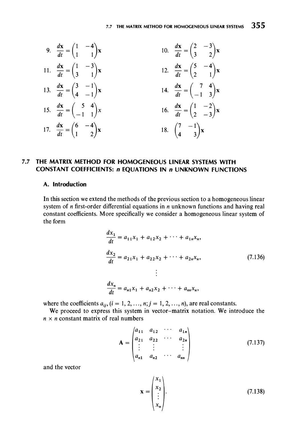
7.6 The Matrix Method for Homogeneous Linear Systems with Constant Coefficients:
Two Equations in Two Unknown Functions 346
7.7 The Matrix Method for Homogeneous Linear Systems with Constant Coefficients:
η Equations in η Unknown Functions 355
Eight Approximate Methods of Solving First-Order Equations 377
8.1 Graphical Methods 377
8.2 Power Series Methods 384
8.3 The Method of Successive Approximations 390
8.4 Numerical Methods 394
Nine The Laplace Transform 411
9.1 Definition, Existence, and Basic Properties of the Laplace Transform 411
9.2 The Inverse Transform and the Convolution 431
9.3 Laplace Transform Solution of Linear Differential Equations with Constant
Coefficients 441
9.4 Laplace Transform Solution of Linear Systems 453
CONTENTS
VII
PART TWO FUNDAMENTAL THEORY AND FURTHER METHODS
Ten Existence and Uniqueness Theory 461
10.1 Some Concepts from Real Function Theory 461
10.2 The Fundamental Existence and Uniqueness Theorem 473
10.3 Dependence of Solutions on Initial Conditions and on the Function / 488
10.4 Existence and Uniqueness Theorems for Systems and Higher-Order Equations 495
Eleven The Theory of Linear Differential Equations 505
11.1 Introduction 505
11.2 Basic Theory of the Homogeneous Linear System 510
11.3 Further Theory of the Homogeneous Linear System 522
11.4 The Nonhomogeneous Linear System 533
11.5 Basic Theory of the wth-Order Homogeneous Linear Differential Equation 543
11.6 Further Properties of the rcth-Order Homogeneous Linear Differential Equation 558
11.7 The rcth-Order Nonhomogeneous Linear Equation 569
11.8 Sturm Theory 573
Twelve Sturm-Liouville Boundary-Value Problems and Fourier Series 588
12.1 Sturm-Liouville Problems 588
12.2 Orthogonality of Characteristic Functions 597
12.3 The Expansion of a Function in a Series of Orthonormal Functions 601
12.4 Trigonometric Fourier Series 60§
Thirteen Nonlinear Differential Equations 632
13.1 Phase Plane, Paths, and Critical Points 632
13.2 Critical Points and Paths of Linear Systems 644
13.3 Critical Points and Paths of Nonlinear Systems 658
13.4 Limit Cycles and Periodic Solutions 692
13.5 The Method of Kryloff and Bogoliuboff 707
Fourteen Partial Differential Equations 715
14.1 Some Basic Concepts and Examples 715
14.2 The Method of Separation of Variables 722
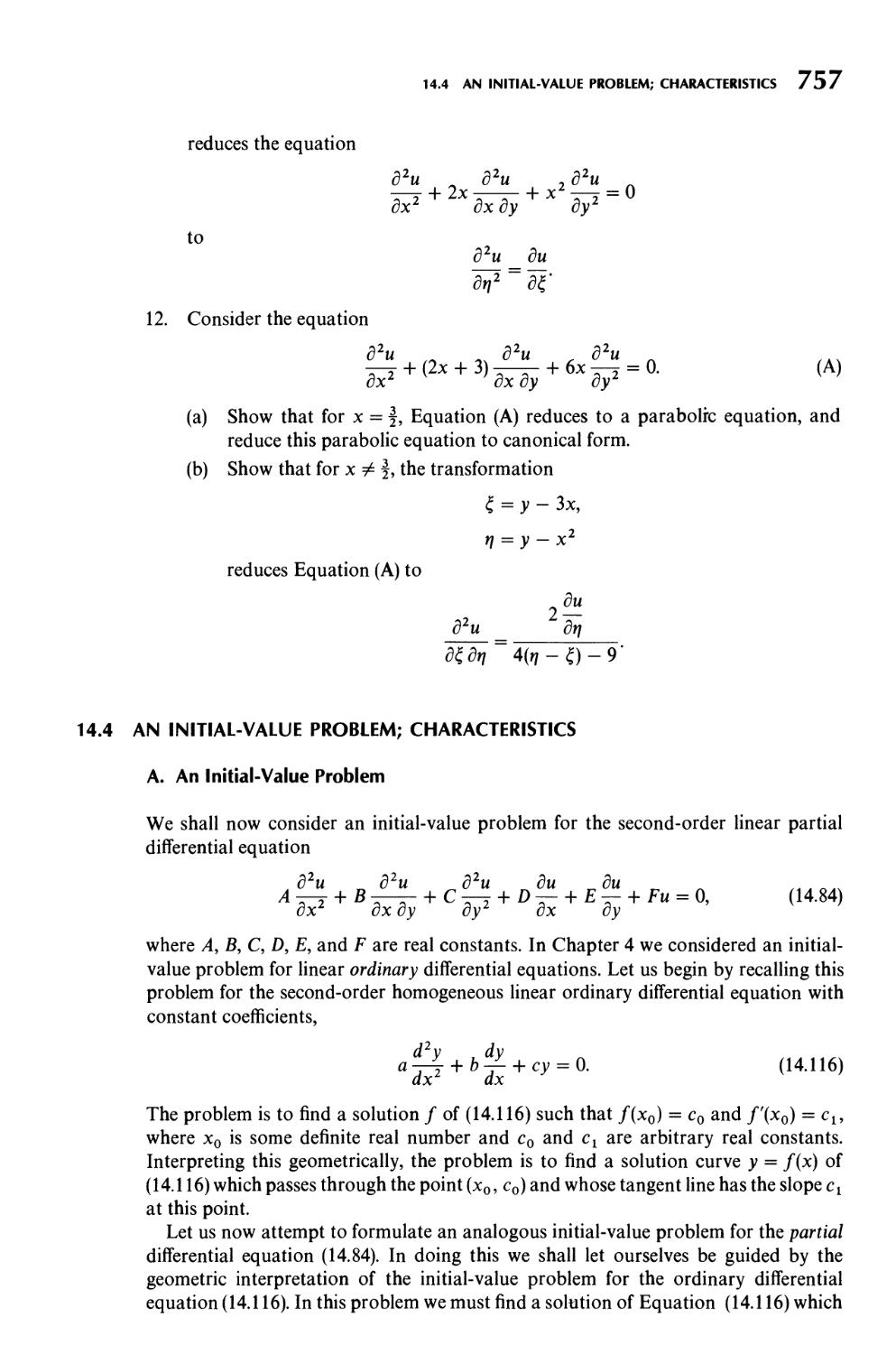
14.3 Canonical Forms of Second-Order Linear Equations with Constant Coefficients 743
14.4 An Initial-Value Problem; Characteristics 757
Appendices 771
Answers 111
Suggested Reading 801
Index 803
=PART ONE=
FUNDAMENTAL METHODS
AND APPLICA TIONS
This page intentionally left blank
CHAPTER ONE
Differential Equations and Their Solutions
The subject of differential equations constitutes a large and very important branch of
modern mathematics. From the early days of the calculus the subject has been an area
of great theoretical research and practical applications, and it continues to be so in our
day. This much stated, several questions naturally arise. Just what is a differential
equation and what does it signify? Where and how do differential equations originate
and of what use are they? Confronted with a differential equation, what does one do
with it, how does one do it, and what are the results of such activity? These questions
indicate three major aspects of the subject: theory, method, and application. The
purpose of this chapter is to introduce the reader to the basic aspects of the subject and
at the same time give a brief survey of the three aspects just mentioned. In the course of
the chapter, we shall find answers to the general questions raised above, answers that
will become more and more meaningful as we proceed with the study of differential
equations in the following chapters.
1.1 CLASSIFICATION OF DIFFERENTIAL EQUATIONS; THEIR ORIGIN AND
APPLICATION
A. Differential Equations and Their Classification
DEFINITION
An equation involving derivatives of one or more dependent variables with respect to one or
more independent variables is called a differential equation.*
* In connection with this basic definition, we do not include in the class of differential equations those
equations that are actually derivative identities. For example, we exclude such expressions as
and so forth.
— (eax)
dx
= aeax,
— (uv) = и — + ν—,
dx dx dx
3
4 DIFFERENTIAL EQUATIONS AND THEIR SOLUTIONS
► Example 1.1
For examples of differential equations we list the following:
d2y fdy^2
dS + Xy(dlc
2+Μ-ή) =°> 0-1)
d4x „ d2x ^ /4 лч
^r + 5^T + 3x = smr, (1.2)
dv dv
Ts + * = v' (L3)
д2и д2и д2и
дх2 ду2 dz
2+T3 + ^I = 0· (1-4)
From the brief list of differential equations in Example 1.1 it is clear that the various
variables and derivatives involved in a differential equation can occur in a variety of
ways. Clearly some kind of classification must be made. To begin with, we classify
differential equations according to whether there is one or more than one independent
variable involved.
DEFINITION
A differential equation involving ordinary derivatives of one or more dependent variables
with respect to a single independent variable is called an ordinary differential equation.
► Example 1.2
Equations (1.1) and (1.2) are ordinary differential equations. In Equation (1.1) the
variable χ is the single independent variable, and у is a dependent variable. In Equation
(1.2) the independent variable is t, whereas χ is dependent.
DEFINITION
A differential equation involving partial derivatives of one or more dependent variables
with respect to more than one independent variable is called a partial differential
equation.
► Example 1.3
Equations (1.3) and (1.4) are partial differential equations. In Equation (1.3) the
variables s and t are independent variables and ν is a dependent variable. In Equation
(1.4) there are three independent variables: x, y, and z; in this equation и is dependent.
We further classify differential equations, both ordinary and partial, according to the
order of the highest derivative appearing in the equation. For this purpose we give the
following definition.
1.1 CLASSIFICATION OF DIFFERENTIAL EQUATIONS; THEIR ORIGIN AND APPLICATION 5
DEFINITION
The order of the highest ordered derivative involved in a differential equation is called the
order of the differential equation.
► Example 1.4
The ordinary differential equation (1.1) is of the second order, since the highest
derivative involved is a second derivative. Equation (1.2) is an ordinary differential
equation of the fourth order. The partial differential equations (1.3) and (1.4) are of the
first and second orders, respectively.
Proceeding with our study of ordinary differential equations, we now introduce the
important concept of linearity applied to such equations. This concept will enable us to
classify these equations still further.
DEFINITION
A linear ordinary differential equation of order n, in the dependent variable у and the
independent variable x, is an equation that is in, or can be expressed in, the form
dny dn~ly dy
where a0 is not identically zero.
Observe (1) that the dependent variable у and its various derivatives occur to the first
degree only, (2) that no products of у and/or any of its derivatives are present, and (3)
that no transcendental functions of у and/or its derivatives occur.
► Example 1.5
The following ordinary differential equations are both linear. In each case у is the
dependent variable. Observe that у and its various derivatives occur to the first degree
only and that no products of у and/or any of its derivatives are present.
d2y [ 5dy_
dx2 dx
2 -^5± + 6у = 0, (1.5)
dx4 dx3 dx
+ x2 -pj + x3 ~- = xex. (1.6)
DEFINITION
A nonlinear ordinary differential equation is an ordinary differential equation that is not
linear.
6 DIFFERENTIAL EQUATIONS AND THEIR SOLUTIONS
► Example 1.6
The following ordinary differential equations are all nonlinear:
dx2 dx
—£ + 5 -f- + 6y2 = 0, (1.7)
dx2 \dx
d2y dy
dx1 dx
2+5Ш +6y = 0, (1.8)
2+5y± + 6y = 0. (1.9)
Equation (1.7) is nonlinear because the dependent variable у appears to the second
degree in the term 6y2. Equation (1.8) owes its nonlinearity to the presence of the term
5(dy/dx)3, which involves the third power of the first derivative. Finally, Equation (1.9)
is nonlinear because of the term 5y(dy/dx), which involves the product of the
dependent variable and its first derivative.
Linear ordinary differential equations are further classified according to the nature
of the coefficients of the dependent variables and their derivatives. For example,
Equation (1.5) is said to be linear with constant coefficients, while Equation (1.6) is linear
with variable coefficients.
B. Origin and Application of Differential Equations
Having classified differential equations in various ways, let us now consider briefly
where, and how, such equations actually originate. In this way we shall obtain some
indication of the great variety of subjects to which the theory and methods of
differential equations may be applied.
Differential equations occur in connection with numerous problems that are
encountered in the various branches of science and engineering. We indicate a few such
problems in the following list, which could easily be extended to fill many pages.
1. The problem of determining the motion of a projectile, rocket, satellite, or planet.
2. The problem of determining the charge or current in an electric circuit.
3. The problem of the conduction of heat in a rod or in a slab.
4. The problem of determining the vibrations of a wire or a membrane.
5. The study of the rate of decomposition of a radioactive substance or the rate of
growth of a population.
6. The study of the reactions of chemicals.
7. The problem of the determination of curves that have certain geometrical
properties.
The mathematical formulation of such problems give rise to differential equations.
But just how does this occur? In the situations under consideration in each of the above
problems the objects involved obey certain scientific laws. These laws involve various
rates of change of one or more quantities with respect to other quantities. Let us re-
1.2 SOLUTIONS 7
call that such rates of change are expressed mathematically by derivatives. In the
mathematical formulation of each of the above situations, the various rates of change
are thus expressed by various derivatives and the scientific laws themselves become
mathematical equations involving derivatives, that is, differential equations.
In this process of mathematical formulation, certain simplifying assumptions
generally have to be made in order that the resulting differential equations be tractable.
For example, if the actual situation in a certain aspect of the problem is of a relatively
complicated nature, we are often forced to modify this by assuming instead an
approximate situation that is of a comparatively simple nature. Indeed, certain
relatively unimportant aspects of the problem must often be entirely eliminated. The
result of such changes from the actual nature of things means that the resulting
differential equation is actually that of an idealized situation. Nonetheless, the
information obtained from such an equation is of the greatest value to the scientist.
A natural question now is the following: How does one obtain useful information
from a differential equation? The answer is essentially that if it is possible to do so, one
solves the differential equation to obtain a solution; if this is not possible, one uses the
theory of differential equations to obtain information about the solution. To
understand the meaning of this answer, we must discuss what is meant by a solution of
a differential equation; this is done in the next section.
Exercises
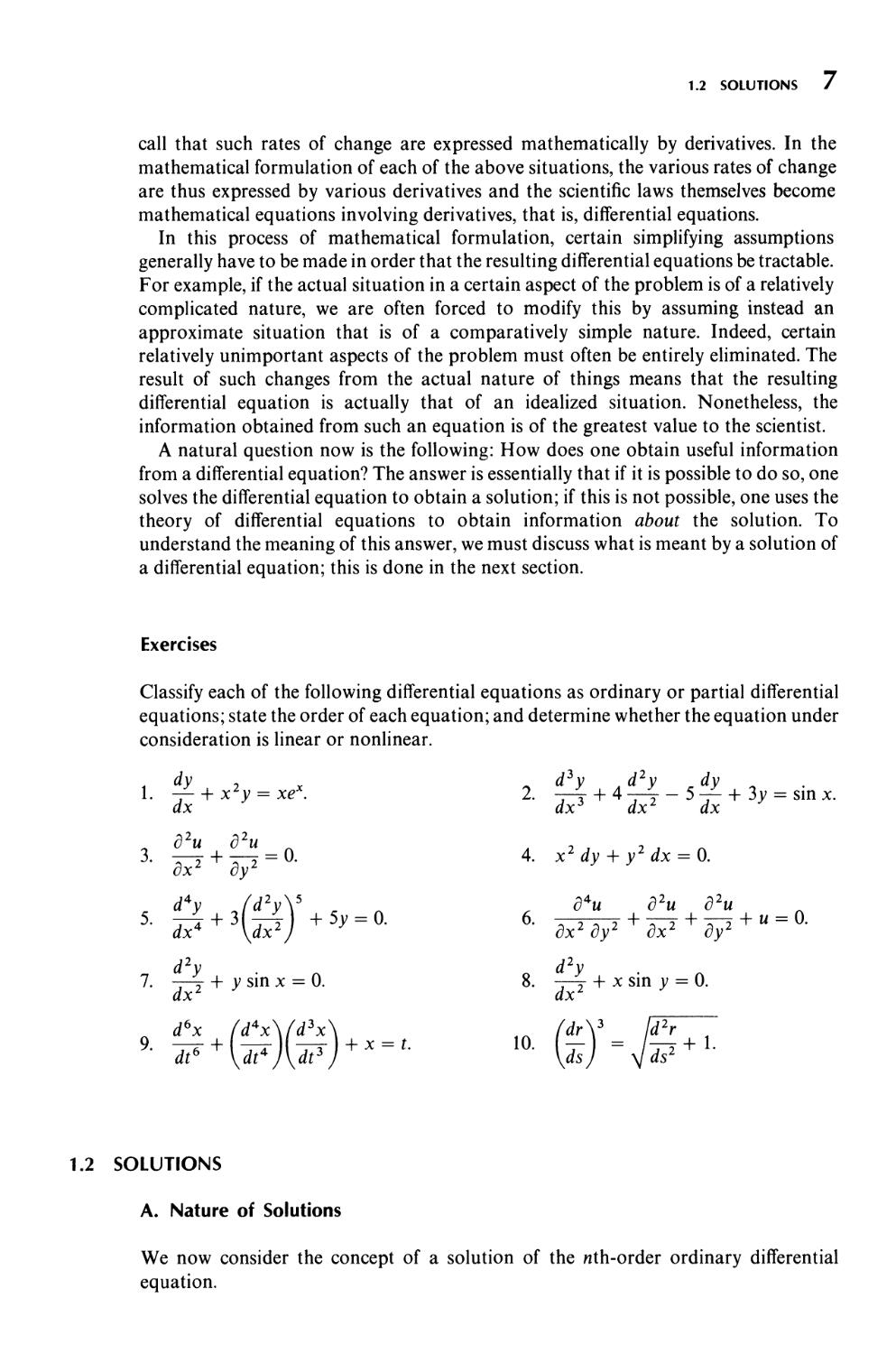
Classify each of the following differential equations as ordinary or partial differential
equations; state the order of each equation; and determine whether the equation under
consideration is linear or nonlinear.
dy 2 _ χ л d3y d2y dy
dx ' dx3 dx2 dx
1. j- + x2y = xex. 2. ΐ7τ + 4^γ- 5^+ Ъу = sin χ.
д2и дЧ
дх2 +а?
д2и д2и л , , , ,
3. —т + —у = 0. 4. х2 dy + у2 dx = 0.
d4y Jd2y\5 c л д*и д2и д2и
d2y „ d2y
—4 + у sin χ = 0. 8. -τ-4
dx dx
, л /лулч x_t ,α /*y_ g.
dt6 \dt4J\dt3J ' ' \dsj yjds2
1.2 SOLUTIONS
A. Nature of Solutions
We now consider the concept of a solution of the nth-order ordinary differential
equation.
8 DIFFERENTIAL EQUATIONS AND THEIR SOLUTIONS
DEFINITION
Consider the nth-order ordinary differential equation
Γ dy_ dy
= 0, (1.10)
dy d"y
where F is a real function of its (n + 2) arguments x, y,-r~, ■ ■ · >"ττ·
1. Let f be a real function defined for all χ in a real interval I and having an nth
derivative (and hence also all lower ordered derivatives) for all xe I. The function f is
called an explicit solution of the differential equation {1.10) on I if it fulfills the following
two requirements:
Flx,f(x),f'(xl...J™{x)] (A)
is defined for all xe I, and
F[x,/(x),Ax),...,/,n,M]=0 (B)
for all χ e I. That is, the substitution of f{x) and its various derivations for у and its
corresponding derivatives, respectively, in {1.10) reduces {1.10) to an identity on I.
2. A relation g{x, у) = О is called an implicit solution of {1.10) if this relation defines
at least one real function f of the variable χ on an interval I such that this function is an
explicit solution of {1.10) on this interval.
3. Both explicit solutions and implicit solutions will usually be called simply solutions.
Roughly speaking, then, we may say that a solution of the differential equation (1.10)
is a relation—explicit or implicit—between χ and y, not containing derivatives, which
identically satisfies (1.10).
► Example 1.7
The function / defined for all real χ by
f{x) = 2 sin χ + 3 cos χ (111)
is an explicit solution of the differential equation
d2y
dx
2 + У = 0 (1-12)
for all real x. First note that / is defined and has a second derivative for all real x. Next
observe that
f'(x) = 2 cos χ - 3 sin x,
f"{x) = - 2 sin χ - 3 cos x.
Upon substituting f"{x) for d2y/dx2 and f{x) for у in the differential equation (1.12), it
reduces to the identity
(- 2 sin χ - 3 cos x) + (2 sin χ + 3 cos x) = 0,
1.2 SOLUTIONS 9
which holds for all real x. Thus the function / defined by (1.11) is an explicit solution of
the differential equation (1.12) for all real x.
► Example 1.8
The relation
x2 + y2 -25 = 0 (1.13)
is an implicit solution of the differential equation
dy
*+ y-^- = 0 (1.14)
dx
on the interval / defined by — 5 < χ < 5. For the relation (1.13) defines the two real
functions /j and /2 given by
f1(x) = y/25-x2
and
f2(x)= -У25-Х2,
respectively, for all real xe/, and both of these functions are explicit solutions of the
differential equations (1.14) on /.
Let us illustrate this for the function fx. Since
f1(x) = y/25-x\
we see that
/ΊΜ =
x/25"
x2
for all real χ e /. Substituting fx(x) for у and f\(x) for dy/dx in (1.14), we obtain the
identity
χ + (J25 - x2) , 1 = 0 or χ - χ = 0,
V \^25^Y2J
which holds for all real xel. Thus the function fx is an explicit solution of (1.14) on the
interval /.
Now consider the relation
x2 + )/2 + 25 = 0. (1.15)
Is this also an implicit solution of Equation (1.14)? Let us differentiate the relation
(1.15) implicitly with respect to x. We obtain
~ dy dy χ
2x + 2v-f- = 0 or -γ-= —.
dx dx у
Substituting this into the differential equation (1.14), we obtain the formal identity
„ + ,(-ϊ)_α
DIFFERENTIAL EQUATIONS AND THEIR SOLUTIONS
Thus the relation (1.15) formally satisfies the differential equation (1.14). Can we
conclude from this alone that (1.15) is an implicit solution of (1.14)? The answer to this
question is "no," for we have no assurance from this that the relation (1.15) defines any
function that is an explicit solution of (1.14) on any real interval /. All that we have
shown is that (1.15) is a relation between χ and у that, upon implicit differentiation and
substitution, formally reduces the differential equation (1.14) to a formal identity. It is
called a formal solution; it has the appearance of a solution; but that is all that we know
about it at this stage of our investigation.
Let us investigate a little further. Solving (1.15) for y, we find that
y=±J-25-x2.
Since this expression yields nonreal values of у for all real values of x, we conclude
that the relation (1.15) does not define any real function on any interval. Thus the
relation (1.15) is not truly an implicit solution but merely a formal solution of the
differential equation (1.14).
In applying the methods of the following chapters we shall often obtain relations that
we can readily verify are at least formal solutions. Our main objective will be to gain
familiarity with the methods themselves and we shall often be content to refer to the
relations so obtained as "solutions," although we have no assurance that these relations
are actually true implicit solutions. If a critical examination of the situation is required,
one must undertake to determine whether or not these formal solutions so obtained are
actually true implicit solutions which define explicit solutions.
In order to gain further insight into the significance of differential equations and
their solutions, we now examine the simple equation of the following example.
► Example 1.9
Consider the first-order differential equation
^ = 2x. (1.16)
ax
The function f0 defined for all real χ by /0(x) = x2 is a solution of this equation. So also
are the functions 'fl9f2, and /3 defined for all real χ by/Дх) = χ2 + l,/2(x) = χ2 + 2,
and /з(х) = χ2 + 3, respectively. In fact, for each real number c, the function f defined
for all real χ by
fc{x) = x2 + c (1.17)
is a solution of the differential equation (1.16). In other words, the formula (1.17) defines
an infinite family of functions, one for each real constant c, and every function of this
family is a solution of (1.16). We call the constant с in (1.17) an arbitrary constant or
parameter and refer to the family of functions defined by (1.17) as a one-parameter
faimily of solutions of the differential equation (1.16). We write this one-parameter
family of solutions as
y = x2 + c. (1.18)
Although it is clear that every function of the family defined by (1.18) is a solution of
(1.16), we have not shown that the family of functions defined by (1.18) includes all of
the solutions of (1.16). However, we point out (without proof) that this is indeed the
1.2 SOLUTIONS 11
case here; that is, every solution of (1.16) is actually of the form (1.18) for some
appropriate real number c.
Note. We must not conclude from the last sentence of Example l .9 that every first-
order ordinary differential equation has a so-called one-parameter family of solutions
which contains all solutions of the differential equation, for this is by no means the case.
Indeed, some first-order differential equations have no solution at all (see Exercise 7(a)
at the end of this section), while others have a one-parameter family of solutions plus
one or more "extra" solutions which appear to be "different" from all those of the
family (see Exercise 7(b) at the end of this section).
The differential equation of Example l .9 enables us to obtain a better understanding
of the analytic significance of differential equations. Briefly stated, the differential
equation of that example defines functions, namely, its solutions. We shall see that this
is the case with many other differential equations of both first and higher order. Thus
we may say that a differential equation is merely an expression involving derivatives
which may serve as a means of defining a certain set of functions: its solutions. Indeed,
many of the now familiar functions originally appeared in the form of differential
equations that define them.
We now consider the geometric significance of differential equations and their
solutions. We first recall that a real function F may be represented geometrically by a
curve у = F(x) in the xy plane and that the value of the derivative of F at x, F'(x), may
be interpreted as the slope of the curve у = F(x) at x. Thus the general first-order
differential equation
T- = f(x,y), (1.19)
ax
where / is a real function, may be interpreted geometrically as defining a slope /(x, y) at
every point (x, y) at which the function / is defined. Now assume that the differential
equation (l. 19) has a so-called one-parameter family of solutions that can be written in
the form
y = F(x,c), (1.20)
where с is the arbitrary constant or parameter of the family. The one-parameter family
of functions defined by (l .20) is represented geometrically by a so-called one-parameter
family of curves in the xy plane, the slopes of which are given by the differential
equation (1.19). These curves, the graphs of the solutions of the differential equation
(1.19), are called the integral curves of the differential equation (1.19).
► Example 1.10
Consider again the first-order differential equation
^ = 2x (1.16)
ax
of Example 1.9. This differential equation may be interpreted as defining the slope 2x at
the point with coordinates (x, y) for every real x. Now, we observed in Example 1.9 that
the differential equation (1.16) has a one-parameter family of solutions of the form
у = χ2 + с,
(1.18)
DIFFERENTIAL EQUATIONS AND THEIR SOLUTIONS
X
Figure 1.1
where с is the arbitrary constant or parameter of the family. The one-parameter family
of functions defined by (1.18) is represented geometrically by a one-parameter family of
curves in the xy plane, namely, the family of parabolas with Equation (1.18). The slope
of each of these parabolas is given by the differential equation (1.16) of the family. Thus
we see that the family of parabolas (1.18) defined by differential equation (1.16) is that
family of parabolas, each of which has slope 2x at the point (x, y) for every real x, and
all of which have the у axis as axis. These parabolas are the integral curves of the
differential equation (1.16). See Figure 1.1.
B. Methods of Solution
When we say that we shall solve a differential equation we mean that we shall find one
or more of its solutions. How is this done and what does it really mean? The greater
part of this text is concerned with various methods of solving differential equations.
The method to be employed depends upon the type of differential equation under
consideration, and we shall not enter into the details of specific methods here.
But suppose we solve a differential equation, using one or another of the various
methods. Does this necessarily mean that we have found an explicit solution /
expressed in the so-called closed form of a finite sum of known elementary functions?
That is, roughly speaking, when we have solved a differential equation, does this
necessarily mean that we have found a "formula" for the solution? The answer is "no."
Comparatively few differential equations have solutions so expressible; in fact, a
closed-form solution is really a luxury in differential equations. In Chapters 2 and 4 we
shall consider certain types of differential equations that do have such closed-form
solutions and study the exact methods available for finding these desirable solutions.
But, as we have just noted, such equations are actually in the minority and we must
consider what it means to "solve" equations for which exact methods are unavailable.
Such equations are solved approximately by various methods, some of which are
considered in Chapters 6 and 8. Among such methods are series methods, numerical
1.2 SOLUTIONS 13
methods, and graphical methods. What do such approximate methods actually yield?
The answer to this depends upon the method under consideration.
Series methods yield solutions in the form of infinite series; numerical methods give
approximate values of the solution functions corresponding to selected values of the
independent variables; and graphical methods produce approximately the graphs of
solutions (the integral curves). These methods are not so desirable as exact methods
because of the amount of work involved in them and because the results obtained from
them are only approximate; but if exact methods are not applicable, one has no choice
but to turn to approximate methods. Modern science and engineering problems
continue to give rise to differential equations to which exact methods do not apply, and
approximate methods are becoming increasingly more important.
Exercises
1. Show that each of the functions defined in Column I is a solution of the
corresponding differential equation in Column II on every interval a < χ < b of
the χ axis.
I
II
(a) f(x) = x + 3e~x (^+y = x+\
(b) f(x) = 2e3x - 5e4x -j^ - 1 -£ + \2y = 0
dx
d2y ? dy
dx2 dx
(с) /(х) = е* + 2х2 + 6х + 7 ^._з^ + 2)/ = 4х
d2y 3dy
dx2 dx
(d) /M = TT-2 (l+x2)^4 + 4x^ + 2)/ = 0
2. (a) Show that x3 + 3xy2 = 1 is an implicit solution of the differential equation
2xy(dy/dx) + x2 + y2 = 0 on the interval 0 < χ < 1.
(b) Show that 5x2y2 — 2x3y2 = 1 is an implicit solution of the differential
equation x(dy/dx) + у = χ3у3 on the interval 0 < χ < f.
3. (a) Show that every function / defined by
f(x) = (x3 +c)e~3x,
where с is an arbitrary constant, is a solvtion of the differential equation
^ + 3у = 3х2е-3х.
dx
(b) Show that every function / defined by
f(x) = 2 + ce~2x\
where с is an arbitrary constant, is a solution of the differential equation
dy A
-L + 4xv = 8x.
dx
DIFFERENTIAL EQUATIONS AND THEIR SOLUTIONS
4. (a) Show that every function /defined by f(x) = cxeAx + c2e 2x, where cx andc2
are arbitrary constants, is a solution of the differential equation
dx2 dx
2 2^-Sy = 0.
(b) Show that every function #defined by g(x) = cie2x + c2xe2x + c3e 2x, where
cuc2, and c3 are arbitrary constants, is a solution of the differential equation
dx3 dx2 dx
3 2-^-4^ + 8^ = 0.
5. (a) For certain values of the constant m the function / defined by f(x) = e"
solution of the differential equation
dx7, dx2 dx
У,-^-4^+Пу = 0.
Determine all such values of m.
(b) For certain values of the constant η the function g defined by g{x) = xn is a
solution of the differential equation
^Z + 2x2^Z_i0x^
dx3 dx2 dx
*3^ + 2x2-r4-10x-£-8y = 0.
Determine all such values of n.
6. (a) Show that the function / defined by f(x) = (2x2 + 2e3x + 3)e '2x satisfies the
differential equation
-f- + 2 ν = 6ex + 4xe ~~2x
dx
and also the condition /(0) = 5.
(b) Show that the function / defined by f(x) = 3e2x — 2xe2x — cos 2x satisfies
the differential equation
dx2 dx
2 4 -—h 4y = — 8 sin 2x
and also the conditions that /(0) = 2 and /'(0) = 4.
7. (a) Show that the first-order differential equation
+ Ы + 1=о
has no (real) solutions,
(b) Show that the first-order differential equation
Чу42
has a one-parameter family of solutions of the form f(x) = (x + c)2, where с is
an arbitrary constant, plus the "extra" solution #(x) = 0 that is not a member
of this family f(x) = (x + c)2 for any choice of the constant с
1.3 INITIAL-VALUE PROBLEMS, BOUNDARY-VALUE PROBLEMS 1 5
1.3 INITIAL-VALUE PROBLEMS, BOUNDARY-VALUE PROBLEMS, AND
EXISTENCE OF SOLUTIONS
A. Initial-Value Problems and Boundary-Value Problems
We shall begin this section by considering the rather simple problem of the following
example.
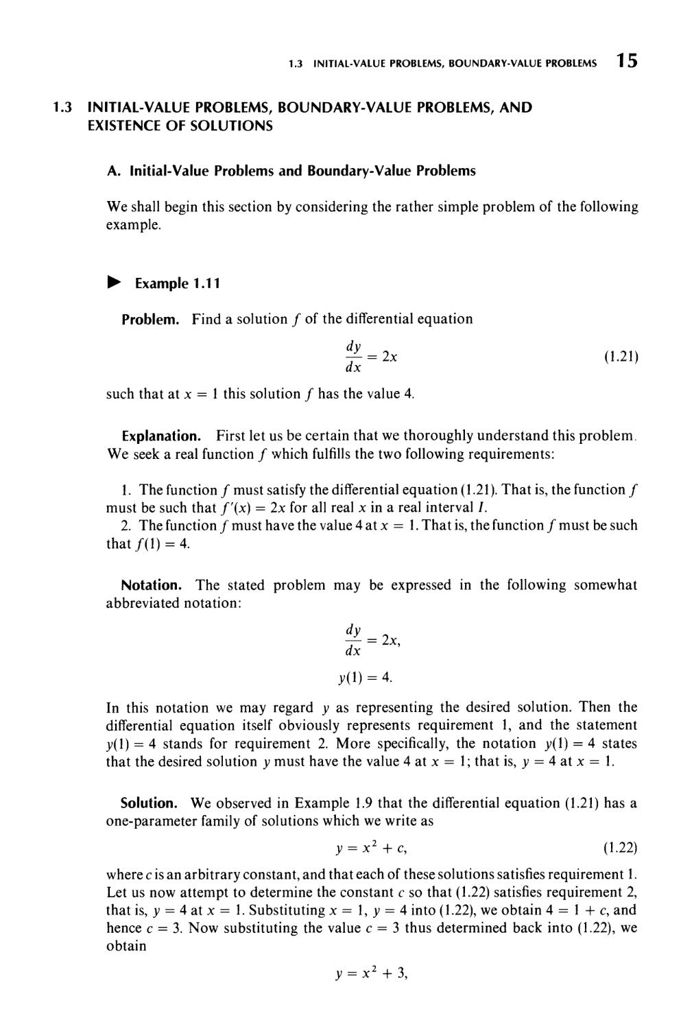
► Example 1.11
Problem. Find a solution / of the differential equation
^ = 2x (1.21)
ax
such that at χ = 1 this solution / has the value 4.
Explanation. First let us be certain that we thoroughly understand this problem.
We seek a real function / which fulfills the two following requirements:
1. The function / must satisfy the differential equation (1.21). That is, the function /
must be such that f'(x) = 2x for all real χ in a real interval /.
2. The function / must have the value 4 at χ = 1. That is, the function / must be such
that/(1) = 4.
Notation. The stated problem may be expressed in the following somewhat
abbreviated notation:
^ = 2*
dx '
)>(!) = 4.
In this notation we may regard у as representing the desired solution. Then the
differential equation itself obviously represents requirement 1, and the statement
y(\) = A stands for requirement 2. More specifically, the notation y(\) = 4 states
that the desired solution у must have the value 4 at χ = 1; that is, у = 4 at χ = 1.
Solution. We observed in Example 1.9 that the differential equation (1.21) has a
one-parameter family of solutions which we write as
y = x2 + c, (1.22)
where с is an arbitrary constant, and that each of these solutions satisfies requirement 1.
Let us now attempt to determine the constant с so that (1.22) satisfies requirement 2,
that is, у = 4 at χ = 1. Substituting χ = 1, у = 4 into (1.22), we obtain 4 = 1 + c, and
hence с = 3. Now substituting the value с = 3 thus determined back into (1.22), we
obtain
У = х2 + 3,
DIFFERENTIAL EQUATIONS AND THEIR SOLUTIONS
which is indeed a solution of the differential equation (1.21), which has the value 4 at
χ = 1. In other words, the function / defined by
fix) = x2 + 3,
satisfies both of the requirements set forth in the problem.
Comment on Requirement 2 and Its Notation. In a problem of this type,
requirement 2 is regarded as a supplementary condition that the solution of the differential
equation must also satisfy. The abbreviated notation y(\) = 4, which we used to
express this condition, is in some way undesirable, but it has the advantages of being
both customary and convenient.
In the application of both first- and higher-order differential equations the problems
most frequently encountered are similar to the above introductory problem in that they
involve both a differential equation and one or more supplementary conditions which
the solution of the given differential equation must satisfy. If all of the associated
supplementary conditions relate to one χ value, the problem is called an initial-value
problem (or one-point boundary-value problem). If the conditions relate to two
different χ values, the problem is called a two-point boundary-value problem (or simply a
boundary-value problem). We shall illustrate these concepts with examples and then
consider one such type of problem in detail. Concerning notation, we generally employ
abbreviated notations for the supplementary conditions that are similar to the
abbreviated notation introduced in Example 1.11.
► Example 1.12
Ί? + > = °>
У(1) = 3,
/d)=-4.
This problem consists in finding a solution of the differential equation
which assumes the value 3 at χ = 1 and whose first derivative assumes the value —4 at
χ = 1. Both of these conditions relate to one χ value, namely, χ = 1. Thus this is an
initial-value problem. We shall see later that this problem has a unique solution.
► Example 1.13
d2y
J*(0)=1,
1.3 INITIAL-VALUE PROBLEMS, BOUNDARY-VALUE PROBLEMS 1 7
In this problem we again seek a solution of the same differential equation, but this time
the solution must assume the value 1 at χ = 0 and the value 5 at χ = π/2. That is, the
conditions relate to the two different χ values, 0 and π/2. This is a (two-point)
boundary-value problem. This problem also has a unique solution; but the boundary-
value problem
d2y
y(0) = 1, y(n) = 5,
has no solution at all! This simple fact may lead one to the correct conclusion that
boundary-value problems are not to be taken lightly!
We now turn to a more detailed consideration of the initial-value problem for a first-
order differential equation.
DEFINITION
Consider the first-order differential equation
j-x = fix, y), (1.23)
where f is a continuous function of χ and у in some domain* D of the xy plane; and let
(хо?Уо) be a point of D. The initial-value problem associated with (1.23) is to find
a solution φ of the differential equation (7.25), defined on some real interval containing x0,
and satisfying the initial condition
Ф(хо) = Уо·
In the customary abbreviated notation, this initial-value problem may be written
Tx=f{X>y)>
У(*о) = Уо-
To solve this problem, we must find a function φ that not only satisfies the differential
equation (1.23) but that also satisfies the initial condition that it has the value y0 when χ
has value x0. The geometric interpretation of the initial condition, and hence of the
entire initial-value problem, is easily understood. The graph of the desired solution φ
must pass through the point with coordinates (x0, y0). That is, interpreted
geometrically, the initial-value problem is to find an integral curve of the differential equation
(1.23) that passes through the point (x0, y0).
The method of actually finding the desired solution φ depends upon the nature of the
differential equation of the problem, that is, upon the form of /(x, y). Certain special
types of differential equations have a one-parameter family of solutions whose
equation may be found exactly by following definite procedures (see Chapter 2). If the
differential equation of the problem is of some such special type, one first obtains the
equation of its one-parameter family of solutions and then applies the initial condition
* A domain is an open, connected set. For those unfamiliar with such concepts, D may be regarded as the
interior of some simple closed curve in the plane.
DIFFERENTIAL EQUATIONS AND THEIR SOLUTIONS
to this equation in an attempt to obtain a "particular" solution φ that satisfies the entire
initial-value problem. We shall explain this situation more precisely in the next
paragraph. Before doing so, however, we point out that in general one cannot find
the equation of a one-parameter family of solutions of the differential equation;
approximate methods must then be used (see Chapter 8).
Now suppose one can determine the equation
g(x,y,c) = 0 (1.24)
of a one-parameter family of solutions of the differential equation of the problem.
Then, since the initial condition requires that у = y0 at χ = x0, we let χ = x0 and
у = у0 in (1.24) and thereby obtain
9{хо,Уо,с) = 0.
Solving this for c, in general we obtain a particular value of с which we denote here by
c0. We now replace the arbitrary constant с by the particular constant c0 in (1.24), thus
obtaining the particular solution
9(х>У>Со) = 0.
The particular explicit solution satisfying the two conditions (differential equation and
initial condition) of the problem is then determined from this, if possible.
We have already solved one initial-value problem in Example 1.11. We now give
another example in order to illustrate the concepts and procedures more thoroughly.
► Example 1.14
Solve the initial-value problem
£=--· (1·25)
ax у
y(3) = 4, (1.26)
given that the differential equation (1.25) has a one-parameter family of solutions which
may be written in the form
x2 + y2 = c\ (1.27)
The condition (1.26) means that we seek the solution of (1.25) such that у = 4 at χ = 3.
Thus the pair of values (3,4) must satisfy the relation (1.27). Substituting χ = 3 and
у = 4 into (1.27), we find
9+16 = c2 or c2 = 25.
Now substituting this value of c2 into (1.27), we have
x2 + y2 = 25.
Solving this for y, we obtain
y= ±y/25-x2.
Obviously the positive sign must be chosen to give у the value +4 at χ = 3. Thus the
function / defined by
f(x) = ^/25-x2, -5 < χ < 5,
1.3 INITIAL-VALUE PROBLEMS, BOUNDARY-VALUE PROBLEMS 1 9
is the solution of the problem. In the usual abbreviated notation, we write this solution
as У = %/25 — χ2-
В. Existence of Solutions
In Example 1.14 we were able to find a solution of the initial-value problem under
consideration. But do all initial-value and boundary-value problems have solutions?
We have already answered this question in the negative, for we have pointed out that
the boundary-value problem
dly
dx
2 + у = 0,
j>(0)=l,
y(n) = 5,
mentioned at the end of Example 1.13, has no solution! Thus arises the question of
existence of solutions: given an initial-value or boundary-value problem, does it
actually have a solution? Let us consider the question for the initial-value problem
defined on page 17. Here we can give a definite answer. Every initial-value problem that
satisfies the definition on page 17 has at least one solution.
But now another question is suggested, the question of uniqueness. Does such a
problem ever have more than one solution? Let us consider the initial-value problem
аУ 1/3
Тх=У '
y(0) = 0.
One may verify that the functions fx and /2 defined, respectively, by
/i(x) = 0 for all real x;
and
/2W = (!*)3/2, *>0; /2(x) = 0, x<0;
are both solutions of this initial-value problem! In fact, this problem has infinitely many
solutions! The answer to the uniqueness question is clear: the initial-value problem, as
stated, need not have a unique solution. In order tb ensure uniqueness, some additional
requirement must certainly be imposed. We shall see what this is in Theorem 1.1, which
we shall now state.
THEOREM 1.1. BASIC EXISTENCE AND UNIQUENESS THEOREM
Hypothesis. Consider the differential equation
dy r
^ = /(*,)>), (1.28)
DIFFERENTIAL EQUATIONS AND THEIR SOLUTIONS
where
1. The function f is a continuous function of χ and у in some domain D of the xy plane,
and
2. The partial derivative df/ду is also a continuous function of χ and у in D; and let
(xo> Уо) be a point in D.
Conclusion. There exists a unique solution φ of the differential equation (1.28),
defined on some interval \x — x0\ < ft, where h is sufficiently small, that satisfies the
condition
ф(х0)=Уо. (1.29)
Explanatory Remarks. This basic theorem is the first theorem from the theory of
differential equations which we have encountered. We shall therefore attempt to
explain its meaning in detail.
1. It is an existence and uniqueness theorem. This means that it is a theorem which
tells us that under certain conditions (stated in the hypothesis) something exists (the
solution described in the conclusion) and is unique (there is only one such solution). It
gives no hint whatsoever concerning how to find this solution but merely tells us that
the problem has a solution.
2. The hypothesis tells us what conditions are required of the quantities involved. It
deals with two objects: the differential equation (1.28) and the point (x0, y0). As far as
the differential equation (1.28) is concerned, the hypothesis requires that both the
function / and the function df/ду (obtained by differentiating /(x, y) partially with
respect to y) must be continuous in some domain D of the xy plane. As far as the point
(x0, y0) is concerned, it must be a point in this same domain D, where / and df/ду are so
well behaved (that is, continuous).
3. The conclusion tells us of what we can be assured when the stated hypothesis is
satisfied. It tells us that we are assured that there exists one and only one solution φ of
the differential equation, which is defined on some interval | χ - x01 < h centered about
x0 and which assumes the value y0 when χ takes on the value x0. That is, it tells us that,
under the given hypothesis on /(x, y), the initial-value problem
У(*о) = Уо,
has a unique solution that is valid in some interval about the initial point x0.
4. The proof of this theorem is omitted. It is proved under somewhat less restrictive
hypotheses in Chapter 10.
5. The value of an existence theorem may be worth a bit of attention. What good is
it, one might ask, if it does not tell us how to obtain the solution? The answer to this
question is quite simple: an existence theorem will assure us that there is sl solution to
look for! It would be rather pointless to spend time, energy, and even money in trying to
find a solution when there was actually no solution to be found! As for the value of the
uniqueness, it would be equally pointless to waste time and energy finding one
particular solution only to learn later that there were others and that the one found was
not the one wanted!
1.3 INITIAL-VALUE PROBLEMS, BOUNDARY-VALUE PROBLEMS 21
We have included this rather lengthy discussion in the hope that the student, who has
probably never before encountered a theorem of this type, will obtain a clearer idea of
what this important theorem really means. We further hope that this discussion will
help him to analyze theorems which he will encounter in the future, both in this book
and elsewhere. We now consider two simple examples which illustrate Theorem 1.1.
► Example 1.15
Consider the initial-value problem
dx
= x2 + y2,
y(l) = 3.
Let us apply Theorem 1.1. We first check the hypothesis. Here /(x, y) = x2 + y2
and ——-— = 2y. Both of the functions / and df/ду are continuous in every domain
У \
D of the xy plane. The initial condition y(\) = 3 means that x0 = 1 and y0 = 3, and the
point (1,3) certainly lies in some such domain D. Thus all hypotheses are satisfied and
the conclusion holds. That is, there is a unique solution φ of the differential equation
ay lax = x2 + y2, defined on some interval \x — \\<h about x0= I, which satisfies
that initial condition, that is, which is such that φ(\) = 3.
► Example 1.16
Consider the two
j dy _ у
dx V/Gc'
2 dy _ у
dx x/x~'
problems:
yW = 2,
У(0) = 2.
Here
f(X>y)=—U2 aIld —1 =~Ш'
χ ' ay xL'z
These functions are both continuous except for χ = 0 (that is, along the у axis). In
problem 1, x0 = 1, y0 = 2. The square of side 1 centered about (1,2) does not contain
the у axis, and so both / and df/ду satisfy the required hypotheses in this square. Its
interior may thus be taken to be the domain D of Theorem 1.1; and (1,2) certainly lies
within it. Thus the conclusion of Theorem 1.1 applies to problem 1 and we know the
problem has a unique solution defined in some sufficiently small interval about x0 = 1.
Now let us turn to problem 2. Here x0 = 0, y0 = 2. At this point neither / nor df/dy
are continuous. In other words, the point (0,2) cannot be included in a domain D where
the required hypotheses are satisfied. Thus we can not conclude from Theorem 1.1 that
DIFFERENTIAL EQUATIONS AND THEIR SOLUTIONS
+ _^_6y = 0,
problem 2 has a solution. We are not saying that it does not have one. Theorem 1.1
simply gives no information one way or the other.
Exercises
1. Show that
y = 4e2x + 2e~3x
is a solution of the initial-value problem
dx2 dx
№ = 6,
/(0) = 2.
Is у = 2e2x + 4e~3x also a solution of this problem? Explain why or why not.
2. Given that every solution of
J-+ У = 2xe~x
dx
may be written in the form у = (χ2 + c)e~x, for some choice of the arbitrary
constant c, solve the following initial-value problems:
(a) ^ + y = 2xe-x, (b) ^ + j, = 2x£T*,
dx dx
y(0) = 2. y{-1) = e + 3.
3. Given that every solution of
— - — - 12 =0
dx2 dx
may be written in the form
у = c^4x + c2e~3x,
for some choice of the arbitrary constants cx and c2, solve the following initial-
value problems:
<■>£-£-'»-* «»£-£-.2,-a
У(0) = 5, У(0)=-2,
y'(0) = 6. y'(0) = 6.
4. Every solution of the differential equation
d2y
dx
2 + y = 0
1.3 INITIAL-VALUE PROBLEMS, BOUNDARY-VALUE PROBLEMS 23
may be written in the form у = c^ sin χ + c2 cos x, for some choice of the arbitrary
constants с! and c2. Using this information, show that boundary problems (a) and
(b) possess solutions but that (c) does not.
d2y
(a) ^+y = 0,
№ = o,
y(n/2) = 1.
d2v
(0 ^+y = o,
y(0) = 0,
№ = i.
Given that every solution of
3d3y
X dx3'
-3x:
,d2y
dx2
d2y
(b) J+y = 0,
У(0) = 1,
y'(n/2)=-l.
+ 6x^--6y = 0
dx
may be written in the form у = clx + c2x2 + c3x3 for some choice of the arbitrary
constants cl,c2, and c3, solve the initial-value problem consisting of the above
differential equation plus the three conditions
y(2) = 0, /(2) = 2, y»(2) = 6.
6. Apply Theorem 1.1 to show that each of the following initial-value problems has
a unique solution defined on some sufficiently small inverval |x — 11 < h about
7.
x0 :
(a)
= 1:
dy 2 .
— = xz sin y,
dx
y(l)=-2.
Consider the initial-value problem
d-l =
dx
P(x)
(b)
y2 +
dl =
dx
y(i) =
Q(*)y,
y2
0.
У(2) = 5,
where P(x) and Q(x) are both third-degree polynomials in x. Has this problem a
unique solution on some interval |x - 2| < h about x0 = 2? Explain why or why
not.
8. On page 19 we stated that the initial-value problem
УФ) = °>
has infinitely many solutions.
24 DIFFERENTIAL EQUATIONS AND THEIR SOLUTIONS
(a) Verify that this is indeed the case by showing that
_ (0, χ < c,
У=№*-с)Г12, x>c,
is a solution of the stated problem for every real number с > 0.
(b) Carefully graph the solution for which с = 0. Then, using this particular
graph, also graph the solutions for which с = 1, с = 2, and с = 3.
CHAPTER TWO
First-Order Equations for Which Exact Solutions Are Obtainable
In this chapter we consider certain basic types of first-order equations for which exact
solutions may be obtained by definite procedures. The purpose of this chapter is to gain
ability to recognize these various types and to apply the corresponding methods of
solutions. Of the types considered here, the so-called exact equations considered in
Section 2.1 are in a sense the most basic, while the separable equations of Section 2.2 are
in a sense the "easiest." The most important, from the point of view of applications, are
the separable equations of Section 2.2 and the linear equations of Section 2.3. The
remaining types are of various very special forms, and the correponding methods
of solution involve various devices. In short, we might describe this chapter as a
collection of special "methods," "devices," "tricks," or "recipes," in descending order of
kindness!
2.1 EXACT DIFFERENTIAL EQUATIONS AND INTEGRATING FACTORS
A. Standard Forms of First-Order Differential Equations
The first-order differential equations to be studied in this chapter may be expressed in
either the derivative form
j- = K*,y) (2-1)
dx
or the differential form
M(x, y) dx + N{x, y) dy = 0. (2.2)
25
FIRST-ORDER EQUATIONS FOR WHICH EXACT SOLUTIONS ARE OBTAINABLE
An equation in one of these forms may readily be written in the other form. For
example, the equation
dy _x2 + y2
dx χ — у
is of the form (2.1). It may be written
(x2 + y2) dx + (y - x) dy = 0,
which is of the form (2.2). The equation
(sin χ + y) dx + (x + 3y) dy = 0,
which is of the form (2.2), may be written in the form (2.1) as
dy sin χ + у
dx χ + 3y '
In the form (2.1) it is clear from the notation itself that у is regarded as the dependent
variable and χ as the independent one; but in the form (2.2) we may actually regard
either variable as the dependent one and the other as the independent. However, in
this text, in all differential equations of the form (2.2) in χ and y, we shall regard у
as dependent and χ as independent, unless the contrary is specifically stated.
B. Exact Differential Equations
DEFINITION
Let F be a function of two real variables such that F has continuous first partial
derivatives in a domain D. The total differential dF of the function F is defined by the
formula
dF(x, y) = — dx + — dy
ox dy
for all (x, у) е D.
► Example 2.1
Let F be the function of two real variables defined by
F(x, y) = xy2 + 2x3y
for all real (x, y). Then
dF(x, y) 2^r2 dF(x, y)
—_ = y* + 6x2)/, — = 2xy + 2χ·\
ox dy
and the total differential dF is defined by
dF{x, y) = {y2 + 6x2y) dx + (2xy + 2x3) dy
for all real (x, y).
2.1 EXACT DIFFERENTIAL EQUATIONS AND INTEGRATING FACTORS 27
DEFINITION
The expression
M(x, y) dx + N(x, y) dy (2.3)
is called an exact differential in a domain D if there exists a function F of two real
variables such that this expression equals the total differential dF(x, y) for all (x, у) е D.
That is, expression (2.3) is an exact differential in D if there exists a function F such
that
d-^ = M(X,y) and d-^ = N(x,y)
ox dy
for all (x, y) g D.
If M(x, y) dx + N(x, y) dy is an exact differential, then the differential equation
M(x, y) dx + N(x, y)dy = 0
is called an exact differential equation.
► Example 2.2
The differential equation
y2 dx + 2xy dy = 0 (2.4)
is an exact differential equation, since the expression y2 dx + 2xy dy is an exact
differential. Indeed, it is the total differential of the function F defined for all (x, y)
by F(x, y) = xy2, since the coefficient of dx is dF(x, y)/(dx) = y2 and that of dy is
dF(x, y)/(dy) = 2xy. On the other hand, the more simple appearing equation
у dx + 2x dy = 0, (2.5)
obtained from (2.4) by dividing through by y, is not exact.
In Example 2.2 we. stated without hesitation that the differential equation (2.4) is
exact but the differential equation (2.5) is not. In the case of Equation (2.4), we verified
our assertion by actually exhibiting the function F of which the expression y2 dx +
2xy dy is the total differential. But in the case of Equation (2.5), we did not back up
our statement by showing that there is no fucntion F such that у dx + 2x dy is its total
differential. It is clear that we need a simple test to determine whether or not a given
differential equation is exact. This is given by the following theorem.
THEOREM 2.1
Consider the differential equation
M(x, y) dx + N(x, y) dy = 0, (2.6)
where Μ and N have continuous first partial derivatives at all points (x, y) in a rectangular
domain D.
FIRST-ORDER EQUATIONS FOR WHICH EXACT SOLUTIONS ARE OBTAINABLE
1. If the differential equation (2.6) is exact in D, then
дЩх, у) _ dN(x, у)
ду дх
for all (x, у) е D.
2. Conversely, if
(2.7)
дЩх, у) _ дЩх, у)
ду дх
for all (χ, у) е D, then the differential equation (2.6) is exact in D..
Proof. Part 1. If the differential equation (2.6) is exact in D, then M'dx + N dy is an
exact differential in D. By definition of an exact differential, there exists a function F
such that
d-^A = M(x,y) and д^=Щх,у)
дх ду
for all (χ, у) е D. Then
d2F(x,y) dM(x,y) d2F(x,y) дЩх,у)
—-—-— = — and —-—-— = —
ду дх ду дх ду дх
for all (χ, у) e D. But, using the continuity of the first partial derivatives of Μ and N, we
have
d2F(x,y) = d2F(x,y)
ду дх дх ду
and therefore
дМ(х, у) _ дЩх, у)
ду дх
for all (χ, у) е D.
Part 2. This being the converse of Part 1, we start with the hypothesis that
дМ(х9 у) _ dN(x, у)
ду дх
for all (x, у) g D, and set out to show that Μ dx + N dy = 0 is exact in D. This means
that we must prove that there exists a function F such that
Щр = «<*,, ,2.8,
and
dF(x, y)
dy
= N(x, y) (2.9)
for all (x, у) е D. We can certainly find some F(x, y) satisfying either (2.8) or (2.9), but
what about both? Let us assume that F satisfies (2.8) and proceed. Then
(х,У) = J
F(x, у) = М(х, у) дх + ф(у), (2.10)
2.1 EXACT DIFFERENTIAL EQUATIONS AND INTEGRATING FACTORS 29
where J M(x, у) дх indicates a partial integration with respect to x, holding у constant,
and φ is an arbitrary function of у only. This ф(у) is needed in (2.10) so that F(x, y)
given by (2.10) will represent all solutions of (2.8). It corresponds to a constant of
integration in the "one-variable" case. Differentiating (2.10) partially with respect to y,
we obtain
Щх,у) -s cM( .. my)
Now if (2.9) is to be satisfied, we must have
д
N(x,y) =
Syj
M(x, у) дх +
аф(у)
dy
(2.11)
and hence
#(y)
dy
= N(x
:,3»-|;JM(x,
y)dx.
Since φ is a function of у only, the derivative άφ/dy must also be independent of x. That
is, in order for (2.11) to hold,
N(x, У) ~ γ I M(x> У) дх
(2.12)
must be independent of x.
We shall show that
д 1
N(x,y)-y \M(x,y)dx
= 0.
We at once have
д
ax
д
N(x,y)-j-
Μ (χ, у) дх
_ дЩх, у)
дх
д2
дх ду
М(х, у) дх.
If (2.8) and (2.9) are to be satisfied, then using the hypothesis (2.7), we must have
M(x, у) дх.
дх ду
Thus we obtain
д2 См< μ S2F(x,y) d2F(x,y) d2
M(x, у) дх =
д_
дх
[щ*,у)-Ц-у
дх ду
М(х, у) дх
ду дх ду дх
дЩх, у) д2
and hence
But by hypothesis (2.7),
д_
д~х
у) - γ Ι Μ(χ' у) дх
дх ду дх
dN(x, у) дМ(х, у)
М(х, у) дх
дх
ду
дМ(х, у) dN(x, у)
ду
дх
FIRST-ORDER EQUATIONS FOR WHICH EXACT SOLUTIONS ARE OBTAINABLE
for all (x, у) е D. Thus
d_
Щх,у)-^-[м(х,у)дЛ = Ъ
for all (x, у) е D, and so (2.12) is independent of x. Thus we may write
Ф(У)
-ί
N(x, у)
ψ "]*>■
Substituting this into Equation (2.10), we have
F{x,y)= [м(х,у)дх+ [\щх,у)- [дЩ*'У) дх
dy.
(2.13)
This F(x, у) thus satisfies both (2.8) and (2.9) for all (x, y) e D, and so Μ dx + N dy = 0
is exact in D. Q.E.D.
Students well versed in the terminology of higher mathematics will recognize that
Theorem 2.1 may be stated in the following words: A necessary and sufficient condition
that Equation (2.6) be exact in D is that condition (2.7) hold for all (x, у) е D. For
students not so well versed, let us emphasize that condition (2.7),
дМ(х, у) дЩх, у)
ду
дх
is the criterion for exactness. If (2.7) holds, then (2.6) is exact; if (2.7) does not hold, then
(2.6) is not exact.
► Example 2.3
We apply the exactness criterion (2.7) to Equations (2.4) and (2.5), introduced in
Example 2.2. For the equation
y2 dx + 2xy dy = 0
(2.4)
we have
M(x, y) = y2, N(x, y) = 2xy,
dM(x,y) = 2 =dN(x,y)
dy
dx
for all (x, y). Thus Equation (2.4) is exact in every rectangular domain D. On the other
hand, for the equation
у dx + 2x dy = 0,
(2.5)
we have
M(x, y) = y, N{x, y) = 2x,
dM(x,y)=l^2 = dN(x,y)
dy dx
for all (x, y). Thus Equation (2.5) is not exact in any rectangular domain D.
2.1 EXACT DIFFERENTIAL EQUATIONS AND INTEGRATING FACTORS 31
► Example 2.4
Consider the differential equation
(2x sin у + y3ex) dx + (x2 cos у + 3y2ex) dy = 0.
Here
M(x, y) = 2x sin у + y3ex,
N(x, y) = x2 cos у + 3y2ex,
дМ(х, у) „ , 2 χ 3Ν(χ, у)
^-^ = 2χ cos у + Зу V = —\-Ш
ду дх
in every rectangular domain D. Thus this differential equation is exact in every such
domain.
These examples illustrate the use of the test given by (2.7) for determining whether or
not an equation of the form M(x, y) dx + N(x, y) dy = 0 is exact. It should be observed
that the equation must be in the standard form M(x, y) dx + N(x, y) dy = 0 in order to
use the exactness test (2.7). Note this carefully: an equation may be encountered in the
nonstandard form M(x, y) dx = N(x, y) dy, and in this form the test (2.7) does not
apply.
С The Solution of Exact Differential Equations
Now that we have a test with which to determine exactness, let us proceed to solve exact
differential equations. If the equation M(x, y) dx + N(x, y) dy = 0 is exact in a
rectangular domain D, then there exists a function F such that
dI^A = M{x,y) and ^Л = Щх9у) for all (χ, у) е Л
ox oy
Then the equation may be written
dF(x, y) dF(x, y)
— dx -\ dy = 0 or simply dF(x, y) = 0.
The relation F(x, у) = с is obviously a solution of this, where с is an arbitrary constant.
We summarize this observation in the following theorem.
THEOREM 2.2
Suppose the differential equation M(x, y) dx + N(x, y) dy = 0 satisfies the
differentiability requirements of Theorem 2.1 and is exact in a rectangular domain D. Then a one-
parameter family of solutions of this differential equation is given by F(x, y) = c, where F
is a function such that
dI^A = M{x,y) and ЩЬЛ = Щх,у) for all (x, у) е D.
ox oy
and с is an arbitrary constant.
FIRST-ORDER EQUATIONS FOR WHICH EXACT SOLUTIONS ARE OBTAINABLE
Referring to Theorem 2.1, we observe that F(x, y) is given by formula (2.13).
However, in solving exact differential equations it is neither necessary nor desirable to
use this formula. Instead one obtains F(x, y) either by proceeding as in the proof of
Theorem 2.1, Part 2, or by the so-called "method of grouping," which will be explained
in the following examples.
► Example 2.5
Solve the equation
(3x2 + 4xy) dx + (2x2 + 2y) dy = 0.
Our first duty is to determine whether or not the equation is exact. Here
M(x, y) = 3x2 + 4xy, N(x, y) = 2x2 + 2y,
дЩх,у) = 4χ dN(x,y) = 4χ
dy dx
for all real (x, y), and so the equation is exact in every rectangular domain D. Thus we
must find F such that
дЗ^ = М{х,у) = Ъх2 + 4ху and ^^-= N(x, y) = 2x2 + 2y.
From the first of these,
F(x, y) = M(x, y) dx + ф(у) = (3x2 + 4xy) dx + ф(у)
= χ3 + 2x2y + ф(у).
Then
dF(x,y)_^ 2 , аф(у)
But we must have
Thus
= 2x2 + ·
dy dy
dF(x, y)
dy
= N(x,y) = 2x2 + 2y.
A ± %l _ ^2 , *Ф(У)
or
2x2 + 2y = 2x2 + ■ ,
dy
Thus ф(у) = у2 + с0, where c0 is an arbitrary constant, and so
F(x, y) = x3 + 2x2y + y2 + c0.
2.1 EXACT DIFFERENTIAL EQUATIONS AND INTEGRATING FACTORS 33
Hence a one-parameter family of solution is F(x, y) = c1? or
x3 + 2x2y + y2 + c0 = cv
Combining the constants c0 and cx we may write this solution as
x3 + 2x2y + y2 = c,
where с = cl — c0 is an arbitrary constant. The student will observe that there is no loss
in generality by taking c0 = 0 and writing ф(у) = у2. We now consider an alternative
procedure.
Method of Grouping. We shall now solve the differential equation of this
example by grouping the terms in such a way that its left member appears as the sum of
certain exact differentials. We write the differential equation
(3x2 + 4xy) dx + (2x2 + 2y) dy = 0
in the form
3x2 dx + (4xy dx + 2x2 dy) + 2y dy = 0.
We now recognize this as
d(x3) + d(2x2y) + d(y2) = d(c),
where с is an arbitrary constant, or
d(x3 + 2x2y + y2) = d(c).
From this we have at once
x3 + 2x2y + y2 = с
Clearly this procedure is much quicker, but it requires a good "working knowledge" of
differentials and a certain amount of ingenuity to determine just how the terms should
be grouped. The standard method may require more "work" and take longer, but it is
perfectly straightforward. It is recommended for those who like to follow a pattern and
for those who have a tendency to jump at conculsions.
Just to make certain that we have both procedures well in hand, we shall consider an
initial-value problem involving an exact differential equation.
► Example 2.6
Solve the initial-value problem
(2x cos у + 3x2y) dx + (x3 - x2 sin у — у) dy = 0,
y(0) = 2.
We first observe that the equation is exact in every rectangular domain D, since
дМ(х,у) л . „ 2 dN(x,y)
^1JI= -2xsin)/ + 3x2 =—^-^
ду У dx
for all real (x, y).
34 FIRST-ORDER EQUATIONS FOR WHICH EXACT SOLUTIONS ARE OBTAINABLE
Standard Method. We must find F such that
dF{x, y)
and
Then
But also
and so
and hence
Thus
dx
M(x, y) = 2x cos у + 3x2y
dF(x,y) л„ л з 2
ду
Ν (χ, у) = χ3 - χ sin у — у.
F(x, у) = M(x, у) дх + ф(у)
(х, у) = Μ (χ,
ί
= (2х cos у + Ъх2у) дх + ф(у)
= х2 cos у + х3у + 0(у),
—V1^ = -* sin у + х3 + _9^.
= ЛГ(х, у) = х3 - х2 sin у — у
дР(х,У) кт,„ ,л . з v2
аф{у)
dy
У2
Ф(у) = -у + ^0.
з. У2
F(x, у) = х1 cos у + х> - — + с0.
Hence a one-parameter family of solutions is F(x, y) = c1? which may be expressed as
3 У2
xz cos у + хлу — — = с.
Applying the initial condition у = 2 when χ = 0, we find с = — 2. Thus the solution of
the given initial-value problem is
2
x2 cos у + x3y —— = — 2.
Method of Grouping. We group the terms as follows:
(2x cos у dx - x2 sin у dy) + (3x2y dx + x3 dy) — у dy = 0.
2.1 EXACT DIFFERENTIAL EQUATIONS AND INTEGRATING FACTORS 35
Thus we have
and so
d(x2 cos y) + d(x3y) -d["—-) = d(c);
3 У2
xz cos у + χ у —— = с
is a one-parameter family of solutions of the differential equation. Of course the initial
condition y(0) = 2 again yields the particular solution already obtained.
D. Integrating Factors
Given the differential equation
M(x, y) dx + N(x, y) dy = 0,
if
дМ(х, у) _ dN(x, у)
ду дх
then the equation is exact and we can obtain a one-parameter family of solutions by
one of the procedures explained above. But if
дМ(х, у) дЩх, у)
ду дх
then the equation is not exact and the above procedures do not apply. What shall we do
in such a case? Perhaps we can multiply the nonexact equation by some expression that
will transform it into an essentially equivalent exact equation. If so, we can proceed to
solve the resulting exact equation by one of the above procedures. Let us consider
again the equation
у dx + 2x dy = 0, (2.5)
which was introduced in Example 2.2. In that example we observed that this equation is
not exact. However, if we multiply Equation (2.5) by y, it is transformed into the
essentially equivalent equation
y2 dx + 2xy dy = 0, (2.4)
which is exact (see Example 2.2). Since this resulting exact equation (2.4) is integrable,
we call у an integrating factor of Equation (2.5). In general, we have the following
definition:
DEFINITION
// the differential equation
M(x, y) dx + N(x, y)dy = 0 (2.14)
FIRST-ORDER EQUATIONS FOR WHICH EXACT SOLUTIONS ARE OBTAINABLE
is not exact in a domain D but the differential equation
μ(χ, y)M(x, y) dx + μ(χ, y)N(x, y) dy = 0 (2.15)
is exact in D, then μ(χ, у) is called an integrating factor of the differential equation (2.14).
► Example 2.7
Consider the differential equation
(3y + 4xy2) dx + (2x + 3x2y) dy = 0. (2.16)
This equation is of the form (2.14), where
M(x, у) = Ъу + 4xy2, N(x, y) = 2x + 3x2y,
дЩх,у) ,^δ dN(x,y)
= 3 + Sxy, — = 2 + вху.
ду дх
Since
дМ(х,у) дЩх,у)
ду дх
except for (x, у) such that 2xy +1=0, Equation (2.16) is not exact in any rectangular
domain D.
Let μ(χ, у) = χ2у. Then the corresponding differential equation of the form (2.15) is
(3xV + 4x V) dx + (2x3y + 3xV) dy = 0.
This equation is exact in every rectangular domain D, since
δ[μ(χ, y)M(x, уУ] 2 3 2 δ[μ(χ, y)N(x, y)]
r = 6xzy + 12xJjr =
ду дх
for all real (x, y). Hence μ(χ, у) = χ2у is an integrating factor of Equation (2.16).
Multiplication of a nonexact differential equation by an integrating factor thus
transforms the nonexact equation into an exact one. We have referred to this
resulting exact equation as "essentially equivalent" to the original. This so-called essentially
equivalent exact equation has the same one-parameter family of solutions as the
nonexact original. However, the multiplication of the original equation by the integrating
factor may result in either (1) the loss of (one or more) solutions of the original, or (2) the
gain of (one or more) functions which are solutions of the "new" equation but not of the
original, or (3) both of these phenomena. Hence, whenever we transform a nonexact
equation into an exact one by multiplication by an integrating factor, we should check
carefully to determine whether any solutions may have been lost or gained. We shall
illustrate an important special case of these phenomena when we consider separable
equations in Section 2.2. See also Exercise 22 at the end of this section.
The question now arises: How is an integrating factor found? We shall not attempt to
answer this question at this time. Instead we shall proceed to a study of the important
class of separable equations in Section 2.2 and linear equations in Section 2.3. We shall
see that separable equations always possess integrating factors that are perfectly
2.1 EXACT DIFFERENTIAL EQUATIONS AND INTEGRATING FACTORS 37
obvious, while linear equations always have integrating factors of a certain special
form. We shall return to the question raised above in Section 2.4. Our object here has
been merely to introduce the concept of an integrating factor.
Exercises
In Exercises 1-10 determine whether or not each of the given equations is exact; solve
those that are exact.
1. (3x + 2y) dx + (2x + y) dy = 0.
2. (y2 + 3) dx + (2xy -4)dy = 0.
3. (2xy + 1) dx + (x2 + Ay) dy = 0.
4. (3x2y + 2) dx - (x3 + y) dy = 0.
5. (6xy + 2y2 - 5) dx + (3x2 + Axy - 6) dy = 0.
6. (Θ2 + l)cos rdr + 26 sin r άθ = 0.
7. (у sec2 χ + sec χ tan x) dx + (tan χ + 2y) dy = 0.
8. i-^ + xjdx + (^7 + y\dy = 0.
2v3/2 4- 1
10. У ^ dx + (3x1/2yl/2 - \)dy = 0.
Solve the initial-value problems in Exercises 11-16.
11. (2xy-3)dx + (x2+ 4y)dy = 0, y(\) = 2.
12. (3x2)/2-)/3 + 2x)dx + (2x3);-3x);2+ \) dy = 0, y(-2)= 1.
13. (2y sin χ cos χ + y2 sin x) dx + (sin2 χ — 2y cos x) dy ='0, y(0) = 3.
14. (yex + 2ex + у2) dx + (ex + 2xy) dy = 0, )/(0) = 6.
15· (^)Λ + (^)^ = 0- *-1) = 1
16· ^Г/з <**+ ^4/1 ^ = 0, У(1) = 8.
17. In each of the following equations determine the constant A such that the
equation is exact, and solve the resulting exact equation:
(a) (x2 + Ъху) dx + {Ax2 + Ay) dy = 0.
/1 1 \ , (Ax+ 1\ ,
(b) ^ + ?)<** + (^-)^ = ο.
FIRST-ORDER EQUATIONS FOR WHICH EXACT SOLUTIONS ARE OBTAINABLE
18. In each of the following equations determine the constant A such that the
equation is exact, and solve the resulting exact equation:
(a) (Ax2y + 2y2) dx + (x3 + 4xy) dy = 0.
,ь> (π+?)*+(ϊ,"ϊ)*'-α
19. In each of the following equations determine the most general function N(x, y)
such that the equation is exact:
(a) (x3 + xy2) dx + N(x, y) dy = 0.
(b) (x~2y~2 + xy~3)dx + N(x, y) dy = 0.
20. In each of the following equations determine the most general function M(x, y)
such that the equation is exact:
(a) M(x, y) dx + (2x V + x4y) dy = 0.
(b) M(x, y) dx + (2yex + y2e3x) dy = 0.
21. Consider the differential equation
(4x + 3y2) dx + 2xy dy = 0.
(a) Show that this equation is not exact.
(b) Find an integrating factor of the form x", where η is a positive integer.
(c) Multiply the given equation through by the integrating factor found in (b)
and solve the resulting exact equation.
22. Consider the differential equation
(y2 + 2xy) dx - x2 dy = 0.
(a) Show that this equation is not exact.
(b) Multiply the given equation through by yn, where η is an integer, and then
determine η so that yn is an integrating factor of the given equation.
(c) Multiply the given equation through by the integrating factor found in (b)
and solve the resulting exact equation.
(d) Show that у = 0 is a solution of the original nonexact equation but is not a
solution of the essentially equivalent exact equation found in step (c).
(e) Graph several integral curves of the original equation, including all those
whose equations are (or can be written) in some "special" form.
23. Consider a differential equation of the form
iy + *f(*2 + У2П dx + iyf(x2 + y2) -x]dy = 0.
(a) Show that an equation of this form is not exact.
(b) Show that l/(x2 + y2) is an integrating factor of an equation of this form.
24. Use the result of Exercise 23(b) to solve the equation
iy + x(x2 + y2)2-] dx + ly(x2 + y2)2 -x]dy = 0.
2.2 SEPARABLE EQUATIONS AND EQUATIONS REDUCIBLE TO THIS FORM 39
2.2 SEPARABLE EQUATIONS AND EQUATIONS REDUCIBLE TO THIS FORM
A. Separable Equations
DEFINITION
An equation of the form
F(x)G(y)dx + f(x)g(y)dy = 0 (2.17)
is called an equation with variables separable or simply a separable equation.
For example, the equation (x — 4)y4 dx — x3(y2 — 3) dy = 0 is a separable
equation.
In general the separable equation (2.17) is not exact, but it possesses an obvious
integrating factor, namely \/f(x)G(y). For if we multiply Equation (2.17) by this
expression, we separate the variables, reducing (2.17) to the essentially equivalent
equation
F{X)dx+4£dy = 0. (2.18)
/(*) G(y)
This equation is exact, since
d_
|_/(x)J dxlG{y)\
Denoting F(x)/f(x) by M(x) and g(y)/G(y) by N(y), Equation (2.18) takes the form
M(x) dx + N(y) dy = 0. Since Μ is a function of χ only and N is a function of у only,
we see at once that a one-parameter family of solutions is
M(x)dx+ N(y)dy = c, (2.19)
where с is the arbitrary constant. Thus the problem of finding such a family of solutions
of the separable equation (2.17) has reduced to that of performing the integrations
indicated in Equation (2.19). It is in this sense that separable equations are the simplest
first-order differential equations.
Since we obtained the separated exact equation (2.18) from the nonexact equation
(2.17) by multiplying (2.17) by the integrating factor \/f(x)G(y), solutions may have
been lost or gained in this process. We now consider this more carefully. In formally
multiplying by the integrating factor l/f(x)G(y), we actually divided by f(x)G(y). We
did this under the tacit assumption that neither f(x) nor G(y) is zero; and, under this
assumption, we proceeded to obtain the one-parameter family of solutions given by
(2.19). Now, we should investigate the possible loss or gain of solutions that may have
occurred in this formal process. In particular, regarding у as the dependent variable as
usual, we consider the situation that occurs if G(y) is zero. Writing the original
differential equation (2.17) in the derivative form
f(xMy)^ + F(x)G(y) = 0,
FIRST-ORDER EQUATIONS FOR WHICH EXACT SOLUTIONS ARE OBTAINABLE
we immediately note the following: If y0 is any real number such that G(y0) = 0, then
у = y0 is a (constant) solution of the original differential equation; and this solution
may (or may not) have been lost in the formal separation process.
In finding a one-parameter family of solutions a separable equation, we shall
always make the assumption that any factors by which we divide in the formal
separation process are not zero. Then we must find the solutions у = у0 of the
equation G(y) = 0 and determine whether any of these are solutions of the original
equation which were lost in the formal separation process.
► Example 2.8
Solve the equation
(x - 4)y4 dx - x3(y2 -3)dy = 0.
The equation is separable; separating the variables by dividing by x3y4, we obtain
(x-4)dx (y2-3)dy
x3 y4
or
(χ-2 _ 4χ-3) dx _ (y-2 _ 3^-4) dy = q
Integrating, we have the one-parameter family of solutions
12 11
+ -T + з = с>
χ xz у у
where с is the arbitrary constant.
In dividing by x3y4 in the separation process, we assumed that x3 # 0 and у4 ф 0.
We now consider the solution у = 0 of y4 = 0. It is not a member of the one-parameter
family of solutions which we obtained. However, writing the original differential
equation of the problem in the derivative form
dy _ (x - A)y4
~dx= x3(y2 -ЗУ
it is obvious that у = 0 is a solution of the original equation. We conclude that it is a
solution which was lost in the separation process.
► Example 2.9
Solve the initial-value problem that consists of the differential equation
χ sin у dx + (x2 + 1) cos у dy = 0 (2.20)
and the initial condition
У(1) = у. (2-21)
We first obtain a one-parameter family of solutions of the differential equation (2.20).
2.2 SEPARABLE EQUATIONS AND EQUATIONS REDUCIBLE TO THIS FORM 41
Separating the variables by dividing by (x2 + 1) sin y, we obtain
x , cos У *
—= r dx + -г—- dy = 0.
xz +1 sin у
Thus
χ dx f cos ν ,
x2 + 1 J sinj; °
where c0 is an arbitrary constant. Recall that
ί
du t , , „ , , , f и if и > 0,
— = In и + С and и =i ·, ^n
w — w if и < 0.
Then, carrying out the integrations, we find
iln(x2 + l) + ln|siny| = c0. (2.22)
We could leave the family of solutions in this form, but we can put it in a neater form in
the following way. Since each term of the left member of this equation involves the
logarithm of a function, it would seem reasonable that something might be
accomplished by writing the arbitrary constant c0 in the form In \cl |. This we do, obtaining
^ln(x2 + 1) + ln|sin>;| = lnlcj.
Multiplying by 2, we have
ln(x2+ 1) -h 2 In |sin j;| = 2 In IcJ.
Since
2 In |sin у | = In (sin y)2,
and
where
we now have
2 In |cj = In c\ = In c,
с = c\ > 0,
In (x2 + 1) + In sin2 у = In с
Since In A + In В = In AB, this equation may be written
In (x2 + l)sin2 у = In c.
From this we have at once
(x2 + l)sin2 y = c. (2.23)
Clearly (2.23) is of a neater form than (2.22).
In dividing by (x2 + l)sin у in the separation process, we assumed that sin у φ 0.
Now consider the solutions of sin у = 0. These are given by у = ηπ (η = 0, ± 1,
±2,...). Writing the original differential equation (2.20) in the derivative form, it is
clear that each of these solutions у = ηπ{η = 0, ±1, ± 2,...) of sin у = 0 is a constant
solution of the original differential equation. Now, each of these constant solutions
FIRST-ORDER EQUATIONS FOR WHICH EXACT SOLUTIONS ARE OBTAINABLE
у = ηπ is a member of the one-parameter family (2.23) of solutions of (2.20) for с = 0.
Thus none of these solutions was lost in the separation process.
We now apply the initial condition (2.21) to the family of solutions (2.23). We have
(12 + l)sin2| = c
and so с = 2. Therefore the solution of the initial-value problem under consideration is
(x2 + l)sin2>; = 2.
B. Homogeneous Equations
We now consider a class of differential equations that can be reduced to separable
equations by a change of variables.
DEFINITION
The first-order differential equation M(x, y) dx + N(x, y) dy = 0 is said to be
homogeneous if when written in the derivative form (dy/dx) = f(x, y), there exists a function g
such that f(x, y) can be expressed in the form g(y/x).
► Example 2.10
The differential equation (x2 — 3y2) dx + 2xy dy = 0 is homogeneous. To see this, we
first write this equation in the derivative form
dy 3y2 — x2
dx 2xy
Now observing that
3y2-x2 _ii_x__l(y\_l ( ι \
2xy 2x 2y 2\x/ ~2\ylxj
we see that the differential equation under consideration may be written as
dx 2\x) 2\y/x)9
in which the right member is of the form g(y/x) for a certain function g.
► Example 2.11
The equation
(y + yjx2 + y2) dx - xdy = 0
is homogeneous. When written in the form
dy _ у -\- Jx2 + y2
dx χ
2.2 SEPARABLE EQUATIONS AND EQUATIONS REDUCIBLE TO THIS FORM 43
the right member may be expressed as
у + Jx2 + y2
or
χ V \X/
depending on the sign of x. This is obviously of the form g(y/x).
Before proceeding to the actual solution of homogeneous equations we shall
consider slightly different procedure for recognizing such equations. A function F is
called homogeneous of degree η if F(ix, ty) = tnF(x, y). This means that if ix and ty are
substituted for χ and y, respectively, in F(x, y), and if tn is then factored out, the other
factor that remains is the original expression F(x, y) itself. For example, the function F
given by F(x, y) = x2 + y2 is homogeneous of degree 2, since
F(tx, ty) = (ix)2 + (ty)2 = t2(x2 + y2) = i2F(x, y).
Now suppose the functions Μ and N in the differential equation M(x, y) dx +
Af(x, y) dy = 0 are both homogeneous of the same degree n. Then since M(ix, ty) =
i"M(x, y), if we let t = 1/x, we have
M(r^r^) = (i)"M(x'y)·
Clearly this may be written more simply as
Μ('·*Η;)"Μ,");
and from this we at once obtain
Likewise, we find
N(x,jO = (^) "^i1^
Now writing the differential equation M(x, y) dx + N(x, y) dy = 0 in the form
dy M(x, y)
we find
dx N(x, y)'
iV"m(i,^ m^
dy Vх/ Vх/ Vх
Clearly the expression on the right is of the form g{y/x), and so the equation M(x, y)
dx + Af(x, y) dy = 0 is homogeneous in the sense of the original definition of homo-
FIRST-ORDER EQUATIONS FOR WHICH EXACT SOLUTIONS ARE OBTAINABLE
geneity. Thus we conclude that if Μ and N in M(x, y) dx + N{x, y) dy = 0 are both
homogeneous functions of the same degree и, then the differential equation is a
homogeneous differential equation.
Let us now look back at Examples 2.10 and 2.11 in this light. In Example 2.10,
Щх<> у) = x2 - 3y2 and N(x, y) = 2xy. Both Μ and N are homogeneous of degree 2.
Thus we know at once that the equation (x2 — 3y2) dx + 2xy dy = 0 is a homogeneous
equation. In Example 2.11, M(x, y)= у + ^Jx2 + y2 and N(x, y) = -x. Clearly N is
homogeneous of degree 1. Since
M(txjy) = ty + J{tx)2 + (ty)2 = t(y + л/х2 + у2) = tlM(x, у),
we see that Μ is also homogeneous of degree 1. Thus we conclude that the equation
(y + -Jx2 + y2) dx - xdy = 0
is indeed homogeneous.
We now show that every homogeneous equation can be reduced to a separable
equation by proving the following theorem.
THEOREM 2.3
//
M(x, y) dx + N(x, y)dy = 0 (2.24)
is a homogeneous equation, then the change of variables у = vx transforms (2.24) into a
separable equation in the variables ν and x.
Proof. Since M(x, y) dx + N(x, y) dy = 0 is homogeneous, it may be written in the
form
dx \x
Let у = vx. Then
and (2.24) becomes
or
dy dv
dx dx
V + Xcu = g{v)
[u — g(v)] dx + χ dv = 0.
This equation is separable. Separating the variables we obtain
dV +^ = 0. (2.25)
ν - g(v) χ
Q.E.D
2.2 SEPARABLE EQUATIONS AND EQUATIONS REDUCIBLE TO THIS FORM 45
Thus to solve a homogeneous differential equation of the form (2.24), we let у = vx
and transform the homogeneous equation into a separable equation of the form (2.25).
From this, we have
h
dv
+
dx
χ
ν - g{v)
where с is an arbitrary constant. Letting F(v) denote
dv
h
ν - g(v)
and returning to the original dependent variable y, the solution takes the form
► Example 2.12
Solve the equation
(x2 - 3y2)dx + 2xydy = 0.
We have already observed that this equation is homogeneous. Writing it in the form
dy χ 3y
dx 2y 2x
and letting у = vx, we obtain
dv 1 3v
dx 2f 2
or
dv 1 ν
χ
or, finally,
dx 2i; 2'
dv _ v2 - 1
dx 2v
This equation is separable. Separating the variables, we obtain
2v dv dx
v2 - 1 χ
Integrating, we find
In11?2- l| = ln|x| + ln|c|,
and hence
|i>2-l| = |cx|,
FIRST-ORDER EQUATIONS FOR WHICH EXACT SOLUTIONS ARE OBTAINABLE
where с is an arbitrary constant. The reader should observe that no solutions were lost
in the separation process. Now, replacing ν by y/x we obtain the solutions in the
form
- 1
= ex
or
I y2 — x21 = |cx|x2.
If у > χ > 0, then this may be expressed somewhat more simply as
2 2 3
yz — χ = ex .
► Example 2.13
Solve the initial-value problem
(y + y/x2 + y2) dx - χ dy = 0,
y(\) = 0.
We have seen that the differential equation is homogeneous. As before, we write it in the
form
dy _ У + χΛ2 + У2
dx χ
Since the initial χ value is 1, we consider χ > 0 and take χ = y/x2 and obtain
£=W'+u
We let у = vx and obtain
or
Separating variables, we find
v +
dx
dv
dx
dv
fvu
v +
У1
h 1
Jl+v2
+ v2.
dx
X
Using tables, we perform the required integrations to obtain
In |i7 + ^/ί^ + ΪΙ = In |x| + In |c|,
or
ν + y/v2 + 1 =
ex.
2.2 SEPARABLE EQUATIONS AND EQUATIONS REDUCIBLE TO THIS FORM 47
Now replacing ν by y/x, we obtain the general solution of the differential equation in
the form
- + Pt + 1 = ex
X \j XZ
or
у + y/x2 + y2 = ex2.
The initial condition requires that у = 0 when χ = 1. This gives с = 1 and hence
у + Jx2 + y2 = x2,
from which it follows that
y = ±(x2-\).
Exercises
Solve each of the differential equations in Exercises 1-14.
1. 4xydx + (x2 + \)dy = 0.
2. (xy + 2x + у + 2) dx + (x2 + 2x) dy = 0.
3. 2r(s2 + l)dr + (r4 + l)ds = 0.
4. esc 3; dx + sec χ dy = 0.
5. tan θ dr + 2r άθ = 0.
6. {ev + l)cos u du + e"(sin и + 1) dv = 0.
7. (x + 4)(y2 + 1) dx + y(x2 + 3x + 2) dy = 0.
8. (x + y) dx - χ dy = 0.
9. (2xy + 3y2) dx - (2xy + x2) dy = 0.
10. v3du + (u3 -uv2)dv = 0.
11. ( χ tan - + у J dx - χ dy = 0.
12. (2s2 + 1st + i2) ds + (s2 + 2si - t2) dt = 0.
13. (x3 + y2 Jx2 + y2) dx - xy Jx2 + y2 dy = 0.
14. (^/x + у + ^/x - y) dx + (y/x - у - y/x + y) dy = 0.
Solve the initial-value problems in Exercises 15-20.
15. (y + 2)dx + y(x + 4)dy = 0, y(-3)= -1.
16. 8 cos2 у dx + esc2 χ dy = 0, y( — I = —.
17. (3x + 8)(y2 + 4) dx - 4y(x2 + 5x + 6) dy = 0, y(l) = 2.
FIRST-ORDER EQUATIONS FOR WHICH EXACT SOLUTIONS ARE OBTAINABLE
18. (x2 + 3y2) dx - 2xy dy = 0, y{2) = 6.
19. (2x - 5y) dx + (4x - y) dy = 0, y(l) = 4.
20. (3x2 + 9xy + 5y2) dx - (6x2 + 4xy) dy = 0, y{2) = - 6.
21. (a) Show that the homogeneous equation
{Ax + By) dx + (Cx + Dy) dy = 0
is exact if and only if В = С.
(b) Show that the homogeneous equation
(Ax2 + Bxy + Cy2) dx + (Dx2 + Exy + Fy2) dy = 0
is exact if and only if В = 2D and Ε = 2C.
22. Solve each of the following by two methods (see Exercise 21(a)):
(a) (x + 2y) dx + (2x - y) dy = 0.
(b) (3x - y) dx - (x + y) dy = 0.
23. Solve each of the following by two methods (see Exercise 21(b)):
(a) (x2 + 2y2) dx + (Axy - y2) dy = 0.
(b) (2x2 + 2x)/+ y2) dx + (x2 + 2xy) dy = 0.
24. (a) Prove that if Μ dx + N dy = 0 is a homogeneous equation, then the change
of variables χ = uy transforms this equation into a separable equation in the
variables и and x.
(b) Use the result of (a) to solve the equation of Example 2.12 of the text.
(c) Use the result of (a) to solve the equation of Example 2.13 of the text.
25. Suppose the equation Μ dx + N dy = 0 is homogeneous. Show that the
transformation χ = r cos 0, у = r sin θ reduces this equation to a separable equation in
the variables r and Θ.
26. (a) Use the method of Exercise 25 to solve Exercise 8.
(b) Use the method of Exercise 25 to solve Exercise 9.
27. Suppose the equation
Μ dx + N dy = 0 (A)
is homogeneous.
(a) Show that Equation (A) is invariant under the transformation
χ = Κξ, y = /о/, (В)
where к is a constant.
(b) Show that the general solution of Equation (A) can be written in the form
x = сф(А, (Q
where с is an arbitrary constant.
2.3 LINEAR EQUATIONS AND BERNOULLI EQUATIONS 49
(c) Use the result of (b) to show that the solution (C) is also invariant under the
transformation (B).
(d) Interpret geometrically the results proved in (a) and (c).
2.3 LINEAR EQUATIONS AND BERNOULLI EQUATIONS
A. Linear Equations
In Chapter 1 we gave the definition of the linear ordinary differential equation of order
n; we now consider the linear ordinary differential equation of the first order.
DEFINITION
A first-order ordinary differential equation is linear in the dependent variable у and the
independent variable χ if it is, or can be, written in the form
γ- + Р(х)У = QW- (2-26)
ax
For example, the equation
dv ,
ax
is a first-order linear differential equation, for it can be written as
which is of the form (2.26) with P(x) = 1 + (1/x) and Q(x) = x2.
Let us write Equation (2.26) in the form
[_P(x)y - β(χ)] dx + dy = 0. (2.27)
Equation (2.27) is of the form
M(x, y) dx + N(x, y) dy = 0,
where
Μ(x, y) = P(x)y - Q(x) and N(x, y) = 1.
Since
^ = P(x) and ^ = 0,
dy ox
Equation (2.27) is not exact unless P(x) = 0, in which case Equation (2.26) degenerates
into a simple separable equation. However, Equation (2.27) possesses an integrating
factor that depends on χ only and may easily be found. Let us proceed to find it. Let us
multiply Equation (2.27) by μ(χ), obtaining
Ых)Р(х)у - μ(χ)<2(χ)] dx + μ(χ) dy = 0. (2.28)
FIRST-ORDER EQUATIONS FOR WHICH EXACT SOLUTIONS ARE OBTAINABLE
By definition, μ(χ) is an integrating factor of Equation (2.28) if and only if Equation
(2.28) is exact; that is, if and only if
- Mx)P(x)y - Μχ)β(χ)] = -^ ίμ(χ)1
This condition reduces to
μ(χ)Ρ(χ) = -^Ιμ№ (2.29)
In (2.29); Ρ is a known function of the independent variable x, but μ is an unknown
function of χ that we are trying to determine. Thus we write (2.29) as the differential
equation
dx
in the dependent variable μ and the independent variable x, where Ρ is a known
function of x. This differential equation is separable; separating the variables, we have
^ = P(x) dx.
μ
Integrating, we obtain the particular solution
ln|//| =
or
P(x) dx
μ = β5 P{x) dx, (2.30)
where it is clear that μ > 0. Thus the linear equation (2.26) possesses an integrating
factor of the form (2.30). Multiplying (2.26) by (2.30) gives
eSP(X)dx 4У + eiPix)dx p(x) = Q(x)eiPix)dx,
dx
which is precisely
— leiPix)dxy-] = Q(x)eiPix)dx.
dx
Integrating this we obtain the solution of Equation (2.26) in the form
/·
espwdxy = eiPMt*Q^ dx + c>
J
where с is an arbitrary constant.
Summarizing this discussion, we have the following theorem:
THEOREM 2.4
The linear differential equation
% + P(x)y = Q(x) (2.26)
dx
2.3 LINEAR EQUATIONS AND BERNOULLI EQUATIONS
51
has an integrating factor of the form
JP(x)dx
Λ one-parameter family of solutions of this equation is
that is,
y = e-ipMdx\ie5Pix)dxQ(x)dx
+ c
Furthermore, it can be shown that this one-parameter family of solutions of the linear
equation (2,26) includes all solutions of (2.26).
We consider several examples.
► Example 2.14
Here
dy_ /2x + 1 ι _ _2x
dx \ χ
(2.31)
P(x)
2x + 1
and hence an integrating factor is
exp P(x)dx = exp
2x+ 1
dx
= exp(2x + In |x|)
= exp(2x) exp(ln |x|) = χ exp(2x).*
Multiplying Equation (2.31) through by this integrating factor, we obtain
xe2x-?- + £?2x(2x+ l)v = x
dx
or
— (xe2xy) = x.
Integrating, we obtain the solutions
or
xelxy = — + с
у = \xe 2x + - e 2x,
where с is an arbitrary constant.
* The expressions ex and exp χ are identical.
FIRST-ORDER EQUATIONS FOR WHICH EXACT SOLUTIONS ARE OBTAINABLE
► Example 2.15
Solve the initial-value problem that consists of the differential equation
(x2 + \)^ + 4χγ = χ (2.32)
ax
and the initial condition
y(2)=l. (2.33)
The differential equation (2.32) is not in the form (2.26). We therefore divide by x2 + 1
to obtain
dy 4x
dx x2 + 1 J x2 + 1
+ τ^—^ = ττ—,' (2-34)
Equation (2.34) is in the standard form (2.26), where
4x
An integrating factor is
exp
Γ \P(x) dx] = exp( ί-^τ) = exp[ln(x2 + l)2] = (x2 + l)2
Multiplying Equation (2.34) through by this integrating factor, we have
(x2 + l)2 ^ + 4x(x2 + l)y = x(x2 + 1)
ax
or
4~ C(x2 + 1)2)>] = x3 + x.
ax
We now integrate to obtain a one-parameter family of solutions of Equation (2.23) in
the form
(x2 + \)2y = ^- + у + с.
Applying the initial condition (2.33), we have
25 = 6 + с
Thus с = 19 and the solution of the initial-value problem under consideration is
(x2+l)^ = y + y+19.
► Example 2.16
Consider the differential equation
y2 dx + (3xy -\)dy = 0. (2.35)
2.3 LINEAR EQUATIONS AND BERNOULLI EQUATIONS 53
Solving for dy/dx, this becomes
dy y2
dx 1 — 3xy'
which is clearly not linear in y. Also, Equation (2.35) is not exact, separable, or
homogeneous. It appears to be of a type that we have not yet encountered; but let us
look a little closer. In Section 2.1, we pointed out that in the differential form of a first-
order differential equation the roles of χ and у are interchangeable, in the sense that
either variable may be regarded as the dependent variable and the other as the
independent variable. Considering differential equation (2.35) with this in mind, let us
now regard χ as the dependent variable and у as the independent variable. With this
interpretation, we now write (2.35) in the derivative form
dx _ 1 — 3xy
dy y2
or
dx 3 1
— + -x = -1. (2.36)
dy у у1
Now observe that Equation (2.36) is of the form
^ + P(y)x = Q(y)
dy
and so is linear in x. Thus the theory developed in this section may be applied to
Equation (2.36) merely by interchanging the roles played by χ and y. Thus an
integrating factor is
exp
P(y) dy = expi - dy) = exp(ln \y\3) = y3.
Multiplying (2.36) by y3 we obtain
У ~r+ 3yzx = у
dy
or
d
[)/3x] = y.
dy
Integrating, we find the solutions in the form
,2
or
y3x = Y + c
1 с
2y y3
where с is an arbitrary constant.
FIRST-ORDER EQUATIONS FOR WHICH EXACT SOLUTIONS ARE OBTAINABLE
B. Bernoulli Equations
We now consider a rather special type of equation that can be reduced to a linear
equation by an appropriate transformation. This is the so-called Bernoulli equation.
DEFINITION
An equation of the form
g + P(x)y = Q(x)y» (2.37)
is called a Bernoulli differential equation.
We observe that if η = 0 or 1, then the Bernoulli equation (2.37) is actually a linear
equation and is therefore readily solvable as such. However, in the general case in which
η φ 0 or 1, this simple situation does not hold and we must proceed in a different
manner. We now state and prove Theorem 2.5, which gives a method of solution in the
general case.
THEOREM 2.5
Suppose η φ 0 or 1. Then the transformation ν = у1 ~п reduces the Bernoulli equation
^ + P(*)y = Q{x)y" (2.37)
to a linear equation in v.
Proof. We first multiply Equation (2.37) by y~n, thereby expressing it in the
equivalent form
y-nj^ + P(x)yl-n = Q(x)· (2.38)
If we let ν = yl ", then
dv _ _n dy
dx dx
and Equation (2.38) transforms into
1 dv
+ P(x)v = Q(x)
1 — η dx
or, equivalently,
^- + (l-n)P(x)v = (l-n)Q(x).
Letting
P,(x) = (1 - n)P(x)
2.3 LINEAR EQUATIONS AND BERNOULLI EQUATIONS 55
and
this may be written
Qi(*) = (l-OQM.
dv
— + P^v = Q^x).
which is linear in v. Q.E.D.
► Example 2.17
£ + у = xy3. (2.39)
This is a Bernoulli differential equation, where η = 3. We first multiply the equation
through by y~3, thereby expressing it in the equivalent form
- -\dy _ -
У J^ + У =x-
If we let υ = yl~n = y~2, then dv/dx = —2y~3(dy/dx) and the preceding differential
equation transforms into the linear equation
1 dv
Writing this linear equation in the standard form
-^-2v= -2x, (2.40)
ax
we see that an integrating factor for this equation is
eSP(x)dx _ e~S2dx = e~2x
Multiplying (2.40) by e~2x, we find
e-2x^-2e~2xv= -2xe~2x
dx
or
— (e-2xv)= -2xe~2x.
dx
Integrating, we find
e-2xv=\e-2x{2x+ l) + c,
υ = χ + j + ce2x,
where с is an arbitrary constant. But
1
У
FIRST-ORDER EQUATIONS FOR WHICH EXACT SOLUTIONS ARE OBTAINABLE
Thus we obtain the solutions of (2.39) in the form
-y = χ + i + ce2x
У
Note. Consider the equation
df{y)dy
+ P(x)f(y) = Q(x), (2.41)
dydx
where / is a known function of y. Letting ν = f(y), we have
dv dv dy df(y) dy
dx dy dx dy dx'
and Equation (2.41) becomes
dv
— + P(x)v = Q{x\
which is linear in v. We now observe that the Bernoulli differential equation (2.37) is a
special case of Equation (2.41). Writing (2.37) in the form
y~n^ + P(x)yl-n = Q(x)
and then multiplying through by (1 — n), we have
where P^x) = (1 - n)P(x) and Q^x) = (1 - n)Q(x). This is of the form (2.41), where
f[y) = yl -"; letting ν = yl ~", it becomes
dv
—+ ρ1(Φ = ρ1(χ),
which is linear in v. For other special cases of (2.41), see Exercise 37.
Exercises
Solve the given differential equations in Exercises 1-18.
1. ά^Λ = βχ\ 2. x*£ + 2x', = l.
dx χ αχ
3. ^ + 3y = 3x2e-3x. 4. ^ + 4x>; = 8x.
dx dx
dx x 1 , о , ч dv
5. — + —= ^. 6. (w2 + 1)— + 4ш> = 3м.
dt t2 t2 du
dy 2x + \
7. х^ + —гТУ = Х~1'
dx χ + 1
2.3 LINEAR EQUATIONS AND BERNOULLI EQUATIONS 57
8. (x2 + x-2)-^+3(x + l)y = x- 1.
ax
9. xdy + {xy + у - 1) dx = 0.
10. у dx + (xy2 + χ - y) dy = 0.
dr
11. — + rtan 0 = cos0.
12. cos 0 dr + (r sin θ - cos4 0) d0 = 0.
13. (cos2 χ — у cos x) dx — (1 + sin x) dy = 0.
14. (у sin 2x — cos x) dx + (1 + sin2 x) dy = 0.
K dy у у2 dy 6
15. = . 16. x— + у = — 2χ°ιΛ
αχ χ χ dx
17. dy + (4y-8y"3)xdx = 0. 18. ^ + ^ti-x = ^-i
dt it xt
Solve the initial-value problems in Exercises 19-30.
19. x^-2y = 2x4, У(2) = 8.
dx
20.
21.
22.
23.
^ + 3x2y = x2, y(0) = 2.
ax
ex\_y - 3(ex + l)2] dx + (ex + 1) dy = 0,
2x(y + 1) dx - (x2 + l)dy = 0, y(l) =
^ + rtan0 = cos20, r^) = l.
У(0)
-5.
dx
24. — -x=sin2i, x(0) = 0.
dt
26. х^+у = (ху)ЗД у(1) = 4.
dx
27. £ + ,-№), where /(*) = {£ ^^'· ,<0) = 0.
Ж | + y./W, where /,„, - β J * ~ ,0' „0,-6.
- + y = /(x), where /(*)= ^ χ > ^
30. (x + 2)£ + y = /(x), where /(*) = {£' J>2,<2' ^ =4
FIRST-ORDER EQUATIONS FOR WHICH EXACT SOLUTIONS ARE OBTAINABLE
31. Consider the equation a(dy/dx) + by = ke Ях, where a, b, and к are positive
constants and Я is a nonnegative constant.
(a) Solve this equation.
(b) Show that if λ = 0 every solution approaches k/b as χ -► oo, but if λ > 0
every solution approaches 0 as χ -► oo.
32. Consider the differential equation
(a) Show that if / and g are two solutions of this equation and c± and c2 are
arbitrary constants, then c^f + c2g is also a solution of this equation.
(b) Extending the result of (a), show that if f, f2 ,...,/„ are η solutions of this
equation and с t, c2,..., cn are η arbitrary constants, then
Σ ckfk
k = l
is also a solution of this equation..
33. Consider the differential equation
£ + P(x)y = 0, (A)
where Ρ is continuous on a real interval /.
(a) Show that the function / such that f(x) = 0 for all χ e I is a solution of this
equation.
(b) Show that if / is a solution of (A) such that /(x0) = 0 for some x0 e /, then
f{x) = 0 for all χ 6 /.
(c) Show that if / and g are two solutions of (A) such that /(x0) = g(xo) for some
x0 6 /, then f(x) = g(x) for all χ e I.
34. (a) Prove that if / and g are two different solutions of
£ + P(x)y = ρ(χ), (A)
then / — g is a solution of the equation
(b) Thus show that if / and g are two different solutions of Equation (A) and с is
an arbitrary constant, then
c(f -g) + f
is a one-parameter family of solutions of (A).
35. (a) Let fx be a solution of
^ + P(x)y = Qi(x)
2.3 LINEAR EQUATIONS AND BERNOULLI EQUATIONS 59
and f2 be a solution of
£ + P(x)y = Q2(x),
where P, Ql9 and Q2 are all defined on the same real interval /. Prove that
f\ + SiiS a solution of
2^ + P(x)y = Qi(x) + Q2(x)
on /.
(b) Use the result of (a) to solve the equation
— + у = 2 sin χ + 5 sin 2x.
αχ
36. (a) Extend the result of Exercise 35(a) to cover the case of the equation
^ + p(x)y = f ρέ(χ),
ax * = i
where P, Qk(fc = 1,2,..., и) are all defined on the same real interval /.
(b) Use the result obtained in (a) to solve the equation
dy * ,
- + ,= Σι8>η*χ.
37. Solve each of the following equations of the form (2.41):
*У { ·
(a) cos у -γ- + - sin у = 1.
αχ χ
(b) (у+1)£ + х(з>2 + 2у) = х.
38. The equation
£ = A(x)y2 + B(x)y + C(x) (A)
is called RiccatVs equation.
(a) Show that if A(x) = 0 for all x, then Equation (A) is a linear equation,
whereas if C(x) = 0 for all x, then Equation (A) is a Bernoulli equation.
(b) Show that if / is any solution of Equation (A), then the transformation
reduces (A) to a linear equation in v.
In each of Exercises 39-41, use the result of Exercise 38(b) and the given solution to
find a one-parameter family of solutions of the given Riccati equation:
39. -γ- = (1 - x)y2 + (2x - \)y - x; given solution f(x) = 1.
ax
FIRST-ORDER EQUATIONS FOR WHICH EXACT SOLUTIONS ARE OBTAINABLE
dy
40. — = -у2 + xy + 1; given solution f(x) = x.
ax
41. -^ = - 8xy2 + 4x(4x + l)y - (8x3 + 4x2 - 1); given solution f(x) = x.
ax
Exercises: Miscellaneous Review
Solve each of the differential equations in Exercises 1-14. Several can be solved by at
least two different methods.
1. 6x2ydx-{x3 + l)dy = 0.
2. (3x V - x) dy + {2xy3 - y)dx = 0.
3. {y - 1) dx + x(x + 1) dy = 0.
4. (x2 - 2y) dx-xdy = 0.
5. (3x - 5y) dx + (x + y) dy = 0.
6. e2 V dx + {e2xy - 2y) dy = 0.
7. (8x3y - 12x3) dx + (x4 + 1) dy = 0.
8. (2x2 + xy + y2) dx + 2x2 dy = 0.
dy 4x3y2 — 3x2y
9.
dx x3 — 2x4y
dv
10. (x + \)-f- + xy = e-x.
ax
dy = 2x - ly
dx 3y — 8x'
12. x2-f- +xy = xy3.
ax
13. (x3 + l)^ + 6x2y = 6x2.
dx
14 dy = 2χ2 + yl
dx 2xy — x2'
Solve the initial value problems in Exercises 15-24.
15. (x2 + y2) dx - 2xy dy = 0, y{\) = 2.
16. 2(y2 + 4) dx + (1 - x2)y dy = 0, y(3) = 0.
17. (е2ху2 - 2x) dx + e2xy dy = 0, y(0) = 2.
18. (3x2 + 2xy2) dx + (2x2)/ + 6y2) dy = 0, y(l) = 2.
19. 4xy^ = y2 + l, y(2)=l.
dx
2.4 SPECIAL INTEGRATING FACTORS AND TRANSFORMATIONS 61
fl, 0<x<2,
(0, χ > 2,
,, f2x, 0 < χ < 2,
/W = U x>2, ^(0) = 4·
2.4 SPECIAL INTEGRATING FACTORS AND TRANSFORMATIONS
We have thus far encountered five distinct types of first-order equations for which
solutions may be obtained by exact methods, namely, exact, separable, homogeneous,
linear, and Bernoulli equations. In the case of exact equations, we follow a definite
procedure to directly obtain solutions. For the other four types definite procedures for
solution are also available, but in these cases the procedures are actually not quite so
direct. In the cases of both separable and linear equations we actually multiply by
appropriate integrating factors that reduce the given equations to equations that are of
the more basic exact type. For both homogeneous and Bernoulli equations we make
appropriate transformations that reduce such equations to equations that are of the
more basic separable and linear types, respectively.
This suggests two general plans of attack to be used in solving a differential equation
that is not of one of the five types mentioned. Either (1) we might multiply the given
equation by an appropriate integrating factor and directly reduce it to an exact
equation, or (2) we might make an appropriate transformation that will reduce the
given equation to an equation of some more basic type (say, one of the five types
already studied). Unfortunately no general directions can be given for finding an
appropriate integrating factor or transformation in all cases. However, there is a
variety of special types of equations that either possess special types of integrating
factors or to which special transformations may be applied. We shall consider a few of
these in this section. Since these types are relatively unimportant, in most cases we shall
simply state the relevant theorem and leave the proof to the exercises.
A. Finding Integrating Factors
The so-called separable equations considered in Section 2.2 always possess integrating
factors that may be determined by immediate inspection. While it is true that some
nonseparable equations also possess integrating factors that may be determined "by
inspection," such equations are rarely encountered except in differential equations texts
on pages devoted to an exposition of this dubious "method." Even then a considerable
amount of knowledge and skill are often required.
22. ?L + y = f(x), where f(x) =
23. (x + 2) -—h у = f(x), where
24. x^ + xy-L·, y(l)=l.
αχ χ
FIRST-ORDER EQUATIONS FOR WHICH EXACT SOLUTIONS ARE OBTAINABLE
Let us attempt to attack the problem more systematically. Suppose the equation
M(x, y) dx + N(x9 y)dy = 0 (2.42)
is not exact and that μ(χ, у) is an integrating factor of it. Then the equation
μ(χ, y)M(x9 y) dx + μ(χ9 y)N(x9 y) dy = 0 (2.43)
is exact. Now using the criterion (2.7) for exactness, Equation (2.43) is exact if and only if
— [Mx, у)Щх, y)] = ^ Ιμ(χ, y)N{x, y)l
This condition reduces to
Щх>У) \ ~M(x,y)
dx
(x, y) = V8M(x,
dy I dy
у) Щх, у)
дх
μ(χ> у)-
Here M and N are known functions of χ and y9 but μ is an unknown function of χ and у
that we are trying to determine. Thus we write the preceding condition in the form
N(x,y)d£-M{x,y)fy
дМ(х, у) 3N(x, у)
ду
дх
μ.
(2.44)
Hence μ is an integrating factor of the differential equation (2.42) if and only if it is a
solution of the differential equation (2.44). Equation (2.44) is a partial differential
equation for the general integrating factor μ, and we are in no position to attempt to
solve such an equation. Let us instead attempt to determine integrating factors of
certain special types. But what special types might we consider? Let us recall that the
linear differential equation
^ + P(x)y = Q(x)
always possesses the integrating factor eiP{x)dx, which depends only upon x. Perhaps
other equations also have integrating factors that depend only upon x. We therefore
multiply Equation (2.42) by μ(χ), where μ depends upon χ alone. We obtain
μ(χ)Μ(χ, у) dx + μ(χ)Ν(χ, у) dy = 0.
This is exact if and only if
^[μ(χ)Μ(χ^)]=^[μ(χ)Ν(χ^)].
Now Μ and N are known functions of both χ and y9 but here the intergrating factor μ
depends only upon x. Thus the above condition reduces to
<ЭМ(х, у) dN(x, у) άμ{χ)
μ(χ) —^— = Μχ) —5— + Ν(χ> у) -
ду
or
1
άμ{χ)
μ(χ) Ν(χ, у)
дх
дМ{х, у) 8Ν(χ, у)
ду
дх
dx
dx.
(2.45)
2.4 SPECIAL INTEGRATING FACTORS AND TRANSFORMATIONS 63
If
1 pM(x, y) _ dN(x, y)
N(x, y) \_ ду дх
involves the variable y9 this equation then involves two dependent variables and we
again have difficulties. However, if
1 pM(x, y) dN(x9 yf
N(x, y) \_ ду дх
depends upon χ only, Equation (2.45) is a separated ordinary equation in the single
independent variable χ and the single dependent variable μ. In this case we may
integrate to obtain the integrating factor
μ(χ) = exp
1
pM(x,y) dN(x>y)l )
Щх9у)1 ду дх J xy
In like manner, if
1 pJV(x, у) дМ(х9 у)1
M(x, у) \_ дх ду J
depends upon у only, then we may obtain an integrating factor that depends only on y.
We summarize these observations in the following theorem.
THEOREM 2.6
Consider the differential equation
M(x, y) dx + N(x9 y) dy = 0.
1
АГ(х, у)
~дМ(х9 у) дЩх9 у)1
ду дх J
depends upon χ only, then
exp
JN(x,
У)
dy
дМ(х, у) dN(
ду
1Ж
is an integrating factor of Equation (2.42). If
1 pAi(x, у) дМ{х9 у)1
M(x, y)l dx dy J
depends upon у only, then
(2.42)
(2.46)
(2.47)
(2.48)
чш^-^м
is an integrating factor of Equation (2.42).
We emphasize that, given a differential equation, we have no assurance in general
that either of these procedures will apply. It may well turn out that (2.46) involves у
FIRST-ORDER EQUATIONS FOR WHICH EXACT SOLUTIONS ARE OBTAINABLE
and (2.48) involves χ for the differential equation under consideration. Then we must
seek other procedures. However, since the calculation of the expressions (2.46) and
(2.48) is generally quite simple, it is often worthwhile to calculate them before trying
something more complicated.
► Example 2.18
Consider the differential equation
(2x2 + y) dx + (x2y -x)dy = 0. (2.50)
Let us first observe that this equation is not exact, separable, homogeneous, linear,
or Bernoulli. Let us then see if Theorem 2.6 applies. Here M(x, y) = 2x2 + y, and
N(x, y) = x2y — x, and the expression (2.46) becomes
1
x2y - :
χ only,
exp(
-[i
К
and
Η
- (2xy -
SO
idx)"
-i)] =
= exp(-
2(1-
x(xy ■
-21n|
xy)
-i)
x|) =
1
~7?
2
X
is an integrating factor of Equation (2.50). Multiplying (2.50) by this integrating factor,
we obtain the equation
2 + 4) dx + (У ~ -) *У = °- (2·51)
The student may readily verify that Equation (2.51) is indeed exact and that the solution
is
2хХ-У- = с.
2 χ
More and more specialized results concerning particular types of integrating factors
corresponding to particular types of equations are known. However, instead of going
into such special cases we shall now proceed to investigate certain useful
transformations.
B. A Special Transformation
We have already made use of transformations in reducing both homogeneous and
Bernoulli equations to more tractable types. Another type of equation that can be
reduced to a more basic type by means of a suitable transformation is an equation of
the form
{αγχ +b^y + cj dx + (a2x + b2y + c2) dy = 0.
We state the following theorem concerning this equation.
2.4 SPECIAL INTEGRATING FACTORS AND TRANSFORMATIONS 65
THEOREM 2.7
Consider the equation
(a^x + bly + cj dx + (a2x + b2y + c2) dy = 0, (2.52)
where al,bl,cl,a2,b2, and c2 are constants.
Case 1. // α2/αί ^ ^2/^1* then the transformation
x = X + K
y = Y + K
where (ft, k) is the solution of the system
ath + btk + ct = 0,
a2ft + b2/c + c2 = 0,
reduces Equation (2.52) to the homogeneous equation
(агХ + ^ У) dAT + (a2X + Ь2 У) ЛУ = 0
in ifte variables X and Y.
Case 2. If a2/ai = b2/bi = k, then the transformation ζ = αγχ -\- b^y reduces the
equation (2.52) to a separable equation in the variables χ and z.
Examples 2.19 and 2.20 illustrate the two cases of this theorem.
► Example 2.19
(x - 2y + 1) dx + (Ax -3y-6)dy = 0. (2.53)
Here al = 1, bl = — 2, a2 = 4, b2 = — 3, and so
a-l = 4 but ±-U±
«! ox 2 at
Therefore this is Case 1 of Theorem 2.7. We make the transformation
χ = X + h,
y=Y + k,
where (A, k) is the solution of the system
h - 2k + 1 = 0,
Ah - 3k - 6 = 0.
The solution of this system is A = ЗД = 2, and so the transformation is
χ = X + 3,
у = Υ + 2.
FIRST-ORDER EQUATIONS FOR WHICH EXACT SOLUTIONS ARE OBTAINABLE
This reduces Equation (2.53) to the homogeneous equation
(X - 2Y) dX + (AX - ЗУ) dY = 0.
(2.54)
Now following the procedure in Section 2.2 we first put this homogeneous equation in
the form
dY 1 - 2(Y/X)
dX 3(Y/X) - 4
and let Υ = νΧ to obtain
This reduces to
v + X
dv 1 — 2v
dX 3v-4
(3p - 4) dv
3v2 - 2v - 1
dX
"Y'
(2.55)
Integrating (we recommend the use of tables here), we obtain
I 3t7 — 3 I
iln|3y2-2t>- II -|ln
3v+ 1
= -ln|X| + ln|Cl|
or
or
ln(3y2 -2v- l)2 - In
1(3» +1)
3»-3
3v+ 1
-m^l,
In
v- 1
= ln
XA
or, finally,
X4\(3v+ l)5\=c\v- 1|,
where с = с\. These are the solutions of the separable equation (2.55). Now replacing
υ by Y/X9 we obtain the solutions of the homogeneous equation (2.54) in the form
|ЗУ + Х|5 =c\Y -X\.
Finally, replacing X by χ — 3 and У by у - 2 from the original transformation, we
obtain the solutions of the differential equation (2.53) in the form
|3()/-2) + (x-3)|5 =c|y-2-x + 3|
or
|x + 3)/-9|5 =c\y-x+ 1|.
► Example 2.20
(x + 2y + 3) dx + (2x + Ay - 1) dy = 0.
(2.56)
2.4 SPECIAL INTEGRATING FACTORS AND TRANSFORMATIONS 67
Here at = 1, bt = 2, a2 = 2, b2 = 4, and a2/al = b2/bl = 2. Therefore, this is Case 2 of
Theorem 2.7. We therefore let
ζ = χ + 2y,
and Equation (2.56) transforms into
(z + 3) dx + (2z - 1)Гг ~ *** ) = 0
or
Ί dx + (2z -\)dz = 0,
which is separable. Integrating, we have
Ix + z2 — ζ = с.
Replacing ζ by χ + 2y we obtain the solution of Equation (2.56) in the form
Ix + (x + 2y)2 - (x + 2y) = с
or
x2 + 4xy + 4y2 + 6x — 2y = с
С. Other Special Types and Methods; An Important Reference
Many other special types of first-order equations exist for which corresponding special
methods of solution are known. We shall not go into such highly specialized types
in this book. Instead we refer the reader to the book Differentialgleichungen:
Losungsmethoden und Losungen, by E. Kamke (Chelsea, New York, 1948). This
remarkable volume contains discussions of a large number of special types of equations
and their solutions. We strongly suggest that the reader consult this book whenever he
encounters an unfamiliar type of equation. Of course one may encounter an equation
for which no exact method of solution is known. In such a case one must resort to
various methods of approximation. We shall consider some of these general methods
in Chapter 8.
Exercises
Solve each differential equation in Exercises 1-4 by first finding an integrating factor.
1. (5xy + 4y2 + 1) dx + (x2 + 2xy) dy = 0.
2. (2x + tan y) dx + (x - x2 tan y) dy = 0.
3. [y2(x + 1) + y] dx + {2xy + 1) dy = 0.
4. {2xy2 + y) dx + (2y3 -x)dy = 0.
In each of Exercises 5 and 6 find an integrating factor of the form xpyq and solve.
5. (4xy2 + by) dx + (5x2y + 8x) dy = 0.
6. (8xV - 2y4) dx + (5xV - 8xy3) dy = 0.
FIRST-ORDER EQUATIONS FOR WHICH EXACT SOLUTIONS ARE OBTAINABLE
Solve each differential equation in Exercises 7-10 by making a suitable transformation.
7. (5x + 2y + 1) dx + (2x + у + 1) dy = 0.
8. (3x - у + 1) dx - (6x - 2y - 3) d>' = 0.
9. (x - 2y - 3) dx + (2x + )/ - 1) dy = 0.
10. (10x-4y+ 12)dx-(x + 5y+3)dy = 0.
Solve the initial-value problems in Exercises 11-14.
11. (6x + 4y+ l)dx + (4x + 2y + 2)d)/ = 0, y(i) = 3.
12. (3x - у - 6) dx + (x + у + 2) dy = 0, y(2) = -2.
13. (2x + 3y + 1) dx + (4x + 6y+l)dy = 0, y(-2) = 2.
14. (4x + Ъу + 1) dx + (x + у + 1) dy = 0, y(3) = -4.
15. Prove Theorem 2.6.
16. Prove Theorem 2.7.
17. Show that if μ(χ, у) and u(x, y) are integrating factors of
M(x, y) dx + N(x, y) dy = 0 (A)
such that μ(χ, y)/v(x, y) is not constant, then
μ(χ, у) = cv{x, у)
is a solution of Equation (A) for every constant c.
18. Show that if the equation
M(x, y) dx + N (x, y)dy = 0 (A)
is homogeneous and M(x, y)x + N(x, y)}; φ 0, then l/[M(x, );)x + N(x, y));] is
an integrating factor of (A).
19. Show that if the equation M(x, y) dx + N(x, y) dy = 0 is both homogeneous and
exact and if M(x, y)x + JV(x, y)y is not a constant, then the solution of this
equation is M(x, y)x + JV(x, y)y = c, where с is an arbitrary constant.
20. An equation that is of the form
у = px + /(p), (A)
where ρ = dy/dx and / is a given function, is called a Clairaut equation. Given
such an equation, proceed as follows:
1. Differentiate (A) with respect to χ and simplify to obtain
[* + /'(P)] ^ = 0. (B)
Observe that (B) is a first-order differential equation in χ and p.
2. Assume χ + f'(p) φ 0, divide through by this factor, and solve the resulting
equation to obtain
P = c, (Q
where с is an arbitrary constant.
2.4 SPECIAL INTEGRATING FACTORS AND TRANSFORMATIONS 69
3. Eliminate ρ between (A) and (C) to obtain
у = ex + f(c). (D)
Note that (D) is a one-parameter family of solutions of (A) and compare the form
of differential equation (A) with the form of the family of solutions (D).
4. Remark. Assuming χ -f f'(p) = 0 and then eliminating ρ between (A) and
x + f'(p) = 0 may lead to an "extra" solution that is not a member of the one-
parameter family of solutions of the form (D). Such an extra solution is usually
called a singular solution. For a specific example, see Exercise 21.
21. Consider the Clairaut equation
ι ι dy
у = px + pz, where ρ = —.
ax
(a) Find a one-parameter family of solutions of this equation.
(b) Proceed as in the Remark of Exercise 20 and find an "extra" solution that is
not a member of the one-parameter family found in part (a).
(c) Graph the integral curves corresponding to several members of the one-
parameter family of part (a); graph the integral curve corresponding to the
"extra" solution of part (b); and describe the geometric relationship between
the graphs of the members of the one-parameter family and the graph of the
"extra" solution.
CHAPTER THREE
Applications of First-Order Equations
In Chapter 1 we pointed out that differential equations originate from the
mathematical formulation of a great variety of problems in science and engineering. In this
chapter we consider problems that give rise to some of the types of first-order ordinary
differential equations studied in Chapter 2. First, we formulate the problem
mathematically, thereby obtaining a differential equation. Then we solve the equation and
attempt to interpret the solution in terms of the quantities involved in the original
problem.
3.1 ORTHOGONAL AND OBLIQUE TRAJECTORIES
A. Orthogonal Trajectories
DEFINITION
Let
F{x9y9c) = 0 (3.1)
be a given one-parameter family of curves in the xy plane. A curve that intersects the
curves of the family (3.1) at right angles is called an orthogonal trajectory of the given
family.
► Example 3.1
Consider the family of circles
x2 + y2 = c2 (3.2)
3.1 ORTHOGONAL AND OBLIQUE TRAJECTORIES 71
with center at the origin and radius c. Each straight line through the origin,
(3.3)
is an orthogonal trajectory of the family of circles (3.2). Conversely, each circle of the
family (3.2) is an orthogonal trajectory of the family of straight lines (3.3). The families
(3.2) and (3.3) are orthogonal trajectories of each other. In Figure 3.1 several members
of the family of circles (3.2), drawn solidly, and several members of the family of
straight lines (3.3), drawn with dashes, are shown.
The problem of finding the orthogonal trajectories of a given family of curves arises
in many physical situations. For example, in a two-dimensional electric field the lines of
force (flux lines) and the equipotential curves are orthogonal trajectories of each other.
We now proceed to find the orthogonal trajectories of a family of curves
F(x,y,c) = 0.
(3.1)
We obtain the differential equation of the family (3.1) by first differentiating Equation
(3.1) implicitly with respect to χ and then eliminating the parameter с between the
derived equation so obtained and the given equation (3.1) itself. We assume that the
resulting differential equation of the family (3.1) can be expressed in the form
ax
(3.4)
Thus the curve С of the given family (3.1) which passes through the point (x, y) has
the slope /(x, y) there. Since an orthogonal trajectory of the given family intersects
each curve of the family at right angles, the slope of the orthogonal trajectory to С at
(x, y) is
1
Я*, У)
Figure 3.1
APPLICATIONS OF FIRST-ORDER EQUATIONS
Thus the differential equation of the family of orthogonal trajectories is
dy 1
A one-parameter family
dx f(x,y)'
G{x,y9c) = 0
(3.5)
or
y = F(x,c)
of solutions of the differential equation (3.5) represents the family of orthogonal
trajectories of the original family (3.1), except possibly for certain trajectories that are
vertical lines.
We summarize this procedure as follows:
Procedure for Finding the Orthogonal Trajectories of a
Given Family of Curves
Step 1. From the equation
F(x,y,c) = 0 (3.1)
of the given family of curves, find the differential equation
| = /(х,У) (3.4)
of this family.
Step 2. In the differential equation dy/dx = f(x, y) so found in Step 1, replace
f(x, y) by its negative reciprocal — l//(x, y). This gives the differential equation
dy _ \
~^~~Ж7) ( ]
of the orthogonal trajectories.
Step 3. Obtain a one-parameter family
G(x, y, c) = 0 or у = F(x, c)
of solutions of the differential equation (3.5), thus obtaining the desired family of
orthogonal trajectories (except possibly for certain trajectories that are vertical lines
and must be determined separately).
Caution. In Step 1, in finding the differential equation (3.4) of the given family, be
sure to eliminate the parameter с during the process.
► Example 3.2
In Example 3.1 we stated that the set of orthogonal trajectories of the family of circles
x2 + y2 = c2 (3.2)
3.1 ORTHOGONAL AND OBLIQUE TRAJECTORIES 73
is the family of straight lines
у = foe. (3.3)
Let us verify this using the procedure outlined above.
Step 1. Differentiating the equation
x2 + y2 = c2 (3.2)
of the given family, we obtain
From this we obtain the differential equation
τ'- (3·6)
ax у
of the given family (3.2). (Note that the parameter с was automatically eliminated in this
case.)
Step 2. We replace — x/y by its negative reciprocal y/x in the differential equation
(3.6) to obtain the differential equation
αχ χ
of the orthogonal trajectories.
Step 3. We now solve the differential equation (3.7). Separating variables, we have
dy _ dx
у χ '
integrating, we obtain
у = foe. (3.3)
This is a one-parameter family of solutions of the differential equation (3.7) and thus
represents the family of orthogonal trajectories of the given family of circles (3.2)
(except for the single trajectory that is the vertical line χ = 0 and this may be
determined by inspection).
► Example 3.3
Find the orthogonal trajectories of the family of parabolas у = ex2.
Step L We first find the differential equation of the given family
у = ex2. (3.8)
Differentiating, we obtain
^ = lex. (3.9)
dx
APPLICATIONS OF FIRST-ORDER EQUATIONS
Figure 3.2
Eliminating the parameter с between Equations (3.8) and (3.9), we obtain the
differential equation of the family (3.8) in the form
dx χ'
(3.10)
Step 2. We now find the differential equation of the orthogonal trajectories by
replacing 2y/x in (3.10) by its negative reciprocal, obtaining
dy_
dx
χ
~2y'
(3.11)
Step 3. We now solve the differential equation (3.11). Separating variables, we have
2y dy = —x dx.
Integrating, we obtain the one-parameter family of solutions of (3.11) in the form
x2 + ly1 = k2,
where к is an arbitrary constant. This is the family of orthogonal trajectories of (3.8); it
is clearly a family of ellipses with centers at the origin and major axes along the χ axis.
Some members of the original family of parabolas and some of the orthogonal
trajectories (the ellipses) are shown in Figure 3.2.
B. Oblique Trajectories
DEFINITION
Let
F{x, y,c) = 0
(3.12)
3.1 ORTHOGONAL AND OBLIQUE TRAJECTORIES 75
be a one-parameter family of curves. A curve that intersects the curves of the family {3.12)
at a constant angle α Φ 90° is called an oblique trajectory of the given family.
Suppose the differential equation of a family is
£ = /(*,)». (3.13)
Then the curve of the family (3.13) through the point (x, y) has slope f(x, y) at (x, y) and
hence its tangent line has angle of inclination tan_1[/(x, y)~\ there. The tangent line
of an oblique trajectory that intersects this curve at the angle α will thus have angle
of inclination
tan^E/ix,)/)] +a
at the point (x, y). Hence the slope of this oblique trajectory is given by
f -\г г, Ч-. 1 f(x> У) + tan α
tan^tan llf{x,y)] + aV = , ;/— .
Thus the differential equation of such a family of oblique trajectories is given by
dy _ f(x, y) + tan α
dx 1 — f(x, )/)tan α
Thus to obtain a family of oblique trajectories intersecting a given family of curves at
the constant angle α φ 90°, we may follow the three steps in the above procedure (page
72) for finding the orthogonal trajectories, except that we replace Step 2 by the
following step:
Step 2'. In the differential equation dy/dx = f(x, y) of the given family, replace
/(x, y) by the expression
/(*,)>) + tan α (314)
1 - /(*, y)tan α
► Example 3.4
Find a family of oblique trajectories that intersect the family of straight lines у = ex at
angle 45°.
Step 1. From у = ex, we find dy/dx = c. Eliminating c, we obtain the differential
equation
di = V- (3.15)
dx χ
of the given family of straight lines.
Step 2\ We replace /(x, y) = y/x in Equation (3.15) by
/(x, y) + tan α _ y/x + 1 _ χ + у
1 — /(χ, }/)tan α 1 — y/x χ — у
APPLICATIONS OF FIRST-ORDER EQUATIONS
(tan α = tan 45° = 1 here). Thus the differential equation of the desired oblique
trajectories is
dy χ + у
dx x — у
(3.16)
Step 3. We now solve the differential equation (3.16). Observing that it is a
homogeneous differential equation, we let у = vx to obtain
dv 1 + ν
v + x-— = - .
dx 1 — ν
After simplifications this becomes
(v — 1) dv dx
v2 + 1 " χ '
Integrating we obtain
^\n(v2 + 1) — arctan ν = -In |x| -In |c|
or
In c2x2(v2 + 1) - 2 arctan ν = 0.
Replacing ν by y/x, we obtain the family of oblique trajectories in the form
In c2(x2 + y2) - 2 arctan - = 0.
Exercises
In Exercises 1-9 find the orthogonal trajectories of each given family of curves. In each
case sketch several members of the family and several of the orthogonal trajectories on
the same set of axes.
1. у = ex3. 2. y2 = ex.
3. ex2 + y2 = 1. 4. у = ecx.
5. у — χ — 1 + ce~x. 6. χ — у = ex2.
7. x2 + y2 = cx3. 8. x2 = 2y- 1 +ce~2y.
2
У С
4 у1
10. Find the orthogonal trajectories of the family of ellipses having center at the
origin, a focus at the point (c, 0), and semimajor axis of length 2c.
11. Find the orthogonal trajectories of the family of circles which are tangent to the у
axis at the origin.
12. Find the value of К such that the parabolas у = c^x2 + К are the orthogonal
trajectories of the family of ellipses x2 + 2y2 — у = c2.
3.2 PROBLEMS IN MECHANICS 77
13. Find the value of η such that the curves xn + yn = ct are the orthogonal
trajectories of the family
У =
1 — c?x
14. A given family of curves is said to be self-orthogonal if its family of orthogonal
trajectories is the same as the given family. Show that the family of parabolas
y2 = lex + c2 is self-orthogonal.
15. Find a family of oblique trajectories that intersect the family of circles x2 + y2 =
c2 at angle 45°.
16. Find a family of oblique trajectories that intersect the family of parabolas y2 = ex
at angle 60°.
17. Find a family of oblique trajectories that intersect the family of curves x + y =
ex2 at angle α such that tan α = 2.
3.2 PROBLEMS IN MECHANICS
A. Introduction
Before we apply our knowledge of differential equations to certain problems in
mechanics, let us briefly recall certain principles of that subject. The momentum of a
body is defined to be the product mv of its mass m and its velocity v. The velocity ν and
hence the momentum are vector quantities. We now state the following basic law of
mechanics:
Newton's Second Law. The time rate of change of momentum of a body is
proportional to the resultant force acting on the body and is in the direction of this
resultant force.
In mathematical language, this law states that
jt(mv) = KF,
where m is the mass of the body, ν is its velocity, F is the resultant force acting upon it,
and К is a constant of proportionality. If the mass m is considered constant, this
reduces to
dv
m — = KF,
dt
or
or
a = K-, (3.17)
m
F = kma,
(3.18)
78 APPLICATIONS OF FIRST-ORDER EQUATIONS
where к = Ι/Κ and a = dv/dt is the acceleration of the body. The form (3.17) is a direct
mathematical statement of the manner in which Newton's second law is usually
expressed in words, the mass being considered constant. However, we shall make use of
the equivalent form (3.18). The magnitude of the constant of proportionality к depends
upon the units employed for force, mass, and acceleration. Obviously the simplest
systems of units are those for which к = 1. When such a system is used (3.18) reduces to
F = ma.
(3.19)
It is in this form that we shall use Newton's second law. Observe that Equation (3.19) is
a vector equation.
Several systems of units for which к = 1 are in use. In this text we shall use only three:
the British gravitational system (British), the centimeter-gram-second system (cgs), and
the meter-kilogram-second system (mks). We summarize the various units of these
three systems in Table 3.1.
Recall that the force of gravitational attraction that the earth exerts on a body is
called the weight of the body. The weight, being a force, is expressed in force units. Thus
in the British system the weight is measured in pounds; in the cgs system, in dynes; and
in the mks system, in newtons.
Let us now apply Newtons's second law to a freely falling body (a body falling
toward the earth in the absence of air resistance). Let the mass of the body be m and let
w denote its weight. The only force acting on the body is its weight and so this is the
resultant force. The acceleration is that due to gravity, denoted by g, which is
approximately 32 ft/sec2 in the British system, 980 cm/sec2 in the cgs system, and
9.8 m/sec2 in the mks system (for points near the earth's surface). Newton's second law
F = ma thus reduces to w = mg. Thus
w
m =
9
(3.20)
a relation that we shall frequently employ.
Let us now consider a body β in rectilinear motion, that is, in motion along a straight
line L. On L we choose a fixed reference point as origin 0, a fixed direction as
positive, and a unit of distance. Then the coordinate χ of the position of В from the origin О
tells us the distance or displacement of B. (See Figure 3.3.) The instantaneous velocity of
В is the time rate of change of x:
dx
TABLE 3.1
British System cgs System
mks System
force
mass
distance
time
acceleration
pound
slug
foot
second
ft/sec2
dyne
gram
centimeter
second
cm/sec2
newton
kilogram
meter
second
m/sec2
3.2 PROBLEMS IN MECHANICS 79
-2
-1
О
В
-f-
+
Figure 3.3
and the instantaneous acceleration of В is the time rate of change of v:
_ dv _ d2x
~ dt ~ dt2 '
Note that x, v, and a are vector quantities. All forces, displacements, velocities, and
accelerations in the positive direction on L are positive quantities; while those in the
negative direction are negative quantities.
If we now apply Newton's second law F = ma to the motion of В along L, noting
that
dv dv dx dv
dt dx dt dx'
we may express the law in any of the following three forms:
d2x „
dv ρ
mv— = F,
ax
(3.21)
(3.22)
(3.23)
where F is the resultant force acting on the body. The form to use depends upon the way
in which F is expressed. For example, if F is a function of time t only and we desire to
obtain the velocity ν as a function of f, we would use (3.21); whereas if F is expressed as a
function of the displacement χ and we wish to find ν as a function of x, we would
employ (3.23).
B. Falling Body Problems
We shall now consider some examples of a body falling through air toward the earth. In
such a circumstance the body encounters air resistance as it falls. The amount of air
resistance depends upon the velocity of the body, but no general law exactly expressing
this dependence is known. In some instances the law R = kv appears to be quite
satisfactory, while in others R = kv2 appears to be more exact. In any case, the
constant of proportionality к in turn depends on several circumstances. In the
examples that follow we shall assume certain reasonable resistance laws in each case.
Thus we shall actually be dealing with idealized problems in which the true
resistance law is approximated and in which certain comparatively negligible factors are
disregarded.
APPLICATIONS OF FIRST-ORDER EQUATIONS
► Example 3.5
A body weighing 8 lb falls from rest toward the earth from a great height. As it falls, air
resistance act upon it, and we shall assume that this resistence (in pounds) is
numerically equal to 2v, where ν is the velocity (in feet per second). Find the velocity and
distance fallen at time t seconds.
Formulation. We choose the positive χ axis vertically downward along the path of
the body В and the origin at the point from which the body fell. The forces acting on the
body are:
1. Fl9 its weight, 8 lb, which acts downward and hence is positive.
2. F2, the air resistance, numerically equal to 2v, which acts upward and hence is the
negative quantity — 2v.
See Figure 3.4, where these forces are indicated.
Newton's second law, F = ma, becomes
dv r r
or, taking g = 32 and using m = w/g = ^ = £,
\dv
Adt
= 8 - 2i>.
Since the body was initially at rest, we have the initial condition
t>(0) = 0.
(3.24)
(3.25)
0
+
F2 = -lv
Fx =8
Earth
Figure 3.4
3.2 PROBLEMS IN MECHANICS 81
Solution. Equation (3.24) is separable. Separating variables, we have
dv
о Τ" = 4 dt'
Integrating we find
—i In |8 -2v\ = 4i + c0,
which reduces to
8-2t? = c1e"8f.
Applying the condition (3.25) we find cx = 8. Thus the velocity at time t is given by
v = 4(1 -<Γ8ί). (3.26)
Now to determine the distance fallen at time f, we write (3.26) in the form
§-«■-.->
and note that x(0) = 0. Integrating the above equation, we obtain
x = 4(i +£e"8i) + c2.
Since χ = 0 when t = 0, we find c2 = — \ and hence the distance fallen is given by
x = 4(i + £<T8i-i). (3.27)
Interpretation of Results. Equation (3.26) shows us that as t -► oo, the velocity ν
approaches the limiting velocity 4(ft/sec). We also observe that this limiting velocity is
approximately attained in a very short time. Equation (3.27) states that as t -► oo, χ also
-► oo. Does this imply that the body will plow through the earth and continue forever?
Of course not; for when the body reaches the earth's surface its motion will certainly
cease. How then do we reconcile this obvious end to the motion with the statement of
Equation (3.27)? It is simple; when the body reaches the earth's surface, the differential
equation (3.24) and hence Equation (3.27) no longer apply!
► Example 3.6
A skydiver equipped with parachute and other essential equipment falls from rest
toward the earth. The total weight of the man plus the equipment is 160 lb. Before the
parachute opens, the air resistance (in pounds) is numerically equal to \v, where υ is the
velocity (in feet per second). The parachute opens 5 sec after the fall begins; after it
opens, the air resistance (in pounds) is numerically equal to ft;2, where υ is the velocity
(in feet per second). Find the velocity of the skydiver (A) before the parachute opens,
and (B) after the parachute opens.
Formulation. We again choose the positive χ axis vertically downward with the
origin at the point where the fall began. The statement of the problem suggests that we
break it into two parts: (A) before the parachute opens; (B) after it opens.
We first consider problem (A). Before the parachute opens, the forces acting upon the
skydiver are:
1. Fx, the weight, 160 lb, which acts downward and hence is positive.
APPLICATIONS OF FIRST-ORDER EQUATIONS
2. F2, the air resistance, numerically equal to \υ, which acts upward and hence is the
negative quantity —\v.
We use Newton's second law F = ma, where F = Fl + F2, let m = w/g, and take
0 = 32. We obtain
di 2
Since the skydiver was initially at rest, ν = 0 when ί = 0. Thus, problem (A), concerned
with the time before the parachute opens, is formulated as follows:
5^=160-±t>. (3.28)
at
v(0) = 0. (3.29)
We now turn to the formulation of problem (B). Reasoning as before, we see that
after the parachute opens, the forces acting upon the skydiver are:
1. Ft = 160, exactly as before.
2. F2 = — f у2 (instead of — \v).
Thus, proceeding as above, we obtain the differential equation
„ dv , ,Λ <. 0
5 — = 160 -ft?2.
at
Since the parachute opens 5 sec after the fall begins, we have υ = vl when t = 5, where
vl is the velocity attained when the parachute opened. Thus, problem (B), concerned
with the time after the parachute opens, is formulated as follows:
5^ =160-ft;2, (3.30)
v(5) = vv (3.31)
Solution. We shall first consider problem (A). We find a one-parameter family of
solution of
5^= 160-it;. (3.28)
at
Separating variables, we obtain
dv
■= -Todt.
t; - 320
Integration yields
ln(i?-320)= -^)i + c0,
which readily simplifies to the form
t; = 320 + c<Ti/10.
3.2 PROBLEMS IN MECHANICS 83
Applying the initial condition (3.29) that ν = 0 at t = 0, we find that с = - 320. Hence
the solution to problem (A) is
v = 320(1 -e-«l% (3.32)
which is valid for 0 < t < 5. In particular, where t = 5, we obtain
v, = 320(1 -е~1/2)ъ 126, (3.33)
which is the velocity when the parachute opens.
Now let us consider problem (B). We first find a one-parameter family of solutions of
the differential equation
5^= 160 -ft;2 (3.30)
at
Simplifying and separating variables, we obtain
dv dt
v2 - 256 8
Integration yields
J_i v" 16 l
32 % + 16
In . ^ = -- + c2
or
t y"16
In — = -At + cle
t? + 16
This readily simplifies to the form
t>- 16
v+ 16
and solving this for υ we obtain
(3.34)
Applying the initial condition (3.31) that t? = t?t at ί = 5, where У! is given by (3.33) and
is approximately 126, to (3.34), we obtain
с =
142^ ·
Substituting this into (3.35) we obtain
16(Ц£«"-*+1)
V ~ ~] 110^20-4ί ' I3'36)
1 "~ 142^
which is valid for t > 5.
Interpretation of Results. Let us first consider the solution of problem (A), given
by Equation (3.32). According to this, as t -+ oo, υ approaches the limiting velocity
320 ft/sec. Thus if the parachute never opened, the velocity would have been
approximately 320 ft/sec at the time when the unfortunate skydiver would have struck the
earth! But, according to the statement of the problem, the parachute does open 5 sec
APPLICATIONS OF FIRST-ORDER EQUATIONS
after the fall begins (we tacitly and thoughfully assume 5 « T, where Τ is the time
чЛ/У2л toft t^Ahx '& 4&ahedl),. Then*, т&глод *ъ *J?/t ^Jii/m tfi ψπ)ϋ&ηι '<©;, ЧщиХекПк
(3.36), we see that as t -+ oo, t; approaches the limiting velocity 16 ft/sec. Thus, assuming
that the parachute opens at a considerable distance above the earth, the velocity is
approximately 16 ft/sec when the earth is finally reached. We thus obtain the well-
known fact that the velocity of impact with the open parachute is a small fraction of
the impact velocity that would have occured if the parachute had not opened. The
calculations in this problem are somewhat complicated, but the moral is clear: Make
certain that the parachute opens!
C. Frictional Forces
If a body moves on a rough surface, it will encounter not only air resistance but also
another resistance force due to the roughness of the surface. This additional force is
called friction. It is shown in physics that the friction is given by μΝ, where
1. μ is a constant of proportionality called the coefficient of friction, which depends
upon the roughness of the given surface; and
2. N is the normal (that is, perpendicular) force which the surface exerts on the body.
We now apply Newton's second law to a problem in which friction is involved.
► Example 3.7
An object weighing 48 lb is released from rest at the top of a plane metal slide that is
inclined 30° to the horizontal. Air resistance (in pounds) is numerically equal to one-
half the velocity (in feet per second), and the coefficient of friction is one-quarter.
A. What is the velocity of the object 2 sec after it is released?
B. If the slide is 24 ft long, what is the velocity when the object reaches the bottom?
Formulation. The line of motion is along the slide. We choose the origin at the top
and the positive χ direction down the slide. If we temporarily neglect the friction and air
resistance, the forces acting upon the object A are:
1. Its weight, 48 lb, which acts vertically downward; and
2. The normal force, N, exerted by the slide which acts in an upward direction
perpendicular to the slide. (See Figure 3.5.)
The components of the weight parallel and perpendicular to the slide have magnitude
48 sin 30° = 24
and
48 cos 30° = 24^3,
respectively, The components perpendicular to the slide are in equilibrium and hence
the normal force N has magnitude 24-УЗ.
3.2 PROBLEMS IN MECHANICS
85
Figure 3.5
Now, taking into consideration-the friction and air resistance, we see that the forces
acting on the object as it moves along the slide are the following:
1. Fl9 the component on the weight parallel to the plane, having numerical value 24.
Since this force acts in the positive (downward) direction along the slide, we have
Fx = 24.
2. F2, the frictional force, having numerical value μΝ = ^(24^/3). Since this acts in the
negative (upward) direction along the side, we have
F2=-6y/3.
3. F3, the air resistance, having numerical value \υ. Since ν > 0 and this also acts in
the negative direction, we have
We apply Newton's second law F = ma. Here F = Fl + F2 + F3 = 24 — ву/З — \υ
and m — w/g = Ц = i· Thus we have the differential equation
Since the object is released from rest, the initial condition is
v(0) = 0.
Solution. Equation (3.37) is separable; separating variables we have
dv dt
48 - 12./3 - ν ~ 3 '
(3.37)
(3.38)
Integrating and simplifying, we find
ν = 48- 12^3 -cie-"3.
The condition (3.38) gives ct = 48 — 12^/3. Thus we obtain
ν = (48- 12УЗ)(1 - е-"3).
Question A is thus answered by letting г = 2 in Equation (3.39). We find
v(2) = (48 - 12^/ЗК! - e'2'3) я 10.2(ft/sec).
(3.39)
APPLICATIONS OF FIRST-ORDER EQUATIONS
In order to answer question B, we integrate (3.39) to obtain
x = (48 - \2yfi)(t + 3e~t/3) + c2.
Since x(0) = 0, с2 = —(48 — 12χ/3)(3). Thus the distance covered at time t is given by
x = (48- 12^/3)^ +3e"i/3-3).
Since the slide is 24 ft long, the object reaches the bottom at the time Τ determined from
the transcendental equation
24 = (48 - 12<УЗ)(Т + Ъе"т - 3),
which may be written as
_ 47+ 2^3
13
The value of Τ that satisfies this equation is approximately 2.6. Thus from Equation
(3.39) the velocity of the object when it reaches the bottom is given approximately by
(48 - 12УЗ)(1 - e-°9) * 12.3 (ft/sec).
Exercises
1. A stone weighing 4 lb falls from rest toward the earth from a great height. As it
falls it is acted upon by air resistance that is numercially equal to it; (in pounds),
where ν is the velocity (in feet per second).
(a) Find the velocity and distance fallen at time t sec.
(b) Find the velocity and distance fallen at the end of 5 sec.
2. A ball weighing 6 lb is thrown vertically downward toward the earth from a height
of 1000 ft with an initial velocity of 6 ft/sec. As it falls it is acted upon by air
resistance that is numerically equal to ft; (in pounds), where ν is the velocity (in feet
per second).
(a) What is the velocity and distance fallen at the end of one minute?
(b) With what velocity does the ball strike the earth?
3. A ball weighing f lb is thrown vertically upward from a point 6 ft above the
surface of the earth with an initial velocity of 20 ft/sec. As it rises it is acted upon
by air resistance that is numerically equal to -^v (in pounds), where υ is the
velocity (in feet per second). How high will the ball rise?
4. A ship which weighs 32,000 tons starts from rest under the force of a constant
propeller thrust of 100,000 lb. The resistance in pounds is numerically equal to
8000u, where υ is in feet per second.
(a) Find the velocity of the ship as a function of the time.
(b) Find the limiting velocity (that is, the limit of υ as t -► + oo).
(c) Find how long it takes the ship to attain a velocity of 80% of the limiting
velocity.
5. A body of mass 100 g is dropped from rest toward the earth from a height of
1000 m. As it falls, air resistance acts upon it, and this resistance (in newtons) is
3.2 PROBLEMS IN MECHANICS 87
proportional to the velocity υ (in meters per second). Suppose the limiting velocity
is 245 m/sec.
(a) Find the velocity and distance fallen at time t sees.
(b) Find the time at which the velocity is one-fifth of the limiting velocity.
6. An object of mass 100 g is thrown vertically upward from a point 60 cm above the
earth's surface with an initial velocity of 150 cm/sec. It rises briefly and then falls
vertically to the earth, all of which time it is acted on by air resistance that is
numerically equal to 200υ (in dynes), where ν is the velocity (in cm/sec).
(a) Find the velocity 0.1 sec after the object is thrown.
(b) Find the velocity 0.1 sec after the object stops rising and starts falling.
7. Two people are riding in a motorboat and the combined weight of individuals,
motor, boat, and equipment is 640 lb. The motor exerts a constant force of 20 lb
on the boat in the direction of motion, while the resistance (in pounds) is
numerically equal to one and one-half times the velocity (in feet per second). If the
boat started from rest, find the velocity of the boat after (a) 20 sec, (b) 1 min.
8. A boat weighing 150 lb with a single rider weighing 170 lb is being towed in a
certain direction at the rate of 20 mph. At time t = 0 the tow rope is suddenly cast
off and the rider begins to row in the same direction, exerting a force equivalent to
a constant force of 12 lb in this direction. The resistance (in pounds) is numerically
equal to twice the velocity (in feet per second).
(a) Find the velocity of the boat 15 sec after the tow rope was cast off.
(b) How many seconds after the tow rope is cast off will the velocity be one-half
that at which the boat was being towed?
9. A bullet weighing 1 oz is fired vertically downward from a stationary helicopter
with a muzzle velocity of 1200 ft/sec. The air resistance (in pounds) is numerically
equal to 16 "5 v2, where ν is the velocity (in feet per second). Find the velocity of the
bullet as a function of the time.
10. A shell weighing 1 lb is fired vertically upward from the earth's surface with a
muzzle velocity of 1000 ft/sec. The air resistance (in pounds) is numerically equal
to 10~4t;2, where ν is the velocity (in feet per second).
(a) Find the velocity of the rising shell as a function of the time.
(b) How long will the shell rise?
11. An object weighing 16 lb is dropped from rest on the surface of a calm lake and
thereafter starts to sink. While its weight tends to force it downward, the
buoyancy of the object tends to force it back upward. If this buoyancy force is one
of 6 lb and the resistance of the water (in pounds) is numerically equal to twice the
square of the velocity (in feet per second), find the formula for the velocity of the
sinking object as a function of the time.
12. An object weighing 121b is placed beneath the surface of a calm lake. The
buoyancy of the object is 30 lb; because of this the object begins to rise. If
the resistance of the water (in pounds) is numerically equal to the square of the
velocity (in feet per second) and the object surfaces in 5 sec, find the velocity of the
object at the instant when it reaches the surface.
APPLICATIONS OF FIRST-ORDER EQUATIONS
13. A man is pushing a loaded sled across a level field of ice at the constant speed of
10 ft/sec. When the man is halfway across the ice field, he stops pushing and lets
the loaded sled continue on. The combined weight of the sled and its load is 80 lb;
the air resistance (in pounds) is numerically equal to ft;, where ν is the velocity of
the sled (in feet per second); and the coefficient of friction of the runners on the ice
is 0.04. How far will the sled continue to move after the man stops pushing?
14. A girl onjaer sled has just slid down a hill onto a level field of ice and is starting to
slow down. At the instant when their speed is 5 ft/sec, the girl's father runs up and
begins to push the sled forward, exerting a constant force of 15 lb in the direction
of motion. The combined weight of the girl and the sled is 96 lb, the air resistance
(in pounds) is numerically equal to one-half the velocity (in feet per second), and
the coefficient of friction of the runners on the ice is 0.05. How fast is the sled
moving 10 sec after the father begins pushing?
15. A case of canned milk weighing 24 lb is released from rest at the top of a plane
metal slide which is 30 ft long and inclined 45° to the horizontal. Air resistance (in
pounds) is numerically equal to one-third the velocity (in feet per second) and the
coefficent of friction is 0.4.
(a) What is the velocity of the moving case 1 sec after it is released?
(b) What is the velocity when the case reaches the bottom of the slide?
16. A boy goes sledding down a long 30° slope. The combined weight of the boy and
his sled is 72 lb and the air resistance (in pounds) is numerically equal to twice their
velocity (in feet per second). If they started from rest and their velocity at the end
of 5 sec is 10 ft/sec, what is the coefficient of friction of the sled runners on the
snow?
17. An object weighing 32 lb is released from rest 50 ft above the surface of a calm
lake. Before the object reaches the surface of the lake, the air resistance (in pounds)
is given by 2v, where υ is the velocity (in feet per second). After the object passes
beneath the surface, the water resistance (in pounds) is given by 6v. Further, the
object is then buoyed up by a buoyancy force of 8 lb. Find the velocity of the
object 2 sec after it passes beneath the surface of the lake.
18. A rocket of mass m is fired vertically upward from the surface of the earth with
initial velocity υ = υ0. The only force on the rocket that we consider is the
gravitational attraction of the earth. Then, according to Newton's law of
gravitation, the acceleration a of the rocket is given by a = — k/x2, where k> 0
is a constant of proportionality and χ is the distance "upward" from the center
of the earth along the line of motion. At time t = 0, χ = R (where R is the radius
of the earth), a——g (where g is the acceleration due to gravity), and ν = v0.
Express a = dv/dt as in Equation (3.23), apply the appropriate initial data, and
note that υ satisfies the differential equation
dv _ gR2
dx x2
Solve this differential equation, apply the appropriate initial condition, and thus
express υ as a function of x. In particular, show that the minimum value of v0 for
which the rocket will escape from the earth is^/lgR. This is the so-called veloc-
3.3 RATE PROBLEMS 89
it у of escape; and using R = 4000 miles, g = 32 ft/sec2, one finds that this is
approximately 25,000 mph (or 7 mi/sec).
19. A body of mass m is in rectilinear motion along a horizontal axis. The resultant
force acting on the body is given by — /ex, where к > 0 is a constant of
proportionality and χ is the distance along the axis from a fixed point O. The body
has initial velocity υ = v0 when χ = x0. Apply Newton's second law in the form
(3.23) and thus write the differential equation of motion in the form
dv .
mv— = — kx.
dx
Solve the differential equation, apply the initial condition, and thus express the
square of the velocity υ as a function of the distance x. Recalling that υ = dx/dt,
show that the relation between υ and χ thus obtained is satisfied for all time t by
where φ is a constant.
33 RATE PROBLEMS
In certain problems the rate at which a quantity changes is a known function of the
amount present and/or the time, and it is desired to find the quantity itself. If χ denotes
the amount of the quantity present at time i, then dx/dt denotes the rate at which the
quantity changes and we are at once led to a differential equation. In this section we
consider certain problems of this type.
A. Rate of Growth and Decay
► Example 3.8
The rate at which radioactive nuclei decay is proportional to the number of such nuclei
that are present in a given sample. Half of the original number of radioactive nuclei
have undergone disintegration in a period of 1500 years.
1. What percentage of the original radioactive nuclei will remain after 4500 years?
2. In how many years will only one-tenth of the original number remain?
Mathematical Formulation. Let χ be the amount of radioactive nuclei present
after t years. Then dx/dt represents the rate at which the nuclei decay. Since the nuclei
decay at a rate proportional to the amount present, we have
Tt = Kx' (3-40)
where К is a constant of proportionality. The amount χ is clearly positive; further, since
χ is decreasing, dx/dt < 0. Thus, from Equation (3.40), we must have К < 0. In order to
APPLICATIONS OF FIRST-ORDER EQUATIONS
emphasize that χ is decreasing, we prefer to replace К by a positive constant preceded
by a minus sign. Thus we let к = — К > 0 and write the differential equation (3.40) in
the form
§--*x. (3.41)
Letting x0 denote the amount initially present, we also have the initial condition
x(0) = xo. (3·42)
We know that we shall need such a condition in order to determine the arbitrary
constant that will appear in a one-parameter family of solutions of the differential
equation (3.41). However, we shall apparently need something else, for Equation (3.41)
contains an unknown constant of proportionality k. This "something else" appears in
the statement of the problem, for we are told that half of the original number
disintegrate in 1500 years. Thus half also remain at that time, and this at once gives the
condition
х(1500)=^х0. (3.43)
Solution. The differential equation (3.41) is clearly separable; separating variables,
integrating, and simplifying, we have at once
x = ce~kt.
Applying the initial condition (3.42), χ = x0 when t = 0, we find that с = x0 and hence
we obtain
x = x0<?~". (3.44)
We have not yet determined k. Thus we now apply condition (3.43), χ = \x0 when
r = 1500, to Equation (3.44). We find
lv _ v ,,-1500*
2Λ0 ~" л0е >
or
(e-*)1500=i
or finally
e-k = (i)i/i5oo (345)
From this equation we could determine к explicitly and substitute the result into
Equation (3.44). However, we see from Equation (3.44) that we actually do not need к
itself but rather only e~k, which we have just obtained in Equation (3.45). Thus we
substitute e~k from (3.45) into (3.44) to obtain
x = x0(e-')' = x0[(i)1/1500]'
or
X = Xo(l)*A500 (346)
Equation (3.46) gives the number χ of radioactive nuclei that are present at time f.
Question 1 asks us what percentage of the original number will remain after 4500 years.
We thus let t = 4500 in Equation (3.46) and find
x — *oUJ — 8*0·
3.3 RATE PROBLEMS 91
Thus, one-eighth or 12.5% of the original number remain after 4500 years. Question 2
asks us when only one-tenth will remain. Thus we let χ = tqX0 in Equation (3.46) and
solve for t. We have
_1 (V\t/1500
10 ~ \2)
Using logarithms, we then obtain
From this it follows at once that
t =1ητο
1500 ln±
or
15001η 10 A^nc/
t = —-—— % 4985 (years).
In 2
B. Population Growth
We next consider the growth of a population (for example, human, an animal species,
or a bacteria colony) as a function of time. Note that a population actually increases
discontinuously by whole number amounts. However, if the population is very large,
such individual increases in it are essentially negligible compared to the entire
population itself. In other words, the population increase is approximately continuous.
We shall therefore assume that this increase is indeed continuous and in fact that the
population is a continuous and differentiable fucntion of time.
Given a population, we let χ be the number of individuals in it at time t. If we assume
that the rate of change of the population is proportional to the number of individuals
in it at any time, we are led to the differential equation
Tt = **· (147)
where к is a constant of proportionality. The population χ is positive and is increasing
and hence dx/dx > 0. Therefore, from (3.47), we must have к > 0. Now suppose that at
time i0 the population is x0. Then, in addition to the differential equation (3.47), we
have the initial condition
x(t0) = x0. (3.48)
The differential equation (3.47) is separable. Separating variables, integrating, and
simplifying, we obtain
χ = cekt.
Applying the initial condition (3.48), χ = x0 at t = i0, to this, we have x0 = cekt0. From
this we at once find с — x0e~kto and hence obtain the unique solution
ok{t-t0)
x = x0e*(r-'0) (3.49)
of the differential equation (3.47), which satisfies the initial condition (3.48).
APPLICATIONS OF FIRST-ORDER EQUATIONS
From (3.49) we see that a population governed by the differential equation (3.47) with
к > 0 and initial condition (3.48) is one that increases exponentially with time. This law
of population growth is called the Malthusian law. We should now inquire whether or
not there are cases in which such a model for population growth is indeed realistic. In
answer to this, it can be shown that this model, with a suitable value of fc, is remarkably
accurate in the case of the human population of the earth during the last several
decades (see Problem 8(b)). It is also known to be outstandingly accurate for certain
mammalian species, with suitable /c, under certain realizable conditions and for certain
time periods. On the other hand, turning back to the case of the human population of
the earth, it can be shown that the Malthusian law turns out to be quite unreasonable
when applied to the distant future (see Problem 8(e)). It is also completely unrealistic for
other populations (for example, bacteria colonies) when applied over sufficiently long
periods of time. The reason for this is not hard to see. For, according to (3.49), a
population modeled by this law always increases and indeed does so at an ever
increasing rate; whereas observation shows that a given population simply does not
grow indefinitely.
Population growth is represented more realistically in many cases by assuming that
the number of individuals χ in the population at time t is described by a differential
equation of the form
^ = kx - λχ2, (3.50)
at
where к > 0 and λ > 0 are constants. The additional term — λχ2 is the result of some
cause that tends to limit the ultimate growth of the population. For example, such a
cause could be insufficient living space or food supply, when the population becomes
sufficiently large. Concerning the choice of — λχ2 for the term representing the effect of
the cause, one can argue as follows: Assuming the cause affects the entire population of
χ members, then the effect on any one individual is proportional to x. Thus the effect on
all χ individuals in the population would be proportional to χ · χ = χ2.
We thus assume that a population is described by a differential equation of the form
(3.50), with constants k> 0 and λ > 0, and an initial condition of the form (3.48). In
most such cases, it turns out that the constant λ is very small compared to the constant
k. Thus for sufficiently small x, the term kx predominates, and so the population grows
very rapidly for a time. However, when χ becomes sufficiently large, the term — λχ2 is of
comparatively greater influence, and the result of this is a decrease in the rapid growth
rate. We note that the differential equation (3.50) is both a separable equation and a
Bernoulli equation. The law of population growth so described is called the logistic law
of growth. We now consider a specific example of this type of growth.
► Example 3.9
The population χ of a certain city satisfies the logistic law
dx I 1 л __«ч
¥ = Toox-(ioFx (151)
where time t is measured in years. Given that the population of this city is 100,000 in
1980, determine the population as a function of time for t > 1980. In particular, answer
3.3 RATE PROBLEMS 93
the following questions:
(a) What will be the population in 2000?
(b) In what year does the 1980 population double?
(c) Assuming the differential equation (3.51) applies for all t > 1980, how large will
the population ultimately be?
Solution. We must solve the separable differential equation (3.51) subject to the
initial solution
x(1980) = 100,000.
Separating variables in (3.51), we obtain
dx
and hence
(10)-2x-(10)"8x2
dx
dt
(10)"2x[l -(10)"6x]
Using partial fractions, this becomes
= dt.
100
1
- + ■
(10)-
dx = dt.
χ ' 1 -(10)~6x
Integrating, assuming 0 < χ < 106, we obtain
100{ln χ - ln[l - (10)"6x]} = t + cx
and hence
χ
,„[.
1 -(10)"6x
— 100^ +C2
Thus we find
1 -(10Γ6χ
Solving this for x, we finally obtain
ce
i/100
ce
i/100
X =
1 +(10r6cei/100'
Now applying the initial condition (3.52) to this, we have
(10)
5 _ .
ce
19.8
from which we obtain
l+(10)-6ce19·8'
(10)5 (10)6
(3.52)
(3.53)
е19-8[1-(10)5(10Г6] 9e19·8'
Substituting this value for с back into (3.53) and simplifying, we obtain the solution in
APPLICATIONS OF FIRST-ORDER EQUATIONS
the form
x = | _. 9^ΐ9.8-ί/ιοο· (3.54)
This gives the population χ as a function of time for t > 1980.
We now consider the questions (a), (b), and (c) of the problem. Question (a) asks for
the population in the year 2000. Thus we let t = 2000 in (3.54) and obtain
(10)6
ν = 1 : % ι ίο 495
l+9e-°·2 ~uy'4y:>·
Question (b) asks for the year in which the population doubles. Thus we let
χ = 200,000 = 2(10)5 in (3.54) and solve for t. We have
2(10)» (Ш)6
I _j_ 9gl9.8-i/100>
from which
,,19.8-i/lOO _ 4
e — 9,
and hence
i*2061.
Question (c) asks how large the population will ultimately be, assuming the differential
equation (3.51) applies for all t > 1980. To answer this, we evaluate lim χ as t -► oo using
the solution (3.54) of (3.51). We find
_00)6
;Гда 1 + 9el
lim x = lim ι , η i9 8-r/ioo = (10)6 = 1000,000.
C. Mixture Problems
We now consider rate problems involving mixtures. A substance 5 is allowed to flow
into a certain mixture in a container at a certain rate, and the mixture is kept uniform by
stirring. Further, in one such situation, this uniform mixture simultaneously flows out
of the container at another (generally different) rate; in another situation this may not
be the case. In either case we seek to determine the quantity of the substance 5 present
in the mixture at time t.
Letting χ denote the amount of 5 present at time i, the derivative dx/dt denotes the
rate of change of χ with respect to t. If IN denotes the rate at which 5 enters the mixture
and OUT the rate at which it leaves, we have at once the basic equation
dx
^ = IN - OUT (3.55)
dt
from which to determine the amount χ of 5 at time t. We now consider examples.
► Example 3.10
A tank initially contains 50 gal of pure water. Starting at time t = 0 a brine containing
2 lb of dissolved salt per gallon flows into the tank at the rate of 3 gal/min. The mixture
3.3 RATE PROBLEMS 95
is kept uniform by stirring and the well-stirred mixture simultaneously flows out of the
tank at the same rate.
1. How much salt is in the tank at any time t > 0?
2. How much salt is present at the end of 25 min?
3. How much salt is present after a long time?
Mathematical Formulation. Let χ denote the amount of salt in the tank at time t.
We apply the basic equation (3.55),
dx χ<ντ ΛΤΤΠη
— = IN - OUT.
at
The brine flows in at the rate of 3 gal/min, and each gallon contains 2 lb of salt. Thus
IN = (2 lb/gal)(3 gal/min) - 6 lb/min.
Since the rate of outflow equals the rate of inflow, the tank contains 50 gal of the
mixture at any time t. This 50 gal contains χ lb of salt at time i, and so the concentration
of salt at time t is j$x lb/gal. Thus, since the mixture flows out at the rate of 3 gal/min, we
have
OUT = fe lb/gal)(3 gal/min) = ^ lb/min.
Thus the differential equation for χ as a function of t is
d* r 3x
di = 6~W (3·56)
Since initially there was no salt in the tank, we also have the initial condition
x(0) = 0. (3.57)
Solution. Equation (3.56) is both linear and separable. Separating variables, we
have
dx 3 f
100 - χ 50
Integrating and simplifying, we obtain
x= 100 + C£?-3i/5°.
Applying the condition (3.57), χ = 0 at t = 0, we find that с = — 100. Thus we have
x= 100(1 -£Γ3ί/5°). (3.58)
This is the answer to question 1. As for question 2, at the end of 25 min, t = 25, and
Equation (3.58) gives
x(25)= 100(1 -e_1-5)»78(lb).
Question 3 essentially asks us how much salt is present as t -► oo. To answer this we let
t -+ oo in Equation (3.58) and observe that χ -► 100.
APPLICATIONS OF FIRST-ORDER EQUATIONS
► Example 3.11
A large tank initially contains 50 gal of brine in which there is dissolved 10 lb of salt.
Brine containing 2 lb of dissolved salt per gallon flows into the tank at the rate of
5 gal/min. The mixture is kept uniform by stirring, and the stirred mixture
simultaneously flows out at the slower rate of 3 gal/min. How much salt is in the tank at any
time t > 0?
Mathematical Formulation. Let χ = the amount of salt at time t. Again we shall
use Equation (3.55):
^ = IN - OUT.
dt
Proceeding as in Example 3.10,
IN = (2 lb/gal)(5 gal/min) = 10 lb/min;
also, once again
OUT = (C lb/gal)(3 gal/min),
where С lb/gal denotes the concentration. But here, since the rate of outflow is different
from that of inflow, the concentration is not quite so simple. At time t = 0, the tank
contains 50 gal of brine. Since brine flows in at the rate of 5 gal/min but flows out at the
slower rate of 3 gal/min, there is a net gain of 5 - 3 = 2 gal/min of brine in the tank.
Thus at the end of t minutes the amount of brine in the tank is
50 + It gal.
Hence the concentration at time t minutes is
lb/gal,
50 + 2i
and so
OUT = ** lb/min.
50 + It '
Thus the differential equation becomes
χ-10-^Лг· (3-59)
at 50 + It v '
Since there was initially 10 lb of salt in the tank, we have the initial condition
x(0) = 10. (3.60)
Solution. The differential equation (3.59) is not separable but it is linear. Putting it
in standard form,
dx 3
Τ" + ^ ™ x = 10>
dt It + 50
3.3 RATE PROBLEMS 97
we find the integrating factor
6ΧΡ(ί2ίΤ50Λ) = (2ί + 50)3/2·
Multiplying through by this, we have
or
Thus
or
dx
{It + 50)3/2 — + 3(2i + 50)1/2x = 10(2i + 50)3/2
at
i- [(2i + 50)3/2x] = 10(2i + 50)3/2.
at
{It + 50)3/2x = 2(2i + 50)5/2 + с
x = 4(ί + 25) + · °
(2ί + 50)3/2*
Applying condition (3.60), χ = 10 at t = 0, we find
10 = 100 + ■ C
(50)3/2
or
с = -(90)(50)3/2 = -22,500^2.
Thus the amount of salt at any time t > 0 is given by
,лл 22,500^2
Exercises
1. Assume that the rate at which radioactive nuclei decay is proportional to the
number of such nuclei that are present in a given sample. In a certain sample 10%
of the original number of radioactive nuclei have undergone disintegration in a
period of 100 years.
(a) What percentage of the original radioactive nuclei will remain after 1000
years?
(b) In how many years will only one-fourth of the original number remain?
2. A certain chemical is converted into another chemical by a chemical reaction. The
rate at which the first chemical is converted is proportional to the amount of this
chemical present at any instant. Ten percent of the original amount of the first
chemical has been converted in 5 min.
(a) What percent of the first chemical will have been converted in 20 min?
(b) In how many minutes will 60% of the first chemical have been converted?
APPLICATIONS OF FIRST-ORDER EQUATIONS
3. A chemical reaction converts a certain chemical into another chemical, and the
rate at which the first chemical is converted is proportional to the amount of this
chemical present at any time. At the end of one hour, 50 gm of the first chemical
remain; while at the end of three hours, only 25 gm remain.
(a) How many grams of the first chemical were present initially?
(b) How many grams of the first chemical will remain at the end of five hours?
(c) In how many hours will only 2 gm of the first chemical remain?
4. A chemical reaction converts a certain chemical into another chemical, and the
rate at which the first chemical is converted is proportional to the amount of this
chemical present at any time. At the end of one hour, two-thirds kg of the first
chemical remains, while at the end of four hours, only one-third kg remains.
(a) What fraction of the first chemical remains at the end of seven hours?
(b) When will only one-tenth of the first chemical remain?
5. Assume that the population of a certain city increases at a rate proportional to the
number of inhabitants at any time. If the population doubles in 40 years, in how
many years will it triple?
6. The population of the city of Bingville increases at a rate proportional to the
number of its inhabitants present at any time t. If the population of Bingville was
30,000 in 1970 and 35,000 in 1980, what will be the population of Bingville in
1990?
7. In a certain bacteria culture the rate of increase in the number of bacteria is
proportional to the number present.
(a) If the number triples in 5 hr, how many will be present in 10 hr?
(b) When will the number present be 10 times the number initially present?
8. Assume that the rate of change of the human population of the earth is
proportional to the number of people on earth at any time, and suppose that this
population is increasing at the rate of 2% per year. The 1979 World Almanac gives
the 1978 world population estimate as 4,219 million; assume this figure is in fact
correct.
(a) Using this data, express the human population of the earth as a function of
time.
(b) According to the formula of part (a), what was the population of the earth in
1950? The 1979 World Almanac gives the 1950 world population estimate as
2,510 million. Assuming this estimate is very nearly correct, comment on the
accuracy of the formula of part (a) in checking such past populations.
(c) According to the formula of part (a), what will be the population of the earth
in 2000? Does this seem reasonable?
(d) According to the formula of part (a), what was the population of the earth in
1900? The 1979 World Almanac gives the 1900 world population estimate as
1,600 million. Assuming this estimate is very nearly correct, comment on the
accuracy of the formula of part (a) in checking such past populations.
(e) According to the formula of part (a), what will be the population of the earth
in 2100? Does this seem reasonable?
3.3 RATE PROBLEMS 99
9. The human population of a certain island satisfies the logistic law (3.50) with
к = 0.03, λ = 3(10)"8, and time t measured in years.
(a) If the population in 1980 is 200,000, find a formula for the population in
future years.
(b) According to the formula of part (a), what will be the population in the year
2000?
(c) What is the limiting value of the population as t -+ oo?
10. This is a general problem about the logistic law of growth. A population satisfies
the logistic law (3.50) and has x0 members at time i0.
(a) Solve the differential equation (3.50) and thus express the population χ as a
function of t.
(b) Show that as t -► oo, the population χ approaches the limiting value /с/Л.
(c) Show that dx/dt is increasing if χ < k/ΐλ and decreasing if χ > k/ΐλ.
(d) Graph χ as a function of t for t > t0.
(e) Interpret the results of parts (b), (c), and (d).
11. The human population of a certain small island would satisfy the logistic law
(3.50), with к = 4^o, λ = (10)"8, and t measured in years, provided the annual
emigration from the island is neglected. However, the fact is that every year 100
people become disenchanted with island life and move from the island to the
mainland. Modify the logistic differential equation (3.50) with the given к and λ so
as to include the stated annual emigration. Assuming that the population in 1980
is 20,000, solve the resulting initial-value problem and thus find the
population of the island as a function of time.
12. Under natural circumstances the population of mice on a certain island would
increase at a rate proportional to the number of mice present at any time,
provided the island had no cats. There were no cats on the island from the
beginning of 1970 to the beginning of 1980, and during this time the mouse
population doubled, reaching an all-time high of 100,000 at the beginning of
1980. At this time the people of the island, alarmed by the increasing number of
mice, imported a number of cats to kill the mice. If the indicated natural rate of
increase of mice was thereafter offset by the work of the cats, who killed 1000 mice
a month, how many mice remained at the beginning of 1981?
13. An amount of invested money is said to draw interest compounded continuously if
the amount of money increases at a rate proportional to the amount present.
Suppose $1000 is invested and draws interest compounded continuously, where
the annual interest rate is 6%.
(a) How much money will be present 10 years after the original amount was
invested?
(b) How long will it take the original amount of money to double?
14. Suppose a certain amount of money is invested and draws interest compounded
continuously.
(a) If the original amount doubles in two years, then what is the annual interest
rate?
1 00 APPLICATIONS OF FIRST-ORDER EQUATIONS
(b) If the original amount increases 50% in six months, then how long will it take
the original amount to double?
15. A tank initially contains 100 gal of brine in which there is dissolved 20 lb of salt.
Starting at time t = 0, brine containing 3 lb of dissolved salt per gallon flows into
the tank at the rate of 4 gal/min. The mixture is kept uniform by stirring and the
well-stirred mixture simultaneously flows out of the tank at the same rate.
(a) How much salt is in the tank at the end of 10 min?
(b) When is there 160 lb of salt in the tank?
16. A large tank initially contains 100 gal of brine in which 10 lb of salt is dissolved.
Starting at t = 0, pure water flows into the tank at the rate of 5 gal/min. The
mixture is kept uniform by stirring and the well-stirred mixture simultaneously
flows out at the slower rate of 2 gal/min.
(a) How much salt is in the tank at the end of 15 min and what is the
concentration at that time?
(b) If the capacity of the tank is 250 gal, what is the concentration at the instant
the tank overflows?
17. A tank initially contains 100 gal of pure water. Starting at t = 0, a brine
containing 4 lb of salt per gallon flows into the tank at the rate of 5 gal/min. The
mixture is kept uniform by stirring and the well-stirred mixture flows out at the
slower rate of 3 gal/min.
(a) How much salt is in the tank at the end of 20 min?
(b) When is there 50 lb of salt in the tank?
18. A large tank initially contains 200 gal of brine in which 15 lb of salt is dissolved.
Starting at t = 0, brine containing 4 lb of salt per gallon flows into the tank at the
rate of 3.5 gal/min. The mixture is kept uniform by stirring and the well-stirred
mixture leaves the tank at the rate of 4 gal/min.
(a) How much salt is in the tank at the end of one hour?
(b) How much salt is in the tank when the tank contains only 50 gal of brine?
19. A 500 liter tank initially contains 300 liters of fluid in which there is dissolved
50 gm of a certain chemical. Fluid containing 30 gm per liter of the dissolved
chemical flows into the tank at the rate of 4 liters/min. The mixture is kept
uniform by stirring, and the stirred mixture simultaneously flows out at the rate of
2.5 liters/min. How much of the chemical is in the tank at the instant it overflows?
20. A 200 liter tank is initially full of fluid in which there is dissolved 40 gm of a
certain chemical. Fluid containing 50 gm per liter of this chemical flows into the
tank at the rate of 5 liters/min. The mixture is kept uniform by stirring, and the
stirred mixture simultaneously flows out at the rate of 7 liters/min. How much of
the chemical is in the tank when it is only half full?
21. The air in a room whose volume is 10,000 cu ft tests 0.15% carbon dioxide.
Starting at t = 0, outside air testing 0.05% carbon dioxide is admitted at the rate
of 5000 cu ft/min.
(a) What is the percentage of carbon dioxide in the air in the room after 3 min?
(b) When does the air in the room test 0.1% carbon dioxide?
3.3 RATE PROBLEMS 101
22. The air in a room 50 ft by 20 ft by 8 ft tests 0.2% carbon dioxide. Starting at t = 0,
outside air testing 0.05% carbon dioxide is admitted to the room. How many
cubic feet of this outside air must be admitted per minute in order that the air in
the room test 0.1% at the end of 30 min?
23. Newton's law of cooling states that the rate at which a body cools is proportional
to the difference between the temperature of the body and that of the medium in
which it is situated. A body of temperature 80 °F is placed at time t = 0 in a
medium the temperature of which is maintained at 50 °F. At the end of 5 min, the
body has cooled to a temperature of 70 °F.
(a) What is the temperature of the body at the end of 10 min?
(b) When will the temperature of the body be 60 °F?
24. A body cools from 60 °C to 50 °C in 15 min in air which is maintained to 30 °C.
How long will it take this body to cool from 100 °C to 80 °C in air that is
maintained at 50 °C? Assume Newton's law of cooling (Exercise 23).
25. The rate at which a certain substance dissolves in water is proportional at the
product of the amount undissolved and the difference cl — c2, where cl is the
concentration in the saturated solution and c2 is the concentration in the actual
solution. If saturated, 50 gm of water would dissolve 20 gm of the substance. If
10 gm of the substance is placed in 50 gm of water and half of the substance is
then dissolved in 90 min, how much will be dissolved in 3 hr?
CHAPTER FOUR
Explicit Methods of Solving Higher-Order
Linear Differential Equations
The subject of ordinary linear differential equations is one of great theoretical and
practical importance. Theoretically, the subject is one of simplicity and elegance.
Practically, linear differential equations originate in a variety of applications to science
and engineering. Fortunately many of the linear differential equations that thus occur
are of a special type, linear with constant coefficients, for which explicit methods of
solution are available. The main purpose of this chapter is to study certain of these
methods. First, however, we need to consider certain basic theorems that will be used
throughout the chapter. These theorems are stated and illustrated in Section 4.1, but
proofs are omitted in this introductory section. By far the most important case is that of
the second-order linear differential equation, and we shall explicitly consider and
illustrate this case for each important concept and result presented. In the final section
of the chapter we return to this fundamental theory and present theorems and proofs in
this important special case. Proofs in the general case are given in Chapter 11.
4.1 BASIC THEORY OF LINEAR DIFFERENTIAL EQUATIONS
A. Definition and Basic Existence Theorem
DEFINITION
A linear ordinary differential equation of order η in the dependent variable у and the
independent variable χ is an equation that is in, or can be expressed in, the form
dnv dn~ly dv
a°{x)d^ + α'{χ)αΨ^ + '■' + α""ι(χ)έ + йп{х)У = FW' (41)
102
4.1 BASIC THEORY OF LINEAR DIFFERENTIAL EQUATIONS 1 03
where a0 is not identically zero. We shall assume that a0,al,...,a„ and F are continuous
real functions on a real interval a < χ < b and that a0(x) Φ 0 for any χ on a < χ < b. The
right-hand member F(x) is called the nonhomogeneous term. // F is identically zero,
Equation (4.1) reduces to
dnv dn~lv dv
α°{χ)αΦ* αι(χ)ώ^ + "" + α""ι(χ)έ + а"{х)У = ° (42)
and is then called homogeneous.
For η = 2, Equation (4.1) reduces to the second-order nonhomogeneous linear
differential equation
d2y t . dy
floW -JZi + αι (*) IT. + «2(*)У = F(x) (4.3)
and (4.2) reduces to the corresponding second-order homogeneous equation
d2y , . dy
"αΨ^^Τχ
«oM -JZi + *i(*) ΊΖ + "г(*)У = 0· (4·4)
Here we assume that a0,a1,a2, and F are continuous real functions on a real interval
a < χ <b and that a0(x) φ 0 for any χ on a < χ < b.
► Example 4.1
The equation
d2y . dy ,
-4 + 3x-4 + x3)/ = £?x
αχζ αχ
is a linear ordinary differential equation of the second order.
► Example 4.2
The equation
d3y d2y ^ 0 dy
-—τ + x -T-2 + 3x2 5y = sin χ
dx dx ax
is a linear ordinary differential equation of the third order.
We now state the basic existence theorem for initial-value problems associated with
and nth-order linear ordinary differential equation:
THEOREM 4.1
Hypothesis
1. Consider the nth-order linear differential equation
flo(*)^ + *i(*) ~^Л + - + fl«-iW^ + an(x)y = F(x), (4.1)
1 04 EXPLICIT METHODS OF SOLVING HIGHER-ORDER LINEAR DIFFERENTIAL EQUATIONS
where a0,a1,...,an and F are continuous real functions on a real interval a <x <b and
a0(x) φ 0 for any χ on a < χ < b.
2. Let x0 be any point of the interval a < χ <b, and letc0,cl,...,cn-1ben arbitrary
real constants.
Conclusion. There exists a unique solution f of (4.1) such that
/(*o) = c09f'(x0) = C!,...,/^"1^) = с„_!,
and this solution is defined over the entire interval a < χ <b.
Suppose that we are considering an nth-order linear differential equation (4.1), the
coefficients and nonhomogeneous term of which all possess the continuity
requirements set forth in Hypothesis 1 of Theorem 4.1 on a certain interval of the χ axis. Then,
given any point x0 of this interval and any η real numbers c0, с t,..., cn _ 1, the theorem
assures us that there is precisely one solution of the differential equation that assumes
the value c0 at χ = x0 and whose /cth derivative assumes the value ck for each к =
l,2,...,n — 1 at χ = x0. Further, the theorem asserts that this unique solution is
defined for all χ in the above-mentioned interval.
For the second-order linear differential equation,
a°^ Ix1 + a^ dx + "2^y = F(X^' (4'3^
the requirements of Hypothesis 1 of Theorem 4.1 are that a0,al9a2, and F be
continuous on a real interval a < χ <b and that a0(x) Φ 0 for any χ on this interval.
Then, if x0 is any point of the interval a < χ <b and c0 and c1 are any two real numbers,
the theorem assures us that there is precisely one solution / of the second-order
differential equation (4.3) which assumes the value c0 at χ = x0 and whose first
derivative assumes the value c1 at χ = x0:
f(xo) = c09 f'(x0) = c1. (4.5)
Moreover, the theorem asserts that this unique solution / of Equation (4.3) which
satisfies conditions (4.5) is defined for all χ on the interval a < χ <b.
► Example 4.3
Consider the initial-value problem
—4 + 3x-^ + x3)/ = ex,
dxL dx
УМ = 2,
/(l)=-5.
The coefficients 1,3x, and x3, as well as the nonhomogeneous term ex, in this second-
order differential equation are all continuous for all values of x, - oo < χ < oo. The
point x0 here is the point 1, which certainly belongs to this interval; and the real
numbers c0 and c1 are 2 and -5, respectively. Thus Theorem 4.1 assures us that a
solution of the given problem exists, is unique, and is defined for all x, — oo < χ < oo.
4.1 BASIC THEORY OF LINEAR DIFFERENTIAL EQUATIONS 1 05
► Example 4.4
Consider the initial-value problem
. d3у d2y ^ , dy
2 —r + χ —-=- + 3x2 Sy = sin x,
dx3 dx2 dx
У(4) = 3,
/(4) = 5,
Л4) = -i
Here we have a third-order problem. The coefficients 2,x, 3x2, and —5, as well as the
nonhomogeneous term sin x, are all continuous for all x, — oo < χ < oo. The point
x0 = 4 certainly belongs to this interval; the real numbers c0,c1, and c2 in this
problem are 3, 5, and —f, respectively. Theorem 4.1 assures us that this problem also has
a unique solution which is defined for all x, — oo < χ < oo.
A useful corollary to Theorem 4.1 is the following:
COROLLARY
Hypothesis. Let f be a solution of the nth-order homogeneous linear differential
equation
dnv d"-1v dv
α°{χ)~αΦ* αι{χ)αΨ^ + '" + α"~ι(χ)έ + йп{х)У = ° (42)
such that
Лхо) = 0,Лхо) = 0,...,/<"-1)(Хо) = 0,
where x0 is a point of the interval a < χ < b in which the coefficients a0,a1,...,anare
all continuous and a0 (χ) Φ 0.
Conclusion. Then f(x) = 0 for all χ on a < χ < b.
Let us suppose that we are considering a homogeneous equation of the form (4.2), all
the coefficients of which are continuous on a certain interval of the χ axis. Suppose
further that we have a solution / of this equation which is such that / and its first η — 1
derivatives all equal zero at a point x0 of this interval. Then this corollary states that
this solution is the "trivial" solution / such that f(x) = 0 for all χ on the above-
mentioned interval.
► Example 4.5
The unique solution / of the third-order homogeneous equation
d3y - d2y л dy 2
dx dx dx
I 06 EXPLICIT METHODS OF SOLVING HIGHER-ORDER LINEAR DIFFERENTIAL EQUATIONS
which is such that
Д2) = Л2) = /("2) = 0,
is the trivial solution / such that/(x) = 0 for all x.
B. The Homogeneous Equation
We now consider the fundamental results concerning the homogeneous equation
dnv άη~4 dv
a°{x) ~U + ai(x) dx~^ + " + a"~lW dJ + a"{x)y = α (4'2)
We first state the following basic theorem:
THEOREM 4.2 BASIC THEOREM ON LINEAR HOMOGENEOUS
DIFFERENTIAL EQUATIONS
Hypothesis. Let /i,/2,.··,/„, be any m solutions of the homogeneous linear
differential equation (4.2).
Conclusion. Then c1f1 + c2f2 + ··· + cmfm is also a solution of (4.2), where
c1,c2,...,cmare m arbitrary constants.
Theorem 4.2 states that if m known solutions of (4.2) are each multiplied by an
arbitrary constant and the resulting products are then added together, the resulting
sum is also a solution of (4.2). We may put this theorem in a very simple form by means
of the concept of linear combination, which we now introduce.
DEFINITION
// /i,/2,--,/m яге т given functions, and cl9c2,.-.,cm are m constants, then the
expression
Clfl +Clfl + ··' + Cmfm
is called a linear combination of fx, f2,..., fm.
In terms of this concept, Theorem 4.2 may be stated as follows:
THEOREM 4.2 (RESTATED)
Any linear combination of solutions of the homogeneous linear differential equation (4.2)
is also a solution of (4.2).
In particular, any linear combination
4.1 BASIC THEORY OF LINEAR DIFFERENTIAL EQUATIONS 107
of m solutions /i,/2,---,/m of the second-ovdev homogeneous linear differential
equation
(4.4)
is also a solution of (4.4).
► Example 4.6
The student will readily '
verify that
+ at
sin χ
d2y
dx2
, Jy
{x)dx- + a
2(x)y = 0
and cos χ are solutions of
+ y = 0.
Theorem 4.2 states that the linear combination cx sin χ + c2 cos χ is also a solution for
any constants cx and c2. For example, the particular linear combination
5 sin χ + 6 cos χ
is a solution.
► Example 4.7
The student may verify that ex, e~x, and e2x are solutions of
d3y d2y dy _
dx3 dx2 dx
Theorem 4.2 states that the linear combination сx ex + c2e~x + c3e2x is also a solution
for any constants c1? c2, and c3. For example, the particular linear combination
2ex -3e~x + \e2x
is a solution.
We now consider what constitutes the so-called general solution of (4.2). To
understand this we first introduce the concepts of linear dependence and linear
independence.
DEFINITION
The η functions fi9f2, · · · ,/„ ore called linearly dependent on a < χ < b if there exist
constants c1,c2,...,c„, not all zero, such that
Cl /l (*) + C2 /2(X) + · · · + CnfnM = 0
for all χ such that a < χ <b.
In particular, two functions /x andf2 are linearly dependent on a < χ <bif there exist
constants cl,c2, not both zero, such that
Cifdx) + c2f2(x) = 0
for all χ such that a < χ <b.
1 08 EXPLICIT METHODS OF SOLVING HIGHER-ORDER LINEAR DIFFERENTIAL EQUATIONS
► Example 4.8
We observe that χ and 2x are linearly dependent on the interval 0 < χ < 1. For there
exist constants ct and c2, not both zero, such that
cxx + c2(2x) = 0
for all χ on the interval 0 < χ < 1. For example, let ct = 2, c2 = — 1.
► Example 4.9
We observe that sin x, 3 sin x, and -sin χ are linearly dependent on the interval
— 1 < χ < 2. For there exist constants cl,c2,c3, not all zero, such that
cx sin χ + c2(3 sin x) + c3( —sin x) = 0
for all χ on the interval — 1 < χ < 2. For example, let с χ = l,c2 = l,c3 = 4.
DEFINITION
The η functions fi,f2,'-,fnare called linearly independent on the interval a < χ < bif
they are not linearly dependent there. That is, the functions fi,f2,--,fn are linearly
independent on a < χ <b if the relation
Ci/iW + c2f2(x) + ··· + cnfn(x) = 0
for all χ such that a < χ <b implies that
cl=c2 = ~-=cn = 0.
In other words, the only linear combination of fl,f2,...,fn that is identically zero on
a < χ < b is the trivial linear combination
0·/ι+0·/2 + ··· + 0·/„.
In particular, two functions fx and f2 are linearly independent on a < χ < b if the
relation
Cifi(x) + c2f2(x) = 0
for all χ on a < χ <b implies that
cl = c2 = 0.
► Example 4.10
We assert that χ and x2 are linearly independent on 0 < χ < 1, since cxx + c2x2 = 0
for all χ on 0 < χ < 1 implies that both cx = 0 and c2 = 0. We may verify this in
the following way. We differentiate both sides of cxx + c2x2 = 0 to obtain ct +
2c2x = 0, which must also hold for all χ on 0 < χ < 1. Then from this we also have
ctx + 2c2x2 = 0 for all such x. Thus we have both
C!X + c2x2 = 0 and cxx + 2c2x2 = 0 (4.6)
4.1 BASIC THEORY OF LINEAR DIFFERENTIAL EQUATIONS 1 09
for all χ on 0 < χ < 1. Subtracting the first from the second gives c2x2 = 0 for all χ on
0 < χ < 1, which at once implies c2 = 0. Then either of (4.6) show similarly that ct = 0.
The next theorem is concerned with the existence of sets of linearly independent
solutions of an nth-order homogeneous linear differential equation and with the
significance of such linearly independent sets.
THEOREM 4.3
The nth-order homogeneous linear differential equation
dnv dn~lv dv
α°{χ)~αΦ + ai{x) ~dx^ + ■" + α"~ι(χ)έ + а"(х)У = ° (42)
always possesses η solutions that are linearly independent. Further, if f{, f2,..., /„ are η
linearly independent solutions of (4.2), then every solution f of (4.2) can be expressed as a
linear combination
cJi +C2/2 + ··· + £„/,,
of these η linearly independent solutions by proper choice of the constants cl,c2,...,cn.
Given an nth-order homogeneous linear differential equation, this theorem assures
us first that a set of η linearly independent solutions actually exists. The existence of
such a linearly independent set assured, the theorem goes on to tell us that any solution
whatsoever of (4.2) can be written as a linear combination of such a linearly
independent set of η solutions by suitable choice of the constants cl, c2, · ·., cn.
For the second-order homogeneous linear differential equation
d2y , ч dy
βοΜ 171 + αι Μ -JZ + аг(х)У = °> (4·4)
Theorem 4.3 first assures us that a set of two linearly independent solutions exists. The
existence of such a linearly independent set assured, let fx and/2 be a set of two linearly
independent solutions. Then if / is any solution of (4.4), the theorem also assures us
that / can be expressed as a linear combination cifi + c2f2 of the two linearly
independent solutions fx and f2 by proper choice of the constants cx and c2.
► Example 4.11
We have observed that sin χ and cos χ are solutions of
<P_y
dx
^ + У = 0 (4.7)
for all x, —oc < χ < 00. Further, one can show that these two solutions are linearly
independent. Now suppose / is any solution of (4.7). Then by Theorem 4.3 / can be
expressed as a certain linear combination cx sin χ + c2 cos χ of the two linearly
independent solutions sin χ and cos χ by proper choice of cx and c2. That is, there exist
two particular constants cx and c2 such that
f(x) = с x sin χ + c2 cos χ
(4.8)
110 EXPLICIT METHODS OF SOLVING HIGHER-ORDER LINEAR DIFFERENTIAL EQUATIONS
for all x, — oo < x < oo. For example, one can easily verify that/(x) = sin(x + π/6) is a
solution of Equation (4.7). Since
. , π\ π .π ч/3 . 1
sin χ + — = sin χ cos - + cos χ sin - = -*— sin χ + - cos x,
6/ 6 6 2 2
we see that the solution sin(x + π/6) can be expressed as the linear combination
V^ · 1
-^— sin χ + ^cos χ
of the two linearly independent solutions sin χ and cos x. Note that this is of the form in
the right member of (4.8) with ct = ^/3/2 and c2 = \.
Now let /i,/2,...,/„ be a set of η linearly independent solutions of (4.2). Then by
Theorem 4.2 we know that the linear combination
Ci/i+c2/2 + --- + cX (4.9)
where clsc2,...,c„ are η arbitrary constants, is also a solution of (4.2). On the other
hand, by Theorem 4.3 we know that if / is any solution of (4.2), then it can be expressed
as a linear combination (4.9) of the η linearly independent solutions fx, /2,..., /„, by a
suitable choice of the constants clsc2,...,c„. Thus a linear combination (4.9) of the
η linearly independent solutions /i,/2,...,/„ in which c1,c2,...,c„ are arbitrary
constants must include all solutions of (4.2). For this reason, we refer to a set of η
linearly independent solutions of (4.2) as a "fundamental set" of (4.2) and call a
"general" linear combination of η linearly independent solutions a "general solution"
of (4.2), in accordance with the following definition:
DEFINITION
// /x, f2 ,...,/„ are η linearly independent solutions of the nth-order homogeneous linear
differential equation
dnv d"~lv dv
α°(χ) ~ύ+ αι{χ) ώ^+'', + α*-ι (x) ix+ a*{x)y = ° (42)
on a < χ < b, then the set Λ, /2, ·.., /„ is called a fundamental set of solutions of (4.2)
and the function f defined by
/(*) = cifi Μ + c2f2(x) + · · · + cnfn(x), a<x<b,
where с19с2,...,сп are arbitrary constants, is called a general solution of (4.2) on
a < χ <b.
Therefore, if we can find η linearly independent solutions of (4.2), we can at once
write the general solution of (4.2) as a general linear combination of these η solutions.
For the second-order homogeneous linear differential equation
a°W Ix1 + GlW dx + aii?C)y = °' (44)
a fundamental set consists of two linearly independent solutions. If /x and f2 are a
4.1 BASIC THEORY OF LINEAR DIFFERENTIAL EQUATIONS 111
fundamental set of (4.4) on a < χ < b, then a general solution of (4.4) on a < χ < b is
defined by
C1/1W + c2f2(x), a<x<b,
where cx and c2 are arbitrary constants.
► Example 4.12
We have observed that sin χ and cos χ are solutions of
d2y
dx
2+^ = 0
for all x, — oo < χ < oo. Further, one can show that these two solutions are linearly
independent. Thus, they constitute a fundamental set of solutions of the given
differential equation, and its general solution may be expressed as the linear
combination
cl sin χ + c2 cos x,
where ct and c2 are arbitrary constants. We write this as у = cx sin χ + c2 cos x.
► Example 4.13
The solutions ex, e~x, and e2x of
d3y 2d2y dy
dx3 dx2 dx
a 2-^-^ + 2y = 0
may be shown to be linearly independent for all x, — oo < χ < oo.Thus,ex, e~x,ande2x
constitute a fundamental set of the given differential equation, and its general solution
may be expressed as the linear combination
clex + c2e~x + c3e2x,
where cl,c2, and c3 are arbitrary constants. We write this as
у = clex + c2e~x + c3e2x.
The next theorem gives a simple criterion for determining whether or not η solutions
of (4.2) are linearly independent. We first introduce another concept.
DEFINITION
Let fx, f2,..., /„ be η real functions each of which has an (n — l)st derivative on a real
interval a < χ < b. The determinant
/i fι fη
/l fl ··· Jn
f(n-l) f(n-l) f(n-l)
J ί J 2 ··· J η
mfi.fi.-.f.)-
112 EXPLICIT METHODS OF SOLVING HIGHER-ORDER LINEAR DIFFERENTIAL EQUATIONS
in which primes denote derivatives, is called the Wronskian of these η functions. We
observe that W(fl,f2,...,fn) is itself a real function defined on a < χ < b. Its value at χ
is denoted by W(fl9f2,... ,/„)(x) or by ^Шх),/2(х),... ,/„(*)].
THEOREM 4.4
The η solutions /i,/2,...,/„ of the nth-order homogeneous linear differential equation
(4.2) are linearly independent on a < χ < b if and only if the Wronskian of fi9f2, · · · ,/„
is different from zero for some χ on the interval a < χ < b.
We have further:
THEOREM 4.5
The Wronskian of η solutions fi,f2,---,fnof (4.2) is either identically zero on a < χ <b
or else is never zero on a < χ < b.
Thus if we can find η solutions of (4.2), we can apply the Theorems 4.4. and 4.5 to
determine whether or not they are linearly independent. If they are linearly
independent, then we can form the general solution as a linear combination of these η
linearly independent solutions.
In the case of the general second-order homogeneous linear differential equation
d2y / ч dy
«о (*) — + βι (*) —. + «2 (х)У = 0, (4.4)
the Wronskian of two solutions fi and f2 is the second-order determinant
W(fuf2)
/i /2
/1 /'2
/l/i "" /Ι/2*
By Theorem 4.4, two solutions fx and/2 of (4.4) are linearly independent on a < χ < b
if and only if their Wronskian is different from zero for some χ on a < χ < b\ and by
Theorem 4.5, this Wronskian is either always zero or never zero on a < χ < b. Thus if
W[/i(*)> /2W] t*0 on a<x<b, solutions fx and/2 of (4.4) are linearly independent
on a < χ < b and the general solution of (4.4) can be written as the linear combination
Ci/iW + c2/2(x),
where cx and c2 are arbitrary constants.
► Example 4.14
We apply Theorem 4.4 to show that the solutions sin χ and cos χ of
d2y
dx
2+^ = 0
4.1 BASIC THEORY OF LINEAR DIFFERENTIAL EQUATIONS 113
are linearly independent. We find that
W(s'm x, cos x)
sin χ
cos χ
cos χ
sin χ
= —sin2 χ — cos2 χ = - 1 Φ 0
for all real x. Thus, since W(sin x, cos χ) φ 0 for all real x, we conclude that sin χ and
cos χ are indeed linearly independent solutions of the given differential equation on
every real interval.
► Example 4.15
The solutions ex, e~x, and e2x of
d3y d2y dy
dx3 dx2 dx
are linearly independent on every real interval, for
W{ex,e~x,e2x) =
for all real x.
e-x e2x
e-x 2e2x
e~x 4e2x
= e2x
1 1
-1 2
1 4
-6е2хФ0
Exercises
1. Theorem 4.1 applies to one of the following problems but not to the other.
Determine to which of the problems the theorem applies and state precisely the
conclusion which can be drawn in this case. Explain why the theorem does not
apply to the remaining problem.
d2y [ 5dy
dx2 dx
(a) XT+ 5 IT+ 6>' = ^ j>(0) = 5, /(0) = 7.
(b)
d2y dy
*с> + 5£ + 6у = е"- т = 5> т = г
2. Answer orally: What is the solution of the following initial-value problem? Why?
^ + x£ + x^ = 0, y(l) = 09 y'(l) = 0.
3. Prove Theorem 4.2 for the case m = η = 2. That is, prove that if jx (x) and f2(x)
are two solutions of
d2y
floW n + fliMr + a2(х)У = °>
dy
then clfl{x) + c2/2(x) is also a solution of this equation, where cl and c2 are
arbitrary constants.
114 EXPLICIT METHODS OF SOLVING HIGHER-ORDER LINEAR DIFFERENTIAL EQUATIONS
4. Consider the differential equation
(a) Show that each of the functions ex and e3x is a solution of differential
equation (A) on the interval a < χ < b, where a and fo are arbitrary real
numbers such that a < b.
(b) What theorem enables us to conclude at once that each of the functions
5ex + 2e3x, 6ex - 4e3x, and -lex + 5e3x
is also a solution of differential equation (A) on a < χ < fo?
(c) Each of the functions
3ex, —4ex, 5ex, and 6ex
is also a solution of differential equation (A) on a < χ < b. Why?
5. Again consider the differential equation (A) of Exercise 4.
(a) Use the definition of linear dependence to show that the four functions of
part (c) of Exercise 4 are linearly dependent on a < χ < b.
(b) Use Theorem 4.4 to show that each pair of the four solutions of differential
equation (A) listed in part (c) of Exercise 4 are linearly dependent on
a < χ < b.
6. Again consider the differential equation (A) of Exercise 4.
(a) Use the definition of linear independence to show that the two functions ex
and e3x are linearly independent on a < χ < b.
(b) Use Theorem 4.4 to show that the two solutions ex and e3x of differential
equation (A) are linearly independent on a < χ < b.
7. Consider the differential equation
d2y ^ dy
(a) Show that e2x and e3x are linearly independent solutions of this equation on
the interval — oo < χ < oo.
(b) Write the general solution of the given equation.
(c) Find the solution that satisfies the conditions y(0) = 2, /(0) = 3. Explain
why this solution is unique. Over what interval is it defined?
8. Consider the differential equation
(a) Show that ex and xex are linearly independent solutions of this equation on
the interval — oo < χ < oo.
(b) Write the general solution of the given equation.
(c) Find the solution that satisfies the condition y(0) = 1, /(0) = 4. Explain why
this solution is unique. Over what interval is it defined?
4.1 BASIC THEORY OF LINEAR DIFFERENTIAL EQUATIONS 115
9. Consider the differential equation
о d2y * dy
dx dx
(a) Show that χ and x2 are linearly independent solutions of this equation on
the interval 0 < χ < oo.
(b) Write the general solution of the given equation.
(c) Find the solution that satisfies the conditions y{\) = 3, /(1) = 2. Explain
why this solution is unique. Over what interval is this solution defined?
10. Consider the differential equation
9d2у dy
x^+x£-4y=°-
(a) Show that χ2 and 1 /χ2 are linearly independent solutions of this equation on
the interval 0 < χ < oo.
(b) Write the general solution of the given equation.
(c) Find the solution that satisfies the conditions y(2) = 3, y'(2) = — 1. Explain
why this solution is unique. Over what interval is this solution defined?
11. Consider the differential equation
d2y ,. dy
(a) Show that each of the functions ex, e4x, and 2ex — 3e4x is a solution of this
equation on the interval — oo < χ < oo.
(b) Show that the solutions ex and e4x are linearly independent on — oo <
X < 00.
(c) Show that the solutions ex and 2ex — 3e4x are also linearly independent on
— 00 < X < 00.
(d) Are the solutions e4x and 2ex — 3e4x still another pair of linearly
independent solutions on — oo < χ < oo? Justify your answer.
12. Given that e~x, e3x, and e4x are all solutions of
— -6—+ 5—+ 12 =0
dx3 dx2 dx
show that they are linearly independent on the interval — oo < χ < oo and write
the general solution.
13. Given that x, x2, and x4 are all solutions of
, d3у л , d2y л dy
x3d-4x2d£+*xI-*y=°>
show that they are linearly independent on the interval 0 < χ < oo and write the
general solution.
116 EXPLICIT METHODS OF SOLVING HIGHER-ORDER LINEAR DIFFERENTIAL EQUATIONS
C. Reduction of Order
In Section 4.2 we shall begin to study methods for obtaining explicit solutions of
higher-order linear differential equations. There and in later sections we shall find that
the following theorem on reduction of order is often quite useful.
THEOREM 4.6
Hypothesis. Let f be a nontrivial solution of the nth-order homogeneous linear
differential equation
dnv dn~lv dv
α°{χ)αΦ* Gl WΌΨ^ + '" + α""ι(χ)έ + а"{х)У = °' (42)
Conclusion. The transformation у = f(x)v reduces Equation (4.2) to an (n — l)st-
order homogeneous linear differential equation in the dependent variable w = dv/dx.
This theorem states that if one nonzero solution of the nth-order homogeneous
linear differential equation (4.2) is known, then by making the appropriate
transformation we may reduce the given equation to another homogeneous linear equation that is
one order lower than the original. Since this theorem will be most useful for us in
connection with second-order homogeneous linear equations (the case where η = 2),
we shall now investigate the second-order case in detail. Suppose / is a known
nontrivial solution of the second-order homogeneous linear equation
d2y . . dy
ao(x)^ + ai(x):£: + a2(x)y = 0. (4.10)
Let us make the transformation
y = f(x)v, (4.11)
where / is the known solution of (4.10) and ins a function of χ that will be determined.
Then, differentiating, we obtain
g = /(*)g + /<(*K (4.12)
d2v d2v dv
^ = /(*W + 2/'(*)-
2 = № τι + 2/'W IT. + /"Wy· (4·13)
Substituting (4.11), (4.12), and (4.13) into (4.10), we obtain
a0(x)\f(x) 0 + 2f'(x) ^ + f"(x)v] + а, (х)Г f(x) £ + /'(*)"
+ a2{x)f{x)v = 0
or
+ ia0(x)f"(x) + ai{x)f\x) + e2(x)/(x)]» = 0.
4.1 BASIC THEORY OF LINEAR DIFFERENTIAL EQUATIONS 117
Since / is a solution of (4.10), the coefficient of ν is zero, and so the last equation reduces
to
a0(x)f(x)^ + [2a0(x)f'(x) + fll(x)/(x)] ^ = 0.
dv
Letting w = dv/dx, this becomes
dw
ao(x)f(x)fo + [2a0(x)f'(x) + fll(x)/(x)]w = 0.
(4.14)
This is a ^rsi-order homogeneous linear differential equation in the dependent variable
w. The equation is separable; thus assuming f(x) φ 0 and a0(x) Φ 0, we may write
dw
w
L fix) «oWJ
Thus integrating, we obtain
ln|w|=-ln[/(x)]2- [^\dx + \n\c
or
с ехр
w =
a0(x)
dx
U(x)Y
This is the general solution of Equation (4.14); choosing the particular solution for
which с = 1, recalling that dv/dx = w, and integrating again, we now obtain
,exp
a0(x)
dx
Lmr
dx.
Finally, from (4.11), we obtain
У = fix)
exp
α0(χ) J
U(x)Y
dx.
(4.15)
The function defined in the right member of (4.15), which we shall henceforth denote by
g, is actually a solution of the original second-order equation (4.10). Furthermore, this
new solution g and the original known solution / are linearly independent, since
W(f, g){x) =
fix) 9(x)
fix) 9'(x)
= [/Ml V = exp
Thus the linear combination
fix) f(x)v
f'{x) /(x)i/ + f'(x)v
'at(x
a0{x)
dx
#0.
cj+c2g
is the general solution of Equation (4.10). We now summarize this discussion in the
following theorem.
118 EXPLICIT METHODS OF SOLVING HIGHER-ORDER LINEAR DIFFERENTIAL EQUATIONS
THEOREM 4.7
Hypothesis. Let f be a nontrivial solution of the second-order homogeneous
linear differential equation
d2y
dy
a°^ d~xI + ai^dx+ Я2^У = °'
(4.10)
Conclusion 1. The transformation у = f{x)v reduces Equation (4.10) to the first-
order homogeneous linear differential equation
dw
(4.14)
in the dependent variable w, where w = dv/dx.
Conclusion 2. The particular solution
exp
L J βρ(*
)
χ)
dx
L7W]2
of Equation (4.14) gives rise to the function v, where
лехР
v(x) =
a0(x)
dx
Uix)Y
dx.
The function g defined by g(x) = f(x)v(x) is then a solution of the second-order equation
(4.10).
Conclusion 3. The original known solution f and the "new" solution g are linearly
independent solutions of (4.10), and hence the general solution of (4.10) may be expressed
as the linear combination
cj+c2g.
Let us emphasize the utility of this theorem and at the same time clearly recognize its
limitations. Certainly its utility is by now obvious. It tells us that if one solution of the
second-order equation (4.10) is known, then we can reduce the order to obtain a linearly
independent solution and thereby obtain the general solution of (4.10). But the
limitations of the theorem are equally obvious. One solution of Equation (4.10) must
already be known to us in order to apply the theorem. How does one "already know" a
solution? In general one does not. In some cases the form of the equation itself or
related physical considerations suggest that there may be a solution of a certain special
form: for example, an exponential solution or a linear solution. However, such cases are
not too common and if no solution at all can be so ascertained, then the theorem will
not aid us.
We now illustrate the method of reduction of order by means of the following
example.
4.1 BASIC THEORY OF LINEAR DIFFERENTIAL EQUATIONS 119
► Example 4.16
Given that у = χ is a solution of
(x2 + 1) 5-4 - 2x ψ + 2y = 0, (4.16)
dx2 dx
find a linearly independent solution by reducing the order.
Solution. First observe that у = χ does satisfy Equation (4.16). Then let
у = xv.
Then
dy dv , d2у d2v л dv
— = x— + v and —-=■ = x—-j + 2—.
αχ αχ rfx^ αχζ dx
Substituting the expressions for y, dy/dx, and d2y/dx2 into Equation (4.16), we obtain
, ο .J d2v ^ dv\ ^ f dv \
{x +i\xdS+2Tx)-2x{xTx + v) + 2xv = 0
or
/ ·> ,ч d2v ^ dv
xx2 + 1 —^- + 2— = 0.
dx1 dx
Letting w = dv/dx we obtain the ^rsi-order homogeneous linear equation
x(x2 + l)-^ + 2w = 0.
dx
Treat
or
ing this
as a separable equation,
dw
w
dw (
w \
we obtain
2dx
~~ " x(x2 + 1)
2 2x \
"x x2 + 1/
Integrating, we obtain the general solution
w =
c(x2 + 1)
x2 ·
dx.
Choosing с = 1, we recall that dv/dx = w and integrate to obtain the function υ given
by
1
v(x) = χ .
χ
Now forming g = fv, where f(x) denotes the known solution x, we obtain the function g
defined by
g(x) = xlx J = x2 — 1.
1 20 EXPLICIT METHODS OF SOLVING HIGHER-ORDER LINEAR DIFFERENTIAL EQUATIONS
By Theorem 4.7 we know that this is the desired linearly independent solution. The
general solution of Equation (4.16) may thus be expressed as the linear combination
cix + €ι(χ2 - 1) °f the linearly independent solutions / and g. We thus write the
general solution of Equation (4.16) as
у = cxx + c2(x2 — 1).
D. The Nonhomogeneous Equation
We now return briefly to the nonhomogeneous equation
dnv dn~lv dv
a°ix)d^ + aiW ώ^ + "■" + α""ι(χ)έ + а"{х)У = F(X)' (4Л)
The basic theorem dealing with this equation is the following.
THEOREM 4.8
Hypothesis
(7) Let ν be any solution of the given (nonhomogeneous) nth-order linear differential
equation {4.1). (2) Let и be any solution of the corresponding homogeneous equation
dnv dn~lv dv
a°{x) ~aVn + aiW ΌΨ^ + '" + αη~ί{χ)~ή + а"{х)У = °· (4'2)
Conclusion. Then и + ν is also a solution of the given (nonhomogeneous) equation
(4.1).
► Example 4.17
Observe that у = χ is a solution of the nonhomogeneous equation
d2y
dS+y = X-
and that у = sin χ is a solution of the corresponding homogeneous equation
ds+y = 0-
Then by Theorem 4.8 the sum
sin χ + χ
is also a solution of the given nonhomogeneous equation
d2y
d^ + y = X·
The student should check that this is indeed true.
4.1 BASIC THEORY OF LINEAR DIFFERENTIAL EQUATIONS 121
Now let us apply Theorem 4.8 in the case where ν is a given solution yp of the
nonhomogeneous equation (4.1) involving no arbitrary constants, and и is the general
solution
Ус = С\У\ +С2У2 + '" + СпУп
of the corresponding homogeneous equation (4.2). Then by this theorem,
Ус + У ρ
is also a solution of the nonhomogeneous equation (4.1), and it is a solution involving η
arbitrary constants cl,c2,...,cn. Concerning the significance of such a solution, we
now state the following result.
THEOREM 4.9
Hypothesis
(7) Let уp be a given solution of the nth-order nonhomogeneous linear equation (4.1)
involving no arbitrary constants. (2) Let
yc = clyl +c2y2 + ··· + cnyn
be the general solution of the corresponding homogeneous equation (4.2).
Conclusion. Then every solution φ of the nth-order nonhomogeneous equation (4.1)
can be expressed in the form
Ус + УР,
that is,
Wi +С2У2 + ··· + cnyn + yp
for suitable choice of the η arbitrary constants cx, c2,..., cn.
This result suggests that we call a solution of Equation (4.1) of the form yc + yp, a
general solution of (4.1), in accordance with the following definition:
DEFINITION
Consider the nth-order (nonhomogeneous) linear differential equation
dnv dn~lv dv
α°{χ)αΦ + αί{χ)αΨ^ + '" + a"-l{x)U + а"{х)У = F{X) (4Л)
and the corresponding homogeneous equation
dnv dn~lv dv
α°{χ)αΦ + αι{χ)αΨ^τ + """ + α""ι(χ)έ + йп{х)У = °* (42)
1. The general solution of (4.2) is called the complementary function of Equation (4.1).
We shall denote this by yc.
122 EXPLICIT METHODS OF SOLVING HIGHER-ORDER LINEAR DIFFERENTIAL EQUATIONS
2. Any particular solution of (4.1) involving no arbitrary constants is called a particular
integral of (4.1). We shall denote this by yp.
3. The solution yc + yp of (4.1), where yc is the complementary function and yp is a
particular integral of (4.1), is called the general solution of (4.1).
Thus to find the general solution of (4.1), we need merely find:
1. The complementary function, that is, a "general" linear combination of η linearly
independent solutions of the corresponding homogeneous equation (4.2); and
2. A particular integral, that is, any particular solution of (4.1) involving no arbitrary
constants.
► Example 4.18
Consider the differential equation
d2y
d^ + y = X-
The complementary function is the general solution
yc = c, sin χ + c2 cos χ
of the corresponding homogeneous equation
A particular integral is given by
Ур = х·
Thus the general solution of the given equation may be written
у = yc + yp = clsinx + c2 cos χ + x.
In the remaining sections of this chapter we shall proceed to study methods of
obtaining the two constituent parts of the general solution.
We point out that if the nonhomogeneous member F(x) of the linear differential
equation (4.1) is expressed as a linear combination of two or more functions, then the
following theorem may often be used to advantage in finding a particular integral.
THEOREM 4.10
Hypothesis
1. Let /Ί be a particular integral of
dny / ,dn~ly ( Ay
^ + M*)^+- + a„_l(x)-
aoW ΙΓη + αιΜT~^T +'" + ViWi; + an(x)y = Ft(x). (4.17)
4.1 BASIC THEORY OF LINEAR DIFFERENTIAL EQUATIONS 123
2. Let f2 be a particular integral of
dny dn~lv dv
a°(x)d7n + ai(x)s^+'"+ α"-ι{χ)ή+ аЛх)у = Fi{x)' (418)
Conclusion. Then klfl + k2f2 is a particular integral of
dny dn~ly dy
(4.19)
where /cx απί/ /c2 are constants.
► Example 4.19
Suppose we seek a particular integral of
d2y
may
—— + и = 3x + 5 tan x.
ax
then consider the two equations
d2y
d^ + y = X
d2y
—— + у = tan x.
dxz
(4.20)
(4.21)
(4.22)
We have already noted in Example 4.18 that a particular integral of Equation (4.21) is
given by
y = x.
Further, we can verify (by direct substitution) that a particular integral of Equation
(4.22) is given by
у = —(cos x)ln |secx + tan x|.
Therefore, applying Theorem 4.10, a particular integral of Equation (4.22) is
у = 3x — 5(cos x)ln |sec χ + tan x|.
This example makes the utility of Theorem 4.10 apparent. The particular integral у = χ
of (4.21) can be quickly determined by the method of Section 4.3 (or by direct
inspection!), whereas the particular integral
у = -(cos x)ln |sec χ + tan x|
of (4.22) must be determined by the method of Section 4.4, and this requires
considerably greater computation.
1 24 EXPLICIT METHODS OF SOLVING HIGHER-ORDER LINEAR DIFFERENTIAL EQUATIONS
Exercises
1. Given that у = χ is a solution of
dx2 dx
x23^r-4x:^ + 4)/ = 0,
find a linearly independent solution by reducing the order. Write the general
solution.
2. Given that у = χ + 1 is a solution of
(x + l)2^-3(x+ l)^ + 3)/ = 0,
&-*♦·>£
find a linearly independent solution by reducing the order. Write the general
solution.
3. Given that у = χ is a solution of
(x2-l)^4-2x^+2); = 0,
<dt dx
find a linearly independent solution by reducing the order. Write the general
solution.
4. Given that у = χ is a solution of
(x2 - χ + 1) ά-\ - (χ2 + χ) ^ + (χ + \)y = О,
..—,£-„>♦„*
find a linearly independent solution by reducing the order. Write the general
solution.
5. Given that у = е2х is a solution of
d2y лау
ΚΛ-Λ, ΧΛ.Λ/
(2*+1)т4-4(* + 1)^ + 4у = 0,
find a linearly independent solution by reducing the order. Write the general
solution.
6. Given that у = χ2 is a solution of
(x3 - х2)^Йг - (*3 + 2*2 - 2x)^ + (2x2 + 2x - 2)y = 0,
ax dx
find a linearly independent solution by reducing the order. Write the general
solution.
7. Prove Theorem 4.8 for the case η = 2. That is, prove that if и is any solution of
and ρ is any solution of
<*2У , ν dy
then u + ν is also a solution of this latter nonhomogeneous equation.
floMxr + αι(χ)τ: + аг(х)у = о
floWjr + «iWr + Μ*))* = **(*)>
4.2 THE HOMOGENEOUS LINEAR EQUATION WITH CONSTANT COEFFICIENTS 1 25
8. Consider the nonhomogeneous differential equation
d2y л dy ^ л -у
—г-Ъ- + 1у = ^.
(a) Show that ex and e2x are linearly independent solutions of the corresponding
homogeneous equation
d2y 3 dy
dx2 dx
2 3^ + 2)/ = 0.
(b) What is the complementary function of the given nonhomogeneous
equation?
(c) Show that 2x2 + 6x + 7 is a particular integral of the given equation.
(d) What is the general solution of the given equation?
9. Given that a particular integral of
^!Z_5^ + 6 =i is =i
dx2 dx 6
a particular integral of
d2y c dy . χ 5
_-5- + 6y = x ,s У = -в+Тв,
and a particular integral of
d2y rdy x . ^x
^-5-4-6, = ^ » ,-T,
use Theorem 4.10 to find a particular integral of
d2v dv
-^r-5-?- + 6y = 2-\2x + 6ex.
dx dx
4.2 THE HOMOGENEOUS LINEAR EQUATION WITH CONSTANT COEFFICIENTS
A. Introduction
In this section we consider the special case of the nth-order homogeneous linear
differential equation in which all of the coefficients are real constants. That is, we shall
be concerned with the equation
dny dn~ly dy л „_
αο^ + αι^ + ·· + α"-^ + α"' = 0 (423)
where a0, a 1,..., an _ x, an are real constants. We shall show that the general solution of
this equation can be found explicitly.
In an attempt to find solutions of a differential equation we would naturally inquire
whether or not any familiar type of function might possibly have the properties that
would enable it to be a solution. The differential equation (4.23) requires a function /
126 EXPLICIT METHODS OF SOLVING HIGHER-ORDER LINEAR DIFFERENTIAL EQUATIONS
having the property such that if it and its various derivatives are each multiplied by
certain constants, the ah and the resulting products, α,·/01-0, are then added, the result
will equal zero for all values of χ for which this result is defined. For this to be the case
we need a function such that its derivatives are constant multiples of itself. Do we know
of functions / having this property that
^ [/(*)] =c/(x)
for all x? The answer is "yes," for the exponential function / such that f(x) = emx, where
m is a constant, is such that
— (emx) = mkemx.
Thus we shall seek solutions of (4.23) of the form у = emx, where the constant m will be
chosen such that emx does satisfy the equation. Assuming then that у = етх is a solution
for certain m, we have:
-L· = memx,
ax
dx2 '
d"y
dxn
Substituting in (4.23), we obtain
a0mnemx + aimn~iemx + ··· + ая _! memx + anemx = 0
or
emx(a0mn + αγγηη~l + · · · + a„_ t m + an) = 0.
Since emx φ 0, we obtain the polynomial equation in the unknown m:
a0mn + fi^m""1 + ··· + an.ym + an = 0. (4.24)
This equation is called the auxiliary equation or the characteristic equation of the given
differential equation (4.23). If у = етх is a solution of (4.23) then we see that the
constant m must satisfy (4.24). Hence, to solve (4.23), we write the auxiliary equation
(4.24) and solve it for m. Observe that (4.24) is formally obtained from (4.23) by merely
replacing the /cth derivative in (4.23) by mk(k = 0,1,2,...,л). Three cases arise,
according as the roots of (4.24) are real and distinct, real and repeated, or complex.
B. Case 1. Distinct Real Roots
Suppose the roots of (4.24) are the η distinct real numbers
ml,m2,...,mn.
4.2 THE HOMOGENEOUS LINEAR EQUATION WITH CONSTANT COEFFICIENTS 127
Then
^пцх ^т2х ргппх
are η distinct solutions of (4.23). Further, using the Wronskian determinant one may
show that these η solutions are linearly independent. Thus we have the following result.
THEOREM 4.11
Consider the nth-order homogeneous linear differential equation {4.23) with constant
coefficients. If the auxiliary equation (4.24) has the η distinct real roots m1?m2,...,пгп,
then the general solution of (4.23) is
у = CiemiX + c2em2X + ··· + cnemnX,
where cl,c1,...,cn are arbitrary constants.
► Example 4.20
Consider the differential equation
d2y 3 dy
dx2 dx
т4"3^ + 2у = 0.
The auxiliary equation is
m2 - 3m + 2 = 0.
Hence
(m — \)(m — 2) = 0, ml = 1, m2 = 2.
The roots are real and distinct. Thus ex and e2x are solutions and the general solution
may be written
у = clex + c2e2x.
We verify that ex and e2x are indeed linearly independent. Their Wronskian is
2x1
W(ex, e2x) =
e e
ex 2e2x
= e3x Φ 0.
Thus by Theorem 4.4 we are assured of their linear independence.
► Example 4.21
Consider the differential equation
d3y ^d2y [ dy
dx3 dx2 dx
3-4zi + i:+6y = o.
The auxiliary equation is
m3 - Am2 + m + 6 = 0.
1 28 EXPLICIT METHODS OF SOLVING HIGHER-ORDER LINEAR DIFFERENTIAL EQUATIONS
We observe that m = — 1 is a root of this equation. By synthetic division we obtain the
factorization
(m + l)(m2 - 5m + 6) = 0
or
(m + l)(m - 2)(m - 3) = 0.
Thus the roots are the distinct real numbers
m1 = — 1, m2 = 2, m3 = 3,
and the general solution is
у = cle~x + c2e2x + c3e3x.
С Case 2. Repeated Real Roots
We shall begin our study of this case by considering a simple example.
► Example 4.22: Introductory Example
Consider the differential equation
The auxiliary equation is
m2 - 6m + 9 = 0
or
(m _ 3)2 = 0.
The roots of this equation are
т{ = 3, m2 = 3
(real but not distinct).
Corresponding to the root mx we have the solution e3x, and corresponding to m2 we
have the same solution e3x. The linear combination cle3x + c2e3x of these "two"
solutions is clearly not the general solution of the differential equation (4.25), for it is not &
linear combination of two linearly independent solutions. Indeed we may write the
combination cle3x + c2 e3x as simply c0e3x, where c0 = cx + c2; and clearly); = c0e3x,
involving one arbitrary constant, is not the general solution of the given second-order
equation.
We must find a linearly independent solution; but how shall we proceed to do so?
Since we already know the one solution e3x, we may apply Theorem 4.7 and reduce the
order. We let
3x
у = e v,
4.2 THE HOMOGENEOUS LINEAR EQUATION WITH CONSTANT COEFFICIENTS 129
where ν is to be determined. Then
— = e — + 3eoxv,
ax dx
d2y . d2v r ,xdv -
-r4 = e ττ + 6e3x — + 9e3xv.
dxz dxz dx
Substituting into Equation (4.25) we have
еЪх^Л + 6e3x^- + 9e3xt; ) - 6[ e3x$--l· 3e3xv) + 9e3xt; = 0
axz dx J \ dx J
or
3*d2v л
Letting w = dv/dx, we have the first-order equation
αχ
or simply
dw
dx
The solutions of this first-order equation are simply w = c, where с is an arbitrary
constant. Choosing the particular solution w = 1 and recalling that dv/dx = w, we find
v(x) = χ + c0,
where c0 is an arbitrary constant. By Theorem 4.7 we know that for any choice of the
constant c0, v(x)e3x = (x + c0)e3x is a solution of the given second-order equation
(4.25). Further, by Theorem 4.7, we know that this solution and the previously known
solution e3x are linearly independent. Choosing c0 = 0 we obtain the solution
у = xe3x,
and thus corresponding to the double root 3 we find the linearly independent solutions
e3x and xe3x
of Equation (4.25).
Thus the general solution of Equation (4.25) may be written
у = cle3x + c2xe3x (4.26)
or
y = (cl+c2x)e3x. (4.27)
With this example as a guide, let us return to the general nth-order equation (4.23). If
the auxiliary equation (4.24) has the double real root m, we would surely expect that emx
and xemx would be the corresponding linearly independent solutions. This is indeed the
case. Specifically, suppose the roots of (4.24) are the double real root m and the (n — 2)
distinct real roots
ml,m2,...,mn-2.
1 30 EXPLICIT METHODS OF SOLVING HIGHER-ORDER LINEAR DIFFERENTIAL EQUATIONS
Then linearly independent solutions of (4.23) are
pmx YPmX pmix pm2X pfnn-2X
and the general solution may be written
у = Ciemx + c2xemx + c3emx + c^em2X + ··· + спетп~2Х
or
У = (ci + c2x)emx + c3emx + c^emiX + ··· + cnemn~2X.
In like manner, if the auxiliary equation (4.24) has the triple real root m,
corresponding linearly independent solutions are
emx, xemx, and x2emx.
The corresponding part of the general solution may be written
{cl + c2x + c3x2)emx.
Proceeding further in like manner, we summarize Case 2 in the following theorem:
THEOREM 4.12
7. Consider the nth-order homogeneous linear differential equation (4.23) with
constant coefficients. If the auxiliary equation (4.24) has the real root m occurring к times,
then the part of the general solution of (4.23) corresponding to this k-fold repeated root is
(cl + c2x + c3x2 + ··· + ckxk~l)emx.
2. If further, the remaining roots of the auxiliary equation (4.24) are the distinct real
numbers mk+l,...,mn, then the general solution of (4.23) is
у = (Cl + c2x + c3x2 + ··· + ckxk~l)emx + ck+lemk + iX + ··· + cnemnX.
3. If however, any of the remaining roots are also repeated, then the parts of the
general solution of (4.23) corresponding to each of these other repeated roots are
expressions similar to that corresponding to m in part 1.
We now consider several examples.
► Example 4.23
Find the general solution of
d3y d2y dy
dx3 dx2 dx
^-4^4-3^+18^ = 0.
The auxiliary equation
m3 -4m2 -3m + 18 = 0
has the roots, 3, 3, —2. The general solution is
у = cte3x + c2xe3x + c3e 2x
4.2 THE HOMOGENEOUS LINEAR EQUATION WITH CONSTANT COEFFICIENTS 131
or
у = (ci + c2x)e3x + c3e~2x.
► Example 4.24
Find the general solution of
d*y ς d3y d2y dy _
dx* dx3 dx2 dx
The auxiliary equation is
m4 - 5m3 + 6m2 + Am - 8 = 0,
with roots 2,2,2, - 1. The part of the general solution corresponding to the three-fold
root 2 is
yi = (c! + c2x + c3x2)e2x
and that corresponding to the simple root — 1 is simply
Уг = с^е~х.
Thus the general solution is у = yt + y2, that is,
у = (cl + c2x + c3x2)e2x + c4e~x.
D. Case 3. Conjugate Complex Roots
Now suppose that the auxiliary equation has the complex number a + Ы {a, b real, i2 =
— 1, b φ 0) as a nonrepeated root. Then, since the coefficients are real, the conjugate
complex number a — bi is also a nonrepeated root. The corresponding part of the
general solution is
fc e(a + bi)x _|_ £ e(a-bi)x
where kl and k2 are arbitrary constants. The solutions defined by e{a + bi)x and e{a~bi)x
are complex functions of the real variable x. It is desirable to replace these by two real
linearly independent solutions. This can be accomplished by using Euler's formula,
ew = cos θ + i sin Θ*
which holds for all real Θ. Using this we have:
kie(a + bi)x + kie(a-bi)x = ^ax^ix + ^gax^bix
= eax[kleibx + k2e-ibx]
= ^[/c^cos bx + ι sin fox) + /c2(cos fox — i sin fox)]
= eax\^(kl + /c2)cos bx + i{kl — /c2)sin fox]
= eax\^cl sin fox 4- c2 cos fox],
* We borrow this basic identity from complex variable theory, as well as the fact that ea*+b,x= eaxe'
holds for complex exponents.
132 EXPLICIT METHODS OF SOLVING HIGHER-ORDER LINEAR DIFFERENTIAL EQUATIONS
where cl = i(kl — /c2), c2 = /^ + k2 are two new arbitrary constants. Thus the part of
the general solution corresponding to the nonrepeated conjugate complex roots a ± bi
is
βαχ\ογ sin fox + с2 cos fox].
Combining this with the results of Case 2, we have the following theorem covering
Case 3.
THEOREM 4.13
1. Consider the nth-order homogeneous linear differential equation (4.23) with
constant coefficients. If the auxiliary equation (4.24) has the conjugate complex roots
a + Ы and a — bi, neither repeated, then the corresponding part of the general solution of
(4.23) may be written
у = eax(cx sin fox + c2 cos fox).
2. If however, a + Ы and a — bi are each k-fold roots of the auxiliary equation (4.24),
then the corresponding part of the general solution of (4.23) may be written
у = 6axl(ci + c2x + c3x2 + · · · + ckxk~l)sm bx
+ (Ck+i +Ck + iX + Q + 3*2 + ··· + c2fcx*_1)cosfox].
We now give several examples.
► Example 4.25
Find the general solution of
d2y
We have already used this equation to illustrate the theorems of Section 4.1. Let us now
obtain its solution using Theorem 4.13. The auxiliary equation m2 + 1 = 0 has the
roots m = ±i. These are the pure imaginary complex numbers a ± bi, where a = 0,
fo = 1. The general solution is thus
у = e0^! sin 1 · χ + c2 cos 1 · x),
which is simply
у = cl sin χ + c2 cos x.
► Example 4.26
Find the general solution of
4.2 THE HOMOGENEOUS LINEAR EQUATION WITH CONSTANT COEFFICIENTS 1 33
The auxiliary equation is m2 — 6m + 25 = 0. Solving it, we find
6 + J36 - 100 6 + 8* „ ,
2 2
Here the roots are the conjugate complex numbers a ± bi, where a = 3, b = 4. The
general solution may be written
у = e3x(ci sin 4x + c2 cos 4x).
► Example 4.27
Find the general solution of
dx4 dx3 dx2 dx
The auxiliary equation is
m4 - 4m3 + 14m2 - 20m + 25 = 0.
The solution of this equation presents some ingenuity and labor. Since our purpose in
this example is not to display our mastery of the solution of algebraic equations but
rather to illustrate the above principles of determining the general solution of
differential equations, we unblushingly list the roots without further apologies.
They are
1 + 2i, 1 - 2f, 1 + 2f, 1 - 2i.
Since each pair of conjugate complex roots is double, the general solution is
у = ex\^(cl + c2x)sin 2x + (c3 + c4x)cos 2x]
or
у = c^ex sin 2x + c2xex sin 2x + c3ex cos 2x + c4xex cos 2x.
E. An Initial-Value Problem
We now apply the results concerning the general solution of a homogeneous linear
equation with constant coefficients to an initial-value problem involving such an
equation.
► Example 4.28
Solve the initial-value problem
d2y 6 dy
dx2 dx
2 - 6 -^ + 25y = 0, (4.28)
J>(0)=-3, (4.29)
/(0)=-l. (4.30)
1 34 EXPLICIT METHODS OF SOLVING HIGHER-ORDER LINEAR DIFFERENTIAL EQUATIONS
First let us note that by Theorem 4.1 this problem has a unique solution defined for all
x, - oo < χ < oo. We now proceed to find this solution; that is, we seek the particular
solution of the differential equation (4.28) that satisfies the two initial conditions (4.29)
and (4.30). We have already found the general solution of the differential equation
(4.28) in Example 4.26. It is
у = e3x(cl sin 4x + c2 cos 4x). (4.31)
From this, we find
-I- = eSx[(3ci - 4c2)sin 4x + (4c! + 3c2)cos 4x]. (4.32)
ax
We now apply the initial conditions. Applying condition (4.29), y(0) = — 3, to Equation
(4.31), we find
-3 = e°(ci sin 0 + c2 cos 0),
which reduces at once to
c2 = -3. (4.33)
Applying condition (4.30), /(0) = - 1, to Equation (4.32), we obtain
-1 = е°ЦЗс1 - 4c2)sin 0 + (4cx + 3c2)cos 0],
which reduces to
4Cl + 3c2= -1. (4.34)
Solving Equations (4.33) and (4.34) for the unknowns cY and c2, we find
cl =2, c2 = — 3.
Replacing с! and c2 in Equation (4.31) by these values, we obtain the unique solution of
the given initial-value problem in the form
у = e3x(2 sin 4x - 3 cos 4x).
Recall from trigonometry that a linear combination of a sine term and a cosine term
having a common argument ex may be expressed as an appropriate constant multiple
of the sine of the sum of this common argument ex and an appropriate constant angle
φ. Thus the preceding solution can be reexpressed in an alternative form involving the
factor sin(4x + φ) for some suitable ф. То do this we first multiply and divide by
7(22) + (-3)2 = y/T3, thereby obtaining
13e-
3x
2 · л 3
sin 4x = cos 4x
Ί3 V13
From this we may express the solution in the alternative form
у = уДЗеЪх sin(4x + φ),
where the angle φ is defined by the equations
• A 3 Λ 2
sin φ = p=, cos φ =
13 ./13
4.2 THE HOMOGENEOUS LINEAR EQUATION WITH CONSTANT COEFFICIENTS 1 35
Exercises
Find the general solution of each of the differential equations in Exercises 1-24.
1 £-*£♦*-*
dxz dx
5 &->&-&»-*
7 &-«έ+,ί'-α
9. ^_4^+13, = 0.
αχ αχ
d2y
dx3 dx2 dx
14. 4^ + 4^-7^ + 2, = 0.
αχ αχ dx
2.
4.
6.
8.
10.
12.
d2y о ^У л
dx2 dx
30-4-v-a
d3y d2y dy
dx3 dx2 dx
<&-£—>■
£ + .£ + *,-a
♦&♦'-*
— -6—+ 12 —
dx3 dx2 dx
»5. 34-6^+12^-8^ = 0.
dx3 dx2 dx
16- т4 + 4^ + 54 + 6у = 0.
d3y d2y dy
dx3 dx2 dx
17. ТЛГ-ТТ + ТГ-З^О.
dx4 + dx2
18. ^ + 8-^+16), = 0.
d5y d4y d3y Λ
dx5 dx4 dx3
d4 ν d3 ν „ d2 ν dv
20. —- - — 3 —- -f — + 2y = 0.
dx4 dx3 dx2 dx
dx4 dx3 dx2 dx
136 EXPLICIT METHODS OF SOLVING HIGHER-ORDER LINEAR DIFFERENTIAL EQUATIONS
Solve the initial-value problems in Exercises 25-42:
d2y 7dy
dx2 dx
26· ΤΊΓ + 7 ir + ™y = 0, y(0) = -4, /(0) = 2.
d2y 6 dy
dx2 dx
dx2 dx
— + 6 —
<ix2 dx
d2y ndy_
dx2 dx
27· t4-6^+83' = 0' 3^(0) = 1, /(0) = 6.
28. 3^ + 4^-4^ = 0, y(0) = 2, /(0)=-4.
29· XT + 6^ + 9y = 0, y(0) = 2, /(0)=-3.
30. 4-^-12^ + 9^ = 0, j>(0) = 4, /(0) = 9.
dx2 dx
31· XT+ 4 ^ + 4^ = 0, y(0) = 3, /(0) = 7.
dx2 dx
32. 9x4-6^ + ); = 0, y(0) = 3, /(0)=-l.
dx2 dx
33. з4-4^ + 29); = 0, у(0) = 0, /(0) = 5.
— + 6 —
dx2 dx
34. XT + 6 if + 58^ = °> 3^(0) = -1, /(0) = 5.
35. ά-Λ +6? + lb = °> 3^(0) = 3, /(0) = -1.
dx dx
d2y [ 2d^
dx2 dx
d2y . dy
>—— + 6 —
dx2 dx
36. -j£ + 2-n: + 5y = b y(0) = 2, /(0) = 6.
37. 9-π^+6:£+5)/ = 0, y(0) = 6, /(0) = 0.
d2y . dy
—V + 4 —
dx dx
38. 4^4 + 4^ +37};- 0, y(0) = 2, /(0)=-4.
^-6 — + 11 —
dx3 dx2 dx
39· хт-6т4+11х:-6); = 0' у(°) = 0> У(0) = о, /'(0) = 2.
d3y ^ d2y . dy
—— — 2—— + 4 —
dx3 dx2 dx
40· XT-2t4 + 4^:-83' = 0' У(0) = 2, y'(0) = 0, /'(0) = 0.
dx3 dx2
41· XT - 3 т4 + 4У = °> >'(°) = 1. № = -8» Л0) = -4.
rf3y 5rf2y | 9rfy
dx3 dx2 dx
42- ^4-5TT + 9^-5y = 0, y(0) = 0, /(0) = 1, /'(0) = 6.
4.3 THE METHOD OF UNDETERMINED COEFFICIENTS 137
43. The roots of the auxiliary equation, corresponding to a certain lOth-order
homogeneous linear differential equation with constant coefficients, are
4, 4, 4, 4, 2 + 3f, 2 - 3i, 2 + 3i, 2 - 3i, 2 + 3i, 2 - 3i.
Write the general solution.
44. The roots of the auxiliary equation, corresponding to a certain 12th-order
homogeneous linear differential equation with constant coefficients, are
2, 2, 2, 2, 2, 2, 3 + 4f, 3 - 4i, 3 + 4i, 3 - 4i, 3 + 4i, 3 - 4i.
Write the general solution.
45. Given that sin χ is a solution of
dx4 dx3 dx2 dx
find the general solution.
46. Given that ex sin 2x is a solution of
d4y ~d3y d2y dy
dx4 dx3 dx2 dx
find the general solution.
4.3 THE METHOD OF UNDETERMINED COEFFICIENTS
A. Introduction; An Illustrative Example
We now consider the (nonhomogeneous) differential equation
dnv dn~lv dy
a°^ + ai^ + - + a-i^ + a"' = F(x)' (4·35)
where the coefficients a0, al9..., an are constants but where the nonhomogeneous term
F is (in general) a nonconstant function of x. Recall that the general solution of (4.35)
may be written
У = Ус + УР,
where yc is the complementary function, that is, the general solution of the
corresponding homogeneous equation (Equation (4.35) with F replaced by 0), and yp is a particular
integral, that is, any solution of (4.35) containing no arbitrary constants. In Section 4.2
we learned how to find the complementary function; now we consider methods of
determining a particular integral.
We consider first the method of undetermined coefficients. Mathematically speaking,
the class of functions F to which this method applies is actually quite restricted; but this
mathematically narrow class includes functions of frequent occurrence and
considerable importance in various physical applications. And this method has one distinct
advantage—when it does apply, it is relatively simple!
138 EXPLICIT METHODS OF SOLVING HIGHER-ORDER LINEAR DIFFERENTIAL EQUATIONS
► Example 4.29: Introductory Example
d2y 2 dy
dx1 dx
2 2-?г-Ъу = 2еАх (4.36)
We proceed to seek a particular solution yp; but what type of function might be a
possible candidate for such a particular solution? The differential equation (4.36)
requires a solution which is such that its second derivative, minus twice its first
derivative, minus three times the solution itself, add up to twice the exponential
function e4x. Since the derivatives of e4x are constant multiples of e4x, it seems
reasonable that the desired particular solution might also be a constant multiple of e4x.
Thus we assume a particular solution of the form
УР = Ae4\ (4.37)
where Л is a constant (undetermined coefficient) to be determined such that (4.37) is a
solution of (4.36). Differentiating (4.37), we obtain
y'p = 4Ae4x and y"p = \6Ae4x.
Then substituting into (4.36), we obtain
16Ae4x - 2(4Ae4x) - 3Ae4x = 2e4x
or
5Ae4x = 2e4x. (4.38)
Since the solution (4.37) is to satisfy the differential equation identically for all χ on
some real interval, the relation (4.38) must be an identity for all such χ and hence the
coefficients of e4x on both sides of (4.38) must be respectively equal. Equating these
coefficients, we obtain the equation
5/1 = 2,
from which we determine the previously undetermined coefficient
Λ-1
Substituting this back into (4.37), we obtain the particular solution
УР = &4Х.
Now consider the differential equation
which is exactly the same as Equation (4.36) except that e4x in the right member has
been replaced by e3x. Reasoning as in the case of differential equation (4.36), we would
now assume a particular solution of the form
yp = АеЪх. (4.40)
Then differentiating (4.40), we obtain
y'p = 3Ae3x and y'p = 9Ae3x.
4.3 THE METHOD OF UNDETERMINED COEFFICIENTS 1 39
Then substituting into (4.39), we obtain
9Ae3x - 2(3Ae3x) - 3(Ae3x) = 2e3x
or
0Ae3x = 2e3x.
or simply
0 = 2e3x,
which does not hold for any real x. This impossible situation tells us that there is no
particular solution of the assumed form (4.40).
As noted, Equations (4.36) and (4.39) are almost the same, the only difference
between them being the constant multiple of χ in the exponents of their respective
nonhomogeneous terms 2e4x and 2e3x. The equation (4.36) involving 2e4x had a
particular solution of the assumed form Ae4x, whereas Equation (4.39) involving 2e3x
did not have one of the assumed form Ae3x. What is the difference in these two so
apparently similar cases?
The answer to this is found by examining the solutions of the differential equation
which is the homogeneous equation corresponding to both (4.36) and (4.39). The
auxiliary equation is m2 - 2m — 3 = 0 with roots 3 and - 1; and so
e3x and e~x
are (linearly independent) solutions of (4.41). This suggests that the failure to obtain a
solution of the form yp = Ae3x for Equation (4.39) is due to the fact that the function e3x
in this assumed solution is a solution of the homogeneous equation (4.41)
corresponding to (4.39); and this is indeed the case. For, since Ae3x satisfies the homogeneous
equation (4.41), it reduces the common left member
d2y ~dy
of both (4.41) and (4.39) to 0, not 2e3x, which a particular solution of Equation (4.39)
would have to do.
Now that we have considered what caused the difficulty in attempting to obtain a
particular solution of the form Ae3x for (4.39), we naturally ask what form of solution
should we seek? Recall that in the case of a double root m for an auxiliary equation, a
solution linearly independent of the basic solution emx was xemx. While this in itself tells
us nothing about the situation at hand, it might suggest that we seek a particular
solution of (4.39) of the form
yp = Axe3x. (4.42)
Differentiating (4.42), we obtain
y'p = 3Axe3x + Ae3x, y"v = 9Axe3x + 6Ae3x.
Then substituting into (4.39), we obtain
(9Axe3x + 6Ae3x) - 2(3Axe3x + Ae3x) - 3Axe3x = 2e3x
1 40 EXPLICIT METHODS OF SOLVING HIGHER-ORDER LINEAR DIFFERENTIAL EQUATIONS
or
{9 A -6A- 3A)xe3x + AAe3x = 2e3x.
or simply
0xe3x + AAe3x = 2e3x. (4.43)
Since the (assumed) solution (4.42) is to satisfy the differential equation identically for
all χ on some real interval, the relation (4.43) must be an identity for all such χ and hence
the coefficients of e3x on both sides of (4.43) must be respectively equal. Equating
coefficients, we obtain the equation
4/1 = 2,
from which we determine the previously undetermined coefficient
A=l
Substituting this back into (4.42), we obtain the particular solution
У ρ = \xe3x.
We summarize the results of this example. The differential equations
and
each have the same corresponding homogeneous equation
This homogeneous equation has linearly independent solutions
and so the complementary function of both (4.36) and (4.39) is
yc = cle3x + c2e~x.
The right member 2e4x of (4.36) is not a solution of the corresponding homogeneous
equation (4.41), and the attempted particular solution
yp = Ae4x (4.37)
suggested by this right member did indeed lead to a particular solution of this assumed
form, namely, yp = je4x. On the other hand, the right member 2e3x of (4.39) is a
solution of the corresponding homogeneous equation (4.41) [with cl = 2 and c2 = 0],
and the attempted particular solution
yp = Ae3x (4.40)
suggested by this right member failed to lead to a particular solution of this form.
However, in this case, the revised attempted particular solution,
у p = Axe3x,
(4.42)
4.3 THE METHOD OF UNDETERMINED COEFFICIENTS 141
obtained from (4.40) by multiplying by x, led to a particular solution of this assumed
form, namely, yp = ^xe3x.
The general solutions of (4.36) and (4.39) are, respectively,
у = c^e3x + c2e~x + fe4x
and
у = cle3x + c2e~x + jxe3x.
The preceding example illustrates a particular case of the method of undetermined
coefficients. It suggests that in some cases the assumed particular solution yp
corresponding to a nonhomogeneous term in the differential equation is of the same
type as that nonhomogeneous term, whereas in other cases the assumed yp ought to be
some sort of modification of that nonhomogeneous term. It turns out that this is
essentially the case. We now proceed to present the method systematically.
B. The Method
We begin by introducing certain preliminary definitions.
DEFINITION
We shall call a function a UC function if it is either (7) a function defined by one of the
following:
(i) xn, where η is a positive integer or zero,
(ii) eax, where a is a constant φ 0,
(iii) sin(bx + c), where b and с are constants, b φ 0,
(iv) cos(bx + c), where b and с are constants, b φ 0,
or (2) a function defined as a finite product of two or more functions of these four types.
► Example 4.20
Examples of UC functions of the four basic types (i), (ii), (iii), (iv) of the preceeding
definition are those defined respectively by
x3, e~2x, sin(3x/2), cos(2x + π/4).
Examples of UC functions defined as finite products of two or more of these four basic
types are those defined respectively by
x2e3x, χ cos 2x, e5x sin 3x,
sin 2x cos 3x, x3e4x sin 5x.
The method of undetermined coefficients applies when the nonhomogeneous
function F in the differential equation is a finite linear combination of UC functions.
142 EXPLICIT METHODS OF SOLVING HIGHER-ORDER LINEAR DIFFERENTIAL EQUATIONS
Observe that given a UC function/, each successive derivative of / is either itself a
constant multiple of a UC function or else a linear combination of UC functions.
DEFINITION
Consider a UC function f. The set of functions consisting of f itself and all linearly
independent UC functions of which the successive derivatives of f are either constant
multiples or linear combinations will be called the UC set of f
► Example 4.31
The function / defined for all real χ by f(x) = x3 is a UC function. Computing
derivatives of /, we find
/' (x) = 3x2, /" (x) = 6x, /'" (x) = 6 = 6 · 1, /(n)(x) = 0 for η > 3.
The linearly independent UC functions of which the successive derivatives of / are
either constant multiples or linear combinations are those given by
Thus the UC set of x3 is the set 5 = {x3,x2,x, 1}.
► Example 4.32
The function / defined for all real χ by f(x) = sin 2x is a UC function. Computing
derivatives of /, we find
/' (x) = 2 cos 2x, /" (x) = - 4 sin 2x,
The only linearly independent UC function of which the successive derivatives of / are
constant multiples or linear combinations is that given by cos 2x. Thus the UC set of
sin 2x is the set 5 = {sin 2x, cos 2x}.
These and similar examples of the four basic types of UC functions lead to the results
listed as numbers 1, 2, and 3 of Table 4.1.
► Example 4.33
The function / defined for all real χ by/(χ) = χ2 sin χ is the product of the two UC
functions defined by x2 and sin x. Hence / is itself a UC function. Computing
derivatives of f we find
/' (x) = 2x sin χ + x2 cos x,
/" (x) = 2 sin χ + 4x cos χ - χ2 sin χ,
/'" (χ) = 6 cos χ — 6x sin χ — χ2 cos χ,
No "new" types of functions will occur from further differentiation. Each derivative of
/ is a linear combination of certain of the six UC functions given by x2 sin x, x2 cosx,
4.3 THE METHOD OF UNDETERMINED COEFFICIENTS 1 43
TABLE 4.1
1
2
3
4
5
6
7
UC function
xn
eax
sin(bx + c) or
cos(bx + c)
xneax
xn sin(bx + c) or
x" cos(fox + c)
eax sin(fox + c) or
eax cos(fox + c)
xneax sin(fox + c) or
x Vх cos(fox + c)
UС set
{x\x*-\x*-\...,xA}
{eax}
{sin(fox + c), cos(fox + c)}
{xVx, хл~ Vх, хл_ Vх,..., xeflX, eax}
{xn sin(fox + с), хл cos(fox + c),
xn_1 sin(fox + c), xn_1 cos(fox + c),
..., χ sin(fox + c), χ cos(fox + c),
sin(fox + c), cos(fox + c)}
{^ax sin(fox + c), eax cos(bx + c)}
{хл^ах sin(fox + с), хл^ах cos(fox + c),
x"~Vxsin(fcx + c), x"~Vxcos(fcx + c),...,
x^ax sin(fox + c), xeax cos(fox + c),
eax sin(fox + c), ^ax cos(fox + c)}
χ sin χ, χ cos x, sin x, and cos x. Thus the set
S = {x2 sin x, x2 cos χ, χ sin χ, χ cos x, sin x, cos x}
is the UС set of χ2 sin x. Note carefully that x2, x, and 1 are not members of this UC set.
Observe that the UC set of the product χ 2 sin χ is the set of all products obtained by
multiplying the various members of the UC set {x 2, x, 1} of χ 2 by the various members
of the UC set {sin x, cos x} of sin x. This observation illustrates the general situation
regarding the UC set of a UC function defined as a finite product of two or more UC
functions of the four basic types. In particular, suppose A is a UC function defined as the
product fg of two basic UC functions / and g. Then the UC set of the product function
h is the set of all the products obtained by multiplying the various members of the UC
set of / by the various members of the UC set of g. Results of this type are listed as
numbers 4,5, and 6 of Table 4.1 and a specific illustration is presented in Example 4.34.
► Example 4.34
The function defined for all real χ by f(x) = x3 cos 2x is the product of the two UC
functions defined by x3 and cos 2x. Using the result stated in the preceding paragraph,
the UC set of this product x3 cos 2x is the set of all products obtained by multiplying
the various members of the UC set of χ3 by the various members of the UC set of
cos 2x. Using the definition of UC set or the appropriate numbers of Table 4.1, we find
that the UC set of x3 is
{x3, x2, x, 1}
1 44 EXPLICIT METHODS OF SOLVING HIGHER-ORDER LINEAR DIFFERENTIAL EQUATIONS
and that of cos 2x is
{sin 2x, cos 2x}.
Thus the UC set of the product x3 cos 2x is the set of all products of each of x3, x2, x,
and 1 by each of sin 2x and cos 2x, and so it is
{x3 sin 2x, x3 cos 2x, x2 sin 2x, x2 cos 2x, χ sin 2x, χ cos 2x, sin 2x, cos 2x}.
Observe that this can be found directly from Table 4.1, number 5, with η = 3, b = 2, and
c = 0.
We now outline the method of undetermined coefficients for finding a particular
integral yp of
dny dn~ly dy
a°^ + ai^^ + *** + a«-^ + ^ = F(x)'
where F is a finite linear combination
F = Aiul + A2u2 + ··· + Amum
of UC functions ul9 u2,...,um, the A-x being known constants. Assuming the
complementary function yc has already been obtained, we proceed as follows:
1. For each of the UC functions
"l "m
of which F is a linear combination, form the corresponding UC set, thus obtaining the
respective sets
Sl,S2,...,Sm.
2. Suppose that one of the UC sets so formed, say Sj, is identical with or completely
included in another, say Sk. In this case, we omit the (identical or smaller) set Sj from
further consideration (retaining the set Sk).
3. We now consider in turn each of the UC sets which still remain after Step 2.
Suppose now that one of these UC sets, say Sl, includes one or more members which are
solutions of the corresponding homogeneous differential equation. If this is the case,
we multiply each member of St by the lowest positive integral power of χ so that the
resulting revised set will contain no members that are solutions of the corresponding
homogeneous differential equation. We now replace St by this revised set, so obtained.
Note that here we consider one UC set at a time and perform the indicated
multiplication, if needed, only upon the members of the one UC set under consideration at
the moment.
4. In general there now remains:
(i) certain of the original UC sets, which were neither omitted in Step 2 nor
needed revision in Step 3, and
(ii) certain revised sets resulting from the needed revision in Step 3.
Now form a linear combination of all of the sets of these two categories, with unknown
constant coefficients (undetermined coefficients).
5. Determine these unknown coefficients by substituting the linear combination
formed in Step 4 into the differential equation and demanding that it identically satisfy
the differential equation (that is, that it be a particular solution).
4.3 THE METHOD OF UNDETERMINED COEFFICIENTS 1 45
This outline of procedure at once covers all of the various special cases to which the
method of undetermined coefficients applies, thereby freeing one from the need of
considering separately each of these special cases.
Before going on to the illustrative examples of Part С following, let us look back and
observe that we actually followed this procedure in solving the differential equations
(4.36) and (4.39) of the Introductory Example 4.29. In each of those equations, the
nonhomogeneous member consisted of a single term that was a constant multiple of a
UC function; and in each case we followed the outline procedure step by step, as far as it
applied.
For the differential equation (4.36), the UC function involved was e4x; and we formed
its UC set, which was simply {e4x} (Step 1). Step 2 obviously did not apply. Nor did Step
3, for as we noted later, e4x was not a solution of the corresponding homogeneous
equation (4.41). Thus we assumed yp = Ae4x (Step 4) substituted in differential equation
(4.36), and found A and hence yp (Step 5).
For the differential equation (4.39), the UC function involved was e3x; and we formed
its UC set, which was simply {еЪх} (Step 1). Step 2 did not apply here either. But Step 3
was very much needed, for e3x was a solution of the corresponding homogeneous
equation (4.41). Thus we applied Step 3 and multiplied e3x in the UC set {e3x} by x,
obtaining the revised UC set {xe3x}, whose single member was not a solution of (4.41).
Thus we assumed yp = АхеЪх (Step 4), substituted in the differential equation (4.39),
and found A and hence yp (Step 5).
The outline generalizes what the procedure for the differential equation of
Introductory Example 4.29 suggested. Equation (4.39) of that example has already
brought out the necessity for the revision described in Step 3 when it applies. We give
here a brief illustration involving this critical step.
Example 4.35
sider the two equations
d2y
Ix2
d2y
dx2 '
dx
-2Tx +
2y =
y =
= x2
■ x2e
(4.44)
ax~ ax
and
d2v dv
(4.45)
ax~ ax
The UC set of x2ex is
5 = {x2ex, xex, ex).
The homogeneous equation corresponding to (4.44) has linearly independent
solutions ex and e2x, and so the complementary function of (4.44) is yc = c^ ex + c2e2x.
Since member ex of UC set 5 is a solution of the homogeneous equation corresponding
to (4.44), we multiply each member of UC set 5 by the lowest positive integral power of
χ so that the resulting revised set will contain no members that are solutions of the
homogeneous equation corresponding to (4.44). This turns out to be χ itself; for the
revised set
S' = {χ V, χ V, xex)
has no members that satisfy the homogeneous equation corresponding to (4.44).
1 46 EXPLICIT METHODS OF SOLVING HIGHER-ORDER LINEAR DIFFERENTIAL EQUATIONS
The homogeneous equation corresponding to (4.45) has linearly independent
solutions ex and xex, and so the complementary function of (4.45) is yc = ct ex + c2xex.
Since the two members ex and xex of UC set 5 are solutions of the homogeneous
equation corresponding to (4.45), we must modify S here also. But now χ itself will not
do, for we would get 5', which still contains xex. Thus we must here multiply each
member of S by χ2 to obtain the revised set
S" = {xV,xV,xV},
which has no member that satisfies the homogeneous equation corresponding to (4.45).
C. Examples
A few illustrative examples, with reference to the above outline, should make the
procedure clear. Our first example will be a simple one in which the situations of Steps 2
and 3 do not occur.
► Example 4.36
^4 - 2 ^ - 3y = 2ex - 10 sin x.
ax ax
The corresponding homogeneous equation is
and the complementary function is
yc = cle3x + c2e~x.
The nonhomogenous term is the linear combination 2ex — 10 sin χ of the two UC
functions given by ex and sin x.
1. Form the UC set for each of these two functions. We find
Si = {e%
S2 = {sin x, cos x}.
2. Note that neither of these sets is identical with nor included in the other; hence
both are retained.
3. Furthermore, by examining the complementary function, we see that none of
the functions ex, sin x, cos χ in either of these sets is a solution of the corresponding
homogeneous equation. Hence neither set needs to be revised.
4. Thus the original sets St and S2 remain intact in this problem, and we form the
linear combination
Aex + В sin χ + С cos χ
of the three elements ex, sin x, cos χ of S1 and 52, with the undetermined coefficients
А, В, С
4.3 THE METHOD OF UNDETERMINED COEFFICIENTS 147
5. We determine these unknown coefficients by substituting the linear combination
formed in Step 4 into the differential equation and demanding that it satisfy the
differential equation identically. That is, we take
уp = Aex + В sin χ + С cos x
as a particular solution. Then
yp = Aex + В cos χ — С sin x,
у ρ = Aex — В sin χ — С cos χ.
Actually substituting, we find
(Aex — В sin χ — С cos x) — 2(Aex + В cos χ — С sin χ)
— 3(Aex + β sin χ + С cos χ) = 2ex - 10 sin χ
or
-AAex + {-AB + 2C)sin χ + {-AC - 2J3)cos χ = 2ex - 10 sin x.
Since the solution is to satisfy the differential equation identically for all χ on some real
interval, this relation must be an identity for all such χ and hence the coefficients of like
terms on both sides must be respectively equal. Equating coefficients of these like terms,
we obtain the equations
-AA = 2, -AB + 1С = -10, -AC -2B = 0.
From these equations, we find that
A=-l β = 2, C=-l,
and hence we obtain the particular integral
уp = —\ex + 2 sin χ — cos x.
Thus the general solution of the differential equation under consideration is
У = Ус + У ρ = cle3x + c2e~x — \ex + 2 sin χ — cos x.
► Example 4.37
%\ - 3 ^ + 2y = 2x2 + ex + 2xex + Ae3x.
ax ax
The corresponding homogeneous equation is
d2y . dy
and the complementary function is
yc = clex + c2e2x.
The nonhomogeneous term is the linear combination
2x2 + £?* + 2x£?x + Ae3x
of the four UC functions given by x2, ex, xex, and e3x.
1 48 EXPLICIT METHODS OF SOLVING HIGHER-ORDER LINEAR DIFFERENTIAL EQUATIONS
1. Form the UC set for each of these functions. We have
51 = {x2,x, 1},
52 = {ex},
53 = {xe\ ex],
S* = {e3'}.
2. We note that S2 is completely included in S3, so S2 is omitted from further
consideration, leaving the three sets
S1 = {x2,x, 1} S3 = {xe\ex}, 54 = {e3x}.
3. We now observe that S3 = {xex, ex} includes ex, which is included in the
complementary function and so is a solution of the corresponding homogeneous
differential equation. Thus we multiply each member of S3 by χ to obtain the revised
family
53 = {x V, xex},
which contains no members that are solutions of the corresponding homogeneous
equation.
4. Thus there remain the original UC sets
S1 = {x2,x, 1}
and
54 = {e3*}
and the revised set
53 = {x2ex, xex}.
These contain the six elements
x2, x, 1, e3x, xV, xex.
We form the linear combination
Лх2 + βχ + С + De3x + £x V + Fxex
of these six elements.
5. Thus we take as our particular solution,
yp = Ax2 + βχ + С + De3x + £x V + Fxex.
From this, we have
y'p = 2Ax + В + 3De3x + £x V + 2Exex + Fxex + Fe\
y"p = 2A + 9De3x + Ex2ex + 4Exex + 2Eex + Fxex + 2Fex.
We substitute yp,y'p, y"p into the differential equation for y, dy/dx, d2y/dx2,
respectively, to obtain:
2 A + 9De3x + £xV + (4£ + F)xex + (IE + 2F)ex
- 3[2Лх + β + 3De3x + £xV + (2£ + F)xex + Fex]
+ 2(Лх2 + βχ + С + De3x + £x V + Fxex)
= 2x2 + ex + 2x£?x + 4e3x,
4.3 THE METHOD OF UNDETERMINED COEFFICIENTS 1 49
or
{2Λ - ЪВ + 1С) + (2J3 - 6Λ)χ + 2Лх2 + 2De3x + (-2£)хех + (IE - F)ex
= 2x2 + ex + 2xex + 4e3x.
Equating coefficients of like terms, we have:
2A-
- 3J3 + 2C = 0,
2B-6A = 0,
2A = 2,
2D = 4,
-2£ = 2,
2E - F = 1.
From this Л = 1, В = 3, С = I, D = 2, Ε = — 1, F = —3, and so the particular
integral is
Ур = χ2 + 3x + I + 2*?3x - χ V - 3x£?x.
The general solution is therefore
у = Ус + yp = Ciex + c2e2x + x2 + 3x + I + 2e3x - χ V - 3xex.
► Example 4.38
d4y d2y ^ 2 A .
—-τ- + —=- = 3xz + 4 sin χ — 2 cos x.
αχ* αχ
The corresponding homogeneous equation is
d4y d2y л
—- Η = 0,
dx4 dx2
and the complementary function is
yc = cl + c2x + c3 sin χ + c4 cos x.
The nonhomogeneous term is the linear combination
3x2 + 4 sin χ — 2 cos χ
of the three UC functions given by
x2, sin x, and cos x.
1. Form the UC set for each of these three functions. These sets are, respectively,
Sx = {x2,x, 1},
52 = {sin x, cos x},
53 — {cos x, sin x}.
2. Observe that S2 and 53 are identical and so we retain only one of them, leaving the
two sets
St = {x2, x, 1}, S2 = {sin x, cos x}.
1 50 EXPLICIT METHODS OF SOLVING HIGHER-ORDER LINEAR DIFFERENTIAL EQUATIONS
3. Now observe that Sl = {x2, x, 1} includes 1 and x, which, as the complementary
function shows, are both solutions of the corresponding homogeneous differential
equation. Thus we multiply each member of the set Sx by x2 to obtain the revised set
o^ = (X , X , X j,
none of whose members are solutions of the homogeneous differential equation. We
observe that multiplication by χ instead of x2 would not be sufficient, since the
resulting set would be (x3, x2, x}, which still includes the homogeneous solution x.
Turning to the set S2, observe that both of its members, sin χ and cos x, are also
solutions of the homogeneous differential equation. Hence we replace S2 by the revised
set
S'2 = {x sin χ, χ cos x}.
4. None of the original UC sets remain here. They have been replaced by the revised
sets S\ and S'2 containing the five elements
χ4, χ3, χ2, χ sin χ, χ cos x.
We form a linear combination of these,
Ax4 + βχ3 + Cx2 + Dx sin χ + Ex cos x,
with undetermined coefficients A, B, C, D, E.
5. We now take this as our particular solution
yp = Ax4 + βχ3 + Cx2 + Dx sin χ + Ex cos x.
Then
y'p = 4Ax3 + 3J3x2 + 2Cx + Dx cos χ + D sin χ — Ex sin χ + Ε cos χ,
Ур = 12Ax2 + 6Bx + 1С — Dx sin χ + 2D cos χ - Ex cos χ — 2Ε sin x,
y'p = 24Ax + 6B — Dx cos χ — 3D sin χ + Ex sin χ — 3£ cos x,
y(piv) = 24A + Dx sin χ - 4D cos χ + Ex cos χ + 4£ sin x.
Substituting into the differential equation, we obtain
24A + Dx sin χ — 4D cos χ + Ex cos χ + 4£ sin χ + 12Лх2 + 6Bx + 2C
— Dx sin χ + 2D cos χ — Ex cos χ — 2E sin χ
= 3x2 + 4 sin χ — 2 cos x.
Equating coefficients, we find
24A + 2C = 0
6B = 0
12/1 = 3
-2D= -2
2E = 4.
Hence A =1, В = 0, С = - 3, D = 1, £ = 2, and the particular integral is
yp = i*4 — 3x2 + χ sin χ + 2x cos x.
4.3 THE METHOD OF UNDETERMINED COEFFICIENTS 151
The general solution is
У = Ус + У ρ
= с^ + c2x + c3 sin χ + c4 cos χ + ^x4 — 3x2 + χ sin χ + 2x cos x.
► Example 4.39 An Initial-Value Problem
We close this section by applying our results to the solution of the initial-value problem
d2v dv
-^--2-f-3y = 2ex-10 sin x, (4.46)
dx ax
№ = 2, (4.47)
/(0) = 4. (4.48)
By Theorem 4.1, this problem has a unique solution, defined for all x, — oo < χ < oo;
let us proceed to find it. In Example 4.36 we found that the general solution of the
differential equation (4.46) is
у = с^еЪх + c2e~x — \ex + 2 sin χ — cos x. (4.49)
From this, we have
— = 3cie3x — c2e~x — \ex + 2 cos χ + sin x. (4.50)
ax
Applying the initial conditions (4.47) and (4.48) to Equations (4.49) and (4.50),
respectively, we have
2 = d*?0 + c2e° -\e° + 2 sin 0 - cos 0,
4 = 3c^° - c2e° - \e° + 2 cos 0 + sin 0.
These equations simplify at once to the following:
cl + c2 = I> 3ct — C2 = 2.
From these two equations we obtain
Substituting these values for cx and c2 into Equation (4.49) we obtain the unique
solution of the given initial-value problem in the form
у = \еЪх + 2e~x — \ex + 2 sin χ — cos x.
Exercises
Find the general solution of each of the differential equations in Exercises 1-24.
d2у ^dy _ A 0
1. -4-3-^-+Zy = 4x2.
d2y 2 dy
dx2 dx
2. —!2--2-^-Sy = 4e2x-2le
1 52 EXPLICIT METHODS OF SOLVING HIGHER-ORDER LINEAR DIFFERENTIAL EQUATIONS
3.
4.
5.
6.
d2y dy
+ 2 — + 5y = 6 sin 2x + 7 cos 2x.
dx2 ' ~ dx
d2V » dy
dx
10 sin 4x.
, , + 2 — + 4у = cos Ax.
dx
d^y
ix:
d2y
dx2
dy_
dx
dx
Ay = 16x - \2e
2x.
αχ dx
^ + 2^+10y = 5*e-
αχ αχ
л d3у А d2y dy
9· d£ + 4d^+ix-6y
18χ2 + 1.
αχ αχ αχ
11.
d3j> , d2y dy
+
dx3 dx2 ' " dx
d3y A d2y
+ 3 -j- - 5y = 5 sin 2x + 10x2 + 3x + 7.
dy
12. 4-^-4-^--5-£+3y = 3x
13.
14.
15.
dx
d2y dy
dx
dx
8x.
+ -£- - by = 10e2* - 18e3x - 6x - 11.
dx2 ' dx
dx2 dx
d3y d2y
-Hr - 3 -г4 + Ay = Aex - lSe~x.
dx0 dxi
2у = 6е~2х + Зех-Ах2.
16. ^_2^_^ + 2y = 9e2x-8e3x.
dx0 dx1 dx
d3y | dy
dx3 dx
17. ^4 + ^ = 2x2 + 4 sin x.
18.
19.
d4y ^d3y ^d2y „ _v , 9v
dxi"3dxi + 2d^ = 3e +6g -6X·
^_6^+ll^-6y = xex-4e2* + 6^.
dx dx dx
d3y , d2y
dy
20. τίγ-4ΤΊΓ + 5Τ- - 2y = 3x V - 7ex.
dx
dx
dx
4.3 THE METHOD OF UNDETERMINED COEFFICIENTS 153
21. -—~ + ν = χ sin x.
dx1
d*y
dx:
22. -3—2 + Ay = 12x2 — 16x cos 2x.
dAy „ d3y ^ d2y
—— -f 2 —— — 3 —-
dx4 dx3 dx2
23. ^4+2^4-3т4= 18*2+ 16xex + 4e3x - 9.
d4v d3v d2v dv
24. —4 - 5 —4 + 7 —4 - 5 -4 + 6y = 5 sin χ - 12 sin 2x.
dx4 dxJ dx2 dx
Solve the initial-value problems in Exercises 25-40.
25. ^_4^+3)/ = 9x2 + 4, y(0) = 6, /(0) = 8.
26. ^-4 + 5 ^ + 4y = 16x + 20ex, y(0) = 0, /(0) = 3.
dxz dx
27. ^-8^+15)/ = 9xe2x, y(0) = 5, /(0) = 10.
28· ΤΊΓ + 73^+ 10у = 4х<Г3х, y(0) = 0, /(0)=-l.
αχζ αχ
29. ^ + 8^+16у = 8г-2ж, y(0) = 2, /(0) = 0.
30· ^т + б^ + 9у = 27г-6ж, у(0)=-2, /(0) = 0.
αχ αχ
dx2 dx
31· -А + 44:+1Ь=^е~2х, УФ) = 0, y'(0) = 4.
32. 0-lo£ + 29y = 8e5^ y(0) = 0, /(0) = 8.
33. ^4 - 4 ^ + 13y = 8 sin 3x, y(0) = 1, /(0) = 2.
ax αχ
34. 0_^-6y = 8e2*-5e3*, j(0) = 3, /(0) = 5.
35. ^-2^ + y = 2xe2* + 6e*, y(0) = 1, /(0) = 0.
ax ax
36. il-y = 3x2e', y(0)=l, /(0) = 2.
37. ^4 + y = 3x2-4sinx, y(0) = 0, y'(0) = l.
ax
38. ^4 + 4y = 8 sin 2x, y(0) = 6, /(0) = 8.
αχ
1 54 EXPLICIT METHODS OF SOLVING HIGHER-ORDER LINEAR DIFFERENTIAL EQUATIONS
d3y ^d2y dy
dx3 dx2 dx
39. -j4 -4-γ4 + 1Γ + 63' = 3xe* + 2e* ~ sin x>
У(0) = ^, /(0) = 0, /'(0) = 0.
'UL-6 — + 9 —
dx3 dx2 dx
40. -r^ - 6 -jAr + 9 -f- - Ay = 8x2 + 3 - 6e2x,
j,(0) = 1, y'(0) = 7, /'(0) = 10.
For each of the differential equations in Exercises 41-54 set up the correct linear
combination of functions with undetermined literal coefficients to use in finding a
particular integral by the method of undetermined coefficients. (Do not actually find
the particular integrals.)
dx2 dx
41. -j^-6-f- + %y = x3 + x + e
— v3 _L ν _L /?~2x
d2y
dx2
42. -jAr + 9y = e3x + e'3x + e3x sin 3x
fl + 4^1
dx2 dx
43. ΐ"τ + 4Τ^ + 5y = e~2x{l + cosx).
d2y 6 dy
dx2 dx
44. -4 - 6 -f- + 9y = χ V + χ Vх + χ Vх
dx2 dx
45. -3-^-+ 6—+ 13y = xe 3xsin2x + x2e 2x sin 3x.
46. ^-3^ + 2^ = xV + 3x.- + 5x2
αχ αχ αχ
47- ^-6d-^+l2^-Sy = xe2x + x2e3x.
d У ^d3y Ad2y ^dy ? _Y _ v/9 ^
τ4 + 3ΤΊΓ + 4τ4 + 3Τ!- + }; = χ ^ x+3^"x/2cos^-·
dx4 dx3 dx2 dx 2
49. 44 " 16)/ = x2sin2x + xVx.
dx*
50. -3-4 + 2 -4 + 5 -4 = x3 + x e x + e x sin 2x.
ax° ax3 ax*
C1 d4y J2y 2
51. -r4 + 2—4 + У = * cosx.
d4v
52. -4+ 16>; = x^V2xsiny2x + ^-V2xcosy2x.
dx
с d4y d2y л 2
53. -7-r + 3 -r-y — 4j> = cosz χ - cosh x.
dx*+ dx2
54. -7^·+ 10-Hr + 9j> = sin χ sin 2x.
4.4 VARIATION OF PARAMETERS 155
4.4 VARIATION OF PARAMETERS
A. The Method
While the process of carrying out the method of undetermined coefficients is
actually quite straightforward (involving only techniques of college algebra and
differentiation), the method applies in general to a rather small class of problems. For
example, it would not apply to the apparently simply equation
d^y
dx2
2 + у = tan x.
We thus seek a method of finding a particular integral that applies in all cases
(including variable coefficients) in which the complementary function is known. Such a
method is the method of variation of parameters, which we now consider.
We shall develop this method in connection with the general second-order linear
differential equation with variable coefficients
α°{χ)αΨ + аЛх)% + аЛх)У = F{X)' (451)
Suppose that yt and y2 are linearly independent solutions of the corresponding
homogeneous equation
d2y , , dy
ax ax
floWlT + «iMz + a2(x)y = 0. (4.52)
Then the complementary function of Equation (4.51) is
ciyi(x) + c2y2{x),
where j^ and y2 are linearly independent solutions of (4.52) and ct and c2 are arbitrary
constants. The procedure in the method of variation of parameters is to replace the
arbitrary constants cl and c2 in the complementary function by respective functions vt
and v2 which will be determined so that the resulting function, which is defined by
»Лх)уЛх) + »г{х)Уг(х)> (4·53)
will be a particular integral of Equation (4.51) (hence the name, variation of
parameters).
We have at our disposal the two functions νγ and v2 with which to satisfy the one
condition that (4.53) be a solution of (4.51). Since we have two functions but only one
condition on them, we are thus free to impose a second condition, provided this second
condition does not violate the first one. We shall see when and how to impose this
additional condition as we proceed.
We thus assume a solution of the form (4.53) and write
yp{x) = Μ*))ΊΜ + v2(x)y2(x). (4.54)
Differentiating (4.54), we have
Ур(х) = M*)/iM + v2(x)y2(x) + y'lWhW + v2(x)y2(x)9 (4.55)
where we use primes to denote differentiations. At this point we impose the
156 EXPLICIT METHODS OF SOLVING HIGHER-ORDER LINEAR DIFFERENTIAL EQUATIONS
aforementioned second condition; we simplify y'p by demanding that
v\(x)yi^) + vf2(x)y2(x) = 0. (4.56)
With this condition imposed, (4.55) reduces to
y'p(x) = M*)/iM + v2(x)y2(x). (4.57)
Now differentiating (4.57), we obtain
y;(x) = M*)/i'M + v2(x)y'2'{x) + v\ {x)y\{x) + v'2{x)y'2{x). (4.58)
We now impose the basic condition that (4.54) be a solution of Equation (4.51). Thus we
substitute (4.54), (4.57), and (4.58) for y, dy/dx, and d2y/dx2, respectively, in Equation
(4.51) and obtain the identity
α0(*)[Μ*)/ι(*) + ^W/2'W + i^'iW/iW + v2(x)y'2(x)']
+ «i(*)l>i(*)/i(x) + М*)/г(*)] + d2{x)lvi{x)yl{x) + ^MhW] = f (*).
This can be written as
+ v2{x)la0{x)y2{x) + а!(х)У2М + ^M^M]
+ floWWM/ι W + v'iWiW] = F{x). (4.59)
Since yx and з>2 are solutions of the corresponding homogeneous differential equation
(4.52), the expressions in the first two brackets in (4.59) are identically zero. This leaves
merely
v'iix)y'iix) + v'2ix)y2ix)
F(x)
a0{x)
(4.60)
This is actually what the basic condition demands. Thus the two imposed conditions
require that the functions vl and v2 be chosen such that the system of equations
yAxW^x) + y2(x)v2(x) = 0,
F(x)
γΊ(χ)ν\(χ) + y2(x)v'2(x) ■■
(4.61)
α0(χ)9
is satisfied. The determinant of coefficients of this system is precisely
\уЛх) У2(х)\
ПШх),Уг(х)'} =
УЛх) Уг(х)
Since yt and y2 are linearly independent solutions of the corresponding homogeneous
differential equation (4.52), we know that W [ у t (x), y2 (x)] # 0. Hence the system (4.61)
has a unique solution. Actually solving this system, we obtain
v\(x) =
0 y2(x)
F(x)
a0(x)
y'lix)
F(x)y2(x)
УЛх) Уг(х)
УЛх) УЛх)
ao(xW\_yl(x),y1(x)Y
4.4 VARIATION OF PARAMETERS 157
i/2(x)
F(x)
/iM
a0(x)
F(x)yl{x)
Thus we obtain the functions vl and i>2 defined by
F(t)y2(t)dt
ao(xWiyi(x)9y2(x)']
J «0
M*) = —7
(O^Cyi (0,^(0]'
F(t)yi(t)dt
Л№ШЪУг№
Therefore a particular integral yp of Equation (4.51) is defined by
yp(x) = Μχ))ΊΜ + v2(x)y2(x),
where 1^ and v2 are defined by (4.62).
(4.62)
B. Examples
► Example 4.40
Consider the differential equation
d^y
dp
—Ί + у = tan x.
The complementary function is defined by
yc(x) = clsin χ + c2cos x.
We assume yp(x) = ^(xjsin χ + u2(x)cos x,
(4.63)
(4.64)
where the functions vt and v2 will be determined such that this is a particular integral of
the differential equation (4.63). Then
y'p{x) = ^(xjcos χ - u2(x)sin χ + ^(xjsin χ + i/2(x)cos x.
We impose the condition
leaving
From this
ν\(χ)ύη χ + i/2(x)cos χ = 0,
y'p(x) = ^(xjcos χ - i;2(x)sin x.
Ур(х) = — Mx)sin x - i^2(x)cos χ + i/^xjcos χ — i/2(x)sin x.
Substituting (4.64) and (4.66) into (4.63) we obtain
v\ (x)cos χ — i/2(x)sin χ = tan x.
(4.65)
(4.66)
(4.67)
1 58 EXPLICIT METHODS OF SOLVING HIGHER-ORDER LINEAR DIFFERENTIAL EQUATIONS
Thus we have the two equations (4.65) and (4.67) from which to determine v\ (x), v'2(x):
i;i(x)sin χ + i/2(x)cos χ = 0,
i;i(x)cos χ — i/2(x)sin χ = tan x.
Solving we find:
v\{x)
v'2(x)
0
tan χ
sin χ
J COS X
cos xl
— sin χ I
cos xl
— sin χ J
- cos χ tan χ
1
= sin x,
Isin χ
|cos χ
Isin χ
|cos χ
0 1
tan x|
cos xl
- sin χ 1
sin χ tan χ — sin2 χ
cos χ — 1
1
cos χ — sec x.
cos χ
cos χ
Integrating we find:
νΛχ) = —cos χ + c3, v2{x) = sin χ — In |sec χ + tan x| + c4. (4.68)
Substituting (4.68) into (4.64) we have
УР(Х) = (-cos χ + c3)sin χ + (sin χ — In |sec χ + tan x| + c4)cos χ
= —sin χ cos χ + c3sin χ + sin χ cos χ
— In | sec χ + tan χ | (cos x) + c4cos χ
= c3sin χ + c4cos χ — (cos x)(ln |sec χ + tan x|).
Since a particular integral is a solution free of arbitrary constants, we may assign any
particular values A and В to c3 and c4, respectively, and the result will be the particular
integral
A sin χ + В cos χ — (cos x)(ln | sec χ + tan χ |).
Thus у = yc + yp becomes
у = c^ sin χ + c2 cos χ + A sin χ + В cos χ — (cos x)(ln |sec χ + tan x|),
which we may write as
у = Ct sin χ + C2 cos χ - (cos x)(ln |sec χ + tan x|),
where C^= c^ + Л, C2 = c2 + B.
Thus we see that we might as well have chosen the constants c3 and c4 both equal to 0
in (4.68), for essentially the same result,
у = c^ sin χ + c2 cos χ — (cos x)(ln |sec χ + tan x|),
would have been obtained. This is the general solution of the differential equation
(4.63).
The method of variation of parameters extends to higher-order linear equations. We
now illustrate the extension to a third-order equation in Example 4.41, although we
4.4 VARIATION OF PARAMETERS 159
hasten to point out that the equation of this example can be solved more readily by the
method of undetermined coefficients.
► Example 4.41
Consider the differential equation
The complementary function is
yc(x) = c±ex + c2e2x + c3e3x.
We assume as a particular integral
yp(x) = vl(x)ex + v2(x)e2x + v3(x)e3x. (4.70)
Since we have three functions vl9v2, v3 at our disposal in this case, we can apply three
conditions. We have:
yp(x) = Vl(x)ex + 2v2{x)e2x + 2v3{x)e3x + v\(x)ex + i>2(x)e2x + ^зМ^3х
Proceeding in a manner analogous to that of the second-order case, we impose the
condition
v\(x)ex + v'2(x)e2x + v'3(x)e3x = 0, (4.71)
leaving
yp(x) = Vi(x)ex + 2i?2(x)e2x + 3»3(х)е3х. (4.72)
Then
y^(x) = ^(x)** + 4i>2(x)e2x + 9v3(x)e3x + i/^x)^ + 2v2(x)e2x + 3i/3(x)e3x.
We now impose the condition
ι>Ί(χ)ί?χ + 2i?'2(x)e2x + 3i?'3(x)e3x = 0, (4.73)
leaving
/;(x) = Μ*)*χ + 4v2(x)e2x + 9v3(x)e3x. (4.74)
From this,
y;f(x) = Vl{x)ex + 8i?2(x)e2x + 27i?3(x)e3x + v\(x)ex + 4i?'2(*)e2x + 9i>'3(x)e3x
(4.75)
We substitute (4.70), (4.72), (4.74), and (4.75) into the differential equation (4.69),
obtaining:
vi(x)ex + 8i?2(x)e2x + 27i?3(x)e3x + v'i(x)ex + 4i?'2(x)e2x + 9i/3(x)e3x
- 6vl(x)ex - 24v2{x)e2x - 54i?3(x)e3x + 11M*)*X + 22v2(x)e2x + 33i?3(x)e3x
— 6vl(x)ex — 6u2(x)e2x - 6u3(x)e3x = ex
or
v\{x)ex + 4ι/2(χ)<?2χ + 9i/3(x)e3x = ex. (4.76)
1 60 EXPLICIT METHODS OF SOLVING HIGHER-ORDER LINEAR DIFFERENTIAL EQUATIONS
Thus we have the three equations (4.71), (4.73), (4.76) from which to determine
v\(x)9 ι/2(χ), i/3(x):
v\(x)ex + v'2{x)elx + v'3(x)e3x = 0,
i>i(x)ex + 2v'2(x)e2x + 3i?3(x)e3x = 0,
v\(x)ex + 4i/2(x)e2x + 9i/3(x)e3x = ex.
Solving, we find
v'^x)
0
0
cx
ex
ex
ex
g2x
2e2x
4e2x
g2x
2e2x
4e2x
g3x
3e3x
9e3x\
e3x
3e3x\
9e3x\
„6x
1 1
2 3
„6x
i/2(x) =
ex
ex
ex
ex
ex
ex
0
0
ex
e2x
2e2x
4e2x
e3x
3e3x
9e3x
e3x
3e3x
9e3x
—e
1 1 1
1 2 3
1 4 9
1 1
1 3
1
2'
2e
6x
= —e
»'зМ =
ex
ex
\ex
\ex
\ex
\ex
e2x
2e2x
4e2x
g2x
2e2x
4e2x
0
0
ex
e3x\
3e3x\
9e3x\
1 1
1 2
2e
6x
We now integrate, choosing all the constants of integration to be zero (as the previous
example showed was possible). We find:
l*-2x
Thus
Vi(x) = ix> vi(x) = e x, v3(x) = -\e
УР(Х) = 2xe* + e xe2x - ie 1хеЪх = \xex + \ex.
Thus the general solution of Equation (4.53) is
У = Ус + УР = ci£x + c2e2x + c3e3x + \xex + \ex
or
у = c\ex + c2e2x + c3e3x + ^xex,
where c'j = ct + |.
In Examples 4.40 and 4.41 the coefficients in the differential equation were constants.
The general discussion at the beginning of this section shows that the method applies
equally well to linear differential equations with variable coefficients, once the
4.4 VARIATION OF PARAMETERS 161
complementary function yc is known. We now illustrate its application to such an
equation in Example 4.42.
► Example 4.42
Consider the differential equation
(χ2 + 1} 1^ " 2x Ίχ + 2y = 6(χ2 + 1)2, (477)
In Example 4.16 we solved the corresponding homogeneous equation
From the results of that example, we see that the complementary function of equation
(4.77) is
yc{x) = clx + c2(x2 - 1).
To find a particular integral of Equation (4.77), we therefore let
yp(x) = vl(x)x + v2(x)(x2-l). (4.78)
Then
/p(x) = M*)' ! + νι(χ)' 2χ + v'i(x)x + ^2(х)(х2 - 1).
We impose the condition
v[(x)x + v'2{x)(x2 - 1) = 0, (4.79)
leaving
y,p{x) = vi{x)· 1 +ό2{χ)·2χ. (4.80)
From this, we find
y;(x) = v\(x) + 2i?2(x) + i?5W * 2x. (4.81)
Substituting (4.78), (4.80), and (4.81) into (4.77) we obtain
(x2 + l)|Vi(x) + 2v2(x) + 2xi/2(x)] — 2x[i;x(x) + 2xi;2(x)]
+ 2[Ot(x)x + i?2W(x2 - 1)] = 6(x2.+ l)2
or
(χ2 + 1)[ι?Ί(χ) + 2χι/2(χ)] = 6(x2 + l)2. (4.82)
Thus we have the two equations (4.79) and (4.82) from which to determine v[(x) and
t/2(x); that is, v\(x) and v2(x) satisfy the system
v\(x)x + ό'2(χ)[χ2 - 1] =0,
ι;;(χ) + ι;2(χ)[2χ] = 6(χ2 + 1).
1 62 EXPLICIT METHODS OF SOLVING HIGHER-ORDER LINEAR DIFFERENTIAL EQUATIONS
0 x2
- ll
|б(х2 + 1) 2х |
χ x2 — 1
1 2x
Solving this system, we find
v\(x) =
v'2{x) =
Integrating, we obtain
Iх
1
Iх
|l
ο Ι
6(x2 + 1)|
x2 - ll
2x J
-6(x2 + l)(x2 - 1)
x2 + l
6x(x2 + 1)
x2 + 1
= -6(x2 - 1),
6x.
yx(x) = — 2x3 + 6x, v2{x) = 3x2,
(4.83)
where we have chosen both constants of integration to be zero. Substituting (4.83) into
(4.78), we have
yp(x) = (-2x3 + 6x)x + 3x2(x2 - 1)
= x4 + 3x2.
Therefore the general solution of Equation (4.77) may be expressed in the form
У = Ус + УР
= c^x + c2(x2 - 1) + x4 + 3x2.
Exercises
Find the general solution of each of the differential equations in Exercises 1-18.
3.
d2y
dx2
d2y
Jx2
d2y
+ у = cot x.
+ у = sec x.
5. ^-Ar + 4ν = sec2 2x.
dx1
с d2y
6. -—~ + ν = tan χ sec x.
dx1
7.
d2y dy
+ 4 — + 5y = e 2x sec x.
dx dx
d2y 2 dy
dx2 dx
i. jj - 2 33 + 5y = ex tan 2x.
9.
d2y dy
-3x
dx2 dx x3
d2y 2 dy
dx2 dx
10. 1-^-2^L + y = xex\nx{x>0).
л Л2У ι
2. —^ + у = tan2 x.
4.
dx
d2y
Jx2
+ у = sec3 x.
4.4 VARIATION OF PARAMETERS 1 63
,« d У
11. —г + ν = sec χ esc χ.
αχ
12. -г-у + ν = tan3 x.
αχ
dx2 dx 1 + ex
ίΛ d2y Ay л 1
14. t4 + 3TL + 2)'
dx2 dx 1 + e2x'
15· -Гл+У =
dx 1 + sin χ
d2y 2 dy
dx2 dx
16. -7^-2^- + y = exsm-1 x.
dx2 dx
п. Н + з^ + 2, = :
d2y dy
dx2 dx
18· ТТ-2^ + У = *1пх (x>0).
19. Find the general solution of
d2v
x2-r^-6x-f-+10y = 3x4 + 6x3,
: — - 6x —
dx2 dx
given that у = χ2 and }/ = x5 are linearly independent solutions of the
corresponding homogeneous equation.
20. Find the general solution of
(x + l)2^- - 2(x + 1)^ + 2y = 1,
dx2 AX+ }dx
given that 3/ = χ + 1 and у = (χ + I)2 are linearly independent solutions of the
corresponding homogeneous equation.
21. Find the general solution of
d2
(x2 + 2x)-4 - 2(x + 1)^ + 2y = (x + 2)2,
А2У <>/ i А\аУ
given that у = χ + 1 and 3/ = χ2 are linearly independent solutions of the
corresponding homogeneous equation.
22. Find the general solution of
d2v »*
x2-4-x(x + 2)y- + (x + 2)y = x3,
d2y , ^ dy
given that у = χ and у = хех are linearly independent solutions of the
corresponding homogeneous equation.
1 64 EXPLICIT METHODS OF SOLVING HIGHER-ORDER LINEAR DIFFERENTIAL EQUATIONS
23. Find the general solution of
x(x - 2)^-4 - (x2 ~ 2)^ + 2(x - l)y = 3x2(x - 2)V,
dx ax
given that у = ex and у = χ2 are linearly independent solutions of the
corresponding homogeneous equation.
24. Find the general solution of
(2x + l)(x + 1)^4 + 2xT~ ~ 2У = (2* + *)2>
αχ ax
given that 3/ = χ and у = (χ + 1)_1 are linearly independent solutions of the
corresponding homogeneous equation.
25. Find the general solution of
(sin2 x) -—=- — 2 sin χ cos χ — + (cos2 χ + 1) ν = sin3 χ,
dxL ax
given that у = sin χ and у = χ sin χ are linearly independent solutions of the
corresponding homogeneous equation.
26. Find the general solution by two methods:
dx3 dx2 dx
4.5 THE CAUCHY-EULER EQUATION
A. The Equation and the Method of Solution
In the preceding sections we have seen how to obtain the general solution of the nth-
order linear differential equation with constant coefficients. We have seen that in such
cases the form of the complementary function may be readily determined. The general
nth-order linear equation with variable coefficients is quite a different matter, however,
and only in certain special cases can the complementary function be obtained explicity
in closed form. One special case of considerable practical importance for which it
is fortunate that this can be done is the so-called Cauchy-Euler equation (or equi-
dimensional equation). This is an equation of the form
й°Х"^+ aiX"~i L·^ + --- + ап-1*^ + апУ= Fix), (4-84)
where a0, a!,..., α„-ι, an are constants. Note the characteristic feature of this
equation: each term in the left member is a constant multiple of an expression of the
form
kdky
X
rfx*'
4.5 THE CAUCHY-EULER EQUATION 1 65
How should one proceed to solve such an equation? About the only hopeful thought
that comes to mind at this stage of our study is to attempt a transformation. But what
transformation should we attempt and where will it lead us? While it is certainly
worthwhile to stop for a moment and consider what sort of transformation we might
use in solving a "new" type of equation when we first encounter it, it is certainly not
worthwhile to spend a great deal of time looking for clever devices which
mathematicians have known about for many years. The facts are stated in the following theorem.
THEOREM 4.14
The transformation χ = e* reduces the equation
dnv dn~lv dv
aoXw + aixn~ld^ + ''' + an-iXu + any = F{x) (484)
to a linear differential equation with constant coefficients.
This is what we need! We shall prove this theorem for the case of the second-order
Cauchy-Euler differential equation
2 dly dy
'Έ* + α*χΈ
a0x2 -r-j + atx-y- + a2y = F(x). (4.85)
The proof in the general nth-order case proceeds in a similar fashion. Letting χ = e\
assuming χ > 0, we have t = In x. Then
dy dy dt 1 dy
dx dt dx χ dt
and
Thus
d2y _}__d_(dy\ dl±(]\_]_ ί^Σ ^_\l_^l
dx2 ~ xdx \dt) dt dx \x) ~ χ \dt2 dx) x2 dt
i f^Z i V — ^ - — (^- - ^
χ [dt2 x) x2 dt~ x2 [dt2 dt
dy dy , d2y d2y dy
χ -— = — and xL
dx dt ~"~ " dx2 dt2 dt'
Substituting into Equation (4.85) we obtain
or
^v dy
dt2 + Ay dt
A0^r + Al^ + A2y = G(t), (4.86)
where
Λ0 = α0, Λί=αί-α0, Λ2 = α2, G(t) = F(el).
1 66 EXPLICIT METHODS OF SOLVING HIGHER-ORDER LINEAR DIFFERENTIAL EQUATIONS
This is a second-order linear differential equation with constant coefficients, which was
what we wished to show.
Remarks. 1. Note that the leading coefficient a0xn in Equation (4.84) is zero for
χ = 0. Thus the basic interval a < χ <b, referred to in the general theorems of
Section 4.1, does not include χ = 0.
2. Observe that in the above proof we assumed that χ > 0. If χ < 0, the substitution
χ = - e* is actually the correct one. Unless the contrary is explicitly stated, we shall
assume χ > 0 when finding the general solution of a Cauchy-Euler differential
equation.
B. Examples
► Example 4.43
- d2y _ dy ,
x2T4-2x-/ + 2)/ = x3.
ax ax
Let χ = e\ Then, assuming χ > 0, we have t = In x, and
dy dy dt 1 dy
dx dt dx χ dt'
d2y _ lid2 у dt\ 1 dy _ 1 id2 у
dx2 ~ x\dt2 dx) x2 dt ~ x2\dt2
Thus Equation (4.87) becomes
dt2 dt dt
or
d2y .dy „
77 - 3 -f- + 2y = e3'.
dt2 dt
dy
(4.87)
(4.88)
The complementary function of this equation is yc = cY e* + c2 e2t. We find a particular
integral by the method of undetermined coefficients. We assume yp = Ae3t. Then
y'p = ЪАе3\ у'р = 9Ae3t, and substituting into Equation (4.88) we obtain
2Ae3t = e3t.
Thus A = \ and we have yp = \еъ\ The general solution of Equation (4.88) is then
у = c^e* + c2e2t + je3t.
But we are not yet finished! We must return to the original independent variable x.
Since e* = x, we find
у = c^x + c2x2 +yx3.
This is the general solution of Equation (4.87).
Remarks. 1. Note carefully that under the transformation χ = el the right member
of (4.87), x3, transforms into e3t. The student should be careful to transform both sides
4.5 THE CAUCHY-EULER EQUATION 167
of the equation if he intends to obtain a particular integral of the given equation by
finding a particular integral of the transformed equation, as we have done here.
2. We hasten to point out that the following alternative procedure may be used.
After finding the complementary function of the transformed equation one can
immediately write the complementary function of the original given equation and then
proceed to obtain a particular integral of the original equation by variation of
parameters. In Example 4.43, upon finding the complementary function c^e* + c2e2t of
Equation (4.88), one can immediately write the complementary function c^ χ + c2 x2 of
Equation (4.87), then assume the particular integral yp(x) = vi(x)x + v2(x)x2, and
from here proceed by the method of variation of parameters. However, when the
nonhomogeneous function F transforms into a linear combination of UC functions, as
it does in this example, the procedure illustrated is generally simpler.
► Example 4.44
dx3 dx2 dx
x3 -4 - 4x^ -4 + 8x -/- - Sy = 4 In x. (4.89)
Assuming χ > 0, we let χ = e\ Then t = In x, and
dy 1 dy
dx χ dt'
d2y _ 1 (d2y dy\
dx2 x2 \dt2 dt)
., d3y
Now we must consider -т—г.
dx
d3y 1 d (d2y dy\ 2 (d2y dy\
Ix^'^dlXdi2 dt) x3\dt2 dt)
1 id3у dt ■ d2y dt\ 2 ld2y
" x2\dt3 dx dt2 dx) x3\dt2
1 (d3y d2y\ 2 /d2y dy\
~x3\dt3 dt2) x3\dt2 dt)
1 (d3y ,d2y dy\
~x3\dt3 dt2 + dt)'
Thus, substituting into Equation (4.89), we obtain
(£-£-§)-<£-£)-(!)
or
dt3 dt2 dt
1
dy
dt
-8
4i
(4.90)
The complementary function of the transformed equation (4.90) is
yc = cle' + c2e2' + c3e4'.
1 68 EXPLICIT METHODS OF SOLVING HIGHER-ORDER LINEAR DIFFERENTIAL EQUATIONS
We proceed to obtain a particular integral of Equation (4.90) by the method of
undetermined coefficients. We assume yp = At + B. Then y'p = A,y'p = y"p = 0.
Substituting into Equation (4.90), we find
144 - ZAt - 8J3 = At.
Thus
-8/1 = 4, \AA-SB = 0,
and so A = —j, В = —f. Thus the general solution of Equation (4.90) is
у = W* + c2e2t + cze4* -±t -Ϊ,
and so the general solution of Equation (4.89) is
у = c^x + c2x2 + c3x4 — \ In χ — f.
Remarks. In solving the Cauchy-Euler equations of the preceding examples, we
observe that the transformation χ = e* reduces
dy dy ~ d2y d2y dy
dx di dx2 di2 di
and
, d3y d3y _ rf2}/ _ dy
x3-r4 to -^-3-^ + 2-
dx3 dt3 dt2 l " dt'
We now show (without proof) how to find the expression into which the general term
ndny
X
dxn'
where η is an arbitrary positive integer, reduces under the transformation χ = e\ We
present this as the following formal four-step procedure.
1. For the given positive integer n, determine
г(г-1Хг-2)-[г-(п-1)].
2. Expand the preceding as a polynomial of degree η in r.
d*y
~dxk
3. Replace rk by -jy, for each к = 1,2,3,..., п.
dny
4. Equate xn -— to the result in Step 3.
For example, when η = 3, we have the following illustration.
1. Since η = 3, η — 1 = 2 and we determine r(r — \)(r — 2).
2. Expanding the preceding, we obtain r3 - 3r2 + 2r.
d у *> d у dy
3. Replacing r3 by -y-j, r2 by —j, and r by —, we have
d3y ~d2y ^dy
dt3 dt2 + dt'
4.5 THE CAUCHY-EULER EQUATION 169
d3y
4. Equating x3 -—r to this, we have the relation
ax*
3d^_d^_ d2y ^dy
X dx3 " dt3 dt2 * dt'
Note that this is precisely the relation we found in Example 4.44 and stated above.
Exercises
Find the general solution of each of the differential equations in Exercises 1 -19. In each
case assume χ > 0.
d2y „ dy Ί d2y dy
αχ αχ - dx dx
d2y A dy Ί d2y „ dy
axz dx dxz dx
dx2 dx 6. χ2—τ - 3x-—+ 13}/= 0.
7. 3x»U-4*£ + 2,-Q.
ax2 ax
~ d2у dy
8. x2 —A? + χ -p- + 9); = 0.
^ + 3x^
dx2 dx
9. 9x^ + 3x^ + }, = 0.
dx2 dx
10. x2 -r4 - 5x ~=f- + 10}; = 0.
dx1 d"
11. x3^-3x2^-4 + 6x^-6)> = 0.
ax ax ax
12. х3^ + 2х2Й-10х^-8, = 0.
dx0 dx1 dx
*d3y ,d2y ^ dy
13. x3 -4 - x2 -4 - 6x -/■ + 18)/ = 0.
axJ dx1 dx
14. x2^-4x^ + 6)/ = 4x-6.
axz ax
15. x^_5x^ + 8, = 2x3.
16. х2^Йг + 4х^ + 2у = 41пх.
ibr ax
d"x2 dx
17. х2-г4 + х-^ + 4у = 2xlnx.
1 70 EXPLICIT METHODS OF SOLVING HIGHER-ORDER LINEAR DIFFERENTIAL EQUATIONS
— + X —
dx2 dx
18. x2-r^ +x^- +y = 4sin\nx.
dx3 dx2 dx
19. χ3-Γ4-χ2τ4 + 2χτ!--23' = χ3·
Solve the initial-value problem in each of Exercises 20-27. In each case assume χ > 0.
^l-2x^
dx2 dx
20. х2-г^-2х-£-10у = 0, v(l) = 5, v'(l) = 4.
fl_4x<!l
dx2 dx
21· *2 T^T - 4* x: + бУ = 0» У(2) = 0, v'(2) = 4.
22. χ^ + 5χ^ + 3ν = 0, v(l)=l, /(l)=-5.
23. x2^4-2v = 4x-8, y(l) = 4, /(!)=-!.
dx2 dx
24. x2 -4 - 4x -f- + 4v = 4x2 - 6x3, v(2) = 4, v'(2) = -1.
^ + 2x^
dx2 <ix
25· ^ΤΤ + 2χΤ--6^=10χ2' 3Ό)=1. /(!)=-6.
^-5x^
dx2 dx
26. x2 ^ - 5x ■£ + 8ν = 2x3, y(2) = 0, v'(2) = - 8.
27. x2_^_6), = lnX) ^ = 1, y(i):
28. Solve:
S-«-2»l
29. Solve:
(2x - 3)2-4 - 6(2x - 3)-f + 12y = 0.
4.6 STATEMENTS AND PROOFS OF THEOREMS ON THE SECOND-ORDER
HOMOGENEOUS LINEAR EQUATION
Having considered the most fundamental methods of solving higher-order linear
differential equations, we now return briefly to the theoretical side of the subject and
present detailed statements and proofs of the basic theorems concerning the second-
order homogeneous equation. The corresponding results for both the general nth-
order equation and the special second-order equation were introduced in Section 4.IB
and employed frequently thereafter. By restricting attention here to the second-order
case we shall be able to present proofs which are completely explicit in every detail.
However, we point out that each of these proofs may be extended in a straight-forward
4.6 THEOREMS ON THE SECOND-ORDER HOMOGENEOUS LINEAR EQUATION 171
manner to provide a proof of the corresponding theorem for the general nth-order case.
For general proofs, we again refer to Chapter 11.
We thus consider the second-order homogeneous linear differential equation
ι2 Λ
a°{x)d^+αΛχ)~£+ai{x)y=°- (491)
where a0, au and a2 are continuous real functions on a real interval a < χ <b and
a0(x) Φ 0 for any χ on a < χ < b.
In order to obtain the basic results concerning this equation, we shall need to make
use of the following special case of Theorem 4.1 and its corollary.
THEOREM A
Hypothesis. Consider the second-order homogeneous linear equation {4.91), where
a0, at, and a2 are continuous real functions on a real interval a < χ < b and a0(x) φ 0
for any χ on a < χ < b. Let x0 be any point of a < χ < b; and let c0 and ct be any two
real constants.
Conclusion 1. Then there exists a unique solution f of Equation {4.91) such that
f(xo) = c0 and f'{x0) = ct, and this solution f is defined over the entire interval
a < χ < b.
Conclusion 2. In particular, the unique solution f of Equation {4.91), which is such
that f{x0) = 0 and f'{x0) = 0, is the function f such that f(x) = 0 for all χ on a < χ < b.
Besides this result, we shall also need the following two theorems from algebra.
THEOREM В
Two homogeneous linear algebraic equations in two unknowns have a nontrivial solution
if and only if the determinant of coefficients of the system is equal to zero.
THEOREM С
Two linear algebraic equations in two unknowns have a unique solution if and only if the
determinant of coefficients of the system is unequal to zero.
We shall now proceed to obtain the basic results concerning Equation (4.91). Since
each of the concepts involved has already been introduced and illustrated in
Section 4.1, we shall state and prove the various theorems without further comments or
examples.
THEOREM 4.15
Hypothesis. Let the functions fx and f2 be any two solutions of the homogeneous
linear differential equation {4.91) on a < χ < b, and let ct and c2 be any two arbitrary
constants.
1 72 EXPLICIT METHODS OF SOLVING HIGHER-ORDER LINEAR DIFFERENTIAL EQUATIONS
Conclusion. Then the linear combination c^f^ + c2f2 of fi andf2 is also a solution
of Equation (4.91) on a < χ < b.
Proof. We must show that the function / defined by
/(*) = ci /i (x) + c2f2{x), α < χ < fc, (4.92)
satisfies the differential equation (4.91) on a < χ < b. From (4.92), we see that
fix) = cxf\(x) + c2f'2(x\ a < χ < ft, (4.93)
and
/"(*) = cj'[{x) + c2f2(x\ a < χ < b. (4.94)
Substituting f(x) given by (4.92), f'(x) given by (4.93), and f"(x) given by (4.94) for y,
dy/dx, and d2y/dx2, respectively, in the left member of differential equation (4.91), we
obtain
ao(x)lcif'l(x) + c2f'i(x)-] + fliMCci/'iM + c2/'2(x)]
+ fl2(*i/iM + c2/2Wl· (4.95)
By rearranging terms, we express this as
cikW/ϊΜ + «iW/iW + «2W/1M]
+ CiffloM/i'M + «iW/iW + Я2М/2М]. (4.96)
Since by hypothesis, fx and f2 are solutions of differential equation (4.91) on a < χ <
b, we have, respectively,
(*o(x)f'i(x) + fliW/ΙΜ + α2(χ)Μχ) = 0
and
floW/i'W + «1W/2M + «2W/2W = °
for all χ on a < χ < b.
Thus the expression (4.96) is equal to zero for all χ on a < χ < b, and therefore so is
the expression (4.95). That is, we have
βο(*)Ι>ι/ϊ(*) + c2/'2'(x)] + a1(x)[c1//1(x) + c2/'2(x)]
+ a2(x)[c1/1(x) + c2/2(x)]=0
for all χ on a < χ < fo, and so the function c^f^ + c2f2 is also a solution of differential
equation (4.91) on this interval. Q.E.D.
THEOREM 4.16
Hypothesis. Consider the second-order homogeneous linear differential equation
(4.91), where a0, at, and a2 are continuous on a < χ < b and a0(x) φ 0 on a < χ < b.
Conclusion. There exists a set of two solutions of Equation {4.91) that are linearly
independent on a < χ < b.
4.6 THEOREMS ON THE SECOND-ORDER HOMOGENEOUS LINEAR EQUATION 1 73
Proof. We prove this theorem by actually exhibiting such a set of solutions. Let x0
be a point of the interval a < χ < b. Then by Theorem A, Conclusion 1, there exists a
unique solution fx of Equation (4.91) such that
Λ(χ0)=1 and f\(xo) = 0 (4.97)
and a unique solution f2 of Equation (4.91) such that
/2(x0) = 0 and f'2(x0)=l. (4.98)
We now show that these two solutions /t and/2 are indeed linearly independent.
Suppose they were not. Then they would be linear dependent; and so by the definition of
linear dependence, there would exist constants cx and c2, not both zero, such that
ci/i(x) + c2/2(x) = 0 (4.99)
for all χ such that a < χ <b. Then also
ci/'i(x) + c2/'2(x) = 0 (4.100)
for all χ such that a < χ <b. The identities (4.99) and (4.100) hold at χ = x0, giving
Cifi(x0) + c2/2(x0) = 0, сч/'Лхо) + c2/'2(x0) = 0.
Now apply conditions (4.97) and (4.98) to this set of equations. They reduce to
Cl(l) + C2(0) = 0, Cl(0) + c2(l) = 0.
or simply с γ = c2 = 0, which is a contradiction (since cx and c2 are not both zero). Thus
the solutions /x and f2 defined respectively by (4.97) and (4.98) are linearly independent
on a < χ < b. Q.E.D.
THEOREM 4.17
Two solutions /Ί and f2 of the second-order homogeneous linear differential equation
(4.91) are linear independent on a < χ <bif and only if the value of the Wronskian of /x
and f2 is different from zero for some χ on the interval a < χ <b.
Method of Proof. We prove this theorem by proving the following equivalent
theorem.
THEOREM 4.18
Two solutions fi and f2 of the second-order homogeneous linear differential equation
(4.91) are linearly dependent on a < χ < bif and only if the value of the Wronskian of /t
and f2 is zero for all χ on a < χ < b:
fi(x) fi(x)
f\(x) f'2(x)
= 0 for all χ on a < χ < b.
Proof. Part 1. We must show that if the value of the Wronskian of ft and f2 is zero
for all χ on a < χ < b, then fx and f2 are linearly dependent on a < χ < b. We thus
1 74 EXPLICIT METHODS OF SOLVING HIGHER-ORDER LINEAR DIFFERENTIAL EQUATIONS
assume that
l/iM /2Μ| = 0
Ι/ΊΜ /2MI
for all χ such that a<x<b. Then at any particular x0 such that a < x0 < b, we have
|/i(*o) /2(^0) I = 0
|/Ί(*ο) Γι(Χο)\ '
Thus, by Theorem B, there exist constants ci and c2, not both zero, such that
Cifi(xo) + c2f2(xo) = 0,
(4.101)
Cif,i(x0) + c2f,2{x0) = 0,
Now consider the function /defined by
/(*) = C1/1M + c2f2{x), a<x<b.
By Theorem 4.15, since /x and /2 are solutions of differential equation (4.91), this
function / is also a solution of Equation (4.91). From (4.101), we have
Дхо) = 0 and /'(x0) = 0.
Thus by Theorem A, Conclusion 2, we know that
f(x) = 0 for all χ on a < χ < b.
That is,
Ci/iM + c2/2(x) = 0
for all χ on a < χ < b, where с х and c2 are not both zero. Therefore the solutions /i and
/2 are linearly dependent on a < χ < b.
Part 2. We must now show that if /x and f2 are linearly dependent on a < χ < b, then
their Wronskian has the value zero for all χ on this interval. We thus assume that /x and
/2 are linearly dependent on a < χ < b. Then there exist constants cx and c2, not both
zero, such that
Ci/iM + c2/2(x) = 0 (4.102)
for all χ on a < χ < b. From (4.102), we also have
cj\(x) + c2f'2(x) = 0 (4.103)
for all χ on a < χ < b. Now let χ = x0 be an arbitrary point of the interval a < χ < b.
Then (4.102) and (4.103) hold at χ = x0. That is,
Cifi(x0) + c2f2(x0) = 0,
Cif\{xo) + c2f2(x0) = 0,
where cx and c2 are not both zero. Thus, by Theorem B, we have
1/iW /2(^0) I = 0
|/'i(*o) /2(^0)1
But this determinant is the value of the Wronskian of /x and f2 at χ = x0, and x0 is an
4.6 THEOREMS ON THE SECOND-ORDER HOMOGENEOUS LINEAR EQUATION 1 75
arbitrary point of a < χ < b. Thus we have
| Λ Μ ΛΜ
|AM AM
for all χ on a < χ < b.
Q.E.D.
THEOREM 4.19
The value of the Wronskian of two solutions fx and f2 of differential equation {4.91)
either is zero for all χ on a < x< b or is zero for no χ on a < χ < b.
Proof. If /i and f2 are linearly dependent on a < χ < b, then by Theorem 4.18, the
value of the Wronskian of /x and/2 is zero for all χ on a < χ < b.
Now let fx and f2 be linearly independent on a < χ < b; and let W denote the
Wronskian of /χ and f2, so that
W{x)
/iW Ш
f\(x) fi(x)
Differentiating this, we obtain
W'(x)
and this reduces at once to
AM AM
f\(x) AM
+
/iM f2(x)
f'lix) AM
W'(x) =
\fi(x) /2M
\f'lix) AM
Since /t and f2 are solutions of differential equation (4.91), we have, respectively,
floMA'M + fliW/'iW + Я2М/1М = 0,
«oMAM + «1 MAM + «гМ/гМ = О,
(4.104)
and hence
f'lix)
аЛх)ГЛх)-а-^Ш,
a0(x)
a0(x)
αμ=-^αμ-^μ
on a < χ < b. Substituting these expressions into (4.104), we obtain
/iW fi(x)
W'{x)
a0{x)
This reduces at once to
аЛх)№)-Щт
W(x)
fiix)
«lM
a0(x)
ЛМ
аЛх)ГЛх)-Щмх)
a0(x)
floM'
a0(x)
/IW
+
/iW
a2(x)
fi(x)
a0(x)
/iW
<*2(*)
ЛМ
1 76 EXPLICIT METHODS OF SOLVING HIGHER-ORDER LINEAR DIFFERENTIAL EQUATIONS
and since the last determinant has two proportional rows, this in turn reduces to
W'(x) = -
a0(x)
/iM f2(x)
/ΊΜ Γι(χ)
which is simply
W(x) =
a0(x)
W(x).
Thus the Wronskian W satisfies the first-order homogeneous linear differential
equation
£+ !!£»„_ α
ax a0(x)
Integrating this from x0 to x, where x0 is an arbitrary point of a < χ < b, we obtain
i(0
W(x) = с ехр
Г fW0
L Jxoflo(0
л
Letting χ
x0, we find that с = W(x0). Hence we obtain the identity
i(0
W(x) = W(x0)exp
Γ ΓχΑι(0
L Jxoflo(0
dt
(4.105)
valid for all χ on a < χ < b, where x0 is an arbitrary point of this interval.
Now assume that W(x0) = 0. Then by identity (4.105), we have W{x) = 0 for all χ on
a< χ <b. Thus by Theorem 4.18, the solutions /x and f2 must be linearly dependent
on a < χ <b. This is a contradiction, since fx and f2 are linearly independent.
Therefore the assumption that W(x0) = 0 is false, and so W(x0) φ 0. But x0 is an
arbitrary point of a < χ < b. Thus W(x) is zero for no χ on a < χ < b.
Q.E.D.
THEOREM 4.20
Hypothesis. Let jx and f2 be any two linearly independent solutions of differential
equation (4.91) on a < χ < b.
Conclusion. Then every solution f of differential equation (4.91) can be expressed as
a suitable linear combination
Clfl +C2f2
of these two linear independent solutions.
Proof. Let x0 be an arbitrary point of the interval a< χ <b, and consider the
following system of two linear algebraic equations in the two unknowns kl and k2:
*ΐ/ΐ(*θ) + *2/2(*θ) = /(*θ)>
kif'x{xo) + k2r2(x0) = f'{xo). (4Л06)
Since fx and f2 are linearly independent on a < χ < b, we know by Theorem 4.17 that
the value of the Wronskian of /x and f2 is different from zero at some point of this
4.6 THEOREMS ON THE SECOND-ORDER HOMOGENEOUS LINEAR EQUATION 1 77
interval. Then by Theorem 4.19 the value of the Wronskian is zero for no χ on
a < χ < b and hence its value at x0 is not zero. That is,
/i(*o) /г(*о)
/'i(xo) fiixo)
#0.
Thus by Theorem C, the algebraic system (4.106) has a unique solution ki=cl and
k2 = с2- Thus for fci = Ci and k2 = c2, each left member of system (4.106) is the same
number as the corresponding right member of (4.106). That is, the number clfl{x0) +
ο2/2(χ0) is equal to the number /(x0), and the number clf\ (x0) + c2/2(x0)ls еЯиа1t0
the number/'(x0). But the numbersCi/^Xo) + c2/2(x0)andc1/i(x0) + c2/2(x0)are
the values of the solution с t /j + c2f2 and its first derivative, respectively, at x0; and the
numbers /(x0) and /'(x0) are the values of the solution / and its first derivative,
respectively, at x0. Thus the two solutions clfi + c2f2 and / have equal values and
their first derivative also have equal values at x0. Hence by Theorem A, Conclusion 1,
we know that these two solutions are identical throughout the interval a < χ <b. That
is,
/W = ci/i(x) + c2/2(x)
for all χ on a < χ < b, and so / is expressed as a linear combination of /x and /2.
Q.E.D.
Exercises
1. Consider the second-order homogenous linear differential equation
dx2 dx
1Z2 ~ 3 TT + Ь = °·
(a) Find the two linearly independent solutions f{ and f2 of this equation which
are such that
/i(0)=l and f\(0) = 0
and
/2(0) = 0 and /2(0)=1.
(b) Express the solution
3ex + 2e2x
as a linear combination of the two linearly independent solutions /i and f2
defined in part (a).
2. Consider the second-order homogeneous linear differential equation
d2y * ^dy
floWn + αί(χ)ΐΖ + а2(х)У = ^ (A)
where a0, au and a2 are continuous on a real interval a < χ < b, and α0(χ) Φ 0 for
all χ on this interval. Let fx and f2 be two distinct solutions of differential
equation (A) on a < χ < b, and suppose /2(x) Φ 0 for all χ on this interval. Let
W[/iM> f2{x)~\ be the value of the Wronskian of /i and/2 at x.
1 78 EXPLICIT METHODS OF SOLVING HIGHER-ORDER LINEAR DIFFERENTIAL EQUATIONS
(a) Show that
d_
dx
for all χ on a < χ < b.
(b) Use the result of part (a) to show that if W[/i(x), /2(x)] = 0 for all χ such that
a < χ <b, then the solutions /x and f2 are linearly dependent on this interval.
(c) Suppose the solutions /x and /2 are linearly independent on a < χ < b, and let
/be the function defined by f(x) = fi(x)/f2(x), a < χ < b. Show that / is a
monotonic function on a < χ < b.
3. Let /i and f2 be two solutions of the second-order homogeneous linear differential
equation (A) of Exercise 2.
(a) Show that if /x and f2 have a common zero at a point x0 of the interval
a < χ < b, then /i and /2 are linearly dependent on a < χ < b.
(b) Show that if /x and /2 have relative maxima at a common point x0 of the
interval a < χ < b, then fx and f2 are linearly dependent on a < χ < b.
4. Consider the second-order homogeneous linear differential equation (A) of
Exercise 2.
(a) Let /i and f2 be two solutions of this equation. Show that if /x and f2 are
linearly independent on a < χ < b and Al, A2, Bl, and B2 are constants such
that AlB2 - Α2Βί Φ 0, then the solutions А ^ + A2f22inaBlfi + B2f2oi
Equation (A) are also linearly independent on a < χ < b.
(b) Let {fl9 f2} be one set of two linearly independent solutions of Equation (A)
on a < χ < b, and let {gu g2) be another set of two linearly independent
solutions of Equation (A) on this interval. Let ^[/i(x),/2M] denote the
value of the Wronskian of /t and f2 at x, and let Wlgl(x), g2(x)~] denote the
value of the Wronskian of gx and g2 at x. Show that there exists a constant
с Ф 0 such that
WUAx\fi{x)] = cWlgi{x\g2{x)-]
for all χ on a < χ < b.
5. Let /i and f2 be two solutions of the second-order homogeneous linear differential
equation (A) of Exercise 2. Show that if fx and f2 are linearly independent on
a < χ <b and are such that/i(x0) = /2'(*o) = 0 at some point x0 of this interval,
then ^(xq) = a2(x0) = 0.
CHAPTER FIVE
Applications of Second-Order Linear Differential Equations
with Constant Coefficients
Higher-order linear differential equations, which were introduced in the previous
chapter, are equations having a great variety of important applications. In particular,
second-order linear differential equations with constant coefficients have numerous
applications in physics and in electrical and mechanical engineering. Two of these
applications will be considered in the present chapter. In Sections 5.1-5.5 we shall
discuss the motion of a mass vibrating up and down at the end of a spring, while in
Section 5.6 we shall consider problems in electric circuit theory.
5.1 THE DIFFERENTIAL EQUATION OF THE VIBRATIONS OF A MASS
ON A SPRING
The Basic Problem
A coil spring is suspended vertically from a fixed point on a ceiling, beam, or other
similar object. A mass is attached to its lower end and allowed to come to rest in an
equilibrium position. The system is then set in motion either (1) by pulling the mass
down a distance below its equilibrium position (or pushing it up a distance above it)
and subsequently releasing it with an initial velocity (zero or nonzero, downward or
upward) at t = 0; or (2) by forcing the mass out of its equilibrium position by giving it a
nonzero initial velocity (downward or upward) at t = 0. Our problem is to determine
the resulting motion of the mass on the spring. In order to do so we must also consider
certain other phenomena that may be present. For one thing, assuming the system is
located in some sort of medium (say "ordinary" air or perhaps water), this medium
produces a resistance force that tends to retard the motion. Also, certain external forces
may be present. For example, a magnetic force from outside the system may be acting
179
1 80 APPLICATIONS OF SECOND-ORDER LINEAR DIFFERENTIAL EQUATIONS
upon the mass. Let us then attempt to determine the motion of the mass on the spring,
taking into account both the resistance of the medium and possible external forces. We
shall do this by first obtaining and then solving the differential equation for the motion.
In order to set up the differential equation for this problem we shall need two laws of
physics: Newton's second law and Hooke's law. Newton's second law was encountered
in Chapter 3, and we shall not go into a further discussion of it here. Let us then recall
the other law that we shall need.
Hooke's Law
The magnitude of the force needed to produce a certain elongation of a spring is
directly proportional to the amount of this elongation, provided this elongation is not
too great. In mathematical form,
\F\ = ks,
where F is the magnitude of the force, s is the amount of elongation, and к is a constant
of proportionality which we shall call the spring constant.
The spring constant к depends upon the spring under consideration and is a measure
of its stiffness. For example, if a 30-lb weight stretches a spring 2 ft, then Hooke's law
gives 30 = (fc)(2); thus for this spring к = 15 lb/ft.
When a mass is hung upon a spring of spring constant к and thus produces an
elongation of amount s, the force F of the mass upon the spring therefore has
magnitude /cs. The spring at the same time exerts a force upon the mass called the restoring
force of the spring. This force is equal in magnitude but opposite in sign to F and
hence has magnitude — /cs.
Let us formulate the problem systematically. Let the coil spring have natural
(unstretched) length L. The mass m is attached to its lower end and comes to rest in its
equilibrium position, thereby stretching the spring an amount / so that its stretched
length is L + /. We choose the axis along the line of the spring, with the origin О at the
equilibrium position and the positive direction downward. Thus, letting χ denote the
displacement of the mass from О along this line, we see that χ is positive, zero, or
negative according to whether the mass is below, at, or above its equilibrium position.
(See Figure 5.1.)
Forces Acting Upon the Mass
We now enumerate the various forces that act upon the mass. Forces tending to pull the
mass downward are positive, while those tending to pull it upward are negative. The
forces are:
1. Fu the force of gravity, of magnitude mg, where g is the acceleration due to
gravity. Since this acts in the downward direction, it is positive, and so
F,=mg. (5.1)
2. F2, the restoring force of the spring. Since χ + / is the total amount of elongation,
by Hooke's law the magnitude of this force is fc(x + /). When the mass is below the end
of the unstretched spring, this force acts in the upward direction and so is negative. Also,
5.1 THE DIFFERENTIAL EQUATION OF THE VIBRATIONS OF A MASS ON A SPRING 181
аккрккр&К
(a) natural length L
£Ш
g 4
(b) mass in equilibrium
position; spring has
stretched length
L+l
Figure 5.1
(c) mass distance χ
below equilibrium
position; spring
stretched to length
for the mass in such a position, χ + / is positive. Thus, when the mass is below the end of
the unstretched spring, the restoring force is given by
F2=-fc(x + Z).
(5.2)
This also gives the restoring force when the mass is above the end of the unstretched
spring, as one can see by replacing each italicized word in the three preceding sentences
by its opposite. When the mass is at rest in its equilibrium position the restoring force F2
is equal in magnitude but opposite in direction to the force of gravity and so is given by
— mg. Since in this position χ = 0, Equation (5.2) gives
or
-mg = _fc(o + Z)
mg = kl.
Replacing kl by mg in Equation (5.2) we see that the restoring force can thus be written
as
F2 = —/ex — mg. (5.3)
3. F3, the resisting force of the medium, called the damping force. Although the
magnitude of this force is not known exactly, it is known that for small velocities it is
approximately proportional to the magnitude of the velocity:
\dx\
\F,\ = a
dt
(5.4)
where a > 0 is called the damping constant. When the mass is moving downward, F3 acts
in the upward direction (opposite to that of the motion) and so F3 < 0. Also, since m is
moving downward, χ is increasing and dx/dt is positive. Thus, assuming Equation (5.4)
to hold, when the mass is moving downward, the damping force is given by
dx
(a > 0).
(5.5)
1 82 APPLICATIONS OF SECOND-ORDER LINEAR DIFFERENTIAL EQUATIONS
This also gives the damping force when the mass is moving upward, as one may see by
replacing each italicized word in the three preceding sentences by its opposite.
4. F4, any external impressed forces that act upon the mass. Let us denote the
resultant of all such external forces at time t simply by F(t) and write
F4 = F(t). (5.6)
We now apply Newton's second law, F = ma, where F = Fx + F2 + F3 + F4. Using
(5.1), (5.3), (5.5), and (5.6), we find
d χ dx
m —.r = mg — kx — mg — a— + Fit)
dt1 dt
or
d2x dx
dt2 dt
m^ + a — + kx = F(t). (5.7)
This we take as the differential equation for the motion of the mass on the spring.
Observe that it is a nonhomogeneous second-order linear differential equation with
constant coefficients. If a = 0 the motion is called undamped; otherwise it is called
damped. If there are no external impressed forces, F(t) = 0 for all t and the motion is
called free; otherwise it is called forced. In the following sections we consider the
solution of (5.7) in each of these cases.
5.2 FREE, UNDAMPED MOTION
We now consider the special case of free, undamped motion, that is, the case in which
both a = 0 and F(t) = 0 for all t. The differential equation (5.7) then reduces to
d*x
т^гт + кх = 0, (5.8)
where m(>0) is the mass and fc(>0) is the spring constant. Dividing through by m
and letting k/m = λ1, we write (5.8) in the form
d2x
The auxiliary equation
-^ + λ2χ = 0. (5.9)
r2 + A2 = 0
has roots r = ±ki and hence the general solution of (5.8) can be written
χ = Cj sin kt + c2 cos kt, (5.10)
where c{ and c2 are arbitrary constants.
Let us now assume that the mass was initially displaced a distance x0 from its
equilibrium position and released from that point with initial velocity v0. Then, in
addition to the differential equation (5.8) [or (5.9)], we have the initial conditions
x(0) = xo, (5.11)
x'(0) = i>0. (5.12)
5.2 FREE, UNDAMPED MOTION 1 83
Differentiating (5.10) with respect to i, we have
— = CjAcos Xt — c2X sin Xt. (5.13)
at
Applying conditions (5.11) and (5.12) to Equations (5.10) and (5.13), respectively, we see
at once that
C2 = *0>
cxX = v0.
Substituting the values of ct and c2 so determined into Equation (5.10) gives the
particular solution of the differential equation (5.8) satisfying the conditions (5.11) and
(5.12) in the form
χ = — sin Xt + x0 cos Xt.
A
We put this in an alternative form by first writing it as
x = cp^sin Xt + у cos Xt\ (5.14)
where
Then, letting
c = ./ty)2 + *o>0. (5.15)
(v0/X) . ,
= -sin φ,
X0 ι
= COS 0,
с
(5.16)
Equation (5.14) reduces at once to
χ = ccos{Xt + φ), (5.17)
where с is given by Equation (5.15) and φ is determined by Equations (5.16). Since
Я = yjk/m, we now write the solution (5.17) in the form
x = ccosi -t + φ). (5.18)
This, then, gives the displacement χ of the mass from the equilibrium position О as a
function of the time t (t > 0). We see at once that the free, undamped motion of the mass
is a simple harmonic motion. The constant с is called the amplitude of the motion and
gives the maximum (positive) displacement of the mass from its equilibrium position.
The motion is a periodic motion, and the mass oscillates back and forth between χ = с
and χ = - с. We have χ = с if and only if
/*
— t + φ = ±2ηπ,
λ/ m
1 84 APPLICATIONS OF SECOND-ORDER LINEAR DIFFERENTIAL EQUATIONS
η = 0, 1, 2, 3,...; t > 0. Thus the maximum (positive) displacement occurs if and only if
m
t= /-r(±2wi-0)>O,
(5.19)
where η = 0, 1, 2, 3,....
The time interval between two successive maxima is called the period of the motion.
Using (5.19), we see that it is given by
2π 2π
. /к/т л
(5.20)
The reciprocal of the period, which gives the number of oscillations per second, is
called the natural frequency (or simply frequency) of the motion. The number φ is called
the phase constant (or phase angle). The graph of this motion is shown in Figure 5.2.
Figure 5.2
► Example 5.1
An 8-lb weight is placed upon the lower end of a coil spring suspended from the ceiling.
The weight comes to rest in its equilibrium position, thereby stretching the spring 6 in.
The weight is then pulled down 3 in. below its equilibrium position and released at
t = 0 with an initial velocity of 1 ft/sec, directed downward. Neglecting the resistance
of the medium and assuming that no external forces are present, determine the
amplitude, period and frequency of the resulting motion.
Formulation. This is clearly an example of free, undamped motion and hence
Equation (5.8) applies. Since the 8-lb weight stretches the spring 6 in. = \ ft, Hooke's
law F = ks gives 8 = k(j) and so к = 16 lb/ft Also, m = w/g = ^ (slugs), and so
Equation (5.8) gives
8 d2x ir
32^+16Х = 0
or
d2x
+ 64x = 0.
dt2
(5.21)
5.2 FREE, UNDAMPED MOTION 185
Since the weight was released with a downward initial velocity of 1 ft/sec from a point
3 in. (= £ ft) below its equilibrium position, we also have the initial conditions
x(0) = i x'(0)=l. (5.22)
Solution. The auxiliary equation corresponding to Equation (5.21) is r2 + 64 = 0,
and hence r = ± 8i. Thus the general solution of the differential equation (5.21) may be
written
χ = ct sin 8i + c2 cos 8i, (5.23)
where ct and c2 are arbitrary constants. Applying the first of conditions (5.22) to this,
we find с2 = 4· Differentiating (5.23), we have
—- = 8cj cos 8i — 8c2 sin 8i.
at
Applying the second of conditions (5.22) to this, we have 8ct = 1 and hence ct = ^.
Thus the solution of the differential equation (5.21) satisfying the conditions (5.22) is
χ = £ sin 8i + ^ cos 8i. (5.24)
Let us put this in the form (5.18). We find
and thus write
Thus, letting
x = ^5^sin8t + 2^5cos8i
А 2-Г5
cos φ = * ,
sin φ = -^—,
(5.25)
we write the solution (5.24) in the form
cos(8i + φ), (5.26)
where φ is determined by Equations (5.25). From these equations we find that φ %
—0.46 radians. Taking y/5 % 2.236, the solution (5.26) is thus given approximately by
x = 0.280 cos(8i-0.46).
The amplitude of the motion >/5/8 % 0.280 (ft). By formula (5.20), the period is
2π/8 = π/4 (sec), and the frequency is 4/π oscillations/sec. The graph is shown in
Figure 5.3.
Before leaving this problem, let us be certain that we can set up initial conditions
correctly. Let us replace the third sentence in the statement of the problem by the
following: "The weight is then pushed up 4 in. above its equilibrium position and
1 86 APPLICATIONS OF SECOND-ORDER LINEAR DIFFERENTIAL EQUATIONS
Figure 5.3
released at t = 0, with an initial velocity of 2 ft/sec, directed upward.'
conditions (5.22) would then have been replaced by
The initial
x(0) = -i
x'(0)= -2.
The minus sign appears before the у because the initial position is 4 in. = у foot above
the equilibrium position and hence is negative. The minus sign before the 2 is due to the
fact that the initial velocity is directed upward, that is, in the negative direction.
Exercises
Note: In Exercises 1-7 neglect the resistance of the medium and assume that no
external forces are present.
1. A 12-lb weight is placed upon the lower end of a coil spring suspended from the
ceiling. The weight comes to rest in its equilibrium position, thereby stretching the
spring 1.5 in. The weight is then pulled down 2 in. below its equilibrium position
and released from rest at t = 0. Find the displacement of the weight as a function of
the time; determine the amplitude, period, and frequency of the resulting motion;
and graph the displacement as a function of the time.
2. A 16-lb weight is placed upon the lower end of a coil spring suspended vertically
from a fixed support. The weight comes to rest in its equilibrium position, thereby
stretching the spring 6 in. Determine the resulting displacement as a function of
time in each of the following cases:
(a) If the weight is then pulled down 4 in. below its equilibrium position and
released at t = 0 with an initial velocity of 2 ft/sec, directed downward.
(b) If the weight is then pulled down 4 in. below its equilibrium position and
released at t = 0 with an initial velocity of 2 ft/sec, directed upward.
(c) If the weight is then pushed up 4 in. above its equilibrium position and
released at t = 0 with an initial velocity of 2 ft/sec, directed downward.
5.2 FREE, UNDAMPED MOTION 187
3. A 4-lb weight is attached to the lower end of a coil spring suspended from the
ceiling. The weight comes to rest in its equilibrium position, thereby stretching the
spring 6 in. At time t = 0 the weight is then struck so as to set it into motion with an
initial velocity of 2 ft/sec, directed downward.
(a) Determine the resulting displacement and velocity of the weight as functions
of the time.
(b) Find the amplitude, period, and frequency of the motion.
(c) Determine the times at which the weight is 1.5 in. below its equilibrium
position and moving downward.
(d) Determine the times at which it is 1.5 in. below its equilibrium position and
moving upward.
4. A 64-lb weight is placed upon the lower end of a coil spring suspended from a rigid
beam. The weight comes to rest in its equilibrium position, thereby stretching the
spring 2 ft. The weight is then pulled down 1 ft below its equilibrium position and
released from rest at t = 0.
(a) What is the position of the weight at t = 5π/12? How fast and which way is it
moving at the time?
(b) At what time is the weight 6 in. above its equilibrium position and moving
downward? What is its velocity at such time?
5. A coil spring is such that a 25-lb weight would stretch it 6 in. The spring is
suspended from the ceiling, a 16-lb weight is attached to the end of it, and the
weight then comes to rest in its equilibrium position. It is then pulled down 4 in.
below its equilibrium position and released at t = 0 with an initial velocity of
2 ft/sec, directed upward.
(a) Determine the resulting displacement of the weight as a function of the time.
(b) Find the amplitude, period, and frequency of the resulting motion.
(c) At what time does the weight first pass through its equilibrium position and
what is its velocity at this instant?
6. An 8-lb weight is attached to the end of a coil spring suspended from a beam and
comes to rest in its equilibrium position. The weight is then pulled down A feet
below its equilibrium position and released at t = 0 with an initial velocity of
3 ft/sec, directed downward. Determine the spring constant к and the constant A if
the amplitude of the resulting motion is v/^and the period is π/2.
7. An 8-lb weight is placed at the end of a coil spring suspended from the ceiling. After
coming to rest in its equilibrium position, the weight is set into vertical motion and
the period of the resulting motion is 4 sec. After a time this motion is stopped, and
the 8-lb weight is replaced by another weight. After this other weight has come to
rest in its equilibrium position, it is set into vertical motion. If the period of this new
motion is 6 sec, how heavy is the second weight?
8. A simple pendulum is composed of a mass m (the bob) at the end of a straight wire
of negligible mass and length /. It is suspended from a fixed point S (its point of
support) and is free to vibrate in a vertical plane (see Figure 5.4). Let SP denote the
straight wire; and let θ denote the angle that SP makes with the vertical SP0 at time
i, positive when measured counterclockwise. We neglect air resistance and assume
that only two forces act on the mass m: Fx, the tension in the wire; and F2, the force
1 88 APPLICATIONS OF SECOND-ORDER LINEAR DIFFERENTIAL EQUATIONS
Figure 5.4
due to gravity, which acts vertically downward and is of magnitude mg. We write
F2 = FT + FN, where FT is the component of F2 along the tangent to the path of m
and FN is the component of F2 normal to FT. Then FN = —Fl and FT = -mg sin 0,
and so the net force acting on m is f\ + F2 = Ft + FT + FN = — mg sin 0, along the
arc P0P. Letting s denote the length of the arc P0P, the acceleration along this arc is
d2s/dt2. Hence applying Newton's second law, we have md2s/dt2 = -mg sin 0.
But since s = /0, this reduces to the differential equation
(b)
.(ΡΘ
It2
ml-j-2 = —mg sin 0
d2Θ g . л л
or —T + τ sin 0 = 0.
dr /
(a) The equation
Λ2 /
is a nonlinear second-order differential equation. Now recall that
„..-,-£4-..,
Hence if 0 is sufficiently small, we may replace sin 0 by 0 and consider the
approximate linear equation
^ + 7"-°
dt2 I
Assume that 0 = 0O and άθ/dt = 0 when t = 0. Obtain the solution of this
approximate equation that satisfies these initial conditions and find the
amplitude and period of the resulting solution. Observe that this period is
independent of the initial displacement.
Now return to the nonlinear equation
-т-у + γ Sin 0 = 0.
dt2 I
5.3 FREE, DAMPED MOTION 1 89
Multiply through by 2 άθ/dt, integrate, and apply the initial condition θ = θ0,
άθ/dt = 0. Then separate variables in the resulting equation to obtain
άθ fig J
, ± H-dt.
^ycos θ - cos 0O V '
From this equation determine the angular velocity άθ/dt as a function of Θ.
Note that the left member cannot be integrated in terms of elementary
functions to obtain the exact solution θ(ή of the nonlinear differential
equation.
FREE, DAMPED MOTION
We now consider the effect of the resistance of the medium upon the mass on the
spring. Still assuming that no external forces are present, this is then the case of free,
damped motion. Hence with the damping coefficient a > 0 and F(t) = 0 for all t, the basic
differential equation (5.7) reduces to
d2x dx
dr dt
m -jy + a — + kx = 0. (5.27)
Dividing through by m and putting k/m = A2 and a/m = 2b (for convenience) we have
the differential equation (5.27) in the form
^f + 2fc^ + A2x = 0. (5.28)
dt2 dt
Observe that since a is positive, b is also positive. The auxiliary equation is
r2 + 2br + λ2 = 0. (5.29)
Using the quadratic formula we find that the roots of (5.29) are
-a±vw-«-__t±^F-1Ij
(5.30)
Three distinct cases occur, depending upon the nature of these roots, which in turn
depends upon the sign of b2 — λ2.
Case 1. Damped, Oscillatory Motion. Here we consider the case in which b < λ,
which implies that b2 — λ2 < 0. Then the roots (5.30) are the conjugate complex
numbers —b± J\2 — b2 i and the general solution of Equation (5.28) is thus
χ = e-bt{Cl sin^A2 - b2 t + c2 coS>/A2 - b2 i), (5.31)
where ct and c2 are arbitrary constants. We may write this in the alternative form
x = ce~bt cos^A2 - b2 t + φ), (5.32)
where с = ^Jc\ + c\ > 0 and φ is determined by the equations
1 90 APPLICATIONS OF SECOND-ORDER LINEAR DIFFERENTIAL EQUATIONS
The right member of Equation (5.32) consists of two factors,
ce ~bt and cos^A2 - b21 + φ).
The factor ce~bt is called the damping factor, or time-varying amplitude. Since с > 0, it
is positive; and since b > 0, it tends to zero monotonically as t -» oo. In other words, as
time goes on this positive factor becomes smaller and smaller and eventually becomes
negligible. The remaining factor, cos^A2 — b2 t + φ), is, of course, of a periodic,
oscillatory character; indeed it represents a simple harmonic motion. The product of
these two factors, which is precisely the right member of Equation (5.32), therefore
represents an oscillatory motion in which the oscillations become successively smaller
and smaller. The oscillations are said to be "damped out," and the motion is described
as damped, oscillatory motion. Of course, the motion is no longer periodic, but the time
interval between two successive (positive) maximum displacements is still referred to as
the period. This is given by
2π
The graph of such a motion is shown in Figure 5.5, in which the damping factor ce~bt
and its negative are indicated by dashed curves.
The ratio of the amplitude at any time Τ to that at time
2π
Τ-
v^
2nb
one period before Τ is the constant
expi -j?
Thus the quantity lnb/y/λ2 — b2 is the decrease in the logarithm of the amplitude ce'bt
over a time interval of one period. It is called the logarithmic decrement.
Figure 5.5
5.3 FREE, DAMPED MOTION 191
If we now return to the original notation of the differential equation (5.27), we see
from Equation (5.32) that in terms of the original constants m, a, and k, the general
solution of (5.27) is
x = Ce-{al2m)t cost f-ii + Д (5.33)
\\] m Am J
Since b < λ is equivalent to a/2m < y/k/m, we can say that the general solution of
(5.27) is given by (5.33) and that damped, oscillatory motion occurs when a < lyfkm.
The frequency of the oscillations
H./^-^t + ^l <5·34)
IS
1 к а2
2n\J m 4m2'
If damping were not present, a would equal zero and the natural frequency of an
undamped system would be (l/2n)y/k/m. Thus the frequency of the oscillations (5.34)
in the damped oscillatory motion (5.33) is less than the natural frequency of the
corresponding undamped system.
Case 2. Critical Damping. This is the case in which b = λ, which implies that
b2 — λ2 = 0. The roots (5.30) are thus both equal to the real negative number —b, and
the general solution of Equation (5.28) is thus
x = (cx + c2t)e~bt. (5.35)
The motion is no longer oscillatory; the damping is just great enough to prevent
oscillation*. Any slight decrease in the amount of damping, however, will change the
situation back to that of Case 1 and damped oscillatory motion will then occur. Case 2
then is a borderline case; the motion is said to be critically damped.
From Equation (5.35) we see that
lim χ = lim ——r-^— = 0.
pbt
Hence the mass tends to its equilibrium position as t -► oo. Depending upon the initial
conditions present, the following possibilities can occur in this motion:
1. The mass neither passes through its equilibrium position nor attains an extremum
(maximum or minimum) displacement from equilibrium for t > 0. It simply
approaches its equilibrium position monotonically as t -► oo.,(See Figure 5.6a.)
2. The mass does not pass through its equilibrium position for t > 0, but its
displacement from equilibrium attains a single extremum for t = Tx > 0. After this
extreme displacement occurs, the mass tends to its equilibrium position monotonically
as t -► oo. (See Figure 5.6b.)
3. The mass passes through its equilibrium position once at t = T2 > 0 and then
attains an extreme displacement at t = T3 > T2, following which it tends to its
equilibrium position monotonically as t -+ oo. (See Figure 5.6c.)
1 92 APPLICATIONS OF SECOND-ORDER LINEAR DIFFERENTIAL EQUATIONS
*4
(a)
(b)
(c)
Figure 5.6
Case 3. Overcritical Damping. Finally, we consider here the case in which b > Я,
which implies that b2 - λ2 > 0. Here the roots (5.30) are the distinct, real negative
numbers
rl = -b + y/br='
and
r2=-b-y/bT^
The general solution of (5.28) in this case is
χ = c*erit + c?er
(5.36)
The damping is now so great that no oscillations can occur. Further, we can no longer
say that every decrease in the amount of damping will result in oscillations, as we could
in Case 2. The motion here is said to be overcritically damped (or simply overdamped).
Equation (5.36) shows us at once that the displacement χ approaches zero as t -► oo.
As in Case 2 this approach to zero is monotonic for t sufficiently large. Indeed, the three
possible motions in Cases 2 and 3 are qualitatively the same. Thus the three motions
illustrated in Figure 5.6 can also serve to illustrate the three types of motion possible in
Case 3.
► Example 5.2
A 32-lb weight is attached to the lower end of a coil spring suspended from the ceiling.
The weight comes to rest in its equilibrium position, thereby stretching the spring 2 ft.
5.3 FREE, DAMPED MOTION 1 93
The weight is then pulled down 6 in. below its equilibrium position and released at
t = 0. No external forces are present; but the resistance of the medium in pounds is
numerically equal to 4(dx/dt), where dx/dt is the instantaneous velocity in feet per
second. Determine the resulting motion of the weight on the spring.
Formulation. This is a free, damped motion and Equation (5.27) applies. Since
the 32-lb weight stretches the spring 2 ft, Hooke's law, F = ks, gives 32 = /c(2) and
so к = 16 lb/ft. Thus, since m = w/g = y§ = 1 (slug), and the damping constant
a = 4, Equation (5.27) becomes
The initial conditions are
d2x dx
dt2 dt
x(0) = i
(5.37)
(5.38)
x'(0) = 0.
Solution. The auxiliary equation of Equation (5.37) is
r2 + Ar + 16 = 0.
Its roots are the conjugate complex numbers - 2 ± lyjbi. Thus the general solution of
(5.37) may be written
x = е'21^^ sin ijbt + c2 cos 2y/3t), (5.39)
where c^ and c2 are arbitrary constants. Differentiating (5.39) with respect to t we
obtain
dx
dt
e'^K-lc, - 2^/302)8111 ijbt + (2x//3cl - 2c2)cos 2^3;]. (5.40)
Applying the initial conditions (5.38) to Equations (5.39) and (5.40), we obtain
lJbcY - 2c2 = 0.
Thus cl = у/3/6, с2 = i and the solution is
x = е~2гЫ— sin 2^3; + - cos ijbt j.
Let us put this in the alternative form (5.32). We have
(5.41)
/3 γ /3
^— sin 2x/3r + - cos 2y/3t = ^—~
1 /3
- sin 2y3i + У— cos 2y3t
Thus the solution (5.41) may be written
/3
^«(2^.-: 1.
x=~e 2,cosl 2^/Зг ..
(5.42)
1 94 APPLICATIONS OF SECOND-ORDER LINEAR DIFFERENTIAL EQUATIONS
Interpretation. This is a damped oscillatory motion (Case 1). The damping factor is
(у/3/3)е~2\ the "period" is 2π/2^/3 = ^/Зп/З, and the logarithmic decrement is
24/3π/3. The graph of the solution (5.42) is shown in Figure 5.7, where the curves χ =
±(^/3/3)e~2t are drawn dashed.
► Example 5.3
Determine the motion of the weight on the spring described in Example 5.2 if the
resistance of the medium in pounds is numerically equal to $(dx/dt) instead of 4(dx/dt)
(as stated there), all other circumstances being the same as stated in Example 5.2.
Formulation. Once again Equation (5.27) applies, and exactly as in Example 5.2 we
find that m = 1 (slug) and к = 16 lb/ft. But now the damping has increased, and we
have a = 8. Thus Equation (5.27) now becomes
d2x dx
-rx+8 — + 16x = 0.
dv dt
The initial conditions
x(0) = i
x'(0) = 0,
are, of course, unchanged from Example 5.2.
(5.43)
(5.44)
Solution. The auxiliary equation is now
r2 + 8r + 16 = 0
and has the equal roots r = —4, —4. The general solution of Equation (5.43) is thus
x = (cl + c2t)e-4\ (5.45)
Figure 5.7
5.3 FREE, DAMPED MOTION 195
where c^ and c2 are arbitrary constants. Differentiating (5.45) with respect to i, we have
dx
dt
(c2 - 4c! - 4c2t)e .
(5.46)
Applying the initial conditions (5.44) to Equations (5.45) and (5.46) we obtain
ci — 2>
c2 - 4cx = 0.
Thus cl = j, c2 = 2 and the soltuion is
x = (i + 2i)£?-4'.
(5.47)
Interpretation. The motion is critically damped. Using (5.47), we see that χ = 0 if
and only if t = —£. Thus χ φ 0 for t > 0 and the weight does not pass through its
equilibrium position. Differentiating (5.47) one finds at once that dx/dt < 0 for all
t > 0. Thus the displacement of the weight from its equilibrium position is a
decreasing function of t for all t > 0. In other words, the weight starts to move back toward
its equilibrium position at once and χ -► 0 monotonically as t -► oo. The motion is
therefore an example of possibility 1 described in the general discussion of Case 2
above. The graph of the solution (5.47) is shown as the solid curve in Figure 5.8.
Figure 5.8
► Example 5.4
Determine the motion of the weight on the spring described in Example 5.2 if the
resistance of the medium in pounds is numerically equal to 10(dx/dt) instead of 4(dx/dt)
(as stated there), all other circumstances being the same as stated in Example 5.2.
Formulation. The only difference between this and the two previous examples is in
the damping constant. In Example 5.2, a = 4; in Example 5.3, a = 8; and now we have
even greater damping, for here a = 10. As before m = 1 (slug) and к = 16 lb/ft. The
differential equation (5.27) thus becomes
d2x 4^dx
-T-T-+ 10— + 16x = 0.
dt2 dt
(5.48)
The initial conditions (5.44) or (5.38) still hold.
1 96 APPLICATIONS OF SECOND-ORDER LINEAR DIFFERENTIAL EQUATIONS
Solution. The auxiliary equation is now
r2 + 10r+ 16 = 0
and its roots are r = — 2, —8. Thus the general solution of Equation (5.48) is
χ = cxe~2t + c2e~8\
where cx and c2 are arbitrary constants. Differentiating this with respect to t to obtain
^= -2Cle-2t-Sc2e-8t
dt
and applying the initial conditions (5.44), we find the following equations for the
determination of cx and c2:
-2ct - 8c2 =0.
The solution of this system is ct = §, c2 = — e\ thus the solution of the problem is
x=\e~2t -i<T8'. (5.49)
Interpretation. Clearly the motion described by Equation (5.49) is an example of
the overdamped case (Case 3). Qualitatively the motion is the same as that of the
solution (5.47) of Example 5.3. Here, however, due to the increased damping, the weight
returns to its equilibrium position at a slower rate. The graph of (5.49) is shown as the
dashed curve in Figure 5.8. Note that in each of Examples 5.2, 5.3, and 5.4, all
circumstances (the weight, the spring, and the initial conditions) were exactly the same,
except for the damping. In Example 5.2, the damping constant a = 4, and the resulting
motion was the damped oscillatory motion shown in Figure 5.7. In Example 5.3 the
damping was increased to such an extent (a = 8) that oscillations no longer occurred,
the motion being shown by the solid curve of Figure 5.8. Finally in Example 5.4 the
damping was further increased (a = 10) and the resulting motion, indicated by the
dashed curve of Figure 5.8, was similar to but slower than that of Example 5.3.
Exercises
1. An 8-lb weight is attached to the lower end of a coil spring suspended from the
ceiling and comes to rest in its equilibrium position, thereby stretching the spring
0.4 ft. The weight is then pulled down 6 in. below its equilibrium position and
released at t = 0. The resistance of the medium in pounds is numerically equal to
2(dx/dt), where dx/dt is the instantaneous velocity in feet per second.
(a) Set up the differential equation for the motion and list the initial conditions.
(b) Solve the initial-value problem set up in part (a) to determine the
displacement of the weight as a function of the time.
(c) Express the solution found in step (b) in the alternative form (5.32) of the text
(d) What is the so-called "period" of the motion?
(e) Graph the displacement as a function of the time.
5.3 FREE, DAMPED MOTION 197
2. A 16-lb weight is placed upon the lower end of a coil spring suspended from the
ceiling and comes to rest in its equilibrium position, thereby stretching the spring
8 in. At time t = 0 the weight is then struck so as to set it into motion with an
initial velocity of 2 ft/sec, directed downward. The medium offers a resistance in
pounds numerically equal to 6(dx/dt), where dx/dt is the instantaneous velocity
in feet per second. Determine the resulting displacement of the weight as a
function of time and graph this displacement.
3. An 8-lb weight is attached to the lower end of a coil spring suspended from a fixed
support. The weight comes to rest in its equilibrium position, thereby stretching
the spring 6 in. The weight is then pulled down 9 in. below its equilibrium position
and released at t = 0. The medium offers a resistance in pounds numerically equal
to 4(dx/dt), where dx/dt is the instantaneous velocity in feet per second.
Determine the displacement of the weight as a function of the time and graph this
displacement.
4. A 16-lb weight is attached to the lower end of a coil spring suspended from a fixed
support. The weight comes to rest in its equilibrium position, thereby stretching
the spring 6 in. The weight is then pulled down 3 in. below its equilibrium position
and released at t = 0. The medium offers a resistance in pounds numerically equal
to \0(dx/dt), where dx/dt is the instantaneous velocity in feet per second.
Determine the displacement of the weight as a function of the time and graph this
displacement.
5. A spring is such that a force of 20 lb would stretch it 6 in. The spring hangs
vertically and a 4-lb weight is attached to the end of it. After this 4-lb weight comes
to rest in its equilibrium position it is pulled down 8 in. below this position and
then released at t = 0. The medium offers a resistance in pounds numerically
equal to 2(dx/di), where dx/dt is the instantaneous velocity in feet per second.
(a) Determine the displacement of the weight as a function of the time and
express this displacement in the alternative form (5.32) of the text.
(b) Find the so-called "period" and determine the logarithmic decrement.
(c) At what time does the weight first pass through its equilibrium position?
6. A 4-lb weight is hung upon the lower end of a coil spring hanging vertically from a
fixed support. The weight comes to rest in its equilibrium position, thereby
stretching the spring 8 in. The weight is then pulled down a certain distance below
this equilibrium position and released at t = 0. The medium offers a resistance in
pounds numerically equal to a(dx/dt), where a > 0 and dx/dt is the instantaneous
velocity in feet perj>econd. Show that the motion is oscillatory if a < ^/3, critically
damped if a = ^/3, and overdamped if a > ^/3.
7. A 4-lb weight is attached to the lower end of a coil spring that hangs vertically
from a fixed support. The weight comes to rest in its equilibrium position, thereby,
stretching the spring 6 in. The weight is then pulled down 3 in. below this
equilibrium position and released at t = 0. The medium offers a resistance in
pounds numerically equal to a(dx/dt), where a > 0 and dx/dt is the instantaneous
velocity in feet per second.
(a) Determine the value of a such that the resulting motion would be critically
damped and determine the displacement for this critical value of a.
1 98 APPLICATIONS OF SECOND-ORDER LINEAR DIFFERENTIAL EQUATIONS
(b) Determine the displacement if a is equal to one-half the critical value found
in step (a).
(c) Determine the displacement if a is equal to twice the critical value found in
step (a).
8. A 10-lb weight is attached to the lower end of a coil spring suspended from the
ceiling, the spring constant being 20 lb/ft. The weight comes to rest in its
equilibrium position. It is then pulled down 6 in. below this position and released
at t = 0 with an initial velocity of 1 ft/sec, directed downward. The resistance of
the medium in pounds is numerically equal to a(dx/dt), where a > 0 and dx/dt is
the instantaneous velocity in feet per second.
(a) Determine the smallest value of the damping coefficient a for which the
motion is not oscillatory.
(b) Using the value of a found in part (a) find the displacement of the weight as a
function of the time.
(c) Show that the weight attains a single extreme displacement from its
equilibrium position at time t = 4^, determine this extreme displacement,
and show that the weight then tends monotonically to its equilibrium
position as i-> 00.
(d) Graph the displacement found in step (b).
9. A 32-lb weight is attached to the lower end of a coil spring suspended from the
ceiling. After the weight comes to rest in its equilibrium position, it is then pulled
down a certain distance below this position and released at t = 0. If the medium
offered no resistance, the natural frequency of the resulting undamped motion
would be 4/π cycles per second. However, the medium does offer a resistance in
pounds numerically equal to a(dx/dt), where a > 0 and dx/dt is the instantaneous
velocity in feet per second; and the frequency of the resulting damped oscillatory
motion is only half as great as the natural frequency.
(a) Determine the spring constant k.
(b) Find the value of the damping coefficient a.
10. The differential equation for the vertical motion of a mass m on a coil spring of
spring constant к in a medium in which the damping is proportional to the
instantaneous velocity is given by Equation (5.27). In the case of damped
oscillatory motion the solution of this equation is given by (5.33). Show that the
displacement χ so defined attains an extremum (maximum or minimum) at the
times tn(n = 0, 1,2,...) given by
1 Γ ( « \ J
tn = — arc tan -- + ηπ - φ ,
ωχ |_ \ 2mω1y J
where
Ik a2
1 у т Am1'
11. The differential equation for the vertical motion of a unit mass on a certain coil
spring in a certain medium is
d2x _. dx l2 _
—^ + 2fo—+ fo2x = 0,
dt2 dt
5.4 FORCED MOTION 199
where b > 0. The initial displacement of the mass is A feet and its initial velocity is
В feet per second.
(a) Show that the motion is critically damped and that the displacement is given
by
χ = (A + Bt + Abt)e~bt.
(b) If A and В are such that
A A B
and
В + Ab b(B + Ab)
are both negative, show that the mass approaches its equilibrium position
monotonically as t -► oo without either passing through this equilibrium
position or attaining an extreme displacement from it for t > 0.
(c) If A and В are such that -A/(B + Ab) is negative but B/b{B + Ab) is
positive, show that the mass does not pass through its equilibrium position
for t > 0, that its displacement from this position attains a single extremum
at t = B/b(B + Ab), and that thereafter the mass tends to its equilibrium
position monotonically as t -► oo.
(d) If A and В are such that — A/(B + Ab) is positive, show that the mass passes
through its equilibrium position at t = —A/(B + Ab), attains an extreme
displacement at t = B/b(B + Ab), and thereafter tends to its equilibrium
position monotonically as t -► oo.
5.4 FORCED MOTION
We now consider an important special case of forced motion. That is, we not only
consider the effect of damping upon the mass on the spring but also the effect upon it of
a periodic external impressed force F defined by F(t) = Fl cos ωί for all t > 0, where Fy
and ω are constants. Then the basic differential equation (5.7) becomes
d2x dx
dt2 dt
m -y-y + a — + kx = Ft cos ωί. (5.50)
Dividing through by m and letting
- = 2b, - = λ2, and ^ = Ei9
mm m
this takes the more convenient form
d χ dx
-j-y- + 2b — + λ2χ = Ei cos ωί. (5.51)
dt2 dt '
We shall assume that the positive damping constant a is small enough so that the
damping is less than critical. In other words we assume that b < λ. Hence by Equation
(5.32) the complementary function of Equation (5.51) can be written
ce
bt cos^A2 - b2t + φ). (5.52)
200 APPLICATIONS OF SECOND-ORDER LINEAR DIFFERENTIAL EQUATIONS
We shall now find a particular integral of (5.51) by the method of undetermined
coefficients. We let
xp = A cos ωί + В sin ωί. (5.53)
Then
dxD A .
—r- = — ω A sin ωί + ωΒ cos ωί,
at
d2x
—r^r = —ω2A cos ωί — ω2Β sin ωί.
at2
Substituting into Equation (5.51), we have
[-2ba>A + (λ2 - ω2)β>ίη ωί + [(A2 - ω2)А + 2koJ3]cos ωί = Εχ cos ωί.
Thus, we have the following two equations from which to determine A and B:
-2bwA + (Α2-ω2)β = 0,
(λ2 -ω2)Α + 2ЫоВ = Е1.
Solving these, we obtain
Ε,{λ2 - ω2)
A =
(λ2-ω2)2 + 4fcW
(5.54)
= 2&ω£!
(Α2-ω2)2 + 4/>2ω2*
Substituting these values into Equation (5.53), we obtain a particular integral in the
form
£
xD = 7T5 T7Y—τγϊ—ϊ [(Λ-2 — o)2)cos cot + 2b<x> sin ωί].
p (A2 - ωζ)ζ + 4iror
We now put this in the alternative "phase angle" form; we write
(A2 — co2)cos ωί + 2bw sin ωί
4/(Α2-ω2)2 + 4/>2ω2
/2-ω2
lj{/2 - ω2)2 + Ab
2ω2
: cos ωί
2bw
Η , sin ωί
^(Α2 - ω2)2 + 4fcW
= у/(λ2 - ω2)2 + 4foW [cos ωί cos θ + sin ωί sin 0]
= y/(X2 - ω2)2 + 4fcW cos(coi - θ),
where
cos 0 =
A2 - ω2
4/(Α2-ω2)2+4/>2ω2'
(5.55)
sin 0 = -
У(А2 - ω2)2 + 4fo
2ω2
5.4 FORCED MOTION 201
Thus the particular integral appears in the form
Ei
^(λ2 - ω2)2 + 4b2w
cosM - 0), (5.56)
where θ is determined from Equations (5.55). Thus, using (5.52) and (5.56) the general
solution of Equation (5.51) is
ρ
χ = Xc + χ = ce~bt cos^A2 - b2t + φ)+ \ COS(C0i - Θ).
y/ij.2 - ω2)2 + Ab2w2
(5.57)
Observe that this solution is the sum of two terms. The first term,
ce~bt cos^A2 — b2t + φ), represents the damped oscillation that would be the entire
motion of the system if the external force Ft cos cot were not present. The second term,
1 cos(coi - 0),
J{X2 - ω2)2 + 4b2w2
which results from the presence of the external force, represents a simple harmonic
motion of period 2π/ω. Because of the damping factor ce~bt the contribution of the
first term will become smaller and smaller as time goes on and will eventually become
negligible. The first term is thus called the transient term. The second term, however,
being a cosine term of constant amplitude, continues to contribute to the motion in a
periodic, oscillatory manner. Eventually, the transient term having become relatively
small, the entire motion will consist essentially of that given by this second term. This
second term is thus called the steady-state term.
► Example 5.5
A 16-lb weight is attached to the lower end of a coil spring suspended from the ceiling,
the spring constant of the spring being 10 lb/ft. The weight comes to rest in its
equilibrium position. Beginning at t = 0 an external force given by F(t) = 5 cos It is
applied to the system. Determine the resulting motion if the damping force in pounds is
numerically equal to 2(dx/dt), where dx/dt is the instantaneous velocity in feet per
second.
Formulation. The basic differential equation for the motion is
d2x dx
dt2 dt
m -j^ + a — + kx = F(t). (5.58)
Here m = w/g = Щ = \ (slug), a = 2, к = 10, and F{t) = 5 cos It. Thus Equation (5.58)
becomes
1 d2x ^dx
- -ту + 2 — + Юх = 5 cos It
2 dt2 dt
or
d χ dx
-иг + 4 — + 20x = 10 cos It. (5.59)
dt2 dt
202 APPLICATIONS OF SECOND-ORDER LINEAR DIFFERENTIAL EQUATIONS
The initial conditions are
x(0) = 0,
*'(0) = 0. ^
Solution. The auxiliary equation of the homogeneous equation corresponding to
(5.59) is r2 + Ar + 20 = 0; its roots are -2 ± Ai. Thus the complementary function of
Equation (5.59) is
xc = ^~2i(c1 sin At + c2 cos At),
where ct and c2 are arbitrary constants. Using the method of undetermined coefficients
to obtain a particular integral, we let
xp = A cos It + В sin It.
Upon differentiating and substituting into (5.59), we find the following equations for
the determination of A and B.
Solving these, we find
Thus a particular integral is
-8/4 + 16J3 = 0,
16/1 + SB = 10.
A=\9 B = l
xp = 2 cos 2i + 4 sin It
and the general solution of (5.59) is
x = xc + Xp = ^~2i(c1 sin At + c2 cos At) + \ cos It + £ sin It. (5.61)
Differentiating (5.61) with respect to i, we obtain
dx
— = e 2t[i-2ct - 4c2)sin At + (-2c2 + 4c,)cos 4i] - sin-2i + £ cos It. (5.62)
αί
Applying the initial conditions (5.60) to Equations (5.61) and (5.62), we see that
C2 + Ί = 0,
Ac, - 2c2 + i = 0.
From these equations we find that
г - _! r - _i
cl — 8' c2 — 2·
Hence the solution is
χ = e~2\-l sin At - \ cos At) + | cos 2i + ± sin 2i. (5.63)
Let us write this in the "phase angle" form. We have first
3 sin At + 4 cos 4i = 5(f sin 4i + f cos 4i) = 5 cos(4i — φ),
where
cos φ = f, sin 0 = f. (5.64)
5.4 FORCED MOTION 203
Also, we have
2 cos It + sin It = y/5 ( — cos It + —-= sin 2i) = Jb cos(2i - 0),
\χ/ J χ/ J /
2 1
cos θ = —=, sin θ = —r=. (5.65)
where
Thus we may write the solution (5.63) as
5e~2t β
χ = — cos(4i - φ) + *— cos(2i - 0), (5.66)
where φ and θ are determined by Equations (5.64) and (5.65), respectively. We find that
φ % 0.64 (rad) and θ % 0.46 (rad). Thus the solution (5.66) is given approximately by
χ = -0.63*Г2' cos(4i - 0.64) + 0.56 cos(2i - 0.46).
Interpretation. The term
5e~2t
cos(4i - φ) « -0.63ί?"2ί cos(4i - 0.64)
о
is the transient term, representing a damped oscillatory motion. It becomes negligible in
a short time; for example, for t > 3, its numerical value is less than 0.002. Its graph is
shown in Figure 5.9a. The term
^ cos(2i - 0) * 0.56 cos(2i - 0.46)
is the steady-state term, representing a simple harmonic motion of amplitude
β
A *0.56
4
and period π. Its graph appears in Figure 5.9b. The graph in Figure 5.9c is that of the
complete solution (5.66). It is clear from this that the effect of the transient term soon
becomes negligible, and that after a short time the contribution of the steady-state term
is essentially all that remains.
Exercises
1. A 61b weight is attached to the lower end of a coil spring suspended from
the ceiling, the spring constant of the spring being 27 lb/ft. The weight comes to
rest in its equilibrium position, and beginning at t = 0 an external force given by
F(t) = 12 cos 20i is applied to the system. Determine the resulting displacement
as a function of the time, assuming damping is negligible.
2. A 16-lb weight is attached to the lower end of a coil spring suspended from the
ceiling. The weight comes to rest in its equilibrium position, thereby stretching the
spring 0.4 ft. Then, beginning at t = 0, an external force given by F(t) = 40 cos 16i
204 APPLICATIONS OF SECOND-ORDER LINEAR DIFFERENTIAL EQUATIONS
(a)
-0.5
123456789
(b)
-0.5
(c)
-0.5 f
Figure 5.9
is applied to the system. The medium offers a resistance in pounds numerically
equal to 4(dx/dt), where dx/dt is the instantaneous velocity in feet per second.
(a) Find the displacement of the weight as a function of the time.
(b) Graph separately the transient and steady-state terms of the motion found in
step (a) and then use the curves so obtained to graph the entire displacement
itself.
3. A 10-lb weight is hung on the lower end of a coil spring suspended from the
ceiling, the spring constant of the spring being 20 lb/ft. The weight comes to rest
in its equilibrium position, and beginning at t = 0 an external force given by
F(t) = 10 cos 8i is applied to the system. The medium offers a resistance in
5.4 FORCED MOTION 205
pounds numerically equal to 5(dx/dt), where dx/dt is the instantaneous velocity in
feet per second. Find the displacement of the weight as a function of the time.
4. A 4-lb weight is hung on the lower end of a coil spring suspended from a beam.
The weight comes to rest in its equilibrium position, thereby stretching the spring
3 in. The weight is then pulled down 6 in. below this position and released at t = 0.
At this instant an external force given by F(t) = 13 sin At is applied to the system.
The resistance of the medium in pounds is numerically equal to twice the
instantaneous velocity, measured in feet per second.
(a) Find the displacement of the weight as a function of the time.
(b) Observe that the displacement is the sum of a transient term and a steady-
state term, and find the amplitude of the steady-state term.
5. A 6-lb weight is hung on the lower end of a coil spring suspended from the ceiling.
The weight comes to rest in its equilibrium position, thereby stretching the
spring 4 in. Then beginning at t = 0 an external force given by F(t) = 27
sin At — 3 cos At is applied to the system. If the medium offers a resistance in
pounds numerically equal to three times the instantaneous velocity, measured
in feet per second, find the displacement as a function of the time.
6. A certain coil spring having spring constant 10 lb/ft is suspended from the ceiling.
A 32-lb weight is attached to the lower end of the spring and comes to rest in
its equilibrium position. Beginning at t = 0 an external force given by F(t) =
sin t + ^ sin It + ^ sin 3i is applied to the system. The medium offers a
resistance in pounds numerically equal to twice the instantaneous velocity, measured
in feet per second. Find the displacement of the weight as a function of the time,
using Chapter 4, Theorem 4.10 to obtain the steady-state term.
7. A coil spring having spring constant 20 lb/ft is suspended from the ceiling. A 32-lb
weight is attached to the lower end of the spring and comes to rest in its
equilibrium position. Beginning at t = 0 an external force given by F(t) =
40 cos It is applied to the system. This force then remains in effect until t = π,
at which instant it ceases to be applied. For t > π, no external forces are present.
The medium offers a resistance in pounds numerically equal to A(dx/dt), where
dx/dt is the instantaneous velocity in feet per second. Find the displacement of the
weight as a function of the time for all t > 0.
8. Consider the basic differential equation (5.7) for the motion of a mass m vibrating
up and down on a coil spring suspended vertically from a fixed support; and
suppose the external impressed force F is the periodic function defined by
F(t) = F2 sin ωί for all t > 0, where F2 and ω are constants. Show that in this case
the steady-state term in the solution of Equation (5.7) may be written
E2
^ω1
sin(wt -.0),
where b = a/2m, λ2 = k/m, E2 = F2/m, and θ is determined from Equations
(5.55).
A 32-lb weight is attached to the lower end of a coil spring suspended vertically
from a fixed support and comes to rest in its equilibrium position, thereby
stretching the spring 6 in. Beginning at t = 0 an external force given by F(t) =
15 cos It is applied to the system. Assume that the damping is negligible.
206 APPLICATIONS OF SECOND-ORDER LINEAR DIFFERENTIAL EQUATIONS
(a) Find the displacement of the weight as a function of the time.
(b) Show that this displacement may be expressed as χ = A(t)sin(15t/2), where
A(t) = 2 sin \t. The function A(t) may be regarded as the "slowly varying"
amplitude of the more rapid oscillation sin(15i/2). When a phenomenon
involving such fluctuations in maximum amplitude takes place in acoustical
applications, beats are said to occur.
(c) Carefully graph the slowly varying amplitude A(t) = 2 sin(i/2) and its
negative —A(t) and then use these "bounding curves" to graph the
displacement χ = ^(i)sin(15i/2).
10. A 16-lb weight is attached to the lower end of a coil spring that is suspended
vertically from a support and for which the spring constant к is 10 lb/ft. The
weight comes to rest in its equilibrium position and is then pulled down 6 in.
below this position and released at t = 0. At this instant the support of the spring
begins a vertical oscillation such that its distance from its initial position is given
by \ sin 2i for t > 0. The resistance of the medium in pounds is numerically equal
to 2(dx/dt), where dx/dt is the instantaneous velocity of the moving weight in feet
per second.
(a) Show that the differential equation for the displacement of the weight from
its equilibrium position is
Id2 χ .л/ dx t 1
21?=-Щх-у)-2^> Where У = 2
and hence that this differential equation may be written
d χ dx
-ΤΎ + 4 — + 20x = 10 sin 2i.
dt2 dt
(b) Solve the differential equation obtained in step (a), apply the relevant initial
conditions, and thus obtain the displacement χ as a function of time.
5.5 RESONANCE PHENOMENA
We now consider the amplitude of the steady-state vibration that results from the
periodic external force defined for all t by F(t) = Fl cos ωί, where we assume that
f\ > 0. For fixed b, A, and Et we see from Equation (5.56) that this is the function /
of ω defined by
^/(A2 - ω2)2 + 4b2co2
If ω = 0, the force F(t) is the constant f\ and the amplitude /(ω) has the value
Εί/λ2 > 0. Also, as ω -^ oo, we see from (5.67) that /(ω)->0. Let us consider the
function / for 0 < ω < oo. Calculating the derivative /'(ω) we find that this
derivative equals zero only if
4ω[2ί>2 - (A2 - ω2)] = 0
and hence only if ω = 0 or ω = ^/λ2 - 2b2. If A2 < 2fo2, ^Jk2 — 2b2 is a complex
number. Hence in this case / has no extremum for 0 < ω < oo, but rather / decreases
5.5 RESONANCE PHENOMENA 207
monotonically for 0 < ω < oo from the value Ε^/λ2 at ω = 0 and approaches zero as
ω -► oo. Let us assume that λ2 > 2b2. Then the function / has a relative maximum at
ωι = v^2 — ^2' anc^ ^*δ тах'тит value is given by
/(ω1)= £l - El
J(2b2)2 + 4fc2(A2 - 2b2) 2Ьу/Х2-Ь2'
When the frequency of the forcing function F1 cos ωί is such that ω = ωί9 then the
forcing function is said to be in resonance with the system. In other words, the forcing
function defined by f\ cos cot is in resonance with the system when ω assumes the value
ωχ at which /(ω) is a maximum. The value ωί/2π is called the resonance frequency of
the system. Note carefully that resonance can occur only if λ2 > 2b2. Since then
A2 > b2, the damping must be less than critical in such a case.
We now return to the original notation of Equation (5.50). In terms of the quantities
m, a, k, and F1 of that equation, the function / is given by
/(ω) = "! ===== (5.68)
m
те
In this original notation the resonance frequency is
ω2
Τ- f—τ- (5-69)
2π \l m 2m2 ;
Since the frequency of the corresponding free, damped oscillation is
1 к а2
2π \Jm Am2'
we see that the resonance frequency is less than that of the corresponding free, damped
oscillation.
The graph of /(ω) is called the resonance curve of the system. For a given system with
fixed m, /c, and Fu there is a resonance curve corresponding to each value of the
damping coefficient a > 0. Let us choose m = к = F1 = 1, for example, and graph the
resonance curves corresponding to certain selected values of a. In this case we have
/(ω) 1
^/(1 - ω2)2 + α2ω
2^2
and the resonance frequency is given by (\/2π)^/\ - a2/2. The graphs appear in
Figure 5.10.
Observe that resonance occurs in this case only if a < y/l. As a decreases from ^/2 to
0, the value ωι at which resonance occurs increases from 0 to 1 and the corresponding
maximum value of /(ω) becomes larger and larger. In the limiting case a = 0, the
maximum has disappeared and an infinite discontinuity occurs at ω = 1. In this case
our solution actually breaks down, for then
208
APPLICATIONS OF SECOND-ORDER LINEAR DIFFERENTIAL EQUATIONS
/(ω)]
4-
3-
2-
1-
о"
i
Ι|
«Ι
1
ι' Ι
к
'.!
Ι II
Ι Ι'
Λ
\ ^^"^ ι
\ ^Ss>[
Χν Ι
Χι
Γ*
ι
1_
1
\α
= 0.25
.-я = 0.5
^^-α=1.5
ι
2
^
ω
Figure 5.10
and /(l) is undefined. This limiting case is an example of undamped resonance, a
phenomenon that we shall now investigate.
Undamped resonance occurs when there is no damping #nd the frequency of the
impressed force is equal to the natural frequency of the system. Since in this case a = 0
and the frequency ω/2π equals the natural frequency (l/2n)yjk/m, the differential
equation (5.50) reduces to
m —ψ + kx = F, cos /— t
dt2 ν m
or
d2x
Η— χ = Ex cos /— i,
dt m ' \j m
where Εγ = F^/m. Since the complementary function of Equation (5.70) is
. [к [k
xc = c, sin /— ί + c2 cos /—i,
\j m у т
we cannot assume a particular integral of the form
Л sin /— t + β cos /— i.
V m ν m
(5.70)
(5.71)
5.5 RESONANCE PHENOMENA 209
Rather we must assume
• . . /* /*
xB = At sin —t + Bt cos —t.
v \l m \J m
Differentiating this twice and substituting into Equation (5.70), we find that
E< m ,
A=— - and β = 0.
2 V fc
Thus the particular integral of Equation (5.70) resulting from the forcing function
El cos у/ к/mt is given by
El [m . Ik
Xp = ^r It1 sin /"" L
p 2 yj к Vm
Expressing the complementary function (5.71) in the equivalent "phase-angle" form, we
see that the general solution of Equation (5.70) is given by
x = ccos, /£» + *) + !· Jjtsin /A,
(5.72)
The motion defined by (5.72) is thus the sum of a periodic term and an oscillatory term
whose amplitude (El/2)y/m/kt increases with i. The graph of the function defined by
this latter term,
Et fm . [k
appears in Figure 5.11. As t increases, this term clearly dominates the entire motion.
One might argue that Equation (5.72) informs us that as t -► oo the oscillations will
become infinite. However, common sense intervenes and convinces us that before this
exciting phenomenon can occur the system will break down and then Equation (5.72)
will no longer apply!
Figure 5.11
210 APPLICATIONS OF SECOND-ORDER LINEAR DIFFERENTIAL EQUATIONS
► Example 5.6
A 64-lb weight is attached to the lower end of a coil spring suspended from the ceiling,
the spring constant being 18 lb/ft. The weight comes to rest in its equilibrium position.
It is then pulled down 6 in. below its equilibrium position and released at t = 0. At this
instant an external force given by F(t) = 3 cos ωί is applied to the system.
1. Assuming the damping force in pounds is numerically equal to 4(dx/dt), where
dx/dt is the instantaneous velocity in feet per second, determine the resonance
frequency of the resulting motion.
2. Assuming there is no damping, determine the value of ω that gives rise to
undamped resonance.
Solution. Since m = w/g = ff = 2 (slugs), к = 18, and F(t) = 3 cos,coi, the
differential equation is
d χ dx
dt2 dt
2 -γγ + a — + 18x = 3 cos ωί,
where a is the damping coefficient. In Part 1, a = 4 and so in this case the differential
equation reduces to
_ d2x dx
2—^ + 4—-+ 18x = 3coscor.
dt2 dt
Here we are not asked to solve the differential equation but merely to determine the
resonance frequency. Using formula (5.69) we find that this is
2^Ут-Кт) = ^^%а42(сус1е8/8ес)·
Thus resonance occurs when ω = χ/7 « 2.65.
In Part 2, a = 0 and so the differential equation reduces to
d2x
—T + 9x = | cos ωί. (5.73)
Undamped resonance occurs when the frequency ω/2π of the impressed force is equal
to the natural frequency. The complementary function of Equation (5.73) is
xc = cl sin 3i + c2 cos 3i,
and from this we see that the natural frequency is 3/2π. Thus ω = 3 gives rise to
undamped resonance and the differential equation (5.73) in this case becomes
d2x
-—- + 9x = \ cos 3i. (5.74)
The initial conditions are x(0) = y, x'(0) = 0. The reader should show that the solution
of Equation (5.74) satisfying these conditions is
χ = \ cos 3i + \ t sin 3i.
5.6 ELECTRIC CIRCUIT PROBLEMS 211
Exercises
1. A 12-lb weight is attached to the lower end of a coil spring suspended from the
ceiling. The weight comes to rest in its equilibrium position thereby stretching the
spring 6 in. Beginning at t = 0 an external force given by F(t) = 2 cos ωί is applied
to the system.
(a) If the damping force in pounds is numerically equal to 3(dx/dt), where dx/dt is
the instantaneous velocity in feet per second, determine the resonance
frequency of the resulting motion and find the displacement as a function of
the time when the forcing function is in resonance with the system.
(b) Assuming there is no damping, determine the value of ω that gives rise to
undamped resonance and find the displacement as a function of the time in
this case.
2. A 20-lb weight is attached to the lower end of a coil spring suspended from the
ceiling. The weight comes to rest in its equilibrium position, thereby stretching the
spring 6 in. Various external forces of the form F(t) = cos ωί are applied to the
system and it is found that the resonance frequency is 0.5 cycles/sec. Assuming that
the resistance of the medium in pounds is numerically equal to a(dx/dt), where
dx/dt is the instantaneous velocity in feet per second, determine the damping
coefficient a.
3. The differential equation for the motion of a unit mass on a certain coil spring
under the action of an external force of the form F(t) = 30 cos ωί is
d χ dx
-—~- + a — + 24x = 30 cos ωί,
dt2 dt
where a > 0 is the damping coefficient.
(a) Graph the resonance curves of the system for a = 0, 2, 4, 6, and 4^/3.
(b) If a = 4, find the resonance frequency and determine the amplitude of the
steady-state vibration when the forcing function is in resonance with the
system.
(c) Proceed as in part (b) if a — 2.
5.6 ELECTRIC CIRCUIT PROBLEMS
In this section we consider the application of differential equations to series circuits
containing (1) an electromotive force, and (2) resistors, inductors, and capacitors. We
assume that the reader is somewhat familiar with these items and so we shall avoid an
extensive discussion. Let us simply recall that the electromotive force (for example, a
battery or generator) produces a flow of current in a closed circuit and that this current
produces a so-called voltage drop across each resistor, inductor, and capacitor. Further,
the following three laws concerning the voltage drops across these various elements are
known to hold:
1. The voltage drop across a resistor is given by
ER = Ri, (5.75)
where R is a constant of proportionality called the resistance, and i is the current.
212 APPLICATIONS OF SECOND-ORDER LINEAR DIFFERENTIAL EQUATIONS
2. The voltage drop across an inductor is given by
L dt
(5.76)
where L is a constant of proportionality called the inductance, and i again denotes the
current.
3. The voltage drop across a capacitor is given by
1
Ec = -p 4,
(5.77)
where С is a constant of proportionality called the capacitance and q is the
instantaneous charge on the capacitor. Since i = dq/dt, this is often written as
Ec
Xc\idL
The units in common use are listed in Table 5.1.
TABLE 5.1
Quantity and symbol Unit
emf or voltage Ε volt (V)
current i ampere
charge q coulomb
resistance R ohm (Ω)
inductance L henry (H)
capacitance С farad
The fundamental law in the study of electric circuits is the following:
Kirchhoff's Voltage Law (Form 1). The algebraic sum of the instantaneous voltage
drops around a close circuit in a specific direction is zero.
Since voltage drops across resistors, inductors, and capacitors have the opposite sign
from voltages arising from electromotive forces, we may state this law in the following
alternative form:
Kirchhoff's Voltage Law (Form 2). The sum of the voltage drops across resistors,
inductors, and capacitors is equal to the total electromotive force in a closed circuit.
We now consider the circuit shown in Figure 5.12.
Figure 5.12
5.6 ELECTRIC CIRCUIT PROBLEMS 213
Here and in later diagrams the following conventional symbols are employed:
Ε Electromotive force (battery or generator)
-ΛΛΛ/V— R Resistor
-^S№№s- L Inductor
1 I с Capacitor
Let us apply Kirchhoff's law to the circuit of Figure 5.12. Letting Ε denote the
electromotive force, and using the laws 1, 2, and 3 for voltage drops that were given
above, we are led at once to the equation
Lit + Ri+hq = E- (5*78)
This equation contains two dependent variables i and q. However, we recall that these
two variables are related to each other by the equation
Using this we may eliminate i from Equation (5.78) and write it in the form
at1* at С
L-^f+ Я^ + -з = £. (5.80)
Equation (5.80) is a second-order linear differential equation in the single dependent
variable q. On the other hand, if we differentiate Equation (5.78) with respect to t and
make use of (5.79), we may eliminate q from Equation (5.78) and write
d2i ndi 1 dE
L-^ + K-*-^--. (5.81)
dt2 dt С dt v '
This is a second-order linear differential equation in the single dependent variable i.
Thus we have the two second-order linear differential equations (5.80) and (5.81) for
the charge q and current i, respectively. Further observe that in two very simple cases
the problem reduces to a ^rsi-order linear differential equation. If the circuit contains
no capacitor, Equation (5.78) itself reduces directly to
L— + Ri = E;
at
while if no inductor is present, Equation (5.80) reduces to
Before considering examples, we observe an interesting and useful analogy. The
differential equation (5.80) for the charge is exactly the same as the differential equation
(5.7) of Section 5.1 for the vibrations of a mass on a coil spring, except for the notations
used. That is, the electrical system described by Equation (5.80) is analogous to the
mechanical system described by Equation (5.7) of Section 5.1. This analogy is brought
out by Table 5.2.
214 APPLICATIONS OF SECOND-ORDER LINEAR DIFFERENTIAL EQUATIONS
TABLE 5.2
Mechanical system
Electrical system
mass m
damping constant a
spring constant к
impressed force F(t)
displacement χ
velocity ν = dx/dt
inductance L
resistance R
reciprocal of capacitance 1/C
impressed voltage or emf Ε
charge q
current i = dq/dt
► Example 5.7
A circuit has in series an electromotive force given by Ε = 100 sin 40i V, a resistor of
10 Ω and an inductor of 0.5 H. If the initial current is 0, find the curreat at time t > 0.
Formulation. The circuit diagram is shown in Figure 5.13. Let i denote the current
in amperes at time t. The total electromotive force is 100 sin 40i V. Using the laws 1 and
2, we find that the voltage drops are as follows:
1. Across the resistor: ER = Ri = 10i.
2. Across the inductor: EL = L— = - —.
at 2 at
Applying Kirchhoff 's law, have the differential equation
-J.+ I0i = 100sin40i,
2dt
or
4- + 20i = 200 sin 40i.
dt
Since the initial current is 0, the initial condition is
i(0) = 0.
(5.82)
(5.83)
Solution. Equation (5.82) is a first-order linear equation. An integrating factor is
ei 20 dt _ e20t
-ΛΛΛΛΑΛ
^ЛШЬг
Figure 5.13
5.6 ELECTRIC CIRCUIT PROBLEMS 215
Multiplying (5.82) by this, we obtain
di
e20t + 20e2orf = 2(χ)β20ί sin 40i
dt
or
— (e20iO = 200e2Oi sin 40i.
dt
Integrating and simplifying, we find
i = 2(sin 40i - 2 cos 40i) + Ce~20t.
Applying the condition (5.83), i = 0 when t = 0, we find С = 4. Thus the solution is
i = 2(sin 40i - 2 cos 40i) + 4e~20t.
Expressing the trigonometric terms in a "phase-angle" form, we have
i = iJsl-^ sin 40i ρ cos 40i ] + 4<Γ20ί
V W5 У5
or
i = 2^5 sin(40i + ψ) + 4e_20',
where φ is determined by the equation
1
(5.84)
■°B>
0 = arccos —j= = arcsin
ν ^
We find φ % — 1.11 rad, and hence the current is given approximately by
i = 4.47 sin(40i - 1.11) + 4β-20ί.
Interpretation. The current is clearly expressed as the sum of a sinusoidal term and
an exponential. The exponential becomes so very small in a short time that its effect is
soon practically negligible; it is the transient term. Thus, after a short time, essentially
all that remains is the sinusoidal term; it is the steady-state current. Observe that its
period π/20 is the same as that of the electromotive force. However, the phase angle
φ % —1.11 indicates that the electromotive force leads the steady-state current by
approximately ^ (1.11). The graph of the current as a function of time appears in
Figure 5.14.
Figure 5.14
216 APPLICATIONS OF SECOND-ORDER LINEAR DIFFERENTIAL EQUATIONS
► Example 5.8
A circuit has in series an electromotive force given by Ε = 100 sin 60i V, a resistor of
2 Ω, an inductor of 0.1 H, and a capacitor of jko farads. (See Figure 5.15.) If the initial
current and the initial charge on the capacitor are both zero, find the charge on the
capacitor at any time t > 0.
Formulation 1, by directly applying Kirchhoff's law: Let i denote the current
and q the charge on the capacitor at time t. The total electromotive force is
100 sin 60f (volts). Using the voltage drop laws 1,2, and 3 we find that the voltage drops
are as follows:
1. Across the resistor: ER = Ri = 2\.
* , · * ^ r di 1 di
2. Across the inductor: Er = L — = — —.
L dt 10 dt
3. Across the capacitor: Ec = — q = 260q.
Now applying Kirchhoff's law we have at once:
1 di
— — + 2i + 260q = 100 sin 60i.
10 di
Since i = dq/dt, this reduces to
— -Л + 2 4- + 260^ = 100 sin 60t.
10 dt2 dt
(5.85)
Formulation 2, applying Equation (5.80) for the charge: We have L = y^, R = 2,
С = 2^o, Ε = 100 sin 60ί. Substituting these values directly into Equation (5.80) we
again obtain Equation (5.85) at once.
Multiplying Equation (5.85) through by 10, we consider the differential equation in
the form
d2q dq
dt2
+ 20 -j + 2600^ = 1000 sin 60i.
(5.86)
©
R = 2 ohms
-ллллл^
L = yq henries
С =^q-farads
Figure 5.15
5.6 ELECTRIC CIRCUIT PROBLEMS 217
Since the charge q is initially zero, we have as a first initial condition
q(0) = 0. (5.87)
Since the current i is also initially zero and i = dq/dt, we take the second initial
condition in the form
q'(0) = 0. (5.88)
Solution. The homogeneous equation corresponding to (5.86) has the auxiliary
equation
r2 + 20r + 2600 = 0.
The roots of this equation are -10 ± 50i and so the complementary function of
Equation (5.86) is
qc = e-10'^! sin 50i + C2 cos 50i).
Employing the method of undetermined coefficients to find a particular integral of
(5.86), we write
qp = A sin 60i + В cos 60i.
Differentiating twice and substituting into Equation (5.86) we find that
Α=-ϋ and В=-Ш,
and so the general solution of Equation (5.86) is
q = e'10t{Ci sin 50i + C2 cos 50i) - # sin 60i - $ cos 60i. (5.89)
Differentiating (5.89), we obtain
Л = e-iOtl(-l0C1 - 50C2)sin 50i + {50Ct - 10C2)cos 50i]
dt
-^ cos 60i + ^ sin 60i. (5.90)
Applying condition (5.87) to Equation (5.89) and condition (5.88) to Equation (5.90), we
have
C2-f? = 0 and 50Q - 10C2--4¥fl = 0.
From these equations, we find that
r — Μ япг| r _ ίο
^1 — 61 ana C2 — 61·
Thus the solution of the problem is
6e~i0t 5
q = ——— (6 sin 50i + 5 cos 50i) - — (5 sin 60i + 6 cos 60i)
61 61
or
q = ЦР- е~ш cos(50i -φ)- Ц^~ cos(60i " θ)>
61 61
218 APPLICATIONS OF SECOND-ORDER LINEAR DIFFERENTIAL EQUATIONS
where cos φ = 5/^/бГ, sin φ = 6/^61 and cos θ = 6/^/61, sin θ = 5/^/бТ. From
these equations we determine φ % 0.88 (radians) and θ % 0.69 (radians). Thus our
solution is given approximately by
q = 0Л1е~ш cos(50i - 0.88) - 0.64 cos(60i - 0.69).
Interpretation. The first term in the above solution clearly becomes negligible after
a relatively short time; it is the transient term. After a sufficient time essentially all
that remains is the periodic second term; this is the steady-state term. The graphs of
these two components and that of their sum (the complete solution) are shown in
Figure 5.16.
(a)
-0.50+
(b)
(O
-0.50+
Figure 5.16
5.6 ELECTRIC CIRCUIT PROBLEMS 219
Exercises
1. A circuit has in series a constant electromotive force of 40 V, a resistor of 10 Ω, and
an inductor of 0.2 H. If the initial current is 0, find the current at time t > 0.
2. Solve Exercise 1 if the electromotive force is given by E(t) = 150 cos 200i V instead
of the constant electromotive force given in that problem.
3. A circuit has in series a constant electromotive force of 100 V, a resistor of 10 Ω,
and a capacitor of 2 χ 10"4 farads. The switch is closed at time t = 0, and the
charge on the capacitor at this instant is zero. Find the charge and the current at
time t > 0.
4. A circuit has in series an electromotive force given by E(t) — 5 sin ΙΟΟί V, a resistor
of 10 Ω, an inductor of 0.05 H, and a capacitor of 2 χ 10"4 farads. If the initial
current and the initial charge on the capacitor are both zero, find the charge on the
capacitor at any time t > 0.
5. A circuit has in series an electromotive force given by E(t) = 100 sin 200i V, a
resistor of 40 Ω, an inductor of 0.25 H, and a capacitor of 4 χ 10 "4 farads. If the
initial current is zero, and the initial charge on the capacitor is 0.01 coulombs, find
the current at any time t > 0.
6. A circuit has in series an electromotive force given by E(t) = 200e "100t V, a resistor
of 80 Ω, an inductor of 0.2 H, and a capacitor of 5 χ 10"6 farads. If the initial
current and the initial charge on the capacitor are zero, find the current at any time
t >0.
7. A circuit has in series a resistor R Ω, and inductor of L Я, and a capacitor of
С farads. The initial current is zero and the initial charge on the capacitor is Q0
coulombs.
(a) Show that the charge and the current are damped oscillatory functions of time
if and only if R < 2X/L/C, and find the expressions for the charge and the
current in this case.
(b) If R > 2y/L/C, discuss the nature of the charge and the current as functions
of time.
8. A circuit has in series an electromotive force given by E(t) = E0 sin ωί V, a resistor
of R Ω, an inductor of L Я, and a capacitor of С farads.
(a) Show that the steady-state current is
. E0fR . X
ι = — I — sin ωί — — cos ωί
where X = Leo - 1/Cco and Ζ = Jx1 + R2. The quantity X is called the
reactance of the circuit and Ζ is called the impedance.
(b) Using the result of part (a) show that the steady-state current may be written
i = γ sin(coi - φ),
where φ is determined by the equations
л R -a X
cos φ = -, sin φ = —
220 APPLICATIONS OF SECOND-ORDER LINEAR DIFFERENTIAL EQUATIONS
Thus show that the steady-state current attains its maximum absolute value
E0/Z at times tn + φ/ω, where
'^Щ (п =1,2,3,...),
are the times at which the electromotive force attains its maximum absolute
value E0.
(c) Show that the amplitude of the steady-state current is a maximum when
1
ω = —■==.
Jlc
For this value of ω electrical resonance is said to occur.
(d) If R = 20, L = i, С = 10"4, and £0 = 100, find the value of ω that gives rise
to electrical resonance and determine the amplitude of the steady-state
current in this case.
CHAPTER SIX
Series Solutions of Linear Differential Equations
In Chapter 4 we learned that certain types of higher-order linear differential equations
(for example, those with constant coefficients) have solutions that can be expressed as
finite linear combinations of known elementary functions. In general, however, higher-
order linear equations have no solutions that can be expressed in such a simple manner.
Thus we must seek other means of expression for the solutions of these equations. One
such means of expression is furnished by infinite series representations, and the present
chapter is devoted to methods of obtaining solutions in infinite series form.
6.1 POWER SERIES SOLUTIONS ABOUT AN ORDINARY POINT
A. Basic Concepts and Results
Consider the second-order homogeneous linear differential equation
d2y dy
and suppose that this equation has no solution that is expressible as a finite linear
combination of known elementary functions. Let us assume, however, that it does have
a solution that can be expressed in the form of an infinite series. Specifically, we assume
that it has a solution expressible in the form
00
c0 + c^x - x0) + c2{x - x0)2 + · · · = £ cn(x - x0)n, (6.2)
n = 0
where c0, cl, c2,... are constants. An expression of the form (6.2) is called a power
series in χ — x0. We have thus assumed that the differential equation (6.1) has a so-
called power series solution of the form (6.2). Assuming that this assumption is valid, we
221
SERIES SOLUTIONS OF LINEAR DIFFERENTIAL EQUATIONS
can proceed to determine the coefficients c0, сx, c2,... in (6.2) in such a manner that the
expression (6.2) does indeed satisfy the Equation (6.1).
But under what conditions is this assumption actually valid? That is, under what
conditions can we be certain that the differential equation (6.1) actually does have a
solution of the form (6.2)? This is a question of considerable importance; for it would be
quite absurd to actually try to find a "solution" of the form (6.2) if there were really no
such solution to be found! In order to answer this important question concerning the
existence of a solution of the form (6.2), we shall first introduce certain basic definitions.
For this purpose let us write the differential equation (6.1) in the equivalent normalized
form
g + Pl(x)g + P2(x), = 0, (6.3)
where
ад = ^ and ρ2(*) = α-ψν
a0(x) a0{x)
DEFINITION
A function f is said to be analytic at x0 if its Taylor series about x0,
exists and converges to f(x) for all χ in some open interval including x0.
We note that all polynomial functions are analytic everywhere; so also are the
functions with values ex, sin x, and cos x. A rational function is analytic except at those
values of χ at which its denominator is zero. For example, the rational function defined
by l/(x2 — 3x + 2) is analytic except at χ = 1 and χ = 2.
DEFINITION
The point x0 is called an ordinary point of the differential equation (6.1) if both of the
functions Ργ and P2 in the equivalent normalized equation (6.3) are analytic at x0. If either
(or both) of these functions is not anaytic at x0, then x0 is called a singular point of the
differential equation (6.1).
► Example 6.1
Consider the differential equation
g + Jt* + „. + 2)jr_a ,6.4,
Here Px(x) = χ and P2(x) = x2 + 2. Both of the functions P1 and P2 are polynomial
6.1 POWER SERIES SOLUTIONS ABOUT AN ORDINARY POINT 223
functions and so they are analytic everywhere. Thus all points are ordinary points of
this differential equation.
► Example 6.2
Consider the differential equation
*-1)Έ? + χΈ+1χ>-°· (65)
Equation (6.5) has not been written in the normalized form (6.3). We must first express
(6.5) in the normalized form, thereby obtaining
d2y χ dy 1 _
dx2 χ — 1 dx x(x — 1)
Here
Pi(x) = -^-r and P2(x) = - -.
χ — 1 x(x — 1)
The function P1 is analytic, except at χ = 1, and P2 is analytic except at χ = 0 and χ = 1.
Thus χ = 0 and χ = 1 are singular points of the differential equation under
consideration. All other points are ordinary points. Note clearly that χ = 0 is a singular
point, even though P1 is analytic at χ = 0. We mention this fact to emphasize that both
P1 and P2 must be analytic at x0 in order for x0 to be an ordinary point.
We are now in a position to state a theorem concerning the existence of power series
solutions of the form (6.2).
THEOREM 6.1
Hypothesis. The point x0 is an ordinary point of the differential equation (6.7).
Conclusion. The differential equation (6.1) has two nontrivial linearly independent
power series solutions of the form
00
X cn(x - x0y, (6.2)
and these power series converge in some interval \x — x0| < R (where R > 0) about x0.
This theorem gives us a sufficient condition for the existence of power series
solutions of the differential equation (6.1). It states that if x0 is an ordinary point of
equation (6.1), then this equation has two power series solutions in powers of χ — x0
and that these two power series solutions are linearly independent. Thus if x0 is an
ordinary point of (6.1), we may obtain the general solution of (6.1) as a linear
combination of these two linearly independent power series. We shall omit the proof of
this important theorem.
224 SERIES SOLUTIONS OF LINEAR DIFFERENTIAL EQUATIONS
► Example 6.3
In Example 6.1 we noted that all points are ordinary points of the differential
equation (6.4). Thus this differential equation has two linearly independent solutions of the
form (6.2) about any point x0.
► Example 6.4
In Example 6.2 we observed that χ = 0 and χ = 1 are the only singular points of the
differential equation (6.5). Thus this differential equation has two linearly independent
solutions of the form (6.2) about any point x0 φ 0 or 1. For example, the equation has
two linearly independent solutions of the form
00
Σ c„(x - 2)"
about the ordinary point 2. However, we are not assured that there exists any solution
of the form
00
Σ c-xn
n = 0
about the singular point 0 or any solution of the form
Σ c*(* -1)"
n = 0
about the singular point 1.
B. The Method of Solution
Now that we are assured that under appropriate hypotheses Equation (6.1) actually
does have power series solutions of the form (6.2), how do we proceed to find these
solutions? In other words, how do we determine the coefficients c0, c1? c2,... in the
expression
00
Σ СЛ* - *o)" (6.2)
n = 0
so that this expression actually does satisfy Equation (6.1)? We shall first give a brief
outline of the procedure for finding these coefficients and shall then illustrate the
procedure in detail by considering specific examples.
Assuming that x0 is an ordinary point of the differential equation (6.1), so that
solutions in powers of χ — x0 actually do exist, we denote such a solution by
00
y = c0 + cl(x- x0) + c2(x - x0)2 + · · · = Σ cn(x - *o)"· (6.6)
n = 0
Since the series in (6.6) converges on an interval |x - x0| < R about x0, it may be
differentiated term by term on this interval twice in succession to obtain
— = cx + 2c2(x - x0) + 3c3(x - x0)2 + · · · = X ncn(x - Xo)""1 (6.7)
ax „=!
6.1 POWER SERIES SOLUTIONS ABOUT AN ORDINARY POINT 225
and
12
d ν °°
-4 = 2c2 + 6c3(x - x0) + 12c4(x - x0)2 + · · · = £ φ - l)c„(x - x0)n~2,
αχ n=2
(6.8)
respectively. We now substitute the series in the right members of (6.6), (6.7), and (6.8)
for у and its first two derivatives, respectively, in the differential equation (6.1). We then
simplify the resulting expression so that it takes the form
Ко + Kt(x - x0) + K2(x - x0)2 + · · · = 0, (6.9)
where the coefficients Kt(i = 0,1,2,...) are functions of certain coefficients cn of
the solution (6.6). In order that (6.9) be valid for all χ in the interval of convergence
|x - x0| < R, we must set
In other words, we must equate to zero the coefficient of each power of χ — x0 in the left
member of (6.9). This leads to a set of conditions that must be satisfied by the various
coefficients cn in the series (6.6) in order that (6.6) be a solution of the differential
equation (6.1). If the cn are chosen to satisfy the set of conditions that thus occurs, then
the resulting series (6.6) is the desired solution of the differential equation (6.1). We shall
illustrate this procedure in detail in the two examples which follow.
► Example 6.5
Find the power series solution of the differential equation
—+ x —
dx2 dx
4x7 + (x2 + 2)p0 (6.4)
d'
in powers of χ (that is, about x0 = 0).
Solution. We have already observed that x0 = 0 is an ordinary point of the
differential equation (6.4) and that two linearly independent solutions of the desired
type actually exist. Our procedure will yield both of these solutions at once.
We thus assume a solution of the form (6.6) with x0 = 0. That is, we assume
V=t cn*n- (6.10)
n = 0
Differentiating term by term we obtain
dv JE
/=Xnc„x"-1 (6.11)
ax „=i
and
ά-\= £ ф-1)с„х"-2. (6.12)
dx „ = 2
Substituting the series (6.10), (6.11), and (6.12) into the differential equation (6.4), we
226 SERIES SOLUTIONS OF LINEAR DIFFERENTIAL EQUATIONS
obtain
oo oo oo oo
Σ n(n - l)cnxn~2 + χ Σ ncnxn~l + x2 £ cnxn + 2 £ с„х" = 0.
n=2 n=l n=0 n = 0
Since χ is independent of the index of summation n, we may rewrite this as
Σ Φ - ικχ"-2 + Σ ***** + Σ c**"+2 +2 Σ c^" = °- (6ЛЗ)
In order to put the left member of Equation (6.13) in the form (6.9), we shall rewrite
the first and third summations in (6.13) so that χ in each of these summations will have
the exponent n. Let us consider the first summation
Σ ф-1)с„х"-2 (6.14)
in (6.13). To rewrite the summation (6.14) so that χ will have the desired exponent n, we
first replace the present exponent η - I'm (6.14) by a new variable m. That is, we let
m = η - 2 in (6.14). Then η = m + 2, and since m = 0 for η = 2, the summation (6.14)
takes the form
Σ {m + 2)(m+l)cM + 2xm. (6.15)
m = 0
Now since the variable of summation is merely a "dummy" variable, we may replace m
by η in (6.15) to write the first summation in (6.13) as
Σ (м + 2)(м+1)с„+2х". (6.16)
л = 0
In like manner, letting m = η + 2, the third summation
Σ cn*n + 2 (6.17)
n = 0
in (6.13) first takes the form
Σ ^-j*"· (618)
m = 2
Then replacing m by η in (6.18), the third summation in (6.13) may be written as
Σ ся-2х-. (6.19)
n = 2
Thus replacing (6.14) by its equivalent (6.16) and (6.17) by its equivalent (6.19),
Equation (6.13) may be written
Σ (η + 2)(n + l)c„ + 2x" + Σ ncnxn + Σ cH-2x" + 2 £ cHx" = 0. (6.20)
n = 0 n=l n = 2 n = 0
Although χ has the same exponent η in each summation in (6.20), the ranges of the
various summations are not all the same. In the first and fourth summations η ranges
from 0 to oo, in the second η ranges from 1 to oo, and in the third the range is from 2 to
oo. The common range is from 2 to oo. We now write out individually the terms in each
summation that do not belong to this common range, and we continue to employ the
6.1 POWER SERIES SOLUTIONS ABOUT AN ORDINARY POINT 227
"sigma" notation to denote the remainder of each such summation. For example, in the
first summation
£ (n + 2)(n+l)cn+2xn
n = 0
of (6.20) we write out individually the terms corresponding to η = 0 and η = 1 and
denote the remainder of this summation by
£ (и + 2)(и + l)c„ + 2x".
n = 2
We thus rewrite
in (6.20) as
£ (и + 2)(п+1)с„ + 2х"
n = 0
2c2 + 6c3x + £ (n + 2)(w + 1)ся + 2хя.
n = 2
In like manner, we write
in (6.20) as
and
in (6.20) as
Σ ncnx"
cix + Σ мс„х"
n = 2
2 Σ сях-
2c0 + Ic^x + 2 Σ c«x"·
« = 2
Thus Equation (6.20) is now written as
oo oo
2c2 + 6c3x + Σ (л + Шп + 1)ся + 2Хл + cix + Σ пспх"
п = 2
оо оо
+ Σ с»-2*п + 2с0 + 2qx + 2 Σ слх" = О·
л = 2 п = 2
We can now combine like powers of χ and write this equation as
oo
(2c0 + 2c2) + (3ct + 6c3)x + Σ [(n + 2)(и + 1)сп+2 + (и + 2)c„ + c„_2]x" = 0.
n = 2
(6.21)
Equation (6.21) is in the desired form (6.9). For (6.21) to be valid for all χ in the
interval of convergence |x — x0| < R, the coefficient of each power of χ in the left
SERIES SOLUTIONS OF LINEAR DIFFERENTIAL EQUATIONS
member of (6.21) must be equated to zero. This leads immediately to the conditions
2c0 + 2c2 = 0, (6.22)
3Cl + 6c3 = 0, (6.23)
and
{n + 2){n + l)c„ + 2 + (n + 2)c„ + c„_2 = 0, η > 2. (6.24)
The condition (6.22) enables us to express c2 in terms of c0. Doing so, we find that
c2= -c0. (6.25)
The condition (6.23) enables us to express c3 in terms of c^ This leads to
_ __i
ct. (6.26)
24
The condition (6.24) is called a recurrence formula. It enables us to express each
coefficient cn + 2 for η > 2 in terms of the previous coefficients cn and c„_2, thus giving
(6.27)
Cn + 2 — ~~
For η = 2, formula (6.27) is
Now
whicl
Now
using (6.25),
this reduces to
ti expresses c4 in terms of c0.
using (6.26),
this reduces to
(м + 2)с„ + с„_2
(η + 1)(л + 2) '
^4= "
c4
For η
c5= ~
c5
Ac2 + c0
12 '
= 4C0>
μ >2.
= 3, formula (6.27) is
5C3 + C!
20 '
--2-/·
(6.28)
(6.29)
which expresses c5 in terms of cx. In the same way we may express each even coefficient
in terms of c0 and each odd coefficient in terms of c^
Substituting the values of c2,c3,c4, and c5, given by (6.25), (6.26), (6.28), and (6.29),
respectively, into the assumed solution (6.10), we have
У = Cq t C^X — CoX — 2*^1"^ "· 4^-0·^ "· 40^1·^ ~r * * *.
Collecting terms in Cq and с ι, we have finally
у = c0(l - x2 + ix4 + · · ·) + Cl(x - ix3 + ^x5 + · · ·), (6.30)
which gives the solution of the differential equation (6.4) in powers of χ through terms
in x5. The two series in parentheses in (6.30) are the power series expansions of two
linearly independent solutions of (6.4), and the constants c0 and q are arbitrary
constants. Thus (6.30) represents the general solution of (6.4) in powers of χ (through
terms inx5).
6.1 POWER SERIES SOLUTIONS ABOUT AN ORDINARY POINT 229
► Example 6.6
Find a power series solution of the initial-value problem
ι — + 3x —
dx2 dx
(χ2 - *) -A +3* if + ху = °> (6·31)
У(0) = 4, (6.32)
y'{0) = 6. (6.33)
Solution. We first observe that all points except χ = ± 1 are ordinary points for the
differential equation (6.31). Thus we could assume solutions of the form (6.6) for any
x0 Φ ± 1. However, since the initial values of у and its first derivative are prescribed at
χ = 0, we shall choose x0 = 0 and seek solutions in powers of x. Thus we assume
У = Σ сях\ (6.34)
л = 0
Differentiating term by term we obtain
dy
dx n = i
and
ft= £ n{n-\)cnx»-\ (6.36)
dx1 n=2
Substituting the series (6.34), (6.35), and (6.36) into the differential equation (6.31), we
obtain
oo oo oo oo
Σ n(n - l)c„x" - Σ «(« - 1)ν"-2 + 3 Σ «С*" + Σ c-.*" + 1 = 0. (6-37)
η —2 η = 2 л-1 л = 0
We now rewrite the second and fourth summations in (6.37) so that χ in each of these
summations has the exponent n. Doing this, Equation (6.37) takes the form
00 00 00 00
Σ n(n - l)c„x" - Σ (и + 2)(и + 1)си+2х" + 3 Σ пс„х" + Σ с.^х" = 0.
η = 2 η = 0 л=1 л = 1
(6.38)
The common range of the four summations in (6.38) is from 2 to oo. We can write out
the individual terms in each summation that do not belong to this common range and
thus express (6.38) in the form
00 00
Σ n(n - l)c„x" - 2c2 - 6c3x - Σ (« + 2)(и + l)c„+2x"
л = 2 л = 2
+ Ъс^х + 3 Σ псп*п + с0х + £ cn-i*n = 0.
л=2 л=2
Combining like powers of x, this takes the form
-2c2 + (c0 + 3c! - 6c3)x
+ Σ [-(" + 2X" + l)c„ + 2 + Φ + 2)cH + c^Jx" = 0. (6.39)
л = 2
230 SERIES SOLUTIONS OF LINEAR DIFFERENTIAL EQUATIONS
For (6.39) to be valid for all χ in the interval of convergence |x — x0| < R, the
coefficient of each power of χ in the left member of (6.39) must be equated to zero. In
doing this, we are led to the relations
-2c 2 = 0, (6.40)
c0 + Ъс1 - 6c3 = 0, (6.41)
and
-{n + 2)(w + 1)ся + 2 + n(n + 2)cn + ся_! = 0, η > 2. (6.42)
From (6.40), we find that c2 = 0; and from (6.41), c3 = £c0 + ic^ The recurrence
formula (6.42) gives
cn+2= \ L: . r1, n>2.
n(n + 2)cn + cn_l
(n + l)(w + 2) '
Using this, we find successively
Q =
8c2 + C!
" 12 ~
15c3 + c2
1
12 Cl'
1
3
C5~ 20 _8Co + 8Cl·
Substituting these values of c2, c3, c4, c5,... into the assumed solution (6.34), we have
or
3; = c0(l + £x3 + £x5 + · · ·) + Ci(x + ix3 + i^x4 + |x5 + · · ·)· (6-43)
The solution (6.43) is the general solution of the differential equation (6.31) in powers of
χ (through terms in x5).
We must now apply the initial conditions (6.32) and (6.33). Applying (6.32) to (6.43),
we immediately find that
c0 = 4.
Differentiating (6.43), we have
Τ- = °ούχ2 + t*4 + ''') + c^ + 2*2 + i*3 + ¥*4 + '' ·)· (6.44)
ax
Applying (6.33) to (6.44) we find that
cY = 6.
Thus the solution of the given initial-value problem in powers of χ (through terms in
x5)is
у = 4(1 + £x3 + ix5 + · · ·) + 6(x + ix3 + t^x4 + |x5 + '' 0
or
у = 4 + 6x + ^x3 + ix4 + ^x5 + · · ·.
6.1 POWER SERIES SOLUTIONS ABOUT AN ORDINARY POINT 231
Remark 1. Suppose the initial values of у and its first derivative in conditions (6.32)
and (6.33) of Example 6.6 are prescribed at χ = 2, instead of χ = 0. Then we have the
initial-value problem
(*2-D-r4 + 3x-£ + *, = <>,
dxz dx (6.45)
y(2) = 4, ,'(2) = 6.
Since the initial values in this problem are prescribed at χ = 2, we would seek solutions
in powers of χ — 2. That is, in this case we would seek solutions of the form
У = Σ сл(х - 2)". (6.46)
л = 0
The simplest procedure for obtaining a solution of the form (6.46) is first to make the
substitution t = χ — 2. This replaces the initial-value problem (6.45) by the equivalent
problem
(t2 + At + 3)-f + (it + 6)-f + (t + 2)y = 0,
dt dt (6<47)
y(0) = 4, /(0) = 6,
in which t is the independent variable and the initial values are prescribed at t = 0. One
then seeks a solution of the problem (6.47) in powers of i,
У= Σ cnt\ (6.48)
n = 0
Differentiating (6.48) and substituting into the differential equation in (6.47), one
determines the cn as in Examples 6.5 and 6.6. The initial conditions in (6.47) are then
applied. Replacing t by χ — 2 in the resulting solution (6.48), one obtains the desired
solution (6.46) of the original problem (6.45).
Remark!. In Examples 6.5 and 6.6 we obtained power series solutions of the
differential equations under consideration but made no attempt to discuss the
convergence of these solutions. According to Theorem 6.1, if x0 is an ordinary point of
the differential equation
J2* -l (л**
floWn + αι(χ)τ: + а2(х)у = °> (6.1)
then the power series solutions of the form (6.2) converge in some interval | χ — x01 < R
(where R > 0) about x0. Let us again write (6.1) in the normalized form
£+™£
2+Л(х)^ + Р2(х))/ = 0, (6.3)
where
α0(χ) α0(χ)
If x0 is an ordinary point of (6.1), the functions Px and P2 have Taylor series expansions
about x0 that converge in intervals |x — x0| < Rt and \x — x0\ < R2, respectively,
232 SERIES SOLUTIONS OF LINEAR DIFFERENTIAL EQUATIONS
about x0. It can be proved that the interval of convergence |x - x0| < R of a series
solution (6.2) of (6.1) is at least as great as the smaller of the intervals | χ — x0| < /^and
|x-x0| <R2.
In the differential equation (6.4) of Example 6.5, Pt (χ) = χ and P2(x) = x2 + 2. Thus
in this example the Taylor series expansions for Pl and P2 about the ordinary point
x0 = 0 converge for all x. Hence the series solutions (6.30) of (6.4) also converge for
all x.
In the differential equation (6.31) of Example 6.6,
3x , _ , v x
x^^T
Λ(*)=-2 Τ aild ^M = 2
In this example the Taylor series for Pt and P2 about x0 = 0 both converge for |x| < 1.
Thus the solutions (6.43) of (6.31) converge at least for |x| < 1.
Exercises
Find power series solutions in powers of χ of each of the differential equations in
Exercises 1-10.
d2y dy _ d2y dy
dx2 dx ' ' dx2 dx
d2y dy ,. 2 . d2y dy
_?+χ_Ζ + (2χ2 + 1)3, = 0. 4. J + x£
d2y dy ,. r d2y dy
dx dx " dxz dx
d2y dy
dx2 dx
7. (x* + i) '+x_iL + XJ, = o.
]1?-{Ъх-2)Тх
*· (х-1)χτ-(3χ-2)^+ 2xy = 0.
з паУ,„2аУ
9. (χ3-l)T^- + x2fL + xy = 0.
αχ dx
d2y , ъ dv
10. (x + 3)-f + (x + 2)^ + y = 0.
Find the power series solution of each of the initial-value problems in Exercises 11-14.
d2y dy
dx2 dx
ii· тз-^-з^О' j,«»=i, /(0) = o.
d2y dy
dx2 dx
!2- XT + ^lf-23' = 0' У(0) = 0, 3»'(0)=1.
13. (x2 + l)^ + x^ + 2xy = 0, у{Щ = 2, уЩ = Ъ.
dx2 dx
14. (2x2-3)^-2x^ + y = 0, y(0)=-l, /(0) = 5.
6.2 SOLUTIONS ABOUT SINGULAR POINTS; THE METHOD OF FROBENIUS 233
Find power series solutions in powers of χ — 1 of each of the differential equations in
Exercises 15 and 16.
d У dy -> d У ^ dy
dx ax ax ax
17. Find the power series solution in powers of χ — 1 of the initial-value problem
d2y dy
: —— + —
dx2 dx
x XT + -ή + 2У = °> У(1) = 2, /(1) = 4.
18. The differential equation
(* ~ *2) ~TJ ~ 2x -f- + n(n + *) У = °>
dx1 dx
where η is a constant, is called Legendre's differential equation.
(a) Show that χ = 0 is an ordinary point of this differential equation, and find
two linearly independent power series solutions in powers of x.
(b) Show that if η is a nonnegative integer, then one of the two solutions found in
part (a) is a polynomial of degree n.
6.2 SOLUTIONS ABOUT SINGULAR POINTS; THE METHOD OF FROBENIUS
A. Regular Singular Points
We again consider the homogeneous linear differential equation
d2y , ч dy
a0(x)T4 + a1(x):£ + a2(x)y = 0, (6.1)
and we assume that x0 is a singular point of (6.1). Then Theorem 6.1 does not apply at
the point x0, and we are not assured of a power series solution
у = | c„(x - xo)" (6-2)
n = 0
of (6.1) in powers of χ - x0. Indeed an equation of the form (6.1) with a singular point
at x0 does not, in general, have a solution of the form (6.2). Clearly we must seek a
different type of solution in such a case, but what type of solution can we expect? It
happens that under certain conditions we are justified in assuming a solution of the
form
У = \х-*о\г Σ c*(x-Xo)H, (6.49)
л = 0
where r is a certain (real or complex) constant. Such a solution is clearly a power series
in χ - x0 multiplied by a certain power of | χ — x01. In order to state conditions under
which a solution of this form is assured, we proceed to classify singular points.
234 SERIES SOLUTIONS OF LINEAR DIFFERENTIAL EQUATIONS
We again write the differential equation (6.1) in the equivalent normalized form
d2y , ot„Jy
2+Р1(х)^ + Р2(х)У = 0, (6.3)
where
dx2 1V 'dx
Fl(x) = ^ and РМ-Щ.
a0{x) a0(x)
DEFINITION
Consider the differential equation (6.7), and assume that at least one of the functions Ργ
and P2 in the equivalent normalized equation (6.3) is not analytic at x0, so that x0 is a
singular point of (6.7). If the functions defined by the products
(x-x0)Pl(x) and (x-x0)2P2(x) (6.50)
are both analytic at x0, then x0 is called a regular singular point of the differential
equation (6.7). If either (or both) of the functions defined by the products (6.50) is not
analytic at x0, then x0 is called an irregular singular point of (6.1).
► Example 6.7
Consider the differential equation
2x2 ^-\ - χ ^ + (x - S)y = 0. (6.51)
dx2 dx
Writing this in the normalized form (6.3), we have
d2y 1 dy χ - 5 _
dx2 2x dx 2x2
HereP^x) = - l/2xandP2M = (x — 5)/2x2. Since both Pl and P2 fail to be analytic at
χ = 0, we conclude that χ = 0 is a singular point of (6.51). We now consider the
functions defined by the products
1 χ - 5
xPi(x) = -- and x2P2(x) = -γ-
of the form (6.50). Both of these product functions are analytic at χ = 0, and so χ = 0 is
a regular singular point of the differential equation (6.51).
► Example 6.8
Consider the differential equation
x2(x - 2)2^ + 2(x -2)^- + (x+l)y = 0. (6.52)
-*- -£♦*-»£
6.2 SOLUTIONS ABOUT SINGULAR POINTS; THE METHOD OF FROBENIUS 235
In the normalized form (6.3), this is
d2y 2 dy χ + 1
αΨ + x2(x - 2) dx + x2(x -2)1У~ '
Here
ΡΛΧ) = ^2) and ΡΑχ) = -^ψ-
Clearly the singular points of the differential equation (6.52) are χ = 0 and χ = 2. We
investigate them one at a time.
Consider χ = 0 first, and form the functions defined by the products
2 χ + 1
xPl (x) = — — and χ2 P2 (x)
x(x-2) zv ' (x-2)2
of the form (6.50). The product function defined by x2P2 (x) is analytic at χ = 0, but that
defined by xPt(x) is not. Thus χ = 0 is an irregular singular point of (6.52).
Now consider χ = 2. Forming the products (6.50) for this point, we have
(x-2)P1(x) = — and (x-2)2P2(x) = ^2^.
Both of the product functions thus defined are analytic at χ = 2, and hence χ = 2 is a
regular singular point of (6.52).
Now that we can distinguish between regular and irregular singular points, we shall
state a basic theorem concerning solutions of the form (6.49) about regular singular
points. We shall later give a more complete theorem on this topic.
THEOREM 6.2
Hypothesis. The point x0 is a regular singular point of the differential equation (6.1).
Conclusion. The differential equation (6.1) has at least one nontrivial solution of the
form
\*-*o\r Σ сл(х-х0)\ (6.49)
л = 0
where r is a definite (real or complex) constant which may be determined, and this solution
is valid in some deleted interval 0 < | χ — x01 < R (where R > 0) about x0.
► Example 6.9
In Example 6.7 we saw that χ = 0 is a regular singular point of the differential equation
^Й"-*^^-5)^0· (6-51)
236 SERIES SOLUTIONS OF LINEAR DIFFERENTIAL EQUATIONS
By Theorem 6.2 we conclude that this equation has at least one nontrivial solution of
the form
n = 0
valid in some deleted interval 0 < |x| < R about χ = 0.
► Example 6.10
In Example 6.8 we saw that χ = 2 is a regular singular point of the differential equation
x2(x - 2)2 ^4 + 2(x - 2) ^ + (x + \)y = 0. (6.52)
ax ax
Thus we know that this equation has at least one nontrivial solution of the form
|x-2|' Σ cn{x-2)\
n = 0
valid in some deleted interval 0 < |x — 2| < R about χ = 2.
We also observed that χ = 0 is a singular point of Equation (6.52). However, this
singular point is irregular and so Theorem 6.2 does not apply to it. We are not assured'
that the differential equation (6.52) has a solution of the form
n = 0
in any deleted interval about χ = 0.
В. The Method of Frobenius
Now that we are assured of at least one solution of the form (6.49) about a regular
singular point x0 of the differential equation (6.1), how do we proceed to determine the
coefficients cn and the number r in this solution? The procedure is similar to that
introduced in Section 6.1 and is commonly called the method of Frobenius. We shall
briefly outline the method and then illustrate it by applying it to the differential
equation (6.51). In this outline and the illustrative example that follows we shall seek
solutions valid in some interval 0 < χ — x0 < R. Note that for all such x, |x — x0| is
simply χ - x0. To obtain solutions valid for - R < χ - x0 < 0, simply replace χ - x0
by -(x - x0) > 0 and proceed as in the outline.
Outline of the Method of Frobenius
1. Let x0 be a regular singular point of the differential equation (6.1), seek solutions
valid in some interval 0 < χ - x0 < R, and assume a solution
oo
у = (χ - x0)r Σ cn(* - *ο)"
n = 0
6.2 SOLUTIONS ABOUT SINGULAR POINTS; THE METHOD OF FROBENIUS 237
of the form (6.49), where c0 Φ 0. We write this solution in the form
y= Σ cn(x-x0)n+r, (6.53)
n = 0
where c0 Φ 0.
2. Assuming term-by-term differentiation of (6.53) is valid, we obtain
iT= Σ (п + г)с„(х-Хо)"+г-' (6-54)
αχ „=ο
and
ά-\ = f (« + г)(и + г - 1)с„(х - х0)"+г~2· (6-55)
αχ и = о
We now substitute the series (6.53), (6.54), and (6.55) for у and its first two derivatives,
respectively, into the differential equation (6.1).
3. We now proceed (essentially as in Section 6.1) to simplify the resulting
expression so that it takes the form
Ko(* - *o)r+* + *i(* - *o)r+*+1 + K2(x - x0)r+k + 2 + · · · = 0, (6.56)
where к is a certain integer and the coefficients K^i = 0, 1, 2,...) are functions of r and
certain of the coefficients cn of the solution (6.53).
4. In order that (6.56) be valid for all χ in the deleted interval 0 < χ - x0 < R, we
must set
K0 = K, = K2 = · · · = 0.
5. Upon equating to zero the coefficient K0 of the lowest power r + к of (x — x0), we
obtain a quadratic equation in r, called the indicial equation of the differential equation
(6.1). The two roots of this quadratic equation are often called the exponents of the
differential equation (6.1) and are the only possible values for the constant r in the
assumed solution (6.53). Thus at this stage the "unknown" constant r is determined. We
denote the roots of the indicial equation by rl and r2, where Re(rx) > Re(r2). Here
Re(r7) denotes the real part of r}{j = 1,2); and of course if ry is real, then Re(r7) is
simply r} itself.
6. We now equate to zero the remaining coefficients Kl, K2,... in (6.56). We are thus
led to a set of conditions, involving the constant r, which must be satisfied by the
various coefficients cn in the series (6.53).
7. We now substitute the root r t for r into the conditions obtained in Step 6, and then
choose the cn to satisfy these conditions. If the cn are so chosen, the resulting series (6.53)
with r = rt is a solution of the desired form. Note that if rt and r2 are real and unequal,
then rl is the larger root.
8. If г2Фг1, we may repeat the procedure of Step 7 using the root r2 instead of rt.
In this way a second solution of the desired form (6.53) may be obtained. Note that if
rt and r2 are real and unequal, then r2 is the smaller root. However, in the case in which
rx and r2 are real and unequal, the second solution of the desired form (6.53) obtained in
this step may not be linearly independent of the solution obtained in Step 7. Also, in the
case in which rt and r2 are real and equal, the solution obtained in this step is clearly
identical with the one obtained in Step 7. We shall consider these "exceptional"
situations after we have considered an example.
238
SERIES SOLUTIONS OF LINEAR DIFFERENTIAL EQUATIONS
► Example 6.11
Use the method of Frobenius to find solutions of the differential equation
2*2 ^A ~ x Ύ- + (* ~ 5)У = 0 (6·51)
dxz ax
in some interval 0 < χ < R.
Solution. Since χ = 0 is a regular singular point of the differential equation (6.51)
and we seek solution for 0 < χ < R, we assume
where c0 Φ 0. Then
and
У=2 с»хП+г> (6.57)
n = 0
^= £ (n + r)^'"1 (6.58)
UX n = 0
ά-\ = £ (η + r)(n + r - \)cnx"+'-2. (6.59)
ax „ = o
Substituting the series (6.57), (6.58), and (6.59) into (6.51), we have
2 £ (n + r)(n + r-\)cnxn+r- £ (n + r)cnxn+r+ £ с„х"+г+1-5 £ cnxn+r = 0.
n=0 n=0 n=0 n=0
Simplifying, as in the examples of Section 6.1, we may write this as
£ [2(и + r)(n + r - 1) - (n + r) - 5]c„x"+r + £ ся_1хя+г = О
or
[2r(r- l)-r-5]c0xr
+ £ {[2(и + г)(м + r - 1) - (и + r) - 5]c„ + ся-1}хя+г = О. (6.60)
This is of the form (6.56), where к = 0.
Equating to zero the coefficient of the lowest power of χ (that is, the coefficient of xr)
in (6.60), we are led to the quadratic equation
2r{r - 1) - r - 5 = 0
(since we have assumed that c0 # 0). This is the indicial equation of the differential
equation (6.51). We write it in the form
2r2 - 3r - 5 = 0
and observe that its roots are
rx = f and r2 = —1.
6.2 SOLUTIONS ABOUT SINGULAR POINTS; THE METHOD OF FROBENIUS 239
These are the so-called exponents of the differential equation (6.51) and are the only
possible values for the previously unknown constant r in the solution (6.57). Note that
they are real and unequal.
Equating to zero the coefficients of the higher powers of χ in (6.60), we obtain the
recurrence formula
[2(n + r)(n + r - 1) - (n + r) - 5]c„ + cn_l = 0, n> 1. (6.61)
Letting r = rx = f in (6.61), we obtain the recurrence formula
[2(n + i){n + |) - (n + f) -5]c„ + с,-! = 0, η > 1,
corresponding to the larger root f of the indicial equation. This simplifies to the form
n(2n + 7)c„+ <:„_! =0, n> 1,
or, finally,
Cn~i
и(2и + 7)'
Using (6.62) we find that
η > 1. (6.62)
— c° — U! — c° — _.£l — co
Cl~~"9~' С2~~22~Г98' Сз~~39~ 7722'""
Letting r = f in (6.57), and using these values of ct, c2, c3,..., we obtain the solution
v - r (Y5I2 _ 1γ7/2 , _I_Y9/2 _ 1 γ11/2 ι . . Λ
У — с0\х 9х + 198х 7722х + /
= С0Х (1 — 9х + Т9"8Х — 7722х +'*')> V · /
corresponding to the larger root rx = f.
We now let r = r2 = — 1 in (6.61) to obtain the recurrence formula
[2{n - 1)(и — 2) — (n — 1) — 5]c„ + с..! = 0, л > 1,
corresponding to this smaller root of the indicial equation. This simplifies to the form
n{2n — 7)c„ + c„_l = 0, η > 1,
or finally
n(2n — 1)
Using this, we find that
Cl — 5C0> C2 — 6Ci — 30C0> C3 — 3C2 — 90C0>
Letting r = — 1 in (6.57), and using these values of cx, c2, c3,... we obtain the solution
у = C0(X + ^ + зох + goX — ' ' ') /β ^ч
= C0X (1 + -5X + JqX + 9qX —··*),
corresponding to the smaller exponent r2 = — 1.
The two solutions (6.63) and (6.64) corresponding to the two roots f and -1,
respectively, are linearly independent. Thus the general solution of (6.51) may be
240 SERIES SOLUTIONS OF LINEAR DIFFERENTIAL EQUATIONS
written
У = CiX (1 — gX + Jg$X — 7722* + ''')+ C2X U + ~5X + "30х + 90* ~~ ' ' *)>
where Q and C2 are arbitrary constants.
Observe that in Example 6.11 two linearly independent solutions of the form (6.49)
were obtained for χ > 0. However, in Step 8 of the outline preceding Example 6.11,
we indicated that this is not always the case. Thus we are led to ask the following
questions:
1. Under what conditions are we assured that the differential equation (6.1) has two
linearly independent solutions
oo
|x — ΧοΓ Σ cn(x-Xo)"
n = 0
of the form (6.49) about a regular singular point x0?
2. If the differential equation (6.1) does not have two linearly independent
solutions of the form (6.49) about a regular singular point x0, then what is the form of a
solution that is linearly independent of the basic solution of the form (6.49)?
In answer to these questions we state the following theorem.
THEOREM 6.3
Hypothesis. Let the point x0 be a regular singular point of the differential equation
(6.1). Let rl and r2 [where Re(rx) > Re(r2)] be the roots of the indicial equation
associated with x0.
Conclusion 1. Suppose rl — r2 φ Ν, where N is a nonnegative integer (that is,
rt - r2 φ 0,1,2,3,...). Then the differential equation (6.1) has two nontrivial linearly
independent solutions yt and y2 of the form (6.49) given respectively by
У1(х)=\х-ХоГ Σ сн{х-Хо)л, (6.65)
л = 0
where с0 φ 0, and
where c% Φ 0.
у2(х) = \х-х0Г Σ <ί(*-*ο)", (6.66)
л = 0
Conclusion 2. Suppose rx — r2 = N, where N is a positive integer. Then the
differential equation (6.1) has two nontrivial linearly independent solutions у х and y2 given
respectively by
yi(x) = \x-Xo\ri Σ с*(х-Хо)л, (6.65)
л = 0
where c0 φ 0, and
y2(x) = \x- x0p Σ c*{x - x0)n + Cj^Mln |x - x0\, (6.67)
n = 0
where c% φ 0 and С is a constant which may or may not be zero.
6.2 SOLUTIONS ABOUT SINGULAR POINTS; THE METHOD OF FROBENIUS 241
Conclusion 3. Suppose rl — r2 = 0. Then the differential equation (6.1) has two
nontrivial linearly independent solutions yx and y2 given respectively by
У1(х) = \х- x0p £ cn(x ~ x0)\ (6.65)
n = 0
where c0 φ 0, and
y2(x) = \x-x0\ri + i Σ с*(х-х0Г + У1(х)1п\х-х0\. (6.68)
n = 0
The solutions in Conclusions 1, 2, and 3 are valid in some deleted interval 0 <
\x — xo\ < R about x0.
In the illustrative examples and exercises that follow, we shall again seek solutions
valid in some interval 0 < χ — x0 < R. We shall therefore discuss the conclusions
of Theorem 6.3 for such an interval. Before doing so, we again note that if 0 <
χ — x0 < R, then |x — x0| is simply χ — x0.
From the three conclusions of Theorem 6.3 we see that if x0 is a regular singular
point of (6.1), and 0 < χ — x0 < R, then there is always a solution
00
УЛх) = (x- *οΓ Σ cn(x - *o)"
n = 0
of the form (6.49) for 0 < χ — x0 < R corresponding to the root rx of the indicial
equation associated with x0. Note again that the root rx is the larger root if rx and r2 are
real and unequal. From Conclusion 1 we see that if 0 < χ - x0 < R and the difference
rx - r2 between the roots of the indicial equation is not zero or a positive integer,
then there is always a linearly independent solution
00
y2{x) = (x-x0Y2 Σ c*(x-xoT
n = 0
of the form (6.49) for 0 < χ - x0 < R corresponding to the root r2. Note that the root
r2 is the smaller root if rx and r2 are real and unequal. In particular, observe that if rx
and r2 are conjugate complex, then rx — r2 is pure imaginary, and there will always be a
linearly independent solution of the form (6.49) corresponding to r2. However, from
Conclusion 2 we see that if 0 < χ — x0 < R and the difference rx — r2 is a positive
integer, then a solution that is linearly independent of the "basic" solution of the form
(6.49) for 0 < χ - x0 < R is of the generally more complicated form
00
y2(x) = (x- x0)r2 £ c*(x - х0)я + QiMln |x - x0|
n = 0
for 0 < χ — x0 < R. Of course, if the constant С in this solution is zero, then it reduces
to the simpler type of the form (6.49) for 0 < χ — x0 < R. Finally, from Conclusion 3,
we see that if rt - r2 is zero, then the linearly independent solution y2(x) always
involves the logarithmic term yx (x)ln | χ — x01 and is never of the simple form (6.49) for
0 < χ - x0 < R.
We shall now consider several examples that will (1) give further practice in the
method of Frobenius, (2) illustrate the conclusions of Theorem 6.3, and (3) indicate
how a linearly independent solution of the more complicated form involving the
logarithmic term may be found in cases in which it exists. In each example we shall take
x0 = 0 and seek solutions valid in some interval 0 < χ < R. Thus note that in each
example |x - x0| = |x| = x.
242 SERIES SOLUTIONS OF LINEAR DIFFERENTIAL EQUATIONS
► Example 6.12
Use the method of Frobenius to find solutions of the differential equation
2χ2 ΤΊΓ + x ^г + (*2 " 3)j = 0 (6.69)
ax ax
in some interval 0 < χ < R.
Solution. We observe at once that χ = 0 is a regular singular point of the
differential equation (6.69). Hence, since we seek solutions for 0 < χ < R, we assume a
solution
y=f cnx"+', (6.70)
n = 0
where c0 # 0. Differentiating (6.70), we obtain
-Γ = Σ (« + r)cnx"+'-1 and -=4 = £ (и + г)(и + г - l)cnxn+'-2.
αχ „ = ο αχ „ = ο
Upon substituting (6.70) and these derivatives into (6.69), we find
2 £ (и + г)(и + г- l)c„x"+r+ £ („ + r)CfiX»+'+ £ с„х"+г+2-3 £ c„x"+r = 0.
Simplifying, as in the previous examples, we write this as
£ [2(и + г)(и + г - 1) + (и + r) - 3]c„x"+r + £ c„_2x"+r = 0
or
[2r(r - 1) + г - 3]c0xr + [2(r + l)r + (r + 1) - 3]^χΓ+1
+ £ {[2(л + r)(n + г - 1) + (η + г) - 3]с„ + с^^х"^ = 0. (6.71)
л = 2
This is of the form (6.56), where к = 0.
Equating to zero the coefficient of the lowest power of χ in (6.71), we obtain the
indicial equation
2r{r -l) + r-3 = 0 or 2r2 - r - 3 = 0.
The roots of this equation are
rt =| and r2 = —1.
Since the difference rx — r2 = f between these roots is not zero or a positive integer,
Conclusion 1 of Theorem 6.3 tells us that Equation (6.69) has two linearly independent
solutions of the form (6.70), one corresponding to each of the roots rt and r2.
Equating to zero the coefficients of the higher powers of χ in (6.71), we obtain the
condition
[2(r + \)r + (r + 1) - 3]C! = 0 (6.72)
and the recurrence formula
[2(w + r){n + r - 1) + (n + r) - У\сп + c„_2 = 0, η > 2. (6.73)
6.2 SOLUTIONS ABOUT SINGULAR POINTS; THE METHOD OF FROBENIUS 243
Letting r = rt = | in (6.72), we obtain lc± = 0 and hence cx = 0. Letting r = rx = f in
(6.73), we obtain (after slight simplifications) the recurrence formula
n(2n + 5)cn + c„_2 = 0, η > 2,
corresponding to the larger root §. Writing this in the form
Cn-2
n{2n + 5Y
we obtain
η > 2,
с? = — -Λ, Ct> = —^4 = 0 (since c, = 0), c4 = —-| = —£-,....
2 18 3 33 v l ' 4 52 936
Note that a// odd coefficients are zero, since c^ = 0. Letting r = | in (6.70) and using
these values of c1? c2, c3,..., we obtain the solution corresponding to the larger root
rt = |. This solution is у = ^(x), where
y^x) = c0x3/2(l - Vsx2 + 9I6X4 -···)· (6.74)
Now let r = r2 = -1 in (6.72). We obtain -Ъс1 =0 and hence cl =0. Letting
r = r2 = — 1 in (6.73), we obtain the recurrence formula
n(2n — 5)cn + c„_2 = 0, η > 2,
corresponding to the smaller root - 1. Writing this in the form
cn = - J"""* , я > 2,
л(2л - 5)
we obtain
^2 = у, с3 = -у = 0 (since cl = 0), c4 = -— = -—,....
In this case also all odd coefficients are zero. Letting r = — 1 in (6.70) and using these
values of cb c2, c3,..., we obtain the solution corresponding to the smaller root r2 =
- 1. This solution is у = у2(х), where
У2(х) = с0х~1(1 + W - -ax4 + · · ·)· (6.75)
Since the solutions defined by (6.74) and (6.75) are linearly independent, the general
solution of (6.69) may be written
y = Ciyl(x) + C2y2(x),
where Cl and C2 are arbitrary constants and yl(x) and y2{x) are defined by (6.74) and
(6.75), respectively.
► Example 6.13
Use the method of Frobenius to find solutions of the differential equation
''0-4-<*!+5>'-0 <676>
in some interval 0 < χ < R.
244 SERIES SOLUTIONS OF LINEAR DIFFERENTIAL EQUATIONS
Solution. We observe that χ = 0 is a regular singular point of this differential
equation and we seek solutions for 0 < χ < R. Hence we assume a solution
y=t cnxn+\ (6.77)
n = 0
where c0 # 0. Upon differentiating (6.77) twice and substituting into (6.76), we obtain
£ („ + r){n + r _ 1)CnX« + r _ £ {n + r)CnXn + r _ £ CnX» + r+2 _ 5 g ^χ„ + , = 0
n = 0 n = 0 n = 0 4n = 0
Simplifying, we write this in the form
00 00
Σ [(η + r)(n + r - 1) - (и + r) - i]c,,x"+' - X c„_2x"+' = 0
or
[r(r - 1) - r - |]c0xr + [(r + l)r - (r + 1) - ί>!ΧΓ+ J
00
+ Σ {[(« + 'Χ» + г - 1) - (η + г) - f]c„ - си_2}х"+' = 0. (6.78)
п = 2
Equating to zero the coefficient of the lowest power of χ in (6.78), we obtain the
indicial equation
r2 - 2r - | = 0.
The roots of this equation are
и -1 r _ _!
"l — 2> r2 — 2-
Although these roots themselves are not integers, the difference rt - r2 between them is
the positive integer 3. By Conclusion 2 of Theorem 6.3 we know that the differential
equation (6.76) has a solution of the assumed form (6.77) corresponding to the larger
root rx = f. We proceed to obtain this solution.
Equating to zero the coefficients of the higher powers of χ in (6.78), we obtain the
condition
[(r + \)r - (r + 1) - $]Ci = 0 (6.79)
and the recurrence formula
[(и + r)(n + r - 1) - (n + r) - f]c„ - c„_2 = 0, η > 2. (6.80)
Letting r = rl =j'm (6.79), we obtain
Acγ = 0 and hence cx = 0.
Letting r = rl = f in (6.80), we obtain the recurrence formula
n(n + 3)c„ - c„_2 =0, μ > 2,
corresponding to the larger root f. Since л > 2, we may write this in the form
cn = /""* л > 2.
6.2 SOLUTIONS ABOUT SINGULAR POINTS; THE METHOD OF FROBENIUS 245
From this we obtain successively
C0 С
~ = 0 (since с! =0),
2 2-5' ό 3·6 ι /> 4 4.7 2·4·5·7'"'"
We note that all odd coefficients are zero. The general even coefficient may be written
°2n = [2 · 4 · 6 · · · (2л)][5 · 7 · 9 · · · {In + 3)]' " ~ L
Letting r = f in (6.77) and using these values of c2„, we obtain the solution
corresponding to the larger root rY = f. This solution is у = )ί(χ), where
'■<*>-с'х"{1+Й + 2ТТТ7+-··]
- '.=■"[■ +1, р^-б-мсГт^-р.^]]· «"»
We now consider the smaller root r2 = —\. Theorem 6.3 does not assure us that the
differential equation (6.76) has a linearly independent solution of the assumed form
(6.77) corresponding to this smaller root. Conclusion 2 of that theorem merely tells us
that there is a linearly independent solution of the form
00
£ c*xn + r2 + Cy^xjln x, (6.82)
n = 0
where С may or may not be zero. Of course, if С = 0, then the linearly independent
solution (6.82) is of the assumed form (6.77) and we can let r = r2 = — \ in the formula
(6.79) and the recurrence formula (6.80) and proceed as in the previous examples. Let us
assume (hopefully, but without justification!) that this is indeed the case.
Thus we let r = r2 = — \ in (6.79) and (6.80). Letting r = —j'm (6.79) we obtain
— 2cx =0 and hence cx = 0. Letting r = —j'm (6.80) we obtain the recurrence formula
n(n-3)cn-cn.2 = 0, n>2, (6.83)
corresponding to the smaller root — \. For η φ 3, this may be written
Cn-2
φ-3)'
η > 2, η Φ 3. (6.84)
For η = 2, formula (6.84) gives c2 = —c0/2. For η = 3, formula (6.84) does not apply
and we must use (6.83). For η = 3 formula (6.83) is 0 · c3 — ct = 0 or simply 0 = 0
(since cx = 0). Hence, for η = 3, the recurrence formula (6.83) is automatically satisfied
with any choice of c3. Thus c3 is independent of the arbitrary constant c0; it is a second
arbitrary constant! For η > 3, we can again use (6.84). Proceeding, we have
C2 C0
c4 =
4 2-4' 5 2-5'
c4 c0
Cn =-
6 6-3 2-4-6-3' 7 4-7 2·4·5·7"'"
We note that all even coefficients may be expressed in terms of c0 and that all odd
246 SERIES SOLUTIONS OF LINEAR DIFFERENTIAL EQUATIONS
coefficients beyond c3 may be expressed in terms of c3. In fact, we may write
co
L2n
Л > 3
[2·4·6···(2λ)][3·5·7···(2λ-3)]'
(even coefficients c6 and beyond), and
c = СЛ
2n + l [2 · 4 · 6 · · · (2л - 2)][5 · 7 · 9 · · · (2л + 1)]'
(odd coefficients c5 and beyond). Letting r = — \ in (6.77) and using the values of cn in
terms of c0 (for even n) and c3 (for odd и beyond c3), we obtain the solution
corresponding to the smaller root r2 = —\. This solution is у = y2{x), where
л > 2
лМ = с0х"1/2 1
[■
+ c3x
-1/2 Y3
X" X" X"
У " I7^ " 2 · 4 · 6 ·Τ
^5
= c0x"1/2| 1-^-- χ4
^2я
2 2-4 яе3 [2 · 4 · 6 · · · (2л)] [3 · 5 · 7 · · · {2п - 3)]
+ с3х
Лп+1
1/2 ν3
χ3+ Σ
яе2 [2 · 4 · 6 · · · (2и - 2)][5 · 7 · 9 · · · (2и + 1)]
(6.85)
and c0 and c3 are arbitrary constants.
If we now let c0 = 1 in (6.81) we obtain the particular solution у = yu(x), where
v.2n
)>ιιΜ = *5/2Γΐ+^Σ
[2·4·6···(2λ)][5·7·9···(2λ + 3)]_
corresponding to the larger root f; and if we let c0 = 1 and c3 = 0 in (6.85) we obtain
the particular solution у = j/2i(4 where
y2i(x) = x
-1/2
1
2 2-4 „t-з [2 · 4 · 6 · · · (2л)] [3 · 5 · 7 · · · (2л - 3)]
corresponding to the smaller root —\. These two particular solutions, which are both
of the assumed form (6.77), are linearly independent. Thus the general solution of the
differential equation (6.76) may be written
y = Clyll{x) + C2y2i{x),
(6.86)
where Cl and C2 are arbitrary constants.
Now let us examine more carefully the solution y2 defined by (6.85). The expression
--1/2
+ Σ
Μ [2 · 4 · 6 · · · (2и - 2)][5 · 7 · 9. · · · (2и + 1)]
of which c3 is the coefficient in (6.85) may be written
,5/2
ι+Σ
,2n-2
Ά [2 · 4 · 6 · · · (2и - 2)][5 · 7 · 9 · · -(2и + 1)]
= x5'2
К
,2п
[2-4-6---(2и)][5-7-9---(2и + 3)]_
6.2 SOLUTIONS ABOUT SINGULAR POINTS; THE METHOD OF FROBENIUS 247
and this is precisely Уц(х). Thus we may write
y2(x) = c0y2i(x) + Сзуи(х), (6.87)
where c0 and c3 are arbitrary constants. Now compare (6.86) and (6.87). We see that the
solution у = у2(х) by itself is actually the general solution of the differential equation
(6.76), even though y2(x) was obtained using only the smaller root — \.
We thus observe that if the difference rt — r2 between the roots of the indicial
equation is a positive integer, it is sometimes possible to obtain the general solution
using the smaller root alone, without bothering to find explicitly the solution
corresponding to the larger root. Indeed, if the difference rl — r2 is a positive integer, it is a
worthwhile practice to work with the smaller root first, in the hope that this smaller
root by itself may lead directly to the general solution.
► Example 6.14
Use the method of Frobenius to find solutions of the differential equation
χ2 τ4 + (*2 - 3x) ^ + Зу = 0 (6.88)
dxz ax
in some interval 0 < χ < R.
Solution. We observe that χ = 0 is a regular singular point of (6.88) and we seek
solutions for 0 < χ < R. Hence we assume a solution
у = £ c„x"+', (6.89)
n = 0
where c0 # 0. Upon differentiating (6.89) twice and substituting into (6.88), we obtain
£ (n + r)(n + r - \)cnxn+r + £ (л + r)cnxn + r+l
n = 0
-3 Σ (η + r)cnxn + r + 3 £ cnxn+r = 0.
и=0 n=0
Simplifying, we write this in the form
Σ L(n + r)(n + r - 1) - 3(л + r) + 3]с„хи + '* + £ (η + г - 1)ся-1х,, + г = 0
л = 0 л=1
ОГ
[r{r - 1) - Зг + 3]с0хг + £ {[(и + г)(п + г - 1) - 3(л + г) + 3]с„
+ (л + г-1)ся-1}х,, + г = 0. (6.90)
Equating to zero the coefficient of the lowest power of χ in (6.90) we obtain the
indicial equation
r2 - 4r + 3 = o.
The roots of this equation are
ri = 3, r2 = 1.
248 SERIES SOLUTIONS OF LINEAR DIFFERENTIAL EQUATIONS
The difference rl—r2 between these roots is the positive integer 2. We know from
Theorem 6.3 that the differential equation (6.88) has a solution of the assumed form
(6.89) corresponding to the larger root rt = 3. We shall find this first, even though the
results of Example 6.13 suggest that we should work first with the smaller root r2 = 1 in
the hopes of finding the general solution directly from this smaller root.
Equating to zero the coefficients of the higher powers of χ in (6.90), we obtain the
recurrence formula
[(л + r)(n + r - 1) - 3(л + r) + 3]c„ + (n + r - Ι)*:,-! =0. η > 1. (6.91)
Letting r = rt = 3 in (6.91), we obtain the recurrence formula
n(n + 2)cn + (n + 2)c„_! =0, η > 1,
corresponding to the larger root 3. Since η > 1, we may write this in the form
c„ = -^4 η > 1.
η
From this we find successively
_ _ Cl _ ^ _ SA — S2 — (~~чсо
ci--c0, c2--y-2!' Сз~ "J' _3!'---'c"~ и! """
Letting r = 3 in (6.89) and using these values of c„, we obtain the solution
corresponding to the larger root rt = 3. This solution is у =)>ι(χ), where
зГ, χ2 χ3 (-1)"хи Ί
У1(х) = СоХ^1-х+2Г-зГ + -" + -^—+ -"J.
We recognize the series in brackets in this solution as the Maclaurin expansion for e~x.
Thus we may write
yi(x) = c0x3e-x (6.92)
and express the solution corresponding to rt in the closed form
y = c0x3e~x,
where c0 is an arbitrary constant.
We now consider the smaller root r2 = 1. As in Example 6.13, we have no assurance
that the differential equation has a linearly independent solution of the assumed form
(6.89) corresponding to this smaller root. However, as in that example, we shall
tentatively assume that such a solution actually does exist and let r = r2 = 1 in (6.91) in
the hopes of finding "it." Further, we are now aware that this step by itself might even
provide us with the general solution.
Thus we let r = r2 = 1 in (6.91) to obtain the recurrence formula
n(n - 2)cn + ис„_! = 0, η > 1, (6.93)
corresponding to the smaller root 1. For η # 2, this may be written
For μ = 1, formula (6.94) gives с! = c0.Fovn = 2, formula (6.94) does not apply and we
must use (6.93). For η = 2 formula (6.93) is 0 · c2 + 2c γ = 0, and hence we must have
6.2 SOLUTIONS ABOUT SINGULAR POINTS; THE METHOD OF FROBENIUS 249
с γ = 0. But then, since cl = c0, we must have c0 = 0. However, c0 φ 0 in the assumed
solution (6.89). This contradiction shows that there is no solution of the form (6.89),
with c0 φ 0, corresponding to the smaller root 1.
Further, we observe that the use of (6.94) for η > 3 will only lead us to the solution yl
already obtained. For, from the condition 0 · c2 + 2c l = 0 we see that c2 is arbitrary;
and using (6.94) for η > 3, we obtain successively
c3 — — c2,
2!'
r - _£±- _°Λ _(-1)"С2
5 3 3! " + 2 — n\ '
..,и > 1.
Thus letting r = 1 in (6.89) and using these values of c„, we obtain formally
CyX
СтХ~
9 - x" xJ (-1)яхя
χ2 χ3 (-l)V
= c9x ^
Comparing this with (6.92), we see that it is essentially the solution у = yi(x).
We now seek a solution of (6.88) that is linearly independent of the solution yt. From
Theorem 6.3 we now know that this solution is of the form
Σ ^x^ + C^Wlnx,
и = 0
(6.95)
where c$ φ 0 and С ф 0. Various methods for obtaining such a solution are available;
we shall employ the method of reduction of order (Section 4.1). We let у = f(x)v, where
f(x) is a known solution of (6.88). Choosing for / the known solution yt defined by
(6.92), with c0= 1, we thus let
у = x3e xv.
From this we obtain
dy_
dx
3 -x
x e
dx
and
d2y
dx2
d2v
= x3£?~*^-4 + 2(3x2£?"x
dxz
+ {3x2e~x -x3e~x)v
dv
(6.96)
(6.97)
*3e~x) Ί- + (*3e~x - 6x2e~x + 6х£?">. (6.98)
dx
Substituting (6.96), (6.97), and (6.98) for у and its first two derivatives, respectively, in
the differential equation (6.88), after some simplifications we obtain
d2v ,. ч dv
Letting w = dv/dx, this reduces at once to the first-order differential equation
χ — + (3 - x)w = 0,
ax
(6.99)
250 SERIES SOLUTIONS OF LINEAR DIFFERENTIAL EQUATIONS
a particular solution of which is w = χ 3ex. Thus a particular solution of (6.99) is given
by
*-3„x
ex dx,
and hence у = y2(x), where
Уг(х):
x3e~x
l·-
ъех dx
(6.100)
is a particular solution of (6.88) that is linearly independent of the solution yx defined
by (6.92).
We now show that the solution y2 defined by (6.100) is of the form (6.95). Introducing
the Maclaurin series for ex in (6.100) we have
y2{x) = x3e
Зл-х
И
X X° Χ
dx
= x3e x
χ 3 + χ 2 +
1
1 χ
+ 7 + ^7 +
6 24
dx.
Integrating term by term, we obtain
1
y2(x) = x*e-
2x2
11 1 1 2
-- + -lnx + -x + —x2 +
x 2 6 48
Now introducing the Maclaurin series for e X,/We may write
y2{x) = χ
x4 + -
■ + ···
1
11 1 ,
χ 6 48
+ ···
+ jx3e xlnx.
Finally, multiplying the two series involved, we have
y2(x) = (_ix - ix2 + |χ3 _ ιχ4 + · · ·) + \x3e~x In χ,
which is of the form (6.95), where yt (x) = x3e~x. The general solution of the differential
equation (6.88) may thus be written
y = Ciyi(x) + C2y2{x),
where Cl and C2 are arbitrary constants.
In this example it was fortunate that we were able to express the first solution y^ in
closed form, for this simplified the computations involved in finding the second
solution y2. Of course the method of reduction of order may be applied to find the
second solution, even if we cannot express the first solution in closed form. In such
cases the various steps of the method must be carried out in terms of the series
expression for γγ. The computations that result are generally quite complicated.
Examples 6.12, 6.13, and 6.14 illustrate all of the possibilities listed in the conclusions
of Theorem 6.3 except the case in which rx — r2 = 0 (that is, the case in which the roots
of the indicial equation are equal). In this case it is obvious that for 0 < χ — x0 < R
both roots lead to the same solution
У ι =(x-x0)r Σ cn{x-*o)\
n = 0
6.2 SOLUTIONS ABOUT SINGULAR POINTS; THE METHOD OF FROBENIUS 251
where r is the common value of r t and r2. Thus, as Conclusion 3 of Theorem 6.3 states,
for 0 < χ — x0 < R, a linearly independent solution is of the form
oo
y2 = {x- x0)r+l £ с* (χ - x0)n + У! (χ) In (χ - χ0).
л = 0
Once )>! (χ) has been found, we may obtain y2 by the method of reduction of order. This
procedure has already been illustrated in finding the second solution of the equation in
Example 6.14. A further illustration is provided in Section 6.3 by the solution of Bessel's
equation of order zero.
Exercises
Locate and classify the singular points of each of the differential equations in Exercises
1-4.
d2y . ^ dy
1. (x2-3x)-r$ + (x + 2)-£ + y = 0.
+ {X iX)
2. (x3+x2)—^ + (x2-2x)-^ + 4y = 0.
d2y „, ^dy
3. (x4-2x3 + x2)-4 + 2(x- l)-f- + x2y = 0.
d2y 2 dy
) —— + χ —
dx2 dx
4. (x5 + x4 - 6x3) —^ + x2 -j- + (x - 2)y = 0.
Use the method of Frobenius to find solutions near χ = 0 of each of the differential
equations in Exercises 5-26.
d2y dy
—— + x —
dx2 dx
5. 2x2—^ + x-f- + {x2- l)y = 0.
d^l^xdl
dx2 dx
6. 2x2 -4 + χ -f- + (2x2 - 3)y = 0.
d2y dy_
dx2 X dx ' V '9
7. χ2 —Ar - χ -j- + χ2 + - \y = 0.
dx2 Xdx + \ +9
• *7T-*T-+ 2* +sb = ft
fl + xdJL + (x2-1-
dx2+ dx + \ 9
9. χ 2-rj + xT- + \x К Ь = 0·
d2y dy
: —_ -|—t-
dx2 dx
10. 2x -4 + -f- + Ь = 0.
^-<*-2>£
11. 3Xrr^-(x-2)-±-2y = 0.
dx2 dx
12. x—4 +2-4 +xv = 0.
252 SERIES SOLUTIONS OF LINEAR DIFFERENTIAL EQUATIONS
■€1 + Л+(^-1-
dx2 dx \ 4
11 *2s?+*iH*2-^=0·
14. x2^4 + (x4 + x)^-y = 0.
ax dx
15. x^-(x2 + 2)^ + xy = 0.
16. х>^ + х^-2У = 0.
ax* ax
17. (2x2 - x)~ + (2x - 2)^- + (-2x2 + 3x - 2)y = 0.
d2y dy_ 3
dx2 X dx 4"
18. x2±£_x!!L + *y = b
— + x —
dx2 dx
19. X2 ,+ ,+(x_1)}; = 0-
20. x2 -4 + (x3 - x)-f- - Ъу = 0.
d2y dy
dx2 dx
И· *2;dr-*ir + 8<*2-l>y-Q·
^ + X2^-^
dx2 dx 4"
22. ^н+^^е-т^о.
d2y dy
:^ + 6^
dx2 dx
24- 2x^ + 6^ + ^ = 0.
d2y dy
dx2 dx
d2^ dy
dx2 dx
25· χ2τ4-χ^7 + (χ2 +1)>; = 0·
26. x^_x^ + (x2_3)};==0.
6.3 BESSEL'S EQUATION AND BESSEL FUNCTIONS
A. Bessel's Equation of Order Zero
The differential equation
x2 ^~ + χ ^ + (x2 - p2)y = 0, (6.101)
where ρ is a parameter, is called BesseVs equation of order p. Any solution of Bessefs
6.3 BESSEL'S EQUATION AND BESSEL FUNCTIONS 253
equation of order ρ is called a Bessel function of order p. Bessel's equation and Bessel
functions occur in connection with many problems of physics and engineering, and
there is an extensive literature dealing with the theory and application of this equation
and its solutions.
If ρ = 0, Equation (6.101) is equivalent to the equation
d2v dv
x^+I+"-0· <6102>
which is called BesseVs equation of order zero. We shall seek solutions of this equation
that are valid in an interval 0 < χ < R. We observe at once that χ = 0 is a regular
singular point of (6.102); and hence, since we seek solutions for 0 < χ < R, we assume a
solution
У= £ cn*n+r, (6.103)
n = 0
where c0 φ 0. Upon differentiating (6.103) twice and substituting into (6.102), we obtain
£ (n + r)(n + r- 1)сихи+г"1+ £ (п + г)сяхя+г~1 + Jc/+r+1=0.
Simplifying, we write this in the form
£ (n + г)2спхп+г~1 + £ си_2хи+г"1 = 0
or
г2с0хг~1 + (1 + r)2Clxr + £ [(и + г)2сп + сп.2]хп + г-1 = 0. (6.104)
и = 2
Equating to zero the coefficient of the lowest power of χ in (6.104), we obtain the
indicial equation r2 = 0, which has equal roots rt = r2 = 0. Equating to zero the
coefficients of the higher powers of χ in (6.104) we obtain
(1 +г)2с, =0 (6.105)
and the recurrence formula
(n + r)2cn + c„_2 = 0, η > 2. (6.106)
Letting r = 0 in (6.105), we find at once that ci=0. Letting r = 0 in (6.106) we obtain
the recurrence formula in the form
л2с„+ c„_2 = 0, n>2,
or
c„ = -ψ, η> 2.
From this we obtain successively
"22' Сз" З2"""^ 1"x//' "4" 42"~22·42'""
| = 0 (since C! = 0), c4 = —-4 =
254 SERIES SOLUTIONS OF LINEAR DIFFERENTIAL EQUATIONS
We note that all odd coefficients are zero and that the general even coefficient may be
written
(-1)% _(-l)'c0
°2n 22·42·62···(2η)2 (η!)222η' "
Letting r = 0 in (6.103) and using these values of c2„, we obtain the solution у = y^x),
where
, ν £(-1)п/хХ2и
If we set the arbitrary constant c0 = 1, we obtain an important particular solution of
Equation (6.102). This particular solution defines a function denoted by J0 and called
the Bessel function of the first kind of order zero. That is, the function J0 is the particular
solution of Equation (6.102) defined by
Writing out the first few terms of this series solution, we see that
, x]_ ^ s_ (6108)
4 +64 2304+ *
Since the roots of the indicial equation are equal, we know from Theorem 6.3 that a
solution of Equation (6.102) which is linearly independent of J0 must be of the form
oo
у = χ Σ cnx" + Λ)(*)ΐη χ>
и = 0
for 0 < χ < R. Also, we know that such a linearly independent solution can be found by
the method of reduction of order (Section 4.1). Indeed from Theorem 4.7 we know that
this linearly independent solution y2 is given by
f e~sdx/x
y2{x) = Mx)][Mx^dx
and hence by
y2(x) = V
™\ш
Λχ)Υ
From (6.108) we find that
г , / ,12 . χ2 3χ4 5χ6
[JoW] =1-T + l2--576 +
and hence
1 , χ2 5χ4 23χ6
[J0(x)]2 2 32 576
6.3 BESSEL'S EQUATION AND BESSEL FUNCTIONS 255
Thus
3>2(x) = J0(x)j(- + |
5x3 23x5 . ,
+ -^r + -^r + ··· )dx
32 576
x2 5x4 23x6
= J0(x)(lnx + T + —+ 3^ + ··
x2 x4 x6 Vx2 5x4 23x6
= Jo(x)lnX + i41-T + 64-2304 + '''AT + T28+3456 +
, , x2 3x4 llx6
= Jo(x)lnx + T- — + Ϊ3824 + ···
We thus obtain the first few terms of the "second" solution y2 by the method of
reduction of order. However, our computations give no information concerning the
general coefficient cj„ in the above series. Indeed, it seems unlikely that an expression
for the general coefficient can be found. However, let us observe that
(~1)22W(1) = 2* = 4'
(_1)3_^1+Γμ L_=_A
v ' 24(2!)2V V 24·22·2 . 128'
26(3!)2V 2 Ъ) 26·62·6 13824*
Having observed these relations, we may express the solution y2 in the following more
systematic form:
x2 x4 / 1\ x6 ( 1 1\
Further, we would certainly suspect that the general coefficient cf„ is given by
„, (-l)n+I/, 1 1 1\
ci„ = \J^ 1+X + T + ··· + -, n>\.
„, (-1)"+1 / 1 1 1
-г» - 22„{nl)2 ^l+2 + з ' ' „
It may be shown (though not without some difficulty) that this is indeed the case. This
being true, we may express y2 in the form
y2(x) = JoWln x + ηΣ 22Я(п!)2 (l + 2 + з + · · · + "J (б·109)
Since the solution y2 defined by (6.109) is linearly independent of J0 we could write the
general solution of the differential equation (6.102) as a general linear combination of
J0 and у2. However, this is not usually done; instead, it has been customary to choose a
certain special linear combination of J0 and y2 and take this special combination
as the "second" solution of Equation (6.102). This special combination is defined by
-[3»2(*) + (7-ln2)JoW],
π
256 SERIES SOLUTIONS OF LINEAR DIFFERENTIAL EQUATIONS
where у is a number called Eulefs constant and is defined by
y=lim(l+- + - + ---+---lnw
0.5772.
It is called the Bessel function of the second kind of order zero (Weber's form) and is
commonly denoted by Y0. Thus the second solution of (6.102) is commonly taken as the
function Y0, where
Yo(x)
»+lv2» / J J |
l+- + - + --- + -) + (y-ln 2) J0(x)
2 3
or
Yo(x) = -
inT + y μ>(χ)+ Σ
(-i)
» + lv2»
22n(n!)2
, 1 1 1
2 3 и
(6.110)
Therefore if we choose Y0 as the second solution of the differential equation (6.102), the
general solution of (6.102) for 0 < χ < R is given by
у = CiMx) + c2Y0(x),
(6.111)
where cx and c2 are arbitrary constants, and J0 and Y0 are defined by (6.107) and (6.110),
respectively.
The functions J0 and Y0 have been studied extensively and tabulated. Many of the
interesting properties of these functions are indicated by their graphs, which are shown
in Figure 6.1.
B. Bessel's Equation of Order ρ
We now consider Bessel's equation of order ρ for χ > 0, which we have already
introduced at the beginning of Section 6.3A, and seek solutions valid for 0 < χ < R.
This is the equation
2d2y t dy
+ x-f- + (x2 -p2)y = 0,
dx2 " dx
(6.101)
Figure 6.1
6.3 BESSEL'S EQUATION AND BESSEL FUNCTIONS 257
where we now assume that ρ is real and positive. We see at once that χ = 0 is a regular
singular point of Equation (6.101); and since we seek solutions valid for 0 < χ < R, we
may assume a solution
У= Σ Cn*n+r, (6.112)
n = 0
where c0 # 0. Differentiating (6.112), substituting into (6.101), and simplifying as in our
previous examples, we obtain
(r2 - p2)c0xr + [(r + l)2 - p2]c!Xr+1
+ Σ {l(n + r)2-p2]cn + cn_2}xn+r = 0. (6.113)
n = 2
Equating to zero the coefficient of each power of χ in (6.113), we obtain
r2 -p2 = 0, (6.114)
i(r + l)2 - P2]c, = 0, (6.115)
and
[(л + r)2 - p2yn + c„_2 =0, η > 2. (6.116)
Equation (6.114) is the indicial equation of the differential equation (6.101). Its roots are
rt = ρ > 0 and r2 = - p. If r t - r2 = 2p > 0 is unequal to a positive integer, then from
Theorem 6.3 we know that the differential equation (6.101) has two linearly
independent solutions of the form (6.112). However, if rt — r2 = 2p is equal to a positive
integer, we are only certain of a solution of this form corresponding to the larger root
ri = P- We shall now proceed to obtain this one solution, the existence of which is
always assured.
Letting r = rt = ρ in (6.115), we obtain (2p + l)cx = 0. Thus, since ρ > 0, we must
have cl = 0. Letting r = rl = ρ in (6.116), we obtain the recurrence formula
n(n + 2p)cn + c„_2 = 0, η > 2,
or
c- = -^r%)· "a2· (6Л17)
corresponding to the larger root p. From this one finds that all odd coefficients are zero
(since с γ = 0) and that the general even coefficient is given by
_ (-l)"co
c2n
[2 · 4 · · · (2n)] [(2 + 2p)(4 + 2p) · · · (2n + 2p)]
(-l)Vo
22"η![(1+ρ)(2 + ρ)···(η + ρ)]'
n> 1.
Hence the solution of the differential equation (6.101) corresponding to the larger root
ρ is given by у = >ί(χ), where
oo (—1)ИХ2и + Р
^(x) = C\?02-n![(l+P)(2+P)---(n + P)]· (6Л18)
258 SERIES SOLUTIONS OF LINEAR DIFFERENTIAL EQUATIONS
If ρ is a positive integer, we may write this in the form
00 (-1)" fx\2n+p
If ρ is unequal to a positive integer, we need a generalization of the factorial function
in order to express y^x) in a form analogous to that given by (6.119). Such a
generalization is provided by the so-called gamma function, which we now introduce.
For N > 0 the gamma function is defined by the convergent improper integral
-I"
Γ(ΛΓ)= e-xxN~4x. (6.120)
If N is a positive integer, it can be shown that
N\ = Γ(Ν + 1). (6.121)
If N is positive but not an integer, we use (6.121) to define N\. The gamma function has
been studied extensively. It can be shown that Γ(Ν) satisfies the recurrence formula
Γ(ΛΓ + 1) = ΛΓΓ(ΛΓ) (Ν > 0). (6.122)
Values of Γ(Ν) have been tabulated and are usually given for the range 1 < N < 2.
Using the tabulated values of Γ(Ν) for 1 < N < 2, one can evaluate Γ(Ν) for all N > 0
by repeated application of formula (6.122). Suppose, for example, that we wish to
evaluate (f)!. From the definition (6.121), we have (f)! = Γ(|). Then from (6.122), we find
that T(f) = |r(|). From tables one finds that Г(|) * 0.8862, and thus (f)! = Г(|) *
1.3293.
For N < 0 the integral (6.120) diverges, and thus Γ(Ν) is not defined by (6.120) for
negative values of N. We extend the definition of T(N) to values of N < 0 by
demanding that the recurrence formula (6.122) hold for negative (as well as positive)
values of N. Repeated use of this formula thus defines T(N) for every nonintegral
negative value of N.
Thus Γ(Ν) is defined for all Ν φ 0, - 1, -2, -3,.... The graph of this function is
shown in Figure 6.2. We now define N\ for all Ν φ -1, -2, -3,... by the formula
(6.121).
We now return to the solution yl defined by (6.118), for the case in which ρ is unequal
to a positive integer. Applying the recurrence formula (6.122) successively with N =
η + ρ, η + ρ - 1, η + ρ — 2,..., ρ + l,we obtain
Γ(η + ρ + 1) = (η + ρ)(η + ρ - 1) · · · (ρ + 1)Γ(ρ + 1).
Thus for p unequal to a positive integer we may write the solution defined by (6.118) in
the form
oo (_ ί\ηχ2η + ρ
s-o 22ии!Г(п + ρ + 1)
α> i—U" /jc\2" + p
-'•yr«'+l>.W + Ul)(2) ,6·123>
Now using (6.121) with N = pandAf = η + ρ, we see that (6.123) takes the form (6.119).
Thus the solution of the differential equation (6.101) corresponding to the larger
6.3 BESSEL'S EQUATION AND BESSEL FUNCTIONS
259
Figure 6.2. Graph of Γ (Ν)
root ρ > 0 is given by (6.119), where p! and (n + p)! are defined by Г(р + 1) and
Г(л + ρ + 1), respectively, if ρ is not a positive integer.
If we set the arbitrary constant c0 in (6.119) equal to the reciprocal of 2pp!, we obtain
an important particular solution of (6.101). This particular solution defines a function
denoted by Jp and called the Bessel function of the first kind of order p. That is, the
function Jp is the particular solution of Equation (6.101) defined by
JPM = Σ
(-1)"
n% n\(n + p)! \ 2
2n + p
(6.124)
where (n + p)! is defined by Γ(η + ρ + 1) if ρ is not a positive integer.
Throughout this discussion we have assumed that ρ > 0 in (6.101) and hence that
ρ > 0 in (6.124). If ρ = 0 in (6.101), then (6.101) reduces to the Bessel equation of order
zero given by (6.102) and the solution (6.124) reduces to the Bessel function of the first
kind of order zero given by (6.107).
If ρ = 1 in (6.101), then Equation (6.101) becomes
d2y dy 2
l)y = 0,
(6.125)
which is Bessel's equation of order one. Letting ρ = 1 in (6.124) we obtain a solution of
Equation (6.125) that is called the Bessel function of the first kind of order one and is
denoted by Jt. That is, the function Jt is defined by
Ш= Σ
(-1)"
n^o и!(и + 1)! \2
2и+1
(6.126)
260 SERIES SOLUTIONS OF LINEAR DIFFERENTIAL EQUATIONS
The graphs of the functions J0, defined by (6.107), and Jb defined by (6.126), are shown
in Figure 6.3.
Several interesting properties of the Bessel functions of the first kind are suggested
by these graphs. For one thing, they suggest that J0 and Jt each have a damped
oscillatory behavior and that the positive zeros of J0 and Jt separate each other. This is indeed
the case. In fact, it may be shown that for every ρ > 0 the function Jp has a damped
oscillatory behavior as χ -+ oo and the positive zeros of Jp and Jp+l separate each other.
We now know that for every ρ > 0 one solution of BessePs equation of order ρ
(6.101) is given by (6.124). We now consider briefly the problem of finding a linearly
independent solution of (6.101). We have already found such a solution for the case in
which ρ = 0; it is given by (6.110). For ρ > 0, we have observed that if 2p is unequal to a
positive integer, then the differential equation (6.101) has a linearly independent
solution of the form (6.112) corresponding to the smaller root r2 = —p. We now
proceed to work with this smaller root.
Letting r = r2 = — ρ in (6.115), we obtain
(-2p+ 1)сг =0.
Letting r = r2 = — ρ in (6.116) we obtain the recurrence formula
n(n-2p)cn + cn-2 = 0, n>2,
or
(6.127)
(6.128)
cn-
И-2
η > 2, η Φ 2ρ.
(6.129)
n(n — 2p)'
Using (6.127) and (6.128) or (6.129) one finds solutions у = у2 (x), corresponding to the
smaller root - p. Three distinct cases occur, leading to solutions of the following forms:
1. If 2p Φ a positive integer,
y2(x) = c0x-p(i+ Σ «2n*2ni
(6.130)
where c0 is an arbitrary constant and the a2„(w = 1, 2,...) are definite constants.
2. If 2p = an odd positive integer,
Уг(х) = Co*-p( 1 + Σ βΐη*2" + c2,x>[ 1 + Σ Ъп*2п I (6.131)
Figure 6.3
6.3 BESSEL'S EQUATION AND BESSEL FUNCTIONS 261
where c0 and c2p are arbitrary constants and β2„ and γ2η(η = 1,2,...) are definite
constants.
3. If 2p = an even positive integer,
У2М = с2/(н|^2„х2А (6.132)
where c2p is an arbitrary constant and the δ2η(η = 1, 2,...) are definite constants.
In Case 1 the solution defined by (6.130) is linearly independent of Jp. In Case 2 the
solution defined by (6.131) with c2p = 0 is also linearly independent of Jp. However, in
Case 3 the solution defined by (6.132) is merely a constant multiple of Jp(x), and hence
this solution is not linearly independent of Jp. Thus if 2p is unequal to an even positive
integer, there exists a linearly independent solution of the form (6.112) corresponding
to the smaller root — p. In other words, if ρ is unequal to a positive integer, the
differential equation (6.101) has a solution of the form у = y2(x), where
Λ(*)= Σ c2nx2"-^ (6.133)
n = 0
and this solution y2 is linearly independent of Jp.
It is easy to determine the coefficients c2n in (6.133). We observe that the recurrence
formula (6.129) corresponding to the smaller root —p is obtained from the recurrence
formula (6.117) corresponding to the larger root ρ simply by replacing ρ in (6.117) by
-p. Hence a solution of the form (6.133) may be obtained from (6.124) simply by
replacing ρ in (6.124) by -p. This leads at once to the solution denoted by J_p and
defined by
χ (-\)n /x\2n~p
'-,(*)= Σ -ir-^-ul? > (6Л34)
n% n\(n - ρ)! \2J
where (n - p)! is defined by Γ(η — ρ + 1).
Thus if ρ > 0 is unequal to a positive integer, two linearly independent solutions of
the differential equation (6.101) are Jp defined by (6.124), and'J_p, defined by (6.134).
Hence, if ρ > 0 is unequal to a positive integer, the general solution of BessePs equation
of order ρ is given by
y = С^р(х) + C2J-p(xh
where Jp and J_p are defined by (6.124) and (6.134), respectively, and C1 and C2 are
arbitrary constants.
If ρ is a positive integer, the corresponding solution defined by (6.123) is not linearly
independent of Jp, as we have already noted. Hence in this case a solution that is
linearly independent of Jp must be given by у = ур(х), where
УрМ = х~р Σ c*x* + CJp(x)lnx,
where С φ 0. Such a linearly independent solution yp may be found by the method of
reduction of order. Then the general solution of the differential equation (6.101) may be
written as a general linear combination of Jp and yp. However, as in the case of Bessel's
equation of order zero, it is customary to choose a certain special linear combination of
Jp and yp and take this special combination as the "second" solution of Equation
262 SERIES SOLUTIONS OF LINEAR DIFFERENTIAL EQUATIONS
(6.135)
(6.101). This special combination is denoted by Yp and defined by
1 oo / η 1 и + p 1\ Γ Ι /χ\2η + ί
where γ is Euler's constant. The solution Yp is called the Bessel function of the second
kind of order ρ (Weber's form).
Thus if ρ is a positive integer, two linearly independent solutions of the differential
equation (6.101) are Jp9 defined by (6.124), and Yp, defined by (6.135). Hence if ρ is a
positive integer, the general solution of BessePs equation of order ρ is given by
y = CtJp(x) + C2Yp(x)9
where Jp and Yp are defined by (6.124) and (6.135), respectively, and C\ and C2 are
arbitrary constants.
Exercises
1. Show that J0(kx), where к is a constant, satisfies the differential equation
d2y dy
: —— Η——
dx2 dx
d2y dy , 2
x-rJ2- + -r!- + k2xy = 0.
2. Show that the transformation
w(x)
reduces the Bessel equation of order p, Equation (6.101), to the form
£+№-'№-*
3. Use the result of Exercise 2 to obtain a solution of the Bessel equation of order \.
4. Using the series definition (6.124) for Jp, show that
d_
dx
and
d_
dx
where к is a constant.
5. Use the results of Exercise 4 to show that
■[x'JF(fcc)]=fcx'JF_1(foc)
■[x"4(M]= -*x-'jr,+ 1(foc),
^[J,(foc)] = */,_, (foe)-£
dxL"pv'"'J -p-""~> ■ x
VP(kx)l = -kJp+l(kx) +^-Jp{kx).
6.3 BESSEL'S EQUATION AND BESSEL FUNCTIONS 263
Hence show that
^ I4(fo)] = \ iJP-i(b) - Jp+i(kx)l
kx
Mkx) = у" 14-i(**) + Jp+i(b)].
6. Using the results of Exercise 5,
(a) express J^x) and — [Λ(χ)] in terms of J0(x) and J2W>
ax
(b) express Jn+ 1/2(x) in terms of J„_ 1/2(x) and 7и_3/2(х).
CHAPTER SEVEN
Systems of Linear Differential Equations
In the previous chapters we have been concerned with one differential equation in one
unknown function. Now we shall consider systems of two differential equations in two
unknown functions, and more generally, systems of η differential equations in η
unknown functions. We shall restrict our attention to linear systems only, and we shall
begin by considering various types of these systems. After this, we shall proceed to
introduce differential operators, present an operator method of solving linear systems,
and then consider some basic applications of this method. We shall then turn to a study
of the fundamental theory and basic method of solution for a standard type of linear
system in the special case of two equations in two unknown functions. Following this,
we shall outline the most basic material about matrices and vectors. We shall then
present the basic method for the standard type of linear system by means of matrices
and vectors, first in the special case of two equations in two unknown functions and
then in the more general case of η equations in η unknown functions. The fundamental
theory for this general case will be presented in Chapter 11.
7.1 DIFFERENTIAL OPERATORS AND AN OPERATOR METHOD
A. Types of Linear Systems
We start by introducing the various types of linear systems that we shall consider. The
general linear system of two first-order differential equations in two unknown
functions χ and у is of the form
dx dv
aiit)lt+ ai(t)dt+ a^t)x + aA(t)y = FlW'
dX dy ™
bl(i)dF + Mt) It + Mt)x + K(t)y = FM
264
7.1 DIFFERENTIAL OPERATORS AND AN OPERATOR METHOD 265
We shall be concerned with systems of this type that have constant coefficients. An
example of such a system is
л dx ^ dy ~ dx л dy
2 — + 3 -f- - 2x + у = t2, — - 2 -f + 3x + 4y = <?'.
dt dt y dt dt
We shall say that a solution of system (7.1) is an ordered pair of real functions (/, g)
such that χ = f(t), у = g(t) simultaneously satisfy both equations of the system (7.1) on
some real interval a < t < b.
The general linear system of three first-order differential equations in three unknown
functions x, y, and ζ is of the form
, ч dx , ч dy . ч dz . ч / ч .ч ,. ч
М*)^ + b2(t)ft + ΜΟ^ + b4(i)x + М')У + Μ')* = ^М, (7-2)
dx dy dz
As in the case of systems of the form (7.1), so also in this case we shall be concerned with
systems that have constant coefficients. An example of such a system is
dx dу л dz
— + -^-2— + 2χ-3)/ + ζ = ί,
dt dt dt
dx dy ^dz
2- f + 3 — + χ + Ay - 5z = sin t,
dt dt dt
dx ^dy dz
— + 2 — + 3x + 2у — ζ = cos t.
dt dt dt
We shall say that a solution of system (7.2) is an ordered triple of real functions (/, g, h)
such that χ = f(t), у = g(t), ζ = h(t) simultaneously satisfy all three equations of the
system (7.2) on some real interval a < t <b.
Systems of the form (7.1) and (7.2) contained only first derivatives, and we now
consider the basic linear system involving higher derivatives. This is the general linear
system of two second-order differential equations in two unknown fucntions χ and y,
and is a system of the form
d2x , d2y , dx , dy
1ё + а^1ё + а^Тг+аЛ1)Ъ
аЛ*)1йТ + α^)-ά + «эЮ — + <* At) it + <*At)x + a6(t)y = F,(i),
(7-3)
d X L / Ч d У L , Ч ^Х I. / \di>
■^r + WO-gr + MO^ + M^
MO^r + b2(t)—^ + b3(t)— + bA(t)± + b5(t)x + b6(t)y = F2(t).
We shall be concerned with systems having constant coefficients in this case also, and
an example is provided by
d2x „ d2y „dx ^dy
dt2 dt2 dt dt
2^2+5~ϊΑ + Ί — + 3^ + 2y = 3i+ 1,
d2x ^ d2y ^ dy
f. 2—— — 2 —
dt2 dt2 dt
3^ + 2^-2^ + 4x + ); = 0.
266 SYSTEMS OF LINEAR DIFFERENTIAL EQUATIONS
For given fixed positive integers m and n, we could proceed, in like manner, to exhibit
other general linear systems of η mift-order differential equations in η unknown
functions and give examples of each such type of system. Instead we proceed to
introduce the standard type of linear system referred to in the introductory paragraph
at the start of the chapter, and of which we shall make a more systematic study later.
We introduce this standard type as a special case of the system (7.1) of two first-order
differential equations in two unknowns functions χ and y.
We consider the special type of linear system (7.1), which is of the form
dx
— = a11(i)x + a12(i))/ + F1(i),
-ft = a2l{t)x + a22(t)y + F2{t).
This is the so-called normal form in the case of two linear differential equations in two
unknown functions. The characteristic feature of such a system is apparent from the
manner in which the derivatives appear in it. An example of such a system with variable
coefficients is
— =t2x + {t+ l).y + i3,
-f. = texx + ί3 ν - e\
dt
while one with constant coefficients is
-г = 2x - 3 ν + 2ί.
dt
The normal form in the case of a linear system of three differential equations in three
unknown functions x, y, and ζ is
dx
— = an(t)x + ai2(t)y + α13(ί)ζ + Fx(t).
dv
-ft = a21(t)x + a22(t)y + a23(t)z + F2(t),
dz
— = α31(ί)χ + аЪ2(г)у + α33(ί)ζ + F3(i).
An example of such a system is the constant coefficient system
dx
—- = 3x + 2 ν + ζ + t,
dt
dv ч
-L = 2x - Ay + 5z - Г,
dt
dz
— = 4x + ν - ϊζ + It + 1.
dt
7.1 DIFFERENTIAL OPERATORS AND AN OPERATOR METHOD 267
The normal form in the general case of a linear system of η differential equations in η
unknown functions χt, x2,..., x„ is
dx
—^ = <*n(t)xi + al2(t)x2 + · · · + aln(t)xn + F^t),
dx
-jf = *2i(0*i + a22(t)x2 + * * * + aln(t)xn + F2(t), (7.5)
dxn
— = anl(t)xl + an2{t)x2 + · ■ · + ann(t)xn + F„(t).
An important fundamental property of a normal linear system (7.5) is its relationship
to a single nth-order linear differential equation in one unknown function. Specifically,
consider the so-called normalized (meaning, the coefficient of the highest derivative is
one) nth-order linear differential equation
dnx d"~lx dx
-J^ + «lW^pr + · · · + ап-Л*)-^ + an(t)x = F(t) (7.6)
in the one unknown function x. Let
dx
Xj — X, X2
d2x dn'2>
·> Xn-i
dt'
(7.7)
di2"""""-1 Λ""2' " at"-1'
From (7.7), we have
dx ifaj d2x dx2 d"'1 dx„_t d"x dx„
lt=~dT' 'dlτ = ~dT,"',dWτ = ~dΓ, ~dt"=~d7
(7.8)
Then using both (7.7) and (7.8), the single nth-order equation (7.6) can be transformed
into
dxt
dx2
i (7-9)
dt
dxn
-fc = -fl»(^i - <**-i(t)x2 -'" - αγ{ί)χη + F(t),
which is a special case of the normal linear system (7.5) of η equations in η unknown
functions. Thus we see that a single nth-order linear differential equation of form (7.6) is
one unknown function is indeed intimately related to a normal linear system (7.5) of η
first-order differential equation in η unknown functions.
268 SYSTEMS OF LINEAR DIFFERENTIAL EQUATIONS
B. Differential Operators
In this section we shall present a symbolic operator method for solving linear systems
with constant coefficients. This method depends upon the use of so-called differential
operators, which we now introduce.
Let χ be an л-times differentiable function of the independent variable t. We denote
the operation of differentiation with respect to t by the symbol D and call D a
differential operator. In terms of this differential operator the derivative dx/dt is
denoted by Dx. That is,
Dx = dx/dt.
In like manner, we denote the second derivative of χ with respect to t by D2x. Extending
this, we denote the nth derivative of χ with respect to t by Dnx. That is,
dnx
D"X = 1F (" = 1>2'->·
Further extending this operator notation, we write
/гч 1 dX
(D + c)x to denote — + ex
dt
and
dnx dmx
(aDn + bDm)x to denote a —- + b -—,
dt" dtm
where a, fo, and с are constants.
In this notation the general linear differential expression with constant coefficients
a0,al9...,an-i,aH,
dnx d"~lx dx
an l· a^ τ- + ■ · ■ + α. ι l· a„x,
0 dt" l dt"'1 n~l dt
is written
{a0D" + aiD"~i + ··· + an.xD + an)x.
Observe carefully that the operators D", D"~l,..., D in this expression do not represent
quantities that are to be multiplied by the function x, but rather they indicate operations
(differentiations) that are to be carried out upon this function. The expression
a0D" + axD"~l + ··· + an-xD + an
by itself, where a0, at,..., an _ t, an are constants, is called a linear differential operator
with constant coefficients.
► Example 7.1
Consider the linear differential operator
3D2 + 5D - 2.
7.1 DIFFERENTIAL OPERATORS AND AN OPERATOR METHOD 269
If x is a twice differentiable function of i, then
d χ dx
{3D2 + 5D - 2)x denotes 3 —T + 5 — - 2x.
dt2 dt
For example, if χ = ί3, we have
(3D2 + 5D - 2)i3 = 3 4t (i3) + 5 -^ (ί3) - 2(ί3) = 18ί + 15ί2 - 2i3.
αί αί
We shall now discuss certain useful properties of the linear differential operator with
constant coefficients. In order to facilitate our discussion, we shall let L denote this
operator. That is,
L = a0Dn + α^η~ι +··· + an-xD + a„,
where a0, a1?..., a„_ 1? a„ are constants. Now suppose that /\ and f2 are both и-times
differentiable functions of ί and Cj and c2 are constants. Then it can be shown that
For example, if the operator L = 3D2 + 5D — 2 is applied to 3i2 + 2 sin i, then
L[3i2 + 2 sin i] = 3L[i2] + 2L[sin i]
or
(3D2 + 5D- 2)(3t2 + 2 sin t) = 3(3D2 + 5D - 2)i2 + 2(3D2 + 5D - 2)sin i.
Now let
Lx = a0Dm + ^/Г"1 + ·■■ + am.,D + am
and
L2 = b0Dn + b^"-1 + ·+ bn^D + bn
be two linear differential operators with constant coefficients a0,ai,...,am-i9am, and
b0,bl,...,bn-l,bn, respectively. Let
and
i2W = b0rn + i^r""1 + ··· + fc^r + b„
be the two polynomials in the quantity r obtained from the operators Lx and L2,
respectively, by formally replacing D by r, D2 by r2,..., Dk by rk. Let us denote the
product of the polynomials L^r) and L2(r) by L(r); that is,
L{r) = L^LM
Then, if / is a function possessing η + m derivatives, it can be shown that
LxL2f = L2LJ = L/f (7.10)
where L is the operator obtained from the "product polynomial" L(r) by formally
replacing r by D, r2 by D2,..., rm + n by Dm+fl. Equation (7.10) indicates two important
properties of linear differential operators with constant coefficients. First, it states the
effect of first operating on / by L2 and then operating on the resulting function by Lt is
the same as that which results from first operating on / by Lt and then operating on
270 SYSTEMS OF LINEAR DIFFERENTIAL EQUATIONS
this resulting function by L2. Second, Equation (7.10) states that the effect of first
operating on / by either Lt or L2 and then operating on the resulting function by the
other is the same as that which results from operating on / by the "product operator" L.
We illustrate these important properties in the following example.
► Example 7.2
Let Li = D2 + 1, L2 = 3D + 2, f(t) = i3. Then
ί-i W = (°2 + iK3^ + 2)'3 = Φ2 + 1)(9ί2 + 2ί3)
= 9(D2 + 1)ί2 + 2(D2 + 1)ί3
= 9(2 + ί2) + 2(6ί + ί3) = 2ί3 + 9ί2 + 12ί + 18
and
L^/ = (3D + 2)(D2 + 1)ί3 = (3D + 2)(6ί + ί3)
= 6(3D + 2)ί + (3D + 2)ί3
= 6(3 + It) + (9ί2 + 2ί3) = 2ί3 + 9ί2 + 12ί + 18.
Finally, L = 3D3 + 2D2 + 3D + 2 and
L/ = (3D3 + 2D2 + 3D + 2)ί3 = 3(6) + 2(6ί) + 3(3ί2) + 2ί3
= 2ί3 + 9ί2+ 12ί+ 18.
Now let L = a0Dn + ^D""1 + ··· + an-xD + a„, where a0, al9..., an-l9 an are
constants; and let L(r) = a0r" + α^""1 + ··· + αη-γτ + α„ be the polynomial in r
obtained from L by formally replacing D by r, D2 by r2,..., D" by r". Let rx, r2,..., rn be
the roots of the polynomial equation L(r) = 0. Then L(r) may be written in the factored
form
L{r) = a0{r - rx)(r - r2) - - · (r - r„).
Now formally replacing r by D in the right member of this identity, we may express the
operator L = a0Dn + axDn~l + · · · + a„_ tD + an in the factored form
L = a0(D-r1)(D-r2)-(^-O·
We thus observe that linear differential operators with constant coefficients can be
formally multiplied and factored exactly as if they were polynomials in the algebraic
quantity D.
C. An Operator Method for Linear Systems with Constant Coefficients
We now proceed to explain a symbolic operator method for solving linear systems with
constant coefficients. We shall outline the procedure of this method on a strictly formal
basis and shall make no attempt to justify it.
We consider a linear system of the form
L3x + Uy = f2{t\ (7'U)
where L1? L2, L3, and L4 are linear differential operators with constant coefficients.
7.1 DIFFERENTIAL OPERATORS AND AN OPERATOR METHOD 271
That is, Lu L2, L3, and L4 are operators of the forms
Li = a0Dm + a1Dm~l + ·
L2sb0D" + b1i)n-1 +··
L3 = <x0Dp + oc1Dp~1 + ■■
^ = β0Ω* + βιΟ''-1+-·
'· + am-i£> + am,
• + b„-lD + b„,
• + αρ_1Ζ) + αρ,
■ + β4.ιΩ + β4,
where the a's, b's, a's, and /?'s are constants.
A simple example of a system which may be expressed in the form (7.11) is provided
by
2 — 2 -— 3x = i,
^dx ^dy
2 — + 2 -/ + 3x + iy = 2.
Introducing operator notation this system takes the form
(2D - 3)x - 2Dy = i,
(2D + 3)x + (2D + % = 2.
This is clearly of the form (7.11), where Lt = 2D — 3, L2 = —2D, L3 = 2D + 3, and
L4 ξ 2D + 8.
Returning now to the general system (7.11), we apply the operator L4 to the first
equation of (7.11) and the operator L2 to the second equation of (7.11), obtaining
L^L^x + L^L2y = L4/1?
L2L3x + L2L^y = L2f2.
We now subtract the second of these equations from the first. Since L^L2y = L2L^y9
we obtain
L^Llx — L2L3X = L4/! — L2J29
or
(LiLt-L2L3)x = LJl-L2f2. (7.12)
The expression LiL4- L2L3 in the left member of this equation is itself a linear
differential operator with constant coefficients. We assume that it is neither zero nor a
nonzero constant and denote it by L5. If we further assume that the functions /x
and /2 are such ihat the right member L±fx — L2f2 of (7.12) exists, then this member
is some function, say gl9 of i. Then Equation (7.12) may be written
L5x = gx. (7.13)
Equation (7.13) is a linear differential equation with constant coefficients in the single
dependent variable x. We thus observe that our procedure has eliminated the other
dependent variable y. We now solve the differential equation (7.13) for χ using the
methods developed in Chapter 4. Suppose Equation (7.13) is of order N. Then the
general solution of (7.13) is of the form
χ = cxUi + c2u2 + ··· + cNuN + Ui9 (7.14)
272 SYSTEMS OF LINEAR DIFFERENTIAL EQUATIONS
where ul,u2,...,uN are N linearly independent solutions of the homogeneous linear
equation L5x = 0, cu c2,..., cN are arbitrary constants, and U1 is a particular solution
of L5x = gl.
We again return to the system (7.11) and this time apply the operators L3 and Lx to
the first and second equations, respectively, of the system. We obtain
ЪъЪхх + L3L2y = L2fl9
LxL3x + LxL^y = LJ2.
Subtracting the first of these from the second, we obtain
{L^Lt - L2L3)y = LJ2 - L3/i.
Assuming that fx and f2 are such that the right member Llf2 — L3fx of this equation
exists, we may express it as some function, say g2, of t. Then this equation may be
written
L5y = g2, (7.15)
where L5 denotes the operator LiL4> — L2L3. Equation (7.15) is a linear differential
equation with constant coefficients in the single dependent variable y. This time we
have eliminated the dependent variable x. Solving the differential equation (7.15) for y,
we obtain its general solution in the form
у = klul + k2u2 + ··· + kNuN + U2, (7.16)
where uu u2,..., uN are the N linearly independent solutions of L5y = 0 (or L5x = 0)
that already appear in (7.14), /c1? k2,..., kN are arbitrary constants, and U2 is a
particular solution of L5y = g2.
We thus see that if χ and у satisfy the linear system (7.11), then χ satisfies the single
linear differential equation (7.13) and у satisfies the single linear differential equation
(7.15). Thus if χ and у satisfy the system (7.11), then χ is of the form (7.14) and у is of the
form (7.16). However, the pairs of functions given by (7.14) and (7.16) do not satisfy the
given system (7.11) for all choices of the constants cl,c2,...,cN,kl,k2,...,kN. That is,
these pairs (7.14) and (7.16) do not simultaneously satisfy both equations of the given
system (7.11) for arbitrary choices of the 2N constants cl9 c2,..., cN, ku k2,...,kN. In
other words, in order for χ given by (7.14) and у given by (7.16) to satisfy the given
system (7.11), the IN constants cl,c2,...,cN,kl,k2,...,kNcannot all be independent
but rather certain of them must be dependent on the others. It can be shown that the
number of independent constants in the so-called general solution of the linear system
(7.11) is equal to the order of the operator LlL4 — L2L3 obtained from the determinant
|^3 ^41
of the operator "coefficients" of χ and у in (7.11), provided that this determinant is not
zero. We have assumed that this operator is of order N. Thus in order for the pair (7.14)
and (7.16) to satisfy the system (7.11) only N of the IN constants in this pair can
be independent. The remaining N constants must depend upon the N that are
independent. In order to determine which of these IN constants may be chosen as
independent and how the remaining N then relate to the N so chosen, we must
substitute χ as given by (7.14) and у as given by (7.16) into the system (7.11). This
determines the relations that must exist among the constants ci,c2,...,cN,kl,k2,...,kN
7.1 DIFFERENTIAL OPERATORS AND AN OPERATOR METHOD 2 73
in order that the pair (7.14) and (7.16) constitute the so-called general solution of
(7.11). Once this has been done, appropriate substitutions based on these relations are
made in (7.14) and/or (7.16) and then the resulting pair (7.14) and (7.16) contain the
required number N of arbitrary constants and so does indeed constitute the so-called
general solution of system (7.11).
We now illustrate the above procedure with an example.
► Example 7.3
Solve the system
^ dx ^dy
2 — -2-7--3x = r,
dt dt
dx dy (7Л7)
2^ + 2^ + 3x + 8>/ = 2.
dt dt
We introduce operator notation and write this system in the form
(2D - 3)x - 2Dy = t,
(2D + 3)x + (2D + S)y = 2. (7Л8)
We apply the operator (2D + 8) to the first equation of (7.18) and the operator 2D to the
second equation of (7.18), obtaining
(2D + 8)(2D - 3)x - (2D + S)2Dy = (2D + 8)i,
2D(2D + 3)x + 2D(2D + 8))/ = (2D)2.
Adding these two equations, we obtain
[(2D + 8)(2D - 3) + 2D(2D + 3)]x = (2D + 8)i + (2D)2
or
(8D2 + 16D - 24)x = 2 + 8i + 0
or, finally
(D2 + 2D-3)x = i + i (7.19)
The general solution of the differential equation (7.19) is
х = С1е' + с2е-Ъг-±г-& (7.20)
We now return to the system (7.18) and apply the operator (2D + 3) to the first equation
of (7.18) and the operator (2D - 3) to the second equation of (7.18). We obtain
(2D + 3)(2D - 3)x - (2D + 3)2Dy = (2D + 3)i,
(2D - 3)(2D + 3)x + (2D - 3)(2D + S)y = (2D - 3)2.
Subtracting the first of these equations from the second, we have
[(2D - 3)(2D + 8) + (2D + 3)2D]>/ = (2D - 3)2 - (2D + 3)i
or
(8D2 + 16D - 2% = 0-6-2-3*
274 SYSTEMS OF LINEAR DIFFERENTIAL EQUATIONS
or, finally,
(D2 + 2D - 3)y = -It - 1. (7.21)
The general solution of the differential equation (7.21) is
y = fc1ef + fc2e"3f + ii + A- (7.22)
Thus if χ and у satisfy the system (7.17), then χ must be of the form (7.20) and у must
be of the form (7.22) for some choice of the constants cl,c2,kl,k2. The determinant of
the operator "coefficients" of χ and у in (7.18) is
2D-3 -2D
2D + 3 2D + 8
= 8D2 + 16D - 24.
Since this is of order 2, the number of independent constants in the general solution of
the system (7.17) must also be two. Thus in order for the pair (7.20) and (7.22) to satisfy
the system (7.17) only two of the four constants сt, c2, к t, and k2 can be independent. In
order to determine the necessary relations that must exist among these constants, we
substitute χ as given by (7.20) and у as given by (7.22) into the system (7.17).
Substituting into the first equation of (7.17), we have
[2схег - 6c2e~M - f] - [2кхе* - 6k2e~3t + ±] - \}cxel + 3c2e~3t - t - jf| = t
or
(-cx - 2kl)et + (-9c2 + 6k2)e~3t = 0.
Thus in order that the pair (7.20) and (7.22) satisfy the first equation of the system (7.17)
we must have
— cx — 2fci = 0,
-9с2 + 6*2 = 0. <7-23>
Substitution of χ and у into the second equation of the system (7.17) will lead to
relations equivalent to (7.23). Hence in order for the pair (7.20) and (7.22) to satisfy the
system (7.17), the relations (7.23) must be satisfied. Two of the four constants m (7.23)
must be chosen as independent. If we choose cx and c2 as independent, then we have
fci = -4ci and k2 =|c2.
Using these values for k{ and k2 in (7.22), the resulting pair (7.20) and (7.22) constitute
the general solution of the system (7.17). That is, the general solution of (7.17) is given
by
1Λ „-3< , Ι* ι 5
У= -\схе1 + \сге 3, + £г +
12>
where Cj and c2 are arbitrary constants. If we had chosen /q and k2 as the independent
constants in (7.23), then the general solution of the system (7.17) would have been
written
x=-2fcie' + ffc2e-3'-ii-u
у = к1е' + к2е-3, + & + &.
7.1 DIFFERENTIAL OPERATORS AND AN OPERATOR METHOD 2 75
An Alternative Procedure. Here we present an alternative procedure for solving
a linear system of the form
Lxx + L2y = /i(i),
L3x + LAy = fM (7Л1)
where Ll, L2, L3, and L4 are linear differential operators with constant coefficients.
This alternative procedure begins in exactly the same way as the procedure already
described. That is, we first apply the operator L4 to the first equation of (7.11) and the
operator L2 to the second equation of (7.11), obtaining
L^L^-l· UL2y = L4/1?
L2L3x + L2L^y = L2f2.
We next subtract the second from the first, obtaining
(L^ - L2L3)x = LJX - L2f2, (7.12)
which, under the same assumptions as we previously made at this point, may be written
L5x = gi. (7.13)
Then we solve this single linear differential equation with constant coefficients in the
single dependent variable x. Assuming its order is N, we obtain its general solution in
the form
χ = c^i + c2u2 + ··· + cNuN + Ui9 (7.14)
where ui,u2,...,uN are N linearly independent solutions of the homogeneous linear
equation L5x = 0,cl,c2,...,cN are N arbitrary constants, and C/x is a particular
solution of L5x = gx.
Up to this point, we have indeed proceeded just exactly as before. However, we now
return to system (7.11) and attempt to eliminate from it all terms that involve the
derivatives of the other dependent variable y. In other words, we attempt to obtain
from system (7.11) a relation R that involves the still unknown у but none of the
derivatives of y. This relation R will involve χ and/or certain of the derivatives of x; but
χ is given by (7.14) and its derivatives can readily be found from (7.14). Finding these
derivatives of χ and substituting them and the known χ itself into the relation R, we see
that the result is merely a single linear algebraic equation in the one unknown y.
Solving it, we thus determine у without the need to find (7.15) and (7.16) or to relate the
arbitrary constants.
As we shall see, this alternative procedure always applies in an easy straightforward
manner if the operators Lb L2, L3, and L4 are all of the first order. However, for
systems involving one or more higher-order operators, it is generally difficult to
eliminate all the derivatives o£-y.
We now give an explicit presentation of the procedure for finding у when Ll,L2,L2),
and L4 are all first-order operators.
Specifically, suppose
Lt = a0D + al9
L2 = b0D + bl9
L3 = oc0D + ab
L4 = jM> + j»i.
276 SYSTEMS OF LINEAR DIFFERENTIAL EQUATIONS
Then (7.11) is
{a0D + ax)x + (b0D + bx)y = Mt),
(a0D + αι)χ + (fi0D + fix)y = f2(t). (7,24)
Multiplying the first equation of (7.24) by β0 and the second by —b0 and adding, we
obtain
ί(α0βο ~ b0a0)D + (aj0 - Mi)]* + (bj0 - Ъ^)у = /?0/i(0 - b0f2(t).
Note that this involves у but none of the derivatives of y. From this, we at once obtain
_ (Mo - α0β0)Ρχ + (Μι - flij80)x + fiofijt) - b0f2(t)
у~ ь^0-ь^ > (,'2"}
assuming bifi0 — Ь0/?! φ 0. Now χ is given by (7.14) and Dx may be found from (7.14)
by straightforward differentiation. Then substituting these known expressions for χ
and Dx into (7.25), we at once obtain у without the need of obtaining (7.15) and (7.16)
and hence without having to determine any relations between constants cf and
ki(i = 1, 2,..., N), as in the original procedure.
We illustrate the alternative procedure by applying it to the system of Example 7.3.
► Example 7.4
Solve the system
. dx -dy
2 — -2-r-3x = i,
dt dt
л dx л dy
2—+ 2-p + 3x + 8)/ = 2.
dt dt
(7.17)
of Example 7.3 by the alternative procedure that we have just described.
Following this alternative procedure, we introduce operator notation and write the
system (7.17) in the form
(2D - 3)x - 2Dy = t,
(2D + 3)x + (2D + i)y = 2. (7,18)
Now we eliminate y, obtain the differential equation
(D2 + 2D-3)x = i + i (7.19)
for x, and find its general solution
х = С1е' + с2е-Ъг-^-£, (7.20)
exactly as in Example 7.3.
We now proceed using the alternative method. We first obtain from (7.18) a relation
that involves the unknown у but not the derivative Dy. The system (7.18) of this
example is so very simple that we do so by merely adding the equations (7.18). Doing so,
we at once obtain
4Dx + Sy = t + 2,
7.1 DIFFERENTIAL OPERATORS AND AN OPERATOR METHOD 277
which does indeed involve у but not the derivative Dy, as desired. From this, we at once
find
у = ΐ(ί + 2 - 4Dx). (7.26)
From (7.20), we find
Ox = Ciet _ Ъсге~Ъг -\.
Substituting into (7.26), we get
у = i(i + 2 - 4c!*1 + 12c2£T3i + f)
= -τ^' + |ο2£-3ί + £ί + -Π2.
Thus the general solution of the system may be written
x = clet + c2e~3t -±t-£,
where ct and c2 are arbitrary constants.
Exercises
Use the operator method described in this section to find the general solution of each of
the following linear systems.
dx dy dx dy
1. — + -f- - 2x - Ay = e\ 2. — + -f- - χ = -It,
dt dt dt dt
dx dy ±t dx dy ,
-r + -r - У = e · τ + -τ - 3x - У = г -
dt dt dt dt
ι dx , аУ it л dx < аУ о о t
3. — + — - χ - 3y = e\ 4. — + -— χ- 2y = 2e\
dt dt dt dt y
dx dy ,t dx dy A 2t
— + -/- + x = еъ\ — + -f-3x-4y = e2t.
dt dt dt dt
r dx dy _. dx dy
5· 2-di+jt-x-y = e * 6· 2^- + ^-3χ-^ = ί'
dx dy - , dx dy
— + -f- + 2x + у = е\ _ + -^- _ 4x - у = *?'.
dt dt dt dt J
^ dx dy ,t ^ dx dy .
-г- + 2 -— 2x - 6у = t. — + 2 -:— 2x — 3y = 1.
di di Л di
л dx dy <* dx dy - A
9. —- + -j- + 2y = sin i, 10. — - -~ - 2x + 4y = t,
dt dt di dt
dx dy л dx dy
— + -f-x-y = 0. -Γ + Τ-
di dt J dt dt
278 SYSTEMS OF LINEAR DIFFERENTIAL EQUATIONS
~dx dy dx dy 2
"· 2li + Tt + x + 5y = 4t> 12 lF + Tt-x + 5y = t>
— + — + 2х + 2у = 2. —- + 2 — - 2χ + 4у = It + 1.
dx dу 9 ^ dx л dy
13. 2 — + -^- + x + у = ί2 + 4ί, 14. 3 — + 2-^-- x + у = ί- 1,
di αί di di
dx dy _ _ _ - dx dy
-— + ^- + 2x + 2y = 2i2 - 2i. — + -f- - χ = ί + 2.
di di di di
лс ^dx dy . , «, ~ ^* <ty
15. 2— + 4-f+ x-у = 3е', 16. 2— + -/-*- у = -2ί,
di rfi di di
ώ ilv A A dx dy -
— + -γ- + 2x + 2y = *?'. — + -γ- + χ - у = ί2.
di di dt dt
dx dy
— + -f- + 2x - у = ί.
Λ di
d2x dy
~de*~dt
19. -y-y + -± - χ + у = 1, 20.
d2y dx
^4 + — -x + y = 0.
d2x dy
l^'Jt
21. in---τ = ί + 1,
d2X
+ ^ = e2<
+ dt '
dx rfy
—+ -Γ-Χ- J> =
d2x
dt2
dt '
dx dy
— + -j- - Ax - у
dt dt
d2x
dt2
+ 4-f + x-
dt
dx dy
— + -f--x + 9y
dt dt
= 0.
= 2e«.
4y = (
= e2'.
dx dy ^ .
-3- + -Г -3x + y = 2i- 1.
di di
In each of Exercises 23-26, transform the single linear differential equation of the form
(7.6) into a system of first-order differential equations of the form (7.9).
^ d2x „ dx ^ , _, d3x ^d2x dx . .,
23. —T-3 — + 2x = i2. 24. -ГТ + 2—y- — -2x = ^3i.
di2 dt dr dt2 dt
_ d3x d2x ^ - dx r ± _ _ _ d4x 2 d2x
25. -ττ + ί-ΓΤ + 2ί -r~5i =0· 26· τ? - ί ту + 2ίχ = cos ί.
di3 di2 di di4 dt2
7.2 APPLICATIONS
A. Applications to Mechanics
Systems of linear differential equations originate in the mathematical formulation of
numerous problems in mechanics. We consider one such problem in the following
example. Another mechanics problem leading to a linear system in given in the
exercises at the end of this section.
7.2 APPLICATIONS 279
► Example 7.5
On a smooth horizontal plane ВС (for example, a smooth table top) an object Ai is
connected to a fixed point Ρ by a massless spring S^ of natural length Lx. An object A2
is then connected to А х by a massless spring S2 of natural length L2 in such a way that
the fixed point Ρ and the centers of gravity Ai and Λ2 all lie in a straight line (see
Figure 7.1).
Figure 7.1
The object At is then displaced a distance at to the right or left of its equilibrium
position Oi9 the object A2 is displaced a distance a2 to the right or left of its equilibrium
position О2, and at time t = 0 the two objects are released (see Figure 7.2). What are the
positions of the two objects at any time t > 0?
Si
'Ушшщ
s2
-*J
d\
Я2
-*J
o.
o2
Figure 7.2
Formulation. We assume first that the plane ВС is so smooth that frictional forces
may be neglected. We also assume that no external forces act upon the system. Suppose
object A! has mass mx and object A2 has mass m2. Further suppose spring 5X has spring
constant &! and spring S2 has spring constant fc2.
Let xt denote the displacement of Αγ from its equilibrium position Ot at time t > 0
and assume that xt is positive when Л! is to the right of Ol. In like manner, let x2
denote the displacement of A2 from its equilibrium position 02 at time t > 0 and
assume that x2 is positive when A2 is to the right of 02 (see Figure 7.3).
Si
^|ТШШЯЯЯЯЯ^
I *i
I
-n
I-
I
! *2 !
Figure 7.3
280 SYSTEMS OF LINEAR DIFFERENTIAL EQUATIONS
Consider the forces acting on A t at time t > 0. There are two such forces, f\ and F2,
where f\ is exerted by spring St and F2 is exerted by spring S2. By Hooke's law
(Section 5.1) the force f\ is of magnitude fcjx! |. Since this force is exerted toward the
left when A t is to the right of Ol and toward the right when A1 is to the left of Ou we
have Fj = — k^ xx. Again using Hooke's law, the force F2 is of magnitude fc2s, where s is
the elongation of S2 at time t. Since s = \x2 — Xi |, we see that the magnitude of F2 is
k2\x2 - Xi\. Further, since this force is exerted toward the left when x2 — xt < 0 and
toward the right when x2 — xt > 0, we see that F2 = k2(x2 — хД
Now applying Newton's second law (Section 3.2) to the object Au we obtain the
differential equation
d2x
Щ -^T = -Mi + k2{x2 - xt). (7.27)
We now turn to the object A2 and consider the forces that act upon it at time t > 0.
There is one such force, F3, and this is exerted by spring 52. Applying Hooke's law once
again, we observe that this force is also of magnitude k2s = k2\x2 — xl\. Since F3 is
exerted toward the left when x2 — xx > 0 and toward the right when x2 - xt < 0, we
see that F3 = — fc(x2 — хД Applying Newton's second law to the object A2, we obtain
the differential equation
m2d^=-k2{x2-xl). (7.28)
In addition to the differential equations (7.27) and (7.28), we see from the statement
of the problem that the initial conditions are given by
χ1(0) = α1, xi(0) = 0, x2(0) = a2, x2(0) = 0. (7.29)
The mathematical formulation of the problem thus consists of the differential
equations (7.27) and (7.28) and the initial conditions (7.29). Writing the differential
equations in the form
d2xl
~dt~2
ml -ГГ + №i + *г)*1 - fc2*2 = 0,
d2x
dt2
(7.30)
m2-I-2--k2xi + fe2x2 = 0,
we see that they form a system of homogeneous linear differential equations with
constant coefficients.
Solution of a Specific Case. Rather than solve the general problem consisting of
the system (7.30) and conditions (7.29), we shall carry through the solution in a
particular case that was chosen to facilitate the work. Suppose the two objects Αγ and
A2 are each of unit mass, so that m^ = m2 = 1. Further, suppose that the springs St and
52 have spring constants kl = 3 and k2 = 2, respectively. Also, we shall take al = -1
and a2 = 2. Then the system (7.30) reduces to
d2xx
dt2
d2x2
dt2
+ 5xt — 2x2 = 0,
2xl + 2x2 = 0,
(7.31)
7.2 APPLICATIONS 281
and the initial conditions (7.29) become
Xl(0) = -1, x\(0) = 0, x2(0) = 2, x'2(0) = 0. (7.32)
Writing the system (7.31) in operator notation, we have
(D2 + 5)xl - 2x2 = 0,
-2xi+(D2 + 2)x2 = 0. (7,33)
We apply the operator (D2 + 2) to the first equation of (7.33), multiply the second
equation of (7.33) by 2, and add the two equations to obtain
[(D2 + 2)(D2 + 5) - 4]X! = 0
or
(D4 + 7D2 + 6)xt = 0. (7.34)
The auxiliary equation corresponding to the fourth-order differential equation (7.34) is
m4 + 7m2 + 6 = 0 or (m2 + 6)(m2 + 1) = 0.
Thus the general solution of the differential equation (7.34) is
xx = c^ sin t + c2 cos t + c3 sinx//6i + c4 cosx//6i. (7.35)
We now multiply the first equation of (7.33) by 2, apply the operator (D2 + 5) to the
second equation of (7.33), and add to obtain the differential equation
(D4 + 7D2 + 6)x2 = 0 (7.36)
for x2. The general solution of (7.36) is clearly
x2 = kt sin t + k2 cos t + k3 sin^/όί + fc4 cos^/fa. (7.37)
The determinant of the operator "coefficients" in the system (7.33) is
Id2+ 5 -2
■2 D2 + 2
= D4 + 7D2 + 6.
Since this is a fourth-order operator, the general solution of (7.31) must contain four
independent constants. We must substitute xx given by (7.35) and x2 given by (7.37) into
the equations of the system (7.31) to determine the relations that must exist among the
constants cl9 c2, c3, c4, ku fc2, fc3, and fc4 in order that the pair (7.35) and (7.37)
represent the general solution of (7.31). Substituting, we find that
k\ = 2c1? k2 = 2c2, /c3 = — 2"C3, ^4 = ~lc4-
Thus the general solution of the system (7.31) is given by
xt = c^ sin t + c2 cos t + c3 sinx//6i + c4 cosx/6i,
x2 = 2c! sin t + 2c2 cos t — yc3 sinx//6i — yc4 cosx/6i.
(7.38)
We now apply the initial conditions (7.32). Applying the conditions xx = — 1,
dxjdt = 0 at t = 0 to the first of the pair (7.38), we find
-1 = c2 + c4,
0 = cI + ^c3. <7J9)
282 SYSTEMS OF LINEAR DIFFERENTIAL EQUATIONS
Applying the conditions x2 = 2, dx2/dt = 0 at t = 0 to the second of the pair (7.38), we
obtain
(7.40)
2 — 2C2 — 2C4>
0 = 2Cl-^c3.
From Equations (7.39) and (7.40), we find that '
Ci = °> c2 = i c3 = 0, c4= -f.
Thus the particular solution of the specific problem consisting of the system (7.31) and
the conditions (7.32) is
χι = lcos ί _ f cos^/όί,
x2 = fcos t + fcos^/oi.
B. Applications to Electric Circuits
In Section 5.6 we considered the application of differential equations to electric circuits
consisting of a single closed path. A closed path in an electrical network is called a loop.
We shall now consider electrical networks that consist of several loops. For example,
consider the network shown in Figure 7.4.
Θ
лп
ллллл-
'4
*2
-ллллл-
,"1
Μ
Figure 7.4
This network consists of the three loops ABMNA, BJKMB, and ABJKMNA.
Points such as В and Μ at which two or more circuits join are called junction points or
branch points. The direction of current flow has been arbitrarily assigned and indicated
by arrows.
In order to solve problems involving multiple loop networks we shall need two
fundamental laws of circuit theory. One of these is Kirchhoff s voltage law, which we
have already stated and applied in Section 5.6. The other basic law that we shall employ
is the following:
Kirchhoff's Current Law. In an electrical network the total current flowing into a
junction point is equal to the total current flowing away from the junction point.
7.2 APPLICATIONS 283
As an application of these laws we consider the following problem dealing with the
circuit of Figure 7.4.
► Example 7.6
Determine the currents in the electrical network of Figure 7.4, if Ε is an electromotive
force of 30 V, Rt is a resistor of 10 Ω, R2 is a resistor of 20 Ω, Lx is an inductor of
0.02 H, L2 is an inductor of 0.04 H, and the currents are initially zero.
Formulation. The current flowing in the branch MNAB is denoted by /, that
flowing on the branch BM by /1? and that flowing on the branch BJKM by /2.
We now apply Kirchhoff's voltage law (Section 5.6) to each of the three loops
ABMNA, BJKMB, and ABJKMNA.
For the loop ABMNA the voltage drops are as follows:
1. Across the resistor R^. 10/.
dit
2. Across the inductor L,: 0.02 —-.
dt
Thus applying the voltage law to the loop ABMNA, we have the equation
0.02^+ 10/= 30. (7.41)
dt
For the loop BJKMB, the voltage drops are as follows:
1. Across the resistor R2\ 20/2.
2. Across the inductor L2: 0.04:
di2
dt
dit
3. Across the inductor L,: —0.02 —-.
dt
The minus sign enters into 3 since we traverse the branch MB in the direction opposite
to that of the current il as we complete the loop BJKMB. Since the loop BJKMB
contains no electromotive force, upon applying the voltage law to this loop we obtain
the equation
-0.02 ^ + 0.04 ^ + 20i2 = 0. (7.42)
dt dt
For the loop ABJKMNA, the voltage drops are as follows:
1. Across the resistor Rt: 10/.
2. Across the resistor R2: 20/2.
di2
3. Across the inductor L2: 0.04 -—.
dt
284 SYSTEMS OF LINEAR DIFFERENTIAL EQUATIONS
Applying the voltage law to this loop, we obtain the equation
lOf + 0.04 φ- + 20i2 = 30. (7.43)
at
We observe that the three equations (7.41), (7.42), and (7.43) are not all independent.
For example, we note that (7.42) may be obtained by subtracting (7.41) from (7.43).
Thus we need to retain only the two equations (741) and (7.43).
We now apply Kirchhoff's current law to the junction point B. From this we see at
once that
i = ii+i2. (7-44)
In accordance with this we replace i by i\ + i2 in (7.41) and (7.43) and thus obtain the
linear system
0.02-^+ ΙΟιΊ + 10ϊ2 = 30,
at
I0it +0.04^ + 30i2 = 30.
at
(7.45)
Since the currents are initially zero, we have the initial conditions
4(0) = 0 and i2(0) = 0. (7.46)
Solution. We introduce operator notation and write the system (7.45) in the form
(0.02D + 10)1! + 10*2 = 30,
10i, + (0.04D + 30)i2 = 30. (7,47)
We apply the operator (0.04D + 30) to the first equation of (7.47), multiply the
second by 10, and subtract to obtain
[(0.04D + 30)(0.02D + 10) - 100] ^ = (0.04D + 30)30 - 300
or
(0.0008D2 + D + 200)1"! - 600
or, finally,
(D2 + 1250D + 250,000)ii = 750,000. (7.48)
We now solve the differential equation (7.48) for ιΊ. The auxiliary equation is
m2 + 1250m + 250,000 = 0
or
(m + 250)(m + 1000) = 0.
Thus the complementary function of Equation (7.48) is
ilc = Cle-250t + c2e-l000\
and a particular integral is obviously ilp = 3. Hence the general solution of the
differential equation (7.48) is
f1=c1^-250i + c2^-1000i + 3. (7.49)
7.2 APPLICATIONS 285
Now returning to the system (7.47), we multiply the first equation of the system by
10, apply the operator (0.02 + 10) to the second equation, and subtract the first from
the second. After simplifications we obtain the differential equation
{D2 + 1250D + 250,000)i2 = 0
for i2. The general solution of this differential equation is clearly
f2 = fc^-250r + fc^-1000r (750)
Since the determinant of the operator "coefficients" in the system (7.47) is a second-
order operator, the general solution of the system (7.45) must contain two independent
constants. We must substitute il given by (7.49) and i2 given by (7.50) into the equations
of the system (7.45) to determine the relations that must exist among the constants
cb c2, ku k2 in order that the pair (7.49) and (7.50) represent the general solution of
(7.45). Substituting, we find that
fci=4ci, k2 = c2. (7.51)
Thus the general solution of the system (7.45) is given by
i^c^-250'*^-1000^,
i2=-±Cle-250t + c2e-i000t. (7,52)
Now applying the initial conditions (7.46), we find that с! + c2 + 3 = Oand — \c± +
c2 = 0 and hence cY = -2 and c2= — 1. Thus the solution of the linear system (7.45)
that satisfies the conditions (7.46) is
;1 = _2£Г250'-е-1000г + 3,
i2 = e-250t-e-l000t.
Finally, using (7.44) we find that
i= _^-250r_2^-iooor + 3
We observe that the current i2 rapidly approaches zero. On the other hand, the
currents, ιΊ and i = ιΊ + i2 rapidly approach the value 3.
С Applications to Mixture Problems
In Section 3.3C, we considered mixture involving the amount of a substance S in a
mixture in a single container, into and from which there flowed mixtures containing 5.
Here we extend the problem to situations involving two containers. That is, we consider
a substance 5 in mixtures in two interconnected containers, into and from which there
flow mixtures containing 5. The mixture in each container is kept uniform by stirring; t
and we seek to determine the amount of substance 5 present in each container at time t.
Let χ denote the amount of 5 present in tank X at time i, and let у denote the amount
of 5 present in tank Υ at time t. We then apply the basic equation (3.55) of Section 3.3C
in the case of each of the unknowns χ and y. Now, however, the "IN" and "OUT" terms
in each of the resulting equations also depends on just how the two containers are
interconnected. We illustrate with the following example.
286 SYSTEMS OF LINEAR DIFFERENTIAL EQUATIONS
► Example 7 J
Two tanks X and Υ are interconnected (see Figure 7.5). Tank X initially contains 100
liters of brine in which there is dissolved 5 kg of salt, and tank Υ initially contains
100 liters of brine in which there is dissolved 2 kg of salt. Starting at time ί = 0,(1) pure
water flows into tank X at the rate of 6 liters/min, (2) brine flows from tank X into tank
Υ at the rate of 8 liters/min, (3) brine is pumped from tank Υ back into tank X at the
rate of 2 liters/min, and (4) brine flows out of tank Υ and away from the system at the
rate of 6 liters/min. The mixture in each tank is kept uniform by stirring. How much
salt is in each tank at any time t > 0?
2 liters brine/min
Tank X
Tank Υ
Figure 7.5
Formulation. Let χ = the amount of salt in tank X at time i, and let у = the
amount of salt in tank Υ at time i, each measured in kilograms. Each of these tanks
initially contains 100 liters of fluid, and fluid flows both in and out of each tank at the
same rate, 8 liters/min, so each tank always contains 100 liters of fluid. Thus the
concentration of salt at time t in tank X is x/100 (kg/liter) and that in tank Υ is
у 1100 (kg/liters).
The only salt entering tank X is in the brine that is pumped from tank Υ back into
tank X. Since this enters at the rate of 2 liters/min and contains y/100 kg/liter, the rate
at which salt enters tank X is 2y/100. Similarly, the only salt leaving tank X is in the
brine that flows from tank X into tank Y. Since this leaves at the rate of 8 liters/min and
contains x/100 kg/liter, the rate at which salt leaves tank X is 8x/100. Thus we obtain
the differential equation
rfx
at
2y 8x
ϊοο"ϊοο
(7.53)
for the amount of salt in tank X at time t. In a similar way, we obtain the differential
equation
dy _ 8x Sy
~dt~m~m
(7.54)
for the amount of salt in tank Υ at time t. Since initially there was 5 kg of salt in tank X
and 2 kg in tank Y, we have the initial conditions
x(0) = 5, y{0) = 2
(7.55)
Thus we have the linear system consisting of differential equations (7.53) and (7.54) and
initial conditions (7.55).
7.2 APPLICATIONS 287
Solution. We introduce operator notation and write the differential equations
(7.53) and (7.54) in the forms
D+m)x-my = 0>
8 / a \ (7-56)
ioox
+ {0+ш)у = °-
We apply the operator (D + y§o) to the first equation of (7.56), multiply the second
equation by y§o, and add to obtain
[о+Шо+ш)-ш]х = 0>
which quickly reduces to
[°2+то+ш]х=0- (7·57>
We now solve the homogeneous differential equation (7.57) for x. The auxiliary
equation is
,16 48
m +Toow + (iooF = 0'
or
т+ш){т+ш) = 0>
with real distinct roots (—1)/25 and ( —3)/25. Thus the general solution of equation
(7.57) is
x = Cle"<1/25)f + c2e"<3/25)r. (7.58)
Now applying the so-called alternative procedure of Section 7.1С, we obtain from
system (7.56) a relation that involves the unknown у but not the derivative Dy. The
system (7.56) is so especially simple that the first equation of this system is itself such a
relation. Solving this for y, we at once obtain
у = 50Dx + 4x. (7.59)
From (7.58), we find
ΠΥ - _£l „-(1/25)1 _ ^£2 „-(3/25)1
X" 25 25
Substituting into (7.59), we get
y = 2Cle-ilI25)t-2c2e-i3I25)t.
Thus the general solution of the system (7.56) is
x = Cle-(i/25)t + c2<T<3/25)<,
y = 2cie-ilI25)t-2c2e-i3I25)t.
(7.60)
288 SYSTEMS OF LINEAR DIFFERENTIAL EQUATIONS
We now apply the initial conditions (7.55). We at once obtain
cl + c2 = 5,
2cl — 2c2 = 2,
from which we find
Ci = 3, c2 = 2.
Thus the solution of the linear system (7.56) that satisfies the initial conditions (7.55) is
х = Зг-(1/25)Г + 2в-(3/25)^
у = 6e~{i/25)t - 4e~(3/25)i.
These expressions give the amount of salt χ in tank X and the amount у in tank Y,
respectively, each measured in kilograms, at any time t (min) > 0. Thus, for example,
after 25 min, we find
x = 3e_1 +2e~3* 1.203 (kg),
y = 6e~l -4e~3 * 2.008 (kg).
Note that as t -► oo, both χ and у -+ 0. Thus is in accordance with the fact that no salt at
all (but only pure water) flows into the system from outside.
Exercises
1. Solve the problem of Example 7.5 for the case in which the object Al has mass
πΐγ = 2, the object A2 has mass m2 = 1, the spring Sj^ has spring constant kl = 4,
the spring S2 has spring constant k2 = 2, and the initial conditions are xx(0) = 1,
x;(0) = 0, x2(0) = 5, and x2(0) = 0.
2. A projectile of mass m is fired into the air from a gun that is inclined at an angle θ
with the horizontal, and suppose the initial velocity of the projectile is v0 feet per
second. Neglect all forces except that of gravity and the air resistance, and assume
that this latter force (in pounds) is numerically equal to к times the velocity
(in ft/sec).
(a) Taking the origin at the position of the gun, with the χ axis horizontal and the
у axis vertical, show that the differential equations of the resulting motion are
d2x , dx
dt2 dt
m -T-2- + к — = 0,
dt2 dt
т7Т + ^ + ^ = 0·
(b) Find the solution of the system of differential equations of part (a).
3. Determine the currents in the electrical network of Figure 7.6 if Ε is an
electromotive force of 100 V, R^ is a resistor of 20 Ω, R2 is a resistor of 40 Ω, Lx is
an inductor of 0.01 H, L2 is an inductor of 0.02 H, and the currents are initially
zero.
7.2 APPLICATIONS 289
Θ
'■■Ι
,*l
ллт.
*2
Ri
12
Figure 7.6
4. Set up differential equations for the currents in each of the electrical networks
shown in Figure 7.7. Do not solve the equations.
(a) For the network in Figure 7.7a assume that Ε is an electromotive force of
15 V, R is a resistor of 20 Ω, L is an inductor of 0.02 H, and С is a capacitor of
10~4 farads.
(b) For the network in Figure 7.7b assume that Ε is an electromotive force of
100 sin 130i V, Rt is a resistor of 20 Ω, R2 is a resistor of 30 Ω, and L is an
inductor of 0.05 H.
(c) For the network of Figure 7.7c assume that Ε is an electromotive force of
100 V, R! is a resistor of 20 Ω, R 2 is a resistor of 10 Ω, С! is a capacitor of 10 " 4
farads, and C2 is a capacitor of 2 χ 10 "4 farads.
L IE) rpc,
(c)
5. Two tanks are interconnected. Tank X initially contains 90 liters of brine in which
there is dissolved 3 kg of salt, and tank Υ initially contains 90 liters of brine in
which there is dissolved 2 kg of salt. Starting at time t = 0, (1) pure water flows into
tank X at the rate of 4.5 liters/min, (2) brine flows from tank X into tank Υ at the
rate of 6 liters/min, (3) brine is pumped from tank Υ back into tank X at the rate of
1.5 liters/min, and (4) brine flows out of tank Υ and away from the system at the
rate of 4.5 liters/min. The mixture in each tank is kept uniform by stirring. How
much salt is in each tank at any time t > 0?
6. Two tanks X and Υ are interconnected. Tank X initially contains 30 liters of brine
in which there is dissolved 30 kg of salt, and tank Υ initially contains 30 liters of
pure water. Starting at time t = 0, (1) brine containing 1 kg of salt per liter flows
into tank X at the rate of 2 liters/min and pure water also flows into tank X at the
290 SYSTEMS OF LINEAR DIFFERENTIAL EQUATIONS
rate of 1 liter/min, (2) brine flows from tank X into tank Υ at the rate of
4 liters/min, (3) brine is pumped from tank Υ back into tank X at the rate of
1 liter/min, and (4) brine flows out of tank Υ and away from the system at the rate
of 3 liters/min. The mixture in each tank is kept uniform by stirring. How much
salt is in each tank at any time t > 0?
7.3 BASIC THEORY OF LINEAR SYSTEMS IN NORMAL FORM:
TWO EQUATIONS IN TWO UNKNOWN FUNCTIONS
A. Introduction
We shall begin by considering a basic type of system of two linear differential equations
in two unknown functions. This system is of the form
dx
— = a11(i)x + a12(i)}' + fi(i),
d (7.61)
-£ = <*2i(t)x + a22(t)y + F2(t).
We shall assume that the functions an, a12, Fu a21, a22, and F2 are all continuous on a
real interval a < t < b. If f\ (t) and F2 (t) are zero for all i, then the system (7.61) is called
homogeneous; otherwise, the system is said to be nonhomogeneous.
► Example 7.8
The system
dx
-dF = 2x-y<
i=3* + 6'<
is homogeneous; the system
-~r = 2x — у — 5L
dt
dy <7-63>
is nonhomogeneous.
DEFINITION
By a solution of the system (7.61) we shall mean an ordered pair of real functions
(f,9l (7.64)
7.3 BASIC THEORY OF LINEAR SYSTEMS IN NORMAL FORM 291
each having a continuous derivative on the real interval a < t < fo, such that
df(t)
dt
dg(t)
= e„(i)/(t) + ai2(t)g(t) + Fi(t),
= a21(t)f(t) + a22(t)g(t) + F2(t),
dt
for all t such that a < t < b. In other words,
x = f(t),
(7-65)
simultaneously satisfy both equations of the system (7.61) identically for a <, t <b.
Notation. We shall use the notation
x = f(t\
,rt (7-65)
to denote a solution of the system (7.61) and shall speak of "the solution
x = fit),
У = 9(tV
Whenever we do this, we must remember that the solution thus referred to is really the
ordered pair of functions (/, g) such that (7.65) simultaneously satisfy both equations of
the system (7.61) identically on а < t < b.
► Example 7.9
The ordered pair of functions defined for all t by (e5\ - 3e5t), which we denote by
χ = e5\
у=-Ъ*'\ (166)
is a solution of the system (7.62). That is,
χ = e5\
y--3e", (766)
simultaneously satisfy both equations of the system (7.62). Let us verify this by directly
substituting (7.66) into (7.62). We have
1(е*') = 2(е51)-(-Зе5%
±(-Зе51) = Це*1) + 6(-Зе>%
or
5e5' = 2e5' + 3e5',
-I5e5, = 3e5'- 18e5'.
292 SYSTEMS OF LINEAR DIFFERENTIAL EQUATIONS
Hence (7.66) is indeed a solution of the system (7.62). The reader should verify that the
ordered pair of functions defined for all t by (e3\ -e3t), which we denote by
χ = еъ\
У= ~еъ\
is also a solution of the system (7.62).
We shall now proceed to survey the basic theory of linear systems. We shall observe a
close analogy between this theory and that introduced in Section 4.1 for the single
linear equation of higher order. Theorem 7.1 is the basic existence theorem dealing with
the system (7.61).
THEOREM 7.1
Hypothesis. Let the functions a n, a12, Fu a2i, a22,and F2inthe system(7.61) allbe
continuous on the interval a < t < b. Let t0 be any point of the interval a < t < b; and let
с γ and с2 be two arbitrary constants.
Conclusion. There exists a unique solution
χ = /W,
у = g(t),
of the system {7.61) such that
f(t0) = cl and g(t0) = c2,
and this solution is defined on the entire interval a < t < b.
► Example 7.10
Let us consider the system (7.63). The continuity requirements of the hypothesis of
Theorem 7.1 are satisfied on every closed interval a <t <b. Hence, given any point t0
and any two constants ci and c2, there exists a unique solution χ = /(ί), у = g(t) of the
system (7.63) that satisfies the conditions f(t0) = cu g(t0) = c2. For example, there
exists one and only one solution χ = /(ί), у = g(t) such that f(2) = 5, g(2) = — 7.
B. Homogeneous Linear Systems
We shall now assume that Ft (t) and F2(t) in the system (7.61) are both zero for all t and
consider the basic theory of the resulting homogeneous linear system
— = an(t)x + al2{t)y,
dy (X67)
— = a2l{t)x + a22{t)y.
7.3 BASIC THEORY OF LINEAR SYSTEMS IN NORMAL FORM 293
We shall see that this theory is analogous to that of the single nth-order homogeneous
linear differential equation presented in Section 4.IB. Our first result concerning the
system (7.67) is the following.
THEOREM 7.2
Hypothesis. Let
and (7.68)
y = 9i(t\ y = 92(t)>
be two solutions of the homogeneous linear system (7.67). Let cx and c2 be two arbitrary
constants.
Conclusion. Then
X = Cifi(t) + C2f2(t),
(7.69)
y = cigi(t) + c2g2(t\ }
is also a solution of the system (7.67).
DEFINITION
The solution (7.69) is called a linear combination of the solutions (7.68). This definition
enables us to express Theorem 7.2 in the following alternative form.
THEOREM 7.2 RESTATED
Any linear combination of two solutions of the homogeneous linear system (7.67) is itself a
solution of the system (7.67).
► Example 7.11
We have already observed that
χ = e5\ χ = еъ\
and
y= -Зе5\ у= -еъ\
are solutions of the homogeneous linear system (7.62). Theorem 7.2 tells us that
χ = cle5t + с2еъ\
у = — 3cle5t — с2еъ\
where cx and c2 are arbitrary constants, is also a solution of the system (7.62). For
294 SYSTEMS OF LINEAR DIFFERENTIAL EQUATIONS
example, if cx = 4 and c2 = -2, we have the solution
χ = 4e5t - 2еъ\
y = -\2еЪх + 2еЪх.
DEFINITION
Let
* = /iW> ^ = /2(i),
and
y = 9i(t)> У = 9г(*)>
be two solutions of the homogeneous linear system (7.67). These two solutions are linearly
dependent on the interval a < t <bif there exist constants c^ and c2, not both zero, such
that
CiMt) + c2f2(t) = 09
ciii(i) + c2ff2(i) = 0, (7,70)
for all t such that a <t <b.
DEFINITION
Let
* = fM * = f2(t\
and
У = 9M У = flf2(0>
be two solutions of the homogeneous linear system (7.67). These two solutions are linearly
independent on a < t <b if they are not linearly dependent on a < t < b. That is,
the solutions χ = /^ί), у = g^(t) and χ = f2(t\ у = g2(t) are linearly independent on
a<t <bif
Cifi(t) + c2f2(t) = 0,
Ci0i(O + c202(i) = O, (7,71)
for all t such that a < t <b implies that
ci = c2 = 0.
► Example 7.12
The solutions
χ = e5\ χ = 2e5\
and
y= -3e5\ y= -6e5\
of the system (7.62) are linearly dependent on every interval a <t <b. For in this case
7.3 BASIC THEORY OF LINEAR SYSTEMS IN NORMAL FORM 295
the conditions (7.70) become
c^e5t + 2c2e5t = 0,
-3Cle5t-6c2e5t = 0, (172)
and clearly there exist constants ct and c2, not both zero, such that the conditions (7.72)
hold on a < t < b. For example, let cx = 2 and c2 = — 1.
On the other hand, the solutions
χ = e5\ χ = еъ\
and
У = — 3e5i, у = — еъ\
of system (7.62) are linearly independent on a < t < b. For in this case the conditions
(7.71) are
c^5' + c2e3t = 0,
-3c1e5i-c2e3i = 0.
If these conditions hold for all t such that a < t < b, then we must have cx = c2 — 0.
We now state the following basic theorem concerning sets of linearly independent
solutions of the homogeneous linear system (7.67).
THEOREM 73
There exist sets of two linearly independent solutions of the homogeneous linear system
(7.67). Every solution of the system (7.67) can be written as a linear combination of any
two linearly independent solutions of (7.67).
► Example 7.13
We have seen that
χ = e5\ χ = e3\
and
y= -Зе5\ у= -еъ\
constitute a pair of linearly independent solutions of the system (7.62). This illustrates
the first part of Theorem 7.3. The second part of the theorem tells us that every solution
of the system (7.62) can be written in the form
χ = c^e5t + c2e3\
у = — 3c^5i — с2еъ\
where cl and c2 are suitably chosen constants.
Recall that in Section 4.1 in connection with the single nth-order homogeneous
linear differential equation, we defined the general solution of such an equation to be a
linear combination of η linearly independent solutions. As a result of Theorems 7.2 and
7.3 we now give an analogous definition of general solution for the homogeneous linear
system (7.67).
296 SYSTEMS OF LINEAR DIFFERENTIAL EQUATIONS
DEFINITION
Let
χ = f№ χ = fi{t\
and
у = gM у = 02(O,
be two linearly independent solutions of the homogeneous linear system (7.67). Let c^ and
c2 be two arbitrary constants. Then the solution
x = cifi(t) + c2f2(t\
У = ^ι0ι(Ο + c2g2(t\
is called a general solution of the system (7.67).
► Example 7.14
Since
χ = e5\ χ = еъ\
and
y= -3<?5', y= -e3\
are linearly independent solutions of the system (7.62), we may write the general
solution of (7.62) in the form
x = c^5i + с2еъ\
у = —3c^5i — с2еъ\
where ct and c2 are arbitrary constants.
In order to state a useful criterion for the linear independence of two solutions of
system (7.67), we introduce the Wronskian of two solutions. Note that this is similar to,
but different from, the now familiar Wronskian of two solutions of a single second-
order linear equation, introduced in Section 4.1.
DEFINITION
Let
x = /i(0, x = fi(t\
and
У = 9i(t), У = 02(O,
be two solutions of the homogeneous linear system (7.67). The determinant
l/i(0 /2(01
(7.73)
\9i(t) д2(Щ
is called the Wronskian of these two solutions. We denote it by W(t).
We may now state the following useful criterion for the linear independence of two
solutions of system (7.67).
7.3 BASIC THEORY OF LINEAR SYSTEMS IN NORMAL FORM 297
W(t) =
(7.73)
THEOREM 7.4
Two solutions
χ = Ш * = /2(0,
and
У = 0i(O. У = ^2(ί),
о/ the homogeneous linear system (7.67) are linearly independent on an interval a < t <b
if and only if their Wronskian determinant
|/i(0 /2WI
is different from zero for all t such that a < t < b.
Concerning the values of W(t\ we also state the following result.
THEOREM 7.5
Let W(t) be the Wronskian of two solutions of homogeneous linear system (7.67) on an
interval a < t < b. Then either W(t) = 0 for all t e [a, b~\ or W(t) = 0 for no t e [a, b].
► Example 7.15
Let us employ Theorem 7.4 to verify the linear independence of the solutions
χ = e5\ χ = еъ\
and
У = — 3e5i, у = —еъ\
of the system (7.62). We have
W(t) =
e5t e3t
-3e5t -e3t
2еы Ф О
on every closed interval a < t < b. Thus by Theorem 7.4 the two solutions are indeed
linearly independent on a < t < b.
C. Nonhomogeneous Linear Systems
Let us now return briefly to the nonhomogeneous system (7.61). A theorem and a
definition, illustrated by a simple example, will suffice for our purposes here.
HEOREM 7.6
Hypothesis. Let
x = /o(0
У = 9o(t)
298 SYSTEMS OF LINEAR DIFFERENTIAL EQUATIONS
be any solution of the nonhomogeneous system (7.61), and let
x = /(r),
у = g(t\
be any solution of the corresponding homogeneous system (7.67).
Conclusion. Then
* = /(0 + /o(* λ
У = Ж) + 0o(O>
is also a solution of the nonhomogeneous system (7.61).
DEFINITION
Let
* = /o(0,
У = 0o(O,
foe аиу solution of the nonhomogeneous system (7.61), and let
x = ^(ί), χ = /2(f)9
and
У = 0i(O У = 02(O,
foe iwo linearly independent solutions of the corresponding homogeneous system (7.67).
Let c{ and c2 be two arbitrary constants. Then the solution
* = cj,(t) + c2f2(t) + /0(r),
y = Ciflfi(i) + c2flf2(i) + flfo(0»
wW foe ca/Ы a general solution of the nonhomogeneous system (7.61).
► Example 7.16
The student may verify that
χ = 2t + 1,
У= -U
is a solution of the nonhomogeneous system (7.63). The corresponding homogeneous
system is the system (7.62), and we have already seen that
χ = e5\ χ = еъ\
and
y= -Зе5\ у= -еъ\
are linearly independent solutions of this homogeneous system. Theorem 7.6 tells us,
7.3 BASIC THEORY OF LINEAR SYSTEMS IN NORMAL FORM 299
for example, that
x = e5t + It + 1,
y= -3e5t-t,
is a solution of the nonhomogeneous system (7.63). From the preceding definition we
see that the general solution of (7.63) may be written in the form
x = c1e5f + c2e3t + 2t + 1,
у = —Ъс^е51 — c2e3t — t,
where cx and c2 are arbitrary constants.
Exercises
1. Consider the linear system
(a)
(b)
(c)
— = 3x + 4y,
dt
Show that
χ = 2e5\ χ = e~\
and
у — e5\ у = —e~\
are solutions of this system.
Show that the two solutions of part (a) are linearly independent on every
interval a < t <b, and write the general solution of the system.
Find the solution
χ = f(t\
у = g(t),
of the system which is such that /(0) = 1 and g(0) = 2. Why is this solution
unique? Over what interval is it defined?
2. Consider the linear system
dx
~di =
dy__
dt "
(a) Show that
χ = Ъеп\
у = 2βΊ\
are solutions of this system.
= 5x + 3y,
= Ax + y.
χ = e~\
and
y=-2
300 SYSTEMS OF LINEAR DIFFERENTIAL EQUATIONS
(b) Show that the two solutions of part (a) are linearly independent on every
interval a < t <b, and write the general solution of the system.
(c) Find the solution
* = /(0,
у = g(t\
of the system which is such that /(0) = 0 and g(0) = 8.
3. (a) Show that
χ = 2e2\ χ = en\
and
У = — 3e2i, у = en\
are solutions of the homogeneous linear system
dx
dt
(b) Show that the two solutions defined in part (a) are linearly independent on
every interval a < t < b, and write the general solution of the homogeneous-
system of part (a).
(c) Show that
χ = ί + 1,
y= -5i-2,
is a particular solution of the nonhomogeneous linear system
— = 5x + 2y + 5i,
dt
dv
-L = 3x + 4v + 17i,
dt y
and write the general solution of this system.
4. Let
χ = f№ χ = fi(t\
and
У = 0i(O, У = 9 lit),
be two linearly independent solutions of the homogejieous linear system (7.67), and
let W(t) be their Wronskian determinant (defined by (7.73)). Show that W satisfies
the first-order differential equation
dW
— =[ali(t) + a22(t)]W.
5. Prove Theorem 7.2.
6. Prove Theorem 7.6.
7.4 HOMOGENEOUS LINEAR SYSTEMS WITH CONSTANT COEFFICIENTS 301
7.4 HOMOGENEOUS LINEAR SYSTEMS WITH CONSTANT COEFFICIENTS:
TWO EQUATIONS IN TWO UNKNOWN FUNCTIONS
A. Introduction
In this section we shall be concerned with the homogeneous linear system
dx
— = axx + bly,
*> .„ ,7·741
— = a2x + b2y,
where the coefficients aubua2, and b2 are real constants. We seek solutions of this
system; but how shall we proceed? Recall that in Section 4.2 we sought and found
exponential solutions of the single nth-order linear equation with constant coefficients.
Remembering the analogy that exists between linear systems and single higher-order
linear equations, we might now attempt to find exponential solutions of the system
(7.74). Let us therefore attempt to determine a solution of the form
χ = Aex\
у = &* ^
where A, J3, and λ are constants. If we substitute (7.75) into (7.74), we obtain
Akekt = axAeXx + bxBex\
Βλβλί = α2Αβλί + b2BeXt.
These equations lead at once to the system
(fl! - λ)Α + ЬгВ = О,
a2A + (b2 - λ)Β = О, (7Л6)
in the unknowns A and B. This system obviously has the trivial solution A = В = 0.
But this would only lead to the trivial solution χ = 0, у = 0 of the system (7.74). Thus
we seek nontrivial solutions of the system (7.76). A necessary and sufficient condition
(see Section 7.5c, Theorem A) that this system have a nontrivial solution is that the
determinant
= 0. (7.77)
L - λ Ъх
a2 b2 - X\
Expanding this determinant we are led at once to the quadratic equation
λ1 - (a, + b2)k -f {а,Ь2 - а2Ь,) = 0 (7.78)
in the unknown A. This equation is called the characteristic equation associated with the
system (7.74). Its roots λχ and λ2 are called the characteristic roots. If the pair (7.75) is
to be a solution of the system (7.74), then / in (7.75) must be one of these roots. Suppose
λ = λγ. Then substituting λ = λγ into the algebraic system (7.76), we may obtain a
302 SYSTEMS OF LINEAR DIFFERENTIAL EQUATIONS
nontrivial solution A l, Bl, of this algebraic system. With these values A t, Bx we obtain
the nontrivial solution
x = Axeki\
У = ВУ1\
of the given system (7.74).
Three cases must now be considered:
1. The roots λχ and A2 are real and distinct.
2. The roots At and A2 are conjugate complex.
3. The roots λχ and A2 are real and equal.
B. Case 1. The Roots of the Characteristic Equations (7.78)
are Real and Distinct
If the roots At and A2 of the characteristic equation (7.78) are real and distinct, it
appears that we should expect two distinct solutions of the form (7.75), one
corresponding to each of the two distinct roots. This is indeed the case. Furthermore,
these two distinct solutions are linearly independent. We summarize this case in the
following theorem.
THEOREM 7.7
Hypothesis. The roots At and A2, of the characteristic equation (7.78) associated with
the system (7.74) are real and distinct.
Conclusion. The system (7.74) has two nontrivial linearly independent solutions of
the form
x = Axekx\ χ = A2ekl\
and
У = Β^λί\ у = B2ek2\
where AUBUA2, and B2 are definite constants. The general solution of the system (7.74)
may thus be written
x = c^A^1 + c2A2eXl\
у = ClJVAli + c2B2eXl\
where ci and c2 are arbitrary constants.
► Example 7.17
dx
~dt
dy
dt
6x — 3y,
(7.79)
2x + y.
7.4 HOMOGENEOUS LINEAR SYSTEMS WITH CONSTANT COEFFICIENTS 303
We assume a solution of the form (7.75):
χ = Aex\
у = Be*. ^
Substituting (7.80) into (7.79) we obtain
AXeXt = 6AeXt - ЪВех\
BXeXt = 2AeXt + Bex\
and this leads at once to the algebraic system
(6 - λ)A - ЪВ = О,
2A + (1 -А)В = 0, (7,81)
in the unknown A. For nontrivial solutions of this system we must have
= 0.
6-λ -3
2 1 -λ
Expanding this we obtain the characteristic equation
λ2 -7A + 12 = 0.
Solving this, we find the roots λγ = 3, λ2 = 4.
Setting λ = λι = 3 in (7.81), we obtain
3Λ - 3B = 0,
2Λ - 2Б = 0.
A simple nontrivial solution of this system is obviously А — В — 1. With these values
of Α, β, and λ we find the nontrivial solution
χ = e3\
3, (7.82)
у = e .
We note that a different solution for A and В here (for instance, Л = В = 2) would only
lead to a solution which is linearly dependent of (and generally less simple than)
solution (7.82).
Now setting λ = λ2 = 4 in (7.81), we find
2/4 - ЪВ = 0,
2Л - ЗБ = 0.
A simple nontrivial solution of this system is A = 3, Б = 2. Using these values of Λ, β,
and A we find the nontrivial solution
χ = 3e4',
y = 2e*< (7'83)
By Theorem 7.7 the solutions (7.82) and (7.83) are linearly independent (one may check
304 SYSTEMS OF LINEAR DIFFERENTIAL EQUATIONS
this using Theorem 7.4) and the general solution of the system (7.79) may be written
χ = схеЪх + Ъс2ем,
у = схеъ* + 2c2e4t,
where ct and c2 are arbitrary constants.
C. Case 2. The Roots of the Characteristic Equation (7.78)
are Conjugate Complex
if the roots λί and λ2 of the characteristic equation (7.78) are the conjugate complex
numbers a + bi and a — bi, then we still obtain two distinct solutions
x = A*e{a + bi)t, x = A*e{a~bi)t,
and (7.84)
У = B*eia + bi)\ у = Bfe(a~bi)t,
of the form (7.75), one corresponding to each of the complex roots. However, the
solutions (7.84) are complex solutions. In order to obtain real solutions in this case we
consider the first of the two solutions (7.84) and proceed as follows: We first express the
complex constants A\ and J3f in this solution in the forms A^ = Ax + iA2 and
β* = βt + [B2, where Ax, A2, Bu and B2 are real. We then apply Euler's formula
ew = cos θ + i sin θ and express the first solution (7.84) in the form
χ = (Α γ + i,42)£?ai(cos bt + i sin bt\
y = (Bx+ iB2)eat(cos bt + i sin bt).
Rewriting this, we have
χ = eat[(Al cos bt — A2 sin bt) + i(A2 cos bt + Ax sin bt)\
у = eat[_(Bi cos bt - B2 sin bt) + i(B2 cos bt + B{ sin bi)]·
(7.85)
It can be shown that a pair [/i(i) + if2{t), gx{t) + ig2{t)] of complex functions is a
solution of the system (7.74) if and only if both the pair [_fi{t), #i(i)] consisting of their
real parts and the pair \_f2{t\ g2{t)] consisting of their imaginary parts are solutions of
(7.74). Thus both the real part
χ = eat{Ax cos bt — A2 sin bt\
у = eat(Bl cos bt - B2 sin bt), (7*86)
x = eat(A2 cos bt + Αγ sin bt),
у = ea\B2 cos bt + Bl sin bt), (7*87)
and the imaginary part
of the solution (7.85) of the system (7.74) are also solutions of (7.74). Furthermore, the
solutions (7.86) and (7.87) are linearly independent. We verify this by evaluating the
Wronskian determinant (7.73) for these solutions. We find
W(t) =
ea\Ax cos bt - A2 sin bt) eat(A2 cos bt + Ax sin bt)\
eat{Bl cos bt - B2 sin bt) eat{B2 cos bt + Bx sin bt) \
= e2at(AlB2-A2Bl). (7.88)
7.4 HOMOGENEOUS LINEAR SYSTEMS WITH CONSTANT COEFFICIENTS 305
Now, the constant Bf is a nonreal multiple of the constant A\. If we assume that
AlB2 - A2Bl = 0, then it follows that B\ is a real multiple of AX, which contradicts
the result stated in the previous sentence. Thus AiB2 — A2Bl # 0 and so the
Wronskian determinant W(t) in (7.88) is unequal to zero. Thus by Theorem 7.4 the
solutions (7.86) and (7.87) are indeed linearly independent. Hence a linear combination
of these two real solutions provides the general solution of the system (7.74) in this case.
There is no need to consider the second of the two solutions (7.84). We summarize the
above results in the following theorem:
THEOREM 7.8
Hypothesis. The roots λχ and λ2 of the characteristic equation (7.78) associated with
the system (7.74) are the conjugate complex numbers a ± Ы.
Conclusion. The system (7.74) has two real linearly independent solutions of the
form
χ = eat(Al cos bt — A2 sin bt), χ = eat(A2 cos bt + Αγ sin bt),
and
у = eat(Bi cos bt - B2 sin bt), у = eat(B2 cos bt + Bx sin bt\
where Au A2, Bl, and B2 are definite real constants. The general solution of the system
(7.74) may thus be written
χ = eatlcl(Al cos bt — A2 sin bt) + c2(A2 cos bt + Αγ sin bt)'],
у = eatlcl(Bl cos bt - B2 sin bt) + c2(B2 cos bt + Bx sin bt)],
where cl and c2 are arbitrary constants.
► Example 7.18
dx
J = 3x + 2y,
dt
-=-5*+,.
We assume a solution of the form (7.75):
χ = Aekt,
у = Bex'.
Substituting (7.90) into (7.89) we obtain
Αλβλ' = 3Aex' + 2Beh,
Βλβλ' = - 5Aex' + Bex\
and this leads at once to the algebraic system
(3 - λ)Α + 2Β = 0,
-54+ (1 -λ)Β = 0,
(7.89)
(7.90)
(7.91)
306 SYSTEMS OF LINEAR DIFFERENTIAL EQUATIONS
in the unknown λ. For nontrivial solutions of this system we must have
I ~5 l-A
Expanding this, we obtain the characteristic equation
A2-4A + 13 = 0.
The roots of this equation are the conjugate complex numbers 2 ± 3/.
Setting A = 2 + 3i in (7.91), we obtain
(1 - 3i)A + IB = 0,
-5Л + (-1 -3i)B = 0.
A simple nontrivial solution of this system is A = 2, В = - 1 + 3i. Using these values
we obtain the complex solution
x = 2e(2 + 3i)i,
y = (-l +3ί>(2 + 3ί)ί,
of the given system (7.89). Using Euler's formula this takes the form
χ = e2tl(2 cos 3i) + i(2 sin 3i)],
у = e2'[(_COs 3i - 3 sin 3i) + i(3 cos 3i - sin 3i)].
Since both the real and imaginary parts of this solution of system (7.89) are themselves
solutions of (7.89), we thus obtain the two real solutions
χ = 2e2t cos 3i,
y= -£?2'(cos3i + 3sin3i), (7,92)
and
χ = 2e2t sin 3i,
у = e2t(3 cos 3i - sin 3i). (?'93)
Finally, since the two solutions (7.92) and (7.93) are linearly independent we may write
the general solution of the system (7.89) in the form
χ = 2e2t(cl cos 3i + c2 sin 3i),
у = e2i[ci( — cos 3i — 3 sin 3i) + c2(3 cos 3i — sin 3i)],
where cx and c2 are arbitrary constants.
D. Case 3. The Roots of the Characteristic Equation (7.78)
are Real and Equal
If the two roots of the characteristic equation (7.78) are real and equal, it would appear
that we could find only one solution of the form (7.75). Except in the special subcase in
which al = b2 Φ 0, α2 = &ι = 0 (see Exercise 33 at the end of this section) this is indeed
true. In general, how shall we then proceed to find a second, linearly independent
solution? Recall the analogous situation in which the auxiliary equation corresponding
7.4 HOMOGENEOUS LINEAR SYSTEMS WITH CONSTANT COEFFICIENTS 307
to a single nth-order linear equation has a double root. This would lead us to expect a
second solution of the form
χ = AteXt,
у = BteXt.
However, the situation here is not quite so simple (see Exercise 34 at the end of this
section). We must actually seek a second solution of the form
χ = (Αγί + A2)eXt,
y = (Bit + B2)eXt. (7*94)
We shall illustrate this in Example 7.19. We first summarize Case 3 in the following
theorem.
THEOREM 7.9
Hypothesis. The roots λί and λ2 of the characteristic equation (7.78) associated with
the system {7.74) are real and equal Let λ denote their common value. Further assume that
system (7.74) is not such that αγ = Ь2ф 0, a2 — bl = 0.
Conclusion. The system (7.74) has two linearly independent solutions of the form
χ = AeXt, x = (Alt-\- A2)ex\
and
у = Век\ у = (Bxt + B2)ex\
where A, B, Al, A2, Bl, and B2 are definite constants, Αγ and Bx are not both zero, and
Bl/Al = B/A. The general solution of the system (7.74) may thus be written
x = cxAeXt + c2(Alt + A2)eXt,
у = cxBeXt + c2(Bxt + B2)ext,
where с γ and c2 are arbitrary constants.
► Example 7.19
dx
dt=4x-y>
dy
Tt=x + 2y-
We assume a solution of the form (7.75):
χ = Ae",
у = Be*'.
Substituting (7.96) into (7.95) we obtain
AXekt = AAekt - Bex\
Βλβλ' = AeM + 2Be**,
(7.95)
(7.96)
308 SYSTEMS OF LINEAR DIFFERENTIAL EQUATIONS
and this leads at once to the algebraic system
(4 - λ) A - В = 0,
A + (2 - λ)Β = 0,
in the unknown Я. For nontrivial solutions of this system we must have
(7.97)
4-Я -1
1 2-Я
= 0.
Expanding this we obtain the characteristic equation
Я2 - 6Я + 9 = 0
or
(Я - 3)2 = 0.
Thus the characteristic equation (7.98) has the real and equal roots 3, 3.
Setting Я = 3 in (7.97), we obtain
(7.98)
A
A
B = 0,
B = 0.
A simple nontrivial solution of this system being A = В = 1, we obtain the nontrivial
solution
3, (7.99)
у = e ,
of the given system (7.95).
Since the roots of the characteristic equation are both equal to 3, we must seek a
second solution of the form (7.94), with Я = 3. That is, we must determine Al, A2, Bu
and В2 (with At and Bv not both zero) such that
(7.100)
χ = (А^ + А2)ег\
у = (Β,ί + В2)еъ\
is a solution of the system (7.95). Substituting (7.100) into (7.95), we obtain
(ЗЛ^ + ЪАг + Ау)еЪ1 = 4(Att + A2)e31 - (Btt + B2)e3',
QBtt + ЪВ2 + BJe3' = {Ait + A2)e3' + 2(Bti + B2)e3'.
These equations reduce at once to
(/1,-Β1)ί + μ2-/11-β2) = 0,
(Al-Bl)t + {A2-Bl-B2) = 0.
In order for these equations to be identities, we must have
Αγ - Βγ =0, A2 - Αγ - B2 = 0,
Αγ - Βί=0, Α2 - Βχ - Β2 = 0.
Thus in order for (7.100) to be a solution of the system (7.95), the constants Al9 A2,
(7.101)
7.4 HOMOGENEOUS LINEAR SYSTEMS WITH CONSTANT COEFFICIENTS 309
Bu and B2 must be chosen to satisfy the equations (7.101). From the equations
At — Bx = 0, we see that Al = В{. The other two equations of (7.101) show that A2
and B2 must satisfy
A2-B2 = Al = Bl. (7.102)
We may choose any convenient nonzero values for Αγ and J^. We choose Αγ = Bx = 1.
Then (7.102) reduces to A2 — B2 = 1, and we can choose any convenient values for A2
and B2 that will satisfy this equation. We choose A 2 = 1, B2 = 0. We are thus led to the
solution
χ = (t + l)e3t,
, зг (7.103)
у = teM. v '
By Theorem 7.9 the solutions (7.99) and (7.103) are linearly independent. We may thus
write the general solution of the system (7.95) in the form
χ = схеЪх + c2{t + l)e3t,
у = c^3i + c2te3\
where cx and c2 are arbitrary constants.
We note that a different choice of nonzero values for Αγ and Βγ in (7.102) and/or a
different choice for A2 and B2 in the resulting equation for A2 and B2 will lead to a
second solution which is different from solution (7.103). But this different second
solution will also be linearly independent of the basic solution (7.99), and hence could
serve along with (7.99) as one of the two constituent parts of a general solution. For
example, if we choose Α γ =Βγ= 2 in (7.102), then (7.102) reduces to A2 — B2 = 2; and
if we then choose A2 = 3, B2 = 1, we are led to the different second solution
X = {It + 3)£?3',
у = {It + l)e3'.
This is linearly independent of solution (7.99) and could serve along with (7.99) as one
of the two constituent parts of a general solution.
Exercises
Find the general solution of each of the linear systems in Exercises 1-22.
1. £ = 5*-2y, 2. ^ = 5x-y,
dy A dy
- = 4x-y. Jt = 3x+y-
d* dx
0 SYSTEMS OF LINEAR DIFFERENTIAL EQUATIONS
7.
9.
11.
13.
15.
17.
19.
21.
dx
dt
dy
dt
dx
It
dy
dt
dx
It
dy
dt
dx
It
dy
dt
dx
It
dy
dt
dx
dt
dy
dt
dx
dt
dy
dt
dx
~dt
dy
dt
dx
dt
dy
dt
= Зх + y,
= Ax + 3y.
= 3x - Ay,
= 2x- 3y.
= χ + 3y,
= Зх + у.
= x-Ay,
= χ + y-
= x-3y,
= Зх + y.
= 4x - 2y,
= 5x + 2y.
= 3x - 2)/,
= 2x + 3y.
= Зх - у,
= Ax — y.
= 5x + Ay,
= -x + y.
dx
6.
8.
10.
12.
14.
16.
18.
20.
22.
dt '
dy
dt
dx
~dt =
dy
dt
dx
dt ~~
dy
dt~
dx
~dt~~
dy
dt~
dx
~dt~~
dy
dt'
dx
Tt~~
dy =
dt
dx
dt '
dy_
dt '
dx
dt ''
dy
dt'
dx
dt :
dy_
Л4.
- 6x — y,
= 3x + 2y.
= 2x - y,
= 9x + 2y.
= 3x + 2y,
= 6x - y.
- 2x — 3y,
= 3x + 2y.
= 5x - Ay,
= 2x + y.
= x-5y,
= 2x — y.
= 6x — 5y,
= x + 2y.
= 7x + Ay,
= -x + 3y.
= χ — 2y,
= 2x - 3y.
7.4 HOMOGENEOUS LINEAR SYSTEMS WITH CONSTANT COEFFICIENTS 311
In each of Exercises 23-28, find the particular solution of the linear system that satisfies
the stated initial conditions.
dx dx
23. —-=-2x + 7y, 24. — =-2x+y,
dt y dt y
dv dv
- = 3* + 2У, ТГ1Х + АУ>
x(0) = 9,y(0)=-l. x(0) = 6, y(0) = 2.
25. — = 2x — 8y, 26. — = 3x + 5 y,
- = х + 6у. л = "2х + 5л
х(0) = 4, у(0) = 1. х(0) = 5, у(0) = -1.
27. — = ох — 4у, 28. — = 7х — у,
dy dy
-f = χ + 2у, -f = 4х + Зу,
dt у dt у
х(0) = 2, у(0) = 3. х(0) = 1, у(0) = 3.
29. Consider the linear system
dx
1 It =a2X + biy"
where al,bi,a2, and b2 are real constants. Show that the transformation t = ew
transforms this system into a linear system with constant coefficients.
30. Use the result of Exercise 29 to solve the system
dx
r- = x+y,
t-j-= -3x + 5y.
dt y
31. Use the result of Exercise 29 to solve the system
d*
t -f- = 2x + y.
dt
312 SYSTEMS OF LINEAR DIFFERENTIAL EQUATIONS
32. Consider the linear system
dx
— = alx + bly,
dy
— = a2x + b2y,
where al,bl, a2, and b2 are real constants. Show that the condition a2bx > 0 is
sufficient, but not necessary, for the system to have two real linearly independent
solutions of the form
χ = Aek\ у = BeXt.
33. Suppose that the roots of the characteristic equation (7.78) of the system (7.74) are
real and equal; and let λ denote their common value. Also assume that the system
(7.74) is such that al = b2 φ 0 and a2 = bx = 0. Show that in this special
subcase there exist two linearly independent solutions of the form (7.75).
34. Suppose that the roots of the characteristic equation (7.78) of the system (7.74) are
real and equal; and let λ denote their common value. Also assume that the system
(7.74) is not such that al = b2 φ 0 and a2 = bx = 0. Then show that there exists no
nontrivial solution of the form
χ = Atek\ у = Btek\
which is linearly independent of the "basic" solution of the form (7.75).
35. Referring to the conclusion of Theorem 7.9, show that Bl/Ai = B/A in the case
under consideration.
7.5 MATRICES AND VECTORS
A. The Most Basic Concepts
The study of matrices and vectors is a large and important subject, and an entire
chapter the size of this one would be needed to present all of the most fundamental
concepts and results. Therefore, after defining a matrix, we shall introduce only those
very special concepts and results that we shall need and use in this book. For the reader
familiar with matrices and vectors, this section will be a very simple review of a few
select topics. On the other hand, for the reader unfamiliar with matrices and vectors, the
detailed treatment here will provide just what is needed for an understanding of the
material presented in this book.
DEFINITIONS
A matrix is defined to be a rectangular array
/«11 «12
Ι /Ί /7
\aml am2
«1я\
«2я
«тя/
7.5 MATRICES AND VECTORS 313
of elements a^(i = 1,2,..., m; j = 1,2,..., n), arranged in m (horizontal) rows and η
(vertical) columns. The matrix is denoted by the boldface letter A, as indicated; and the
element in its ith row andjth column, by aVj, as suggested. We write A = (a^), and call A
an m χ η matrix.
We shall be concerned with the two following special sizes of matrices.
1. A square matrix is a matrix for which the number of rows is the same as the
number of columns. If the common number of rows and columns is n, we call the
matrix annxw square matrix. We write
A =
a2l
«12
'22
«1я\
a2n
\unl an2 "· annj
2. A vector (or column vector) is a matrix having just one column. If the vector has η
rows (and, of course, one column), we call it an η χ 1 vector (or η χ 1 column vector).
We write
Μ
Iх»/
The elements of a matrix (and hence, in particular, of a vector) may be real numbers,
real functions, real function values, or simply "variables." We usually denote square
matrices by boldface Roman or Greek capital letters and vectors by boldface Roman or
Greek lowercase letters.
Let us give a few specific examples.
The matrix
A =
/ 1
2
7
4
3
0
5
-1
6
4
-3
3
A
-5
2
-6/
is a 4 x 4 square matrix of real numbers; whereas Φ defined by
Φ(ί)
is a 3 χ 3 square matrix of real functions defined for all real t.
The vector
/ з\
1
2
5
\-2/
314 SYSTEMS OF LINEAR DIFFERENTIAL EQUATIONS
is a 5 x 1 column vector of real numbers; the vector φ defined by
/
φ(ί)
tex
2ex + 11
is a 3 χ 1 column vector of real functions defined for all real t; and the vector
χ =
4
is a 4 χ 1 column vector in the four variables xl9 x2, x3, x4.
The elements of a vector are usually called its components. Given an η χ 1 column
vector, the element in the ith row, for each i = 1, 2,..., n, is then called its ith
component.
For example, the third component of the column vector с illustrated above is 2, and
its fourth component is 5.
For any given positive integer n, the η χ 1 column vector with all components equal
to zero is called the zero vector and is denoted by 0. Thus if η = 4, we have the 4 χ 1
zero vector
Ho
\0)
DEFINITION
We say that two m χ η matrices A = (ay) and В = (Ьу) are equal if and only if each
element of one is equal to the corresponding element of the other. That is, A and В are
equal if and only if atj = by for i = 1,2,..., m and j = 1,2,..., n. If A and В are equal, we
write A = B.
Thus, for example, the two 3x3 square matrices
*12
A = \ a2i a
*31
22
*32
«13\
*23
and В = I - 1
0
are equal if and only if
6,
5,
*21
1,
'22
5
0
-2
0,
«23 = 8, a3i = 0, a32 = -2, and a33 = -A.
We then write A = B.
7.5 MATRICES AND VECTORS 315
Likewise, the vectors
/Xi\
W
and с
/-з\
7
2
\"6/
are equal if and only if
Xl — J, %2 — Л X3 — <<Ц Х4
We then write χ = с.
DEFINITION Addition of Matrices
The sum of two m χ η matrices A = (a^) and В = (fo^·) is defined to be them χ и matrix
С = (с0), where c0· = α0· + bVpfor / = 1,2,..., m ami; = 1,2,..., и. We write С = A + B.
We may describe the addition of matrices by saying that the sum of two m χ η
matrices is the m χ η matrix obtained by adding element-by-element.
Thus, for example, the sum of the two 3x3 square matrices
and B =
is the 3 χ 3 square matrix
/1-5 4 + 4
C= 6+ 1 2-1
\9 + 6 8 + 2
We write С = A + B.
Likewise, the sum of the vectors
хЛ
x2
w
and у =
1УЛ
Уг
Уз
\уч
is χ + у =
Χ2 + у2
*з + Уз
^х4 + у4/
DEFINITION Multiplication by a Number
The product of the m χ η matrix A = (ay) and the number с is defined to be them χ η
matrix В = (fo^·), where bi} = cai} for i = 1,2,..., m and j = 1, 2,..., n. We write В = с A.
We may describe the multiplication of an m χ η matrix A by a number с by saying
that the product so formed is the m χ η matrix that results from multiplying each
individual element of A by the number c.
Thus, for example, the product of the 3 χ 3 square matrix
316 SYSTEMS OF LINEAR DIFFERENTIAL EQUATIONS
by the number 3 is the 3 χ 3 square matrix
/ 3-2 3·(-3) 3-6
B= 3·(-7) 3·4 3(-l)
\ 3-0 3-5 3-2
We write В = ЗА.
Likewise, the product of the vector
x2
\X4/
6 -9 18\
21 12 -3
0 15 6j
by the number 5 is the vector
We write у = 5x.
5xt\
5x2
5x3
\54
DEFINITION
Let\l,\2,...y\mbemn χ 1 vectors, and let с 1? с 2,...,сж be m numbers. Then an element
of the form
clxl +c2x2 + ··· + cmxm
is an η χ 1 vector called a linear combination of the vectors xb x2,..., xm.
For example, consider the four 3 χ 1 vectors
/ ч и /1\
«ι = -1 » x2= 2 , x3= -3 , x4 =
\ 3/ W \-2/
and the four real numbers 2, 4, 5, and — 3. Then
/ 2\ /3\ / 1
2xl + 4x2 + 5x3 — 3x4 = 2
/4\
5
4+12 + 5-12
= |-2 + 8-15-15| =
6 + 4-10 + 0
is a linear combination of xb x2, x3, and x4.
7.5 MATRICES AND VECTORS 317
DEFINITION
Let
/«11 «12 *·· «ln\
«21 «22 '" «2n
\«nl
and χ =
x2
7
\x*
be an η χ η square matrix and an η χ 1 vector, respectively. Then the product Ax of the
η χ η matrix A by the η χ 1 vector χ is defined to be the η χ 1 vector
Ax
(allxl + a12x2 + ··· + а1ихи\
«21-^1 "· «22-^2 ι" ' ' ' "Г «2п-^п
«*ι*ι + «„2*2 + ··· + annxnj
\"и1л1 Τ ии2л2
Note that Ax is a vector. If we denote it by у and write
У = Ax,
where
Уг
[У.
then we have
J>1 =«11*1 +«12*2 + ··· + «ΐΛ,
У2 = «21*1 +«22*2 + ··· + «2Л>
У* = «„i*i + «„2*2 + ··· + «„л;
that is, in general, for each i = 1,2,..., n,
For example, if
Уг = ««1*1 + «i2*2 + ·'· + ainXn = X GijXj.
A =
then
(2xx — 4x2 + 7x3
5xt + 3x2 — 8x3
-3x! + 6x2 + x31
Before introducing the next concept, we state and illustrate two useful results, leaving
their proofs to the reader (see Exercise 7 at the end of this section).
318 SYSTEMS OF LINEAR DIFFERENTIAL EQUATIONS
Result A. J/ A is an η χ η square matrix and χ and у are η χ 1 column vectors, then
A(x + y) = Ax + Ay.
Result B. J/ A is an η χ η square matrix, χ is an η χ 1 column vector, and с is a
number, then
A(cx) = c(Ax).
► Example 7.20
We illustrate Results A and В using the matrix
2
-1
3
the vectors
and
and the number с = 3.
Illustrating Result A, we have
^з + Узу
' 2(xi + yi) + (x2 + У2) + 3(x3 + Уз)
-(*i + У1) + 4(x2 + y2) + (x3 + y3)
k 3(xi + У1) - 2(x2 + y2) + 5(x3 + y3)
2xt + x2 + 3x3\ / 2yt + у2 + 3y3
-Χ! + 4x2 + x3 + -у! + 4у2 + уз
^Зх! - 2x2 + 5x3/ \3у! - 2y2 + 5y3
3\
1
Illustrating Result B, we have
A(cx) =
= Ax + Ay.
6xl + 3x2 + 9x3
— 3xx + 12x2 + 3x3
9xx — 6x2 + 15x3j
c(Ax).
7.5 MATRICES AND VECTORS 319
We have seen examples of vectors whose components are numbers and also of
vectors whose components are real functions defined on an interval [a, b]. We now
distinguish between these two types by means of the following definitions:
DEFINITIONS
1. A vector all of whose components are numbers is called a constant vector.
2. A vector all of whose components are real functions defined on an interval [a, b] is
called a vector function.
DEFINITIONS
Let φ be the η χ 1 vector function defined by
ΙΦΜ\
Ы0
φ(0 =
\*„W/
for all t on a real interval [a, b].
(1) Suppose the components 4>\(t\ <M0> · · · > Фл(0 are differentiable on [a, b]. Then the
derivative of φ is the vector function defined by
/#i(0\
άφ{ί)
dt
dt
άφ2(ί)
dt
άφΜ
\ dt
for all t e [a, b].
(2) Suppose the components φι{ή, φ2{ή,..., φ„(ί) are integrable on [a, b]; and let t0 and
t e [a, b], where t0 < t. Then the integral of φ from t0 to t is the vector function defined by
ф(м) du =
J to
Thus the derivative of a given vector function all of whose components are
differentiable is the vector function obtained from the given vector function by
320 SYSTEMS OF LINEAR DIFFERENTIAL EQUATIONS
differentiating each component of the given vector function. Likewise, the integral from
t0 to t of a given vector function, all of whose components are integrable on the given
interval, is the vector function obtained from the given vector function by integrating
each component of the given vector function from i0 to t.
► Example 7.21
The derivative of the vector function φ defined for all t by
/ 4i3
φ(ί) = 2ί2 + 3ί
\ 2e3t
is the vector function defined for all t by
12i2
4i + 3|.
6e3t
dt
Also, the integral of φ from 0 to t is the vector function defined for all t by
In \ I \
ф(м) du
4u3 du
•2 + Ъи)аи
2e3udu
» /,.
h3 + b2
He3' - 1)
Exercises
1. In each case, find the sum A + В of the given matrices.
(а) А = Г ^| and B =
2 1
3\
(b) A = | -1 0 5
-4 3 -2
0 4\
(c) A = | —2 -1 -3
6 2 5
2. In each case, find the product cA of the given matrix A and the number с
(a) A = (; J), c = 3.
7.5 MATRICES AND VECTORS 321
(b) A
(c) A =
5
4
0
1
6
3
-1
-3
3
3
•2
1
5
0
2
2
-2
-6
-4.
c= -3.
3. In each case, find the indicated linear combination of the given vectors
Xl =
X, =
(a)
(b)
(c)
/ 3\ I-
2
-1
\ 4/
2Xi + 3x2 — x3.
3xt — 2x2 + 4x4.
— xt + 5x2 — 2x3 + 3x4.
1\
3
5
A
|. хз =
/2\
4
0
W
and
/-1\
2
•3
\ 5/
4. In each case, find the product Ax of the given matrix A by the given vector x.
(a) A
(b) A =
(c) A =
X =
xt + 2x2
iX2 - X3
Illustrate Results A and В of this subsection using the matrix
3-1 2\
A
5
-5
2i
the vectors
X =
and у =
and the number с = 4.
6. In each case, find (i) the derivative and (ii) the integral from 0 to t of the vector
function φ that is defined.
/ 5i2
-6ί3 + ί2
\ It1 - 5i
(a) φ(ί) =
(с) φ(ί)
322 SYSTEMS OF LINEAR DIFFERENTIAL EQUATIONS
/ e3t
(b) φ(0= (2i + 3)e3<|.
\ t2e3t
I sin 3ί \
cos 3i
t sin 3i
W cos 3i/
7. Prove Results A and В of the text (page 318).
B. Matrix Multiplication and Inversion
DEFINITION Multiplication of Matrices
* Let A = (α0·) be anm χ η matrix and В = (Ьи) be an η χ ρ matrix. The product AB is
defined to be the m χ ρ matrix С = (Су), where
η
Cij = апЬ^ + ai2b2j + · · · + ainbnj = £ aikbkj (7.104)
k=l
for all i = 1, 2,..., m and all] = 1, 2,..., p. We write С = AB.
Concerning this definition, we first note that A has m rows and η columns, В has η
rows and ρ columns, and the product С = AB has m rows (the same number as A has)
and ρ columns (the same number as В has). Next observe that the number of columns in
A is equal to the number of rows in B. Matrix multiplication is defined only when this is
the case, that is, only when the number of columns in the first matrix is the same as the
number of rows in the second. Then the element ci} in the ith row andyth column of the
product matrix С = AB is the sum of the η products that are obtained by multiplying
each element in the ith row of A by the corresponding element in thejth column of B.
► Example 7.22
Let
and B-( л 3
о)
Matrix A is a 3 χ 2 matrix (3 rows, 2 columns), and matrix В is a 2 χ 3 matrix (2 rows, 3
columns). Thus the number of columns in A is equal to the number of rows in B, and so
AB is defined. Also, the number of columns in В is equal to the number of rows in A, so
BA is defined. Thus, for these two matrices A and B, both of the products AB and BA
are defined.
We first find the 3 χ 3 matrix AB:
-2
7.5 MATRICES AND VECTORS 323
(2)(4) + (l)(-l)
(-l)(4) + (3)(-l)
(4)(4) + (5)(-l)
7 7 -4^
-7 7 2
11 23 -8y
We now find the 2 χ 2 matrix BA:
(2)(2) + (1X3)
-l)(2) + (3)(3)
(4)(2) + (5)(3)
(2)(-
-1)(-
(4)(-
•2) + (l)(0)\
-2) + (3)(0)
■2) + (5)(0)
BA =
/
(4)(2) + (2)(-l) + (-2)(4)
(-l)(2) + (3)(-l)+ (0)(4)
(
(4)(l) + (2)(3) + (-2)(5)
-l)(l) + (3)(3)+ (0)(5)
■2 0
■5 8
For the matrices A and В of Example 7.22, we note that although the products AB
and BA are both defined, they are not of the same size and hence are necessarily not
equal. Now suppose two matrices A and В are such that AB and BA are both defined
and of the same size. (Note that this will always be the case when A and В themselves
are both η χ η square matrices of the same size.) We are led to inquire whether or not
AB and BA are necessarily equal in such a case. The following example shows that they
are not:
► Example 7.23
Let
V
2
4
-6
and B =
1
0
2
3
-1
1
-2
3
-1
We observe that A, B, AB, and BA are all 3 χ 3 matrices. We find
/ 2 1 -1\/1 3 -2\
AB
4 3 -2
v-6 2 5J
I (2)(l) + (l)(4) + (-
(4)(l) + (3)(4) + (-
\(-6)(l) + (2)(4) +
-1 3
1 -1-
-1)(2)
-2)(2)
(5)(2)
(2)(3) + (l)(-l) + (-l)(l)
(4)(3) + (3)(-l) + (-2)(l)
-6)(3) + (2)(-l)+ (5)(1)
(2)(-2) + (1)(3) + (-1)(-1)ϊ
(4)(-2) + (3)(3) + (-2)(-l)|
(_6)(-2) + (2)(3)+ (5)(-l);
/4
12
12
4
7
-15
0
3
13
324 SYSTEMS OF LINEAR DIFFERENTIAL EQUATIONS
and
BA =
/U)(2) +
= (4X2)+ (-
\(2)(2) +
(3)(4) + (-2)(-
-1)(4)+ (3)(-
(1)(4) + (-!)(-
26
-14
14
6
7
3
-17
13
-9
(1)(1)+ (3)(3) + (-2)(2)
(4)(l) + (-l)(3)+ (3)(2)
(2)(1)+ (l)(3) + (-l)(2)
(1)(-1)+ (3)(-2) + (-2)(5)\
(4)(-l) + (-l)(-2)+ (3X5)
(2)(-l)+ (l)(-2) + (-l)(5)
Thus, even though AB and BA are both of the same size, they are not equal. We write
AB φ ΒΑ in this case.
The preceding example clearly illustrates the fact that matrix multiplication is not
commutative. That is, we do not have AB = BA in general, even when A and В and the
two products AB and BA are all η χ η square matrices of the same size. However, we
point out that matrix multiplication is associative,
and distributive,
(AB)C = A(BC),
A(B + C) = AB + AC,
for any three matrices А, В, С for which the operations involved are defined.
Now consider annxw square matrix A = (α0·). The principal diagonal of A is the
diagonal of elements from the upper left corner to the lower right corner of A; and the
diagonal elements of A are the set of elements that lie along this principal diagonal, that
is, the elements ax x, a22, · · ·, ann · Now, for any given positive integer n, then xn square
matrix in which all the diagonal elements are one and all the other elements are zero is
called the identity matrix and is denoted by I. That is, I = (ai}), where ai} — 1 for all i = j
and atj = 0 for i φ j (i = 1,2,..., n; j = 1,2,..., n). Thus if η = 4, the 4 χ 4 identity
matrix is
1=1
1 0 0 0\
0 10 0
0 0 10
,0001
/
If A is an arbitrary η χ η square matrix and I is the η χ η identity matrix, then it
follows at once from the definition of matrix multiplication that
AI = IA = A.
7.5 MATRICES AND VECTORS 325
We now consider the following problem involving matrix multiplication: Given an
η χ η square matrix A, we seek another η χ η square matrix В such that AB = I, where
I is the identity matrix. In order to discuss the existence of such a matrix B, we need
the following definition.
DEFINITION
Let A be an η χ η square matrix. The matrix A is called nonsingular if and only if its
determinant is unequal to zero: | A| #0. Otherwise, the matrix A is called singular.
► Example 7.24
The matrix
ν
of Example 7.23 is nonsingular; for we find
~~ 13 — 2l I 4 -2l I 4 3l
IAI = I ί l -\Г\г »Η-ί Γ -« Γ4"α
-6 2 5 Ι ' ' ' ' ' '
We are now in a position to state the following basic result concerning the existence
of a matrix В such that AB = I.
Result C. Let К be an η χ η square matrix, and let I be the η χ η identity matrix.
Then there exists a unique η χ η square matrix В such that AB = BA = I if and only if A
is nonsingular, that is, if and only if | A | #0.
DEFINITION
Let Abe an η χ η nonsingular matrix, and let I be the η χ η identity matrix. The unique
η χ η matrix В such that AB = BA = I is called the inverse of A. We denote the unique
inverse of A by A'1 and thus write the defining relation between a given matrix A and its
inverse A'1 in the form
A A
A 4 = 1.
(7.105)
Now suppose that A is a nonsingular η χ η matrix, so that the existence and
uniqueness of its inverse A~ * is assured. We now consider the question of finding A"l.
Several distinct methods are known. We shall introduce, illustrate, and use a method
that involves the use of determinants. Although this method is not very efficient except
when η = 2 or η = 3, it will be sufficiently useful for our purposes in this text. In order to
describe the procedure, several preliminary concepts will be introduced and illustrated.
326 SYSTEMS OF LINEAR DIFFERENTIAL EQUATIONS
DEFINITIONS
Let Abe an η χ η matrix, and let ai} be the element in the ith row and jth column of A.
(1) The minor of ai} is defined to be the determinant of the (n — 1) χ (η — 1) matrix
obtained from A by deleting the ith row and jth column of A. We denote it by Mi3.
(2) The cofactor of a^ is defined to be the minor Mi} of aV} multiplied by the number
(- l)i+j. We denote it by Ci}. Thus we have Ci} = (- \)i+iMi}.
(3) The matrix of cofactors of the elements of A is defined to be the matrix obtained
from A by replacing each element aV} of A by its cofactor C0(i = 1,2,.. ,,n;j = 1,2,. ..,и).
We denote it by cof A.
Thus the minor Mtj of atj is formally obtained simply by crossing out the row and
column in which atj appears and finding the determinant of the resulting matrix that
remains. Then the cofactor Cu of au is obtained simply by multiplying the minor Mfj by
+ 1 or — 1, depending upon whether the sum i + ; of the row and column of a^ is
respectively even or odd.
► Example 7.25
Consider the 3 χ 3 matrix
A =
We find the cofactor of the element a23 = — 2 in the second row and third column of A.
We first find the minor M23 of a23. By definition, this is the determinant of the 2 χ 2
matrix obtained from A by deleting the second row and third column of A. Clearly this
is
M23 =
2 1
-6 2
10.
Now, by definition, the cofactor C23 of a23 is given by
C23 = (-1)2+3M23=-10.
In like manner, we find the cofactors of the other elements of A. Then, replacing each
element ai} of A by its cofactor Cl}, we obtain the matrix of cofactors of A,
cof A =
/
\
3
2
1
2
1
3
-2
5
-1
5
-1
-2
4
-6
2
-6
2
4
-2
5
-1
5
-1
-2
4 3|\
-6 2|\
2 1
-6 2
2 ll 1
4 3|/
-8
4
0
7.5 MATRICES AND VECTORS 327
DEFINITION
Let A = (α^) beanm χ η matrix. The transpose of A is then χ m matrix В = (bfj·), where
bij = ajhi = 1,2,..., η J = 1, 2,..., m. ΓΛαί is, ifte transpose of anm χ η matrix A is ifte
μ χ m matrix obtained from A by interchanging the rows and columns of A. We denote the
transpose of A by AT.
For example, the transpose of the 3 χ 3 matrix
/ 2 1 -1>
A= 4 3 -2
\-6 2 5j
of Example 7.25 is the 3 χ 3 matrix
/2 4 -6\
AT= 1 3 2 .
\-l -2 5/
Note, in particular, that the transpose of the η χ 1 column vector
/xi\
X =
is the 1 χ μ row vector
DEFINITION
\Хи/
X — (Xl9 X2->- ··, Xn)-
Let К be an η χ η square matrix, and let cof A be the matrix of cofactors of A. The
adjoint of A is defined to be the transpose of the matrix of cofactors of A. We denote the
adjoint of A by adj A, and thus write
adj A = (cof A)r.
► Example 7.26
In Example 7.25 we found that the matrix of cofactors of the matrix
/ 2 1 -i\
A= 4 3 -2
\-6 2 5J
is the matrix
19 -8 26Ϊ
cofA = |-7 4 -10 |.
1 0 2,
328 SYSTEMS OF LINEAR DIFFERENTIAL EQUATIONS
Thus the adjoint of A, being the transpose of cof A, is given by
19
adjA = (cofA)T
We are now in a position to state the following important result giving a formula
for the inverse of a nonsingular matrix.
Result D. Let Abe an η χ η nonsingular matrix. Then the unique inverse A~l of A is
given by the formula
A"1 =^ (adj A), (7.106)
where \A\is the determinant of A and adj A is the adjoint matrix of A.
Looking back over the preceding definitions, we observe that to find the inverse
A~l of a given nonsingular matrix A, we proceed as follows:
(1) Replace each element ai} of A by its cofactor Cu to find the matrix of cofactors
с of A of A;
(2) Take the transpose (interchange the rows and columns) of the matrix of A found
in step (1) to find the adjoint matrix adj A of A; and
(3) Divide each element of the matrix adj A found in step (2) by the determinant | A |
of A. This gives the inverse matrix A-1.
► Example 7.27
Consider again the 3 χ 3 matrix
/ 2 1 -1\
A= 4 3 -2 ,
\-6 2 5)
already considered in Examples 7.24, 7.25, and 7.26. In Example 7.24 we found that
|A| = 4
and thus noted that since | A | # 0, A is nonsingular. Thus by Result С and the definition
immediately following, we know that A has a unique inverse A "l. Now by Result D we
know that A~l is given by
A-1=-J-(adjA) = i(adjA).
|A|
In Example 7.25 we found
19 -8 26\
cof A = | -7 4 -10 ;
1 0 2/
7.5 MATRICES AND VECTORS 329
and then, in Example 7.26, we obtained
adj A = (cof A)r
Thus we find
/ 19 -7 1\
I 4 0
A-I=i(adjA) = -
\ 26 -10 2
/ 19
4
13
\ 2"
1 0
The reader should now calculate the products AA ~l and A ~l A and observe that both
of these products are indeed the identity matrix I.
Just as in the special case of vectors, there are matrices whose elements are numbers
and matrices whose elements are real functions defined on an interval [a, ft]. We
distinguish between these two types by means of the following definitions:
DEFINITIONS
(/) A matrix all of whose components are numbers is called a constant matrix.
(2) A matrix all of whose components are real functions defined on an interval [α, ft] is
called a matrix function.
DEFINITION
Let A defined by
A(t)
/αη(ί) al2(t)
«2l(0 «22(0
βι.(0\
a2„(t)
\a.i(t) a„2(t) ■■■ a„„(t)j
be an η χ η matrix function whose elements α^(ί) (i = 1, 2,..., n; j = 1, 2,..., и) are
differentiable on an interval [a, ft]. Then A is said to be differentiable on [a, ft], and the
derivative of A is the matrix function defined by
dA(t)
dt
/e'u(0 «12(0 fl'i.(t)\
α'21(ί) α'22(ί) a'2„(t)
\a'nl(t) a'n2(t) a'„„(t)j
for all t e [a, ft].
330 SYSTEMS OF LINEAR DIFFERENTIAL EQUATIONS
Thus the derivative of a given matrix function all of whose elements are
differentiable is the matrix function obtained from the given matrix function by
differentiating each element of the given matrix function.'
► Example 7.28
The derivative of the matrix function A defined for all t by
A(0
3i2 eM
5i3 3e2t
is the matrix function defined for all t by
d\(t) _ ( 6i 4e4'
~dT~\15t2 6e2t
We close this section by stating the following useful result on the differentiation of a
product of differentiable matrices. Note that the order of the factors in each product
cannot be reversed, since matrix multiplication is not commutative.
Result E. Let A and В be differentiable matrices on [a, fo]. Then the product AB is
differentiable on [a, b], and
for all t e [a, b~\.
Exercises
In each of Exercises 1-10, given the matrices A and B, find the product AB. Also, find
the product BA in each case in which it is defined.
1. A
2. A
3. A =
4. A =
5. A
7.5 MATRICES AND VECTORS 331
6. A =
7. A
9. A
10. A =
11. Given a square matrix A, we define A2
definition, find A2 and A3 if
AA, A3 = AAA, and so forth. Using this
12. Given the matrix
find A2 + ЗА + 21, where I is the 3 χ 3 identity matrix.
Find the inverse of the given matrix A in each of Exercises 13-
14. A =
16.
24.
18. A =
20.
-1 I)
1 21
3 4
332 SYSTEMS OF LINEAR DIFFERENTIAL EQUATIONS
25. Verify Result Ε for matrices A and В defined on an arbitrary real interval [a, fo] as
follows:
A(i) =
/ t2 t 1
2ί 3ί t |, B(i)
ί2 ί3'
С. Linear Independence and Dependence
Before proceeding, we state without proof the following two theorems from algebra.
THEOREM A
A system of η homogeneous linear algebraic equations in η unknowns has a nontrivial
solution if and only if the determinant of coefficients of the system is equal to zero.
THEOREM В
A system of η linear algebraic equations in η unknowns has a unique solution if and only if
the determinant of coefficients of the system is unequal to zero.
DEFINITION
A set of m constant vectors v1? v2,..., vm is linearly dependent if there exists a set of m
numbers c1? c2,..., cm, not all of which are zero, such that
clyl +c2y2 + ··· + cm\„
0.
► Example 7.29
The set of three constant vectors
VI
7.5 MATRICES AND VECTORS 333
is linearly dependent, since there exists the set of three numbers 2, 3, and - 1, none of
which are zero, such that
2v1 + 3v2 + (-l)v3 = 0.
DEFINITION
Λ set of m constant vectors is linearly independent if and only if the set is not linearly
dependent. That is, a set of m constant vectors vx, v2,..., vm is linearly independent if the
relation
-1*1 Τ <^2*2
0
implies that
ci — c2 — **' — cm — 0·
► Example 7.30
The set of three constant vectors
, = (;), „
and v, = 2
is linearly independent. For suppose we have
CiVi + c2\2 + c3v3 = 0; (7.107)
that is,
c,(iM~i)+e!)-M
This is equivalent to the system
Ci-c2 = 0,
ct +2c2 + 2c3 =0, (7.108)
Ci + c3 = 0,
of three homogeneous linear algebraic equations in the three unknowns cl9 c2, c3. The
determinant of coefficients of this system is
1 -1 0
1 2 2
1 0 1
= 1 #0.
Thus by Theorem A, with η = 3, the system (7.108) has only the trivial solution
с ι = с2 = c3 = 0. Thus for the three given constant vectors, the relation (7.107) implies
сj = c2 = c3 = 0; and so these three vectors are indeed linearly independent.
334 SYSTEMS OF LINEAR DIFFERENTIAL EQUATIONS
DEFINITION
The set of m vector functions ф1? ф2, . .,фт is linearly dependent on an interval
a < t < b if there exists a set of m numbers c1? c2,..., cm, not all zero, such that
^ιΦι(ί) + с2ф2(0 + ··· + смфм{г) = 0
for all t e [a, fo].
► Example 7.31
Consider the set of three vector functions ф1? ф2, and ф3, defined for all t by
e2t\ I e2t\ I e2t\
Φι(0=|2*2'
[5e2<J
φ2(ί) = | 4e2'|, and φ3(ί)
Пе2<]
respectively. This set of vector functions is linearly dependent on any interval
a < t < b. To see this, note that
W'j
,2i \
,2r\
/0\
+ (-l)| 4e2t +(-2) e2t = 0 ;
lie2'/ \2e2' θ/
3| 2e2t
{5e24
and hence there exists the set of three numbers 3,-1, and - 2, none of which are zero,
such that
3φ1(ί) + (-1)φ2(ί) + (-2)φ3(ί) = 0
for all t ε [α, b~\.
DEFINITION
A set of m vector functions is linearly independent on an interval if and only if the set is
not linearly dependent on that interval. That is, a set of m vector functions φχ, φ2,..., фт
is linearly independent on an interval a < t <b if the relation
^ιΦι(0 + ^2φ2(ί) + ··· + стфт(0 = О
for all t ε [a, b ] implies that
Cl =c2 = ··· = cm = 0.
► Example 7.32
Consider the set of two vector functions φχ and φ2, defined for all t by
<M0=g) and Ф2(0=(2^)>
respectively. We shall show that φχ and φ2 are linearly independent on any interval
a < t < b. To do this, we assume the contrary; that is, we assume that ^x and φ2 are
7.5 MATRICES AND VECTORS 335
linear dependent on [a, b]. Then there exist numbers cx and c2, not both zero, such that
Ci«Mi) + c2<Mt) = 0,
for all t e [a, b]. Then
cxe% + c2e2t = 0,
c^'+ 2c2e2i = 0;
and multiplying each equation through by e~\ we have
ci + c2^ = °>
Cj + 2c 2e* = 0,
for all t e [a, b]. This implies that cx + c2e' — cx-¥ 2c2e% and hence 1=2, which is an
obvious contradiction. Thus the assumption that фг and ф2 are linearly dependent on
[a, b] is false, and so these two vector functions are linearly independent on that
interval.
Note. If a set of m vector functions ф1? ф2,..., фт is linearly dependent on an
interval a <t <b, then it readily follows that for each fixed f0 e [a, b], the
corresponding set of m constant vectors φ1(ί0), φ2(ί0), · · ·, фт(*о)ls linearly dependent.
However, the analogous statement for a set of m linearly independent vector
functions is not valid. That is, if a set of m vector functions φι,φ2 , фт is linearly
independent on an interval a<t<b, then it is not necessarily true that for each fixed
f0 e [a, b], the corresponding set of m constant vectors φ1(ί0), φ2(ί0),..·, фт(*о) ls
linearly independent. Indeed, the corresponding set of constant vectors φ1(ί0),
Фг(*о)> ""> Ф|я(*о) таУ be linearly dependent for each t0 e [a, b]. See Exercise 7 at the end
of this section.
Exercises
1. In each case, show that the given set of constant vectors is linearly dependent.
/ 3\ / 13\ / 2\
(c) v,
2. In each case, show that the given set of constant vectors is linearly independent,
(a) Vl = I 1 , v2= 0 , v3= -1
Ю
1
336 SYSTEMS OF LINEAR DIFFERENTIAL EQUATIONS
(b) v,
(c) v1 =
3. In each case, determine the value of к so that the given set of constant vectors is
linearly dependent.
/ 3\
v, =
4. In each case, show that the set of vector functions фь ф2, ф3, defined for all t as
indicated, is linearly dependent on any interval a < t < b.
2e3t\ I 4e3t\
(a) φ1(ί) = | 3s3'|, φ2(ί) =
Λ3ί
-5e3f |, φ3(0
\ 5e3t
sin t + cos f \ / 2 sin t
(b) φ1(ί) = | 2sini , φ2(ί) = 4 sin t -cos t |,
cos t J \ — sin ί
4 cos t
φ3(ί) = [ 2 cos ί
2 sin t — 4 cos t
5. In each case, show that the set of vector functions ^t and φ2 defined for all t as
indicated, is linearly independent on any interval a <t < b.
e3t
4e3t
(a) φ1(ί) = (^) and φ2(ί)
(b) ΦΛΟ
A and φ2(0 = lt
6. Show that the set of two vector functions φ) and φ2 defined for all t by
Φι(ί) = (o) and Фг(0 = (Г
respectively, is linearly independent on any interval a < t < b.
7. Consider the vector functions фх and ф2 defined by
ФИО =
and φ2(ί)
tel
7.5 MATRICES AND VECTORS 337
respectively. Show that the constant vectors φ^ίο) and φ2(ίο) are linearly
dependent for each t0 in the interval 0 < t < 1, but that the vector functions φχ and
φ2 are linearly independent on 0 < f < 1.
8. Let
„(0 -
«li\
(i = 1,2,..., и),
\a«i/
be a set of η linearly independent vectors. Show that
α
α,
11 "12
«12 «22
α*ι α„2
«1.
«2π
#0.
D. Characteristic Values and Characteristic Vectors
Let A be a given η χ η square matrix of real numbers, and let 5 denote the set of all
η χ 1 column vectors of numbers. Now consider the equation
Ax = λχ
(7.109)
in the unknown vector χ e 5, where Я is a number. Clearly the zero vector 0 is a solution
of this equation for every number λ. We investigate the possibility of finding nonzero
vectors χ e 5 which are solutions of (7.109) for some choice of the number A. In other
words, we seek numbers λ corresponding to which there exist nonzero vectors χ that
satisfy (7.109). These desired values of λ and the corresponding desired nonzero vectors
are designated in the following definitions.
DEFINITIONS
A characteristic value (or eigenvalue) of the matrix A is a number λ for which the
equation Ax = λχ has a nonzero vector solution x.
A characteristic vector (or eigenvector) of A is a nonzero vector χ such that Ax = λχ
for some number λ.
► Example 7.33
Consider the 2 χ 2 square matrix
-3
338 SYSTEMS OF LINEAR DIFFERENTIAL EQUATIONS
Observe that
and so
6 -3
2
DOM1*) - <©-
12
This is of the form Ax = Ax, where A is the given 2x2 matrix, λ = 4, and χ = (\). Thus
A = 4 is a characteristic value of the given matrix A and χ = (2) is a corresponding
characteristic vector of A.
On the other hand, we shall now show that λ = 2 is not a characteristic value of this
matrix A. For, if it were, then there would exist a nonzero vector χ = (**) such that
6 -3
2 1
Performing the indicated multiplications on each side of this equation and then
equating the corresponding components, we would have
or simply
OX^ — *%2 — ^^1>
.ZXj ~r X2 == ^^2>
4xx — 3x2 = 0,
2x1 — x2 = 0.
Since the determinant of coefficients of this homogeneous linear algebraic system is
unequal to zero, by Theorem A the only solution of the system is the trivial solution
Xj = x2 = 0. That is, we must have
x = 0,
which is a contradiction.
We proceed to solve the problem of determining the characteristic values and
vectors of an μ χ η square matrix A. Suppose
la
11
*21
42
is the given η χ η square matrix of real numbers, and let
x2
X =
\x„/
7.5 MATRICES AND VECTORS 339
Then Equation (7.109) may be written
/au al2 ... au
'21
*22
«2«
\«„1 «„2 ··· Я,...,
and hence, multiplying the indicated entities,
Μ
w
Ιχλ
\x"l
jailxi +α12χ2 + ··· + а1ихи
«21*1 +«22*2 + ··· + «2п*п
/Axt\
λχ2
\αηίχί + α„2χ2 + ··· + аиихи/ \Ахи//
Equating corresponding components of these two equal vectors, we have
«11*1 + «12*2 + '" + «1п*п = ΛΧι,
«21*1 + «22*2 + ··· + «2π*π = >**2,
«nl*l + «и2*2 + "' + «ии*и
and rewriting this, we obtain
(an - X)xt + «12*2 + '·· +
«21*1 + («22 — ^)*2 + ·" +
Ax„;
й|Ди
«9.X,
2пли
о,
о,
(7.110)
«„1*1 +
«*2*2 + ··· + (ann- λ)χη = 0.
Thus we see that (7.109) holds if and only if (7.110) does. Now we are seeking nonzero
vectors χ that satisfy (7.109). Thus a nonzero vector χ satisfies (7.109) if and only if its
set of components Xi,x2,...,x« is a nontrivial solution of (7.110). By Theorem A of
Section 7.5C, the system (7.110) has nontrivial solutions if and only if its determinant of
coefficients is equal to zero, that is, if and only if
αη — λ
42
*21
fl?? — λ
«In
«2„
лп2
0.
(7.111)
It is easy to see that (7.111) is a polynomial equation of the nth degree in the unknown λ.
In matrix notation it is written
\A - λΙ\ = 0,
where I is the η χ η identity matrix (see Section 7.5B). Thus Equation (7.109) has a
nonzero vector solution χ for a certain value of λ if and only if λ satisfies the nth-degree
polynomial equation (7.111). That is, the number Я is a characteristic value of the
340 SYSTEMS OF LINEAR DIFFERENTIAL EQUATIONS
matrix A if and only if it satisfies this polynomial equation. We now designate this
equation and also state the alternative definition of characteristic value that we have
thus obtained.
DEFINITION
Let A = (α^) be an η χ η square matrix of real numbers. The characteristic equation of
A is the nth-degree polynomial equation
\αιι-λ al2 ··· aln I
I ani an2 '" ann ~ * I
in the unknown A; and the characteristic values of A are the roots of this equation.
Since the characteristic equation (7.111) of A is a polynomial equation of the nth
degree, it has η roots. These roots may be real or complex, but of course they may or
may not all be distinct. If a certain repeated root occurs m times, where 1 < m < n, then
we say that that root has multiplicity m. If we count each nonrepeated root once and
each repeated root according to its multiplicity, then we can say that then χ η matrix A
has precisely η characteristic values, say λί9 X2,..., Λ„.
Corresponding to each characteristic value Xk of A there is a characteristic vector
\k (k = 1, 2,..., n). Further, if \k is a characteristic vector of A corresponding to
characteristic value Xk, then so is c\k for any nonzero number с We shall be concerned
with the linear independence of the various characteristic vectors of A. Concerning
this, we state the following two results without proof.
Result F. Suppose each of the η characteristic values Xu Α2>···> Κ °f the η χ η
square matrix A is distinct (that is, nonrepeated); and let x1,x2,...,x„ be a set of
η respective corresponding characteristic vectors of A. Then the set of these η
characteristic vectors is linearly independent.
Result G. Suppose then χ η square matrix A has a characteristic value of multiplicity
m, where 1 < m < n. Then this repeated characteristic value having multiplicity m has ρ
linearly independent characteristic vectors corresponding to it, where 1 < ρ < т.
Now suppose A has at least one characteristic value of multiplicity m, where 1 <
m < n; and further suppose that for this repeated characteristic value, the number ρ
of Result G is strictly less than m; that is, ρ is such that 1 < ρ < т. Then corresponding
to this characteristic value of multiplicity m, there are less than m linearly independent
characteristic vectors. It follows at once that the matrix A must then have less than η
linearly independent characteristic vectors. Thus we are led to the following result:
Result H. // then χ η matrix A has one or more repeated characteristic values, then
there may exist less than η linearly independent characteristic vectors of A.
7.5 MATRICES AND VECTORS 341
Before giving an example of finding the characteristic values and corresponding
characteristic vectors of a matrix, we introduce a very special class of matrices whose
characteristic values and vectors have some interesting special properties. This is the
class of so-called real symmetric matrices, which we shall now define.
DEFINITION
A square matrix A of real numbers is called a real symmetric matrix of AT = A.
For example, the 3 χ 3 square matrix
/ 2 -1 4\
A= -1 0 3
\ 4 3 1/
is a real symmetric matrix, since A7 = A.
Concerning real symmetric matrices, we state without proof the following
interesting results:
Result I. All of the characteristic values of a real symmetric matrix are real numbers.
Result J. // A is an η χ η real symmetric square matrix, then there exist η linearly
independent characteristic vectors of A, whether the η characteristic values of A are all
distinct or whether one or more of these characteristic values is repeated.
► Example 7.34
Find the characteristic values and characteristic vectors of the matrix
Solution. The characteristic equation of A is
I1"" 21=0.
I 3 2-λ\
Evaluating the determinant in the left member, we find that this equation may be
written in the form
А2-ЗА-4 = 0
or
(A - 4)(A + 1) = 0.
Thus the characteristic values of A are
A = 4 and A= -1.
342 SYSTEMS OF LINEAR DIFFERENTIAL EQUATIONS
The characteristic vectors χ corresponding to a characteristic value Я are the nonzero
vectors
χ = I M such that Ax = Ax.
w
With A = 4, this is
G №<:)·
Performing the indicated multiplications and equating corresponding components, we
see that xl and x2 must satisfy
X^ ~r £X2 ~~ ^"-^'1>
jX± "Γ £X2 = ^"^2j
that is,
«3Xj -— £X2i
3xl = 2x2.
We see at once that xi = 2k, x2 = 3fc is a solution for every real k. Hence the
characteristic vectors corresponding to the characteristic value λ = 4 are the vectors
where fc is an arbitrary nonzero number. In particular, letting к = 1, we obtain the
particular characteristic vector
G)
corresponding to the characteristic value λ = 4.
Proceeding in like manner, we can find the characteristic vectors corresponding to
Я = — 1. With Я = -1 and χ = (£'), the basic equation Ax = Ях is
G »-G;>
We leave it to the reader to show that we must have x2 = - *i. Then xl = k,x2 = —k
is a solution for every real k. Hence the characteristic vectors corresponding to the
characteristic value Я = -1 are the vectors
where к is an arbitrary nonzero number. In particular, letting к = 1, we obtain the
particular characteristic vector
(-0
corresponding to the characteristic value Я = — 1.
7.5 MATRICES AND VECTORS 343
► Example 7.35
Find the characteristic values and characteristic vectors of the matrix
7 -1 6\
A = 1-10 4 -12.
-2 1 -1/
Solution. The characteristic equation of A is
1-λ -1 6
-10 Α-λ -12
-2 1 -ί-λ
= 0.
Evaluating the determinant in the left member, we find that this equation may be
written in the form
λ3 - 10A2 + 3U-30 = 0.
or
(λ - 2)(λ - 3)(λ - 5) = 0.
Thus the characteristic values of A are
χ = 2, λ = 3, and λ = 5.
The characteristic vectors χ corresponding to a characterictic value λ are the nonzero
vectors
x = x?
such that Ax = λχ.
With λ = 2, this is
7
10
-2
-1
4
1
Performing the indicated multiplications and equating corresponding components, we
see that x1, x2, x3 must be a nontrivial solution of the system
lxx — x2 + 6x3 = 2x1?
— 10xj + 4x2 — 12x3 = 2x2,
— 2xj + x2 — X3 = 2X3;
that is,
5xj — x2 + 6x3 = 0,
— 10xj + 2x2 — 12x3 = 0,
— 2xj + x2 — 3x3 = 0.
Note that the second of these three equations is merely a constant multiple of the first.
344 SYSTEMS OF LINEAR DIFFERENTIAL EQUATIONS
Thus we seek nonzero numbers xl, x2, x3 that satisfy the first and third of these
equations. Writing these two as equations in the unknowns x2 and x3, we have
— x2 + 6x3 = — 5xl,
X2 «■'-^з == £Х\·
Solving for x2 and x3, we find
x2 = —X! and x3 = —xl.
We see at once that xl = fc, x2 = — fc, x3 = — fc is a solution of this for every real fc.
Hence the characteristic vectors corresponding to the characteristic value λ = 2 are the
vectors
where к is an arbitrary nonzero number. In particular, letting к = 1, we obtain the
particular characteristic vector
1\
1
■V
corresponding to the characteristic value λ = 2.
Proceeding in like manner, one can find the characteristic vectors corresponding
to λ = 3 and those corresponding to λ = 5. We give only a few highlights of these
computations and leave the details to the reader. We find that the components xl, x2,
x3 of the characteristic vectors corresponding to λ = 3 must be a nontrivial solution of
the system
4xx — x2 + 6x3 = 0,
— 10χχ + x2 — 12x3 = 0,
— 2x, + x2 — 4x3 = 0.
From these we find that
— 2xl and x3 = —xl
and hence xx = fc, x2 = — 2k, x3 = — к is a solution for every real fc. Hence the
characteristic vectors corresponding to the characteristic value λ = 3 are the vectors
fc
x = | -2k \
-fc
where fc is an arbitrary nonzero number. In particular, letting fc = 1, we obtain the
particular characteristic vector
1\
-2
•v
corresponding to the characteristic value λ = 3.
7.5 MATRICES AND VECTORS 345
Finally, we proceed to find the characteristic vectors corresponding to λ = 5. We find
that the components x1? x2, x3 of these vectors must be a nontrivial solution of the
system
2xl — x2 + 6x3 = 0,
— lOx! — x2 — 12x3 = 0,
— 2xx + x2 — 6x3 = 0.
From these we find that
x2 = —2xi and 3x3 = —2xx.
We find that xx = 3fc, x2 = — 6k, x3 = — 2k satisfies this for every real k. Hence the
characteristic vectors corresponding to the characteristic value λ = 5 are the vectors
where к is an;arbitrary nonzero number. In particular, letting к = 1, we obtain the
particular characteristic vector
corresponding to the characteristic value λ = 5.
Exercises
In each of Exercises 1-14 find all the characteristic values and vectors of the matrix.
2 G -0-
3. ι.: :ι.
5.
7. 2 3 -4. 8.
9. 1 3 1 . 10.
11. 0 2 2 . 12.
346 SYSTEMS OF LINEAR DIFFERENTIAL EQUATIONS
-2 5 5\ -2 6 -18^
13. | -1 4 .5 . 14. 12 -23 661
3-3 2/ I 5 -10 29
7.6 THE MATRIX METHOD FOR HOMOGENEOUS LINEAR SYSTEMS
WITH CONSTANT COEFFICIENTS: TWO EQUATIONS IN
TWO UNKNOWN FUNCTIONS
A. Introduction
We now return to the homogeneous linear systems of Section 7.4 and obtain
solutions using matrix methods. In anticipation of more general systems, we change
notation and consider the homogeneous linear system in the form
άχγ _
—— = allxl + ai2x2,
dX2 <7·112>
dt
^21-^1 ~r~ ^22-^2>
where the coefficients αίί,αί2,α2ί, α22 are real constants.
We shall now proceed to express this system in a compact manner using vectors and
matrices. We introduce the 2 χ 2 constant matrix of real numbers,
A = (aii ai2\ (7.113)
\a2l a22)
and the vector
χ-(£). (7.114)
Then by definition of the derivative of a vector,
[άΧγ
dx
It
dt
dx2 j
~dt
and by multiplication of a matrix by a vector, we have
Αχ = Λ*η all\iXl\ = ίαίίΧί + <*12*2
V*21 C122J\X2J Va21^1 + Cl22X2
Comparing the components of dx/dt with the left members of (7.112) and the
components of Ax with the right members of (7.112), we see that system (7.112) can be
expressed as the homogeneous linear vector differential equation
£ = Ax. (7.115)
7.6 THE MATRIX METHOD FOR HOMOGENEOUS LINEAR SYSTEMS 347
The real constant matrix A that appears in (7.115) and is defined by (7.113) is called the
coefficient matrix of (7.115).
We seek solutions of the system (7.112), that is, of the corresponding vector
differential equation (7.115). We proceed as in Section 7.4A, but now employing vector
and matrix notation. We seek nontrivial solutions of the form
xx = <xie
x2 = OL2e
where a1? a2, and λ are constants. Letting
α = (αι) and
(7.116)
we see that the vector form of the desired solution (7.116) is χ = <xeXt. Thus we seek
solutions of the vector differential equation (7.115) of the form
(7.117)
where α is a constant vector and Я is a number.
Now substituting (7.117) into (7.115) we obtain
Xaext = AaeXt
which reduces at once to
and hence to
Αα = χα (7.118)
(A - AI)a = 0,
where I is the 2 χ 2 identity matrix. Written out in terms of components, this is the
system of two homogeneous linear algebraic equations
(an - Α)αχ + a12a2 = 0,
_l/ η η (7Л19)
a^o^ + (a22 - Λ)α2 = 0,
in the two unknowns o^ and a2. By Theorem A of Section 7.5C, this system has a
nontrivial solution if and only if
= 0, (7.120)
|αη-Α αι2
that is, in matrix notation,
|A — AI| = 0. (7.121)
Looking back at Section 7.5D, we recognize (7.120) as the characteristic equation of
the coefficient matrix A = (afj·) of the vector differential equation (7.115). Expanding the
determinant in (7.120), we express the characteristic equation (7.120) as the quadratic
equation
λ2 - (αη + а22)Я + (αιια22 ~ «ΐ2«2ΐ) = ° (7.122)
in the unknown λ. We recall that the roots λι and λ2 of this equation are the
characteristic values of A. Substituting each characteristic value λ·ί9 (i = 1, 2), into
348 SYSTEMS OF LINEAR DIFFERENTIAL EQUATIONS
system (7.119), or the equivalent vector equation (7.118), we obtain the corresponding
nontrivial solution
a(i) =
«n
cc2i
(i = 1, 2), of (7.119). We recognize the vector α(ί) as the characteristic vector
corresponding to the characteristic value Xh (i = 1,2).
We thus see that if the vector differential equation
dx
at
Ax
(7.115)
has a solution of the form
χ = v.eXt,
(7.117)
then the number λ must be a characteristic value Af of the coefficient matrix A and the
vector α must be a characteristic vector a(l) corresponding to this characteristic value Af.
B. Case of Two Distinct Characteristic Values
Suppose that the two characteristic values λί and λ2 of the coefficient matrix A of the
vector differential equation (7.115) are distinct, and let a(1) and a(2) be a pair of
respective corresponding characteristic vectors of A. Then the two distinct vector
functions x(1) and x(2) defined, respectively, by
,<u
(0 = «
(Ό^ί
Λ2)
(t) = a(2)e
(2)„A2t
(7.123)
are solutions of the vector differential equation (7.115) on every real interval [a, b]. We
show this for the solution x(1) as follows: From (7.118), we have
Αια(1) = Aa(1);
and using this and the definition (7.123) of x(1)(i), we obtain
rfx(1)(i)
dt
•=A1al
(D^t
Ax(1)(i),
which states that x(1)(i) satisfies the vector differential equation (7.115) on [a, b].
Similarly, one shows that x(2) is a solution of (7.115).
The Wronskian of solutions x(1) and x(2) is
W(\(i\ x(2))(t) =
0Lliekit oci2eX2t
0L2lekxt oc22eXlt
= e
(Ai+A2)t
"11
«21
42
By Result F of Section 7.5D, the characteristic vectors a(1) and a(2) are linearly
independent. Therefore, using Exercise 8 at the end of Section 7.5C, we have
«11 «12
«21 «22
#0.
Then since β{λι + λ2* φ 0 for all t, we have W(\{1\ χ(2))(ί) φ 0 for all t on [a, b]. Thus by
Theorem 7.4 the solutions x(1) and x(2) of (7.115) defined by (7.123) are linearly
7.6 THE MATRIX METHOD FOR HOMOGENEOUS LINEAR SYSTEMS 349
independent on [a, b]; and so a general solution is given by c^x*1* + c2x(2) where ct
and c2 are arbitrary constants. We summarize the results obtained in the following
theorem.
THEOREM 7.10
Consider the homogeneous linear system
dxt
It
dx2
that is, the vector differential equation
dt
—r- — allxl + al2x2,
— a2lxl + a22x2,
(7.112)
dX Ax, (7.115)
where
«21 «22/ \X2
and йц,а12,а21,а22 are real constants.
Suppose the two characteristic values λι and λ2 of A are distinct; and let a(1) and a(2) be
a pair of respective corresponding characteristic vectors of A.
Then on every real interval, the vector functions defined by a.{l)eXit and aL{2)eXlt form a
linearly independent set of solutions of (7.115); and
χ = c1a(1)^Ali + c2OLi2)eX2t,
where cx and c2 are arbitrary constants, is a general solution of (7.115) on [a, b~\.
► Example 7.36
Consider the homogeneous linear system
-— = 6xi- 3x2,
at
άχι
— = 2x1+x2,
(7.124)
that is, the vector differential equation
Η >where 4;:)· ,7·125»
The characteristic equation of the coefficient matrix A = (f ~\) is
|6 — Λ -3
|А-Л|
1-Я
0.
350 SYSTEMS OF LINEAR DIFFERENTIAL EQUATIONS
Expanding the determinant and simplifying, this takes the form λ2 — Ίλ + 12 = 0
with roots λι = 3, λ2 = 4. These are the characteristic values of A. They are distinct
(and real), and so Theorem 7.10 applies. We thus proceed to find respective
corresponding characteristic vectors a(1) and a(2). We use (7.118) to do this.
With λ = λγ = 3 and α = α(1) = (£), (7.118) becomes
^6 — 3\/а^
2 1/\а2/ \а2
from which we at once find that ol^ and a2 must satisfy
6ol1 — За2 = 3a1? al = a2,
or
2ax + a2 = 3a2, ax = a2.
A simple nontrivial solution of this system is obviously ax = a2 = 1, and thus a
characteristic vector corresponding to λί = 3 is
1
1
V', that is, * = Γ3ί), (7.126)
Then by Theorem 7.10,
4, -- ν
is a solution of (7.125).
For λ = λ2 = 4 and а = а(2) = (£), (7.118) becomes
21)C;)=<:;
from which we at once find that ol^ and a2 must satisfy
6ax - 3a2 = 4a!, 2a! = 3a2,
or
2ax + a2 = 4a2, 2ax = 3a2.
A simple nontrivial solution of this system is obviously ocl = 3, a2 = 2, and thus a
characteristic vector corresponding to λ2 = 4 is
a<2) =
Then by Theorem 7.10,
V", that is, х = (£Г), (7-127)
is a solution of (7.125).
Also by Theorem 7.10 the solutions (7.126) and (7.127) of (7.125) are linearly
independent, and a general solution is
e3t\ /3e4'
Х = СА^) + С2\2е4г1,
7.6 THE MATRIX METHOD FOR HOMOGENEOUS LINEAR SYSTEMS 351
where cY and c2 are arbitrary constants. That is, in scalar language, a general solution
of the homogeneous linear system (7.124) is
Xl = Cle3t + 3c2£?4', x2 = схеЪх + 2c2e*\
where ct and c2 are arbitrary constants.
The system (7.124) of this example is, aside from notation, precisely the system (7.79)
of Example 7.17. A comparison of these two illustrations provides useful insight.
Let us return to the homogeneous linear system (7.112) and further consider the
result stated in Theorem 7.10. In that theorem we stated that if the two characteristic
values λι and λ2 of A are distinct and if a(1) and a(2) are two respective corresponding
characteristic vectors of A, then the two functions defined by
а(1)£?я" and a(:V2i
constitute a pair of linearly independent solutions of (7.112). Note that although we
assume that λι and λ2 are distinct, we do not require that they be real Thus the case of
distinct complex characteristic values is also included here. Since the coefficients in
system (7.112) are real, if complex characteristic values exist, then they must be a
conjugate-complex pair.
Suppose λι = a + bi and λ2 = a — bi are a pair of conjugate-complex characteristic
values of the coefficient matrix A of system (7.112). Then the corresponding linearly
independent solutions
a(l)e(a + bi)t an(j ^2)e(a-bi)t
are complex solutions. In such a case, we may use Euler's formula е1в = cos θ + i sin θ
to replace this linearly independent complex pair of solutions by a related linearly
independent real pair of solutions. This is accomplished exactly as explained in Section
7.4C and is illustrated in Example 7.18.
C. Case of a Double Characteristic Value
Suppose that the two characteristic values Ax and λ2 of the coefficient matrix A of the
vector differential equation (7.115) are real and equal. Let λ denote this common
characteristic value, and let α be a corresponding characteristic vector. Then just as in
the previous subsection, it is readily shown that the vector function defined by <*eXt is a
solution of (7.115) on every real interval [a, b]. But now, except in the special subcase in
which αη = α22 φ 0, al2 — a2l — 0, there is only one solution of this form. Looking
back at the results of Section 7.4D and expressing them in vector notation, we would
now seek a second solution of the form
χ = (γί + β)Λ (7.128)
where γ and β are to be determined so that this is indeed a solution.
We thus assume a solution of differential equation (7.115) of this form (7.128),
differentiate, and substitute into (7.115). We at once obtain
(yi + β)λβλί + yext = A(jt + $)ext.
Then dividing through by eXt φ 0 and collecting terms in powers of t, we readily find
(Ay - Ay)t + (Αβ + γ - Αβ) = 0.
352 SYSTEMS OF LINEAR DIFFERENTIAL EQUATIONS
This holds for all t e [a, fo] if and only if
λγ - Αγ = 0,
Αβ + γ-Αβ = 0. (7Л29)
The first of these gives Αγ = λγ or (A — λϊ)γ = 0. Thus we see that γ is, in fact, a
characteristic vector α of A corresponding to characteristic value λ. The second of
(7.129) with γ = α gives Αβ - Αβ = α, from which we have
(Α-ΑΙ)β = α (7.130)
as the equation for the determination of β in (7.128). Thus in the assumed solution
(7.128), the vector γ is, in fact, a characteristic vector of A corresponding to
characteristic value λ, and the vector β is determined from (7.130). Direct substitution
of (7.128) with these choices of γ and β verifies that it is indeed a solution. Moreover, it
can be shown that the two solutions thus obtained,
<xeXt and (αί + ф)ек\
are linearly independent; therefore, a linear combination of them constitutes a general
solution of (7.115). We summarize these results in the following theorem.
THEOREM 7.11
Consider the homogeneous linear system
dt
dx2
It
that is, the vector differential equation
where
«11*1 + «12*2?
= Я21*1 +«22*2,
(7.112)
f-Ax, (7.115)
«21 «22/ \*2
and an, al2, a2l, a22 are real constants which are not such that αη = α22 Φ 0,
«12 = «2i = 0. Suppose the two characteristic values λΥ and λ2 of A are real and equal;
and let λ denote their common value. Let a be a corresponding characteristic vector of A
and let β be a vector satisfying the equation
(Α-ΑΙ)β = α. (7.130)
Then on every real interval, the vector functions defined by
aeXt and (αί + β)^ (7.131)
form a linearly independent set of solutions of (7.115); and
χ = с^ек1 + c2(m + $)eXt,
where cx and c2 are arbitrary constants, is a general solution of (7.115) on [a, b].
7.6 THE MATRIX METHOD FOR HOMOGENEOUS LINEAR SYSTEMS 353
►
Example 7.37
Consider the homogeneous
linear system
dt
dx2
-ΊΓ = χι
I ~~ X2
+ 2x2,
(7.132)
that is, the vector differential equation
dx /4 -1\ ,
-— = χ where χ =
dt V1 V
The characteristic equation of the coefficient matrix
A = (4 ~!l is |A-AI| =
(7.133)
4 -1
1 2
4-Х -1
1 2-Х
= 0.
Expanding the determinant and simplifying, this takes the form X2 — 6X + 9 = 0, with
the double root X = 3. That is, the characteristic values of Λ are real and equal and so
Theorem 7.11 applies.
Proceeding to apply it, we first find a characteristic vector α corresponding to the
characteristic value λ = 3. With λ = 3 and α = (£*), (7.118) becomes
4 -1
1 2
= 3
from which we at once find that ocl and a2 must satisfy
4ax — a2 = 3ax al = oci = oc2,
or
flrf -f 2яг2 =3#2,
#i = #! - a2-.
A simple nontrivial solution of this system is obviously ocl = oc2 = 1, and thus a
characteristic vector corresponding to λ = 3 is
α =
Then by Theorem 7.11,
that is, χ =
,3i
(7.134)
is a solution of (7.133).
By Theorem 7.11, a linearly independent solution is of the form (αί + β)βΑί, where
α = (ι)> λ = 3, and β satisfies (A — ϊΐ)β = α. Thus β = (ββ\) satisfies
3
о да-о
354 SYSTEMS OF LINEAR DIFFERENTIAL EQUATIONS
which quickly reduces to
,1 -lJUJvi
From this we at once find that βι and β2 must satisfy
βι~β2= 1,
βι-β2=
ΙΑ simple nontrivial solution of this system is βχ = 1, β2 = 0. Thus we find the desired
vector
»-i
Then by Theorem 7.11,
χ =
[Q1 + Q}>·, .ha, is, х-(*;Г) С.35)
is a solution of (7.133).
Finally, by the same theorem, solutions (7.134) and (7.135) are linearly independent,
and a general solution is
e3t\ f(t + \)еъ{
where cl and c2 are arbitrary constants. That is, in scalar language, a general solution
of the homogeneous linear system (7.132) is
X! = c^3i + c2(t + \)еъ\
x2 = c^3'
where cl and c2 are arbitrary constants.
x2 = c^3' + с2геъ\
Exercises
Find the general solution of each of the homogeneous linear systems in Exercises 1-18,
using the vector-matrix methods of this section, where in each exercise
fc>
.. $■- 5 ~% 2 * f? -!ь
3 4,
dt \4 -1/ dt \3 1
dx
G > < f ■(-? >
5. $=i3 % 6. * (« "!u
dt~\3 Iх 8· л"1б -ι
7.7 THE MATRIX METHOD FOR HOMOGENEOUS LINEAR SYSTEMS 355
11.
13.
15.
17. — =
dx
dt ~
dx
lt =
dx
dt ~
dx
li~
dx
ТГ
/1 -4'
(i i.
/i -з
Ь ι
/3 -Г
(4 -1
( 5 4
V-i к
/6 -4'
1 2
dx
10· Τ"
dt
12.
14.
dx
di
dx
"dl
16. -Г-
dx
It
2 -3
3 2
5 -4
2 1
7 4
-1 3
1 -2
18.
•3
7.7 THE MATRIX METHOD FOR HOMOGENEOUS LINEAR SYSTEMS WITH
CONSTANT COEFFICIENTS: η EQUATIONS IN η UNKNOWN FUNCTIONS
A. Introduction
In this section we extend the methods of the previous section to a homogeneous linear
system of и first-order differential equations in и unknown functions and having real
constant coefficients. More specifically we consider a homogeneous linear system of
the form
dxl
~dt
dx2
It
«ιΛ + αι2χ2 + ··· + α1ηχ„,
= α2ίχί + a22x2 + ·■· + a2„x„,
(7.136)
dt
anix\ + anix2 + ''' + an„x„,
where the coefficients a;j·, (i = 1,2,..., n;j = 1,2,..., и), are real constants.
We proceed to express this system in vector-matrix notation. We introduce the
и χ и constant matrix of real numbers
and the vector
/«11 «12
«21 «22
«»1 «п2
/Xl\
X2
w
«ln\
«2n
(7.137)
(7.138)
356 SYSTEMS OF LINEAR DIFFERENTIAL EQUATIONS
Then by definition of the derivative of a vector,
IdxA
' dt *
dx
Έ
dt
dx„
\ dt
and by multiplication of a matrix by a vector, we have
dx-,
/au ai2'-aln\
Ax
^21 a22'"a2n
a„< anl'-ani
\«n
/*i\ /^11*1 + «12^2 + *·· + ainxn\
Ι Χ2 Ι = fl21*l + <*22*2 + * * * + a2nXn
\Xnj \ЯЯ1*1 + ^„2*2 + ··· + ЛЯЯХ„/
Comparing the components of dx/dt with the left members of (7.136) and the
components of Ax with the right members of (7.136), we see that system (7.136) can be
expressed as the homogeneous linear vector differential equation
dx
It
= Ax.
(7.139)
The real constant matrix A that appears in (7.139) and is defined by (7.137) is called the
coefficient matrix of (7.139).
DEFINITION
By a solution of the system (7.136), that is, of the vector differential equation (7.139), we
mean an η χ 1 column-vector function
ΙφΛ
Фг
Ф =
*■/
whose components φι, φ2,..., φη each have a continuous derivative on the real interval
a < t <b, and which is such that
#i(0
dt
d4>2(t)
dt
= «n0i(O + αι2φ2(ή + ··· + αίηφη(ί),
= α2ϊφι(ί) + α22φ2(ί) + ··· + α2ηφη(ή,
<1φη(ή
dt
= β„ι<Μ0 + яя202(О + ··· + атФп№>
7.7 THE MATRIX METHOD FOR HOMOGENEOUS LINEAR SYSTEMS 357
for all t such that a < t < b. In other words, the components φι, φ2,..., φη of φ are such
that
*2 = <M0
x* = <l>n(t)
simultaneously satisfy all η equations of the system (7.136) identically on a < t < b.
We proceed to introduce the concept of a general solution of system (7.136). In the
process of doing so, we state several pertinent theorems. The proofs of these results will
be found in Section 11.2. Our first basic result is the following.
THEOREM 7.12
Any linear combination of η solutions of the homogeneous linear system (7.136) is itself a
solution of the system (7.136).
Before going on to our next result, the reader should return to Section 7.5C and
review the concepts of linear dependence and linear independence of vector functions.
We now state the following basic theorem concerning sets of linearly independent
solutions of the homogeneous linear system (7.136).
THEOREM 7.13
There exist sets of η linearly independent solutions of the homogeneous linear system
(7.136). Every solution of the system (7.136) can be written as a linear combination of any
η linearly independent solutions of (7.136).
As a result of Theorems 7.12 and 7.13, we now give the following definition of a
general solution for the homogeneous linear system (7.136) of η equations in η
unknown functions.
DEFINITION
Let
Φι =
ΙΦιι\
Фи
\Φηΐ]
,φ2
ΙφίΛ
022
\φηΐ]
> · · · > Φ„ =
Ψΐη\
Φΐη
\Φη
be n linearly independent solutions of the homogeneous linear system (7.136). Let
ci 9 с2, · · ·, cn be η arbitrary constants. Then the solution
x = c φ (f) + c φ (ί) + ... + cHfa(t),
358 SYSTEMS OF LINEAR DIFFERENTIAL EQUATIONS
that is,
*i = Ci0u(t) + c2012(f) + ··· + ся01я(г),
*2 = ^i02i(O + c2022(t) + ··· + спф2п(г),
xn = cAnib) + ^2φη2(ή + · · · + спфт(г),
is called a general solution of the system (7.136).
In order to state a useful criterion for the linear independence of η solutions of the
system (7.136), we introduce the following concept.
DEFINITION
Consider the η vector functions φΐ5 φ2,..., φ„ defined, respectively, by
«МО
/01l(O^
021 (О
,«мо
/0n(O\
022(0
\<М0/
The η χ η determinant
1<Α.2(0 Ι
011 012
021 022
0π1 0»2
,···,Φ„(0 =
01π
02η
/01„(θ\
02„(Ο
,0ππ(Ο,
(7.140)
0„
(7.141)
is called the Wronskian of the η vector functions фь φ2,..., φ„ defined by (7.140). We
will denote it by ^(Φι,φ2,...,φ„) and its value at t by ^(Φι,φ2,...,φ„)(0·
We may now state the following useful criterion for the linear independence of и
solutions of the homogeneous linear system (7.136).
THEOREM 7.14
η solutions Φι,φ2,.·.,φ„ of the homogeneous linear system (7.136) are linearly
independent on an interval a < t < bif and only if
*ηΦι,Φ2,...,Φ*)(0*ο
for all t e \_a, fo].
Concerning the values of W(^^, φ2,..., φ„), we also state the following result.
THEOREM 7.15
Let φι, φ2,..., φ„ be n solutions of the homogeneous linear system (7.136) on an interval
a<t<b. Then either W(^u φ2,..., φ„)(ί) = 0 for all t e [a, b] or W(§u φ2,..., φ„)(ί)
= 0 for note [a,fo].
7.7 THE MATRIX METHOD FOR HOMOGENEOUS LINEAR SYSTEMS 359
Having introduced these basic concepts and results, we now seek solutions of the
system (7.136). We shall proceed by analogy with the presentation in Section 7.6A.
Doing this, we seek nontrivial solutions of system (7.136) of the form
χ 2 == ^2^ >
xn = anex\
(7.142)
where als a2,..., a„, and λ are constants. Letting
and χ =
(7.143)
w
we see that the vector form of the desired solution (7.142) is
χ = <teXt.
Thus we seek solutions of the vector differential equation (7.139) which are of the form
χ = *ex\ (7.144)
where α is a constant vector and Я is a number.
Now substituting (7.144) into (7.139), we obtain
λαβλί = \cieXt
which reduces at once to
Aa = Aa (7.145)
and hence to
(A - Д)а = 0,
where I is the η χ η identity matrix. Written out in terms of components, this is the
system of η homogeneous linear algebraic equations
(лц-Я)а1+ α12α2+···+ αίη<χη = 0,
a2i0Ci + (α22 - λ)α2 + ··· + α2ηαη = 0,
«ni«i + «Я2«2 + '·· + (ann - λ)αη = 0,
(7.146)
in the n unknowns α1? α2,..., α„. By Theorem A of Section 7.5C, this system has a
nontrivial solution if and only if
αη-λ αί2 ··· aln
a7i α21-λ ··· a2n
*21
*nl
= 0;
(7.147)
that is, in matrix notation,
|A - AI| = 0.
360 SYSTEMS OF LINEAR DIFFERENTIAL EQUATIONS
Looking back at Section 7.5D, we recognize Equation (7.147) as the characteristic
equation of the coefficient matrix A = (al7) of the vector differential equation (7.139).
We know that this is an nth-degree polynomial equation in A, and we recall that its
roots Ab A2,...,A„ are the characteristic values of A. Substituting each characteristic
value A;,(i = 1,2,...,и), into system (7.146), we obtain the corresponding nontrivial
solution
otl = αΗ,α2 =a2l.,...,a„ = am·,
(i = 1,2,..., n), of system (7.146). Since (7.146) is merely the component form of (7.145),
we recognize that the vector defined by
/4
, (i=l,2,...,n), (7.148)
y(i)
is a characteristic vector corresponding to the characteristic value АД/ = 1, 2,..., ή).
We thus see that if the vector differential equation
^ = Ax (7.139)
at
has a solution of the form
x = *ekt (7.144)
then the number A must be a characteristic value A, of the coefficient matrix A and the
vector α must be a characteristic vector a(i) corresponding to this characteristic value Af.
B. Case of π Distinct Characteristic Values
Suppose that each of the η characteristic values Ab A2,..., A„ of the η χ η square
coefficient matrix A of the vector differential equation is distinct (that is, nonrepeated);
and let a(1), a(2),... ,a(n) be a set of η respective corresponding characteristic vectors of
A. Then the η distinct vector functions xl5 x2,..., x„ defined, respectively, by
χ(1)(ί) = a( V",x(2)(i) = α(2)£?4...,χ(,,)(0 = a(V"r (7.149)
are solutions of the vector differential equation (7.139) on every real interval [a, fo]. This
is readily seen as follows: From (7.145), for each i = 1, 2,..., n, we have
V0 = Aa(i);
and using this and the definition (7.149) of x(I)(i), we obtain
"±-^1 = A^'V'' = Aa(V'' = Αχ(ί)(ί),
at
which states that x(i)(i) satisfies the vector differential equation
dx
^=Ax, (7.139)
on [a, fo].
7.7 THE MATRIX METHOD FOR HOMOGENEOUS LINEAR SYSTEMS 361
Now consider the Wronskian of the η solutions x(1), x(2),..., \{n\ defined by (7.149).
We find
W(\{1\\{2),...,\{n))(t) =
oclleXit ocl2eX2t'-oci„e
oc2ieXit oc22e
A„t
*2t · · -/y_ 0λ"1
'*2Пе
*meXit otn2eX2t-"ccnneXnt
«11 «12
«21 «22
= £(Αι+*2+···+Αη)ί
«1л
«2л
α-i «*
By Result F of Section 7.5D, the η characteristic vectors a(1), a(2),..., α(η) are linearly
independent. Therefore, using Exercise 8 at the end of Section 7.5C, we have
«11 «12
«21 «22 *·· «2
α„ι a„
/0.
Further, it is clear that
g(Ai + A2 + -"+A„)t φ Q
for all t. Thus W(\il\ x(2),..., \{n))(t) Φ 0 for all t on [a, fe]. Hence by Theorem 7.14, the
solutions x(1), x(2),..., \{n\ of vector differential equation (7.139) defined by (7.149), are
linearly independent on [a, b]. Thus a general solution of (7.139) is given by
C!X(1) + C2X(2) + ·" + C„X
(я)
where cu c2..., cn are и arbitrary numbers. We summarize the results obtained in the
following theorem:
THEOREM 7.16
Consider the homogeneous linear system
dt
dx2
~dt
= αίίχί +α12χ2 + ··· + ainxn,
= α2ίχί +α22χ2 + ·" + a2nxn,
(7.136)
fan
dt
— anlxl + an2x2 + ··· + annxn,
that is, the vector differential equation
— = Ax,
dt
(7.139)
362 SYSTEMS OF LINEAR DIFFERENTIAL EQUATIONS
where
lan ai2 '" ain\
m u22
x2
\unl
'/
and the ai},(i = 1,2,..., n;j = 1,2,..., n), are real constants.
Suppose each of the η characteristic values λι,λ2,...,λη of A is distinct; and let
a(1), a(2),..., a(n) be a set of η respective corresponding characteristic vectors of A.
Then on every real interval, the η vector functions defined by
OL{l)eXit,a{2)eX2t,...,^eXnt
form a linearly independent set of solutions of (7.136), that is, (7.139); and
χ = ^oW" + c2a(2V2' + ··· + сп*{п)ек»\
where cl,c2,.-.,cn are η arbitrary constants, is a general solution of (7.136).
► Example 7.38
Consider the homogeneous linear system
dxx
dt
dx2
dt
ахъ
dt
= 7x1 — x2 + 6x3,
= — lOxj + 4x2 — 12x3,
= —2.Χγ "г X2 ·$3>
that is, the vector differential equation
7-1 6\
-10 4 -121 x, where χ
-2 1 -1,
dx
dt
Assuming a solution of (7.151) of the form
that is,
χ = cneXt,
Xl = %1еХ\ X2 = &2ek\ ХЪ = α3^Αί>
(7.150)
(7.151)
we know that λ must be a solution of the characteristic equation of the coefficient
matrix
A =
7
10
-2
-1
4
1
6
-12.
-1
7.7 THE MATRIX METHOD FOR HOMOGENEOUS LINEAR SYSTEMS 363
This characteristic equation is
|A-AI| =
7-A -1
-10 4-A
-2 1
6
-12
1-Я
= 0.
Expanding the determinant and simplifying, we see that the characteristic equation is
A3 - 10A2 + 31Д - 30 = 0,
the factored form of which is
(A - 2)(A - 3)(A - 5) = 0.
We thus see that the characteristic values of A are
Ax = 2, A2 = 3, and A3 = 5.
These are distinct (and real), and so Theorem 7.16 applies. We thus proceed to find
characteristic vectors αα), α(2), α(3) corresponding respectively to λΐ9λ2, A3. We use the
defining equation
Αα = λα (7.145)
to do this.
For A = At = 2 and
a2 Ь
= *<!) =
α = α
\C
defining equation (7.145) becomes
ι7 -1
-10 4
\-2 1
Performing the indicated multiplications and equating corresponding components of
this, we find
7ax — a2 + 6a3 = 2a1?
— 10a! + 4a2 — 12a3 = 2a2,
— 2a! + a2 — a3 = 2a3.
Simplifying, we find that a1? a2, a3 must satisfy
5ax — a2 + 6a3 = 0,
- 10a! + 2a2 - 12a3 = 0, (7.152)
— 2a! + a2 — 3a3 = 0,
The second of these three equations is merely a constant multiple of the first. Thus we
seek nonzero numbers a1? a2, a3 that satisfy the first and third of these equations.
Writing these two as equations in the unknowns a2 and a3, we have
-a2 + 6a3 =
a2 - 3a3 =
-5a!,
2a!.
364 SYSTEMS OF LINEAR DIFFERENTIAL EQUATIONS
Solving for a2 and a3, we find
a2 = —ocl and a3 = — a^
A simple nontrivial solution of this is ax = l,a2 = — l,a3 = — 1. That is, ax = l,a2 =
— 1, a3 = — 1 is a simple nontrivial solution of the system (7.152). Thus a characteristic
vector corresponding to λι = 2 is
Then by Theorem 7.16,
is a solution of (7.151).
For λ = λ2 = 3 and
f(D
1
l-ij
- 1 I e2t, that is,
a2t j
(7.153)
α = α
(2)
(7.145) becomes
1
4
1
6\
-12
-!J
h\
«2
\«з/
Performing the indicated multiplications and equating corresponding components of
this and then simplifying, we find that a1? a2, a3 must satisfy
4ax — a2 + 6a3 = 0,
— 10a! + a2 — 12a3 = 0,
— 2a! + a2 — 4a3 = 0.
From these we find that
■2a! and α3 = —αχ.
A simple nontrivial solution of this is a! = l,a2 = — 2, a3 = —1. Thus a characteristic
vector corresponding to A2 = 3 is
Then by Theorem 7.16,
-2\e3t, that is,
e3i\
■2e3t
^3i
(7.154)
is a solution of (7.151).
7.7 THE MATRIX METHOD FOR HOMOGENEOUS LINEAR SYSTEMS 365
For λ = λ* = 5 and
α = α
(3)
(7.145) becomes
/ 7
-10
I-2
Performing the indicated multiplications and equating corresponding components of
this, and then simplifying, we find that α1? α2, α3 must satisfy
2a! — a2 + 6a3 = 0,
— 10αχ — oc2 — 12a3 = 0,
— 2a! + a2 — 6a3 = 0.
From these we find that
A simple nontrivial solution of this is al = 3, a2
vector corresponding to λ3 = 5 is
a2 = —2al and 3a3 = —2al.
- 6, a3 = — 2. Thus a characteristic
f(3) _
i-2
Then by Theorem 7.16,
3\
χ = ( -6 e5t, that is,
-2/
(7.155)
is a solution of (7.151).
Also by Theorem 7.16, the solutions (7.153), (7.154), and (7.155) are linearly
independent, and a general solution is
X = С
where cu c2, and c3 are arbitrary constants. That is, in scalar language, a general
solution of the homogeneous linear system (7.150) is
xi = cie2t + c2e3t + 3c3e5i,
x2 = —c^e11 — 2c2e3t — 6c3e5t,
-Cte
c2e
2c3e5\
where cl,c2, and c3 are arbitrary constants.
366 SYSTEMS OF LINEAR DIFFERENTIAL EQUATIONS
We return to the homogeneous linear system (7.136), that is, the vector differential
equation
^ = Ax, (7.139)
where A is an и χ η real constant matrix, and reconsider the result stated in Theorem
7.16. In that theorem we stated that if each of the η characteristic values λί9 λ2,... ,λη of
A is distinct and if a(1), a(2),..., a(n) is a set of η respective corresponding characteristic
vectors of A, then the η functions defined by
form a fundamental set of solutions of (7.139). Note that although we assume that λί9
Α2>···> Κ are distinct, we do not require that they be real. Thus distinct complex
characteristic values may be present. However, since A is a real matrix, any complex
characteristic values must occur in conjugate pairs. Suppose λί = a + Ы and λ2 =
a — Ы form such a pair. Then the corresponding solutions are
a(i)e(«+w)r and ь(2)е(а-ы»9
and these solutions are complex solutions. Thus if one or more distinct conjugate-
complex pairs of characteristic values occur, the fundamental set defined by a{i)eXi\
i= 1,2,..., n, contains complex functions. However, in such a case, this fundamental
set may be replaced by another fundamental set, all of whose members are real
functions. This is accomplished exactly as explained in Section 7.4C and illustrated in
Example 7.18.
C. Case of Repeated Characteristic Values
We again consider the vector differential equation
Tt = Ax' (7Л39)
where A is an η χ η real constant matrix; but here we give an introduction to the case in
which A has a repeated characteristic value. To be definite, we suppose that A has a real
characteristic value λί of multiplicity m, where 1 < m < n, and that all the other
characteristic values Яж+1, Am + 2,..·, К (if there are any) are distinct. By result G of
Section 7.5D, we know that the repeated characteristic value λί of multiplicity m has ρ
linearly independent characteristic vectors, where 1 < ρ < т. Now consider two
subcases: (1) ρ = m; and (2) ρ <m.
In Subcase (1), ρ = m, there are m linearly independent characteristic vectors a(1),
a(2),..., a(m) corresponding to the characteristic value λί of multiplicity m. Then the η
functions defined by
OL{l)eXit a(2)eAli ... 0L(m)eXit a(m + 1)eAm+li ... aL{n)eXnt
form a linearly independent set of η solutions of differential equation (7.139); and a
general solution of (7.139) is a linear combination of these η solutions having η
arbitrary numbers as the "constants of combination."
7.7 THE MATRIX METHOD FOR HOMOGENEOUS LINEAR SYSTEMS 367
► Example 7.39
Consider the homogeneous linear system
dt
dx2
~dt
dx3
dt
or in matrix form,
Assuming a solution of the form
that is,
-— OX ^ ~r X2 ^3>
== X± ~r 3X2 ^3>
== OX± ~r ЭХ2 ^3>
1 χ, where χ =
χ = aek\
(7.156)
1хг\
U2I
(7.157)
xl=cclext, x2 = cc2ex\ x3 = cc3eXt,
we know that λ must be a solution of the characteristic equation of the coefficient
matrix
This characteristic equation is
|A-AI| =
3-Я 1 -1
1 3-Я -1
3 3 -1-Я
= 0.
Expanding the determinant and simplifying, we see that the characteristic equation is
Я3 - 5Я2 + 8Я - 4 = 0,
the factored form of which is
(Я - 1)(Я - 2)(Я - 2) = 0.
We thus see that the characteristic values of A are
At = 1, Я2 = 2 and Я3 = 2.
Note that whereas the number 1 is a distinct characteristic value of A, the number 2 is a
repeated characteristic value. We again use
Αα = λα (7.145)
to find characteristic vectors corresponding to these characteristic values.
368 SYSTEMS OF LINEAR DIFFERENTIAL EQUATIONS
Fori = 1, and
*2 |>
*3J
(7.145) becomes
Performing the indicated multiplications and equating corresponding components of
this and then simplifying, we find that ab a2, a3 must be a nontrivial solution of the
system
2a! + a2 — «3 = 0,
ax + 2a2 — a3 = 0,
3ax + 3a2 — 2a3 = 0.
One readily sees that such a solution is given by
at = 1, a2 = 1, a3 = 3.
Thus a characteristic vector corresponding to λί = 1 is
/1\
»<!>= I 1
Then
\3/
that is,
(7.158)
is a solution of (7.157).
We now turn to the repeated characteristic value λ2 = λ3 = 2. In terms of the
discussion just preceding this example, this characteristic value 2 has multiplicity
m = 2 < 3 = n, where η = 3 is the common number of rows and columns of the
coefficient matrix A. For λ = 2 and
(7.159)
(7.145) becomes
,3 3 -1
= 2 \oc7
Equating corresponding coefficients of this and simplifying, we find that a^, α2, a3 must
7.7 THE MATRIX METHOD FOR HOMOGENEOUS LINEAR SYSTEMS 369
a nontrivial solution of the system
α1 + α2 ~
α1 + α2 -
3αχ + 3α2 —
«3
«3
3α3
= 0,
= 0,
= 0.
Note that each of these three relations is equivalent to each of the other two, and so the
only relationship among a1? a2, a3 is that given most simply by
<*! +α2-α3 = 0. (7.160)
Observe that
al = 1, a2 = — 1, «3 = 0
and
«i = Ь α2 = °> «3 = 1
are two distinct solutions of this relation (7.160). The corresponding vectors of the form
(7.159) are thus
and Ι α(3) =
respectively. Since each satisfies (7.145) with λ = 2, each is a characteristic vector
corresponding to the double root λ2 = λ3 = 2. Furthermore, using the definition of
linear independence of a set of constant vectors, one sees that these vectors a(2) and a(3)
are linearly independent. Thus the characteristic value λ = 2 of multiplicity m = 2 has
the ρ = 2 linearly independent characteristic vectors
and
corresponding to it. Hence this is an illustration of Subcase (1) of the discussion
preceding this example. Thus, corresponding to the twofold characteristic value λ = 2,
there are two linearly independent solutions of system (7.157) of the form <teXt. These
are
that is,
or
a(2)e2' and a(3)e2i,
l\e2t and
e2t\
e2t\ and 0 , (7.161)
respectively.
370 SYSTEMS OF LINEAR DIFFERENTIAL EQUATIONS
The three solutions
/ e'\ / e2,\ le2,\
A, \-e2'\, and 0
\3e7 \ ° / Iе /
given Ьу{7.158) and (7.161) are linearly independent, and a general solution is
/ e'\ / e2t\ je2,\
x = cA e' \ + c2 1-е2' +c3 Ο ,
Wl \ о / И
where ci,c2, and c3 are arbitrary constants. That is, in scalar language, a general
solution of the homogeneous linear system (7.156) is
*i = c\<? + (c2 + c3)e2\
x2 = C]/ - c2e2\
x3 = Ъсхег + c3e2t.
where ci,c2, and c3 are arbitrary numbers.
One type of vector differential equation (7.139) which always leads to Subcase (1),
ρ = m, in the case of a repeated characteristic value λγ is that in which the η χ η
coefficient matrix A of (7.139) is a real symmetric matrix. For then, by Result J of
Section 7.5D, there always exist η linearly independent characteristic vectors of A,
regardless of whether the η characteristic values of A are all distinct or not.
We now turn to a consideration of Subcase (2), ρ < т. In this case, there are less than
m linearly independent characteristic vectors a(1) corresponding to the characteristic
value λί of multiplicity m. Hence there are less than m linearly independent solutions of
system (7.136) of the form a.{l)eXit corresponding to λι. Thus there is not a full set of η
linearly independent solutions of (7.136) of the basic exponential form aik)eXkt, where Xk
is a characteristic value of A and a(k) is a characteristic vector corresponding to Xk.
Clearly we must seek linearly independent solutions of another form.
To discover what other forms of solution to seek, we first look back at the analogous
situation in Section 7.6C. The results there suggest the following:
Let Я be a characteristic value of multiplicity m = 2. Suppose ρ = 1 < m, so that
there is only one type of characteristic vector α and hence only one type of solution of
the basic exponential form aeXt corresponding to λ. Then a linearly independent
solution is of the form
(«f + ЮЛ
where α is a characteristic vector corresponding to λ, that is, α satisfies
(A - Л)а = 0;
and β is a vector which satisfies the equation
(A - ΑΙ)β = α.
Now let λ be a characteristic value of multiplicity m = 3 and suppose ρ <m. Here
there are two possibilities: ρ = 1 and ρ = 2.
7.7 THE MATRIX METHOD FOR HOMOGENEOUS LINEAR SYSTEMS 371
If ρ = 1, there is only one type of characteristic vector α and hence only one type of
solution of the form
aekt (7.162)
corresponding to λ. Then a second solution corresponding to λ is of the form
(at + β)Λ (7.163)
where α is a characteristic value corresponding to λ, that is, α satisfies
(Α-ΑΙ)α = 0; (7.164)
and β is a vector which satisfies the equation
(Α-ΑΙ)β = α. (7.165)
In this case, a third solution corresponding to λ is of the form
a^ + Pi + yV, (7.166)
where α satisfies (7.164), β satisfies (7.165), and γ satisfies
(А-Л)у =β. (7.167)
The three solutions (7.162), (7.163), and (7.166) so found are linearly independent.
If ρ = 2, there are two linearly independent characteristic vectors a(1) and a(2)
corresponding to λ and hence there are two linearly independent solutions of the
form
(7.168)
(7.169)
(7.170)
(7.171)
Now we must be careful here. Let us explain: Since a(1) and a(2) are both
characteristic vectors corresponding to λ, both α = α(1) and α = α(2) satisfy (7.170). However, in
general, neither of these values of α will be such that the resulting equation (7.171) in β
will have a nontrivial solution for β. Thus, instead of using the simple solutions a(1) or
a(2) of (7.170), a more general solution of that equation is needed. Such a solution is
provided by
α = feia(1) + k2*i2\ (7.172)
where kt and k2 are suitable constants. We now substitute (7.172) for α in (7.171) and
determine kl and k2 so that the resulting equation in β will have a nontrivial solution for
β. With these values chosen for kl and k2, we thus have the required α and now find the
desired nontrivial β. The three resulting solutions (7.168) and (7.169) thus determined
are linearly independent. We illustrate this situation in the following example.
Then a third solution
where α satisfies
and β satisfies
a'V and «(2>e*.
corresponding to λ is of the form
(at + РУ,
(A - Xl)a = 0,
(A - ΑΙ)β = a.
372 SYSTEMS OF LINEAR DIFFERENTIAL EQUATIONS
► Example
7.40
Consider the homogeneous
linear system
dXi
dt
dx2
~1T
= 4xx + 3x2 + x:
= —4xx — 4x2 —
i>
2x3,
(7.173)
or in matrix form,
dx
dt
-jl = Sxt + 12x2 + 6x3,
at
4 3 l\
= 1—4 —4 -2|x, where χ
8 12 6/
Assuming a solution of the form
(Xl\
4
(7.174)
that is,
χ = aek\
Xl = al^> X2 = а2^Я'> Х3 = a3^>
we know that λ must be a solution of the characteristic equation of the coefficient
matrix
/ 4 3 1\
A= -4 -4 -2
\ 8 12 oj
This characteristic equation is
Ι4-Λ 3 1
|А-Л|= -4 -4-A -2 1=0.
|8 12 6-λ
Expanding the determinant and simplifying, we see that the characteristic equation is
λ3 - 6λ2 + 12/1-8 = 0,
the factored form of which is (λ - 2)3 = 0. We thus see that the characteristic values of
A are
λι = λ2 = л3 = 2.
That is, the number 2 is a triple characteristic value of A. We again use
Aa = Да (7.145)
to find the corresponding characteristic vector(s) a.
With Д = 2 and
а = а
2 >
(7.175)
7.7 THE MATRIX METHOD FOR HOMOGENEOUS LINEAR SYSTEMS 373
(7.145) becomes
4 3 1\/аД
-4 -4 -2||а2
= 2|α2 ι
12 о/\аз/
Performing the indicated multiplications and equating corresponding components of
this and then simplifying, we find that а1? а2, а3 must be a nontrivial solution of the
system
2ocx + За2 + a3 = 0,
— 4a! — 6a2 — 2a3 = 0,
8a! + 12a2 + 4a3 = 0.
Each of these three relationships is equivalent to each of the other two, and so the only
relationship among а1? а2, а3 is that given most simply by
2a! + 3a2 +a3 = 0. (7.176)
Observe that
ax = 1, a2 = 0, a3 = — 2
and
a1 = 0, a2 = 1, a3 = — 3
are two distinct solutions of relation (7.176). The corresponding vectors of the form
(7.175) are thus
f(D
and
respectively. Since each satisfies (7.145) with λ = 2, each is a characteristic vector
corresponding to the triple characteristic value 2. Furthermore, it is easy to see that the
two characteristic vectors a(1) and a(2) are linearly independent, whereas every set of
three characteristic vectors corresponding to characteristic value 2 are linearly
dependent. Thus the characteristic value λ = 2 of multiplicity m = 3 has the ρ = 2
linearly independent characteristic vectors
l\ I °\
«(1,= | 0| and a(2)= 1
(7.177)
corresponding to it. Hence this is an illustration of the situation described in the
paragraph immediately preceding this example. Thus corresponding to the triple
characteristic value λ = 2 there are two linearly independent solutions of system (7.173)
of the form aex'. These are a(I,e2' and ot(2)e2', that is,
and I 1 \e2t
374 SYSTEMS OF LINEAR DIFFERENTIAL EQUATIONS
or
0
and
2'
e
i-3e2'
respectively.
A third solution corresponding to λ = 2 is of the form
where α satisfies
and β satisfies
(A - 2I)ot = 0
(A - 2Ι)β = α.
(7.178)
(7.179)
(7.180)
(7.181)
Since both a(l) and ot<2) given by (7.177) are characteristic vectors of A corresponding to
λ = 2, they both satisfy (7.180). But, as noted in the paragraph immediately preceding
this example, we need to use the more general solution
a = fe1a(I) + fe2a(2)
of (7.180) in order to obtain a nontrivial solution for β in (7.181).
Thus we let
α = fcia(1) + fc2a(2) =
and then (7.181) becomes
2
-4
3
-6
12
*i
-2/q — 3fc2/
Performing the indicated multiplications and equating corresponding components of
this, we obtain
2j8i+ 302+ j83= kl9
-40!- 6β2-2β3= k29
80! + 1202 + 403 = -2kl - 3fe2.
(7.182)
Observe that the left members of these three relations are all proportional to one
another. Using any two of the relations, we find that k2 = —2kl. A simple nontrivial
solution of this last relation is k^ = 1, k2 = — 2. With this choice of /q and k2, we find
(7.183)
7.7 THE MATRIX METHOD FOR HOMOGENEOUS LINEAR SYSTEMS 375
and the relations (7.182) become
20i + 302 + 03 = 1,
-4A- 602-203=-2,
80t + 1202 + 403 = 4.
Each of these is equivalent to
20, + 302 + 03 = 1.
A nontrivial solution of this is
01 = ^2 = 0, 03 = 1;
and thus we obtain
(7.184)
Therefore, with α given by (7.183) and β given by (7.184), the third solution (7.179) is
that is,
(7.185)
The three solutions defined by (7.178) and (7.185) are linearly independent, and a
general solution is the linear combination
of these three, where cu c2, c3 are arbitrary constants. That is, in component form, a
general solution of system (7.173) is
xi = cie2t + c3^2i>
x2 = c2e2t - 2c3te2t,
x3 = -2Cie2t - 3c2e2t + c3(4i + \)e2\
where cb c2, c3 are arbitrary constants.
Exercises
Find the general solution of each of the homogeneous linear systems in Exercises 1-24,
where in each exercise
x = \x2 .
376 SYSTEMS OF LINEAR DIFFERENTIAL EQUATIONS
i. *{1 з1 -Χ. 2. £-(! "з ~!l.
dt [* 1 -4) dt [-3 -6 β/
3. £=( ί _3 "!L 4. £ = ίθ 2 Ίΐ.
dt \-з 1 -1/ * \o -1 s/
5. £=(2 0 з)х. 6. £«(ί 0 ll.
л (2 3 0/ dt \o 1 1/
^ / 1 -2 0\ . /-1 3 -3\
7. ±- -2 3 Ox. 8. £- -3 5 -3 x.
dt \ 0 0 2/ * \ 3 3 -7/
9. £-( 8 3 δΐ. 10. £=(f f l]x.
dt \-8 0 -5] dt \i ! f/
. /1 -3 9\ /3 $ -4\
П. ^=o -5 18 x. 12. £= 0 ^ f x.
rft \o -3 10/ dt \o f f/
/ 11 6 18\ /l 9 9\
13. — = 9 8 18 x. 14. -£= 0 19 18 x.
* (-9 -6 -1б] * \θ 9 10]
-12
5
-10
-3
5
-1
4
-4
-1
6\
-1
X.
8/
-з\
7x.
-З/
4\
-7x.
2
CHAPTER EIGHT
Approximate Methods of Solving First-Order Equations
In Chapter 2 we considered certain special types of first-order differential equations
having closed-form solutions that can be obtained exactly. For a first-order differential
equation that is not of one or another of these special types, it usually is not apparent
how one should proceed in an attempt to obtain a solution exactly. Indeed, in most
such cases the discovery of an exact closed-form solution in terms of elementary
functions would be an unexpected luxury! Therefore, one considers the possibilities of
obtaining approximate solutions of first-order differential equations. In this chapter we
shall introduce several approximate methods. In the study of each method in this
chapter our primary concern will be to obtain familiarity with the procedure itself and
to develop skill in applying it. In general we shall not be concerned here with theoretical
justifications and extended discussions of accuracy and error. We shall leave such
matters, important as they are, to more specialized and advanced treatises and instead
shall concentrate on the formal details of the various procedures.
8.1 GRAPHICAL METHODS
A. Line Elements and Direction Fields
In Chapter 1 we considered briefly the geometric significance of the first-order
differential equation
£-/(*. A (8-1)
where / is a real function of χ and y. The explicit solutions of (8.1) are certain real
functions, and the graphs of these solution functions are curves in the xy plane called
the integral curves of (8.1). At each point (x, y) at which f(x, y) is defined, the differential
equation (8.1) defines the slope f(x, y) at the point (x, y) of the integral curve of (8.1)
that passes through this point. Thus we may construct the tangent to an integral curve
377
378 APPROXIMATE METHODS OF SOLVING FIRST-ORDER EQUATIONS
of (8.1) at a given point (x, y) without actually knowing the solution function of which
this integral curve is the graph.
We proceed to do this. Through the point (x, y) we draw a short segment of the
tangent to the integral curve of (8.1) that passes through this point. That is, through
(x, y) we construct a short segment the slope of which is f(x, y), as given by the
differential equation (8.1). Such a segment is called a line element of the differential
equation (8.1).
For example, let us consider the differential equation
dy_
dx
= 2x + y.
(8.2)
Here f(x, y) = 2x + y, and the slope of the integral curve of (8.2) that passes through
the point (1,2) has at this point the value
/(1,2) = 4.
Thus through the point (1, 2) we construct a short segment of slope 4 or, in other words,
of angle of inclination approximately 76° (see Figure 8.1). This short segment is the line
element of the differential equation (8.2) at the point (1,2). It is tangent to the integral
curve of (8.2) which passes through this point.
Let us now return to the general equation (8.1). A line element of (8.1) can be
constructed at every point (x, y) at which f(x, y) in (8.1) is defined. Doing so for a
selection of different points (x, y) leads to a configuration of selected line elements that
indicates the directions of the integral curves at the various selected points. We shall
refer to such a configuration as a line element configuration.
For each point (x, y) at which f{x, y) is defined, the differential equation (8.1) thus
defines a line segment with slope f(x, y), or, in other words, a direction. Each such
point, taken together with the corresponding direction so defined, constitutes the so-
called direction field of the differential equation (8.1). We say that the differential
equation (8.1) defines this direction field, and this direction field is represented
graphically by a line element configuration. Clearly a more thorough and carefully
constructed line element configuration gives a more accurate graphical representation
of the direction field.
yk
3 +
2+
1 +
Figure8.1 Line element of differential equation (8.2) at point (1,2).
8.1 GRAPHICAL METHODS 379
For a given differential equation of the form (8.1), let us assume that a "thorough and
carefully constructed" line element configuration has been drawn. That is, we assume
that line elements have been carefully constructed at a relatively large number of
carefully chosen points. Then this resulting line element configuration will indicate the
presence of a family of curves tangent to the various line elements constructed at the
different points. This indicated family of curves is approximately the family of integral
curves of the given differential equation. Actual smooth curves drawn tangent to the
line elements as the configuration indicates will thus provide approximate graphs of
the true integral curves.
Thus the construction of the line element configuration provides a procedure for
approximately obtaining the solution of the differential equation in graphical form. We
now summarize this basic graphical procedure and illustrate it with a simple example.
Summary of Basic Graphical Procedure
1. Carefully construct a line element configuration, proceeding until the family of
"approximate integral curves" begins to appear.
2. Draw smooth curves as indicated by the configuration constructed in Step 1.
► Example 8.1
Construct a line element configuration for the differential equation
dy
-£ = 2x + y, (8.2)
and use this configuration to sketch the approximate integral curves.
Solution. The slope of the exact integral curve of (8.2) at any point (x, y) is given by
f{x, y) = 2x + y.
We evaluate this slope at a number of selected points and so determine the
approximate inclination of the corresponding line element at each point selected. We
then construct the line elements so determined. From the resulting configuration we
sketch several of the approximate integral curves. A few typical inclinations are listed
in Table 8.1 and the completed configuration with the approximate integral curves
appears in Figure 8.2.
TABLE 8.1
χ у
1 1
2 ~~2
i о
1 1
2 2
i ι
ι -i
1 0
1 h
1 1
dy/dx
(Slope)
1
2
1
3
1
2
3
2
2
I
2
3
Approximate inclination
of line element
27°
45°
56°
63°
56°
63°
68°
72°
380 APPROXIMATE METHODS OF SOLVING FIRST-ORDER EQUATIONS
Figure 8.2
Comments. The basic graphical procedure outlined here is very general since it can
be applied to any first-order differential equation of the form (8.1). However, the
method has several obvious disadvantages. For one thing, although it provides the
approximate graphs of the integral curves, it does not furnish analytic expressions for
the solutions, either exactly or approximately. Furthermore, it is extremely tedious and
time-consuming. Finally, the graphs obtained are only approximations to the graphs
of the exact integral curves, and the accuracy of these approximate graphs is uncertain.
Of course, apparently better approximations can be obtained by constructing more
complete and careful line element configurations, but this in turn increases the time and
labor involved. We shall now consider a procedure by which the process may be
speeded up considerably. This is the so-called method of isoclines.
B. The Method of Isoclines
DEFINITION
Consider the differential equation
£ = /(*,,)· (8-1)
A curve along which the slope f(x, y) has a constant value с is called an isocline of the
8.1 GRAPHICAL METHODS 381
differential equation {8.1). That is, the isoclines of (8.1) are the curves f(x, у) = c, for
different values of the parameter с
For example, the isoclines of the differential equation
ir = 2x + у (8.2)
dx
are the straight lines 2x + у = с. These are of course the straight lines у = — 2x + с of
slope - 2 and ^-intercept c.
Caution. Note carefully that the isoclines of the differential equation (8.1) are not in
general integral curves of (8.1). An isocline is merely a curve along which all of the line
elements have a single, fixed inclination. This is precisely why isoclines are useful. Since
the line elements along a given isocline all have the same inclination, a great number of
line elements can be constructed with ease and speed, once the given isocline is drawn
and one line element has been constructed upon it. This is exactly the procedure that we
shall now outline.
Method of Isoclines Procedure
1. From the differential equation
£ = /(х,У) (8-1)
determine the family of isoclines
f(x,y) = c, (8.3)
and carefully construct several members of this family.
2. Consider a particular isocline /(x, y) = c0 of the family (8.3). At all points (x, y) on
this isocline the line elements have the same slope c0 and hence the same inclination
a0 = arctan c0, 0° < a0 < 180°. At a series of points along this isocline construct line
elements having this inclination a0.
3. Repeat Step 2 for each of the isoclines of the family (8.3) constructed in Step 1. In
this way the line element configuration begins to take shape.
4. Finally, draw the smooth curves (the approximate integral curves) indicated by
the line element configuration obtained in Step 3.
► Example 8.2
Employ the method of isoclines to sketch the approximate integral curves of
^ = 2x + y. (8.2)
dx
Solution. We have already noted that the isoclines of the differential equation (8.2)
are the straight lines 2x + у = с or
y= -2x + c. (8.4)
382 APPROXIMATE METHODS OF SOLVING FIRST-ORDER EQUATIONS
Figure 8.3
InFigure 8.3 we construct these lines for с = — 2, —§, - 1, — |,0,y, l,f, and 2. On each
of these we then construct a number of line elements having the appropriate inclination
α = arctan c, 0° < α < 180°. For example, for с = 1, the corresponding isocline is у =
— 2x + 1, and on this line we construct line elements of inclination arctan 1 = 45°. In
the figure the isoclines are drawn with dashes and several of the approximate integral
curves are shown (drawn solidly).
► Example 8.3
Employ the method of isoclines to sketch the approximate integral curves of
%- = x2 + y2. (8.5)
ax
Solution. The isoclines of the differential equation (8.5) are the concentric circles
x2 + у2 = с, с > 0. In Figure 8.4 the circles for which с = y£, £, -fa, 1, ff, |, f§, and 4
have been drawn with dashes, and several line elements having the appropriate
inclination have been drawn along each. For example, for с = 4, the corresponding
isocline is the circle x2 + y2 = 4 of radius 2, and along this circle the line elements have
inclination arctan 4 % 76°. Several approximate integral curves are shown (drawn
solidly).
8.1 GRAPHICAL METHODS
383
Figure 8.4
Exercises
Employ the method of isoclines to sketch the approximate integral curves of each of
the differential equations in Exercises 1-12.
1.
dx
= 3x — y.
3 ri = J-
9.
dx
dx
dy
dx
dy
dx'
dy
dx
dy
У
~ χ2'
Зх — у
x + у'
= y3-x2.
Зх 4-у + х3
5x — у
(1 -x2)y-x
2.
4.
10. -4-
12. 4- =
dx
dx
dy_
dx
dy
dx
dy
dx
dy
X
= x2 + 2y2.
= sin χ — y.
3x + 2y + x2
χ + 2y
sin χ + у
x-y
10(1 -x2)y-x
dx
APPROXIMATE METHODS OF SOLVING FIRST-ORDER EQUATIONS
POWER SERIES METHODS
A. Introduction
Although the graphical methods of the preceding section are very general, they suffer
from several serious disadvantages. Not only are they tedious and subject to possible
errors of construction, but they merely provide us with the approximate graphs of the
solutions and do not furnish any analytic expressions for these solutions. Although we
have now passed the naive state of searching for a closed-form solution in terms of
elementary functions, we might still hope for solutions that can be represented as some
type of infinite series. In particular, we shall seek solutions that are representable as
power series.
We point out that not all first-order differential equations possess solutions that can
be represented as power series, and it is beyond the scope of this book to consider
conditions under which a first-order differential equation does possess such solutions.
In order to explain the power series methods we shall assume that power series
solutions actually do exist, realizing that this is an assumption that is not always
justified.
Specifically, we consider the initial-value problem consisting of the differential
equation
% = Нх>У) (8-1)
and the initial condition
y{x0) = y0 (8.6)
and assume that the differential equation (8.1) possesses a solution that is representable
as a power series in powers of (x — x0). That is, we assume that the differential equation
(8.1) has a solution of the form
oo
y = c0 + c^x - x0) + c2(x - x0)2 + · · · = £ cn(x - x0)n (8.7)
n = 0
that is valid in some interval about the point x0. We now consider methods of
determining the coefficients c0, cu c2,... in (8.7) so that the series (8.7) actually does
satisfy the differential equation (8.1).
B. The Taylor Series Method
We thus assume that the initial-value problem consisting of the differential equation
(8.1) and the initial condition (8.6) has a solution of the form (8.7) that is valid in some
interval about x0. Then by Taylor's theorem, for each χ in this interval the value y(x) of
this solution is given by
y(x) = y(x0) + y'(x0)(x - x0) + —2p (x - *o)2 + '' *
= Σ^(*-*οΓ· (8-8)
я = 0 П\
8.2 POWER SERIES METHODS 385
From the initial condition (8.6), we have
У(хо) = Уо>
and from the differential equation (8.1) itself,
У(хо) = Яхо>Уо)·
Substituting these values of y(x0) and /(x0) into the series in (8.8), we obtain the first
two coefficients of the desired series solution (8.7). Now differentiating the differential
equation (8.1), we obtain
g = i-[/(x,,)]=A(x,,) + /y(x,,)g
= Л(*,й + Л(*з№.Л (8.9)
where we use subscripts to denote partial differentiations. From this we obtain
У"(хо) = /x(*o, Уо) + fy(xo> Уо)Д*о, У о)·
Substituting this value of /'(x0) into (8.8), we obtain the third coefficient in the series
solution (8.7). Proceeding in like manner, we differentiate (8.9) successively to obtain
d^ d*y_ dny
From these we obtain the values
f\x0\y™(x0\...9y*\x0),....
Substituting these values into (8.8), we obtain the fourth and following coefficients in
the series solution (8.7). Thus the coefficients in the series solution (8.7) are successively
determined.
► Example 8.4
Use the Taylor series method to obtain a power series solution of thelnitial-value
problem
^ = x2 + y\ (8.10)
ax
y(0) = l, (8.11)
in powers of x.
Solution. Since we seek a solution in powers of x, we set x0 = 0 in (8.7) and thus
assume a solution of the form
oo
У = C0 + CiX + C2X2 + · · · = £ CnXn.
n = 0
By Taylor's theorem, we know that for each χ in the interval where this solution is valid
2! + "i-o n\
v"(0) °° v(n)(0)
y(x) = № + /(0)x + Шx2 + ... = Σ LAI x*u (8.i2)
386 APPROXIMATE METHODS OF SOLVING FIRST-ORDER EQUATIONS
The initial condition (8.11) states that
y(0) = l, (8.13)
and from the differential equation (8.10) we see that
/(0) = 02 + l2 = l. (8.14)
Differentiating (8.10) successively, we obtain
(8.15)
(8.16)
(8.17)
их их их
dy
Substituting χ = 0, у = 1, — = 1, into (8.15), we obtain
dx
/(0) = 2(0) + 2(1)(1) = 2. (8.18)
dy_ = 1 (Py
dx ' dx2
/"(0) = 2 + 2(1)(2) + 2(1)2 = 8. (8.19)
dy_ = <^Z = 2 <^У
dx ' dx2 ' dx2
d2y
dx2 '
d3y
dx3
d*y
dx4
-*♦*£·
= 2 + 2ydS+2[dx:)-
= 2yd3y 1 6dyd2y.
dx3 dx dx2
Substituting у = 1, — = 1, —^ = 2 into (8.16), we obtain
Finally, substituting у=1,-£=1,у4 = 2'т4 = 8 into (8·17)> we find that
y^(0) = (2)(1)(8) + (6)(1)(2) = 28. (8.20)
By successive differentiation of (8.17), we could proceed to determine
d5y d6y
~αΨ'1χ^""'
and hence obtain
y(v)(0),y(vi)(0),·...
Now substituting the values given by (8.13), (8.14), (8.18), (8.19), and (8.20) into (8.12), we
obtain the first five coefficients of the desired series solution. We thus find the solution
2 2 8 3 28 4
);=2!Χ3!Χ4ί
4 7
= 1 + χ + x2 + - x3 + - x4 + · · ·. (8.21)
3 6
C. The Method of Undetermined Coefficients
We now consider an alternative method for obtaining the coefficients Cq, c1? C2, · · · in
the assumed series solution
00
у = c0 + q(x - x0) + c2(x - x0)2 + · · · = X cn(x - x0)n (8.7)
n = 0
8.2 POWER SERIES METHODS 387
of the problem consisting of the differential equation (8.1) with initial condition (8.6).
We shall refer to this alternative method as the method of undetermined coefficients. In
order to apply it we assume that f(x, y) in the differential equation (8.1) is representable
in the form
/(x, y) = a00 + a10(x - x0) + a0l{y - y0) + a20(x - x0)2
+ ax t{x - x0){y - y0) + a02(y - y0)2 + ···. (8.22)
The coefficients aV} in (8.22) may be found by Taylor's formula for functions of two
variables, although in many simple cases the use of this formula is unnecessary. Using
the representation (8.22) for f(x, y), the differential equation (8.1) takes the form
dy
— = α00 + al0{x - x0) + a0i(y - y0) + a20{x - x0)2
+ au(x - x0){y - y0) + a02(y- y0)2 + ···. (8.23)
Now assuming that the series (8.7) converges in some interval |x — x0| < r(r > 0)
about x0, we may differentiate (8.7) term by term and the resulting series will also
converge on |x — x0| < r and represent y\x) there. Doing this we thus obtain
/ = cl + 2c2(x - x0) + 3c3(x - x0)2 + · · ·. (8.24)
ax
We note that in order for the series (8.7) to satisfy the initial condition (8.6) that у = y0
at χ = x0, we must have c0 = y0 and hence
У- Уо = Ci(* ~ xo) + c2{x - x0)2 + '''. (8.25)
Now substituting (8.7) and (8.24) into the differential equation (8.23), and making use
of (8.25), we find that
cx + 2c2(x - x0) + 3c3(x - x0)2 + · · ·
= «oo + <*io(* - ^o) + <*οιΙ>ι(χ - ^o) + ci(x ~ ^o)2 + ·"]
+ α20(χ-χ0)2 + αη(χ - x0)lci(x- x0) + c2(x - x0)2 + ···]
+ cioiicdx ~ x0) + c2(x - x0)2 + "Ύ + ···· (8.26)
Performing the multiplications indicated in the right member of (8.26) and then
combining like powers of (x — x0), we see that (8.26) takes the form
cx + 2c2(x — x0) + 3c3(x — x0)2 + "'
= a00 + (a10 + α0ι^ι)(χ - x0)
+ (a0lc2 + a20 + fluq + a02cl)(x - x0)2 + ···. (8.27)
In order that (8.27) be satisfied for all values of χ in the interval |x — x0| < r, the
coefficients of like powers of (x — x0) on both sides of (8.27) must be equal. Equating
these coefficients, we obtain
cl = ^00>
2c2 = al0 + a0ici> (8·28)
3c3 = a0lc2 + a20 + ^n^! + ^02ci>
388 APPROXIMATE METHODS OF SOLVING FIRST-ORDER EQUATIONS
From the conditions (8.28) we determine successively the coefficients ct, c2, c3,... of the
series solution (8.7). From the first of conditions (8.28) we first obtain cx as the known
coefficient a00. Then from the second of conditions (8.28) we obtain c2 in terms of the
known coefficients ai0 and a0i and the coefficient cx just determined. Thus we obtain
c2 = i(aw + floi^oo)· In like manner, we proceed to determine c3,c4,.... We observe
that in general each coefficient cn is thus given in terms of the known coefficients atj in
the expansion (8.22) and the previously determined coefficients cl,c2,...,cn-l.
Finally, we substitute the coefficients c0, cu c2,... so determined into the series (8.7)
and thereby obtain the desired solution.
► Example 8.5
Use the method of undetermined coefficients to obtain a power series solution of the
initial-value problem
% = x2 + y2> (8Л0)
y(0)=l, (8.11)
in powers of x.
Solution. Since x0 = 0, the assumed solution (8.7) is of the form
у = c0 + ctx + c2x2 + c3x3 + · · ·. (8.29)
In order to satisfy the initial condition (8.11), we must have c0 = 1 and hence the series
(8.29) takes the form
у = 1 + Cix + c2x2 + c3x3 + · · ·. (8.30)
Differentiating (8.30), we obtain
-j- = C! + 2c2x + 3c3x2 + 4c4x3 + · · ·. (8.31)
For the differential equation (8.10) we have /(x, y) = x2 + y2. Since x0 = 0 and
y0= 1, we must expand x2 + y2 in the form
£ ацхЪ-W·
Since
y2 = (y - l)2 + 2(y - 1) + 1,
the desired expansion is given by
X2 + y2 = I + 2(y - 1) + X2 + (y - l)2.
Thus the differential equation (8.10) takes the form
% = 1 + 2(y - 1) + x2 + (y - l)2. (8.32)
ax
8.2 POWER SERIES METHODS 389
Now substituting (8.30) and (8.31) into the differential equation (8.32), we obtain
cx + 2c2x + 3c3x2 + 4c4x3 + ···
= 1 + 2(ctx + c2x2 + c3x3 + ···) + x2 + (ci* + c2x2 + --·)2· (8.33)
Performing the indicated multiplications and collecting like powers of χ in the right
member of (8.33), we see that it takes the form
cl + 2c2x + 3c3x2 + 4c4x3 + ···
= 1 + Ic^x + (2c2 + 1 + c\)x2 + (2c3 + 2c1c2)x3 + ···. (8.34)
Equating the coefficients of the like powers of χ in both members of (8.34), we obtain
the conditions
Ci = 1,
2c2 = 2ci9
3c3 - 2c2 + 1 + c2, (8·35)
4c4 = 2c3 + 2clc2,
From the conditions (8.35), we obtain successively
Ci = 1,
c2=ci = 1,
c3=i(2c2 + l+c2) = f, (8·36)
c4=H2c3 + 2Clc2) = i(¥)=l
Substituting the coefficients so determined in (8.36) into the series (8.30), we obtain the
first five terms of the desired series solution. We thus find
y= 1 +x + x2 4-fx3 + ^x4 + ·".
We note that this is of course the same series previously obtained by the Taylor series
method and already given by (8.21).
Remark. We have made but little mention of the interval of convergence of the
series involved in our discussion. We have merely assumed that a power series solution
exists and converges on some interval |x — x0| < r(r > 0) about the initial point x0. In
a practical problem the interval of convergence is of vital concern and should be
determined, if possible. Another matter of great importance in a practical problem is
the determination of the number of terms which have to be found in order to be certain
of a sufficient degree of accuracy. We shall not consider these matters here. Our
primary purpose has been merely to explain the details of the methods. We refer the
reader to more advanced treatises for discussions of the importance questions of
convergence and accuracy.
APPROXIMATE METHODS OF SOLVING FIRST-ORDER EQUATIONS
Exercises
Obtain a power series solution in powers of χ of each of the initial-value problems in
Exercises 1-7 by (a) the Taylor series method and (b) the method of undetermined
coefficients.
1. j; = x + y, У(0)=1. 2. £ = χ2 + 2)/2, y(0) = 4.
3. ^=\+xy2, y(0) = 2. 4. ^ = X3+J,3 y(0) = 3.
ax ax
5. j- = χ + sin y, y(0) = 0. 6. j- = 1 + χ sin y, y(0) = 0.
dv
7. -f- = ex + χ cos y, y{0) = 0.
αχ
Obtain a power series solution in powers of χ — 1 of each of the initial-value problems
in Exercises 8-12 by (a) the Taylor series method and (b) the method of undetermined
coefficients.
8. £ = x2+)/2, y(l) = 4. 9. £ = χ3+);2, y(l)=l.
10. -J- = x + y + y2, y(l)=l. 11. -/ = x + cos>;, y(l) = π.
αχ αχ
12. -^- = x2 + xsin);, y(l) = J.
αχ 2
THE METHOD OF SUCCESSIVE APPROXIMATIONS
A. The Method
We again consider the initial-value problem consisting of the differential equation
and the initial condition
У(хо) = Уо- (8-6)
We now outline the Picard method of successive approximations for finding a solution
of this problem which is valid on some interval that includes the initial point x0.
The first step of the Picard method is quite unlike anything that we have done before
and at first glance it appears to be rather fruitless. For the first step actually consists of
making a guess at the solution! That is, we choose a function ф0 and call it a "zeroth
approximation" to the actual solution. How do we make this guess? In other words,
8.3 THE METHOD OF SUCCESSIVE APPROXIMATIONS 391
what function do we choose? Actually, many different choices could be made. The only
thing that we know about the actual solution is that in order to satisfy the initial
condition (8.6) it must assume the value y0 at χ = x0. Therefore it would seem
reasonable to choose for φ0 a function that assumes this value y0 at χ = x0. Although
this requirement is not essential, it certainly seems as sensible as anything else. In
particular, it is often convenient to choose for φ0 the constant function that has the
value y0 for all x. While this choice is certainly not essential, it is often the simplest, most
reasonable choice that quickly comes to mind.
In summary, then, the first step of the Picard method is to choose a function φ0 which
will serve as a zeroth approximation.
Having thus chosen a zeroth approximation φ0, we now determine a first
approximation φι in the following manner. We determine φ^χ) so that (1) it satisfies the
differential equation obtained from (8.1) by replacing у in f(x, y) by ф0(х), and (2) it
satisfies the initial condition (8.6). Thus φί is determined such that
^[Φι(*)]=/ΙΧΦο(*)] (8.37)
and
ФЛхо) = Уо- (8.38)
We now assume that /[χ, φ0(χ)1 is continuous. Then φι satisfies (8.37) and (8.38) if and
only if
0ιΜ = 3Ό+ Γ fit, 0o(O] dt. (8.39)
From this equation the first approximation φι is determined.
We now determine the second approximation φ2 in a similar manner. The function
φ2 is determined such that
^ [&(*)] = Л*. ФЛх)1 (8-40)
and
ф2(х0) = у0. (8.41)
Assuming that /[x,<Mx)] ls continuous, then φ2 satisfies (8.40) and (8.41) if and
only if
Ф2(х) = Уо+\" fit, <t>t№ dt. (8.42)
From this equation the second approximation ф2 is determined.
We now proceed in like manner to determine a third approximation ф3, a fourth
approximation ф4, and so on. The nth approximation ф„ is determined from
Ф*(х) = Уо+ Ι /ΙΛ0,,-ι(Ο]Λ, (8.43)
where φ„_ί is the (n — l)st approximation. We thus obtain a sequence of functions
Φθ>Φΐ>Φ2>···>Φ„>···,
392 APPROXIMATE METHODS OF SOLVING FIRST-ORDER EQUATIONS
where φ0 is chosen, φι is determined from (8.39), φ2 is determined from (8.42),..., and in
general φη is determined from (8.43) for η > 1.
Now just how does this sequence of functions relate to the actual solution of the
initial-value problem under consideration? It can be proved, under certain general
conditions and for χ restricted to a sufficiently small interval about the initial point x0,
that (1) as η -► oo the sequence of functions φη defined by (8.43) for η > 1 approaches a
limit function φ, and (2) this limit function φ satisfies both the differential equation (8.1)
and the initial condition (8.6). That is, under suitable restrictions the function φ defined
by
Φ = Urn Φα
η-* oo
is the exact solution of the initial-value problem under consideration. Furthermore, the
error in approximating the exact solution φ by the nth approximation φη will be
arbitrarily small provided that η is sufficiently large and that χ is sufficiently close to the
initial point x0.
B. An Example; Remarks on The Method
We illustrate the Picard method of successive approximations by applying it to the
initial-value problem of Examples 8.4 and 8.5.
► Example 8.6
Use the method of successive approximations to find a sequence of functions that
approaches the solution of the initial-value problem
^ = x2 + y2, (8.10)
ax
y(0)=l. (8.11)
Solution. Our first step is to choose a function for the zeroth approximation φ0.
Since the initial value of у is 1, it would seem reasonable to choose for ф0 the constant
function that has the value 1 for all x. Thus, we let ф0 be such that
Фо(х) = 1
for all x. The nth approximation фп for η > 1 is given by formula (8.43). Since
f(x,y) = x2 + y2
in the differential equation (8.10), the formula (8.43) becomes in this case
0*M=1+ Γ{ί2 + [^-ι(0]2}Α, η>\.
8.3 THE METHOD OF SUCCESSIVE APPROXIMATIONS 393
Using this formula for η = 1, 2, 3,..., we obtain successively
01(χ)=1+ Γ{ί2 + [0ο(ί)]2}Λ
= 1 + (ί2 + \)dt= 1 +x +
ί:
ί:
3 '
φ2(χ)=ι+\ {t2 + ΐφ^)-]2}dt = ι + \ \t2 + li + t + -
ι +
["(
π·
t3\2
dt
1 + It + 2ί2 + — +
2t3 2г4 ί6
+ ■
Λ
2χ3
2χ5 χ7
03(χ)=ΐ+Γ{ί2 + [<Α2(ί)]2}Λ
ι РТг Λ 2 2ί3 ί4 2ί5 г7
= 1 + Цг 41 + t + t +τ+6-+π + 63
)']
dt
. ΡΤ< „ , , Юг3 8ί4 29r5 47ί6 164t7
= 1+Η1+2£ + 4£ + — + Τ + 1Γ + -4Γ + ^Ϊ5-
299ί8 8ί9 184г10 ί11 4г12 г14"
+ 1260 + 105 + 4725 + Ϊ89 + 945 + 3969
dt
, 4х3 5х4 8х5 29х6 47х7 41х8 299х9
4х10 184Х11 х12 4х13 х15
525 51,975 2268 12,285 59,535
We have chosen the zeroth approximation ф0 and then found the next three
approximations Φι, ф2, and ф3 explicitly. We could proceed in like manner to find ф4,
φ5,... explicitly and thus determine successively the members of the sequence {φη} that
approaches the exact solution of the initial-value problem under consideration.
However, we believe that the procedure is now clear, and for rather obvious reasons we
shall not proceed further with this problem.
Remarks. The greatest disadvantage of the method of successive approximations is
that it leads to tedious, involved, and sometimes impossible calculations. This is amply
illustrated in Example 8.6. At best the calculations are usually very complicated, and in
general it is impossible to carry through more than a few of the successive integrations
exactly. Nevertheless, the method is of practical importance, for the first few
approximations alone are sometimes quite accurate.
However, the principal use of the method of successive approximations is in proving
existence theorems. Concerning this, we refer the reader to Chapter 10.
APPROXIMATE METHODS OF SOLVING FIRST-ORDER EQUATIONS
Exercises
For each of the initial-value problems in Exercises 1-8 use the method of successive
approximations to find the first three members φί9φ2, Фъ °f a sequence of functions
х + У, УФ) = 1.
1 + xy\ y(0) = 0.
sin χ + y2, y(0) = 0.
1 + 6xy4, y(0) = 0.
In this section we introduce certain basic numerical methods for approximating the
solution of the initial-value problem consisting of the differential equation
% = f(*>y) (8-1)
and the initial condition
У(хо) = Уо- (8·6)
Numerical methods employ the differential equation (8.1) and the condition (8.6) to
obtain approximations to the values of the solution corresponding to various, selected
values of x. To be more specific, let у denote the solution of the problem and let h
denote a positive increment in x. The initial condition (8.6) tells us that у = y0 at χ = x0.
A numerical method will employ the differential equation (8.1) and the condition (8.6)
to approximate successively the values of у at xx = x0 + h,x2 = Xi + h,x3 =
x2 + h,....
Let us denote these approximate values of у by yl9 y2, y3,..., respectively. That is, we
let yn denote the approximate value of у at χ = xn = x0 + nh, η = 1, 2, 3,.... Now all
that we know about у before starting is that у = y0 at χ = x0. In order to get started we
need a method that requires only the value yn in order to obtain the next value yn +1. For
we can apply such a method with η = 0 and use the initial value y0 to obtain the next
value ylt A method that uses only yn to find yn + i, and that therefore enables us to get
started, is called a starting method. Once we have used a starting method to find yl9 we
can repeat it with η = 1 to find y2, with η = 2 to find y3, and so forth. However, once we
have several calculated values at our disposal, it is often convenient to change over to a
method that uses both yn and one or more preceding values yn_uyn- 2,... to find the
next value yn + l. Such a method, which enables us to continue once we have got
that approaches the exact solution of the problem.
7. £-2, + ,'. ,(0)-0. 8. %
NUMERICAL METHODS
A. Introduction; A Problem for Illustration
8.4 NUMERICAL METHODS 395
sufficiently well started, is called a continuing method. Most of our attention in this text
will be devoted to starting methods.
Our principal objective in this section is to present the actual details of certain basic
numerical methods for solving first-order initial-value problems. In general, we shall
not consider the theoretical justifications of these methods, nor shall we enter into
detailed discussions of matters such as accuracy and error.
Before turning to the details of the numerical methods to be considered, we
introduce a simple initial-value problem that we shall use for purposes of illustration
throughout this section. We consider the problem
dy
-^ = 2x + y, (8.2)
y(0) = 1. (8.44)
We have already employed the differential equation (8.2) to illustrate the graphical
methods of Section 8.1. We note at once that it is a linear differential equation and
hence it can be solved exactly. Using the methods of Section 2.3, we find at once that its
general solution is
y= -2(x+ \) + ce\ (8.45)
where с is an arbitrary constant. Applying the initial condition (8.44) to (8.45), we find
that the exact solution of the initial-value problem consisting of (8.2) and (8.44) is
y= -2(x+ l)+3ex. (8.46)
We have chosen the problem consisting of (8.2) and (8.44) for illustrative purposes for
two reasons. First, the differential equation (8.2) is so simple that numerical methods
may be applied to it without introducing involved computations that might obscure
the main steps of the method to a beginner. Second, since the exact solution (8.46) of the
problem has been found, we can compare approximate solution values obtained
numerically with this exact solution and thereby gain some insight into the accuracy of
numerical methods.
Of course in practice we would not solve a simple linear differential equation such as
(8.2) by a numerical method. The methods of this section are actually designed for
equations that can not be solved exactly and for equations that, although solvable
exactly, have exact solutions so unwieldy that they are practically useless.
B. The Euler Method
The Euler method is very simple but not very practical. An understanding of it,
however, paves the way for an understanding of the more practical (but also more
complicated) methods which follow.
Let у denote the exact solution of the initial-value problem that consists of the
differential equation
£ = /(*,)» (8.1)
and the initial condition
У(хо) = Уо-
(8.6)
396 APPROXIMATE METHODS OF SOLVING FIRST-ORDER EQUATIONS
Let h denote a positive increment in χ and let xt = x0 + h. Then
f Xl f Xl dy
f(x, y) dx = —dx = y(xi)- y(x0).
Since y0 denotes the value y(x0) of the exact solution у at x0, we have
УМ = Уо +
/(χ, у) dx.
(8.47)
If we assume that /(x, y) varies slowly on the interval x0 < χ < χί9 then we can
approximate /(x, y) in (8.47) by its value /(x0, Уо) at the left endpoint x0. Then
y(*i)~y0 +
Уо) rf*·
But
Thus
/(*o> Уо) dx = f(x0, y0)(xi - Xo) = hf(xo, Уо)·
У(х1)*Уо + ¥(Хо>Уо)·
Thus we obtain the approximate value yt of у at xt = x0 + h by the formula
У1=Уо +¥(*о,Уо)· (8.48)
Having obtained j^ by formula (8.48), we proceed in like manner to obtain y2 by the
formula y2 = У1 + Mixu У1)» Уз by the formula y3 = y2 + й/(х2, y2), anc· so forth. In
general we find yn + iin terms of yn by the formula
yn+i =yn + hf(Xn>yn)·
(8.49)
Figure 8.5
8.4 NUMERICAL METHODS 397
Before illustrating the method, we give a useful geometric interpretation. The graph
of the exact solution у is a curve С in the xy plane (see Figure 8.5). Let Ρ denote the
initial point (x0, y0) and let Τ be the tangent to С at P. Let Q be the point at which the line
χ = x1 intersects С and let N be the point at which this line intersects T. Then the exact
value of у at xl is represented by Lg. The approximate value yt is represented by LN,
since LN = LM + MN = y0 + Ρ Μ tan θ = y0 + hf(x0, y0). The error in
approximating the exact value of у at xx by j^ is thus represented by NQ. The figure suggests
that if h is sufficiently small, then this error NQ will also be small and hence that the
approximation will be good.
It is clear that the Euler method is indeed simple, but it should also be apparent from
our discussion why it is not very practical. If the increment h is not very small, then the
errors in the approximations generally will not be small and thus the method will lead
to quite inaccurate results. If the increment h is very small, then the computations will
be more lengthy and so the method will involve tedious and time-consuming labor.
► Example 8.7
Apply the Euler method to the initial-value problem
fx = 2X + y, (8.2)
y(0) = 1. (8.44)
Employ the method to approximate the value of the solution у at χ = 0.2,0.4,0.6,0.8,
and 1.0using(l)/t = 0.2,and(2)/i = 0.1. Obtain results to three figures after the decimal
point. Compare with the exact value determined from (8.46).
Solution. 1. We use formula (8.49) with f(x, y) = 2x + у and h = 0.2. From the
initial condition (8.44), we have x0 = 0, y0 = 1. We now proceed with the calculations.
(a) x, = x0 + h = 0.2, f(x0, y0) = /(0, 1) = 1.000,
У ι = У о + ¥(*о, У о) = 1000 + 0.2(1.000) = 1.200
(b) х2 = хх + h = 0.4, f(xu у у) = /(0.2, 1.200) = 1.600,
y2 = yt + hf(xu у,) = 1.200 + 0.2(1.600) = 1.520.
(c) х3 = x2 + h = 0.6, f(x2, y2) = /(0.4, 1.520) = 2.320,
у3 = у2 + hf(x2, y2) = 1.520 + 0.2(2.320) = 1.984.
(d) x4 = х3 + h = 0.8, /(х3, у3) = /(0.6, 1.984) = 3.184,
У* = Уз + hf(x3,y3) = 1.984 + 0.2(3.184) = 2.621.
(e) х5 = х4 + h = 1.0, Дх4, у4) = /(0.8, 2.621) = 4.221,
у5 = у4 + hf(x4, у4) = 2.621 + 0.2(4.221) = 3.465.
These results, corresponding to the various values of x„, are collected in the second
column of Table 8.2.
2. We now use formula (8.49) with /(x, y) = 2x + у and h = 0.1. Of course we again
have x0 = 0, y0 = 1. The calculations follow.
(a) X! = x0 + h = 0.1, /(x0, y0) = /(0, 1) = 1.000,
yi = yo + hf{x0, y0) = 1.000 + 0.1(1.000) = 1.100.
398 APPROXIMATE METHODS OF SOLVING FIRST-ORDER EQUATIONS
TABLE 8.2
Xn
0.0
0.1
0.2
0.3
0.4
0.5
0.6
0.7
0.8
0.9
1.0
using h = 0.2
1.000
—
1.200
—
1.520
—
1.984
—
2.621
—
3.465
using h = 0.1
1.000
1.100
1.230
1.393
1.592
1.831
2.114
2.445
2.830
3.273
3.780
У
1.000
1.116
1.264
1.450
1.675
1.946
2.266
2.641
3.076
3.579
4.155
(b) x2 = xt + h = 0.2, f(xu yt) = /(0.1, 1.100) = 1.300,
y2 = yt + hf(xu yt) = 1.100 + 0.1(1.300) = 1.230.
(c) x3=x2 + h = 0.3, f(x2, y2) = /(0.2,1.230) = 1.630,
Уз = У2 + hf{x2, y2) = 1.230 + 0.1(1.630) = 1.393.
(d) xA = x3 + h = 0.4, f(x3, y3) = /(0.3, 1.393) = 1.993,
У а = Уз + ¥(*з, Уз) = 1-393 + 0.1(1.993) = 1.592.
(e) х5 = х4 + h = 0.5, /(х4, у4) = /(0.4,1.592) = 2.392,
Уз = Ул + ¥(х4, Уа) = 1-592 + 0.1(2.392) = 1.831.
(f) х6 = х5 + h = 0.6, f(x5,y5) = /(0.5, 1.831) = 2.831,
Уб = Уз + ¥(*з, Уз) = 1.831 + 0.1(2.831) = 2.114.
(g) х7 = х6 + h = 0.7, /(х6, у6) = /(0.6,2.114) = 3.314,
Уп = Ув + ¥(*б, Ув) = 2.П4 + 0.1(3.314) = 2.445.
(h) χ8 = х7 + h = 0.8, /(х7, у-,) = /(0.7,2.445) = 3.845,
у8 = Уп + hf(x-,, yj) = 2.445 + 0.1(3.845) = 2.830.
(i) х9 = х8 + h = 0.9, /(х8, у8) = /(0.8, 2.830) = 4.430,
У9 = Ув + ¥(х8, У8) = 2.830 + 0.1(4.430) = 3.273.
(J) xl0 = x9 + h= 1.0, /(х9, у9) = /(0.9, 3.273) = 5.073,
Ум = У 9 + ¥(х9> У9) = 3.273 + 0.1(5.073) = 3.780.
These results are collected in the third column of Table 8.2. The values of the exact
solution y, computed from (8.46) to three figures after the decimal point, are listed in the
fourth column of Table 8.2. From this table we compute the errors involved in both
approximations at χ = 0.2,0.4,0.6,0.8, and 1.0. These errors are tabulated in Table 8.3.
A study of these tables illustrates two important facts concerning the Euler method.
First, for a fixed value of h, the error becomes greater and greater as we proceed over a
larger and larger range away from the initial point. Second, for a fixed value of x„, the
error is smaller if the value of h is smaller.
8.4 NUMERICAL METHODS 399
TABLE 8.3
*„
0.2
0.4
0.6
0.8
1.0
Error
using h =
0.064
0.155
0.282
0.455
0.690
0.2
Error
using h = 0.1
0.034
0.083
0.152
0.246
0.375
Exercises
1. Consider the initial-value problem
dy 0
— = χ - 2y,
ax
y(0) = 1.
(a) Apply the Euler method to approximate the values of the solution у at χ =
0.1, 0.2, 0.3, and 0.4, using h = 0.1. Obtain results to three figures after the
decimal point.
(b) Proceed as in part (a) using h = 0.05.
(c) Find the exact solution of the problem and determine its values at χ = 0.1,0.2,
0.3, and 0.4 (to three figures after the decimal point).
(d) Compare the results obtained in parts (a), (b), and (c). Tabulate errors as in
Table 8.3.
2. Proceed as in Exercise 1 for the initial-value problem
dy
У(0) = 2.
C. The Modified Euler Method
In Section В we observed that the value y(xi) of the exact solution у of the initial value
problem
dy
^ = Лх,Л (8.1)
У(Хо) = Уо, (8·6)
at xx = x0 + h is given by
У(Хг) = Уо+ \lf(x,y)dx. (8.47)
Jxo
In the Euler method we approximated /(x, y) in (8.47) by its value /(x0, Уо) at the left
400 APPROXIMATE METHODS OF SOLVING FIRST-ORDER EQUATIONS
endpoint of the interval x0 < χ < χ ι and thereby obtained the approximation
У1=Уо + ЬЯх0,Уо) (8.48)
for у at xx. It seems reasonable that a more accurate value would be obtained if we were
to approximate f(x, y) by the average of its values at the left and right endpoints of
x0 < x < xl9 instead of simply by its value at the left endpoint x0. This is essentially
what is done in the modified Euler method, which we shall now explain.
In order to approximate f(x, y) by the average of its values at x0 and xl9 we need to
know its value f[_xu )>(xi)] at x^ However, we do not know the value у{х^ of у at x^
We must find a first approximation y[l) for ^(x^, and tQ do this we proceed just as we
did at the start of the basic Euler method. That is, we take
у[1) = Уо + ¥(*о,Уо) (8.50)
as the first approximation to the value of у at χ l. Then we approximate /[x x, y(x x)] by
/(Χι, y^), using the value у^] found by (8.50). From this we obtain
f(Xo9yo) + f(Xi9y{i1)) ,o,n
2 ' (o.Di)
which is approximately the average of the values of/(x, y) at the endpoints x0 and xt.
We now replace /(x, y) in (8.47) by (8.51) and thereby obtain
уу, = уо+/(*о.Уо) + Л*1.^\ (852)
as the second approximation to the value of у at xt.
We now use the second approximation yY] to obtain a second approximation
f(xi9 yY]) for the value of f(x, y) at x^ From this we proceed to obtain
y\» = y0+f{X<»y°)+2f{Xl>y[2\ (8.53)
as the third approximation to the value of у at x^ Proceeding in this way we obtain a
sequence of approximations
v(l) y(2) y(3)
У1 > У1 > У1 >···
to the value of the exact solution у at x1# We proceed to compute the successive
members of the sequence until we encounter two consecutive members that have the
same value to the number of decimal places required. We take the common value of
these two consecutive members as our approximation to the value of the solution у at
x1 and denote it by yt.
Having finally approximated у at xt by yi9 we now move on and proceed to
approximate у at x2 = Xi + h. We proceed in exactly the same way as we did in finding
yl. We find successively
yi2l) = yl +йДх1,)>1),
,?,„ +№,.*) + №,.?!,») k
у« = п+1^Щ1^тк, №54)
8.4 NUMERICAL METHODS 401
until two consecutive members of this sequence agree, thereby obtaining an
approximation у2 to the value of у at x2.
Proceeding further in like manner one obtains an approximation y3 to the value of у
at x3, and so forth.
► Example 8.8
Apply the modified Euler method to the initial-value problem
γ- = 2x + y, (8.2)
ax
y(0) = 1. (8.44)
Employ the method to approximate the value of the solution у at χ = 0.2 and χ = 0.4
using h = 0.2. Obtain results to three figures after the decimal point. Compare with the
results obtained using the basic Euler method with h = 0.1 and with the exact values
(Example 8.7, Table 8.2).
Solution. Here f(x, y) = 2x + y, x0 = 0, and y0 = 1, and we are to use h = 0.2. We
begin by approximating the value of у at xx = x0 + h = 0.2. A first approximation y^
to this value is found using formula (8.50). Since /(x0, Уо) = ДО, 1) = 1-000, we have
y[" = Уо± hf(x0, y0) = 1.000 + 0.2(1.000) = 1.200.
We now use (8.52) to find a second approximation y(l] to the desired value. Since
f(xi9 yM) = /(0.2, 1.200) = 1.600, we have
y?) = yQ + /(*,,у,) + /(*,,уГ>) h = 1000 + i.ooQ + 1.600 (0 2) = im
We next employ (8.53) to find a third approximation y{*\ Since /(x1,y(12)) =
/(0.2, 1.260)= 1.660, we find
yY>_ fo + /(.../.) + /(>,./,") k-ljm + «u»(02)_ ,266
Proceeding in like manner, we obtain fourth and fifth approximations >;(14) and у{*\
respectively. We find
y[4) = yo + Я*о,Уо)у(Х1,у\*) h = , 000 + 1-000+1-666 (0 2) = L261
and
y[5) = yo + /(х„У,) + /(х.уУ>) h = im + 1.000 + 1-667 (0 2) = i267
Since the approximations y{*] and >;(15) are the same to the number of decimal places
required, we take their common value as the approximation уг to the value of the
solution у at xx = 0.2. That is, we take
yx = 1.267. (8.55)
402 APPROXIMATE METHODS OF SOLVING FIRST-ORDER EQUATIONS
We now proceed to approximate the value of у at x2 = Xi + ft = 0.4. For this
purpose we employ the formulas (8.54), using j^ = 1.267. We find successively
У{21) = 3Ί + hf(xi9 yx) = 1.267 + 0.2(1.667)
1.600,
yf) = yi + /(*„*)+ /(*„3*») h = {Ш + 1-667 + 2.400 (0 2) = L64
уз, = yi + А^иЩДз^П h = L267 + 1667 + 1474 ^ = ши
У?
У ι + s «
«„,„ 1.667 + 2.481 ^^ , гм
\2(Л + (0.2) = 1.682,
У/);
У ι + h
1.267+ 1·667:2482 (0.2) =1.682.
Since the approximations y(24) an(l ^25) are both the same to the required number of
decimal places, we take their common value as the approximation y2 to the value of the
solution у at x2 = 0.4. That is, we take
Уг
1.682.
(8.56)
We compare the results (8.55) and (8.56) with those obtained using the basic Euler
method with h = 0.1 and with the exact values. For this purpose the various results and
the corresponding errors are listed in Table 8.4.
The principal advantage of the modified Euler method over the basic Euler method
is immediately apparent from a study of Table 8.4. The modified method is much more
accurate. At χ = 0.4 the error using the modified method with h = 0.02 is 0.007. The
corresponding error 0.083 using the basic method with ft = 0.1 is nearly twelve times as
great, despite the fact that a smaller value of h was used in this case. Of course at each
step the modified method involves more lengthy and complicated calculations than the
basic method. We note, however, that the basic method would require many individual
steps to give a result as accurate as that which the modified method can provide in a
single step.
TABLE 8.4
Exact value of у
xn (to three decimal places)
0.2 1.264
0.4 1.675
Using basic Euler method
with ft = 0.1
Approximation
yn Error
1.230 0.034
1.592 0.083
Using modified Euler
with ft = 0.2
Approximation
У„ Error
1.267 0.003
1.682 0.007
Exercises
1. Consider the initial-value problem
/ = 3x + 2y,
dx
У(0) = 1.
8.4 NUMERICAL METHODS 403
(a) Apply the modified Euler method to approximate the values of the solution у
at χ = 0.1, 0.2, and 0.3 using h = 0.1. Obtain results to three figures after the
decimal point.
(b) Proceed as in part (a) using h = 0.05.
(c) Find the exact solution of the problem and determine its values at χ = 0.1,0.2,
and 0.3 (to three figures after the decimal point).
(d) Compare the results obtained in parts (a), (b), and (c), and tabulate errors.
2. Proceed as in Exercise 1 for the initial-value problem
-f = 2x- у,
ax
y(0) = 3.
3. Consider the initial-value problem
ax
y(0) = 1.
(a) Apply the modified Euler method to approximate the values of the solution у
at χ = 0.1, 0.2, and 0.3, using h = 0.1. Obtain results to three figures after the
decimal point.
(b) Apply the Euler method to approximate the values of the solution у at
χ = 0.1, 0.2, and 0.3, using h = 0.1. Obtain results to three figures after the
decimal point.
(c) Compare the results obtained in parts (a) and (b) and tabulate errors.
D. The Runge-Kutta Method
We now consider the so-called Runge-Kutta method for approximating the values of
the solution of the initial-value problem
% = f^y)^ (8Л)
У(хо) = Уо> (8-6)
at xl = x0 + h, x2 = Χι + К and so forth. This method gives surprisingly accurate
results without the need of using extremely small values of the interval h. We shall give
no justification for the method but small merely list the several formulas involved and
explain how they are used.*
To approximate the value of the solution of the initial-value problem under
consideration at xt = x0 + h by the Runge-Kutta method, we proceed in the following
way. We calculate successively the numbers ku /с2, &з> ^4> and ^o defined by the
* See F. Hildebrand, Introduction to Numerical Analysis, 2nd ed. (McGraw-Hill, New York, 1974).
404 APPROXIMATE METHODS OF SOLVING FIRST-ORDER EQUATIONS
formulas
and
Then we set
fci = hf(x09y0),
*з = ^(*о+^Л>+у), (8-57)
k4 = hf(x0 + К Уо + fc3),
/C0=i(fc1+2fc2 + 2fc3 + fc4).
3Ί = JO + *o (8.58)
and take this as the approximate value of the exact solution at xl = x0 + h.
Having thus determined yl9 we proceed to approximate the value of the solution at
x2 = xi + h m an exactly similar manner. Using xt = x0 + h and yt as determined by
(8.58), we calculate successively the numbers fcb fc2, fc3, fc4, and Kl defined by
fc4 = hf(xx + h, yi + k3),
^i = β(*ι + 2fc2 + 2fc3 + fc4).
j>2 = 3Ί + ^! (8.60)
and
Then we set
and take this as the approximate value of the exact solution at x2 = *i + h.
We proceed to approximate the value of the solution at x3 = x2 + К x4 = x3 + h,
and so forth, in an exactly similar manner. Letting yn denote the approximate value
obtained for the solution at xn = x0 + nh, we calculate successively kl9 k2, fc3, fc4, and
Kn defined by
к ι = hf(xn,yn),
fc2 = V^-+ 2'Λ + у I
fc3 = Vi^+^ + y Ь
^4 = Hf(xn + h,yn + fc3),
8.4 NUMERICAL METHODS 405
and
K„ = *(*, + 2k2 + 2fc3 + k4).
Then we set
Уп+1 =Уп + К
and take this as the approximate value of the exact solution at x„ + 1 = x„ + h.
► Example 8.9
Apply the Runge-Kutta method to the initial-value problem
Tx=2x+y>
,y(0) = 1.
(8.2)
(8.44)
Employ the method to approximate the value of the solution у at χ = 0.2 and χ = 0.4
using h = 0.2. Carry the intermediate calculations in each step to five figures after the
decimal point, and round off the final results of each step to four such places. Compare
with the exact value.
Solution. Here f(x, y) = 2x + y, x0 = 0, y0 = 1, and we are to use h = 0.2. Using
these quantities we calculate successively kl9 k2, k3, fc4, and K0 defined by (8.57). We
first find
Then since
and
we find
Next, since
we find
fci = hf(x09 y0) = 0.2/(0, 1) = 0.2(1) = 0.20000.
*o+?| = 0 + ^(0.2) = 0.1
к 1
Уо + -1 = 1.00000 + - (0.20000) = 1.10000,
k2 = hf(x0 +^yo+j) = 0-2/(0.1, 1.10000)
= 0.2(1.30000) = 0.26000.
Уо + JL = 1.00000 + - (0.26000) = 1.13000,
k3 = ¥[ *o + 2> 3Ό + у
0.2/(0.1,· 1.13000)
0.2(1.33000) = 0.26600.
406 APPROXIMATE METHODS OF SOLVING FIRST-ORDER EQUATIONS
Since x0 + ft = 0.2 and y0 + k3 = 1.00000 + 0.26600 = 1.26600, we obtain
К = hf(x0 + ft, y0 + k3) = 0.2/(0.2, 1.26600)
= 0.2(1.66600) = 0.33320.
Finally, we find
K0 = i(fct + 2k2 + 2k3 + fc4) = £(0.20000 + 0.52000 + 0.53200 + 0.33320)
= 0.26420.
Then by (8.58) the approximate value of the solution at xt = 0.2 is
у ι = 1 + 0.2642 = 1.2642. (8.61)
Now using yt as given by (8.61), we calculate successively kt, k2, k3, k4, and Kl
defined by (8.59). We first find
Then since
and
we find
Next, since
we find
kt = hf(xu yt) = 0.2/(0.2, 1.2642) = 0.2(1.6642) = 0.33284.
x1+^ = 0.2 + ^(0.2) = 0.3
3Ί + γ = 1.26420 + ^ (0.33284) = 1.43062,
k2 = hf(Xl + ^. 3Ί + y) = 0-2/(0.3, 1.43062)
= 0.2(2.03062) = 0.40612.
y, + — = 1.26420 + X- (0.40612) = 1.46726,
k3 = hf(Xl + Ϊ, у, + Щ = 0.2/(0.3, 1.46726)
= 0.2(2.06726) = 0.41345.
Since xx + ft = 0.4 and yi+k3 = 1.26420 + 0.41345 = 1.67765, we obtain
К = hf(Xl +h,yi + k3) = 0.2/(0.4, 1.67765)
= 0.2(2.47765) = 0.49553.
Finally, we find
Kl = £(*t + 2k2 + 2k3 + kA)
= ^(0.33284 + 0.81224 + 0.82690 + 0.49553) = 0.41125.
We round off Kl according to the well-known rule of rounding off so as to leave the
8.4 NUMERICAL METHODS 407
last digit retained an even one. Then by (8.60) we see that the approximate value of the
solution at x2 = 0.4 is
y2 = 1.2642 + 0.4112 = 1.6754. (8.62)
As before, the exact values are determined using (8.46). Rounded off to four places
after the decimal point, the exact values at χ = 0.2 and χ = 0.4 are 1.2642 and 1.6754,
respectively. The approximate value at χ = 0.2 as given by (8.61) is therefore correct to
four places after the decimal point, and the approximate value at χ = 0.4 as given by
(8.62) is likewise correct to four places!
The remarkable accuracy of the Runge-Kutta method in this problem is certainly
apparent. In fact, if we employ the method to approximate the solution at χ = 0.4 using
h = 0.4 (that is, in only one step); we obtain the value 1.6752, which differs from the
exact value 1.6754 by merely 0.0002.
Exercises
1. Consider the initial-value problem
y(0) = 1.
(a) Apply the Runge-Kutta method to approximate the values of the solution у
at χ = 0.1, 0.2, and 0.3, using h = 0.1. Carry the intermediate calculations in
each step to five figures after the decimal point, and round off the final results
of each step to four such places.
(b) Find the exact solution of the problem and compare the results obtained in
part (a) with the exact values.
2. Proceed as in Exercise 1 for the initial-value problem
dy ,
Тх=2х~У'
y(0) = 3.
3. Proceed as in part (a) of Exercise 1 for initial-value problem
ax
y(0) = 1.
E. The Milne Method
The Euler method, the modified Euler method, and the Runge-Kutta method are all
starting methods for the numerical solution of an initial-value problem. As we have
already pointed out, a starting method is a method that can be used to start the
solution. In contrast, a continuing method is one that cannot be used to start the
solution but that can be used to continue it, once it is sufficiently well started. In this
408 APPROXIMATE METHODS OF SOLVING FIRST-ORDER EQUATIONS
section we consider briefly a useful continuing method, the so-called Milne method. We
shall give no justification for this method but shall merely list the formulas involved and
indicate how they are employed.*
The Milne method can be used to approximate the value of the solution of the initial-
value problem
% = f^y^ <8Л)
У(Хо) = Уо (8.6)
at x„+1 = x0 + (n + l)ft, provided the values at the four previous points x„_3, x„-2,
x„_i, and x„ have been determined. We assume that these four previous values have
been found and denote them by yn-3, yn-2, Уп-u anc· Уп> respectively. Then we can
use (8.1) to determine dy/dx at x„_2, *„-i> and χη· That is, we can determine
У'п-2 = f(xn-2> Уп-21Уп-1= f(xn-i> Уп-il and y'n = f(xn, yn). These various
numbers being determined, the Milne method proceeds as follows:
We first determine the number y(nll 1 given by the formula
Ah
y(nli = Уп-з +у (2у'п - Уп-, + 2уя_2). (8.63)
Having thus determined y(„lu we next determine the number у'Ц\ given by
УЛ)1=/(хя + 1,УЙ1). (8.64)
Finally, having determined y'£+\, we proceed to determine the number y^l^ given by
/nli = Уп-ι + 3 (У-ΐι + *У'п + У'п-i)· (8.65)
If the numbers y{nll t determined from (8.63) and y[2l x determined from (8.65) are the
same to the number of decimal places required, then we take this common value to be
the approximate value of the solution at x„ + 1 and denote it by ^„ + 1.
If the numbers y{nll x and y[2l 1 so determined do not agree to the number of decimal
places required and all of the calculations have been checked and appear to be correct,
then we proceed in the following way. We calculate the number
v(2) _ v(l)
Ρ _ Уп + ι Уп + ι
29
which is the principal part of the error in the formula (8.65). If Ε is negligible with
respect to the number of decimal places required, then we take the number y(n2l 1 given
by (8.65) as the approximate value of the solution at x„ +! and denote it by yn +1. On the
other hand, if Ε is so large that it is not negligible with respect to the number of decimal
places required, then the value of h employed is too large and a smaller value must be
used.
We observe that once the values y0, yt, y2, and y3 have been determined, we can use
the Milne formulas with η = 3 to determine y4. Then when y4 has been determined by
the formulas, we can use them with η = 4 to determine y5. Then proceeding in like
manner, we can successively determine у6,Ут,··-· But we must have y0, yx, y2, and y3 in
order to start the Milne method. Of course y0 is given exactly by the initial condition
* See J. Scarborough, Numerical Mathematical Analysis, 6th ed. (Johns Hopkins, Baltimore, 1966).
8.4 NUMERICAL METHODS 409
(8.6), and we can find yl, y2, and y3 by one of the previously explained starting methods
(for example, by the Runge-Kutta method).
► Example 8.10
Apply the Milne method to approximate the value at χ = 0.4 of the solution у of the
initial-value problem
% = 2x + y, (8.2)
ax
У(0) = 1, (8.44)
assuming that the values at 0.1,0.2, and 0.3 are 1.1155,1.2642, and 1.4496, respectively.
Solution. We apply the formulas (8.63), (8.64), and (8.65) with η = 3. We set
x0 = 0, y0= 1.0000,
Xl =0.1, yt = 1.1155,
x2 = 0.2, у 2 = 1.2642,
x3 = 0.3, y3 = 1.4496,
and x4 = 0.4. Then using f(x, y) = 2x + y, we find
/ι=/(*ι,}Ί) = /(0.1, 1.1155)= 1.3155,
Уг = Я*г,Уг) = /(0.2, 1.2642) = 1.6642,
Уз = Яхз,Уз) = /(0.3, 1.4496) = 2.0496.
We now use (8.63) with η = 3 and h = 0.1 to determine у%\ We have
У(41) = Уо + ^Р (2У3 - У2 + 2y\)
= 1.000 + ^(4.0992 - 1.6642 + 2.6310) = 1.6755.
Having thus determined y{^\ we use (8.64) with η = 3 to determine y$l). We find
y'll) = /(x4, yP) = /(0.4, 1.6755) = 2.4755.
Finally, having determined y'll\ we use (8.65) with η = 3 and h = 0.1 to determine y^\
We obtain
Л2) = У2 + -^-(у21) + 4у3 + у2)
= 1.2642 + ^ (2.4755 + 8.1984 + 1.6642)
= 1.6755.
Since the numbers y^] and y^] agree to four decimal places, we take their common
value as the approximate value of the solution at x4 = 0.4 and denote it by yA. That is,
0 APPROXIMATE METHODS OF SOLVING FIRST-ORDER EQUATIONS
we set
y4 = 1.6755.
Using (8.46), the exact value at χ = 0.4, rounded off to four places after the decimal
point, is found to be 1.6754.
Exercises
1. Apply the Milne method to approximate the value at χ = 0.4 of the solution у of
the initial-value problem
— = 3x + 2y,
ax
У(0) = 1,
assuming that the values at 0.1, 0.2, and 0.3 are 1.2375, 1.5607, and 1.9887,
respectively.
2. Apply the Milne method to approximate the value at χ = 0.4 of the solution у of
the initial-value problem
dy Ί
ax
У(0) = 3,
assuming that the values at 0.1, 0.2, and 0.3 are 2.7242, 2.4937, and 2.3041,
respectively.
CHAPTER NINE
The Laplace Transform
In this chapter we shall introduce a concept that is especially useful in the solution
of initial-value problems. This concept is the so-called Laplace transform, which
transforms a suitable function / of a real variable t into a related function F of a real
variable s. When this transform is applied in connection with an initial-value problem
involving a linear differential equation in an "unknown" function of i, it transforms the
given initial-value problem into an algebraic problem involving the variable s. In
Section 9.3 we shall indicate just how this transformation is accomplished and how the
resulting algebraic problem is then employed to find the solution of the given initial-
value problem. First, however, in Section 9.1 we shall introduce the Laplace transform
itself and develop certain of its most basic and useful properties.
9.1 DEFINITION, EXISTENCE, AND BASIC PROPERTIES OF THE
LAPLACE TRANSFORM
A. Definition and Existence
DEFINITION
Let f be a real-valued function of the real variable i, defined for t > 0. Let sbea variable
that we shall assume to be real, and consider the function F defined by
F(s)=\ e~stf(t)dt, (9.1)
for all values of s for which this integral exists. The function F defined by the integral
(9.1) is called the Laplace transform of the function f. We shall denote the Laplace
transform F of f by ^{f} and shall denote F(s) by У? {f(t)}.
411
412 THE LAPLACE TRANSFORM
In order to be certain that the integral (9.1) does exist for some range of values of s, we
must impose suitable restrictions upon the function / under consideration. We shall do
this shortly; however, first we shall directly determine the Laplace transforms of a few
simple functions.
► Example 9.1
Consider the function / defined by
f(t) = 1, for t > 0.
Then
e~st- ldt = lim e~st · 1 dt = lim
R-*<x> JO jR->oo
&{!} = e~st· \dt= lim
J0 Л-°о Jo
-ы\1-·—
K-+00 \_S S
for all s > 0. Thus we have
if{l}=- (s>0).
(9.2)
► Example 9.2
Consider the function / defined by
f(t) = t, for t > 0.
Then
#{t)
i:
lim
K-^oo
e st · t dt = lim e st · t dt
я-» Jo
1 e~sR
--—(sR + l)
[e~st
^-(st + 1)
s s*
for all s > 0. Thus
<£{t)
(s > 0).
(9.3)
► Example 9.3
Consider the function / defined by
f(t) = ea\ for t > 0.
Гао rR
Se{eat}= e~steatdt= lim e{a
Jo Л-^с» Jo
. ,im I'-
~s)tdt= lim
K-^oo
e(a-s)t'
a — s
s)R |
■ s a — s
for all s > a.
a — s s — a
9.1 DEFINITION, EXISTENCE, AND BASIC PROPERTIES OF THE LAPLACE TRANSFORM 413
Thus
&{e"} =
s — a
(s > a).
(9.4)
► Example 9.4
Consider the function / defined by
f(t) = sin bt for t > 0.
Гай ГЯ
& {sin bt}= e~stsinbtdt = lim
Jo л->°° Jo
e st · sin bt dt
Thus
lim
K->oo
lim Г
s2 + fc:
(s sin bt + b cos bt)
s2 + fc2
b e~sR
-z -T = —r (s sin bR + b cos bR)
s2 + b2 s2 + b2
for all s > 0.
if{sinfoi}
s2 + fc2
(s > 0).
(9.5)
► Example 9.5
Consider the function / defined by
f(t) = cos bt for t > 0.
Лоо ЛЯ
if{cosfoi}= e~st - cos bt dt = lim
Jo Я-оо Jo
e st cos foi di
lim
K->oo
lim
Я->оо
s2 + b2
„~sR
( — scos bt + fosin bt)
(-s cos bR + b sin bR) +
s2 + fo
s2 + fc2
for all s > 0.
s2 + fc2
Thus
& {cos bt} =
s2 + b2
(s > 0).
(9.6)
In each of the above examples we have seen directly that the integral (9.1) actually does
exist for some range of values of s. We shall now determine a class of functions / for
which this is always the case. To do so we first consider certain properties of functions.
414 THE LAPLACE TRANSFORM
DEFINITION
A function f is said to be piecewise continuous (or sectionally continuous) on a finite
interval a < t < bif this interval can be divided into a finite number of subintervals such
that (7) / is continuous in the interior of each of these subintervals, and (2) f(t)
approaches finite limits as t approaches either endpoint of each of the subintervals from its
interior.
Suppose / is piecewise continuous on a < t < b, and i0, a < t0 < b, is an endpoint
of one of the subintervals of the above definition. Then the finite limit approached by
f(t) as t approaches i0 from the left (that is, through smaller values of t) is called the
left-hand limit of f(t) as t approaches i0, denoted by lim,^i0_ f(t) or by f(t0 -).
In like manner, the finite limit approached by f(t) as t approaches i0 from the right
(through larger values) is called the right-hand limit of f(t) as t approaches i0,
denoted by lim^i0+ f(t) or f{t0 + ). We emphasize that at such a point i0, both
f(t0 —) and f(t0 +) are finite but they are not in general equal.
We point out that if / is continuous on a < t < b it is necessarily piecewise
continuous on this interval. Also, we note that if / is piecewise continuous on
a < t <b, then / is integrable on a < t < b.
► Example 9.6
Consider the function / defined by
f(t) =
1, 0<i<2,
1, t > 2.
/ is piecewise continuous on every finite interval 0 < t < b, for every positive number b.
At t = 2, we have
f(2-)= lim f(t)=-l
f(2 + )= lim /(i)=+l.
t-2 +
The graph of / is shown in Figure 9.1.
F(t)k
It
Figure 9.1
9.1 DEFINITION, EXISTENCE, AND BASIC PROPERTIES OF THE LAPLACE TRANSFORM 415
DEFINITION
A function f is said to be of exponential order if there exists a constant α and positive
constants i0 and Μ such that
e-«\f(t)\<M (9.7)
for all t > t0 at which f(t) is defined. More explicitly, if f is of exponential order
corresponding to some definite constant α in {9.7\ then we say that f is of exponential
order eat.
In other words, we say that / is of exponential order if a constant α exists such that
the product e~at \f(t)\ is bounded for all sufficiently large values of t. From (9.7) we
have
\f(t)\<Me« (9.8)
for all t > t0 at which f(t) is defined. Thus if / is of exponential order and the values
f(t) of / become infinite as t -► oo, these values cannot become infinite more rapidly
than a multiple Μ of the corresponding values eat of some exponential function. We
note that if / is of exponential order eat, then / is also of exponential order efit for any
β>α.
► Example 9.7
Every bounded function is of exponential order, with the constant α = 0. Thus, for
example, sin bt and cos bt are of exponential order.
► Example 9.8
The function / such that f(t) = eat sin bt is of exponential order, with the constant
α = a. For we then have
*-ef|/(r)| = e-ateat\sm bt\ = |sin bt\,
which is bounded for all t.
► Example 9.9
Consider the function / such that f(t) = i", where η > 0. Then e~at\ f(t)\ is e~attn. For
any α > 0, lim^oo e~Mtn = 0. Thus there exists Μ > 0 and t0 > 0 such that
e~at\f(t)\ =e~attn<M
for t > t0. Hence f(t) = tn is of exponential order, with the constant α equal to any
positive number.
► Example 9.10
The function / such that f(t) = e'2 is not of exponential order, for in this case
e~at\f(t)\ is et2~at and this becomes unbounded as t -+ oo, no matter what is the value
of a.
416 THE LAPLACE TRANSFORM
We shall now proceed to obtain a theorem giving conditions on / that are sufficient
for the integral (9.1) to exist. To obtain the desired result we shall need the following two
theorems from advanced calculus, which we state without proof.
THEOREM A Comparison Test for Improper Integrals
Hypothesis
1. Let g and G be real functions such that
0 < g{t) < G(t) on a < t < oo.
2. Suppose J* G(t) at exists.
3. Suppose g is integrable on every finite closed subinterval of a < t < oo.
Conclusion. Then J* g(t) dt exists.
THEOREM В
Hypothesis
1. Suppose the real function g is integrable on every finite closed subinterval of
a < t < oo.
2. Suppose J* \g(t)\ dt exists.
Conclusion. Then J* g(t) dt exists.
We now state and prove an existence theorem for Laplace transforms.
THEOREM 9.1
Hypothesis. Let f be a real function that has the following properties:
1. f is piecewise continuous in every finite closed interval 0 < t < b (b > 0).
2. f is of exponential order; that is, there exists α, Μ > 0, and t0 > 0 such that
e-«\f(t)\<M for t>t0.
Conclusion. The Laplace transform
Ρν*/(ί)Λ
of f exists for s > a.
Proof. We have
Γ e-"f(t) dt = f ° e-«f(t) dt + Γ e-«f(t) dt.
Jo J0 J ίο
By Hypothesis 1, the first integral of the right member exists. By Hypothesis 2,
e~st\f(t)\ < e-stMeat = Me~is~a)t
9.1 DEFINITION, EXISTENCE, AND BASIC PROPERTIES OF THE LAPLACE TRANSFORM 41 7
for t > t0. Also
Γ Me-{s~a)t'
R-+ao I
Гсх> PR
Me-{s~a)t dt = Mm Me-{s-a)tdt= lim
- ш. μα
=[^~V(s"a)io if
s — a
r^-(s-a)i0 __ e-(s-a)R-i
s > a.
Thus
Γ
J ίο
Me (s α)ί di exists for s > a.
I to
Finally, by Hypothesis 1, e~st \f(t)\ is integrable on every finite closed subinterval of
t0 < t < oo. Thus, applying Theorem A with g(t) = e~st\ /(i)|and G(t) = Me~is~a)\v/Q
see that
ί
e si I/Ml ^ exists if s > a.
ίο
In other words,
f00
| β Λ/ΜΙ dt exists if s > a,
J ίο
and so by Theorem В
Г00
e~stf(t)dt
J ίο
also exists if s > a. Thus the Laplace transform of / exists for s > α. Q.E.D.
Let us look back at this proof for a moment. Actually we showed that if / satisfies the
hypotheses stated, then
Γ
J to
e~st\f(t)\dt exists if s > a.
Further, Hypothesis 1 shows that
° e~st\f{t)\dt exists.
Thus
/*oo
e~st\f(t)\ dt exists if s > a.
Jo
In other words, if / satisfies the hypotheses of Theorem 9.1, then not only does if {/}
exist for s > a, but also if {1/1} exists for s > a. That is,
I
e Si/M di is absolutely convergent for s > a.
о
418 THE LAPLACE TRANSFORM
We point out that the conditions on / described in the hypothesis of Theorem 9.1 are
not necessary for the existence of $£ {/}. In other words, there exist functions / that do
not satisfy the hypotheses of Theorem 9.1, but for which ^{f} exists. For instance,
suppose we replace Hypothesis 1 by the following less restrictive condition. Let us
suppose that / is piecewise continuous in every finite closed interval a < t < fo, where
a > 0, and is such that | tnf(t)\ remains bounded as t -► 0+ for some number n, where
0 < η < 1. Then, provided Hypothesis 2 remains satisfied, it can be shown that <£ {/}
still exists. Thus for example, if f(t) = t"1/3, t > 0, i? {/} exists. For although / does
not satisfy the hypothesis of Theorem 9.1 [/(i) -► oo as t -* 0+ ], it does satisfy the less
restrictive requirement stated above (take η = f), and / is of exponential order.
Exercises
In each of Exercises 1-6, use the definition of the Laplace transform to find i?{/(i)}
for the given f(t).
1. f(t) = t\
2. f(t) = sinh t.
5, 0 < t < 2,
0, t > 2.
4, 0 < t < 3,
2, t > 3.
i, 0 < t < 2,
3, ί > 2.
0, 0 < t < 1,
i, 1 < t < 2,
1, i>2.
3. /(i) =
4. /(i) =
6. /(i) =
B. Basic Properties, of the Laplace Transform
THEOREM 9.2 The Linear Property
Let /i and f2 be functions whose Laplace transforms exist, and let cl and c2 be constants.
Then
&{cifi(t) + c2f2(t)} = c^iMt)} + c2£P{f2(t)}.
Proof. This follows directly from the definition (9.1).
(9.9)
► Example 9.11
Use Theorem 9.2 to find if {sin2 at}. Since sin2 at = (1 — cos 2αί)/2, we have
J5f{sin2 at} = <£{i - \ cos 2at}.
9.1 DEFINITION, EXISTENCE, AND BASIC PROPERTIES OF THE LAPLACE TRANSFORM 419
By Theorem 9.2,
&{i - Ί cos 2at} = ±JS?{1} - ^if{cos 2at}.
By (9.2), if {1} = 1/s, and by (9.6), if {cos 2at} = s/(s2 + 4a2). Thus
111 s 2a2
: 2 ' s " 2 ' s2 + 4a2 " s(s2 + 4a2)'
if {sin2 at}
(9.10)
THEOREM 9.3
Hypothesis
7. Lei f be a real function that is continuous for t > 0 and 0/ exponential order eat.
2. Let f (the derivative of f) be piecemse continuous in every finite closed interval
0<t<b.
Conclusion. Then if {/'} exists for s > a; and
if{/'(i)}=sif{/(i)}-/(0). (9.11)
Proof. By definition of the Laplace transform,
if{/'(i)}= Hm [Re-«f'(t)dt9
Я-°о Jo
provided this limit exists. In any closed interval 0 < t < R, f\t) has at most a finite
number of discontinuities; denote these by it, ί2,..., ί«> where
0 < tl < t2 < '" < tn < R.
Then we may write
[R fti rt2 Г-R
e-stf\t)dt=\ e-stf\t)dt+\ Γ7;(ί)Λ + ···+ e-stf\t)dt.
J0 J0 Jfi Jtn
Now the integrand of each of the integrals on the right is continuous. We may therefore
integrate each by parts. Doing so, we obtain
Γ e-stff(t) dt = Γ*-*/(θΤ + 5 Γ e-stf(t) dt + Γ*-*/(θ1
ί
+ 5 e-stf(t)dt + --- +
[e'"mZ
CR
+ S
e-stf{t)dt.
By Hypothesis 1, / is continuous for t > 0. Thus
Ж") =Ж+),/(*2-)= Д'2+),..·,/('„-)=/('«+)·
Thus all of the integrated "pieces" add out, except for e~s'/(t)|,=0 an(* е~я/(01»=л-»
and there remains only
Г е-«Г(1) dt = -/(0) + e-°Rf(R) + s Г e~stf{t) dt.
Jo Jo
But by Hypothesis 1 / is of exponential order eat. Thus there exists Μ > 0 and t0 > 0
420 THE LAPLACE TRANSFORM
such that e~at\ f{t)\ < Μ for t > t0. Thus |<?"**/(*)I < Me-{s~a)R for R > t0. Thus if
s > a,
lim e~sRf(R) = 0.
Further,
Thus, we have
lim s e s[
Я-αο Jo
•f(t)dt = s^{f(t)}.
lim e_s'/'i
Λ-» Jo
lim e"T(iMi =-Я0) + si?{/(i)},
R-^c» Jo
and so ££{f\t)} exists for s > α and is given by (9.11). Q.E.D
► Example 9.12
Consider the function defined by f(t) = sin2 at. This function satisfies the hypotheses
of Theorem 9.3. Since f\t) = 2a sin at cos at and /(0) = 0, Equation (9.11) gives
By (9.10),
Thus,
$£{2a sin at cos at} = sif {sin2 at}.
,„<.-> л 2а2
if {sin2 at} =-
2\'
s(s2 + 4a2)
2a1
5£\2a sin αί cos at}
s2 + 4a2'
Since 2a sin at cos at = a sin 2αί, we also have
if{sin2ai} =-^ —=-.
1 j s2 + 4a2
Observe that this is the result (9.5), obtained in Example 9.4, with b = 2a.
We now generalize Theorem 9.3 and obtain the following result:
THEOREM 9.4
Hypothesis
1. Let f be a real function having a continuous (n — l)st derivative f{n~l) (and hence f,
/',..., f(n~2) are also continuous) for t > 0; and assume that f f"',..., fin~i] are all of
exponential order eat.
2. Suppose fin) is piecemse continuous in every finite closed interval 0 < t <b.
9.1 DEFINITION, EXISTENCE, AND BASIC PROPERTIES OF THE LAPLACE TRANSFORM 421
Conclusion, i? {f(n)} exists for s > α and
<?{fn)(t)} = sn<?{f(t)} - s"-y(0) - 5"-2/'(0) - s""3r(0) - ··· - f{"-l)(0).
(9.12)
Outline of Proof. One first proceeds as in the proof of Theorem 9.3 to show that
J?{f(n)} exists for s > α and is given by
2>{fW}=s2>{r-"}-f"-l\0).
One then completes the proof by mathematical induction.
► Example 9.13
We apply Theorem 9.4, with η = 2, to find if {sin bt}, which we have already found
directly and given by (9.5). Clearly the function / defined by f(t) = sin bt satisfies the
hypotheses of the theorem with α = 0. For η = 2, Equation (9.12) becomes
J?{Л0} = s2<?{f(t)} - sf(0) - /'(0). (9.13)
We have f\t) = b cos bt, f'\t) = -b2 sin bt, ДО) = 0, /'(0) = b. Substituting into
Equation (9.13) we find
if {-b2 sin bt} = s2<£{sin bt} - b,
and so
(s2 + fc2)i?{sinfci} = fc.
Thus,
& {sin bt}=-? -j (s>0),
c } s2 + b2
which is the result (9.5), already found directly.
THEOREM 9.5 Translation Property
Hypothesis. Suppose f is such that &{f} exists for s > a.
Conclusion. For any constant a,
<?{eatf(t)} = F(s-a) (9.14)
for s > a + a, where F(s) denotes if {f{t)}.
Proof. F(s) = Se{f(t)} = J* e~stf(t) dt. Replacing s by s - a, we have
F(s -a)=\ e-^a)tf(t) dt = Г e-«le«f(t)-] dt = <?{eatf(t)}.
Jo Jo
Q.E.D
422 THE MPIACE TRANSFORM
► Example 9.14
Find Se{ea,t}. We apply Theorem 9.5 with f(t) = t.
<£{eat) = F(s - a),
where F(s) = Se{f{t)} = Se{t). By (9.3), ie{t) = 1/s2 (s > 0). That is, F(s) = 1/s2 and
so F(s — a) = 1/(5 - a)2. Thus
Sf{eat}
1
(5 - a)2
(5 > a).
(9.15)
► Example 9.15
Find £C{ea sin ί>ί}. We let f(t) = sin bt. Then if {e"' sin bi} = F(s - a), where
b
Thus
and so
F(s) = if {sin bt} =
F(s - a)
s2 + b2
b
(5 > 0).
jS?{e" sin itt}
(s - a)2 + b2
(s - a)2 + Ь
2 , иг
(s > a).
(9.16)
THEOREM 9.6
Hypothesis. Suppose f is a function satisfying the hypotheses of Theorem 9.1, with
Laplace transform F, where
-t
Conclusion
F(s)=\ e-"f(t)dt.
#{tnf(t)} = (-iy-^[F(s)l
(9.17)
(9.18)
Proof. Differentiate both sides of Equation (9.17) и times with respect to s. This
differentiation is justified in the present case and yields
F'(5) = (-l)1
F"(s) = (-1)2
e-*tf(t)dt,
e-«t2f{t)dt,
F<n>(s) = (-1)"
e-s,t"f(t) dt,
from which the conclusion (9.18) is at once apparent.
Q.E.D
9.1 DEFINITION, EXISTENCE, AND BASIC PROPERTIES OF THE LAPLACE TRANSFORM 423
► Example 9.16
Find S£ {t2 sin bt}. By Theorem 9.6,
where
(using (9.5)). From this,
if {i2 sin bi} = (-l)2^[F(s)],
L·
F{s) = &(sin bt} =-: -=-
1 } s2 + b2
iwa- 2b
and
Thus,
ds L~ V"/J (s2 + b2)2
d2 6bs2-2b3
ds2 L (5)J " (s2 + b2)3 *
6bs2 - 2b3
if{i2 sink}
2 , к2\Ъ '
(s2 + b2)
Exercises
1. Use Theorem 9.2 to find if {cos2 at}.
2. Use Theorem 9.2 to find if {sin at sin bt}.
3. Use Theorem 9.2 to find if {sin3 at} and then employ Theorem 9.3 to obtain
if {sin2 at cos at}.
4. Use Theorem 9.2 to find if {cos3 at} and then employ Theorem 9.3 to obtain
if {cos2 at sin at}.
5. If 5£{t2} = 2/s3, use Theorem 9.3 to find ^{t3}.
6. If 5£{t2} = 2/s3, use Theorem 9.4 to find &{t*}.
7. Use (9.11) and (9.13) to find if {ДО} if
f"(t) + 3/'(i) + 2/(t) = 0, /(0) = 1, and /'(0) = 2.
8. Use (9.11) and (9.13) to find if {/(0} if
Л0 + 4/'(t) - 8/(i) = 0, /(0) = 3, /'(0) = -1.
9. Use Theorem 9.5 to find &{eatt2}.
10. Use Theorem 9.5 to find &{eat sin2 bt}.
11. Use Theorem 9.6 to find 5£{t2 cos bt}.
12. Use Theorem 9.6 to find if {i3 sin bt}.
424 THE LAPLACE TRANSFORM
13. Use Theorem 9.6 to find JSf{tVf}.
14. Use Theorem 9.6 to find JSf {i V}.
C. Step Functions, Translated Functions, and Periodic Functions
In the application of the Laplace transform to certain differential equations
problems, we shall need to find the transform of a function having one or more finite
discontinuities. In dealing with these functions, we shall find the concept of the so-
called unit step function to be very useful.
For each real number a > 0, the unit step function ua is defined for nonnegative t by
K(t) =
0, t < a,
(see Figure 9.2a). In particular, if a = 0, this formally becomes
JO, ί<0,
Uo{t) = \l r>0;
but since we have defined ua in (9.19) only for nonnegative i, this reduces to
u0(t) =1 for t > 0
(9.19)
(9.20)
(see Figure 9.2b).
The function ua so defined satisfies the hypotheses of Theorem 9.1, so J?{ua(t)}
exists. Using the definition of the Laplace transform, we find
&{ua(t)} = Γ e~stua(t)dt= Γ e-st(0)dt+ Г e~st{\)dt
J0 J0 Ja
= 0 + lim e~st at = lim —*—
lim
K->oo
-e sR + e~
for s > 0.
Thus we have
^{«.(0}=— (s>0).
(9.21)
A variety of so-called step functions can be expressed as suitable linear combinations
of the unit step function ua. Then, using Theorem 9.2 (the linear property), and
$£{ua(t)}, we can readily obtain the Laplace transform of such step functions.
1h
-^t
->'
(a)
Figure 9.2
9.1 DEFINITION, EXISTENCE, AND BASIC PROPERTIES OF THE LAPLACE TRANSFORM 425
J I l_J I I I L_L
■*-'
► Example 9.17
Figure 9.3
Consider the step function defined by
[0, 0<i<2,
/(0=3, 2<i<5,
[0, t > 5.
The graph of / is shown in Figure 9.3. We may pxpress the values of / in the form
[0-0, 0<i<2,
f(t) =3-0, 2 < t < 5,
[3 — 3, t > 5.
Hence we see that / is the function with values given by
f 0, 0 < t < 2,
l3, i>2,
minus the function with values given by
fO, 0 < t < 5,
[3, t>5.
Thus f(t) can be expressed as the linear combination
3m2(0 - 3m5(0
of the unit step functions u2 and u5. Then using Theorem 9.2 and formula (9.21), we find
3e~2s
JSP{/(i)} = J?{3ii2(0-3ii3(i)}
3^"5s 3__2s
= -[e
s s
,-5г
]·
Another useful property of the unit step function in connection with Laplace
transforms is concerned with the translation of a given function a given distance in the
positive direction. Specifically, consider the function / with values f(t) defined for t > 0
(see Figure 9.4a). Suppose we consider the new function that results from translating
the given function / a distance of a units in the positive direction (that is, to the right)
and then assigning the value 0 to the new function for t < a. Then this new function is
defined by
0,
fit
a\
0 <t < a,
t > a
(9.22)
426 THE LAPLACE TRANSFORM
(see Figure 9.4b). Then since the unit step function ua is defined by
fO, 0<ί<α,
[1, t>a,
we see that the function defined by (9.22) is ua(t)f(t — a). That is,
f0, 0 < t < a,
ua(t)f(t - a)
f(t -a), t > a
(9.23)
(note Figure 9.4b again).
Concerning the Laplace transform of this function we have the following theorem.
Graph of fit)
(a)
■^i
->'
Graph of ua(t)f(t-a)
(b)
Figure 9.4
THEOREM 9.7
Hypothesis. Suppose f is a function satisfying the hypotheses of Theorem 9.1 with
Laplace transform F so that
F(s)
i.V"
'f(t)dt;
and consider the translated function defined by
fO, 0 < t < a,
ua(t)f(t -a) =
f{t — a\ t > a.
Conclusion. Then,
that is,
JS?{H.(i)/(i - a)} = e--X{f(t)}
&{u.(t)f(t ~ a)} = e-~F(s).
(9.24)
(9.25)
9.1 DEFINITION, EXISTENCE, AND BASIC PROPERTIES OF THE LAPLACE TRANSFORM 427
Proof
Se{u.{t)f(t - a)} = f °° e-°'ua(t)f{t - a) dt
= \" e~st-0dt + e-stf(t-a)
dt
e-stf(t-a)dt.
Jo
Letting t — a = τ, we obtain
e~stf(t -a)dt= Γ e-siT+a)f(x) dx
= e~as Γ β-°τ/(τ) dx = e-as<?{f(t)}.
Thus
^Kit)fit - a)} = e-as<?{f(t)} = e-asF(s). Q.E.D
In applying Theorem 9.7 to a translated function of the form (9.24), one must be
certain that the functional values for t > a are indeed expressed in terms of t — a. In
general, this will not be so; and if it is not, one must first express these functional values
for t > a so that this is so. We shall illustrate this in each of Examples 9.18 and 9.19.
► Example 9.18
Find the Laplace transform of
, ч fO 0 < t < 5,
*(t) = it-3, t>5.
Before we can apply Theorem 9.7 to this translated function, we must express the
functional values t — 3 for t > 5 in terms of t - 5, as required by (9.24). That is, we
express t - 3 as (t — 5) + 2 and write
, (0, 0 < t < 5,
^) = |(r-5) + 2, r>5.
This is now of the form (9.24), and we recognize it as
(0, 0 < t < 5,
■"W"-5)-(„-5) + 2, ,>5,
where f(t) = t + 2, t > 0. Hence we apply Theorem 9.7 with f(t) = t + 2. Using
Theorem 9.2 (the Linear Property) and formulas (9.2) and (9.3), we find
F(s) = <e{t + 2} = se{x\ + ise {1} = \ + -.
428 THE LAPLACE TRANSFORM
Then by Theorem 9.7, with a = 5, we obtain
&{u5(t)f(t - 5)} = e~5sF(s) = e-5s(± + -).
This then is the Laplace transform of the given function g(t).
► Example 9.19
Find the Laplace transform of
g(t)
o,
0<i <
2'
sin t, t > —.
2
Before we can apply Theorem 9.7, we must express sin t in terms of t — π/2, as required
by (9.24). We observe that sin t = cos(i — π/2) for all i, and hence write
g(t) =
0,
0< t <
r
π \ π
coslt--, t>-.
This is now of the form (9.24), and we recognize it as
uK/2(t)f(t - π/2) =
0,
0<ί <
Г
π \ π
cos(i--l, ί>-,
where f(t) = cos ί, t > 0. Hence we apply Theorem 9.7 with f{t) = cos t. Using
formula (9.6) with b = 1, we obtain
F(s) = if {cos ή =
s2 + l
Then by Theorem 9.7, with a = π/2, we obtain
<?{g(t)}=<?{un/2(t)f(t-n/2)} =
se
-(n/2)s
s2 + l
We next obtain a result concerning the Laplace transform of a periodic function. A
function / is periodic of period P, where Ρ > 0, if f(t + P) = /(i) for every ί for which /
is defined. For example, the functions defined by sin bt and cos bt are periodic of period
2n/b.
THEOREM 9.8
Hypothesis. Suppose f is a periodic function of period Ρ which satisfies the
hypotheses of Theorem 9.1.
9.1 DEFINITION, EXISTENCE, AND BASIC PROPERTIES OF THE LAPLACE TRANSFORM 429
Conclusion. Then
&e-«f(t)dt
1 -e
^{/(o}=jo, :-Γ· (9·26)
Proof. By definition of the Laplace transform,
<?{f(t)}= Γ e-stf(t)dt. (9.27)
The integral on the right can be broken up into the infinite series of integrals
ГР Г2Р ГЗР
e~stf(t) dt + e~stf{t) dt + e~stf(t) dt + ···
J0 JP J2P
>+l)P
e-stf(t)dt---. (9.28)
nP
We now transform each integral in this series. For each η = 0,1,2,..., let t = и + nP in
the corresponding integral
"(n+l)P
e-stf(t)dt.
Г
JnP
Then for each η = 0, 1, 2,..., this becomes
*p
Γ
e-siu + nP)f(u + nP)du. (9.29)
But by hypothesis, / is periodic of period P. Thus f(u) = f(u + P) = f{u + IP) =
• · · = /(м + иР) for all u for which / is defined. Also e-s(u + nP) = e~sue~nPs, where the
factor e~nPs is independent of the variable of integration и in (9.29). Thus for each
η = 0,1,2,..., the integral in (9.29) becomes
e-nPs
(*P
e~suf(u)du.
о
Hence the infinite series (9.28) takes the form
e-suf{u)du + e~Ps e~suf{u)du
о Jo
+ e~2Ps
ГР ГР
e~suf(u) du + ··· + e~nPs e~suf{u) du + ···
= [1 +£?-ps + £?-2Ps + · -- + e-nPs + ···] e~suf{u)du. (9.30)
Now observe that the infinite series in brackets is a geometric series of first term 1 and
common ratio r = e ~ Ps < 1. Such a series converges to 1 /(1 — r), and hence the series in
brackets converges to 1/(1 - e~Ps). Therefore the right member of (9.30), and hence
that of (9.28), reduces to
ir0e-"f(u)du
1
,-Ps
430 THE LAPLACE TRANSFORM
Then, since this is the right member of (9.27), upon replacing the dummy variable и by i,
we have
&Ш)
SF0e-"f(t)dt
Q.E.D.
fit)
► Example 9.20
Find the Laplace transform of / defined on 0 < ί < 4 by
1, 0 < t < 2,
1, 2<i<4,
and for all other positive t by the periodicity condition
f(t + 4) = f(t).
The graph of / is shown in Figure 9.5. Clearly this function / is periodic of period
Ρ = 4. Applying formula (9.26) of Theorem 9.8, we find
.St*-"/®*
1 -e"
1
#№)}=> , „-*,
l-e~*s
1
1 -e~*s
1
1 -e~As
ί e-s,(l)dt+ \ e-s\-\)dt
|~-e-*|2 £2ϋΓ1
L s Ιο s |2J
[-c_2s+ 1 +e"4s-e_2s]
1 -2e"2s + e'4s
s{\-e~*s)
(1-е"25)2
s(l-<T2s)(l + <T2s)
1
,-2s
s(l + <T2s)
Exercises
Find 3f{f(t)} for each of the functions / defined in Exercises 1-18.
10, 0 < t < 6, л .. ч ί 0, 0 < t < 10,
ΐ· Л0 =
5, ί > 6.
2. ЛО
3, ί>10.
J—4-
-1h
-i—\-
6I
->t
Figure 9.5
9.2 THE INVERSE TRANSFORM AND THE CONVOLUTION 431
3. f(t) =
5. /(f) =
7. /(f) =
9. f(t) =
П. /W =
13. /(i) =
15. f(t) =
Π. /(ί) =
4, 0 < t < 6,
0, ί > 6.
0, 0 < t < 5,
2, 5 < t < 7,
0, t > 7.
1, 0<i<2,
2, 2 < ί < 4,
3, 4 < t < 6,
0, ί > 6.
f 2, 0 < ί < 3,
0, 3 < t < 6,
2, ί > 6.
0, 0 < t < 2,
ί, ί > 2.
ί, 0 < t < 3,
3, ί > 3.
0, 0 < ί < π/2,
cos t, t > π/2.
0, 0 < t < 4.
ί _ 4 4 < ί < 7,
3, ί > 7.
4. f(t) =
6. /(f) =
8. /(f) =
10. f(t) =
12. /(f) =
14. f(t) =
16. /(t) =
18. /(*) =
2, 0 < ί < 5,
0, ί > 5.
f 0, 0 < t < 3,
-6, 3<i<9,
0, ί > 9.
9, 0 < ί < 5,
6, 5 < t < 10,
3, 10<ί<15,
0, t > 10.
4, 0 < t < 5,
0, 5 < ί < 10,
3, ί > 10.
0, 0 < ί < 4,
3ί, ί > 4.
2ί, 0<ί<5,
10, ί > 5.
0, 0 < t < 2,
<?Λ ί>2.
6, 0 < ί < 1,
8 - 2ί, 1 < ί < 3,
2, ί > 3.
9.2 THE INVERSE TRANSFORM AND THE CONVOLUTION
A. The Inverse Transform
Thus far in this chapter we have been concerned with the following problem: Given a
function /, defined for t > 0, to find its Laplace transform, which we denoted by $£ {/}
or ¥. Now consider the inverse problem: Given a function F, to find a function / whose
Laplace transform is the given F. We introduce the notation if "l {F} to denote such a
function /, denote $£ "l {F(s)} by f(t), and call such a function an inverse transform of
F. That is,
means that f(t) is such that
Three questions arise at once:
f{t) = tf-'{F{s)}
&{f(t)} = F(s).
1. Given a function F, does an inverse transform of F exist?
2. Assuming F does have an inverse transform, is this inverse transform unique?
3. How is an inverse transform found?
432 THE LAPLACE TRANSFORM
In answer to question 1 we shall say "not necessarily," for there exist functions F that
are not Laplace transforms of any function /. In order for F to be a transform it must
possess certain continuity properties and also behave suitably as s -► oo. To reassure
the reader in a practical way we note that inverse transforms corresponding to
numerous functions F have been determined and tabulated.
Now let us consider question 2. Assuming that F is a function that does have an
inverse transform, in what sense, if any, is this inverse transform unique? We answer
this question in a manner that is adequate for our purposes by stating without proof the
following theorem.
THEOREM 9.9
Hypothesis. Let f and g be two functions that are continuous for t > 0 and that have
the same Laplace transform F.
Conclusion. f(t) = g(t) for all t > 0.
Thus if it is known that a given function F has a continuous inverse transform /, then
/ is the only continuous inverse transform of F. Let us consider the following example.
► Example 9.21
By Equation (9.2), if {1} = 1 /s. Thus an inverse transform of the function F defined by
F(s) = 1/5 is the continuous function / defined for all t by f(t) = 1. Thus by Theorem
9.9 there is no other continuous inverse transform of the function F such that F(s) = 1/s.
However, discontinuous inverse transforms of this function F exist. For example,
consider the function g defined as follows:
9(t) =
Then
1, 0 < t < 3,
2, i = 3,
1, t > 3.
JS?{flf(i)}= e-stg{t)dt=\ e-stdt+\ e~st dt
Jo Jo J3
L s Jo k-+oo|_
e а
s
R 1
if 5 > 0.
3 *
Thus this discontinuous function g is also an inverse transform of F defined by
F(s) = 1/s. However, we again emphasize that the only continuous inverse transform
of F defined by F(s) = 1/s is / defined for all t by f(t) = 1. Indeed we write
*-{b
with the understanding that / defined for all t by f(t) = 1 is the unique continuous
inverse transform of F defined by F(s) = 1/s.
9.2 THE INVERSE TRANSFORM AND THE CONVOLUTION 433
Finally, let us consider question 3. Assuming a unique continuous inverse transform
of F exists, how is it actually found? The direct determination of inverse transforms will
not be considered in this book. Our primary means of finding the inverse transform of a
given F will be to make use of a table of transforms. As already indicated, extensive
tables of transforms have been prepared. A short table of this kind appears on page
434.
In using a table of transforms to find the inverse transform of a given F, certain
preliminary manipulations often have to be performed in order to put the given F(s) in a
form to which the various entries in the table apply. Among the various techniques
available, the method of partial fractions is often very useful. We shall illustrate its use
in Example 9.23.
► Example 9.22
1
Using Table 9.1, find if-1
s2 + 6s+ 13
Solution. Looking in the F(s) column of Table 9.1 we would first look for F(s)
1 h
-. However, we find no such F(s); but we do find F(s)
as2 + bs + c' ' (s + a)2 + fc2
1
s2 + 6s + 13
(number 11). We can put the given expression 2 , /:„ , n *n ^s f°rm as f°U°ws:
1 1 1
s2 + 6s + 13 (s + 3)2 + 4 2 (s + 3)2 + 22'
Thus, using number 11 of Table 9.1, we have
|s2 + 6s+13J 2 |(s + 3)2 + 22j 2
► Example 9.23
1
Using Table 9.1, find if"1
Φ2 + l)j'
Solution. No entry of this form appears in the F(s) column of Table 9.1. We employ
the method of partial fractions. We have
1 A Bs + C
+ ■
s(s2 + 1) s s2 + 1
and hence
1 = (A + B)s2 + Cs + A.
Thus
A + В = О, С = 0, and A = I.
434 THE LAPLACE TRANSFORM
TABLE 9.1 LAPLACE TRANSFORMS
1
2
3
4
5
6
7
8
9
10
11
12
13
14
15
16
f(t) = ^-l{F(s)}
1
eat
sin bt
cos bt
sinh bt
cosh bt
«"(и = 1,2,...)
tV(n = l, 2,...)
t sin bt
t cos i>t
е"л sinbt
e~"' cos bt
sin bt — bt cos bt
2P
t sin bt
2b
Ua(t)
[see equations
(9.19) and (9.21)]
"a(0/(i - a)
[see Theorem 9.7]
F(s) = JS?{/(t)}
1
s
1
s — α
ft
s2 + ft2
s
s2 + ft2
ft
s2-b2
s
s2-b2
n!
7+T
n\
{s-a)n+1
2bs
(s2 + b2)2
s2-b2
(s2 + b2)2
b
(s + a)2 + ft2
s + a
(s + a)2 + ft2
1
(s2 + ft2)2
s
(s2 + b2)2
e-as
S
e~asF(s)
9.2 THE INVERSE TRANSFORM AND THE CONVOLUTION 435
From these equations, we have the partial fractions decomposition
1 _ 1 s
s(s2 + 1) ~ s "" s2 + Γ
Thus
s(s2 + 1)J (sj (s2 + 1
By number 1 of Table 9.1, i?_1{l/s} = 1 and by number 4, i?_1{s/(s2 + 1)} = cos t.
Thus
^"Ί/21 14l=l-COSf.
\s(s2 + 1) j
We now give two examples of finding the inverse transform of a function that
involves one or more terms of the form e~asF(s).
► Example 9.24
Find
' s s s
Solution. By number 1 of Table 9.1, we at once have
By number 15, we see that
'■M^-1·
&-li — } = u.(t). (9.31)
Here ua is the unit step function [see Equations (9.19) and following] defined for a > 0
by
[1, t > a,
and for a = 0 by
u0(t) =1 for t > 0.
Applying (9.31) and (9.32) with a = 3 and α = 7, respectively, we have
, (V3s) fo, o< t < 3,
and
s J ,w 11, r>7.
^-4i^UM„-i?· °ГГ7· ««4)
436 THE LAPLACE TRANSFORM
Thus we obtain
f5 3e~3s 2e~ls)
[s s s j
Now using (9.33) and (9.34), we see that this equals
f 5 - 0 - 0, 0 < t < 3,
5-3-0, 3 < ί < 7,
5-3-2, i>7;
and hence
JST
5 3e
-3s 0„-7s
left, 0 < t < 3,
2, 3 < t < 7,
0, t > 7.
► Example 9.25
Find
,s s
Solution. This is of the form JSP_1{^"asF(s)}, where α = 4 and F(s) = 2/s2 + 5/s.
By number 16 of Table 9.1, we see that
&-l{e-asF(s)} = ua(t)f(t-ci)·
(9.35)
Here ua is the unit step function defined for a > 0 by (9.32) and f(t) = $£ ~l {F(s)} [see
Theorem 9.7]. By number 1 of Table 9.1, we again find if _1{l/s} = 1; and by
number 7 with η = 1, we obtain $£ ~l {1/s2} = t. Thus
f(t) = <?-l{F(s)} = JST i|^ + ^1 = 2i + 5,
and so f{t - 4) = 2(t - 4) + 5 = 2t - 3. Then by (9.35), with a = 4,
&-l{e-*sFis)} = u4it)fit-4y9
that is,
jSf-i^-4-, +
2 5\ /4ΓΛ ^Ί Ο, 0<ί<4,
? + -\\ = иШ2г-Ъ-\= \ t>4.
Exercises
Use Table 9.1 to find if ~l {F(s)} for each of the functions F defined in Exercises 1 -28:
2 „ _ 3s
1. F(s) =
3. F(S) =
s2 + 9'
(s - 2)4
2. F(s)-s2_4.
4. F(S):
5s
s2 + 4s + 4'
9.2 THE INVERSE TRANSFORM AND THE CONVOLUTION 437
5.
7.
9.
11.
13.
15.
17.
19.
21.
23.
25.
0-7
F(S):
F(S):
F[S):
F(s)-
F(s) =
F(s)--
F(S)-
F(S):
F(s) =
F(s)--
F(S)-
s + 2
s2 + 4s + 7'
1
~ s3 + 4s2 + 3s'
s + 3
~(s2 + 4)2"
5
~(s + 2)5'
2s+ 7
"(s + 3)4'
s-2
~ s2 + 5s + 6'
7s + 12
" s2 + 9 '
s2 + 9 ·
s + 8
_s2 + 4s + 13
e-As _e-7s
s2
1 +e-*s
s2 + 4 '
2[1 + <T(,,s)/2]
"(πβ)/2
6.
8.
10.
12.
14.
16.
18.
20.
22.
24.
26.
?8
F(s) =
F(s) =
F(s) =
F(s) =
F(s) =
F(s) =
F(s) =
F(s) =
F(s) =
F(s) =
F(s) =
Fi.^ =
s+ 10
"s2 + 8s + 20'
5 + 1
"s3 + 2s'
s + 5
s4 + 3s3 + 2s2'
7
(2s + l)3'
8(s + 1)
= (2s-l)3'
2s+ 6
" 8s2 - 2s - 3'
5s + 8
"s2 + 3s- 10'
s+10 ,
" s2 + 2s - 8 "
2s+ 9
"s2 + 4s + 13
e-3s _ e-8s
s3
2-e"3s
s2 + 9 '
4(e"2s- 1)
-3s
s2 - Is + 5
s(s2 + 4)
B. The Convolution
Another important procedure in connection with the use of tables of transforms is that
furnished by the so-called convolution theorem which we shall state below. We first
define the convolution of two functions / and g.
DEFINITION
Let f and g be two functions that are piecewise continuous on every finite closed interval
0 < t < b and of exponential order. The function denoted by f* g and defined by
-I
f(t)*9(t)= №g{t-x)dx
(9.36)
is called the convolution of the functions f and g.
438 THE LAPLACE TRANSFORM
Let us change the variable of integration in (9.36) by means of the substitution и =
t — τ. We have
f(t)*g(t)
f{x)g{t -τ)άτ =
f(t - u)g(u) du
= j>
Thus we have shown that
)f(t-u)du = g(t)*f(t).
f*g = g*f
(9.37)
Suppose that both / and g are piecewise continuous on every finite closed interval
0 < t < b and of exponential order eat. Then it can be shown that /* g is also piecewise
continuous on every finite closed interval 0 < t < b and of exponential order eia+€)\
where e is any positive number. Thus $£{f*g} exists for s sufficiently large. More
explicitly, it can be shown that $£{f*g} exists for s > a.
We now prove the following important theorem concerning if {/* g}.
THEOREM 9.10
Hypothesis. Let the functions f and g be piecewise continuous on every finite closed
interval 0 < t < b and of exponential order eat.
Conclusion
<e{f*g}=<e{f}<e{g) (9.38)
for s> a.
Proof. By definition of the Laplace transform, $£ {f * g) is the function defined by
f(x)g(t - τ) άτ
dt.
The integral (9.39) may be expressed as the iterated integral
Γ [ e-stf{x)g{t-x)dxdt.
Jo Jo
Further, the iterated integral (9.40) is equal to the doyble integral
e-stf{x)g{t-x)didt,
(9.39)
(9.40)
(9.41)
where Rt is the 45° wedge bounded by the lines τ = 0 and t = τ (see Figure 9.6).
We now make the change of variable
u = t — τ,
ν = τ, (9.42)
to transform the double integral (9.41). The change of variables (9.42) has Jacobian 1
and transforms the region R^ in the τ, t plane into the first quadrant of the u, ν plane.
9.2 THE INVERSE TRANSFORM AND THE CONVOLUTION 439
Figure 9.6
Thus the double integral (9.41) transforms into the double integral
\\e-s{u+v)f(v)g(u)dudv,
where R2 is the quarter plane defined by и > 0, ν > 0 (see Figure 9.7).
The double integral (9.43) is equal to the iterated integral
(9.43)
e-s(u+v)f(v)g{u)dudv.
о Jo
But the iterated integral (9.44) can be expressed in the form
e Mg{u) du.
e-svf(v)dv\
Jo Jo
(9.44)
(9.45)
But the left-hand integral in (9.45) defines <&{/} and the right-hand integral defines
$£{g}. Therefore the expression (9.45) is precisely if {f}&{g}.
We note that since the integrals involved are absolutely convergent for s > a, the
operations performed are indeed legitimate for s > a. Therefore we have shown that
<?{f*g} =<?{/} <?{g} fors>a.
w4
Q.E.D.
Figure 9.7
440 THE LAPLACE TRANSFORM
Denoting 5£ {/} by F and $£ {g} by G, we may write the conclusion (9.38) in the form
JS?{/(i)*i(i)} = F(s)G(s).
Hence, we have
if -l {F(s)G(s)} = f(t) * g(t) = Γ f(x)g(t - τ) dx, (9.46)
and using (9.37), we also have
2>-1{F(s)G(s)}=g(t)*f(t)
g{T)f{t-T)dx. (9.47)
Suppose we are given a function Η and are required to determine $£ ~l {H(s)}. If we
can express H{s) as a product F(s)G(s), where if _1{F(s)} = /(i)and if _1{G(s)} = g(t)
are known, then we can apply either (9.46) or (9.47) to determine Hf~l{H(s)}.
► Example 9.26
Find £f~l<-—^ — > using the convolution and Table 9.1.
[Φ + 1)J
Solution. We write l/s(s2 + 1) as the product F(s)G(s), where F(s) = 1/s and
G(s) = l/(s2 + 1). By Table 9.1, number 1, f{t) = £"l{l/s} = 1, and by number 3,
g(t) = if_1{l/(s2 + 1)} = sini. Thus by (9.46),
and by (9.47),
2~ι\.,.ι. <Λ = fit)*git) = J 1 · sin(t ~ τ)*τ>
1
sir
Jo
^~Ίφ2 + 1)| = </(0*/(0= I sini-ldT.
The second of these two integrals is slightly more simple. Evaluating it, we have
if-1!—3^—-1 = 1-cost.
\s(s2 + l)j
Observe that we obtained this result in Example 9.23 by means of partial fractions.
Exercises
In each of Exercises 1-6 find i£ ~ ^{H(s)\ using the convolution and Table 9.1.
1. H(s) = -5—\ τ- 2. H(5) = -j—l—j.
v ' s2 + 5s + 6 w s2 + 3s - 4
3. Я(5)= .} ... 4. tf(s) '
s(s2 + 9)' ' w s(s2 + 4s+13)'
5. H(s) = 2il ,4. 6. tf(s)
s2(s + 3) w (s + 2)(s2 + l)
9.3 LAPLACE TRANSFORM SOLUTION OF LINEAR DIFFERENTIAL EQUATIONS 441
9.3 LAPLACE TRANSFORM SOLUTION OF LINEAR DIFFERENTIAL
EQUATIONS WITH CONSTANT COEFFICIENTS
A. The Method
We now consider how the Laplace transform may be applied to solve the initial-value
problem consisting of the nth-order linear differential equation with constant
coefficients
dnv dn~lv dv
а°1^ + аЧР^ + " + а-1а1 + а"у = т (948)
plus the initial conditions
y(0) = co,y'(0) = ci9...9 y(n-l)(0) = cn^. (9.49)
Theorem 4.1 (Chapter 4) assures us that this problem has a unique solution.
We now take the Laplace transform of both members of Equation (9.48). By
Theorem 9.2, we have
л· Г · к'
*ο*\-άΥ+*ι*\-*=τ\ +
■■■ + «.-ι^Μ + an<e{y(t)} = &{b(t)}. (9.50)
We now apply Theorem 9.4 to
*£WP}-~*ii
in the left member of Equation (9.50). Using the initial conditions (9.49), we have
= s"<e{y(t)} - c0s"-1 - c.5"-2 - - - c.j,
^Ц = s--l<?{y(t)} - s"-2y(0) - s'~ V(0) - ··· - У
= s--1JS?{y(i)} - Co*""2 - ciS'~3 -■■■- c„_2,
if Щ = si?{y(t)} - y(0) = sSe{y(t)} - c0.
Thus, letting Y(s) denote SC{y(t)} and B(s) denote Sf{b(t)}, Equation (9.50) becomes
[a05n + ois'-1 + ··· + a„_x5 + an]Y(s)
-c0[a05',-1 + a1s',-2+-+a„_1]
- c^aos"-2 + a^"'3 + ■■■ + a„_2]
-•••-c„-2l<hs + ai~\ -cn-la0 = B(s). (9-51)
Since b is a known function of t, then B, assuming it exists and can be determined, is a
known function of s. Thus Equation (9.51) is an algebraic equation in the "unknown"
Y(s). We now solve the algebraic equation (9.51) to determine Y(s). Once Y(s) has been
442 THE LAPLACE TRANSFORM
found, we then find the unique solution
y(t) = X-l{Y(s)}
of the given initial-value problem using the table of transforms.
We summarize this procedure as follows:
1. Take the Laplace transform of both sides of the differential equation (9.48),
applying Theorem 9.4 and using the initial conditions (9.49) in the process, and
equate the results to obtain the algebraic equation (9.51) in the "unknown" Y(s).
2. Solve the algebraic equation (9.51) thus obtained to determine Y(s).
3. Having found Y(s), employ the table of transforms to determine the solution
y(t) = J?~l{Y(s)} of the given initial-value problem.
B. Examples
We shall now consider several detailed examples that will illustrate the procedure
outlined above.
► Example 9.27
Solve the initial-value problem
d-l-2y = e"\ (9.52)
y(0) = 3 (9.53)
Step 1. Taking the Laplace transform of both sides of the differential equation
(9.52), we have
JSpfeJ - 2JSP{y(f)} = JSP{e5f>. (9.54)
Using Theorem 9.4 with μ = 1 (or Theorem 9.3) and denoting if{y{t)} by Y{s), we may
express if {dy/dt} in terms of Y(s) and y(0) as follows:
Applying the initial condition (9.53), this becomes
Using this, the left member of Equation (9.54) becomes sY(s) — 3 - 2Y(s). From
Table 9.1, number 2, if {e5t} = l/(s - 5). Thus Equation (9.54) reduces to the algebraic
equation
[5-2]У(5)-3=-Ц (9.55)
s — 5
in the unknown Y(s).
9.3 LAPLACE TRANSFORM SOLUTION OF LINEAR DIFFERENTIAL EQUATIONS 443
Step 2. We now solve Equation (9.55) for Y(s). We have
[s-2]Y(s) = ^
S — J
and so
n* 3s"14
(5 - 2)(5 - 5)
Step 3. We must now determine
t(s-2)(s-5)j'
We employ partial fractions. We have
3s - 14 Л В
+
(s-2)(s-5) s-2 s-5'
and so 3s - 14 = A(s - 5) + B(s - 2). From this we find that
Л = f and В = i
and so
*-!■ ":'4.>-^-{лии-
[(s - 2)(5 - 5) J 3 (5 - 2j 3 (s-5
Using number 2 of Table 9.1,
Thus the solution of the given initial-value problem is
► Example 9.28
Solve the initial-value problem
d2y 2dy
dt2 dt
_!_2-Z-83, = 0, (9.56)
У(0) = 3, (9.57)
/(0) = 6. (9.58)
Step 1. Taking the Laplace transform of both sides of the differential equation
(9.56), we have
&50>-2&SM-S&{y(t)} = 2>{O}. (9.59)
444 THE LAPLACE TRANSFORM
Since i?{0} = 0, the right member of Equation (9.59) is simply 0. Denote $£{y{t)} by
Y(:). Then, applying Theorem 9.4, we have the following expressions for У? {d2y/dt2}
and £?{dy/dt} in terms of Y(s), y(0), and /(0):
&^ = s2Y(s)-sy(0)-y'(0),
Applying the initial conditions (9.57) and (9.58) to these expressions, they become:
Now, using these expressions, Equation (9.59) becomes
s2Y(s) - 3s - 6 - 2sY(s) + 6 - 87(s) *= 0
or
[s2 - 2s - 8] 7(s) - 3s = 0. (9.60)
Step 2. We now solve Equation (9.60) for Y(s). We have at once.
Y^ = i—Jr^·
(s - 4)(s + 2)
5tep 3. We must now determine
[is - 4)(5 + 2)
We shall again employ partial fractions. From
3s A B
+ ■
(s - 4)(s + 2) 5-4 s + 2
we find that A = 2, В = 1. Thus
{(s - 4)(s + 2)j [s - 4J (s + 2
By Table 9.1, number 2, we find
<е~1{——\ = e*' and iT1/ 1
(s - 4j [s + 2
Thus the solution of the given initial-value problem is
у = 2eM + e~2'.
9.3 LAPLACE TRANSFORM SOLUTION OF LINEAR DIFFERENTIAL EQUATIONS 445
► Example 9.29
Solve the initial-value problem
^y^y = e-2tsmt, (9.61)
at
y{0) = 0, (9.62)
/(0) = 0. (9.63)
Step 1. Taking the Laplace transform of both sides of the differential equation
(9.61), we have
We} + ^(ί)} = ^~2' Sin ^ (9,64)
Denoting $£{y(t)} by Y(s) and applying Theorem 9.4, we express J?{d2y/dt2} in terms
of Y{s), )/(0), and /(0) as follows:
d2y
&l^ = s2Y(s)-sy(0)-y'(0).
Applying the initial conditions (9.62) and (9.63) to this expression, it becomes simply
dt2
# \-ά =*2^);
and thus the left member of Equation (9.64) becomes s2Y(s) + Y(s). By number 11,
Table 9.1, the right member of Equation (9.64) becomes
1
(s + If + Γ
Thus Equation (9.64) reduces to the algebraic equation
(s + If + 1
in the unknown Y(s).
Step 2. Solving Equation (9.65) for Y{s), we have
1
(52 + 1)У(5)= , ' , , (9.65)
Y(s) =
(s2 + l)[(s + If + 1]
Step 3. We must now determine
(s2 + 1)[(5 + If + 1]
We may use either partial fractions or the convolution. We shall illustrate both
methods.
446 THE LAPLACE TRANSFORM
7. Use of Partial Fractions. We have
1 As + В Cs + D
(s2 + l)(s2 + 4s + 5) " s2 + 1 + s2 + 4s + 5*
From this we find
1 = (As + B)(s2 + 4s + 5) + (Cs + D)(s2 + 1)
= (Л + C)s3 + (4Л + В + D)s2 + (5A + 4J3 + C)s + (5J3 + D).
Thus we obtain the equations
A + С = 0,
4Л + β + D = 0,
5 A + 4J3 + С = 0,
5J3 + D = 1.
From these equations we find that
A = — 8", Β = -ξ, С = -ξ, D = -ξ,
and so
^"{(s2 + l)(s2 + 4s + 5)j = "8 'S?"1{ir+Tj + 8 ^ jsM^i
s2 + 4s + 5
+ 1&-Ί-2 \ Έ\. (9.66)
8 s2 + 4s + 5j v '
In order to determine
^-'{ртЫ^-'Ыгп?· (9·67)
we write
s _ s + 2 2
s2 + 4s + 5 ~ (s + 2)2 + 1 ~ (s + 2)2 + 1
Thus the expression (9.67) becomes
x-<eA 5 + 2 Ulg-'( ί
8 }(s + 2)2 + lj+8 j(s + 2)2+l
and so (9.66) may be written
^_1{(52 + 1)(52 + 45 + 5)|="8^ l?TTj+8^ ll?TlJ
8 \(s + 2)2 + 1
8 j(s + 2)2 + 1
9.3 LAPLACE TRANSFORM SOLUTION OF LINEAR DIFFERENTIAL EQUATIONS
447
Now using Table 9.1, numbers 4, 3, 12, and 11, respectively, we obtain the solution
y(t) = -|cos t + {sin t + \e~2x cos t + ^e~2t sin t
or
1 e~2t
y(t) = - (sin t - cos t) + —— (sin t + cos i).
8 8
(9.68)
2. Use of the Convolution. We write
1
1
as the product
F(s)G(s), where F(s)
S2 + 1
(s2 + l)[(s + 2)2 + 1]
and G(s) = ;— лч2 1 . By Table 9.1, number 3,
(s + 2)2 + 1
ДО = 2-
1
s2 + 1
= sin t, and by number 11, g(t) = У l
1
(s + 2)2 + 1
e sin r. Thus by Theorem 9.10 using (9.46) or (9.47), we have, respectively,
r'i4l)[('+2)4l]} = fit)*dit) = jo 5ίη Τ · e"2<,"I, Sin(i " T) dX
or
if'
1
(s2 + l)[(s + 2)2 + 1]
= g(t)*f(t) =
e 2t sin τ · sin(i — τ) dx.
The second of these integrals is slightly more simple; it reduces to
(sin r) I e~2t sin τ cos τ dx — (cos t) | e~2t sin2 τ <ίτ.
'ί>"!':
Introducing double-angle formulas this becomes
sin t \ cos t \ cos t \
—— β~2τύχ\2τάτ —- e~2x dx +——\ e~2xcos2xdx.
2 Jo 2 Jo 2 Jo
Carrying out the indicated integrations we find that this becomes
-2τ
• \e 2t, · ^ ^ ч7 cos ^
-sin ί —— (sin 2x -f cos 2x) Η——
L 8 Jo 4
0-2τ
+ COS ί
8
(sin 2τ — cos 2x)
,-2i
• (sin t sin 2i + sin t cos 2i) +
sin t e z cos ί cos t
€ *"1 COS t
+ —r— (cos t sin 2i - cos t cos 2ί) Η——.
о 8
Using double-angle formulas and simplifying, this reduces to
1 e'2t
- (sin t — cos t) Η—— (sin t + cos i),
8 8
which is the solution (9.68) obtained above using partial fractions.
448 THE IAPIACE TRANSFORM
► Example 9.30
Solve the initial-value problem
d^> d*y dy
dt3 + dt2 + dt
3 + 4-jf + 5 -f + ly = 10 cos t, (9.69)
№ = 0, (9.70)
/(0) = 0, (9.71)
/'(0) = 3. (9.72)
Step 1. Taking the Laplace transform of both sides of the differential equation
(9.69), we have
Sf|^|J + ^{Щ + 5!?Щ + 2J?{y(t)} = lOSe{cos i}. (9.73)
We denote S£{y{t)} by Y(s) and then apply Theorem 9.4 to express
in terms of Y(s), y(0), y'(0), and y"(0). We thus obtain
^SJ = s3Y(s) - s2y(0) - 5/(0) - /'(0),
dt2
Sei-ri} = s2Y(s)-sy(0)-y'(0),
*\%} = ,Y(,)-№
Applying the initial conditions (9.70), (9.71), and (9.72), these expressions become
^|^т1 = 53У(я)-3,
&<-nr} = s2Y(s)>
d_^y
dt2
Thus the left member of Equation (9.73) becomes
s3Y(s) - 3 + 4s2Y(s) + 5sY(s) + 2Y(s)
or
[s3 + 4s2 + 5s + 2]7(s)-3.
By number 4, Table 9.1,
10if{cosi}=^.
9.3 LAPLACE TRANSFORM SOLUTION OF LINEAR DIFFERENTIAL EQUATIONS 449
Thus Equation (9.73) reduces to the algebraic equation
10s
(s3 + 4s2 + 5s + 2) Y(s) - 3 = -P— (9.74)
s + 1
in the unknown Y(s).
Step 2. We now solve Equation (9.74) for Y{s). We have
(s3 + 4s2 + 5s + 2)Y(s) = J—;
s + 1
or
3s2 + 10s + 3
Y(s)
(s2 + l)(s3 + 4s2 + 5s + 2)'
Step 3. We must now determine
„_!_, 3s2 + 10s + 3
(s2 + l)(s3 + 4s2 + 5s + 2)
Let us not despair! We can again employ partial fractions to put the expression for Y(s)
into a form where Table 9.1 can be used, but the work will be rather involved. We
proceed by writing
3s2 + 10s + 3 _ 3s2 + 10s + 3
(s2 + l)(s3 + 4s2 + 5s + 2) ~ (s2 + l)(s + l)2(s + 2)
А В С Ds + E
~s + 2 + s+l+(s+l)2 + s2 + T ( '
From this we find
3s2 + 10s + 3 = A(s + l)2(s2 + 1) + B(s + 2)(s + l)(s2 + 1)
+ C(s + 2)(s2 + 1) + (Ds + E)(s + 2)(s + l)2, (9.76)
or
3s2 + 10s + 3 = (A + В + £>)s4 + (2A + 3B + С + AD + E)s3
+ (2/4 + 3B + 2C + 5D + 4E)s2
+ (2A + 3B + С + 2D + 5E)s + (A + 2B + 2C + 2E).
From this we obtain the system of equations
A + В + D = 0,
2A + 3B + C + 4D + E = 0,
2A + 3B + 2C + 5D + 4E = 3, (9.77)
2A + 3B + C + 2D + 5E= 10,
A + 2B + 2C + 2E = 3.
Letting s = — 1 in Equation (9.76), we find that С = -2; and letting s = —2 in this
same equation results in A = -1. Using these values for A and С we find from the
450 THE LAPLACE TRANSFORM
system (9.77) that
β = 2, D= -1, and Ε = 2.
Substituting these values thus found for A, B, C, D, and Ε into Equation (9.75), we see
that
(s2 + l)(s3 + 4s2 + 5s + 2)J [s + 2 J [s + 1
+ 2iT
(s+l)2j js2 + l
1
s2 + 1
Using Table 9.1, numbers 2, 2, 8, 4, and 3, respectively, we obtain the solution
y(t) = -e~2' + 2e~' - 2te~' - cost + 2sini.
► Example 9.31
Solve the initial-value problem
d2y 2dy
dt2 dt
2+2-£+5y = h(t), (9.78)
where
y(0) = 0, (9.80)
/(0) = 0. (9.81)
Step 1. We take the Laplace transform of both sides of the differential equation
(9.78) to obtain
зьнз?
&{-£) + 2&\-±\ + 5JSP{y(i)} = JSP{fc(0}. (9.82)
Denoting if {y(i)} by Y(s), using Theorem 9.4 as in the previous examples, and then
applying the initial conditions (9.80) and (9.81), we see that the left member of
Equation (9.82) becomes [s2 + 2s + 5] Y(s). By the definition of the Laplace transform,
from (9.79) we have
ioo Гп rp-st~\n ι ___ e-ns
e-"h(t)dt=\ e~"dt = \ — \ = ·
Thus Equation (9.82) becomes
1 - e~ns
[s2 + 2s + 5] Y{s) = . (9.83)
9.3 LAPLACE TRANSFORM SOLUTION OF LINEAR DIFFERENTIAL EQUATIONS 451
Step 2. We solve the algebraic equation (9.83) for Y(s) to obtain
1 -e~*s
Y(s) =
s(s2 + 2s + 5Y
Step 3. We must now determine
[s(s2 + 2s + 5)
Let us write this as
s(s2 + 2s + 5) j [s(s2 + 25 + 5) j '
and apply partial fractions to determine the first of these two inverse transforms.
Writing
1 A Bs + C
- +
s(s2 + 2s + 5) s s2 + 2s + 5'
we find at once that A = 3, В = —j, С = -f. Thus
s(s2 + 2s + 5) J 5 (sj 5 [(s + l)2 + 4
5 [s) 5 {(s + l)2 + 4
10 [(s+l)2 + 4
1 * -, л 1 , · л
= ---« cos 2ί — —- e sin 2ί,
using Table 9.1, numbers 1,12, and 11, respectively. Letting
1
and
we thus have
We now consider
By Theorem 9.7,
F(S) s(s2 + 2s + 5)
f(t) = \- \e~x cos It - ^e~x sin 2i,
<?-l{F(s)}=f(t).
)s(s2 + 2s + 5) J l "
<?-l{e-«°F(s)}=un(t)f(t-n\
452 THE LAPLACE TRANSFORM
where
Thus,
Un(t)f(t - π):
Ό,
О < ί < π,
f(t -π), t> π.
<£-
s{s2 + 2s + 5) I
О, 0 < t < π,
i _ ie-(t-n) cos 2(ί _ π) _ J^-c-*) sin 2(ί - π), ί > π
0, 0 < ί < π,
i _ ie-(t-«) cos 2ί _ ^-«-*> sin 2ί, ί > π.
Thus the solution is given by
Γ ι _ e~™
f(t) - un(t)f(t - π)
j-je ' cos It - xfr£? ' sin It - 0, 0 < ί < π,
ι
1 - Le~* cos It - ^e~l sin 2i - ^ + ^e~{t~n) cos 2ί + τ^~(ί_π) sin 2ί, ί > π,
or
y(t) =
1 - £?~4 cos2i + -sin2i) , 0
e— \{en - l)cos It + Γ Γ isin 2ί
< t < π,
ί > π.
Exercises
Use Laplace transforms to solve each of the initial-value problems in Exercises 1-18:
1. ft~y = e3t, y(0) = 2.
3.
5.
dy cdy r
-j4 - 5 -j- + by = 0,
dt2 dt
y(0) = 1, /(0) = 2.
d2y
+ 4y = 8,
Λ2
y(0) = 0, /(0) = 6.
7. 4^-^-2y= 18e-,sin3i,
di2 dt
dv
2. -j- + y = 2sint, y(0)
at
4. g + *-I2,-a
y(0) = 4, /(0)=-l.
y(0) = 2, /(0) = 4.
„ d2 у .dy _,,
di2 dt
№ = o, /(0) = 3.
y(0) = 1, /(0) = 0.
9.4 LAPLACE TRANSFORM SOLUTION OF LINEAR SYSTEMS 453
dt2 dt dr dt
y(0) = 0, /(0) = -1. y(0) = 5, y'(0) = 10.
d3y Л2у dy
dt3 dt2+ dt
11. tj-5-д + 7^-3^ = 20 sin t,
y(0) = 0, /(0) = 0, /'(0)=-2.
— -6—+ 11 —
dt3 dt2 dt
12. ^-6^+11^-6^ = 36^',
j(0)=-l, /(0) = 0, /'(0)=-6.
rf2y dy
13· 17Т-3^ + 23' = ад, , ,, f2, 0 < r < 4,
-ji - 3 -j- + 2y = h(t), f■
Л Л where ft(t) = I
0, г > 4,
rf2y dy
14 1^ + 5^ + 6^ = ^' ,,., f6, 0 < f < 2,
О, ί > 2,
у(0) = 0, уЩ = 0.
d2y dy
Л2 Л ' where h(t) =
у(0) = О, уЩ = 0.
d2y dy
15· 17Т + 41Г + 53; = '1(г), , ,, Π, 0<ί<π/2,
«ί αί where ft(t) = < ' ,„
' (0, г > π/2,
j(0) = 0, /(0) = 1.
d2v dv
16· ~J7i + (>Tt+*y = h{t)> и ,,4 ί3' 0<ί<2π,
«ί «ί where Λ ί = {
' (0, г > 2π,
у(0)=1, У(0)=-1.
d2y
17· "ГТ + 4>'= W), , ,, Г-4г + 8я, 0<ί<2π,
«г where h(t I = <
' j 0, ί > 2π,
y(O) = 2, >'(0) = 0.
d2y
-rj + y = h{t),
at where h(t)
d2y
18· "ту + J = M), , ,, ίί, 0<ί<π,
>·(0) = 2, >'(0) = 3.
π, t > π,
9.4 LAPLACE TRANSFORM SOLUTION OF LINEAR SYSTEMS
A. The Method
We apply the Laplace transform method to find the solution of a'first-order system
dx dy
ai~dt+a2lt+a3X + а*У = ^ *'
dx d (9'84)
b!-£ + b2-^ + b3x + bAy = β2(ί),
454 THE LAPLACE TRANSFORM
where ai9a2,a39a49bl9b2,b39 and b4 are constants and βι and β2 are known functions,
that satisfies the initial conditions
x(0) = c1 and y(0) = c29 (9.85)
where cl and c2 are constants.
The procedure is a straightforward extension of the method outlined in Section 9.3.
Let X(s) denote <£ {x(t)} and let Y(s) denote <£{y(t)}. Then proceed as follows:
1. For each of the two equations of the system (9.84), take the Laplace transform of
both sides of the equation, apply Theorem 9.3 and the initial conditions (9.85), and
equate the results to obtain a linear algebraic equation in the two "unknowns" X(s)
and Y(s).
2. Solve the linear system of two algebraic equations in the two unknowns X(s) and
Y(s) thus obtained in Step 1 to explicitly determine X(s) and Y(s).
3. Having found X(s) and 7(s), employ the table of transforms to determine the
solution x(t) = ^~l{X(s)} and y(t) = 5£~l{Y(s)\ of the Siven initial-value
problem.
B. An Example
► Example 9.32
Use Laplace transforms to find the solution of the system
— - 6x + 3y = Se\
at
£-2.-,-*,
(9.86)
that satisfies the initial conditions
x(0)=-l,
y(0) = 0.
(9.87)
Step 1. Taking the Laplace transform of both sides of each differential equation of
system (9.86), we have
2>Щ - 6&{x(t)} + 3<?{y(t)} = JS?{8e'},
<£Щ - 2<£{x(t)} - <?{y(t)} = 2>{4e'}.
(9.88)
Denote &{x(t)} by X(s) and &{y(t)} by Y(s). Then applying Theorem 9.3 and the
initial conditions (9.87), we have
<£ \Ά = sX(s) - x(0) = sX(s) + 1,
(d ) (989)
^U\ = sY(s)-y(0) = sY(s).
9.4 LAPLACE TRANSFORM SOLUTION OF LINEAR SYSTEMS 455
Using Table 9.1, number 2, we find
if{8e'}=-^- and ^{4e'}=-^—. (9.90)
s— 1 5—1
Thus, from (9.89) and (9.90), we see that Equations (9.88) become
5X(5)+ 1 -6X(s) + 3y(s) =
sY(s) - 2X{s) - 7(5) =
s-V
4
s-V
which simplify to the form
(s-6)X(s) + 3Y(s) = -2--U
s — 1
-2X(s) + (s-i)Y(s)=-^-,
s — 1
or
-s + 9
(s - 6)X(s) + 3Y(s) =
-2X(s) + (s- l)Y(s) =
5-1 '
4
(9.91)
5- 1
Step 2. We solve the linear algebraic system of the two equations (9.91) in the two
"unknowns" X (s) and Y(s). We have
(s - l)(s - 6)X(s) + 3(s - l)Y(s) = -s + 9,
12
-6Jf(s) + 3(s- l)7(s) =
5- 1
Subtracting we obtain
12
(s2-7s+ l2)X(s)= -s + 9
s-V
from which we find
-s2 + 105-21 -s + 7
X(s) = -
(s - l)(s - 3)(s - 4) (s-l)(s-4)·
In like manner, we find
2s-6 2
Y(s) =
(s - l)(s - 3)(s - 4) (s-l)(s-4)·
5tep3. We must now determine
456 THE LAPLACE TRANSFORM
and
y(t) = ^-l{Y(s)} = ^-1
(s - l)(s - 4)
We first find x(t). We use partial fractions and write
-s + 7 A B
+
(s - l)(s - 4) s - 1 s - 4
From this we find
Л = -2 and β= 1.
Thus
x(i)=-2js?-^-!-r} + js?-1^ *
[s — 1 ( I s — 41
and using Table 9.1, number 2, we obtain
x{t)= -2е* + е4г. (9.92)
In like manner, we find y(t). Doing so, we obtain
y(t) = -\*x + ieM. (9.93)
The pair defined by (9.92) and (9.93) constitute the solution of the given system (9.86)
that satisfies the given initial conditions (9.87).
Exercises
In each of the following exercises, use the Laplace transform to find the solution of the
given linear system that satisfies the given initial conditions.
dx ^ o, dx
1. ^ + , = 3**, 2. ^-2y = 0,
% + x-O, di + x-3y = 2,
dt dt
x(0) = 2, y(0) = 0. x(0) = 3, y(0) = 0.
3. ^-5x + 2y = 3e4t, 4. *±-2x-3y = 0,
dt dt
dy dy
^-4x + , = 0, Tt+X + 2y = U
x(0) = 3, y(0) = 0. x(0) = -1, y(0) = 0.
5. -£ - 4x + 2y = It, 6. -^ + χ + у = 5c2',
rfi dt
x(0) = 3, y(0) = 5. x(0) = 3, y(0) = 2.
9.4 LAPLACE TRANSFORM SOLUTION OF LINEAR SYSTEMS 45 7
_ л dx dy _,
dx dy ^
x(0) = 2, j(0) = 1.
^ ^dx dy
9. 2 —+ 4-p + x-.y = 3ef,
d* dy
-— + -f + 2x + 2y = e\
dt dt
x(0) = 1, y(0) = 0.
d2x Jx dv
10. ту-Зт + у + 2х-]; = 0,
di2 dt dt
dx dy ^
n ^dx dy
8. 2 — + -f + χ + 5y = 4i,
-τ- + — + 2x + 2y = 2,
x(0) = 3, y(0)=-4.
x(0) = 0, y(0) = -1, x'(0) = 0.
This page intentionally left blank
=PART TWO =
FUNDAMENTAL THEORY AND
FUR Τ HER ME Τ HODS
459
This page intentionally left blank
CHAPTER TEN
Existence And Uniqueness Theory
In certain of the preceding chapters we stated and illustrated several of the basic
theorems of the theory of differential equations. However, in these earlier chapters our
primary interest was in methods of solution, and our interest in theory was secondary.
Now that we have become familiar with basic methods, we shall direct our attention to
the more theoretical aspects of differential equations. In particular, in this chapter we
shall state, prove, and illustrate existence and uniqueness theorems for ordinary
differential equations. In order to fully understand the proofs of these theorems, we
shall need to be familiar with certain concepts of real function theory. Since the reader
may not be familiar with all of these topics, our first section will be devoted to a brief
survey of some of them.
10.1 SOME CONCEPTS FROM REAL FUNCTION THEORY
A. Uniform Convergence
We assume at once that the reader is familiar with the most basic concepts and results
concerning functions of one real variable. To be specific, he should be familiar with
continuous functions and their properties, and also with the basic theory of
differentiation and integration.
This much assumed, let us recall the definition of convergence of a sequence {cn} of
real numbers.
DEFINITION A
Λ sequence {cn} of real numbers is said to converge to the limit с if, given any e > 0, there
exists a positive number N such that
\СП-С\ <€
for all η > N. We indicate this by writing lim cn = c.
461
462 EXISTENCE AND UNIQUENESS THEORY
► Example 10.1
Let cn = n/(n + 1), η = 1, 2, 3,....
η
Then lim
fi-^oo Π + 1
1. For, given 6 > 0,
\c„ -c\
1
1
n+ 1
< 6
\n + 1
provided η > (1/β) - 1. Thus, given e > 0, there exists N = (1/e) - 1 such that
η
η + 1
■- 1
< 6 for all n> N.
Hence we conclude that the given sequence converges to 1.
Let us now consider a sequence {/„} of real functions, each of which is defined on a
real interval a < χ < b. Let χ be a particular real number belonging to this interval.
Then {/„(*)} is simply a sequence of real numbers. If this sequence {/„(*)} of real
numbers converges to a limit f(x\ then we say that the sequence {/„} of functions
converges at this particular x. If the sequence {/„} converges at every χ such that
a < χ < fo, then we say that the given sequence of functions converges pointwise on the
interval a < χ < b. More precisely, we have:
DEFINITION В
Let {/„} be a sequence of real functions, each function of which is defined for all χ on a
real interval a < χ < b. For each particular χ such that a < χ <b consider the
corresponding sequence of real numbers {/„(*)}. Suppose that the sequence {fn(x)}
converges for every χ such that a < χ < b, and let f(x) = lim fn(x) for every χ e [a, fo].
n-* oo
Then we say that the sequence of functions {/„} converges pointwise on the interval
a < χ < fo, and the function f thus defined is called the limit function of the sequence
{a
► Example 10.2
Consider the sequence of functions {/„} defined for all χ on the real interval 0 < χ < 1
by
m =
nx
nx + 1
0<х<1 (и = 1,2,3,...).
The first three terms of this sequence are the functions fl9 f2, and f3 defined,
respectively, by
Mx) =
x+ Г
m
2x
2x+ Г
Mx) =
3x
3x+l
For χ = 0, the corresponding sequence {/„(0)} of real numbers is simply 0, 0, 0,...,
which obviously converges to the limit 0. For every χ such that 0 < χ < 1, the
10.1 SOME CONCEPTS FROM REAL FUNCTION THEORY 463
corresponding sequence of real numbers is
/«(*) =
nx
nx + 1
Since
nx
■= 1
lim
„^oo ПХ + 1
for every such x, we see that the sequence {/„} converges to / such that f(x) = 1 for
0 < χ < 1. Thus the sequence {/„} converges point wise on 0 < χ < 1, and the limit
function is the function / defined by
/(0) = 0,
/(x) =1, 0 < χ < 1.
The graphs of the functions fi9 /5, /10, defined, respectively, by
/iW =
x+ Γ
/s(*) =
5x
5x4- 1
, and /10(x) =
Юх
10x + Γ
as well as that of the limit function /, appear in Figure 10.1.
Now suppose that each term of a sequence {/„} of real functions which converges
pointwise on a < χ < b is a continuous function on a < χ < b. Can we conclude from
this that the limit function / will also be continuous on a < χ < bl The answer to this
equation is "no," for under such circumstances / might be continuous or it might not
be. For instance, in Example 10.2, each /„ is continuous on 0 < χ < 1, and the sequence
{/„} converges pointwise on 0 < χ < 1. However, the limit function / is such that
/(0) = 0 but /(x) = 1 for 0 < χ < 1; thus this limit function is certainly not continuous
Figure 10.1
464 EXISTENCE AND UNIQUENESS THEORY
on 0 < χ < 1. To be certain that the limit function of a sequence of continuous
functions is itself continuous we shall need a "stronger" type of convergence than mere
pointwise convergence. One such type of convergence is uniform convergence, which we
shall now introduce.
In order to introduce the concept of uniform convergence, let us turn back to the
definition of pointwise convergence and recast it in the more basic language of
Definition A. We have:
DEFINITION B'
Let {/„} be a sequence of real functions, each of which is defined on the real interval
a < χ < b. The sequence {/„} is said to converge pointwise to f on a < χ < b9 if, given
any e > 0, for each χ such that a < χ < b there exists a positive number N (in general
depending both on e and on x) such that
\fn(x)-f(x)\<e
for every n> N.
Now observe carefully that in general the number N of this definition depends not
only upon 6 but also on x. For a given 6, different numbers N(x) are in general required
for different points x. However, if, given € > 0, there exists one single N such that
|/„(х)-Дх)|<€
for every χ such that a < χ < b for every n> N9 then we say that the convergence is
uniform on a < χ < b. More precisely, we state·:
DEFINITION С
Let {fn} be a sequence of real functions, each of which is defined on the real interval
a < χ <b. The sequence {/„} is said to converge uniformly to f on a < χ <bif given
any e > 0, there exists a positive number N (which depends only upon e) such that
\fn(x)-f(x)\<€
for alln> N for every χ such that a < χ < b.
Geometrically, this means that given 6 > 0, the graphs of у = fn(x) for all η > N all
lie between the graphs of у = f(x) + e and)/ = f(x) — 6 for α < χ < b (see Figure 10.2).
► Example 10.3
Consider the sequence of functions {/„} defined for all χ on the real interval 0 < χ < 1
by
MX
/n(x) = ^TT' °^x^1 (»= 1,2,3,...).
For χ = 0, the corresponding sequence {/„(0)} of real numbers in 0, 0, 0,..., and
10.1 SOME CONCEPTS FROM REAL FUNCTION THEORY 465
/(*)+€
Figure 10.2
lim /„(0) = 0. For every χ such that 0 < χ < 1, we have
/«(*)
nx
nx + 1
and lim fn(x) = x.
Thus the sequence {/„} converges pointwise on 0 < χ < 1 to the limit function /
defined by f(x) = x, 0 < χ < 1. Further, the convergence is uniform on 0 < χ < 1. To
see this, consider
ΙΛΜ-/ΜΙ = \-^-χ\
nx + 1
nx + 1
Given 6 > 0, we have
< 6
provided
nx + 1
1 1
η > .
6 X
But for χ such that 0 < χ < 1, we have
1 1 1
<-- 1.
€ X €
Thus if we choose N = (1/e) — 1, we have
1 1
n>
6 X
for all n> N. Hence, given e > 0, there exists N = (1/e) — 1 (depending only upon e
and not on x) such that |/„(x) — /(x)| < e for all η > N for every χ such that 0 < χ < 1.
In other words, the convergence is uniform on 0 < χ < 1. The graphs of the functions
fl9f59 and fl0 defined, respectively, by
Λ Μ
fs(x)
5x2
x + i' J3y"' 5x + l
as well as that of /, appear in Figure 10.3
, and /10(x)
10x2
ΙΟχ + Γ
466 EXISTENCE AND UNIQUENESS THEORY
0 0.5 1 x
Figure 10.3
We now state and illustrate two important theorems on uniformly convergent
sequences, which we shall use in the existence proof in Section 10.2 We shall not prove
these theorems here, since the proofs may be found in most texts on advanced calculus
and real analysis.
THEOREM A
Hypothesis
L Let {/„} be a sequence of real functions which converges uniformly to f on the
interval a < χ < b.
2. Suppose each function fn (n = 1,2,3,...) is continuous on a < χ < b.
Conclusion. The limit function f is continuous on a < χ < b.
► Example 10.4
In Example 10.3 we saw that the sequence of functions {/„} defined on the real interval
0 < χ < 1 by
nx
'»M=;^T7 («= 1,2,3,...)
nx + 1
converges uniformly to a limit function / on 0 < χ < 1. Further, each function
fn(n= 1,2, 3,...) is continuous on 0 < χ < 1. By Theorem A we conclude at once that
the limit function / is also continuous on 0 < χ < 1. Indeed, in this example, the
10.1 SOME CONCEPTS FROM REAL FUNCTION THEORY 467
limit function / is that defined by f(x) = χ,Ο < χ < 1, and clearly this function
/ is continuous on 0 < χ <.l.
THEOREM В
Hypothesis
1. Let {/„} be a sequence of real functions which converges uniformly to f on the
interval a < χ < b.
2. Suppose each function fn(n = 1, 2, 3,...) is continuous on a < χ < b.
Conclusion. Then for every α and β such that a < α < β < b9
Γβ Γβ
lim fn{x) dx = lim fn(x) dx.
n->co Jot Ja n->ao
► Example 10.5
We illustrate this theorem by again considering the sequence of functions {/„}
discussed in Examples 10.3 and 10.4 and defined by
m =
шг
nx + 1'
0<x< 1 (и = 1,2,3,...).
The hypothesis of Theorem В is identical with that of Theorem A, and we have already
noted in Example 10.4 that the sequence under consideration satisfies this hypothesis
on 0 < χ < 1. Thus we can conclude that
lim fn(x) dx = lim fn(x) dx.
я-»оо JO JO n-»oo
Since lim fn(x) = f(x) = χ in this example, our conclusion here is that
n-*oo
lim dx = χ dx.
n->oo Jo ПХ + 1 Jo
We shall verify this directly.
J0 nx + 1 J0 |_ η n(nx + 1)J
dx
= — + -γ ln(nx + 1)
2 η ηζ
1 1 ln(n + 1)
o 2 η
Thus
fi-^oo Jo MX "τ" ^
dx = lim
n-* oo
"1 1 ln(w + 1)"
2 η η2
Clearly \l0xdx = \ also, and our conclusion is thus verified.
468 EXISTENCE AND UNIQUENESS THEORY
Let us now consider briefly the uniform convergence of an infinite series of real
functions, each of which is defined on a real interval a < χ <b.
DEFINITION D
oo
Consider the infinite series £ un of real functions un(n = 1, 2, 3,...), each of which is
defined on a real interval a < χ <b. Consider the sequence {fn} of so-called partial sums
of this series, defined as follows:
/ι ="i»
/2=Mi +U2,
f3 = ul+u2 + u39
fn = "l + "2 + "3 + ··· + "я,
oo
The infinite series £ un is said to converge uniformly to f on a <x< bif its sequence of
partial sums {/„} converges uniformly to f on a < χ < b.
The following theorem gives a very useful test for uniform convergence of series.
THEOREM С Weierstrass /W-Test
Hypothesis
1. Let {Mn} be a sequence of positive constants such that the series of constants
oo
Σ Μη converges.
oo
2. Let £ unbe a series of real functions such that | un(x) | < Mn for all χ such that
a < χ <b and for each η = 1,2,3,....
oo
Conclusion. The series £ un converges uniformly on a < χ < b.
► Example 10.6
00 sin nx
Consider the series ]£ —^— on the interval 0 < χ < 1. The sequence {1/n2} is a
n=l П
oo l
sequence of positive constants which is such that the series ]£ -j is convergent. Let us
n=l П
take Mn = 1/n2 and observe that
Wn(x)\
sin nx
n2
4=M«
10.1 SOME CONCEPTS FROM REAL FUNCTION THEORY 469
for all χ such that 0 < χ < 1 and for each η = 1, 2, 3,.... Thus by Theorem С the series
00 sin nx
Σ —2~ converges uniformly on 0 < χ < 1.
„=ι η
В. Functions of Two Real Variables; the Lipschitz Condition
DEFINITION Ε
1. A set of points A of the xy plane will be called connected if any two points of A can
be joined by a continuous curve which lies entirely in A.
2. A set of points A of the xy plane is called open if each point of A is the center of a
circle whose interior lies entirely in A.
3. An open, connected set in the xy plane is called a domain.
4. A point Ρ is called a boundary point of a domain D if every circle about Ρ contains
both points in D and points not in D.
5. A domain plus its boundary points will be called a closed domain.
► Example 10.7
The set of all points (x, y) lying within the ellipse x2 + 2y2 = 1 and characterized by
x2 + 2y2 < 1 is a domain D. The boundary points of D are the points of the ellipse
itself. The set of points (x, y) such that x2 + 2y2 < 1 within and on the ellipse is a closed
domain.
We assume that the reader is at least somewhat familiar with functions / of two real
variables χ and y9 defined on a domain of the xy plane or on such a domain plus its
boundary. Let us recall a few useful concepts and results.
DEFINITION F
Let f be a real function defined on a domain D of the xy plane, and let (x0, y0) be an
(interior) point of D. The function f is said to be continuous at (x0, y0) if given any e > 0,
there exists α δ > 0 such thai
for all (x, y)e D such that
| χ — x01 < δ and \ у — y0 \ < δ.
DEFINITION G
Let fbea real function defined on D9 where D is either a domain or a closed domain of the
xy plane. The function f is said to be bounded on D if there exists a positive number Μ
such that |/(x, y)\ < Μ for all (x, y) in D.
470 EXISTENCE AND UNIQUENESS THEORY
THEOREM D
Hypothesis. Let f be defined and continuous on a closed rectangle R: a < χ < b9
с <y <d.
Conclusion. Then the function f is bounded on R.
► Example 10.8
The function / defined by /(x, y) = χ + у2 is continuous on the closed rectangle
R\0 < χ < 1,0 < у < 2. Thus by Theorem D, the function / is bounded on R. In fact,
we have \f(x9 y)\ = \x + y2\ < 5 for all (x, у) е R.
Having disposed of these preliminaries, we now introduce a concept which will be of
paramount importance in the existence and uniqueness proof of Section 10.2.
DEFINITION Η
Let f be defined on D, where D is either a domain or a closed domain of the xy plane. The
function f is said to satisfy a Lipschitz condition (with respect to y) in D if there exists a
constant к > 0 such that
\Ях,У1)-Ях,У2)\£к\У1-у2\ (10.1)
for every (x, у J and (x, y2) which belong to D. The constant к is called the Lipschitz
constant.
Let us investigate the geometric significance of the Lipschitz condition. Let (x,yi)
and (x, y2) be any two points in D having the same abscissa x. Consider the
corresponding points
Pi'-lx, yi,f(x> У\У] and Ρ2'·Ιχ, Уп f(x, Уг)~\
on the surface ζ = /(χ, у), and let α (0 < α < π/2) denote the angle which the chord
joining Ργ and P2 makes with the xy plane. Then if condition (10.1) holds in D, tan α is
bounded in absolute value and so the chord joining P1 and P2 is bounded away from
being perpendicular to the xy plane. Further, this bound is independent of χ for points
(x, yx) and (x, y2) belonging to D.
If / satisfies condition (10.1) in D, then for each fixed χ the resulting function of у is a
continuous function of у for (x, y) belonging to D. Note, however, that condition (10.1)
implies nothing at all concerning the continuity of / with respect to x. For example, the
function / defined by
f{x, y) = y + [x],
where [x] denotes the greatest integer less than or equal to x, satisfies a Lipschitz
condition in any bounded domain D. For each fixed x, the resulting function of у is
10.1 SOME CONCEPTS FROM REAL FUNCTION THEORY 471
continuous. However, this function / is discontinuous with respect to χ for every
integral value of x.
Now suppose the function / is such that — exists and is bounded for all (x, у) е D.
Then by the mean-value theorem of differential calculus, for any (x, у J and (x, y2) e D
there exists ξ, where ξ is between y{ and y2, such that
f(x>yi)-f(x>y2) = (yi -Уг)
df(x, ξ)
Thus
\Ях,У1)-/(х,У2)\ = \У1 -Уг\
1 — УУ1
df(x, ξ)
dy
У1> dy ■
< lub
(x,y)<=D
df(x,y)
dy
\У1 ~Уг\,
provided (χ, ξ) e D. Thus we have obtained the following very useful result.
THEOREM Ε
Μ.
Hypothesis. Let f be such that — exists and is bounded for all (x, y) e D, where D is a
dy
domain or closed domain such that the line segment joining any two points of D lies
entirely within D.
Conclusion. Then f satisfies a Lipschitz condition (with respect to y) in D, where the
Lipschitz constant is given by
■ lub
(x,y)eD
Щх, У)
dy
► Example 10.9
Consider the function / defined by /(x, y) = y2, where D is the rectangle defined by
|x| < a, \y\ < b. Then —r^— = 2y, and so — exists and is bounded for all (x, у) е D.
dy dy
Thus by Theorem E, the function / satisfies a Lipschitz condition in D, where the
Lipschitz constant к is given by 2b. If we directly apply the definition of Lipschitz
condition instead of Theorem E, we find that
\f(x,yi)-f(x>y2)\ = \У\-У1\ = \У1 +У2Н.У1 -Уг\<ЩУ1 - У2\
foral\{x,yi),{x,y2)eD.
Note that the sufficient condition of Theorem Ε is not necessary for / to satisfy a
Lipschitz condition in D. That is, there exist functions / such that / satisfies a Lipschitz
condition (with respect to y) in D but such that the hypothesis of Theorem Ε is not
satisfied.
472 EXISTENCE AND UNIQUENESS THEORY
► Example 10.10
Consider the function / defined by f(x, y) = x\ y\, where D is the rectangle defined by
|x| <a,\y\<b. We note that
\/(х,У1)-Ях,У2)\ = \х\У1\-х\У2\\£\х\\У1 -У2\<а\У1 - Уг\
for all (x, уД (χ, y2) e D. Thus / satisfies a Lipschitz condition (with respect to y) in D.
However, the partial derivative — does not exist at any point (x, 0) e D for which χ # 0.
ду
Exercises
1. Consider the following sequences of functions {/„} which are defined for all χ on
the real interval 0 < χ < 1. Show that each of these sequences converges uniformly
onO <x< 1.
(a) /„(x) = -i-, 0<x<l (n= 1,2,3,...).
X + Π
(b) /„(*) = *--, 0<x<l (n= 1,2,3,...).
η
2. Consider the sequence of functions {/„} defined for all χ on the real interval
0 < χ < 1 by
Ш = —*-τ> 0 < χ < 1 (n = 1, 2, 3,...).
nx + 1
(a) Show that the sequence {/„} converges point wise to a function / on
0<x < 1.
(b) Does /„ converge uniformly to / on 0 < χ < 1?
(c) Does /„ converge uniformly to / on \ < χ < 1?
3. (a) Prove the following theorem:
Hypothesis. Let {/„} be a sequence of real functions defined on a < χ < b,
and suppose /„ converges point wise to a function / on a < χ < b. Let {φη} be
a sequence of positive real numbers such that lim фп = О. Finally, suppose
n-*oo
that for each η = 1, 2, 3,..., |/(x) - /„(x)| < φη for all χ e [a, fo].
Conclusion. Then {/„} converges uniformly to / on a < χ < b.
(b) Use the theorem of part (a) to show that the sequence of functions {/„} defined
by fn(x) = (sin nx)/n converges uniformly on 0 < χ < 1.
4. Prove Theorem A.
5. Show that each of the following infinite series converges uniformly on every
interval -a < χ < a, where α is a positive number.
, ч Ά xn ,t ч Ά cos nx t ч ", sin 2nx
(a) Σ ΓΓ· (b) Σ —IT-· (c) Σ
n=i n\ n=i η2 Μ {In - \){2n + 1)
10.2 THE FUNDAMENTAL EXISTENCE AND UNIQUENESS THEOREM 473
6. Show that each of the functions defined as follows satisfies a Lipschitz condition in
the rectangle D defined by |x| < a, | y\ < b.
(a) f(x,y) = x2 + y2.
(b) f(x, y) = xsiny + у cos x.
(c) /(x,jO = xV4
(d) f(x, y) = A(x)y2 + B(x)y + C(x), where A, B, and С are continuous on
|x| < a.
7. Show that neither of the functions defined in (a) and (b) satisfies a Lipschitz
condition throughout any domain which includes the line у = 0.
(a) f{x,y) = y2lz-
(b) Лх,^) = ч/Ы.
8. Consider the function / defined by f(x, y) = x\ y\ for (x, у) e D, where D is the
rectangle defined by | χ | < a, | у \ < b. In Example 10.10 it is stated that — does not
exist for (x, 0) 6 D, where χ Φ 0. Show that this statement is valid.
9. Consider the function / defined by
f(x,y) =
4x3v
-Τ-Γ-2, (x,y)/(0,0),
0, (x,)/) = (0,0).
Show that / does not satisfy a Lipschitz condition throughout any domain which
includes (0,0).
[Hint: Let a and b be real constants and consider |/(x, yi)-f{x, y2)\ with
(x, уг) = (χ, αχ2) and (χ, y2) = (χ, fox2).]
10.2 THE FUNDAMENTAL EXISTENCE AND UNIQUENESS THEOREM
A. The Basic Problem and a Basic Lemma
We now formulate the basic problem with which this chapter is primarily concerned.
DEFINITION
Let Ό be a domain in the xy plane and let (x0, y0) be an (interior) point of D. Consider the
differential equation
T- = f(x,y\ (Ю.2)
ax
where f is a continuous real function defined on D. Consider the following problem.
We wish to determine:
1. an interval α < χ < β of the real χ axis such that oc < x0 < β, and
474 EXISTENCE AND UNIQUENESS THEORY
2. a differentiable real function φ defined on this interval [α, β~\ and satisfying the
following three requirements:
(0 IX Ф(ХУ\ G £*» and thus fix, ф(х)~\ is defined, for all χ e [a, j5].
άφ(χ)
(ii) —— = fix, ф(х)~\, and thus φ satisfies the differential equation (10.2), for all
χ e [a, 0].
(Hi) ф(х0) = у0.
We shall call this problem the initial-value problem associated with the differential
equation (10.2) and the point (x0, y0). We shall denote it briefly by
У(хо) = Уо>
and call a function φ satisfying the above requirements on an interval [a, /J] a solution of
the problem on the interval [a, /J].
// φ is a solution of the problem on [a, /J], then requirement (ii) shows that φ has a
continuous first derivative φ' on [α, β~\.
In order to investigate this problem we shall need the following basic lemma.
LEMMA
Hypothesis
1. Let f be a continuous function defined on a domain D of the xy plane.
2. Let φ be a continuous function defined on a real interval α < χ < β and such that
[χ, φ(χ)~\ e D for all χ e [α, β~\.
3. Let x0 be any real number such that oc < x0 < β.
Conclusion. Then φ is a solution of the differential equation dy/dx = f(x, y) on
[α, β~\ and is such that ф(х0) = Уо tf and only if φ satisfies the integral equation
Γ
Ф(х) = Уо+\ fU, Φ(1)1 dt (10.4)
for all χ e [a, /J].
Proof. If φ satisfies the differential equation dy/dx = f(x, y) on [a, /J], then
άφ(χ)/άχ = fix, ф(х)~\ for all χ e [α, β~\ and integration yields at once
Ф(х) = [X KU 0(0] dt
Jxo
+ C.
If also ф(х0) = Уо, then we have с = y0 and so φ satisfies the integral equation (10.4) for
all χ e [a, /?].
10.2 THE FUNDAMENTAL EXISTENCE AND UNIQUENESS THEOREM 475
Conversely, if φ satisfies the integral equation (10.4) for all xe[a, j5], then
differentiation yields
^ = /[*,*(*)]
dx
for all χ e [a, /J] and so φ satisfies the differential equation dy/dx = f(x, y) on [α, /?];
also Equation (10.4) shows that φ(χ0) = y0- Q.E.D
B. The Existence and Uniqueness Theorem and Its Proof
We shall now state the main theorem of this chapter.
THEOREM 10.1
Hypothesis
1. Let D be a domain of the xy plane, and let f be a real function satisfying the
following two requirements:
(i) f is continuous in D;
(ii) f satisfies a Lipschitz condition (with respect to y) in D; that is, there exists a
constant к > 0 such that
\f(x,yi)-f(x,yi)\ik\yi-y2\ (10.1)
forall(x,yl),(x,y2)eD.
2. Let (x0, y0) be an (interior) point of D; let a and b be such that the rectangle
R: \x — x0\ < a, \y — y0\ < b, lies in D; let Μ = max |/(x, y)\ for (x, у) е R; and let
h = min(a, b/M).
Conclusion. There exists a unique solution φ of the initial-value problem
Tx=f{X>A
У(хо) = Уо>
on the interval \x — x0| < h. That is, there exists a unique differentiable real function φ
defined on the interval \x — x0| < h which is such that
άφ(χ)
(i) —-— = fix, ф(х)] for all χ on this interval;
dx
(ii) φ(χ0) = y0.
Remarks. Since R lies in D, f satisfies the requirements (i) and (ii) of Hypothesis 1 in
R. In particular, since / is thus continuous in the rectangular closed domain R, the
constant Μ defined in Hypothesis 2 actually does exist. Let us examine more closely the
number h defined in Hypothesis 2. If а < b/M, then h = α and the solution φ is defined
for all χ in the interval \x — x0\ < α used in defining the rectangle R. If, however,
b/M < a, then h = b/M < a and so the solution φ is assured only for all χ in the
476 EXISTENCE
AND UNIQUENESS THEORY
4
У = Уо + b
D
χ = Xq — a
[r
1
R\
^ ^/1^0, .Уо) ^Ч»
χ = л
I
Χ = Xo + Λ
о + Л
* = .Уо-
fa / b\ fa-
Figure 10.4 The case in which —<a so that η = min a, 77 = 77.
Μ \ Μ J Μ
smaller interval |x — x0| < h < a associated with the smaller rectangle /?! defined
by |x - x0| < h < a, | у - y0\ < b (see Figure 10.4).
Method of Proof. We shall prove this theorem by the method of successive
approximations. Let χ be such that |x - x0| < h. We define a sequence of functions
Φΐ,Φ2,Φ3>···,Φη,···
called the successive approximations (or Picard iterants) as follows:
ФЛх) = Уо+ flt,yo]dt,
J xo
Фг(х) = Уо+\ fit, Φι(ί)1 dt,
Jxo
Фз(х) = Уо + fit, Φ2(ί)1 dt,
(10.5)
Фп(х) = Уо +
/[*,&-1 (01 Α.
We shall divide the proof into five main steps in which we shall show the following.
1. The functions {фп} defined by (10.5) actually exist, have continuous derivatives,
and satisfy the inequality | фп(х) - y0\ < b on |x - x0| < h; and thus /[χ, φ„(χ)] is
defined on this interval.
10.2 THE FUNDAMENTAL EXISTENCE AND UNIQUENESS THEOREM 477
2. The functions {φη} satisfy the inequality
Μ (kh)n
к п\
3. As η -► oo, the sequence of functions {φη} converges uniformly to a continuous
function φ on | χ — x01 < h.
4. The limit function φ satisfies the differential equation dy/dx = f(x, y) on
\x - x0\ < h and is such that ф(х0) = у о-
5. This function φ is the only differentiable function on | χ — x01 < h which satisfies
the differential equation dy/dx = f{x, y) and is such that ф{х0) = Уо-
The Proof. Throughout the entire proof we shall consider the interval [x0,
x0 + ft]; similar arguments hold for the interval [x0 - ft, x0].
1. In this first step of the proof we use mathematical induction. Assume фп-1 exists,
has a continuous derivative, and is such that \фп_1(х) — y0\ < b for all χ such that
x0 < x < Xo + h. Thus [χ, φ„-!(χ)] lies in the rectangle R and so /[x, 0„-i(x)] is
defined and continuous and satisfies
|/[x, φ„-!(χ)]| < Μ on [x0, x0 + h].
Thus since
ί
Ф„(х) = Уо+ /[t,<A„-i(i)]^,
we see that ф„ also exists and has a continuous derivative on [x0, x0 + ft]. Also,
\Фп(х)~Уо\ =
/[ί,Λ-ι(0]Λ
|/[ί,^-ι(0]|Λ
<\ Mdt
JXO
= M(x - x0) < Mh<b.
Thus, also, [x, 0„(x)] lies in R and hence /[x, 0„(x)] is defined and continuous on
[x0, x0 + h]. Clearly φ1 defined by
ФЛх) = Уо +
fit, Уо1 dt
exists and has a continuous derivative on this interval. Also,
\ФЛх)-у0\ ^
\f[t,y0]\dt<M(x-x0)<b
and so /[x, 0! (x)] is defined and continuous on the interval under consideration. Thus,
by mathematical induction, each function фп of the sequence (10.5) possesses these
desired properties on [x0, x0 + h].
2. In this step we again employ mathematical induction. We assume that
М/с""2
\фп-Лх)-фп-2(х)\<-, —(χ - ХоГ"1 on |>о>*о + Л]. (Ю.6)
(η - 1)!
478 EXISTENCE AND UNIQUENESS THEORY
Then
\Фп(х)-Фп-Лх)\ =
ί"
Jxo
{/[ί,^-ι(ί)]-Λί,^-2(ί)]}Λ
/[t,^-l(t)]-/[t,^-2(i)]|A·
Since by Step 1,|</>„(χ) — y0\ < b for all η on [x0, x0 + Λ], the Lipschitzcondition (10.1)
applies with yx = φ„-1(χ) and y2 = <£„_2(x), and we have
\f\_t, 0,_,(x)] - /[t, 4>„-2(x)]| < ΛΙ^-,ίχ) - ф„-2(х)\.
Thus we have
\φ„(χ) - φ,,-άχ)] < fc|0„-i(t) - φ„-2(ή\ at.
JXO
Now using the assumption (10.6), we have
fx М/с""2
|0я(х)-0я-1(х)|^Л ^Γ1)[(ί"χο),,"1Λ
_ М/с"-1 p
τ*]
(ί-χ0)"_1Λ
Mfe""1
π!
(χ - χ0)π.
That is, we now have
Mk"'1
\Фш(х) -Фп-Лх)\< —г- (χ ~ χο)\
И!
(Ю.7)
which is precisely inequality (10.6) with (η — 1) replaced by η. When η = 1, we have as in
Step 1:
\ФЛх)-Уо\^Щх-Хо)·
This is inequality (10.7) when η = 1. Thus by induction the inequality (10.7) is satisfied
on [x0, x0 + ft] for all n.
Since
М/с"-1 ч М/с"-1 , M(kh)n
И!
П
we have
i>„(x)-<A„-iWI<
Μ (fcfc)"
T~nT
(10.8)
for и = 1, 2, 3,... on [x0, x0 + Й].
3. Now the series of positive constants
Μ « (khf _Mkh Μ {khf_ Μ (khf_
10.2 THE FUNDAMENTAL EXISTENCE AND UNIQUENESS THEOREM 479
converges to
у iekh - 1].
Also, the series
is such that (10.8) is satisfied for all χ on the interval x0 < χ < x0 + A, for each η =
1, 2, 3,.... Thus by the Weierstrass M-test (Theorem C), the series
oo
)>o+ Σ [0i(*)-0i-i(*)]
converges uniformly on [x0, x0 + A]. Therefore its sequence of partial sums {Sn}
converges uniformly to a limit function φ on [x0, x0 + A]. But
η
Sn(x) = Уо + Σ ίΦ((χ) - Ψί-ιΜ] = 0*Μ·
In other words, the sequence фп converges uniformly to φ on [x0, x0 + A]. Thus, since
each 0„ is continuous on [x0, x0 + A], Theorem A shows that the limit function φ is also
continuous on [x0, x0 + A].
4. Since each φη satisfies \φη(χ) — y0\<b on [x0, x0 + A], we also have
Ι Φ(χ) — Уо I ^ b on Cxo» xo + Λ]. Thus /[x, 0(x)] is defined on this interval and we can
further apply the Lipschitz condition (10.1) with yx = φ(χ) and y2 = фп{х). Doing so,
we obtain
I/IX ФШ - /IX ФпШ < к\ф(х) - фп(х)\ (10.9)
for хб[х0,х0 + А]. By Step 3, given e > 0, there exists N > 0 such that
\ф(х) — фп{х)\ < β/fc for all η > N and all χ on [x0, x0 + A]. Thus
к\ф(х)-фп(х)\<к(^\ = е (10.10)
for all η > N and all χ on the interval under consideration. Thus from (10.9) and (10.10)
we see that the sequence of functions defined for η = 1,2,3,... by /[χ, φη{χ)~] converges
uniformly to the function defined by /[χ, φ{χ)~] on [x0, x0 + A]. Also, each function
defined for η = 1,2,3,... by /[χ, φη{χ)~] is continuous on this interval. Thus Theorem В
applies and
fit, ФпШ dt
xo
fit, 4>(t)l dt.
xo
ф(х) = lim φη + ί(χ) = )>o + urn
n-* oo n-*oo
= y0 +\ lim fit, φ„(ί)2 dt = y0 +
Jxo "-"»
In short, the limit function φ satisfies the integral equation
Ф{х) = Уо + fit, ФШ dt
Jxo
on [x0, x0 + A]. Thus by the basic lemma, the limit function φ satisfies the differential
480 EXISTENCE AND UNIQUENESS THEORY
equation dy/dx = f(x, y) on [x0, x0 + h] and is such that ф(х0) = у0. We have thus
proved the existence of a solution of the basic initial-value problem (10.3) on the
interval [x0, x0 + ft].
5. We now prove that the solution φ is unique. Assume that φ is another
differentiable function defined on [x0, x0 + ft] such that
#(x)
dx
= fix, Ψ(χ)1
and ф(х0) = Уо- Then certainly
\Ф(х)-Уо\<Ъ
(10.11)
on some interval [x0,x0 + δ]. LetXi be such that |^(x) — y0\ < foforx0 < χ < xt and
l*A(xi) - .Vol = ^ Suppose xl < x0 + ft. Then
Mt =
Μ*ι)-)Ό
fo b *,
> 7 > M.
xt — x0 ft
But by the mean-value theorem there exists ζ, where x0 < ζ < χγ, such that
M, = |f©l = l/[^(i)]l<M,
a contradiction. Thus xt > x0 + ft and the inequality (10.11) holds for x0 < χ <
x0 + ft, and so
\ф(х)-у0\<Ь
(10.12)
on the interval x0 < χ < x0 + ft.
Since φ is a solution of dy/dx = f(x, y) on [x0, x0 + ft] such that φ{χ0) = Уо, from
the basic lemma we see that φ satisfies the integral equation
Ф(х) = Уо + Л«, Ά(0] dt
J χο
on [x0, x0 + ft]. We shall now prove by mathematical induction that
knb(x - x0)"
\φ(χ)-φη(χ)\<-
n\
on [x0, x0 + ft]. We thus assume that
\ф(х)-фп-г(х)\<
k"-lb(x-x0)n
(n - 1)!
on [x0, x0 + Λ]. Then from (10.5) and (10.13) we have
(10.13)
(10.14)
(10.15)
Мх)-ФЛх)\ =
f
{/[ί,^(0]-/[ί,^-ι(ί)]}Λ
Ι/[ί.^(ί)]-/[ί,^-ι(0]|Λ·
By Equation (10.12) and Step 1, respectively, the Lipschitz condition (10.1) applies with
)>i = φ(χ) and у2 = φ„-ι(χ). Thus we have
\φ{χ) - φη(χ)\ <
к\ф(1)-ф„^{1)\сИ.
10.2 THE FUNDAMENTAL EXISTENCE AND UNIQUENESS THEOREM 481
By the assumption (10.15) we then have
I «AM
-*■">'«* J. (-■). *
fe"b Γ(ί-χ0)"~||χ _ /с"Ь(х - χ0)"
which is (10.15) with (и — 1) replaced by n. When η = 1, we have
\φ(χ) - φι{χ)\ < Γ |/[ί, <Μ0] - fit, 3Ό]Ι Λ
<fc
I^W-yol*^ fcfo(* -*o)>
which is (10.14) for η = 1. Thus by induction the inequality (10.14) holds for all η on [x0,
x0 + ft]. Hence we have
(kh)n
\ф(х)-фЛ*)\<ЬК-^- (10.16)
for η = 1, 2, 3,... on [x0, x0 + ft].
Now the series У b—— converges, and so lim b—— = 0. Thus from (10.16),
ф(х) = lim фп(х) on [x0, x0 + ft]. But recall that ф(х) = lim фп(х) on this interval.
«-►oo «-►oo
Thus,
ф(х) = ф{х)
on [x0, x0 + ft]. Thus the solution φ of the basic initial-value problem is unique on [x0,
x0 + ft].
We have thus proved that the basic initial-value problem has a unique solution on
[x0, x0 + ft]. As we pointed out at the start of the proof, we can carry through similar
arguments on the interval [x0 — ft, x0]. We thus conclude that the differential equation
ay I ax = f(x, y) has a unique solution φ such that φ(χ0) = y0 on\x — x0\ < h.
Q.E.D.
C. Remarks and Examples
Notice carefully that Theorem 10.1 is both an existence theorem and uniqueness
theorem. It tells us that
if (i) / is continuous, and
(ii) / satisfies a Lipschitz condition (with respect to y) in the rectangle R,
then (a) there exists a solution φ of dy/dx = f(x, y), defined on | χ — x0| < ft, which
is such that ф{х0) = Уо'-> and
(b) this solution φ is the unique solution satisfying these conditions.
Let us first concern ourselves with the existence aspect, Conclusion (a). Although the
above proof made use of both Hypotheses (i) and (ii) in obtaining this first conclusion,
other methods of proof can be employed to obtain conclusion (a) under Hypothesis (i)
482 EXISTENCE AND UNIQUENESS THEORY
alone. In other words, the continuity of / in R is a sufficient condition for the existence
of solutions as described in conclusion (a).
We now turn to the uniqueness aspect, conclusion (b). The continuity of / alone is not
sufficient to assure us of a unique solution of the problem. That is, the function / must
satisfy some additional condition besides the continuity requirement in order to obtain
the uniqueness conclusion (b). One such additional condition which is sufficient for the
uniqueness is of course the Lipschitz condition. Other less restrictive conditions are
also known, however. For example, the Lipschitz condition (ii) could be replaced by the
condition
\f(x>yi)~ f(*> Уг)\ <к\У1 -)>2|1п
1
\У1 -У2\
for all (χ, yt) and (x, y2) in a sufficiently small rectangle about (x0, y0), and uniqueness
would still be assured.
► Example 10.11
Consider the initial-value problem
dy
,1/3
(10.17)
y(0) = 0.
Here f(x, y) = yl/3 is continuous in the rectangle R:\x\ < a,\y\ < b about the origin.
Thus there exists at least one solution of dy/dx = yl/3 on |x| < h such that y(0) = 0.
Existence of a solution of problem (10.17) being thus assured, let us examine the
uniqueness aspect. If / satisfies a Lipschitz condition in R, then Theorem 10.1 will
apply and uniqueness will also be assured. We have
fix, У
i)~ f(x,y2)
У ι -Уг
=
Ι..1/3 _ 1/3
/ι Уг
Ι У1-У2
and y2= —δ, this becomes
δ1'3-(-δ)1
δ-(-δ)
/з|
1
Since this becomes unbounded as δ approaches zero, we see that / does not satisfy a
Lipschitz condition throughout any domain containing the line у = 0, and hence not in
R. Thus we can not apply Theorem 10.1 to obtain a uniqueness conclusion here. On the
other hand, we must not conclude that uniqueness is impossible simply because a
Lipschitz condition is not satisfied. The simple truth is that at this point we can draw no
conclusion one way or the other about uniqueness in this problem.
In fact, the problem does not have a unique solution; for we can actually exhibit two
solutions. Indeed, the functions фх and ф2 defined, respectively, by φι(χ) = 0 for all x,
and
Фг(х) =
2^3/2
(ίχ)
0,
x>0,
χ <0,
are both solutions of problem (10.17) on the interval — 00 < χ < 00.
10.2 THE FUNDAMENTAL EXISTENCE AND UNIQUENESS THEOREM 483
We further observe that Theorem 10.1 is a "local" existence theorem or an existence
theorem "in the small." For it states that if / satisfies the given hypothesis in a domain
D and if (x0, y0) is a point of D, then there exists a solution φ of
dy
= fix, У),
dx
У(хо) = Уо,
defined on an interval \x — x0\ < h, where h is sufficiently small. It does not assert that φ
is defined for all x, even if / satisfies the given hypotheses for all (x, y). Existence "in the
large" cannot be asserted unless additional, very specialized restrictions are placed
upon /. If / is linear in y, then an existence theorem in the large may be proved.
► Example 10.12
Consider the initial-value problem
dy
die
y(\)=-L
Тх=У
(10.18)
Here f(x, y) = y2 and ' = 2y are both continuous for all (x, y). Thus using
dy
Theorem Ε we observe that / satisfies the hypothesis of Theorem 10.1 in every
rectangle R,
\x - 1| <a, \y + 1| < b,
about the point (1, - 1) (see Figure 10.5).
yk
-\ + b
R
-1+ l· +-—-
χ = 1 — a
1(1,-1)
r-
x= 1 + a
y=-1-b
Figure 10.5
484 EXISTENCE AND UNIQUENESS THEORY
As in Theorem 10.1, let Μ = max |/(x, y)\ for (x, y) e R, and h = min (a, b/M).
Then Theorem 10.1 asserts that the initial-value problem (10.18) possesses a unique
solution defined on |x - 1| < h.
Now in this case Μ = (- 1 - b)2 = (b + l)2 and so
h = min
b
a,
(b + l)2
Now consider
From
m=^w
F'(b)= l
(b + l)3
we see that the maximum value of F(b) for b > 0 occurs at b = 1; and we find F{\) = |.
Thus if a > j,
b
<a
(b + 1)
for all b > 0 and so
regardless of the value of a. If, however, a < £, then certainly h < \. Thus in any case
h < i For b = 1, a > i
min a,
(fo + l)2
min (a, i) = i.
This is the "best possible" ft, according to the theorem. That is, at best Theorem 10.1
assures us that the initial-value problem (10.18) possesses a unique solution on the
interval f < χ < f. Thus, although the hypotheses of Theorem 10.1 are satisfied for all
(x, y), the theorem only assures us of a solution to our problem on the "small" interval
|x-l|<i
On the other hand, this does not necessarily mean that the actual solution of problem
(10.18) is defined only on this small interval and nowhere outside of it. It may actually
be defined on a much larger interval which includes the "small" interval | χ — 11 < \ on
which it is guaranteed by the theorem. Indeed, the solution of problem (10.18) is readily
found to be у = — (1/x), and this is actually defined and possesses a continuous
derivative on the interval 0 < χ < oo (see Figure 10.6).
D. Continuation of Solutions
Example 10.12 brings up another point worthy of consideration. In this problem,
the solution у = —(1/x) was actually defined on the interval 0 < χ < oo, while
Theorem 10.1 guaranteed its existence only for J < χ < f. We might thus inquire
10.2 THE FUNDAMENTAL EXISTENCE AND UNIQUENESS THEOREM 485
Уь
-i-
-2-
i
0
[·*
, 1
4 1
1 !
1
1
I
/U,-D
-H<
I
4
Η
2
►
X
Figure 10.6
whether there is any way in which our theory could be applied to assure us that a
solution is actually defined over a larger interval than that guaranteed by the basic
application of Theorem 10.1.
Suppose then that / satisfies the hypotheses of Theorem 10.1 in D and that
(x0, y0) e D. Let R: \x — x0| < a,\y — y0\ < b be a rectangle lying in D which gives rise
to the "best possible" h of the conclusion of Theorem 10.1. Then a single application of
the Theorem 10.1 asserts that the initial-value problem
dx
= /(*, У),
(10.19)
У(хо) = Уо>
possesses a unique solution ф0 on | χ — x01 < h, but nothing is implied about φ0 outside
this interval. Now let us consider the extreme right-hand point for which we are thus
assured that φ0 is defined. This is the point (x1? yt), where xt = x0 + h, yx = 0o(xi)·
Since this point is a point of R, it is certainly a point of the domain D in which the
hypotheses of Theorem 10.1 are satisfied. Thus we can reapply Theorem 10.1 at the
point (xu yi) to conclude that the differential equation dy/dx = f(x, y) possesses a
unique solution φγ such that 0ι(Χι) = )Ί, which is defined on some interval
X! < χ < Χι + Λχ, where hx > 0.
Now let us define φ as follows:
,( . _ J0o(*)> x0- h<x<x0 + h = xu
[Φι(χ), Χι < χ < Χι + hx.
We now assert that φ is a solution of problem (10.19) on the extended interval
x0 — h < χ < хг + hx (see Figure 10.7). The function φ is continuous on this interval
and is such that φ(χ0) = y0. For x0 — h < χ < x0 + h we have
f
Фо(х) = Уо + fit, ФШ dt
486
EXISTENCE AND UNIQUENESS THEORY
yk
D
R
_ Фо(х) -
X^Uo, Уо)
Axi,yi)\
* = *o +
x = x\ + hi
Figure 10.7
and hence
1
Ф(х) = Уо + /[ί, 0(0] *
on this interval. On the interval x0 + h < χ < xt + ft1? we have
<Μ*) = )Ί +
/ft, 0i(*)]*,
or
ί
Since yl = φ0(χί) = y0 + /[ί, 0(ί)] di, we thus have
ί
0W = Уо + /ft 0(0] dt
(10.20)
(10.21)
on the interval x0 + h < χ < xl + ht. Thus, combining the results of (10.20) and
(10.21) we see that φ satisfies the integral equation (10.21) on the extended interval
x0 - h < χ < xt + Ηγ. Since φ is continuous on this interval, so is /[x, 0(x)]. Thus,
άφ{χ)
dx
/[x, 0(x)]
on [x0 - h, Χι + hi~\. Therefore φ is a solution of problem (10.19) on this larger
interval.
10.2 THE FUNDAMENTAL EXISTENCE AND UNIQUENESS THEOREM 487
The function φ so defined is called a continuation of the solution φ0 to the interval
[x0 - ft, xt + ftj. If we now apply Theorem 10.1 again at the point [xj + hl9
Φ(χι + ^i)]> we таУ thus obtain the continuation over the still longer interval
x0 - h < χ < x2 + h2 where x2 = Xi + fti and ft2 is positive. Repeating this process
further, we may continue the solution over successively longer intervals x0 —
ft < χ < x„ + ft„ extending farther and farther to the right of x0 + ft. Also, in like
manner, it may be continued over successively longer intervals extending farther and
farther to the left of x0 - ft.
Thus repeating the process indefinitely on both the left and the right, we continue the
solution to successively longer intervals \_an, bn~\, where
[x0- ft, x0 + ft] = K,fo0] с [a^bj с [a2,fo2] с··· с [a„,fcj c···.
Let a = lim a„ and b = lim fo„.
n-> oo n-* oo
We thus obtain a largest open interval a < χ < b over which the solution φ such that
0(xo) = Уо таУ be defined. It is clear that two cases are possible:
1. a = — oo and b = + oo, in which case φ is defined for all x, — oo < χ < + oo.
2. Either a is finite or b is finite or both.
Note carefully that even if / is continuous and satisfies a Lipschitz condition in every
bounded domain D, we still cannot conclude that (1) will necessarily be the case. The
initial-value problem dy/dx = y2, y(l) = -1 of Example 10.12 illustrates this. The
solution of this problem (given by у = - [1/x]) is defined for 0 < χ < oo and so a = 0,
despite the fact that / such that /(x, y) = y2 is continuous and satisfies a Lipschitz
condition in every bounded domain. Note, however, that this / does not satisfy a
Lipschitz condition in any unbounded domain defined bya<x<fo, -oo<>;< +oo.
On the other hand, suppose that for the initial-value problem dy/dx = f(x, y),
У(хо) = Уо? the function / is continuous and does satisfy a Lipschitz condition in an
unbounded domain a < χ < b, —co<y< +00 which includes (x0, y0). Then we can
be more definite concerning the largest open interval over which the solution of this
initial-value problem is defined. In this connection we state without proof the following
theorem.
THEOREM 10.2
Hypothesis
1. Let f be continuous in the unbounded domain D: a < χ < b, — со < у < +oo.
2. Let f satisfy a Lipschitz condition (with respect to y) in this unbounded domain. That
is, assume there exists к > 0 such that
\f(x,yi)-f(x,y2)\ ^k\yx - y2\
foral\{x,yi),(x,y2)eD.
Conclusion. Л solution φ of dy/dx = f(x, y) such that ф{х0) = Уо> where (x0, y0) is
any point of D, is defined on the entire open interval a < χ < b.In particular, if a = — 00
and b = + 00, then φ is defined for all x, — 00 < χ < + oo.
488 EXISTENCE AND UNIQUENESS THEORY
For example, a solution of the initial-value problem
— = F(x)y, у(х0) = Уо,
where F is continuous for - oo < χ < + oo, is defined for all x, - oo < χ < + oo.
Exercises
1. Consider the initial-value problem
^ = //3, У(хо) = Уо-
(a) Discuss the existence of a solution of this problem.
(b) Discuss the uniqueness of a solution of this problem.
2. For each of the following initial-value problems show that there exists a unique
solution of the problem if y0 # 0. In each case discuss the existence and uniqueness
of a solution if y0 = 0.
(a) % = У2,Ъ> У(хо) = Уо-
(b) 2^ = y/\y\> У(*о) = Уо.
3. For each of the following initial-value problems find the largest interval | χ | < h on
which Theorem 10.1 guarantees the existence of a unique solution. In each case
find the unique solution and show that it actually exists over a larger interval than
that guaranteed by the theorem.
(a) ^-=\+y\ y(0) = 0.
(b) % = ely, У(0) = 0.
4. Show that Theorem 10.1 guarantees the existence of a unique solution of the
initial-value problem
£ = x2 + y\ y(0) = 0
on the interval |x| < v/2/2.
10.3 DEPENDENCE OF SOLUTIONS ON INITIAL CONDITIONS
AND ON THE FUNCTION f
A. Dependence on Initial Conditions
We now consider how the solution of the differential equation dy/dx = f(x, y) depends
upon a slight change in the initial conditions or upon a slight change in the function / It
10.3 DEPENDENCE OF SOLUTIONS 489
would seem that such slight changes would cause only slight changes in the solution.
We shall show that under suitable restrictions this is indeed the case.
We first consider the result of a slight change in the initial condition y(x0) = y0. Let
/ be continuous and satisfy a Lipschitz condition with respect to у in a domain D, and
let (x0, y0) be a fixed point of D. Then by Theorem 10.1 the initial-value problem
dy и \
Tx=f{^A
У(хо) = Уо>
has a unique solution φ defined on some sufficiently small interval \x — x0\ < h0. Now
suppose the initial у value is changed from y0 to Y0. Our first concern is whether or not
the new initial-value problem
£ = /<*. л
ax
У(хо) = yo>
(10.22)
also has a unique solution on some sufficiently small interval |x — x0| < hv If Y0 is
such that | Y0 - y0 \ is sufficiently small, then we can be certain that the problem (10.22)
does possess a unique solution on some such interval |x - x0| < h^. In fact, let the
rectangle R: \χ - x01 < a, \ у - y0\ < b, lie in D and let Y0 be such that \Y0 - y0\ < b/2.
Then an application of Theorem 10.1 to problem (10.22) shows that this problem
has a unique solution φ which is defined and contained in R for \x - x0\ <hu
where hl = min(a, b/2M) and Μ = max |/(x, y)\ for (x, у) е R. Thus we may assume
that there exists δ > 0 and h > 0 such that for each Y0 satisfying \Y0 - y0\ < δ, problem
(10.22) possesses a unique solution φ(χ, Υ0) on |x — x0| < h (see Figure 10.8).
We are now in a position to state the basic theorem concerning the dependence of
solutions on initial conditions.
4
\ 1
\x = x0 - h0
χ — xo — h
У = Уо + ^
] Φ (χ)
УЧ(хо> У о)
' ! Φ(χ,Υο)^
_U^o, Уо) ^У
! У = Уо-&
х = Хо
1
X = Х0 + Л0
Figure 10.8
490 EXISTENCE AND UNIQUENESS THEORY
THEOREM 10.3
Hypothesis
/. Let f be continuous and satisfy a Lipschitz condition with respect to y, with
Lipschitz constant k, in a domain D of the xy plane; and let (x0, y0) be a fixed point of D.
2. Assume there exists δ > 0 and h > 0 such that for each Y0 satisfying \Y0 — y0\ < δ
the initial-value problem
possesses a unique solution φ(χ, Y0) defined and contained in D on\x — x0\ < h.
Conclusion. // φ denotes the unique solution of (10.22) when Y0 = y0, and φ denotes
the unique solution of (10.22) when Y0 = y0, where \y0 — y0\ = ot < δ, then
\φ(χ) - φ(χ)\ < δίβΙίΗ on |x-x0|<fc.
Thus the solution φ(χ, Υ0) of problem (10.22) is a continuous function of the initial value
Y0at Y0 = y0.
Proof. From Theorem 10.1 we know that
φ = lim φη,
n-*ao
where
Ф*(х) = Уо+\ Rt^n-i(t)ldt (и =1,2,3,...),
and0o(x) = y0;\x- x0\ < h.
In like manner,
φ = lim φη9
n-*ao
where
Фп(х) = Уо+\ RtJn-i(tndt (n= 1,2,3,...),
апаф0(х) = у0;\х- x0\ < h.
We shall show by induction that
\фп(х) - φη(χ)\ <δ,Σ У Ί 0) (Ю.23)
on [x0,x0 + Ό, where к is the Lipschitz constant. We thus assume that on
[x0,x0 + Л],
\фп^(х) - фп.,(х)\ < δ, ηγ^χ-χοΥ (1024)
i = o ;!
10.3 DEPENDENCE OF SOLUTIONS
491
Then
\Φη(Χ) ~ Φη(Χ)\ =
ι
Уо+\ /[t,U,-i(t)]A-JO- /[ί.λ-ι(0]Λ
<\Уо- Уо\ +
[Ί/[ί,ί.-ι
J*o
Γ
(0]-/[ί,Λ-ι(0]|Λ.
Applying the Lipschitz condition, we have
I/O,0*-iM] -Я*,0„-iM]l ^fe|0n-iW- λ-ιΜΙ;
and so, since | y0 — y0\ = δί9
\Φ*(χ)-Φ*(χ)\£*ι +^
Jxo
Using the assumption (10.24), we have
l^-iW-^-iWIA.
!&(*)■
Since
f* n-l hj(t _ Y W'
<Απ(χ)|<^+Π δ, Σ { ■, ο) *
Jxo j=o ;!
n-l LJ Г* Г n-l Μ'+^γ _ γ V+1
-*i + «i Σ тг ('-*ο)'*-ψ+Σ * Τ
«1
yfcJ+'(*-So)'*r
A (; +1)!
= ίιΐ —π—'
we have
\ш-ш\*ь1к'{х ХоУ
А Я
which is (10.24) with (и — 1) replaced by n.
Also, on [x0, x0 + ft], we have
\Ф\(х)- 0i ΜI
7o +
/[t, 7o] dt - y0
flU y0l dt
4
1
<\Уо~Уо\+ \fitJol-fit,y0l\dt
< <^ + fe| j?o — Уо1 Л = ^ + /с^(х - x0).
Thus (10.23) holds for η = 1. Hence the induction is complete and (10.23) holds on
[x0, x0 + ft]. Using similar arguments on [x0 — ft, x0], we have
iZ<\ л(\\*я ν Их-xol^ , £ (kh)j
\Фп(х) ~ Фп(х)\ <^ιΣ Π ^^ιΣ -η-
i = o ;! j = o Г-
for all χ on |x - x0| < ft, η = 1, 2, 3,.... Letting η -+ oo, we have
oo (bU\J
\φ(χ) - φ(χ)\ < δι Σ4--
j=o ;!
492 EXISTENCE AND UNIQUENESS THEORY
But Σ ~τ~ = ^fch' anc* so we have the desired inequality
j=o J\
\ф(х)-ф(х)\<61екН on |х-х0|<й.
The remaining statement of the conclusion is now obvious. Q.E.D.
Thus under the conditions stated, if the initial values of the two solutions φ and φ
differ by a sufficiently small amount, then their values will differ by an arbitrarily small
amount at every point of \x - x0\ < h. Geometrically, this means that if the
corresponding integral curves are sufficiently close to each other initially, then they will
be arbitrarily close to each other for all χ such that | χ - x01 < h.
B. Dependence on the Function f
We now consider how the solution of dy/dx = f(x, y) will change if the function / is
slightly changed. In this connection we have the following theorem.
THEOREM 10.4
Hypothesis
1. In a domain D of the xy plane, assume that
(i) f is continuous and satisfies a Lipschitz condition with respect to y, with
Lipschitz constant k.
(ii) F is continuous,
(iii) \F(x, y) - f{x, y)\ < e for (x, y) g D.
2. Let (x0, y0) be a point of D; and let
(i) φ be the solution of the initial-value problem
Tx=f{X>yl
У(хо)= Уо-
(ii) φ be a solution of the initial-value problem
Тх = р^уХ
У{Хо) = Уо,
(iii) [x, 0(x)] and [x, ^(x)] 6 D for \x - x0| < h.
Conclusion. Then
\ф(х) - xjj(x)\ <Uekh - 1) on \x-x0\<h.
Proof. Let ф0(х) = ф(х) and define a sequence of functions {фп} by
Фп(х) = Уо +
fit, φη-^Ώ dt, \x -x0\<h (n= 1, 2, 3,...).
Then φ = lim φη is a solution of dy/dx = f(x, y) such that φ(χ0) = y0 on | χ — x01 < h.
10.3 DEPENDENCE OF SOLUTIONS
493
By Hypothesis l(i) the initial-value problem dy/dx =_/(x, y\ y(x0) = y0, has a unique
solution^n |x — x0| < h. Thus from Hypothesis 2(i) φ(χ) = φ(χ) on |x - x0| < ft, and
so lim φη = φ.
η-* οο
From Hypothesis 2(ii) we have
Ф(х) = Уо + Fit, ф(т dt, \x - x0\ < ft.
Jxo
We shall show by induction that
\ΦΜ-Φ(χ)\<*Σ -, ο)
on [x0, x0 + ft]. We thus assume that on this interval
ΙΛ-ιΜ-*Μΐ£«Σ { o)
(10.25)
(10.26)
i=i
Then
Ш - «AMI
Уо + Г /D, Фя-Лт dt-y0- Г F[t, *(t)] dt
J XO J XO
4
Jx<
l/[i,U.-i(t)]-F[t,*(0]l*.
We now write F(x, y) = /(x, y) + δ(χ, у). Then
Шх) - «AMI < Γ |/[ί, λ-ΛΟ] - fit, 4>(t)l - Sit, ФШ dt.
JXO
Applying the inequality \A - B\ < \A\ + |J3| and then the Lipschitz condition
satisfied by /, we have
>η(χ)-φ(χ)\< Γ|/[ί,Φ.-1(ί)]-/[ί^(0]|Λ+ Γ|ί[ί,
Jxo Jxo*
<k i"|t1(i)-#p+ Γ
Jxo J л
•MO] ΙΛ
№,W)]|A.
Now using the assumption (10.26) and the fact that
\o(x,y)\ = \F(x,y)-f(x,y)\<e,
we obtain
ι*
i.(x) - «AMI < fce "χ ~ Γ (t _ Xo)J Л
7=1 Л Jxo
edi
»-' Hx-x0)J+1 ^, £ fcJ" 4x - *o)J
= 6Д 0·+1)! +^--о)^Д— .
Thus (10.26) holds with (n - 1) replaced by n. Also Hypothesis 1 (iii) shows that
\Ux) - «AMI < Г \fit, Ф(Ю - Fit, *(i)]| dt < | * e dt = e(x - x0)
J xo J xo
on [x0, x0 + ft]. Thus (10.25) holds for η = 1. Thus the induction is complete and so
(10.25) holds on [x0, x0 + Λ] for η = 1, 2, 3,....
494 EXISTENCE AND UNIQUENESS THEORY
Using similar arguments on [x0 — h, x0], we thus have
llM /,v,^ "kj-l\x-x0\j e » {kh)j
\φη(χ) - φ(χ)\ < 6 Χ l— ^- < - £ Чр-
for all χ on Ι χ - x01 < ft, η = 1, 2, 3,....
Letting μ -+ oo, we obtain
€ °° (khV
\Φ(χ)-Φ(χ)\<τΣ4-'
But £ —— = ekh — 1. Thus we obtain the desired inequality
j=i J-
\ф(х)-ф{х)\<^{екН- 1) on |х-х0|<й. Q.£.D
Thus, under the hypotheses stated, if e is sufficiently small, the difference between the
solutions φ and φ will be arbitrarily small on | χ - x01 < h. The following example
illustrates how this result can be used to advantage.
► Example 10.13
Consider the initial-value problem
= x2 + у2 + у + 1,
*У .2 ± „2
rfx
,(0) = o. (10·27)
The differential equation of this problem cannot be solved explicitly by any of the
methods which we have studied, but the differential equation dy/dx = у + 1 can be. If χ
and у are sufficiently small, the difference |(x2 + y2 + у + 1) - (у + 1)| = |x2 + y2\
will be less than or equal to any given 6 > 0. Thus the solution of problem (10.27) will
differ from that of the problem
di= {
dx
,(0) = o (la28>
by an arbitrarily small amount if χ and у are sufficiently small. We can thus use the
explicit solution of problem (10.28) to obtain information about the solution of
problem (10.27) in a sufficiently small neighborhood of (0, 0).
Exercises
1. The differential equation dy/dx = sin(xy) cannot be solved explicitly by any of our
methods, but the differential equation dy/dx = xy can be. Explain why and how we
can use the explicit solution of the initial-value problem
dv
-£ = xy, y(0) = 0,
10.4 EXISTENCE AND UNIQUENESS THEOREMS 495
to obtain information about the solution of the initial-value problem
£ = йфу), уф) = 0,
if χ and у are sufficiently small.
10.4 EXISTENCE AND UNIQUENESS THEOREMS FOR SYSTEMS
AND HIGHER-ORDER EQUATIONS
A. The General Case
Our first concern is the basic existence and uniqueness theorem for an initial-value
problem involving a system of η first-order differential equations of the form
dy\
^ = Мх,У»У2,...,Уп), (Ю.29)
-^ = Мх>У1>У2,---,Уп)>
in the η unknowns yl9 У2>---> yn> where /1? /2,..., /„ are η continuous real functions
defined in some domain D of real (n + l)-dimensional x, yl9 y2,..., y„ space.
DEFINITION
By a solution of the system (10.29) we shall mean an ordered set of η continuously
differentiable real functions
defined on some real χ interval a < χ < b such that
[χ, φ^χ), 02(x),...,0„(x)]6D
and
#i(x)
dx = /i IX ФЛх), Фг{х\ · ·., Фп(х)1
= /г IX ФЛх), Фг(х\ · · ·, Фп{х)\
άφ2{χ)
dx
афп{х) fr ,,,,,, . ( чп
—j— = /„IX Φι(x), Фг{х\ · · ·, Фп(х)1
for all χ such that a < χ < b.
496 EXISTENCE AND UNIQUENESS THEORY
Corresponding to Theorem 10.1 we have following theorem dealing with the system
(10.29). Since its proof parallels that of Theorem 10.1 we shall merely outline the major
steps of the proof and omit the details.
THEOREM 10.5
Hypothesis
/. Let the functions fx ,f2,--,fnbe continuous in the (n + l)-dimensional rectangle R
defined by
\x-x0\<a, \yl-cl\<bi,...,\yn-cn\<bn,
where (x0, cl9..., cn) is a point of real (n + l)-dimensional (x,yi9..., yn) space and a,
bl,...,bnare positive constants.
Let Μ be such that
\Мх>У1>У2>--->Уп)\ ^ M fari= 1,2,..., η forall(x,yl9y2,...9yn)eR.
• ί bl b2 bA
L^ = mm^,-,-,..,-J.
2. Let the functions f(i = 1,2,..., и) satisfy a Lipschitz condition with Lipschitz
constant к in R. That is, assume there exists a constant к > 0 such that
\fi(*> УиУг,-··, Уп) ~ Ях, У и Уг, · · · > Уп)\
zk(\yi-yl\ + \y2-y2\ + - + \yH-yH\) (Ю.зо)
for any two points (χ, yx, y2,..., yn\ (x9yuy29...9 Уп) e Я, and for i = 1, 2,..., n.
Conclusion. There exists a unique solution
of the system
-^ = /Лх,УиУ2,--,Уп)>
^ = /2(х,УиУ2,...,Уп), (Ю.29)
dy» ft \
-^=МХ>У1,У2,---,Уп)>
such that
Φΐ(Χθ) = Cl> 0г(*о) = С29...,фп(х0) = Cn,
defined for \x — x0\ < h.
Outline of Proof. We first define functions фи] by
ФгАХ) = Сг 0'= 1,2,...,W)
10.4 EXISTENCE AND UNIQUENESS THEOREMS 497
and
Фи№) = ct + Γ №, 0ij-i(i),..-, ^j-i(0] Л (Ю.31)
(i= 1,2,..., w;; = 1,2,3,...).
We then prove by mathematical induction that all of the function φί} so defined are
continuous and satisfy the relations
\Фи(х)~ Ci\ ^bi 0= 1, 2,...,w;; = 1,2,3,...)
on |x - x0| < ft. This much assured, the formulas (10.31) and the Lipschitz condition
(10.30) can be used to obtain the following inequality by another induction:
\Φυ(χ) - Фи-Лх)\ £ η
(i = 1, 2,..., η; j = 1, 2, 3,...; | χ - x01 < h). Thus also
Μ (knhY
\Фах)-Фи-Лх)\<^--^- (Ю.32)
(i = 1,2,..., n; j = 1, 2, 3,...). This enables us to conclude that for each i = 1,2,..., n,
the sequence {$itJ·} defined by
Фи(х) = Фио(х) + Σ [0i.pW " Φι.ρ-ι(χ)1 U = 1> 2, 3,...)
Ρ=ί
converges uniformly to a continuous function φί. We may then show that each
φι (i = 1,2,..., n) satisfies the integral equation
Φι(χ) = Ci + Ш <M0, · · ·, Φη(ί)1 dt,
Jxo
on |x — x0| < h. From this we have at once that
dx
fi[x, 0i(x),...,0„(x)]
on I x — x01 < h and φί(χ0) = c^i = 1, 2,..., n).
Our outline of the existence proof is thus completed. It is clear that it paralles that for
the case η = 1 given for Theorem 10.1. The proof of the uniqueness in the present case
also parallels that of Theorem 10.1, and we shall leave it to the reader to make the
necessary changes and complete the present outline.
Theorem 10.5 can be used to obtain an existence and uniqueness theorem for the
basic initial-value problem associated with an nth-order differential equation of the
form
Txn
DEFINITION
iny I dy d"-lyl
ΈΓ' = '1™ι;>···>ά^ϊ (ΐα33)
Consider the differential equation
dny
dxn f
Γ dy dn~lvl
498 EXISTENCE AND UNIQUENESS THEORY
where f is a continuous real function defined in a domain D of real (n + l)-dimensional
(*, У, y\ · · ·, y(n~l))-space. By a solution of Equation (10.33) we mean a real function φ
having a continuous nth derivative (and hence all lower-ordered derivatives) on a real
interval a < χ < b such that
[х,ф(х\ф'(х)9--,Ф{п~1)Ше[>
and
ф<"\х) = fix, ф(х), ф\х\..., φ<"- "(χ)]
for all χ such that a < χ < b.
THEOREM 10.6
Hypothesis. Consider the differential equation
d^l _ J dy_ d"-ly
άχη~]^^άχ'''"άχη-\
(10.33)
where the function f is continuous and satisfies a Lipschitz condition of the form
(10.30) in a domain D of real (n + l)-dimensional (x, y, /,..., y(n~l))-space. Let
(x0, c0, cx,..., cn_!) be a point of D.
Conclusion. There exists a unique solution φ of the nth-order differential equation
such that
φ(χ0) = c0, ф'(х0) = с,,..., φ(η-1)(χ0) = c„_!, (10.34)
defined on some interval \x — x0\ <h about χ = x0.
Proof
Let yt=y, y2 =-—,..., yn.
dx9'"9 yn dxn
Then the nth-order differential equation (10.33) is equivalent to the system of η first-
order equations
dx
dy2
= Уз,
(10.35)
dx У»
dx У»
dyn-i
-^ = Кх,У1,У2>--->Уп]·
If φ is a solution of (10.33) which satisfies the conditions (10.34), then the ordered set
of functions Φι,φ2,···,Φη> where φχ = φ,φ2 = Φ',···,Φ„ = φ{η~ι\ is a solution of the
10.4 EXISTENCE AND UNIQUENESS THEOREMS 499
system (10.35) which satisfies the conditions
0i(*o) = co, Φι(Χο) = С1,---,Фп(Хо) = cn-v (10.36)
Conversely, if φί9 φ2,···, Φη is a solution of (10.35) which satisfies conditions (10.36),
then the function φ, where φ = φΐ9 is a solution of the differential equation (10.33)
which satisfies condition (10.34).
Since (x0, c0, cl9...9 cn-{) is a point of D, there exists an {n + l)-dimensional
rectangle R about this point such that the function / satisfies the stated hypotheses in
R. Thus the system (10.35) satisfies all the hypotheses of Theorem 10.5 in R. Hence
there exists a unique solution φί9 φ2,'",Φ„ of system (10.35) which satisfies the
conditions (10.36) and is defined on some sufficiently small interval \x — x0\ < h about
χ = x0. Thus if we set φ = φί9 the above-noted equivalence of (10.33) and (10.34) with
(10.35) and (10.36) gives the desired conclusion. Q.E.D
B. The Linear Case
We now consider the linear system
+ <*ln(x)yn + Fx(x)9
+ а2я(х)уя + F2(x), (10.37)
+ ann(x)yn + F„(x),
where the coefficients ai} and the functions F-x are continuous on the interval a < χ < b.
We first prove a lemma.
LEMMA
Hypothesis. Let the functions ai} and f)(l, 2,..., n\ j = \,2,...,n)be continuous on
the interval a < χ < b.
Conclusion. Then the functions f defined by
f(x, У1,У2>--->Уп) = <*п(х)У1 + <*ц{х)Уг + ·' · + ain(x)yn + F^x)
{i = 1, 2,..., n)9 satisfy a Lipschitz condition on
a < χ < b, — oo < yt < + oo (i = 1, 2,..., n).
That is, there exists a constant к > 0 such that
\Ях,У1>У2>--->Уп)-Мх>У1>У2>--->Уп)\
<к(\Ух -У1\ + \У2-Уг\ + ~- + \Уп-Уп\)
for all χ such that a < χ < b and any two sets of real numbers у 1, y2,..., yn and у 1, y2,...,
yn(i= l,2,3,...,w).
dyx
— = all{x)yl +al2{x)y2 +
-j^- = a2l(x)yl +a22(x)y2 +
*Уп
dx
■<*п\(х)У\ +<*пг{*)Уг + ш"
500 EXISTENCE AND UNIQUENESS THEORY
Proof. Since each of the functions aV) is continuous on a < χ < b, corresponding to
each of these functions there exists a constant ki} such that \ai}{x)\ < ki} for χ e [a, b]
(i= 1, 2,..., n;j = 1, 2,..., n). Letfc = тах{/с0}Гог i = 1,2,..., η; j = 1, 2,..., л. Then
| аи(х)\ < к for χ e \_a, b]. Then for every χ e [a, b] and any two sets of real numbers yx,
y2,..., yn and yt, у2,..., yn, we have
Ш*, У и У2, · · ·, Уп) ~ fi(x, У и Уг,- ··, Уп)\
= \ац(х)У1 + ЯггМУг + · · · + агя(х)й, + /\(x)
- ап(х)У1 - ai2(x)y2 -···- аы{х)уп - f)(x)|
= kiMCVi - У Δ + «ггМСУг ~ Уг\ + "' + <*.·«(*)[ U. ~ О
< \ац(*)\\У1 - уЛ + к-гМПзъ - у21 + ··· + КМПЛ. - й.1
<^(Ι^ι-7ιΙ + Ι^2-72ΐ + ··· + Ι^-ΛΙ). β.£.Λ
We now obtain the basic existence theorem concerning the linear system (10.37).
THEOREM 10.7
Hypothesis
/. Let the coefficients aV} and the functions F^i, j = 1,2,..., n) in the linear system
dyx
— = all(x)yl + ai2(x)y2 + ··· + ain{x)yn + F^x),
~j^ = a2i(x)yi + a22(x)y2 + ' * * + а2п(х)Уп + Ы*),
. (10.37)
-^ = апЛх)У1 + «ягМУг + · · · + ann(x)yn + F„(x),
be continuous on the real interval a < χ < b.
2. Let x0 be a point of the interval a < χ < b, and let cl9 c2,..., cnbe a set of η real
constants.
Conclusion. There exists a unique solution
Φΐ,Φ2,···,Φη
of the system (10.37) such that
Φι(Χο) = ci> 0г(*о) = c2,..., φη(χ0) = cn,
and this solution is defined on the entire interval a < χ < b.
Outline of Proof. The system (10.37) is a special case of the system (10.29) with
which Theorem 10.5 is concerned, and the present outline of proof parallels that given
for Theorem 10.5. We first define functions φί} by
0i\o(*) = Cf 0'= 1,2,..., и)
10.4 EXISTENCE AND UNIQUENESS THEOREMS 501
and
Фи(х) = Ci + [fln(O0i.j-1(0 + ''' + <UO0„,j-1(0 + fi(0] Л (Ю.38)
JXO
(i = 1, 2,..., n;; = 1, 2, 3,...) on a < χ < b. The functions φί} so defined are
continuous on the entire interval a < χ < b. Also, by hypothesis there exists Μ > 0 such
that |ail(x)c1 + · · · + ain(x)cn + fj(x)| < Μ (ί = 1, 2,..., η), α < χ < b.
By the lemma the functions defined by
an(x)yl + ai2(x)y2 + ··· + ain(x)yn + fj(x)
satisfy a Lipschitz condition on α < χ < b. We can thus use the formulas (10.38) and
this Lipschitz condition to obtain by induction the inequality
.A / ч jl / 4. M(kn)j-l\x-X0\j
\Фи(х) - Фи-^х)] < .; —,
(i= 1, 2,..., η; j = 1, 2, 3,...) on the entire interval a < χ < b. Thus also
Μ (knH)j
\фи(х) - Фи-Л*)\ <γη—Τ- (10·39)
(i = 1, 2,..., η;; = 1, 2, 3,...), a < χ < b, where Я = max(|a - x0|, \b - x0|). The
inequality (10.39) here corresponds to the inequality (10.32) in the proof of
Theorem 10.5. The remainder of the proof outlined for Theorem 10.5 now carries over
to the present case for a < χ < b and we obtain the desired conclusion.
Now we are in a position to obtain the basic existence theorem for the initial-value
problem associated with a single nth-order linear differential equation.
THEOREM 10.8
Hypothesis
7. Consider the differential equation
dnv dn~lv dv
a°{x) a\n + aiW L·^ + """ + α"~lW ~t + йп{х)У = F(X)' (10'40)
where a0,ai,...,an-l,an, and F are continuous on the interval a < χ < b and a0(x) Φ 0
on a < χ < b.
2. Let x0 be a point of the interval a < χ < b, and let c§^ с x,..., cn- xbe a set of η real
constants.
Conclusion. There exists a unique solution φ of (10.40) such that
ф(х0) = с0, ф'(х0) = с19...,ф{"-1\х0) = cH.i9 (10.41)
and this solution is defined over the entire interval a < χ < b.
Proof. As in the proof of Theorem 10.6, we let
502 EXISTENCE AND UNIQUENESS THEORY
Then the nth-order linear differential equation (10.40) is equivalent to the linear system
dx
dy2
dx
dy„-
dx
Уз,
(10.42)
dx a0(x) 1 a0(x) 2 a0(x) n a0(x)'
If φ is a solution of (10.40) which satisfies the conditions (10.41), then the ordered set of
functions φΐ9 02,.., φ„, where φγ = φ, φ2 = Φ',-·-, Φη = Φ(η~ι\ is a solution of the
linear system (10.42) which satisfies the conditions
Φι(Χο) = co> <M*o) = ci9...^n(x0) = cn-i. (10.43)
Conversly, if φί9..., φη is a solution of (10.42) which satisfies (10.43), then the function
φ = Φι is a solution of the differential equation (10.40) which satisfies conditions
(10.41).
The system (10.42) is simply a special case of the linear system (10.37) to which
Theorem 10.7 applies. Thus the system (10.42) possesses a unique solution фи..., фп
defined on the entire interval a < χ < b which satisfies the conditions (10.43). Thus if
we set φ = φϊ9 the above-noted equivalence of (10.40) and (10.41) with (10.42) and
(10.43) gives the desired conclusion. Q.E.D
Observe that this is the basic existence theorem which was first stated without proof
at the beginning of Chapter 4 (Theorem 4.1). Two examples illustrating it were given in
that chapter (page 104) and it has been tacitly employed in the intervening pages
whenever initial-value problems were solved. We given one further example.
► Example 10.14
Consider the initial-value problem:
/ 2 ^ч d2y / у Ady 1
dx2 dx 2x + 3
У(2) = 0,
/(2) = 4.
The coefficient of у is continuous except at χ = —|. The remaining coefficients and the
nonhomogeneous term are continuous for all values of x, — oo < χ < oo. The leading
coefficient (x2 — χ — 6) equal zero at χ = — 2 and χ = 3. Thus the hypothesis of
Theorem 10.8 is satisfied in every closed interval a < χ < b such that — | < a <
x0 = 2 < b < 3. Therefore the given initial-value problem has a unique solution, and
we are assured that this solution is defined over every such closed interval a < χ <b.
10.4 EXISTENCE AND UNIQUENESS THEOREMS 503
In Chapter 4 we stated an important corollary to this theorem concerning the
homogeneous equation
dnv dn~lv dv
a°{x) ~ύ+αι(χ) j^+*"+ α"~ι (x) ~L·+йп{х)у=a (ia44)
We now restate this corollary, which will soon be very useful to us, and give its proof.
COROLLARY
Hypothesis. The function φ is a solution of the homogeneous equation (10.44) such
that
ФЫ = 0, Ф'(х0) = 0,...9ф<п-1\хо) = 0, (10.45)
where x0 is a point of an interval a < χ < bon which the coefficients a09al9...9a„are all
continuous and a0(x) φ 0.
Conclusion. φ(χ) = 0 for all χ such that a < χ <b.
Proof. First note that φ such that φ(χ) = 0 for all χ e [a, b~\ is indeed a solution of
the differential equation (10.44) which satisfies the initial conditions (10.45). But by
Theorem 10.8 the initial-value problem composed of Equation (10.44) and conditions
(10.45) has a unique solution on a < χ < b. Hence the stated conclusion follows.
Exercises
1. Consider the third-order differential equation
dx3~X +ydx+[dx2
of the form (10.33) of the text.
(a) Does there exist a unique solution φ of the given equation such that
0(0) =1, 0'(O)=-3, 0"(O) = O?
Explain precisely why or why not.
(b) Find the system of three first-order equations of the form (10.35) to which the
given third-order equation is equivalent
2. Does there exist a solution of the initial-value problem
(χ2 ~ 4) dx* + 2x ~άί + (S'n Х)У = °'
y(0) = 0, /(0) = 1, /'(0)=1, /"(0)=-l?
If so, is the solution unique and over what interval are we assured that it is defined?
Explain precisely.
504 EXISTENCE AND UNIQUENESS THEORY
3. Given that each of the functions fx and f2 defined for all χ by
are
ΛΜ =
= sin χ and f2(x) ■
solutions of the initial-value problem
d2y
dV>+y-
y(0) = 0, у
oo /.
= 0,
''(0) = 1,
-1)и+1
(2η-
.χ2.-1
I)!-
for all χ, — оо < χ < oo, what theorem enables us to conclude that fx (x) = /2(x) for
all x, — oo < χ < oo? Explain.
4. Consider the differential equation
d2y dy
αο(χ) rr + fliMi: + a2(x)y = 0, (A)
where a0, al9 and a2 are continuous for all x, — oo < χ < oo, and α0(χ) φ 0 for all
values of x.
(a) Let / be a nontrivial solution of differential equation (A), let /' denote the
derivative of /, and let x0 e [a, b]. Prove that if /(x0) = 0, then /'(x0) Φ 0.
(b) Let / and g be two distinct nontrivial solutions of differential equation (A),
and suppose there exists x0 e [a, b~\ such that /(x0) = #(*o) = 0· Prove that
there exists a constant с such that /= eg.
[Hint: Observe that the function h defined by h{x) = Af(x) — Bg(x), where
A = g'{x0) and В = f'(x0)9 is also a solution of differential equation (A).]
5. Complete the details of the proof of Theorem 10.5.
6. Complete the details of the proof of Theorem 10.7.
CHAPTER ELEVEN
The Theory of Linear Differential Equations
We stated and illustrated certain basic theorems on higher-order linear differential
equations in Chapter 4 and on linear systems in Chapter 7. Our main purpose in
introducing them in these earlier chapters was to have them available as background
material for the methods which followed. In this chapter it is the theory itself that is of
primary concern. Here we shall restate and also prove the various theorems previously
introduced and shall also proceed to obtain and illustrate further theorems on higher-
order linear equations and linear systems. We shall begin by developing the basic
theory of linear systems.
11.1 INTRODUCTION
We consider the normal form of linear system of η first-order differential equations in η
unknown functions хих29-'-9хп· As noted in Section 7.1A, this system is of the
form
— = ali(t)xi +al2(t)x2 + '-' + ain(t)xn + F^i),
ax-,
-^ = fl2iW*i + 022(0*2 + ··· + aln(t)xn + F2(i), (11.1)
dx
-£ = M0*i + я„2(0*2 + ··· + ann{t)xn + Fn(t).
We shall assume that all of the functions defined by au(t), i = 1,2,...,nj = l,2,...,n,
505
506 THE THEORY OF LINEAR DIFFERENTIAL EQUATIONS
and Ff(i), i = 1,2,..., и, are continuous on a real interval a < t < b. If all Ff(i) = 0,
i = l,2,...,/i, for all i, then the system (11.1) is called homogeneous. Otherwise, the
system is called nonhomogeneous.
► Example 11.1
The system
— = 7Xi - x2 + 6x3,
—-^ = — 10xi + 4x2 — 12x3,
at 1 2 3>
(11.2)
^Хз
= — 2xl + x2
■ *з>
is a homogeneous linear system of the type (11.1) with η = 3 and having constant
coefficients. The system
dxl
~dt
dx2
dt
dx3
dt
= lxl — x2 + 6x3 — 5i — 6,
= - 10xi + 4x2 - 12x3 - 4i + 23,
δΧΙ τ- X2 -^з ι" ^,
(11.3)
is a nonhomogeneous linear system of the type (11.1) with η = 3, the nonhomogeneous
terms being — 5i - 6, -At + 23, and 2, respectively.
We note that the system (11.1) can be written more compactly as
dx- n
-17-= Σ atjflxj + Ftit) (f=l,2,...,n).
We shall now proceed to express the system in an even more compact manner using
vectors and matrices. We introduce the matrix A defined by
jan(t) ai2(t)
A(i) = .
\<*„ι(0 MO
and the vectors F and χ defined respectively by
F(i) =
{Fat) \
hit)
au(t)\
a«n(t),
Μ
(11.4)
and χ =
(11.5)
\m
\x.
11.1 INTRODUCTION 507
Then (1) by definition of the derivative of a vector, and (2) by multiplication of a matrix
by a vector followed by addition of vectors, we have respectively
dx
dt
and
A(i)x + F(i) =
a2i(t) a22(t)
Iхι
+
JFi(t)\
\F2(t)\
WW
\M0 ani(t) '" ann(t)l \Xnl
Ιαίί(ήχί + ai2(t)x2 + ··· + ain(t)xn + ^(ί)\
a21(i)Xi + a22(t)x2 + ··· + α2„(ί)χ„ + F2(t)
\anl{t)xl + a„2(i)x2 + ··· + ann{t)xn + ^(i)/
Comparing the components of dx/dt with the left members of (11.1) and the
components of A(i)x + F(i) with the right members of (11.1), we see that system (11.1)
can be expressed as the linear vector differential equation
dx
dt
= A(t)x + F(i).
(11.6)
Conversely, if A(i) is given by (11.4) and F(i) and χ are given by (11.5), then we see that
the vector differential equation (11.6) can be expressed as the system (11.1). Thus the
system (11.1) and the vector differential equation (11.6) both express the same relations
and so are equivalent to one another. We refer to (11.6) as the vector differential equation
corresponding to the system (11.1), and we shall sometimes call the system (11.1) the
scalar form of the vector differential equation (11.6). Henceforth throughout this
section, we shall usually write the system (11.1) as the corresponding vector differential
equation (11.6).
► Example 11.2
The vector differential equation corresponding to the nonhomogeneous system (11.3)
of Example 11.1 is
~ = A(t)x + F(i),
508 THE THEORY OF LINEAR DIFFERENTIAL EQUATIONS
where
/7-1 6\ lxl
A(t) = J —10 4 -12 , x= x2|, and F(t) =
\ -2 1 -1/ \x3
Thus we can write this vector differential equation as
7 -1 6\ / - 5f - 6
4 -12 x + -4f + 23
1-1/ \ 2
where χ is the vector with components xu x2, x3, as given above.
DEFINITION
By a solution of the vector differential equation {11.6) we mean an η χ 1 column vector
function
Φ =
ΙΦΐ
1Φι
(11.7)
\Φ.Ι
whose components Φι,Φζ^-^Φη each have a continuous derivative on the real interval
a < t < b, which is such that
at
= Α(ί)φ(ί) + F(i) (11.8)
for all t such that a < t < b. In other words, χ = φ(ί) satisfies the vector differential
equation (11.6) identically on a < t < b. That is, the components φ1,φ2,..·,φηο/ tyare
such that
*i = 0i(O>
x2 = φ2(ή,
; (П.9)
χ* = ΦΜ
simultaneously satisfy all η equations of the scalar form (11.1) of the vector differential
equation (11.6) for a < t < b. Hence we say that a solution of the system (11.1) is an
ordered set of η real functions ф19ф2,---,ФП9 еас^ having continuous derivatives on
a < t <b, such that
*i = Φι(ή,
x2 = φ2(ή,
: (11.9)
x* = Φη(*)>
simultaneously satisfy all η equations of the system (11.1) for a < t <b.
11.1 INTRODUCTION 509
► Example 11.3
The vector differential equation corresponding to the homogeneous linear system
—_ = 7xt - x2 + 6x3,
^ = - lOXi + 4x2 - 12x3, (11.2)
at
ι — ZX ι τ* X? -^i»
is
dx
dt
10 4 -12|x, wherex = |x2|. (11.10)
The column vector function φ defined by
e3t
Φ(0= \-2e3
-e3t
is a solution of the vector differential equation (11.10) on every real interval a < t < b;
for χ = φ(ί) satisfies (11.10) identically on a < t < b, that is,
Thus
Xi = e3\
x2= ~2e3\ (11.11)
x3 = — e ,
simultaneously satisfy all three equations of the system (11.2) for a < t < b, and so we
call (11.11) a solution of the system.
The linear system (10.37) of Theorem 10.7 and the linear system (11.1) of this chapter
are identical, except for obvious changes in notation. Thus we see that Theorem 10.7 is
in fact the basic existence and uniqueness theorem dealing with the linear system (11.1).
Rewriting this theorem in the notation of vectors and matrices, we thus have the
following basic existence and uniqueness theorem dealing with the vector differential
equation (11.6).
THEOREM 11.1
Consider the vector differential equation
dx
— = A(i)x + F(i) (11.6)
510 THE THEORY OF LINEAR DIFFERENTIAL EQUATIONS
corresponding to the linear system (11.1) of η equations in η unknown functions. Let the
components a^t), i = 1, 2,..., n,j = 1,2,..., n, of the matrix A(i) and the components
Fi(t), i = 1,2,..., n, of the vector F(i) all be continuous on the real interval a < t <b. Let
t0 be any point of the interval a < t < b, and let
с =
w
be an η χ 1 column vector of any η numbers cl,c2,...,cn.
Then there exists a unique solution
φ =
φ2
w
of the vector differential equation {11.6) such that
Φ(*ο) =c;
that is,
0i(*o) = ci,
ΦιΨο) = c2,
ΦηΨο) = Сю
and this solution is defined on the entire interval a < t < b.
11.2 BASIC THEORY OF THE HOMOGENEOUS LINEAR SYSTEM
(11.12)
(11.13)
We now assume that all F^t) = 0, i = 1, 2,..., n, for all t in the linear system (11.1) and
consider the resulting homogeneous linear system
dxx
— = aii(t)xi + al2(t)x2 + ··· + ain(t)xn9
dx2
~dt
= a2l(t)xi + a22{t)x2 + ··· + a2n(t)xn9
(11.14)
dxt
~dt
" = «ni (O^i + я*2(0*2 + ··· + ann(t)xn.
The corresponding homogeneous vector equation is the equation of the form (11.6) for
which F(i) = 0 for all t and hence is
dX A/ 4
-=A(i)x.
(11.15)
11.2 BASIC THEORY OF THE HOMOGENEOUS LINEAR SYSTEM 511
Throughout Sections 11.2 and 11.3 we shall always make the following assumption
whenever we write or refer to the homogeneous vector differential equation (11.15): We
shall always assume that (11.15) is the vector differential equation corresponding to the
homogeneous linear system (11.14) of η equations in η unknown functions and that the
components α^(ί), i = 1,2,..., nj = 1,2,..., n, of the η χ η matrix Α(ί) are all
continuous on the real interval a< t <b. Our first result concerning Equation (11.15) is an
immediate consequence of Theorem 11.1.
COROLLARY TO THEOREM 11.1
Consider the homogeneous vector differential equation
dx
- = A(i)x. (11.15)
Let t0 be any point of a < t < b; and let
ΙφΛ
W/
be a solution of (11.15) such that φ(ί0) = 0, that is, such that
0ι(ίο) = 02(ίο) = ·- = 0-(ίο) = Ο. (H.16)
Then φ(ί) = 0foralltona<t< b; that is,
ΦΛί) = Φ2(ΐ) = "' = Φη(ί) = 0
for all t on a < t < b.
Proof. Obviously φ defined by φ(ί) = 0 for all t on a < t < b is a solution of the
vector differential equation (11.15) that satisfies conditions (11.16). These conditions
are of the form (11.13) where cl = c2 = '- = cn = 0; and by Theorem 11.1 there is a
unique solution of the differential equation satisfying such a set of conditions. Thus
φ such that φ(ί) = 0 for all t on a < t < b is the only solution of (11.15) such that
φ(ί0) = 0. Q.E.D.
THEOREM 11.2
Λ linear combination of m solutions of the homogeneous vector differential equation
§ = A(f)x (11.15)
is also a solution of (11.15). That is, if the vector functions φ1? φ2,..., фт are m solutions
of (11.15) and ci,c2,..-,cm are m numbers, then the vector function
m
Φ= Σ сЛк
k=i
is also a solution of (11.15).
512 THE THEORY OF LINEAR DIFFERENTIAL EQUATIONS
Proof. We have
Af ι Σ с*Фк(*)
at \_k = i
Now since each φ* is a solution of (11.15),
Thus we have
ΛΪ
= Α(ί)φΛ(ί) for к = 1, 2,..., m.
Σ С*Ф*(0
= £ <*Α(ί)φ4(ί).
We now use Results A and В of Section 7.5A. First applying Result В to each term in the
right member above, and then applying Result A (m - 1) times, we obtain
X ckA(i)<Mi) = Σ A(i)[c*<M01 = Α(ί) Σ <*фк(0.
k=l k=i k=l
Thus we have
that is,
d
Jt
Σ С^М
at
= A(i)
Σ С*Ф*(0 l·
.k = l J
= Α(ί)φ(ί),
for all t on a < t < b. Thus the linear combination
Φ= Σ с/сФ/с
к=1
is a solution of (11.15).
Q.E.D.
Before proceeding, the student should return to Section 7.5C and review the concepts
of linear dependence and linear independence of vector functions.
In each of the next four theorems we shall be concerned with η vector functions, and
we shall use the following common notation for the η vector functions of each of these
theorems. We let φ!, φ2,..., φ„ be the n vector functions defined respectively by
Φι(0 =
*ll(0\
02l(O
\0„l(O/
,φ2(ί) =
I Фи®
Φ22(ί)
\φ„2(ί)Ι
,···,φη(ί) =
Φΐη(ί)
ФгМ
\φμ)
(11.17)
Carefully observe the notation scheme. For each vector, the first subscript of a
component indicates the row of that component in the vector, whereas the second
subscript indicates the vector of which the component is an element. For instance, ф35
would be the component occupying the third row of the vector ф5.
11.2 BASIC THEORY OF THE HOMOGENEOUS LINEAR SYSTEM 513
DEFINITION
The η χ η determinant
\Φίί 012 ·" Φΐη\
Γ21 Φ12 "■■ ΦΑ (11.18)
\ΦηΙ Φη2 ·" Φηη\
is called the Wronskian of the η vector functions φ1? φ2,..., φ„ defined by (77.77). We
will denote it by И^(фь ф2,·.., φ„) and its value at t by W(^l, φ2,..., φ„)(ί)·
THEOREM 11.3
If the η vector functions фь ф2,..., ф„ defined by {11.17) are linearly dependent on
a <t < b, then their Wronskian W(^l, ф2,..., φ„)(ί) equals zero for all t on a < t < b.
Proof. We begin by employing the definition of linear dependence of vector
functions on an interval: Since φι,φ2,..,φ„ are linearly dependent on the interval
a <t < b, there exist η numbers cl,c2,---,cn, not all zero, such that
с1ф1(0 + с2ф2(0 + -" + сяф11(0 = 0
for all t e [a, b]. Now using the definition (11.17) of φι,φ2,...,φ„, and writing the
preceding vector relation in the form of the η equivalent relations involving
corresponding components, we have
Ci0n(i) + с2ф12(г) + ··· + сяф1н{г) = О,
ci02i(*) + C2<M0 + ··· + спф2п(г) = О,
ci<M0 + с2фп2(г) + ··· + спфпп(г) = О,
for all t е [α, b]. Thus, in particular, these must hold at an arbitrary point t0 e [a, b].
Thus, letting ί = t0 in the preceding η relations, we obtain the homogeneous linear
algebraic system
0ii(*o)ci + ΦιιΨο^ι + '·· + ΦΐηΨοΚ = О,
021(ίΟ)^ι + Ф22^0)С2 + ··· + ΦΐηΨοΚ = 0,
<M*o)Cl + Фп2^о)С2 + ··· + ФПП{^)СП = О,
in the n unknowns сь с2,..., си. Since c1? c2,..., c„ are not all all zero, the determinant
of coefficients of the preceding system must be zero, by Theorem A of Section 7.5C.
That is, we must have
10ii(ίο) Φιι(*ο) ·" Φΐη(*ο)\
021 (ίθ) Φΐ2^θ) ·" 02π(*θ) _П
0ϋΐ(*θ) Φη2(*θ) '" Фпп(*о)
514 THE THEORY OF LINEAR DIFFERENTIAL EQUATIONS
But the left member of this is the Wronskian W(tyu φ2,..., Φ„)(ί0)· Thus we have
^(Φι,φ2,.·.,Φ«)('ο) = 0.
Since t0 is an arbitrary point of [a, b], we must have
»ΧΦι, Φ2,···,*.)(*) = 0
for alltona<t<b. Q.E.D.
Examine the proof of Theorem 11.3 and observe that it makes absolutely no use of
the properties of solutions of differential equations. Thus it holds for arbitrary vector
functions, whether they are solutions of a vector differential equation of the form
(11.15) or not.
► Example 11.4
In Example 7.31 of Section 7.5C we saw that the three vector functions φ1? φ2, and φ3
defined respectively by
le2t\ I e2t \ le2t
фх(0 = 2e2\ φ2(ί) = 4e2t , and φ3(ί) = e2t
\5e2t) \ne2t) \2e2t
are linearly dependent on any interval a<t<b. Therefore, by Theorem 11.3 their
Wronskian must equal zero for all t on a < t < b. Indeed, we find
*ПФьФ2,ФзЖ)
e2t e2t e2t
2e2t 4e2t e2t
5e2t Ue2t 2e2t
= 0 for all t
THEOREM 11.4
Let the vector functions φ, φ2,..., φ„ defined by{11.17)ben solutions of the homogeneous
linear vector differential equation
dx
^ = A(i)x. (11.15)
// the Wronskian W{^x, φ2,..., φ„)(ί0) = 0 at some t0 e [a, b], then φ!, φ2,..., φ„ are
linearly dependent on a < t < b.
Proof. Consider the linear algebraic system
Ci0ii(*o) + c20i2(*o) + '·· + с„ф1п(г0) = 0,
Ci02i(*o) + с2ф22^0) + ··. + cn<j)2n(t0) = 0, (11.19)
Cl0„l(iO) + С2Фп2^о) + '·· + Снфт(г0) = 0,
in the η unknowns cu c2,..·, cn. Since the determinant of coefficients is
ИФьФ2,...,Ф-)(*о) and ^(φ1,Φ2,...,Φ„)(ίο) = 0
11.2 BASIC THEORY OF THE HOMOGENEOUS LINEAR SYSTEM 515
by hypothesis, this system has a nontrivial solution by Theorem A of Section 7.5C.
That is, there exist numbers cl, c2,..., c„, not all zero, that satisfy all η equations of
system (11.19). These η equations are the η corresponding component relations
equivalent to the one vector relation
Ci<M*o) + С2Ф2С0) + ··· + с„ф„('о) = 0. (11.20)
Thus there exist numbers cu c2, ·.., cn9 not all zero, such that (11.20) holds.
Now consider the vector function φ defined by
Φ(0 = ^ιΦι(0 + с2ф2(0 + ··· + с„ф„(0 (И.21)
for all t e [a, b]. Since ф1? ф2,..., φ„ are solutions of the differential equation (11.15)
by Theorem 11.2, the linear combination φ defined by (11.21) is also a solution of
(11.15). Now from (11.20), we see that this solution φ is such that φ(ί0) = 0. Thus
by the corollary to Theorem 11.1, we must have φ(ί) = 0 for all t e [a, b]. That is,
using the definition (11.21).
^ιΦι(ί) + с2ф2(0 + ··· + с„ф„(0 = 0
for all t g [a, b], where cl9 c2,..., cn are not all zero. Thus, by definition, фь ф2,..., φ„
are linearly dependent on a < t < b Q.E.D.
► Example 11.5
Consider the vector functions фьф2, and ф3 defined respectively by
Φι(0 = \-2еЛ Φ2(0= -4β3Ί, and φ3(ί)= 6e3' .
\ -e3t J \-^37 \ 3^3i /
It is easy to verify that Φι, φ2, and φ3 are all solutions of the homogeneous linear vector
differential equation
/7-1 6\ lXl
-10 4 -12 x, where χ = x2 | (11.10)
-2 1 -1/ \x,
dx
dt
\
K*i
on every real interval α < t < b (see Example 11.3). Thus, in particular, ф1?ф2, and φ3
are solutions of (11.10) on every interval [a, b] containing t0 — 0. It is easy to see that
*ПФьФ2,Фз)(0) =
1
-2
-1
2
-4
-2
-3
6
3
= 0.
Thus by Theorem 11.4, фь ф2, and ф3 are linearly dependent on every [a, b]
containing 0. Indeed, note that
Φι(0 + Φ2(0 + Φ3(ί) = 0
for all t on every interval [a, b], and recall the definition of linear dependence.
Note. Theorem 11.4 is not true for vector functions фь ф2,..., ф„ that are not
solutions of a homogeneous linear vector differential equation (11.15). For example,
516 THE THEORY OF LINEAR DIFFERENTIAL EQUATIONS
consider the vector functions φ{ and φ2 defined respectively by
t\ . ... ft2
Φι(0 = (0) and φ2(ί)
It can be shown that φ! and φ2 are not solutions of any differential equation of the form
(11.15) for which η = 2 [see I. G. Petrovski, Ordinary Differential Equations (Prentice-
Hall, Englewood Cliffs, N.J., 1966), Theorem, pages 110-111, for the method of doing
so]. Clearly
*ПФ1,ф2Жо)
^0 *0
0 0
= 0
for all t0 in every interval a <t <b However, φχ and φ2 are not linearly dependent. To
show this, proceed as in Example 7.32; see Exercise 6 at the end of Section 7.5C.
THEOREM 11.5
Let the vector functions φ^φ^.,.,φ,, defined by (11.17) be η solutions of the
homogeneous linear vector differential equation
dx
— = A(i)x (11.15)
on the real interval [a, b]. Then
either W($u φ2,..., φ„)(ί) = 0 for all t e [a, b],
or W($u φ2,..., φ„)(ί) = 0 for note [a, b].
Proof. Either ^(φχ, φ2,..., φ„)(ί) = 0 for some t e [a, b]
or W^i, φ2,..., φ„)(ί) = 0 for no t e [a, b].
If ^(Φι,φ2,...,φ„)(ί) = 0 for some t e [a, fo], then by Theorem 11.4, the solutions
ф!,ф2,...,ф„ are linearly dependent on [a, b]\ and then by Theorem 11.3,
^(Φι > Φ2 > · · · > Φ«)(0 = 0 for all t e [α, b]. Thus the Wronksian of ^ί, φ2,..., ф„ either
equals zero for all t e [a, b] or equals zero for no t e [a, b]. Q.E.D.
THEOREM 11.6
Let the vector functions Φι,φ2,···>Φ„ defined by (11.17) be η solutions of the
homogeneous linear vector differential equation
dx
^ = A(i)x (11.15)
on the real interval [a, b]. These η solutions фь ф2,..., ф„ of (11.15) are linearly
independent on [a, b] if and only if
for all t e [a, b].
11.2 BASIC THEORY OF THE HOMOGENEOUS LINEAR SYSTEM 517
Proof. By Theorems 11.3 and 11.4, the solutions Φι,φ2,...,φ„ are linearly
dependent on [a, b~\ if and only if ^(φι,φ2,...,φ„)(0 = 0 for all t e [a, b~\. Hence,
φι,φ2,..,φ„ are linearly independent on [a, b~\ if and only if ^(φι,φ2,...,Φ„)(ίο) ^ 0
for some t0 e \_a,b~]. Then by Theorem 11.5, ^(Φι,φ2,...,Φ„Χί0) ^ 0 for some t0 e
[a,b] if and only if ^(Φι,φ2,...,φ„Χ0 # 0 for all t e [a,b]. β.Ε.Ζλ
► Example 11.6
Consider the vector functions ф1?ф2, and ф3 defined respectively by
I e2t
Φι(0 =
/
,3ί
o2t
φ2(0 =
\
— e
-2e3< , and φ3(ί) =
\
(11.22)
It is easy to verify that φι, φ2, and ф3 are all solutions of the homogeneous linear vector
differential equation
where χ
(11.10)
on every real interval a < t < b. We evaluate
Щф1,ф2,ф3)(1) =
o2t
— e
— e
?3t
2e3t
3i
3e5t
-6e5t
-2e5t
= —e
#0
for all real t. Thus by Theorem 11.6, the solutions фьф2, and ф3 of (11.10) defined by
(11.22) are linearly independent on every real interval [a, b].
DEFINITIONS
Consider the homogeneous linear vector differential equation
dx
dt
= A(i)x,
(11.15)
where χ is an η χ 1 column vector.
1. A set of η linearly independent solutions of (11.15) is called a fundamental set of
solutions of (11.15).
2. A matrix whose individual columns consist of a fundamental set of solutions of
(11.15) is called a fundamental matrix of (11.15). That is, if the vector functions фи
ф2,..., φ„ defined by (11.17) make up a fundamental set of solutions of (11.15), then the
η χ η square matrix
/<M0 0i2(O ··· 0i*(O\
</>2l(0 022(0 ··' 02*(O
\ΦηΑ*) Φηΐ(*) '·· 0m,(O/
is a fundamental matrix of (11.15).
518 THE THEORY OF LINEAR DIFFERENTIAL EQUATIONS
► Example 11.7
In Example 11.6 we saw that the three vector functions фь ф2, and ф3 defined
respectively by
o2t
Φι(ί)
,2f
Φ2(ί)
/
\
-2e3,\, and φ3(ί)
(11.22)
are linearly independent solutions of the differential equation
dx
It
7 -1
6\
-10
4 -12
1 -1
x,
/
(11.10)
on every real interval [a, b]. Thus these three solutions фь ф2, and ф3 form a
fundamental set of differential equation (11.10), and a fundamental matrix of the
differential equation is
' ггг e3t 3e5t
■e2t -2e3t -6e5t
■e2t -e3t -2e5
We know that the differential equation (11.10) of Examples 11.6 and 11.7 has the
fundamental set of solutions фь ф2, ф3 defined by (11.22). We now show that every
vector differential equation (11.15) has fundamental sets of solutions.
THEOREM 11.7
There exist fundamental sets of solutions of the homogeneous linear vector differential
equation
- = A(i)x.
(11.15)
Proof. We begin by denning a special set of constant vectors Uj,u2,...,u„. We
define
l'\
/o
0
1 0
w
r2 =
/°\
1 1
0
,0
w
.···.■«=!
/°\
01
0
1 Ui
■
That is, in general, for each i = l,2,...,n, u(· has ith component one and all other
components zero. Now let Φι,φ2>···,Φ« be the η solutions of (11.15) that satisfy the
11.2 BASIC THEORY OF THE HOMOGENEOUS LINEAR SYSTEM 519
conditions
that is
Φί(*ο) = «ί (i= 1,2,..., и),
Φΐ(*θ) = "ьФг^о) = 42,···,Φπ(*θ) = «π,
where ί0 is an arbitrary (but fixed) point of [a, b]. Note that these solutions exist and are
unique by Theorem 11.1. We now find
W^l^2,...^n)(t0)=W(ul,U2,...,Un) =
1 0
0 1
0 0
= 1 #0.
Then by Theorem 11.5, \ν(φί9φ2,...,φη)(ή Φ 0 for all ί e [α, b]; and so by
Theorem 11.6 solutions φι,φ2,··.,φ„ are linearly independent on [a, b]. Thus, by
definition, Φι,φ2,...,φ„ form a fundamental set of differential equation (11.15).
Q.E.D
THEOREM 11.8
Let Φι,φ2,·.,φ„ defined by {11.17) be a fundamental set of solutions of the
homogeneous linear vector differential equation
dx
Έ
A(i)x
(11.15)
and let φ be an arbitrary solution of (11.15) on the real interval [a, b]. Then φ can be
represented as a suitable linear combination of φί, φ2,..., φ„; that is, there exist numbers
cl,c2,...,c„ such that
Φ = £ιΦι + с2ф2 + ··· + сиф„
on [a, b~].
Proof. Suppose φ(ί0) = u0, where t0 e [a, b~\ and
/"io\
\ Un0
is a constant vector. Consider the linear algebraic system
Cl01l(*O) + C2012(*o) + '·· + 0„φίη(ί0) = U10,
^102ΐ(ίθ) + С2022(^о) + '·· + Спф2п^0) = U20,
(11.23)
Cl0nl(iO) + C2<t>n2(t0) + '·· + СпФпп^о) = «*0>
520 THE THEORY OF LINEAR DIFFERENTIAL EQUATIONS
of η equations in the η unknowns ci, c2,..., cn. Since φ{, φ2,..., φ„ is a fundamental set
of solutions of (11.15) on [a, b], we know that фь ф2,..., ф„ are linearly independent
solutions on [a, b~\ and hence, by Theorem 11.6, W{fyu φ2,..., Φ«)(ίο) ^ 0. Now
observe that ^(φχ, ф2,..., Φ„)(ίο) *s the determinant of coefficients of system (11.23)
and so this determinant of coefficients is unequal to zero. Thus by Theorem В of
Section 7.5C, the system (11.23) has a unique solution for cu c2,..., cn. That is, there
exists a unique set of numbers cl,c2,...,cn such that
^ιΦι(ίο) + £2φ2(ί0) + ··· + cA('o) = uo>
and hence such that
Φ(ίο) = ϋο= Σ с*<Ма (И.24)
Now consider the vector function ψ defined by
Ψ(0 = Σ скфк(0·
k=l
By Theorem 11.2, the vector function ψ is also a solution of the vector differential
equation (11.15). Now note that
η
Ψ(Ό)= Σ С*Фк(*о)·
k=i
Hence by (11.24), we obtain ψ(ί0) = φ(ί0). Thus by Theorem 11.1 we must have
ψ(ί) = φ(ί) for all t e [a, b]. That is
ΦΜ = Σ с*ф*(0
fe = l
for all t e [a, b]. Thus φ is expressed as the linear combination
Φ = £ιΦι + с2ф2 +·· + с„фя
of Φι, Фг»···» Φη where сь с2,..., с„ is the unique solution of system (11.23). Q.E.D.
As a result of Theorem 11.8, we are led to make the following definition.
DEFINITION
Consider the homogeneous linear vector differential equation
dx
^- = A(i)x, (11.15)
where xisann χ 1 column vector. By a general solution of (11.15), we mean a solution of
the form
С1Ф1 +С2Ф2 + ··· + cA,
where ci,c1,...,cnaren arbitrary numbers and φχ, φ2,..., φ„ is α fundamental set of
solutions of (11.15).
11.2 BASIC THEORY OF THE HOMOGENEOUS LINEAR SYSTEM 521
► Example 11.8
Consider the differential equation
d* I 7 -1 6
— = -10 4 -12 |x, where x = |x2|. (11.10)
* \-2 1 -.,
In Example 11.7 we saw that the three vector functions фь ф2, and ф3 defined
respectively by
I e2t
Φι(0
e2t\, φ2(ί)= \-2e3tl and φ3(0= "6* (11.22)
-e2t -e3t
form a fundamental set of differential equation (11.10). Thus by Theorem 11.8 if φ is an
arbitrary solution of (11.10), then φ can be represented as a suitable linear combination
of these three linearly independent solutions φι, φ2, and φ3 of (11.10). Further, if cx, c2,
and c3 are arbitrary numbers, we see from the definition that cl^l + с2ф2 + с3ф3 is a
general solution of (11.10). That is, a general solution of (11.10) is defined by
e2t \ I e3t \ I 3e5t
-2e3i| + cJ-6e5'
,3i
-e2t\ +c2
{-e2ti
-e" I \-2e5t\
and can be written as
*i = cie2t + c2e3t + 3c3e5i,
x2 = -Cle2t - 2c2e3t - 6c3e5\
^з = -cxe2i - c2e3t - 2c3e5t,
where cl,c2, and c3 are arbitrary numbers.
Exercises
In each of Exercises 1-6, determine whether or not the matrix in Column I is a
fundamental matrix of the corresponding linear system in Column II.
I II
dx
at ~~
2.
3.
dx
dt
dx
It
522 THE THEORY OF LINEAR DIFFERENTIAL EQUATIONS
5.
0
0
e'
e'
3e'
e«
e«
e'
3e' 2eM\,
e* eM J
e2t e2,\
-e2' 0
0 e2')
>
te' e2' \
(i + l)e« 2e2t\,
(t + 2)e' 4e2t
11.3 FURTHER THEORY OF THE HOMOGENEOUS LINEAR SYSTEM
THEOREM 11.9
Let
Φ
Ι Φΐ1 Φΐ2 -·· Φΐη\
Фг\ Фгг -" 02п
^„ι Фт ··· Ф, ;
be a fundamental matrix of the homogeneous linear vector differential equation.
dx
dt
A(i)x,
(11.15)
aw/ /ei φ foe an arbitrary solution of {11.15) on the real interval [a, fo]. Then there exists a
suitable constant vector
1СЛ
c2
such that
on [a, fo].
φ = Фс
(11.25)
Proof. Since Φ is a fundamental matrix of differential equation (11.15), its
individual columns
<k =
ΙΦιλ
\фгЛ
\Фпк}
(к = 1,2,...,η), constitute a fundamental set of solutions of (11.15). Thus by
11.3 FURTHER THEORY OF THE HOMOGENEOUS LINEAR SYSTEM 523
Theorem 11.8 there exist numbers cl,c2,...,cn such that
Φ = ^ιΦι + с2Фг + ·" + СЖ
on [α, Ь]. In component form, this is
Φΐ = €ΐΦΐΙ + <?2012 + ·*· + СпФ\п
Φι = £\Фг\ + С2Ф22 + ··· + спФ2п
Фп = ΖίΦηΙ + ^2φη2 + ··· + Спфпп.
Now observe that
/<40ιι + сгФ\2 + ·" + спфЛ 1фп φί2 ···
<Ч021 +С2022 + ··· + C*02* | 021 022 ·"
^ΐΦηΙ +^2Φη2 + ··· + СА„/ \0Я1 0*2 ·"
In vector form this is precisely
φ = Фс,
where
/Ci\
с =
\cn)
Φΐη\Ι^ΐ
Φ2η ^2
Фпп}\Сп
(11.25)
Q.E.D.
Note. In terms of the concept of general solution, we see that the result of
Theorem 11.9 can be expressed as follows: The general solution of the homogeneous
linear vector differential equation (11.15) can be written in the form Фс, where Φ is a
fundamental matrix of (11.15) and с is an arbitrary η-rowed constant vector.
► Example 11.9
As noted in Examples 11.7 and 11.8 we have seen that the three vector functions defined
by (11.22) form a fundamental set of differential equation (11.10). It follows
immediately that
e3t 3e5t
I e2t
Φ(ί)
V
— e
?3t
,3i
is a fundamental matrix of differential equation (11.10). Thus an arbitrary solution φ(ί)
of (11.10) can be written in the form
Φ(0 = Ф(0с,
where с = \c2 is a suitable constant vector.
524 THE THEORY OF LINEAR DIFFERENTIAL EQUATIONS
THEOREM 11.10
The unique solution φ of the homogeneous linear vector differential equation
dx
— = A(i)x (ПЛ5)
that satisfies the initial condition
φ(ί0) = χ0, (11.26)
where t0 e [a, b], can be expressed in the form
ф(0 = Ф(0Ф_1(Го)хо, (11-27)
where Φ(ί) is an arbitrary fundamental matrix of differential equation (11.15).
Proof. By Theorem 11.9 there exists a constant vector с such that φ(ί) = 0(i)c for
all t e [a, b~]. Thus, in particular, φ(ί0) = <b{t0)c; and applying the initial condition
(11.26), we have x0 = &{t0)c. The determinant |Φ(ί)| is the Wronskian of the η linearly
independent solutions of (11.15) that constitute the individual columns of the
fundamental matrix Φ(ί). Thus by Theorem 11.6 we have |Φ(ί0)Ι Φ 0; and so Φ(ί0) is
nonsingular and its inverse Φ" 1{t0) exists. Thus we obtain
<b-\t0)x0 = <i>-i(t0m0)c = ic = c.
Now, using this value of c, we find
φ(ί) = Φ(ί)φ-1(ί0)Χο· Q.E.D.
► Example 11.10
Suppose we seek the unique solution φ of the differential equation
7-1 6\ /χλ
4 -12 χ, where x=x2, (11.10)
ι -i/ W
that satisfies the initial condition
φ(0) = χ0, where x0 = | 4 |. (11.28)
By Theorem 11.10, this solution is given by
φ(ί) = Φ(ί)φ-1(0)χο, (11.29)
where Φ(ί) is a fundamental matrix of differential equation (11.10). In Example 11.9 we
observed that
e2t
-e2'
-e2'
e3t
-2e3'
-e3'
3e5'
-6e5t
-2e5t
Φ(ί)
is such a fundamental matrix. After performing the required calculations (see Exer-
11.3 FURTHER THEORY OF THE HOMOGENEOUS LINEAR SYSTEM 525
cise 1(a) at the end of this section), we find
Φ~ι(ή =
and hence
-e
0
0
•3<ГЗГ|
/ 2
φ-40) =
-4
1
1
-1
0
Thus, using (11.29), the solution of the problem is
I e2'
φ(ί) =
— e
le
It
-)
/-1(
We write this as
— e
2e2t - 6e3t + 3e5t
-2e2t + \2еЪг -бе5"
-2e2t + 6e3t - 2e5t
x, = 2e2t - 6e3t + 3e5\
x2= -2e2t+ \2ezt - 6e5\
(11.30)
= -2e2t + 6e2
2e5
We should note that the determination of Φ_1(ί) requires some calculations (we
again refer to the aforementioned Exercise 1(a)). For this reason, the following
alternate procedure for solving the problem is preferable.
In Example 11.8, we noted that the general solution of the differential equation
(11.10) can be written as
cxe2t + c2e3t + 3c3£?5',
2t - 2c2e3t - 6c3e5\
o2t
,3i
2c3e5t.
Λι ■
x2 = —c^e
x3 = — cle~l — c2e
In terms of components, the given initial condition (11.28) is
Xl(0)= -1, x2(0) = 4, x3(0) = 2.
Applying these conditions to (11.31) we at once have
c^ c2-l· 3c3 = -1,
-ct - 2c2 - 6c3 = 4,
-Ci -c2 -2c3 = 2.
(11.31)
(11.32)
526 THE THEORY OF LINEAR DIFFERENTIAL EQUATIONS
This system of three linear algebraic equations in the three unknowns cl9c2,c3 has the
unique solution
2, c2
-6, c3 = 1.
Substituting these values back into (11.31) we again obtain the unique solution (11.30)
of the given initial-value problem.
Comparing this alternate procedure for solving the given initial-value problem with
that which uses formula (11.29) we note that obtaining the solution of the system (11.32)
also requires some calculations (we here refer to Exercise 1(b) at the end of this
section). Nonetheless, the alternate procedure seems more practical.
THEOREM 11.11
// the η vector functions
Φ*
/0u\
02*
\Фпк]
(к = 1,2,..., и),
satisfy the homogeneous linear vector differential equation
- = A(t)x
on the real interval [a, b], then the matrix function
Ф =
/011 012 *·· Φίη\
021 022 ··· 02л
is such that
\0„1 Фп
άΦ(ή
Фп,
at
Α(ί)Φ(ί)
(11.15)
(11.33)
for all t g [a, b]\ and conversely.
In particular, if Φ is a fundamental matrix of (11.15) on [a, b], then Φ satisfies (11.33)
on [a, b].
Proof. Since φ^ satisfies dx/dt = A(i)x on [a,b], we have φ^(ί) = Α(ί)φ*(ί) for all
t g [a, b] (к = 1,2,..., η). That is,
/0u(O\ /fluW ai2(t) ··· ain(t)\ 1ф1к(г)\
MO MO ·" аФ)
0д(О
«nl(0 anl(t) "' MO
0**(O/
11.3 FURTHER THEORY OF THE HOMOGENEOUS LINEAR SYSTEM 527
and hence
ФШ = Σ α»(*)ΦίΜ
ί=1
for all t e [a, b] (j = 1, 2,..., n; к = 1,2,..., η). Now observe that this derivative ф)к{г)
is the element injth row and /cth column of the derivative Φ'(ί) of Φ(ί). On the other
hand, we see that the element in thejth row and the /cth column of the product
Α(ί)Φ(0 '
/«u(0 «12(0
MO MO
■■ aiH(t)\
■■ aJn(t)
\«nl(0 β.2(0 ··· an«{t)\
ΙΦΐ lit)
Φιι(ί)
\a„i(t)
Φι&)
ФгМ
Фп&)
Фш(г)\
Φΐη(ί)
Φ»η(ί)
is also
Σ α]ΜΦιώ)>
i=l
for all t e [a, b~\ (j = 1, 2,..., n; к = 1,2,..., η). Therefore, we have
Φ'(ί) = Α(ί)Φ(0
for all t e [a, b].
Conversely, suppose Φ'(ί) = Α(ί)Φ(ί) for all t e [a,b]. Then equating
corresponding columns of Φ'(ί) and Α(ί)Φ(ί), we at once have
φί(ί) = Α(ί)φ4(ί),
t e [a, b~\ (k = 1, 2,..., ή). Thus each ф^ (к = 1, 2,..., η) satisfies differential equation
(11.15) on [α, b].
Finally, the statement concerning a fundamental matrix of (11.15) is now obvious
Q.E.D.
► Example 11.11
Referring back to Example 11.10 and applying Theoremll.il, we see that the
fundamental matrix
I e2t
Φ(ί) =
2r
— e
\-e2t
of the differential equation
dx
~dt
I 7
-10
\-2
is such that
dm
at
-1
4 -
1
7 -1
(11.10)
= -10
528 THE THEORY OF LINEAR DIFFERENTIAL EQUATIONS
for all real f. That is, for all real t, we have
/ 2e2'
■2e2'
-2e2'
\-
3e3t
-6e3'
-3e3'
„3f
5l\
\—e
e"' 3e
-2e3' -6e5t
-e3t -2e5'
The student should carry out the indicated multiplication in the right member and thus
directly verify the validity of this equality.
DEFINITION
П
The trace of an η χ η matrix A is given by the formula tr A = ]T an. That is, the trace of
A is the sum of its main diagonal elements.
THEOREM 11.12 Abel-Liouville Formula
Let the functions
Фдс =
ΙΦίλ
\ΦιΛ
\Фпк]
, (fe = 1,2,..., η),
be η solutions of the homogeneous linear vector differential equation
dx
dt
A(i)x
(11.15)
on the real interval [a, b]; let t0 be any point of [a, b]; and let W denote the Wronskian of
Φΐ,Φ2,..·,Φη· Then
W{t)= W(i0)exp tvA(s)ds
L·Jto
for all t g [a, b~\.
Proof. We differentiate the Wronskian determinant
011 012 *·· Фщ
Фи Фгг '" Φΐη
(11.34)
w-.
ΦιΙ Φι2
Φί*
Φη\ Φη2 '" Φη>
11.3 FURTHER THEORY OF THE HOMOGENEOUS LINEAR SYSTEM 529
to obtain
W =
011 012
021 022
0il 0i2
0Ί*
02*
Φίη
+
0*1
011
021
0*2 '
012 *
022 *
* Φηη
- 01*
·· 02*
011 012 ·" 01*
021 022 *·· 02*
ΦιΙ 0ί2 *·· Φ in
0*1 0*2
0*i
0ί1 0ί2
Φ\η
0*1 0*2 ··· 0*
011 012 ··· 01*
021 022 *·· 02*
Φϋ Φι2 '" Φίη
0*1 0*2 ··· Φηη
(11.35)
Here, and throughout the rest of the proof, primes denote derivatives with respect to t.
Thus W is the sum of η determinants, in each of which the elements of precisely one
row are differentiated. Since фь (к = 1, 2,..., η), satisfies the vector differential
*
equation (11.15), we have φ^ = Афь (к = 1, 2,..., η), and so ф\к = ]Г a^jk,
(i = 1, 2,..., n;j = 1, 2,..., n). Substitute these for the indicated derivatives in each
of the η determinants in the preceding expression (11.35) for W. Then the ith
determinant, (i = 1,2,..., ή) in (11.35) becomes
0ii 012 *·· 0i*
021 022 ··* 02*
011 012 ··' 01*
021 022 ·*· 02*
Φη 0ί2 ··· Φ in
0*1 0*2 ·'· 0*«
Σ аиФп Σ αυΦ]2 ··· Σ аЖ
0*1 0*2 ··· Φηη
Writing out each of the indicated sums in the preceding determinant and using
fundamental properties of determinants, we see that it breaks up into the following sum
of η determinants:
+ da
011 012 *
021 022 *
011 012 '
0*1 0*2 *
011 012 *
021 022 *
0il 0i2 '
0*1 0*2 *
* 01*
* 02*
* 01*
* Φηη
' 01*
* 02*
* Φίη
' Φηη
+ Я.-2
+ * * * + Я**
0u 012 ··· 0ι*
021 022 ··· 02*
021 022 ··· 02*
0*1 0*2 *·· Φηη
011 012 *·· 01*
021 022 *·· 02*
0*1 0*2 ··· Φηη
0*1 0*2 ··· Φηη
530 THE THEORY OF LINEAR DIFFERENTIAL EQUATIONS
Each of these η determinants has two equal rows, except the ith one, and the coefficient
of this exceptional one is au. Since a determinant having two equal rows is zero, this
leaves only the single exceptional determinant having the coefficient au. Thus we have
0ii 0i2 ·*· Φιη
021 022 ·*· 02л
Φ п Ф\г '" Φ\η
Φ η 1 0*2
Φη<
= «,·.
011 012 ··* Φίη
Φίί 022 ··· Φίη
Φίί Φίί ··· Φίη
Φηί 0*2
0*ι
for each i = 1, 2,.
, п.
Using this identity with i = 1, 2,..., n, we replace each of the η determinants in (11.35)
accordingly. Doing so, (11.35) then takes the form
W' = axl
+ Я|,
011 012
021 022
Φίί 0i2
0*1 0*2
011 012
021 022
Φίί 0i2
0*1 0*2
01*
02*
Φιη
Φηη
Φίη
Φίη
Φίη
Φηη
+ dy
Φίί Φίί '" Φίη
Φίί 022 ··· 02*
0ί1 0ί2
Φιη
Φηί 0*2 ··· 0*i
011 012 *··
021 022 *··
+ ···+<*„
0ί1 0ί2
0*1 0*2
01*
02*
Φιη
Φηη
That is, W = \ Σ ajj ^ and
so
W' = (trA)W.
(11.36)
That is, (11.36) states that W satisfies the first-order scalar homogeneous linear
differential equation
dW(t)
at
= [trA(i)]^(i)·
Integrating this, we at once obtain
W(t) = с ехр
J ίο
A(s) ds
Letting t = i0, we find that с = W(t0), and hence we obtain the stated Abel-Liouville
formula
W(t) = W(t0) exp
tr \(s)ds .
ίο J
(11.34)
Q.E.D.
11.3 FURTHER THEORY OF THE HOMOGENEOUS LINEAR SYSTEM 531
Exercises
1. This exercise deals with the verification of certain algebraic calculations referred to
in Example 11.10.
(a) Find the inverse of the matrix
/ e2t
1-е2'
u*
e3'
-2e3'
-e3t
3e5'
-6e51
-2e5'
(b) Find the solution of the linear algebraic system
с^+ c2 + 3c2 = -1,
-cl -2c2 - 6c3 = 4,
Cj C2 ^^-3 == *"
2. (a) Show that
e5t e3t
·*>-,, 3e„
is a fundamental matrix of the linear system
dx /6-1
dt \3 2Γ
(b) Use Formula (11.27) of Theorem 11.10 to find the unique solution φ of this
linear system that satisfies the initial condition
«0)=(J
(c) Verify directly that Φ defined in part (a) satisfies Formula (11.33) of Theorem
11.11.
3. (a) Show that
e3'
^)-,c.3, „,,-з,
K5e3' -3e
is a fundamental matrix of the linear system
dx (-2 1
dt \ 5 2/X·
(b) Use Formula (11.27) of Theorem 11.10 to find the unique solution φ of this
linear system that satisfies the initial condition
Φ(0) = ^
(c) Verify directly that Φ defined in part (a) satisfies Formula (11.33) of Theorem
11.11.
532 THE THEORY OF LINEAR DIFFERENTIAL EQUATIONS
4. (a) Show that
Φ(ί)
e' e5'
-2ё 2e5t
is a fundamental matrix of the linear system
dx /3 1
dt
4 3
x.
(b) Use Formula (11.27) of Theorem 11.10 to find the unique solution φ of this
linear system that satisfies the initial condition
Φ(0) =
Verify directly that Φ defined in part (a) satisfies Formula (11.33) of Theorem
11.11.
(c)
(a) Show that
Ы
φ(ί) =
о
2e' 2e2' 3e5,\
\ e' e2t e5
is a fundamental matrix of the linear system
dx
Έ
(b) Use Formula (11.27) of Theorem 11.10 to find the unique solution φ of this
linear system that satisfies the initial condition
(c) Verify directly that Φ defined in part (a) satisfies Formula (11.33) of Theorem
11.11.
6. (a) Show that
Φ(ί):
e' e31
e' e3'
3e' 2e3'
is a fundamental matrix of the linear system
dx
dt
/5 2
7 0
11.4 THE NONHOMOGENEOUS LINEAR SYSTEM 533
(b) Use Formula (11.27) of Theorem 11.10 to find the unique solution φ of this
linear system that satisfies the initial condition
(c) Verify directly that Φ defined in part (a) satisfies Formula (11.33) of Theorem
11.11.
7. Let Φ be a fundamental matrix of dx/dt = A(i)x on [a, b], and let С be a constant
nonsingular matrix.
(a) Show that ФС is also a fundamental matrix of dx/dt = A(i)x on [a, b~\.
(b) Show that in general СФ is not a fundamental matrix of dx/dt = A(i)x on
[>, b].
(c) Determine В such that СФ is a fundamental matrix of dx/dt = B(i)x on [a, b~\.
11.4 THE NONHOMOGENEOUS LINEAR SYSTEM
We return briefly to the nonhomogeneous linear vector differential equation
dx
— = A(i)x + F(i), (11.6)
where A(i) is given by (11.4) and F(i) and χ are given by (11.5). We shall see the solutions
of this nonhomogeneous equation are closely related to those of the corresponding
homogeneous equation
dx
— = A(i)x. (11.15)
THEOREM 11.13
Let φ0 be any solution of the nonhomogeneous linear vector differential equation
dx
— = A(i)x + F(i); (11.6)
let φί, φ2,..., φ„ be a fundamental set of solutions of the corresponding homogeneous
differential equation
^T = A(r)x; (11.15)
and let cl,c2,...,cnbe η numbers.
Then: (1) the vector function
Φο+ Σ M>* (П.37)
k=l
534 THE THEORY OF LINEAR DIFFERENTIAL EQUATIONS
is also a solution of the nonhomogeneous differential equation (11.6) for every choice of
cl9c2,...,c„;and
(2) an arbitrary solution φ of the nonhomogeneous differential equation (11.6) is of the
form (11.37) for a suitable choice of ci,c2,...,cn.
Proof. (1) We show that (11.37) satisfies (11.6) for all choices of ci9 c2,..., cn. We
have
Now since φ0 satisfies (11.6), we have
<*φ0(ί)
dt
= Α(ί)φ0(ί) + F(i);
and since by Theorem 11.2, ΣΖ= ι c&k satisfies (11.15), we also have
Thus
d_
dt
*=1
»]■
Φο(0 + Σ СкШ = Α(ί)φ0(ί) + F(i) + Α(ί)
4Σ с*Ф*(0
= A(f) Γφο(ί) + Д скфк(Г)1 + F(i).
That is,
where
and so
dt
Α(ί)φ(ί) + F(i)
Ψ = Φο + Σ <*фк;
fc=l
Ψ = Φο + Σ с*Ф*
fc = l
is a solution of (11.6) for every choice of cl9 c2, · · ·, cn.
(2) Now consider an arbitrary solution φ of (11.6) and evaluate the derivative of the
difference φ — φ0. We have
dtl
ΦΜ - ФоМ
d^(t) d*o(t)
dt dt
Since both φ and φ0 satisfy (11.6) we have respectively
d¥t)
dt
d+p(t)
dt
= Α(ί)φ(ί) + F(f),
Α(ί)φο(ί) + F(i).
11.4 THE NONHOMOCENEOUS LINEAR SYSTEM 535
Thus we obtain
d
dt WW - Φο(0] = [Α(ί)φ(ί) + F(f)] - [Α(ί)φο(0 + F(t)],
which at once reduces to
^[Φ(ί)-φο(ί)]=Α(ί)[φ(ί)-φ0(ί)].
Thus φ — φο satisfies the homogeneous differential equation (11.15). Hence by Theorem
11.8, there exists a suitable choice of numbers cl,c1,...,cn such that
π
Φ-Φο = Σ с*Фк-
k=i
Thus the arbitrary solution φ of (11.6) is of the form
Φ = Φο+ Σ <*k (Π-37)
k=i
for a suitable choice of c1? c2,..., cn. Q.E.D.
DEFINITION
Consider the nonhomogeneous linear vector differential equation {11.6) and the
corresponding homogeneous linear vector differential equation (11.15). By a general
solution of (11.6), we mean a solution of the form
С1Ф1 + С2Ф2 + *·· + спфп + ф0,
where cl,c1,...,cn are η arbitrary numbers, Φι,φ2,···,Φπ IS a fundamental set of
solutions of (11.15), and φ0 is any solution of (11.6).
► Example 11.12
Consider the nonhomogeneous differential equation
dx
Έ
-10 4 -12|x+ |-4i + 23| (11.3)
\
and the corresponding homogeneous differential equation
dx
~di
(11.2)
These were introduced in Example 11.1 where they were written out in component
form; and (11.2) has been used in Example 11.8 and several other examples as well. In
536 THE THEORY OF LINEAR DIFFERENTIAL EQUATIONS
Example 11.8 we observed that φ1? φ2, φ3 defined respectively by
,3i \ / Ъе5г
Φι(ί)
e2t \
Λ2ί
o2t
φ2(ί)= -2*4 and φ3(ί) =
(11.22)
*3t
form a fundamental set of the homogeneous differential equation (11.2) [or (11.10) as it
is numbered there]. Now observe that the vector function φ0 defined by
/ 2r
<M0 =
3i — 2
-i + U
is a solution of the nonhomogeneous differential equation (11.3). Thus a general
solution of (11.3) is given by
that is,
χ = Cl4>!(i) + с2ф2(1) + с3фз(0 + φ0(ί),
I e2t
X = С,
-**| + c2|
e3t \ / 3e5' \ I It
-2е3Ч + с3 -6е5Ч + I 3t — 2
*3t
-2e
5i
■i+ lj
where ci9 c2, and c3 are arbitrary numbers. Thus a general solution of (11.3) can be
written as
Xl = Cie2t + c2e3t + 3c3e5i + 2i,
3i
x2 = —cle"'1 — 2c7e
e2t
„2t
2c - 6c3e5t + 3i - 2,
3i 2c3e5' - ί + 1,
x3 = — с^е" — c2e
where cu c2, and c3 are arbitrary numbers.
We now develop a systematic procedure for finding a solution of the
nonhomogeneous linear vector differential equation
dx
It
A(r)x + F(r),
(11.6)
assuming that we know a fundamental matrix of the corresponding homogeneous
linear vector differential equation
dx
dt
= A(i)x.
(11.15)
Specifically, let Φ(ί) be a fundamental matrix of (11.15) on [a, b]. Then by the note
immediately following Theorem 11.9, the general solution of (11.15) can be expressed in
the form
x(i) = Ф(0с
(11.38)
where с is an arbitrary и-rowed constant vector. We shall now proceed as we did in the
analogous case of the single nth-order nonhomogeneous linear differential equation in
11.4 THE NONHOMOGENEOUS LINEAR SYSTEM 537
Section 4.4, that is, by variation of parameters. We thus replace the constant vector с in
(11.38) by the vector function v(i), thereby obtaining
χ(ί) = Φ(ί)ν(ί), (11.39)
where v(i) will be determined so that (11.39) will be a solution of the nonhomogeneous
differential equation (11.6).
Differentiating (11.39), we obtain
x'(i) = Φ'(ί)ν(ί) + Φ(ί)ν'(ί); (11.40)
and substituting (11.39) and (11.40) into (11.6) we find
Φ'(ί)ν(ί) + Φ(ί)ν'(ί) = Α(ί)[Φ(ί)ν(ί)] + F(i). (11.41)
Since Φ(ί) is a fundamental matrix for the homogeneous differential equation (11.15),
by Theorem 11.11, Φ'(ί) = Α(ί)Φ(ί). Hence Φ'(ί)ν(ί) = Α(ί)Φ(ί)ν(ί), and so (11.41)
reduces to
Φ(ί)ν'(ί) = F(i).
Since Φ(ί) is a fundamental matrix of (11.6), by Theorem 11.6 we know that |Φ(ί)Ι # 0
on [a, b] and hence Φ" l(t) exists and is unique on this interval. Hence, we at once have
v'(i) = <D-1(i)F(i);
and integrating, we obtain
y(t) =
ф-1(и)¥(и)аи,
where t0 and t e [a, b~\. Thus a solution of the assumed form (11.39) is given by
x(i) = Φ(ί)
ф-1(и)¥(и)аи.
We shall now show that every function of this form is indeed a solution of the
nonhomogeneous differential equation (11.6).
THEOREM 11.14
Let Φ be a fundamental matrix of the homogeneous linear vector differential equation
dx/dt = A(i)x on [a, b]. Then Φ0 defined by
φ0(ί) = Φ(ί) Ф~1(иЩи) du, (11.42)
J ίο
where t0 e [a, b], is a solution of the nonhomogeneous linear vector differential equation
J = A(t)x + F(t) (11.6)
on [a, b].
538 THE THEORY OF LINEAR DIFFERENTIAL EQUATIONS
Proof. Differentiating (11.42), we find
φ'0(ί) = φ'(ί) ' φ"l(u)F(u) du + Ф(г)ф-\г)Щ)
J to
= φ'(ί)
Ф_1(и)Р(и)<*и + Р(0.
Since Φ(ί) is a fundamental matrix of the homogeneous differential equation
dx/dt = A(i)x, by Theorem 11.11 we have Φ'(ί) = Α(ί)Φ(ί). Thus we find that
φί,(ί) = Α(ί)Φ(ί) Φ~ »F(u) du + F(i). (11.43)
J to
Also from (11.42), we find
Α(ί)φο(ί) + F(i) = Α(Ι)Φ(ί)
Φ_Ι(«)Γ(Μ)ίίΜ + Γ(ί). (11.44)
Comparing (11.43) and (11.44), we see that φ0(ί) defined by (11.42) is such that
ФЬ(0 = Α(ί)Φο(ί) + F(i);
that is, every function φ0(ί) defined by (11.42) satisfies the nonhomogeneous differential
equation (11.6). Q.E.D.
► Example 11.13
Consider the nonhomogeneous differential equation
Clearly this is of the form (11.6), where
The corresponding homogeneous differential equation is
dx /6 -3N
dt \2 l'X· (1L46>
This is the system (7.79) of Example 7.17 (in different notation). In that example, we
found that
Φι(ί) = (£!) ^d Ф2(0 = (^) (П.47)
constitute a fundamental set (pair of linearly independent solutions) of (11.46). Thus a
fundamental matrix of (11.46) is given by
(еЪг Ъем\
11.4 THE NONHOMOGENEOUS LINEAR SYSTEM 539
By Theorem 11.14 we know that
φ0(ί) = Φ(ί)
Φ-'("№)<&
is a solution of (11.45) for every real number i0. For convenience, we choose t0 - 0. We
thus proceed to evaluate
φ0(ί) = Φ(ί) Γ' ф-\и)¥(и) du, (11.49)
where Φ(ί) is given by (11.48) and F(u) = ί * ). We find that
*-i/ , f-2e-3u 3e~3u
Thus (11.49) becomes
V Зе4'\ Г'/-2е-3и Зе-3и\/е5и
,e3< 2ем)\Л e-*« -e~4" [ 4
;3' Зе*'\ f' i-2e2u + 12e_3"\
>3< 2e4'JJ<A e" - 4<r4»j
e
e
e3t Зе*'\/-е2,-4е-3, + 5
e3' 2eM)\ el + e"4'- 2
2e51 - 1 + Se3t - 6e4'
e5' - 2 + 5e3' - 4e4'
This, then, is a solution of the nonhomogeneous differential equation (11.45). In
component form it is
Xl = 5e3' - 6e4' + 2e5' - 1,
x2 = Se3t - AeM + e5' - 2.
Observe that it can also be expressed in the form
φ0(ί) = 5φχ(ί) - 2φ2(ί) + φ$(ί), (11.50)
where φχ and φ2 are the fundamental set of homogeneous differential equation (11.46)
defined by (11.47) and φ$(ί) is given by
♦*>-(?-"*')·
The reader should verify that both φ0(ί) and φ$(ί) satisfy the nonhomogeneous
differential equation (11.45) and he should then observe how (11.50) thus illustrates
Theorem 11.13 conclusion (1).
THEOREM 11.15
The unique solution φ of the nonhomogeneous linear vector differential equation
i| = A(t)x + FW (11.6)
540 THE THEORY OF LINEAR DIFFERENTIAL EQUATIONS
that satisfies the initial condition
Ф(*о) = Хо, (П.51)
where t0 e [a, b], can be expressed in the form
φ(ί) = Φ(ί)φ-4ίο)Χο + Φ(ί)
Ф~1(иЩи)аи, (11.52)
where Φ(ί) is an arbitrary fundamental matrix of the corresponding homogeneous vector
differential equation
dx
— = A(i)x (11.15)
Proof. By Theorem 11.13, Conclusion (2), the solution φ сап be expressed in the
form
Φ(ί) = Σ С*«М0 + <М0, (П.53)
k=l
where the ck are suitably chosen constants, the фл are a fundamental set of (11.15),
and ф0 is any solution of (11.6). The proof of Theorem 11.9 shows that the linear
combination £j[=1 cktyk in (11.53) can be written as Фс, where Φ is the fundamental
matrix of (11.15) having the φ^ as its individual columns. Also, by Theorem 11.14 a
solution φο of (11.6) is given by
Φο(0 = Φ(0
Ф~1{иЩи)аи,
J to
where Φ is this same fundamental matrix of (11.15). Thus the solution φ given by (11.53)
takes the form
l Г Ф~1{и)¥{и
J to
φ(ί) = ф(;)с + Φ(ί) Ф~1(и)¥(и)аи. (11.54)
J ίο
Now apply the initial condition φ(ί0) = x0, Equation (11.51). Letting t = i0 in (11.54)
we obtain
φ(ί0) = O(i0)c + 0
(since the integral from i0 to i0 is zero); and hence application of the initial condition
gives
*o = ф('о)с
Since |Φ(ί0)| Φ 0, Φ~ 1(ί0) exists and we find
Φ'1(ί0)χ0 = ф-^оЖ'оК = Ic = с.
Thus substituting this value of с back into (11.54) we obtain the solution in the form
φ(ί) = Φ(ί)Φ_1(ίο)Χο + Φ(ί)
Φ_1(Μ)Ρ(ιι)έίιι. (11.52)
ίο
Q.E.D.
11.4 THE NONHOMOCENEOUS LINEAR SYSTEM 541
► Example 11.14
Find the unique solution φ of the nonhomogeneous differential equation
that satisfies the initial condition
Φ(0) = ('). (Π.55)
By Theorem 11.15, we know that the desired solution can be expressed in the form
(11.52), where Φ(ί) is a fundamental matrix of the corresponding homogeneous
differential equation
and where
ί0 = 0, хо = (Д and F(u) = r4
From Example 11.13 we know that a fundamental matrix of (11.46) is given by
(еЪх Ъе*х\
Ф(0 = (ез, 2е.,} (П.48)
In that example we also found that
Φ l(t) =
and from this we at once obtain
•-m-(~i J
Hence, applying (11.52) with these assorted matrices, vectors, and values, we see that
the desired solution is given by
i/4 (e3t 3e4'\/-2 3\/9\ fe3t 3e4'\ f f-2e~3u Зе-3и\/е5и\^
(11.56)
The first term on the right quickly reduces to
-4( /'
e3t Зе4,\/-б\_/-6е3'+ 15e4'
e3' 2е4'Д 5l~[-6e3t+ 10e4'
(11.57)
The second term on the right is precisely the solution φ0(ί) of Example 11.13, and this
was evaluated there and found to be
5e3t - 6e4' + 2e51 - 1\
5ез._4е4,+ es,_2l· (П-58)
542 THE THEORY OF LINEAR DIFFERENTIAL EQUATIONS
Adding these two constituent parts (11.57) and (11.58) of (11.56), we find the desired
solution
0(i) = Ue3' + 6,-+ e--l)'
In component form this is
x1 = -еъ* + 9е* + 2е51- 1,
x2= -e3t + 6e* + e5t-2.
Exercises
For each of the nonhomogeneous linear systems in Exercises 1-6,
(a) find a fundamental matrix of the corresponding homogeneous system, and
(b) find a solution of the given nonhomogeneous system.
ώ_/ΐ 2\ / 6e'
dt~\3 2Г + \-6е2
„ dx /3 -1\ (2e2t
4 Λ-U -ljX4-2
dx_(3 l\ /-2sini
Л ~ \4 3/X V 6cosi
dx_fl -5\ / 5cos2i
* л7 \2 -i;x + v-5sin2i
7. Find the unique solution φ of the nonhomogeneous linear system
dx_f-10 6\ fl0e~3t
dt "V-12 7/X +Vl8e"3f
that satisfies the initial condition φ(0) = (
8. Find the unique solution φ of the nonhomogeneous linear system
dx_f -1 1\ (Ъем
Л "V-12 б;Х + \8^
/2
that satisfies the initial condition ф(0) = I
11.5 THE nth-ORDER HOMOGENEOUS LINEAR DIFFERENTIAL EQUATION 543
11.5 BASIC THEORY OF THE nth-ORDER HOMOGENEOUS LINEAR
DIFFERENTIAL EQUATION
A. Fundamental Results
Throughout Sections 11.5 and 11.6 we shall be concerned with the single nth-order
homogeneous linear scalar differential equation
dnx dn~1x dx
a°{t)~aY + fllW a^ +'" + α"_ι(ί) It + α"(ί)χ = °' (1L59)
where a0, α1ν.., an-l9 an are continuous on an interval a <t <b and a0(t) Φ 0 on
a <t <b. Let L„ denote the formal nth-order linear differential operator defined by
dn d"'1 d
К = a0(t) — + ax(t) ^—r + · · · + a„_ t(t) - + a„(t). (11.60)
Then differential equation (11.59) may be written
L„x = 0. (11.61)
If we divide through by a0(t) on a < t < b, we obtain the equation
^ + ^^ + ...+^£ + ^x = 0. (11.62)
dtn a0(t) dtn l a0(t) dt a0(t) v ;
dnx
This equation, in which the coefficient of —- is 1, is said to be normalized.
The basic existence theorem for the initial-value problem associated with the nth-
order homogeneous linear scalar differential equation (11.59) is the following special
case of Theorem 10.8.
THEOREM 11.16
Hypothesis
1. Consider the differential equation
dnx dn~lx dx
a°^~aY + fllW Л^ + '" + α""ι(ί)~dt + α"(ί)χ = °' (1L59)
where a0, a1,..., α„_ l, and an are continuous on the interval a < t < b, and a0(t) Φ 0 on
a < t < b.
2. Let t0 be a point of the interval a < t < b, and let c0, с1,.~.,с„_1Ье a set of η real
constants.
Conclusion. There exists a unique solution φ of (11.59) such that
Φ(ί0) = Co, 4>'(t0) = cl9...9 ф("-1)(10) = ся-19 (11.63)
and this solution is defined over the entire interval a < t < b.
544 THE THEORY OF LINEAR DIFFERENTIAL EQUATIONS
The following important corollary to this theorem will soon be very useful to us.
COROLLARY
Hypothesis. The function φ is a solution of the homogeneous equation (11.59) such
that
φ(ίο) = 0, 0,(ίο) = Ο,...,0("-1)(ίο) = Ο, (11.64)
where t0 is a point of an interval a< t < b on which the coefficients αθ9αί9...,αη are all
continuous and a0(t) φ 0.
Conclusion. φ(ή = 0 for all t such that a < t < b.
Proof. First note that φ such that φ(ή = 0 for all t e [a, b~\ is indeed a solution of
the differential equation (11.59) which satisfies the initial conditions (11.64). But by
Theorem 11.16 the initial-value problem composed of Equation (11.59) and conditions
(11.64) has a unique solution on a < t < b. Hence the stated conclusion follows.
In the statements of this theorem and corollary we have explicitly stated the
hypothesis that the coefficients a0, al9..., a„ are all continuous on the interval a <t <b
under consideration and that a0(t) Φ 0 there. In the remainder of this section and
in Section 11.6, we shall always make this assumption whenever we refer to the
homogeneous linear differential equation (11.59). That is, we always assume that in
homogeneous linear differential equation (11.59) the coefficients a0, al9..., an are all
continuous on the interval a < t < b under consideration and that the leading coefficient
a0(t) φ 0 on this interval.
In the proofs of Theorem 10.6 and 10.8 we noted that a single nth-order differential
equation is closely related to a certain system of η first-order differential equations.
We now investigate this relationship more carefully in the case of the nth-order
homogeneous linear scalar differential equation
dnx dn~lx dx
α°(ί)IF + αι(ί) rf?^r+'" + a"-l{t)It + a"{t)x = α (1L59)
Let
χ ι — χ
dx
_d2X
(11.65)
x„-. =
tn-l
at"
_ά"~ιχ
"~ at"'1
11.5 THE nth-ORDER HOMOGENEOUS LINEAR DIFFERENTIAL EQUATION 545
Differentiating (11.65), we have
dx dxt d2x dx2
dx,-i dnx dx„
^T'lF^Hf {1L66)
dt dt' dt2 dt,""dt--i
The first η - 1 equations of (11.66) and the last и — 1 equations of (11.65) at once give
(11.67)
Now assuming
Using both (11
Combining (11
dxt dx2
a0(t) Φ 0 on a < t < b, (11.59) is
dnx an(t) α,,-^ήάχ
dt" ~ a0(t) a0(t) dt
.65) and (11.66), this becomes
dt a0{t)Xl a0(t)
.67) and (11.68), we have
dxx
dx7
dxn-
" dt
1
equivalent to
:2 ~ "
al(t)dn'lx
a0(t) dt"~l
adt)
a0(t)Xn'
(11.68)
dt
= x.
(11.69)
dx„
dt
d*n
dt
^ 1 7~~\ ^2
a0(t)
a0(t)
fli(0
a0(t)
This is a special homogeneous linear system of the form (11.1). In vector notation, it
is the homogeneous linear vector differential equation
where
χ =
Ιχλ
X ... X
and
A =
dx
It
1 °
0
0
I- —
\ «0
= A(t)x,
1
0
0
_<V-_i
«0
0
1
0
_«„-2
«0
• 0
• 0
0
_«2
a0
0 \
0
1
_^L
ao/
(11.70)
The equation (11.70) is sometimes called the companion vector equation of nth-order
scalar equation (11.59).
546 THE THEORY OF LINEAR DIFFERENTIAL EQUATIONS
Now suppose / satisfies the nth-order homogeneous linear differential equation
(11.59). Then
αο(ί)/(η)(ί) + M0/(n_1)(0 + ··· + «.-i(0A0 + a.(t)№ = 0,
for t e [a, b]. Consider the vector ψ defined by
/«mo \ Int) \
(11.72)
4K0 =
«МО
«МО
Φ,-lit)
=
Wo /
m
f"(t)
f("-2)(t)
\f("-l)(t)l
From (11.72) and (11.73) we see at once that
<M0 = <M0,
«МО = «МО,
φ'β-ι(ί) = φΜ
ΜΛ„-*Μώ
Μ-±
МО
(hJt.)-·-
(11.73)
(11.74)
a0(t)
a0(t)
«i(0
βο(0
ΦΜ
Comparing this with (11.69), we see that the vector φ defined by (11.73) satisfies the
system (11.69).
Conversely, suppose
/<M0\
>2(t)l
«MO
Wo
satisfies system (11.69) on [a, b]. Then (11.74) holds for all t e [a, i>]. The first η - 1
equations of (11.74) give
<M0 = «МО
«МО = «МО = <М0
(11.75)
φη(ή = ^(ί) = φ;_2(ί) = ■■■ = ф1ГиМ,
and so φ'„{ί) = φψ{ί). The last equation of (11.74) then becomes
MO
«ΑΠΟ -
MO , (Λ an-i(t) ,, м
«мо-—^«мо
α0(ί)
«о(0
a0(t)
0Г1](О
or
ао(0<Ми,(0 + «i(0«tf-11(0 + ··· + i.-iWfi(0 + М0«М0 = 0.
Thus φχ is a solution / of the nth-order homogeneous linear differential equation
11.5 THE nth-ORDER HOMOGENEOUS LINEAR DIFFERENTIAL EQUATION 547
(11.59) and moreover (11.75) shows that, in fact,
//(0 \
4*0 =
fit)
f"(t)
\/(и"1)(0/
We have thus obtained the following fundamental result.
THEOREM 11.17
Consider the nth-order homogeneous linear differential equation
d"x
dx
«k»(0 -jf + ai(f) ^pr + "' + an-1(0 -£ + e.(0* = 0.
(11.59)
and ifte corresponding homogeneous linear system (11.69). If f is a solution of (11.59) on
[a, b~\, then
I'r ^
ф =
is a solution of (11.69) on [a, fo]. Conversely, if
ΙΦΛ
Φι
(11.76)
Φ =
\*·/
is a solution of (11.69) on [a, fo], ί/ien its first component φι is a solution f of (11.59) on
[a, b~\ and φ is, in fact, of the form (11.76).
The following corollary is an immediate consequence of the theorem.
COROLLARY TO THEOREM 11.17
// / is the solution of the nth-order homogeneous linear differential equation (11.59) on
[a, b~\ satisfying the initial condition
f(to) = c0, f\to) = cu /"(t0) = c2,...,/<--1)(t0) = cn_1,
then
φ
//
\r
\f"
\/<-
\
"Ί
548 THE THEORY OF LINEAR DIFFERENTIAL EQUATIONS
is the solution of corresponding homogeneous linear system (11.69) on [a, b~\ satisfying the
initial condition
Φ(ίο) =
lc°\
\4
Conversely, if
φ =
Ι Φι
Φι
\Фп1
is a solution of (11.69) on [a, b] satisfying the initial condition
ФЛк) = c0, Ф2(к) = си 03 (ί0) =c2,...,0„(io) = cn-n
then φί is the solution f of (11.59) on [a, fo] satisfying the initial condition
f(to) = c0, f'(t0) = cl9 f"(t0) = c2,...,fi,,-i)(t0) = cH-i.
We shall now employ these stated relationships between the solutions of (11.59) and
(11.69) to obtain results about the solutions of (11.59) from the corresponding theorems
about solutions of (11.69). We first obtain the following basic result.
THEOREM 11.18
Λ linear combination of m solutions of the nth-order homogeneous linear differential
equation
dnx
dx
α°^~αΥ* α^)~αΨΓγ^'" + α""ι(ί) It + α"(ί)* = °
(11.59)
is also a solution of (11.59). That is, if the functions fu f2,..., fm are m solutions of
(11.59) and ci9c2,...,cm are m numbers, then the function
f = Σ ckfk
is also a solution of (11.59).
Proof. By hypothesis, fi,f2,---,fm are solutions of (11.59). Therefore by
Theorem 11.17,
φ1 =
\h-ij
. Φ2 =
//2 \
f'l
\/2 /
,--->Фт =
If-. \
I / m
\h-»l
11.5 THE nth-ORDER HOMOGENEOUS LINEAR DIFFERENTIAL EQUATION 549
are solutions of homogeneous linear system (11.69). Then by Theorem 11.2,
m
Φ= Σ с*Ф*
k=i
is also a solution of (11.69). That is,
/1/·1· \
ι m I
Σ cJ'x
\ k = i
is a solution of (11.69). Then by the converse part of Theorem 11.18, the first
component of this,
m
Σ Ск§к->
k=\
is a solution of (11.59). Q.E.D.
We now show that the relationship between solutions of (11.59) and (11.69) preserves
linear independence. We first review the definitions of linear dependence and
independence for solutions of (11.59) and solutions of (11.69).
B. Fundamental Sets of Solutions
DEFINITION
The m solutions fl9 f2,..., fm of the nth-order homogeneous linear differential equation
(11.59) are linearly dependent on a < t < b if and only if there exist m numbers
cl,c2,...,cm, not all zero, such that
Cifi{t) + c2f2(t) + --- + cmfm{t) = 0
for all t such that a < t < b.
DEFINITION
The m solutions fx, f2,..., fm of the nth-order homogeneous linear differential equation
(11.59) are linearly independent on a < t < b if and only if they are not linearly
dependent on the interval. That is, the solutions fi,f2,---,fmare linearly independent on
a < t < b if and only if
cJAt) + c2f2(t) + ··· + cmfm(t) = 0
for all t such that a < t < b implies that
550 THE THEORY OF LINEAR DIFFERENTIAL EQUATIONS
DEFINITION
The m solutions ф1? ф2,..., фш of the homogeneous linear system (11.69) are linearly
dependent on a < t < b if there exists m numbers Ci,c2,...,cm,not all zero, such that
<αΦι(0 + с2ф2(0 + ··· + стфт(0 = 0
for all t such that a < t < b.
DEFINITION
The m solutions ф1? ф2,..., фт of the homogeneous linear system (11.69) are linearly
independent on a < t < bif and only if they are not linearly dependent on this interval.
That is, the solutions φ1? φ2,..., фт are linearly independent on a < t < bif and only if
the relation
^ιΦι(ί) + с2ф2(0 + ··· + стфт(0 = 0
for all t such that a < t < b implies that
Ci =c2 = --- = cm = 0.
/Л \
\f\
vr»!
> Ф2 =
Ifl \
f'l
>···>Φη =
/Λ \
/:
ι f'{n~l)
THEOREM 11.19
If the solutions /t, f2,..., /„ of the nth-order homogeneous linear differential equation
(11.59) are linearly independent on a < t < b, then the corresponding solutions
Φι
of the homogeneous linear system (11.69) are linearly independent on a <t <b; and
conversely.
Proof. If /1, /2,..., /„ are linearly independent on a < t < b, then the relation
C1/1W + c2/2(i) + ··· + cnfn(t) = 0 (11.77)
for all t e [a, b~\ implies that cx = c2 = * * * = cn = 0. Now suppose
<αΦι(0 + с2ф2(0 + ··· + спфп(1) = 0 (11.78)
for all t e [a, b~\. The first scalar component relation of the vector relation (11.78) is
precisely (11.77). So if (11.78) holds for all t e [a, b], so does (11.77), and this implies
ct = c2 = · · · = cn = 0. Thus if (11.78) holds for all t e \_a, b~\, then we must have ci =
c2 = - - - = cn = 0; and therefore φχ, φ2,..., φ„ are linearly independent on a < t < b.
Now suppose fi9 f2,..., fn are linearly dependent on a < t < b. Then there exist
numbers c1,c2,...,c„, not all zero, such that
C1/1W + c2/2(i) + ··· + cnfn(t) = 0
(11.79)
11.5 THE nth-ORDER HOMOGENEOUS LINEAR DIFFERENTIAL EQUATION 551
for all t e [a, b]. Differentiating this η — 1 times we obtain
Cif'i(t) + c2f'2(t) + - + c.№ = 09
с1/;(о + с2/;(о + - + с./:(о = о,
cjr^t) + c2frl)(t) + - + с„/Г υ(0 = 0,
all of which hold for all t e [a, b]. Relations (11.79) and (11.80) together are η scalar
relations which are equivalent to the single vector relation
(11.80)
Ci<M0 + с2ф2(0 + ··· + сифи(0 = 0
(11.81)
for all t e [a, b]. Thus there exist numbers cb c2,..., c„, not all zero, such that (11.81)
holds for all t e [a, b]; and so φ1? φ2,..., φ„ are linearly dependent on a < t < b. Thus
the linear dependence of /i, f2,..., /„ on a < t < b implies that of φχ, φ2,..., φ„ on the
same interval; and so the linear independence of фь ф2,..., ф„ on a < t < b implies
that of fx, f2 ,...,/„ on this interval, which is the converse part of the theorem.
Q.E.D.
DEFINITION
Let fu /2,..., /„ be η real functions, each of which has an (n
a < χ < b. The determinant
l)st derivative on
h h
f'l f'l
/Г1» /Г1»
·· fn
- fn
h
(и-1)
η
where the primes denote derivatives, is called the Wronskian of the η functions fu f2,...,
/„. We denote it by W(fl9 /2,...,/„) and denote its value at t by W(flyf2,...,fn){t).
Let /i,/2v,/nben solutions of the nth-order homogeneous linear differential
equation (11.59) on a < t < b, and let
φ1 =
be the corresponding solutions of homogeneous linear system (11.69) on a < t < b. By
definition, the Wronskian of the η solutions fx, f2 ,...,/„ of (11.59) is
/Λ \
/Ί
l/r1»)
. Φ2 =
//2 \
f'l
\Jl J
> · ··, Φη =
//. \
J η
\rr»j
к fl
f'l f'l
у(И-1) /-(""О .
- fn
- fn
■■ h
(и-1)
Now note that by definition of the Wronskian of η solutions of (11.69) (Section 11.2),
this is also the Wronskian of the η solutions фь ф2,..., φ„ of (l 1.69). That is,
mfufi,·-, m) = щ+ι, Φι, ■ ■ ■, Ф.Х0
(11.82)
552 THE THEORY OF LINEAR DIFFERENTIAL EQUATIONS
for all t e [a, ft]. By Theorem 11.5, either \У(ф19 φ2,..., φ„)(ί) = 0 for all t e [a, ft] or
^(φ1,φ2,...,φ„)(ί) = 0 for no tela, ft]. Thus either W(fx,f2,...,fn)(t) = b for all
te[a, ft] or W(fl,f2,...,fn)(t) = § for no tela, ft]. Thus we have obtained the
following result.
THEOREM 11.20
Let fi,f2,...,f„ben solutions of the nth-order homogeneous linear differential equation
(11.59) on a<t<b. Then either W(fu f2,..., f„)(t) = 0 for all ί e [a, fc] or
Щ1иЬ,...,Ш = 0 for no tela, ft].
By Theorem 11.19 the solutions fl9 f2,..., fn of (11.59) are linearly independent on
la, ft] if and only if the corresponding solutions
<K =
(fl \
f\
> Ф2 =
/Л \
,...,фя
\f\-l)i \fri)l \/r'7
of (11.69) are linearly independent on [a, ft]. By Theorem 11.6, the solutions ф1? ф2,...,
φ„ of (11.69) are linearly independent on [a, ft] if and only if \ν($γ, φ2,..., φπ)(ί) Φ 0
for all t e [a, ft]. Thus, using (11.82), ф1? ф2,..., φ„ are linearly independent on [a, ft] if
and only if W(fu f2,..., fn)(t) φ 0 for all ί 6 [a, ft]. Combining this with the first
sentence of this paragraph, we see that /i, f2 ,...,/„ are linearly independent on [a, ft] if
and only if W(fx, f2,..., fn)(t) φ 0 for all t e la, ft]. Thus we have the following results.
THEOREM 11.21
Let /i, f2,..., /„ be η solutions of the homogeneous linear differential equation
dnx
dx
«o(0 -1^ + α^)-ι^τ + ··* + fl--1(0-57 + a^x = °
(11.59)
on la, ft]. These η solutions fx, f2 ,...,/„ of (11.59) are linearly independent on la, ft] if
and only if
w(fuf2,--,L)(t)*o
for all t e la, ft].
Using this result and that of Theorem 11.20, we at once obtain the following
corollary.
COROLLARY TO THEOREM 11.21
Let fu f2,..., /„ be η solutions of the homogeneous linear differential equation (11.59)
on la, ft]. These η solutions are linearly dependent on la, ft] if and only if
W(fuf2,...,fn)(t) = bforalltela,b-\.
11.5 THE nth-ORDER HOMOGENEOUS LINEAR DIFFERENTIAL EQUATION 553
► Example 11.15
Consider the third-order homogeneous linear differential equation
,d3x
dt3
л ^ d2x л dx
4i2—^ + 8i —- 8x = 0.
dt2 dt
(11.83)
The overall hypothesis of this section that the coefficients be continuous and the
leading coefficient be unequal to zero holds on every interval a < t < b not including
zero. One can easily verify that the functions ft, f2, f3 defined respectively by /i (t) = i,
Л(0 = i2» /з(0 = t* are all solutions of (11.83) on any such interval. Evaluating the
Wronskian of these solutions, we find
W(fl9f29f3)(t)=W(t,t29t*) =
At3 It
lit2 2
= -6i4#0.
Thus by Theorem 11.21, the three solutions /\, f2, f3 are linearly independent on every
interval a <t < b, not including zero.
DEFINITION
A set of η linearly independent solutions of the nth-order homogeneous linear differential
equation (11.59) is called a fundamental set of (11.59).
THEOREM 11.22
There exist fundamental sets of solutions of the nth-order homogeneous linear differential
equation
dnx
dx
α°(ί) ~αΥ + αι(ί) ΌΨ^ + * * * + α*-1(0 -Jt + αη^)χ = 0
(11.59)
on a < t < b.
Proof. By Theorem 11.7 there exists fundamental sets of the corresponding
homogeneous linear system (11.69) on [a, fo]. Let
Φι =
be such a set. By definition of fundamental set of (11.69), these solutions фь φ2,..., φ„
of (11.69) are linearly independent on [a, b~\. Then by the converse part of
Theorem 11.19, the corresponding solutions /ι,/2>···>Λ °f (11-59) are linearly
independent on [a, b~\. Finally, by definition of fundamental set of (11.59) these
solutions /ι,/2>···> fn constitute a fundamental set of (11.59) on [a, b]. Q.E.D.
/Λ \
vH
> Φ2 =
//2 \
f'l
[л--"!
»···.φ»=
Ifn \
Γη
[h-»l
554 THE THEORY OF LINEAR DIFFERENTIAL EQUATIONS
We now exhibit a fundamental set of (11.59). Consider the solutions
4>! =
/Ί
VH
> Φ2 =
//2 \
f'l
V2 1
,···,Φ„ =
of corresponding homogeneous linear system (11.69) defined respectively by
/0\
0
0
Φι (ίο) =
0
0
Φ2(ίο) =
/o\
1
0
Φ»(ίο) =
that is, in general, by
/F'(io)
1, j = i-l, (i= 1, 2,...,n;j = 0, Ι,.,.,η
1)·
(11.84)
By the Corollary to Theorem 11.17, /i, /2, ···,/„ is a set of solutions of (11.59) which
satisfy the same initial condition (11.84). That is,fl,f2,...,f„ are η solutions of (11.59)
such that
AUo) = 1
f'i(h) = 0
/ί(ίο) = 0
Λ(ίο) = 0
fiih) = 1
то) = о
/Γ2,(ίο) = 0 /<Γ2)(ίο) = 0
/<ΓΙ,(ίο) = 0 /Γ1,(ίο) = 0
/B(t0) = 0
f'n(to) = 0
Λ'(ίο) = 0
/Τ2,(ίο) = 0
/Г"(г.)=1·
(11.84)
Thus the Wronskian W(ft, f2,..., f„)(t0) = i, that is, is not zero; and so by
Theorem 11.20, W{fuf2,..., fn){t) φ 0 for all ί e [a, b\ Thus by Theorem 11.21, the
solutions fi,f2,---,fn of (11.59) so defined form a fundamental set of (11.59) on [a, b].
We thus see that any η solutions fi,f2,--.,f„ of Equation (11.59) which satisfy
conditions of the form (11.84) at some point t0 of a < t < b are linearly independent on
a < t < b. However, there are also sets of и linearly independent solutions of
Equation (11.59) which do not satisfy conditions of the form (11.84) at any one point i0
of a < t < b. For example, the functions fy and f2 defined respectively by /Ί(ί) = sin i,
f2(t) = sin ί + cos t are a set of linearly independent solutions of
+ x = 0
on every closed interval a<t <b, but there is no point i0 such that /Ί(ί0) = 1,
/Ί(ίο) = 0,/2(ίο) = 0,/2(ί0) = 1.
11.5 THE nth-ORDER HOMOGENEOUS LINEAR DIFFERENTIAL EQUATION 555
THEOREM 11.23
Let ft, f2,..., /„ be a fundamental set of solutions of the nth-order homogeneous linear
differential equation
dnx d"~lx dx
βο(*) ^ + «i(0 -jprr + — + a.-i(t)~£+ a„(t)x = 0, (11.59)
and let f be an arbitrary solution of (11.59) on [a, b]. Then f can be represented as a
suitable linear combination of fu f2 ,...,f„. That is, there exist numbers с t, c2,.. ■, c„ such
that
f=clfl + c2f2 + ··· + c„f„
(11.85)
on [a, b].
Proof. Let
Ф =
f
Φι =
/Λ \
In
, Φ2
//2 \
f(ruj
> · · ·. Φ,. =
If» \
\/r»
be the solutions of the related homogeneous linear system (11.69) corresponding
respectively to the solutions /, fl9 /2,..., L of (11.59). Since /i, /2,..., L are a
fundamental set of (11.59) on [a, b], they are linearly independent on [a, fo]. Then by
Theorem 11.19, Φι,φ2,...,φ„ are linearly independent on [a, b]; that is, they
constitute a fundamental set of (11.69) on [a, fo]. Thus by Theorem 11.8 there exist
numbers c1,c2,...,cn such that
Φ = ^ιΦι + с2ф2 + ··· + сифи.
The first component of this vector relation is
/ = с1/1 + с2/2 + - + си/и. (11.85)
Thus there exist numbers c1? c2,...yc„ such that (11.85) holds. Q.E.D.
► Example 11.16
Every solution / of
d2x
dt2
+ x = 0
can be expressed as a linear combination of any two linearly independent solutions /x
and f2. For example, if f(t) = 2 sin t + 4 cos i, /t(i) = sin t, and /2(i) = cos i, we have
/(i) = 2/i(i) + 4/2(i); while if /i(i) = sin ί and f2(t) = sin ί + cos i, we have f(t) =
-2Л(0 + 4/2(0.
556 THE THEORY OF LINEAR DIFFERENTIAL EQUATIONS
Exercises
1. Consider the third-order homogeneous linear differential equation
d3x d2x dx
7Τ-ττ + Τ-χ = °·
dt3 dt2 dt
(a) Find the three linearly independent solutions fl9 f2, f3 of this equation
which are such that
/ι(0)=1, Λ(0) = 0, /3(0) = 0,
/Ί(θ) = α /'2(0) = i, /з(0) = о,
/ϊ(θ) = ο, /2(0) = о, /3(0) = 1,
respectively.
(b) Express the solution
2 sin t + 3 cos t + 5e*
as a linear combination of the three linearly independent solutions /i, f2, and
/3 defined in part (a).
2. (a) Show that e\ e\t - 1), and 2ex — e2t are linearly independent solutions of
d3x A d2x c dx
dt3 dt2 dt
(b) Express the solution 2el + 3te* + Ae2t as a linear combination of the three
linearly independent solutions of part (a).
(c) Find another set of three linearly independent solutions of the given equation.
3. (a) Show that sin(i3) and cos(i3) is a fundamental set of the differential equation
d2x ^dx Λ ς
dt2 dt
on every closed interval [a, b], where 0 < a < b < oo.
(b) Show that t, t2, and i3 is a fundamental set of the differential equation
, d3x ^ , d2x , dx
t3 —-ς- - 3i2 —r + 6i —- - 6x = 0
dr dr di
on every closed interval [a, fo], where 0 < a < b < oo.
4. Consider the second-order homogeneous linear differential equation
d2x , ч dx
w + aMJt
«o(0 -ΖΓ + «i (0 ^r + e2(0x = 0, (A)
where α0> αι> and a2 are continuous on an interval a < t < b, and α0(ί) # 0 on this
interval. Let / and g be distinct solutions of differential equation (A) on a < t < b,
and suppose <?(ί) φ 0 for all г е [a, b].
(a) Show that
d_
It
g(t)
WU{t),g{t)-\
• i9{t)T for all re [a, b].
11.5 THE nth-ORDER HOMOGENEOUS LINEAR DIFFERENTIAL EQUATION 557
(b) Use the result of part (a) to show that if W\_f(t\ g{t)~\ = 0 for all t e [a, ft],
then the solutions / and g are linearly dependent on this interval.
(c) Suppose the solutions / and g are linearly independent on a < t < ft, and let h
be the function defined by h(t) = f(t)/g(t), a < t < b. Show that h is a
monotonic function on a < t < b.
5. Let / and g be two solutions of the second-order homogeneous linear differential
equation (A) of Exercise 4.
(a) Show that if / and g have a common zero at i0 e [a, ft], then / and g are
linearly dependent on a < t < b.
(b) Show that if / and g have relative maxima at a common point i0 e [a, ft], then
/ and g are linearly dependent on a < t < ft.
6. Consider the second-order homogeneous linear differential equation (A) of
Exercise 4. Let / and g be two solutions of this equation. Show that if / and g are
linearly independent on a < t < ft and Au A2, Bt, and B2 are constants such that
AiB2 - Α2Βί φ 0, then the solutions Atf + /42^andB1/+ B2got Equation (A)
are also linearly independent on a < t < ft.
7. Let / and g be two solutions of the second-order homogeneous linear differential
equation (A) of Exercise 4. Show that if / and g are linearly independent on
a < t<b and are such that f"{t0) = g"{t0) = 0 at some point i0 e [a, ft], then
«i(io) = a2(t0) = 0.
(a) Show that the substitution
χ = у ехр
Г-i (4(0 a]
transforms the second-order homogeneous linear differential equation
d2x _ _ dx
2 +Pi(t) — + P2(t)x = 0 (A)
dtz 1W dt
into the second-order homogeneous linear differential equation
g + U,-i™-l
^<P2(t)-^P\(t)-^iPl(t)r}y = o (B)
in which the first-derivative term is missing.
(b) If g^t) and g2(t) is a fundamental set of Equation (B) on an interval
a < t < ft, show that
/i(O = 0i(Oexp -i \Pi(t)dt
and
/2(0 = ff2(0exp|
is a fundamental set of Equation (A) on this interval.
)Гч|л(0л]
558 THE THEORY OF LINEAR DIFFERENTIAL EQUATIONS
9. Use the substitution given in Exercise 8(a) to transform the differential equation
d2x _ _ dx ( 0 1N
^ + (2t+l)- + ^ + t + -,x =
0
(Q
into an equation (D) of the form (B) (of Exercise 8) in which the first-derivative
term is missing. Obtain a fundamental set of the equation (D) which thus results,
and use this fundamental set to obtain a fundamental set of the given equation (C).
11.6 FURTHER PROPERTIES OF THE nth-ORDER HOMOGENEOUS
LINEAR DIFFERENTIAL EQUATION
A. More Wronskian Theory
We first use Theorem 11.12, the Abel-Liouville formula for homogeneous linear
systems, to obtain the corresponding result for the single nth-order homogeneous
linear scalar differential equation
dnx
dx
a°^~dt"+ а^~(к^ + '" + α""ι(ί) It + aMx = °*
(11.59)
THEOREM 11.24 Abel-Liouville Formula
Let /i, f2,..., /„ be η solutions of the homogeneous linear differential equation (11.59) on
a < t < ft; and let t0 e [a, ft]. Let Wdenote the Wronskian of fl9 f2,..., f„. Then
W{t) = W(t0) exp
ro ao(s)
ds
(11.86)
for all t e [a, fo].
Proof. Since fl9f29...9 f„ are solutions of (11.59), by Theorem 11.17,
//. \ \h \ ι/. \
φ1 =
f\
φ2 =
v'ri
2
fl
П
,···,Φπ =
/•(л-1)/
h I
Γη
J η
(и-1)
are η solutions of the homogeneous linear system (11.69) on [a, fo]. Let W* denote the
Wronskian of φ1? φ2,..., φ„. Then by Theorem 11.12, the Abel-Liouville formula for
systems,
W*(t) = W*(t0)exp
tr \(s)ds\
(11.87)
where A is the coefficient matrix of system (11.69), holds for all t e [a, ft]. By formula
(11.82), W*(t) = W(t) for all t e [a, ft]. Also, the coefficient matrix A of system (11.69) is
11.6 THE nth-ORDER HOMOGENEOUS LINEAR DIFFERENTIAL EQUATION 559
given by (11.71); and from this we see that tr A(s) in (11.87) is simply — a^/a^s). Thus
(11.87) reduces at once to
H>]
W(t) = W(t0) exp - -TT ^ · Q.E.D.
► Example 11.17
The coefficients t2 + 1 and It in the differential equation
are continuous for all i, — oo < ί < oo, and t2 + 1 # 0 for all real t. The reader can
verify that /t and f2 defined, respectively, by
fx(i) = 1 and f2(t) = arctan ί
are solutions of Equation (11.88) on — oo < t < oo. Since
11 arctan t
1
W(fuf2)(t)
0
1+г2
l + г
1 #o
on every finite closed interval a < t < b, we conclude that fx and /2 are a set of linearly
independent solutions of Equation (11.88) on every such interval. In this case the Abel-
Liouville formula
W(t) = W(t0) exp
L Jtoao(s) J
becomes
for all t e [a, b].
rh=rhiexp['i^ds]
In order to obtain the next theorem, we shall need the following result from linear
algebra, which we state without proof.
THEOREM A
Suppose m> n. Then a system of η homogeneous linear algebraic equations in m
unknowns always has nontrivial solutions.
THEOREM 11.25
Suppose m> n\ and let fi9f2,...,fmbea set of m solutions of the nth-order homogeneous
linear differential equation (11.59) on a < t < b. Then fi,f2,---,fm are linearly
dependent on a < t < b.
560 THE THEORY OF LINEAR DIFFERENTIAL EQUATIONS
Proof. By hypothesis, fi,f2,---,fm are m solutions of the nth-order equation
(11.59) on a < t < b, where m> n. Let i0 be a point of the interval a <t <b and
consider the following system of η homogeneous linear algebraic equations in the m
unknowns ki,k2,...,km·
kifiito) + k2f2(t0) + ■■· + kmfm(t0) = 0,
kif'iito) + k2f'2(t0) + ·■· + kmf'm(t0) = 0,
: (11.89)
*ι/(Γ l)(t0) + k2fri\t0) + - + kmft~l\to) = 0.
By Theorem A this system has a solution
kl = c1? k2 = c2,..., km = cm,
where c1? c2,..., cm are not all zero.
Now consider the function / defined by
fit) = cJdt) + c2f2(t) + · · · + cmfm(t) (11.90)
for all t on a < t < b. The function / is a linear combination of the solutions /i, /*2> · · · >
/„,. Hence by Theorem 11.18 the function / is also a solution of Equation (11.59) on
a < t < b.
Now differentiate (11.90) (n - 1) times and let t = t0 in (11.90) and the (n - 1)
derivatives so obtained. We have
/(ίο) = ^ιΛ(ίο) + c2f2(t0) + ··· + cmfm(t0),
Γ{t0) = cj\{t0) + c2f'2{t0) + ··· + cmf'm(t0l
fin~l)(t0) = cjr^to) + с2/Г υ(ίο) + '·· + c/ίΓ υ(Ό).
The right members of these expressions are precisely the left members of Equations
(11.89) with the unknowns kt replaced by cf (i = 1, 2,..., m). Since c1? c2,..., cm is a
solution of the system (11.89), we see at once that the solution / of Equation (11.59) is
such that
/(ίο) = //(ίο) = ··· = /(""1)(ίο) = 0.
Thus by the Corollary to Theorem 11.16 we conclude that f(t) = 0 for all t such that
a<t<b. Thus from (11.90) we have
cxfi(t) + c2f2(t) + · · · + cmfm(t) = 0,
a < t <b, where cl,c2,...,cm are not all zero. Thus the solutions fi,f2,---,fm are
linearly dependent on a < t < b. Q.E.D.
The Corollary to Theorem 11.21 states a necessary and sufficient condition that η
solutions of the nth-order homogeneous linear differential equation
dnx dn~lx dx
«oW -г; + «i (t) -t^t + ' ·' + a»- iW -17 + a«W* = 0 (11-59)
11.6 THE nth-ORDER HOMOGENEOUS LINEAR DIFFERENTIAL EQUATION 561
be linearly dependent on a < t < b. This condition is that the value of the Wronskian
of the η solutions be zero for all t on a < t < b. We now inquire whether or not this
condition remains both necessary and sufficient if the η functions involved are not
necessarily solutions of an nth-order homogeneous linear differential equation but are
merely functions having a continuous (n — l)st derivative on a < t < b. The following
theorem tells us that the condition is still necessary.
THEOREM 11.26
Hypothesis
/. Let each of the functions /Ί,/2>···>/« ^ave a cont^nuous (n ~ l)st derivative on
a<t <b.
2. Let the functions /1? f2,..., /„ be linearly dependent on a < t < b.
Conclusion. W(fl9 f2,-", f»)(t) = 0 for all t on a < t < b.
Proof. Since /i ,./2,..., /„ are linearly dependent on a < t < b, there exist constants
с!, с2,..., c„, not all zero, such that
cJAt) + c2f2(t) + ■■· + c„f„(t) = 0 (11.91)
for all t on a < t < b. From (11.91) we obtain
cJ'Ai) + c2f'2{t) + ■■■ + c„f'„(t) = 0,
(11.92)
cj(r l)(t) + c2frl)(t) + ■■■ + cj<ru(t) = 0
for all t e [a, b~\. Now let t = t0 be an arbitrary point of a < t < b. Then (11.91) and
(11.92) hold at t = i0. That is, the relations
Ci/i(io) + c2f2(t0) + ■■■ + c„f„(t0) = 0
Ci/'i(io) + c2f'2(t0) + ■■■ + c„f'„(t0) = 0
cJT U(h) + c2fTl\t0) + ■■■ + cef<rl>(t0) = 0.
hold, where cx, c2,..., cn are not all zero. Thus by Chapter 7, Section 7.5, Theorem A, we
have
/i(*o) Λ(ίο) ··· fn(h)
/Ί(ίο) fiih) ··· /'«(ίο)
/ГЧо) f{rl)(t0) ... frl)(t0)
But this determinant is the value of the Wronskian of fl9 f2,..., /„ at t = i0, and i0 is an
arbitrary point of [a, b]. Hence
mfi,fi,---,fn)(t) = o
for all ί e [a, b].
Q.E.D.
562 THE THEORY OF LINEAR DIFFERENTIAL EQUATIONS
We now consider whether or not the condition W(fl,f2,...,fn)(t) = 0 for all t on
a < t < b is still sufficient for linear dependence in the present case. The following
example shows that it is not.
► Example 11.18
Consider the functions fi9f2, and f3 defined, respectively, by
Λ(0 = Λ Λ(ί) = ι, Λ(ί) = |ί|3·
Each of these functions has a continuous second derivative on every interval a < t <b.
Further,
W{fi9 f29 f3)(t) =
t3 1 |i|3
3ί2 Ο 3ί|ί|
6ί Ο 6|ί|
о,
a<t<b.
But the functions fi9f29 and f3 are not linearly dependent on any interval a < t <b
which includes t = 0 (see Exercise 3 at the end of this section).
Thus we see that the condition W(fl9 f2,..., fn){t) = 0 for all t on a < t < b is not
sufficient for linear dependence in general. However, we shall obtain the following
result.
THEOREM 11.27
Hypothesis
7. Let each of the functions fi9 f29...9f„ have a continuous (n — l)st derivative on
a<t<b.
2. Suppose W(fl9f2,... ,fn)(t) = 0 for all t on a < t < b.
3. Suppose the Wronskian of some (n — 1) of the functions fi,f2,...,fn is unequal
to zero for all t on a < t < b. That is, without loss in generality, suppose that
W(fi,f2,...,fM-i)(t) *Oforalltona<t< b.
Conclusion. Then the functions fi,f2,.-,fn we linearly dependent on a < t < b.
Proof. The equation
^[/i(0,m...,/„-iM,*]=0;
that is,
\(t)
'\(t)
hit)
flit)
··· fn-iit)
... Г.-i(t)
X
X
= 0
(11.93)
f{ruit) frl\t) ... /?-iu(0 χ'"-1'
is a homogeneous linear differential equation of order (n — 1). By Hypothesis 1 the
11.6 THE nth-ORDER HOMOGENEOUS LINEAR DIFFERENTIAL EQUATION 563
coefficients are continuous on a < t < b. The coefficient of n_l is W(fl9 /2,...,
fn-i){t\ and by Hypothesis 3 this is never zero on a < t < b. If any one of
fi(t),f2(t), ·..,/„- i(i) is substituted for χ in Equation (11.93), the resulting determinant
will have two identical columns. Thus each of the functions ft, f2,..., /„ -1 is a solution
of the differential equation (11.93) on a < t < b. By Hypothesis 2 the function /„ is also
a solution of Equation (11.93) on a < t < b. Thus on a < t < b the η functions
fnfii-'-ifn-iifn are aU solutions of the differential equation (11.93). Since this
differential equation is of order (n - 1), we know from Theorem 11.25 that no set of η
solutions of it can be linearly independent. Thus the functions /i,/2,... ,/„ are linearly
dependent on a < t < b. Q.E.D.
► Example 11.19
Although the functions /i, /2, /3 of Example 11.18 are not linearly dependent on any
interval a < t < b, including t = 0, it is clear that they are linearly dependent on every
interval a < t < b which does not include t = 0. Observe that on any such interval not
including t = 0 the hypotheses.of Theorem 11.27 are indeed satisfied. In particular,
note that Hypothesis 3 holds, since
W(fi9f2)(t)-.
3i2 0
= _3i2 #0 fori #0.
Theorem 11.22 showed that every nth-order homogeneous linear differential
equation (11.59) possesses sets of η linearly independent solutions on a < t < b, and
Theorem 11.21 showed that the value of the Wronskian of such a set is unequal to zero
on a < t < b. Now, given a set of η functions having continuous nth derivatives and a
nonzero Wronskian on a < t < b, does there exist an nth-order homogeneous linear
differential equation for which this set of η functions constitutes a fundamental set (set
of η linearly independent solutions) on a < t < bl In answer to this we shall obtain the
following theorem.
THEOREM 11.28
Hypothesis
1. Let fi,f2,---,fn be a set of η functions each of which has a continuous nth
derivative on a < t < b.
2. Suppose W(fx, /2,..., fn)(t) # 0 for all t on a < t < b.
d"x
Conclusion. There exists a unique normalized (coefficient of —- is unity)
homogeneous linear differential equation of order η (with continuous coefficients) which has
fi,f2i---ifnasa fundamental set on a < t < b. This equation is
wiMt),f2(t),...,fMx]_Q mQ4.
игшл(о,...,л(0] ' { '
564 THE THEORY OF LINEAR DIFFERENTIAL EQUATIONS
Proof. The differential equation (11.94) is actually
fi(t) fiit) ... f„(t) χ
f'i(t) fiit) ■■■ f'.(t) *'
/HO
/ПО
/no
,.<«)
Ait)
flit)
flit)
flit)
fnit)
f'M
/Γυ(0 /Γυ(0 ··· /Г "(О
= 0.
(11.95)
This is of the form
d"x
if+Piit)Tr
χ dx
o,
and so is a normalized homogeneous linear differential equation of order n. Also, by
Hypotheses 1 and 2 the coefficients p((i = 1,2,..., n) are continuous on a < t < b. If any
one of fi(t),f2(t),...,f„(t) is substituted for χ in Equation (11.95), the resulting
determinant in the numerator will have two identical columns. Thus each of the
functions /i, /2, ...,/„ is a solution of Equation (11.94) on a < t < b; and by Theorem
11.21 we see from Hypothesis 2 that these solutions are linearly independent on
a < t < b. Thus Equation (11.94) is indeed an equation of the required type having
/1 > /2 > · · · > fn as a fundamental set.
We must now show that Equation (11.94) is the only normalized nth-order
homogeneous linear differential equation with continuous coefficients which has this
property. Suppose there are two such equations
dnx ^dn~lx /4rfx
(11.96)
dx
• + r„.1(t)— + r„(t)x-=0.
Λ=· + ίι(ί)Λ-
+
d'x
-dr+rAt)HF-
+
Then the equation
[fliW - riM] -π^τ + * * * + IaW ~ r"M]* = °
dt
(11.97)
is a homogeneous linear differential equation of order at most (n — 1), and the
coefficients in Equation (11.97) are continuous on a < t < b. Further, since /t, f2,..., /„
satisfy both of Equations (11.96) these η functions are all solutions of Equation (11.97)
on a < t < b.
We shall show that ^i(i) — ^i(0 = 0 for all t on a < t < b. To do so, let i0 be a point of
the interval a<t<b and suppose that q^o) — Γχ(ί0) Φ 0. Then there exists a
subinterval /, α ^ t < β, of a < t < b containing i0 such that q^t) — r^t) φ 0 on /.
Since the η solutions /i,/2,...,/« of Equation (11.97) are linearly independent on
a<t<b, they are also linearly independent on /. Thus on /, Equation (11.97) of order
at most (n - 1), has a set of η linearly independent solutions. But this contradicts
Theorem 11.25. Thus there exists no i0 e [a, b] such that q^to) — 74 (ί0) φ 0. In other
words, q^t) - r^t) = 0 for all t on a < t < b.
11.6 THE nth-ORDER HOMOGENEOUS LINEAR DIFFERENTIAL EQUATION 565
In like manner, one shows that qk(t) — rk(t) = О, к = 2, 3,..., η, for all t on a < t < b.
Thus Equations (11.96) are identical on a < t < b and the uniqueness is proved.
Q.E.D.
► Example 11.20
Consider the functions /i and f2 defined, respectively, by /i(i) = t and f2(t) = tex. We
note that
W{fi9f2)(t) =
t tex
1 tex + el
ί V #0 for t φ 0.
Thus by Theorem 11.28 on every closed interval a < t < b not including t = 0 there
exists a unique normalized second-order homogeneous linear differential equation
with continuous coefficients which has /i and f2 as a fundamental set. Indeed, Theorem
11.28 states that this equation is
W[t, te\ x]
0.
W[t, tex~\
Writing out the two Wronskians involved, this becomes
t tex χ
1 tex + el x'
0 tex + 2ex x"
=0.
t tel
1 tex + ex
Since
t t χ
1 t + 1 x'
0 t + 2 x"
rf2x
i2 -p- - ί(ί + 2) ^ + (i + 2)x and
rfx
at
t t
1 i+ 1
t\
we see that this differential equation is
d2x
dt2
'-¥)%+№-*
B. Reduction of Order
In Chapter 4 we introduced the process of reduction of order of an nth-order
homogeneous linear differential equation. There we stated the basic theorem without
proof and went on to consider the second-order case in greater detail. We employed the
process in Chapter 4 and later in Chapter 6. We shall now restate the basic theorem,
give its proof, and indicate further how it may be employed.
566 THE THEORY OF LINEAR DIFFERENTIAL EQUATIONS
THEOREM 11.29
Hypothesis. Let f be a nontrivial solution of the nth-order homogeneous linear
differential equation
d"x
dn~lx
dx
α°(ί) If + αι(ί) IF^ + "'+ a"- l{t)lt + a"{t)x = α
(11.59)
Conclusion. The transformation
χ = f(t)v
(11.98)
reduces Equation (11.59) to an (n — \)st-order homogeneous linear differential equation in
the dependent variable w, where w = dv/dt.
Proof. Let χ = f(t)v. Then
d2x
d2V
dt2 -/(ί)^Τ + 2/'(ί)ΐΓ + Γ(ί)»,
dv_
dt
dnx
dnv
,,.dn-lv n(n-l)
/(0^+чГ'«атт +
f"(t)
d"-2i
+ - + Pm\t)v.
dtn Jy~' dt" ' '* y~' d?-1 ' 2! J y"' df'2
Substituting these expressions into the differential equation (11.59), we have
Г d'v d"~lv
floW I/W ^r + nf'(t) ^r + · · · + rn\t)v
J»-2,
№-ά-^τ + (« - i)/'W^гт + ··· + r-l\t)v
+ ··· + α„_1(ί)
/(г)ё + /,(г)у
+ a„(t)f(t)v = 0
or
floW/W^ + ina0(t)f'(t) + βι(ί)/(0]
A"-1
dv
+
+ [«Αθ(ί)/("_1)(ί) + - + β.-ΐ(ί)/(ί)]
Λ
+ [ао(0/(п)(0 + а1(г)/<и"1,(г) + ··· + а„-1(г)/'(г)*+ а.(г)Л0]» = 0. (11.99)
Now since / is a solution of Equation (11.59), the coefficient of ν is zero. Then, letting
w = dv/dt, Equation (11.99) reduces to the (и - l)st-order equation in w,
A0(t)
dt"
ΐ + ^ι(θΐ^ + ··· + Λ-ι(ί)νν = 0, (11.100)
dt
11.6 THE nth-ORDER HOMOGENEOUS LINEAR DIFFERENTIAL EQUATION 567
where
Mt) = a0{t)f{t\
Al(t) = na0(t)f'(t) + ai(t)f(t\···,
Ая-г(г) = na0(t)f"-l\t) + - + α,-ΜΜ).
Q.E.D.
Now suppose that wl9 w2,..., w„_ x is a known fundamental set of equation (11.100).
Then νί9 v2,...9 ^и-ι defined by
^i(i) = \*i(t)dt9 v2(t)= w2(t)dt9...9vn.i(t) = Wn-Mdt
is a set of (л - 1) solutions of Equation (11.99). Also, the function v„ such that v„(t) = 1
for all t is a solution of Equation (11.99). These η solutions vl9 v2,..., vn of Equation
(11.99) are linearly independent. Then, using (11.98) we obtain η solutions fi9 where
fAt) = f(t)vi(t)(i = 1,2,..., n) of the original nth-order equation (11.59). The η solutions
fi so defined are also linearly independent and thus constitute a fundamental set of
Equation (11.59).
One may extend Theorem 11.29 to show that if m (where m < n) linearly independent
solutions of Equation (11.59) are known, then Equation (11.59) may be reduced to a
homogeneous linear equation of order (n — m).
Exercises
1. In each case, verify the truth of the Abel- Liouville formula (Theorem 11.24) for the
given fundamental set of the given differential equation.
(a) Fundamental set: sin(i3), cos(i3).
Differential equation:
d2x л dx
i^r- 2^ + 9i5x = 0.
dr dt
(b) Fundamental set: ί, ί2, ί3.
Differential equation:
, d3x Л ~ d χ , dx
Г -—r-- 3r —=- + 6i —■ - 6x = 0.
dt3 dt2 dt
2. Let / and g be defined, respectively, by
ГО, t > 0,
" \t29 i<0.
Λβ-{α ',<? and 9,,)
Show that i^(/, gf)(i) = 0 for all t but that / and g are not linearly dependent on any
interval a < t < b which includes t = 0.
3. Consider the functions considered in Example 11.18, namely, /t, /2, and /3 defined
respectively by
fi(t) = t\ /2(i)=l, /3(i) = UI3.
(a) Show that each of these functions has a continuous second derivative on every
interval a < t < b.
568 THE THEORY OF LINEAR DIFFERENTIAL EQUATIONS
(b) Show that these three functions are not linearly dependent on any interval
which includes t = 0.
4. In each case find the unique normalized homogeneous linear differential equation
of order 3 (with continuous coefficients) which has the given set as a fundamental
set on some interval a < t <b.
(a) t, t2, e\
(b) t, sin t, cos t.
(c) U t\ t5.
(d) e\t\t2e\
5. The differential equation
(i3 _ 2t2) ^J - (i3 + It2 - 6i) d4~ + (3ί2 - 6)x = 0
at at
has a solution of the form i", where η is an integer.
(a) Find this solution of the form tn.
(b) Using the solution found in part (a) reduce the order and find the general
solution of the given differential equation.
6. Given that the differential equation
* d3x , ^ 1 d2x ^ , ^dx
t3 ^y - (t + 3)i2 ^y + 2t(t + 3) — - 2(i + 3)x = 0
has two linearly independent solutions of the form i", where η is an integer, find the
general solution.
7. Let {/, g] and {F, G] be two fundamental sets of the differential equation
d2x , ч dx
ao(t)^T + al(t)— + a2(t)x = 0
on a < t < b. Use the Abel-Liouville formula to show there exists a constant с φ Ο
such that W(f, g)(t) = cW(F, G){t) for all t e [a, b].
8. Consider the normalized nth-order homogeneous linear differential equation
dnx dn~lx dx
~άϊ + ™ -^T + - + P.-i(t)-£ + Ρ*№ = o, (A)
where P^i = 1, 2,..., ή) are continuous on a <t <b. Let fl9f29...9f„ be a
fundamental set of this equation on a < t < b. By the uniqueness result of
Theorem 11.28 the differential equation (A) may be written
wUMf2(t),-.-,fn(t),x] = 0 (m
wUi(t),f2(t),...,№] ' { ]
d"~lx
and the coefficients of l)_l in the two expressions (A) and (B) for the differential
equation must be identical. Equate these coefficients to show that
mfi,/2,-,f.)
11.7 THE nth-ORDER NONHOMOGENEOUS LINEAR EQUATION 569
satisfies the first-order differential equation
^ + pl(t)w= o.
Note that this paves the way for the proof of the Abel-Liouville formula
(Theorem 11.24) in the case of the normalized nth-order equation.
11.7 THE nth-ORDER NONHOMOGENEOUS LINEAR EQUATION
In this section we consider briefly the nth-order nonhomogeneous linear scalar
differential equation
dnx d"~lx dx
ao(t)-^ + MO-^T + '·· + an-i(t)— + an(t)x = F(t). (11.101)
Using the operator notation already introduced in Section 11.5 of this chapter, we may
write this as
Lnx = F(t), (11.102)
where, as before,
dn dn~l d
L"= a°^ ΌΫ+ α^ ΌΨ^ +''' + a"~l® dt + a"^'
We now prove the basic theorem dealing with Equation (11.102).
THEOREM 11.30
Hypothesis
1. Let ν be any solution of the nonhomogeneous equation (11.102).
2. Let и be any solution of the corresponding homogeneous equation.
Lnx = 0. (11.103)
Conclusion. Then и + vis also a solution of the nonhomogeneous equation (11.102).
Proof. We have
Ln[u(t) + ι?(ί)]
dn d"~l
= a0(t) — [ii(i) + ι?(ί)] + at(t) —r [ii(0 + »(0]
d
+ ··· + an^(t)jt\u{t) + v(t)] + an(t)[u(t) + i?(0]
dn dn~l d
= a0(t) — u(t) + at{t) -j^-l ii(0 + ' · * + an.,(t) - u(t) + α„(0"(0
dn dn~l d
+ *o(0 -jpi v{t) + a,(t) —r v(t) + ·'' + an. ,(t) - v(t) + an(t)v(t)
= Ln[u(ty] + Lnlv(t)l
570 THE THEORY OF LINEAR DIFFERENTIAL EQUATIONS
Now by Hypothesis 1, L„[t;(i)] = F(t); and by Hypothesis 2, L„[u(i)] = 0. Thus
Ln[u{t) + t?(i)] = F(t); that is, и + t? is a solution of Equation (11.102). Q.£.D.
In particular, if /i,/2>·.·,/,! is a fundamental set of the homogeneous equation
(11.103) and ν is any particular solution of the nonhomogeneous equation (11.102) then
Cifi +c2f2 + ··· + cnfn + v
is also a solution of the nonhomogeneous equation (11.102). If a fundamental set
fuf2>--->fn of the corresponding homogeneous equation (11.103) is known, then a
particular solution of the nonhomogeneous equation (11.102) can always be found by
the method of variation of parameters. This method was introduced in Chapter 4,
Section 4.4. In that section we gave a detailed development of the method for the case
of the second-order equation and considered several illustrative examples. We now
state and prove the relevant theorem for the general nth-order equation.
THEOREM 11.31
Hypothesis
1. Let /i, f2,..., /„ be a fundamental set of the homogeneous equation
Lnx = 0 (11.103)
on the interval a < t < b.
2. Let ν be a function defined by
v(t) = ΜΟ/ιίΟ + v2(t)f2(t) + ■■■ + v„(t)f«(t), (11-104)
a < t <b, where vl,v2,.-.,v„ are functions such that
v\{t)h{t) + v'2(t)f2(t) + ■■■ + v'„(t)f„(t) = 0,
v\{t)f\{t) + v'2(t)f'2(t) + ■■■ + v'„(t)f'„(t) = 0,
(11.105)
v'i(t)fr2)(t) + v'2(t)pr2\t) + ■■· + v'n(t)fr2)(t) = 0,
F(t)
Mt)f(r u(t) + v2(t)fru(t) + ■■■ +1/.(0/?_ "(0 = ,л,
a0(t)
for a < t < b.
Conclusion. Each such function ν is a particular solution of the nonhomogeneous
equation
Lnx = F(t) (11.102)
on a < t < b.
Proof. We first consider the linear algebraic system (11.105) in the η unknowns
v\(t), v'2(t),..., v'„(t). The determinant of coefficients of this system is
»ΧΛ,Λ,...,Λ)(ί).
11.7 THE nth-ORDER NONHOMOGENEOUS LINEAR EQUATION 571
Since /i,/2,...,/« is a fundamental set of the homogeneous equation (11.103) on
a < t < b, this determinant is different from zero for all t e [a, fo]. Therefore the system
(11.105) uniquely determines v\(t), v'2(t)9...9 v'n(t\ a < t < b, and hence M0> v2(t),...,
v„(t) may be determined by antidifferentiation.
In this manner functions ν are indeed defined by (11.104). We must now show that
any such function ν satisfies the nonhomogeneous equation (11.102).
Differentiating (11.104), we obtain
V'(t) = M0/'l(0 + O2(t)f'2(t) + '·· + Vn{t)fn(t)
+ v\(t)Mt) + v2(t)f2(t) + ··· + mm,
and using the first equation of (11.105) this reduces to
At) = Μ0/ΊΜ + v2(t)f2(t) + ··· + vn(t)fM (П.106)
Differentiating (11.106), we obtain
v-(t) = можо + можо + ··· + ve(t)/:(t)
+ Μ0/ΊΜ + 1/2(0/2(0 + - + MO/MO;
and using the second equation of (11.105) this reduces to
v"(t) = мо/ϊίθ + M0/3(0 + - + ve(t)f:(t). (Π-107)
Proceeding in like manner, we also obtain
v-'(t) = μο/ϊ'(ο + мо/по + - + мо/ло,
^_1)(0 = МО/Г 1}(0 + Μ0/(Γ1}(0 + - + МО/Г "(О, (11.108)
F(i)
»(и)(0 = Μ0/ί°(0 + М0Я°(0 + ··· + МО/ПО +
a0{t)'
We now substitute (11.104), (11.106), (11.107), and (11.108) into the
nonhomogeneous differential equation (11.102). We obtain
T(0 + v2(t)fV{t) + ··· + vj(t)p;\t) + F(i)
or
L «ο(0.
+ adWiWfr1*) + v2{t)fri\t) + ··· + »П(0/Г u(i)J
+ ··· + Α.(0[«Ί(0Λ(0 + ΜΟΛίΟ + ··· + ».(0/.(0] = F(0
MOKCX/TC) + МО/Г1^) + ··· + «.(0/1(0]
+ v2(t)[_a0(t)ff{t) + βι(ί)/Γ u(0 + ··· + β.(ί)Λ(0]
+ ··· + MOKW/HO + βι(0/ίΓ_1)(0 + ··· + β.(0/.(0]
+ F(f) = F(i). (11.109)
Since fl,f2,...,f„are solutions of the homogeneous equation (11.103) on a < t <, b,
each of the expressions in brackets in (11.109) is equal to zero for all t e [a, b]. Therefore
(11.109) reduces to F(t) = F(t) and thus the function ν satisfies the nonhomogeneous
differential equation (11.102) on a < t < b. Q.E.D.
572 THE THEORY OF LINEAR DIFFERENTIAL EQUATIONS
We now prove the so-called superposition principle for particular solutions of
Equation (11.102).
THEOREM 11.32
Hypothesis
/. Let Lnx = Fi(t), i = l,2,...,m, be m different nonhomogeneous linear equations,
each of which has the same left member
dnx dn~lx
Lnx = a0{t) — + at(t) -^γ + · · · + an{t)x.
2. Let f be a particular solution of Lnx = F^t), i = 1, 2,..., m.
Conclusion. Then £ fcJJ is a particular solution of the equation
i=i
l„x = Σ №λ
where kl9k2,...,km are constants.
Proof. We have
Γ m Ί d" Г т
Ι.Σ/.·/·(θ| = α0(ί)^| Σ^(θ
+ —+ β.(0
Σ Ш)
= fcj a0(t) — Mt) + ··· + я.(0Л(0
+ ···
+ fc,
.[«•(0|г
fm(t) + — + ajf)fjt)
= klL„lfl(m + --- + kmL„lfm(t)l
By Hypothesis 2, ft satisfies L„x = F((t), i = 1, 2,..., m. Thus !.,,[/,(i)] = Fi(i),...,
L.D-(i)] = f-(iXandsoL,
Σ W)
solution of L„x = Σ ktFt(t).
= fciFi(0 + ··· + fc^FJO-Thatis £ fc^.isa
ρ.£.Λ
Exercises
1. Show that Theorem 11.30 does not in general apply to nonlinear equations by
showing that although / such that f(t) = t is solution of
d2x 9 dx 9
dt2 dt
and g such that g(t) = 1 is a solution of
d*x
dt2
dx
- t*-— + χ
dt
11.8 STURM THEORY 573
the sum / + g is not a solution of
d2x Ί dx ι
Ту-ί 2~r + x = 1.
dt2 dt
2. Apply the superposition principle for particular solutions (Theorem 11.32) to find a
particular solution of
d2x _ Д sin kt
^2~~x = kh~k2~~'
11.8 STURM THEORY
A. Self-Adjoint Equations of the Second Order
In Chapter 14 we shall present a basic method for obtaining a formal solution of a type
of problem which involves a partial differential equation and various supplementary
conditions. Many problems of this type actually arise in the application of differential
equations to certain problems of mathematical physics and engineering. In solving
such problems we encounter boundary-value problems involving second-order
ordinary differential equations; many of these second-order ordinary differential
equations are, or can be transformed into, so-called self-adjoint form. In this section we
shall consider some basic properties of these second-order self-adjoint ordinary
differential equations. We begin by introducing the adjoint of a second-order
homogeneous linear differential equation.
DEFINITION
Consider the second-order homogeneous linear differential equation
d2x , ч dx
IS+^Tt
ao(t)^r + αι(ι)-17 + MO* = 0, (11.110)
where a0 has a continuous second derivative, αγ has a continuous first derivative, a2 is
continuous, and a0(t) φ 0 on a < t < b. The adjoint equation to Equation (11.110) is
d2 d
-^2 l<*o(t)x] ~ jt M)x] + a2(t)x = 0,
that is, after taking the indicated derivatives,
d χ dx
-^ + [2^(0-^(0]-
*o(0^rr + [2αΌ(0 - flxM] ^7 + М)(0 " *'iW + *ι№* = 0, (П.111)
where the primes denote differentiation with respect to t.
Note. We assume the additional hypothesis on a0 and αγ stated in the
definition in order that each of the coefficients in the adjoint equation (11.111) be
continuous on a < t < b.
574 THE THEORY OF LINEAR DIFFERENTIAL EQUATIONS
► Example 11.21
Consider
Ί d2x „ dx
t2 —T + It — + 8x = 0.
dt2 dt
Here a0(t) = t2, a^t) = It, a2{t) = 8. By (11.111), the adjoint equation to this
equation is
or simply
d χ dx
t2 -τγ + [4ί - It] — + [2 - 7 + 8] χ = 0
at dt
9d2x . dx
t2-rT-3t--+3x = 0.
dt2 dt
The adjoint equation of the adjoint equation of Equation (11.110) is always the
original equation (11.110) itself (see Exercise 2 at the end of this section). We now turn
to the special situation in which the adjoint equation (11.111) of Equation (11.110) is
also Equation (11.110) itself.
DEFINITION
The second-order homogeneous linear differential equation
d2x , ч dx
lS+a>{t)Tt
ao(t)inT + al(t) — + a2(t)x = 0 (11.110)
is called self-adjoint if it is identical with its adjoint Equation (11.111).
THEOREM 11.33
Consider the second-order linear differential equation
d2x , чdx
IS+^Tt
ao(t) ^T + *i(0 ^7 + a2(t)* = 0, (11.110)
where a0 has a continuous second derivative, αγ has a continuous first derivative, a2 is
continuous, and a0(t) #0 on a < t < b. A necessary and sufficient condition that
Equation (11.110) be self-adjoint is that
jt [eoW] = flt(i) (H.112)
on a < t < b.
Proof. By the definition, the adjoint equation to Equation (11.110) is
d2x ™ ,, ч , ч-, dx
-^ + [2β№)-β1(ί)]-
floW απ + [2βό(0 - βι(0] -ι: + KW - a\(t) + а2№ = ο. (ИЛИ)
11.8 STURM THEORY 575
If condition (11.112) is satisfied, then
2α'0(ί) - ax(t) = ax(t)
and
α2(ί) - a\(t) + a2(t) = a2(t).
These relations show that Equations (11.110) and (11.111) are identical; that is,
equation (11.110) is self-adjoint.
Conversely, if Equations (11.110) and (11.111) are identical then
2a'0(t) - a^t) = a^t)
and
flg(i) - a\{t) + a2(t) = a2(t).
The second of these conditions shows that a'0(t) = a^t) + c, where с is an arbitrary
constant. From the first condition we see that a'0(t) = a^t). Thus с = 0 and we have the
condition (11.112). Q.E.D.
COROLLARY
Hypothesis. Suppose the second-order equation
d2x , dx
ao{t)^T + ai{t) — + a2{t)x = Q (11.110)
is self-adjoint.
Conclusion. Then Equation (11.110) can be written in the form
i2(t)x = 0. (11.113)
d\ rfxl
Proof. Since Equation (11.110) is self-adjoint, condition (11.112) is satisfied. Thus
Equation (11.110) may be written
d2x , ч dx
«o(0 -ГТ + «o(0 — + «2(0* = 0
or
d_
dt
«0(0^
+ a2{t)x = 0.
Q.E.D.
► Example 11.22 Legendre's equation
d2x ^ dx
dt2 dt
is self-adjoint, for a0(t) = 1 - i2, a^t) = -It and (d/dt)(i - t2) = -It. Written in the
(1-£2)^-2г^+и(и + 1)х=0
576 THE THEORY OF LINEAR DIFFERENTIAL EQUATIONS
form (11.113), it is
dt\_
<'-<
+ n(n + l)x = 0.
THEOREM 11.34
Hypothesis. The coefficients a0,al9 and a2 in the differential equation
d2x
dx
a°W It2 + ai(t)~dt + ai(t)X = °
are continuous on a < t < b, and a0(t) φ 0 on a < t < b.
(11.110)
Conclusion. Equation (11.110) can be transformed into the equivalent self-adjoint
equation
on a < t < b, where
P(t) = exp
d Г«, ч dx~\
J MO J
+ Q(t)x = 0
™'Ш*"
J Mi)
by multiplication throughout by the factor
1 expl №dt
(11.114)
(11.115)
(11.116)
ao(t) |_J ao(0
Proof. Multiplying Equation (11.110) through by the factor (11.116) we obtain
ΓΓα,(ί) ,~\d2x a,(t) Γ Ca^t) ,ΐώ α2(ί) Γ f αι(0 , Ί
ехР Ит4^Ь^- + -^ехР ~Т7Л -Г + ^ГТехР ΗττΛ χ = °·
This equation is clearly self-adjoint and may be written as
d_{ rf^iWjI^l MO
dt I U MO JrfiJ +α0(ί)6>
«i 0 j 1
MO J
or
+ β(ί)* = 0,
where Ρ and β are given by (11.115).
Q.E.D.
► Example 11.23
Consider the equation
d χ - dx
—T-2t-— + 2x = 0.
dt2 dt
(11.117)
11.8 STURM THEORY 577
Here a0(t) = t2, a^t) = -2i, a2{t) = 2. Since a'0(t) = It φ -It = a^t), Equation
(11.117) is not self-adjoint. Let us form the factor (11.116) for this equation. We have
1
a0(t)
exp
MultiplyingEquation(ll.117)by l/i4onany intervals < t < b which does not include
t = 0, we obtain
1 d2x 2 dx 2
^^"P^ + F '
Since
-(-
dt\t2
this equation is self-adjoint and may be written in the form
d_V\_ dx]
+ pf* = 0.
B. Some Basic Results of Sturm Theory
Henceforth we write the self-adjoint second-order equation in the form
d Г n,Jx
Jt[P^_
+ Q(t)x = 0,
(11.118)
where Ρ has a continuous derivative, Q is continuous, and P(t) is > 0 on a < t < b.
In order to obtain our first result we shall need a well-known theorem on point sets
which is known as the Bolzano-Weierstrass theorem. Suppose £ is a set of points on
the t axis. A point i0 is called a limit point of Ε if there exists a sequence of distinct points
ii> h> t3,...of Ε such that lim tn = t0. The Bolzano-Weierstrass theorem states that
every bounded infinite set Ε has at least one limit point.
We now proceed to study Equation (11.118).
THEOREM 11.35
Hypothesis
/. Let f be a solution of
d_
It
P(t)
dxl
~dt\
+ Q(t)x = 0,
(11.118)
having first derivative /' on a < t < b.
2. Suppose f has an infinite number of zeros on a < t < b.
Conclusion. Then f(t) = 0 for all t on a < t < b.
578 THE THEORY OF LINEAR DIFFERENTIAL EQUATIONS
Proof. Since / has an infinite number of zeros on [a, fo], by the Bolzano-
Weierstrass theorem the set of zeros has a limit point i0, where i0 e [a, b]. Thus there
exists a sequence {tn} of zeros which converges to i0 (where tn φ ί0)· Since / is
continuous, lim f(t) = f(t0), where t -► i0 through any sequence of points on [a, b].
Let t -> t0 through the sequence of zeros {i„}. Then
lim/(t) = 0 = /(i0).
ί-ίθ
Now since f'{t0) exists,
ГМ-toW-™
where t -> t0 through the sequence {i„}. For such points
Л0-/(<о) = 0 andthus Лго) = 0.
t — t0
Thus / is a solution of Equation (11.118) such that f(t0) = f'(t0) = 0. Hence by the
Corollary to Theorem 11.16 we conclude that
f(t) = 0 for all t on a < t < b.
Q.E.D
THEOREM 11.36 Abel's Formula
Hypothesis. Let f and g be any two solutions of
d_
at
dx~\
P(t)—\ + Q(t)x = 0 (11.118)
at
on the interval a < t < b.
Conclusion. Then for all t on a < t < fo,
P(t)UW(t)-f'(t)g(t)-] = k, (11.119)
where к is a constant.
Proof. Since / and g are solutions of (11.118) on a < t < fo, we have
jtlP(t)fW + Q(t)f(t) = o (11.120)
and
jtlPW(t)l + Q№t) = o (H.121)
for all t e [a, fo]. Multiply (11.120) by -g(t) and (11.121) by f(t) and add to obtain
f(t) j iP(t)gW ~ g(t) j lP(t)f'(t)l = 0. (11.122)
11.8 STURM THEORY 579
Now integrate both sides of (11.122) from a to t. Using integration by parts, we
obtain
f(s)P(s)g'(s)
\ ~ Г РШШ'(5) ds - g(s)P(s)f'(s)\ + Γ P(s)f'(s)g'(s) ds = 0,
\a J a \a J a
which reduces to
P(t)U(t)9'(t) - f\t)g(m = P(a)U(a)g'(a) - f'(a)g(a)l
The right member is a constant k, and thus we have Abel's formula (11.119).
Q.E.D.
THEOREM 11.37
A. Hypothesis. Let f and g be two solutions of
Ρ(ί)^] + ρ(ί)Χ = 0 (ПЛ18)
d
Jt
such that f and g have a common zero on a < t < b.
Conclusion. Then f and g are linearly dependent on a < t < b.
B. Hypothesis. Let f and g be nontrivial linearly dependent solutions of Equation
(11.118) on a < t < b, and suppose f(t0) = 0, where t0 is such that a < t0 < b.
Conclusion. Then g(t0) = 0.
Proof
A. We apply Abel's formula
P(t)UW(t) ~ №g(t)l = k. (11.119)
Let i0 e [a, fo] be the common zero of / and g. Letting t = t0 in the formula (11.119) we
obtain к = 0. Thus
P(t)U(t)g'(t) - /'(i)ff(0] = 0 for all t s La, b].
Since we have assumed throughout that P(t) > 0 on a < t < b, the quantity in brackets
above must be zero for all t on a < t < b. But this quantity is W(f, g)(t). Thus by the
corollary to Theorem 11.21, the solutions / and g are linearly dependent on a < t < b.
B. Since / and g are linearly dependent on a < t < b, there exist constants cx and c2,
not both zero, such that
cif(t) + c2g{t) = 0, (11.123)
for all t on a < t < b. Now by hypothesis neither / nor g is zero for all ton a <t <b. If
сγ = 0, then c2g(t) = 0 for all t on a < t < b. Since g is not zero for all t on [a, fo], we
must have c2 = 0, which is a contradiction. Thus cx Φ 0, and likewise c2 φ 0. Thus
neither ct nor c2 in (11.123) is zero. Since f(t0) = 0, letting t = i0 in (11.123), we have
c2g(t0) = 0. Thus g(t0) = 0. Q.E.D.
580 THE THEORY OF LINEAR DIFFERENTIAL EQUATIONS
► Example 11.24
The equation
d2x
dt2
is of the type (11.118), where P(t) = Q(t) = 1 on every interval a < t < b. The linearly
dependent solutions Λ sin t and В sin t have the common zeros t = ± nn (n =
0, 1,2,...) and no other zeros.
C. The Separation and Comparison Theorems
THEOREM 11.38 Sturm Separation Theorem
Hypothesis. Let f and g be real linearly independent solutions of
ш[р{1)Щ + тх = 0 (1U18)
on the interval a < t < b.
Conclusion. Between any Wo consecutive zeros of f there is precisely one zero of g.
Proof. Let tl and t2 be two consecutive zeros of / on [a, b]. Then by
Theorem 11.37, Part A, we know that gitj φ 0 and g(t2) Φ 0. Now assume that g has no
zero in the open interval tt < t < t2. Then since the solutions / and g have
continuous derivatives on [a, b], the quotient f/g has a continuous derivative on the
interval tt < t < t2. Further, f{t)/g(t) is zero at the endpoints of this interval. Thus by
Rolle's theorem there exists ξ, where it < ζ < t2, such that
-\Щ =0-
But
d \f{t)\_W(g,f){t)
dtlg(t)\ ig(t)f '
and thus since / and g are linearly independent on a < t < b,
i[m\*° on ii<i<t2·
This contradiction shows that g has at least one zero inti<t<t2.
Now suppose g has more than one zero in tt < t < t2, and let t3 and i4 be two such
consecutive zeros of g. Then interchanging / and g, the preceding paragraph shows
that / must have at least one zero t5 in the open interval t3 < t < i4. Then tl < t5 < t2,
and so tl and t2 would not be consecutive zeros of /, contrary to our assumption
concerning ^ and t2. Thus g has precisely one zero in the open interval tt < t < t2.
Q.E.D.
11.8 STURM THEORY
581
ΦΜ
<Ы0 </>iW φ2(ί)
Figure 11.1
We may restate Theorem 11.38 in the following form: The zeros of one of two real
linearly independent solutions of Equation (11.118) separate the zeros of the other
solution (see Figure 11.1).
► Example 11.25
We have already observed that the equation
d2x
dt:
+ x = 0
is of the type (11.118). The functions / and g defined, respectively, by f(t) = sin t and
g(t) = cos t are linearly independent solutions of this equation. Between any two
consecutive zeros of one of these two linearly independent solutions there is indeed
precisely one zero of the other solution.
THEOREM 11.39 Sturm's Fundamental Comparison Theorem
Hypothesis. On the interval a < t < b,
1. Let φχ be a real solution of
d_
It
2. Let φ2 be a real solution of
d_
It
P(t)
dxl
~dt\
+ е1(Фс = о.
dx\
P{t)— +ρ2(ί)χ = ο.
(11.124)
(11.125)
3. Let Ρ have a continuous derivative and be such that P(t) > 0, and let Qt and Q2 be
continuous and such that Q2(t) > Qi(t).
Conclusion. // ii and t2 are successive zeros of φι on [a, b], then φ2 has at least
one zero at some point of the open interval tl < t < t2.
Proof. Assume that φ2 does not have a zero on the open interval tl<t<t2. Then
without loss in generality we can assume that φ^ί) > Oand02(i) > 0οηίχ < t < t2.By
582 THE THEORY OF LINEAR DIFFERENTIAL EQUATIONS
hypothesis, we have
dt
L7Wi(0] + Qi(OM) = o,
(11.126)
^[P(O02(O]+ 62(0*2(0 = 0,
(11.127)
for all t e [a, b]. Multiply (11.126) by <j>2(t) and (11.127) by фу(ί), and subtract, to obtain
<M0^ [IWKO] - <Μθ| [W2(0] = [β2(0 - GlWWiWMO· (Π.128)
Since
02(0 ^ [Ρ(0ΦΊ(0] - <M0 ^ [W2(0] = jt {ΛΟΜΊίΟΜΟ - & (0M0]},
the identity (11.128) reduces to
jt {P№\(t)4>2(t) - ФМФШ} = [β2(0 - 6ι(0]<Μ0<Μ0·
We now integrate this from tt to t2 to obtain
*" d
dt
{Ρ(Ο[0Ί(Ο02(Ο-Φι(Ο02(Ο]}Λ =
[Q2(O-6l(O]*l(O02(O*
or
РШФШгМ - ФШШ
ti Jtl
[β2(Ο-βι(Ο]0ι(Ο02(ί)Λ· (Π.129)
Since φι(ΐι) = Φι(ί2) = 0, the equality (11.129) becomes
Р(г1)ф\(г2)ф1(г1) - P(tM\(tMi(h) =
[62(Ο-βι(Ο]0ι(Ο02(ΟΛ. (П.130)
By hypothesis, P(t2) > 0. Since 01(t2) = 0 and ^(t) > 0 on tt < t < t2, we
have 0Ί(ί2) < 0. Since φ2(ί) > 0 on ti < t < t2, we have φ2(ί2) > 0. Thus
Р{г2)ф\{г2)ф2{г2) < 0. In like manner, we have P{t^\{t^2{ti) > 0. Thus, the left
member of (11.130) is not positive.
But by hypothesis Q2(t) - Q^t) > 0 on ti < t < t2, and so the right member of
(11.130) is positive. Thus the assumption that ф2 does not have a zero on the open
interval tl < t < t2 leads to a contradiction, and so ф2 has a zero at some point of this
open interval. Q.E.D.
As a particular case of importance, suppose that the hypotheses of Theorem 11.39
are satisfied and that tx is a zero of both φι and φ2. Then if t2 and ξ are the "next" zeros
of φί and 02, respectively, we must have ξ < t2 (see Figure 11.2).
► Example 11.26
Consider the equations
d2x
dt2
+ A2x = 0
(11.131)
11.8 STURM THEORY 583
Figure 11.2
and
dt
2 + B2x = 0,
(11.132)
where A and В are constants such that В > А > 0. The functions φί and φ2 defined
respectively by φ^ί) = sin At and φ2(ί) = sin Bt are real solutions of these respective
equations. Consecutive zeros of sin At are
ηπ , (и + 1)π , Λ . л
— and -—-^- (л = 0, ±1, ±2,...).
Л л
Theorem 11.39 applies, and so we are assured that sin Bt has at least one zero ξη such
that
ηπ (η+ 1)π
у <£„<—~A (w = 0, ±1, ±2,...).
In particular, ί = 0 is a zero of both sin At and sin Bt. The "next" zero of sin At is π/Α,
while the "next" zero of sin Bt is π/Β; and clearly π/Β < π/A.
Exercises
1. Find the adjoint equation to each of the following equations:
, ч 9 d2x _ ibc
a ί2—τ + 3ί— + 3χ = 0.
(b) (2ί+1)0 + ί3^ + χ = Ο.
Λ
d2x
(c) ί2ττ + (2i3 + 7i) ^ + (8i2 + 8)x = 0.
dx
lit
d2x
dx
(d) ίττ-(ί +2ί"ί)τ + (ί2 + ί- 1)χ = 0,
Λ
Λ
584 THE THEORY OF LINEAR DIFFERENTIAL EQUATIONS
2. Show that the adjoint equation of the adjoint equation (11.111) of the equation
d2x / чdx
ao(t)^r + fli(0^r + ai(t)x = 0 (11.110)
is the original equation (11.110) itself.
3. Show that each of the following equations is self-adjoint and write each in the
form (11.113).
, ч * d2x ^ о dx
a ί3—2- + 3ί2 — + χ = 0.
dt2 dt
d2x dx
—T + cos t —
dt2 dt
(b) sin t -j-γ + cos t — + 2x = 0.
4. Transform each of the following equations into an equivalent self-adjoint
equation:
, ч 9 d2x dx
(a) t2—T + i — + x = 0.
(b) (ί* + ί2)^ + 2ί3^ + 3χ = 0.
rf2x rfx
—T - tan ί —
(C) tani—+ x = 0.
(d) Л0^г + »(0* = 0.
5. (a) A first-order differential equation of the form
dx
— + a{t)x + b(i)x2 + c{t) = 0
dt
is called a Riccati equation. Show that the transformation
rw ч dx
P{t)Tt
и =
X
transforms the self-adjoint second-order equation
d_
Jt
into the special Riccati equation
du 1
dx'
P(t)-\ + Q(t)x = 0
dxl
It]
ft+W)u2 + Q{t) = 0-
11.8 STURM THEORY 585
(b) Use the result of part (a) to transform the self-adjoint equation
+ (1 - t)x = 0 (A)
d_
It
dx
t —
dt
into a Riccati equation. For this Riccati equation find a solution of the
form ctn. Then employ the transformation of part (a) to find a solution of
Equation (A). Finally, use the method of reduction of order to obtain the
general solution of Equation (A).
6. Use the Sturm separation theorem to show that between any two consecutive
zeros of sin It + cos It there is precisely one zero of sin It — cos It.
7. (a) Show that every real solution of
dhc
at
-j^ + (t + l)x = 0
has an infinite number of positive zeros.
(b) More generally, show that if q is continuous and such that q(t) > 0 for t > 0
and к is a positive constant, then every real solution of
^f + Ш + /c2]x = 0
has an infinite number of positive zeros.
8. Show that if q is continuous and q(t) < 0 throughout a < t < b, then no nontrivial
solution of
d2x
-^ + «Φ = о
can have more than one zero on a < t < b.
9. Consider the equation
at
2 + q(t)x = 0, (A)
where q is continuous on a < t < b and such that 0 < m < q(t) < M. Let φί
be a solution of Equation (A) having consecutive zeros at tx and t2 (where
a<tl<t2<b). Show that
< U - ί, <
[Hint: Consider a solution φ2 of -^γ + Mx = 0 which is such that 02(ii) = 0,
<M .v/m
.dhc
It
and apply Theorem 11.39.]
10. Consider the differential equation
dhc
dt
2 + q(t)x = 0, (A)
where q is continuous and g(i) > 0 on a < t < b. Let qm denote the minimum
586 THE THEORY OF LINEAR DIFFERENTIAL EQUATIONS
value of q(t) on a <t < b. Show that if qm > k2n2/{b — a)2, then every real
solution of Equation (A) has at least к zeros on a < t < b.
[Hint: Consider the zeros of the real solutions of
d2x k2n2
at2 (b - a)2
and apply Theorem 11.39.]
11. Consider the Bessel differential equation
,'£ + ,§ + „>-pV-o, <a>
where ρ is a parameter. Suppose t > 0; and let [α, α + π], where a > 0, be an
arbitrary interval of length π on the positive t axis. Prove the following result:
If ρ = 0, every such interval [α, α + π] contains at least one zero of any
solution of the Bessel differential equation (A) of order zero; and if ρ > j, every
such interval [α, α + π] contains at most one zero of any nontrivial solution of
the Bessel differential equation of order p.
[Hint: According to the result stated in Exercise 2 of Section 6.3 the
transformation
, = !*»
reduces Equation (A) to the form
d2
or, equivalently,
(В)
Note that if a solution / of an equation of the form (B) has a zero at t0 > 0, then
the solution g such that g(t) = f(t)/yJ7oi the corresponding Bessel equation (A)
also has a zero at t0. Then apply Theorem 11.39 to compare the number of zeros
of solutions of Equation (B) to the number of zeros of solutions of
at2
-I + u = 0.-]
12. Consider the differential equations
ί[ρ(ί)£] + βι(ί)* = ° (Α)
and
ή Γ ΛυΊ
+ Qi(t)x = 0, (В)
d Г п/ ч dx
where P has a continuous derivative and is such that P{t) > 0, and Qt and Q2 are
11.8 STURM THEORY 587
continuous and such that Q2(t) > d(i) on a < t < b. Let t0 and tl be such that
a < t0 < tt < b. Let φί be the solution of Equation (A) such that φι{ί0) = c0,
φ\(ί0) = cl, and let φ2 be the solution of Equation (B) such that φ2(ί0) = c0
and φ'2(ί0) = cl9 where c0 > 0 and cx > 0 if c0 = 0. Suppose that φ2(ή > 0 for
t0< t < tl.
Show that φ^ί) > ф2{г) for t0 < t < tv
[Hint: Proceed as in the proof of Theorem 11.39 to show that
РШФ'АШЦ - 0i(OMO] = [' IQiis) - <2Л*)Ш*)Ф2(*) ds
J to
for all t e [a, b]. Thus show that the function h such that h(t) = Φι(ί)/φ2{ή is
increasing for t0 < t < tu and observe the value h{t0).~]
CHAPTER TWELVE
Sturm-Liouville Boundary- Value Problems and
Fourier Series
In Chapter 1 we encountered boundary-value problems consisting of a second-order
linear differential equation and two supplementary conditions which the solution of
the equation must satisfy. In this chapter we shall consider a special kind of boundary-
value problem known as a Sturm-Liouville problem. Our study of this type of problem
will introduce us to several important concepts including characteristic function,
orthogonality, and Fourier series. These concepts are frequently employed in the
applications of differential equations to physics and engineering. In Chapter 14 we
shall use them to obtain solutions of boundary-value problems which involve partial
differential equations.
12.1 STURM-LIOUVILLE PROBLEMS
A. Definition and Examples
Our first concern in this chapter is a study of the special type of two-point boundary-
value problem given in the following definition:
DEFINITION
We consider a boundary-value problem which consists of
1. a second-order homogeneous linear differential equation of the form
έ \m лО+ iq(x)+Xr{x)b=°' (121)
where p, q, and r are real functions such that ρ has a continuous derivative, q and r are
588
12.1 STURM-LIOUVILLE PROBLEMS 589
continuous, and p(x) > 0 and r(x) > 0 for all χ on a real interval a < χ <b; and λ is a
parameter independent of x; and
2. two supplementary conditions
А1У(а) + А2у'(а) = 0,
в1У(Ъ) + в2у'(Ъ) = о, (112)
where Аь A2, B^and B2 are real constants such that Αγ and A2 are not both zero and Bl
and B2 are not both zero.
This type of boundary-value problem is called a Sturm-Liouville problem (or Sturm-
Liouville system).
Two important special cases are those in which the supplementary conditions (12.2)
are either of the form
or of the form
y(a) = 0, y(b) = 0 (12.3)
y\a) = 0, y\b) = 0. (12.4)
► Example 12.1
The boundary-value problem
d2y , n
(12.5)
y(0) = 0, y{n) = 0 (12.6)
is a Sturm-Liouville problem. The differential equation (12.5) may be written
dx dx
+ [0 + Д-1]у = 0
and hence is of the form (12.1), where p(x) = 1, q(x) = 0, and r(x) = 1. The
supplementary conditions (12.6) are of the special form (12.3) of (12.2).
► Example 12.2
The boundary-value problem
d
dx
~xd-l
dx
+ [2x2 + Ax3;
3y(l) + 4/(1) = 0,
ы
2) - 3/(2) = 0,
r3l„ =
(12.7)
(12.8)
is a Sturm-Liouville problem. The differential equation (12.7) is of the form (12.1),
where p(x) = x, q(x) = 2x2, and r(x) = x3. The conditions (12.8) are of the form (12.2),
where a = 1, b = 2, At = 3, A2 = 4, Bt = 5, and B2 = -3.
590 STURM-LIOUVILLE BOUNDARY-VALUE PROBLEMS AND FOURIER SERIES
Let us now see what is involved in solving a Sturm-Liouville problem. We must find
a function / which satisfies both the differential equation (12.1) and the two
supplementary conditions (12.2). Clearly one solution of any problem of this type is the
trivial solution φ such that ф(х) = О for all values of x. Equally clear is the fact that this
trivial solution is not very useful. We shall therefore focus our attention on the seareh
for nontrivial solutions of the problem. That is, we shall attempt to find functions, not
identically zero, which satisfy both the differential equation (12.1) and the two
conditions (12.2). We shall see that the existence of such nontrivial solutions depends
upon the value of the parameter λ in the differential equation (12.1). To illustrate this,
let us return to the Sturm-Liouville problem of Example 12.1 and attempt to find
nontrivial solutions.
► Example 12.3
Find nontrivial solutions of the Sturm-Liouville problem
d*y
dx
^ + λγ = 0, (12.5)
y(0) = 0, y(n) = 0. (12.6)
Solution. We shall consider separately the three cases λ = 0, λ < 0, and λ > 0. In
each case we shall first find the general solution of the differential equation (12.5). We
shall then attempt to determine the two arbitrary constants in this solution so that the
supplementary conditions (12.6) will also be satisfied.
Case 1: λ = 0. In this case the differential equation (12.5) reduces at once to
and so the general solution is
у = Ci + c2x. (12.9)
We now apply the conditions (12.6) to the solution (12.9). Applying the first condition
y(0) = 0, we obtain q = 0. Applying the second condition y(n) = 0, we find that
q + c2n = 0. Hence, since cx = 0, we must also have c2 = 0. Thus щ order for the
solution (12.9) to satisfy the conditions (12.6), we must have cx= c2 = 0. But then the
solution (12.9) becomes the solution у such that y{x) = 0 for all values of x. Thus if
the parameter λ = 0, the only solution of the given problem is the trivial solution.
Case 2: λ < 0. The auxiliary equation of the differential equation (12.5) is
m2 + λ = 0 and has the roots ± y/ — λ. Since in this case Я - 0, these roots are real and
unequal. Denoting y/ — λ by a, we see that for λ < 0 the general solution of (12.5) is of
the form
у = Cle*x + с2е~ах. (12.10)
We now apply the conditions (12.6) to the solution (12.10). Applying the first condition
y(0) = 0, we obtain
ct + c2 = 0. (12.11)
12.1 STURM-LIOUVILLE PROBLEMS 591
Applying the second condition y(n) = 0, we find that
cie** + c2e-** = 0. (12.12)
We must thus determine cx and c2 such that the system consisting of (12.11) and (12.12)
is satisfied. Thus in order for the solution (12.10) to satisfy the conditions (12.6), the
constants cl and c2 must satisfy the system of Equations (12.11) and (12.12). Obviously
cl = c2 = 0 is a solution of this system; but these values of c^ and c2 would only give
the trivial solution of the given problem. We must therefore seek nonzero values of ct
and c2 which satisfy (12.11) and (12.12). By Chapter 7, Section 7.5C, Theorem A, this
system has nonzero solutions only if the determinant of coefficients is zero. Therefore
we must have
1 1
e™ e~a
0.
But this implies that ean = e~an and hence that α = 0. Thus in order for a nontrivial
function of the form (12.10) to satisfy the conditions (12.6) we must have α = 0. Since
α = у/ — λ, we must then have λ = 0. But λ < 0 in this case. Thus there are no non-
trivial solutions of the given problem in the case λ < 0.
Case 3: λ > 0. Since λ > 0 here, the roots ±y/ - λ of the auxiliary equation of
(12.5) are the conjugate-complex numbers ± yfki. Thus in this case the general solution
of (12.5) is of the form
у = Ci sinv/Lc + c2 cosv/Lc. (12.13)
We now apply the conditions (12.6) to this general solution. Applying the first
condition y(0) = 0, we obtain
cx sin 0 + c2 cos 0 = 0
and hence c2 = 0. Applying the second condition y(n) = 0, we find that
cx siny/λπ + c2 cosy/ΐπ = 0.
Since c2 = 0, this reduces at once to
cisins/in = 0 (12.14)
We must therefore satisfy (12.14). At first glance it appears that we can do this in either
of two ways: we can set q = 0 or we can set 8ΐη^π = 0. However, if we set ct = 0,
then (since c2 = 0 also) the solution (12.13) reduces immediately to the unwanted trivial
solution. Thus to obtain a nontrivial solution we can not set cl = 0 but rather we must
set
8ΐην/1π = 0. (12.15)
If к > 0, then sin kn = 0 only if к is a positive integer η = 1, 2, 3, Thus in order to
satisfy (12.15), we must have y[X= n, where η = 1, 2, 3,.... Therefore, in order that the
differential equation (12.5) have a nontrivial solution of the form (12.13) satisfying the
conditions (12.6), we must have
λ = η2, where η = 1,2,3,.... (12.16)
In other words, the parameter λ in (12.5) must be a member of the infinite sequence
1,4,9, 16,. ..,и2,....
592 STURM-LIOUVILLE BOUNDARY-VALUE PROBLEMS AND FOURIER SERIES
Summary. If Λ < 0, the Sturm-Liouville problem consisting of (12.5) and (12.6)
does not have a nontrivial solution; if λ > 0, a nontrivial solution can exist only if λ is
one of the values given by (12.16). We now note that if λ is one of the values (12.16), then
the problem does have nontrivial solutions. Indeed, from (12.13) we see that nontrivial
solutions corresponding to λ = η2 (η = 1, 2, 3,...) are given by
у = cn sin nx (n = 1, 2, 3,...), (12.17)
where cn (n = 1, 2, 3,...) is an arbitrary nonzero constant. That is, the functions defined
by ct sin x, c2 sin 2x, c3 sin 3x,..., where cl, c2, c3,... are arbitrary nonzero constants,
are nontrivial solutions of the given problem.
B. Characteristic Values and Characteristic Functions
Example 12.3 shows that the existence of nontrivial solutions of a Sturm-Liouville
problem does indeed depend upon the value of the parameter λ in the differential
equation of the problem. Those values of the parameter for which nontrivial solutions
do exist, as well as the corresponding nontrivial solutions themselves, are singled out by
the following definition:
DEFINITION
Consider the Sturm-Liouville problem consisting of the differential equation (12.1) and
the supplementary conditions (12.2). The values of the parameter λ in (12.1) for which
there exist nontrivial solutions of the problem are called the characteristic values of the
problem. The corresponding nontrivial solutions themselves are called the characteristic
functions of the problem*
► Example 12.4
Consider again the Sturm-Liouville problem
d2y
^y + ky = 0, (12.5)
y(0) = 0, y(n) = 0. (12.6)
In Example 12.3 we found that the values of λ in (12.5) for which there exist nontrivial
solutions of this problem are the values
λ = η2, where η = 1,2,3,.... (12.16)
These then are the characteristic values of the problem under consideration. The
characteristic functions of the problem are the corresponding nontrivial solutions
у = cn sin nx (n = 1, 2, 3,...), (12.17)
where cn (n = 1, 2, 3,...) is an arbitrary nonzero constant.
* The characteristic values are also called eigenvalues; and the characteristic functions are also called
eigeniunctions.
12.1 STURM-LIOUVILLE PROBLEMS 593
► Example 12.5
Find the characteristic values and characteristic functions of the Sturm-Liouville
problem
/(1) = 0, /(e2*) = 0, (12.19)
where we assume that the parameter Я in (12.18) is nonnegative.
Solution. We consider separately the cases Я = 0 and Я > 0. If λ = 0, the
differential equation (12.18) reduces to
d_
~dx
[4]-
The general solution of this differential equation is
)/ = Cln|x| + C0,
where С and C0 are arbitrary constants. If we apply the conditions (12.19) to this
general solution, we find that both of them require that С = 0 but neither of them
imposes any restriction upon C0. Thus for Я = 0 we obtain the solutions у = C0, where
C0 is an arbitrary constant. These are nontrivial solutions for all choices of C0 Φ 0.
Thus Я = 0 is a characteristic value and the corresponding characteristic functions are
given by у = C0, where C0 is an arbitrary nonzero constant.
If λ > 0, we see that for χ Φ 0 this equation is equivalent to the Cauchy-Euler
equation
л
d2y dy
dx2 dx
+ x-/ + A)/ = 0. (12.20)
2 + ky = 0. (12.21)
Letting χ = e\ Equation (12.20) transforms into
Έ
Since Я > 0, the general solution of (12.21) is of the form
У = C^ UXiyJXt + C2 COSy/lt.
Thus for λ > 0 and χ > 0 the general solution of (12.18) may be written
у = c^ sin(>/I In x) + c2 cos [y/λ In x). (12.22)
We now apply the supplementary conditions (12.19). From (12.22) we find that
d-L = °-^Δ cos (УЯ In x) - ^ un{Ji In x) (12.23)
.for χ > 0. Applying the first condition /(1) = 0 of (12.19) to (12.23), we have
Ci^/λ COS (y/λ In 1) - c2 yi tan(y/X In 1) = 0
594 STURM-LIOUVILLE BOUNDARY-VALUE PROBLEMS AND FOURIER SERIES
or simply clyfX = 0. Thus we must have
ct = 0. (12.24)
Applying the second condition y\e2n) = 0 of (12.19) to (12.23), we obtain
с1уДе~2п cos(^l In e2n) - с2уДе'2к sin (,/I In e2n) = 0.
Since q = 0 by (12.24) and In e2n = 2π, this reduces at once to
с2уДе-2п un{2nJ~X) = 0.
Since c^ = 0, the choice c2 = 0 would lead to the trivial solution.
We must have sin (2π>/3) = 0 and hence 2πχ/Α = ηπ, where η = 1, 2, 3,.... Thus in
order to satisfy the second condition (12.19) nontrivially we must have
λ = Ά- (η =1,2,3,...). (12.25)
Corresponding to these values of λ we obtain for χ > 0 the nontrivial solutions
у = Cn cos(^) (n = 1, 2, 3,...), (12.26)
where the Cn(n = 1, 2, 3,...) are arbitrary nonzero constants.
Thus the values
1 9 25 r^_
'4' '4' '"^'"'Т' "'
given by (12.25) for η > 0, are the characteristic values of the given problem. The
functions
C0, Ct cosl :^r:i I, C2 cos(ln x), C3 cos'
/lnx\
{—у
given by (12.26) for η > 0, where C0, C1? C2, C3,... are arbitrary nonzero constants,
are the corresponding characteristic functions.
For each of the Sturm-Liouville problems of Examples 12.3 and 12.5 we found an
infinite number of characteristic values. We observe that in each of these problems the
infinite set of characteristic values thus found can be arranged in a monotonic
increasing sequence*
λ^ < λ2 < A3 < ···
such that A„ -+ + oo as η -+ + oo. For example, the characteristic values of the problem
of Example 12.3 can be arranged in the monotonic increasing sequence
1 <4<9< 16<··· (12.27)
such that λη = η2 -+ +ooasM-> +oo. We also note that in each problem there is a one-
parameter family of characteristic functions corresponding to each characteristic
value, and any two characteristic functions corresponding to the same characteristic
value are merely nonzero constant multiples of each other. For example, in the problem
of Example 12.3 the one-parameter family of characteristic functions corresponding to
the characteristic value n2 is cn sin их, where cn Φ 0 is the parameter.
* An infinite sequence {xn} is said to be monotonic increasing if xn+1 > xn for every n.
12.1 STURM-LIOUVILLE PROBLEMS 595
We might now inquire whether or not all Sturm-Liouville problems of the type
under consideration possess characteristic values and characteristic functions having
the properties noted in the preceding paragraph. We can answer in the affirmative by
stating the following important theorem.
THEOREM 12.1
Hypothesis. Consider the Sturm-Liouville problem consisting of
1. the differential equation
d_
Ίχ
'**%
+ Й(х) + Яг(х)]у = 0, (12.1)
where ρ, q, and r are real functions such that ρ has a continuous derivative, q and r are
continuous, and p(x) > 0 and r(x) > 0 for all χ on a real interval a < χ < b; and λ is a
parameter independent of x; and
2. the conditions
А1У(а) + А2у'(а) = 0,
в1у(Ь) + в2/(Ь) = о> (112)
where Al, A2, Bu and B2 are real constants such that Ax and A2 are not both zero and Bt
and B2 are not both zero.
Conclusions
1. There exists an infinite number of characteristic values λη of the given problem.
These characteristic values λη can be arranged in a monotonic increasing sequence
λι < λ2 < λ3 < -"
such that λη -► + oo as η -+ + oo.
2. Corresponding to each characteristic value λη there exists a one-parameter family
of characteristic functions φη. Each of these characteristic functions is defined on
a < χ < b, and any two characteristic functions corresponding to the same characteristic
value are nonzero constant multiples of each other.
3. Each characteristic function φη corresponding to the characteristic value λη (η =
1, 2, 3,...) has exactly (n — 1) zeros in the open interval a < χ < b.
We regard the proof of this theorem as beyond the scope of this book; therefore we
omit it.
► Example 12.6
Consider again the Sturm-Liouville problem of Examples 12.3 and 12.4,
ay
dx
2 + Я); = 0, (12.5)
y(0) = 0, y(n) = 0. (12.6)
We have already noted the validity of Conclusions 1 and 2 of Theorem 12.1 for this
596 STURM-LIOUVILLE BOUNDARY-VALUE PROBLEMS AND FOURIER SERIES
problem. The infinite number of characteristic values λη = n2 (n = 1, 2, 3,...) can be
arranged in the unbounded monotonic increasing sequence indicated by (12.27); and
the characteristic functions cn sin nx(cn φ 0), corresponding to λη = η2, possess the
properties stated.
We now illustrate Conclusion 3 by showing that each characteristic function
cn sin nx corresponding to λη = η2 has exactly (n - 1) zeros in the open interval 0 <
χ < π. We know that sin nx = 0 if and only if nx = kn, where к is an integer. Thus the
zero of cn sin nx are given by
ΙζΊΤ
x = _ (fe = 0, ± 1, ±2,...). (12.28)
η
The zeros (12.28) which lie in the open interval 0 < χ < π are precisely those for which
к = 1, 2, 3,..., η - 1. Thus, just as Conclusion 3 asserts, each characteristic function
cn sin nx has precisely (n — 1) zeros in the open interval 0 < χ < π.
Exercises
Find the characteristic values and characteristic functions of each of the following
Sturm-Liouville problems.
i. gf + яу-а Λθ) = ο, Л)-о.
dx2
1 ТГТ + ХУ = °> У(°) = °> /(π) = 0.
d*y
dx2
3. -χτ + Лу = 0, уф) = 0, y(L) = 0, where L > 0.
d2v
4. -4 + Яу = 0, /(0) = 0, у'(Ц = 0, where L > 0.
dx
5. ^4 + Ay = 0, y(0) = 0. y(n) - /(π) = 0.
dx
6. j^ + iy-o, m-yW-o, j<«)-/(«)-α
[
* έϊ*ι+黣
* i[.
χ2+ 1
[Hint: Let x = tan t.]
1 </>>
+ ггт-гу = 0, >>(0) = 0, у(1) = 0.
Зх2 + 1 dx^
[Hint: Let t = χ3 + χ.]
+ Α(3χ2 + Ι) у = 0, у(0) = 0, у(тг) = 0.
12.2 ORTHOGONALITY OF CHARACTERISTIC FUNCTIONS 597
12.2 ORTHOGONALITY OF CHARACTERISTIC FUNCTIONS
A. Orthogonality
We now introduce the concept of orthogonality of functions in the following definition.
DEFINITION
Two functions f and g are called orthogonal with respect to the weight function r on the
interval a < χ < bif and only if
t
ь
f{x)g{x)r{x) dx = 0.
► Example 12.7
The functions sin χ and sin 2x are orthogonal with respect to the weight function
having the constant value 1 on the interval 0 < χ < π, for
(sin x)(sin 2x)(l) dx = —-—
о 3
= 0.
о
DEFINITION
Let {φη},η = 1,2, 3,..., be an infinite set of functions defined on the interval a < χ < b.
The set {φη} is called an orthogonal system with respect to the weight function r on
a < χ < b if every two distinct functions of the set are orthogonal with respect to r on
a < χ < b. That is, the set {φη} is orthogonal with respect to r on a < χ < b if
ί
ь
фт(х)фп(х)г(х) dx = 0 for тфп.
► Example 12.8
Consider the infinite set of functions {фп}, where фп{х) = sin nx (n = 1, 2, 3,...), on the
interval 0 < χ < π. The set {φη} is an orthogonal system with respect to the weight
function having the constant value 1 on the interval 0 < χ < π, for
: . ..... sin(m - n)x sin(m + n)x
(sin mx)(sin nx)(\)dx
о
2(m - n) 2(m + n)
= 0 for m Φ η.
о
Note. In Examples 12.7 and 12.8 and also in all later examples in this chapter which
involve orthogonality, the weight function r is the function having the constant value 1
on the interval of the problem. Of course one should not conclude from this that the
598 STURM-LIOUVILLE BOUNDARY-VALUE PROBLEMS AND FOURIER SERIES
weight function r is always r(x) = 1 for all χ under consideration in every problem
involving orthogonality. For instance, see Exercise 3 at the end of this section and also
the orthogonality relation involving the Bessel function of the first kind of order zero in
Section 14.2D.
B. Orthogonality of Characteristic Functions
We now state and prove a basic theorem concerning the orthogonality of characteristic
functions of a Sturm-Liouville problem.
THEOREM 12.2
Hypothesis. Consider the Sturm-Liouville problem consisting of
1. the differential equation
d
■ [*»>£] + «.>
а,гг,,.., . «v") + Ar(x)]y = 0, (12.1)
where p, q, and r are real functions such that ρ has a continuous derivative, q and r are
continuous, and p(x) > 0 and r(x) > 0 for all χ on a real interval a < χ < b; and A is a
parameter independent of x; and
2. the conditions
Aiy(a) + A2y'(a) = 09
Biy(b) + B2y'{b) = 0,
where Al,A29Bl, and B2 are real constants such that A t and A2 are not both zero and Bt
and B2 are not both zero.
Let Am and A„ be any two distinct characteristic values of this problem. Let фт be a
characteristic function corresponding to Am and let фп be a characteristic function
corresponding to A„.
Conclusion. The characteristic functions фт and фп are orthogonal with respect to
the weight function r on the interval a < χ < b.
Proof. Since фт is a characteristic function corresponding to Am, the function фт
satisfies the differential equation (12.1) with A = Aw; and since фп is a characteristic
function corresponding to A„, the function φη satisfies the differential equation (12.1)
with A = A„. Thus, denoting the derivatives of фт and фп by ф'т and ф'п, respectively, we
have
^ [pWfcW] + Ш + Amr(x)]0m(x) = 0, (12.29)
^ ШФШ + Ш + λΑχΏΦΛχ) = о, (12.30)
for all χ such that a < χ <b. Multiplying both sides of (12.29) by φη(χ) and both sides of
12.2 ORTHOGONALITY OF CHARACTERISTIC FUNCTIONS 599
(12.30) by фт{х) and then subtracting the results we obtain
ΦηΜ^ΙρΜΦηΜ] + ЛтФт(х)Фп(х)г(х) ~ Φη>(Χ)-^ίΡ(χ)Φ'η(Χ)1ί
-ληφΜ(χ)φη(χ)Γ(χ) = 0,
and hence
d d
(<*« - К)Фт{х)Фп{х)г{х) = Фт(х)-^1Р(Х)Ф'П(Х)] ~ Фп Μ ^ 1р(х)Ф'т(х)1
We now integrate both members of this identity from a to b to obtain
(Ят - λη) J 0m(x)<M*)r(x) dx = Г фт(х) А |>(хШх)] dx
-Γφ.μ£οΚ^:Μ]Λ. 02.31)
Applying integration by parts to each integral in the right member of (12.31), this right
member becomes
р(х)ф,п(х)ф,т(х) dx - фя(х)р(х)ф'т(х)\ + р(х)ф,т(х)ф,„(х) dx
Ja \a Ja
Фт(х)Ф'п(х) ~ Фп(*)Фт(х) \>\ ·
Фт(х)Р(х)Ф'п(х)
or simply
\p(x)
Therefore the identity (12.31) becomes
(Яж - λΗ) J фт(х)Ф*Шх) dx = р{Ь)1фт{Ъ)ф'п{Ъ) - фп{Ъ)Ф'ш№
- Р{а)1Фт№'п{а) - фл(а)Фт(а)1 (12.32)
Since фт and фп are characteristic functions of the problem under consideration, they
satisfy the supplementary conditions (12.2) of the problem. If A2 = B2 = 0 in (12.2),
these conditions reduce to y(a) = 0, y(b) = 0. Then in this case фт(а) = 0, фт(Ь) = 0,
фп{а) = 0, and фп{Ь) = 0, and so the right member of (12.32) is equal to zero.
If A2 = 0 but B2 Φ 0 in (12.2), these conditions reduce to у (a) = 0, βγφ) + y'{b) = 0,
where β = £!/β2 · Then the second bracket in the right member of (12.32) is again equal
to zero. Also, the first bracket in this member may then be written
ίβφ„Φ) + Ф'МШЬ) - Wm(b) + Ф'т(Ь)ШЪ),
and so it is also equal to zero. Thus in this case the right member of (12.32) is equal to
zero.
In like manner, if either A2 Φ 0, B2 = 0 or A2 Φ 0, B2 Φ 0 in (12.2), then the right
member of (12.32) is equal to zero. Thus in all cases the right member of (12.32) is equal
to zero and so
(L - A„) J фт(х)ФпШх) dx = 0.
Since Xm and λ„ are distinct characteristic values, their difference km — λη Φ 0. Therefore
600 STURM-LIOUVILLE BOUNDARY-VALUE PROBLEMS AND FOURIER SERIES
we must have
Г
Фт(х)Фп(х)г(х) dx = °>
and so фт and фп are orthogonal with respect to r on a < χ < b. Q.E.D.
Let {A„} be the infinite set of characteristic values of a Sturm-Liouville problem,
arranged in a monotonic increasing sequence λι < λ2 < Я3 < ···. For each η =
1, 2, 3,..., let φη be one of the characteristic functions corresponding to the
characteristic value A„. Then Theorem 12.2 implies at once that the infinite set of characteristic
functions 01? 02, 03,... is an orthogonal system with respect to the weight function r
on a < χ < b.
► Example 12.9
Consider once more the Sturm-Liouville problem
d2*
-^ + ky = 0, (12.5)
y(0) = 0, y(n) = 0, (12.6)
which we have already investigated in Examples 12.3,12.4, and 12.6. Corresponding to
each characteristic value A„ = n2 (n = 1, 2, 3,...) we found the characteristic functions
cn sin nx (n = 1, 2, 3,...), where cn (n = 1, 2, 3,...) is an arbitrary nonzero constant. Let
{φη} denote the infinite set of characteristic functions for which cn = 1 {n = 1, 2, 3,...).
That is,
φη(χ) = sin nx (0 < χ < π; η = 1, 2, 3,...).
Then by Theorem 12.2, the infinite set {φη} is an orthogonal system with respect to the
weight function r, where r(x) = 1 for all x, on the interval 0 < χ < π. That is, Theorem
12.2 shows that
(sin mx)(sin nx)(l) dx = 0 (12.33)
for m = 1, 2, 3,...; η = 1, 2, 3,...; m φ η. We have already noted the validity of (12.33)
in Example 12.8.
Exercises
Directly verify the validity of the conclusion of Theorem 12.2 for the characteristic
functions of each of the Sturm-Liouville problems in Exercises 1, 2, and 3.
1. ^ + λγ = 0, y(0) = 0, y(n/2) = 0.
(See Exercise 1 at the end of Section 12.1.)
12.3 EXPANSION OF A FUNCTION IN A SERIES OF ORTHONORMAL FUNCTIONS 601
dx2
2. Т4 + Яу = 0, /(0) = 0, y'(L) = 0,
where L > 0. (See Exercise 4 at the end of Section 12.1.)
№'-*
3· ^h^l + ^ = o, /(D = o, /(**") = o.
(See Example 12.5 of the text.)
Let {P„}, η = 0, 1, 2,..., be an infinite set of polynomial functions such that
1. P„ is of degree η, η = 0, 1, 2,...,
2. P„(l) = 1, и = 0, 1,2,..., and
3. the set {P„} is an orthogonal system with respect to the weight function r such
that r(x) = 1 on the interval - 1 < χ < 1.
Construct consecutively the members P0, Pi9 P2, and P3 of this set by writing
P0(x) = a0,
Ptix) = b0x + bi9
P2(x) = c0x2 + c^x + c2,
P3(x) = d0x3 + dxx2 + d2x + d3,
and determining the constants in each expression so that it has the value 1 at χ = 1
and is orthogonal to each of the preceding expressions with respect to r on
-1 <x < 1.
12.3 THE EXPANSION OF A FUNCTION IN A SERIES OF
ORTHONORMAL FUNCTIONS
A. Orthonormal Systems
We proceed to introduce the concept of an orthonormal system.
DEFINITION
A function f is called normalized with respect to the weight function r on the interval
a < χ < b if and only if
lf(x)l2r(x)dx = l.
f
► Example 12.10
The function / such that f(x) = 4/2/π sin χ is normalized with respect to the weight
function having the constant value 1 on the interval 0 < χ < π, for
( /- sin χ I (1) dx = - \ sin2 χ dx
JoVV71 / π Jo
π 2
602 STURM-LIOUVILLE BOUNDARY-VALUE PROBLEMS AND FOURIER SERIES
DEFINITION
Let {φη} (η = 1, 2, 3,...) be an infinite set of functions defined on the interval a < χ < b.
The set {φη} is called an orthonormal system with respect to the weight function r on
a < χ < bif (1) it is an orthogonal system with respect to r on a < χ < b and (2) every
function of the system is normalized with respect tor on a < χ < b. That is, the set {φη} is
orthonormal with respect to r on a < χ < bif
Фт(х)Фп(х)г(х) dx
0 for тфп,
1 for m = n.
► Example 12.11
Consider the infinite set of functions {фп}, where фп(х) = yjl/π sin nx (n = 1, 2, 3,...)
on the interval 0 < χ < π. The set {φη} is an orthogonal system with respect to the
weight function having the constant value 1 on the interval 0 < χ < π, for
α
I— sin mx\l — sin nx )(1) dx = 0 for m Φ η.
Further, every function of the system is normalized with respect to this weight function
on 0 < χ < π, for
T(Jsinnx)
sin nx I (1) dx = 1.
Thus the set {φη} is an orthonormal system with respect to the weight function having
the constant value 1 on 0 < χ < π.
Now consider the Sturm-Liouville problem consisting of the differential equation
(12.1) and the supplementary conditions (12.2). Let {A„} be the infinite set of
characteristic values of this problem, arranged in a monotonic increasing sequence λι <
λ2 < Λ3 < · · ·. If φη (η = 1, 2, 3,...) is one of the characteristic functions corresponding
to the characteristic value A„, then we know from Theorem 12.2 that the infinite set of
characteristic functions φι, φ2, Фъ>··· is an orthogonal system with respect to the
weight function r on a < χ < b. But this set of characteristic functions is not necessarily
orthonormal with respect to r on a < χ < b.
Now recall that if φη is one of the characteristic functions corresponding to A„, then
кпфп, where kn is an arbitrary nonzero constant, is also a characteristic function
corresponding to A„. Thus from the given set of characteristic functions φί9 φ2, φ$,...,
we can form a set of "new" characteristic functions к^фи к2ф2, к3ф3,...; and this
"new" set is also orthogonal with respect to r on a < χ < b. Now if we can choose the
constants ki9 k2,k3.... in such a way that every characteristic function of the "new" set
is also normalized with respect to r on a < χ < b, then the "new" set of characteristic
functions к1ф1,к2ф2,к3ф3,... will be an orthonormal system with respect to r on
a < χ < b.
We now show that the constants kl,k2,k3,... can indeed be chosen so that the set
fc1</>1, к2ф2,к3ф3,... is orthonormal. Recall that the function r in the differential
equation (12.1) is such that r(x) > 0 for all χ on the interval a < χ <b. Also recall that
by definition no characteristic function φη(η= 1,2,3,...) is identically zero on
12.3 EXPANSION OF A FUNCTION IN A SERIES OF ORTHONORMAL FUNCTIONS 603
a < x < b. Therefore
mb
Γ
Шх)1 Μ*) dx = Κπ > 0 (η = 1, 2, 3,...),
ffeH
2
r(x) dx = 1 (n = 1, 2, 3,...).
and so
Thus the set
is an orthonormal set with respect to r on α < χ < b. We have thus shown that from a
given set of orthogonal characteristic functions φΐ9 φ2, φ3,..., we can always form the
set of orthonormal characteristic functions к1ф1, к2ф2, к3ф3,..., where
1 l (η =1,2,3,...)· (12.34)
Φη—τ=Φ2>-η=Φ?»···
κη У#Ш*)]М*М*
► Example 12.12
The Sturm-Liouville problem consisting of the differential equation (12.5) and the
conditions (12.6) has the set of orthogonal characteristic functions {фп}, where
фп(х) = cn sin nx (n = 1, 2, 3,...; 0 < χ < π), and cn (n = 1, 2, 3,...) is a nonzero
constant. We now form the sequence of orthonormal characteristic functions {кпфп},
where kn is given by (12.34). We have
Kn=i\cn si
2
sinnx)2{\)dx=^-,
1 1 /2
Kn cnyJn
КФп(х) = {— /-) (с* sin их) = -sinnx {η = 1, 2, 3,...).
Thus the Sturm-Liouville problem under consideration has the set of orthonormal
characteristic functions {φη}. were ^„(x) = y/2/π sin nx (n = 1, 2, 3,...; 0 < χ < π). We
observe that this is the set of orthonormal functions considered in Example 12.11.
B. The Expansion Problem
We now consider a problem which has many applications and has led to the
development of a vast amount of advanced mathematical analysis. Let {φη} be an
orthonormal system with respect to a weight function r on an interval a < χ < b, and
let / be an "arbitrary" function. The basic problem under consideration is to expand
the function / in an infinite series of the orthonormal functions φϊ9 φ2, φ3,....
604 STURM-LIOUVILLE BOUNDARY-VALUE PROBLEMS AND FOURIER SERIES
Let us first assume that such an expansion exists. That is, we assume that
fix) = Σ с„фя(х) (12-35)
for each χ in the interval a < χ < b. Now assuming that this expansion does exist, how
do we determine the coefficients cn (n = 1, 2, 3,...)? Let us proceed formally for the
moment, without considering questions of convergence. We multiply both sides of
(12.35) by фк(х)г(х), where r is the weight function and фк is the fcth function of the
system {фп}, thereby obtaining
oo
/(х)фк(х)г(х) = Σ спфп(х)фк(х)г(х).
We now integrate both sides of this equation from a to b and obtain
/(*)&(■
x)r(x) dx =
Σ спФп(х)Фк(х)Лх)
oo ГЬ
dx= Σ \ спФп(х)Фк(х)г{х) dx,
л=1 Ja
assuming that the integral of the sum in the middle member is the sum of the integrals
in the right member. Under this assumption we thus have
Дх)фк{х)г(х) dx= Σ cn
Фп(х)Фк(х)г(х) dx.
(12.36)
But {фп} is an orthonormal set with respect to r on a < χ < b, and so
I
b , . . , , w w |0 for η Φ к,
Therefore every term except the fcth term in the series in the right member of (12.36) is
zero, and the /cth term is simply ck · 1 = ck. Thus (12.36) reduces to
/(х)фк(х)г(х) dx = ck.
This is a formula for the fcth coefficient (fc = 1, 2, 3,...) in the assumed series expansion
(12.35). Thus under suitable convergence conditions the coefficients cn in the expansion
(12.35) are given by the formula
/(х)фп(х)г(х) dx (n = 1, 2, 3,...).
(12.37)
In particular, we note that if the series Σ спФп(х) converges uniformly to f(x) on
n=l
a < χ < b, then the above formal procedure is justified and we are assured that the
coefficients cn are given by the formula (12.37).
Now, given an orthonormal system {фп} and a function /, we can form the series
Σ СпФп>
(12.38)
where cn (n = 1, 2, 3,...) is given by formula (12.37). But note carefully that this formula
was obtained under the assumption that / is representable by an expansion of the form
(12.38). Therefore in general the expansion (12.38) obtained using formula (12.37) is
indeed a strictly formal expansion. That is, in general we have no assurance that the
series (12.38) determined by (12.37) converges pointwise on [a, b]. Further, if this series
12.3 EXPANSION OF A FUNCTION IN A SERIES OF ORTHONORMAL FUNCTIONS 605
does converge at a point χ on [a, b~], we have no assurance that it converges to f(x) at
this point. To be assured that the formal expansion (12.38) does converge to f{x) at
every point χ of [a, b], the functions / and {φη} must satisfy certain restrictive
conditions. It is beyond the scope of this book to attempt to give a detailed discussion
of the various conditions on / and {φη} which are sufficient for the convergence of this
expansion. However, we shall state without proof one basic convergence theorem
concerned with the case in which the system {φη} is the system of orthonormal
characteristic functions of a Sturm-Liouville problem.
THEOREM 12.3
Hypothesis
1. Consider the Sturm-Liouville problem
d
IpM^]+ [«(*)
dx . n«, j„ ι ■ «ν*) + Mxfty = 0,
А1У(а) + А2у'(а) = 09
В1У(Ь) + В2у'(Ь) = 0,
where ρ, q, and r are real functions such that ρ has a continuous derivative, q and r are
continuous, and p(x) > 0 and r(x) > 0 for all χ on the real interval a < χ < b.
Let {λη} (η = 1,2,3,...) be the infinite set of characteristic values of this problem,
arranged in a monotonic increasing sequence λγ < λ2 < λ3 < ···. Let {φη} (η =
1,2,3,...) be the corresponding set of orthonormal characteristic functions of the given
problem.
2. Let f be a function which is continuous on the interval a < χ < b, has a piecewise
continuous derivative f on a < χ < b, and is such that f(a) = 0 if φι{α) = 0 and f(b) = 0
?ΦιΦ) = 0.
Conclusion. The series
where
Σ СпФп,
Ях)Фп(х)г(х) dx (η =1,2,3,...),
converges uniformly and absolutely to f on the interval a < χ < b.
► Example 12.13
Obtain the formal expansion of the function /where f(x) = πχ — x2,0 < χ < π, in the
series of orthonormal characteristic functions {φη} of the Sturm-Liouville problem
dx
2 + Ay = 0, (12.5)
y(0) = 0, y{n) = 0. (12.6)
Discuss the convergence of this formal expansion.
606 STURM-LIOUVILLE BOUNDARY-VALUE PROBLEMS AND FOURIER SERIES
Solution. In Example 12.12 we found that the orthonormal characteristic functions
{φη} of the problem under consideration are given by
/2
Φη(χ) = /— sin ηχϊ 0 < χ < π {η = 1, 2, 3,...).
V π
We now form the series
where for each η = 1, 2, 3,...
cn= /(х)фп(х)г(х) dx
{πχ - x2)I /— sin nx ](1) dx
Σ СпФА*\
(12.39)
/2 Γ f" · f"
/—π χ sin nx dx —
νπί Jo Jo
πχ
sin nx cos nx
η
χ2 sin nx dx
2x
2 Sin MX + —^ COS ПХ
cos ηπ I — ( -~- cos ππ cos ηπ — ,
и м nJ
cos nx
)l]
/2 2
π μ"
(1 — cos ηπ)
— - —τ if η is odd,
ί π nJ
Ιθ if n is even.
Thus the series (12.39) becomes
We write
£ 8 . 8 » sin(2n - l)x
> —τ sin nx or - > — i~.
«t-i πη3 π Μ {2η - Ι)3
(л odd)
2 8 A sin(2n - l)x 0<.<π
(12.40)
π „^ι (2η - l)3
to denote that the series (12.40) is the formal expansion of / in terms of the
orthonormal characteristic functions {φη}. We note that the first few terms of this
expansion are
\[
sin χ sin 3x sin 5x
l3 +^~
'J
Let us now discuss the convergence of this formal expansion. We note first that the
coefficients p, q, and r in the differential equation (12.5) satisfy Hypothesis 1 of
Theorem 12.3. Let us now see if the function / satisfies Hypothesis 2. Since / is a
polynomial function, it certainly satisfies the requirements of continuity and a piece-
12.3 EXPANSION OF A FUNCTION IN A SERIES OF ORTHONORMAL FUNCTIONS 607
wise continuous derivative on 0 < χ < π. Hypothesis 2 also requires that /(0) = 0 if
(^(0) = 0 and f(n) = 0 if Φι{π) = 0. These requirements are also fulfilled, for
φ,(0)= /-sin 0 = 0, /(0) = 0,
φι(π)= /-8ίηπ = 0, /(π) = π2 - π2 = 0.
\j π
Thus all the hypotheses of Theorem 12.3 are satisfied and we conclude that the series
(12.40) converges uniformly and absolutely to π χ — χ2 on the interval 0 < χ < π. Thus
we may write
9 8 " sin(2n - l)x
πχ - x2 = - Σ -^ ήΓ-' 0 < χ < π.
Exercises
1. Consider the set of functions {φη}, where
0i(*) = -?=>
νπ
Φη+Λχ)= /-cos nx (n = 1,2, 3,...),
on the interval 0 < χ < π. Show that this set {φη} is an orthonormal system with
respect to the weight function having the constant value 1 on 0 < χ < π.
2. Obtain the formal expansion of the function / defined by f(x) = x(0 < χ < π), in a
series of orthonormal characteristic functions {φη} of the Sturm-Liouville
problem
dx2
t4 + ^ = o,
y(0) = 0,
y(n) = 0.
3. Obtain the formal expansion of the function / defined by f(x) = 1(1 < χ < en\ in
a series of orthonormal characteristic functions {φη} of the Sturm-Liouville
problem
dx Iх dx]
λ
χ
y(i) = o,
У(еж) = 0.
(See Exercise 7 at the end of Section 12.1.)
4. Obtain the formal expansion of the function / defined by f(x) = In x, 1 < χ < e2n,
in a series of orthonormal characteristic functions {φη} of the Sturm-Liouville
608 STURM-LIOUVILLE BOUNDARY-VALUE PROBLEMS AND FOURIER SERIES
problem
d_
~dx~
dy_
dx
λ
+ -y = o,
χ
/(1) = 0,
У\е2п) = 0,
where λ > 0 (see Example 12.5 of the text).
12.4 TRIGONOMETRIC FOURIER SERIES
A. Definition of Trigonometric Fourier Series
In Section 12.3 we introduced the problem of expanding a function / in a series of the
form
Σ спФп,
(12.38)
where {φη} (η = 1, 2, 3,...) is an orthonormal system with respect to a weight function r
on a < χ < b. We first assumed that an expansion for / of the form (12.38) does indeed
exist. Then, assuming suitable convergence, we found that the coefficients cn in (12.38)
are given by
Дх)фп(х)г(х) dx (n = 1, 2, 3,...).
(12.37)
We noted that in general this is a strictly formal expansion and that certain restrictions
must be imposed upon / and {фп} in order to be assured that the series (12.38) thus
formed does indeed converge to / on a < χ < b. Nevertheless, assuming that the
functions involved in (12.37) are integrable, we can determine the formal expansion
(12.38) and give it a name, even though we have no assurance in advance that it actually
represents the given function / in any sense. This is essentially what we do in the
following definition.
DEFINITION
Let {φη}(η = 1, 2, 3,...), be an orthonormal system with respect to a weight function r on
a < χ < b. Let f be a function such that for each η = 1, 2, 3,..., the product ίφ^τ is
integrable on a < χ < b. Then the series
Σ спФп,
(12.38)
where
c„ =
Ях)фя(х)г(х) dx {n = 1,2, 3,...). (12.37)
is called the Fourier series of f relative to the system {фп}; the coefficients cn are called the
12.4 TRIGONOMETRIC FOURIER SERIES 609
Fourier coefficients of f relative to {φη}\ and we write
oo
л=1
We now proceed to introduce an important special class of Fourier series. For this
purpose, consider the system of functions {фп} defined by
lM*)=l,
ф2п(х) = cos^ (n = 1, 2, 3,...), (12.41)
^2* + i(*) = sin— (n= 1,2,3,...),
for all χ on the interval —L< χ < L, where L is a positive constant. Since
ΪΥ171Χ YITIX
cos —— cos —— dx = 0 (m, η = 0, 1, 2,...; m φ η\
_L L L
mux mix
sin —— sin —— dx = 0 (m, η = 1, 2, 3,...; m φ η\
_L L L
L mux . ηπχ , л 7 л 4 ^ 4 ^ ^
cos——sin—— dx = 0 (m = 0, 1, 2,...; л = 1, 2, 3,...),
-l L L
we see that the system (12.41) is orthogonal with respect to the weight function r defined
by r(x) = 1 on — L < χ < L. Now note that
J.
(l)2 dx = 2L,
_ -L
cos2
-L
{^\dx = L (n= 1,2,3,...),
and
ι f wix\
sin2! —— \dx = L (n = 1, 2, 3,...).
Thus the corresponding orthonormal system is the system of functions {φη} defined by
<Mx)=-L=
φ2η(χ) = -L cos ~ (n= 1, 2, 3,...), (12.42)
02n + iW = -7=sin-— (n= 1,2,3,...),
on the interval - L < χ < L.
Now suppose / is a function such that the product /φ„ is integrable for each function
φη of the system (12.42) on the interval —L< χ < L. Then we can form the Fourier
61 0 STURM-LIOUVILLE BOUNDARY-VALUE PROBLEMS AND FOURIER SERIES
series of / relative to the orthonormal system {фп} defined by (12.42). This is of the form
(12.38), were the coefficients cn are given by (12.37). Thus using (12.37), with r(x) = 1, we
find the Fourier coefficients
Cb 1
h = /(χ)φί(χ)άχ =
(12.43)
[ J{x)dx,
cin = /M02nW dx = —7= f(x) cos -^- dx,
C2n + i=\ Ях)Ф2п + Лх)Лх=-у=\ /(x)sin^dx,
(n = 1, 2, 3,...). Thus the Fourier series of / relative to the orthonormal system {фп}
defined by (12.42) is
oo
Σ СпФп,
where cn (n = 1, 2, 3,...) is given by (12.43) and φη (η = 1, 2, 3,...) is, of course, given by
(12.42). We now write this series in the form
oo
ΖΐΦΐ + Σ (С2пФ2п + ϊΐη+ίΦΐη+ΐ)'
n=l
Substituting cn (n = 1, 2, 3,...) given by (12.43) and φη(η= 1, 2, 3,...) given by (12.42)
into this series, it takes the form
1
\\f{X)dX
1
+ [JrJ
ft \ ' ППХ л
j(x) sin——αχ
1 ηπχ
-^cos-—
1 . ηπχ
— sin-—
L L .
Rewriting this slightly, it assumes the form
f(x) dx
-L
4
ηπχ .
) cos —— dx
Lj
COS
ft \ ' ППХ А
f(x) sin —— dx
-l L
ηπχ
ΊΓ
. ηπχ
sin——
Thus the Fourier series of / relative to system (12.42) may be written as
1
ηπχ
ηπχ
-α0+ Σ Κ cos — + b„ sin —
where
з"=Н1
ηπχ
f(x) cos —— dx (n = 0, 1, 2, 3,...),
K =
ηπχ
f(x) sin —— dx (n = 1, 2, 3,...).
Li
This special type of Fourier series is singled out in the following definition.
12.4 TRIGONOMETRIC FOURIER SERIES 611
DEFINITION
Let f be a function which is defined on the interval —L<x<L and is such that the
integrals
П71Х Г П71Х
f(x) cos —— dx and f(x) sin —— dx
-l L J_L L
(n = 0, 1, 2,...) exist. Then the series
1 ® / ηπχ f . ηπχ\
-α0 + J- U» cos — + Ья sin — I, (12.44)
where
'■■iLf(x
ηπχ
) cos —— dx (n = 0, 1, 2,...),
1
I
nux
f{x) sin — dx {n = 1, 2, 3,...),
-L L
(12.45)
is called the trigonometric Fourier series of f on the interval —L<x<L. We denote
this by writing
г, ч ! £ ( ηπχ , · ηπχ\
/Μ~2α° + 4- Hncos—+ ЬЯ81П—I, -L<x<L.
The numbers an (n = 0, 1, 2,...) and bn(n = 1, 2, 3,...) defined by (12.45) will be called
simply the Fourier coefficients of f.
Thus to find the trigonometric Fourier series of a function / having the required
integrability properties on — L < χ < L, we determine the Fourier coefficients from
(12.45) and substitute these coefficients into the series (12.44). There are two important
special cases in which the determination of the Fourier coefficients is considerably
simplified. These are the cases in which / is either a so-called even function or a so-
called odd function.
A function F is said to be an even function if F( — x) = F(x) for every x. If F is an even
function, the graph of у = F(x) is symmetric with respect to the у axis and
F(x) dx = 2
F(x) dx
for every с > 0. A function F is said to be an odd function if F( — x) = — F(x) for every x.
If F is an odd function, the graph of у = F(x) is symmetric with respect to the origin and
F(x) dx = 0
J -c
for every с > 0.
Now suppose we wish to find the trigonometric Fourier series of an even function /
Then each function Fn defined by
F„(x) = /(x)cos^ (и = 0,1,2,...)
61 2 STURM-LIOUVILLE BOUNDARY-VALUE PROBLEMS AND FOURIER SERIES
is also even, since
^(-*) = f(-x) cos ( ——J = f(x) cos — = F„(x).
Therefore
η
CL
Fn(x) dx = 2
L
Fn(x)dx (n = 0,1,2,...)·
and so
1 [L f( ηπχ 2 CL f(
a"= Γ ^cos ~T~ Γ ^
Further, each function Gn defined by
ηπχ , , Λ , Λ
χ) cos—— αχ (м = 0, 1, 2,...).
1-/
G„(x) = /(x) sin — (м = 1, 2, 3,...)
is odd, since
YITIX \ П71Х
G„(-x) = f(-x) sin ( -—J = -/(x) sin — = -G„(x).
Therefore
f
G„(x)dx = 0 (n= 1,2,3,...),
-L
and so
L mix
f(x) sin —— dx = 0 (n = 1, 2, 3,...).
-l ^
Thus the trigonometric Fourier series of an even function / on the interval
— L < χ < L is given by
where
1 £ ηπχ ... ...
~<*ο + L a„cos-—, (12.46)
α"= Ι Γ /(x) cos ^ rfx (" = °'*'2' · ·e)' (1147)
In like manner, one finds that the trigonometric Fourier series of an odd function /
on the interval —L< χ < Lis given by
Zbnsin^, (12.48)
where
i%L . ηπχ
f(x) sin -—dx (n= 1, 2, 3,...). (12.49)
We note that in general the trigonometric Fourier series of a function / is a strictly
formal expansion, for we have said nothing concerning its convergence. We shall
12.4 TRIGONOMETRIC FOURIER SERIES 613
discuss this important matter briefly in Part D of this section. In the meantime, let us
gain some facility in finding trigonometric Fourier series by considering the following
examples.
B. Examples of Trigonometric Fourier Series
► Example 12.14
Find the trigonometric Fourier series of the function / defined by
f(x) = |x|, — π < χ < π,
on the interval — π < χ < π (see Figure 12.1).
Solution. In this problem L = π. Since /( —χ) = |—χ| = |χ| = /(χ) for all x, the
function / is an even function. Therefore the trigonometric Fourier series of / on
— π < χ < π is given by (12.46) with L = π, where the coefficients an are given by (12.47)
with L = π. Thus, since | χ | = χ for 0 < χ < π, we have
2 Γπ 2 Γπ
a0=— \ f(x) dx = — χ dx = π,
π Jo π J0
and
2 Γπ 2 Γπ
ιη = — /(χ) cos nx dx = —
π Jo π Jo
χ cos nx dx
cos nx χ sin
t- +
η ηχΎ
η Jo
cos ηπ — 1
η
(-l)--l"
4
=·, η odd
πη
О, п even
(η =1,2,3,...).
— 7Г
J]
7Г -
0
ι
Αχ) = \х\у
7Γ
χ
Figure 12.1
4 STURM-LIOUVILLE BOUNDARY-VALUE PROBLEMS AND FOURIER SERIES
Thus the required series is
π 4 ^ cos nx π Α ^ cos(2m — l)x
ΓπΑ η2 = 2 " π ,Μ {2η - Ι)2
(η odd)
and we write
π 4 Tcos χ
+
cos 3x cos 5x
+ —r~
π 4 " cos(2m - l)x
2 π „ = ι (2м - 1)
2 '
32
— π < χ < π.
► Example 12.15
Find the trigonometric Fourier series of the function / defined by
f(x) = x, -4<x<4,
on the interval — 4 < χ < 4 (see Figure 12.2).
Figure 12.2
Solution. In this problem L = 4. Since /(— x) = — χ = —/(χ) for all x, the function
is an odd function. Therefore the trigonometric Fourier series of / on — 4 < χ < 4 is
given by (12.48) with L = 4, where the coefficients bn are given by (12.49) with L = 4.
12.4 TRIGONOMETRIC FOURIER SERIES 61 5
Thus we have
M r . ηπχ . if4, ηπχ .
f(x) sin —— ax = - Ι χ sin —— αχ
о ^ ^ J0 4
1 Γ 16 . ηπχ 4χ ηπχ
= - -=—=- sin — cos ——
2\_η2π2 4 ηπ 4
8 8(-l)" 8(-
= COS И7Г = =
4
0
1)-+1
(n = 1,2,3,...).
ηπ ηπ ηπ
Thus the required series is
8 " (-1)" + 1 . ηπχ 8 Γ · πχ 1 . πχ 1 . 3πχ
- > sin —— = - sin — sin —- + - sin ——
π η^ί η 4 π |_ 4 2 2 3 4
and we write
8 » (-1)"+1 . ηπχ
π „ = ι м
sin-—, — 4 < χ < 4.
► Example 12.16
Find the trigonometric Fourier series of the function / defined by
[π, — π < χ < О,
[χ, 0 < χ < π,
on the interval — π < χ < π (see Figure 12.3).
/Μ
(12.50)
Figure 12.3
Solution. In this problem L = π. The function / defined by (12.50) is neither even
nor odd. Therefore the trigonometric Fourier series of this function on —π < χ < π is
given by (12.44) with L = π, where the coefficients an and bn are given by (12.45) with
L = π. We find
a0
-1-Г т
:) dx
1
π dx +
Γπ Ί 3π
JoxdxJ=T;
61 6 STURM-LIOUVILLE BOUNDARY-VALUE PROBLEMS AND FOURIER SERIES
cos nx dx + χ cos nx dx
Ι Γη iffo r*
„ = — f(x) cos nx dx = - π cos nx dx +
^ J-π π1]-π Jo
1 (Τπ8ίητζχΊ0 Vcosnx xsinnxl*)
1 |~cos ηπ — 1~|
=-L ^ J
If" 1 Γ f°
„ = - Дх) sin nx dx = - π si
(-!)"-!
η odd
(η =1,2,3,...);
0, η even
sin их x sin nx dx
_ 1 IT 7icosnx"l° |~sin их xcosmx-]"!
π 1L n J-« L ^2 w Joj
r
-1 H--1
π \ nj η
Thus the required series is
3π », Γ(— 1)" — 1
(η =1,2,3,...)·
M.f
ππ
cos nx — sin nx
η
3π /2
= —— — cos χ + sin χ
4 \π
1
sin 2x
2 о 1 . ^ \ 1 . ^
— cos 3x + - sin 3x — - sin 4x —
9π 3/4
Now that we have gained some familiarity with the actual details of finding
trigonometric Fourier series, we call attention to a matter which is of considerable
importance in this connection. Suppose / is a function defined and integrable on an
interval a < χ < b, and suppose g is a function such that #(x) = f(x) for all except a
finite number of points of the interval a < χ < b. Then it is shown in advanced calculus
that
f(x) dx.
g{x)dx= .
Now suppose / is a function which is defined on the interval — L < χ < L and is such
that the integrals
fL rt ч ппх л л [L ^ ч · ηπχ а
f(x) cos —— dx and f(x) sin —— dx
(n = 0, 1, 2,...) exist, and suppose g is a function such that #(x) = f(x) for all except a
finite number of points of -L< χ < L. Then
— #(x) cos —— dx = — f(x) cos —— dx (n = 0, 1,2,...).
L J -l L L J -l L
— ^(x) sin —— dx = — /(x)sin—— dx (n = 1, 2, 3,...).
The left members of these two identities are the Fourier coefficients of g, and the right
members are the Fourier coefficients of / Thus / and g have the same Fourier
coefficients (12.45) and hence the same trigonometric Fourier series (12.44). We thus see
that if/ and g are two functions which have the same values at all except a finite number
12.4 TRIGONOMETRIC FOURIER SERIES 617
of points of the interval — L< χ < L, then / and g have the same trigonometric
Fourier series on — L < χ < L, assuming that the Fourier coefficients of either of these
functions exist.
► Example 12.17
In Example 12.16 we found the trigonometric Fourier series of the function / defined
by
\π, — π < χ < О,
[χ, О < χ < π,
on the interval — π < χ < π (see Figure 12.3 again). The series is
/W
(12.50)
3π
+ Σ
=— cos nx — sin nx
πη η
4 „ = ι
Now consider the function g defined by
(π, — π < χ < 0,
(12.51)
д(х) =
Г
о,
х, 0 < χ < π.
(See Figure 12.4 and compare with Figure 12.3.)
The functions / and g have the same values except at χ = 0; for f(x) = g(x) = π,
— π < χ < 0, and f(x) = g(x) = χ, 0 < χ < π, but /(0) = 0 and g(0) = π/2. Thus, since
/ and g have the same values at all except a finite number (in this case, one) of points of
— π < χ < π, they have the same trigonometric Fourier series on this interval. Thus the
trigonometric Fourier series of the function #on — π < χ < π is also the series (12.51).
Figure 12.4
Exercises
For each of the functions / defined in Exercises 1-8 find the trigonometric Fourier
series of / on — π < χ < π.
1· f(x) = x, — π < χ < π.
618 STURM-LIOUVILLE BOUNDARY-VALUE PROBLEMS AND FOURIER SERIES
2. f(x) = χ2, — π<χ<π.
— 2, — π < χ < О,
2, 0 < χ < π.
(О, -π<χ<0,
[2, 0 < χ < π.
О, - π < χ < 0,
[χ2, 0 < χ < π.
ίΟ, -π < χ < -π/2,
)1, -π/2<χ<0,
2, 0 < χ < π/2,
13, π/2 < χ < π.
7. /(χ) = χ|χ|, — π < χ < π.
8. /(χ) = ех, — π < χ < π.
For each of the functions / defined in Exercises 9-16 find the trigonometric Fourier
series of / on the interval stated.
9. /(Χ) = |Χ|9 -6<χ<6.
10. Дх) = 2х+1, -1<х<1.
3. f(x) =
4. f(x) =
5. /М=л 2
6. /(χ)'
11. /(*) =
12. f(x) =
13. /(x) =
14. /(x) =
0, -3<x<0,
1, 0 < χ < 3,
f-2, -4<x<0,
0, χ = О,
2, 0 < χ < 4,
О, -L<x<0,
L, 0 < χ < L,
0, -L<x< -L/2,
on the interval - 3 < χ < 3.
on the interval — 4 < χ < 4.
on the interval —L< χ < L.
on the interval —L<x<L.
[U -L/2<x<L,
15. f(x) = ax + b, —L< χ < L, where a and b are constants.
1, -L<x<0,
16. fix) = { ' Λ ' on the interval -L<x<L.
J ' [L - x, 0 < χ < L,
C. Fourier Sine Series and Fourier Cosine Series
In Example 12.12 we noted that the Sturm-Liouville problem
-4 + h = °>
dx
y(0) = 0, y(n) = 0
(12.5)
(12.6)
12.4 TRIGONOMETRIC FOURIER SERIES 619
has the set of orthonormal characteristic functions {ψ„} defined by
/2 .
ΨηΜ
sin nx,
0<x< π (n = 1,2, 3,...).
If we replace the second condition (12.6) by the more general condition y(L) = 0, where
L > 0; we obtain the problem
d*_y
dx
dr + ^ = o,
y(0) = 0, y(L) = 0.
This problem has the set of orthonormal characteristic functions {φη} defined by
/2 . ηπχ
0<x<L (n= 1,2,3,...).
(12.52)
Let us now consider the problem of expanding an "arbitrary" function / which is
defined on 0 < χ < L in a series of these orthonormal functions {φη}. In other words,
given a function / defined on 0 < χ < L, let us find the Fourier series of / relative to
the orthonormal system {φη} defined by (12.52). From the definition of Fourier series
we see that the desired series is of the form
oo
Σ СпФп,
n=l
where фп(п = 1, 2, 3,...), is given by (12.52) and
Cb CL fl ηπχ
c„ = /(х)фп(х)г(х) dx = f(x) - sin — dx (n = 1, 2, 3,...).
Thus the series takes the form
1[ЛГ/(х)"п^"х
/2 . ηπχ
— sin
1L L
or
where
£ f . ηπχ
Σ b*sin—,
-h:
J (x) sin —— dx
(n= 1,2,3,...).
This special type of Fourier series is identified in the following definition.
DEFINITION
Let fbea function which is defined on the interval 0 < χ < L and is such that the integrals
ί
ηπχ
f(x) sin —— dx (n = 1, 2, 3,...)
о L
620 STURM-LIOUVILLE BOUNDARY-VALUE PROBLEMS AND FOURIER SERIES
exist. Then the series
ηπχ
Σ bnsm—, (12.53)
where
-r
ΙίΤίΧ
f(x)sin — dx (n = 1,2,3,...), (12.54)
о L
is called the Fourier sine series of f on the interval 0 < χ < L. We indicate this by writing
ηπχ
f(x)~ Σ Min—-, 0<x<L
We thus see that a function / having the required integrability properties on
0 < χ < L can be formally expanded into a sine series of the form (12.53) with
coefficients given by (12.54). We observe that this expansion is identical with the
trigonometric Fourier series (12.48) of the odd function which is defined on
— L< χ < L and which coincides with / on 0 < χ < L.
Now suppose that we wish to expand a function / defined on 0 < χ < L into a series
of cosines instead of a series of sines. If we consider the Sturm-Liouville problem
d*y
dx2
dr + ^ = o,
/(0) = 0, y\L) = 0 (where L > 0),
we find that the set of orthonormal characteristic functions of this problem is the set
{φη} defined by
Г2. ητιχ
φη+ί(χ)= b;cos-^> 0<x<L (и = 1,2,3,...).
Using the definition of Fourier series one finds that the Fourier series of a function /
relative to this orthonormal system is the series identified in the following definition.
DEFINITION
Let fbea function which is defined on the interval 0 < χ < L and is such that the integrals
j>
exist. Then the series
where
2
ηπχ . , л 4 ^
) cos —— dx (n = 0, 1, 2,...)
1 £ ППХ ч^^ч
χ<*ο+ Σ «я cos-г-, (12.55)
Ζ „=ι L
ηπχ
f(x) cos —- dx (n = 0, 1, 2,...), (12.56)
12.4 TRIGONOMETRIC FOURIER SERIES 621
is called the Fourier cosine series of f on the interval 0 < χ < L. We indicate this by
writing
/(.
ηπχ
A V"« tin*,
x) ~ χ ao + L· an cos ~T ' 0 < χ < L
2 „=i L
Note that this expansion is identical with the trigonometric Fourier series (12.46) of
the even function which is defined on —L< χ < L and which coincides with / on
0 < χ < L.
► Example 12.18
Consider the function / defined by
f(x) = 2x, 0 < χ < π.
(See Figure 12.5.) Find (1) the Fourier sine series of / on 0 < χ < π, and (2) the Fourier
cosine series of / on 0 < χ < π.
Solution
1. In this problem L = π. The Fourier sine series of/on 0 < χ < π is given by (12.53)
with L = π, where the coefficients bn are given by (12.54) with L = π. We find
bn =
f(x) sin nx dx
_2f"
π Jo
2x sin nx dx
sin nx χ cos nx
4cosnn (-1)"+14
(w= 1,2,3,...)-
>i
2π-
0
[
/fix) = 2χ
ж
χ
Figure 12.5
622 STURM-LIOUVILLE BOUNDARY-VALUE PROBLEMS AND FOURIER SERIES
Thus the Fourier sine series of / on 0 < χ < π is
- (-1Г1 .
4 > sin nx
= 4 sin χ — -
L 2
sin 2x + - sin 3x —
This expansion is identical with the trigonometric Fourier series (12.48) of the odd
function g defined by
g(x) = 2x, — π < χ < π,
on the interval — π < χ < π (see Figure 12.6).
2. The Fourier cosine series of / on 0 < χ < π is given by (12.55) with L = π, where
the coefficients an are given by (12.56) with L = π. We find
f(x) dx
2x dx = 2π:
2 Γ"
π Jo
2 Γπ 2 Γπ
„ = — \ f{x) cos nx dx = —
π Jo π Jo
_ 4 |~cos
π\_ η
2x cos nx dx
1 MX X Sin ΠΧ
+
= —7 (cos ηπ — 1)
о ™
= -г И-1)"- Π
8
πη
2'
м odd
О, м even
(м = 1, 2, 3,...). Thus the Fourier cosine series of / on 0 < χ < π is
8 Д cos nx
71 Σ Τ-
π „=! П1
(η odd)
8 » COS(2M - 1)X
π"πΛ (2fi-l)2
8 |~cos χ
cos 3x cos 5x
32
■ + ■
+
Figure 12.6
12.4 TRIGONOMETRIC FOURIER SERIES 623
Figure 12.7
This expansion is identical with the trigonometric Fourier series (12.46) of the even
function h defined by
h(x) = |2x|, — π < χ < π,
on the interval — π < χ < π (see Figure 12.7).
3. f(x)
4. f(x)
Exercises
For each of the functions / defined in Exercises 1-6 find (a) the Fourier sine series of /
on 0 < χ < π, and (b) the Fourier cosine series of / on 0 < χ < π.
1. f(x) =l, 0 < χ < π.
2. /(χ) = χ, 0 < χ < π.
0, 0 < χ < π/2,
2, π/2 < χ < π.
χ, 0 < χ < π/2,
π — χ, π/2 < χ < π.
5. /(χ) = sin χ, 0 < χ < π.
6. /(χ) = ex, 0 < χ < π.
For each of the functions / defined in Exercises 7-12 find (a) the Fourier sine series of /
on 0 < χ < L, and (b) the Fourier cosine series of / on 0 < χ < L.
7. /(x) = 2L, 0<x<L.
8. f(x) = 4x, 0 < χ < L.
0, 0 < χ < L/2,
L2, L/2 < χ < L.
9. /Μ = ϊ,2
624 STURM-UOUVILLE BOUNDARY-VALUE PROBLEMS AND FOURIER SERIES
10.
11.
12.
/(*) = ·
^, 0 ^ χ < L/2,
L — χ
-jjj-, L/2<x<L.
f(x) = Lx - x2, 0 < χ < L.
/(*) = «
2 3L
χ , 0 < χ < —,
9L2 9Lx 3L
D. Convergence of Trigonometric Fourier Series
In Part A of this section we defined the trigonometric Fourier series of a function / on
the interval - L < χ < L. According to our definition one finds the trigonometric
Fourier series of / by first determining certain constants (the Fourier coefficients of /)
from the formulas
-■4I>
nnx
)cos —dx (n = 0,1,2,...),
(12.45)
n = l\ /Wsin_^7dx (w= 1,2,3,...),
and then substituting these constants into the series
1 ® / ППХ . . nnx\ ,**лл\
2 ao + Σ [an cos — + bn sin — -1. (12.44)
We have already pointed out that this development is a formal expansion since no
mention of convergence is made. Thus the following equations arise concerning the
trigonometric Fourier series (12.44) of the function /
1. Is the trigonometric Fourier series of / convergent for some or all values of χ in the
interval -L<x<U
2. If the trigonometric Fourier series of / converges at a certain point χ of this
interval, does it converge to /(x)?
In this section we shall state a theorem which will enable us to answer these questions
in a manner which is satisfactory for our purposes.
As a first step toward stating this theorem, let us consider a general trigonometric
series of the form (12.44). We shall say that a function F is periodic of period Ρ if there
exists a constant Ρ > 0 such that F(x + P) = F(x) for every χ for which F is defined. In
particular, the functions defined by sm(nnx/L) and cos(nnx/L) are periodic of period
2L/n. Now observe that if F is periodic of period P, then F is also periodic of period nP,
where η is a positive integer. Hence for every positive integer n, the functions defined by
sin(^x/L) and cos(nnx/L) are also periodic of period 2L. We thus see that every term
12.4 TRIGONOMETRIC FOURIER SERIES 625
in the series (12.44) is periodic of period 2L. Therefore if the series converges for all x,
then the function defined by the series must be periodic of period 2L.
In particular, suppose that the series (12.44) is the trigonometric Fourier series of a
function / defined on —L<x<L and assume that this series converges for every χ
in this interval. Then this series will also converge for every value of x(— oo < χ < oo)
and the function so defined will be periodic of period 2L. This suggests that a
trigonometric Fourier series of the form (12.44) might possibly be employed to represent a
periodic function of period 2L for all values of x. Such a representation is indeed
possible for a periodic function which satisfies suitable additional conditions. The
convergence theorem which we shall state gives one set of such conditions. In order to
state this theorem as simply as possible, we introduce the following definition.
DEFINITION
Λ function f is said to be piecewise smooth (or sectionally smooth) on a finite interval
a < χ < bif this interval can be divided into a finite number of subintervals such that (1) f
has a continuous derivative f in the interior of each of these subintervals, and (2) both
f(x) and f'(x) approach finite limits as χ approaches either endpoint of each of these
subintervals from its interior. In other words, we may say that f is piecewise smooth on
a < χ < bif both f and f are piecewise continuous on a < χ < b.
► Example 12.19
The function / defined on the interval 0 < χ < 5 by
/(*) =
2-х,
1,
x-4,
0<x< 1,
1 < χ < 3,
3 < χ < 4,
4 < χ < 5,
is piecewise smooth on this interval (see Figure 12.8).
We now state the convergence theorem for trigonometric Fourier series on the
interval -L< χ < L
Figure 12.8
626 STURM-LIOUVILLE BOUNDARY-VALUE PROBLEMS AND FOURIER SERIES
THEOREM 12.4
Hypothesis. Let f be a function such that
1. f is periodic of period 2L, and
2. f is piecewise smooth on the interval — L< χ < L.
Conclusion. The trigonometric Fourier series of f
1 « / ηπχ f . ηπχ\
~ ao + Σ К cos —- + bn sin —- , (12.44)
where
1 Γ** mix
a" = L f(*)cos — dx (и = 0,1,2,...),
1 fL .. ч . τζπχ ,
" = I \ ^ Sm ~L~
(12.45)
(«=1,2,3,...),
converges at every point χ to the value
/(* + ) + /(*-)
(12.57)
w/iere f{x + ) is the right-hand limit of f at χ and f(x~) is the left-hand limit of f at x.
In particular, if f is also continuous at x, the value (12.57) reduces to f(x) and the
trigonometric Fourier series of f at χ converges to f(x).
We observe that the value (12.57) is the arithmetic mean ("average") of the right-
hand and left-hand limits of / at x. r
► Example 12.20
Consider the function / defined for χ in the interval — π < χ < π by
/(*> = {"' Γπ-Χ<°' (12.58)
v ' (χ, 0 < χ < π, ν ;
and for all other x by the periodicity condition
/(χ + 2π) = /(χ) for all χ. (12.59)
(See Figure 12.9.)
The condition f(x + In) = f(x) for all χ states that / is periodic of period In.
Further, the function / is piecewise smooth on the interval — π < χ < π. Thus the
hypothesis of Theorem 12.4 is satisfied by this function / (with L = π).
On the interval - π < χ < π the function / is identical with the function / of
Example 12.16. Thus the trigonometric Fourier series (12.44) of / is the series
M,[!
3π » Γ( —1)" — 1 1 .
cos nx — sin nx
4 „=ι ηη η
(12.51)
which was determined in Example 12.16.
12.4 TRIGONOMETRIC FOURIER SERIES 627
Figure 12.9
The conclusion of Theorem 12.4 assures us that the series (12.51) converges to
f{X + )+f(X-)
(12.57)
at every point x, — oo < χ < oo. Further, since / is continuous at every χ except χ =
±2ηπ(η = 0, 1, 2,...), the series (12.51) converges to f(x) at every χ except χ = ±2ηπ
(и = 0, 1, 2,...). For example, at χ = π, the series (12.51) is
3π ™ 1 -(-1)"_3π 2 «
~T + Α ΖΖϊ -Τ + Ζ ^.
1
4 ' „^ яи2 4 ' π η^Ί (2и - Ι)2 4
and this converges to f(n) = π. Thus we may write
π 2 Γ Ι
1 1
3π 2 Г1 1 1 Ί
from which we obtain the interesting result
1
π^ _ 1 1 1
(In - l)2
+ ···.
(12.60)
At each point χ = ±2ηπ (η = 0,1,2,...), at which / is discontinuous, we find that
/(* + ) = /(0 + ) = 0, f(x-) = /(0-) = π, and hence
/(χ + ) + /(χ-) = π
2 2*
Thus at χ = + 2ηπ (и = 0,1,2,...), the series (12.51) converges to the value π/2. For
example, at χ = 0, the series is
3π » (-!)"-! _3π 2
1
4 ' „^ πτζ2 4 π „^ (2м - I)2
and this converges to π/2. Thus we may write
π 3π 2 ^
1
2 4 π^!(2Μ-1)2'
and this again leads to the result (12.60).
628 STURM-LIOUVILLE BOUNDARY-VALUE PROBLEMS AND FOURIER SERIES
Figure 12.10
In summary, we see that the trigonometric Fourier series (12.51) of the function /
defined by (12.58) and (12.59) converges for all χ to the function g defined by
9(x) = '
π, — π < χ < 0,
π
χ, 0 < χ < π,
g(x + In) = g(x) for all χ
(See Figure 12.10 and compare with Figure 12.9.)
(12.61)
Concerning the convergence of Fourier sine and Fourier cosine series on the interval
0 < χ < L, we state the following theorem.
THEOREM 12.5
Hypothesis. Let f be a function which is piecewise smooth on the interval 0 < χ < L.
Conclusion
7. The Fourier sine series of f
f>„sin^, (12.53)
where
K = ^[LJ(x)un~dx (и = 1,2,3,...), (12.54)
converges to the value
f(X+) + f(X-)
for every χ such that 0 < χ < L.
In particular, if f is also continuous at x, 0 < χ < L, the Fourier sine series of f at χ
converges to f(x).
The Fourier sine series of f converges to zero at χ = 0 and χ = L.
12.4 TRIGONOMETRIC FOURIER SERIES 629
The Fourier sine series of f converges at every point χ to the value
g(x + ) + g(x-)
2
where g is the odd, periodic function of period 2L which coincides with f in the interval
0 < χ < L and is such that g(0) = g(L) = 0.
2. The Fourier cosine series of f
1 °° ηκχ
~<*ο + Σ anCOS——, (12.55)
l „=i L
where
Un = l\L /(x) cos ΊΓ dx {n = °' *'2' * * ·)β (1156)
converges to the value
/(χ + ) + /(χ-)
2
for every χ such that 0 < χ < L.
In particular, if f is also continuous atx,0<x<L, the Fourier cosine series of f at x
converges to f(x).
The Fourier cosine series of f converges to f(0 +) at χ = 0 and to f(L —) at χ = L.
The Fourier cosine series of f converges at every point χ to the value
where h is the even, periodic function of period 2L which coincides with f in the interval
0 < χ < L.
► Example 12.21
Consider the function / defined by
f(x) = x, 0 < χ < π.
The Fourier sine and cosine series of / on 0 < χ < π are readily found to be
2 £ (~lr+1SinWX (12.62)
and
π 4 · cos(2tt - l)x
Τ 2- ~~гй, й2~' (12.63)
2 π „ = ι (2м — 1)^
respectively.
The function / is piecewise smooth on 0 < χ < π; in fact, it is continuous on this
interval. Therefore, applying Theorem 12.5, we see that the Fourier sine series (12.62)
and the Fourier cosine series (12.63) of / both converge to f(x) at every χ such that
0 < χ < π. Further, the sine series (12.62) converges to zero at χ = 0 and χ = π; and
the cosine series (12.63) converges to /(0 + ) = 0 at χ = 0 and to f(n — ) = π at χ = π.
630 STURM-LIOUVILLE BOUNDARY-VALUE PROBLEMS AND FOURIER SERIES
(12.64)
The sine series (12.62) converges at every point χ to the value
g(x+) + g(x-)
2
where g is the odd, periodic function of period 2π which coincides with / in the interval
0 < χ < π and is such that g(0) = g(n) = 0. This function g is defined by
g(x) = x, 0 < χ < π,
g{x) = 0, χ = π,
g( — x)= —g(x) for all x,
g(x + 2π) = g(x) for all x.
Its graph is shown in Figure 12.11. For this function g we see that
9ix+) + g(x-) = g{x)
for every x. Thus the sine series (12.62) converges at every point χ to the value g(x) given
by (12.64).
The cosine series (12.63) converges at every point χ to the value
Л(дс + ) + Л(*-)
where h is the even, periodic function of period 2π which coincides with / in the interval
0 < χ < π. This function h is defined by
h(x) = x, 0 < χ < π,
h(-x) = h{x) for all x, (12.65)
h(x + In) = h(x) for all x.
Its graph is shown in Figure 12.12. For this function h we see that
»(*+)+ц*-)=Мх)
for every x. Thus the cosine series (12.63) converges at every point χ to the value h(x)
given by (12.65).
Figure 12.11
12.4 TRIGONOMETRIC FOURIER SERIES 631
Figure 12.12
Exercises
1. Consider the function / defined for χ on the interval — π < χ < π by
ί 0, - π < χ < О,
f(x) = j χ + 1, 0 < χ < π/2,
I 2x, π/2 < χ < π,
and for all other χ by the periodicity condition
f(x + 2π) = /(χ) for all x.
Discuss the convergence of the trigonometric Fourier series of / In particular,
determine the value to which the series converges at each of the points χ = 0,
χ = π/2, and χ = π.
2. Consider the function / defined on the interval — π < χ < π by
ί(χ + π)2, — π < χ < 0,
fix) =
0 < χ < π/3,
8, π/3 < χ < 2π/3,
5, 2π/3 < χ < π,
and for all other x by the periodicity condition
f(x + In) = f(x) for all x.
Discuss the convergence of the trigonometric Fourier series of / Determine those
values of χ in — π < χ < π at which this series does not converge to f(x) and
determine the value to which the series does converge at each of these points.
CHAPTER THIRTEEN
Nonlinear Differential Equations
The mathematical formulation of numerous physical problems results in differential
equations which are actually nonlinear. In many cases it is possible to replace such a
nonlinear equation by a related linear equation which approximates the actual
nonlinear equation closely enough to give useful results. However, such a
"linearization" is not always feasible; and when it is not, the original nonlinear equation itself
must be considered. While the general theory and methods of linear equations are
highly developed, very little of a general character is known about nonlinear equations.
The study of nonlinear equations is generally confined to a variety of rather special
cases, and one must resort to various methods of approximation. In this chapter we
shall give a brief introduction to certain of these methods.
13.1 PHASE PLANE, PATHS, AND CRITICAL POINTS
A. Basic Concepts and Definitions
In this chapter we shall be concerned with second-order nonlinear differential
equations of the form
d2x _ f dx
Λ5" Γ'Λ
2 -F(x, —). (13.1)
As a specific example of such an equation we list the important van der Pol equation
d χ dx
^ + μ(χ2-1)- + χ = 0, (13.2)
where μ is a positive constant. We shall consider this equation at a later stage of our
632
13.1 PHASE PLANE, PATHS, AND CRITICAL POINTS 633
study. For the time being, we merely note that (13.2) may be put in the form (13.1), where
rY dx\ / 9 4dx
Let us suppose that the differential equation (13.1) describes a certain dynamical
system having one degree of freedom. The state of this system at time t is determined by
the values of χ (position) and dx/dt (velocity). The plane of the variables χ and dx/dt is
called a phase plane.
If we let у = dx/dt, we can replace the second-order equation (13.1) by the equivalent
system
dx
= У>
(13.3)
Tt=h
We can determine information about Equation (13.1) from a study of the system (13.3).
In particular we shall be interested in the configurations formed by the curves which the
solutions of (13.3) define. We shall regard t as a parameter so that these curves will
appear in the xy plane. Since у = dx/dt, this xy plane is simply the x, dx/dt phase plane
mentioned in the preceding paragraph.
More generally, we shall consider systems of the form
dy <114>
where Ρ and Q have continuous first partial derivatives for all (x, y). Such a system, in
which the independent variable t appears only in the differentials dt of the left members
and not explicitly in the functions Ρ and Q on the right, is called an autonomous system.
We shall now proceed to study the configurations formed in the xy phase plane by the
curves which are defined by the solutions of (13.4).
From Chapter 10, Section 10.4A, Theorem 10.5, it follows that, given any number i0
and any pair (x0, y0) of real numbers, there exists a unique solution
χ = ДО,
(13.5)
of the system (13.4) such that
У = g{t\
/(ίο) = *o>
д(*о) = Уо-
If / and g are not both constant functions, then (13.5) defines a curve in the xy plane
which we shall call a path (or orbit or trajectory) of the system (13.4).
If the ordered pair of functions defined by (13.5) is a solution of (13.4) and tt is any
real number, then it is easy to see that the ordered pair of functions defined by
* = /(*- hi
(13.6)
y = g(t- h),
634 NONLINEAR DIFFERENTIAL EQUATIONS
is also a solution of (13.4). Assuming that / and g in (13.5) are not both constant
functions and that tx φ 0, the solutions defined by (13.5) and (13.6) are two different
solutions of (13.4). However, these two different solutions are simply different
parametrizations of the same path. We thus observe that the terms solution and path
are not synonymous. On the one hand, a solution of (13.4) is an ordered pair of functions
(f g) such that χ = f(t), у = g{t) simultaneously satisfy the two equations of the system
(13.4) identically; on the other hand, a path of (13.4) is a curve in the xy phase plane,
which may be defined parametrically by more than one solution of (13.4).
Through any point of the xy phase plane there passes at most one path of (13.4). Let
С be a path of (13.4) and consider the totality of different solutions of (13.4) which
define this path С parametrically. For each of these defining solutions, С is traced out
in the same direction as the parameter t increases. Thus with each path С there is
associated a definite direction, the direction of increase of the parameter t in the
various possible parametric representations of С by the corresponding solutions of the
system. In our figures we shall use arrows to indicate this direction associated with a
path.
Eliminating t between the two equations of the system (13.4), we obtain the equation
dx Р(х9уУ { }
This equation gives the slope of the tangent to the path of (13.4) passing through the
point (x, y), provided the functions Ρ and Q are not both zero at this point. The one-
parameter family of solutions of (13.7) thus provides the one-parameter family of paths
of (13.4). However, the description (13.7) does not indicate the directions associated
with these paths.
At a point (x0, y0) at which both Ρ and Q are zero, the slope of the tangent to the
path, as defined by (13.7), is indeterminate. Such points are singled out in the following
definition.
DEFINITION
Given the autonomous system
dx
dy (13·4>
a point (x0, y0) at which both
P(*o, Уо) = ° and Q(xo ,Уо) = 0
is called a critical point* of (13.4).
* The terms equilibrium point and singular point are also used.
13.1 PHASE PLANE, PATHS, AND CRITICAL POINTS 635
► Example 13.1
Consider the linear autonomous system
dx
dy <Ш>
— = -χ.
dt
Using the methods developed in Chapter 7, we find that the general solution of this
system may be written
χ = ct sin t — c2 cos i,
у = cl cos t + c2 sin i,
where q and c2 are arbitrary constants. The solution satisfying the conditions x(0) = 0,
y(0) = 1 is readily found to be
χ = sin i,
(13.9)
у = cos t.
This solution defines a path Cx in the xy plane. The solution satisfying the conditions
x(0) = - 1, y(0) = 0 is
χ = sin(i - π/2),
/* n\ (13·10)
у = cos(i - π/2). ν '
The solution (13.10) is different from the solution (13.9), but (13.10) also defines the same
path Cv That is, the ordered pairs of functions defined by (13.9) and (13.10) are two
different solutions of (13.8) which are different parametrizations of the same path Cl.
Eliminating t from either (13.9) or (13.10) we obtain the equation x2 + y2 = 1 of the
path C^ in the xy phase plane. Thus the path C^ is the circle with center at (0, 0) and
radius 1. From either (13.9) or (13.10) we see that the direction associated with С l is the
clockwise direction.
Eliminating t between the equations of the system (13.8) we obtain the differential
equation
di--x-, 03.11)
dx у
which gives the slope of the tangent to the path of (13.8) passing through the point
(x, y), provided (x, у) Ф (0, 0).
The one-parameter family of solutions
χ2 + y2 = c2
of Equation (13.11) gives the one-parameter family of paths in the xy phase plane.
Several of these are shown in Figure 13.1. The path Cx referred to above is, of course,
that for which с = 1.
636 NONLINEAR DIFFERENTIAL EQUATIONS
Figure 13.1
Looking back at the system (13.8), we see that P(x, у) = у and β(χ, y) = -x.
Therefore the only critical point of the system is the origin (0, 0). Given any real number
i0, the solution χ = f(t), у = g(t) such that f(t0) = g(t0) = 0 is simply
x = 0,
y = o,
for all t.
We can also interpret the autonomous system (13.4) as defining a velocity vector field
V, where
V(x,y) = lP{x9y),Q(x9y)l
The χ component of this velocity vector at a point (x, y) is given by P(x, y), and the
у component there is given by Q(x, y). This vector is the velocity vector of a
representative point R describing a path of (13.4) defined parametrically by a solution
χ = f(t), у = g(t). At a critical point both components of this velocity vector are zero,
and hence at a critical point the point R is at rest.
In particular, let us consider the special case (13.3), which arises from a dynamical
system described by the differential equation (13.1). At a critical point of (13.3) both
dx/dt and dy/dt are zero. Since
dy
dt
dt2
we thus see that at such a point the velocity and acceleration of the dynamical system
described by (13.1) are both zero. Thus the critical points of (13.3) are equilibrium
points of the dynamical system described by (13.1).
We now introduce certain basic concepts dealing with critical points and paths.
13.1 PHASE PLANE, PATHS, AND CRITICAL POINTS 637
DEFINITION
A critical point (x0, y0) of the system (13.4) is called isolated if there exists a circle
(x - x0)2 + (y - y0)2 = r2
about the point (x0, y0) such that (x0, y0) is the only critical point of {13.4) within this
circle.
In what follows we shall assume that every critical point is isolated.
Note. For convenience, we shall take the critical point (x0, y0) to be the origin (0, 0).
There is no loss in generality in doing this, for if (x0, y0) Φ (0, 0), then the translation of
coordinates ξ = χ — χ0,η = у — у0 transforms (x0, y0) into the origin in the ξη plane.
DEFINITION
Let С be a path of the system (13.4), and let χ = f(t), у = g(t) be a solution of (13.4) which
represents С parametrically. Let (0, 0) be a critical point of (13.4). We shall say that the
path С approaches the critical point (0,0) as t -+ + oo if
lim /(i) = 0, lim g(t) = 0. (13.12)
t-> + oo t-* + oo
Thus when we say that a path С defined parametrically by χ = f(t), у = g(t)
approaches the critical point (0, 0) as t -► + oo, we understand the following: a point R
tracing out С according to the equations χ = f(t), у = g(t) will approach the point
(0, 0) as t -► +oo. This approach of a path С to the critical point (0, 0) is independent of
the solution actually used to represent С That is, if С approaches (0, 0) as t -► + oo,
then (13.12) is true for all solutions χ = f(t), у = g(t) representing С
In like manner, a path Cx approaches the critical point (0,0) as t -► — oo if
lim /i(i) = 0, lim ^(0 = 0,
t-* - oo t-* - oo
where χ = /i(i), у = g^(t) is a solution defining the path Cv
DEFINITION
Let С be a path of the system (13.4) which approaches the critical point (0,0) of (13.4) as
t -+ + oo, and let χ = f(t), у = g(t) be a solution of (13.4) which represents С
parametrically. We say that С enters the critical point (0,0) as t -+ + oo if
Hm ^T (13.13)
i- + oo J(t)
exists or if the quotient in (13.13) becomes either positively or negatively infinite as t -+
+ 00.
We observe that the quotient g(t)/f(t) in (13.13) represents the slope of the line
joining critical point (0,0) and a point R with coordinates [f(t), g(t)~] on С Thus when
we say that a path С enters the critical point (0,0) as t -► + oo we mean that the line
joining (0,0) and a point R tracing out С approaches a definite "limiting" direction as
ί -► +00.
638 NONLINEAR DIFFERENTIAL EQUATIONS
B. Types of Critical Points
We shall now discuss certain types of critical points which we shall encounter. We shall
first give a geometric description of each type of critical point, referring to an
appropriate figure as we do so; we shall then follow each such description with a more
precise definition.
(1) The critical point (0,0) of Figure 13.2 is called a center. Such a point is
surrounded by an infinite family of closed paths, members of which are arbitrarily close
to (0, 0), but it is not approached by any path either as t -► + oo or as t -► - oo.
More precisely, we state:
DEFINITION
The isolated critical point (0,0) of {13 A) is called a center if there exists a neighborhood
of (0, 0) which contains a count ably infinite number of closed paths Pn(n = 1, 2, 3,...),
each of which contains (0, 0) in its interior, and which are such that the diameters of the
paths approach 0 as η -+ oo [but (0, 0) is not approached by any path either ast-* + oo or
as i-> — oo].
Note. The preceding definition contains several terms which may be unfamiliar to
some readers. Moreover, an explanatory statement concerning the infinite number of
closed paths should be made. We proceed to discuss these matters.
1. We define a neighborhood of (0, 0) to be the set of all points (x, y) lying within some
fixed (positive) distance d of (0, 0).
Figure 13.2
13.1 PHASE PLANE, PATHS, AND CRITICAL POINTS 639
2. An infinite set is called countable if it can be put into one-to-one correspondence
with the set of all positive integers. An example of a countable set is the set of all
rational numbers.
3. An infinite set is uncountable if it is not countable. An example of an uncountable
set is the set of all real numbers.
4. It can be shown that an uncountably infinite set always contains a countably
infinite subset. Thus the definition of center does not exclude the possibility of an
uncountably infinite set of closed paths each of which contains (0,0) in its interior.
Indeed, in the case of a linear system and all of the nonlinear systems which we
shall encounter in this text, there always exists such an uncountably infinite set of
closed paths containing the center in their interior.
5. We call the diameter of a closed curve С the maximum of the distance d(A, B)
between points A and β on С for all possible pairs of points A and В on C.
(2) The critical point (0, 0) of Figure 13.3 is called a saddle point. Such a point may be
characterized as follows:
1. It is approached and entered by two half-line paths (АО and BO) as t -+ + oo, these
two paths forming the geometric curve AB.
2. It is approached and entered by two half-line paths (CO and DO) as t -+ - oo, these
two paths forming the geometric curve CD.
3. Between the four half-line paths described in (1) and (2) there are four domains Rl9
R2, R3, R4, each containing an infinite family of semi-hyperbolic-like paths which
do not approach О as t -+ + oo or as t -+ — oo, but which become asymptotic to
one or another of the four half-line paths as t -+ + oo and as t -+ — oo.
I c
Figure 13.3
640 NONLINEAR DIFFERENTIAL EQUATIONS
More precisely, we state:
DEFINITION
The isolated critical point (0, 0) of {13.4) is called a saddle point if there exists a
neighborhood of (0, 0) in which the following two conditions hold:
1. There exist two paths which approach and enter (0,0) from a pair of opposite
directions ast^> + oo, and there exist two paths which approach and enter (0,0) from a
different pair of opposite directions as t -+ — oo.
2. In each of the four domains between any two of the four directions in (1) there are
infinitely many paths which are arbitrarily close to (0, 0) but which do not approach (0, 0)
either as t -+ + oo or as t -» — oo.
(3) The critical point (0, 0) of Figure 13.4 is called a spiral point (or focal point). Such
a point is approached in a spiral-like manner by an infinite family of paths as t -» + oo
(or as t -► — oo). Observe that while the paths approach 0, they do not enter it. That is, a
point R tracing such a path С approaches О as t -+ + oo (or as t -> — oo), but the line OR
does not tend to a definite direction, since the path constantly winds about O.
More precisely, we state:
DEFINITION
The isolated critical point (0, 0) of (13.4) is called a spiral point (or focal point) if there
exists a neighborhood of (0, 0) such that every path Ρ in this neighborhood has the
following properties:
1. Ρ is defined for all t > t0 (or for all t < t0) for some number i0;
Figure 13.4
13.1 PHASE PLANE, PATHS, AND CRITICAL POINTS 641
2. Ρ approaches (0, 0) as t -► + oo (or as t -► — oo); and
3. Ρ approaches (0, 0) in a spiral-like manner, winding around (0, 0) an infinite number
of times as t-+ + oo (or as t -+ — oo).
(4) The critical point (0, 0) of Figure 13.5 is called a node. Such a point is not only
approached but also entered by an infinite family of paths as t -+ + oo (or as t -► - oo).
That is, a point Я tracing such a path not only approaches О but does so in such a way
that the line OR tends to a definite direction as t -+ + oo (or as ί -► — oo). For the node
shown in Figure 13.5 there are four rectilinear paths, АО, ВО, CO, and DO. All other
paths are like "semiparabolas." As each of these semiparabolic-like paths approaches
O, its slope approaches that of the line AB.
More precisely, we state:
DEFINITION
The isolated critical point (0, 0) of (13.4) is called a node if there exists a neighborhood of
(0,0) such that every path Ρ in this neighborhood has the following properties:
1. Ρ is defined for all t > t0 lor for all t < i0] for some number t0;
2. Ρ approaches (0, 0) as t -+ + oo [or as t -► — oo]; and
3. Ρ enters (0, 0) as t -+ + oo [or as t -+ — oo].
C. Stability
We assume that (0, 0) is an isolated critical point of the system
dx
dt
= P(x, y),
dy
(13.4)
Figure 13.5
642 NONLINEAR DIFFERENTIAL EQUATIONS
and proceed to introduce the concepts of stability and asymptotic stability for this
critical point.
DEFINITION
Assume that (0, 0) is an isolated critical point of the system (13.4). Let С be a path of
(13.4); let χ = f(t\ у = g(t) be a solution of (13.4) defining С parametrically. Let
D(t) = s/U(t)Y + W)V (13.14)
denote the distance between the critical point (0, 0) and the point R: [/(i), g(t)~] on C. The
critical point (0, 0) is called stable if for every number e > 0, there exists a number δ > 0
such that the following is true: Every path С for which
D(t0) < δ for some value t0 (13.15)
is defined for all t > t0 and is such that
D(t)<€ fort0<t<oo. (13.16)
Let us try to analyze this definition, making use of Figure 13.6 as we do so. The
critical point (0, 0) is said to be stable if, corresponding to every positive number 6, we
can find another positive number δ which does "something" for us. Now what is this
"something"? To answer this we must understand what the inequalities in (13.15) and
(13.16) mean. According to (13.14), the inequality D(t0) < δ for some value i0 in (13.15)
means that the distance between the critical point (0,0) and the point R on the patch С
must be less than δ at t = t0. This means that at t = i0, R lies within the circle Kt of
radius δ about (0, 0) (see Figure 13.6). Likewise the inequality D(t) < e for i0 < t < oo
in (13.16) means that the distance between (0, 0) and R is less than e for all t > i0, and
hence that for t > i0, R lies within the circle K2 of radius e about (0. 0). Now we can
understand the "something" which the number δ does for us. If (0, 0) is stable, then
every path С which is inside the circle Kt of radius δ at t = t0 will remain inside the
Figure 13.6
13.1 PHASE PLANE, PATHS, AND CRITICAL POINTS 643
circle K2 of radius t > t0. Roughly speaking, if every path С stays as close to (0, 0) as we
want it to (that is, within distance e) after it once gets close enough (that is, within
distance <5), then (0, 0) is stable.
DEFINITION
Assume that (0, 0) is an isolated critical point of the system (13.4). Let С be a path of
(13.4); and let χ = f(t), у = g(t) be a solution of {13.4) representing С parametrically. Let
D(t) = V[/(i)]2 + №)T (13.14)
denote the distance between the critical point (0, 0) and the point R: \_f{t\ g{t)~] on C.
The critical point (0, 0) is called asymptotically stable if (1) it is stable and (2) there
exists a number δ0 > 0 such that if
D(t0) < δ0 (13.17)
for some value t0, then
lim /(i) = 0, lim g(t) = 0. (13.18)
f-> + oo t-* + oo
To analyze this definition, note that condition (1) requires that (0, 0) must be stable.
That is, every path С will stay as close to (0, 0) as we desire after it once gets sufficiently
close. But asymptotic stability is a stronger condition than mere stability. For, in
addition to stability, the condition (2) requires that every path that gets sufficiently
close to (0, 0) [see (13.17)] ultimately approaches (0, 0) as t -+ + oo [see (13.18)]. Note
that the path С of Figure 13.6 has this property.
DEFINITION
A critical point is called unstable if it is not stable.
As illustrations of stable critical points, we point out that the center in Figure 13.2,
the spiral point in Figure 13.4, and the node in Figure 13.5 are all stable. Of these three,
the spiral point and the node are asymptotically stable. If the directions of the paths in
Figures 13.4 and 13.5 has been reversed, then the spiral point and the node of these
respective figures would have both been unstable. The saddle point of Figure 13.3 is
unstable.
Exercises
For each of the autonomous systems in Exercises 1 and 2, (a) find the real critical points
of the system, (b) obtain the differential equation which gives the slope of the tangent to
the paths of the system, and (c) solve this differential equation to obtain the one-
parameter family of paths.
dx 1 dx
L Tt=x~y> 2- rfT*
dy 2 dy
— = χ — y. — = sin x.
dt J dt
644 NONLINEAR DIFFERENTIAL EQUATIONS
3. Consider the linear autonomous system
dx
~di = X'
dy
Tt=x + y-
(a) Find the solution of this system which satisfies the conditions x(0) = 1,
y(0) = 3.
(b) Find the solution of this system which satisfies the conditions x(4) = e,
y{A) = Ae.
(c) Show that the two different solutions found in (a) and (b) both represent the
same path.
(d) Find the differential equation which gives the slope of the tangent to the
paths, and solve it to obtain the one-parameter family of paths.
4. Consider the linear autonomous systems
(a) Έ=-χ, (b) - = 4*
— = -2v —=-x
dt У' at
Show that the critical point (0,0) of system (a) is asymptotically stable, but that the
critical point (0, 0) of system (b) is stable but not asymptotically stable.
13.2 CRITICAL POINTS AND PATHS OF LINEAR SYSTEMS
A. Basic Theorems
Our main purpose in this chapter is the study of nonlinear differential equations and
the corresponding nonlinear autonomous systems of the form (13.4). We shall be
interested in classifying the critical points of such nonlinear systems. In Section 13.3 we
shall see that under appropriate circumstances we may replace a given nonlinear
system by a related linear system and then employ this linear system to determine the
nature of the critical point of the given system. Thus in this section we shall first
investigate the critical points of a linear autonomous system.
We consider the linear system
dx
— = ax + by,
at
dy A <13Л9>
— = ex + dy,
at
where a, b, c, and d (in the right member of the second equation) are real constants. The
13.2 CRITICAL POINTS AND PATHS OF LINEAR SYSTEMS 645
origin (0, 0) is clearly a critical point of (13.19). We assume that
\a b
с d
#0, (13.20)
and hence (0, 0) is the only critical point of (13.19).
Recall that in Chapter 7 we sought and found solutions of (13.19) of the form
χ = Aekt,
у = Be-. (1121)
We saw there that if (13.21) is to be a solution of (13.19), then λ must satisfy the
quadratic equation
λ2 - (a + d)X + (ad - be) = 0, (13.22)
called the characteristic equation of (13.19). Note that by condition (13.20) zero cannot
be a root of the equation (13.22) in the problem under discussion.
Let λι and λ2 be the roots of the characteristic equation (13.22). We shall prove that
the nature of the critical point (0, 0) of the system (13.19) depends upon the nature of
the roots λχ and λ2. We would expect three possibilities, according as λγ and λ2 are real
and distinct, real and equal, or conjugate complex. But actually the situation here is not
quite so simple and we must consider the following five cases:
1. At and λ2 are real, unequal, and of the same sign.
2.· λ i and λ2 are real, unequal, and of opposite sign.
3. At and λ2 are real and equal.
4. λί and λ2 are conjugate complex but not pure imaginary.
5. At and λ2 are pure imaginary.
Case 1
THEOREM 13.1
Hypothesis. The roots λγ and λ2 of the characteristic equation (13.22) are real,
unequal, and of the same sign.
Conclusion. The critical point (0, 0) of the linear system (13.19) is a node.
Proof. We first assume that λγ and λ2 are both negative and take λί < λ2 < 0. By
Theorem 7.7 of Chapter 7 the general solution of the system (13.19) may then be
written
χ = clAleXlt + c2A2ek2t,
y = clBlex>t + c2B2ex>t, (1123)
where Al9 Bu A2, and B2 are definite constants and Αί Β2 Φ Α2Βγ, and where cx and c2
are arbitrary constants. Choosing c2 = 0 we obtain the solutions
χ = clAleXit,
y-c^e"; (1324)
646 NONLINEAR DIFFERENTIAL EQUATIONS
choosing cl = 0 we obtain the solutions
χ = c2A2eXlt,
y = c2B2e* <13·25)
For any ct > 0, the solutions (13.24) represent a path consisting of "half" of the line
Btx = Aty of slope BJA^ For any ci < 0, they represent a path consisting of the
"other half" of this line. Since λγ < 0, both of these half-line paths approach (0, 0) as
t -► + oo. Also, since y/x = Bl/Al, these two paths enter (0, 0) with slope Bl/Ai.
In like manner, for any c2 > 0 the solutions (13.25) represent a path consisting of
"half" of the line B2x = A2y; while for any c2 < 0, the path so represented consists of
the "other half" of this line. These two half-line paths also approach (0, 0) as t -► + oo
and enter it with slope B2/A2.
Thus the solutions (13.24) and (13.25) provide us with four half-line paths which all
approach and enter (0, 0) as t -► + oo.
If сγ φ 0 and с2 φ 0, the general solution (13.23) represents nonrectilinear paths.
Again, since λί < λ2 < 0, all of these paths approach (0,0) as t -► + oo. Further, since
у cxBxek* + c2B2ek2t (ciBi/c2)eiXl~X2)t + В
2
we have
χ ογΑ^λ« + c2A2ek2t (c^AJc^e^'^1 + A2
У B2
lim
t-*ao X
and so all of these paths enter (0, 0) with limiting slope B2/A2.
Thus all the paths (both rectilinear and nonrectilinear) enter (0, 0) as t -► + oo, and all
except the two rectilinear ones defined by (13.24) enter with slope B2/A2. According
to the definition of Section 13.IB, the critical point (0,0) is a node. Clearly, it is
asymptotically stable. A qualitative diagram of the paths appears in Figure 13.7.
If now λί and λ2 are both positive and we take λί > λ2 > 0, we see that the general
solution of (13.19) is still of the form (13.23) and particular solutions of the forms (13.24)
and (13.25) still exist. The situation is the same as before, except all the paths approach
and enter (0,0) as t-> — oo. The qualitative diagram of Figure 13.7 is unchanged,
except that all the arrows now point in the opposite directions. The critical point (0, 0) is
still a node, but in this case it is clear that it is unstable.
Case 2
THEOREM 13.2
Hypothesis. The roots λί and λ2 of the characteristic equation (13.22) are real,
unequal, and of opposite sign.
Conclusion. The critical point (0, 0) of the linear system .(13.19) is a saddle point.
Proof. We assume that λί < 0 < λ2. The general solution of the system (13.19)
may again be written in the form (13.23) and particular solutions of the forms (13.24)
and (13.25) are again present.
For any ci>0, the solutions (13.24) again represent a path consisting of "half" the
line Βγχ = Aly; while for any c^ < 0, they again represent a path consisting of the
13.2 CRITICAL POINTS AND PATHS OF LINEAR SYSTEMS 647
Figure 13.7
"other half" of this line. Also, since λγ < 0, both of these half-line paths still approach
and enter (0, 0) as t -► + oo.
Also, for any c2 > 0, the solutions (13.25) represent a path consisting of "half" the
line B2x = A2y\ and for any c2 < 0, the path which they represent consists of the "other
half" of this line. But in this case, since λ2 > 0, both of these half-line paths now
approach and enter (0, 0) as t -► — oo.
Once again, if ct φ 0 and c2 # 0, the general solution (13.23) represents non-
rectilinear paths. But here since λι < 0 < λ2, none of these paths can approach (0, 0) as
t -► + oo or as t -► — oo. Further, none of them pass through (0, 0) for any i0 such that
- oo < t0 < + oo. As t -► + oo, we see from (13.23) that each of these nonrectilinear
paths becomes asymptotic to one of the half-line paths defined by (13.25). As t -> — oo,
each of them becomes asymptotic to one of the paths defined by (13.24).
Thus there are two half-line paths which approach and enter (0, 0) as t -► + oo and
two other half-line paths which approach and enter (0, 0) as t -► - oo. All other paths
are nonrectilinear paths which do not approach (0, 0) as t -► + oo or as t -► — oo, but
which become asymptotic to one or another of the four half-line paths as t -► + oo and
as t -► - oo. According to the description and definition of Section 13.IB, the critical
point (0, 0) is a saddle point. Clearly, it is unstable. A qualitative diagram of the paths
appears in Figure 13.8.
Case 3
THEOREM 13.3
Hypothesis. The roots λχ and λ2 of the characteristic equation (13.22) are real and
equal.
648
NONLINEAR DIFFERENTIAL EQUATIONS
Figure 13.8
Conclusion. The critical point (0, 0) of the linear system (13.19) is a node.
Proof. Let us first assume that Ax = λ2 = λ < 0. We consider two subcases:
3(a) a = d^0,b = c = 0.
3(b) All other possibilities leading to a double root.
We consider first the special case 3(a). The characteristic equation (13.22) becomes
λ2 - 2αλ + a2 = 0
and hence λ = a = d. The system (13.19) itself is thus simply
dx
dt
= Ax,
dy .
The general solution of this system is clearly
χ = c,e
c7e
(13.26)
where cx and c2 are arbitrary constants. The paths defined by (13.26) for the various
values of ct and c2 are half-lines of all possible slopes. Since λ < 0, we see that each of
these half-lines approaches and enters (0, 0) as t -► + oo. That is, all the paths of the
system enter (0, 0) as t -► + oo. According to the definition of Section 13.IB, the critical
13.2 CRITICAL POINTS AND PATHS OF LINEAR SYSTEMS 649
point (0, 0) is a node. Clearly, it is asymptotically stable. A qualitative diagram of the
paths appears in Figure 13.9.
If λ > 0, the situation is the same except that the paths enter (0, 0) as t -► - oo, the
node (0, 0) is unstable, and the arrows in Figure 13.9 are all reversed.
We mention that this type of node is sometimes called a star-shaped node.
Let us now consider Case 3(b). Here the characteristic equation has the double root
λ < 0, but we exclude the special circumstances of Case 3(a). By Theorem 7.9 of
Chapter 7 the general solution of the system (13.19) may in this case be written
x = ClAeXt + c2{Alt + A2)eXt,
у = CiBeXt + с2{В^ + B2)eXt,
(13.27)
where the /I's and J3's are definite constants, cl and c2 are arbitrary constants, and
Βγ/Αγ = В/А. Choosing c2 = 0 in (13.27) we obtain solutions
χ = ciAeXt,
y = clBeXt.
(13.28)
For any ct > 0, the solutions (13.28) represent a path consisting of "half" of the line
Bx = Ay of slope B/A; for any ct < 0, they represent a path which consists of the
"other half" of this line. Since λ < 0, both of these half-line paths approach (0, 0) as
t -► + oo. Further, since y/x = B/A, both paths enter (0, 0) with slope B/A.
If c2 φ 0, the general solution (13.27) represents nonrectilinear paths. Since λ < 0, we
see from (13.27) that
lim χ = 0, lim у = 0.
t-* + oo t-*· + oo
Thus the nonrectilinear paths defined by (13.27) all approach (0, 0) as t -► + oo. Also,
Figure 13.9
650 NONLINEAR DIFFERENTIAL EQUATIONS
since
у _ ctBe^ + c2{Blt + B2)eXt _ (c^B/cJ + B2 + B^t
χ ~ cxAeXl + c2(Ait + A2)eXt ~ (c^A/c^ + A2 + A^9
we see that
t-> + oo Χ Αι A
Thus all the nonrectilinear paths enter (0, 0) with limiting slope B/A.
Thus all the paths (both rectilinear and nonrectilinear) enter (0, 0) as t -► + oo with
slope B/A. According to the definition of Section 13.1B, the critical point (0, 0) is a node.
Clearly, it is asymptotically stable. A qualitative diagram of the paths appears in
Figure 13.10.
If λ > 0, the situation is again the same except that the paths enter (0, 0) as t -► — oo,
the node (0, 0) is unstable, and the arrows in Figure 13.10 are reversed.
Case 4
THEOREM 13.4
Hypothesis. The roots λί and λ2 of the characteristic equation (13.22) are conjugate
complex with real part not zero (that is, not pure imaginary).
Conclusion. The critical point (0, 0) of the linear system (13.19) is a spiral point.
Proof. Since λί and λ2 are conjugate complex with real part not zero, we may write
these roots as α ± ίβ, where α and β are both real and unequal to zero. Then by
Figure 13.10
13.2 CRITICAL POINTS AND PATHS OF LINEAR SYSTEMS 651
Theorem 7.8 of Chapter 7, the general solution of the system (13.19) may be written
x = eat[cl(Ai cos βί - A2 sin βί) + c2(A2 cos βί + Ay sin βί)~\,
(13 29)
у = ел[с1(В1 cos βί - Β2 sin βί) + c2{B2 cos βί + Bx sin 0ί)]> '
where /41} /42, #i, and B2 are definite real constants and Cy and c2 are arbitrary
constants.
Let us first assume that α < 0. Then from (13.29) we see that
lim χ = 0 and lim у = 0
t-> + oo t-* + oo
and hence all paths defined by (13.29) approach (0, 0) as t -► + oo. We may rewrite
(13.29) in the form
χ = eat(c3 cos βί + c4 sin /ft),
• о ^ (13.30)
у = eat{c5 cos βί + c6 sin βί), ν '
where c3 = ciAl + c2A2, c4 = C;^ - ciA2, c5 = clBl + c2B2, and c6 = c2#i -
clB2. Assuming с! and c2 are real, the solutions (13.30) represent all paths in the real xy
phase plane. We may now put these solutions in the form
χ = K^cosifit + фу),
у = K2e*< cosQSi + ф2\ (Ш1)
where Ky = ^с\ + c\, K2 = ^/с\ + c\ and фу and φ2 are defined by the equations
COS 0! = —, COS 02 = —,
Ky K2
Sm 0! = - —, Sin 02 = - —.
Let us now consider
у _ K2eat cos(0i + ф2)
χ ~ Kyeatcos{fii + 0!)'
Letting X = K2/Kl and ф3 = фу — ф2, this becomes
j? = К cos(fti + 0j - 03)
X COS(/ft + 0t)
fcos(j?i + фу) cos 03 + sin(/?i + 0!) sin 03
(13.32)
(13.33)
cos(0i + фу)
= К [cos ф3 + sin ф3 tan(/?i + 0J],
provided cos(/ft + фу) ф 0. As a result of the periodicity of the trigonometric functions
у
involved in (13.32) and (13.33) we conclude from these expressions that lim - does
t-* + oo X
not exist and so the paths do noi enier (0, 0). Instead, it follows from (13.32) and (13.33)
that the paths approach (0, 0) in a spiral-like manner, winding around (0, 0) an infinite
number of times as t -► + oo. According to the definition of Section 13.IB, the critical
652 NONLINEAR DIFFERENTIAL EQUATIONS
Figure 13.11
point (0, 0) is a spiral point. Clearly, it is asymptotically stable. A qualitative diagram of
the paths appears in Figure 13.11.
If α > 0, the situation is the same except that the paths approach (0, 0) as t -► — oo,
the spiral point (0, 0) is unstable, and the arrows in Figure 13.11 are reversed.
Case 5
THEOREM 13.5
Hypothesis. The roots λγ and λ2 of the characteristic equation (13.22) are pure
imaginary.
Conclusion. The critical point (0, 0) of the linear system (13.19) is a center.
Proof. Since Ax and λ2 are pure imaginary we may write them as α ± βί, where
α = 0 but β is real and unequal to zero. Then the general solution of the system (13.19) is
of the form (13.29), where α = 0. In the notation of (13.31) all real solutions may be
written in the form
χ = Kx cos(/?i + 0Д
у = K2 cosQSi + φ2), (13·34)
where Κί9 Κ2, φί9 and φ2 are defined as before. The solutions (13.34) define the paths in
the real xy phase plane. Since the trigonometric functions in (13.34) oscillate indefinitely
between ± 1 as t -► + oo and as t -► - oo, the paths do not approach (0, 0) as t -► + oo
or as t -► - oo. Rather it is clear from (13.34) that χ and у are periodic functions of t and
13.2 CRITICAL POINTS AND PATHS OF LINEAR SYSTEMS 653
Figure 13.12
hence the paths are closed curves surrounding (0, 0), members of which are arbitrarily
close to (0, 0). Indeed they are an infinite family of ellipses with center at (0, 0).
According to the definition of Section 13.1 B, the critical point (0, 0) is a center. Clearly,
it is stable. However, since the paths do not approach (0, 0), the critical point is not
asymptotically stable. A qualitative diagram of the paths appears in Figure 13.12.
We summarize our results in Table 13.1. The stability results of column 3 of this table
lead at once to Theorem 13.6.
THEOREM 13.6
Consider the linear system
dx
Tt=ax + by,
dy
dt
(13.19)
ex + dy,
where ad — be φ 0, so that (0, 0) is the only critical point of the system.
1. If both roots of the characteristic equation (13.22) are real and negative or
conjugate complex with negative real parts, then the critical point (0,0) of (13.19) is
asymptotically stable.
2. If the roots of (13.22) are pure imaginary, then the critical point (0, 0) of (13.19) is
stable, but not asymptotically stable.
3. If either of the roots of (13.22) is real and positive or if the roots are conjugate
complex with positive real parts, then the critical point (0, 0) of (13.19) is unstable.
654
NONLINEAR DIFFERENTIAL EQUATIONS
TABLE 13.1
Nature of roots λγ and λ2 of
characteristic equation
λ2 - (a + d)X + (ad -bc) = 0
real, unequal, and of same sign
real, unequal, and of opposite
sign
real and equal
conjugate complex but not pure
imaginary
pure imaginary
Nature of critical point
(0, 0) of linear system
dx
Tt=ax + by,
dy
— = ex + dy
dt
node
saddle point
node
spiral point
center
Stability of critical
point (0, 0)
asymptotically stable
if roots are negative;
unstable if roots are
positive
unstable
asymptotically stable
if roots are negative;
unstable if roots are
positive
asymptotically stable
if real part of roots is
negative; unstable if
real part of roots is
positive
stable, but not
asymptotically stable
B. Examples and Applications
► Example 13.2
Determine the nature of the critical point (0,0) of the system
dt
dy
= 2x — ly,
dt
3x-iy
and determine whether or not the point is stable.
Solution. The system (13.35) is of the form (13.19) where a = 2, b
d = — 8. The characteristic equation (13.22) is
Λ* + 6λ + 5 = 0.
(13.35)
- 7, с = 3, and
Hence the roots of the characteristic equation are λ γ = — 5, λ2 = — 1. Since the roots
are real, unequal, and of the same sign (both negative), we conclude that the critical
13.2 CRITICAL POINTS AND PATHS OF LINEAR SYSTEMS 655
point (0, 0) of (13.35) is a node. Since the roots are real and negative, the point is
asymptotically stable.
► Example 13.3
Determine the nature of the critical point (0, 0) of the system
dy (1136)
dt
and determine whether or not the point is stable.
Solution. Here a = 2, b = 4, с = — 2, and d = 6. The characteristic equation is
λ2 - 8Я + 20 = 0
and its roots are 4 + 2/. Since these roots are conjugate complex but not pure
imaginary, we conclude that the critical point (0, 0) of (13.36) is a spiral point. Since the
real part of the conjugate complex roots is positive, the point is unstable.
Application to Dynamics. Recall that in Chapter 5 we studied the free vibrations
of a mass on a coil spring. The differential equation for the motion was
d2x dx
dt2 dt
m^Y + a—+ fcx =0, (13.37)
where m > 0, a > 0, and к > 0 are constants denoting the mass, damping coefficient,
and spring constant, respectively. We use α instead of a for the damping coefficient here
to avoid confusion with the coefficient a of the system (13.19).
The dynamical equation (13.37) is equivalent to the system
dx
Tt=y'
dy k a <1138>
— = x у.
at m m
The solutions of the system (13.38) define the paths (phase trajectories) associated with
the dynamical equation (13.37) in the xy phase plane. From (13.38) the differential
equation of these paths is
dy kx + осу
dx my
We observe that (0, 0) is the only critical point of the system (13.38). The auxiliary
equation of the differential equation (13.37) is
mr2 + ar + fc = 0, (13.39)
while the characteristic equation of the system (13.38) is
A2+-A + - = 0. (13.40)
m m
656
NONLINEAR DIFFERENTIAL EQUATIONS
TABLE 13.2
Damping
factor oc
α = 0 (no
damping)
α < 2у/кт
(under-
damped)
α = lyjkm
(critically
damped)
α > 2y/km
(over-
damped)
Nature of
roots of
auxiliary and
characteristic
equations
pure
imaginary
conjugate
complex with
negative real
parts
real, equal,
and negative
real, unequal,
and negative
Form of solution of
dynamical equation
yj m 2m
χ = с cos(coi + φ)
x = ce~ptcos(coit + φ),
where
ω, = J ω2 - β\
x = (cl ^c2t)e~pt
x = Cient + c2er2\
where
Г1 = -)8 + У)82^2,
ν2=-β-^β2-ω2
Nature of
critical point
(0, 0) in xy
phase plane
(stable) center
asymptotically
stable spiral
point
asymptotically
stable node
asymptotically
stable node
Interpretation
oscillatory
motion.
Displacement
and velocity
are periodic
functions of
time
damped
oscillatory
motion.
Displacement
and velocity
-►0 through
smaller and
smaller
oscillations
displacement
and velocity
-►0 without
oscillating
displacement
and velocity
-►0 without
oscillating
The two equations (13.39) and (13.40) clearly have the same roots λγ and λ2. We
summarize the possible situations in Table 13.2, which gives the form of the solution of
the dynamical equation, the phase plane analysis of the critical point, and a brief
interpretation.
Exercises
Determine the nature of the critical point (0, 0) of each of the linear autonomous
systems in Exercises 1-8. Also, determine whether or not the critical point is stable.
1.
dx
It
= χ + 3y,
dy
dt
3x + y.
13.2 CRITICAL POINTS AND PATHS OF LINEAR SYSTEMS 657
^ dx dy
1 ¥ = 3x + 2* jt = x + 2y-
^ dx dy
1 -di = 3x + 4y> i=3x + 2y-
4. —- = 2x + 5 ν, —- = χ — 2v.
Л dt J
c dx dy
5· тг2х~Ау> тг2х~2у-
r dx dy
6. —- = χ — 2 v, —- = 4x + 5 v.
dt ' dt
dx dy
~ dx „ ίίν
9. Consider the linear autonomous system
dx
-d4 = x + y>
^ = ЗХ-У·
(a) Determine the nature of the critical point (0, 0) of this system.
(b) Find the general solution of this system.
(c) Find the differential equation of the paths in the xy plane and obtain the
general solution of this differential equation.
(d) Using the equation of the family of paths [the general solution obtained in
part (c)], carefully plot the paths which pass through each of the following
points: (1, 1), (-1, -1), (1, -3), (-1, 3), (0, 2), (0, -2), (0, 4), (0, -4), (1,
— 1), ( — 1, 1), (2, — 2), ( — 2, 2). Does the configuration thus obtained agree
with your answer to part (a)? Comment.
10. Consider the linear autonomous system
dx
—- = ax + by,
at
л (A)
where a, b, c, and d are real constants.
(a) Show that if a = d, and b and с are of opposite sign, then the critical point
(0, 0) of system (A) is a spiral point.
(b) Show that if a = d, and either b or с = 0, then the critical point (0, 0) of (A) is
a node.
658 NONLINEAR DIFFERENTIAL EQUATIONS
(c) Show that if a = d, and b and с are of the same sign and such that ^/bc <\a\,
then the critical point (0, 0) of (A) is a node.
(d) Show that if a = d, and b and с are of the same sign and such that ^fbc > \a\,
then the critical point (0, 0) of (A) is a saddle point.
(e) Show that if a = —d and ad > be, then the critical point (0, 0) of (A) is a
center.
(f) Show that if a = -d, and b and с are of the same sign, then the critical point
(0, 0) of (A) is a saddle point.
13.3 CRITICAL POINTS AND PATHS OF NONLINEAR SYSTEMS
A. Basic Theorems on Nonlinear Systems
We now consider the nonlinear real autonomous system
dx
(13.4)
We assume that the system (13.4) has an isolated critical point which we shall choose
to be the origin (0, 0). We now assume further that the functions Ρ and Q in the right
members of (13.4) are such that P(x, y) and Q(x, y) can be written in the form
P(x, y) = ax + by + P^x, y),
Q(x,y) = cx + dy + Qi(x,y), (1141)
where
1. a, b, c, and d, are real constants, and
h\
/0,
a b
с d
and
2. Pl and Q,^ have continuous first partial derivatives for all (x, y), and are such that
Um _^= ,.m МЬУ) =0 (1342)
(x,y)-+(0,0) ^Jx2 -f- y2 (x,y)-+(0,0) ^/x2 + y2
Thus the system under consideration may be written in the form
dX , ww ν
— = ax + by + Pt(x, y),
dv
-j-t = ex + dy + Q,(x, y),
where a, b, c, d, P1? and Qt satisfy the requirements (1) and (2) above.
(13.43)
13.3 CRITICAL POINTS AND PATHS OF NONLINEAR SYSTEMS 659
If P(x, y) and β(χ, y) in (13.4) can be expanded in power series about (0, 0), the system
(13.4) takes the form
dx [dP~\ YdP~\ 2 2
dy
dt
+
+ ···.
(13.44)
This system is of the form (13.43), where P^x, y) and β^χ, у) are the terms of higher
degree in the right members of the equations. The requirements (1) and (2) will be met,
provided the Jacobian
d(P, Q)
д{х, у)
/0.
(0,0)
Observe that the constant terms are missing in the expansions in the right members of
(13.44), since P(0, 0) = β(0,0) = 0.
► Example 13.4
The system
dx ,
— = x + 2)/+ x2,
at
|=-3x-4y + 2/
is of the form (13.43) and satisfies the requirements (1) and (2). Here a = 1, b = 2,
с = — 3, d = —4, and
\a b
\c d
= 2/0.
Further Р^х, у) = χ2, β^χ, у) = 2у2, and hence
Pi(x,y)
lim
= lim
(χο»-(0.0) ^/x2 + у2 (x.y)-(O.O) y/χ2 + у
and
lim
Qi(x,y)
lim
2y2
(x,y)-(0,0) ^Jx2 + y2 (x,y)-(0,0) у/χ2 + у
= 0
= 0.
By the requirement (2) the nonlinear terms P^x, y) and Qt(x, y) in (13.43) tend to zero
more rapidly than the linear terms ax + by and ex + dy. Hence one would suspect that
the behavior of the paths of the system (13.43) near (0, 0) would be similar to that of the
paths of the related linear system
dx
— = ax + by,
at
dy
Tt=cx + dy,
(13.19)
660 NONLINEAR DIFFERENTIAL EQUATIONS
obtained from (13.43) by neglecting the nonlinear terms. In other words, it would seem
that the nature of the critical point (0, 0) of the nonlinear system (13.43) should be
similar to that of the linear system (13.19). In general this is actually the case. We now
state without proof the main theorem regarding this relation.
THEOREM 13.7
Hypothesis. Consider the nonlinear system
dx Ί
-— = ax + by + Pax, y),
at
d (13.43)
-| = ex + dy + Qt(x, y),
where a, b, c, d, Pu and Ql satisfy the requirements (1) and (2) above. Consider also the
corresponding linear system
dx
— = ax + by,
dt
dy A <Ш9>
obtained from (13.43) by neglecting the nonlinear terms P^x, y) and Qi(x, y). Both
systems have an isolated critical point at (0, 0). Let λί and λ2 be the roots of the
characteristic equation
λ2 - (a + d)X + {ad -bc) = 0 (13.22)
of the linear system (13.19).
Conclusions
1. The critical point (0, 0) of the nonlinear system (13.43) is of the same type as that of
the linear system (13.19) in the following cases:
(i) If λγ and λ2 are real, unequal, and of the same sign, then not only is (0, 0) a node of
(13.19), but also (0, 0) is a node of (13.43).
(ii) If λγ and λ2 are real, unequal, and of opposite sign, then not only is (0, 0) a saddle
point of (13.19), but also (0, 0) is a saddle point of (13.43).
(Hi) If λί and λ2 are real and equal and the system (13.19) is not such that a = d / 0,
b = с = 0, then not only is (0, 0) a node of (13.19), but also (0, 0) is a node of (13.43).
(iv) If λί and λ2 are conjugate complex with real part not zero, then not only is (0, 0) a
spiral point of (13.19), but also (0, 0) is a spiral point of (13.43).
2. The critical point (0, 0) of the nonlinear system (13.43) is not necessarily of the same
type as that of the linear system (13.19) in the following cases:
(v) If λί and λ2 are real and equal and the system (13.19) is such that a = d φ 0, b =
с = 0, then although (0, 0) is a node of (13.19), the point (0, 0) may be either a node or
a spiral point of (13.43).
13.3 CRITICAL POINTS AND PATHS OF NONLINEAR SYSTEMS 661
(a) (b)
Figure 13.1 За Linear system. Figure 13.13b Nonlinear system.
(vi) If λι and λ2 are pure imaginary, then although (0, 0) is a center of {13.19), the point
(0, 0) may be either a center or a spiral point of (13.43).
Although the critical point (0, 0) of the nonlinear system (13.43) is of the same type as
that of the linear system (13.19) in cases (i), (ii), (Hi), and (iv) of the conclusion, the actual
appearance of the paths is somewhat different. For example, if (0, 0) is a saddle point of
the linear system (13.19), then we know that there are four half-line paths entering (0, 0),
two for t -+ + oo and two for t -+ — oo. However, at the saddle point of the nonlinear
system (13.43), in general we have four nonrectilinear curves entering (0,0), two for
ι _► + oo and two for t -+ - oo, in place of the half-line paths of the linear case (see
Figure 13.13).
Theorem 13.7 deals with the type of the critical point (0, 0) of the nonlinear system
(13.43). Concerning the stability of this point, we state without proof the following
theorem of Liapunov.
THEOREM 13.8
Hypothesis. Exactly as in Theorem 13.7.
Conclusions
1. If both roots of the characteristic equation (13.22) of the linear system (13.19) are
real and negative or conjugate complex with negative real parts, then not only is (0, 0) an
662 NONLINEAR DIFFERENTIAL EQUATIONS
asymptotically stable critical point of (13.19) but also (0, 0) is an asymptotically stable
critical point of (13.43).
2. If the roots of (13.22) are pure imaginary, then although (0, 0) is a stable critical
point of (13.19), it is not necessarily a stable critical point of (13.43). Indeed, the critical
point (0, 0) of (13.43) may be asymptotically stable, stable but not asymptotically stable,
or unstable.
3. If either of the roots of (13.22) is real and positive or if the roots are conjugate
complex with positive real parts, then not only is (0, 0) an unstable critical point of (13.19),
but also (0, 0) is an unstable critical point of (13.43).
► Example 13.5
Consider the nonlinear system
d* A ι
—- = χ + Ay - x\
dt
dy л , (1145)
— = 6x — у + 2xy.
at
This is of the form (13.43), where P^x, y) = —x2 and Qi(x, y) = 2xy. We see at once
that the hypotheses of Theorems 13.7 and 13.8 are satisfied. Hence to investigate the
critical point (0, 0) of (13.45), we consider the linear system
dx
dy Λ <13·46>
--fix-,,
of the form (13.19). The characteristic equation (13.22) of this system is
λ2 - 25 = 0.
Hence the roots are λι = 5,λ1= — 5. Since the roots are real, unequal, and of opposite
sign, we see from Conclusion (ii) of Theorem 13.7 that the critical point (0, 0) of the
nonlinear system (13.45) is a saddle point. From Conclusion (3) of Theorem 13.8 we
further conclude that this point is unstable.
Eliminating dt from Equations (13.45), we obtain the differential equation
£ = 6x-y + 2xy
dx χ + Ay — xz
which gives the slope of the paths in the xy phase plane defined by the solutions of
(13.45). The first-order equation (13.47) is exact. Its general solution is readily found to
be
x2y + 3x2 - xy - 2y2 + с = 0, (13.48)
where с is an arbitrary constant. Equation (13.48) is the equation of the family of paths
in the xy phase plane. Several of these are shown in Figure 13.14.
13.3 CRITICAL POINTS AND PATHS OF NONLINEAR SYSTEMS 663
Figure 13.14
► Example 13.6
Consider the nonlinear system
Using the expansion
we write this system in the form
dx
dt ~
dy =
dt
sin χ = χ -
;form
dx
dt
— 4y
sin χ -
sin 2x
x3
"3! +
x3
-τ'
4*
-5y.
x5
5!
x5
120
dy 4x3 4x5
dt y 3 15
(13.49)
(13.50)
The hypotheses of Theorems 13.7 and 13.8 are satisfied. Thus to investigate the critical
664 NONLINEAR DIFFERENTIAL EQUATIONS
point (0, 0) of (13.49) [or (13.50)], we consider the linear system
dx
A (13·51)
The characteristic equation of this system is
λ2 + 4λ + 3 = 0.
Thus the roots are λί = —3,λ2= — 1. Since the roots are real, unequal, and of the
same sign, we see from Conclusion (i) of Theorem 13.7 that the critical point (0,0) of the
nonlinear system (13.49) is a node. From Conclusion (1) of Theorem 13.8 we conclude
that this node is asymptotically stable.
► Example 13.7
In this example we shall find all the real critical points of the nonlinear system
dx <,
(13.52)
= -бу + 6x2,
dt
and determine the type and stability of each of these critical points.
Clearly (0, 0) is one critical point of system (13.52). Also observe that (13.52) is of the
form (13.43) and that the hypotheses of Theorems 13.7 and 13.8 are satisfied. To
determine the type of critical point (0, 0), we consider the linear system
dx
of the form (13.19). The characteristic equation of this linear system is
λ2 - 2λ - 48 = 0,
and thus the roots are λί = 8 and λ2= -6. Since the roots are real, unequal, and of
opposite sign, we see from Conclusion (ii) of Theorem 13.7 that the critical point (0, 0)
of the given nonlinear system (13.52) is a saddle point. From Conclusion (3) of
Theorem 13.8 we conclude that this critical point is unstable.
We now proceed to find all other critical points of (13.52). By definition, the critical
points of this system must simultaneously satisfy the system of algebraic equations
8x - y2 = 0,
-6y + 6x^ = 0. <13-53>
From the second equation of this pair, у = χ2. Then, substituting this into the first
13.3 CRITICAL POINTS AND PATHS OF NONLINEAR SYSTEMS 665
equation of the pair, we obtain
8χ - χ4 = 0,
which factors into
x(2 - x)(4 + 2x + x2) = 0.
This equation has only two real roots, χ = 0 and χ = 2. These are the abscissas of the
real critical points of (13.52); the corresponding ordinates are determined from у = χ2.
Thus we obtain the two real critical points (0, 0) and (2,4).
Since we have already considered the critical point (0,0) and found that it is an
(unstable) saddle point of the given system (13.52), we now investigate the type and
stability of the other critical point (2, 4). To do this, we make the translation of
coordinates
ξ = x ~ 2,
A (13.54)
η = У ~ 4,
which transforms the critical point χ = 2, у = 4 into the origin ξ = η = 0 in the ξη
plane. We now transform the given system (13.52) into (ξ, η) coordinates. From (13.54),
we have
χ = £ + 2, з/ = ^ + 4;
and substituting these into (13.52) and simplifying, we obtain
An (1155)
ft = 24 - 6η + 6ξ\
which is (13.52) in (ξ, η) coordinates. The system (13.55) is of the form (13.43) and the
hypotheses of Theorems 13.7 and 13.8 are satisfied in these coordinates. To determine
the type of the critical point ξ = η = 0 of (13.55), we consider the linear system
The characteristic equation of this linear system is
λ2 - 2λ + 144 = 0.
The roots of this system are 1 ± y/l43i, which are conjugate complex with real part not
zero. Thus by Conclusion (iv) of Theorem 13.7, the critical point ξ = η = 0 of the
nonlinear system (13.55) is a spiral point From Conclusion (3) of Theorem 13.8, we
conclude that this critical point is unstable. But this critical point is the critical point
χ = 2, у = 4 of the given system (13.52). Thus the critical point (2,4) of the given
system (13.52) is an unstable spiral point.
In conclusion, the given system (13.52) has two real critical points, namely:
1. critical point (0,0); a saddle point; unstable;
2. critical point (2,4); a spiral point; unstable.
666 NONLINEAR DIFFERENTIAL EQUATIONS
► Example 13.8
Consider the two nonlinear systems
dx
dy <13-56>
dt~x'
and
dx
Tt = -y~xi>
dy (13·57>
, = x.
dt
The point (0, 0) is a critical point for each of these systems. The hypotheses of
Theorem 13.7 are satisfied in each case, and in each case the corresponding linear
system to be investigated is
dx
= -У,
(13.58)
dy
— = x.
dt
The characteristic equation of the system (13.58) is
λ2 + 1 = 0
with the pure imaginary roots ± I Thus the critical point (0, 0) of the linear system
(13.58) is a center. However, Theorem 13.7 does not give us definite information
concerning the nature of this point for either of the nonlinear systems (13.56) or (13.57).
Conclusion (vi) of Theorem 13.7 tells us that in each case (0, 0) is either a center or a
spiral point; but this is all that this theorem tells us concerning the two systems under
consideration.
Hurewicz {Lectures on Ordinary Differential Equations, p. 99) shows that the critical
point (0, 0) of the system (13.56) is a center, while the same point for the system (13.57) is
a spiral point.
Suppose we consider a nonlinear real autonomous system of the form
where no linear terms are present and Ρ and Q are of the respective forms
P(x, y) = Ax2 + Bxy + Cy2
and Q(x9 y) = Dx2 + Exy + Fy2.
13.3 CRITICAL POINTS AND PATHS OF NONLINEAR SYSTEMS 667
Then we find that the origin (0, 0) will be one of several types of critical point which are
of a more complicated nature than any of the simple types that we have previously
encountered.
► Example 13.9
Two systems of the preceding type are given by
dx
dt
dy
dt
and
dx
dt
dy
dt
Qualitative portraits of the paths in the neighborhood of the critical point (0, 0) for the
systems (13.59) and (13.60) are shown in Figures 13.15 and 13.16, respectively.
The systems of this example and their corresponding phase plane portraits in the
neighborhood of their common critical point (0, 0) should be sufficient to suggest that a
wide variety of critical points is possible for various types of more general nonlinear
systems. Indeed, for the general nonlinear autonomous system
dx
It
dy
dt
2xy,
(13.59)
3y2 - x\
(13.60)
2y2 — xy.
(13.4)
Q(x, y),
Figure 13.15
Figure 13.16
668 NONLINEAR DIFFERENTIAL EQUATIONS
an infinite number of possible types of critical points exists, and, depending upon the
nature of the nonlinear terms in (13.4), there are an infinite number of types which are
incredibly complicated.
B. Nonlinear Conservative Systems
Let us consider a dynamical system in which the dissipation of energy is so slow that it
may be neglected. Thus neglecting this slow dissipation, we assume the law of
conservation of energy, namely, that the sum of the kinetic energy and the potential
energy is a constant. In other words, the system is regarded as conservative.
Specifically, we consider a particle of mass m in rectilinear motion under the action
of restoring force F which is a function of the displacement χ only. The differential
equation of motion is thus
dhc
dt2
m^2=F(x), (13.61)
where we assume that F is analytic for all values of x. The differential equation (13.61) is
equivalent to the nonlinear autonomous system
dx
(13.62)
Tt=y>
dy _ F(x)
dt m
Eliminating dt we obtain the differential equation of the paths defined by the
solutions of (13.62) in the xy phase plane:
£ = ^. (13.63)
dx my
Separating variables in this equation, we obtain
my dy = F(x) dx.
Suppose χ = x0 and y( = dx/dt) = y0att = t0. Then, integrating, we find
F(x) dx
xo
\my2 - \my\ =
or
fx Γχο
%my2-\ F(x) dx = Ъту% - \ F(x)dx. (13.64)
Jo Jo
But jm(dx/dt)2 = \my2 is the kinetic energy of the system and
V(x) = - F(x) dx
is the potential energy. Thus Equation (13.64) takes the form
{my1 + V(x) = h, (13.65)
13.3 CRITICAL POINTS AND PATHS OF NONLINEAR SYSTEMS 669
where the constant
h = %myl -
F(x) dx = %myl + V(x0) > 0
is the total energy of the system.
Since Equation (13.65) was obtained by integrating (13.63), we see that (13.65) gives
the family of paths in the xy phase plane. For a given value of h, the path given by
(13.65) is a curve of constant energy in this plane. In other words, along a particular
path the total energy of the system-is a constant; this expresses the law of conservation
of energy.
The critical points of the system (13.62) are the points with coordinates (xc, 0), where
xc are the roots of the equation F(x) = 0. These are equilibrium points of the given
dynamical system. From the differential equation (13.63) we see that the paths cross
the χ axis at right angles and have horizontal tangents along the lines χ = xc. From
Equation (13.65) we observe that the paths are symmetrical with respect to the χ axis.
From the equation (13.65) of the paths we find at once
y=±J-lh-V(x)l (13.66)
This may be used to construct the paths in the following convenient way.
1. On a rectangular χ Υ plane construct the graph of У = V(x) and the lines У = h, for
various values of h [see Figure 13.17a, where one such line is shown]. For each
fixed value h this shows the difference h — V(x) for each x.
2. Directly below the xY plane draw the xy phase plane, with the у axis on the same
vertical line as the У axis [see Figure 13.17b]. For each χ multiply the difference
h — V(x) obtained from the graph in Step (1) by the constant factor 2/m and
use (13.66) to plot the corresponding у value on the phase plane.
We observed that the critical points of the system (13.62) are the points (xc, 0) such
that F(xc) = 0. Now note that F(x) = - V\x\ and recall that V\xc) = 0 implies that
V(x) has either a relative extremum or a horizontal inflection point at χ = xc. We thus
conclude that all the critical points of (13.62) lie on the χ axis and correspond to points
where the potential energy V(x) has a relative minimum, a relative maximum, or a
horizontal inflection point. We now discuss each of these three possibilities, using the
graphical technique just introduced.
1. Suppose V(x) has a relative minimum at χ = xc (see Figure 13.18).
Let V(xc) = h0 > 0, and consider the path corresponding to a typical value ht of h
such that hi> h0. For h = hl9 the values of у given by (13.66) are real for αγ < χ < Ъ±
and equal to zero at both χ = αί and χ = blt Hence, using the symmetry of the paths,
we see that the path corresponding to h = ht is a closed ellipse-like curve surrounding
the critical point (xc, 0). This is typical of all paths corresponding to all h > h0 and
sufficiently near to the critical point (xc, 0). Thus, we conclude that if the potential
energy V(x) has a relative minimum at χ = xc, then the critical point (xc, 0) is a center
and so is stable.
2. Suppose V(x) has a relative maximum at χ = xc (see Figure 13.19).
670 NONLINEAR DIFFERENTIAL EQUATIONS
У4
г = л
(α) (χ, Υ) plane
(b) phase plane
Figure 13.17
Let V(xc) = h0 > 0, and consider the paths corresponding to a typical value hl of h
such that hl < h0. For ft = Л1э the values of у given by (13.66) are real both for χ < αγ
(and sufficiently close to χ = at) and for χ > bl (and sufficiently close to χ = foj; the
value of у is equal to zero at both χ = αγ and χ = bl. Thus for χ < at (and sufficiently
close to χ = αγ\ the path corresponding to h = hl is a hyperbolic-like curve opening to
the left of χ = au whereas, for χ > b^ (and sufficiently close to x = bl) the path
corresponding to h = hx is a hyperbolic-like curve opening to the right of χ = b^.
Now consider the paths corresponding to a typical value h2 of ft such that h2> h0.
For h = h2, the values of у given by (13.66) are real for all χ sufficiently close to xc.
Moreover, the positive value of у has a relative minimum (say m) corresponding to
χ = xc, and the negative value has a relative maximum (which would then be
—m) corresponding to χ = xc. Thus for all χ sufficiently close to xc, the paths
corresponding to h = h2 are a pair of hyperbolic-like curves, one opening upward
above (xc, m) and the other opening downward below (xc, —m).
13.3 CRITICAL POINTS AND PATHS OF NONLINEAR SYSTEMS 671
Figure 13.18
Figure 13.19
672 NONLINEAR DIFFERENTIAL EQUATIONS
Finally, consider the paths corresponding to h = h0 itself. For h = h0, the value of у
given by (13.66) for χ = xc is zero. The values of у given by (13.66) for χ φ xc (and
sufficiently close to χ = xc) are real and of opposite sign. Thus, there are two geometric
curves which cross the χ axis at χ = xc, and these two curves provide four paths which
approach and enter the critical point (xc, 0), two as t -► + oo and two as t -► — oo. From
the discussion in this and the two preceding paragraphs, we conclude the following. If
the potential energy V(x) has a relative maximum at χ = xc, then the critical point
(xc, 0) is a saddle point and so is unstable.
3. Suppose V(x) has a horizontal inflection point at χ = xc (see Figure 13.20).
To be definite, suppose V(x) is strictly increasing for all χ φ xc (and sufficiently close
to xc); and let V(xc) = h0 > 0. Then, proceeding as in the discussions of cases 1 and 2,
we find that the paths (for χ sufficiently close to xc) have the appearance shown in the
phase plane part of Figure 13.20. For typical h φ h0 (say ht < h0 or h2 > h0), the paths
merely have x-axis symmetry and intersect that axis at right angles. For ft = h0, the
symmetry remains, but the path has a so-called cusp as it passes through the critical
point (xc, 0) (see Figure 13.20 again).
The critical point (xc, 0) is a "degenerate" type of critical point and is unstable. The
case in which V(x) is strictly decreasing (instead of increasing) is analogous.
We have presented a graphical treatment of the situation. We point out that an
analytic treatment, using principles of elementary calculus, could also be employed to
obtain the same results. We summarize these results as the following theorem.
Figure 13.20
13.3 CRITICAL POINTS AND PATHS OF NONLINEAR SYSTEMS 673
THEOREM 13.9
Let
ml£ = F{x)' (1361)
where F is analytic for all values of x, be the differential equation of a conservative
dynamical system. Consider the equivalent autonomous system
dx
Tt=y>
dt m
and let (xc, 0) be a critical point of this system. Let V be the potential energy function of
the dynamical system having differential equation (13.61); that is, V is the function defined
by
V(x) = - Γ F(x) dx.
Then we conclude the following:
1. If the potential energy function has a relative minimum αί χ = xc, then the critical
point (xc, 0) is a center and is stable.
2. If the potential energy function has a relative maximum at χ = xc, then the critical
point (xc, 0) is a saddle point and is unstable.
3. If the potential energy function has a horizontal inflection point at χ = xc, then the
critical point (xc, 0) is of a "degenerate" type called a cusp and is unstable.
► Example 13.10
Suppose F(x) = 4x3 — 4x and m = 1. Then the differential equation (13.61) of motion
is
——. = 4χ3 — 4χ.
dt2
The equivalent nonlinear system (13.62) is
dx
(13.67)
ТГУ*
*l = 4x3 - 4x.
dt
The critical points of this system are (0, 0), (1, 0), and (— 1, 0). The differential equation
(13.63) of the paths in the xy phase plane is
dy _ 4x3 — 4x
dx ν
674 NONLINEAR DIFFERENTIAL EQUATIONS
Integrating this we obtain the family of paths
\y2 - x4 + 2x2 = h. (13.68)
This is of the form (13.65), where
-I
V(x) = - I F(x) dx = -x4 + 2x2 (13.69)
is the potential energy.
We now construct the xy-phase-plane diagram by first constructing the curve Υ =
V(x) and the lines У = h for various values of h in the xY plane [see Figure 13.21a].
From this χ У plane we read off the values h — V(x) = h + x4 — 2x2 and plot the paths
in the xy phase plane directly below [see Figure 13.21b] using
y= ±У2(й + х4-2х2).
From the formula
V(x) = -x4 + 2x2
for the potential energy, we find
V'(x) = -4x3 + 4x = -4x(x + l)(x - 1)
and
K"(x)= -12x2 + 4.
Thus we see that V'{x) = 0 at χ = -1, χ = 0, and χ = 1. We also observe that V'\-1)
< 0, V"(0) > 0, V"(\) < 0. Thus the potential energy function V has a relative
minimum at χ = 0 and relative maxima at χ = — 1 and χ = 1. Hence, by Theorem 13.9,
the critical point (0, 0) is a center and is stable and the critical points (— 1, 0) and (1,0)
are saddle points and are unstable.
From Figure 13.21 we see that if the total energy h is less than 1 and χ is initially
between — 1 and + 1, then the corresponding paths are closed and hence the motion is
periodic. If, however, h > 1, the paths are not closed and the motion is not periodic. The
value h = 1 clearly separates the motions of one type (periodic) from those of another
(nonperiodic). For this reason the corresponding path is called a separatrix. We observe
the nature of the critical points from the phase plane diagram. The point (0, 0) is clearly
a center, while the points (1,0) and (— 1, 0) are saddle points.
► Example 13.11
Consider a simple pendulum which is composed of a mass m (the bob) at the end of a
straight wire of negligible mass and length /. Suppose this pendulum is suspended from
a fixed point 5 and is free to vibrate in a vertical plane. Let χ denote the angle which the
straight wire makes with the vertical ray from 5 downward at time t (see Section 5.2,
Exercise 8, and Figure 5.4, where θ there has been replaced by χ here). We neglect air
resistance and assume that the only forces acting on the mass m are the tension in the
wire and the force due to gravity. Then the differential equation of the displacement of
the pendulum is
d2x g .
13.3 CRITICAL POINTS AND PATHS OF NONLINEAR SYSTEMS
675
(a)
(b)
Figure 13.21
676 NONLINEAR DIFFERENTIAL EQUATIONS
where g is the acceleration due to gravity. For simplicity, we let g = / = 1, and consider
the special case
d2x
—*- = — sin x.
dt2
This differential equation is of the form (13.61), where m = 1 and F(x) = —sin x.
The equivalent nonlinear system of the form (13.62) is
dx
dy
— = — sin x.
dt
The critical points of this system are the points (xc,0), where xc are the roots of
sin χ = 0. Thus the critical points are the infinite set of points
(ηπ, 0), where η = 0, ±1, ± 2,....
The differential equation of the paths in the xy phase plane is
ing,
dx
we obtain the family of paths
sin χ
У
\y2 = COS X 4- С
or
\y2 + (1 - cos x) = ft,
where \y2 is the kinetic energy,
V(x)
F(x) dx = si
о Jo
sin χ dx = 1 — cos χ
is the potential energy, and h = с + 1 is the total energy of the system.
We may now construct the xy-phase-plane diagram by first constructing the curve
γ = V(x) and the lines Υ = h for various values of h > 0 in the χ У plane [see
Figure 13.22a]. From this xY plane, we read off the values h — V(x) = h + cos χ — 1
and plot the paths in the xy phase plane directly below [see Figure 13.22fo] using
y= ±^/2(к + cosx- 1).
From the formula
V(x) = 1 — cos χ
for the potential energy, we find
V\x) = sin χ and V"(x) = cos x.
Thus we see that V\x) = 0 at χ = ηπ, where η = 0, ±1, ± 2,.... We also observe that
V"(nn) > 0 if η is even and V"(nn) < 0 if η is odd. Thus the potential Qnergy function V
has a relative minimum at χ = 2ηπ for every even integer In (n = 0, ±1, ± 2,...) and a
13.3 CRITICAL POINTS AND PATHS OF NONLINEAR SYSTEMS 677
Figure 13.22
relative maximum at χ = (2n + 1)π for every odd integer In + 1 (n = 0, ± 1, ± 2,...).
Hence, from Theorem 13.9 we conclude the following: The critical points
(2ηπ, 0), η = 0, ± 1, ± 2,..., are centers
and are stable; and the critical points
[(2n + 1)π, 0], η = 0, ± 1, ± 2,..., are saddle points
and are unstable.
From Figure 13.22 we see that if the total energy h is less than 2, then the
corresponding paths are closed. Each of these paths surrounds one of the centers
(2mc,0). Physically, all of these (stable) centers correspond to exactly one physical
state, namely, the pendulum at rest with the bob in its lowest position (the stable
equilibrium position). Thus, each closed path about a center corresponds to a periodic
back-and-forth oscillatory motion of the pendulum bob about its lowest position.
On the other hand, if the total energy h is greater than 2, then the corresponding
paths are not closed. Clearly x->+ooasi->+ooify = dx/dt > 0, and χ -► — oo as
t -► + oo if у = dx/dt < 0. Thus the motion corresponding to such a path does not
define χ as a periodic function of t. Nevertheless, physically, the corresponding motion
is periodic. To see this, we note the following: All of the (unstable) saddle points
[(2n 4- 1)π, 0] correspond to exactly one physical state, namely, the pendulum at rest
with the bob in its highest position (the unstable equilibrium position); and each of the
nonclosed paths corresponds to a physically periodic round-and-round motion of the
pendulum about its point of support.
678 NONLINEAR DIFFERENTIAL EQUATIONS
The total energy value h = 2 separates the back-and-forth type of motion from the
round-and-round type. The paths corresponding to h = 2 are the ones which enter the
saddle points as t -► + oo or t -► — oo, and are the separatrices.
Dependence on a Parameter. We briefly consider the differential equation of a
conservative dynamical system in which the force F depends not only on the
displacement χ but also on a parameter λ. Specifically, we consider a differential
equation of the form
d*x
dt
2 =F(x,A), (13.70)
where F is analytic for all values of χ and λ. The differential equation (13.70) is
equivalent to the nonlinear autonomous system
dx
dy (1171)
For each fixed value of the parameter A, the critical points of (13.71) are the points with
coordinates (xc, 0), where the abscissas xc are the roots of the equation F(x, λ) = 0,
considered as an equation in the unknown x. In general, as λ varies continuously
through a given range of values, the corresponding xc vary and hence so do the
corresponding critical points, paths, and solutions of (13.71). A value of the parameter
λ at which two or more critical points coalesce into less than their previous number (or,
vice versa, where one or more split up into more than their previous number) is called a
critical value (or bifurcation value) of the parameter. At such a value the nature of the
corresponding paths changes abruptly. In determining both the critical values of the
parameter and the critical points of the system (13.71), it is often very useful to
investigate the graph of the relation F(x, λ) = 0 in the χλ plane.
► Example 13.12
Consider the differential equation
ί-J = x2 _ 4χ + λ (Ι3 72)
of the form (13.70), where
F(x,A) = x2-4x + /l (13.73)
and Я is a parameter. The equivalent nonlinear system of the form (13.71) is
dx
1й = у'
dy 2 <Ш4>
dt
The critical points of this system are the points (x1; 0) and (x2,0), where xt and x2 are
13.3 CRITICAL POINTS AND PATHS OF NONLINEAR SYSTEMS 679
the roots of the quadratic equation F(x, λ) = 0; that is,
x2-4x + A = 0, (13.75)
in the unknown x. We find
2 ""v
Thus the critical points of (13.74) are
(2 + J4 - A, 0) and (2 - J A - λ, 0). (13.76)
For λ < 4, the roots 2 ± v/4 —Λ of the quadratic equation (13.75) are real and
distinct; for λ = 4, the roots are real and equal, the common value being 2; and for
Я > 4, they are conjugate complex. Thus for λ < 4, the critical points (13.76) are real
and distinct. As λ -► 4 —, the two critical points approach each other; and at λ = 4,
they coalesce into the one single critical point (2, 0). For λ > 4, there simply are no real
critical points. Thus we see that λ = 4 is the critical value of the parameter.
We consider the three cases introduced in the preceding paragraph.
1. λ < 4. For each fixed value λ0 of λ such that λ0 < 4, the critical points of (13.74)
are the real distinct points with coordinates
(2 + У4-Ао,0) and (2-^4-^,0).
For each such λ0, the potential energy function V is the function of χ only defined by
'Χ γ3
(χ2 — 4x + λ0) dx = —— 4- 2x2 — A0x.
о 3
Then
K'(x, λ0) = -F(x, λ0) = -x2 + 4x - λ0 and K"(x, A0) = -2x + 4.
Let χ = 2 — ^/4 — λ0 . Then
П2-л/4-Я0,Я0) = 0 and V'\2 - ^4 - A0, A0) > 0.
Thus the potential energy K(x, A0) has a relative minimum at χ = 2 — ^/4 — λ09 and so
the critical point (2 — ^/4 — λ0,0) is a c^ni^r and is stable. In like manner, one finds that
the critical point (2 + ^/4 — A0,0) is a saddle point and is unstable. As a particular
illustration of Case 1, we choose λ0 = 3 < 4. Then the two critical points are (1, 0), the
center, and (3, 0), the saddle point. A qualitative portrait of the critical points and paths
in the xy phase plane for this value λ0 = 3 is shown in Figure 13.23.
2. λ = 4. As already noted, this is the critical value of the parameter and there is
only the one critical point (2, 0) of the system (13.74) corresponding to it. With χ = 2
and λ0 = 4, we quickly find that K'(2,4) = 0 and F"(2, 4) = 0. However, it is easy to see
that К'"(хД0) = —2 for all χ and λθ9 and so K'"(2,4) Φ 0. Thus the potential energy
has a horizontal inflection point at χ = 2, and so the critical point (2,0) is a so-called
cusp and is unstable. A qualitative portrait of the critical point and paths in the xy
phase plane is shown in Figure 13.24.
3. λ > 4. For each fixed value λ0 of λ such that λ0 > 4, there are no real critical
points of the system (13.74). Of course, there are still paths in the xy phase plane and a
qualitative portrait of them for λ0 = 5 > 4 is shown in Figure 13.25.
У(хЛо)
-
F(x, λ0) dx = —
680 NONLINEAR DIFFERENTIAL EQUATIONS
Figure 13.23
Figure 13.24
In the general discussion preceding this example, we pointed out that the graph of
the relation F(x, λ) = 0 in the χλ plane is often useful in determining both the critical
values of the parameter λ and the critical points of the given nonlinear system (13.71).
We illustrate this for the particular system (13.74) of this example. From (13.73) we
again observe that F(x, λ) = χ2 — Αχ + λ in this example and hence that F(x, λ) = 0 is
x2 — Ax + λ = 0. Writing this relation as
λ = —χ2 + 4x,
(13.77)
we see at once that its graph in the χλ plane is a parabola with vertex at the point (2, 4),
axis along the line χ = 2, and which opens downward (see Figure 13.26).
13.3 CRITICAL POINTS AND PATHS OF NONLINEAR SYSTEMS 681
Figure 13.25
Figure 13.26
For each fixed value of λ, the critical points of system (13.74) are the points in the xy
phase plane having coordinates (xc, 0), where xc is a root of λ = — χ2 + 4x, considered
as an equation in x. From the graph of λ = — χ2 + 4x, we at once observe the following
results: For each fixed λ0 < 4, there exist two real critical points (xc, 0) of the system
(13.74). The abscissas xc of these two points are the abscissas of the two points in the χλ
plane where the horizontal line λ = λ0 intersects the parabola λ= — χ2 + 4x. For
λ0 = 4, there exists only one real critical point (xc, 0) of the system (13.74). The abscissa
xc of this point is the abscissa 2 of the single point where the horizontal line λ0 = 4 is
tangent to the parabola λ = — χ2 + 4x at its vertex. Finally, for λ0 > 4, there exist no
real critical points (xc, 0) of the system (13.74), since the horizontal line λ = λ0 lies
above the vertex of the parabola λ = — χ2 + 4x and so never intersects the parabola.
682 NONLINEAR DIFFERENTIAL EQUATIONS
C. Liapunov's Direct Method
In Section 13.3B we observed the following concerning an equilibrium point of a
conservative dynamical system: If the potential energy has a relative minimum at the
equilibrium point, then the equilibrium point is stable; otherwise, it is unstable. This
principle was generalized by the Russian mathematician Liapunov to obtain a method
for studying the stability of more general autonomous systems. The procedure is
known as Liapunov's direct (or second) method.
Consider the nonlinear autonomous system
dy (114)
Assume that this system has an isolated critical point at the origin (0, 0) and that Ρ and
Q have continuous first partial derivatives for all (x, y).
DEFINITIONS
Let £(x, y) have continuous first partial derivatives at all points (x, y) in a domain D
containing the origin (0, 0).
1. The function Ε is called positive definite in D if £(0, 0) = 0 and £(x, y) > 0 for all
other points (x, y) in D.
2. The function Ε is called positive semidefinite in D if £(0, 0) = 0 and £(x, y) > 0 for
all other points (x, y) in D.
3. The function Ε is called negative definite in D if £(0, 0) = 0 and £(x, y) < 0 for all
other points in D.
4. The function Ε is called negative semidefinite in D if £(0, 0) = 0 and £(x, y) < 0
for all other points (x, y) in D.
► Example 13.13
The function £ defined by £(x, y) = x2 + y2 is positive definite in every domain D
containing (0, 0). Clearly, £(0, 0) = 0 and £(x, y) > 0 for all (x, у) Ф (0, 0).
The function £ defined by £(x, y) = x2 is positive semidefinite in every domain D
containing (0, 0). Note that £(0, 0) = 0, £(0, j;) = 0 for all (0, y) such that у Ф 0 in D, and
£(x, y) > 0 for all (x, y) such that χ Φ 0 in D. There are no other points in D, and so we
see that £(0, 0) = 0 and £(x, y) > 0 for all other points in D.
In like manner, we see that the function £ defined by £(x, y) = — x2 — y2 is negative
definite in D and that defined by £(x, y) = — x2 is negative semidefinite in D.
DEFINITION
Let £(x, y) have continuous first partial derivatives at all points (x, y) in a domain D
containing the origin (0, 0). The derivative of £ with respect to the system (13.4) is the
13.3 CRITICAL POINTS AND PATHS OF NONLINEAR SYSTEMS 683
function Ё defined by
£(x,,) = ^P(x,,) + ^e(x,,). (13.78)
► Example 13.14
Consider the system
dx 1
dy
тг~у+х%
(13.79)
2
and the function Ε defined by
E(x9y) = x2 + y2. (13.80)
For the system (13.79), P(x, y) = -x + y2, β(χ, y) = —y + x2; and for the function Ε
defined by (13.80),
дЕ(х,у) дЕ(х9у)
-hT = 2x' -8y- = 2y·
Thus the derivative of Ε defined by (13.80) with respect to the system (13.79) is given by
£(x, y) = 2x(-x + y2) + 2y(-y + x2) = -2(x2 + y2) + 2(x2j; + xy2).
(13.81)
Now let С be a path of system (13.4); let χ = f(t\ у = g(t) be an arbitrary solution of
(13.4) defining С parametrically; and let £(x, y) have continuous first partial derivatives
for all (x, y) in a domain containing C. Then £ is a composite function of t along C; and
using the chain rule, we find that the derivative of Ε with respect to i along С is
= ЕШ), g(t)~\PU{t\ 0(f)] + WW, 9(t)lQU(t), g(ty]
= E[f(t),g(t)l (13.82)
Thus we see that the derivative of £[/(f), g(t)] with respect to t along the path С is
equal to the derivative of Ε with respect to the system (13.4) evaluated at χ = f(t),
У = 9(t\
DEFINITION
Consider the system
^ = P(x,y), jt = Q(x,y). (13.4)
Assume that this system has an isolated critical point at the origin (0, 0) and that Ρ and Q
684 NONLINEAR DIFFERENTIAL EQUATIONS
have continuous first partial derivatives for all (x, y). Let E(x, y) be positive definite for all
(x, y) in a domain D containing the origin and such that the derivative £(x, y) of Ε with
respect to the system (13.4) is negative semidefinite for all (x, у) е D. Then h is called a
Liapunov function for the system {13.4) in D.
► Example 13.15
Consider the system
dx
~dt
dy
dt
and the function Ε defined by
E(x,y) = x2 + y2, (13.80)
introduced in Example 13.14. Obviously the system (13.79) satisfies all the
requirements of the immediately preceding definition in every domain containing the critical
point (0, 0). Also, in Example 13.13 we observed that the function Ε defined by (13.80) is
positive definite in every such domain. In Example 13.14, we found the derivative of Ε
with respect to the system (13.79) is given by
£(x, y) = -2(x2 + y2) + 2(x2y + xy2) (13.81)
for all (x, y). If this is negative semidefinite for all (x, y) in some domain D containing
(0,0), then Ε defined by (13.80) is a Liapunov function for the system (13.79).
Clearly £(0, 0) = 0. Now observe the following: If χ < 1 and у φ 0, then xy2 < y2\
if у < 1 and χ # 0, then x2y < x2. Thus if χ < 1, у < 1, and (χ, у) Φ (0, 0), х2у +
xy2 < χ2 + у2 and hence
-(χ2 + у2) + (х2у + xy2) < 0.
Thus in every domain D containing (0, 0) and such that χ < 1 and у < 1, £(x, y) given
by (13.81) is negative definite and hence negative semidefinite. Thus Ε defined by (13.80)
is a Liapunov function for the system (13.79).
We now state and prove two theorems on the stability of the critical point (0, 0) of
system (13.4).
THEOREM 13.10
Consider the system
dx
dt
dy
dt
Assume that this system has an isolated critical point at the origin (0, 0) and that Ρ and Q
have continuous first partial derivatives for all (x, y). If there exists a Liapunov function
-Х + Г,
-y + x1,
(13.79)
(13.4)
Q(x,y).
13.3 CRITICAL POINTS AND PATHS OF NONLINEAR SYSTEMS 685
Ε for the system (13.4) in some domain D containing (0, 0), then the critical point (0, 0) of
(13.4) is stable.
Proof. Let K€ be a circle of radius € > 0 with center at the critical point (0, 0), where
6 > 0 is small enough so that this circle K€ lies entirely in the domain D (see
Figure 13.27). From a theorem of real analysis, we know that a real-valued function
which is continuous on a closed bounded set assumes both a maximum value and a
minimum value on that set. Since the circle K€ is a closed bounded set in the plane and Ε
is continuous in D and hence on K€9 the real analysis theorem referred to in the
preceding sentence applies to Ε on K€ and so, in particular, Ε assumes a minimum value
on K€. Further, since Ε is also positive definite in D (why?), this minimum value must be
positive. Thus Ε assumes a positive minimum m on the circle K€. Next observe that
since Ε is continuous at (0, 0) and £(0, 0) = 0, there exists a positive number δ satisfying
δ < € such that E(x, y) <m for all (x, y) within or on the circle Κδ of radius δ and center
at (0, 0). (Again see Figure 13.27.)
Now let С be any path of (13.4); let χ = f(t\ у = g(t) be an arbitrary solution of
(13.4) defining С parametrically; and suppose С defined by \_f(t\ g(t)~\ is at a point
within the "inner" circle Κδ at t = t0. Then
EWo)> g(toi] < m.
Since Ё is negative semidefinite in D (why?), using (13.82), we have
dEU(t\g(t)\
at
for \_f(t\ g(t)~\ e D. Thus E\_f(t\ g(t)~\ is a nonincreasing function of t along C. Hence
EU(t\g(t)-]<EU(to\9(to)']<™
Figure 13.27
686 NONLINEAR DIFFERENTIAL EQUATIONS
for all t > t0. Since E[f(t), g(t)~\ would have to be >m on the "cuter" circle K€, we see
that the path С defined by χ = f(t\ у = g(t) must remain within K€ for all t > t0. Thus,
from the definition of stability of the critical point (0, 0), we see that the critical point
(0, 0) of (13.4) is stable. Q.E.D.
THEOREM 13.11
Consider the system
dy
(13.4)
Assume that this system has an isolated critical point at the origin (0, 0) and that Ρ and Q
have continuous first partial derivatives for all (x, y). If there exists a Liapunov function
Ε for the system (13.4) in some domain D containing (0,0) such that Ε also has the
property that Ё defined by (13.78) is negative definite in D, then the critical point (0, 0) of
(13.4) is asymptotically stable.
Proof. As in the proof of the previous theorem, let K€ be a circle of radius € > 0
with center at the critical point (0, 0) and lying entirely in D. Also, let С be any path of
(13.4); let χ = f(t\ у = g(t) be an arbitrary solution of (13.4) defining С parametrically;
and suppose С defined by \_f(t\ g(t)~\ is at a point within K€ at t = t0 (see Figure 13.28).
Figure 13.28
13.3 CRITICAL POINTS AND PATHS OF NONLINEAR SYSTEMS 687
Now since £ is negative definite in D, using (13.82), we have
dt
<0
for [/(i), g(t)~\ e D. Thus E[f(t)9 g(t)~\ is a strictly decreasing function of t along C.
Since £ is positive definite in D, E\_f(t)9g(t)]>0 for [ДО, g(i)] e D. Thus
lim £[/(0, #(0] exists and is some number L > 0. We shall show that L = 0.
f-*oo
On the contrary, assume that L > 0. Since Ε is positive definite, there exists a positive
number γ satisfying у < € such that £(x, y) < L for all (x, y) within the circle Ky of
radius γ and center at (0,0) (again see Figure 13.28). Now, we can apply the same real
analysis theorem on maximum and minimum values that we used in the proof of the
preceding theorem to the continuous function £ on the closed region R between and on
the two circles K€ and Ky. Doing so, since £ is negative definite in D and hence in this
region R which does not include (0, 0), we see that Ё assumes a negative maximum — к
on R. Since E\_f{t\ g(t)~\ is a strictly decreasing function of t along С and
lim£[/(i),0(i)] = L,
f-*oo
the path С defined by χ = f(t)9 у = g(t) cannot enter the domain within Ky for any
t > t0 and so remains in R for all t > t0. Thus we have E\_f{t\ g(t)~\ < — к for all
t > t0. Then by (13.82) we have
dEU{%git)1 = EWU(t)li-k (13.83)
for all t>t0. Now consider the identity
Eifit), g(t)-] - £[/(t0), g(t0)l = £ ШШМ-dt. (13.84)
Then (13.83) gives
E№), git)! - E[/(t0), 0(to)3 < - f fcdt
and hence
£[/(0, »(*)] ^ £[/(a fffto)] - k(t - i0)
for all t > t0. Now let t -► oo. Since — fe < 0, this gives
lim £[/(*), 0(0] = -oo.
f-*oo
But this contradicts the hypothesis that Ε is positive definite in D and the assumption
that
Thus L = 0; that is,
lim £[/(i),0(O] = L>0.
lim £[/(0, 0(0] = 0.
Since £ is positive definite in D, £(x, y) = 0 if and only if (x, y) = (0, 0). Thus,
lim £[/(0, 0(0] = 0
688 NONLINEAR DIFFERENTIAL EQUATIONS
if and only if
lim f(t) = 0 and lim g(t) = 0.
But, from the definition of asymptotic stability of the critical point (0,0), we see that the
critical point (0,0) of (13.4) is asymptotically stable.
► Example 13.16
Consider the system
dx
dt
*У
dt
and the function Ε defined by
E(x9y) = x2 + y\ (13.80)
previously studied in Examples 13.14 and 13.15. Before that, in Example 13.13, we
noticed that the function Ε defined by (13.80) is positive definite in every domain
containing (0, 0). In Example 13.14, we found the derivative of Ε with respect to the
system (13.79) is given by
£(x, y) = -2(x2 + y2) + 2(x2y + xy2). (13.81)
Then, in Example 13.15, we found that Ё defined by (13.81) is negative semidefinite in
every domain containing (0,0) and hence that Ε defined by (13.80) is a Liapunov
function for the system (13.79) in every such domain. Now, applying Theorem 13.10, we
see that the critical point (0, 0) of (13.79) is stable.
However, in Example 13.15 we actually showed that Ё defined by (13.81) is negative
definite in every domain D containing (0, 0). Thus by Theorem 13.11, we see that the
critical point (0,0) of (13.79) is asymptotically stable.
Note that the asymptotic stability of the critical point (0, 0) of system (13.79) could
also be determined by applying Theorem 13.8.
Liapunov's direct method is indeed "direct" in the sense that it does not require any
previous knowledge about the solutions of the system (13.4) or the type of its critical
point (0,0). Instead, if one can construct a Liapunov function for (13.4), then one can
"directly" obtain information about the stability of the critical point (0, 0). However,
there is no general method for constructing a Liapunov function, although methods for
doing so are available for certain classes of equations.
Exercises
Determine the type and stability of the critical point (0, 0) of each of the nonlinear
autonomous systems in Exercises 1-6.
dx ι dy . Ί
1. — = x + x2-3xy9 -γ= -2х + у + Ъу2.
-χ + у2,
(13.79)
-y + χ2,
13.3 CRITICAL POINTS AND PATHS OF NONLINEAR SYSTEMS 689
2. -^ = χ + 4v + 3x4, -l = 2x-3y- y2 + 2x3.
di dt
3. — = χ + у + χ2);, — = Зх - у + 2ху0,
at at
dx dy
4. -τ- = у + tan χ, -— = у cos x.
r dx ,ч2 ^ · / ч
5. — = (j; + 1)^ - cos χ, — = sin(x + у).
6. — = χ — 2у + ^xy — cos2 χ, — = sin(x + ν)·
dt at
7. Consider the autonomous system
dx
dt
(a) Determine the type of the critical point (0, 0).
(b) Obtain the differential equation of the paths and find its general solution.
(c) Carefully plot several of the paths found in step (b) to obtain a phase plane
diagram which clearly exhibits the nature of the critical point (0, 0).
(d) Obtain the differential equation of the paths of the corresponding reduced
linear system and find its general solution.
(e) Proceed as in step (c) for the paths found in step (d).
(f) Compare the results of the two phase plane diagrams constructed in steps (c)
and (e). Comment.
8. Consider the autonomous system
dx Ί
— = Юх + x2,
dt
аУ лл.. . -,3
ir20y+x>
and proceed as in Exercise 7.
9. The differential equation
d2x
J 2 - ,ν5 - 5x4 + 5x3 + 5x2 - 6x
dt2
is of the form -γγ = F(x) and may be considered as the differential equation of a
dhc
It2
nonlinear conservative dynamical system.
(a) Obtain the equivalent nonlinear autonomous system and find its critical
points.
690 NONLINEAR DIFFERENTIAL EQUATIONS
(b) Obtain the differential equation of the paths in the xy phase plane and show
that its general solutions is \y2 + V(x) = h, where
ч:
V(x) = - F(x) dx.
(c) Carefully construct the graph of Υ = V(x) along with the lines Υ = h for
several well-chosen values of h in an auxiliary xY plane. Then use this
auxiliary diagram to sketch the paths \y2 + V(x) = h in the xy phase plane.
(d) Use the phase plane diagram constructed in part (c) to determine the type of
each of the critical points found in step (a). Also use the diagram to draw
conclusions concerning the motion described by the second-order nonlinear
equation of the problem.
10. Proceed as in Exercise 9 for the differential equation
dhc
dt2
-j-γ = sin χ (cos χ — 1).
Υ — sin x(2cos χ — 1).
11. Proceed as in Exercise 9 for the differential equation
d2x
—τ = x5— 3x4 + x3 + 3x2 - 2x.
dt2
12. Proceed as in Exercise 9 for the differential equation
£x
dt
13. Consider the nonlinear system
dx _ 7
- = 6x-y + x,
dy ^ 9
— = αχ + 2y + y\
which depends on a parameter a. Assuming that α # — 12, determine the type of
the critical point (0, 0) of the system as a function of a.
14. For the system
dx
Tt=5x~y>
-Z = 3χ + ν + 2x2 - x3,
dt
(a) find all critical points;
(b) determine the type of each critical point (α, β) for which a ^ 0.
15. Find the real critical points of each of the following systems, and determine the
type and stability of each critical point found.
/ ч dx dx 9
(a) Tt=x + Ay> Ж = х + У~х-
13.3 CRITICAL POINTS AND PATHS OF NONLINEAR SYSTEMS 691
/i ч dx 9 dy
(b) — = χ - у + χ2, -f = 12x - by + xy.
αί at
16. Find the real critical points of each of the following systems, and determine the
type and stability of each critical point found.
(a)
(b)
Tt~y x' Tt~*x y-
dx ι dy ._ 2
— = 2x - у + χ2, -£ = - 12x + у + у2
αί at
17. Consider the differential equation
d2x 2 _ .
-7-=- = χ — ox + Я,
ar
where Я is a real parameter independent of x.
(a) Find the critical value Я0 of the parameter Я.
(b) Let Я = 5. Find the critical points of the related autonomous system, make a
qualitative sketch of the paths in the xy phase plane, and determine the type
of each critical point.
(c) Let λ = λ0 [the critical value determined in part (a)]. Proceed as in part (b).
18. Consider the differential equation
d2* 7 η л
__ = χ2 - Αχ + 9,
at
where Я is a real parameter independent of x.
(a) Find the critical values of the parameter Я.
(b) Let Я = 10. Find the critical points of the related autonomous system, make
a qualitative sketch of the paths in the xy phase plane, and determine the
type of each critical point.
(c) Let λ = λ0 [the positive critical value determined in part (a)]. Proceed as in
part (b).
19. For each of the following systems, construct a Liapunov function of the form
Ax2 + By2, where A and В are constants, and use the function to determine
whether the critical point (0, 0) of the system is asymptotically stable or at least
stable.
/ ч dx . 2 2 dy
(a) — = -x + 2x2 + j;2, -j-=-y + xy.
/1.4 dx * ι dy 2 λ
(b) — = -x + y-x3 -xy2, -j^= -х-у-х У- У-
t \ dx 3 dy 3
(c) Tt = -X~y-X> Tt = x~y-y'
(d) ^=-3x + x3 + 2x),2, |=-2), + ЪЛ
692 NONLINEAR DIFFERENTIAL EQUATIONS
13.4 LIMIT CYCLES AND PERIODIC SOLUTIONS
A. Limit Cycles
We have already encountered autonomous systems having closed paths. For example,
the system (13.67) of Section 13.3B has a center at (0, 0) and in the neighborhood of this
center there is an infinite family of closed paths resembling ellipses (see Figure 13.21). In
this example the closed paths about (0, 0) form a continuous family in the sense that
arbitrarily near to any one of the closed paths of this family there is always another
closed path of the family. Now we shall consider systems having closed paths which are
isolated in the sense that there are no other closed paths of the system arbitrarily near
to a given closed path of the system.
What is the significance of a closed path? Given an autonomous system
dy (13·4)
one is often most interested in determining the existence of periodic solutions of this
system. It is easy to see that periodic solutions and closed paths of (13.4) are very closely
related. For, in the first place, if χ = /i(i), у = g^t), where /i and gt are not both
constant functions, is a periodic solution of (13.4), then the path which this solution
defines is a closed path. On the other hand, let С be a closed path of (13.4) defined by a
solution χ = f{t\ у = g(t) of (13.4), and suppose f(t0) = x0, g{t0) = y0. Since С is
closed, there exists a value tt = t0 + T, where Τ > 0, such that f(t{) = x0, gitj = y0.
Now the pair χ = f{t + T), у = g(t + T) is also a solution of (13.4). At t = i0, this
latter solution also assumes the values χ = x0, у = у0. Thus by Chapter 10,
Section 10.4A, Theorem 10.5, the two solutions χ = f{t\ у = g(t) and χ = f(t + T), у =
g(t + T) are identical for all t. In other words, f(t + T) = f(t\ g(t + T) = g{t) for all t,
and so the solution χ = f{t\ у = g{i) defining the closed path С is a periodic solution.
Thus, the search for periodic solutions of (13.4) falls back on the search for closed paths.
Now suppose the system (13.4) has a closed path C. Further, suppose (13.4) possesses
a nonclosed path C1 defined by a solution χ = f(t\ у = g(t) of (13.4) and having the
following property: As a point R traces out Cx according to the equations χ = f(t),
у = g(t), the path Сх spirals and the distance between R and the nearest point on the
closed path С approaches zero either as t -+ + oo or as t -+ — oo. In other words, the
nonclosed path C^ spirals closer and closer around the closed path С either from the
inside of С or from the outside either as t -+ + oo or as t -+ — oo (see Figure 13.29 where
C*! approaches С from the outside).
In such a case we call the closed path С a limit cycle, according to the following
definition:
DEFINITION
Л closed path С of the system {13 A) which is approached spirally from either the inside or
the outside by a nonclosed path Cx of {13A) either ast^ + oo or as t -► — oo is called a
limit cycle of {13A).
13.4 LIMIT CYCLES AND PERIODIC SOLUTIONS 693
4
Figure 13.29
► Example 13.17
The following well-known example of a system having a limit cycle will illustrate the
above discussion and definition.
_ = у + χ(1 - χ2 - у2),
dy
dt
= -x + y(l - χ2 - у2).
(13.85)
То study this system we shall introduce polar coordinates (r, 0), where
χ = r cos Θ,
у = r sin Θ.
From these relations we find that
dx
dy dr
dt dt dt
dy dx Ί άθ
dt dt dt
(13.86)
(13.87)
Now, multiplying the first equation of (13.85) by χ and the second by у and adding, we
obtain
xTt+yd{t = (*2 + y2)0-x2-y2)·
694 NONLINEAR DIFFERENTIAL EQUATIONS
Introducing the polar coordinates defined by (13.86), and making use of (13.87), this
becomes
r- = r*(l-r*).
For r φ 0, we may thus write
Now multiplying the first equation of (13.85) by у and the second by χ and subtracting,
we obtain
dx dy 9 9
y*-x* = y +x-
Again using (13.87), this becomes
2^ 2
-r — = г
dt '
and so for r φ 0 we may write
— = -1
Thus in polar coordinates the system (13.85) becomes
dt
(13.88)
From the second of these equations we find at once that
0= -t + i0,
where i0 is an arbitrary constant. The first of the equations (13.88) is separable.
Separating variables, we have
dr
r(l — r1)
and an integration using partial fractions yields
lnr2-ln|l-r2| = 2i + ln|c0|.
After some manipulations we obtain
,2 coe2t
Г l+c0e2r
Thus we may write
r = —=====, where с = —.
у/1 + ce~2t c0
13.4 LIMIT CYCLES AND PERIODIC SOLUTIONS 695
Thus, the solution of the system (13.88) may be written
1
r =
J\ + ce-2<
0 = -t + t0,
where с and t0 are arbitrary constants. We may choose t0 = 0. Then θ = — ί; using
(13.86), the solution of the system (13.85) becomes
cos t
χ =
ч/Ь?
ее
= 27'
= sint (13·89)
У JI +ce~2t'
The solutions (13.89) of (13.85) define the paths of (13.85) in the xy plane. Examining
these paths for various values of c, we note the following conclusions:
1. If с = 0, the path defined by (13.89) is the circle x2 + y2 = 1, described in the
clockwise direction.
2. If с φ 0, the paths defined by (13.89) are not closed paths but rather paths having a
spiral behavior. If с > 0, the paths are spirals lying inside the circle χ 2 + y2 = 1. As
t -+ + oo, they approach this circle; while as t -+ — oo, they approach the critical
point (0, 0) of (13.85). If с < 0, the paths lie outside the circle x2 + y2 = 1. These
"outer" paths also approach this circle as t -► + oo; while as t -► lnx/|c], both |x|
and | y\ becomes infinite.
Since the closed path x2 + y2 = 1 is approached spirally from both the inside and
the outside by nonclosed paths as t -► + oo, we conclude that this circle is a limit cycle
of the system (13.85). (See Figure 13.30).
B. Existence and Nonexistence of Limit cycles
In Example 13.17 the existence of a limit cycle was ascertained by actually finding this
limit cycle. In general such a procedure is, of course, impossible. Given the autonomous
system (13.4) we need a theorem giving sufficient conditions for the existence of a limit
cycle of (13.4). One of the few general theorems of this nature is the Poincare-
Bendixson theorem, which we shall state below (Theorem 13.13). First, however, we
shall state and prove a theorem on the nonexistence of closed paths of the system (13.4)
THEOREM 13.12 Bendixson's Nonexistence Criterion
Hypothesis. Let D be a domain in the xy plane. Consider the autonomous system
dx
(13.4)
¥ = PM'
t = Q{X'n
696 NONLINEAR DIFFERENTIAL EQUATIONS
Figure 13.30
where Ρ and Q have continuous first partial derivatives in D. Suppose that
dP(x,y) , dQ(x,y)
+ ■
has the same sign throughout D.
дх dy
Conclusion. The system {13.4) has no closed path in the domain D.
Proof. Let С be a closed curve in D; let R be the region bounded by C; and apply
Green's theorem in the plane. We have
lP(x,y)dy-Q(x9y)dx]
Uk
dP(x, y) dQ(x, y)
dx
dy
ds,
where the line integral is taken in the positive sense. Now assume that С is a closed
path of (13.4); let χ = f(t), у = g(t) be an arbitrary solution of (13.4) defining С
parametrically; and let Τ denote the period of this solution. Then
dm
dt
dg(t)
dt
along С and we have
{P(x,y)dy-Q(x,y)dx-\
= PU(t), 9(t)l
= QU(t),9U)l
т'ртм)1Щ-отш)1*М*
dt
dt
13.4 LIMIT CYCLES AND PERIODIC SOLUTIONS 697
= Γ WW' МШШ g(t)1 - Q№), д(г)ЖЛг), g(t)}} *t
= o.
Thus
Я.
'дР(х,у) | dQ(x,y)
дх dy
ds = 0.
But this double integral can be zero only if —-r1 1 -r1— changes sign. This is a
contradiction. Thus С is not a path of (13.4) and hence (13.4) possesses no closed path
in D. Q.E.D.
► Example 13.13
dx _ .
—- = 2x + у + χό,
dt
dt
(13.90)
Here
and
P(x,y) = 2x + y + x3,
Q{x, y) = 3x-y + y\
ox oy
Since this expression is positive throughout every domain D in the xy plane, the system
(13.90) has no closed path in any such domain. In particular, then, the system (13.90) has
no limit cycles and hence no periodic solutions.
Having considered this nonexistence result, we now turn to the Poincare-Bendixson
existence theorem, the proof of which is outside the scope of this book. We shall merely
state the theorem and indicate its significance. In order to make the statement of the
theorem less involved, we introduce two further concepts.
DEFINITION
Let С be a path of the system {13.4) and let χ = f(t), у = g(t) be a solution of (13.4)
defining C. Then we shall call the set of all points of С for t >t0, where t0 is some value of
t, a half-path of (13.4). In other words, by a half-path of (13.4) we mean the set of all
points with coordinates [/(i), #(*)] fort0<t< + oo. We denote a half-path of (13.4) by
698 NONLINEAR DIFFERENTIAL EQUATIONS
DEFINITION
Let C+ be a half-path of {13A) defined by χ = f(t), у = g(t) for t>t0. Let (xb yt)bea
point in the xy plane. If there exists a sequence of real numbers {tn}, η = 1,2,..., such
thatt„^> +oo and\_f{tn\ g{tn)~\ ->(*i, y^asn^ + oo, then we call (xl9 у J a limit point
of C + . The set of all limit points of a half-path C+ will be called the limit set of C+ and
will be denoted by L(C + ).
► Example 13.19
The paths of the system (13.85) are given by Equations (13.89). Letting с = 1 we obtain
the path С defined by
cos t
χ =
sin t
(13.91)
The set of all points of С for t > 0 is a half-path C + . That is, C+ is the set of all points
with coordinates
cos t sin t
_JY+e^ yi+7
-It
0< t < +oo.
Consider the sequence 0, 2π, 4π,..., 2ηπ,..., tending to +oo as n-> +oo. The
corresponding sequence of points on С + is
[cos 2ηπ sin 2ηπ Ί , Λ < л
, , , (м = 0, 1,2,...),
and this sequence approaches the point (1, 0) as η -► + oo.
Thus (1, 0) is a /imii pomi of the half-path C + .
The set of all limit points of С+ is the set of points such that x2 + y2 = 1. In other
words, the circle x2 + y2 = 1 is the /imii s^i of C+.
We are now in a position to state the Poincare-Bendixson theorem.
THEOREM 13.13 Poincare-Bendixson Theorem; "Strong" Form
Hypothesis
7. Consider the autonomous system
dx
¥ = Ρ(χ,Λ
iy (114)
where Ρ and Q have continuous first partial derivatives in a domain D of the xy plane. Let
ϋγ be a bounded subdomain of D, and let R denote Ογ plus its boundary.
13.4 LIMIT CYCLES AND PERIODIC SOLUTIONS 699
2. Let C+ defined by χ = f(t), у = g(t\ t >t0, be a half-path of (13.4) contained
entirely in R. Suppose the limit set L(C + ) of C+ contains no critical points of (13.4).
Conclusion. Either (1) the half-path C+ is itself a closed path [in this case C+ and
L(C + ) are identical], or (2) L(C+) is a closed path which C+ approaches spirally from
either the inside or the outside [in this case L(C+) is a limit cycle]. Thus in either case,
there exists a closed path of (13.4) in R.
A slightly weaker but somewhat more practical form of this theorem may be seen at
once. If the region R of Hypothesis 1 contains no critical points of (13.4), then the limit
set L(C+) will contain no critical points of (13.4) and so the second statement of
Hypothesis 2 will automatically be satisfied. Thus we may state:
THEOREM 13.1 ЗА Poincare-Bendixson Theorem; "Weak" Form
Hypothesis
1. Exactly as in Theorem 13.13.
2. Suppose R contains no critical points of (13.4).
Conclusion. If R contains a half-path of (13.4), then R also contains a closed path of
(13.4).
Let us indicate how this theorem may be applied to determine the existence of a
closed path of (13.4). Suppose the continuity requirements concerning the derivatives
of P(x, y) and Q(x, y) are satisfied for all (x, y). Further suppose that (13.4) has a critical
point at (x0, y0) but no other critical points within some circle
Κ : (χ - x0)2 + (y- y0f = r2
about (x0, y0) (see Figure 13.31). Then an annular region whose boundary consists of
two smaller circles К^(х — x0)2 + (y — y0)2 = r\ and K2:(x — x0)2 + (y — y0)2 =
r\, where 0 < rl < r2 < r, about (x0, y0) may be taken as a region R containing no
critical points of (13.4). If we can then show that a half-path C+ of (13.4) (for t > some
i0) is entirely contained in this annular region R, then we can conclude at once that a
closed path C0 of (13.4) is also contained in R.
The difficulty in applying Theorem 13.1 ЗА usually comes in being able to show that
a half-path C+ is entirely contained in R. If one can show that the vector
[P(x, y), Q(x, y)] determined by (13.4) points into R at every point of the boundary of R,
then a path С entering R at t = t0 will remain in R for t > t0 and hence provide the
needed half-path C + .
► Example 13.20
Consider again the system (13.85) with critical point (0,0). The annular region R
bounded by x2 + y2 = \ and x2 + y2 = 4 contains no critical points of (13.85). If we
can show that R contains a half-path of (13.85), the Poincare-Bendixson theorem
("weak" form) will apply.
700
NONLINEAR DIFFERENTIAL EQUATIONS
Figure 13.31
In our previous study of this system we found that
at
= r(l
for r > 0, where r = ^Jx2 + y2. On the circle x2 + y2 = £, dr/di > 0 and hence r =
yjx2 + y2 is increasing. Thus the vector [P(x, y), β(χ, y)] points into R at every point
of this inner circle. On the circle x2 + y2 = 4, dr/di < 0 and hence r = ^/x2 + y2 is
decreasing. Thus the vector [P(x, );), β(χ, }/)] also points into R at euery point of this
outer circle. (See Figure 13.32, in which this situation is illustrated qualitatively.) Hence
a path С entering R at t = i0 will remain in R for t > i0, and this provides us with the
needed half-path contained in R.
Thus by the Poincare-Bendixson theorem ("weak" form), we know that R contains a
closed path C0. We have already seen that the circle χ2 + y2 = 1 is indeed such a closed
path of (13.85).
C. The Index of a Critical Point
We again consider the system (13.4), where Ρ and Q have continuous first partial
derivatives for all (x, y), and assume that all of the critical points of (13.4) are isolated.
Now consider a simple closed curve* С [not necessarily a path of (13.4)] which passes
* By a simple closed curve we mean a closed curve having no double points; for example, a circle is a
simple closed curve, but a figure eight is not.
13.4 LIMIT CYCLES AND PERIODIC SOLUTIONS 701
Figure 13.32
eUb.vi)
Р(хиУх)
Figure 13.33
through no critical points of (13.4). Consider a point (xi9yi) on С and the vector
[Pfri, j>i), 6(*i, )>i)] defined by (13.4) at the point (x1? yt). Let θ denote the angle from
the positive χ direction to this vector (see Figure 13.33).
Now let (xls у J describe the curve С once in the counterclockwise direction and
return to its original position. As (xl9 yj describes C, the vector [P(x1? }^), 6(χι> )Ί)]
changes continuously, and consequently the angle θ also varies continuously. When
(*i> .Vi) reaches its original position, the angle θ will have changed by an amount ΔΘ.
We are now prepared to define the index of the curve C.
702 NONLINEAR DIFFERENTIAL EQUATIONS
DEFINITION
Let θ denote the angle from the positive χ direction to the vector [P(xi, уД Q(xl9 )>i)]
defined by (13.4) at (x1? y^. Let ΑΘ denote the total change in θ as (x1? yt) describes the
simple closed curve С once in the counterclockwise direction. We call the number
the index of the curve С with respect to the system (13.4).
Clearly ΔΘ is either equal to zero or a positive or negative integral multiple of 2π and
hence / is either zero or a positive or negative integer. If [P(xl9 уД Q(xi9 )>i)] merely
oscillates but does not make a complete rotation as (xl, у J describes C, then / is zero. If
the net change ΑΘ in θ is a decrease, then / is negative.
Now let (x0, y0) be an isolated critical point of (13.4). It can be shown that all simple
closed curves enclosing (x0, y0) but containing no other critical point of (13.4) have the
same index. This leads us to make the following definition.
DEFINITION
By the index of an isolated critical point (x0, y0) of (13.4) we mean the index of a simple
closed curve С which encloses (x0, y0) but no other critical points of (13.4).
From an examination of Figure 13.34 we may reach the following conclusion
intuitively: The index of a node, a center, or a spiral point is + 1, while the index of a
saddle point is -1.
We now list several interesting results concerning the index of a simple closed curve
С and then point out several important consequences of these results. Most of these
results are intuitively obvious, but few are easy to prove rigorously. 1д each case when
we say index we shall mean the index with respect to the system (13.4) where P(x, y) and
Q(x, y) have continuous first partial derivatives for all (x, y) and (13.4) has only isolated
critical points.
1. The index of a simple closed curve which neither passes through a critical point of
(13.4) nor has a critical point of (13.4) in its interior is zero.
2. The index of a simple closed curve which surrounds a finite number of critical
points of (13.4) is equal to the sum of the indices of these critical points.
3. The index of a closed path of (13.4) is + 1.
From these results the following conclusions follow as once.
(a) A closed path of (13.4) contains at least one critical point of (13.4) in its interior
[for otherwise, by (1), the index of such a closed path would be zero; and this would
contradict (3)].
(b) A closed path of (13.4) may contain in its interior a finite number of critical
points of (13.4), the sum of the indices of which is + 1 [this follows at once from (2) and
(3)].
13.4 LIMIT CYCLES AND PERIODIC SOLUTIONS 703
Center Spiral Point Saddle
Figure 13.34
D. The Lienard-Levinson-Smith Theorem and the van der Pol Equation
Throughout this chapter we have stated a number of important results without proof.
We have done this because we feel that every serious student of differential equations
should become aware of these results as soon as possible, even though their proofs
are definitely beyond our scope and properly belong to a more advanced study of our
subject. In keeping with this philosophy, we close this section by stating without proof
an important theorem dealing with the existence of periodic solutions for a class of
second-order nonlinear equations. We shall then apply this theorem to the famous van
der Pol equation already introduced at the beginning of the chapter.
THEOREM 13.14 Lienard-Levinson-Smith
Hypothesis. Consider the differential equation
d2x dx
έτ + /(χ)1^ + 9(χ) = 0, (13.92)
where f g, F defined by F(x) = J* f(u) du9 and G defined by G(x) = J* g(u) du are real
functions having the following properties:
1. f is even and is continuous for all x.
2. There exists a number xQ > 0 such that F(x) < 0 for 0 < χ < xQ and F(x) > 0 and
monotonic increasing for χ > x0. Further, F(x) -► oo as χ -► oo.
704 NONLINEAR DIFFERENTIAL EQUATIONS
3. g is odd, has a continuous derivative for all x, and is such that g(x) > 0 for χ > 0.
4. G(x) -* oo as χ -* oo.
Conclusion. Equation (13.92) possesses an essentially unique nontrivial periodic
solution.
Remark. By "essentially unique" in the above conclusion we mean that if χ = φ(ή is
a nontrivial periodic solution of (13.92), then all other nontrivial periodic solutions of
(13.92) are of the form χ = φ(ί — ίχ), where tt is a real number. In other words, the
equivalent autonomous system
dx
jt = -my - g(x\
has a unique closed path in the xy plane.
One of the most important examples of an equation of the form (13.92) which
satisfies the hypotheses of Theorem 13.14 is the van der Pol equation
d χ dx
^ + /1(*2-D¥ + * = 0, (13.2)
where μ is a positive constant. Here f(x) = μ(χ2 — 1), g(x) = x,
F(X)-
and
/i(u2 - l)du = μ[ — -χ),
G(x) =
x2
udu = —-.
о 2
We check that the hypotheses of Theorem 13.14 are indeed satisfied:
1. Since /(— χ) = μ(χ2 — 1) = /(χ), the function / is even. Clearly it is continuous for
all x.
2. F(x) = μ(χ3/3 - χ) is negative for 0 < χ < л/3. For χ > ^β, F(x) is positive and
monotonic increasing (it is, in fact, monotonic increasing for χ > 1). Clearly
F(x) -► oo as χ -► oo.
3. Since g( — x)= —x= — g(x), the function g is odd. Since g'(x) = 1, the derivative of
g is continuous for all x. Obviously g(x) > 0 for χ > 0.
4. Obviously G(x) -► oo as χ -► oo.
Thus the conclusion of Theorem 13.14 is valid, and we conclude that the van der Pol
equation (13.2) has an essentially unique nontrivial periodic solution. In other words,
the equivalent autonomous system
dx
Tt=y>
dy 2 <13·93)
— = μ(1- x2)y - x,
has a unique closed path in the xy plane.
13.4 LIMIT CYCLES AND PERIODIC SOLUTIONS 705
(c) μ = 10
(b) μ = 1
Figure 13.35
The differential equation of the paths of the system (13.93) is
4y _ μ(1 - x2)y - χ
dx ν
(13.94)
Using the method of isoclines (Section 8.1B) one can obtain the paths defined by (13.94)
in the xy plane. The results for μ = 0.1, μ = 1, and μ = 10 are shown in Figure 13.35a,
13.35b, and 13.35c, respectively. The limit cycle С in each of these figures is the unique
closed path whose existence we have already ascertained on the basis of
Theorem 13.14. For μ = 0.1 we note that this limit cycle is very nearly a circle of radius 2.
For μ = 1, it has lost its circle-like form and appears rather "baggy," while for μ = 10,
it is very long and narrow.
706 NONLINEAR DIFFERENTIAL EQUATIONS
Exercises
1. Consider the nonlinear autonomous system
dx
— = Ax-Ay- x{x2 + y2),
— = Ax + Ay - y{x2 + y2).
(a) Introduce polar coordinates (r, Θ) and transform the system to polar
coordinate form.
(b) Apply the Poincare-Bendixson theorem to show that there exists a limit cycle
between the circles
x2+y2=± and x2 + y2 = 16.
(c) Find the explicit solutions χ = f(t), у = g(t) of the original system. In
particular, find "the" periodic solution corresponding to the limit cycle whose
existence was ascertained in step (b).
(d) Sketch the limit cycle and at least one of the nonclosed paths.
2. Proceed as in Exercise 1 for the system
^ = y + ^4=ll-(x2 + y2)l
dt jx2 + y2
dt y/x2 + y2
Consider the nonlinear differential equations in Exercises 3-7. In each case apply one
of the theorems of this section to determine whether or not the differential equation has
periodic solutions.
d2x .dx dx
dt2 dt dt
d2^ ch idx\3
dt2 dt \dt) ~
5. ^ + (χ* + χ2)^ + (χ3 + χ) = α
6. ^T + (5x4-6x2)^ + x3 = 0.
dt2 dt
dt2 dt
8. Consider the nonlinear autonomous system
dx 9
аУ л 2
Tt = 2y-y-
13.5 THE METHOD OF KRYLOFF AND BOGOLIUBOFF 707
(a) Locate, classify (as to type), and list the index of each of the critical points.
(b) Find the equation of the paths of the system in the xy phase plane and sketch
several of these paths.
(c) Determine the index of each of the following simple closed curves with respect
to the given system. In each case explain how the index was determined.
(i) 4(x2 + y2) = 1.
(ii) 100(x2 + y2) = 441.
(iii) x2 + y2 = 9.
(iv) 4(x2 + y2) - 8(x + 2y) + 11 = 0.
13.5 THE METHOD OF KRYLOFF AND BOGOLIUBOFF
A. The First Approximation of Kryloff and Bogoliuboff
In this section we consider a method of finding an approximate solution of an equation
of the form
£ + Λ + „/(*,£) = 0, 03.95,
where μ is a sufficiently small parameter so that the nonlinear term μ/(χ, dx/dt) is
relatively small. The method which we shall discuss is due to the Russian scientists
Kryloff and Bogoliuboff, and it is basically a method of variation of parameters.
If μ = 0 in Equation (13.95), then Equation (13.95) reduces to the linear equation
dbc
dt
2 +ω2χ = 0. (13.96)
The solution of Equation (13.96) may be written
χ = as'm(cot + φ), (13.97)
where a and φ are constants. The derivative of the solution (13.97) of (13.96) is
dx
— = αω cos(wt + φ). (13.98)
dt
If μ φ 0 but sufficiently small (that is, | μ \ « 1), one might reasonably assume that the
nonlinear equation (13.95) also has a solution of the form (13.97) with derivative of the
form (13.98), provided that a and φ now be regarded as functions of t rather than
constants. This is precisely what we shall do in applying the Kryloff-Bogoliuboff
method. That is, we assume a solution of (13.95) of the form
χ = a{t) sin[>i + 0(f)], (13.99)
where a and φ are functions of t to be determined, such that the derivative of the
solution (13.99) is of the form
dx
— = ωα(ή cos[>i + φ(ί)]. (13.100)
dt
708 NONLINEAR DIFFERENTIAL EQUATIONS
Differentiating the assumed solution (13.99), we obtain
— = ωα{ή cos[>i + 0(i)] + a{t) — cos[>i + 0(i)]
at at
+ ^ sin[G>t + 0(f)]. (13.101)
at
In order for dx/dt to be of the desired form (13.100), we see from (13.101) that we must
have
a(t)-r- cos[coi + 0(f)] + -^ sin[u)t + 0(f)] = 0. (13.102)
Now differentiating the assumed derivative (13.100), we obtain
d2x do
-jY = —ω2α(ί) sin[coi + 0(ί)] — ωα(ΐ) — sin[coi + 0(ί)]
+ ω -^ cos[coi + φ{ί)\ (13.103)
Substituting the assumed solution (13.99), its assumed derivative (13.100), and the
second derivative given by (13.103) into the differential equation (13.95), we obtain
- ω2 a(t) sin[coi + 0(ί)] - ωα(ί)—sin[caf + 0(ί)]
at
+ ω — cos[coi + 0(ί)] + ω2α(ί) sin[coi + 0(ί)]
dt
+ μ/{α{ή sin[u)t + 0(f)], ωα(ί) cos[u)t + 0(f)]} = 0
or
ω — cos[coi + 0(ί)] - ωα(ί) -γ- sin[coi + 0(ί)]
dt dt
= -itf{a(t)sin[a)t + 0(f)], u>a(t)cos|>t + 0(f)]}. (13.104)
Let 0(t) denote ωί + φ(ή. Then Equations (13.102) and (13.104) may be written
sin 0(t) 4- + «(0 cos 0(t) -4- = 0
αί αί
da Λ6 (13Л05)
ω cos 0(t) — - ωα{ή sin 0(t) -f- = -μ/[α(ί) sin 0(ί), ωα(ί) cos 0(f)].
dt dt
Solving the system (13.105) for da/dt and άφ/dt, we obtain the following equations:
da a
— = -— f[a(t) sin 0(t), ωα(ί) cos 0(f)] cos 0(i),
αί ω
Ц a <ШОб>
-£ = -^- /[α(ί) sin 0(t), ωα(ί) cos 0(t)] sin 0(t).
αί ωα(ί)
These are the exaci equations for the functions a and φ in the solution of the form
(13.99) with derivative of the form (13.100). Note that they are nonlinear and
13.5 THE METHOD OF KRYLOFF AND BOGOLIUBOFF 709
nonautonomous and hence are quite complicated, to say the least. In order to make
these equations tractable, we now apply the first approximation of Kryloff and
Bogoliuboff.
From Equations (13.106) we see that da/dt and άφ/dt are both proportional to the
small parameter μ. Hence although a and φ are functions of i, they are slowly varying
functions of t during a period Τ = 2π/ω of t. That is, in a time interval of length 2π/ω,
a(t) and φ(ί) are almost constant, while 0(i) = cot + φ(ί) increases by approximately In.
Thus in the right members of (13.106) we regard a(t) and φ(ί) as constant during an
interval of 2π in 0 and then replace the functions of the right members of (13.106) by
their mean values over such an interval in 0. This leads to the equations
da ц Γ2π
f(a sin 0, ωα cos 0) cos 0 άθ,
da μ_ С2'
dt 2ηω j0
_μ_Ρ"
πωα}0 '
άφ μ Ρ" (13Л07)
—- = f(a sin 0, ωα cos 0) sin θ άθ.
dt 2ηωα ' J '
These are the equations of the first approximation of Kryloff and Bogoliuboff for the
functions a and φ of the solution (13.99). We hasten to point out that we have not
rigorously justified this procedure. Assuming that the procedure is justifiable for the
problem under consideration, a first approximation to the solution of Equation (13.95)
is thus given by
χ = a(t) sin[>i + 0(f)], (13.99)
where a{t) and φ(ή are determined by Equations (13.107).
B. Two Special Cases
Case /. The term f(x, dx/dt) depends upon χ only. If f(x, dx/dt) in Equation (13.95)
depends upon χ only, then the equation reduces to
^4 + ω2χ + μ/(χ) = 0. (13.108)
Then f{a sin 0, ωα cos Θ) becomes simply f(a sin 0), and the Equations (13.107)
reduce at once to
"' : sin 0) cos 0d0,
dt 2ηω
άφ_ = _μ_
dt 2πωα
— f(<> sir
πω J0
(13.109)
f(a sin 0) sin 0 άθ.
Consider the integral in the right member of the first equation of (13.109). Letting
и = a sin 0, we have
f(a sin 0) cos 0 άθ = -\ f(u) du = 0.
Jo a Jo
Thus from the first equation of (13.109) we see that da/dt = 0, and so the amplitude a(t)
is a constant a0. The second equation of (13.109) now reduces to
^ = F(a0), (13.110)
71 0 NONLINEAR DIFFERENTIAL EQUATIONS
where
.( )= μ Г2'
2πωα0 J0
^2π
F(a0) = —Z— I f{a0 sin Θ) sin θ άθ. (13.111)
Thus from (13.110), φ(ή = F(a0)t + φ0, where φ0 is a constant of integration.
Hence the first approximation to the solution of (13.108) is given by
χ = a0 sin{[F(a0) + ω]ί + φ0}, (13.112)
where the constant F(a0) is given by (13.111).
Therefore in the special case (13.108) in which the nonlinear term /(x) depends upon
χ only (and not on άχ/at), the first approximation to a solution is a periodic oscillation
the period of which depends upon the amplitude.
Case 2. The term f(x, dx/dt) depends upon dx/dt only. In this case Equation (13.95)
reduces to
ίϊ + Λ+/,/(|) = 0. ,Π,.,3)
Thus /(α sin θ, ωα cos Θ) becomes simply /{ωα cos Θ), and Equations (13.107) now
reduce to
2πω Jo '
— = — -τ^— Ι /(ωα cos Θ) cos θ άθ,
dt 2πω]0 JX '
άφ μ Γ- (13Л14)
-τ- = ^— /{ωα cos θ) sin θ άθ.
dt ζπωα^
Letting u = ωα cos θ in the integral in the right member of the second equation of
(13.114), we have
Γ2π ι Γωα
/(ωα cos θ) sin θ άθ = /(и) аи = 0.
Jo Μ )ωα
Thus from the second equation of (13.114) we see that άφ/at = 0, and so φ(ί) is a
constant φ0.
Hence the first approximation to the solution of (13.113) is given by
χ = a(i)sin[coi + φ0], (13.115)
where a(t) is given by the first equation of (13.114).
Therefore in the special case (13.113) in which the nonlinear term /(ax/at) depends
upon άχ/at only (and not on x), the first approximation to a solution is a nonperiodic
oscillation of variable "amplitude" having the same frequency (ω/2π) as that of
solution (13.97) of the related linear equation (13.96).
C. Examples
We now apply the equations of the first approximation of Kryloff and Bogoliuboff to
several differential equations of the form (13.95).
13.5 THE METHOD OF KRYLOFF AND BOGOLIUBOFF 71 1
► Example 13.21
Consider the differential equation
d2x
—2 + ωΔχ + μχ~
О,
(13.116)
where μ is a small parameter. Here /(x, dx/dt) = f(x) = x3, and hence
Equation (13.116) is of the special form (13.108) in which the nonlinear term depends
upon χ only. Thus the first approximation to the solution of (13.116) is given by
(13.112), where F(a0) is determined by (13.111). Since f(a0 sin Θ) = al sin3 0, we see
from (13.111) that
*2π
F(a0) =
μα%
«о Jo
Λ2π
J.sm*
al sin3 0 sin 0 d6
θάθ = -
μα% /3π\ Ζμα\
2πωJ0 2πω \ 4 / 8ω
Thus the first approximation to the solution of Equation (13.116) is given by
'ϊμαΐ
χ = aa sin
8ω
+ ω)ί + φ0 ,
(13.117)
where a0 (the amplitude) and φ0 are arbitrary constants. Observe that the period
2π
3/я*о
8ω
+ ω
of the oscillation (13.117) is a function of the amplitude.
► Example 13.22
Consider the differential equation
d2x
dt
Υ + arx + μ
dx\2 idx)y
dt) \dt
= 0,
where μ is a small parameter. Here
/
dx\ r(dx\ [dx\2 fi
dx}3
dt
(13.118)
and hence Equation (13.118) is of the special form (13.113) in which the nonlinear term
depends upon dx/dt only. Thus the first approximation to the solution of (13.118) is
given by (13.115), where the amplitude a(t) is determined from the first equation of
(13.114). Since f(coa cos θ) = ω2a2 cos2 θ + ω3α3 cos3 θ, this equation is
%2π
(ω2α2 cos2 θ + ω3α3 cos3 θ) cos θ άθ
da _ μ С2
dt 2πω)0
or
da
It
μωα
2π
fin Λ2π
cos3 θ άθ + ωα \ cos4 θ άθ
: cos*6de .
71 2 NONLINEAR DIFFERENTIAL EQUATIONS
Since
cos30d0 = O and
cos40d0 = ^,
4
this reduces at once to
da 3μω2α3
~dt= 8 '
(13.119)
Separating variables in (13.119) and integrating, we obtain
1 3μω2
2a2
■t + c,
where с is an arbitrary constant. If a(0) = a0, then с = 1/2αο. We thus have
1 3μω2 1
and so
2a2
a = 2
■t +
2a2
2>
f4 + 3μω2α\ΐ'
Thus the first approximation to the solution of Equation (13.118) is given by
x = 2
sin[coi + 0O].
14 + 3μω2αΙί
Assuming μ > 0, the amplitude of this oscillation tends to zero as t -► oo.
► Example 13.23
Consider the van der Pol equation
d2x . у Λάχ
(13.2)
where 0 < μ « 1. This equation is of neither of the special forms (13.108) or (13.113)
considered above but rather of the more general form (13.95), where ω2 = 1 and
fix,
dx
It
(x2-l)
dx
It'
Therefore the first approximation to the solution of (13.2) is given by (13.99), where a(t)
and φ(ή are determined by Equations (13.107) and where ω = 1.
Since f(a sin 0, a cos 0) = (a2 sin2 0 — \)a cos 0, the Equations (13.107) become
(a2sin20- l)acos20d0,
da
It
d<p
dt ~
_ _£_
2π
2πα In
sin2 0 - \)a cos 0 sin 0 d0.
13.5 THE METHOD OF KRYLOFF AND BOGOLIUBOFF 71 3
Since
Γ2π π
sin20cos20d0 = -,
Jo 4
Λ2π
sin30cos0d0 = O, and
Jo
equations reduce at once to
da μα (
Tt~T\
Γ2π
cos20d0 = 7i,
Λ2π
cos 0 sin 0 d0 =
Jo
4
(13.120)
From the second of Equations (13.120) we see at once that φ{ή = φ0, a constant.
Thus by (13.99) the first approximation to the solution is given by
χ = a(t) sin(i + φο),
where a(t) is to be found from the first of Equations (13.120). Separating variables in
this equation we obtain
φ^-ϊα (Ш21)
Integrating and simplifying we find that
a1-A
and hence
a2
a2=-
1 -се-"''
If a(0) = a0 > 0, then с = (al — 4)/al and hence
, 4 a**"'
a\ ) 4
*" НЬ" К" 1+^r (β"1-!)
Thus the first approximation to the solution of the van der Pol equation (13.2) for
0 < μ « 1 is given by
αηβμί/2
χ = , °2 = sin(i + φο), (13.122)
1+^(^-1)
where a0 is the initial value of the amplitude.
If a0 = 2, the first approximation (13.122) reduces to the periodic function defined by
x = 2sin(i + φ0) (13.123)
with constant amplitude 2.
714 NONLINEAR DIFFERENTIAL EQUATIONS
If 0 < a0 < 2 or if a0 > 2, we see that
hm a(t) = hm . = 2.
f-»oo f-»oo / (In
1 +-f (^ -i)
Thus for any finite a0 > 0 except a0 = 2 the nonperiodic oscillation given by (13.122)
tends to the periodic oscillation given by (13.123) as t -► oo.
Now we must remember that the formula (13.122) is only a first approximation to
the exact solution of Equation (13.2). Hence our above observations give only an
approximate appraisal of the actual situation. Nevertheless, if 0 < μ « 1, they indicate
the actual situation quite well. Equation (13.2) has only one type of nontrivial periodic
solutions, and these periodic solutions are given approximately by (13.123). All other
nontrivial solutions of Equation (13.2) are nonperiodic oscillations which tend to one
of the aforementioned periodic solutions as t -► oo. These nonperiodic solutions are, of
course, given approximately by (13.122).
In the previous section of this chapter we studied the phase plane paths associated
with the van der Pol equation (13.2). We recall that there is a unique closed path, a limit
cycle which all nonclosed paths approach as t -► oo. For 0 < μ « 1, this limit cycle is
approximately a circle of radius 2, and the nonclosed paths approach this nearly
circular path spirally as t -► oo. The limit cycle is represented approximately by the
periodic oscillations (13.123) above, while the spiral paths are represented
approximately by the nonperiodic oscillations (13.122).
Exercises
Use the method of Kryloff and Bogoliuboff to find a first approximation to the
solution of each of the differential equations in Exercises 1-6. In each case assume that
0 < μ « 1 and that the initial value of the "amplitude" a(t) of the "solution" is given by
a0 > 0.
d2x
1. -Ί-τ + ω2χ + μχ5 = 0.
dt2
d2x dx \dx\
2. —Γ + χ + μ— — =0.
dt2 dt \dt\
3· -J^ + V
ЮЧ
dhc
dt
d2x , , л _ dx
+ ω2χ = 0.
4. ^-f + ω2χ + μ{χ2 + 1)^ = 0.
dt2 dt
d2x - [ x dx
r d2x /8 , Λάχ Λ
6. ^х-^*4-1]^0·
CHAPTER FOURTEEN
Partial Differential Equations
In the previous chapters of this text we have concentrated upon ordinary differential
equations. In this final chapter we shall give a brief introduction to partial differential
equations. The subject of partial differential equations is a vast one, and an entire book
of this size could be devoted to an introduction to it. In this short chapter we shall
merely introduce certain basic concepts of partial differential equations and present a
basic method of solution which is very useful in many applied problems.
14.1 SOME BASIC CONCEPTS AND EXAMPLES
A. Partial Differential Equations and Their Solutions
Let us first recall that a partial differential equation is a differential equation which
involves partial derivatives of one or more dependent variables with respect to one or
more independent variables. We shall say that a solution of a partial differential
equation is an explicit or implicit relation between the variables which does not contain
derivatives and which identically satisfies the equation. In certain very simple cases a
solution can be obtained immediately.
For example, consider the first-order partial differential equation
frx2+y2' (R1)
in which и is the dependent variable and χ and у are independent variables. We have
already solved equations of this type in Chapter 2. The solution is
-i
(x2 + у2) дх + ф(у),
715
71 6 PARTIAL DIFFERENTIAL EQUATIONS
where J(x2 + у2) dx indicates a "partial integration" with respect to x, holding у
constant, and φ is an arbitrary function of у only. Thus the solution of Equation (14.1)
is
x3
и = — + ху2 + ф{у\ (14.2)
where φ is an arbitrary function of y.
As a second example, consider the second-order partial differential equation
d2u
Wrx = x3~y- (143)
We first write this in the form
δ /ди\ ,
and integrate partially with respect to y, holding χ constant, to obtain
where φ is an arbitrary function of x. We now integrate this result partially with respect
to x, holding у constant, and so obtain the solution of Equation (14.3) in the form
и = ^-^ + /(*) + 0(Л (14.4)
where / defined by f(x) = J* ф(х) dx is an arbitrary differentiable function of χ and g is
an arbitrary function of y.
As a result of these two simple examples, we note that whereas ordinary differential
equations have solutions which involve arbitrary constants, partial differential
equations have solutions which involve arbitrary functions. In particular, we note that
the solution (14.2) of the first-order partial differential equation (14.1) contains one
arbitrary function, and the solution (14.4) of the second-order partial differential
equation (14.3) contains two arbitrary functions.
Let us now consider the nature of a typical mathematical problem which involves a
partial differential equation and which originated in the mathematical formulation of
some physical problem. Such a problem involves not only the partial differential
equation itself, but also certain supplementary conditions (so-called boundary
conditions or initial conditions or both). The number and nature of these conditions depend
upon the nature of the physical problem from which the mathematical problem
originated. The solution of the problem must satisfy both the partial differential
equation and these supplementary conditions. In other words, the solution of the
whole problem (differential equation plus conditions) is a particular solution of the
differential equation of the problem. In Section 2 of this chapter we shall consider a
basic method which may be employed to obtain this particular solution in certain cases.
First, however, we consider briefly the class of partial differential equations which most
frequently occurs in such problems. This is the class of so-called linear partial
differential equations of the second order.
14.1 SOME BASIC CONCEPTS AND EXAMPLES 71 7
B. Linear Partial Differential Equations of the Second Order
The general linear partial differential equation of the second order in two independent
variables χ and у is an equation of the form
д2и д2и гд2и ди ди
дх2 дх ду ду2 дх ду
where A, B, C, D, E, F, and G are functions of χ and y. If G(x, y) = 0 for all (x, y),
Equation (14.5) reduces to
д2и д2и гд2и ди ди
дх2 дх ду ду2 дх ду
А~^л+В д—5" +CTT + D— + £— + Fm = G, (14.5)
AlT2+Binr+cir2+D—. + E— + Fm = 0. (14.6)
Concerning solutions of Equation (14.6), we state the following basic theorem, which is
analogous to Theorem 11.18 for linear ordinary differential equations.
THEOREM 14.1
Hypothesis. Let fi,f2,---->fnben solutions of Equation (14.6) in a region R of the xy
plane.
Conclusion. The linear combination c^ + c2f2 + "· + cnfn, where ci9c2,...,cn
are arbitrary constants, is also a solution of Equation (14.6) in the region R.
Extending this, it may be shown that the following theorem is also valid.
THEOREM 14.2
Hypothesis
1. Let fi,f2,'--,f„,'.'bean infinite set of solutions of Equation (14.6) in a region R
of the xy plane.
2. Suppose the infinite series
00
Σ Λ = /ι + Λ + ··· + Λ + ···
converges to f in R, and suppose this series may be differentiated term by term in R to
obtain the various derivatives (of f) which appear in Equation (14.6).
00
Conclusion. The function f (defined by f = £ /„) is also a solution of Equation
n=l
(14.6) in R.
We now consider an important special class of second-order linear partial
differential equations, the so-called homogeneous linear equations of the second order
with constant coefficients. An equation of this class is of the form
d2u , д2и д2и л ,л л „,
a^ + b^ + V = 0' (14Л)
718 PARTIAL DIFFERENTIAL EQUATIONS
where a, b, and с are constants. The word homogeneous here refers to the fact that all
terms in (14.7) contain derivatives of the same order (the second).
We shall seek solutions of (14.7) of the form
u = f(y + mx), (14.8)
where / is an arbitrary function of its argument (having sufficient derivatives)* and m is
a constant. Differentiating (14.8), we obtain
d:
d2u
dx2 ~ m2f'b + mX\
= mf'b + mx), (14.9)
τη = f"(y + mx>-
дх dy
dy2
Substituting (14.9) into Equation (14.7), we obtain
am2f"(y + mx) + bmf"{y + mx) + cf"(y + mx) = 0
or
f"(y + mx)[am2 + bm + c] = 0.
Thus /(y + mx) will be a solution of (14.7) if m satisfies the quadratic equation
am2 + bm + c = 0. (14.10)
We now consider the following four cases of Equation (14.7).
1. α φ 0, and the roots of the quadratic equation (14.10) are distinct.
2. α φ 0, and the roots of (14.10) are equal.
3. a = 0, b φ 0.
4. a = 0, b = 0, с ф 0.
In Case 1 let the distinct roots of (14.10) be mt and m2. Then Equation (14.7) has the
solutions
/(y + m^) and g{y + m2x),
where / and g are arbitrary functions of their respective arguments. Applying
Theorem 14.1, we see that
f(y + mix) + g(y + m2x) (14.11)
is a solution of Equation (14.7).
In Case 2, let the double root of (14.10) be m^ Then Equation (14.7) has the solution
f(y + mix\ where / is an arbitrary function of its argument. Further, it can be shown
that in this case Equation (14.7) also has the solution xg(y + т^х\ where g is an
* In this chapter, whenever we state that a solution is an "arbitrary" function of its argument, we shall
always mean an arbitrary function having a sufficient number of derivatives to satisfy the differential
equation.
14.1 SOME BASIC CONCEPTS AND EXAMPLES 71 9
arbitrary function of its argument. Hence by Theorem 14.1 we see that
f(y + m^x) + xg(y + m^x) (14.12)
is a solution of (14.7)
In Case 3, the quadratic equation (14.10) reduces to bm + с = 0 and hence has only
one root. Denoting this root by ml9 Equation (14.7) has the solution f(y + mxx), where
/ is an arbitrary function of its argument. Further, it can be verified at once that in this
case g(x), where g is an arbitrary function of χ only, is also a solution of Equation (14.7).
Thus by Theorem 14.1, we see that
fiy + mrf + gix) (14.13)
is a solution of (14.7).
Finally, in Case 4, Equation (14.10) reduces to с = 0, which is impossible. Thus in this
case there exist no solutions of the form (14.8). However, in this case the differential
equation (14.7) is simply
dy2 dy \dyj
Integrating partially with respect to у twice in succession, we obtain и = f(x) + yg{x\
where / and g are arbitrary functions of χ only. Thus in this case
№ + yg(x) (14.14)
is a solution of (14.7).
In each of the four cases under consideration we have obtained a solution of (14.7)
which involves two arbitrary functions. Every equation of the form (14.7) with
constant coefficients is in one and only one of the four categories covered by Cases 1
through 4. Thus Equation (14.7) always has a solution which involves two arbitrary
functions. This solution is given by (14.11) in Case 1, by (14.12) in Case 2, by (14.13)
in Case 3, and by (14.14) in Case 4.
We now consider two simple examples.
► Example 14.1
Find a solution of
д2и д2и д2и _
дх2 дх dy dy2
which contains two arbitrary functions.
Solution. The quadratic equation (14.10) corresponding to the differential equation
(14.15) is
m2 - 5m + 6 = 0,
and this equation has the distinct roots mx = 2 and m2 = 3. Therefore this is an
example of Case 1. Hence using (14.11) we see that
u = f{y + 2x) + g{y + 3x)
is a solution of (14.15) which contains two arbitrary functions.
720 PARTIAL DIFFERENTIAL EQUATIONS
2 4^ + 4^=0 <14·16)
► Example 14.2
Find a solution of
д2и д2и d2u
дх2 дх ду ду
which contains two arbitrary functions.
Solution. The quadratic equation (14.10) corresponding to the differential equation
(14.16) is
m2 - Am + 4 = 0,
and this equation has the double root ml = 2. Therefore this is an example of Case 2.
Hence using (14.12) we see that
и = f(y + 2x) + xg{y + 2x)
is a solution of (14.16) which contains two arbitrary functions.
We close this section by classifying equations of the form (14.6) in the special case in
which the coefficients Л, B, C, D, E, and F are real constants. We shall illustrate this
classification with certain of the famous equations of mathematical physics.
DEFINITION
A ~^2 + BT~T~ + CTT + D— + £— + Fu = 0, (14.6)
The second-order linear partial differential equation
д2и д2и д2и ди ди
дх2 дх ду ду2 дх ду
where А, В, С, D, E, and F are real constants, is said to be
1. hyperbolic if B2 - A AC > 0;
2. parabolic if B2 - A AC = 0;
3. elliptic if B2 - AAC < 0.
► Example 14.3
The equation
y--T = 0 (14.17)
д2и д2и
дх2 ду
is hyperbolic, since Л = 1,Б = 0,С = - l,andB2 - AAC = 4 > 0. Equation (14.17) is a
special case of the so-called one-dimensional wave equation, which is satisfied by the
small transverse displacements of the points of a vibrating string. Observing that
Equation (14.17) is a homogeneous linear equation with constant coefficients, we find
at once that it has the solution
u = f(y + x) + g(y-x),
where / and g are arbitrary functions of their respective arguments.
14.1 SOME BASIC CONCEPTS AND EXAMPLES 721
► Example 14.4
The equation
Й-?-° (14Л8)
oxz с у
is parabolic, since A = 1, В = С = 0, and В2 — 4AC = 0. Equation (14.18) is a special
case of the one-dimensional heat equation (or diffusion equation), which is satisfied by
the temperature at a point of a homogeneous rod. We observe that Equation (14.18) is
not homogeneous.
► Example 14.5
The equation
d2u dhi
дх2 ду
^ + Б=° <14·19)
is elliptic, since A = 1, В = 0, С = 1, and В2 - A AC = -4 < 0. Equation (14.19) is the
so-called two-dimensional Laplace equation, which is satisfied by the steady-state
temperature at points of a thin rectangular plate. Observing that Equation (14.19) is a
homogeneous linear equation with constant coefficients, we find at once that it has the
solution
" = /()> + ΐχ) + 9(У - ix),
where / and g are arbitrary functions of their respective arguments.
Exercises
For each of the differential equations in Exercises 1-10 find a solution which contains
two arbitrary functions. In each case determine whether the equation is hyperbolic,
parabolic, or elliptic.
1.
3.
7.
9.
д2и д2и д2и
дх2 дх ду ду2
д2и д2и д2и
дх2 дх ду ду2
д2и д2и
дх2 + ду2"
д2и д2и
дх2 дх ду
д2и д2и д2и
дх2 дх ду ду2
0.
0.
= 0.
2.
4.
6.
8.
10.
д2и д2и д2и
дх2 дхду ду2
д2и д2и д2и
дх2 дх ду ду2
д2и з^-О
δχ ду ду2
д2и д2и д2и
дх2 дх ду ду2
д2и д2и д2и
дх2 дх ду ду2
722 PARTIAL DIFFERENTIAL EQUATIONS
11. Consider the equation
д2и п д2и „д2и ^ ди „ди
ox ox о у oyL ox о у
where A, B, C, D, E, and F are functions of χ and y. Extending the definition of the
text, we say that this equation is
(i) hyperbolic at all points at which B2 — 4AC > 0;
(ii) parabolic at all points at which B2 - 4AC = 0; and
(iii) elliptic at all points at which B2 — 4AC < 0.
(a) Show that the equation
/ ι .4 д2и ^ д2и д2и
{x2 - 1) —=- + 2y —— - —-=■ = 0
v } дх2 У дхду ду2
is hyperbolic for all (x, y) outside the region bounded by the circle x2 +
y2 = 1, parabolic on the boundary of this region, and elliptic for all (x, y)
inside this region.
(b) Determine all points (x, y) at which the equation
д2и д2и д2и ди _
дх2 дх ду ду2 дх
(i) is hyperbolic;
(ii) is parabolic;
(iii) is elliptic.
14.2 THE METHOD OF SEPARATION OF VARIABLES
A. Introduction
In this section we introduce the so-called method of separation of variables. This is a
basic method which is very powerful for obtaining solutions of certain problems
involving partial differential equations. Although the class of problems to which the
method applies is relatively small, it nevertheless includes many problems of great
physical interest.
We have already pointed out that the mathematical statement of such a problem
involves (1) a partial differential equation and (2) certain supplementary conditions.
The solution of the problem is a function which satisfies both the equation and the
various conditions, and the task before us is to find such a function. Let us recall a
common procedure in solving analogous problems involving ordinary differential
equations and supplementary conditions. In such a problem we first find the general
solution of the ordinary differential equation and then apply the supplementary
conditions, one at a time, to obtain the particular solution which satisfies them. Should
we attempt to follow a similar procedure in problems in which the differential equation
is partial instead of ordinary? Generally speaking, the answer is "no." In the first place,
14.2 THE METHOD OF SEPARATION OF VARIABLES 723
it is often impossible to obtain a "general" solution of the partial differential equation;
and in the second place, even if such a solution can be found, it is usually impossible to
apply the supplementary conditions to it. How then should we proceed? Instead of first
finding the most general solution and then specializing it to obtain the particular
solution desired, we shall first find particular solutions which satisfy some of the
supplementary conditions and then combine these particular solutions in some manner
to obtain a solution which satisfies all of the supplementary conditions. That is, instead
of "breaking down" to the desired particular solution, the method of separation of
variables in partial differential equations is one of "building up" to it.
In attempting to apply the method of separation of variables to a partial differential
equations problem, one makes a certain basic assumption at the outset. If the partial
differential equation involves η independent variables x1? x2,..., x„, one first assumes
that the equation possesses product solutions of the form ΧίΧ2·'·Χ„, where Xt is a
function of xt only (i = 1,2,..., ή). If the method actually does apply to the problem,
then this basic assumption will produce η ordinary differential equations, one in each of
the unknown functions Xx (i = 1,2,..., n). Certain of the supplementary conditions of
the problem lead to supplementary conditions which must be satisfied by certain of the
functions X{. Thus at this stage of the method, one must solve η problems in ordinary
differential equations, some of which involve initial or boundary conditions. The
solutions of these η problems produce particular solutions of the form XlX2"Xn
which satisfy some of the supplementary conditions of the original problem. One must
now attempt to combine these particular solutions in some manner to produce a
solution which satisfies all of the original supplementary conditions. One does this by
first applying Theorem 14.2 to obtain a series solution and then applying the remaining
supplementary conditions to this series solution.
We point out that the procedure outlined in the preceding paragraph is a strictly
formal one. We shall illustrate it in considerable detail in parts В, С, and D of this
section, and our treatment there will again be of a strictly formal nature. We have not
made, and shall not make, any attempt to justify the procedure; but at least we should
be aware of some of the questions with which a rigorous treatment would be
concerned. In the first place, there is the question of existence. Does a solution of the
given partial differential equations problem actually exist? In analogous problems
involving ordinary differential equations we have seen that existence theorems are
available which often enable us to answer questions of this type. Existence theorems for
problems in partial differential equations are also known (see Greenspan, Introduction to
Partial Differential Equations, for example), and these theorems can often be applied to
answer the existence equation. But even if such a theorem answers this question in the
affirmative, how do we know that a solution can be built up by the method which we
have outlined? Even if the method seems to work formally, the various steps require
justification. In particular, questions of convergence enter the problem, and a rigorous
justification of the method involves a careful study of these convergence questions.
Finally, assuming that each step can be justified and that the final result is indeed a
solution, the question of uniqueness enters the picture. Is the solution obtained the only
solution of the problem? Uniqueness theorems are known which can often be applied
to answer this question.
In summary, our treatment of the method of separation of variables is a formal one.
In a rigorous treatment one must show (1) that the formal "solution" obtained actually
does satisfy both the partial differential equation and all of the supplementary
conditions, and (2) that the solution thus justified is the only solution of the problem.
724 PARTIAL DIFFERENTIAL EQUATIONS
B. Example: The Vibrating String Problem
We now illustrate the method of separation of variables by applying it to obtain a
formal solution of the so-called vibrating string problem.
The Physical Problem. Consider a tightly stretched elastic string the ends of
which are fixed on the χ axis at χ = 0 and χ = L. Suppose that for each χ in the interval
0 < χ < L the string is displaced into the xy plane and that for each such χ the
displacement from the χ axis is given by /(x), where / is a known function of χ
(see Figure 14.1).
yk
fix)
О
Figure 14.1
Suppose that at t = 0 the string is released from the initial position defined by /(x),
with an initial velocity given at each point of the interval 0 < χ < L by g(x), where g is a
known function of x. Obviously the string will vibrate, and its displacement in the у
direction at any point χ at any time t will be a function of both χ and t. We seek to find
this displacement as a function of χ and t; we denote it by у or y(x, t).
We now make certain assumptions concerning the string, its vibrations, and its
surroundings. To begin with, we assume that the string is perfectly flexible, is of
constant linear density p, and is of constant tension Τ at all times. Concerning the
vibrations, we assume that the motion is confined to the xy plane and that each point
on the string moves on a straight line perpendicular to the χ axis as the string vibrates.
Further, we assume that the displacement у at each point of the string is small
compared to the length L and that the angle between the string and the χ axis at each
point is also sufficiently small. Finally, we assume that no external forces (such as
damping forces, for example) act upon the string.
Although these assumptions are not actually valid in any physical problem,
nevertheless they are approximately satisfied in many cases. They are made in order to
make the resulting mathematical problem more tractable. With these assumptions,
then, the problem is to find the displacement у as a function of χ and t.
The Mathematical Problem. Under the assumptions stated it can be shown that
the displacement у satisfies the partial differential equation,
d2y
dx2
d^y_
dt29
(14.20)
14.2 THE METHOD OF SEPARATION OF VARIABLES 725
where α2 = Τ/p. This is the one-dimensional wave equation, a special case of which we
have already studied in Example 14.3. Since our primary concern here is to illustrate
the method of separation of variables, we omit the derivation of the equation.
Since the ends of the string are fixed at χ = 0 and χ = L for all time i, the
displacement у must satisfy the boundary conditions
y(0, t) = 0, 0 < t < oo;
y{L, t) = 0, 0 < t < oo. (14*21)
At ί = 0 the string is released from the initial position defined by /(x), 0 < χ < L,
with initial velocity given by g(x), 0 < χ < L. Thus the displacement у must also satisfy
the initial conditions
y(x, 0) = f(x), 0 < χ < L;
—^— = 0(x), 0 < χ < L.
This, then, is our problem. We must find a function у of χ and t which satisfies the
partial differential equation (14.20), the boundary conditions (14.21), and the initial
conditions (14.22).
Solution. We apply the method of separation of variables. We first make the basic
assumption that the differential equation (14.20) has product solutions of the form XT,
where X is a function of χ only and Τ is a function of t only. To emphasize this, we write
y(x, t) = X(x)T(t). (14.23)
We now differentiate (14.23) and substitute into the differential equation (14.20).
Differentiating, we find
d2y _ d2X d2y _ d2T
~d^~Tl^ and WXW'9
substituting, we obtain
From this we obtain at once
dx2 dt2
d2X d2T
«2-γ- = -jr- (14.24)
Since X is a function of χ only, the left member of (14.24) is also a function of χ only
and hence is independent of t. Further, since Τ is a function of t only, the right member
of (14.24) is also a function of t only and hence is independent of x. Since one of the two
equal expressions in (14.24) is independent of t and the other one is independent of x,
both of them must be equal to a constant k. That is, we have
d2X
dx2
ol2 ——- = к and
d2T
dt2
τ
= k.
726 PARTIAL DIFFERENTIAL EQUATIONS
From this we obtain the two ordinary differential equations
dx2 α
and
Tt
d2X A* = 0 (14.25)
2 -fcT = 0. (14.26)
Let us now consider the boundary conditions (14.21). Since y(x, t) = X(x)T(t),WQSGG
that y(0, t) = X(0)T(t) and y(L, t) = X(L)T(t). Thus the boundary conditions (14.21)
take the forms
X(0)T(t) = 0, 0<i< oo;
X(L)T(t) = 0, 0<i< oo.
Since T(t) = 0, 0 < t < oo, would reduce the assumed solution (14.23) to the trivial
solution of (14.20), we must have
ЛГ(0) = 0 and X(L) = 0. (14.27)
Thus the function X in the assumed solution (14.23) must satisfy both the ordinary
differential equation (14.25) and the boundary conditions (14.27). That is, the function
X must be a nontrivial solution of the Sturm-Liouville problem
g-i.X-0. 04.25)
X(0) = 0, X{L) = 0. (14.27)
We have already solved a special case of this problem in Example 12.3 of Chapter 12.
Our procedure here will parallel the treatment in that example. We must first find the
general solution of the differential equation (14.25). The form of this general solution
depends upon whether к = 0, к > 0, or к < 0.
If к = 0, the general solution of (14.25) is of the form
χ = Ci + c2x. (14.28)
We apply the boundary conditions (14.27) to the solution (14.28). The condition
X(0) = 0 requires that ct = 0. The condition X(L) = 0 becomes cl + c2L = 0. Since
ci = 0, this requires that c2 = 0 also. Thus the solution (14.28) reduces to the trivial
solution.
If к > 0, the general solution of (14.25) is of the form
χ = С1еЛх,а + с2е~ Лх1\ (14.29)
Applying the boundary conditions (14.27) to the solution (14.29), we obtain the system
of equations
Ci + c2 = 0,
Cle^L* + с2е-^· = 0. (1430)
To obtain nontrivial solutions of this system, we must have
= 0.
1 1
14.2 THE METHOD OF SEPARATION OF VARIABLES 727
But this implies that e^L/* = e~^L/a and hence that к = 0, contrary to our assumption
in this case. Thus the system (14.30) has no nontrivial solutions, and so the solution
(14.29) also reduces to the trivial solution.
Finally, if к < 0, the general solution of (14.25) is of the form
X = ct sin ^Ξ^ + c cos ν^Ξ^. (1431)
α α
Applying the boundary conditions (14.27) to the solution (14.31), we obtain
c2 = 0
and
. J^kL J^L л
Ci Sin — h C2 COS — = 0.
α α
Since c2 = 0, the latter condition reduces to
С! sin-^ = 0.
α
Thus to obtain nontrivial solutions of the form (14.31), we must have
^kL
nn (n = 1,2, 3,...),
and so
n2n2oc2
k= jj- (м = 1,2,3,...). (14.32)
We thus find that the constant к must be a negative number of the form (14.32). We
recognize these values of к as the characteristic values of the Sturm-Liouville problem
under consideration. The corresponding nontrivial solutions (the characteristic
functions) of the problem are then
Χη = οηύη^ψ- {η = 1,2,3,...), (14.33)
where the cn (n = 1, 2, 3,...), are arbitrary constants. We thus find that the function X in
the assumed solution (14.23) must be of the form (14.33). That is, corresponding to each
positive integral value of n, we obtain functions Xn of the form (14.33) which will serve
as the function X in the product solution (14.23).
Let us now return to the differential equation (14.26) which the function Τ in (14.23)
must satisfy. Since к must be of the form (14.32), the differential equation (14.26)
becomes
d^T n2n2oc2
~dt
2 +-7Т-Г=°,
where η = 1, 2, 3, For each such value of n, this differential equation has solutions
of the form
Тп = спЛ sin —— + спЛ cos —— (n= 1,2,3,...), (14.34)
728 PARTIAL DIFFERENTIAL EQUATIONS
where the спЛ and c„t2 (n= 1, 2, 3,...), are arbitrary constants. Thus the function Τ in
the assumed solution (14.23) must be of the form (14.34). That is, corresponding to each
positive integral value of n, we obtain functions Tn of the form (14.34) which will serve as
the function Tin the product solution (14.23).
Therefore, corresponding to each positive integral value of η (η = 1, 2, 3,...), we
obtain solutions
Xn ln
nnx
c„ sin-
. nnOLt nnOCt
СпЛ Sin— h C„t2 COS——
which have the product form (14.23).
We set an = спспЛ and bn = спспЛ (η = 1, 2, 3,...), and write these solutions as
Уп(х> 0
nnx
sin
. nUOLt , nUOLt
an sin — h bn cos ——
(n = 1,2,3,...). (14.35)
We point out that each of these solutions (14.35) satisfies both the partial differential
equation (14.20) and the two boundary conditions (14.21) for all values of the constants
an and bn.
We must now try to satisfy the two initial conditions (14.22). In general no single one
of the solutions (14.35) will satisfy these conditions. For example, if we apply the first
initial condition (14.22) to a solution of the form (14.35) we must have
bn sin
nnx
f(x), 0 < χ < L,
where η is some positive integer; and this is clearly impossible unless / happens to be a
sine function of the form A sin(nnx/L) for some positive integer n.
What can we do now? By Theorem 14.1 every finite linear combination of solutions
of (14.20) is also a solution of (14.20); and by Theorem 14.2, assuming appropriate
convergence, an infinite series of solutions of (14.20) is also a solution of (14.20). This
suggests that we should form either a finite linear combination or an infinite series of
the solutions (14.35) and attempt to apply the initial conditions (14.22) to the "more
general" solutions thus obtained. In general no finite linear combination will satisfy
these conditions, and we must resort to an infinite series.
We therefore form an infinite series
Σ У*(*> <)= Σ
nnx
sin
. nnOCt , nnOLt
an sin — h bn cos —-—
of the solutions (14.35). Assuming appropriate convergence, Theorem 14.2 applies and
assures us that the sum of this series is also a solution of the differential equation
(14.20). Denoting this sum by y(x, i), we write
, ч £ Γ · ηπχ
y(x> 0 = Σ \Sln -γ-
Π- 1 [_ Li
. nnOLt , nnOLt
an sin — h bn cos —-—
(14.36)
We note that y(0, t) = 0 and y(L, t) = 0. Thus, assuming appropriate convergence, the
function у given by (14.36) satisfies both the differential equation (14.20) and the two
boundary conditions (14.21).
14.2 THE METHOD OF SEPARATION OF VARIABLES 729
Let us now apply the initial conditions (14.22) to the series solution (14.36). The first
condition y(x, 0) = f(x), 0 < χ < L, reduces (14.36) to
ηπχ
Σ bn sin — = /(x), 0 < χ < L. (14.37)
Thus to satisfy the first initial condition (14.22), we must determine the coefficients bn so
that (14.37) is satisfied. We recognize this as a problem in Fourier sine series (see
Section 12.4C). Using (12.54) we find that the coefficients bn are given by
2_
L
-- П TEX
/(x)sin—-ax (л = 1,2,3,...). (14.38)
о L
Thus in order for the series solution (14.36) to satisfy the initial condition y(x, 0) = /(x),
0 < χ < L, the coefficients bn in the series must be given by (14.38).
The only condition which remains to be satisfied is the second initial condition
(14.22), which is
dy(x, 0)
dt
From (14.36), we find that
= g(x), 0 < χ < L.
dy(x, t) °° ΓππαΊΓ . ππχΊΓ nnoct . nnoct
^^=n?1hr sinir\\a"cos-r-b°sin-r
The second initial condition reduces this to
£ αηηπα . ηπχ / ч
Σ -\-sm-r = β(*\ 0 < χ < L.
n = l L· L
Letting An = annnoc/L (n = 1, 2, 3,...), this takes the form
00 liKX
X An sin — = g(x\ 0 < χ < L. (14.39)
и = 1 L
Thus to satisfy the second initial condition (14.22), we must determine the coefficients
An so that (14.39) is satisfied. This is another problem in Fourier sine series. Using
(12.54) again, we find that the coefficients An are given by
2 fL ηπχ
Αη = τ\ 0(*)sin—- dx (n = 1,2, 3,...).
L Jo L
Since An = a„nnoc/L (n = 1, 2, 3,...), we find that
nux
g(x)sin —-dx (и = 1, 2, 3,...)· (14.40)
nnoc " nnoc
0
L
Thus in order for the series solution (14.36) to satisfy the second initial condition
(14.22), the coefficients a„ in the series must be given by (14.40).
Therefore, the formal solution of the problem consisting of the partial differential
equation (14.20), the two boundary conditions (14.21), and the two initial conditions
(14.22) is
"~ ~"~ nnoct
У(х, 0 = Σ
sin
лях~|Г . nnoct , nnoc
(14.36)
730 PARTIAL DIFFERENTIAL EQUATIONS
where
and
dx (n = 1, 2, 3,...).
2 fL , ч . ηπ*
an = g(x)sm —
nnoc J0 L
2 CL ηπχ
bn = L] /Wsin^7rfx (и =1,2,3,...)·
(14.40)
(14.38)
Summary. We briefly summarize the principal steps in the solution of this problem.
The initial step was to assume the product solution XT given by (14.23). This led to the
ordinary differential equation (14.25) for the function X and the ordinary differential
equation (14.26) for the function T. We then considered the boundary conditions
(14.21) and found that they reduced to the boundary conditions (14.27) on the function
X. Thus the function X had to be a nontrivial solution of the Sturm-Liouville problem
consisting of (14.25) and (14.27). The next step was to solve this Sturm-Liouville
problem. We did this and obtained for solutions the functions Xn given by (14.33). We
then returned to the differential equation (14.26) for the function Τ and obtained the
solutions Tn given by (14.34). Thus, for each positive integral value of n, we found the
product solutions XnTn denoted by yn and given by (14.35). Each of these solutions yn
satisfied both the partial differential equation (14.20) and the boundary conditions
(14.21), but no one of them satisfied the initial conditions (14.22). In order to satisfy
these initial conditions, we formed an infinite series of the solutions yn. We thus
obtained the formal solution у given by (14.36), in which the coefficients an and bn were
arbitrary. We applied the initial conditions to this series solution and thereby
determined the coefficients an and bn. We thus obtained the formal solution у given by
(14.36), in which the coefficients an and bn are given by (14.40) and (14.38), respectively.
We emphasize that this solution is a formal one, for in the process of obtaining it we
made assumptions of convergence which we did not justify.
A Special Case. As a particular case of the vibrating string problem, we consider
the problem of the so-called plucked string. Let us suppose that the string is such that
the constant a2 = 2500 and that the ends of the string are fixed on the χ axis at χ = 0
and χ = 1. Suppose the midpoint of the string is displaced into the xy plane a distance
0.01 in the direction of the positive у axis (see Figure 14.2).
0.0,0) x
14.2 THE METHOD OF SEPARATION OF VARIABLES 731
Then the displacement from the χ axis on the interval 0 < χ < 1 is given by /(x),
where
/w =
50' °^2;
χ 1 1 , (1441)
-50 + 50' 2^L
Suppose that at t = 0 the string is released from rest from the initial position defined by
f(x), 0 < χ < 1. Let us find the formal expression (14.36) for the displacement y(x, t) in
the у direction, in this special case.
The coefficients an and bn in the expression (14.36) are given by (14.40) and (14.38),
respectively. In the special case under consideration we have α = 50, L = 1, and f(x)
given by (14.41). Further, since the string is released from rest, the initial velocity is
given by g(x) = 0, 0 < χ < 1. Therefore from (14.40) we find that
Using (14.38),
К
we find that
an =
Ρ
= 2 1 /(x)sin ηπχ
Jo
, f1/2 χ .
= 2 — sin ηπχ
Jo 50
2
— лс 2 2 Sln
25η π
ηπ
Ύ
0
dx
(«
dx + 2
(n
= 1,
= 1,
D
2,3,
2,3,.
( χ
V 50
...).
·)·
+
Ί sin ηπχ dx
Hence the even coefficients b2n = 0 (n = 1, 2, 3,...), and the odd coefficients are given
by
(-1)"_12
b»-l = 25?&r=W ("=1-2.3,...).
Therefore in the special case under consideration the expression (14.36) for the
displacement is
2 » (-1)"-1
25π2 „h{2n- l)2
^(x' 0 = ^^T Σ n„ П2 sin[(2n - 1)πχ] cos[50(2m - 1)πί].
С. An Example Involving the Laplace Equation
We now consider a second example of the application of the method of separation of
variables to a partial differential equations problem. The problem which we shall
consider originated from a problem of physics, but we shall not enter into a discussion
of this related physical problem. Our sole purpose in presenting this second example is
to help the reader to gain greater familiarity with the various details of the method
under consideration.
732 PARTIAL DIFFERENTIAL EQUATIONS
2+^2 = 0 (14-42)
Problem. Apply the method of separation of variables to obtain a formal solution
u(x, y) of the problem which consists of the two-dimensional Laplace equation
d2u dhi
дх2 dy
and the four boundary conditions
ii(0, у) = 0, 0<y<b; (14.43)
u(a,y) = 0, 0<y<b; (14.44)
u(x, 0) = 0, 0 < χ < a; (14.45)
u(x, b) = f{x), 0 < χ < a. (14.46)
We point out that the numbers a and b are definite positive constants and the function /
is a specified function of x, 0 < χ < a.
Formal Solution. We first make the basic assumption that the differential equation
(14.42) has product solutions of the form XY, where X is a function of χ only and У is a
function of у only. That is, we assume solutions
u(x,y) = X(x)Y(y). (14.47)
We now differentiate (14.47) and substitute into the differential equation (14.42).
Differentiating, we find
d2u
dx2 ~
substituting, we obtain
From this we obtain at once
vd2x d2u vd2Y
YHS and W2 = X^;
^S-0 = o·
d2X d2Y
dx2 dy2
~ΊΓ~ у"'
(14.48)
The left member of (14.48) is a function of χ only and so is independent of y. The right
member of (14.48) is a function of у only and so is independent of x. Therefore the two
equal expressions in (14.48) must both be equal to a constant k. Setting each member of
(14.48) equal to this constant fc, we obtain the two ordinary differential equations
and
Let us now consider the four boundary conditions (14.43) through (14.46). The first
three of these are homogeneous, but the fourth one is not. Let us attempt to satisfy the
three homogeneous conditions first. Since u(x, y) = X(x)Y(y), we see that the three
14.2 THE METHOD OF SEPARATION OF VARIABLES 733
2 + /сУ = 0, (14.51)
homogeneous conditions (14.43), (14.44), and (14.45) reduce to
X{0)Y{y) = 0, 0<y<b;
X{a)Y{y) = 0, 0<y<b;
and
Х(х)У(0) = 0, 0 < χ < α; respectively.
Since either X(x) = 0, 0 < χ < a, or Y(y) = 0, 0 < у < b, would reduce the assumed
solution (14.47) to the trivial solution of (14.42), we must have
X(0) = 0, X(a) = 0, and У(0) = О.
Thus the function X in the assumed solution (14.47) must be a nontrivial solution of
the Sturm-Liouville problem
d2X
-—r-kX = 0, (14.49)
axL
X(0) = 0, X(a) = 0. (14.50)
Further, the function Υ in (14.47) must be a nontrivial solution of the problem
d*Y
dy
Π0) = 0. (14.52)
The Sturm-Liouville problem (14.49) and (14.50) is essentially the same as the
problem (14.25) and (14.27) which we encountered and solved in connection with the
vibrating string problem in Part В of this section. Indeed, the present problem (14.49)
and (14.50) is merely the special case of the problem (14.25) and (14.27) in which a2 = 1
and L = a. Thus if we set a2 = 1 and L = a in the results (14.32) and (14.33) of the
problem (14.25) and (14.27), we shall obtain the desired results for the present problem
(14.49) and (14.50). Doing this, we first find from (14.32) that the constant к in (14.49)
must be given by
η2π2
k= 2- (n= 1,2,3,...). (14.53)
a
Then from (14.33) we find that the corresponding nontrivial solutions of the problem
(14.49) and (14.50) are
nnx
Xn = cnsin (n = 1,2, 3,...), (14.54)
a
where the cn (n = 1, 2, 3,...) are arbitrary constants. That is, corresponding to each
positive integral value of n, we obtain functions Xn of the form (14.54) which will serve
as the function X in the product solution (14.47).
We now return to the problem (14.51) and (14.52) involving the function У. Since к
must be of the form (14.53), the differential equation (14.51) becomes
dy2 a2 '
where η = 1, 2, 3,.... For each such value of n, this differential equation has the general
734 PARTIAL DIFFERENTIAL EQUATIONS
solution
Уя = сяЛе**«° + сн,2е-"*>1° (п =1,2,3,...),
where спЛ and спЛ {п = 1,2,3,...), are arbitrary constants. In order to satisfy the
condition (14.52), we must have
СпЛ + Cn,2 =0 (Л = 1,2,3,...).
Thus nontrivial solutions of the problem (14.51) and (14.52) are
Yn = спЛ{еппу,а - e-"«y,a) (n= 1,2,3,...),
where the спЛ (η = 1, 2, 3,...), are arbitrary constants. Using the identity ee —
e~e = 2 sinh 0, we may put these solutions in the form
У„ = с'пЛ sinh^ (n = 1, 2, 3,...), (14.55)
a
where the c'ni (n = 1, 2, 3,...), are arbitrary constants. Thus, corresponding to each
positive integral value of n, we obtain functions Yn of the form (14.55) which will serve as
the function Υ in the product solution (14.47).
Hence, corresponding to each positive integral value of n(n = 1, 2, 3,...), we obtain
solutions
Γ . ηπχ
, . unny
cn x sinh
a
which have the product form (14.47). We set Cn = спс'пЛ (η = 1,2,3,...), and write these
solutions as
un(x> У) = C„ sin sinh (n = 1, 2, 3,...). (14.56)
a a
Each one of these solutions (14.56) satisfies both the partial differential equation (14.42)
and the three homogeneous boundary conditions (14.43), (14.44), and (14.45) for all
values of the constant C„.
We must now apply the nonhomogeneous boundary condition (14.46). In order to
do this, we form an infinite series
Ά , ч Ά - . ηπχ плу
Σ Μ«(χ> у) = Σ cnsm —smh —
of the solutions (14.56). Assuming appropriate convergence, Theorem 14.2 applies and
assures us that the sum of this series is also a solution of the differential equation
(14.42). Denoting this sum by u(x, y\ we write
u(x, У)=1 Cn sin — sinh ^. (14.57)
„=i a a
We observe that w(0, y) = 0, u(a, y) = 0, and u(x, 0) = 0. Thus, assuming appropriate
convergence, the function и given by (14.57) satisfies both the differential equation
(14.42) and the three homogeneous boundary conditions (14.43), (14.44), and (14.45).
We now apply the nonhomogeneous boundary condition (14.46) to the series
solution (14.57). Doing so, we obtain at once
Д „ . ηπχ . , плЬ r. ч
> Cn sin sinh = j (x), 0 < χ < a.
„ = i a a
14.2 THE METHOD OF SEPARATION OF VARIABLES 735
Letting An = Cn s'mh(nnb/a) (n = 1, 2, 3,...), this takes the form
00 nnx
У An sin = f(x), 0 < χ < a. (14.58)
Thus in order to satisfy the condition (14.46), we must determine the coefficients An so
that (14.58) is satisfied. This is a problem in Fourier sine series. Using (12.56), we find
that the coefficients An are given by
2
a
/(x)sin dx (n = 1, 2, 3,...).
о a
Since An = Cn sinh(nnb/a) (n = 1, 2, 3,...), we find that
A 2 ι α nitx
/(x)sin dx (n = 1,2,3,...)· (14.59)
r
. , nnb . , nnb In a
sinh a sinh —
a a
Thus in order for the series solution (14.57) to satisfy the nonhomogeneous boundary
condition (14.46), the coefficients Cn in the series must be given by (14.59).
Therefore the formal solution of the problem consisting of the partial differential
equation (14.42) and the four boundary conditions (14.43) through (14.46) is
°2, ηπχ nny
u(x,y)= У C„sin sinh , (14.57)
„ = i a a
where
nnb J0 a
~ . ηπχ
Cn = /(x)sin dx (n= 1,2,3,...). (14.59)
a sinh
a
D. An Example Involving Bessel Functions
In this example we shall apply the method of separation of variables to a problem in
which the partial differential equation has a variable coefficient. As a result of this
variable coefficient we shall encounter certain difficulties which were not present in the
two previous examples. Further, we shall need to know a few results which we have not
yet proved. Whenever such a result is needed, we shall state it without proof.
► Problem Apply the method of separation of variables to obtain a formal
solution u(x, t) of the problem which consists of the partial differential equation
d2u 1 ди ди
dx2 χ dx dt
and the three conditions
1. ii(L, t) = 0, i>0; (14.61)
2. u(x, 0) = f(x)9 0 < χ < L, (14.62)
where / is a prescribed function of x, 0 < χ < L; and
3. lim u(x, t) = 0 (14.63)
i->oo
for each x, 0 < χ < L.
736 PARTIAL DIFFERENTIAL EQUATIONS
Formal Solution. We begin by making the basic assumption that the differential
equation (14.60) has product solutions of the form
u(x,t) = X(x)T(t\ (14.64)
where X is a function of χ only and Τ is a function of t only. Upon differentiating (14.64)
and substituting into the differential equation (14.60), we obtain
ά2Χ Ι ΑΧ ΛάΤ
αχ χ αχ at
From this we obtain at once
1 (d2X 1 dX\ 1 dT пл_
χ[-α^ + χ^) = τ1ί' (1465)
The left member of (14.65) is a function of χ only and so is independent of t. The right
member of (14.65) is a function of t only and so is independent of x. Therefore the two
equal expressions in (14.65) must both be equal to a constant k. Setting each member of
(14.65) equal to this constant fc, we obtain the two ordinary differential equations
££ + !«**-0 (14.66)
αχ χ dx
and
AT
— - fcT = 0. (14.67)
dt
The effect of the variable coefficient (1/x) in the partial differential equation (14.60)
appears here, for the ordinary differential equation (14.66) also has this same variable
coefficient.
We shall need the general solutions of both of the ordinary differential equations
(14.66) and (14.67). Equation (14.67) is the more promising of the two; let us work with
it first. We find at once that the general solution of (14.67) is of the form
T=Cek\ (14.68)
where С is an arbitrary constant.
Let us now examine the three conditions (14.61), (14.62), and (14.63) to see if any of
them will lead to further information about the solution (14.68). The first two of these
conditions lead to conditions on the function X. Let us therefore examine the third
condition (14.63). Since u(x, i) = X(x)T(t), this condition reduces to
X(x)[lim T(i)] = 0
t->oo
for each x, 0 < χ < L. Hence we require that
lim T{t) = 0.
t->oo
From this we see that the constant к in (14.68) must be a negative number. Therefore we
set к = - λ2, where λ is real and positive. The general solution (14.68) of the differential
equation (14.67) now takes the form
T=Ce"x\ (14.69)
where С is an arbitrary constant.
14.2 THE METHOD OF SEPARATION OF VARIABLES 737
Let us now return to the differential equation (14.66) for X. Since к = —λ2 it now
takes the form
αχ χ ax
or equivalently,
χ2^Χ+χ^Χ+ λ2χ2χ = Q (14 70)
ax ax
The transformation θ = λχ reduces (14.70) to the equation
л0 d2X л dX Λθ„
θ2^ + θΐθ+θ2χ = 0-
We readily recognize this equation as the Bessel equation of order zero. Its general
solution may be written
X = сМв) + с2Г0(в),
where J0 and Y0 are the Bessel functions of order zero of the first and second kind,
respectively, and c^ and c2 are arbitrary constants (see Section 6.3). Thus the general
solution of (14.70) may be written
X = cMXx) + c2 Υ0{λχ), (14.71)
where cx and c2 are arbitrary constants.
Let us now return to the condition (14.63). This condition requires that
lim u(x, t) = 0
t->oo
for each x, 0 < χ < L. For χ = 0 this becomes
lim w(0, t) = 0
i->oo
or
X(0)[lim T(i)] = 0.
t->oo
In order to satisfy this condition we must require that X(0) be finite. We recall that
Jo(0) = 1. However, it can be shown that
lim Υ0(λχ) = — oo.
x->oo
Thus in order for X(0) to be finite we must set c2 = 0. Thus the solution (14.71) reduces
to
X = cML·). (14.72)
Let us now consider the condition (14.61). We have already noticed that this
condition leads to a condition on X. Indeed, it reduces to
X(L)T(t) = 0, i>0;
thus we must have X(L) = 0. Applying this to the solution (14.72), we see that λ must
satisfy the equation
J0{XL) = 0. (14.73)
738 PARTIAL DIFFERENTIAL EQUATIONS
In Section 6.3B we pointed out that the function J0 has a damped oscillatory behavior
as χ -► + oo. Thus the equation J0(x) = 0 has an infinite sequence of positive roots
xn (n = 1,2,3,...). Let us arrange these positive roots such that xn < x„+1 (n = 1,
2, 3,...). Then there exists a monotonic increasing sequence of positive numbers
each of which satisfies Equation (14.73). Thus corresponding to each positive integer n,
the differential equation (14.70) has solutions which satisfy the condition (14.61). These
solutions are of the form
X* = CiMKx) (n= 1,2,3,...), (14.74)
where the citn(n = 1, 2, 3,...) are arbitrary constants and the λη(η = 1, 2, 3,...) are the
positive roots of Equation (14.73). That is, corresponding to each positive integer n, we
obtain functions X„ of the form (14.74) which will serve as the function X in the product
solution (14.64).
Let us now return to the solution (14.69) of the differential equation (14.67). We see
that, corresponding to each positive integer n, the differential equation (14.67) has
solutions of the form
Tn = cltne-^ (n= 1,2,3,...), (14.75)
where the cln (η = 1, 2, 3,...) are arbitrary constants and the λη (η = 1, 2, 3,...) are the
positive roots of Equation (14.73). That is, corresponding to each positive integer n, we
obtain functions Tn of the form (14.75) which will serve as the function Tin the product
solution (14.64).
Hence, corresponding to each positive integral value of η (η = 1, 2, 3,...), we obtain
product solutions of the form
u„(x, t) = AnJ0(Kx)e~Xn2t (n = 1, 2, 3,...), (14.76)
where the An = clncln (n = 1, 2, 3,...) are arbitrary constants.. Each one of these
solutions (14.76) satisfies the partial differential equation (14.60) and the conditions
(14.61) and (14.63) for all values of the constant An.
We must now apply the initial condition (14.62). In order to do this, we form an
infinite series of the solutions (14.76). Assuming appropriate convergence, the sum of
this series is also a solution of the partial differential equation (14.60). We denote this
sum by u(x, i) and thus write
00
u(x, t) = Σ AMkx)e-x"2t. (14.77)
Applying the initial condition (14.62) to the series solution (14.77), we obtain
00
Σ ΑΜληχ) = f(x), 0 < χ < L. (14.78)
Thus in order to satisfy the initial condition (14.62), the coefficients An must be
determined so that (14.78) is satisfied. In other words, we must expand the function / in
a series of Bessel functions of the first kind of order zero, valid on the interval 0 <
χ < L.
Here we have encountered a new difficulty, and this difficulty leads to matters which
are outside the scope of this book. Nevertheless, we shall indicate briefly what can be
14.2 THE METHOD OF SEPARATION OF VARIABLES 739
done. This is one place where we need to know certain of the results which we referred
to at the beginning of this section. Let us state them and get on with the problem!
In the first place, it can be shown that if the numbers λη {η = 1, 2, 3,...) are the
positive roots of the equation J0{XL) = 0, then the set of functions defined by {J0(Xnx)}
(n = 1, 2, 3,...) is an orthogonal system with respect to the weight function r such that
r(x) = χ on the interval 0 < χ < L. Therefore,
xJ0(Xmx)J0(Xnx) dx = 0 (m = 1, 2, 3,...; η = 1, 2, 3,...; m φ ή).
Further, if m = n, we have
хШ*пХ)Г dx = rn>0 (n = 1, 2, 3,...).
(14.79)
In Section 12.3A we learned how to form a set of orthonormal functions from a set of
orthogonal characteristic functions of a Sturm-Liouville problem. Applying this
procedure to the orthogonal set defined by {J0(Xnx)}> we obtain the corresponding
orthonormal system {фп}, where
фп(х) = —7=- (n= 1,2,3,...),
(14.80)
and Г„ (n = 1, 2, 3,...) is given by (14.79). Let us now recall the results of Section 12.3B
concerning the formal expansion of a function / in a series
Σ СпФп
of orthonormal functions {фп}. According to (12.37) the coefficients cn in the expansion
of/ in the series of orthonormal functions фп defined by (14.80) are given by
c„ =
r„J
xf(x)J0(Xnx) dx (n = 1, 2, 3,...).
Thus this expansion takes the form
1
CL
xf{x)J0{Xnx) dx
1 ΜλΛχ)
and we write formally
/Μ = Σ F" xf(x)M^x) dx Ц>(4.*)> 0 < χ < L. (14.81)
Comparing (14.78) and (14.81), we see that if the coefficients An in (14.78) are given by
1
CL
xf(x)MKx) dx (и = 1, 2, 3,...),
(14.82)
then the requirement (14.78) will be formally satisfied. We note that the constants Г„ in
(14.82) are given by (14.79). That is,
Ги = | x[J0(A„x)]2 dx (n = 1,2, 3,...).
ч:
740 PARTIAL DIFFERENTIAL EQUATIONS
This integral can be evaluated in terms of values of the Bessel function of the first kind
of order one, Jlt Indeed, it can be shown that
Γ
and thus
хШКх)? άχ = γ ШЪЦУ (η = 1, 2, 3,...),
Г„ = у[Л(^)]2 (η = 1,2,3,...)·
Thus the coefficients A„ in (14.78) are given by
An = r2rf0 ,,-,2 xfWottnX) dx (n = 1, 2, 3,...). (14.83)
_2_
Finally, then, we obtain the formal solution of the problem consisting of the partial
differential equation (14.60) and the conditions (14.61), (14.62), and (14.63). The formal
solution is
00
u(x,t) = £ AnJ0(knx)e"^\
where
2 fL
Λn = Lirj ,λ щ2 xf(x)J0(K*) dx {η = 1, 2, 3,...),
the λη (η = 1, 2, 3,...), are the positive roots of the equation J0(kL) = 0, and J0 and Jx
denote the Bessel functions of the first kind of orders zero and one, respectively.
Remarks and Observations. At the risk of being unduly repetitious, but with the
good intentions of promoting a cautious attitude, we emphasize that the results which
we have obtained are strictly formal results. We assumed "appropriate convergence" of
the series in (14.77), and we have said nothing concerning the convergence of the Bessel
function expansion which we obtained for the function /. In order to relieve our
consciences concerning the latter point, we state that there do exist classes of functions
/ such that the expansions (14.78), in which the coefficients An are given by (14.83), is
valid on the interval 0 < χ < L. The study of these classes is definitely beyond the scope
of this book, and we refer the reader to more advanced works for a discussion of this
and other pertinent problems of convergence.
Finally, we point out that the problem which we have considered here gives some
indication of the types of difficulties which may be encountered if the method of
separation of variables is applied to a problem in which the partial differential equation
has variable coefficients. The variable coefficient (1/x) in the partial differential
equation (14.60) led to the variable coefficient (1/x) in the ordinary differential equation
(14.66) which resulted from the separation of the variables. A similar situation occurs in
other problems in which the partial differential equation has variable coefficients. In
such problems, one or more of the ordinary differential equations which result from the
separation process will also contain variable coefficients. Obtaining the general
solutions of these ordinary differential equations can then be a formidable task in its
own right. But even if these general solutions can be obtained, they may involve
functions which will lead to further difficulties when one attempts to apply certain of
14.2 THE METHOD OF SEPARATION OF VARIABLES 741
the supplementary conditions. This sort of difficulty occurred in the problem of this
section when we tried to apply the initial condition (14.62). We were forced to consider
the problem of expanding the function / in a series of Bessel functions, valid on the
interval 0 < χ < L. A similar situation often occurs in other problems which involve a
partial differential equation with variable coefficients. In such problems one is faced
with the task of expanding a prescribed function / in a series of nonelementary
orthonormal functions {φη}, valid on a certain interval. The set of orthonormal
functions {φη} might happen to be one of the many such sets which have been carefully
studied, or it might turn out to be a set about which little is known. In any case,
additional difficulties may occur which will necessitate further study and possibly some
research.
Exercises
1.
Use the method of separation of variables to find a formal solution y(x, t) of each of the
problems stated in Exercises 1-4
d2y _ d2y
dx2 " ~dt2'
3/(0, t) = 0, 0 < t < oo,
y(n, t) = 0, 0 < t < oo,
y(x, 0) = sin 2x, 0 < χ < π,
ду(х, 0)
2.
dt
= 0, 0 < χ < π.
д2у _ д2у
дх2 "dt2'
3/(0, t) = 0, 0 < t < oo,
у(3п, t) = 0, 0 < t < oo,
у(х, 0) = 2 sin3 χ, 0 < χ < 3π,
ду(х, 0)
dt
О, 0 < χ < 3π.
дх2 " dt2'
3/(0, ί) = 0, 0 < t < oo,
3/(3, ί) = 0, 0 < t < oo,
χ, 0 < χ < 1,
1, 1 < χ < 2,
3-х, 2 < χ < 3,
У(х, 0) =
ду(х, 0)
dt
О, 0 < χ < 3.
742 PARTIAL DIFFERENTIAL EQUATIONS
dx2 dt2'
y(0, t) = 0, 0 < t < oo,
y{n, t) = 0, 0 < t < oo,
)>(x, 0) = sin2 x, 0 < χ < π,
at
= sin χ, Ο < χ ^ π.
д2и
дх2
и(0, t) =
u(L, t) =
=
0,
0,
ди
ft'
ί>0,
t>0,
5. Apply the method of separation of variables to obtain a formal solution u(x, i) of
the problem which consists of the heat equation
the boundary conditions
and the initial condition
u(x, 0) = f(x), 0 < χ < L,
where L > 0, and / is a specified function of x, 0 < χ < L.
6. Use the method of separation of variables to find a formal solution u(x, y) of the
problem which consists of the partial differential equation
дх2 ду~ ле '
where A > 0 and α > 0, and the conditions
ιι(0, у) = 0, у>0,
!4(L,jO = 0, y>0,
u(x, 0) = /(x), 0 < χ < L.
[Hini: Let w(x, y) = v(x, y) + ^(x), where φ is such that υ satisfies the
"homogeneous" equation
d2v dv
дх2 ду
and the homogeneous boundary conditions
O(0,y) = 09v(L,y) = 0.·]
7. Use the method of separation of variables to find a formal solution u(x, y) of the
problem which consists of Laplace's equation
д2и дЧ_
дх2 + ду2 "
14.3 CANONICAL FORMS 743
and the boundary conditions
M(0, y) = 0, 0 < у < π,
"(π> У) — 0» 0 < у < π,
м(х, π) = 0, 0 < χ < π,
и(х, 0) = /(х), 0 < χ < π,
where / is a specified function of χ, 0 < χ < π.
8. Use the method of separation of variables to obtain a formal solution u(r, Θ) of the
problem which consists of the equation
дг2 + rdr + r2 дв2 " '
the periodicity condition
u(r, θ) = u(r, θ + 2π), 0 < г < L, for all values of θ,
and the boundary conditions
w(0, θ) = α, where a is finite,
w(L, 0) = f(0), where / is a prescribed function of 0, for all values of Θ.
14.3 CANONICAL FORMS OF SECOND-ORDER LINEAR EQUATIONS
WITH CONSTANT COEFFICIENTS
A. Canonical Forms
In this section we restrict our attention to second-order linear partial differential
equations of the form
д2и д2и д2и ди ди
дх2 дх ду ду2 дх ду
ΛΊΓτ + Β ΤΊΓ + C ΊΓ2 + D — + E — + Fu = °' ({484)
in which the coefficients A, B, C, D, E, and F are real constants. This equation is a special
case of the more general equation (14.6) in which these coefficients are functions of χ
and y. In Section 14.1 we classified such equations according to the sign of B2 — AAC.
Using this classification, Equation (14.84) is said to be
1. hyperbolic if B2 - AAC > 0;
2. parabolic if B2 - AAC = 0;
3. elliptic if B2 - AAC < 0.
We shall now show that in each of these three cases .Equation (14.84) can be reduced
to a more simple form by a suitable change of the independent variables. The simpler
forms which result in this way are called canonical forms of Equation (14.84). We
therefore introduce new independent variables ξ, η by means of the transformation
£ = «x,)0, Ч = Ч(*,)0. (14.85)
744 PARTIAL DIFFERENTIAL EQUATIONS
We now compute derivatives of u, regarding ξ and η as intermediate variables, so that
и = «(ξ, η), where ξ and η are given by (14.85). We first find
δχ δξ дх δη дх
and
δΛ = δ_αδ_ξ + δαδη
ду δξ ду δη δγ
δΗι
δχ
We find
д2и _ δ (δη
δχ2 δχ \δχ
δξδχ\δχ) δχδχ\δξ) δηδχ\δχ) δχδχ\δη)' { ' '
Since ξ = ξ(χ, y) and η = η(χ, у),
Using (14.86), we next determine -a 2.
д ίδξ\ ... δ2ξ
tofe) issmply Έ?
and
θ (3η\ . д2Ц
-^-j is simply ^.
ιτ .δ /3ii\ , д (ди\ ....
However, in computing -г— Игр ап" -^— т~ Ь t"e situation is somewhat more
ox \αξ) οχ \δη/
complicated and we must be careful to remember what is involved. We are regarding и
as a function of ξ and η, where ξ and η are themselves functions of χ and y. That is,
и = ιι(ξ, η), where ξ = ξ(χ, у) and η = η(χ, у). Thus — and — are regarded as
functions of ξ and η, where ξ and η are themselves functions of χ and y. That is, — = η^ξ, η)
δξ
and — = м2(£, */)> where in each case ξ = ξ(χ, у) and η = η(χ, у). With this in mind,
δη
we compute -z-[ir=). We have
дх \δξ;
д (ди\ _ д ди1 δξ ди1 дг^
and since ut = —, we thus find
д (ди\ _ д2и δξ д2и δη
)2.
с2
дх \δξΙ δξ2 дх δη δ ξ дх'
14.3 CANONICAL FORMS 745
In like manner, we obtain
д_(дп
δχ \δη
δ2η δξ δ2ηδη
δξ δη δχ δη2 δχ'
Substituting these results into (14.88), we thus obtain
δ2η δη δ2ξ δξ (δ2η δξ δ2η δη
δχ2
δ\ιδ2ξ δξ^ίδ4δξ^
Τξδχ2 + ~δχ~\δξ2δχ* δηδξΐχ
+
δη
δη
δ2η δη ( δ2η δξ δ4δη\
δχ2 δχ \δξ δη δχ δη2 δχ)'
Assuming η(ξ, η) has continuous second derivatives with respect to ξ and η, the so-
called cross derivatives are equal, and we have
^2
δ4
δχ2
2 „ δ2η δξδη δ2η
δξ δη δχ δχ δη2
δ^_(9ξ_
δξ2 \δχ
δηδ2ξ διιδ2η
+ δξ δχ2 + δη δχ2'
(14.89)
In like manner, we find
д2и
д2и δξ δξ д2и
δχ δ у δξ δχ δγ δξ δη
δξ δη δξ δη
δχ δγ δγ δχ
δ2ιι δη δη ди δ2ξ
-Ι '- —!. -| _
δη2 δχ ду δξ δχ δγ
δη δ2η
δη δχ δγ
(14.90)
and
dht_
Ъу2
д2и (δξ
δξ2 \ду
+ 2
δ2η δξ δη δ2η (δη
δξ δη δγ δγ δη \δγ
дид^ dudhj_
+ δ~ξ δγ2 +'δη"δγ2'
(14.91)
We now substitute (14.86), (14.87), (14.89), (14.90), and (14.91) into the partial
differential equation (14.84), to obtain
ιΓ-ί-
+ 2
δ2η δξ δη δ2η
+ ■
δξ δη δχ δχ δη
διιδ2ξ διιδ2η
4"δξδχ2"^"δη'δχ2
Γδ2αδξδξ δ2η (δξδη δξδη\ δ2\ι δη δη
^{Wdxfy* δξδη \δχ'δγ + δ~γδ~χ)+ ~δη~2~δχ~~δγ +
Γ[δ^(δξ
w2W
ди δ2ξ ди δ2η
δξ δχ δγ δη δχ δγ
2 д2и δξδη dW<W дидЧ дид^
δξ δη δγ δγ δη2 \δγ/ δξ δγ2 δη δγ2
Ιδξδχ δηδχ] L
δη δξ δη δη
δξ δγ δη ду
+ Fn = 0.
Rearranging terms, this becomes
δχ δγ \δγ
κι:
) ] δξ2 + [ΖΑ δχ δχ + ΰ\δχ δγ
+
δξ δη>
δγ δχ.
746 PARTIAL DIFFERENTIAL EQUATIONS
+ 2C
d^drf
ду ду
d2u
δξδη
+
дх) дх ду \ду
дЧ_
δη2
\л— В-^- С— D— £^Π —
[_ дх1 дх ду ду2 дх ду] д£,
δ2η δ2η δη δη
δ χ δ у δ γ2 δ χ δ у
δη
δη
+ Fu = 0.
Thus using the transformation (14.85), the equation (14.84) is reduced to the form
δ2\ι _ δ2η _ δ2η _ δη _ δη
3η
"I^ + Bl^ + Cl^ + i>I^ + £l^ + FlW = 0'
д¥
where
Λ,
дξ
c^2
(14.92)
A(A)2 + BAA + C
\δχ) δχ δγ \δγ
-2Λ^^- в(^^- ^^L\ 2Γ^^
1 δχ δχ \δχ δγ δγ δχ) *~~ *"'
δγ δ γ9
(14.93)
£>ι
Λ^ + β^
cbc2 cbc <ty
+ C^4 + D^ + £
52>/
and
£'=ν + Β
*i = f·
a2>?
дх ду
ду2
,82η
,дА
δχ
δγ1
δη
\ L
δχ
дА
ду'
δη
Ту
We now show that the new equation (14.92) can be simplified by a suitable choice of
ξ(χ, γ) and η(χ, γ) in the transformation (14.85). The choice of these functions ξ and η
and the form of the resulting simplified equation (the canonical form) depend upon
whether the original partial differential equation (14.84) is hyperbolic, parabolic, or
elliptic.
B. The Hyperbolic Equation
Concerning the canonical form in the hyperbolic case, we state and prove the following
theorem.
THEOREM 14.3
Hypothesis. Consider the second-order linear partial differential equation
δ2η . _ δ2η _ δ2η „ δη „δη
"δχ2
A^r + B -^—^- + Cj-j + D— + Ε— + Fu = 0,
δχ δγ
δχ
ду
(14.84)
14.3 CANONICAL FORMS 747
where the coefficients A, B, C, D, E, and F are real constants and B2 — A AC > 0 so that
the equation is hyperbolic.
Conclusion. There exists a transformation
ξ = ξ(χ9γ), η = η(χ,ν) (14.85)
of the independent variables in (14.84) so that the transformed equation in the independent
variables (ξ, η) may be written in the canonical form
d2u jdu du f /. „Λ„ν
= d— + e — + /u, (14.94)
(14.95)
δξ δη δξ δη
where d, e, and f are real constants.
If Α φ 0, such a transformation is given by
ξ = λλχ + у,
η = λ2χ + у,
where λι and λ2 are the roots of the quadratic equation
Αλ2 + Βλ + С = 0. (14.96)
// A = 0, Β Φ 0, С Φ 0, swc/i α transformation is given by
ζ = χ,
В
(14.97)
/у X = 0, Β Φ 0, С = 0, such a transformation is merely the identity transformation
ζ = x,
(14.98)
η = γ.
Proof. We shall first show that the transformations given by (14.95), (14.97), and
(14.98) actually do reduce Equation (14.84) so that it may be written in the form (14.94)
in the three respective cases described in the conclusion. We shall then observe that
these three cases cover all possibilities for the hyperbolic equation, thereby completing
the proof.
We have seen that a transformation of the form (14.85) reduces Equation (14.84) to
the form (14.92), where the coefficients are given by (14.93). In the case Α Φ 0, we apply
the special case of (14.85) given by
ξ = λιχ + γ,
η = λ2χ + γ,
where λγ and λ2 are the roots of the quadratic equation
Αλ2 + Βλ + С = 0. (14.96)
Then the coefficients in the transformed equation (14.92) are given by (14.93), where
ξ(χ, у) and η(χ, у) are given by (14.95). Evaluating these coefficients in this case we find
748 PARTIAL DIFFERENTIAL EQUATIONS
that
Ax = Αλ\ + BXy + C,
Bt = 2ΑΧγχ2 + B(Xi + x2) + 2c
л,,С\ J в\ «„ В2-4АС
= 2A[-) + B[—-\ + 2C = -
kAJ \ A) -A
Cy = Αλ\ + Βλ2 + С,
Dt = DXt + E,
Et = DX2 + E,
Fi = F.
Since At and X2 satisfy the quadratic equation (14.96), we see that Ar = 0 and Cx = 0.
Therefore in this case the transformed equation (14.92) is
B2 — 4AC\ d2u ,„, „ du /F. „ du „ л ,..п^
~^a-) ν[ΊΓη + <w' + Ε)Υξ + {ολ> + E)T, + Fu = 0- (R99)
Since B2 - AAC > 0 [Equation (14.84) is hyperbolic], the roots λι and λ2 of (14.96) are
real and distinct. Therefore the coefficients in (14.99) are all real. Furthermore, the
leading coefficient (β2 — AAC)/(—A) is unequal to zero. Therefore we may write the
transformed equation (14.99) in the form
d2u tdu du
where the coefficients
. А(ОХг+Е) Α{ϋλ2 + Ε) , AF
B2 - AAC ' B2 - AAC ' J B2 - AAC
are all real. This is the canonical form (14.94).
Now consider the case in which A = 0, Β φ 0, С φ 0, and apply the special case of
(14.85) given by
ξ = χ,
B (14.97)
In this case the coefficients in the transformed equation (14.92) are given by (14.93),
where ξ(χ, у) and η(χ, у) are given by (14.97). Evaluating these coefficients (recall A = 0
here), we find that
0,
F, = F.
B2
с1 = В(-|) + с(
Di = D9 El=D
-u
EB
14.3 CANONICAL FORMS 749
Therefore in this case the transformed equation is
B2\ д2и ди fDC-EB\du „
— + Fu = 0.
2\ дги ди (I
Ο/δξδη 3ξ \ С J δη
Since ( — B2)/C φ 0, we may write this in the form
д2и ди ди
■ = d— + e— + fu,
δξ δη δξ δη
where the coefficients
CD DC- ЕВ _ CF
~B2~' β~ ~B2 ' f~~&
are all real. This is again the canonical form (14.94).
Finally, consider the case in which A = 0, Β φ 0, С = 0. In this case Equation (14.84)
is simply
„ д2и 3u 3u
дх ду дх ду
and the identity transformation (14.98) reduces it to
„ д2и ^ди ^ди
δξ δη δξ δη
Since Β φ 0, we may write this in the form
д2и ди ди
d— + e-r- + fu,
дξ дη дξ дη
where
A D E f F
d=~& е=~в> f=~B'
This is again the canonical form (14.94). In effect, in this special case (A = 0, Β φ Ο,
С = 0) Equation (14.84) may be put in the canonical form (14.94) simply by
transposing the appropriate terms and dividing by B.
We now observe that the three special cases considered exhaust all possibilities for
the hyperbolic equation (14.84). We first note that either A = 0 or Α φ 0. All cases in
which Α φ 0 are covered by the first of the three special cases which we have
considered. Turning to the cases in which A = 0, it would appear that the following four
distinct possibilities deserve consideration: (a) Β φ 0, С φ 0; (b) Β φ 0, С = 0; (с) В = 0,
С φ 0; and (d) В = 0, С = 0. We note that (a) and (b) are covered by the second
and third of the three special cases which we have considered. Concerning (c) and
(d), in both cases B2 - AAC = 0, contrary to hypothesis. In particular, if (c) holds,
Equation (14.84) is parabolic (not hyperbolic); and if (d) holds, Equation (14.84) is of
the first order.
We thus observe that the three special cases considered cover all possibilities for the
hyperbolic equation (14.84). Thus there always exists a transformation (14.85) which
transforms the hyperbolic equation (14.84) into one which may be written in the
canonical form (14.94). Q.E.D
750 PARTIAL DIFFERENTIAL EQUATIONS
► Example 14.6
Consider the equation
д2и д2и д2и ди ди
дх2 дх ду ду2 дх ду
2 +41ΓΊΓ-5Τ-2 + 6— + 3^-9w = a (14.100)
We first observe that β2 — A AC = 36 > 0 and so Equation (14.100) is hyperbolic. Since
Α φ 0, we consider the transformation
ξ = λ& + у,
η = λ2χ + γ,
where λχ and λ2 are the roots of the quadratic equation λ2 + 4λ — 5 = 0. We find that
λί = 1 and λ2 = —5, and so the transformation (14.95) is
ξ = * + у,
с _l (14.101)
τ/ = — 5x + y. v '
Applying (14.101) to Equation (14.100), we see that this equation transforms into
Dividing by —36 and transposing terms, we obtain the canonical form
d2u 1 ди 3 ди 1
дξдη 4δξ Ьдц 4
и.
С. The Parabolic Equation
We now investigate the canonical form in the parabolic case and obtain the following
theorem.
THEOREM 14.4
Hypothesis. Consider the second-order linear partial differential equation
д2и д2и д2и ди ди
дх2 дх ду ду2 дх ду
where the coefficients А, В, С, D, Е, and F are real constants and В2 — 4AC = 0 so that
the equation is parabolic.
^^ + B4^7 + C^ + D- + E- + Fu = 0, (14.84)
Conclusion. There exists a transformation
ξ = ξ(χ,ν), η = η(χ,ν) (14.85)
of the independent variables in (14.84) so that the transformed equation in the
14.3 CANONICAL FORMS 751
independent variables (ξ, η) may be written in the canonical form
д2и _ ди ди
— = d— + e— + fi*, (14.102)
where d, e, and f are real constants.
If Α φ 0 and С φ 0, such a transformation is given by
ξ = kx + у,
(14.103)
w/i^r^ A is the repeated real root of the quadratic equation
Ak2 + Bk + C = 0. (14.104)
If А Ф0 and С = 0, such a transformation is given by
,-x <14Л05>
If A = 0 and С φ 0, swc/i α transformation is merely the identity transformation
(14.106)
4 = У-
Proof. We shall proceed in a manner similar to that by which we proved Theorem
14.3.
If Α Φ 0 and С # 0, we apply the transformation (14.103) to obtain the transformed
equation (14.92) with coefficients (14.93), where in this case ξ(χ, у) and η(χ, у) are given
by (14.103). Evaluating these coefficients we find that
At = ЛА2 + ЯЯ + С,
Bt = Βλ + 2C,
D^ = Dk + F, #! = F, Ft = F.
Since Я satisfies the quadratic equation (14.104), we see at once that Αγ = 0. Also,
since B2 - 4AC = 0, Я = -В/2Л and so
Б2 ^ 4АС-В2 Λ
Thus in the present case the transformed equation (14.92) is
d2u , „ „Зм „ 5m
_+(Z)A+£)_ + £_
С ^-2 + {Dk + F) — + F — + Fm = 0. (14.107)
Since к is real, all coefficients in (14.107) are real; and since С Ф 0, we may write
equation (14.107) in the form
д2и 5м ди
752 PARTIAL DIFFERENTIAL EQUATIONS
where the coefficients
Dk + Ε Ε Γ F
d=—с-' е=~с f=~c
are all real. This is the canonical form (14.102).
If Α φ 0 and С = 0, we apply the transformation (14.105) to obtain the transformed
equation (14.92) with coefficients (14.93), where in this case ξ(χ, у) and η(χ, у) are given
by (14.105). Evaluating these coefficients, we obtain
At = С = 0,
Bl = B = 0 (since B2 - AAC = 0 and С = 0),
Cx = Α Φ 0,
Dl = E, El= D, Ft = F.
Thus in the case under consideration the transformed equation (14.92) is
A д2и „ди 5u
οψ ΰξ δη
Since Α φ 0, we may write this in the form
d2u du du
where the coefficients d = - E/A, e = — D/A, and f = - F/A are all real. This is again
the canonical form (14.102).
Finally, consider the case in which A = 0 and С φ 0. Since В2 - AAC = 0, we must
also have В = 0. Therefore in this case Equation (14.84) is simply
, d2u du du
ду2 дх ду
and the identity transformation (14.106) reduces it to
„ д2и ^ди „du
δη2 δξ δη
Since С ф 0, we may write this in the form
d2u du du
where d= -D/C,e= -E/C,f= -F/C. This is again the canonical form (14.102). We
thus see that in this special case (A = 0, В = 0, С ф 0) Equation (14.84) may be put in
the canonical form (14.102) simply by transposing the appropriate terms and dividing
by С
Finally, we observe that the three special cases considered exhaust all possibilities for
the parabolic equation (14.84). For, either A = 0 or Α φ 0. If Α φ 0, either С ф 0 or
С = 0. These two possibilities are, respectively, the first and second special cases
considered, and so all cases in which Α Φ 0 are thus covered. If A = 0, either С ф 0 or
С = 0. The first of these two possibilities is the third special case considered. Finally,
consider the situation in which A = 0 and С = 0. Since B2 — AAC = 0, we must also
have В = 0 and so Equation (14.84) reduces to a first-order equation.
C^-2 + D— + £ — + Fw = 0,
14.3 CANONICAL FORMS 753
Therefore there always exists a transformation (14.85) which transforms the
parabolic equation (14.84) into one which may be written in the canonical form
(14.102). Q.E.D.
► Example 14.7
Consider the equation
д2и д2и д2и ди ди
дх2 дх ду ду2 дх ду
We observe that В2 - A AC = 0, and so Equation (14.108) is parabolic. Since Α φ 0
and С φ 0, we consider the transformation
ξ = λχ + у,
(14.103)
2-6^ + 9^ + 2- + 3--u = 0. (14.108)
where λ is the repeated real root of the quadratic equation λ2 — 6λ + 9 = 0. We find
that λ = 3, and so the transformation (14.103) is
ξ = Зх + у,
(14.109)
1 = У-
Applying (14.109) to Equation (14.108), we see that this equation transforms into
л д2и пди ^ ди
Dividing by 9 and transposing terms, we obtain the canonical form
д2и ди 1 ди 1
D. The Elliptic Equation
Finally, we prove the following theorem concerning the canonical form in the elliptic
case.
THEOREM 14.5
Hypothesis. Consider the second-order linear partial differential equation
д2и д2и д2и ди ди
дх2 дх ду ду2 дх ду
A1^2+B7^7 + C7-I + D- + E- + Fu = 0, (14.84)
where the coefficients А, В, С, Д Е, and F are real constants and B2 — 4AC < 0 so that
the equation is elliptic.
Conclusion. There exists a transformation
ξ = ξ(χ^), η = η(χ^) (14.85)
754 PARTIAL DIFFERENTIAL EQUATIONS
of the independent variables in (14.84) so that the transformed equation in the independent
variables (ξ, η) may be written in the canonical form
д2и д2и ди ди
W+W=d*i + eT«+fu> (14110)
where d, e, and f are real constants.
Such a transformation is given by
ξ = ax + y,
и (14.111)
η = bx, v '
where a ± bi (a and b real, b φ 0) are the conjugate complex roots of the quadratic
equation
Αλ2 + ВХ + С = Ъ (14.112)
Proof. Since B2 - A AC < 0, we cannot have A = 0 in the elliptic case. Thus
Equation (14.112) is a full-fledged quadratic equation with two roots. The condition
B2 — AAC < 0 further shows that these two roots must indeed be conjugate complex.
We apply the transformation (14.111) to obtain the transformed equation (14.92)
with coefficients (14.93), where in this case ξ(χ, у) and η{χ, у) are given by (14.111).
Evaluating these coefficients we find that
Αγ = Aa2 + Ba + C,
Bi = 2Aab + Bb = b{2Aa + B)
Ct = Ab2 φ 0 (since Α φ 0, b φ 0)
Dt = Da + £, E^ = Db, Ft = F.
Since a + bi satisfies the quadratic equation (14.112), we have
A(a + bi)2 + B(a + bi) + C = 0
or
Therefore
and
Thus
and
[A(a2 - b2) + Ba + C] + [b{2Aa + B)]i = 0.
A(a2 - b2) + Ba + С = 0
b(2Aa + B) = 0.
A^ = Aa2 + Ba + C = Ab2
Bi =0.
Hence the transformed equation (14.92) is
д2и д2и\ /гх ^ди л. ди
Ab2{^ + »») + {Da + E)»Ji + Db™ + Fu = 0. (14.113)
14.3 CANONICAL FORMS 755
Since a and b are real, all coefficients in (14.113) are real; and since Ab2 φ 0, we may
write Equation (14.113) in the form
where the coefficients
ίς
d =
д2и д2и ди ди
δξ2 дц2 δ£ δη
Da Λ-Ε D
F
'Jb2
are all real. This is the canonical form (14.110). Q.E.D.
► Example 14.8
Consider the equation
д2и д2и д2и ди ди
дх2 дхду ду2 дх ду
10 + 2^ + 5^+^;-2--3и = 0. (14-114)
We observe that В2 — AAC = —16 < 0 and so Equation (14.114) is elliptic. We
consider the transformation
ξ = ax + y,
и (14.111)
η = Ьx,
where a ± bi are the conjugate complex roots of the quadratic equation λ2 + 2λ +
5 = 0. We find that these roots are — 1 ± 2i, and so the transformation (14.111) is
ξ = -x + y,
, = 2x. <14Л15>
Applying (14.115) to Equation (14.114), we see that this equation transforms into
л д2и л д2и ^ ди ^ ди
Dividing by 4 and transposing terms, we obtain the canonical form
д2и д2и _Ъ_ди _\_ди 3
W* ν~4^~2^ + 4M*
Ε. Summary
Summarizing, we list in Table 14.1 the canonical forms which we have obtained for the
second-order linear partial differential equation
д2и п д2и „д2и ди „ди „ л ,*лп^
A тт + βίγ^γ + cir^ + Dir + είγ+ Fm = °> (14·84)
дх дх о у δ у дх о у
where А, В, С, Д Е, and F are real constants.
756 PARTIAL DIFFERENTIAL EQUATIONS
TABLE 14.1
Type of Canonical form
equation (14.84) (where d, e, and f are real constants)
hyperbolic: д2и ди ди
B2-4AC>0 ~δξ3η= Τξ*βΊϊη*ϊη
parabolic: д2и _ ди ди
В2-4ЛС = 0 W= Τξ*βΤη*)Η
elliptic: д2и д2и ди ди
Exercises
Transform each of the partial differential equations in Exercises 1-10 into canonical
form.
1 ^_5^_ 6—= 0
дх2 дх ду ду2
^!ϋ_4_^_ 4^-0
дх2 дх ду ду2
д2и д2и д2и ди
дх2 дх ду ду2 дх
д2и д2и д2и ди
дх2 дх ду ду2 дх
д2и д2и \<χΰ1χι о дм
дх2 дх ду ду2 ду
д2и д2и д2и ди Q
дх2 дх ду ду2 дх
д2и д2и ди
дх ду ду2 дх
д2и д2и ди ди
дх2 дх ду дх ду
2 —-2-^- 5 —
дх2 дх ду ду2
д2и д2и ди ди
дх2 дх ду дх ду
11. Show that the transformation
{ = у-т,
η = χ,
14.4 AN INITIAL-VALUE PROBLEM; CHARACTERISTICS 757
reduces the equation
to
12. Consider the equation
д2и д2и 2 d2u _
дх2 дх ду ду2
d2u _ du
~3η2=Τξ*
l^ + (2* + 3)^ + 6*^2=0· (A)
d2u //% ^4 d2u , d2u
(a) Show that for χ = §, Equation (A) reduces to a parabolic equation, and
reduce this parabolic equation to canonical form.
(b) Show that for χ φ f, the transformation
ξ = У ~ Зх,
reduces Equation (A) to
du
d2u δη
θξδη 4(ι,-{)-9'
14.4 AN INITIAL-VALUE PROBLEM; CHARACTERISTICS
A. An Initial-Value Problem
We shall now consider an initial-value problem for the second-order linear partial
differential equation
д2и д2и д2и du du
дх2 дх ду ду2 дх ду
ΑΊ^2+Β ΤΓΊΓ. + СТ"2 + D—.+E— + Fu = 0> (14·84)
where Л, В, С, D, E, and F are real constants. In Chapter 4 we considered an initial-
value problem for linear ordinary differential equations. Let us begin by recalling this
problem for the second-order homogeneous linear ordinary differential equation with
constant coefficients,
i^ + b^-
dx2 dx
«т4 + ^ + су = 0. (14.116)
The problem is to find a solution / of (14.116) such that /(x0) = ^o anc· f'(xo) = ci»
where x0 is some definite real number and c0 and cx are arbitrary real constants.
Interpreting this geometrically, the problem is to find a solution curve у = f(x) of
(14.116) which passes through the point (x0, c0) and whose tangent line has the slope c^
at this point.
Let us now attempt to formulate an analogous initial-value problem for the partial
differential equation (14.84). In doing this we shall let ourselves be guided by the
geometric interpretation of the initial-value problem for the ordinary differential
equation (14.116). In this problem we must find a solution of Equation (14.116) which
758 PARTIAL DIFFERENTIAL EQUATIONS
satisfies certain supplementary conditions (the initial conditions). A solution of
Equation (14.116) is a function / of the one real variable x, and this defines a curve
у = f(x) (a solution curve) in the xy plane. In the analogous problem for the partial
differential equation (14.84), we shall also seek a solution which satisfies certain
supplementary conditions. But a solution of Equation (14.84) is a function φ of the two
real variables χ and y, and this defines a surface и = ф(х, у) (a solution surface) in three-
dimensional x, у, и space. Geometrically speaking, then, for the partial differential
equation (14.84) we must find a particular solution surface и = ф(х, у) in χ, у, и space.
Now in the initial-value problem for the ordinary differential equation (14.116), there
are two supplementary requirements which the solution curve у = f(x) in the xy plane
must satisfy. First, the solution curve у = f(x) must pass through a prescribed point
(x0, c0) in the xy plane; and, second, this solution curve must be such that its tangent
line has a prescribed slope cx at this point. What sort of analogous requirements might
be imposed in an initial-value problem for the partial differential equation (14.84)?
Instead of prescribing a point in the xy plane through which the solution curve must
pass, we would prescribe a curve in x, у, и space through which the solution surface must
pass. Instead of prescribing a slope for the tangent line to the solution curve at the
prescribed point, we would prescribe a normal direction for the tangent plane to the
solution surface along the prescribed curve. We thus formulate an initial-value problem
for the partial differential equation (14.84) in the following geometric language.
We seek a solution surface и = ф(х, у) of the partial differential equation (14.84)
which (a) passes through a prescribed curve Г (the initial curve) in x, у, и space, and (b) is
such that its tangent plane has a prescribed normal direction at all points of the initial
curve Г.
Let us now proceed to formulate this initial-value problem analytically. To do so, let
us assume that the prescribed curve Г has the parametric representation
χ = x(i), у = y(t), и = u(t)
for all t on some real interval /. Now let t0e I and consider the corresponding point on
Г. This point has coordinates (x0, y0, u0), where x0 = x(i0)> У о = y{h\ uo = u(to)- If
the solution surface и = ф(х, у) is to pass through Г at (x0, y0, u0), then we must have
u0 = ф(х0, у о) or, equivalently, u(t0) = 0[x(io)> У(*о)]· Therefore the requirement that
the solution surface и = ф(х, у) pass through the entire curve Г is expressed by the
condition
и(г) = Ф1х(г)9у(г)] (14.117)
for all t e I.
We now consider the requirement that the tangent plane to the solution surface
и = ф(х, у) have a prescribed normal direction at all points of Г. Let us assume that
this prescribed normal direction is given by [p(i), g(i), -1] for all t e I. Recalling that
the normal direction to the tangent plane to и = ф(х, у) is given by
1Фх(х, У), Фу(х, У), ~ 1],*
' Here and throughout the remainder of the chapter it is convenient to employ subscript notation for the
various partial derivatives of φ. Thus we denote
дф L ,<?</> , д2ф
— by фх, — by фу, —
дх ду дх
д2ф д2ф
—~ by фху, and —
дудх ду2-
Ьу ф*' ~, ЬУ фУ> Ία ЬУ Ф*
14.4 AN INITIAL-VALUE PROBLEM; CHARACTERISTICS 759
we see that the requirement under consideration is expressed by the conditions that
Рк) = Фх1х(г),уШ
q{t) = <i>y[_my{t)\ (R118)
for all t e L
We have thus far said nothing concerning the nature of the functions x, у, и which
define Г or the functions p, q which prescribe the normal direction. Let us assume that
each of these five functions is analytic for all t e /. We must now observe that the
functions ρ and q cannot be chosen arbitrarily. For, from (14.117) we must have
^-bimm^ + bimmitg
for all t e J; and since (14.118) must hold for all t e J, this reduces to
for all t e I. Thus the functions ρ and q are not arbitrary; rather they must satisfy the
identity (14.119).
In our attempt to formulate the initial-value problem analytically, we have thus
introduced a set of five functions defined by {x(i), y(t), u{t), p(t), q(t)}, where (1) χ =
*(0> У = У{г\ u = WM is the analytic representation of a prescribed curve Г in x, у, и
space, (2) [p(i), q(t), — 1] is the analytic representation of a prescribed normal direction
along Г, and (3) these five functions satisfy the identity (14.119). Such a set of five
functions is called a strip, and the identity (14.119) is called the strip condition.
We may now state the initial-value problem in the following way.
Initial-Value Problem. Consider the second-order linear partial differential
equation
д2и д2и гд2и ди ди
дх2 дх ду ду2 дх ду
A^-2+B1^7 + Cl^ + °-. + E-. + Fu = 0, (14.84)
where A, B, C, D, E, and F are real constants. Let x(i), y(t), u(t), p(t), and g(i) denote five
real functions, each of which is analytic for all t on a real interval /. Further, let these
five functions be such that the condition
holds for all t e I. Let R be a region of the xy plane such that [x(i), }/(i)] e R for all t e /.
We seek a solution ф(х, у) for the partial differential equation (14.84), defined for all
(x, у) е R, such that
0WO^(O] = "(O, (14.117)
and
0*1X0, y(ty] = p(t),
<i>y[.mym = q{t\ (14,118)
for all t e /.
760 PARTIAL DIFFERENTIAL EQUATIONS
► Example 14.9
Consider the partial differential equation
д2и д2и л д2и л
г? + 1ыГу-2э? = 0 <14Л20>
and the five real functions defined by
x(t) = t, y(t) = t2, u(i) = i4 + 2i2, ρ(ί) = 4ί, q{t) = 2t2 (14.121)
for all real t. We observe that these five functions satisfy the strip condition (14.119);
indeed we have
At3 + At = (4t)(l) + (2t2)(2t)
for all real t. We may therefore interpret the set of five functions defined by (14.121) as a
strip and state the following initial-value problem.
We seek a solution ф(х, у) of the partial differential equation (14.120), defined for all
(x, y), such that
φ(ΐ, t2) = t4 + 2i2,
0χ(ί,ί2) = 4ί, (14.122)
фу(и t2) = 2ί2,
for all real t.
Geometrically, we seek a solution surface и = ф(х, у) of the partial differential
equation (14.120) which (a) passes through the space curve Г defined by
x = t, у = ί2, и = t4 + 2ί2
for all real t, and (b) is such that its tangent plane has the normal direction (4i, 2i2, -1)
at all points of Γ.
We now observe that a solution of this problem is the function φ defined by
ф(х, у) = 2x2 + у2
for all (x, y). In the first place, this function φ satisfies the partial differential equation
(14.120). For we find that
Фхх(х, У) = 4, фух(х, У) = 0, and фуу(х, у) = 2,
so that
Фхх(х, У) + Фух(х, У) - 2фуу(х, у) = 0
for all (x, у). In the second place, the conditions (14.122) are satisfied. Clearly
ф(г, t2) = It2 + t4 for all real t. From фх(х, у) = 4x, we see that φχ(ί, t2) = At for all
real i; and from фу(х, у) = 2y, we see that фу(и t2) = 2t2 for all real t.
We shall now examine the initial-value problem from a slightly different viewpoint,
again employing useful geometric terminology in our discussion. Suppose, as before,
that the curve Г through which the solution surface и = ф(х, у) must pass is defined by
x = x(t), y = y(t), u = u(t) (14.123)
for all t on some real interval /. Then the projection of Г on the xy plane is the curve Г0
14.4 AN INITIAL-VALUE PROBLEM; CHARACTERISTICS 761
defined by
x = x(t), y = y(t) (14.124)
for all t g I. Employing this curve Γ0, we may express the initial-value problem in the
following form.
We seek a solution ф(х, у) of the partial differential equation (14.84) such that φ, φχ,
and фу assume prescribed values given by u(t), p{t), and q{t), respectively, for each t e J,
or, in other words, at each point of Г0 [where we assume that the five functions given
by x(i), y(t), u(t), p(t), and q(t) satisfy the strip condition (14.119)].
We shall find that this interpretation of the initial-value problem will be useful in the
discussion which follows.
B. Characteristics
Continuing our discussion of the initial-value problem, let us now assume that the
problem has a unique solution ф(х, у) defined on a region R (of the xy plane) which
includes the curve Г0. Let us also assume that at each point of Г0 the solution ф(х, у)
has a power series expansion which is valid in some circle about this point. Now let
t0G I and let x0 = x(i0), У о = y(to)> so that (x0, y0) is a point of Г0. Then for all (x, y)
in some circle К about (x0, y0) we have the valid power series expansion
ф(х, у) = ф(х0, у о) + 1фх(х0, у0){х - х0) + Фу(*о> Уо)(У ~ Уо)1
+ 2| [Α*(χο, Уо)(х ~ *о)2 + 2Фху(*о, Уо)(х ~ Хо)(У ~ Уо) (14.125)
+ Фуу(*о>Уо)(У-Уо)2] +···.
The solution ф(х, у) will be determined in the circle К if we can determine the
coefficients
0(*o> Уо), 0х(*о> Уо), Фу(*о, У о), Фхх(*о, Уо),·· ·
in the expansion (14.125).
Now we already know the first three of these coefficients. For the initial-value
problem requires that φ, φχ, and фу assume prescribed values given by u(t), p(t), and
g(i), respectively, at each point of Г0. Therefore at the point (x0, y0) at which t = t0, we
have
Ф(хо> Уо) = u(h)>
Фх(хо>Уо) = РЬо)>
and
Фу(*о>Уо) = Я(*о)-
Let us now attempt to calculate the next three coefficients in (14.125). That is, let us
see if we can determine
Фхх(хо>Уо)> ФхУ(хо>Уо)> Фуу(*о,Уо)· (14.126)
To do this, we need to know conditions which these numbers must satisfy. One such
condition is readily available: it can be obtained at once from the partial differential
762 PARTIAL DIFFERENTIAL EQUATIONS
equation (14.84)! For, since ф(х, у) is a solution of (14.84) in the region R, we have
Афхх(х> У) + Вфху(х, У) + Сфуу(х, у) = -Офх{х, у) - Ефу{х, у) - F0(x, у)
for all (χ, у) е R. Thus, since (х0, У о) е Д> we have the condition
Афхх(*о, У о) + Вфху(х0, у 0) + Сфуу{х0, у 0)
= -1>фх{*о, Уо) ~ Ефу(*о> Уо) ~ Рф(*о, Уо)- (14.127)
Now along the curve Г0 we know that
0x[x(i), y(t)] = p(i)
and
<M>(0> У(0] = «(0·
Differentiating these identities with respect to i, we find that along the curve Г0 we have
, dx
dy dg
Since (x0, y0) is a point of Γ0, we thus obtain the two additional conditions
χ'(ί0)φχχ{χ0, y0) + /(ίο)<Μ*ο> Уо) = Ah) (14.128)
and
х'Ьо)Фху(Хо> У о) + У'Ьо)фуу(х0, ус) = q'ih), (14.129)
,,.,,.,,. , ,, ч , ι , rdx dy dp da . ,
where χ (ί0), /(ί0), ρ (ί0)> anc· <1 (h) denote the values of —, —, —, and —, respectively,
dt dt dt dt
at t = t0.
Let us examine more closely the three conditions (14.127), (14.128), and (14.129).
They are actually a system of three linear algebraic equations in the three unknown
numbers (14.126); all other quantities involved are known numbers! A necessary and
sufficient condition that this system have a unique solution is that the determinant of
coefficients be unequal to zero (Section 7.5C, Theorem B). Therefore in order to have a
unique solution for the three coefficients (14.126), we must have
Δ(ίο);
ABC
x'(io) /(to) 0
0 x'(t0) /(t0)
Φ0.
Conversely, if Δ(ί0) φ 0, we can determine the three coefficients (14.126) from the linear
system consisting of Equations (14.127), (14.128), and (14.129).
We have assumed that the solution ф(х, у) has a power series expansion of the form
(14.125) at each point of the curve Г0. Thus if the determinant
Δ(ί)
ABC
dx dy
dt dt
-г- 4- о
о — ^l
dt dt
Φ0
14.4 AN INITIAL-VALUE PROBLEM; CHARACTERISTICS 763
at all points of Γ0, we can determine the values of фхх, фху, and фуу all along Г0. We can
then attempt to find the values of the higher derivatives of ф(х, у) along Г0, employing
a procedure similar to that by which we found the values of the three second
derivatives. One can show that if Δ(ί) φ 0 at all points of Г0, then the values of these
higher derivatives can be determined all along Г0. In this manner we find the
coefficients in the series expansion of ф(х, у) along Г0.
It can be shown that if Δ(ί) φ 0 at all points of Γ0, then there exists a unique solution
of the initial-value problem. On the other hand, if Δ(ί) = 0 at all points of Γ0, then
there is either no solution or infinitely many solutions.
Let us now consider a curve Г0 at all points of which
Δ(ί)
ABC
dx dy
dt dt
0
dx dy
dt dt
= 0.
Expanding this determinant, we thus see that
Uy^2
dt
dx dy idx^2
dt dt \dt
0
at all points of Γ0. Therefore Г0 must be a curve having an equation ζ(χ, у) = с0 which
satisfies
A dy2 - В dx dy + С dx2 = 0. (14.130)
We thus investigate the solutions of Equation (14.130). We shall divide this
discussion into the following three subcases: (a) Α φ 0; (b) A = 0, С φ 0; and (с) А = 0,
C = 0.
Subcase (а): А ф 0. In this case if follows from (14.130) that the curve Γ0 is defined
Ъу у = ф(х), where ф(х) satisfies the ordinary differential equation
\dx J dx
From this equation we see that
dy В + J В2 - 4AC dy В - J В2 - AAC
= ?■ ОГ = .
dx 2A dx 2A
Thus if Α φ 0 the curve Γ0 must be a member of one of the families of straight lines
defined by
В + JB2 - 4AC
2A
\x + Ci
or у
В - J В2 - AAC
2A
x + c2. (14.131)
where c^ and c2 are arbitrary constants.
Subcase (b): A = 0, С ф 0. In this case it follows from (14.130) that Γ0 is defined
by χ = 6(y\ where 6(y) satisfies the ordinary differential equation
dx\2 dx
dy) dy
764 PARTIAL DIFFERENTIAL EQUATIONS
From this equation we see that
dx В dx
dy С dy
Thus if A = 0 and С φ 0, the curve Г0 must be a member of one of the families of
straight lines defined by
D
x = — У + ct or x = c2, (14.132)
where cl and c2 are arbitrary constants.
Subcase (с): А = О, С = 0. In this case it follows at once from (14.130) that the
curve Г0 must be a member of one of the families of straight lines defined by
y = cl or x = c2, (14.133)
where ci and c2 are arbitrary constants.
Thus if Г0 is a curve at all points of which Δ(ί) = 0, then Γ0 must be one of the
straight lines defined by (14.131), (14.132), or (14.133). Any such curve Г0 in the xy plane
along which Δ(ί) = 0 is called a characteristic (or characteristic base curve) of the partial
differential equation (14.84). In other words, a characteristic of (14.84) is any curve Γ0 in
the xy plane having an equation ((x, y) = c0 which satisfies
Ady2 -Bdxdy + C dx1 = 0. (14.130)
We have shown that the characteristics of the partial differential equation (14.84) are
straight lines. Specifically, if Α φ 0, they are the straight lines defined by (14.131); if
A = 0 and С φ 0, they are those defined by (14.132); and if A = 0 and С = 0, they are
given by (14.133).
Let us consider the connection between the characteristics of the partial differential
equation (14.84) and the initial-value problem associated with this equation. Recall that
in this problem we seek a solution ф(х, у) of (14.84) such that φ, φχ, and фу assume
prescribed values given by u{t\ p(t), and q(t), respectively, at each point of a curve Г0 (in
the xy plane) defined by χ = x{t), у = y{t) for all t on some real interval /.
Further recall that if
ABC
dbc dy
dt dt
0 — ΪΙ
dt dt
Δ(ί)
is unequal to zero at all points of Γ0, then this initial-value problem has a unique
solution; but if Δ(ί) = 0 at all points of Γ0, then there is either no solution or infinitely
many solutions. Now we have defined a characteristic of (14.84) as a curve in the xy
plane along which Δ(ί) = 0. Thus we may say that if the curve Γ0 is nowhere tangent to
a characteristic, then the initial-value problem has a unique solution; but if Г0 is a
characteristic, then the problem has either no solution or infinitely many solutions.
We now examine the characteristics of Equation (14.84) in the hyperbolic, parabolic
and elliptic cases. We shall find it convenient to consider once again the three subcases
(a) Α Φ 0, (b) A = 0, С φ 0, and (с) А = 0, С = 0.
14.4 AN INITIAL-VALUE PROBLEM; CHARACTERISTICS 765
Subcase (a): Λ φ 0. In this case the characteristics of (14.84) are the families of
straight lines defined by (14.131). If Equation (14.84) is hyperbolic, then B2 - AAC > 0
and (14.131) defines two distinct families of real straight lines. If (14.84) is parabolic,
then β2 — AAC = 0, the two families of straight lines coincide, and (14.131) defines only
one family of real straight lines. If (14.84) is elliptic, then B2 - AAC < 0, the lines
defined by (14.131) are not real, and there are no real characteristics.
Subcase (b): A = 0, С φ 0. In this case the characteristics are defined by (14.132).
Since A = 0, B2 - AAC = B2 > 0 and so the elliptic case cannot occur. In order for
Equation (14.84) to be hyperbolic, we must have Β φ 0 and then (14.132) defines two
distinct families of real straight lines. In the parabolic case, we must have В = 0 and
then the two families coincide, so that (14.132) defines only one family of real straight
lines.
Subcase (c): A = 0, С = 0. In this case we must have Β φ 0 in order for
Equation (14.84) to be of the second order. But then B2 - AAC = B2 > 0, and so
Equation (14.84) must be hyperbolic. The characteristics are given by (14.133) and
hence are two distinct families of real straight lines.
Let us summarize what we have thus found concerning the nature of the
characteristics of Equation (14.84). If Equation (14.84) is hyperbolic, then the
characteristics consist of two distinct families of real straight lines. If Equation (14.84) is
parabolic, then the characteristics consist of a single family of real straight lines. If
Equation (14.84) is elliptic, then there are no real characteristics.
We observe the significance of these results as they relate to the initial-value problem
associated with Equation (14.84). Recall that if the curve Γ0 is nowhere tangent to a
characteristic, then the initial-value problem has a unique solution. In the elliptic case
there are no real characteristics and so this requirement concerning Г0 is automatically
satisfied. Thus if Equation (14.84) is elliptic, the associated initial-value problem has a
unique solution. In the hyperbolic and parabolic cases real characteristics exist; they
are certain straight lines. Thus if Equation (14.84) is hyperbolic or parabolic, the
associated initial-value problem has a unique solution if the curve Г0 is nowhere
tangent to one of the straight lines which is a characteristic.
► Example 14.10
Find the characteristics of the equation
д2и д2и ^ д2и л
We first note that A = Ι, Β = 1, С = -2, and В2 - AAC = 9 > 0. Therefore
equation (14.120) is hyperbolic and so the characteristics consist of two distinct
families of real straight lines. Let us proceed to find them. We have observed that they
satisfy the equation
Ady2 - Bdxdy + C dx2 = 0. (14.130)
For Equation (14.120), Equation (14.130) reduces to
dy2 -dxdy-2dx2 = 0,
766 PARTIAL DIFFERENTIAL EQUATIONS
and so the characteristics of Equation (14.120) are the solutions of
From this we see that
T^ = 2 or ^=-1.
ax ax
Thus the characteristics of Equation (14.120) are the straight lines of the two real
families defined by
у = 2x + cx and y=-x + c2, (14.134)
where cY and c2 are arbitrary constants (see Figure 14.3).
In Example 14.9 we considered an initial-value problem associated with
Equation (14.120). We sought a solution ф(х, у) of Equation (14.120), defined for all (x, y),
such that
φ(ΐ, t2) = t* + 2i2,
0χ(ί,ί2) = 4ί, (14.122)
фу{г, t2) = It2,
for all real t. The curve Г0 defined for all real t by χ = ί, у = t2 is tangent to a
characteristic (14.134) of Equation (14.120) only at t = 1 and t = —\. Thus on any
interval a <t <b not including either of these two values, we are assured that this
initial-value problem has a unique solution. Recall that in Example 14.9 we observed
that a solution valid for all (x, y) is the function φ defined by ф(х, у) = 2x2 + у2.
Figure 14.3
14.4 AN INITIAL-VALUE PROBLEM; CHARACTERISTICS 767
In Section 14.3 we proved that Equation (14.84) can always be transformed into an
equation having a so-called canonical form. This reduction involved a transformation
ξ = ξ(χ,γ), η = η(χ,γ) (14.85)
of the independent variables in (14.84). In Theorems 14.3, 14.4, and 14.5 we listed
specific transformations of this form which led to the desired reduction in the
hyperbolic, parabolic, and elliptic cases, respectively. The resulting canonical forms
were given by (14.94), (14.102), and (14.110) in these three respective cases. The specific
transformations listed for the various cases are directly related to the characteristics of
the Equation (14.84). We shall not attempt to determine the exact nature of this
relation in all cases; rather we shall restrict our investigation to the case in which
Equation (14.84) is hyperbolic and Α Φ 0.
Theorem 14.3 states that if Equation (14.84) is hyperbolic and Α Φ 0, then a specific
transformation which leads to the desired canonical form is given by
ξ = λιχ + у,
η = λ2χ + у,
where λί and λ2 are the roots of the quadratic equation
Αλ2 + Βλ + С = 0. (14.96)
More explicitly, this transformation may be written
~-B-jB2-AAC
■t
{ ■ 2Л
[ 2A \Х + У-
x + y,
(14.135)
Turning to the characteristics of Equation (14.84) in the case under consideration, we
note that they are the two distinct families of straight lines defined by
Ρ
x + с
and (14.131)
where cx and c2 are arbitrary constants. Comparison of (14.135) and (14.131) clearly
indicates the relation between the canonical form-producing transformation and the
characteristics in this case. For here the transformation is given by ξ = ξ(χ, у),
η = η(χ, y\ where ξ(χ, у) = си η(χ, у) = с2 are the two families of characteristics of
Equation (14.84).
► Example 14.11
Let us again consider the equation
д2и д2и
дх2 дх ду
^d2u
■2ψ
ι. (14.120)
Since Equation (14.120) is hyperbolic and Α φ 0, a canonical form-producing
768 PARTIAL DIFFERENTIAL EQUATIONS
transformation is given by ξ = ξ(χ, у), η = η(χ, у), where {(χ, у) = ci9 η(χ, у) = с2 are
the two families of characteristics of Equation (14.120). In Example 14.10 we found
that the characteristics of Equation (14.120) are the straight lines defined by (14.134).
Therefore the two families of characteristics are given by
у — 2x = с γ and у + χ = c2,
and a canonical form-producing transformation of Equation (14.120) is given by
ξ = у - 2x,
(14.136)
η = у + χ.
Applying (14.136) to Equation (14.120), we see that this equation transforms into
д2и д2и
-7 ——- = 0 and hence into —— = 0, (14.137)
δξ δη δξ δη
which is the canonical form in the hyperbolic case. We observe that the particular
characteristics у = 2x and у = - χ transform into the coordinate axes ξ = 0 and
η = 0, respectively, in the ξη plane.
We note that we may obtain a solution of Equation (14.137) involving two arbitrary
functions merely by integrating first with respect to ξ and then with respect to η. We
thus obtain the solution
и = № + д{ц\
where / and g are arbitrary functions of their respective arguments. Using (14.136) to
return to the original independent variables χ and y, we obtain the solution
w = f(y ~ 2*) + д(У + x)
of Equation (14.120) involving the two arbitrary functions / and g. We point out
that this solution could be obtained directly by the procedure outlined in Section 14.1.
Exercises
1. Consider the partial differential equation
d2u
0 (A)
δχ dy
and the five real functions defined for all real t by
x(t) = t, y(t) = 3 - i, u(t) = U
p(t) = t, q(t) = t - 1.
(a) Show that these five functions satisfy the strip condition (14.119). Then
consider the initial-value problem in which one seeks a solution ф(х, у) of
partial differential equation (A), defined for all (x, y) such that
ф(г, 3 - t) = i,
фх(г, 3 - t) = i,
0,(t,3-t) = f- 1,
for all real и Interpret this problem geometrically.
14.4 AN INITIAL-VALUE PROBLEM; CHARACTERISTICS 769
2 Я ,2 - О (В)
(b) Show that the function φ defined for all (x, y) by
x2 y2 3
is a solution of the initial-value problem considered in part (a).
2. Consider the partial differential equation
d2u d2u
дх2 ду
and the five real functions defined for all real t by
x(t) = t, y(t) = 0, u(t) = t* + i2,
p(t) = 4i3 + 2i, q(t) = At.
(a) Show that these five functions satisfy the strip condition (14.119). Then
consider the initial-value problem in which one seeks a solution ф(х, у) of
partial differential equation (B), defined for all (x, y), such that
0(ί,Ο) = ί4 + ί2,
0χ(ί,Ο) = 4ί3 + 2ί,
фу(и 0) = 4ί
for all real t. Interpret this problem geometrically.
(b) Show that the function φ defined for all (x, y) by
ф(х, у) = χ4 + 6x V + у4 + χ2 + у2 + Аху
is a solution of the initial-value problem considered in part (a).
For each of the partial differential equations in Exercises 3 through 6, determine
whether or not real characteristics exist. For those equations for which families of real
characteristics exist, find these families and sketch several members of each family.
d2u d2u pd2M_Q 4 З^м д2и лд^_г)
дх2 дх ду ду2 ' ' дх2 дх ду ду2
д2и д2и сд^_г) 6 2^!ϋ д2ц 6^_0
дх2 дх ду ду2 ' ' дх2 дх ду ду2
This page intentionally left blank
APPENDIX ONE
Second- and Third-Order Determinants
Determinants played an important role on a number of occasions in several chapters.
Although certain definitions and theorems involved nth-order determinants, the
relevant illustrative examples and exercises were concerned almost entirely with
second- and third-order determinants. In this brief appendix, we discuss the evaluation
of these two simple cases.
The second-order determinant denoted by
*21
*12
*22
is defined to be
«11«22 "" «12«21·
Thus, for example, the second-order determinant
I 6 5
|-3 2
is given by
(6)(2)-(5)(-3) = 27.
The third-order determinant denoted by
«n
a2l
«31
a
12
a
13
«22 «23
«32 «33
(1)
771
772 APPENDIX ONE
may be defined as
*22
*23
*33
*12
*21
*31
«23
«33
+ ax
*21
*31
*22
(2)
where each of the three second-order determinants involved is evaluated as explained
in the preceding paragraph. Thus, for example, the third-order determinant
(3)
is given by
(1)
4
5
-2
6
-(2)
3
-1
-2
6
+ (-3)
3 4
-1 5
= (1)[(4)(6) - (-2)(5)] - (2)[(3)(6) - (-2)(-1)] + (-3)[(3)(5) - (4)(- 1)]
= (24 + 10) - 2(18 - 2) - 3(15 + 4) = -55.
The expression (2) for the third-order determinant (1) is sometimes called its
expansion by cofactors along its first row. Similar expansions exist along each remaining
row and along each column, and each of these also gives the value defined by (1). We list
these other five expansions for evaluating (1):
*21
*31
*12
*13
«12
«32
«12
«22
«22
«32
«21
«31
«21
«31
«13
«33
«13
«23
«23
«33
«23
«33
«22
«32
+ «22
-«32
-«21
+ «22
-«23
«11
«31
«11
«21
«12
«32
«11
«31
«11
«31
«13
«33
«13
«23
«13
«33
«13
«33
«12
«32
~ «23
+ «33
+ «31
-«32
+ «33
«11
«31
«11
«21
«12
«22
«11
«21
«11
«21
«12
«32
«12
«22
«13
«23
«13
«23
«12
«22
(4)
(5)
(6)
(7)
(8)
For example, we evaluate the determinant (3) using the expansion (7), its so-called
expansion along its second column. We have
-(2)
3
-1
-2
6
+ (4)
1
-1
-3
6
-(5)
1
3
-3
-2
= -(2)[(3)(6) - (-2)(- 1)] + (4)[(1)(6) - (-3)(- 1)]
= -2(18 - 2) + 4(6 - 3) - 5(-2 + 9) = -55.
(5)[(l)(-2)-(-3)(3)]
Of course, one does not need all six of the expansions (2), (4), (5), (6), (7), and (8) to
evaluate the determinant (1). Any one will do. In particular, the expansion (2) which we
gave initially is quite sufficient for the evaluation. However, we shall see that under
certain conditions it may happen that a particular one of these six expansions involves
considerably less calculation than the other five.
SECOND- AND THIRD-ORDER DETERMINANTS 773
We now state and illustrate certain results that facilitate the evaluation of
determinants. We first have:
Result A. If each element in a row (or column) of a determinant is zero, then the
determinant itself is zero.
Result B. If each element in a row (or column) of a determinant is multiplied by the
same quantity c, then the value of the determinant itself is also multiplied by c.
Thus, for the third-order determinant (1), if each element in its second row is
multiplied by c, we have
For example, we have
1 2
12 16
-1 5
«11
ca2i
«31
-3
-8
6
al2 al3
ca22 ca23
«32 «33
=
1 2
= с
«u
«12
«13
«21 «22 «23
«31 «32 «33
-3
4(3) 4(4) 4(-2)
-1 5
6
= 4
1 2
3 4
-1
5
-3
-2
6
Result С If two rows (or columns) of a determinant are identical or proportional,
then the determinant is zero.
For example,
2
2
6
4
5
12
0,
because the first and third rows of this determinant are proportional.
Result D. (1) Suppose each element of the first row of a third-order determinant is
expressed as a sum of two terms, thus
«n = bn + cn, al2 = bl2 + c12, al3 = bl3 + c13.
Then the given determinant can be expressed as the sum of two determinants, where the
first is obtained from the given determinant by replacing aiibybii,ai2by fo12, and al3
by bl3, and the second is obtained from the given determinant by replacing al l by cl l,
«i2 by c12, and al3 by c13. That is,
Ьц+Сц bi2 + Ci2 bl3+cl3
*31
«22
«32
*23
*33
*ii
«21
«31
bl2
«22
«32
*13
«23
«33
+ !
Cll
«21
31
•Ί2
«22
«32
<-13
«23
«33
(2) Analogous results hold for each of the other rows and for each column.
For example, we see that
3 + 5 6 + 2 7 + 1
4 8-2
9 -4 -7
3 6 7
4 8-2
9 -4 -7
5 2 1
4 8-2
9 -4 -7
774 APPENDIX ONE
and similarly that
-2 1 +
5-3
6 + 9
2 1
3 5
4 6
7
-1
5
+
-2 8 7
3 -3 -1
4 9 5
Result E. The value of a determinant is unchanged if each element of a row (or
column) is multiplied by the same quantity с and then added to the corresponding
element of another row (or column).
Thus, for the third-order determinant (1), if each element of the second row is
multiplied by с and then added to the corresponding element of the third row, we have
«u о
12
«n
a21 a22 «23
«31 «32 a33
=
«11 «12
«13
«21 «22 «23
«3i + ca21 «32 + ca22 a33 + ca23
For example, we have
5 7-1
1 4 -2
6 -i
> 8
=
5 7-1
1 4 -2
6 + (
3)(1
I) -5 + (3)(4) 8 + (3)(-2)
=
5 7
1 4
9
7
-1
-2
2
Result Ε is very useful in evaluating third-order determinants. It is applied twice to
introduce two zeros, one after the other, in a certain row (or column). Then when one
employs the expansion of the determinant along that particular row (or column), two
of the second-order determinants in the expansion are multiplied by zero and hence
drop out. Thus the given third-order determinant is reduced to a multiple of a single
second-order determinant. We illustrate by evaluating determinant (3) in this manner,
introducing two zeros in the first column and then using expansion (6) along this
column:
1 2
3 4
-1 5
1 2 -3
3 + (-3)(l) 4 + (-3)(2) -2 + (-3)(-3)
-1+(1)(1) 5 + (l)(2) 6 + (l)(-3)
1
2
-3
0-2 7
|0 7 3
(1)
1 —
-2 7
7 3
2 7
7 3
=
-(0)
(-
■2)(
2 -3
7 3
3) - (7)(
+ (0)
7)=-
2
-2
-55.
-3
7
APPENDIX TWO
X
0.1
0.2
0.3
0.4
0.5
0.6
0.7
0.8
0.9
1.0
1.1
1.2
1.3
1.4
1.5
1.6
1.7
1.8
1.9
2.0
2.1
2.2
2.3
2.4
2.5
2.6
2.7
2.8
2.9
In χ
-2.303
-1.609
-1.204
-0.916
-0.693
-0.511
-0.357
-0.223
-0.105
0.000
0.095
0.182
0.262
0.336
0.405
0.470
0.531
0.588
0.642
0.693
0.742
0.788
0.833
0.875
0.916
0.956
0.993
1.030
1.065
X
3.0
3.1
3.2
3.3
3.4
3.5
3.6
3.7
3.8
3.9
4.0
4.1
4.2
4.3
4.4
4.5
4.6
4.7
4.8
4.9
5.0
5.1
5.2
5.3
5.4
5.5
5.6
5.7
5.8
5.9
In χ
1.099
1.131
1.163
1.194
1.224
1.253
1.281
1.308
1.335
1.361
1.386
1.411
1.435
1.459
1.482
1.504
1.526
1.548
1.569
1.589
1.609
1.629
1.649
1.668
1.686
1.705
1.723
1.740
1.758
1.775
X
6.0
6.1
6.2
6.3
6.4
6.5
6.6
6.7
6.8
6.9
7.0
7.1
7.2
7.3
7.4
7.5
7.6
7.7
7.8
7.9
8.0
8.1
8.2
8.3
8.4
8.5
8.6
8.7
8.8
8.9
In χ
1.792
1.808
1.825
1.841
1.856
1.872
1.887
1.902
1.917
1.932
1.946
1.960
1.974
1.988
2.001
2.015
2.028
2.041
2.054
2.067
2.079
2.092
2.105
2.116
2.128
2.140
2.152
2.163
2.175
2.186
X
9.0
9.1
9.2
9.3
9.4
9.5
9.6
9.7
9.8
9.9
10
20
30
40
50
60
70
80
90
100
In χ
2.197
2.208
2.219
2.230
2.241
2.251
2.262
2.272
2.282
2.293
2.303
2.996
3.401
3.689
3.912
4.094
4.248
4.382
4.500
4.605
775
776 APPENDIX TWO
x ex e
0.0 1.000 1.0000
0.1 1.105 0.9048
0.2 1.221 0.8187
0.3 1.350 0.7408
0.4 1.492 0.6703
0.5 1.649 0.6065
0.6 1.822 0.5488
0.7 2.014 0.4966
0.8 2.226 0.4493
0.9 2.460 0.4066
1.0 2.718 0.3679
1.1 3.004 0.3329
1.2 3.320 0.3012
1.3 3.669 0.2725
1.4 4.055 0.2466
1.5 4.482 0.2231
1.6 4.953 0.2019
1.7 5.474 0.1827
1.8 6.050 0.1653
1.9 6.686 0.1496
2.0 7.389 0.1353
2.1 8.166 0.1225
2.2 9.025 0.1108
2.3 9.974 0.1003
2.4 11.023 0.0907
2.5 12.182 0.0821
2.6 13.464 0.0743
2.7 14.880 0.0672
2.8 16.445 0.0608
2.9 18.174 0.0550
χ ex e x
3.0 20.086 0.0498
3.1 22.198 0.0450
3.2 24.533 0.0408
3.3 27.113 0.0369
3.4 29.964 0.0334
3.5 33.115 0.0302
3.6 36.598 0.0273
3.7 40.447 0.0247
3.8 44.701 0.0224
3.9 49.402 0.0202
4.0 54.598 0.0183
4.1 60.340 0.0166
4.2 66:686 0.0150
4.3 73.700 0.0136
4.4 81.451 0.0123
4.5 90.017 0.0111
4.6 99.484 0.0101
4.7 109.947 0.0091
4.8 121.510 0.0082
4.9 134.290 0.0074
5 148-4 0.00674
6 403.4 0.00248
7 1096.6 0.00091
8 2981.0 0.00034
9 8103.1 0.00012
10 22026.5 0.00005
ANSWERS TO
ODD-NUMBERED EXERCISES
Section 1.1
1. Ordinary; first; linear.
3. Partial; second; linear.
5. Ordinary; fourth; nonlinear.
7. Ordinary; second; linear.
9. Ordinary; sixth; nonlinear.
Section 1.2
5. (a) 2,3,-2. (b) -1,-2,4.
Section 1.3
1. No; one of the supplementary conditions is not satisfied.
3. (а) у = 3e*x + 2e~3x. (b) у = -2е~Ъх.
5. у = 2x - 3x2 + x3.
7. Yes.
Section 2.1
1. 3x2 + Axy + y2 = с
3. χ 4· x2y + 2y2 = c.
5. 3x2y + 2y2x -5x-6y = c.
7. у tan χ + sec χ + у2 = с.
9. s2 - s = ci.
11. x2y - 3x + 2/ = 7.
13. у2 cos χ — у sin2 χ = 9.
15. -3y + 2x + y2 = 2xy.
17. (a) A = |; 2x3 + 9x2y + 12/ = с
(b) A = -2; 2x2 - 2/ - χ = cxy2.
777
778 ANSWERS TO ODD-NUMBERED EXERCISES
19. (a) x2y + с (b) 2х~1у~ъ - f*V4 + с
21. (b) x2. (c) x4 + *y = c.
Section 2.2
1. (x2 + \fy = с
3. r2 + s = c{\ - r2s).
5. r sin2 θ = с.
7. (χ + 1)6(}/2 + 1) = c(x + 2)4.
9. y2 + xy = ex3.
11.
13.
15.
17.
19.
23.
. У
sin — = ex.
X
(χ2+ 3,2)3/2 = x3lncx3
x + 4 = (y + 2)2e-iy+l\
16(x + 3)(x + 2)2 = 9(j>2 + 4)2.
(2x + j,)2 = I2(y - x).
(a) x3 - y3 + 6xy2 = с
(b) 2x3 + 3x2y + 3xy2 = с
Section 2.3
1.
3.
5.
7.
9.
11.
13.
15.
17.
19.
21.
23.
25.
)> = X3 + CX~3.
у = (χ3 + c)e~3*.
χ = 1 + ceI/f.
3(x2 + x)y = x3 — 3x + c.
y = x~l(\ +ce~x).
r = (Θ + c)cos Θ.
2(1 + sin x)y = χ + sin χ cos χ + с.
y = (l +сх-1у1.
y = (2 + ce-Sx2)ll\
у = χ4 — 2x2.
у = (ex + Ι)2.
2r = sin 2Θ + ^2 cos Θ.
x*y* = χ4 + 15.
27. y =
29. y =
2(1 -<?~x), 0<x<l,
2{e- \)e~\ x> 1.
£?~*(x+l), 0<x<2,
2e~x + e~2, x>2.
&£~Ях
31. (a) y = - r + ce-bx/a if λ Φ b/a;
b — αλ
кхе + ce-bx/a iix = b/(L
a
35. (b) у = sin χ — cos χ + sin 2x — 2 cos 2x + ce~
37. (a) 2x sin у - χ2 = с.
(b) у2 + 2у + се~х2 - 1=0.
39. y = {x-2 + ce~x)~l + 1.
41. у = {2 + се~2х2у1 + x.
ANSWERS TO ODD-NUMBERED EXERCISES 779
Section 2.3. Miscellaneous Exercises
1.
3.
5.
7.
9.
11.
13.
15.
17.
19.
21.
23.
(x3 + I)2 = \cy\.
xy + 1 = c(x + 1).
(3x - y)2 = \c(y - x)\.
y = | + c(x4 + l)-2.
x*y2 — x3y = с
(2x + 3y)2 = \c(y - x)\.
y= 1 +c(x3 + l)~2.
у = (χ2 + 3x)1/2.
у = е"*(2х2 + 4)1/2.
()>2 + l)2 = 2x.
у = (χ2 + l)1/2/2.
(x + 2))> = x2 + 8, 0 < χ < 2,
(x + 2)y = 4x + 4, χ > 2.
Section 2.4
1. 4x5y + 4*У + x4 = с
3. x)/2ex + yex = c.
5. хъу\ху + 2) = с.
7. 5x2 + Axy + y2 + 2x + 2y = с
9. ln[c(x2 + y2 - 2x + 2); + 2)] + 4 arctanj ~J- j = 0.
11. 12x2 + 16xy + 4)/2 + 4x + Sy - 89 = 0.
13. χ + 2y - ln|2x + 3y - 1| - 2 = 0.
21. (a) y = cx + c2. (b) у = -x2/4.
Section 3.1
1. x2 + 3};2 = fc2
3. x2 + y2 - In у2 = к.
5. x = ;y- 1 +ke~y.
7. x2}/ + y3 = k.
9. / = 2x- 1 +ke~2x.
11. x2 + y2 = fc;y.
13. n = 3.
15. ln(x2 + y2) + 2 arctan(;y/x) = с
17. ln|3x2 + Ъху + 4)/2| - (2/y39)arctan[(3x + δ^/^χ] = с.
Section 3.2
1. (a) ι; = 8(1 - e~M\ χ = 2(4ί - 1 + е~м).
(b) 8 ft/sec; 38 feet.
3. Rises 10.92 feet.
5. (a) υ = 245(1 - e~tI25), χ = 245[ί + 25(^"ί/25 - 1)].
(b) ί = 5.58 sec.
7. (a) 10.36 ft/sec. (b) 13.19 ft/sec.
_ 256[91 + 59<Γί/4]
"~ 91-59<Γί/4 "
780 ANSWERS TO ODD-NUMBERED EXERCISES
V5(l-e-"»)
l + e-w ■
13. 16.18 feet.
15. (a) 10.96 ft/sec. (b) 20.46 ft/sec.
17. 4.03 ft/sec.
19. v2 = -(k/m)x2 + v^ + (k/m)x%.
Section 3.3
1. (a) 59.05%. (b) 2631 years.
3. (a) 50/2 grams, (b) 12.5 grams, (c) 10.29 hours.
5. 63.5 years.
7. (a) 9 times original number; (b) 10.48 hours.
9. (a) X (10)6 ·
11.
1 +4е59.4-3(Д00>
(b) 312,966; (c) 1,000,000.
_(10)5[3eI5(198°-,)/(10)4-2]
~~ ge15(1980-()/(10)4 _ j -
13. (a) $1822.10. (b) approx. 11.52 years.
15. (a) 112.311b. (b) 17.33 minutes
17. (a) 318.531b. (b) 2.74 minutes.
19. 11,179.96 grams.
21. (a) 0.072%. (b) 1.39 minutes.
23. (a) 63.33 °F. (b) 13.55 minutes.
25. 7.14 grams.
Section 4.1 В
7. (с) у = Зе2х - еЪх.
9. (с) у = 4х — х2.
Section 4.1 D
1.
3.
5.
9.
У =
У =
У =
Ур~-
Section 4.2
1.
3.
5.
7.
9.
11.
13.
15.
У =
У =
У =
У =
У =
У =
У =
У =
с ι χ ~г с2х ·
с^х + с2(х2 + 1).
с^2* + с2(х+ 1).
= -f - 2х + Зех.
■■ Cie2x + с2еЪх.
Ciex/2 + c2e5x/2.
с±ех + с2е~х + съеЪх.
(С! + с2х)е*х.
е2*^! sin Зх + с2 cos Зх).
с^ sin Зх + с2 cos Зх.
: (с! + с2х)ех + съеЪх.
■ (с1 + с2х + съх2)е2х.
ANSWERS TO ODD-NUMBERED EXERCISES 781
17. у = с±ех + c2 sin χ + c3 cos x.
19. )> = Ci + c2x + c3x2 + (c4 + c5x)ex.
21. у = c^2x + c2e3x + e~x(c3 sin χ + c4 cos x).
9y/2xll(„ 0;„ V^X ^ ^ _ ,/2x
23. у = eV2x/2 C! sin -^r h c2 cos
+ *?
^/2^sinv^ + C4C0Sv|iY
25. )/ = 2£?4x + £?-3x.
27. )/ = -£?2х + 2е4х.
29. )/ = (3x + 2)£?-3x.
31. з; = (13х + 3)г-2х.
33. у = e2x sin 5x.
35. у = e"3x(4 sin 2x + 3 cos 2x).
37. у = 3£?-(1/3)x[sin f χ + 2 cos f x].
39. у = ex - 2e2x + e3x.
41. у = Це-х-Ц-е1х + \хе1х.
45. у = ογ sin χ + c2 cos χ + e~x(c3 sin 2x + c4 cos 2x).
Section 4.3
1. у = Ciex + c2e2x + 2x2 + 6x + 7.
3. у = e-*^ sin 2x + c2 cos 2x) + 2 sin 2x — cos 2x.
sin 4x 3 cos 4x
5. у = e x(ci sinx/3x + c2 cosx/3x) +
26 52
7. y = cxe x + c2e 5x + z{ex + e5x)·
9. у = cxex + c2£?"2x + c3*?~3x + 3x2 + χ + 4.
. _ _ . 9 sin 2x 2cos2x ^ ~
11. у = c^e + e (c2 sin 2x + c3 cos 2x) — 1 — 2x
_9x_82
~T~25*
13. у = c^2x + c2e~3x + 2x*?2x - 3*?3x + χ + 2.
15. у = c^~x + (c2 + c3x)e2x + 2ex - 2xe~x.
2x3
17. у = С! + c2 sin χ + c3 cos χ + —г 4x — 2x sin x.
X €X 3x€X
19. у = cxex + c2e2x + c3e3x + —- + —- + 4xe2x + e*x.
21. у = С! sin χ + c2 cos χ — 4-х2 cos χ + \x sin x.
x4 4x3 19 e3x
23. 3/ = d + c2x + c3ex + c^e 3x - — -x2 + 2x V - 9xex + —-
2 3 6 27
25. у = -6ex + 2еЪх + 3x2 + 8x + 10.
27. у = 3e3x - 2e5x + 3xe2x + 4e2x.
29. y = 4xe~*x + 2e~2x.
782 ANSWERS TO ODD-NUMBERED EXERCISES
-2x
31. у = £?~2x(f sin 3x - 2 cos 3x) + 2e
33. у = 3[e2x(sin 3x + 2 cos 3x) + sin 3x + 3 cos 3x].
35. у = (χ + 5)ί?χ + 3x V + 2xe2x - 4e2x.
37. у = 6 cos χ - sin χ + 3x2 - 6 + 2x cos x.
39. y =
le~
20
Ъ\е2х 3xex 5ex sin χ
40 + ~4~ + ~4 10~"
41. Ур
43. yp
45. yp
47. yp
49. y,
54. y,
53. yp
or
= Ax3 + Bx2 + Cx + D + Ее-2*.
= Ле"2х + Bxe~2x sin χ + Cxe~2x cos x.
= Ах2е~Ъх sin 2x + Вх2е~Ъх cos 2x + Cxe~3x sin 2x
+ Dxe~3x cos 2x + £x2e~2x sin 3x + Fx2e~2x cos 3x
+ Gxe~2x sin 3x + Hxe~2x cos 3x + Ie~2x sin 3x + Je~2x cos 3x.
= Ax*e2x + Bx Vх + Cx Vх + Dxe3x + £e3x.
= Лх3 sin 2x + Bx3 cos 2x + Cx2 sin 2x + Dx2 cos 2x + Ex sin 2x
Fx cos 2x + Gx5e2x + Hx*e2x + /x Vх + Jx2e2x + Kxe2x.
= Лх4 sin χ + £x4 cos χ + Cx3 sin χ + Dx3 cos χ + Fx2 sin χ
+ Fx2 cos x.
= A + Bx sin 2x + Cx cos 2x + Dxex + Exe~x
у = Ax sin2 χ + Bx cos2 χ + Cx sin χ cos χ + Dx sinh χ + Ex cosh x.
Section 4.4
1. )> = Ci sin χ + c2 cos χ + (sin x)[ln |csc χ — cot x|].
у = Ci sin χ + c2 cos χ + (cos x)[ln |cos x|] + χ sin x.
3.
5.
7
9
11
13
15
. ^ ^ sin 2x rl , _ ,_ 1
у = cl sin 2x + c2 cos 2x Η — [In |sec 2x + tan 2x|] — -.
у = β~2χ{ογ sin χ + c2 cos x) + xe~2x sin χ + (In |cos x|)e~2x cos x.
1
у = ογ sin χ + c2 cos χ + [sin x][ln |csc χ — cot x|]
— [cos x][ln | sec χ + tan x|].
у = Cle~x + c2e~2x + (e~x + <?~2x)[ln (1 + £?*)].
у = C! sin χ + c2 cos χ + (sin x)[ln (1 + sin x)] — χ cos χ —
cos2 χ
1 + sin x'
17. у = c^e x + c2e 2x + e xln|x|-e 2x — dx.
19. у = c^x2 + c2x5 - 3x3 - fx4.
21. у = Ci(x + 1) + c2x2 — x2 — 2x + x2 In |x|.
23. у = ciex + c2x2 + хъех — 3x2ex.
x2
25. у = c^ sin χ H- c2 χ sin χ + — sin x.
Section 4.5
1. у = CiX + C2X3.
3. y = cixl/2 + c2x3/2.
ANSWERS TO ODD-NUMBERED EXERCISES 783
5. у = c^ sin(ln x2) + c2 cos(ln x2).
7. у = c^x2 + c2x1/3.
9. y = (cl + c2lnx)x1/3.
11. у = c^x + c2x2 + c3x3.
13. >/ = (cx -h c2 In x)x3 + c3x"2.
15. у = CiX2 + c2x4 — 2x3.
χ In x2 4x
5 25'
17. у = cl sin(ln x2) + c2 cos(ln x2) +
x3
19. у = (cl + c2 In x)x + c3x2 + —.
21. y= -2x2 + x3.
23. у = x_1 + x2 - 2x + 4.
25. у = -x2 + 2x~3 + 2x2 In x.
27. , = Д_ + у-1пх + -|
29. у = c^lx - 3) + c2(2x - 3)3.
Section 4.6
1. (а) Л(х) = 2ex - e2\ f2(x) = -ex + e2*. (b) 5Л(х) + 7/2(x).
Section 5.2
cos 16i
1. χ = —-—; \ (ft), π/8 (sec), 8/π oscillations/sec.
6
3. (a) x = —-—. (b) \ (ft), π/4 (sec), 4/π oscillations/sec.
π ηη 5π ηπ
(c) ί = 48+^(" = 0,1,2,...). (d) t = — + _(n = 0, 1,2,...).
^ /4 sin 10i cos 10i /1чХ/34/гч ,,,,,, .„ .
5. (a) x = 1 —. (b) -y— (ft); π/5 (sec); 5/π oscillations/sec.
(c) 0.103 (sec); -3.888 ft/sec.
7. 18 lb.
Section 5.3
1 d2x dx
lit2 * It
L (a) 7^2- + 2—+ 20x = 0,x(0) = ix'(0) = 0.
-/ь/sin 8i cos 8i
Ιο) x = vAe-4t cos(8i _ φι where φ x o.46.
(d) π/4 (sec).
784 ANSWERS TO ODD-NUMBERED EXERCISES
3. x = (6i + t)<T8'.
г /ч _„,/sin 16t 2cosl6t\ -/5 o,
5. (a)x = e (—3—+ 3 рх = Цг-е-8,со8(Ш-ф), where
φ « 0.46.
(b) π/8 (sec); π. (с) 0.127.
7. (a) x = (i + 2t)e"8'.
(b) χ = е~4,Ы^ sin 4^ +Jcos 4^31).
(c) x = ( + 2V 3 |с(-1б + 8Л)( + Ρ ~ 2уЗ |с(-1б-8Л)(
9. (a) 64. (b) 873.
tioi
1.
3
η 5.4
cos 12i - cos 20i
X" 4
й, sin 8i
χ = -Ъ.еГы 4-
5. χ = e
= *-**
( ^— sin 4^/2i + cos Ayjlt) + sin 4i - cos At.
3 sin At
1. x = e~2t[ 2 cos 4i I + sin It + 2 cos 2i, 0 < ί < π;
*=,ei"-')e""(^+2cos4')·'^·
9. (a) x = cos It — cos 8i.
Section 5.5
, , ч 2^2 e~*4-Jb sin Ajbt - cos Ajbt)
1. (a) -^—; χ = *—* ^ ■*—'-
π Ιο
^/2 sin A^flt + cos 4^/2*
+ 18
, ft ί sin 8i
(b) 8; χ = ——.
3. (b) 2/7^3^/5/4. (c) ^22/2π; 15,723/23.
Section 5.6
1. ϊ = 4(1 - e"50f).
1 _ p~500t
3. q = —^ ;/=10,-500i.
5. ί = £Γ80'(-4.588 sin 60ί + 1.247 cos 60ί) - 1.247 cos 200ί + 1.331 sin 200ί.
ANSWERS TO ODD-NUMBERED EXERCISES 785
7. q = e
- Rt/2L
QofcR . /V4L-R2c \ f^L-R'c >
. . V Sill-* ρ t +60COS ρ ί
χ =
2Q0
j4Lc - R2c2
\ iJcl )
Section 6.1
Γ » (-1)пх2л 1 Г « (-l)"x2"+I
L ^41+^[2-4-6-(2»)3j + C{X + „g1[3-5-7-(2n +
»)].
3· y = C(l-T-24 + ·
5. у = c0 1 - χ
2 + 3 + 40
x3 x5
+ ···
χ3 χ4 χ5
+ Cil Х--Г Г+-7Г + ··
,1 χ3 3χ5
7· ^^'-τ^*
χ3 χ4 3χ5
χ4 17χ7
9· ^ = М1+Т + Т8+-) + с1(х + т + —
+
11. з»=1+ Σ
-2л
= Σ—·
.*Ί[2·4·6···(2η)] „t-O2"n!
. „ 7х3 х4 21х5
15. у = с0|1-
(х-1)2 (х-1)3 5(х - I)4 , (х - I)5 .
-j __ 1 _ Г * * *
+ сТ(х-1)-
I 12
(Х - 1)2 | (х - 1)3 {х _ 1)5 ^
17. у = 2 + 4(х - 1) - 4(х - I)2 +
12
4(х - I)3 (х - I)4 2(х - I)5
3
15
Section 6.2
1. χ = 0 and χ = 3 are regular singular points.
3. χ = 1 is a regular singular point; χ = 0 is an irregular singular point.
+ c^wl1-T+i-
5. , = С1х(1-- + 616
7. ^^3(1-^ + ^--] + С2х2^1-- + ш-·
^ тЛ Зх2 9х4 \ „ ..,/ Зх2 9х4 \
786 ANSWERS TO ODD-NUMBERED EXERCISES
11. y = Cl[l+x+^ + -
13. , = c^(.44.
+c^i+1v2+54+
+ c,x-"(i-£ + £-...|.
[oo γ2η ~| Γ oo v2n
ι + Σ 4л + c2x3 ι + Σ rrWVr
л=i 2"n! J |_ „=ι [5 · 7 · 9 · · · (2и +
3)].
χ2 χ4
Ci(l+y + — +
χ2 χ4
+ С2хЦ 1 +^ + ^ +
χ2 χ3
17. y = Cl[l-x+ — - — +
+ C2x-M 1 +
35
Зх2
χ
2 -Τ +
Се" + C2x_Ie*, where С = Q - C2.
19
■ -4,+i.t^:
+ c
■[--H-i
29x2
+
4>Ί(λ)1π|χ| ,
144 J 4 ·
where )ί(χ) denotes the solution of which Ct is the coefficient.
21. y = Clx* 1-
+
X2 X4
C{X"2(^"Y"^ + '")+^l(X)ln|X|}
23. j,
25. у
where )ί(χ) denotes the solution of which Ct is the coefficient.
(-l)"2"x
-c{1+.t
(и!)2
+ C5
22x3
4x- 3x2 +—=— + ··· + }Ί(χ)1η |χ|
where )ί(χ) denotes the solution of which Ct is the coefficient.
(-1)"х2л
= С1х|"1+Д
г, Г*3
^[2·4·6···(2η)]2
Их7
+ ---+у
i(x) In |x| ,
128 13824
where yt(x) denotes the solution of which Ct is the coefficient.
Section 6.3
3. y.
cl sin χ + c2 cos χ
Section 7.1
1. x = ce-2ty= _2ce-2i +Le*t _±et^
3. χ = ce 3i + —, у ■■
2ce~3t e3t
ANSWERS TO ODD-NUMBERED EXERCISES 787
5. χ = c^ sin t + c2 cos t,
(Ъс1 + c2\ . /c, - 3c2\ e* e~*
7. x = c1c^' + c2e_v5'-t+i
_ jic^' ^/бс2е-л' l_l_e^
У~ 6 6 +6 6 3 '
sin ί c,e' sin ί
9. х-с1в·-— ,У--— + — ·
11. χ = c^4' + c2e~2t - t + 1, у = -c^4' + c2£?"2i + i.
13. χ = d + c2£?~2i + 2i2 + i, у = (1 - cj - 3c2£?~2i - t2 - 3i.
15. χ = c^e1 + c2e~2i — tex\
У = {\-сУ-\с2е-2* + 1е\
3f ί 2 f 5c^3i ί 4
17. x = Cl, + ---j, = c2* ---.
t2
19. χ = cl + c2i + съег + c^e l — —,
у = (Cl - c2 + 1) + (c2 + l)i + c4e ' - -.
21. х = сх+сге+съе --Г--7Г'
О У
у = I 3ct + у J + c2e' - 3c3e 3' - - - у.
23. --*„
—-£= -2x! +3x2 + Г.
dxx
25. -^ = χ2,
dx2
~dt
*3>
dx
^21= -2t3x2 - ίχλ + 5ί4.
di
Section 7.2
1. xx = 2 cos t — cos 2i, x2 = 4 cos ί + cos It.
lOe"1000' 5£?-4000ί ΙΟ*?"1000' 5£?-4000ί 5
3. 4= J 3—+ 5, i2= _ + __ + -.
5. χ = e~tll° + 2e-tl3°, у = -2e-t/l° + 4e~t/30.
788 ANSWERS TO ODD-NUMBERED EXERCISES
Section 7.3
1. (c) χ
2e5t-e
-\y = e5t + e-1.
Section 7.4
1.
3.
5.
7.
9.
11.
13.
15.
17.
19.
21.
23. x =
25. χ:
27. χ:
31. χ
χ =
X
X
X
X =
X =
X =
X =
y =
X
X
X =
схег + с2еъ\ у = Ic^e1 + c2e3t.
2c^4i + c2e~\ у = Ъсхем — c2e~\
c^e1 + c2e5t, у = -Ic^e1 + 2c2e5t.
Ic^e1 + c2e~\ у = схех + c2e~\
cxeM + c2e~2t, у = cYeM - c2e~2t.
2et(-cl sin It + c2 cos 2i), у = β\ογ cos It + c2 sin It).
e^Ci cos 3i + c2 sin 3i), у = et{cl sin 3i — c2 cos 3i).
2^3i(c! cos 3i + c2 sin 3i),
e3t[ci(cos3t + 3sin3i) + c2(sin3i — 3cos3i)].
e3t(Ci cos 2i + c2 sin 2i), у f= e3i(ci sin 2i - c2 с™ ОА
c^' + c2te\ у = Ic^e* + c2(2i - l)^f.
-2c^3i + c2(2i + l)e3', у = c^3' - c2te3t.
2e5t + le-5\y = 2e5t-3e-5t.
4e4i[cos It - 2 sin 2i], у = e4i[cos It + 3 si:
, cos 2i).
2е5' + 7<Г5,,)> = 2е5,-3<Г5'.
4e4'[cos 2i - 2 sin 2t], у = e^Ecos 2i + 3 sin It].
2eM - 8ie4', у = 3e4' - 4te4'.
3cti4 + c2i-1, у = 2c χί* - с2Г'.
Section 7.5A
2.
3.
3e3'
(b) (i) |(6i + ll)e3'
\(3i2 + 2t)e3> j
\
(e3' - l)/3
(ii) I le3,(6t + 7) - 7]/9
\[e3'(9i2 - 6i + 2) - 2]/27/
ANSWERS TO ODD-NUMBERED EXERCISES 789
Section 7.5B
1. AB
5. AB = I 9 1 , BA not denned.
\10 4/
/42 14 4\ I I 7 5)
7. AB= J 34 15 9 , BA= -8 4 8
6 -4 -2/ 1-6 36 50J
9. AB =
BA not defined.
11. A2 =2 -3
13.
ΑΙ 5. A~l =
t ,1/16 -1/8
-3/8 -1/4
1-1/5 2/5 -3/5\
17. A-1 = I 1 -1 1
p6/5 7/5 -3/5J
(-2 19/3 l/3\
19. A_1= | 0 -2/3 1/3
1 -7/3 -1/3J
4 1 -6\
21. A_1= 11/2 1/2 -1 .
1-3 -1 5/
1 -1/5 2/5\
23. A-1^ 1-2 1 -1 ,
0 -1/5 2/5/
Section 7.5C
3. (а) к = 3, (b) к = 2.
790 ANSWERS TO ODD-NUMBERED EXERCISES
Section 7.5 D
1. Characteristic values: — 1 and 4;
Respective corresponding characteristic vectors:
(-*) and (»)·
where in each vector к is an arbitrary nonzero real number.
3. Characteristic values: — 1 and 6;
Respective corresponding characteristic vectors:
{-4k)and G*)
where in each vector к is an arbitrary nonzero real number.
5. Characteristic values: 7 and — 2;
Respective corresponding characteristic vectors:
0 - U)·
where in each vector к is an arbitrary nonzero real number.
7. Characteristic values: 1, 2, and —3;
Respective corresponding characteristic vectors:
l"\lk) lk\
\k\,\2kl and 7* ,
WW W
where in each vector к is an arbitrary nonzero real number.
9. Characteristic values: 2, 3, and — 2;
Respective corresponding characteristic vectors:
Й· (::)·and (i4
where in each vector к is an arbitrary nonzero real number.
11. Characteristic values: 1, 3, and 4;
Respective corresponding characteristic vectors:
Шand (?}
where in each vector к is an arbitrary nonzero real number.
13. Characteristic values: —1,2, and 3;
Respective corresponding characteristic vectors:
i5k\l5k\ lk\
3k \, I 5k \, and \k\.
\-2kj \-kj \o)
where in each vector к is an arbitrary nonzero real number.
ANSWERS TO ODD-NUMBERED EXERCISES 791
Section 7.6
1. X! = схе% + с2еЪх, x2 = Ic^e* + c2e3t.
3. X! = 2c^4i + c2e~\ x2 = 3c^4i — c2e~\
5. X! = c^e1 + c2e5i, x2 = —20^' + 2c2e5i.
7. X! = c^4i + c2e~2t, x2 = c^4i — c2e~2t.
9. X! = 2e'( — cx sin 2i + c2 cos 2i), x2 = е'^ cos It + c2 sin 2i).
11. xx = e^ cos 3i + c2 sin 3i), x2 = et{c1 sin 3i — c2 cos 3i).
13. xt = c^e* + c2ie', x2 = Ic^e* + c2(2i - \)e\
15. X! = -2c^3i + c2(2i + l)*?3i, x2 = схеъ% - c2te3t.
17. X! = 2c^4i + c2(2i + l)*?4i, x2 = c^4' + c2te4i.
Section 7 J
1. X! = cxex + c2e2t + c3e~3i,
x2 = c^e1 + 2c2e2i + 7c3e~3i,
хз = схе* + c2e2t + llc3e~3t.
3. X! = c^2i + c2e3t + c3e~2i,
x2 = -c2e3t -c3e~2\
x3 = — c^e21 — c2e3t + 4c3e~2i.
5. X! = c^e51 + 2c2e_i,
x2 = c^5i — c2e~x + c3e~3i,
x3 = c^e5* — c2e_i — c3e~3i.
7. x1= -2с^(2+^ + 2с2г(2-^,
x2 = (l + ^)с1в(2+Лк + (_ ι + У5)с2^2"^,
x3 = c3*?2i.
9. X! = C^_i + C3^3i,
x2 = Ic^e'* + c2e3i,
x3 = — 2c1e~i — c3e3i.
11. X! = c^4i + c2e',
x2 = 2c^4i + 3c2e* + 3c3e',
*3 = Cle*' + C2e% + С3^·
13. χγ = c^e'1 + 2c2e2i,
x2 = c^_i + 3c3e2i,
x3 = — c^eV — c2e2t — c3e2t.
15. X! = c^e1 + 2c3e4i,
x2 = c2e3t - c3e*\
x3 = c^e1 + 2c2e3i + c3eM.
17. X! = c^e1 + c3e"2i,
x2 = -2^' + c2e~2t + c3(i - l)e"2i,
x3 = — c2e~2i — c3te~2t.
19. xx =c^_i + съеъ\
x2 = -Ic^e'1 + c2e3i + c3(i - l)e3i,
x3 = — c2e3t — c3te3t.
2U, *„2f
21. x1=c1^2i + c3i^
x2 = c2e2t - 2c3te2t,
x3 = -2c^2i - 3c2*?2i + c3(4i + l)^2i.
23. x1 = Ic^e21 + 2c2i^2i + c3{t2 + l)^2i,
x2 = -c^2i - c2i^2i - \c3t2e2\
*з= -c2^2i-c3(i-3)^2i.
792 ANSWERS TO ODD-NUMBERED EXERCISES
Section 8.2
* x"
1. y=i+x + 2Y— = -χ - 1 + 2ex.
n = 2 П\
3. y = 2 + x + 2x2+^- + —— + ···.
3 4
χ2 χ3 χ4 χ5
У 2 ^ 6 24 ^ 120
2 x3 x4
. «,, ,v 7(x-l)2 14(x-l)3 73(x-l)4
9. у = 1 + 2(x - 1) + 2 + 3 + 12 +
(x - l)2 (x - l)5
Section 8.3
1. <M*) = 1 + у, &(*) = 1 + у + γ, ФзМ = 1 + у + у + Jg ·
■γ» ^» ν ν*^ Υ Ύ* Υ* Υ*
3. *,(*) = у, *,(*) = у + 20, Ф3(х) = у + 20 + Ϊ60 + 4400·
e2* l
5. φ^χ) = ех-1, ф2(х) = — -ех + х + -,
, / ч еАх еЪх хе2х е2х „ х „ х χ3 χ2 χ 107
φ^ = -ϊβ-Ύ + — + Ύ~2Χ£ +2е +Т + У + 4-^·
7. *lW = χ2, Ш = χ* + Χγ, *,(*) = ^2+T + ^ + W + 7^·
Section 8.4B
1. (a) 0.800, 0.650, 0.540, 0.462. (b) 0.812, 0.670, 0.564, 0.488.
(с) 0.823,0.688,0.586,0.512.
Section 8.4C
1. (a) 1.239, 1.564, 1.995. (b) 1.238, 1.562, 1.991. (c) 1.237, 1.561, 1.989.
3. (a) 1.112, 1.255, 1.445. (b) 1.100, 1.222, 1.375.
Section 8.4D
1. (a) 1.2374, 1.5606, 1.9886. (b) 1.2374, 1.5606, 1.9887.
3. 1.1115,1.2531,1.4398.
Section 8.4E
1. 2.5447.
ANSWERS TO ODD-NUMBERED EXERCISES 793
Sectioi
1.
3.
5.
л 9.1 A
2
s3-
-(i-e~2s).
s
1 e-2s e~2s
— + 2-
s* s s
Section 9.1 В
1.
3.
5.
7.
9.
11.
13.
s2 + 2a2
s(s2 + 4a2)'
if (sin3 at} = —= τ—-*—T-^-,
1 ' (s2 + a2)(s2 + 9a2)
Jzr{sin at cos ai} = —5 r—^——r-
1 ' (s2 + a2)(s2 + 9a2)
6
s4-
s + 5
s2 + 3s + 2'
2
(s-a)3-
2s(s2 - 3b2)
(s2 + f>2)3 '
6
(s - a)4
Section 9.1C
1.
3.
5.
7.
9.
5e-6s
s
-(1-е-6*),
s
-(e-5s-e-7s).
s
1 +e-2s + e~^-3e-6s
s
2(1 -<T3s + <r6s)
794 ANSWERS TO ODD-NUMBERED EXERCISES
11. e'
hl·-
13. -jil-e-3").
,-«/2
17.
s2 + 1 '
e-4s _g-7s
s2
Section 9.2A
1.
3.
5.
7.
2 sin 3t
3 '
5rV»
6 '
e~2' cos4/3t.
1 e~' e~
3~~2~ + ~б"
9.
4ί sin 2ί + 3 sin 2t — 6t cos It
16
п. -At4<r2'.
13.
15.
iV
"(1+0·
4Г2' +
Sell. 7 cos 3t + 4 sin 3t.
iO, 0 < t < π,
19. f(t) =
21. f(t) =
23. /(i)=|
25. f(t) =
27. /(t) =
— 5 cos 3ί - 2 sin 3ί, ί > π.
О, 0 < t < π/2,
e-2(t-n/2^2 Cos 3ί - sin 3ί], ί > π/2.
0, 0 < t < 4,
ί - 4, 4 < t < 7,
3, t > 7.
у sin 2ί, 0 < ί < π.
sin 2ί, ί > π.
£?' sin 2ί, 0 < t < π/2,
(1 -^_7t/2Vsin2i, ί>π/2.
Section 9.2B
1. «Γ2'-*?"3'.
ANSWERS TO ODD-NUMBERED EXERCISES 795
3. (1 - cos 3i)/9.
5. (-1 +3ί + £Γ3ί)/9.
Section 9.3
Ъег + e3t
1. У
3. y = e2t
5. у = 2 - 2 cos It + 3 sin It.
7. у = 2e2i — 3έ?_ί - e_i sin 3i + e~x cos 3i.
9. y = ^-2i-^-3i-2^"3i.
П. у = (3 _ 4i)ef + sin ί - 3 cos t.
13. y= -2el + e2t + 1, 0 < ί < 4;
у = 2(е~* - \)el + (1 - e~s)e2\ t > 4.
15. у = ^[1 + £?"2ί(3 sin ί - cos ί)], 0 < ί < π/2,
£?"2'
у = —- l(eK + 3)sin ί - (2*?π + l)cos ί], ί > π/2.
17. у = -1 + 2π + \ sin 2ί + (2 - 2π)ΰ08 2ί, 0 < t < 2π,
.V = (2 — 2π)ΰ08 2ί, ί > 2π.
Section 9.4
2 2 ' 2 2
3. -2e4 5e4ij= -4е' + 4£?4'.
5. χ = 3 + It + f ί3, у = 5 + 5ί - 2ί2 + f ί3.
7. χ = 8 sin t + 2 cos ί,
у = - 13 sin ί + cos t + — ——.
2 2
9. χ = e~2t - te\ у = \ег - \e~2t + te\
Section 10.2
1. (a) There exists a solution φ on some interval |x — x0| < h about χ = x0.
(b) There exists a unique solution on | χ — x01 < h.
ί π
3. (a) \x\<-;y = tanx, |x| <-.
(b) 1*1 ^2^= 2 ' ~°° <X<2*
Section 10.4
^i _ .. dy2 d^, _ 2
1. (a) Ye, (b)^-,,,-£-,,,-£-*' + *»+,*.
3. Theorem 10.8
796 ANSWERS TO ODD-NUMBERED EXERCISES
Section 11.2
1. Yes.
3. No.
5. Yes.
Section 11.3
1. See Example 11.10 in the text.
3. (b) xt = (1 l/4)e3' + (9/4)e-3t, x2 = (55/4).3' - (27/4)e"3'.
5. (b) *! = 6e\ x2 = 6e' - 3e5', x3 = 3e' - e5t.
7. (c) B = CAC_1.
Section 11.4
1.
3.
5.
7.
«(££> «(£>
<:^::> «(_',;£
, , / β· β5' \ ... / cos ί
(аЧ-2.' 2.4 (b)Ut-3co
/-6<Г' + 3<Г2' + 4<Г3'\
\-9е-' + 4.-2'+'3.-37'
Section 11.5
1.
,. „ , , e' sin ί cos t
(а) Л(0 = у- —+ —,
/2(t) = sin i,
ex sin ί cos ί
/з(0= ~~ ~j ζ ·
(b) 8/i(i) + 7/2(i) + 2fM
9. -^-<у = 0;)> = £?',и = £?-';х = ехр( —
/ ί2 + 3ί
χ = exp —
Section 11.6
5. (a) x = i3. (b) x = cit3 + c2te\
Section 11.8
d2x dx
L (a)i2^+t^ + 2x = 0·
ANSWERS TO ODD-NUMBERED EXERCISES 797
d2x dx
(b) (It + 1)— + (4 - i3)- + (1 - 3i2)x = 0.
d2x
dx
(c) t2 —γ - (2ί3 + 3ί) — + {It2 + 3)x = 0.
dt
d2x
dt
dx
(d) i3 —у + (ί3 + St2 - t)— + {At2 + Hi - 2)x = 0.
dt2 ' v" ' "" "' Λ
5. (b) и = — ί, χ = e_i, χ = c^e'1 + c2^_i
Л"1***.
Section 12.1
1. Я = 4n2 (n = 1, 2, 3,...);y = cn sin 2nx(n = 1, 2, 3,...).
/ηπ\2 , „ „ . ηπχ , Λ ^
IT/ (n=1'2,3,...);y = cnsin — (n= 1,2,3,...).
5. Я = ос2, where αΠ (η = 1, 2,3,...) are the positive roots of the equation
α = tan πα; у = cn sin ocnx (n = 1, 2, 3,...).
7. Я = η2 (η = 1, 2, 3,...); у = с„ sin(n ln|x|) (n = 1, 2, 3,...).
9. λ = 16η2 (η = 1/2, 3,...);y = cn sin(4n arctan χ) (η = 1,2,3,...).
Section 12.3
з. ^1-(-",5|П|,1,|,||Л^112-"*1'
π „=ι η
π „ =ι 2η — 1
Section 12.4B
- (-l)"+1sinnx Γ . si
1. 2 > = 2 sin χ
п=1 П L
sin 2x sin 3χ
+
^ 4 » /l-cosmi\ . 8 » sin(2n-l)x
3· ~ Σ sin ηχ = - £ — —.
π „ = ι V η Ι π „ = ι 2η - 1
5. £+£""*-"
6 η^ί (| П2
2 cos χ +
cos их +
π2 Γ Λ / 4\ . Ί fcos 2χ π sin 2χΊ
= -τ + - 2 cos χ + π sin χ + —
6 |_ V η) J L 2 2 J
[2 cos Зх 1 / 4 \ . л Ί Tcos 4х π sin 4x1
——Ы^чНтН j-J+"'
'· Ж-1У-»-$
sin nx.
9. 3 +
12 » [(-!)'-1"
π2 Λ |_ и2
ηπχ
cos-
. 24 £ 1 (2η - 1)πχ
= 3-^J1(273TjtC0S^^·
798 ANSWERS TO ODD-NUMBERED EXERCISES
nnx 1 2 £ 1 . (2n- 1)πχ
sm—= - + - X ~ г sin
3 2 π „ = ι In — 1
2 π„^[ η J
10 L L * Γΐ_(_ΐ)»Ί . nnx L 2L * 1 . (2л
13. - + - У sin —— = - + — У sin -—
2 π Π^ι L η J L 2 π ,Μ 2и - 1
— 1)πχ
15· fo + —Σ.
Section 12.4C
2aL · (-1)"+1 . nnx
sin .
π n=i η L
1. (a) - > sin их = - ) — —. (b) 1.
π A [ η J π „^ 2n - 1 v '
/ 4 * cos(mc/2) - cos nn .
3. (a) - У ——— sin их.
яА и
/uv 4 4 * sin(w7i/2) < 4 £ (-1)"
(b) 1 - - X ——— cos их = 1 + - £ „„ \ cos(2n - l)x.
π„ = ι и
5. (a) sin x. (b) ) —= -.
; ; π π Μ An2 - 1
π η =ι 2η— \
_ 4L * ΓΙ -(-1)4 . ππχ 8L - 1 . (2η-
7. (a) — > sin —— = — У sin -
π„^ι[ η J L π „4-! 2и - 1 L
1)πχ
(b) 2L.
9. (a) — Σ
π и=1
2L2 £, cos(n7i/2) — cos ηπ . ηπχ
sin
L2 2L2 * sm(nn2) nnx
(b) -τ Σ ——— cos —-
' 2 π „4-! η L
L2 2L·2 * (-1)" (2n- 1)πχ
= -χ- + — Σ ^——cos
, 4L2 *;
2 π я=ι 2и — 1
1
(-1)"~| . ηπχ _ 8i? *
^ ГП~Г~ π3 Λ (2η
1 . (2η - 1)πχ
sin .
1)л
(b)
Τ " π2 Μ Ι η1 JC0S L " 6 π2 Λ η:
2ηπχ
2cosL
Section 12.4D
1. At χ = 0, series converges to \\ at χ = π/2, to (3π + 2)/4; and at χ = π, to π.
Section 13.1
1. (a) (0, 0), (1, 1); (b) ^ = ^—Ц; (с) х3 - Ъху + у3 = с.
3. (a) x = *?', у = 3^f + tel\ (b) χ = *?'~3, у = te'~3;
(c) The equation of the common path is у = x(ln |x| + 3);
(d) The family of paths is у = x(ln |x| + c).
ANSWERS TO ODD-NUMBERED EXERCISES 799
Section 13.2
1. Saddle point, unstable.
3. Saddle point, unstable.
5. Center, stable.
7. Node, unstable.
9. (a) Saddle point; (b) χ = c^e21 + c2e~2\ у = cxe2t - 3c2e~2t.
(c) The general solution is 3x2 - 2xy - y2 = с
Section 13.3
1. Node, unstable.
3. Saddle point, unstable.
5. Saddle point, unstable.
7. (a) Saddle point, (b) y2 = 2{x + e"x + c). (d) x2 - y2 = с
9. (a) Critical points are (- 1, 0), (0, 0), (1, 0), (2, 0), and (3, 0).
(d) (0,0) and (2, 0) are centers; the other three are saddle points.
11. (a) Critical points are (- 1, 0), (0, 0), (1, 0), and (2, 0).
(d) (0, 0) is a center; (—1,0) and (2, 0) are saddle points; (1,0) is a "cusp."
13. Saddle point if α < — 12; node if — 12 < α < 4; spiral point if α > 4.
15. (a) (0, 0), saddle point, unstable; (f, -γξ), spiral point, unstable.
(b) (0, 0), node, asymptotically stable; (2, 6), saddle point, unstable; (3, 12),
node, unstable.
17. (a) λ0 = 9.
(b) Center at (1, 0); saddle point at (5, 0).
(c) "Cusp" at (3, 0).
19. (a) E(x, y) = x2 + y2\ asymptotically stable,
(c) E(x, y) = x2 + y2\ asymptotically stable.
Section 13.4
_ 2 cos(4i - i0) _ 2 sin(4i - i0)
(c) x = TfT^'y = 1/Γ77Ρ*"'
χ = 2 cos(4i - i0), у = 2 sin(4i - i0).
3. Equation has periodic solutions.
5. Equation has no nontrivial periodic solutions.
7. Equation has no nontrivial periodic solutions.
Section 13.5
1. χ = a0 sin
3. χ
2α0 . Γ In {ΖαΙμωΗ + 4) ± "Ι
. " =sin cot +— °Γ , + φ0 \.
5. χ = a0e-"'2 sinLi - Щ^- + φλ
800 ANSWERS TO ODD-NUMBERED EXERCISES
Section 14.1
1. и = f(y + x) + g(y + 6x); hyperbolic.
3· μ = /(у - Зх) + Х0(у - 3x); parabolic.
5. и = f(y + ix) + #(>> - ix); elliptic.
7. и = f(y) + g{y + 2x); hyperbolic.
9· « =fh ~ f ) + 4 У + у)' hyperbolic.
11. (b) Hyperbolic at all (x, y) such that у < χ2/4.
Section 14.2
1. y(x, i) = sin 2xcos 2i.
3. y(x, t) = 2^ Ьи sin—г—cos-—-, where
и=1 3 3
b„ = 2 2 sin — cos—(и = 1, 2, 3,...)
12 . ηπ ηπ
j-^r Sin — COS —
n2n2 2 6
= 6^β/η2π2 (η = 1, 7, 13,...); -бУз/и2712 (η = 5, 11, 17,...);
0 (η even or n = 3,9,15,...).
5. u(x, t) = £ c„ sin——e~n2lt2t/L2, where
п=1 Ь
2 fL . ηπχ
c„ = - f(x)sin — dx(n= 1,2,3,...).
7.
w(x> У) = Σ an sin их sinh Ό — π)> where
л=1
2 Γπ .
/ϊ — Ι Τι Υ^ С1Т1 MY /JY ^И — 1 ^
ии — :■ ι / ιλι bin ΓίΛ ил \η — ι, ι
π sinh ηπ J0
Section 14.3
1.
3.
5.
7.
9.
г2м
с2и си 1 5м
δξ δη δ ξ 2 δη'
δ2u δ2u δu
ψ^^ = Τξ'
δ2u 1 /<5μ 5ιΛ
δ ξ δη 6\δξ δη)'
czw с и 2
ее оу 9
Section 14.4
3. у = 2х + с1? .у = -4х + с2.
5. No real characteristics exist.
Suggested Reading
The following are other introductions to differential equations:
BOYCE, W., and R. DIPRIMA. Elementary Differential Equations and Boundary
Value Problems, 3rd ed. (Wiley, New York, 1977).
BRAUER, F., and J. NOHEL. Ordinary Differential Equations, 2nd ed. (Benjamin,
New York, 1973).
BRAUN, M. Differential Equations and Their Applications: An Introduction to
Applied Mathematics, 3rd ed. (Springer-Verlag, New York, 1983).
DERRICK, W., and S. GROSSMAN. Elementary Differential Equations with
Applications, 2nd ed. (Addison-Wesley, Reading, Mass., 1981).
FINIZIO, N., and G. LADAS. Ordinary Differential Equations with Modern
Applications, 2nd ed. (Wadsworth, Belmont, Calif., 1982).
FINNEY, R., and D. OSTBERG. Elementary Differential Equations with Linear
Algebra (Addison-Wesley, Reading, Mass., 1976)
RAINVILLE, E., and P. BEDIENT. Elementary Differential Equations, 6th ed. (Mac-
millan, New York, 1981).
REISS, E., A. CALLEGRI, and D. AHLUWALIA. Ordinary Differential Equations with
Applications (Holt, Rinehart, & Winston, New York, 1976).
SANCHEZ, D., R. ALLEN, and W. KYNER. Differential Equations, An Introduction
(Addison-Wesley, Reading, Mass., 1983).
SPIEGEL, M. Applied Differential Equations, 3rd ed. (Prentice-Hall, Englewood
Cliffs, N.J., 1981).
WYLIE, С R. Differential Equations (McGraw-Hill, New York, 1979).
ZILL, D. A First Course in Differential Equations with Applications, 2nd ed. (Prindle,
Weber, & Schmidt, Boston, 1982).
An introduction to matrices and vectors is presented in the following text:
CAMPBELL, H. An Introduction to Matrices, Vectors, and Linear Programming, 2nd
ed. (Prentice-Hall, Englewood Cliffs, N.J., 1977).
An introduction to uniform convergence is contained in the following text:
ROSS, K. Elementary Analysis: The Theory of Calculus (Springer-Verlag, New York,
1980).
The following are more advanced works on ordinary differential equations:
ARNOLD, V. Ordinary Differential Equations (MIT Press, Cambridge, Mass., 1973).
ARROWSMITH, D., and С PLACE. Ordinary Differential Equations (Chapman &
Hall, London, 1982).
BIRKHOFF, G., and G.-C. ROTA. Ordinary Differential Equations, 3rd ed. (Wiley,
New York, 1978).
BRAUER, F., and J. NOHEL. Qualitative Theory of Ordinary Differential Equations
(Benjamin, New York, 1969).
CODDINGTON, E., and N. LEVINSON. Theory of Ordinary Differential Equations
(McGraw-Hill, New York, 1955).
COLE, R. Theory of Ordinary Differential Equations (Appleton-Century-Crofts, New
York, 1968).
CORDUNEANU, С Principles of Differential and Integral Equations (Allyn & Bacon,
Boston, 1971).
801
802 SUGGESTED READING
HALE, J. Ordinary Differential Equations (Wiley-lnterscience, New York, 1969).
HARTMAN, P. Ordinary Differential Equations (Wiley, New York, 1964).
HIRSCH, M., and S. SMALE. Differential Equations, Dynamical Systems, and Linear
Algebra (Academic Press, New York, 1974).
HUREWICZ, W. Lectures on Ordinary Differential Equations (Technology Press and
Wiley, New York, 1958).
JORDAN, D., and P. SMITH. Nonlinear Ordinary Differential Equations (Clarendon
Press, Oxford, 1977).
LAKIN, W., and D. SANCHEZ. Topics in Ordinary Differential Equations: A
Potpourri (Prindle, Weber & Schmidt, Boston, 1970).
MILLER. R., and A. MICHEL. Ordinary Differential Equations (Academic Press, New
York, 1982).
SANCHEZ, D. Ordinary Differential Equations and Stability Theory: An Introduction
(Freeman, San Francisco, 1968).
The following are works dealing with partial differential equations:
BERG, P., and J. MCGREGOR. Elementary Partial Differential Equations (Holden-
Day, San Francisco, 1966).
CHURCHILL, R., and J. BROWN. Fourier Series and Boundary Value Problems, 3rd
ed. (McGraw-Hill, New York, 1978).
DENNEMEYER, R. Introduction to Partial Differential Equations and Boundary Value
Problems (McGraw-Hill, New York, 1968).
MYINT-U, T. Partial Differential Equations of Mathematical Physics (Elsevier, New
York, 1973).
POWERS, D. Boundary Value Problems, 2nd ed. (Academic Press, New York,
1979).
SAG AN, H. Boundary and Eigenvalue Problems in Mathematical Physics (Wiley,
New York, 1961).
WEINBERGER, H. A First Course in Partial Differential Equations (Blaisdell, New
York, 1965).
INDEX
Abel-Liouville formula:
for linear systems, 528
for «th order linear equations, 558
Abel's formula, 578
Adjoint equation, 573
Amplitude, 183
Analytic function, 222
Applications:
to electric circuit problems, 211, 282
to geometric problems, 70
to mechanics problems, 77, 179, 278, 655, 668,
674, 724
to mixture problems, 94, 285
to population growth, 91
to rate problems, 89
Approach, of path to critical point, 637
Approximate methods, first-order equations:
graphical, 377
numerical, 394
power series, 384
successive approximations, 390
Asymptotic stability of critical point, 643, 653,
661, 682, 686
Autonomous system, 633
Auxiliary equation, 126
Beats, 205 (Exercise 9)
Bendixson's nonexistence criterion, 695
Bernoulli differential equation, 54
Bessel functions:
Л first kind, order one, 259
of first kind, order/), 259
of first kind, order zero, 254
of second kind, order/), 262
of second kind, order zero, 256
Bessel's differential equation:
applications to partial differential equations, 737
of order/), 252, 256, 586 (Exercise 11)
of order zero, 253
Boundary-value problem, 16, 588
Canonical forms, of partial differential, equations,
743, 746, 750, 753, 756
Cauchy-Euler differential equation, 164
Center, 638, 652, 660
Characteristic equation, 301, 340, 360, 645
Characteristic function:
definition of, 592
existence of, 595
expansion in series of, 603
orthogonality of, 598
orthonormal system of, 602
Characteristic roots, 301
Characteristics, of partial differential equations,
761, 764
Characteristic values:
of matrix, 337, 340, 360
of Sturm-Liouville boundary-value problem, 592
Characteristic vectors, 337, 340
Clairaut's equation, 68 (Exercise 20)
803
INDEX
Companion vector equation, 545
Comparison theorem of Sturm, 581
Complementary function, 121
Continuation of solutions, 484
Continuing methods, 395, 407
Convergence:
of sequence, 461, 464
of series, uniform, 468
of trigonometric Fourier series, 624
Convolution, 437
Critical damping, 191
Critical point
approached by path, 637
criteria for determination of type of, 645, 654
(Table 13.1), 660
definition of, 634
entered by path, 637
index of, 700
isolated, 637
of linear system, 644
of nonlinear system, 658
stability of, 642, 653, 661, 682, 684
types of, 638
Damped oscillatory motion, 189
Damping, 187
Damping factor, 190
Damping force, 181
Dependence of solutions:
on initial conditions, 488
on a parameter, 678
Determinants, fundamentals of, 771
Differential equation:
analytic significance of, 11
definition, 3
geometric significance of, 11
Differential operator, 268
Direction field, 378
Domain, 469
Entering, of path to critical point, 637
Equidimensional differential equation, 164
Euler method, 395
Euler's constant, 256
Even function, 611
Exact differential, 27
Exact differential equation, 27
Existence theorems:
for characteristic values and functions of
Sturm-Liouville Problems, 595
for closed paths of nonlinear systems, 698
for first-order initial-value problems, 19, 475
for Laplace transforms, 416
for linear differential equation with given
fundamental set, 563
for linearly independent solutions:
linear systems, 295, 357, 361
«th-order linear equations, 109, 553
second-order linear equations, 112, 223, 240
for linear systems, initial-value problems, 292,
500, 509
for nonlinear systems, initial-value problems, 496
for «th-order linear equations, initial-value
problems, 103, 501, 543
for «th-order nonlinear equations, initial-value
problems, 498
for periodic solutions of nonlinear equations, 703
Expansion in series of orthonormal functions, 603
Exponential order, functions of, 415
Exponents of differential equation, 237
Focal point, 640
Forced motion, 199
Fourier coefficients, 608, 611
Fourier cosine series, 620
Fourier series, relative to orthonormal system, 608
Fourier series, trigonometric:
convergence, 624
definition of, 611
of even function, 611
examples illustrating, 613
of odd function, 612
Fourier sine series:
applied to partial differential equations, 729,735
definition of, 619
Free damped motion, 189
Free undamped motion, 182
Frequency, natural, 184
Frobenius, method of, 236
Fundamental matrix, 517
Fundamental set of solutions, 110, 517, 553
Gamma function, 258
Graphical methods, 377
Half-path, 697
Heat equation, 721, 742 (Exercise 5)
Homogeneous differential equation:
first-order, 42
linear, higher, 102, 106, 125, 543, 558
linear partial of second-order, 717
linear systems, 290, 292, 505, 510
Homogeneous function of degree «, 43
Hooke'slaw, 180
Improper integrals, 416
Index:
of critical point, 700
of curve, 700
Indicial equation, 237
Initial-valve problem:
for first-order ordinary differential equations,
17,473
for linear partial differential equations, 757, 759
for «th-order linear ordinary differential
equations, 1, 3, 501
for «th-order ordinary differential equations, 498
INDEX 805
for systems of linear ordinary differential
equations, 292, 500, 510
for systems of nonlinear ordinary differential
equations, 496
Iritegral curve, 11, 377
Integral equation, 474
Integrating factor.
definition of, 35
for first-order linear differential equations, 50
methods of finding, 61
special types of, 63
Inverse Laplace transform, 431
Irregular singular point, 234
Isocline, 380
KirchofFs laws, 212, 282
Kryloff and Bogoliuboff, method of, 707
Laplace differential equation, 721, 731, 742
(Exercise 7)
Laplace transform:
convolution, 437
definition of, 411
of derivatives, 419
existence of, 416
inverse transform, 431
linear property, 418
of periodic functions, 428
properties of, 418
solution of linear differential equations by, 441
solution of systems of linear differential
equations by, 453
of step functions, 424
table of, 434
of translated functions, 426
translation property, 421
Legendre's differential equation, 233 (Exercise 18),
575
Liapunov function, 684
Liapunov's direct method, 682
Lienard-Levinson-Smith Theorem, 703
Limit cycle, 692
Limit set, of half-path, 698
Linear algebraic systems, theorems on, 171, 332,
559
Linear combination, 106, 293, 316
Linear dependence:
of constant vectors, 332
of functions, 107
of solutions, 294, 549
of vector functions, 334
Linear independence:
of constant vectors, 333
of functions, 108
of solutions, 109,294,549
of vector functions, 334
Linear ordinary differential equations:
first-order, 49
higher-order:
companion vector equation of, 545
constant coefficients, 125, 441
definition of, 5, 102
existence theorems for, 103, 501, 543
general solution of, 110, 122, 501
homogeneous, 102, 106, 125, 510, 522, 543
Laplace transform solution of, 441
nonhomogeneous, 120, 137, 155, 569
reduction of order, 116, 565
relation to linear system, 267, 544
theory of, 102, 543, 558, 569
second-order.
applications of, 179
general, 103,107,112,116,221
self-adjoint, 574
Sturm theory, 577
theory of, 170
Linear partial differential equation, 717
Line element, 378
Lipschitz condition, 470
Logarithmic decrement, 190
Matrix:
adjoint of, 327
characteristic equation of, 340, 347
characteristic values of, 337, 340, 347
characteristic vectors of, 337, 340
coefficient matrix, 347, 356
cofactor of an element of, 326
definitions, basic, 312-315
derivative of, 329
fundamental matrix, 517
identity matrix, 324
inverse of, 325
minor of an element of, 326
multiplication of, 322
nonsingular, 325
product of, by vector, 317
symmetric matrix, 341
transpose of, 327
Method:
of Euler, 395
of Euler, modified, 399
of Frobenius, 236
of isoclines, 380
of Kryloff and Bogoliuboff, 707
of Liapunov, direct, 682
of Milne, 407
of Runge-Kutta, 403
of separation of variables, 722
of successive approximations, 390
of power series, 384
of Taylor series, 384
of undetermined coefficients, 137, 386
of variation of parameters, 155, 537, 570
Milne, method of, 407
Modified Euler method, 399
Negative definite function, 682
INDEX
Negative semidefinite function, 682
Newton's second law, 77, 182
Node, 641, 645, 648, 660
Nonhomogeneous differential equation,
higher-order linear, 102,120,137,155,569
Nonlinear differential equation, 5, 632
Normalized function, 601
Normalized linear differential equation, 543, 563
Numerical methods, 394
Oblique trajectories, 74
Odd function, 611
Operator method for linear systems, 270
Order, of a differential equation, 5
Ordinary point, 222
Orthogonal functions, 597
Orthogonal trajectory, 70
Orthonormal system, 601
Overcritical damping, 192
Partial differential equations:
canonical forms of, 743, 746, 750, 753, 756
characteristics of, 761, 764
classification of, 720
elliptic, 720, 753
homogeneous linear, 717
hyperbolic, 720, 746
infinite series of solutions of, 717
initial-value problem for, 757, 759
parabolic, 720, 750
separation of variables in, 722
Particular integral:
definition of, 121
methods of finding, 137, 155, 570
superposition principle for, 572
Path, 633
Pendulum problem, 187 (Exercise 8), 674
Periodic function, 624
Periodic motion, 183
Periodic solutions, 692, 703
Period of motion, 184, 190
Phase constant, 184
Phase plane, 633
Picard method of successive approximations, 390
Piecewise continuous function, 414
Piecewise smooth function, 625
Plucked string problem, 730
Poincare-Bendixson theorem, 698
Pointwise convergence, 462
Positive definite function, 682
Positive semidefinite function, 682
Power series solutions, 221, 384
Recurrence formula, 228, 239
Reduction of order, 116, 565
Regular singular point, 324
Resonance, 206
Restoring force, 180
Riccati equation, 59 (Exercise 38), 584
(Exercise 5)
Runge-Kutta method, 403
Saddle point, 640, 646, 660
Self-adjoint equation, 574
Separable differential equation, 39
Separation of variables, method of, 722
Separation theorem, of Sturm, 580
Separatrix, 674
Series solutions:
of first-order differential equations, 384
about ordinary point, 221, 223
about regular singular point, 233, 235, 240
of second-order linear differential equations, 221
Simple harmonic motion, 183
Singular point, 222
Solution:
definition, 8
explicit, 8
of first-order initial-value problem, 17, 473
formal, 10
fundamental set of, 110, 517, 553
general, wth-order linear differential equations,
110, 121
general, system of linear differential equations,
273, 296, 298, 520, 535
geometric significance of, 11
implicit, 8
of «th-order ordinary differential equation, 8, 497
one-parameter family of, 10
of partial differential equation, 715
of system of linear ordinary differential
equations, 265, 272, 290, 356, 508
of system of ordinary differential equations, 495
Spiral point, 640, 650, 660
Spring constant, 180
Stability of critical point, 642, 653, 661, 682
Starting methods, 394
Steady state term, 201
Step function, 424
Strip condition, 759
Sturm comparison theorem, 581
Sturm-Liouville problem:
application of, to partial differential
equations, 726, 733
definition of, 588
properties of solutions of, 595, 598
Sturm separation theorem, 580
Sturm theory, 577
Superposition principle, 572
Systems of linear differential equations:
applications of, 278
coefficient matrix of, 347, 356
constant coefficients, 270, 301, 346, 355
critical points of, 644
existence theorems for solutions of, 292, 295,
349,352,362,500,509,518
INDEX 807
fundamental matrix of, 517
fundamental set of solutions of, 517
general solution of, 273, 296, 298, 520, 535
homogeneous, normal form, 290, 292, 505, 510
Laplace transform solution of, 453
matrix method for solving, 346, 355
nonhomogeneous, normal form, 290, 297, 505,
533
normal form, 266, 505
operator methods for, 270, 275
relation to single higher-order linear equation,
267, 545
scalar form, 507
solution of, 272, 290, 508
theory, normal form, 297, 499, 505
types of, 264
vector form, 346, 356, 507, 545
Systems of nonlinear differential equations:
autonomous, 633, 658
conservative, 668
critical points of, 634, 658, 673
derivative of a function with respect to, 682
examples of, 662
for η first-order, 495
without linear terms, 667
Taylor series method, 384
Total differential, 26
Transient term, 201
Trivial solution, 105
Two-point boundary-value problem, 16, 588
UC function, 141
UC set, 142
Undetermined coefficients, method of:
for first-order differential equations, 386
for «th-order linear differential equations, 137
table for, 143
Uniform convergence, 464, 468
Uniqueness of solutions, 19, 103, 475, 482
Unit step function, 424
Van der Pol equation, 704, 712
Variables separable, equations with, 39
Variation of parameters, 155, 537, 570
Vector
constant vector, 319
definitions, basic, 313, 314
derivative of vector function, 319
integral of, 319
linearly dependent, 332, 334
linearly independent, 333, 334
product of matrix by, 317
vector differential equation, 346, 356, 507, 545
vector function, 319
Vibrating string problem, 724
Vibrations of mass on spring, 179
Wave equation, 720, 724
Weierstrass M-test, 468
Wronskian, 111, 296, 358, 513, 551
Zeros of solutions, 260, 579, 595
Printed and Bound by KIN KEONG PRINTING CO РТЕ LTD - Republic of Singapore