Imperial College Press Advanced Physics Texts - Vol. 3
TOPICS IN
statistical
Mechanics
I
I*'
i^y
Brian Cowan
Imperial College Press

Imperial College Press Advanced Physics Texts
Forthcoming:
Elements of Quantum Information
by Martin Plenio & Vlatko Vedral
Physics of the Environment
by Andrew Brinkman
Modern Astronomical Instrumentation
by Adrian Webster
Symmetry, Groups and Representations in Physics
by Dimitri Vvedensky & Tim Evans

Topics in
Statistical
Mechanics
Brian Cowan
Royal Holloway, University of London, UK

Published by
Imperial College Press
57 Shelton Street
Covent Garden
London WC2H9HE
Distributed by
World Scientific Publishing Co. Pte. Ltd.
5 Toh Tuck Link, Singapore 596224
USA office: 27 Warren Street, Suite 401-402, Hackensack, NJ 07601
UK office: 57 Shelton Street, Covent Garden, London WC2H 9HE
British Library Cataloguing-in-Publication Data
A catalogue record for this book is available from the British Library.
TOPICS IN STATISTICAL MECHANICS
Copyright © 2005 by Imperial College Press
All rights reserved. This book, or parts thereof, may not be reproduced in any form or by any means,
electronic or mechanical, including photocopying, recording or any information storage and retrieval
system now known or to be invented, without written permission from the Publisher.
For photocopying of material in this volume, please pay a copying fee through the Copyright
Clearance Center, Inc., 222 Rosewood Drive, Danvers, MA 01923, USA. In this case permission to
photocopy is not required from the publisher.
ISBN 1-86094-564-3
ISBN 1-86094-569-4 (pbk)
Typeset by Stallion Press
Email: enquiries@stallionpress.com

PREFACE
David Goodstein
'Ludwig Boltzmann, who spent much of his life studying
statistical mechanics, died in 1906, by his own hand. Paul
Ehrenfest, carrying on the work, died similarly in 1933. Now
it is our turn to study statistical mechanics.
Perhaps it will be wise to approach the subject cautiously/
— in States of Matter, 1975, Dover N.Y.
Statistical Mechanics, more than any other branch of Physics, is beset with
problems of methodology and presentation. Philosophers have argued
over the meaning of probability, particularly when applied to a single
"event". Mathematicians have neatly side-stepped the issue by stripping
away physical interpretation and treating probability simply as a
"measure" accompanied by a set of rules. But disengaging from reality in this
way is of scant use to Physics. For Physicists, probability and the statistical
method continue to cause their share of anguish. The statistical method
was a contributory factor to Boltzmann's suicide and possibly to that of
Paul Ehrenfest. Even today the conundrums of Quantum Mechanics have
aspects of probability at their heart. \
In Statistical Mechanics, the operational approach of the
mathematicians is paralleled by the Information Theory approach of E. T. Jaynes.
True, this method is championed by some outstanding pedagogues, but I
confess to finding it distinctly unappealing. Certainly it might be an
expedient way to obtain results, but (to my mind) il obscures understanding.
And understanding is central to th* Physicist's endeavours. By contrast,
the ensemble formalism of seholnrs mich rts T, I,. Hill provides maximum

vi Topics in Statistical Mechanics
clarity and physical meaning. Some might find this overly formal; I find it
distinctly appealing.
The second structural issue is the relationship between Statistical
Mechanics and the older discipline of Thermodynamics. Should these be
developed independently or are they better treated in a unified manner?
Landau was a strong supporter of the latter view and I have mostly been
persuaded by his arguments. At the undergraduate level this philosophy
benefited from the magnificent exposition of Reif (also his volume in the
Berkley Physics series). It is probable that this had a major impact on the
intellectual formation of many of today's professional physicists. It was
certainly an ideal preparation for study of the appropriate Landau and
Lifshitz volume(s). Nevertheless there is no doubt that classical
thermodynamics has its strengths. Most important is the model-independence of
its results. Aspects of its abstract formalism may deter some and indeed
parts of its deeper logic may be obscure: witness the gradual conversion
to the Caratheodory viewpoint by Zemansky through the many editions
of his Thermodynamics textbook. These days the logical aspects of
Classical Thermodynamics have been elegantly clarified and reformulated by
Callen, but this is probably not appropriate at an undergraduate level.
Regardless of the deeper philosophical issues, this second matter has
been mostly resolved through necessity. The increasing pressure on the
undergraduate curriculum means that in most UK universities there is
no longer the space available to present self-contained courses on
Classical Thermodynamics and Statistical Mechanics. Indeed this is the case at
Royal HoUoway University of London. However the introduction of the
four-year undergraduate integrated Masters degree, the M.Sci or M.Phys,
has helped and allowed the incorporation of some more advanced
material into the degree programmes.
Within the University of London, King's, Queen Mary, Royal
HoUoway, and University Colleges collaborate in the joint teaching of the
fourth year of the M.Sci degree, with lectures held in central London. This
has allowed a wide range of courses to be provided, many of which are
at the cutting edge of the subject. And at the same time this has given
the opportunity for a more detailed coverage of some material latterly
squeezed out of the traditional three-year B.Sc. degrees.
This book has arisen out of such an intercollegiate course in Statistical
Mechanics that I have taught to M.Sci fourth year students over the last ten
or so years. Such intercollegiate teaching presents its own challenges. At
the completion of their third year, students are required to have reached

Preface
vn
a common standard and level for embarking on the intercollegiate fourth
year, although presentation and flavour will have been different in each
college. This is particularly the case in the area of thermal physics, for the
reasons outlined in the first few paragraphs above. And, because of this,
the learning material for this course provided to students included some
more elementary "foundation" material, albeit presented from a slightly
more mature standpoint. Approximately half the material of Chapters One
and Two falls into this category.
This was a "paperless" course, whereby students were provided with
lecture notes and other learning material on the web. That included the
lecture calendar, problem exercises, etc., all of which students could access
remotely from their home college or from elsewhere. I was alerted to the
wider appeal of the course material when I started to receive requests from
students, outside London and around the world, for answers to
problem exercises (often with deadlines!) and queries about unclear portions
of the notes. This became strikingly poignant on occasions when the
college web service was interrupted. Then I would often find frantic email
enquiries asking where the material had gone. So when I was approached
by Imperial College Press to consider producing a book version of the
course, I eventually agreed. This book comprises a re-working of the
course material, incorporating changes and suggestions from the various
cohorts of students, colleagues and reviewers commissioned by ICR
Electromagnetic units have traditionally been the cause of many
problems to students learning their Physics from a range of sources. It was
expected that such difficulties would have been eliminated through the
adoption of the SI system. But there has been resistance. Kittel's Solid
State Physics book has settled on a compromise whereby many equations
are quoted in both their Gaussian and SI forms. I have adopted, almost
exclusively, SI units although I am unhappy about aspects of the B-H
controversy that this can lead to. However readers should note that I use
the symbol M to represent total magnetic moment rather than magnetic
moment per unit volume. I also confess to the eccentricity of representing
the complex dynamical susceptibility as x(^) = x'(^) + ix"(^) rather than
the more common complex conjugate form.
I am indebted to many people, Louise, my wife and Abigail, my
daughter have become used to an academic husband and father who is so
often absent — mentally, if not physically. My teachers Michael Richards
and Bill Mullin stimulated what was to heroine an ongoing obsession
with this branch of physics. Their endeavours prepared me for study of

viii
Topics in Statistical Mechanics
the Landau and Lifshitz volumes; I continue to be thrilled with the
incisive clarity and remarkable depth of those books. In my early teaching
career I learned much from Roland Dobbs and from Mike Hoare. More
recently, Bob Jones has repeatedly demonstrated his encyclopaedic
knowledge of statistical mechanics in responding to my obscure questions. His
gentle approach has often helped in formulating a student-friendly
treatment of a difficult topic. And as ever, John Saunders remains my "critical
friend"; he continues to be a constant source of inspiration in so many
ways. Above all, I am grateful to the many students whom I have had
the privilege of teaching. Their observations, questions, and indeed
objections, have helped me to clarify my own views while eliminating sloppy
argumentation. Nevertheless, these acknowledgements in no way imply
an abrogation of my pedagogical duties. Errors, both of omission and of
commission, remain my responsibility alone.
I dedicate this book to the memory of my father, Stanley Cowan, who
died in February 1997. He was an engineer of rare ingenuity and a man
of exceptional patience. He bore his terminal illness with a serenity that
humbled those who knew him. He strongly believed in the power of
mathematics in the solution of problems and he imbued me with that belief. He
encouraged me to ask questions and although a robust debater, he kept an
open mind to the end.
Brian Cowan
December 2004.

CONTENTS
Preface v
1 The Methodology of Statistical Mechanics 1
1.1 Terminology and Methodology 1
1.1.1 Approaches to the subject 1
1.1.2 Description of states 3
1.1.3 Extensivity and the thermodynamic limit 3
1.2 The Fundamental Principles 4
1.2.1 The laws of thermodynamics 4
1.2.2 Probabilistic interpretation of the First Law 6
1.2.3 Microscopic basis for entropy 7
1.3 Interactions — The Conditions for Equilibrium 8
1.3.1 Thermal interaction — Temperature 8
1.3.2 Volume change — Pressure 10
1.3.3 Particle interchange — Chemical potential 12
1.3.4 Thermal interaction with the rest of the
world — The Boltzmann factor 13
1.3.5 Particle and energy exchange with the rest
of the world — The Gibbs factor 15
1.4 Thermodynamic Averages 17
1.4.1 The partition function 17
1.4.2 Generaliwud exprcNNion for entropy 18
1.4.3 Free energy 20
1.4.4 Thermodynamic variables 21
1.4.5 Fluctuation! , 21
u

X
Topics in Statistical Mechanics
1.4.6 The grand partition function 23
1.4.7 The grand potential 24
1.4.8 Thermodynamic variables 25
1.5 Quantum Distributions 25
1.5.1 Bosons and fermions 25
1.5.2 Grand potential for identical particles 28
1.5.3 The Fermi distribution 29
1.5.4 The Bose distribution 30
1.5.5 The classical limit — The Maxwell distribution ... 30
1.6 Classical Statistical Mechanics 31
1.6.1 Phase space and classical states 31
1.6.2 Boltzmann and Gibbs phase spaces 33
1.6.3 The Fundamental Postulate in the classical case ... 34
1.6.4 The classical partition function 35
1.6.5 The equipartition theorem 35
1.6.6 Consequences of equipartition 37
1.6.7 Liouville's theorem 38
1.6.8 Boltzmann's H theorem 40
1.7 The Third Law of Thermodynamics 42
1.7.1 History of the Third Law 42
1.7.2 Entropy 43
1.7.3 Quantum viewpoint 44
1.7.4 Unattainability of absolute zero 46
1.7.5 Heat capacity at low temperatures 46
1.7.6 Other consequences of the Third Law 48
1.7.7 Pessimist's statement of the laws of
thermodynamics 50
2 Practical Calculations with Ideal Systems 54
2.1 The Density of States 54
2.1.1 Non-interacting systems 54
2.1.2 Converting sums to integrals 54
2.1.3 Enumeration of states 55
2.1.4 Counting states 56
2.1.5 General expression for the density of states 58
2.1.6 General relation between pressure and energy . . . . 59
2.2 Identical Particles 61
2.2.1 Indistinguishability 61
2.2.2 Classical approximation 62

Contents xi
2.3 Ideal Classical Gas 62
2.3.1 Quantum approach 62
2.3.2 Classical approach 64
2.3.3 Thermodynamic properties 64
2.3.4 The 1/N! term in the partition function 66
2.3.5 Entropy of mixing 67
2.4 Ideal Fermi Gas 69
2.4.0 Methodology for quantum gases 69
2.4.1 Fermi gas at zero temperature 70
2.4.2 Fermi gas at low temperatures — simple model ... 72
2.4.3 Fermi gas at low temperatures — series expansion . 75
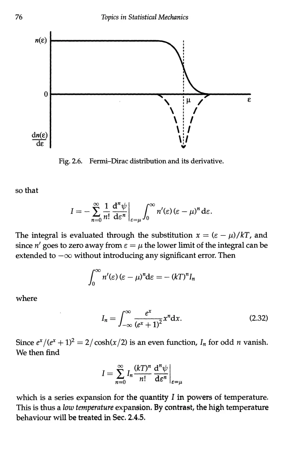
Chemical potential 78
Internal energy 80
Thermal capacity 81
2.4.4 More general treatment of low temperature
heat capacity 81
2.4.5 High temperature behaviour — the classical limit . . 84
2.5 Ideal Bose Gas 87
2.5.1 General procedure for treating the Bose gas 87
2.5.2 Number of particles — chemical potential 88
2.5.3 Low temperature behaviour of Bose gas 89
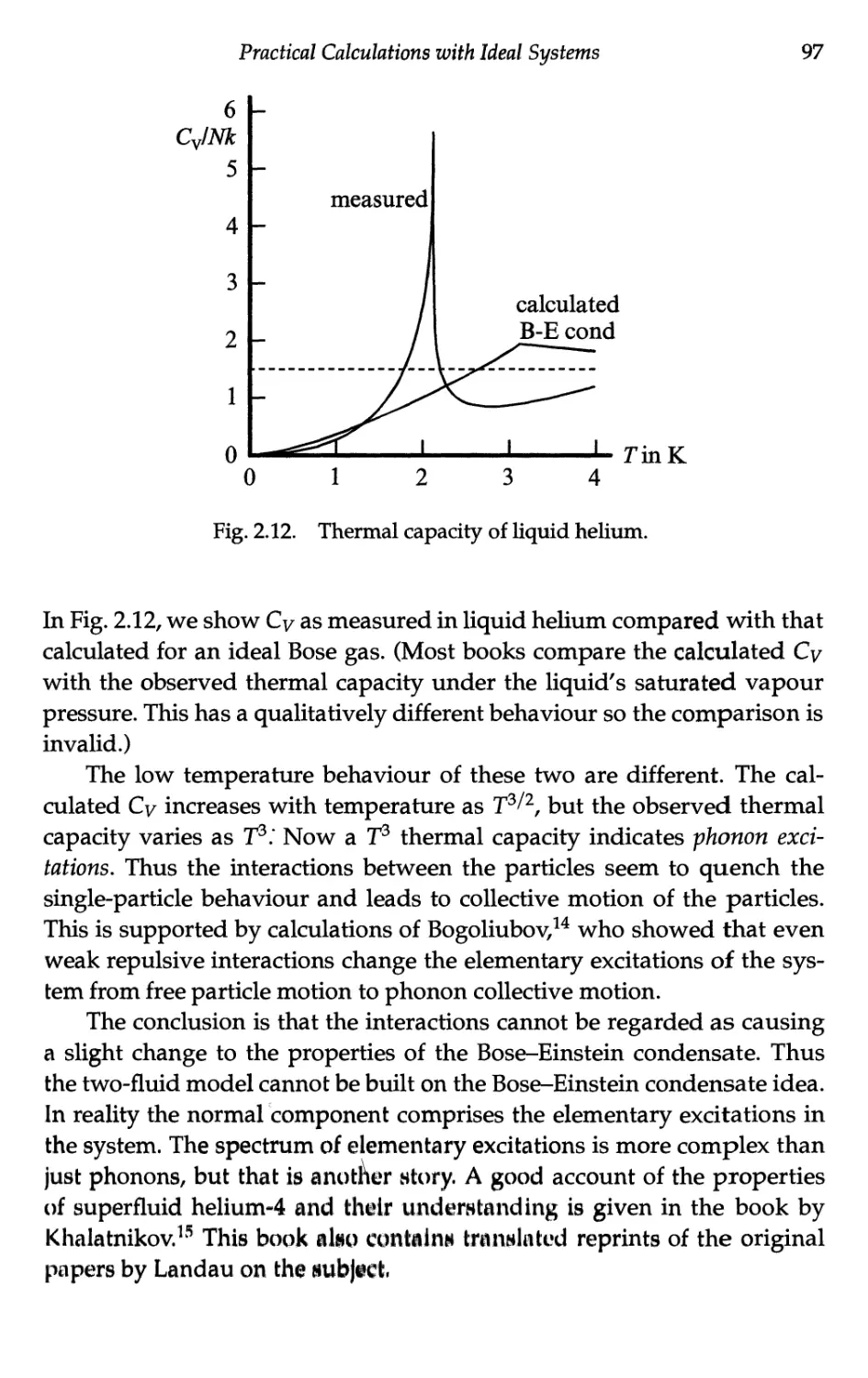
2.5.4 Thermal capacity of Bose gas — below Tc 91'
2.5.5 Comparison with superfluid 4He and
other systems 93
2.5.6 Two-fluid model of superfluid 4He 95
2.5.7 Elementary excitations 96
2.6 Black Body Radiation — The Photon Gas 98
2.6.1 Photons as quantised electromagnetic waves .... 98
2.6.2 Photons in thermal equilibrium — black
body radiation 99
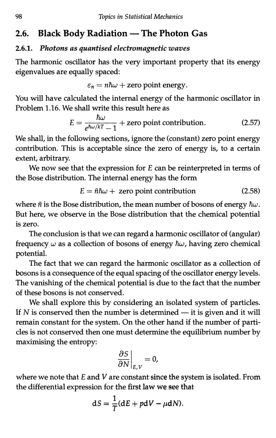
2.6.3 Planck's formula 100
2.6.4 Internal energy and heat capacity 102
2.6.5 Black body radiation in one dimension 103
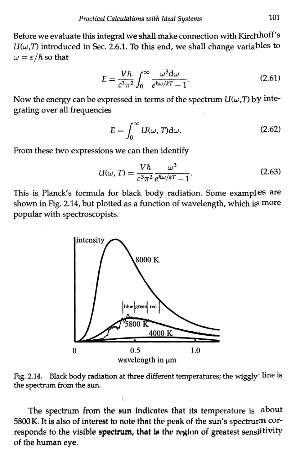
2.7 Ideal Paramagnet 105
2.7.1 Partition function and free energy 105
2.7.2 Thermodynamic properties 106
2.7.3 Negative tempera I tire* 110
27.4 Thermodynamic of ntfgallvi* temperatures 112

xii
Topics in Statistical Mechanics
3 Non-Ideal Gases 120
3.1 Statistical Mechanics 120
3.1.1 The partition function 120
3.1.2 Cluster expansion 121
3.1.3 Low density approximation 122
3.1.4 Equation of state 123
3.2 The Virial Expansion 124
3.2.1 Virial coefficients 124
3.2.2 Hard core potential 124
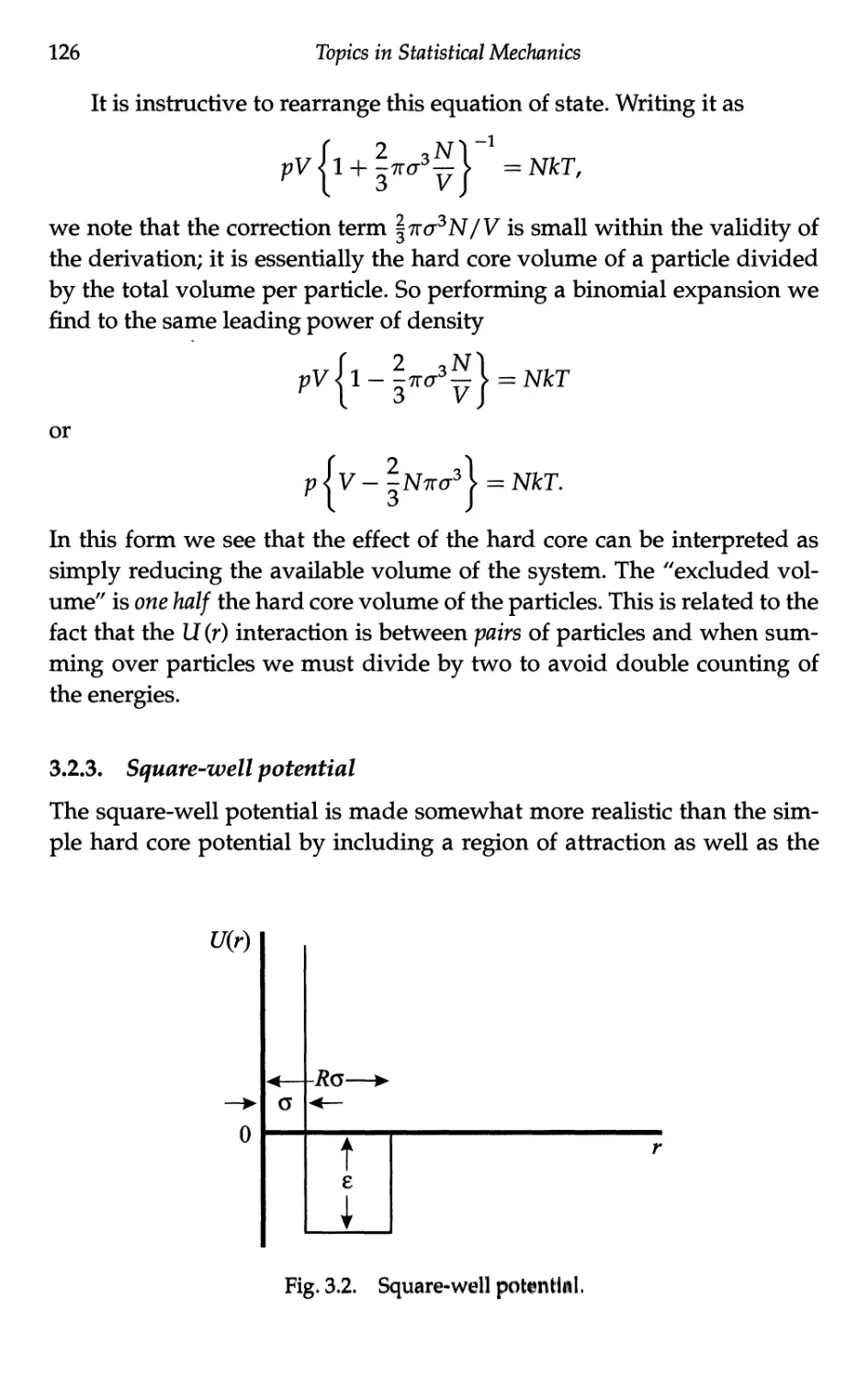
3.2.3 Square-well potential 126
3.2.4 Lennard-Jones potential 127
3.2.5 Second virial coefficient for Bose and Fermi gas . . . 130
3.3 Thermodynamics 130
3.3.1 Throttling 130
3.3.2 Joule-Thomson coefficient 131
3.3.3 Connection with the second virial coefficient 132
3.3.4 Inversion temperature 134
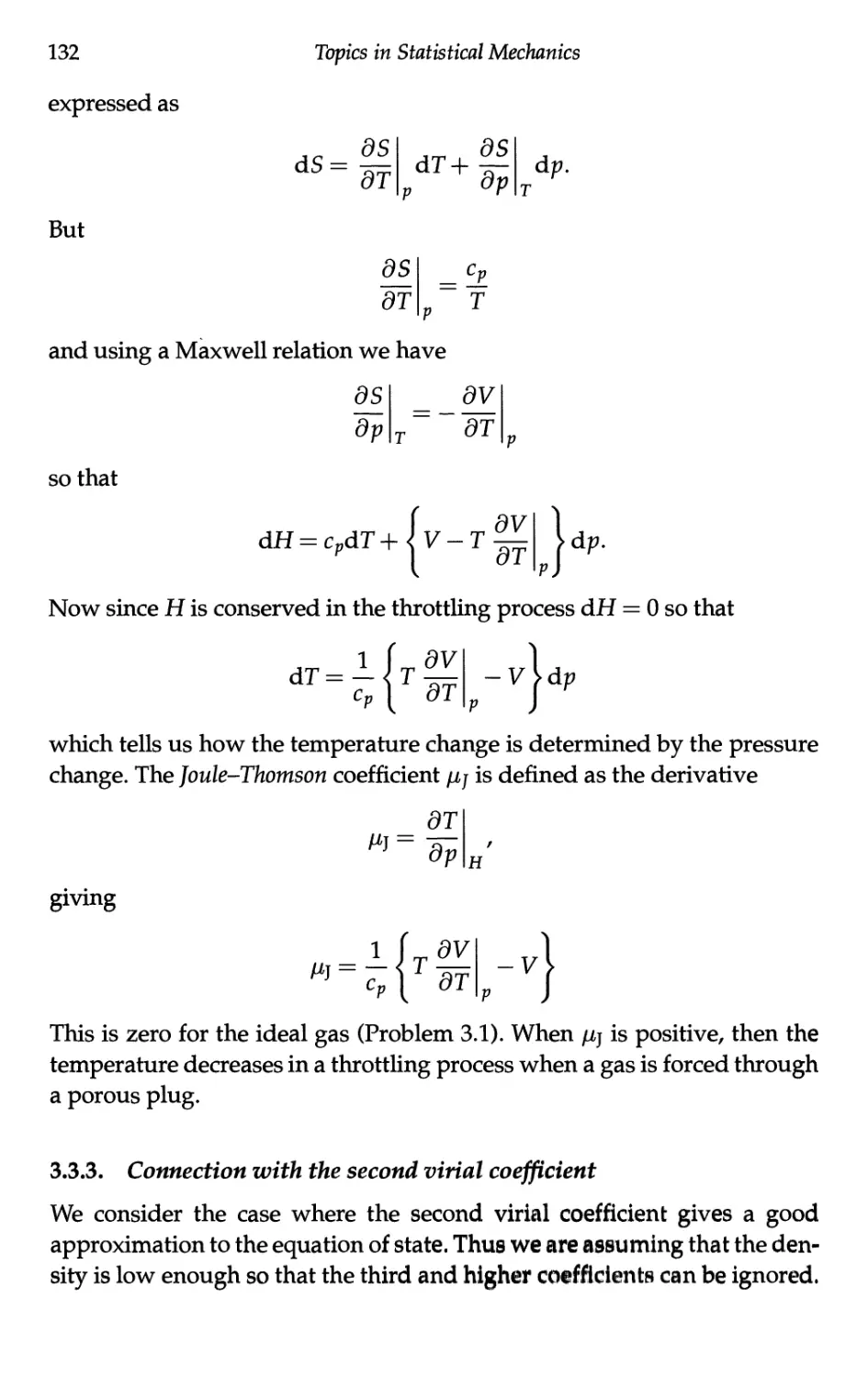
3.4 Van der Waals Equation of State 134
3.4.1 Approximating the partition function 134
3.4.2 Van der Waals equation 135
3.4.3 Microscopic "derivation" of parameters 137
3.4.4 Virial expansion 138
3.5 Other Phenomenological Equations of State 139
3.5.1 The Dieterici equation 139
3.5.2 Virial expansion 139
3.5.3 The Berthelot equation 140
4 Phase Transitions 143
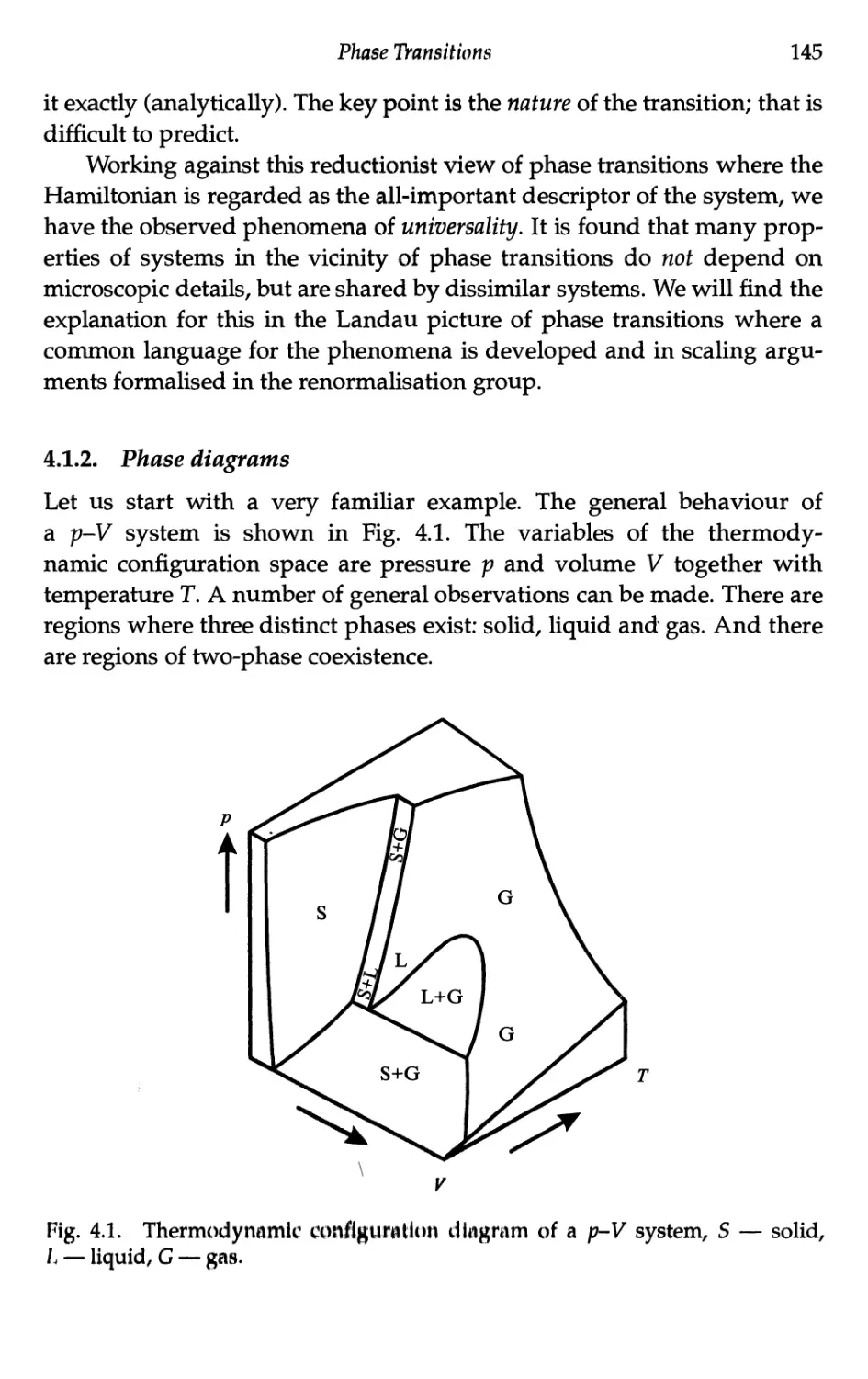
4.1 Phenomenology 143
4.1.1 Basic ideas 143
4.1.2 Phase diagrams 145
4.1.3 Symmetry 147
4.1.4 Order of phase transitions 148
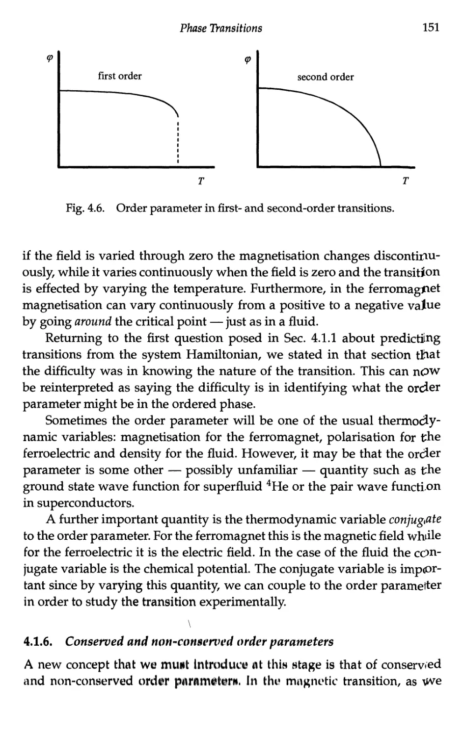
4.1.5 The order parameter 149
4.1.6 Conserved and non-conserved order parameters . . 151
4.1.7 Critical exponents 152
4.1.8 Scaling theory 154
4.1.9 Scaling of the free energy 158

Contents xiii
4.2 First-Order Transition — An Example 159
4.2.1 Coexistence 159
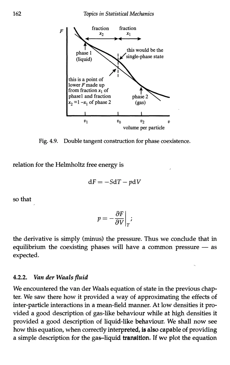
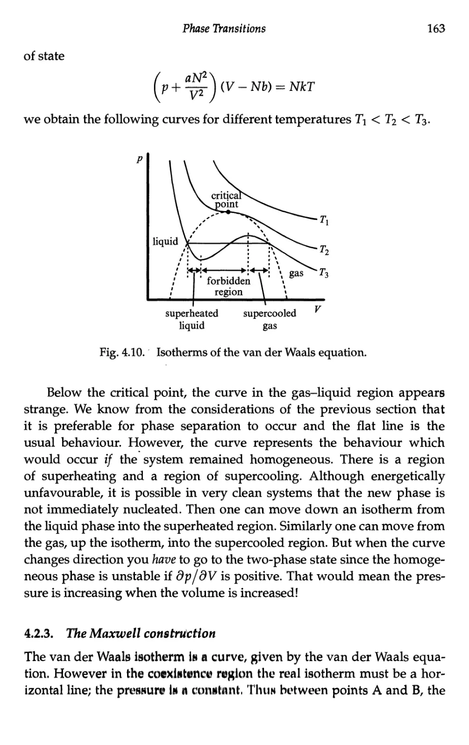
4.2.2 Van derWaals fluid 162
4.2.3 The Maxwell construction 163
4.2.4 The critical point 165
4.2.5 Corresponding states 166
4.2.6 Dieterici's equation 168
4.2.7 Quantum mechanical effects 169
4.3 Second-Order Transition — An Example 170
4.3.1 The ferromagnet 170
4.3.2 The Weiss model 172
4.3.3 Spontaneous magnetisation 173
4.3.4 Critical behaviour 176
4.3.5 Magnetic susceptibility 177
4.3.6 Goldstone modes 178
4.4 The Ising and Other Models 180
4.4.1 Ubiquity of the Ising model 180
4.4.2 Magnetic case of the Ising model 182
4.4.3 Ising model in one dimension 184
4.4.4 Ising model in two dimensions 185
4.4.5 Mean field critical exponents 188
4.4.6 The XY model 190
4.4.7 The spherical model 191
4.5 Landau Treatment of Phase Transitions 191
4.5.1 Landau free energy 191
4.5.2 Landau free energy for the ferromagnet 193
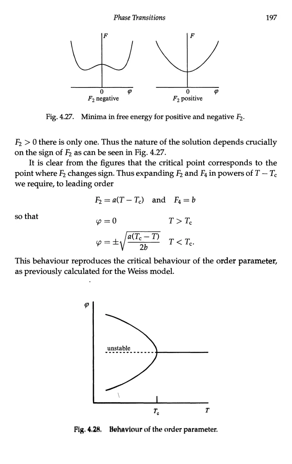
4.5.3 Landau theory — second-order transitions 196
4.5.4 Thermal capacity in the Landau model 198
4.5.5 Ferromagnet in a magnetic field 199
4.6 Ferroelectricity 201
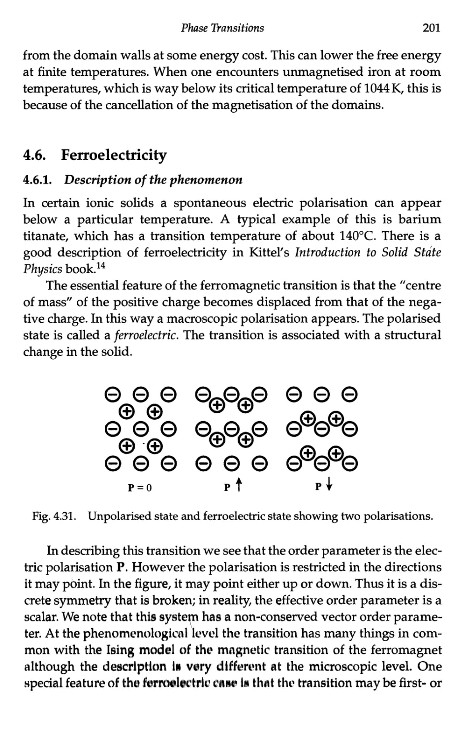
4.6.1 Description of the phenomenon 201
4.6.2 Landau free energy 202
4.6.3 Second-order case 203
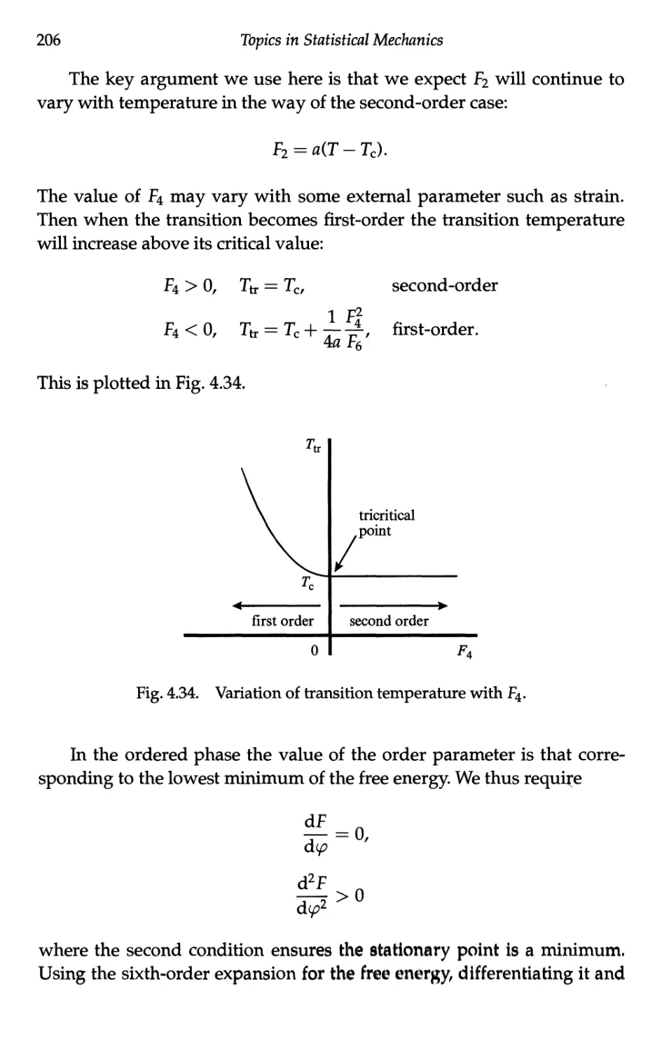
4.6.4 First-order case 204
4.6.5 Entropy and latent heat at the transition 208
4.6.6 Softmoden 209
4.7 Binary Mixtures 210
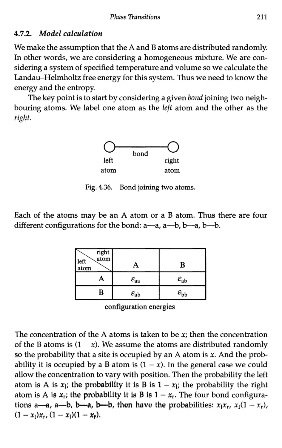
4.7.1 Banicidefti 210
4.7.2 Modd calculation ,,,,,, 211

xiv Topics in Statistical Mechanics
4.7.3 System energy 212
4.7.4 Entropy 213
4.7.5 Free energy 214
4.7.6 Phase separation — the lever rule 215
4.7.7 Phase separation curve — thebinodal 217
4.7.8 The spinodal curve 219
4.7.9 Entropy in the ordered phase 220
4.7.10 Thermal capacity in the ordered phase 222
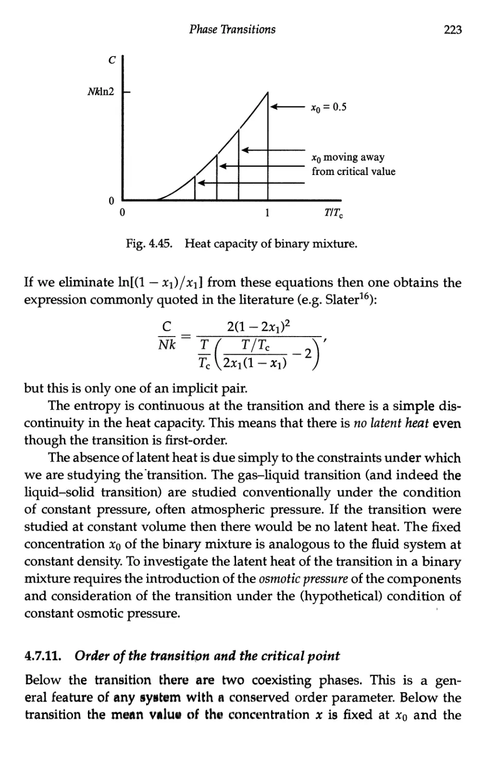
4.7.11 Order of the transition and the critical point 223
4.7.12 The critical exponent /3 225
4.8 Quantum Phase Transitions 226
4.8.1 Introduction 226
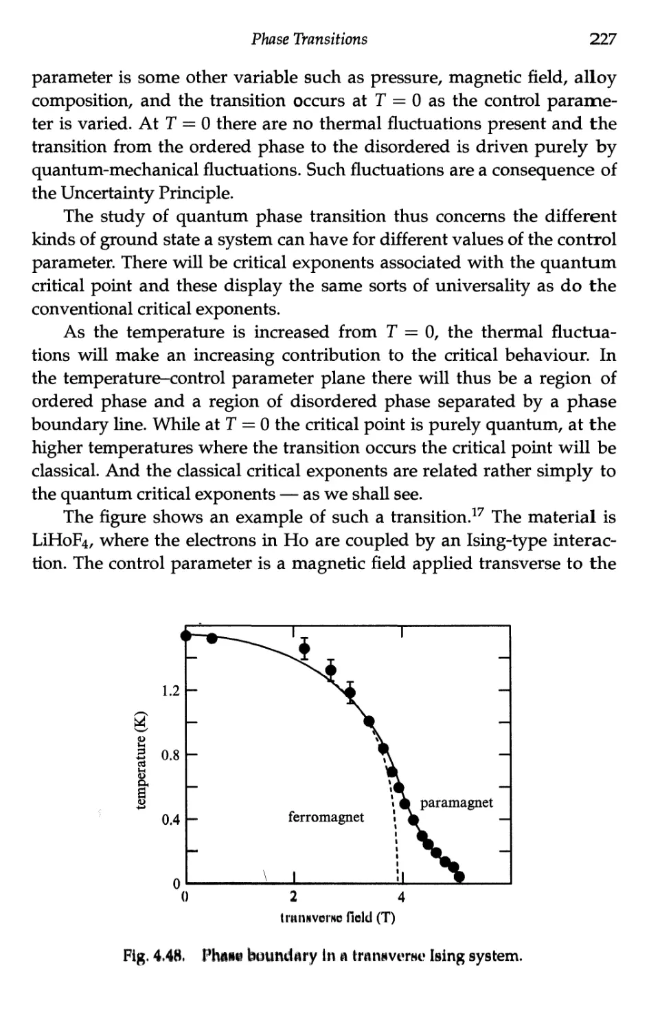
4.8.2 The transverse Ising model 228
4.8.3 Revision of mean field Ising model 228
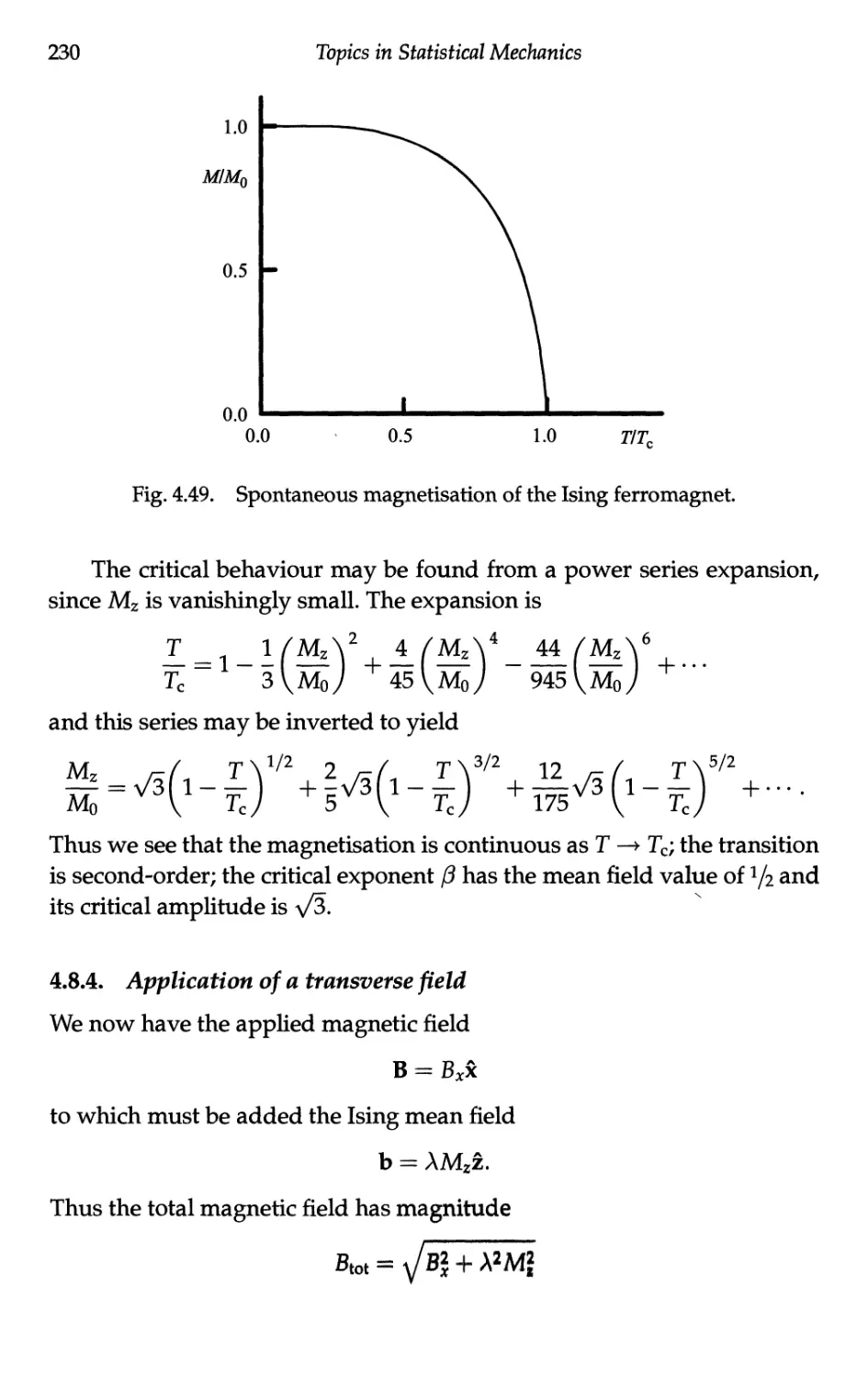
4.8.4 Application of a transverse field 230
4.8.5 Transition temperature 232
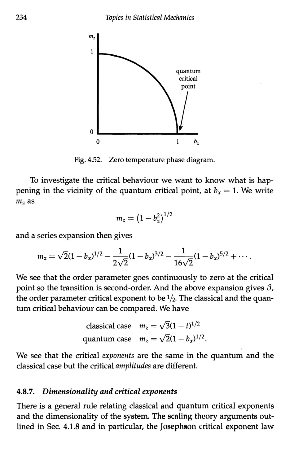
4.8.6 Quantum critical behaviour 233
4.8.7 Dimensionality and critical exponents 234
4.9 Retrospective 236
4.9.1 The existence of order 236
4.9.2 Validity of mean field theory 237
4.9.3 Features of different phase transition models .... 238
5 Fluctuations and Dynamics 243
5.1 Fluctuations 244
5.1.1 Probability distribution functions 244
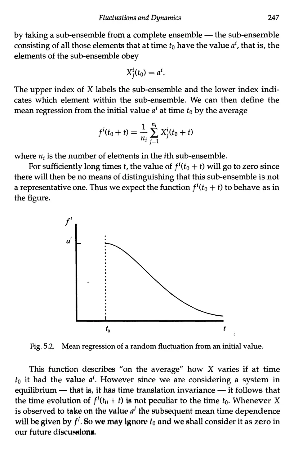
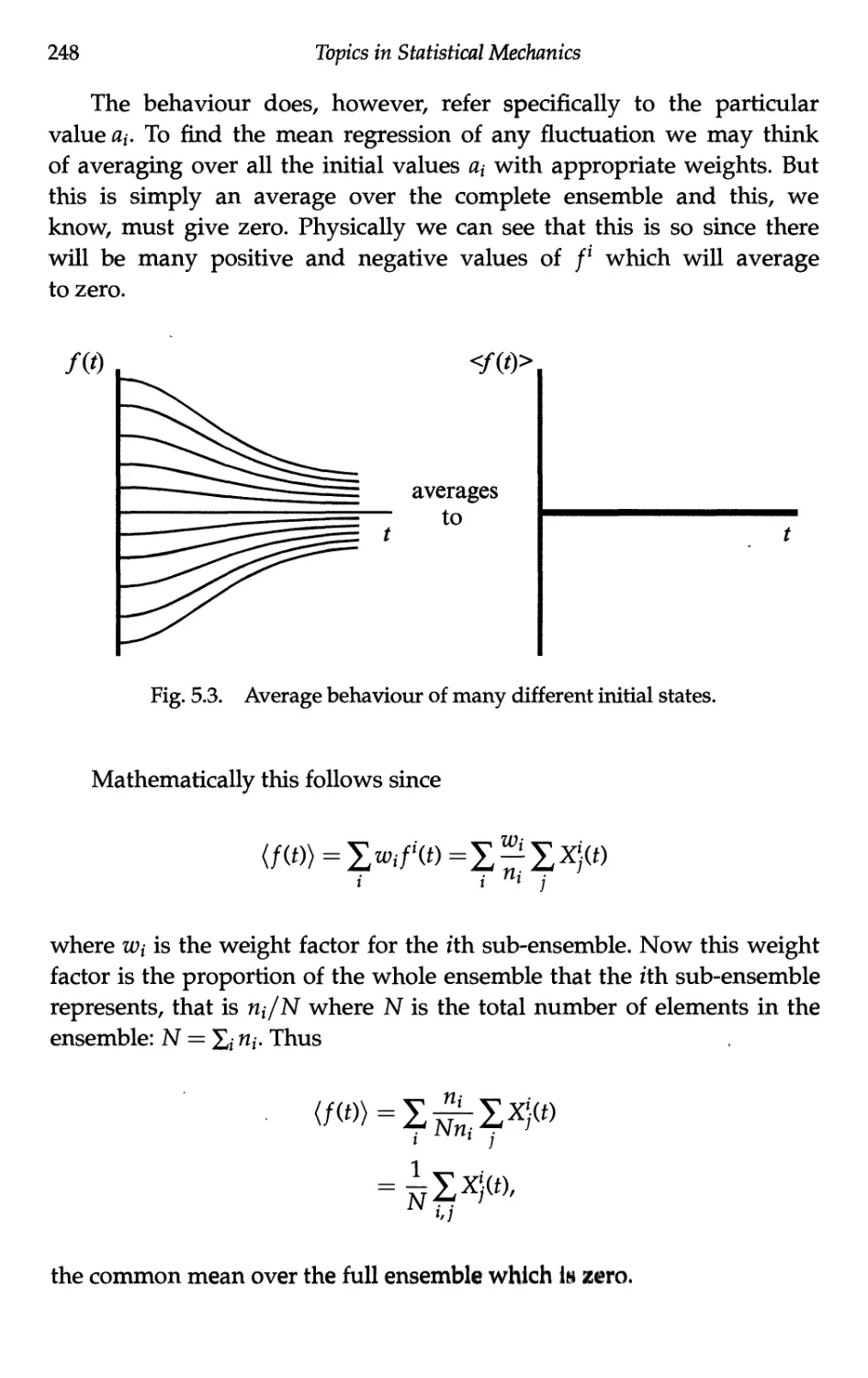
5.1.2 Mean behaviour of fluctuations 246
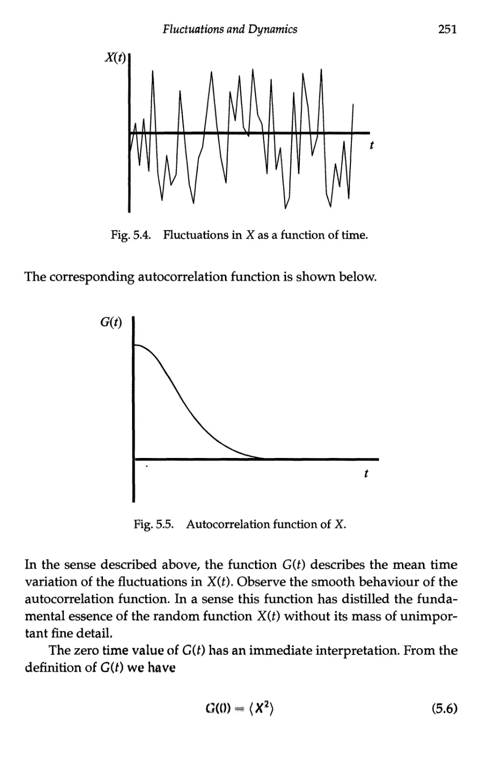
5.1.3 The autocorrelation function 250
5.1.4 The correlation time 253
5.2 Brownian Motion 254
5.2.1 Kinematics of a Brownian particle 255
5.2.2 Short time limit 257
5.2.3 Long time limit 258
5.3 Langevin's Equation 260
5.3.1 Introduction 260
5.3.2 Separation of forces 261
5.3.3 The Langevin equation 263
5.3.4 Mean iquare velocity and equipartition 264

Contents xv
5.3.5 Velocity autocorrelation function 265
5.3.6 Electrical analogue of the Langevin equation 267
5.4 Linear Response — Phenomenology 268
5.4.1 Definitions 268
5.4.2 Response to a sinusoidal excitation 270
5.4.3 Fourier representation 271
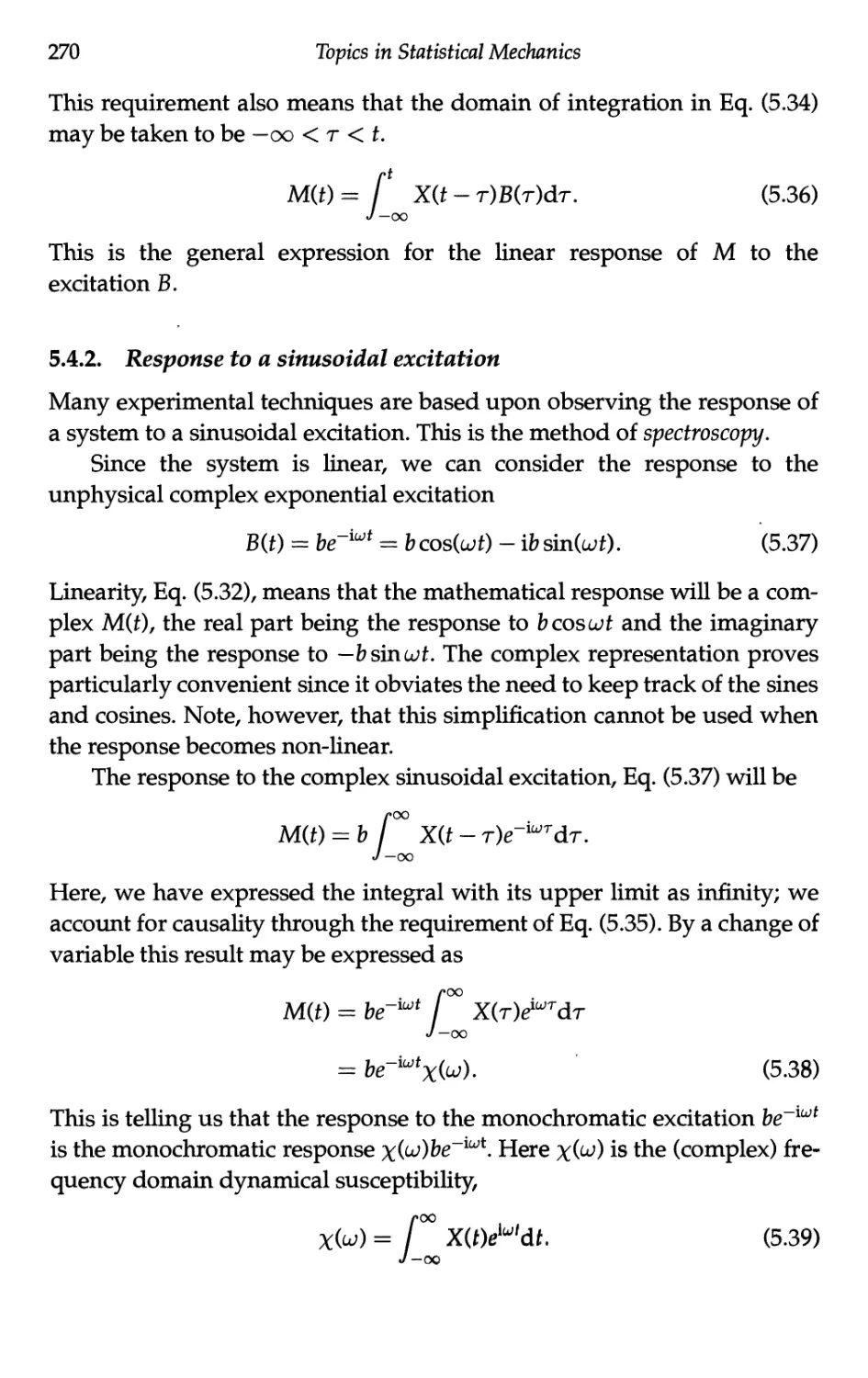
5.4.4 Response to a step excitation 272
5.4.5 Response to a delta function excitation 273
5.4.6 Consequence of the reality of X(0 274
5.4.7 Consequence of causality 275
5.4.8 Energy considerations 277
5.4.9 Static susceptibility 278
5.4.10 Relaxation time approximation 280
5.5 Linear Response — Microscopies 281
5.5.1 Onsager's hypothesis 281
5.5.2 Nyquist's theorem 283
5.5.3 Calculation of the step response function 285
5.5.4 Calculation of the autocorrelation function 286
Appendixes 291
Appendix 1 The Gibbs-Duhem Relation 291
A.l.l Homogeneity of the fundamental relation 291
A.1.2 The Euler relation 291
A.1.3 A caveat 292
A.1.4 The Gibbs-Duhem relation 292
Appendix 2 Thermodynamic Potentials 293
A.2.1 Equilibrium states 293
A.2.2 Constant temperature (and volume): the
Helmholtz potential 295
A.2.3 Constant pressure and energy: the
Enthalpy function 296
A.2.4 Constant pressure and temperature: the Gibbs
free energy 296
A.2.5 Differential exproHHionw for the potentials 297
A.2.6 Natural vaYiablwand the Maxwell relations 298
Appendix 3 Mathematical Notebooks 299
A.3.1 Chemical potential of I'Wml ^in at
low temperatureM ,,,., 299

xvi
Topics in Statistical Mechanics
A.3.2 Internal energy of the Fermi gas at
low temperatures 301
A.3.3 Fugacity of the ideal gas at high
temperatures — Fermi, Maxwell and Bose cases . . . 303
A.3.4 Internal energy of the ideal gas at high
temperatures — Fermi, Maxwell and Bose cases . . . 307
Appendix 4 Evaluation of the Correlation Function Integral 310
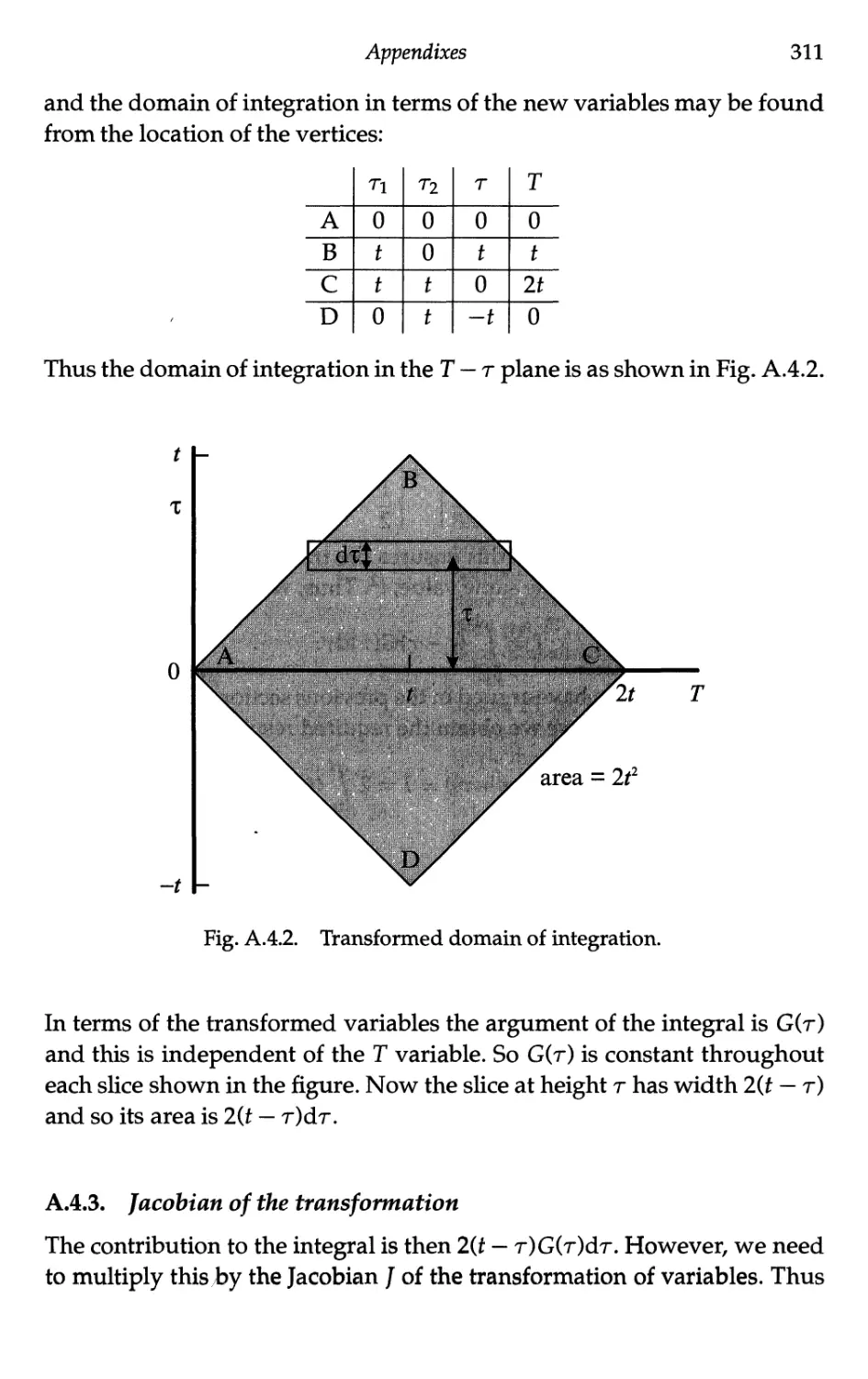
A.4.1 Initial domain of integration 310
A.4.2 Transformation of variables 310
A.4.3 Jacobian of the transformation 311
Index 313

CHAPTER ONE
THE METHODOLOGY OF STATISTICAL
MECHANICS
This chapter provides an overview of statistical mechanics and
thermodynamics. Although the discussion is reasonably self-contained, it is
assumed that this is not the reader's first exposure to these subjects. More
than many other branches of physics, these topics are treated in a variety
of different ways in the textbooks in common usage. The aim of the
chapter is thus to establish the perspective of the book, the standpoint from
which the topics in the following chapters will be viewed. The textbook
by Bowley1 is recommended to the novice as a clearly-argued
introduction to the subject; indeed all readers will find many of the examples of
this book treated by that book in a complementary fashion.
1.1. Terminology and Methodology
1.1.1. Approaches to the subject
Thermodynamics is the study of the relationship between macroscopic
properties of systems such as temperature, volume, pressure, magnetisation,
compressibility, etc. Statistical Mechanics is concerned with
understanding how the various macroscopic properties arise as a consequence of the
microscopic nature of the system. In essence it makes macroscopic
deductions from microscopic models,
The power of thermodynamics, m formulated in the traditional
manner (e.g. Zemansky2) is that I to cleductionH tire quite general; they do not
rely, for their validity, on the microscopic luitun1 of the system. Einstein
1

2
Topics in Statistical Mechanics
expressed this quite impressively when he wrote3
"A theory is the more impressive the greater the simplicity of its premises
is, the more different kinds of things it relates, and the more extended is
its area of applicability. Therefore the deep impression which classical
thermodynamics made upon me; it is the only physical theory of
universal content concerning which I am convinced that, within the framework
of the applicability of its basic concepts, will never be overthrown."
On the other hand statistical mechanics, as conventionally presented (e.g.
Hill4) is system-specific. One starts from particular microscopic
models, say the Debye model for a solid, and derives macroscopic
properties such as the thermal capacity. It is true that statistical mechanics will
give relationships between the various macroscopic properties of a
system, but they will only apply to the system/model under consideration.
Results obtained from thermodynamics, on the other hand, are model-
independent and general.
Traditionally thermodynamics and statistical mechanics were
developed as independent subjects, with "bridge equations" making the links
between the two. Alternatively the subjects can be developed together,
where the Laws of Thermodynamics are justified by microscopic
arguments. This reductionist view was adopted by Landau. In justification he
wrote5:
"Statistical physics and thermodynamics together form a unit. All the
concepts and quantities of thermodynamics follow most naturally,
simply and rigorously from the concepts of statistical physics. Although
the general statements of thermodynamics can be formulated non-
statistically, their application to specific cases always requires the use
of statistical physics."
The contrast between the views of Einstein and Landau is apparent. The
paradox, however, is that so much of Einstein's work was reductionist and
microscopic in nature whereas Landau was a master of the macroscopic
description of phenomena. This book considers thermodynamics and
statistical mechanics in a synthetic manner; in that respect it follows more
closely the Landau approach.

The Methodology of Statistical Mechanics
3
1.1.2. Description of states
The state of a system described at the macroscopic level is called a
macrostate. Macrostates are described by a relatively few variables such
as temperature, pressure and volume.
The state of a system described at the microscopic level is called a
microstate. Microstates are described by a very large number of variables.
Classically you would need to specify the position and momentum of
each particle in the system. Using a quantum-mechanical description you
would have to specify all the quantum numbers of the entire system.
So whereas a macrostate might be described by under ten variables, a
microstate will be described by over 1023 variables.
The fundamental methodology of statistical mechanics involves
applying probabilistic arguments about microstates, regarding macro-
states as statistical averages. It is because of the very large number of
particles involved that the mean behaviour corresponds so well to the observed
behaviour — that fluctuations are negligible. Recall that for N particles the
likely fractional deviation from the mean will be 1/y/N. So if you calculate
a mean pressure of mole of air at one atmosphere, it is likely to be correct
to within ~10~~12 of an atmosphere. It is also because of the large number
of particles involved that the mean, observed behaviour corresponds to
the most probable behaviour — the mean and the mode of the distribution
differ negligibly.
Statistical Mechanics is slightly unusual in that its formalism is
easier to understand using quantum mechanics for descriptions at the
microscopic level rather than classical mechanics. This is because the idea of a
quantum state is familiar, and often the quantum states are discrete. It is
more difficult to enumerate the states of a classical system; it is best done
by analogy with the quantum case. The classical case will be taken up in
Sec. 1.6.
1.1.3. Extensivity and the thermodynamic limit
The thermodynamic variables describing macrostates fall into two classes.
Quantities such as energy E, number of particles N and volume V, which
add when two similar systems are combined, are known as extensive
variables. And quantities such as pressure p and temperature T, which remain
independent when similar systems an* combined, are known as intensive
variables.

4
Topics in Statistical Mechanics
As we have argued, thermodynamics concerns itself with the
behaviour of "large" systems and usually, for these, finite-size effects are
not of interest. Thus, for example, unless one is concerned specifically with
surface phenomena, it will be sensible to focus on systems that are
sufficiently large that the surface contribution to the energy will be negligible
when compared to the volume contribution. This is possible because the
energy of interaction between atoms is usually sufficiently short-ranged.
In general one will consider properties in the limit N —> oo, V —> oo while
N/V remains constant. This is called the thermodynamic limit.
It should be apparent that true extensivity of a quantity such as energy
arises only in the thermodynamic limit.
[Gravitation is a long-range force. It is apparent that gravitational energy
is not truly extensive; this is examined in Problem 1.2. This non-extensivity
makes for serious difficulties when trying to treat the statistical
thermodynamics of gravitating systems. A generalisation of the definition of entropy
to accommodate non-extensive systems was proposed by Tsallis in 1989.
An account this is contained in the review article by Tsallis6 and
subsequent articles in the same journal.]
1.2. The Fundamental Principles
1.2.1. The laws of thermodynamics
Thermodynamics, as a logical structure, is built on its four assumptions or
laws (including the zeroth).
Zeroth Law: If system A is in equilibrium with system B and with system
C then system B is in equilibrium with system C. Equilibrium here is
understood in the sense that when two systems are brought into contact
then there is no change. This law was formalised after the first three laws,
but because it was believed to be more fundamental it was called the Zeroth
Law. The Zeroth Law recognises the existence of states of equilibrium and
it points us to the concept of temperature, a non-mechanical quantity that
can label (and order) equilibrium states.
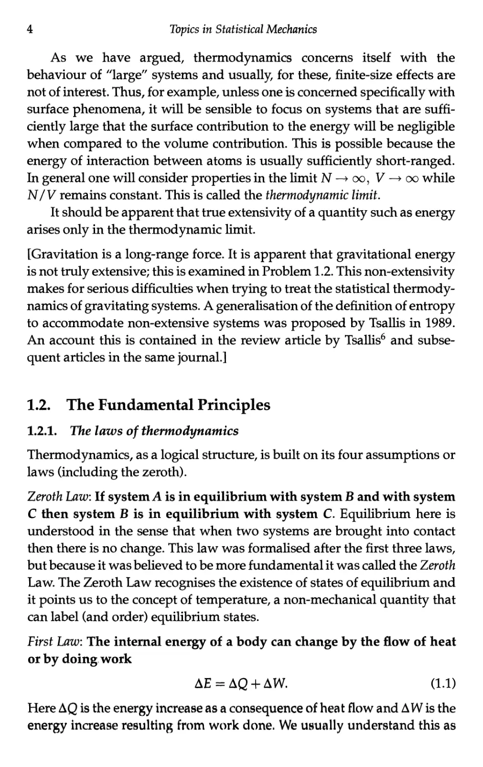
First Law: The internal energy of a body can change by the flow of heat
or by doing work
AE = AQ + AW. (1.1)
Here AQ is the energy increase as a consequence of heat flow and AW is the
energy increase resulting from work done. We usually understand this as

The Methodology of Statistical Mechanics
5
a statement about the conservation of energy. But in its historical context
the law asserted that as well as the familiar mechanical form of energy,
heat also was a form of energy. Today we understand this as the kinetic
energy of the constituent particles of a system; in earlier times the nature
of heat was unclear.
Note that some older books adopt the opposite sign for AW; they consider
AW to be the work done by the system rather than the work done on the
system.
Second Law (this law has many formulations): Heat flows from hot to cold,
or It is not possible to convert all heat energy to work. These statements
have the great merit of being reflections of common experience. There are
other formulations such $s the Caratheodory statement (see the books by
Adkins7 or Pippard8): In the neighbourhood of any equilibrium state of
a thermally isolated system there are states which are inaccessible, and
the entropy statement (see Callen's book9): There is an extensive quantity,
which we call entropy, which never decreases in a physical process. The
claimed virtue of the Caratheodory statement is that it leads more rapidly
to the important thermodynamic concepts of temperature and entropy:
this at the expense of common experience. But if this is believed to be a
virtue then one may as well go the "whole hog" and adopt the Callen
statement. A major exercise in classical thermodynamics is proving the
equivalence of the various statements of the Second Law. In whatever form, the
Second Law leads to the concept of entropy and the quantification of
temperature (the ZerothLaw just gives an ordering: A is hotter than B). And it
tells us there is an absolute zero of temperature.
Third Law: The entropy of a body tends to zero as the temperature tends
to absolute zero. The Third Law will be discussed in Sec. 1.7. We shall
see that it arises as a consequence of the quantum behaviour of matter at
the microscopic level. However we see immediately that the Third Law is
telling us there is an absolute zero of entropy.
An even more fundamental aspect of the Zeroth Law is the fact of the
existence of equilibrium states. If systems did not exist in states of
equilibrium then there would be no maerostates and no hope of description in
terms of small numbers of variables. Then there would be no discipline
of thermodynamics and phenomena would have to be discussed solely in
terms of their intractable microscopic descriptions. Fortunately this is not
the case; the existence of htalon of equilibrium aIIown our simple minds to
make some sense of a complex world.

6
Topics in Statistical Mechanics
1.2.2. Probabilistic interpretation of the First Law
The First Law discusses the way the energy of a system can change. From
the statistical standpoint we understand the energy of a macroscopic
system as the mean value since the system can exist in a large number of
different microstates. If the energy of the /th microstate is E; and the probability
of occurrence of this microstate is Pj then the (mean) energy of the system
is given by
E = Xp;Er (L2>
The differential of this expression is
dE = Xp;dE; + XE;dp;' ^-¾
;' /
this indicates the energy of the system can change if the energy levels
Exchange or if the probabilities Pj change.
The first term X/P/dE;- relates to the change in the energy levels dE;.
This term is the mean energy change of the microstates and we shall show
below that this corresponds to the familiar "mechanicar energy, the work
done on the system. The second term X/E;dP; is a consequence of the
change in probabilities or occupation of the energy states. This is
fundamentally probabilistic and we shall see that it corresponds to the heat flow
into the system.
In order to understand that the first term corresponds to the work
done, let us consider a pV system. We shall see (Sec. 2.1.3) that the energy
levels depend on the size (volume) of the system:
Ej = Ej(V)
so that the change in the energy levels when the volume changes is
<9E7
Then
V pa p. ■= V p
dv
We are assuming that the change in volume occurs at constant Pj, then
'dV
I i

The Methodology of Statistical Mechanics
7
But we identify dE/dV = —p, so that
£PydEy = -pdV. (1.4)
/
And thus we see that the term XyPydEy corresponds to the work done on
the system. Then the term XyEydPy corresponds to the energy increase of
the system that occurs when no work is done; this is what we understand
as heat flow.
We have seen, in this section, that the idea of heat arises quite logically
from the probabilistic point of view.
1.2.3. Microscopic basis for entropy
By contrast to macroscopic thermodynamics, statistical mechanics is built
on a single assumption, which we will call the Fundamental Postulate of
statistical mechanics. We shall see how the Laws of thermodynamics may
be understood in terms of this Fundamental Postulate, which dates back
to Boltzmann. The Fundamental Postulate states: All microstates of an
isolated system are equally likely. Note, in particular, that an isolated
system will have fixed energy E, volume V and number of particles N
(extensive quantities). We conventionally denote by Q(E, V, N) the
number of microstates in a given macrostate (E, V, N). Then from the
Fundamental Postulate it follows that the probability of a given macrostate is
proportional to the number of microstates corresponding to it Q, (E, V, N):
PocQ(E,V,N). (1.5)
If we understand the observed equilibrium state of a system as the most
probable macrostate, then it follows from the Fundamental Postulate that
the equilibrium state corresponds to the macrostate with the largest
number of microstates. We are saying that Q is maximum for an equilibrium
state.
Since Q, for two isolated systems is multiplicative, it follows that the
logarithm of Q is additive. In other words InQ is an extensive quantity.
We define entropy S as
S-fclnQ. (1.6)
At this stage k is simply a constant; later we will identify it as Boltzmann's
constant.
Since the logarithm is a monolonk1 function it follows that the
equilibrium state will have maximal tmtropy So we Immediately obtain the

8 Topics in Statistical Mechanics
Second Law. And now we understand the Second Law from the
microscopic point of view; it is hardly more than the tautology "we are most
likely to observe the most probable state"!
1.3. Interactions — The Conditions for Equilibrium
When systems interact their states will often change, the composite system
evolving to a state of equilibrium. We shall investigate what determines
the final state. We will see that quantities such as temperature emerge in
the description of these equilibrium states.
1.3.1. Thermal interaction — Temperature
Let us allow two systems to exchange energy without changing volume
or numbers of particles. In other words we allow thermal interaction only;
the systems are separated by a diathermal wall.
E'r' N'\\
E2V2N2\\
Ex Vx Nx
E2 V2 N2
fixed diathermal wall
Fig. 1.1. Thermal interaction.
Now
Qi=Qi(Ei,Vi,Ni)
Q2 = Q2(E2,V2,N2)
and Vi, Ni, V*2 > N2 are all fixed.
The energies Ei and E2 can vary subject to the restriction Ei + E2 = Eo,
a constant.
Our problem is this: after the two systems are brought together what
will be the equilibrium state? We know that the systems will exchange
energy, and they will do this so as to maximise the total number of
microstates for the composite system.
For different systems the £is multiply so that we have
n = Qt(E,)f22(E2) (1.7)
— we can ignore V\, N\, Va, Ni as they do not change,

The Methodology of Statistical Mechanics
9
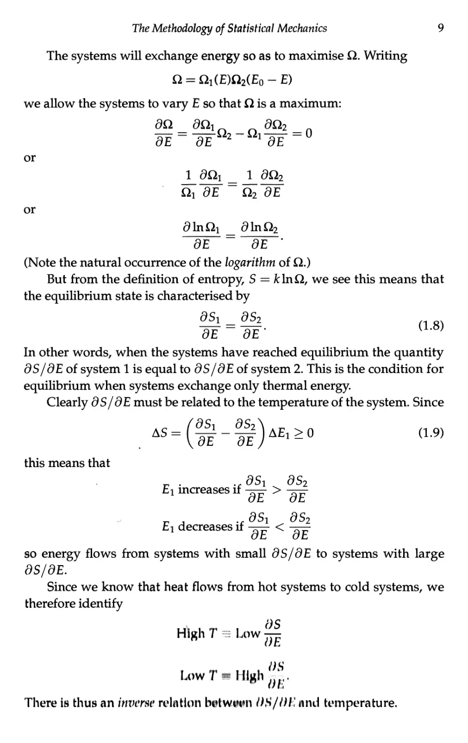
The systems will exchange energy so as to maximise Q. Writing
Q = Qi(E)Q2(Eo-E)
we allow the systems to vary E so that Q is a maximum:
da dQln da2 n
or
1 flQi _ 1 <9fl2
Qi <9E Q2 #E
or
<91nQi _ <91nQ2
<9E ~ <9E '
(Note the natural occurrence of the logarithm of Q.)
But from the definition of entropy, S = A:lnQ, we see this means that
the equilibrium state is characterised by
WW (L8)
In other words, when the systems have reached equilibrium the quantity
dS/dEoi system 1 is equal to d S /d E of system 2. This is the condition for
equilibrium when systems exchange only thermal energy.
Clearly dS/dE must be related to the temperature of the system. Since
this means that
.r0Si dS2
El increases if w>w
Ei decreases if -^=- < -^-
oE <9E
so energy flows from systems with small dS/dE to systems with large
dS/dE.
Since we know that heat flows from hot systems to cold systems, we
therefore identify
High T == Low ^|
LowT= High '
There is thus an invcrsv relation betwwn OS/01-', niul temperature.

10
Topics in Statistical Mechanics
We define statistical temperature by
1
T
ds
OE'
When applied to the ideal gas this will give us the result
pV = NkT.
(1.10)
(1.11)
And it is from this we conclude that the statistical temperature
corresponds to the intuitive concept of temperature as measured by an ideal
gas thermometer. Furthermore the scale of temperatures will agree with
the Kelvin scale (ice point at 273.18 K) when the constant k in the
definition of S is identified with Boltzmann's constant.
When the partial derivative OS/dE is evaluated, N and V are constant.
So the only energy flow is heat flow. Thus the equation defining statistical
temperature can also be written as
AQ = TAS.
(1.12)
We can now write the energy conservation expression for the First Law:
AE = AQ + AW (1.13)
as
AE = TAS - pAV (for pV systems).
(1.14)
1.3.2. Volume change — Pressure
We now allow the volumes of the interacting systems to vary as well,
subject to the total volume being fixed. Thus we consider two systems
separated by a movable diathermal wall.
E2 V2 N2\\
ExVl Nx
1 " J
E2 V2N2\\
V 1
movable diathermal wall
Fig. 1.2. Mechanical and thermal interaction.

The Methodology of Statistical Mechanics
11
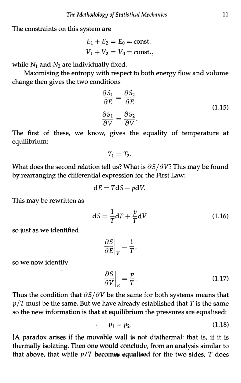
The constraints on this system are
Ei + E2 = Eq = const.
Vi + V2 = Vo = const.,
while Ni and N2 are individually fixed.
Maximising the entropy with respect to both energy flow and volume
change then gives the two conditions
dS1 _ 8S2
dE ~ dE
(1.15)
dS1 _ 0S2
dV ~ dV
The first of these, we know, gives the equality of temperature at
equilibrium:
Ti = T2.
Whcft does the second relation tell us? What is dS/dV? This may be found
by rearranging the differential expression for the First Law:
This may be rewritten as
so just as we identified
so we now identify
dE = TdS - pdV.
dS=idE+|dV
(1.16)
ds
dE
ds_
ov
1_
I
T
(1.17)
Thus the condition that dS/dV be the same for both systems means that
p/T must be the same. But we have already established that T is the same
so the new information is that at equilibrium the pressures are equalised:
P\ - p2.
(1.18)
[A paradox arises if the movable wall in not diathermal: that is, if it is
thermally isolating. Then one would conclude, from an analysis similar to
that above, that while ///T became eqviflll^ed for the two sides, T does

12
Topics in Statistical Mechanics
not. On the other hand, a purely mechanical argument would say that
the pressures p should become equal. The paradox is resolved when one
appreciates that without a flow of heat, thermodynamic equilibrium is not
possible and so the entropy maximum principle is not applicable. Thus
p/T will not be equalised. This issue is discussed in greater detail by
Callen.9]
1.3.3. Particle interchange — Chemical potential
Let us keep the volumes of the two systems fixed, but allow particles to
traverse the immobile diathermal wall.
E, V, N,\\
E2V2N2\
]-[
tf.FIJV, j E2V2N2
A 1
T
fixed permeable diathermal wall
Fig. 1.3. Heat and particle exchange.
The constraints on this system are
Ei + E2 = Eo = const.
Ni + N2 = No = const.,
while V\ and V2 are individually fixed.
Maximising the entropy with respect to both energy flow and particle
flow then gives the two conditions
dS1 _ dS2
dE ~ dE
dS1 _ dS2
ON ~ dN'
The first of these, we know, gives the equality of temperature at
equilibrium:
Ti = T2.
What does the second relation tell us? What is dS/dN? This may be found
from the First Law in its extended form:
dE = TdS - pdV + /xdN (1.19)

The Methodology of Statistical Mechanics
13
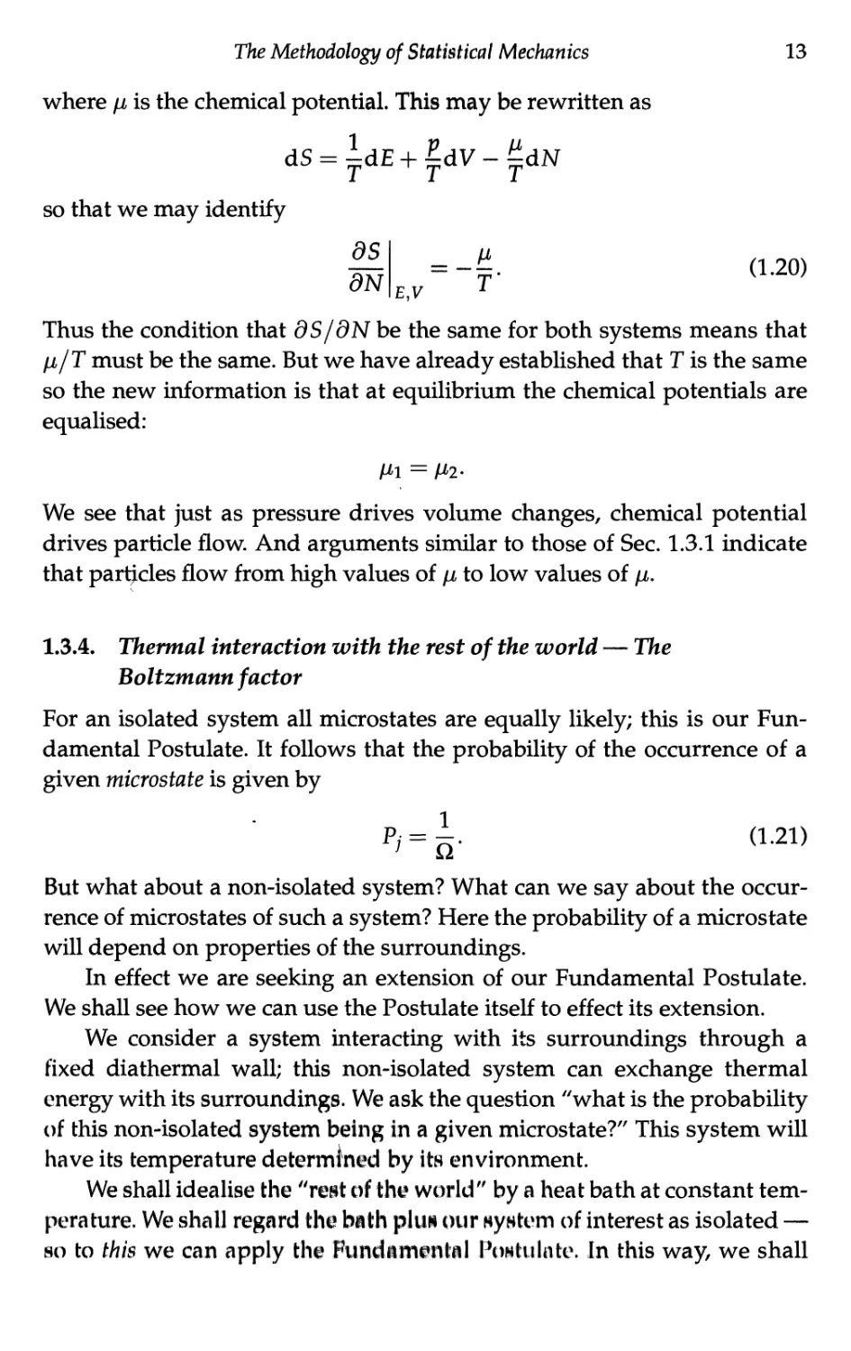
where fi is the chemical potential. This may be rewritten as
d
so that we may identify
dS = idE + |dV-^dN
as
dN
= -£• (1.20)
E,V 1
Thus the condition that dS/dN be the same for both systems means that
fi/T must be the same. But we have already established that T is the same
so the new information is that at equilibrium the chemical potentials are
equalised:
Mi = M2-
We see that just as pressure drives volume changes, chemical potential
drives particle flow And arguments similar to those of Sec. 1.3.1 indicate
that particles flow from high values of /i to low values of /i.
1.3.4. Thermal interaction with the rest of the world — The
Boltzmann factor
For an isolated system all microstates are equally likely; this is our
Fundamental Postulate. It follows that the probability of the occurrence of a
given microstate is given by
Py = i. (1.21)
But what about a non-isolated system? What can we say about the
occurrence of microstates of such a system? Here the probability of a microstate
will depend on properties of the surroundings.
In effect we are seeking an extension of our Fundamental Postulate.
We shall see how we can use the Postulate itself to effect its extension.
We consider a system interacting with its surroundings through a
fixed diathermal wall; this non-isolated system can exchange thermal
energy with its surroundings. We ask the question "what is the probability
of this non-isolated system being in a given microstate?" This system will
have its temperature determined by its environment.
We shall idealise the "rent of the world" by a heat bath at constant
temperature. We shall regard the bath plua our nyntem of interest as isolated —
so to this we can apply the Fundamental ftiNtulntc. In this way, we shall

14
Topics in Statistical Mechanics
be able to find the probability that the system of interest is in a particular
microstate. This is the "wine bottle in the swimming poor' model of Reif .10
fixed diathermal wall
heat bath
1
system of interest
"energy E
total energy ET
Fig. 1.4. Thermal interaction with the rest of the world.
The £2s multiply, thus
or
T T T
Total Bath System of interest
QtT = Qt3(ET-E)Qt(E).
Now the Fundamental Postulate tells us that the probability the system of
interest has energy E is proportional to the number of microstates of the
composite system that correspond to that energy partition
P(E)ocftB(ET-E)ft(E).
But here £l(E) = l since we are looking at a given microstate of energy E —
there is one microstate. So
P(E)ocftB(ET-E).
It depends solely on the bath. In terms of entropy, since S = fclnQ,
P(E) oc es<ET-E>/* (1.22)
where S is the entropy of the bath. This type of expression, where
probability is expressed in terms of entropy is an inversion of the usual usage
where entropy and other thermodynamic properties are found in terms
of probabilities. This form was much used by Einstein in his treatment of
fluctuations.

The Methodology of Statistical Mechanics
15
Now the subsystem is very small compared with the bath; E <C Ej. So
we can perform a Taylor expansion of S:
S(Et-E) = S(Et)-E^ + ---
oE
but
dS_}_
OE ~ 7°
the temperature of the bath, so that
S(ET - E) = S(ET) - |
assuming we can ignore the higher terms. Then
P(E) oc es<Ex>/*e-E/*T
But the first term es("Ej^k is simply a constant, so we finally obtain the
probability
P(E)(xe~E'kT. (1.23)
This is the probability that a system in equilibrium at a temperature T
will be found in a microstate of energy E. The exponential factor e~E/kT is
known as the Boltzmann factor, the Boltzmann distribution function or the
canonical distribution function.
The Boltzmann factor is a key result. Feynman says11
"This fundamental law is the summit of statistical mechanics, and the
entire subject is either a slide-down from the summit, as the principle
is applied to various cases, or the climb-up to where the fundamental
law is derived and the concepts of thermal equilibrium and temperature
clarified".
1.3.5. Particle and energy exchange with the rest of the world —
The Gibbs factor
We now consider an extension of the Boltzmann factor to account for
microstates where the number of particles may vary. Our system here
can exchange both energy m\d partition with the rest of the world. The
microstate of our system of interest Ih now specified by a given energy and
a given number of particle**, Our question will be "what is the probability
that the system of intereHt will be found with energy E and IV particles?"

16
Topics in Statistical Mechanics
fixed diathermal >! ^-
permeable wall ^----
heat bath
system of interest
"energy E
particles N
total energy ET
total particles NT
Fig. 1.5. Particle and energy exchange with the rest of the world.
In this case Q>t is a function of both E and N.
QT = QB(ET - E, NT - N)Q(E, N).
Now the Fundamental Postulate tells us that the probability the system
of interest has energy E and N particles is proportional to the number of
microstates of the composite system that correspond to that energy and
particle partition
P(E,N)ocQB(ET-E,NT-N)Q(E,N).
But as before, Q (E, N) — 1 since we are looking at a single microstate. So
P(E, N) oc QB(ET - E,NT-N).
It depends solely on the bath. In terms of entropy, since S = fclnQ,
P(E, N) oc ^t-e,nt-n)//c (1 24)
where S is the entropy of the bath.
Now the subsystem is very small compared with the bath; E <C Et and
N <C N't- So, as before, we can do a Taylor expansion of S:
S(ET - E, NT - N) = S(ET, Nt) - E|| - N^ + • • •

The Methodology of Statistical Mechanics 17
but
dE " T
dS _ \i
dN~~ T
so that
S(Et-E,Nt-N) = S(Et,Nt)-| + ^
assuming we ca;n ignore the higher terms. Then
P(E,N)Kes<*M'ke-<E-'M>'kT.
But es(ET?^T)/fc js simpiy a constant, so we finally obtain the probability
P(E,N)oce-(E-^^kT. (1.25)
This is the probability that a system held a temperature T and chemical
potential /i will be found in a microstate of energy E, with N particles. The
exponential factor g-(E-/*N)Ar is sometimes known as the Gibbs factor, the
Gibbs distribution function or the grand canonical distribution function.
1.4. Thermodynamic Averages
The importance of the previously derived probability distribution
functions is that they may be used in calculating average (observed) values
of various macroscopic properties of systems. In this way the aims of
Statistical Mechanics, as outlined in Sec. 1.1.1 are achieved.
1.4.1. The partition function
The probability that a system is in the ;th microstate, of energy Ej(N, V) is
given by the Boltzmann factor, which we write as:
p-Ej(N,V)/kT
pi(N>v^=mw a26)
where the normalization constant Z is given by
Z(/V,V,7V 5> f:<<N'v)/*7\ (1.27)
I
Here we have been particular to lndkmte the functional dependencies.
Energy eigenstates depend on the »lge of (lit* gytitem (standing waves),

18
Topics in Statistical Mechanics
and the number of particles. And we are considering our system to be in
thermal contact with a heat bath; thus the temperature dependence. We do
not, however, allow particle interchange.
The quantity Z is called the (canonical) partition function. Although it
has been introduced simply as a normalisation factor, we shall see that it
is a very useful quantity indeed.
1.4.2. Generalised expression for entropy
For an isolated system the micro-macro connection is given by the Boltz-
mann formula S = fclnQ, where Q is a function of the extensive variables
of the system
Q = Q(E,V,N).
But now, at a specified temperature, the energy E is not fixed, rather it
fluctuates about a mean value (E).
To make the micro-macro connection when E is not fixed we must
generalise the Boltzmann expression for entropy by looking at a collection
of (macroscopically) identical systems in thermal contact. The composite
system may be regarded as being isolated, so to that we may apply the rule
S — fclnQ, and then the mean entropy of a representative single system
may be found.
collection of i
dentical systems
Mil 1
U
■
system of interest
Fig. 1.6. Gibbs* ensemble for evaluating generalised entropy.
The reason for calling this a Gibbs ensemble will become clear when you have encountered
Sec. 1.6.2.

The Methodology of Statistical Mechanics 19
Let us consider M identical systems, and let there be n; of these
systems in the /th microstate. We assume that this is a collection of a very
large number of systems. Then the systems other than that of particular
interest may be regarded as a heat bath.
The number of possible microstates of the composite system
corresponds to the number of ways of rearranging the subsystems:
Ml
&=—=—=—= (1.28)
ni\n2\n^\ •••
and the total entropy of the composite system is then
Stat = fclnf , f!, V (1.29)
Since all the numbers here are large, we may make use of Stirling's
approximation for the logarithm of a factorial, Inn! « n Inn — n, so that
Stot = fc( MlnM — ]£n;lnn; ).
Now if we express the first M as £/ n; then
Stot = fc(]£ttylnM-]£ttylntty J
We are interested in the mean entropy of our particular system. We have
been considering a composite of M systems, so the mean entropy is simply
the total entropy divided by M. Thus
But rij/M is the fraction of systems in the /th state, or the probability of
finding our representative system in the /th state:
So we can now express the entropy of a non-isolated system in terms of
the state probabilities as
S *-*£Py In P/, (1.30)

20
Topics in Statistical Mechanics
or
S = -k(lnPy), (1.31)
the average value of the logarithm of the P;s. This is the Gibbs
expression for the entropy. For an isolated system this reduces to the original
Boltzmann expression.
1.4.3. Free energy
In the new expression for entropy we actually know the values for the
probabilities — they are given by the Boltzmann factor:
e-Ej(N,V)/kT
where we recall that the normalisation factor is given by the sum over
states, the partition function Z
zwun^e-ww™.
We then have
Thus
and since Z is
hP, = -(ii+lnz).
s-t(|t + i.z)
independent of j we have
S = ^ + fclnZ.
T
Now in the spirit of thermodynamics we do not distinguish between mean
and actual values — since fluctuations will be of order l/\/N. Thus we
write
E~TS = -fcTlnZ.

The Methodology of Statistical Mechanics
21
The quantity E — TS is rather important and it is given a special name:
Upl-wihnl+7 frpp pwpyctii r\v cimnlv fvPP PYiPvcru Tho ci7mV»r»1 F ic USed.
1.11V. UUUILIXIV M—l -L i-f XU JLMI.11V1 *.JLJL L I-'VJL IMJL Lb U11VI M. V J.U U> V1L «.
Helmholtz free energy, or simply/ree energy. The symbol F is
F = E - TS
so that we can write
F=-fcrinZ.
(1.32)
(1.33)
1.4.4. Thermodynamic variables
A host of thermodynamic variables can be obtained from the partition
function. This is seen from the differential of the free energy. Since
d£ = TdS - pdV + /j,dN
it follows that
dF=-Sdr-pdV + /idAT.
We can then identify the various partial derivatives:
01nZ|
H
OF
dT
dF_
' dv
dF_
dN
= kT
V,N
= kT
dT
dlnZ
+ fclnZ
V,N
T,N
dV
= -kT
dlnZl
T,V
dN
T,V
Since E = F + TS we can then express the internal energy as
E = kT2
2 dlnZ
dT
V,N
(1.34)
(1.35)
Thus we see that once the partition function is evaluated by summing
over the states, all relevant thermodynamic variables can be obtained by
differentiating Z.
1.4.5. Fluctuations
An isolated system has a well-defined energy. A system in contact with
a heat bath has a well-deflned temperature. However it is continually

22 Topics in Statistical Mechanics
exchanging energy with the heat bath. We calculate the average value of
the energy from
<91nZ|
{E)=kT2
dT
\V,N
but the instantaneous value of the energy in the system will be
fluctuating about this value. What is the magnitude of these fluctuations? (In this
section we denote the instantaneous energy by E and the average energy
by(E).)
We shall evaluate the RMS (root mean square) of the energy
fluctuations <te, defined by
aE = {(E-(E))2)1/2. (1.36)
By expanding this out we obtain
<ri = (E2>-2<E>2 + (E>2
= (E2) - (E)2. (1.37)
We evaluate cte in the following way. Starting from the expression for
(E)as
<E> = ilE/e-V*r
we see that we could obtain (E2) by differentiating with respect to
temperature so that another E; comes down in the summation. It is simpler to
obtain Z on the left-hand side first.
(E)Xe-E'/fcT=i;E;-e-v^.
i i
We differentiate this with respect to temperature (at constant volume):
W. y E/kT (£)y£ E/kT J_ y £2-Ej/kT
dT Y +m2ft' vp-Y'
This is then divided by the partition function, to give
dT "*" fcT2 kV- '
or
(E2)-(E)2 = fcT2^. (1.38)

The Methodology of Statistical Mechanics
This may be written as
{E2)-{E)2 = kT2Cv
23
(1.39)
since we recognise the derivative of energy, dE/dTas the thermal capacity.
Thus the RMS variation in the energy is given by
(1.40)
aE = VkT*Cv.
Since Cy and (E) are both proportional to the number of particles in the
system, the fractional fluctuations in energy vary as
crE 1
<£> ~ Vn
which gets smaller and smaller as N increases.
(1.41)
P(E)
\E) E
Fig. 1.7. Fluctuations in energy for a system at fixed temperature.
We thus see that the importance of fluctuations vanishes in the
thermodynamic limit N —> oo, V —> oo while N/V remains constant. And it is
in this limit that statistical mechanics has its greatest applicability.
1.4.6. The grand partition function
Here we are concerned with systems of variable numbers of particles. The
energy of a (many-body) state will depend on the number of particles in
the system. As before, we label the (ninny-body) states of the system by ;,
but note that the jth state will b© different for different N. In other words,
we need the pair {N, /} for specification of n slate. The probability that

24 Topics in Statistical Mechanics
a system has N particles and is in the /th microstate, corresponding to a
total energy E^j is given by the Gibbs factor, which we write as:
g-[EW|/(N,V)-AiN]/fcr
PN,j(V,T,,)= _(y>T;/i) (1.42)
where the normalization constant S is given by
B(V, T, /x) = ^ e-^/N.io-MNl/fcr. (L43)
N,;
Here both T and /i are properties of the bath. The quantity S is called the
grand partition function. It may also be written in terms of the canonical
partition function Z for different N:
S(V, T, ii) = XZ(N, V, I)e^/fcr. (1.44)
N
We will see that S is also a useful quantity.
1.4.7. The grand potential
The generalised expression for entropy in this case is
S = -*(lnPNi/).
Here the probabilities are given by the Gibbs factor:
e-[ENij(N,V)-vN]/kT
PN/V,T,»)= E(VTfi)
where the normalisation factor, the sum over states, is the grand partition
function S. We then have
lnPN,y = -(^-^ + lns)
En,/ _ mN
kT kT
Thus
which is given by
x kT kT
S=(|>_SM+)ttaa. (1.45>
Now in the spirit of thermodynamics we do not distinguish between mean
and actual values — since fluctuations will be of order \/y/N. Thus we

The Methodology of Statistical Mechanics
25
write
E-TS + /iN=-fcTlnS.
(1.46)
The quantity E — TS + fiN is equal to — pV by the Gibbs-Duhem/Euler
relation (see Appendix 1) so that we can write
pV = kT]nZ.
The quantity pV is referred to as the grand potential.
(1.47)
1.4.8. Thermodynamic variables
Just as with the partition function, a host of thermodynamic variables can
be obtained from the grand partition function. This is seen from the
differential of the grand potential. Since
dE = TdS-pdV + fidN,
we can subtract Vdp from both sides to give
d(p V) = SdT + pdV + Nd/A.
We can then identify the various partial derivatives:
dpV
p =
N =
T
dpV
dv
dpV
dfi
V,H
T,/i
T,V
= kT
= kT
= kT
<91nS
dT
91n3
dV
dlnS
+ fclnS
dfi
v,n
T,/i
T,V
fcT1 -
(1.48)
Thus we see that once the grand partition function is evaluated by
summing over the states, all relevant thermodynamic variables can be obtained
by differentiating S.
1.5. Quantum Distributions
1.5.1. Bosons and fermiom
All particles in nature can bi classified Into ono of two groups according
to the behaviour of their wavi function under the exchange of identical

26 Topics in Statistical Mechanics
particles. For simplicity let us consider just two identical particles. The
wave function can then be represented as
¥ = ¥(ri,r2)
where
r\ is the position of the first particle
and
Ti is the position of the second particle.
Let us interchange the particles. We denote the operator that effects this by
T (the permutation operator). Then
^0-1,^) = ^0-2,^).
We are interested in the behaviour of the wave function under interchange
of the particles. So far we have not drawn much of a conclusion. Let us
now perform the swapping operation again. Then we have
?2xF(ri, r2) = F¥(r2,ri) = V(ra, r2);
the effect is to return the particles to their original states. Thus the operator
T must obey
¢^ = 1.
And taking the square root of this we find for T
5P = ±1. (1.49)
In other words the effect of swapping two identical particles is either to
leave the wave function unchanged or to change the sign of the wave
function.
This property continues for all time since the permutation operator
commutes with the Hamiltonian. Thus all particles in nature belong to
one class or the other. Particles for which
T = +1 are called bosons
while those for which
T = —1 are called fermions.
Fermions have the important property of not permitting multiple
occupancy of quantum states. Consider two particles in the same state, at the

The Methodology of Statistical Mechanics
27
same position r. The wave function is then
V = V(r,r).
Swapping over the particles we have
But W — *F(r, r) so that 2*F = +¥ since both particles are in the same state.
The conclusion is that
*¥(r,r) =-*¥(r,r)
and this can only be so if
*F(r,r) = 0.
Now since *¥ is related to the probability of finding particles in the given
state, the result *F = 0 implies a state of zero probability — an impossible
state. We conclude that it is impossible to have more than one fermion in
a given quantum state.
This discussion was carried out using t\ and r-i to denote position
states. However that is not an important restriction. In fact, they could
have designated any sort of quantum state and the same argument would
follow. This is the explanation of the Pauli exclusion principle obeyed by
electrons.
We conclude:
For bosons we can have any number of particles in a quantum state.
For fermions we can have either 0 or 1 particle in a quantum state.
But what determines whether a given particle is a boson or a fermion?
The answer is provided by quantum field theory. And it depends on the
spin of the particle. Particles whose spin angular momentum is an integral
multiple of ft are bosons while particles whose spin angular momentum
is integer plus a half ft are fermions. (In quantum theory ft/2 is the
smallest unit of spin angular momentum.) It is not straightforward to
demonstrate this fundamental connection between spin and statistics. Feynman's
heroic attempt is contained in hii 1986 Dirac memorial lecture.12 However
a slightly more accessible account Is contained in Tomonaga's book The
Story of Spin,13

28
Topics in Statistical Mechanics
For some elementary particles we have:
electrons \
protons I s 1 ^fermions
neutrons J 2
photons S = 1
7r mesons i„
n mesons J
For composite particles (such as atoms) we simply add the spins of
the constituent parts. And since protons, neutrons and electrons are all
fermions we can say:
Odd number of fermions —> fermion
Even number of fermions —> boson.
The classic example of this is the two isotopes of helium. Thus
3He is a fermion
4He is a boson.
At low temperatures these isotopes have very different behaviour.
1.5.2. Grand potential for identical particles
The grand potential allows the treatment of systems of variable numbers
of particles. We may exploit this in the study of systems of non-interacting
(or weakly-interacting) particles in the following way. We focus attention
on a single-particle state, which we label by k. The state of the entire
system is specified when we know how many particles are in each different
(single-particle) quantum state.
many-particle state = {n\, 712,..., n*,...}
Energy of state = ^^k£k
k
No. of particles = ^ nk.
k
Here e^ is the energy of the fcth single-particle state. Note that the e* are
independent of N.
Now since the formalism of the grand potential is appropriate for
systems that exchange particles and energy with their surroundings, we may
now consider as our "system" the subsystem comprising the particles in a
► bosons.

The Methodology of Statistical Mechanics 29
given state k. For this subsystem
E = nkek
N = nk
so that the probability of observing this, i.e. the probability of finding nk
particles in the fcth state (provided this is allowed by the statistics) is
e-{nkek-nky)/kT
P„,(V,T,M) = -
- k
where the grand partition function for the subsystem can be written
ttjfc
Here nk takes only values 0 and 1 for fermions and 0,1,2,..., oo for
bosons. The grand potential for the "system" is
(pV)k = kT ]nZk
= kT\n^{e-^-^kT}n\ (1.50)
The grand partition function for the entire system is the product
3 = 11¾
k
so that the grand potential (and any other extensive quantity) for the entire
system is found by summing over all single-particle state contributions:
k
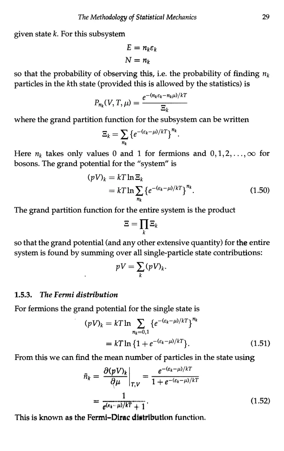
1.5.3. The Fermi distribution
For fermions the grand potential for the single state is
(pV)k = kTln X {e-^-MkT}nk
= kTln{l+e-(£*-MkT}. (1.51)
From this we can find the mean number of particles in the state using
4^i
e-(,ek-ii)/kT
1
«u,-M*+r (L52)
This is known as the Fermi-Diwc distribution function.

30
Topics in Statistical Mechanics
The grand potential for the entire system of fermions is found by
summing the single-state grand potentials
pV = fcTXln{l + e'^-^kT}. (1.53)
k
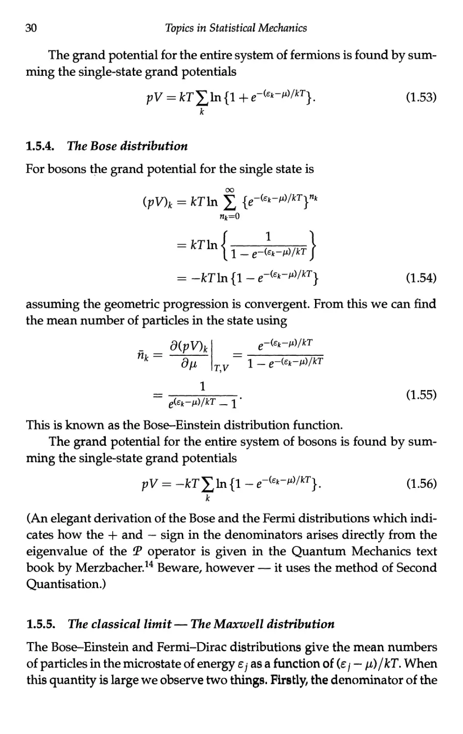
1.5.4. The Bose distribution
For bosons the grand potential for the single state is
00
(pV)* = fcTln £ {c-ta-tf/W}"*
nk=0
= mn{l-e-(l-,)Ar}
= -fcrin {1 - c-fc*-M)/Wj. (1 54)
assuming the geometric progression is convergent. From this we can find
the mean number of particles in the state using
nk=d(^
1
e-(ejfc-/i)/*T
TV~ 1 _ e-(e*-/i)/*T
(1.55)
e(ek-n)/kT _ ^ '
This is known as the Bose-Einstein distribution function.
The grand potential for the entire system of bosons is found by
summing the single-state grand potentials
pV = -fcT£ln{l - e-fe*-P>/W}. (1.56)
k
(An elegant derivation of the Bose and the Fermi distributions which
indicates how the + and — sign in the denominators arises directly from the
eigenvalue of the T operator is given in the Quantum Mechanics text
book by Merzbacher.14 Beware, however — it uses the method of Second
Quantisation.)
1.5.5. The classical limit — The Maxwell distribution
The Bose-Einstein and Fermi-Dirac distributions give the mean numbers
of particles in the microstate of energy Sj as a function of (e/ - /x)/fcT. When
this quantity is large we observe two things. Firstly, the denominator of the

The Methodology of Statistical Mechanics
31
distributions will be very much larger than one, so the +1 or —1
distinguishing fermions from bosons may be neglected. And secondly, the large
value for the denominator means that fij, the mean occupation of the state,
will be very much less than unity.
This condition will apply to all states, down to the ground state of
£j = 0, if fi/kT is large and negative. This is the classical limit where
the issue of multiple state occupancy does not arise and the distinction
between fermions and bosons becomes unimportant. We refer to such
(imaginary) particle as maxwellons, obeying Maxwell-Boltzmann
statistics. Thus, for these particles the mean number of particles in the state is
given by
nk = e-<e*-MkT.
The three distribution functions are shown in Fig. 1.8. Observe, in
particular, that when fi = e the Fermi occupation is one half, the Maxwell
occupation is unity and the Bose occupation is infinite.
n
(z-\i)lkT
-4-2024
Fig. 1.8. Fermi-Dirac, Maxwell-Boltzmann and Bose-Einstein distribution
functions.
1.6. Classical Statistical Mechanics
1.6.1. Phase space and classical states
The formalism of statistical mechanicH developed thus far relies very
much, at the microscopic livd, on the UN* of (micro)states. We count the
number of states, we sum over itAtoi, «tc. Thl« is all very convenient to

32
Topics in Statistical Mechanics
do within the framework of a quantum-mechanical description of systems
where states of a (finite or bound) system are discrete, but what about
classical systems. How is the formalism of classical statistical mechanics
developed — what is a "classical state"?
A classical microstate is a state for which we have complete
information at the microscopic level. In other words, we must know the position
and velocity of all particles in the system. (Position and velocity, since the
equations of motion — Newton's laws — are second-order differential
equations in time.)
For reasons related to the Lagrangian and the Hamiltonian
formulation of mechanics it proves convenient to work in terms of the position
and the momentum rather than velocity of the particles in the system. This
is because it is then possible to work in terms of generalised coordinates
and momenta — such as angles and angular momenta — in a completely
independent way; one is not constrained to a particular coordinate
system. Thus we will say that a classical microstate is specified by the
coordinates and the momenta of all the constituent particles. A single particle
has three coordinates x, y, z and three momentum components px, py, pz
so it needs six components to specify its state. The coordinates are
conventionally denoted by q and the momenta by p. This pq space is called phase
space.
\P
I evolution of
I ^*—w phase point in time
phase point \ J
Fig. 1.9. Phase space.
The state of a particle is denoted by a point in phase space. Its evolution
in time is represented by a curve in phase space. It should be evident that

The Methodology of Statistical Mechanics
33
during its evolution the phase curve of a point cannot intersect since there
is a unique path proceeding from each location in phase space.
A quantum state may be specified by a set of quantum numbers. A
classical system is specified when we know the position and momentum
coordinates of all the particles. But what is the classical analogue of the
quantum state? We need to know this so that we may use the analogous
Boltzmann expression for entropy, and we want to understand how to
construct partition functions for classical systems. And fundamentally, of
course, the definition of the classical state must be consistent with the
Fundamental Postulate.
The classical analogue of a quantum state, a "classical state" is
specified as a cell in phase space. For a single particle with coordinates qX/ qy, qz
and momentum components px, py, pz we have
"classical state" oc AqxAqyAqzApxApyApz = A3pA3q for simplicity.
This will not be proved, but it is eminently plausible. The question of the
constant of proportionality is interesting. The value of this constant may be
ascertained by comparing the partition functions as calculated classically
and quantum-mechanically in the classical limit (high temperature/low
density). One finds that for each pq pair there is a factor of h~l. This is
certainly dimensionally correct, but what business has Planck's constant
to appear in a fundamentally classical result? For a single particle we then
have
"classical state" corresponds to AqxAqyAqzApxApyApz = h3.
The number of "classical states" in a small region of phase space is then
A3pA3q/h. The general rule, then, is that the sums over states in the
quantum case correspond to integrals over phase space in the classical case:
I -i/d3pdV (1.57)
single n J
particle
states
1.6.2. Boltzmann and Gibb§ phase spaces
The microstate of a system i§ represented by a point in phase space.
A different microstate will be represented by a different point in phase
space. In developing the statistical approach to mechanics we must talk

34
Topics in Statistical Mechanics
about different microstates — so we are considering different points in
phase space and probabilities associated with them. Boltzmann and Gibbs
looked at this in different ways. Boltzmann's idea was that a gas of N
particles would be represented by N points in the six-dimensional phase space.
The evolution of the state of the system with time is then described by the
"flow" of the "gas" of points in the phase space. This sort of argument only
works for weakly interacting particles, since later arguments are based on
the movement of the points in phase space being independent.
Gibbs adopted a rather more general approach. He regarded the state
of a system of N particles as being specified by a single point in a 6N-
dimensional phase space. The six-dimensional phase space of Boltzmann
is sometimes referred to as /x-space and the 6N-dimensional phase space
of Gibbs is sometimes referred to as T-space.
In both cases, one applies probabilistic arguments to the collection of
points in phase space. This collection is called an ensemble. So in
Boltzmann's view a single particle is the system and the N particles comprise
the ensemble while in Gibbs's view the assembly of particles is the system
and many imaginary copies of the system comprise the ensemble. In the
Boltzmann case one performs averages over the possible states of a single
particle, while in the Gibbs case one is considering possible states of the
entire system and applying probabilistic arguments to those.
Both views are useful. The Boltzmann approach is easier to picture but
it can only be applied to weakly interacting particles. The Gibbs approach
is more powerful as it can be applied to strongly interacting systems where
the particles cannot be regarded as being even approximately independent.
The probability of finding a system in a microstate in the region dpdq
of phase space is given by pdpdq where p is the density of representative
points in the phase space. So the probability density of the microstate p, q
is given by pip, q).
1.6.3. The Fundamental Postulate in the classical case
If we say that all (quantum) states are equally likely, then the classical
analogue will be that all points in phase space are equally likely. The
quantum version of the Fundamental Postulate refers to an isolated system. This
is a system for which E, V and N are fixed. Classically when the energy
is fixed, this restricts the accessible region of phase space to a constant-
energy hypersurface. Similarly, fixing V and N determines which regions
of phase space are available. The classical version of the Fundamental

The Methodology of Statistical Mechanics 35
Postulate then states that for an isolated system all available regions of
phase space on the constant energy hypersurface are equally likely.
The probability of a macrostate corresponding to a region of phase
space will then be proportional to the number of phase points in the
region. So correctly normalised, it will be given by the density of points
pip, q) where by p and q we mean the set of all momentum coordinates
and all position coordinates.
1.6.4. The classical partition function
The classical analogue of the quantum partition function is given by
Z = J_Je-H(Pi,*)/krd3Npd3N? (1 5g)
when we are considering distinguishable particles. For indistinguishable
particles there is the factor of 1/N! (Sec. 2.3.4)
z=m^Ie'mpi",)/kTd3Npd3Nq (L59)
and there is the possibility of factorising the expression for Z.
The function H(pz, qi) is the energy of the system expressed as a
function of the position and momentum coordinates q\ and p,-.
1.6.5. The equipartition theorem
The equipartition theorem is concerned with the internal energy
associated with individual degrees of freedom of a system. It has important
consequences for the behaviour of the thermal capacity of classical systems.
We ask the question "What is the internal energy associated with a
given degree of freedom — say p*?". That is easy to write down:
(Ei) = i f E^^-^-^.Pi-Pr-^VfcrjSN^sNp^ (L60)
Assuming the energy E, depends only on the pz and not on the other
p's and q's, we can factorise that bit out of the exponential and write the
integral as
^ rnopi~i
'' je -tyA'rdpj J jifune integral m above - no p,]

36
Topics in Statistical Mechanics
So the second integral in numerator and denominator cancel, leaving the
simple expression
{ ° fe-Wdpi '
This may be simplified by writing (3 — 1/kT and using
^ = -33^
so that
tiferMdiH
<E<> =
fe-^dpi
or
At this stage we must be more specific about the functional form of Ez(pz).
Since pi is a momentum then for a classical particle Ez(pz) = p?/2ra — a
quadratic dependence. For simplicity let us write simply
Ei = bp\
for some constant b. The integral is then
fe^E<dpi=Je-^dpi.
We do not actually need to evaluate this. Remember that we are going to
differentiate the logarithm of the integral with respect to /3; all we want is
the ^-dependence. Let us make a change of variable and put
The integral then becomes
so that
—wHk"+i,,/rWd»}-

The Methodology of StatisHeal Mechanics 37
The second term is independent of /3 so upon differentiation it vanishes.
Thus differentiating we obtain
w=^
or, in terms of T:
(E{) = ^kT. (1.61)
The general conclusion here may be stated as the Equipartition
theorem: For a classical (non-quantum) system each degree of freedom with
a quadratic dependence on coordinate or momentum gives a contribution
to the internal energy of kT/2.
[Incidentally, if Ez oc qforpf then (E,-) = kT/n.]
1.6.6. Consequences of equipartition
We consider two examples — lattice vibrations, and a gas of particles.
For the case of lattice vibrations each atom is essentially three
harmonic oscillators, one in the x, y and z directions. Thus for N atoms we
have 3N harmonic oscillators. Now in this case, both the position and
momentum coordinates contribute a quadratic term to the energy. The
internal energy is then
E = 3NkT (1.62)
in the non-quantum (high temperature) limit. Differentiation with respect
to temperature gives the isochoric thermal capacity
Q, = 3Nk
= 3R per mole. (1.63)
Considering now a gas of noninteracting particles, there is no contribution
to the energy from the position coordinates. Only the momentum
coordinates contribute a quadratic Ijerm to the energy and the internal energy is
then
E-jN*T (1.64)

38
Topics in Statistical Mechanics
in the non-quantum (high temperature) limit. Differentiation with respect
to temperature gives the (isochoric) thermal capacity
o, = |n*
3
= -R per mole. (1.65)
The thermal capacity of the solid is double that of the fluid because only
in the solid do the position coordinates contribute to the internal energy.
[In fact the walls of a box of gas can be modelled as an oscillator with a
power law potential V oc xn where n —> oo.]
Equipartition breaks down when quantum effects become important.
In Sec. 2.3.3 we shall see that the internal energy of a single quantum
free particle corresponds to |fcT: the equipartition value for the three
spatial degrees of freedom. However, once we have a collection of N
identical particles comprising a quantum gas, the internal energy is given, in
Sec. 2.4.5, by
where a = +1 for fermions, zero for "classical" particles and —1 for
bosons. The equipartition result occurs at high temperatures and as the
gas cools, quantum effects become important. For fermions the internal
energy increases above the equipartition value, while for bosons the
internal energy decreases below the equipartition value.
In Problem 1.16 you will see that the internal energy of a quantum
harmonic oscillator may be written as
E = kT+l2kT + -"
The first term represents the high-temperature equipartition value. The
second (and higher) terms indicate the internal energy increasing above
its high-temperature value as the temperature is lowered.
1.6.7. Liouville's theorem
We ask the question "How does a macroscopic system evolve in time?".
The answer is that it will develop in accordance with the Second Law of

The Methodology of Statistical Mechanics
39
thermodynamics; the system evolves to the state of maximum entropy
consistent with the constraints imposed. Can this be understood from
microscopic first principles? In other words, can the law of entropy
increase be derived from Newton's laws? Both Boltzmann and Gibbs
agonised over this.
We need a definition of entropy which will be suitable for use in the
classical case. The problem is that there are no discrete states now, since p
and q can vary continuously. By analogy with the generalised expression
for entropy:
S = -*XP/lnP;.,
/
since the probability (density) is given by the density of points in phase
space, we now have
S = —k phxpdpdq. (1.66)
It is essentially (minus) the average of the logarithm of the density of
points in phase space.
If one calculates the way points move around phase space under the
influence of the laws of mechanics one finds that the "flow" is
incompressible. Thus the density remains constant. This result is known as Liouville's
theorem. We need the machinery of Hamiltonian mechanics to show this.
If you are happy with Hamiltonian mechanics the proof is sketched below.
But the implication.is that since p remains constant then the entropy
remains constant, so the Second Law of thermodynamics seems to be
inconsistent with the laws of mechanics at the microscopic level.
To demonstrate Liouville's theorem we first note that the flow of
points in phase space must obey the equation of continuity, since the
number of points is conserved:
^ + divvp = 0. (1.67)
However, in this case p depends on the position and momentum
coordinates, q and p. Thus the divergence contains all the d/dq derivatives and
all the d/dp derivatives. An^ the "velocity" v has components dp/dt as
well as the usual dq/dt. TIiuh the divergence term is actually
,. I) /dp \ , 0 /dq \

40
Topics in Statistical Mechanics
(these equations really contain all the q and p coordinates; the above, as
elsewhere, is a shorthand simplification). We expand the p and q
derivatives to give
P \3p dt dq &t)P^ dp dt dq dt
and then we use Hamilton's equations
dp__dH dq _ OH
dt~ dq' dt~ dp
in the first bracket. Then
0_dp d_dq^___^2L °2H =q
dp dt dq dt dpdq dqdp
Thus we find that
9p_j_apdp_j_apd^=0
dt dp dt dq dt
But we recognise this as the total derivative of p; it is the derivative of the
density when moving with the flow in phase space. This is zero. Thus as
the representative points evolve and flow in phase space, the local density
remains constant. This is the content of Liouville's theorem, expressed in
its usual form as
^=0. (1.68)
at
We have a paradox: since p remains constant during evolution then the
entropy remains constant; the Second Law of thermodynamics seems to
be inconsistent with the laws of mechanics at the microscopic level.
1.6.8. Boltzmann's H theorem
The resolution of the paradox of the incompatibility between Liouville's
theorem and the Second Law may be understood from the nature of the
"flow" of points in phase space. Boltzmann defined a quantity H, which
was the integral of p In p over phase space and he obtained an equation of
motion for H as a probabilistic differential equation for the flow of points
into and out of regions of phase space. We shall adopt a variant of the
approach of Gibbs to study the evolution of Boltzmann's H. Please note
this H is neither the Hamiltonian of the previous section nor the enthalpy
function; this is Boltzmann's H.

The Methodology of Statistical Mechanics
41
The flow of points in phase space is complicated. Since we have a
given number of elements in our ensemble, the number of points in phase
space is fixed. So Liouville's theorem is saying that the multidimensional
volume occupied by the points is constant. But the flow can be "dendritic"
with fingers spreading and splitting in all directions.
Fig. 1.10. Evolution of a region of phase space.
And as this happens, there will come a time when it is difficult to
distinguish between what is an occupied region and what is an unoccupied
region of phase space; they will be continually folded into each other.
Gibbs argued that there was a scale in phase space, beyond which it was
not possible (or at least reasonable) to discern. If the details of the state
"3" above are too fine to discern, then it will simply appear as a region of
greater volume and less density.
Fig. 1.11. Apparent reduction in density in phone space.

42
Topics in Statistical Mechanics
The procedure of taking an average over small regions of phase space
is known as "coarse graining". Gibbs showed rigorously (rather than by
just using diagrams as here) that the coarse grained density of points in
phase space decreased as time proceeded.15
Thus the conclusion is that the coarse-grained H decreases, or the
coarse-grained entropy increases.
There is a relation with quantum mechanics, which may be invoked in
the question of coarse-graining. The volume of a "cell" in phase space is a
product of p, q pairs. Now the Uncertainty Principle tells us that we cannot
locate a point within a pq area better than Planck's constant. This gives the
ultimate resolution that is achievable in specifying the state of a system —
so at the fundamental level there is a firm justification for coarse-graining.
Quantum mechanics has a habit of popping up in the most unexpected
areas of statistical thermodynamics. This theme continues into the next
section.
1.7. The Third Law of Thermodynamics
1.7.1. History of the Third Law
The Third Law of thermodynamics arose as the result of experimental
work in chemistry, principally by the famous chemist Nernst. He
published what he called his "heat theorem" in 1906. A readable account of
the history of the Third Law and the controversies surrounding its
acceptance is given by Dugdale.16
Nernst measured the change in Gibbs free energy and the change in
enthalpy for chemical reactions which started and finished at the same
temperature. At lower and lower temperatures he found that the changes
in G and the changes in H became closer and closer.
Nernst was led to conclude that at T = 0 the changes in G and H were
the same. And from some elementary thermodynamic arguments he was
able to infer the behaviour of the entropy at low temperatures.
Changes in H and G are given by
AH = TAS + VAp
AG =-SAT-{-VAp.
Thus AG and AH are related by
AG = AH - TAS - SAT

The Methodology of Statistical Mechanics
energy
43
• AG
AH
0 T
Fig. 1.12. Nernst's observations.
and if the temperature is the same before and after, AT = 0, so then
AG = AH -TAS.
This is a very important equation for chemists.
Now Nernst's observation may be stated as
AH-AG-+0 asT->0,
which implied that
TAS -^0 as T -^0.
1.7.2. Entropy
On the face of it this result is no surprise since the factor T will ensure the
product TAS goes to zero. But Nernst took the result further. He studied
how fast AH - AG tended to zero. And his observation was that it always
went faster than linearly. In other words he concluded that
AH-AG
0 as T -► 0.
(1.69)
So even though 1/T was getting bigger and bigger, the quotient
(AH - AG)/T still tended to zero. But we know that
AH-AG
= AS.
So from this, Nernst drew tht conclusion
AS «•* 0 !■ T -> 0.
(1.70)

44
Topics in Statistical Mechanics
The entropy change in a process tends to zero at T = 0. The entropy thus
remains a constant in any process at absolute zero. We conclude:
• The entropy of a body at zero temperature is a constant, independent of
all other external parameters.
This was the conclusion of Nernst; it is sometimes called Nernst's heat
theorem. It was subsequently to be developed into the Third Law of
thermodynamics.
1.73. Quantum viewpoint
From the purely macroscopic perspective the Third Law is as stated above:
at T = 0 the entropy of a body is a constant. And many conclusions can
be drawn from this. One might ask the question "what is the constant?".
However we do know that thermodynamic conclusions about
measurable quantities are not influenced by any such additive constants since one
usually differentiates to find observables. (But a constant of minus infinity,
as found for the entropy of the classical ideal gas, might be problematic.)
If we want to ask about the constant then we must look into the
microscopic model for the system under investigation. Recall the Boltzmann
expression for entropy:
S = fclnQ
where Q is the number of microstates in the macrostate. Now consider the
situation at T = 0. Then we know the system will be in its ground state,
the lowest energy state. But this is a unique quantum state. Thus for the
ground state
Q = l
and so
S = 0.
Nernst's constant is thus zero and we then have the expression for the
Third Law:
• As the absolute zero of temperature is approached the entropy of all
bodies tends to zero.
We note that this applies specifically to bodies that are in thermal
equilibrium. The Third Law can be summarised as
. * >0 as T -+0. (1.71)
a anything

The Methodology of Statistical Mechanics
45
The above discussion is actually an over-simplification. In reality there
may be degeneracy in the ground state of the system; then the above
argument appears to break down. However, recall that entropy is an
extensive quantity and that the entropy of the system should be considered in
the thermodynamic limit. In other words, strictly, we should examine how
the intensive quantity S/V or S/N behaves in the limit V —> oo, N —► oo. If
the degeneracy of the ground state is g then we must look at the behaviour
of ln(g)/N. This will tend to zero in the thermodynamic limit so long as
g increases with N no faster than exponentially. This is the
fundamental quantum-mechanical principle behind the Third Law. The interested
reader should consult the paper by Leggett17 for a deeper discussion of
these points.
To complete this discussion, it is instructive to see how the Third Law
would fail if classical mechanics were to apply down to T = 0. We saw, in
Sec. 1.6.7, that the Gibbs expression for entropy:
S=-fc£PylnP;
/
must be replaced, in the classical case by:
S = —k plnpdpdq,
where p is the density of points in phase space. This is necessary because
in the classical case there are no discrete states and the momenta and
coordinates, p and q, can vary continuously.
As the temperature is lowered, the mean energy of the system will
decrease. And corresponding to this, the "volume" of phase space
occupied will decrease. In particular, the momentum coordinates q will vary
over a smaller and smaller range. In the T —► 0 limit the momentum range
will become localised closer and closer to q = 0. The volume of occupied
phase space shrinks to zero and the entropy thus tends to -oo. This indeed
is the limiting value indicated by the classical treatment of the Ideal Gas,
in Sec. 2.3.3.
The Uncertainly Principle of quantum mechanics limits the low-
temperature position-momentum of a system; you cannot localise points
in phase space to a volume smaller than the appropriate power of Planck's
constant. This fundamental limitation of the density of phase points
recovers the Third Law. Thus again we see the intimate connection between
quantum mechanics and the Third lnw.
The Second Law tells us that thrr* 1« an absolute zero of temperature.
Now we see that the Third I s w t«»ll» u* Huw In nn Absolute zero of entropy.

46 Topics in Statistical Mechanics
1.7A. Unattainability of absolute zero
The Third Law has important implications concerning the possibility of
cooling a body to absolute zero. Let us consider a sequence of adiabatic
and isothermal operations on two systems, one obeying the Third Law
and one not.
(a)
Fig. 1.13. Approaching absolute zero. System (a) not obeying the Third Law can
get to T = 0 in two steps. System (b) obeying the Third Law cannot get to T = 0 in
a finite number of steps.
Taking a sequence of adiabatics and isothermals between two values
of some external parameter we see that the existence of the Third Law
implies that you cannot get to T = 0 in a finite number of steps. This is, in
fact, another possible statement of the Third Law.
Although one cannot get all the way to T — 0, it is possible to get closer
and closer. Figure 1.14, adapted and extended from Pobel's book,18
indicates the success in this venture.
1.7,5. Heat capacity at low temperatures
The Third Law has important consequences for the heat capacity of bodies
at low temperatures. Since
C =
dQ
dT
(1.72)

The Methodology of Statistical Mechanics
47
1850
1900 1950
Year
2000
2:. 1.14. The road to absolute zero.
and the Third Law tells us that
8T~
0 as T -► 0,
we then have
C -> 0 as T -> 0.
(1.73)
Classical models often give a constant heat capacity. For an ideal gas
(Sec. 2.3.3)

48
Topics in Statistical Mechanics
independent of temperature. The Third Law tells us that this cannot hold
at low temperatures. And indeed we shall see that for both Fermi and Bose
gases Cy does indeed go to zero at T = 0.
1.7.6. Other consequences of the Third Law
Most "response functions" or susceptibilities — generalised spring
constants — go to zero or to a constant as T —> 0 as a consequence of the
Third Law. This is best seen by examining the relevant Maxwell relation
(Appendix A.2.6). For example consider the thermal expansion coefficient.
The Maxwell relation here is
0V
dT
OS
dp
The right-hand side is zero by virtue of the Third Law. Thus we
conclude that
0V
dT
0 as T -► 0;
the expansion coefficient goes to zero.
An interesting example is the susceptibility of a paramagnet, which we
will treat in Sec. 2.7. The connection with the model pV system is made via
M —> p
where M is the total magnetic moment. The magnetic susceptibility is
(neglecting factors of /i0)
1 dM
so that
X =
xv-
V dB
dp
There is no Maxwell relation for this, but consider the variation of the
susceptibility with temperature:
d(XV)
dT
82M
~ dTdB
d2P
dTdV

The Methodology of Statistical Mechanics
49
The order of differentiation can be reversed here. In other words
d dM _d_dp
dB dT ~* dVdT'
And now we do have a Maxwell relation:
dp
dT
es
v~ dV
dM
T*~ dT
ds
v~ dB
T
The Third Law tells us that the right-hand side of these equations goes to
zero as T —► 0. We conclude then that
||->0 as r -+0
or
const, as T —► 0.
(1.74)
The Third Law tells us that the magnetic susceptibility becomes constant
as T -»• 0. But what does Curie's law, Eqs. (2.76) and (2.77) say? This states
_ C
A. rr-i
where C is the Curie constant. From this we conclude
X —> oo as T —» 0!!
This is completely incompatible with the Third Law.
But Curie's law is a specifically high temperature result (strictly, it
applies to the small B/T limit). The general expression for the
magnetisation of an ideal paramagnet of N spin 1/2 moments \i is, Eq. (2.75):
kT
M = N/itanh
and corresponding to this, the susceptibility is
Njj?_
VkT
-*Mg
Now we see that
X -> 0 as T -> 0
in conformity with the Third Law, so long as the magnetic field B is finite.
Of course, you have to use a magnetic field, however small, to measure the
susceptibility. Nevertheless, even In the Absence of an externally-applied
magnetic field, there will be nn Internal field present: the dipole fields

50
Topics in Statistical Mechanics
of the magnetic moments themselves. Thus the Third Law is not under
threat.
There is a further consideration in the case of fluid systems. In a fluid,
where the particles must be treated as delocalised, the statistics will also
have an effect. Recall the behaviour of fermions at low temperatures, to be
treated in Sec. 2.4. Very roughly, only a fraction T/T? of the particles are
free and available to participate in "normal" behaviour. We then expect
that the Curie law behaviour will be modified to
or
C
x TF
which is indeed a constant, in conformity with the Third Law. This result is
correct, but a numerical calculation must be done to determine the
numerical constants involved.
1.7.7. Pessimist's statement of the laws of thermodynamics
As we have now covered all the laws of thermodynamics we can present
their statements in terms of what they prohibit in the operation of Nature.
• First Law: You cannot convert heat to work at greater than 100%
efficiency
• Second Law: You cannot even achieve 100% efficiency — except at
r = o.
• Third Law: You cannot get to T = 0.
This is a simplification, but it encapsulates the underlying truths, and it is
easy to remember.
Problems
1.1. Demonstrate that entropy, as given by the Boltzmann expression
S = fcln Q, is an extensive property. The best way to do this is to argue
clearly that Q is multiplicative.
1.2. Demonstrate that gravitational energy is not extensive: show that
the gravitational energy of a sphere of radius r and uniform density
varies with volume as Vn and find the exponent n.

The Methodology of Statistical Mechanics
51
1.3. In investigating the conditions for the establishment of equilibrium
through the transfer of thermal energy the fundamental requirement
is that the entropy of the equilibrium state should be a maximum.
Equality of temperature was established from the vanishing of the
first derivative of S. What follows from a consideration of the second
derivative?
1.4. Do particles flow from high ji to low ji or vice versa? Explain your
reasoning.
1.5. In the derivation of the Boltzmann factor the entropy of the bath was
expanded in powers of the energy of the "system of interest". The
higher order terms of the expansion are neglected. Discuss the
validity of this.
1.6. The Boltzmann factor could have been derived by expanding Q
rather than by expanding S. In that case, however, the expansion
cannot be terminated. Why not?
1.7. Show that InN! = X^Li Inn. By approximating this sum by an
integral obtain Stirling's approximation: InN! « NlnN — N.
1.8. Show that the Gibbs expression for entropy: S = —k^jPjlnPj,
reduces to the Boltzmann expression S = fclnQ in the case of an
isolated system.
1.9. What is the condition that the geometric progression in the
derivation of the Bose-Einstein distribution is convergent?
1.10. Show that the trajectory of a Id harmonic oscillator is an ellipse
in phase space. What would the trajectory be if the oscillator were
weakly damped.
1.11. Why cannot the evolutionary curve in phase space intersect? You
need to demonstrate that the evolution from a point is unique.
1.12. Starting from the expression for the Gibbs factor for a many-particle
system, write down the grand partition function S and show how
it may be expressed as the product of Ek, the grand partition
function for the subsystem comprising particles in the fcth single-particle
state.
1.13. (Difficult) This problem considers the probability distribution for the
energy fluctuations in the canonical ensemble. The moments of the
energy fluctuations are defined by
*• i
where /3 = -1/kT and e i» an arbitrary (at this stage) energy.

52 Topics in Statistical Mechanics
Show that
^ = e^n{Ze^}
and use this to prove that the fluctuations in an ideal gas obey a nor-
mal distribution around e. (You really need to use a computer algebra
system to do this problem.)
1.14. For a single-component system with a variable number of particles,
the Gibbs free energy is a function of temperature, pressure and
number of particles: G = G(T,p,N). Since N is the only extensive
variable upon which G depends, show that the chemical potential
for this system is equal to the Gibbs free energy per particle: G = Nfi.
1.15. Use the definition of the Gibbs free energy together with the result
of the previous question to obtain the Euler relation of Appendix 1.
1.16. The energy of a harmonic oscillator may be written as muj2x2/2 +
p2/2m so it is quadratic in both position and momentum — thus,
classically, equipartition should apply. The energy levels of the
quantum harmonic oscillator are given by en = (| + n)fiw. Show that the
partition function of this system is given by
^1 - hoo
Z=2Cosech—
and that the internal energy is given by
_ 1,_ , hu hu hu
E = -hujcoth —— = fc /t_ h —-.
2 2kT ehuj/kT_1 2
Show that at high temperatures E may be expanded as
E = fcT+12fcT + -
Identify the terms in this expansion.
References
1 R. Bowley and M. Sanchez, Introductory Statistical Mechanics, 2nd ed. (Oxford
University Press, 1999).
2 M. W. Zemansky and R. H. Dittman, Heat and Thermodynamics (McGraw-Hill,
1968).
3 P. A. Schilpp (Ed.), Albert Einstein: Philosopher-Scientist (Open Court Publishing
Co., 1949). In Autobiographical Notes.
4 T. L. Hill, Introduction to Statistical Thermodynamic (Addison Wesley, 1960).

The Methodology of Statistical Mechanics
53
5 L. D. Landau and E. M. Lifshitz, Statistical Physics (Pergamon Press, 1980), in
the Preface.
6 C. Tsallis, Nonextensive statistics: Theoretical, experimental and computational
evidences and connections, Brazilian J. Phys. 29 (1999) 1.
7 C. J. Adkins, Equilibrium Thermodynamics, 3rd ed. (Cambridge University Press,
1983).
8 A. B. Pippard, Elements of Classical Thermodynamics (Cambridge University
Press, 1966).
9 H. B. Callen, Thermodynamics and an Introduction to Thermostatistics, 2nd ed.
(John Wiley, 1985).
10 F. Reif, Fundamentals of Statistical and Thermal Physics (McGraw-Hill, 1965).
11 R. P. Feynman, Statistical Mechanics (Benjamin, 1972).
12 R. P. Feynman, The reason for antiparticles, in Elementary Particles and the Laws
of Physics — The 1986 Dirac Memorial Lectures, ed. S. Weinberg (Cambridge
University Press, 1987).
13 S. Tomonaga, The Story of Spin (University of Chicago Press, 1997).
14 E. Merzbacher, Quantum Mechanics (John Wiley, 1970).
15 R. C. Tolman, The Principles of Statistical Mechanics (Oxford University Press,
1938).
16 J. S. Dugdale, Entropy and its Physical Meaning (Taylor and Francis, 1996).
17 A. J. Leggett, On the minimum entropy of a large system at low temperatures,
Ann. Phys. N.Y. 11 (1972) 80-106.
18 F. Pobel, Matter and Methods at Low Temperatures (Springer-Verlag, 1992).
\

CHAPTER TWO
PRACTICAL CALCULATIONS WITH
IDEAL SYSTEMS
2.1. The Density of States
2.1.1. Non-interacting systems
The concept of a non-interacting system is hypothetical since a system of
truly non-interacting components could not achieve thermal equilibrium.
Thus we are really interested in assemblies of very weakly interacting
systems. To be precise, the interactions must be sufficient to lead to thermal
equilibrium, but weak enough that these interactions have negligible effect
on the energy of the individual particles. We note parenthetically, that
the rate at which an equilibrium state is established will depend on the
strength of the interactions; this is the subject of non-equilibrium statistical
mechanics. Some aspects will be touched upon in Chapter 5.
Since the single-particle states have well-defined energies, it follows
that one can obtain full thermodynamic information about such a system
once the energies of the single-particle states and the mean number of
particles in each state is known. Then all thermodynamic properties are found
by performing sums over states and distribution functions. And for infinite,
or very large systems, such sums may usually be converted to integrals.
2.1.2. Converting sums to integrals
In quantum statistical mechanics there are many sums over states to be
evaluated. An example is the partition function
Z(N, V,T) = ^e~E<w'V)/kT.

Practical Calculations with Ideal Systems
55
It is often convenient to approximate the sums by integrals. And since the
individual states are densely packed, negligible error is introduced in so
doing. Now if g(s) is the number of states with energy between e and
s + de then the sum may be approximated by
ye-E,(N,v>/*r_> f" g{£)e-e/kTds
Jo
Here g(e) is referred to as the (energy) density of states. If we are studying the
properties of a gas then the microstates to be considered are the quantum
states of a "particle in a box". And the density of states for a particle in a
box may be evaluated in the following way.
2.1.3. Enumeration of states
We consider a cubic box of volume V. Each side has length V1/3.
Elementary quantum mechanics tells us that the wave function of a particle in
the box must go to zero at the boundary walls; only standing waves are
allowed.
X _ yl/3
2 2
Fig. 2.1. Standing waves in a box
In the general case, the allowed wavelengths A satisfy A/2 = V1/3/n, that is
A„ = -V1/3/ n = 1,2,3,4,...,
n
oo.
In three dimensions there will be a A for the x, y and z directions:
yl/3 yl/3 yl/3
nx riy nz
Or, since this corresponds to the components of the wave vector
kx = 2n/\nx,etc,
, __ 7T , It , 7T
(2.1)

56
Topics in Statistical Mechanics
We can now use the deBroglie relation p = fck to obtain the momentum
and hence the energy.
And so for a free particle, the energy is then
,= p2 = Pl + Py + pl
2m 2m
which is
7T /l / o 9 9\
p. = 1 n . 4- n . 4- n 1.
VV3
(2.2)
zmv^J x "
In this expression it is the triple of quantum numbers (nx, ny, nz) which
specify the quantum state. Now each triple defines a point on a cubic grid.
If we put
then the energy is given by
= n2h2R2
£~ 2mV2/r
Observe that the energy levels depend on the size of the container. We
used this fact in the considerations of Sec. 1.2.2 on the probabilistic
interpretation of the First Law.
2.1.4. Counting states
Now the number of states of energy up to e, denoted by N(e), is given by
the number of points in the octant up to e(R). (An octant is used since nx,
riy and nz are restricted to being positive.) And the number of points in the
octant is approximately equal to the volume of the octant:
But since
we then obtain
me)\\*#.
-essf"
N,£)=^<2mt)3/J-

Practical Calculations with Ideal Systems
57
012345678 nx
Fig. 2.2. Counting of quantum states.
Recall that the density of states g(s) is defined by saying that the number
of states with energy between e and e + de is g(e). In other words
g(e)de = N(e + de) - N(e)
or, simply
dN(e)
g(s) =
ds
So differentiating N(s) we obtain
1 V
^)=J^sC2m^^
(2.3)
4 7T2ft3
which is the required expression for the density of states.
For completeness we shall also give the expressions for the density of
states in two and in one dimension. These will be discussed in some of the
problems. In a two-dimensional system of area A the density of states is
g(e) = —T2 (two dimensions); (2.4)
observe this is independent of energy. And in a one-dimensional system
of length L the density of stakes is
1/2
g(e) = —r [ -sr J *™^2 (one dimension).
(2.5)

58
Topics in Statistical Mechanics
2.1.5. General expression for the density of states
The result of the previous section gives the (energy) density of states for
free particles confined to a box of specified volume. This, we argued, was
appropriate for the consideration of ideal gases. And it will indeed be quite
adequate for the consideration of the classical ideal gas in both the classical
and quantum mechanical cases.
In order to be able to treat systems comprising elements other than
free particles we need to adopt a more general approach than that of the
previous section. Central to that approach was the energy-momentum
relation (really the energy-wave vector relation) of the particles:
e = p2/2m = h2k2/2m. But in the general case this may not be
appropriate. Thus at relativistic speeds free particles would obey e = \/c2p2 + ra2c4
and extreme-relativistic/massless particles, e = cp. In these cases as well
as those with other energy-momentum relations a more general approach
is needed for the density of states.
The key to the general treatment is to consider the density of states in
fc-space. The point is that the quantisation condition discussed above still
applies to the fc-states. The wave function for any elements confined to a
box must vanish at the walls. This means that the standing wave condition
still applies — in other words
lr — ^ lr — ^ lr — ^
Kx - yijs71*' Ky ~ yV3ny Kz - yT/3nz'
The allowed states correspond to integer nx, ny and nz, so that there is a
uniform density of states in fc-space.
The number of states up to a maximum k value is then the volume of
the octant
N(fc) = --7rR3 = --7r(n2 + n2+n2)
And since nx = kxV1/3/n, etc. it follows that
Nik) = ^.
The density of states in fc-space, which we shall denote by g(fc), is then the
derivative of N(fc), so that
Recall that the energy density of states is defined as
, . dJV
*(e)=dF-

Practical Calculations with Ideal Systems
59
And this can be expressed in terms of g(k) by using the chain rule for
differentiation
, , dN dNdk /fx Ids
Z(£)=te = ted-e=8(k)/dk'
Thus we have the general result
*>-£*/£ lZ6)
where we must eliminate k in favour of s. Thus to find the energy
density of states in this general case we need to know the energy-momentum
(energy-wave vector) relation for the particles or excitations.
For completeness we shall also give the general expressions for the
density of states in two and in one dimensions. In a two-dimensional
system of area A the general density of states is
g(e) = —k I — (two dimensions). (2.7)
And in a one-dimensional system of length L the general density of
states is
#(e) = — / — (one dimension). (2.8)
° 7T/ dfc
2.1.6. General relation between pressure and energy
It is possible to obtain a very general relation between the internal energy
and the pressure of a-gas of particles. Central to the argument is the
understanding, discussed in Sec. 2.1.3 that the energy levels of a particle in a box
depend on the volume of the box, Eq. (2.2).
From the differential expression for the First Law, it follows that
dE\
" P = ~dV\s'
We may write the internal energy in terms of the energy levels £y and the
occupation numbers of these states rif.
/
And the differential of this expression is
dE = J///df f + ]T £/dw/.
I /
These expressions should be compared with those in the discussion of the
probabilistic interpretation of the Plrul Lnw In Sec. 1.2.2. There, we used

60
Topics in Statistical Mechanics
the Gibbs approach to the calculation of mean values; here we use the
Boltzmann approach. Apart from that they are equivalent.
The second term of the differential expression vanishes at constant
entropy. Thus we identify
dE
dV
Now the energy levels depend on V as a simple power. We shall write
ej = AVn
so that
dv~AnV
which is convenient to be written as
dgy _ AnVn _ ej_
dV~ V ~HV
Thus the expression for the pressure becomes
^ dej n ^ E
For (non-relativistic) particles of mass m (so that the kinetic energy is
p2/2m) we saw, in Sec. 2.1.3, Eq. (2.2), that n = -2/3. So in this case
2 F
p=-- (2.9)
or
VV=\E- (2.10)
It is important to appreciate the generality of this result. It relies only on
the power law dependence of the energy levels upon volume. It applies
to quantum particles irrespective of statistics and thus it applies to
classical particles as well. It only holds, however, for non-interacting particles;
with interactions the energy levels will depend on volume in a much more
complicated way.
As a further example we can consider a gas of ultra-relativistic/
massless particles. In this case the energy-momentum relation e = cp leads

Practical Calculations with Ideal Systems 61
to the energy levels
e =
^(nl + nl + nlf2 (2.11)
so now the index n is -1/3 and
Pv=l^' (2.12)
This result applies to a gas of photons, and in that case the
expression gives the radiation pressure as one third of the energy density. The
identical expression for radiation pressure is conventionally derived in
electromagnetism1 — without the need for quantum arguments.
2.2. Identical Particles
2.2.1. Indistinguishability
Since the partition function is proportional to probabilities it follows that
for composite systems the partition function is a product of the partition
functions for the individual subsystems. The free energy is proportional
to the logarithm of the partition function and this leads to the extensive
variables of composite systems being additive.
In this section we shall examine how the (canonical) partition function
of a many-particle system is related to the partition function of a single
particle.
If we had an assembly of N identical but distinguishable particles the
resultant partition function would be the product of the N (same) partition
functions of a single particle, z
Z = zN. (2.13)
The key question is that of indistinguishability of the atoms or molecules of
a many-body system. When two identical molecules are interchanged the
system is still in the same microstate, so the distinguishable particle result
overcounts the states in this case. Now the number of ways of redistributing
N particles when there are n\ particles in the first state, n-i particles in the
second state, etc. is
N\
, , , (2.14)
\ Mil ^2* ^3! • • •
so that for a given distribution {w<} the partition function for identical
indistinguishable particles 1§
2,.511.¾^^. (2.15)
N\

62
Topics in Statistical Mechanics
2.2.2. Classical approximation
The problem here is the occupation numbers {nz}; we do not know these
in advance. However at high temperatures the probability of occupancy
of any state is small; the probability of multiple occupancy is then
negligible. This is the classical regime, where the thermal deBroglie wavelength
is very much less than the inter-particle spacing. The thermal deBroglie
wavelength is the wavelength, corresponding to the momentum,
corresponding to the kinetic energy corresponding to a temperature T. This will
appear in Sec. 2.3.1. Under these circumstances the factors n\\ n^. n3!...
can be ignored and we have a soluble problem.
In the classical case, we have then
N!
The Helmholtz free energy
F = -kTlnZ
is thus
F= -NfcTlnz + fcTlnN!. (2.16)
This is N times the Helmholtz free energy for a single particle plus an extra
term depending on T and N. So the second term can be ignored so long as
we differentiate with respect to something other than T or N. Thus, when
differentiating with respect to volume to find the pressure, the result is
N times that for a single particle.
The structure of Eq. (2.16) and in particular the logical necessity for the
1/N! term in the classical gas partition function will be explored further
in Sec. 2.3.4.
23. Ideal Classical Gas
2.3.1. Quantum approach
The partition function for a single particle is
z(V,T) = ^e-e'(v^kT
i
where e\ is the energy of the /th single-particle state; these states were
enumerated in Sec. 2.1.3. As explained previously, th© ©nergy states are closely

Practical Calculations with Ideal Systems
63
packed and this allows us to replace the sum over states by an integral
using the density of states g(e) = y(2m)3/2e1/2/47r2^3:
/•CO
= / g(e)e~£/kTde
Jo
1 V
!_L(2m)3/2r£i/2rArd£.
4 7T2h3 Jo
Following a change of variable this may be expressed, in terms of a
standard integral, as
The integral is y/n/2, so that
Z=U^) V=A* (2-17)
where
A=V^r- ai8)
Now the parameter A is known as the thermal deBroglie wavelength;
within a numerical factor it is the wavelength corresponding to the
momentum corresponding to the thermal kinetic energy of the particle.
Thus, in a sense, it represents the quantum "size" of the particle.
For a gas of N particles we then have
N
Z-^ = „.j,,
We use Stirling's approximation, InNl = NlnN — N, when evaluating the
logarithm:
lnZ = -NlnN + N + Nlnz = Nln
mkT\3/2Ve
Inh2) N
(2.19)
from which all thermodynamic properties can be found, by the formulae
of Sec. 1.4.4. ^
Since Stirling's approximation becomtw true in the thermodynamic
limit it follows that by invoking Stlrling'N approximation we are
implicitly taking the thermodynamic limit,

64
Topics in Statistical Mechanics
2.3.2. Classical approach
It is instructive to consider the calculation of the single-particle partition
function from the classical point of view. The classical partition function is
given by the integral
where for the ideal gas e = p2/2m. Thus the q integrals are trivial, giving a
factor V, and we have
l3
Z —
V
87T3ft3
f00 e-^2mkTdp
J—oo
The integral is transformed to a pure number by changing variables:
p = xy/lmkT so that
As in the quantum calculation, the physics is all outside the integral and
the integral is just a pure number. The value of the integral is y/n so that
just as in the "quantum" calculation; we obtain the identical result. This
justifies the use of h in the normalization factor for the classical state
element of phase space.
2.3.3. Thermodynamic properties
In order to investigate the thermodynamic properties of the classical ideal
gas we start from the Helmholtz free energy, Eq. (2.19):
' ftrikT\3,lVe\
F =-kTkiZ = NkTki
\2ir#)
N
Then upon differentiation we obtain
01nZ
p = kT
8V
= NkT
T.N
fllnz
dV
NkT
V '

Practical Calculations with Ideal Systems
65
This is the ideal gas equation, and from this we identify k as Boltzmarm's
constant. Furthermore, we see that the ideal gas temperature thus
corresponds to the "statistical" temperature introduced in the previous chapter.
The internal energy is
E^kT
<91nZ
dT
V,N
dT 2
This result was obtained previously from equipartition. It also gives
another important property of an ideal gas: the internal energy depends
only on temperature (not pressure or density). This is known as Joule's
law. From the energy expression we obtain the thermal capacity
c -dE
Cv~dT
V,N
2
It is a constant, independent of temperature, in violation of the Third Law.
This is because of the classical approximation — ignoring multiple state
occupancy, etc. We also find the entropy and chemical potential:
S = Nfcln
M
-fcTln
(mkT\3/2V5/2
\2ith1) N
/mkT\3/2v'
\2irh2) N
(2.20)
The formula for the entropy is often expressed as
S = Nk ]nV-NklnN+-Nk]nT+ Nks0 (2.21)
where the reduced "entropy constant" so is given by
3, ( mk \ 5
So = 2m(wJ+2-
The above expression for the entropy is known as the Sackur-Tetrode
equation. It is often interpreted as indicating different contributions to
the entropy: the volume contribution in the first term, the number
contribution in the second term and the temperature contribution in the third
term. Such an identification ii tntirtly incorrect; this matter is explored in
Problem 2.3.

66
Topics in Statistical Mechanics
2.3.4. The 1/N! term in the partition function
In Sec. 2.2.2 we argued that the factor 1/N! was needed in the partition
function of a classical gas of identical particles. In this section, we explore
this idea further and we shall see that the factor is required to ensure that
the mathematical expression for the Helmholtz free energy is extensive —
as it obviously must be.
The partition function for a gas of N classical particles may be
written as
Z=—zN
N!
l_fmkT^\/N
N!
lis* v"- Q22>
If we use Stirling's approximation for the factorial in the form
N! '
(equivalent to the usual expression InN! ~ NlnN — N ) then the
expression for Z becomes
The Helmholtz free energy is given by
F = -fcTlnZ
N
AT,^, ifmkT\3/2 V\
Here the argument of the logarithm is intensive because the extensive V is
divided by the extensive N. Then the N outside the logarithm ensures that
the free energy is an extensive quantity as required.
It is to be expected that the full extensivity of F will only become
manifest in the thermodynamic limit — i.e. upon using Stirling's
approximation.
The important point to note is that the N inside the logarithm is a
consequence of the 1/N! in the partition function. Without this factor the
N would not be there; then F would not be extensive. This is a further
justification of the 1 / NT! factor.

Practical Calculations with Ideal Systems
67
2.3.5. Entropy of mixing
Let us consider the mixing of two gases. Figure 2.3 shows a container
with a wall separating it into two regions. In the left-hand region there
are Ni particles and in the right there are N2 particles. We shall assume
that both regions are at the same temperature and pressure. Furthermore
we will assume that the number density N/V is the same on both sides.
\\ N, T P
N2 T P
Fig. 2.3. Mixing of gases.
We shall investigate what happens when the wall is removed. In particular,
we shall consider what happens when the gases on either side are different
and when they are the same.
When the partition is in place the partition function is simply the
product of the partition functions of two systems. We use the partition function
expression of Eq. (2.3) so that
ZiZ
1^2
= A- (!!^L\ 'v* JL fmkTX2/ yfh
W \2irh2) 1 N2! \2irh2) 2 '
Ni
This may be simplified to
1 ( TtlKl \ vn1vn2
A~ WW \27rfr) Vl Vl '
This is the same whether the particles are identical or different.
Now we shall remove the separating wall and allow the gases to mix.
There are two cases to consider: identical and different particles.
(a) Identical particles
If the particles are identical then the new partition function is that
corresponding to N = Ni + N2, V ^ Vi + Vi. Thus the "after" partition function
will be
Z =
1
fmkT\MNl ,w/2
(N{ + N2)\ V^rP/
(l/i + l/2f1+N2).

68
Topics in Statistical Mechanics
The ratio of the after to before partition function is
Zbefore (Ni + N2)! V*^ *
This may be simplified. Since Vi/Ni = V2/N2 = V/N, it follows that
V1 = VNi/N and V2 = VN2/N so that
Zafter Ni«N2! NN
Zbefore N! N^N*2'
Upon using Stirling's approximation — that is, upon taking the
thermodynamic limit — this expression becomes unity. That is, in the case of
identical particles
^ after = ^before*
So for identical particles there is no effect from removing the
separating wall and the original (macro-)state will be recovered if the wall is
replaced. This is as expected on physical grounds, but the result would
not have been obtained if the 1/N! term in the partition function had not
been used.
(b) Different particles
If the particles on the two sides were different, then on removing
the wall we have a composite system with Ni type-1 particles in the
volume V = V\ + V2 and N2 type-2 particles in the same volume. Thus we
have
z=j- f^ry*i /^yN2/v
Nil \2-Kh1) N2! \2ith2)
_ 1 fmkT\3N^ N
NilN2l \2-Kh1)
The ratio of the after to the before partition function is then
Zafter = VN
Zbefore V^V^'
In this case, the "after" partition function is different to the "before". Then,
for unlike particles, the free energy and some of the other thermodynamic
parameters will change when the wall is removed.

Practical Calculations with Ideal Systems
69
The change in the free energy is given by
^ after
^after - ^before — ~"Win
= -Jfcrin
yNiyN2
This will lead to a change of entropy. Since
dF\
\V,N
it follows that the entropy change upon removal of the wall is
VN }
S~ OT
AS = kln<
VNiyN2
= NklnV- N1klnV1 - N2klnV2 .
This may be written as
AS = Mfcln -^ + N2fcln -^ (2.24)
V\ V2
which shows that the entropy increases when the wall is removed. This
increase of entropy when two different gases are mixed is known as the
entropy of mixing. The expression may be understood from the Boltzmann
entropy expression, using simple counting arguments: the first term gives
the entropy increase of the Ni type-1 particles expanding from volume V\
into volume V while the second term gives the entropy increase of the
N2 type-2 particles expanding from volume V2 into volume V.
2.4. Ideal Fermi Gas
2.4.0. Methodology for quantum gases
The Bose-Einstein and the Fermi-Dirac distribution functions give the
mean number of particles in a given single particle quantum state in terms
of the temperature T and the chemical potential fi. The temperature and
chemical potential are the intensive variables that determine the
equilibrium distribution n(e). Now We hove a good intuitive feel for the
temperature of a system. But the chamical potential is different. This determines
the number of particles in the aiyilem when it is in thermal equilibrium
with a particle reservoir. In reality/ however, it may be more intuitive to
speak of a system containing a given (mean) number of particles. In that

70
Topics in Statistical Mechanics
case, it is the number of particles in the system that determines the
chemical potential.
Now the number of particles in the system is given by
N = Xrcfe)
i
which converts to the integral
N= an(s)g(s)ds
Jo
where g(e) is the energy density of states, a is the factor which accounts
for the degeneracy of the particles' spin states. This is 2 for electrons since
there are two spin states for a spin S = xjr, more generally it will be
IS + 1, (but see Sec. 2.6.3 dealing with photons — massless particles are
a special case).
The expression for N is inverted to give /i, which can then be used
in the distribution function to find the other properties of the system. For
instance, the internal energy of the system would be found from
i
or, in integral form
/»oo
E= aen(e)g(e)de.
Jo
Thus the methodology for treating a quantum gas starts with the
expression for the number of particles N. The expression is inverted to find the
chemical potential ji. This is substituted into the distribution function n(e),
from which all other properties may be found.
2.4.1. Fermi gas at zero temperature
At zero temperature the Fermi-Dirac distribution function
n^ = e(£-M)AT_|_ l
(for notational convenience we have dropped the bar over n) becomes a
box function
n (e) = 1 e < /j,
= 0 e > /i ,

Practical Calculations with Ideal Systems
71
Note that in general the chemical potential depends on temperature. Its
zero temperature value is called the Fermi energy
eF = /i(T = 0).
And the temperature defined by fcTp = £f is known as the Fermi
temperature.
n(e)
1
0
8F 8
Fig. 2.4. Fermi-Dirac distribution at T = 0.
In accordance with the methodology described in the previous section, the
first thing to do is to evaluate the total number of particles in the system in
order to find the chemical potential — the Fermi energy in the T = 0 case.
The density of states is given by Eq. (2.3):
#>-\£f *#**".
Where appropriate we shall consider spin 1/z particles such as electrons or
3He atoms, when we will take a = 2. The total number of particles in the
system is
aV
N =
47T2fi3
aV
(2m?12 f \
Jo
^(Imevf1.
V2ds
And this may be inverted to obtain the Fermi energy
ev *
1m
(2.25)

72
Topics in Statistical Mechanics
This gives the chemical potential at zero temperature. Observe that it
depends on the density of particles in the system N/V, so the Fermi energy
is, as expected, an intensive variable.
The Fermi energy provides a useful energy scale for the consideration
of the properties of Fermi systems. For this reason, it proves useful and
instructive to work in terms of this parameter and we therefore express
the density of states in terms of the Fermi energy
8() Zaef
= ^ ^Y/2. (2.26)
2a £p \£f/
Having obtained the zero-temperature chemical potential, the Fermi-
Dirac function is now completely specified at T = 0, and we can proceed
to find the zero temperature internal energy of the system. This is given by
£(7 = 0) = -^ jTV/Me,
2ef ■
which evaluates to
E = |NeF. (2.27)
The internal energy is proportional to the number of particles in the system
and so it is, as expected, an extensive quantity.
This considerable ground state energy is a consequence of the Pauli
exclusion principle.
2.4.2. Fermi gas at low temperatures — simple model
The effect of a small finite temperature may be modelled very simply
by approximating the Fermi-Dirac distribution function by a piecewise-
linear function. This must match the slope of the curve at e = ji, and the
derivative is found to be
l£—/*
This indicates that the energy width of the transition region is As ~ kT.

Practical Calculations with Ideal Systems
73
\i-2kT jll jLi>-2£r
Fig. 2.5. Simple modelling of Fermi-Dirac distribution.
The distribution function, in this approximation, is then
n(e) = 1,
= 1--
= 0,
-/i + 2fcT
4fcT '
0 < £ < [i - 2kT
fj, - 2kT < s < fi + 2fcT
/i + 2fcT<e
from which the thermodynamic properties may be calculated.
The chemical potential may now be found by considering the total
number of particles in the system:
a»oo
N = a / n(e)g(e)de
Jo
/ n(s)e^2de.
Jo
3N
Observe that here the number N appears on both sides and so it cancels.
The reason for this is that we have chosen to express the density of states
in terms of the Fermi energy. Thus, while the N cancels from both sides
the number (density) is contained in the Fermi energy. So in this approach
we are really expressing the Fermi energy in terms of the chemical
potential:
4/24! rW(ff)ffv2dff
1 2 Jo
and we wish to invert this rtUtion to glv© the chemical potential in terms
of the Fermi energy (and temperature).

74
Topics in Statistical Mechanics
Using the approximate form for n(e), upon integration, this gives
or, on simplifying:
The Fermi energy is then the 2/3 power of this
( 1 /fcT\2 3 /fcT\4
JF=,|1+_(_)+_(_j
which, by the binomial theorem, gives £f as
2/3
+ '
2 1 /t^\4
I l /fcr\z i /itr.
•-" 1+3(-ir)+«(7ri+"
i op2 _i_(*P4
3 /i 45 /i:
This may be inverted to give ji in terms of ep-
= M + ?— + 7^-3- + '
This shows that as the temperature is increased from T= 0 the chemical
potential decreases from its zero temperature value, and the first term is
inT2.
In a similar way the internal energy is found to be
up to the term in T4.
We should note that the approximation of the Fermi-Dirac
distribution used in this section provides only a model that allows the simple
calculation of properties of the Fermi gas, indicating their general behaviour
at low temperatures. But the coefficients of the powers of kT/e^ are
incorrect; this is simply a model that permits demonstration of the qualitative
low temperature behaviour.

Practical Calculations with Ideal Systems
75
2.4.3. Fermi gas at low temperatures — series expansion
We do have formal expressions for the exact thermodynamic behaviour of
a gas of fermions. In the previous section, a model was described which
treated the deviations from T = 0 behaviour in a simplistic and qualitative
way. What is required is a systematic procedure for calculating finite (but
low) temperature behaviour. We shall see that such a procedure is possible
based on the special shape of the Fermi-Dirac distribution function; this
approach was pioneered by Arnold Sommerfeld.2
Very generally, one requires to evaluate integrals of the form
a»oo
I = n(e)(p(e)de
Jo
where n(e) is the Fermi-Dirac distribution function and ip(e) is the function
to be integrated over, including the density of states. If we define i\)(e), the
integral of ip(e), by
i/j(e) = / <p(s)d£
then the expression for I may be integrated by parts to give
a»oo
I = n(e)i>(e)\™ - n'(e)^(e)de.
Now since n(oo) = 0 from the form of the Fermi-Dirac function, and
^(0) = 0 from its definition, the first term vanishes and one is left with
a»oo
1 = - n'{e)^{e)de. (2.31)
Jo
In evaluating this integral, the important point to note is that nf(s) is
sharply peaked at e — /i, particularly at the lowest of temperatures; this
was Sommerfeld's key point.
It then follows that an efficiently convergent series for I may be
obtained by expanding ^(e) about e = fi and integrating Eq. (2.31) term
by term. The expansion is
us V l dV| < \n
M-0"1 »C I-r-/l

76
Topics in Statistical Mechanics
«(e)
d»(e)
de
1 I_
\ XV- /
\ : /
\ i /
1 V
£
Fig. 2.6. Fermi-Dirac distribution and its derivative.
so that
I
.y 1 dVI
^ n* d£n
a»oo
/ ^(eXe-A^de.
7o
The integral is evaluated through the substitution x — (e — /i)/fcT, and
since n' goes to zero away from e = n the lower limit of the integral can be
extended to — oo without introducing any significant error. Then
/»oo
/ tt'(s)(s-M)Ms=-(fcm„
Jo
where
oo (ex + If
;Xndx.
(2.32)
Since ex/(ex +1)2 = 2/cosh(x/2) is an even function, In for odd n vanish.
We then find
I=f I (fcT)nd^
n=0
n\ den
£=/J,
which is a series expansion for the quantity I in powers of temperature.
This is thus a low temperature expansion. By contrast, the high temperature
behaviour will be treated in Sec. 2.4.5.

Practical Calculations with Ideal Systems 77
The general expression for the integrals is
In = (2-22-nK(ri)ri!
or equivalently
In = (-ir/2(2-2n)irnBn
for even n; here £(n) is Riemann's zeta function and Bn is the nth Bernoulli
number. Thus we may write I as
1= X (2-22-n)C(n)(fcDn V
n=0
even n
The first few I„ values are
Jo = l
h = 7T2/3
U = 7tt4/15
I6 = 31tt6/21
J8 = 127tt8/15
Iio = 25557r10/33,
de"
£=/»
so that
7T' „ „,2 d V*
i = w+T(m d£2
7tt4 „ _4 dV
+ 360(fcT) dl
e=fjL
+ ■
e—\i
or, in terms of the original function (p(e),
1= / <^(s)ds + — (fcT)
7o 6
2 d^
de
e=^
+g>S
+ •
(2.33)
e—\i
Note this is not quite the simple power series it appears since the
chemical potential ji also depends upon temperature. Thus chemical
potential must always be found before proceeding to the other thermodynamic
quantities.
We should also point out that in extending the integrals in Eq. (2.32)
to minus infinity, we are neglecting exponentially small terms. Landau
and Lifshitz3 pointed out that the renultant expansion is thus asymptotic
and not a convergent series, This In dramatically illustrated in the two-
dimensional case, considered in Problem 2.n.

78
Topics in Statistical Mechanics
These series expansions are conveniently evaluated using a computer
symbolic mathematics system such as Mathematica. It is then expedient to
recast the expression for I as
I
/»oo
■ / n'(e)\l)(e)&E
Jo
1 r°° e(e-fi)/kT
~kfj0 (e(e-v)/kT + tf
Then making the substitution x = (e — fi)/kT, and extending the lower
limit of the integral to — oo as explained above,
/OO gX
~tb(kTx + u)dx.
-oo (ex +1)2
The procedure for evaluating the low temperature series for I then
comprises expanding ip about ji in powers of x and integrating term by term.
Chemical potential
The chemical potential may now be found by considering the total number
of particles in the system:
/•OO
N = a / n(e)g(e)de
Jo
ley1 Jo
Observe that here the number N appears on both sides and so it
cancels. The reason for this is that we have chosen to express the density
of states in terms of the Fermi energy. Thus while N cancels from both
sides the number (density) is contained in the Fermi energy. So in this
approach we are really expressing the Fermi energy in terms of the
chemical potential
-3/2 _ 3
'F "2
/ n(e)elf2de (2.34)
Jo

Practical Calculations with Ideal Systems ™
and we wish to invert this relation to give the chemical potential P1 terms
of the Fermi energy (and temperature).
In this case
t ^ 3N 1/2
and
Then using the above result in Eq. (2.8) or using the Mathematica prpcedure
in the Appendix, we find
=.3/2.
3/2 J, ?r23 fkTY 7tt4 9 /kTY
= ^{1 + Ti{t) + 36016 (7) + *
or, upon simplification:
The Fermi energy is then the 2/3 power of this
which, by the binomial theorem, gives £f as
(, 21 ,/fcn2 1 4 /fcT\4 ,
2/3
7T2 (fcT)2 7T4 (fcT)4
12 /i +180 /i3
= ^ + ^- + ^-3- + --
and to the same order this may be inverted to give
/i = eF 11
-^(^.^(^ + ...1 (2.

80
Topics in Statistical Mechanics
This shows that as the temperature is increased from T = 0 the chemical
potential decreases from its zero temperature value, and the first term is
in T2. The procedure can be extended easily to find higher powers of T
in the expansion; indeed the Mathematica code in Appendix 3 can do this
automatically.
Internal energy
The internal energy for the gas of fermions is given by:
/•CO
E = a en(e)g(e)de
Jo
/»oo
■ / n(e)e3/2de,
Jo
3N_
so that in this case
and
/ x 3N 3/2
^S) 5 3/2e •
~F
Then using the above result in Eq. (2.33) or using the Mathematica
procedure in the Appendix, we find
_ 3 N^2 n2 29 NMV2 7ir* 9 NM-3/2
5 £3/2 + 6^ ' 4 £3/2 36(T ^ 16^372-+ -"
F F F
This, however, gives the energy in terms of \i, which has a temperature
dependence of its own. Thus we must substitute for /i, from Eq. (2.35).
This will then give the temperature dependence of the internal energy. Up
to the term in T4 it is:
r. 3xr ^xr fkTY ^\r fkTY
) 80 \eF)
+ •••1. (2.36)
This procedure can be extended easily to find higher powers of T in
the expansion; indeed the Mathematica code in the Appendix can do this
automatically.

Practical Calculations with Ideal Systems
81
Thermal capacity
The thermal capacity is found by differentiating the internal energy with
respect to temperature:
c -dE
Cv~df
so that
xn jVfcT 3tt4 fkT\3 ) ,„„_
Cy = Nfc|Y_--(-j +..j. (2.37)
We see that the heat capacity goes to zero with temperature, in agreement
with the Third Law. And in this case it goes to zero linearly. In this limit
we observe that Cv is y ^ times the classical value.
2.4.4. More general treatment of low temperature heat capacity
The low temperature heat capacity of real fermions, such as electrons or
liquid 3He, is observed to follow the linear temperature behaviour above,
but the coefficient can be different from that calculated from Eq. (2.37)
*-*»*£(«=*)
2/3
where we have substituted for the Fermi energy. The simplest
interpretation of this observation is to ascribe to the system an effective mass, in
terms of which the above equation becomes rehabilitated.
At a deeper level the explanation is that for such systems the
dispersion relation connecting the energy and the momentum is not that
appropriate for free particles and so the density of states may be different from
the form used above. For this reason it is instructive to consider the heat
capacity of a system of fermions where the form for the density of states
function is not assumed. This means we are no longer considering non-
interacting fermions and so strictly this is a topic for the next chapter.
However we shall place the discussion here as it follows naturally from
our previous considerations. In order to proceed we shall utilise a
generalisation of the Sommerfeld expansion method. Our treatment was inspired
by the discussion of Reif .4
In accordance with our general procedure, the first thing to do is to
obtain a suitable expression for the chemical pnlentinl far the system. Since

82 Topics in Statistical Mechanics
we are considering low temperatures, we know that \l will be close to the
Fermi energy, but we will require the small deviation from this value.
The number of particles in the system is given by
/•CO
N = a / n(e)g(e)de
Jo
where here g(s) is our general expression for the density of states. In terms
of the Sommerfeld expansion, Eq. (2.8), here
(p{e) — ag(e)
so that up to second-order
N = a [* g(e)de + a^-QcT)2gf(e).
Jo o
In this expression we shall split the integral in the first term into the range
from 0 to £f and the range from £F to /r.
N = a rg(e)de + a Tg(e)de + a?- (fcT)2g\e).
JO Jev O
Here the first integral is simply the total number of particles N. In the
second integral we note that Sp is close to \i and that over this small range
the argument of the integral, g(s) will hardly change. Thus the second term
may be approximated by
a(/x-£F)g(£F).
Since the third term already has a T2 factor, we introduce negligible error
here by replacing e by £p- Then we have
(/i-£F)g(£F) + y(fcT)V^) = 0
so that to this order of approximation
M-£F = -^(fcT)2^. (2.38)
6 g(eF)
This gives the leading order deviation of the chemical potential from the
zero-temperature value of the Fermi energy.

Practical Calculations with Ideal Systems 83
Now moving to the calculation of the internal energy, in this case
we have
/
(p(e) = aegis).
Then the series for the energy may be written in a similar way as
E = ol f ' eg(e)de + a f sg(s)ds + a^-(fcT)2 {g(e) + sgf(s)} .
Here the first term is the ground state energy E0. In the second term £F is
again close to \l and over this small range the argument of the integral,
eg(e) will hardly change. Thus the second term may be approximated by
a(/i-£F)£Fg(£F).
But now we have an expression for the /i - £F in Eq. (2.38). Thus the second
term may be written as
-a^-(kTfg'(eF)sF.
And since the third term already has a T2 factor we introduce negligible
error by replacing e by £p- Then we have
2 2
E = E0- ^ftDVkF)^F + a^-(fcT)2 {g(£F) + £Fg'teF)}
which simplifies to
E = E0 + a^(kT)2g(£F)
as the derivative terms cancel. This result shows that the internal energy
depends on the density of states only at the Fermi surface.
The heat capacity is found by differentiating the internal energy. So
in the low temperature limit the heat capacity of an assembly of fermions
with arbitrary dispersion relation and thus arbitrary density of states is
Cv^ln^gisv^T. (2.39)
We see that the low temperature hent enpneity remains linear in
temperature, and we see that it i« determined by the denHity of states at the Fermi
surface.

84
Topics in Statistical Mechanics
2.4.5. High temperature behaviour — the classical limit
We now turn our attention to the behaviour of a Fermi gas at high
temperatures. When the temperature is high, the probability of occupation of
the individual single-particle states becomes significantly less than unity.
Then the Fermi distribution
n(e) =
e(£-fJL)/kT _|_ I
is much less than unity; the denominator is much greater than unity;
the exponential is then large compared with +1 in the denominator. So
in that limit that +1 in the denominator becomes negligible; the
distinction between fermions and bosons — and indeed classical particles
(maxwellons) — disappears. You should recall our discussion in Sec. 2.2.2,
where we argued that quantum effects become insignificant when the
probability of occupation of the states is small. Mathematica notebooks for
these calculations are given in Appendixes 3.3 and 3.4.
In this limit we shall treat the Bose, Fermi and classical cases together,
by writing the distribution function as
1
n(e) =
e(e-n)/kT _j_ a
where
a = +1 for fermions
= 0 for maxwellons
= -1 for bosons
and the exponential is much greater than unity. We then reexpress n(s) as
e(li-e)/kT
n{8) = l+ae^-e)/kT
so that the exponential in the denominator is now small and we can thus
perform a binomial expansion:
= e^-s)/kT^ _ ae(»s)/kT _,_ a2e2(»-e)/kT }
We shall use this series expansion to evaluate the "Fermi energy". Of
course, the concept of the Fermi energy is peculiar to Fermi systems; it
represents the highest filled energy state at T = 0. And this is entirely
meaningless for bosons and classical particles, where the Pauli exclusion

Practical Calculations with Ideal Systems 85
principle does not apply. Nevertheless, we shall adopt an "effective" Fermi
energy through the expression of Eq. (2.25):
£¥ 2m\ a VJ '
Thus in effect we are using £F simply as a characteristic energy that
conveniently parameterises the number density N/V.
In order to find the chemical potential we must then invert the
expression, from Eq. (2.34),
ey2 = \J^n{E)e^de
which we shall do in terms of the above expansion.
£3/2 = 3 r°° ((^£)/kT _ ae2(»-e)/kT + a2e3(»-e)/kT _ 1 £l/2 fe
This can be integrated term by term to give
We regard this as a power series in e^lkT, known as the fugacity, which we
can then invert to give
In the classical case we take a = 0, whereupon
\ 3/2
or
3/2"
I a / fr I
McUMlctl^fcTlOR
If we substitute for £f from Eq. (2.25) then we arrive at the previously
obtained expression for the clflWHlcal gnu chtmk'cil potential in Eq. (2.20).

86
Topics in Statistical Mechanics
We can express the series for the fugacity as
<W*T =
4 /V
3^ [kT
3/2
i+4
1 f£L
ttUT
3/2
+
24(9-4V3)^£F
\fcT/
+ •••
Then, upon taking the logarithm, we can express the high temperature/
low density chemical potential in terms of its classical value plus a series
of correction terms
,-^^(^^(^...}.
(2.40)
In the Fermi case (a = +1) the chemical potential is above the classical
value while in the Bose case (a — —\) the chemical potential falls below
the classical value.
Observe that /z/ep may be written as a function of the single variable
fcT/ep. In particular, the classical/maxwellon chemical potential is
*.(-cr
H kT
— -—log
£p £f
3V5r\
kT
Upon substituting for the Fermi energy, we obtain the classical ideal gas
chemical potential as
M:
-itrin
(mkT\3/2V
in agreement with that calculated in Sec. 2.3.3.
Using a series procedure similar to that above (Appendix 3.4), we may
find the internal energy of the three gases as
E-Hi+VH(ff
3/2
+ flz
(2.41)
where we recall that a = —1 for fermions, 0 for maxwellons and +1 for
bosons. And then from the general relation, Eq. (2.10), pV = 2E/3 we
obtain the equation of state for the gases as
\ 3/2
pV = NkT{l +
avll{m)
+ a\..
(2.42)
Observe that the pressure of the fermion gis in increased over that of the
classical gas, while the pressure of the boson gtiH In decreased.

Practical Calculations with Ideal Systems
87
Some tables and series expressions for the thermodynamic
properties of Fermi gases are given by Ebner and Fu5 and references therein.
There are some informative Mathematica notebooks by J. Kelly published
on the Web.6
2.5. Ideal Bose Gas
There is no restriction on the number of bosons occupying a single state.
This means that at low temperatures there will be a considerable
occupation of the low-energy states. This is in contrast to the Fermi case where the
Pauli exclusion principle restricts the state occupation. Thus the behaviour
of the Bose gas and the Fermi gas will be particularly different at low
temperatures. Indeed the zero-temperature states are very different. The
Fermi gas has all states up to the Fermi level occupied, with a resultant
significant internal energy. Since there is no restriction on occupation, the
ground state of the Bose gas will have all particles occupying the same
lowest energy single-particle state. This macroscopic occupation of the
lowest single-particle state is known as Bose-Einstein condensation; its
possibility was predicted by Einstein in 1925. The early treatment of this
phenomenon by London7 is still one of the clearest.
2.5.1. General procedure for treating the Bose gas
The Bose-Einstein distribution is
which gives the mean number of bosons in the state of energy e in a system
at temperature T and chemical potential //. From this, the average value of
a general function of energy /(e) is given by
f = !/(£,')«(£,■)
i
where the sum is taken over the single-particle energy states.
Conventionally, this sum is transformed to an integral over energy states using the
density of states function #(r) m;

88
Topics in Statistical Mechanics
where g(e) is given by Eq. (2.3):
*(£)=4^(2m)3/2£l/2-
The procedure, as described, will give the expression for f in terms of the
system's characterising intensive parameters T and /i. But, as we have seen
already, the chemical potential is best eliminated in terms of the total
number of particles in the system. Thus the first task must be to consider the
expression for the number of particles.
2.5.2. Number of particles — chemical potential
One is inclined to write the expression for the number of particles in the
system by integrating over the number of particles in each quantum state:
A»QO
N = Yuni -> / g(e)n(s)de.
However there is a problem with this. We know that at low enough
temperatures there will be a large number of particles in the ground state,
of energy e = 0. But the density of states g(e) is proportional to e1/2 (in
three dimensions). This means that it gives zero weight to the ground state.
There is an error introduced in transforming from a sum over states to an
integral using the density of states. Ordinarily there will be no problem
with the neglect of a single state. But if there is an appreciable occupation
of this state then the error becomes serious. Since the e1^1 factor neglects
completely the ground state we must add this "by hand" to the calculation
for N. Thus we write (using a spin degeneracy factor a of unity):
N = N°+ Sw(2m)3/2 f tSfzi ** C-43>
where No is the number of particles in the ground state.
For the Bose-Einstein distribution, and since e for the ground state is
zero, it follows that
N, '
e-l*/kT _ 1 *
If the ground state occupation is appreciable — above a few hundred, for
instance, then the denominator will be small which means that the
exponential will differ only slightly from unity. Than //, munt be very small (and

Practical Calculations with Ideal Systems
89
negative) so that
^ = 1-^+..-^-^/^
or
H~-kT/N0. (2.44)
We conclude that macroscopic occupation of the ground state is
associated with a vanishingly small chemical potential.
2.5.3. Low temperature behaviour of Bose gas
At low temperatures, when N0 is appreciable, then the chemical potential
is very small and it can be ignored, compared with e in the integral for the
number of excited particles. In Problem 2.9 we see that this is so, typically,
for N0 > 1015 or N0/N > 10"8. This is a very small fraction of the number
of particles in the system. Then, within this approximation, the expression
for N becomes
N = No + t-^ (2m)3/2 J ,L' . de.
rV2
47r2ft3^"" Jo e£A~l
The integral may be "tidied" by the substitution x = s/kT whereupon
The integral in this expression is a pure number. Let us just denote it by
Ij/2 for the moment, and consider its actual value later. Then the number
of excited particles in the system is given by
Nex = ^(2mfcr)3%2 (2.45)
which varies with temperature. There will be a certain temperature when
Nex will be equal to the total number of particles in the system N — at least
according to this equation. In reality the expression will become invalid
when No becomes too small, \but let us just use this as a mathematical
definition of a characteristic temperature Tc, that is, let us define Tc by
JV *ji, (2^1^)^2 f1/2.
4nm

90
Topics in Statistical Mechanics
Then the expression for N becomes
N = No + N(L\ (2.46)
which may be inverted to give the number of particles in the ground state as
' in-
N0 = N 1-
(2.47)
This expression is valid for very low temperatures; clearly we must have
T <TC, but how close to Tc can one go? In fact one can go very close
indeed since we require the absolute value of No to be large. And as one has
N ~ 1023 it follows that the fractional value N0/N will be small — perhaps
10~8, while N0 will still be enormous at ~1015. So, as shown in Problem 2.9
we can use the above expression for No for temperatures T <TC right up to
within ~10~8 Tc of Tc. Then we can identify the temperature Tc as a
transition temperature, below which there will be a macroscopic occupation of
the ground state. This is known as the Bose-Einstein condensation and it
happens at temperature Tc. It is the only phase transition in nature that
happens in the absence of any interactions.
N0/N
0 Tc T
Fig. 2.7. Ground state occupation for Bose gas.
The transition temperature is given by
_2n2h2 f N 12/3
c~ mk |27rI1/2Vj
(2.48)

Practical Calculations with Ideal Systems 91
where 1^ is the integral (different from the I integrals of the Fermi-Dirac
case)
/o
The integral may be expressed as
7*=L —idx- (2A9)
hft. = r(3/2)C(3/2)
where T() is Euler's gamma function and ¢() is the Riemann zeta function.
These have values
H3/2) = vV2
¢(3/2) = 2.612...
and from these we may write Tc as
mk
/-JL-V
\ 2.612V /
ft2 fAn2/3
2.5.4. Thermal capacity of Bose gas — below Tc
To find the thermal capacity of the Bose gas we must first obtain an
expression for the internal energy. We shall do this all within the
approximation of neglecting the chemical potential. In other words, our results
will be valid for temperatures below the Bose-Einstein condensation
temperature.
The internal energy is given by
poo
■ / eg(e)n
Jo
Here we do not need to worry about the ground state occupation since it
contributes nothing to the internal energy. The expression for E is
-«ti(2w)3/2 / - * •,.,., --- de,

92 Topics in Statistical Mechanics
and as in the previous case the integral may be "tidied" by the substitution
x = s/kT whereupon
V „/„ ./„ r°° r3/2
E =
47T2ft3
(2m)3/2(fcT)5/2 / -^—rdx.
Jo ex -1
Again, the integral in this expression is a pure number. By analogy with
the previous case, let us just denote it by I3/2 for the moment, and
consider its actual value later. Then the internal energy of the assembly of
Bosons is
E = 4^3(2m)3/2(fcT)5/2j3/2 (Z51)
and upon differentiation the thermal capacity (at constant volume) is
Cv = ^^kamkT)3%2. (2.52)
But since the number of particles in the system is given by
N=4^(2mfcTc)3/2^ (253)
— in reality this is the definition of the transition temperature Tc — we
may express the thermal capacity as
We already have the value of the integral 1^; it remains then, to find the
value of the integral I3/2. This is defined by
ex-l
h/2= I ~—rdx.
-i:
The integral may be expressed in terms of the gamma and zeta functions as
I3/2 = r(5/2)C(5/2).
These have values
1X5/2) = 3^/4
¢(3/2) =1.342...

Practical Calculations with Ideal Systems
93
so that below Tc the thermal capacity is given by
Cv
3/2
1.342
2 J 2.612
/T\3/2
L926Nfcfe) *
(2.55)
This should be compared with the classical value of 3Nfc/2. Above the
transition temperature Cy will fall, gradually, to the classical value.
2Nk\-
Nk U
TITC
1 2
Fig. 2.8. Thermal capacity of a Bose gas.
2.5.5. Comparison with superfluid 4He and other systems
In 1995 Bose-Einstein condensation was observed in rubidium vapour8
and in lithium vapour.9 An undemanding account of these discoveries
is given in the article by Meacher and Ruprecht.10 The density of these
gases was very low so that the inter-particle interactions were very small.
The condensation temperature was thus very low and temperatures in the
nanokelvin range were required, achieved by laser confinement and laser
cooling of the trapped vapour cloud.
The Bose-Einstein condensation was obwerved in rubidium vapour by
imaging the density and momentum distribution of the atoms. Figure 2.911
nhows the velocity distribution of mbldlum atoms at three different

94
Topics in Statistical Mechanics
Fig. 2.9. Bose-Einstein condensation in rubidium vapour. Three velocity
distributions of the rubidium atoms at three different temperatures.
temperatures. The left frame shows the velocity distribution at 400 nK, just
before the appearance of the Bose-Einstein condensate. The centre frame is
at 200 nK, just after the appearance of the condensate. And the right frame
is at 50 nK, after further evaporation leaves a sample of nearly pure
condensate. The area of view of each image is 200 /jity by 270 /zm. The
appearance of the peak indicates the existence of a significant number of atoms
in the ground state.
The interest in the two different materials was because rubidium has
a remnant repulsive interaction while the remnant interaction in lithium
is attractive; in both these cases the Bose-Einstein condensation was
observed. However in both these cases the amount of material involved
precluded the measurement of any thermodynamic properties. The case is
different for liquid helium.
The common isotope of helium, 4He, is found to go superfluid
at a temperature of 2.172 K. In 1924, Kamerlingh Onnes observed that
something strange happened to liquid 4He at this temperature and in
1932 Keesom and Clausius observed a cusp in the heat capacity,
indicative of a phase transition. Subsequently the low-temperature phase was
observed to flow with no viscosity — superfluid behaviour. The calculated

Practical Calculations with Ideal Systems
95
Bose-Einstein condensation transition temperature for particles whose
mass and volume corresponds to those of liquid 4He is 3.13 K. Since these
temperatures are similar it is possible that the superfluidity is related to
the Bose-Einstein condensation. This was first suggested in 1938 by
London12 and by Tisza.13 The possibility is supported by the fact that at these
temperatures 3He, a fermion, does not become superfluid; there is no such
transition. The small difference in transition temperatures is ascribed to
the interatomic interactions in liquid 4He, which are neglected in the Bose
gas model.
The following discussions will consider interacting bosons, so strictly
this is a topic for the next chapter. However we shall place the discussion
here as it follows naturally from our previous considerations.
2.5.6. Two-fluid model of superfluid 4He
The two fluid model is a very successful thermodynamic/macroscopic
model of superfluid helium. It was proposed by Tisza in 1938. The Bose-
Einstein condensation gives a microscopic motivation for the model, but it
cannot be regarded as a microscopic justification — as we shall see.
According to the two-fluid model the superfluid comprises a mixture
of two interpenetrating fluids. One is the normal component and the other
is the superfluid component. The density of the liquid is then expressed as
the sum
p = ps + pn. (2.56)
The normal component is assumed to have properties similar to the fluid
above the transition. The superfluid component is assumed to have zero
entropy. As the temperature is lowered below the transition temperature
the superfluid fraction grows at the expense of the normal fraction. And
at T = 0 the normal component has reduced to zero.
Originally, as proposed by Tisza, the connection with Bose-Einstein
condensation was made by identifying the superfluid component with the
macroscopically occupied ground state of the Bose gas. Since these
particles are all in the same single-particle state there is only one microstate
corresponding to this and its entropy is thus zero. However subsequently
Landau proposed that the normal component should be associated with
the elementary excitations of the system.
An experiment by Andronlkashvlli measured the normal component
of superfluid helium using a stuck of discs ONclllnling in the liquid.

96 Topics in Statistical Mechanics
Fig. 2.10. Andronikashvili's experiment.
The normal component will move with the discs while the superfluid
component will be decoupled. The resonant frequency of the disc assembly
will depend on its effective mass. Thus the normal component can be
measured through the resonant frequency of the discs.
1.0
P/Po
0.8
0.6
0.4
0.2
"o 0.2 0.4 0.6 0.8 1.0 '"°
Fig. 2.11. Ground state fraction.
The normal fraction, as measured by Andronikashvili, is compared with
the fractional ground state occupation for the Bose-Einstein condensation
in Fig. 2.11. There is a qualitative similarity, but the discrepancy is serious.
2.5.7. Elementary excitations
The difference between superfluid helium and the Bose-Einstein
condensed fluid is made more apparent by measurements of thermal capacity.
4He - Experiment
(Andronikashvili)
v
Bose-Einstein condensation
calculated ground state fraction\
I I I L
TIT

Practical Calculations with Ideal Systems
97
6
CylNk
5
4
3
2
1
0
0 12 3 4
Fig. 2.12. Thermal capacity of liquid helium.
In Fig. 2.12, we show Cy as measured in liquid helium compared with that
calculated for an ideal Bose gas. (Most books compare the calculated Cy
with the observed thermal capacity under the liquid's saturated vapour
pressure. This has a qualitatively different behaviour so the comparison is
invalid.)
The low temperature behaviour of these two are different. The
calculated Cy increases with temperature as T3/2, but the observed thermal
capacity varies as T3: Now a T3 thermal capacity indicates phonon
excitations. Thus the interactions between the particles seem to quench the
single-particle behaviour and leads to collective motion of the particles.
This is supported by calculations of Bogoliubov,14 who showed that even
weak repulsive interactions change the elementary excitations of the
system from free particle motion to phonon collective motion.
The conclusion is that the interactions cannot be regarded as causing
a slight change to the properties of the Bose-Einstein condensate. Thus
the two-fluid model cannot be built on the Bose-Einstein condensate idea.
In reality the normal component comprises the elementary excitations in
the system. The spectrum of elementary excitations is more complex than
just phonons, but that is another story. A good account of the properties
of superfluid helium-4 and their understanding is given in the book by
Khalatnikov.15 This book also contains translated reprints of the original
papers by Landau on the subj«ct,
calculated
B-E cond
L. Tin Tf

98
Topics in Statistical Mechanics
2.6. Black Body Radiation — The Photon Gas
2.6.1. Photons as quantised electromagnetic waves
The harmonic oscillator has the very important property that its energy
eigenvalues are equally spaced:
en = nhu + zero point energy.
You will have calculated the internal energy of the harmonic oscillator in
Problem 1.16. We shall write this result here as
E = h^/kT h zero point contribution. (2.57)
We shall, in the following sections, ignore the (constant) zero point energy
contribution. This is acceptable since the zero of energy is, to a certain
extent, arbitrary.
We now see that the expression for E can be reinterpreted in terms of
the Bose distribution. The internal energy has the form
E = nhu + zero point contribution (2.58)
where n is the Bose distribution, the mean number of bosons of energy hu.
But here, we observe in the Bose distribution that the chemical potential
is zero.
The conclusion is that we can regard a harmonic oscillator of (angular)
frequency a; as a collection of bosons of energy huu, having zero chemical
potential.
The fact that we can regard the harmonic oscillator as a collection of
bosons is a consequence of the equal spacing of the oscillator energy levels.
The vanishing of the chemical potential is due to the fact that the number
of these bosons is not conserved.
We shall explore this by considering an isolated system of particles.
If N is conserved then the number is determined — it is given and it will
remain constant for the system. On the other hand if the number of
particles is not conserved then one must determine the equilibrium number by
maximising the entropy:
dS
dN
= 0,
E,V
where we note that E and V are constant since the system is isolated. From
the differential expression for the first law we see that
dS=^(dE + pdV-/idN).

Practical Calculations with Ideal Systems
99
So the entropy derivative is
as
ON
E,V
Hi
T
and we conclude that the equilibrium condition for this system, at finite
temperatures, is simply
/z = 0.
In other words ji = 0 for non-conserved particles.
2.6.2. Photons in thermal equilibrium — black body radiation
It is known that bodies glow and emit light when heated sufficiently. In
1859 Kirchhoff laid down a challenge: to derive the mathematical formula
for the radiation spectrum. This challenge was one of the key factors in the
development of quantum theory.
The spectrum of radiation emitted by a body depends on its
temperature. The spectrum also depends on the nature of its surface — to
a more or lesser extent. However Kirchhoff appreciated that there was
an idealisation that could be considered, when the surface absorbs all
the radiation that falls upon it. Such a surface appears to be black and
Kirchhoff speculated on the spectrum of the radiation emitted by such
a black body. He appreciated that the radiation was in thermal
equilibrium with the body and that therefore the spectrum depended only
on the temperature. The intensity of the spectrum was thus some
function U(uj, T) and Kirchhoff's challenge was thus to find the form of this
function.
The spectrum is then a property of the radiation and not of the body
under consideration. Thus we can make a model system, an idealisation
of the situation which retains the important features of the problem, but
which is possible to solve.
Our model is simply a cavity, which is connected to the outside world
by a small hole. We shall look through the hole at the spectrum of the
radiation in the cavity.
We consider the electromagnetic waves to be in thermal equilibrium
with the walls. The photons will have a distribution given by the Bose-
Einstein formula, but with zero chemical potential. And we then calculate
the properties of this photon gui by the mtHluuls of statistical mechanics.

100
Topics in Statistical Mechanics
h
Fig. 2.13. Radiation from a cavity.
2.6.3. Planck's formula
In Sec. 2.1.5 we saw that the general expression for the energy density of
states in three dimensions is given by Eq. (2.6):
gKe) 2^/ dfc'
where k is to be eliminated in terms of £. For photons there is a linear
relation between e and k:
e = fock
where c is the speed of light. Thus the density of states is
1 Ve2
8(e) =
(2.59)
2c37r2h3'
Now although photons have a spin S = 1, they have zero mass. Quantum-
mechanically this means that only Sz = —1 and +1 orientations occur;
Sz = 0 orientation is suppressed. Classically this is understood because
electromagnetic waves propagate as transverse disturbances; there are no
longitudinal waves. The photons' two quantum states correspond to the
two polarisation states of the electromagnetic waves. This means that we
must take a degeneracy factor a or photons to be 2. And so the internal
energy for the photon gas in thermal equilibrium is given by
g(e)e&£
ee/kT _ I
V f°° g3d£
cH2h? h ^TJfrTT
Jo
(2.60)

Practical Calculations with Ideal Systems
101
Before we evaluate this integral we shall make connection with Kircfrhoff 's
U(uj,T) introduced in Sec. 2.6.1. To this end, we shall change variables to
uj = e/h so that
_ Vh r°° u3du
~ c%2 Jo eh"/kT -1'
(2.61)
Now the energy can be expressed in terms of the spectrum U{u,T) by
integrating over all frequencies
E= U(u>, Ddw.
Jo
From these two expressions we can then identify
U(u, T) =
Vh
or
¢3^2 ehu/kT _ I '
(2.62)
(2.63)
This is Planck's formula for black body radiation. Some examples are
shown in Fig. 2.14, but plotted as a function of wavelength, which i£ more
popular with spectroscopists.
8000 K
0 0.5
wavelength in um
Fig. 2.14. Black body radiation at three different temperatures; the wiggly' line is
the spectrum from the sun.
The spectrum from the sun indicates that its temperature is about
5800 K. It is also of interest to note thill the peak of the sun's spectrurm
corresponds to the visible apecfcrum, thul In the region of greatest sensitivity
of the human eye.

102
Topics in Statistical Mechanics
A remarkable example of black body radiation is the spectrum of
electromagnetic radiation arriving from outer space. It is found that when
looking into space with radio telescopes, a uniform background
electromagnetic "noise" is seen. The spectrum of this is found to fit the black body
curve — for a temperature of approximately 2.7 K. The conclusion is that
the equilibrium temperature of the universe is 2.7 K, which is understood
as the remnant "glow" from the Big Bang. The data shown in Fig. 2.15
comes from the COBE satellite and it fits the Planck black body curve for
a temperature of 2.74 K. The quality of the fit of the data to the theoretical
curve is quite remarkable.
120 |
100 b f ^k
| 60 \ 9 \
0| , , , 1 ! , 1 inP030000
0 2 4 6 8 10 12 14 16 18 20
inverse wave length in cm1
Fig. 2.15. Cosmic background radiation plotted on 2.74 K black body curve.
2.6.4. Internal energy and heat capacity
We now integrate the expression for the photon free energy in the previous
section, Eq. (2.60)
_ V r°° £3ds
~ cH2h3 Jo e£/kT - 1'
By changing the variable of integration to x = huj/kT the integral becomes
a dimensionless number

Practical Calculations with Ideal Systems 103
The integral may be evaluated numerically or it may be found in terms of
the gamma function to give
00 x3dx _ 7T^
ex - 1 ~ 15
so that the internal energy is
Jo
The heat capacity is found by differentiating the internal energy
c -m
Cv-~dT
giving
4ttW 3
Cv=l5TWT- (2>65)
We see that the photon heat capacity is proportional to T3. Also note that
the heat capacity goes to zero as T —» 0 in conformity with the Third Law.
2.6.5. Black body radiation in one dimension
We shall see that by considering black body radiation in one
dimension, we can make an important connection with electrical noise, a topic
that will be treated in Chapter 5. We may regard a waveguide as a one-
dimensional black body cavity, and to start with we shall imagine this
waveguide to connect black body cavities at either end. We imagine the
cavities and the waveguide to be at a common temperature T and we
consider the equilibrium thermal radiation in the waveguide.
Fig. 2.16, WiViguidi joining Iwo black body cavities.

104 Topics in Statistical Mechanics
In a one dimension cavity of length I the energy density of states is
given by Eq. (2.8):
,, I /de
where e = chk for photons. Thus, the density of states is
g(e) = -^, (2.66)
nch
independent of energy. The internal energy is then found by integrating:
eg(e)de
r
= 2
Jo
21 r
nchJo
ee/kT _ I
ede
ee/kT _ I'
In the three-dimensional case, we made connection with the radiation
spectrum by changing variables to u = e/h. However in the electrical case
it is conventional to work in terms of the frequency /, so we change
variables to / = e/lnh = e/h so that
Snlh f°° fdf
r
JO
c Jo el7Thf/kT -1"
This enables us to identify the radiation spectrum U(/, T) as
(2.67)
4/ hf
^-^ = 7^77^1- (2-68)
From the electrical point of view an infinitely long transmission line is
equivalent to a finite line terminated with its characteristic resistance.
Fig. 2.17. Transmission line terminated with its characteristic resistance.
In this case the spectrum of radiation in the transmission line will be
the same. Thus the resistors may be regarded as emitting and absorbing
the radiation. The time for the radiation to propagate along the waveguide

Practical Calculations with Ideal Systems 105
is l/c. Thus the rate of energy flow, the power, in a frequency range A/ is
given by
PA/ = 4^TTA/- (2-69)
This may be interpreted as a random current or voltage in the resistors, in
a frequency range A/, of mean square value
(2.70)
In the high-temperature/equipartition limit these expressions become
{V2)M = 4kTRAf
4 (2.71)
<I2)A/ = -WA/,
independent of h and frequency. These random voltage/current
fluctuations are a consequence of the thermal motion of the current-carriers in the
resistors. As we shall see in Chapter 5, this phenomenon was predicted by
Einstein in 1906, observed by Johnson in 1927. The spectrum of the
fluctuations was explained theoretically by Nyquist in the same year.
2.7. Ideal Faramagnet
2.7.1. Partition function and free energy
Our treatment of the ferromagnet and the paramagnet-ferromagnet
transition in Chapter 4 will be based upon an extension of the conventional
model for the paramagnet — that is, an assembly of non-interacting,
stationary magnetic moments. For this reason we shall present, in the
following few sections, a summary of the properties of the ideal paramagnet.
For convenience we shall consider magnetic moments of spin ty- This will
correspond to electrons, and the treatment is simplified for that case. In a
magnetic field B a magnetic moment /i will have an energy -/i • B. Now
a spin 72 may point either parallel or antlparallel to the applied magnetic

106 Topics in Statistical Mechanics
field. Then the energy of these states will be
sT = -fj,B = -jhB/2
si = +/iB = +7fi,B/2
where 7 is the magnetogyric (gyromagnetic) ratio of the moments. We
denote the energy /xB by e, then the partition function Z for the entire
system is
where z is the partition function for a single one of the N spins. This
is the expression for a collection of distinguishable identical subsystems.
Although the spins themselves are certainly indistinguishable, we are
considering a solid assembly where the subsystems can be distinguished by
their positions. Now z is the sum over the two states
z = Y,e'eilkT = f'kT + e~*'kT = 2cosh(£/fcD
i
where s = jiB. Then
Z = {2cosh(e/fcT)}N (2.72)
and the connection with thermodynamics is made through the expression
for the (magnetic) free energy
F = -fcTlnZ.
Thus we have
F = -NfcTln(2cosh{e/fcT}). (2.73)
2.7.2. Thermodynamic properties
The various thermodynamic properties are found through differentiation.
The differential of F, in the magnetic case, is
dF = -SdT-MdB. (2.74)
The magnetic moment M is given by
dF\
IT
or
M=8B
= N"tanh{w)
M = N/itanh(^); (2.75)
this is the equation of state for the paramagnet.

Practical Calculations with Ideal Systems
107
Figure 2.18 shows the magnetisation as a function of e/kT = fiB/kT.
At small fields B we have linear behaviour but saturation sets in at higher
fields/lower temperatures when the dipoles are all aligned along the field
so that no more magnetisation can be created.
12 3 4 5
Fig. 2.18. Magnetisation of a paramagnet.
\kBlkT
In the low field/high temperature limit the tanh may be expanded to
first order: tanh x ~ x. Then
M = Nfj/
B_
kT
In this limit we have M proportional to B and inversely proportional to T.
Then the magnetic susceptibility x — jjlqM/VB is
X==»°VkT'
(2.76)
This result is known as Curie's law. One conventionally writes the
magnetisation as
where C is known as the Curie constant.
Observe that Curie's law Is like the ideal gas equation of state:
(2.77)
M m cariit x

108
Topics in Statistical Mechanics
is like
1 P
— = const x ^.
In this respect we may regard Curie's law as the equation of state of the
ideal paramagnet.
The other variable we find from dF is the entropy:
OF
dT
= Nk
In < 2 cosh
— tanh [ —
kT \kT
(2.78)
This is shown as a function of temperature (kT/B). At high temperatures
the entropy approaches fcln2 per particle as each moment has a choice of
two states (two orientations).
SINk
12 3 4
Fig. 2.19. Entropy of a paramagnet.
kTI\xB
We observe that the entropy tends to zero as TIB tends to zero. When
the field B is finite this indicates behaviour in accord with the Third Law.
The case of zero external fields must be treated carefully, as discussed in
Sec. 1.7.6. The reality is that there will always be internal magnetic fields
present: those produced by the dipoles themselves. Thus the Third Law
is safe.
The internal energy is found as
E = F + TS = -N/aB tanh (^) ,
which, we see, corresponds to -MB.
(2.79)

Practical Calculations with Ideal Systems
The heat capacity is given by:
cm
0.4
0.3
0.2
0.1
cB =
h /
r /
<9T
"*(£M#)
109
(2.80)
■ ' ' ' ■
12 3 4 5 kfl\iB
Fig. 2.20. Thermal capacity of a paramagnet.
The thermal capacity of the paramagnet has a characteristic peak
at kT = fiB. The peak is a consequence of the magnetic energy being
bounded from above (unlike mechanical energy). This is known as the
Schottky peak.
We finish this section by considering the equilibrium fluctuations in
the magnetisation of a paramagnet. The magnetic moment of each spin l/i
particle is plus or minus ji. The square of the magnetic moment of each
particle is then ji1, so that the mean square magnetisation for the assembly
of N particles is then
(M2) = N/A
This may be regarded as the mean square of the fluctuations in the
magnetisation from its mean value of zero. This may be related to the Curie
law susceptibility in Eq. (2.76), thus
1
Y\-/'o^(M2).
(2.81)
Here we see how the magnetisation response function, the magnetic
susceptibility, is related to the equilibrium fluctuations in the
magnetisation. This is analogous to our result of Bee, 1.4.5 where we saw that the

110
Topics in Statistical Mechanics
heat capacity (energy response function) was related to the equilibrium
energy fluctuations. Indeed these are both special cases of the fluctuation-
dissipation theorem, which we will encounter in Chapter 5.
2.7.3. Negative temperatures
The occupation of the up state and the down state are given by the
appropriate Boltzmann factors. Since, as we have seen the energies of the two
states are
£| = — flB
el = +/iB,
it follows that since
pT = er£TAyz, Vi = e-eJvr/Zf
then the number of spins in the up and the down states are
NT - Ne^kT/zf Nl = Ne~^kT/z.
And then we see that the ratio of occupation of the up and down states is
= e2^kT. (2.82)
Thus ordinarily there will be more spins in the up state than the down
state; this follows since the up state has a lower energy than the down
state.
It is clear that by pumping energy into this system, we will flip spins
from the lower energy "up" state to the higher energy "down" state. And
we can conceive of pumping energy, in this way until the populations of
the two states becomes equalised. Moreover, we could continue to pump
even more energy into the system so that there are more spins in the
(higher energy) down state than the (lower energy) up state. This would
be a strange configuration for our system, but in the interests of simplicity
we could still apply Eq. (2.82) to describe it. In particular, we could use this
equation to specify the temperature of our system. Then we would reach
the following conclusions:
1. The "normal" situation, where the occupation of the lower energy state
is higher than the occupation of the upper energy state corresponds to
a situation where the temperature is a positive quantity.

Practical Calculations with Ideal Systems
111
2. When the populations of the two states are equalised, this corresponds
to an infinite temperature.
3. When the occupation of the higher energy state is higher than the
occupation of the lower energy state, the system would have a negative
temperature.
Things become clearer when we plot the resultant temperature against
the population ratio. We observe that there is a linear relation between
inverse temperature and the logarithm of the population ratios. So in this
context the inverse temperature is a more natural variable to use. In the
figure we see that starting at large occupation of the up state corresponds
to a low (positive) temperature — far right-hand side. Then feeding energy
in, so that the up state occupation decreases, the temperature increases —
moving to the left. The temperature diverges to plus infinity as the
populations equalise. And then with greater occupation of the down state, the
temperature returns from minus infinity and then it increases towards zero
from the negative side.
40 V
20 [
°r
-20 [
-40 [
0.1 0.2 0.5 1 2 5 10 0.1 0.2 0.5 1 2 5 10
Fig. 2.21. Temperature and inverse temperature as a function of population ratio.
It may be argued that the discussion justifying the concept of
negative temperatures is somewhat artificial. It relies upon inversion of the
Boltzmann factor expression for the population probabilities. Now the
Boltzmann factor exp —e/kT gives the population probabilities for a system
in thermal equilibrium at a temperature T. But to what extent can we regard
the states discussed in the section above as being in thermal equilibrium?
We were able to sidestep this question in the introductory discussion
through restricting the consideration to spin y? particles where each has
L

112
Topics in Statistical Mechanics
the choice of two orientations. Then any value for Nf and Nj will give
a temperature value through Eq. (2.76). The situation is different,
however, for spins S > xj% If there are more that two possible spin states then
only specific numbers of particles occupying the different states will
correspond to the Boltzmann factor expression and thus to states of thermal
equilibrium.
As an example, consider the case of S = 1, where there are three spin
orientations: £z = — 1,0 and +1. The energies of these states, in a magnetic
field B, are
£i = — jlB
£_1 = +/iB
so that the populations of the three states will be
Ni = Ne^kT/z
N0 = N/z
N_i = Ne~^kT/z.
And only when the populations obey a relation such as this, can one
ascribe a temperature to the system.
If we use the ratio N\/N-\ as the independent variable (by analogy
with the spin l/i case) then in this case we have the supplementary
condition No = y/NiN-i. Only when this is satisfied, will the system be in
thermal equilibrium and we can ascribe a temperature to it. In real
systems the (small) interactions between the spins will be such as to establish
this thermal equilibrium. We will return to this point at the end of the next
section.
2.7.4. Thermodynamics of negative temperatures
The thermodynamic definition of temperature, from the First Law, is
given by
T~ dE'
Now in "normal" systems, the entropy is a monotonically increasing
function of the energy. In this case, the derivative will be positive and so

Practical Calculations with Ideal Systems
113
negative temperatures will not arise. We see that to have a negative
temperature the entropy must be a decreasing function of the energy. This is
possible with a spin system.
At the lowest energy all spins will be in their lowest energy state; all
spins in the same state then means low (zero) entropy. Then as the energy
increases, an increasing number of spins will be promoted to the higher
state. Here the disorder is increasing and so the entropy is decreasing. With
sufficient energy the populations will become equalised; this corresponds
to the maximum entropy possible. And then as the energy continues to
increase, an increasing number of spins will find themselves in the higher
energy state. Finally, at the maximal energy, all spins will be in the higher
energy state and the entropy once again will become zero. This behaviour
will now be calculated.
SlNklha
Fig. 2.22. Entropy of a spin l/i paramagnet as a function of energy.
The entropy is most conveniently expressed in terms of the Gibbs
expression
S = -Nfc£p/In p/
/
where the pj are the probabilities of the single-particle states. Restricting
our discussion to the spin xjt case, there are two states to consider:
S^-Mf({pilnp] + pilnpi}.
These probabilities may be expressed in terms of the magnetisation as
1 + M/Nu I M/Nfi

114
Topics in Statistical Mechanics
or, since the energy is given by E = —MB,
1 - E/E0 1 + E/E0
Pt = —y~> Pi = —-^-
where Eo is the energy corresponding to the saturation magnetisation:
Eo = N/iB. Thus the entropy is given by
«-?H-K)-K)-KM'-£)}-
This is shown in Fig. 2.22.
It should be appreciated that a fundamental requirement for the
existence of negative temperatures is that the system's energy must be
bounded from above.
In the previous section we showed the heat capacity of the paramag-
net for positive temperatures. The same expression holds for negative
temperatures. Thus, we obtain the heat capacity shown in Fig. 2.23. Note that
the heat capacity remains positive at negative temperatures. This ensures
stability of the system.
-2-10 1 2 kTlyS
Fig. 2.23. Heat capacity of a paramagnet at positive and negative temperatures.
We finish this section with some general comments about negative
temperature states. Since a fundamental requirement for states of negative
temperature is that the energy must be bounded from above, this means
that in any real system the degree of freedom with such bounded energy
states must be thermally isolated from the normal (unbounded) degees of

Practical Calculations with Ideal Systems
115
freedom. Then the negative temperature applies to the subsystem and it
is, in reality, a quasi-equilibrium state.
Such quasi-equilibrium states are of interest only to the extent that
they are reasonably long-lived. And they are only meaningful to the
extent that the quasi-equilibrium state is established on a timescale much
shorter than this. The first observations of negative temperatures were
in the nuclear spins of lithium in LiF crystals.16 There the relaxation
time for the interaction between the spin degrees of freedom and the
normal degrees of freedom was of the order of five minutes while the
internal equilibrium of the Li nuclear spins was established in less than
10-5 second.
Problems
2.1. In Sec. 2.1 we saw that the density of free-particle states for a three-
dimensional volume V was shown to be
S(e)=j-^3(2m)3/V/2.
° 4 7r2fr
This followed from counting the number of states in the octant of
radius
R = Jnl + n?y + nl.
By similar arguments show that in two dimensions, by counting the
number of states in the quadrant of radius
the density of states is given by
mA
8(e) =
27Th2
where A is the area. Note in two dimensions the density of states is
independent of energy.
And similarly, show that in one dimension the density of states is

116
Topics in Statistical Mechanics
2.2. In Sees. 2.3.1 and 2.3.2 the ideal gas partition function was
calculated quantum-mechanically and classically. Although the
calculations were quite different, they both resulted in (different) Gaussian
integrals. By writing the Gaussian integral of the classical case as
r dx r dy r dze-^y2^
J—oo J—oo J—oo
and transforming to spherical polar coordinates, you can perform
the integration over 6 and <p trivially. Show that the remaining
integral can be reduced to that of the quantum case.
2.3. The Sakur-Tetrode equation, discussed in Sec. 2.3.3,
S = NklnV- NklnN + ^NfclnT + Nks0
is often interpreted as indicating different contributions to the
entropy: the volume contribution is in the first term, the number
contribution in the second term and the temperature contribution in the
third term. Show that such an identification is fallacious, by
demonstrating that the various contributions depend on the choice of units
adopted — even though the total sum is independent. Discuss the
origin of the fallacy.
2.4. Show that the Fermi energy for a two-dimensional gas of fermions is
27rh2N
am A
where A is the area of the system.
2.5. Show that the chemical potential of a two-dimensional gas of
fermions may be expressed analytically as
V = kTln{e£*/kT-l}.
2.6. Calculate the low temperature chemical potential of a two-
dimensional gas of fermions by the Sommerfeld expansion method
of Sec. 2.4.3. Observe that the temperature series expansion
terminates. Compare this result with the exact result of the previous
question. Discuss the difference between the two results.
2.7. The general formula for the Fermi integrals In of Sec. 2.4.3 was
quoted as
/OO pX
.ooW+Wx"dx
= (2-22-")C(n)»l

Practical Calculations with Ideal Sys terns 117
Derive this result. (You might find the discussion in Landau and
Lifshitz, Statistical Physics, helpful.)
2.8. Obtain the chemical potential fi, the internal energy E and the heat
capacity Cv for system with general density of states g(e) as in
Sec. 2.4.4. That is, show that these are given in terms of the behaviour
of the density of states at the Fermi surface.
2.9. Consider the Bose gas at low temperatures. You saw in Sees. 2.5.2
and 2.5.3 that when the occupation of the ground state is appreciable
then the chemical potential ji is very small and it may be ignored,
compared with e in the integral for the number of excited states.
Show that when the ground state occupation No is appreciable
then ji may be approximated by
fjb kT/N0.
Now consider the more stringent requirement that /i may be
neglected in comparison with e in the integral for the number of
excited states. This will be satisfied if ji is much less than the energy
S\ of the first excited state. The expression for S\ is
n2h2
Where does this expression come from?
Show that the condition /i <C S\ is satisfied when N » 1015
(approximately) when considering 1cm3 of 4He (molar volume
27 cm3) at a temperature of about 1K.
Thus, show that the expression
N„ = »{l-(|)3/2j
is then valid to temperatures below Tc right up to within ^10-8TC of
the critical temperature.
2.10. Liquid 4He has a molar volume at saturated vapour pressure of
27 cm3. Treating the liquid as an ideal gas of bosons, find the
temperature at which Bose-Einstein condensation will occur. How will
this temperature change as the pressure on the fluid is increased?
2.11. The superfluid transition temperature of liquid helium decreases with
increasing pressure, Very approximately 0Tc/dp ~ -0.015 Kbar-1.
How does this compare with the behaviour predicted from the Bose-
Einstein condensation?

118
Topics in Statistical Mechanics
2.12. Show that below the transition temperature the entropy of a Bose gas
is given by
Since the number of excited particles is given by
/ T \ 3/2
N^N{tC/
show that the entropy per excited particle is given by
S 5½½ „1.28*.
Nex 3 ^/2
Discuss the connection between this result and the two-fluid model
of superfluid 4He.
2.13. Show that the Bose-Einstein transition temperature of a gas of
bosons and the Fermi temperature for a gas of "similar" fermions
are of comparable magnitude. Discuss why this should be.
2.14. In Sec. 2.6 we studied a paramagnetic solid: a collection of essentially
distinguishable magnetic moments. If we were to consider a (classical)
gas of indistinguishable magnetic moments, how would the
partition function be modified? What would the observable consequences
of this modification?
2.15. Show, using arguments similar to those in Sec. 2.1.3, that the
energy levels of an ultra-relativistic or a massless particle with
energy-momentum relation E = cp are given by
Hence show that the pressure of a gas of such particles is one third
of the (internal) energy density.
2.16. Evaluate the Fermi temperature for liquid 3He, assuming it to be a
Fermi "gas". Its molar volume is 36 cm3. Calculate the de Broglie
wavelength at T = Tp and show that it is comparable to the interpar-
ticle spacing as expected.
2.17. In Problem 2.1 we found the expression for the energy density of states
g(e) for a gas of fermions confined to two dimensions and we saw
that it was independent of energy. What surface density of electrons
is necessary in order that Tp = 100 mK? Show that/ for a given area,

Practical Calculations with Ideal Systems
119
the low temperature heat capacity is independent of the number of
electrons.
2.18. Use the Sommerfeld expansion method of Sec. 2.4.3 to show that the
Fermi-Dirac distribution function may be approximated, at low
temperatures, by
__i__ . ofc -e)- ^kT)28'(e -„) + ...
where 0 is the unit step function and 5f is the first derivative of the
Dirac delta function.
Can you write down the general term of the series?
References
1 B. I. Bleaney and B. Bleaney, Electricity and Magnetism, 3rd ed. (Oxford
University Press, 1976).
2 A. Sommerfeld, Z. Physik. 47 (1928) 1.
3 L. D. Landau and E. M. Lifshitz, Statistical Physics (Pergamon Press, 1980).
4 F. Reif, Fundamentals of Statistical and Thermal Physics (McGraw-Hill, 1965).
5 C. Ebner and Hui-Hsing Fu, J. Low Temp. Phys. 16 (1974) 43-50.
6 J. Kelly, http://www.physics.umd.edu/courses/CourseWare/Statistical-
Physics/
7 F London, Superfluids, Vol II: Macroscopic Theory ofSuperfluid Helium (John Wiley,
1954); Reprinted (Dover, 1964).
8 M. H. Anderson, J. R. Ensher, M. R. Matthews, C. E. Weiman and E. A. Cornell,
Science 269 (1995) 198.
9 C. C. Bradley, C. A. Sackett, J. J. Tollett and R. G. Hulet, Phys. Rev. Lett. 75 (1995)
1687.
10 D. Meacher and P. Ruprecht, Physics World 8 (1995) 21.
11 E. Cornell, Very cold indeed: The Nanokelvin physics of Bose-Einstein
condensation,/. Res. Natl. Inst. Stand. Technol. 101 (1996) 419.
12 F London, Nature 141 (1938) 643.
13 L. Tisza, Nature 141 (1938) 913.
14 N. Bogoliubov, J. Phys. (USSR), 11 (1947) 23.
15 I. M. Khalatnikov, An Introduction to the Theory of Superfluidity (Benjainin, 1965).
16 E. M. Purcell and R. V. Pound, Phys. Rev. 81 (1951) 279.
\

CHAPTER THREE
NON-IDEAL GASES
This chapter is devoted to considering systems where the interactions
between particles can no longer be ignored. We note that in the previous
chapter we did indeed consider, albeit briefly, the effects of interactions in
fermion and in boson gases. This chapter is concerned more with a
systematic treatment of interatomic interactions. Here the quantum aspect is
a complication and most of the discussions will thus take place within the
context of a classical description.
3.1. Statistical Mechanics
3.1.1. The partition function
We are now considering gases where the interactions between the particles
cannot be ignored. Our starting point is that everything can be found from
the partition function. We will work, initially, in the classical framework
where the energy function of the system is
i i<j
Because of the interaction term U (^, <jy) the partition function can no
longer be factorised into the product of single-particle partition functions.
The many-body partition function is

Non-Ideal Gases
111
where the factor 1/N! is used to account for the particles being
indistinguishable.
While the partition function cannot be factorised into the product of
single-particle partition functions, we can factor out the partition function
for the non-interacting case since the energy is a sum of a momentum-
dependent term (kinetic energy) and a coordinate-dependent term
(potential energy). The non-interacting partition function is
V f -Zfrikr j3N
Zid = NmJe ^ d V
where the V factor comes from the integration over q,. Thus the interacting
partition function is
1 r -(xu(?,-,?,))Ar
Z = Zidwje \<« I' d3V
The "correction term" is referred to as the configuration integral. We
denote this by Qn
QN=Wje V*' )1 d3\
Different authors have different prefactors such as Vor N\, but that is not
important. The partition function for the interacting system is then
1 /V\N
and the attention now focuses on evaluation/approximation of the
configuration integral Q^.
3.1.2. Cluster expansion
We need a "small quantity" in terms of which to perform an expansion. To
this end, we define
fi. = e-UUi,qi)/kT_1
so that fij is only appreciable when the particles are close together. In such
terms the configuration integral is
where the exponential of the bum has been factored into the product of
exponentials.

122
Topics in Statistical Mechanics
Next we expand the product as:
II(i + /y) = i + Z/'/ + IX/yfr + -
i<j i<j i<jk<l
The contributions to the second term are significant whenever pairs of
particles are close together. Diagrammatically we may represent the
contributions to the second term as:
O—O
Contributions to the third term are significant either, if i, j, k, I are distinct,
when pairs i - j and k - I are simultaneously close together or, if j = k in
the sums, when triples i, j, I are close together. The contributions to the
third term may be represented as:
k I I
O—O
o—o
i j i j
The contributions to the higher order terms may be represented in a
similar way. The general expansion in this way is called a "cluster expansion"
for obvious reasons.
3.1.3. Low density approximation
In the case of a dilute gas, we only need to consider the effect of pairwise
interactions — the first two terms. This is because the probability of two
given pairs being simultaneously close is small and the probability of three
atoms being close is also small. Then we have
II(i + /y)*i + Ifo
i<j i<j
so that, within this approximation,
= i+/S/yd8V
A

Non-Ideal Gases
123
There are N(N —1)/2 terms in the sum since we take all pairs without
regard to order. Since the particles are identical, each integral in the sum
will be the same, so that
8-1 + ^//^
The VN in the denominator has now become V since the integration over
i, j 7^ 1,2 gives a factor VN_1 in the numerator.
Finally, then, we have the partition function for the interacting gas:
Z = 2id{l + M^/[e-^-l]rfr}
and on taking the logarithm, the free energy is the sum of the non-
interacting gas free energy and the new term
F = Fid - fcTln {l + Mlil J [*-«»/«■ - l]d3r} .
In this low density approximation the second term in the logarithm,
which accounts for pairwise intractions, is much less than the first term —
Otherwise the third and higher order terms would also be important. But
if the second term is small then the logarithm can be expanded. Also,
obviously (N — 1) can be approximated by N. Thus we obtain
r —1TM IVT -1 -.3
fid-fcr^/V^Ar-iK
A more rigorous treatment of the cluster expansion technique, including
the incorporation of the higher order terms, is presented in the article by
Mullin.1
3.1.4. Equation of state
The pressure is found by differentiating the free energy:
OF
? = -dv
T,N
NkT N2kT
2V1
\
J[e-™/kT-l]d3
We see that the effect of the Interaction U (r) can be regarded as
modifying the pressure from the ld«nl gm value, The net effect can be either
attractive or repulsive; decreasing or increasing the pressure. This will be

124
Topics in Statistical Mechanics
considered, for various model interaction potentials U(r). However before
that we consider a systematic way of generalising the gas equation of state.
3.2. The Virial Expansion
3.2.1. Virial coefficients
At low densities we know that the equation of state reduces to the ideal
gas equation. A systematic procedure for generalising the equation of state
would therefore be as a power series in the number density N/ V. Thus we
write
£-»;+ftm(S)\*m(S)V...
The B factors are called virial coefficients. And Bn is called the nth virial
coefficient. By inspecting the equation of state derived above, we see that
this is equivalent to an expansion up to the second virial coefficient. We
see that the second virial coefficient is given by
B2(r) = -l|[e-^>M-l]d3r
Since tl(r) is spherically symmetric we can integrate over the angular
coordinates, giving
B2 (T) = -2tt f" r2 [e-W/kT - l] dr
which should be "relatively" easy to evaluate once the form of the inter-
particle interaction U(r) is known. It is also possible to evaluate higher
order virial coefficients, but this becomes more difficult.
3.2.2. Hard core potential
(The reader is referred to Reichl2 for further details of the models in the
next three sections.)
The hard core potential is specified by
U(r) = oo r < a
= 0 r>a.
Here the single parameter a is the hard core radius, This is actually
modelling the particles as "billiard balls". There is no interaction when the

Non-Ideal Gases
125
U(r)
Fig. 3.1. Hard core potential.
particles are separated greater than a and they are prevented, by the
interaction, from getting closer than a. It should, however, be noted that this
model interaction is unphysical since it only considers the repulsive part;
there is no attraction at any separation.
For this potential we have
e-U(r)/kT = Q r<(T
= 1 r> a
so that the expression for B2(T) is
B2(T) = 27r f° r2dr
Jo
= 3™-
In this case, we see that the second virial coefficient is independent of
temperature, and it is always positive. The equation of state, in this case, is
PV=,N/rT{l + |™3£}
which indicates that the effect of the hard core is to increase the pV product
over the ideal gas value.

126
Topics in Statistical Mechanics
It is instructive to rearrange this equation of state. Writing it as
pv|l + |ff<73^\ =NkT,
we note that the correction term ^na3N/V is small within the validity of
the derivation; it is essentially the hard core volume of a particle divided
by the total volume per particle. So performing a binomial expansion we
find to the same leading power of density
pV^l-^na3^=NkT
or
p<V-^N7ra3\=NkT.
In this form we see that the effect of the hard core can be interpreted as
simply reducing the available volume of the system. The "excluded
volume" is one half the hard core volume of the particles. This is related to the
fact that the U(r) interaction is between pairs of particles and when
summing over particles we must divide by two to avoid double counting of
the energies.
3.2.3. Square-well potential
The square-well potential is made somewhat more realistic than the
simple hard core potential by including a region of attraction as well as the
o
/to—►
^
t
8
_j_
r
Fig. 3.2. Square-well potential.

Non-Ideal Gases
127
repulsive hard core. The potential is specified by
U (r) = oo 0<r<a
= — e a <r < Ra
= 0 Ra<r
so we see that it depends on three parameters: cr, e and R.
For this potential we have
e-u(r)/kT = 0 o<r<a
= e£/kT a <r < Ra
= 1 Ra <a
so that the expression for B2(T) is
B2 (T) = -2tt J (-1) I' r2dr + (e£/kT - l) ^ ^drj
= ?7ra3{l-(R3-l)(^Ar-l)}.
In this case, using the more realistic potential, we see that the second virial
coefficient depends on temperature. At low temperatures, where BiiT) is
negative, this indicates that the attractive part of the potential is dominant
and the pressure is reduced compared with the ideal gas case. And at
higher temperatures, where it is intuitive that the small attractive part of
the potential will be negligible, BiiT) will be positive and the pressure will
be increased, as in the hard sphere case. The temperature at which B2(T)
goes through zero is called the Boyle temperature, denoted by Tg. At very
high temperatures we see from the expression for B2(T) that it will saturate
at the value 27r<r3/3. Thus the general form of the second virial coefficient
is as shown in Fig. 3.3.
3.2.4. Lennard-Jones potential
The Lennard-Jones potential is a very realistic representation of the
interatomic interaction. It cornpriHOH nn attractive 1/r6 term with a repulsive
1/r12 term. The form of the attractive part is well-justified as a
description of the attraction arising from fluctuating electric dipole moments. The
repulsive term is simply a paw^r lnw approximation to the effect of the

128
Topics in Statistical Mechanics
Fig. 3.3. Second virial coefficient as a function of temperature.
U(r)
Fig. 3.4. Lennard-Jones potential.
overlap of electronic orbits. We write the Lennard-Jones potential as
12 / \6^
i / rr i —
U(r) = 4e-
which depends on the two parameters: s and R.
The integral for the second virial coefficient is
which cannot be evaluated analytically. However, we can simplify
somewhat by substituting x = r/a and T* = kT/e and integrating by parts.

Non-Ideal Gases
129
In this way we find
B2(T)=?7r<734-
f
Jo
12
vl2
*\e-H*-*)
dx.
This is a function of temperature. The most direct way to proceed from
here is to expand the exponential and integrate term by term. This gives a
series for the second virial coefficient in inverse powers of temperature:
B2(T)
-7rcr
2n-l
(2n+l)/4
where T is Euler 's gamma function (the generalisation of the factorial
function to non-integral argument).
Figure 3.5 shows the second virial coefficient as calculated from the
Lennard-Jones potential and the square-well potential. It also shows
experimental data for helium-4 and argon. Note that the calculated square-
well curve saturates at high temperature at a value related to the hard core
dimension. The data for helium indicate a slight reduction at higher
temperatures, where the energetic collisions can cause the atoms to come even
closer together. This is also shown for the Lennard-Jones calculated form;
in that model, the hard core is not so hard. The deviations in the helium
data at low temperatures are due to quantum effects.
Fig. 3.5. Second virial coefficient!: theory and experiment. The solid line is for the
Lennard-Jones potential and the daihud line for Nqimre-well potential.

130
Topics in Statistical Mechanics
3.2.5. Second virial coefficient for Bose and Fermi gas
At low temperatures the equation of state of a quantum gas will depart
from the ideal gas law. We saw this in Sec. 2.4.5. It is often stated that
requirements of quantum statistics leads to "exchange forces" on classical
"Boltzmann" particles; the exclusion principle for fermions gives a
repulsive force while bosons experience an attraction. Such a view can,
however, be seriously misleading.3
Since there is no real interaction potential, the method of the above
calculations for the second virial coefficient is not appropriate. It is more
sensible to go directly for the equation of state, approximated by
expanding in powers of density. This is essentially what was done in Sec. 2.4.5 in
considering the high temperature/low density limit of the quantum gas.
There we obtained corrections to the ideal gas equation of state in
powers of (the hypothetical) Fermi energy over kT. Upon substituting for the
"Fermi energy" we find
f 7T3/2N ft3 1
y \ 2a V(mT)3/1)
where the + is for fermions and the — is for bosons. Here a is the spin
degeneracy factor. Thus, we may conclude
7T3/2 fl3
2a (mT)3/1
Note that this is monotonic in T; furthermore it is not analytic in 1/T.
3.3. Thermodynamics
3.3.1. Throttling
In a throttling process, a gas is forced through a flow impedance such as a
porous plug. For a continuous process, in the steady state, the pressure will
be constant (but different) on either side of the impedance. When this
happens to a thermally isolated system, so that heat neither enters nor leaves
the system, then it is referred to as a Joule-Kelvin or Joule-Thompson
process. This is fundamentally an irreversible process, but the arguments of
thermodynamics are applied to such a system simply by considering the
equilibrium initial state and the equilibrium final state which are applied
way before and way after the actual process, This throttling process may
be modelled by the diagram below.

Non-Ideal Gases
131
KVV^UVVWVVVVV^SVVVVVWVVVVVVVVVVVM
Pi Vx Tx
l\W\\\\\\\\\\\\\\V\^\\\\\WN\\W\^M
m\ww\w\\w\w\v
3
Pi V2 T2
\\\\\\\\\\\\\\\\\\
^VVVVVVVVV\\\^MX^VVVVV\VV\VVVV^^
before after
Fig. 3.6. Joule-Kelvin throttling process.
Work must be done to force the gas through the plug. The work done is
PldV- I
AW
pO pV2
= - padV - / p2dV = p1V1- p2V2.
Jv1 Jo
Since the system is thermally isolated, the change in the internal energy is
due entirely to the work done:
E2-Ei = piV1-p2V2
or
E1 + P1V1 = E2 + p2V2.
The enthalpy H is defined by
H=E + pV
thus we conclude that in a Joule-Kelvin process the enthalpy is conserved.
The interest in the throttling process is that whereas for an ideal gas the
temperature remains constant, it is possible to have either cooling or
warming when the process happens to a non-ideal gas. The operation of
most domestic refrigerators is based on this.
3.3.2. Joule-Thomson coefficient
The fundamental differential relation for the enthalpy is
dH = TdS4-Vdp.
It is, however, rather more convenient to use T and p as independent
variables rather than the natural S and /;. This is effected by expressing
the entropy as a function of T and p whereupon its differential may be

132
expressed as
But
Topics in Statistical Mechanics
dS-
as
dT
P dp
dp.
ds
dT
and using a Maxwell relation we have
dS\ __dV
dp\T dT
so that
dV
dH = cpdT+lV-T^
•dp.
Now since H is conserved in the throttling process dH = 0 so that
vldp
c„ dT
which tells us how the temperature change is determined by the pressure
change. The Joule-Thomson coefficient /xj is defined as the derivative
MJ
dT
dp
H
giving
1*1 ■■
cA dT
V
This is zero for the ideal gas (Problem 3.1). When /ij is positive, then the
temperature decreases in a throttling process when a gas is forced through
a porous plug.
3.3.3. Connection with the second virial coefficient
We consider the case where the second virial coefficient gives a good
approximation to the equation of state. Thus we are assuming that the
density is low enough so that the third and higher coefficients can be ignored.

Non-Ideal Gases
133
This means that the second virial coefficient correction to the ideal gas
equation is small and then solving for V in the limit of small B2(T) gives
y= — + NB2(T)
so that the Joule-Thomson coefficient is then
dB2(T)
-*1
Mj
^NTfdB2(T) B2(T)\
cp \ dT T J
Within the low density approximation, it is appropriate to use the ideal
gas thermal capacity
so that
cv = ^Nk
MJ
_2T (dB2(T) B2(T)'
_ 5fc \ dT T
600
500 h
.5 40°
8 300 K
£ 200
100
P - |x = 0
1 v
1 "S
f~ |x positive: v v
cooling
1—
r-
1 1 l_
|X negative:
heating
s
\
\
\
\
\
\
J
I
/
s
*s
1 1 1
^0 20 30 40 50
Pressure in MPa
Fig. 3.7. Isenthftlps and invurglan eurvi* for nitrogen.

134 Topics in Statistical Mechanics
6BJT) BAT)
^?<0=>m<0
Fig. 3.8. Behaviour of the Joule-Thomson coefficient.
3.3.4. Inversion temperature
The behaviour of the Joule-Thomson coefficient can be seen from the
following construction. We take the shape of B2(T) from the square-well
potential model. While not qualitatively correct, this does exhibit the
general features of a realistic interparticle potential.
We see that at low temperatures the slope of the curve, dB/dT is
greater than B/T so that /ij is positive, while at high temperatures the slope
of the curve, dB/dT is less than B/T so that /ij is negative. The
temperature where /ij changes sign is called the inversion temperature, T[.
The inversion curve for nitrogen is shown as the dashed line in
Fig. 3.7. We see that at high temperatures /ij is negative, as expected. As the
temperature is decreased, the inversion curve is crossed and /ij becomes
positive. Note, however that the low density approximation implicit in
going only to the second virial coefficient keeps us away from the lower
temperature region where the gas is close to condensing, where the Joule-
Thomson coefficient changes sign again.
3.4. Van der Waals Equation of State
3.4.1. Approximating the partition function
Rather than perform an exact calculation in powers of a small parameter
(the density), in this section we shall adopt a different approach by making
an approximation to the partition function, which should be reasonably

Non-Ideal Gases
135
valid at all densities. Furthermore the approximation we shall develop will
be based on the single-particle partition function. We shall, in this way,
obtain an equation of state that approximates the behaviour of real gases.
This equation was originally proposed by van der Waals in his Ph.D.
Thesis in 1873. An English translation is available4 and it is highly readable;
van der Waals's brilliance shines out.
In the absence of an interaction potential the single-particle partition
function is
V
Recall that the factor V here arises from integration over the position
coordinates. The question now is how to account for the interparticle
interactions — in an approximate way. Now the interaction U(r) comprises
a repulsive hard core at short separations and an attractive long tail at large
separations. And the key is to treat these two parts of the interaction in
separate ways. The hard core excludes regions of space from the integration
over position coordinates. This may be accounted for by replacing V by
V — Vex where Vex is the volume excluded by the hard core. The attractive
long tail is accounted for by including a factor in the expression for z of
the form
e-(E)/kT
where (E) is an average of the attractive part of the potential. Thus, we
arrive at the approximation
V-V<
ex
A3
-e
-(E)/vr
Note that we have approximated the interaction by a mean field assumed
to apply to individual particles. This allows us to keep the simplifying
feature of the free-particle calculation where the many-particle partition
function factorises into a product of single-particle partition functions. This is
accordingly referred to as a mean field calculation.
3.4.2. Van der Waals equation
The equation of state is found by differentiating the free energy expression:
lrTl)lnl
Kl m
...,., Dlnz
~ Nkl i>y
T.N (JV

136
Topics in Statistical Mechanics
Now the logarithm of z is
lnz = ln(V-Vex)-31nA-
so that
NkT
_n_ <91nz
(E)/kT
d(E>
V-Ve:
■N
dV
since we allow the average interaction energy to depend on volume
(density). This equation may be rearranged as
d(E) NkT
p + N-
dV
V-Ve:
or
p + N
d(E)
dV
(V-Vex) = NkT.
This is similar to the ideal gas equation except that the pressure is
increased and the volume decreased from the ideal gas values. These are
constant parameters. They account, respectively, for the attractive long tail
and the repulsive hard core in the interaction. Conventionally we express
the parameters as al^/V1 and Nb, so that the equation of state is
N2
P + ay2 )(V-Nb) = NkT
and this is known as the van der Waals equation.
Some isotherms of the van der Waals equation are plotted in Fig. 3.9
for three temperatures Ti > T2 > T3. On the right-hand side of the plot,
Fig. 3.9. van der Waals tsolhtrms.

Non-Ideal Gases
137
corresponding to low density, we have gaseous behaviour; here the van
der Waals equation gives small deviations from the ideal gas behaviour.
On the left-hand side, particularly at lower temperatures, the steep slope
indicates incompressibility. This is indicative of liquid behaviour. The
nonmonotonic behaviour at low temperature is peculiar and indeed it is non-
physical. This will be discussed in detail in the next chapter.
The van der Waals equation gives a good description of the behaviour
of both gases and liquids. In introducing this equation of state we said that
the method should treat both low-density and high-density behaviour, and
this has been done admirably. For this reason, Landau and Lifshitz5 refer to
the van der Waals equation as an interpolation equation. The great power
of the equation, however, is that it also gives a good qualitative description
of the gas-liquid phase transition, to be discussed in Chapter 4.
3.4.3. Microscopic "derivation" of parameters
In the mean field discussion the repulsive and attractive parts of the inter-
particle interaction were treated separately. Within the spirit of this, let us
consider how the two parameters of the van der Waals equation might be
related to the two parameters of the Lennard-Jones inter-particle
interaction potential. The repulsion is strong; particles are correlated when
they are very close together. We accounted for this by saying that there
is zero probability of two particles being closer together than a. Then, as
in the hard core discussion of Sec. 3.2.1, the region of co-ordinate space is
excluded, and the form of the potential in the excluded region (U(r) very
large) does not enter the discussion. Thus, just as in the discussion of the
hard core model, the excluded volume will be
Vex = gN7T(73,
one half of the total hard core volume.
The attractive part of the potential is weak. Here, there is very little
correlation between the positions of the particles; we therefore treat their
distribution as approximately uniform. The mean interaction for a single
pair of particles (Ei) is then
1 /TXJ

138
Topics in Statistical Mechanics
Now there are N(N -1)/2 pairs, each interacting through U(r), so
neglecting 1, the total mean energy per particle is
{E) = (E1)N/2
47TCT3 N
In the van der Waals equation, it is the derivative of this quantity we
require. Thus we find
d(E) 4 3{N\2
Niv = ra (v)£-
These results give the correct assumed N and V dependence of the
parameters used in the previous section. So finally, we identify the van der Waals
parameters a and b as
4 3
b = \*f.
3.4.4. Virial expansion
It is a straightforward matter to expand the van der Waals equation as a
virial series. We express p/kT as
JL N aNl
kT~ V-Nb kTV2
/N\ A .NY1 a /N *
= v)V-bv) -W{v
and this may be expanded in powers of N/V to give
Thus we immediately identify the second virial coefficient as
B2vw(r) = b-^
This has the form as sketched for the square-well potential. For this model
we can find the Boyle temperature and the inversion temperature:
t a

Non-Ideal Gases
139
So we conclude that for the van der Waals gas the inversion temperature
is double the Boyle temperature.
Incidentally, we observe that the third and all higher virial
coefficients, within the van der Waals model, are constants independent of
temperature.
3.5. Other Fhenomenological Equations of State
3.5.1. The Dieterici equation
The Dieterici equation of state is one of a number of purely phenomenon
logical equations crafted to give reasonable agreement with the behaviour
of real gases. The Dieterici equation may be written as
p(y-Nb) = NkTe-*&.
As with the van der Waals equation, this equation has two parameters,
a and b, that parameterise the deviation from ideal gas behaviour. The
interest in the Dieterici equation is that it gives a reasonable description
of the behaviour of fluids in the vicinity of the critical point. This will be
discussed in Chapter 4, in Sec. 4.2. For the present, we briefly examine the
virial expansion of the Dieterici equation. In other words we will look at
the way this equation treats the initial deviations from the ideal gas.
3.5.2. Virial expansion
In order to obtain the virial expansion we express the Dieterici equation as
V N _Na
-L- = p kTV
kT V-Nb
And from this, we may expand to give the series in N/V
This gives the second virial coefficient to be
2 kT
This is the same as that for the van der Waals gas, and the parameters
a and b may thus be Identified with those of the van der Waals model.
As a consequence, we conclude thai both the van der Waals gas and the

140 Topics in Statistical Mechanics
Dieterici gas have the same values for the Boyle temperature and the
inversion temperature.
The third virial coefficient is given by
we see that this depends on temperature, unlike that for the van der Waals
equation, which is temperature-independent.
3.5.3. The Berthelot equation
As with the Dieterici equation, the Berthelot equation is another of phe-
nomenological origin. The equation is given by
(p + ^)(V-Nb) = NkT.
The parameters of the Berthelot equation are given by a and b. We observe
this equation is very similar to the van der Waals equation; there is a slight
difference in the pressure-correction term that accounts for the long
distance attraction of the intermolecular potential.
Since the Berthelot and van der Waals equation are related by
a = a/kT it follows that the Berthelot second virial coefficient is given by
2 (fcT)2
Problems
3.1. Show that the Joule-Kelvin coefficient is zero for an ideal gas.
3.2. Derive the second virial coefficient expression for the Joule-Kelvin
coefficient
_2r(dB2(T) B2(T)\
MJ ~ 5k \ dT T J
and find the inversion temperature for the square-well potential gas.
3.3. For the van der Waals gas, show that Tb — ^ and 71 = j|.
3.4. Show that for a van der Waals fluid the critical parameters are given
by Vc — 3Nb, pc = 2^?, kTc = ^. Express these critical quantities in
terms of the microscopic interaction (Lennard-Jones) parameters e
andcr.

Non-Ideal Gases
141
3.5. Show that, for a van der Waals fluid, the combination of critical
parameters pcVc/NkTc takes the universal value 3/8.
3.6. Show that for the Dieterici fluid, the critical parameters are given
by Vc — 2Nb, pc = -^., kTc = ^, and that the universal combination
pcVc/NkTc has the value 2/e2 = 0.271.
3.7. Show that the partition function for an interacting gas may be
expressed as
where Z^ is the partition function for a non-interacting gas. In terms
of this expression explain why the partition function of a hard sphere
gas might be approximated by
z-z^)".
3.8. Show that the approximate partition function for the hard sphere gas
in the previous question leads to the equation of state p (V — Nb) =
NkT. This is sometimes called the Clausius equation of state. Give a
physical interpretation of this equation.
Show that the first few virial coefficients are given by B2 (T) = b,
B3 (T) = b1, B4 (T) = b3, etc. These virial coefficients are independent
of temperature. Discuss whether this is a fundamental property of
the hard sphere gas, or whether it is simply a consequence of the
approximated partition function.
3.9. For a general interatomic interaction potential U(r) we may define
an effective hard core dimension d by U(d) = kT. What is the
significance of this definition? Show that for the Lennard-Jones potential
of Sec. 3.2.4, d is given by
[1 + v/l+fcT/sJ
Plot this to demonstrate that d is a very slowly varying function of
temperature.
If you have access to a symbolic mathematics system such as
Mathematica or Maple, show that at low temperatures
/, I kT , 19 fkT\2 \
d~"[l 2471 1152 (t) — J"

142
Topics in Statistical Mechanics
So how high must the temperature be so that d differs appreciably
from its zero temperature value?
How does d vary for the hard core and the square-well potentials
of Sees. 3.2.2 and 3.2.3?
3.10. The one-dimensional analogue of the hard sphere gas is an assembly
of rods constrained to move along a line (the Tonks model). For such
a gas of N rods of length I confined to a line of length L, evaluate the
configuration integral Qjs/. Show that in the thermodynamic limit the
equation of state is
f(L-Nl) = NkT
where / is the force, the one-dimensional analogue of pressure.
Comment on the similarities and the differences from the hard
sphere equation of state mentioned in Problem 3.8 (Clausius
equation) and the van der Waals equation of state.
3.11. Compare the square-well and the van der Waals expressions for the
second virial coefficient. Show that they become equivalent when the
range of the square-well potential tends to infinity while its depth
tends to zero.
References
1 W. J. MuUin, A new derivation of the virial expansion, Amer. J. Phys. 40 (1972)
1473.
2 L. E. Reichl, A Modern Course in Statistical Mechanics, 2nd ed. (Wiley, 1998).
3 W. J. MuUin and G. Blaylock, Quantum statistics: is there an effective fermion
repulsion or boson attraction? Amer. J. Phys. 71 (2003) 1223.
4 J. S. Rowlinson and J. D. van der Waals, On the Continuity of the Gaseous and
the Liquid States, Studies in Statistical Mechanics XIV, ed. J. L. Lebowitz (North
Holland, Amsterdam, 1988).
5 L. D. Landau and E. M. Lifshitz, Statistical Physics (Pergamon Press, 1980).

CHAPTER FOUR
PHASE TRANSITIONS
4.1. Phenomenology
4.1.1. Basic ideas
In Chapter 3 we saw how interactions can affect the behaviour of
systems, modifying properties from those of the corresponding ideal (non-
interacting) system. Nevertheless a gas was still recognisable as a gas,
albeit with somewhat altered properties; the interactions did not change
the fundamental nature of the system. There is, however, another
consequence of interactions when, by altering a thermodynamic variable such
as temperature, pressure, etc. there can suddenly occur a dramatic change
in the system's properties; there is a transition to a qualitatively different
state. We refer to this as a phase transition.
Phase transitions present a challenge to statistical mechanics. At the
transition point the system exhibits, by definition, singular behaviour. As
one passes through the transition the system moves between analytically
distinct parts of the phase diagram. But how can this be? The
thermodynamic behaviour is embodied in the partition function. Thus the
partition function must contain the details of any phase transition; it should
exhibit the singular behaviour. But the partition function is merely a sum
of Boltzmann factors — exponentials of the energy, which must
therefore be analytic. There is a paradox: docs the partition function contain the
description of a phase transition or does it not? This question was a source
of worry to physicists. And It wns debuted at the van der Waals Centenary
Conference in November 1937, When n vote was taken it transpired that
opinion was approximately equally divided between those who believed
_LM

144
Topics in Statistical Mechanics
the partition function did contain details of a sharp transition and those
who believed it did not!
The paradox was resolved by H. Kramers. He suggested that the
singular behaviour only appears when the thermodynamic limit is taken — that
is, when N and V go to infinity while the density N/V remains constant.
This view was vindicated through the work of T. D. Lee and C. N. Yang
published in 19521 (see also the book Statistical Mechanics by Huang2).
Lee and Yang considered the fugacity z = e^^7 as a complex quantity, a
function of the complex inverse temperature. There are zeros in the
complex z plane. Lee and Yang found that as the thermodynamic limit is
approached, one or more zeros of this function moves towards the real
axis. It is this that causes a zero in the partition function, resulting in its
singular behaviour.
Interactions are responsible for phase transitions. (The Bose-Einstein
condensation is the only exception to this; there a phase transition occurs
in the absence of interactions.) As a very rough "rule of thumb", often the
temperature of the phase transition is approximately related to the
interaction energy by kT « Emt. Thus the exchange interaction between electronic
spins —hJSi • S2 leads to a ferromagnetic transition at the Curie
temperature Tc « hj/k. However, in some cases it might not be immediately clear
how to quantify the "interaction". In the BCS theory of
superconductivity, it is interactions between lattice vibrations and the electrons that result
in the superconducting transition. The transition temperature is given by
kT = 1.14fkJD^_1^(0)y where cjd is the Debye frequency characterising the
phonons, p(0) is the density of electron states at the Fermi surface and
V is the volume. Here huv may be regarded as the characteristic energy,
but the effect of the exponential is to shift the naively expected transition
temperature by orders of magnitude; the rule of thumb is thus useless in
this case.
From the reductionist perspective the first question one might ask
about phase transitions is: "given the Hamiltonian for a system, can we
predict whether there will be a phase transition?" The answer to this is:
"probably in general no", for reasons that should become apparent. The
second question might then be: "knowing that there is a transition and
knowing the nature of that transition, can we predict the temperature of
the transition from the Hamiltonian?" The answer to this question is that
we can usually apply the rule above; often we can find a better
approximation to the temperature of the transition; very occasionally we can find

Phase Transitions
145
it exactly (analytically). The key point is the nature of the transition; that is
difficult to predict.
Working against this reductionist view of phase transitions where the
Hamiltonian is regarded as the all-important descriptor of the system, we
have the observed phenomena of universality. It is found that many
properties of systems in the vicinity of phase transitions do not depend on
microscopic details, but are shared by dissimilar systems. We will find the
explanation for this in the Landau picture of phase transitions where a
common language for the phenomena is developed and in scaling
arguments formalised in the renormalisation group.
4.1.2. Phase diagrams
Let us start with a very familiar example. The general behaviour of
a p-V system is shown in Fig. 4.1. The variables of the
thermodynamic configuration space are pressure p and volume V together with
temperature T. A number of general observations can be made. There are
regions where three distinct phases exist: solid, liquid and gas. And there
are regions of two-phase coexistence.
Fig. 4.1. Thermodynamic configuration diagram of a p-V system, S — solid,
I — liquid, G — gas.

146
Topics in Statistical Mechanics
If we project the configuration diagram onto the p-T plane then the
surfaces of coexistence become lines (why?). Such a phase diagram is
shown in Fig. 4.2. Solid, liquid and gas regions are seen, separated by the
coexistence lines. All three phases coexist at the triple point and the liquid-
gas line terminates at the critical point. At the critical point, the distinction
between the gas and the liquid phases disappears.
solid
triple J
point 1
\/,
A critical
/ point
/ /
/ liquid /
gas
Fig. 4.2. Phase diagram of a p-V system.
Many phase transitions involve a symmetry change. Often it is quite
clear what symmetry is involved. Thus the liquid-solid and the gas-solid
transitions both involve the breaking of translational symmetry. In the case
of superfluids and superconductors it took many years until the
appropriate symmetry was identified — gauge symmetry. However, in the case of
the liquid-gas transition there is no symmetry broken. We will see what
symmetries are broken in different types of phase transition in the next
section.
The corresponding configuration diagram for a ferromagnetic
magnetic system is shown in Fig. 4.3.
The phase diagram for the system is the projection of this diagram
onto the B-T plane. This is shown in Fig. 4.4.
When the magnetic field is positive the magnetisation is pointing up.
When the magnetic field is negative the magnetisation is pointing down.
Above the critical temperature there is no magnetisation when B is zero,
so one moves smoothly from the up state to the down state. But below the
critical temperature there is a magnetisation in the absence of a magnetic

Phase Transitions
147
Fig. 4.3. Thermodynamic configuration diagram of a magnetic system.
| UP
* down
critical point
/
«*
phase boundary
Fig. 4.4. Phase diagram for a magnetic system.
field. Then as B decreases through zero the magnetisation flips from up
to down.
4.1.3, Symmetry
At the highest temptraturts a system will be at its most disordered. It
will have the highest symmttry poiilbl©, and this will be the symmetry of

148 Topics in Statistical Mechanics
the system's Hamiltonian. As the temperature is lowered, when there is a
phase transition, that symmetry is frequently broken; the resultant system
will have a lower symmetry. Consider a magnet in zero magnetic field. The
Hamiltonian contains Si • S2 which is rotationally invariant. Above the
transition temperature there is no magnetisation and the system has rotational
symmetry. But when cooled through the ferromagnetic transition a
magnetisation appears spontaneously. This defines a direction and the rotational
symmetry is broken. Other systems have other symmetries broken:
• Crystal Translational symmetry
• Ferromagnet Rotational symmetry
• Ferroelectric Inversion symmetry
• Superfluid Gauge symmetry
In general the ordered phase will possess a symmetry lower (i.e. less
symmetric) than that of the system Hamiltonian.
Note, however, that the liquid-gas transition does not involve a
change of symmetry; not all transitions involve symmetry breaking.
4.1.4. Order of phase transitions
Historically, the first stage in discussing phase transitions from a general
perspective was the introduction of the idea of the order of the
transition; this was the first step in classifying the nature of the non-analytic
behaviour at the transition. When two phases coexist they have a common
temperature and a common pressure (magnetic field). Thus the phases will
each have the same Gibbs free energy.
In Fig. 4.5 we show the variation of the Gibbs free energy G for two
different phases of a system — say solid and fluid, where the curves
intersect. The equilibrium state will correspond to the lower G, so we see that
the phase transition occurs at the point where the Gibbs free energy is the
same for both phases. The observed G will thus display a kink at the phase
transition.
Traditionally phase transitions were characterised, by Paul Ehrenfest,
on the basis of the nature of the kink in G. If the nth derivative of G
with respect to T (keeping other intensive variables constant) is
discontinuous then it was said that the transition was nth order. Now since
dG/dT\p = -S we see that the discontinuity in dG/dT is the change
in entropy between the two phases. Thus at a first-order transition the

Phase Transitions
149
phase 1
\ \ kink in G at transition
X^^^W ^^-^^^phase 2
actual state: ^^^^ ""
minimum G
\IT
Fig. 4.5. Variation of Gibbs free energy for two phases.
entropy changes discontinuously, while at second- and higher order
transitions the entropy varies continuously. And since the latent heat, the heat
absorbed, is given by TAS it follows that there is latent heat involved with
a first-order transition, but not with higher orders.
Nowadays the classification scheme is not used in quite this way;
there are only first- and second-order transitions. First-order transitions
are defined as above. And all transitions which are not first-order are
called second-order. So if there is latent heat involved in a phase transition
then it is first-order,- otherwise it is second-order. Following the entropy
considerations above, first-order transitions are also called discontinuous
transitions, while so-called second-order transitions are also referred to as
continuous transitions. A different way of specifying the distinction will
be seen in the following section.
4.1.5. The order parameter
The modern general theory of phase transitions started with the work of
Landau in the 1930s. In developing a general treatment of phase transition
phenomena we must use a language applicable to all systems. On
warming a ferromagnet (in zero field) the magnetisation goes to zero at the
critical point. On warming a fluid along the coexistence curve the difference
between the liquid and gan dennltleH goes to zero at the critical point. And
on warming a superfluld the auperfluid dermity goes to zero at the critical
point, The general feature 1» that there l§ mil? quantity which goes to zero

150
Topics in Statistical Mechanics
at the critical point. When there is a symmetry broken on cooling through
the critical point, this special quantity will be related to that symmetry.
The special quantity is a measure of the order present in the system; it was
called, by Landau, the order parameter. In the general case, we will use <p
to denote the order parameter. For convenience, we will sometimes
normalise ip to be unity in the fully-ordered state.
The nature of the order parameter is important; the magnetisation of
a ferromagnet is a vector; the fluid density is a scalar. The order parameter
for superfluid 4He is a complex variable; those for liquid crystals and for
superfluid 3He are tensors.
System
Ferromagnet
Ferroelectric
Fluid
Superfluid 4He
Superconductor
Ising
Order parameter
magnetisation
polarisation
density difference
ground state wavefunction
pair wavefunction
Ising 'magnetisation'
M
P
(n - nc)
^0
^s
m
vector
vector
real scalar
complex scalar
complex scalar
real scalar
We note that a complex scalar may, equivalently, be represented as a two-
component vector.
The ferromagnet will be treated in Sec. 4.3 and again in Sec. 4.5.2. The
ferroelectric is treated in Sec. 4.6. The fluid is covered in Sec. 4.2. Super-
fluids and superconductors are beyond the scope of this book. The Ising
model is treated in Sec. 4.4. This is a magnet model where the interaction
is restricted to the z direction. Its order parameter is a scalar. And there is a
further magnet model where the interaction is restricted to the x-y plane.
This is called the XY model; its order parameter is two-dimensional. It is
mentioned briefly in Sec. 4.4.6.
The behaviour of the order parameter at the transition point gives a
way to distinguish the order of the phase transition. As with the entropy,
the order parameter changes discontinuously in a first-order transition,
but continuously in a second-order transition; this reinforces the
designation discontinuous and continuous transition. This behaviour is indicated in
Fig. 4.6. Note that the apparent order of the transition may depend on the
way the phase boundary is crossed. Thus while in general the liquid-gas
transition is first-order, it is second-order when crossing the critical point
from along the coexistence curve. Similarly, in the ferromagnet below Tc,

Phase Transitions
151
first order
second order
T T
Fig. 4.6. Order parameter in first- and second-order transitions.
if the field is varied through zero the magnetisation changes discontmu-
ously, while it varies continuously when the field is zero and the transition
is effected by varying the temperature. Furthermore, in the ferromagnet
magnetisation can vary continuously from a positive to a negative value
by going around the critical point — just as in a fluid.
Returning to the first question posed in Sec. 4.1.1 about predicting
transitions from the system Hamiltonian, we stated in that section tlftat
the difficulty was in knowing the nature of the transition. This can n(?w
be reinterpreted as saying the difficulty is in identifying what the order
parameter might be in the ordered phase.
Sometimes the order parameter will be one of the usual
thermodynamic variables: magnetisation for the ferromagnet, polarisation for the
ferroelectric and density for the fluid. However, it may be that the order
parameter is some other — possibly unfamiliar — quantity such as the
ground state wave function for superfluid 4He or the pair wave function
in superconductors.
A further important quantity is the thermodynamic variable conjugate
to the order parameter. For the ferromagnet this is the magnetic field whiile
for the ferroelectric it is the electric field. In the case of the fluid the
conjugate variable is the chemical potential. The conjugate variable is
important since by varying this quantity, we can couple to the order parameter
in order to study the transition experimentally.
4.1.6. Conserved and non-comvrvvd order parameters
A new concept that we mutft Introduce at lhi» stage is that of consented
and non-conserved order puramttew. In the1 mngiu'tic transition, as we

152
Topics in Statistical Mechanics
have seen, below the transition there is a spontaneously occurring
magnetisation. This is the order parameter for that system. The value of the
order parameter is determined from thermodynamic arguments by
minimising the appropriate free energy.
In the case of the gas-liquid transition the order parameter is
essentially the density (more precisely the difference between the density and
its value at the critical point). Above the transition the density of the
system is determined by external constraints: the volume and the number
of atoms. Below the transition, the system separates into liquid and gas
components. The liquid has a high density while the gas has a low
density. However the mean density is still a fixed quantity; it is determined
by the external constraints and not by minimising a free energy. The fluid
system is thus said to have a conserved order parameter. We shall see that
the binary mixture is another such system. The magnet, by contrast, has a
non-conserved order parameter.
For a full treatment of systems with a conserved order parameter we
must allow the order parameter to vary from place to place by
introducing a position-dependent order parameter density.3 It is then the integral of
the order parameter density over the system's volume, which is the
conserved quantity. The solution to this problem then gives the spatial
dependence of the order parameter — in particular, it gives the variation at the
interface between the different phases. There is a simpler approach, due
to Gibbs,4 that ignores the energy associated with the interface and
simply considers coexisting regions with two different (uniform) values of the
order parameter.
4.1.7. Critical exponents
In Sec. 4.1.1 we stated that many properties of systems in the vicinity of
phase transitions do not depend on microscopic details, but are shared
by dissimilar systems. In using a common description of phase transition
phenomena, it is customary and convenient to specify the nature of the
singular behaviour of quantities at the critical point. This is achieved through
the introduction of critical exponents (and critical amplitudes). One of the
successes of the modern theories of critical phenomena is in finding
relations between the various critical exponents; this is achieved using scaling
theory, as we shall see in the next section.
The first members of the critical exponent family are denoted by a,
(3, 7 and 6. These describe the singularity of the heat capacity, order

Phase Transitions
153
parameter, susceptibility and equation of state, respectively. In terms of
the reduced temperature
Tc
they are defined (using the ferromagnet variables, for example) through
heat capacity C ~ \t\~a
order parameter m ~ \t[
susceptibility x ~ N~7
equation of state atTc m ~ \B\ ' .
Here the order parameter is the magnetisation density, the magnetic
moment per unit volume.
There are two more critical exponents, which are connected with
the spatial variation of fluctuations in the order as the critical point is
approached. For this, we need to introduce the spatial correlation function
for the order parameter. We define the correlation function
g(r) = (m(r)m(0))
where mix) is the magnetisation density at position r. The physical
significance of correlation functions such as these is explained in Chapter 5 in
Sec. 5.1.3.
In the vicinity of the critical point, the behaviour of the order
parameter spatial correlation function is written as
And from this we obtain two more exponents, v and 77. These describe
the divergence in the correlation length I and the power law decay p that
remains at t = 0, when I has diverged. The exponents are defined through
correlation length I ~ \t\~u
power law decay atTc p = d — 2 + rj
where d is the dimensionality of the system (it will turn out to be of interest
to consider systems of dimensionality other than three).
A comprehensive theory of critical phenomena will give values for
the critical exponents, HowtfV^r It turns out that there are fundamental

154
Topics in Statistical Mechanics
relations between the critical exponents, so that of the six exponents only
two are independent. This is understood from scaling theory, which we will
encounter in the next section.
4.1.8. Scaling theory
Scaling theory involves the application of dimensional analysis to the study
of the critical point. Near the critical point there are large fluctuations in
the order parameter of the system. A dramatic example of this is the critical
opalescence observed in fluids. This is a consequence of the density
fluctuations that become very large at the critical point. As the critical point is
approached, the fluctuations occur over longer and longer distances; this
is the correlation length I referred to in the previous section.
Now I is an important length parameter in the system, and it becomes
of macroscopic magnitude near the critical point. Since this length is
macroscopic, it implies that microscopic details of the system become
unimportant close to the critical point. Thus there is universality in
critical phenomena.
Scaling theory relies on the hypothesis that close to the critical point
the anomalous part of all quantities with the dimension of length will be
proportional to the characteristic length I. And quantities of the
dimension [length]" will correspondingly be proportional to ln. We use the
notation [... ] to denote the dimensions of a quantity. We consider the
dimensionality some of the quantities that appear in, or lead to, the critical
exponent definitions. A clear account of scaling theory is given in Huang's
Statistical Mechanics?
(a) Thermal capacity critical exponent a
Let us start with the Gibbs free energy G, which, by differentiating twice
with respect to temperature, will give the thermal capacity. Now G/kT is
dimensionless, although extensive, so that g — G/kTV, which is finite in
the thermodynamic limit, has the dimensions of inverse volume:
where d is the dimensionality of the system.
The scaling hypothesis is that L is proportional to the critical length I,
whose critical exponent is defined to be v\
l~\t

Phase Transitions 155
so that in the vicinity of the critical point we expect
Now thermal capacity is the second derivative of the Gibbs free energy
with respect to temperature. So the definition of the exponent a:
c~\t\-a
implies the critical behaviour of g can also be written as
U|2-a:
Equating these two forms for the exponent of g then gives
a = 2 — i>d,
showing how the heat capacity critical exponent relates to the critical
length exponent and the system dimensionality.
(b) Order parameter critical exponent /3
Now consider the order parameter — in the ferromagnet case this is the
magnetisation per unit volume. The critical exponent /3 is defined through
m~\tf.
But we can also express the dimensionality of the order parameter from the
spatial correlation function (correlation functions and their significance
will be discussed in Chapter 5)
g(r) = (m(r)m(O)) - r^e"'/1.
Thus
_ j-(<*-2+ty)
so that
[m] = L(2-^>/2.
Now according to the scaling hypothesis, that L ^ |t|_I/ then we have
m~itp*-'-">/2.
Equating these two forms for the exponent of m then gives
(j*~u(2-d-ri)/2,
showing how the order parameter critical exponent relates to the
critical length exponent the power law decay exponent and the system
dimensionality.

156 Topics in Statistical Mechanics
(c) Susceptibility critical exponent 7
Next we consider the susceptibility, which gives the critical exponent
7 defined by
Now the susceptibility is related to the order parameter's spatial
correlation function g(r) defined above. This may be seen from the fluctuation
expression for the susceptibility obtained at the end of Sec. 2.7.2, Eq. (2.81):
X = to^j <M2>.
The magnetisation M is given by the integral over the magnetisation
density m. Thus in n dimensions
M= fm(i)dnr
and then
(M2) = fdnn y dBr2<m(n)mfe)>.
On the assumption of translational invariance we can arbitrarily fix t\ to
be at the origin and remove the first integral by simply multiplying by V,
the n-dimensional volume
(M2) = V f {m(0)m(x))dnr.
And then the susceptibility is given by
X = Mo^/(m(0)m(r))dV
This is a most important result. Our "derivation" relies on results of
Chapter 2 for non-interacting particles. But the result is more general than
that; thus our treatment should be regarded as no more than a plausibility
argument.
The critical behaviour of the correlation function is given by
(m(r)m(O)) ~ r"^e"r//

Phase Transitions 157
then it follows that
[JfcTx] = IT* x I*
from the definition of p: p = d — 2 + rj. So using the scaling hypothesis
L ~ \t\~uwe then have
Equating these two forms for the exponent of x tnen gives
7 = ^(2-7?),
showing how the susceptibility critical exponent relates to the critical
length exponent and the power law decay exponent.
(d) Equation of state critical exponent S
Finally, we look at the equation of state. From the definitions of /3 and S
we can write
so then we have
B~\tf*.
Now B is related to the Gibbs free energy through
so that
[B] = [g]/[ml
We have already found that [g] = lrd and [m] = i(2-d-rj)/i SQ #^
IB] = [g]/[m] = L~V+d-v)/2,
Using the scaling hypothesis L ~ |t|_z/ we then have
B~ |f|^<2+rf-i)/2w
Equating these two forms for \he exponent of B then gives
6 m u(2 + A ~ /,)/2/?,
for the equation of §tat@ critlcil ixponint.

158
Topics in Statistical Mechanics
By taking linear combinations of the above results we express the
relations in the traditional manner as
7 = v(2 — rj) Fisher law
a + 2/3 + 7 = 2 Rushbrooke law
7 = (3(5 — 1) Widom law
vd = 2 — a Josephson law
The experimental verification of these results is strong evidence in favour
of the scaling hypothesis. Thus it would appear that the correlation length
is the only length of importance in the vicinity of the critical point. A
consequence of the hypothesis is that only two critical exponents need be
calculated for a specific system. Note the Josephson law is the only one to
make explicit mention of the spatial dimensionality d.
4.1.9. Scaling of the free energy
The scaling hypothesis has important consequences for the free energy of
systems in the vicinity of the critical point. In particular, it has important
consequences for the singular part of the free energy. Following Fisher5 we
shall define the reduced free energy f(T, B) as
J kTV
where AF is the deviation of the singular part of the free energy from its
value at the critical point. We have divided by kT to make the quotient
dimensionless. However it is still extensive, so we divide by the volume
to produce an intensive quantity, with dimensions of inverse volume.
The scaling hypothesis is equivalent to the assumption that in the
vicinity of the critical point the reduced free energy has the functional
structure:
f(T,B) = A\t\2-ar(D-^\.
Here A and D are non-universal parameters that depend on the particular
system. Essentially A sets the energy scale and D sets the magnetic field
scale. The quantities a and A are the two universal exponents — recall
the discussion of the previous section that there are only two independent
exponents. Here a is the heat capacity exponent and A is related to the
familiar critical exponents through A = 2 - a - ft The universal function

Phase Transitions
159
Y(y) is defined so that Y(0) = 1; thus the need for the A prefactor. There
are two branches to Y, one for t > 0 and one for t < 0. And as y —► oo the
two branches must meet as t goes through zero.
From the above free energy function, all the scaling laws of the
previous section may be derived5; see Problems 4.9 and 4.10. Thus we may
regard the assumption that the free energy has the above form to be
equivalent to the scaling hypothesis of the previous section.
4.2. First-Order Transition — An Example
In this section we shall consider the liquid-gas transition in a fluid. This
is an example of a first-order transition with a conserved order
parameter. The order parameter for this system is the density. The system has a
conserved order parameter since its mean density is fixed (the volume is
regarded as fixed).
4.2.1. Coexistence
In transitions involving a conserved order parameter the ordered phase
can only evolve through spatial variation of the order parameter density —
so that its integral over all space remains constant. Now a full solution of
such a system would determine this spatial variation. However there is an
approximation due to Gibbs4 that sidesteps this complexity. The
approximation must be justified a posteriori, but its basic assumption is that the
system evolves into regions with two distinct values for the order
parameter: two coexisting phases. At the boundary between the phases the order
parameter will vary between that of the two distinct phases. The change
will not be abrupt as that is energetically costly. Thus the Gibbs approach
is a "thin wall" approximation where the fraction of particles in the
intermediate regions is assumed to be extremely small.
When two phases coexist, then adding a small quantity of heat energy
will result in the conversion of a small amount of the ordered phase to the
disordered phase; there will be latent heat involved. Similarly, changing
the volume at constant temperature will alter the proportions of the two
phases. The coexistence region for a liquid-gas system is shown in Fig. 4.7.
Clearly, during coexistence the pressure remains constant; the pressure
depends only on the temperature.
A system will separate Into two phases if it is energetically favourable
to do so. Let us consider a fluid synt^m held at constant temperature and

160
Topics in Statistical Mechanics
Fig. 4.7. Coexistence region, showing p-V isotherms for liquid-gas system.
volume. Then the appropriate thermodynamic potential is the Helmholtz
free energy F(T, V). This free energy will be minimised when a constraint
on the system is removed. In this case the "constraint" is the requirement
that the system be uniform or homogeneous. We now remove this
constraint and ask whether the free energy could be reduced through the
system becoming inhomogeneous.
Figure 4.8 shows the Helmholtz free energy of a system at constant
temperature as a function of volume per particle or specific volume v. The
F
F\\
Fo\
F'
Fl
phase 1 ^^^^
(liquid) N^1
1
^1
ixN,
phase 2
(gas)
_J 1
Vi v0 v2 v
volume per particle
Fig. 4.8. Helmholtz free energy curve.

Phase Transitions
161
solid curve in this figure shows the free energy that a homogeneous
system would have. The system comprises N atoms or molecules
occupying a volume V. The volume per particle of the homogeneous system is
^o — V/N. We now ask if the system could lower its free energy by
becoming inhomogeneous. In particular we explore the possibility that it
segregates into regions of specific volume v-i and v2.
If this happens, it will be subject to the constraint that the total
number of particles is fixed. Thus if a fraction ql\ of the particles is in regions
of specific volume V\ and a fraction a2 = 1 — ol\ in regions of specific
volume v2 then
V\ol\ +v2a2 = v0
so that the fractions are given by
V2 -Vq Vq- Vi
OL\ = , a2 = .
V2 — V\ v2 — V\
Then the free energy of the inhomogeneous system will be given by
F = aiF\ + a2F2
= V2F1-V1F1 Fi~F2
V2 — V\ V2 — V\
'-Vq.
This expression is linear in uq. It is a linear interpolation between points
(Vi, Fi) and (v2, F2). Thus the free energy of this inhomogeneous system
will be given by the chord in Fig. 4.8, where it intersects the line v = Vo;
this is indicated as Ff in the figure.
We now have the condition for the system to remain homogeneous or
to segregate. This depends upon whether Ff is below F$ or not; whenever
Ff falls below Fo it will be favourable to separate into regions of different
specific volume or density. Thus if the free energy curve is concave, as in
Fig. 4.2, phase separation will occur, while if the curve is convex then it is
favourable to remain homogeneous.
The lowest free energy is achieved when the straight line becomes a
double tangent, as shown in Fig. 4.9. This determines the equilibrium state:
having the lowest possible free energy for a given particle density. For
obvious reasons it is referred to m the double tangent construction.
The two coexisting phasii have a common tangent in the F-V plane.
In other words dF/dV\f is feh§ %mm tor both phases. Now the differential

162
Topics in Statistical Mechanics
fraction fraction
x2 xi
►^ ►
phase
(liquid)
this would be the
^single-phase state
this is a point of
lower F made up
from fraction jq of
phase 1 and fraction
jc2=1 -Jtj of phase 2
»1
i?o v2 v
volume per particle
Fig. 4.9. Double tangent construction for phase coexistence.
relation for the Helmholtz free energy is
dF=-SdT-pdV
so that
dF
the derivative is simply (minus) the pressure. Thus we conclude that in
equilibrium the coexisting phases will have a common pressure — as
expected.
4.2.2. Van der Waals fluid
We encountered the van der Waals equation of state in the previous
chapter. We saw there how it provided a way of approximating the effects of
inter-particle interactions in a mean-field manner. At low densities it
provided a good description of gas-like behaviour while at high densities it
provided a good description of liquid-like behaviour. We shall now see
how this equation, when correctly interpreted, is also capable of providing
a simple description for the gas-liquid transition, If we plot the equation

Phase Transitions 163
of state
we obtain the following curves for different temperatures T\ < T2 < T3.
superheated supercooled
liquid gas
Fig. 4.10. Isotherms of the van der Waals equation.
Below the critical point, the curve in the gas-liquid region appears
strange. We know from the considerations of the previous section that
it is preferable for phase separation to occur and the flat line is the
usual behaviour. However, the curve represents the behaviour which
would occur if the system remained homogeneous. There is a region
of superheating and a region of supercooling. Although energetically
unfavourable, it is possible in very clean systems that the new phase is
not immediately nucleated. Then one can move down an isotherm from
the liquid phase into the superheated region. Similarly one can move from
the gas, up the isotherm, into the supercooled region. But when the curve
changes direction you have to go to the two-phase state since the
homogeneous phase is unstable if dp/dV is positive. That would mean the
pressure is increasing when the volume is increased!
4.2.3. The Maxwell construction
The van der Waals isotherm in a curve, given by the van der Waals
equation. However in the coixlitancw region the real isotherm must be a
horizontal line; the preseiure ii « eonitmit, TIuih between points A and B, the

164
Topics in Statistical Mechanics
van der Waals curve is replaced by a straight line. The question is where
to position the line; what is the constant pressure during coexistence?
p
p
vx v2 v
Fig. 4.11. Maxwell construction on an isotherm.
Since p = — dF/dV| T it follows that the p-V curve of Fig. 4.11 is essentially
(minus) the derivative of the free energy graph of Fig. 4.9. In particular the
curved p-V isotherm comes from the derivative of the homogeneous
system free energy curve, while the constant pressure coexistence isotherm
comes from the derivative of the double tangent line. From this the
coexistence pressure may be determined in the following way.
The difference in the free energy between the pure liquid and the pure
gas, Fi — ¥2 may be found by integrating p with respect to V along the
isotherm:
rvl
F1-F2= pdV.
Jv2
Now we may integrate either along the straight line or along the curve
between points A and B of Fig. 4.11. If we integrate along the straight
line the free energy difference is the area under the straight line joining A
and B. And if we integrate along the curve, the free energy difference is
then the area under the van der Waals curve joining A and B. The free
energy must be the same either way and thus the area of the curve above
the straight line must be equal to the area below the line. This is known
as the Maxwell construction. It permits determination of the pressure of the
coexisting phases.
liquid \
coexistence
*__ 1 jjflfrii
gas
^

Phase Transitions
165
[When the two phases coexist they have equal temperature,
pressure and chemical potential. We have accommodated temperature
equality since we are talking about an isotherm. We have also accommodated
pressure equality since this followed directly from the double tangent
construction. It remains to consider the equality of chemical potentials of the
two phases; this means that particles do not wish to flow from one phase
to the other. We shall examine the consequence of the requirement that the
chemical potential at point A be equal to that at point B, in Fig. 4.11. This
will give a further insight into the Maxwell construction.
The chemical potential is the Gibbs free energy per particle, /i = G/N.
So let us find the change in chemical potential between points A and B and
set this to zero. The differential expression for G is given by
dG = -SdT + Vdp.
So at constant temperature we then have
••point B
AG = / Vdp.
J point A
It is convenient to reexpress this through integrating by parts:
AG=Pv\;:li- f\dV
JVA
= P(Va-Vb)- [V*pdV.
JvA
The first term is the area below the straight line joining A and B. The
second term is the area below the van der Waals curve joining A and B. Thus
AG is the difference between these two areas. And so the requirement that
the chemical potentials are equal at points A and B again leads to the
requirement that the area of the shaded part of the curve must be zero;
we recover the Maxwell construction.]
The book by Mazenko6 treats the Maxwell construction for the
van der Waals fluid quite extensively.
4.2.4. The critical point
At the critical point, the distinction between the liquid and the gas
disappears; the two phases become equivalent. This means that at the
critical point the discontinuity in DG/HT vanishes and thus the transition
becomes second-order. In oth#r word» the first-order transition becomes
second-order at the critical point. For the liquid-gas case if the density is

166
Topics in Statistical Mechanics
fixed to be equal to that at the critical point, then as the system is cooled it
will pass through the critical point to a state of two-phase coexistence.
Professionals in the business of phase transitions usually restrict their
attention to what is happening in the vicinity of the critical point — and to
the universality of the behaviour that emerges there, and thus the
concentration is on critical exponents, etc.
The critical point for the liquid-gas system is the point of inflection,
where
dp
dV
= 0 and dl?
T ov2
o.
The volume, pressure and temperature at this point are found, in terms of
the van der Waals parameters a and b, to be
4.2.5. Corresponding states
If we define reduced dimensionless variables v, n and t by
V p T
V=TT, TT=—, t= —
Vc Pc Tc
then the van der Waals equation takes on the universal form:
3\/ 1\ St
This is universal in that there are no system-specific quantities. In other
words, when the critical volume, temperature and pressure of a system
are known then in terms of the reduced variables all fluids should obey
the same equation. This is known as the Law of Corresponding States.
Furthermore, the quantity pcVc/NkTc is predicted to have the universal value
3/8 = 0.375 for all liquid-gas systems.
As a demonstration of Corresponding States, Fig. 4.12 shows liquid-
gas coexistence data for a number of substances plotted in reduced form,
originally by Guggenheim.7 And the points do indeed fall reasonably well
onto a universal curve. However this is not the curve predicted from the
van der Waals equation, the dotted curve in the figure.
We conclude that the law of corresponding states does seem to be
followed, but the van der Waals equation does not give a good description of
the universal behaviour.

Phase Transitions
167
1.00 h
T/Tc
0.90 h
0.80
0.70
0.60
h
[■
i i r
gas Jgg
i i i
a*-^-J-^L
+ Ne
• A
■ Kr
x Xe
a N2
v02
n CO
0 CH4
' ' 1
«Sk liquid
\ "*\
III!
1 "I" J
^
1 +l 1
0.0 0.2 0.4 0.6 0.8 1.0 1.2 1.4 1.6 1.8 2.0 2.2 2.4 2.6
P/Pc
Fig. 4.12. Liquid-gas coexistence.
The explanation of this is that the Law of Corresponding States is not
reliant on the precise details of the van der Waals equation. It follows solely
from the assumption that the energy of interaction between the particles
is of the form
U(r) = ef(r/a)
where the energy parameter e and the distance parameter a are different
for different substances, but the functional form of f is the same. In other
words, the assumption is that the interaction is of a universal form with a
scaling energy and a scaling length characterising the substance. So
everything which follows from this interaction, such as the equation of state,
the critical quantities, etc. must be functions only of these two parameters.
Thus the universality when working in terms of the reduced variables,
even if this is not precisely in accordance with the predictions of the van
der Waals equation. Furthermore, since pc, Vc and Tc are simply functions
of e and a we can eliminate the two variables from the three equations
so that the dimensionless quantity pcVc/NkTc is independent of e and a.
While the van der Waals equation gives 0.375 for this quantity,
experimental measurements give a value of 0.292 ± 0.002 for many substances.
PcVc/NkTc
4He
0.308
Ne
0.305
\
A
0.291
Kr
0.290
Xe
0.278
N2
0.292
o2
0.292
CO
0.294
CH4
0.280
Values of pvVv/NkTv for vnriouN substances.

168
Topics in Statistical Mechanics
4.2.6. Dieterici's equation
We encountered the Dieterici equation in Sec. 3.5.1. This is a purely phe-
nomenological equation with far less microscopic justification than the
van der Waals equation. However, as stated in Chapter 3, the Dieterici
equation gives a better description of behaviour near the critical point than
does the van der Waals equation. We write the equation in the form
Na
p(y-Nb) = NkTe-*r
where, as we saw, the parameters a and b have precisely the same
interpretation as in the van der Waals equation.
The critical point for the liquid-gas system is the point of inflection,
where
dp
OV
= 0 and °2p
T dv1
= o.
T
The volume, pressure and temperature at this point are found to be
Vc = 2Nb, Pc = -^e~\ kTc = ^.
Then in terms of the reduced dimensionless variables v, n and t
V p T
Vc pc Tc
the Dieterici equation takes on the universal form:
7T [v — - ) = -re «*.
V 2J 2
As with the reduced van der Waals equation, this is universal in that there
are no system-specific quantities. In other words, when the critical
volume, temperature and pressure of a system are known, then in terms of
the reduced variables all fluids should obey the same equation.
For the Dieterici equation the critical point ratio is given by
NkTc
= 0.271.
This is closer to the experimental 0.292 than the van der Waals value of
0.375. It is for this reason that one says the Dieterici equation gives a better
description of a fluid's behaviour in the vicinity of-the critical point.

Phase Transitions
169
4.2.7. Quantum mechanical effects
The observant reader will notice in Fig. 4.12 that the data points for
liquid neon show a small but consistent deviation from the universal line.
Neon is the lightest molecule shown in the figure and its mass is the key.
This may be seen even more dramatically in the behaviour of helium,
which is significantly lighter. In Fig. 4.13, we show the Guggenheim
plot coexistence data again, this time augmented by points from the two
helium isotopes.8
1.00U
T/Tc
0.90U
0.80
0.70
0.60
r~
I
h
N
—i 1 r
gas Jgg
/
-J 1 L_
—' 1 '
#3He
*4He
+ Ne
• A
■ Kr
x Xe
A N2
v 02
n CO
O CH4
_. 1 ._
>z
*
-1
i .i r
^ liquid
# *\ +\
* *\ ^
* * \
* \
* * *
* *
# | *
r
+^
i
r
\n
+ T
n
•\
-\
•\
L\
0.0 0.2 0.4 0.6 0.8 1.0 1.2 1.4 1.6 1.8 2.0 2.2 2.4 2.6
P/Pc
Fig. 4.13. Liquid-gas coexistence including data for helium.
The breakdown of Corresponding States occurs as a consequence of
quantum effects; this happens when the thermal deBroglie wavelength A
becomes comparable with the interparticle separation. Then it is no longer
appropriate to treat the particles as classical objects. We encountered A in
Chapter 2 where we found
A = h
2tt
mkT'
Here m is the mass of the particles. This shows how A increases when m is
small. At the critical point we can write A as

170
Topics in Statistical Mechanics
where e is the energy parameter of the Lennard-Jones potential, since
Then the ratio Ac /a compares the thermal deBroglie wavelength with the
interparticle spacing in the vicinity of the critical point; a is the length
parameter of the Lennard-Jones potential. We tabulate values of this ratio
for most substances in Fig. 4.13.
Ac/a
3He
1.595
4He
1.388
Ne
0.307
A
0.096
Kr
0.053
Xe
0.033
N2
0.119
o2
0.103
Values of the quantum parameter Ac /a for various substances.
For most substances we see that the ratio is small; the thermal deBroglie
wavelength is significantly smaller than the interparticle spacing and the
particles therefore behave classically. Neon is marginal; here the thermal
deBroglie wavelength is beginning to become significant. And the
classical picture is entirely inappropriate in the case of helium; there quantum
effects become crucial. We should also note that a full quantum treatment
would include the effect of statistics; recall that 4He obeys Bose-Einstein
statistics whereas 3He obeys Fermi-Dirac statistics. There is a quantum
extension of the law of Corresponding States, introduced by de Boer9
in 1948.
4.3. Second-Order Transition — An Example
4.3.1. The ferromagnet
The essential phenomenon associated with the ferromagnet is that below
a certain temperature a magnetisation will spontaneously appear in the
absence of an applied magnetic field. It is understood that the
interaction responsible for ferromagnetism is the exchange interaction between
electron spins. The origin of the exchange interaction is the necessity to
antisymmetrise the electronic wavefunction, together with the Coulomb
repulsion between electrons. Then the symmetric and the
antisymmetric wavefunctions have different energies and this may be written as an
effective spin-dependent Hamiltonian:
nn
I.I

Phase Transitions
171
called the Heisenberg Hamiltonian. You should be familiar with this from
your Atomic Physics studies. The essential feature of this interaction is
that when J is positive the energy is minimised when the spins are parallel;
this is the energetically favourable state. When J is negative the favourable
state occurs when neighbouring spins are antiparallel; this is an antiferro-
magnet. Note that the exchange interaction is rotationally invariant. The
sum is over nearest neighbours and J is called the exchange frequency.
As written above, the sum counts each pair twice since both i and j
vary freely. For this reason we will sometimes use the alternate way of
expressing the same thing:
nn
Hx = -2HJ XSfSy
i<j
since in this case the restriction i < j avoids the double counting.
The phase diagram for a ferromagnet is shown in Fig. 4.14. The system
is restricted to the surface, and there is a second, lower surface at negative
B and M. The surface is symmetric under M—>—M,B-^—B. Note that
there is a smooth variation between positive and negative magnetisation
only at B = 0 and for T > Tc. Otherwise the change is discontinuous.
Fig. 4.14. Phase diagram for a magnetic system.
\
For temperatures below the critical temperature a magnetisation
isotherm is shown in Fig, 4.15. Sine© B «■ 0 when the magnetisation inverts,
there is no cost in energy.

172 Topics in Statistical Mechanics
discontinuous path through B = 0
Fig. 4.15. Variation of M as B goes through zero.
4.3.2. The Weiss model
The behaviour of the ferromagnet is contained in its Hamiltonian. In the
presence of a magnetic field B, assumed to point in the z direction the
Hamiltonian is
nn
# = -fi7B.XS;-fcjXSrSy
i l>i
where the first term is the usual —M • B term for the Zeeman interaction
between magnetic moments and a magnetic field; 7 is the magnetogyric
ratio of the electron. Writing this Hamiltonian as
we see that the effect of the exchange term is to contribute some extra
magnetic field at the site of each spin due to its neighbours.
The extra field at each site is different; it is a result of the particular
disposition of the site's neighbours. Furthermore the field at a site will
vary because of the time evolution of the neighbouring moments induced

Phase Transitions
173
by the Hamiltonian. However the time-averaged field at different sites will
be expected to be the same. In the model introduced by Pierre Weiss in
1907 the extra field is taken to be the same, and constant, throughout the
specimen. The Weiss model is thus a mean field model. The mean extra
magnetic field is then
= n/(S)/7
where n is the number of nearest neighbours of a site.
We have, then, a single-particle effective Hamiltonian. The
properties of this system may be found from the paramagnet model treated in
Chapter 2. There we found the magnetisation (total magnetic moment) of
an assembly of N spins of magnitude h/2 is given by
so that
M = N^tanh^.
2 2kT
In the presence of a magnetic field the magnetisation M will be parallel
to B. Now we must add the mean extra field
b = -L S> = ^tjzM
7 N^h
so that the magnetisation is then
M = N^tanh^|
2 2kT
{»+?&"}•
This is an implicit equation relating magnetisation, magnetic field and
temperature. It provides a mathematical representation of the phase
diagram shown in the previous section. The equation is, however, non-linear
and impossible to solve analytically. But we can find the spontaneous
magnetisation and the critical temperature; we do this in the next section.
4.3.3. Spontaneous magnetisation
In zero applied magnetic fltld a magnetlNation will spontaneously appear
when the temperature falls bilow the critical temperature. This may be

174
Topics in Statistical Mechanics
seen from the equation for magnetisation. When B = 0, this becomes
M = N^tanh "[T M.
2 2fcTN7
This is still a non-linear and implicit equation that is difficult to solve
analytically. But we can adopt a graphical method, which is highly instructive.
We define the auxiliary quantity X by
nj
X
-M
2kTNj
and then we have two simultaneous equations in two unknowns. The
solution corresponds to the intersection of the curves representing the two
equations:
M = N^tanhX
2
nj
These equations are plotted for three different temperatures in Fig. 4.16
below.
M=N
m=^^Lx
0 12 3 4^
Fig. 4.16. Graphical solution for spontaneous magnetisation.
We observe there is always a solution at M = 0. At high temperatures,
as expected, this is the only solution. At low temperatures, however, there
is a second solution where the line intersects thi curve at a non-zero value

Phase Transitions
175
of M. We shall see below in Sec. 4.5.2 that this corresponds to the
energetically favourable solution. Thus for temperatures below a critical value
there will be a non-zero magnetisation. The critical temperature is that for
which the straight line is tangential with the tanh at the origin, when
7¾ _ 2kTN7
2 ~ nj '
that is,
T -—I
lc~ Ah1'
In the case of a 2d square lattice, for which n = 4, one then has
kTc = hj
an example of our 'rule of thumb' for the transition temperature
mentioned in Sec. 4.1.1.
Although an analytic solution for M in terms of T is not possible,
we can solve for T in terms of M. The magnetisation obeys the implicit
equation
which can be written as
M = Mq tanh
\MoTJ
where Mo = Njh/2, the saturation magnetisation and Tc = hnj/Ak, the
critical temperature. The tanh equation may be inverted and solved in the
following way. We write it as
MTC . , _, ( M
, . m — tanh . ,,
M0 T \M0
= 1 /1 + M/M0\
2 "Vl-M/Moj'
so that
T_ _ 2M/Mp
Tc ~ (\ + M/M0\ •
{n(l+_
Vl - M/M0J
Admittedly, this gives the temperature in terms of the magnetisation
rather than vice versa, but It In an explicit expression. When plotted, this
gives the form for the variation of spontaneous magnetisation with
temperature. This solution In shown In Fig, 4.17.

176
Topics in Statistical Mechanics
1.0
M/M0
0.5
0.0
0.0 0.5 1.0 T/Tc
Fig. 4.17. Spontaneous magnetisation of a ferromagnet.
4.3.4. Critical behaviour
In the vicinity of the critical point the magnetisation will be very small. In
that case we may expand the tanh:
Mo ~Nk~f 3 \MoTj +'"
(since tanh x = x — x3/3 H ).
This expression may now be rearranged to give
which gives the behaviour of the magnetisation in the region of the critical
point. This shows the initial growth of the magnetisation as the
temperature is decreased through the critical point.
The dominant, singular, part of this behaviour is contained in the fac-
1/9
tor (1 — T/Tc) . In particular, it is the exponent l/i which characterises
how M "takes off" from zero. This is the critical exponent /3 introduced in
Sec. 4.1.7. Thus our conclusion is that the Weiss mean field model gives a
value of 1/i for /3.
The coefficient of the dominant singular temperature behaviour, here
the coefficient of (l-T/Tc)1/2, is called the critical amplitude. For the
Weiss mean field model the magnetisation critical amplitude is thus seen
to be V^.

Phase Transitions 177
4.3.5. Magnetic susceptibility
The equation of state for the non-interacting paramagnet is given by
M = Nftanh|f
or, in terms of the saturation magnetisation Mo = N^h/l:
, MoB
M = Mo tanh —p
At high temperatures/low polarisation the tanh is expanded to leading
order, resulting in a linear relation between M and B
NkT
In this case one can define a magnetic suscqrtibility x
1 M
X ~ HoV B "
(The factor /xo is included to make x dimensionless.) The susceptibility of
the non-interacting paramagnet is then
* = -*£-!
x n0N2kT'
The 1/T dependence of the susceptibility is known as Curie's law.
We now include the effect of the mean field, which can be written (in
terms of Tc) as
so that now the magnetisation is
MS /„ Nk
M=Nkj(B + MTcM
NkT T
This may be solved to give
so that the susceptibility is now
\ Nk(T-Tc)
¥2
*"" tH)VNk(T 'f\Y

178
Topics in Statistical Mechanics
This is similar to Curie's law except that the temperature T is replaced by
T — Tc. By contrast to Curie's law this is referred to as the Curie-Weiss law.
I Curie law Curie-Weiss law
0 Tc T
Fig. 4.18. Curie and Curie-Weiss laws.
We see that by plotting the inverse susceptibility as a function of
temperature, the transition temperature may be found by extrapolating
to zero.
The Curie-Weiss susceptibility exhibits divergent behaviour as the
critical point is approached. The exponent of (T — Tc)_1 is 1. This is the
critical exponent 7. Thus we conclude that the Weiss mean field model
gives a value of 1 for the exponent 7.
4.3.6. Goldstone modes
The essential feature of the ferromagnetic transition is that below a
critical temperature a spontaneous magnetisation appears. This happens
in the absence of an applied magnetic field. Thus the magnetisation
appears in a completely arbitrary direction. The interaction responsible
for the transition is the Heisenberg exchange Hamiltonian and this is
rotationally invariant. Nevertheless, the vector magnetisation must point
in some direction. And thus the transition breaks the symmetry of the
Hamiltonian.
There is, of course, also the M = 0 solution and this does respect the
symmetry of the Hamiltonian but the non-zero M solution, the symmetry-
breaking solution, is energetically favourable. This means that the ground
state of the system is highly degenerate. We may denote the set of
degenerate states by |f), where i is the unit vector pointing in the direction of the

Phase Transitions
179
magnetisation. It is an observed fact that the ground state of this system is
always one of the |f) states; one never observes a linear superposition of
such states, even though this is allowed by the laws of quantum
mechanics. This paradox is discussed in Huang's Statistical Mechanics book,2
p. 301. However this is essentially the classic paradox of Schrodinger's
cat which goes to the very heart of quantum theory.
ttttttttttt Wtttttttt \\\\\\\\\\\ \\\\\\\\\\\
ttttttttttt wwmn \\\\\\\\\\\ \\\\\\\\\\\
ttttttttttt nunntn \\\\\\\\\\\ \\\\\\\\\\\
Fig. 4.19. Different possible ground states.
The ground state corresponds to a uniform order parameter; the
magnetisation points in the same direction throughout the specimen. Now it
costs energy to deform the order parameter. So if we consider a sinusoidal
spatially varying order parameter M(r):
M (r) = Mo{cos(k • r)x + sin(k • r)y}
then this will have an energy above that of the ground state. This
expression for M(r) is the spatial part of a spin wave with wavevector k. In the
limit k —> 0 the expression reduces to the uniform ground state with the
magnetisation pointing in the x direction. Thus the energy of the spin wave
goes to zero continuously as k goes to zero.
\\\\\\mt///ttm\\\
\\\\\\mttvftttim
\\\\\\mttffftmm
I < X/2 = nlk * I
Fig. 4.20. Spatial variation of the order parameter.
\
This is the physical content of Goldstone's theorem which states that
when a continuous symmetry 1» broken there will be excitations
involving variations in the ordtr p«r«m«t#r «nd the dispersion relation for these

180
Topics in Statistical Mechanics
excitations, e(k), satisfies
s (k) -► 0 as k -> 0.
These excitations are known as Goldstone modes or, when quantised, as
Goldstone bosons. They are the low temperature excitations and thus they
determine the low temperature thermal properties of the system.
The fact that e{k) goes to zero continuously means that there is no
energy gap between the ground state and the excitations. This may also
be interpreted as saying that the Goldstone bosons have zero mass. And
this property follows only when the interaction responsible for the
symmetry breaking, here the exchange Hamiltonian, is of short range. We may
contrast this with the superconducting transition. There the long range of
the Coulomb force results in a gap in the plasmon excitation spectrum;
then the bosons have mass. This is the condensed matter analogue of the
Higgs mechanism of quantum field theory whereby elementary particles
acquire mass.
Note that Goldstone modes only appear when a continuous symmetry
is broken. The order parameter cannot vary continuously in space when
it is a discrete symmetry that is broken, such as that for the Ising model
treated in the next section.
4.4. The Ising and Other Models
4.4.1. Ubiquity of the Ising model
The Ising model is a simple Hamiltonian model introduced to treat fer-
romagnetism. It was originally proposed in the early 1920s by Wilhelm
Lenz in an attempt to explain ferromagnetism from microscopic first
principles. This was after Weiss had introduced the mean field model of
ferromagnetism, but before the advent of the quantum Heisenberg exchange
Hamiltonian (which we had used to motivate the Weiss mean field). This
pre-quantum model comprises an assembly of magnetic moments each
of which can point either parallel or antiparallel to a given direction. It
was Lenz's hope that this very simplest of interacting systems would
exhibit a ferromagnetic transition. Lenz set this as a problem to his
student Ernst Ising. Ising was able to solve only the one-dimensional case
and he was disappointed to discover that there was no phase transition.
It was then not until the 1940s that the two-dimensional case was solved
by Lars Onsager, giving a ferromagnetic transition at a finite temperature.

Phase Transitions
181
However, the three-dimensional Ising model is still not solved; probably it
does not admit an analytic solution. A very readable account of the history
of the Ising model is given in the review by Brush.10
Note that the (Weiss) mean field model and its predictions make no
mention of the spatial dimension. Within that context the discovery of the
difference between the one- and two-dimensional case of the Ising model
was rather surprising.
The Ising model is one of the simplest descriptions of a system that
leads to a phase transition. It is important furthermore because,
notwithstanding its magnetic origin, it can be applied to a variety of dissimilar
physical systems. This is an example of the phenomenon of universality
in phase transitions. Perhaps of even more importance is the fact that the
Ising model in two dimensions has been solved analytically. This is one
of the very few microscopic models of interacting systems that have been
solved exactly, to exhibit a phase transition.
The Ising model is specified in terms of a Hamiltonian, so it is a
complete microscopic description — but it keeps this description as simple as
possible. It is a lattice model; the moments are fixed on sites. Often
interactions are permitted only between nearest neighbours. The order parameter
is a scalar: the expectation value of the Ising "spin". The insight of Lenz
was in stripping away all superfluous aspects of the ferromagnet while
keeping the essence of the system that leads to a transition.
We will write the Ising Hamiltonian down in the next section. For the
present, we simply note that this involves the energies of neighbouring
pairs of the magnetic moments. We shall denote the directions in which the
moments can point as up and down. Parallel neighbours have one energy,
e^, while antiparallel neighbours have another, e^. In the case that
the parallel state is energetically favourable and the ordered phase will
thus be ferromagnetic. But when
the antiparallel state is favoured and the ordered phase will be
antiferromagnetic.
The Ising description need not, however, be restricted to real magnetic
moments. For example, consider n binary mixture of A atoms and B atoms,
as we shall do in Sec. 4.7. Here Again the interaction energies depend upon
neighbouring particles. We can Imagine thai an A atom is represented by

182
Topics in Statistical Mechanics
an "up moment" and a B atom by a "down moment". The analogue of
the ferromagnetic state is phase-separation, when the A atoms coalesce
together as do the B atoms. However if it is favourable for unlike atoms to
be neighbours, then we have the analogue of the antiferromagnet and the
ordered phase will be a superlattice structure.
Finally, consider a fluid system modelled as a lattice gas. We interpret
an up moment as a molecule on the site, while a down moment indicates
an empty site: a hole. Adsorption on a surface is an example of this model
in two dimensions.
We see how, by interpreting the parameters appropriately, the Ising
model may be used to describe a variety of physical systems. In most of
the following we will use the language of the magnetic case, but the
generalisation to other systems is straightforward. However one should note
the distinction between conserved and non-conserved order parameters.
For the binary mixture the order parameter is conserved; the numbers of
A and B atoms is fixed. However in the magnetic case the ord^r parameter
is not conserved as spins may flip. The lattice gas model has a fixed
number of molecules. If the number of available sites is fixed then the order
parameter is conserved. But if the number of available sites is unlimited
then the order parameter is not conserved. In the magnetic description we
may imagine applying a magnetic field to the system; this will determine
the fraction of up and down moments. In the case of the non-conserved
order parameter, this field is a free parameter. But for the conserved order
parameter case this field is a "chemical potential" whose value is
determined by the conserved quantity; it fixes the number of A and B atoms in
the binary mixture or the number of molecules in the lattice gas model.
4.4.2. Magnetic case of the Ising model
In the magnetic Ising model we have a magnetic moment on each lattice
site which may point either "up" or "down". As there are only two states,
this is reminiscent of a spin 1/i problem. It is thus appropriate to utilise
a spin operator description, taking the up direction as pointing along the
z axis. We then assign to each site a spin with eigenvalue Sz — +1^ if it
carries an "up" moment and Sz = — 1/i if it carries a "down" moment.* We
*Traditional treatment of the Ising model ascribes the values f 1 and -1 to the two values of
the Ising "spin". We adopt a different convention that makts better connection with the spin
V2 quantum mechanical description of the Heisenbirg magnet.'

Phase Transitions 183
must count the number of parallel and antiparallel neighbour pairs. This
may be effected through consideration of the product of two
neighbouring spins' eigenvalues; it will have magnitude +1/4 if the neighbours are
parallel and —1/4 if they are antiparallel:
SZSZ = +1/4 for parallel spins
SZSZ = —1/4 for antiparallel spins.
It then follows that
2SZSZ- —i/2 = 0 for parallel spins
= -1 for antiparallel spins
so that the quantity —(2S?Sy — 1/2) can be used to count the number of
antiparallel spins. Similarly
2S-Sy —1/2 = 1 for parallel spins
= 0 for antiparallel spins
so in a similar way the quantity 2SZSZ +1/2 can be used to count the
number of parallel spins.
Thus we have
% = - I (2SJS5-vi)
z>;'nn
NTT= X (2SfSJ + i/2)
i>;'nn
where tt indicates parallel spins of either orientation. In terms of the
interaction energies £^ and ^introduced in the previous section the energy of
the system is then
E = N^e^ + N^e^i
= -2(en-en) X SfS? +const.
z>/nn
The constant term may be ignored. And then the expression for the Ising
I lamiltonian may be written as
0t> - -2ft/ ^ SzSzj
/>/nn
where ft/ = £jj £||. Note that the definition of J in our treatment of
the Ising model is a factor of four greater than that used in conventional

184
Topics in Statistical Mechanics
treatments. This has been done purposely to maintain consistency with the
J used in the Heisenberg model.
We can see from the expression for 9i this is just a part of the
Heisenberg Hamiltonian considered previously. The Heisenberg
interaction S,- • Sy is here approximated by the product S{Sj — essentially we are
taking only the z-z part of the dot product.
If we include an external magnetic field B parallel to the up direction
then the Hamiltonian is
/>;nn i
The absence of any x or y spin operators is of vital importance. There are
only z spin operators and these will therefore all commute. This means
that while we have used the quantum-mechanical language of spin 1/2 and
spin operators this is simply a convenient mathematical device and the
model is really classical; there are no quantum aspects to the system.
We should also point out that the Weiss mean field treatment of the
Heisenberg ferromagnet is equally appropriate for the Ising model. Thus
most of the results in Sec. 4.3 carry over to the Ising case. The only
difference is that the order parameter for the Heisenberg magnet can point
in any direction while the Ising magnetisation can only point "up" or
"down". The Heisenberg magnet breaks a continuous symmetry while the
Ising transition breaks a discrete symmetry.
4.4.3. Ising model in one dimension
As Ising discovered, in one dimension the model exhibits no phase
transition. This is an important deviation from the mean field prediction,
indicating that the spatial dimension is important. The absence of a
transition in Id may be seen in the following elegant argument, due to
Landau.11
The essence of Landau's argument is to show that at any non-zero
temperature the ordered phase is energetically unfavourable. Let us assume
that there is an ordered phase below some critical temperature Tc and
let us examine the stability of this phase. We are considering a chain of
N ordered spins. Now let us introduce a small element of disorder by
reversing all spins from the nth site onwards.
This will increase the energy by hj (there is no applied magnetic field),
the contribution coming from the opposite-pointing pair. The entropy of

Phase Transitions
185
ttttttttttttttttuuw
Fig. 4.21. Chain with spins reversed from one point onwards.
the system will also increase. Since there is a choice of N sites, after which
spins are flipped, the reversal will increase the entropy by k In N. The effect
of the reversal is thus to increase the free energy F = E — TS by
AF = hJ-kTlnN.
The equilibrium state of the system is that for which F is a minimum. In the
thermodynamic limit (N —> oo) the second term of AF will always
dominate so that the reversal operation results in a reduction of the free energy.
And further reversal operations will further reduce the free energy. Thus
for all non-zero temperatures the entropy term triumphs over the energy
term and the equilibrium configuration for the system is the disordered
state. So only at T = 0 can the ordered state exist; at all finite temperatures
it is unstable. There is no finite-temperature phase transition in an infinite
one-dimensional lattice.
This behaviour is shown from a full microscopic calculation. In
the presence of a magnetic field B the fractional magnetisation of the
one-dimensional Ising system is given (see Plische and Bergersen12 for
details) by
sinh^ftB/fcT
m = ; — T77-
(smh2jhB/kT + e-hJ/kT)1/2
As expected, we see that when B = 0 there is no spontaneous
magnetisation at any temperature except T = 0. Nevertheless at low temperatures
such that
sinh27nB/fcT>e"fl///cr/
for any field B, however small, there will occur the saturation
magnetisation.
4.4.4. Ising model in two dimensions
The literature on the 2d Ising model is vast; there are even entire books
devoted to the subject, There are various methods for calculating the

186
Topics in Statistical Mechanics
partition function and the transition temperature. However all are
complicated, requiring more space than we can reasonably devote in this
book. We thus content ourselves with quoting the main results. For
further details, we refer the reader to Landau and Lifshitz.11
In two dimensions the Ising model exhibits a phase transition. The
analytic expression for the transition temperature was derived by Onsager
in 1944. The free energy was found, somewhat later, to be
F = -Nkln(2coshhJ/2kT) - ^ FIn 1 (l + y/l - k2sin2 cp) dip
where
2
K ~ coshhJ/2kTcothhJ/2kT'
The transition occurs at the singularity in F, at a critical temperature of
Tc = 0.567hJ/k,
the solution of the equation
2 tanh2 HJ/2kTc = 1 or sinh hJ/2kTc = 1.
The spontaneous (reduced) magnetisation, the order parameter, is
given by
m = {1 - (sinhftJ/2fcT)-4}1/8.
m
1.0 I —-_^^
08 I \
0.6 [- 1
0,2 r
0 I I I 1 I I I I I I 1 I I I I
0 0.2 0.4 0.6 0.8 1.0 1.2 TITC
Fig. 4.22. Order parameter for 2d Ising model.

Phase Transitions
187
The critical exponents for the 2d Ising model may be calculated. We
compare these with the two we obtained from the mean field model:
2d Ising model /3 7
mean field l/i 1
exact calc. 1fa 7A
The thermal capacity of the Ising system in the vicinity of the phase
transition is shown in Fig. 4.23, together with that calculated from two
approximate models.
The mean field calculation gives the simplest behaviour. Note that as
the temperature is reduced from above the transition there is no "precursor "
of the impending critical behaviour. The Bethe-Peirls approximation is an
attempt to better the mean field calculation. It considers the effects of nearest
neighbour interactions exactly, while the spins further away are treated in
mean field. Here the predicted critical temperature is somewhat better and
there is a small increase in the thermal capacity before the transition occurs.
The precursor in the thermal capacity is an indication that something
is "going on" before the transition actually occurs. This is evidence of the
importance of fluctuations in the vicinity of the critical point. In Sec. 4.5.2
we shall see how the mean field/Landau approach indicates, through the
dramatic flattening of the free energy at the critical point, that large
fluctuations in the order parameter can occur at negligible cost. However mean
field theories takes no account of the existence of such fluctuations. The
initial assumption that all particles experience the same constant "mean
field", precludes the incorporation of such fluctuations.
exact 2d calculation
1 h
\ /
\/
\M
Bethe-Peirls
approximation
/
/
mean field
approximation
0.567 0.721 1 kTIJ
Fig. 4,23. I lent capacity of 2d Ising model.

188
Topics in Statistical Mechanics
4.4.5. Mean field critical exponents
In treating the Weiss model of the ferromagnet we obtained values for
two of the critical exponents. In that mean field treatment no mention was
made of the dimensionality of the order parameter or of the
dimensionality of space. Thus mean field arguments will apply equally to the
ferromagnet and the Ising model. Note, however, that in contrast to the results
of the above two sections, the mean field treatment gives results
independent of the spatial dimension.
Recall we found /3 = 1/i for the order parameter exponent and 7 = 1
for the susceptibility exponent. In this section we will use general mean
field arguments to extend that discussion, to obtain a, the thermal capacity
exponent and S the equation of state exponent.
(a) Thermal capacity critical exponent a
The thermal capacity is found from the internal energy of the system by
differentiating with respect to temperature. Now the internal energy is
given by
E = -MB
where B is the sum of the external and internal fields.
So in the absence of an external field we have
E^M2 T<TC
E = 0 T>TC.
But we know that M ~ (T — Tc)1/2; that is the order parameter critical
behaviour. Thus, we have
E~T-TC T <TC
E = 0 T>TC.
And differentiating to find the thermal capacity, this gives
C = const T <TC
= 0 T>TC.
The result is that the thermal capacity is discontinuous at the critical point.
Observe this in the mean field curve of Fig. 4.23. Such behaviour is
observed in the superconducting transition, but not for real ferromagnets.

Phase Transitions
189
In terms of a critical exponent, a discontinuity is understood as a
power law behaviour
C~-(T-TC)X
x
as the quantity x tends to zero. Thus we have the conclusion that the
thermal capacity critical exponent a is zero in the mean field model.
(b) Equation of state critical exponent 5
We now turn to the critical exponent connected with the equation of state
at T = Tc. Recall that 5 is defined by
M - Bll5
evaluated at the critical point. We have to consider here the behaviour of
the magnet in the presence of a magnetic field. The equation of state is
conveniently written as
M , f M0B M Tc 1
Mo=tanh\NfcT + MoT/-
Now in the vicinity of the critical point M is small and if we restrict the
discussion to small values of B then we may expand tanh. Thus we expand
as far as
M0 ~ NkT + M0 Y 3 \ NkT + M0 T J + ' " '
Since we are considering the relation between M and B at the critical point,
we set T = Tc, giving
M _ M0B M 1 f M0B M_Y
Mo ~ NkTc + M0 3 \ NkTc + M0 J '
or
M0B _ 1 f MoB A413
NkTc ~ 3 \ NkTc + M0 J '
This can be rearranged as
M _ /3M0B11/3 M0B
M0~\NkTcj NkTc'
Now when B is small it is the first term on the right-hand side that will
dominate. Thus we find that ^t the critical point
M~B^3
and so we identify the critical exponent S as 3 in the mean field
approximation.

190
Topics in Statistical Mechanics
We are unable to derive the mean field results v = V2 and rj = 0 here
as the calculations are rather more complicated. See Huang2 for details.
We give below the critical exponents for the three-dimensional fer-
romagnet, comparing values calculated from the mean field theory with
those measured experimentally.13
3d f erromagnet a /3 7 5 v rj
mean field 0 V2 1 3 y2 0
experiment -0.14 0.3 1.4 0.7 0.04
In the case of the two-dimensional Ising model we can compare
the true calculated critical exponents with those from the mean field
approximation.
2d Ising a (3 7 5 v rj
mean field 0 1/2 1 3 1/2 °
exact calculation 0 1/s 7A 15 1 l/±
From these results we must conclude that while the mean field theory
provides a good qualitative model for behaviour at the critical point,
quantitatively it leaves something to be desired. This is because of the limitations
imposed by the fundamental assumption of the mean field model; using a
mean field involved neglecting the variation in the actual field from site to
site. It is precisely these fluctuations, which are neglected, that determine
the behaviour in the vicinity of the critical point.
4.4.6. The XY model
The interaction Hamiltonian for the XY model is given by
i>j nn
This is an extension of the Ising Hamiltonian, but not the full Heisenberg
Hamiltonian. The order parameter for this model is the magnetisation in
the x-y plane; it is a vector of dimension D = 2. Thus the order parameter
is two-dimensional. Since the magnetisation can point in any direction in
the x-y plane, it can vary continuously; the XY transition thus breaks a
continuous symmetry. This model is regarded as a good description for
the superfluid transition in liquid 4He. Estimates for critical exponents for
this model in three spatial dimensions are 7 = 4/i and a = 0.

Phase Transitions
191
4.4.7. The spherical model
This model was proposed by Mark Kac (pronounced Cats). The spin
variables, and the order parameter are here of infinite dimension. In practice,
one would consider spin variables of dimension D and then take the limit
of D —► oo. The interaction Hamiltonian thus takes the form
9{ = -2h] X (SfSJ + S?SP + S]S] + ... + SPsf).
i>/nn
This is a mathematical extension of the Heisenberg model; the spherical
model has the disadvantage that it does not really correspond to a physical
system. But in 1952, Theodore Berlin obtained the solution of this model in
one, two and three dimensions. He found that in one and two dimensions
there was no transition to an ordered phase, but there was a transition
at finite temperature in three dimensions. For a three-dimensional simple
cubic lattice the critical temperature is found to be
kTc = 0.989ftJ.
So unlike the Ising model, there is no transition in two dimensions.
4.5. Landau Treatment of Phase Transitions
4.5.1. Landau free energy
In order to develop a general theory of phase transitions it is necessary
to extend the concept of the free energy. For definiteness we will, in this
section, consider the case of a ferromagnet, but it should be appreciated
that the ideas introduced apply more generally.
The (magnetic) Helmholtz free energy has proper variables T and B.
In differential form
dF=-SdT-MdB
and the entropy and magnetisation are thus given by
A, 9F
When the temperature and magnetic field are specified the magnetisation
(the order parameter in this system) is determined — from the second of
the above differential relations. It is possible however, perhaps because of
some constraint, that the §y§tem may be in a quasi-equilibrium state with
a different value for Iti xmtgntttMtlon. Then the Helmholtz free energy

192
Topics in Statistical Mechanics
corresponding to that state will be greater than its equilibrium value; it
will be a minimum when M takes its equilibrium value. This is equivalent
to the law of entropy increase discussed in Chapter 1 and extended in
Appendix 2 on thermodynamic potentials.
The conventional Helmholtz free energy applies to systems in
thermal equilibrium, as do all thermodynamic potentials. The above
discussion leads us to the introduction of a "constrained" Helmholtz free energy
for quasi-equilibrium states, which we shall write as
F(T, B : M).
The conventional Helmholtz free energy is a mathematical function of T
and B; when T and B are specified, then the equilibrium state of the system
has Helmholtz free energy F(T, B). The system we are considering here is
prevented from achieving its full equilibrium state since its magnetisation
is constrained to take a certain value. The full equilibrium state of the
system is that for which F(T, B : M) is minimised with respect to variations
in M, i.e.
dF{T, B : M)
dM
= 0.
This constrained free energy is often called the Landau free energy (or
clamped free energy). In a "normal" system one would expect the Landau
free energy to possess a simple minimum at the equilibrium point, as
shown in Fig. 4.24.
F(T,B:M)
FJLT.B)
M
M
eq
Fig. 4.24. Variation of Landau free energy with magnetisation.

Phase Transitions
193
4.5.2. Landau free energy for the ferromagnet
In order to visualise what underlies the Landau theory of phase
transitions we shall review the Weiss model of the ferromagnetic transition from
the point of view of constrained free energy. Thus we shall consider the
Landau free energy of this system.
The Helmholtz free energy is defined as
F = E-TS.
We will evaluate the internal energy and the entropy separately. Since we
require the constrained free energy we must be sure to keep M as an explicit
variable. The internal energy is given by
/
BdM.
The magnetic field, in the Weiss model, is the sum of the applied field and
the local (mean) field
B = B0 + b.
We shall write the local field in terms of the critical temperature:
Nkr
K
Integrating up the internal energy we obtain
h = M™-
n w NkTc/ M\
E = -B0M ^( — )
2
2 \M0J '
For the present we will consider the case where there is no external applied
field. Then Bo = 0, and in terms of the reduced magnetisation m = M/Mq
(the order parameter) the internal energy is
v NkTc 2
E = — mz.
Now we turn to the entropy. This is most easily obtained from the
definition
S = -N*2pylnP/
I
where pj are the probabilities of the single-particle states. It is simplest to
treat spin J, which is appropriate for electrons. Then there are two states

194
to sum over:
Topics in Statistical Mechanics
S = —Nk [pj In p| + p| In p^].
Now these probabilities are simply expressed in terms of ra, the fractional
magnetisation
1 + ra
1 — ra
pT = —— and Pi =
so that the entropy becomes
Nk
S = — [21n2 -(1 + m)ln(l + ra) - (1 - m)ln(l - m)].
We now assemble the free energy F = E — TS, to obtain
Nk
F = -—{Tcm2 + T[21n2 -(1 + m)ln(l + m) - (1 - m)ln(l - m)]}.
This is plotted for temperatures less than, equal to and greater than the
critical temperature.
Landau
free
energy
T/Tc= 1.2 • lT/Tc=l
0.5
TITC = 0.8
rf »»
Fig. 4.25. Landau free energy for Weiss model ferromagnet.
The occurrence of the ferromagnetic phase transition can be seen quite
clearly from this figure. For temperatures above Tc we see there is a
single minimum in the Landau free energy at m = 0, while for temperatures
below Tc there are two minima on either side of the origin. The symmetry
changes precisely at Tc. There the free energy has flattened, meaning that m
may make excursions around m = 0 with negligible cost of free energy —
hence the large fluctuations at the critical point

Phase Transitions
195
Strictly speaking, Fig. 4.25 applies to the Ising case where the order
parameter is a scalar; the order parameter must choose between the values
±ra. The XY model is better represented by Fig. 4.26 where, below the
transition, the magnetisation can point anywhere in the x-y plane in the
minimum of the "wine bottle" potential. Similarly for the 3d Heisenberg
model, Fig. 4.26 would apply where mx and my axes really refer to the
three axes of the order parameter mx, my and raz.
Fig. 4.26. Low temperature Landau free energy.
The behaviour in the vicinity of the critical point is even clearer if we
expand the free energy in powers of the order parameter. Straightforward
evaluation gives, neglecting the constant term,
We see that the essential information is contained in the quartic form for
the free energy in the vicinity of the critical point. This will have either one
or two minima, depending on the values of the coefficients; the critical
point occurs where the coefficient of m2 changes sign. This abstraction of
the essence of critical phenomena in terms of the general behaviour of the
free energy was formalised by Landau. We have replaced the variable T in
the second term by the constant Tc since we are restricting discussion to
the vicinity of the critical point,

196
Topics in Statistical Mechanics
4.5.3. Landau theory — second-order transitions
Landau's theory concerns itself with what is happening in the vicinity of
the phase transition. In this region the magnitude of the order
parameter will be small and the temperature will be close to the transition
temperature. When the problem is stated in this way the approach is clear:
the Landau free energy should be expanded as a power series in these
small parameters. The fundamental assumption of the Landau theory of
phase transitions is that in the vicinity of the critical point the free energy
is an analytic function of the order parameter so that it may indeed be thus
expanded. In fact this assumption is, in general, invalid. The Landau
theory is equivalent to mean field theory (in the vicinity of the transition) and,
as with mean field theory, it is the fluctuations in the order parameter at
the transition point which are neglected in this approach. Nevertheless,
Landau theory provides a good insight to the general features of phase
transitions, describing many of the qualitative features of systems even if
the values of the critical exponents are not quite correct.
The free energy is written as a power series in the order parameter (p
F = 1¾ + ft ¥? + F2ip2 + F3ip3 + F4</ + • • •
First we note that Fo can be ignored here since the origin of the energy
is entirely arbitrary. Considerations of symmetry and the fact that F is a
scalar may determine that other terms should be discarded. For instance,
if the order parameter is a vector (magnetisation) then odd terms must be
discarded since only M • M will give a scalar. In this case, the free energy
is symmetric in (p, so that
F = F2<£2 + F4</ + ---.
There is a minimum in F when dF/dip — 0. Thus the equilibrium state may
be found from
^=2F2^ + 4F4^3 = 0.
di(p
This has solutions
(p = 0 and ip = ±
We must have F4 positive so that F increases far away from the minima
to ensure stability. Then if F2 < 0 there are three stationary points while if
Vzf-

Phase Transitions
F2 negative F2 positive
Fig. 4.27. Minima in free energy for positive and negative F2.
F2 > 0 there is only one. Thus the nature of the solution depends crucially
on the sign of F2 as can be seen in Fig. 4.27.
It is clear from the figures that the critical point corresponds to the
point where F2 changes sign. Thus expanding F2 and F4 in powers of T — Tc
we require, to leading order
F2 — a(T — Tc) and F4 = b
so that
(p = 0
T>TC
, a(Tc-T) T^T
This behaviour reproduces the critical behaviour of the order parameter,
as previously calculated for the Weiss model.
r T
Fig. 4.28, Behaviour of lha order parameter.

198
Topics in Statistical Mechanics
We see that when cooling through the critical point the equilibrium
magnetisation starts to grow. But precisely at the transition point the
magnetisation must decide in which way it is going to point. This is a bifurcation
point. It is referred to as a pitchfork bifurcation because of its shape.
This model gives the critical exponent for the order parameter, /3, to
be l/i. This is expected, since in the vicinity of the critical point the
description is equivalent to the Weiss model.
When (p is small (close to the transition) it follows that the leading
terms in the expansion are the dominant ones and we can ignore the higher
order terms. We have seen in this section that only terms up to fourth-order
in if were necessary to give a Landau free energy leading to a second-
order transition: a free energy that can vary between having a single and
a double minimum depending on the values of the coefficients. Landau's
key insight here was to appreciate that it is not that the higher order terms
may be discarded, it is that they must be discarded in order to exhibit the
generic properties of the transition. When terms above <^4 are discarded
this is known as the ip4 model.
4.5.4. Thermal capacity in the Landau model
We have already seen that the Weiss model leads to a discontinuity in the
heat capacity (critical exponent a = 0). We can now examine this from the
perspective of the Landau theory. The free energy is given by
F=F0+a(T-rcV2 + b</.
We have included the Fo term here and we shall permit it to have some
smooth temperature variation, which is nothing to do with the transition.
The entropy is found by differentiating the free energy
c dF c 2
S = —^ = S0-a(p\
This shows the way the entropy drops as the ordered phase is entered. We
see that the entropy is continuous at the transition
T > Tc, ip = 0 S = S0(T)
T<TC, <P = ±\/a(Tc~T) S = S0(T) + ^(T-TC).
The thermal capacity is given by

Phase Transitions 199
Thus we find
T>TC, C = C0
„ „ „ „ a2T
T<TC, C = Co + -^-.
At the transition there is a discontinuity in the thermal capacity given by
AC=-w-
This is in accord with the discussion of the Weiss model; here we find the
magnitude of the discontinuity in terms of the Landau parameters.
4.5.5. Ferromagnet in a magnetic field
In the presence of a magnetic field a ferromagnet exhibits certain features
characteristic of a first-order transition. There is no latent heat involved,
but the transition can exhibit hysteresis. The literature is divided as to
whether this is truly a first- or second-order transition. In the case of a
first-order transition the free energy may no longer be symmetric in the
order parameter; odd powers of <p might appear in F. And the energy of
a ferromagnet in the presence of a magnetic field has an additional term
(—M • B) linear in the magnetisation.
For temperatures above Tc the effect of a free energy term linear in cp
is to shift the position of the minimum to the left or right. Thus there is an
equilibrium magnetisation proportional to the applied magnetic field.
Let us consider the Ising magnet in the presence of a magnetic field.
For temperatures below Tc the effect of the linear term is to raise one
minimum and to lower the other. We plot the form of F as a function of the
order parameter for a number of different applied fields.
We see that in zero external field, since F is symmetric in (p, there are
two possible values for the order parameter on either side of the origin.
Once a field is applied the symmetry is broken. Then one of the states
is the absolute minimum. But the system will remain in the metastable
equilibrium. As the field is increased the left-hand side of the right-hand
minimum gets shallower and shallower. When it flattens it is then possible
for the system to move to the absolute minimum on the other side.
These considerations indicate that the behaviour of the magnetisation
discussed in Sec, 4.3,1 is not quite correct for the Ising magnet. There, we
stated that the magnetisation Inverts as B goes through zero. But in reality
there will be hystmnit, a specilc characteristic of first-order transitions.

200
Topics in Statistical Mechanics
\B = B3
B = B2
B = Bj
B = 0
increasing
fields
Fig. 4.29. Variation in free energy for different magnetic fields.
The discussion gave the equilibrium behaviour whereas hysteresis is a
quasi-equilibrium phenomenon.
Fig. 4.30. Hysteretic variation of magnetisation below Tc.
This hysteretic behaviour we have discussed only applies to the Ising
magnet, not the XY magnet nor the Heisenberg magnet which both have
broken continuous symmetries. Then the magnetisation can always shift in
the distorted "wine bottle" potential to move to the lowest free energy.
Real (Heisenberg) magnets do, however, exhibit hysteresis. This
happens through the formation of domains: regions where the magnetisation
points in different directions. Domain formation provides extra entropy

Phase Transitions
201
from the domain walls at some energy cost. This can lower the free energy
at finite temperatures. When one encounters unmagnetised iron at room
temperatures, which is way below its critical temperature of 1044K, this is
because of the cancellation of the magnetisation of the domains.
4.6. Ferroelectricity
4.6.1. Description of the phenomenon
In certain ionic solids a spontaneous electric polarisation can appear
below a particular temperature. A typical example of this is barium
titanate, which has a transition temperature of about 140°C. There is a
good description of ferroelectricity in Kittel's Introduction to Solid State
Physics book.14
The essential feature of the ferromagnetic transition is that the "centre
of mass" of the positive charge becomes displaced from that of the
negative charge. In this way a macroscopic polarisation appears. The polarised
state is called a ferroelectric. The transition is associated with a structural
change in the solid.
e e 0 Qjsue e e e
© © © © © ©
© © © euOje ensrfe
© © @ @ © ©
© © © © © © 0¾¾
p = o p t pI
Fig. 4.31. Unpolarised state and ferroelectric state showing two polarisations.
In describing this transition we see that the order parameter is the
electric polarisation P. However the polarisation is restricted in the directions
it may point. In the figure, it may point either up or down. Thus it is a
discrete symmetry that is broken; in reality, the effective order parameter is a
scalar. We note that this system has a non-conserved vector order
parameter. At the phenomenologicnl level the transition has many things in
common with the Ising model of the magnetic transition of the ferromagnet
although the description is very different at the microscopic level. One
special feature of th§ ferroelectric cust* i» Hint the transition may be first- or

202
Topics in Statistical Mechanics
second-order. We will use the Landau approach to phase transitions to
examine this system and we shall be particularly interested in what
determines the order of the transition.
Our previous example of a first-order transition, the liquid-gas system
was one with a conserved order parameter. Similarly, phase separation
in a binary alloy, to be treated in Sec. 4.7 is a first-order system with a
conserved order parameter. Here, however, we will encounter a first-order
transition where the order parameter is not conserved.
4.6.2. Landau free energy
The order parameter is the electric polarisation, but in keeping with our
general approach we shall denote it by ip in the following. In the spirit of
Landau we shall expand the (appropriate) free energy in powers of ip: s
F = F0 + Fi(p + F2<p2 + F3<p3 + F4<p4 + F5<p5 + F6<p6 + • • • .
On the assumption that the crystal lattice has a centre of symmetry the
odd terms of the expansion will vanish. Furthermore in the absence of an
applied electric field there will be no F\ip term. We can ignore the constant
term Fo and so the free energy simplifies to
F = F2ip2 + F4</ + F6ip6 + • • • .
Here, we have allowed for the possibility that terms higher than the fourth
power may be required (unlike the ferromagnetic case).
When we considered the ferromagnet we truncated the series at the
fourth power. A necessary condition to do this was that the final
coefficient, F*, was positive so that the order parameter remained bounded. If
we were to have a system where F4 was negative then we would have to
include higher order terms until a positive one were found. The simplest
example is where Fe is positive and we would truncate there. We will see
that in this case the order of the transition is determined by the sign of the
F4 term.
If F4 is positive then in the spirit of the Taylor expansion we can ignore
the Fe term and the general behaviour, in the vicinity of the transition,
is just as the ferromagnet considered previously. As the temperature is
cooled below the transition point the order parameter grows continuously
from its zero value.
If F4 is negative then in the simplest case we need a positive Fe term
to terminate the series. The general form of the free energy curve then has
three minima, one at <p = 0 and one equally spiced on either side,

Phase Transitions 203
Fig. 4.32. Conventional second-order transition.
Fig. 4.33. Inclusion of sixth-order terms.
At high temperatures the minimum at cp = 0 is lower while at low
temperatures the minima on either side will be lower. The transition point
corresponds to the case where all three minima occur at the same value
of F. There is thus a jump in the order parameter at the transition as <p
moves from one minimum to another.
Here, we see that the transition is characterised by a jump in the order
parameter and there is the possibility of hysteresis in the transition since
the barrier to the lower minimum must be surmounted. These are the
characteristics of a first-order transition.
4.6.3. Second-order case \
The analysis follows that previously carried out for the ferromagnet case.
Here F4 is positive and the free energy is

204 Topics in Statistical Mechanics
when we ignore the sixth- and higher order terms. There is a minimum in
F when dF/dip = 0. Thus the equilibrium state may be found from
^=2F2^ + 4F4^3 = 0.
This has solutions
ip = 0 and ip = ±
We recall that the nature of the solution depends crucially on the sign of F2.
[If we include the sixth-order term in the free energy expansion then
the non-zero solution for the order parameter is
2 h L L 3F2F6\
This reduces to the previously obtained expression when F6 is neglected,
as can be seen from the expansion of (p in terms of F6:
]
We know that F4 must be positive and the critical point corresponds to the
point where F2 changes sign. Thus expanding F2 and F4 in powers of T — Tc
we require, to leading order
F2 = a(T - Tc) and F4 = b
so that
<£ = 0 T>TC
la(Tc-T)
This is the conventional Landau result for a second-order transition.
4.6.4. First-order case
In a first-order transition we must include the sixth-order term in the free
energy expansion. In this case, we have
F = F2<p2 + F4^4 + F6(^6
where we note that F4 < 0 and Fe > 0.
m*

Phase Transitions
205
At the transition point there are three minima of the free energy curve
and they have the same value of F, namely zero (since we have taken Fo to
be zero). Thus the transition point is characterised by the conditions
F{u>) = 0 and ^-=0
dip
or
F2<£2 + F4</ + F6</ = 0
2F2<p + 4F4^3 + 6F6<p5 = 0.
We know we have the <p = 0 solution; this can be factored out. The others
are found from solving the simultaneous equations
F2 + F4^2 + F6</ = 0
F2 + 2F4^2 + 3F6</ = 0.
The solution to these is
F4
or
<P =
as we know that F4 is negative.
This gives the discontinuity in the order parameter at the transition
since ip will jump from zero to this value at the transition. Thus we can
write
A<p =
This vanishes as F4 goes to zero; in other words, the transition becomes
second-order. Thus we have shown that when F4 changes sign the
transition becomes second-order. The point of changeover from first- to second-
order is referred to as the tricritical point.
At the transition point the value of F2 may be found as the second
solution to the simultaneous equation pair. The result is
This means that in the first-order case the transition does not correspond
to the vanishing of ¥%, which Wi nevertheless continue to call the critical
point.

206
Topics in Statistical Mechanics
The key argument we use here is that we expect F2 will continue to
vary with temperature in the way of the second-order case:
F2 = a(T-Tc).
The value of F4 may vary with some external parameter such as strain.
Then when the transition becomes first-order the transition temperature
will increase above its critical value:
F4 > 0, I* = Tct
second-order
1 F42
F4 < 0, Ttr = Tc + — -f, first-order.
4a F6
This is plotted in Fig. 4.34.
T*\
\\
Tc
first order
0
tricritical
point
/
second order
F*
Fig. 4.34. Variation of transition temperature with F4.
In the ordered phase the value of the order parameter is that
corresponding to the lowest minimum of the free energy. We thus require
dF
d^F
dip2
= 0,
>0
where the second condition ensures the stationary point is a minimum.
Using the sixth-order expansion for the free energy, differentiating it and

Phase Transitions
207
discarding the <p = 0 solution gives
Remember that F4 is negative here. We have to choose the positive root
to obtain the minima; the negative root gives the maxima. Using the
conventional temperature variation for ¥2 together with the expression for the
transition temperature Ttr in terms of the critical temperature Tc gives the
temperature variation of the order parameter for the first-order transition:
,_|F4|f /471-3^-7-]
The figure below shows the temperature variation of the order parameter
for the case where Ttr/Tc = 1.025.
<P
rtr t
Fig. 4.35. Order parameter in a first-order transition.
This shows clearly the discontinuity in the order parameter at Ttr,
characteristic of a first-order transition.
Caveat
There is a contradiction in the use of the Landau expansion for treating
first-order transitions. The justification for expanding the free energy in
powers of the order parameter and the truncation of this expansion is
based on the assumption that the order parameter is very small. Another
way of expressing this In to say that the Landau expansion is applicable

208
Topics in Statistical Mechanics
to the vicinity of the critical point. This is fine in the case of second-order
transitions where, when the ordered phase is entered, the order
parameter grows continuously from zero. However the characteristic of a first-
order transition is the discontinuity in the order parameter. In this case, the
assumption of a vanishingly small order parameter is invalid. When the
ordered phase is entered the order parameter jumps to a finite value. There
is then no justification for a small-*/? expansion of the free energy. There are
two ways of accommodating this difficulty.
Notwithstanding the invalidity of terminating the free energy
expansion, the qualitative discussion of Sec. 4.6.2 still holds. In particular, it
should be apparent that the general features of a first-order transition can
be accounted for by a free energy which is a sixth-order polynomial in
the order parameter. From this perspective, we may regard the Landau
expansion as putting the simplest of mathematical flesh on the bones of a
qualitative model.
It is clear, however, that the free energy expansion becomes more
respectable as the discontinuity in the order parameter becomes smaller,
particularly when it goes to zero. Thus the theory is expected to describe
well the changeover between first-order and second-order at the tricritical
point. Transitions where the discontinuity in the order parameter is small
are referred to as being weakly first-order. We conclude that the Landau
expansion should be appropriate for weakly first-order transitions.
4.6.5. Entropy and latent heat at the transition
The temperature dependence of the free energy in the vicinity of the
transition is given by
F = F0(T) + a(T - Tc)<p2 + F4</ + F6<p6.
Here Fo(T) gives the temperature dependence in the disordered, high
temperature phase, and the coefficient of ip2 gives the dominant part of the
temperature dependence in the vicinity of the transition. The temperature
dependence here is similar to that of the second-order case, treated in the
context of the ferromagnet.
The entropy is given by the temperature derivative of F according to
the standard thermodynamic prescription

Phase Transitions
209
in this case
C 9F0 2
S = -dT~aip'
The second term indicates the reduction in entropy that follows as the
order grows in the ordered phase. We see that if there is a discontinuity
in the order parameter then there will be a corresponding discontinuity in
the entropy of the system.
In the first-order transition there is a discontinuity in the order
parameter at T = Ttr. The latent heat is then given by
L = -TtrAS
= aTtrkip2.
This shows how the latent heat is directly related to the discontinuity in
the order parameter — both characteristics of a first-order transition. The
discontinuity in ip is given by
so we can write the latent heat as
F4 is negative for a first-order transition. This expression shows how
the latent heat vanishes as F4 vanishes when the transition becomes
second-order.
4.6.6. Soft modes
In the ferroelectric, excitations of the order parameter are optical phonons;
the positive and negative charges oscillate in opposite directions. In other
words the polarisation oscillates. These are not Goldstone bosons since it is
not a continuous symmetry that is broken. And thus the excitations have a
finite energy (frequency) in the p —» 0 (fc —» 0) limit. This is a characteristic
of optical phonons.
The frequency of the optical phonons depends on the restoring force
of the interatomic interaction and the mass of the positive and negative
ions. Now, let us consider the destruction of the polarisation as a
ferroelectric is warmed through Its critical temperature. We are interested here
in the case of a second-order transition. At the critical point, the Landau

210
Topics in Statistical Mechanics
free energy exhibits anomalous broadening; the restoring force vanishes
and the crystal becomes unstable. And this means that the frequency of
the optical phonon modes will go to zero: they become "soft".
For further details of soft modes see the books by Burns15 and Kittel14.
4.7. Binary Mixtures
We have already seen the gas-liquid transition of a fluid as an example of
a system exhibiting a first-order transition with conserved order
parameter. And in the previous section the ferroelectric had a first-order
transition with non-conserved order parameter. In this section, we shall examine
phase separation in a binary mixture. This is a first-order transition with
a conserved order parameter. By comparing and contrasting these
different systems we should be able to identify their similarities and differences.
We should also note that the binary alloy model treated in this section is
equivalent to the Ising model (with a conserved order parameter). And
the procedures described in Sec. 4.7.2 and beyond correspond to the mean
field treatment of this Ising model.
4.7.1. Basic ideas
Consider a mixture of two atomic species A and B, with relative
proportions x and 1 — x. For clarity we shall consider a solid system, but many of
the arguments will also apply to liquid mixtures. We thus imagine an alloy
whose composition is specified by AxBi_x. We assume that the energy of
the system is specified in terms of the nearest neighbour interactions and
we will denote
eaa energy of a single a—a bond
£bb energy of a single b—b bond
eab energy of a single a—b bond.
A microstate of this system is specified by indicating the occupancy of
each lattice site as an A or a B atom. Each microstate will have a given
energy, found from a consideration of what neighbours each site has. And
from these energies the partition function could be found. This would then
give all the thermodynamic properties of the system. Unfortunately, such
a procedure would be prohibitively complicated. Instead, we shall use an
approximation method.

Phase Transitions
111
4.7.2. Model calculation
We make the assumption that the A and B atoms are distributed randomly.
In other words, we are considering a homogeneous mixture. We are
considering a system of specified temperature and volume so we calculate the
Landau-Helmholtz free energy for this system. Thus we need to know the
energy and the entropy.
The key point is to start by considering a given bond joining two
neighbouring atoms. We label one atom as the left atom and the other as the
right.
Q >-, o
left right
atom atom
Fig. 4.36. Bond joining two atoms.
Each of the atoms may be an A atom or a B atom. Thus there are four
different configurations for the bond: a—a, a—b, b—a, b—b.
P\ right
left \atom
atom ^\
A
B
A
^aa
£ab
B
^ab 1
%,
configuration energies
The concentration of the A atoms is taken to be x; then the concentration
of the B atoms is (1 — x). We assume the atoms are distributed randomly
so the probability that a site is occupied by an A atom is x. And the
probability it is occupied by a B atom is (1 — x). In the general case we could
allow the concentration to vary with position. Then the probability the left
atom is A is X\) the probability it is B is 1 — x\) the probability the right
atom is A is xx) the probability it is B is 1 — xr. The four bond
configurations a—a, a—b, b—a, b—b, then have the probabilities: x\xx, x\{\ — xr),
(l-*i)*r,(l-*i)(l-*r).

212
Topics in Statistical Mechanics
left \at°m
atom ^s^
A
B
A
XlXl
(l-*l)*r
B
X{ (l-xr)
(1-xM-Xt)
configuration probabilities
4.7.3. System energy
We have defined the energies {£aa/£bb/£cc} of the three types of bonds
above and we now know the probability of occurrence of each
configuration. The mean energy for the bond will be the sum of the energies of
each state multiplied by its probability
e\r = £aa*l*r + £ab*l(l ~ *r) + £abd ~ *l)*r + ^bbO ~ X\)(l ~ *r).
We are assuming that the composition of the system is homogeneous so
that the concentration is independent of position; x\ = xr = constant, x. In
this case, the mean energy per bond reduces to
e = x2eaa + (1- x)2ebb + 2x(l - x)eab.
which may be rearranged as
e = xeaa + (1- x)ehh + x(l - x){2eab - (eaa + £bb)}-
The expression for the internal energy is found by considering a
system containing N atomic sites in a lattice where each atom has s
neighbours. Then the number of neighbour bonds will be Ns/2; the divisor
of 2 removes double counting. The internal energy of the system is then
E = Nse/2 or
Ns
E = — [x2£aa + (1- x)2Shh + 2x(l - x)eah] .
This may be written in a more suggestive form as
E =
Ns
xsaa + (1- x)sbb + 2x(l -x)[e.
'ab "
£aa + £bb
where the first two terms represent the energy of the separated pure
phases E0
Ns
E0 = -rrlx£m + (1 - xky^l

Phase Transitions
213
and the third term thus gives the energy of mixing Em
E^Nsxa-*)^*-^^)).
It is then convenient to define the energy
1,
£ = £ab — 2^£aa + £bb)/
the difference between the "unlike" neighbour energy and the mean of the
two "like" neighbour energies. This will turn out to be the characteristic
energy of the system. Then, the energy of mixing takes the simple form
Em = Nsx(l — x)e.
Observe that the energy of mixing is invariant under the transformation
x —> 1 — x. In other words Em is symmetric about the line x = \/2. Any
system whose energy satisfies this condition (regardless of the precise
expression for its energy of mixing) is referred to as a strictly regular solution.
An ideal solution is one for which e = 0. In this case the energy of
mixing is zero; the energy is independent of the microscopic structure. An
ideal solution cannot lower its energy by changing its structure.
By contrast when e ^ 0 then the solution can lower its energy by
rearranging itself in an ordered structure. When s < 0 then a—b bonds are
preferred and the ordered state will be a superlattice. (Clearly this would
only happen in a solid.) And when e > 0 then a—a and b—b bonds are
preferred; the ordered state will comprise separate regions of phase-separated
atoms. (This would happen in both solids and liquids.)
4.7.4. Entropy
Each site can be occupied by an A atom or a B atom; it has two states. The
probability that it is an A atom is x and the probability that it is a B atom
is (1 — x). The entropy of a given site is then — k[x lnx + (1 — x) ln(l — x)],
so that for a solid of N atomic sites the entropy will be
S = -Nk(x\nx + (1 - *)ln(l - *)].
You should recognlne that thin expression for the entropy is identical to
that for the spin '/a magnet; there each site also had two states.

214
Topics in Statistical Mechanics
4.7.5. Free energy
The system has its temperature and volume fixed thus the Helmholtz free
energy is the appropriate thermodynamic potential to use. Since
F = E - TS
we then have
Ns
F = — [xeaa + d- x)sbb + 2x(l - x)s] + NkT[x lnx + (1 - x) ln(l - x)].
This is plotted in Fig. 4.37. We see that at high temperatures the free energy
curve has a single minimum whereas at lower temperatures a double
minimum develops.
lowr
highT
0 x 1
Fig. 4.37. Free energy of binary alloy.
We shall see that the low temperature free energy leads to phase
separation.
Fig. 4.38. Free energy leading to phase separation.

Phase Transitions
215
Between x = X\ and x = x2 it is possible to lower the free energy by phase
separation by dropping down from the curve to the double tangent line,
with a mixture of phases at densities X\ and x2. This is analogous to the
situation with the liquid-gas system treated in the van der Waals approach
in Sec. 4.2.1. And as with the fluid case, in the phase separation region
some parts are metastable while some parts are unstable.
Instability occurs whenever dF/dx is a decreasing function of x, that is,
when d2F/dx2 < 0. Then the system is unstable with respect to
infinitesimal density fluctuations. This happens in the region X3 to X4. This is
known as the spinodal region. If the temperature is quenched into this
region then one has spontaneous phase separation, referred to as spinodal
decomposition.
By contrast, the regions X\ to X3 and x4 to x2 are metastable. Here, it is
possible to remain in the inhomogeneous phase unless a density
fluctuation of sufficient magnitude occurs. The system is unstable with respect
to finite density fluctuations. Clearly, if one waits long enough a
fluctuation of sufficient magnitude will occur (but it might be a very long wait
indeed).
In the phase diagram (the x-T plane) the homogeneous phase and the
metastable phase are separated by the phase separation or binodal line. The
metastable phase and the unstable phase are separated by the spinodal
line. We shall see that for the model considered here the locus of these two
lines may be calculated.
4.7.6. Phase separation — the lever rule
The phase separation curve is found by the double tangent construction,
introduced in Sec. 4.2.1; this determines the region where the free energy
may be reduced from its "homogeneous phase" value by separating into
two phases.
The system will separate into regions of concentration X\ and regions
of concentration x2. The fractions of the substance in the two phases are
determined by the lever rule. Let us denote the fraction of the substance in
the phase of concentration X\ by a; then the fraction in the other phase, of
concentration x2 will be 1 — a. The number of A atoms in the X\ phase will
be Nax\, while the number o\ A atoms in the x2 phase will be N(l — a)x2.
The sum of these will give the total number of A atoms in the system, Nx0,
where xq is the concentration of A titomn in the homogeneous phase. Thus

216
Topics in Statistical Mechanics
0 *i x2 * I
Fig. 4.39. Double tangent construction.
we have the equality
Nxq = Nax-i + N(l — a)x2.
This may be solved for the fractions a and 1 — a to give
a =
1-a
%2 — X\
Xo — X\
X2 — X1
This has a simple interpretation in terms of distances on the phase
diagram. This is called the lever rule.
fraction of x2 fraction of xx
0 *i
Fig. 4.40. Th® Itvtr ruk,

Phase Transitions
217
4.7.7. Phase separation curve — the binodal
The concentrations X\ and x2 of the two separated phases are determined
from the double tangent construction. So essentially we must solve the
simultaneous equations
dF(x)
dx
dF(x)
*i
dx
x2
F(x2) = F(xi) + (x2 - x{)
dF{x)
dx
*2/*l
for x\ and x2-
In general, this could be a difficult problem. But there is an important
simplification that helps in the case of a strictly regular solution. We can
perform the double tangent construction on the free energy of mixing Fm:
-f"m — tltn
TS.
This is possible because the energy Eo which we have neglected
Eo = f[*eaa + (l-*)ebb]
is a linear function of x. This means that removing Eo from the free energy
is equivalent to a vertical shear of the free energy graph. The double
tangent construction is unchanged; the straight line still touches the free
energy curve tangentially at the two points x = X\ and x = x2.
For a strictly regular solution the free energy of mixing is symmetrical
about x = 1/2. Thus the two minima will be equally spaced on either side
0 *i x x2 1
Fig. 4.41. Double l«ngtnl coiifMmiiion for free energy of mixing.

218
Topics in Statistical Mechanics
of x = 1/2, and the symmetry now implies that the minima will be at the
same height. In other words, on the free energy of mixing curve the
double tangent construction is a horizontal line joining the minima of the free
energy.
The concentrations X\ and x2 of the two separated phases are
determined from the condition
dFm(x) =
dx
where
Fm(x) = Nsx(l - x)e + NkT[x lnx + (1 - x) ln(l - x)].
The derivative of this is
dFff
dx
= Nse(l-2x)~NkTln
m
We should set this expression equal to zero and then solve the equation
for x, giving the two solutions X\ and x2 as a function of temperature.
Unfortunately an explicit expression cannot be obtained. However, it is
possible to express T as a function of x, which gives the locus of the phase
separation line:
se(l-2x)
ps Jfcln[(l-x)/x]'
The transformation x —> 1 — x leaves the expression for Tps unchanged, so
there are two solutions for x corresponding to a given temperature.
The critical temperature Tc corresponds to the maximum Tps, occuring
at x = 1/2 by symmetry. One must be careful in taking the limit correctly.
Since
1-2¾ _ 1
*Ji/2ln[(l-x)/x] ~ 2
it follows that the critical temperature is given by
From this, we can write the phase separation temperature as
T 2(1-2x)
ip8-ln[(l-x)A]'r'
And from this we plot the phase separation curve «h shown in Fig. 4.42.

Phase Transitions
0 0,5 x l
Fig. 4.42. Phase separation of a binary alloy.
4.7.8. The spinodal curve
The spinodal curve traces out the region of instability in the T-x plane.
This is characterised by the vanishing of the second derivative of F (or the
free energy of mixing), points x3 and X4 of Fig. 4.38. Thus, we require
d*F
dx2
= 0.
We found the first derivative in the previous section:
dK
in
dx
= Nse(l-2x)-NkTln
(^)
and differentiating once more gives
d2E
= -2Ns€ + NkT[ t-!—+ 1
dx2 ' \1 — x ' x,
Setting this equal to zero gives the spinodal temperature as a function of x
Tsp=yX(l-l)
or, in terms of the critical temperature
\
Tip = Axil - x)Tc.
The spinodal line is below the plmwo neparation line. They meet at the
critical point where x m 1/2 (for u ilrlclly regular solution).

220
Topics in Statistical Mechanics
phase separation line
critical point
0 0.5 x 1
Fig. 4.43. Phase separation and spinodal line.
4.7.9. Entropy in the ordered phase
In the homogeneous phase we saw that the entropy of the system is
given by
S = -Nk[xlnx + (1- x)ln(l - x)]
where x is the concentration of the A species. Thus in the homogeneous
phase S is independent of T so that the thermal capacity is zero
C = 0 in the homogeneous phase.
In the ordered state we have regions of concentration X\ and regions of
concentration x2- The lever rule tells us how much of each phase we have
fraction — of phase 1,
Xi — X\
fraction of phase 2.
Xi — X\
The entropy of the two phases is
Si = —Nifc[xilnxi + (1 — xi)ln(l — x{)\
S2 = — N2fc[x2lnx2 + (^- *2)ln(l — x2)]
so that the total system entropy will be
Xi — Xq
S = -Nk-
■Nk
X2 — X\
*Q-Xl
X2 — X\
[xi In x\ + (1- *i)ln(l - X\)]
[z2ln*2 + (l-^)ln(l-*2)].

Phase Transitions
221
An important simplification follows for strictly regular solutions. In that
case, we have symmetry about x = 1/2 and
x2 = 1 — X\.
The entropy is then
S = -Nfc[*i In xl + (1 - xi) ln(l - x\)].
The entropy is independent of the initial concentration x0 and it depends
only on the concentration of the separated states. Since we could have
equally used xi in the entropy expression it is clear that the total entropy
does not depend explicitly on the relative fractions of the two phases.
It further follows that in the separated region the entropy (and
therefore the thermal capacity) will be independent of the initial concentration.
The temperature at which phase separation occurs will depend on xo but
once the separated region is entered the entropy (and therefore the
thermal capacity) will join a universal curve. This happens for a strictly regular
solution.
In the ordered phase we find that the entropy depends on
temperature since now entropy depends on X\ (or xi) and X\ (or xi) depends on
temperature:
S = S(xi) <- S = -Nk[Xi In*! + (1- xi)ln(l - x{)]
and
x1=x1(T)<-T =
2(1-2x0
rTc.
ln[(l-xi)/xil"
Although an explicit expression for S in terms of T cannot be found, we
can make a parametric plot by varying x\. This is shown in Fig. 4.44.
s
Mln2|-
0
/"
z
z
T"
xQ = 0.5
xQ moving away
from critical value
0 1 TITQ
Fig. 4,44, Entropy of ph«s« «eparnted binary mixture.

222 Topics in Statistical Mechanics
4.7.10. Thermal capacity in the ordered phase
The heat capacity is found from the entropy
r_dQ
dT
-T—
dT'
The differentiation is performed on a function of a function since entropy
depends on x\, and x2 depends on T. Thus we use
dS _ dS_ I dT
dT ~ dx1 J dx1'
The derivatives are evaluated as
d*i V *i J
.{
dT 2TC f l-2xi
dxi ln[(l — Xi)/xi] \ Xi(l — Xi)ln[(l — xO/xi] J '
Again, we cannot assemble these into an explicit function of C in terms of
T but we can make use of a parametric plot since
The thermal capacity is
so that in this case
2(1-2x0
lntd-xO/xa] c*
n rndS
dT
s = 2(1-2x0 T Nfcln[(l - x1)/x1]
V X! y ln[(l-xi)/xi]\xi(l-xi)ln[(l-xi)/xi] J
Thus, we have the implicit pair
xi(l - xi)(l - 2x!)ln2[(l -x{)/xi\ )
C = Nk
1 - 2xi - 2(1 - xi)xi ln[(l - xi)/xt]
2(1-2x0
lntd-xO/xO °
We plot this in Fig. 4.45.

Phase Transitions 223
C
Nk\n2
0
0 1 T/Tc
Fig. 4.45. Heat capacity of binary mixture.
If we eliminate ln[(l — Xi)/xil from these equations then one obtains the
expression commonly quoted in the literature (e.g. Slater16):
C _ 2(1 -2x1)2
Nk~ T_ f T/Tc
Tc\2x1(l-x1)
but this is only one of an implicit pair.
The entropy is continuous at the transition and there is a simple
discontinuity in the heat capacity. This means that there is no latent heat even
though the transition is first-order.
The absence of latent heat is due simply to the constraints under which
we are studying the transition. The gas-liquid transition (and indeed the
liquid-solid transition) are studied conventionally under the condition
of constant pressure, often atmospheric pressure. If the transition were
studied at constant volume then there would be no latent heat. The fixed
concentration x0 of the binary mixture is analogous to the fluid system at
constant density. To investigate the latent heat of the transition in a binary
mixture requires the introduction of the osmotic pressure of the components
and consideration of the transition under the (hypothetical) condition of
constant osmotic pressure.
4.7.11. Order of the transition and the critical point
Below the transition there are two coexisting phases. This is a
general feature of any syifcem with a conserved order parameter. Below the
transition the mean valut of the concentration x is fixed at x0 and the
^±
x0 = 0.5
x0 moving away
from critical value

224
Topics in Statistical Mechanics
proportions of the two phases, of concentrations X\ and x2 are determined
by the requirement that the mean density be equal to x0; this is the content
of the lever rule.
So the order parameter density for a system with conserved order
parameter has two distinct values below the transition. Of course, this
ignores the variation at the boundary between the two phases. For the
binary mixture these two values would be x\ and x2.
1
X
0
Tps(x0) T
Fig. 4.46. Order parameter values of the transition.
Above the transition the order parameter density is a constant x0- On
passing through the transition ip\ is continuous, but ip2 is discontinuous.
It is the discontinuity that characterises the transition as being first-order.
But we reiterate that since x$ is constant the entropy is continuous, the
thermal capacity is not infinite, and there is no latent heat.
Things are different, however, at x = 1/2. Here the order parameter
density values are both continuous at the transition so this qualifies as
a second-order transition. We also observe that the phase separation point
and the spinodal point coincide so that there is no metastable regipn, and
so no hysteresis. And finally since both the first and the second derivatives
of the Helmholtz free energy (of mixing) vanish the minimum is
anomalously broad so that there can be large fluctuations in the order
parameter (with negligible free energy cost). We recall all these as characteristics
of a second-order transition. The point at x = 1/2, where the transition
becomes second-order is thus called the critical point.
We have the general rule that a first-order transition becomes second-
order at a critical point. It was the assumption of a strictly regular solution

Phase Transitions
225
that placed the critical point at x = 1/2. In the general case the critical
point occurs at the concentration for which the transition temperature is a
maximum (stationary).
4.7.12. The critical exponent /3
The critical exponents refer to the critical point so we shall examine the
binary mixture specifically in the xq = 1/2 case. It is convenient to utilise
an order parameter that grows from zero at the critical point so we shall
define
ip = x-l/2.
Then the phase separation curve
2(1-2¾)
ln[(l-x)/x] c
may be expressed in terms of tp as
T 2(1 - 2x)
Tc in(i-y)-lnQ-y)
+1/2
Fig. 4.^7. Critical behaviour.
We would like to expand ip In powers of 1 - T/Tc to obtain the
order parameter critical exponent /f, This is most conveniently done by

226 Topics in Statistical Mechanics
expanding 1 — T/Tc in powers of ip and then inverting the series. We find
, T 4 2 64 4
which may be inverted to yield
In other words we have found that
at the critical point, the usual mean field value of (3 = 1/2.
Finally, we must mention an important distinction between systems
with conserved and non-conserved order parameters at the critical point.
The diagram above, showing the critical point may be similar in both
cases, but the interpretation is different. For a non-conserved order
parameter when the critical point is approached there is a bifurcation and the
system breaks symmetry by choosing one rather than the other branch. By
contrast, for a conserved order parameter both branches are chosen; we
have coexisting fractions determined by the lever rule.
4.8. Quantum Phase Transitions
4.8.1. Introduction
In a conventional second-order phase transition there is an ordered phase
existing at low temperatures. As the temperature is raised this order is
destroyed by thermal fluctuations. And at the critical point the order
disappears completely. The temperature of the critical point is determined by
the competing requirements of energy minimisation, favouring order, and
entropy maximisation, favouring disorder. Our consideration is restricted
to second-order phase transitions where the "anomalous broadening" of
the free energy minimum allows large excursions of the order parameter at
negligible cost. These diverging fluctuations in the order parameter result
in a collapse of the order and we can thus say that the transition is driven
by the fluctuations.
Temperature is the control parameter in a conventional phase
transition; as the temperature is varied the critical point is traversed. By contrast
a quantum phase transition occurs at zero temperature. Here the control

Phase Transitions
227
parameter is some other variable such as pressure, magnetic field, alloy
composition, and the transition occurs at T = 0 as the control
parameter is varied. At T = 0 there are no thermal fluctuations present and the
transition from the ordered phase to the disordered is driven purely by
quantum-mechanical fluctuations. Such fluctuations are a consequence of
the Uncertainty Principle.
The study of quantum phase transition thus concerns the different
kinds of ground state a system can have for different values of the control
parameter. There will be critical exponents associated with the quantum
critical point and these display the same sorts of universality as do the
conventional critical exponents.
As the temperature is increased from T = 0, the thermal
fluctuations will make an increasing contribution to the critical behaviour. In
the temperature-control parameter plane there will thus be a region of
ordered phase and a region of disordered phase separated by a phase
boundary line. While at T = 0 the critical point is purely quantum, at the
higher temperatures where the transition occurs the critical point will be
classical. And the classical critical exponents are related rather simply to
the quantum critical exponents — as we shall see.
The figure shows an example of such a transition.17 The material is
LiHoF4, where the electrons in Ho are coupled by an Ising-type
interaction. The control parameter is a magnetic field applied transverse to the
0 2 4
t runs verse field (T)
Fig, 4.48, Phftii boundary In a trAmtverae Mng system.

228
Topics in Statistical Mechanics
Ising spin direction. The dotted curve shows the result of calculation based
on a mean field approximation of the Ising interaction. The solid line
incorporates the effects of the nuclear hyperfine interaction as well.
4.8.2. The transverse Ising model
The transverse Ising model is a simple system exhibiting a quantum
critical point. In this model the Ising interaction is supplemented by
a magnetic field transverse to the Ising direction. Thus we write the
Hamiltonian as
i>j nn i
The first term is the Ising interaction and the second term represents the
interaction with an applied magnetic field in the x direction, Bx.
In the absence of the external field we have the conventional Ising
model. The interaction favours parallel spins and the ground state then
corresponds to aligned spins either in the +z or the —z direction. When
the transverse field is applied its effect is to induce transitions between
the up and down spin states. This is because the Hamiltonian no longer
commutes with the spin z component
[#,si]^o,
and using the Heisenberg equation of motion.
Thus the effect of the transverse magnetic field is to cause fluctuations
in the z component of the spins. And these fluctuations will act to destroy
the order of the Ising ground state. For high enough values of ihe
transverse field the order will be fully destroyed and then the ground state will
be qualitatively different. Thus the ground state is altered by the control
parameter.
4.8.3. Revision of mean field Ising model
For clarity let us revise the mean field treatment of the conventional Ising
model, described now in a form suitable for the addition of a transverse
field. In the absence of interactions the magnetisation of an assembly of
N spin Y2 magnetic moments ji is given by

Phase Transitions
229
where T is the temperature. Clearly the magnetisation will point in the
direction of the applied magnetic field. The saturation magnetisation Mo
is given by
Mo — Nfi
so we may write the magnetisation as
M = M0tanhf ^-J.
In the mean field approach to the Ising hamiltonian the SlzS{ interaction
is approximated by the average nSlz(Sz) where n is the number of
neighbours surrounding each particle. In terms of the magnetisation this may
be written as a magnetic field b:
b = AMzz.
(Since the magnetisation is defined as the total magnetic moment, the
dimensions of A are /io over volume.) Spontaneous magnetisation then
occurs, in the absence of B, as the solution to
Mz = Motanh (-j^-j^r J
or
Mz U(MZTC\
where Tc, the critical temperature is given by
r _AMg
The tanh equation is solved by writing it as
Mo T VMo/
1 /1 + MZ/M0\
2mVl-M2/MoJ'
and then
T _ 2MZ/M0
Tc~\ (\ + Mz/Mpy
\l-Mz/Mo)
When plotted, this givss the usual form for the variation of spontaneous
magnetisation with temperature

230
Topics in Statistical Mechanics
0.0 0.5 1.0 T/Tc
Fig. 4.49. Spontaneous magnetisation of the Ising ferromagnet.
The critical behaviour may be found from a power series expansion,
since Mz is vanishingly small. The expansion is
Tc 3\Mo) + 45\Mo) 945 VMo;
and this series may be inverted to yield
1/2 9 _/ T\3/2
5/2
^4-9+K4)+I^(4)-•
Thus we see that the magnetisation is continuous as T —► Tc; the transition
is second-order; the critical exponent /3 has the mean field value of 1/i and
its critical amplitude is y/3.
4.8.4. Application of a transverse field
We now have the applied magnetic field
B = Bxx
to which must be added the Ising mean field
b — AMzz.
Thus the total magnetic field has magnitude
Btot = ^B2 + A2M2

Phase Transitions
231
Fig. 4.50. Resultant magnetic field.
and it points in a direction 6 from the x axis, where
. AMZ
sin0 = . .
V/B|TA2M2
Now the mean field recipe says that the magnetisation is given by
M = M0tanh( ^-^
and it points in the direction parallel to the field. Thus
M = Motanh(¥ i^j*
However what we are interested in is the magnetisation in the z direction.
We know the direction of M: parallel to Btot- So to find the component in
the z direction we require
Mz = Msin0,
or
M2 =
XMZ
\/Bi + xmi
Mq tanh
A4oVB| + A2M|
N
kT
This may be tidied up a little, but it is helpful first, to re-express in terms of
reduced variables. Since Mq 1» the maturation magnetisation it follows that
AMo is the "saturation" Intomul field. Let us measure the transverse field

232
Topics in Statistical Mechanics
in multiples of this. That is, we define
bx = Bx/\Mq.
We also define the reduced variables
mz = Mz/Mo and t — T/Tc.
Then mz satisfies the implicit equation
y^r7^=tanhvl±
m\
4.8.5. Transition temperature
The transition from the ordered phase to disordered phase corresponds
to the vanishing of Mz. In general, the temperature at which the transition
occurs will be a function of the transverse field. Setting raz = 0 in the above
equation then gives the (b^-dependent) critical temperature in the equation
bx=tanh—£-.
This may be inverted to give
bx
tc(bx)
= tanh 1 bx
1, fl + bx\
so that
2bx
tcQ>x) =
' J^»>
.1-k
In terms of the full variables this is
TC(BX) _ 2Bx/\Mq
Tc(Bx = 0) ^/AMo + B,
VAMo-B,
and this is plotted in Fig. 4.51 below.
This curve corresponds to the dotted line plotted with the
experimental data in the introduction.

Phase Transitions
233
UBx)/Tc(Bx = 0)
1.0
0.8
0.6
0.4
0.2
0 0.2 0.4 0.6 0.8 1.0 1.2
BX/XMQ
Fig. 4.51. Variation of critical temperature with transverse field.
4.8.6. Quantum critical behaviour
In terms of reduced variables, the equation of state for the system may be
written as
= lyjml + b\
The quantum critical behaviour occurs at zero temperature. The control
parameter is bx; this is the analogue of temperature in the classical case. So
to study the zero-temperature phase diagram we need the dependence of
mx on bz.
Since we are assuming that both mx and bz are finite then in the limit of
t —■> 0 the logarithm must become infinite. And to achieve this, the
denominator will go to zero. In other words
1 - \jm\ + b2x = 0
or \
This is plotted in Fig. 4.52.

234
Topics in Statistical Mechanics
quantum
critical
point
0 1 bx
Fig. 4.52. Zero temperature phase diagram.
To investigate the critical behaviour we want to know what is
happening in the vicinity of the quantum critical point, at bx = 1. We write
mz as
m, = (1 - bl)1/2
and a series expansion then gives
m3
-^-^-^(1-^--^0-^+-.
We see that the order parameter goes continuously to zero at the critical
point so the transition is second-order. And the above expansion gives /3,
the order parameter critical exponent to be l/i. The classical and the
quantum critical behaviour can be compared. We have
classical case mz = V^l — t)ll2
quantum case mz = y/l{\ — bx)ll2.
We see that the critical exponents are the same in the quantum and the
classical case but the critical amplitudes are different.
4.8.7. Dimensionality and critical exponents
There is a general rule relating classical and quantum critical exponents
and the dimensionality of the system. The scaling theory arguments
outlined in Sec. 4.1.8 and in particular the Josephson critical exponent law

Phase Transitions
235
demonstrate the importance of the system's dimensionality to the critical
exponents.
Let us write the Boltzmann factor appearing in the system's partition
function as e~EP where /3 = 1/fcT. This has a certain similarity to the
quantum generator of time evolution etEt/h and the generator of spatial
displacement etpx/h. We can thus regard the Boltzmann factor as a generator
of an (imaginary) spatial displacement. And as the temperature goes to
zero the spatial displacement goes to infinity — what one understands as
the thermodynamic limit. The sum or integral over Boltzmann factors in
the partition covers the spatial extent of the system. And in the limit of
zero temperature the Boltzmann factors involve an additional dimension
to be traversed.
Since it is understood that the partition function contains all
thermodynamic information about a system the above argument implies that a
zero-temperature critical point in a system of n dimensions will have the
same behaviour as a conventional critical point in a system of n +1
dimensions. And since the mean field approximation is independent of the
system's dimensionality we conclude that the mean field approximation will
give the same critical exponents for the classical and the corresponding
quantum critical point.
We know that mean field approaches give behaviour that, while
qualitatively true, are often not in quantitative agreement with observed
critical behaviour. For each system (Hamiltonian) there is a marginal spatial
dimensionality d* such that when the number of dimensions is greater
than d* the results of mean field theory are exact.18 When the number of
dimensions is less than d* then mean field theory is quantitatively wrong;
then fluctuations are significant. When the number of dimensions is equal
to d* there are only logarithmic corrections to the results of mean field
theory. Thus the designation marginal dimensionality.
The marginal dimensionality for a dipole-coupled Ising system, such
as LiHoF4 described above, is 3. Thus we' expect mean field theory to
give, to first-order, the correct critical behaviour for the classical
critical behaviour. And it will then certainly be correct for the quantum critical
behaviour. In other words, for this system, the quantum and the
classical critical behaviour should be the same: the mean field behaviour. We
saw above that the mean field calculation gave the same value for the
exponent /?: one half.
We found that the susceptibility critical exponent 7 had the value 1
for the mean field Ising ferromngnet. So we conclude that for LiHoF4 both

236
Topics in Statistical Mechanics
the classical and the quantum values of the exponent 7 should have the
value 1. Figure 4.53 below17 shows susceptibility measurements in the
vicinity of both the classical and the quantum critical points. The lines
through the data both have a slope of —1 indicating 7 = 1 in both cases.
(T-T)/T
v c' c
10° 10-2 lO"* 10°
(h.-h^/h;
Fig. 4.53. Quantum (below) and classical (above) critical behaviour of IAH0F4.
4.9. Retrospective
We have now completed our survey of different types of phase transitions.
You will have observed similarities between systems and you will have
observed differences. In this final section we shall look back over the
various examples considered and we shall make some general observations
and comments.
4.9.1. The existence of order
Ising discovered that his model exhibited no phase transition in one
dimension. In other words, in the one-dimensional Ising model displays
long-range order only at T = 0. Onsager discovered that the Ising model
did have a phase transition in two dimensions. In other words, the Ising
model has a transition to an ordered state at finite temperatures in two
(and higher) dimensions.

Phase Transitions
237
Somewhat surprisingly, Mermin and Wagner19 argued that the
Heisenberg model would not exhibit long-range order in two, but it would
in three and higher dimensions. Thus the Ising model has a transition in
two dimensions but the Heisenberg model does not. Why should this be?
The key difference is the dimensionality of the order parameter D. For the
Ising model D = 1 while for the Heisenberg model D = 3. We also note
that for the spherical model (D = oo), Kac reached the same conclusions
as for the Heisenberg model.
The Mermin-Wagner theorem, sometimes attributed Berezinskii,
Hohenberg or Peirls, states that there can be no long range order resulting
from a broken continuous symmetry (D = 2 or above) in two or lower
spatial dimension. But there can be long range order resulting from a broken
discrete symmetry (D = 1) in a system of two spatial dimensions — the
Ising model is an example of this. However in one spatial dimension there
can be no long range order at all. This may be established by an energy-
entropy argument similar to that in Sec. 4.4.3 above for the Id Ising model.
We may summarise as follows:
• For d > 3 you can always have an ordered phase — a broken discrete or
continuous symmetry.
• For d = 2 you cannot break a continuous symmetry, only a discrete
symmetry. So only the Ising model has a phase transition in 2d; there is no
ordered phase for the Heisenberg model or the spherical model.
• For d = 1 you cannot break any symmetry; no ordered phase is possible
in Id above T = 0..
The borderline case corresponds to d = 2 and D = 2. In this case, it is
possible to have orientational order; this is the Kosterlitz-Thouless20
transition. Unfortunately this is outside the scope of this book. Figure 4.54
indicates the various possibilities.
Finally we mention the question (using the magnetic description) of
the magnitude of the spin vector. For a spin S = 1/2 each moment has
one of two projections along a given axis. For higher spin there will be a
larger number of projections. The spin magnitude is another "dimension"
which characterises systems. Of particular importance, when S —» oo the
moments are classical and there are no quantum effects.
4.9.2. Validity of mean field theory
In Sec. 4.8.7 we learned thai for «wh Hyntem (Hamiltonian) there is
a marginal spatial dlmeniiionitlUy rf* Mich that when the number of

238
Topics in Statistical Mechanics
Fig. 4.54. Dimensionality and order.
dimensions is greater than d* the results of mean field theory are exact. We
have also seen that the spatial dimension is crucial in determining whether
a system will undergo a phase transition. It is therefore surprising that the
spatial dimension enters nowhere in the mean field modelling of phase
transitions. In fact, we saw that for a spatial dimension of four or greater
the mean field description becomes exact.
It is usually the case that for short-range interactions the marginal
dimensionality d* is 4. However, when the interactions have longer range,
such as dipole or Coulomb interactions, then the marginal
dimensionality can be less; an example is the dipole-coupled Ising system treated in
Sec. 4.8.
There is, however, a practical question when considering the validity
of mean field theory. How close to the transition must one be to observe the
(possible) breakdown of mean field theory? There are some systems, such
as superconductors, where one needs to be impossibly close to the
transition to observe the breakdown. For such systems, experimentally, they
appear to follow mean field behaviour even though d* = 4. The Ginzburg
criterion specifies how close one must be; an extensive discussion of all
these issues is given in the paper by Als-Nielsen and Birgenau.18
4.9.3. Features of different phase transition models
The main classification criterion we have used in discussing phase
transitions has been the order of the transition — first-order or second-order.

Phase Transitions
239
Recall that this is essentially a generalisation/abuse of Ehrenfest's original
classification; in reality we distinguish discontinuous and continuous
transitions. The second classification related to whether the order parameter
was conserved or non-conserved. During this chapter we have seen
examples of all four possible combinations of these possibilities.
The liquid-gas transition is an example of a first-order transition in
a system with a conserved order parameter. This transition has a
critical point, thus one observes a second-order transition when travelling
along the critical isochore. The solid-fluid transition is another example
of a first-order transition in a system with a conserved order parameter.
However in this case, because there is a change in symmetry between
the phases, there is no critical point and the transition never becomes
second-order.
The ferromagnet and the ferroelectric are both examples of
transitions with non-conserved order parameters. The ferroelectric transition
can be either first-order or second-order, depending on the conditions.
And the changeover is at the tricritical point. The ferromagnetic
transition is second-order. However, there is no reason why such a transition
may not become first-order under the right circumstances. The table below
summarises these and some other examples.
conserved
order
parameter
non-
conserved
order
parameter
First-order
liquid-gas
(but 3 critical
point)
binary alloy
(but 3 critical
point)
solid-fluid
(no critical
point)
ferroelectric
at high
pressure
->
-
—»
tricritical
<— point —>
Second-order
liquid-gas along
critical isochore
binary alloy at
critical
concentration
ferromagnet
ferroelectric
at low
pressure
Symmetry
broken
none
none
translational
llLVdlldlU-t;
rotational
lIlVd.Ild.IlLe
inversion
symmetry

240
Topics in Statistical Mechanics
Problems
4.1. Obtain an expression for the Helmholtz free energy for the Weiss
model in zero external magnetic field, in terms of the magnetisation.
Plot F(M) for T>TC,T = TC and T < Tc.
4.2. Show that F = ^ Ut - Tc)m2 + \m4 + • • •} for the Weiss model
ferromagnet in the limit of small m. Explain the appearance of Tc in
the m4 term.
4.3. Show that d2F/d<p2 > 0 below Tc at the two roots <p = ±^-F2/2F4
in the Landau model. Show that d2F/d(p2 < 0 below Tc and
d2F/dip2 > 0 above Tc at the single root (p = 0. What is the
physical meaning of this?
4.4. In the Landau theory of second-order transitions calculate the
behaviour of the order parameter below the critical point, <p(T),
when the sixth-order term in the free energy expansion is not
discarded. What influence does this term have on the critical
exponent /3? Comment on this.
4.5. A ferroelectric has a free energy of the form
F = a(T-Tc)P2 + bP* + cP6 + DxP2 + Ex2
where P is the electric polarisation and x represents the strain.
Minimise the system with respect to x. Under what circumstances is
there a first-order phase transition for this system?
4.6. Consider a one-dimensional binary alloy where the concentration of
A atoms varies slowly in space: x = x(z). Show that the spatial
variation of x results in an additional term in the free energy per bond
of a2e{dx/dz)2, where a is the spacing between atoms and s is the
energy parameter defined in Sec. 4.7.3.
4.7. Show that in the vicinity of the critical point the free energy of the
binary alloy may be written as
Fm = F0 + 2NkUT-Tc)(x-^j +^Tc(x-^j +^Tc(x-^j +•• j
Discuss the Landau truncation of this expression; in particular,
explain at what term the series may/should be terminated.
4.8. Plot some isotherms of the Clausius equation of state p(V - Nb) =
NkT. How do they differ from those of an ideal gas? Does this
equation of state exhibit a critical point? Explain your reasoning.

Phase Transitions
241
4.9. The scaling expression for the reduced free energy is given in
Sec. 4.1.9 by
f(T,B) = A\t\2-«Y(D^\.
Show that the heat capacity is given by
. d2/(t,B)
c *~ =
dt2
and hence identify a as the heat capacity critical exponent.
4.10. Using the scaling expression for the reduced free energy in the
previous section, show that the magnetisation is given by
dB
and hence show that the order parameter exponent /3 is given by
/3 = 2- a -A.
Show that the magnetic susceptibility is given by
d2f(t,B)
V r^j -
X dB2
and hence show that the susceptibility exponent 7 is given by
7 = 2 - a - 2A.
4.11. Show that the Landau free energy has the scaling form of Problem
4.9 above, with a = 0.
References
1 C. N. Yang and T. D. Lee, Phys. Rev. 87 (1952) 404; T. D. Lee and C. N. Yang,
Phys. Rev. 87 (1952) 410.
2 K. Huang, Statistical Mechanics, 2nd ed. (Wiley, 1987).
3 V. L. Ginzburg and L. D. Landau, On the Theory of Superconductivity, translation
in Collected Papers ofL. D. Landau (Pergamon Press, 1965), pp. 546-568.
4 J. W. Gibbs, Trans. Connecticut Acad. ScL, 3 (1875-1878) 108; The Collected Works,
Vol. 2 (Longman and Green, NY, 1928).
5 M. E. Fisher, Scaling, Universality and Renormalisation Group Theory, Lecture
Notes in Physics, Vol, 186, Crlllaii Phenomena (Springer-Verlag, 1983).
6 G. F. Mazenko, Equilibrium StolMical Mechanics* (Wiley, 2000).
7 E. A. Guggenheim, Thermodynamic* (North Holland, 1949); Applications of
Statistical Mechanics (Oxford, 1966),

242
Topics in Statistical Mechanics
8 J. Wilks, The Properties of Liquid and Solid Helium (Oxford, 1967).
9 J. de Boer, Physica 14 (1948) 139.
L0 S. G. Brush, History of the Lenz-Ising model, Rev. Mod. Phys. 39 (1967) 883.
11 L. D. Landau and E. M. Lifshitz, Statistical Physics (Pergamon Press, 1980).
L2 M. Plische and B. Bergersen, Equilibrium Statistical Physics, 2nd ed., (World
Scientific, 1994).
L3 H. E. Stanley, Introduction to Phase Transitions and Critical Phenomena (Oxford,
1971).
L4 C. Kittel, Introduction to Solid State Physics, 7th ed. (Wiley, 1996).
L5 G. Burns, Solid State Physics (Academic Press, 1986).
L6 J. C. Slater, Introduction to Chemical Physics (McGraw-Hill, 1939).
L7 D. Bitko, T. F. Rosenbaum and G. Aeppli, Quantum critical behaviour for a
model magnet, Phys. Rev. Lett. 77 (1996) 940.
L8 J. Als-Nielsen and R. J. Birgeneau, Mean field theory, the Ginzburg criterion,
and marginal dimensionality of phase transitions, Am. J. Phys. 45 (1977) 554.
L9 D. Mermin and H. Wagner, Absence of ferromagnetism or antiferromagnetism
in one- or two-dimensional isotropic Heisenberg models, Phys. Rev. Lett. 17
(1966) 1133-1136.
-° J. M. Kosterlitz and D. J. Thouless, J. Phys. C: Solid State Phys. 6 (1973)
1181-1203.

CHAPTER FIVE
FLUCTUATIONS AND DYNAMICS
The traditional subject of thermodynamics is wrongly named. It deals,
essentially, with equilibrium states and the relations between these
equilibrium states. The existence of equilibrium states is essential to our
understanding of the macroscopic world at a quantitative level. Although
macroscopic systems must be described, at the microscopic level, by a
very large number of variables, the equilibrium states of such systems are
described in terms of only a few thermodynamic parameters. It is on this
fortunate aspect of nature that the discipline of thermodynamics is based.
Classical thermodynamics relates different equilibrium states of a
system. One state may have been transformed into the other by passing
"quasi-statically" through a sequence of intermediate (almost) equilibrium
states or the process might be completely irreversible, such as the Joule-
Kelvin throttling, where all one can speak of are the initial and final
equilibrium states. In the former case we can draw an "indicator diagram"
showing the variation of thermodynamic variables^ in the process. In the
latter case, all we can plot are the initial and final points. Classical
thermodynamics and its microscopic underpinning of equilibrium statistical
mechanics recognises the existence of initial and final states, but it can tell
nothing about the dynamics of the transformation processes. Thus the
designation thermodynamics is a misnomer.
Equilibrium systems have no dynamics, almost by definition. This
is true "on the average", but of course, there are fluctuations. By
contrast, non-equilibrium systems do have dynamics. Common experience
(and indeed the Second Law of thermodynamics) tells us that a non-
equilibrium system will evolve towards a state of equilibrium. The

244 Topics in Statistical Mechanics
subject of non-equilibrium statistical mechanics deals with this approach to
equilibrium.
Before making direct appeal to the microscopies of particular systems
it is of interest to ask what deductions can be made from specifically
macroscopic considerations. As with equilibrium "thermodynamics" the
macroscopic approach can relate different properties of a system, but it
cannot go much further than this. Adkins's Equilibrium Thermodynamics1
discusses thermoelectricity from this perspective and the limitations of
the approach are clearly discussed. Further progress in the macroscopic
approach can be made through the addition of some new "laws".
Traditionally Onsager's reciprocity law is used. More modern is the use of
the law of minimum entropy production. Both of these are discussed in
Kondepundi and Prigogine's Moderm Thermodynamics.2
The behaviour of specific systems must be treated, as in the
equilibrium case, by looking at the microscopies, and applying statistical
arguments. In particular, this is necessary if we want to study the time
dependence of thermodynamic variables in non-equilibrium systems, and
their variation as the system evolves towards equilibrium. MacDonald3
coined the phrase "time dependent statistical mechanics" for this.
5.1. Fluctuations
5.1.1. Probability distribution functions
When a thermodynamic property is fixed, its conjugate variable fluctuates
about a mean value. Thus we saw that when the temperature was fixed
there were fluctuations in energy. In a small region of a system there will
be fluctuations in all extensive variables. Here, we are regarding the small
region as being a subsystem in equilibrium with a reservoir comprising the
rest of the system. Thus the conditions of the equilibrium are that all
intensive variables are fixed: temperature, pressure, chemical potential, etc.
To examine the fluctuations in the subsystem we must consider
the appropriate thermodynamic potential, here the Gibbs free energy
G(T, p, ji), since T, p, and ji are fixed. We ask the question: What is the
probability of the occurrence of a fluctuation of magnitude X?
When considering an isolated system we saw that the Boltzmann
relation S = k In Q could be inverted, following Einstein, to give the probability
of observing a fluctuation of magnitude X as
P(X) oc <?S(X)/*, (5.1)

Fluctuations and Dynamics
245
An open system, that is, one having fixed values of its intensive variables
is specified by its Gibbs free energy and the probability of a fluctuation of
magnitude X is then
P(X) oc e~G™lkT. (5.2)
(The probability would be given by P(X) oc es(x)A where S(X) is the total
entropy of the system plus reservoir. It becomes P(X) oc e~Gi>X)tkT where
G(X) is the Gibbs free energy of the system alone.)
In equilibrium G is a minimum.
Fig. 5.1. Equilibrium value of Gibbs free energy.
Here X could be a general extensive variable or an order parameter
of a phase transition. For convenience we shall put Xo — 0 so that the
variable X measures* the deviation from the mean (equilibrium) value.
For small deviations of X from its equilibrium value we may write
G(X) = G(0) + X —
X2 82G
+ 2 8X2
+ •
Since the equilibrium position is a minimum, the linear term vanishes. The
leading term in X is thus quadratic. To leading order in X the probability
is then
P(X) oc exp - {(G(0) + G"(0)X2/2)/fcT}
or
PiXlix^^. (5.3)
This is a Gaussian probability distribution, which has the general form
P(X)<xv *W>,

246
Topics in Statistical Mechanics
And from this we can identify the mean square measure of the fluctuations
of Xas
We see that the broader the minimum in G the greater the magnitude of the
fluctuations. So, in particular, at a critical point where we saw that Gff —> 0
the fluctuations become infinite. This is an important property of a critical
point. We also note that the fluctuations will diverge at the spinodal point
of a first-order transition.
5.1.2. Mean behaviour of fluctuations
The mean value of a thermodynamic quantity X is constant for a system in
equilibrium; this is essentially the definition of equilibrium. However on
the microscopic scale X will fluctuate with time, as dictated by the
equations of motion of the system. The deviations of X from the mean will
average to zero: equally likely to be positive or negative, but the square of
the deviations of X from the mean will have a non-zero average. For
convenience, let us redefine X by subtracting off its mean value; our newly
defined X has zero mean: (X) = 0. But as mentioned above, (X2) ^ 0, and
in general, certainly for even n, we will have (XM) ^ 0. These "moments"
can often be calculated without too much difficulty. However they give no
indication about the time dependence of the fluctuations.
[Ensembles and averages
It is not immediately obvious what is meant by taking an average in this
case. If many copies of the system are imagined, each having the same
values for the macroscopic observables then one can consider the average
evaluated over this collection of copies. The imaginary collection of copies
is an ensemble and the average is called an ensemble average^
What can we say about the time variation of the fluctuations without
completely solving the equations of motion for the system? Can we define
a quantity that describes the mean time evolution of the variations? At a
particular time to, we may observe that the variable X has the value a1:
X(t0) = ai.
This will subsequently develop in time so that the observed mean becomes
zero. We can talk of the mean time dependence of X from this value a1

Fluctuations and Dynamics
247
by taking a sub-ensemble from a complete ensemble — the sub-ensemble
consisting of all those elements that at time to have the value a\ that is, the
elements of the sub-ensemble obey
X){to) = a\
The upper index of X labels the sub-ensemble and the lower index
indicates which element within the sub-ensemble. We can then define the
mean regression from the initial value a1 at time to by the average
ftto + o = -Xx;tto + o
where nz is the number of elements in the fth sub-ensemble.
For sufficiently long times t, the value of f\to + t) will go to zero since
there will then be no means of distinguishing that this sub-ensemble is not
a representative one. Thus we expect the function fl(to + t) to behave as in
the figure.
Fig. 5.2. Mean regression of a random fluctuation from an initial value.
This function describes "on the average" how X varies if at time
to it had the value a1. However since we are considering a system in
equilibrium — that is, it has time translation invariance — it follows that
the time evolution of /'(fo + 0 is not peculiar to the time to- Whenever X
is observed to take on the value a1 the subsequent mean time dependence
will be given by /'. So we may Ignore fo and we shall consider it as zero in
our future discuMloni.

248
Topics in Statistical Mechanics
The behaviour does, however, refer specifically to the particular
value a\. To find the mean regression of any fluctuation we may think
of averaging over all the initial values a\ with appropriate weights. But
this is simply an average over the complete ensemble and this, we
know, must give zero. Physically we can see that this is so since there
will be many positive and negative values of fl which will average
to zero.
fit)
<f(t)>
averages
to
Fig. 5.3. Average behaviour of many different initial states.
Mathematically this follows since
where w\ is the weight factor for the fth sub-ensemble. Now this weight
factor is the proportion of the whole ensemble that the fth sub-ensemble
represents, that is rij/N where N is the total number of elements in the
ensemble: N = £,- nz. Thus
</<*» = Z^X*,e>
Ni
hi
the common mean over the full ensemble which Is zero.

Fluctuations and Dynamics
249
Instead of the direct mean we could evaluate the mean of the squares
of the regressions of the sub-ensembles. In this way, positive and negative
variations will all contribute without cancelling each other. We then have
</2<t)> = 5>{/'<»}2
i
but this involves cross terms between members of the ensemble. The idea
of correlations between different elements of an ensemble is completely
unphysical, the mathematics is becoming complicated, so we shall reject
this approach.
Another possibility is to take the average of the magnitude of the fit),
defining
(/(0)mag = I^|f(0|
Unfortunately there are mathematical difficulties in manipulating
modulus functions, but this approach gives a good lead. In fact, this method of
defining an average is equivalent to taking a mean with a weight function
Si which is positive for positive a1 and negative for negative a1: l
</(0>mag = ^Xe,XXJ.(*)
N
1
= -Xe,X}(*).
Written in this form the expression for the average behaviour of the
regression seems promising. The only difficulty is with the strange weight

250 Topics in Statistical Mechanics
function
6,- = 1 if a1 > 0
£,- = -1 iffl'<0.
Instead of this discontinuous function e multiplying the components,
there is a much more straightforward weight function that satisfies the
fundamental requirement of respecting the sign of a1: we could use a1
themselves. In other words, in evaluating the average behaviour of the
natural fluctuations we weight each element of the ensemble by its initial
value. We have then
h&*P
or, since XUO) = X*(0) = a1, it can be written as
lXxj<o)x;.(»
hi
and in this form we have achieved an important progress in that the
average is over the complete ensemble (with no cross terms) and can be
written as
(X(O)X(O).
This is our expression for the "average" regression of a fluctuation from
some initial value back to the mean.
5.1.3. The autocorrelation function
The above expression is the mean over the ensemble where each element
is weighted in proportion to its initial value. This function of the randomly
varying quantity X(t) is known as the autocorrelation function. We shall
denote it by the symbol G(t):
G(0 = (X(0)X(0). (5.5)
In Fig. 5.4, we show the typical behaviour for the fluctuation of a
thermodynamic variable about its mean value.

Fluctuations and Dynamics
251
Fig. 5.4. Fluctuations in X as a function of time.
The corresponding autocorrelation function is shown below.
Git)
Fig. 5.5. Autocorrelation function of X.
In the sense described above, the function G(t) describes the mean time
variation of the fluctuations in X(t). Observe the smooth behaviour of the
autocorrelation function. In a sense this function has distilled the
fundamental essence of the random function X(t) without its mass of
unimportant fine detail
The zero time value of G(t) has an immediate interpretation. From the
definition of G(t) we have
0(0)-(X2)
(5.6)

252
Topics in Statistical Mechanics
the mean square value of the fluctuating variable. For long times, as we
have argued above, G(t) must go to zero.
If X is not defined so that its average (X) is zero then we must modify
the definition of the autocorrelation function to
G(0 = <(X(0)-<X»(X(0-<X»>
= <x(o)xa» - <x(o)(x)) - «x)x(o) + «x)(x))
= (X(O)Xtf)) - (X)2,
since
((x)xa)) = (x)(xa)) = (x)2.
The time-translation invariance property, which we stated to be a
property of equilibrium systems now becomes the stationarity principle:
(X(r)Xa + r)) = (X(0)Xa)):
i.e.
equilibrium => stationarity.
And stationarity implies the time-reversal behaviour. From stationarity
we have:
(X(-r)X(O)) = (X(O)X(r))
but classically the X commute, so that
(X(-r)X(O)) = (X(r)X(O))
or
G(t) = G(-0. (57)
[A paradox
The correlation function G(t) has the physical significance that a "large"
fluctuation will be expected on average to die out according to G(t). A
large fluctuation will occur infrequently and on the "large" scale X may
be assumed to decay to its equilibrium value.
We say that G(t) traces the mean decay of a fluctuation. Now according
to this view one would expect G(—t) to tell us of the past history of the
fluctuation. But we have the time-reversal rule G(t) = G(—t). Our zero of
time always seems to coincide with the peak value of the fluctuation — but
how can this be consistent with time-translation Invariance? There seems

Fluctuations and Dynamics
253
to be a paradox; the time origin is important. The resolution is that the
zero of time is unique because according to the values of X at this time the
sub-ensembles are selected. That is, the weighting factors of the averaging
procedure are selected at the zero of time.]
5.1.4. The correlation time
The autocorrelation function, as we have seen, starts at a finite value and
it decays to zero as the time argument increases. This indicates to us the
average way that a fluctuation dies out. The correlation function indicates
the time scale of the variations of the random variable. We quantify this
time scale by introducing a correlation time rc such that for times much
shorter than this G(t) will hardly have changed, while times much longer
than this G(t) will have gone to zero.
G(0:
Gtf)
G(0) t <C rc
0 t > rc.
The correlation time is indicated in the figure.
G(t)
Fig. 5.6. Correlation time of an autocorrelation function.
The above statements about the correlation time do not give a recipe
for its numerical evaluation; it simply describes what happens at times
much shorter and much longer, It is convenient to have a precise
mathematical specification and we shall me that the definition we adopt will
make direct connection with future conNldemttons.

254
Topics in Statistical Mechanics
The correlation time is a "rough measure" of the width of the
correlation function. Now a rough measure of the area of the correlation
function is a rough measure of its width multiplied by a rough measure of
its height. A rough measure of the height of the correlation function is its
initial height G(0). And its area is most conveniently expressed as the
integral. Thus, we are saying
/»oo
/ G(t)dt = rcG(0)
Jo
or
T<=G6J)f <*»'• (5'8)
This expression is taken as the definition of the correlation time.
The autocorrelation function is an important function of a random
variable. We will encounter autocorrelation functions frequently in what
follows. We will also see that the area under the autocorrelation function
is an important quantity and because of this we will make frequent use of
the correlation time as defined above.
5.2. Brownian Motion
In 1828, Robert Brown observed that tiny grains of pollen immersed in
water underwent a perpetual random motion. He went on to observe this
effect in a whole range of powdered substances. Brown's conclusion was
that the motion was due to some "life force" in all inorganic matter. Today,
the importance of his work is in the universality of the effect. It was Einstein
in 1905,4 who explained the origin of the motion as arising from the
constant bombardment of the particles by the atoms or molecules of the fluid
in which it is immersed.
The key point about Brownian motion is that it is the motion of a
macroscopic body arising from impacts from atoms/molecules bi the
surrounding fluid.
The macroscopic body, which nevertheless might be quite small, may
be pollen grains in water, smoke particles in air, particles of ink pigment
in water, the mirror of a traditional galvanometer. The random motion of
all these may be observed. For the present, we shall not consider examples
such as the galvanometer mirror where there is a "restoring force" acting
on the Brownian particle.

Fluctuations and Dynamics
255
Fig. 5.7. Brownian motion of a particle in two dimensions.
5.2.1. Kinematics of a Brownian particle
For simplicity we shall consider motion of a Brownian particle in one
dimension; the generalisation to two and three dimensions is
straightforward. The location of the particle is not bounded and as time increases
it will travel further and further from the origin. The square of the
displacement for a typical trajectory is shown in the figure. We see that the
mean square displacement increases (even though in one dimension there
is always a finite probability of the particle returning to the origin).
t
Fig. 5.8. Typical squared displacement of Brownian particle.
We shall investigate the mean square displacement of the particle. At
this stage we consider the kinematics of the particle. That is, we will treat
things at a descriptive (but quantitative) level without delving into the
dynamics and the forcti Involved.

256
Topics in Statistical Mechanics
The distance travelled by the Brownian particle in a time t may be
found by integrating up its velocity:
Jo
X(t)= / V(J)&T.
Jo
Here v(r) is the particle's velocity at time r.
The square of the displacement is then
x\t) = if\{r)dr\
= / v(ji)&ti I I7(r2)dr2
Jo Jo
= / dri / dT2v(T1)v(T2)
Jo Jo
so the mean square displacement is
(x2(t)) = f&n /'d7i(p(riM7i)>.
Jo Jo
We see that the mean square displacement is given in terms of the velocity
autocorrelation function.
Gvin - r2) = (z?(tiMt2)).
Here we have used the subscript v to indicate that it is the
autocorrelation function of the velocity. The stationarity of the random velocity (a
consequence of thermal equilibrium) is indicated in the argument (ji — r2).
This allows us to take a further step in the expression for the mean square
displacement. We may change variables in the double integral to
T = T\—T2
T = n + r2
whereupon we may integrate over the variable T. This is a non-trivial
procedure, detailed in Appendix 4; the result is
{x2(t))=2[t
Jo
(t-T)Gv(r)&T. (5.9)
This is a useful expression, as we shall see. It is worthwhile to re-emphasise
what has been achieved at this stage. Using only kinematics we have
found an expression for the mean square of the Brownian particle in terms
of the particle's velocity autocorrelation function. This also reinforced the

Fluctuations and Dynamics
257
idea that autocorrelation functions are useful quantities when considering
random processes.
Pursuing the kinematical arguments further we will see that the above
expression for the mean square displacement can be simplified in two
limiting cases.
5.2.2. Short time limit
The natural time scale for the process we are considering (the only time
scale we have at this stage) is the velocity correlation time, which we shall
denote by rv. Recall we have the definition, Eq. (5.8):
More particularly, we have the statement that
Gv(t) « G*(0) t < rv)
the autocorrelation function will have changed negligibly from its initial
value. So when we consider times much shorter than rV/ we may replace
Gv(t) by Gv(0) in the integral expression for (x2(t)). But in this case Gv(0)
comes out of the integral and we have
(^(0)=2(3,,(0) f\t- r)dr.
Jo
Now the integral may be evaluated simply, giving
(x2(t)) = 2GV(0) \t [* dr - [* t&t 1
= 2GV(0) [t2 - t2/2]
= Gv(0)t2-
The mean square displacement is proportional to the square of the time
interval. We may write our result as
(x2(t)) = (v2)t2. (5.10)
This indicates that the Brownian particle is moving essentially freely; at
these short times thtrt have not be©n sufficient atomic impacts to have any
significant effect on the particle. Thte 1§ referred to as the ballistic regime.

258
Topics in Statistical Mechanics
5.2.3. Long time limit
The other statement about the correlation time is
Gv(t) «0 t > rv)
the autocorrelation function will have decayed to zero at long times. So
when we consider times much longer than rv, Gv(t) will be zero and in
the expression for (x2(t)) we will make negligible error by extending the
upper limit of the integral to infinity
/»oo
(x2(t))=2 (t-r)Gv(r)dr.
Jo
The integral may be rearranged as
/»oo /»oo
(x2(t)) = It / Gv(j)&t - 2 / rGv(r)dr.
Jo Jo
The second term (independent of time) is negligible compared with the
first at long times, so we conclude that in the long time limit
/»oo
(x2(t)) = It / Gv(j)&t. (5.11)
Jo
Now we see that the mean square displacement of the Brownian particle
is proportional to time (rather than the t1 of the ballistic regime).
You should recall that a mean square displacement proportional to
time is characteristic of a diffusive process. And in fact in Id, the solution
of the diffusion equation gives directly
(xHt)) = IDt (5.12)
where D is the diffusion coefficient.
Thus we conclude that in the long time limit the motion of the
Brownian particle is diffusive, and its diffusion coefficient is given by
/»oo
D= Gv(t)dt
Jo
or
/»oo
D = / (v(0)v(t))dt.
Jo
The diffusion coefficient is given by the area under the velocity
autocorrelation function. The long time limit, when t > rVf is called the diffusive
regime.

Fluctuations and Dynamics
259
Recall that the definition of the correlation time was given in terms of
the area under the autocorrelation function, Eq. (5.8):
T" = G3ojfG"(,)d''
From this, it follows that we may write the diffusion coefficient as
D = G*(0)t*
or
D = (v2)tv. (5.13)
Again we re-emphasise that the preceeding discussion is purely kinemat-
ical. All the quantities we have considered are properties of the Brownian
particle. The random atomic bombardment causes the velocity of the
particle to vary randomly but we have not, as yet, considered the dynamics
of the collision processes.
Although we shall not consider the dynamics of the collision
processes in this section, since the system of Brownian particle plus
surrounding fluid is regarded as being in thermal equilibrium, we may
apply the equipartition theorem to the Brownian particle. The objection
might be raised that equipartition is a classical result which becomes
invalid when issues of indistinguishability and multiple occupation of
states becomes important. However, we will apply equipartition
specifically to the Brownian particle, not to the surrounding medium. And since
the Brownian particle is a macroscopic object its behaviour may be
understood purely in classical terms. Since it is in thermal equilibrium with a
bath at a temperature T the equipartition theorem tells us that
\m{v2) = ±kT (5.14)
in one dimension, where M is the mass of the Brownian particle. The mean
square velocity is then
This is a consequence of the microscopic atomic bombardment from the
surrounding fluid, but the expression is a purely thermodynamic result
independent of the ditiiili of the interaction. It is sufficient that thermal
equilibrium is estibiiihtd.

260
Topics in Statistical Mechanics
Equipartition allows us to write the diffusion coefficient of the
Brownian particle as
kT
D = —rv. (5.16)
M
This does not mean that the diffusion coefficient is proportional to
temperature since the velocity correlation time will, in general, depend on
temperature. At a certain level this is still a kinematical result about the
Brownian particle since rv is also a property of the Brownian particle. What
we really want to know is how the interactions with the atoms of the
surrounding medium affect the particle's motion. For this we need to consider
the dynamics of the process.
5.3. Langevin's Equation
5.3.1. Introduction
The task of examining the dynamics of Brownian motion was initiated by
Langevin in 1908. Langevin wrote down an equation of motion for the
Brownian particle. Essentially, this was an equation of the form F = ma,
but Langevin's important contribution was in the way he viewed the force
acting on the Brownian particle. Our treatment is inspired by the papers
of Uhlenbeck and Ornstein5 and Wang and Uhlenbeck.6
Langevin wrote the force acting on the particle as
Fit) = f(t) - -v. (5.17)
M
He regarded the force F(t) acting on the particle as being made up of two
contributions: a random part f(t) and a systematic or friction force
proportional to and opposing the particle's velocity v. The constant /i in the
friction force is known as the mobility. This view of the forces acting is
eminently sensible; we know that there will be random atomic bombardments
and a body moving in a fluid is known to experience friction.
The Langevin equation is written
M^- = f(t)--v(t) (5.18)
dt J \i
and this must be solved for the velocity v(t).
Considering the specific problem of Brownian motion as outlined in
the previous sections, it is to be expected that by solution of the Langevin

Fluctuations and Dynamics
261
equation an expression for the velocity autocorrelation function may be
found in terms of the random force f(t). This will be done below.
The Langevin equation is, however, capable of much more. In
particular, it will give a relation between the random force and the friction force.
This is a result of considerable generality and importance since it connects
in a fundamental way the random fluctuations in the system f(t) and the
dissipation characterised by the friction (or the mobility). This connection,
in its general form, is known as the fluctuation dissipation theorem.
5.3.2. Separation of forces
It is commonly stated that it is a hypothesis of Langevin's approach that the
force on the Brownian particle may be decomposed as the sum of a
random part and a systematic friction part proportional to velocity. We shall
see that this decomposition may actually be justified and understood in
terms of the different centres of mass frames of the fluid and the Brownian
particle.7
A Brownian particle at rest in the centre of mass frame of the fluid
medium suffers bombardments from the atoms of the fluid. These
bombardments will result in a random force. On average there will be as many
impacts in each direction so the average of the force will be zero.
Now consider the particle moving with respect to the centre of mass
frame of the fluid. Then the impacts from the front will be at a greater
relative velocity and the impacts from the rear will be at a lesser relative
velocity. This will result in a mean force acting on the particle in opposition
to its motion. We can see this from a simple model. Let us consider two
impacts, one from the rear and one from the front, where the atoms are
moving with velocities +v and —v. with respect to the fluid centre of mass.
Fig. 5.9. Bombardment of Brownian particle.
The impact from the atom to the left transfers momentum mAv to the
Brownian particle. Assuming the atom mass m is very much less than
that of the Brownian particle M, Its velocity will be reversed. Its change
of velocity is then twice the relative velocity, 2(v ~ V), so the momentum

262
Topics in Statistical Mechanics
transferred is then
Apieft = 2m(v - V).
In the impact from the right the change of velocity of the atom will
similarly be twice the relative velocity, in this case 2(v + V). So the momentum
transferred from this impact is
Apright = 2m(i7 +V).
The net momentum transfer is the difference between these
Ap = — 4m y.
Then if there are n impacts per unit time the net force on the Brownian
particle will be
—4nraV.
On average, in the centre of mass frame of the fluid, there will be
equal impacts from the left and right, leading to an average force of the
above form.
It is of interest to observe that we have derived a force of friction
proportional to velocity. This is in contrast to elementary discussions which
state that the friction force is assumed to be proportional to velocity. The
hidden assumption in our treatment is that the motion of the Brownian
particle does not disturb the atomic motions of the fluid. This should be
true if the velocity is small or the fluid is not too dense. This is, essentially,
a "linear" approximation since if the motion does affect the fluid then that
will feed back as an additional force on the particle, changing its motion,
which will feed back to the fluid and ... round and round.
We have seen that Langevin's decomposition of the forces acting on
the Brownian particle may be understood in terms of the different centres
of mass frames of the fluid and the particle. The random force fit), whose
mean value is zero, is supplemented by a mean force proportional to and
opposing the velocity of the particle. Thus, we have justified writing the
force as
Fit) = fit) - -v
M
and we see that the mobility /i should be related to fit) in a fundamental
way. This relation will follow from our consideration of the solution of the
Langevin equation.

Fluctuations and Dynamics
263
5.3.3. The Langevin equation
We write the Langevin equation as
dt \i J
which emphasises its structure as an inhomogeneous linear first-order
ordinary differential equation with source fit). It is convenient to make
a simplification by the substitutions
M
_ J_
7~ M/i*
Then the Langevin equation becomes
dv(t)
dt
This has solution
+ *yv(t) = A(t).
v(t) = v(0)e-^ + f e^u-f)A(u)du.
Jo
The first term represents the transient part of the solution: that which
depends on the initial conditions and which arises from the solution to the
corresponding homogeneous equation. This is the complementary
function. The second term represents the steady state response to the source
"force" A(t). This is the particular integral and this part persists when all
memory of the initial condition has gone.
It is conventional to enunciate properties of the (scaled) random
force A(t).5 These are listed as
1. (A(t)) = 0. This follows, in our treatment, from the considerations of
the centre of mass frame of the fluid.
2. (Ait-OAfa)) = 0 unless h is "almost identical with" t2. We understand
this to mean that the correlation time of the random force is short.
3. (A2(t)) has some definite value (independent of t).
We may develop property 2 by approximating
(A(h)A(t2)) = A25(h-t2). (5.20)
If we integrate this we obtain
A2 - f%} (A(Q)A(t))dt (5.21)
so that A2 is the aria undtr tht (scaled) random force correlation function.

264
Topics in Statistical Mechanics
As a simple application of the above results we can examine the mean
value of v (t). We find for a given initial condition
(v(t)) = v(0)e-^f (5.22)
since by property 1 (A(t)) = 0. This tends to zero as time proceeds and
memory of the initial condition fades.
5.3.4. Mean square velocity and equipartition
By similar arguments, we can now examine the mean square velocity. A
key result then follows when we exploit the equipartition theorem to relate
the equilibrium mean square velocity of the Brownian particle to the
temperature of its surrounding medium. The expression for the mean square
velocity is
(v*(t)) = v2(0)e-W + 2e-^f [* e^u(v(0)A(u))du
Jo
+ e-^f f du f dwe^u+w){A(u)A(w)).
The first term is the transient response which dies away at long times; it
is of no interest. The second term vanishes since there is no correlation
between v(ff) and A(t). The third term is of interest since it describes the
equilibrium state of the particle, independent of the initial conditions. In
this term, we make use of property 2 and approximate the force
autocorrelation function by the delta function expression, Eq. (5.20):
(A(h)A(h)) = A2S(h - t2).
This forces w = u when the integral over w is performed. Thus, we obtain
at long times
(v2(t)) = A2e-^f f&ue1^
Jo
Ah-2*.
27
-(^-1)
= ^(1-<T27'). (5.23)
27
And in the long time limit this takes on the time-independent value
n ' 27

Fluctuations and Dynamics
265
The importance of this expression becomes apparent when we exploit the
equipartition theorem. This tells us, as we have seen,
^) = £ (5.24)
so that
i = WrA (5-25)
which provides us with a relation between the mobility (contained in 7)
and the random force (contained in A). From the definition of 7, that for
A2 and that for A(t), we can express the mobility as
J-^£tf»/M|* (5-26)
This expression achieves the objective of relating the two forces in the
Langevin equation, the mobility or friction force and the random force
of atomic bombardment. The structure of this expression is that the
systematic/dissipative force is expressed in terms of the autocorrelation
function of the random/fluctuation force. This is a very general result,
called the fluctuation dissipation theorem. The kT factor that appears in the
relation between the macroscopic and the microscopic force is, recall, a
consequence of equipartition.
5.3.5. Velocity autocorrelation function
In our kinematical analysis of Brownian motion we saw that the motion of
the Brownian particle was conveniently expressed in terms of the
velocity autocorrelation function. The calculation of this is only slightly more
complicated than that of the mean square velocity. We have
pf pt-\-T
(v(t)v(t + r)> = vH0)e~^2t+T) + e-^lt+T) du dwe^u+w)(A(u)A(w))
Jo Jo
where the cross term vanishes, as above. And as discussed above, the first
term is of no interest since at long times t the memory of the initial state
is lost. The steady-state behaviour is contained in the remaining term. To
proceed, we use property 2 of the force autocorrelation function and the
delta function approximation. This* forces w = u when the integral over
w is performed. The calculation In Identical to that for the mean square

266
Topics in Statistical Mechanics
velocity, except for the additional e 7r prefactor
or
Gv(t) = {v2(0))e-^. (5.27)
Thus, we conclude that the correlation time for the velocity autocorrelation
function is simply the damping time associated with the friction force
We saw that the diffusion coefficient of the Brownian particle was given in
terms of rv by
which we can now re-express as
M7
or
D = fikT. (5.28)
This connection between the diffusion coefficient and the mobility is
known as the Einstein relation. That is fine; it is purely kinematical and
descriptive. But the real advance is that the fluctuation dissipation
theorem of the previous section allows us to express this in terms of the
fluctuating microscopic forces. That is the true content of the Einstein
relation.
[A paradox
Thermal equilibrium is intimately connected with time translation invari-
ance. And on general grounds one can argue that correlation functions
such as that for the velocity must then decay exponentially (in any time
interval of a given duration the function decreases by the same factor). Our
calculation above for Gv(t) conforms to this. This general result is known as
Doob's theorem.8 However, we have a problem. Such behaviour is
incompatible with microscopic reversibility which implies that Gv(t) = Gv(—t)f so
that assuming Gv(t) is analytic at the origin, all its odd derivatives would
have to vanish. The paradox is resolved, however, when we recall we used
the delta function approximation for the force autocorrelation time. This

Fluctuations and Dynamics
267
causes bad behaviour at t = 0. For a smoothed Gf(t) we would find that
Gv(t) was exponential over most of its range, but for very short times it
would flatten off. Doob's theorem would not apply at very short times; it
is a thermodynamic/hydrodynamic result so that is no problem.]
5.3.6. Electrical analogue of the Langevin equation
The Langevin equation, Eq. (5.19):
wdi?(£) 1 /iX ,,.
M—— + -17(0 = f(t)
at ji
describes the velocity v(t) of the Brownian particle of mass M in terms of
the mobility ji (inverse friction) and the random force f(t). However the
real achievement of the approach was in relating the mobility to the
random force, Eq. (5.26). In this section we shall explore an electrical analogue
of this.
Imagine an electrical circuit comprising an inductor of inductance L
and a resistor of resistance R. The current I flowing in the circuit results
from the motion of a very large number of electrons. The voltage V across
the circuit is given by
L^±+RKt) = V(t). (5.29)
at
The random motion of the electrons will result in a randomly fluctuating
voltage V(t). Then the analogy between the above two equations is quite
clear. We can follow the analogy through the arguments of the previous
sections. In particular, the analogue of the fluctuation-dissipation result,
Eq. (5.26) gives
1 f°°
R=2kTj_ (V(0)V(t))dt. (5.30)
This shows how the resistance (dissipation) is related to the fluctuations of
voltage. This will be explored further in Sec. 5.5.2 where we shall consider
Nyquisf s theorem.
In Problem 5.9 you will examine a different electrical analogue of the
Langein equation which results in relating resistance to the current
fluctuations thus:
k"rkfflimm)dL (5-31)

268
Topics in Statistical Mechanics
5.4. Linear Response — Phenomenology
5.4.1. Definitions
In this section we turn to the question of the response of a system to an
externally applied disturbance. This is a non-equilibrium problem and so
it is outside the area of applicability of equilibrium statistical mechanics.
A special case of this question is the way a system evolves to its
equilibrium state from an initial non-equilibrium configuration. The general case
involves the introduction of the concept of the dynamic susceptibility; for
magnetic systems this is a generalisation of the magnetic susceptibility
discussed in Chapter 2.
We consider an arbitrary system, to which we apply a generalised
force B. And we observe the response M to this force. In the magnetic
case, B could be an applied magnetic field and M could be the
magnetisation response. But the discussion will remain more general than this.
Fig. 5.10. Excitation B and its response M.
The response depends on the force; M is a function of B. Thus we write
M = f(B).
We shall now assume that our system obeys the following three rules:
(a) Linearity
If Mi is the response to the force Bi and M2 is the response to the force B2
then the response to the force aB\ + /3B2 is given by aM\ + /3M2. In other
words, the response function / obeys the rule
/(aBi + /?B2) - afiBJ + /3/(B2). (5.32)
Physically we would expect the response to be linear for sufficiently small
excitation B.
If we now consider time variation, then we expect that M at a given
time will depend on B at other times. The condition of linearity means that
M at a given time will depend linearly on B at other times. Thus M(0 will

Fluctuations and Dynamics
269
be a linear functional of B(r):
M(t)
/x«,
r)B(r)dr.
(5.33)
The function X is known as the time domain dynamical susceptibility or
response function.
(b) Stationarity
If the time variation of Bit) is shifted by an amount tf then the response
M(0 will be shifted by the same amount tf. This is the physical requirement
of time translation invariance. If we apply this time shift to Eq. (5.33) we
find that time translation invariance requires that
X(t + tf,T + tf) = X(t,T).
This indicates that the response function X depends only on the time
difference t — r. And then Eq. (5.33) can be written as
M(t)= fx(t-r)B(r)dr.
(5.34)
In many respects the response function X(t — r) describes the memory of
the system. M(t) will depend strongly on the excitation B(r) when t is close
to r, and less so as t becomes more distant from r.
X(t)
Fig. 5.11. General form of the response function.
(c) Causality
It is a fundamental principle of Physics that effect cannot precede cause.
Thus in Eq. (5.34) we §©t that this requires that X(t) is zero for negative t:
xm^o f<0.
(5.35)

270 Topics in Statistical Mechanics
This requirement also means that the domain of integration in Eq. (5.34)
may be taken to be — oo < r < t.
Mft) = [ X(t- r)B(r)dr. (5.36)
J — oo
This is the general expression for the linear response of M to the
excitation B.
5.4.2. Response to a sinusoidal excitation
Many experimental techniques are based upon observing the response of
a system to a sinusoidal excitation. This is the method of spectroscopy.
Since the system is linear, we can consider the response to the
unphysical complex exponential excitation
B{t) = be~iwt = bcosM) - ifcsinM). (5.37)
Linearity, Eq. (5.32), means that the mathematical response will be a
complex M(0, the real part being the response to bcosoot and the imaginary
part being the response to — bsinut. The complex representation proves
particularly convenient since it obviates the need to keep track of the sines
and cosines. Note, however, that this simplification cannot be used when
the response becomes non-linear.
The response to the complex sinusoidal excitation, Eq. (5.37) will be
/oo
X(t-1-)6-^1-.
-oo
Here, we have expressed the integral with its upper limit as infinity; we
account for causality through the requirement of Eq. (5.35). By a change of
variable this result may be expressed as
/oo
XirW^dr
-OO
= be-iutX(uj). (5.38)
This is telling us that the response to the monochromatic excitation be~luJt
is the monochromatic response x(^)be~la;t- Here x(^) is the (complex)
frequency domain dynamical susceptibility,
/00
X(()glw'cU. (5.39)
-00

Fluctuations and Dynamics 271
It is simply the Fourier transform of the time domain dynamical
susceptibility. The fact that x(^) is complex is a reflection of the phase shift between
excitation and response.
As argued above, linearity means that we can separate the real and
imaginary parts. Thus
3¾ {x(u)be-iujt} is the response to 3¾ {be~iuJt}
and similarly for the imaginary parts. If we write x(^) in terms of its real
and imaginary parts:
X(cj) = x'M + *x"M
then we see that
Mx'O^) cosoot + x"^) sintctf) is the response to bcosoot. (5.40)
Thus x^) gives the in-phase component of the response and x"(^) gives
the quadrature component. The phase shift is thus given by the phase
angle of x(^)-
5.4.3. Fourier representation
Any excitation B(0 can be made up from a superposition of sinusoids:
InJ-
B(t)= — / Ku)e-lutduj.
Now the response to b(u)e~luJt is given by Eq. (5.38). Let us call this
m{uj)e-iwt. Then
m(u)eiuJt = xMKw)eia"
so that on integrating over u we obtain
/00 A*0O
■00 J — OO
where the left-hand side of this equation is the Fourier transform of M(t),
that is,
M(0=* ~- /X m(u)e^utduj.
2n J (X,

272
Thus the equation
Topics in Statistical Mechanics
m(uj) = x(vMu)
expresses the relation between the Fourier transform of the excitation and
the response.
m(u)
J —c
MltWdt
(5.41)
1 /*°°
M(0 = — / m(u)e-lutdu.
2n J-oo
The same Fourier transform relations hold also for b(uj), B(t) and x(^)/ X(£).
5.4.4. Response to a step excitation
Let us consider the response to a step excitation. We imagine a constant
excitation to have been applied back into the past and we remove this at
time t = 0. Clearly for negative times the response M(t) will be a constant.
And the interest then focuses on how M(t) relaxes to its new equilibrium
value when B drops to zero.
B(t)
*=0 t *=0
Fig. 5.12. Step excitation and its response.
Here, the excitation is specified to be
B(t) = b r < 0
= 0 r >0
or
B(r)^b94r)

Fluctuations and Dynamics 273
where 0_(r) is the unit step (off) function. Then the response, according to
Eq. (5.34), is given by
Mstep(t) = bf X(t-r)dr
J—oo
or, upon change of variables
/oo
X(r)dr. (5.42)
Of course, this holds only for times t > 0.
5.4.5. Response to a delta function excitation
Let us now consider the response to a delta function, or spike, excitation.
Now B(t) is specified as
B(t) = b5(r)
where 5(r) is the Dirac delta function.
B(t)
M(t)
t=0 t *=0 t
Fig. 5.13. Delta function excitation and its response.
Then the response, according to Eq. (5.34) is given by
/oo
Xtt-T)<5(r)dr
-OO
and, upon using the properties of the delta function, this becomes
M6(0 = bX(t). (5.43)
This is just the response function X(/) introduced above. In other words
X(0 may be regnrded m the response to a delta function of unit strength.

274
Topics in Statistical Mechanics
The delta function is minus the derivative of the unit step function.
The linearity condition relates the responses to these excitations. And
indeed directly from Eqs. (5.42) and (5.43) we see that
M^) = -^Mstep(0.
It will prove useful to define the function O(0 as the response to a unit step
excitation just as X(0 is the response to a delta function excitation. Then
X(t) = ~Mt). (5.44)
at
5.4.6. Consequence of the reality of X(t)
In this section we shall revisit the use of complex quantities in linear
response questions. The response to a real time-dependent excitation B(0
is a real quantity M(t). And these are related by the integral expression,
Eq. (5.36). Thus, we conclude that the kernel X(0 must be a real function.
However its Fourier transform, x^)/ the dynamical susceptibility, can be
complex. We shall see that the reality of the time function has important
consequences for the frequency function.
In Eq. (5.39):
/00
-co
let us take the complex conjugate. This gives
/CO
XWe-^dt
-CO
since the real X(0 remains unchanged. And if we now replace u by —u
we have
/CO
X(t)eMdt = x(w)
-co
so we conclude that
x*(-u) = X(W). (5.45)
This is the consequence of the reality of X(t).

Fluctuations and Dynamics
275
In terms of the real and imaginary parts of the susceptibility this gives
the pair of relations
x'M = x'(-w)
X"(u) = -x"(-w).
(5.46)
Thus x^) is an even function and x"^) is an odd function. This means
that x"(0) must be zero; obviously there cannot be a quadrature response
at zero frequency, the static case.
0 (O
Fig. 5.14. Real and imaginary part of the dynamical susceptibility.
5.4.7. Consequence of causality
The requirement of causality was expressed in Eq. (5.35), that X(t) is zero
for negative times. We can express this condition by
X(0 = 0+(OX(O (5.47)
where 0+(0 is the unit step (on) function. We also have the result
0-(t)X(t) = 0. (5.48)
These equations put an important restriction on the dynamic susceptibility
x(^). This is most easily seen from the convolution theorem for Fourier
transforms:
/00 1 /'OO
F(t) G(0<-lu"di = 5^- / /(u/) g(uj - u/)du/ (5.49)
•00 *7T" ./-00
where F(t), f(u) and G(t), g(u) ar© Fourier transform pairs, as defined by
Eq. (5.41).

276 Topics in Statistical Mechanics
Now the Fourier transform of the two step functions is
i
J{Mt)} = <Uu;) =
cj + ie
—i
> £
0+.
u — is )
So the Fourier transform of Eq. (5.47) is, using Eq. (5.49):
X(a/)du/
i f°
, u; — u/ + is
and from Eq. (5.48)
2tt J-oo w — ujf — is
We define the principal part of the integral along the real line by
T P™ /(a/)da/ = Um f r»-* /(a/)da/ | /*°° /(cjQdo/l
and we shall accept this as equal to
1 [ f°° /(o/)da/ /-°° /(cjQdo/ |
2 \7-oo u; —u/ + ie ./-oo u — u' — iej'
Then from Eqs. (A37) and (A38) we obtain
i r°° y(u/)du/
7T J-oo CJ — U/
The appearance of i in this equation means that if we separate the real and
imaginary parts, x! *s given in terms of x" and vice versa.
x'M
1 T /-0° x'W)do;'
7T 7-oo U~Uf
1 /^0° Y'(u/)du/
7r ./-oo cj — u/
(5.50)
These are known as the Kramers-Kronig relations; they are purely a
consequence of causality. They tell us that the real and imaginary parts of
the susceptibility are not independent; the real part may be found from
knowledge of the imaginary part at all frequencies and vice versa.

Fluctuations and Dynamics 277
5.4.8. Energy considerations
If we regard the excitation B(t) as a force and the response M(0 as a
displacement, then the element of work done is given by
dW=BdM. (5.51)
And the power dissipated, the rate of doing work is then
dW_BdM
dt ~ dt '
For a periodic excitation we can find the mean power dissipated by
averaging this expression over a cycle.
From Eq. (5.40) we see that the response to an excitation B(t) = b cosut is
M(0 = b(xf(u) cosut + x"(w) smut).
Then the power dissipated is then
p = ujb2( -x'(w) (cos ut smut) + x"M (cos2ut)).
The cos sin average is zero and the cos2 average is 1/2. Thus we find
the power dissipated depends solely on the imaginary part of the
dynamical susceptibility. In other words, dissipation occurs in the response that is
90° out of phase with the excitation. Since the energy dissipation must be
positive, a requirement of the Second Law of thermodynamics, this puts
a further general restriction on the dynamical response: ux"(w) must be
positive at all frequencies.
There is, of course, a certain arbitrariness in what we choose to call a
generalised force or excitation and in what we call a generalised
displacement or response. However we shall adopt Eq. (5.51) as a defining relation
so that, in general, the excitation B and the response M are related by
B~~~8M~-' (5*52)
Thus they are the regular extensive-intensive conjugate pairs of
thermodynamics.

278 Topics in Statistical Mechanics
We can use this result to examine the dimensions of the generalised
susceptibility. The defining equation for the dynamical response function
gives us the result
[M] = [X][B]
and the energy expression above tells us that
[B] = [energy]/[M].
By eliminating [B] we then find that
txl = [M2]/[energy];
the dynamical susceptibility thus has the dimensions of the square of the
response divided by energy. In a similar way, we see that the dimensions
of the dynamical response function are
[X] = [M2]/[energy][time]
and the dimensions of the step response function are
[O] = [M2]/[energy].
5.4.9. Static susceptibility
The static susceptibility is the response to a constant excitation. This may
be regarded as the zero-frequency limit of the frequency-dependent
susceptibility x(u)- We denote the static susceptibility by xo- Thus
Xo = x(w -► 0). (5.53)
We can relate the static susceptibility to the time domain response
function through the Fourier transform relation, Eq. (5.39), taking the zero-
frequency limit. Then, we find
/»oo
Xo = / X{t)dt; (5.54)
Jo
the static susceptibility is the area under the time response function. We
also note that the static susceptibility is equal to the zero-time value of the
step response function, defined in Sec. 5.4.5.
O(0) = xo- (5.55)
This may be seen from Eq. (5.44).

Fluctuations and Dynamics
279
We know that the imaginary part of x vanishes at zero frequency. So
the static susceptibility may be expressed as the zero-time value of the real
part of the susceptibility:
Xo = X'(w - 0). (5.56)
Now the zero-frequency value of x! mav be found from the Kramers-
Kronig relation:
Xo = ~ -dw. (5.57)
n J-oo oo
This is the basis of resonance methods used to measure very small static
susceptibilities in terms of power absorption. Observe that there is no need
to take the principal part of the integral as x" vanishes (sufficiently fast) at
u = 0, so that there is no pole in the integral.
We finish this section by making a connection between the generalised
susceptibility discussed here and the magnetic susceptibility treated in
Chapter 2. The magnetic susceptibility is defined, in the SI system of units,
as the ratio of the magnetisation per unit volume to the applied magnetic
H field. It is not our place here to discuss the rights and wrongs of this
definition. But we note two points that follow. Firstly, since we are using
magnetisation per unit volume, this is an intensive quantity. The magnetic
field is an intensive quantity and this means that the magnetic
susceptibility is intensive. Secondly, since the magnetisation per unit volume and the
H field have the same dimensions, this means that the magnetic
susceptibility is dimensionless. These are the consequences of the SI definition
of electromagnetic units. Now let us look at the generalised
susceptibility of this chapter, in the magnetic case. The response here is the total
magnetisation — an extensive quantity. The magnetic field is intensive so
this means that the generalised susceptibility is extensive. And here the
appropriate magnetic field is the B field, to ensure the product of the
excitation and the response has the dimensions of energy. We then conclude
that the electromagnetic susceptibility and the generalised susceptibility
are related by
V
Xgm = — Xem- (5.58)
/1()
In Chapter 2 we found the Curie law static magnetic susceptibility of
an assembly of N magnetic moments /i, We can now recast the results

280
Topics in Statistical Mechanics
expressed in Eqs. (2.12) and (2.13), as the generalised static susceptibility
of this chapter, using Eq. (5.58). The result is
Xo = ^// = ^<M2>. (5.59)
5.4.10. Relaxation time approximation
The memory of a system to a disturbance is most directly specified in the
step response function, O(0, schematically displayed in Fig. 5.12. This is a
decaying function and the more rapidly it decays, the less memory the
system has of distantly occurring excitations. Indeed the characteristic time of
this relaxation may be regarded as the "memory time" of the system.
Subsequent discussion will relate the step response function to the
autocorrelation function of the response variable. Thus the memory time is also the
correlation time, introduced in Sec. 5.1.4.
It is often observed that the relaxation of the step response function
follows (at least approximately) a decaying exponential
0(0 = Xoe-t/T (5.60)
since we know that the zero-time value of the step response function is
the static susceptibility. In this section we shall explore the consequences
of this.
The dynamical response function is minus the derivative of 0(0
X(t) = Xoj*-'/r.
And the frequency domain susceptibility is given by the Fourier
transform. Thus
X(")=:r-^-' (5.61)
1 — 1UT
its real and imaginary parts being given by
1
X'(w) = Xo:
1 + uj2t1 (5.62)
IK \ UT
1 + tcTT*
It is these functions that are plotted in Fig. 5.14.
This is often called the Debye form for the dynamical susceptibility.
The electric susceptibility of many dielectrics follows this form to a
reasonable extent.

Fluctuations and Dynamics
281
5.5. Linear Response — Microscopies
5.5.1. Onsager's hypothesis
We have discussed many formal aspects of the dynamical response
function X(t) and its Fourier transform, the dynamical susceptibility x(u).
These provide a description for the evolution of a system from a non-
equilibrium state, following a disturbance and they also give the energy
dissipation under the application of a such disturbance. The formalism is
quite elegant, but it does not tell us how to calculate any of these from
microscopic first principles. In this respect, it is more of the nature of
thermodynamics rather than of statistical mechanics.
It is possible to calculate such response functions from microscopic
first principles, certainly in the linear regime, using statistical-mechanical
perturbation theory. However such techniques are, unfortunately, fairly
complicated; they require methods beyond the scope of this book. The
interested reader is referred particularly to the works of Ryogo Kubo.9 We
shall give a flavour of these methods in Sees. 5.5.3 and 5.5.4 below.
Fortunately there is another way, perhaps a more intuitive way, of
tackling the question; this was pioneered by Lars Onsager. Imagine
looking at the equilibrium fluctuations in a system, perhaps observing through
a microscope the fluctuations in a fluid. The observed quantity will vary
in some random way about its mean value. Sometimes there will be small
excursions and sometimes, large excursions from the mean. These
excursions return, on the average, to the mean value. Now imagine that
someone has applied a disturbance to this system, driving the system from
equilibrium, and then the disturbance is removed. The system will then
return to its equilibrium state. Through our microscope we would see the
observed quantity fluctuating while it returns, on average, to its
equilibrium value. Onsager made the remarkable hypothesis10 that one would
not be able to distinguish between the two situations. In other words,
he assumed that the relaxation of a system following a disturbance is
the same as the average regression of a fluctuation in an equilibrium
system.
This is indeed remarkable. It says that the behaviour of a non-
equilibrium system may be understood by studying the properties of the
corresponding equilibrium system. Alternatively, one may say that at the
microscopic level there is no distinction between equilibrium and non-
equilibrium. But then, of course, equilibrium is a thoroughly macroscopic
concept.

282
Topics in Statistical Mechanics
The point, for us, is that we already know the average way
fluctuations, in an equilibrium system, regress towards the mean. This is given by
the autocorrelation function of the fluctuating quantity, (M(O)M(O),
discussed and explained in Sees. 5.1.2 and 5.1.3. The relaxation following the
removal of a disturbance is described by the step response function 0(0-
Thus Onsager's hypothesis may be expressed as
0(0 = /3(M(0)M(0) (5.63)
where /3 is a constant to be determined. From the considerations of
Sec. 5.4.8 we know that /3 has the dimensions of inverse energy.
A full microscopic calculation is needed to determine the value of /3.
For inspiration, we shall look at the zero-time value of Eq. (5.63). Since
¢(0) is equal to the static susceptibility xo/ we have
Xo = /3(M2).
Compare this with the magnetic case, expressed in Eq. (5.59). We are thus
led to identify /3 with 1/fcT. It is plausible that this result is more generally
applicable; we assert that it is so.
The equation for the step response function
*(t)=i<M(0)M»);
or, equivalently for the dynamical response function
X(0 = -1; A (M(O)M(O) (5.64)
is indeed the correct classical result, as could be derived using statistical-
mechanical perturbation theory. A quantum-mechanical calculation gives
a more complicated temperature dependence, which reduces to the above
expression in the high temperature limit. The kT factor is essentially a
reflection of equipartition.
The dynamical susceptibility is then found from the Fourier transform
of X(0:
1 /«00
x(cj) = - — J (M(0)M(0)e^ dt (5.65)
or, upon integration by parts
x(w) = Xo + ^/ (M(0)M(f))eiw'df.

Fluctuations and Dynamics
283
This shows how the dynamical susceptibility depends on the
autocorrelation function of the equilibrium fluctuations in the response variable.
5.5.2. Nyquist's theorem
As early as 1906, Einstein11 predicted that the random motion of charge
carriers in a conductor would lead to fluctuations of voltage or current in
any system in thermal equilibrium. This was first observed by Johnson12
and subsequently explained theoretically by Nyquist,13 who calculated the
power spectrum of the fluctuations.
In order to frame this treatment within the discussion of the previous
sections, the generalised force will now be taken as the applied voltage V
and the generalised response will be the electrical charge Q. Then the
linear response relation between these two will be
Q(t) = Jx(t-r)V(t)dr
or, in the frequency domain
Thus in electrical terms we identify the generalised susceptibility in this
case as a frequency-dependent capacitance. Then the imaginary part of
this will be related to conductance and thus dissipation. Recall we saw
in Sec. 5.4.8 that the imaginary part of the generalised susceptibility was
connected with dissipation.
The admittance Y is given by iu multiplied by the capacitance, so that
from Eq. (5.65), this is
Note, here, that Q(t) is the electric current I(t). Let us integrate the above
equation by parts in such a way as to differentiate the other Q. This
will give
1 /»oo
Y(a;) = —y (K0)I(t))eluJtdt
This result tells us that the electrical admittance of an object is related to
the equilibrium current fluctuations in it. Indeed we can decompose the
admittance into its real and imaginary parts; the conductance G and the

284
Topics in Statistical Mechanics
susceptance S
Y(cj) = G(cj) + iS(u;)
so that
1 f°°
G(u) = — (I(0)Kt))cosutdt
Ki Jo
1 f°°
The expression for GdJ) is a generalisation of Eq. (5.31) derived through
the Langevin equation discussion.
Nyquist's result follows from inverting the expression for the
conductance G(u)
(7(0)7(0) = kT- / G(u) cosut du.
7T Jo
If we now let t tend to zero, then we obtain the mean square value for the
current fluctuations
(f) = fHi / G(cj)dj. (5.66)
Thus, in a frequency band A/ = Au/ln, there will be a contribution to the
mean square current of
(I2)A/=4fcTGA/. (5.67)
Alternatively, in a resistance of R = 1/G, there will be mean square voltage
fluctuations of
(y2)A/=4fcTRA/. (5.68)
This so-called "Johnson noise" is commonly heard as the hiss from the
loudspeakers of a hi-fi amplifier when there is no signal output.
We first encountered Johnson noise as the thermal equilibrium black
body radiation in the (one-dimensional) terminated transmission line, in
Sec. 2.6.5. That treatment obtained the full quantum-mechanical result,
of which Eqs. (5.67) and (5.68) are the high temperature/equipartition
limit. We next saw it from the perspective of the electrical analogue of the
Langevin equation, in Sec. 5.3.6.

Fluctuations and Dynamics
285
5.5.3. Calculation of the step response function
We introduced the step response function in Sec. 5.4.4. We imagined a
constant excitation B(t) = b to have been applied back into the past, and we
remove this at time t = 0. For negative times the response M(t) will be a
constant. And interest focuses on how M(t) relaxes to its new equilibrium
value when B drops to zero.
B(t)
>0) = b®(t)
t=0 t t=0
Fig. 5.15. Step response.
The step response function O(t) is then defined, for t > 0, as
Otf) = 1m«.
b
(5.69)
And the question is then to (try and) calculate this from first principles.
In this section, we shall show how O(0 is related to the autocorrelation
function of M(t), obtaining the Onsager expression. By no means can the
derivation be regarded as rigorous, but it is hoped that the flavour of the
procedure will be appreciated. The question of how the autocorrelation
function may be calculated will be considered in the following section.
The mean value of the response M(t) is found by evaluating the
average, weighted by the appropriate Boltzmann factor:
(M(t)) = ^Mi(t)e-E^T.
Now the system has been prepared by applying the "field" b for negative
times. This has the effect of altering the energy levels by adding the term
bMi. Then in calculating the mean values we must use the appropriately-
modified Boltzmann factor
(mt))^lj^Mi(t)e-iF^bM^kT.

286 Topics in Statistical Mechanics
So the step response function is then
^ = ^1^^^^-
bZ .
The point about linear response is that we take the excitation b to be very
small. In this case, we can make the approximation
e-iE^Mi)/kT „ e-Et/kT{1 + bMi/kT).
And then
Otf) = llY(l + bMi/kT)Mi(t)e-Ei/kT
bZi
which may be written as
Otf) = \{M(t)) + -^(M(O)M(O).
Here the averages are evaluated over the equilibrium ensemble. The first
term is the equilibrium value of the response — in the absence of any
excitation. We may take this to be zero. The second term is the linear response
to the excitation. Observe that b has cancelled, indicating that it is indeed
a linear response. Here we have taken M from the shifted energy to be
the zero-time value, as it has this value for all negative times. Thus we
conclude that the step response function, in the linear regime is given by
O(0=^(M(0)M(f)>, (5.70)
as proposed in Sec. 5.4.10.
The important point about this result — we have mentioned it before
but it is worth repeating it — is that the relaxation from a non-equilibrium
state is expressed in terms of the fluctuations in the equilibrium state.
5.5.4. Calculation of the autocorrelation function
The calculation of the dynamical susceptibility from microscopic first
principles is clearly a very difficult problem. As with our introductory
discussion of the foundations of statistical mechanics, some sort of statistical
treatment will be needed to solve any real problem. Moreover, almost all
calculational procedures will involve the use of approximations.

Fluctuations and Dynamics
287
There are some general methods of approach, often using a Boltzmann
equation, to calculate the evolution of a system in phase space from
specified initial conditions. Unfortunately this is beyond the scope of this
book. However we note that the discussions in Sec. 5.4 impose various
constraints on any autocorrelation function so-calculated. In terms of the
dynamical susceptibility X(t) and its Fourier transform, the frequency-
dependent susceptibility x^)/we know that:
• causality places restrictions on the relationship between the real part
x'(^) and the imaginary part x"^);
• energy considerations restrict x"^) to be positive for all (positive)
frequencies;
• the reality of X(t) requires that x"(0) is zero;
• causality and microscopic reversibility require that the first derivative
O'CO) is zero; the reason for this is explored in Problem 5.3.
So any approximately calculated susceptibility must satisfy these
requirements.
Hydrodynamic considerations will often give further information; the
long-time behaviour of X(t) and the low-frequency behaviour of x(^) wiU
have further constraints imposed upon them. The way in which such
hydrodynamic constraints may be incorporated into the description of
correlation functions has been extensively explored by Kadanoff and Martin.14
In a very few cases a full quantum-mechanical description of the
dynamics might be appropriate. Spin diffusion in a paramagnet is a
classical example of this.15 It is then possible to calculate the short-time
behaviour of X(t) as a power series in time. Higher-order derivatives
become increasingly difficult to evaluate, but knowledge of the first few
derivatives may be combined with long-time hydrodynamic information
through the use of an appropriate interpolation procedure. The reader is
referred to the author's book on Nuclear Magnetic Resonance,16 particularly
the section dealing with solid 3He, for further details. Section 6.3.7 of that
book also shows how short-time expansions actually place constraints on
the behaviour of the correlation functions at long times.
Problems
5.1. A random quantity has an exponential autocorrelation function
G(0 = G(0)e~7'. Calculate its correlation time using the usual
definition. ,

288 Topics in Statistical Mechanics
5.2. Show that the autocorrelation function of a periodically varying
quantity m(t) = m cos ut is given by
G(t) = — cos ut.
Show that the autocorrelation function is independent of the phase of
m(t). In other words, show that if m(t) = mcos(ut + cp), then G(t) is
independent of if.
5.3. The dynamical response function X(t) must vanish at zero times, as
shown in Fig. 5.13. What is the physical explanation of this? What is
the consequence for the step response function O(t)? Is this
compatible with an exponentially decaying 0(0?
5.4. In Sec. 5.3 we examined the form of the dynamical susceptibility x(^)
that followed from the assumption that the step response function
0(0 decayed exponentially. In this question consider a step response
function that decays with a Gaussian profile, O(t) = Xo£~f ^2r •
Evaluate the real and imaginary parts of the dynamical susceptibility and
plot them as a function of frequency. The real part of the
susceptibility is difficult to evaluate without a symbolic mathematics system
such as Mathematica. Compare and discuss the differences and
similarities between this susceptibility and that deduced from the
exponential step response function (Debye susceptibility).
5.5. The Debye form for the dynamical susceptibility is
1
X'(w) = Xo
X"(w) = Xo
1+u;2t2
UT
'l+U2T2'
Plot the real part against the imaginary part and show that the figure
corresponds to a semicircle. This is known as a Cole-Cole plot.
5.6. Plot the Cole-Cole plot (Problem 5.5) for the dynamical susceptibility
considered in Problem 5.4. How does it differ from that of the Debye
susceptibility.
5.7. The full quantum-mechanical calculation of the Johnson noise of a
resistor gives
Show that this reduces to the classical Nyquist expression at low
frequencies. At what frequency will there start to be serious deviations
from the Nyquist value? Estimate the value of this frequency.

Fluctuations and Dynamics
289
5.8. Show that for the Debye susceptibility, the relation
Xo = ~ da;
IT J-oo U
holds. Demonstrate that x" vanishes sufficiently fast at u = 0 so there
is no pole in the integral and there is thus no need to take the principal
part of the integral in the Kramers-Kronig relations.
5.9. In Sec. 5.3.6 we considered an electrical analogue of the Langevin
Equation based on a circuit comprising an inductor and a resistor.
In this problem we shall examine a different analogue: a circuit of
a capacitor and a resistor. Show that the equation analogous to the
Langevin equation, in this case, is
Hence show that the fluctuation-dissipation result relates the
resistance to the current fluctuations through
x-ar/j1™"0'*-
References
1 C. J. Adkins, Equilibrium Thermodynamics, 3rd ed. (Cambridge University Press,
1983).
2 D. Kondepundi and I. Prigogine, Modern Thermodynamics (John Wiley, 1998).
3 D. K. C. MacDonald, Noise and Fluctuations (John Wiley, 1962).
4 A. Einstein, Investigations on the Theory of Brownian Movement (Dover, 1956).
5 G. E. Uhlenbeck and L. S. Ornstein, On the theory of the Brownian motion, Phys.
Rev. 36 (1930) 823; Reprinted in Selected Papers on Noise and Stochastic Processes,
Ed. N. Wax (Dover: NY, 1954).
6 M. C. Wang and G. E. Uhlenbeck, On the theory of the Brownian motion II,
Rev. Mod. Phys. 17 (1945) 323; Reprinted in Selected Papers on Noise and Stochastic
Processes, Ed. N. Wax (Dover: NY, 1954).
7 B. Cowan, Classical Mechanics (Routledge and Kegan Paul, London, 1984).
8 J. L. Doob, The Brownian movement and stochastic equations, Ann. Math.
43 (1942) 351; Reprinted in Selected Papers on Noise and Stochastic Processes,
Ed. N. Wax (Dover: NY, 1954).
9 R. Kubo, Some Aspects of the Statistical-Mechanical Theory of Irreversible Processes,
Colorado Summer Institute for Theoretical Physics 1958, p. 181 (Interscience
Publishers, 1959); R. Kubo, The fluctuation-dissipation theorem, Rep. Prog. Phys.
24(1966)255.

290
Topics in Statistical Mechanics
10 L. Onsager, Reciprocal relations in irreversible processes I and II, Phys. Rev. 37
(1931) 405; 38 (1931) 2265.
11 A. Einstein, Ann. Phys. 19 (1906) 289; 19 (1906) 371.
12 J. B. Johnson, Nature 119 (1927) 50; Phys. Rev. 29 (1927) 367; Phys. Rev. 32
(1928) 97.
13 H. Nyquist, Phys. Rev. 29 (1927) 614; Phys. Rev. 32 (1928) 110.
14 L. P. Kadanoff and P. C. Martin, Hydrodynamic equations and correlation
functions, Ann. Phys. (NY) 24 (1963) 419-469.
15 B. Cowan and M. Fardis, Direct measurement of spin diffusion from spin
relaxation times in solid 3He, Phys. Rev. B44 (1991) 4304-4313.
16 B. Cowan, Nuclear Magnetic Resonance and Relaxation (Cambridge University
Press, 1997).

APPENDIXES
Appendix 1
The Gibbs-Duhem Relation
A.1.1. Homogeneity of the fundamental relation
The Gibbs-Duhem relation follows from the fact that entropy is an
extensive quantity and that it is a function of the other extensive variables of
the system. An important mathematical result can be derived just from
this. We saw that (for a pV system) entropy is a function of the energy, the
volume and the number of particles in the system: S = S(E, V, N) and this
can, formally, be rearranged to write the energy as a function of S, V and N
E = E(S,V,N).
This is referred to as the "fundamental relation" for the system.
Now since E, S, V and N are all extensive variables, the fundamental
relation function E = E(S, V, N) is homogeneous. In other words, if the
size of the system is multiplied by a constant A then E, S, V and N are all
multiplied by the same A. Thus
E(AS, Ay, AN) = AE(S, V, N).
A.1.2. The Euler relation
In order to investigate the consequences of this homogeneity let us
differentiate this expression with respect to A; we find
dE(XS,XV,XN)d(XS) <9E(AS, XV, AN) fl(AV) dE(AS, XV, AN) fl(AN)
d(\S) d\ + 0(XV) OX + d(XN) dX
= E(S, V, N)

292
Topics in Statistical Mechanics
or
dE(XS,XV,XN)c , 3E(AS,Ay,AN)T7 , 3E(AS, XV, AN) AT
—aosj—s+—gov)—y+—£(an)—N=E^V^'
If we now set the value of A to unity then the derivatives are simply T, — p
and \i so that
E = TS-pV + iiN.
This is the Gibbs-Duhem relation1; at least it is so called by some authors.
A better designation is the "Euler relation", following Callen.2 This is
appropriate because of Euler's interest in the mathematical properties of
homogeneous functions.
A.1.3. A caveat
We remark, parenthetically, that the student should not be misled by this
equation. In learning about thermodynamics one encounters the concept
of a function of state, and the fact that heat and work are not functions
of state; they depend on path. The Euler relation tells us that there are
three contributions to the internal energy: TS, —pV and /j,N. But we cannot
identify TS as the heat content, — pV as the work content and /j,N as the
chemical content. In other words, the path-dependent J Tds is different
from the function of state TS, etc.
A.1.4. The Gibbs-Duhem relation
Probably more authentically deserving of the title Gibbs-Duhem relation
is the result of combining the Euler relation with the differential form for
dE (the First Law expression), namely
dE = TdS-pdV + /xdN
to give
SdT-Vdp + Ndv = 0.
This tells us that the intensive variables T, p and \i are not independent,
which may be surprising. We understand temperature and pressure as
(independent) variables over which we have fairly direct control. And by
varying these we can effect heat and volume "flow". Similarly we learned
that particles can be induced to flow by varying the chemical potential.
Certainly, our "feel" for chemical potential is not so intuitive as that for

Appendixes
293
temperature and pressure, but we are helped by the mathematical
analogies with T and p. However, now we see that if we regard T and p as
independent variables then ji depends on T and p; it is not independent.
Appendix 2
Thermodynamic Potentials
The discussions in this Appendix draw unashamedly on the treatment of
Callen.2 That discussion is so clear and intuitive; it cannot be improved
upon. The reader is most certainly advised to read Callen's book at some
stage of his/her studies.
A.2.1. Equilibrium states
We have seen that the equilibrium state of an isolated system —
characterised by E, V, N — is determined by maximising the entropy S. On
the other hand, we know that a purely mechanical system settles down to
the equilibrium state that minimises the energy: the state where the forces
Fi = —dE/dXi vanish. In this section we shall see how to relate these two
ideas. And then in the following sections we shall see how to extend the
ideas.
By a purely mechanical system we mean one with no thermal degrees
of freedom. This means no changing of the populations of the different
quantum states — i.e. at constant entropy. But this should also apply for a
thermodynamic system at constant entropy. So we should be able to find
the equilibrium state in two ways:
• Maximise the entropy at constant energy,
• Minimise the energy at constant entropy.
That these approaches are equivalent may be seen by considering the form
of the E — S — X surface for a system. Here X is some extensive quantity
that will vary when the system approaches equilibrium like the energy or
the number of particles in one half of the system.
At constant energy the plane E = Eo intersects the E — S — X surface
along a line of possible states of the system. We have seen that the
equilibrium state — the state of maximum probability — will be the point of
maximum entropy: the point P on the curve.
But now consider the same system at constant entropy. The plane
S = So intersects the E - S - X surface along a different line of possible

294
Topics in Statistical Mechanics
The equilibrium state P as a point of
minimum energy at constant entropy.
The equilibrium point P as a point of
maximum entropy at constant energy.
Fig. A.2.1. Alternative specification of equilibrium states (after Callen2).
states. Comparing the two pictures we see that the equilibrium point P is
now the point of minimum energy.
Equivalence of the entropy maximum and the energy minimum
principles depends on the shape of the E — S — X surface. In particular, it
relies on
(a) S having a maximum with respect to X — guaranteed by the
Second Law;
(b) S being an increasing function ofE — dS/dE = 1/T > 0 means
positive temperatures;
(c) E being a single-valued continuous function of S.
To demonstrate the equivalence of the entropy maximum and the energy
minimum principles we shall show that the converse would lead to a
violation of the second law.
Assume that the energy E is not the minimum value consistent with
a given entropy S. Then let us take some energy out of the system in the
form of work and return it in the form of heat. The energy is then the same
but the entropy will have increased. So the original state could not have
been an equilibrium state.
The equivalence of the energy minimum and the entropy maximum
principle is rather like describing the circle as having the maximum area
at fixed circumference or the minimum circumference for a given area.

Appendixes
295
We shall now look at the specification of equilibrium states when
instead of energy or entropy, other variables are held constant.
A.2.2. Constant temperature (and volume): the Helmholtz
potential
To maintain a system of fixed volume at constant temperature we shall put
it in contact with a heat reservoir. The equilibrium state can be determined
by maximising the total entropy while keeping the total energy constant.
The total entropy is the sum of the system entropy and that of the
reservoir. The entropy maximum condition is then
dST = dS + dSres = 0 1
d2ST < 0. J
The entropy differential for the reservoir is
Jr Circes
aSreS = —
*res
__dE
T
since the total energy is constant. The total entropy maximum condition is
then
T I
d2S_^<0. ]
T )
Or, since T is constant,
d(E-TS) = 0 1
d2(E - TS) > 0, J
which is the condition for a minimum in E — TS. But we have encountered
E — TS before, in the consideration of the link between the partition
function and thermodynamic properties. This function is the Helmholtz free
energy F. So we conclude that
at constant N, V and T, F = E — TS is a minimum
— The Helmholtz minimum principle.
We can understand this as a competition between two opposing effects.
At high temperatures the entropy tends to a maximum, while at low
temperatures the energy tends to a minimum. And the balance between these

296
Topics in Statistical Mechanics
competing processes is given, at general temperatures, by minimising the
combination F = E — TS.
A.2.3. Constant pressure and energy: the Enthalpy function
To maintain a system at constant pressure we shall put it in mechanical
contact with a "volume reservoir". That is, it will be connected by a
movable, thermally isolated piston, to a very large volume. As before, we can
determine the equilibrium state by maximising the total entropy while
keeping the total energy constant. Alternatively and equivalently, we can
keep the total entropy constant while minimising the total energy.
The energy minimum condition is
dET = dE + dEres = 0 1
d2ET > 0. J
In this case, the reservoir may do mechanical work on our system:
dEres = -presdVres = pdV
since the total volume is fixed. We then write the energy minimum
condition as
dE + pdV = 0 1
d2E + pd2V > 0, J
or, since p is constant
d(E + pV) = 0 1
d2(E + pV) > 0. J
This is the condition for a minimum in E + pV. This function is called the
Enthalpy, and it is given the symbol H. So we conclude that
at constant N, p and E,H = E + pV is a minimum
— The Enthalpy minimum principle.
A.2.4. Constant pressure and temperature: the Gibbs free energy
In this case, our system can exchange both thermal and mechanical energy
with a reservoir; both heat energy and "volume" may be exchanged.
Working in terms of the minimum energy at constant entropy condition for the

Appendixes 297
combined system + reservoir
dET = dE + dEres = 0 1
d2ET > 0. J
In this case, the reservoir gives heat energy and/or it may do mechanical
work on our system:
dEres = TresdSres — presdVres = ~~ TdS + pdV
since the total energy is fixed. We then write the energy minimum
condition as
dE - TdS + pdV = 0 1
d2E - Td2S + pd2V > 0, J
or, since T and p are constant
d(E-TS + pV) = 0 1
d2(E -TS + pV) > 0. J
This is the condition for a minimum inE — TS + pV. This function is called
the Gibbs free energy, and it is given the symbol G. So we conclude that
at constant N, p and T,G = E — TS + pV is a minimum
— The Gibbs free energy minimum principle.
A.2.5. Differential expressions for the potentials
The internal energy, Helmholtz free energy, enthalpy and Gibbs free
energy are called thermodynamic potentials. Clearly they are all functions
of state. From the definitions
F= E-TS Helmholtz function
H = E + pV Enthalpy function
G= E-TS + pV Gibbs function
and the differential expression for the internal energy
dE = TdS - pdV
we obtain the differential expressions for the potentials:
df=-SdT-pdV
dH = TdS + Vdp
dG = -SdT+Vdp.

298
Topics in Statistical Mechanics
A.2.6. Natural variables and the Maxwell relations
Each of the thermodynamic potentials has its own natural variables. For
instance, taking E, the differential expression for the first law is
dE = TdS - pdV.
Thus if E is known as a function of S and V then everything else — like
T and p — can be obtained by differentiation, since T — dE/dS\v and
p = —dE/dV\. If, instead, E were known as a function of, say, T and V,
then we would need more information, such as an equation of state, to
completely determine the remaining thermodynamic functions.
All the potentials have their natural variables in terms of which the
dependent variables may be found by differentiation:
E(S, V), dE = TdS - pdV,
F(T,V), dF = -SdT-pdV,
H(S,p), dH = TdS + Vdp,
G(J,p), dG = -SdT+Vdp,
as
s—^
dT
dS
* &r
p =
p =
dE
8V
dF\
dV
v =
V = -
m
dp
8G
dp
If we differentiate one of these results with respect to a further variable
then the order of differentiation is immaterial; differentiation is
commutative. Thus, for instance, using the energy natural variables we see that
d_
dV
d_
:dS
d_
dS
d_
rdV
and operating on E with this we obtain
d_
dV
dE
ds
d_
dS
5E
dv
so that we obtain the result
dv\
dp\
"dS\

Appendixes
299
Similarly, we get one relation for each potential by differentiating it with
respect to its two natural variables
dT
ov
as
av
dT
dp
dS
dp
dp
s~~dS
dpi
T~df\v
dv\
s~ dS\p
dv
T~ dT
The Maxwell relations give equations between seemingly different
quantities. In particular, they often connect easily measured, but uninteresting
quantities to difficult-to-measure, but very interesting ones.
Another application of the Maxwell relations is in the study of glassy
systems and other quasi-equilibrium states of matter. The validity of the
Maxwell relations relies on the assumption of a state of thermal
equilibrium. An experimental demonstration that a Maxwell relation does not
hold is then an indication that the system under investigation is not in a
state of thermal equilibrium.
Appendix 3
Mathematica Notebooks
This Appendix contains various Mathematica Notebooks for the calculation
of properties of gases in the low- and high-temperature limits. Mathematica
input lines are indicated by typewriter bold text while Mathematica
output lines are indicated by typewriter normal text.
A.3.1. Chemical potential of Fermi gas at low temperatures
This Mathematica Notebook evaluates the low temperature chemical
potential of a Fermi gas as a power series in temperature using the
Sommerfeld method discussed in Sec. 2.4.3.

300 Topics in Statistical Mechanics
This approach is based on using the following approximation for the
internal energy iterms of the chemical potential
.3/2 _ f°° eW* + M)3/2
The bracket in the numerator is expanded as a series in powers of
temperature and then the integral is evaluated term by term.
Let us first specify the order of the power series expansion n:
n = 4
4
Now define the numerator bracket zz
zz= (kTx + /x)A(3/2)
(kTx + /x)3/2
and then evalute its power series expansion
sz=Series[zz, {x,0,n}]
3/2 3 _ 3kT2x2 kT3x3 3kT4x4 r l5
u3/2 + -kTV/ix + -j- -7- + 0[x]5
P 2 VP 8,//1 16/x3/2 128/x5/2
This is a series object. It must be converted to a regular polynomial before
it can be integrated — make it Normal:
nsz = Normal [sz]
3kT4x4 kT3x3 3kT2x2 3 ,-3/0
and now we can do the integration
ef 32 = Integrate [Exp [x] nsz/ (Exp [x] + 1) A2,
{x,-Infinity,Infinity}] // Apart
TkT4^4 kT27r2 3/2
640/i5/2 S^Jl ^
The expression for the Fermi energy is found by taking the 2/3 power
ef = ef32A(2/3)
( 7kT47T4 kT27T2 3/2\2/3
V 640^/2 + 8VJU +M )

Appendixes 301
and this can then be expressed as a power series by:
sef = Series [ef, {/x, Infinity, n}]
|5
1 kT27T2 1 A Afl^3
1
T + ^^ + —kT47r4 - +0, ,
± 12/x 180 \vj LMJ
This is the series for Ef in terms of /x, which must be inverted to give a
series for \l in terms of Ef. However there seems to be a bug in Mathematica
so that it is necessary to make the series Normal and then turn it into
another series before inverting it.
nef = Normal [sef ]
kT47T4 kT27T2
180/x3 12/x
snef = Series [nef, {ji, Infinity, n}]
l kT27r2 l 4 4/i\3 ri""
t H H kT47r4 - + 0 -
i 12/x 180 \fjij LM.
The next command inverts the series, giving \l in terms of the Fermi
energy.
smu = InverseSeries[snef, Ef]
l kT27r2 l- 447i\3 ri
i (kT47r4) — + 0
^ 12Ef 80 \Ef/ '
Ef
mu = Normal [ smu ]
kT27T2 kT47T4
Ef-
12Ef 80Ef3
This is the required low temperature series expression for the chemical
potential.
A.3.2. Internal energy of the Fermi gas at low temperatures
This Mathematica Notebook evaluates the low temperature internal energy
of a Fermi gas as a power series in temperature using the Sommerfeld
method discussed in Sec. 2.4.3. It uses the series for the chemical potential
obtained in the previous Notebook.

302 Topics in Statistical Mechanics
This approach is based on using the following approximation for the
internal energy in terms of the chemical potential
r 3N f°° ex(kTx + ii)5/2 ^
E = - —rn; / ; r^ dx
f
5 eI/2J-oo (e* + l)2
F
The bracket in the denominator is expanded as a series in powers of
temperature and then the integral is evaluated term by term.
Let us first specify the order of the power series expansion n:
n = 4
4
Now define the numerator bracket zz
zz= (kTx + /x)A(5/2)
(kTx + /x)5/2
and then evalute its power series expansion
sz = Series [zz, {x, 0,n}]
u5/2 + -kTu3/2x H k^v/ux2 H — -7- + 0[x]5
This is a series object. It must be converted to a regular polynomial before
it can be integrated — make it Normal:
nsz = Normal [sz]
5kT4x4 5kT3x3 15 2 2 _ 5 3/2 B/2
-7- H — H kTV*//! + -kTxu3/2 + u5/2
128/x3/2 16,//1 8 VP 2 p p
and now we can do the integration
enoNoef 32 = (3/5) Integrate [Exp [x] nsz/ (Exp [x] + 1)A2,
{x,-Infinity,Infinity}] // Apart
7kT47r4 3 2 2 _ 3/x5/2
^ + -kT27r2v7I+ ——
640/x3/2 8 VP 5
Now we substitute in for the chemical potential, from a previous
calculation
kT27T2 kT47T4
/i = Ef -
Ef-
12Ef 80Ef3
kT27T2 kT47T4
12Ef 80Ef3

Appendixes
303
enoNoef32
7kT47r4 3 0 0 / kT27r2 kT47r4
AACi fv-f kT27T2 kT^rfV
3/ kT27T2 kT47T4\5/2
+ - [ Ef -
+ -kT27T2A/Ef
3/2 8 V 12Ef 80Ef3
5 V 12Ef 80Ef2
energyoN = enoNoef32/EfA(3/2)
/
TkT4 7T4
Ef3/2
640 (Ef - -j^j- - g^jjj
A3/2
\
3 , , I kT27i-2 kT%4 3 / kT27r2 kTW72
+ -kT27r2i/Ef-:^-^ " +- I Ef- ,
8 V 12Ef 80Ef3 5 V 12Ef 80Ef3,
J
Series[energyoN, {kT,0,n}]
3Ef 7r2kT2 37r4kT4 r lB
-^ + ^Er-^bEf3-+0[kT]
This is the required low temperature series expression for the internal
energy.
A.3.3. Fugacity of the ideal gas at high temperatures — Fermi,
Maxwell and Bose cases
This Mathematica Notebook evaluates the high temperature fugacity (and
thus the chemical potential) of the Fermi, Maxwell and Bose gases.
This approach is based on using the following approximation for the
Fermi energy in terms of the chemical potential
3/2 = 3 r° £1/2 H
F 2 Jo &-Mn + a
where a is +1 for fermions, 0 for maxwellons and -1 for bosons.

304 Topics in Statistical Mechanics
We write x = e^e~^/kT in order to expand the numerator in powers
of this.
Let us first specify the order of the power series expansion n:
n = 4
4
Now define the denominator factor de
de = l/(l + ax)
1
1 + ax
and we expand this as a series
sde = Series [de, {x,0,n}]
1 - ax + a2x2 - a3x3 + a4x4 + 0[x]5
ar is the argument of the integral for the Fermi energy. We introduce the
fugacity z also:
ar=(eA(l/2) x Normal [sde]) /. x -» z Exp[(-e)/kT]
_e_ / e 2e 3e 4e \
Vee~kTZ ( l-ae~kTz + a2e"kTZ2 - a3e~kTz3 + a4e"kTZ4 }
And now we integrate to find the 3/2 power of the Fermi energy
Ef32= (3/2)Integrate[ar, {e,0,Infinity},
Assumptions —> Re[kT]>0]
kT^y/TrzdSOO + az(-450\/2 + az(200 y5 + 9az(-25 + Sy^az))))
2400
Apart[Ef32]
-kT3/2^Fz - -akT3/2A/^z2 + -a2kT3/2A/V - — a3kT3/2^z4
4 V 8 V 2 4 V3 32 V
20 V 5
Ef = Ef32A(2/3)
(^)^(^/^(1800 + az(-450\/2 + az(200y/3 + 9az(-25 + 8y/5az)))))2/3
4032/3

Appendixes 305
Here is the series expression for the Fermi energy
SEf = Series [Ef, {z,0,n}]
2 \2/ 225/6
( 1 2, 3/2s2/3^V/3 a2(kT3/2)2/3(f)l/3\ -/a
+^_a2(kT3/2)2/3(_) +—1^L-y<*
1 3/1T8/2x2/3^\l/8 a3(kT3/2)2/3(f)l/3
8a(kT/)/l6) 2162»/«
+ V8
+ ^pEV3Jzii/3+Q[z]i4/3
We now invert the series to find the fugacity z in powers of the Fermi
energy
zz = InverseSeries [SEf, eF]
4(^)3/%F3/2
/(kT3/»)i/3\3/2 / 2a2 aqSa'-S^A _9/2
4V2aeF3 41, kT3/' ^ 1,27^^ + sikT3* )eF
9kT37r 3^?
1
+
3VtF
4
V
kT3/2
=,<Vr3/2W3 / 2a2 , 405^8^¾^ R
a(j5T > \SixFi H 243kT3*r J V *
9kT3y^^
+
8\/2a(15a2 - 8\/3a2)(kT3/2)2/3
2187kT*V/^3pV/2
+ 8(27a3 + 26 V2a3 - 26 V6a3)(kT3/2)2/3 \ ^ \ Q[^iB/2
729^^¾^ ) )
In order to simplify this series expression we must first make it
"normal"

306 Topics in Statistical Mechanics
nz = Normal [zz]
r , 4PF3/2 ffrT3/2>1/3V/2
4A/2aeF3 4eF^ y kT3/2 J 1
9kT37T 3y/if 3y/if
(
4eF6
V kT3/2 / I «wA/^T
+
+
+
)1/3
^1 V kT3'
8V2a(15a2 - 8A/3a2)(kT3/2)2/3
8(27a3 + 26y/2a3 - 26 V6a3)(kT3/2)2/3'
729kTev/^7r3/2
- -9/2 /(kT3/2W3\3/2 / 2a2 , 2(15a2-8V/3a2)\
\ kT3/2 ) \27kT37T "l 81kT37T y
30F
and then expand as a series in inverse powers of temperature
snz = Series [nz, {kT, Infinity, n}]
4eF3/2^)3/2|4V2aeF3(^)3|ri19/2
3^ 9n LkTJ
This is the result we seek, the fugacity z in powers of 1 /T
We find the classical fugacity by setting a = 0.
classicalz = Normal [snz /. a —> 0]
4eF^(£)3/2
The Fermi fugacity is found by setting a = 1
£ermiz= Normal [snz /. a —► 1]
4V2eF3 4eF3/2 (^)3/2
9kT37T + 3v/i

Appendixes 307
And the Bose fugacity is found by setting a = — 1
bosez = Normal [snz /. a —■> -1]
4V2eF3 4eF3/2(^)3/2
9kT37T + 3y/7T
A3 A. Internal energy of the ideal gas at high temperatures — Fermi,
Maxwell and Bose cases
This Mathematica Notebook evaluates the high temperature internal
energy of the Fermi, Maxwell and Bose gases.
This approach is based on using the following approximation for the
internal energy in terms of the chemical potential
„ 3N /-°0 e3/2
Jo
de
2eF Jo e(£-^/fcT + a
where a is +1 for fermions, 0 for maxwellons and —1 for bosons. The
chemical potential (fugacity) is imported from a previous Mathematica Notebook
as a similar high temperature series.
We write x = e^-\^lkT in order to expand the numerator in powers
of this.
Let us first specify the order of the power series expansion n:
n = 4
4
Now define the denominator factor de
de= 1/(1 +ax)
1
1 + ax
and we expand this as a series
sde = Series [de, {x,0,n}]
1 - ax + a2x2 - a3x3 + a4x4 + 0[x]5
ar is the argument of the integral for the internal energy. We introduce the
fugacity z also:
ar=(eA(3/2) x Normal [sde]N/eFA (3/2)) / . x -► z
Exp[(-e)/kT]
e3/2e~kTNz ( 1 - ae"i^z + a2e"kTz2 - a3e"kTz3 + a4e"kTz4 )
eF3/2

308 Topics in Statistical Mechanics
And now we integrate to find the internal energy EE
EE= (3/2)Integrate[ar, {e,0,Infinity},
Assumptions —> Re4[kT] > 0]
kT5/2Nv/7Tz(l08000+az(-13500\/2+az(4000\/3+27az(-125+32\/5az))))
96000eF3/2
Apart[EE]
9kT5/2N0Fz _ QakT^N^/fz2 a^T^N^/fz3
8eF3/2 32eF3/2 8eF3/2
9a3kT5/2Ny^z4 9a4kT5/2Nx/fz5
256eF3/2 + 200eF3/2
We now import the series expression for the fugacity
3V^r 9^r
4A/2aeF3 4eF3/2 (^)3/2
9kT37r + 30F
EEE = Apart [Simplify [EE /. z —»zz,
Assumptions —> Re[kT]>0]]
3kTN 512^|a9eF27/2N 512a8eF12N
1 Y 1
2 164025kT25/27r9/2 10935^111^
4(-25a7eF21/2N+ 128Vl0a7eF21/2N)
+
+
18225kT19/27r7/2
8(25\/2a6eF9N - 64A/5a6eF9N)
6075^^3
4(-2025a5eF15/2N + 100 >/6a6eF15/2N + 864\/l0a5eF15/2N)
54675kT13/27r5/2
4(1125v/2a4eF6N - 500y/3a4eF6N - 288A/5a4eF6N)
30375kT57r2

+
Appendixes
-18a3eF9/2N - Sly^eF9^ + 16V6a3eF°/2N
162kT7/27r3/2
-27a2eF3N + 8V3a2eF3N aeF3/2N
+ ^7-^ +
81kT27T 2V^T\/27r
Here is the series expression for the internal energy
SEEE = Series [EEE, {kT, Infinity, n}]
3N aeF3/^^ / a2eF3N 8a2eF3Nx / !
i y I / i \ /
_2_
kT
+
2V27T
+ -
37T
+
27V37T
kT
309
+ -
3eF9/2N | S^eF^N a3eF9/2N\ /^y/2 ^ r^n 9/2
9tt3/2
27tt3/2
9A/27T3/2
1 v
7^
kT/
/2
+ 0
r 11
LkTJ
The Maxwell (classical) case is found by setting a = 0
EnergyMaxwell = Normal [ SEEE] / . a —► 0
3kTN
The Fermi case is found by setting a — 1
EnergyFermi = SEEE / . a —> 1
3N ep3/2N\/kT / eF3N 8eF3N
£ 2V2tt V 37r 27V37T
1_
kT
+
eF9/2N , 8v/|eF9/2N eF9/2N
27tt3/2 9\/27r3/:
9tt3/2
+
The Bose case is found by setting a = — 1
EnergyBose = SEEE / . a —> -1
3N (eF3/2N)^" / eF3N 8eF3N
_2_
kT
2x/2tt
+
3tt 27A/37T
+
/eF9/2N S^/jeF^N eF9/2N
9tt3/2 27tt3/2 9v^tt3/2
kT
9/2

310 Topics in Statistical Mechanics
Appendix 4
Evaluation of the Correlation Function Integral
A.4.1. Initial domain of integration
In Sec. 5.2.1 we made use of the integral identity
f&n f dr2G(n -r2) = 2 f (t- r)G(r)dr,
Jo Jo Jo
which, we stated, was obtained by an appropriate change of variables. In
this Appendix we shall show how this result is evaluated.
The integral
I =/ dri / dr2G(ri — 7^)
Jo Jo
is a two-dimensional integral whose domain of integration is
0 < 7i < t, 0<r2<t.
In the T\ — Ti plane this is the square with vertices A, B, C, D, shown in
Fig. A.4.1.
area = t2
0 t %2
Fig. A.4.1. Original domain of integration.
A.4.2. Transformation of variables
The argument of the integral is t\ — r-i, this is constant along the lines
t\ = ri + const. It thus makes sense to change variables to
r = T\ — ti
T = 7-1+7¾

Appendixes
311
and the domain of integration in terms of the new variables may be found
from the location of the vertices:
A
B
C
D
Tl
0
t
t
0
T2
0
0
t
t
T
0
t
0
-t
T
0
t
It
0
Thus the domain of integration in the T — r plane is as shown in Fig. A.4.2.
Fig. A.4.2. Transformed domain of integration.
In terms of the transformed variables the argument of the integral is G(r)
and this is independent of the T variable. So G(r) is constant throughout
each slice shown in the figure. Now the slice at height r has width 2(t — r)
and so its area is 2(t — r)dr.
A.4.3. Jacobian of the transformation
The contribution to the integral is then 2(t — r)G(r)dr. However, we need
to multiply this by the Jacobian J of the transformation of variables. Thus

312
Topics in Statistical Mechanics
the integral is
1 = 2 f a-r)G(r)/dr.
The Jacobian is needed since the area of the transformed domain is double
that of the original whereas the value of the integral must be independent
of the transformation. Consider the case where G(r) = 1. Then
I = f dn f dT2G(7i - r2) = t1,
Jo Jo
the original domain area. The Jacobian is given by
dr\
!fr
dr\
~dr
drz
Ifr
dr2
~df
1
2
1
2
1
2
1
2
1
~2'
precisely the required value; this ensures the transformed integral in the
case where G(r) = 1 has the same value, t2. Thus, we conclude that
I
i>
r)G(r)dr.
Usually, as indeed we have argued in the previous sections, G(r) is an even
function. And in that case we obtain the required result
f dn [ dT2G(7i - r2) = I - 2 f (t - r)G(r)dr.
Jo Jo Jo
References
1 J. W. Gibbs, On the equilibrium of heterogeneous substances, Trans. Conn.
Acad. 3 (1876), 108-248; Trans. Conn. Acad. 3 (1878), 343-524; Reprinted in The
Collected Works, Vol. 1 (particularly pp. 87-88), pp. 55-349 (Longmans, NY, 1931),
P. Duhem, Le Potentiel Thermodynamique et ses Applications (Hermann, Paris,
1886).
2 H. B. Callen, Thermodynamics and an Introduction to Thermostatistics, 2nd ed. (John
Wiley, 1985).

INDEX
^4 model, 198
T-space, 34
//-space, 34
absolute zero, 5
Adkins, C. J., 5, 244
Aeppli, G., 227
Als-Nielsen,J.,238
analytic, 196
Anderson, M. H., 93
Andronikashvili, 95
antiferromagnet, 171
autocorrelation function, 250, 256,265,
282,285-287
Bergersen, B., 185
Berlin, T., 191
Bernoulli number, 77
Bethe-Peirls approximation, 187
bifurcation, 198
billiard balls, 124
binary mixtures, 210
binodal, 215, 217
Birgenau, R. J., 238
Bitko, D., 227
black body radiation, 98, 99
Blaylock, G., 130
Bleaney, B. I., 61
Bogoliubov, N., 97
Boltzmann equation, 287
Boltzmann factor, 13,285
Boltzmann phase space, 33
Boltzmann's constant, 7,10
Boltzmann's H, 40
bombardments, 261
Bose distribution, 30
Bose gas, 87, 303
Bose-Einstein condensation, 87,93, 95,
144
boson, 25,26, 28, 98
Bowley, R., 1
Boyle temperature, 127,138
Bradley, CC, 93
bridge equations, 2
Brown, R., 254
Brownian motion, 254, 260
Brush, S. G., 181
Burns, G., 210
Callen,H.B.,5,12,292,293
Caratheodory, C, 5
causality, 269, 275, 287
caveat, 207
centre of mass frame, 261
characteristic resistance, 104
chemical potential, 12,13, 69,88,98,
292, 299, 302
chemical potential of ideal gas, 65
clamped free energy, 192
classical approximation, 62
classical gas, 62
classical limit, 30,84

314
Topics in Statistical Mechanics
classical partition function, 35
classical states, 31
Clausius, R., 94
cluster expansion, 121
coarse graining, 42
coarse-grained entropy, 42
coexistence, 145,159
complementary function, 263
complex representation, 270
composite particles, 28
configuration integral, 121
conjugate variable, 244
consequence of causality, 275
conserved order parameter, 151,182,
210,239
constrained free energy, 193
continuous symmetry, 180,190
convolution theorem, 275
Cornell, E., 93
correlation function, 153,266
correlation function integral, 310
correlation length, 153,154
correlation time, 253
corresponding states, 166,169
counting states, 56
Cowan, B., 261,287
critical amplitude, 152,176,230
critical behaviour, 230
critical exponent, 152,230,234
critical opalescence, 154
critical point, 146,149,151,154,165,
224,239,246
critical temperature, 173
crystal, 148
Curie constant, 107
Curie's law, 107,177,279
Curie-Weiss law, 178
de Boer, J., 170
deBroglie relation, 56
Debye, P., 280
Debye model, 2
delta function, 273
delta function excitation, 273
density of states, 54, 57
diathermal, 8
dielectrics, 280
Dieterici's equation, 139,168
diffusion, 258
diffusion coefficient, 258, 266
diffusive regime, 258
dimensional analysis, 154
dimensionality, 153,158, 234
Dirac, P. A. M., 273
discrete symmetry, 180
distinguishable particles, 61
Dittman, R. H., 1
domains, 200
Doob,J.L.,266
Doob's theorem, 266
double tangent, 161
Dugdale,J.S.,42
dynamical response, 282
dynamical susceptibility, 269,270,275,
280,282,286
dynamics, 243,255,260
Ebner, C, 87
effective Fermi energy, 85
Ehrenfest, P., 148,239
Einstein, A., 1,2,14,87,105,244, 254,
283
Einstein relation, 266
electric susceptibility, 280
electrical analogue, 267
electrical noise, 103
electromagnetic waves, 98
electrons, 28, 81
elementary excitations, 96,97
elementary particles, 28
energy, 4,293
energy dissipation, 281
energy hypersurf ace, 34
energy levels, 56
energy minimum, 294
ensemble, 34
Ensher, J. R., 93
enthalpy, 131, 296
entropy, 5, 7,43, 220, 293
entropy maximum, 294

Index
315
entropy of ideal gas, 65
entropy of mixing, 67, 69
environment, 13
equation of continuity, 39
equation of state, 106,107,123
equilibrium, 4, 8,243, 281
equilibrium ensemble, 286
equilibrium states, 4,5,293
equipartition, 65, 259, 264, 282,284
equipartition theorem, 35
Euler, L., 292
Euler gamma function, 91
Euler relation, 291
excitation, 277
exponential, 280
extensive, 3
fugacity, 85,144,303, 306
function of state, 292
Fundamental Postulate, 7
fundamental relation, 291
gamma function, 91,103,129
gas, 145
gas-liquid transition, 162
gauge symmetry, 146,148
Gaussian, 245
generalised coordinates, 32
generalised displacement, 277
generalised force, 277
generalised susceptibility, 279
Gibbs distribution, 17 "
Gibbs-Duhem relation, 291, 292
Gibbs ensemble, 18
Gibbs entropy, 20
Gibbs factor, 15,17
Gibbs free energy, 148, 296
Gibbs, J. W., 152, 292
Gibbs phase space, 33
Ginzburg criterion, 238
Ginzburg, V. L., 238
glassy systems, 299
Goldstone bosons, 180, 209
Goldstone modes, 178,180
Goldstone's theorem, 179
grand partition function, 23, 24
grand potential, 24,25, 28
gravitation, 4
Guggenheim, E. A., 166,169
gyromagnetic ratio, 106
H theorem, 40
Hamilton's equations, 40
Hamiltonian mechanics, 39
hard core potential, 124
harmonic oscillator, 37, 51,52, 98
heat, 4
heat bath, 18
heat capacity, 153,198, 222
Heisenberg, W., 180
Heisenberg equation of motion, 228
Heisenberg Hamiltonian, 171
Fardis, M., 287
Fermi distribution, 29, 84
Fermi energy, 71, 72, 300
Fermi gas, 69, 299, 301, 303
Fermi temperature, 71
fermion, 25,26,28
ferroelectric, 148,150, 201,239
ferroelectricity, 201
ferromagnet, 105,147,148,150,170,
199
ferromagnetism, 170 .
Feynman, R. P., 15,27
First Law, 4,56, 292
first-order transition, 148,159, 239, 246
Fisher law, 158
Fisher, M. E., 158
fluctuation, 281
fluctuation dissipation theorem, 110,
261,265, 266
fluctuations, 3,14,21,109,110,154,
187,196, 226, 235,243, 244,246, 281,
283
fluid, 150
Fourier representation, 271
Fourier transform, 271
free energy, 20,21,185
friction force, 260
Fu, H.-H., 87 /

316
Topics in Statistical Mechanics
Heisenberg model, 195
helium isotopes, 28
Helmholtz free energy, 21,160,191,
211,214,295
high temperature behaviour, 84
Hill,T.L.,2
homogeneity, 291
homogeneous phase, 215
Huang, K., 144,154,179,190
Hulet,R.G.,93
hydrodynamic, 267,287
hysteresis, 199, 203
ideal gas, 10, 303,307
ideal gas temperature, 65
ideal solution, 213
identical particles, 61
indistinguishability, 61
infinite temperature, 111
intensive, 3
interactions, 8
internal energy, 4,80,301, 307
inversion symmetry, 148
inversion temperature, 138
Ising, E., 180
Ising hamiltonian, 229
Ising model, 150,180
isolated system, 244
Jacobian, 311
Johnson, J. B., 283
Johnson noise, 105,284
Josephson law, 158,234
Joule's law, 65
Joule-Kelvin, 130
Joule-Thompson, 130
Joule-Thomson coefficient, 132
fc-space, 58
Kac, M., 191
Kadanoff, L. P., 287
Kamerlingh Onnes, H., 94
Keesom, W., 94
Kelly, J., 87
Kelvin scale, 10
Khalatnikov, I. M., 97
kinematics, 255, 256
kinetic energy, 5
Kirchhoff,G.,99
Kittel, C, 201, 210
Kondepundi, D., 244
Kosterlitz, J. M., 237
Kramers, H. A., 144
Kramers-Kronig relation, 276,279
Kubo,R.,281
Landau free energy, 191
Landau, L. D., 2,77,95,97,137,145,
149,150,184,186,187,195,202, 238
Landau theory, 196
Langevin, P., 260
Langevin equation, 260, 263,284
latent heat, 149,159,209
laws of thermodynamics, 4
Lee,TD.,144
Leggett,A.J.,45
Lennard-Jones potential, 127
Lenz,W.,180
lever rule, 215
Lifshitz, E. M., 2,77,137,184,186
linear response, 268,281,286
linearity, 268
Liouville's theorem, 38,39
liquid, 145
liquid 3He, 81
liquid 4He, 190
liquid-gas transition, 159
lithium vapour, 93
London, R, 87,95
long time limit, 258
low density approximation, 122
low temperature expansion, 76
MacDonald,D.K.C,244
macrostate, 3
magnetic free energy, 106
magnetic susceptibility, 48,107,177,
279

Index
317
magnetogyric ratio, 106,172
marginal dimensionality, 235, 237
Martin, P. C, 287
Mathematica Notebooks, 299
Matthews, M. R., 93
Maxwell construction, 163,164
Maxwell distribution, 30
Maxwell gas, 303
Maxwell relation, 48,298,299
maxwellons, 31
Mazenko, G. R, 165
Meacher, D., 93
mean, 3
mean field, 135,162,173,184,187,
237
mean regression, 247
mean square velocity, 264
mechanical system, 293
memory, 269,280
memory time, 280
Mermin, D., 237
Merzbacher, E., 30
mesons, 28
metastable phase, 215
microscopic reversibility, 287
microstate, 3
minimum entropy production, 244
mobility, 260
mode, 3
momentum, 32
Mullin,W.J.,123,130
multiple occupancy, 62
natural variables, 298
negative temperature, 110-112
Nernst, W., 42
Nernsf s heat theorem, 44
neutrons, 28
Newton's laws, 39
non-conserved order parameters, 151,
182,239
non-interacting system, 54
nuclear magnetic resonance, 287
Nyquist, H., 105,283
Nyquist's theorem, 283
occupation numbers, 62
Onsager, L., 180,186,281, 285
Onsager's hypothesis, 281
Onsager reciprocity law, 244
open system, 245
order of phase transitions, 148
order parameter, 149,150,153,181
order parameter density, 152
Ornstein, L. S., 260
osmotic pressure, 223
paramagnet, 105,287
particle in a box, 55
particular integral, 263
partition function, 17,18,20,120
Pauli exclusion principle, 27, 72, 87
phase diagram, 145,146
phase separation, 215
phase separation curve, 217
phase space, 31,32
phase transitions, 143
phenomenology, 268
photon gas, 98
photons, 28, 99
Pippard, A. B., 5
pitchfork bifurcation, 198
Planck's constant, 33, 45
Planck's formula, 100
Plische, M., 185
Pobel, R, 46
polarisation, 201
pollen, 254
Pound, R. V, 115
power series, 300, 302
precursor, 187
Prigogine, L, 244
principal part, 276
protons, 28
Purcell, E. M., 115
quantum distributions, 25
quantum field theory, 27
quantum gases, 69
quantum numbers, 3
quantum phase transitions, 226
»35,

318
Topics in Statistical Mechanics
quantum theory, 99
quantum-mechanical fluctuations, 227
quartic, 195
quasi-equilibrium, 115,299
radiation spectrum, 101,104
random function, 251
reduced temperature, 153
reductionist, 2,144,145
refrigerators, 131
regression, 250,281
regular solution, 213,217,221
Reichl, L. E., 124
Reif, R, 14, 81
relaxation time approximation, 280
renormalisation, 145
response, 277
Riemann's zeta function, 77,91
Rosenbaum, T. R, 227
rotational symmetry, 148
Rowlinson, J. S., 135
rubidium vapour, 93
Ruprecht, P., 93
Rushbrooke law, 158
Sackett, C. A., 93
Sackur-Tetrode equation, 65
Sanchez, M., 1
scaling, 145
scaling theory, 152,154
Schilpp, P. A., 2
Schottky peak, 109
Schrodinger's cat, 179
Second Law, 5,45,243
second-order transition, 149,170,239
second quantisation, 30
second virial coefficient, 124,129
separation of forces, 261
short-time expansions, 287
short time limit, 257
sinusoidal excitation, 270
Slater, J. C, 223
soft modes, 209,210
solid, 145
solid-fluid transition, 239
Sommerfeld, A., 75, 81
Sommerfeld method, 299
spectroscopy, 270
spherical model, 191
spin diffusion, 287
spinodal, 215
spinodal curve, 219
spinodal point, 246
spontaneous magnetisation, 173,176,
229
square-well potential, 126
standing waves, 17,55
Stanley, H. E., 190
state, 3
static susceptibility, 278,280
stationarity, 269
statistical temperature, 10, 65
steady state response, 263
step excitation, 272
step function, 273,275
step response, 282
step response function, 280,285
Stirling's approximation, 19,51, 63
structural change, 201
superconductivity, 144
superconductors, 146
superfluids, 146,148
superlattice, 213
surroundings, 13
susceptibility, 153
symmetry, 146,147
Taylor expansion, 15,16
temperature, 4, 8
thermal deBroglie wavelength, 62, 63,
169
thermal equilibrium, 54,112,266
thermal expansion, 48
thermal fluctuations, 226
thermal interaction, 8
thermodynamic, 267
thermodynamic limit, 3,4, 23, 63,144
thermodynamic potentials, 293
thermoelectricity, 244
Third Law, 5,42,44,45,65,81,103,108

Index
319
Thouless, D. J., 237
throttling, 130
Tisza, L., 95
Tollett,J.J.,93
Tolman, R. G, 42
Tomonaga, S., 27
transformation, 243
transient, 263
translation invariance, 266
translational symmetry, 148
transverse Ising model, 228
tricritical point, 208,239
triple point, 146
Tsallis, G, 4
Uhlenbeck, G. E., 260
uncertainty principle, 45,227
universality, 145,154,167,181,254
van der Waals equation, 134,166
van der Waals fluid, 162
van der Waals, J. D., 135
velocity autocorrelation function, 265
virial coefficients, 124
virial expansion, 124
Wagner, H., 237
Wang, M. G, 260
waveguide, 103
weakly first-order transitions, 208
Weiman, G E., 93
Weiss, P., 173,180
Weiss model, 172,173,193
Widom law, 158
Wilks,J.,169
work, 4
XY model, 150,190,195
Yang, G N., 144
Zemansky, M. W, 1
Zeroth Law, 4

' Topics in
Statistical
Mechanics
Building on the material learned by students in their first few years of study,
this book presents an advanced level course on statistical and thermal physics.
It begins with a review of the formal structure of statistical mechanics and
thermodynamics considered from a unified viewpoint. After a brief revision
of non-interacting systems, emphasis is laid on interacting systems. First,
weakly interacting systems are considered, where the interest is in seeing how
such interactions cause small deviations from the non-interacting case. Second,
systems are examined where interactions lead to drastic changes, namely phase
transitions. A number of specific examples are given, and these are unified
within the Landau theory of phase transitions. The final chapter of the book
looks at non-equilibrium systems and the way these evolve towards equilibrium.
Here, fluctuations play a vital role, as is formalized in the Fluctuation-Dissipation
theorem.
Imperial College Press
www.icpress.co.uk