/


Автор: Kerson H.
Теги: mathematics physics mathematical physics higher mathematics statistics statistical physics taylor & francis
ISBN: 0-7404-0941
Год: 2001


Текст
Introduction to
Statistical Physics
Kerson Huang
Professor of Physics Emeritus
Massachusetts Institute ofTechnology
Cambridge, Massachusetts
USA
"fldca
London and New York
Also available as a printed book
see title verso for ISBN details
Introduction to Statistical Physics
Introduction to
Statistical Physics
Kerson Huang
Professor of Physics Emeritus
Massachusetts Institute of Technology
Cambridge, Massachusetts
USA
London and New York
F<rstpublished200 IbyTaylorSiFrancis
11 New Fetter Lane. London EC4P 4EE
Simultaneous I/ published in the USA and Canada
by Taylor & Francis Inc.
29 West 35th Street. New York NY 10001
Toy/or & France is an imprint of the Taytor & France Group
This edition published in the Taylor & Francis e-Library, 2002.
© 2001 Kerson Huang
All rights reserved, No part of this book may be reprinted or reproduced
or utilisad in any form or by any electronic, mechanical, or'other means,
now known or hereafter invented, including photocopying and recording.
or in any information storage or retrieval system, without permiss ion in
writing from the publishers.
Every effort has been made to ensure that the advice and information
in this book is true and accurate at the time of going to press. However,
neither the publisher nor the authors can accept any legal responsibility
or liability for any errors or omissions that may be made. In the case of
drug administration, any medical procadure or the use of technical
equipment mentionad within this book, you are strongly advis ad to
consult the manufacturer's guidelines.
flrftfeh Library Cataloguing In Pubfxathn Data
A catalogue record for this book is available from the British Library
Library of Congress Catahffng fri PuHicatron Data
Huang Kerson, 1928-
fntraduction to statistical physics / Kerson Huang.
p. cm.
Includes bibliographical references and index.
ISBN 0-7404-0941 •* (hardcover: alk. paper) - ISBN 0-7484-0942-4 (pbk.: alk paper)
I. Statistical physjes. I. Title.
QCI74.8.H02 2OOI
530J5'95-dc2l
2001023960
ISBN 0-7484-0942-4 (pbk)
ISBN 0-7484-0941-6 (hbk)
ISBN 0-2034S494-0 Mater e-lwbk ISBN
ISBN 0-203-7931S-S (Adobe eReader Foimat)
To the memory of Herman Feshbach (1917-2000)
Contents
Preface
1 The macroscopic view
1.1 Thermodynamics 1
1.2 Thermodynamic variables 2
1.3 Thermodynamic limit 3
1.4 Thermodynamic transformations 4
1.5 Classical ideal gas 7
1.6 First law of thermodynamics 8
1.7 Magnetic systems 9
Problems 10
2 Heat and entropy
2.1 The heat equations 13
2.2 Applications to ideal gas 14
2.3 Carnot cycle 16
2A Second law of thermodynamics 18
2.5 Absolute temperature }9
2.6 Temperature as integrating factor 21
2.7 Entropy 23
2.8 Entropy of ideal gas 24
2.9 The limits of thermodynamics 25
Problems 26
3 Using thermodynamics
3.1 The energy equation 30
3.2 Some measurable coefficients 31
3.3 Entropy and loss 32
xiii
1
13
30
vlll Contents
3.4
3.5
3.6
3.7
3.8
3.9
The teniperatum-entropy diagram 35
Condition for equilibrium 36
HelmJwltzfree energy 36
Gibbs potential 38
Maxwell relations 38
Chemical potential 39
Problems 40
4 Phase transitions
4J
4.2
4.3
4.4
4.5
4.6
4.7
4.8
First-order phase transition 45
Condition for phase coexistence 47
Clapeyron equation 48
van der Waals equation of state 49
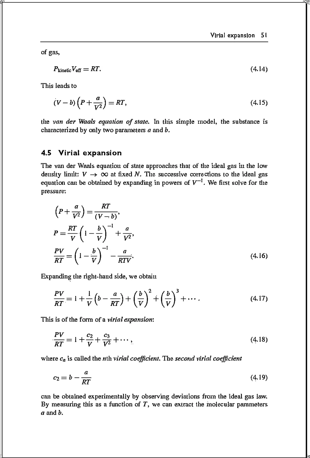
Wria I expansion 51
Critical pomt 52
Maxwell construction 53
Scaling 54
Problems 56
5 The statistical approach
5.1
5.2
5.3
5.4
5.5
5.6
5.7
5.8
The atomic view 60
Phase space 62
Distribution function 64
Ergodic hypothesis 65
Statistical ensemble 65
Microcanonical ensemble 66
Tl\e most probable distribution 68
Lagrange multipliers 69
Problems 71
6 MaxweU-Boltziiiami distribution
6.}
6.2
6.3
6.4
6.5
6.6
6.7
6.8
6.9
Determining the parameters 74
Pressure of an ideal gas 75
Equipartitioj] of energy 76
Distribution of speed 77
Entropy 79
Derivation of thennodynamics 80
Fluctuations 81
T}\e Boltzmann factor 83
Time's arrow 83
Problems 85
45
60
74
7 Transport phenomena
7.1
7.2
7.3
7.4
7.5
7.6
7.7
7.8
Collisionless and hydrodynamic regimes
Maxwell's demon 91
Non-viscous hydrodynamics 91
Sound-waves 93
Diffusion 94
Heat conduction 96
Viscosity 97
Navier-Stokes equation 98
Problems 99
8 Quantum statistics
8.1 Thermal wavelength 102
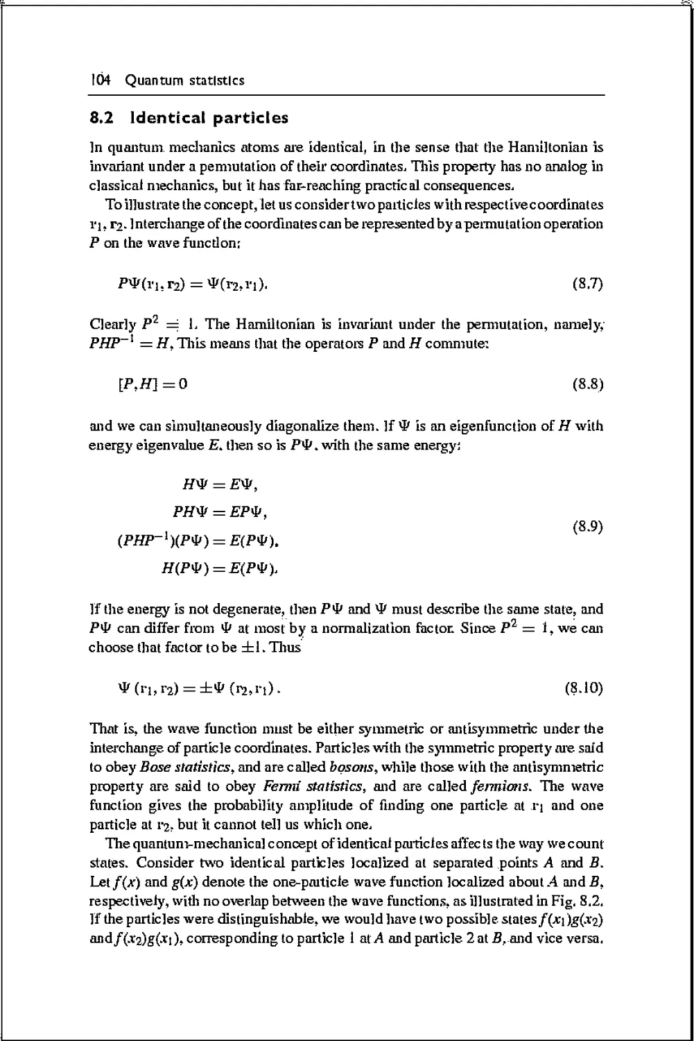
8.2 Identical particles 104
8.3 Occupation numbers 105
8.4 Spin 107
8.5 Microcanonical ensemble 108
8.6 Fermi statistics 109
8.7 Bose statistics 110
8.8 Determining the parameters III
8.9 Pressure 112
8.10 Entropy 113
8.11 Free energy 114
8.12 Equation of state 114
8.13 Classical limit 115
Problems 117
9 The Fermi gas
9.1 Fermi energy 119
9.2 Ground state 120
9.3 Fermi temperature 121
9.4 Low-temperature properties 122
9.5 Particles and holes 124
9.6 Electrons in solids 125
9.7 Semiconductors 127
Problems 129
10 The Bose gas
10.1 Photons 132
10.2 Bose enliancement 134
10.3 Phonons 136
10.4 Debye specific heat 137
x Contents
10.5 Electronic specific heat }39
10.6 Conservation of particle number 140
Problems 141
11 Bose-Eiustein condensation
1}.} Macroscopic occupation 144
1 }.2 The condensate 146
11.3 Equation of state 148
11.4 Specific heat 149
11.5 How a phase is formed 150
11.6 Liquid-helium 152
Problems 154
12 Canonical ensemble
12.} Microcanonical ensemble }57
12.2 Classical canonical ensemble 157
12.3 The partition function 160
12.4 Connection witii thermodynamics 160
12.5 Energy fluctuations 16}
12.6 Minimization of free energy 162
12.7 Classical ideal gas 164
12.8 Quantum ensemble 165
12.9 Quantum partition function 167
12.10 Choice of representation }68
Problems 168
13 Grand canonical ensemble
13.1 T7ie particle reservoir 173
13.2 Grand partition function 173
13.3 Number fluctuations 174
13.4 Connection witfi thermodynamics 175
13.5 Critical fluctuations 177
13.6 Quantum gases in the grand canonical ensemble 178
13.7 Occupation number fluctuations 180
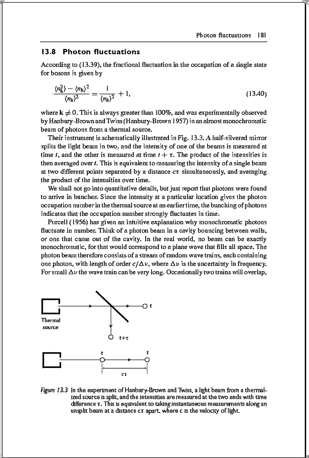
13.8 Photon fluctuations 181
13.9 Pair creation 182
Problems 184
14 The order parameter
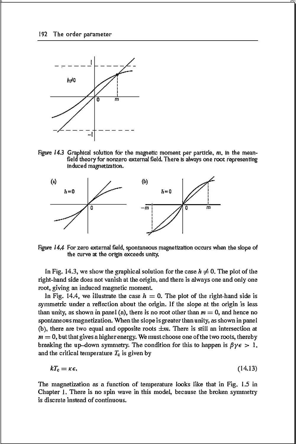
14.1 Broken symnietry 188
14.2 Ising spin model 189
14.3 Ginsburg-Landau theory 193
144
157
173
188
Contents xl
14.4 Mean-field theory 196
14.5 Critical exponents 197
14.6 Fluctuation-dissipation theorem 199
14.7 Correlation length 200
14.8 Universality 201
Problems 202
15 Superfluidity 205
15.} Condensate wave function 205
15.2 Mean-field theory 206
15.3 Gross—Pitaevsky equation 208
15.4 Quantum phase coherence 210
15.5 Superfluidflow 21}
15.6 Superconductivity 2}3
15.7 Meissnereffect 2}4
15.8 Magnetic flux quantum 2} 4
15.'9 Josephson junction 216
15.10 The SQUID 220
Problems 222
16 Noise 226
16.1 Thermal fluctuations 226
16.2 Nyquist noise 227
16.3 Brownian motion 229
16.4 Einstein's theory 23}
16.5 Diffusion 233
16.6 Einstein's relation 234
16.7 Molecular reality 236
16.8 Fluctuation and dissipation 237
Problems 238
17 Stochastic processes 240
17.} Randomness and probability 240
17.2 Binomial distribution 241
17.3 Poisson distribution 243
17.4 Gaussian distribution 244
17.5 Central limit theorem 245
17.6 Shot noise 247
Problems 249
xll Contents
18 Time-series analysis 252
18.} Ensemble of paths 252
18.2 Power spectrum and correlation function 254
18.3 Signal and noise 256
18.4 Transition probabilities 258
18.5 Markov process 260
18.6 Fokker—Planck equation 26}
18.7 Langevin equation 262
18.8 Brownianmotion revisited 264
18.9 The Monte-Carlo method 266
18.10 Simulation of the Ising model 268
Problems 270
Appendix: Mathematical reference 274
Notes
References
Index
281
282
284
Preface
This book is based on the lecture notes for a one-semester course on statistical
physics at M.I.T., which I have taught to advanced undergraduates. They were
expected to have taken introductory courses in classical and quantum physics,
including thermodynamics. The object of this book is to guide the reader quickly
but critically through a statistical view of the physical world.
The tour is divided into stages. First we introduce thermodynamics as a plie-
nomenological theory of matter, and emphasize the power and beauty of such
an approach. We then show how all this can be derived from the laws governing
atoms, with the help of the statistical approach. This is done using the ideal gas,
both classically and quantum mechanically. We show what a wide range of
physical phenomena can be explained by the properties of the Bose gas and the Fermi
gas. Only then do we launch into the formal methods of statistical mechanics, the
canonical ensemble and the grand canonical ensemble.
In the last stage we return to phenomenology, using insight gained from the
microscopic level. The order parameter is introduced to describe broken
symmetry, as manifested in superfluidity and superconductivity. We spend quite some
time on noise, beginning with Einstein's description of Brownian motion, through
stochastic processes and time-series analysis, and ending with the Monte-Carlo
method.
There is more material in this book than one could comfortably cover in one
semester, perhaps. As a rough division, twelve chapters in this book ore on "general
topics7' and six on "special applications". A course might cover all of the general
topics, with choices of special applications that vary from year to year. Among the
general topics are Chapters 1—3 on thermodynamics, Chapters 5, 6 and 8 on the
kinetic theory of the ideal gas* Chapters 9 and 10 on the Bose and Fermi gases,
Chapters J2 and 13 on formal statistical mechanics, and Chapters 17 and 18 on
stochastic processes. That leaves six chapters on such things as transport
phenomena, Bose-Einstein condensation, Josephson junction, and Brownian motion.
The emphasis of tills book is on physical understanding.rather than calculational
techniques, although Dirac would say that to understand is to know how to
calculate. I have included quite a few problems at the end of each chapter for the latter
purpose.
xlv Preface
I would like to thank the M.I.T. students who had.endured 8.08t and Aleksey
Lomakin and Patrick Lee, with whom I have enjoyed teacliingthat course, wliich
led to the writing of this book.
Kerson Huang
Boston, Massachusetts , 2001
Chapter I
The macroscopic view
I.I Thermodynamics
The world puts on different faces for observers using different scales in the
measurement of space and time. The everyday, macroscopic world, as perceived on the
scale of meters and seconds, looks very different from that of the atomic
microscopic world, which is seen on scales smaller by some ten orders of magnitude.
Different still is the submicroscopic realm of quarks, which is revealed only when
the scale shrinks further by another ten orders of magnitude. With an expanding
scale in the opposite direction, one enters the regime of astronomy, and ultimately
cosmology. These different pictures arise from different ways of organizing data,
while the basic laws of physics remain the same.
The physical laws at the smallest accessible length scale are the most
"fundamental", but they are of little use on a larger scale, where we must deal with
different physical variables. A complete knowledge of quarks tells us nothing
about the structure of nuclei, unless we can define nuclear vaiiables in terms of
quarks, and obtain their equations of motion from those for quarks, Needless to
say, we are unable to do this in detail, although we can see how .this could be done
in principle. Therefore, each regime of scales has to be described phenomenolog-
ically, in terms of variables and laws observable in that regime. For example, an
atom is described in terms of electrons and nuclei without reference to quarks. The
subnuclear world enters the equations only implicitly, through such parameters as
the mass ratio of electron to proton, which we take from experiments in the atomic
regime. Similarly, in the macroscopic domain, where atoms are too small to be
visible, we describe matter in terms of phenomenoiogical variables such as
pressure and temperature, The atomic structure of matter enters the picture implicitly,
in terms of properties such as density and heat capacity, which can be measured
by macroscopic instruments.
From experience, we know that a macroscopic body generally settles down, or
"relaxes" to a stationary state after a short time. We call this a state of thermal
equilibrium. When the external condition is changed, the existing equilibrium
state will change, andr after a relatively short relaxation time, settles down to
another equilibrium state. Thus, a macroscopic body spends most of the time in
2 The macroscopic view
some state of equilibrium, punctuated by almost sudden transitions, In our study
of macroscopic phenomena, we divide the subject roughly under the following
headings:
• Thermodynamics is a phenomenoiogical theory of equilibrium states and
transitions among them,
• Statistical mechanics is concerned with deducing the thermodynamic
properties of a macroscopic system from its microscopic structure,
• Kinetic tlieory aims at a microscopic description of the transition process
between equilibrium states.
This book is concerned mainly with statistical methods, which provide a bridge
between the microscopic and the macroscopic world. We begin our study with
thermodynamics, because it is a highly successful phenomenoiogical theory, which
identifies the correct macroscopic variables to use, and serves as a guide post for
statistical mechanics.
1.2 Thermodynamic variables
As a rule, properties of a macroscopic system can be classified as either extensive
or intensive;
• Extensive quantities are proportional to the amount of matter present,
• Intensive quantities are independent of the amount of matter present,
Genemlly, there are only these two categories, because we can neglect surface
effects, A macroscopic body is typically of size L ~ 1 m, while the range of
atomic forces is of order 7¾ ~ 10-10 m. The macroscopic nature is expressed by
the ratio Ljr\\ ™ 10 , The surface-to-volume ratio, rendered dimensionless in
terms of the range of atomic forces, is of order ro/L ™ .10 , The extensive
property expresses the "saturation property" of atomic forces, i,e., an atom can
''feel" only as far as the range of the force. The intensive property' means that atoms
in the interior of the body do not feel the presence of the surface,
Exceptions arise when any of the following conditions prevail;
• The system is small,
• There is a non-uniform external potential.
• There are long-ranged interparficle forces, such as the Coulomb repulsion
between charges, and the gravitational attraction between mass elements.
• The geometry is such that the surface is important.
These exceptions occur in important physical systems. For example, the volume
of a star is a non-linear function of its mass, due to the long-ranged gravitational
interaction. We illustrated the different cases in Fig. 1.1,
Thermodynamic limit 3
Extensive
Small system
o o° O O » 0
O ° O
Long-ranged interaction
or in external field
Not extensive
Strange shape
Figure J. J A body has extensive properties If surface effects can be neglected, so that the
energy is proportional to the number of particles. In these pictures, the surface
layer is indicated by a heavy line.
1.3 Thermodynamic limit
We consider a materia! body consisting of N atoms in volume V, with no
nonuniform external potential, in the idealized limit
N -J- 00, V
— = fixed number.
V
<x>,
(1.1)
This is called the'thermodynamic limits in which the system is translntionally
invariant.
The thermodynamic state is specified by a number of thermodynamic variables,
which are assumed to be either extensive (proportional to N), or intensive
(independent of N). We consider a generic system described by the three variables P,
Vand T, denoting, respectively, the pressure, volume and the temperature:
The pressure Pt an intensive quantity, is the force per unit area that the body
exerts on a wall, which can be that of the container of the system, or it maybe
one side of an imaginary surface inside the body. Uhderequilibriumconditions
in the absence, of external potentials, the pressure must be uniform throughout
the body. It is convenient to measure pressure in terms of the atmospheric
4 The macroscopic view
pressure at sea level:
1 arm = 1.013 x 10⁶dynecm~2 = 1.103 x 10⁵Nm~2 (1.2)
• The volume V measures the spatial extent of the body, and is an extensive
quantity. A solid body maintains its own characteristic density JV/V. A gas,
however, fills the entire volume of its container.
• The temperature T, an intensive quantity, is measured by some thermometer.
It is an indicator of thermal equilibrium. Two bodies in contact with each
other in equilibrium must have the same temperature. Since the two bodies in
question can be different parts of the same body, the temperature of a body in
equilibrium must be uniform. The temperature is also a measure of the energy
content of a body, but the notion of energy has yet to be defined., through the
first law of thermodynamics.
In the thermodynamic limit we must use only intensive quantities,
mathematically speaking. Instead of V we should use the specific volume v = V/N, or
the density n = NfV* However, it is convenient to regard V as a large but finite
number,, for this corresponds to the everyday experience of seeing the volume of
a macroscopic body expand or contract, while the number of atoms is fixed.
There are systems requiring other variables in addition to, or in place of, P, V
and T. Common examples are the magnetic field and magnetization for a magnetic
substance, the strain and stress in elastic solids, or the surface area and the surface
tension.
1.4 Thermodynamic transformations
When a body is in thermal equilibrium, the thermodynamic variables are not
independent of one another, but are constrained by an equation of state of the form
/(P,V,T)=0, (1.3)
where the function f is characteristic of the substance. This leaves two
independent variables out of the original three. Geometrically we can represent the
equation of state by a surface in the state space spanned by P, V, T, as shown in
Fig. 1.2. All equilibrium states must lie on this surface. We regard/as acontinuous
differentiable function, except possibly at special points.
A change in the external condition will change the equilibrium state of a system.
For example, application of external pressure will cause the volume of a body to
decrease. Such a change is called a thermodynamic transformation* The initial
and final states are equilibrium states. If the transformation proceeds sufficiently
slowly, the system can be considered to remain in equilibrium. In such a case, we
say that the transformation is quasi-static. This usually means that the
transformation is reversible, in that the system will retrace the transformation in reverse when
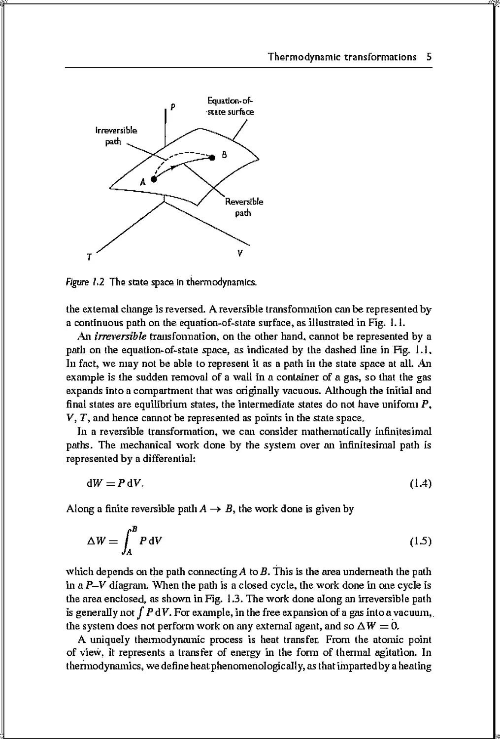
Thermodynamic transformations 5
Equation-of-
state surface
figure hi The state space in thermodynamics.
the external change is reversed. A reversible transformation can be represented by
a continuous path on the equation-of-state surface, as illustrated in Fig. 1.1.
.An irreversible transformation, on the other hand, cannot be represented by a
path on the equation-of-state space, as indicated by the dashed line in Fig. 1.1,
In fact, we may not be able to represent it as a path in the state space at all. An
example is the sudden removal of a wall in a container of a gas, so that the gas
expands into a compartment that was originally vacuous. Although the initial and
final states are equilibrium states, the intermediate states do not have uniform P,
V, T, and hence camiot be represented as points in the state space.
In a reversible transformation, we can consider mathematically infinitesimal
paths. The mechanical work done by the system over an infinitesimal path is
represented by a differential:
&W = PAV, (1.4)
Along a finite reversible path A —>■ 5, the work done is given by
AW= J PdV (1.5)
which depends on the path connecting j4 to 5. This is the area underneath the path
in a P—V diagram. When the path is a closed cycle, the work done in one cycle is
the area enclosed, as shown in Fig. 1.3. The work done along an irreversible path
is generally not/PdV. For example, in the free expansion of a gas into a vacuum,,
the system does not perform work on any external agent, and so AW = 0r
A uniquely thermodynamic process is heat transfer. From the atomic point
of view, it represents a transfer of energy in the form of thermal agitation. In
thermodynamics, we define heat phenomehologically, as that impartedby a heating
6 The macroscopic view
I Work
Figure J3 The work done In a closed cycle of transformations Is represented by the area
enclosed by the cycle in a P-V diagram.
element, such as a flame or a heating coil. An amount of heat AQ absorbed by a
body causes a rise AT in its temperature given by
AQ = CAT, (1.6)
where C is the heat capacity of the substance. We imagine the limit in which
AQ and AT become infinitesimal. The heat capacity is an extensive quantity. The
intensive heat capacity per particle (C/JV), per mole (C/«), or per unit volume
(C/V), are called specific heats.
The fact that heat is a form of energy was established experimental ly, by
observing that one can increase the temperature of a body by AT either by transferring
heat to the body, or performing work on it A practical unit for heat is the calorie^
originally defined as the amount of heat that will mise the temperature of 1 g of
water from 14.5°C to 15.5°C at sea level. In current usage, it is defined exactly in
terms of the joule:
lcal = 4.184J. (1.7)
Another commonly used unit is the British thermal unit (Btu):
!Btu= 1,055J. (1.8)
The heat absorbed by a body depends on the path of the trans format ion. as is
true of the mechanical work done by the body. We can speak of the amount of
heat absorbed in a process; but the "heat of a body", like the "work of a body", is
meaningless. Commonly encountered transformations are the following:
• T = constant (Isothermal process)
• P = constant (Isobaric process)
• V = constant (Constant-volume process)
• AQ = 0 (Adiabatic process).
Classical ideal gas 7
We use a subscript to distinguish the different types of paths, as for example Cy
and Cpt representing, respectively, the heat capacity at constant volume and
constant pressure. The heat capacity is only one of many thermodynamic coefficients
that measure the response of the system to an external source. Other examples are
1 AV
K = —— (Compressibility),
1 AV
a = ——— (Coefficient of thermal expansion). 0*9)
These coefficients can be obtained from experimental measurements. In principle,
they can be calculated from atomic properties using statistical mechanics.
1.5 Classical ideal gas
The simplest tliemiodynamic system is the classical ideal gas, which is a gas in
the limit of low density and high temperature. The equation of state is given by
the ideal-gas law
PV=MT, (1.10)
where T is the ideal gas temperature, measured in kelvin (K). and
Jfc-= 1-381 x 10_16ergK_1 (Boltzmann's constant). (1.11)
As we shall see. the second law of thermodynamics implies T > 0, and the lower
bound is called the absolute zero. For this reason, T is also called the absolute
temperature. The heat capacity of a nionatomic ideal gas at constant volume, Cy.
has the value
Cy=§Aft. (1.12)
These properties of the ideal gas were established experimentally, and can be
derived theoretically in statistical mechanics.
Thermodynamics does not assume the existence of atoms. Instead of the number
of atoms N, we can use the number of gram moles «, which is a chemical property
of the substance. The two are related through
Nk=nR.
(1.13)
R = 8.314 x 10' erg K-1 (Gas constant).
The ratio R/k is Avogadro's number, the number of atoms per mole:
A0=- = 6.022 x 10²³. (1.14)
Indeed, the atomic picture emerged much later and gained acceptance only after a
long historic struggle (see Chapter 16 on Brownian motion).
8 The macroscopic view
Figure \A Isotherms of an ideal gas, and various paths of transformations.
The equation of state can be represented graphically in a P- V diagram, as shown
in Fig. 1.4, which displays a family of curves at constant T called isotherms.
Indicated on this graph are the reversible paths corresponding to various types of
transformations:
• ab is isothermal
• be proceeds at constant volume
• cd is at constant pressure
• de is isothermal
• abedea is a closed cycle
• df is non-isothermaL
To keep the temperature constant during an isothermal transformation, we keep
the system in thermal contact with a body so large that its temperature is not
noticeably affected by heat exchange with our system. We call such a body a heat
reservoir* or heat bath.
1.6 First law of thermodynamics
The first law expresses the conservation of energy by including heat as a fomi of
energy. It asserts that there exists a function of the state, internal energy t/. whose
change in any thermodynamic transformation is given by
AU = AQ-AW, (1.15)
that is, A U is independent of the path of the transformation, although AQ and A W
are path-dependent. In a reversible infinitesimal transformation, the infinitesimal
Magnetic systems 9
changes dQ and dW are not exact differentials, in the sense that they do not
represent the changes of definite functions, but their difference
dU = dQ-dW (1.16)
is an exact differential.
1.7 Magnetic systems
For a magnetic substance, the thermodynamic variables are the intensive magnetic
field H and the extensive magnetization M. which are unidirectional and uniform
in space. The magnetic field is generated by external real currents (and not induced
currents), and the magnet work done by the system is given by
dW=-H.dM. (1.17)
The first law takes the form
dU = dQ + HdMt (1.18)
which maps into that for a PVT system under the correspondence H -o- —P.
M*+ V.
For a paramagnetic substance, a magnetic field induces a magnetization density
given by
Y = x**- (1.19)
The magnetic susceptibility ;[ obeys Curie's law.
X = f (1.20)
Thus, we have the equation of state
M=—, (1.21)
where /c = coV.
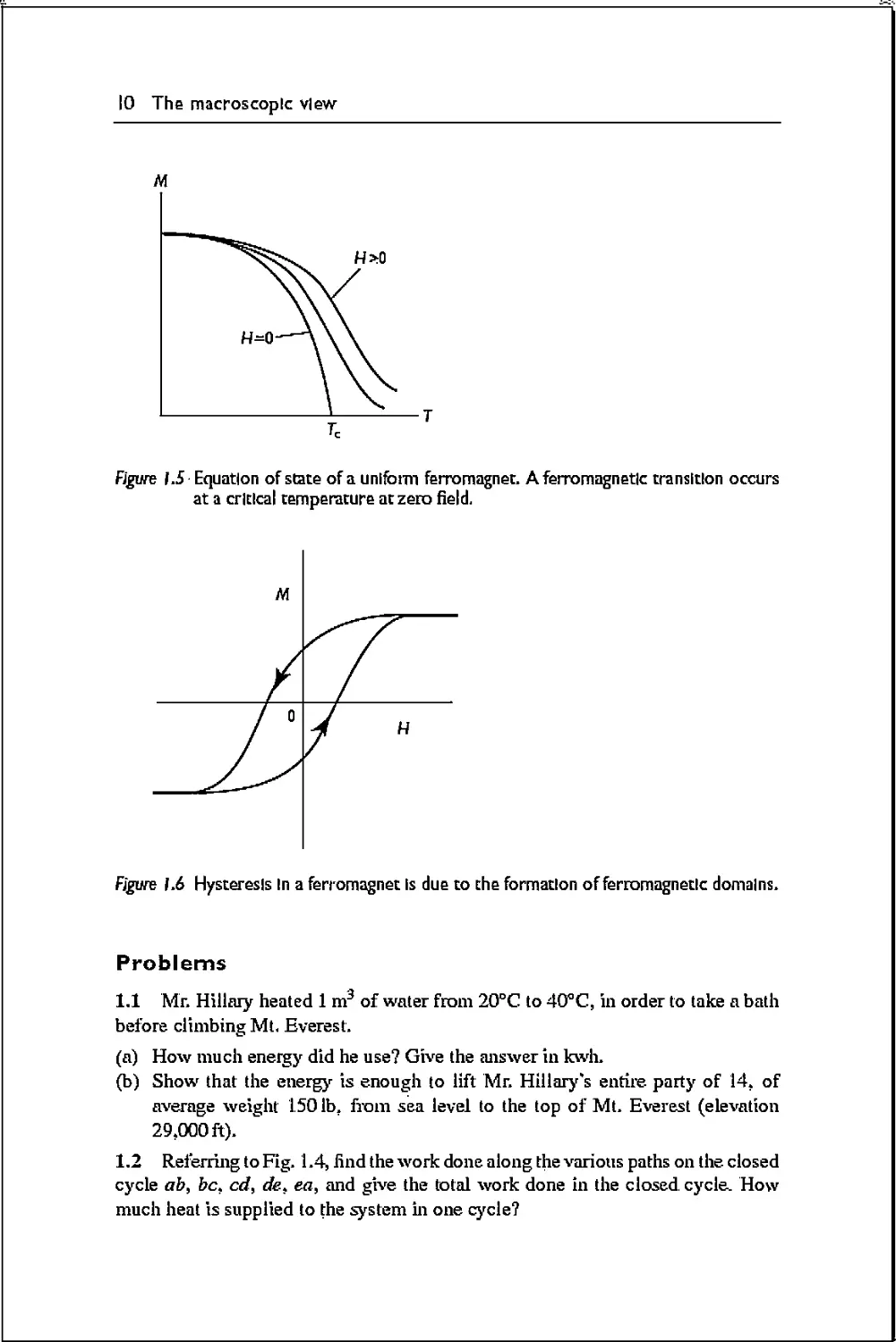
An idealized uniform ferromagnetic system has a phase transition at a critical
temperature Tc, and becomes a permanent magnet for T < Tc in the absence of
external field. However, there is no phase transition in the presence of an external
field. The equation of state is illustrated graphically in the M—T diagram of Fig. 1.5.
A real ferromagnet is not uniform, but breaks up into domains with different
orientations of the magnetization. The configuration of the domains is such as to
minimize the magnetic energy, by reducing the fringing fields that extend outside of
the body. Each domain behaves according to the uniform case depicted in Fig. 1.5.
At a fixed T < Tc, the domain walls move in response to a change in H. to either
consolidate old domains orcreate new ones. This is adissipative process, and leads
to hysteresis, as shown hi the M—H plot of Fig. .1.6.
10 The macroscopic view
Figure 1.5 Equation of state of a uniform ferromagnet. A ferromagnetic transition occurs
at a critical temperature at zero field.
Figure 1.6 Hysteresis In a ferromagnet is due to the formation of ferromagnetic domains.
Problems
1.1 Mr. Hillary heated 1 m3 of water from 20°C to 40°C, in order to take a bath
before climbing Mt, Everest.
(a) How much energy did he use? Give the answer in kwh.
(b) Show that the energy is enough to lift Mr. Hillary's entire party of 14, of
average weight 1501b, from sea level to the top of Mt. Everest (elevation
29,000 ft).
1.2 Referring to Fig. 1.4, find the work done along the various paths on the closed
cycle ab, be. cd, de. ea, and give the total work done in the closed cycle. How
much heat is supplied to the system in one cycle?
Problems 11
1.3 An ideal gas undergoes a reversible transformation along the path
b
V__ (T_
Vo ~ \T0
where Vb> Tq and b are constants.
(a) Find the coefficient of thermal expansion.
(b) Calculate the work done by the gas when the temperature increases by AT.
1.4 In a non-uniform gas. the equation of state is valid locally, as long as the
density does not change too rapidly with position. Consider a column of ideal gas
under gravity at constant temperature. Find the density asa function of height, by
balancing the forces acting on a volume element.
1.5 Two solid bodies labeled 1 and 2 are in thermal contact with each other. The
initialtemperatu'reswere7"t.72, with7"t > 72.Theheatcapacitiesare, respectively.
C\ and Ci. What is the final equilibrium temperature, if the bodies are completely
isolated from the external world?
1.6 A paramagnetic substance is magnetized in an external magnetic field at
constant temperature. How much work is require to attain a magnetization Ml
1.7 A hysteresis curve (see Fig. 1.6) is given by the formula
M = Motanh(tf±#o).
where the + sign refers to the upper branch, and the — sign refers to the lower
branch. The parameter Hq is called the "coersive force". Show that the work done
by the system in one hysteresis cycle is — 4MqHq,
1.8 The atomic nucleus: The atomic nucleus contains typically fewer than 300
protons and neutrons. It is an example of a small system with both short- and
long-ranged forces. The mass is given by the semi-empirical Weizsacker formula
(deShalit 1994):
M = Zmp + Nma - axA + a2A2{3 + «37773 + «4-—7—^- + &{A)t
where Z is the number of protons. JV is the number of neutrons, and A = Z+N. The
masses of protons and neutrons are, respectively, »?p and;n„. and <7j(/ = 1..,, ,4)
are numerical constants:
volume energy: a\ = 16MeV/c\
surface energy: ai = 19,
Coulomb energy: 03 = 0,72,
symmetry energy; a^ = 28,
The symmetry energy favors A = Z. The term S(A) is the "pairing energy" that
gives small fluctuations.
12 The macroscopic view
Take Z = N = A/2, mn « m$, and neglect 5(A), so that
M = (Hip - a{)A + aaA2'3 + ^A5*\
Make a log plot of M fromA = 1 to A = ltF, and indicate the range in which M
can be considered as extensive,
1,9 The false vacuum'. In the theory of the "inflationary universe", a pin-point
universe was created during the Big Bang in a "false" vacuum state characterized
by a finite energy density wo, while the true vacuum state should have zero energy
density (Guth 1992).
An ordinary solid, too, has finite characteristic energy per unit volume, but it
occupies a definite volume, given a total number of particles. If we put the solid
in a box larger than that volume, it would not fill the box, but "rattle1' in it. Not so
for the false vacuum. It must have the same energy density whatever its volume,
and this makes it a strange object indeed.
(a) Imagine putting the false vacuum in a cylinder with piston, with a true vacuum
outside. If we pull on the piston to increase the volume of the false vacuum
by dV. show that the false vacuum performs work dlV = —ho dV. Hence the
false Vacuum has negative pressure P = —uq.
(b) According to general relativity the radius R of the universe obeys the equation
d2R 4jt , „„ „
__=__G(„0_3W
where c is the velocity of light, and
G = 6.673 x 10~8cni3/gs2 = 6.707 x ICr^GeV-2^3
is Newton's constant (gravitational constant). For the false vacuum, this
reduces to
d2R _ R
I 3c2
SttGwo
Thus, the radius of the universe expands expands exponentially with time
constant t. According to theory, u0 = (1015 GeV)4/(?jc)3 =■ 1096 erg/cm3.
Show that
T w 10-Ms.
Chapter 2
Heat and entropy
2.1 The heat equations
Thermodynamics becomes a mathematical science when we regard the state
functions, such as the internal energy, as continuous differentiable fanctions of the
variables P, VaiidT. The constraint imposed by the equation of state reduces the
number of independent variables to two. We may consider the internal energy to
be a function of any two of the variables. Under infinitesimal increments of the
variables, we can write
dU(P,V) = ( —) dP+( —) dV,
/dU\ /3CA
d[/(P, 7) =(-)^+(-)^, (2,)
/au\ /du\
iU<-V^={-3v)TiV+{-3f)viT'
where a subscript on a partial derivative denotes the variable being held fixed. For
example. (3 U/dP)y is the derivative with respect to P at constant V. These partial
derivatives are thermodynamic coefficients to be taken from experiments.
The heat absorbed by the system can be obtained from the first law, written in
the form dQ = dU + P dV:
<-(S)."[(£H--
aD-(li7)ra'+(aF),dr+pav- <*"
"-[Wr*']"*®."-
14 Heat and entropy
In the second of these equations, we must regard V as a function of P and T, and
rewrite
dV = (—\ dP + (—\ d7". (2.3)
The second equation then reads
"-[©^©j-e5^).-- -
It is convenient to define a state function called the entfialpyi
H = U+PV. (2.5)
The heat equations in terms of dQ are summarized below:
--©.-♦[GSM--
-[(^♦'(aMS).--
We can immediately read off the heat capacities at constant V and P:
These are useful, because they express the heat capacities as derivatives of state
functions.
2.2 Applications to ideal gas
We now use the first law to deduce some properties of the ideal gas. Joule performed
a classic experiment on free expansion, as illustrated in Fig. 2.1. A thermally
insulated ideal gas was allowed to expand freely into an insulated chamber, which
was Initially vacuous , After a new equilibrium was established, in which the gas
fills bodi compartments, the final temperature was found to be the same as the
initial temperature. We can draw the following conclusions:
• AW = 0, since the gas pushes into a vacuum.
• AQ = 0, since the temperature was unchanged.
• AU = 0, by the first law.
Applications to Ideal gas 15
Insulatingwails ... . . ^
, Hole with stopper
z
■T./
fl»
/
Vacuum
.
Sffi
Ideal £as
Before -After
Figure 2.} Free expansion of an ideal gas.
Choosing V and 7" as independent variables, we conclude that U( Vi,T) = t/fVjT),
that is, U is independent of V:
U = U(T).
(2.8)
Of course. U is proportional to the total number of particles N, which has been
kept constant.
The heat capacity at constant volume can now be written as a total derivative:
(2.9)
Cy=(™) =^.
\BT/Y d7"
Assuming that Cy is a constant, we can integrate the above to obtam
U(T)= J CydT = CvTt (2.10)
where the constant of integration has been set to zero by defining U = 0 at T = 0,
It follows that
CP =
-(3),-(
dU d(MT)
= ~df^ 37"
= Cy+Nk,
Thus, for an ideal gas,
CP-Cy= Nk.
d(U + PV)\
dT )P
(2.11)
(2.12)
We now work out the equation governing a reversible adiabatic transformation.
Setting dQ = 0, we have dU = —P dV, Since dU = Cy d7\ we obtain
CvdT+PdV = Q.
(2.13)
16 Heat and entropy
Using the equation of state PV = NkT, we can write
d(PV) PdV + VdP
iT = ANir= m ■ (2J4>
Thus,
CV(P dV + V dP) + NkP dV = 0,
CvVdP + (Cv+Nk)PdV = Oi (2.15)
CvVdP+CPP dV = 0t
or
dP dV
— + y— = 0, (2.16)
where
y = % (2.17)
Assuming that y is a constant,, an integration yields
IuP= —y In V + Constant. (2.LS)
or
PVY = Constant. (2.19)
Using the equation of state, we can rewrite this in the equivalent fomi
TV-1 = Constant. (2.20)
Since y > 1 according to (2.12). an adiabatic path has a steeper slope than an
isothemi in a P-V diagram, as depicted in Fig. 2.2.
23 Carnot cycle
In a cyclic transformation, the final state is the same as the initial state and.
therefore, At/ = 0, because U is a state function. A reversible cyclic process can be
represented by a closed loop in the P—V diagram. The area of the loop is the total
work done by the system in one cycle. Since At/ = 0, it is also equal to the heat
absorbed:
AW = AQ= <f) P dV = Area enclosed. (2.21)
A cyclic process converts work into heat, and retarns the system to its original
state. It acts as a heat engine, for the process can be repeated indefinitely. If the
cycle is reversible, it lans as a refrigerator in reverse.
Carnot cycle 17
Adiabatic
sotherm
Figure 2.2 Adiabatic line has a steeper slope than an Isotherm.
D Isotherm
T Adiabatic
Figure 2,3 Carnot cycle on P-V diagram of Ideal gas.
A Carnot cycle is a reversible cycle bounded by two isotherms and two adiabatic
lines. The working substance is .arbitrary, but we illustrate it for an ideal gas in
Fig. 2.3, where 7¾ > T[, The system absorbs heat Qi along the isothemi 7*2, and
rejects heat Q\ along 7*i, with Q\ > 0 and Qi > 0, By the first law. the net work
output is
W = fi2-Gl-
(2.22)
In one cycle of operation, the system receives an amount of heat Qi from a hot
reservoir, performs work IV, and rejects "waste heat" Q\ to a cold reservoir. The
efficiency of the Carnot engine is defined as
V Qi Qi
(2.23)
18 Heat and entropy
>- W
Figure 2.4 Schematic representation of Carnot engine.
which is 100% if there is no waste hent, i.e. Q\ = 0. But, as we shall see, the
second law of thermodynamics states that this is impossible,
We represent the Carnot engine by the schematic diagram shown in Fig, 2.4.
which emphasizes the fact that the working substance is irrelevant. By reversing
the signs of Q\ and Qi, and thus Wt we can run the engine in reverse as a Carnot
refrigerator.
2.4 Second law of thermodynamics
The second law of thermodynamics expresses the common wisdom that "heat does
not flow uphill". It is stated more precisely by Clausius:
There does not exist a thermodynamic transformation whose sole effect is to
deliver heat from a reservoir of lower temperature to a reservoir of higher
temperature.
An equivalent statement is due to Kelvin:
There.does not exist a thermodynamic transformation whose sole effect is to
extract heat from a reservoir and convert it entirely into work.
The important word is "sole". The processes referred to may be possible, but
not without other effects. The logical equivalence of the two statements can be
demonstrated by showing that the falsehood of one implies the falsehood of the
other. Consider two heat reservoirs at respective temperatures 7¾ and T[, with
r2 > 7-,.
Absolute temperature 19
(a) If the Kelvin statement were false, we could extract heat from 7"j and convert
it entirely into work. We could then convert the work back to heat entirely, and
deliver it to T% (there being no law against this). Thus, the Clausius statement
would be negated.
(b) If the Clausius' statement were false, we could let an amount of heat Qi flow
uphill, from 7"j to T%. We could then connect a Camot engine between .7¾ and
7"j, to extract Qi from 7*2, and return an amount Q\ < Qi back to 7"j. The net
work output is Qi — Q\ > 0. Thus, an amount of heat Qi — Q\ is converted
into work entirely, without any other effect. Tliis would contradict the Kelvin
statement. ■
In the atomic view, heat transfer represents an exchange of energy residing in
the random motion of the atoms. In contrast, the performance of work requires
an organized action of the atoms. To convert heat entirely into work would mean
that chaos spontaneously reverts to order. This is extremely improbable, for in
the usual scheme of things, only one configuration corresponds to order, while all
others lead to chaos, The second law Is the thermodynamic way of expressing this
Idea.
2.5 Absolute temperature
The second law Immediately implies that a Camot engine cannot be 100 % efficient,
for otherwise all the heat absorbed from the upper reservoir would be converted
into work in one cycle of operation. There is no other effect, since the system
returns to its original state.
We can show that no engines working between two given temperatures can be
more efficient than a Camot engine. Since only two reservoirs are present, a Camot
engme simply means a reversible engine. What we assert then is that an irreversible
engme cannot be more efficient than a reversible one,
ConsideraCarnotengine Cand an engineX (notnecessarily reversible) working
between the reservoirs 7¾ and 7"j, with 7¾ > 7"j, as shown in Fig. 2.5. We shall
run C in reverse, as a refrigerator C, and feed the work output of X to C. Table 2.1
shows a balance sheet of heat.transfer in one cycle of joint operation.
The total work output Is
WW = (02 - Gi) - (22 - Gi> (2-24)
Now arrange to have Q'2 = Qi* Then, no net heat was extracted from the reservoir
7¾. which can be ignored. An amount of heat Q\ — Q\ was extracted from the
reservoir T\, and converted entirely into work with no other effect. This would
violate the second law, unless Q \ < Q^, Dividing both sides of this Inequality by ■
Qi, and us big the fact that 22 — 22* we have
(2.25)
20 Heat and entropy
Qi
i
Qi
*
w
w
\
QI
Figure 2.5 Driving a Carnot refrigerator C with an engine X.
Table 2.1
Engine
X
c
Balance sheet of
heat transfer
From Ti
-Qi
ToTi
-Qi
Therefore, 1 -(Qi/Q2) > 1 - ($/00, or
ye > m-
(2.26)
As a corollary, a]] Camot engines have the same efficiency; since X may be a
Carnot engine. This shows that the Carnot engine is universal, in tliat it depends
only on the temperatures involved, and not on the working substance.
We define the absolute temperature 8 of a heat reserveir such that the ratio of
the absolute temperatures of two reservoirs is given by
ft 0i .
(2.27)
where /7 is the efficiency of a Camot engine operating between the two
reservoirs. The advantage of this definition is that it is independent of the properties of
any working substance. Since Q\ > 0 according to the second law. the absolute
temperature is bounded from below:
> 0.
(2.28)
The absolute zero* 0 = 0, is a limiting value which we can never reach, again
according to the second law.
The absolute temperature coincides with the ideal gas temperature defined by
T =. PVfNk* as we can show by using an idea] gas as working substance in
TomperaturQ as Integrating factor 21
i
a Camot engine. Thus. 8 = T, and we shall henceforth denote the absolute
temperature by 7".
Tlie existence of absolute zero does not mean that the temperature scale
terminates at the low end, for the scale is an open set without boundaries. It is a
matter of convention that we call T the temperature. We could have used 1 /T as
the temperature, and what is now absolute zero would be infinity instead.
2.6 Temperature as integrating factor
We can look upon the absolute temperature T as the integrating factor that converts
the Inexact differentia] dQ into an exact differential dQ/T* In order to show this,
we first prove a theorem due to Clausius:
In an arbitrary cyclic process P, the following inequality holds:
dQ
-^- < 0, (2.29)
where the equality holds if P is reversible.
It should be emphasized that the cycle process need not be reversible. In order
to prove the assertion, divide the cycle P into K segments labeled i = 1,..., K.
Let the ith segment be in contact with a reservoir of temperature 7"/, from which it
absorbs an amount of heat 2,. The total work output of P is, by the first law,
w=Y^Qi- (2-30)
f=t
Note that not all the Qi can be positive, for otherwise heat would have been
converted into work with no other effect, in contradiction to the second law.
Imagine a reservoir at a temperature 7¾ > 7"/ (all j), with Camot engines Q
operating between 7¾ and each of the temperatures 7/. The setup is illustrated
schematically in Fig. 2.6. Suppose that, in one cycle of operation, the Camot
engine Q absorbs heat Qj from the 7¾ reservoir, and rejects Q-t to the T\ reservoir.
By definition of the absolute temperature, we have
f=£. (2.3.)
In one cycle of operation of the joint operations {P + C\ -|— * + Cg},
• the reservoir 7"/ experiences no net change, for it receives Q-It and delivers the
same to the system;
• the lieal extracted from the 7¾ reservoir is given by
K K
i=\ 1=1 1{
ft* = ^Qf» = r0^f; (2.32)
22 Heat and Qntropy
the total work output is
ww = w+J2 [dP - a] = £ Q? = Q*.
(2.33)
An amount of heat Qtct would be entirely converted, into work with no othereffect,
and thus violate the second law, unless 2tot < 0* or
/=1 ll
In the limit K —¥■ 00. this becomes
(2.34)
if'
(2.35)
which proves the first part of the theorem.
If P is reversible, we can run the operation {P + Ci + * —|- Cjv} in reverse. The
signs for Qj are then reversed, and we conclude that $pdQ/T > 0. Combining
<2|
Pj
qP
^T~
C| C\j7
^\J£
C2
/
* c
lT1.
J. Reservoir y0
T
- /, ^
?c >
<2i
Q2
Closed cycle P
Figure 2.6 Construction to provQ Clauslus' theorem.
Entropy 23
this with the earlier relation, which still holds, we have
£
— = 0 (if P is reversible). (2.36)
P T
This completes the proof. ■
A corollary to the theorem is that, for a reversible open path P, the integral
fpdQ/T depends only on the endpoints. and not on the particular path. In order
to prove this, join the endpoints by a reversible path Pft whose reversal is denoted
by — P1. The combined processes P — P' then represents a closed reversible cycle.
Therefore, fP_P, dQ/T = 0, or
f dQ f dQ
This shows that dQ divided by the absolute temperature is an exact differential.
■
2.7 Entropy
The exact differential
dQ
dS=— (2.38)
defines a state function S called the entropy, up to an additive constant. The entropy
difference between any two states B and A is given by
fB dQ
S(B) - S(A) = I — (along reversible path), (2.39)
where the integral extends along any reversible path connecting B to A. The resu] t
is. of course, independent of the path, as long as such a reversible path exists.
What if we integrate along an irreversible path? Let P be an arbitrary path IVorh
A to B, reversible or not. Let if be a reversible path with the same endpoints. The
combined process P — R is a closed cycle and. therefore, by Clausius' theorem.
Jp_RdQ/T <0,or
Jp T -Jr T'
(2.40)
Since tlie right-hand side is the definition of the entropy difference between the
final state B and the initial state A, we have
5(5)- S(A) > / -^, (2.41)
'[f-
24 Heat and Qntropy
where the equality holds if the process is reversible. For an isolated system, wluch
does not exchange heat with the externa] world, we have dQ = 0 and, therefore,
A5> 0.
(242)
This means that the entropy of an isolated system never decreases, and it remains
constant during a reversible transformation.
We emphasize the following points:
• The principle that the entropy never decreases applies to the "universe"
consisting of a system and its environments. It does not apply to a non-isolated
system, whose entropy may increase or decrease.
• Since the entropy is a state function, the entropy change of the system in
going from state A to state B is 1¾ — 5a, regardless of the path, which
may be reversible or irreversible. For an irreversible path, the entropy of
the environment changes, whereas for a reversible path it does not.
• TheentropydifferenceSfl— S& isnotnecessarilyequaltothe integral f, dQ/T.
It is equal to the integral only if the path fromA to B is reversible. Otherwise,
it is generally larger than the integral.
2.8 Entropy of ideal gas
We can calculate the entropy of an ideal gas as a function of V and T by integrating
dS = dQ/T. In Fig. 2.7, we approach point A along two alternative paths, with
V kept fixed along path 1, and T kept fixed along path 2. Along path 1, we have
J dQ/T = CVJ dT/T and, hence,
S(V, 7") = S(V, T0) + Cv
rT dT T
/ — = S(V,7b) + Cvln—.
JTo t to
(243)
1 \path 2
[isothermal)
|A
Path 1
! To "
1 1
Figure 2.7 Calculating the entropy at point A.
The limits of thermodynamics 25
In order to determine S(V,Tq), we integrate dS = dQ/T along the isothermal
path 1. Since dU = 0, we have
dV
dg =dW = PdV= NkT —. (2.44)
Thus,
S(VtT) = S{VQ,T)+Nk f ^=S<y0tT)+Nk]a^-. (2.45)
JVa V Vq
Comparing the two expressions for 5(V. 7"), we conclude that
S(V, T0) = Co + Aft In V, (2.46)
where Co is on arbitrary constant. Absorbing the constant Vq into Co, we can write
S(V, T) = Co + Aft In V + Cv In 7". (2.47)
For a monatomic gas, we have Cy = l-Aft and, hence,
S( Vt T) = Co + Aft In (VT3/2). (2.48)
The constant Co is to be determined, and it could depend on N. A problem
arises when N changes, for S behaves like N]n V, and is not extensive, unless
somehow Co contains a term —Nk In N. As we shall see in Section \ 2.6, quantum
mechanics supplies the remedy by fixing Cq. The corrected entropy is given by
the Sacker-Tetrode equation
g-lnK)],
S = JVfc I - _ ln ("A )J ' <Z49>
w here n = N/V and A = J 27utrfmkT. The 1 atter is c a] 1 ed the thermal wavelength.
which is of order of the deBroglie wavelength of a particle with energy Xr7".
2.9 The limits of thermodynamics
Thermodynamics is an elegant theory and a very useful practical tool. The
self-consistency of the mathematical structure has been demonstrated through
axiomatic formulation. However, confrontation with experiments indicates that
thennodynamics is valid only insofar as the atomic structure of matter can be
ignored.
In the atomic picture, thermodynamic quantities are subject to small fluctuations.
The second law of thennodynamics is tiiie only on the macroscopic scale, when
such fluctuations can be neglected. It is constantly being violated on the atomic
scale.
Taking the second law as absolute would lead to the conclusion that the entropy
of the universe must forever increase, leading towards an ultimate "heat death".
Needless to say, thisceased to be imperative in the atomic picture. We shall discuss
the meaning of macroscopic irreversibility in more detail in Section 6.9.
26 Heat and Qntropy
Problems
2.1 An idea] gas undergoes a reversible transformation along the path P = aV ,
where a and b are constants, with a > 0. Find the heat capacity C along this path.
2.2 The temperature in a lake is 300 K at the surface, and 290 K at the bottom.
What is the maximum energy that can be extracted thermally from 1 g of water by
exploiting the temperature difference?
2.3 A nuclear power plant generates 1 MW of power at a reactor temperature of
600°F. It rejects waste heat into a nearby river, with a flow rate of 6,000fr/s, and
an upstream temperature of 7QPF. The power plant operates at 60% of maximum
possible efficiency. Find the temperature rise of the river
2.4 A slow-moving stream carrying hot spring water at temperature Ti joins a
sluggish stream of glacial water at temperature 7\. The water downstream has a
temperature T between 7^ and 7"t, and flows much faster, at a velocity v. Assume
tliat the specific heat of water is a constant, and that the entropy of water has the
same temperature dependence as that of an idea] gas.
(a) Find v, neglecting the velocities of the input streams. (Hint: The net change
In thermal energy was converted to kinetic energy.)
(b) Find the lower bound on T and the upper bound on v imposed by the second
law of thermodynamics. (Hinfc The total entropy cannot decrease.)
2.5 A cylinder of cross-sectional area A is divided into two chambers 1 and 2,
by means of a frictionless piston. The piston as well as the walls of the chambers
are heat-insulating, and the chambers initially have equal length L. Both chambers
are filled with 1 mo] of helium gas, with initial pressures 2/¾ and Pot respectively.
The.piston is then allowed to slide freely, whereupon the gas in chamber 1 pushes
the piston a distance a to equalize the pressures to P.
a
—>
2P0
Po
< L >< L $\
(a) Find the distance a traveled by the piston.
(b) If W is the work done by the gas in chamber 1, what are the final temperatures
7"t and 7^ in the two chambers? What is the final pressure P?
(c) Find Wt the work done.
ProblQms 27
2.6 The equation of state of radiation is PV = £//3. Stefan's law gives U/V =
oT*, wither'=x2&f{[5£c\
(a)
(b)
2.7
Find the entropy of radiation as a function of V and 7".
During the Big Bang, the radiation, initially confined within a small
region, expands adiabarically and cools down. Find the relation between the
temperature T and the radius of the universe R.
Put an ideal gas through a Carnot cycle and show that the efficiency is ;/ =
I — 7"t/7"2, where 7^ and 7"t are the ideal-gas temperatures of the Ileal reservoirs.
This shows that the ideal-gas temperature coincides with the absolute temperature.
2.8 The Diesel cycle is illustrated in the accompanying diagram. Let r = Vt/Vi
(compression ratio) and rc = V3/V2 (cutoff ratio). Assuming that the working,
substance is an ideal gas with Cp/Cy = y, find the efficiency of the cycle.
Diesel cycle
2 fc
Fuel
Injection
2.9 The Otto cycle is shown in the accompanying diagram, where r = V\_/V2 is
the compression ratio. The working substance is an ideal gas. Find the efficiency.
Adiabatic
ignition
28 Heat and Qntropy
2.10 An ideal gas undergoes a cyclic transformation abca (see sketch) such that
Isotherm
2V„ V
• ab is at constant pressure, with Vj> = 2Vat
• be is at constant volume.
• ca is at constant temperature.
Find the efficiency of this cycle, and compare it with that of the Camot cycle
operating between the highest and lowest available temperatures.
2.11 A monatomic classical ideal gas is taken from points to point B in the P—V
diagram shown in the accompanying sketch, along three different reversible paths
ACB.ADB wndAB, with P2 = 2P\ and ^¾ = 2V[. The thick lines are isotherms:
vv
\
A
\
/
^-.
8
"'2
V, V
(a) Find the heat supplied to the gas in each of the three transformations, in tenris
ofA%,Pt andTi.
(b) What is the heat capacity along the paihABl
(c) Find the efficiency of the heat engine based on the closed cycle ACBD>
2.12 Here is a device that allegedly violates the second law of thermodynamics.
Consider the surface of rotation shown in heavy lines in the accompanying sketch.
It is made up of parts of the surfaces of two confocal ellipsoids of revolution, and
that of a sphere. The inside surface is a perfect mirror. The foci are labeled^ and 5.
ProblQms 29
Surface of rotation
Confocal Sphere
ellipsoids centered
atB
The argument goes as follows: If two black bodies of equal temperature are
initially placed at A and 5, then all the radiation fromA will reach B, but not vice
versa, because radiation from B hitting the spherical surface wil I be reflected back.
Therefore, the temperature of B will increase spontaneously, while that of A will
decrease spontaneously, and this would violate the second law.
(a) Why would a spontaneous divergence of temperatures violate the second law?
fb) Is the assertion true for physical black bodies?
Chapter 3
Using thermodynamics
3.1 The energy equation
In Chapter 2, we obtained the thermodynamic equations in terms of dQ which
give the amount of heat absorbed by a system when the independent variables
change. However, the formulas involve derivatives of the interna] energy, wliich
is not directly measurable. We can obtain more practical results by rewriting the
equations by exploiting the fact that d5 = dQ/T is an exact differential. We
illustrate the method using (2.6). with T and V as independent variables:
[©,-]
de = 7"d5 = Cvd7'+ I 1 +P dV. (3.1)
Dividing both sides by T, we obtain an exact differential:
which must be of the form
35 95
d5=—d7" +—dV. (3.3)
BT BV
Here we have suppressed the subscripts on partial derivatives. Thus, we can identify
95 Cy
35 1 VdU 1
3V=t\1v+P\- (3'4)
Since differentiation is a commutative operation, we have
3 35 _ 3 35
dVdT ~ STdV'
Hence
(3.5)
_L*=J_|^-+I.
dV T 37" ""
m+p)i
Some measurable coefficients 3!
The left-hand side can be written as T dCy/dV. since T is kept fixed for the
differentiation. Using Cy = dll/dT, we can rewrite the last equation in the form
1 3 dU 1
Vdu i i r d du dpi
bv+p\+jbvw+M- (3J)
After canceling identical terms on both sides, we obtain the energy equation
\dvj
T
where we have restored the subscripts. The derivative of the interna] energy is now
expressed in terms of readily measurable quantities.
In Chapter 2, from Joule's .free expansion experiment, we deduced that die
internal energy for an ideal gas depends only on the temperature, and not the
volume, i.e. (dUfdV)r = 0. Now we can show that this is implied by the second
law, through the energy equation. Using the equation of state for the ideal gas, we
have
—J =- (ideal gas). (3.9)
Therefore, by the energy equation,
(j£\ = 0 (ideal gas). (3.10)
3.2 Some measurable coefficients
The energy equation relates the experimentally inaccessible quantity (3 U/dV)j to
(3P/3X)y. The latter, in turn, can be related to other thermodynamic coefficients.
Using the chain rule for partial derivatives (see Appendix), we can write
[dTj
_ 1 _ (3V/37")P _ a
v~~ (dT/dV)P (dV/dP)T - - (dV/P)T ~ «?
(3.11)
where a and kt ore among some directly measurable coefficients:
1 /3V\
a. = — I r—— 1 (coefficient of thermal expansion),
1 [W\
kj = I I (isothermal compressibility), (3.12)
V\dP/T
m,
K-s = 1 J (adiabatic compressibility).
32 Ustng thermodynamics
Substituting the new form of (dPfdT)y mto (dU/dV)r, and then the latter into
equation (3.1), we obtain
TdS = CvdT+ — dV. (3.13)
This "7"d£ equation" gives the heat absorbed hi terms of directly measurable
coefficients. Using T and P as independent variables, we have
TdS = CPdT- a7Vd/\ (3.14)
If V and P are used as independent variables, we rewrite d7" in terms of dV and
dP:
dT={^) dV+(^\ dP=-^dV+^dP. (3.15)
\dVjp \3Pjv "V a
In summary, the T dS equations are
TdS=CvdT+— dV,
/ct
TdS = CpdT - aTVdP, (3.16)
TdS = — d V + \-^L - aTV) dP.
aV \ a }
3.3 Entropy and loss
In Chapter 2, we showed that the entropyof an isolated system remains constant
during a reversible process, but it increases during an irreversible process, when
the system goes out of thermal equilibrium. Useful energy is lost in the process,
and the increase of entropy measures the loss.
In order to illustrate this point, consider 1 mo] of an ideal gas at temperature
7", expanding from volume V\ to V2- Let us compare the entropy change for a
reversible isothermal expansion and an irreversible free expansion. The processes
are schematically depicted hi Fig.3r 1 .They have the same initial and final states, as
indicated on the P—V diagram in Fig. 3.2. However, the path for the free expansion
cannot be represented on die diagram, because the pressure is not well defined.
In the reversible isothermal expansion, At/ = 0 because U depends oaly on the
temperature for an idea] gas. By the first law, we have
AQ = AW= / —dV=RTln—. (3.17)
Jvi v v\
Entropy and loss 33
Hear reservoir T
Isothermal expansion
orofinnran^
■WW
ifc
Free expansion
Figure 3,1 Reversible Isothermal expansion and Irreversible free expansion. In the former
case, the temperature Is maintained by a heat reservoir, and the work done Is
stored externally.
Free expansion
(non-equilibrium)
Reversible
Isothermal expansion
Figure 3.2 Isothermal expansion and free expansion. The latcer cannoc be represented by
a path, because pressure Is not well defined during the process.
The work done AW is stored in a spring attached to die moving wall, and it can
be used to compress die gas back to the initial state. The entropy change of die gas
is given by
f dQ AQ V2
(ASkas = J — =■ —= R In—.
(3.18)
34 Using thermodynamics
Since the heat reservoir delivers an amount of heat A Q to the gas at temperature
7", its' entropy change is
(A5wnBk = -AQ/T = -*li3. (3.19)
Vl
Thus, there is no change in the entropy of die "universe" made up of the system
and its environment:
(ASjunhene = <AS)Sns + (ASWnoIr = 0. (3.20)
In the free expansion, AW = 0 because the gas expands into a vacuum. Since
the temperature of the gas does not change, according to Joule's experiment, there
is no heat transfer between the gas and its environment. Therefore,
(A.SW™* = 0. (3.21)
The entropy change of the gas is the same as that calculated before, since it depends
only on the initial and final states:
(A5)gas = R hi—. (3.22)
Therefore,
(ASW„e=*ln^r. (3.23)
Had the transformation proceeded reversibly, the gas could have performed work
amounting to
AW = RThx^- = 7-(ASwrao. (3.24)
The Increase in total entropy is a reflection of the loss of useful energy.
In heat conduction, an amount of heat AQ is directly transferred from a hotter
reservoir 7½ to a cooler one 7"i, and the entropy change of the universe is
AQ AQ
(AS)™, = -f. - _J£ > 0. (3.25)
This shows that heat conduction is always irreversible. The only reversible way to
transfer heat from 7^ to T\ is to connect a Carnot engine between the two reservoirs,
so that the work output can be used to reverse die process.
The temperature-entropy diagram 35
3.4 The temperature-entropy diagram
We can use the entropy 5 as a thermodynamic variable and represent a
thermodynamic process on a T—S diagram, instead of the P—V diagram. In such a
representation, adiabatlc lines are vertical lines, and the area under a path is die
heat absorbed: fTdS = AQ.
A Carnot cycle is a rectangle, as illustrated In Fig. 3.3r The heat absorbed is
equal to the area^ +B. The heat rejected Is equal to the area 5, and the total work
output is A The efficiency is, therefore,
H =
A+B
(3.26)
The T—S diagram is helpful in analyzing non-Carnot cycles, as illustrated in
Fig. 3.4. The cycle in the left pane] is equivalent to two Carnot cycles labeled
1 and 2 in the right pane], ranning simultaneously. The efficiencies of diese cycles
<h
I
T
Figure 3.3 Carnot cycle on a T—S diagram
T T
D
figure 3.4 The non-Carnot cycle on the left panel Is equivalent to the two cycles shown
on the right panel.
36 Using thermodynamics
It
A + C
1J~ A+B+C+D'
Is clear that ?/ < ?/i and ?/
ij <iran(?/i,7j2).
<
7/2
Thus.
are given by the ratios of die areas indicated in the sketch:
m = , ?/2 = ■ (3.27)
' A+B ' C+D
The overall cycle takes in as heat input A+B + C + D and outputs total work
A+C. Thus, the overall efficiency is
(3.28)
(3,29)
This shows that the largest and smallest available temperatures must be used to
obtain the highest efficiency possible.
3.5 Condition for equilibrium
The first law states At/ = AQ- PAV. Using Clausius' theorem, AQ < 7"AS.
we have
At/ < TAS - AW. (3.30)
Thus, At/ < 0 for a system with AS = AW = 0. This means that the internal
energy will seek the lowest possible value, when the system is thermally and
mechanically isolated. For infinitesimal reversible changes, we have
dU = TdS-PdV. (3.31)
Thus, the natural variables for U are S and V. If the function U(S, V) is known.
we can obtain all thermodynamic properties through the formulas
p=-lZ). -(¾.
(-)
These are known as Maxwell relations.
3.6 Helmholtz free energy
It is difficult to manipulate 5 and Vin the laboratory', but it is far easier to change T
and V. 11 is thus natural to ask. "What Is the equilibrium condition at constant T, V?"
Helmholtz free energy 37
In order to answer this question, we go back to the inequality At/ < TAS — AW.
If T is kept constant, we can rewrite it in the form
AW < -A(U - TS). (3.33)
If AW'= 0, then(t/— TS) < 0. This motivates us to define a new thermodynamic
function, the Helmholtz free energy (or simply/ree energy)-.
A=U-TS. (3.34)
The earlier inequality now reads
AA < -AW. (3.35)
If AW = 0, then AA < 0. Tlie equilibrium condition for a mechanically isolated
body at constant temperature is .that the free energy be minimum.
For infinitesimal reversible transformations, we have dA = d£/ — TdS — SdT.
Using the first law, we can reduce this to
dA=-/MV-Sd7\ (3,36)
If we know the. function A(T, V), then all thermodynamic properties can be
obtained through the Maxwell relations
P = -m, S=-m. (3.37,
\dvj
T
\dTjy'
The first of these reduces to the intuitive relation P = —dll/dV at absolute zero.
In order to illustrate the minimization of free energy, consider the arrangement
shown in Fig. 3.5. An ideal gas is contained in a cylinder divided into two
compartments of volumes V\ and V2, respectively, with a dividing wall that can slide
without friction. The entire system is in thennal contact with a heat reservoir of
temperature 7\ As the partition slides, the total volume V = Vt + V2 as well as the
temperature T remain constant. Intuitively, we know that the partition will slide
to such a position as to equalize the pressures on both sides. How can we show
this purely on thermodynamic grounds? The answer is that we must minimize the
Heat resenoir T
Pi -*-
-«- /¾
Figure 3.5 The sliding partition will come to rest at such a position as to minimize the free
energy. This Implies equalization of pressure: Pj = P2,
38 Ustng thermodynamics
free energy. This means that, when equilibrium is established, any small displace
of the partition will produce no change in the free energy to first order, i.e.
dA 3.4
with the constraint & Vf + & V2 = 0. Thus, the condition for equilibrium
/ 3.4 3.4 \
( ) svt = a
\3Vl 3V2/
Since T Is constant, the partial derivatives give the pressures; hence, P{
3.7 Gibbs potential
(3.38)
is
(3.39)
= Pi-
We have seen that the thermodynamic properties of a system can be obtained from
the function U(S, V) or from _4(V, 7"). depending on the choice of Independent
variables. The replacement of U by A = U — TS was motivated by the fact that
dU = T dS — PdV, and we want to replace the term TdS by SdT. Tills is an
example of a Legendre transformation.
Let us now consider P and T as independent variables. We introduce die Gibbs
potential G, by making a Legendre trans formation on A,
G=A + PV.
Then,dG = dA + PdV + VdP = -SdT - PdV + PdV +VdP, ot
dG = -SdT + VdP.
(340)
(3.41)
The condition for equ Ilibrium at constant T, and P Is that G be at a minimum. We
now have further Maxwell relations
V={~dp)T' S = ~\df)p'
(3.42)
The Gibbs potential Is useful In describing chemical processes, which usually take
place under constant atmospheric pressure.
3.8 Maxwell relations
The following basic functions are related to one another through
transformations:
U(StV):dU=TdS-PdV,
A(VtT): dA = -SdT -PdVr
G{PrTy.dG=-SdT + VdP,
H(S,P):dH=TdS+VdP.
Legendre
(3.43)
Chemical potential 39
Each function is expressed in terms of its natural variables. When these variables
are held fixed, the corresponding function is at a minimum in thermal
equilibrium. Thermodynamic functions can be obtained through the Maxwell relations
summarized in the diagram in Fig. 3.6.
3.9 Chemical potential
So far. in thermodynamic transformations, we have kept the number of particles
N constant. When N does change, the first law is generalized to the form
dU = dQ-d\V + y,dNt (3.44)
where fi is called the chemical potential, the energy needed to add one paiticle to
a thermally and mechanically isolated system. For a gas-liquid system, we have
dU = TdS-PdV + fidN. (3.45)
The change in free energy Is given by
dA=-SdT-PdV + fidN, (3.46)
which gives the Maxwell relation
Similarly, for processes at constant P and T, we consider die change in the Gibbs
potential:
dG = -SdT - VdP+y,aN (3.48)
V A T
•X-
S H P
Figure 3.6 Mnemonic diagram summarizing the Maxwell relations. Each quantity at the
center of a row or column Isflankedby Its natural variables. The partial derivative
with respect to one variable, with the other kept fixed, Is arrived at by following
the diagonal line originating from that variable. Attach a minus sign If you go
against the arrow,
40 Using thermodynamics
and obtain
"=©,/ (349)
Problems
3.1 We derive some useful thermodynamic relations in this problem.
(a) The TdS equations remain valid when dS = 0. Exploiting this fact, express
Cy and Cp in terms of adiabatic derivatives and show that
Cp _ KT_
Cy /CS'
(b) Equate the right-hand side of die two TdS equations, and then use P and V
as independent variables. From this, derive the relation
a2TV
Cp — Cy = .
(c) Using the Maxwell relations, show that
=-(;
«-nS),. «-'(£),-
3.2 When the number of particles changes in a thermodynamic transformation,
it is important to use the correct form of entropy for an ideal gas, as given by the
Sacker-Tetrode equation (2.49).
(a) Use the Sacker-Tetrode equation to calculate ^(V, T) and G(P,T)i'ov an ideal
gas. Show, in particular, that
A(V>T) = NkT[hi(n)?)-]]>
where n is the density, and /mkT Is the thermal wavelengdi.
(b) Obtain the chemical potential for an ideal gas from (dAfdN)y? and
(dGfdN)pj-. Show that you get the same answer
fi=lcThi(nk3).
3.3 A glass flask with a long narrow neck, of small cross-sectional area A, is
filled with 1 mo] of a dilute gas with Cp/Cy = y, at temperature 7". A glass bead
of mass m fits snugly into the neck, and can slide along the neck without friction.
Problems 41
Find the frequency of small oscillations of the bead about its equilibrium position.
This gives a method to measure y.
:± Equilibrium
f position
I Gas j
3.4 A cylinder with insulating walls is divided into two equal compartments by
means of an insulating piston of mass M, which can slide without friction. The
cylinder has cross section j4. and the compartments are of length L. Each
compartment contains 1 mol of a classical ideal gas with Cp/Cy = y, at temperature 7¾
(see sketch).
(a) Suppose the piston Is adiabatically displaced a small distance ,v <£ L,
Calculate, to first ordering, the pressures Pi,/¾ and temperatures 7*t.7*2in the two
chambers.
(b) Find the frequency of small adiabatic oscillations of the piston about its
equilibrium position.
(c) Now suppose that the piston has a small heat conductivity, so that heat flows
from 1 to 2 at the rate dQ/dt = KAT, where K is very small, and A7" =
T\ — 7½. Find the rate of increase of the entropy of the universe,
(d) Entropy generation implies energy dissipation, which damps the oscillation.
Calculate the energy dissipated per cycle.
42 Ustng thermodynamics
3.5 A liquid has an equilibrium density corresponding to specific volume vo(7").
Its free energy can be represented by
A( V, T) = Nao(T)[vo(T) - v]2 - Nf(T),
where v = V/JV.
(a) Find the equation of state P(y. T) of the liquid.
(b) Calculate the isothennal compressibility /cr and the coefficient of thermal
expansion, a.
(c) Find the chemical potential.
Note: For v > 1¾ the pressure becomes negative and., therefore, unphysicaL See
Problem 44 for remedy,
3.6 A mixture of two ideal gases undergoes an ndiabatic transformation. The
gases 01¾ labeled 1 and 2 Their densities and specific heats are denoted by tij, C\y.
Cpj (j = 1,2). Show that the pressure P and volume V of the system obeys the
constraint PV% = constant, where
niCVi+n2CV2'
(Hint: The entropy of the system does not change, but those of the components do.
For the entropy change of an idea] gas. use AS = Nk]n(VffVi)+NCy]n(Tf/Ti)t
where/ and i denote final and initial values.)
3.7 Two thin disks of metal were at temperatures Ti and 7"j. respectively., with
7¾ > 7"j. They are brought into thermal contact on their flat surfaces, and came to
equilibrium under atmospheric pressure, in thermal isolation..
(a) Find the final temperature.
(b) Find the increase in entropy of the universe.
3.8 The thermodynamic variables for a magnetic system are H. M and T, where
H is the magnetic field, M the magnetization and T the absolute-temperature. The
magnetic work is d\V = —H dM, and the first law states that dU = T dS +H dM.
The equation of state is given by Curie's law, M = /cH/T, where /c > 0 is a
constant. This is valid only at small H and high T. The heat capacity at constant
H is denoted by C#, and that at constant M is C«. Many thermodynamic relations
can be obtained from those of a P—V—T system by the correspondence H ■&■ —P,
(a) Show that
C"=H„' c"={w)H-H{wl-
Problems 43
(b) From the analog of the energy equation and Curie's law. show that
fBU\
3M
.= 0.
This is the analog.of the statement that the internal energy of the ideal gas is
independent of the volume,
(c) Show that
Ch — Cm = —■
K
3.9 Define the free energy A(M. T) and Gibbs potential G(H, T) of a magnetic
system by analogy with the P-V-T system.
(a) Show that
dA=-SdT + H6M>
dG=-SdT-MdH.
(b) Show that (3S/dH)T = (3M/37>; hence
fdS\ _ /cH
(c) With the help of the chain rale, show that
\*n)s
/cH
3.10 Adiabatic demagnetization: A paramagnet cools when the magnetic field
is decreased adiabatic ally. The path shown hi the accompanying diagram can be
used to cool the system to very low temperatures.
(a) Using the propeities derived in the last problem, verify the qualitative behavior
of S as a function of T and H .
44 Using thermodynamics
(b) Put Hi = 0. H\ = //. Assume Cm = aT , where a is a constant. Find
the heat absorbed by the system along the path of isothemia] magnetization
A^-B,
(c) In the adiabatic demagnetization B —>■ C, calculate T\ as a function of .7¾
and//.
Chapter 4
Phase transitions
4.1 First-order phase transition
When water boils, it undergoes a phase transition from a liquid to a gas phase.
The equation of state in each of these phases is a regular function, continuous
with continuous derivatives: but in going from one phase to another it abruptly
changes to a different regular function. The liquid-gas transition is a "first-order
phase transition", in that the first derivative of the Gibbs potential is discontinuous
across the phase boundary. By the Maxwell relations V = — (dG/dP)T and S =
— (dGfdT)p , the density and entropy are discontinuous.
There are second-order phase transitions, in which the first derivatives of G are
continuous, but the second derivatives change discontinuous!y. Examples include
the gas-liquid transition at the critical point, the ferromagnetic transition, and
the superconducting transition. We shall discuss the first-order transition in more
detail.
.An isotherm, exhibiting a first-order gas-liquid transition is shown in the P-V
diagram of Fig. 4.1. At the point 1 the-system is all liquid, at point 2 it is all gas,
and in between the system is a mixture of liquid and gas in the states 1 and 2,
respectively. They coexist in thermal equilibrium, at a pressure called the vapor
pressure.. Smce the two phases have different densities, the total volume changes
at constant pressure as the relative proportion is changed, generating the horizontal
portion of the isotherm.
The P-V diagram is a projection of the equation-of-state surface shown in
Fig, 4.2, where we have included a first-order liquid-solid phase transition as
well. The gas-liquid transition region is topped by a critical point, which lies
on the critical isotlienn. The transition regions are ruled surfaces perpendicular
to the pressure axis. When projected onto the P—T plane, they appear as lines
representing phase boundaries. This is depicted in Figr 4.3.
Following are some important properties:
• Latent heat. Since the coexisting phases have different entropies, the system
must absorb or release heat during a phase transition. When a unit amount of
phase 1 is converted into phase 2, an amount of latent heat is liberated:
1= Tq(S2-S\),
(4.1)
46 Phase transitions
AM liquid
Gas-liquid
All gas
Vi v2
Figure 4.1 An Isotherm exhibiting a first-order phase transition.
Critical isotherm
Gas-liquid
transition
Liquid-solid
transition
Figure 4.2 Equation of state surface, showing gas-llquld and llquid-solld phase transitions,
both of first order, (Not to scale.) Isotherms are shown as heavy lines, and the
transition regions are shaded gray
Condition for phase coexistence 47
Line of
phase- co existenc e
(Phase boundary)
Figure 43 TheP-T digram shows phase boundaries, or lines of phase coexistence.
where 7"o is the absolute temperature at which die two phases can coexist,
and Sj is the specific entropy of the idi phase. The specific entropy may mean
entropy per particle, per mole, per unit mass, or per unit volume.
• Critical point: At the critical point the gas and the liquid have equal density
and specific entropy. The phase transition becomes second-order at this point.
There is no critical point for the liquid-solid transition.
• Triple point: The line along which gas, liquid, and solid can all coexist projects
onto the triple point in the P—T diagram.
4.2 Condition for phase coexistence
In a first-order transition; the coexisting phases have the same P and 7". The
condition for equilibrium, therefore, is that the total Gibbs potential be minimum.
The relative proportion of the two phases present may vary, but each phase is
characterized by its chemical potential - the Gibbs potential per particle. We use
the equivalent quantity gi(P, T), the Gibbs potential per unit mass, and represent
the total Gibbs potential in the form
G = m\g\ +ni2gi, (4.2)
where im is the mass of phase i, with a fixed total mass m = m\ +-mi* The
contributions from the two phases are additive because we have neglected surface
effects. In equilibrium, G is at a minimum with respect to mass transfer from one
phase to the other. If we transfer a small amount of mass 8m from one phase to the
other at constant P and T, the change SG should vanish, to first order:
SG = g\8m\ + giSni2 = 0, (4.3)
48 Phase transitions
with the constraint 8ni\ = —&nvi = Snu Therefore, the condition for phase
coexistence is (g\ — g2)Sm = 0. Since Sin is arbitrary, we must have
Ag=g2-gi=0. (44)
That is, the coexisting phases must have equal chemical potential. The derivatives
of g are discontinuous across the phase boundary:
(37-),
-^p J = —s (specific entropy).
P (4.5)
/dg\
I ] = v (specific volume).
\dPJT
As the name first-order transition implies, there are finite differences in the specific
entropy and specific volume:
As = S2 — St = — > 0,
37 (4.6)
Av = vo — vi = > 0.
1 dP
4.3 Clapeyron equation
Since the three variables Ag, As, Av are functions of P, 7", there must exist a
relation among them/(Ag, As, Av) = 0, and we can apply the cliain rule in the
form
(^),®*(wX=-'- (47)
or
O(As)/ar>P = _g0 (48)
(d(Ag)/3P)T \3TJ
AS
In equilibrium, Ag = 0, and (dP/dTij^g-Q gives the slope of the transition line on
the P—T diagram:
^=(2) ■ (4.9)
For the gas-liquid transition, P is the vapor pressure. Substituting this definition
into (4.7), and using (4.6), we obtain
dP As
^ = ^r> (4-10)
dl Av
van der Waals equation of state 49
Av>0
As>0
AP
AT
■>0
Av<0
As>0
AP
AT
-<0
Figure 4.4 The slope of the liquid—solid boundary can have either sign, depending on
whether the liquid contracts or expands upon freezing.
dP_
~df~
TAv
(411)
where I = TAs is the Intent heat. This is called the Clapeyron equation. Depending
on the sign of Av, the slope 6P/dT may be positive or negative, as illustrated in
Fig, 4.4. The upper pane] shows the P-7" diagram for n substance like CO2, which
contracts upon freezing. The lower pnne] shows that for H2O, wluch expnnds upon
freezing.
In n second-order phase transition the first derivatives of g vnnish, and the
Clapeyron equntion is replaced by a condition involving second derivatives, (See
Problem 4,10.)
4.4 van der Waals equation of state
The gns-liquid phase transition owes its existence to intermolecular interactions.
The potentin] energy U{r) between two molecules as n function of their separntion
r hnve the qualitative form shown in Fig. 4.5. It has a repulsive core whose radius
/Qisof the order of n few angstroms, due to the electrostatic repulsion between the
SO Phase transitions
Figure 4.5 Intermolecuiar potential
electronclouds. Tlie inset in Figr 4.5 shows why ro can be regarded as the molecular
diameter. Outside the repulsive core is an attractive tail due to mutual electrostatic
polarization. The depth of the attractive part is generally of the order of 1 eV, but
varies widely among molecular species. It gives rise to chemical valence and the
crystal structure of solids, and thus plays an important role in the everyday world.
To take the intermolecuiar interaction into account in a qualitative fashion, we
separate the effects of the repulsive core and the attractive tail. The hard core
excludes a certain volume around a molecule, so other molecules have less room
in which to move. The effective volume is therefore smaller than the actual volume:
Vea=V-b>
(4.12)
where V is the total volume of the system, and b is the total excluded volume, of
the order of b w JVjt/^/6. For a fixed number of atoms, it is a constant parameter.
The pressure of a gas arises from molecules striking the wall of the container.
Compared with the case of the ideal gas, a molecule in a real gas hits die wall with
less kinetic energy, because it is being held back by the attraction of neighboring
molecules. The reduction in the pressure is proportional to the number of pairs of
interacting molecules near the wall, and thus to the density. Accordingly we put
P — "kinetic t^jj
(4.13)
where Pkioetic is the would-be pressure in the absence of attraction, and a is a
constant propordonal to jV2. Van der Waals makes the assumption that, for 1 mol
Vlrlal expansion 51
of gas,
PldoetfcVeff = J?7\ (414)
This leads to
(V-b)(p + ^=RT, (415)
the van der Waals equation of state. In this simple model, the substance is
characterized by only two parameters a and b.
4.5 Virial expansion
The van der Waals equation of state approaches that of the ideal gas in the low
density limit: V —>■ OO at fixed N. The successive corrections to the ideal gas
equation can be obtained by expanding in powers of V~ . We first solve for the
pressure;
RT ( b\~x a
p=tV-t) +w
PV {. b\~l a
H)
RT \ VJ KTV
Expanding the right-hand side, we obtain
(416)
This is of the form of a virial expansion:
where ca is called the nth virial coefficient. The second \irial coefficient
C* = b-Rj (4-19)
can be obtained experimentally by observing deviations from the ideal gas law.
By measuring this as a function of T, we can extract the molecular parameters
a and b.
52 Phase transitions
4.6 Critical point
The van der Waals isotherms are sketclied in Figr 4r6. The equation is a cubic
polynomial in V:
(V-b)(PV2+a) =RTV2,
PV* - (bP + RT) V2 + aV -ba = 0.
(4.20)
There is a region in whicli the polynomial has three real roots. As we increase T
these roots move closer together, and merge at T = Tc> the critical point. For
T > TCt one real root remains, while the odier two become a complex-conjugate
pair. We can find the critical parameters Pc, Vc, TCt as follows. At the critical point
the equation of state must be of the form
(y-yc)3 = o,
V3 - 3VCV2 +3V*V - Vc3 = 0.
(4.21)
V, V2 V2 v
Figure4r6 Isotherms of the van der Waals gas. The critical point Is at C
Maxwell construction 53
Comparison with (4.20) yields
3VC
-ivl
v|
They can
RTC
Pc
vc
a
= ~P~'*
ba
be solved to
&a
~27bi
a
~ 27&2'
= 3&r
give
(422)
(423)
4.7 Maxwell construction
The van der Wools isotherm is a monotonic function of V for T > Tc, Below 7"c.
however, there is a "kink" exhibiting negative compressibilityr This is unphysical,
and its origin can be traced to the implicit assumption that the density is always
uniform. Actually; as we shall see, the system prefers to undergo a first-order phase
transition, by breaking up into a mixture of phases of different densities.
According to the Maxwell relation P = —(dA/dVfr ; the free energy can be
obtained as the area under the isotherm;
A(V.T) = - f PdV, (424)
i/isotherm
Let us cany out the integration graphically: as indicated in Figr 4r7, The volumes
V\,V2 are defined by the double-tangent construction. At any point along die
tangent, such as X, the free energy is o linear combination of those at 1 and 2. and
thus represents a mixture of two phases. This non-uniform state has the some P
and T as the unifonn state 3, but it has a lower free energy, as is obvious from
the graphical constractionr Therefore the phase-separated state is the equilibrium
stater
The states 1 and 2 are defined by the conditions
dA dA
^- = — (equal pressure), (425)
A2^Ai dA
— — = —— (common tangent), (426)
V2— V\ dvi
54 Phase transitions
p
i vi | i v2
^L
Figure 4J The Maxwell construction.
Thus,
-(A2-A{)=-^(V2-Vl\
r
JVi
PdV = Pi(V2- Vt).
(4,27)
(4,28)
This means the areas A and B in Fig, 4,7 are equal to each other, The horizontal
line in Fig, 4^7 is known as the Maxwell construction.
4.8 Scaling
The van der Waals equation of state assumes a universal form if \ve measure P,V
and T in terms of their critical values. Introducing the dimensionless quantities
P _ T _ V
P = —. T = —. V = —,
p.: 7-, vc'
(4,29)
Scaling 55
TJTC
Figure 4.8 The boundary curve of the gas—Itqutd transition region becomes universal when
the temperature 7 and the density/] are measured In terms of their values at the
critical point. After Guggenheim (1945).
we can rewrite the equation of state in the form
HH'^W'-
(430)
This is a universal equation, for the coefficients a and b have disappeared.
The scaling law is partly borne out by experiments. The critical data for the
elements involved vary widely, as shown in Table 4-1. Yet, the scaled densities of
the liquid and gas at the phase boundary' depend on the scaled temperature in a
universal manner, as shown in Fig. 4.8. The universal behavior can be fit by
«L — "G
=K-£f-
(4.31)
where ?Jl is the density of the liquid phase and ?iq, that of the gas phase. The
exponent 1/3 is a "critical exponent" conventionally denoted by the symbol 8.
Although the van der Waals equation of state predicts the scaling behavior, it gives
8=1/2 instead of the experimental value. This indicates that the model is not
adequate for quantitative purposes. (Huang 1987, Section 17.5.)
56 Phase transitions
Table 4. f Critical data
Element Tc (aC) Pc (atm)
Ne -288.7 26.9
A -122.3 48.0
Kr -63.8 54.3
Xe 16.6 58.0
N2 -146 58.0
02 -118.4 50.1
CO -140.0 34.5
CH4 -82.1 45.8
Problems
4.1 Calculate the change in entropy of the "universe" when 10 kg of water,
initially at 20DC. is placed in thermal contact with a heat reservoir at — 10DC. until it
becomes ice at that temperature. Assume that the entire process takes place under
constant atmospheric pressure. The following data are given:
CP of water = 4.1 SO J/kg deg.
CP of ice = 2,090 J/kg deg.
Heat of fusion forice = 3.34xl03 J/kg.
4.2 Integrate the Clapeyron equations near a triple point to obtain the equations
for the three transition lines meeting at that point. Make the following assumptions:
• the gas can be treated as Ideal,
• the latent heats are constants.
• the molar volumes of solid and liquid are nearly equal constants, negligible
compared to that of gasr
4.3 Water expands upon freezing, so dP/dT < 0 on the P—T diagram (see
Fig. 4.4). Calculate the rate of change of the melting temperature of ice with
respect to pressure from the Clapeyron equation, using the following data:
Heat of melting of ice £ = 1.44 J
Molar volume of ice Vj = 20 cm
Molar volume of water 1¾ = IS cm
4.4 Reconsider the model of a liquid in Problem 3.5, with free energy
A(Vt T) = Nao(T) [vo(T) - vf - W),
where v = V/N, and 1^(7"), ao(T),f(T) are functions of the temperature only.
(a) If v > vq(T), then the pressure would be negative, but this assumes that the
liquid is being stretched uniformly. Actually, the liquid would rather not fill the
entire volume available, but remain at specific volume VQr Thus, the pressure
Problems 57
would remain zero for v > 1¾. Show this using an argument similar to that for
the Maxwell construction. (See accompanying sketch.)
A{V.T)
(b) Suppose the liquid is in thermal equilibrium with its vapor, wliich can be
treated as an ideal gas of density «. There are two conditions to be fulfilled, the
pressures and chemical potentials must equalize. Write down these conditions.
Show v < 1¾) and v —>■ 1¾ only at 7".= 0.
(c) For nkT/ao < 1, show nk3 = e-ffl3", where A = (ZjctffmtT)1*2*
4.5 (a) In a liquid-gas transition, the specific volume of the liquid (phase 1) is
usually negligible compared with that of the gas (phase 2), which usually can
be treated as an ideal gas. Let i = 7/(¾ —si) be the latent heat of evaporation
per particle. Under the approximations mentioned, show that
TdP
~PdT
at'
(b) Use this formula to obtain the latent heat per unit mass for liquid JHe, in 0,2 K
increments of 7", from the following table of vapor pressures of He. The mass
of a3Heatomis??i = 5,007 x lO^g,
TflC)
0.200
0.201
0.400
0.401
0.600
0.60!
o.aoo
0.60!
1.000
LOOS
1.200
1.205
P (microns of Hg)
0.012!
0.0130
28.12
28.71
544.5
550.3
2892
2912
8842
9053
20163
20529
58 Phase transitions
4.6 Sketch the Gibbs potential G(P, T) of the van der Waals gas as a function of
P at constant 7". In particular, show the behavior in the transition region. Derive
the Maxwell construction using the principle of minimization of G,
4.7 (a) Calculate the free energy A(V, T) fori mol of a van der Waals gas. (Hint'.
Integrate — f P dV along an isotherm. Determine the unknown additive
function of T by requiring _4(V, 7") to approach that of an ideal gas as V —*■ OO.
given in Problem 3,2.)
(b) Show that Cy of a van der Waals gas is a function of T only, (Hinti Use
Cy = -T(d2A/dT2)v (Problem 3,4). Show (dCv/dV)T = 0.)
4.8 Find the relationship between T and V for .the reversible adiabatic
transformation of a van der Waals gas, assuming that Cy is a constant. Check that it
reduces to the ideal gas result when a = £ = 0, (Hint: Use the TdS equation in
(3.16).)
4.9 Form the attached table of the second virial coefficient for 1 mol of Ne. find
the best fits for the coefficients aandb in the van der Waals equation of state (Data
from Holborn 1925).
T(K)
60
90
125
175
225
275
375
475
575
675
ci (cm
-20
-8
0
7
9
I!
12
13
14
4
4.10 The transition line of a second-order phase transition is shown in the
accompanying P—T diagram. The first derivatives of the Gibbs potential, giving specific
density and entropy, are continuous across this line. The second derivatives, such
as compressibilities, are discontinuous. Show that the slope of the transition line
is given by
dP ct\ — «2
dT icti — #7*2
where a denotes the coefficient of thermal expansion, and kt the isothermal
comp ressibility.
Problems 59
(Hint; Calculate the change of volume AV along the transition line. The results
for pliase 1 and phase 2 must agree.)
Chapter 5
The statistical approach
5.1 The atomic view
Experiments show tliat 1 g mo] of any dilute gas occupies the same molar volume
Vo =2.24x 10* cm3 (5,1)
at STP (standard temperature and pressure);
T0 = 273,15K,
P0 = 1 ami. (5,2)
From this we can obtain the gas constant R = PqVq/Tq. The ratio of the molar
volume to Avogadro's number gives the density of any gas at STP;
Density = 2.70 x 10¹⁹ atoms/cm3, (5,3)
This indicates the large number of atoms present hi a macroscopic volume. We
use the term "atom" here in a generic sense, to denote the smallest unit in the gas,
which may in fact be a diatomic molecule such as H2-
A gas can approach thermal equilibrium because of atomic collisions. The
scattering cross section between atoms is of the order of
a =jrro,
(5.4)
/¾ w 10-scm,
where /q is the effective atomic diameter. The average distance traveled by an
atom between two successive colUsionsis called the mean free path, whose order
of magnitude is given by
Aw—, (5.5)
nowhere /J is the particle density. This can be seen as follows. Consider a cylindrical
volume inside the gas. of cross-sectional area A, as depicted in Fig. 5.1. If the
The atomic view 61
(ME
< ►
X
Figure 5. f The atoms In the project view begin to overlap when the length of the cylinder
Is of the older of the mean free path X.
length of the cylinder is small, it contains few atoms, and in the projected end view
the images of the atoms rarely overlap. As the length of the cylinder increases*
more and more atoms are included, and the images begin to overlap when the
length ofthe cylinder is of the order of the mean free path. At that point the area .4
is roughly equal to the cross-sectional area of all theatomsM = (AX)(iig), which
gives (5.5). At STP we have
1» 10-5 cm. (5.6)
Thus, on a macroscopic scale, an atom can hardly move without colliding with
another atom.
We have learnt from thermodynamics that the interna] energy per particle in an
ideal gas is ijkT, Equating this to the average kinetic energy of an atom, we obtain
\mv2 = |*Z\ (5.7)
Thus, the average velocity' is
62 The statistical approach
For numerical calculations, it is useful to remember that
ir«) — eV at 7" = 300 K,
40 (5.9)
wiec2«0.5MeV,
where me is the mass of the electron, and c is the velocity of light. Thus, for H2
gas at 300 K, we have
v2 _3fcT
c2 mc2
3(weV)o.5x^x2x2000ev"4x10""- (5'10)
Using* c = 3x IO10 m/s, we get
v« 105 cin/s. (5.11)
This is the speed with which a gas expands into a vacuum in a free expansion. Tlie
average time between successive collisions is called the collision time:
r=-«10-10s, (5.12)
v
which is of the order of the relaxation time towards local thermal equilibrium.
5.2 Phase space
In classical mechanics, the state of an atom at any instant of time is specified by
its position r and momentum p. The six' components of these quantities span the
phase space, of one atom. For N atoms* tlie total number of degrees of freedom
is 6JV, and the total phase space is a 6JV-dimensional space. The motions of the
particles are governed by the Hamiltonian
N D2 1
* <* '>=E t- + 9 E U(Vi - *> (5,13)
where £/( i') is the interatomic potential. The Hamiltonian equations of motions are
BH
P/ = -^-.
a vi
3p/
In the absence of external time-dependent forces, H has no explicit dependence
on the time. Tlie value of the Hamiltonian is the energy, which is a constant of the
motion.
Phase space 63
We use the shorthand (p, r) to denote all the momenta and coordinates. The 6JV-
dimensional space spanned by (p, r) is called the T-space. A point in this space,
called a representative point* corresponds to a state of the JV-body system at a
particulartime. As time evolves, the representative point traces out a trajectory. It
never intersects itself, because the solution to the equations of motion is unique,
given initial conditions. Because of energy conservation, it always lies on an energy
surface* a hypersurface in T-space defined by
H(p,r)=E.
(5,15)
Because of atomic collisions, the trajectory is jagged, and exceedingly sensitive to
initial conditions. It essentially makes a self-avoiding random walk on the energy
surface. A symbolic representation of T-space is indicated in Fig. 5.2,
We can alternatively represent the state of the atomic system by specifying the
states of each atom, in the 6D phase space of a single atom spanned by (p, r)r This
space is called the jt-space, and the system is represented by N w 101 points,
as illustrated schematically in Fig. 5.2. As time evolves, these points move and
collide with one another, and the aggregate billows like a cloud.
We shall confine our discussion to the idea] gas* which is the low-density limit
of a real gas. In this limit the atomic interactions make only small contributions to
the total energy, and we can approximate the total energy by die sum of energies
of the individual atoms. However, the interactions cannot be eatirely ignored, for
they are responsible for the establishment of thermal equilibrium. It is important
to realize that the ideal gas is not a gas with no interactions, but corresponds to the
limiting case in which the interaction potential approaches zero.
Energy surface
Locus of
representative point
T- space
(6 N- di men sion a I)
w
v.*.
Cell volume=At
U- space
(6-dimensional).
figure 5.2 in T-space, the history of an N-partlcle system Is represented by one trajectory
on a (6N — l)-dlmenslonal energy surface. In /t-space. It Is represented by a
cloud of N points In a 6D space,
64 The statistical approach
53 Distribution function
We are interested in the statistical properties of the atomic system, rather than the
behavior of the individual atoms. In particular, we wish to calculate the distribution
function/(p.r,/) defined as follows. Divide jt-space into cells, which are 6D
volume elements
Ar = Apx Apy Apz Ax Ay Az (5.16)
A cell is assumed to be large enough to contain a large number of atoms and
yet small enough to be considered infinitesimal on a macroscopic scale. From a
macroscopic point of view, atoms in the zth cell have unresolved positions 17, and
momenta p/, and a common energy e,- = pf/2m. The number of atoms in cell i
at time t is called the occupation number «,-. and the distribution function is the
occupation number per unit volume:
/(PM7,0At=h;. (5.17)
Since there are N atoms with total energy E, wre have the conditions
X> = iV,
2^niGt = E.
I
The unit for the phase—space volume Ar is so far arbitrary. This does not lead
to ambiguities when'/At appear together, but when/ appears alone, as in the
expression for entropy later, we vA]] have an arbitrary undetermined constant. As
we shall see, quantum mechanics ultimately determines the unit to be h . where h
is Planck's constant.
In the thermodynamic limit, we assume that/(p.r, t) approaches a continuous
function, and regard At as mathematically infinitesimal:
Az = dlpd^r. (5.19)
We can then write
/
d3pd3rf(p,v,t) = N,
1
a (5,20)
d3pd3rf(pfvtt)^- = E.
2m
If the density is uniform, then/(p, r, t) is independent of rr We denote it by/(p. /).
and write
/
d3pf(p,t)=^,
I
3 P2 E (5'2,)
Statistical ensemble 65
The distribution function evolves in time according to the microscopic equations
of motion, and we assume that it will eventually approach a time-independent
form ^(p, r), which corresponds to themial equilibrium. Our task Is to find the
equilibrium distribution, and to deduce from it the thermodynamics of the ideal gas.
5.4 Ergodic hypothesis
The representative point in T-space, corresponds to a state of the JV-particle system,
and traces out a trajectory on an energy surface as time goes on. After some tune,
long compared to the collision time, about ]0-1 s for a gas at STR, the trajectory'
should reach some kind of steady state, which correspoads to thermal equilibrium.
We know from mechanics that, for N > 3. the motion is generally "chaotic", in
the sense diat two points initially close to each other will diverge exponentially with
time. At successive time intervals which are large compared to the collision time,
we expect that the trajectory in F-space performs a random walk over the whole
energy surface. This is the essence of the ergodic Iiypotliesis, More precisely, one
can prove the following for certain artificial systems;
Given a sufficiently long time, the representative point of an isolated system
will come arbitrarily close to any given point on the energy surface,
Ergodic theory is a rigorous mathematical discipline that aims to prove
statements like the above for various choices of systems, but it does not provide a
criterion for "sufficiently long time". The question of relaxation time is a
dynamical one. while the methods of ergodic theory are based on avoidance of dynamics.
Thus, although the ergodic theorem gives us conceptual understanding, it does not
hold any promise for practical applications.
5.5 Statistical ensemble
Our measuring instruments have finite resolutions, and they effectively perform
averages over tune intervals that are small on a macroscopic scale, but large
compared to the collision time. The basis of the statistical method is the assumption
that this tune averaging can be replaced by an average over a suitably chosen
collection of systems called a statistical ensemble. This.is an infinite collection of
identical copies of the system, characterized by a distribution function p(p,r,t)
in T-space;
p(p, r, i)dp dr = Number of systems in dp dr at time t: (5,22)
where
(p,r) = (Pi PiVi i*t i'n),
dpdr = d3Npd3Nr. (5r23)
66 The statistical approach
The probability, per unit phase—space volume, of finding the system in dp dr at
time t is given by
p(p.r,t)
Probability density ■= , . (5,24)
The ensemble average of a physical quantity Ofp.r) is defined as
<°)=/dp/-dHT'?')0(rr)- <s-25>
Jdpdrp(p,r,t)
It is important to keep in mind that members of the ensemble are mental copies of
the system, and do not interact with one another.
As.the system approaches thermal equilibrium, the ensemble evolves into an
equilibrium ensemble with a time-independent distribution function p(p, r). The
ensemble average with respect to p(p, r) then yields thermodynamic quantities. We
assume that p(p, r) depends on (p, r) only through the Hami]Ionian, and denote it by
p(H(p,r)), This automatically makes it time-independent, since the Hamiltonian
is a constant of the motion.
5.6 Microcanonical ensemble
For an isolated system, p is constant over an energy surface, according to the
ergodic hypothesis. This condition is known as the assumpdon of equal a priori
probability, and defines the microcanonical ensemble'.
where A is some fixed number that specifies the tolerance of energy measurements,
with A«£ The volume occupied by the microcanonical ensemble is, in arbitrary
units,
T(E,V)= f dpdrp(H(p,r)) = f dpdr, (5,27)
J J E<H(ps)<E+A
where the dependence on the spatial volume V comes from the 1 iniits of the
integrations over dr. This is the volume of the shell bounded by the two energy surfaces
with respective energies E + A and E. Since A <K E, it can be obtained by
multiplying the surface area of the energy surface E by the thickness A of the she]].
The surface area, in turn, can be obtained from the volume of the ulterior of the
Microcanonicai ensemble 67
£+A
Vdume HE)
Figure 5.3 The volume F of the thin shell can be obtained from the volume <I> of the
interior of the shell: r = (3<I>/3E)A,
surface. Thus,
^=^.
r (5*28)
d>(E,V) = / dpdr,
JH(p.q)<E
where <1>(E, V) is the volume of phase space enclosed by die energy surface E, as
illustrated in Fig. 5.3. Ensemble averages are independent of the unit used for T,
The entropy is defined to be proportional to the logarithm of the number of
available states, which is measured by the phase—space volume in T-space:
S(E, V) = k In T(E, V). (5,29)
The factor k, which is Boltzmann's constant, establishes the unit; The arbitrariness
of the units for T means that S is defined up to an arbitrary additive constant.
The reason for taking the logarithm of r is to make S additive for independent
systems. Two independent non-interacting systems have separate distributions p
and p' respectively, and they occupy volumes V and V' in their respective T-spaces.
The total T-space is tlie.direct product of the two spaces, and the total volume is the
product rr'. Another way of stating this is that the probability of two independent
68 The statistical approach
events is the product of the individual probabilities. Thus, the total entropy is
fc]n(rr') = jtinr + fc]nr'. (5.30)
To obtain thermodynamic functions tlirough the Ivlaxwe]] relations, we need to
obtain the function E(St V) from S(E, V). Since tliis is a cumbersome procedure
in genera], we use simpler alternative routes whenever possible.
5.7 The most probable distribution
As we have seen, the state of a gas of N atoms is represented by one point inT-space,
and N points in £t-space. If we permute-the positions of the N points in jt-space,
we wi]] generate a new state of the gas, which corresponds to a different point in
T-space. Such a permutation, however, does not affect the distribution {nj}, which
counts only the number of points in a given volume element, regardless of which
ones reside in the volume element. Therefore, a given distribution {/ijjcorresponds
to a collection of states in T-space; it "occupies*' a volume in T-space, which we
denote by
Q{«,}=Q{Hh»2,...}. (5.31)
The total volume in T-space is
r(E,V) = ]TQ{«i,H2,...}, (5.32)
i".-l
where the sum X\H,i extends over all possible sets {/¾} that satisfy the constraints
(5r 18). Tlie ensemble average of the occupation number /¾ can be written as
W^-'f" "^ (5.33)
On the other hand, we define the most probable distribution {«,-} as die set of
occupation numbers that maximizes Q{ni\ under the constraints (5.18). We shall
calculate /¾ rather than (/¾). since that presents an easier mathematical task. We
shall show afterwards that /¾ —>■ (/¾) in the thermodynamic limit.
To find the most probable distribution, picture thecells of £t-space as an array of
boxes with n; identical balls in the ith box, as illustrated in Fig. 5.4. Tlie number of
2 ._ k
Figure 5.4 Place m balls in box I, ri2 balls in box 2, etc.
Lagrange multipliers 69
microscopic states corresponding to this distribution is the number of permutations
of the N balls that leaves the distribution unchanged:
where gi is the intrinsic probability for the ith cell. Actually gi = 1, but it is
convenient to keep it arbitrary for mathematical purposes.
Since Q{«;} is by definition at a maximum, its change upon a variation of the set
{«;} must be of second-order smallness. That is, 5Q{«j} = 0 under the variation
iii —>■ «i + Siii with the constraints
(535)
^cite( = 0.
We use the equivalent condition
(5]n%}=0, (5.36)
since the logarithm is a monotonia function.
5.8 Lagrange multipliers
Because of the constraints, we cannot vary the «; independently. Using the method
of Lagrange multipliers derived in the Appendix, we consider a modified problem
In Q{hj} + a ^/¾ - 3 ]F)ejH*
= 0, (5.37)
where a and 6 are fixed parameters called Lagrange multipliers. We now vary
each m independently, and after obtaining In Q{iii\ as a function of a and B, we
determine a and p so as to satisfy the constraints (5.18).
From (5,34) we have
hiQ{«,} = InM - ^lnfljl + ^n/mgj (5.38)
i i
Assuming that N and «j are large compared to unity, we can use the Stirling,
approximation hi «L w n inn — nt which is derived in the Appendix, and write
lnJVlwJV^lnJV-JV,
' (5,39)
y^inzifi» y^n/iiifl/—y^/ij.
70 The statistical approach
Setting £, ni = JVj we have
In Q{«,} w N In JV -N+V] [~"i 1» «/+(!+ a)«f - P^i + «1
Varying the «j independently, we obtain
J2 [~ In m + a- fa + In gf] Sni = 0.
Since the £n(-.are arbitrary' and independent, we must have
Inn; = a — £e/ + lng/,
nt = giCe~?€i,
where C = ea. We now set gi = 1 and write
nj = Ce"fr'.
The Lagi'ange multipliers are determined by the conditions
C]TV^=JV,
i
In the limit N —¥■ 00. we make the replacement
"/ -*■ /(Pi* *>) d3^d3r.
Wl]'
(540)
(541)
(542)
(543)
(5.44)
(545)
For a free gas- in the absence of external potentials the distribution function is
independent of r:
/(p) = Ce-^^.
Thus the conditions become
1 f 3 P2 E
(546)
(547)
The distribution function/(p) is called the MaxwelL-Boltzinann distribution- It
describes a unifomi free gas in thermal equilibrium, with density n and energy per
particle E/JV.
Problems 71
Problems
5.1 Hydrogen gas is contained in a cy] inder at STP. Estimate the number of times
the wall of the cylinder is being hit by atoms per second, per unit area.
5.2 A room of volume 3 x3 x3 m contains ah'at STP. Treating the air molecules
as independent objects, estimate the probability that you will find a 1 cm volume
somewhere in the room totally devoid of air, due to statistical fluctuations. Do the
same for a 1 A volume.
5.3 In a. gas at STP, let p(r) dr be the probability that an atom has a nearest
neighbor between distances r and r + dr, F'mdp(r).
5.4 In an atomic beam experiment a collimated beam of neutral Na atoms
traverses a vacuum chamber for a distance of 10 cm, How good a vacuum is required
for the beam to remain we] 1-colli mated during the transit?
5.5 Neutrinos are the most weakly interacting particles we know of, and they
con penetrate the earth with the greatest of ease. This has caused some writer to
worry about neutrinos hitting ''a lover and his lass*' from beneath the bed (by way
of Nepal), Is the fear well founded?
(a) Assuming a neutrino cross section of a = 10 cm for collision with a
nucleon, estimate the neutrino mean free path in water.
(b) Sources for neutrinos include cosmic-ray reactions in the atmosphere, and
astrophysical events. For the sake of argument, assume there is a neutrino flux
of 50 cm s-1. Show that a person of mass 150 kg would get hit by a neutrino
about once in a lifetime. (Perhaps that's what kills the person.)
5.6 To calculate the phase—space volume of an idea] gas in the microcanouical
ensemble, we need the surface area of an w-dhnensional sphere of radius R. Tlie
volume of an «-sphere of radius R is of the form
<!>„(*) =CW*W.
The surface area is
Xa(R) =nCaR«-x.
A]] we need is the constant C„. Show that
2^
C„ =
r(f+i)'
where T(z) is the gamma function.
Suggestion: We know that /_Kdi exp (—Xsr) = yfxfX, Thus,
/CO
dq ... dxn e-A^+"-Htf = (jr/kff2.
■DO
Now rewrite the integral in spherical coordinates as nC„ hT dR if11-1 exp (—XR2\,
which is a gamma function.
72 The statistical approach
5.7 The Hamiltonian for a free classical ideal gas of JV atoms can be written as
H =p\ -\-p\ + * " +^3A'> where we have chosen units such that 2m = 1,
(a) Show that the phase—space volume is T(E, V) = XbV^S„(-«/E)j where Kq is
a c onstant, and n = 3JV.
(b) Calculate S^, and obtain the entropy S(Et V). Verify that it agrees with the
result from thermodynamics,
5.8 If we put the idea] gas in an externa] harmonic-oscillator potential, the
Hamiltonian would become H = (pf+J^ + 'r'+/¾) + fri+^ + '''H-7^)? m
special units.
(a) Show that the phase—space volume is T(E, V) = K\ E„(\/E), where K\ is a
constant, and n = 6N.
(b) Find the entropy of the system,
5.9 Random walk: An atom in a gas experiences frequent and erratic collisions.
A simple way to simulate its motion is to suppose that it executes a random walk.
In this problem we study a random walk in one dimension.
Consider a particle making successive random steps along the .v-axis. The steps
are of equal length, and the probability of going forward or backward is ~* Let
W(fc,») be the probability that the particle is k steps from the starting point, after
taking n random steps. Show the following results:
(a) The pardcle made a total of (ii +k)/2 steps forward, and (n —.k)/2 steps
backward.
(b) The forward steps can be chosen in (") ways, where /- = (/1 + jfc)/2. Each
of these choices are mutually exclusive, with intrinsic probability 2~tt. Adding
these probabilities leads to the result
W(k,n) =
E(n + Jfc)/2]lK»-jt)/2]['
(c) For /i ^ 1, and /i ^ £, use of the Stir] ing approximation and the power series
expansion for the logarithm leads to
W(fc.B)« /He-*1/*
V JT/I
The probability of returning to the origin after a large number of steps n is
therefore W(0,/i) « y/Tfxn.
(d) Define linear distance by x = fas, where jxq is the size of the step in length
units. Define the duration t of a step by t = nta, where to is the duration of
a step in seconds, The probability that the particle is located between x and
xdx at time t is W(xt t) dx, where
\V(x:t) = —± e-*V4Dj.
V4xE>t
Problems 73
with
This is the diffusion law, and D is the diffusion constant.
5.10 Regard atomic motion in a gas as a random walk due to collisions, give an
order-of-magnitude estimate of the time it would take an air molecule in a room
to traverse a distance of 1 cm. What about 1 m?
5.11 A gas of iV atoms can return to an initial state after a certain period of time,
through random coincidence. For example, in the free-expansion experiment, the
gas escapes into an initially empty compartment. Yon can expect that the genie
will spontaneously return to the bottle after some time.
Based on random walk, give an argument to show that this time is of the order
of e collision times.
Chapter 6
Maxwell-Boltzmann distribution
6.1 Determining the parameters
The iVlnxwell-Boltzmann distribution for an idea] gas is
/(p^Ce-ft***. (6.1)
The conditions that determine the parameters C and ft are
dW(p) =»>
2 „ (6-2)
/
where n is the density of the gas, and E/N is the energy per particle.
To explicitly calculate C and fit we need the Gaussian integral
/'
J—i
dre"*** = /y. (6.3)
v a
'—DO
Related integrals can be obtained by differentiating both sides with respect to A:
dx^e-4* = ^
^°° (6.4)
dx .aV"**1 =
4X5/2
and so on. Thus,
/•00 , , ,
ii = C dpt d/72 dp3e-^+^+^
J—CO
Pressure of an ideal gas 75
With A = Pfhn, we obtain
Next we calculate E/Nt the energy per particle
f = ^ /" dp, dp2dp3 (pf +pl+pl) e-***i«J>
3 /i\3/2
_ 2m
Therefore,
*) 2jk(j) = A^=W (6J)
5 = -—. (6.8)
K 2JV
We shall show that p = 1 /ff.
6.2 Pressure of an ideal gas
The pressure of an ideal gas is the average force per unit area that it exerts on
the wall of its container. Take the wall to be normal to the x-axis, and assume
that the wall is perfectly reflecting. When an atom withx-component velocity v* is
reflected by the wall, it wi] 1 transfer an amount of momentum 2mvx to the wall. The
force acting on the wall is the momentum transfer per unit time, and the pressure
is die force pei'unit area of the wall;
Pressure = (Momentum transfer per atom) x (Flux of atoms). (6r9)
The flux is the number of atoms crossing unit area per second, and this is equal
to the number of atoms contained in a cylinder of length equal to vx, of unit cross
section. This is Illustrated in Figr 6.L Thus,
Flux of atoms = vxf(p) d3p, (6.10)
The pressure is given by
P = f d3p (2imi)v^(p) = m f d3p i£/(p). (6,11)
Jvx>0 J
76 Maxweli-Boltzmann distribution
Unit area
Wall
Figure 6. i in one second, all the atoms with x-component velocity vx would have evacuated
a cylinder of length numerically equal to vx.
In the integrand, we may replace v% by j(v£+ K+ vz) — P /3m . Thus,
=-/
3m J
j3„„2
2E
^PV(P)=3y.
(6,12)
This gives the equation of state of an ideal gas, and relates the energy per particle
to the absolute temperature;
N~2k1'
Since we have earlier shown E/N = 3/(2^), this gives p = 1 fkT*
The parameters in the Maxwell-fioKzmann distribution are therefore
_ 1
P= AT*
C =
(2jrmkT)3/2'
(6,13)
(6,14)
6.3 Equipartition of energy
The factor 3 in the formula.E/N = jkT represents the number of translational
degrees of freedom, the number of momentum components appearing in the energy
of an atom;
1
^ = 2^-+4+^
(6,15)
Each quadratic term in the energy contributes kT/2 to the internal energy per
particle, hence, k/2 to the specific heat at constant volume, This is known as the
principle of equipartition of energy.
Distribution of speed 77
If our -'atoms" are polyatomic molecules, there will be additional quadratic
terms in the energy, representing rotational and vibrational degrees of freedom.
Each of these terms will contribute k/2 to the specific heat additive] y, as long
as the thermal energy kT is sufficient to excite them quantum-mechanically, For
example, a diatomic molecule such as H2 has two rotational and one vibrational
degrees of freedom. Its energy is of the form
A + l + (^ + ^vY (6,16)
J /2 1% • „2 ..,.,2
where P is the total momentum, and J± and J\t respectively, denote the angular
momentum peipendicular and parallel to the symmetry axis of the molecule. The
last two terms represent the energy of a harmonic oscillator corresponding to the
vibrational mode. These quantities have to be treated as quantum operators, In
particular, the rotational and vibrational energies have discrete eigenvalues, and
have minimal energies £Tro[ and WVjt,, respectively. Examples of these threshold
values are listed in Table 6,1,
At room temperature the thermal energy is not sufficient to excite die vibrational
mode of H2, and so its specific heat is -|)fc. Figure 6,2 shows the heat capacity of
1 mol of molecular hydrogen over a wide range of temperatures on a logarithmic
scale. Thus We see quantum mechanics at work even at high temperatures, (See
Problem 8,8,)
6.4 Distribution of speed
The distribution function is independent of position for a gas in the absence of
external potentials, Thisnieanstliat atoms move with the same Maxwellian velocity
distribution in every volume element in the air around you. Because of the isotropy
of space, the distribution depends only on the magnitude/? of the momentum* Thus,
the components of the velocity' average to zero:
mj&pfip)
Table 6.1 Variational and rotational excitation
temperatures (Wilson 1975)
Tm (K) T* (K)
H2 85.4 6100
N2 186 3340
02 107 2230
78 Maxwell-Boltzmann distribution
7/2
5/2
3/2--
1/2
10 50 100 500 1000 5000
T(K)
Figure 6.2 Heat capacity per mole of Hj as function of temperature In log scale. After
Present (1958),
The mean square velocity is not zero:
2 (P2) /dW/(p) 3kT
{v)-~^-m^f^pf(p)--^ (6'J8)
and leads tonroot-mean-square velocity
3kT
m
(6,19)
From tliis we obtain the mean kinetic energy
2"^> = 2kT
(6,20)
which agrees with the equipartition principle
The effective volume element in momentum space is 4irp dp. The quantity
Anp fip) is the distribution of speed, the number of atoms per unit volume per
unit interval of p whose magnitude of momentum lies between p and p + dp, A
qualitative graph of the speed distribution is shown in Fig, 6,3, The area under the
entire curve is the particle density h. The area under the curve forp > p\ is the
density of particles with magnitude of momenta greater ihanpp The momentum
at the maximum ispo = -JlmkT, and the corresponding velocity is called the most
Entropy 79
4xp2f<P)
figure 6.3 Maxwell-Boltzmann distribution of speed,
probable velocity:
VQ =
2JcT
tn
(6,21)
If the gas moves as a whole with uniform velocity vq, then hi maximizing Q{ni}
we must add the constraint that the average momentum per particle is po = »ivq*
This leads to a momentum distribution centered about po:
/(p)=Ce-ife-K>>\
(6.22)
6.5 Entropy
hi Chapter 5 we have defined the entropy as
S = k In T(Et V) = J2 In £2{«f}
(6,23)
and tliis yields the correct thermodynamic entropy for an ideal gas, (See
Problem 5,7,) Actually, we can just keep the largest term in the sum, and take
S = k In Q{«/}, for this gives the same answer ill the thermodynamic limit. Let us
calculate its
S ^-^
- = hi Q{ni} = N[iiN-2_j "< In m ,-
= NlnN-V dV(p)lu/(p).
-/
(6,24)
80 Maxwell-Bokzmann distribution
Using the Maxwell-BoItzmann distribution, we
j d3pf(p) ln/(p) = cjd3p e"Ap2 In (Ce
= C f d3pe-^1(lnC-
=(ChiC) I d3pe~*?1
Noting diat
C j d3pe-kF = m.
kC f d3p p2e-AP2 = 4x\C f dppte-*?
3JW 3
we obtain
jd3pf(v)[iif(v)=n[nC -|>i.
Putting all this together, we fmd
^ = h.(VZ*»)-M>.
have
-"'I
-V)
- AC f d3p p2e"Ap2
(6.25)
(6,26)
(6,27)
(6,28)
where Sq is an arbitrary constant This agrees with that obtained in thermodynamics ,
This result shows that, in the thermodynamic limit, almost all
microcanonical ensemble have die distribution
more directly later.
states in the
{/if}. We shall demonstrate this
6.6 Derivation of thermodynamics
We can now derive the thermodynamics of an
ideal gas. The equation of state
PV = NkT was obtained earlier. The internal energy is just the total
system;
U(T) = E = \NkT.
energy of the
(6,29)
Thus Cy = f JVjfc, and PV = it/. We have calculated the entropy, which can be
written in the form
S 3
— = In V + - In T.
Nk 2
(6,30)
Both U and S are determined only up to ah arbitrary additive constant (which may
depend on JV),
Fluctuations 81
Taking the differential of 5t we have
dS dV 3 dU
Using the equation of state to write d V/V = (P/T) dV„ we can rewrite the above
as
dS=— (dU + PdV). (632)
The first law of diermodynamics is a definition of the heat absorbed;
dQ = dU+PdV, (633)
The second law is the statement
dQ = TdS, (634)
stating that T is the integrating factor that makes dQ/T an exact differential.
That the entropy of an isolated system never decreases is implied by the fact that
it is a monotonically increasing function of the volume. For an isolated system,
the only thing that can happen is that the volume increases* as when a wall of the
container of the gas is suddenly withdrawn.
6.7 Fluctuations
We now calculate the mean-square fluctuation about the average occupation (/ij)*
and indicate that it vanishes when JV —>■ 00r This will show that (n/) andii/ coincide
in that limit r
Starting with
JV1
^=.,^-^-^ (635>
we now find that the factors g; are useful for
3
gt^— &{m} = »t^{»ih (6.36)
Thus the ensemble average of the occupation number is
9 ^
= £*—In >Qfa}
3lnT
= - r (637
82 Maxwell-Bokzmann distribution
where
vi = in Si. (6.38)
The ensemble average of n£ is
j2 E{)If]"ifo{»i}_ ia2r
_ 9 / l ar\ :i /3rV
V 3¾ / V 3v* /
3
3
= -=^(»*) + {»*)2. (6*39)
Svjt
Therefore, the mean-square fluctuation of/¾ is
{«2)-{«*)2 = g*^-. (640)
The left-hand side can also be written as {[/¾ — (¾)] ).
Assuming for the moment that
{i*)«nfc = ftCe-^ (641)
we have
8^ = ^-^=(,,,). (M2)
Thus,
{»?) -(¾)2 =fot)- (643)
In the thermodynamic limit V —> 00, the number of cells increase, since they have
fixed sizes. The physically relevant quantity is not the occupation of a single cell,
but that of a group of cells a = £^H/, such that die fractional occupation a/N
approaches a finite limit. We can then show (See probr 13.3) that
{(a/N)2) - {a/N)2=N-i{a/N), (644)
This vanishes like N~ whenJV—> 00, like a "normal fluctuation".
We conclude that the most probable distribution is almost a certainty, and that
the Maxwell-Boltzmann distribution is the most prevalent condition. Suppose all
possible states of the gas with given JV and E are placed in a jar, symbolically
Time's arrow 83
speaking, and you reach in to pick out one state at random, You are almost certain
to pick a state which will have the Maxwell-Boltzmami distribution.
The fluctuations cannot be ignored on an atomic length scale, however, in
particular, the entropy is subject to fluctuations. The second law of themiodynaniics
is valid only when these fluctuations can be neglected,
6.8 The Boltzmann factor
Our derivation of the most probable distribution does not specifically assume that
we are dealing.with a classical gas, It only assumes that we have a collection of
non-interacting units with energy e; for the state L Thus, we have actually proven
a more general result;
If a system has possible states labeled by z, and the energy of the state i is e/,
then the relative probability for finding the system hi state i is given by the
Boltzmann factor e~eif , The absolute probability for the occurrence of the
state l is
It should be emphasized that s~e^ is the relative probability for the occurrence
olr the state i. not the energy value e/, The distinction is important, because
different states can have the same energy, and this is called a degeneracy in quantum
mechanics,
6.9 Time's arrow
According to the second law of thermodynamics, the entropy of an isolated system
can never decrease. This seems to be a vahd conclusion, for most events on the
macroscopic scale are irreversible. As we all know, it is useless to ciy over spilled
milkr Therefore, there appears to be an "arrow of time" that points towards an
increase of entropy, and distinguishes past from futurek How is this to be reconciled
with the tune-reversal invariance of the microscopic laws of physics?
Consider Figk 6,4r which shows two successive frames of a movie of a gas
contained in a partitioned box, with a hole through which the particles can pass,
Common sense tells us that frame (a) must precede frame (b). and this establishes
the aiTow of time.
The equations of motion have solutions for which (a) evolves into (b) or vice
versa, In fact we can always reverse the history by reversing all the velocities of the
particles instantaneously. However, the situations (a) and (b) are not symmetrical,
As an initial state, almost any state that looks like (a) will evolve into a uniform
state like (b)k But an initial state (b) will not evolve into (a), unless it is very
carefully prepared to achieve that purpose.
(645)
84 Maxwell-Boltzmann distribution
♦* ***.*
;**.»•/.
. *.** * •
♦.*•*:*•*.
* :**.*♦
. ♦ • * . * *
* * *** . V\
• ♦ • . ♦
. ♦ ♦ . . . ♦ . . .
♦ t . * .
. • * . . *
Figure 6A If these are two successive frames of a movie, common sense tells us that (a)
must precede (b), and this establishes "time's arrow''
•
♦
Figure 6,5 In this case, one cannot tell which frame precedes which.
The point is that, in the 3JV-dimensional phase space of the system, the initial
conditions that will make (b) evolve into (a) have a negligible measure, when N
is large, On the other hand, most non-uniform states like (a) will develop into a
uniform state like (b), because such evolutions are overwhelmingly favored by
phase space*
If we start with an "average" initial condition, (b) has a chance to evolve into
(a) only after the order of e collision times* (See Problem 5.1.1,) For JV *w 100 as
depicted in Fig* 6*4, this time is much longer than the age of the universe, which
is a mere 10 s.
If JV is small, as illustrated in Fig* 6*5. then the system can evolve from (a) to
(b) or vice versa with equal probability, and there is complete reversibility Time's
arrow, therefore, is not inherent in the equation of motion, but is the property of
a large-JV system set by the initial condition, The spilling of milk is irreversible,
because someone had prepared the milk in the extremely improbable state of being
inside the milk bottle.
In die case of the whole universe, unless the Big Bang was "prepared" in any
special way, we must conclude that time's arrow signifies the spontaneous breaking
of time-reversal invariance* On the other hand, it is believed that the interaction
of elementary particles contains an extremely weak component, diat violates time-
reversal invariaiicer It is possible that this could have tilted the Big Bang along a
preferred time axis*
Problems 85
Problems
6.1 The energy of individual atoms in a gas fluctuates about an average value
\kT because of collisions.
(a) Verify tlu's by calculating e, the mean of e = p /2»i, with respect to the
Maxwe 11-B oltzmann distribution
(b) Show that e2-e2 = f(jtr)2,
6.2 Find the energy distribution function P(E) for a classical non-relativist ic
ideal gas, such that P(E) dE is the density of atoms with energy between E and
E+dE.
6.3 If there is an external potential U(i-), then the distribution function is
nonuniform in space;
/(p,r) = Ce-[ft)2^+I/(r))^
A column of gas under gravity has a temperature independent of height z. Show
that the density as a function of height is given by
where g is the acceleration due to gravity,
6.4 In the atmosphere the temperature varies with height; Assume that there is a
steady-state adiabatic convection, i,e. no heat transfer in the vertical direction,
(a) Show that the temperature T(z) changes with height z according to
dT y-l
k—=-i mg>
dz y
Find T(z) and the altitude of the top of the atmosphere where the temperature
becomes zero.
(b) Show that the pressure P(z) changes with height according to
dP mg
Integrate this to find P(Z)>
6.5 A gas in equilibrium has a distribution function
/(p,i') = C0( 1 + yx) (ZnmkT)-3*1 exp (-^p2/2nikT),
where x is die distance along an axis with a fixed origin, y is a constant. What is
the nature of the force acting on the gas?
6.6 Molecules in a centrifuge rotate about an axis at constant angular velocity
<u. They are at rest in the rotating frame, but experience a centrifugal forcemaPr.
86 Maxwell-Boltzmann distribution
where r is die normal distance from the axis* This is equivalent to an external
potential
U(r) = -|mwV.
Two dilute gases of molecular masses m\ and »12 respectively, are placed in
a centrifuge rotating at a circular frequency w. Derive the ratio nt/112 of their
densities as a function of the distance r from the axis of rotation
6.7 The Maxwell-Boltzmann distribution for a relativistic gas is
/(p) = Ce-VSW)«',
where we use units in which the velocity of light is c = 1 *
(a) Find the most probable velocity* Obtain its non-re lativistic (kT <g m) and
ultra-relativistic (kT ]£> m) limits, both with first-order correcdons*
(b) Set lip an expression for the pressure. Show that PV = U/3 in the ultra-
relativistic limit, where U is the average energy*
(c) Find the velocity distribution function/(v), such that/(v) d v is the density
of particles whose velocity lies in the volume element dv, Find the non-
relativistic limit to first order in vfc,
(d) At what temperatures would relativistic effects be important for a gas of Hi
molecules?
6.8 The Doppler formula for the observed frequency/ from a source moving
with velocity 1¾ along the line of sight of an observer is
/=*(i+i).
where/0 is the frequency in the rest frame of the source.
(a) What is the distribution in frequency of a particular spectral line radiated from
a gas at temperature Tl
(b) Find the breadth of the line, defined as the variance (/ — jb) -
(c) Atomic hydrogen and atomic oxygen are both present in a hot gas. How much
broaderis the hydrogen line compared to the oxygen line, of roughly the same
frequency?
6.9 Neutrinos are particles whose energy-momentum relation is given by e(p) =
cp> where c is the velocity of lightr Consider JV neutrinos in a volume V, at a
temperature T sufficiently high that the system can be treated as a classical gas.
(a) Find the heat capacity Cy of the system.
(b) Find the pressure of the system in terms of the internal energy U, Give it in
temis of the temperature.
6.10 If we integrate the Maxwell-BoItzmann distribution over from some
momentum up. we are faced with error functions
2 f™
Problems 87
[See Handbook of' Matfiematical Functions, M, Abramowitz and L Ar Stegun. Eds.
(National Bureau of Standards. 1964).]
(a) Show die following asymptotic behavior for large y;
Jy Ity 4y3 8/ J
(Hint: Transform to new integration variable t = jt. The asymptotic behavior
of the integral f a df/ 'e-'can be obtainedby repeated partial integrations.)
(b) Differentiate L cLce-Ax~ with respect to A, and then set A = 1. to obtain die
asymptotic formulas
/ dx.v2e-^« — (/+1/2),
/ dx*4 e_x* « (/ + y2 + 3/4),
Jy 2y
6.11 Suppose a surface of the container of a gas absorbs all molecules striking
It with a normal velocity greater than vq. Find the absorption rate IV per unit area.
6.12 The atmosphere contains molecules widi high velocities that can escape die
earth's gravitational field.
(a) What fraction of the H2 gas at sea level, at temperature 300 K, can escape
from the earth's gravitational field?
(b) Give an order-of-magnltude estimate of the time needed for the escape, on die
basis of a random walk.
6.13 A gas of JV atoms was initially in equilibrium in a volume V at temperature
T. In an evaporation process, all atoms with energy greater than €q = p2/2m were
allowed to escape, and the gas eventually reestablishes a new equilibrium. Assume
y=€0/kT^> 1,
(a) Find the change AjV in the number of atoms, and the change AE in the energy
of the gas, as functions of €q,
(b) Find the fractional change in temperature AT jT as a function of AN/N.
(Hint' Find A7" via E/N = MT. Express €q in terms of AN using an Iterative
process assuming the sniallness of the latter,)
6.14 The following exercises illustrate the equipartition of energy,
(a) A long thin needle floats in a gas at constant temperature. On the average, Is
its angular momentum vector nearly parallel to or perpendicular to the long
axis of the grain? Explain.
(b) A capacitor, C = 100 jjlF. in a passive circuit (no driving voltage) is at
temperature T = 300 K. Calculate the mis voltage fluctuation.
88 Maxwell-Bokzmann distribution
6.15 Consider an insulated space ship which is a cylinder of length L and cross
section^ filled with air (treated as JV2 gas) at STP. It is brought to a sudden stop
from an initial velocity of 7km/sr
(a) Assuming that a good fraction of the original translational kinetic energy of
the air was converted to heat, estimate the temperature rise inside the space
ship, Will the astronauts be fried?
(b) Suppose the space ship was stopped by constant deceleration a parallel to the
axis of the cylinder, such that the air was in local equilibrium. Show that the
pressure difference between the front and back of the space ship is given by
AP^PoO-e"™^),
where «1 is the mass of an air molecule.
(c) Assuming maL/kT <g 1, find the force F exerted on the space ship by the air
inside, the total work W done by the air, and the temperature rise inside the
space ship.
(d) What condition must be imposed on the deceleration to allow the establishment
of local equilibrium?
Chapter 7
Transport phenomena
7.1 Collisionless and hydrodynamic regimes
A gas tends towards thermal equilibrium through atomic collisions, which can
transport mass, momentum, and energy from one part of the system to another.
On average, these quantities are transported over a mean free path A per collision.
An important parameter in the description of transport phenomena is the ratio
A/L; where L is an external length scale, such as the size of the container, or the
wavelength of a density variation. Two extreme limits are amenable to analytical
treatment:
Collisionless regime: A ^> L,
Hydrodynamic regime: A <£ L.
We can illustrate the two cases by looking at how a gas flows through a hole in the
wall, of dimension L, as shown in Fig. 7.1.
When A ]£> L, the atom that went through the hole came from a last collision
very far from the hole, and will not collide with another atom again until it gets
very far from the hole* The passage through the hole can be described by ignoring,
collisions. A practical example is air leaking into a vacuum system through a very
small crack.
When A <g L, an atom makes many collisions during the passage, and thermal-
izes with the local atoms during its journey. As a consequence, it moves as part of
a collective flow. This regime is described by hydrodynamics.
In the collisionless regime, atoms escape through a hole in the wall through
effusion. Let us set up the x-axis normal to the area of the hole. The flux of
atoms through the hole, due to those with momenta lying in the element dp. is
given by
dl=vxf(p)d3p.
(7.1)
90 Transport phenomena
Collisfonless regime
I
Hydrodynamic regime
Figure 1.1 Different regimes corresponding to different magnitudes of the mean free path
relative to physical dimensions.
The total flux is then
=/
l*/(p)d3/>
(7.2)
where
C = n (27rmkT)~V2 ■
We easily obtain the result
/=«
kT
7xm
(7.3)
(74)
Since the flux is proportional to 1¾. fast atoms have a higher flux than slow ones, and
so the escaped gas has a higher average energy per particle than the gas left behind.
If the original volume contains a mixture of two gases at the same temperature,
with atomic masses m\,ni-2, and densities m,»2, then they effuse out of a small
hole at different rates, with a ratio
h
ill /m.2
«2 V m\
(7.5)
This formula is the basis for a method to separate nuclear isotopes.
Non-viscous hydrodynamics 91
In the hydrodynamic regime, where A « L, the gas reaches local thermal
equilibrium over a distance small compared to L, but large compared to A, It has
well-defined local properties that vary slowly in space and in time:
T(v.t): Local temperature
n(v.t): Local density (7.6)
u(r. t): Local flow velocity
The flow trajectory with u as tangent vector is called a "streamline". In general die
system settles into local thermodynamic equilibrium rather quickly, in the order of
acollision time, but it takes much longer for the system to appro acliauniformstater
The local equilibrium is described by a local Maxwell-Boltzmann distribution
f(p,i',t) = Cn(\\t) exp
|p-mu(i',0P
(7/7)
2mkT(v.t)
where the local variables are governed by the equations of hydrodynamics.
7.2 Maxwell's demon
As we have noted, effusion is a velocity filter, but it acts in the same manner in
both directions, A velocity filter that acts only in one direction would violate the
second law of thermodynamics.
Maxwell imagined a way to do this by postulating a "demon" who operates a trap
door in a wall separating two gases A and B. which were initially in equilibrium
at the same temperature. The demon opens the door and allows fast atoms to
go from A to B, but not the slow ones, and allows slow atoms to go from B
to A. but not the fast ones. As time goes on, the average energy in A will rise,
while that in B will fall. Thus the temperature of A will rise and that of B will
fall "spontaneously". This' fanciful idea has provoked much debate, centering on
whedier the demon should be considered part of the system, whether he/she/it
has entropy, etc, Szilard (1929) pointed out that the demon needs information
concerning the velocity of the approaching atoms, and that the second law can be
preserved by regarding information as negative entropy. This idea has blossomed
into the field of information theory, with applications to the theory of computation
(Leff 1990).
7.3 Non-viscous hydrodynamics
The hydrodynamic regime is based on the smallness of X/L, where L refers to the
characteristic wavelength of spatial variations. To the lowest order, we consider
the limit k/L —*- 0. in which collisions are neglected, and the changes in the local
variables are governed solely by conservation laws. This leads to non-viscous
hydrodynamics. In this limit the local equilibrium persists indefinitely; there is ho
damping mechanism for it to decay to a uniform state.
92 Transport phenomena
The relevant conservation laws are those for number of particles, and for
momentum and energy. Because of particle conservation, the mass density
p(i; t) = iwi(i% t)
satisfies the equation of continuity
dp
——|- V ' (pu) = 0 (Continuity equation),
3/
(7.8)
(7.9)
The conservation of momentum is expressed through Newton's equation F =
ma in a local frame co-moving with the gas along a s treamline. Consider an element
of the gas contained between x and x+ dx. in a small cylinder of normal cross
section .4, In the absence of collisions, the .^component of the force acting on it
due to neighboring gas elements arises purely from hydrostatic pressure:
dP
dFx = [P(x) - P(x + dr)] A = -A— cLc,
dx
(7.10)
where P(x) is the local pressure. This is the total net force on the element if we
neglect collisions, which can create a shear force that leads to viscosity.
Newton's equation now states
—A cU = d/«,
dx dr
where the mass element dm is given by
dm = Ap dx.
Thus, we have
d% , dP
dt dx
where diixfdt isevaluated in the co-moving framej In a fixed frame
it is given by
d(<* dtix { d d d \
dt dt \ dx ydy ~dz)
Generalizing the above considerations to any component of u,
external force per unit volume t"3*. we obtain Eider's equation
p I — +u -v]u+VP = fxt (Euler's equation).
(7.11)
(7.12)
(7.13)
a the laboratory,
(7.14)
and adding an
(7.15)
\Vlien collisions are ignored, there is no mechanism for energy transfer between
a gas element and its neighbor This means a gas element can only undergo
Sound waves 93
adiabntic trans fomiat ions in a co-moving frame along a streamline. Fbr an ideal
gas we have
[ — + u -V) {Pp~y) =0 (Adiabatic condition), (7/16)
where y = Cp/Cy, and the local equation of state gives P = pkTfm.
To be consistent with the premise k/L —*- 0, we must assume small deviations
from equilibrium. Accordingly, we retain the local velocity u, and all spatial and
time derivatives, only to first order Second older quantities, defined as products
of first-order quantities, will be neglected. In particular we put
V - (pu) = pY - u + u - Vp w pV - ut (7.17)
because u . Yp is of second-order smalhiess. This approximation leads to the
linearized equations of non-viscous hydrodynamics:
dp
p^-+VP=fe*f (7.18)
at
^-) = 0-
where P = pkTfm,
7.4 Sound waves
Differentiating the first hydrodynamics equation with respect to time and retaining
only first-order terms, we obtain
a2p 3u
^ + „V.- = 0, (7.19,
where a term (dp/dt)Y ■ u has been neglected, because it is the product of
two derivatives, and thus of second order, Substituting du/dt from the second
hydrodynamics equation with fext = 0? we have
e*)'-
\^-pV-[-V)P=0, (7.20)
To first order, this is equivalent.to
—£--^ = 0. (7.21)
at2
94 Transport phenomena
To evaluate Vt. we make use of the third hydrodynamics equation:
[©.»]
where ks is the adiabatic compressibilitVr Thus we have
(7.22)
2 1 32P
v2p-^ = o,
(7.23)
where
yfpifs
(7.24)
This gives a ware equation for a sound wave of velocity c. Taking collisions into
account will lead to the damping of sound.
7.5 Diffusion
In die next approximation, we take collisions into account to first order in k/L.
and this leads to transport phenomena. We shall not go into systematic treatments,
but only give heuristic discussions, beginning with diffusion.
Suppose the density of a gas at points 1 and 2 along the x-axls are »i and
/irrespectively. Atomic collisions tend to iron out the density variation} because there
is a higher flux of particles going from the high density to the low density region,
as indicated in Fig. 7.2. This gives rise to diffusion. This is sometimes called "self-,
diffusion", to distinguish it from "mutual diffusion", where one atomic species
diffuses in the medium of another species. We assume that the temperature is
uniform, so that the atoms have a most probable velocity v = ^/2kT/mT. On
average, 1/6 of the atoms travel along the positivcc-axis, and 1/6 along the negative
■> x
Figure 7.2 Diffusion results from the flux of particles being more In one direction than the
other, due to a density gradient
Diffusion 95
;t-axis, in 3 D space. The flux of paiticles from 1 to 2 is the refore n\ v/6. that from
2 to 1 is «2v/6, and the net flux from 1 to 2 is (n\ — ii2)v/6.
The densities at 1 and 2 can affect each other only If the separation is larger than
a mean free path. Assume that they are separated by a distance /o of the order of
the mean free path. The.v-component of the particle current density can be written
as
6 3.v
The minus sign occurs because a positive gradient along the ;t-axis drives particles
in the negative direction, In vector notation, we have
j = -DWn,
D = ^ (7.26)
where D is a transport coefficient called the diffusion constant.
The particle current satisfies the continuity equation
^+V.j = 0. (7.27)
Using j obtained earlier, we obtain the diffusion equation:
3«(r. 0 ?
—^- -DV2n(i>') = 0. (7,28)
The solution, with the initial condition that there were N particles at r = 0, is
where r = |r|. The initial condition is
n(v,t)—>NS3(i-y (730)
Conservation of particles is expressed through the fact
I d3rn(r,t) = N. (7.31)
As time goes on. the particles diffuse out from the origin, forming a Gaussian
distribution with an expanding width -jAitDt,
Using v = ■y/lkT/m, /o = 2k = 2/(hct), where a is die collision cross section,
we obtain
D«-—/ , (7.32)
3/icr V m
which Is an order-of-magnitude estimate.
96 Transport phenomena
The phenomenon of diffusion can be approached from different perspectives. It
can be treated in terms of random walk (Problem 5:4), Brownian mod on (Section
16.4), and general stochastic processes (Section 17,.5. Problem 18.6).
7.6 Heat conduction
Assume now that the density n is uniform, while the temperature T varies slowly
in space, The flux of particles in Fig. 7,2 is now equal to hv/6 in both directions.
The average kinetic energy per particle is IfcT/2. where I is the number of degrees
of freedom. The heat flux from 1 to 2 is given by the flux of thermal energy
ml nvmlkdT
*=T2<«-i-"i>»—rri- ("3)
We can write, in vector notation,
q = -*V7\
k = —Ttvrocy, (7-34)
6
where cy = lk/2. and k is a transport coefficient called the coefficient of thermal
conductivity. Taking v .= -JlkT jn\. /q = 2A, = 2/(hct), we have the order-of-
magnitude estimate
k=-^J . (7.35)
3na V m
When no work is performed, the heat absorbed by an element is equal to the
increase in its internal energy, according to the first law of thermodynamicsr This
leads to the conservation law
V-q+^=0, (7.36)
where wis the internal energy per unit volume. Using (7.34), we have
— - kV2T = 0, (7.37)
For an ideal gas u = «cy7", where cy is the specific heat per particle. Thus we
have a diffusion equation called the heat conduction equation:
V27" = 0, (7.38)
dt ncv v '
Viscosity 97
7.7 Viscosity
The velocity of a gas flowing past a wall has a profile as illustrated in Fig, 7.3*
Here, the gas is flowing along the ^-direction with a non-uniform flow velocity
nx(y)' The gas sticks to the wall at y = 0. as expressed by the fact ux(0) = 0. We
assume that the density and temperature are uniform.
Consider a plane normal to the y-axis. shown as the dotted line in Fig. 7.3*
The gas above this plane experiences a frictional force per unit area Fy given
empirically by
dux(y)
Fy = —V-
9.V
(7.39)
which defines i\ the coefficient of viscosity* This force is caused by a transport of
i4;t-component momentum" along the y-direction. from 1 to 2 in Fig, 7,3r We now
calculate v, using the theoretical definition
Fy = Flux of "^-component momentum",along the y-direction.
(7.40)
Note that ux is the average collective flow velocity, and the transpoited
momentum is that of die collective flow. The individual molecules, of course, dart about
in all directions with average speed v relative to the flow velocity. Since the
"^component momentum" per particle is mux. and the flux of particles in the
y-direction is nv/6, we have
1
(7-41)
Choosing the points 1 and 2 to be separated by a distance ro of the order of a mean
free path, we obtain
1 .
v = —nvmrbi
o
Putting ro = 2X. we have the estimate
V2mkT
(7-42)
(7.43)
«»
>x
Figure 73 Panicles sticking to the wall cause viscosity.
98 Transport phenomena
Note that this is independent of the density, a surprising prediction bonie out by
experiments on gases.
7.8 Navier-Stokes equation
When viscosity is taken into account, the forces acting on a fluid element are no
longer normal to the surfaces of the element. The hydrostatic pressure P is now
generalized to a pressure tensor P#, which gives the /th component of the force
per unit area acting on the z'th face, as illustrated in Fig, 7,4 Tlie vector force F(- on
the z'th face has the components indicated below;
Fi=JA(PM,Pi2,-Pi3)?
F2 =A(PiuP22,P23), (7.44)
F3=A(P3uP32,P33),
wliere A is the surface area. We can thus split the pressure tensor into two terms:
P^agP+Ffa (7.45)
where the off-diagonal term P'« depends on the viscosity, and turns out to have the
form (Huang 1987. Section 5.8)
The generalization of Euler's equation reads
3P(f
g+u.V)tfi
3»
=JT*
(7.46)
(7.47)
Figure 7.4 Due to viscosity, forces acting on a liquid element are not normal to the surface
of the element, but have a shear component
Problems 99
or, more explicitly.
p(^+u-v)u + v(P-jV.u)-vV2u=fOTt, (7,48)
where f^Ms the external force per unit volume. This is known as the NavierStokes
equation.
The existence of viscosity furnishes a new scale In hydrodynamics. The
dimensionality of viscosity is
force/area ma L m
(7.49)
velocity/length tL2 u Lt'
where m = mass, u = velocity, L = length, t = time. Using v we can define
a dimensionless quantity characterizing hydrodynamic flow called die Reynolds
number:
R=^, (7.50)
v
where
p = mass density,
L= characteristic length,
(7.51)
no = flow velocity,
v = viscosity.
For a stationary object of size L. immersed in a fluid of mass density p. and
viscosity v. flowing with velocity Uq, this number marks the onset of turbulence.
When R <£ 1 the fluid flows past the object in streamline How, and when R ]£> 1
we have turbulent flow,
Problems
7.1 A high-vacuum chamber develops a small crack of area <r. and air from the
outside leaks in by effusion.
(a) Find the rate of air molecules leaking hi through the crack.
(b) After a very short time, the leak was discovered, and patched up by diligent
studentSj The small amount of gas came to equilibrium inside the chamber.
Show that its absolute temperature is higher than that of the air outside by a
factor 4^3. (/fr'wf: Suppose the leak existed for atime r. Calculate the energy £
and number of molecules N that got through during that time, The equilibrium
temperature inside the chamber is determined by the ratio E/N.)
7.2 Natural uranium ore contains isotopes 238U and 2i>U with abundances
99,27% aad 0.73%. respectively. To increase die relative abundance of 235U,
100 Transport phenomena'
a sample of natural uranium is vaporized, and made to effuse successively into
a series of vacuum chambers. How many stages are required to achieve equal
abundance in the two isotopes?
7.3 Show that the velocity'of sound in an ideal gas is
where y = Cp/Cy. Evaluate this for air (nitrogen) at STP.
7.4 Sound propagates adiabatically because the effect of heat conduction can be
neglected Verily this in a real gas. as follows.
Consider a sound wave of wavelength L and period r = L/ct where c is the
sound velocity. Let A7" be the variation in temperature overL. Then the magnitude
of the heat flux is q « KAT/L* where K is the coefficient of thermal conductivity.
Tlie amount of heat transferred by conduction across unit area over the distance
L is, therefore, Q\ = qz = KAT/c. The amount of heat needed to equalize the
temperature is Qi = Q>A7". Thus, heat conductivity may be ignored if Q\ <£ Qi-
Test this condition for a sound wave with L = 1.0 ft in air at STP, with the
following data;
p = 0.08 lb ft-3,
c= 1088 fts-1,
Cp^O^Btulb-'CF)-',
K = 0.0157Btuhr_I ft-1 (°F)_I.
7.5 Rederive the equation for a sound wave, using the Navier-Stokes equation
instead of the Euler equation. Find the damping coefficient for sound.
7.6 A long thin tube along the x-axis contains a gas of N particles initially
concentrated at x = 0. A particle detector is placed at x = L. At what time does
the detector register the first signal?
7.7 A gas is sealed between the thermal panes of a window. The insulating power
of the window is taken to be the inverse of the coefficient of thermal conductivity
of the gas. Normally the gas is air. of average molecular weight 30. What should
be the molecular weight of the gas. in order to double the insulating power? Hint:
Consider how the coefficientof thermal conductivity depends on molecular weight,
through the mass of the molecule and the collision cross section.
7.8 Heat is generated uniformly in the Earth's interior due to radioactivity, at
the rate W cal g s . Assume that the Earth is spherically symmetric with radius
if. uniform mass density p, and coefficient of thermal conductivity k* Ignore the
effect of all other heat sources.
Find the temperature T(r), as a function of distance r from the center of Earth.
Problems 101
7.9 During heat transfer characterized by the heat flux vector q. there is both
entropy flow and Irreversible entropy production.
(a) Show that the entropy density's satisfies the equation
ds 1
- + -v.„ = o,
where T Is the absolute temperature.
(b) Show that the rate of entropy production is given by Rs = q ■ V(l/7"), hence
7.10 The temperature of a pond is just above freezing. The temperature of the
air suddenly drops by A7\ and a sheet of Ice begins to form at the surface of the
pond, and thickens as time goes on. Find the rate at which the thickness of the ice
sheet grows. (Consider only the transition of water to ice and ignore the cooling of
the ice once it is formed. Let the latent heat of ice be £. the mass density of water
p. and the coefficient of thermal conductivity of ice *:.)
Chapter 8
Quantum statistics
8.1 Thermal wavelength
Atoms In a gas are actually wave packets. They can be pictured as billiard balls at
high temperatures, because their size is much smaller than the average iiiterparticle
distance. As the temperature decreases, however, the wave packets begin to spread,
and when they begin to overlap with each other, specific quantum effects must be
taken into account.
The spatial extension of a wave packet is governed by the de Broglie wavelength
Xq = h/po, where po is the average momentum. For a gas in equilibrium at
temperature 7", it is given through
^3-= |*7\ (8.1)
2m 2 " v '
which gives Ao = h/y/3mkT. We can make a wave packet by superimposing plane
waves whose wavelengths lie in the neighborhood of Ao- The spatial extension Ax
and die momentum spread Ap must satisfy the uncertainty relation AxAp ~ ?i.
There is freedom to adjust A.v and Ap„ but for reasonable choices Ao serves as an
order-of-magnitude estimate of the degree of spatial localization.
We define the thermal wavelength by
2jt?i2
where the numerical factors are chosen to give a neater appearance to some
formulas* For a system to be in the classical regime. A should be much smaller than
the average iiiterparticle distance /q. Since the latter is proportional to n f , where
n is the density, the condition can be stated as
tik3 «; 1 (Classical regime), (8.3)
Quantum effects become important at temperatures lower than die "degeneracy
temperature" 7¾ corresponding to
«A w 1 (Onset of quantum effects), (8-4)
Thermal wavelength 103
At this point, the wave functions of different atoms begin to overlap, and we must
treat the system according to quantum mechanics.
The condition nk = 1, or
nv 3/2
2jt?A _
mkT
(8.5)
defines a line in the T-n plane that serves as a rough division between the classical
and quantum regimes, as indicated in Fig, 8/1.
The degeneracy temperature 7¾ is given by
kT0 =
2jt»'
.2/3
(8.6)
Its value varies over a wide range for different physical systems, as Indicated
in Table 8.1. For example, at room temperature, a gas at STP can be described
classically, whereas electrons in a metal are in the extreme quantum region Liquid
helium has a degeneracy temperature in between. At 2J7K.it makes a transition
to a quantum phase that exhibits superfluidity,
Classical
region n??= 1
/ \
Quantum
region
Figure 8, f Classical and quantum regimes In the temperature-density plane. The rough
dividing line Is rik2 = I, where >, Is the thermal wavelength,
Tabie 8./ Quantum degeneracy temperatures
System
Density (cm3) T0 (K)
H2gas 2x10" 5xl0-2
Liquid 4He 2X.I022 2
Electrons In metal IG22 I0"1
104 Quantum statistics
8.2 Identical particles
In quantum mechanics atoms are identical, in the sense that the Hamiltonian is
invariant under a permutation of their coordinates. Tills property has no analog in
classical mechanics, but it has far-reaching practic al consequences.
To illustrate the concept, let us consider two particles with respective coordinates
i'l,r2- Interchange of the coordinates can be represented by a permutation operation
P on the wave function:
P*d-isia) = *(n,i-i). (8.7)
Clearly P = L The Hamiltonian is invariant under the permutation, namely;
PHP = H. This means that the operators P and H commute;
[PM]=0 (8.8)
and we can simultaneously diagonalize them. If 1* is an eigenfunctton of H with
energy eigenvalue E. then so is F*. with the same energy}
HW = £*,
PHW = EPV,
, (8.9)
(PHP-l)(P^) = E(P^).
H(PV) = E(PV),
If the energy is not degenerate, then PV and *I* must describe the same state, and
P*f* can differ from *I* at most by a normalization factor. Since P = 1. we can
choose that factor to be ±1. Thus
*(ri,r2) = ±*(r2,n). (8.10)
That is. the wave function must be either symmetric or antisymmetric under the
interchange of particle coordinates. Particles with the symmetric property are said
to obey Bose statistics, and are called bosons, while those with the antisymmetric
property are said to obey Fermi statistics, and are called femiions. The wave
function gives the probability amplitude of finding one particle at .i'i and one
particle at rj. but it cannot tell us which one.
The quantum-mechanical concept of identical particles affec ts the way we count
states. Consider two identical particles localized at separated points A and B.
Let f(x) and g(x) denote the one-paiticie wave function localized about .4 and 5.
respectively, with no overlap between the wave functions, as illustrated in Fig, 8,2,
If the particles were distinguishable, we would have two possible, states f{x\ )g(X2)
and/(.V2)g(.Vt). corresponding to particle 1 at A and particle 2 at B, and vice versa,
Occupation numbers 105
JUL
Figure 6,2 We can place two identical particles at the sites A and 6, but It Is Impossible to
specif/ which one Is at A and which at B.
For identical particles, however, there is only one state, with wave function
*(.vi ,*2) = f(xi )g(x2) i/teteUi), (8,11)
where the + sign corresponds to Bose statistics, and the— sign to Fenui statistics.
Since indisthiguishability affects the counting of states, it has a direct effect on die
entropy of the system.
8.3 Occupation numbers
For N identical particles, the wnve function ^(i-\,..,, is) niust be an even (odd)
function under die interchange of any pair of coordinates for bosons (ferniions).
We can construct a complete set of JV-body wave functions by first considering a
complete ortlionomial set of single-particle wave functions ua(r)f satisfying
f d3r 11^)11^) = 8^ (8.12)
where a is a single-particle quantum number. We then form a product of N of these
wave functions, and symmetrize or aiitisymmetrize the product with respect to the
coordinates {iJi,.., ,ijn}, Equivnlently, we can symmetrize (or antisymmetrize)
with respect to the set of single-particle labels {ai,.,, ,ck^}. The JV-body wave
function so obtained has the form
*0l 1^) = -^=^^^(11)---^(^)1, C8-13)
whereP is apemiutationof tlieset {ai,.,,,a^}, and the sum extends overall JV!
permutations. The signature factor 8p is unity for bosons, while for ferniions it is
106 Quantum statistics
given by
SP =
I if P is an even permutation
— 1 if P is an odd permutation
(forferniions)
(8.14)
In the fermion case, the wave function is a determinant; called the Slater
determinant:
¢(11,...,1¾) =
VW
«l(l'l) Hl(l'2)
«2(lJl) «2(l"2)
Ml(lW)
H2(lJtf)
ww(iw)
(for fermions)
(8.15)
We see immediately that # vanishes whenever two single-particle wave functions
are the same, e.g, if «t(r) = i*2(r)j Tl"s 1S tne statement, of the Paw/i exclusion
principle.
Because of indistinguishability; the JV-body wave function is labeled by the set
{«!;■■■ , afi}i in which the ordering of the set is irrelevant. To make this explicit,
we specify the number of particles na in the state a. The number na is called the
occupation number of the single-particle state a, with the allowed values
«« =
0,1 f 2, ■ ■ ■ ,oo for bosons,
0, 1 forferniions.
For an JV-particle system, they satisfy the condition
(8.16)
(8.17)
A sum over states is a sum overall possible sets {na} satisfying (8.17).
For free particles, it is convenient to choose the single-particle functions to be
plane waves. The label a corresponds to the wave vector It:
"k(r)=
I
Jfcr
(8.18)
In the thermodynamic limit, we can replace the sum over plane-wave states by an
integral:
?-w/*-/^
(8.19)
This has the form of a classical phase-space integral, with unit specified to be /j3,
the minimum cell size according to the uncertainty principle, hi this limit (8.17)
Spin 107
for a uniform gas can be written as
/
h3np = Tt, (8,20)
where Np is the number of particles with momentum p, and « = N/V is the density.
In the classical limit, «p is related to the momentum distribution function/(p)
defined in (5.17) through
«P=ftV(P)' (S.21)
8.4 Spin
For particles with spin, the single-particle states are labeled by wave vector k and
spin state si
a = {k,s}. (8,22)
The single-particle wave function is given by
uks(v)=-j=eik-TxAa), (S.23)
where a is the spin coordinate. For a spin ^ particle such as the electron, both s
and a are two-valued, and
;&fff) = S»' (8.24)
Sometimes it is convenient to display the spin components in matrix form;
*«=(!^2V (8-25)
./«k*i(r)\
} ^_,(r) )
In most of our applications, we will not be concerned with the wave functions.
What is important is that we include all quantum numbers in the sum over states.
For particles of spin 5, we have
2S+t
W=£'fe=]C]Cflto. (8.26)
a 5=1 k
For a free gas in equilibrium, «fo is independent of the spin state, and the spin suni
simply gives a factor 25 + 1. Thus, the particles with different spin orientations
form independent gases, each containing N/(2S + 1) particles, This is why we can
speak of spiuless fermions, from a mathematical point of view.
108 Quantum statistics
8.5 Microcanonical ensemble
The microcanonical ensemble is a collection of states with equal weight. For non-
interacting particles, states specified by the occupations numbers {na} are equally
probable, as long as tliey satisfy the constraints
a
J2^H* = E> <8'27)
a
where ettis the energy of the single-particle state labeled by a. hi the
thermodynamic limit; the spectrum of states form a continuum. As an aid to the counting
oFstates, we divide the spectrum into discrete cells numbered i = 1,2,3,..., with
gi states in cell i, as illustrated schematically in Fig. 8.3. Each cell must contain
a large number of states, but the cell should be small enough that the energies of
the states are unresolved on a macroscopic scale. We denote the cell energy by e;;
and refer to gi as the cell degeneracy. The cell occupation numbers »/ satisfy the
constraints
I
J2^i'H = E. (8.28)
I
It should be noted that the division into cells is an imprecise coarse-graining
process. The cell degeneracy g\ is an interim number that should disappear from the
final expressions of physical quantities.
Because of coarse graining, the cell occupation {ni\ corresponds to more than
one quantum-mechanical state. The set {«;} corresponding to the maximum number
of quantum states is called the most probable set, and we assume that it describes
thermal equilibrium. Tile development here bears a formal resemblance to the
classical ensemble discussed in Section 5.6, but the fact that we have identical
particles changes the rules for counting states; we have to use "quantum statistics".
To find the number of ways in which {«,} can be realized, we assign particles
into single-particle quantum states, without paying attention to which particle goes
into which cell, since the exchange of pailicles in different cells does not produce
Cell degeneracy
Cell occupation n\ ri2
Figure 8,3 Grouping the continuum of states Into cells, in order to facilitate counting.
Fermi statistics 109
anew state. Thus, we can independently calculate the occupation of each cell, and
multiply the results. The number of ways to obtain {«/} is therefore
^{fU} = Y\wj(»j), (8.29)
i
where \Vj(tij) is the number of ways to put nj particles into the /th cell, which
contains gj single-particle states.
Tlie formula (8.29) is very different from the corresponding classical formula
(5.34), The classical way of counting in effect accepts all wave functions regardless
of symmetry properties under the interchange of coordinates, Tlie set of acceptable
wave functions is far greater than the union of the two quantum cases. The
classical way of counting is sometimes called "Boltzmanii statistics", but it actually
corresponds to no statistics.
8.6 Fermi statistics
For fermions. each single-particle state can accommodate at most one particle,
and thus each state is either occupied or empty. To place nj fermions into gj states,
we pick the nj occupied states out of a total of gj states. Tlie number of ways to
achieve this is given by the binomial coefficient
^(»;)= ,&i „■ (3-30)
Therefore
Qfr}=n t g}[ m- <s-3i>
Assuming that nj and gj are large numbers, we use the Stirling approximation to
obtain
In Q{«/} = ^2 [ln#' — In n>i — Hgj - «/)]]
i
w X) [Siln Si ~ nJlttnJ -<Si- "/) lnC£ ~ «/)] ■ (s-32)
i
The most probable distribution {/¾} is obtained by maximizing this> subject to
constraints. Using Lagrange multipliers, we require
In Q{«/} + a ^/i; - $ ]£%;«/
J i
= 0,
110 Quantum statistics
under independent variations of each ?y. This leads to
J2 S»j [~ In «/ + ln(g -nj) + a- pej\ = 0. (8.33)
J
Since tlie Snj are independent and arbitrary, we must have
- In nj +. ln(jy -n/) + a- fa = 0, (8.34)
which gives
»i = F5WTT- (8'35)
This is tlie Fermi distribution.
8.7 Bose statistics
The jth cell is subdivided into gj compartments by means of gj — 1 partitions,
and each compartment can hold any number of bosons. We can vary the particle
numbers in the compartments by repositioning the partitions. The number of ways
to populate the cell with nj bosons is to throw the nj particles into the cell, in
any manner whatsoever, and then count the number of distinct configurations
obtainable, when we permute the iij particles together with the gj — 1 partitions:
This gives
In Q{«/} « £ [(„; +gJ) ]n(H; + &) - nj In n, - gj ln#] f (8.37)
3
where we have put gj—i ^ gj> Tlie most probable distribution is obtained through
the condition
£a«y[ln(«/+#-l)-ln«y + tt-0g]=O, (8.38)
J
with the result
%= «iL ■• <8-39>
This is the Bose distribution,
Determining the parameters i I i
8.8 Determining the parameters
The Fermi and Bose cases con be discussed together, by writing
ni = g4.fl i , +: Fem^ -'- Bose> (8*4°)
e—a+P£j ± .1
where we have omitted die bar over iij for simplicity The total number of particles
is given by
N = V $ . (8.41)
j
We may replace the sum over cells j by a sum overstates k, through the replacement
X>^X> (S.42)
j k
Thus
^=E^r±T- ("3)
k
where e* = ft k2/2m. with k = |kj.The cell degeneracy, which was a mathematical
device, lias now disappeared from the formula.
In the thermodynamic limit, we have
/d3k 1 1 C°° k2
'^e-^±l = 2?/0 d*e-+**±r (SM)
where n is the density. Let us make the substitution /}¾ = x , or jfc = xJ2mff}ft.
Then
1 /2m\3/2 /1°0 x2
2jr2\pt,2) /0 e-fl+*'±l V
The density should remain finite in the limit /J —*- Or This requires that the integral
vanish, which in turn requires
e-* —► oor (8.46)
0-yO v
Thus the term ±1 can be neglected in this limit,, and we have
«k —► efl"^S (8.47)
0-yO
which corresponds to the Maxwell-Boltzniann distribution. Therefore, we define
the temperature 7" through
p=w (8'48)
Both the Bose and Fermi distributions approach the classical distribution in the
high-temperature limit, because at high temperatures the particles tend to populate
112 Quantum statistics
the excited states sparsely, and when there are few particles in a state, it matters
little whethet they are bosons ot fetmions.
The Lagtange multiplier a is detetmined by the condition (8.45). which can be
tew tit ten as
3 4 /1°° .v2
l3.= / dv—j-^ .
«AJ = —— / dv—;—; . (8.49)
where z = ea is called ihefitgacity. The diemical potential fj, is defined tlirough
z=e?lt. (8.50)
The occupation number for state k can now be written in the form
This is the most probable occupation number, which is in principle different from
the ensemble average. As in the classical case, the two coincide in the
thermodynamic limit, but we postpone the proof to Chapter 13. where formal tools will
be introduced
8.9 Pressure
The pressure of the quantum idea] gas can be calculated usmg (6.11), which is based
on the particle flux impinging on a wall arising from a momentum distiibiition/Cp):
P = f d3p(2i»ii)v,/(p) = m f d3p vj/fe). (8.52)
Using/(p) = /j-3?ip, and the fact that i^ can be replaced by 4-v2, we can rewrite
" = !/^p£±T- <8-53>
Changing the variable of integration such that /}¾ = .t2. l.e.
}2mkT y/4Jrx
where A is the thermal wavelength, we obtain
P 1 8 f™ .T4
Entropy 113
The internal energy is given by
U =
= E-
ejt
d3* ek
"'e^zbl
J (2jt)3 Z
(2jr)3z-t^±r
Comparison with (8.53) yields the relation
PV = ju.
(8.56)
(8.57)
Tills holds for the idea] Fermi and Bose gas, as well as the classical ideal gas. It
depends only on the fact that the particles move in three dimensions with energy-
momentum relation e cc (/¾ +pt+Pj).
8.10 Entropy
The entropy can be obtained froni S = h]a Q. We use (8.32) for the Fermi case,
and (8.37) for the Bose case, to obtain
?U±i
- mffini^m^1
m-
(8.58)
k J±l w f±l - %
where % = z-le-Pe. Using the definition (8.56) for U, and (8.17) for N, we obtain
|=-WInz+^±X:in(]±rt-^).
(8.59)
with + for the Fermi case, and- — for the Bose case.
In the thermodynamic limit the last term becomes an integral^ and we can make
a partial integration. We show this explicitly for the Fermi case:
V
2^
/ dAA^np+ae-*)
Jo z '
V pi
& 3
2 U PV
6jt2 m Jo ""z'-'e^+l 3*7* feT"
The same final result holds for the Bose case. Therefore, we have the relation
(8.60)
S=j(U + PV-Nfi)t
(8.61)
where fj, is the chemical potential defined in (8.50). This verifies the
thermodynamic relation 7--1 = 35/3*7.
i 14 Quantum statistics
8.11 Free energy
We can identify the free energy as
A=Np-PVi (8.62)
for this obeys the Maxwell relations
(£)„=-*• (8-63)
Thus (8.61) reduces to the thermodynamic relation
A=U-TS. (8.64)
From (8.59) we obtain explicitly
A=NkT]nzTkTj2hi(] ±se~*ff)* (8-65)
k
where + holds for the Fermi case and — for the Bose case.
8.12 Equation of state
The equation of state is no longer the simple relation P = nkT. It can be presented
in parametric form by combining (8.55) and (8.49):
>.3P _ 8 f™ xA
kT 3^/jF,
„ (8.66)
„*3 * ^--^
Jx Jo z-1^
0F/o g-le*~±\
The integrals on the right-hand sides can be expanded in powers of z'
8 f°° V* -2,.3
4 /•«) .j.2 _2 „3
Classical limit 115
It is convenient to introduce a class of Fermi functions ft(z) and Bose functions
Ekiz) '
oo J.
(8,68)
They obey the recursion relations
z-jjk(z)= -fk-[(z),
d (8-69)
^lEk(z) = gk-\{z),
with integral representations
gk(z)J y^F r(2Jt- 1) Jo z-te*±l' K
where T(«) is the ganmm function. We can then write the parametric equations of
state for the. Fermi case as
k3P
W-f5/2(^ (8.71)
*3» =/3/2(z);
and the Bose case as
(8.72)
>.3P
X3n = &/2(z).
The Fermi functions have a singularity at z ■= —1. which lies outside of the
physical region. The Bose functions have a singularity at z = 1, which leads to
Bose—Einstein condensation, as we shall discuss in a later chapter.
8.13 Classical limit
In the high-temperature limit A —>- 0 and hence z —> 0, both quantum gases
approach the classical behavior P = ukT. As the temperature decreases, their
behaviors begin to diverge from each other, and when we approach the quantum
region nk3 w 1 they become dramatically different. We examine the classical
neighborhood in more detail.
i 16 Quantum statistics
We want to solve for the fugacity as a function of density and temperature from
the equation
^ = ^^+^- (8.73)
In the first approximation, we take
z^nk3. (8.74)
The occupation number approaches the 'Maxwell—Boltzmann distribution:
«p«/<3/(p) (3.75)
and, as noted before, we recover the classical equation of state.
The next approximation can be obtained by'iteration. Rewrite (8.73) to second
order in the form
z = nk3±^ (8.76)
and substitute die first approximation z = nk3 on the right-hand side. This gives
n)?
(8.77)
The second term is the first quantum correction, which has opposite signs for Fermi
and Bose statistics. The equations of state are
>.3P z2
= ^ ± W-j *w (»*3 ± W-j +- <s*78>
which leads to
= 1 ± TT^nk3 + ■-• ■ (8.79)
nkT
where the upper signs are for Fermi statistics and the lower signs for Bose statistics.
Compared to the classical gas of the same density and temperature, die pressure
is larger for Fermi statistics, and smaller for Bose statistics. This indicates an
effective repulsion between identical fermions, and attraction between identical
bosons, even though there is no interparticle potential, These effective interactions
arise from the correlations imposed by the symmetry of the quantum-mechanical
wave function,
Problems 117
Problems
8.1 The thermal wavelength A ■= J2jr7i /mkT applies only to non-relativistic
particles. For an ultra-relativistic particle, or a photon, show that it would be
replaced by
where c is the velocity of light. What would be the degeneracy temperature 7"o?
8.2 Consider the temperature-density (T-n) diagram of a free electron gas.
Indicate the regions in which the system should be treated (a) relativistically. and (b)
quantum mechanically.
8.3 At high temperatures the heat capacity Cy of a non-relativistic monatomic
gas approaches ^Nk. Find the first quantum correction for both Fermi and Bose
statistics. Express the correction in terms of 7"/7"o. where 7¾ is the degeneracy
temperature.
8.4 For a gas at very low density or very high temperature, such that An —> 0.
the occupation number approaches
ik = ze-*S
independent of statistics. Although this has classical form,, the energy spectrum eA
is still quantum mechanical.
(a) Show that z = Nf Q, where
e = E
-0¾
e
is called the partition function,
(b) Show that the internal energy per particle is given by
U 3
— = lnfi
N dp
(c) For a polyatomic molecule, the energy has contributions from translational
motion, and internal degrees of freedom such as rotations and vibrations:
e = etrans + ^rot + ^vib- Show that the partition function factorizes, and the
specific heat capacity decomposes into a sum of terms;
Q = 2trans2rot2vlb*
Cy = Ctmos ~^~ Crot ~^~ cvitr>
where the subscripts refer to contributions from translational, rotational, and
vibrational modes.
i 18 Quantum statistics
8.5 The translational energy is labeled by a wavevector k, with ek = ?* k /2m.
Show that
_ V
titrnns — , 3 >
ctmns *
8.6 A simple mode] for the rotational energy is e;H1 = 7i &(£ + 0/2/, where
£= 0,1.2,- ..;i» = —£.... yl; and I is the moment of inertia. Thus
00
1=0
(a) For kT <£ 7i /21 keep only the first two terms in 2«*, Show that
-«3 (^).-^.
(b) For kT ]^> ft /2/ approximate the sum over £ by an integral. Show that
~T~ "
(c) Make a qualitative sketch of U/N and cr as functions of temperature. Does
Cfot approach the asymptotic value from above or from below?
8.7 The vibrational energy is e„ = %m {i\ + ^), where n = 0> 1>2>... and w is
the vibrational frequency,
(a) Show that
— = ^-^
k
Make a qualitative sketch of cvit, as a function of temperature,
(b) Find themean value Jji+iJandiiiean-squarefluctuatioii{(n+4-] }~{"+4-} *
8.8 On the basis of die specific heats calculated above, we can now undei'stand
why equipartition works only'among degrees of freedom excited, as illustrated in
Fig. 6,2- Reproduce that figure qualitatively, and relate die threshold temperatures
to the parameters hi the energy spectrum.
8.9 Consider anharmonic vibrations with energy efl = 7i(ui7ii + i)+&(B+4-) 1,
where 6« 1. Find the vibrational specific lieat to first order in b. Use the results
of Problem 8 r7(b).
Chapter 9
The Fermi gas
9.1 Fermi energy
In the low-temperature limit T —> 0. the Fermi distribution has the behavior
_ 1 (0 ife* > t*> ,q.n
"k _ efKet-r) + j ^o 11 if ek < ft. { ' }
Using the step function
we can write
«k=-*;0(p-Q). (9.3)
7-yU
This means that all states with energy below the Fermi energy
eP = p(ii,0) (9.4)
are. occupied, and all those above are empty. In momentum space the occupied
states lie within the Fermi sphere of radiuspp> as illustrated in Fig. 9.1. Such a
condition is called "quantum degeneracy".
We can determine the Fermi energy through die condition
N= J2 1. (9.5)
states with
£<£F
For free fermions of spin S the condition gives
where kp =ppfh is the Fermi wave number. Thus
,,= ^+1^, (9.7)
120 The Fermi gas
Figure 9.1 At absolute zero, all states within the Fermi sphere In momentum are occupied,
and all others are empty. The radius of the sphere Is. the Fermi momentum
pf =. fifcp, where kf Is the Fermi wave vector The Fermi energy Is cf = pp/2m.
and
t/5
~2m\2S+]J
(9.8)
ep
9.2 Ground state
At absolute zero> the sjfstem is in its quantum-mechanical ground state. The internal
energy is given by
V(2S+\) /* ^fi2k2
U0
~ (2jt)3 ^2m^ 5 ^F'
On the other hand,
V(25+1)4jt 3
2m
JV =
kL
(2tt)3 3
Thus, the internal energy per paiticle at absolute zero is
2,,2
U0 _ 3 *zJfc
77" ~~ 5~2m~
3
(9.9)
(9.10)
(9.11)
This relation is independent of 5.
Fermi temperature 121
We have shown in Section 8.9 that PV = %U at any temperature, Thus, at
absolute zero
P0 = -Hep.
(9.12)
This zero-point pressure arises from the fact that there must be moving paiticles'at
absolute zero> since the zero-momentum state can hold only one particle of given
spin state. Assuming a metal to be a Fermi gas of electrons contained in a box.
with a density n « 1022 cm-3, we find a zero-point pressure
/¾
1010 erg cm-3
104atm.
(9.13)
9.3 Fermi temperature
At a finite temperature, the occupation number n(e) as a function of the single-
particle energy e has the qualitative shape shown in the left panel in Fig. 9.2. In the
right panel, we show the momentum space, where particles within a layer beneath
the Fermi surface are excited to a layer above, leaving "holes'* beneath the Fermi
surface.
We define the Fermi temperature Tp by
ep = AJp.
(9.14)
For low temperatures T ^ 7p.tlie distribution deviates from that at T = 0 mainly
in the neighborhood of e = ep> in a layer of the thickness of order £7". That is,
particles at energies of order kT below the Fermi energy are excited to energies
of order kT above the Fermi energy. For T ^> Tp the distribution approaches the
classical Maxwell-Boltzmami distribution.
The Fermi energy for electrons in a metal is typically ep w 2eV> which
corresponds to Tp « 2 x 10 K. Therefore, at room temperatures electrons are frozen
Occupation number
V2mfcT
Momentum space
Figure 9.2 Left panel: Occupation number of a Fermi gas near absolute zero. Right panel:
A layer beneath the Fermi surface Is excited to above the Fermi surface, leaving
holes behind.
122 The Fermi gas
below the Fermi level, except for a fraction T/Tp « 0,015. Since the average
excitation energy per particle is kT > the internal euergy is of order (T/Tp) NkTt
and the specific heat capacity tends to zero:
C T
This is why the electronic contributions to the specific heat of a metal can be
neglected at room temperature.
9.4 Low-temperature properties
The large z limit corresponds to nX3 ^> 1. At a fixed density, this corresponds to
T <K 7V, the degenerate limit. The condition forz is given in Section 8.12:
n>?=fvl{zy (9.16)
In the low-temperature region z is large, and we cannot use the power series for
^/2* The relevant asymptotic formula is derived in the Appendix:
^4k+ii+4 (9-i7)
4 r -2
Keeping only the first term above, we obtain from (9.16)
2/3
~~ T
]„e«^^»^yj=^. (9.18)
This gives the correct limiting value for the chemical potential fi. = ep.
To the next order, we use the equation
and rewrite it in the form
4 a Vinz
Substituting the first approximation ]n^ = Tp/T on the right-hand side, we then
obtain
]nz w —
ft^fF
-mi-
(9.21)
Low-temperature properties 123
Density fixed
figure 93 Chemical potential of the ideal Fermlgas. The Maxwell- Boltzmann case Is shown
for comparison.
Combining tlus with the high-temperature limit given in Section 8.13, we can
sketch the qualitative behavior of the chemical potential as a function of temper-
ature> as shown in Fig. 9.3> where the Maxwell-Boltzmann curve refers to the
high-temperature limit fi = kThifuX ).
The interna] energy is given by
U = 5^ek»k =
V AkK
(2jt)3 2m
f,
dkk Jik-
(9.22)
We make apaitial integration:
V 4jrfi2 f00 .. A5 3fik
£/ = -
(2JT)3 2m
_ V Antfp
~ (2tt)3 2m
_ V0ft4 CL
~ 20jr2m2 J0
I. *r
r
fle*
3e
djfc-
5 [z-l^+[fdk
[e#e-/i>+l]
2'.
(9.23)
where e = f,rlr/2m. At low temperatures the integrand is peaked about k = kp.
We evaluate it by expanding Ar about that point, and use the expansion for fj,
obtained earlier. The result is
U = -^JVeF
1 +
57T2
12
(i
) +
(9.24)
124 The Fermi gas
CyfNk
Figure 9.4 Specific heat of ideal Fermi gas.
from which we obtain the equation of state
57T2
2U 2
P = = -«ep
3 V 5
1 +
5^ (T
12 \TP
)"*
The heat capacity is given by
Cy X2 T
A qualitative plot of the specific heat is shown in Fig. 9.4.
(9.25)
(9.26)
9.5 Particles and holes
The absence of a fermion of energy e, momentum p. charge e, coiTesponds to the
presence of a hole with
Energy = -e„
Momentum = —p>
Charge = — e.
(9.27)
Since the number of fenmons in a quantum state is 0 or 1 > the number of holes
is 1 minus the number of fermions. It follows that, in a Fernu gas in thermal
equilibrium, the average occupation number for particles and holes are given by
1
Particle: «p = —stz—; r-
1
Hole: 1 — tin =
(9.28)
p - ^-0 + j'
where e = p2/2??i. As illustrated in Fig. 9.5, the number of excited paiticles is
equal to the number of holes. When an excited fermion falls into an unoccupied
Electrons In solids 125
Fermi surface
figure 9.5 Particle excited to above the Fermi surface, leaving a hole beneath the Fermi
surface.
state, it appears that a particles and a hole have annihilated each other. In tlus sense,
a hole is an "antiparticle".
The concept of holes is useful only at low temperatures T <£ 7V, when there
are relatively few of them below the Fermi surface^ with the same number of
excited particles above the Fermi surface. Only the holes and excited particles
participate in thermal activities., while the rest of the fermions, which constitute
the overwhelming majority, lie dormant beneath the Fermi surface, When the
temperature is so high that there are a large number of holes, the Fermi surface is
"washed out", and the system approaches a Maxwell-Bo]tziriann distribution of
particles.
9.6 Electrons in solids
An electron in the ionic lattice of a solid sees a periodic potential, and experiences
partial transmission and reflection as it travels through the lattice. The reflected
waves can interfere coherently with the original wave to produce complete
destructive interference in certain energy ranges. Thus,, energy gaps occur in the spectrum
of the electron, and the lattice acts like a band-pass filter. A two-band spectrum is
illustrated in Fig. 9.6, with a "valence band" with maximum energy €q, separated
by an energy gap A from die "conduction band" above it. Suppose the energy
bands are filled with electrons. The two spin states of the electron only supply
a factor of 2 in the counting of states. If the density is very low. we have a free
Fermi gas with €p <^ £0> and the band structure has little relevance. Interesting
phenomena happen when the valence band is almost filled, or a bit overfilled.
Suppose at absolute zero the valence band is completely filled, and the
conduction band completely empty. Such a system is called a "natural semiconductor".
As the temperature increases, thermal excitation will cause some electrons to be
excited across the gap into the conduction band, leaving holes in the valence band.
126 The Fermi gas
Free-particle -^/
Dispersion Spectrum
Figure 9.6 Band structure In the energy of an electron In a periodic potential
The particles and holes behave like free charge carriers, and'the system exliibits
electrical conductivity. As illustrated in Fig. 9.6> the dispersion curve near the
edges of the bands can be locally approximated by parabolas. An excited electron
near the bottom of the conduction band has energy
ec = e0 + A +
2mc
(9.29)
where p is an effective momentum vector, and mc is an effecdve mass. Similarly,
an empty state, just below the top of the valence band, has energy
ev = e0 —
2?«v
The density of particles and holes are thus given by
"part
"tote
-2 ffp. L
/0 + 1*
*P
= '/3
1
3/2
Assuming /J(ec — A*) 3* *> an^ AKa* ~~ ev) ]5> 1, we have
(9.30)
(9.31)
(9.32)
Semiconductors 127
Overall electrical neutrality requiresiiput = Hhote> which determines the chemical
potential:
^ = ^+^- + 2^ In ^. (9.33)
2 4 My
The value at 7" = 0 gives the Fermi energy as €q + A /2t which is located in the
middle of the energy gap, The approximations made here are valid if /J A ^> !■
The particle and hole densities are now given by
—/2(^5T-
For an esdmate, use the typical values A/k = 0.7 eV. and mc = niy = int where
m is the free electron mass. At room temperature. T = 300 K, we find n^m w
1..6 x 1.013 cm"3, which is to be compared with a charge carrier density of lO20
for a metal. The electrical conductivity of a natural semiconductor is therefore
negligible.
There are,, however* gapless natural semiconductors with A = 0, such as cn-Sn
and Hg-Te. In these cases the charge carrier densities become large, and the
dependence on temperature goes like T ".
9.7 Semiconductors
The electronic energy spectrum in a real solid rarely looks like that shown in
Fig. 9.6,, because there always exist impurities in the latdce that can trap electrons
into bound states. These impurities act as sources or sinks for electrons, and cases
of pracdca] interest are depicted in Fig. 9.7.
In n-type semiconductors (n for negative), the bound levels lie below the bottom
of the conduction band by an energy S« A. and they are filled by electrons at
absolute zero. As the temperature increases, these levels donate electrons to the
originally empty conduction band. For this reason they are called donor levels.
In p-type semiconductors (p for positive), the bound levels lie above the top of
the valence band by &' <g A, and are empty at absolute zero. As the temperature
increases, they accept electrons excited from the valence band, thereby
creating holes. For this reason they are called acceptor feve/s. We neglect excitations
between bands.
For the n-type semiconductor, let us measure energy with respect to the bottom
of the conduction band. Suppose there are no bound states per unit volume, of
128 The Fermi gas
Acceptor levels
n-type semiconductor
p -typ e semic on d u ctor
Figure 9J Impurities In the lattice of the solid can trap electrons Into bound states, with
energy levels In the band gap.
energy —5. The density of electrons in the donor levels at temperature T is
2?id
"ckiQor —
e-#*+/i) + f
(9.35)
The density of electrons in the conduction band is given by Hpartm (9.32)> with
co + A = 0 in our convention;
_2z
"part — TJ'
A =
2rf
mckT
(936)
where z = e^ is the fugacity. and A is the thermal wavelength with respect to the
effective mass mc- Since electrons in the conduction band were excited from the
fully occupied donor levels, we must have 7ipQrt + "donor = 2«d. or
2£
13 + „-t0-j
2«d
= 2nD.
;i ■ ^-le-^_|_].
To solve for z> rewrite this in the form
The solution is
(9.37)
(9.38)
(9.39)
Problems 129
which lends to
"port = ^3- (VW3+1- l) ■ (940)
As the temperature rises from absolute zero, die density of particles in the
conduction band initially increases exponentially like T3f^s~s^kT, but flattens to a plateau
at 2»D) when the donor levels are depleted. The particle density can be adjusted
by changing /id- In practice this is done through "doping" - mixing in varying
amounts of impurity material.
The p-type semiconductors can be discussed in the same manner, with holes
replacing particles:
"tot* = -^3- (y4haa3 + J - 1J » (9.41)
where n\ is the number of acceptor states per unit volume and \ = J2jt?i /wiykT.
Problems
9.1 A meta] contains a high density of electrons, with interparticle distance of
the order of 1 A. However, the mean free path of electrons at room temperature is
very large, of the order of 1CTA, This is because only a small fraction of electrons
neaT the Fermi surface are excited- How does the mean free path depend on the
temperature?
9.2 Mode] a heavy nucleus of mass number A as a free Fermi gas of an equal
number of protons and neutrons, contained in a sphere of Tadius R = /&A ' „
where /¾ = 1.4 x .10 cm. Calculate the Fermi energy and the average energy
per nucleoli in MeV.
9.3 Consider a relativistic gas of N particles of spin 5 obeying Fermi statistics,
enclosed in volume V. at absolute zero. The energy-momentum relation is E =
J (pc) + (hkt2)2, where m is the rest mass.
(a) Find the Fermi energy at density n.
(b) Define the internal energy U as the average of £ — mc , and the pressure P
as die average force per unit area exerted on a perfectly-reflecting wall of the
container. Set up expressions for these quantities in the form of integrals, but
you need not evaluate them.
(c) Show that PV =■ 2U/3 at low densities, and PV = U/3 at high densities.
State the criteria for low and high densities.
130 The Fermi gas
(d) There may exist a gas of neutrinos (and/or antineutrinos) in the cosmos.
(Neutrinos are masslessfermions of spin 5.) Calculate the Fermi energy (in eV) of
such a gas, assuming a density of one particle percrrr.
9.4 Consider an ideal gas of non-Telativistic atoms at density n, with mass m,
spin 2 and magnetic moment^. The spin-up and spin-down atoms constitute two
independent gases.
(a) In external magnetic field H at absolute zero, the atoms occupy all energy
levels below a certain Fermi energy e(H). Find the number N± of spin-up and
spin-down atoms. (Hint: The energy of an atom is (p /2m) zp ftH.)
(b) Find the minimum external field that will completely polarize the gas, as a
function of the total density n.
9.5 Mode] a neutron star as an ideal Fermi gas of neutrons at absolute zero, in
the gravitational field of a heavy center of mass M.
(a) Show that the pressure P of a gas in the gravitational field of a heavy mass
M obeys the equation dPfdr = —yMp(r)fr, where y is the gravitational
constant, r is the distance from the mass, and p(r) is the mass density of the
gas.
(b) Show that P = ap ™„ where a is a constant, and find p as a function of distance
from the center. (Hmti Consider how P and p depend on the chemical potential
in a Fermi gas,)
9.6 Consider an ideal Fermi gas of JV spinless electrons of mass m. In addition
to the usual free-particle states, a single electron has N bound states that have the
same energy —e.
(a) Write down expressions for JV& and AJf. the average number of bound and'free
particles hi the gas.
(b) Write down the condition determining the fugacity z = e^.
(c) Find z as a function of temperature and density, assuming that Z ^ 1. At what
temperatures is this assumption valid?
(d) Find the density of free particles in die low-temperature and high-temperature
limits.
9.7 At room temperature the electron distribution in a metal is close to that at
absolute zero. There are relatively few electrons excited above the Fermi energy,
leaving holes in the Fermi sea. Show that the probability P(A) of finding an
electron with energy A above the Fermi energy is equal to the probability 2(A) of
finding a hole at energy A below the Fermi energy,
9.8 Consider a 2D Fernu gas consisting of N electrons of spin ■%. confined in a
box of area A.
(a) What is the density of single-particle states in momentum space?
(b) Calculate the density D(e) of single particle states in energy space, and sketch
the result.
(c) Find the Fermi energy and Fermi momentumj
Problems 131
(d) Find the internal energy at T' = 0 as a function of N and A.
(e) Find the surface tension at T = 0 as a function of N and A. (Hint:
6E=TdS + dA + fidN.)
(f) In 3D the chemical potential is proportional to T near T = 0. Will the
behavior in 2D be stronger, weaker, or the same?
Chapter 10
The Bose gas
10.1 Photons
Photons are the quanta of the electromagnetic field. They are bosons whose number
is not conserved, for they may be created and absorbed singly. The Lagrange
multiplier corresponding to total number is absent; and the chemical potential fj,
is zero. This means that the particles con disappear into the vacuum.
A photon travels at the speed of light c. with energy-momentum relation
€=cp. (10.1)
where p is the magnitude of the momentum p.The wave number fc and the frequency
co are defined through
Tito
p=U = —, (10,2)
c
Its intrinsic spin is % but it has only two spin states corresponding to the states of
left and right circular polarization. Any enclosure with walls made of matter must
contain a gas of photons at the same temperature as the walls, due to emission
and absorption of photons by the atoms in the walls. Such a system is called a
''black-body cavity", and the photon it contains is called "black-body radiation7*.
The average occupation number of the state with momentum p is
The absence of the chemical potential makes tliemiodynamic calculations very
simple. The average number of photons is
N=2Yin, = 2vj^-^—v (10,4)
where V is the volume of the system, and the factor 2 comes from the states of
polarization, The density of photons is
4JT*2 1 f°° . co2 /kT\3
n =
r" 4jt^ /•» mL /try ,tnc
I dfc-s-i = ^-^1 dco— =*-[ — ) , (0.5)
(2jt)3/0 e^*-l jtWo e^ - 1 \%c J
Photons 133
with
dx = 4 £(3) w 0.23. (10.6)
e* — 1
l r
where $(z) is the Riemann zeta function.
The interna] energy is given by
^ 8jtcV f°° p3
u=2\*v=-irjo dp^~-
jQ d»-acr-r. (10.7)
x2<? Jo effa-i'
which leads to Stefan's law
U
V
„2
fc4
(10.8)
~ 15(fc)3'
where a is called Stefan's constant* The specific heat(perunit volume) is therefore
cy =4aT3, (10.9)
The energy density can be expressed in the form
U _ r
dw«(wj), (10.10)
where u(tot T) is the energy density per unit frequency interval;
This is the Planck distribution.
The pressure can be obtained through the method described in Section 8,9
modified for photon kinematics, Consider photons reflecting from a wall norma] to the
x-axis, For photons of momentum p. which make an angle G with the x-axis. the
flux of photons is c cos G, and the momentum imparted to the wall per reflection
is 2p cos 0. Therefore the pressure is given by
P = 2 I -^- 2pcn? cos2Gt (10.12)
where a factor 2 conies from the two polarizations, The restriction px > 0 means
0 < G < tt/2, Going to spherical coordinates, we get a factor 4 from the G
134 The Bose gas
!
1-2 -i
O.S -
(U -
0.0
T=Z73 K
1 r
0 4
"l 1 1 1 1 1 r
S 12 16 20
Frequency (cycles/cm)
Figure 1QA Observed frequency spectrum of cosmic baclcground radiation* Solid line Is a
Planck distribution with 7 = 2.73 K. (The unit cm Is ^ x I0"'0 s, the time for
light to travel I cm.) After Mather (1990).
integration, and obtain
_8jt£ /c
dp
P3
eto- f
(10.13)
(10.14)
Comparison with (10,7) leads to the relation
3 V
This relation also holds for massive particles at temperatures so high that they
move at close to light speed. It is to be compared with the relation P = |U/V for
a nonrelativistic gas of particles.
Cnir universe is filled uniformly with black-body radiation, as can be inferred
from the measurements shown in Fig, 10.1, The experimental points fit perfectly a
Planck distribution of temperature 2,735±0,05 K. called the "cosmic background
radiation *. which is thought to be a relic of the Big Bang,
10.2 Bose enhancement
We have seen in Section 8,13 that there is a statistical attraction between free
bosons, even though there is no interaction potential. The difference between the
Planck distribution and the Maxwell-Bo]tzmann distribution can be attributed to
this attraction, as Einstein showed, in what has come to be known by the historical
but clumsy name of "theory of A and B coefficients",
Consider a two-level atom in the wall of a black-body cavity, with level a at a
higher energy than level b, Suppose the energy difference is 7ia>, so that the
populations of the two levels in equilibrium are maintained by emission or absoiption of
Bose enhancement 135
(Bu)nb C p (A+fluK
Figure 10,2 Population of atomic levels maintained by photon exchange. The photon
distribution function Is denoted by u, and A and B are the Einstein coefficients,
photons of frequency co in the black-body radiation, "Bose enhancement" refers to
the fact that the rates of these processes are enhanced by the presence of photons
of the same frequency,
Let?ia andrtt, denote, respectively, the number of atoms in levelsa and b, Einstein
postulates the following rate equations:
-^- = —(A + Bu)na +Bun\i,
d* (10.15)
drib
= (A + 5m) Jia — 5tf?ib*
dt
where u = u(cot T) is the energy density of photons per unit frequency, The gain
and loss for level a is illustrated in Fig, 10,2, Since atoms leaving a must go to b,
and vice versa, we must have d(?ia + ?ib) /dt = 0, The coefficient^ is the rate of
spontaneous emission, an intrinsic process independent of the environment, The
coefficients expresses Bose enhancemenL It gives the rate of stimulated emission
induced by the presence of other photons of the same frequency,
In equilibrium we must have dna/dt = dn^/df = 0, which requires
(A + AijHa = Bun*. (10.16)
On the other hand, the ratio of the populations should be given by the Boltzmann
factor
^- = e-^"\ (10.17)
»b
Combining the last two equations, we can solve for u, and obtain
Comparison with (10,11) gives^/5 = ncat/jt tf, 1 f we had omitted the stimulated
emission term 5m on the left-hand side of (10.16), we would have obtained the
Maxwell-Boltzmann distribution u = (A/B) e-^.
136 The Bose gas
103 Phonons
A solid can be idealized as acrystal lattice of atoms, and the small-amplitude
vibrations can be described in terms of normal modes, which are harmonic oscillators,
The quanta of these normal modes are calledphojiojis. They obey Bose statistics,
and their number is not conserved, A phonon of momentum p has energy
€p = cp, (10.19)
where p = |p|, c is the propagation velocity, and co is the frequency, There are
three modes of oscillation] one longitudinal mode corresponding to sound Waves,
and two transverse modes. We have taken the velocities of all tliree modes to be
equal for simplicity,
The difference between n phonon and n photon, apart from the existence of a
longitudinal mode, is that the frequency spectrum of a phonon has an upper cutoff,
owing to the finite lattice spacing of the underlying crystal, Consider the simple
example of beads on a string, as shown in Fig, 10,3, We see that the half-wavelength
of oscillations cannot be less than the lattice spacing,
Debye proposes the following mode] for the normal modes of a solid. Consider
waves in a box of volume V. with periodic boundary conditions. The modes are
Figure 103 The collective oscillations of a finite number of .particles have a minimum
wavelength, hence a cutoff frequency,
Debye specific heat 137
plane waves labeled by a wavevector k, The number of modes in the element d k
is Vd kf(27t) . Tlie frequency distribution function/(w) is defined by
3V 9
f(co) dco = -—r47rfc2dfc, (10.20)
(2jt>>
where co = ck and the factor 3 takes into account the longitudinal and transverse
modes. Thus,
3w2V
f(a3)=2^- (10'21)
The total number of modes of the system must be equal to 3N, where N is die
number of atoms in the lattice, Tlie cutoff frequency co,n, or Debye frequency, is
defined by the requirement
/ f{co)dco = 3N (10.22)
which gives
a>,„= (6jt2«)1/3 , (10.23)
wheren = N/V is the density of atoms, The characteristic energy nco,n defines the
Debye temperature Tq\
kTD=n(amt (10.24)
Real solids have a more complicated frequency spectrum due to specifics of the
crystalline structure, but Debye's simple model reproduces the quadratic behavior
at low frequencies, as shown in Fig, 10,4,
In the Debye model, a.solid at low temperature is represented by a.collection
of phonons. The picture becomes inaccurate at higher temperatures, when phonon
interactions become important, and breaks down altogether when the solid melts.
10.4 Debye specific heat
In the Debye model the internal energy per atom is given by
C/ 1 „ 3V /•*« - fiw
£/1 3V r« 2 fiw
_ 12jt?i r
~ n{2jc? Jo
dai— , (10.25)
e^ - 1
By changing the variable of integration to t = ptico, and introducing the variable
« = -y, (10.26)
138 The Bose gas
0.5
o)(2kx!0!3s-!)
figure JOA The frequency spectrum of AL The dashed curve Is that of the Debye theory,
and the solid curve Is experimental, After Walker (1956),
we can rewrite the energy per atom in the form
-=3kTD(u),
where D(u) is the Debye function
3 f t3
D(n)=— dt-f—r.
u3 J0 e' - 1
D(u) has the asymptotic behaviors
3 1
D(u) « 1 u H u1 H
' 8 20
(«« 1).
D{u)* —-+0(e-a) (w»l).
The specific heat in the Debye model is given by
Nk dT
(10.27)
(10.28)
(10.29)
(10.30)
which is n universal function of T/Tq, The universal character is verified by
expei'imehts, as we can see from the plot in Fig, 10,5, Near absolute zero, the
specific heat behaves like T3, which is n reflection of die linear dispersion law
Electronic specific heat 139
Figure 10,5 Universal curve for the specific heat In the Debye model, Data for different
elements are fitted by. adjusting the Debye temperature TDj After Wannler
(1966),
e = cp for phonons. It deviates from this form at higher temperatures, when the
effect of the cutoff becomes important,
The high-temperature asymptote 3A% conforms to the law ofDutoiig and Petit,
This value can be understood in terms of the equipaitition of energy among 3JV
harmonic oscillators, each with energy/?2 + q2 (in appropriate units), and thus
contributing a term k to the heat capacity. Of course, the high-temperature limit
here means that all degrees of freedom of the lattice are fully excited, but not so
high that it melts - an effect.that lies outside the scope of this model.
10*5 Electronic specific heat
There are electrons in the lattice of a solid, and they contribute to the specific heat
of the solid. How Important the contribution is depends on the temperature, and
at room temperature it is completely negligible. As we can see from Fig, 10,5,
the Debye specific heat at T = 300 K for common metals is of order 3k, but
the electronic contribution Is of order (T/Tp)k, with 7p ~ 40,000 K. Thus the
electronic contribution amounts to less than 1 %, As the temperature decreases,
however, die electronic contribution becomes more important. If we expand the
specific heat in powers of 7", then up to order T it should have the foim
CV
Nk
= c\
(*)♦«(*)♦««)
+a©+
(10,31)
1-40 The Bose gas
Cy!T MAnol-K2)
35x10—♦
30
25
20
15
10
5
0'
0 50 100 150 200 250 300 350 400 450
p(K)2
figure 10,6 Specific heat of KCL Data for different elements are fitted by adjusting the
Debye temperatuce TD, After Wannler (1966),
where the first three terms come from the electronic Fermi gas, and the Inst term
comes from the Debye model. The c„ are numerical coefficients. Since 7"p ^> 7b,
we can neglect the two terms in the middle, and approximate the above by
-^war + W3, (1032)
Thus, at low temperatures, a plot of CyfT against T2 should give a straight line,
This is indeed borne out by experiments, as shown In Fig, 10,6, The density of
electrons can be obtained from the data, (See Problem 10,10,)
10.6 Conservation of particle number
Why are some particle numbers conserved and others not? It depends entirely on
their interactions, Phonons in a solid are not "real" particles, for we know that
they are collective modes of the atoms in the solid. They are created and absorbed
singly, because that is how they interact with the atomic lattice. On the other hand,
photons and electrons are considered "real", because we have no evidence to the
contrary.
Photons are created and absorbed singly by charged particles. Electrons can be
created and destroyed only together with its antiparticle, the positron; by emission
of a photon. Thus, the number of electrons minus the number of positions is
conserved. If there are no positrons present, or if the energy of 1 MeV required
to create an electron-positron pair is not available, then the electron number Is
effectively conserved. Similarly, the number of baryons (of which the nucleon Is
Problems 141
the lightest example) minus the number of antibaryons Is conserved, The pattern of
fundamental interactions is such that bosons can be created or annihilated singly,
while fermions are created or annihilated only In association with an antlfermion,
(See Huang 1992.)
Atoms are stable in the everyday world, because there are no antinucleons
present. It requires at least 2GeV to create a nucleon—antinucleon pair, and this
greatly exceeds the thermal energy at room temperature. Were it not for the
conservation of baryons, the bundle of energy locked up in the rest mass of the proton
would prefer to assume other forms that give a larger entropy. The hydrogen atom
would quickly disappear in a shower of mesons and gamma rays. We can use the
Boltzmann factor toestimate the probability for finding a proton of rest mass M
at room temperature, if there were no conservation laws
e-JltfjH-w e-3xl0» (10i33)
This gives us an appreciation of the importance of baryon conservation.
Problems
10.1 Review of quantum harmonic oscillator, The modes of the electromagnetic
field in a cavity, or the phonon modes in a solid, can be described by quantized
harmonic oscillators. Consider one such mode with Hamiltonian
1 o WW2 9
where p,q are hemiitian operators defined by the commutation relation
lp,q] = -#i,
(a) Make the transformation to annihilation operator a and creation operator a':
Show that
H = 1ia>(a*a + {),
[a,a1] = h
(b) Show diat the eigenvalues of a'a are Integers n = 0,1,2,,,,,
(c) Let | tt) be an eigenstate of a'a belonging to the eigenvalue n. Show that
a\n) = *Jn\n — 1),
The factors +fh~,^/n+ 1 lead to Bose enhancement.
142 The Bose gas
1(K2 A black body is an Idealized object that absorbs all radiation falling upon
it, and emits radiation according to Stefan's Law,
A star is maintained by Internal nuclear burning at an absolute temperature 7",
It is surrounded by a dust cloud heated by radiation irom the star. Treating both
the star and the dust cloud as black bodies, show that in radiative equilibrium
(a) the dust cloud reduces the radiative flux from the star to the outside world by
half;
(b) the temperature of the dust cloud is 2~l' 7",
10.3 The Earth's temperature Is maintained through heating by the Sun, Treating
both Sun and Earth as black bodies, show that.the ratio of the Earth's temperature
to the Sun's is given by
7slq V 1L
where Rsaa is the radius of the Sun, and L is the distance between the Sun and the
Earth,
10.4 A window pane in a house has reflection coefficient r, i,e. it reflects a
fraction r, and transmits a fraction 1 — r of incident radiation, The temperature
outside is Tq. Assume there is no heat source in the house, and neglect heat transfer
inside the house due to conduction and convection. Show that the temperature just
inside the window is
t/i
T = T0 '
(&)
10.5 Show that the entropy of a photon gas is given by S = ^U/T, hence the
entropy density is
— =-aT3.
V 3
where a = jf fc /(.15(fic) ) is Stefan's constant.
10.6 The background cosmic radiation has a Planck distribution temperature
with temperature 2,73 K. as shown in Fig. 10,1,
(a) What is the photon density in the universe?
(b) What is the entropy per photon?
(c) Suppose the universe expands adiabatically. What would the temperature be
when the volume of the universe doubles?
10.7 Einstein model of solid: The Einstein model is a cruder version of the Debye
model, in which all phonons have the same frequency coq. The simplicity of the
model makes it useful for qualitative understanding,
(a) Give the internal energy of this model.
(b) Find the heat capacity. How does it behave near absolute zero?
(c) Show that the free energy is given by
A = 3NkT]n(l -e-^1^).
Problems 143
10.8 A solid exists in equilibrium with its vapor> which is treated as a classical
ideal gas. Assume that the solid has a binding energy e per atom. Use the Einstein
model.
(a) Give the free energy for the total system consisting of solid and vapor, (For
the classical ideal gas. you must use correct Boltzmann counting.)
(b) What is die condition for equilibrium between vapor and solid?
(c) Find the vapor pressure P(T),
10.9 A model of a solid taking into account the structural energy of the lattice
postulates a free energy of the form
A(yrT)=$(V)+A9hDaont
where <p(V) is a structural energy, and A^aon is the contribution from phonons.
At absolute zero, there are no phonons, and the volume of the solid is determined
by minimizing $(V). Near die minimum we may write
^(V)=-^, + y(V-V0)2.
At higher temperatures, there is a slu'ft in the minimum due to the fact that the
phonon frequency increases when the lattice spacing decreases:
dco(k) _ dV
co(k) ~ Y V *
where }/ is known as Gruneisen's constant.
(a) Neglect the vapor pressure and take the pressure of the solid to be zero. Find die
equilibrium condition using the Einstein mode] for the phonon contribution.
(b) Find the equilibrium volume of the solid as a function of temperature, and
calculate the coefficient of thermal expansion.
10.10 In the specific heat formula (10.32) for solids Cy/Nk = aT + W3„ die
first term represents the contribution from electrons in the solid, and the second
from phonons.
(a) Give a in terms of the electron density n.
(b) Give b in terms of the Debye temperature 7b-
(c) Obtain the numerical values of a and b from the graph in Fig, 10.6 for KC1,
and find n and 7b
10.11 Surface waves on liquid helium have a dispersion relation given by
where k is the wavenuniber of the surface wave, a the surface tension, and p
the mass density of the liquid. Treating the excitations as bosons with no number
conservation, find die internal energy per unit area as a function of temperature.
Chapter 11
Bose-Einstein condensation
I LI Macroscopic occupation
Considera gas of bosons whose total number is conserved. The equation for tlie
fugacity is
nk = g3/i(z)
(11.1)
and a qualitative plot of the function g-^^ *1S shown in Fig. 11. \, Tlie function has
infinite slope at z = 1. since
«J _£
and the series diverges at z = 1^ It is thus bounded by the value
(11.2)
(11.3)
i=i
Figure J J.J This function refers to particles with non-zero momentum, and Is bounded
by ft/a(l) = 2.612. When nk2 exceeds this value, particles must go Into the
zero-momentum state, leading to Bose-Elnsteln condensation.
Macroscopic occupation 145
where $(z) is the Riemann zeta function. There is no solution to (11.1) unless
n>? <g3{2{\). (114)
This condition can be violated by increasing the density, or lowering the
temperature. What then would be the value of £?
To answer this question, recall that in deriving (11.1) in Section 8.12. we have
passed to the infinite-volume limit and replaced the sum over states by an
integration. This assigns zero weight to die state of zero momentum, for the volume
element 4jrp dp vanishes atp = 0. In the formula (11.1). n is actually die
density of particles with non-zero momentum, and diis is the quantity bounded by
(11.4). When this bound is exceeded, the excess particles cannot disappear, as
photons would, because their number is conserved. They are forced to go into
the zero-momentum state, and tills single quantum state becomes macmscopicaUy
occupied* i.e. occupied by a finite fraction of the particles. This plienonienon is
called Bose—Einstein condensation*
The fugacity z is stuck at 1 during the Bose—Einstein condensation. Thus,
__ \^/n~y? = g3p,{z) lfnX3 <g3/z(i) (Gasphase), (1].5)
[1 if hX3 > g3^(l) (Condensed phase). \ ' )
The critical value nk3 =g3y^(l) corresponds to
This gives the boundaiy between the gas phase and condensed phase, as shown in
the m-7" diagram of Fig. 11.2. At fixed density », the critical line defines a critical
temperature 7"c:
»■■ = —fef-
m t (3/2)
At a given temperature T, it defines a critical density nc'>
Tliecheniicalpotential^t = kT Inzis zero in the condensed phase. Its qualitative
behavior in comparison with the Fermi gas and classical gas is shown in Fig. 11.3.
1-46 Bose-Elnsteln condensation
•■' s Gas phase
Figure /12. Phase diagram of Bose-Elnsteln condensation In the density-temperature
plane.
Density fixed
\
Maxwell-
Bolczmann
Figure 11.3 Qualitative behavior of the chemical potential for the Bose, Fermi and classical
ideal gases.
11.2 The condensate
The Bose-Einstein condensate consists of particles in the zero-momentum state.
Their number no is determined through die relation
N = no + -jg3/20)>
(114)
Thus,
*J0__ j _ £3/2(0
N ~ n\3
The condensate 147
£(3/2)
= 1
^r
(11.10)
This is illustrated in Fig.l 1.4.
The momentum distribution p np is shown in Fig. 11.5'for both 7" > 7"c and
T < 7"c. The area under the curve gives the density of particles 4tt/j fQ dpp np*
Above Tc the graph looks qualitatively like the Maxwell-Boltzmann distribution.
Below 7"c a <S function appears at zero momentum, representing the condensate.
figure 11.4 Condensate fraction - the fraction of particles with momentum zero.
(5-function
Figure 11.5 Area underthe curve Is proportional to the density of particles. Below the
transition temperature, a delta-function appears at zero momentum, representing
the condensate contribution.
1-48 Bose-Elnsteln condensation
and its strength increases as T —>■ 0> and at absolute zero only the S function
remains. Because we are plotting/)2 times die occupation number, it has the rather
singular form p 8(p).
113 Equation of state
The equation of stute as a function of fugacitywas derived in Section 8/12:
S5/2(z)
P
a3
(11.11)
This is valid in both the gas and condensed phase, because particles with zero-
momentum do not contribute to the pressure. Since z = 1 in the condensed phase,
the pressure becomes independent of density:
P
g5/2(0
A3 :
01.12)
where £5/2(0 = 3.413 •--,
In the gas phase we have to solve for z from (11 ,..1), At low densities, winch
corresponds to small z, the system approaches a classical idea] gas. At higher
densities, we have to obtain the solution through numerical methods. The qualitative
isotherms are shown in the P—V diagram in Fig, 11.6. The Bose—Einstein
condensation appears as a first-order phase transition.The vapor pressure is independent
of the density:
P = CqT6?2,
It can be verified that the vapor pressure satisfies the Clapeyron equation.
(11.13)
Transition line'
Figure 11.6 Qualitative Isotherms of the idea! Bose gas. The Bose-Elnsteln condensation
shows up as a first-order phase transition.
Specific heat 149
The horizontal part of an isotherm in Fig. 1L6 represents a mixture of the gas
phase and the pure condensate, and the latter occupies zero volume because there is
no interparticle interaction. In a real Bose gas> which has non-zero compressibility,
the Bose-^Einstein condensation would be a second-order, instead of a first-order
phase transition, Thishas been observed indirectly in liquid helium, which we shall
describe later, and more explicitly in dilute atomic gases trapped in an external
potential, which will be discussed in Chapter 15,
11.4 Specific heat
The internal energy is given by
U = \PV, (11/14)
The heat capacity per particle at constant volume is therefore
*=-?-(**) . (11.15)
Aft 2nk \BTjy
We shall calculate this separately in the condensed and gas phase. In the condensed
phase P = Co 7°^ Therefore
£ = Jj£^ ct<tj. 01,«,
The behavior near absolute zero should be compared with other types of behavior
we know:
• T ^. for conserved bosons with e <Xp
• 7". for conserved fermions with e cc jr
• T , for non-conserved bosons withe <Xp,
In the gas phase we have
fdP\ ( 3 kT\ kT ( 3 \
\Jf)v = \Jf-}?)v85<2®+-}? [jfWtojy
= *^+*T£fiW(il) , (1L17)
2 X3 A3 z \9Tjy K }
where z must be regarded as a function of T and V: The derivative (dzf3T)y can
be obtained by differentiating both sides of (11/1). with the result
/dz\ 3»X3 z
\3TJy 2T gi^z)
150 Bose-Elnsteln condensation
C^lNk
3/2 -
0 1 VTC
Figure 1 \J Specific heat of idea! Bose gas.
Thus we obtain die result
Nk 4 «X3 4gtJ2(z)
In the high-temperature limit gn(z) ^ Z ^ ffA3, and we recover tlie classical limit 4-.
The specific heat is continuous at the transition temperature, as we can verify
from (11.16) and (11.19):
CV _^ 15g5/2(l)
NicT^T* 4 g3/2(l)'
However, the slope is discontinuous, (See Problem 11.40 A qualitative plot of tlie
specific heat is shown in Fig. 11,1,
(11.20)
11.5 How a phase is formed
The Bose—Einstein condensation of an idea] gas is one of die few examples of a
phase transition that can be described completely in terms of microscopic physics.
It is interesting to see how tlie equation of state develops a discontinuous behavior.
To examine the onset of the Bose—Einstein condensation, let us go back to the
condition fors at finite volume:
JV__l_y^
1
Vy^e^.i'
In taking tlie limit V -
1 v- f <$P
00, we make the replacement
/r5 '
(11,21)
(11,22)
How a phase Is formed 151
which assigns zero measure to die state p = 0, In doing so, we have ignored die
density of the particles in the zero-momentum stute:
no
V
1
Vl-z
(11.23)
We have a case of non-uniform convergence here, for diis quantity approaches
different values depending on the order in which we take the limits V —>■ DO and
z^ 1:
hm lini — = 0,
z-*i v-*-k) V
,. »o
hm hm— = do,
V-s-KJi-yl V
(11.24)
Let us separate out this term in (11,21). and replace the rest by its large V limit:
'3- 1
N _ 1 z [ d*p
e#V2ui _ }
1 z 1
(11.25)
The two terms on the right-hand side are shown in Fig, 11.8, for finite V and for
V —> oo. In the limit V —> do, the term V~ z/0 ~ £) "1S zero f°r z < U and
indeterminate at z = 1. Thus, the density of zero-momentum particles tiq/V is
zero for s < 1, but assumes whatever value is required to satisfy (11,21) at£ = 1.
The fugacity as a function of nX is shown in Fig, 11,9, It is a continuous function
for finite V, however large. In the limit V —>■ 00. however, it approaches different.
functions for tik3 > £(3/2), and nk3 < £(3/2), In particular, it is a constant
function z = 1 in the latter region.
1612
1612
V finite
Figure ! f.8 In the Infinite-volume limit, the condensate occupation number effectively adds
a straight vertical rise to g2/i at z = I,
152 Bose-Elnsteln condensation
V
figure 11,9 The fugaclty approaches different limiting functions for different ranges of nA3,
In the Infinite-volume limit.
lii summary, the equation of state is a regular function of n and T for finite
volume, however large. However, in the limit V —>■ 00 it can approach different
1 uniting forms for different values of w and 7". Although the idealized discontinuous
phase transition occurs only in the thermodynamic limit, macroscopic systems are
sufficiently close to that limit as to make the idealization useful.
11.6 Liquid helium
Liquid 4He exhibits a second order transition, which can be interpreted as a
Bose—Einstein condensation modified by strong interatomic interactions. The
specific heat has the fonn shown in Fig. 11.10 and die phase transition is called a
"A-transition" after the shape of the curve. Below the critical temperature the
liquid is a "superfiuid", which appears to have zero viscosity, and manifests
quantum behavior on a macroscopic scale. The data at the transition point are
given by
7"c=. 2172 K
ne = 2.16 x 1022 cm-3, (11,26)
vc = 46.2A3/atom.
Substituting nc into (11..,7) yields 7"c « 3,15 K, which is of the right order of
magnitude. Near absolute zero, the specific heat of liquid helium behaves like T ,
instead of T (2 as in the idea] Bose gas, because interatomic interactions give rise
to phonon excitations.
The low-energy excitations in liquid^He, called "quasiparticles", can be created
through neutron scattering. The experimental dispersion relation e(fc), which gives
Vflnfce
:::: o{\!V) '
Liquid helium 153
Figure 11,10 Specific heat of liquid "^He. The A-transltlon at 7 = 2.17 K goes between
two liquid phases, both In equilibrium with a gas phase. The specific heat Is
measured along the vapor pressure curve. After Hill (1957),
20
10
0
/ phonon
/ 1 1
2A
A
1
r rotan
I 1 1 1 1
ifi
0 1 k0 3 4
Wmenumber (A-1)
Figure 11.11 Dispersion curve of quaslpartlcles In liquid ''He obtained through neutron
scattering. The data points are very dense, with errors about the width of
the line plotted. After Donelly (1981) for 0 < k. < 15A~'.Glyde(l99B) for
k>2Sk~\
the energy ofthequnsipaiticle as a function of wave number, is shown in Fig, 11.11.
The phonon branch yields
epho[»n — Tick.
c=239±5m/s,
(11.27)
154 Bose-Elnsteln condensation
where c is the sound velocity. Near the J'roton" minimum, the dispersion curve fits
tf(k-hf
^rotoo — -A +
(11.28)
la
A = 8.65 ±0,04 K,
ko= 1.92 ±0,01 A-1,
a = (0.16 ± 0.01)m,
where »i is the mass of a helium atom.
Problems
11.1 Verily tlie Clapeyron equation for dP/dT for the Bose—Einstein
condensation.
11.2 Tlie Bose functions ga(z) = ]CfcLr^~ * have the following expansions
near z = 1:
gsfliz) = 2.363 v3f2 + 1.342 - 2.612* - 0.730 v2 + --,
gitfz) = 2.612 - 3,455 v ^ + 1.460 v + ■ • •,
where v = — In £. They are related through g^f2 = —dgsfefdv.
Find the fugacitys of an ideal Bose gas of density n, as a function of the
temperature 7 in the neighborhood of 7 = 7C. For 7 < 7C we have of course
£=1. For 7 >. 7C, obtain the first few terms of a power-series expansion in
7-7c.
11.3 Show that the equation of state of the ideal Bose gas in die gas phase, has
the virial expansion
-£- = 1 + a2(n)?)+a3 (wX3)2 +
nkT
where
1 .1 2
°2 = =, a3 =1:^-
11.4 Show that the slope of the heat capacity of an idea] Bose gas has a
discontinuity at 7 = 7C given by
-(*L\ =.3M--
(Hhiti Calculate the internal energy via U = %PV-)
Nk
37 /f^j^ 7C
Problems 155
11.5 Suppose the particle spectrum has a gap A > Os
f-A (k=0),
e{tC)-\tte/2m (jfc>0).
Show how this would modify the Bose—Einstein condensation.
(a) From the equation determining the fugacity. show that the condensation
happens when z = exp (—£ A).
(b) Assuming A /£7"o <K 1, where 7"o is the transition temperature for A = 0. find
the shift in transition temperature Tc — 7"o, Use the expansion of g3/2(s) near
£ = 1, given in Problem 11,2.
11.6 The heat capacity of liquid 4He near absolute zero should be dominated by
contributions from phonons and Totons.
(a) Calculate the contribution Cphorem from a gas of non-conserved bosons, with
dispersion relation
e(k)=1ick.
(b) Calculate the contribution C^ton from a gas of non-conserved bosons with
dispersion relation
2a
11.7 Compare C = Cphorem+Qmon to the specific heat data given in the following
table. The phonon and roton data from scattering experiments are given in(l 1.27)
and (11,28). The number density and mass density of liquid ^He are respectively
w = 2.16 x 10²² cnT3, and p = 0.144 g/cm3.
Temp
0,60
0,65
0,70
0,75
0,80
0,85
0,90
0,95
1,00
Speaffc heat
0,0051
0,0068
0.0098
0.0146
0,0222
0.0343
0.0510
0.0743
0.1042
11.8 Consider a box divided into two compartments. One compartment contains
an almost degenerate idea] Fermi gas of atoms with mass m\ and density n\. The
other compaitmeht contains an idea] Bose gas of atoms of mass mi and density
156 Bose-Elnsteln condensation
«2 below the transition temperature for Bose—Einstein condensation. The
dividing wall can slide without friction, and conducts heat, so the two gases come to
equilibrium with the same pressure and temperature.
(a) Show that the pressure of the Fermi gas has the form
p'=c'[m)'n •
where c\ is a numerical constant.
(b) Show that the vapor pressure of the Bose gas has the form
where c^ is a numerical constant.
(c) Give the condition on the temperature for the Femii gas to be approximately
degenerate,
(d) Give the condition for the pressure to equalize.
(e) Find the condition on mi/mz in order that (c) and (d) are both satisfied.
11.9 By repeating the argument that leads to Bose—Einstein condensation in
3D, show that the transition temperature approaches zero in an ideal Bose gas of
particles in 2D.
11.10 If the mechanism for photon absorption or emission can be neglected,
as may happen in some cosmological settings, the number of photons would be
conserved. Can a photon gas undergo Bose—Einstein condensation under these
circumstances? If so, give the critical photon density at temperature 7".
Chapter 12
Canonical ensemble
12.1 Microcanonical ensemble
The time has come to look beyond the idea] gas, and consider systems with
interactions: a dense gas, a liquid, a solid. We already have the principle for doing
this, for the microcanonical ensemble defined in Chapter 5 can be applied to any
system, not just the ideal gas.
All members of the microcanonical ensemble have the same energy £, to witliin
a small tolerance. The entropy of tliesystem is given by
S(E) = klnr(E)t (12.1)
where k is Boltzmann's constant, and T(E) is the total number of states of the
system at energy E. The dependence on the number of particles and total volume
have been left understood. For thermodynamics, the interna] energy U is given by
U = E (122)
and the absolute temperature T by
1 . 35(E)
T 3E
(12.3)
The formulation holds both for classical and quantum physics,
Tlus method is very convenient when we deal with discrete degrees of
freedom, so that calculating T(E) is a matter of combinatorics, as illustrated by many
problems in this chapter. For systems like a real gas, wluch is specified by a
Hamiltonian, the microcanonical ensemble is not as easy to use, and we seek a
more convenient ensemble.
12.2 Classical canonical ensemble
The key to the new method is to relax the requirement that the energy be fixed, by
allowing the system to exchange energy with a heat reservoir. The reservoir and the
system form an isolated total system, which can be treated in the microcanonical
158 Canonical ensemble
ensemble, and no new principle is required. What is new is the emphasis. We focus
our attention on the subsystem we are interested in, and try to find the probability
distribution in its own phase space.
Consideran isolated system divided into twosubsystems: a "large" one regarded
as a heat reservoir, and a "small** one on which we focus our attention. In the end,
of course, even the small system is made to approach tlie thermodynamic limit.
The canonical ensemble is the ensemble for the small system. Let us label tlie
small system l,and die heat reservoir 2, as illustrated schematically in Fig. 12.1.
Neglecting the interactions across the boundary between the two system, we take
the total Hamiitonian to be the sum
H(puq\,P2>qz) = Hitpuqi) + #2(7*2,52),
(12.4)
where {/?i.#t}, {p2> <?2}> respectively, denote the momenta and coordinates of the
two subsystems. Tlie total number of particles N. and total energy E, are given by
JV = JV[ + Jv2>
E=EX+E2.
(12,5)
We keep N\ and JV2 separately fixed, but allow E\ and E2 to fluctuate. In other
words, die dividing walls between the subsystem allow energy exchange, but not
particle exchange. We assume that system 1 is infmitesimally small in comparison
with system 2, even though both are macroscopic systems}
JV2»JV[,
(12.6)
System of interest
figure (2.( We focus attention on a "small" system I. which Is part of a larger system.
The rest of the system 2 acts as a heat reservoir for system I.
Classical canonical ensemblQ 159
The phase- space volume occupied by system 2 is given by
r2(E2)= / dp2d?2, (12.7)
JEs
where the subscript E2 is shorthand for the condition
¾ < H2ip2y q2)<E2 + A, (12.8)
We are interested in the probability of occurrence of the microstate {pi, q\] of
subsystem 1, regardless of the state of system 2i
Probability that 1 isindpidgi <xdpidqir2(E -E\), (12.9)
This gives the distribution function p\(p\,qt) of system 1 in its own T spaces
Pi<Puqi) = ri(E-El)
= r2(E-Hl(pltqi)). (12,10)
SinceEi <£ E. we expand the above in powers of E\ to lowest order. It is convenient
to expand the logaritlim of T2, which can be expressed in terms of the entropy of
system 2:
kiD.r2(E-Ei) = Sz(E-Ei)
3S2(E')
= S2(E)-El
BE*
+
E'=E
«S2(£)-|k (12.11)
where T is the temperature of system 2. This relation becomes exact in the limit
when system 2 becomes a heat reservoir. The temperature of the heat reservoir T
fixes the temperature of system 1.
The density function for system 1 is therefore
Pl<Pl,qi) = ***><**-*>*. (12.12)
The first factor is a constant, which can be dropped by redefining the normalization.
In the second factor the energy of the system can be replaced by its Hamiltonian.
Thus
Pl(Pl,«l) = e-W''*\ (12.13)
with
"=w (12-14)
This is the catiomcai ensemble, appropriate for a system with a fixed number of
particles, in contact with a heat reservoir at temperature 7". Since we shall refer
160 Canonical ensemble
Heat reservoir T
Micro canonical
Canonical
Figure Ml Schematic representations of the mlcrocanonlcal ensemble and canonical
ensemble.
only to the small system from now on, the subscript 1 is unnecessary, and will be
omitted. Schematicrepresentations of the microcanonica] and canonical ensembles
are given in Fig. 12,2.
12.3 The partition function
The partition function for the canonical ensemble is defined by
dpdq ,
fiw(7\V) = y^le-W-*
r = JV!/j
3N
(12,15)
where dp = dp, dq = d g, and each d q integration ranges over the volume
V of the system. The factor r serves two purposes. It makes Qw dimensionless
by supplying the unit h for an elementary cell in phase space, and it supplies
a factor JV!, known as "correct Boltzmann counting", to take into account the
indistinguishability of the particle in quantum mechanics.
As we shall see, all thermodynamic information can be obtained from the
partition function. In particular, the entropy Is completely determined, with ho arbitrary
constants, and the factor JV! will make it an extensive quantity.
12.4 Connection with thermodynamics
The thermodynamic internal energy is the ensemble average of the energy:
U={H) =
(12.16)
fdpdqe-PMP-ti '
This can be obtained from the partition function by differentiation with respect to^:
U = -—lnQN.
dp
(12,17)
Energy fluctuations 161
The general connection between the canonical ensemble and tliennodynamics is
given by the statement
QrfTW^e-/""™ (12,18)
where A(V, T) is the Helniholtz energy.
To show that (12.18) correctly identifies the free energy, let us rewrite it in the
form
fdpdqemVJ)-H<p4)] = u (lzl9)
Differentiating both sides with respect to fit we obtain
f d^EAevJV/^)] [A(v^T) + p?^l ^H(piq)~\=0, (12,20)
The'first two terms are not functions ofp, q and can be taken outside of the integral,
which is equal to 1, The second term gives the internal energy. Thus
^+,^-1, = 0.
W (12,21)
3A(V*T)
A(V* T) - T—^-^- - U = 0,
This is consistent with the thermodynamic relations
BA(Vt 7")
~ BT * (12,22)
A = U-TS,
Therefore, we have a correct definition of A(Vt 7"), from which we can obtain all
thermodynamic functions through the Maxwell relations,
12*5 Energy fluctuations
The systems in the canonical ensemble have different energies, whose values
fluctuate about the mean energy U determined by the temperature. To calculate
162 Canonical ensemble
the mean-square fluctuation of the energy we start with the expression
U=--^lnjdpdqS-^, (12-23)
and differentiate with respect to ft:
BU JdpdqH2^H (JdpdqH£^f
~bJ~~ fdpdqe-fM + (/dpd^e-^)2
= -{H2) + {H)2, (12.24)
Using thermodynamic definitions, we can rewrite
BU BUBT 2BU
~B~p = ~BT~B~p = ~ ' ~BT
(12.25)
Thus
{H2) - {H)2 = kT2Cv, (12,26)
for mncroscopicsystems the left-hand side is of order JV, while the right-haud side
is of order JV, Energy fluctuations are therefore "normal", and become negligible
when JV —?- 00, Tills is why the results of the canonical and luicrocanonical
ensembles coincide in that limit,
12.6 Minimization of free energy
We have leai'ned in themiodynamics that a system at fixed V, T will seek the state of
minimum free energy. This principle can be derived using the canonical ensemble.
Note that the partition function (12,15) is an integral overstates, but the integrand
depends only on the Haiuiltonian, whose value is the energy. We can convert the
integral into one over the energy by writing
QN(V-T)= f dEe-P f ^-8(H(p,q)-E), (12,27)
This is a trivial rewriting, for the dE integration can be done by simply setting
E = H(p, q). The dp dq integral now gives the density of states at energy E\
a>(E) = f ^¾ {H(p, q)-E), (12,28)
which is related to the entropy by
S{E) = k\na}(E), (12,29)
Minimization of free energy 163
Thus
&v(V,7-) = j dEa>(E)e-fiE = j dEs-fi[E-TS(E)] (12.30)
or
QN{V,T) = fdEe-PAiE\ (12.31)
whereA(E) = E- 73(E).
The dominant contribution to the integral will come from the value of E for
which A{E) is minimum. This can be seen as follows. Let the minimum of A(E)
occur at E, which is determined by the condition
= 1^-^111 =°" (12'32>
=E I d£p J£=£
3^
M E
This gives
3S
3E
= L (12.33)
E=E 1
which is just the thermodynamic relation between entropy and temperature. Tlie
second derivative of A{E) gives
d2A d2S
3^=-^ (1"4)
From the Maxwell relation 3E/BS = — 7", we have 3S/BE = —1/7". Hence,
B2S 1 37- 1 lnirs
(12.35)
BE2 T2 BE T2CV
Thus, the second derivative is positive:
d2A 1
BE2 ~ TCy
(12.36)
showing that the free energy at E has a rainimum (and not maximum). Now expand
A(E) about the minimum;
A(E)=A{E) + ^-(E-E)2 + >^ (12.37)
Neglecting the higher-order terms, we have
QN(V, 7-) = e"W) f d£ *-&-*)* fWW (j 2 3g)
In the thermodynamic lirait Cy becomes Infinite, and the integrand is very sharply
peaked at E = E, as illustrated in Fig. 12,3. Tin's is why we caii neglect the higher-
order terms, and evaluate the integral by extending tlie limits of integration from
164 Canonical ensemble
Figure f 2.3 When the partition function Is expressed as an Integral over energy, the
Integrand Is sharply peaked at £ = £ corresponding to a minimum In the free
energy A = E—JS.
—oo to oo> to obtain
QN = y/lirkl^Cv e-^(t\
In Gjv( V* T) = -^- + i In (2*kT*CY)
(12.39)
In the thermodynamic limit, tlie first temi is of order JV> while the second temi is
of order In JV, and can be neglected Thus, we see that the system seeks a state of
minimum free energy.
12.7 Classical ideal gas
We illustrate tlie classical canonical ensemble with the ideal gas. Tlie Hamiltoiiian
is given by
/=1
The partition function is
d™pdiNq _
Qn(T
■•>-/
N\tfN
&-p<.P5+>»+p-K)f2m
Yi(r^s-^\ -±(n
(12.40)
(12.41)
(12.42)
Quantum ensemblQ 165
where A = %/2k7i fmkT is the thermal wavelength. Thus, the free energy Is
given by
A(VtT) = -kTlnQNa,V)
= NkT [ln(»A3) - 1 ]. (12.43)
where?i = JV/V, and we have used the Stirling approximation In Nl w JVlnJV — JV,
The chemical potential is given by the Maxwell relation
and the entropy is given by
s=-©v=4f-in("4 (i2-45)
More explicitly,
5 5 V 3 /mkT\
^ = 2+^+2^} (,i46)
This is the Sacher—Tetrode equationt which fixes the defects in the theniiodynamic
result in Section 2.S.
12.8 Quantum ensemble
A state of a quantum-mechanical system is described by a complex wave function,
which has a phase, for which there is no classical analog. In the definition of a
quantum ensemble, the relative phases of the wave functions are assumed to be
random number In practice, this means that there Is no quantum Interference
between two different members of the ensemble.
Consider a quantum system whose instantaneous wave function at time t is
^(x\ f;X), where x denotes all the coordinates of the system, and X those of
the environment, such as a heat reservoir., We can expand the wave function In
terms of the elgenfunctions tjfn of the Hamiltonian H of the system, with energy
eigenvalue En:
Hfa=En^ (12.47)
The expansion has the fomi
. J' (12.48)
ji <f
The expansion coefficients cN(X, t) contain all the dependences on t and X* If the
c„ are definite complex numbers, then *I* corresponds to one pure quantum state.
166 Canonical ensemble
When the relative phases of c„ are regarded as random numbers,, then *I* represents
an incoherent superposition of states-a quantum ensemble.
The phase of cw(X> /) is of course a definite number, But, due to the complexity of
the environment, it is an extremely sensitive function. It changes by a large multiple
of 2tt, under even the slightest changes in X and/.This is the physical reason why
the phase is essentially random. This idea is implemented in the followingnianner.
The expectation values of any observable 0 is given by
(*, 0*) = J24cm°™ <12*49)
SlJtl
where Onm is the matrix element:
0«i = I dxffe)Ofm{x). (12.50)
The themial average is obtained by integrating this over the coordinates of the
environment, and averaging the result over times
{0) = f dX{V,0^)=^, Om f dXc*cm> (12.51)
" J1.JW "
where an ovei'head bar denotes averaging over a time interval which is large
compared with the relaxation time, but small on a macroscopic scale.
The assumption of random phase is the statement
/
dX c*(X, t)cm{X, /) = 0 if n ^ m. (12.52)
That is, the relative phase varies so rapidly and erratically with time that it averages
to zero. The thermal average now takes the form
(0)=½^. (12.53)
where pn = f dX^!2,
The quantum ensemble is defined by pw, the relative probabilities for the
occurrence of the iitli energy eigenstate. We can define an operator/), the density matrix^
which is diagonal with respect to energy eigenstates, with eigenvalue pa:
{n\p\m) =8mpa> (12.54)
where |?i) is an energy eigenstate of the system. In terms of some other sets of
states, of course, (?i|p|»i) will not be diagonal, in generaL The thermal average
Quantum partition function 167
can now be written as
TdpO)
<°)=-^r. "2-55>
where Tr denotes the sum of diagonal elements, This formula is independent of
the matrix representation. That is, it has the same value in any basis, including
ones in which p is not diagonal.
12.9 Quantum partition function
The canonical ensemble corresponds to the choice
pa =&-**» (12.56)
The density matrix is given by
p = ][V^|n) (»| = e~PH J2l«> {"I = *~fiH> 02,57)
n n
where we have used the fact that £w | n) {n \ = 1 for a complete set. The thermal
average now takes the form
Tr(Oe-^)
The quantum partition function can be written in the form
Gw(V,r) = Tre-^ (12.59)
where the trace extends over all states whose wave functions satisfy specified
boundary conditions, with the correct symmetry as dictated by the statistics of
the particles. The number of particles N enters through the Hamiltonian operator
H. the volume V enters through the boundary condition imposed on the wave
functions of the system, and of course the temperature enters through ft = IfkT.
The internal energy is given by
U=(H)=^~iuQ (12.60)
dp
and the free energy.4(V, T) can be obtained through the formula
e-£4 = Tre-^. (12.61)
168 Canonical ensemble
12.10 Choice of representation
The quantum partition function is independent of the choice of representation.
That Is, we can write
Tre"^ = ][^{a|e~^V) (12,62)
a
where \a) is a member of any complete orthonornial set of states, as long as it
satisfies the boundary conditions and symmetries of the system:
X>){«| = 1. (12.63)
If we choose \a) = |n), then since e~& \n) = e-^ °|?i), we have
Tre"^ = J2e ~^E"' (12.64)
ji
From a formal point of view this appears to be n. natural choice, In practical
applications, however, the eigenvalues of H are usually unknown. It would then
be more practical to choose a set \a) convenient for making approximations.
Problems
12.1 A perfect crystal has JV lattice sites and M interstitial locations. An energy
A is required to remove an atom from a site and place it in an interstitial, when
the number of displaced atoms,n, Is much smaller than JV or M.
(a) How raany ways are there of removing n atoms from JV sites?
(b) How raany ways are there of placing n atoms on M interstltials?
(c) Use the microcanonical ensemble to calculate the entropy as a function of
total energy E, and define the temperature.
(d) Show that the average number of displaced atoms n at temperature T is given
by
« -AfkT
(JV -n){M- n)
Obtain n for A » £T, and A « £T.
(e) Use tlus model for defects in a solid Set JV' = M, and A = 1 eV. find the
defect concentration at 7" = 1,000 and 300 K,
12.2 A one-dimensional chain, fixed at one end, is made of JV identical elements
each of length <7, The angle between successive elements can be either 0° or 180°,
as shown in the acconipanymg sketch. There is no difference in the energies of
these two possibilities. We can think of each element as either pointing right (+)
Problems 169
or left (— )« Suppose JV± is the number of =b elements, and L is the total length of
the chain, We have
JV=JV+ + JV_,
L=<7(JV+-AL),
An interesting feature of this model is that the internal energy does not depend on
L, but there is a tension r defined through
d£/= 7" dS + r
dill arises statistically, through the fact that the end wants to be free to sample phase
space.
Find the following quantities, using the microcanonical ensemble;
(a) the entropy as a function of JV and N+
(b) the free energy as a function of JV and JV+
(c) the tension r as a function of 7\JV,L,
"12,3 A chain made of JV segments of equal length a hangs from the ceiling, A
mass m is attached to the other end under gravity. Each segment can be in eidier
of two states, up or down, as illustrated in the sketch.
170 Canonical ensemble
(a) Show that the partition function at temperature T is given by
0„=(l+e-^f.
(b) Find the entropy of the chain,
(c) Find the internal energy, and determine the length of the chain.
(d) Show that the chain obeys Hooke's law, namely, a small force pulling on the
chain increases its length proportionately. Find the proportionality constant.
12.4 The unwinding of a double-stranded DNA molecule is like unzipping a
zipper. The DNA has JV links, each of which can be in one of two states; a closed
state with energy 0, and an open state with energy A, A liuk can open only if all
the links to its left are already open, as illustrated in the sketch.
open closed
(a) Show that the paitftion function of the DNA chain is
1 _ s-Vf+l)&f£T
Qn =
1_ e-a/w
(b) Find the average number of open links in the low-temperature limit kT <K A,
12.5 Consider a piece of two-dimensional graphite where N carbon atoms form
a honeycomb lattice. Assume that it costs energy A to remove a carbon atom from
a lattice site and place it in the center of a hexagon to form a vacancy and an
interstitial, as shown in the sketch,
(a) Show that there are JV/2 possible locations for interstitials.
Vacancy
Problems 171
(b) Consider a microcanonical ensemble of the system, at given total energy £.
For M interstitials, find the statistical entropy for large JV and M.
(c) Define the temperature by T = dS/BE^ and find E as a function of 7", for
T -?- 0 and T -?- oo,
12.6 A particle can exist in only three states labeled n = 1,2,3, The energies ea
of these states depend on a parameter ,v > 0, with two of the energies degenerate:
e\ = €2 = bjr — ^cr,
€3 = bjr + ex,
where b and c are constants,
(a) Find the Helmholtz free energy per particle a{x,T) = An(x,T)/N for a
collection of N such particles, assuming that there are no inter-particle
interactions.
(b) lf,v is allowed to freely vary at constant7", itwill assurae an equilibrium value
x that minimizes the free energy. Find x as a function of 7\ Show that there is
a phase transition, and find the transition temperature. Assume that x is small,
and expand da{xt T)/3x in a power series in x to order,ir.
Tlus model can be used to describe ions in a crystal subject to a uniform strain
characterized by the parameterx.The phase transition is known as the "cooperative
Jahn-Teller" phase transition.
"12.7 Set up the partition function of a classical relativistic ideal gas and obtain the
free energy in terms of an integral. In the non-relativistic and the ultra-relativist ic
limits, show that the chemical potentials are given by
Non-relativistic: ^ w mc2■+ kT Ii^bX3) (A = y^rf/mfcT),
Ultra-relativistic: ^ w kT ln(nl3) (L = n2f31ic/kT).
12.8 Consider a non-relativistic free quantum gas obeying "Boltzmann
statistics." This means that the paiticles are regarded as distinguishable; no particular
symmetry is imposed on the wave function with respect to the exchange of
particles. (It would be more accurate to refer to this case as "no statistics".) Calculate
the quantum partition function, and obtain the equation' of state.
12.9 Consider a collection of N non-interacting one-dimensional harmonic
oscillators, with total Hamiltonian
(a) Calculate the classical partition function, taking the phase-space element to
be dp dq/r, where r is an arbitrary scale factor.
(b) Obtain the entropy, internal energy, and heat capacity.
172 Canonical ensemble
12.10 Consider the N non-interacting harmonic oscillators in quantum statistical
mechanics.
(a) The problem of distinguishable harmonic oscillators is the Einstein model of a
solid studied in Problem 10.1. Fmd the free energy via the partition function.
Go to the high-temperature limit, compare the results with that of the last
problem, and determine the scale factor r in the classical problem.
(b) Write down the quantum partition function for N indistinguishable harmonic
oscillators, for Bose and Fermi statistics. You need not evaluate them.
12.11 Consider a system of N non-interacting spins, whose energies in a
magnetic field B are given by ±£iqB, Ignore translational motion.
(a) Calculate the partition function £?#.
(b) Calculate the average magnetic moment (M),
(c) Find the mean-square fluctuation {M ) — {M) .
Chapter 13
Grand canonical ensemble
13.1 The particle reservoir
The grand canonical ensemble is built upon the canonical ensemble by relaxing
the restriction to a definite number of particles. The relative probability of finding
the system with JV particles at temperature 7". in a volume V. is taken to be
p(N,V>T)=z?QN(V,n (13.1)
where z = s^p is the fugacity. The chemical potential fj, is a given external
parameter, in addition to the temperature The system exchanges energy with a heat
reservoir at temperature 7". which determines the average energy, and it exchanges
particles with a "particle reservoir * of chemical potential fj,„ which determines the
average number of particles. A schematic representation of the ensemble is shown
in Fig. 13.1.
The grand canonical ensemble is a more realistic representation of physical
systems than the canonical ensemble, for we can rarely fix the total number of
particles in a macroscopic system. A typical example is a volume of air in the
atmosphere. The particle reservoir in this case is the rest of the atmosphere. The
number of air molecules in the volume considered fluctuates about a mean value
determined by the rest of the atmosphere.
13.2 Grand partition function
The ensemble average in the grand canonical ensemble is obtained by averaging
the canonical average over the number of particles N. For example, the internal
energy is given by
where 1¾ is the average energy in the canonical ensemble:
EN = ~lnQN^ (13.3)
dp
174 Grand canonical ensemble
Heat reservoir T
Particle reservojr/i
Figure 13.1 Schematic representation of the grand canonical ensemble. The s/stem
exchanges particles with a particle reservoir with fixed chemical potential
and exchanges energy with a heat reservoir at fixed temperature.
It is useful to introduce the grand partition function-.
JV=0
in terms of which we can write
(134)
U = -—\iiQ{ZiV,Ty
dp
In the thermodynamic limit V —»- 00, we expect that
1
— In Q(z, V, T) —*■ Finite limit
V V-t-tx)
(13.5)
(13.6)
13.3 Number fluctuations
The average number of particles is given by
J_, z" Qn Bz
(137)
Specifying R determines the cheimcal potential fj, = kT In £. The mean-square
fluctuation can be obtained by differentiating again with respect to s;
-8-3 incr-vn S^^Qw rEJ^Qyf
= iV2 - N2.
Connection with thermodynamics 175
In terms of the chemical potential we can write
9 3ll 3 _ 9
*r = zirT- =kTir^ <13*8>
az oz afj, dfj,
Thus
«2
N*^N2= (kT)2 — In Q(z> V, 7"). (13.9)
dfi*
Dividing both sides by V , we have the density lluctuation
(£T)2 32
"2~"2= y2 3 2 lnQfeVfT). (13.10)
Assuming (13.6), we see that this vanishes like V-' in the thermodynamic limit,
and makes the grand canonical ensemble equivalent to the canonical ensemble.
13.4 Connection with thermodynamics
Assuming that the number fluctuation is vanisliingly small, we need to keep only
the largest term in the sum over JV:
00 r - n
In Q(z, V,T)= In J2^Qn(V, T) « In /fitfV, T)
Nil
= Nlnz+h-iQff(ytT) = -^-+lnQff(VtT)t (13.11)
where JV is the average number of particles. Now put
AN(VtT) = Na(v.T)>
where n(v, T) is the free energy per particle, and v = V/JV. Then we have
lnQfeV,r)=-^rEA*-fl^r)]: (13.12)
kT
where v = V/N.
176 Grand canonical ensemble
The pressure is given by n Maxwell relation:
[dAN(y,T)l 3
I or -W.3
'J
3V
= ^^^1=.^11. (,3.,3)
3V 3v v
The chemical potential is given by
*= |—sr-Jw=fl(v'r)+JV-aw— (13*14)
Since
3a(v. 7") 3a 3v V 3(7
3jv = a^&v = ~ iv1 a7*
we have
(13.15)
{j, = a(vtT) - v—^ . (13.16)
3v
Thus we obtain the thermodynamic relation
At = a(v, 7) + Pv. (13.17)
Using (13.12) we obtain
\nQ(z,VtT)=—t (13.18)
and combining with (13.7) leads to the equation of state in parametric form:
* (13.19)
For simplicity in notation, we have omitted the overhead bar indicating ensemble
average, as 111/1= JV/V. since there is no danger of confusion here.
Critical fluctuations 177
13.5 Critical fluctuations
We can now express the density fluctuation in terms of measurable thermodynamic
coefficients. From (13.1.0) and (13.18). we have
S _2 kT d2P
}12 - II1 == T.
V dp,2
From (13.16) we obtain
3« d2a(v) dP
-f- = -v^-V- = v—. (13.20)
3v 3V2 3v y
where the dependence on T is left understood. Thus
dP _ 3P 3v _ dP/dv _ 1
9« 3v 9« du/dv v
(13.21)
92P _ 1 3v _ *r
3;t2 v2 3^; v2 *
where
m
^=--(.- (13.22)
r
is die isothennal compressibility. Thus we obtain
n2 — «2 M>r
(13.23)
When V —*■ DO, this vanishes unless /cr —*- 00. which happens at the critical point.
The strong density fluctuations at the critical point occur on a molecular scale,
where the atoms come together momentarily to form large clusters, only to break
loose again. The scattering cross section of light is proportional to the mean-square
fluctuation of density, and becomes very large at the critical point. This gives rise
to the phenomenon ofcritical opalescence* In C02> the intensity of scattered light
increases a million fold at 7"c = 304 K, Pc = 74 atm. and the normally transparent
liquid turns milky white.
During a first-order phase transition, the pressure is independent of volume in
the transition region, and one ought think that /cr = DO: but this is not so because
Kr refers to the compressibility of a pure phase. In the transition region, the system
is a mixture, and the compressibilities of the components remain finite. It Is hue
that the density of the mixture will fluctuate, if there is no gravity to keep the two
phases apart; but such fluctuations occur on a macroscopic scale, and do not lead
to opalescence. This is illustrated in Fig. 13.2.
178 Grand canonical ensemble
Density fluctuates
on molecular scale
Density fluctuates
on macroscopic scale
Figure 13.2 Critical opalescence at the critical point Is due to che Intense scattering of
light by density fluctuations on a molecular scale. Density fluctuations on a
macroscopic scale, such as chat In a liquid—gas mixture, does not scatter light
as strongly.
13.6 Quantum gases In the grand canonical ensemble
For the quantum ideal gases, we can represent the energy eigenvalues in the form
E{n}= 22 "k^k,
k
(13,24)
where n^ is the occupation number of the single-particle state with wavevector k,
energy e^ = ft k2/2m. The statistics is specified through the range /¾ = 0.1 for
fermions, and ?ik = 0,1,..., DO f°r bosons, The canonical partition function is
Qn(V,T)= £ e
-0EW
(13.25)
where the sum is over all possible sets of occupation numbers {«} subject to the
condition £k n^ = N. This constraint makes it impossible to calculate this sum.
Quantum gases in the grand canonical ensemble 179
Consider now the grand partition function:
JV=0
= £ X) z^e-W^, (13.26)
JV=0 («)
where we have replaced the power N in * by E5?;5. The double summation now
collapses to n single sum over {n} without constraint:
K)
EE-E- <13-27>
tf=0 1«) (Ji)
Etflfc=tf
On the left side we first sum over the set of occupation numbers with a given Nt
and then sum over all N. On the right we have exactly the same sum, except that
we don't bother to regroup the terms. We can further rewrite
*v.e"^*=n** n (e^r=n (^t ■ 03-23)
q k k
Thus
Q(ztVtT)= J2 ^V*^*^
(«o.« t
JID «!
The average occupation number is given by
1 ( + : Fermi)
(13.30)
r-'e^'il (-:Bose)
We go to the limit V —> 00 and obtain the equations of state
p i i r°°
TF=T,{a 0(¾ v'r> = ±71 / drf ln (1 ±*e~M) ■ (13-30
AT V 1m1 Jo v '
Making a partial integration using
j dkk2f(k) = —f(k) -j dk-—^rj(k), (13.32)
ISO Grand canonical ensemble
we obtain
2 f d3k et 2
P = - 7—r-f = -U. (13.33)
3 J (2jr)3r-'e^±l 3 V '
This agrees with the result obtained in the microcanonical ensemble in Section 8.9.
13.7 Occupation number fluctuations
To calculate the mean-square fluctuation in the average occupation number of the
ideal gases, we start with the formula
{nk) = 1 £flke-'E'*<*-rf. (13.34)
^ iflk)
Differentiating both sides with respect to ejj for k ^ 0, we have
F-W = "£ £^^^ " 7^ £^^^. (13.35)
The last term on the right-hand side is of the form
(nk) = p{nk)2, (13,36)
3 1nQ, t „, ,2
3ek
Thus
3
(^)=-^)+^02 (13,37)
dek
{4)-(„k)2=_iJ_(„k)
p3ek
e-««-rt ( _ , Fermi)
[l±e-^-^] ( + : Bose)
This can also be rewritten as
(13,38)
(«2> ~ («k>2 = (¾) =F ("k>2 [ + J b™° (13,39)
The result for Fermi statistics is obvious, because «k = «k, The above formulas
are derived assuming k ^ 0, This makes little difference in the Fermi case. In the
Bose case, it excludes the fluctuation of the Bose-Einstein condensate.
For a macroscopic system, the energy levels form a continuum in the
thermodynamic limit. It is then more relevant to consider a group of states. It can be shown
that the fluctuation in the occupation of a group of states with k ^ 0 is always
normal (see Problem 13,11), The fluctuation of a single state is relevant only for
the Bose—Einstein condensate. It can be shown that the condensate fluctuation is
larger than normal (see Problem 13.12),
Photon fluctuations 181
13.8 Photon fluctuations
According to (13.39). the fractional fluctuation in the occupation of a single state
for bosons is given by
i
{>*y
+ i,
(1340)
where k ^ 0. This is always greater than 100%. and was experimentally observed
by Hanbury-Brown and Twiss (Hanbury-Brown 1957) in an almost monochromatic
beam of photons from a thermal source.
Their instrument is schematically illustrated in Fig. 13.3. A half-silvered mirror
splits the light beam in two. and the intensity of one of the beams is measured'at
time t„ and the other is measured at time t + r. The product of the intensities is
then averaged over t. This is equivalent to measuring the intensity of a single beam
at two different points separated by a distance cr simultaneously, and averaging,
the product of the intensities over time.
We shall not go into quantitative details, but just report that photons were found
to arrive in bunches. Since the intensity at a particular location gives the photon
occupation numberin the thermal source at an earlier time, the bundling of photons
indicates that the occupation number strongly fluctuates in time.
Purcell (1956) has given an intuitive explanation why monochromatic photons
fluctuate in number. Think of a photon beam in a cavity bouncing between walls,
or one that came out of the cavity. In the real world, no beam can be exactiy
monochromatic, for that would correspond to a plane wave that fills all space. The
photon beam therefore consists of a stream of random wave trains, each containing
one photon, with length of order c/Av, where Av is the uncertainty in frequency.
For small Av the wave train can be very long. Occasionally two trains will overlap.
* Ot
O t+i
c
-o > o
figure 133 In the experiment of Hanbury-Brown and Twlss, a light beam from a thermal-
Ized source is split, and the intensities are measured at the two ends with time
difference r. This is equivalent to taking Instantaneous measurements along an
unsplit beam at a distance cr apart, where c Is the velocity of light.
182 Grand canonical ensemble
and when that happens one gets either 0 or 4 photons. This is why the photons
appear bunched together,
The phenomenon observed can be quantitatively explained in terms of classical
electromagnetic waves, and it has been questioned whether it has anything to do
with Bose statistics. The answer is yes, because the Bose statistics allows many
photons to be in the same state, which leads to a classical electromagnetic wave
when the number is large enough.
It should be mentioned that a laser beam does not show fluctuations in intensity.
That's because a laser is not in a thennalized state; it is a coherent superposition
of states with different numbers of photons.
13,9 Pair creation
The grand canonical ensemble includes systems with different particle numbers,
with a mean value N determined by the chemical potential This makes sense only
if JV is a conserved quantity, forotherwise the chemical potential would be zero,
as in the case of photons. In the everyday world, the truly conserved quantity is
N — N* where JV and N are, respectively, the number of atoms and antiatoms. It
appears that N is conserved only because there are no antiatoms around at room
temperature.
We consider an example In which both particle and antiparticle are important.
This is the case of electrons and positrons in the interior of a star, which can be
pair-created and pair-annihilated through the reaction
e+-|-e_ <=i radiation, (1341)
where the radiation consists of photons with a Planck distribution at a very high
temperature. The reaction establishes an average value for the conserved quantum
number JV+—JV_, where JV± is the number of positrons and electrons, respectively.
To find the equilibrium condition, it is not necessary to know the transition rate,
which determines how long it will take to establish equilibrium.
The grand partition function is given by
IX) oo
Q=J2 J2^-N-Qn+Qn„> (1342)
where Qn is the partition function for a free electron or positron gas. Writing
QN = e-^ *, ands = e^1', we have
00 00
ln Q=k X) X) ^p \-p K-+An+- -v(N+ -*->]} - c1343>
N+=ON„=0
Pair creation 183
Assuming that the fluctuations of JV± are small, we keep only the largest term in
the sum. which is determined by the conditions
-AN+ = v,
d+ (13^4)
Ait = —v.
3JV_ "
Thus, the chemical potentials of the two gases must be equal and opposite;
H++H-=0, (13.45)
where \i = dAijfdN, This will detennine the equilibrium ratio of electrons and
positrons.
Assuming kT <£ mc2, we use the non-relativistic limit (See Problem 12.7)
li = kT In («X3) + mc1, (13.45)
where A = J2jt7i fnikT is the thermal wavelengtli. It is important to keep the rest
energy mc . because we are considering reactions that convert mass into energy
and vice versa. The condition for equilibrium is then
kT [In (n+>?) + In («-A3)] + 2m<? = 0, (13.47)
where «± = JV±/V. We can rewrite the formula as
«+«_ = ^e-^VH", (13.48)
Assuming the initial value
n-.-n+=no. (13.49)
where «o > 0, we obtain
n\ + mn+ ~ A-V2"*2/*7' = 0. (13.50)
For«+/?io « I) the solutions are
«o A6«q
^z. w j _l L-e-^c2/^,
ho A6n£
(13.51)
184 Grand canonical ensemble
Problems
13.1 A lattice gas consists of JV0 sites, each of which maybe occupied by at most
one atom. The energy of a site is e if occupied, and 0 if empty. The atoms are
indistinguishable.
(a) Calculate the grand partition function Q(z,T) at fugacitys and temperature T.
(b) What fraction of the sites are occupied?
(c) Find the heat capacity as a function of T at fixed z-
13.2 Carbon-monoxide poisoning happens when CO replaces O2 on Hb
(hemoglobin) molecules in the blood stream. Consider a model of Hb
consisting of N sites, each of which may be empty (energy 0). occupied by O2 (energy
ei), or occupied by CO (energy ¢2). A.t body temperature 37°C. the fugacities of
O2 and CO are. respectively, z\ = 10-3 and z% = 10 .
(a) Consider first the system in the absence of CO. Find €\ (in eV) such that 90%
of the Hb sites are occupied by O2.
(b) Now admit CO. Find t"2 (in eV) such that 10% of die sites are occupied by O2.
13.3 Gas molecules can adsorb on the surface of a solid at N possible
adsorption sites. Each site has binding energy e, and can accommodate at
most one molecule. The adsorbed molecules are in equilibrium with a gas
surrounding the solid (see sketch). We can treat the system of adsorbed
molecules in a grand canonical ensemble with temperature T and chemical
potential \i.
Gas of molecules
Adsorbed
molecules
(a) If there are M adsorbed molecules, what is the energy E(M) of the system?
What is the degeneracy T(M) of the energy?
(b) Write down the grand partition function of the system as a sum over M,
Determine the thermal average M as the value that maximized the summand.
(c) Suppose the gas surrounding the solid has pressure P. Calculate M using the
ideal-gas expression for ^.
(d) FindW-M2.
Problems 185
13.4 (a) Calculate the isothermal compressibility of a van der Waals gas near
the critical volume, with T —> Tc from above. Use the reduced form of the
equation of state, with the critical point located at P = V = T = 1,
(b) Describe how the density fluctuation diverges when T —> J"c from above,
13.5 In Section 13,9 we worked out the equilibrium distribution of electrons and
positrons in the low-temperature limit kT <K trie , Solve the problem in the ultra-
relativistic limit. In the higli-tempernture limit kT <K mc?. The chemical potential
in this limit is given in Problem 12,7;
/A.«*rin(iiL3),
vPHc
L =
kT
13.6 A chemical reaction, such as 2¾ + O2 ^ 2H20, can be denoted in the
form
viXi + 1*2X2 + --^ v[Yi + \>'2Y2 + •••
Taking vj = — v,-,'we can rewrite this as
I
The numbers v; are called stoichiometric coefficients. Consider a mixture of Ni
molecules of the type X/.
(a) Show that in a chemical reaction the changes SNi in the numbers satisfy the
relation
SN\ _ SN2 _
vi v2
Thus, SNi/vj is independent of i, and we can put SNi = i'/5iV, where SN is
some constant.
(b) Assume that the total Helmlioltz free energy of the mixture is the sum of those
of the components, Minimize the free energy by varying N{ at constant volume
and temperature, and show that in thermodynamic equilibrium
^2 vw=°>
where ill is the chemical potential of the /th component
13.7 Apply the results of the last problem to 2H2+O2 ^ 2H2O, treating the
components as classical ideal gases. Number the components 1, 2, 3, The masses are
mi = 2m, m2 = 32m,«73 = l&n, where mis the nucleon mass. The stoichiometric
coefficients are vi = 2,1¾ = 1,1¾ = —2.
(a) Show that there are two conservation laws: m — 2/¾ = A, and «1 + 713 = B,
where A.B are constants.
186 Grand canonical ensemble
(b) Assume that initially there was no H2O, that H2 and O2 were present in the
ration 2:1., and that the density of H2 was «0- Find the equation determining
«l/«0 as a function of temperature, and solve it in the high-temperature and
low-temperature limits. Give the results for/¾/no and «3/710-
13.8 The equation of state of a P—V—T system can be written in the parametric
form
P I °°
N 1 ^ ,
*3«
where A = J2jt7i frnkT, and bi are coefficients known as "clusterintegrals", with
h = \.
(a) Find bt for the ideal Bose gas and the ideal Fenni gas.
(b) For low densities, we can expand the pressure in a power series in the density
n = N/V called the virial expansion:
= l+a2(^n)+a3(X3n)2 +
NkT
where at is called the £th virial coefficient. They can be expressed in terms
of the cluster integrals by eliminating z from the parametric equation of state.
Show that
(¾ = —bi,
ai=Ab\- 2A3.
13.9 Consider an ideal Fermi gas of N spinless particles, with single-particle
states labeled by a set of quantum numbers {A}. Denote the energy levels by ex.
(a) Suppose the energy spectrum consists of a bound state of energy — B that is
g-fold degenerate, plus the usual free-particle energy spectrum ejt = ¾ fr/2m.
Assume g = aV, where Vis the volume, and a is aconstant. Give the equation
of state in parametric form.
(b) Find z at high temperatures, as a function of temperature T and density n. to
lowest order.
(c) In the same approximation, find the pressure P, and the densities n& and n/ of
bound and free particles, respectively.
Problems 187
13.10 For oil ideal quantum gas show that
I 3
(«kip) - («k> («p> = _fl"^~<"P> <k ^ P>-
Since (hp) does not depend on ej[, this gives
(«k»p> - («k> («P) = 0 (k ^ p).
(Hint: Differentiate the grand partition function with respect to ep. and then ej[).
13.11 We have obtained the fluctuation for the occupation of a single state. For
a macroscopic system, the energy levels form a continuum, and it is more relevant,
to consider a group of states. Let a be the occupation number of a group G:
keG
Show, with help from the result of the last problem,
{a2} - {a}2 = {a} T ^(¾)2 < ~ : FemriX +: Bose)
keG
In the limit V —> 00, the sum ]T^ approaches an integral V(2jt) f drk. If no
level is mac rose opic ally occupied, then the right-hand side is of order V. while the
left-hand side is of order V2. In that cose, the fluctuation is normal. This is always
true for the Fermi case, and is also true for the Bose case in the gas phase.
13.12 Condensate fluctuation: The formulas for occupation-number
fluctuations given so far have excluded the zero-momentum state. The missing
information is relevant for an ideal Bose gas in the region of Bose-Einstein condensation.
Show that the condensate fluctuation is above normal, as follows.
(a) Show that the number of particles in the condensate has a mean-square
fluctuation
(^) -{no}2 = £[(»*> -(¾)2] '
(Hint: Use the definition «o = N — X^jg "*■)
(b) Show that the fluctuation is proportional to V^/3 when T < Tc. (Hint: In the
thermodynamic limit V —> 00, the sum on the right-hand side diverges at
Z = 1. Keep V large but finite, and estimate the asymptotic V dependence. To
do this, you must consider how the energy levels merge into a continuum for
large V. Use periodic boundary conditions.)
Chapter 14
The order parameter
14.1 Broken symmetry
Nature does not always favor the most symmetrical arrangements contrary to
metaphysical expectations. Aristotle held that planetary orbits must be circles because
they were "perfect"—apparently they are not. Another example is given in Problem
14.1.
As a rule, matter at low temperatures goes into a phase that does not possess
the intrinsic symmetry of the system. Atoms solidify into a crystal lattice, which
violates the translational invarianceof the Homiltonian. The atomic spins in a
ferromagnetic material line up along a definite direction, violating rotational invariants.
When the Homiltonian is invariant under a certain symmetry operation, and the
ground state is not invariant, that symmetry is said to be "spontaneously broken \
Suppose Pis a symmetry operation under which die Hamiltonion H is invariant,
and ^o is a ground state wave function. We have
P~lHP = H. (14A)
This means that
p-lHPV0=EoV0>
H(P90) = £b(P*o). (14.2)
lf-P^O is a different state from SPo, it is on equally valid ground state. Therefore,
if the symmetry is broken, the ground state must be degenerate.
In the breaking of a continuous symmetry, the ground state must be infinitely
degenerate. For a ferroniognet, the total spin of the system must point along a
definite direction, but it can be any direction in space. A consequence of this
degeneracy is the existence of spin wave excitations, in which the spin direction
varies slightly from point to point in space, as illustrated in Fig. 14.1. In the long
wavelength limit, the excitation energy is vanishingly small, because locally the
system is in a possible ground state. This is call a "Goldstone mode", the signature
of a broken continuous symmetry (See Huang 1998, Chapter 15).
Islng spin model 189
urn ///// ^-
Equivalent ground states
Spin wave
F/gure 14-.1 Broken rotational symmetry: A ferromagnet has an Infinite number of
degenerate ground states, although the system can be In only one of them.
The symmetry Is expressed through the existence of spin waves. In which
neighboring points In this system are In slightly different ground states.
The physical origin of spontaneous magnetization is the attraction between
parallel spins. They prefer to be aligned and rotate as a block. However, this tendency
towards organization is opposed by random thermal fluctuations, and the
balance between these opposite forces determines the average block size at a given
temperature. At high temperatures, the block size is small, their random spin
orientations cancel each other, and there is no net magnetization. As the temperature
is decreased, larger blocks become more stable, and it becomes increasingly rare
that the block-spin direction will, change as a result of thermal motion. This is
because changing the block-spin direction requires the spontaneous cooperative
rotation of the individual spins, and this is very unlikely for large blocks. Broken
symmetry comes about because the system gets trapped in some configuration for
a very long time. That is, it originates from a failure of ergodicity.
The competition between spin alignment and thermal motion can be seen in the
free energy A = U — TSt where U prefers minimization through spin alignment,
whereas S seeks maximization by randomizing the spin orientations. When T is
decreased, the forces of alignment gain favor, and win at T = Tc, where U —
TCS = 0. The emergence of spontaneous magnetization gives rise to a sharp phase
transition in the thermodynamic limit. The rotational symmetry is broken in the
low-temperature phase, and "restored" in the high-temperature phase. The main
subject of this chapter is a phenomenological theory of such a phase transition,
which is generally of second order.
From the spontaneous magnetization we abstract the notion of an "order
parameter", whose emergence below a critical temperature marks a symmetry-breaking
phase transition. Some physical examples of the order parameter are given in
Table 14.1.
14.2 Ising spin model
We illustrate spontaneous symmetry breaking in a simple model of ferromag-
netism, the Ising spin model. It consists of a lattice of two-valued spins si = ±1
190 The order parameter
Table 14.1 Order parameters
System Order parameter Symmetry broken
Ferromagnet Magnetization Rotational Invarlance
Antlferromagnet Staggered magnetization Rotational Invarlance
Coexisting liquid—gas Density difference Spatial homogeneity
Superfluld Condensate wave function Global gauge Invarlance
I I I k~~A
Rectangular lattice Triangular lattice
K=4 K»fi
Figure 14.2 Examples of ising spin model. In 2D. sc denotes the number of nearest
neighbors.
in a D-dimensional space. The number of nearest neighbors to any given site is
denoted by a:. Some 2D examples are shown in Fig. 14.2. We assume that the total
number of sites N is so large that physical results are independent of the boundary'
conditions.
A spin configuration is denoted by {s} = {s[tS2,...,s^}, with energy given by
E{s) = -ej^spj-hj^si, (14.3)
where {if) denotes a nearest-neighbor pair of sites, and h is a uniform external
magnetic field. The magnetic moment of a spin is unity in ourunits. The constant c
is positive for a ferromagnet, and negative foran antiferro magnet. We shall assume
c > 0. The canonical ensemble average of the total spin is the magnetization
where ft =. 1 jkT. We coll this the order parameter.
Islng spin mode! 191
When h = 0 there is up-down invariance: E{s) = E{—s). Thus, it seems
that spontaneous magnetization is impossibles for, by changing the variable of
summation from {s} to {—s}, we find M(0) = — M(0)s and therefore M(0) = 0.
The resolution oi: the paradox lies in the argument we gave earlier in the limit
N —> 00, at sufficiently low temperatures, the-system cannot sample all available
configurations in finite time. Mathematically, this is expressed through the fact
that, at sufficiently low temperatures, the limits h —> 0, and N —> 00 do not
commute:
11m limM(/i)=0,
lim lira M(h)^0. (14.5)
h-*QN-*ca
The second limit corresponds to spontaneous symmetry breaking.
We shall find M(Ii) using an approximate method. The energy of a particular
spin S{ is given by
w(si) = —sib — esj'S^sj, (14.6)
on*
where im means "nearest-neighbor to". The mean-field approximation consists of
replacing each nearest-neighbor spin by the average spin pei" particle, denoted by
MQi)
"Kh)=N ■ <l4,7)
Thus, the sum over nearest-neighbor spins yields a factor Km:
w(si) = - [A + exm] s}. (14.S)
The spin s,- sees an eifective magnetic field
hrt=h + K£m. (14.9)
In thermal equilibrium, let there be N+ up spins, andAL down spins in the system.
Their probabilities must be given by
Thus, the average spin is
N+-N- e^-e-0**
jV e^Lir_|_e-^ff
= tanli (^Aaff). (14.11)
Using (14.9), we obtain the self-consistency condition
m = tanli (p (h + xem)), (14.12)
which can be solved graphically, by plotting the left-hand sides and right-hand
sides on a graph, and finding their intersections.
192 The order parameter
Figure 14.3 Graphical solution for the magnetic moment per particle, m. In the mean-
field theory for nonzero external field. There Is always one root representing
Induced magnetization.
Figure 14,4 For zero external field, spontaneous magnetization occurs when the slope of
the curve at the origin exceeds unit/.
In Fig. 14.3, we show the graphical solution for the case h ^ 0. The plot of the
right-hand side does not vanish at the origin, and there is always one and only one
root, giving an induced magnetic moment.
In Fig. 14.4, we illustrate the case h = 0. The plot of the right-hand side is
symmetric under a reflection about the origin. If the slope at the origin is less
than unity, as shown in panel (a), there is no root other than m = 0, and hence no
spontaneous magnetization. When the slope is greater than unity, as shown in panel
(b), there are two equal and opposite roots ±m. There is still an intersection at
m = 0, but that gives a higherenergy. We must choose one of the two roots, thereby
breaking the up-down symmetry'. The condition for this to happen is ftye > .1.
and the critical temperature J"c is given by
kTc = sce, (14.13)
The magnetization as a function of temperature looks like that in Fig. 1.5 in
Chapter 1. There is no spin wave in this model, because, the broken symmetry
is discrete instead of continuous.
Ginsburg-Landau theory 193
Figure 14.5 Specific heat of Islng spin mode! In the mean-field approximation.
In the mean-field approximation, the internal energy of the particle is
U = -MAeff = -Nm(h + Jt7"oiH).
The specific heat at constant external field at h = 0 is given by
„ 1 fdU\ nlrr dm
C = — = -2kTcm—.
N\3Tjhsi0 3T
(1414)
(1415)
Its qualitative behavior is depicted in Fig. 14.5.
The mean-field approximation is not correct in details. It predicts a phase
transition independent of D, but actually there is no phase transition for D = 1.
Nevertheless, it illustrates in a simple way how spontaneous magnetization can
suddenly arise, in a theory dealing only with continuous functions. This idea
inspires a more elaborate theory of the order parameter, which we discuss next.
14.3 Ginsburg-Landau theory
The Ginsburg-Landau theory is based on the view that second-order phase
transitions have universal properties, in that they depend only on the nature of the order
parameter, independent of the finer details of the system.
We ignore all the microscopic details of the system, and describe it only through
a field <p(x) in Z>-dimensional space, which is modeled after the magnetization
density. The statistical ensemble describing the system is the collection of all
possible functional forms <p, weighted according to a Boltzmann factor e"*"^,
where E[<p] is a functional of ¢, called the Landau free energy, postulated to have
the form
Wl =
Mi
- \V$(x)\£ + Q($(x)) - h(x)(P(x
•>]■
(1416)
Note that there is a kinetic term \V<p\ , a potential £2(0), and an external field
h(x)r The kinetic tenn imposes an energy cost for a gradient in <p, and drives the
194 The order parameter
system towards uniformity. The potential is chosen as a power series in A with
even powers:
ntf(*)) = roA\x) + u0A\x) + - -. (14.17)
This gives the system an "up-down" symmetry, with respect to 0 —*■ — A, The
parameters ro and mq are functions of the temperature. We require Uq > 0, so that
£[0] has alowerbound*. but ro can have either sign. In fact, a phase transition occurs
when ro changes sign. In a more general model, we can consider a multi-component
A, for example a complex number, or a vector quantity.
Note that a functional such as E[A] is a number whose value depends on the
functional form of A. In contrast, a .function such as Q(A(x)) is a.number whose
value depends on die value of A at .v.
Ourobject is to describe the phase transition corresponding to the breaking of the
up-down symmetry. The symmetry-breaking phase transition happens when the
ensemble average of A becomes nonzero. Thus, the important configurations for
A are small near the transition point, and we keep only the first two non-vanishing
terms in the potential.
The partition function is obtained by integrating over all possible functional
forms of A;
Q[h] = J'(D^)e-™, (14.18)
where fi = 1 /kTt and f (DA) denotes functional integration. We imagine that this
formula is the result of summing over microscopic configurations with the same
A, and that the entropy factor arising from this process has been incorporated into
the definition of E[A] — hence the name "free energy". The thermodynamic free
energy is given by
Alh]=-kT In Qlh] (14.19)
and the ensemble average of a quantity O is given by
The functional integration can be performed as follows. We replace the
continuous space oix by a discrete lattice of points {.vi,X2,...}. Let us denote At = A(xj).
A functional integral over A can be approximated by the multiple integral over the
Independent values {¢[. fa, }:
/i»00 1*00
(DA)= \ dA{\ d-fc — (14.21)
This is illustrated in Fig. 14.6. We approach the continuum limit by making the
lattice spacing smaller and smaller with respect to some fixed scale. In the limit.
Glnsburg-Landau theory 195
>-x
Figure 14.6 The functional Intagral over 4' can be approximated by Integrating over the
values of 0(x,). Independently at a discrete set of Xj. The continuum limit Is
taken after a physical quantity Is calculated with this method.
the functional integration includes continuous as well as discontinuous functions.
In fact, the vast majority of the functions ore discontinuous, but because of their
large kinetic contribution, they give small contributions to the partition function.
The continuum limit of the functional integral itself may be ambiguous, but it
usually exists for an ensemble average.
The order parameter is taken to be
M =
tjdDx$(x)Y
(14.22)
which is analogous to magnetization. For a uniform external field h we can obtain
M through
M=——.
The susceptibility is
1 3M
X =
V 3/j'
(14.23)
(14.24)
where V is the total volume of the system. The heat capacity at constant external
field is given by
C = -T
.3¾
dt1'
(14.25)
196 The order parameter
14.4 Mean-field theory
We shall not discuss die full theory involving functional integrals, but go straight to
the mean-field approximation. In a uniform external field /r, the field <p fluctuates
about a constant In the mean-field approximation we ignore the fluctuations and
put
(p(x) = HI,
(1426)
which is the order parameter density. The Landau Tree energy now becomes a
function E(m), which is also die thermodynamic free energy, and will be denoted
by A(»i):
A(m) = V (roffi + uom — Ian) .
Minimizing this leads to the equation
2rotn + 4uo?n — /i = 0.
For k = 0 we have
ro
(-1¾)
m I m +
= 0
(14.27)
(14.28)
(14.29)
with the possible roots 0, ±i/—ro/2uo . Since m must be real, the second pair of
roots is acceptable only if /¾ < 0. The potential Q(?») has the behavior shown in
Fig. 14.7, which exhibits minima at
i;
(ro >0),
±y/-ro/2u0 (ro < 0).
(14.30)
For ro < 0. the root hi = 0 is a maximum, and the system must choose between
the two degenerate minima, thus breaking the symmetry.
figure 14.7 Model of a second-order symmetry-breaking phase transition. The potential
develops two equivalent minima when the parameter r0 changes sign.
Critical exponents 197
To model a second-order symmetry-breaking phase transition, we choose
m=bt, (1431)
where b is a positive real constant, and
f = ^-I. (1432)
The parameter mo is chosen to be independent of t. Then we have
(* > 0),
1°
V7 («<ox (1433)
where hio = «Jbf1Uty- This b ehavior agrees with the mean-field theory of the 1 sing
spin model, in the neighborhood of t = 0 (see Problem 142), We have assumed
that the system chooses the positive minimum instead of the negative one. We can
tilt the system in favor of this choice by keeping an infinitesimally small positive
external field wlule approaching t —> 0~~ .
Note that the model works with continuous functions, and yet we get a second-
order phase transition with discontinuous properties such as the specific heaL This
comes about because the minimum point of a smooth curve can jump to a new
value discontinuously, when the curve is continuously deformed. Thisis the insight
underlying "catastrophe theory" (Thorn 1972, Zeenian 1977).
14.5 Critical exponents
At the critical point, a thermodynamic function generally contains a term regular
in t, plus a singular part that behaves like a power of t. The power is called
the critical exponent. The following exponents ce,{i,y are defined at h = 0
as*-* 0:
M~ \t\? (Order parameter),
X ~ \t\~r (Susceptibility), (1434)
C ~ \t\~a (Heat capacity),
where ~ means "singular part is proportional to". (Note that ft here is not l/kT.)
These exponents should be the same whether we approach the critical point from
above or below; but the proportionality constant can be different, and may be zero
on one side. Another exponent S is defined at t = 0 as h —y 0+:
M ~ h1** (Equation of state). (1435)
Critical exponents are interesting because they are universal, being shared by a
class of systems. An indication of this is the fact that the Ginsburg-Landau theory
198 The order parameter
can describe a wide class of physical systems,
dependent only on the dimensionality of space,
order parameter (which is one in the model we
of terms in the potential.
Let us calculate the critical exponents in the
we immediately obtain
>4
At 1 = 0 and h > 0, we Substitute the value
4mo»i — h = 0. Therefore
S = 3.
but has set of critical exponents
.he number of components of the
are considering) and the number
mean-field theory. From (14.33)
(14.36)
r =-0 into (14.28), and obtain
(14.37)
To calculate the susceptibility %t we differentiate both sides of (14.28) with respect
to h, obtaining
1
X~ 2bt + l2uQ?7i2'
Substituting (1.4.33) into the right-hand side, we
Uibt)-1 (*>o),
X {(6&f)-1 (t <0).
Hence
y=l.
Fbr/i = 0 and t —> 0, we have from (14.27) ant
A f 0 (t > 0),
V~\(-b2/4ito)t2 (t<0),
from which we obtain
C fo (r>0),
V ~ \b2Tc/(2u0) (t<0).
This gives
« = 0.
(14.38)
have
(14.39)
(14.40)
(14.33)
(1441)
(14.42)
(1443)
For comparison, we list the critical exponents for various systems in Table 1.4.2.
The exponent v is to be defined in a later next section. As we suspect, the mean-
field approximation is deficient, as evidenced by the fact that its critical exponents
are independent of D.
Fluctuation—dissipation theorem 199
Table 14.2 Experimentalvaluesofcrltlcalexponentsfromvarloussystems
System a $ y & v
Mean-field theory 0^ 13^
2D Islng model (exact) 0^ \ 15 1
3D Islng model (approx) 0.12 0,31 1125 5 0.64
Experiments (D = 3) 0-0.14 0,32-0,39 1.3-1.4 4-5 0.6-0.7
14.6 Fluctuation-dissipation theorem
We define the correlation function by
G(x,y) = {$(x)$(y)} - (#v)>tf>ty)>. (14.44)
If there is no correlation between the values of the field at a* and y, then the joint
average {<f>(x)<f>(y)) would be the same as the product of the individual averages, and
we would have G(x,y) = 0. In general, the correlation is not zero, but approaches
zero with increasing distance |x — y|.
In a uniform external field, the system is translationally invariant, and G depends
only on x — y. For the same reason, {(p(x)} = {¢¢0)). Thus we consider
G(x) = 0(*#(O)) - {¢¢0))2. (14.45)
According to (14.22), the order parameter is given by
yj(fl»)e^0)
where we have replaced fdrx<f>(x) by V(p(0). Differentiating both sides with
respect to h, we obtain
1 9M J3/(Z^)e-^i^(0)/dD.v^(.v)
V Sh /(D0)e-Wl * '
which can be rewritten as
X=-^JdDxG(x). (14.48)
This is the fluctuation-dissipation tlieorem. Tlie dissipation refers to the
susceptibility on the left-hand side, and the fluctuation refers to the correlation function
on the right-hand side. This theorem occurs in various forms in different contexts.
We shall discuss its microscopic basis in Section 16.8,
200 The order parameter
14.7 Correlation length
To get an idea of how correlations decay with distance, we calculate the mean field
rn(x) in the presence of an external field concentrated at one point:
h(x) = hQSD(x). (14.49)
We can find an equation for *«(.*) by minimizing the Landau free energy
E[$] = JdDx \j |V^(a')|2 + n$2(x) + u0<p\x) -h0$(x)SD(x)\. (14.50)
I |2 1 9 • •
The term |V^(a)| may be replaced by —j0(x)V <p(x), by performing a partial
integration. Put
<£(*) = m(x) + S0(.v), (14.51)
where S<p is considered to be small. The mean field is defined by the fact that the
first-order Variation of E[<p] should Vanish:
0 = SE[$] = I dDx [^V2?«(x) + 2rom2(x) + 4u0m3(x) - h0SD(x)] S<f>(x).
(14.52)
Since S<p is arbitrary, we must have
-V2m(A') + 2rom(x) +4u0ni3ti) = h0SD(x). (14.53)
This is an inhomogenous nonlinear Schrodinger equation (NLSE), which occurs
in such diverse fields as plasma physics, quantum optics, superfiuidity, and. in a
relativistic version, theory of elementary particles.
To get a solvable equation, we drop the nonlinear m term, arguing that m is
small for t > 0, The equation becomes
-V2m(x) + 2r0m(x) = h08D(x). (14.54)
Taking the Fourier transform of both sides we obtain
(X*+2n)fti(k)=h- (14.55)
where m(k) is the Fourier transform of m(x) :
tn(k)= J dDxe~&'xiti(x),
n,(x)= / —-peffi'Vfc). (14.56)
Universality 20!
Thus
*m = W^' (1457)
and the inverse transform gives
lD,-
For large |x| for D > 2 we have
J (2tt) ,
m(x) « C0——, (1459)
where Co is a constant, and
f = (2/¾)-1^ = (2^)-1^ (14.60)
is called the correlation length. Its behavior at the critical point defines the critical
exponent v:
f ~r\ (14.61)
According to our calculation
v = £. (14.62)
This is a mean-field value, since we have ignored fluctuations.
The correlation length ff is finite at temperatures above the critical point, and
sets a scale for the exponential decay of correlations with distance. At the critical
point £ diverges. There is no length scale at this point, and the exponential law is
replaced by a power law. According to (14.59). the power law has the form \x\ .
but this is not reliable, because we have neglected the (p term in the potential. A
more careful analysis gives
m(x) ~ Ix]2-0-* (i = 0). (14.63)
The dimension of space seems to havechanged toD+r], which is a critical exponent
called the "anomalous dimension".
14.8 Universality
We cannot resolve spatial structures smaller than £. because the field organizes
itself into uniform blocks of approximately that size. As we approach the critical
point, £ increases, and we lose resolution. At the critical point, when ff diverges,
we cannot see any details at all. Only global properties, such as the dimension of
202 The order parameter
space, or the number of degrees of freedom, distinguishes one systern from another.
That is why systems at the critical point fall into universality classes characterized
by their critical exponents.
Imagine that you are blind-folded in a room, which you can probe only with
a very long pole. You can find out whetlier the room is ID, 2D or 3D by trying
to move the pole, but you can learn little else. Similarly, if you put on very dark
eyeglasses, you would conclude that all places on Earth are the same, characterized
by a 24-hour light-dark cycle. To experience something new, you would have to
go to Mars. (Or take those glasses off.)
Problems
14.1 A highway system is proposed to connect four cities located at the corners
of a unit square, as shown in the upper panel of the accompanying sketch. Show
that the total length of the system can be reduced by adopting either of the schemes
in the lower panel. Find the distance a that minimizes the length.
X
XX
This is an example of broken symmetry. The invariance of the square under a
90° rotation is expressed through the fact that there are two minimal schemes that
go into each other under the rotation.
14.2 In the mean-field treatment of the Ising model, find the magnetic moment
M from (14.12) at h = 0 in the neighborhood of the transition temperature J"c,
where M is small. Show M fw y37, hence ($=-%.
14.3 Check the fluctuation-dissipation theorem (14.48) in mean-field theory, by
verifying that f d xm(x) and x have, the same critical exponent.
14.4 Verify (14.59) for D = 3, i.e.
J (2jr)3k2+2r0 4jt|x|
Problems 203
14.5 To describe a structural phase transition, for example the cubic-to-tetragonal
tiansition of barium titanate (BaTiOj), it is necessary to include a strain parameter
e in the free energy as well as the order parameter r}. Take the Landau free energy
in the mean-field approximation to be
Eft, e) = atr)2 + bif + ce2 + grfe,
where t = T — J"c, and a, b, c, g are positive constants. In particular, g is called the
coupling constant.
(a) Minimize the free energy ivitli respect to e for fixed t], to determine e as a
function of j].
(b) Obtain the effective free energy for i] alone. What is the neiv "renormalized"
value, b, of b?
(c) What happens to b as a function of g? What happens to the phase transition
as a function of g?
14.6 Tlie nematic liquid crystal used in displays can be described by an order
parameter S corresponding to the degree of alignment of molecular directions. In
the ordinary fluid phase 5 = 0. Tlie transition between die ordinary fiuid phase
and a nematic phase can be modeled via the mean-field Landau free energy
E(S)=atS2+bS3+cS*
ivhere t = T — Tq, and a.b.c are positive constants. Tlie third-order coefficient b
is usually small.
(a) Sketch E(S) for a runge of J", from T ]3> Tq, through T = Tq to T < Jo-
Comment on the value of S at the minimum of E(S) at each value of T
considered.
(b) What are the conditions for E(S) to be minimum?
(c) Find the transition temperature J"c. (It is not Tq.)
(d) Is there a latent heat associated with the phase transition? If so, what is it?
(e) How does the order parameter vary below 7"c7
14.7 A system has a two-component order parameter: {<fi\, ¢2}. The mean-field
Landau free energy is
E(fa, <H) = Eq + «' (4>\ + <$) + b(4>\ + ¢2)2 + c (tff + ¢2)
where t = T — T"c, and a.b are positive constants.
(a) Represent the order parameter as a vector on a plane. Use polar coordinates
to write ¢1 = (p cos 9, (p[ = 0 sin B, where (p = J(p2 + ¢£. Minimize the free
energy with respect to <p. and show that its minimum occurs at the minimum of
b= b + c (cos4 8 + sin*8)
204 The order parameter
(b) Find the values of the order parameter in the ordered phase for the three
possibilities c < 0, c = 0, c > 0.
(c) For c < 0. suppose the order parameter is parallel to the .v-axis. Calculate the
susceptibility %x with respect to on external field applied in the x-direction,
and Xy m the >'-direction.
Chapter 15
Superfluidity
15.1 Condensate wave function
In the ideal Bose gas, a finite fraction of the particles occupy the same single-
particle state below a critical temperature, forming a Bose-Eiristein condensate.
When the particles have mutual interactions, however, single-particle states are no
longer meaningful. Nevertheless, we can still define a condensate wave function
yfr(v), as the quantum amplitude for removing a particle from the condensate at
position r. Its complex conjugate ^*(r) is the amplitude for creating a particle.
We can imagine creating a particle in the condensate by inducing a transition
into it. As we saw in Section 10.2, Bose enhancement makes the rate proportional
to the existing density of bosons. Thus, the creation amplitude ^*(r) should be
proportional to the square root of the density. We define |^(r, t)\ d rasthenumber
of condensate particles in the volume element dr. so that the total number of
particles in the condensate is
/
d3r |^(r)|2 = NQr (15.1)
As we shall see, yfr satisfies a nonlinear Schrodinger equation, and differs from an
ordinary wave function in that the normalization cannot be changed arbitrarily.
We take yfr to be the field whose ensemble average gives the order-parameter
density for Bose—Einstein condensation. The Landau free energy is taken to be
E[f,f*]=fd3r
|Hv^|2+t£/-^V + f(^V):
cm)
where |V^| = V^r* - V^r, m is the moss of the particles, E/(r) is an external
potential, and \i is the chemical potential that determines Nq, Because of die
presence of the term ($*$) , the normalization of ty cannot be changed without
changing g.
In the Ginsburg-Landau philosophy, (15.2) is to be used near the critical
temperature J"c, where ifr —> 0- On the other hand, (15,2) can be derived from a
206 Superfluidity
microscopic point of view (Huang 1987, Section 13.S), as an effective Hamlltonian
for a dilute Bose gas at low temperatures, with
47ra%
(153)
where a is the "scattering length," the diameter of the hard-sphere equivalent of
an atom. The conditions for the validity of this picture are
n^a«\,
l«\, (154)
wheren = iVo/V, and X = JTjtTi fmkTis the thermal wavelength. Therefore, we
can use (15.2) either in the neighborhood of T = Tc or T = 0,
The grand partition function of the condensate is given by
Q = j(Df)(Dr^-^-r\ (15.5)
where /(Dt£)(Dt£*) denotes functional integrations over the real and imaginary
parts of yfr independently. Being a complex number, the order parameter yfr has
both a modulus and a phase. The Landau free energy is invariant under the phase
change
ir'^-e-Kf*, (15,6)
where x is a constant. This symmetry is known as global gauge invariancet and
implies the conservation of particles. It is spontaneously broken when the ensemble
average
(f(x)) =-^ J (Df)(D^)&-^[^t]f(x) (15,7)
does not vanish, since this quantity must have a definite phase. Just as spontaneous
magnetization breaks rotational ihvariance, Bose—Einstein condensation breaks
global gauge ihvariance.
15.2 Mean-field theory
We shall use the mean-field approximation, and take (^} to be the function that
minimizes the Landau free energy, neglecting all fluctuations. From now on, we
write yfr in place of (^} to simplify the notation, and call It the order parameter.
Mean-field theory 207
n0(W*o
n0(W*o
Figure 15.1 The potential plotted over the complex i^-plane- For \i > 0 the ground state
corresponds to some point A, with a definite phase, thus breaking global gauge
Invarlance- The Goldstone mode corresponds to A running along the dashed
circle as the spatial location changes-
In the absence of an external field (U = 0), ^ is uniform, and the kinetic term in
the Landnu free energy vanishes:
E[f,f*] = VQo(f,f*).
The potential
S
Qow,r)=^m4-n\f\2
(15.8)
(15.9)
is plotted, in Fig- 15.1 over the complex ^r-plane- For \i < 0 the onlyminimum
occurs at yfr = 0. Foru. > 0 the potential has a wine-bottle sliape, with a continuous
distribution of minima along a trough, shown as a dashed circle in Fig. 15,1.,
In the ground state Tfr(x) is at the same point A for all space. Since it has a
fixed phase, gauge Invnriance is spontaneously broken- It is re-expressed througli
the existence of tlie Goldstone mode, which corresponds to choosing a slightly
different A for a slightly different x (see Problem 15.9),
Carrying out the minimization of Qq, we obtain
\f\ =
{H < 0),
H/g (M>0).
(15.10)
When ix, < 0, there is no condensate. When f.t > 0 the normalization condition
(15.1) gives
li =
gNo
(15.11)
208 Superfluidity
This is the value of the chemical potential in the neighborhood of T = 0, where
there is practically no thermal cloud, and Nq is essentially the number of particles
in the system. In the ideal Bose gas, we have \i = 0 in tlie condensed phase. This
is no longer true in this model, owing to the interparticle interactions represented
by g. The chemical potential now depends on the condensate density, giving the
condensate a finite compressibility.
We can use our model in the neighborhood of T = J"c, where \i changes sign.
We assume as usual
H = btt (15,12)
wliere t = 1 — (T/Tc), By comparison with (15,11), we obtain
No = \ 0 (, <0),
V { bt/g (*>0). {l^U)
In this approximation, of course, all the critical exponents are mean-field
exponents.
15,3 Gross-Pitaevsky equation
From now on, we concentrate on the low-temperature aspect of the model. When
there is a non-uniform external potential £/( r), the order parameter is no longer
constant. Minimization of the Landau free energy (15,2) leads to a nonlinear
Schrodinger equation (NLSE):
%2 o 7
f = Hf, (15.14)
which is known as the Gross-Pitaevsky equation in the present context. This can
be generalized to a time-dependent equation
a2 2 2
* = »-^p 05.15)
which reduces to the previous equation if we put ifr(y,t) = ^(r.O)exp (—itli/'h).
The normalization fdr\ijr\ is a constant of the motion. The time-dependent
equation not only describes the condensate, but also the Goldstone mode (see
Problem 15,9).
Bose-Einstein condensation has been experimentally achieved in dilute gases
of bosonic alkali atoms confined in an external potential (Ketterle 1999). The
condensate typically contains the order of 10 particles, with a spatial extension
of order 10-2 cm. The average .density is of order 1012 cm-3, and the transition
temperature is of order 10-7 K, Compared with liquid ^He, the density is smaller
Gross-Pltaevsky equation 209
by ten orders of magnitude, and the transition temperature lower by seven orders
of magnitude.
At finite temperatures, a condensate is in equilibrium with a thermal cloud of
non-condensed particles. In a uniform system there is no spatial separation between
condensed and non-condensed particles, and the Bose—Einstein condensation is a
condensation in momentum space. In a non-uniform potential, however, the
condensation happens in real space, because the condensate wave function is peaked
about the lowest point in the potential, and stands above the thermal cloud. Near
the center, where the gradient of the wave function is small, we can neglect the
kinetic term in (15.14), and obtain
hKr)|2«-[/i -U{r)J. (15.16)
g
This is called the "Thomas-Fermi approximation" after an approximation in atomic
physics.
The spatial condensation is experimentally demonstrated in Fig. 15.2, in a gas
of Na atoms confined in a harmonic optical potential formed by laser beams. The
density profiles of the gas at successively lower temperatures show the onset of
-400 0 400
Position (Um)
Figure 152 Density profile of a gas of Na atoms confined In a harmonic optical
potential, at successively lower temperatures. Bose-Elnsteln condensation occurs
at 1.7fiK, when a central peak emerges, representing the condensate wave
function. The width of the peak Is 0.03 cm, which Is to be compared with a
width of 0.005 cm of the harmonic-oscillator wave function In the absence of
Interpartlcle Interactions. After Stenger (1998).
210 Superfluidity
Bose—Einstein condensation at about 1.7x10 K, when a peak representing the
condensate wave function begins to emerge from the background, With decreasing
temperatures the condensate grows at the expense of the themial cloud. Below
0.5 x 10 K almost all atoms are in the condensate. The condensate wave function
fits (15:16), with a width of about 0,03 cm. This is to be compared with 0.005 cm,
the width of the harmonic oscillator wave function for non-interacting atoms. We
see that the repulsion between atoms broadens the peak considerably.
15.4 Quantum phase coherence
The order parameter embodies the idea of die macroscopic occupation of a single
mode, and this implies quantum phase coherence. If you pull particles out of the
condensateonebyone, conceptually speaking, you would find that their wave
functions all have the same phase. This coherence is the true essence of Bose—Einstein
condensation, and can be demonstrated experimentally. The wave function of a
condensate moving as a whole can be represented by a plane wave, except near
the edges. Consider two separate condensates moving towards each other, and
eventually overlapping, as illustrated in Fig, 153. The total wave function is the
sum of the two wave functions, for an atom can be in either condensate:
f(r.t) = Cie^-"'0 + C2e^r-^°, (15.17)
where Qare constants, and. ?kwj = ft kf/2Mj, where M; is the mass of the /th
condensate (i =1,2). The density of the total system is given by
\f(r. 1)\2 = |c1e'tklJ-M|0 + C2er'^T-^|2
= jct|2+ |C2|2 + 2Re [CiCzeWz-W-K'n—iit^ (15J8)
The last temi exhibits interference fringes. Fig. 15.4 shows a photograph of the
fringes produced by interference between two Na condensates.
Figure 15.3 Two condensates approach each other, overlap, and exhibit Interference
fringes.
Superfluld flow 211
Figure ISA Photograph of Interference fringes produced by two overlapping condensates
of Na atoms. The separation between fringes Is 1.5 x 10 cm. Courtesy W.
KetteHe.
The ideal Bose gas has no phase coherence, unless we define it as the limit of
an Interacting gas. The ground stnte wave fimction of tlie ideal gas is a product of
single-particle wave functions:
*o =Ho(il)"'«o(rtf).
(15.19)
We can change the phase of each factor «o independently, for that merely changes
the overall pliase factor, which is arbitrary. However, if there are interactions, no
matter how weak, then the wave function acquires a correction:
*b=[flb(ri)"-«bdw)] + *'
(15.20)
and we can no longer change the phase of the first factor relative to the second in an
aibitraiy manner. Thus, phase coherence relies on interactions, just as spontaneous
magnetization relies on spin-spin attractions.
15.5 Superfluid flow
The time-dependent NLSE (15.15) conserves tlie number of paiticles in the
condensate. We have a continuity equation
^i+V-j = 0, (15.21)
at
where n is the particle density, and j is the particle current density;
jfr) = ^r (f*Vf -fWf). (15.22)
Putting
f = v£e*\ (15.23)
212 Superfluidity
we have
j= — Vp?
m
from which we identify the superfluid velocity
(15.24)
vs = — Vp,
(15.25)
which describes a flow of the condensate without dissipation.
The circulation of the superfluid velocity field around n closed path C is
w dr * vs = — (p ds ■ Vco.
/c '" Jc
(15.26)
The integral on the right-hand side is the change of the phase angle upon traversing
the loop C, andiiiustbean integer multiple of 2jt, by continuity of the condensate
wave function. Therefore the circulation is quantized:.
i
hsc
c lJ1
(15.27)
A vortex is a flow pattern with a 'non-vanishing vorticity concentrated along a
directed line called the vortex core. In Fig. 15.5 we show a vortex line, in which
the vorticity is contained in a linear core, and a vortex ring, whose core is a closed
curve. The circulation is zero around any closed loop not enclosing the vortex core,
and non-zero otherwise, as illustrated by the loop C in the figure.
Vortex core
Vortex line Vortex ring
Figure I5J> Vbrtex line and vortex ring.
Superconductivity 213
For the-vortex line, cylindericol symmetry dictates that the velocity field vs(r)
depend only on the normal distance 7-11-0111 the voitex core. Using (15.27), we have
I.
hsc
dd rvs(r) = —.
0 ™
Thus
hsc
v*(r) = —,
mr
which, according to (15.25), gives
(15.28)
(15.29)
(15.30)
where 6 is the angle around the vortex core. This phase is defined only mod(2jr),
but the superfiuid velocity is unique. When /--^-0, the continuum picture breaks
down at some atomic distance, which provides a cutoff to (15.29), and gives a
finite radius to the vortex core.
15.6 Superconductivity
The Ginsburg-Landau theory was originally designed to describe
superconductivity. Physically, the condensate is made up of Cooper pairs, which are two-electron
bound states with spin zero. The order parameter satisfies an NLSE called the
Ginsburg-Landau equation:
ft2 /„ 2ieTi \2 ,,
— (V- A I + af + b
2?h\ c }
\*f
& = 0,
(15.31)
where a arid b are constants. This equation contains coupling to a vector potential
A, which gives an external magnetic field B =. V x A. The coupling constant e
is the magnitude of the electron's charge. That is. the charge of the electron is — e
and the charge of a Cooper pair is — 1e. This equation is invariant under the local
gauge transformation
A
(15.32)
where /(r) is an arbitrary function. We shall impose the Coulomb gouge condition
V - A =0. The conserved current density is given by
efi . ^ , 4e2 ,0
j =— ^*Vf- fVf) f\2 A.
mi ' mc
(15.33)
As we con verify by direct calculation, it satisfies V ■ j = 0. We have included on
overall factor of 2e by convention. The Ginsburg-Landau equation accounts for
all die salient manifestations of superconductivity, including the Meissner effect
and magnetic flux quantization (De Genne 1966, Chapter 6),
214 Superfluidity
15.7 Meissner effect
In a uniform magnetic field, the order parameter is uniform, and the current density
becomes
j=-^A, (15.34)
nic
where n = \ifr\ is the density of the condensate. This is known as the London
equation. It is not explicitly gauge invariant, because we are using the Coulomb
gauge. The vector potential must of course satisfy Maxwell's equation
VxVxA = —j. (15.35)
c
Using V x V x A = V(V ■ A)-V2A and V ■ A =0, we obtain
(V-i^U = 0. (15.36)
For uniibmi A, the solution is A = 0. This means that the magnetic field must
vanish inside a superconductor, and so should the current density. This is the
Meissner effect.
If the superconductor is immersed in a uniform magnetic field, then die field
can penetrate into the superconductor only within a layer of thickness called the
penetration depth:
"=fev (15-37)
A current density exists in this layerto shield theinteriorfrom the external magnetic
field, and this makes up the superconducting current.
15.8 Magnetic flux quantum
Consider a hollow pipe made of a superconducting material like lead, with a
total magnetic ilux <I> inside the hollow pipe, as shown in Fig. 15.6. Inside the
superconducting material the magnetic field is zero, and hence the vector potential
has "pure gauge" form
A = V;f. (I5.3S)
On the other hand, its line integral along the closed loop C must give the total flux:
i
ds ■ A = (P. (15.39)
c
Magnetic flux quantum 215
Magnetic flux
figure 15.6 Magnetic flux Inside the superconducting pipe Is quantized In units of
(D0/2 = hc/2e.
For a circular loop C, this can be satisfied by choosing
9®
X =
2tt
(1540)
where 6 is an angle around the loop. However, the vector potential must be
removable through a gauge transformations for otherwise there will be a current inside
the superconductor according to (15.34). In this gauge transformation, the order
parameter undergoes the phase change
Since yfr must be periodic in 6 with period 2, we have
2e<D
lie
= Kt
where k is an integer. Tliis quantization condition can be rewritten as:
fl> = —tD0.
2
where
he
(D0 = — « 10-7 Gauss cm2.
E
(15.41)
(15.42)
(15.43)
216 Superfluidity
is the magnetic flux quantum. If the quantization condition is violated, then
transient currents will be induced to bring the flux to a quantized value.
15.9 Josephson junction
Writing the order parameter in the fomi( 15.23), we can rewrite the current density
(15.33) as
lelin „ Aehi
j = Vp = A.
m
mc
(15.44)
The first tenuis a supercurrent density driven by a spatial variation of the phase <p.
Consider two separate superconductors 1 and 2. with respective order parameters
fa = -v^ete.
(15.45)
If <f[ > tpi, then current will flow from 1 to 2, provided there is an electrical
link. We can provide a weak link by sandwiching between 1 and 2 a thin wafer of
insulator, so that the Cooper pairs can pass through via quantum tunneling. This is
called a Josephson junction. In a typical arrangement, the assembly is maintained
at a temperature of 1.5 K. The sandwich has an area 0.025 x 0.065 cm , with an
insulating layer of thickness 2000 A.
As illustrated in Fig. 15.7, we apply a voltage difference V between the
superconductors, so that a current I flows across the junction. The reference point for
Superconductors
Insulator
Voltage
r* »■
Current I
figure I5J A Josephson Junction.
Josephson {unction 217
voltage is so chosen that the voltage is— V/2 at Land V/2at2. Since the tunneling
link is very weak, we couple the two systems linearly. We model the equations for
the order parameters afterthe NLSE, but neglect the nonlinear self-interactions:
dr
th^=-eVf2 + Kfu (15.46)
dt
where A' is a coupling constant. The charge carriers are Cooper pairs with charge
—2c Our object is to study the current-voltage characteristic of the Josephson
junction.
We now go to the representation (15.45). The first of the coupled equations
becomes
-^- --^-VW =eV*M + K^i{^\ (15.47)
A^jii i or
where dots denote time derivatives. Equating real and imaguiary parts on both
sides, and putting
<? = <?2-<?U (15.48)
we obtain the equations
din 2K
—— = —- V«i«2 sin <p.
at n
d<pi eV K /n£~
-JT = —T ~ T\—COS(P- (15.49)
dt /i /i V «t
The second set of equations can be obtained by interchanging the indices 1 and 2.
and reversing the sign of V:
difc IK , ,
—— = ——*Jn\ni sin <p,
dt A
-jL = -r- tJ—cos 9* (1530)
d* A AY «2 <- ;
From these we obtain
dp 2eV K / fnT fW\
-£■ = — -- ./— - ./— cos9. (15.51)
dt n A \V «2 V "t /
Assuming Hi «* /¾. we neglect the second term on the right-hand side and get
da 2cV
-^=--. (15.52)
dj n
218 Superfluidity
The Joseplison current is defined by
drti
I = e—- = /osinai. (15.53)
dt
where Iq is a constant:
2eK
h = ^-Jnm, (15.54)
The current-voltage characteristic is therefore given by
I = Iq sin co,
ft dtp
v=Ysi- (15-55)
As we shall see, the behavior of this system is most peculiar. If we apply n DC
voltage, we get an AC current of such high frequency thnt it averages to zero. On
the other hand, if we apply an AC voltage, we get a DC current.
15.9.1 DCJosephson effect
Let us apply a constant voltage
V = V0. (15.56)
We can integrate d<p/dt = leVoffi to obtain
£^) = ^ + ^^. (15.57)
ft
The current is given by
/(*) = h sin (<po + ^^) - <15-58)
For a typical voltage Vq = 10 V, we have
^°=35x-1012s-1. (1559)
ft
Therefore the current oscillates with n very high frequency and averages to zero;
/„ = 0.
(15.60)
Josephson {unction 219
/5.9.2 AC Josephson effect
Consider an AC voltage
V(t) = V0 + Vi cos art. (15.61)
We can write
dco
— = coq+coi cos cot, (15.62)
dt
where
(15.64)
2e 2e
tuo = l-Vb, a>\ = —Vx. (15.63)
n n
Thus
CO\
<p(t) =<po + coqI H sin tot,
CO
I(t) =/os'm [^¾ + coQt H sin cot J .
To simplify the notation, put
co\
A = (pQ + coQt, B = —smart. (15.65)
Suppose co\ <K coq, then
I(t) = /o sin (.4 + B) =Iq (sin A cos B + sin B cosA)
fw/o (sinA + ScosA)
[a>i 1
sin (0o + coot) H sin wi cos (¢0 + a*)*)
= /0 sin (0o + a/0*)
a)i
+ h-z- fsin (00 + (^ + mo)0 + sin (¢0 + (10- mo)/)] - (15.66)
2a>
Upon time-averaging, all oscillating temis go to zero, and only the last terni
survives:
/.= (° . ^t^ (15.67)
y IosmcpQ (co « 0¾).
The average current as a function of frequency has a sharp peak at
coq = -^-. (15.68)
Using the AC Josephson effect, the value of e/h can be measured to very high
accuracy.
220 Su pet-flu I dlty
15.10 The SQUID
Consider the presence of a vector potential A. which gives rise to a magnetic field
and electric field given by
B = V x A,
E = -VV-- . (15.69)
c 3r
We generalize (15.55) by making the replacement
1 d f
V -* V+ / dr ■ A, (15.70)
cdt J
where the integral is taken along some path in space. Thus, the voltage equation
in (15.55) becomes
dei 2e 2e d f
-¥-=— V + / dr-A. (15.71)
dt ft licdt] K
Integrating this gives
<P(t) = <pv + — j dtV + — J dr - A. (15.72)
The cun'ent is given by ([5.55):
/=/0sinL)+-^y dtV + ^J dr-A . (15.73)
All this is preparation for describing the SQUID (superconducting quantum
interference device), a device to measure magnetic flux, with enough sensitivity to
detect one flux quantum. The arrangement is shown in Fig. 15.S. Two Josephson
junctions a and b are connected in parallel. The cuirents flowing through the
junctions are respectively
/n=.
(15.74)
/o sin I eq + — / dr ■ A j ,
lb = Iq sin I kq + — j dr ■ A j.
If there is a magnetic field V x A through the loop, then
/dr-A- /dr-A=0 ds • A =<D, (15.75)
The SQUID 221
Figure /5.8 A SQUID consists of two Josephson junctions connected In parallel forming
a loop. Magnetic flux through the loop Induces currents In the loop.
where <D is the total magnetic flux going through the loop. We can put
I.
I.
dr* A = -<!> + C0,
dr. A= — 4> + C0,
where Co is a constant that can be absorbed into ^¾. Thus
la = h sin ( ^¾ + -^- ) s
Ib = I0 sin ( tpo -- ^ ).
Adding these, we obtain the total current
/ = ft[.In(W+£)+.ln(W-£)]
lie J
fed>\ /2jrtD\
= 2Iq sin ^¾ cos I — j = 2Iq sin ^¾ cos I —— j ,
(15.76)
(15.77)
(15.78)
where <Do is the elementary flux quantum given in (15,43), As <P changes, the
current oscillates with a period <Dq as illustrated in Fig. 15.9.
222 Superfluidity
f
WW
Figure 15.9 Current response to magnetic flux In a SQUID, The oscillation period Is one
flux quantum. This gives the device great sensitivity.
Problems
15.1 In the photograph in Fig, 15.4, the interference fringes between two Bose—
Einstein condensates have a spacing of lixlO era. Fund the relative velocity
between the two condensates.
15.2 Estimate the scattering length a of sodium atoms from the data contained in
Fig. 15.2. as follows. Use the Thomas-Fermi approximation (15..16) for the
condensate profile. Use (15.11) for the chemical potentials withiVb/V «10** cm-3.
The oscillator potential has a characteristic length /¾ = y/Ti/mo) =5x10⁻³ cm.
The half width of the condensate is 3x 10~2 cm.
15.3 Cold trapped atoms: Consider a gas of N non-interacting non-relativistic
bosons of mass hi in an external harmonic-oscillator potential in 3D. The
Hamiltoman of a particle is
where p = pj. +pl +pt and ir = x + y + Z. Let |n) be an eigenstate of H.
where n = [nx, nyt /ijj, with/ix = 0,1,2,.... etc. The energy eigenvalues are
En = 1io> (nx + ny + «5 + |).
The fugacity z is determined through
n=y:-i ! ■
Vz-'expCSn/ftT)-!
The chemical potential is \i = kT In z-
Problems 223
(a) Show that
(n|/-2 |n) = rl (nx +iiy + nz + §),
where /¾ = y/Ti/mok (Hint; Write jc2 in terms of creation and annihilation
operators (see Problem 10.1).)
(b) Prove the viriol theorem
1 , o, mor , t , 1
2wv 2 v ' 2
(c) Show that the thermal average of r2 is
<'2 > = f E("' + ">'+ * + f) H«Pft/m-|-
15.4 Continuing with the previous problem, estimate die transition
temperature of the Bose-Einstein condensation, as follows. For £T 3> 7ico, it is a good
approximation to replace the sum over tlie quantum numbers by an integral.
10
1.0
as -
ao -
I
x0
0¾
, t
-
10
Temperature /N"3(nK]
Calculate the temperature 7¾ at which \i = \ta>. Show that
where 6 is a numerical constant. This is not intensive because of tlie
external potential. The Nlfi dependence is verified by experiments, as sliown in the
accompanying figure (after Mewes 1966),
224 Su pet-flu I dlty
15.5 Continuing with the previous problem.
(a) Evaluate \i as a function of N and T in the classical limit, when tlie term — 1
in the Bose distribution may be dropped. Show that
(b) Evaluate tlie mean-square radius (/^} of the trapped gas in the classical limit.
Show that
{^=3^ (J) W'P.
(c) Make qualitative plots of \i and (r } as functions of 71, extrapolate down to
7¾. and comment on what happens below 7¾.
15.6 Consider a non-magnetic superconducting medium filling the half space
x > 0. Suppose at x.= 0- there is a unifomi magnetic field normal to die x-axis.
Find the magnetic field B(x) in the medium,
15.7 Tlie state of a Josephson junction is specified by tlie superfluid phase
difference <p between two superconducting wafers, coupled through quantum-
mechanical tunneling. Tlie current-voltage characteristic is given through
I = Iq sin <pt
V = — ^.
2e dt
where I is the current flowing through thejunction and V the voltage drop across
the junction, Tlie constant Iq characterizes the coupling strength,
(a) Consider a circuit, in which a Josephson junction is connected in series
with a resistor R, and a voltage source Uq. Set up tlie equation for the time
development of <p*
(b) For*: = IqR/Uq > 1.,.show that the current approaches a limiting value /^,,
while V -?- 0
15.8 Solitoiv Show that the ID NLSE has a soliton solution, as follows. From
(15.15)
with g = 4jTflft fnu Rewrite the equation in the form
where z = (7z/2m)r, andA = 8jra,
Problems 225
Show that the following is a solution for X > 0:
where B = x — vz, b = v^/8, and
f(6) = b-JljX tanh (b9).
Note; The solution is a "dark soliton* propagating with velocity v. The case X < 0
supports a !<bright soliton", Bolh dark and bright solitons have been created in an
optical fiber, which is governed by a NLSE,
"15.9 Bogoltibo\' spectrum: The Goldstone mode in the condensate is the long-
wavelength limit of a phonon mode described by the time-dependent NLSE
{\5A5\
(a) Take U = 0. Show that the uniform solution is tj/q = yfiiexp (—ipttfh)t where
n is the condensate density, and \i = gii.
(b) Perturb the uniform solution by putting yfr(xt t) = ^¾ +/(■*, t) exp (—ipLtfh),
where/(.v, t) is small, and to be kept only to first order. Show that
(c) Solve the equation by putting.
fix, t) = tf e-/(w-fa) + V*e/*M-fa\
where U and V* are complex constants. Show that
Q) = —\/fc2 + 167ran.
2m
This is called the Bogolubov spectrum.
(d) What is the sound velocity?
Chapter 16
Noise
16.1 Thermal fluctuations
Thermodynamic quantities are supposed to be constant when the system is in
thermal equilibrium, if we measure them with higher and higher precisions however,
there will come a point when we will notice that their values undergo small
fluctuations . For examples the pressure is the force per unit area exerted by atoms on a
boundary surface, and it fluctuates because of the randomness of atomic impacts.
The internal energy fluctuates because of energy exchange with a heat reservoir,
which proceeds via atomic collisions. These fluctuations appear as thermal noise,
and indicate the granular structure of matter.
We have calculated mean-square fluctuations in statistical mechanics, such as
those for energy and density. We can usually ignore them, because they are van-
ishingly small in the thermodynamic linut. For example, according to (13.23). the
mean-square fluctuation in the number of particles in a volume V is
{n2)-(N)2 = -^-kt, (16.1)
where n is the density and Kt is the isothermal compressibility. For an ideal gas
this gives
f(jV2|-(JV)2 1
{JV}2 ~~ y/W
2 --^- <16"2>
Numerically, this is utterly insignificant for amacroscopic volume of gas. However,
in a volume of dimension 4000 A, of the order of the wavelength of visible light,
the number of atoms at STP is about 1.8 x 1.0^, and the fractional mis fluctuation
becomes 0.07%. This can be perceived indirectly through the scattering of light,
as for example in the blue of the sky.
Whether thermal noise is significant. therefores depends on the length scale we
use. In this chapter, we study two types of noise accessible to direct observation,
the Nyquist noise in an electrical resistors and the Brownian motion of colloidal
particles in suspension.
Nyquist noise 227
16.2 Nyquist noise
The thermal motion of electrons in metals produces electrical noise, which is
audible when amplified, as in a radio signal. The spontaneous fluctuations in the
voltage V(t) or current I(t) average to zero, but the rms fluctuations are not zero.
In circuit elements that store energy, such as a capacitor C or inductance L, these
fluctuations can beobtained through theequipaitition of energy (see Problem 6.14):
^LP=^kT. (163)
For a dissipative element such as a resistor, however, the fluctuations depend on
its environment in a circuit.
For the spontaneous voltage fluctuation across the free ends of an open resistor.
Nyquist (Nyquist 1928) derived the result
V2 = 4itt-7/Av, (164)
where R is the resistance of the resistor. J the absolute temperature, and An is
the band width — the frequency range of the fluctuations. This result relates the
voltage fluctuation to the resistance, and is an example of a fluctuation-dissipation
theorem.
An intuitive argument for the result is as follows. The resistor at temperature
T exchanges energy with a heat reservoir, and the average heat dissipation in the
frequency range Av is
JtRockTAv. (16.5)
Using Ohm's law/ = V/Rt we obtain
V^ocRkTAv. (16.6)
For quantitative results, consider a transmission line of length L and impedance
R. We terminate the transmission line at both ends with resistances R. so that
traveling waves along the line are totally absorbed at the ends with no reflection.
Let V(i) be the voltage and /(f) the current in one of the resistors. The frequency
of the fundamental mode is
*& = ■£• (16-7)
At a finite temperature T all higher modes are excited, with frequencies
vn=% /1=1,2,3,... (16.8)
228 Noise
The occupation number of the nth mode is [exp ('hcoa/kT) — l] where 0¾ =
27rvn. Hence the energy residing in the nth mode is
For'hcDfj/kT <£; 1 i we can use the approximation
Ea^kT. (16.10)
In the baad width Av there are Av/vq modes, and the total energy is
kTAv 2kTL
E = = Av. (16.11)
vo c
The energy can be regarded as residing in two traveling waves in opposite
directionss and the time it takes to travel's e the line is
L
*=-. (16.12)
c
Thus the energy absorbed per s econd by each resistor is
W = —=kTAv (16.13)
It
and the power delivered to each resistor is
~pR = kTAv (16.14)
As indicated in the lumped-circuit diagram of Fig. 16.1, the voltage across a
resistor is V = 2IR. Therefore I = V/2R. Multiplying both sides by /, we obtain
V2
/2iJ=—- (16.15)
Hence
V^ = 4kTRAv. (16.16)
This is known as the Nyquist tlieorem, and predicts a universal linear relation
between V and R. true for all materials. Numerically the voltage fluctuation is of
R
1
>
Figure 16.1 Lumped circuit diagram used In deriving the Nyquist theorem.
Brownian motion 229
'H
• Carbon filament
+ Advance wire
* CuSOj in H20
v NaCI in H20
s K2CrOinH2Q
o Ca(N02) in H20
0 02 0.4 0.6 X 10⁶
Resistance (Ohms)
Figure 16.2 Nyquist or Johnson noise: mean-square voltage fluctuation across the open
ends of a resistor, as a function of temperature. The Nyquist theorem predicts
the straight line, with a universal slope.
the order of microvolts, but Johnson (Johnson I92S) measured it, and verified the
Nyquist relation, as shown in Fig. 16.2. He obtained Boltzmann's constant to an
accuracy of 8%,
16.3 Brownian motion
In Brownian motion, we cansee with our own eyes the manifestations of molecular
thermal motion. This was unsettling to the nineteenth-century mind, which would
rather stick toclassical mechanics and thermodynamics* However, the experiments
of Perrin on tills subject, which won him the physics Nobel prize in 1926,
demonstrated that matter is not the pristine continuum of classical thermodynamics, but
made up of noisy atoms* In his words (Perrin 1909):
When we consider a fluid moss in equilibrium, for example some water in a
glass, all the parts of the moss appear completely motionless to us* if we put
into it an object of greater density it falls and, if it is spherical, it falls exactly
vertically* The fall, it is true, is the slower the smaller the object: but, so long
as it is visible, it falls and always ends by reaching the bottom of the vessel.
When at the bottom, as is well known, it does not tend again to rise, and tills is
one way of enunciating Carnot's principle (impossibility of perpetual motion
of the second sort ).
These familiar ideas, however, only hold good for the scale of size to which
our organism is accustomed, and the simple use of the microscope suffices to
£
£
b
4
2
XlO"12
Jt
t
J%
l 1
230 Noise
impress on us new ones which substitute a kinetic for the old static conception
of the fiuid state.
Indeed it would be difficult to examine for long preparations in a liquid
medium without observing that all the particles situated in the liquid, instead
of assuming a regular movement of fall or ascent, according to their density,
are, on the contrary, animated with a perfectly irregular movement. They go
and come, stop, start again, mount, descend, remount again, without in the
least tending toward immobility. This is the Brownian movement, so named in
memory of the naturalist Brown, who described it in 1.827 (very shortly after
the.discovery of the achromatic objective), then proved that the movement was
not due to living auimalculae, and recognized that the particles in suspension
are agitated the more briskly the smaller they are....
The figure reproduced here (Fig. 16.3) shows three drawings obtained by
tracing the segments which join the consecutive positions of the same granules
of mastic at intervals of 30 seconds.... They only give a very feeble idea of
the prodigiously entangledcharacter of the real trajectory. If the positions were
indicated, from second to second, each of these rectilinear segments would be
replaced by a polygonal contour of 30 sides, relatively as complicated as the
drawing here reproduced, and so on.
Over a vast range of the size of time steps, the Brownian path is a fractal, and a
precise local velocity cannot be defined. In general, the path length L and the step
Figure 16.3 Brownian motion as sketched by Perrln, at thirty-second Intervals. The grid
stze Is 3.2 jjl, and radius of the particle Is 0.53 u..
Einstein's theory 231
size t are related through a power law:
L = <7T1-D, (16.17)
where a is a constant, and D defines the fractal dimension of the path. A smooth
curve has a length independent of the step size, and therefore corresponds to D = 1,
It turns out that the Brownian path has D = 2, Thus, as we make the step size
smaller and smaller, the path length increases inversely (that is, until we reach the
molecular collision time).
16.4 Einstein's theory
Einstein thought of Brownian motion as apossible means to demonstrate the atomic
nature of matter, without being aware of Brown's early observations. In his 1905
theory (Einstein 1905, 1906), a Brownian path is divided into finite steps of equal
length, which eventually tends to zero. It is assumed that such a step, regardless of
size, is the result of a large numberof smaller steps. This is the idea of a "stochastic
variable", a more complete discussion of which will be given In the next chapter.
Consider a particle moving in one dimension, with coordinate x(t). which we
know only through a distribution of probable values. During the time interval
'between t and t + z, suppose x undergoes the change
.x->x+A (— oo < A < oo). (16.18)
The probability distribution for A may be obtained as follows. Consider N such
particles, and let dJV be the number of particles .displaced by a distance between
A and A + dA, during the time interval between t and t+z. The probability for
the displacement to occur is given by the fraction of particles so displaced:
dJV
/r(A)dA=—, (16.19)
which defines the probability per unit displacement/-(A), a non-negative function
with the properties
£
/,(A)=/r(-A),
dA/r(A)= 1. (16.20)
The second condition means that^( A) should vanish faster than A-1 as A —> oo.
Let n(x,t) be the density of particles. The number of particles being displaced
out of the interval dx during the time interval t is given by
Mx,t)dx] \j + PI dA/r(A), (16.21)
where the first factor is the number originally in d.v, and the second factor is the
probability of outflow. As dx —> 0, the gap between —dx and dx. in the range
232 Noise
of Integration becomes insignificant, and the outflow is 100%. Therefore, all the
particles found in dent time t +z arrived during the time interval t. That is.
b(jc, * + t) dv = j dA/r ( - A) n(x + A, t) dx, (16.22)
J—M
Since^.( — A) =i/i(A) we have
n(x,t + z) = j dAfT(A)n(x + A,t). (16.23)
J—30
This is an expression of the conservation of poiticles.
We now expand n(x, t + z) in powers of t, and n(x + A, t) in powers of A:
n(x, t) + z— 1
/1°0 T dn(xj) A2d2n(x.t) I
= J^AMA) ^.0+A-|^i+--i^i + ...J. (16.24)
The integral in the first term on the right is unity, and that in the second term
vanishes because/r(A) is an even function. Successive terms on the right-hand
side should rapidly become smaller, as t —*- 0. Thus,'we have
dn(x,t) d2n(x,t)l /00 .. a2
11 r
2J-c
dAA^fA), (16.25)
dt dx2
which becomes exact in the limit t —*- 0. Assuming the existence of the limit
D=lim— / dAA2/r(A). (16.26)
we obtain the diffusion equation
at dx2
The .diffusion constant D, which depends only on the second moment of the
probability distribution^fA), can be token from experiments.
Diffusion 233
16.5 Diffusion
The solution to the diffusion equation Is
fl(jr> t) = .J^-^A**). (16.28)
•JAxDt
which is normalized such that
\ dxn(x,t)=l, (16.29)
J—30
and n(x, t) satisfies the initial condition
«Ut)^i(.v). (1630)
It gives the probnbility density of finding a particle at x at time t, knowingthnt it
was nt x = 0 nt t = 0. The generalization of the diffusion equation to 3D Is
9«(i\ t) o
—iJ- = DVV,0, (16.31)
with solution
To verify the diffusion law experimentally^ Perrin translated each sketched
Brownian path poiallel to itself, so that they have a common origin in the plane of
the paper. The theoretical distribution is thus
rdr
(47rDt)W
r dze-^^^ = ^e-'V (16.33)
J—M P
where r is the radial distance in the plane, and p = -jADt. For Perrin's
experiments p = 7'16 p,. The distribution of 365 events is shown in Fig. 16,4¾ and the
comparison with theory' is shown In 'Fig, 16,5.
Einstein's simple and physical theory laid the foundation for a formal theory of
stochastic processes, The important points are the following;
• The diffusion law Is hisensitive to the form offT(A)> We can arrive at the
same law by assuming that, at some small scale, a Brownian particle executes
a random walk of equal step size (see Problem 5.9).
• The Brownian displacement, which is a sum of a large number of random
steps, has a Gaussian distribution. This is the central limit theorem.
234 Noise
Rgure 16,4 Perrin translated 365 projected Brownlan paths to a common origin. In order
to check the diffusion law.
loo —
4 8 12 16
Displacement ((f)
Rgure 16,5 Verification of the diffusion law In Brownlan motion. Solid curve Is theory and
the dots represent data from Fig. 16.4.
16.6 Einstein's relation
The conservation of the number of Brownion particles is expressed by the
continuity equation
(16.34)
Einstein's relation 235
where j Is the particle current density. Combining this with the diffusion equntioii
dn/dt = DVhi, we obtain V- (j+DV/i) = 0, or
j=-DVn. (16.35)
This shows that a density gradient produces a particle current (see Problem 16.S).
Consider particles moving through a medium under an external force field
F„t(L0=-Vtf(L-). (16.36)
The particles eventually reach a terminal drift velocity proportional to the force:
u = r?FMt, (16.37)
which defines the mobility /;. The drift current density «u produces a gradient in
n, which in turn produces a counteracting diffusion current j. In equilibrium these
currents must balance each other, and hence
j+mi=0, (16.38)
-DVn - rpiVU = 0. (16.39)
On the other hand, in equilibrium we must have the Boltzmann distribution
n(v) = n(0)e~UVifKrt (16.40)
which gives
V„=-™ (.6.4.)
kT
Substituting this into (16,39), we obtain
^VE/ - ipiVU = 0, (16.42)
and hence
D = kTih (16.43)
This is Einstein's relation, historically the first fluctuation-dissipation theorem.
We shall return to this at the end of the chapter.
236 Noise
16.7 Molecular reality
At the end of the iuneteenth century, three physical constants remained poorly
known: Avogadro's number ,4o, BoltzmamTs constant k, and the fundamental
charge e. Einstein's relation provides a way to experimentally measure Avogadro's
number.
According to Stokes' law, a sphere moving at a terminal velocity u in a liquid
experiences africtioual force
F = 6jravu, (16.44)
where a is the radius of the sphere, and v is the coefficient of viscosity of the liquid.
The mobility is therefore
/; = 67rav, (16.45)
By Einstein's relation we have
D
6nav =—. (16.46)
Using the relation k = R/Aq, where R is the gas constant and Aq is Avogadro's
number , we have
SjravRT
A0=——. (16.47)
Perrin obtained A\rogadrors number from this relation, among others, and arrived
at a weighted average:
A0 = 7.05 x 10²³ (Modern value: 6.02 x 10²³). (16.48)
Using this, Perrin was able to obtain k and e (see Problem 16.7).
Finally, we quote Perrin (Perrin 1909) on molecular reality and the second law
of thernio dynamics:
It is clear that this agitation (the Brownian motion) is not contradictory to the
principle of the conservation of energy... But it should be noticed, that it is
not reconcilable with the rigid enunciations too frequently given to Camot's
principle .. .Onemustsay: "Onthescaleofsize which interests us practically,
perpetual motion of the second sortis in general so insignificant that it would
be absurd to take it into account.".,.
On the other hand, the practical importance of Carnot's principle is not
attacked, and I hardly need state at length that it would be imprudent to count
upon the Brownian movement to lift the stones intended for the building of a
house.,..
I think that it will henceforth be difficult to defend by rational arguments
a hostile attitude to molecular hypotheses, which, one after another, carry
Fluctuation and dissipation 237
conviction, and to which at least as much confidence will be accorded as
to the principles of energetics. As is well understood, there is no need to
oppose these two great principles, the one against the other, and the union of
Atomistics and Energetics will perpetuate their dual triumph.
16.8 Fluctuation and dissipation
The atomicity of matter not only gives rise to fluctuations of thermodynamic
variables, it also explains why there is friction, .As Einstein's relation D/kT = ?; shows*
fluctuations and dissipations are different aspects of the same physics:
• Fluctuation'* In the absence of external force, the path of a Brownion particle
fluctuates because of random molecular impacts. This is manifested through
diffusion, characterized by the diffusion constant £>.
• Dissipation', An external force is needed to drag a Brownian particle through
the medium, because there is friction created by random molecular impacts.,
characterized by the mobility 7],
These two aspects are illustrated in Fig, 16,6. The general partem of the
fluctuation-dissipation theorem is best exemplified by that froniGinsburg-Landau
theory in Section 14.6:
pfdDjcMx)$(0)) = x* (16.49)
where we can regard (p(x) as the magnetic moment density, and d = 1 /AT*. The
integrand on the left-hand side is a correlation function in the absence of external
magnetic field. The susceptibility on the right-hand side is defined by the linear
response (¢)¾ = /A, where (¢)^ is the average magnetic moment density in the
presence of a small uniform external magnetic field /i.
(a) Fluctuation (b) Dissipation
Figure 16.6 Two aspects of the motion of a bod/ In a grainy medium: fluctuation (diffusion)
and dissipation (mobility). They are united through Einstein's relation.
238 Noise
Table 16.1 Various forms of the fluctuation-dissipation
theorem
Quantity
\bltage
Energy
Density
Fkictuation-dissipatKn theorem
p (W- P2) = 4RAv
p{B-&\=TCv
phi-Tn = V-\n2icT
Reference
Section 16-2
Section 124
Section 134
Iu the case of Brownian motion, a more explicit form of the Einstein relation,
derived later in Section 18.8, fits the pattern:
pj dt{v(t)v(0)} = 7j. (16.50)
On the left-hand side we have the velocity correlation function in the absence of
an external field, and on the right-hand side we have the susceptibility 7] from the
linear response (v)f = qF, where (v)f is the average velocity in the presence of the
external force F. In Table 16.1. we list the other fluctuation-dissipation theorems
encountered in our studies.
It should be emphasized that these relations are valid only if
• the fluctuations represent small deviations from the state of thermodynamic
equilibrium:
• the system responds in a linear manner to a small disturbance.
In view of these conditions, we would not be surprised if the fluctuation-
dissipation theorem foils in highly nonlinear systems, or in systems that take years
to reach thermal equilibrium, such as glasses.
Problems
16.1 The Nyquist theorem holds at high temperatures. Find the first quantum
correction to it. At what temperature would it be necessary to take this correction
into account, for a resistor of length I mm?
16.2 Model a Brownian displacement as a path of fractal dimension 2, Start with
a straight line of unit length between two fixed points. Draw a new path connecting
the some endpoints with twice the length, and repeat this procedure as often as
you can manage to do.
16.3 Show that Brownian particles in suspension form on ideal gas. with equation
of state PV = NfcT, where P is the partial pressure of the suspended particles.
16.4 Verify the solution (16.28) to the diffusion equation, in particular, the
normalization (16.29) and the initial condition (16.30).
Problems 239
16.5 (a) Pen-in cited p = *jADt = 7-16^,, and t = 30 s, Find the diffusion
constant D forthe Brownian pEuticles, and compare it with that for the self-diffusion
constant of (½ molecules at STP. which can be estimated from Section 7.5, How
far would an Oj molecule travel in the some time?
(b) Find the mobility of a Brownian particle at a temperature 7* = 300 K, What
force is required to drag the particle at a velocity of 1 cm/s?
16.6 Calculate the Boltzmann's constant k = R/Aq, and the electronic charge
e = F/Aq, using Perrin's value of Avogodro's number Aq = 7.05 x 10 , Here.
R = 8,32 x 10 erg K is the gas constant and F = 2,9 x 10 ^ esu is the Faraday,
the amount of charge dissociated in 1 g mol of substance through electrolysis.
16.7 The diffusion equation can be derived in many different ways. Apart from
Einstein's derivation discussed in this chapter (which was historically one of the
first) it can also be derived from the random walk, as shown in Problem 5.9. Here.
we give another derivation, and some generalizations.
(a) Start with (16.35). j = —DVn, as an empirical "constitutive relation" between
the diffusion current j and the gradient of the density. Combining it with the
continuity equation, obtain the diffusion equation in the absence of external
force
= DVV
dt
(b) When there is an external force Tej£, the total particle current is the sum of the
diffusion current —DVn and the drift current «rOTt/^- where 7] is the mobility.
Show that the diffusion equation is generalized to
dn o
— = DVzn - r?FOTt - V/l
dt
This is a special case of the Fokker-Planck equation.
(c) If the diffusing particle can be absorbed by the medium with on absorption
probability per second V(r)> show that die diffusion equation is generalized
to
— = DVhi - Vn.
dt
In pure-imaginary time, this becomes the Schrodinger equation, with
Chapter 17
Stochastic processes
17.1 Randomness and probability
In physics, the term stochastic refers to probabilistic considerations and the notion
of probability is based on the frequency' of occurrence of random events. From a
physical point of view, therefore, the central questions are
• What is meant by randomness?
• How can we decide whether a process is random?
According to our intuitive notions, a random event is one whose outcome is
uncertain and unpredictable. More specifically, it is an event for which an infinitesimal
change in the initial conditions could radically affect the outcome.
The flipping of a "true" coin has 50% chance of being heads or tails. That is to
say. die outcome is random. Actually, tliis defines what we mean by a true coin.
If we toss a particular coin a million times, and heads turned up 49.9% of the
time, we would conclude that either the coin is biased, or we have not tossed it
enough times. For us to revise our notion of a true coin will require the shock of
monumental failures. From this point of view, probability is a physical concept no
different from any other. (For general reference on probability see Feller 196S.)
We now formulate these ideasmore precisely. Imagine that n independent
experiments are performed under identical conditions. If outcome A is obtained in iia
of the experiments, then the probability that A occurs is
PA = lim—. (17.1)
Jl-HB 11
The following basic properties of probability follows from this definition:
• If two events A and B are mutually exclusive, then the probability that either
A or B occurs is the sum of their probabilities P& + Pb-
• If two events A and B are independent of each other, then the probability for
their simultaneous occurrence is the product of their probabilities PaPb-
Binomial distribution 241
In an experiment whose outcome must be one of a number of mutually exclusive
events labeled \,...tK. the probability P( associated with the ifli event is a real
number satisfying
K
;=t
There are practical difficulties in using this definition to experimentallymeasure
probability. First, we do not have infinite tune at our disposal; secondly no two
actual experiments can be completely identical, Thus, the true function of this
definition is to guide us in assigning a priori probabilities .to events. Whether or
not the assignment is appropriate is determined by confronting our theory with
reality,
A stochastic variable is a quantity whose possible values occur with a certain
probability distribution. It is defined when we give
• the range of its possible values y;
• the probability P(y) for the occurrence of y.
The sum of two stochastic variables is a stochastic variable.
The simplest stochastic variable is the outcome y for tossing a coin. Suppose
the coin is biased, so that the probability for heads is/? and tlicit for tails (I — p).
The possible values may be taken to be
I!
(heads),
y-*" (tails), U'JJ
with probability
P(l)=i>,
(174)
P<0) =!-/>,
In Einstein's theory of Brownian motion discussed in the last chapter, the
displacement A over a time interval t is a continuous stochastic variable, with range
—00 < A < 00. The probability that it has a value between A and A+ dA is
/r(A)dA. In tliis theory in the limit t —*■ 0, only the second moment of/r(A) is
relevant.
17.2 Binomial distribution
To put our notion of stochastic variables to use, we derive some probability
distributions that can serve as tests for randomness.
242 Stochastic processes
Consider first the sum of a number of stochastic variables, for example, tlie
result of tossing a coin n times independently:
i=y,+...+yjl, (17.5)
The possible values are
k=0,1 n. (17.6)
The probability P(k) can be obtained through the binomial theorem, which states
that, in tlie expansion of (1+x)" in powers of .v, the coefficient of at is the binomial
coefficient
n\ m
(17.7)
KkJ kl(n-k)\
Let us write
(]+*)* = (!+x)-..(I+j). (17.S)
ti footers.
To obtain jr. we pick one x each from k of the factors on tlie right-hand side. The
coefficient of xr is the number of ways we can choose it factors out of then factors.
Therefore, (j,) is tlie number of ways to choose k tilings out of n things.
Now. imagine n identical coins being tossed simultaneously. There are (£) ways
of choosing tlie k coins tliat turn up heads, Tlie probability for each of tlie choices
is/^(1 — pY~kt where p is the probability for heads, Tlie probability P(k), which
we redesignate as B(k: n,p), is thus given by
m"'p)=T^h^pt(i-p)"~k- (17-9)
This is called tlie binomial distribution, the probability for getting k heads in
n tosses of a coin, with p tlie intrinsic probability for heads. For a true coin
p=l/2.
The first few moments of the distribution are
ii
J^B(k;n,p)=l,
ii
(*)= ^kB(k;n,p)=np, (17,10)
a
(A2) = ]T k2B(h n, p) = irp2 + np( 1 - p).
The variance, or mean-square fluctuation, is
{l2)-(k)2=np(\-p). (17,11)
A plot of tlie distribution is shown in Fig, 17..1.
Poisson distribution 243
Bfeari
n = 10
p=0.3
Figure 17.1 The binomial distribution gives the probability of getting k heads Inn tosses of
a biased ooln, with p the Intrinsic probability for heads.
173 Poisson distribution
The Poisson distribution is tlie limit of the binomial distribution when p —*■ 0 and
n —y 00, with fixed np=za".
P(k; a) = Urn B (k;n, —) .
ii-KX) V n /
(17.12)
It is known as tlie "lnw of small probabilities" for this reason. With the help of
Stirling's formula, it is straightforward to obtain
P(k;a) = ^*-°. (17.13)
The first few moments are
IX)
][><fc;a)=L
IX)
{k} = ^/iP(Jt;a) = a, (17.14)
k=Q
IX)
(jfc2) = J^k2P(k;a) = a(a + 1).
k=Q
Thus the- variance is
{k2)-{kf = a, (17.15)
A 3D representation of tlie Poisson distribution is shown in Fig. 17.2.
2-44 Stochastic processes
Figure J 7.2 The Potsson distribution (17,13), The variable k Is discrete, while o Is
continuous. Curves at constant large o approach a Gaussian distribution In k.
As.an example of the Poisson distributions suppose you try to sell walrus
whiskers on the telephone. The demand for the'product is essentially zero, but
you make a thousand phone calls. What is the chance that you will make ten sales?
Twenty sales? If you know the probability of asale, you can calculate the chances
via the Poisson distribution.
If you do not know the probability'; and want to find out, you can make a thousand
phone calls everyday for a year. At the end of the period you tally up die number
of days N(k) in which you made k = 0,1,2,... sales. If there is enough data, the
histogram of N(k) should resemble a Poisson distribution. You can then normalize
it so the total area is 1, and try to (it it with a Poisson distribution by adjusting a.
The probability of a sale is then p = a/1000.
17.4 Gaussian distribution
The Poisson distribution gives the probability for discrete counts k. It is peaked
about k = a, with width ^/a. For sufficiently large a, the values of k in the
neighborhood of the peak can be treated as continuou s, and the Poisson distribution
goes over to the Gaussian distribution, also known as the normal distribution.
In the neighborhood of k .= a, for a ]3> 1« we can use.the Stirling formula to
write
1 eft-o-Hfe til (o/Jfc)
(17.16)
Central limit theorem 245
Using the approximation
-(t)=-[' + (|-')]
"(t-O-^i-1)2- (m7)
we obtain
P(k;a) « -^e"*-*1/2*. (17.18)
Since it « a, we can replace /: by u everywhere, except in the quantity (k — a)
in the exponent. Putting x=t-u.we obtain the result
G(x;a) = e-*^. (17.19)
V2JTCT
where x is regarded as a continuous variable. The moments are
/DO
dxG0t:,j)= 1
■DO
-00
(fc) = / dx*G(fc;ff) = 0, (17,20)
J-00
/DO
d.v ^0(^0)=0.
■DO
Clearly, the variance is a. Plots of the Gaussian distribution for different a, are
shown in Fig. 17.3.
17.5 Central limit theorem
We often work with the sum of a large number of stochastic variables. For example,
to test the "tiueness" of a coin, we make a large number n of tosses, with outcomes
yi (i = ],,„,«), and consider the probability distribution of k = X^>'j. For
sufficiently large n, we should have the Gaussian distribution (17.19), which is
centered at a = np, with width *Ja, Changing the variable to
*=-y> (17.21)
we obtain the Gaussian distribution
, l e-fr-jWfa (17,22)
-/lira
The coin is true if p = i.
246 Stochastic processes
Figure /7.3 The Gaussian distribution (17.19). The central limit theorem states that
the sum of a large number of stochastic variables obeys this distribution.
Independent of the probability distributions of the summands.
As another example, let y t, >"2,... represent the displacements in the coordinate
of a Brownian particle at successive time intervals r sslO-10 s, on a molecular
scale. If we make observations at one-second intervals, we are measuring the sum
x = At + A2 H h A,i,
(17.23)
where n is of the order 10 . We learned in the lost chapter that, regardless of the
detailed form of the probability P(A). the distribution of x is a Gaussian
y/AxDt
a-jV<4&)
(17.24)
where D is proportional to the second moment of P(A), and t is the observation
time in seconds.
Summarizing these results, we can assert; Hie sum of a large number of
stochastic variables obeys the Gaussian distribution, regardless of the probability
distributions ofifie individual stochastic variables.
This is the central limit theorem. The important property of the Gaussian
distribution is its uiriversality, which makes its "bell curve" so ubiquitous, from error
analysis in laboratory experiments to the forecast of longevity in a population.
Shot noise 247
17.6 Shot noise
Shot noise consists of a series of events randomly distributed over a long period
of time. Practical examples abound:
• raindrops impinging on a window pane during a rainstorm,
• electrons arriving at die anode of a vacuum tube.
• cars crossing an intersection during rush hour,
• customers going up to a service counter.
In reality, of course, these events are subject to modulations. But, during a stretch
of time when they appear to be in a steady state, we model them as a random
stream.
We can map this problem into the coin-tossing problem discussed earlier. Let
us divide the time axis into bins, each of duration J", and let K\ be the number of
events in the /th bin, as shown in Fig, 174, We regard the collection of bins as
a statistical ensemble describing the process. The average frequency of events is
defined by
K\ + - - + KM
v= lim — -. (17,25)
m-do MT
Let the unit of time be Af. The probability of a hit during At is p = vAt We
consider At —> O.sop becomes vanishihgly small. Then, gettuig a hitis like getting
heads in tossing a biased coin, with intrinsic probability p. There are n = T/At
intervals in the bin, and we con think of them as n tosses of the coin. Thus, the
probability of getting k, hits inn tries is given by the binomial distribution B(k; tup).
Now going to the limit n —> oo, p —> 0, with fixed np = a, where a is given by
a = vTt (17,26)
the probability of getting k hits in time T is given by the Poisson distribution
a* .
P(k;a) = — e-. (17,27)
ATI
The average number of liits is (it) = a. The distribution depends on T only
through a.
K events
■111 I M I
■*t
-< >■
7
Figure \7A Shot noise consists of a stream of events distributed randomly over a long
period of time. Here, the time axis Is divided Into periods of equal durations,
and the collection of these periods form a statistical ensemble.
248 Stochastic processes
Suppose an event happening at time t = 0 produces a measurable effect/(f)*
such as the sound of a rain drop, or a current triggered by an electron. Tlie output
from the streams of random events is represented by the function
I(t)= J^fO—tt)-
(17.28)
k=-x
Generally, f(t) makes a "plop" that is zero before t = 0, and is significant only
for a finite time A. Thus, at any given tt only a finite number of events contribute
significantly to the output function, namely, those that lie within the width A. As
an illustration, let us represent the sound of a raindrop arriving at time t = 0 by
[0 (*<0),
(17.29)
where X is a constant. Then 1(f) has the form shown in Fig. 17.5.
Campbell's theorem states the simple results
/oa
dr/(0,
■oa
/oa
dtf2(t),
■oa
(17.30)
where (I(t)} denotes the average over an ensemble of time periods of duration J\
with t hold fixed in that period. Tlie average rums out to be independent of t. in
tlie limit T -*- oo.
Figure /7x5 The sound of raindrops. A drop arriving att = 0 produces sound represented
byf(r> = 0(r>6-<.
Problems 249
flt-ti)
■+*!
Figure 17.6 The Integral of the function over t\ Is the area under the curve, except when
t Is within a width A of the boundaries.
To prove the first statement of Campbell's theorem, we first consider the cases
where exactly k events arrive in the period T, and average over the arrival times
*!»•••»&• We then average over the Poisson distribution fork:
^))=^(^1^,..1^1/(,-^)+...^-,,)]
T T
= YjkP(k,a) f ^Lf(t-ti) = v [ dtif(t-ti\
* Jo 1 Jo
(17.31)
where we have used the fact that the average of it over the Poisson distribution
gives ct, and a/T = v. Suppose the width of/(f) is A, Then, as long as 7"3> A.
the integral over t\_ is essentially the area under/(/), except when t lies within A
of die endpoints of the time period. This is illustrated in Fig. 17.6. Since the latter
cases are insignificant when T —*- 00. we have proved the first part of die theorem.
The second part takes longer to prove, but the method is the same (see Problem
17.7),
Let P(I) d/ be the probability that the value of I(i) lies between I + d/ and /.
For large frequency v of the events, I(t) is a sum of a large number of stochastic
variables, and therefore obeys aGaussian distribution by the central limit theorem.
Thus we have
P(I) =
1
^-{l-afjlb
(17.32)
where
a =(7(0).
b =(/¾)) -(/(0)2.
(17.33)
Problems
17.1 There were twelve rain showers last week, but none happened on Tuesday.
Is it safe to leave the umbrella home tills Tuesday?
250 Stochastic processes
17.2 An MIT student drives to school and porks illegally on the street. One week
she received 12 parking tickets, oil on either Monday or Wednesday Would you
advise her to park in o pay lot on Mondays and Wednesdays?
17.3 A man in Hong Kong gets off work at Approximately 5 PM every day;
and walks to the Mong Kok subway station, where he could toke o northbound
or southbound train from the same platform. The man takes the first train that
comes. (Need we explain? He has o house in Lowu and o condo in Wanchai.) The
trains run on ostrict schedule: a northbound train leaves every five minutes, and a
southbound train leaves every five minutes. Over the years he wound up north in
Lowu 70% of the time. Why?
17.4 Describe a procedure to test the quality of o random-number generator,
based on the Poisson .distribution. Carry it out in your personal computer.
17.5 The behavior of a certain type of semiconductor diode can be modeled by
the current-voltage characteristic
I0[exp(V/V0)-l] (V^O).
Fund the probability density for the current in terms of the probability density for
the voltage.
17.6 A device sqitares the input: y = cor. Suppose the input x has a Royleigh
probability density
^-(0 (*<0)
Fund the probability density for;y.
17.7 The sound of raindrops is represented by the output function
I(t)=J2f.f(t -^ &), as defined in (1.7.28). Follow the step outlined below to show
that its correlation function is given by
G(T) = (I(l)I(t+T)) = VJ dtf(t)f(t + T) + (vf dtfOYJ ,
where v is overage frequency of raindrops. The symbol (* **) denotes an average
over an ensemble of time periods of duration J", with fixed t and r, in the limit
T —> oo. For z = 0f this is the second part of Campbell's theorem.
(o) Consider first exactly K raindrops falling during the period J"*, average over
the times at which they fall, then average over o Poisson distribution Pa(K)
of values of K. Show that
M ttplJo T Jo T
where a = vT, and the times J", t, r, u are oil integers in appropriate units.
Problems 25!
(b) Consider separately the contribution from terms with i = j, and tliose with
i ^ j. Show that
G(Z) = ) 'Pcr(X)|- I dtlftt-ttfit+T-ti)
/" dtif{t-ti)J dt2f(i+T-t2)\.
K(K-\) rT
j2
(c) Since/(^) has a finite width, and T —> oo, show that for all values of t -\-z
except for a negligible set within n width of the boundaries of [0,71, we have
.00 t Tf fOO
[CHT
K(K- 1) '" nn" ,21
T2
Obtain the final form by summing over K.
(d) R>r/(t) = 0(t)e-*f, show that
«« = ($+&)'■**■
Chapter 18
Time-series analysis
I8J Ensemble of paths
A time-series is a stochastic variable v(r) that depends on time. We have seen an
example of this in the output of shot noise, Here, we study its time-dependent
aspects in greater depth. (For reference see Wang 1945, Wax 1954.) For concrete-
ness we can think of v(t) as the velocity of a Brownian particle^ It does not have a
definite form, but is a member of an ensemble of paths, as Illustrated In Fig. IS. 1.
The various records of v(t) describe the time evolution of identically constituted
systems under the action of random forces in the environment.
As we can see In Fig. 1S, 1. there is a distribution of v-volues at each time, but that
does not describe the time-series completely, We need to specify the correlations
*- t
Figure 18J An ensemble of paths.representing a stochastic process.
Ensemble of paths 253
in time, and this is done by specifying a hierarchy of probability distributions,
Using the abbreviation I for {vt, ti), we list them as follows:
Wi(l).
W2(l(2),
W3(L2,3)
i (I8.I)
Here, Wjfcf I ,....&) dvi,...,dvjt is the joint probability of finding that v has a value
between vt and vt + dvj at time t\, between 1¾ and 1¾ + dv2 at time fo,' • -, and
between vjt and vjt + dvj& at time ft.
Clearly, 1¼ must be positive-definite, and symmetric under the interchange of
{vj, t\\ with {vy.ty}. The nth joint probability must imply all the lower ones Wj; with
k < m
/do /•«;
dv*+1.../ dvaWa(l 11). (18.2)
DO J—SO
In principle, we can measure these distributions from records like those in Fig. 18..1,
given a sufficiently large sample. To find 11¾ 1,2), for example, we follow the
dotted lines at M and /2 in Fig. 18.1, and find the fraction of records for which
v(ti) = viand v(t2.) = V2, to within specified tolerances.
We shall limit our attention to stationary ensembles, for which the probability
distributions are invariant under time translation. This means that Wi(yu M) is
independent of t\_, and 1¼ depends only on the relative times fj — 12 etc.
Many physical processes approach a steady state after the transients have died
down. In these coses, we admit only the time records taken during the steady state.
In Brownian motion, the path of a single particle never reaches a steady state, but
the velocity does.
For a stationary ensemble, time average is equivalent to ensemble average. The
collection of time records, say from t = 0 to 1 = J", can be obtained from one time
record, say the first one, by cutting out successive blocks of length T*
We can of course think of situations where time average is different from
ensemble average, even in a stationary situation, Suppose we toss a coin N times in
succession. Is the number of heads the same as those obtained by tossing N
coins simultaneously as N —*- 60? The answer is obviously no, even in the
large N limit, for there is a possibility that in the first experiment we will get
all heads. Such a sequence, however, is very unlikely for large N, and in the
limit N —*- OQ they have measure zero. The equivalence between the time
average and ensemble average is conditioned upon the neglect of such zero-measure
cases.
254 Time-series analysis
18.2 Power spectrum and correlation function
There is an intuitive relation between spectrum and correlations as GJ. Taylor
explains so well (Taylor 193S):
When a prism is set up in the path of a beam of white light it analyses the
time variation of electric intensity at a point into its harmonic components and
separates them into a spectrum. Since the velocity of light for all wavelengths-
is the same, the time variation analysis is exactly equivalent to a harmonic
analysis of the space variation of electric intensity along the beam.
This idea is illustrated in Fig. 18,2. To.formulate it mathematically, we begin with
the Fourier expansion
v(i) = f ^e-wv« (1S.3)
/-do 2^
with inverse transform
vB = f dre^'vC)- (18.4)
■/-DO
Since v(r) is real, we must have
*-« = v£. (13.5)
The correlation function (v(n)v(f2)} depends only on fj — t-2 for a stationary
ensemble. Let us see what this implies for the Fourier transform:
/0° dtujd(U2
n .2 (Woa) e*P(- wwi'l - «W2*2). (18.6)
■DO (.""O
Putting /i = T + t/2, ti = T — z/% we can write the exponent as
T
Q>lh+a>2t2 =(o>\ +o>z)T +(o>i -co?)—, (18.7)
Correlation Fourier Spectrum
analyzer
Figure 18.2 Spectral analysis of a stream of events can reveal the correlations along the
stream. For a stationary process, correlation at two different locations at the
same time Is equivalent to that at the same location at different times.
Power spectrum and correlation function 255
Thus
/0° dcoido)2 / t\
—jT2-{vBIv„>) exp (-\(o>\ +Q>2)T -\(o)i - ^2) '
(18.8)
The right-hand side should be independent of J", and that means (vo,, vBj} must be
zero, unless co\ +o>2 = 0- That is. it must have the form
KW = 2tt 5(w|M(^i +a>2). (18.9)
The coefficient S(co) is called the power spectrum, which we assume to be real.
withS((u) = S(— to). When 5(a)) is independent of tot we have w/ufe noise.
We can now write
<v(H)v<f2))= f ^5(W)e-^^ (18.10)
f00 da) , „
(Ht>(0)) = J_ ^T5^>e
L
Tlie inverse Fourier transfomi gives
/DO
df (v(r)v(Q))ew
■DO
y.00
d»(v(*)v(0))cos(c»). (18.12)
da;
= / S(o>) cos (a)r), (18.11)
0 7T
-»r
As expected on intuitive grounds, the power spectrum and the correlation function
are Fourier transfonus of each other. This relation, discovered by Wiener (Wiener
1930), and rediscovered by Kintclune (Kintchine 1934), is sometimes called the
Wiener-Kintcfiwe theorem. It appears to be trivial in our derivation, but not so to
mathematicians who would not use the Dirac delta function.
Putting 1 = 0. we have
Jq jt
<v*) = / 5(a)). (18.13)
JO JT
If we think of v(t) as a current, then the above equation represents the power
dissipated in a unit resistance. The power dissipated in the frequency interval
between to and to + dco is jt-1S((u).
256 Time-series analysis
Power spectrum
6
X
A
+
P
o
u=|5ft/s
20
25
30
35
Correlations
20 fH
2ku
Figure 18.3 Thepowerspecrrumofrurbulencelnawlndtunnel.wlthaveragewlndspeedu,
''Correlations" refer to the right-hand side of (18.14). which should be equal to
the power spectrum by the Wlener-Klntchlne theorem. After (Taylor 1938).
.An experimental verification of the Wiener-Kintchine theorem was obtained by
G.I. Taylor from measurements of local velocities vin turbulence in a wind tuimel
(Taylor 1938). To verify (18.12). S((o) and (v(*)v(0)) should be measured at the
same location in the wind tunnel. Equivalently, one can measure (v{..v/m)v(0)} for
different distances x from the fixed location, where His the average velocity of the
wind Thus, the relation to be tested can be cast in the form
uS(o>)
=MfHv©«°>H(T)-
(18.14)
In Fig, 18.3. the two sides of the above equation ore obtained through independent
measurements, and plotted as functions oftu/Ms for a series ofu's. As we can see.
they are in excellent agreement.
183 Signal and noise
From our perspectives noise is defined by the fact that all its Fourier components
are stochastic variables with zero mean, i.e. (v^) = 0, A signal, therefore, is any
definite additive periodic component.
Signal and noise 257
Figure 18.4- The correlation function G(t) and power spectrum S(co) fora stochastic
process without periodic components: White noise corresponds to the limit
y —y co.
If v(t) does not contain periodic components, then the correlation function
approaches zero when t —> 00. As an illustrative example, let us assume that
it decays exponentially:
G(t) = (v(Ov(0)> = Ce"y|r|J
The corresponding power spectrum is easily found to be
Cb
S{co) =
op- + y2'
(18.15)
(18.16)
This is known as a Loretitzian distribution. Qualitative plots of G(t) and S(co)
are shown in F-ig. 18.4. The power spectrum approaches white noise in the limit
y -*■ oo.
Suppose there is a periodic component, so that v{t) has the form
v(0 = m(0 + A sin (a/o t).
where «(0 has no periodic component. Assuming
<h(0«(0)) = Ce-rM
(18.17)
(18.18)
258 Time-series analysis
AC signal
Figure 18.5 Periodic components showupas spikes In the power spectrum.
we obtain
G(t) = Ce-vH +A2sin (toot).
S(co) =
Cb
co2 + y2
+ 2xA28(co -coq).
(18.19)
An ac signal of frequency coq will show up as a spike in the power spectrum at
co = coq, A dc signal will give a spike at co = 0, This is illustrated in Fig. 18.5,
18.4 Transition probabilities
We con describe the ensemble in tenns of transition probabilities) which are
conditioned probabilities that give the probability for on event when certain conditions
Transition probabilities 259
are specified, We introduce the notation
P(l | 2) = Probability density of finding 2, when 1 is given
P(l. 21 3) = Probability density of finding 3. when 1,2 are given
P(I,2,3 | 4) = Probability density of finding 4, when I, 2 ,3 are given
: (18.20)
where I stands for{vi,£|},etc, and probnbility density means probability per unit
interval of v. The given variables are listed to the left of the vertical bar, and
the variable to be found is to the righL They are related to the joint probability
distributions as follows;
W2(l,2) = Wi(l)P(l|2)
W3(1,2,3) = W2(1,2)P(1.2|3)
W3(l,2,3,4) = W2(l;2,3)P(i,2,3|4)
i (18.21)
The transition probabilities must be positive-definite, and should satisfy the
normalization condition
I d^P(l| 2)=1. (18.22)
J—30
Since W\(2) = f dv\ W2( 1.2), we have
Wi(2) = J dviWi(\)P(\ | 2). (18.23)
This is an integral equation for W\ with P(l | 2) as the kernel.
Unlike TV2(1,2), P(l | 2) is not symmetric in 1.,2. Using the symmetry of
W2(l,2), we obtain from (18.21) the relation
Wi(l)P(l | 2) = Wi(2)P(2\ 1). (18.24)
That is, the transition probability weighted by the probability of the initial state is
symmetric This property is known as detailed balance.
260 Time-series analysis
18.5 Markov process
The simplest stochastic process is a "purely random" process, in which there are
no correlations. All distributions are then determined by W\ \
(18.25)
W3(i,2,3)=Wi(l)Wi(2)Wi(3),
and so on. Such would be the case for the successive tossing of a coin. However,
a continuous physical variable v(t) cannot be purely random, because v(f) and
v(t + df) must be correlated, for sufficiently small df,
Next in complexity comes the Markov process, which is defined by the property
P(l,2 n-1 \n) = P(n-\ \n) (ta > r„_i > '-> t\). (18.26)
That is, the system has no memory beyond the last transition. All information
about the process is contained in P(l | 2) or equivalently TV2(1,2). For example,
from (18.21) we obtain
^3(1,2,3)= W2(1,2)P(12|3) = W2(1,2)P(2|3)
= Wi(l)P(l |2)P(2|3). (18.27)
The basic transition probability P(l | 2) cannot be arbitrary, but must satisfy the
condition
P(l|3) = I dv2P(l | 2)P(2 j 3), (18.28)
J—30
More explicitly,
P(Vl>tl\Vs,i3)= I dV2P(vi,M|V2,f2)P(V2,f2U>f3). (18.29)
J-co
This is called the Stnoluchowski equation, or Chapman^Kolmogorov equation.
Given that P(/ \j) are the only independent transition probabilities, this is obvious
from the law of composition of probabilities implied by (18.2).
Markov processes are important, because most physical processes are of this
type. Brownian motion falls into this category, and so do quantum mechanical
transitions, where the transition probability per unit time is given by "Fermi's
golden rule"
^P(l|2)=^-|flf2|2p2, (18.30)
where t = t\ — fe, H[2 is the matrix element of the interaction Hamiltonian, and
P2 is the density of final states.
Fokker-Planck equation 261
18.6 Fokker— Planck equation
We now derive an equation for P(l \ 2) in a Markov process, under the assumption
that small displacements occur over small time intervals. First, let us make explicit
the invariance under time translation by writing
P(l|2) = P(vi,fi|v2,f2) = P(vi|v2,fe-*i). (18.31)
The Smoluchowski equation can be written in the form
P(v\utt + At) = I dwP(v| w, t)P(w | h, At). (1 8.32)
J—30
For a small time interval A/, we assume that the following.limits exist;
1 /1°°
A(v)= lim — I dw(w — v)P(v\ w.Af),
Ai-Q At J-oo
1 f°°
B(v)= lim — I dw (w - v)2P(v | w, A/). (18.33)
Tlie higher moments of P(v\ w. At) are assumed to be 0(At) . These functions con
be rewritten as
A(v)= lim —(Av),
Ol-tQ At
I (18.34)
BM = La±\Ai((Av)2}>
where v is an initial value that changes to v + Av in the time interval At, and we
average Av over the ensemble.
Consider the integral
/oo BP(v I i/ t\ I f00
duR(u)— ' * = lim — / duR(u)[P{v\iut+At)-P(v\utt)]>
oo dt Ar-Q At J-oo
(18.35)
where R(u) is an arbitrary function. Use the Smoluchowski equation to rewrite die
first term on the right-hand side as
dii R(u) J dw P(v\ w. t)P(w\u, At). (18.36)
J duR(n) J
Now interchange the. order of the integrations, and expand R(u) about u = w in a
Taylor series:
R(u) = R(w) + (u- w)Rf(w) + hu - w)2R"(w) -\ (18.37)
262 Time-series analysis
Substituting these results into (.18,35)) we obtain
j duR(H)— = I dw P(v|w, r) R'(w)A(w) + -R\w)B(w) .
J-oo St J-oo L " J
(18.38)
On the right-hand side, we make partial integrations, and change the integration
variable from w to u, to rewrite it in the fomi
/1°° f 9 1 a2 1
J ^ d« I -m— (ap) + 2^(«)^2 (fip)| * (18-39>
where A = A(«)» fi = S(h), P = P(v|u, *). Thus,
£ d.*M [If + A (AP) - 1^ (BP)] = 0, (18.40)
Since R is arbitrary', we have the Fokker—Planck equation
dP Q Id
Here, P = P(v\utt) is a function of u and t, with v as the initial condition. The
functions A(u) and B(u) depend on the dynamics of the system.
18.7 Langevin equation
To illustrate how we may incorporate dynamics into the discussion of a stochastic
process, let v be the velocity of a particle. The Newtonian equation of motion is
dv F
— +yv=- (18.42)
dt m
where}/ is a damping coefficient, and F(i) is a randomly fluctuating external force.
This is called the Langevin equation.
The same equation holds for the current in a RL circuit, if we identify m = L
and my = Rt where L is the inductance and R is the resistance. In this case, F is
a fluctuating voltage due to thermal noise.
Langevln equation 263
We specify the random force through the properties
(FM)=0,
(18.43)
where F& = F*^ is the Fourier transform of F(i). The correlation function
associated with the force is
{F(n)F(t2)} = j ^Kiefr-'**. (18.44)
For a white-noise spectrum, K(co) is independent of cot and we have
{F(ti)F(t2)} = 27zK08(t\ - t2) (white noise). (18.45)
This means that the correlation time is zero, i.e. much shorter than anyother
physical time scale in the problem. In Brownian motion, the correlation time for die
force is of order 10 s, the molecular collision time. It is certainly much smaller
than the observational time scale of seconds. Thus, for all practical purposes, a
Brownian particle is driven by white noise.
Taking the Fourier transform of both sides of (18.42), we obtain
Fa
—\cdvw + yv„ = —, (18.46)
m
v„ = ^——, (18.47)
»i y — \co
The power spectrum of v can be obtained by calculating
1 {FlF^}
Kv*) =
m2 (y + ko)(y — ho')
2xK((o)
S(qj-co'). (18.48)
m\y2 + oP-)
Therefore the power spectrum of v is
S(a»= ^ (18.49)
m\y2 + or)
By the Wiener-Kintchine theorem, we have
/.
dte-^^OKO)) = K^ . (18.50)
-co m*(y£ + a>£)
In the Langevin equation, the force acting on a particle due to its environment is
divided into a detemiinistic friction yv and a stochastic component F. The method
works for linear systems. For nonlinear systems, the distinction between friction
and random force caii be ambiguous and can lead to inconsistencies (Van Kampen
1982).
264 Time-series analysis
18.8 Brownian motion revisited
We return to Brownian motion as an illustration of the more formal approach
discussed in this chapter. We regard v as the velocity, but our discussion applies
equally well to Nyquist noise, or any system driven by white-noise force (18.45).
We begin by calculating the functions (18.34) for the Fokker-Planck equation.
Integrating.the Langevin equation (18.42) from a fixed initial value v, we have
Av = -yvAt+ — / dt'F(t'), (18.51)
m J i
It is necessary to integrate over F, even though Af is small, because F fluctuates
extremely rapidly. Using (F) = 0, we obtain
A(v)=-j/u (18.52)
Next we need
<(Av)2) = j/V(A02+— / d/, / dfe<F(f|)F(fc)>. (18.53)
m Jt Jt
Using (18,45), the double integral above can be shown to be 2jtKq AL Thus
2ttKo
B(v) =-5-. (18.54)
The Fokker-Planck equation now reads
-j- ~ Yt- (vF) - —^-r-j- = °» (18'55>
Bt 9v ml dv1
where F(v,/)dv is the probability of finding v within dv, at time t, when an initial
value 1¾ was specified at t = 0. The solution is
F(v, t) = _J_e-(v^J3;^, (18.56)
V2jtm
where
—w
a = voe r .
»=4^0--)■ (18-57)
This is a Gaussian distribution, as expected, since v is the sum of a large number of
Fourier components, which are stochastic variables. When t —> 00, it approaches
a stationary Gaussian with variance
(**) = -^-. (18.58)
nv-y
This shows that the velocities of Brownian particles eventually attain a MaxweU—
Boltzmann distribution.
Brown I an motion revisited 265
We can obtain the coordinate, distribution of Brownian particles from the
velocity distribution. Chandrasekliar (Chandrasekliar 1943) has done this by a direct
method. We follow an indirect but simpler route.
The coordinate .v must have n Gaussian distribution, because v = £■ does.
Therefore all we have to do is find its variance. The Langevin equation is
a2x dx F
-2-+,,-=-. (18.59
dt£ at m
Multiply both sides by a- and take the ensemble average;
•rS)+''(^) = 0' (18-60)
where we have used (xF) = 0, because, while x changes sign under reflection, F
does noL The above can be rewritten in the form
1 d /d^2\ . ,, y /d*2.
where lir\ = », The solution for t —> 6o is
!dx2\ 2u Kq
2„2*
(18.62)
D = ^=ct (18.64)
dt f y mly
or
tfl = -%T (18-63)
The diffusion constant is defined such that the above is 2Dt. Therefore
Kq_
2m2y*
Einstein's relation can be obtained by noting that hr) = kT/m by the equi-
partition of energy Comparison with (18.58) gives K = mykTt and this leads
to
D = ^—. (18.65)
Tmy
Thus, the mobility is
,= JU (18.66)
Going back to (18.50) and putting co = 0, we obtain
P / dt(v(0vt0)> = j}r (18.67)
JQ
where ft = 1/kT. This is a more explicit form of the lluctiiation-dissipntion
theorem.
266 Time-series analysis
18.9 The Monte-Carlo method
The Monte-Carlo method is a computer algorithm to simulate a thermal
ensemble. .An ideal statistical ensemble consists of an infinite number of copies of
the system, for the purpose of taking thermal averages. No computer has a
large enough memory for that. So we generate the members of the ensemble
one at a time, and replace the ensemble average by a time average. The
accuracy of a computation would be limited by computing time instead of computer
memory.
Consider a system whose state is denoted by C, and the energy of the state
by E(C). In the canonical ensemble with temperature T, with ft = l/XT, the
relative probability for the occurrence of C in the ensemble is e-^£^. and the
thermodynamic average of any quantity 0(C) is given by
Our object is to instruct the computer to generate a sequence of states with the
canonical distribution, Le. states should be output with relative probability e-" * K
Let/(C) be the probability distribution of a given ensemble. The equilibrium
ensemble corresponds to
feq(C)=_ _agOTJ (18.69)
We want to generate a sequence of states C\ —> C? —> - - - Cn + Ca+\ ^----,
which starts with an arbitrary initial state Cj, and, after a "'warm up*' period of n
steps, reaches a steady sequence of equilibrium states. From the nth step on. the
t;time average" with respect to the sequence should be equivalent to an ensemble
average over a canonical ensemble.
The objective is achieved through a Markov process with transition probability
^(Ci|C2) for C\ —> C2. It is the conditioned probability of finding the system in
C2, when it is initially in C\. We impose the following conditions:
P(Ct|C2)>0s
X><Ci|C2)=l,
e~fiE(Cl)P(Ci I C2) = e~^(Ci)P(C2 I CO. (18.70)
The first two are necessary properties of any probability. The last is the statement
of detailed balance, when the system is in contact with a heat reservoir
Theorem; The Markov process defined by (18.70) eventually leads to the
equilibrium ensemble.
The Monte-Carlo method 267
Proof: Summing the detailed balance statement over states Cj, we obtain
^V^'PCCt | C2) = J^e-^C^P(C2 | Q).
d d
On the right-hand side we note ^2C P(C2 | CO = 1 • Thus
Ci
(18,71)
(18,72)
This shows that the equilibrium distribution is an eigenstate of the transition matrix.
The "distance" between two ensembles f\(C) and^(C) may be measured by
rf(fl^) = ][><0-./2<C)|,
(18,73)
Suppose^ is obtained from/i through n transition: /2(C) = 5^^/^^^^ I *^F
The distance between^ and the equilibrium ensemble is given by
£ |^(C) -/«,(01 = y, T,MC')P(C' 1Q -MQ
c c c
= E E 1/^ -/«1(0] *(CI Q
c e
(18,74)
c c
where we have used (18,72) in the second step. Putting ]T]C P(C' | C) = 1 in the
last step, we obtain the inequality
£ |/i(C) -/«,(C)| < £[fi(C) -/«,(C)],
(18,75)
This shows that the distance from the equilibrium cannot decrease as the result of
a transition, ■
The Metropolis algorithm gives a recipe in conformity with the rules (18,70),
as follows:
• Suppose the state is C,
• Make a trial change to C',
• If//(C) < //(C), accept the change,
• If //(C) > //(C), accept the change conditionally, with probability
<r/l[ff(C)-ff(C)]r
268 Time-series anal/sis
The conditional change in the last statement simulates thermal fluctuations. The
relative transition probability corresponding to this algorithm is
T<r\r\ I1 \iE(C')<E(C),
T(C\C)= jeH?[£(C>)-£(o] if E(Cf} > E(C)^ (18.76)
The transition probabilily is obtained by properly normalizing the above:
, T(C\C)
P(C I d) = ■=-—■—-—.. (18,77)
18.10 Simulation of the Ising model
We illustrate the Monte-Carlo method with the lsing model, which we discussed
in Chapter 14, Consider a 2D square lattice. The ilh lattice site has a spin s\ = ±1.
with nearest-neighbor interaction energy —e, A state is specified by all the spins:
C = {si sN), (18,78)
The energy of the state is
where h is the external magnetic field, and where c > 0 for feiromagnetism, and
c < 0 for antiferroniagnetisni, and (y) denotes a nearest-neighbor pair of sites.
We shall consider the ferromagnetic case. The magnetization is given by
M(C) = ^sh (18,80)
f
A nonzero ensemble average for/i = 0 indicates spontaneous magnetization
We set up the lattice in the computer by assigning memory locations to the
sites, and choose a definite boundary condition. It is simplest to choose periodic
boundary conditions. After initializing the lattice spins, say all spins up for a "cold"
start, or random assignments for a "hot" start, we are ready to begin., We update
thelatticebygoing.through the spins one by one, and decide whether or not to flip
it. This is called "one sweep" of the lattice. When examining st, we only need to
know its four nearestTueighbor spins. The interaction energy of sj is given by
Wi = —€Si 2_isj ~ ?IS!> (18,81)
on I
where nn stands for "nearest*neighbor to". If we flip s^ then W/ changes sign. The
Metropolis algorithm says:
if!i7>0, flips, (18 8^)
if wi < 0, flip si with probability e ^, ^
After this is done, we go to the next spin and repeat the algorithm, until we have
done this for all the spins in the lattice. This completes one sweep of the lattice,
Simulation of the Islng model 269
and produces a transition C -+ C', We keep making sweeps, until we think the
lattice is ;'wanned up". Then we can start taking data.
For the lsing model, or any model in which the site variable s has a limited runge
of possible values, there is a more efficient algorithm called the heat bath method,
which amounts to "touching" the /th spin with a heat bath. The interaction energy
of a spin s is
w = s(Z+h), (18.83)
where S is the sum of nearest*neighbor spins. We take the probability of flipping
to be
J"
(18.S4)
e^ + e~Pv'
It is easily seen that this is a probability that satisfies detailed balance. Tims, if
s = 1 the flip probabihty is
r=1+e-U+„,- (i8-85>
If s = — 1, the Hip probability is
'-r=1+ew-H,r "8-86>
The sum of nearest-neighbor spins has the possible values
£=4,2,0,-2,-4. (18.87)
We can calculate the values of T and 1 — 7* for each of the values of S, and store
them as a lookup table. This is done only once to initialize the program. During
runtime, we decide whether or not to flip the spin s by looking up 7* if s = 17 and
1 — T if s = — 1. It can be shown that one step in the heat bath method is equivalent
to an infinite number of Metropolis steps. However, the heat bath method becomes
unwieldy if s has a large number of possible values.
Having given possible recipes for the transition probability, let us now describe
the overall implementation of the simulation. We generate a sequence of states,
with the first block of states regaided as wamiups. The states after that in the
sequence should have a canonical distribution, and are taken to be members of the
equilibrium ensemble. The sequence as illustrated in the following scheme:
(C\ -+ .--► C'K) -+ (d -+C2^>>>). (18.88)
IT"""** The ensemble
wimiiips
A member of the ensemble Q is kept in memory only for as long as needed to
peif orm measurements, and is overwritten by the next member. In the measurement
270 Time-series anal/sis
process, we calculate the energy E(Ci), the square of the energy E"(C/), and the
magnetization Af(Cj), These quantities are accumulates additively as C\ is replaced
by C;.|-i, so that as the program proceeds, we keep miming totals
E = E(Cl) + E(C2) + ~-
E2 = E2(d) + E2(C2) + ■ ■ * (18.89)
M = M(Cl) + M(d) + —
If desired, we can calculate and accumulate other quantities.
Suppose at tlie end of the run we generated a total of K states in tlie ensemble.
We then calculate the following ensemble averages
K
(E2) = -J^E\d\ (18.90)
K
The heat capacity is given by
kT2
C = — ({E2)-{E)2). (18.91)
These numbers constitute the output of the program in one complete mn.
To calculate the statistical errors in the output, we have to make a large number
of independent mns. The results for a measured quantity should have a Gaussian
distribution, from which we can find the mean and variance.
Problems
18.1 Tlie coiTelation function for "the sound of raindrops" is given in Problem
17.7.
(a) Show that the power spectrum is given by
5(a)) =«|/M|2 +¢/(/))2 2jtSM,
where/c is the Fourier transform of/(/), the sound of a single raindrop, and
I = ^2kf(t — ft) is the output stream,
(b) Obtain S(co) for/(/) = 9{t)e~xt and interpret the result. Is there a white-noise
component?
18.2 Tlie shot noise in a diode is described by the voltage V(t) = R ]T^ tp(t — ft),
where <p(t) represents a pulse of current, Tlie arrival times /^ are random, with an
Problems 271
average rate v. The output is put through a low-pass filter, so only low frequencies
are observed. Find the power spectrum in the low-frequency limit.
18.3 Random telegraph signals: A stream of random telegraph signals I(t) in
a time interval [0,71] is illustrated in the accompanying figure, where Z* —*- 00
eventually. The signals have'values either a or —a, and are of random length. The
zeros on the time axis are distributed according to a Poisson distribution, with
average rate v. We consider an ensemble of time intervals. Find the correlation
function and power spectrum, by going through the following steps.
/(i)
t+T
(a) The correlation function (I(t)I(t+ r)} is obtained by averaging the product
over the ensemble, with fixed t and t. It is independent of t because the
ensemble is stationary. Referring to the illustration, we see that the product
is a if the factors have the same sign, and —a if they have opposite signs.
Thus show that
{I(t)I(t + r)> = JPew - <72Podd,
where Pevea, P0di &re> respectively, the probability that there are an even and
odd number of sign changes in the time interval r .
(b) Show that
(I(t)I(t+ r)>=fl2e-2L,K
(c) Fmd the power spectrum,
18.4 Show that the Smoluchowsld equation (18.28) follows from thebasic
property of probabilities (18.2) and the definitionsof transition probabilities (18.21).
Hint: Start with the equation W3(3.1,2) = / d*t W4(3,1,4,2) from (18.2), with
the variables in the order shown. Express W$ and W4. in terms of P(i \j) with the
help of (18.21) and (18.26).
18.5 Probability of a pa tin If we consider an ensemble of paths x(t), we should
be able to assign a probability V[xJ that is a functional of the path. We do this in
this problem for the case of Brownian motion.
(a) For Brownian motion, generalize the results in Section 16.5 to show that the
transition probability density of finding x at lime t, given that it had the value
272 Time-series anal/sis
xq at rime [q, is
P(xtt\x0rtQ) =
V4jtD(* - jo)
exp
\ 4D(t-t0))'
(b) Let a Brownian path x(t) be specified by the positions xi at time t\ (i =
0,1,...,«), with [q < t\ < •-■ < /rt, as illustrated in the accompanying
figure. The probability density for the path is given by
V[x] =P(xn,ta\xII-i,ttl-i)">P(x2,h\xuti)P(xiti |.yo.'o)-
->*<t)
Tliat is, when multiplied by d.vo dx\ • - - dx^, this gives the probability that the
Brownian particle is found beiweemYf+da'jandjq, at rime/f, for/ = 0,1,..., u.
Show that it satisfies the law of composition of probabilities, he. if we sum
this probability density over all possible paths having the same endpoints, we
obtain the transition probability density to go from the initial point to the final
point:
/DO /-DO
dv„_i •- I &x\P{x\.
-DO J—CO
Hint: Prove the relation for n = .1 and n = 2 by direct integration. Prove the
general result by induction.
18.6 Path-integral representation: The probability for a Brownian path x(t) can
be represented by a Feynman path integral, as follows.
(a) Choose an equal time inteival r between the rime steps. Using the explicit
form of P(x, t j A"o, fo),.sho\v that
7?[jf] = (AxDz)-'1?1 exp
Problems 273
Take the limit n —> oo, r —*- 0 to obtain
V[x] = //exp (-75. f d^2) »
where x is the velocity of the path x(i')t and // is a normalization constant,
(b) Show that the transition probability can be written as the Feynman path
integral:
P(x,t\x0fto)=// J (±x)sxp(-— J dt'x2),
where the integral extends over all paths x(t') with the conditions m(iq) = Ati*
x(t) = x. This result gives a path-integral representation of the solution to the
diffusion equation.
"18.7 Write and nm a computer program to obtain the transition temperature Tc
of the 2D Ising model using the Monte-Carlo method. The exact value of Tc is
given by tanh2 (2efkTc) = 1/2, or
—-- = 2.269185.
Appendix
Mathematical reference
A.I Stirling's approximation
In statistical analyses we frequently encounter the factorial
ni = I -2-../1. (A.l)
For large n, Stirling's approximation gives
«1 « n"e-i,V2Jrn, (A.2)
or
Inn! ss«ln/j — h + In*J1xn. (A.3)
Usually the first two terms suffice. Tlie relative error of this formula is about
(12n)-t, which is about 2% for n = 4.
To derive Stirling's approximation, start with the representation
/00
dr /"e-'.
<A4)
The integrand has a maximum at t = n. The value at the maximum gives «1
ri?e~a. Expanding the integrand about the maximum yields the corrections.
A.2 The delta function
The Dirac delta function S(x) is zero if x ■£. 0, and infinite if x = 0, such that
/
dx8(x)=l. (A.5)
where the range of integration includes x = 0, It is not a function in the ordinary
sense, since it's value is not defined where it is non-zero. We use it with the
Exact differential 275
understanding that eventually it will find its way into an integral. Mathematicians
call it a "distribution.''
Some useful properties of the delta function are
8(x) = S(-x),
8(ax)=-±-8(x). (A.6)
1*1
For any given function/(.v), we have
Jdxf(x)8(x^a)=f(a). (A.7)
Its integral is the step function
| 1 (x > 0),
J 0 (x<0).
The derivative of the delta function is the e-function
The Fourier analysis is given by
*<*> = /1^- <A'10>
In higher dimensions the delta function is defined as the product of ID delta
functions. For example,
83(r) = S(x)S(y)S(z) = f -^- elk\ (A. 11)
J (2jt)
A.3 Exact differential
The differential
df = AOc,y)dx + B(x,y)dy (A-12)
is said to be an "exact differential" if there exists a function/^, y) which changes
according to the above when its independent variables are changed. We must have
If (A'13)
276 Mathematical reference
Since differentiation is commutative, we have
BA _BB
By Bx
This is the condition for an exact differential.
A.4 Partial derivatives
Suppose three real variables x, y and z are constrainedby one condition/fx^VjZ) =
0, where/ is a regular function. Partial derivatives have the properties
UvJwU/l UJW*
where w, the quantity being held fixed, is some function of the variables.
A.5 Chain rule
The diairi rule states
(£).©.©,-
This follows from
d/=^d*+^dy + ^dz = 0, CA.17)
dx By dz
where Bf/dx denotes the partial derivative with respect to X,- with the other two
variables kept fixed. From this we get
/dx\ Bf/By
\dy). df/B.x'
/By\ Bf/dz
\dz)x Bf/By'
/dz\ df/Bx
\Bx)y Bf/dz
The desired relation is obtained by multiplying the above together.
(A.1S)
Lagrange multipliers 277
A.6 Lagrange multipliers
Consider a function of n variables/(x), where x represents an /i-component vector.
An extremum of/(x) is determined by
d/(x) = dx.V/tx) = 0,
(A.19)
where dx represents an arbitrary infinitesimal change inx. If, however, there exists
a constraint
g(x)=Q, (A.20)
then dx camiot be completely arbitrary, but must besucli as to maintain dg = 0 or
dg = dx-Vg = 0, (A.2I)
This requires dx to be tangent to the surface g = 0, as represented schematically
in Fig. A.l, We have to find the extreniuni of/(x) on the surface g(x) = 0.
An arbitrary differential dx can be resolved into transverse (orthogonal) and
longitudinal (tangential) components with respect to the given surface:
dx = dxr + dxL. (A.22)
The condition for an extremum is
dxt - V/ = 0. (A.23)
Since dx/,' Vg = 0 by definition, the above can be generalized to
dxt'V(f + Kg) = 0, (A.24)
Absolute
maximum
Figure AI Illustrating the method of Lagrange multipliers to find a constraint maximum.
278 Mathematical reference
where X is an arbitrary number. Let us choose X such that it satisfies
dxr.V(f + Xg)=0. (A.25)
Then, by adding this equation to the previous one, we have dx - V(f + Xg) = 0, or
d\f(x)+Xg(x)]=0t (A.26)
without any constraint. The parameter X is called a Lagrange multiplier. To solve
the problem, we can first find x for arbitrary X. Denoting the result by x(X), we
determine X by requiring g(x(X)) = 0. This determines the location of the desired
extreniuni x(X).
To summarize: the extremum of/ subject to the constraint g = 0 can be found
by finding the extreniuni of/+ Xg. and then detennining X so as to satisfy the
constraint.
A.7 Counting quantum states
A free particle in quantum mechanics is described by the wave function
^k<r) = -J=eik"r, (A.27)
where the wave vector k labels the state. This is normalized to one particle in the
volume V, Periodic boundary conditions require
where in is a vector whose components have possible values 0.±1,±2, ....Thus
k *mi, = 0 niod(2rr), and the spectrum of k is given by:
k = ^. (A.29)
where n is a vector whose components have possible values 0,±1,±2,,...
Since the spacing between successive values is 2jt/L, the spectrum approaches
a continuum as L —> 00.
A sum over states is denoted by:
DO 00 00
1:=1: e e • <*»»
k «I =—DO 112=-00113=—CO
In the limit L —> 00, tliis approaches a multiple integral. The spacing between
values of/,pi is given by
lit
Aifct = — A«i, (A.31)
Fermi functions 279
and A«i = 1, Thus
tX> LX> t 00 j /«00
E = E A'* = ^ E Ati-^2^/ dfcl- CA-32>
111=-00 111=-00 fc=-D0
Therefore
E -^/-¾ <A33,
E- ^/dW—• (A34)
In terms of the momentum p = Tik, we have
V /• i3 /" dVd3p
This shows that the volume of a basic cell in phase space is
70 = A3, (A.35)
A.8 Fermi functions
The Fermi functions have the power series expansions
DO J
/afe) = ]£(-l)M* (A.36)
We illustrate the large z behavior by calculating that ioifyiiz)^ Go back to the
integral representation (9,xx), and put y = .y2, z = ew :
For v, the factor (eP~v + 1 )-1, which is the occupation number, is nearly a step
function, whose derivative is nearly a delta function. If we can rework the
integrand into something Involving that derivative, then most of the contribution to
the integral would come from the neighborhood of the Fermi surface y = v. With
this goal in mind, we make a partial integration;
*--i|fD^rr-!f*^b|
= —= / dyy3'2 «. CA.38)
3^FJo JJ (eJ^ + 1)2
280 Mathematical reference
The integrand is now peaked at y = u. We putv = v + i and obtain
4,,3/2 fcc , ,.3/2 j
fy2(z)=-— d* 1+-) r (A.39)
3Jk J-v \ v) (er+l)2
We are interested in large v, so thelowerlimit isnear—00. Accordingly, we write
4v3/2 ,00 / -3/2 e,
£,2fe) = T^ / dr (1+-) ——-2 + 0(0, (A.40)
3^/F/_M V v/ (e'+l)2
The asymptotic expansion is obtained by neglecting 0(e~v)t and expanding the
factor (1 + t/v) * in inverse powers of v = ln.s
4V3/2 r00 / 3 t 1 /2 \ e'
3^ /-oo V 2 v S v2 J (e' +1)2
In the power series, only terms of even power in t survive the integration. Thus
4v3'2 /3 \
where
/* = 2 / d*-
'"=2/
(e'+l)2'
/o=l, (A.43)
It is interesting to note
Ia = (n —1)!(2»)(1 -2l^)f(n) («even), (A.44)
where f (s) = ]Ci=l ^~* 's me Riemann zeta function, a celebrated lunction of
number theory.
For our purpose we only need the first few terras in the asymptotic expansion;
fyiiz)
4
3V^ .
ih^m + T^k + -l (A-45>
Notes
16 Noise
1 Carrot's principle is what we call the second law of thermodynamics,
2 'Mastic' is an ingredient used in the preparation of varnish, from the bark of
Pistaeia lentiscus from Chios Island.
17 Stochastic processes
1 From the OxfordEnglish Dictionary: Stochastic, a. Now mreoiobs* Pertaining
to conjecture, 1720 Swift, Right ofPreced. betw. Physicians & Civilians II, I
am Master of the Stochastik Art, and by Virtue of that, I divine, that those Greek
Words have crept from the Margin into the Text. 16SS Cudworth, Freewill (1838)
40 There is need and use of this, stochastical judging and opining concerning
truth and falsehood in human life.
References
Chandrasekhar, S, Rev Mod. Physt, 15, 1 (1943), see eq. (172).
De Gennes, RG, Superconductivity of Metals and Alloys. W A. Benjamins New York (1966),
deShalit, A. and Feshbach. H, Theoretical Nuclear Physics, VoL 1, p, 11. Joii'n Wiley,
New York (1974).
Donelly, RJ, et aL J. Low Temp. Phys, t 44, 471 (19S1).
Einstein, A, Ann. d. Phys., 17, 549 (1905)J, 19, 371 (1906),
Feller, W. An Introduction to Probability Tfieory and its Applications, 3rd edn. Jolin Wiley,
New York (196S).
Glyde, H.R. etal. Europhys. Lett.,43,422 (199S).
Guggenheim, EA, J, Chenh Phys., 13, 253 (1945).
Guth, A. In The Oskar Klefn Memorial Lectures (ed. G, Ekspong), Vol. 2. World Scientific
Publishing, Singapore (1992).
Holborn, L. and Otto. K. Z Physlk, 33,1 (1925).
Hill, R,W and Lounasmaa, (XV.Phil. Mag.,2. 143 (1957).
Hanbury-Brown, R. and TWiss, R.O, Nature. 177, 27 (1957).
Huang, K. Statistical Mechanics, 2ud edn. John Wiley, New York (1987).
Huang, K. Quarks, Leptons, and Gauge Fields, 2nd edn. World Scientific Publishing,
Singapore (1992).
Huang, K. Quantum Field Theory, from Operators to Path Integrals. John Wiley,
New York (199S).
Johnson, LB, Phys. Rev., 32, 97 (1928),
Keesom, PLL and Pearlman, N, Phys. Rev., 91,1354 (1953).
Ketterle, W, Durfee, D,S, and Stamper-Kurn, D/M. In Bose-Einsteln Condensation In
Atomic Gases, Proceedings of the International School of Physics "Enrico Fermi"*
Course CXL (eds. M. Inguscio. S. Stringari and C.E, Wieman) pp. 67-176. IOS Press,
Amsterdam (1999),
Kintchiae, A, Math. Ann., 109,604 (1934),
Leff, H,S. Maxwell's Demon: Entropy, Inprmatlon, Computing (eds. H.S, Leff and
A,F. Rex). Princeton University Press, Princeton (1990),
Mather, hC. et al. Ap. J., 354, L37 (1990),
Mewes, M,-0. et at. Phys. Rev. Lett., 77,416 (1996),
Nyquist, U.Phys. Rev., 32,110 (192S).
References 283
Perrin, MJ.Ann. Chem. £T/Yiv.s.,Sme series (September, 1909) (translated from Hie French
by E Soddy), reprinted ia MJ. Nye, The Question of the Atom: From the Karlsruhe
Congress to the Solmy Conference, 1860-1911, Tomash Publishers, Los Angeles (1984),
Present, R.D, Kinetic Theory of Gases. McGraw-Hill, New York (1958),
Purcall, E. Nature, 178, 1449 (1956),
Stenger, J. etMl.J. Low Temp. Phys., 113, 167 (1998).
Szilard, L.Zf.Physfk, 5:\ 840 (1929).
Taylor, G,I, Proc. Roy. Soc., A 164 (193S), included in The Scientific Papers of Sir Geoffrey
Ingram Taylor, Vol. n (ed. G,K. Batchelor). Cambridge University Press, Cambridge,
England (1960),
Thorn, R. Structural Stability and Morphogenesis. Benjamin, New York, in French 1972,
English translation byD,H, Fowler 1975,
Van Kampen, N,G, Stochastic Processes In Physics and Chemistry, p, 246. North-Holland,
Amsterdam (1981),
Walker, OB, Phys. Rev., 103,, 547 (1956).
Wang, M.C. and Uhlenbeck, G.E. Rev. Mod. Phys., 17,113 (1945),
Wannier, G.H, Statistical Physics. John Wiley, New York (1966).
Wax, N. (ed,). Selected Papers on Noise and Stochastic Processes. Dover Publications,
New York (1954):
Wiener, N. Acta Math., 55, 117 (1930).
Wilson. A.H. Thermodynamics and Statistical Mechanics. Cambridge University Press,
Cambridge (1957).
Zeeman, E.C. (ed.) Catastrophe Theory, Selected Papers 1972-1977. Addison-Wesley.
Reading, MA (1977),
Index
Absolute zero 20
Acceptor level 127
Adiabatic demagnetization 43
Adiabatic process 6,16
Annihilation operator 141
Anomalous dimension 201
Avogadro's number 7
Binomial distribution 242
Binomial theorem 242
Blacki-bodyvcavity 133; radiation
132
Bogolubov spectrum 225
Boltzmann factor S3
BoltzmannJs constant 7
Bose: distribution 110,112: enhancement
135, 141; function 115,154; statistics
104,110,171
Bose-Einstein condensate 146,205;
fluctuations of 187
Bose-Einstein condensation 145
Boson 104
British thermal unit (BTU) 6
Brownian motion 264
Calorie 6
Campbell's theorem 248
Canonical ensemble 159; energy
fluctuations hi 162; and
thermodynamics 161
Caraot; cycle 17; engine 18; refrigerator
18
Catastrophe theory 197
Central limit theorem 233,246
Chain rale 276
Chapman-Kolmogorov equation 260
Chemical potential 39,47,112; ofidealgas
40, 171
Clapeyron equation 48
Clauslus theorem 21
Cluster integral 186
Coerslve force 11
Collision time 62
Collislonless regime 89
Compressibility 7; adiabatic 31,94;
isothermal 31, 177
Condensate wave function 205,209
Conduction band 125
Constitutive relation 239
Cooper pair 213
Correct Boltzmann counting 160
Correlation length 201
Cosmic background radiation 134
Creation operator 141
Critical; data 56; exponent 55< 197:
opalescence 177: point 47
Debye; function 13S; model of solid 136;
specific heat 137; temperature 137
Degeneracy temperature 103
Density fluctuation 175,177,226
Density matrix 166
Detailed balance 259,266
Diesel cycle 27
Diffusion; from atomic collisions 95; from
Brownian motion .233; from constitutive
relation 239; from random walk 71
Index 285
Diffusion constant 232
Dirac delta function 274
Distribution function; of momentum 64;
of speed 77
Donor level 127
Doppler effect 86
dg equations 15
Efficiency 17
Effusion 89
Einstein's; model of solid 142;
relation 235,23 S; theory of A and B
coefficients 134; theory of Brownian
motion 231
Energy equation 31
Energy surface 63
Ensemble average 66, 194
Ensemble of paths 253
Enthalpy 14
Entropy; in free expansion 34; and lost
work 34: statistical definition 67;
thermodynamic definition 23
Entropy of ideal gas; from statistical
definition 81; from thermodynamics 24:
quantum mechanical 113
Equal a priori probability, assumption
of 66
Equation of continuity 92
Equation of state 3; of quantum gases
115
Equilibrium conditions; at constant P, T
38; at constant Vt T 37; for isolated
system 36.
Equipartition of energy 76, S7,
139,227
Ergodic hypothesis 65
Ergodicity failure of 1S9
Error function 86
Euler's equation 92
Exact differential 275
Extensive property 2
False vacuum 12
Fermi; distribution 110,112; energy 120;
function 115,279; statistics 104,109;
temperature 121
Fermion 104
Fermi's golden rule 260
Ferromagnet 9
First law of thermodynamics 8; statistical
derivation of 81
Fluctuation-dissipation theorem 199,227.
235,238,265
Flux of particles 75,90
Fokker-Planck equation 239,262
Fourier expansion 254
Fractal dimension 231
Free energy 37; of ideal gas 40;
minimization 38, 54, 164
Free expansion 14
Fugacity 112
Functional integral 194
rspace 63
Gas constant 7
Gauge invariance, global 206
Gaussian; distribution 244; integral 74
Gibbs potential 38
Ginsburg-Landau theory 193,205,213
Golds tone mode 188,207,225
Grand canonical ensemble 173:
and thermodynamics 175
Grand partition function 174
Gravitational constant 12
Gross-Pitaevsky equation 208
GruneisenJs constant 143
Hanbury-Brown and Twiss, experiment
of 181
Harmonic oscillator, quantum-mechanical
141
Heat bath S
Heat bath method 269
Heat capacity 6; at constant pressure
15,40; at constant volume 7, 15,40, SO;
of magnetic systems 42,43
Heat conduction 96
Heat equations 14
Heat reservoir 8
Heat transfer 5
Helmholtz free energy (see free energy)
286 Index
Hole 124
Hydro dynamic equations, non-viscous
93
Hydrodynamic regime 89, 91
Hysteresis 9
Ideal-gas law 7: derived in grand
canonical ensemble 178; derived via
atomic collisions 76
Inflationary universe 11
Intensive property 2
Internal erergy 8; of ideal gas 31,80
Ising model 189; computer simulation
268; transition temperature 273
Isobaric process 6
Isotlieraial process 6
Jahn-Teller phase transition 171
Josephson junction 216
Joule's free expansion experiment 14
Lagrange multiplier 69,277
Lambda transition 152
Landau free energy 193, 205
Langevin equation 262
Latent heat 46.49; of liquid He 3.57
Lawof DulongandPetit 139
Legendre transformation 3S
Liquid helium 152; specific heat data
155
Lorentzian distribution 257
Macroscopic occupation 145
Magnetic field 9
Magnetic fiux quantum 215
Markov process 260
Maxwell; construction 54, 57; demon 91;
relations 39
Maxwell-Boltzmann distribution 70; local
91; for relativistic gas 86; with exteraal
potential 85
Mean free path 60
Mean-field approximation 191.196
Meissner effect 214
Metropolis algorithm 267
Microcanonlcal ensemble 66,108, 158;
and thermodynamics 158
Mobility 235
Most probable; distribution 68;
velocity 79
^-space 63
Navler-Stokes equation 99
Newton's constant 12
NLSE (see nonlinear Schrbdinger equation)
Nonlinear Schrodinger equation 200,208,
224
Normal distribution 244
n-sphere; surface area of 71:
volume of 71
Nyquist theorem 22S
Occupation number, for classical gas 64,
1 SO. 187; for quantum gas 106:
fluctuations of 82
Order parameter 189, 190, 195
Otto cycle 27
Pair creation 182
Paramagnet 9
Particle reservoir 174
Partition function 160; for atom 117;
and thermodynamics 161:
quantum-mechanical 167
Pauli exclusion principle 106
Penetration depth 214 ■
Periodic boundary condition 278
Phase space 62
Phase transition; first-order 45;
second-order 45,58
Phonon 136
Photon 132
Planck distribution 133
Poisson distribution 243
Power spectrum 255
Index 287
Pressure 3; from atomic collisions 75:
of quantum gases 112, 116
Pressure tensor 98
Probability 241;joint 253;ofapath
271;patli-integral representation
272
P-T diagram of phase boundaries
47,49
Purely random process 260
P-V diagram; of first-order transition 46;
for ideal gas S
Quantum degeneracy 119
Quasiparticle 152
Random phase, assumption of 166
Random telegraph signals 271
Random walk 32
Randomness 241
Rayleigh probability density 250
Relaxation time 1
Representative point 63
Reynolds number 99
Rms velocity 78
Roton 154
Sacker-Tetrode equation 25, 165
Scattering length 206
Second law of thermodynamics 18: alleged
violation of 28; Clausius statement of
18; Kelvin statement of 1S; statistical
derivation of 81
Second virial coefficient 51;ofNe 58
Semiconductor; natural 125; ff-type 127;
p-type 127
Shot noise 247
Slater determinant 106
Smbluchowski equation 260
Soliton 224
Sound velocity 95: of ideal gas 100
Sound wave 93. 100
Specific heat 6
Spin 107
Spin wave 189
Spontaneous emission 135
Spontaneous symmetry breaking
188,191
SQUID (superconducting quantum
interference device) 220
Stationary ensemble 253
Statistical ensemble 65;
quantum-mechanical 166
Stefan's constant 133
Stimulated emission 135
Stirling approximation 69,275
Stochastic variable 241
Stoichiometric coefficient 185
STP (standard temperature and pressure)
60
Streamline 91
Superconductivity 213
Supercurrent 216
Superfluid 152: flow 212; velocity 212
Tds equations 32
Temperature 3; absolute 7,20; ideal gas
7
Thermal; conductivity, coefficient of 96;
equilibrium 1; expansion, coefficient
of 7,31; wavelength 25, 103
Thermodynamic; limit 3; state 3;
transformation 4
Thomas-Fermi approximation 209
Time's arrow 83
Transformation; irreversible 5;
quasi-static 4; reversible 4
Transition probability 25S
Triplepoint 47
TS diagram 35
Universality 201
Valence band 125
Van der Waal equation of state 51;
critical parameters 53; universal
form 55
Vapor pressure 49; of Bose-Einstein
condensate 1.4S
288 Index
Virial; coefficient 51, 186; expansion 51;
theorem 223
Viscosity 97
Volume 4
Vortex 212
Weizacker nuclear mass formula 11
White noise 255,263
Wiener-Kintchine theorem 255
Work; magnetic- 9; mechanical 5
Physicai constants
Planck's constant h = 6,626 x 10 ergs
h = hjlir = 1.054 x 10⁻²⁷ ergs
Velocity of light c = 3 x 1010 cm s_1
Proton charge e=4.803x l(T10esu= 1.602 x 10_19C
Proton mass Mp = 1.673 x .10-Mg
Electron mass me = 9.110 x 10⁻²⁸g
Avogadro's number Aq = 6.022 x 10²³
Boltzman's constant k = 1.381 x 10~16 erg K_1
Gas constant R = 8.314 x 10⁷ erg irtnol-1
Density oi water at STP 1 g cm
Specific heat capacity (Q>) I cat g K
of water at STP
Conversions
Length, weight, temperature
1 litre = 103 cm3
1 in = 2,54 cm
1 lb = 0.453 kg
X°C = (273.15 + X)K
X°F=§(X-32)°C
Energy
1 J= 107 erg
1 eV = 1.602 x 10"12 erg
1 eV/fc = 1.160 x 10⁴K
1 col =4.184 J
1 Btu = 1055 J
1 ft lb = 1356 J
lkwh = 3.6x 10⁶ J
Power
1 W= Us"1
lhp=550ftlbs-l = 746W
Pressure
1 atm= 1.013 x I06dyocm~a = 760nim Hg
1 bar=750mgHg = lO^dyncm"2
1 torr= 1 mmHg = 1333dyncm
1 Pa= I0~5bar = lOdyncm-2