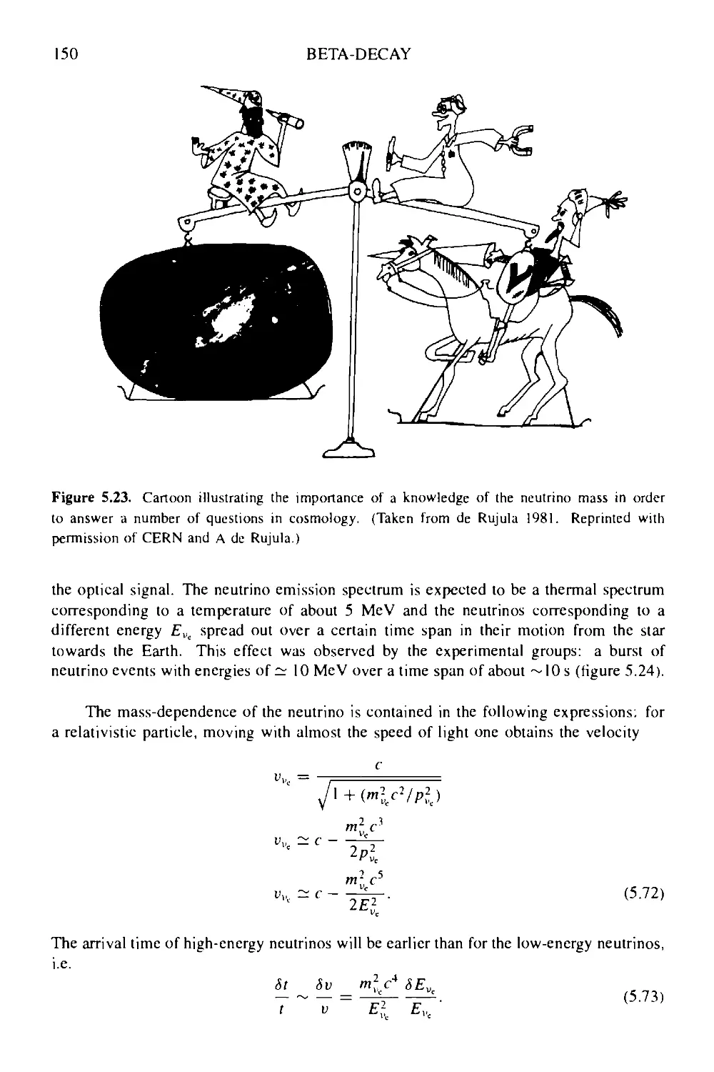
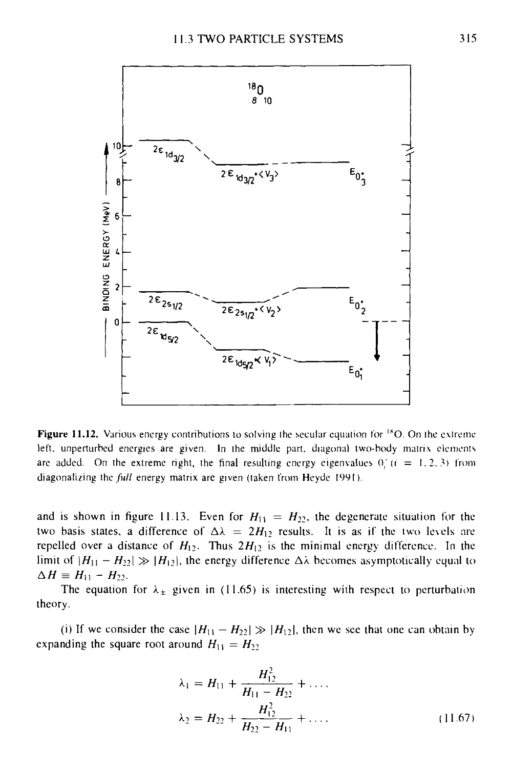
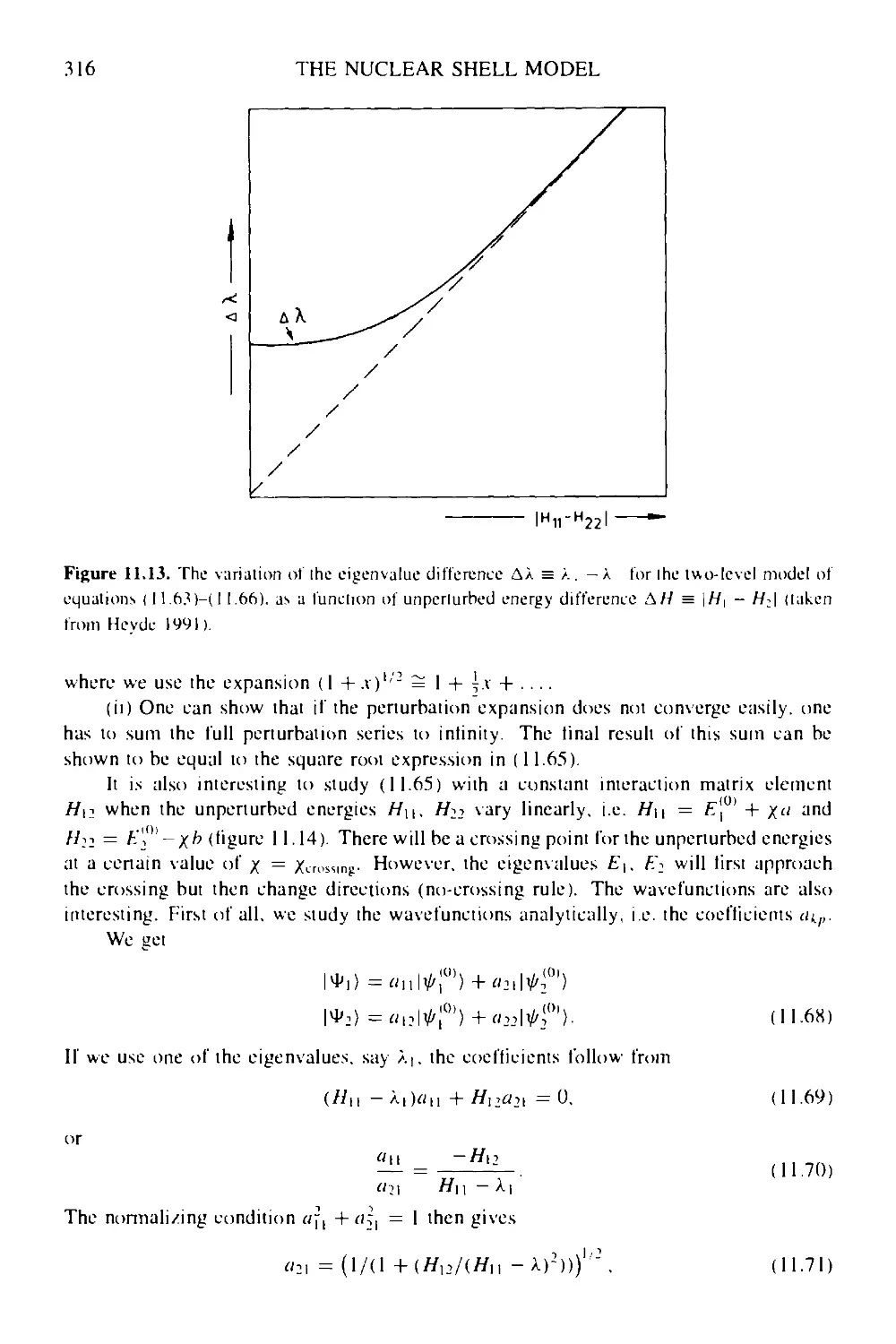
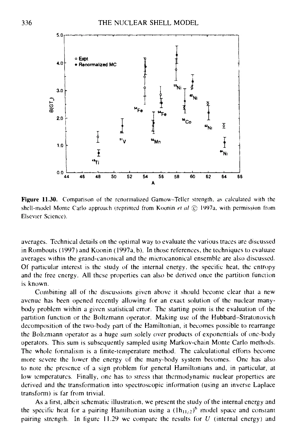
/


Текст
GRADUATE STUDENT SERIES IN PHYSICS
Series Editor:
Professor Douglas F Brewer, MA, DPhil
Emeritus Professor of Experimental Physics, University of Sussex
BASIC IDEAS AND CONCEPTS
IN NUCLEAR PHYSICS
AN INTRODUCTORY APPROACH
SECOND EDITION
К HEYDE
Institute for Theoretical Physics ant! Nuclear Physics
Universiteit Gent, Belgium
INSTITUTE OF PHYSICS PUBLISHING
Bristol and Philadelphia
© ЮР Publishing Ltd 1994, 1999
All rights reserved. No part of this publication may be reproduced, stored in a retrieval
system or transmitted in any form or by any means, electronic, mechanical, photocopying,
recording or otherwise, without the prior permission of the publisher. Multiple copying
is permitted in accordance with the terms of licences issued by the Copyright Licensing
Agency under the terms of its agreement with the Committee of Vice-Chancellors and
Principals.
IOP Publishing Ltd and the author have attempted to trace the copyright holders of all the
material reproduced in this publication and apologize to copyright holders if permission
to publish in this form has not been obtained.
British Library Cataloguing-in-Publication Data
A catalogue record for this book is available from the British Library.
ISBN 0 7503 0534 7 hbk
0 7503 0535 5 pbk
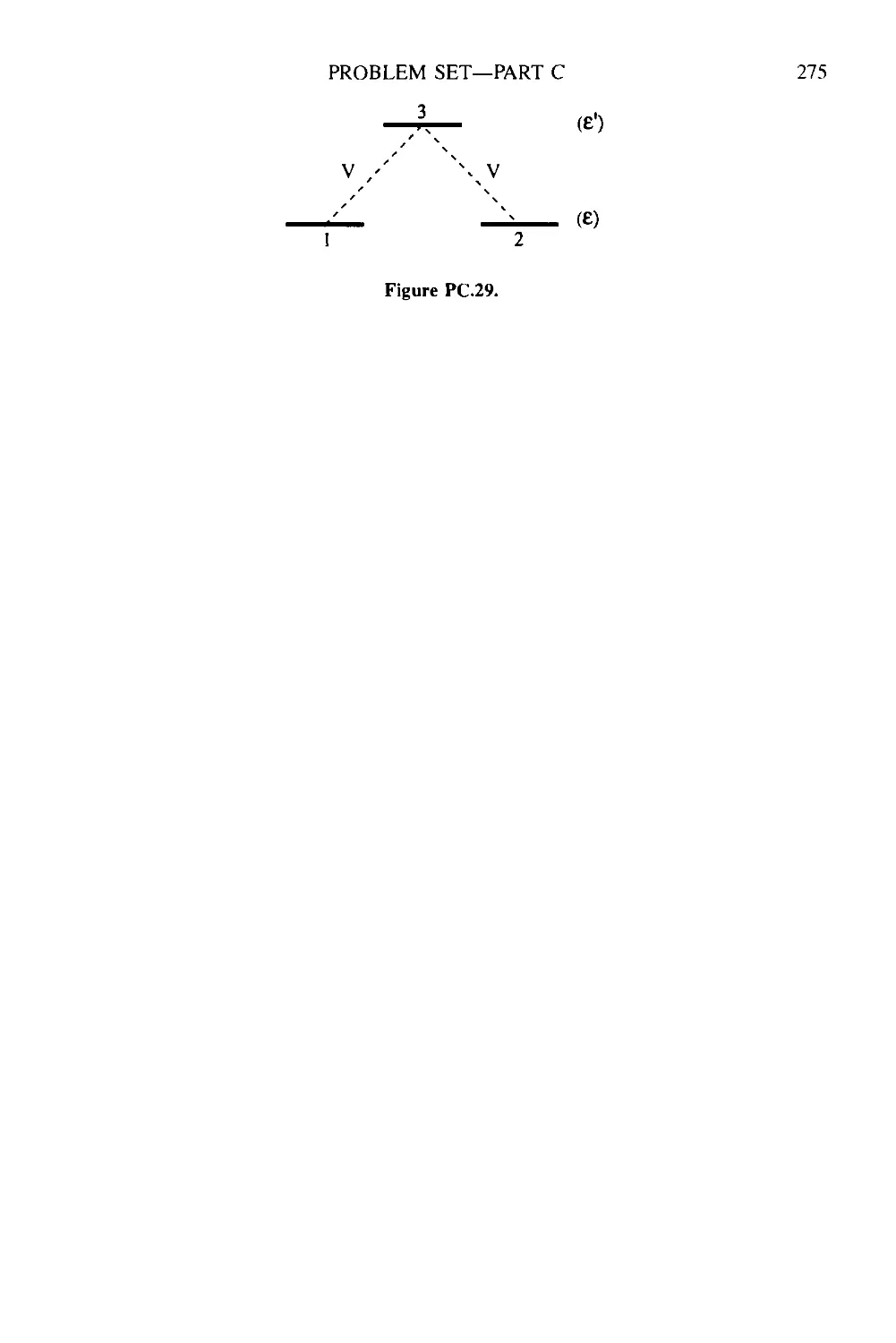
Library of Congress Cataloging-in-Publication Data are available
First edition 1994
Second edition 1999
Published by Institute of Physics Publishing, wholly owned by The Institute of Physics,
London
Institute of Physics Publishing, Dirac House, Temple Back, Bristol BS1 6BE, UK
US Office: Institute of Physics Publishing, The Public Ledger Building, Suite 1035, 150
South Independence Mall West, Philadelphia, PA 19106, USA
Typeset in TgX using the IOP Bookmaker Macros
Printed in the UK by Bookcraft Ltd, Bath
For Daisy, Jan and Mieke
CONTENTS
Acknowledgements xiii
Preface to the Second Edition xv
Introduction xvii
PART A
KNOWING THE NUCLEUS:
THE NUCLEAR CONSTITUENTS AND CHARACTERISTICS
1 Nuclear global properties 1
1.1 Introduction and outline 1
1.2 Nuclear mass table 1
1.3 Nuclear binding, nuclear masses 3
1.4 Nuclear extension: densities and radii 9
1.5 Angular momentum in the nucleus 12
1.6 Nuclear moments 14
1.6.1 Dipole magnetic moment 14
1.6.2 Electric moments—electric quadrupole moment 18
1.7 Hyperfine interactions 20
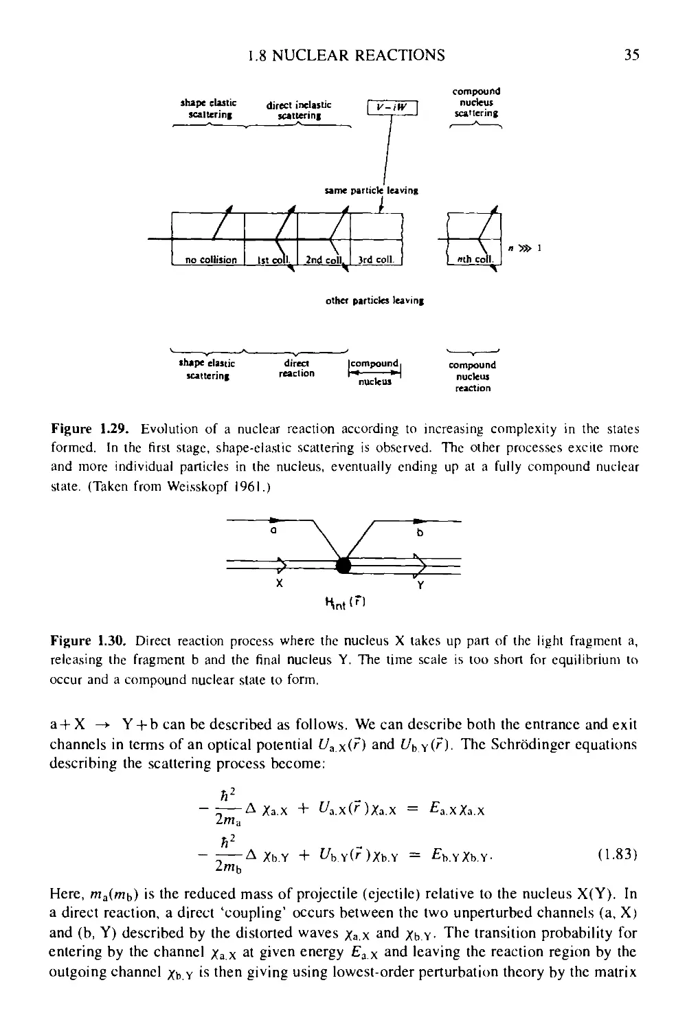
1.8 Nuclear reactions 25
1.8.1 Elementary kinematics and conservation laws 26
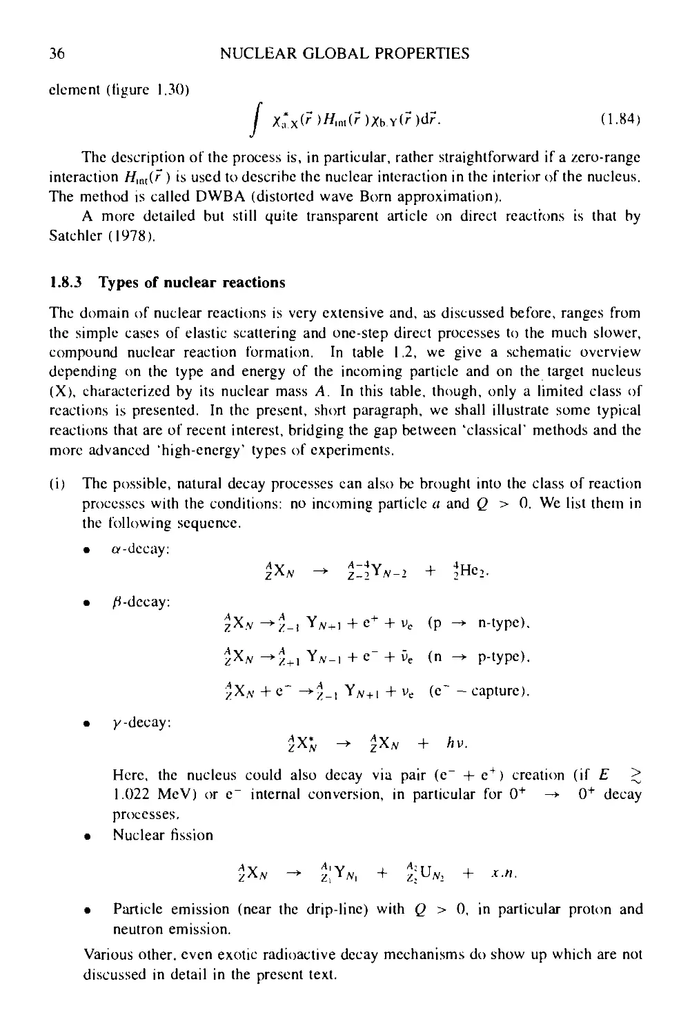
1.8.2 A tutorial in nuclear reaction theory 31
1.8.3 Types of nuclear reactions 36
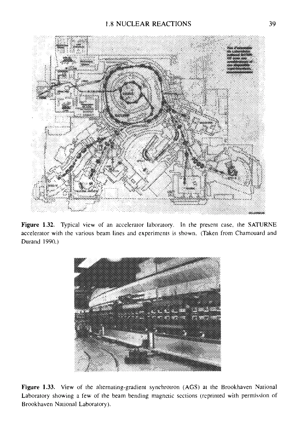
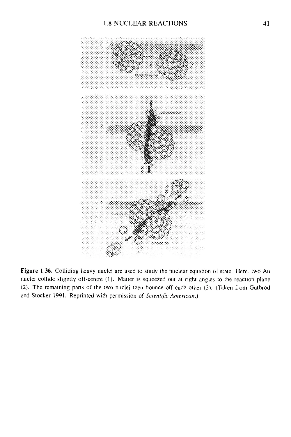
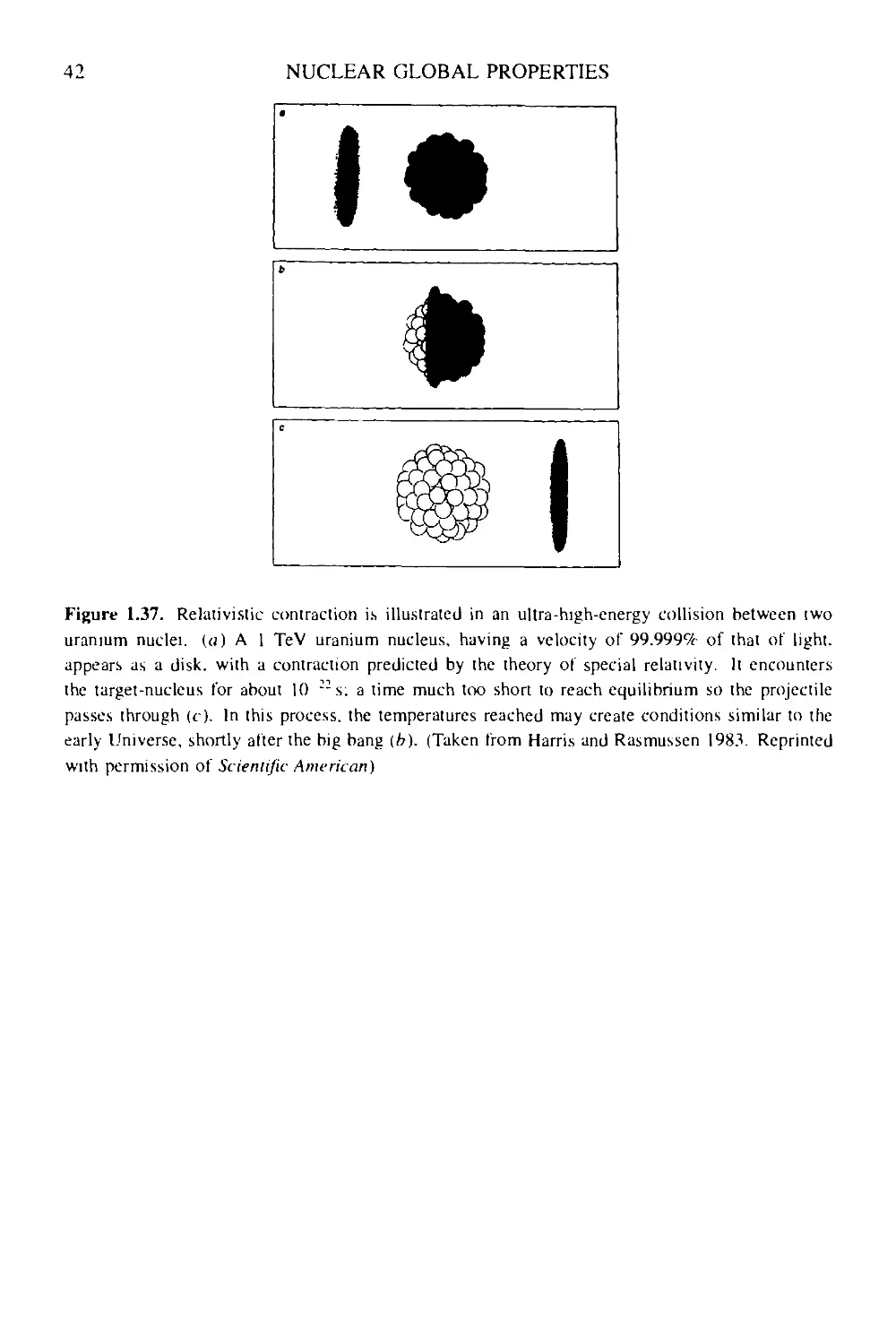
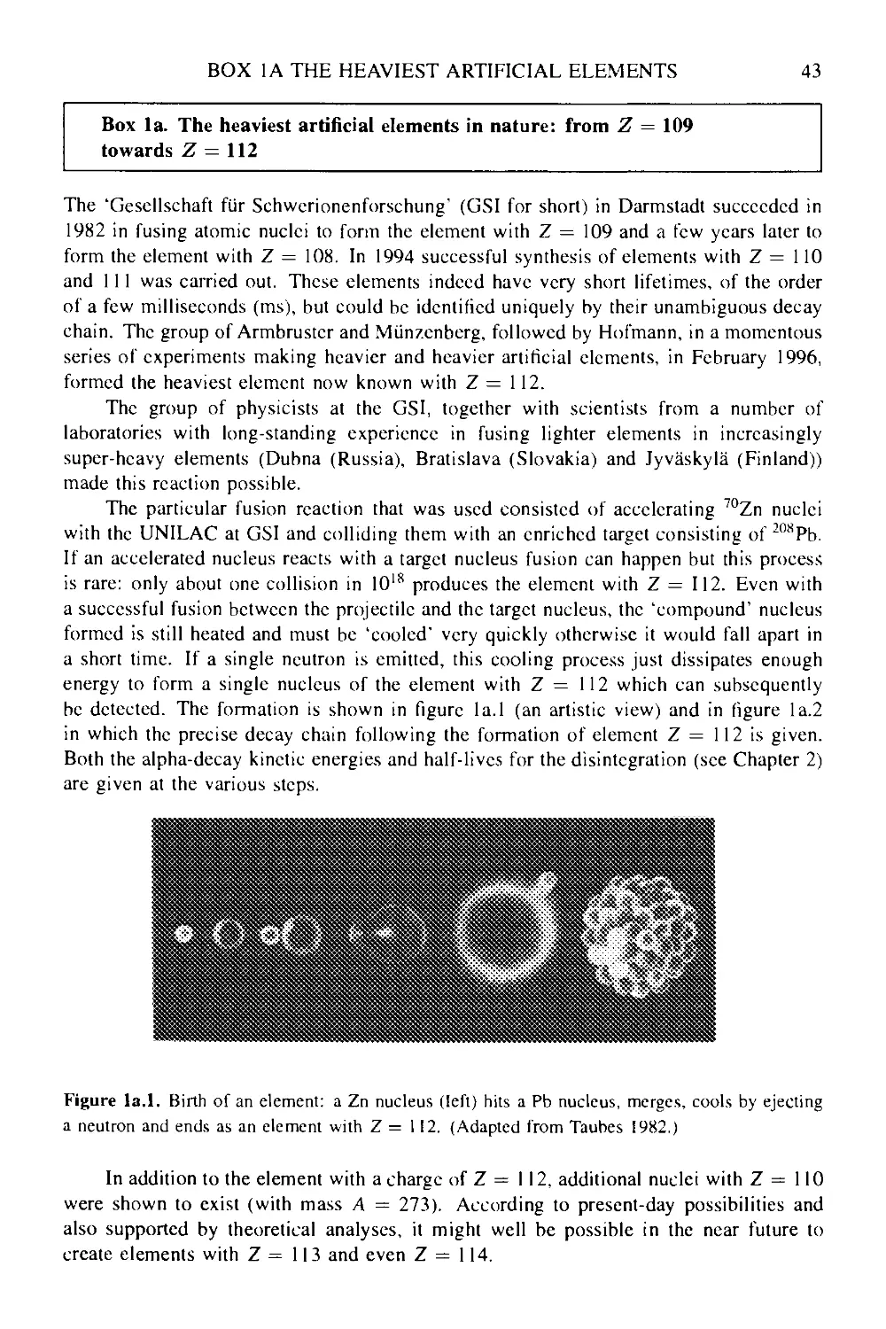
Box la The heaviest artificial elements in nature: from Z — \09 towards Z = 1 12 43
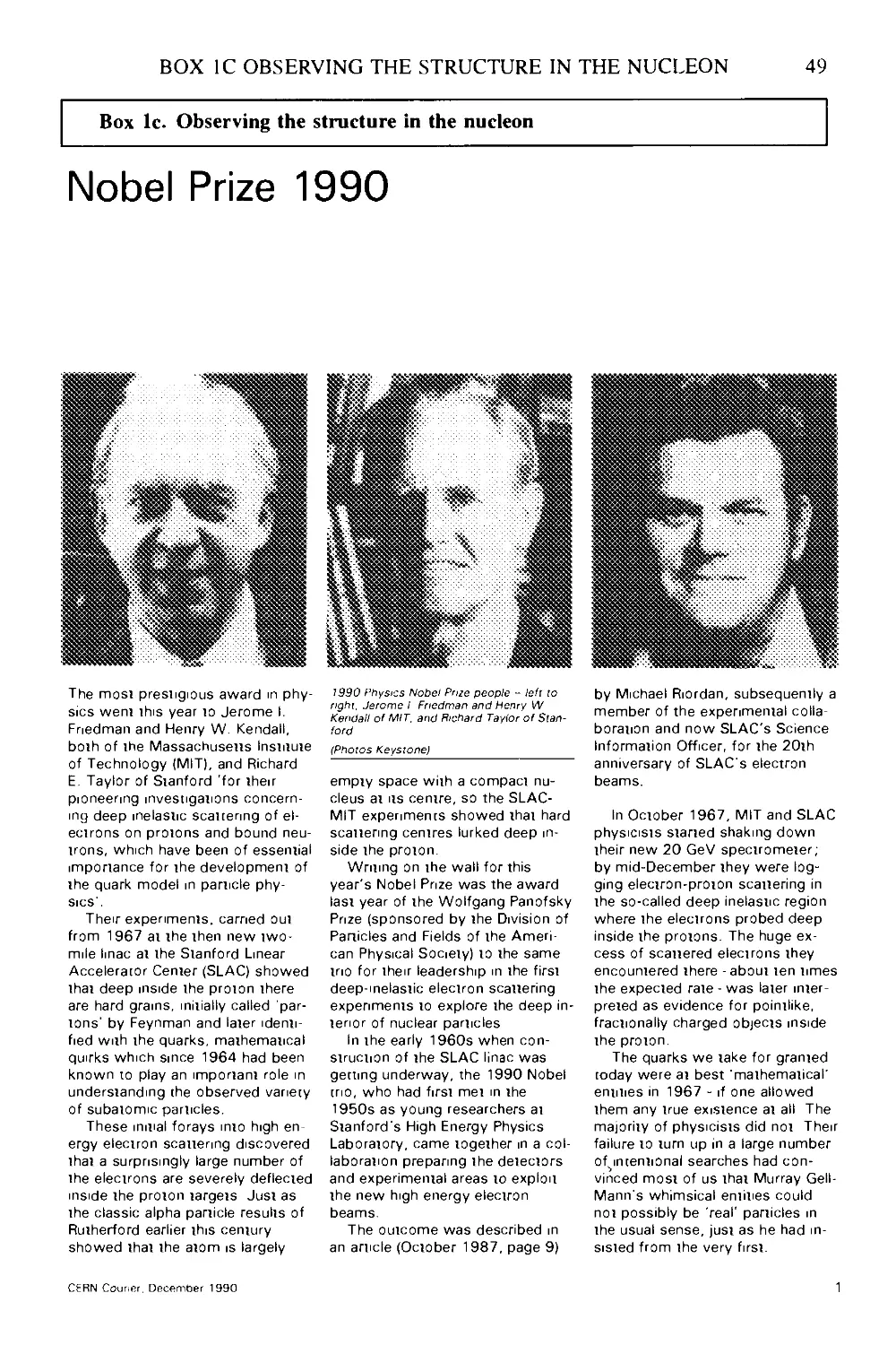
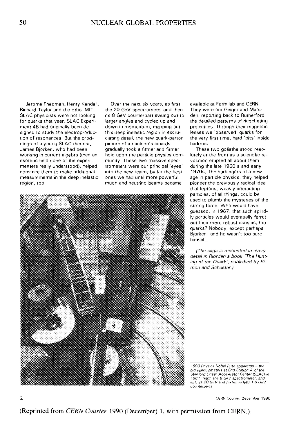
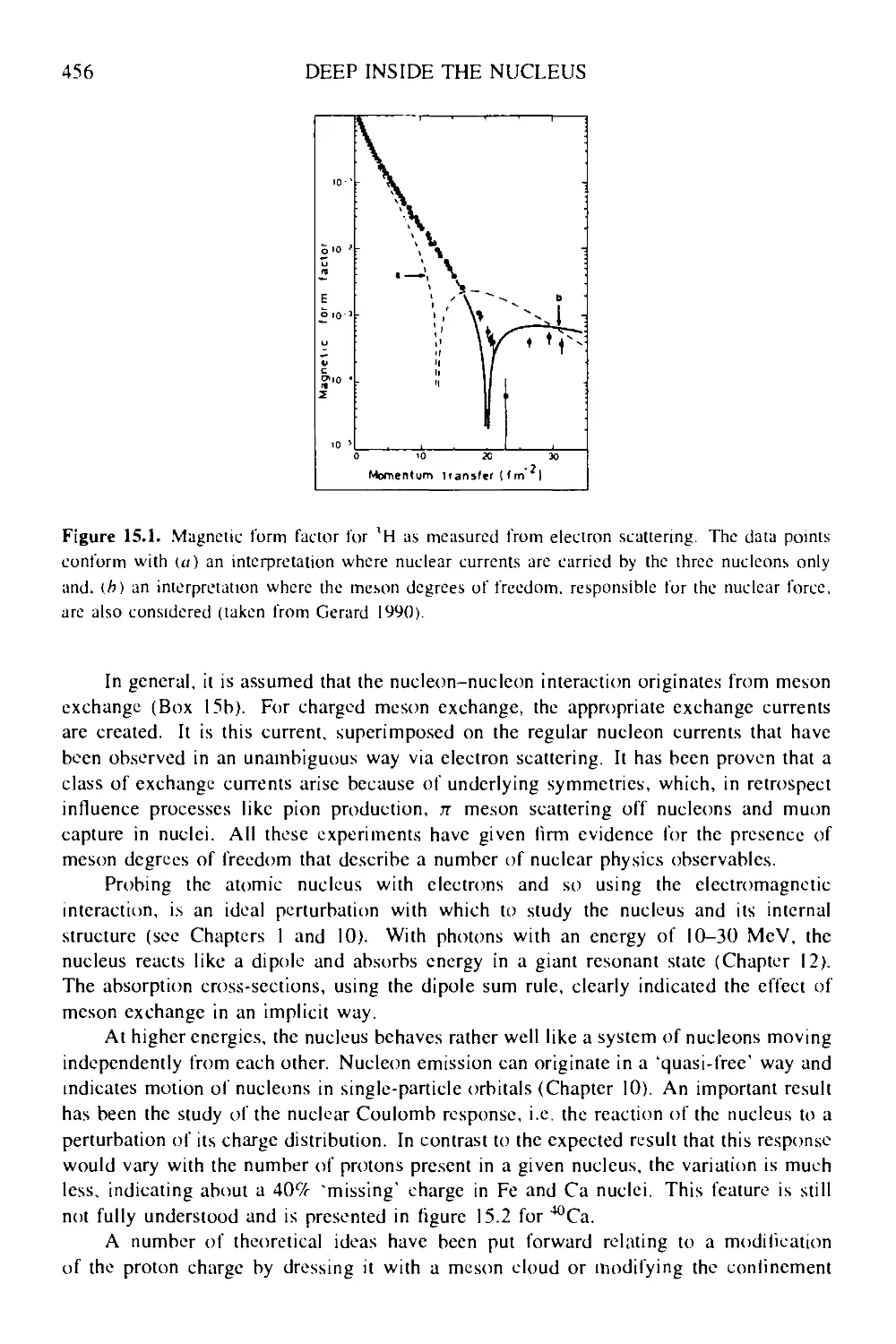
Box lb Electron scattering: nuclear form factors 45
Box lc Observing the structure in the nucleon 49
Box Id One-particle quadrupole moment 51
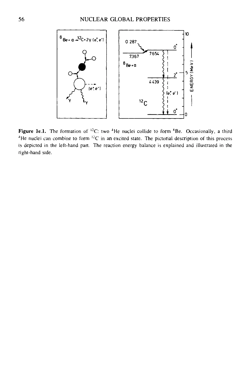
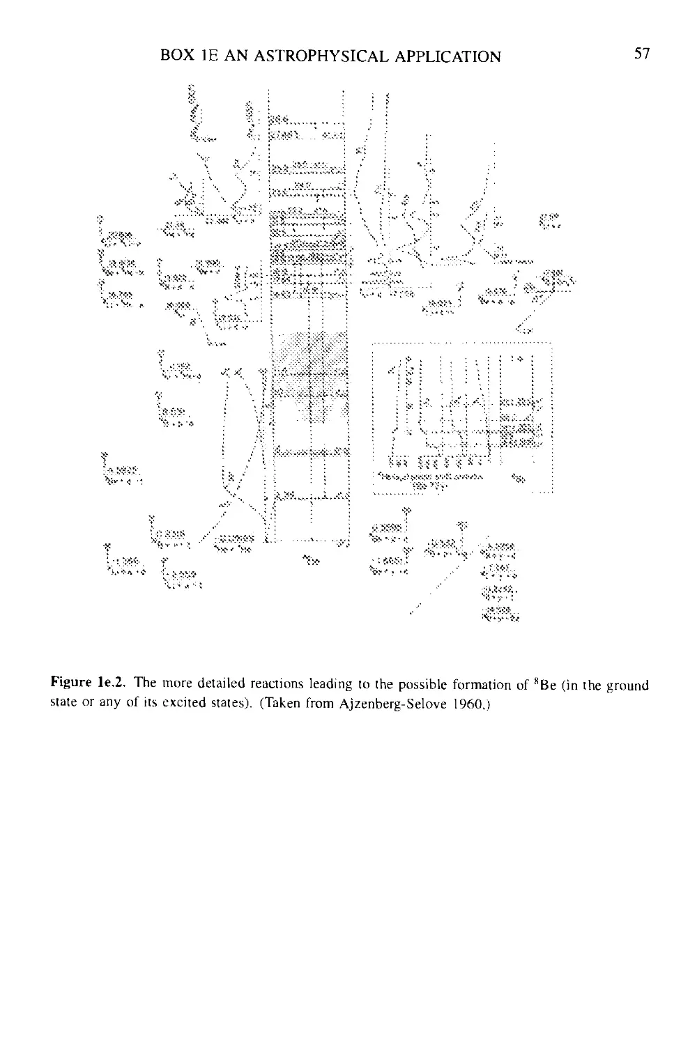
Box le An astrophysical application: alpha-capture reactions 55
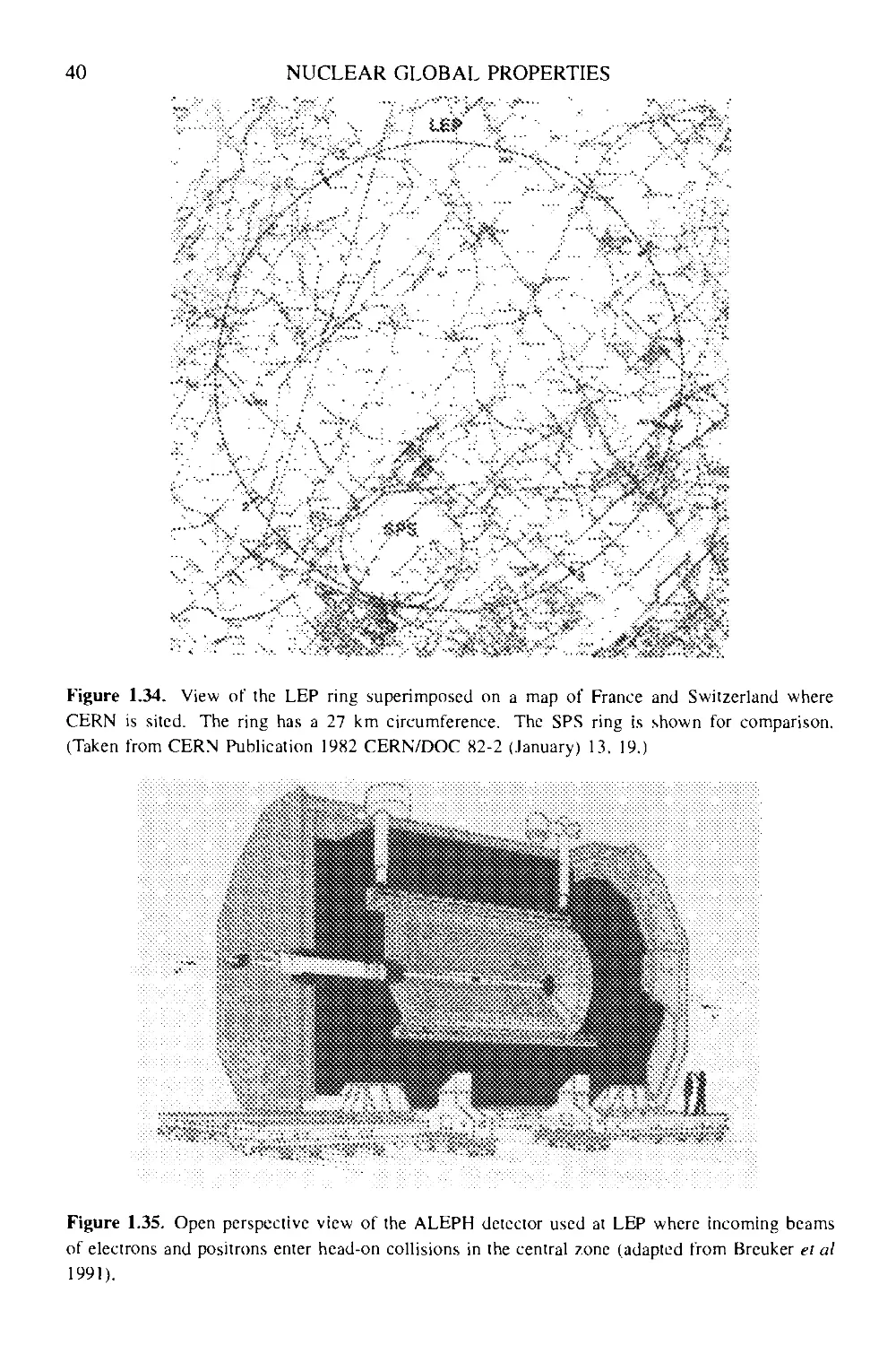
Box If New accelerators 58
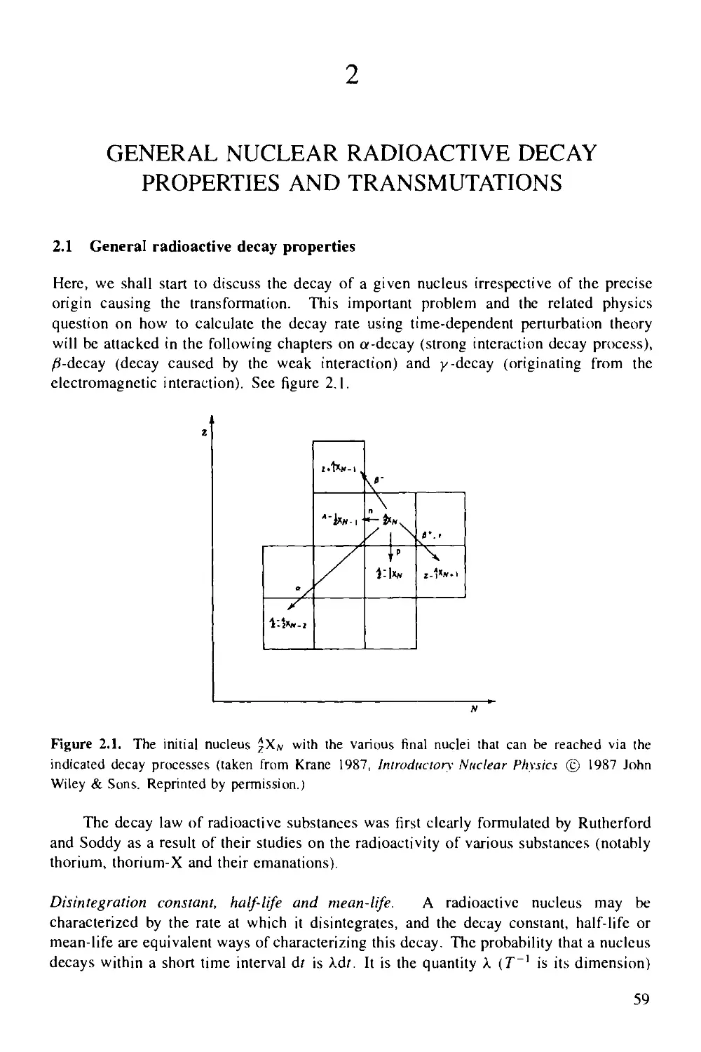
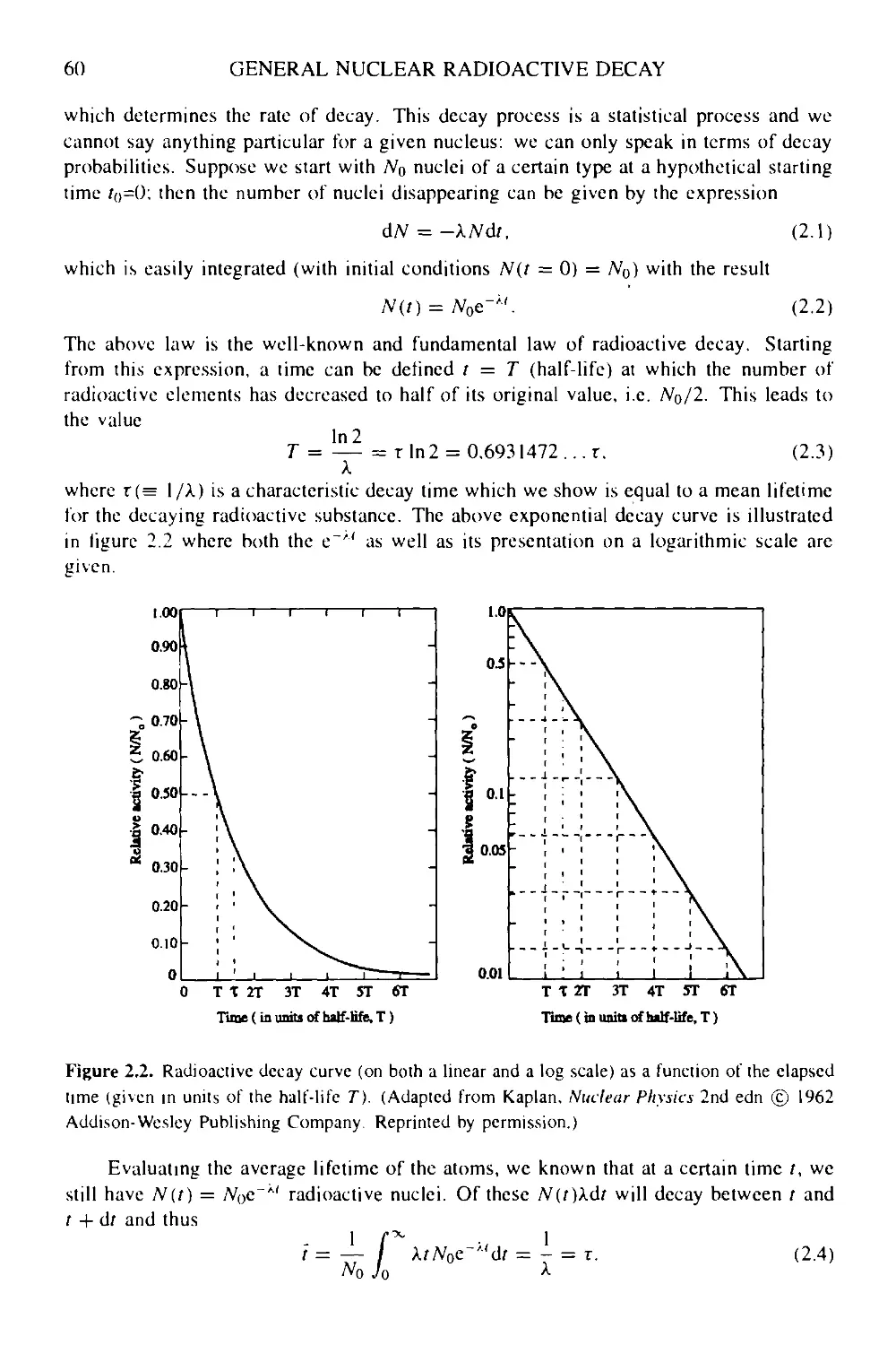
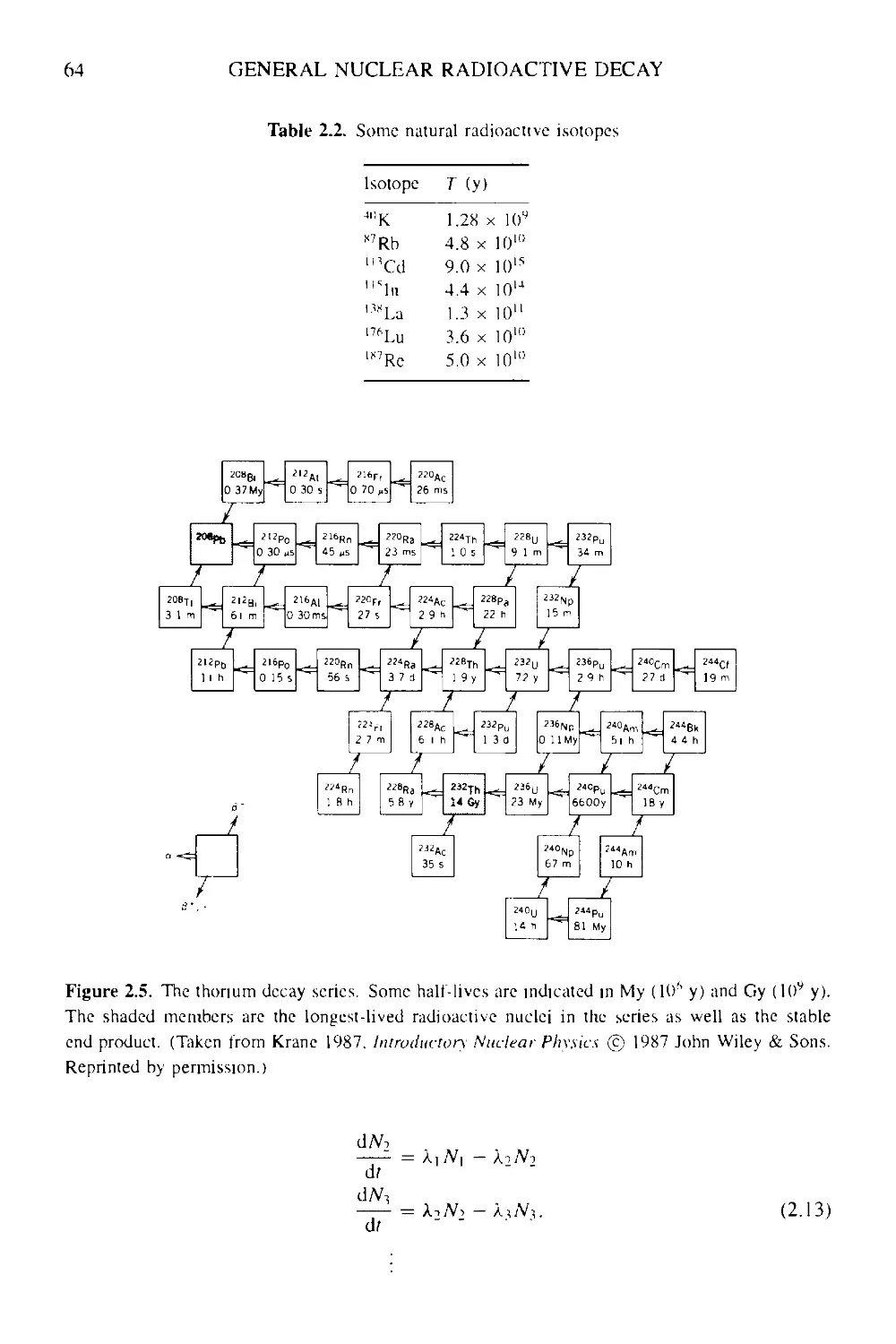
2 General nuclear radioactive decay properties and transmutations 59
2.1 General radioactive decay properties 59
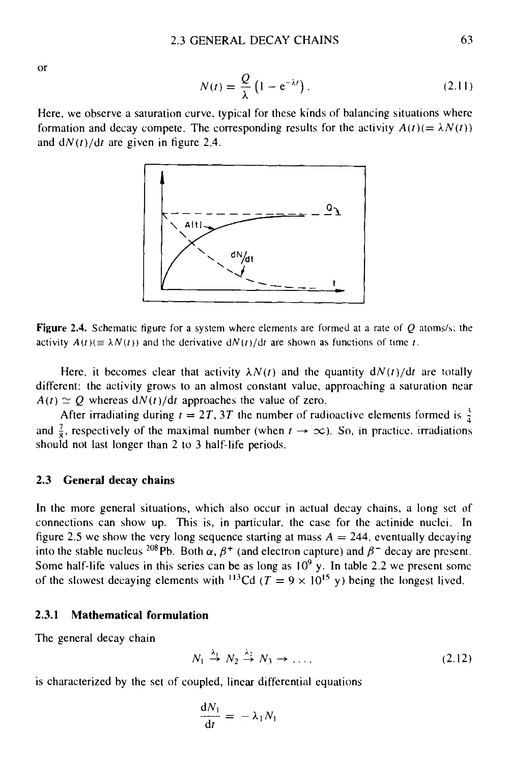
2.2 Production and decay of radioactive elements 62
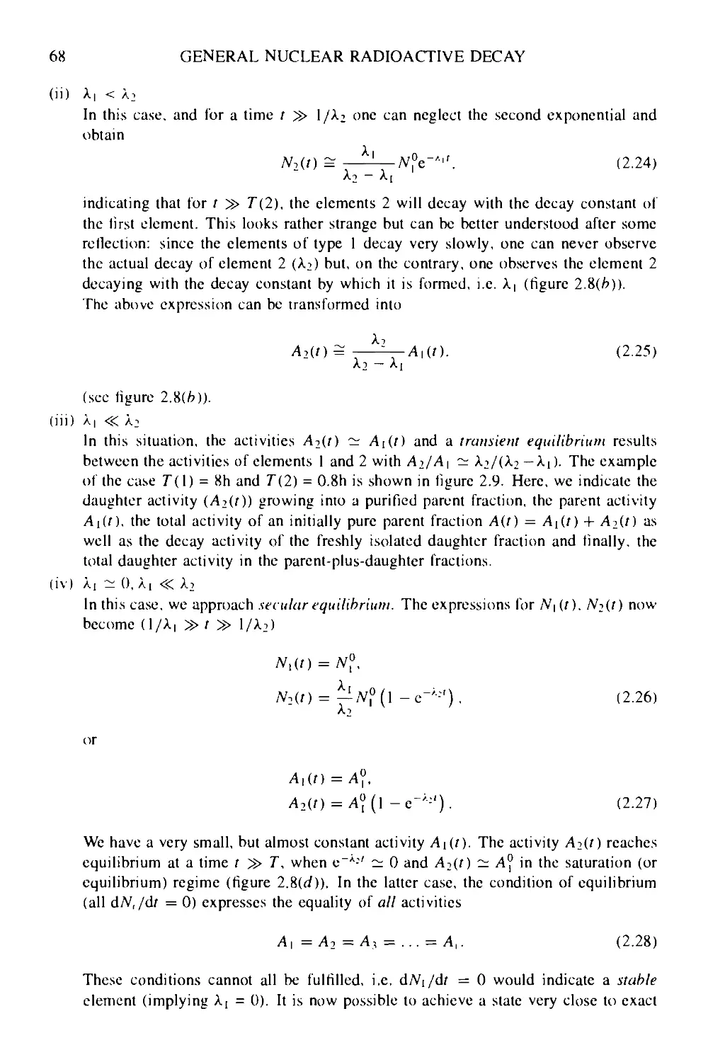
2.3 General decay chains 63
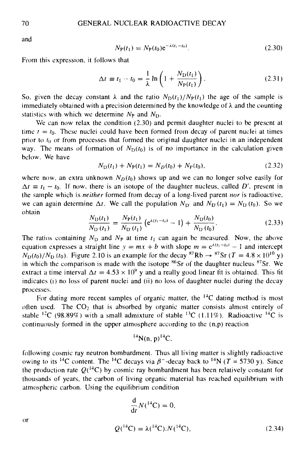
2.3.1 Mathematical formulation 63
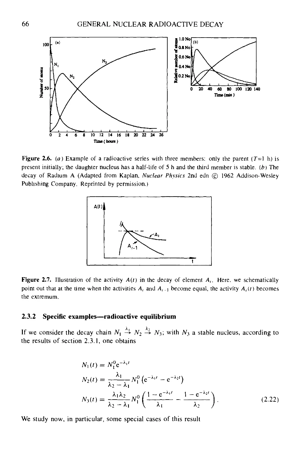
2.3.2 Specific examples—radioactive equilibrium 66
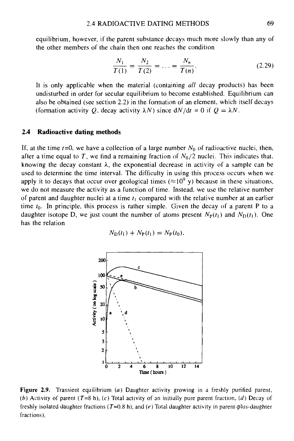
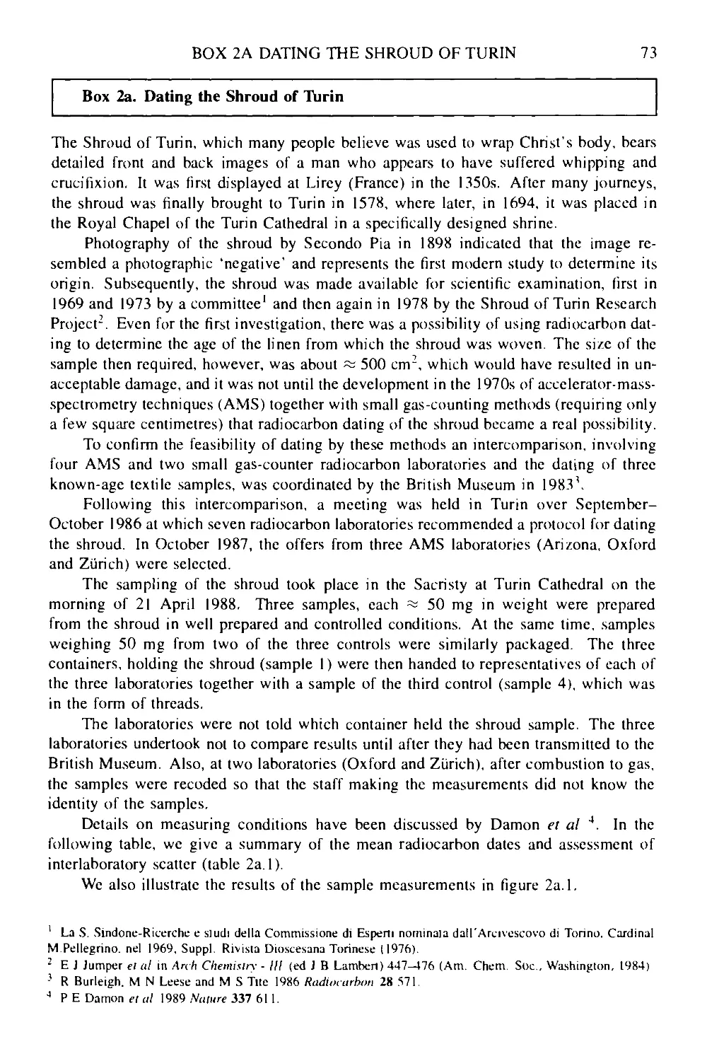
2.4 Radioactive dating methods 69
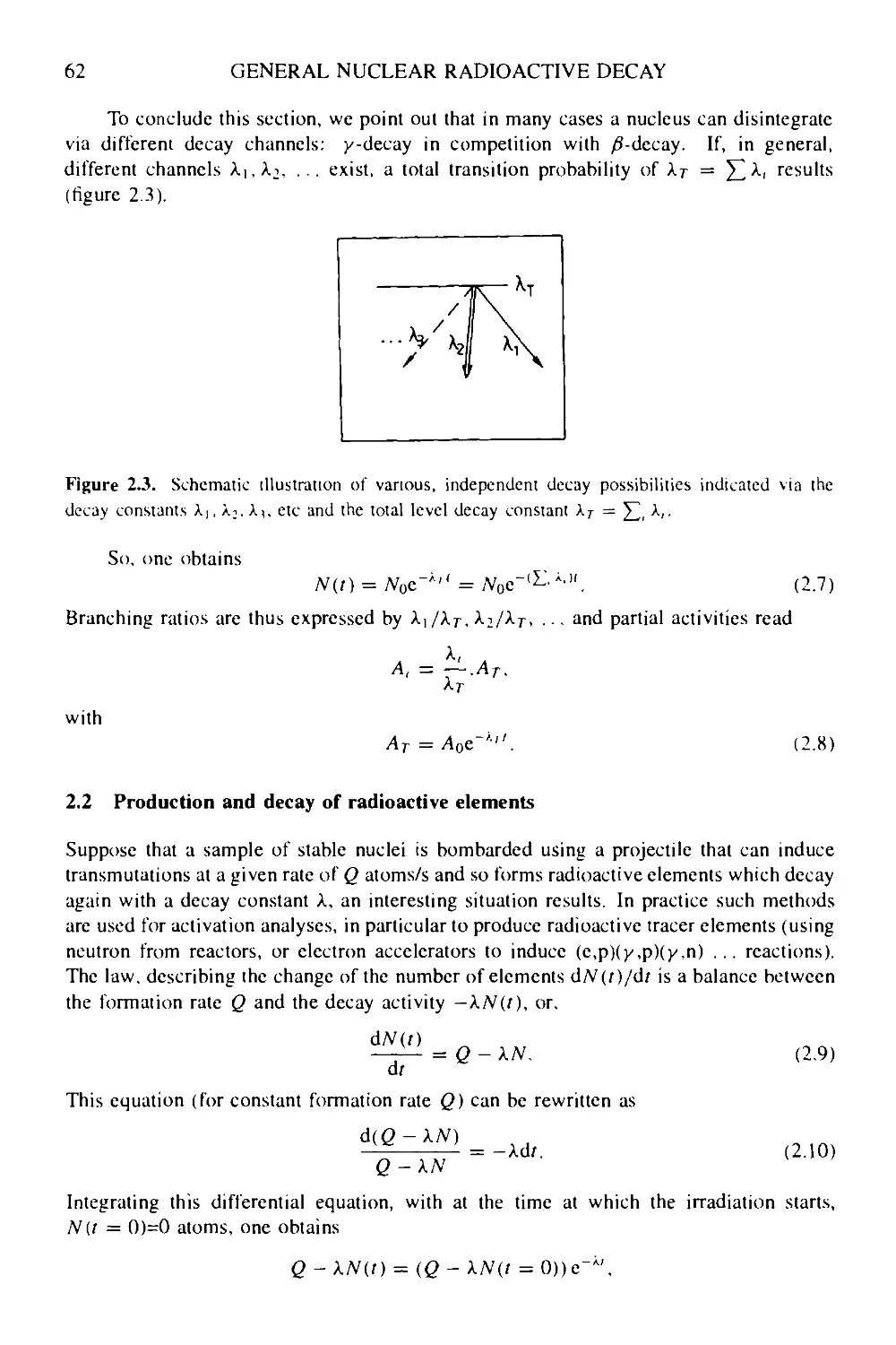
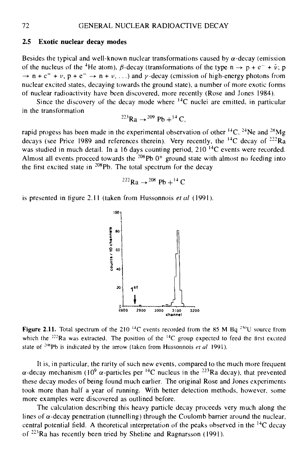
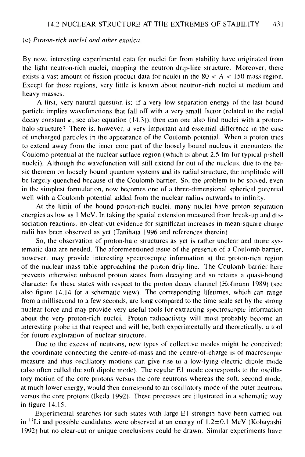
2.5 Exotic nuclear decay modes 72
vii
viii CONTENTS
Box 2a Dating the Shroud of Turin 73
Box 2b Chernobyl: a test-case in radioactive decay chains 75
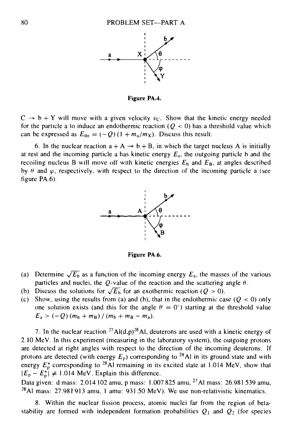
Problem set—Part A 79
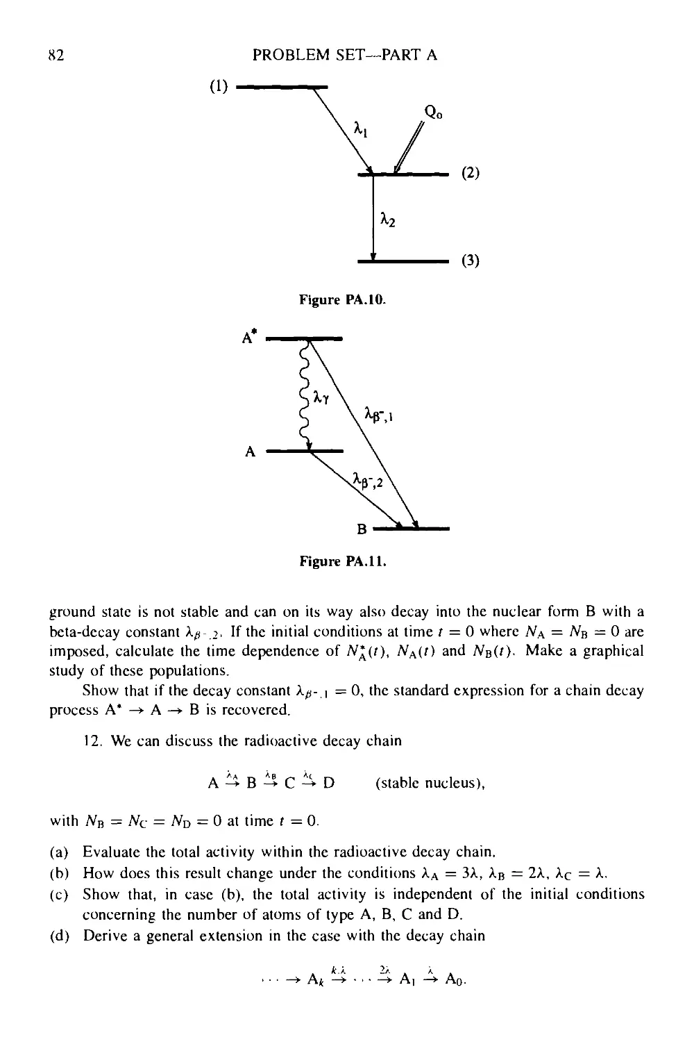
PART В
NUCLEAR INTERACTIONS: STRONG, WEAK AND
ELECTROMAGNETIC FORCES
3 General methods 89
3.1 Time-dependent perturbation theory: a general method to study
interaction properties 89
3.2 Time-dependent perturbation theory: facing the dynamics of the three
basic interactions and phase space 91
4 Alpha-decay: the strong interaction at work 94
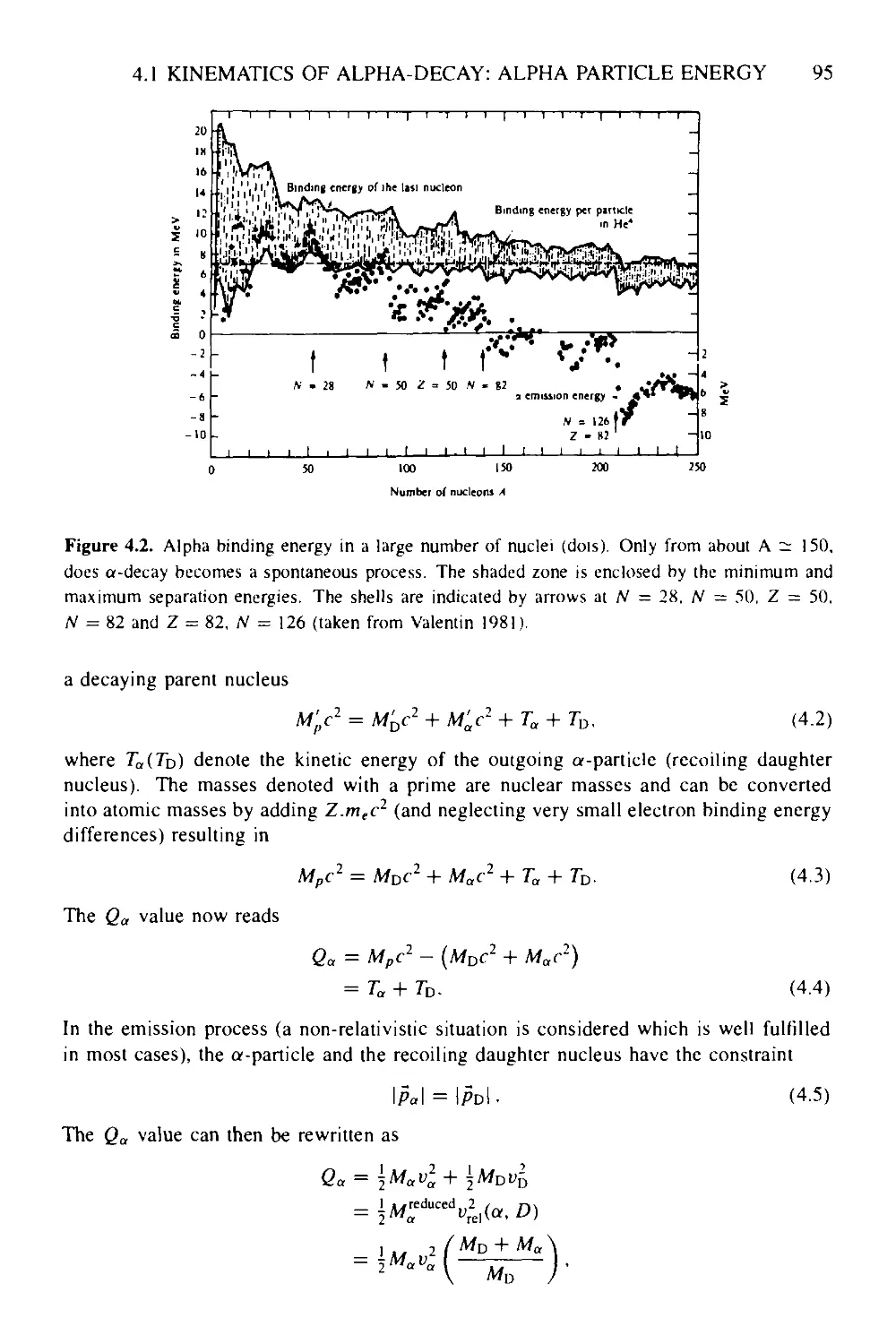
4.1 Kinematics of alpha-decay: alpha particle energy 94
4.2 Approximating the dynamics of the alpha-decay process 96
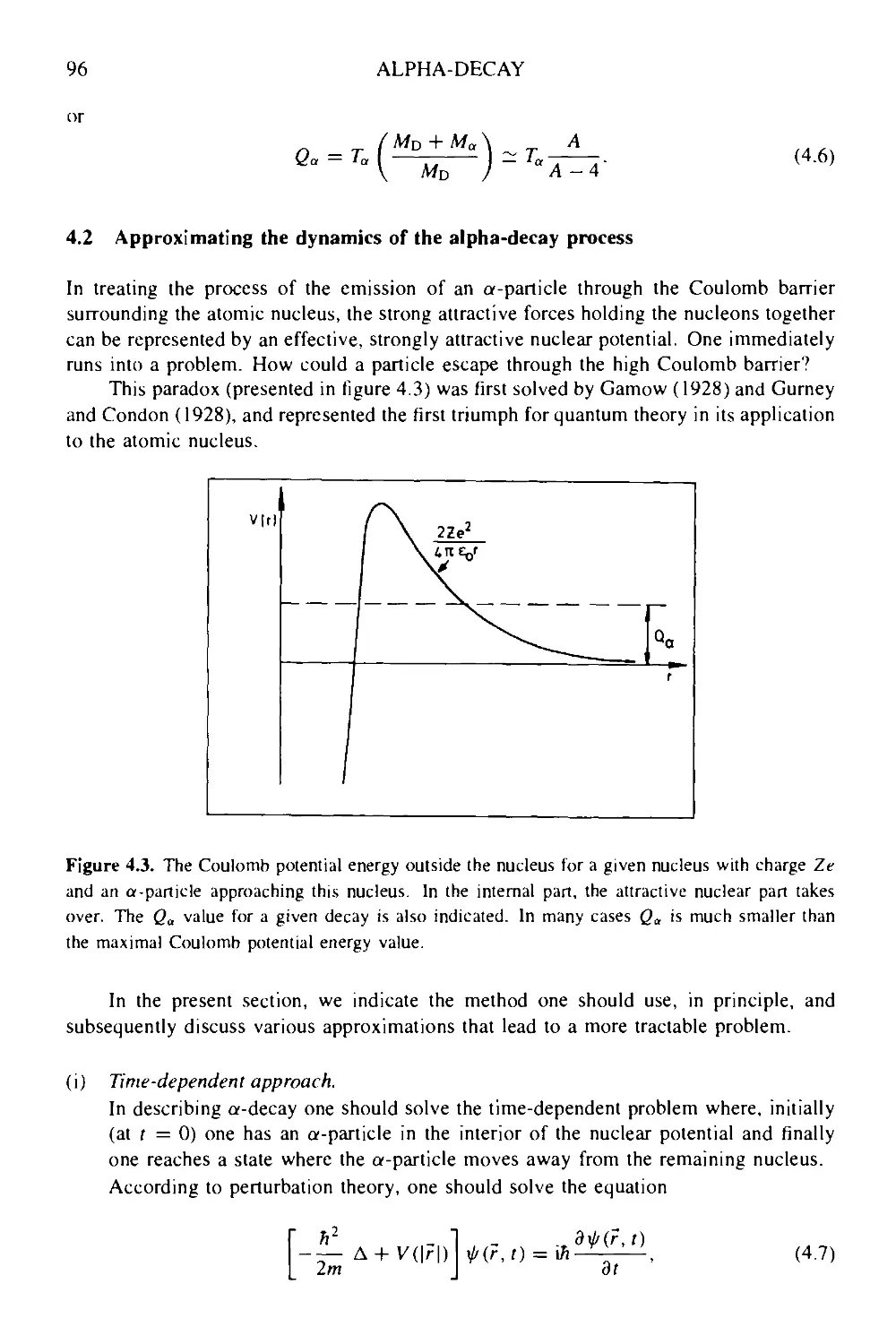
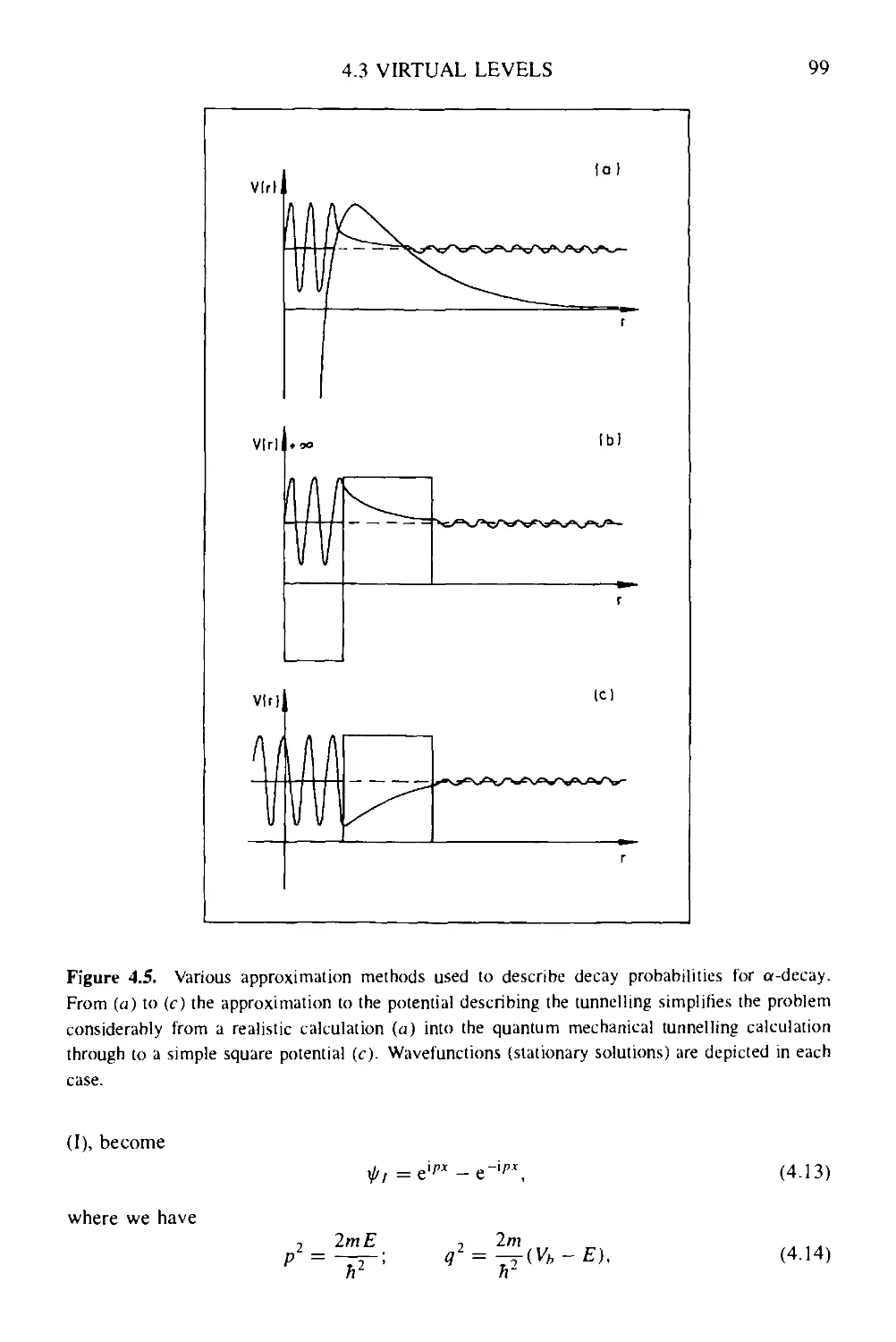
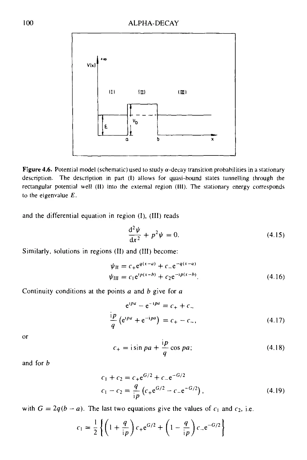
4.3 Virtual levels: a stationary approach to a-decay 98
4.4 Penetration through the Coulomb barrier 102
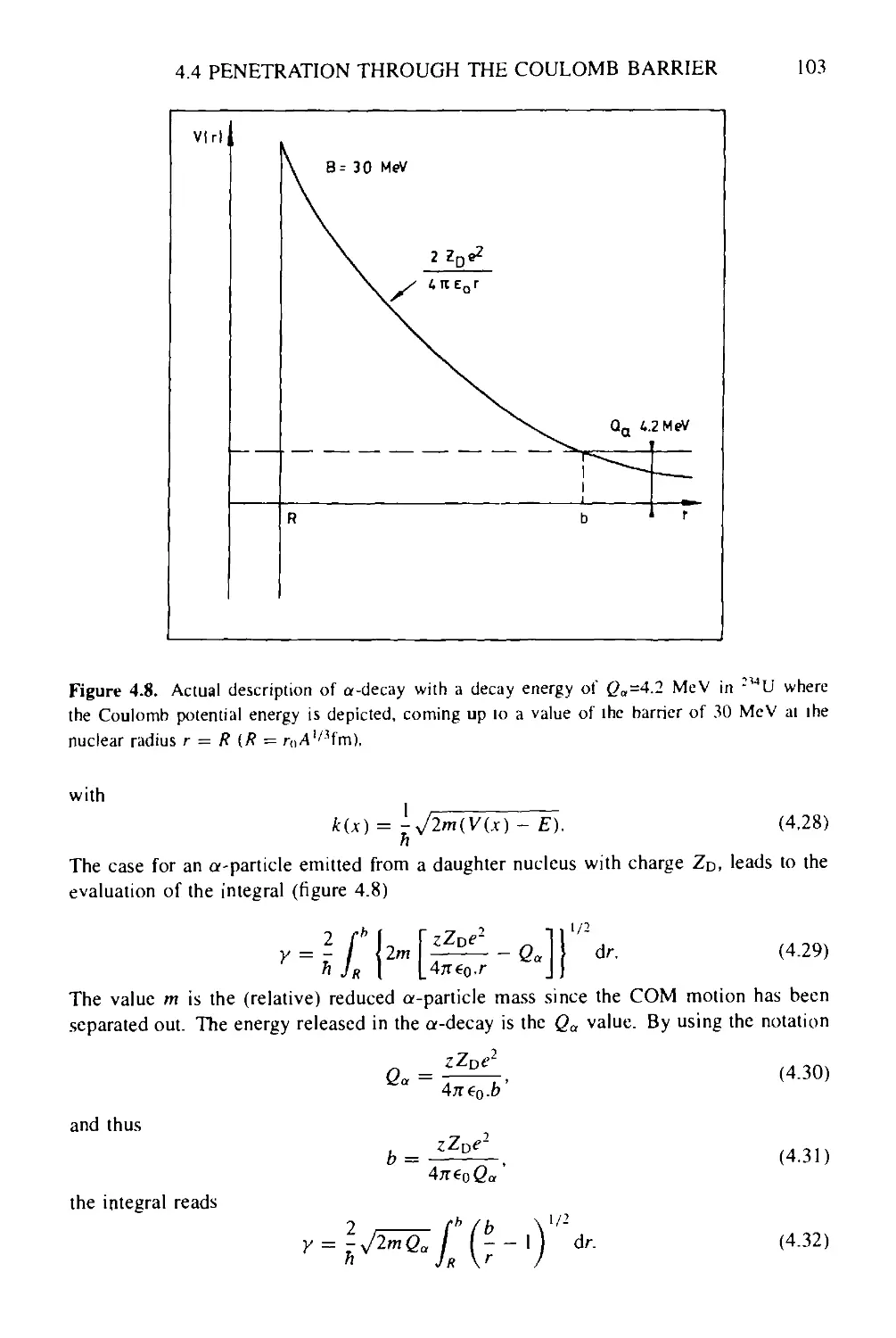
4.5 Alpha-spectroscopy 105
4.5.1 Branching ratios 105
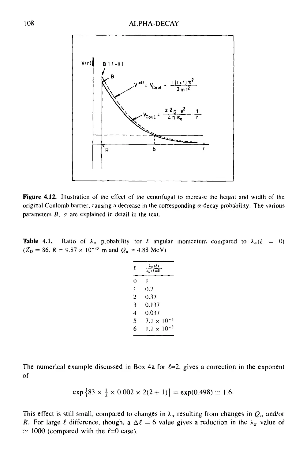
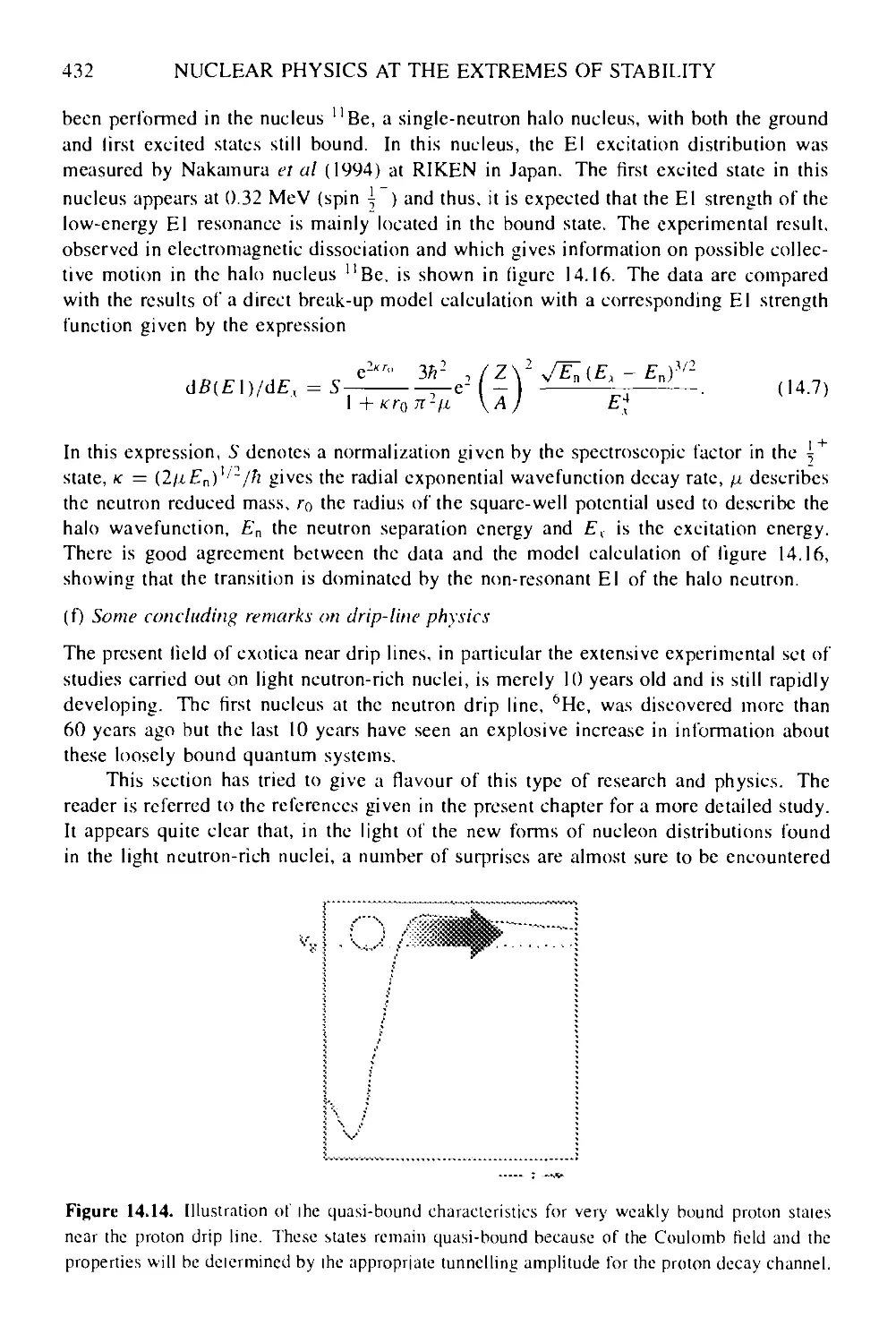
4.5.2 Centrifugal barrier effects 106
4.5.3 Nuclear structure effects 109
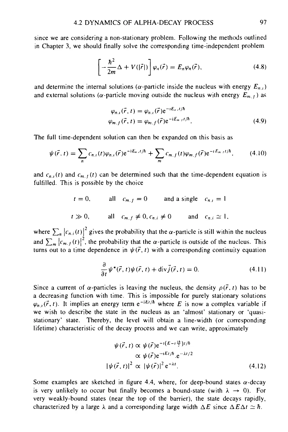
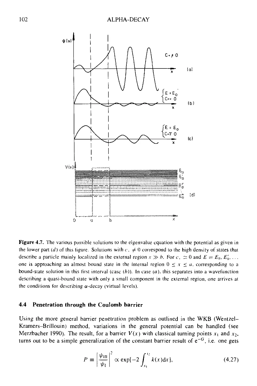
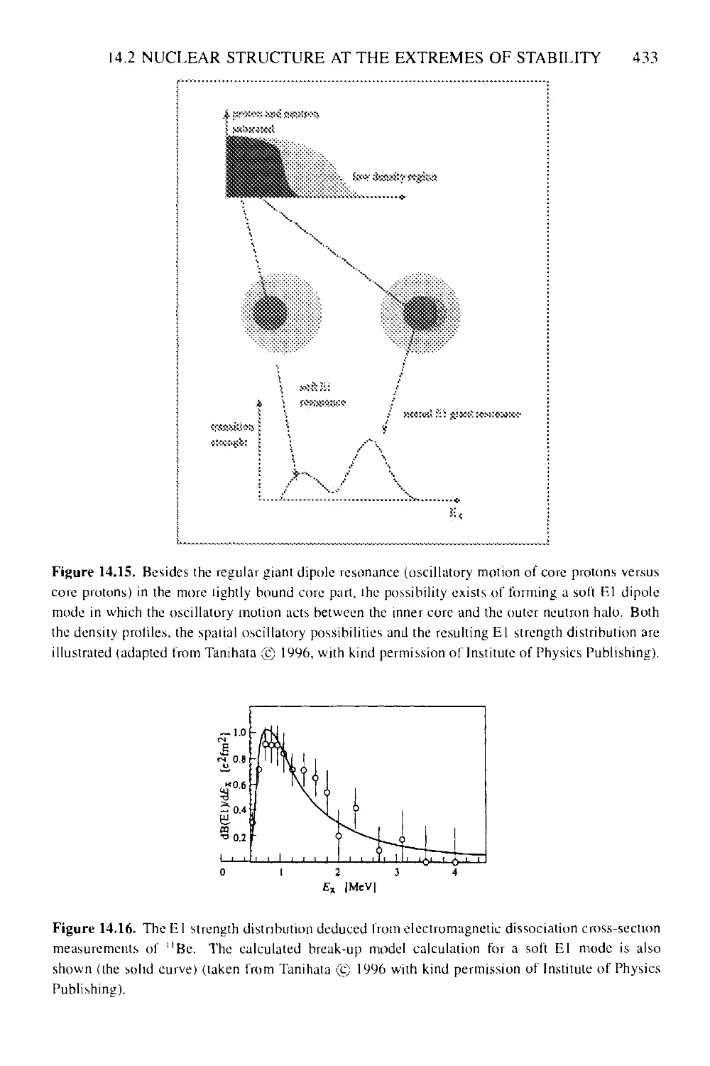
4.6 Conclusion 109
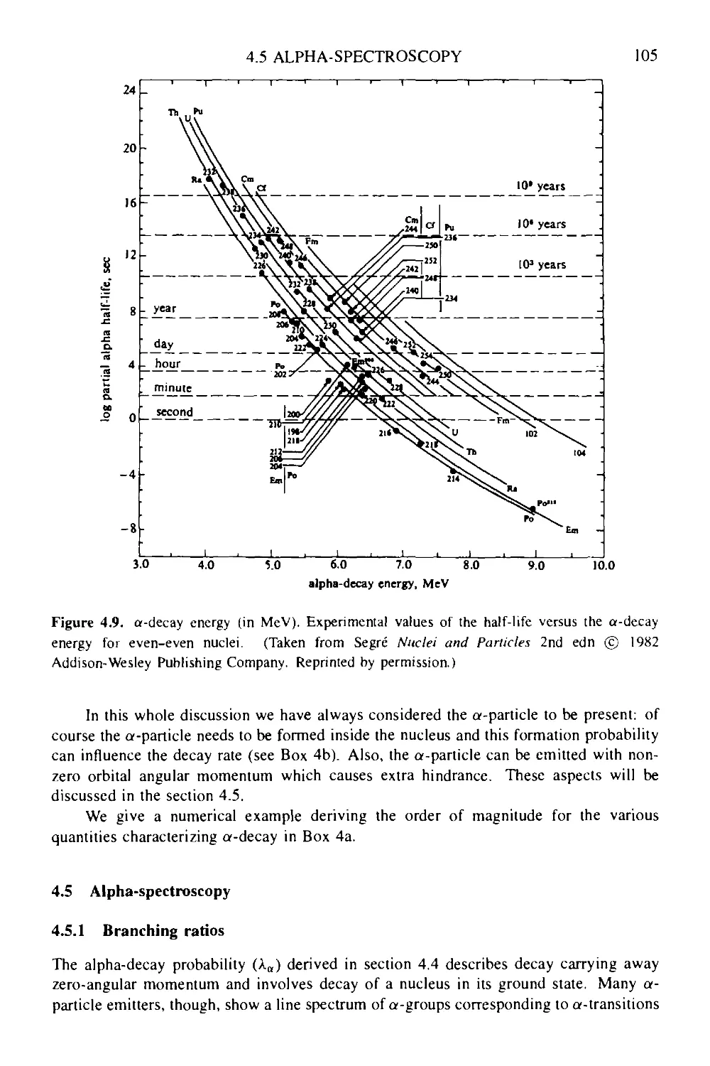
Box 4a a-emission in 928UL6 111
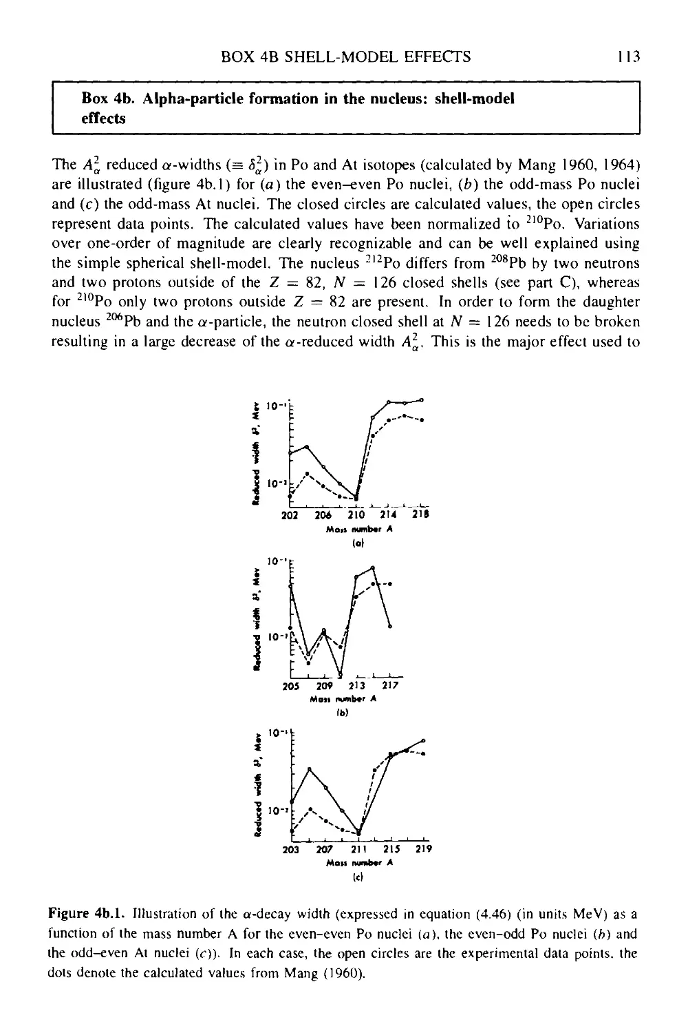
Box 4b Alpha-particle formation in the nucleus: shell-model effects 113
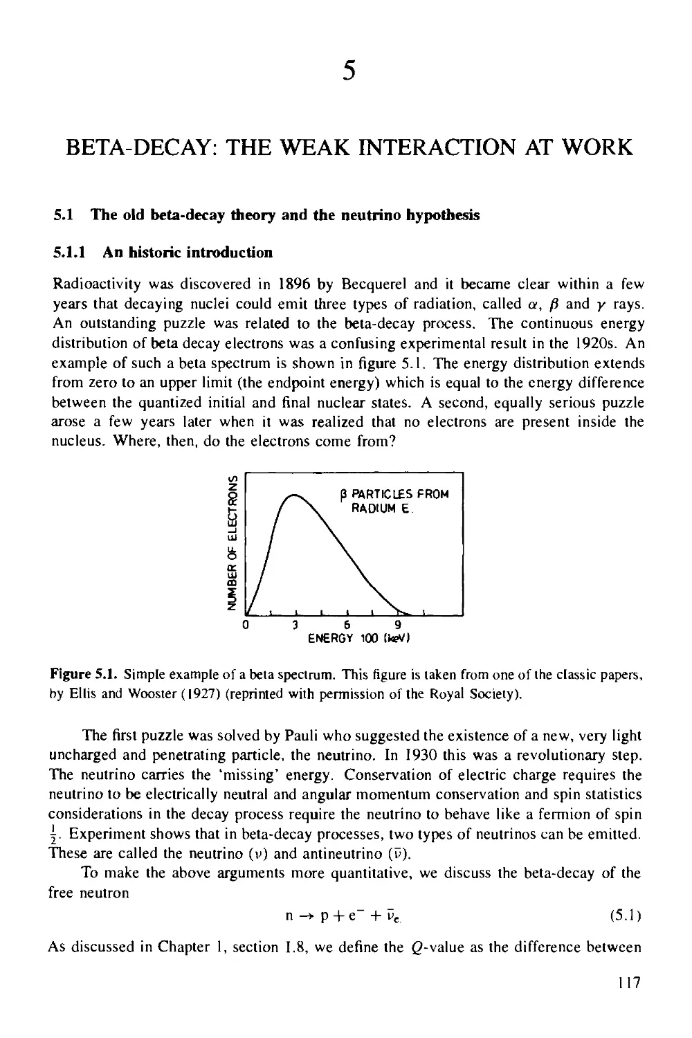
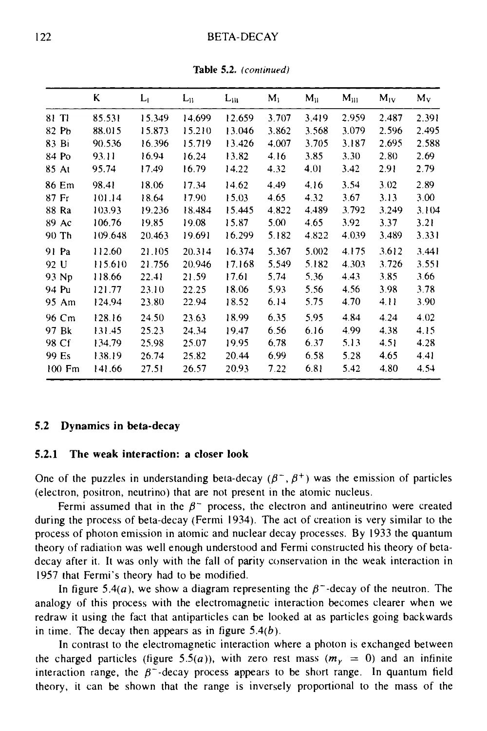
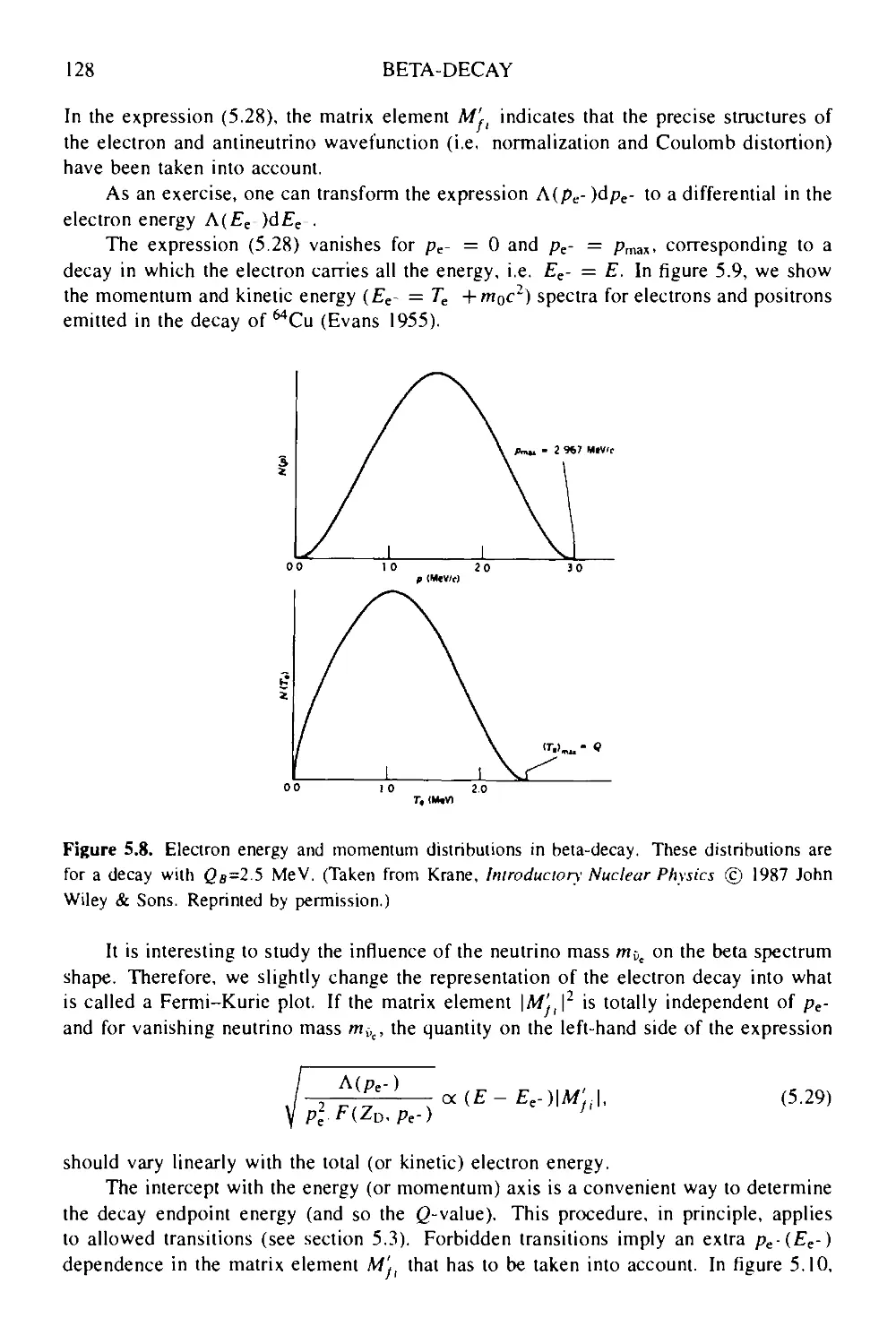
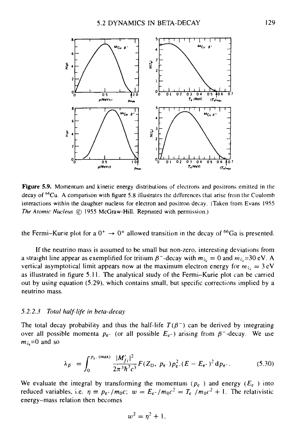
5 Beta-decay: the weak interaction at work 117
5.1 The old beta-decay theory and the neutrino hypothesis 117
5.1.1 An historic introduction 117
5.1.2 Energy relations and Q-values in beta-decay 118
5.2 Dynamics in beta-decay 122
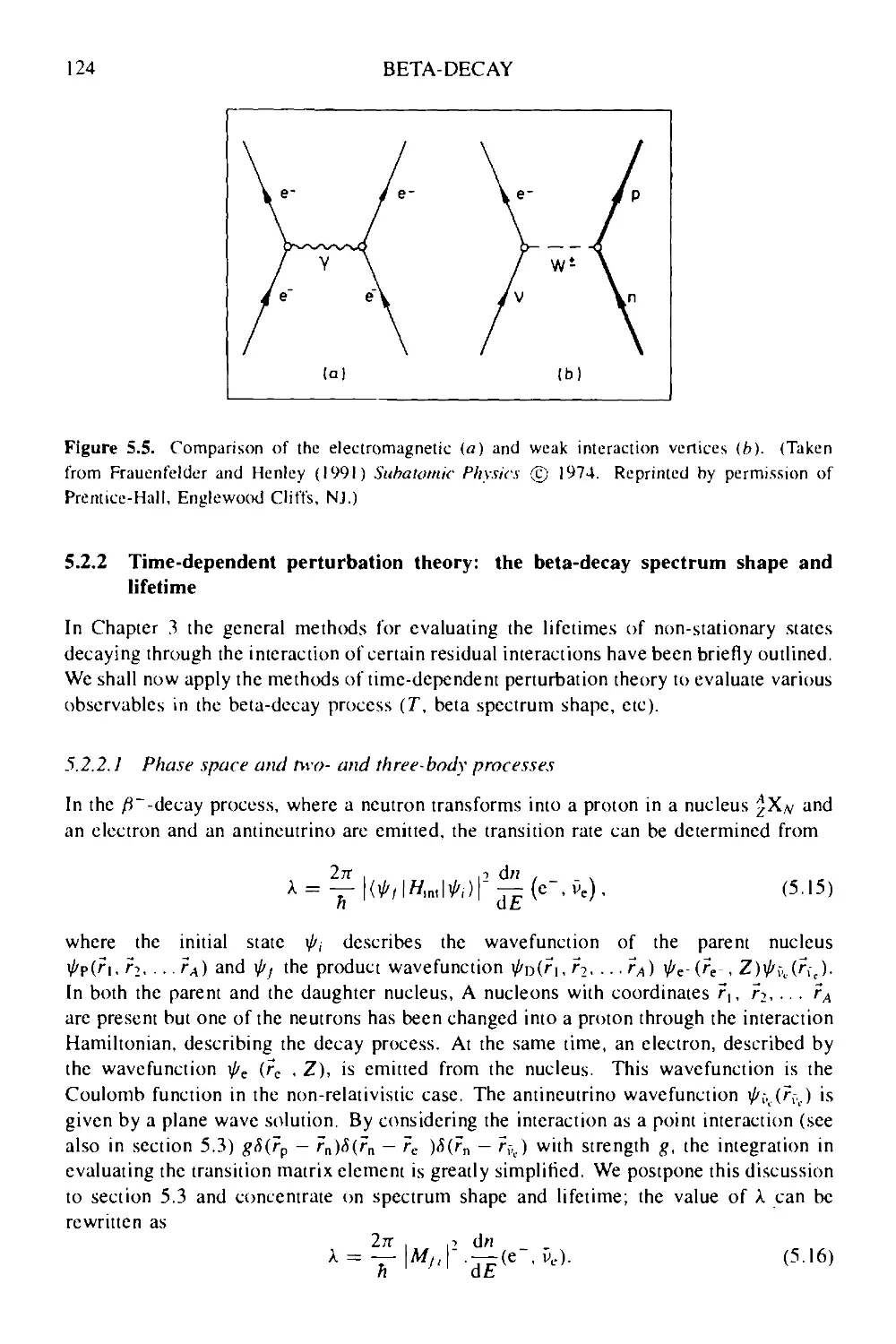
5.2.1 The weak interaction: a closer look 122
5.2.2 Time-dependent perturbation theory: the beta-decay spectrum
shape and lifetime 124
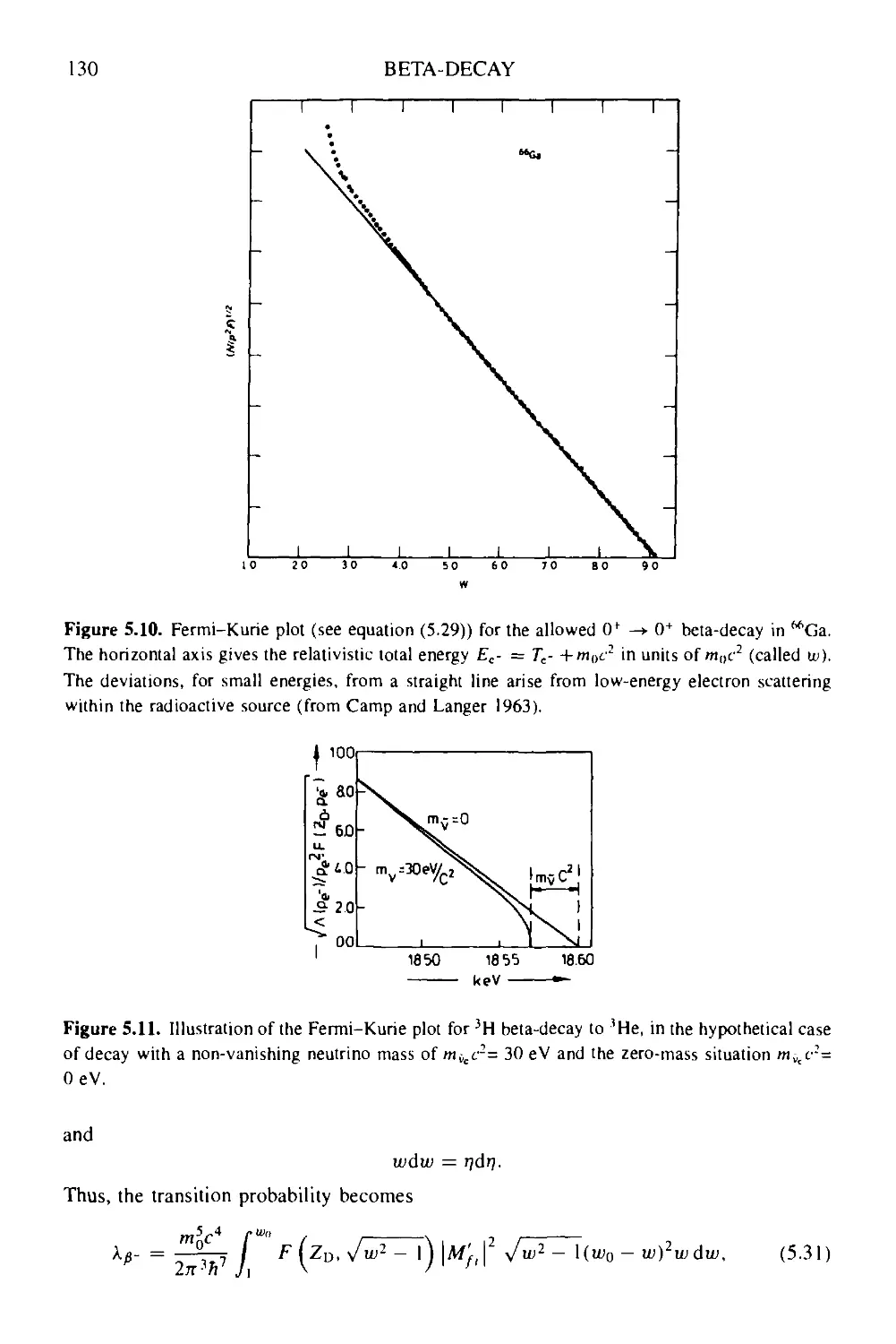
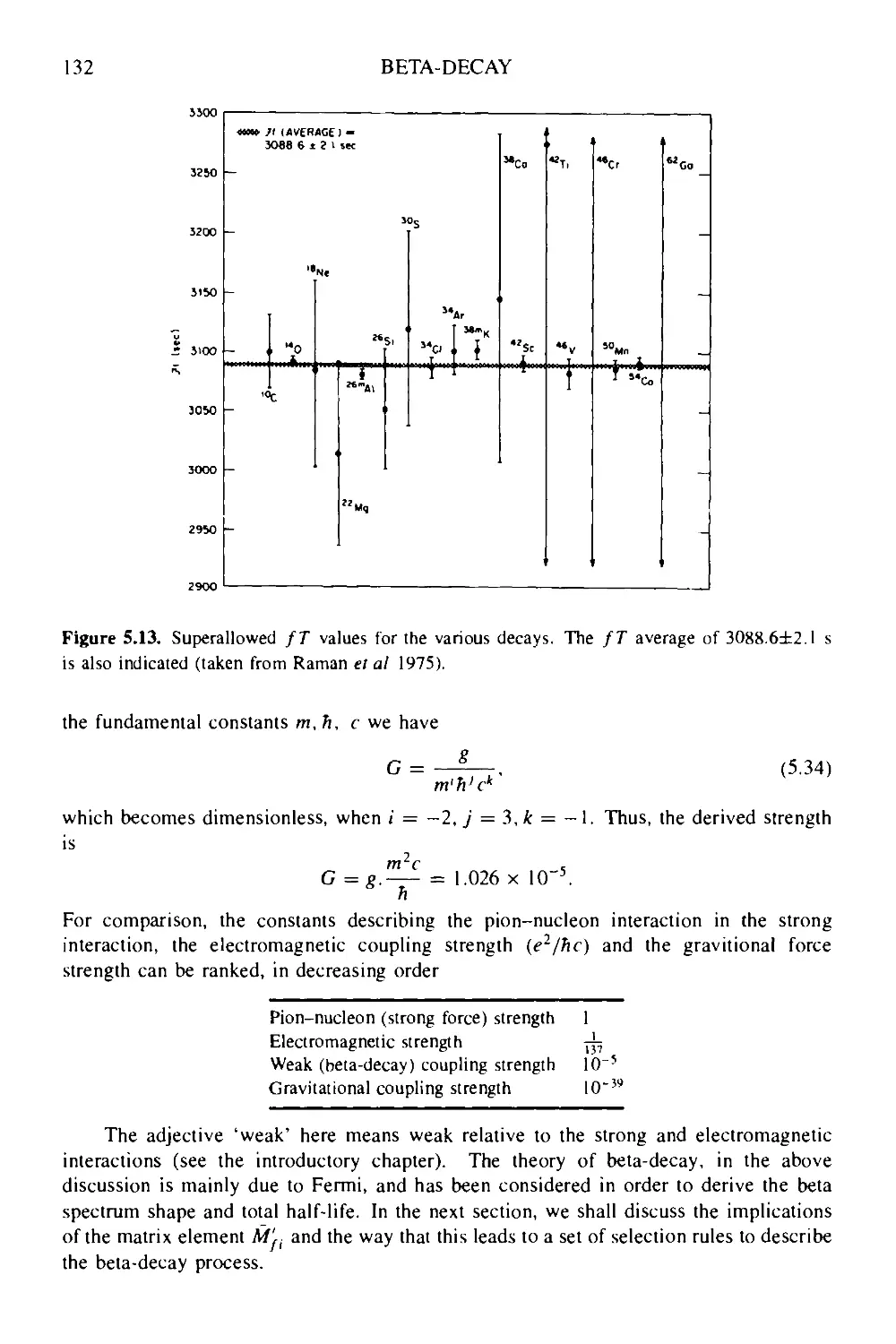
5.3 Classification in beta-decay 133
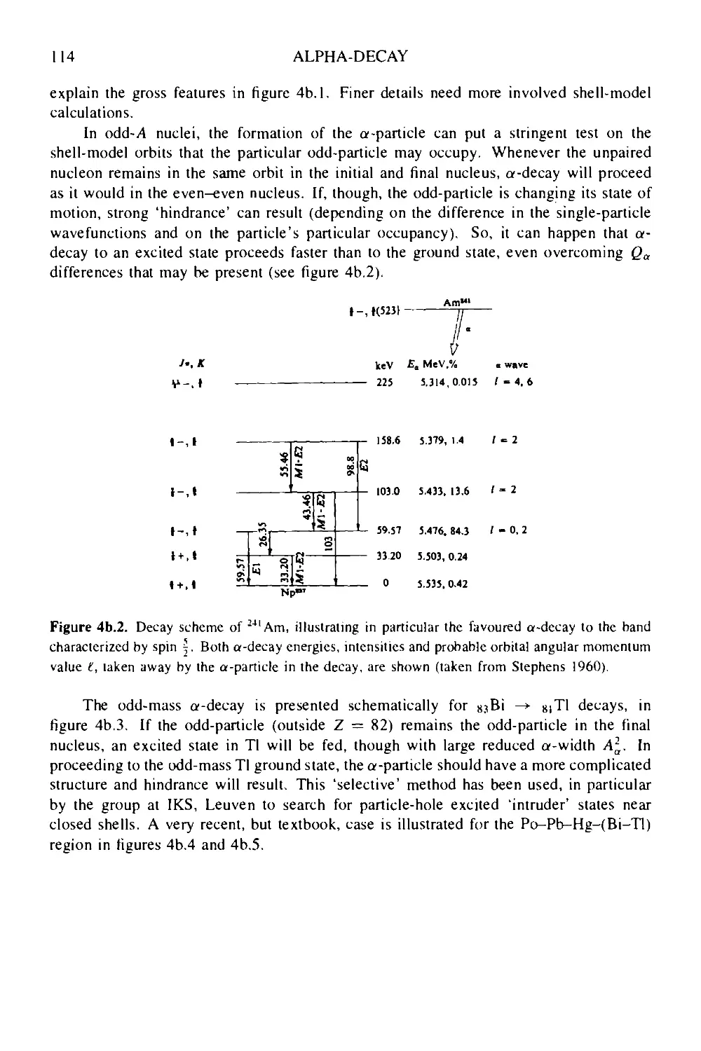
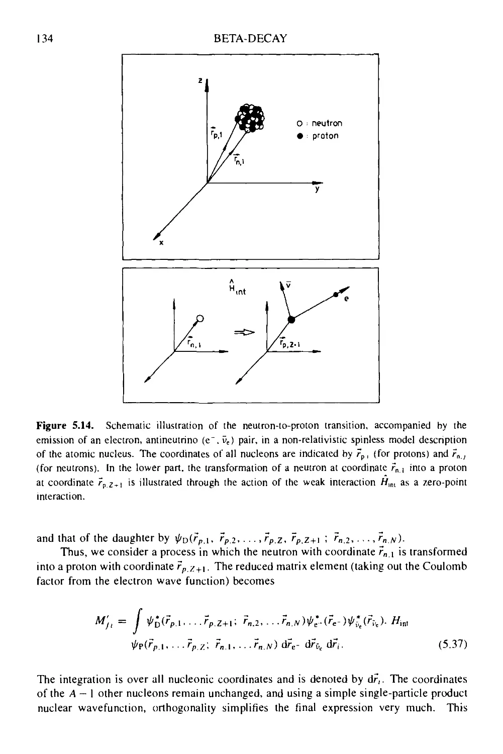
5.3.1 The weak interaction: a spinless non-relativistic model 133
5.3.2 Introducing intrinsic spin 136
5.3.3 Fermi and Gamow-Teller beta transitions 137
5.3.4 Forbidden transitions 137
5.3.5 Electron-capture processes 138
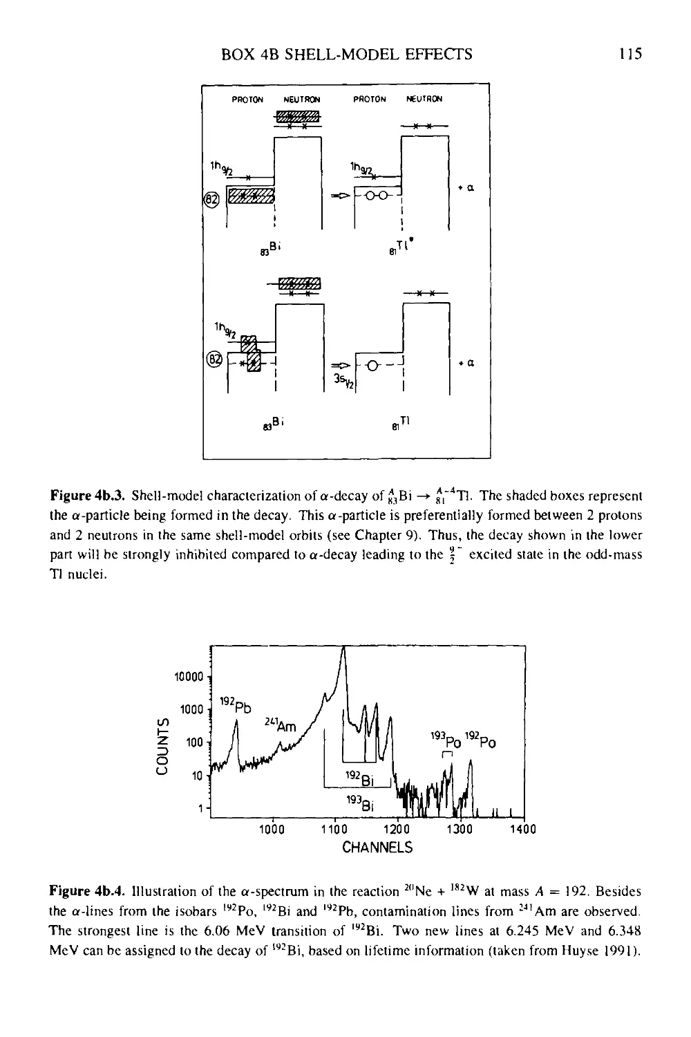
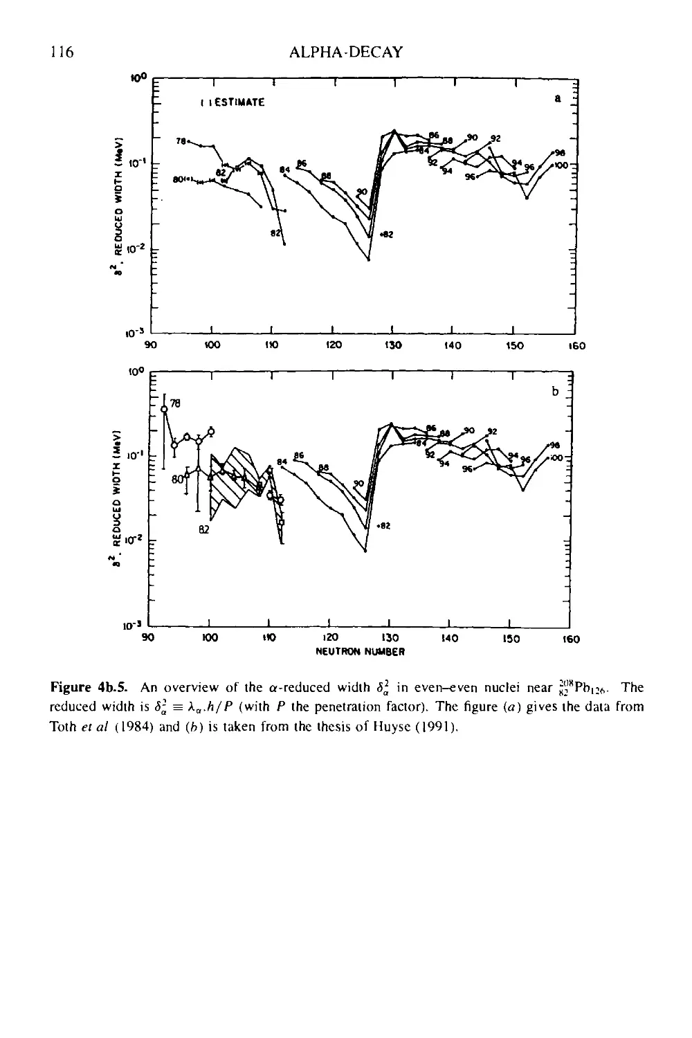
5.4 The neutrino in beta-decay 140
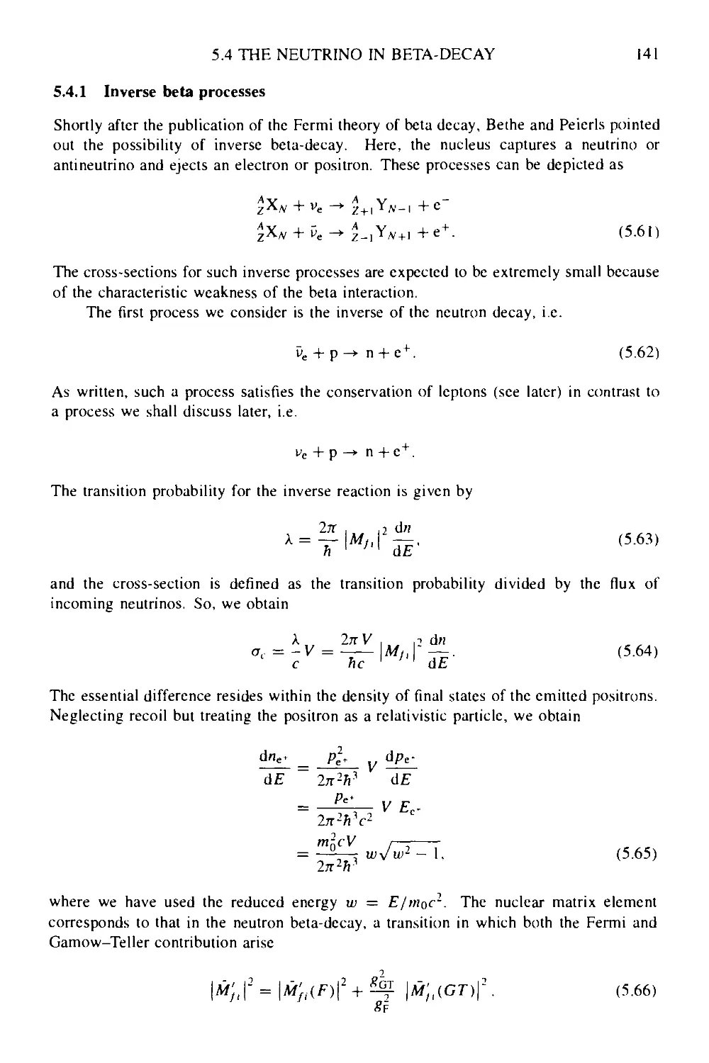
5.4.1 Inverse beta processes 141
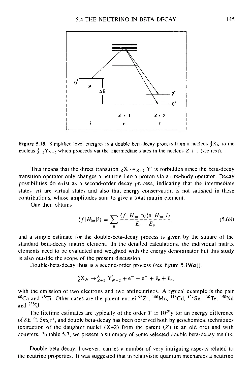
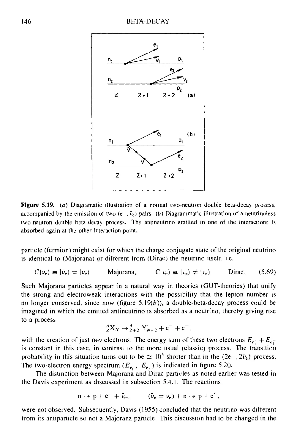
5.4.2 Double beta-decay 144
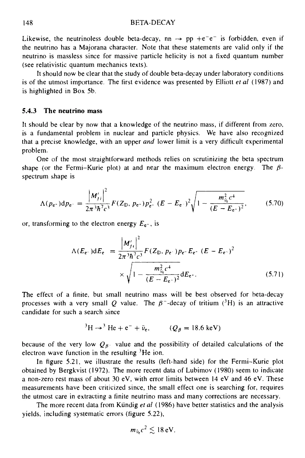
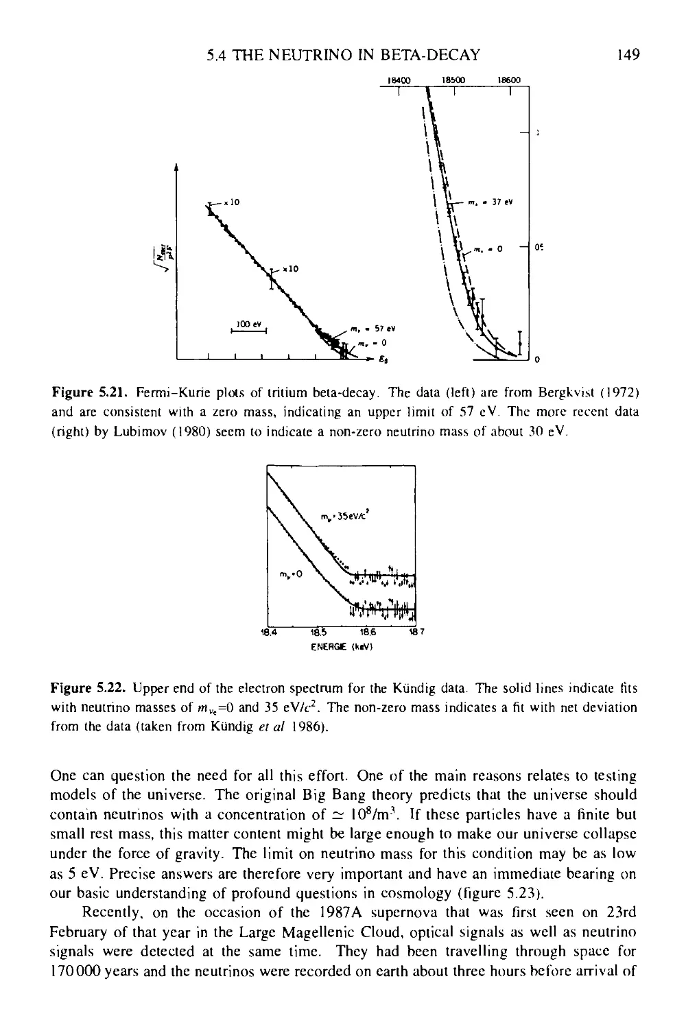
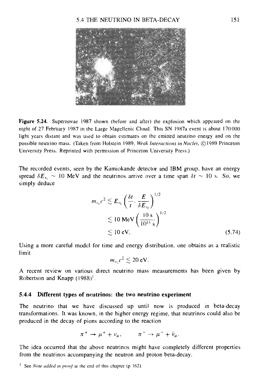
5.4.3 The neutrino mass 148
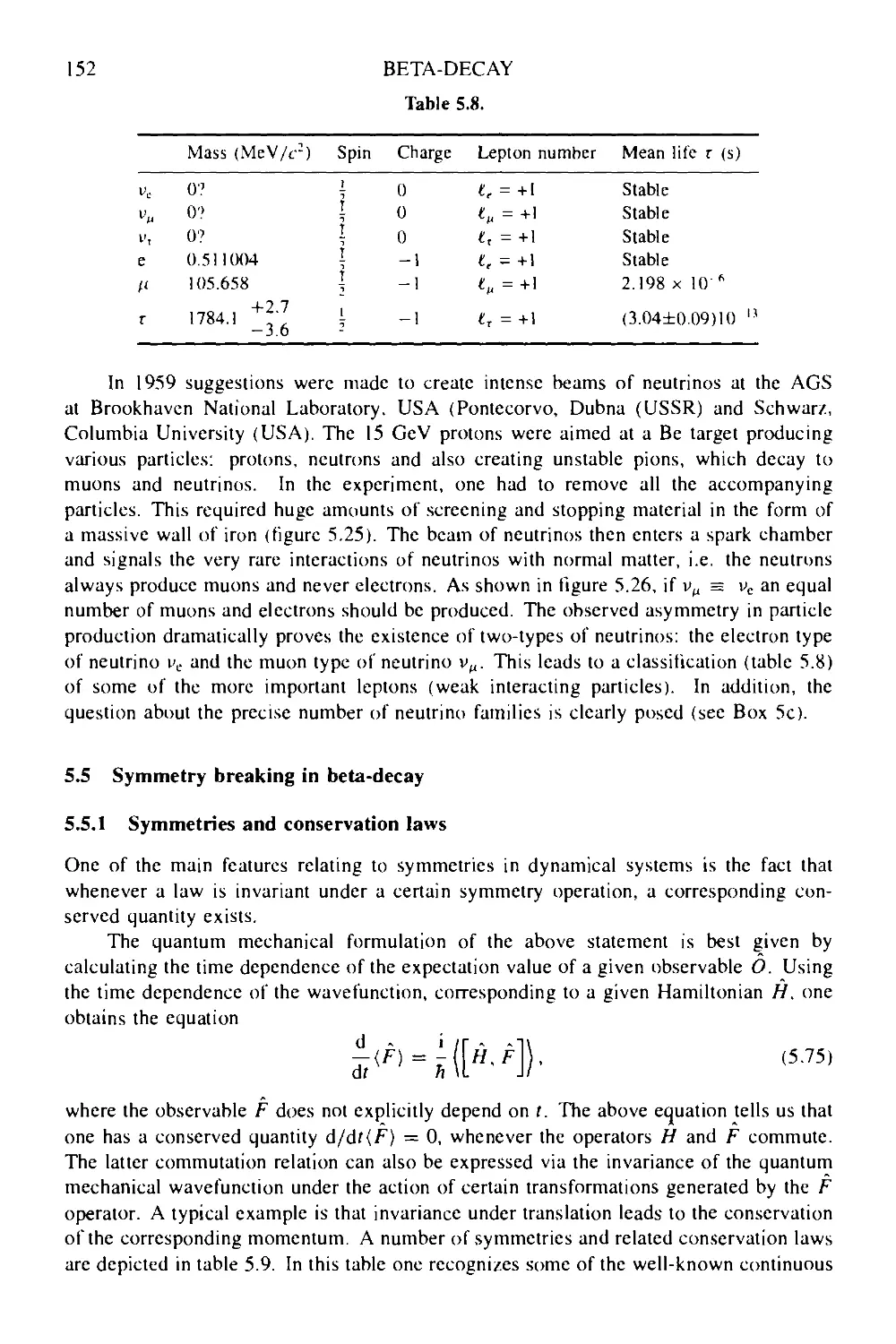
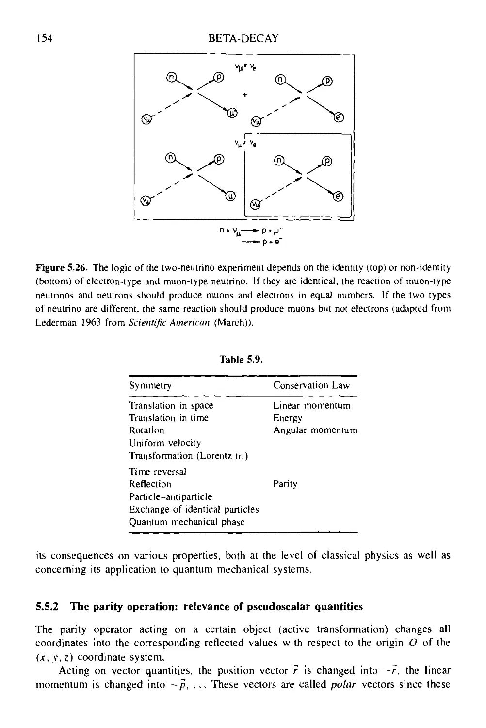
5.4.4 Different types of neutrinos: the two neutrino experiment 151
CONTENTS ix
5.5 Symmetry breaking in beta-decay 152
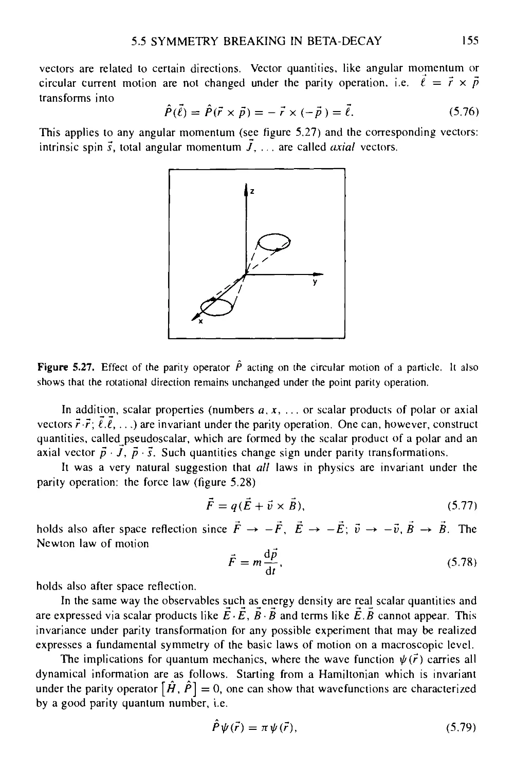
5.5.1 Symmetries and conservation laws 152
5.5.2 The parity operation: relevance of pseudoscalar quantities 154
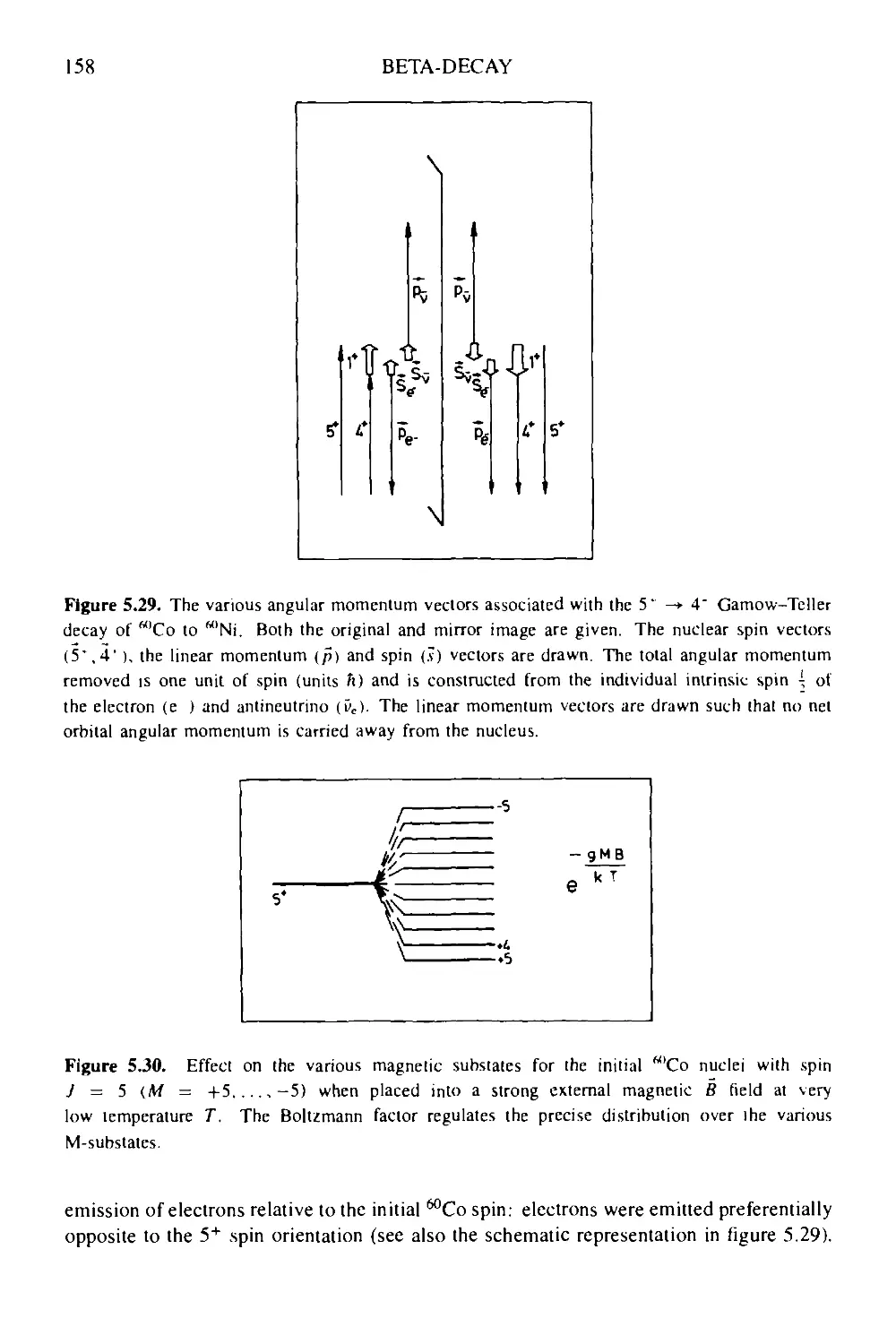
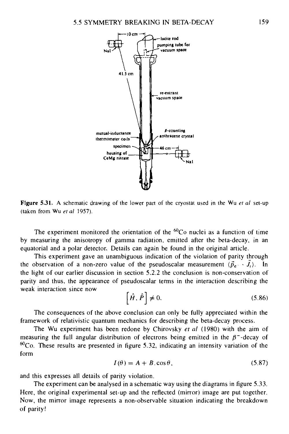
5.5.3 The Wu-Ambler experiment and the fall of parity conservation 157
5.5.4 The neutrino intrinsic properties: helicity 160
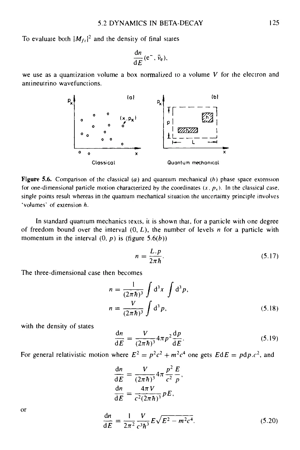
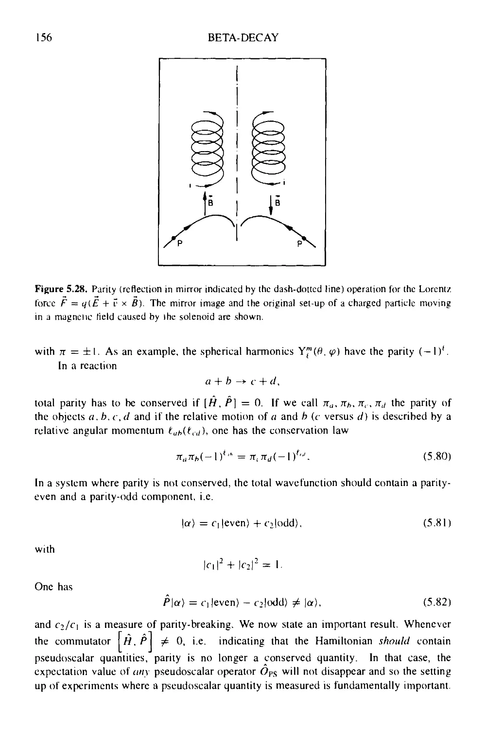
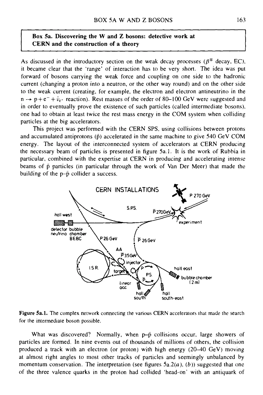
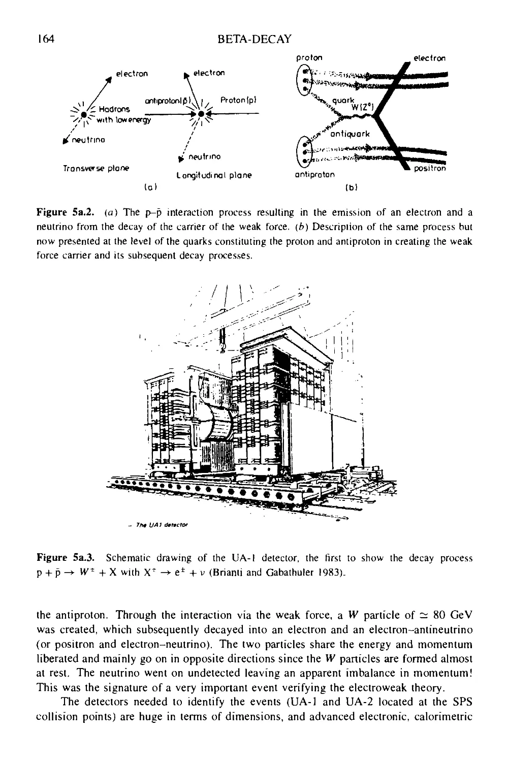
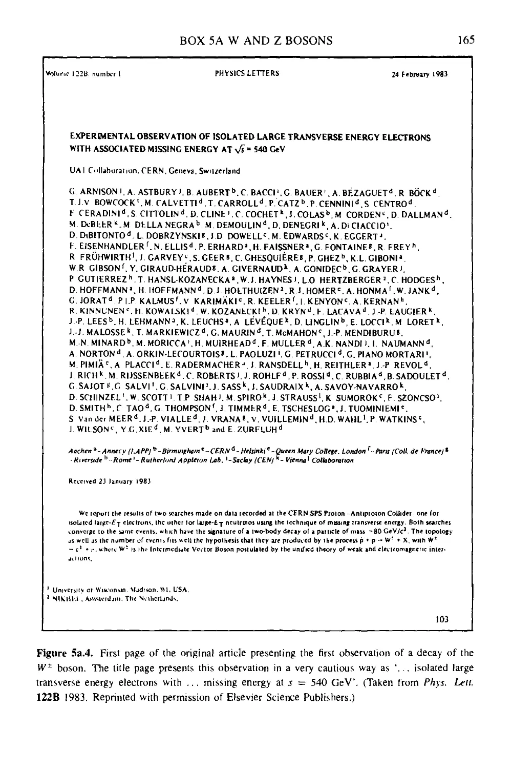
Box 5a Discovering the W and Z bosons: detective work at CERN and the
construction of a theory 163
Box 5b First laboratory observation of double beta-decay 167
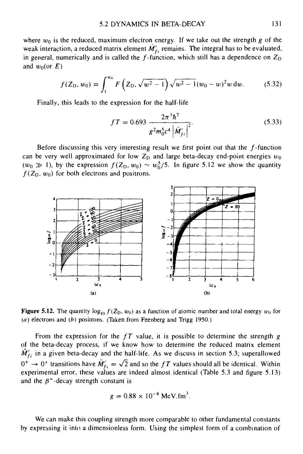
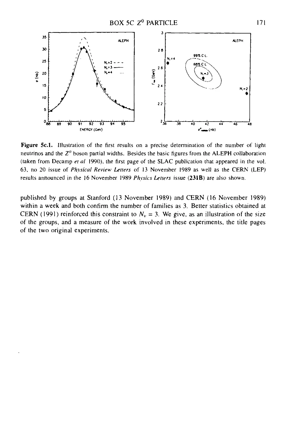
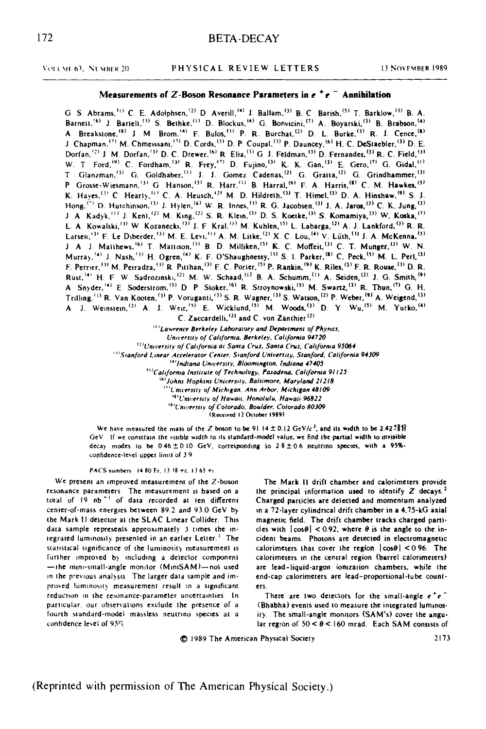
Box 5c The width of the Z° particle: measuring the number of neutrino families 170
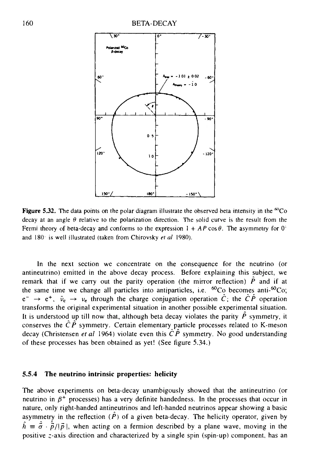
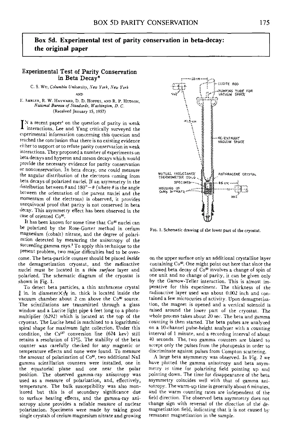
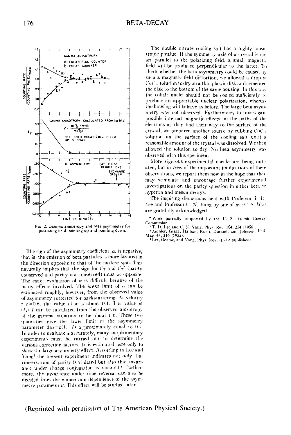
Box 5d Experimental test of parity conservation in beta-decay: the original paper 175
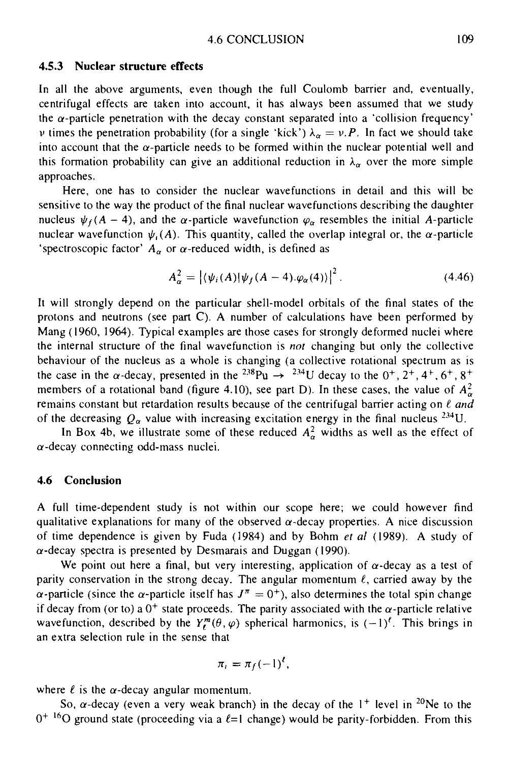
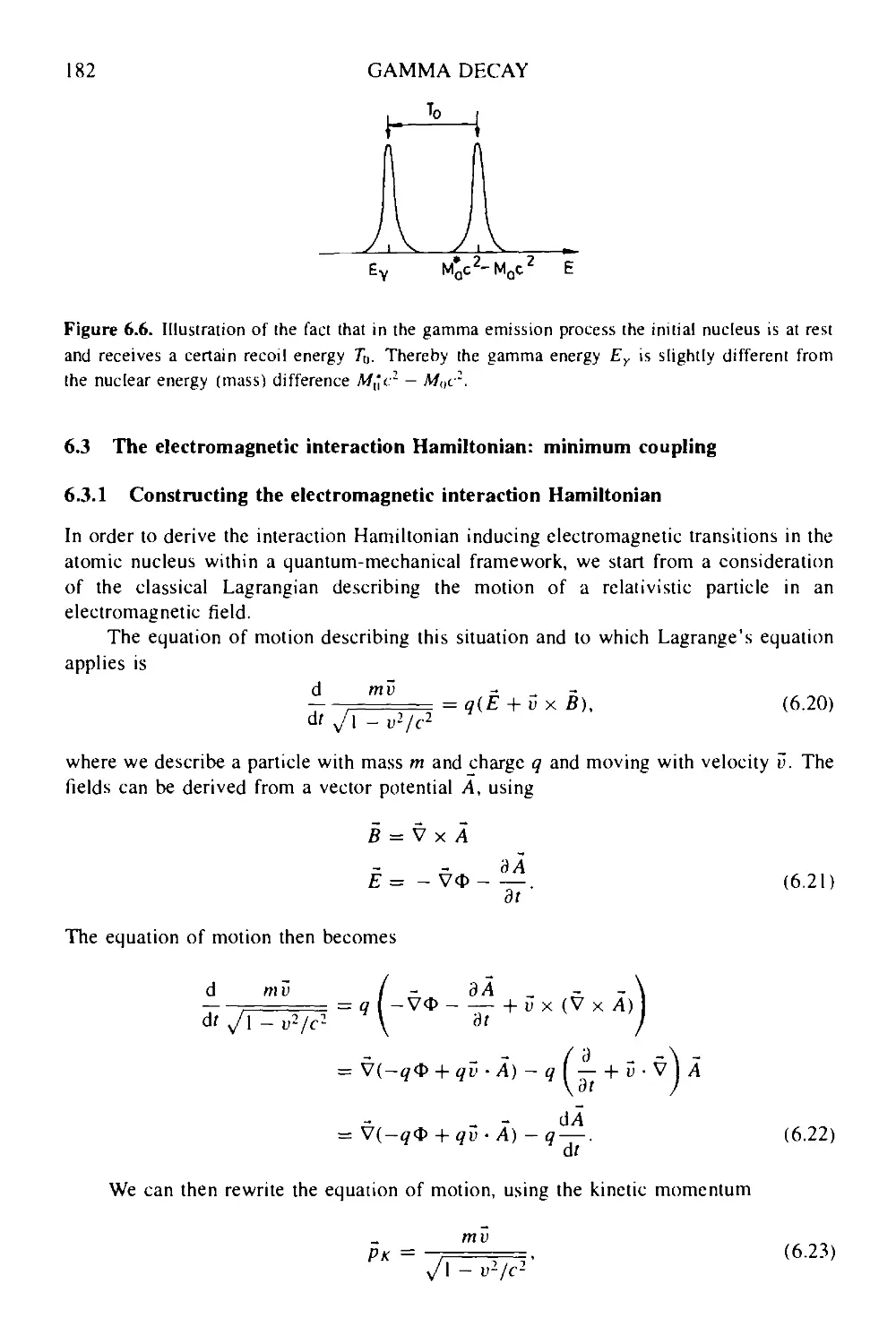
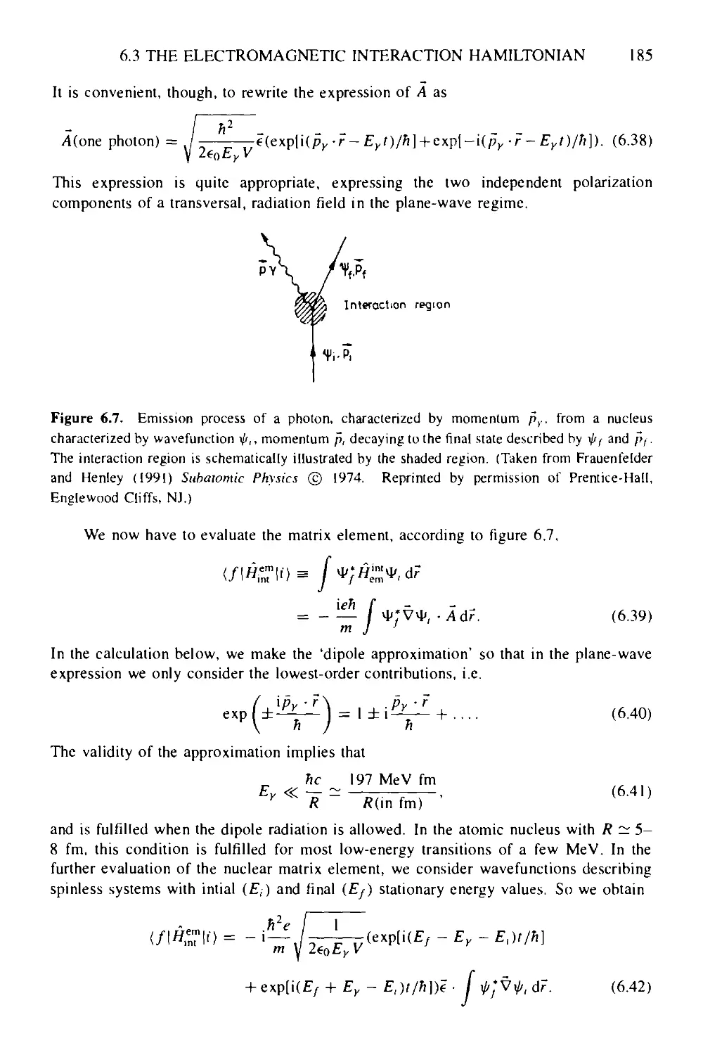
6 Gamma decay: the electromagnetic interaction at work 177
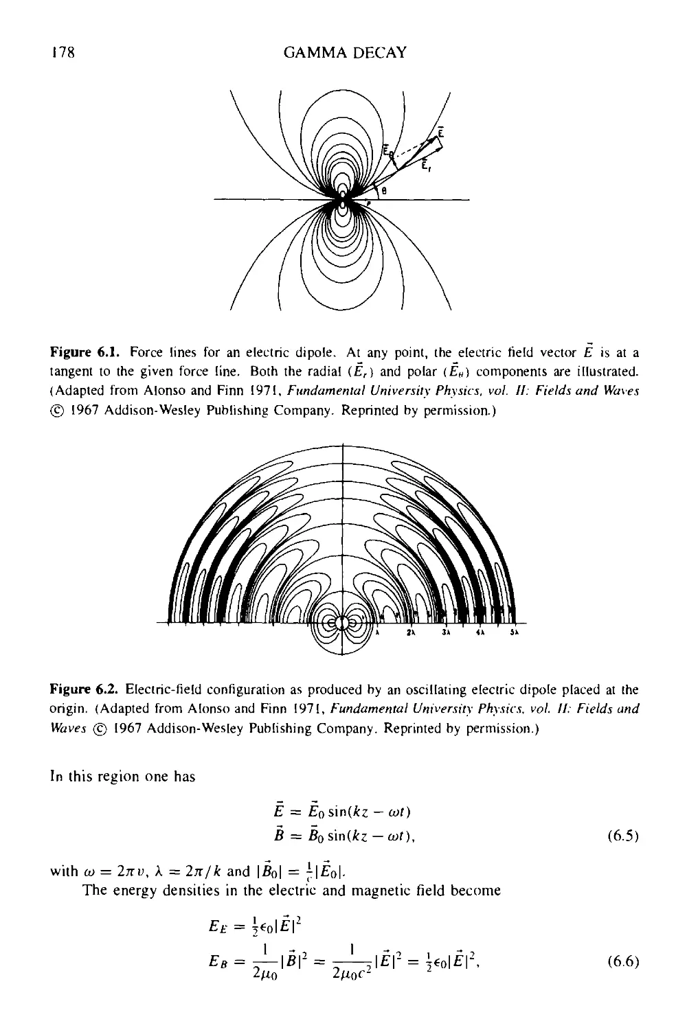
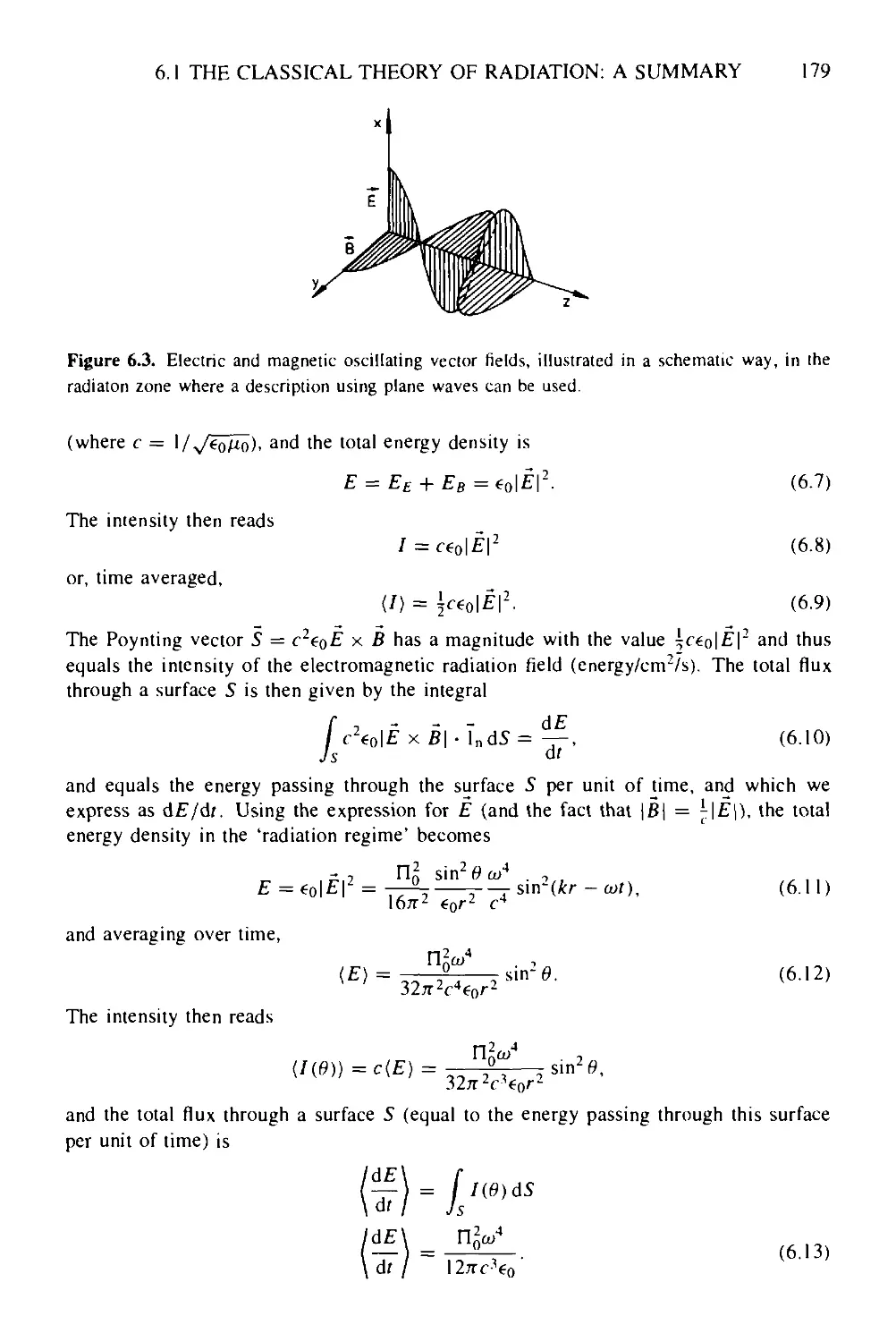
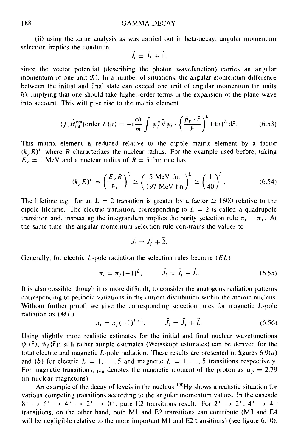
6.1 The classical theory of radiation: a summary 177
6.2 Kinematics of photon emission 181
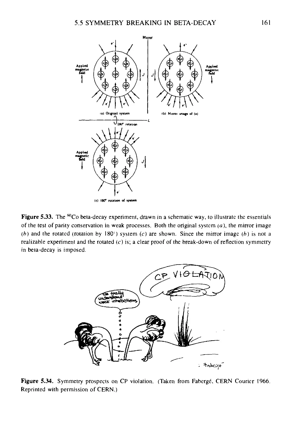
6.3 The electromagnetic interaction Hamiltonian: minimum coupling 182
6.3.1 Constructing the electromagnetic interaction Hamiltonian 182
6.3.2 One-photon emission and absorption: the dipole approximation 184
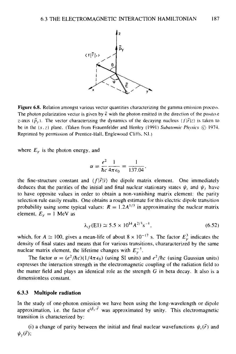
6.3.3 Multipole radiation 187
6.3.4 Internal electron conversion coefficients 189
6.3.5 E0—monopole transitions 193
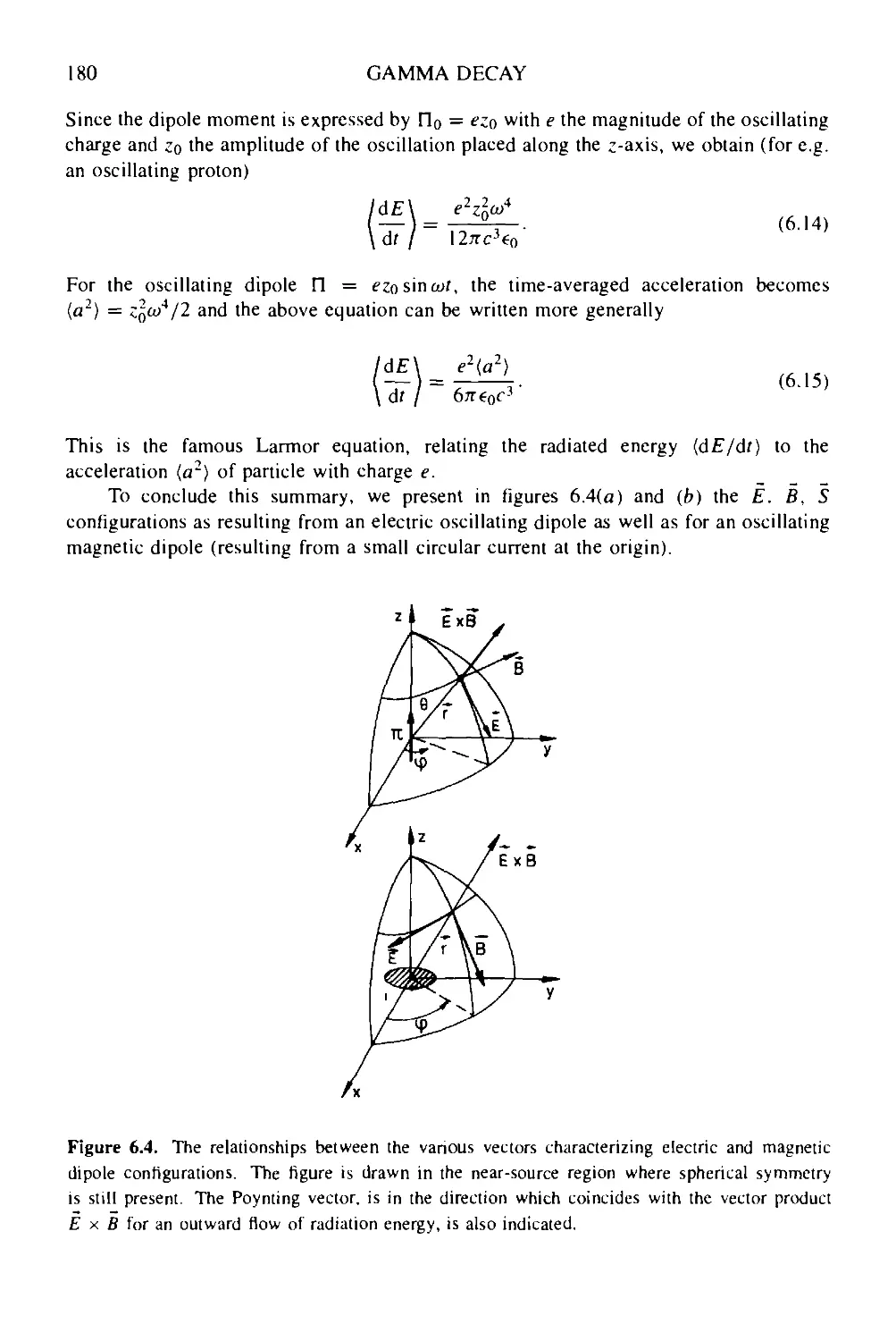
6.3.6 Conclusion 195
Box 6a Alternative derivation of the electric dipole radiation fields 196
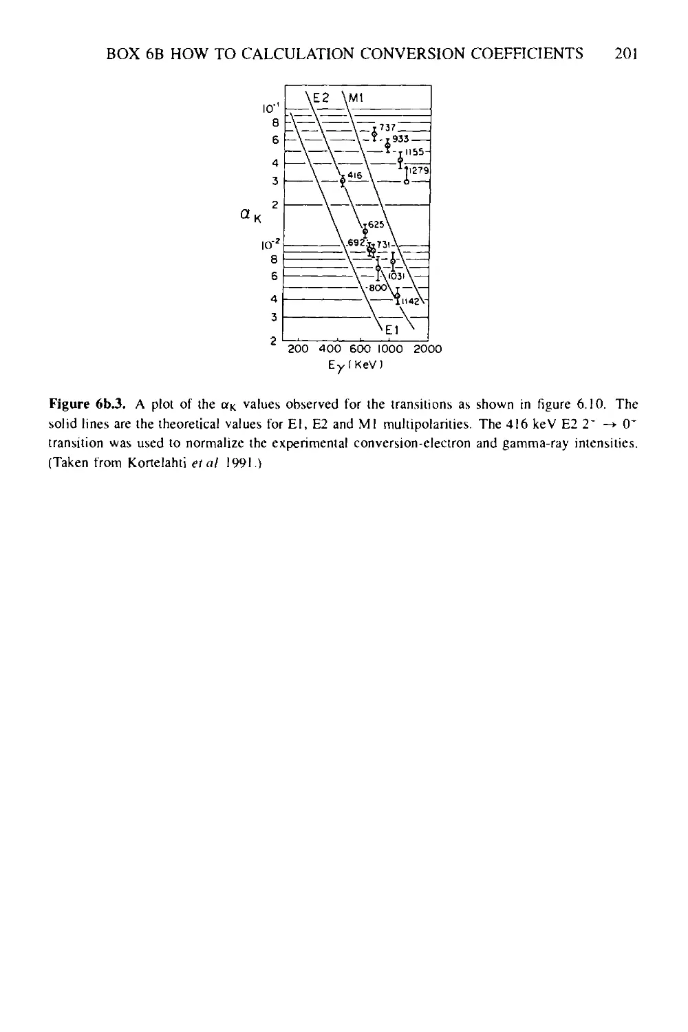
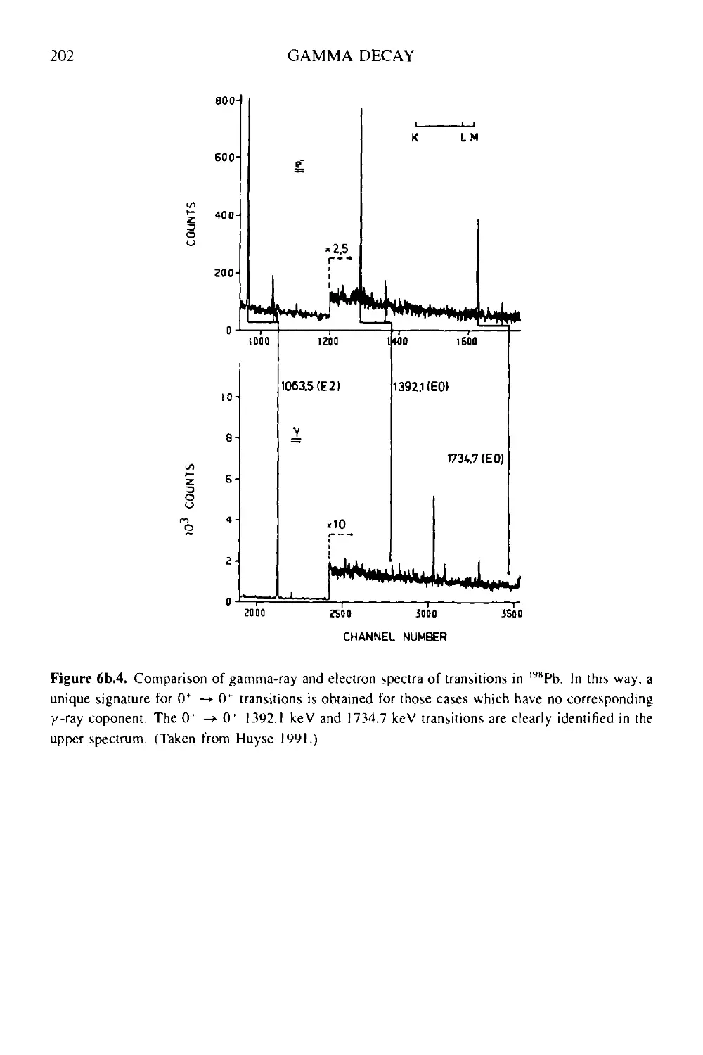
Box 6b How to calculate conversion coefficients and their use in determining
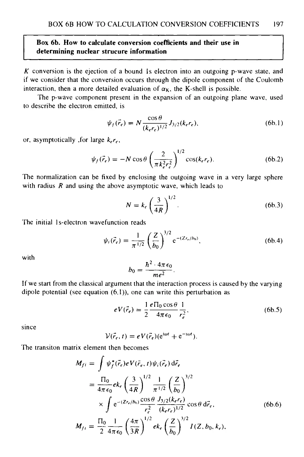
nuclear strucure information 197
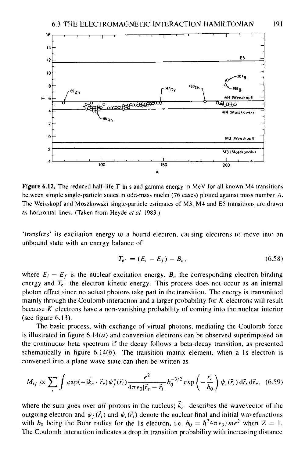
Problem set—Part В 203
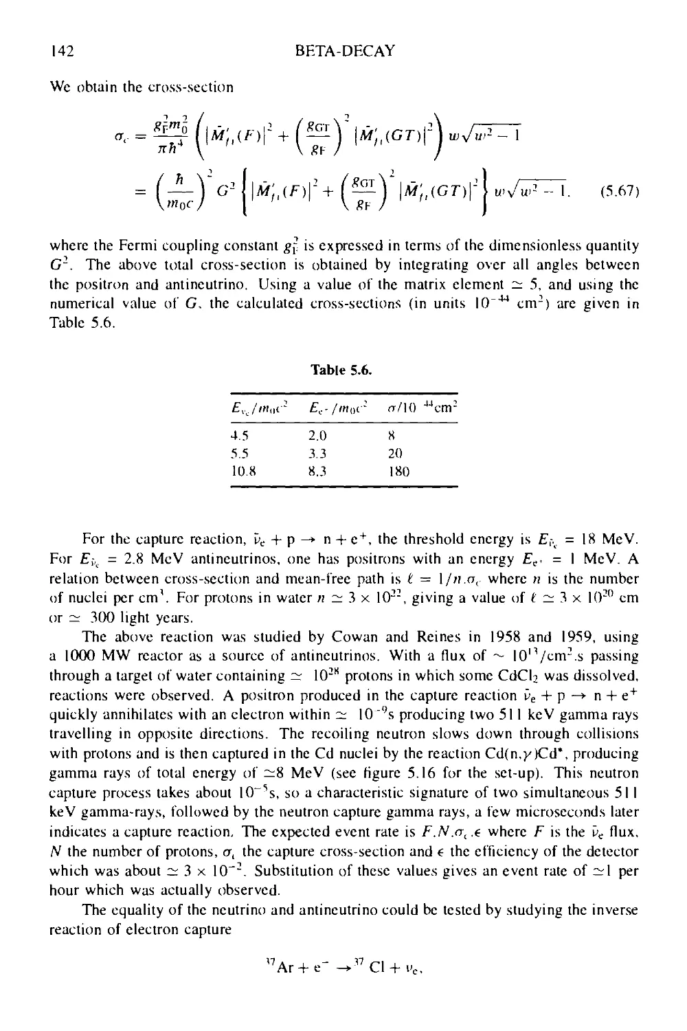
PART С
NUCLEAR STRUCTURE:
AN INTRODUCTION
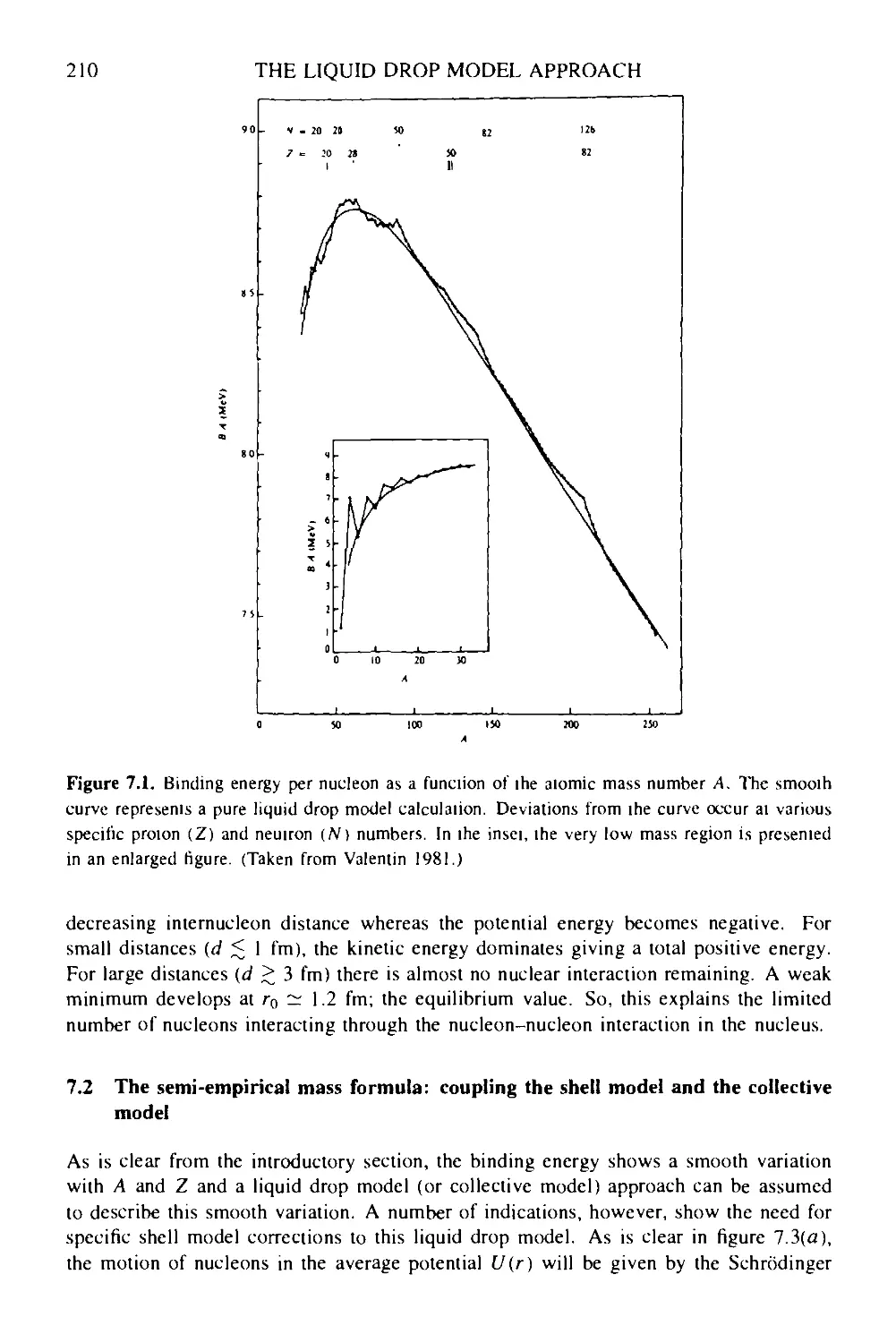
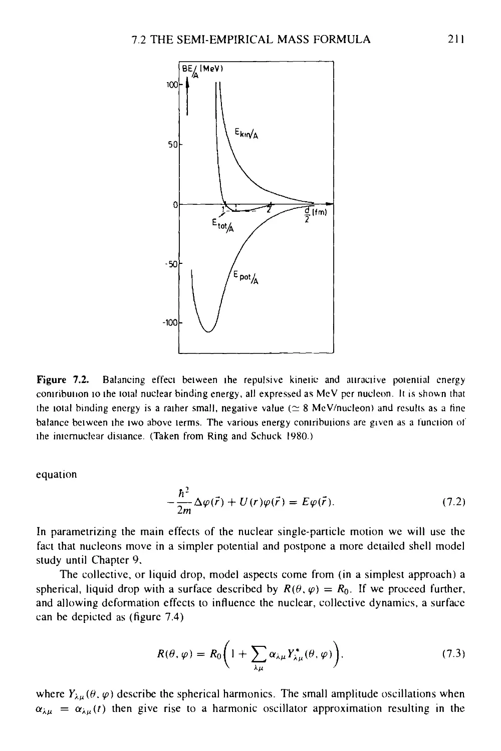
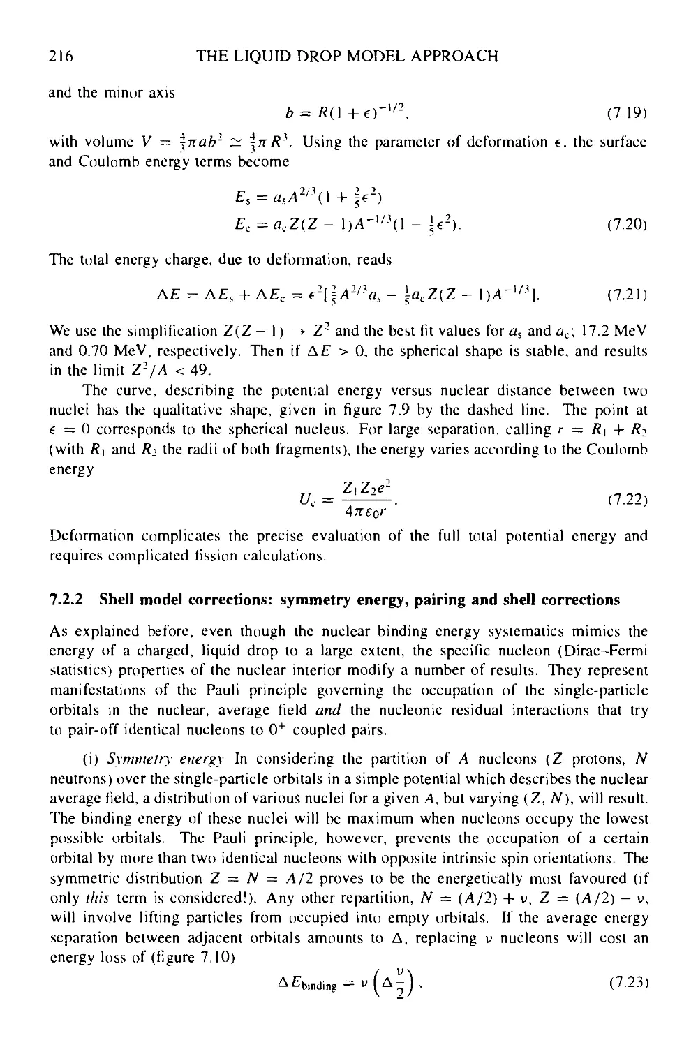
7 The liquid drop model approach: a semi-empirical method 209
7.1 Introduction 209
7.2 The semi-empirical mass formula: coupling the shell model and the
collective model 210
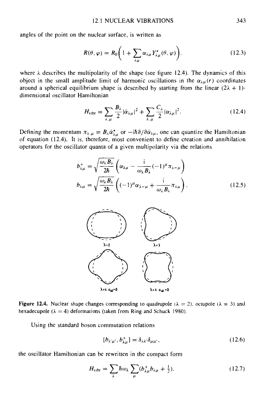
7.2.1 Volume, surface and Coulomb contributions 213
7.2.2 Shell model corrections: symmetry energy, pairing and shell
corrections 216
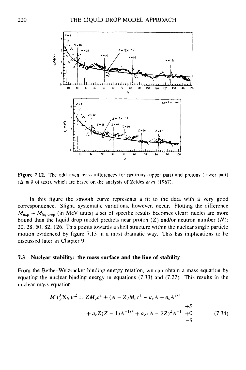
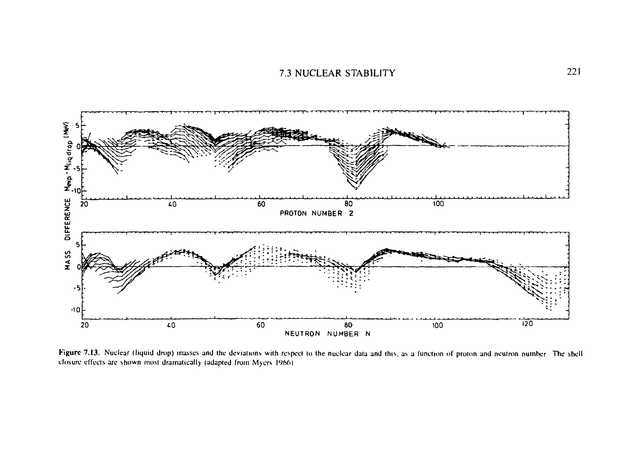
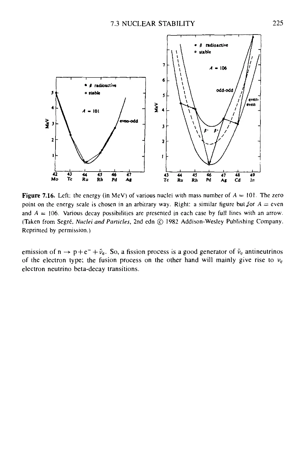
7.3 Nuclear stability: the mass surface and the line of stability 220
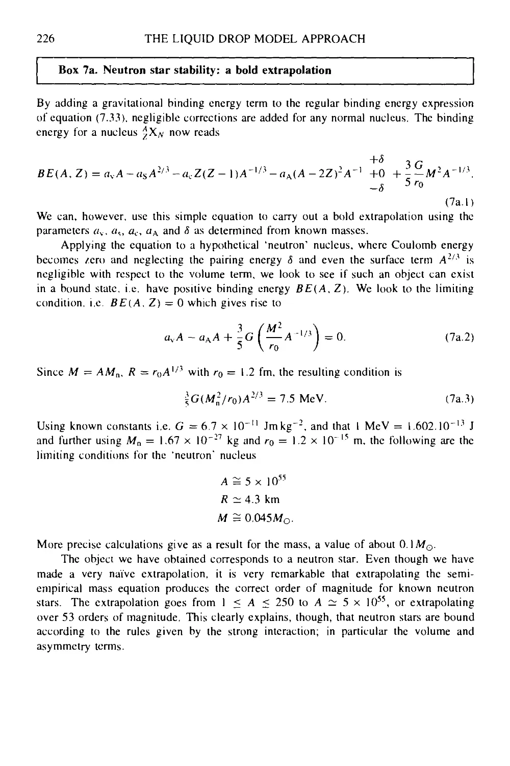
Box 7a Neutron star stability: a bold extrapolation 226
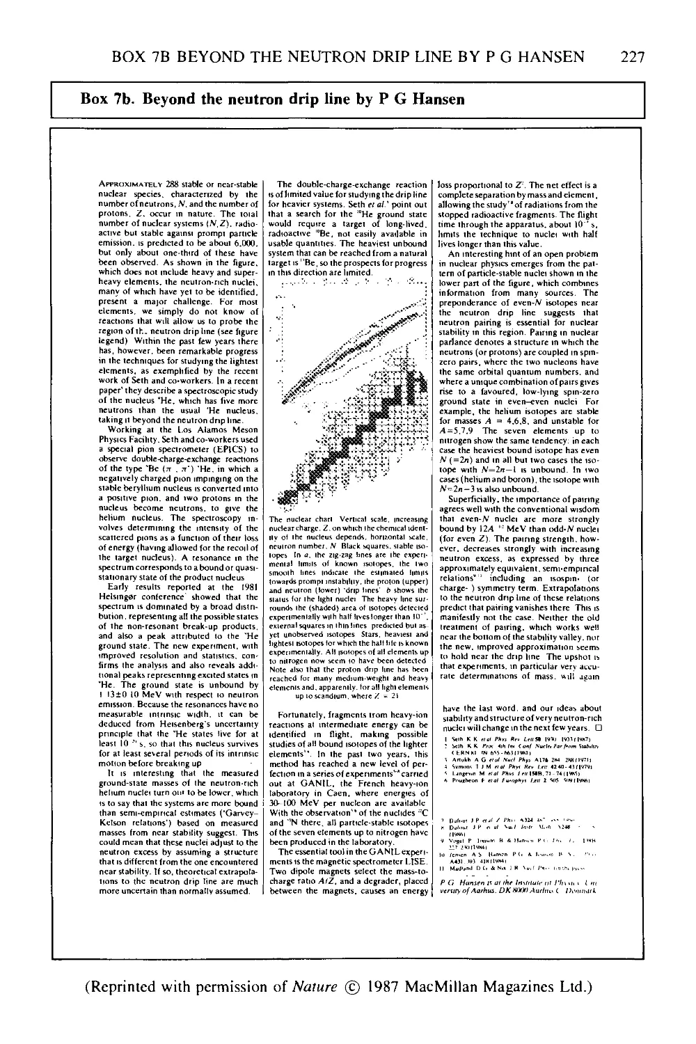
Box 7b Beyond the neutron drip line by P G Hansen 227
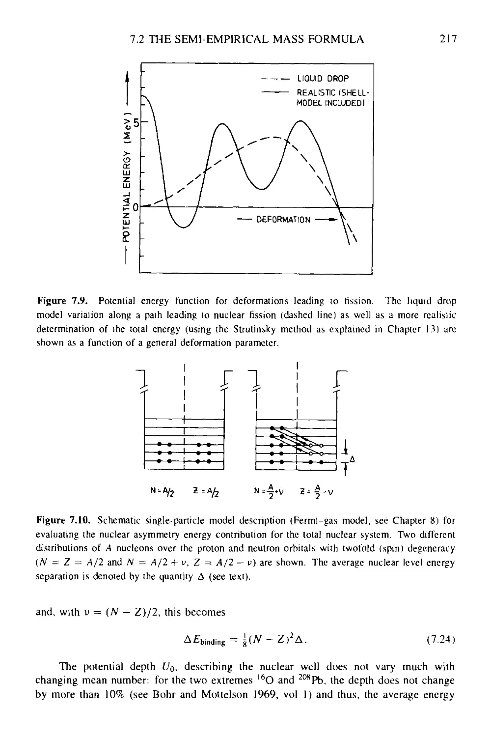
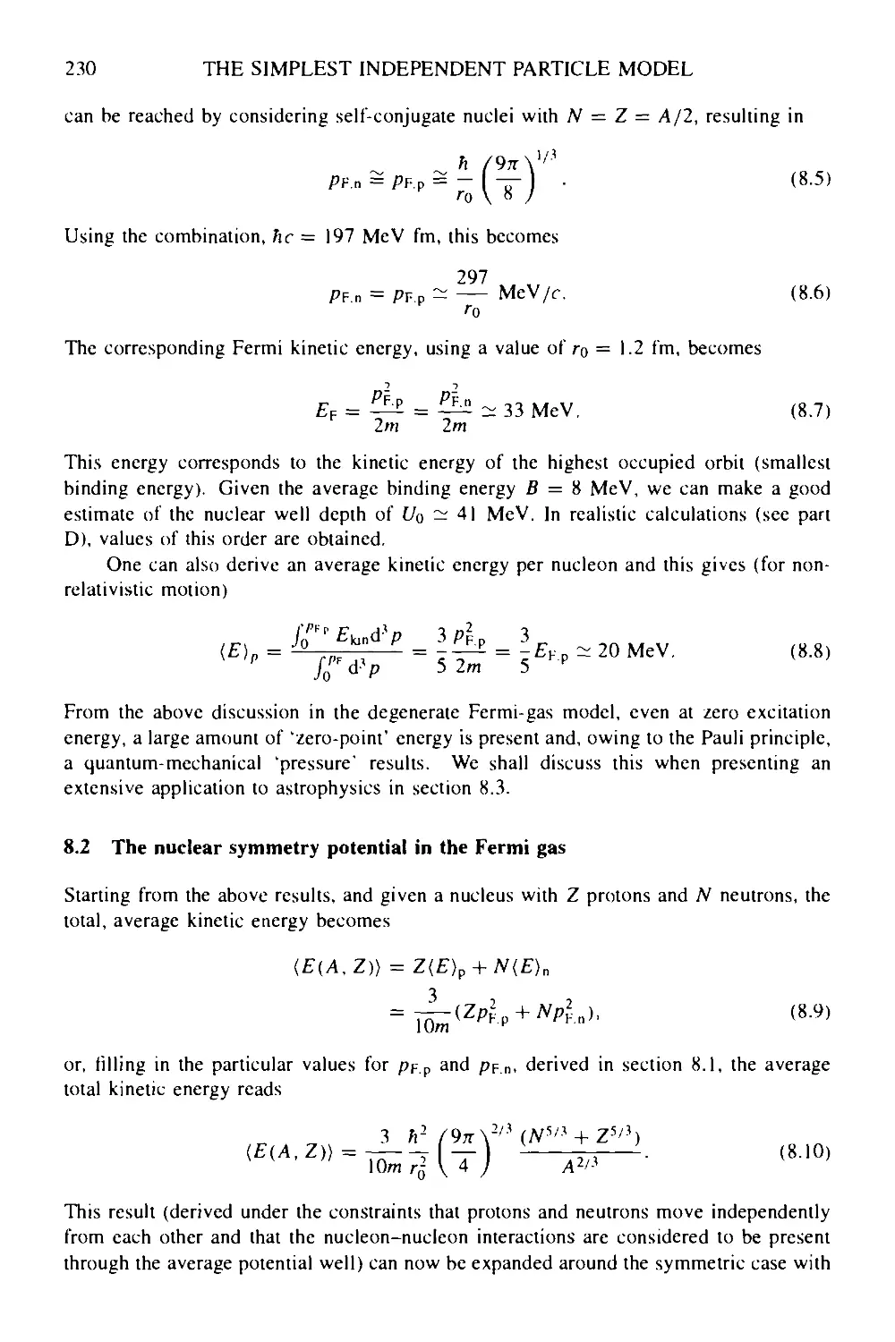
8 The simplest independent particle model: the Fermi-gas model 228
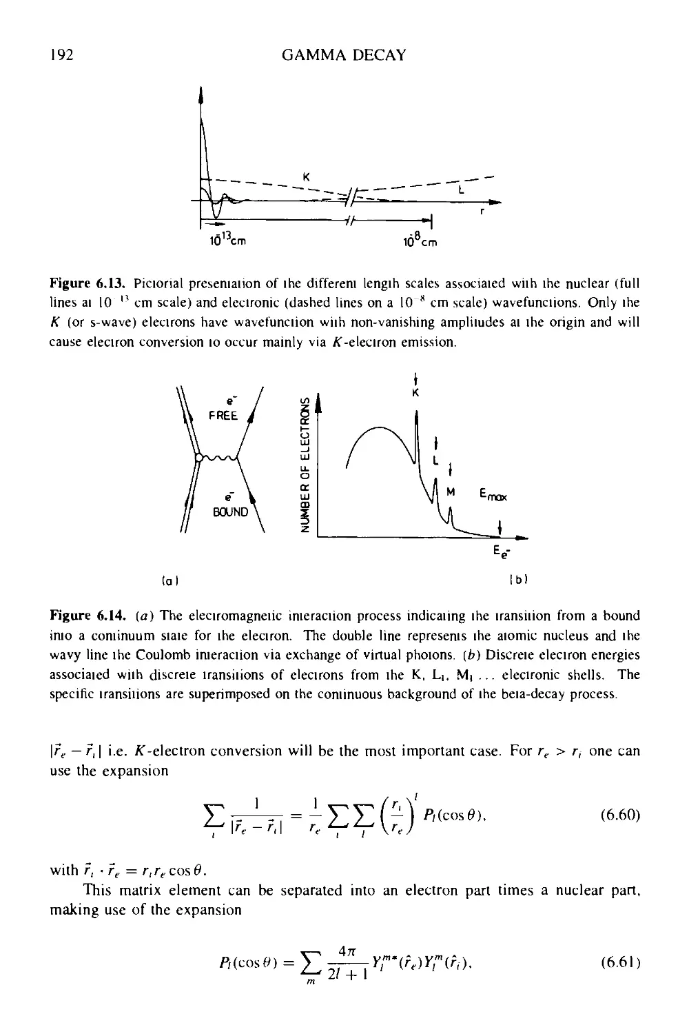
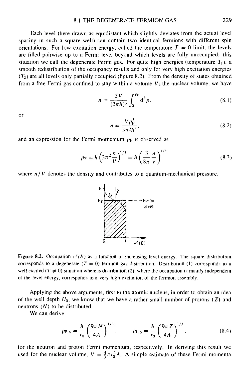
8.1 The degenerate fermion gas 228
8.2 The nuclear symmetry potential in the Fermi gas 230
8.3 Temperature T — 0 pressure: degenerate Fermi-gas stability 231
x CONTENTS
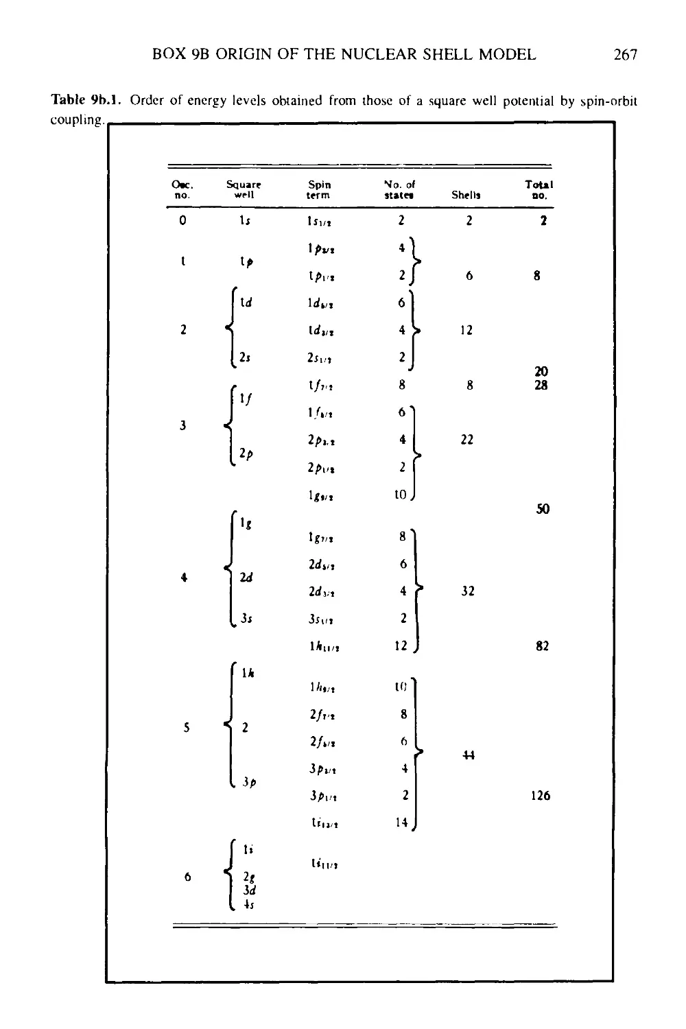
9 The nuclear shell model 236
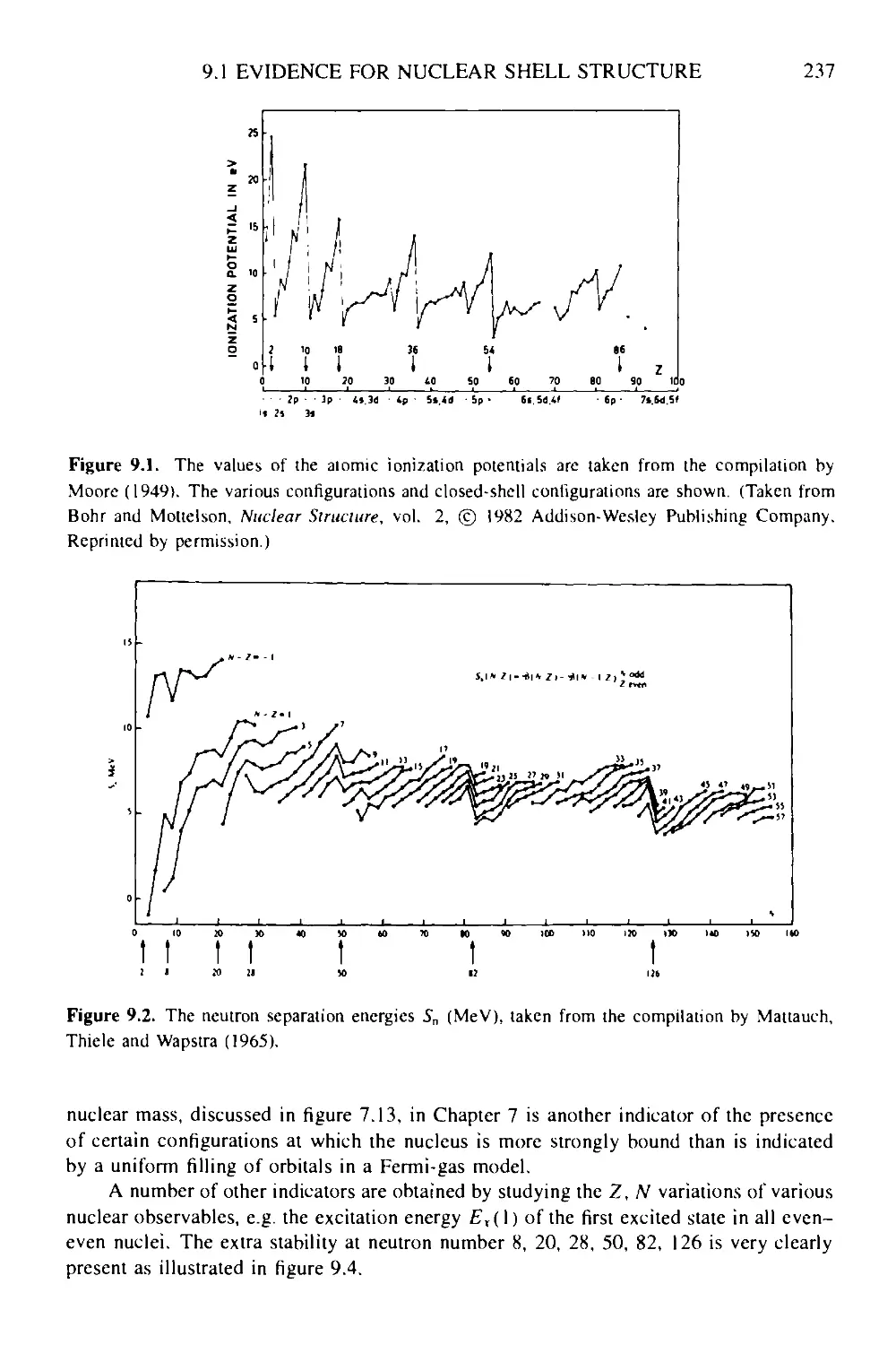
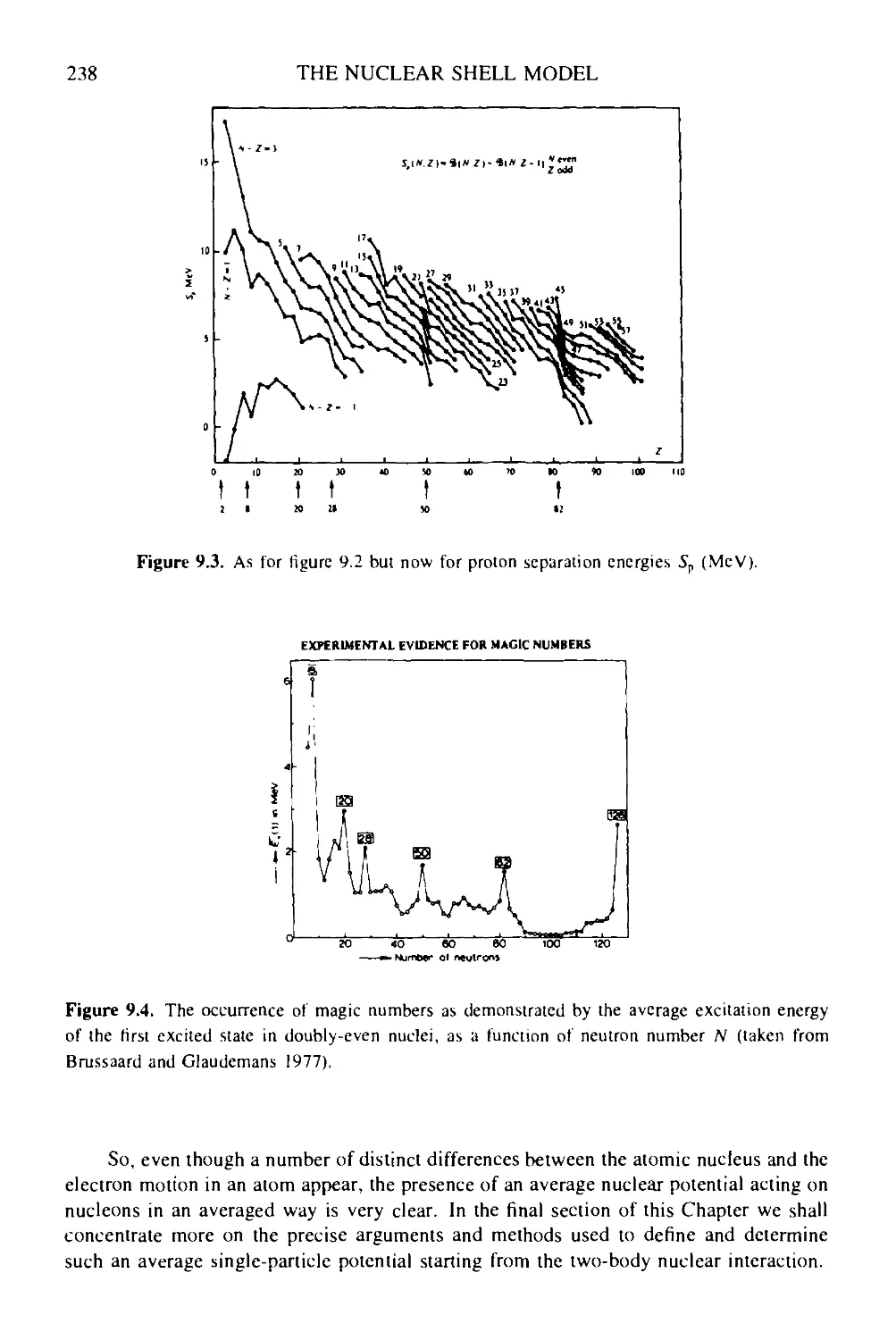
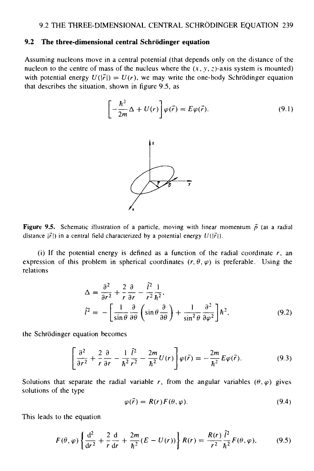
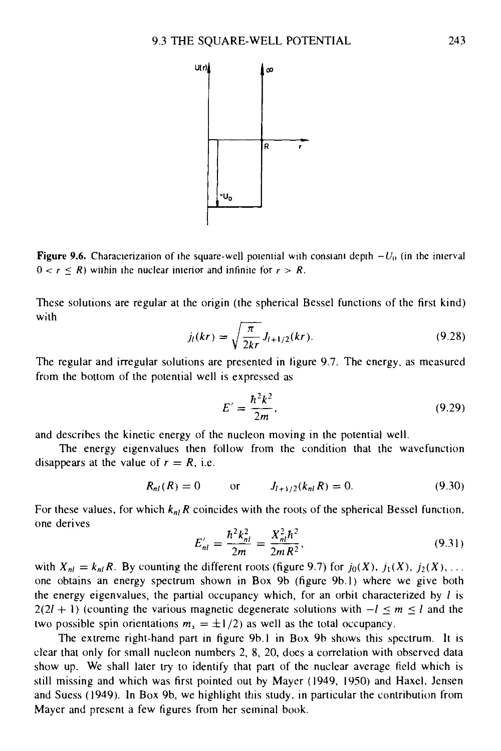
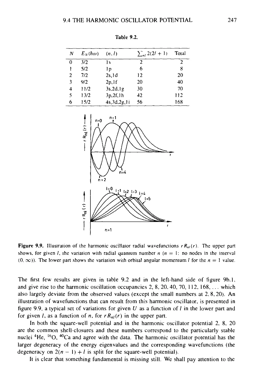
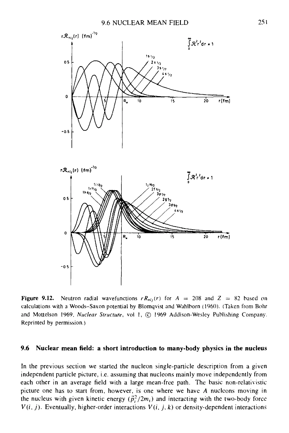
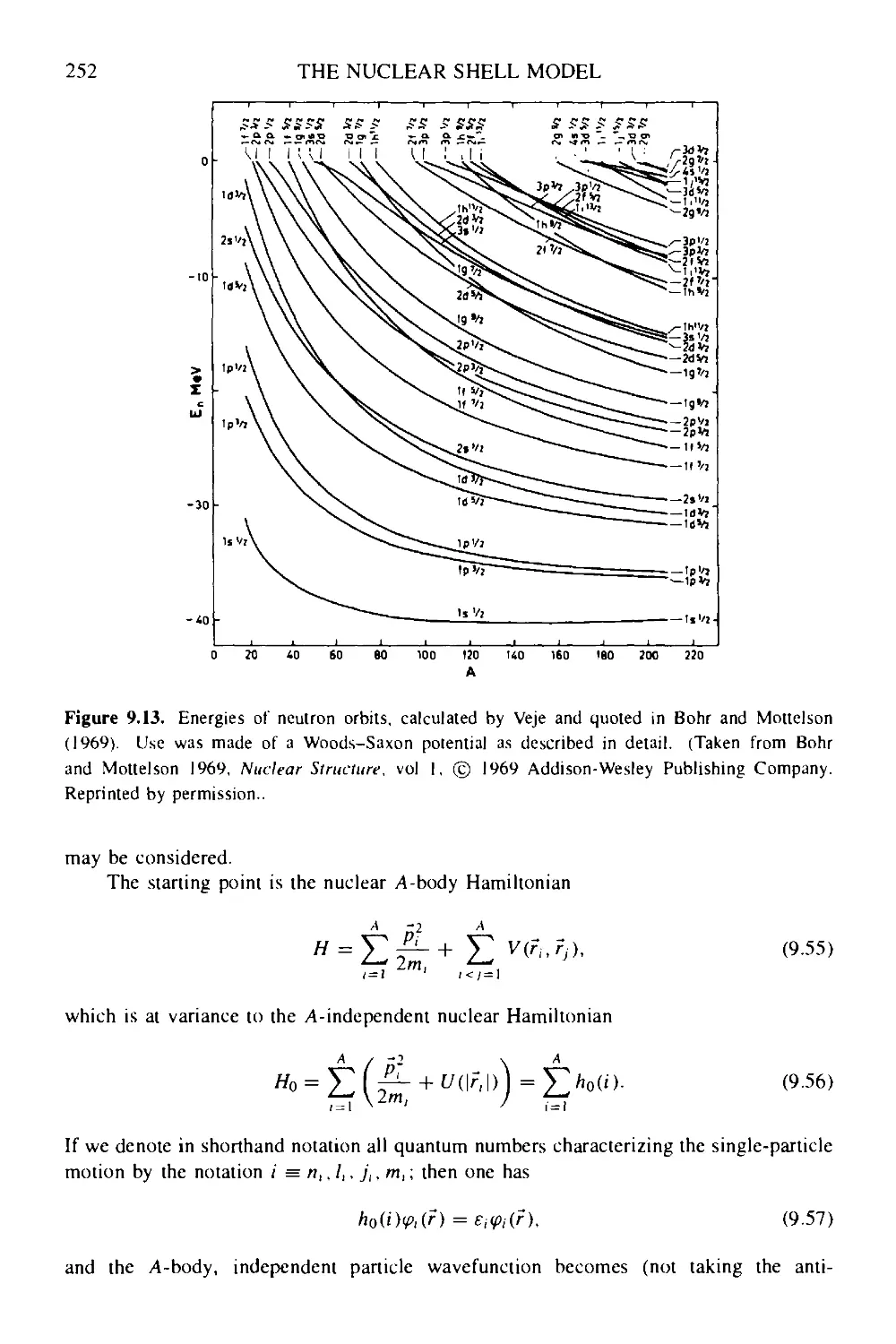
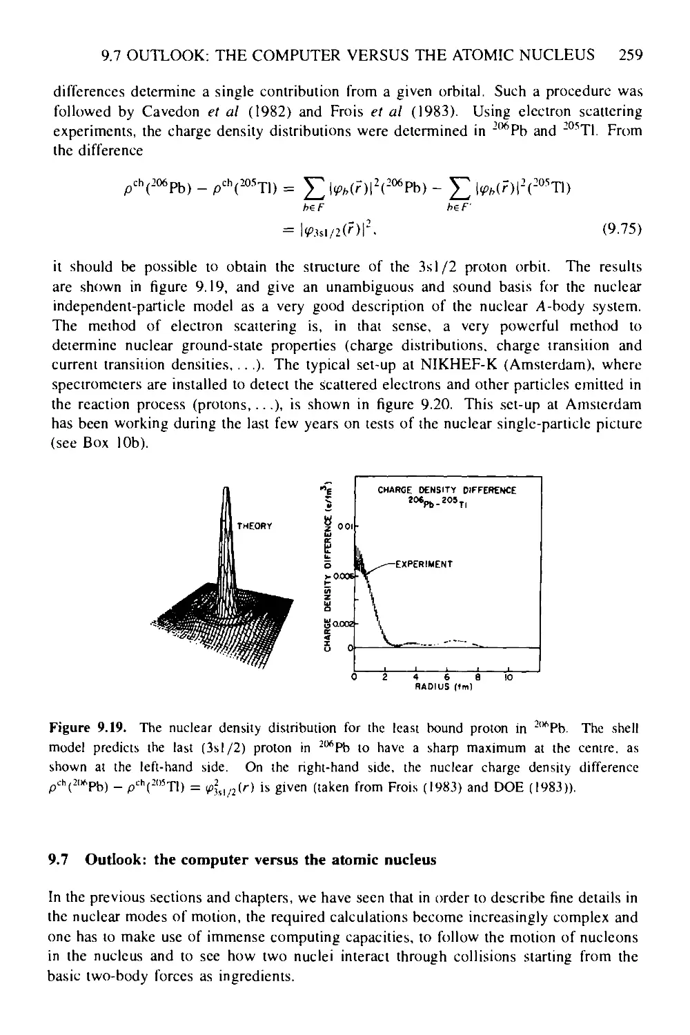
9.1 Evidence for nuclear shell structure 236
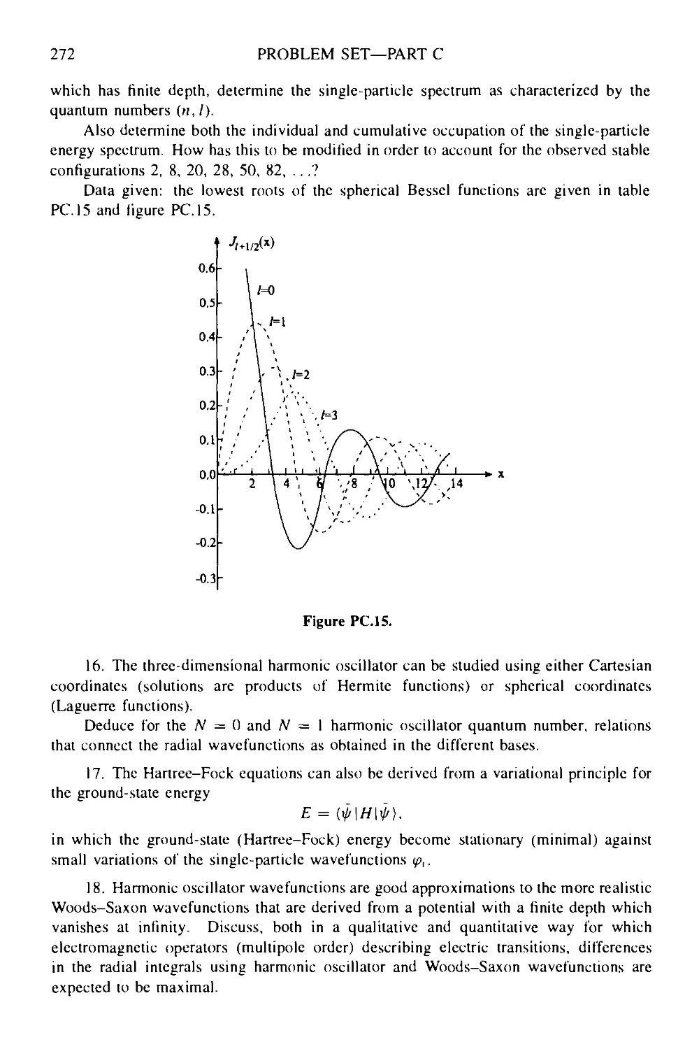
9.2 The three-dimensional central Schrodinger equation 239
9.3 The square-well potential: the energy eigenvalue problem for bound
states 242
9.4 The harmonic oscillator potential 244
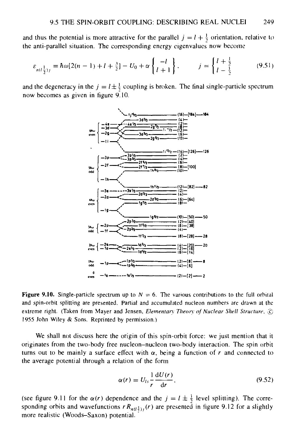
9.5 The spin-orbit coupling: describing real nuclei 248
9.6 Nuclear mean field: a short introduction to many-body physics in the
nucleus 251
9.6.1 Hartree-Fock: a tutorial 253
9.6.2 Measuring the nuclear density distributions: a test of
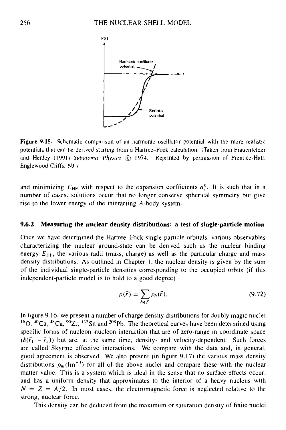
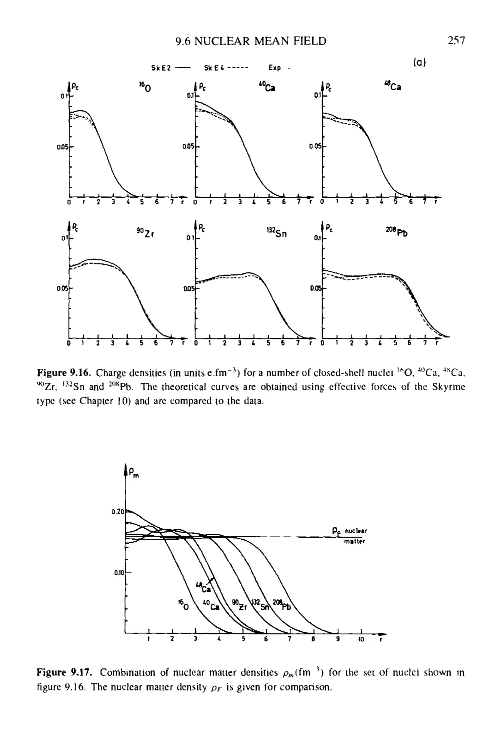
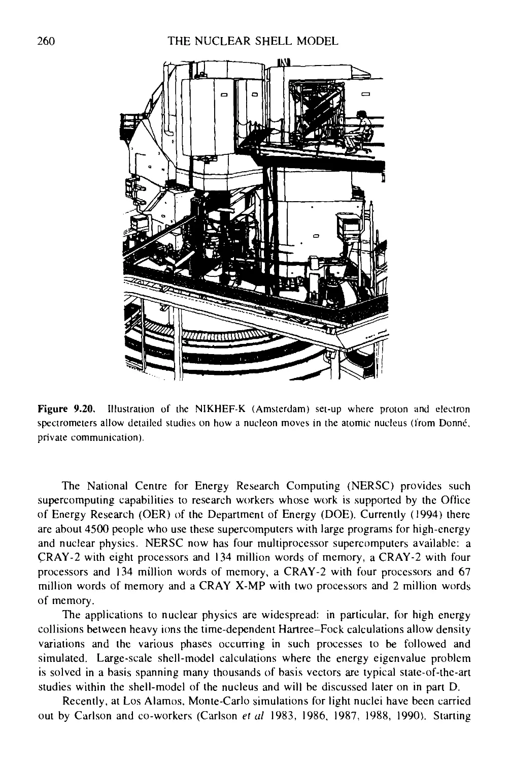
single-particle motion 256
9.7 Outlook: the computer versus the atomic nucleus 259
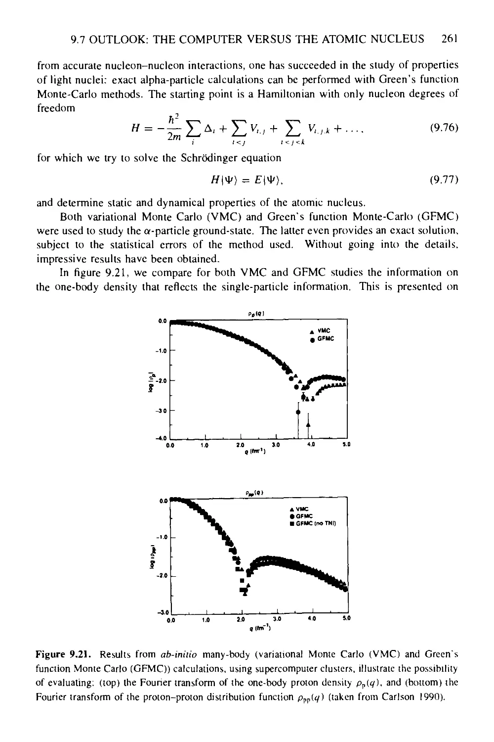
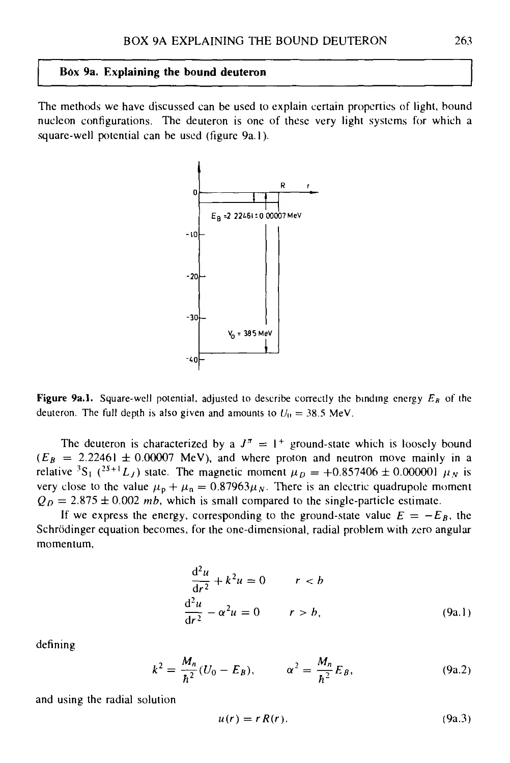
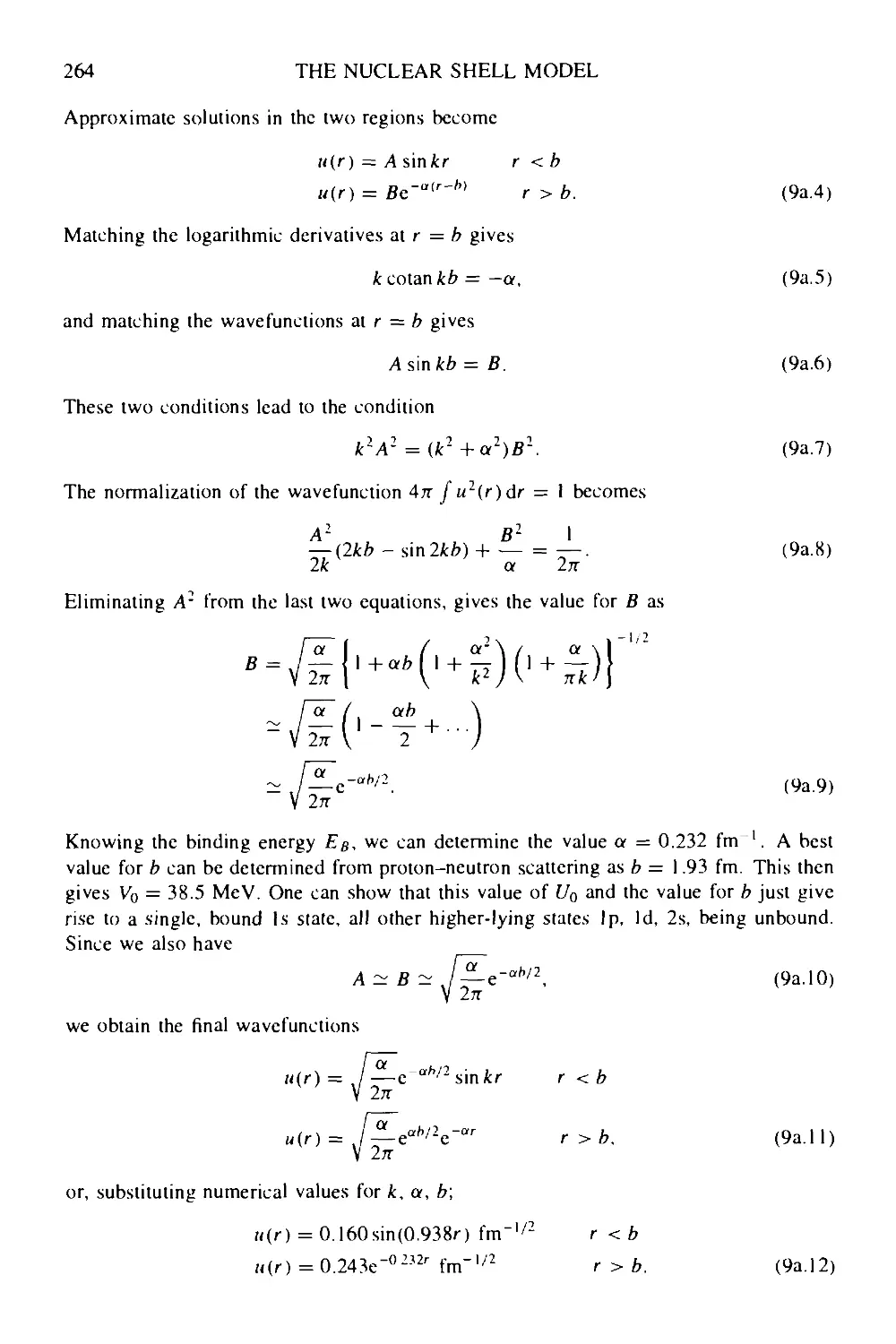
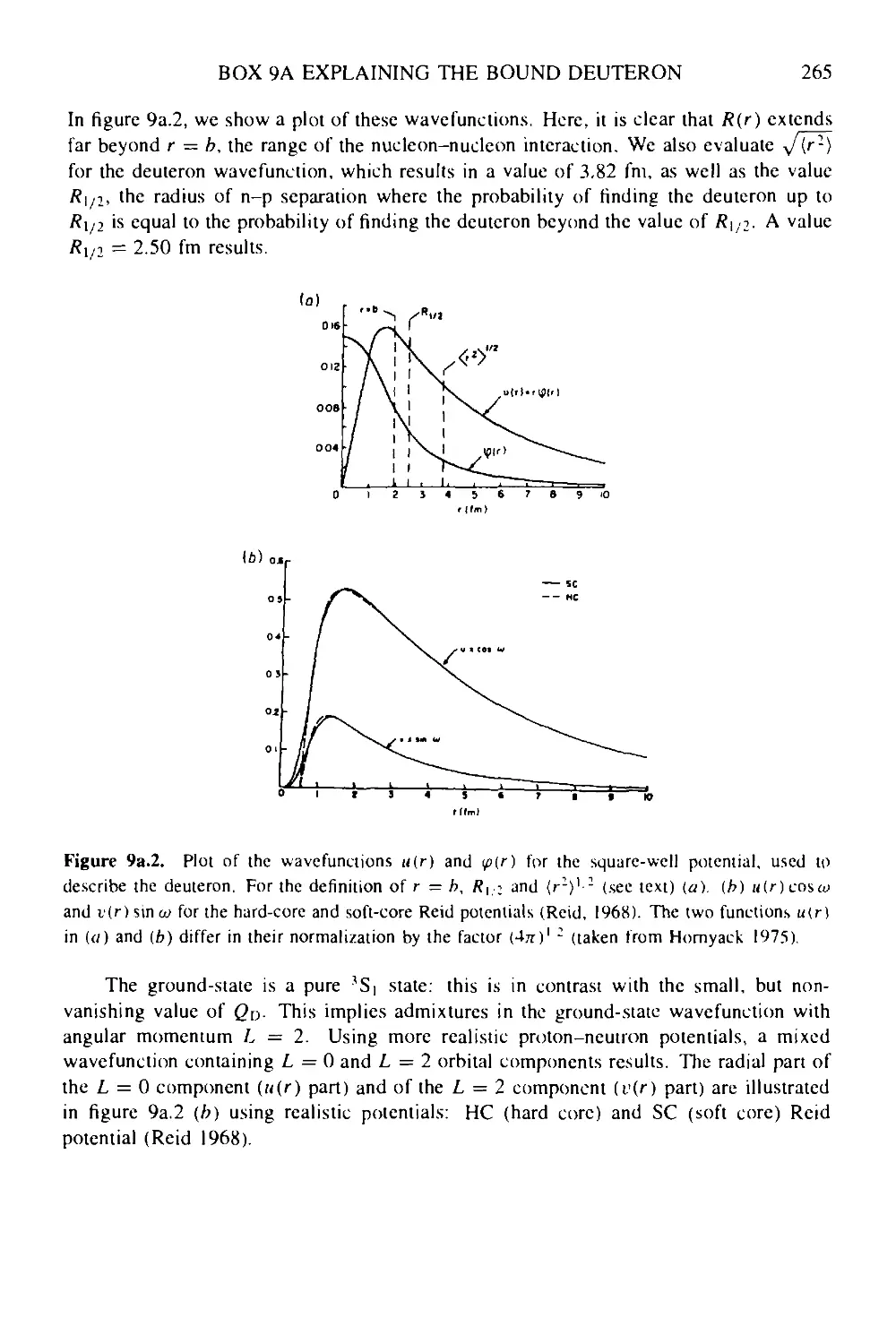
Box 9a Explaining the bound deuteron 263
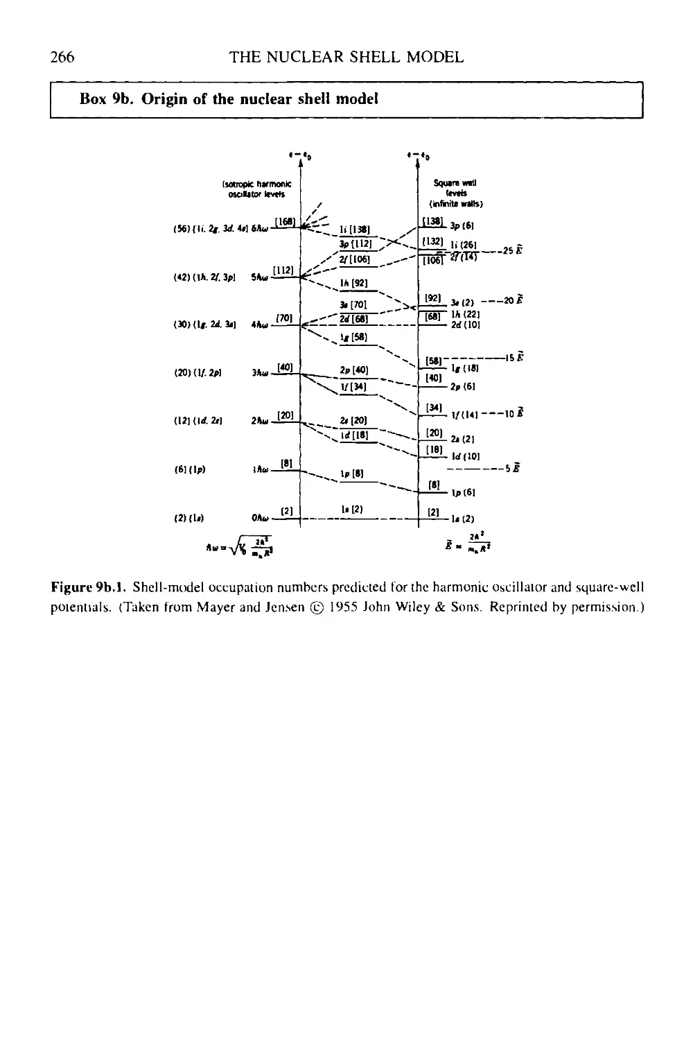
Box 9b Origin of the nuclear shell model 266
Problem set—Part С 269
PARTD
NUCLEAR STRUCTURE:
RECENT DEVELOPMENTS
10 The nuclear mean-field: single-particle excitations and global nuclear
properties 279
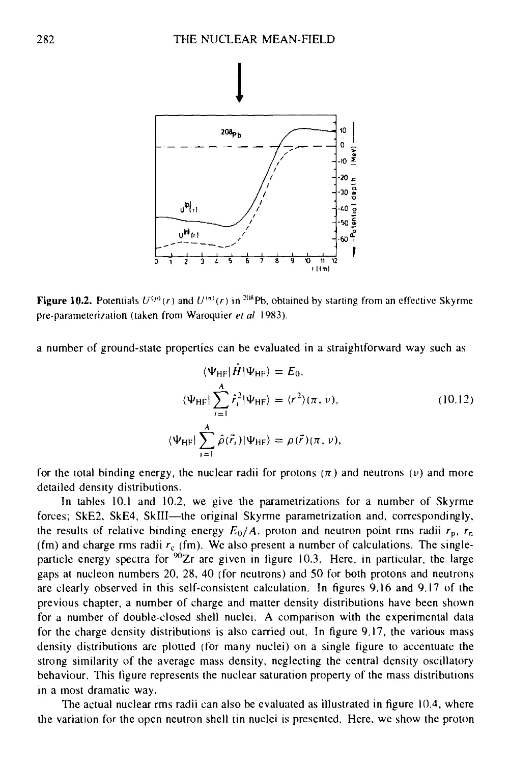
10.1 Hartree-Fock theory: a variational approach 279
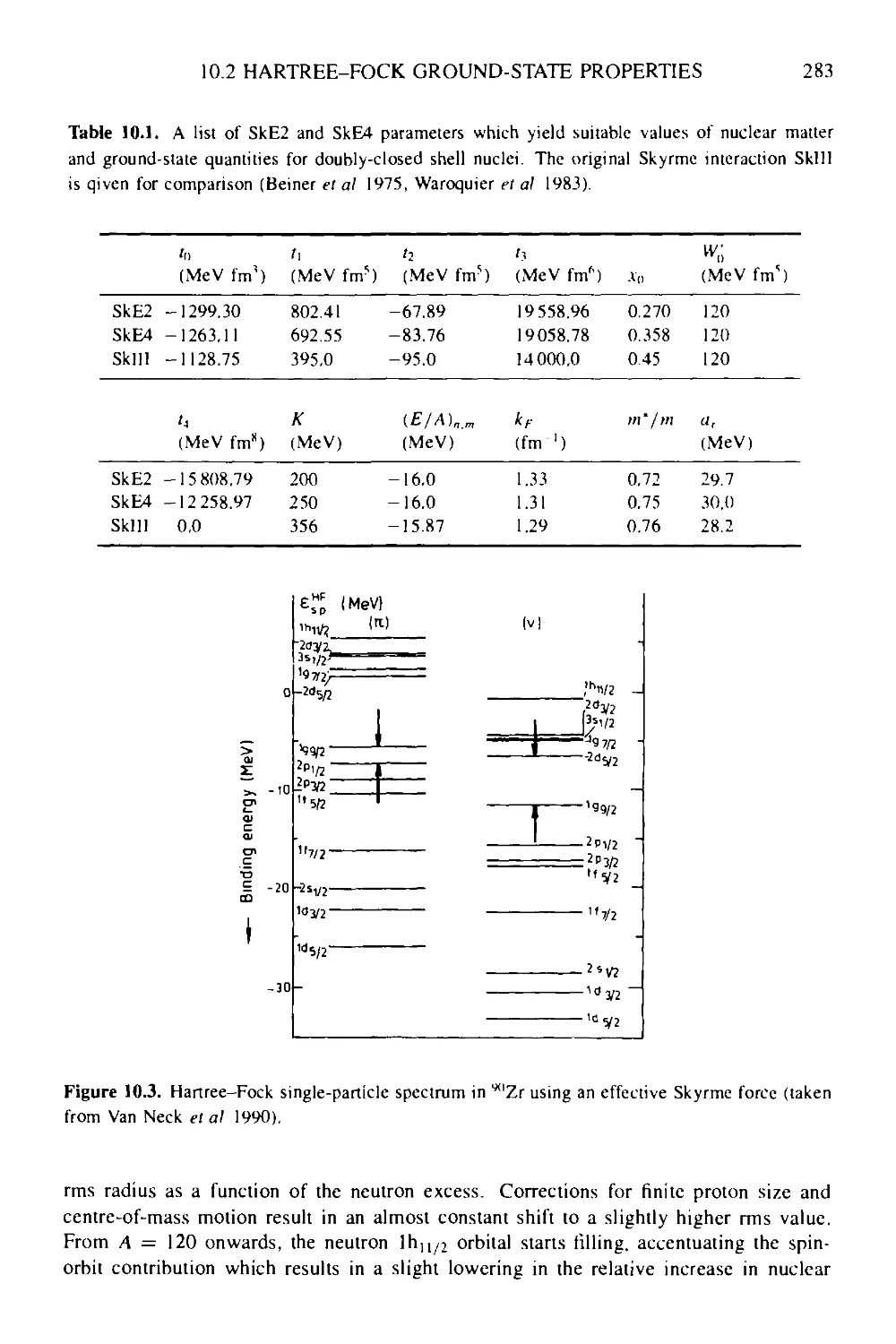
10.2 Hartree-Fock ground-state properties 281
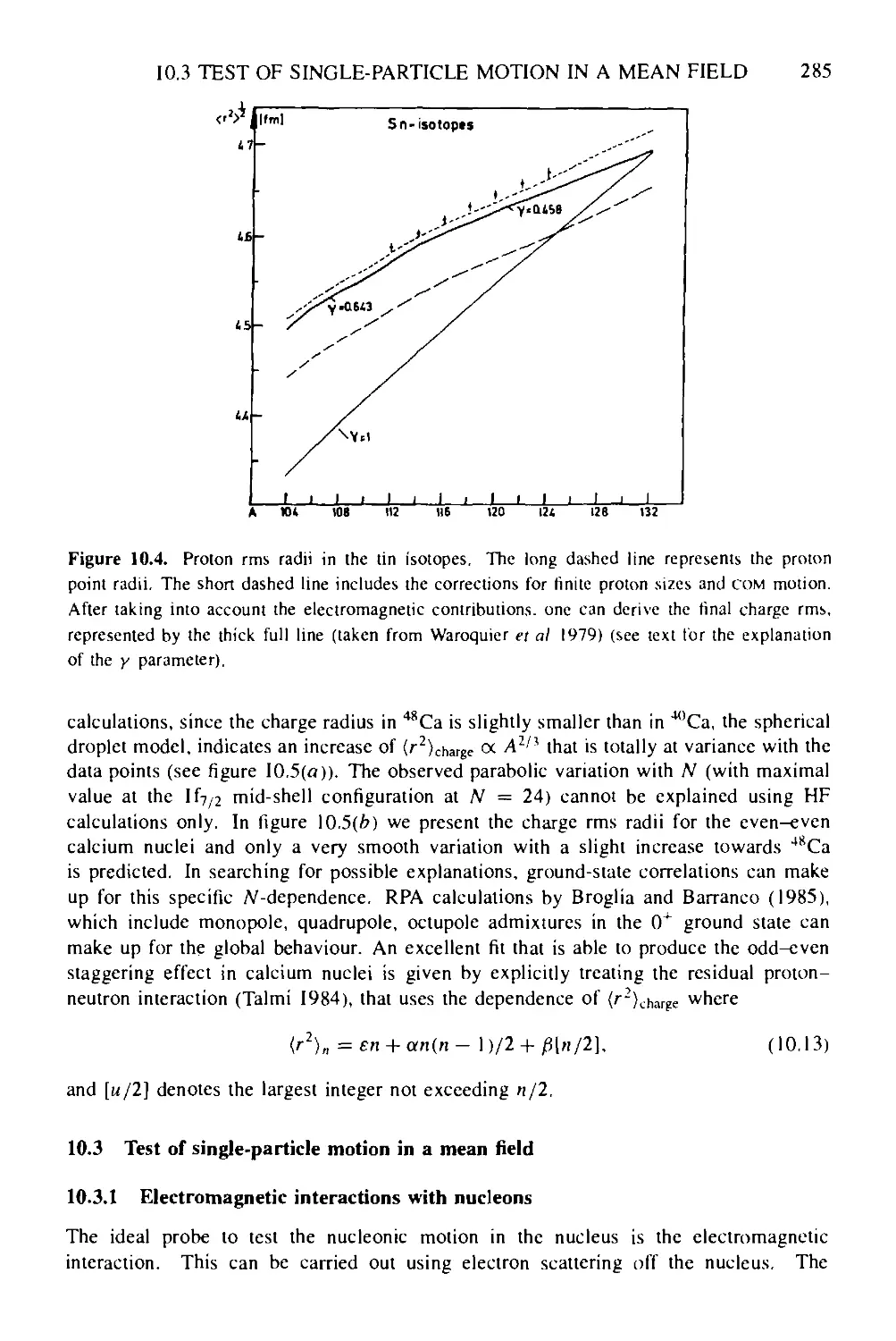
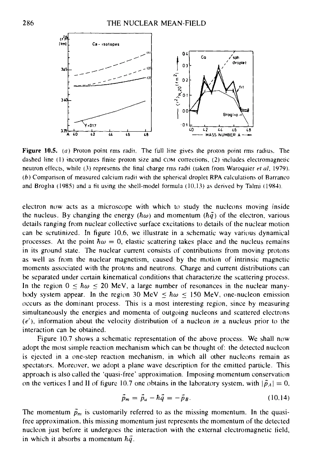
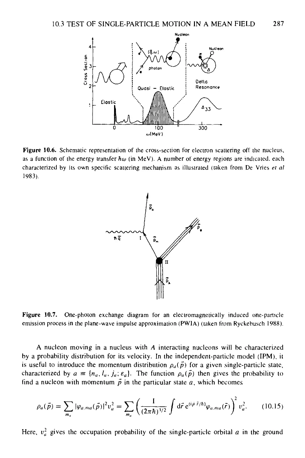
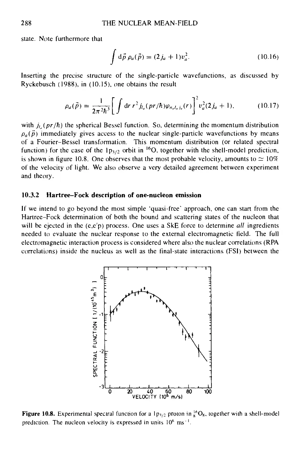
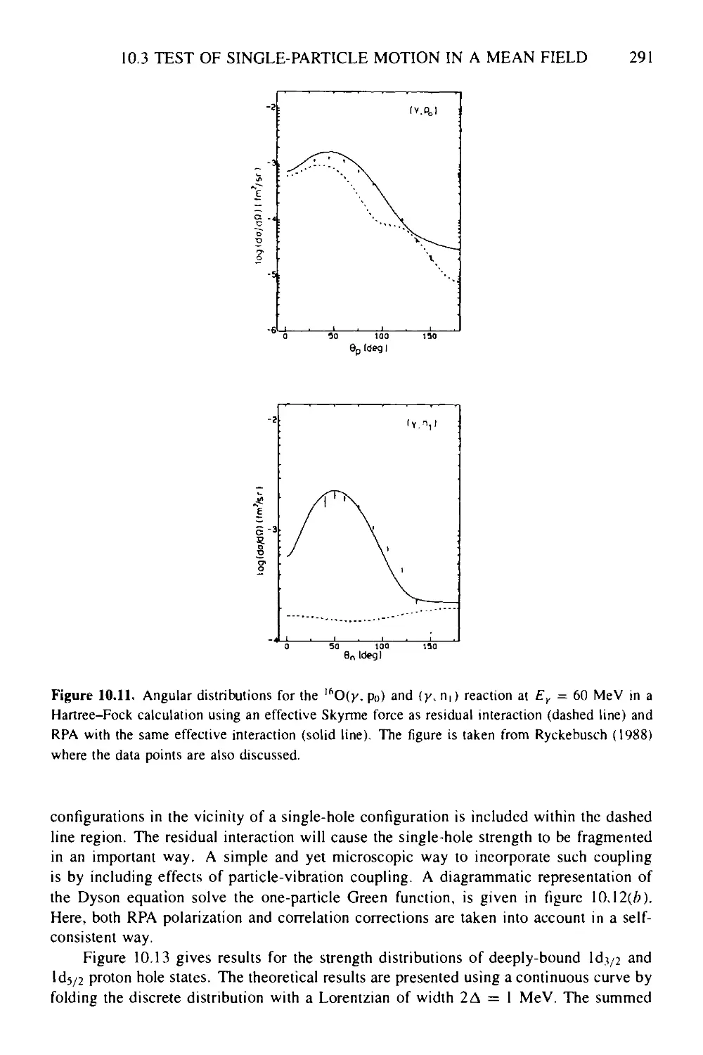
10.3 Test of single-particle motion in a mean field 285
10.3.1 Electromagnetic interactions with nucleons 285
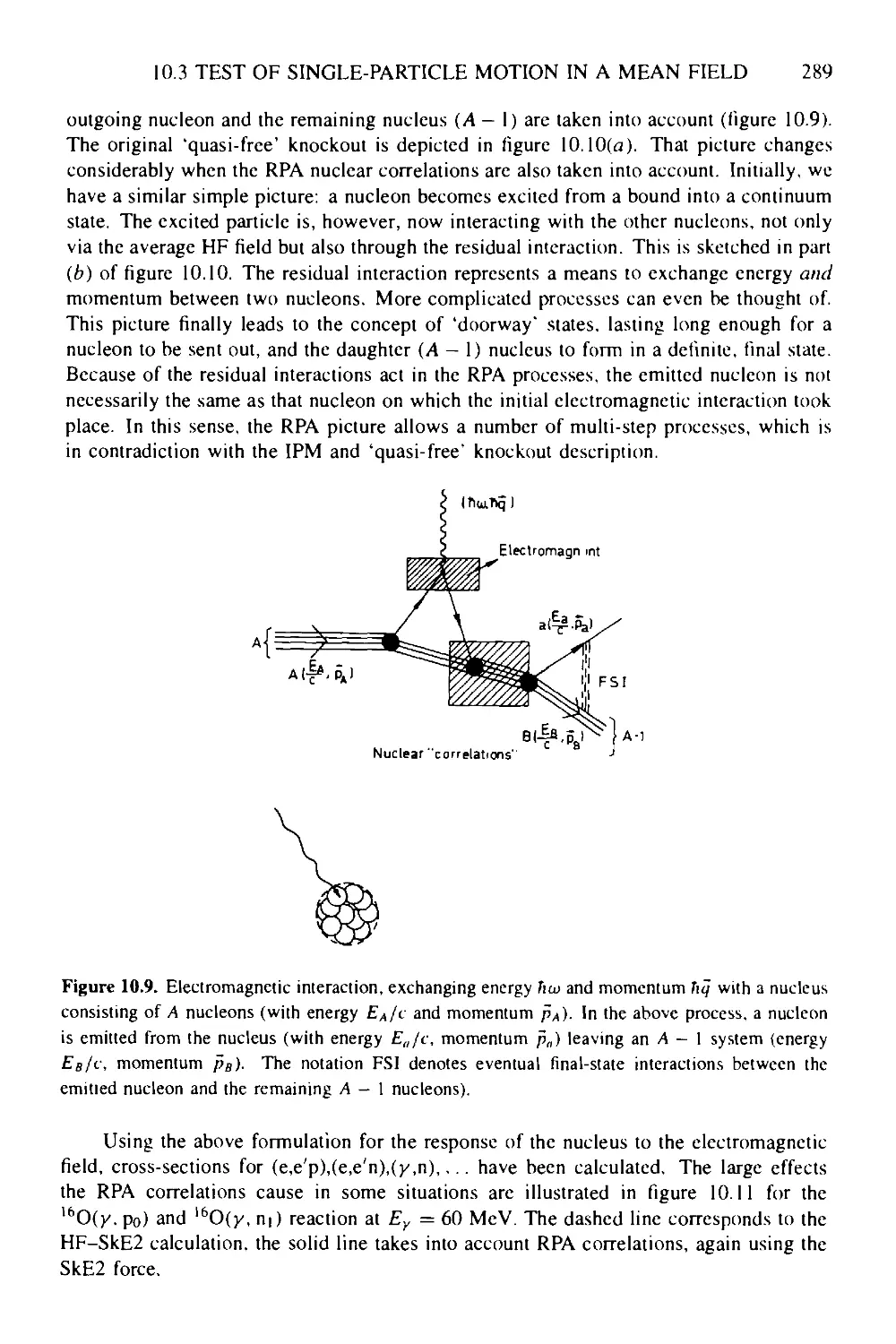
10.3.2 Hartree-Fock description of one-nucleon emission 288
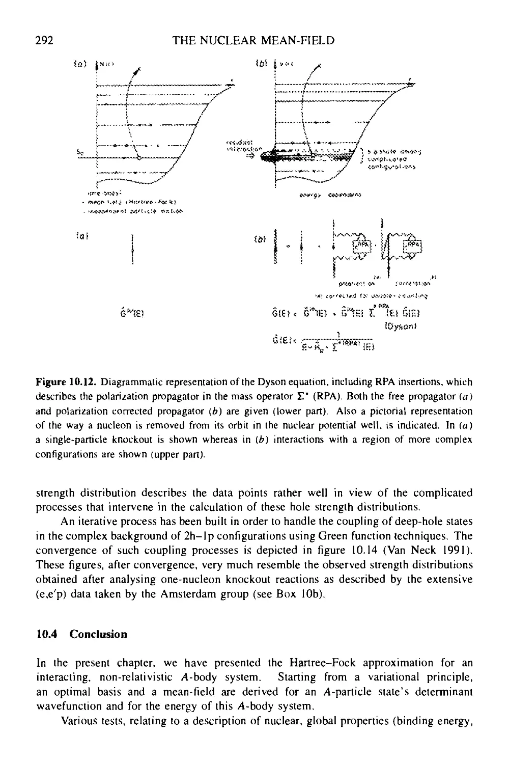
10.3.3 Deep-lying single-hole states—fragmentation of single-hole
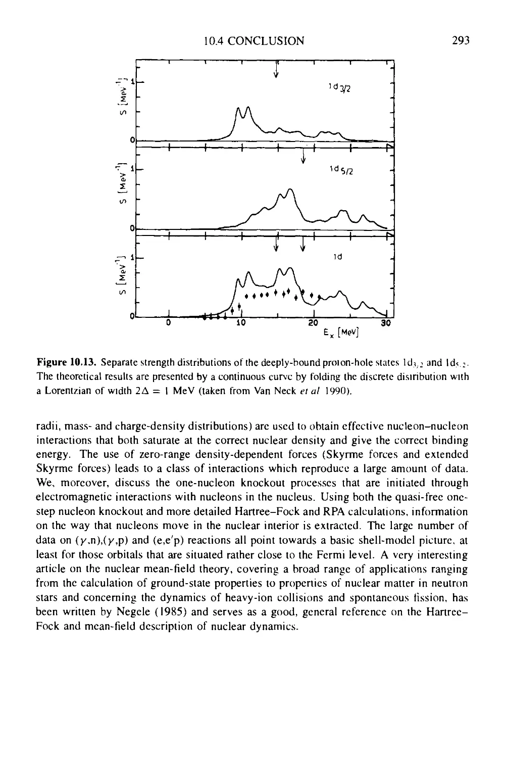
strength 290
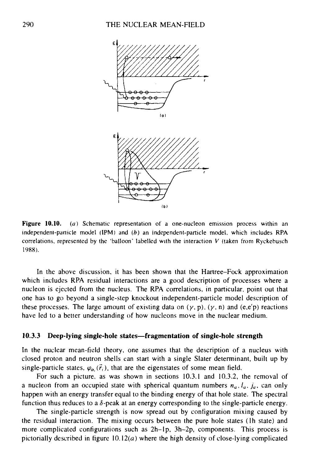
10.4 Conclusion 292
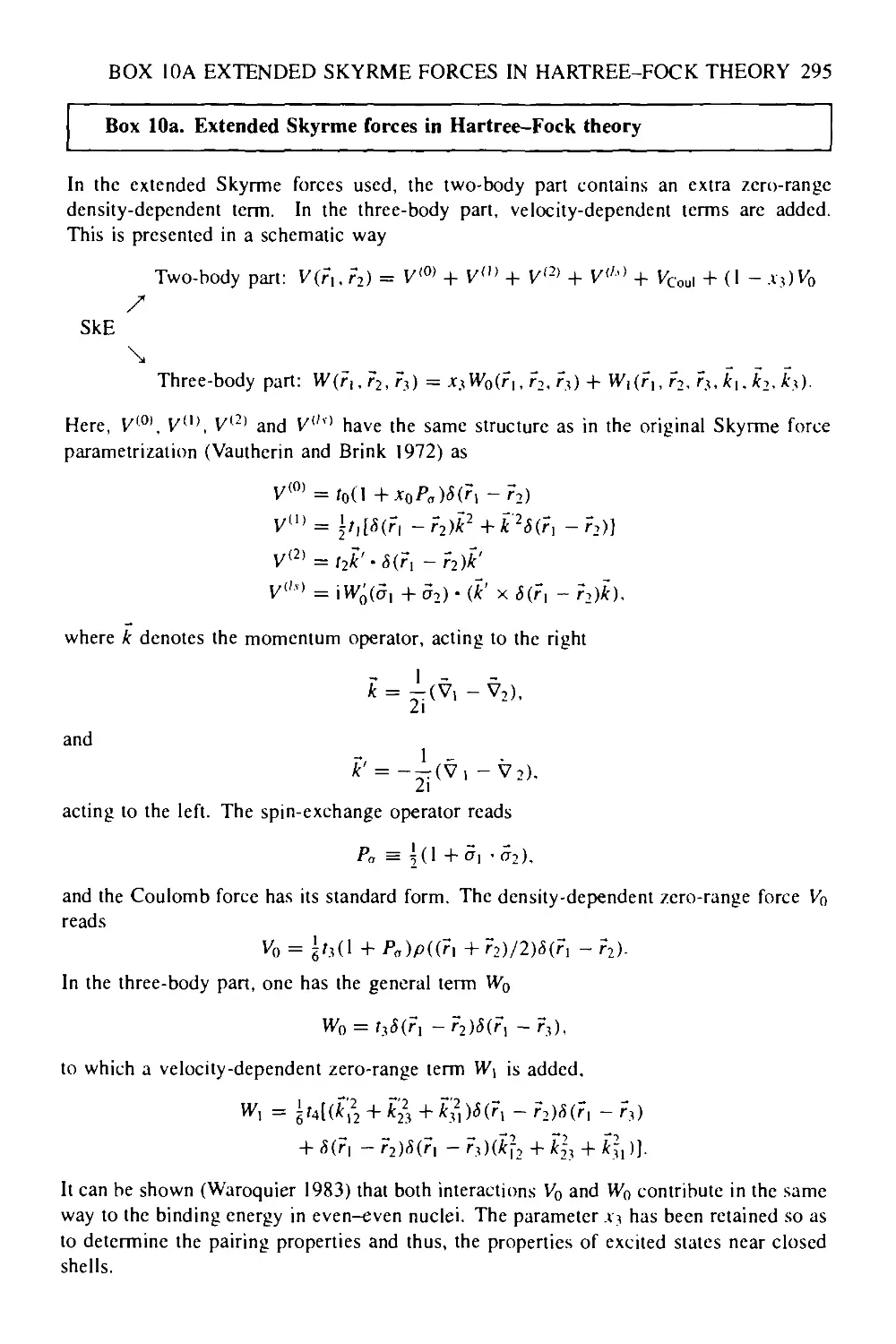
Box 10a Extended Skyrme forces in Hartree-Fock theory 295
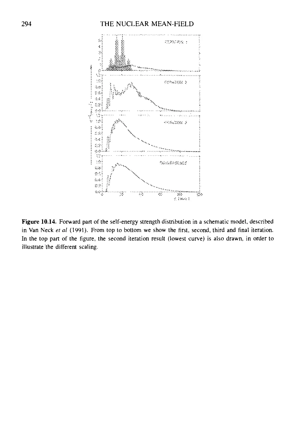
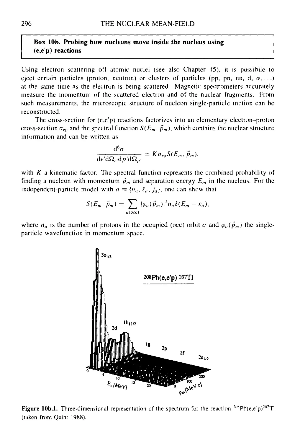
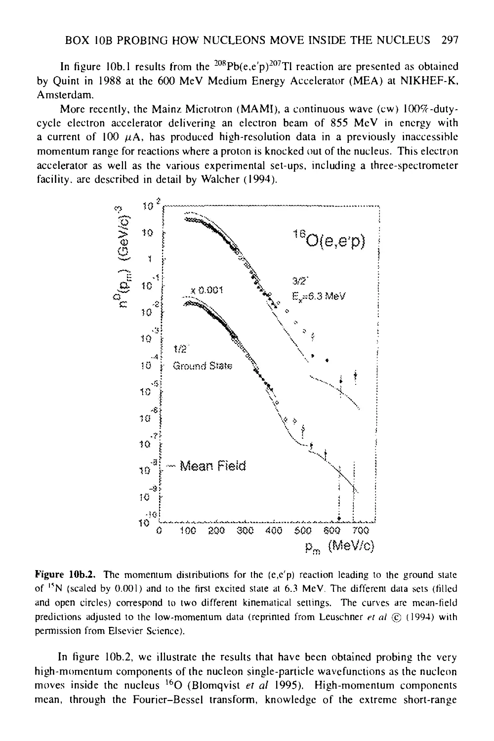
Box 10b Probing how nucleons move inside the nucleus using (e.e'p) reactions 296
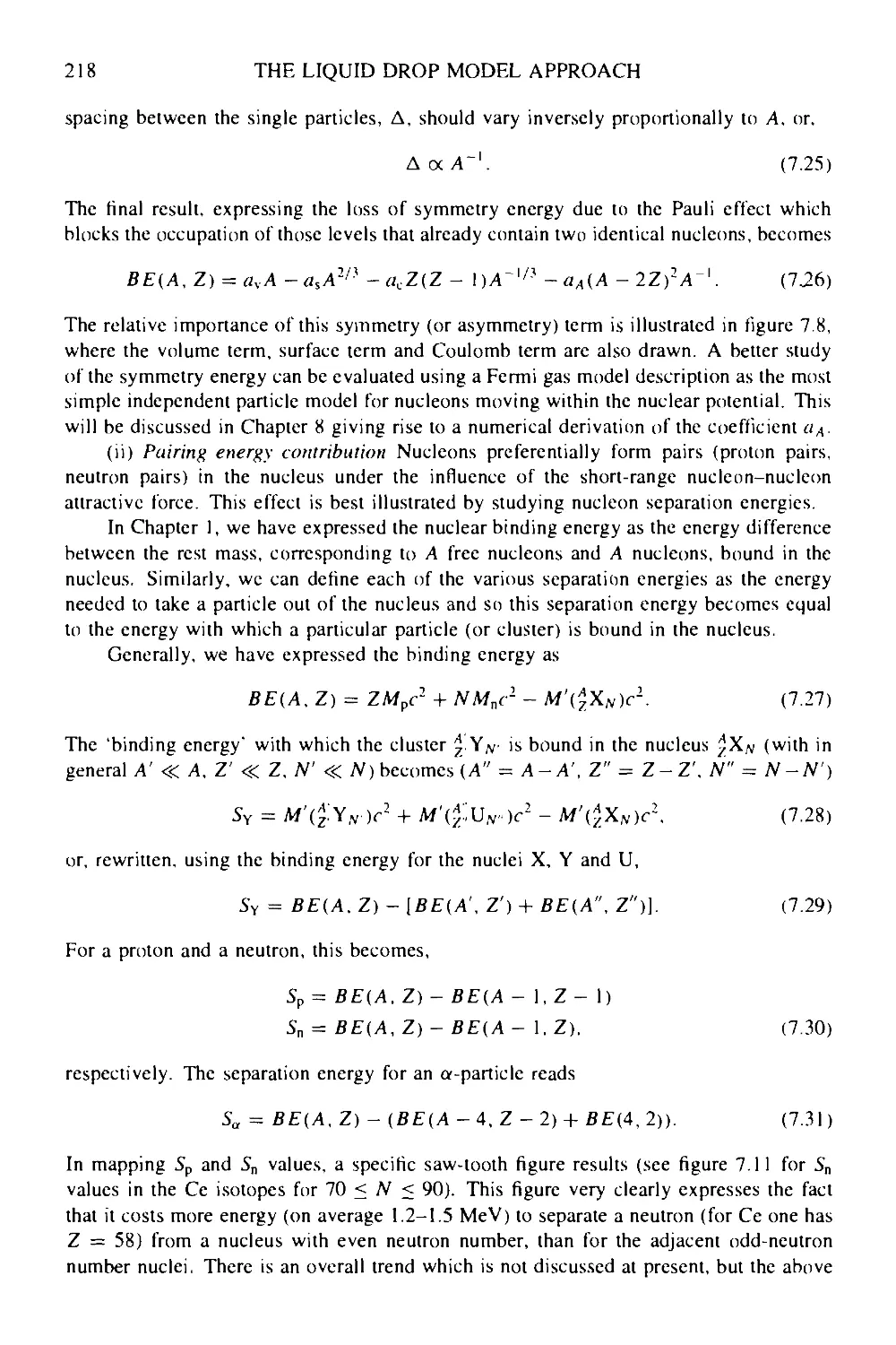
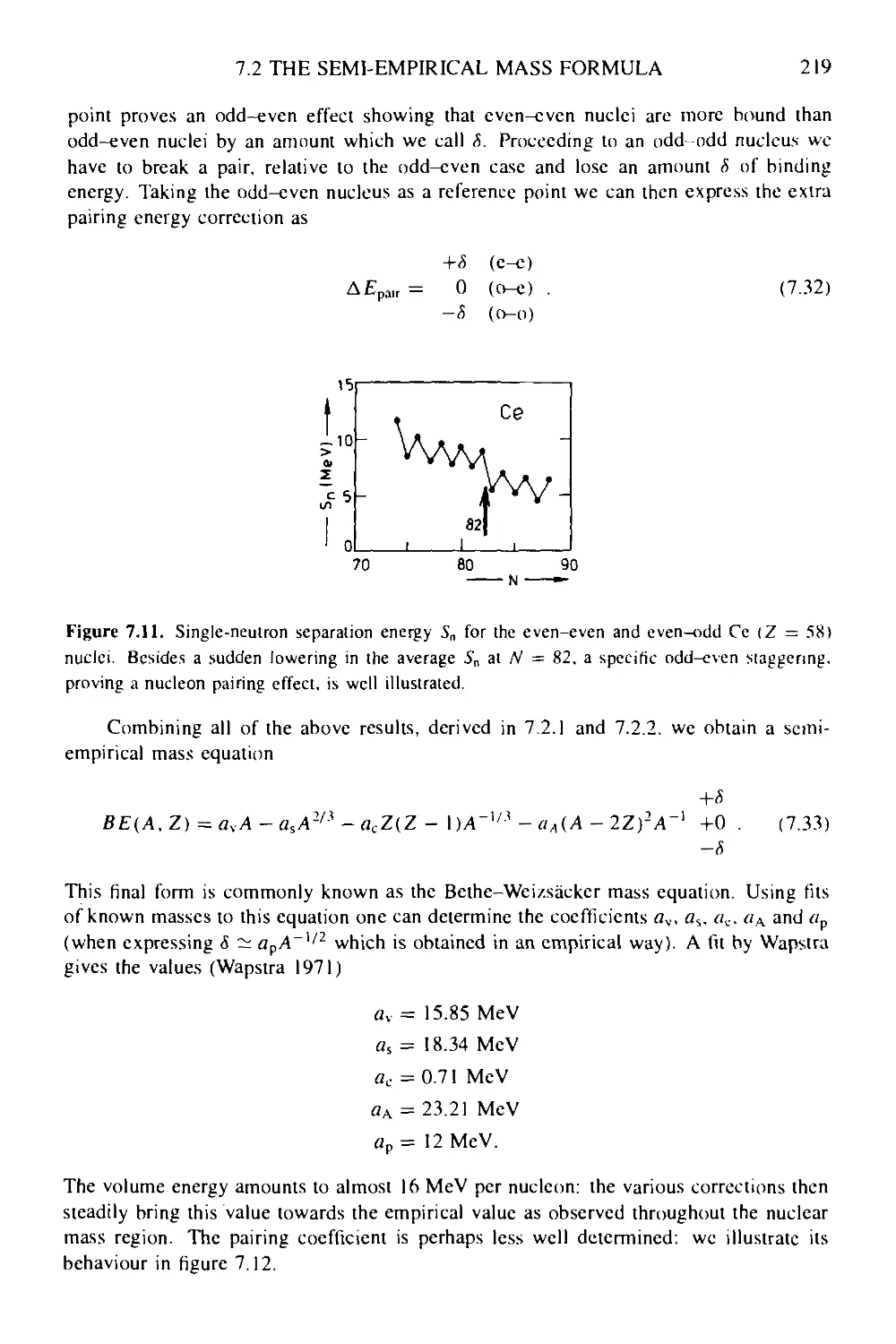
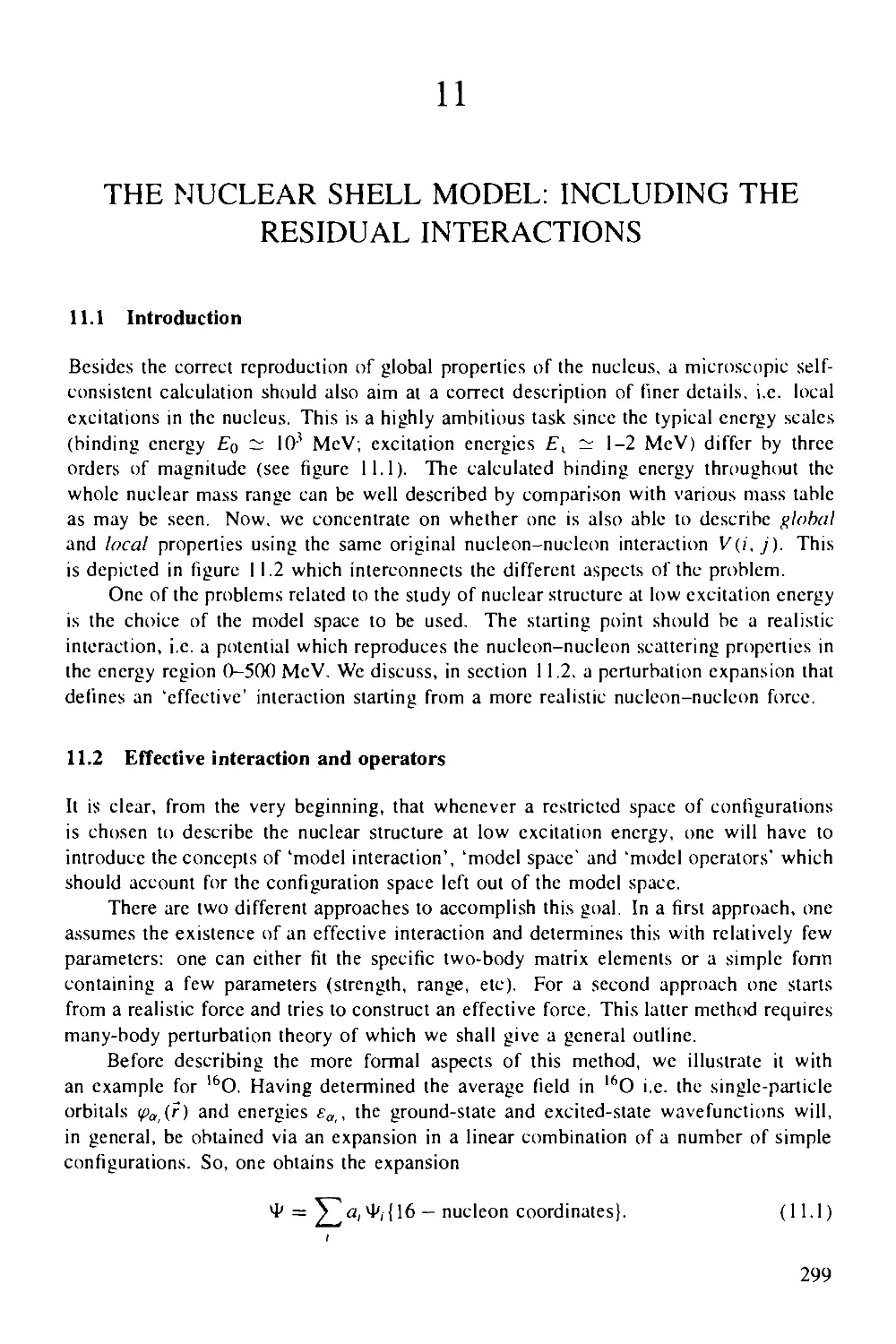
11 The nuclear shell model: including the residual interactions 299
11.1 Introduction 299
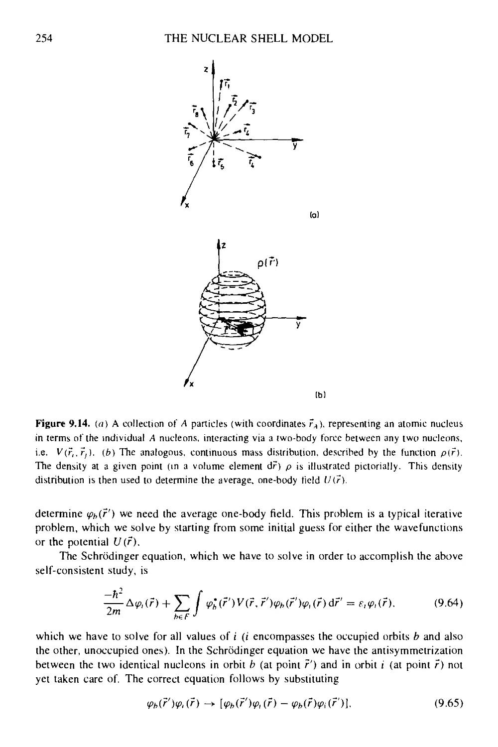
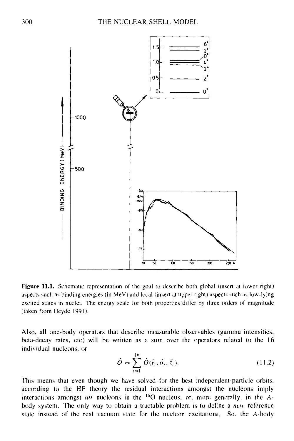
11.2 Effective interaction and operators 299
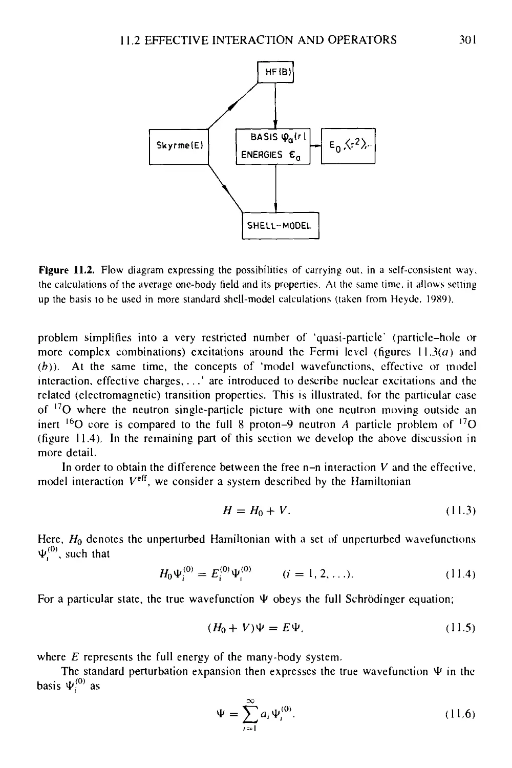
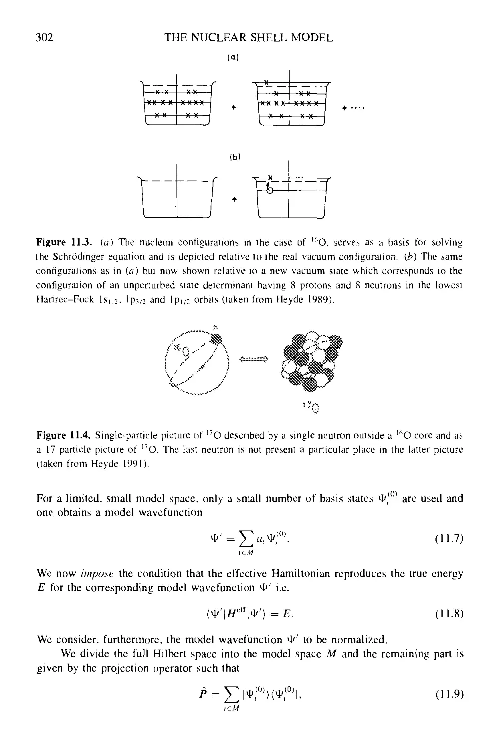
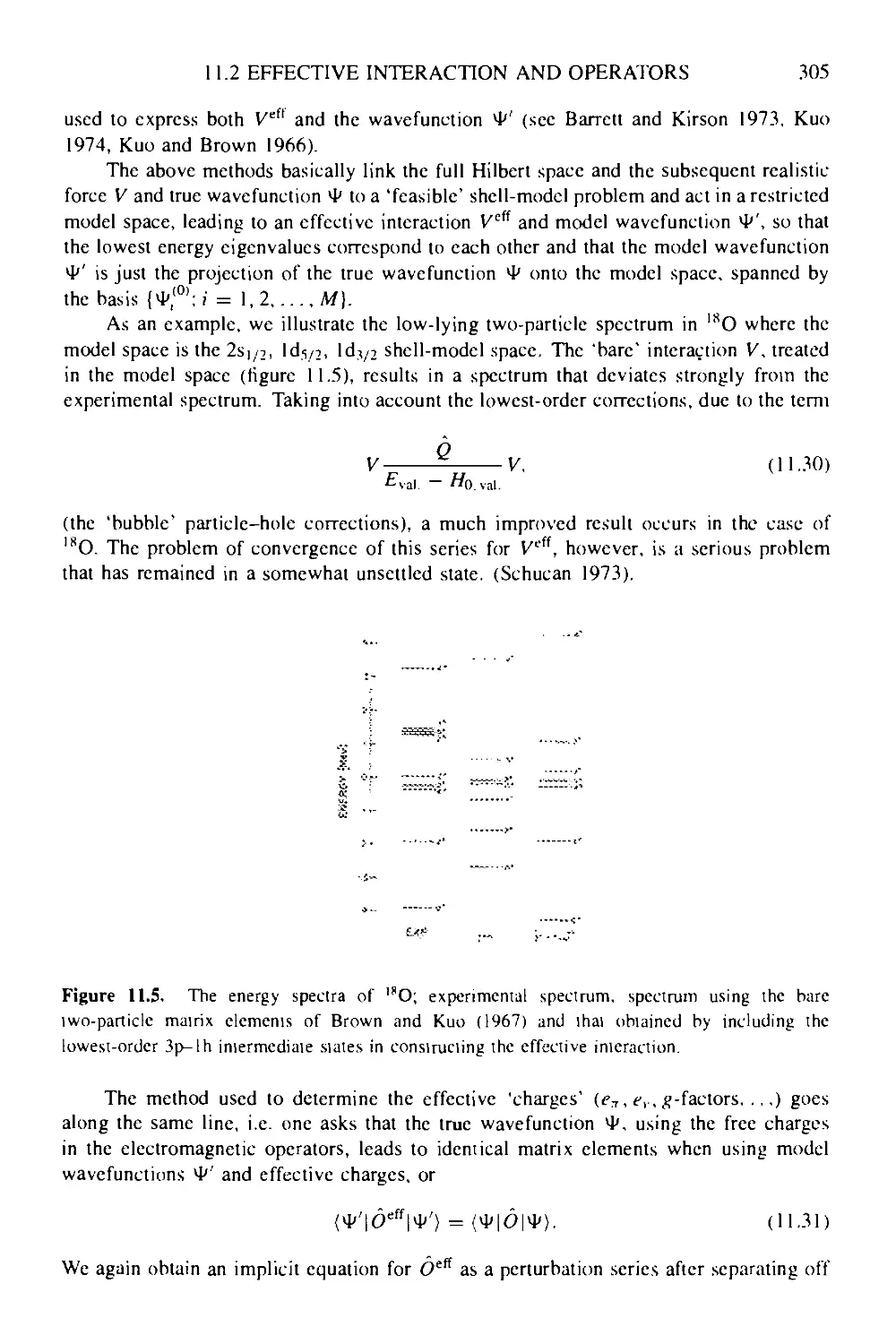
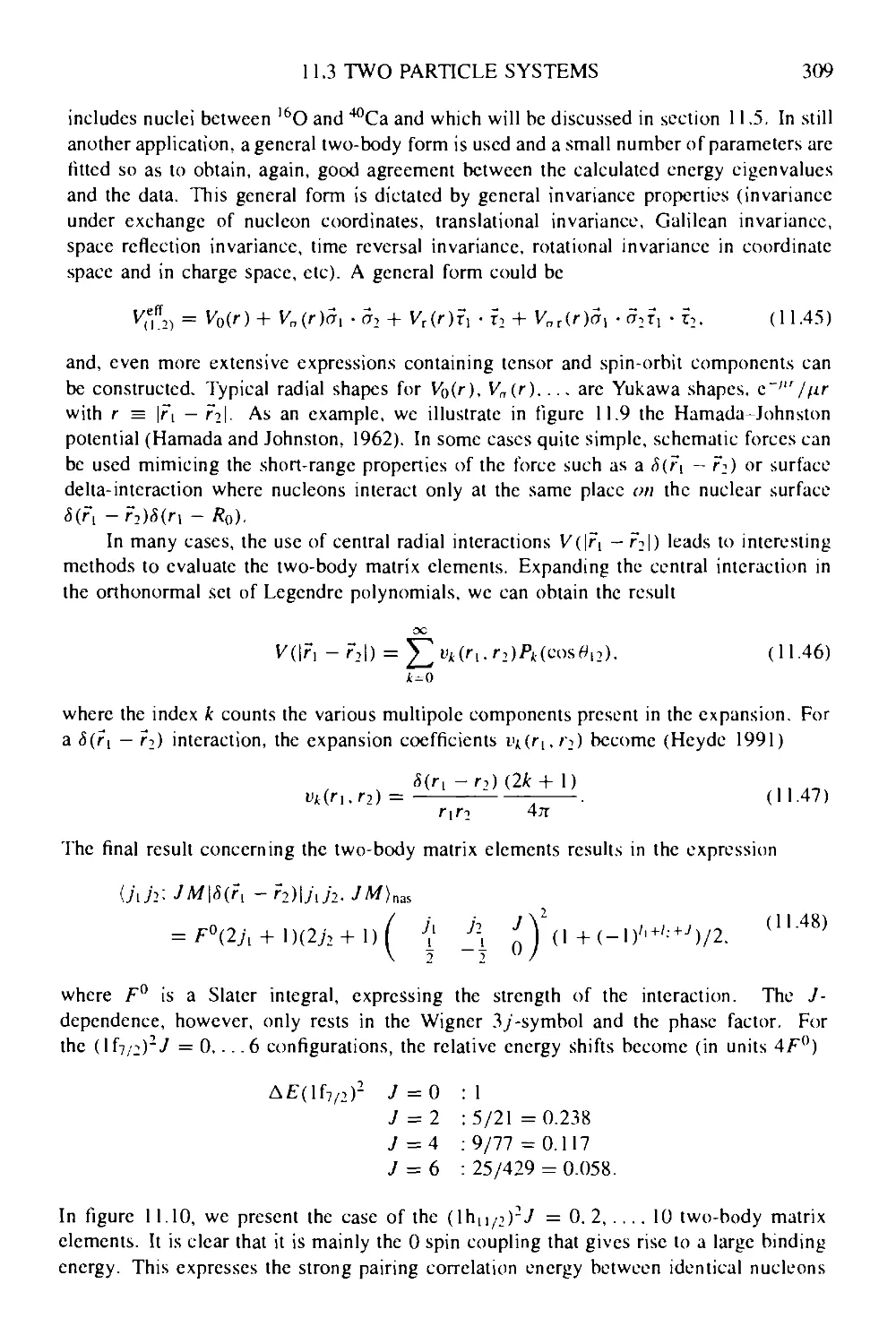
11.3 Two particle systems: wavefunctions and interactions 306
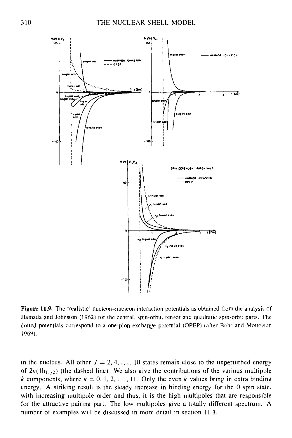
11.3.1 Two-particle wavefunctions 306
11.3.2 Configuration mixing: model space and model interaction 311
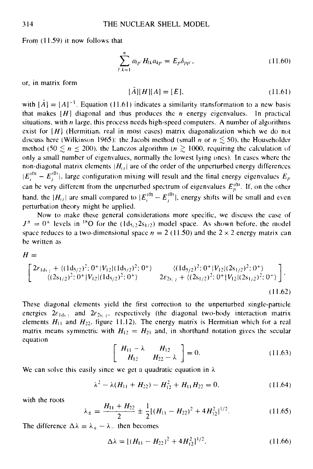
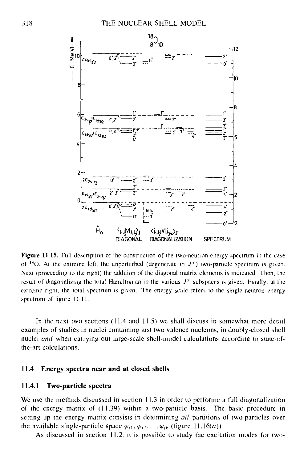
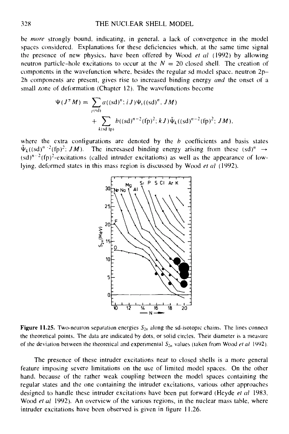
11.4 Energy spectra near and at closed shells 318
11.4.1 Two-particle spectra 318
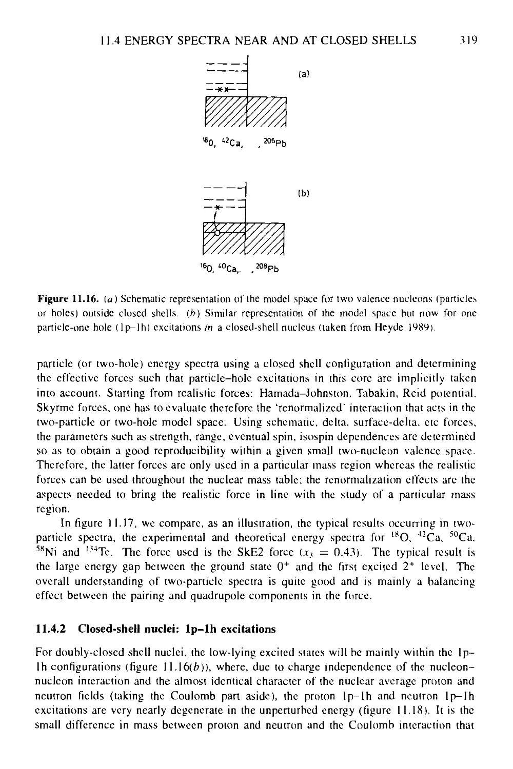
11.4.2 Closed-shell nuclei: lp-lh excitations 319
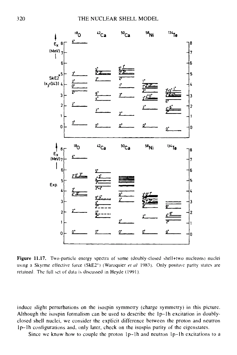
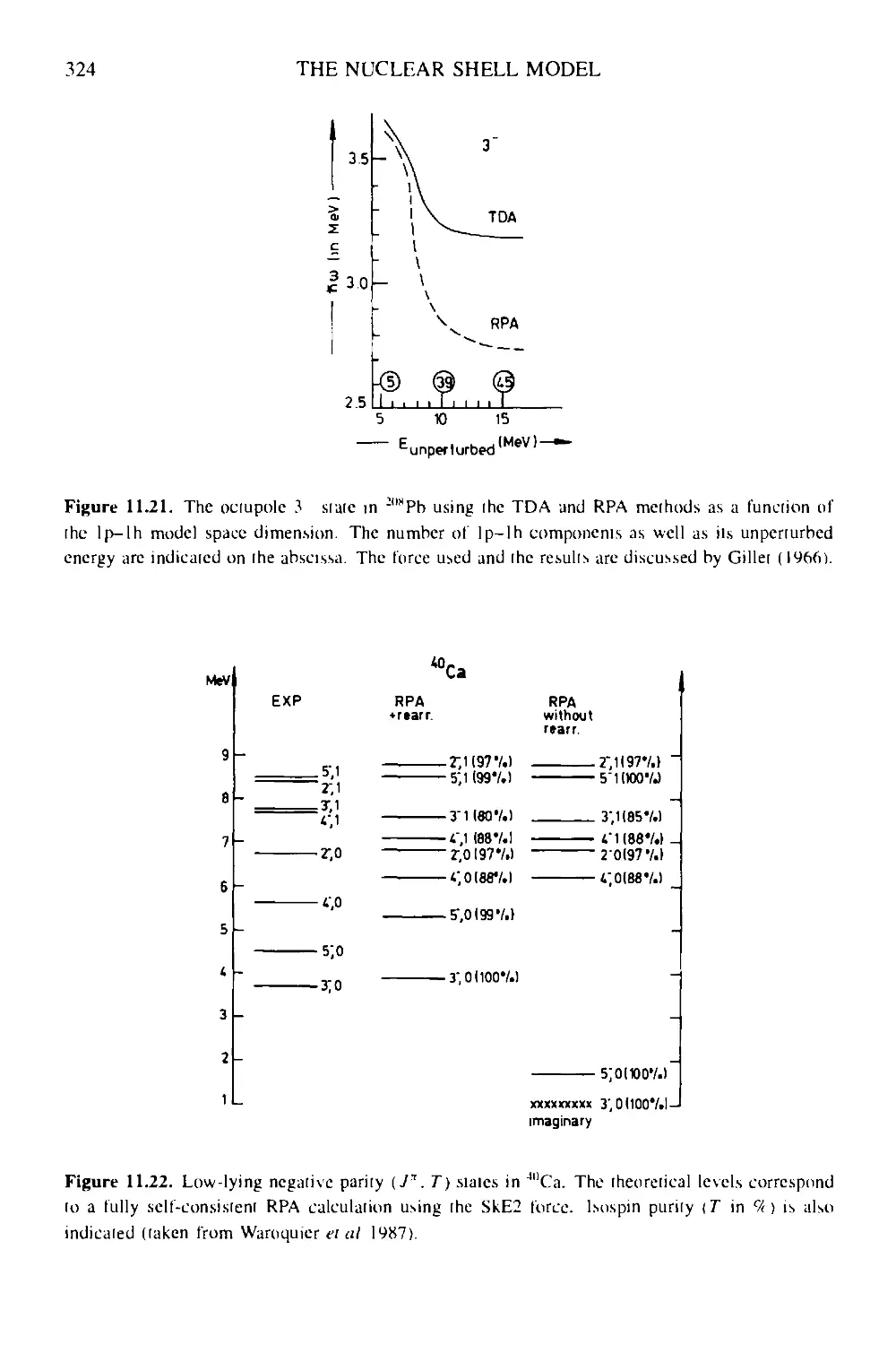
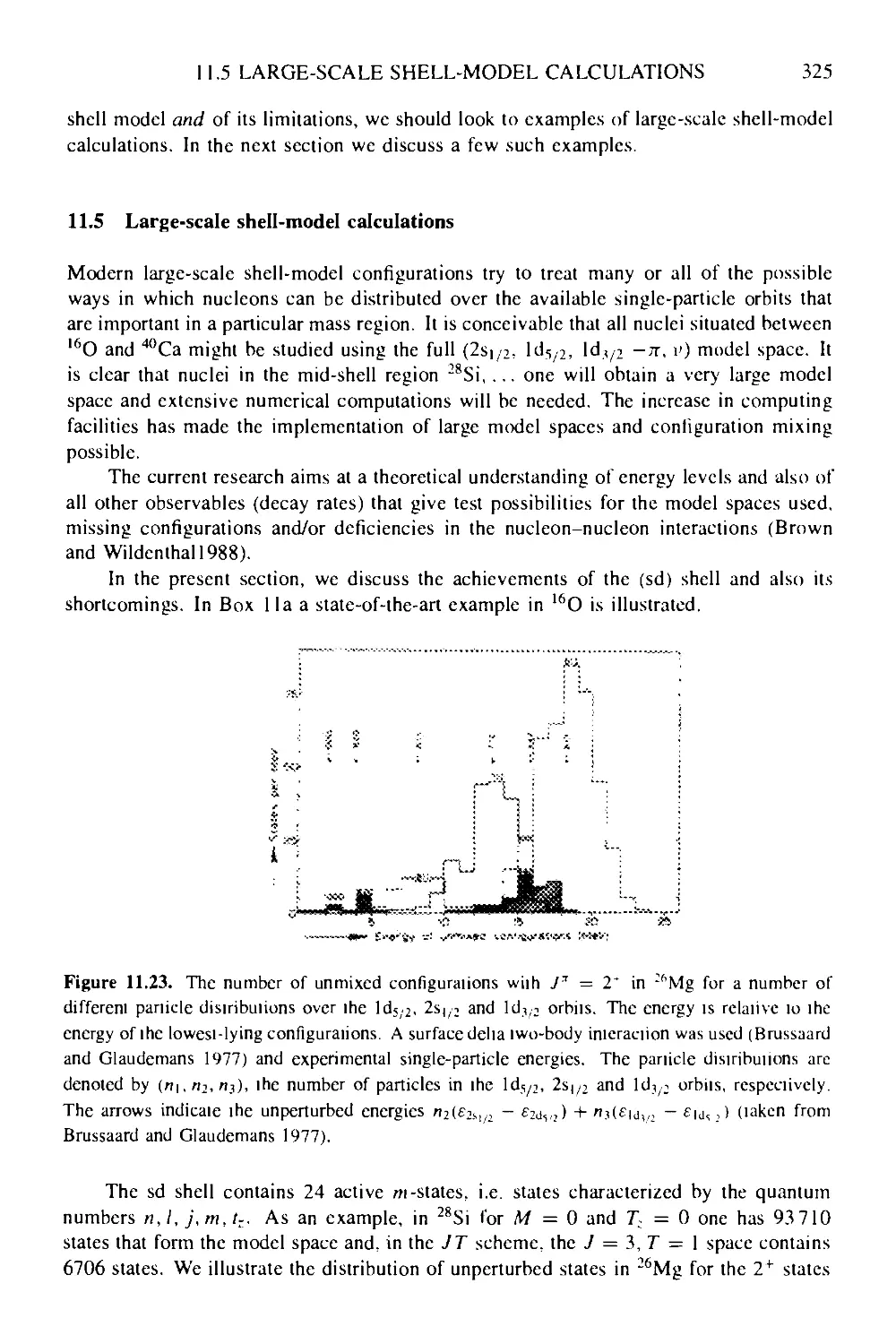
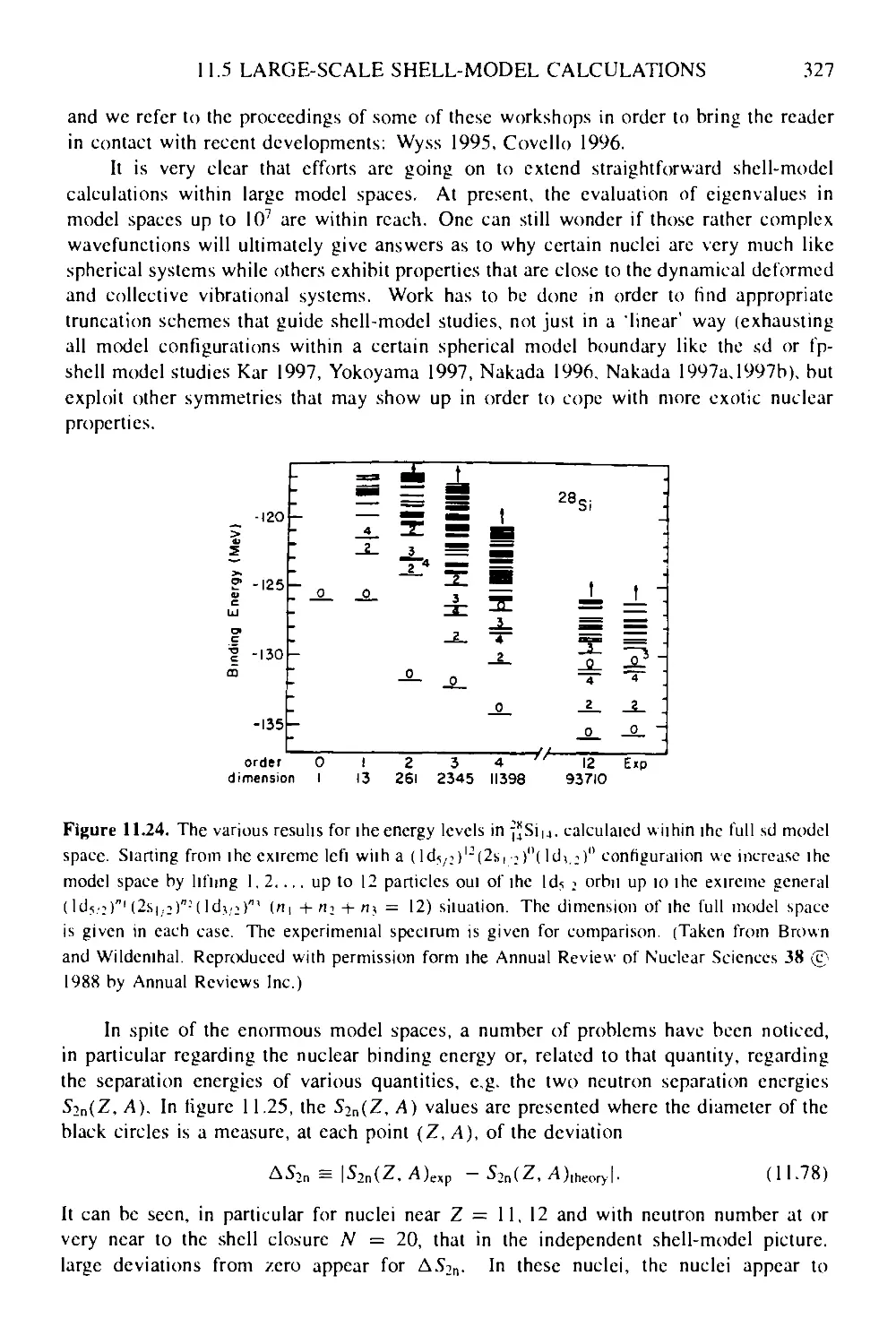
11.5 Large-scale shell-model calculations 325
CONTENTS xi
11.6 A new approach to the nuclear many-body problem: shell-model Monte-
Carlo methods 329
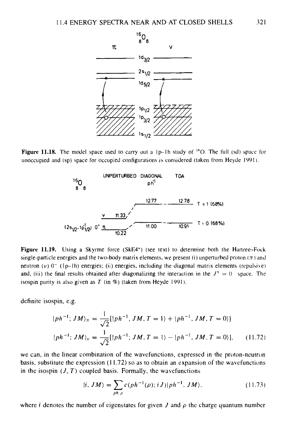
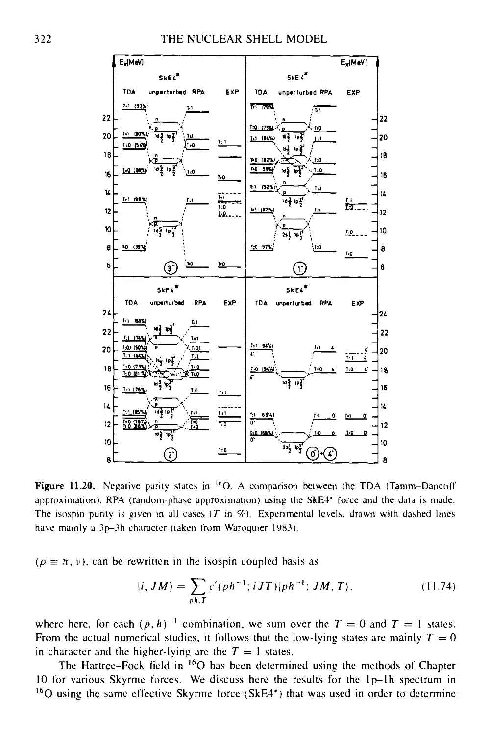
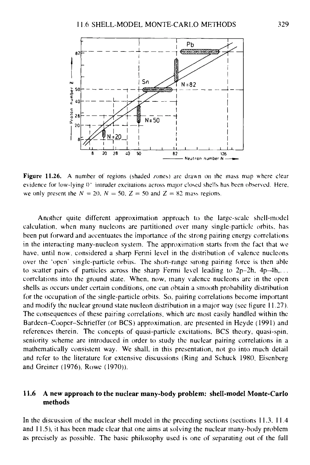
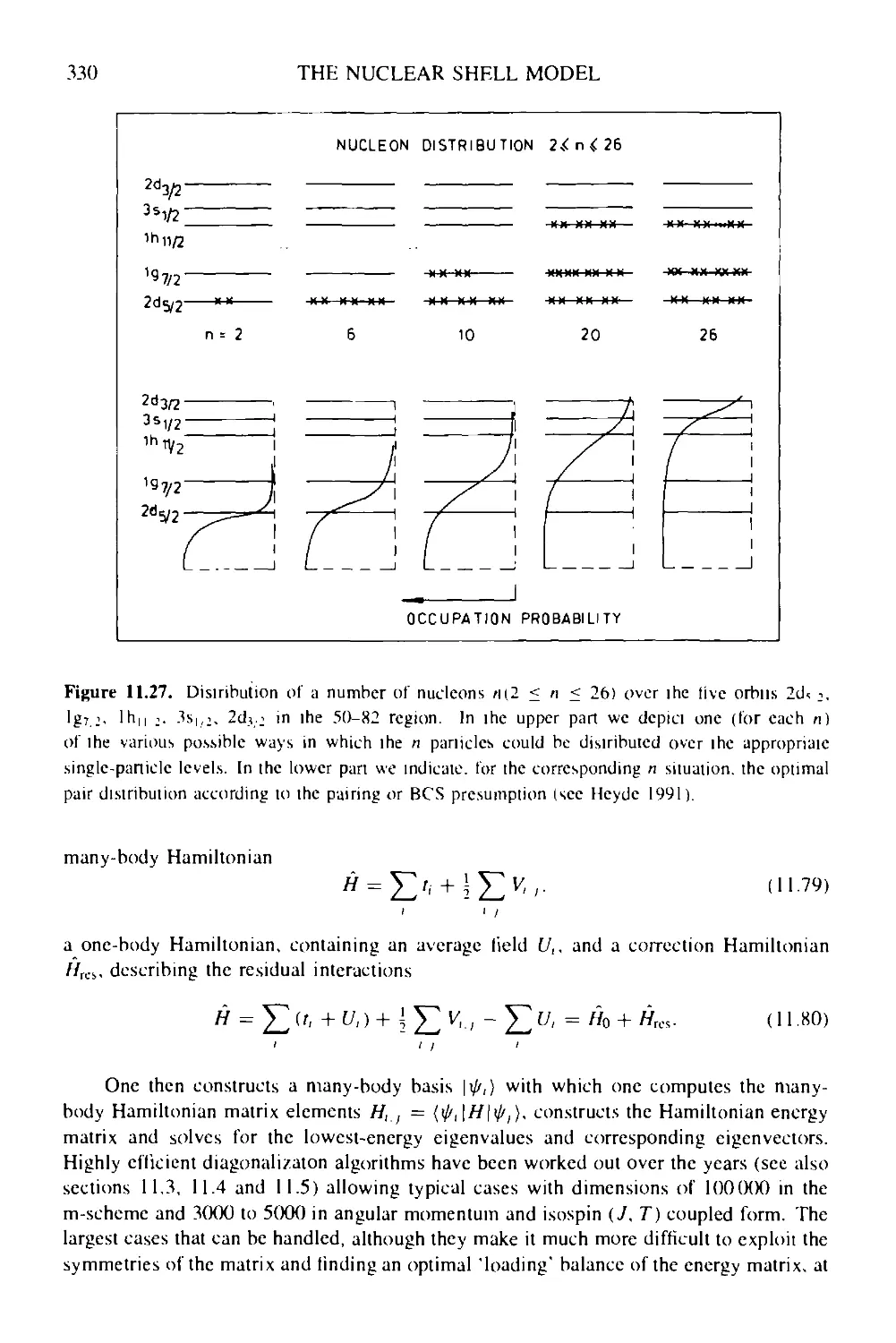
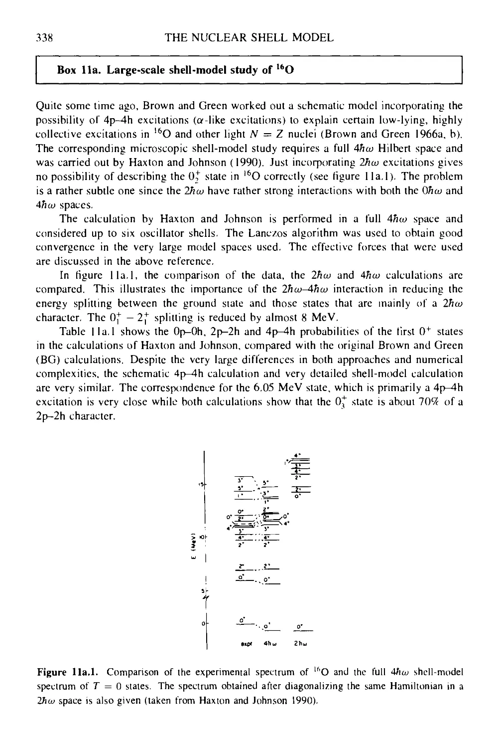
Box 1 la Large-scale shell-model study of I6O 338
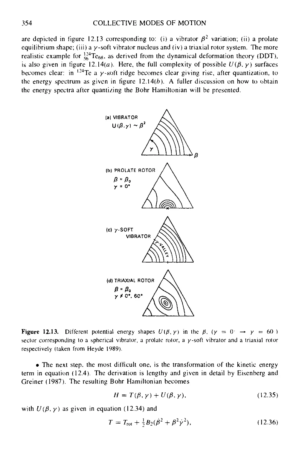
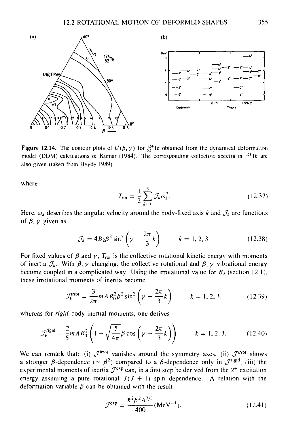
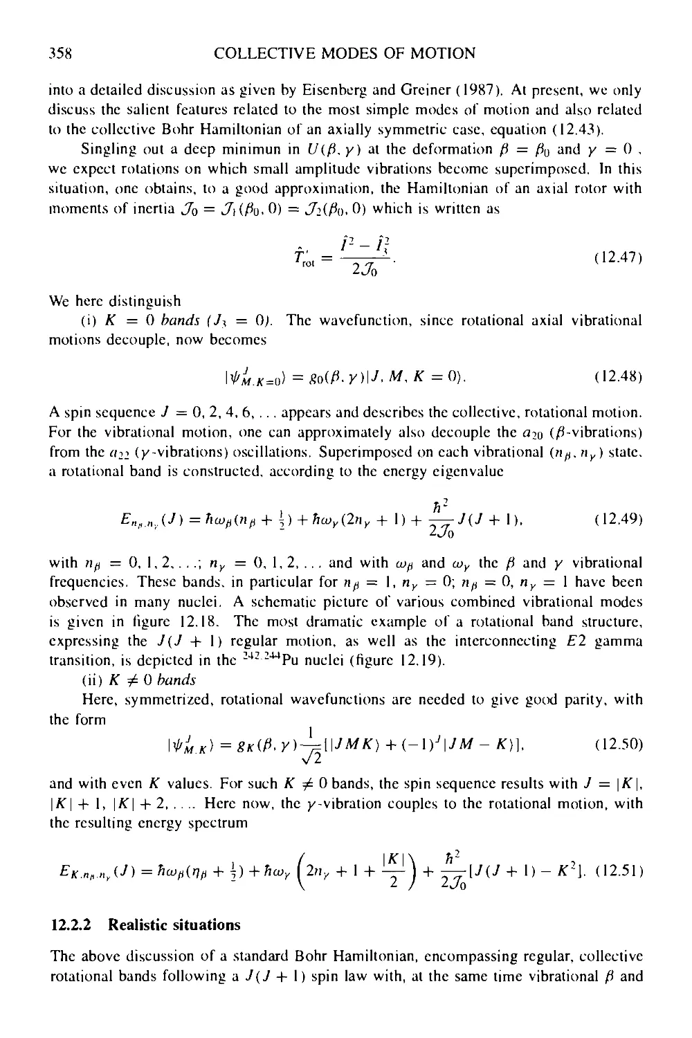
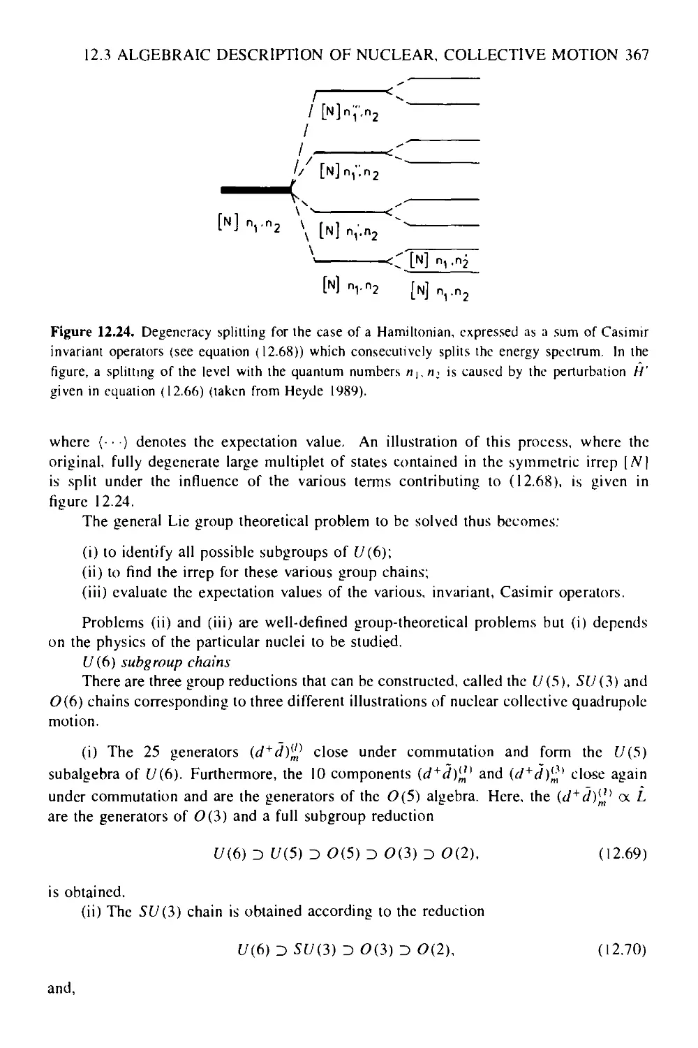
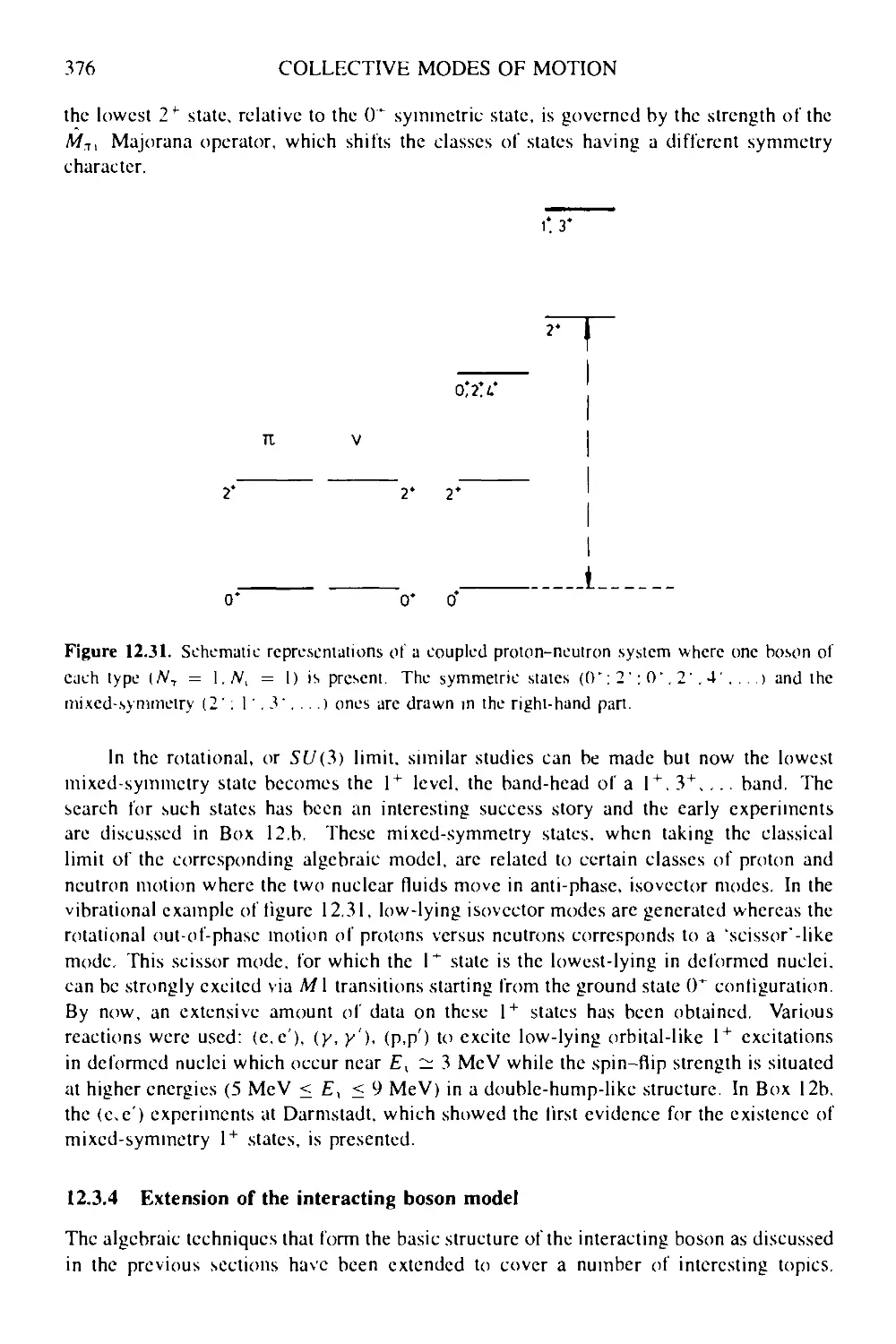
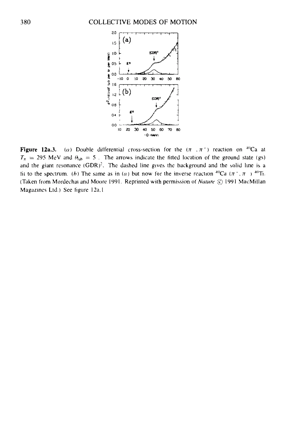
12 Collective modes of motion 340
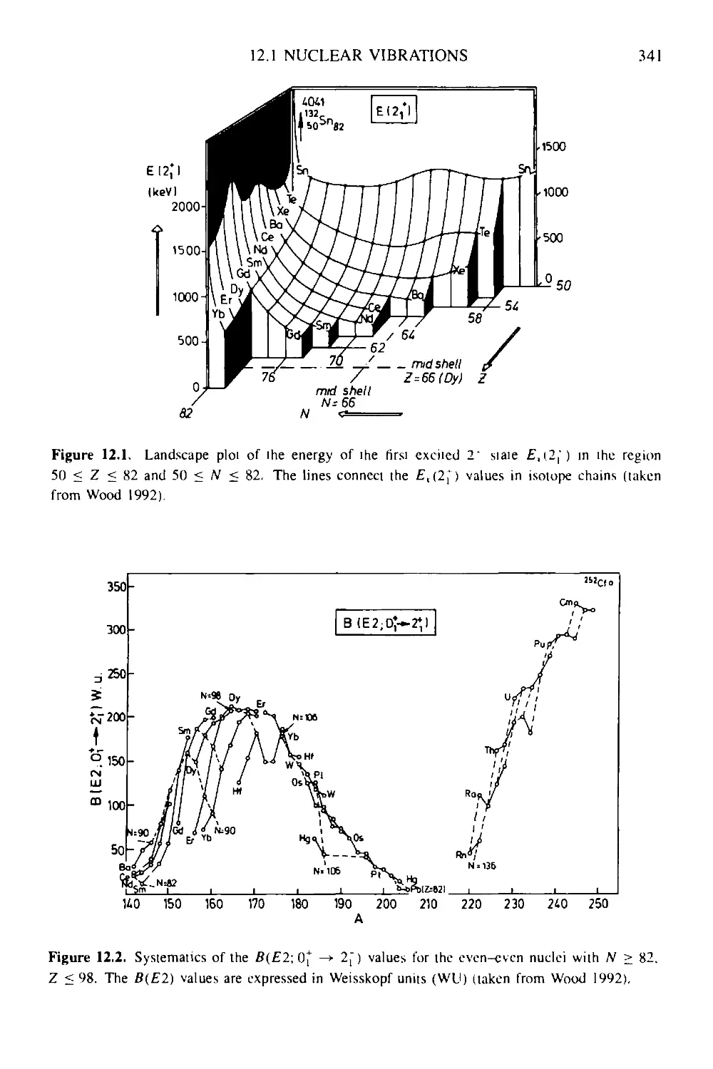
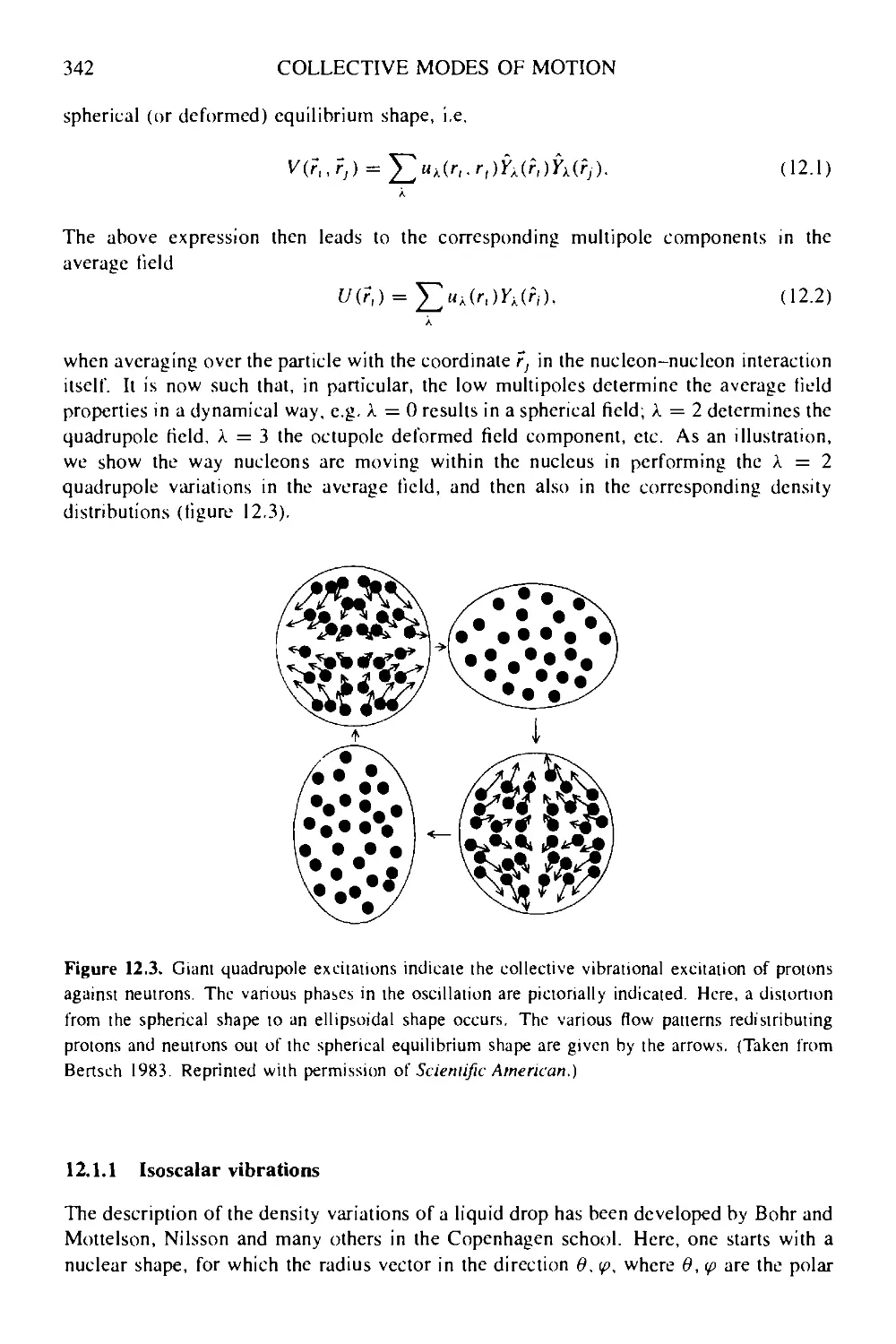
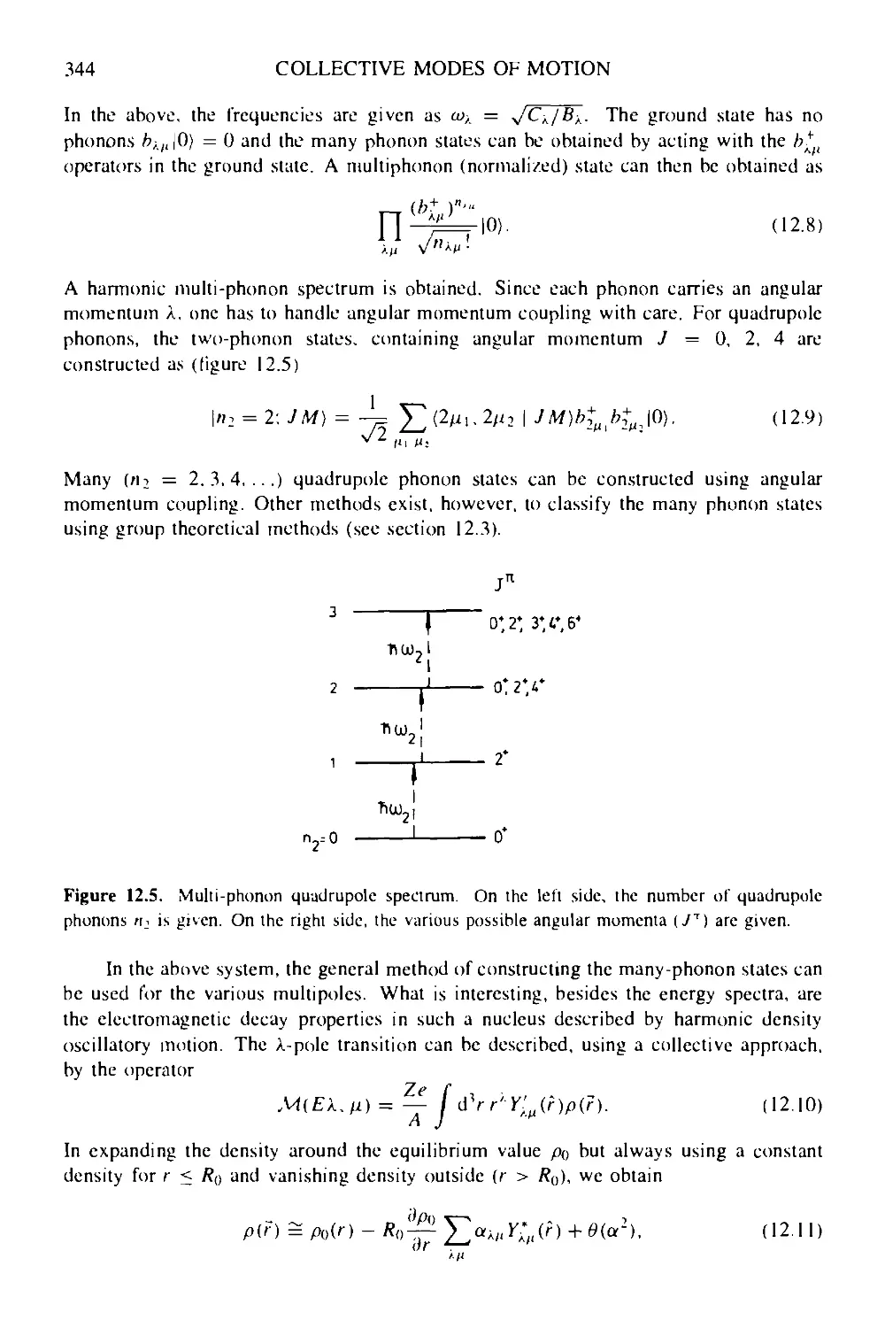
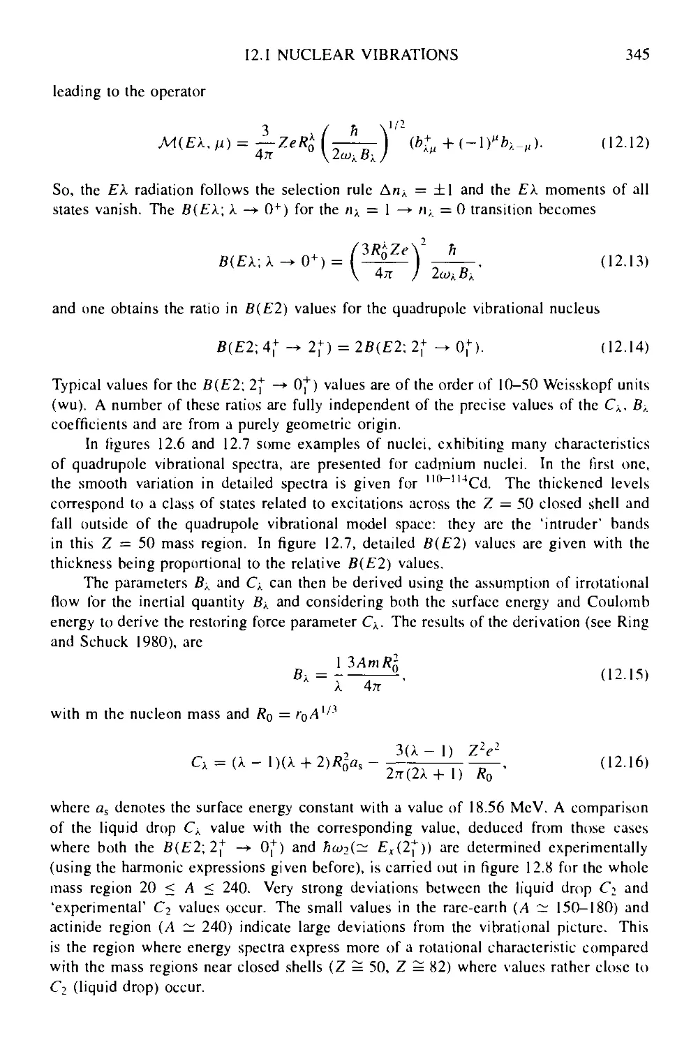
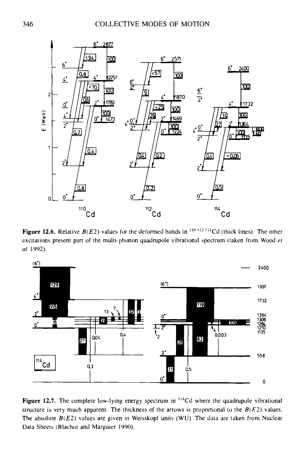
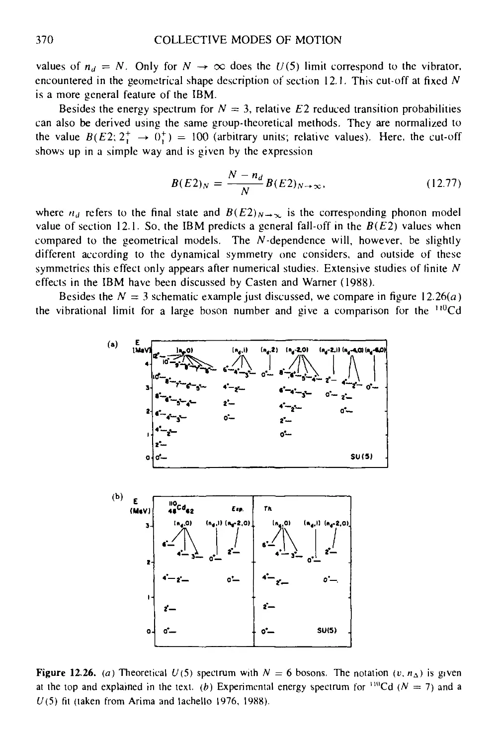
12.1 Nuclear vibrations 340
12.1.1 Isoscalar vibrations 342
12.1.2 Sum rules in the vibrational model 347
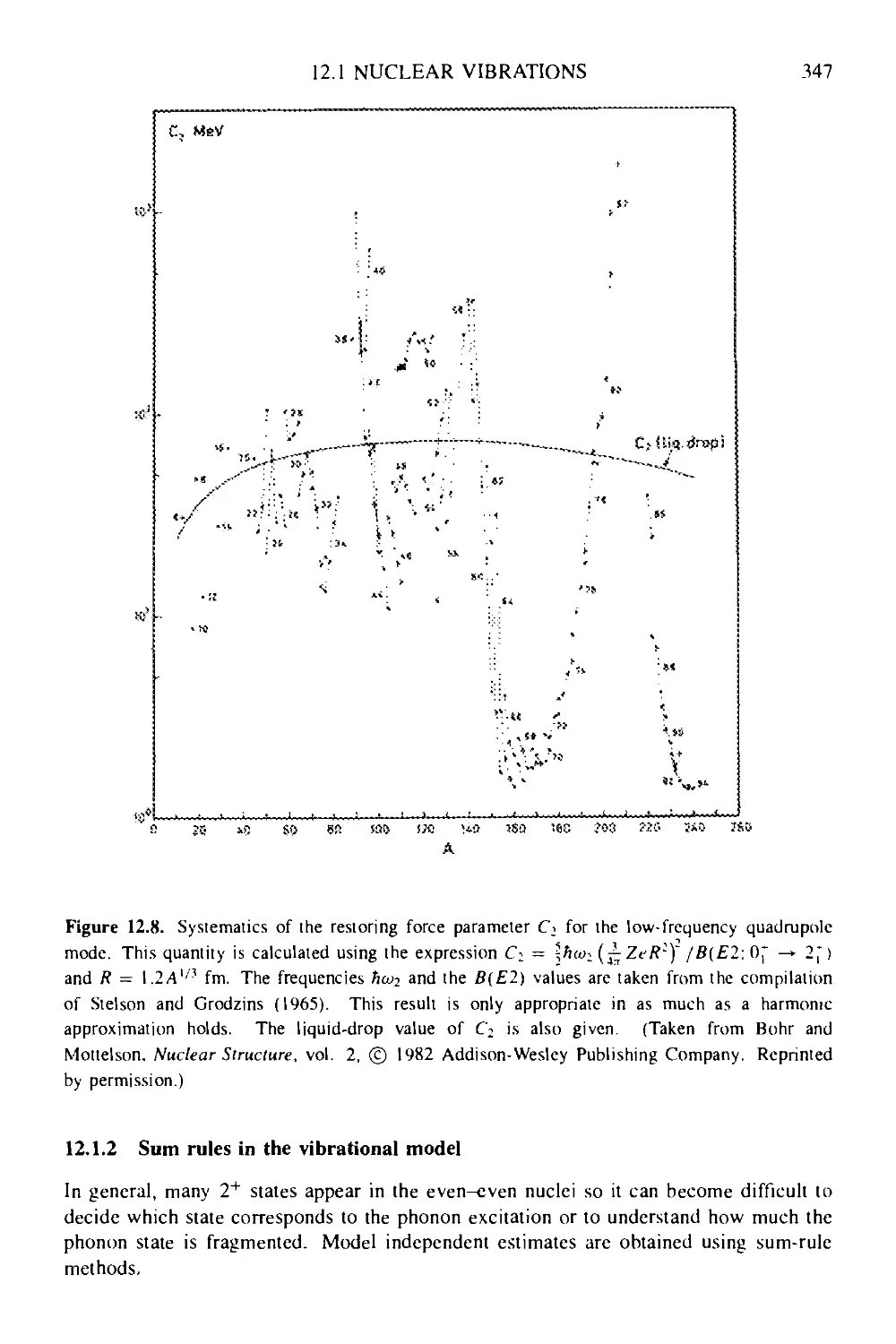
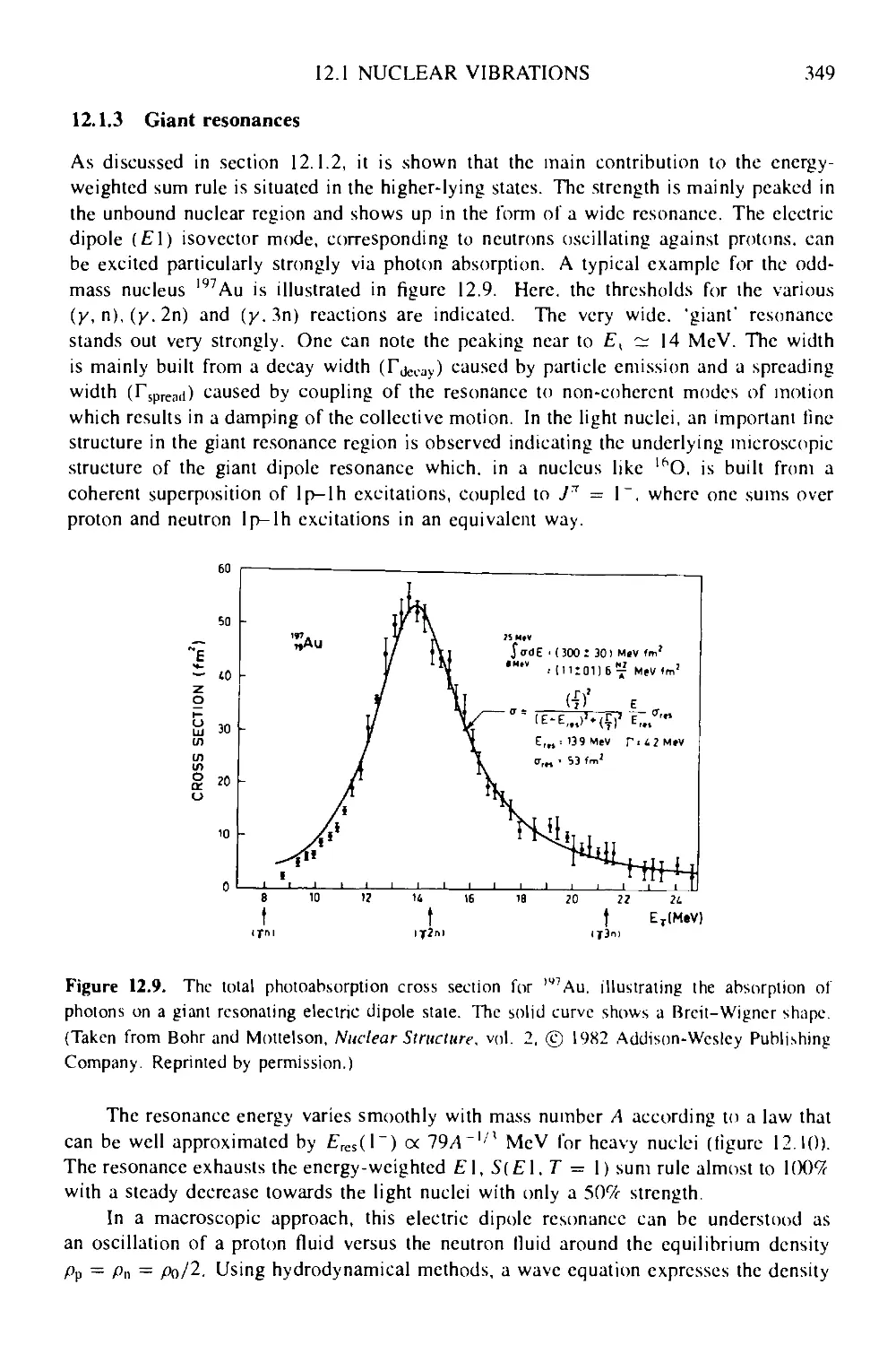
12.1.3 Giant resonances 349
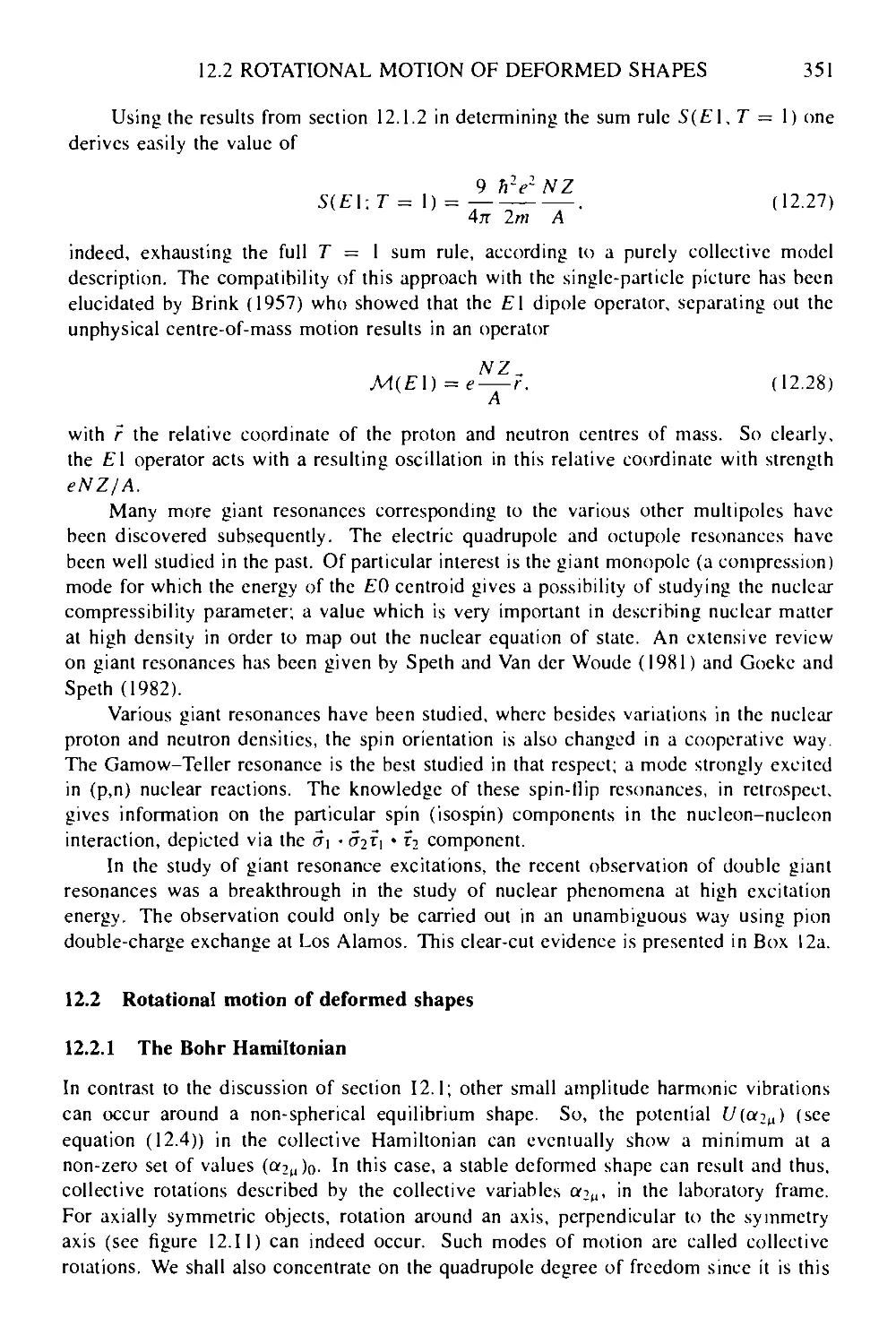
12.2 Rotalional motion of deformed shapes 351
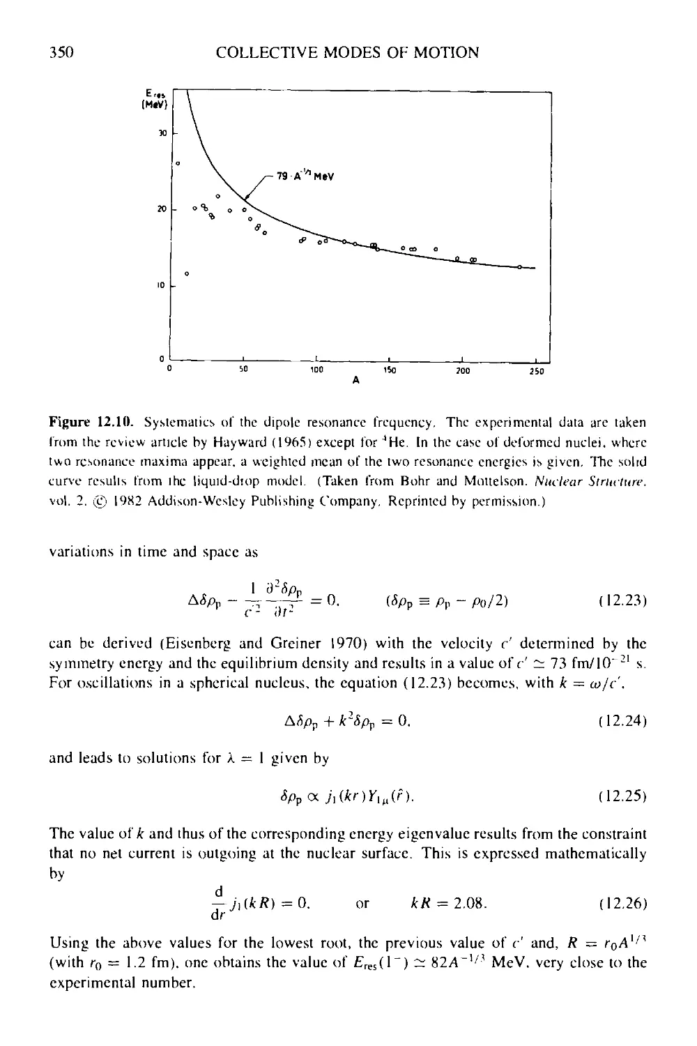
12.2.1 The Bohr Hamiltonian 351
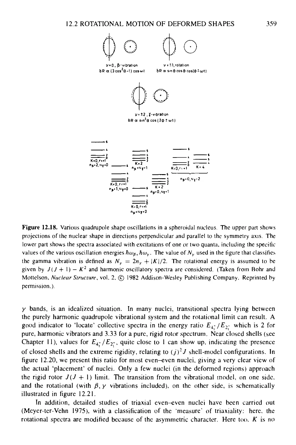
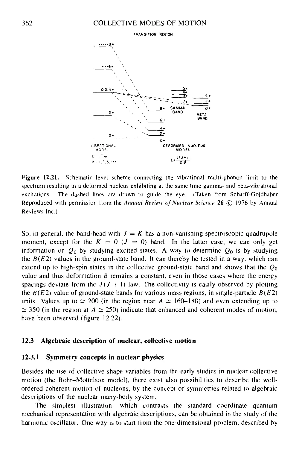
12.2.2 Realistic situations 358
12.2.3 Electromagnetic quadrupole properties 360
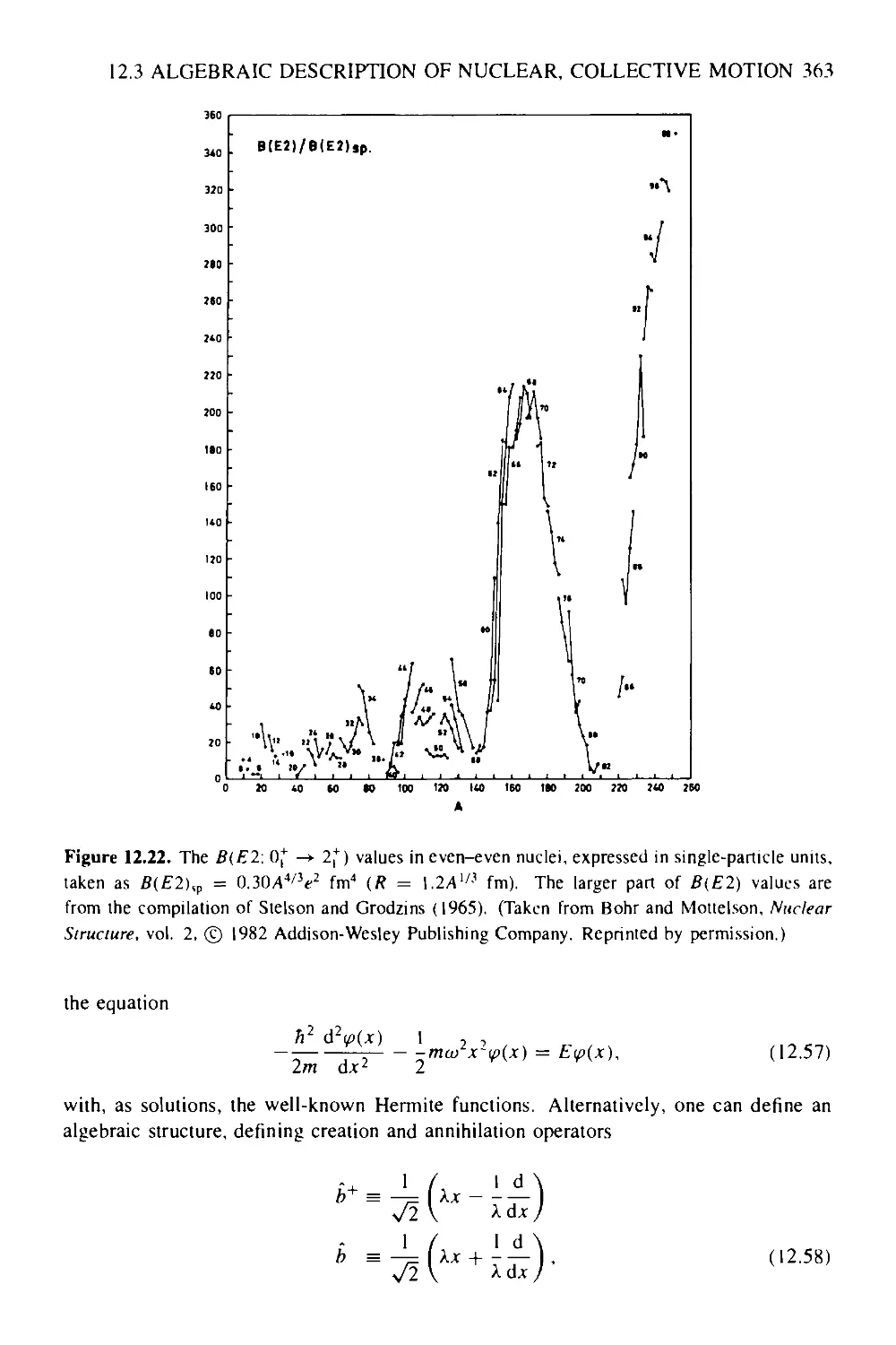
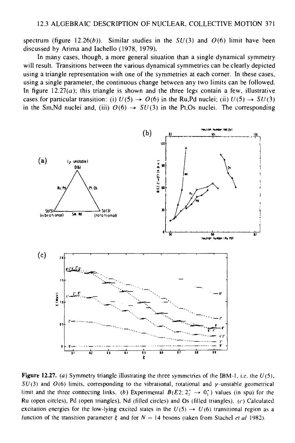
12.3 Algebraic description of nuclear, collective motion 362
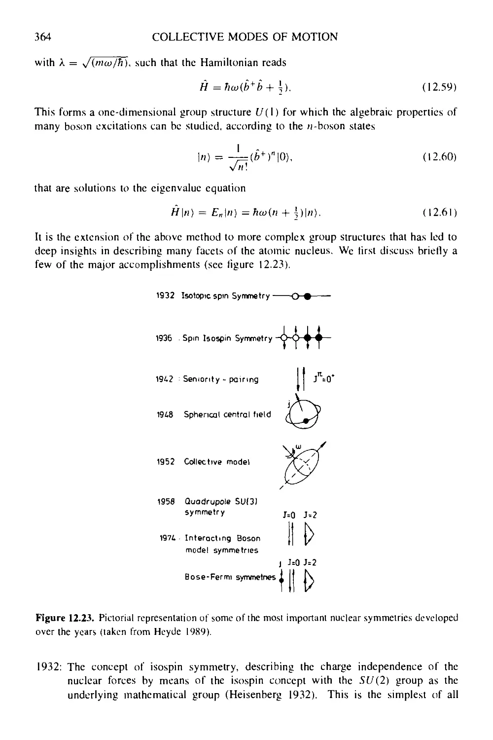
12.3.1 Symmetry concepts in nuclear physics 362
12.3.2 Symmetries of the IBM 365
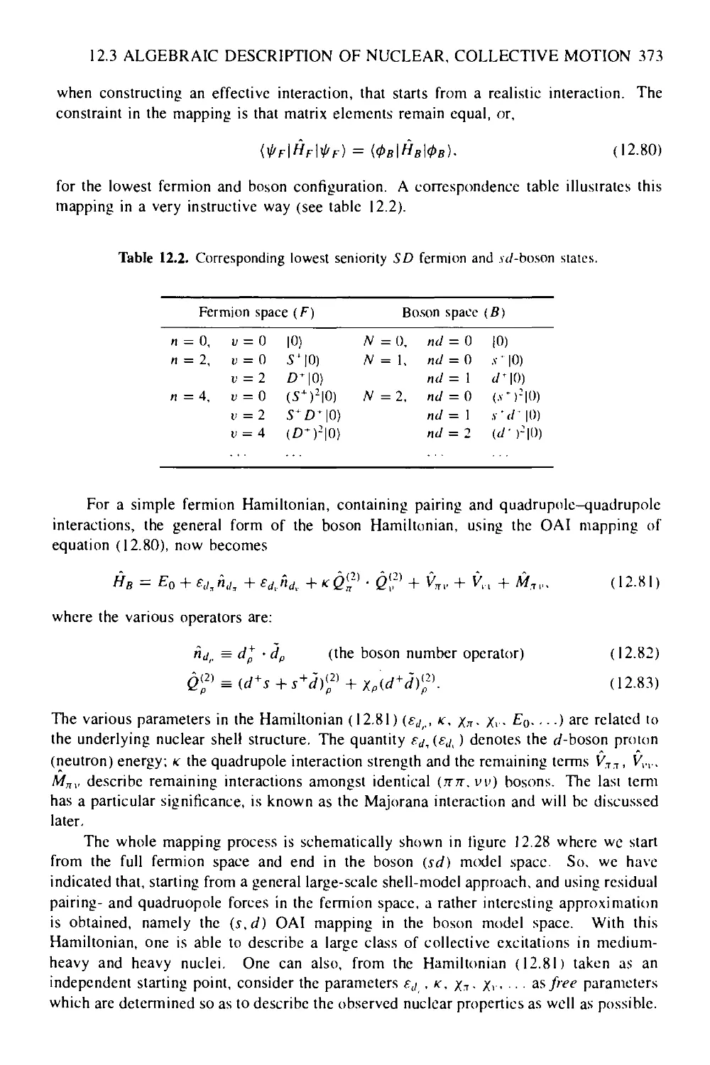
12.3.3 The proton-neutron interacting boson model: IBM-2 372
12.3.4 Extension of the interacting boson model 376
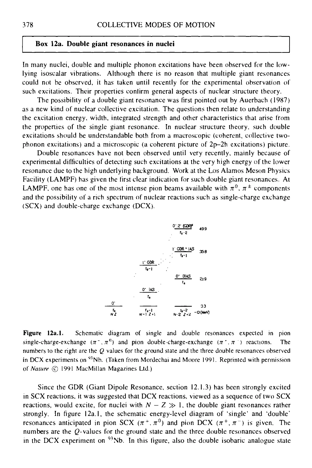
Box 12a Double giant resonances in nuclei 378
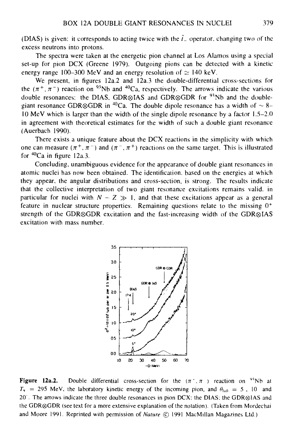
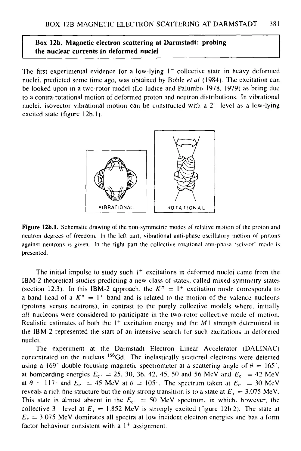
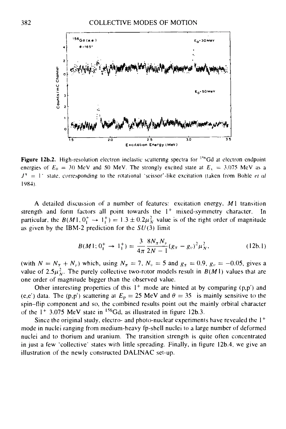
Box 12b Magnetic electron scattering at Darmstadt: probing the nuclear currents
in deformed nuclei 381
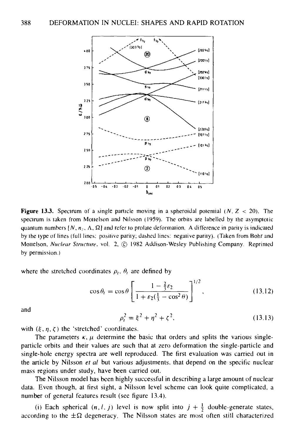
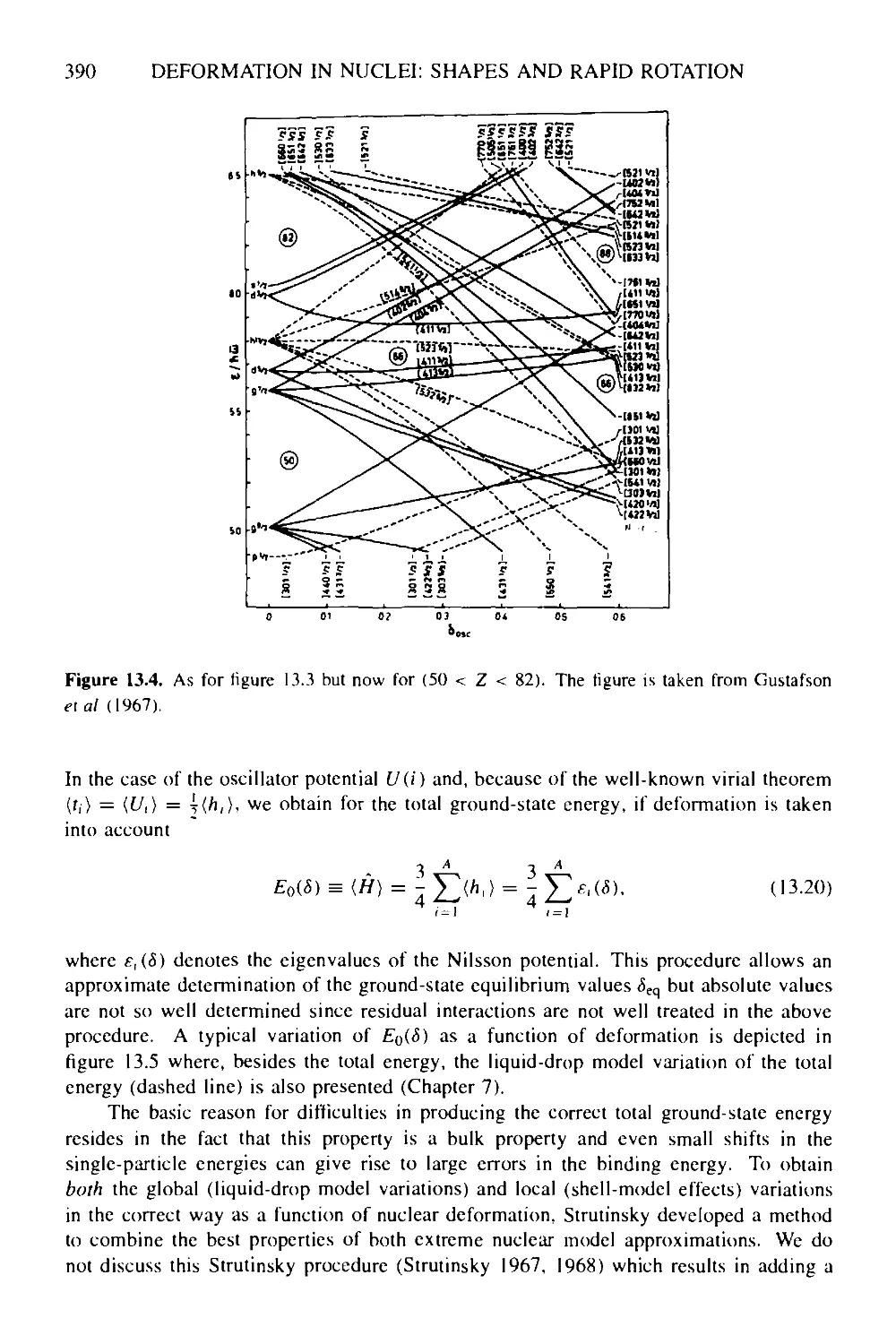
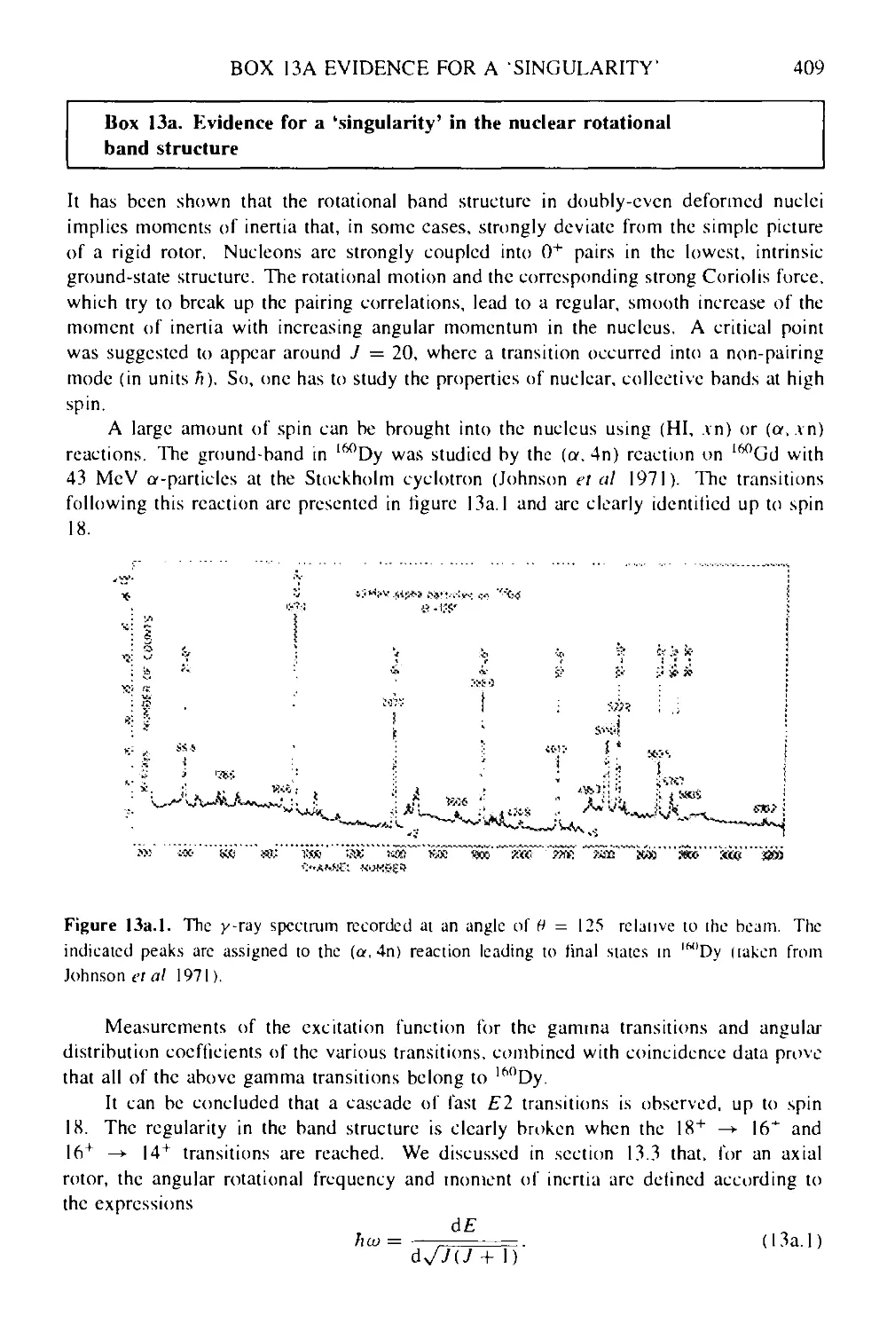
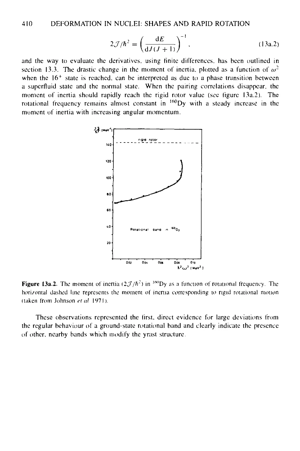
13 Deformation in nuclei: shapes and rapid rotation 384
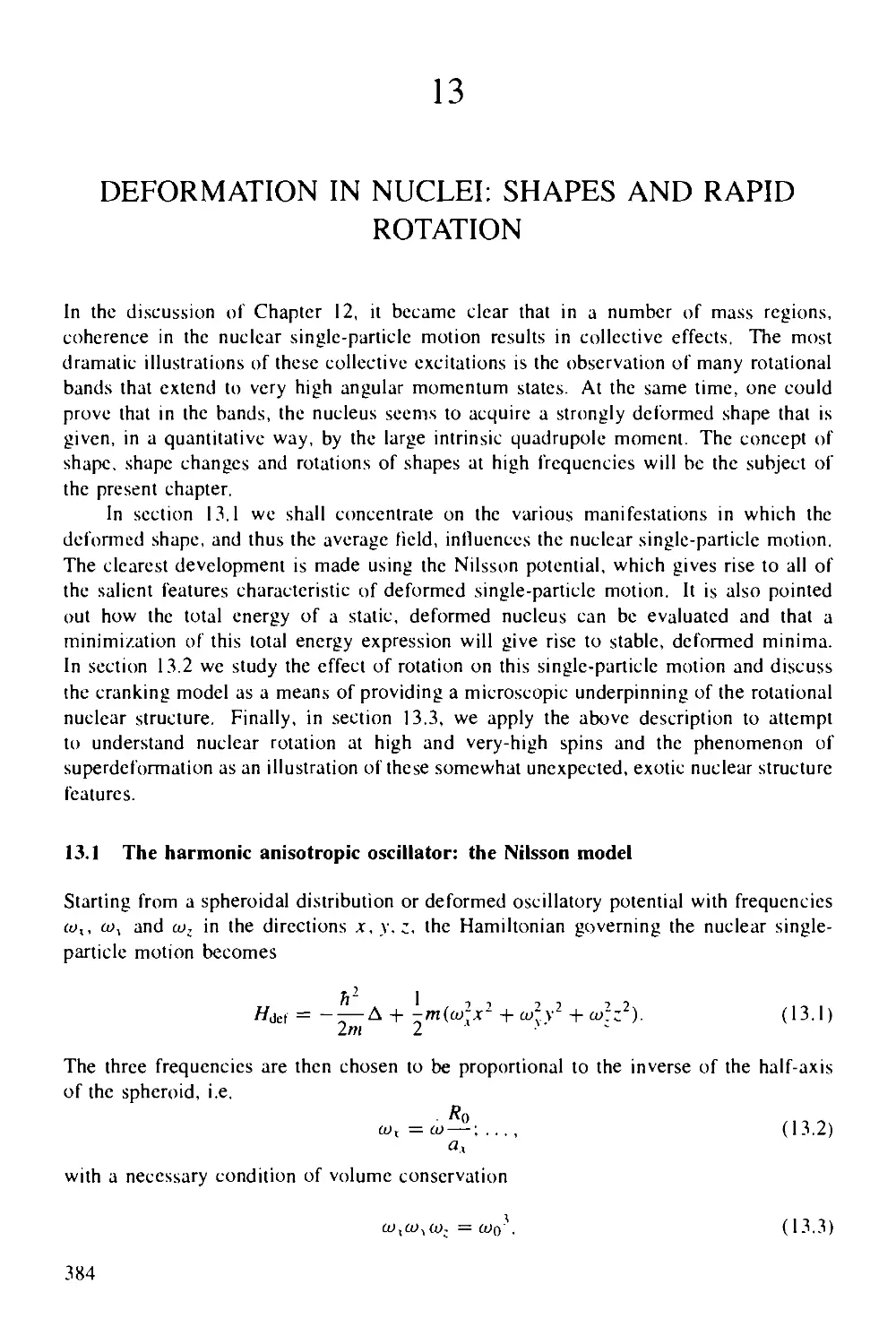
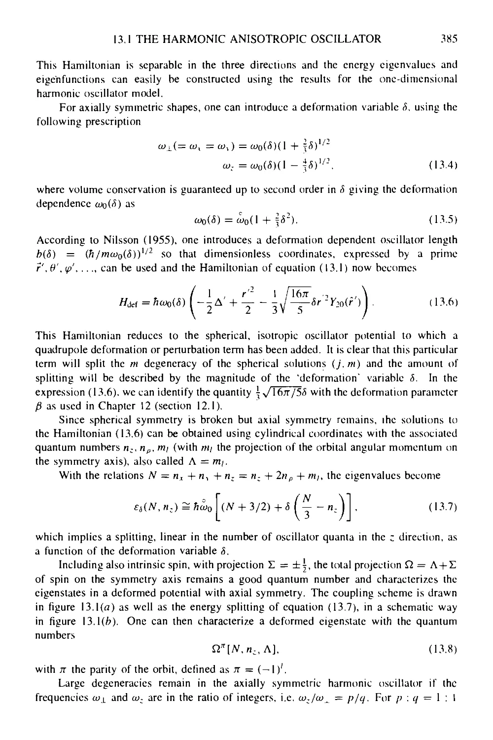
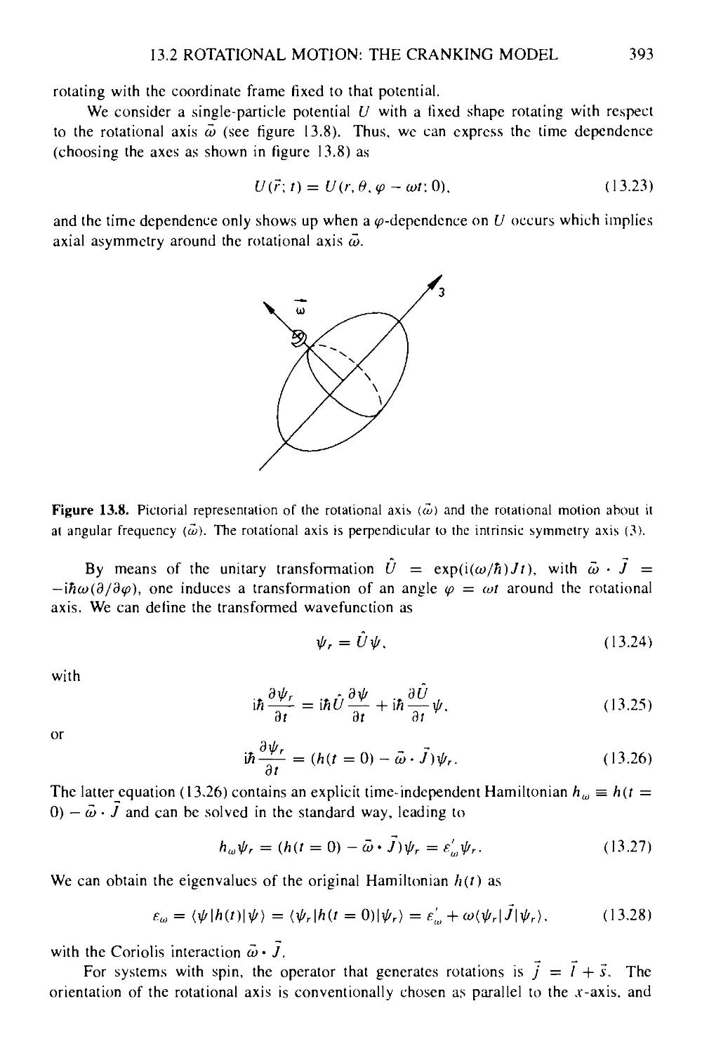
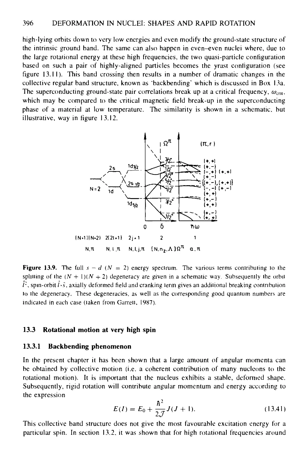
13.1 The harmonic anisotropic oscillator: the Nilsson model 384
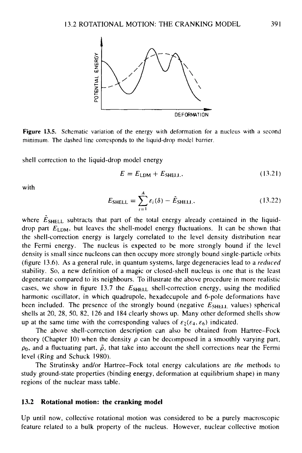
13.2 Rotational motion: the cranking model 391
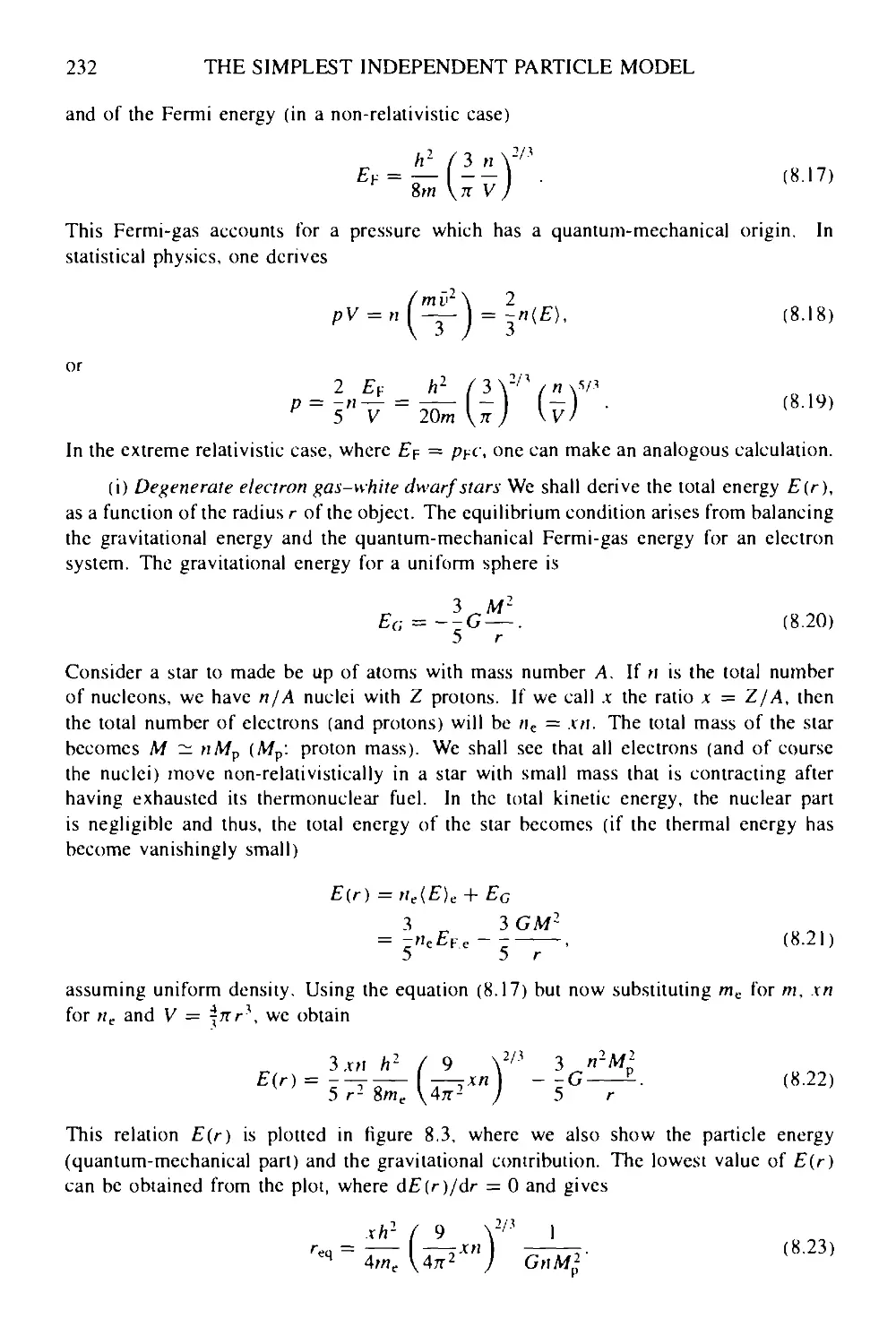
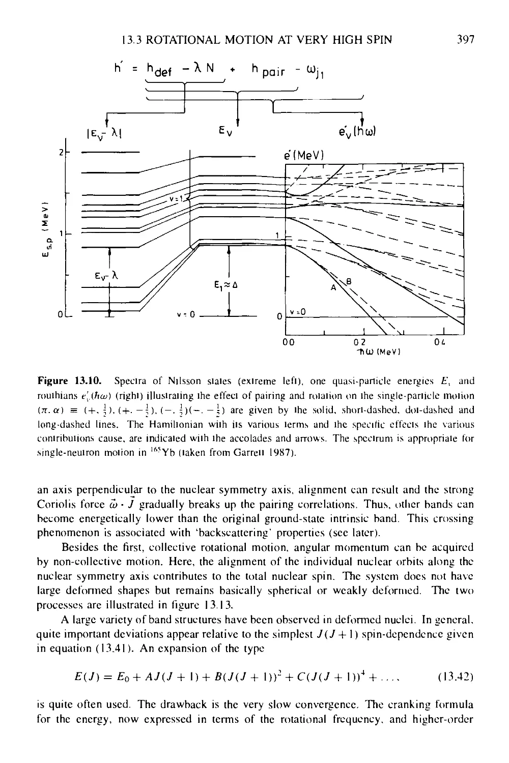
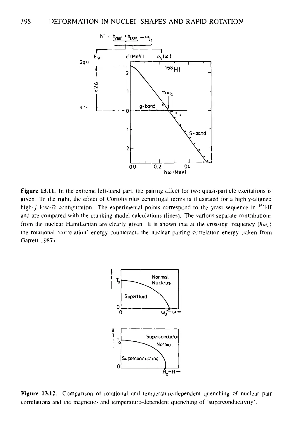
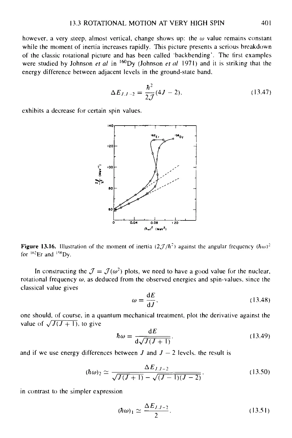
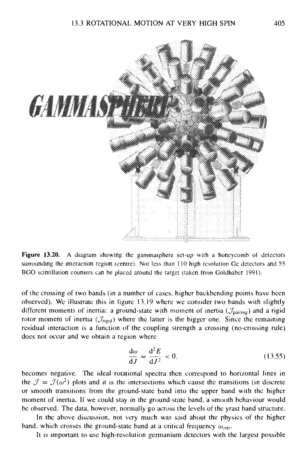
13.3 Rotational motion at very high spin 396
13.3.1 Backbending phenomenon 396
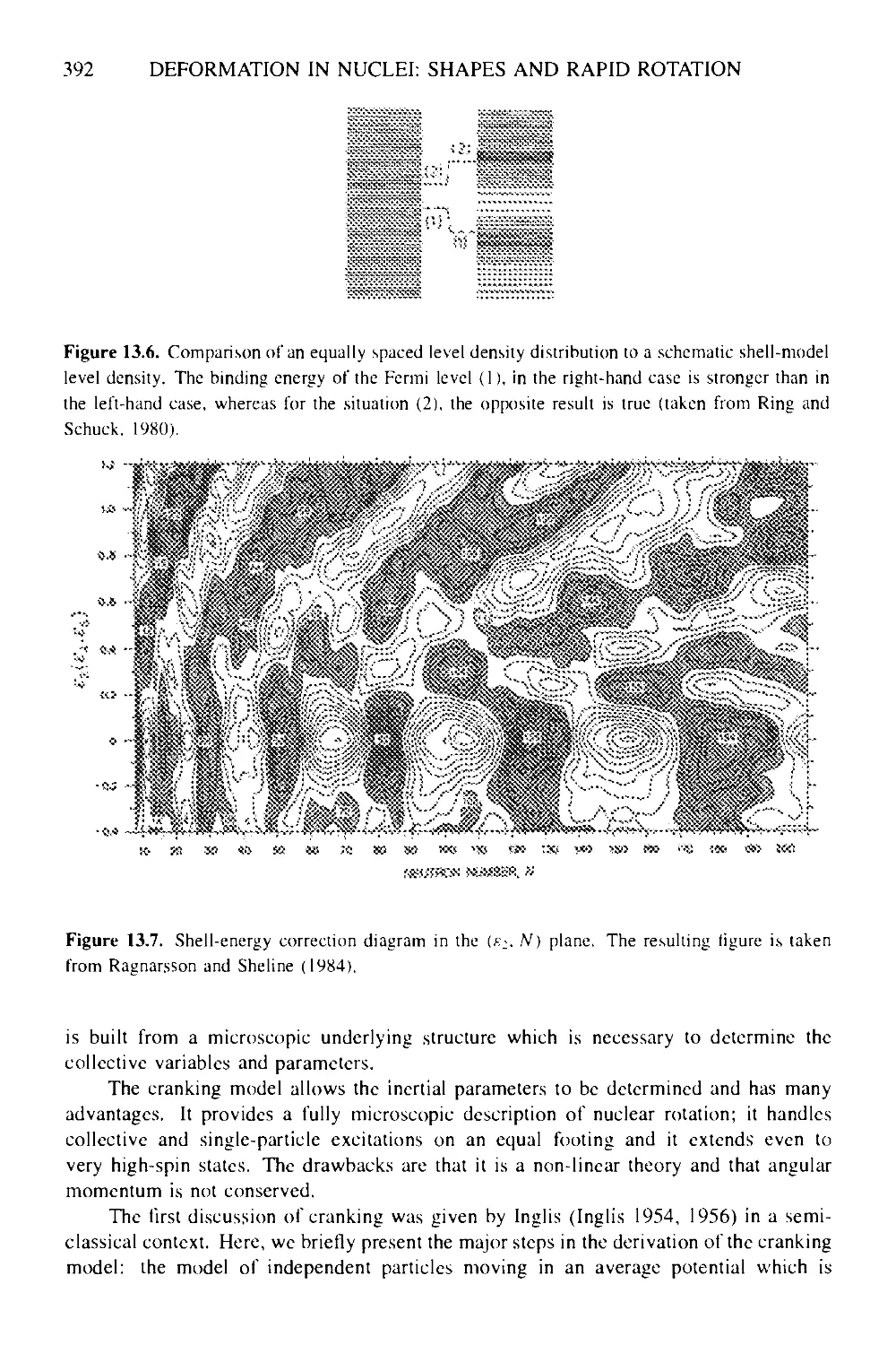
13.3.2 Deformation energy surfaces at very high spin: super- and
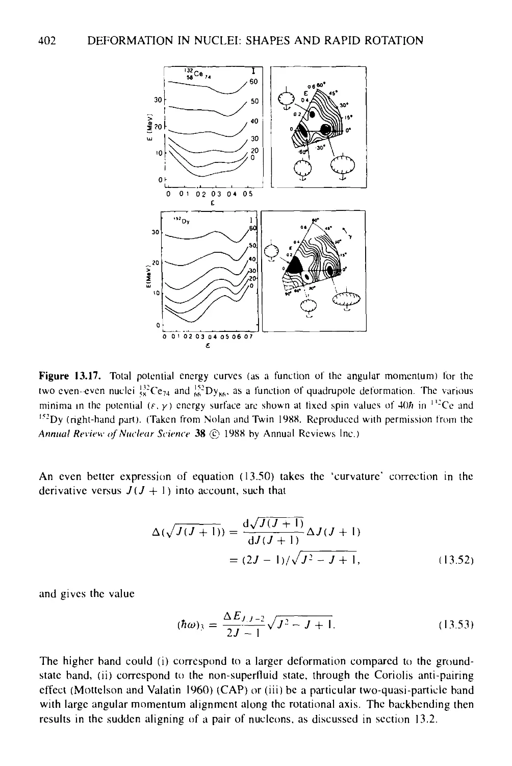
hyperdeformation 403
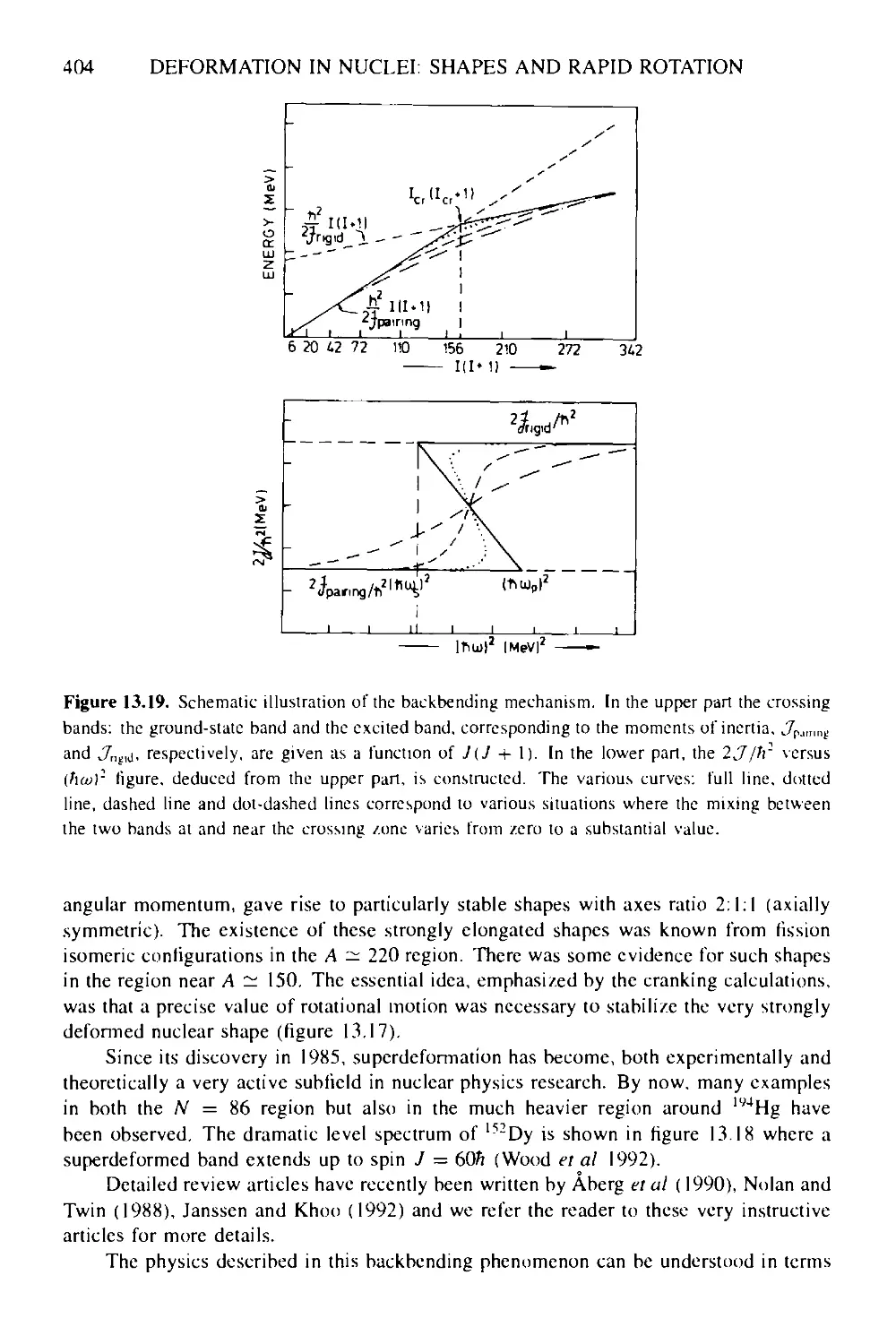
Box 13a Evidence for a 'singularity' in the nuclear rotational band structure 409
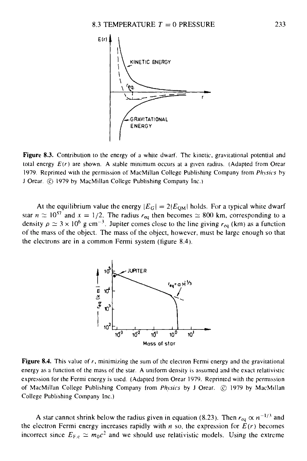
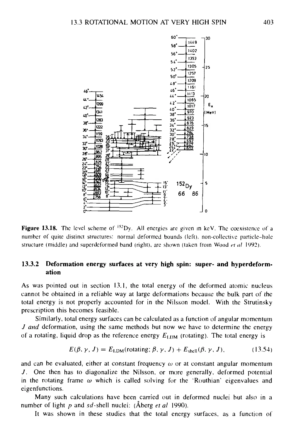
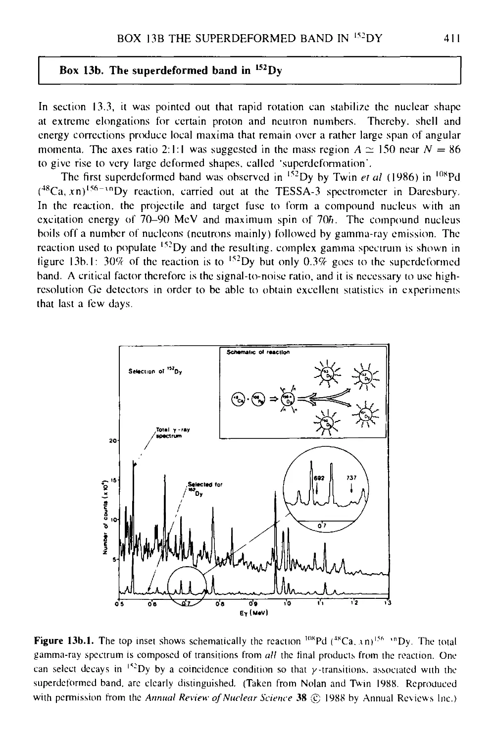
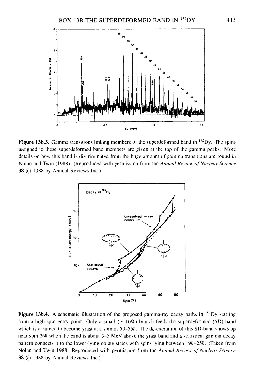
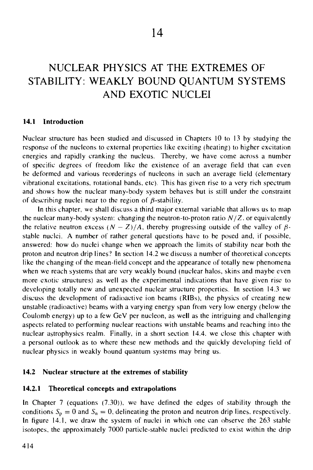
Box 13b The superdeformed band in l52Dy 411
14 Nuclear physics at the extremes of stability: weakly bound quantum systems
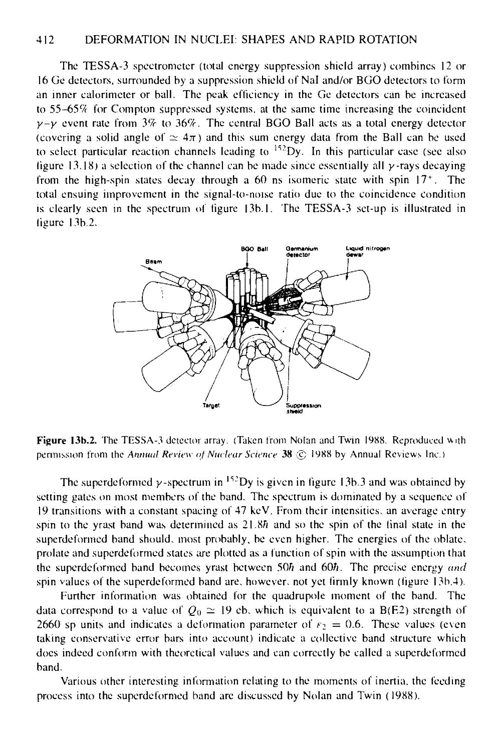
and exotic nuclei 414
14.1 Introduction 414
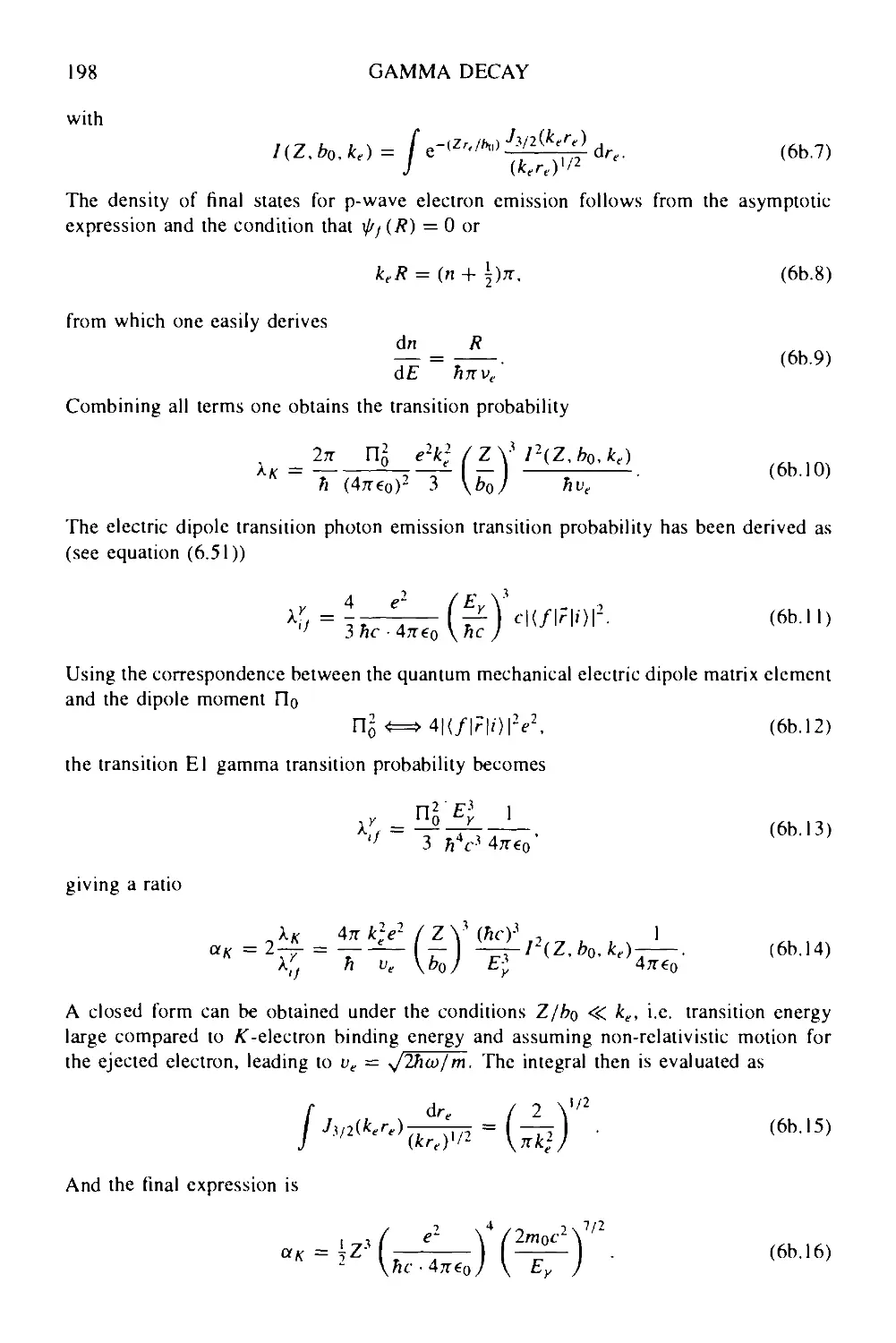
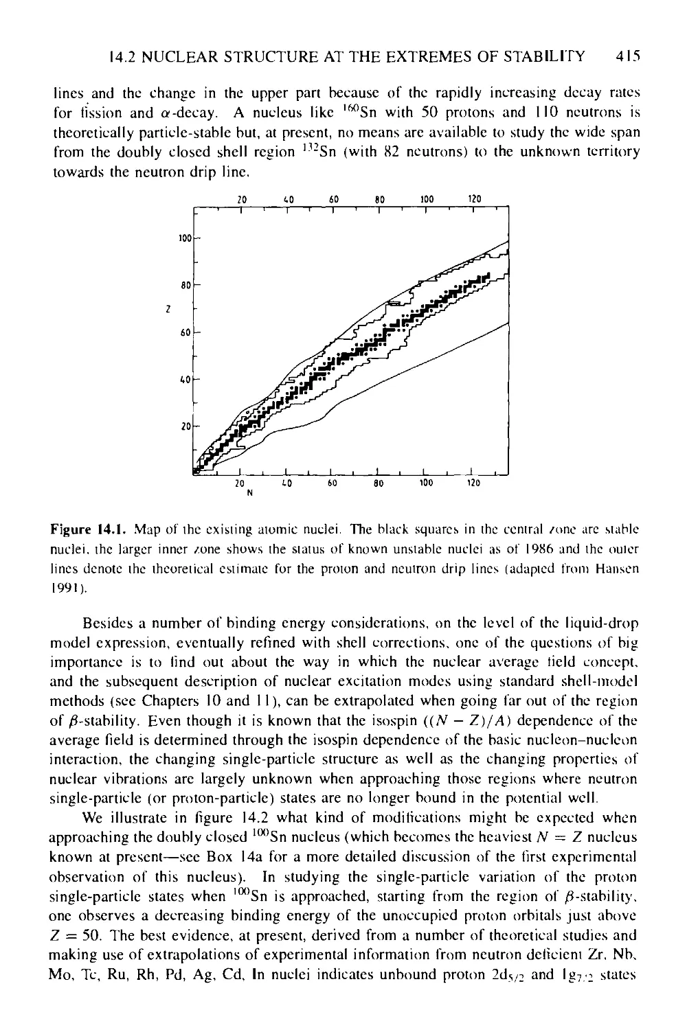
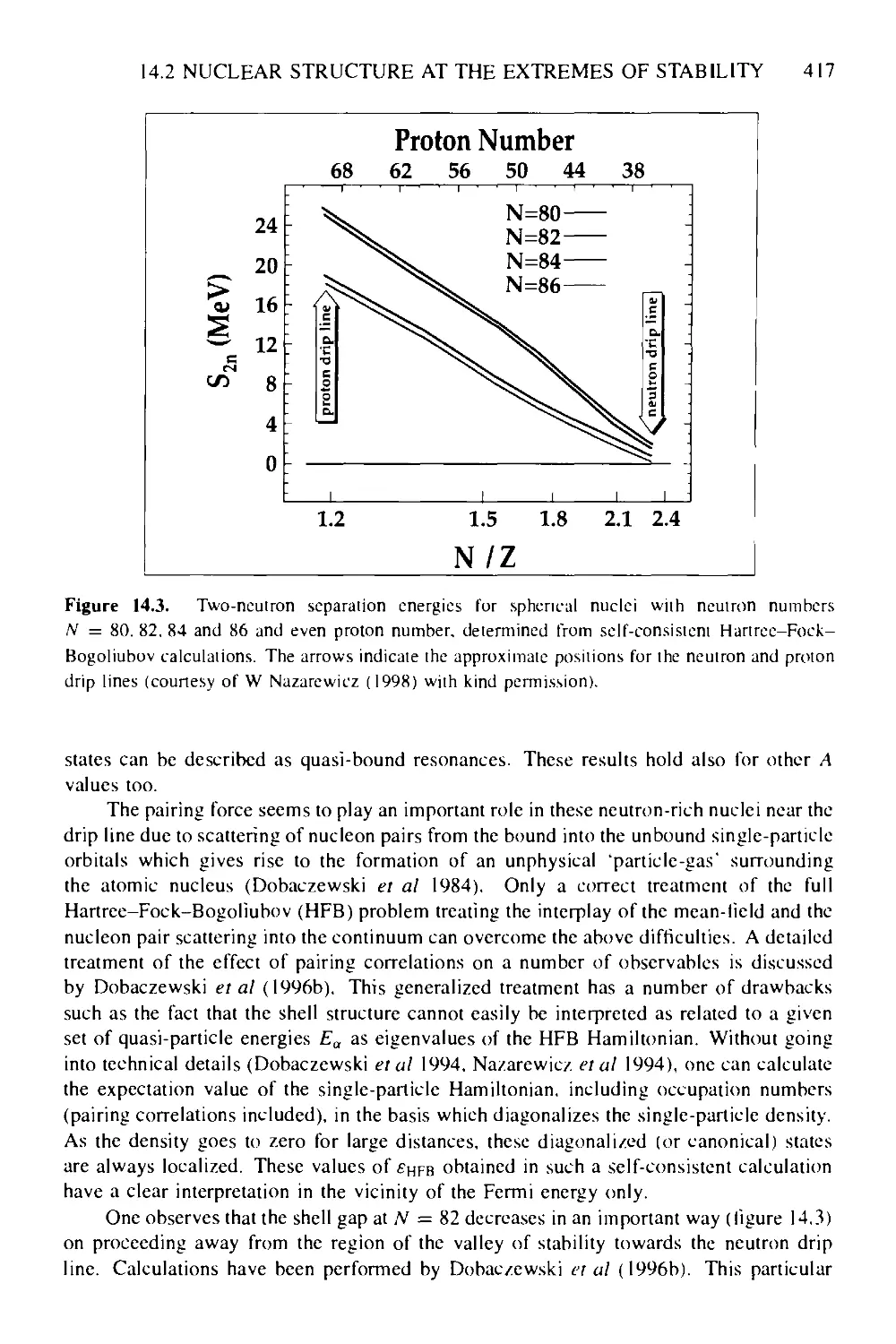
14.2 Nuclear structure at the extremes of stability 414
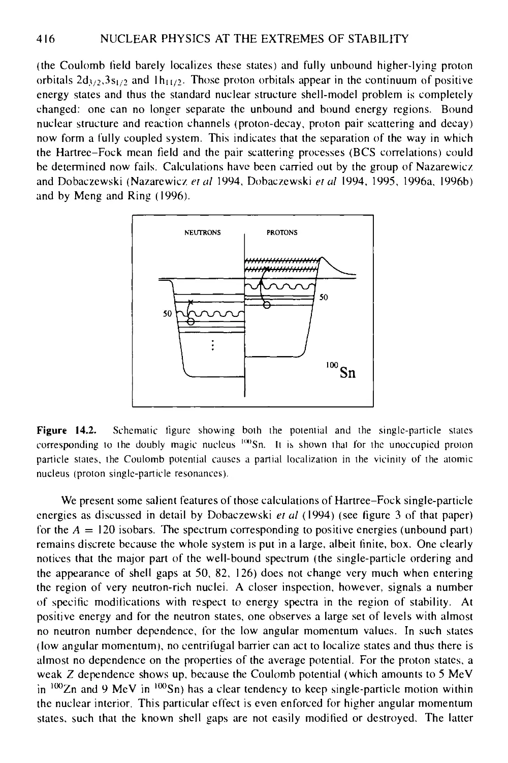
14.2.1 Theoretical concepts and extrapolations 414
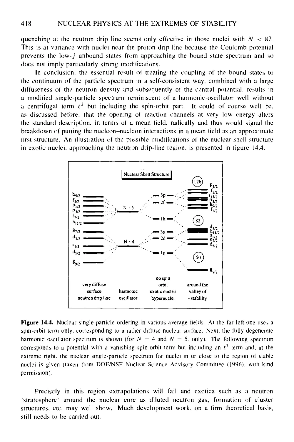
14.2.2 Drip-line physics: nuclear halos, neutron skins, proton-rich nuclei
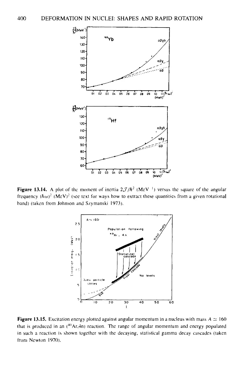
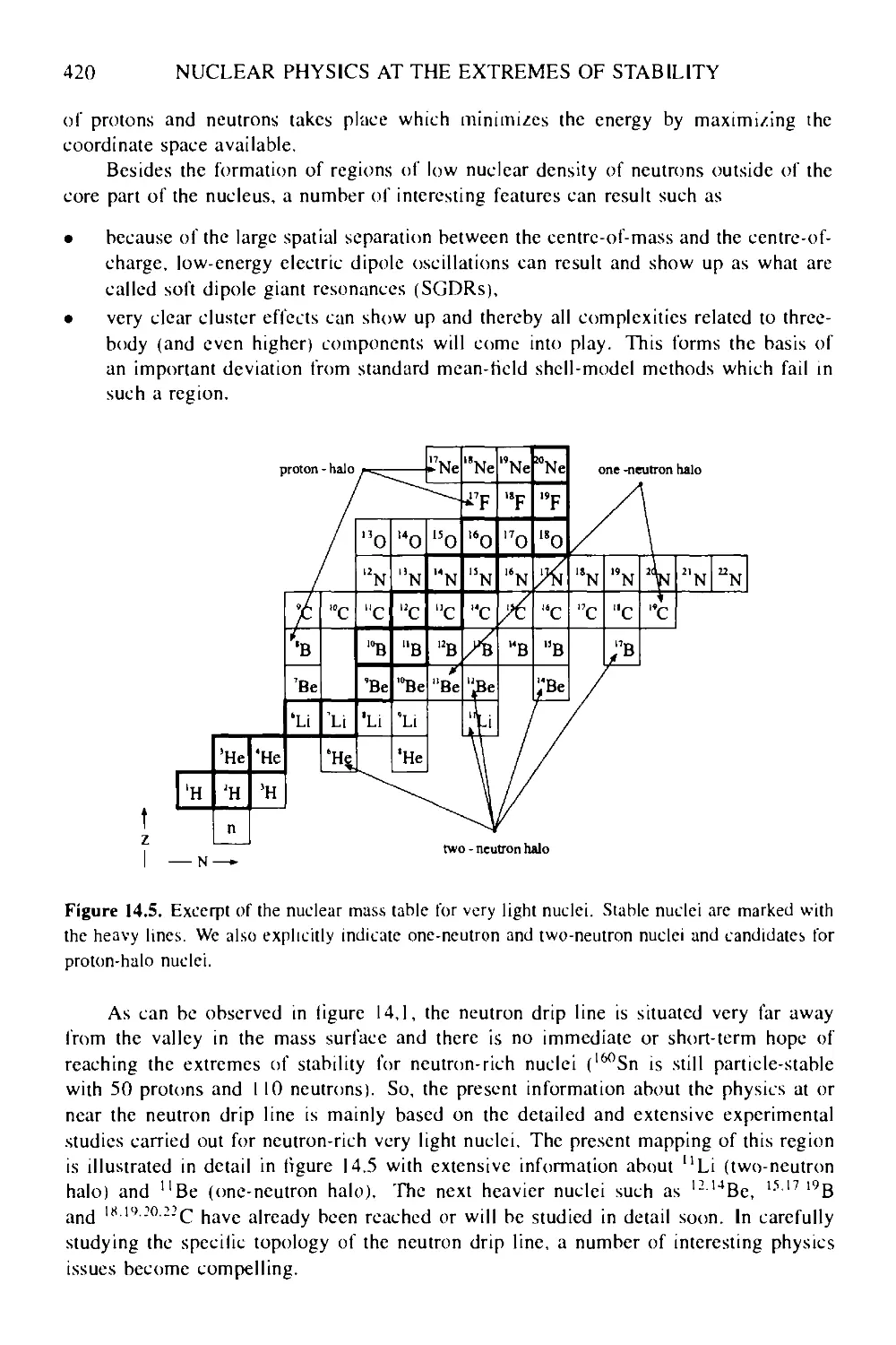
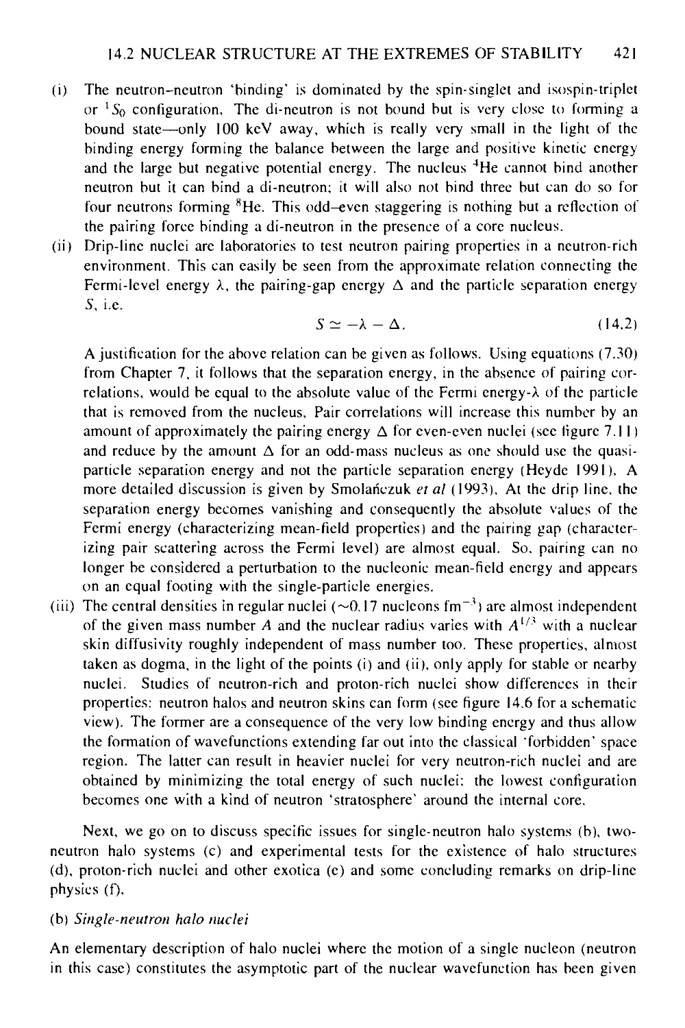
and beyond 419
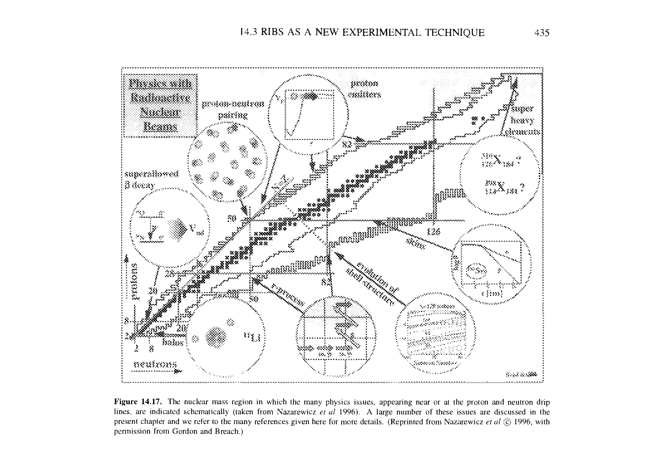
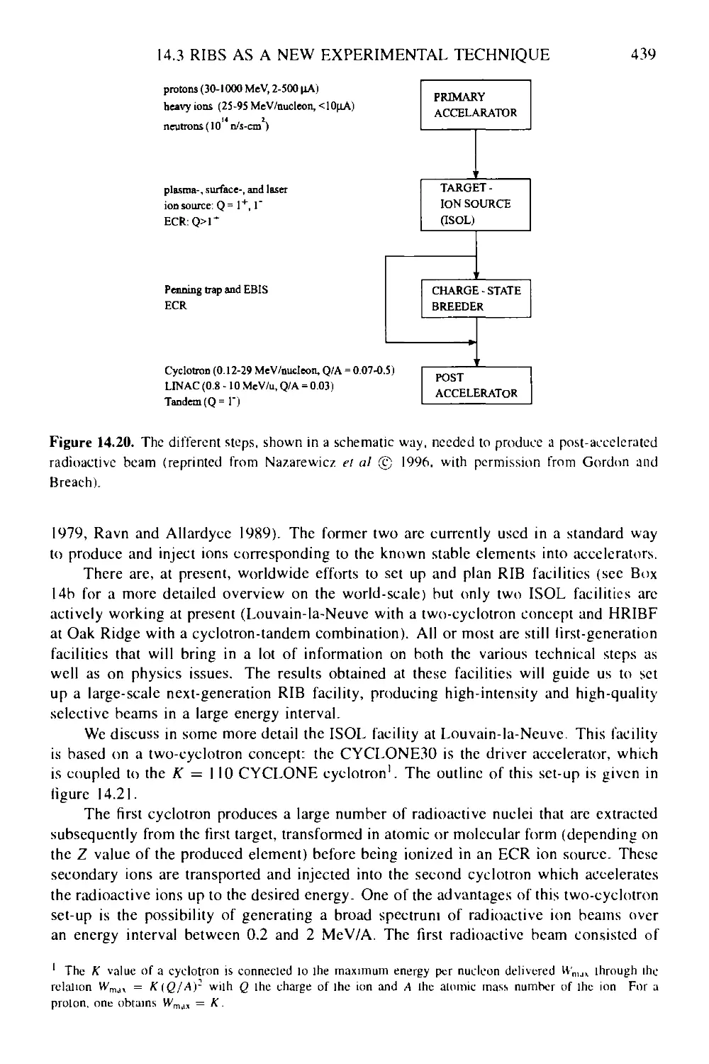
14.3 Radioactive ion beams (RIBs) as a new experimental technique 434
14.3.1 Physics interests 434
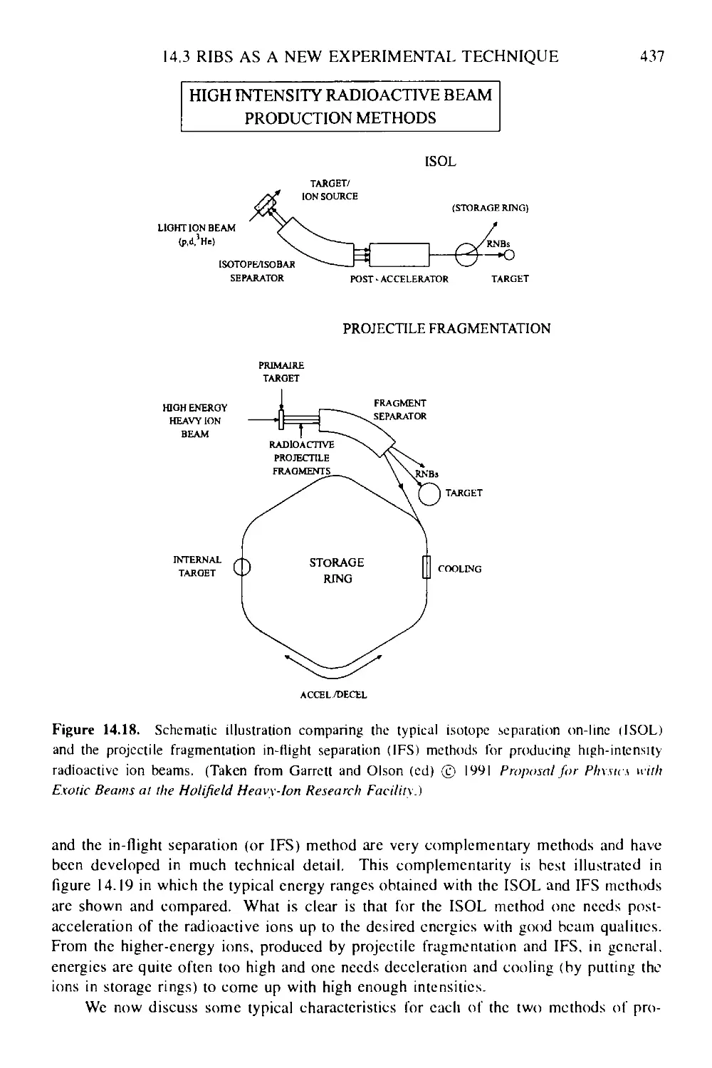
14.3.2 Isotope separation on-line (ISOL) and in-flight fragment
separation (IFS) experimental methods 436
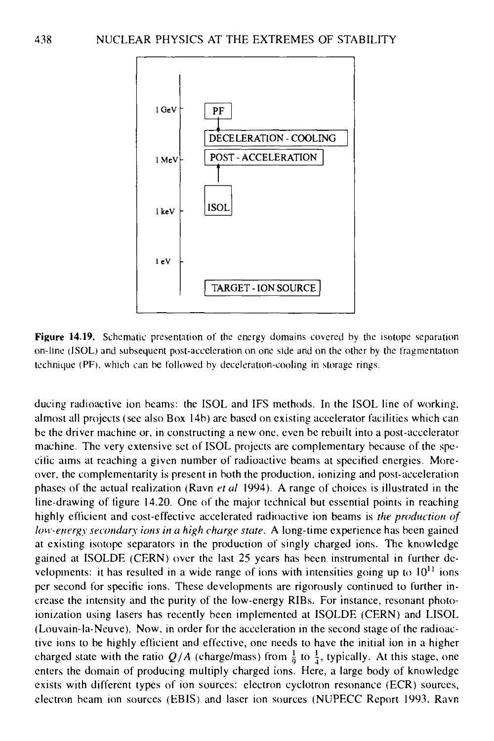
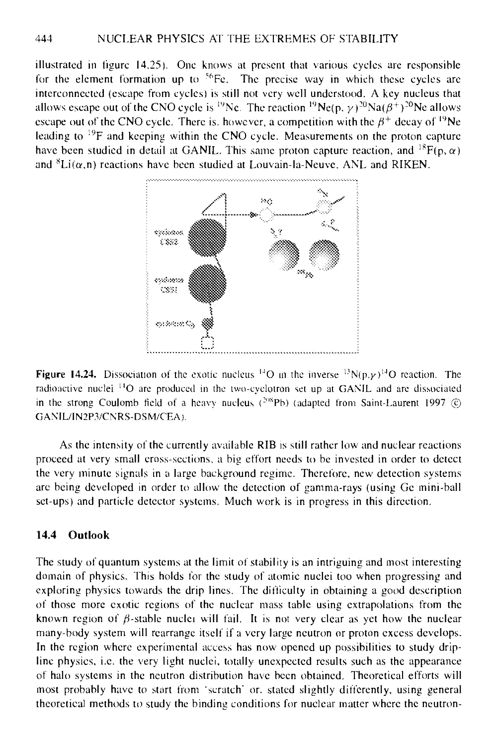
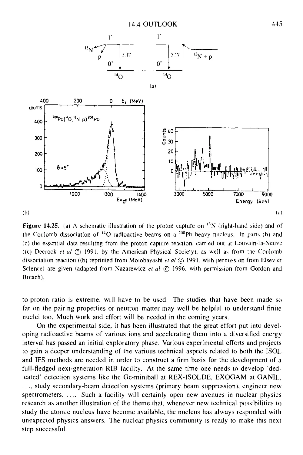
14.3.3 Nuclear astrophysics applications 442
14.4 Outlook 444
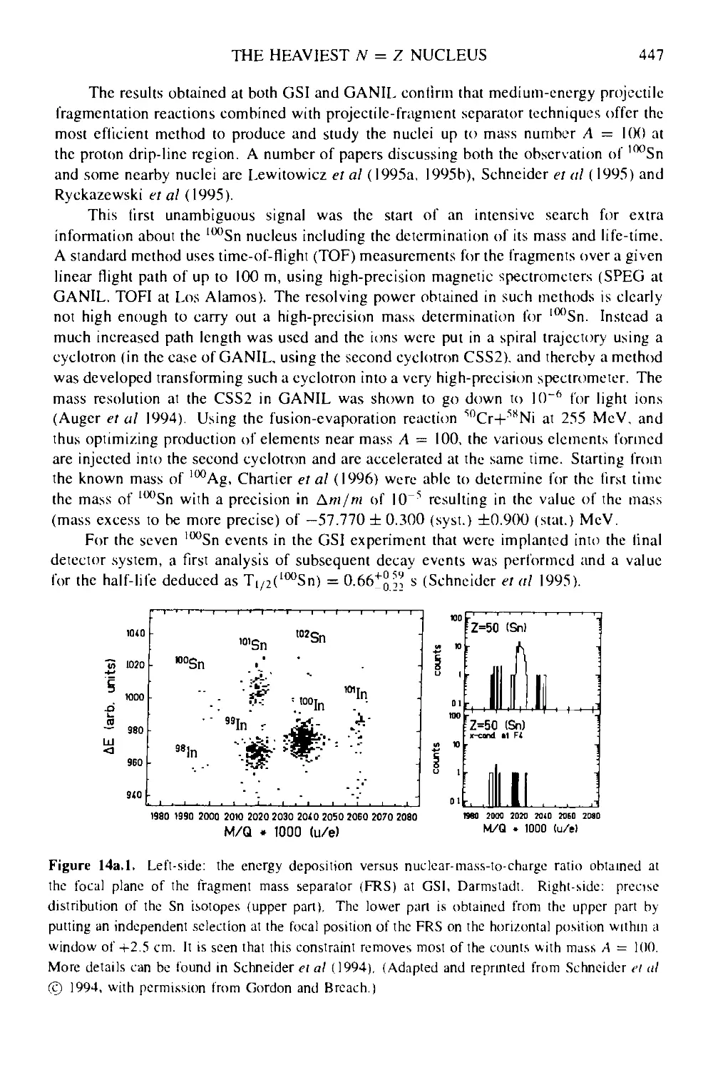
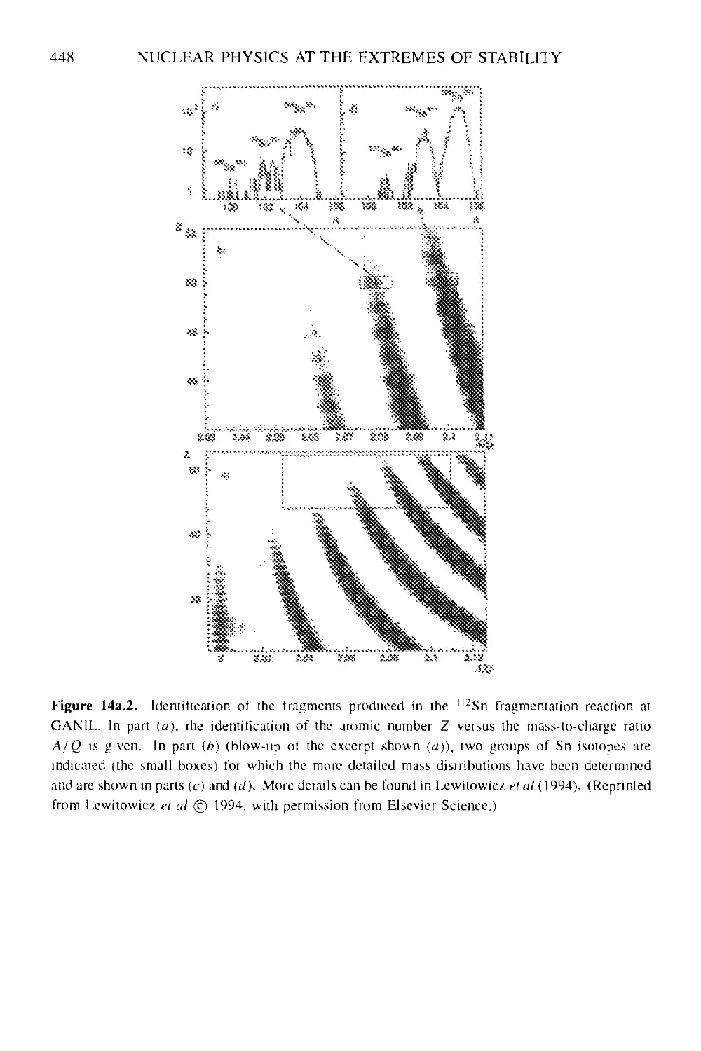
Box 14a The heaviest N = Z nucleus l00Sn and its discovery 446
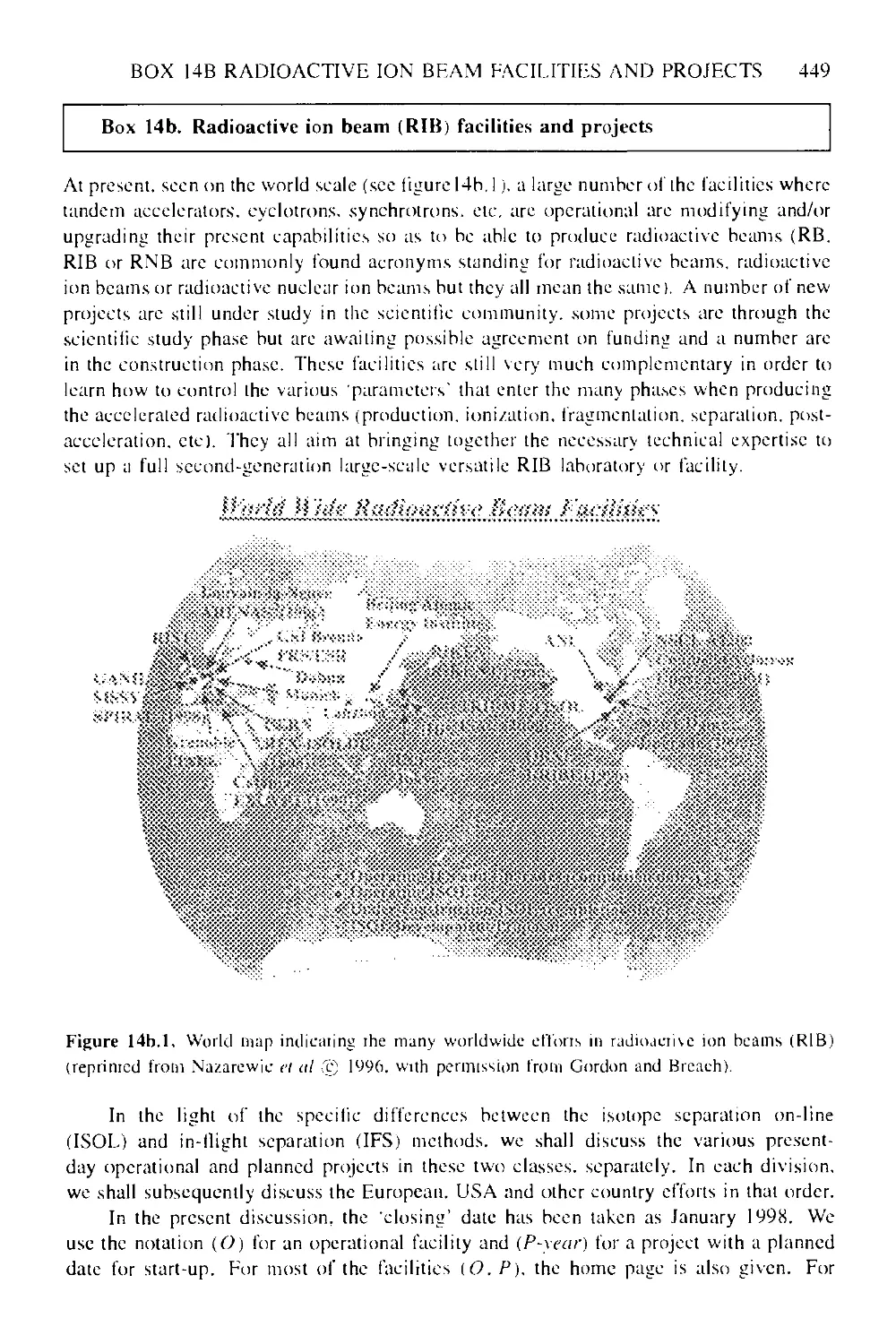
Box 14b Radioactive ion beam (RIB) facilities and projects 449
xii CONTENTS
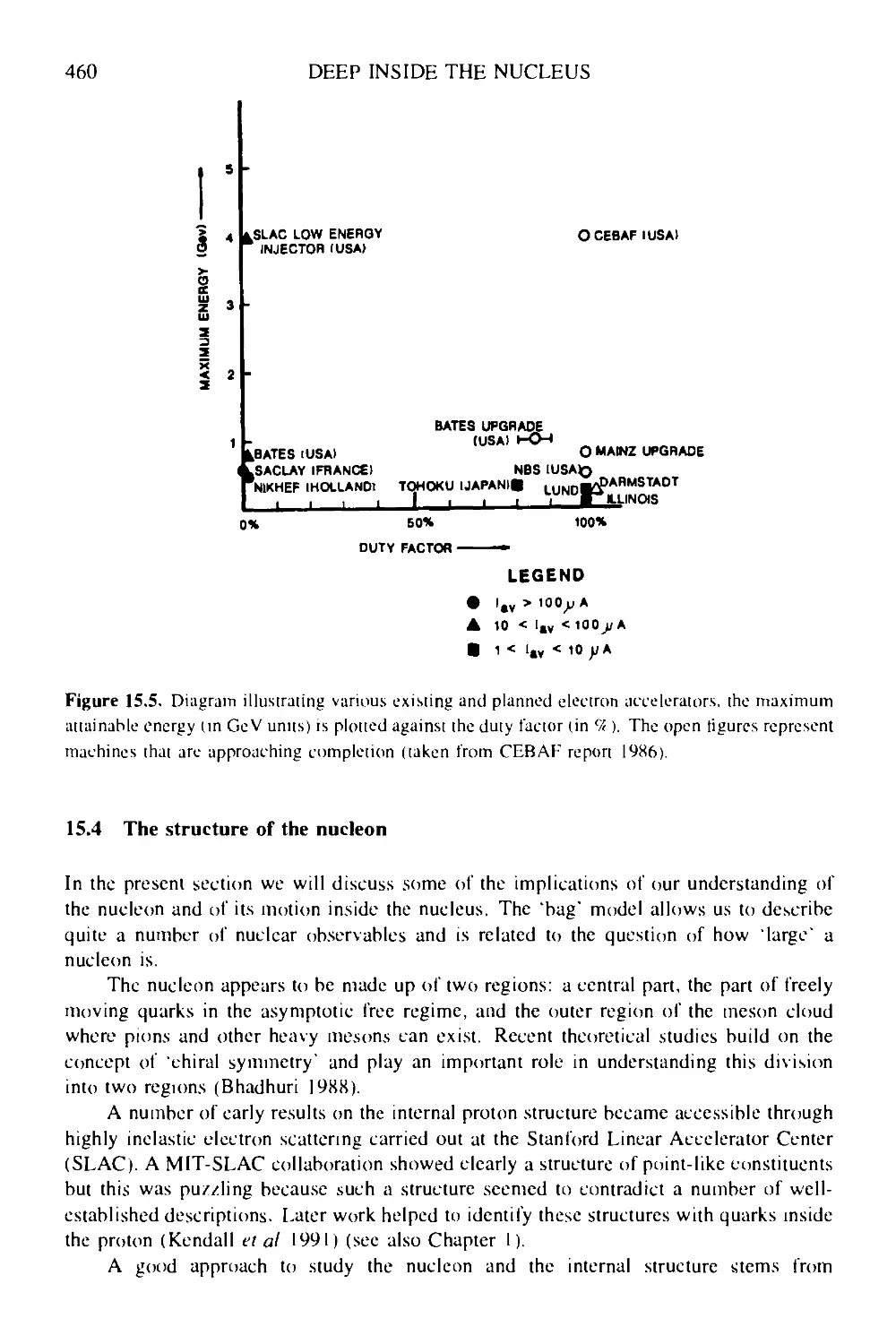
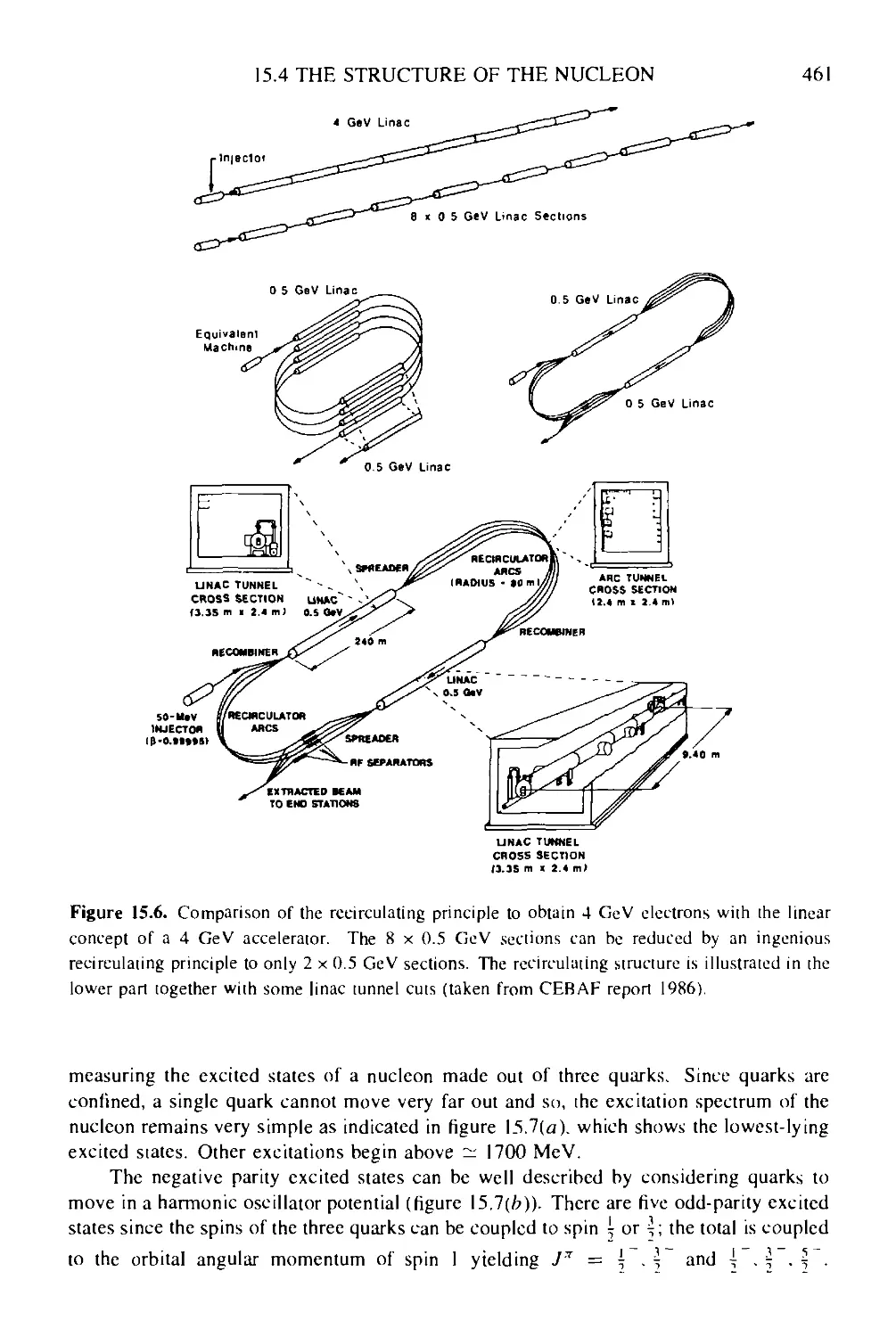
15 Deep inside the nucleus: subnuclear degrees of freedom and beyond 455
15.1 Introduction 455
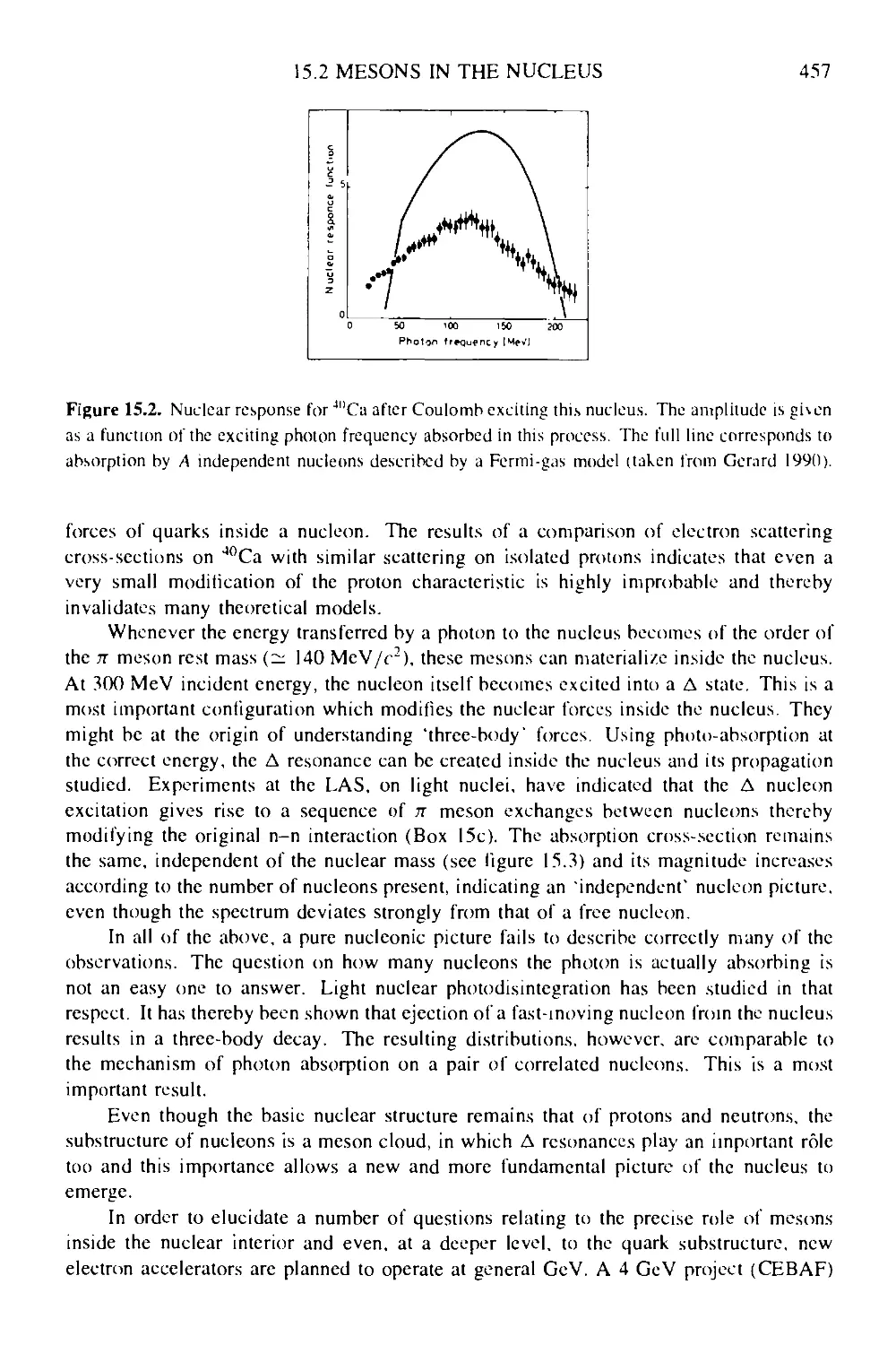
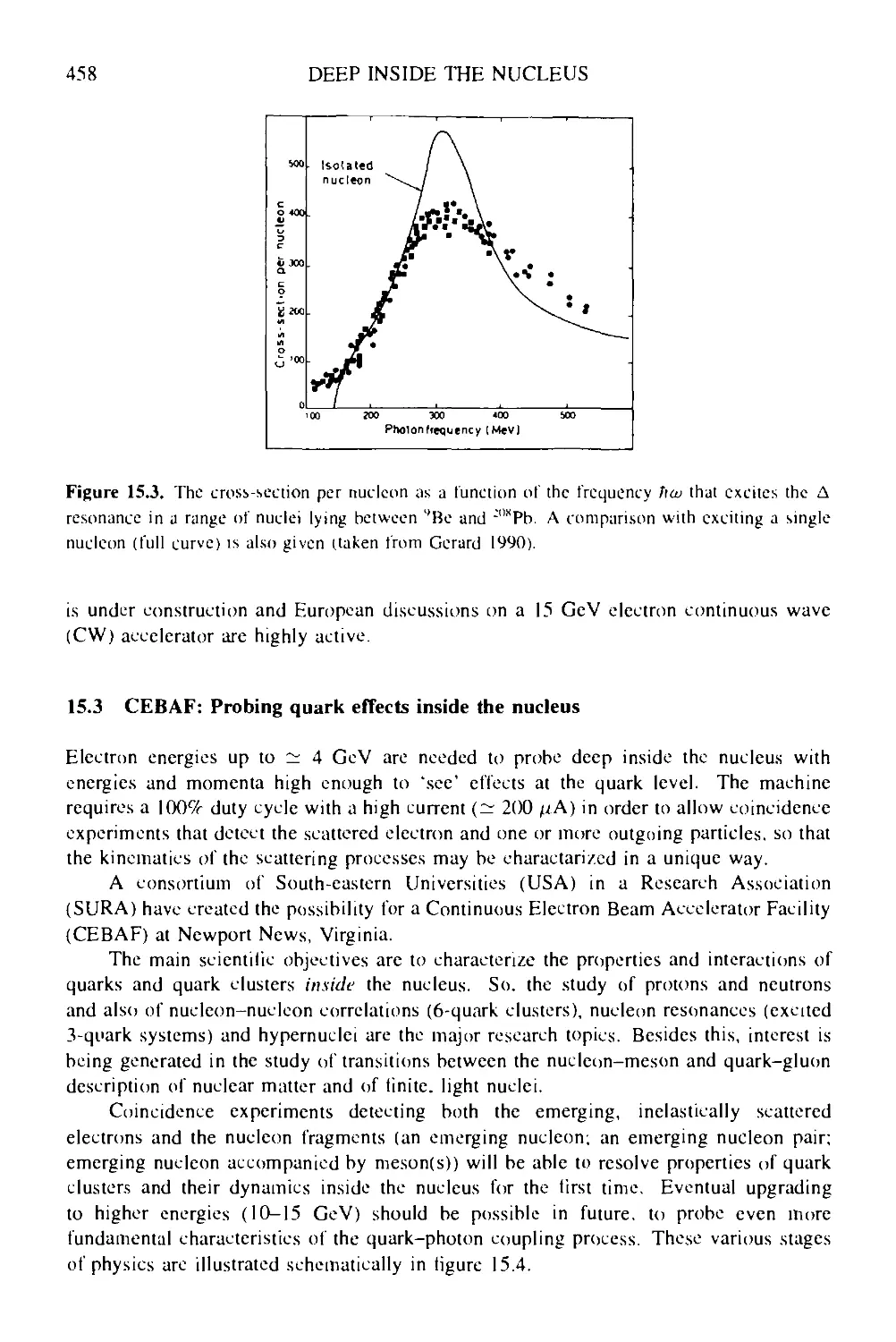
15.2 Mesons in the nucleus 455
15.3 CEBAF: probing quark effects inside the nucleus 458
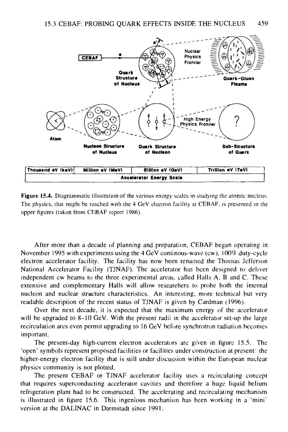
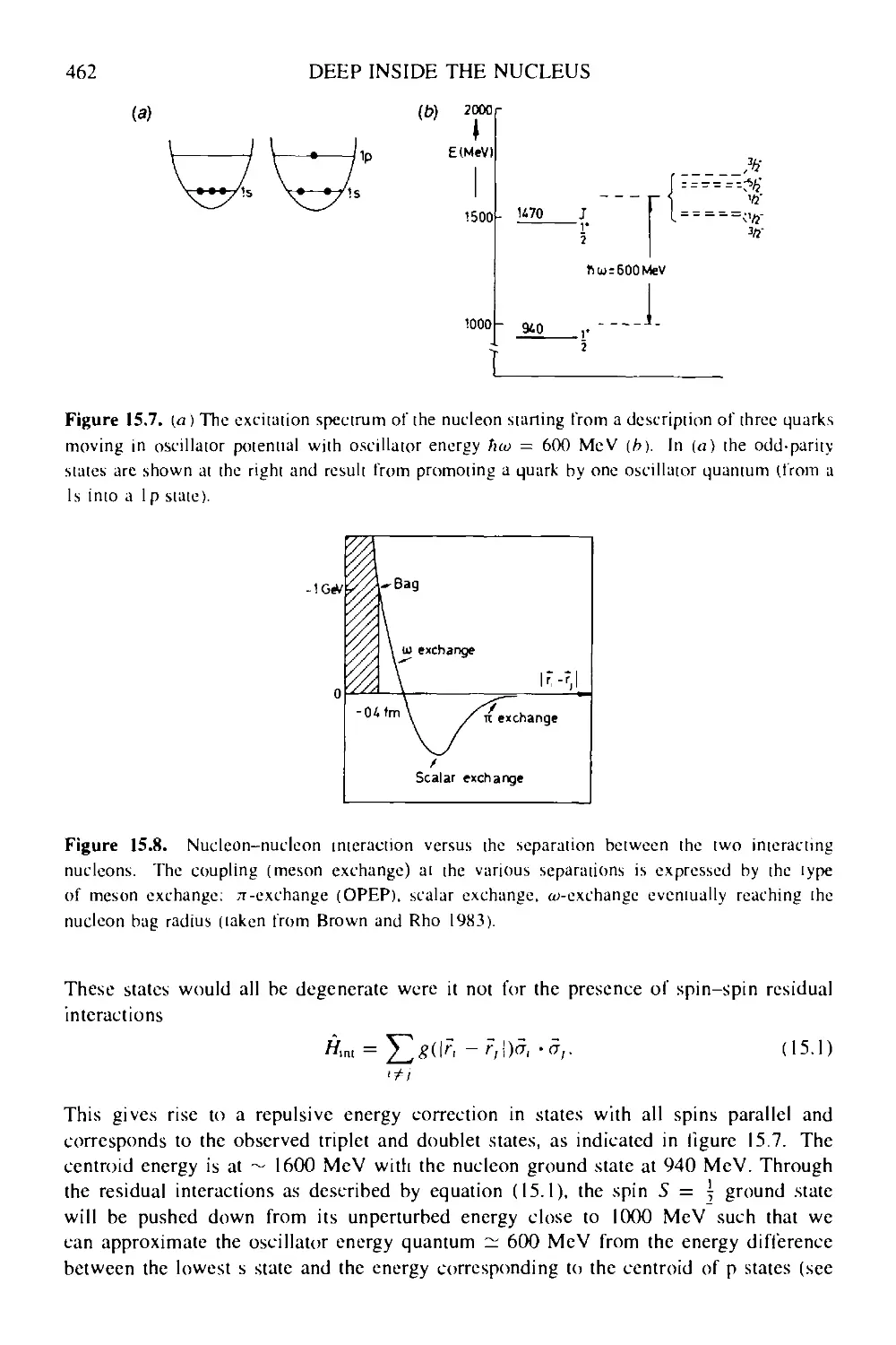
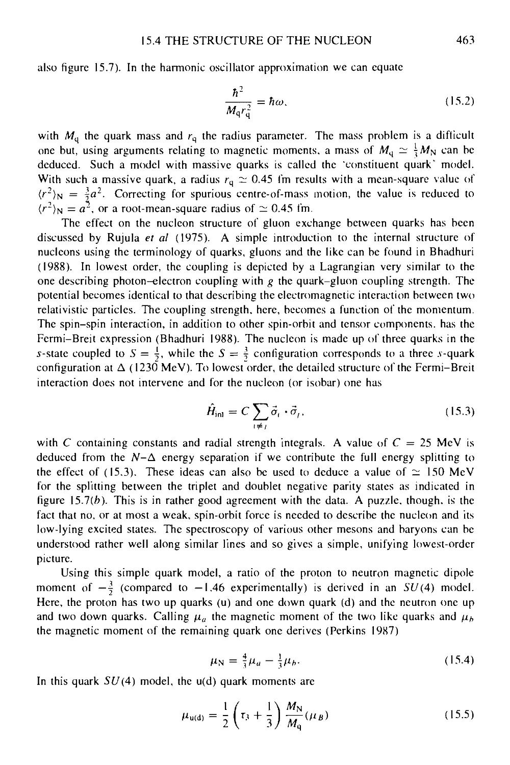
15.4 The structure of the nucleon 460
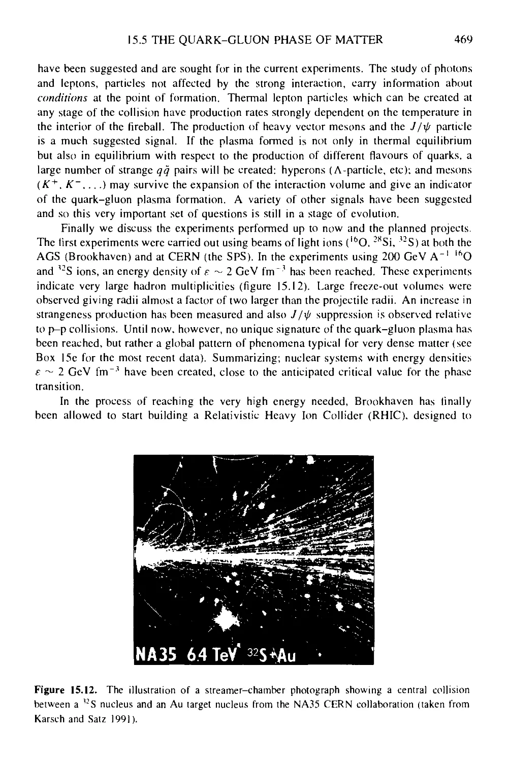
15.5 The quark-gluon phase of matter 465
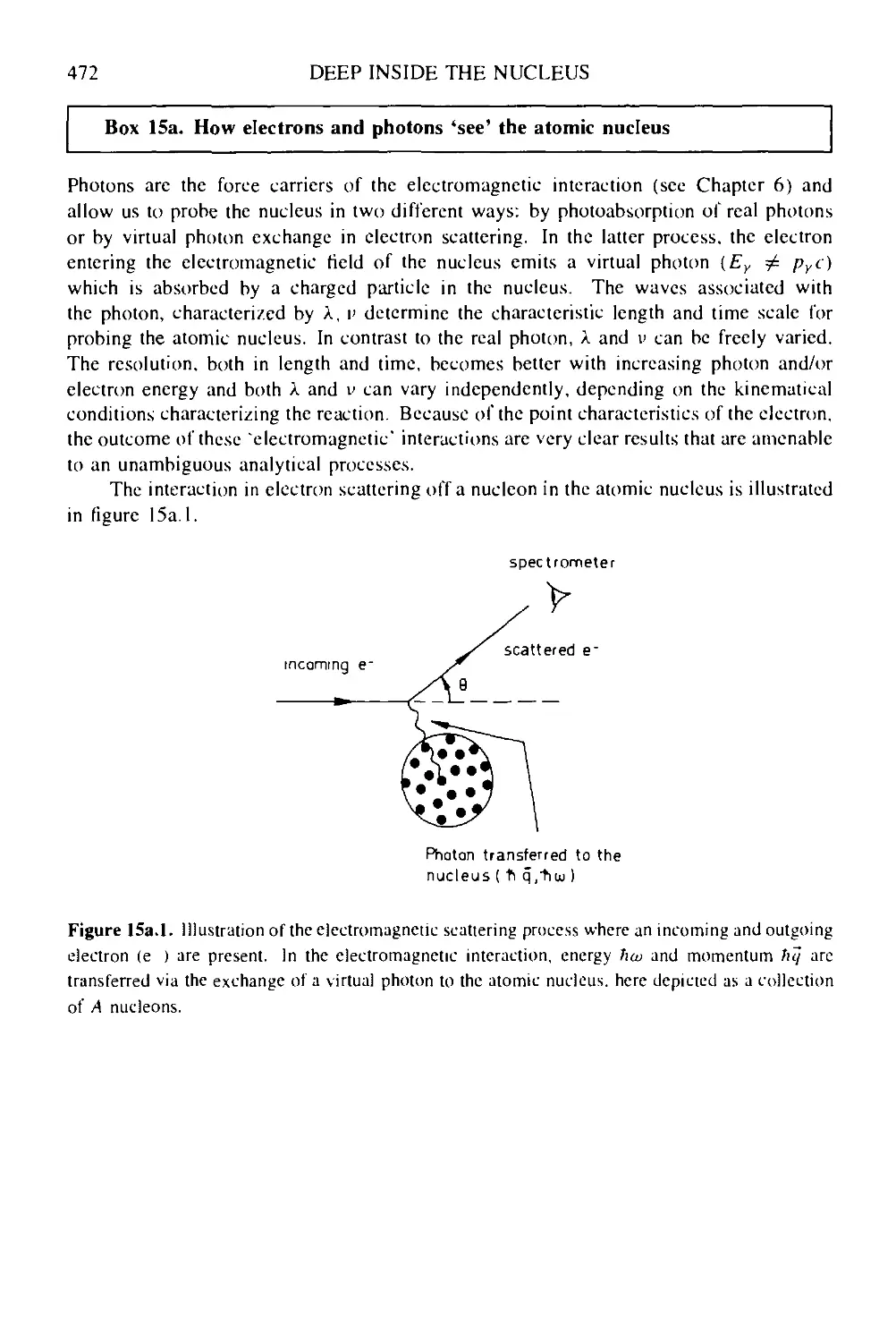
Box 15a How electrons and photons 'see' the atomic nucleus 472
Box 15b Nuclear structure and nuclear forces 473
Box 15c The Л resonance and the Д-N interaction 474
Box 15d What is the nucleon spin made of? 475
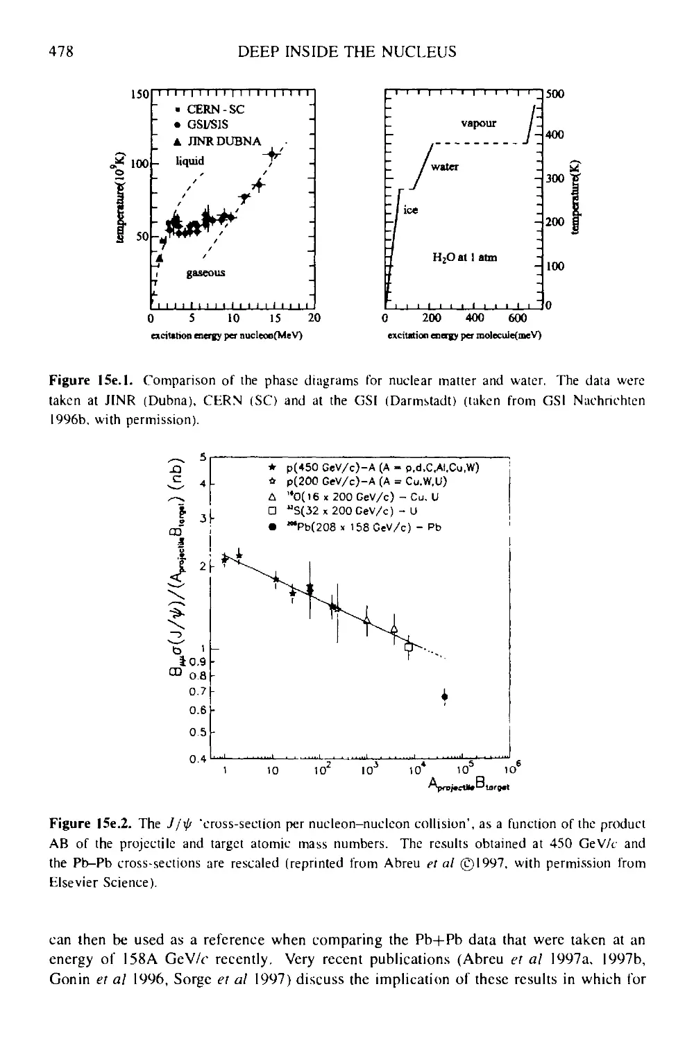
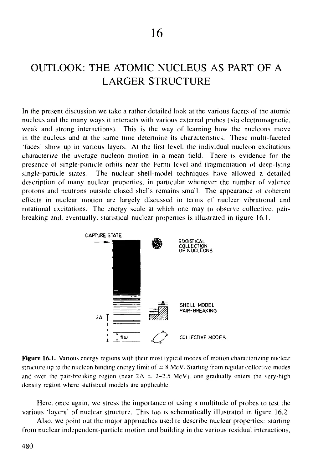
Box 15e The quark-gluon plasma: first hints seen? 477
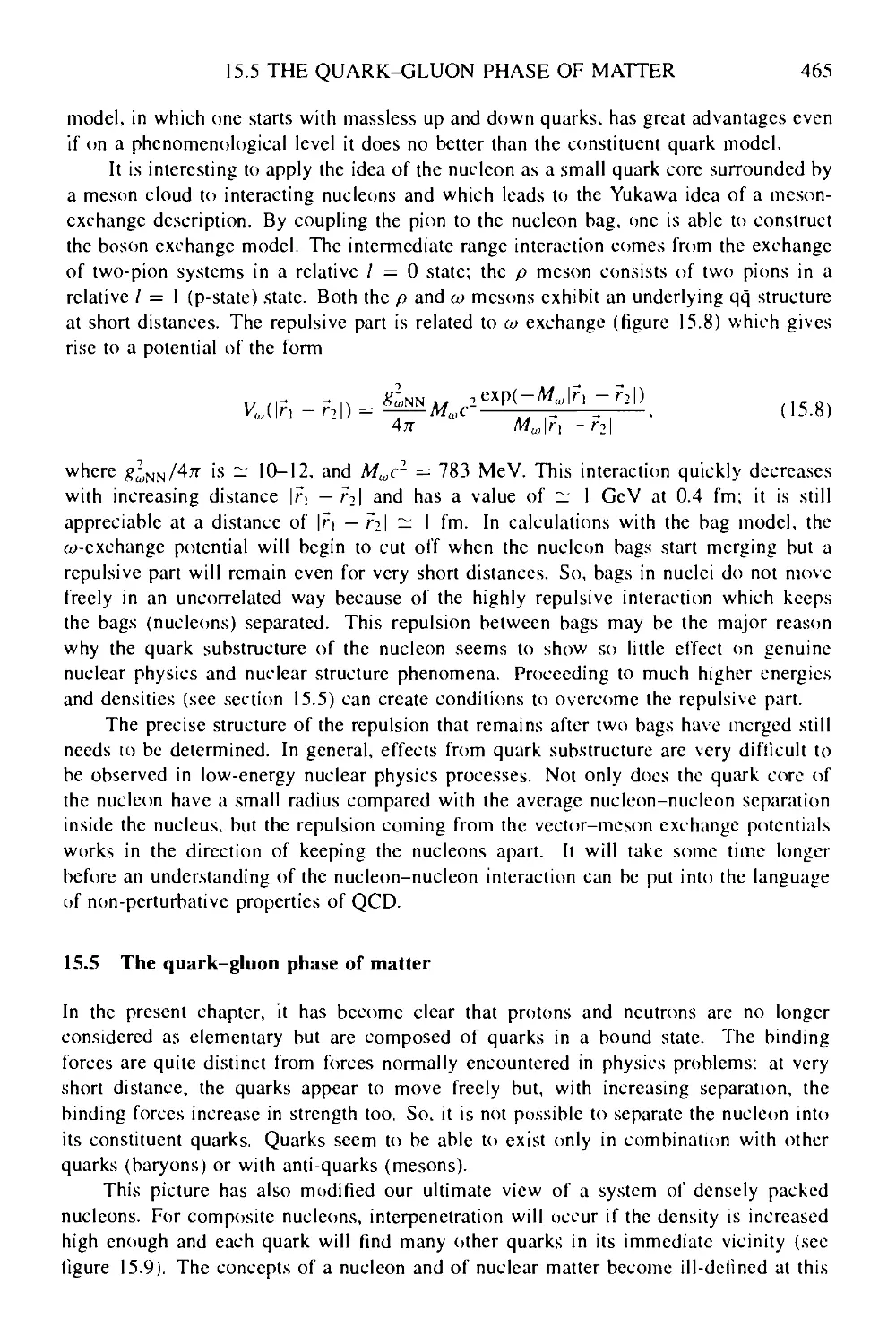
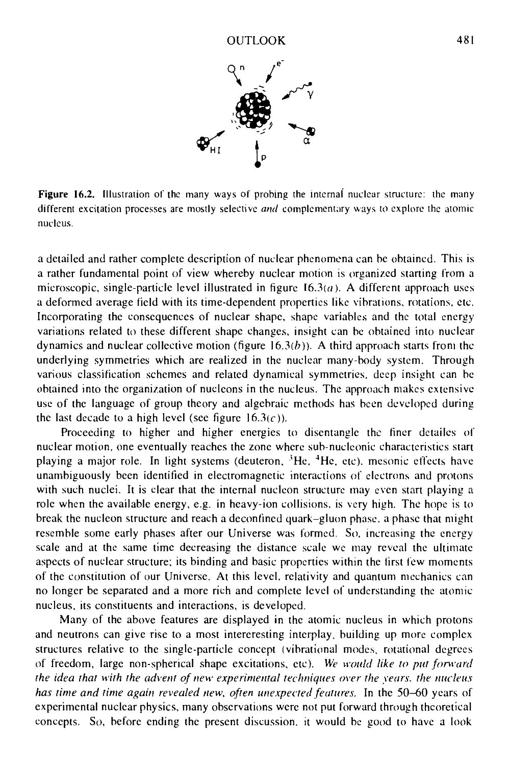
16 Outlook: the atomic nucleus as part of a larger structure 480
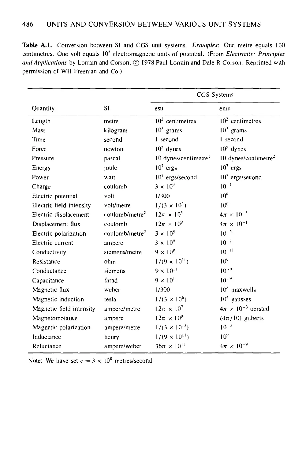
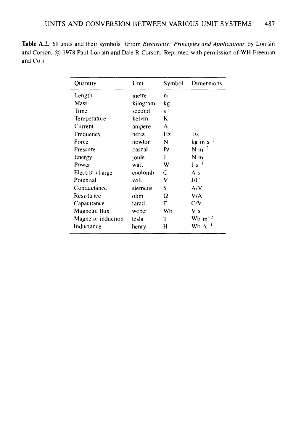
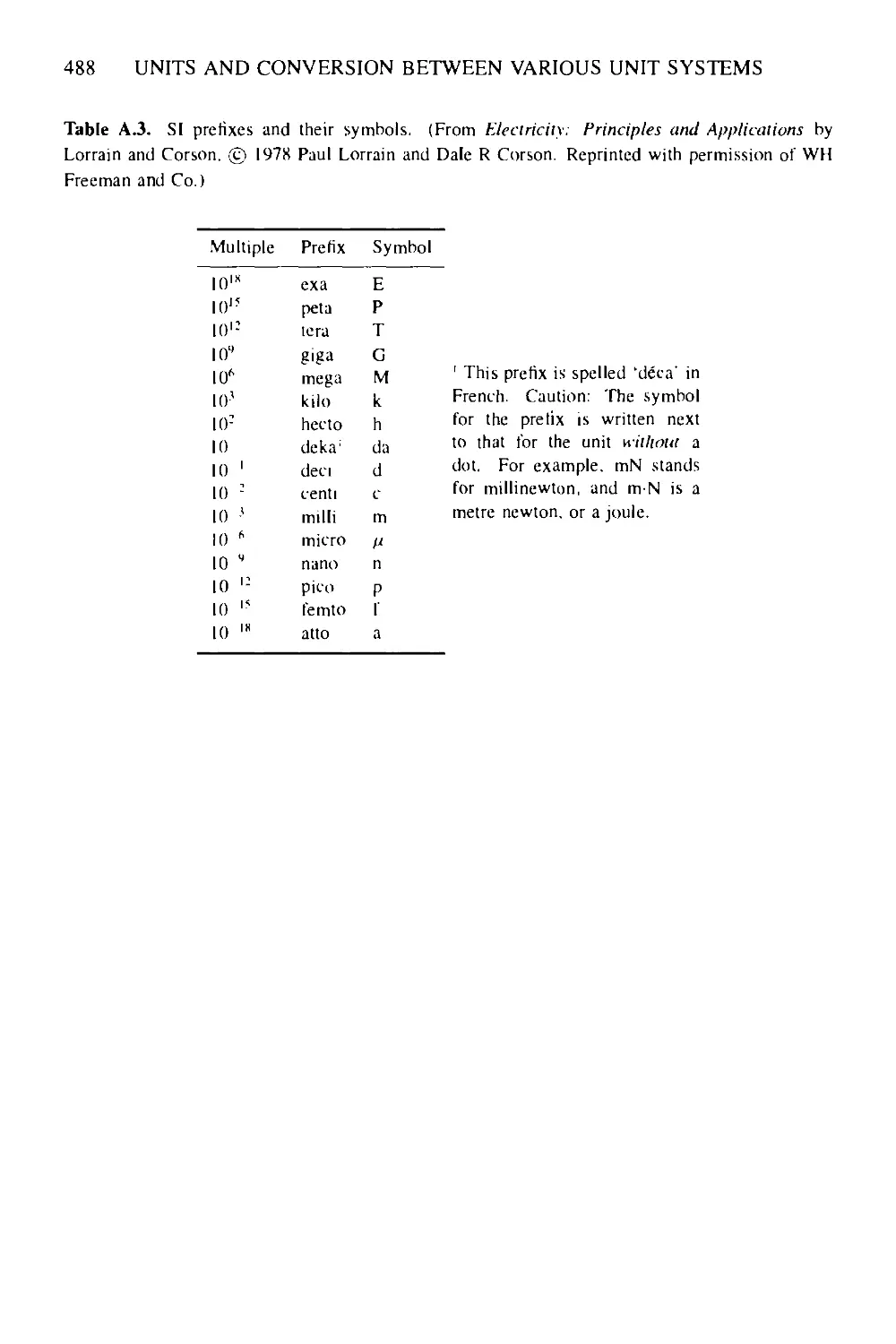
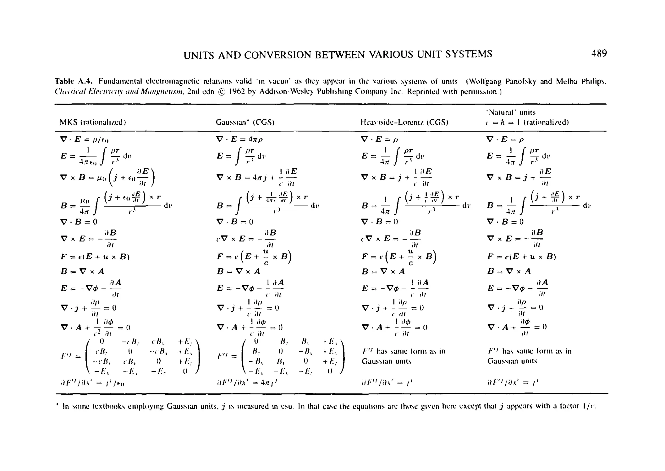
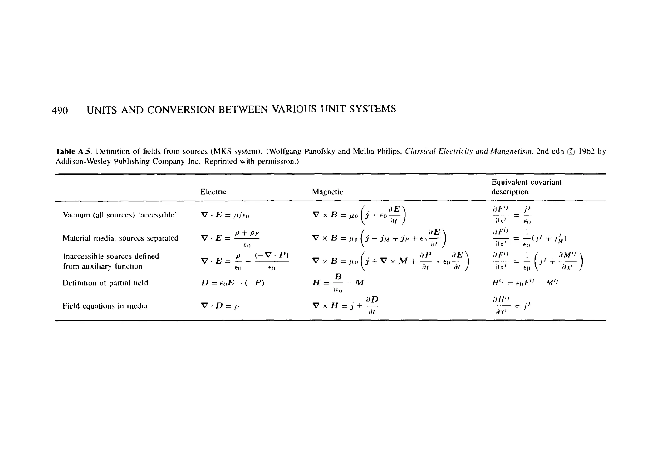
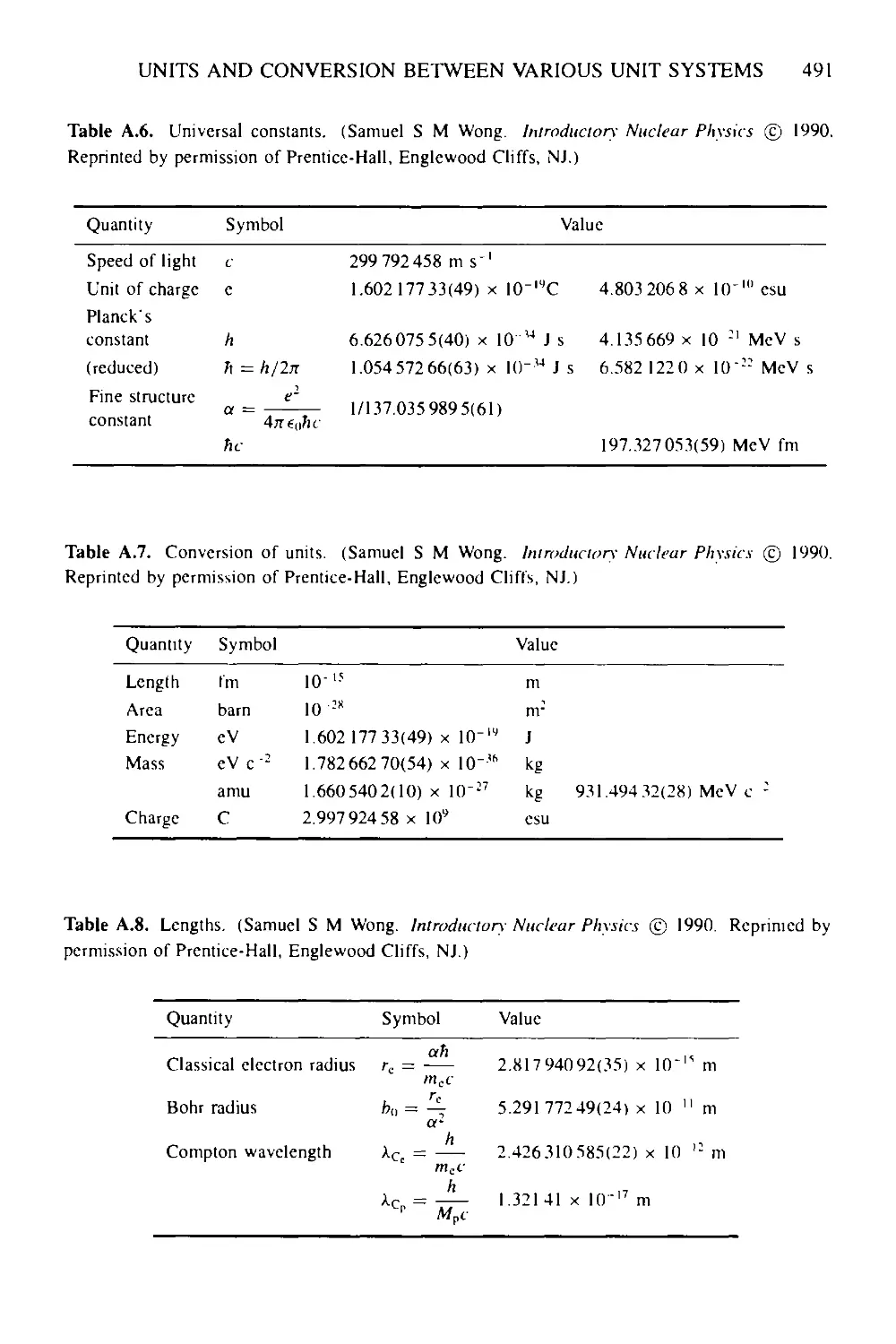
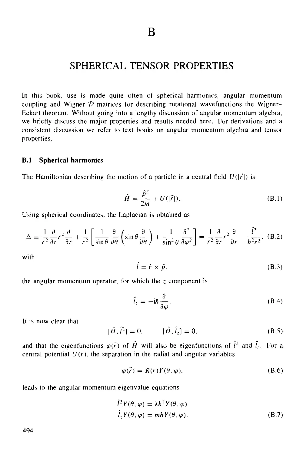
A Units and conversion between various unit systems 485
В Spherical tensor properties 494
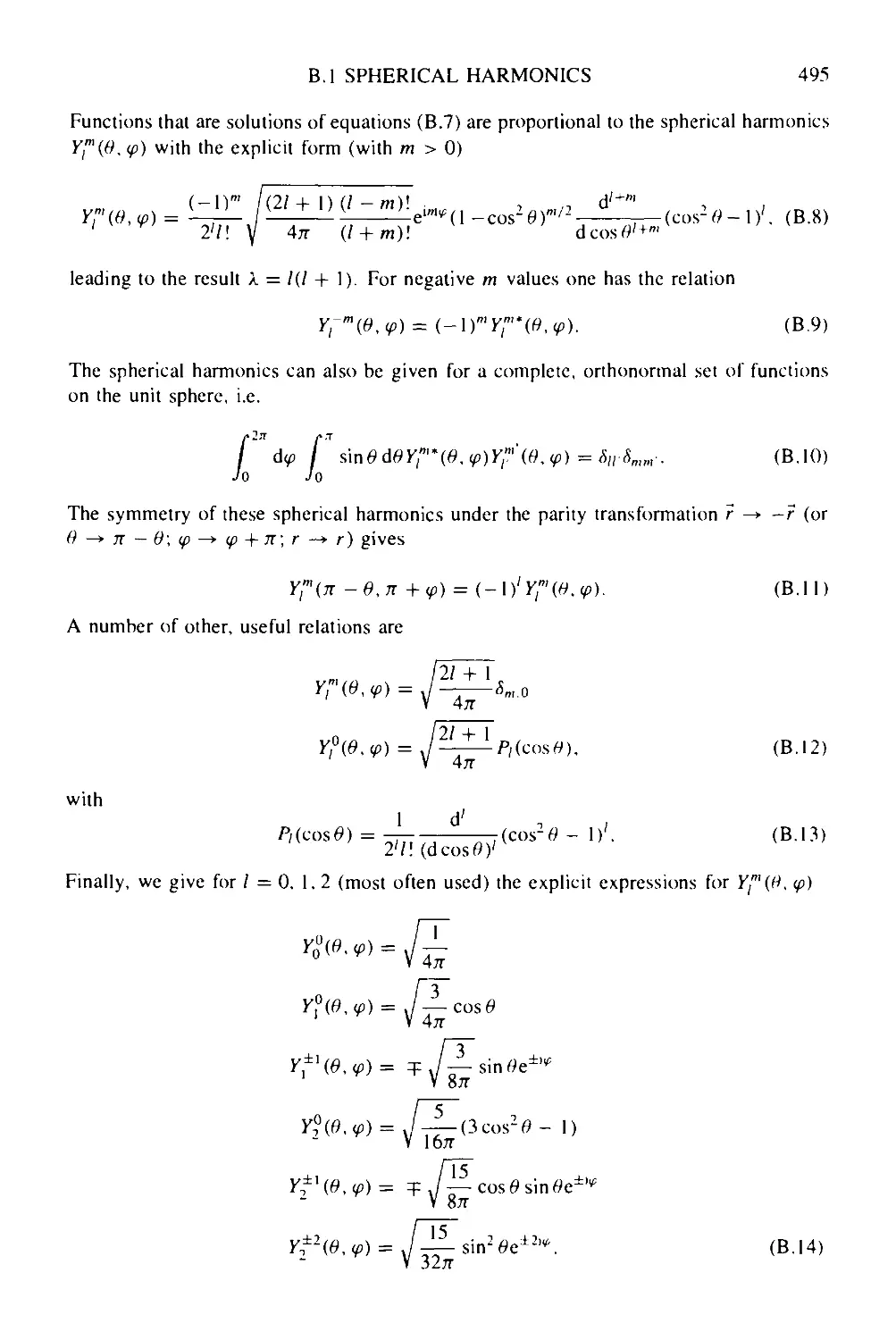
B.I Spherical harmonics 494
B.2 Angular momentum coupling: Clebsch-Gordan coefficients 496
B.3 Racah recoupling coefficients—Wigner 6y-symbols 497
B.4 Spherical tensor and rotation matrix 498
B.5 Wigner-Eckart theorem 500
С Second quantization—an introduction 501
References 505
Index 517
ACKNOWLEDGEMENTS TO THE FIRST EDITION
The present book project grew out of a course taught over the past 10 years at the
University of Gent aiming at introducing various concepts that appear in nuclear physics.
Over the years, the original text has evolved through many contacts with the students
who, by encouraging more and clearer discussions, have modified the form and content in
almost every chapter. 1 have been trying to bridge the gap, by the addition of the various
boxed items, between the main text of the course and present-day work and research in
nuclear physics. One of the aims was also of emphasizing the various existing connections
with other domains of physics, in particular with the higher energy particle physics and
astrophysics fields. An actual problem set has not been incorporated as yet: the exams
set over many years form a good test and those for parts А, В and С can be obtained by
contacting the author directly.
I am most grateful to the series editors R Betts, W Greiner and W D Hamilton for
their time in reading through the manuscript and for their various suggestions to improve
the text. Also, the suggestion to extend the original scope of the nuclear physics course
by the addition of part D and thus to bring the major concepts and basic ideas of nuclear
physics in contact with present-day views on how the nucleus can be described as an
interacting many-nucleon system is partly due to the series editors.
I am much indebted to my colleagues at the Institute of Nuclear Physics and the
Institute for Theoretical Physics at the University of Gent who have contributed, maybe
unintentionally, to the present text in an important way. More specifically, I am indebted
to the past and present nuclear theory group members, in alphabetical order: С De Coster.
J Jolie, L Machenil, J Moreau, S Rombouts, J Ryckebusch. M Vanderhaeghen, V Van
Der Sluys, P Van Isacker, J Van Maldeghem, D Van Neck, H Vincx, M Waroquier and G
Wenes in particular relating to the various subjects of part D. I would also like to thank
the many experimentalist, both in Gent and elsewhere, who through informal discussions
have made many suggestions to relate the various concepts and ideas of nuclear physics
to the many observables that allow a detailed probing of the atomic nucleus.
The author and Institute of Physics Publishing have attempted to trace the copyright
holders of all the ligures, tables and articles reproduced in this publication and would like
to thank the many authors, editors and publishers for their much appreciated cooperation.
We would like to apologize to those few copyright holders whose permission to publish
in the present form could not be obtained.
XIII
PREFACE TO THE SECOND EDITION
The first edition of this textbook was used by a number of colleagues in their introductory
courses on nuclear physics and I received very valuable comments, suggesting topics to
be added and others to be deleted, pointing out errors to be corrected and making various
suggestions for improvement. I therefore decided the time had come to work on a revised
and updated edition.
In this new edition, the basic structure remains the same. Extensive discussions
of the various basic elements, essential to an intensive introductory course on nuclear
physics, are interspersed with the highlights of recent developments in the very lively field
of basic research in subatomic physics. I have taken more care to accentuate the unity
of this field: nuclear physics is not an isolated subject but brings in a large number of
elements from different scientific domains, ranging from particle physics to astrophysics,
from fundamental quantum mechanics to technological developments.
The addition of a set of problems had been promised in the first edition and a number
of colleagues and students have asked for this over the past few years. 1 apologize for the
fact these have still been in Dutch until now. The problems (collected after parts А, В
and C) allow students to test themselves by solving them as an integral part of mastering
the text. Most of the problems have served as examination questions during the time I
have been teaching the course. The problems have not proved to be intractable, as the
students in Gent usually got good scores.
In part A, most of the modifications in this edition are to the material presented
in the boxes. The heaviest element, artificially made in laboratory conditions, is now
Z = 112 and this has been modified accordingly. In part B, in addition to a number
of minor changes, the box on the 17 keV neutrino and its possible existence has been
removed now it has been discovered that this was an experimental artefact. No major
modifications have been made to part C.
Part D is the most extensively revised section. A number of recent developments
in nuclear physics have been incorporated, often in detail, enabling me to retain the title
'Recent Developments'.
In chapter 11, in the discussion on the nuclear shell model, a full section has been
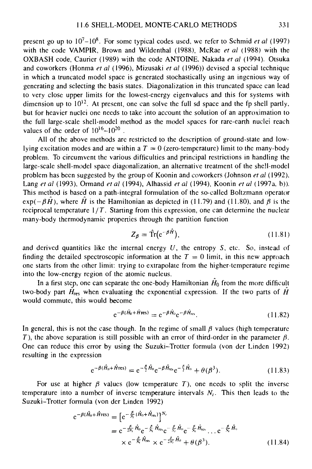
added about the new approach to treating the nuclear many-body problem using shell-
model Monte-Carlo methods.
When discussing nuclear collective motion in chapter 12. recent extensions to the
interacting boson model have been incorporated.
The most recent results on reaching out towards very high-spin states and exploring
nuclear shapes of extreme deformation (supcrdeformation and hyperdeformation) are
given in chapter 13.
A new chapter 14 has been added which concentrates on the intensive efforts to reach
out from the valley of stability towards the edges of stability. With the title 'Nuclear
xv
xvi PREFACE TO THE SECOND EDITION
physics at the extremes of stability: weakly bound quantum systems and exotic nuclei',
we enter a field that has progressed in major leaps during the last few years. Besides the
physics underlying atomic nuclei far from stability, the many technical efforts to reach
into this still unknown region of 'exotica' are addressed. Chapter 14 contains two boxes:
the first on the discovery of the heaviest N — Z doubly-closed shell nucleus, l0OSn, and
the second on the present status of radioactive ion beam facilities (currently active, in
the building stage or planned worldwide).
Chapter 15 (the old chapter 14) has been substantially revised. Two new boxes have
been added: 'What is the nucleon spin made of?' and 'The quark-gluon plasma: first
hints seen?'. The box on the biggest Van de Graaff accelerator at that time has been
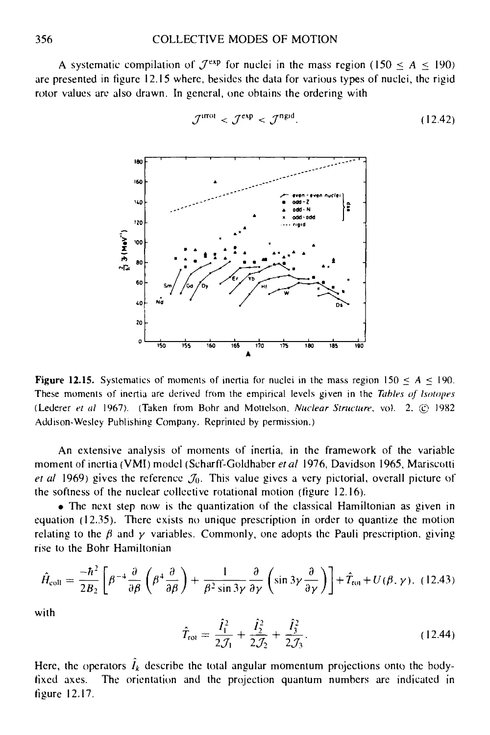
deleted.
The final chapter (now chapter 16) has also been considerably modified, with the
aim of showing how the many facets of nuclear physics can be united in a very neat
framework. I point out the importance of technical developments in particle accelerators,
detector systems and computer facilities as an essential means for discovering new
phenomena and in trying to reveal the basic structures that govern the nuclear many-
body system.
I hope that the second edition is a serious improvement on the first in many respects:
errors have been corrected, the most recent results have been added, the reference list
has been enlarged and updated and the problem sections, needed for teaching, have been
added.
The index to the book has been fully revised and I thank Phil Elliott for his useful
suggestions.
I would like to thank all my students and colleagues who used the book in their
nuclear physics courses: 1 benefited a lot from their valuable remarks and suggestions.
In particular, I would like to thank E Jacobs (who is currently teaching the course at
Gent) and R Bijker (University of Mexico) for their very conscientious checking and for
pointing out a number of errors that I had not noticed. I would particularly like to thank
R F Casten, W Nazarewicz and P Van Duppen for critically reading chapter 14, for many
suggestions and for helping to make the chapter readable, precise and up-to-date.
I am grateful to the CERN-ISOLDE group for its hospitality during the final phase
in the production of this book, to CERN and the FWO (Fund for Scientific Research-
Flanders) for their financial support and to the University of Gent (RUG) for having made
the 'on-leave' to CERN possible.
Finally, I must thank R Verspille for the great care he took in modifying figures
and preparing new figures and artwork, and D dutre-Lootens and L Schepens for their
diligent typing of several versions of the manuscript and for solving a number of TgX
problems.
Kris Heyde
September 1998
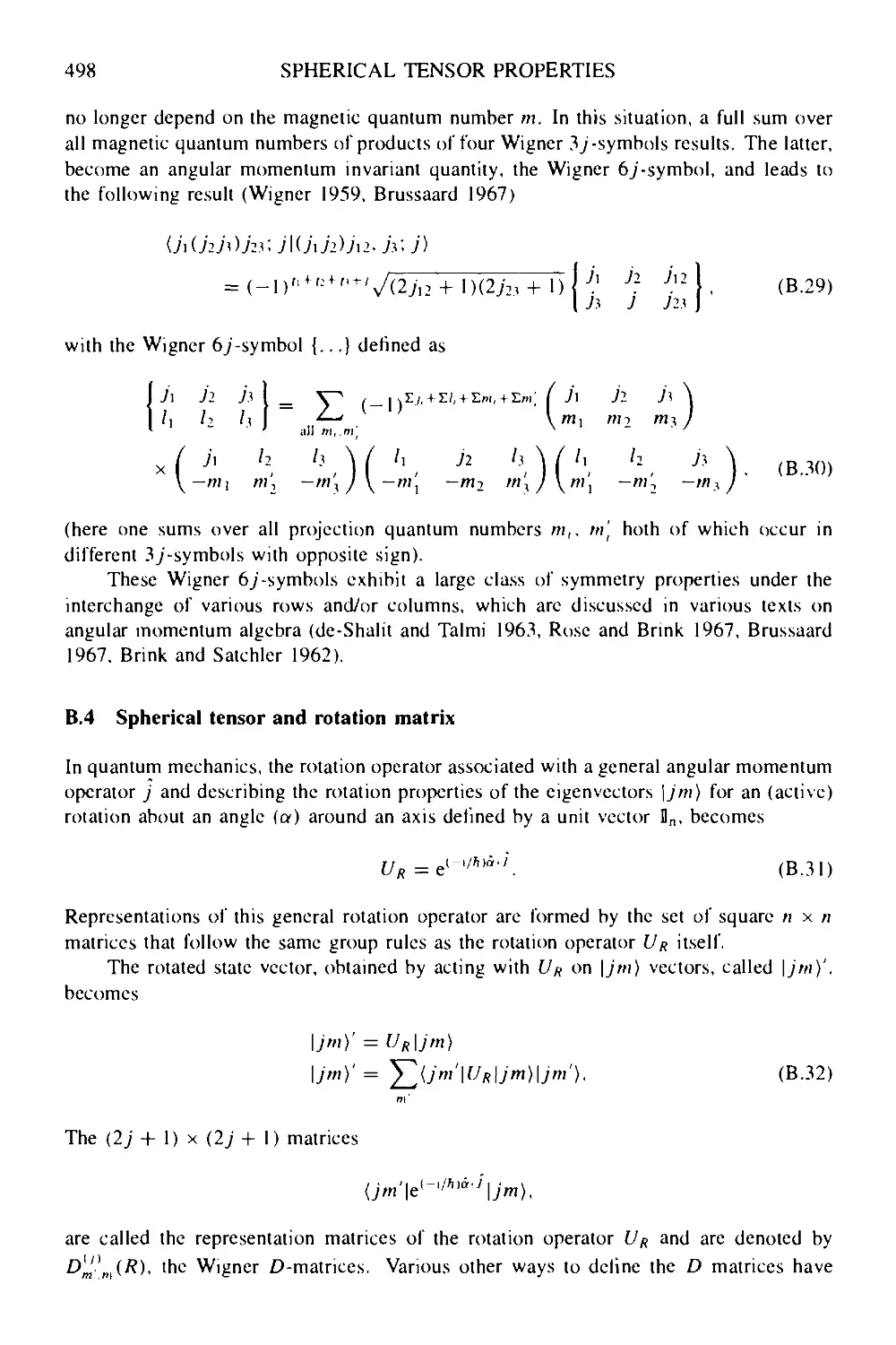
INTRODUCTION
On first coming into contact with the basics of nuclear physics, it is a good idea to obtain
a feeling for the range of energies, densities, temperatures and forces that arc acting on
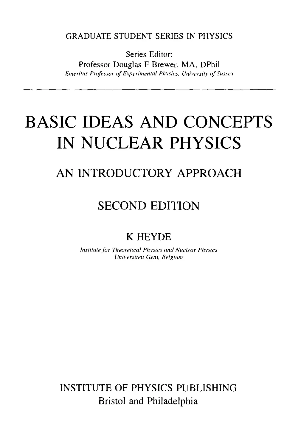
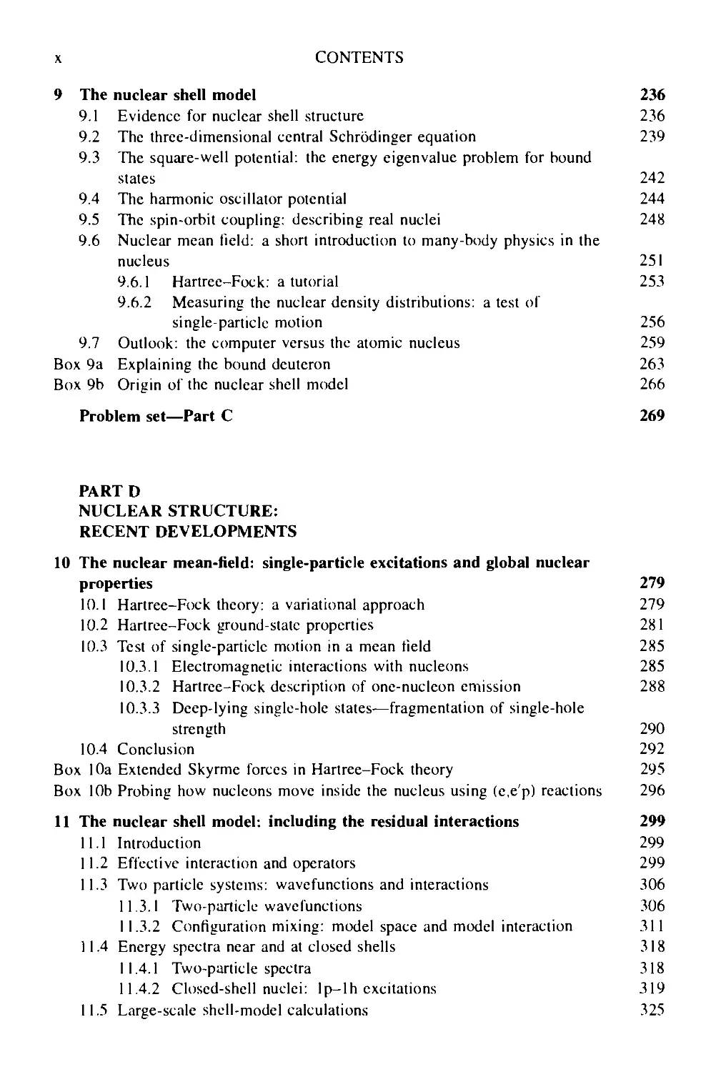
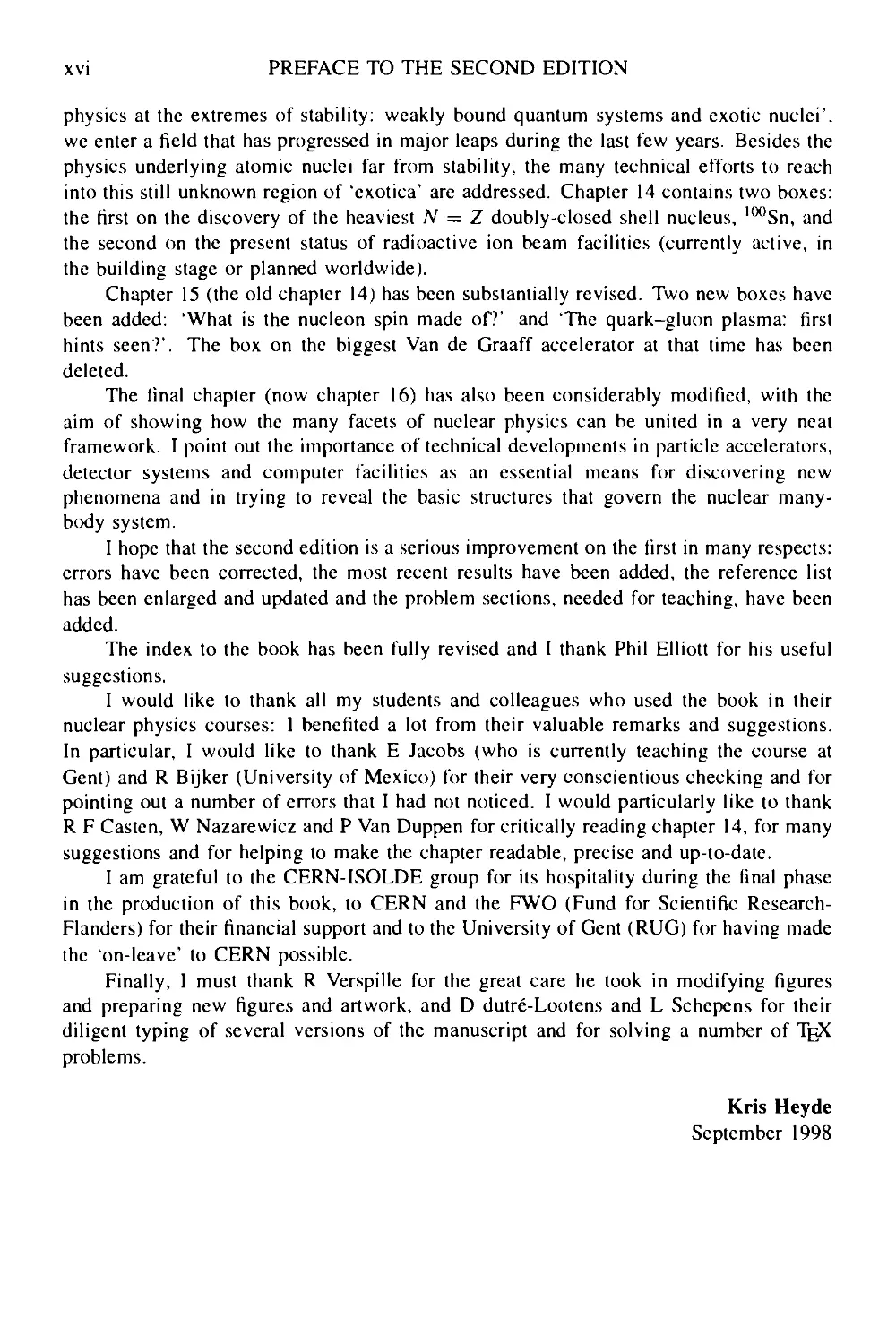
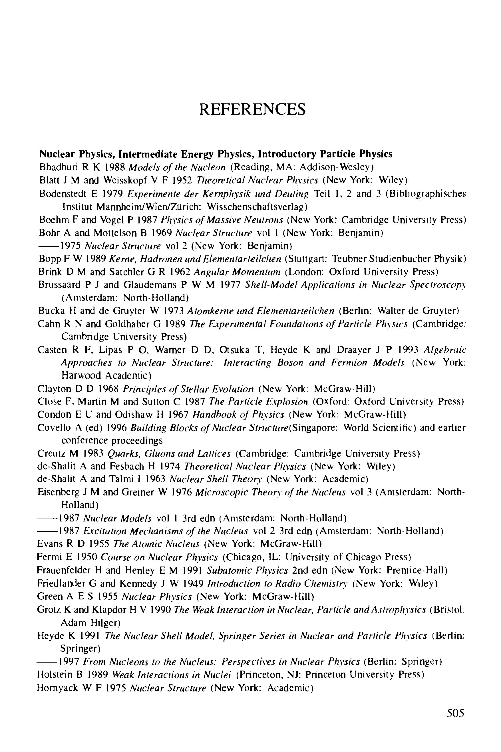
the level of the atomic nucleus. In figure I.I, we introduce an energy scale placing the
nucleus relative to solid state chemistry scales, the atomic energy scale and, higher in
energy, the scale of masses for the elementary particles. In the nucleus, the lower energy
processes can come down to 1 keV, the energy distance between certain excited states in
odd-mass nuclei and X-ray or electron conversion processes, and go up to 100 McV. the
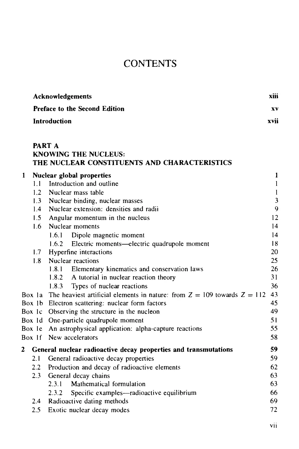
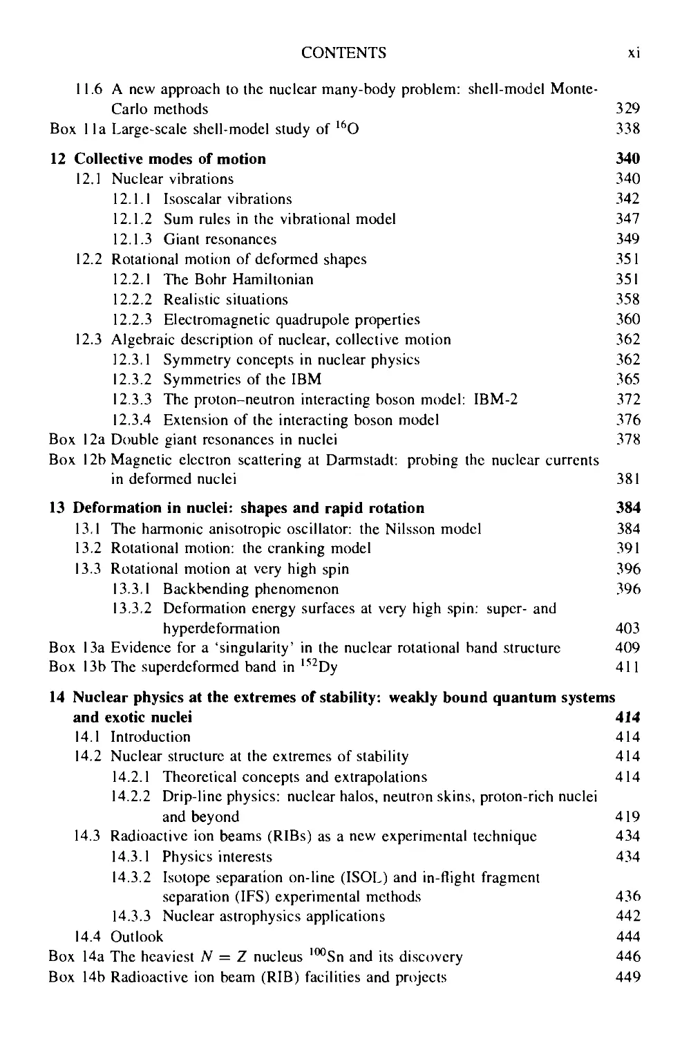
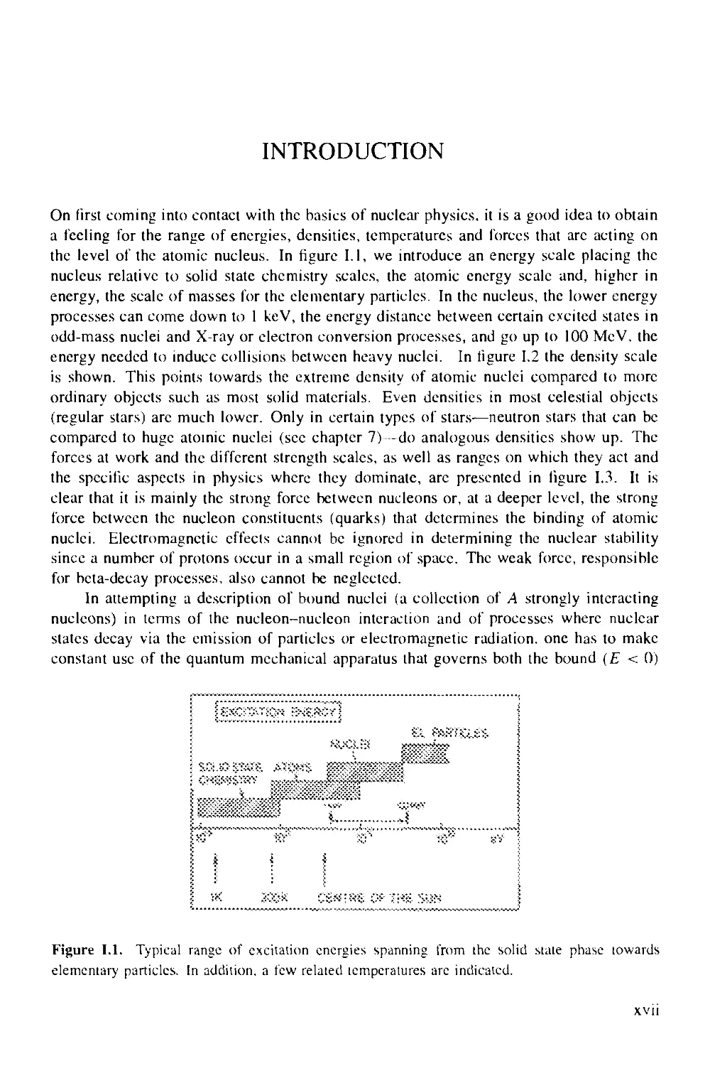
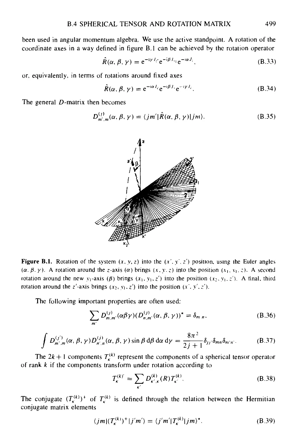
energy needed to induce collisions between heavy nuclei. In figure 1.2 the density scale
is shown. This points towards the extreme density of atomic nuclei compared to more
ordinary objects such as most solid materials. Even densities in most celestial objects
(regular stars) arc much lower. Only in certain types of stars—neutron stars that can be
compared to huge atomic nuclei (sec chapter 7)—do analogous densities show up. The
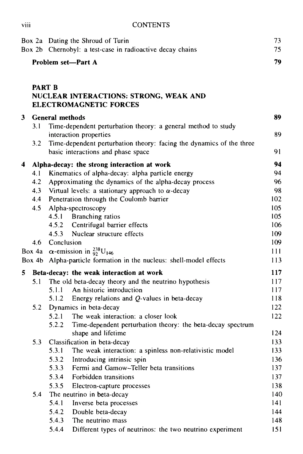
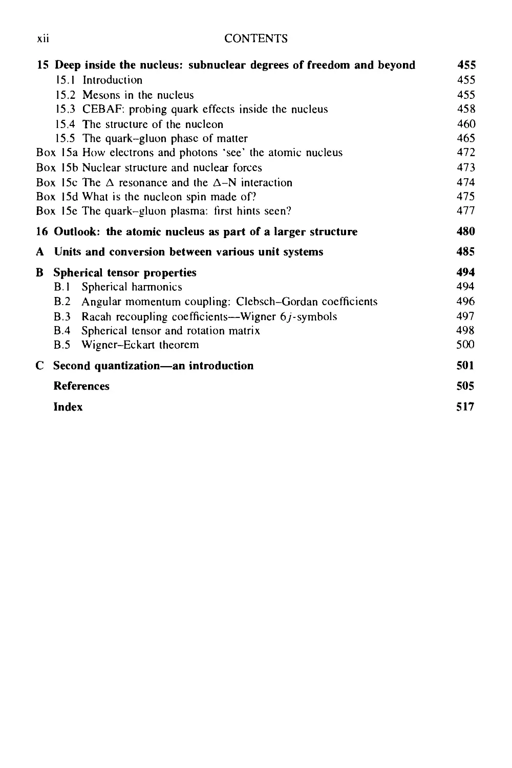
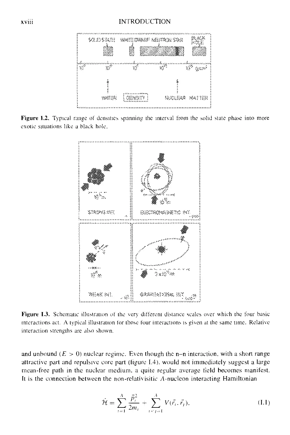
forces at work and the different strength scales, as well as ranges on which they act and
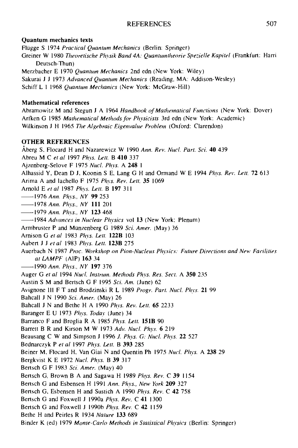
the specific aspects in physics where they dominate, arc presented in figure 1.3. It is
clear that it is mainly the strong force between nudeons or, at a deeper level, the strong
force between the nucleon constituents (quarks) that determines the binding of atomic
nuclei. Electromagnetic effects cannot be ignored in determining the nuclear stability
since a number of protons occur in a small region of space. The weak force, responsible
for beta-decay processes, also cannot be neglected.
In attempting a description of bound nuclei (a collection of A strongly interacting
nuclcons) in terms of the nucleon-nucleon interaction and of processes where nuclear
states decay via the emission of particles or electromagnetic radiation, one has to make
constant use of the quantum mechanical apparatus that governs both the bound (E < 0)
J
;к
Figure I.I. Typical range of excitation energies spanning from (he solid siale phase towards
elementary particles. In addition, a tew related temperatures are indicated.
XVII
XVIII
INTRODUCTION
■:.■.■■ ■•,■:■■
. ^.. ,.-•. .
Figure 1.2. Typical range of densities spanning (he interval from the solid stale phase into more
exotic situations like a black hole.
':!"# W
Ш '&'>?■
Figure 1.3. Schematic illustration oi the very diiTerenl distance scales over which the four basic
interactions act. A typical illustration tor those tour interactions is given at the same time. Relative
interaction strengths are also shown.
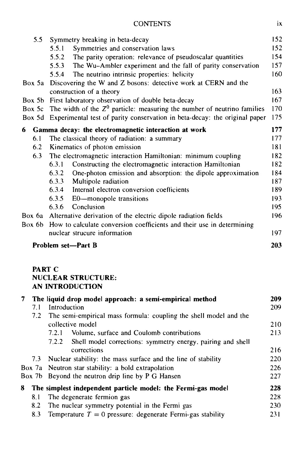
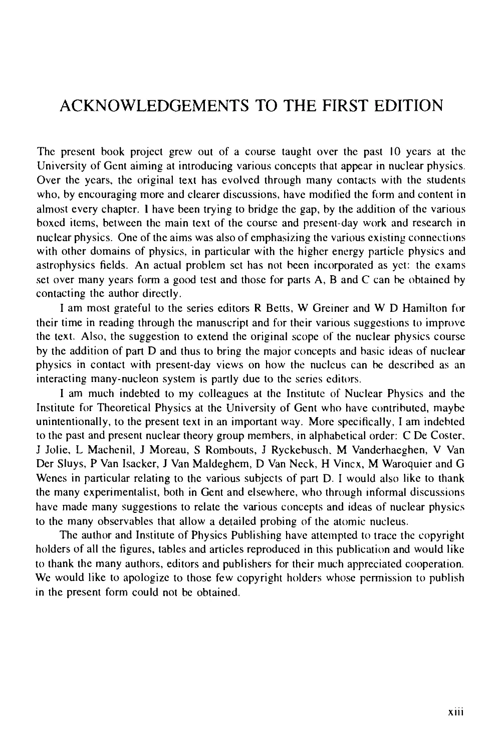
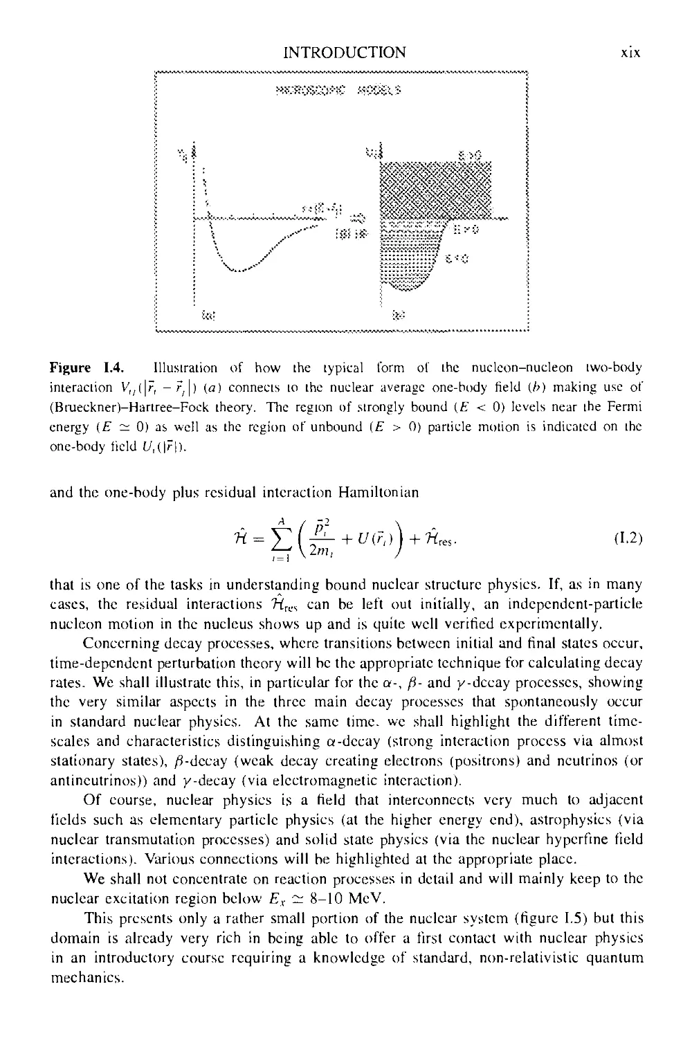
and unbound (£ > 0) nuclear regime. Even though the n-n interaction, with a short range
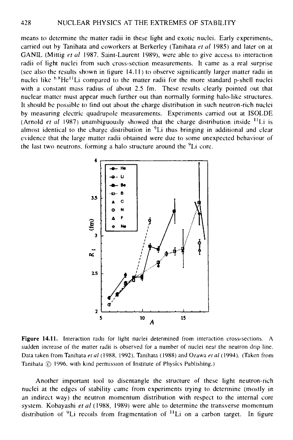
attractive part and repulsive core part (figure 1.4). would not immediately suggest a large
mean-free path in the nuclear medium, a quite regular average field becomes manifest.
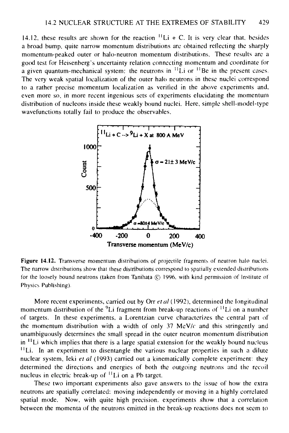
It is the connection between the non-relativisitie A-nuclcon interacting Hamiltonian
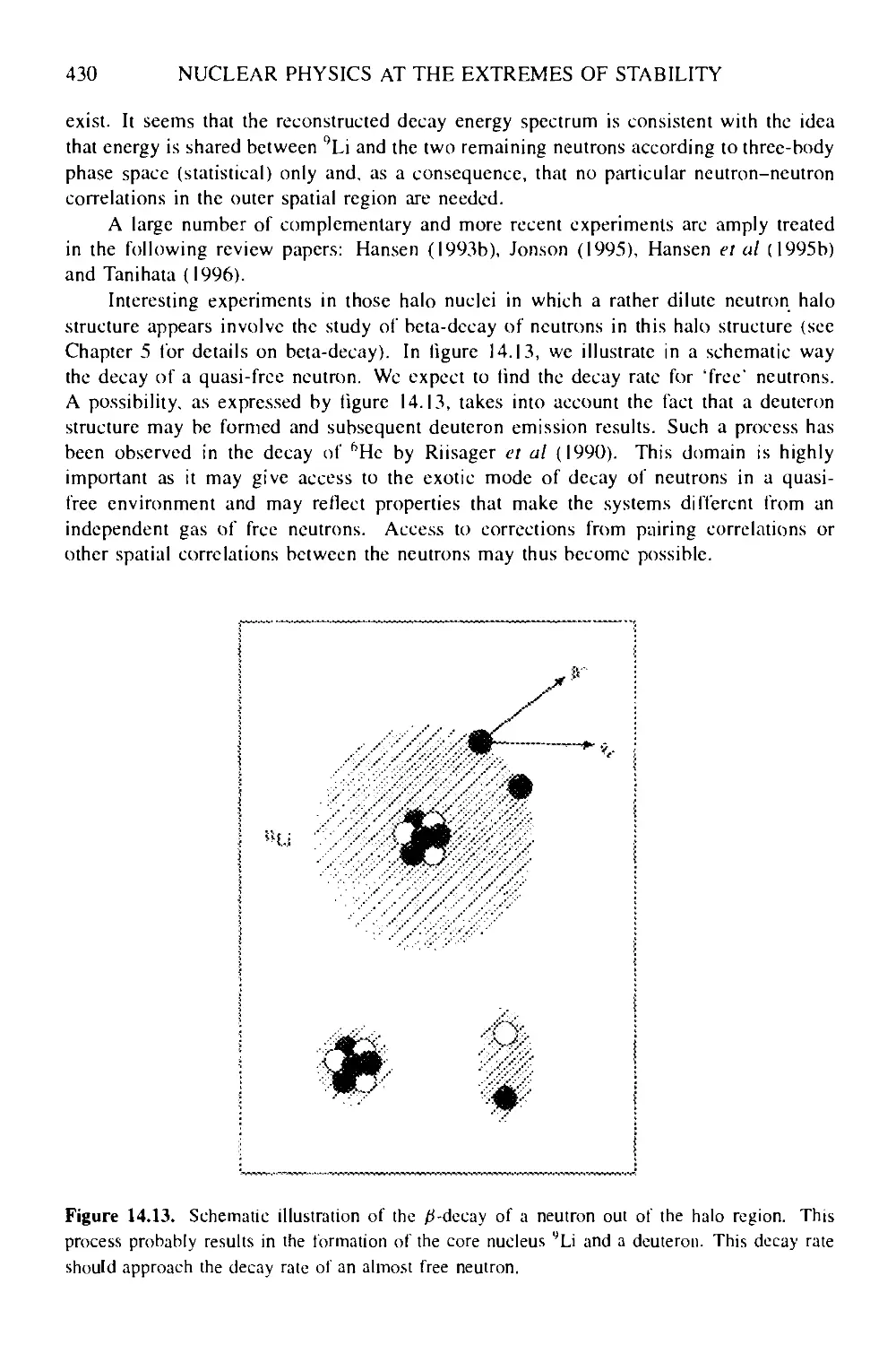
INTRODUCTION
XIX
\
V.,
Штш?;;:'°
'■«'•
Figure I.4. Illustration of how the typical form of the nucleon-nucleon two-body
interaction К;(|г, - r; ) (a) connects to the nuclear average one-body field (b) making use of
(Brueckner)-Hartree-Fock theory. The region of strongly bound (E < 0) levels near the Fermi
energy (E ~ 0) as well as the region of unbound (E > 0) particle motion is indicated on the
one-body field U,(\r\).
and the one-body plus residual interaction Hamiltonian
1=1
A.2)
that is one of the tasks in understanding bound nuclear structure physics. If, as in many
cases, the residual interactions 7irL.s can be left out initially, an independent-particle
nucleon motion in the nucleus shows up and is quite well verified experimentally.
Concerning decay processes, where transitions between initial and final states occur,
time-dependent perturbation theory will be the appropriate technique for calculating decay
rates. We shall illustrate this, in particular for the a-, f>- and y-decay processes, showing
the very similar aspects in the three main decay processes that spontaneously occur
in standard nuclear physics. At the same time, we shall highlight the different time-
scales and characteristics distinguishing a-decay (strong interaction process via almost
stationary states), /?-dccay (weak decay creating electrons (positrons) and neutrinos (or
antincutrinos)) and y-decay (via electromagnetic interaction).
Of course, nuclear physics is a field that interconnects very much to adjacent
fields such as elementary particle physics (at the higher energy end), astrophysics (via
nuclear transmutation processes) and solid state physics (via the nuclear hyperfine field
interactions). Various connections will be highlighted at the appropriate place.
We shall not concentrate on reaction processes in detail and will mainly keep to the
nuclear excitation region below Ex — 8-10 McV.
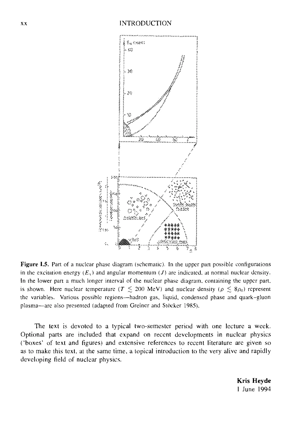
This presents only a rather small portion of the nuclear system (figure 1.5) but this
domain is already very rich in being able to offer a first contact with nuclear physics
in an introductory course requiring a knowledge of standard, non-relativistic quantum
mechanics.
XX
INTRODUCTION
***** ■
Figure 1.5. Part of a nuclear phase diagram (schematic). In the upper part possible configurations
in the excitation energy (£,) and angular momentum (У) arc indicated, at normal nuclear density.
In the lower part a much longer interval of the nuclear phase diagram, containing (he upper part,
is shown. Here nuclear temperature (T < 200 MeV) and nuclear density (p < 8pA) represent
the variables. Various possible regions—hadron gas, liquid, condensed phase and quark-gluon
plasma—are also presented (adapted from Greiner and Stockcr 1985).
The text is devoted to a typical two-semester period with one lecture a week.
Optional parts are included that expand on recent developments in nuclear physics
('boxes' of text and figures) and extensive references to recent literature arc given so
as to make this text, at the same time, a topical introduction to the very alive and rapidly
developing field of nuclear physics.
Kris Heyde
1 June 1994
PART A
KNOWING THE NUCLEUS:
THE NUCLEAR CONSTITUENTS AND
CHARACTERISTICS
NUCLEAR GLOBAL PROPERTIES
1.1 Introduction and outline
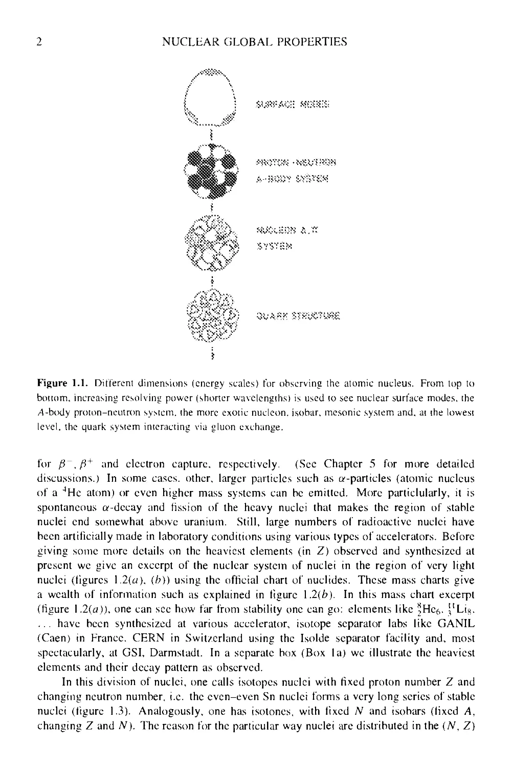
In this chapter, we shall discuss the specific characteristics of the atomic nucleus that
make it a unique laboratory where different forces and particles meet. Depending on the
probe we use to 'view' the nucleus different aspects become observable. Using probes
(c~, p. tt±,...) with an energy such that the quantum mechanical wavelength л = h/p
is of the order of the nucleus, global aspects do show up such that collective and surface
effects can be studied. At shorter wavelengths, the Л-nueleon system containing Z
protons and N neutrons becomes evident. It is this and the above "picture' that will
mainly be of use in the present discussion. Using even shorter wavelengths, the mesonic
degrees and excited nueleon configurations (Л. ...) become obsenable. At the extreme
high-energy side, the internal structure of the nuelcons shows up in the dynamics of an
interacting quark-gluon system (figure 1.1).
Besides more standard characteristics such as mass, binding energy, nuclear
extension and radii, nuclear angular momentum and nuclear moments, we shall try to
illustrate these properties using up-to-date research results that point towards the still quite-
fast evolving subject of nuclear physics. We also discuss some of the more important
ways the nucleus can interact with external fields and particles: hyperfine interactions
and nuclear transmutations in reactions.
1.2 Nuclear mass table
Nuclei, consisting of a bound collection of Z protons and N neutrons (A nuelcons) can
be represented in a diagrammatic way using Z and N as axes in the plane. This plane
is mainly filled along or near to the diagonal N = Z line with equal number of protons
and neutrons. Only a relatively small number of nuclei form stable nuclei, stable against
any emission of particles or other transmutations. For heavy elements, denoted as ')X\.
with A > 100, a neutron excess over the proton number shows up along the line where
most stable nuclei arc situated and which is illustrated in figure 1.3 as the grey and dark
zone. Around these stable nuclei, a large Zone of unstable nuclei shows up: these nuclei
will transform the excess of neutrons in protons or excess of protons in neutrons through
/3-deeay. These processes are written as
NUCLEAR GLOBAL PROPERTIES
ж$ —
\W
j
Figure 1.1. Different dimensions (energy scales) for observing the atomic nucleus. From lop to
bonom, increasing resolving power (shorter wavelengths) is used ю see nuclear surface modes, the
,4-body proton-neutron system, the more exoiic nucleon. isobar, mesonic system and, ai the lowest
level, the quark system interacting via gluon exchange.
for f}~, fi+ and electron capture, respectively. (See Chapter 5 for more detailed
discussions.) In some cases, other, larger particles such as a-particles (atomic nucleus
of a 4Hc atom) or even higher mass systems can be emitted. More particularly, it is
spontaneous a-decay and fission of the heavy nuclei that makes the region of stable
nuclei end somewhat above uranium. Still, large numbers of radioactive nuclei have
been artificially made in laboratory conditions using various types of accelerators. Before
giving sonic more details on the heaviest elements (in Z) observed and synthesized at
present we give an excerpt of the nuclear system of nuclei in the region of very light
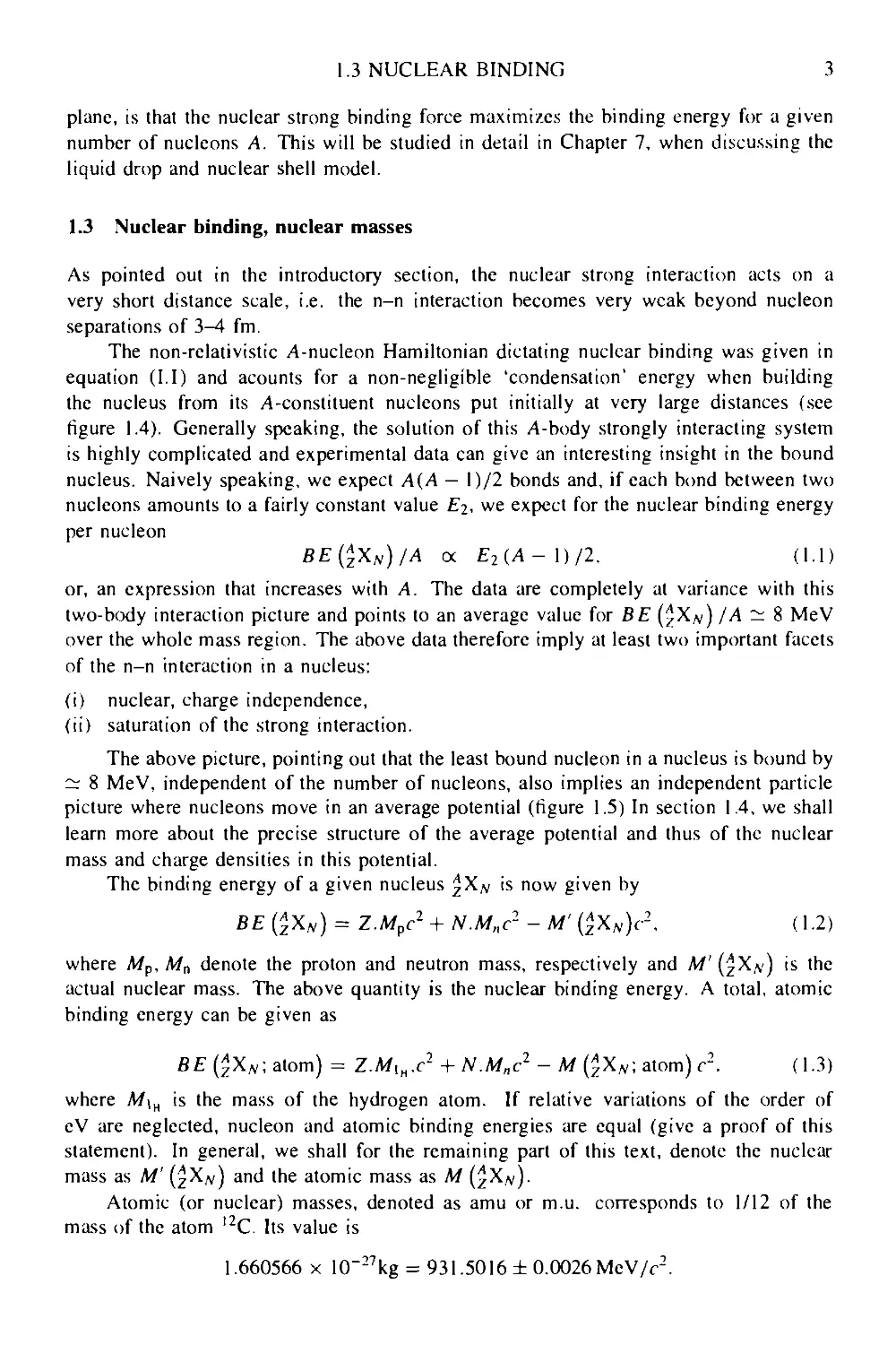
nuclei (figures \.2(a), (/?)) using the official chart of tiuclides. These mass charts give
a wealth of information such as explained in figure 1.2(£>). In this mass chart excerpt
(figure 1.2(a)), one can see how far from stability one can go: elements like ?Hc6. _''Lir.
... have been synthesized at various accelerator, isotope separator labs like GANIL
(Caen) in France. CERN in Switzerland using the Isolde separator facility and, most
spectacularly, at GSI, Darmstadt. In a separate box (Box la) we illustrate the heaviest
elements and their decay pattern as observed.
In this division of nuclei, one calls isotopes nuclei with fixed proton number Z and
changing neutron number, i.e. the even-even Sn nuclei forms a very long series of stable
nuclei (figure 1.3). Analogously, one has isotoncs, with fixed N and isobars (fixed Л,
changing Z and /V). The reason for the particular way nuclei are distributed in the (/V, Z)
1.3 NUCLEAR BINDING 3
plane, is that the nuclear strong binding force maximizes the binding energy for a given
number of nucleons A. This will be studied in detail in Chapter 7, when discussing the
liquid drop and nuclear shell model.
1.3 Nuclear binding, nuclear masses
As pointed out in the introductory section, the nuclear strong interaction acts on a
very short distance scale, i.e. the n-n interaction becomes very weak beyond nucleon
separations of 3-4 fm.
The non-relativistic Л-nucleon Hamiltonian dictating nuclear binding was given in
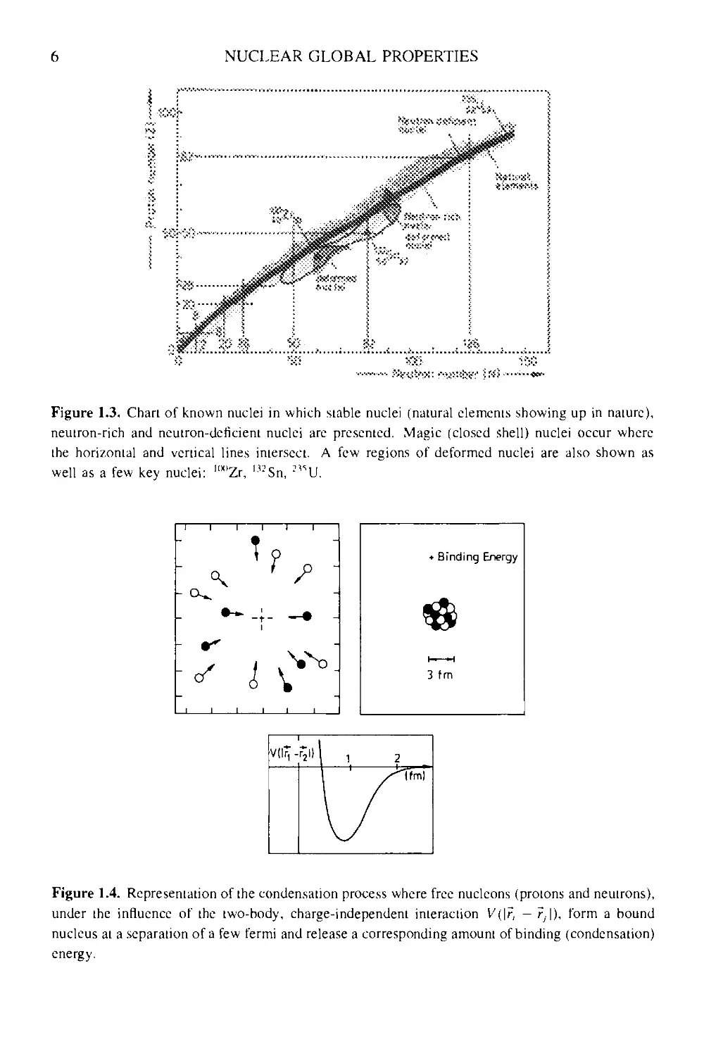
equation (I.I) and acounts for a non-negligible 'condensation' energy when building
the nucleus from its Л-constituent nucleons put initially at very large distances (see
figure 1.4). Generally speaking, the solution of this Л-body strongly interacting system
is highly complicated and experimental data can give an interesting insight in the bound
nucleus. Naively speaking, we expect A(A — l)/2 bonds and, if each bond between two
nucleons amounts to a fairly constant value Ei, we expect for the nuclear binding energy
per nucleon
BE{*XN)/A oc E2(A- l)/2, A.1)
or, an expression that increases with A. The data are completely at variance with this
two-body interaction picture and points to an average value for BE (£Xjv) /A ~ 8 MeV
over the whole mass region. The above data therefore imply at least two important facets
of the n-n interaction in a nucleus:
(i) nuclear, charge independence,
(ii) saturation of the strong interaction.
The above picture, pointing out that the least bound nucleon in a nucleus is bound by
~ 8 MeV, independent of the number of nucleons, also implies an independent particle
picture where nucleons move in an average potential (figure 1.5) In section 1.4, we shall
learn more about the precise structure of the average potential and thus of the nuclear
mass and charge densities in this potential.
The binding energy of a given nucleus ^Xjv is now given by
BE(AZXN) = Z.MpC1 + N.M,,c2 - M' (zXjv)r2, A.2)
where Mp, Mn denote the proton and neutron mass, respectively and M' (^Хл) is the
actual nuclear mass. The above quantity is the nuclear binding energy. A total, atomic
binding energy can be given as
BE{*XN;a\om) = Z.M1h.c2 + N.Mnc2 - M (£Х„; atom) c2. A.3)
where M\H is the mass of the hydrogen atom. If relative variations of the order of
eV are neglected, nucleon and atomic binding energies are equal (give a proof of this
statement). In general, we shall for the remaining part of this text, denote the nuclear
mass as M' (^X/v) and the atomic mass as M (^Xjv).
Atomic (or nuclear) masses, denoted as amu or m.u. corresponds to 1/12 of the
mass of the atom 12C. Its value is
1.660566 x 10~27kg = 931.5016 ± 0.0026 MeV/r2.
NUCLEAR GLOBAL PROPERTIES
III
ill
ill
ш
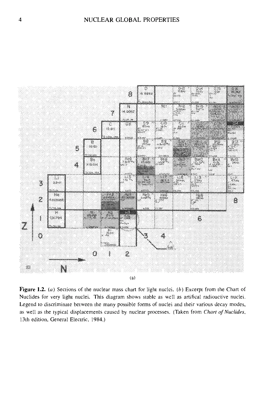
Figure 1.2. (a) Seciions of (he nuclear mass chart for light nuclei, (b) Excerpt from (he Chart of
Nuclides for very tight nuclei. This diagram shows stable as well as artifical radioactive nuclei.
Legend to discriminaie beiween (he many possible forms of nuclei and (heir various decay modes,
as well as (he Lypical displacements caused by nuclear processes. (Taken from Chart of Nuclides,
13ih edition, General Eleciric, 1984.)
1.3 NUCLEAR BINDING
Displacements Caused by Nuclear
Bombardment Reactions
<■■•:•;:*
Ш&ш v.
а , in
P , n
P , P"
У i n
3Нв. п
P . У
У ■ P
n , np
J
n, pd
-,n
I, p
4 ■ P
t , 3He
1 , P
Relative Locations of the
Products of Various
Nuclear Processes
. «,
P~ Out
» ...
Origmo
Nucleus
p < pro
'h, ,n
„ „
^* out
or
. ,„
. ,„
t = tutor ( H>
а • aipha particle
P~* negative electn
P+* positron
• • electron captui
(b)
Figure 1.2. Continued
NUCLEAR GLOBAL PROPERTIES
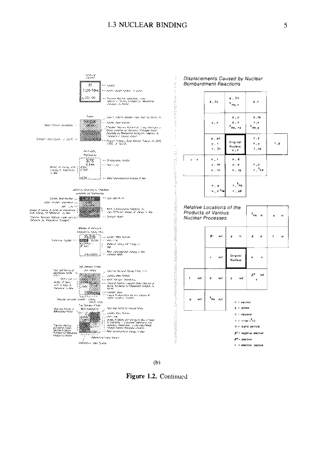
Figure 1.3. Chart of known nuclei in which stable nuclei (natural elements showing up in nature),
neutron-rich and neutron-deficient nuclei are presented. Magic (closed shell) nuclei occur where
the horizontal and vertical lines intersect. A few regions of deformed nuclei are also shown as
well as a few key nuclei: "x)Zr, '"Sn, 2"U.
Figure 1.4. Representation of the condensation process where free nucleons (proions and neutrons),
under the influence of the two-body, charge-independent interaction V(\r, — ?y|), form a bound
nucleus at a separaiion of a few fermi and release a corresponding amouni of binding (condensation)
energy.
1.3 NUCLEAR BINDING
1
t •-
«Be
• ti
1
1
»CI
1
1
.1...
F '
I
1
1
"j '°Cd
As .«*
1
1
1
к
I
1
l»0y
1
i
i
i
i
-
...
i i i i
i
100
Mass number Л
200
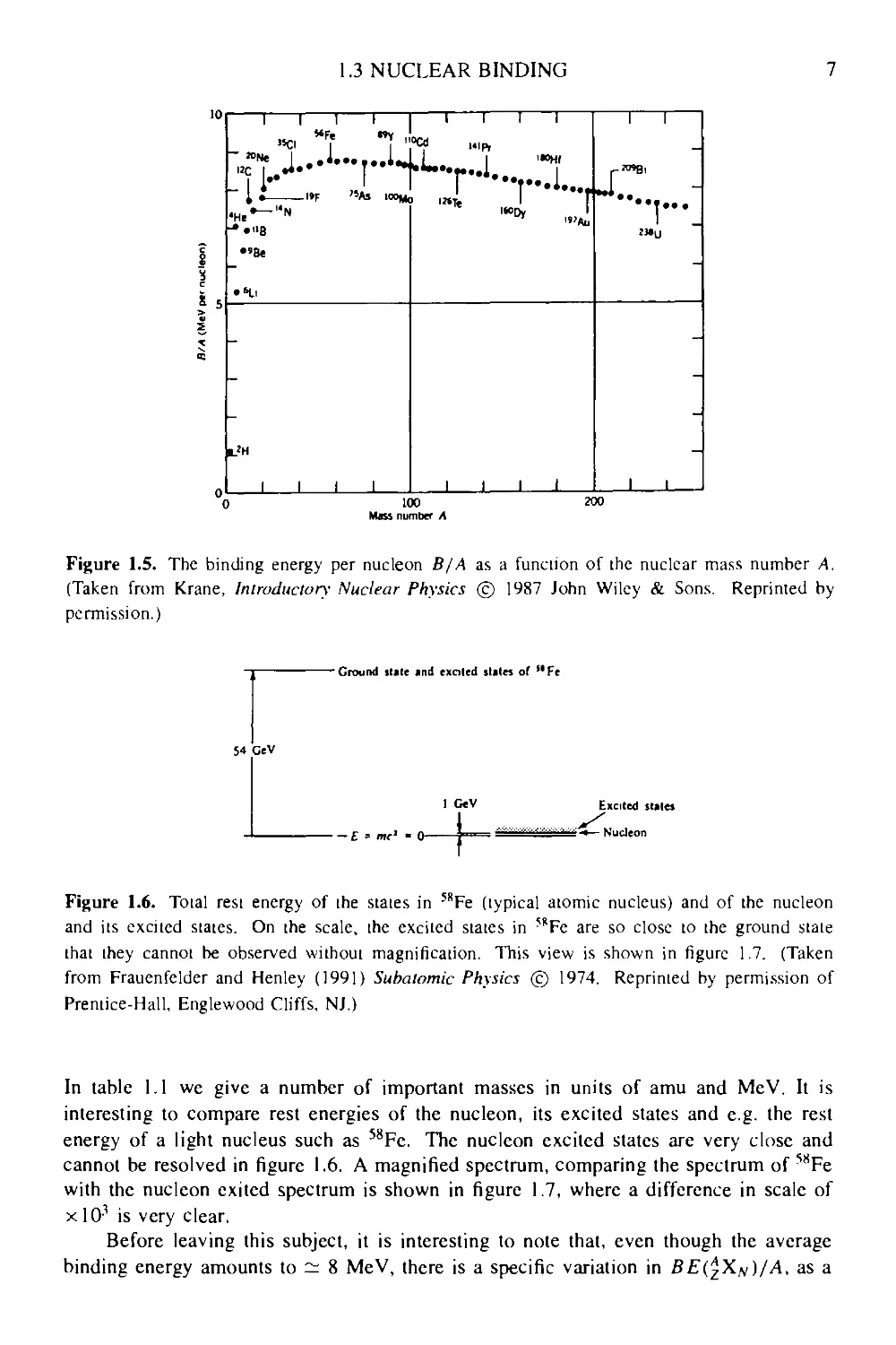
Figure 1.5. The binding energy per nucleon B/A as a function of the nuclear mass number A.
(Taken from Krane, Introductory Nuclear Physics © 1987 John Wiley & Sons. Reprinted by
permission.)
"Ground stjte ind excited states of "Fe
CeV
- - E = me1
Excited stales
— Nudeon
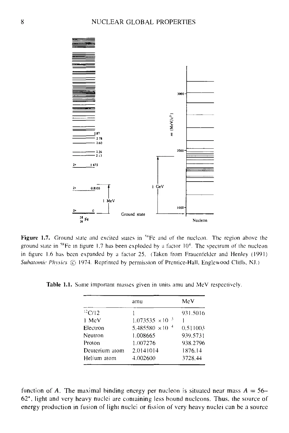
Figure 1.6. Total rest energy of the states in 58Fe (typical aiomic nucleus) and of the nucleon
and its excited states. On the scale, the excited states in 5RFe are so close to the ground state
that they cannot be observed without magnification. This view is shown in figure 1.7. (Taken
from Frauenfelder and Henley A991) Subatomic Physics © 1974. Reprinted by permission of
Prentice-Hall, Englewood Cliffs, NJ.)
In table 1.1 we give a number of important masses in units of amu and MeV. It is
interesting to compare rest energies of the nucleon, its excited states and e.g. the rest
energy of a light nucleus such as 58Fe. The nucleon excited states are very close and
cannot be resolved in figure 1.6. A magnified spectrum, comparing the spectrum of 58Fe
with the nucleon exited spectrum is shown in figure 1.7, where a difference in scale of
x 10-1 is very clear.
Before leaving this subject, it is interesting to note that, even though the average
binding energy amounts to cr 8 MeV, there is a specific variation in BE(^XN)/A, as a
NUCLEAR GLOBAL PROPERTIES
2 78
2.60
-2.26
- 2 13
I MeV
Ground state
I GeV
Nucleon
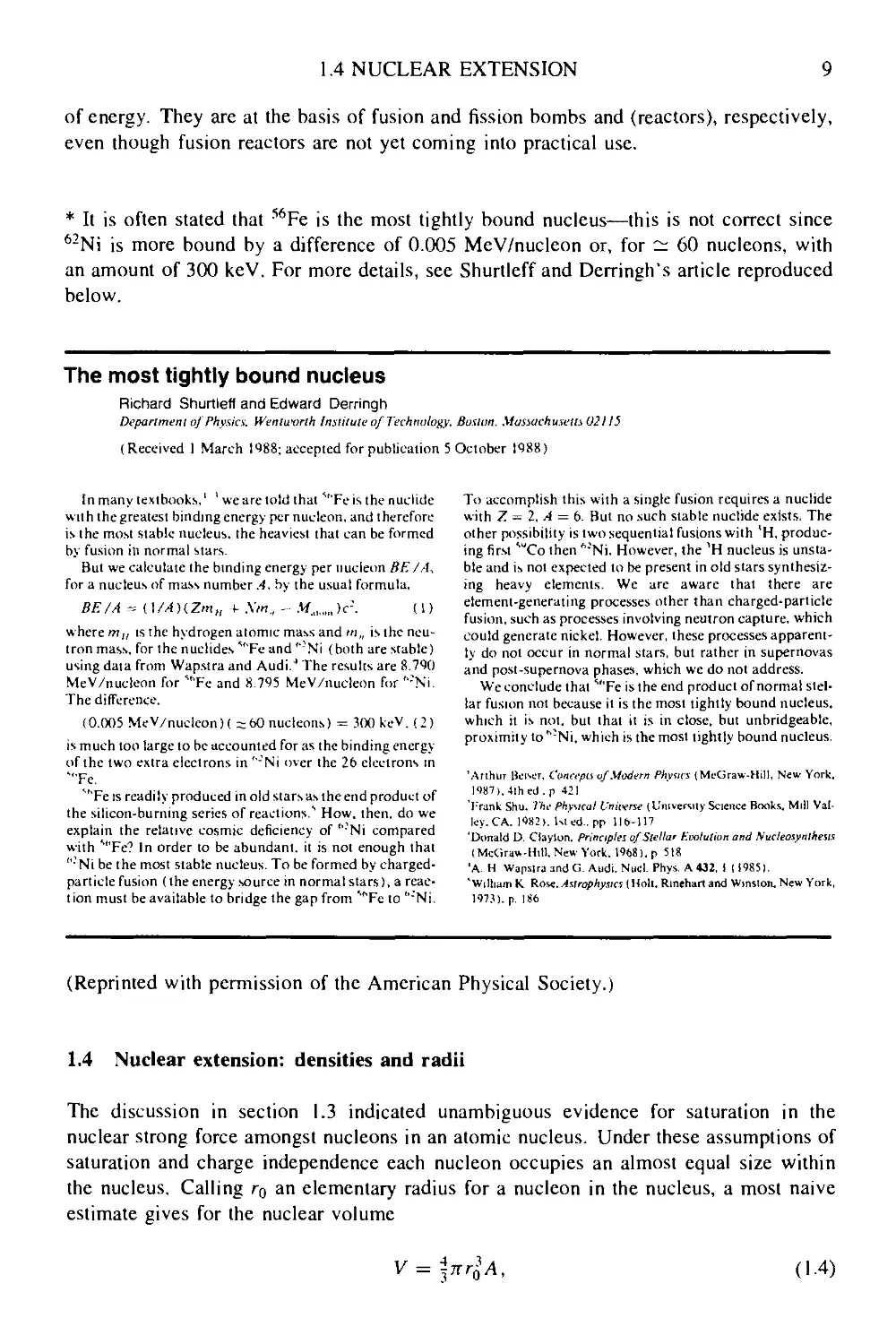
Figure 1.7. Ground stale and excited Mates in *KFc and of the nucleon. The region above the
ground suite in ™Fc in figure 1.7 has been exploded by a factor I04. The spectrum of the nucleon
in figure 1.6 has been expanded by a factor 25. (Taken from Frauenfcldcr and Henley A991)
Subatomic Physics (e) 1974. Reprinted by permission of Prentice-Hall. Englcwood Cliffs. NJ.)
Table 1.1. Some important masses given in units amu and MeV respectively.
i:C/12
I MeV
Electron
Neutron
Proton
Deuterium atom
Helium atom
amu
1
1.073535 x 10 3
5.485580 xlO 4
1.008665
1.007276
2.0141014
4.002600
MeV
931.5010
I
0.511003
939.5731
938.2796
1876.14
3728.44
function of A. The maximal binding energy per nucleon is situated near mass A = 56-
62*, light and very heavy nuclei are containing less bound nuclcons. Thus, the source of
energy production in fusion of light nuclei or fission of very heavy nuclei can be a source
1.4 NUCLEAR EXTENSION 9
of energy. They are at the basis of fusion and fission bombs and (reactors), respectively,
even though fusion reactors are not yet coming into practical use.
* It is often stated that 56Fe is the most tightly bound nucleus—this is not correct since
62Ni is more bound by a difference of 0.005 MeV/nucleon or, for ~ 60 nucleons, with
an amount of 300 keV. For more details, see Shurtleff and Derringh's article reproduced
below.
The most tightly bound nucleus
Richard Shurtleff and Edward Derringh
Department of Physics. Wenlworth Institute of Technology. Boston. Massachusetts 02115
(Received 1 March 1488; accepted for publication 5 October 1488)
In many textbooks,1 ' we are told that s"Fe is the nuclide
with the greatest binding energy per nucleon, and therefore
is the most stable nucleus, ihe heaviest that can be formed
by fusion in normal stars.
But we calculate the binding energy per nucleon BE /A*
for a nucleus of mass number A, by the usual formula,
BF./A = (\/A)(Zm„ + Xm., - ,М„ )с". A)
where m„ is the hydrogen atomic mass and m,, is the neu-
neutron mass, for thenuclides*"Feand'°Ni (both are stable)
using data from Wapstra and Audi.4 The results are 8.7QO
MeV/nucleon for "Те and 8.795 MeV/nucleon for ":Ni.
The difference.
@.005 MeV/nucleon)( = 60 nucleons) = 300 keV. B)
is much too large to be accounted for as the binding energy
of the two extra electrons in '°Ni over the 26 electrons in
-■Fe.
^"Fe is readily produced in old stars as the end product of
the silicon-burning series of reactions.s How, then, do we
explain the relative cosmic deficiency of ";Ni compared
with *""Fe? In order to be abundant, it is not enough that
A'Ni be the most stable nucleus. To be formed by charged-
particle fusion (the energy source in normal stars), a reac-
reaction must be available to bridge the gap from '"'Fe to ";Ni.
To accomplish this with a single fusion requires a nuclide
with Z = 2, A = 6. But no .such stable nuclide exists. The
other possibility is two sequential fusions with *H, produc-
producing first '"'Co then *:Ni. However, the 'H nucleus is unsta-
unstable and is not expected to be present in old stars synthesiz-
synthesizing heavy elements. We are aware that there are
element-generating processes other than charged-particle
fusion, such as processes involving neutron capture, which
could generate nickel. However, these processes apparent-
apparently do not occur in normal stars, but rather in supernovas
and post-supernova phases, which we do not address.
We conclude that 4"Fe is the end product of normal stel-
stellar fusion not because it is the most tightly bound nucleus,
which it is not. but that it is in close, but unbridgeable,
proximity to ^'Ni, which is the most tightly bound nucleus.
'Arthur Ikiser, Concepts of Modern Physics (McGraw-Hill, New York.
1487),4lhed.p 421
'Frank Shu. The Physical L'niirrse (University Science Books. Mill Val-
Valley. CA. 1082). 1st ed.. pp 11(>-117
'Donald D. Cfaylon. Principles of Stellar Evolution and Nucleosynthesis
(McGraw-Hill. New York. 1968). p 518
'A. H WapslraandG. Audi. Nucl. Phys. A 432, I A9851.
'William К Rose. Astrophysics (Holt. Rinehart and Winston. New York,
197.4. p. 186
(Reprinted with permission of the American Physical Society.)
1.4 Nuclear extension: densities and radii
The discussion in section 1.3 indicated unambiguous evidence for saturation in the
nuclear strong force amongst nucleons in an atomic nucleus. Under these assumptions of
saturation and charge independence each nucleon occupies an almost equal size within
the nucleus. Calling re, an elementary radius for a nucleon in the nucleus, a most naive
estimate gives for the nuclear volume
A.4)
10
NUCLEAR GLOBAL PROPERTIES
or
= r0A
1/3
A.5)
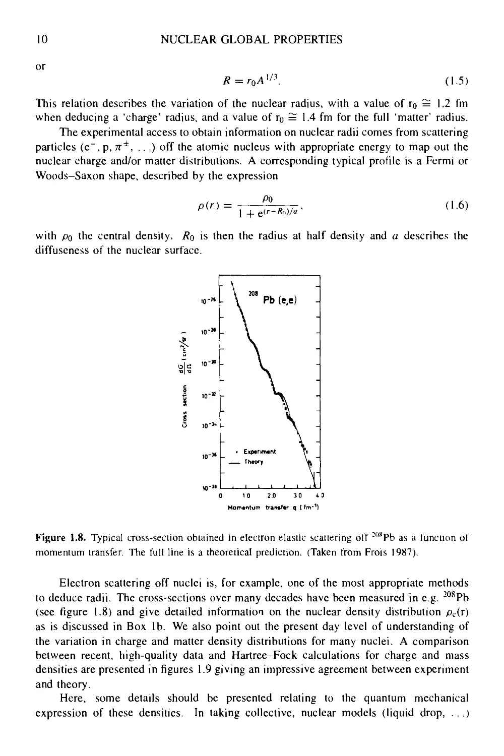
This relation describes the variation of the nuclear radius, with a value of ro = 1.2 fm
when deducing a 'charge' radius, and a value of ro = 1.4 fm for the full 'matter' radius.
The experimental access to obtain information on nuclear radii comes from scattering
particles (e~, p, n±, ...) off the atomic nucleus with appropriate energy to map out the
nuclear charge and/or matter distributions. A corresponding typical profile is a Fermi or
Woods-Saxon shape, described by the expression
p(r) =
Po
c(r-Rn)/a '
A.6)
with po the central density. /?o is then the radius at half density and a describes the
diffuseness of the nuclear surface.
I ,o-
Pb (e,e)
0 10 2.0 3 0 10
Momentum trantitr q t fm*1)
Figure 1.8. Typical cross-section obtained in electron elastic scattering off ;"*Pb as a function of
momentum transfer. The full line is a theoretical prediction. (Taken from Frois 1987).
Electron scattering off nuclei is, for example, one of the most appropriate methods
to deduce radii. The cross-sections over many decades have been measured in e.g. 208Pb
(see figure 1.8) and give detailed information on the nuclear density distribution pL(r)
as is discussed in Box lb. We also point out the present day level of understanding of
the variation in charge and matter density distributions for many nuclei. A comparison
between recent, high-quality data and Hartree-Fock calculations for charge and mass
densities are presented in figures 1.9 giving an impressive agreement between experiment
and theory.
Here, some details should be presented relating to the quantum mechanical
expression of these densities. In taking collective, nuclear models (liquid drop, ...)
1.4 NUCLEAR EXTENSION
11
{ i > 7 о i i i I i . 7 - a" ! i \ i iii 7
0.20
ОЮ-
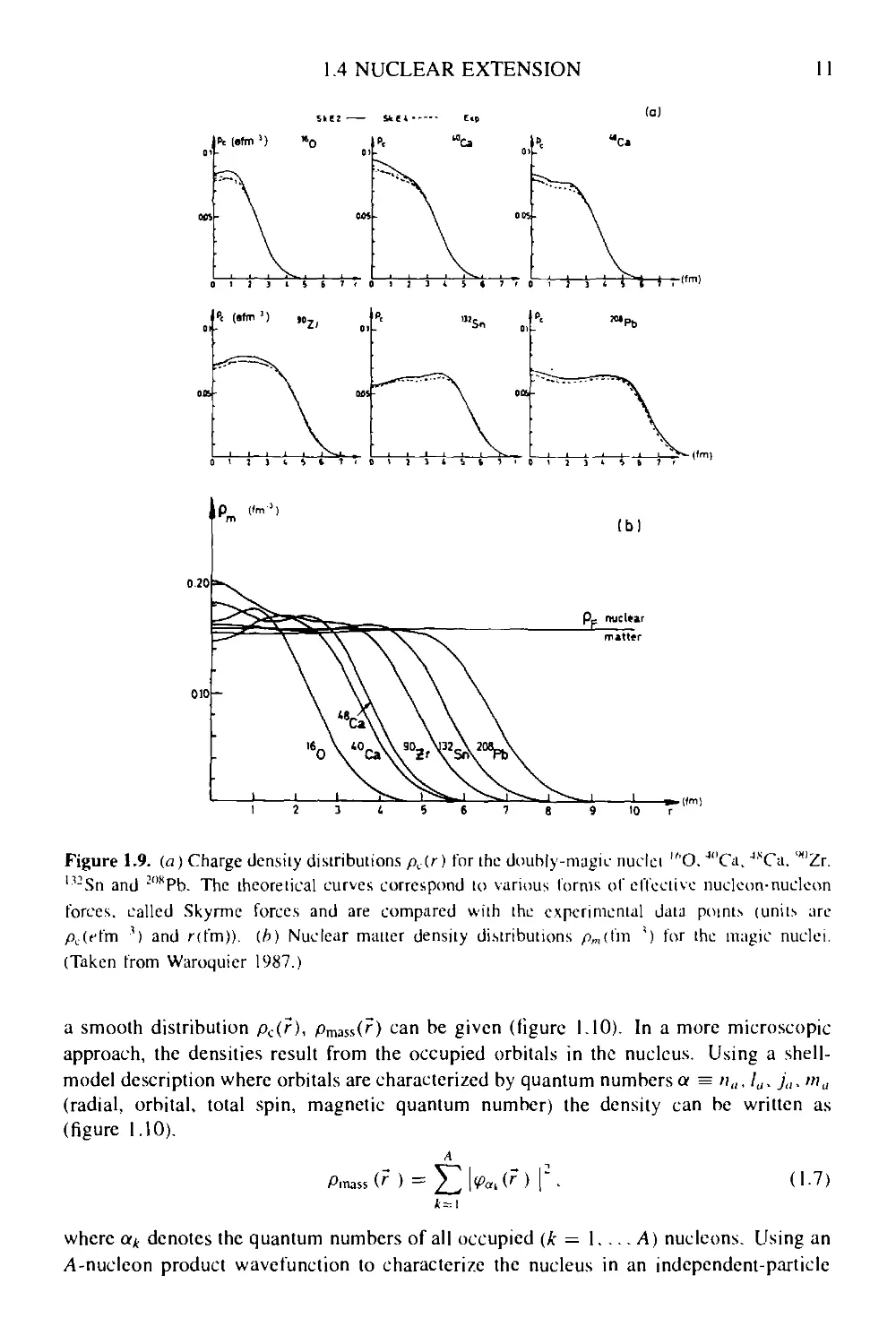
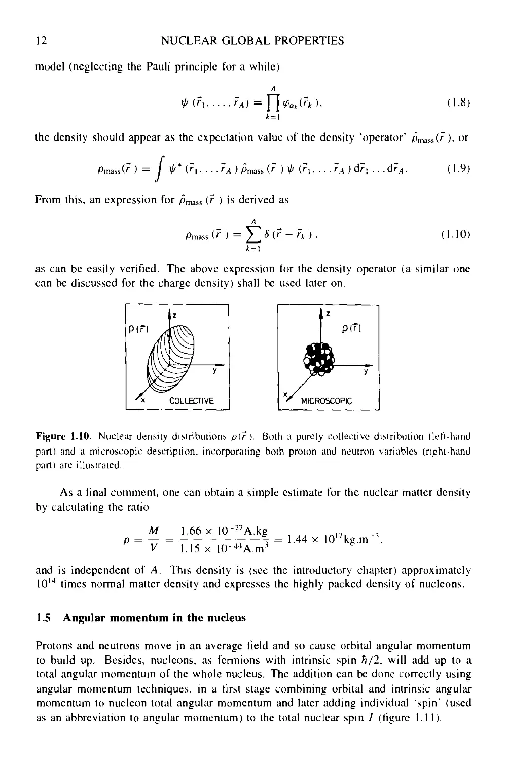
Figure 1.9. (a) Charge density distributions pc(r) for the douhly-magic nuclei lhO. J"Gi. JliCa. '"Zr.
":Sn and 2"8Pb. The theoretical curves correspond to various forms of effective nuclcon-nuclcon
forces, called Skyrme forces and are compared with the experimental data points (units arc
pL(ffm ■') and r(fm)). (b) Nuclear matter density distributions pmi(m ') for the magic nuclei.
(Taken from Waroquier 1987.)
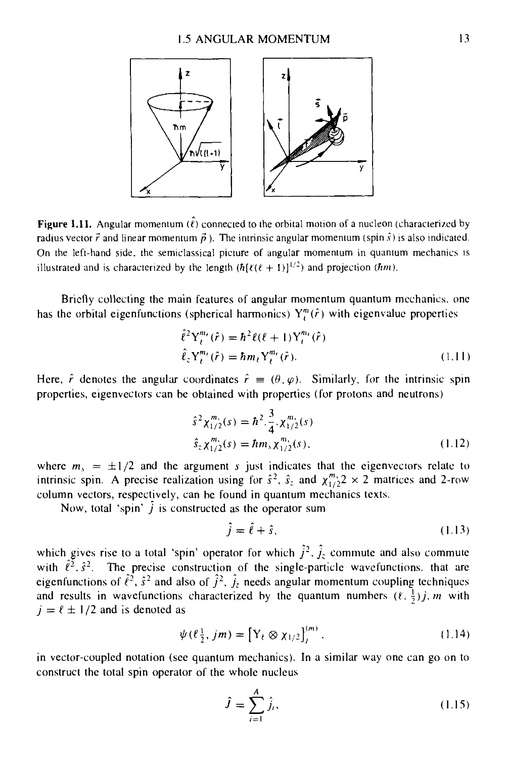
a smooth distribution pc(r), pmiS!,(r) can be given (figure 1.10). In a more microscopic
approach, the densities result from the occupied orbitals in the nucleus. Using a shell-
model description where orbitals are characterized by quantum numbers a = /;„, Iu, ja. "'«
(radial, orbital, total spin, magnetic quantum number) the density can be written as
(figure 1.10).
A.7)
/t=l
where a* denotes the quantum numbers of all occupied (k = 1.... A) nucleons. Using an
Л-nucleon product wavefunction to characterize the nucleus in an independent-particle
12 NUCLEAR GLOBAL PROPERTIES
model (neglecting the Pauli principle for a while)
Pak(rk), A-8)
the density should appear as the expectation value of the density 'operator' pmaii(r). or
Pmass(r ) = / V (f\, ■ - ■ ГА ) Pmass (r ) Ф (r,. . . .fA ) dr, . . . (irA . ( 1.9)
From this, an expression for pmass (f ) is derived as
A
Pmass v Г ) z
A.10)
as can be easily verified. The above expression for the density operator (a similar one
can be discussed for the charge density) shall be used later on.
V
1 7
I P<*1
/
MICROSC0PC
У
Figure 1.10. Nuclear density distributions p(r ). Both a purely collective distribution (left-hand
part) and a microscopic description, incorporating both proton and neutron variables (right-hand
part) are illustrated.
As a final comment, one can obtain a simple estimate for the nuclear matter density
by calculating the ratio
M 1.66 x 10~27A.kg ., ,
P=~= . .. , = 1-44 x 10I7kg.m-\
V
1.15 x
and is independent of A. This density is (see the introductory chapter) approximately
1014 times normal matter density and expresses the highly packed density of nucleons.
1.5 Angular momentum in the nucleus
Protons and neutrons move in an average field and so cause orbital angular momentum
to build up. Besides, nucleons, as fermions with intrinsic spin h/2. will add up to a
total angular momentum of the whole nucleus. The addition can be done correctly using
angular momentum techniques, in a first stage combining orbital and intrinsic angular
momentum to nucleon total angular momentum and later adding individual 'spin' (used
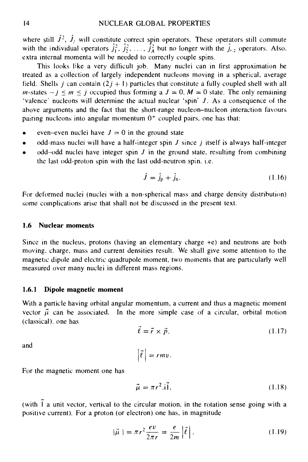
as an abbreviation to angular momentum) to the total nuclear spin / (figure 1.11).
1.5 ANGULAR MOMENTUM
13
Figure 1.11. Angular momenium U) connected to the orbital motion of a nucleon (characterized by
radius vector r and linear momenium p ). The intrinsic angular momenium (spin л) is also indicated.
On the left-hand side, the semiclassical picture of angular momenium in quantum mechanics is
illustrated and is characterized by the length (h[t(t + I)]'") and projection (Л/и).
Briefly collecting the main features of angular momentum quantum mechanics, one
has the orbital eigenfunctions (spherical harmonics) Y"'(r) with eigenvalue properties
€;Y7'(r)=»mjY*'(r). A.11)
Here, r denotes the angular coordinates r = (9.<p). Similarly, for the intrinsic spin
properties, eigenvectors can be obtained with properties (for protons and neutrons)
=hmsx"'/2(s).
A.12)
where ms = ±1/2 and the argument s just indicates that the eigenvectors relate to
intrinsic spin. A precise realization using for s2, s- and Xw'->2 х 2 matrices and 2-row
column vectors, respectively, can be found in quantum mechanics texts.
Now, total 'spin' j is constructed as the operator sum
j = t + s. A.13)
which gives rise to a total 'spin' operator for which j2. jz commute and also commute
with £2.s2. The precise construction of the single-particle wavefunctions. that are
eigenfunctions of B, s2 and also of j2, j, needs angular momentum coupling techniques
and results in wavefunctions characterized by the quantum numbers (t,,\)j,m with
j = i ± 1/2 and is denoted as
\(f(t\, jm) = [Y; <g) xi/2] "' • A-14)
in vector-coupled notation (see quantum mechanics). In a similar way one can go on to
construct the total spin operator of the whole nucleus
A.15)
; = l
14 NUCLEAR GLOBAL PROPERTIES
where still У2, J: will constitute correct spin operators. These operators still commute
with the individual operators jf, />:, ..., j\ but no longer with the j,z operators. Also,
extra internal momenta will be needed to correctly couple spins.
This looks like a very difficult job. Many nuclei can in first approximation be
treated as a collection of largely independent nucleons moving in a spherical, average
field. Shells j can contain Bj + 1) particles that constitute a fully coupled shell with all
//i-states — j < m < j occupied thus forming a J = 0, M = 0 state. The only remaining
'valence' nucleons will determine the actual nuclear 'spin' J, As a consequence of the
above arguments and the fact that the short-range nucleon-nucleon interaction favours
pairing nucleons into angular momentum 0+ coupled pairs, one has that:
• even-even nuclei have J = 0 in the ground state
• odd-mass nuclei will have a half-integer spin J since j itself is always half-integer
• odd-odd nuclei have integer spin J in the ground state, resulting from combining
the last odd-proton spin with the last odd-neutron spin, i.e.
J=]p+)n- A16)
For deformed nuclei (nuclei with a non-spherical mass and charge density distribution)
some complications arise that shall not be discussed in the present text.
1.6 Nuclear moments
Since in the nucleus, protons (having an elementary charge +e) and neutrons are both
moving, charge, mass and current densities result. We shall give some attention to the
magnetic dipole and electric quadrupole moment, two moments that are particularly well
measured over many nuclei in different mass regions.
1.6.1 Dipole magnetic moment
With a particle having orbital angular momentum, a current and thus a magnetic moment
vector /1 can be associated. In the more simple case of a circular, orbital motion
(classical), one has
t=?y.p. A.17)
and
t = rmv.
For the magnetic moment one has
д=лт2,й, A.18)
(with 1 a unit vector, vertical to the circular motion, in the rotation sense going with a
positive current). For a proton (or electron) one has, in magnitude
2л г 2m
1.19)
1.6 NUCLEAR MOMENTS 15
and derives (for the circular motion still)
j}t = —t I in Gaussian units) . A.20)
2m \2mc '
2m
Moving to a quantum mechanical description of orbital motion and thus of the
magnetic moment description, one has the relation between operators
and
^.z = ~e:. A.22)
2m
The eigenvalue of the orbital, magnetic dipole operator, acting on the orbital
eigenfunctions Y' then becomes
= ^m,Y?'(f). A.23)
Zm
If we call the unit eh/2m the nuclear (if m is the nucleon mass) or Bohr (for electrons)
magneton, then one has for the eigenvalue Дл-(Дв)
ixt,z = mtnn. A.24)
For the intrinsic spin, an analoguous procedure can be used. Here, however, the
mechanism that generates the spin is not known and classic models are doomed to fail.
Only the Dirac equation has given a correct description of intrinsic spin and of its origin.
The picture one would make, as in figure 1.12, is clearly not correct and we still need
to introduce a proportionality factor, called gyromagnetic ratio gs. for intrinsic spin /i/2
fermions. One obtains
A.25)
as eigenvalue, for the /iv, operator acting on the spin XwiU) eigenvector. For the electron
this gs factor turns out to be almost —2 and at the original time of introducing intrinsic
h/2 spin electrons this factor (in 1926) was not understood and had to be taken from
experiment. In 1928 Dirac gave a natural explanation for this fact using the now famous
Dirac equation. For a Dirac point electron this should be exact but small deviations given
by
a = ^, A.26)
were detected, giving the result
a"p = 0.001159658D). A.27)
Detailed calculations in QED (quantum electrodynamics) and the present value give
16
NUCLEAR GLOBAL PROPERTIES
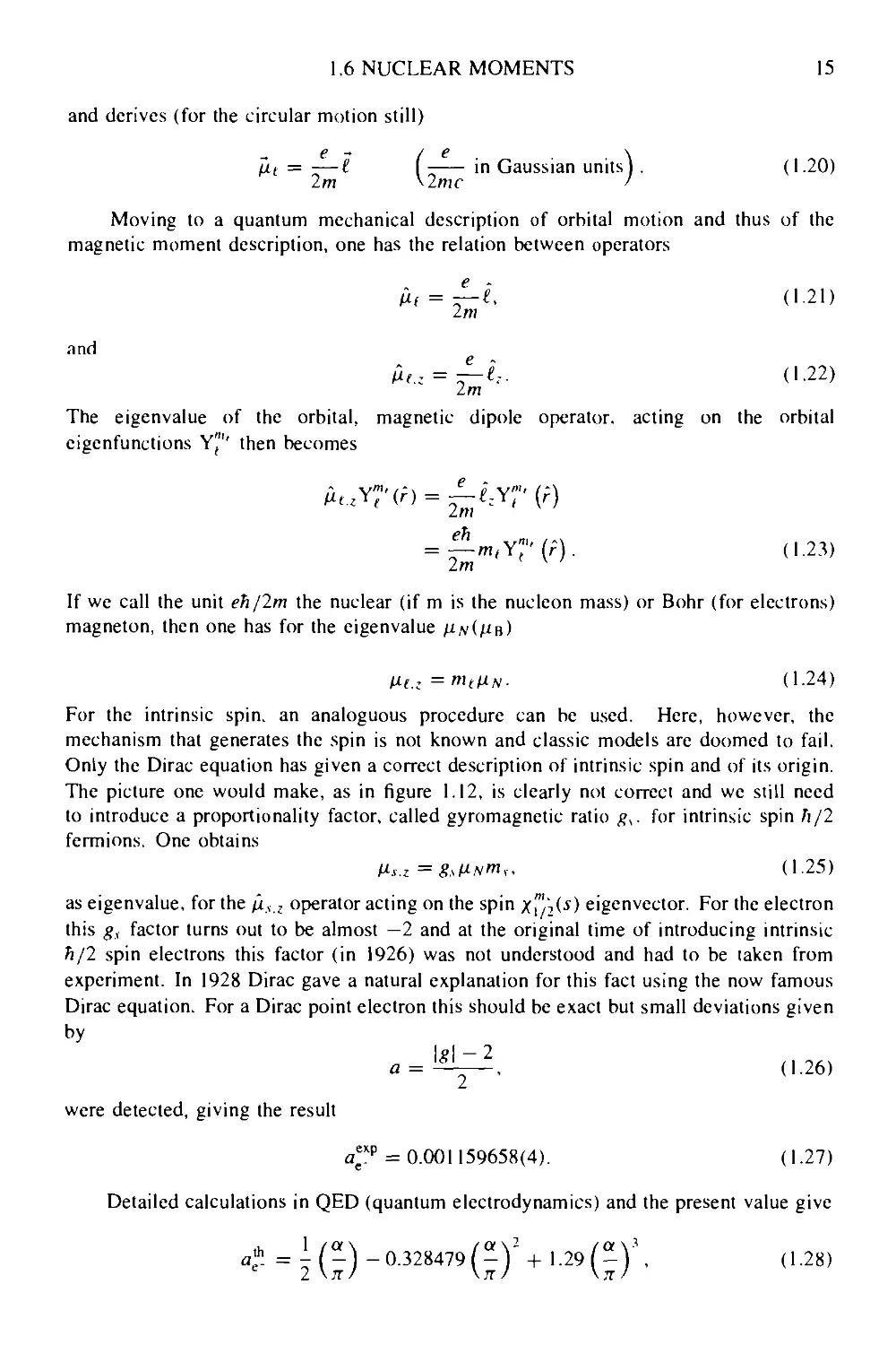
Figure 1.12. In the upper part, the relationships between the intrtnsic (Д, ) and orbital (/~i, )
magnettc moments and the corresponding angular moment vectors (ft/2 and C, respectively) are
indicated. Thereby gyromagnetic factors are defined. In the lower part, modifications to the
single-electron ^-factor are illustrated. The physical electron ^-factor is not just a pure Dtrac
particle. The presence of virtual photons, e'e" creation and more complicated processes modtly
these free electron properties and are illustrated. (Taken from Frauenfelder and Henley A991)
Subatomic Physics © 1974. Reprinted by permission of Prentice-Hall, Englewood Cliffs, NJ.)
with or = el/hi\ and the difference (a[h - a"p) /aih = B ± 5) x 1(Г6, which means 1
part in 105 (for a nice overview, see Crane A968) and lower part of figure 1.12).
This argumentation can also be carried out for the intrinsic spin motion of the
single proton and neutron, and results in non-integer values for both the proton and the
neutron, i.e. g, (proton) = 5.5855 and £s(neutron)= -3.8263. The fact is that, even for
the neutron with zero charge, an intrinsic, non-vanishing moment shows up and points
towards an internal charge structure for both the neutron and proton that is not just a
simple distribution. From electron high-energy scattering off nucleons (see section 1.4)
1.6 NUCLEAR MOMENTS
17
NUCLEUS
NUCLEON
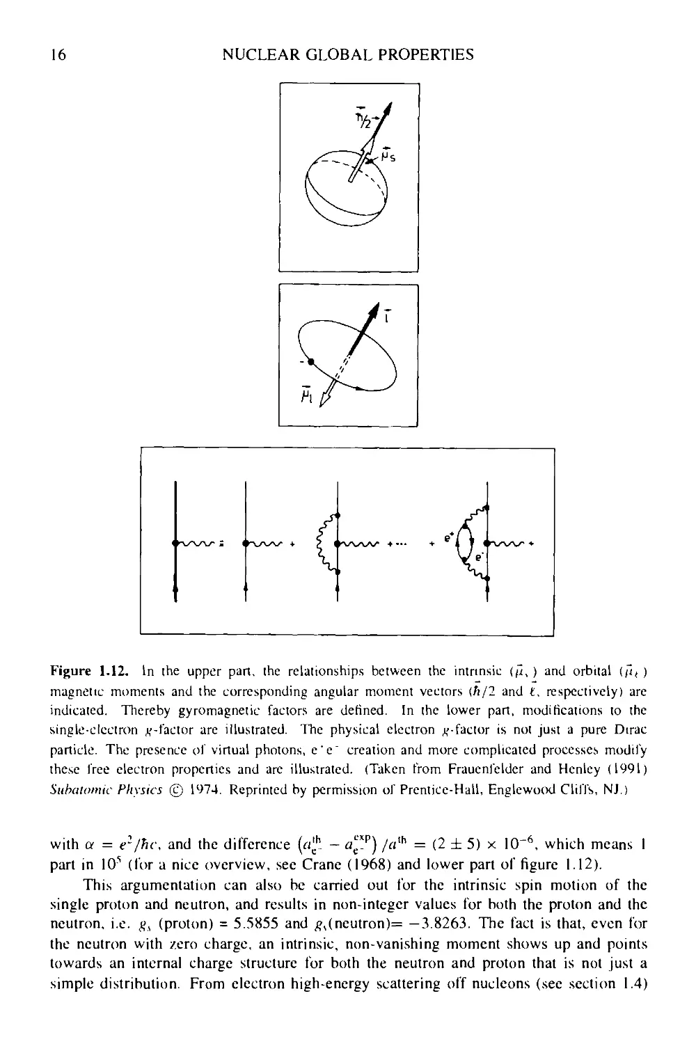
Figure 1.13. Charge distributions of nucleons deduced from the analyses of clastic electron
scattering of]' protons (hydrogen target) and off neutrons (from a deuterium target). In the lower
parts, the typical difference between a nuclear and a nucleon density distribution are presented.
a charge form factor can be obtained (see results in figure 1.13 lor the charge density
distributions pcharge(r) for proton and neutron). As a conclusion one obtains that:
• Nucleons are not point particles and do not exhibit a well-defined surface in contrast
with the total nucleus, as shown in the illustration. Still higher energy scattering
at SLAC (Perkins 1987) showed that the scattering process very much resembled
that of scattering on points inside the proton. The nature of these point scatterers
and their relation to observed and anticipated particles was coined by Feynman as
'partons' and attempts have been made to relate these to the quark structure of
nucleons (see Box lc).
One can now combine moments to obtain the total nuclear magnetic dipole moment and
obtain:
f*j.z=gjf*\'"j- A 29)
with gj the nuclear gyromagnetic ratio. Here too, the addition rules for angular
momentum can be used, to construct (i) a full nucleon ^-factor after combining orbital
and intrinsic spin and (ii) the total nuclear dipole magnetic moment. We give, as an
informative result, the g-factor for free nucleons (combining I and s to the total spin j)
as
± ( A30
where the upper sign applies for the j = t + \ and lower sign for the j ~ t — \
orientation. Moreover, these ^-factors apply to free 'nucleons". When nucleons move
18
NUCLEAR GLOBAL PROPERTIES
inside a nuclear medium the remaining nucleons modify this free Rvalue into 'effective'
^-factors. This aspect is closely related to typical shell-model structure aspects which
shall not be discussed here.
1.6.2 Electric moments—electric quadrupole moment
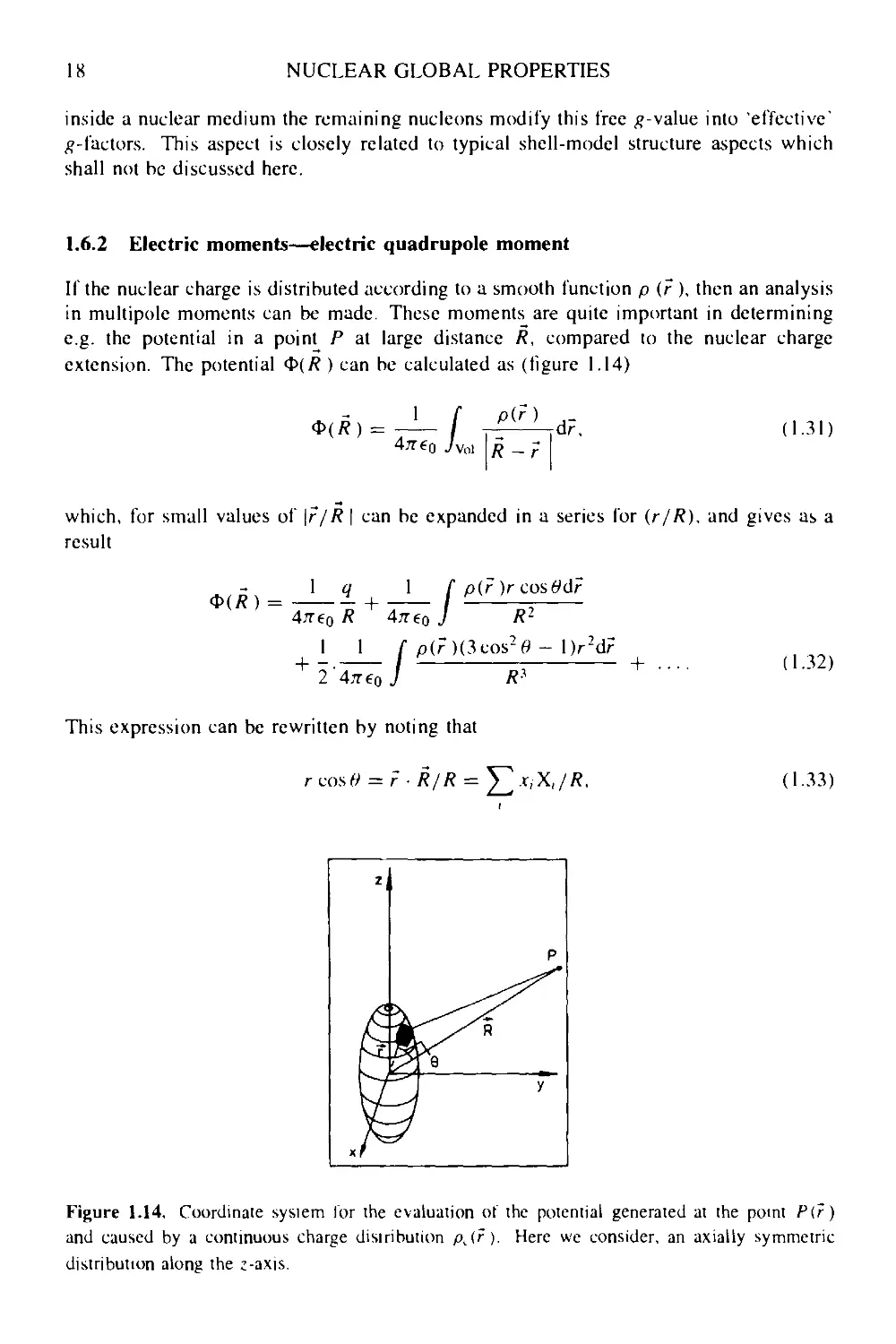
If the nuclear charge is distributed according to a smooth function p (r ), then an analysis
in multipole moments can be made. These moments are quite important in determining
e.g. the potential in a point P at large distance R, compared to the nuclear charge
extension. The potential <P(R ) can be calculated as (ligure 1.14)
A.31)
vol R -
which, for small values of \r/R \ can be expanded in a series for (r/R), and gives as a
result
q 1 f p(r )r cos#dr
R 4л-€0 J R2
2d?
1 1 f p(r )Ccos20 - \)r7
This expression can be rewritten by noting that
r cos в = f
A.32)
A.33)
I
X t
p
Figure 1.14, Coordinate sysiem lor the evaluation of the potential generated at the pomt P(r)
and caused by a continuous charge disiribution pM). Here we consider, an axially symmetric
distribution along the г-axis.
1.6 NUCLEAR MOMENTS 19
(with x, for ! = 1, 2, 3 corresponding to л, у, z, respectively). In the above expression,
q is the total charge /Vo| p(r)dr. Using the Cartesian expansion we obtain
with
Pi = I p(r)x,d?,
c,-jCj - r2S4 )d?. A.35)
= /
the dipole components and quadrupole tensor, respectively. The quadrupole tensor Q4
can be expressed via its nine components in matrix form (with vanishing diagonal sum)
/ 3*2-r2 Здгу Зл; \
Q^\ Ъху Ъу2-г2 3yz . A.36)
\ 3xz 3y; 3;2-r2 /
Transforming to diagonal form, one can find a new coordinate system in which the
non-diagonal terms vanish and one gets the new quadrupole tensor
Q^l 3y2-r: |. A.37)
The quantity Q-z-z = f p(r )(Зг2 — r2)dr is also denoted as the quadrupole moment
of the charge distribition, relative to the axis system (i, y, z)- For a quantum mechanical
system where the charge (or mass) density is given as the modulus squared of the
wavefunction \р^(г, ), one obtains, the quadrupole moment as the expectation value
of the operator J2t Cz2 - r2), or J2i V( 16Jr/5)r,2Y?(r,) and results in
Q(J, M) = f xlf'jMG,
for a microscopic description of the nuclear wavefunction or,
Q(J, M) = I \pjM (r ) (Зг2 - r2)\pJM(r )dr, A.39)
in a collective model description where the wavefunction depends on a single coordinate
r describing the collective system with no internal structure.
Still keeping somewhat to the classical picture (see equation A.39)), one has a
vanishing quadrupole moment Q = 0 for a spherical distribution p(r ), a positive value
Q > 0 for a prolate (cigar-like shape) distribution and a negative value Q < 0 for an
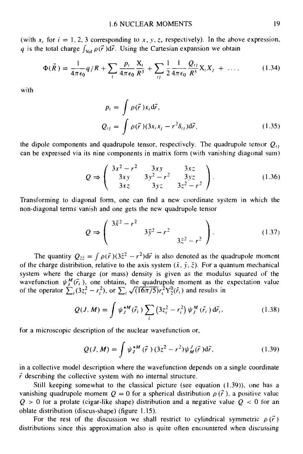
oblate distribution (discus-shape) (figure 1.15).
For the rest of the discussion we shall restrict to cylindrical symmetric p (r )
distributions since this approximation also is quite often encountered when discussing
20
NUCLEAR GLOBAL PROPERTIES
z
Ш
г*
\y
Figure 1.15. In the upper part the various density distributions that give rise to a vanishing, positive
and negative quadrupole moment, respectively. These situations correspond to a spherical, prolate
and oblate shape, respectively. In the lower part, the orientation of an axially symmetric nuclear
density distribution p(r) relative to the body-fixed axis system (i, y, z) and to a laboratory-fixed
axis system x. y, z is presented. This situation is used to relate the intrinsic to the laboratory (or
spectroscopic) quadrupole moment as discussed in the text.
actual, deformed nuclear charge and mass quadrupole distributions. In this latter case, an
interesting relation exists between the quadrupole moment in a body-fixed axis system
A, 2, 3) (which we denote with i, y, z coordinates) and in a fixed (x, y, z) laboratory
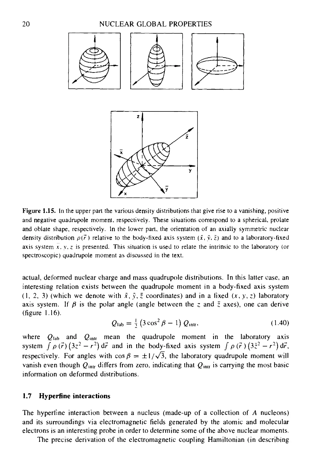
axis system. If fl is the polar angle (angle between the z and г axes), one can derive
(figure 1.16).
G1ab = lCc0S2^-l)G,n.r. A-40)
where £>ы> and Qim mean the quadrupole moment in the laboratory axis
system / p (r) Cz2 — r2) dr and in the body-fixed axis system j p (?) Cc2 — r2) dr,
respectively. For angles with cos fi = ±l/\/3, the laboratory quadrupole moment will
vanish even though QiMl differs from zero, indicating that Qm, is carrying the most basic
information on deformed distributions.
1.7 Hyperfine interactions
The hyperfine interaction between a nucleus (made-up of a collection of A nucleons)
and its surroundings via electromagnetic fields generated by the atomic and molecular
electrons is an interesting probe in order to determine some of the above nuclear moments.
The precise derivation of the electromagnetic coupling Hamiltonian (in describing
1.7 HYPERFINE INTERACTIONS
21
Figure 1.16. The spectroscoptc (or laboratory) quadrupole moment can be obtained using a
semiclassical procedure of averaging the intrinsic quadrupole moment (delined relative to> the
z-axis) over the precession of./ about the laboratory г-axis. The intrinsic system is tilted out
of the laboratory system over an angle fi.
non-relativistic systems) will be discussed in Chapter 6. We briefly give the main results
here.
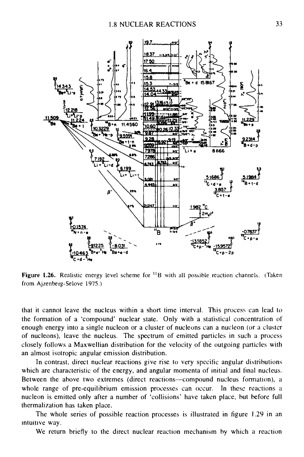
The Hamiltonian describing the nucleons (described by charges e, and currents j, )
in interaction with external fields, described by the scalar and vector potentials Ф (r ) and
A (r), is obtained via the 'minimal electromagnetic coupling' substitution /5, —> p, — e, A,
or
£<■♦■
1 = 1
This Hamiltonian can be rewritten as
A „2 A -
In neglecting the term, quadratic in A at present, we obtain
H = H0 + He.m. (Coupling),
with
He m (coupling) = -
e, pt A
1-
e, Ф.
For a continuous charge and current distribution this results in
Hem (coupling) = - / j ■ Adr + I p<l>dr.
A.41)
A.42)
A.43)
A.44)
A.45)
Using this coupling Hamiltonian, we shall in particular describe the magnetic dipolc
moment (via Zeeman splitting) and the electric quadrupole moment interacting with
external fields.
With #o describing the nuclear Hamiltonian with energy eigenvalues Ej and
corresponding wavefunctions \pf, there remains in general an A/-degeneracy for the
substates since
f^Ej^f. A.46)
22 NUCLEAR GLOBAL PROPERTIES
M
3/2
•-V2
fl=O 0*0
Figure 1.17. Zeeman splitting of the energy levels of a quantum-mechanical system characterized
by angular momentum J = \ and a ^'-factor xj in an external field B. The В field is oriented
along the posttive c-axis with #у > 0.
Including the electromagnetic coupling Hamiltonian, the degeneracy will be lifted, and
depending on the interaction Hc,m (coupling) used, specific splitting of the energy levels
results. For the Zeeman splitting, one has (figure 1.17)
Whyperfine = -Д • S, A.47)
and, relating Д to the nuclear total spin, via the g-factor as follows
A.48)
A.49)
For a magnetic induction, oriented along the z-axis (quantization axis) J • В becomes
J: В and the interaction energy reduces to
-gjLiNMB. A.50)
Here now, the 2У + 1 substates are linearly split via the magnetic interaction and
measurements of these splittings not only determine the number of states (and thus J)
but also gj when the induction В is known. The above method will be discussed in
some detail for the electric quadrupole interaction too, for axially symmetric systems.
We first discuss the general, classical interaction energy for a charge distribution p (r )
with an external field Ф(г ) and secondly derive the quantum mechanical effects through
the degeneracy splitting. The classical interaction energy reads
ft
the expectation value of the hyperfine perturbing Hamiltonian becomes
-int — /
./vol
p(FL>(r)dF. A.51)
integrating over the nuclear, charge distribution p (r ) volume, and Ф (r ) denotes the
potential field generated by electrons of the atomic or molecular environment. In view
of the distance scale relating the charges generating Ф (r ) (the charge density pe (r ))
1.7 HYPERFINE INTERACTIONS 23
and the atomic nucleus volume, Ф (r ) will in general be almost constant or varying by
a small amount over the volume only, allowing for a Taylor expansion into
/дф\ i / Э2Ф \
Ф (r ) = Ф (r H + V ( — x' + о I- ^"^ v'v' + • • • • ( L52)
The corresponding energy then separates as follows into
with
j (,7)x,xid7. A.53)
Then a monopole, a dipole, a quadrupole, . .. interaction energy results where the
monopole term will induce no degeneracy splitting, the dipole term gives the Stark
splitting, etc. In what follows, we shall concentrate on the quadrupole term only
(q). By choosing the coordinate system (x, y, ;) such that the non-diagonal terms in
(У2Ф/9л',3.с;H , (i ф j) vanish, we obtain for the interaction energy, the expression
Adding, and substracting a monopole-like term, this expression can be rewritten as
Two situations can now be distinguished:
In situations where electrons at the origin are present, i.e. j-electrons, and these
electrons determine the external potential field Ф (r ), which subsequently becomes
spherically symmetric, the first term disappears and we obtain (since АФ = —
r-</(m) Pel(O) f - 2j- -, ess
tnt = —2^~ J Р(Г (
as the interaction energy. This represents a 'monopole' shift and all levels
(independent of M) receive a shift in energy, expressed by E4^, a shift which
is proportional to both the electron density at the origin pei@) and the mean-square
radius describing the nucleon charge distribution p (r ). Measurements of E^1'
leads to information about the nuclear charge radius.
24 NUCLEAR GLOBAL PROPERTIES
• In situations where a vanishing electron density at the origin occurs, ДФ = 0 and
only the first term contributes. In this case the particular term can be rewritten as
l( — ) f
6 V Эу2 H J
:2)d?
)C.v:-r2)d?
)C=2-r2)dr. A.57,
In cases where the cylindrical symmetry condition for the external potential
holds, the quadrupole interaction energy becomes
(F)Cc2-(.c2 +v2 + c2))dF. A.58)
or
The classical expression can now be obtained, by replacing the density p(r ) by the
modulus squared of the nuclear wavefunction
D = i (™\ j iP*uCr)(lz2 - г2)ФУ(
?, A.60)
and now rewriting C;2-r2) as r2Ccos2^- 1) or r2 y/( \6n/5)Y°2(r), the quadrupole
interaction energy becomes
One can now also use a semi-quantum-mechanical argument to relate the laboratory
quadrupole moment to the intrinsic quadrupole moment, using equation A.40), with
fi the angle between the laboratory c-axis and intrinsic c-axis and where the quantum-
mechanical labels J and M are replaced in terms of the tilting angle /3 in the
classical vector model for angular momentum J (vector with length h>JJ(J + 1)
and projection hM) (ligure 1.16). Thereby
3M2-J(J+\)
id л. n Gintr- (L62)
1.8 NUCLEAR REACTIONS 25
Finally, one obtains the result that the interaction energy is quadratic in the
projection quantum number M and, because of the quadrupdole interaction, breaks
the degeneracy level 7 into 7 + | doubly-degenerate levels. We point out that a
correct quantum-mechanical description, using equation A.61) where the expectation
value is
A.63)
has to be evaluated, making use of the Wigner-Eckart theorem (Heyde 1991). Thus,
one obtains
t ту , ' V II A67r/5)t/2r2Y2(r) || 7). A.64)
4 \dz2 /о У2У + 1
with a separation into a Clebsch-Gordan coupling coefficient and a reduced
((|| ... ||>) matrix element. Putting the explicit value of the Clebsch-Gordan
coefficient, one has
ЗЛ/2-7G + 1) ^
GG + \)BJ- \)BJ + 1М2У + 3))1 " ' "
A.65)
For M = 7, one obtains the result (maximal interaction)
16л- / 7B7-1)
G + ,)B7+,)B7+3)(У » ^ « J)- ('-66)
which vanishes for 7 = 0 and J — \-
Since typical values of the intrinsic quadrupole moment are 5 x 10~24 cm2 E barn),
one needs the fields that atoms experience in solids to get high enough field gradients in
order to give observable splittings. Atomic energies are of the order of eV and atomic-
dimensions of the order of 10"s cm. So, typical field gradients are of the order of
|ЭФ/Эс| = 10sVcm-' or |Э2Ф/Эг2| ^ 10l6Vcnr2, and splittings of the order of
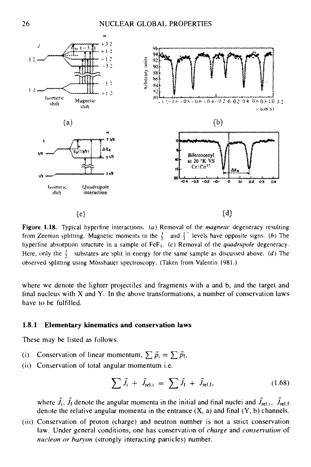
{Ечт) а е(ЭгФ/Э;г)о • Gmtr oc 5 x 10"seV can result. A typical splitting pattern
for the case of 57Fe with a spin value of 7" = \ in its first excited state is shown
in figure 1.18. Resonant absorption from the 7T = \ ground state can now lead to
the absorption pattern and from the measurement of a splitting to a nuclear quadrupole
moment whenever C2Ф/Зг2H is known. On the other hand, starting from a known
quadrupole moments, an internal field gradient C2Ф/;);2H can be determined. In the
other part of the figure, the magnetic hyperfine or Zeeman splitting of 57Fe is also
indicated. A discussion on one-particle nucleon quadrupole moments and its relation to
nuclear shapes is presented in Box Id.
1.8 Nuclear reactions
In analysing nuclear reactions, nuclear transmutations may be written
X + av" * Ул> + byv
A-67)
26
NUCLEAR GLOBAL PROPERTIES
- """■* *-. - И,! + i.;
(a)
V»
I I.
vl
—LJ >|Л
(b)
(c) <d)
Figure 1.18. Typical hyperfinc interactions, (a) Removal of the magnetic degeneracy resulting
from Zeeman splitting. Magnetic moments in the j and \ levels have opposite signs, {b) The
hyperfine absorption structure in a sample of FeF,. (c) Removal of the quadrupole degeneracy.
Here, only the \ substates arc split in energy for the same sample as discussed above, (d) The
observed splitting using Mbssbauer spectroscopy. (Taken from Valentin 1981.)
where we denote the lighter projectiles and fragments with a and b, and the target and
final nucleus with X and Y. In the above transformations, a number of conservation laws
have to be fulfilled.
1.8.1 Elementary kinematics and conservation laws
These may be listed as follows.
(i) Conservation of linear momentum, ^ /5, = ^ pf,
(ii) Conservation of total angular momentum i.e.
A.68)
where У,. Jf denote the angular momenta in the initial and final nuclei and irei.i, JK\.(
denote the relative angular momenta in the entrance (X, a) and final (Y, b) channels.
(iii) Conservation of proton (charge) and neutron number is not a strict conservation
law. Under general conditions, one has conservation of charge and conservation of
nucleon or ban-on (strongly interacting particles) number.
1.8 NUCLEAR REACTIONS
(iv) Conservation of parity, n, such that
27
A.69)
where the parities of the initial and final nuclei and projectiles (incoming, outgoing)
are considered.
(v) Conservation of total energy, which becomes
Tx + M'^.c1 + 7a + M'a.c2 = 7V + My.c2 + 7b + М'ъ.с2.
A.70)
with 7", the kinetic energy and M[.c2 the mass-energy. In the non-relativistic
situation, the kinetic energy T, = \M[v2. One defines the Q-value of a given
reaction as
A.71)
A.72)
which can be rewritten using the kinetic energies as
= 7V + Tb - Tx - 7"a.
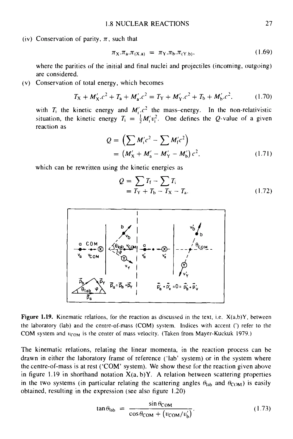
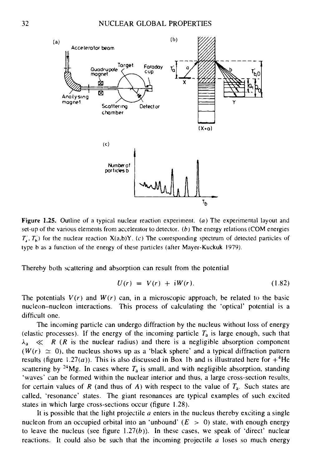
Figure 1.19. Kinematic relations, for the reaction as discussed in the text, i.e. X(a.b)Y. between
the laboratory (lab) and the centre-of-mass (COM) system. Indices with accent (') refer to the
COM system and vCOM is the center of mass velocity. (Taken from Mayer-Kuckuk 1979.)
The kinematic relations, relating the linear momenta, in the reaction process can be
drawn in either the laboratory frame of reference ('lab' system) or in the system where
the centre-of-mass is at rest ('COM' system). We show these for the reaction given above
in figure 1.19 in shorthand notation X(a, b)Y. A relation between scattering properties
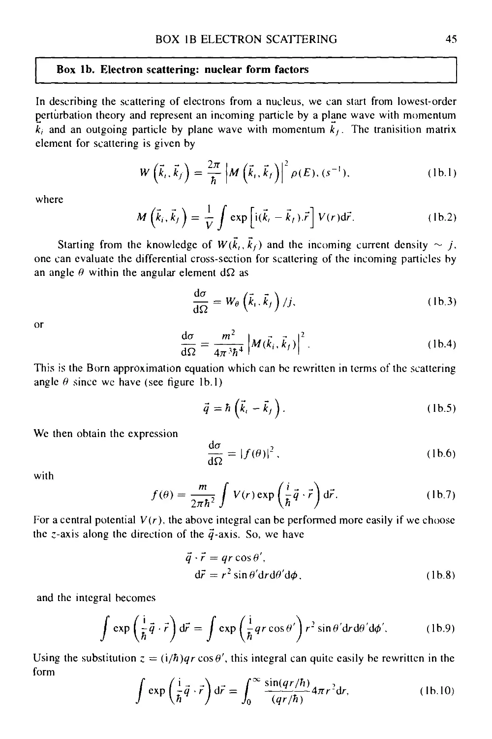
in the two systems (in particular relating the scattering angles 0]3b and Йсом) 's vastly
obtained, resulting in the expression (see also figure 1.20)
sin
A.73)
28
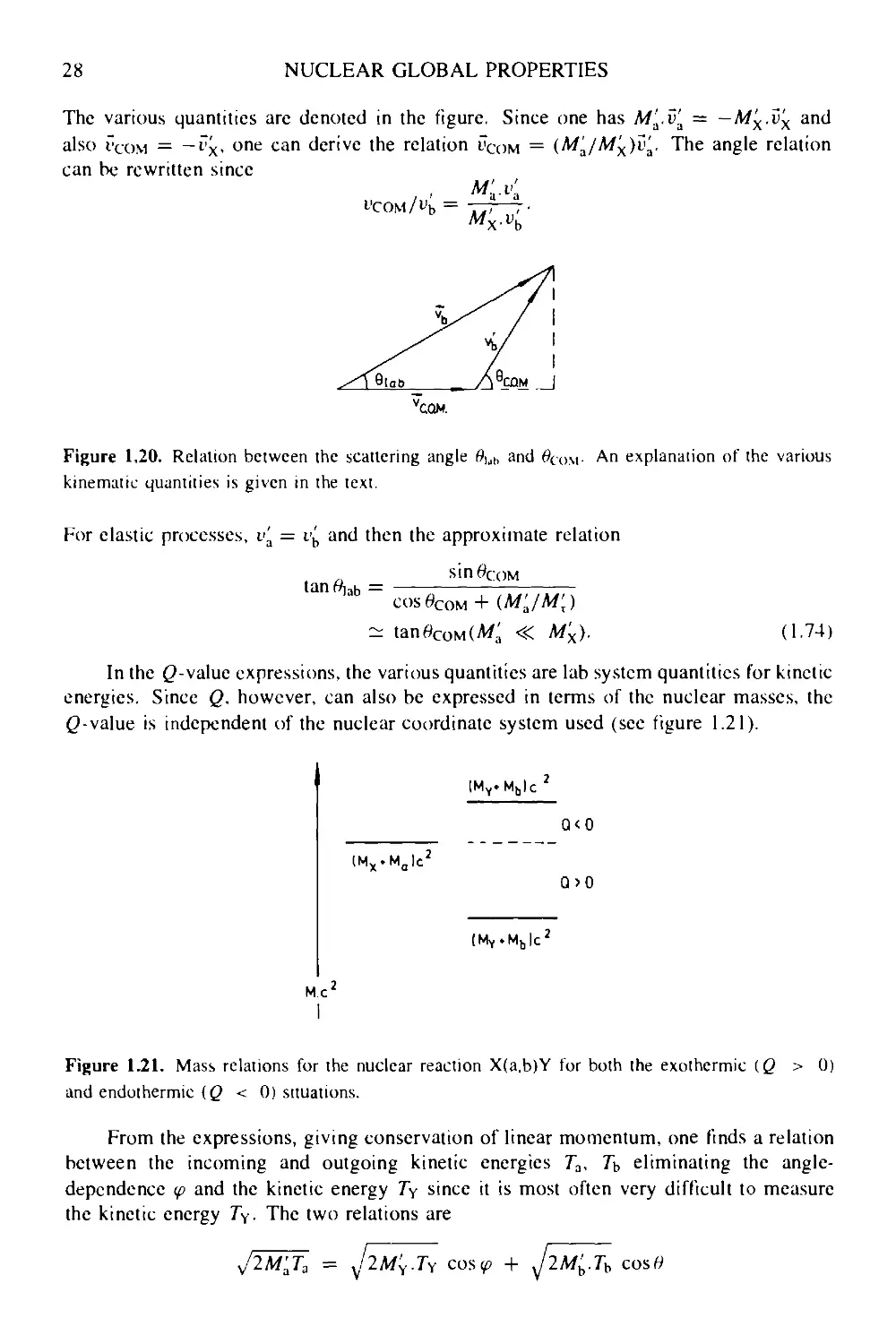
NUCLEAR GLOBAL PROPERTIES
The various quantities are denoted in the figure. Since one has Л/а.па = — Mx.v'x and
also Гсом = -v'x, one can derive the relation uC0M = (M'a/Mx)v'a. The angle relation
can be rewritten since
M!d.v'a
"COM.
Figure 1.20. Relation between the scattering angle виь and #сом- An explanation of the various
kinematic quantities is given in the text.
For elastic processes, v'a = i£ and then the approximate relation
tan #ьь = ' '■
cos0COM + (A/a/A/;)
— tan0coM(A/a <К M'x). A74)
In the £>-value expressions, the various quantities are lab system quantities for kinetic
energies. Since Q, however, can also be expressed in terms of the nuclear masses, the
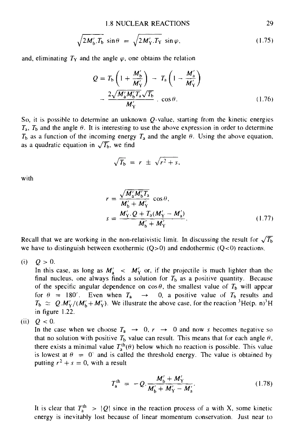
£>-value is independent of the nuclear coordinate system used (see figure 1.21).
Q<0
(Mx.Malc2
Q>0
Me'
Figure 1.21. Mass relations for the nuclear reaction X(a.b)Y for both the exothermic (Q > 0)
and endothermic (Q < 0) situations.
From the expressions, giving conservation of linear momentum, one finds a relation
between the incoming and outgoing kinetic energies 7"a, 7ь eliminating the angle-
dependence <p and the kinetic energy 7y since it is most often very difficult to measure
the kinetic energy 7y. The two relations are
J costf
1.8 NUCLEAR REACTIONS 29
12М'Ь.ТЬ sin» = j2My.TY sintp, A.75)
and, eliminating 7y and the angle <p, one obtains the relation
My
costf. A.76)
So, it is possible to determine an unknown Q-value, starting from the kinetic energies
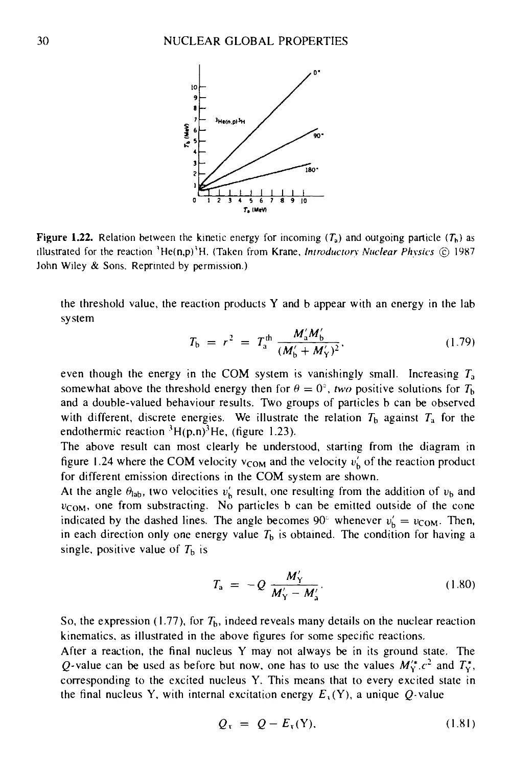
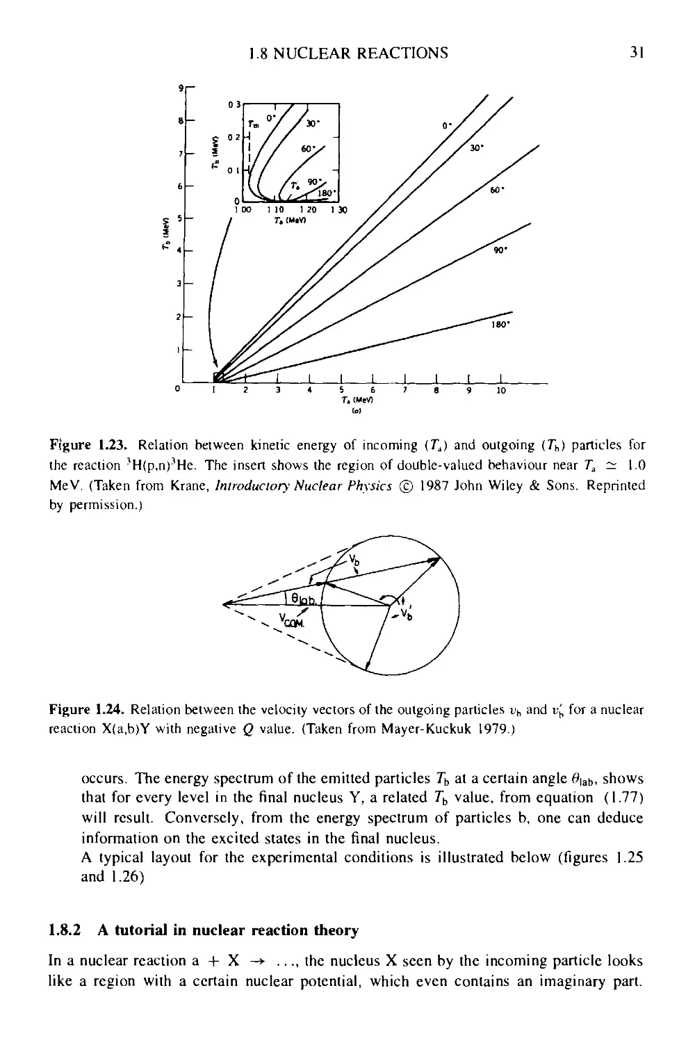
7~a, 7ь and the angle в. It is interesting to use the above expression in order to determine
7"b as a function of the incoming energy Ta and the angle в. Using the above equation,
as a quadratic equation in ^/%, we find
JTy, = r ±
with
/ЩЩтл
r \;
Mb + My
M^ + My '
Recall that we are working in the non-relativistic limit. In discussing the result for УТь
we have to distinguish between exothermic (Q>0) and endothermic (Q<0) reactions.
CO Q > 0.
In this case, as long as M'a < Л/у or, if the projectile is much lighter than the
final nucleus, one always finds a solution for 7"ь as a positive quantity. Because
of the specific angular dependence on cos#, the smallest value of 7|, will appear
for в = 18СГ. Even when Ta —*■ 0, a positive value of 71, results and
7"b ~ Q.My/(M^ + My). We illustrate the above case, for the reaction 3He(p. nKH
in figure 1.22.
(ii) Q <0.
In the case when we choose Ta —*■ 0, r —* 0 and now s becomes negative so
that no solution with positive T^ value can result. This means that for each angle в,
there exists a minimal value 7ath@) below which no reaction is possible. This value
is lowest at в = 0~ and is called the threshold energy. The value is obtained by
putting r1 + s = 0, with a result
lh M! + ML
T> - -gx+VV (L78)
It is clear that 7"ath > \Q\ since in the reaction process of a with X, some kinetic
energy is inevitably lost because of linear momentum conservation. Just near to
30
NUCLEAR GLOBAL PROPERTIES
~ 3H«n
I I I I I I I
3 4 5 6 7
r.iMtvi
89 10
Figure 1.22. Relation between the kinetic energy for incoming G"a) and outgoing particle G"b) as
illustrated for the reaction 'He(n,p)(H. (Taken from Krane, Introductory Nuclear Physics © 1987
John Wiley & Sons. Reprinted by permission.)
the threshold value, the reaction products Y and b appear with an energy in the lab
system
rth a b
= r = Тл
\2'
A.79)
even though the energy in the COM system is vanishingly small. Increasing T3
somewhat above the threshold energy then for в = 0\ two positive solutions for 7~ь
and a double-valued behaviour results. Two groups of particles b can be observed
with different, discrete energies. We illustrate the relation 7"b against Тл for the
endothermic reaction 'H(p,nKHe, (figure 1.23).
The above result can most clearly be understood, starting from the diagram in
figure 1.24 where the COM velocity vC0M and the velocity v'b of the reaction product
for different emission directions in the COM system are shown.
At the angle #iab, two velocities v'b result, one resulting from the addition of vb and
ucom. one from substracting. No particles b can be emitted outside of the cone
indicated by the dashed lines. The angle becomes 90° whenever ub = ucom- Then,
in each direction only one energy value 7~ь is obtained. The condition for having a
single, positive value of 7~ь is
= -Q
A.80)
So, the expression A.77), for 7"ь, indeed reveals many details on the nuclear reaction
kinematics, as illustrated in the above figures for some specific reactions.
After a reaction, the final nucleus Y may not always be in its ground state. The
Q-value can be used as before but now, one has to use the values My.c1 and 7~y,
corresponding to the excited nucleus Y. This means that to every excited state in
the final nucleus Y, with internal excitation energy £,(Y), a unique Q-value
Qx = G-£,(Y).
A.81)
1.8 NUCLEAR REACTIONS
31
5 6
Г, (MeV)
Figure 1.23. Relation between kinetic energy of incoming G"J and outgoing G"b) particles for
the reaction ?H(p,nKHe. The insert shows the region of doable-valued behaviour near Тл ~ 1.0
MeV. (Taken from Krane, Introductory Nuclear Physics © 1987 John Wiley & Sons. Reprinted
by permission.)
Figure 1.24. Relation between the velocity vectors of the outgoing particles vb and v'b for a nuclear
reaction X(a,b)Y with negative Q value. (Taken from Mayer-Kuckuk 1979.)
occurs. The energy spectrum of the emitted particles 7ь at a certain angle 0|аь, shows
that for every level in the final nucleus Y, a related 7"b value, from equation A.77)
will result. Conversely, from the energy spectrum of particles b, one can deduce
information on the excited states in the final nucleus.
A typical layout for the experimental conditions is illustrated below (figures 1.25
and 1.26)
1.8.2 A tutorial in nuclear reaction theory
In a nuclear reaction a + X -»• ..., the nucleus X seen by the incoming particle looks
like a region with a certain nuclear potential, which even contains an imaginary part.
32
NUCLEAR GLOBAL PROPERTIES
(b)
Accelerator beom
Qoadropde • cup y ~a
magnet \ v
Analysing
magnei
Scoitenng Detector
chamber
(c)
Number с f
particles b
IX.O)
Figure 1.25. Outline of a typical nuclear reaction experiment, (a) The experimental layout and
set-up of the various elements from accelerator to detector, (b) The energy relations (COM energies
7,'. 7"b) for the nuclear reaction X(a,b)Y. (c) The corresponding spectrum of detected particles of
type b as a function of the energy of these particles (after Mayer-Kuckuk 1979).
Thereby both scattering and absorption can result from the potential
U(r) = V(r) + \W(r).
A.82)
The potentials V(r) and W(r) can, in a microscopic approach, be related to the basic
nucleon-nucleon interactions. This process of calculating the 'optical' potential is a
difficult one.
The incoming particle can undergo diffraction by the nucleus without loss of energy
(elastic processes). If the energy of the incoming particle 7~a is large enough, such that
Aa « R (R is the nuclear radius) and there is a negligible absorption component
(W(r) ~ 0), the nucleus shows up as a 'black sphere" and a typical diffraction pattern
results (figure 1.27(a)). This is also discussed in Box lb and is illustrated here for +4He
scattering by 24Mg. In cases where 7"a is small, and with negligible absorption, standing
'waves' can be formed within the nuclear interior and thus, a large cross-section results,
for certain values of R (and thus of A) with respect to the value of 7"a. Such states are
called, 'resonance' states. The giant resonances are typical examples of such excited
states in which large cross-sections occur (figure 1.28).
It is possible that the light projectile a enters in the nucleus thereby exciting a single
nucleon from an occupied orbital into an 'unbound' (E > 0) state, with enough energy
to leave the nucleus (see figure 1.27(b)). In these cases, we speak of 'direct' nuclear
reactions. It could also be such that the incoming projectile a loses so much energy
1.8 NUCLEAR REACTIONS
33
Figure 1.26. Realistic energy level scheme for "B with all possible reaction channels. (Taken
from Aj/enberg-Selove 1975.)
that it cannot leave the nucleus within a short time interval. This process can lead to
the formation of a 'compound' nuclear state. Only with a statistical concentration of
enough energy into a single nucleon or a cluster of nucleons can a nucleon (or a cluster
of nucleons), leave the nucleus. The spectrum of emitted particles in such a process
closely follows a Maxwellian distribution for the velocity of the outgoing particles with
an almost isotropic angular emission distribution.
In contrast, direct nuclear reactions give rise to very specific angular distributions
which are characteristic of the energy, and angular momenta of initial and final nucleus.
Between the above two extremes (direct reactions—compound nucleus formation), a
whole range of pre-equilibrium emission processes can occur. In these reactions a
nucleon is emitted only after a number of 'collisions' have taken place, but before full
thermalization has taken place.
The whole series of possible reaction processes is illustrated in figure 1.29 in an
intuitive way.
We return briefly to the direct nuclear reaction mechanism by which a reaction
34
NUCLEAR GLOBAL PROPERTIES
(a)
? units]
_g
a.
|ю2
tn
1Л
о
о 10
1
\ a *Mg elastic scatt
\ R0--5 97tm
\
\
у ^
(b)
VIr)
l ч
8 10 12
2k Rosin|6/2]
U 16
Figure 1.27. (a) Illustration of the reaction cross-section for elastic scattering of alpha particles
on :4Mg. The various diffraction minima are indicated as a function of the momentum transfer,
(Taken from Blair et al 1960), (b) Schematic illustration of a typical direct reaction process (for
explanation see the text.)
.I.,,,,.,,-.
V^^-.-.^^^^.-.^^-^^
Figure 1.28. Typical regions of an excited nucleus where we make a schematic separation into
three different regimes: I—region of bound states (discrete states); II—continuum with discrete
resonances; and III—statistical region with many overlapping resonances. The cross-section
function is idealized in the present case. (Taken from Frauenfelder and Henley A991) Subatomic
Physics © 1974. Reprinted by permission of Prentice-Hall, Englewood Cliffs, NJ.)
1.8 NUCLEAR REACTIONS
35
shape elastic
scattering
t.
direct inelastic
scattering
same particle leaving
no collision I 1st coll. I 2nd coll I 3rd coll
other particles leaving
direct
reaction
Figure 1.29. Evolution of a nuclear reaction according to increasing complexity in the states
formed. In the first stage, shape-elastic scattering is observed. The other processes excite more
and more individual particles in the nucleus, eventually ending up at a fully compound nuclear
state. (Taken from Weisskopf 1961.)
Hint 'Г>
Figure 1.30. Direct reaction process where the nucleus X takes up part of the light fragment a,
releasing the fragment b and the final nucleus Y. The time scale is too short for equilibrium to
occur and a compound nuclear state to form.
a+ X —> Y + b can be described as follows. We can describe both the entrance and exit
channels in terms of an optical potential Ua.x(r) and Uby(r). The Schrodinger equations
describing the scattering process become:
- r A Xa.X + ^a.x(r)Xa.X = £a.xXa.X
2
2mb
+
A.83)
Here, та(тъ) is the reduced mass of projectile (ejectile) relative to the nucleus X(Y). In
a direct reaction, a direct 'coupling' occurs between the two unperturbed channels (a, X)
and (b, Y) described by the distorted waves Xa.x and Xb.Y- The transition probability for
entering by the channel Xa.x at given energy E3 x and leaving the reaction region by the
outgoing channel Xb.Y 's then giving using lowest-order perturbation theory by the matrix
36 NUCLEAR GLOBAL PROPERTIES
element (figure 1.30)
f.*x(r )//int(r )Хь.у('')dr. A.84)
The description of the process is, in particular, rather straightforward if a zero-range
interaction Hm(r ) is used to describe the nuclear interaction in the interior of the nucleus.
The method is called DWBA (distorted wave Born approximation).
A more detailed but still quite transparent article on direct reactions is that by
Satchler A978).
1.8.3 Types of nuclear reactions
The domain of nuclear reactions is very extensive and, as discussed before, ranges from
the simple cases of elastic scattering and one-step direct processes to the much slower,
compound nuclear reaction formation. In table 1.2, we give a schematic overview
depending on the type and energy of the incoming particle and on the target nucleus
(X), characterized by its nuclear mass A. In this table, though, only a limited class of
reactions is presented. In the present, short paragraph, we shall illustrate some typical
reactions that are of recent interest, bridging the gap between 'classical' methods and the
more advanced 'high-energy' types of experiments.
(i) The possible, natural decay processes can also be brought into the class of reaction
processes with the conditions: no incoming particle a and Q > 0. We list them in
the following sequence.
• a-decay:
• ft -decay.
у-decay:
Here, the nucleus could also decay via pair (e~ + e+) creation (if E >
1.022 MeV) or e" internal conversion, in particular for 0+ —> 0+ decay
processes.
• Nuclear fission
£Х„ -> z!Y". + £и*: + x.n.
• Particle emission (near the drip-line) with Q > 0, in particular proton and
neutron emission.
Various other, even exotic radioactive decay mechanisms do show up which are not
discussed in detail in the present text.
JV+l +
A v
Z-l '
e* + ve
e- + ve
?x*
(P
(n
(e
+
-*•
hv.
n-type).
p-type).
capture).
1.8 NUCLEAR REACTIONS 37
Table 1.2. Table of nuclear reactions listing reaction products for a variety of exprimental
conditions. (Taken from Segre Nuclei and Particles 2nd edn © 1982 Addison-Wesley Publishing
Company. Reprinted by permission.)
Energy оГ
incident particle
Low, 0-1 krV
Intermediate,
I 500 kcV
High, 0.5-10
MeV
Int.
n
'res.
fie].
res.1
nicl.l
7i' incl.:
p
■rmediate nuc
f
So appre-
appreciable
у
ires.'i
n
/-(inel.l
lei 30 >
a
No appre-
appreciable
n
у
p
(res. i
n
p
A >
- No
г
p
n
pn
90
Inc iden
d
apprr-
iable
i particle
n
у
nicl..
л el.:
у
;res.'i
P
H
N'
V.
л
!>•■
v
ea\ у пш
f
a appre-
appreciable
reartion
pry small
cross
section
inel.l
lei
,л > чо
No appre-
appreciable
reaction
V
f
v
ery small
cro^s
secnon
d
No apprr-
ciablr
reaction
\'ery small
cross
section
P
n
pn
(res. for (res. tor (re-s. for
lower lower lower
energies' energies) energies!
Very high. 2ri 2л 2л p 2л 2л 2ч р
10-50 MeV n:inel.; я п 2л n/ineU n n 2п
n(el.' /i(inel.' p рп п'\Л.; р finel. p tip
р np Tip Зл /' пр пр Згт
up 2p 2p (/inel.l pn '2p 2p <f[inel.'
1р х xinel.1 tritons 'lp i vinel.'i tritons
Three or Three or Three or Three or Three or Three or Three or Three or
more mote more more more more more. more
particles particle? particles particles partit les panicles panicles panicles
(ii) As outlined before, and presented in table 1.2, a large variety of nuclear, induced
reactions can be carried out. Most of the easy processes use accelerated, charged
particle beams with projectiles ranging from e~,e+ particles up to highly stripped
heavy ions. In the accelerating process, depending on the particle being accelerated
and the energy one is interested in, various accelerator techniques are in use.
One of the oldest uses a static potential energy difference realized in the Van de
Graaff accelerator, mainly used for light, charged particles. Various new versions,
such as the two-stage tandem were developed, and is explained in figure 1.31.
Linear accelerators have been used mainly to obtain high-energy e~ beams. At the
high-energy accelerator centres (CERN, SLAC, ...) linear accelerators have been
used to pre-accelerate protons before injecting them in circular accelerators. Even
circular, e~ accelerators have been constructed like LEP at CERN. By constructing
with a very large radius and thus, a small curvature, rather low losses due to radiation
are present. Also, special 'low-loss' radiofrequency cavities have been built.
Many accelarators make use of circular systems: cyclotron accelerators are very
often used in nuclear structure research (see the SATURNE set up at Saclay where
projectiles ranging from protons to heavy ions can be used figure 1.32). At the
high- and very-high-energy side, starting from the early AGS (Alternating-gradient
synchrotron) at the Brookhaven National Laboratory (figure 1.33), over the LEP
38
NUCLEAR GLOBAL PROPERTIES
charging belt
acceleration tube pressure vessel acceleration lube
for + ions for - ions
Figure 1.31. Two-state tandem accelerator. 1—source of positive ions. 2—canal for adding
electrons. 3—negative ions are pre-accelerated to 80 keV and injected into the Van de Graaff
accelerator where they receive a potential energy of 5 MeV. 6—the ions are stripped of electrons
and become positively charged by passing through a gas at low pressure. 7—the positive ions are
accelerated by a further 5 MeV so that their total potential energy is 10 MeV. The kinetic energy
of the emerging ions depends on their charge states in the two stages of acceleration, e.g. if single
charged in each stage their kinetic energy will be 10 MeV. 8—deflecting and analysing magnet.
9—switching magnet. (High-Voltage Engineering Corp.. Burlington. MA.)
e . e+ facility at CERN, projects are underway for building a superconducting
supercollider in the USA.
The scale of the AGS (Alternating Gradient Synchrotron) and the LEP installations
are illustrated in the following pages and thus, give an impression of the huge scale
of such projects (figure 1.34).
The accelerator mechanisms, projectiles used and various recent possibilities are
discussed in e.g. Nuclei and Particles, second edition (Segre 1982) and Box If.
In conjunction with the accelerator processes, the detectors needed to measure
the appropriate particles (energy, angular distributions, multiplicities, .. .), can
sometimes be huge, as in the high-energy experiments. Interesting physics should
result from the versatility in the detection systems and from the creativity of the
physicists running a particular experiment (figure 1.35).
Reactions that are attracting much attention at present, in recent projects and in
planned experiments, are heavy ion reactions. These will eventually be done using
heavy ions moving at relattvistic speeds. At Brookhaven, the RHIC (Relativistic
Heavy-Ion Collider), is being built (figures 1.36 and 1.37). The main aims are to
study the properties of nuclear matter at high densities and high temperature. It is
hoped that, eventually, conditions near to those that characterized the early Universe
will be created in laboratory conditions. For further reading, see the reference list.
1.8 NUCLEAR REACTIONS
39
Figure 1.32. Typical view of an accelerator laboratory. In the present case, the SATURNE
accelerator with the various beam lines and experiments is shown. (Taken from Chamouard and
Durand 1990.)
Figure 1.33. View of the alternating-gradient synchrotron (ACS) at the Brookhaven National
Laboratory showing a few of the beam bending magnetic sections (reprinied with permission of
Brookhaven National Laboratory).
40
NUCLEAR GLOBAL PROPERTIES
- ..■ <■■■■ ,';
. . ?■•■■■$ . '
: .*.v. г
■; <«.
'■ ^:i.X^,;-;.'./:
. :у- . . .- ■' .о •
... '>••■• *
^ У
кЪ ^4 У
■:' >. ■■■.:■ * .•;:.
. ..;..*ifi£sf:i ■ i ■■'■■■■:
■. ■■...■ j^... ..;....j.-
Figure 1.34. View of the LEP ring superimposed on a map of France and Switzerland where
CERN is sited. The ring has a 27 km circumference. The SPS ring is shown for comparison.
(Taken from CERN Publication 1982 CERN7DOC 82-2 (January) 13, 19.)
Figure 1.35. Open perspective view of the ALEPH detector used at LEP where incoming beams
of electrons and positrons enter head-on collisions in the central zone (adapted from Breuker el al
1991).
.8 NUCLEAR REACTIONS
41
Figure 1.36. Colliding heavy nuclei are used to study the nuclear equation of state. Here, two Au
nuclei collide slightly off-centre A). Matter is squeezed out at right angles to the reaction plane
B). The remaining parts of the two nuclei then bounce off each other C). (Taken from Gutbrod
and Stocker 1991. Reprinted with permission of Scientific American.)
42
NUCLEAR GLOBAL PROPERTIES
I
Figure 1.37. Relativistic contraction is illustrated in an ultra-high-energy collision between iwo
uranium nuclei, (a) A 1 TeV uranium nucleus, having a velocity of 99.999* of that of light,
appears as a disk, with a contraction predicted by the theory of special relativity. It encounters
the target-nucleus for about 10 2:s: a time much too short to reach equilibrium so the projectile
passes through (c). In this process, the temperatures reached may create conditions similar to the
early Universe, shortly after the big bang {b). (Taken from Harris and Rasmussen 1983. Reprinted
with permission of Scientific American)
BOX 1A THE HEAVIEST ARTIFICIAL ELEMENTS 43
Box la. The heaviest artificial elements in nature: from Z = 109
towards Z = 112
The 'Gesellschaft fur Schwcrionenforschung' (GSI for short) in Darmstadt succeeded in
1982 in fusing atomic nuclei to form the element with Z = 109 and a few years later to
form the element with Z = 108. In 1994 successful synthesis of elements with Z = 110
and 111 was carried out. These elements indeed have very short lifetimes, of the order
of a few milliseconds (ms), but could be identified uniquely by their unambiguous decay
chain. The group of Armbrustcr and Miinzenberg, followed by Hoi'mann, in a momentous
series of experiments making heavier and heavier artificial elements, in February 1996,
formed the heaviest element now known with Z = 112.
The group of physicists at the GSI, together with scientists from a number of
laboratories with long-standing experience in fusing lighter elements in increasingly
super-heavy elements (Dubna (Russia), Bratislava (Slovakia) and Jyvaskyla (Finland))
made this reaction possible.
The particular fusion reaction that was used consisted of accelerating 70Zn nuclei
with the UNILAC at GSI and colliding them with an enriched target consisting of 208Pb.
If an accelerated nucleus reacts with a target nucleus fusion can happen but this process
is rare: only about one collision in 1018 produces the element with Z = 112. Even with
a successful fusion between the projectile and the target nucleus, the 'compound' nucleus
formed is still heated and must be 'cooled' very quickly otherwise it would fall apart in
a short time. If a single neutron is emitted, this cooling process just dissipates enough
energy to form a single nucleus of the element with Z = 112 which can subsequently
be detected. The formation is shown in figure la.l (an artistic view) and in figure la.2
in which the precise decay chain following the formation of element Z = 112 is given.
Both the alpha-decay kinetic energies and half-lives for the disintegration (see Chapter 2)
are given at the various steps.
Figure la.l. Birth of an element: a Zn nucleus (left) hits a Pb nucleus, merges, cools by ejecting
a neutron and ends as an element with Z = 112. (Adapted from Taubes 1982.)
In addition to the element with a charge of Z = 112, additional nuclei with Z = 110
were shown to exist (with mass A = 273). According to present-day possibilities and
also supported by theoretical analyses, it might well be possible in the near future to
create elements with Z = 113 and even Z = 114.
44 NUCLEAR GLOBAL PROPERTIES
For more technical details, we refer the reader to Annbruster and Miinzenberg
A989), Hofmann A996), GSI-Nachrichten A996a).
;: С '
..............J
Figure la.2. Decay chain with a-decuys characterizing (he decay of the element with charge
Z = 112. (Taken from GSI-Nachreichlen. 1996a. with permission.)
BOX IB ELECTRON SCATTERING 45
Box lb. Electron scattering: nuclear form factors
In describing the scattering of electrons from a nucleus, we can start from lowest-order
perturbation theory and represent an incoming particle by a plane wave with momentum
it; and an outgoing particle by plane wave with momentum kj. The tranisition matrix
element for scattering is given by
Г1). (lb.l)
where
M
(*,-, kj ) = ^ f exp [i(*, - k, ).r] V(r)dF. (lb.2)
Starting from the knowledge of W(k,,kf) and the incoming current density — j.
one can evaluate the differential cross-section for scattering of the incoming particles by
an angle в within the angular element d£2 as
or
da т2
M(khk,)
(lb.4)
dfi 4л--V
This is the Born approximation equation which can be rewritten in terms of the scattering
angle в since we have (see figure lb.l)
?=»(*,-*,). (lb.5)
We then obtain the expression
with
For a central potential V(r), the above integral can be performed more easily if we choose
the c-axis along the direction of the ^-axis. So, we have
q • r = qr cos в',
dr = r2 sin в'AгAв'Aф, (lb.8)
and the integral becomes
/ exp I -q r jdr = J exp ( X-qr cosfl' j г ыпв'йгйв'йф'. (lb.9)
Using the substitution ; = (\/h)qr cos0', this integral can quite easily be rewritten in the
form
/"exp(Vr)dr= rS
J \b / Jo
46 NUCLEAR GLOBAL PROPERTIES
and for the scattering amplitude f(B) we obtain the result
f@)
_ 2m Г
M Jo
V(r)r sin(qr/h) ■ dr.
(lb.ll)
We now discuss three applications: A) scattering by the Coulomb potential 1/r; B)
scattering off a nucleus with a charge density p(r) (spherical nucleus); C) scattering by
a square well potential.
k,
Figure lb.l. Linear momenlum diagram represenling inilial (£,). final (jt;) and iransferred (</)
vectors in eleclromagnelic inleraclions.
Figure lb.2. Coordinates r. .v and ( in the scattering process (see text).
(i) Coulomb (Rutherford) scattering. Using the potential V(r) — Ze2/r. we
immediately obtain
and thus
2mZe2
s,\n(qr/h)dr
1 7 ^ Г ОС
Ш lim / sin(qr/h)e~r'"dr
hq «-»Jo
2mZe2
. -, 1
z
which is indeed, the Rutherford scattering differential cross-section.
(lb.12)
(lb.13)
BOX 1В ELECTRON SCATTERING
47
Figure lb.3. Angular distribution for elastic scattering on the square-well potential, as discussed
in the text, obtained using the Born approximation with plane waves (see equation I.b.20) and
with kRn = 8.35. The data correspond to 14.5 MeV neutron scattering on Pb. (Taken from
Mayer-Kuckuk 1979.)
(ii) Electron scattering off a nucleus. In figure lb.2 we show (he scattering process
where r is the radial coordinate from the center of the nucleus, t is the coordinate
of the moving electron measured from the centre of the nucleus with Г = r + s. The
volume element Zep(r)dr contributes to the potential felt by the electron as
Ze2
p(r)dr.
(lb.14)
Now, (he scattering amplitude ((в) becomes
mZe2
2nh2
/ / exp | -q • (r + s) | drds
f / i - Л - mZe2 f \ / i , Л -
= / p(r)e\p[-q-r\dr.-—j / - e\p I-q ■ s \ ds
J \h ) 2nh- J s \h )
= /
Jo
sm(qr/h)
(qr/h)
2mZe2
—
hq
(lb.15)
The final result for daldQ is modified via the finite density distribution p(r) and
the correction factor is called the charge nuclear form factor F2(q) and contains the
48 NUCLEAR GLOBAL PROPERTIES
information about the nuclear charge density distribution p(r). Thus one has
In comparing a typical electron scattering cross-section, as derived here, to the
realistic stituation for 2(wPb (figure 1.8), the measured cross-section, as a function
of the momentum transfer q, can be used to extract the p(r) value in 208Pb.
(Hi) Scattering by a square-well potential. Using a potential which resembles closely a
nuclear potential (compared to the always present Coulomb part) with V(r) = — Vo
for r < Rq and V(r) = 0 for r > Ro (where Ro is the nuclear radius) we obtain for
fW)
/(fl)= ~ mV° I rs\n(qr/h).dr. (lb.17)
nq Jo
The integral becomes
(h2/q2)\s\n(qr/h) - (qr/h)co&(qr/h)}. (lb.18)
and the cross-section is
da ,1 "
kin(qR0/h) - (qR0/h).cw(qR0/h)V .
From figure lb.l. we obtain the result that q = 2Д:й sin@/2) with к = k, = kf
for elastic scattering. Using this relation between q and the scattering angle, we
can express dcr/dfi, for given к and Rq, as a function of the scattering angle в and
obtain
0-/?g [sinB*/?osin0/2) - 2А:Л0 sin0/cosBAr^osi0/2)]
This scattering cross-section, which is valid at high incident energies, results in a
typical diffraction pattern. A large contribution occurs only for forward scattering
if qRq < \.or sinfr/2 < l/2fcflrj. In figure lb.3, we compare the result using
equation lb.20, with kRo = 8.35, with data for 14.5 MeV neutron scattering on Pb.
Even though the lit is not good at the diffraction minima, the overall behaviour in
reproducing the data is satisfactory.
BOX 1С OBSERVING THE STRUCTURE IN THE NUCLEON
49
Box lc. Observing the structure in the nucleon
Nobel Prize 1990
The mosi presngious award in phy-
physics weni ihis year 10 Jerome I.
Friedman and Henry W. Kendall,
boih of ihe Massachuseiis Insmuie
of Technology (MIT|, and Richard
E. Taylor of Sianford 'for iheir
pioneering mvestiganons concern-
concerning deep melasiic scaitenng of el-
ecirons on proions and bound neu-
irons, which have been of essemial
imponance for ihe developmem of
ihe quark model m panicle phy-
physics'.
Their expenmenis. earned oui
from 1967 ai ihe ihen new iwo-
mile Imac ai ihe Sianford Linear
Accelerator Cenier (SLAC) showed
lhai deep inside ihe proion ihere
are hard grains, miiially called par-
ions' by Feynman and laier idenn-
fied wuh ihe quarks, maihemancal
quirks which since 1964 had been
known to play an imporiam role in
understanding the observed variety
of subaiomic panicles.
These inmal forays mio high en-
energy eleciron scauermg discovered
lhai a surprisingly large number of
ihe elecirons are severely deflecied
inside ihe proion largeis Jusi as
ihe classic alpha panicle resulis of
Ruiherford earlier ihis ceniury
showed lhai ihe aiom is largely
1990 Physics Nobel Prize people - left to
right, Jerome I Friedman and Henry W
Kendall of MIT. and Richard Tayior of Stan-
Stanford
(Photos Keystone)
empiy space wiih a compaci nu-
nucleus ai us cenire, so the SLAC-
MIT experiments showed lhai hard
scauermg cenires lurked deep in-
inside ihe proion.
Wriung on ihe wall for this
year's Nobel Prize was the award
lasi year of ihe Wolfgang Panofsky
Prize (sponsored by ihe Division of
Panicles and Fields of ihe Ameri-
American Physical Socieiyl ю ihe same
ino for iheir leadership in ihe firsi
deep-melasiic eleciron scauering
expenmenis 10 explore ihe deep in-
lenor of nuclear panicles
In ihe early 1960s when con-
siruciion of ihe SLAC linac was
getting underway, the 1990 Nobel
tno, who had firsi mei in ihe
1950s as young researchers ai
Sianford's High Energy Physics
Laboraiory, came logeiher m a col-
laboranon preparing ihe deieciors
and experimemal areas 10 explon
ihe new high energy eleciron
beams.
The ouicome was described m
an arncle (Ociober 1987, page 9)
by Michael Riordan, subsequemly a
member of the experimemal colla-
boranon and now SLAC's Science
Informaiion Officer, for ihe 20ih
anniversary of SLAC's electron
beams.
In Ociober 1967, MIT and SLAC
physicisis sianed shaking down
iheir new 20 GeV speciromeier;
by mid-December ihey were log-
logging eleciron-proion scauering in
ihe so-called deep inelasnc region
where ihe elecirons probed deep
inside ihe proions. The huge ex-
excess of scauered elecirons ihey
encoumered ihere - aboui len nmes
ihe expecied raie - was laier mier-
preied as evidence for poimlike,
fracnonally charged objecis inside
ihe proion.
The quarks we lake for granied
today were ai best 'maihemaiical'
enniies in 1967 - if one allowed
ihem any irue exisience ai all The
majoriiy of physicisis did noi Their
failure lo lurn up in a large number
of^mteniional searches had con-
convinced mosi of us lhai Murray Gell-
Mann's whimsical eniines could
noi possibly be 'real' panicles in
ihe usual sense, jusi as he had m-
sisied from ihe very firsi.
CERN Courier, December 1990
1
50
NUCLEAR GLOBAL PROPERTIES
Jerome Friedman, Henry Kendall,
Richard Taylor and ihe oiher MIT-
SLAC physicisis were noi looking
for quarks thai year. SLAC Experi-
meni 4B had originally been de-
designed to siudy ihe eleciroproduc-
lion of resonances. Bui ihe prod-
dings of a young SLAC iheonsi,
James Bjorken, who had been
working in current algebra (ihen an
esoteric field none of ihe experi-
meniers really undersiood), helped
convince ihem 10 make additional
measuremems in ihe deep inelasnc
region, 100.
Over ihe nexi six years, as firsi
ihe 20 GeV specirometer and then
iis 8 GeV coumerpan swung oui ю
larger angles and cycled up and
down in momemum, mapping oui
ihis deep inelasnc region in excru-
excruciating deiail, ihe new quark-panon
piciure of a nucleon's innards
gradually look a firmer and firmer
hold upon ihe panicle physics com-
community. These two massive spec-
iromeiers were our principal eyes'
into the new realm, by far the best
ones we had uniil more powerful
muon and neutrino beams became
available ai Fermilab and CERN.
They were our Geiger and Mars-
den, reporting back ю Ruiherford
ihe deiailed paiterns of ricocheiing
projeciiles. Through iheir magneiic
lenses we 'observed' quarks for
ihe very firsi lime, hard 'pits' inside
hadrons
These iwo goliaihs siood reso-
luiely ai ihe front as a scientific re-
voluiion erupted all about ihem
during ihe late 1960 s and early
1970s. The harbingers of a new
age in particle physics, they helped
pioneer the previously radical idea
thai lepions, weakly inieracting
particles, of all things, could be
used 10 plumb ihe mysteries of ihe
sirong force. Who would have
guessed, in 1967, that such spind-
spindly particles would eventually ferret
out their more robust cousins, the
quarks? Nobody, except perhaps
Bjorken-and he wasn't too sure
himself.
(The saga is recounted in every
detail in Hiordan's book 'The Hunt-
Hunting of the Quark', published by Si-
Simon and Schuster.)
1990 Physics Nobel Prize apparatus - the
big spectrometers at End Station A of the
Stanford Linear Accelerator Center fSLAC) in
196'7- right, the 8 GeV spectrometer, and
left, us 20 GeV and (extreme left} 1 6 GeV
counterparts
CERN Courier, December 1990
(Reprinted from CERN Courier 1990 (December) 1, with permission from CERN.)
BOX 1D ONE-PARTICLE QUADRUOPLE MOMENT 51
Box Id. One-particle quadrupole moment
Consider the motion of a point-like particle with charge q rotating in a circle with radius
R outside a spherical core. Neglecting interaction effects between the particle and the
core, we obtain for the intrinsic quadrupole moment Q,ntr
Q,ntr = q0z'2-R2) = -qR2. (ld.l)
Using the semiclassical arguments discussed before, one obtains for the possible values
Q(J, M), the expression
ЩЯ1'
Thus, the quadrupole operator, Q, has 7+1/2 distinct eigenvalues, corresponding to
the value of M(±M), when evaluating its expectation value by a semiclassical method.
By convention, Q(J, 7) is called the quadrupole moment of the corresponding quantum
state and is denoted by Q. For the above point-like single-particle motion one obtains
W^r2-»
or
e = -*eri-*2' (ld4)
for 7/0.
In a more precise way, if a radial wavefunction Rni(r) is associated with
the single-particle motion, one has to replace R2 by the average value (r2) =
/0°° Rni(r)r2Rn((r)r2dr and obtain the results
Q = -я-ш\(г2)ы J Ф o,
(ld.5)
B = 0 7=0,1/2.
This model can be used for a doubly-magic nucleus with an outer additional nucleon
outside or a single nucleon missing from a closed shell. One can evaluate the average
value of Q if one simplifies the radial wavefunction to a constant value within the nuclear
radius R = r0A]/*. One then obtains (r2) = |л2, and the results
Q - -\eR2jj^i for an extra particle 7 / 0,/ \.
(ld.6)
Q = \eRl тт for anextra 'hole< J Ф
Here, we have assumed that the extra particle is a proton with charge +e and that a
proton hole has charge -e. The corresponding distribution is represented in figure ld.l.
A measure of nuclear deformation, independent of the size of the nucleus is obtained
from the value of the reduced quadrupole moments, Q/ZR2, where R is the radius of
the sphere. One observes in figure Id.2 that near to closed shells, quadrupole moments
52
NUCLEAR GLOBAL PROPERTIES
Figure ld.l. Coordinates used to evaluate the intrinsic quadrupole moment of a single nucleon
with charge q in a circular orbit with radius R.
ZR'
30-
-10
T I Г T Г
пег*
I I I I
I I I I I I
20
60 80 100
no. of odd nudtons
120 140
Figure Id.2. The reduced nuclear quadrupole moments as a function of the number of odd
nucleons. The quantity Q/ZR2 gives a measure of the nuclear quadrupole deformation. (Taken
from Segre Nuclei and Panicles 2nd edn © 1982 Addison-Wesley Publishing Company. Reprinted
by permission.)
BOX ID ONE-PARTICLE QUADRUOPLE MOMENT 53
agree well with a single particle (or hole) outside an inert, spherical core. In some
regions though, very large quadrupole moments occur. Rainwater A950) suggested that
motion of the single particle deforms the whole nucleus and that the observed quadrupole
moment results from a collective distortion of many orbits. This collective model has
been developed by Bohr and Mottelson since 1952. Using this model and the concept
of nuclear deformation, landscapes have been mapped (see figures ld.2 and figure ld.3).
These dramatically show the strongly pronounced spherical shapes associated with closed
shells at certain N and/or Z values. The measure of deviation from a spherical shape
can be given using various parametrizations of the shape, e.g. the ellipsoid with axial
symmetry, as in the Nilsson model (Nilsson 1955).
Moreover, a nucleus can change its shape when rotating. It has been shown, quite
recently, that important modifications to the nuclear shape show up at high rotational
frequencies (Simpson et al 1984).
The predicted shape variations are shown in figure ld.4 where the nucleus is depicted
as rotating in the plane of the figure. At low spin, the nucleus has a prolate shape relative
to the symmetry axis, denoted by S. At intermediate spins the rotation forces some matter
into the rotating plane, but now the axis S is no longer a symmetry axis and the nucleus
becomes triaxial. At high spins, the matter is distributed in the plane of rotation, but
again in a regular pattern. Now, the symmetry axis coincides with the rotational axis and
the nucleus flattens into an 'oblate' shape. It is this latter set of shapes that was observed
in l58Er by Simpson et al A984).
In order to understand the experimental signature for such shape changes, one must
consider the concept of 'rotational frequency' for a microscopic object. The nuclear,
excited states are strictly characterized by the angular momentum quantum number
7, rather than a>, which is a classical quantity. A rotating nucleus gives rise to a
rotating, deformed electric field which can emit electromagnetic radiation. The rotational
frequency of the nucleus can then be deduced from the frequency of the emitted y-
radiation. If the concept of genuine rotation is meaningful in the nucleus, this quantity
should vary in a smooth way as a function of the energy in l<18Er, relative to that
of a classical rotor with the same spin and frequency. In figure ld.4, one observes,
however, some frequencies u>\, а>гУ шроУ. - - where the classical frequency almost stays
constant whereas the energy increases rapidly. These points correspond to a breakdown
of classical motion due to specific shell-model aspects, known as 'rotational alignment'by
which nucleons tend to become localized in the plane of rotation and thus contribute to
the triaxiality of the system.
54
NUCLEAR GLOBAL PROPERTIES
Figure ld.3. A nuclear 'landscape' of shapes. The total energy as a function of nuclear mass
and of the deviation from the spherical shape, as a reference level, is illustrated in a contour
plot. Calculations are from Ragnarsson and Nilsson. The lowest-lying areas (dark regions) are the
'valleys' corresponding to minimum energy and to the stable, spherical nuclei. The most stable
regions correspond to the D0,40), E0,82) (82,126) (Z, N) combinations. The side-valleys (shaded
regions) correspond to less stable prolate-shaped nuclei.
Low u intermediate u
r . /s
High u
Figure ld.4. Typical rare-earth shape changes as a function of increasing rotational frequency
w (see text in Box Id). In the lower part, the energy of the nucleus 158Er, relative to that of a
classical rotor ErM with the same angular momentum J and frequency ш. Angular momentum
values are indicated along the curve and are in units of h. (Taken from Rowley 1985. Reprinted
with permission of Nature © 1985 MacMillan Magazines Ltd.)
BOX IE AN ASTROPHYSICAL APPLICATION 55
Box le. An astrophysical application: alpha-capture reactions
St&rs are ideal places for manufacturing elements such as carbon and oxygen, which are
the basic constituents of planets and people. All those elements that have been formed,
though, very much depend on some remarkable coincidences in the laws of physics,
sometimes also called the 'antropic' principle.
About 75% of a star is hydrogen, about 25% is helium and a mere 1% or so consists
of heavier elements: this proportion is an important clue that all heavier elements (C,
O, ...) have been manufactured inside of the stars. This process of nuclear synthesis is
quite well understood (see Fowler 1984), though a number of key difficulties remained
for some time. It was known how the present abundances of hydrogen and helium and
some other light elements such as deuterium and lithium were created in the early phase
of the universe formation, starting from the 'standard' model. Even early studies in 1950
by Gamow indicated the difficulties of forming heavier elements by synthesis inside stars.
But how do stars perform this 'trick' ?
We know that the nucleus 4He is extremely stable (~ 28 MeV of binding energy)
and so, nuclei which form an a-like composition show an increased stability compared
with nearby nuclei. Carbon C a particles) and oxygen Da particles) are particularly
stable elements in that respect. Once these elements are formed in the right quantities,
heavier element formation looks quite straightforward using the subsequent interaction
with a-particles (in stars or in the laboratory).
A problem showed up, however, at the very first stages. Two 4He nuclei can form
8Be if they have the correct kinetic energy (Q = -0.094 MeV). The nucleus 8Be, though,
is extremely unstable, breaking apart again into two 4He nuclei, within a lifetime of only
~ 10~17 s. So, how then can I2C be formed which even needs an extra 4He nucleus to
merge with 8Be to form a I2C nucleus.
In 1952, Salpeter suggested that I2C might be formed in a rapid two-step process (see
figure le.l) with two 4He nuclei, colliding to form a sBe nucleus which was then hit by a
third 4He nucleus in the very short time before desintegration took place. Hoyle, though,
puzzled out that, even though the above process looked highly exotic and unprobable, the
presence of a resonance level in l2C might make the process feasible. This coincidence,
proved later by Fowler, allows indeed the formation of 12C and thus of all heavier
elements. When two nuclei collide and stick together, the new nucleus that is formed
carries the combined mass (minus the mass defect caused by the strong interaction forces)
plus the combined, relative kinetic energy of motion. It now occurs that in the reaction
sBe + 4He + 7нс ->■ l2C*.
a resonance in 12C* is formed at 7.654 MeV excitation energy and a COM kinetic energy
of 0.287 MeV is needed to come into 'resonance' with the excited state in 12C. The
temperature inside the stars is such that in He-burning, the thermal motion can supply
this small energy excess.
The combined mass M'(sBe)c2 + M'DHe)c2 = 7.367 MeV, just about 4% less
than the l2C* excited state of 7.654 MeV. It is this coincidence which has allowed 12C
formation and that of heavier elements (figure le.2) (Gribben and Rees 1990 and Livio
etal 1989).
56
NUCLEAR GLOBAL PROPERTIES
■
0 287
"V 0* -
* 7654
7367
8Be^a
£439
12C
I
1
1
1
| 2
|
1
leTtf)
|
|
r
Ю
111
b\
о
а:
UJ
0
Figure le.l. The formation of i:C: two 4He nuclei collide to form "Be. Occasionally, a third
4He nuclei can combine to form I2C in an excited state. The pictorial description of this process
is depicted in the left-hand part. The reaction energy balance is explained and illustrated in the
right-hand side.
BOX IE AN ASTROPHYSICAL APPLICATION
57
:«№.:
Figure le.2. The more detailed reactions leading to the possible formation of 8Be (in the ground
state or any of its excited states). (Taken from Ajzenberg-Selove 1960.)
NUCLEAR GLOBAL PROPERTIES
Box If. New accelerators
/-U7/ before the foundations of the Superconducting Super Collider f.S'.S'C'j have been laid in Texas,
people are brooding about the next generation of particle accelerators.
К ilu кк-пып,,1о£\ ol the panicles ol
мим с г i (иi should 1,-M-i hni which .14 \ci.
Jo 1НЧ the Hi^s hos.-rl k.tlkci // ) is
niHMiii ihe пьы conspicuous Ib precik-
.iiiil c\i*ieiH.c is .1 corner si one iИ ihe
LT.illJ lillltk J iheork's >'l ili.ilfcr .1 uWI-
>ci|iicike ot ilic .i-wuim'tric 1 hi.ii ni.irk
ilk' low-oien:\ world лс In с 111 Natur.ilh ,
■.Atrv new .uccleuror comiriiMrito opera-
operation r.K*-f4 people's hopes that thrs time.
\ir .-hi4\e pjfin.lL' «ill he loguJ And
-nil Mew accelerator disappoints
H11I is 11 possible lh.il 1 he .K-.ekr.itor
people h.ive heen looking in the wronj;
pl.iL i.-- ' (V in iru- iiili I pi.Kes m ilic w rone
•*.i\s' Икм iru\ be the implication ot an
.iruinutni пом. piii torw.ud h\ Richard
Ц1.нгксп1чч1сг .irk! Sidnc\ I) Drell ol the
Si.niIntJ I 111e.11 Accelerator ( enler
|/р/|и R< , / ,r/ «it M^4 |4sm I o he
(.in Hlaiikc-fitviler .ind [Veil .ire not sn
niikti coiKcrncd ro cheer on ihe hunt lor
ilk Hitps hoson ,is In ijukle the Je-itn o|
'In.
ol
irtulc
ck
ncu .iltcl lllosi- no» bcilli! Innll (III' .il
( >iiu\.i .1 Mil i'* ciiinv.ilcnt .K Vrpukhov I
..i .ih-uit lobclSM'lll tcvlsl
lUu.ml those in.khmo .ill iiliul.il
.,ч1'кт.!1ог* [hive .iff likek I.' follow
ill .i p.in ">t linear
ele
i! he.1
ol c
'rrs ,nul positionv lot 1 ii-4l eleitroirsi .it
nh othei In he uoilhvtlnk (he p.irti-
k> .11 e.iJi Iv.nn vs.HI lU\e In he awvii
ii'i^ L-ie.itei tli.ui NKI t.e\ ккп1К I
e\ .4 mole whuh-Aoilklnol heposvihle
,i iii4iil.ii in.к lime I44.1U4 innsi ot the
neri-л fUif info ,n.^e-ler.ifioir woulii he
.ипргК i.kIi.iU-lI .m.i\ ,ii;.nn .1- s\ [Kill и-
'П i.nii.ili.m So\ let рЬ\«.ц.1«.Г-. .il \
.ill,
1.1,
;J .1 III
.■III
..I Ihi4 kind
H.ikit hv Ilk ,lc
rJ
I'eer
loss и( energ\ in Ihuse parts ot a tr.tjeetors
111 "Ahii/h inier-utHins ;ire supposed not |o
oeeur h\ shapin-tt Ihe еоипкт-агеи1аппц
beams .ippropnatfl\ ■ gixinp e,ieh of
1 hem ,1 nhhtiri-like crnss-sceiiun tor
ev^imple . so that I heir interperietraliorl is л
minimum
Bui u-h.it happen-, when the oppositeh
(uitellni£ (Karris arc sluped riot чо js tt>
ntirumi/e the Uks о I ener^s h\ thrs mcthj-
nism, huf to пымпи/е 'I ' I hen. the
argument eoes (here will he a^pioiis
pro ilia tn hi ot single photons, hut the
I'hiFMi'i' nt produLirij; p.nr-i ot phorons мгп-
ult.iruuisl\ «ill be disproportionate^
\\ К
sihle
I Ik
«ill Lten le.Kl to the production ot p.nrsol
plioiolis sut(reientl\ oner^etre lor rhe-ir
mier.Ktion toe\hrhit ph\sitjl phenomen.i
nor oiherw, ise* easiK oh\er\.ihle '
the.inswer 11 *аг|1 hj\e heeriiiui-Nsed is
\es Ihe tnsl sle-p. (he e.ik iit-itmn ol the
Lh.irKe th.it a sin^k* екччгоп in .1 lr.i\elhnu
pulse ol.s.i\ do. Irons* ill uiter.iet wilh j
positron heli) lor the sjke ol the .н^и
nrenf. lr\e*l in sp.ke t^ -n.,tli.ul.ittofi tor the
leu hooks ol quantum cleilrixlsn^iiiics
WI1.1l emerges from it is л hirielion
es-enti.ilK .( proh.fhiliK ttistr that ion
speirKini; Ihe «.h.nae lh.il Ihe nio\int
ot its monieriUini lo r.idi.ilion in the lorrn
ol single photons Str,nii!eK i.ikul.ilirii;
the ilniiiiv that p.nrs ot photons *\\\ he
proJiKed is Ihen л iI.issil.iI proh.ihilitx.
.llnll.l
lH
p'
i. unioinh tori.es within .1 ir.i^elliiie pulse
ol eh.1ri.44i p.irfieles repe.ifei.lk destrov
fire toheu'riie ot llie motion tir fhe eiul
the ^ikul.Hion h.is to he lunnerK.il hut
the resulb .ire elear eut
llnelb lire nrter.ii.lion ot rihKui-sh.i(xd
.rls<
ieh p.n
mdistinguishahk* trom th.il ol hthti -u^h
thiit seen end-on ihere are IM eleeuon-
or positrons per squjrc eentimeire ol
crossseetktn 1 he^ do not menlion lh.il
lor priiche.il purposes ihe lalerjl dimen
Mori o( the pulses w.i|| he measured hi mi\
nol centimetres hut th.it is standard pr.a ■
tree in electron .lccelerjtor l.rhor.itones
And the length (ar resr rn the lahoralor».
fr.ime) nf e-ach pulse will he r.irhei less
than n millimetre
Wh.it. in ihesf Lircumstanei's will ihe
copious production ot enertetu ph'H.in
pairs produce1 This iv where rhe Hin^
huson ponies rn for .i>. л particle whose
cvrsterii'c stems I r0111 the .is\ mnie*rr\ in ihe
real workl hctwi4'n strong, weak and eke
trom.ijini-di. tori.es // miiNi inler.ni *iiti
alnuist e\er\thini> in si^ht In parln.ul.ir
e\cri thouiih it m.i\ lack ekMra i h.irire ir
should he produced as a srniile .md recoi:
111/ahle eniit\ in Ihe niler.iclnni o| rw.i
sulheieniK encriietic photons
Kirt o| the trouhlc- with // is Hi,,1
nohoih knows how m.issi\e it m,i\ he rH,i
ft\e lo <'ther p.trfkle-s. huf I here <■■ ,i\ (e.i-l
.1 iJunee (h.it 11 ihe m.tss |s kvs th.in those
ot Ihe mlermeOrate ^eelor hoson- nieji.i
ftng fhe we.ik rmelear irifir.tctiini Ihe II
.mil / so l.ir recognized onl\ .11 ( I K\
f Ы
tlu
elier
n[ p.irlkks jieneraii-U h\ oihei тсць
llut it Ihe Hl.isv ot the I lli!j.'s biivin м
i-re.iter than Ihe еци^ак-Щ nt Mm de\
there witl he .1 greater ch.nin' ol Inuiint
Midi's hosiins 111.111 eleilrnn collider wh.o>e
he.iflls h.ne heeli .ippropruiek shaped ro
enhairee double photi 111 intel.ktion fh.m
nr ihe Oireil coll won ol oppnoiklv
charged ek-cfronv Blam kenhe-ckl Jiki
Drell s.i\ lhal Ihe oh\ioLi«. evpennieiit
Kfi
iniL comes n will he hinlr .if Serpnkho\
n ihe I infect St.iics ,nKl I июре. theie
г, .iK.tfHitpk woikiiti: ,iv.i\
П1.пгкч'гг1ччк-1 .mil 0>c'U .не tirsi юн
шщ1 will) , nu4li.iiiisni In uhnh v'lli
Ol I k
'■'IhJ.'I ,mi-i ni питч uiiilui .im-ki
m. .in.i «huh ныв,, ni ilu n.iiiK
:, li'4i.ik!^ i iK .и mill ,'l Iv .iilivn.ib
■i-_- In .null.и „,ik(.i:,,|s ni whktl
I ^. ,'l pi'Silnwis ,iuU-U4li,,|i. Jl, iiKU
:v.w in ,'pposiK .liun.oils inr iv.iinpli
"!• i'l (Mlllli,'' Wilt piillllKl' pflilli'llS
■I ill !(КЛ tiXIl,- di'S,- 1И1.Н U ,,ltKI ^ \i(l И
ill [Mltl.K Ili'll !• 1ПЧ ЧП MIIUTI.ik .(S N1
Vlilln II is ,U.I.-ill.,l\ !,, lnhh,- llK
clleiilc'ik plrniorb 111.Л nrleiacf with e.kh
olhei hut pirKes v\ith sqn.it elliptk.il
^rovs-M-iiioriv will he rel.it»vcl\ prolrtu
snuries ill flu m i he c'sseine ot the .ir^ii
nient is ihi ^oiKlusioti that I here should he
viiciMiisijiKc. hi which tjieJul shanini! ol
wupki bf c\pt4tti.i ы \4*ld In с % с ш ^ ,i
d.i\ hut ih.it upfiiin/inulht- hc.tnish.ipi- to
I Ik iiilin.'sl "M llns .iiL'ununt i^ noI 1,1
.4
»l k-
•lln
ihi Ji.
.■^Р.1Г.П1-РЧК-О.
.Ill ,1Ш'1СГ.1|КГ «ill
,.| Ph,.|,m plb.lon
IMULKlll'llS 1П SC4T.lt i4,klS Hi lll.lillll
Huk Imn ," Ii4-pi'itui»
II IS W.Ultl Klldlllli; ,41 lilt in.ltlllUull- I IJlll .НС .111 UllllllUir.lU'J niHS.HKl 111.I*
ol wll.tl is ршромч! "hktl ...II t't totj i llllst.lktll II vMtlt4'(Ilk Itsllllkl I,'sit tb
triirn Itlt illiini.lk.ll I'Vllllpk'S wild wtlktl ,|lli,kiv Itl, J,S|^ik-|S itspniu! t^\ .in.i
Ml,l(kktllt4, Iff .111,1 Drcll lllnsti.ik1 Itkir L'KIL' IO UlMf I tk .Ц.1ГЧ1 i'l ttk' if,'
cilticv |U'.,plt sli.nllil ht lo,ikini;t.,r // .4
оси ih.u liiuit^li ptmlnn mici.Kiion. .iri
Ihe lllcili.lllisill \n «hkh 4 should 1ч
solicit Inn Ih.ll Itk- i,,|Ucilh,Ml.it v\isit.,n-
ol lll.utlillc litsiillk-rs lti.il t4',inisll,ltll.Hi
I pi
III
hnu \Miti ..
John Miiddov
(Taken from Maddox. Reprinted with permission of Nature © 1984 MacMillan
Magazines Ltd.)
GENERAL NUCLEAR RADIOACTIVE DECAY
PROPERTIES AND TRANSMUTATIONS
2.1 General radioactive decay properties
Here, we shall start to discuss the decay of a given nucleus irrespective of the precise
origin causing the transformation. This important problem and the related physics
question on how to calculate the decay rate using time-dependent perturbation theory
will be attacked in the following chapters on a-decay (strong interaction decay process),
/3-decay (decay caused by the weak interaction) and /-decay (originating from the
electromagnetic interaction). See figure 2.1.
V
У
*-]*.. ■
К''
Д
у
р
ч
Figure 2.1. The initial nucleus ^\n with the various final nuclei that can be reached via the
indicated decay processes (taken from Krane 1987, Introductory Nuclear Physics © 1987 John
Wiley & Sons. Reprinted by permission.)
The decay law of radioactive substances was first clearly formulated by Rutherford
and Soddy as a result of their studies on the radioactivity of various substances (notably
thorium, thorium-X and their emanations).
Disintegration constant, half-life and mean-life. A radioactive nucleus may be
characterized by the rate at which it disintegrates, and the decay constant, half-life or
mean-life are equivalent ways of characterizing this decay. The probability that a nucleus
decays within a short time interval d; is A.d;. It is the quantity A. G" is its dimension)
59
60
GENERAL NUCLEAR RADIOACTIVE DECAY
which determines the rate of decay. This decay process is a statistical process and we
cannot say anything particular for a given nucleus: we can only speak in terms of decay
probabilities. Suppose we start with Nq nuclei of a certain type at a hypothetical starting
time ?()=(): then the number of nuclei disappearing can be given by the expression
dN = -\Ndt, B.1)
which is easily integrated (with initial conditions N(t = 0) = No) with the result
N(t) = /Voe~'(. B.2)
The above law is the well-known and fundamental law of radioactive decay. Starting
from this expression, a time can be defined t = T (half-life) at which the number of
radioactive elements has decreased to half of its original value, i.e. No/2. This leads to
the value
T = — = г In 2 = 0.6931472... r. B.3)
Л
where r(= I/A.) is a characteristic decay time which we show is equal to a mean lifetime
for the decaying radioactive substance. The above exponential decay curve is illustrated
in figure 2.2 where both the e~'( as well as its presentation on a logarithmic scale are
given.
1.0
0.5 ---
I o.i
I 0.05-
0.01
. • _ J
1
1
---
_ \- _
1
\
- - -
i К
, ! ;\
T X 2T 3T 4T 5T CT
Time (in units of half-life, T)
T X 2T 3T 4T 5T CT
Time (in unit» of half-life, T)
Figure 2.2. Radioactive decay curve (on both a linear and a log scale) as a function of the elapsed
time (given in units of the half-life T). (Adapted from Kaplan. Nuclear Physics 2nd edn © 1962
Addison-Wesley Publishing Company. Reprinted by permission.)
Evaluating the average lifetime of the atoms, we known that at a certain time ;, we
still have N(t) = N^c^''' radioactive nuclei. Of these N{t)Xdt will decay between ; and
; + d; and thus
■=-f
No Jo
XtNoc~'"dt = - = т.
Л
B.4)
2.1 GENERAL RADIOACTIVE DECAY PROPERTIES
61
In table 2.1, we show the half-life T for some of the longest-lived nuclei. These half-lives
are of the order of the time scale describing slow transformations in the Universe.
Table 2.1. Some characteristics of the disintegration series of the heavy elements. (Taken from
Krane 1987, Introduclon Nuclear Physics © 1987 John Wiley & Sons. Reprinted by permission.)
Name of series
Thorium
Neptunium
Uranium
Actinium
TypeJ
An
An + 1
An+ 2
An + 3
Final
Nucleus
(Stable)
2A«Pb
2<NBi
2l*Pb
207 pb
Longest-lived member
Nucleus
-"Th
:"Np
:'*U
:-1?U
Half-life
(y)
1.41 x 10"'
2.14 x 10⁶
4.47 x 10"
7.04 x 10s
"n is an integer.
For smaller values (ranging over the period years to seconds), the T value can be
determined by measuring the 'activity' for the decaying radioactive substance. As a
definition of the quantity 'activity', we specify the rate at which a certain radioactive
species is generating decay products. In each decay (a,/3, y, ...), some measurable
objects are emitted that can be detected with a measuring apparatus, with the relation
d/Vu = -d/V = XN(t)dt.
B.5)
The rate of emission then reads
—ii
at
or
A = Лое"
B.6)
with A, the activity of the decaying substance which follows the same e л' decay law and
thus leads to an easy way of determining experimentally the A.G~) value by a graphical
method.
We remind the reader here that activity is defined via XN(t) and not dN(t)/dt. For
a simple, single decay process both quantities are identical. For more complex situations
where a radioactive decay is only a certain part of a complex decay chain, both quantities
are clearly different. One can even find situations (see section 2.2) where dN(t)/dt-0
but XN(t) /0.
Some of the more often used units characterizing the activity are
1 Curie = 1 Ci = 3.7 x 10'° disintegrations/s
1 Rutherford = 1 R = 106 disintegrations/s
1 Becquerel = 1 Bq = 1 disintegration/s
62
GENERAL NUCLEAR RADIOACTIVE DECAY
To conclude this section, we point out that in many cases a nucleus can disintegrate
via different decay channels; /-decay in competition with /3-decay. If, in general,
different channels A.,,A.2, ... exist, a total transition probability of Ar = £ A, results
(figure 2.3).
Figure 2.3. Schematic illustration of various, independent decay possibilities indicated via the
decay constants A.,, a:. A.,, etc and the total level decay constant XT = £r X,.
So. one obtains
Branching ratios are thus expressed by A,/Ar. A2/Ar, ... and partial activities read
with
2.2 Production and decay of radioactive elements
B.7)
B.8)
Suppose that a sample of stable nuclei is bombarded using a projectile that can induce
transmutations at a given rate of Q atoms/s and so forms radioactive elements which decay
again with a decay constant A, an interesting situation results. In practice such methods
are used for activation analyses, in particular to produce radioactive tracer elements (using
neutron from reactors, or electron accelerators to induce (e,p)(/,p)(y,n) ... reactions).
The law. describing the change of the number of elements dN(t)/dt is a balance between
the formation rate Q and the decay activity -X.N(t), or.
dN(t)
QXN
This equation (for constant formation rate Q) can be rewritten as
d(Q-XN)
B.9)
,2.10)
Integrating this differential equation, with at the time at which the irradiation starts,
N(t = 0)=0 atoms, one obtains
Q - XN(t) = (Q- X.N(t = 0))е^\
2.3 GENERAL DECAY CHAINS
63
or
= ^(l-e-*').
B.11)
Here, we observe a saturation curve, typical for these kinds of balancing situations where
formation and decay compete. The corresponding results for the activity A(t)(= a/V(O)
and dN(t)/dt are given in figure 2.4.
Figure 2.4. Schematic figure for a system where elements are formed at a rate of Q atoms/s; the
activity A(t)(= A.WU)) and the derivative d/V(()/d( are shown as functions of time (.
Here, it becomes clear that activity XN(t) and the quantity dN(t)/dt are totally
different: the activity grows to an almost constant value, approaching a saturation near
A(t) ~ Q whereas dN(t)/dt approaches the value of zero.
After irradiating during ; = 27", 37" the number of radioactive elements formed is j
and \, respectively of the maximal number (when ; ->• oc). So, in practice, irradiations
should not last longer than 2 to 3 half-life periods.
2.3 General decay chains
In the more general situations, which also occur in actual decay chains, a long set of
connections can show up. This is, in particular, the case for the actinide nuclei. In
figure 2.5 we show the very long sequence starting at mass A = 244, eventually decaying
into the stable nucleus 2o8Pb. Both a, fi+ (and electron capture) and fi~ decay are present.
Some half-life values in this series can be as long as 109 y. In table 2.2 we present some
of the slowest decaying elements with Cd G" = 9 x 10¹⁵ y) being the longest lived.
2.3.1 Mathematical formulation
The general decay chain
is characterized by the set of coupled, linear differential equations
d/V,
d; ~ ' '
B.12)
64
GENERAL NUCLEAR RADIOACTIVE DECAY
Table 2.2. Some natural radioactive isotopes
Isotope
4"K
"Rb
mCd
"M.i
lwLa
176Lu
'"Re
T
1.
4.
9.
4.
1.
3.
5.
(У)
,28 >
,8 x
Ox
4 x
3 x
.6 X
0 X
< 1(>4
10'"
10'5
10'4
10"
10'"
10'"
/
20BT|
3 1 m
2086|
0 37My
/
■"■"A!
0 30 s
0 30 «s
/
6| m
1 I h
с
t
-
1
0 70 ,s
216Rn
45 »5
216A,
0 30 ms
216p0
0 15 s
220Ac
26 ms
220Ra
23 ms
/
27 s
56 s
0 5
2 9 h
J
224Ra
3 7 a
i
?2irt
2 7m
/
8 h
9 1 m
T
228pa
22 h
/
9y
/
228Ac
6 I h
/
58y
3d m
1
15 m
72 у
7
30
232Th
24 Gy
/
35 s
236pu
29 h
/
0 11 My
/
23 My
27 a
5l h
/
240Pu
6600y
7
240Np
67 m
f
2"CI
19 m
Uh
/
2"Cm
18 у
7
10 h
2"Pu
81 My
Figure 2.5. The thorium decay scries. Some halt-lives are indicated in My A0'' y) and Gy (К)9 у).
The shaded members are the longest-lived radioactive nuclei in the scries as well as the stable
end product. (Taken from Krane 1987, Introductory Nuclear Phv.sics © 1987 John Wiley & Sons.
Reprinted by permission.)
d/V2
IF
= A|/V| - X2N2
IF
= A.-.M - /
B.13)
2.3 GENERAL DECAY CHAINS 65
Using the theory of solving coupled, linear differential equations with constant coefficients
A.,, one can show that a general solution can be obtained as
B.14)
with initial conditions
au = N\(t = 0),
к
£fl*,=0. B.15)
/=i
One can obtain the coefficients ak., by substituting the above general solution into the
differential equation, leading to a set of algebraic equations in the unknown coefficients
at.,. For the particular case of N2(t) we obtain
-A.ia2ie";" - А.2а22е~Л:' = A.1aue"Al' - A.2a2ie"A|' - л2й2:е~Л:',
or
«21 = " —«11. «22 = " —«11- B.16)
A2 — Л] Л| — л2
Carrying out this process, we obtain the general solution
«<u = . *"' «t-i..- B.17)
kk - kj
or
A.1 Xl • • • ki— [
aki = — — a,,. B.18)
*■' (X,-X,)(X2-X,)...(X, -k,)
The results for a radioactive series with 7"=lh, 7"=5h, 7"=эс (figure 2.6(a)) and
secondly the decay of the radium A decay series where the RaABl8Po) —> RaB(-l4Pb)
-> RaCBl4Bi) -> RaDBl0Pb) (see Evans, p 251) decay chain occurs (figure 2.6(b)) are
presented.
From the above radioactive decay equations, a rather general property shows up.
One can write that
dM
—!- = y,-iN,.l-kiN,. B.19)
d;
or
d/V,
A.,—- = X,(A,_, -A,), B.20)
dr
which can be rewritten as
^1 = Х,(Л,_, -Л,)- B.21)
d;
This relation states that for a given term A,(t), the extremum (maximum) occurs
when Л,_1 = A, (figure 2.7).
66
GENERAL NUCLEAR RADIOACTIVE DECAY
0 20 40 «0 80 100 120 140
Time (mill)
0 2 4 б 8 10 12 14 16 18 20 22 24 26
Tlme(baun )
Figure 2.6. (a) Example of a radioactive series with three members: only the parent G=1 h) is
present initially; the daughter nucleus has a half-life of 5 h and the third member is stable, (b) The
decay of Radium A (Adapted from Kaplan, Nuclear Physics 2nd edn © 1962 Addison-Wesley
Publishing Company. Reprinted by permission.)
Figure 2.7. Illustration of the activity A(t) in the decay of element A,. Here, we schematically
point out that at the time when the activities A, and A,_] become equal, the activity A,(O becomes
the extremum.
2.3.2 Specific examples—radioactive equilibrium
If we consider the decay chain Nt ^> /V2 -> Ny, with N3 a stable nucleus, according to
the results of section 2.3.1, one obtains
N2(t) =
A-2-A.1
A.iA.2
1 -e
-A,/
1 -e"
A-2 -A.1 ' V A. i A.2
We study now, in particular, some special cases of this result
B.22)
2.3 GENERAL DECAY CHAINS
67
(i) A., > A.2
In this case, and for a time t 3> 1/A.i, one can neglect the first exponential and
obtain
N2(t) = - !— /V,V^\ B.23)
Л| — Л.2
indicating that after some time t ^> 7~A); the elements M will decay with there
own decay constant A.2 (see figure 2.8(a)).
Time /
Figure 2.8. Activity curves for various parent-daughter relationships: (a) short-lived parent
(rP < rD); (b) long-lived parent (rP > rD); (c) very long-lived parent (тР » td); (d) almost
stable, or constantly replenished parent (rP » / » rD). We also indicate the time tAo(max) at
which the daughter activity becomes maximal in the cases (a), (b) and (c)) (taken from Marmier
and Sheldon, 1969)
68 GENERAL NUCLEAR RADIOACTIVE DECAY
(ii) A.| < л;
In this case, and for a time ; 3> \/X2 one can neglect the second exponential and
obtain
N2(t) = ——/V°e-'-|r. B.24)
indicating that for t » 7"B), the elements 2 will decay with the decay constant of
the first element. This looks rather strange but can be better understood after some
reflection: since the elements of type 1 decay very slowly, one can never observe
the actual decay of element 2 (X2) but, on the contrary, one observes the element 2
decaying with the decay constant by which it is formed, i.e. A.| (figure 2.8(/?)).
The above expression can be transformed into
B.25)
A,(f)
Л.2 — |
(sec figure 2Mb)).
(iii) л| «A;
In this situation, the activities A2(t) — Ai(t) and a transient equilibrium results
between the activities of elements 1 and 2 with Ai/A\ ~ \2/(\2 — A.i). The example
of the case T( 1) = 8h and 7~B) = 0.8h is shown in figure 2.9. Here, we indicate the
daughter activity (A2(t)) growing into a purified parent fraction, the parent activity
A\(t), the total activity of an initially pure parent fraction A(t) = A[(t) + A2(t) as
well as the decay activity of the freshly isolated daughter fraction and finally, the
total daughter activity in the parent-plus-daughter fractions.
(IV) A, ~ 0, A, « A2
In this case, we approach secular equilibrium. The expressions for N\ (t). N2A) now-
become A/A.i » t » 1/A.t)
" ' 1 '
N2(t) = — /V,°(l -c";:'), B.26)
Ал
or
Al(t) = Ai,
A2(t) = A°l(\-c->:'). B.27)
We have a very small, but almost constant activity Ai(t). The activity Лт(') reaches
equilibrium at a time ; » 7", when e~*:' 2r 0 and A2(t) ~ A° in the saturation (or
equilibrium) regime (figure 2.8(</)). In the latter case, the condition of equilibrium
(all d/V,/dt = 0) expresses the equality of all activities
A, = A2 = A., = ... = A,. B.28)
These conditions cannot all be fulfilled, i.e. d/Vi/d; = 0 would indicate a stable
element (implying A., = 0). It is now possible to achieve a state very close to exact
2.4 RADIOACTIVE DATING METHODS
69
equilibrium, however, if the parent substance decays much more slowly than any of
the other members of the chain then one reaches the condition
/V,
T(\) TB)
T(n)'
B.29)
It is only applicable when the material (containing all decay products) has been
undisturbed in order for secular equilibrium to become established. Equilibrium can
also be obtained (see section 2.2) in the formation of an element, which itself decays
(formation activity Q, decay activity XN) since dN/dt = 0 if Q = A./V.
2.4 Radioactive dating methods
If, at the time ;=0, we have a collection of a large number Nq of radioactive nuclei, then,
after a time equal to 7", we find a remaining fraction of Nq/2 nuclei. This indicates that,
knowing the decay constant A., the exponential decrease in activity of a sample can be
used to determine the time interval. The difficulty in using this process occurs when we
apply it to decays that occur over geological times (~109 y) because in these situations,
we do not measure the activity as a function of time. Instead, we use the relative number
of parent and daughter nuclei at a time t\ compared with the relative number at an earlier
time ;0- In principle, this process is rather simple. Given the decay of a parent P to a
daughter isotope D, we just count the number of atoms present Nv(ti) and ND(ti). One
has the relation
= NP(t0).
Figure 2.9. Transient equilibrium (a) Daughter activity growing in a freshly purified parent,
(b) Activity of parent G"=8 h), (c) Total activity of an initially pure parent fraction, (d) Decay of
freshly isolated daughter fractions G"=0.8 h), and (e) Total daughter activity in parent-plus-daughter
fractions).
70 GENERAL NUCLEAR RADIOACTIVE DECAY
and
B.30)
From this expression, it follows that
So, given the decay constant A. and the ratio N^,(ti)/Np(ti) the age of the sample is
immediately obtained with a precision determined by the knowledge of A. and the counting
statistics with which we determine /V> and No-
We can now relax the condition B.30) and permit daughter nuclei to be present at
time / = r0. These nuclei could have been formed from decay of parent nuclei at times
prior to fo or from processes that formed the original daughter nuclei in an independent
way. The means of formation of Nu(to) is of no importance in the calculation given
below. We have
ND(ti) + Np(ti) = ND(t0) + NpUo), B.32)
where now, an extra unknown No(to) shows up and we can no longer solve easily for
At = t{ — to- If now, there is an isotope of the daughter nucleus, called D', present in
the sample which is neither formed from decay of a long-lived parent nor is radioactive,
we can again determine Д;. We call the population /VD and ND-(t[) = No ('o). So we
obtain
Nd-Ui) tyr('i) V ЛЫ'о)
The ratios containing ND and /v> at time ;, can again be measured. Now, the above
equation expresses a straight line v = m.x + b with slope in = с'Л1'~'") — 1 and intercept
ND(to)/Nb(to). Figure 2.10 is an example for the decay *7Rb -> 87SrG" = 4.8 x l()'°y)
in which the comparison is made with the isotope s6Sr of the daughter nucleus 87Sr. We
extract a time interval Л; = 4.53 x К)9 у and a really good linear lit is obtained. This fit
indicates (i) no loss of parent nuclei and (ii) no loss of daughter nuclei during the decay
processes.
For dating more recent samples of organic matter, the I4C dating method is most
often used. The СОт that is absorbed by organic matter consists almost entirely of
stable I2C (98.89(/f) with a small admixture of stable nC A.1195-). Radioactive I4C is
continuously formed in the upper atmosphere according to the (n,p) reaction
14N(n,pI4C.
following cosmic ray neutron bombardment. Thus all living matter is slightly radioactive
owing to its I4C content. The 14C decays via fi~-decay back to I4N G" = 5730 y). Since
the production rate Q(UC) by cosmic ray bombardment has been relatively constant for
thousands of years, the carbon of living organic material has reached equilibrium with
atmospheric carbon. Using the equilibrium condition
— /VA4C) = 0,
d;
or
<2('4C) = A.A4C)./VA4C), B.34)
2.4 RADIOACTIVE DATING METHODS
71
one derives that with about 1 atom of I4C one has 1012 atoms of I2C. Knowing the
half-life of I4C as 5730 y, each gramme of carbon has an activity of 15 decays/min.
When an organism dies, equilibrium with atmospheric carbon ceases: it stops acquiring
new I4C and one now has
/!•»
Сло)е"
B.35)
So, one can determine At = t} - t0 by measuring the specific activity (activity per
gram) of its carbon content. The activity method breaks down for periods of the order
of Д;>107\ Recent techniques, using accelerators and mass spectrometers, count the
number of I4C atoms directly and are much more powerful (see Box 2a).
A major ingredient is, of course, the constancy of Q for I4C over the last 20000 y.
Comparisons using date determination of totally different origin give good confidence
in the above method. During the last 100 years, the burning of fossile fuels has upset
somewhat the atmospheric balance. During the 1950s-1960s. nuclear weapons have
placed additional I4C in the atmosphere leading to
0(I4C) = (?(I4C; cosmic ray) + £>(I4C; extra), B.36)
perhaps doubling the concentration over the equilibrium value for cosmic-ray production
alone.
1 00
95
90
ВО
75
70
_ 1 1 1 1
1 1 1 1 1
-
/
V,,,,
1
/
/ Age -
- 0 7003
1
1
/
4 53
0 04
1 ' /-
/-;
,10',
» 10' 1
-
. 0OO04(?«)
1
Ill-
0.5 10 15 20 25 30 35 40 45 50
Figure 2.10. The Rb-Sr dating method, allowing for the presence of some initial *7Sr. (Taken
from Wetherhill 1975. Reproduced with permission from the Annual Review of Nuclear Science
25 © 1975 by Annual Reviews Inc.)
72
GENERAL NUCLEAR RADIOACTIVE DECAY
2.5 Exotic nuclear decay modes
Besides the typical and well-known nuclear transformations caused by a-decay (emission
of the nucleus of the 4He atom), /J-decay (transformations of the type n —> p + e + v; p
—> n + c~ + v, p + c~ —> n + v, ...) and у -decay (emission of high-energy photons from
nuclear excited states, decaying towards the ground state), a number of more exotic forms
of nuclear radioactivity have been discovered, more recently (Rose and Jones 1984).
Since the discovery of the decay mode where I4C nuclei are emitted, in particular
in the transformation
rapid progess has been made in the experimental observation of other I4C, 24Ne and 2XMg
decays (see Price 1989 and references therein). Very recently, the I4C decay of 222Ra
was studied in much detail. In a 16 days counting period, 210 I4C events were recorded.
Almost all events proceed towards the 2O8Pb 0+ ground state with almost no feeding into
the first excited state in 2OSPb. The total spectrum for the decay
222Ra
208
Pb+l4C
is presented in ligure 2.11 (taken from Hussonnois et al A991).
9 60
3000 3100
channel
Figure 2.11. Total spectrum of the 210 UC events recorded from the 85 M Bq :<I)U source from
which the :::Ra was extracted. The position of the UC group expected to feed the first excited
state of ;"sPb is indicated by the arrow (taken from Hussonnois et al 1991).
It is, in particular, the rarity of such new events, compared to the much more frequent
a-decay mechanism A09 a-particles per I4C nucleus in the 223Ra decay), that prevented
these decay modes of being found much earlier. The original Rose and Jones experiments
took more than half a year of running. With better detection methods, however, some
more examples were discovered as outlined before.
The calculation describing this heavy particle decay proceeds very much along the
lines of or-decay penetration (tunnelling) through the Coulomb barrier around the nuclear,
central potential field. A theoretical interpretation of the peaks observed in the I4C decay
of 223Ra has recently been tried by Sheline and Ragnarsson A991).
BOX 2A DATING THE SHROUD OF TURIN 73
Box 2a. Dating the Shroud of Turin
The Shroud of Turin, which many people believe was used to wrap Christ's body, bears
detailed front and back images of a man who appears to have suffered whipping and
crucifixion. It was first displayed at Lirey (France) in the 1350s. After many journeys,
the shroud was finally brought to Turin in 1578, where later, in 1694, it was placed in
the Royal Chapel of the Turin Cathedral in a specifically designed shrine.
Photography of the shroud by Secondo Pia in 1898 indicated that the image re-
resembled a photographic 'negative' and represents the first modern study to determine its
origin. Subsequently, the shroud was made available for scientific examination, first in
1969 and 1973 by a committee1 and then again in 1978 by the Shroud of Turin Research
Project2. Even for the first investigation, there was a possibility of using radiocarbon dat-
dating to determine the age of the linen from which the shroud was woven. The size of the
sample then required, however, was about % 500 cm2, which would have resulted in un-
unacceptable damage, and it was not until the development in the 1970s of accelerator-mass-
spectrometry techniques (AMS) together with small gas-counting methods (requiring only
a few square centimetres) that radiocarbon dating of the shroud became a real possibility.
To confirm the feasibility of dating by these methods an intercomparison, involving
four AMS and two small gas-counter radiocarbon laboratories and the dating of three
known-age textile samples, was coordinated by the British Museum in 1983\
Following this intercomparison, a meeting was held in Turin over September-
October 1986 at which seven radiocarbon laboratories recommended a protocol for dating
the shroud. In October 1987, the offers from three AMS laboratories (Arizona, Oxford
and Zurich) were selected.
The sampling of the shroud took place in the Sacristy at Turin Cathedral on the
morning of 21 April 1988. Three samples, each = 50 mg in weight were prepared
from the shroud in well prepared and controlled conditions. At the same time, samples
weighing 50 mg from two of the three controls were similarly packaged. The three
containers, holding the shroud (sample 1) were then handed to representatives of each of
the three laboratories together with a sample of the third control (sample 4), which was
in the form of threads.
The laboratories were not told which container held the shroud sample. The three
laboratories undertook not to compare results until after they had been transmitted to the
British Museum. Also, at two laboratories (Oxford and Zurich), after combustion to gas,
the samples were receded so that the staff making the measurements did not know the
identity of the samples.
Details on measuring conditions have been discussed by Damon et al 4. In the
following table, we give a summary of the mean radiocarbon dates and assessment of
interlaboratory scatter (table 2a. 1).
We also illustrate the results of the sample measurements in figure 2a. 1.
' La S. Sindone-Ricerche e sludi della Commissione di Esperti nominaia dall'Arcivescovo di Torino. Cardinal
M.Pellegrino. nel 1969, Suppl. Rivista Dioscesana Torinese A97ft).
2 E J Jumper el al in Anh Chemistry - III (ed J В Lambert) 447-176 (Am. Chem Soc. Washington. 1984)
3 R Burleigh. M N Leese and M S Tite 1986 Radiocarbon 28 571
4 P E Damon et al 1989 Nature 337 61 1.
74
GENERAL NUCLEAR RADIOACTIVE DECAY
Table 2a.1. A summary of the mean radiocarbon dates for the four samples.
Sample
Arizona
Oxford
Zurich
Unweighted average
Weighted average
X2Bdf)
Significance level (%)
1
646±31
750±30
676±24
691 ±31
689±16
6.4
5
2
927±32
940±30
941 ±23
936±5
937±16
0.1
90
3
1995±46
1980±35
1940±30
1972±16
1964±20
1.3
50
4
722±43
755±30
685±34
721 ±20
724±20
2.4
30
Dates are in years BP (years before 1950).
Radiocarbon dating of the Shroud of Turin
P. E. Damon', D. J. Donahue', B. H. Gore', A. L. Hatheway', A. J. T. Jull",
T. W. Linick', P. J. SerceP, L. J. Toolin', С R. Bronk', E. T. Hall',
R. E. M. Hedges', R. Housley', I. A. Law', С Perry1, G. Bonani', S. Trumbore11*,
W. Woelfli1, J. С Ambers', S. G. E. Bowman", M. N. Leese' & M. S. Tite'
* DepartmcnT of Geoscpences ^ DepanmenT of Ph\sic^h Limserstiy of Arizona, Tucson, Arizona &5/21, LSA
; Research Labowiory for Archaeology and Hisior'y of Art. I'niwrsiiy of Oxford, Oxford, OX 1 3QJ. UK
Lemonl-Dohert) Geological Observatory. Columh/a Lmversiiy, Palisades. New York 10964, USA
* Research Uboraiory, British Museum, London. WCIB3DG. UK
Very small samples from the Shroud of Turin have been dated by accelerator mass spectromeiry m laboratories at Arizona,
Oxford and Zurich. As controls, three samples whose ages had been determined independently were also dated. The results
provide conclusive evidence that the Itnen of ihe Shroud of Turin is mediaeval
Radiocafbon age (yf sp)
Mean radiocarbon dates, with ±\rr errors, оГ ihe Shroud
of Turin and conrrol samples, as '.up piled by tht ihree laboraionei
(A, Anzona, O. Oitfofd, Z. /unch* (See abo Table 2.) ТЪе shroud
m age чсэ1е Ages arc given m yt bp lyeaK before I9S0) The age
оГ ihe shroud ■■, obiained as ad 1260-1390, wiih al least 95%
confidence
Figure 2a.1. Taken from Damon et at 1989. Reprinted with permission of Nature © 1989
MacMillan Magazines Ltd.
BOX 2B CHERNOBYL 75
Box 2b. Chernobyl: a test-case in radioactive decay chains
In the Chernobyl reactor accident in April 1986, the radioactive material that was released
came directly into the environment as a radioactive dust, propelled upward by intense
heat and the rising plume of hot gases from the burning graphite. It would be difficult
to design a better system for releasing the radioactivity so as to maximize its impact on
public health. Another unfortunate circumstance was that the Soviets had not been using
that reactor for producing bomb grade plutonium and therefore the fuel had been in the
reactor accumulating radioactivity for over two years'.
The most important radioactive releases were:
(i) Noble gases, radioactive isotopes of krypton and xenon which are relatively abundant
among the fission products. Essentially all of these were released, but fortunately
they do little harm because, when inhaled, they are promptly exhaled and so do not
remain in the human body. They principally cause radiation exposure by external
radiation from the surrounding air, and since most of their radiation is not very
penetrating, their health effects are essentially negligible.
(ii) BII has an eight-day T value. Since it is highly volatile, it is readily released—at
least 20% of the '"I in the Chernobyl reactor was released into the environment.
When taken into the human body by inhalation or by ingestion with food and drink,
it is efficiently transferred lo the thyroid gland where its radiation can cause thyroid
nodules or thyroid cancers. These diseases represent a large fraction of all health
effects predicted from nuclear accidents, but only a tiny fraction would be fatal.
(iii) l37Cs with a 30-year T value and which decays with a 0.661 MeV gamma transition.
About 13% of the l37Cs at Chernobyl was released. It does harm by being deposited
on the ground where its gamma radiation continues to expose those nearby for many
years. It can also be picked up by plant roots and thereby get into the food chain
which leads to exposure from within the body.
Here we discuss some results obtained by Uyttenhove6 B June 1986) from measurements
on the decay fission products signaling the Chernobyl accident. All results have been
obtained using high-resolution gamma-ray spectroscopy. Air samples were taken by
pumping 5 to 10 m' of air through a glass fibre filter. The filters were subsequently
measured in a fixed geometry. In figure 2b. 1, we show a typical spectrum, taken on 2
May at 12 noon with a 10000 litre of air sample. The measuring time was 10000 s. The
main isotopes detected (with activity in Bq/m3 and T value) were
шТе A8; 78.2 h) 1(uRu D.5; 39.4 d)
'"I A0.6; 2.3 h) "Mo A.4; 6.02 h)
1311 (8.5; 8.04 d) 124Tc C.5; 33.6 d)
mCs D.3; 30.2 y) 14llBa B.3; 12.8 d)
mCs B.1; 2.04 y) 14l>La B.3; 40.2 h)
136Cs @.6; 13.0 d)
J Uyttenhove. Internal Report B/6/1986).
76
GENERAL NUCLEAR RADIOACTIVE DECAY
1
Figure 2b.l.
From these, one obtains a total activity of 58.1 Bq/m3 (see figure 2b.2). All important
fission fragments are present, indicating very serious damage on the fuel rods of the
damaged reactor. The measuring technique only allows the measurement of those isotopes
that adhere to dust particles. For 13II, this seems to be only 30% of the total activity.
The highest activity was recorded on Friday, 2 May. In the evening, the activity
dropped to about 23% and this was the same for all isotopes. On Saturday morning,
3 May, the activities stayed at about the same value. Then, the activity dropped rather
ISOTOPE DISTRIBUTION
CE3
Ш.
gggg
134-Cs
Figure 2b.2.
BOX 2B CHERNOBYL
77
1-131 !е»Ш Cs-i37 Ш~1Ш
ISOTOPE
2/5*8
Ш
2/S ft
Щ: ft
4/5
I
iSi. 'i '■<*.'•'
G 138S 1CKS Gf.
SOC 800 JOOtS 1200
1600 18&C! 20?:
Figure 2b.4.
78 GENERAL NUCLEAR RADIOACTIVE DECAY
quickly and at 22 h, it decreased to less than 2% of the maximal values (see figure 2b.3),
In figure 2b.4, we show part of a measurement for 120 g of milk. The iodine
concentration decreases rather fast but the long-lived Cs isotopes ('"Cs in particular) are
still very clearly observable,
To conclude, we have shown that using high-resolution gamma-ray spectroscopy. a
rapid and unambiguous detection of fission products can monitor nuclear accidents, even
over very long distances if enough activity is released.
PROBLEM SET—PART A
1. For a single nucleon (proton, neutron), the total angular momentum is given by the
sum of the orbital and the intrinsic angular momentum. Calculate the total magnetic
dipole moment д for both the parallel (j = t + 1/2) and anti-parallel (j = I - 1/2)
spin-orbital orientation.
Hint; Because the magnetic dipole vector д is not oriented along the direction
of the total angular momentum vector j, a precession of д around j will result and,
subsequently, the total magnetic dipole moment will be given by the expression
Mi
Furthermore, you can replace the expectation value of the angular momentum vector (j2)
by j(j+ 1),
Use g(p) = 5.58д^, g(n) = -3.83д^, g(p) =
2. Describe the quadrupole interaction energy for an axially symmetric nucleus
with total angular momentum / and projection M( — I < M < I) that is placed inside
an external field with a field gradient that also exhibits axial symmetry around the z-
axis, The nuclear distribution is put at an angle в (the angle between the c-axis and the
symmetry axis of the nucleur distribution), We give the relation Q(z) = -?Ccos2# — 1),
We give, furthermore, the following input data; 32Ф/Зг2 = 1020Vm"~, Q = 5 barn.
Also draw, for the quantities as given before, the particular splitting of the magnetic
substates for an angular momentum / = 3/2 caused by this quadrupole interaction.
3. Show that it is possible to derive a mean quadratic nuclear radius for an atomic
nuclear charge distribution starting from the interaction energy of this atom placed in an
external field, generated by the atomic s-electrons surrounding the atomic nucleus. Can
we use this same method when considering the effect caused by p, d, etc, electrons?
Derive also the mean square radius for an atomic nucleus with Z protons, simplifying
to a constant charge density inside the atomic nucleus,
4. In the nuclear reaction a + X—► Ъ + Y + Q, the recoil energy of the nucleus Y
cannot easily be determined, in general.
Eliminate this recoil kinetic energy £y from the reaction equation for the Q-value,
i.e. Q = Ey + £b — £a (the nucleus X is at rest in the laboratory coordinate system)
making use of the conservation laws for momentum and energy (see figure PA.4). Discuss
this result.
5. As a consequence of the conservation of linear momentum in the laboratory
coordinate axis system, the compound system С that is formed in the reaction a + X —►
79
PROBLEM SET—PART A
Figure PA.4.
С —► b + Y will move with a given velocity uc. Show that the kinetic energy needed
for the particle a to induce an endothermic reaction (Q < 0) has a threshold value which
can be expressed as £ц,г = ( — (?) A + тл/т\). Discuss this result.
6, In the nuclear reaction a + A —*■ b + B, in which the target nucleus A is initially
at rest and the incoming particle a has kinetic energy £a, the outgoing particle b and the
recoiling nucleus В will move off with kinetic energies £ь and £в, at angles described
by 9 and <p, respectively, with respect to the direction of the incoming particle a (see
figure PA.6).
Figure PA.6.
(a) Determine </2Гь as a function of the incoming energy £a, the masses of the various
particles and nuclei, the Q-value of the reaction and the scattering angle 6,
(b) Discuss the solutions for ,/£ь for an exothermic reaction (Q > 0).
(c) Show, using the results from (a) and (b), that in the endothermic case (Q < 0) only
one solution exists (and this for the angle 0=0") starting at the threshold value
E3 > (-(?) (mb + mB) / (mb + ma - ma).
7. In the nuclear reaction 27Al(d,pJ8Al, deuterons are used with a kinetic energy of
2.10 MeV. In this experiment (measuring in the laboratory system), the outgoing protons
are detected at right angles with respect to the direction of the incoming deuterons. If
protons are detected (with energy Ep) corresponding to 28A1 in its ground state and with
energy E* corresponding to 28A1 remaining in its excited state at 1.014 MeV, show that
|£p - £*| / 1.014 MeV, Explain this difference.
Data given: d mass: 2.014 102 amu, p mass: 1,007 825 amu, 27A1 mass: 26.981 539 amu,
28A1 mass: 27.981 913 amu, 1 amu: 931.50 MeV). We use non-relativistic kinematics.
8. Within the nuclear fission process, atomic nuclei far from the region of beta-
stability are formed with independent formation probabilities (?, and Q2 (for species
PROBLEM SET—PART A
81
1 and 2, respectively). These nuclei decay with decay probabilities of A.^ and A.K.
respectively, to form stable nuclei (see figure PA.8),
Figure PA.8.
Figure PA.9.
Calculate N\, N2* and N2 as functions of time (with initial conditions of N\, N* and
N2 = 0 at ; = 0),
Is there a possibility that N£A) decays with a pure exp(-A.^-;) decay law?
9. Consider a nucleus with the following decay scheme (see figure PA.9). If, at
time ; = 0, all nuclei exist in the excited state A, calculate the occupation of the states
В and С (as a function of time t). Study the particular cases in which one has
(a) A,, = 0,
(b) A., = A.2 = A.., = A.,
(c) A., = A.., = A./2; A.2 = A..
10. In a radioactive decay process, nuclei of type 1 (with initial condition that
Ni(t = 0) = No) decay with the decay constant A.) into nuclei of type 2. The nuclei
of type 2, however, are formed in an independent way with formation probability of
Qo atoms per second and then, subsequently decay into the stable form 3 with decay
constant A2 (see figure PA. 10).
Determine N\(t), N2A) and N3A) and discuss your results,
11. The atomic nucleus in its excited-state configuration, indicated by A*, can decay
in two independent ways: once via gamma-decay with corresponding decay constant \y
into the ground-state configuration A and once via beta-decay into the nucleus В with
decay constant kp- 1 (see figure PA.11). After the gamma-decay, the nucleus A in its
82
PROBLEM SET—PART A
Qo
Figure PA.10.
Figure PA.ll.
ground state is not stable and can on its way also decay into the nuclear form В with a
beta-decay constant A.^- j< If the initial conditions at time ; = 0 where Na = Л'в = О are
imposed, calculate the time dependence of N^(t), NA(t) and NB(O- Make a graphical
study of these populations.
Show that if the decay constant A.^- j = 0, the standard expression for a chain decay
process A* —► A —► В is recovered.
12. We can discuss the radioactive decay chain
(stable nucleus),
with
(a)
(b)
(с)
(d)
= Nc = Nd — 0 at time t = 0.
Evaluate the total activity within the radioactive decay chain.
How does this result change under the conditions А.д = ЗА., А.в = 2A., A.c = A..
Show that, in case (b), the total activity is independent of the initial conditions
concerning the number of atoms of type А, В, С and D.
Derive a general extension in the case with the decay chain
к.к
A, -»• Ao.
PROBLEM SET—PART A 83
13. At the starting time (; = 0) we have N^ nuclei of type A. These nuclei decay
into stable nuclei of type В with a decay constant А.д, As soon as nuclei of type В are
formed, we bring these back into the species A using an appropriate nuclear reaction,
characterized by the formation probability А.в.
Determine the occupation for nuclei of type A and В as a function of time and make
a graphical study.
Study the special cases with (a) A.B = 0, (b) A.A <K А.в and (c) A.A = А.в,
14. Show that in the decay chain A —*■ В -* С Д- D (stable), in which the product
N(A)o-A.a represents the constant activity of a very long-lived radioactive source, the
number of atoms of type D collected in the time interval @, f) is given by the expression
(A.c(A.B - A.c))
How does this expression change if the decay chain stops at the element C.
15. A radioactive element В is being produced in the time interval Afy with a
formation rate of Qo (atoms per second). These nuclei of type В transform into elements
of type С with decay constant A.B, which, in their turn, decay into stable nuclei with
decay constant X^,
(a) What happens to the activity of elements of type В and С at time t after the initial
irradiation process forming the elements of type В has been stopped,
(b) If we have been performing the irradiation for a long enough time, such that an
equilibrium has formed between the activities of elements В and C, show that the
acitivity of element C, a time t after stopping the initial irradiation process, is given
by the expression
16, The radioactive elements В are activated for a time to with formation rate Q
(atoms per second) and the decay chain then proceeds as В -4 С Д- D (stable),
(a) Find the activity of both the elements В and C, after the irradiation process is
stopped,
(b) Show that the maximal activity of element С occurs at a time Д;ти after stopping
the irradiation, which is given as
1 A -e-*'")
Д'т» = " — In (
-e-AB'")
(c) What is this maximal activity of element C?
84 PROBLEM SET—PART A
17. The ratio between the number of daughter and parent nuclei in the decay chain
P —* D (with decay constant X) is given at the time f|, knowing that at the starting time
fo all elements were of type P only.
(a) Calculate the time interval At = t\ — fo as a function of this ratio.
(b) Show that this method, if X is known, presents an appropriate dating method.
(c) Study the application in which we study the decay of lnl\\ into the stable 2O8Pb
nuclei. In a piece of rock one observes the presence of 3.65 g of 242Th and 0.75 g
of 2twPb. What is the age of the rock starting from the above Th/Pb ratio.
Given are: AB32Th) = 1.41 x 10¹⁰ year and Avogadro's number: 6.022 045 x
1O23 mol.
18. The production and decay A4C ->14 N + p~ with half-life 7/2 = 5730 year) of
radioactive 14C is in equilibrium in the earth's atmosphere. The equilibrium mass ratio
of 14C/l:C is 1.3 x 10~12 in organic material. Show that the decay rate of 14C in 'living'
organic material amounts to one disintegration per second for each 4 g of carbon.
Determine the age of a carbon species of 64 g in which two disintegrations per
second are measured.
19. Within a given activation process, using a pulsating system, radioactive elements
of type A are formed at a production rate of Qo atoms per second. These nuclei A are
unstable and decay into the elements В with a decay constant X. If the process runs as
follows: radiation in a time interval At = 7"|/2, waiting time At = T\/i, radiation time
Af = 7*1/2, waiting time At = T\/2, etc, determine the number of elements A formed
straight after the nth irradiation period. What is the maximal number of nuclei of type
A that can eventually be formed (or determine the limit for n —* oc).
20. By the use of an intense neutron source and using the nuclear reaction
"P(n, yI2P. radioactive S2P is produced at a production rate of Qo = Ю7 atoms per
second.
Study the activity (as a function of time) if, at the start of the irradiation, an initial
activity of Ao = 5 x 10⁶ disintegrations per second of 42P was already present. Make a
graphical study of the various terms contributing to the total activity of 12P (the half-life
T1/2 C2P) = 14 days). Also study the particular situation in which the initial activity Ao
is identical to the formation rate Qo.
21. We consider the radioactive decay chain X —* Y —* Z with decay constants X\
and Xy respectively.
(a) Determine the time at which the daughter activity becomes maximal.
(b) Derive an approximate expression for this time t and for the corresponding maximal
activity if we have X\ — Ay.
(c) In the case Ax — 0 (with Ax <K Ay) and with the initial condition that at time t = 0,
all elements are of type X, determine the total activity in the decaying system.
22. We consider a decay chain • • • A3 -»• A2 -*■ Ai Л Ао, for which the decay
constant decreases with a constant value of X at each transformation step.
Determine the total activity of the decaying system.
PROBLEM SET—PART A 85
23. Consider the decay in the following chain X-> Y-»Z-»U..., Show that
for a relatively short accumulation time / (short with respect to the various half-lives4
in the given decay chain), the number of atoms of type U is given by the expression
N(U) = N(X)okxkYkz(t3e\).
PART В
NUCLEAR INTERACTIONS: STRONG,
WEAK AND ELECTROMAGNETIC FORCES
GENERAL METHODS
3.1 Time-dependent perturbation theory: a general method to study interaction
properties
Having introduced the general properties of the atomic nucleus (Chapter 1) and the study
of nuclear decay characteristics, without concentrating on the precise origin of the decay
processes however, we shall now discuss in more detail the various manifestations of
transitions that happen in the nuclear A-body system.
The three basic interactions that are very important at the 'level' of the atomic
nucleus and its constituents are the strong (hadronic), weak (beta-decay processes) and
the electromagnetic (radiation processes) interactions. It is this last interaction, described
by an interaction Hamiltonian #,„, for characterizing systems non-rclativistically which
causes transitions between the various stationary states in the nucleus.
In figure 3.1, we illustrate a number of typical transitions caused by the various
interactions: (a) the emission and absorption of a boson (the photon or a pion) by a
fermion; the coupling constants are denoted by e and /„,va-, respectively. There also
exists the possibility of changing a boson (photon) into another boson (vector p meson),
as expressed in (b). The force between two nucleons is mediated by exchanging the
charge carrier which, in this case is the pion, with coupling strength /T,v.v (c). Finally,
also in (c), we present the basic diagram expressing the beta-decay process where protons
(p), neutrons (n), neutrinos (v) and electrons (e~) couple with interaction strength G.
The above processes are the basic ingredients that indeed result in the observable
transition processes that occur in the nucleus like a-decay or emission of particles within
a cluster, the /?T and electron capture processes and emission of gamma radiation. The
general method to study the decay constant for these specific processes is time-dependent
perturbation theory where transitions result from the specific interaction #,„,. One thus
needs to evaluate (in lowest order, if allowed)
2 dn
h7' C1)
dfc
where \pf\ \^0) describe the stationary states and dn/dE is the density of final states
appropriate to the particular process and with conservation laws like energy conservation,
momentum conservation, etc. These decay probabilities separate into two pieces: (i) a
phase space term and (ii) the matrix element where the dynamics of the process enters
via the initial and final state wavefunction and the interaction Hamiltonian.
In Chapters 4, 5 and 6 we shall, by this method, study typical examples of the
strong decay (a-decay), weak decay (/?-decay) and electromagnetic decay (y-decay),
making use as much as possible of the common physics underlying the evaluation of the
transition probabilities (A-values). In each of the chapters we shall discuss in introductory
89
90
GENERAL METHODS
GROUND
STATE
EXCITED
STATE
NUCLEON N
EXCITED
NUCLEON
'rtNN*
\
V
(ol
gYP '
у
VECTOR
PHOTON
MESON
(Ы
Figure 3.1. Various illustrations indicating basic inieraciion strengths, (a) Emission and absorption
of a boson 'charge' carrier by a fermion. The coupling constants are denoted by e and A.vv-
respectively, (b) Transforming a boson into another boson with coupling strength xyf>. (c) The
force between lwo nucleons via lhe exchange of a meson (here, for instance, a pion) with coupling
strength /T.v,v and the coupling strength G characterizing the weak interaction transformation
processes. (Taken from Frauenfelder and Henley A991) Subatomic Physics © 1974. Reprinted
by permission of Prentice-Hall. Englewood Cliffs, NJ.)
sections the kinematics and phase space factors, before embarking on the more interesting
implications of the interaction dynamics. We shall arrange the text such that these three
chapters can be studied largely in an independent way.
Even though we shall illustrate the various basic interactions with the alpha-decay
process, beta-decay and gamma-emission from excited states in atomic nuclei, we shall
introduce in each chapter some of the most recent illustrative examples and point towards
remaining problems.
It is clear that the approach, using non-relativistic perturbation theory, is restricted
to low- and medium energy processes. More generally, one should use quantum field
theory treating the matter and radiation fields (photon, pion, quark, gluon, etc) on the
same footing and construct the various quantum mechanical amplitudes that lead from an
3.2 TIME-DEPENDENT PERTURBATION THEORY 91
initial to a given final state. The language of Feynmann- diagrams has been instrumental
in depicting such calculations in a most illustrative and appealing way (see texts on
relativistic quantum mechanics, QED and quantum field theory).
3.2 Time-dependent perturbation theory: facing the dynamics of the three basic
interactions and phase space
As shown before and extensively discussed in quantum mechanics, the transition rate
from initial rate i to the final state / becomes
J-it ici\ " tew ~ d/z
X = — (\l/f\Hm\\l/l0)) —. C.2)
f, h \y, mtiv, dE
in lowest order. The matrix element itself depends on the very specific interaction one
is studying and the wavefunctions describing the initial and final nuclear wavefunctions.
Phase space dn/dE takes into account the number of final states and conforms
with energy conservation, momentum conservation, etc knowing that we have the basic-
quantum mechanical uncertainty relation Ax.Apx > h which gives the minimal clement
in phase space to which one can localize a particle. In a one-dimensional problem, with
a particle constrained over a length L and moving with momentum in the interval @. p).
the number of states of a freely moving particle is (figure 3.2)
LP
This equation can be verified solving the one-dimensional quantum mechanical problem
for a particle constrained in the interval @, L) and counting the number of momentum
states up to the value p (figure 3.3). For a general, three-dimensional problem one has
and the corresponding density of states reads
dn _ V d
dE ~~ BпЬУ dE
V .d
using the relation E2 = p2c2 + щсл.
In the case of two particles, moving fully independently, one has
with its generalization to /V independent particles
r
w C-7)
92
GENERAL METHODS
L
У/////Л
X
p
X
Figure 3.2. Classical and quantum mechanical one-dimensional phase space. In the classical case,
the state is presented by a point, in the quantum mechanical case, on the other hand, a state has to
be described by a phase space volume px.L = h.
Figure 3.3. Energy spectrum for a particle moving inside a one-dimensional potential in the interval
@. L). denoted by the quantum number N.
In many cases constraints on conservation of linear momentum are present e.g. two
particles with momentum such that (in the COM system) p~\ + p2 = 0. In such situations
the total number of final states is determined by just one of the particles, say 1. The
number of .states is identical to equation C.4) or
BЯЙI
C.8)
3.2 TIME-DEPENDENT PERTURBATION THEORY 93
but the density of final states will differ from equation C.5) since £ now denotes: the
total energy of the two particles. Thus one obtains
with
d£ = d£, +d£2
i\J- C10)
Because of momentum conservation, p2 = p2 and p\dp\ = рг&Ръ so the differential
d£ becomes
._ (Ei +E2) ,
d£ = p,——=—cdpu C.11)
t\t-i
and the corresponding density for the two-body (correlated) decay becomes finally
*A = _1 M^ C,2)
d£ 2п2с2Ьг (Ex + Ei)'
This method can also be extended to many particles, but constraining
P\ +P2 + ..-P» =0, C.13)
leading to (N - 1 (-independent particles in the final state.
We shall need the above phase space factors, in particular when studying beta-decay
processes where one has a recoiling nucleus and the emission of an electron (positron)
and an antineutrino (neutrino).
ALPHA-DECAY: THE STRONG INTERACTION AT
WORK
4.1 Kinematics of alpha-decay: alpha particle energy
Alpha radioactivity has been known for a long time in heavy nuclei. One of the main
reasons for this decay mode to appear as a spontaneous process is the large binding
energy of the alpha-particle B8.3 MeV).
The collection of data on «-decay energy shows a rather abrupt change, indicating
a new region of «-emitters, at Z = 82 (A = 212) presenting an additional example of
the stability of shells in the atomic nucleus. These features will be discussed later on in
Chapter 7 (see figure 4.1). In plotting the information on «-binding energy, i.e.
= (Л/'B:зХл,-2) + Л/'BНе2) - M'(AZXN)) с2
= BE(A. Z) - (BE(A - 4, Z - 2) + 28.3 MeV),
D.1)
one knows that when this quantity becomes negative, the a-particle will no longer be
a bound particle and will be emitted spontaneously from the initial nucleus ^X.v. The
results are shown as dots in figure 4.2 with the first few negative values occurring at
A ~ 150.
In deriving some of the more important quantities on a-decay, we can write up
(according to the discussion in Chapter 1 on nuclear reactions) the 2-value equation for
a 7o
220
230 240
250
Figure 4.1. The a-decay energy in the mass region 200 < A < 260. The lines connect the various
isotopic chains. The large and rapid variation around /4 = 212 indicates evidence for nuclear shell
structure due to lhe presence of closed shells in the nucleus ™Pbi;6 (taken from Valentin 1981).
94
4.1 KINEMATICS OF ALPHA-DECAY: ALPHA PARTICLE ENERGY
95
>
£
с
s
1
20
IK
16
14
12
10
В
6
4
0
-2
-4
-6
-8
-10
1—
1
v\
'\
' ' 1
■-;:«
i—i—
'i "A
m
_i
?
j i
т—
l—i—i—г
—i—г
Binding cncrgj of ihe las
A —
U
'il
s
J
I
-28 N
, I I
M,hV
, •
••
*
- 50
I 1
~i—i—г
nucleon
•
*
_l_
r'f iJ i' j'l
fit?/*
' 1
. 50 N -
I.I 1
—1—i—i—i—i i i—i—i r
-
-
_
Binding energy per particle _
in He'
•
у • •
82 « J/|\b
я emission energy - Л^ *^
N = 126 f Г
Z - 82 '
1 I 1 1 1 1 1 1 1 1
100 ISO
Number of nucleons Л
200
Figure 4.2. Alpha binding energy in a large number of nuclei (dois). Only from about A ~ 150,
does a-decay becomes a spontaneous process. The shaded zone is enclosed by the minimum and
maximum separation energies. The shells are indicated by arrows at N = 28. N — 50. Z = 50.
N = 82 and Z = 82, N = 126 (taken from Valentin 1981).
a decaying parent nucleus
/ „2
m;,c2 = m'dc2 + м'пс
D.2)
where 7"„(Го) denote the kinetic energy of the outgoing a-particle (recoiling daughter
nucleus). The masses denoted with a prime are nuclear masses and can be converted
into atomic masses by adding Z.mec2 (and neglecting very small electron binding energy
differences) resulting in
The Qa value now reads
Mpc2 = MDc2 + Mac2 +Ta + TD.
Qa = Mpc2 - (MDc2 + Mac2)
= Ta + 7b.
D.3)
D.4)
In the emission process (a non-relativistic situation is considered which is well fulfilled
in most cases), the a-particle and the recoiling daughter nucleus have the constraint
D.5)
The Qa value can then be rewritten as
Qo, = \Mavl
= iACdu«42el(a, D)
Ma
96
ALPHA-DECAY
or
?« = та (-
— та
A-4
D.6)
4.2 Approximating the dynamics of the alpha-decay process
In treating the process of the emission of an a-particle through the Coulomb barrier
surrounding the atomic nucleus, the strong attractive forces holding the nucleons together
can be represented by an effective, strongly attractive nuclear potential. One immediately
runs into a problem. How could a particle escape through the high Coulomb barrier?
This paradox (presented in figure 4.3) was first solved by Gamow A928) and Gurney
and Condon A928), and represented the first triumph for quantum theory in its application
to the atomic nucleus.
V|rl
I
f\ 2Zp2
f
Figure 4.3. The Coulomb potential energy outside the nucleus for a given nucleus with charge Ze
and an a-particle approaching this nucleus. In the internal part, the attractive nuclear part takes
over. The Qa value for a given decay is also indicated. In many cases Qa is much smaller than
the maximal Coulomb potential energy value.
In the present section, we indicate the method one should use, in principle, and
subsequently discuss various approximations that lead to a more tractable problem.
(i) Time-dependent approach.
In describing a-decay one should solve the time-dependent problem where, initially
(at t = 0) one has an a-particle in the interior of the nuclear potential and finally
one reaches a state where the a-particle moves away from the remaining nucleus.
According to perturbation theory, one should solve the equation
2m
dt
D.7)
4.2 DYNAMICS OF ALPHA-DECAY PROCESS 97
since we are considering a non-stationary problem. Following the methods outlined
in Chapter 3, we should finally solve the corresponding time-independent problem
[h2 1
- — Л + V(\r\)\(p,,(r) = En<pnG), D.8)
and determine the internal solutions (a-particle inside the nucleus with energy £„.,)
and external solutions (a-particle moving outside the nucleus with energy Em j) as
D.9)
The full time-dependent solution can then be expanded on this basis as
F-"'!/h, D.10)
and o,.,(r) and cm t(t) can be determined such that the time-dependent equation is
fulfilled. This is possible by the choice
t = 0, all cm j = 0 and a single cn , = 1
t » 0, all cmJ Ф 0, cn.i ф 0 and cni ~ 1,
where J2n \cn.i(t)\ gives the probability that the a-particle is still within the nucleus
and J2m \cmj @| . the probability that the a-particle is outside of the nucleus. This
turns out to a time dependence in \j/(r, t) with a corresponding continuity equation
— VV, 'Wr, t) + d\vj(r, t) = 0. D.11)
at
Since a current of a-particles is leaving the nucleus, the density p(r, t) has to be
a decreasing function with time. This is impossible for purely stationary solutions
4>n ,(r, t). It implies an energy term е~'£'/й where E is now a complex variable if
we wish to describe the state in the nucleus as an 'almost' stationary or 'quasi-
stationary' state. Thereby, the level will obtain a line-width (or corresponding
lifetime) characteristic of the decay process and we can write, approximately
\//(r,t) ос (£)/й
ос
IV(r,0l2 ос |V(Ol2e-Al. D.12)
Some examples are sketched in figure 4.4, where, for deep-bound states a-decay
is very unlikely to occur but finally becomes a bound-state (with Л -> 0). For
very weakly-bound states (near the top of the barrier), the state decays rapidly,
characterized by a large Л and a corresponding large width AE since AEAt ~ h.
98
ALPHA-DECAY
Figure 4.4. Schematic representation of the level width Д£ in a-decay according to the energy
of the corresponding quasi-bound state in the potential constructed from the nuclear force (internal
region) and the Coulomb energy (in the external region).
(ii) Approximations.
To simplify the above to a more more realistic case of a-decay, one can make a
number of approximations that still keep the main quantum-mechanical tunnelling
aspect, that characterize the slow process and move towards a stationary problem.
This is because in a large number of a-decay cases, the process can be described as
an 'almost' stationary problem (figure 4.5).
So, at level (a) we still consider the full Coulomb potential but study only real
eigenvalues (no actual decay). At a simpler level (b), we approximate the potential
by a nuclear square-well potential separated by a rectangular potential from the
region where a free a-particle could exist. The most simple case to study (c)
(Merzbacher 1970) is the simple transmission of a plane wave through a rectangular
potential. Even the latter case (c) can be used to obtain estimates for penetrability
in a-decay. This case will not be discussed here but we shall solve situation (b) in
section 4.3.
4.3 Virtual levels: a stationary approach to a-decay
The potential with which we solve the a-decay problem is given in figure 4.6, where in
region (I) stationary solutions describe the a-particle in the nucleus where the lifetime of
the level in realistic cases is very long compared to the time that is typical of nucleon
frequencies. In the external region, the a-particle can be considered as a free particle
(region III).
At the point x=0, the barrier goes to infinity, so, solutions in this interval, region
4.3 VIRTUAL LEVELS
99
Figure 4.5. Various approximation methods used to describe decay probabilities for a-decay.
From (a) to (c) the approximation to the potential describing the tunnelling simplifies the problem
considerably from a realistic calculation (a) into the quantum mechanical tunnelling calculation
through to a simple square potential (c). Wavefunctions (stationary solutions) are depicted in each
case.
(I), become
where we have
= eipx - e
2m E
P =
2m
D.13)
D.14)
100
ALPHA-DECAY
Vlx)
Ш
III
i.
a
1Ш
(
Vb
(Ш1
b x
Figure 4.6. Potential model (schematic) used to study a-decay transition probabilities in a stationary
description. The description in part (I) allows for quasi-bound states tunnelling through the
rectangular potential well (II) into the external region (III). The stationary energy corresponds
to the eigenvalue E.
and the differential equation in region (I), (III) reads
Similarly, solutions in regions (II) and (III) become:
D.15)
D.16)
Continuity conditions at the points a and b give for a
or
e" - t'ipa =
— (ep
4
c+ = i sin pa H cos pa;
Я
and for b
Cl - C2 = 1. (c+cG/2 - c_e-G/2),
with G = 2q(b — a). The last two equations give the values of C\ and cj, i.e.
-|c_e-c/21
D.17)
D.18)
D.19)
4.3 VIRTUAL LEVELS
101
D.20)
and the wavefunction
+ r c-
reads
• -G/2
IP
D.21)
or, written in a slightly different way
- n „G/2
si
= c+eG/21 cos p(x -b) + - sin p(x - b)
I P
_e~G/21 cos p(x -b)-- sin p(x - b)\
and the ratio
(IV'iiil2
C+C-.
D.22)
D.23)
In almost all cases, | Viul is much larger than |^,|. We are now interested in those
situations where фщ is as small as possible, i.e. c+=0 or,
• ■ ]P
c+ = l sin pa H cos pa,
Я
p
tan(pa) = ,
q
or
tan
.a = -
D.24)
D.25)
Those values of E(Eq) which fulfil the above equation correspond to solutions where
a very small intensity occurs in the external region III. These energy eigenvalues Eo
correspond to 'virtual' levels in region (I) for which the a-particle are mainly localized
within the nucleus with a very small penetrability through the barrier into the external
region. The various possible solutions are given in figure 4.7 where, in the lower part
(d), the virtual (mostly separated levels Eo) levels are drawn, these levels are embedded
within the continuum of the free a-particle moving relative to the nucleus in the external
region. The penetrability is then given by the expression
ос е
ос ехр --V2m(Vfc-£)(&-a)
D.26)
So, for E = Eo, a-decay can be described with the above penetrability; for E ф Ео(с+ Ф
0), the wave function \j/(x) describes the process where an a-particle is moving mainly
on the right-hand side of the potential barrier.
102
ALPHA-DECAY
la)
Ib)
Id
Figure 4.7. The various possible solutions to the eigenvalue equation with the potential as given in
the lower part (d) of this figure. Solutions with c\ ф 0 correspond to the high density of states that
describe a particle mainly localized in the external region x S> b. For c. ~ 0 and E — Ea. £,',, ...
one is approaching an almost bound state in the internal region 0 < x < a. corresponding to a
bound-state solution in this first interval (case (b)). In case (a), this separates into a wavefunction
describing a quasi-bound state with only a small component in the external region, one arrives at
the conditions for describing a-decay (virtual levels).
4.4 Penetration through the Coulomb barrier
Using the more general barrier penetration problem as outlined in the WKB (Wentzel-
Kramers-Brillouin) method, variations in the general potential can be handled (see
Merzbacher 1990), The result, for a barrier V(x) with classical turning points л, and x2,
turns out to be a simple generalization of the constant barrier result of e~G, i.e. one gets
p =
a exp[
-2 f '
Л i
k(x)dx]
D.27)
4.4 PENETRATION THROUGH THE COULOMB BARRIER
103
Vlrl
\
R
B= 30 MeV
p-
1
b
QQ 4.2 MeV
—-—
r
Figure 4.8. Actual description of a-decay with a decay energy of Qa=4.2 MeV in :14U where
the Coulomb potential energy is depicted, coming up lo a value of lhe barrier of 30 MeV ai lhe
nuclear radius r = R (R = r<)Al/3fm),
with
1
Их) = -y/2m(V(x)- E),
h
D,28)
The case for an a-particle emitted from a daughter nucleus with charge Zd, leads to the
evaluation of the integral (figure 4.8)
У = 7
dr.
D.29)
The value m is the (relative) reduced a-particle mass since the COM motion has been
separated out. The energy released in the a-decay is the Qa value. By using the notation
zZDe2
and thus
the integral reads
Qa =
b =
4n@.b'
zZDe2
1/-'
dr.
D.30)
D.31)
D.32)
104 ALPHA-DECAY
Using integral tables, or elementary integration techniques, the final result becomes
2b ,
у = —\J2mQa { arccos
h
D.33)
If we substitute back for the value of b, using the fact that Qa — \mv2 (with m the
reduced a-mass and v the relative (a-daughter nucleus) velocity) and 2mQa = m2v2, we
can get the final result
4zZDe2 f [R [R
Y - -. г-- iarccos\/r ~ x/rv1 ~ T
4n@hv V b V b V b
D.34)
We also know (see figure 4.8) that R/b = Qa/B, where В is the height of the Coulomb
barrier at the nuclear radius R
zZDe2
and
в =
Qa =
For thick barrier penetration R/b <K 1 (Qa/B
arccos s/R/b by я/2 — y/R/b. Thereby we get
4zZDe2
у ~
which can be rewritten in the form
zZDe2
D.35)
1), we can approximate the
D.36)
у ~
2(ohv
1 /8г:
;2mR\
1/2
71 €0
D.37)
The decay constant is now obtained by multiplying the probability of barrier penetration
by a frequency which expresses, in a simple way, the frequency of impacts on the
barrier. The latter value can be estimated as the 'internal' a-particle velocity divided by
the nuclear radius, so we finally obtain for Xa(z = 2)
К = — exp
ZDe2 4e(ZornR\42
€[)П V n \ 7Z€q /
D.38)
If we replace v by
obtained under the form
~)a/m and take the log, a relation between log T and Qa is
b
log T = a +
D.39)
This law was empirically deduced as the Geiger-Nutall law of a-decay (Geiger and Nutall
1911, 1912) which is quite well verified by the quantum mechanical calculation carried
out here. The data, expressing this variation are presented in figure 4.9, where the large
span of T(a) values, ranges from beyond I09 у down to IO~6 s in 2l2Po.
4.5 ALPHA-SPECTROSCOPY
105
24
20
16
-4
-8
3.0 4.0 5.0 6.0 7.0
alpha-decay energy, MeV
8.0
9.0
10.0
Figure 4.9. a-decay energy (in MeV). Experimental values of the half-life versus the a-decay
energy for even-even nuclei. (Taken from Segrd Nuclei and Particles 2nd edn © 1982
Addison-Wesley Publishing Company. Reprinted by permission.)
In this whole discussion we have always considered the a-particle to be present: of
course the a-particle needs to be formed inside the nucleus and this formation probability
can influence the decay rate (see Box 4b). Also, the a-particle can be emitted with non-
nonzero orbital angular momentum which causes extra hindrance. These aspects will be
discussed in the section 4.5.
We give a numerical example deriving the order of magnitude for the various
quantities characterizing a-decay in Box 4a.
4.5 Alpha-spectroscopy
4.5.1 Branching ratios
The alpha-decay probability (ka) derived in section 4.4 describes decay carrying away
zero-angular momentum and involves decay of a nucleus in its ground state. Many a-
particle emitters, though, show a line spectrum of a-groups corresponding to «-transitions
106
ALPHA-DECAY
to various nuclear excited states in the final nucleus. This is confirmed by the fact that
gamma rays have been observed with energies corresponding to the energy differences
between various a-groups.
A typical example, for the decay of 238Pu to 234U is shown in figure 4.10 where
various groups are observed with a rapidly decreasing intensity as decay energy falls.
Part of the decrease is understood since the corresponding Qa is also decreasing and in
the light of the dependence of T(a) on Qa, a decrease in the partial decay probability
results. A more serious effect is the fact that a large angular momentum is carried away
when decay proceeds to the higher-lying excited states. In the example, we proceed from
a У* = 0+ to JJ = 0+,2+,4+,6+ and 8+ states, implying that the angular momenta
carried away by the a-particle are L=0, 2, 4, 6 and 8, respectively. It is important to learn
how increasing the L value influences the a-decay rate Xa. The range of high-energy
alpha particles is shown in figure 4.11.
@.2. »)«»
@,0, +) 0
micniiiy к I r £, keV
(rt) (/>)
Figure 4.10. (a) Decay scheme of 23*Pu showing a number of a-transitions into the excited
states (and ground state) of the final nucleus ■34U. The a-decay intensities are indicated (numbers
between brackets). (Taken from Stephens I960, Segre Nuclei and Particles 2nd edn © 1982
Addison-Wesley Publishing Company. Reprinted by permission.). (£>) Corresponding spectrum of
a-particles. The number N{Ea) is proportional to the various intensities. The maximum Ea value
is 5.59 MeV in the present case.
4.5.2 Centrifugal barrier effects
The correct differential equation for solving the a-penetration problem (radial equation)
for a general angular momentum eigenstate I, characterizing the decay reads (with
R(r) = u(r)/r)
1 + \)h2'
h2 d2u(r) \2(Z-2)e2
\)h2l
'2 J
2m dr2 L 4neo.r 2mr
when the a-particle transmission is described by a wavefunction
u(r) = E,
D.40)
D.41)
4.5 ALPHA-SPECTROSCOPY
107
Figure 4.11. A cloud chamber photograph of a-particles from the decay of 2l4Bi —*■ 2l4Po —►
2ll)Pb. An almost constant range for the 7.69 MeV a-panicles is very well illustrated (taken from
Philipp 1926).
This can be interpreted in a way that, for (. ф 0 values, the potential the a-particle has
to tunnel through becomes bigger by the quantity (.((. + \)h2/2mr2 and gives rise to an
effective potential
pff 2(Z -2)e2 t(t+ \)h2
4neo.r
2mr2
D.42)
This is illustrated in figure 4.12 and the effect can be analyzed by its effect on the ka
value. If we call a the value of the increase in height of the centrifugal barrier at r = R
relative to the Coulomb barrier height at r = R, we obtain
a =
2mR2
\)h2 4ne0R
' 2ZDe2
mRZDe2
D.43)
or
a ~ 0.002 (.((.+ 1).
The increase of the barrier height В to the value B(\ + o) leads to a small (but non-
negligible) effect on the second term in the expression for ka as given in equation D.38).
The analysis has to be changed since we now have
R
~b
Qa
B(\
and
~в7ТТ^~Ч в V г)
This shows up in the new expression for Xa,
ZDe2
D.44)
D.45)
108
ALPHA-DECAY
V(r)
В 1 1*0]
и
X
R
b
-О Г
■^~ ~-
r
Figure 4.12. Illustration of the effect of the centrifugal to increase the height and width of the
original Coulomb barrier, causing a decrease in the corresponding a-decay probability. The various
parameters B. a are explained in detail in the text.
Table 4.1. Ratio of Xa probability for t angular momentum compared to Xa(t
(ZD = 86. R = 9.87 x 10-'5 m and Qa = 4.88 MeV)
= 0)
0
1
2
3
4
5
6
1
0.7
0.37
0.137
0.037
7.1 x
I.I X
io-3
io-3
The numerical example discussed in Box 4a for 1=1, gives a correction in the exponent
of
exp {83 x \ x 0.002 x 2B + 1)} = exp@.498) ~ 1.6.
This effect is still small, compared to changes in ka resulting from changes in Qa and/or
R, For large I difference, though, a At = 6 value gives a reduction in the Aa value of
~ 1000 (compared with the £=0 case).
4.6 CONCLUSION 109
4.5.3 Nuclear structure effects
In all the above arguments, even though the full Coulomb barrier and, eventually,
centrifugal effects are taken into account, it has always been assumed that we study
the a-particle penetration with the decay constant separated into a 'collision frequency'
v times the penetration probability (for a single 'kick') ka = v.P. In fact we should take
into account that the a-particle needs to be formed within the nuclear potential well and
this formation probability can give an additional reduction in ka over the more simple
approaches.
Here, one has to consider the nuclear wavefunctions in detail and this will be
sensitive to the way the product of the final nuclear wavefunctions describing the daughter
nucleus \j/f{A — 4), and the a-particle wavefunction <pa resembles the initial A-particle
nuclear wavefunction \j/,(A). This quantity, called the overlap integral or, the a-particle
'spectroscopic factor' Aa or a-reduced width, is defined as
It will strongly depend on the particular shell-model orbitals of the final states of the
protons and neutrons (see part C). A number of calculations have been performed by
Mang A960, 1964). Typical examples are those cases for strongly deformed nuclei where
the internal structure of the final wavefunction is not changing but only the collective
behaviour of the nucleus as a whole is changing (a collective rotational spectrum as is
the case in the «-decay, presented in the 218Pu ->• 2MU decay to the 0+, 2+, 4+, 6+, 8+
members of a rotational band (figure 4.10), see part D). In these cases, the value of A2a
remains constant but retardation results because of the centrifugal barrier acting on I and
of the decreasing Qa value with increasing excitation energy in the final nucleus 2M\J.
In Box 4b, we illustrate some of these reduced A2a widths as well as the effect of
«-decay connecting odd-mass nuclei.
4.6 Conclusion
A full time-dependent study is not within our scope here; we could however find
qualitative explanations for many of the observed a-decay properties. A nice discussion
of time dependence is given by Fuda A984) and by Bohm et al A989). A study of
«-decay spectra is presented by Desmarais and Duggan A990).
We point out here a final, but very interesting, application of «-decay as a test of
parity conservation in the strong decay. The angular momentum (., carried away by the
a-particle (since the a-particle itself has J" = 0+), also determines the total spin change
if decay from (or to) a 0+ state proceeds. The parity associated with the a-particle relative
wavefunction, described by the У™{в,ц>) spherical harmonics, is (— \)(. This brings in
an extra selection rule in the sense that
n, =*/(-!)',
where t is the a-decay angular momentum.
So, a-decay (even a very weak branch) in the decay of the 1+ level in 20Ne to the
0+ 16O ground state (proceeding via a £=\ change) would be parity-forbidden. From this
no
Л11Ш-Ы-ХЛ\'
:'':-:'-:-:-:-<-,-^;':;:'::S:-:'" № &к*. л.«^чл
^■■&&>&w&
Figure 4.13. a-decay from a J4 = Г level in 2(lNe. Only particular levels of interest that can
be of use in testing parity non-conservation in a-decay are shown. (Taken from Frauenfelder and
Henley A991) Subatomic Physics © 1974. Reprinted by permission of Prentice-Hall, Englewood
Cliffs, NJ.)
experiment, a limit on the parity mixed component contributing to the
is derived as
amplitude (parity-odd)
0+ a-decay,
<3x
amplitude (parity-even)
which is good evidence of parity conservation in the strong interaction amongst nucleons
in the nucleus (the above is illustrated in figure 4.13).
BOX 4A «-EMISSION IN ^8U,46 1 11
Box 4a. a-emission in
We consider a numerical example in detail for the emission of 4.2 MeV a-particles from
928Ui46. We neglect, however, recoil effects since
maMD
m = = 3.932 amu,
ma + A/D
and
TD = ^-Ja= 0.07 MeV.
Mo
The relative a-particle velocity is obtained as
2=IA2x 107ms-'.
For the radius, we use R = г$.АХ1* (with ro=l .4 fm), so for the daughter nucleus ^4Thi44,
we have
R = 8.6 fm.
If we calculate the collision frequency of a-particles at the barrier we take vm ~ v and
derive the result
|=l.7x 102ls-V
The first term in the exponent for Xa becomes
-ZDe2 90 x A.6 x IP'19J
(Ohv ~ 8.8542 x 102 x 1.054 x 10"-14 x 1.42 x 107 ~
(using e=l.6x 109C; h = 1.054 x 10⁴ J.s; €0 = 8.8542 x 10² C2/(N.m2)). In a
similar way, we obtain for the second term of Xa
4e /ZDmR\l/2 _ 4 x 1.6 x 109 /90 x 4 x 1.66 x 1O7 x 8.6 x 10"l5\ 1/2 _
T \ if0 ) 1.054 x 10⁴ \ 3.14 x 8.8542 x 102 ) =§ '
So, we obtain for the sum of the exponents
and, correspondingly for ka,
ka = (vJl) ,p = ,.7 x ,o2' x 10-39s-' - 1.7 x 10~18s-\
V R '
or
T(a) =4.1 x 10¹⁷ s= 1.3 x 10ю у.
The experimental half-life in this particular case is 0.45 x 10¹⁰ y, a remarkable agreement,
taking all simplifications into account.
112 ALPHA-DECAY
From the expression for B, the barrier height at the nuclear radius R, we obtain the
result
2
"Zr,e
В = —— = 482 x 104 J = 30 MeV
4R
(using 1 MeV = 1.60 x 10~i;( J). Similarly, we get a result for the exit radial value b
since
Qa
This indicates, indeed, a thick barrier (R - 8.6 fm) and the approximation Rjb <C 1
is fulfilled well here. The expression for ka is very sensitive in its dependence on the
nuclear radius R Only a 2% change in R results in changes of ka by a factor 2. The
known a-decay results are all consistent with the use of a value r0 ~ 1.4-1.5 fm in
calculating the nuclear radius R.
BOX 4B SHELL-MODEL EFFECTS
13
Box 4b. Alpha-particle formation in the nucleus: shell-model
effects
The A2 reduced «-widths {= <52) in Po and At isotopes (calculated by Mang 1960, 1964)
are illustrated (figure 4b. 1) for (a) the even-even Po nuclei, (b) the odd-mass Po nuclei
and (c) the odd-mass At nuclei. The closed circles are calculated values, the open circles
represent data points. The calculated values have been normalized to 2l0Po. Variations
over one-order of magnitude are clearly recognizable and can be well explained using
the simple spherical shell-model. The nucleus 212Po differs from 2O8Pb by two neutrons
and two protons outside of the Z = 82, /V = 126 closed shells (see part C), whereas
for 210Po only two protons outside Z = 82 are present. In order to form the daughter
nucleus 206Pb and the a-particle, the neutron closed shell at N = 126 needs to be broken
resulting in a large decrease of the «-reduced width A2, This is the major effect used to
202 204 210 214 21»
Mais number A
(o)
205 20» 113 317
Mail m*nb*r A
fa)
10-'
203 207 211 215 219
Мам nu<wb«r A
(«I
Figure 4b. 1. Illustration of the a-decay width (expressed in equation D.46) (in units MeV) as a
function of the mass number A for the even-even Po nuclei (a), the even-odd Po nuclei (b) and
the odd-even At nuclei (c)). In each case, the open circles are the experimental data points, the
dots denote the calculated values from Mang A960).
14
ALPHA-DECAY
explain the gross features in figure 4b. 1. Finer details need more involved shell-model
calculations.
In odd-A nuclei, the formation of the a-particle can put a stringent test on the
shell-model orbits that the particular odd-particle may occupy, Whenever the unpaired
nucleon remains in the same orbit in the initial and final nucleus, a-decay will proceed
as it would in the even-even nucleus. If, though, the odd-particle is changing its state of
motion, strong 'hindrance' can result (depending on the difference in the single-particle
wavefunctions and on the particle's particular occupancy). So, it can happen that a-
decay to an excited state proceeds faster than to the ground state, even overcoming Qa
differences that may be present (see figure 4b,2),
»-,
Am
keV
225
E.
t
MeV,%
5.314, 0.015
a
I
wave
-4.6
l+.l
с 5
Np«"
158.6 5.379, 1.4 I = 2
103.0 5,433, 13.6 I - 2
5».57 5.476. 84.3 1-0,2
33 20 5,503, 0.24
0 5,535.0.42
Figure 4b.2. Decay scheme of 24lAm, illustrating in particular the favoured a-decay to the band
characterized by spin |. Both a-decay energies, intensities and probable orbital angular momentum
value t, laken away by the a-particle in the decay, are shown (taken from Stephens 1960).
The odd-mass a-decay is presented schematically for 8JBi ->■ 8|T1 decays, in
figure 4b,3. If the odd-particle (outside Z = 82) remains the odd-particle in the final
nucleus, an excited state in Tl will be fed, though with large reduced a-width A^. In
proceeding to the odd-mass Tl ground state, the a-particle should have a more complicated
structure and hindrance will result. This 'selective' method has been used, in particular
by the group at IKS, Leuven to search for particle-hole excited 'intruder' states near
closed shells. A very recent, but textbook, case is illustrated for the Po-Pb-Hg-(Bi-TI)
region in figures 4b.4 and 4b.5.
BOX 4B SHELL-MODEL EFFECTS
115
Figure 4b.3. Shell-model characterization of a-decay of £,Bi -*■ ,, Tl. The shaded boxes represent
the a-particle being formed in the decay. This a-particle is preferentially formed between 2 protons
and 2 neutrons in the same shell-model orbits (see Chapter 9). Thus, the decay shown in the lower
part will be strongly inhibited compared to a-decay leading to the |~ excited state in the odd-mass
Tl nuclei.
l93Pol92Po
I II I
1000
1100 1200
CHANNELS
1300
1400
Figure 4b.4. Illustration of the a-spectrum in the reaction 2"Ne + I82W at mass A = 192. Besides
the a-lines from the isobars l92Po, l92Bi and l92Pb, contamination lines from :4|Am are observed.
The strongest line is the 6.06 MeV transition of l92Bi. Two new lines at 6.245 MeV and 6.348
MeV can be assigned to the decay of 192Bi, based on lifetime information (taken from Huyse 1991).
116
ALPHA-DECAY
120 130
NEUTRON NUMBER
F0
Figure 4b-5. An overview of the a-reduced width $1 in even-even nuclei near ™РЬ|16. The
reduced width is <S;j = Xa.h/P (with P the penetration factor). The figure (a) gives the data from
Toth elal A984) and (b) is taken from the thesis of Huyse A991).
BETA-DECAY: THE WEAK INTERACTION AT WORK
5.1 The old beta-decay theory and the neutrino hypothesis
5.1.1 An historic introduction
Radioactivity was discovered in 1896 by Becquerel and it became clear within a few
years that decaying nuclei could emit three types of radiation, called a, fi and у rays.
An outstanding puzzle was related to the beta-decay process. The continuous energy
distribution of beta decay electrons was a confusing experimental result in the 1920s. An
example of such a beta spectrum is shown in figure 5.1. The energy distribution extends
from zero to an upper limit (the endpoint energy) which is equal to the energy difference
between the quantized initial and final nuclear states. A second, equally serious puzzle
arose a few years later when it was realized that no electrons are present inside the
nucleus. Where, then, do the electrons come from?
p f%RTict£S FROM
RADIUM E
3 6 9
ENERGY 100 (ksV)
Figure 5.1. Simple example of a beta spectrum. This figure is taken from one of the classic papers,
by Ellis and Wooster A927) (reprinted with permission of the Royal Society).
The first puzzle was solved by Pauli who suggested the existence of a new, very light
uncharged and penetrating particle, the neutrino. In 1930 this was a revolutionary step.
The neutrino carries the 'missing' energy. Conservation of electric charge requires the
neutrino to be electrically neutral and angular momentum conservation and spin statistics
considerations in the decay process require the neutrino to behave like a fermion of spin
j. Experiment shows that in beta-decay processes, two types of neutrinos can be emitted.
These are called the neutrino (v) and antineutrino (п).
To make the above arguments more quantitative, we discuss the beta-decay of the
free neutron
n -► p + e~ + пе. E.1)
As discussed in Chapter 1, section 1.8, we define the 2-value as the difference between
17
118 BETA-DECAY
the initial and final nuclear mass energies, i.e.
Q = (Mn- Mp- Me- - Mojc2, E.2)
(in what follows we denote the rest-mass of the electron Me-c2 as moc2). For the decay
of the neutron at rest, this Q value equals
Q = Tp + Te- +7V E.3)
For the moment, we ignore the proton recoil kinetic energy Tp which is only ~ 0.3
keV. The electron and antineutrino will then share the decay energy B-value) which
explains the observed electron spectrum shape. We also deduce that Q ~ (Ге-)тах.
The measured maximum electron energy is 0.782 ± 0.013 MeV. From measured
proton, neutron and electron masses, one derives
Q = Mnc2 - Mpc2 - m0c2 - Мьес2
= 939.573 MeV - 938.280MeV - 0.5 11 MeV - Micc2
= 0.782 MeV - M^c2. E.4)
So, within the precision of the measurement A3 keV), we can take the neutrino as
massless (see section 5.4). Conservation of linear momentum can be used to identify beta-
decay as a three-body process but this requires momenta measurements of the recoiling
nucleus in coincidence with the emitted electron, registering the momentum. These
experiments are difficult because of the very low recoiling energy of the final nucleus
after beta-decay. In figure 5.2, we illustrate this using a picture obtained in a cloud
chamber for the 6He decay process
^He4 —* Li, + e~ + ve,
(Csikay and Szalay 1957). Whatever the mass of the neutrino might be, the existence of
the additional particle is required by these experiments, from momentum addition.
5.1.2 Energy relations and g-values in beta-decay
In most decay processes, we shall use the notation T and E for kinetic and total energy,
respectively. The masses denoted with the accent (M1) give the nuclear mass whereas
masses denoted by (M) give the total atomic mass. If we consider the neutrino massless,
it moves with the speed of light like photons and thus
£u = Tv = pvc. E.5)
In describing the beta-decay processes, relativistic kinematics should be used in general.
The nuclear recoil has such a low energy that non-relativistic methods apply.
We now consider the three basic beta-decay processes: /3~-decay ( n —>• p +e~ +
i>e); /S+ -decay ( p —»■ n -I- e+ -I- ve) and electron capture EC ( p + e~ —»■ n + we) that
may appear in a nucleus My (P: parent nucleus) with Мц (D: final or daughter nucleus)
as the final nucleus.
5.1 THE OLD BETA-DECAY THEORY
119
Figure 5.2. Recoil of a Li nucleus following the beta decay of 6He. The lithium ion is at the
left-hand side and the electron is the curved track. The photograph was taken in a low-pressure
cloud chamber (taken from Csikay and Szalay 1957).
(i) The Qp- value for the transmutation is
A v v A \
E.6)
Qp- = Te-
= M'vc2 -
moc2.
We can convert the nuclear masses into atomic masses, using the expression
z
Л/рс2 =
Zmoc2 -
E.7)
E.8)
where the fi, represents the binding energy of the (th electron. So, one obtains for
the Qp- value the result (neglecting the very small differences in electron binding
energy between the daughter and parent atoms)
Qp- = MPc2 - MDc2.
E.9)
Thus, the p process is possible (exothermic with Qp- > 0) with the emission of
an electron and an antineutrino with positive kinetic energy whenever Л/Р > MD.
(ii) The Qp+ value for the transmutation
^Y
ZAN
ve,
is
Qp+ = Te+ + TVt
— moc2
E.10)
E.11)
120 BETA-DECAY
Using the same method as in equation 5.8 to transform nuclear masses in atomic
masses, one obtains the result
Qp* = MPc2 - (MDc2 + 2moc2) . E.12)
So, the f}+ process has a threshold of 2moc2 in order for the process to proceed
spontaneously (Qp+ > 0).
(iii) A process, rather similar to /?+-decay by which the nuclear charge also decreases
by one unit (Z ->• Z - 1), is called electron capture, can also occur. An atomic
electron is 'captured' by a proton, thereby transforming into a bound neutron and
emitting a neutrino. This process leaves the final atom in an excited state, since a
vacancy has been created in one of the inner electron shells. It is denoted by
^^, ve, E.13)
and has a <2ec value
Gec = Л/ре2 - (MDc2 + Bn) , E.14)
with В„, the electron binding energy of the nth electron (n =K, Lb L», Lin, Mb ...)
in the final atom. Here too, a constraint, albeit not very stringent, is present on the
mass difference Mpc2 — MDc2. Following the electron capture process, the vacancy
created is very quickly filled as electrons from less bound orbitals make downward
transitions thereby emitting characteristic X-rays. These processes will be discussed
in more detail in section 5.2.
The various constraints on Qp-, Qp + , 6ec are illustrated in figures 5.3(a) and (b).
If beta-decay proceeds to an excited nuclear state as the final state, the appropriate
g-value has to be reduced from the ground state-to-ground state value.
In table 5.1 we present a few Q values for typical /?-decay processes.
Table 5.1. (Taken from Krane, Introductory Nuclear Physics © 1987 John Wiley & Sons.
Reprinted by permission.)
Decay
23Ne->
"Tc^
25AI->
124,^
l5O + e
4lCa + ,
23Na + с
"Ru + e
25Mg + (
124Te + e
" -* "N
Г — 4IK
:- + Oc
~ + ue
:* + vc
f + Vc
+ "с
Type
p-
f)-
p+
EC
EC
Q (MeV)
4.38
0.29
3.26
2.14
2.75
0.43
T
38 s
2.1 x
7.2 s
4.2 s
1.22
I.Ox
10'
s
I05
У
У
In table 5.2 we give the electron binding energies for nuclei with 37 < Z <
100. These allow a precise determination of possible electron capture processes and
the particular electron shells through which these can proceed (taken from Krane 1987).
5.1 THE OLD BETA-DECAY THEORY
121
Table 5.2. Electron binding energies (in keV) in different shells (taken from Wapstra eI al 1959).
37
38
39
40
41
42
43
44
45
46
47
48
49
50
51
52
53
54
55
56
57
58
59
60
61
62
63
64
65
66
67
68
69
70
71
72
73
74
75
76
77
78
79
80
Rb
Sr
Y
Zr
Nb
Mo
Tc
Ru
Rh
Pd
Ag
Cd
In
Sn
Sb
Те
I
Xe
Cs
Ba
La
Ce
Pr
Nd
Pm
Sm
Eu
Gd
Tb
Dy
Ho
Er
Tm
Yb
Lu
Hf
Та
W
Re
Os
Ir
Pt
Au
Hg
К
15.201
16.107
17.038
17.996
18.989
20.003
21.05
22.118
23.218
24.349
25.515
26.711
27.938
29.201
30.492
31.815
33.171
34.588
35.984
37.441
38.931
40.448
41.996
43.571
45.19
46.843
48.520
50.221
51.990
53.777
55.601
57.465
59.383
61.313
63.314
65.323
67.41 1
69.519
71.673
73.872
76.109
78.392
80.726
83.119
L,
2.067
2.217
2.372
2.529
2.701
2.867
3.04
3.225
3.411
3.603
3.807
4.019
4.237
4.465
4.699
4.939
5.190
5.453
5.721
5.994
6.270
6.554
6.839
7.128
7.42
7.739
8.055
8.379
8.713
9.044
9.395
9.754
10.120
10.488
10.869
11.266
11.678
12.092
12.524
12.967
13.415
13.875
14.355
14.843
Lu
1.866
2.008
2.154
2.305
2.468
2.628
2.80
2.966
3.145
3.330
3.525
3.728
3.937
4.156
4.381
4.613
4.854
5.101
5.359
5.624
5.896
6.170
6.446
6.723
7.02
7.313
7.620
7.930
8.252
8.580
8.912
9.261
9.617
9.979
10.347
10.736
11.132
11.537
11.957
12.385
12.821
13.270
13.735
14.214
L.ii
1.806
1.941
2.079
2.220
2.373
2.523
2.68
2.837
3.002
3.172
3.353
3.539
3.730
3.929
4.133
4.342
4.559
4.782
5.011
5.247
5.490
5.729
5.969
6.209
6.46
6.717
6.980
7.243
7.515
7.790 :
M,
0.324
0.359
0.394
1.429
1.472
1.506
1.55
1.585
1.625
1.669
1.719
1.771 (
1.824
1.883
1.944
.006
.074
.15
.216
.292
.368
.440
.514
.576
.65
.723
.803
.881
.968
.045
8.067 2.124
8.657 :
8.649 :
8.944 :
9.242 :
.204 2
.307 :
.398 1
м„
1.250
1.281
Э.312
1.342
Э.383
1412
1.45
1.484
1520
1557
1603
1652
1.701
1756
1.812
).869
1.932
.00
.071
.141
.207
.276
.340
.405
.47
.542
.615
.691
.772
.857
.924
.009
.094
.174
.489 2.262 :
9.558 2.597 2
9.878 2
10.200 2
10.533 2
.704 2
.812 2
.362 I
.464 :
Mm
0.240
0.270
0.300
0.328
0.366
0.394
0.43
1.460
1.495
0.530
0.572
1.617
1.663
1.714
1.766
J.8I8
1.876
1.941
.003
.066
.126
.188
.246
.298
.36
.420
.483
.546
.617
.674
.743
.680
.889
.951
2.022
.104
.190
.568 2.275
.929 2.677 2
10.871 3.048 2
11.213 3
11.561 3
11.291 3
12.287 3
.168 2
.791 :
.904 2
.294 3.020 2
.428 3
.564 3
.151 2
.282 2
.364
.456 :
.548 :
.643 :
.745 :
.848 :
M,v
0.114
0.137
0.159
>. 181
0.211
0.234
0.26
0.283
0.310
0.339
0.374
0.41 1
0.450
0.493
0.537
0.583
0.633
0.67
1.738
1.795
Э.853
1.906
1.955
.001
.05
.108
.164
.217
.277
.332
.387
.451
.516
.576
.637
.173
.789
.865
.947
.029
.113 :
.199 2
.294 :
.389 :
Mv
0.112
0.134
0.157
0.178
0.208
0.230
0.25
0.279
0.305
0.334
0.368
0.405
0.442
0.484
0.487
0.572
0.621
0.67
0.724
1.780
1.838
Э.889
Э.935
1978
1.03
.080
.134
.186
.242
.294
.347
.407
.471
.529
.587
.658
.731
.802
.880
.959
.038
.118
.208
.298
122
BETA-DECAY
Table 5.2. (continued)
81 Tl
82 Pb
83 Bi
84 Po
85 At
86 Em
87 Fr
88 Ra
89 Ac
90 Th
91 Pa
92 U
93 Np
94 Pu
95 Am
96 Cm
97 Bk
98 Cf
99 Es
100 Fm
К
85.531
88.015
90.5.36
93.11
95.74
98.41
101.14
103.93
106.76
109.648
112.60
115 610
118.66
121.77
124.94
128.16
131.45
134.79
138.19
141.66
1 5.349
15.873
16.396
16.94
17.49
18.06
18.64
19.236
19.85
20.463
21.105
21.756
22.41
23.10
23.80
24.50
25.23
25.98
26.74
27.51
14.699
15.210
15.719
16.24
16.79
17.34
17.90
18.484
19.08
19.691
20.314
20.946
21.59
22.25
22.94
23.63
24.34
25.07
25.82
26.57
L,.i
12.659
13.046
13.426
13.82
14.22
14.62
15.03
15.445
15.87
16.299
16.374
17.168
17.61
18.06
18.52
18.99
19.47
19.95
20.44
20.93
M,
3.707
3.862
4.007
4.16
4.32
4.49
4.65
4.822
5.00
5.182
5.367
5.549
5.74
5.93
6.14
6.35
6.56
6.78
6.99
7.22
Ми
3.419
3.568
3.705
3.85
4.01
4.16
4.32
4.489
4.65
4.822
5.002
5.182
5.36
5.56
5.75
5.95
6.16
6.37
6.58
6.81
M,i,
2.959
3.079
3.187
3.30
3.42
3.54
3.67
3.792
3.92
4.039
4.175
4.303
4.43
4.56
4.70
4.84
4.99
5.13
5.28
5.42
M,v
2.487
2.596
2.695
2.80
2.91
3.02
3.13
3.249
3.37
3.489
3.612
3.726
3.85
3.98
4.11
4.24
4.38
4.51
4.65
4.80
Mv
2.391
2.495
2.588
2.69
2.79
2.89
3.00
3.104
3.21
3.331
3.441
3.551
366
3.78
3.90
4.02
4.15
4.28
4.41
4.54
5.2 Dynamics in beta-decay
5.2.1 The weak interaction: a closer look
One of the puzzles in understanding beta-decay (/3~,/3+) was the emission of particles
(electron, positron, neutrino) that are not present in the atomic nucleus.
Fermi assumed that in the f}~ process, the electron and antineutrino were created
during the process of beta-decay (Fermi 1934). The act of creation is very similar to the
process of photon emission in atomic and nuclear decay processes. By 1933 the quantum
theory of radiation was well enough understood and Fermi constructed his theory of beta-
decay after it. It was only with the fall of parity conservation in the weak interaction in
1957 that Fermi's theory had to be modified.
In figure 5.4(a), we show a diagram representing the /S~-decay of the neutron. The
analogy of this process with the electromagnetic interaction becomes clearer when we
redraw it using the fact that antiparticles can be looked at as particles going backwards
in time. The decay then appears as in figure 5.4(fo).
In contrast to the electromagnetic interaction where a photon is exchanged between
the charged particles (figure 5.5(a)), with zero rest mass (my = 0) and an infinite
interaction range, the /S~-decay process appears to be short range. In quantum field
theory, it can be shown that the range is inversely proportional to the mass of the
5.2 DYNAMICS IN BETA-DECAY
123
exchanged 'charge' carrier. Thus, a hypothetical particle, the intermediate boson (W*)
is exchanged. In this' way, the symmetry aspects' relating electromagnetic and weak
interactions are introduced.
In Box 5a, we illustrate the recent work that led to the discovery of these intermediate
bosons (W±, Z°) and to the construction of a unification in our understanding of the
electromagnetic and weak interactions. This research at CERN is one of the most
dramatic pieces of work where theory and state-of-the art particle detection techniques
proved unification ideas (Salam 1980, Weinbcrg 1974, 1980, Glashow 1961, 1980) to be
basically correct: ideas that have been developed on what is called the 'Standard Model'.
Figure 5.3. {a) The atomic masses for parent-daughter systems illustraling the energy relations in
$~ and /*~ (EC) decay processes. The various (Э-values are indicated with 2m()<:(~ 1022 keV)
as a threshold for ft' decay, (b) The mass relationships in electron capture between the parent and
daughter atom. Since the final atom is left in an excited state M^c2, the various possibilities for
capture in a L Mi, ... configuration are schematically represented.
Figure 5.4. Example of neutron decay (a) and neutrino absorption Ф). It is assumed that the
absolute values of the matrix elements are equal. The diagrams give a pictorial description of the
weak-interaction process.
124
BETA-DECAY
Figure S.5. Comparison of the electromagnetic (a) and weak interaction vertices (b). (Taken
from Frauenfelder and Henley A991) Subatomic Plnsics © 1974. Reprinted by permission of
Prentice-Hall, Englewotxi Cliffs, NJ.)
5.2.2 Time-dependent perturbation theory: the beta-decay spectrum shape and
lifetime
In Chapter 3 the general methods for evaluating the lifetimes of non-stationary states
decaying through the interaction of certain residual interactions have been briefly outlined.
We shall now apply the methods of time-dependent perturbation theory to evaluate various
observables in the beta-decay process (T, beta spectrum shape, etc).
5.2.2.1 Phase space and two- and three-body processes
In the /J~-decay process, where a neutron transforms into a proton in a nucleus £X/v and
an electron and an antineutrino are emitted, the transition rate can be determined from
E.15)
where the initial state \b, describes the wavefunction of the parent nucleus
V'p^i. ri, ... rA) and V'y the product wavefunction фи(г\, r2, ... rA) \j/e- (re-, Z)V4v(r,c).
In both the parent and the daughter nucleus, A nucleons with coordinates r,, r>, .. . rA
are present but one of the neutrons has been changed into a proton through the interaction
Hamiltonian, describing the decay process. At the same time, an electron, described by
the wavefunction \j/e (rc , Z), is emitted from the nucleus. This wavefunction is the
Coulomb function in the non-relativistic case. The antineutrino wavefunction ^.(r,-,.) is
given by a plane wave solution. By considering the interaction as a point interaction (see
also in section 5.3) gS(rp - rn)S(rn - re )<S(Fn - ric) with strength g, the integration in
evaluating the transition matrix element is greatly simplified. We postpone this discussion
to section 5.3 and concentrate on spectrum shape and lifetime; the value of Л can be
rewritten as
2л- , 2 dn
т\щ,
:(e"
E.16)
5.2 DYNAMICS IN BETA-DECAY
125
To evaluate both \Mf, |2 and the density of final states
dn
we use as a quantization volume a box normalized to a volume V for the electron and
antineutrino wavefunctions.
(ol
L-Px>
(Ы
ТГ
il
Clossical
Quantum mechanical
Figure 5.6. Comparison of the classical (a) and quantum mechanical (fe) phase space extension
for one-dimensional particle motion characterized by the coordinates (д. /?,). In the classical case.
single points result whereas in the quantum mechanical situation the uncertainty principle involves
'volumes' of extension h.
In standard quantum mechanics texts, it is shown that, for a particle with one degree
of freedom bound over the interval @, L), the number of levels n for a particle with
momentum in the interval @, p) is (figure 5.6(b))
n =
The three-dimensional case then becomes
1
2nh'
E.17)
n =
n =
BяйK
V
with the density of states
dn
dp
-AnpA — .
E.18)
E.19)
dE BяйK d£
For general relativistic motion where E2 = p2c2 +т2с* one gets EdE = pdp.c2, and
dn V p2 E
or
dn
dF,
dE
dn
d£~ ~
1
In-
Bяй)? '
AnV
c2Bnh)
V
E\
c2
-,PE
Ie2
p'
- m2c\
E.20)
126 В ETA-DECAY
In the actual /3"-decay process, an electron (pe-, E,.-), an antineutrino p^, £\-1() and a
recoiling nucleus^,Y^_i(py. £V) contain the full kinematics (figure 5.7) such that in
the three-body process, only two particles appear free and independent with the conditions
/?e - + Pic + P\ = 0
E = £e + Eit + EY. E.21)
The resulting density of states is then the product of the independent densities of final
states of the electron and the neutrino and becomes
d*dM, *»*.<>««.• E.22)
The differentiation d/d£ indicates how the integral changes under a variation of the total
decay energy E. In order to evaluate the density
dn
we need to specify the specific process we are interested in. If we evaluate the density
of states for electrons emitted with an energy between Ee and Ee- +d£e (independent
of neutrino variable), Ee and consequently pe- are kept constant and the variation does
not affect the electron observables. One obtains
An V2dne-dn0c , , 2 Apie
iC V] = P; dpP E23)
Since we use E = Ee + Е^,с + Е\ and neglect the very small nuclear recoil energy, for
constant Ee , we obtain
d d
Combining the above results, we obtain for the density of final states of an electron
emitted with energy in the interval Ee-, Ee + dEe and momentum in the interval pe-,
pt- +d/v (integration is over the angles d£V and d$l-Vt)
d!(e~- v = ^¥?pl {E ~ E<- Jf ~ urfed* • E24)
The above expression reduces to a much simpler form for т^е = О.
5.2.2.2 The beta spectrum shape
The partial decay probability, i.e. the probability of emitting an electron with energy in
the interval Ee , £c- -I- d£e and momentum in the interval pe , pe + dpe , is
E'25)
5.2 DYNAMICS IN BETA-DECAY
127
Figure 5.7. The energy and linear momenta (Ec-,/>c ), (£;,.,/>„,.) (Ey./>y) for the electron,
antineutrino and recoiling nucleus in the /J-decay of a nucleus.
The quantized volume of the normalized box will cancel in the electron and neutrino
wavefunctions that appear in the matrix element |Л/;,|2 since, in general.
M,
The neutrino wavefunction is written as
= f Wi, r2,... rA)i>;. (re-, z)V* (h.)
ur2 rA)drldr2. ..drAdre-dric.
E.26)
For the electron, a pure plane wave approximation is too crude and one has to take
into account the distortion of the electron wavefunction caused by interaction with the
electrostatic field of the nucleus. Quantitatively, the main effect is to alter the magnitude
of the electron wave function at the origin such that
2nr]
E.27)
with
Ze2
and the positive (negative) sign is used for /S~(/S+)-decay, and ve- denotes the final
velocity of the electron. The function F(Z, pe-) is called the Fermi function and slightly
distorts the beta spectrum shape, as shown in figure 5.8. For small rj values (small Z,
large momentum pt) the Fermi function approaches unity.
Combining all of the above contributions, the partial decay probability A(pe-)dpe-
becomes (see figure 5.8 for a typical plot)
M)
A(/v)d/v = ,F(ZD. pc ) p; (£ -
1 -
E.28)
128
BETA-DECAY
In the expression E.28), the matrix element M'fl indicates that the precise structures of
the electron and antineutrino wavefunction (i.e, normalization and Coulomb distortion)
have been taken into account.
As an exercise, one can transform the expression A(pe- )dpe- t0 a differential in the
electron energy A(Ee-)dEe--
The expression E.28) vanishes for pe = 0 and pe- = pma,, corresponding to a
decay in which the electron carries all the energy, i.e. £e- = £• In figure 5.9, we show
the momentum and kinetic energy (£e = Te +moc2) spectra for electrons and positrons
emitted in the decay of MCu (Evans 1955).
. 2 9*7 MtV'f
" 0
Г, IMtVI
Figure 5.8. Electron energy and momentum distributions in beta-decay. These distributions are
for a decay with QB=2.5 MeV. (Taken from Krane, Introductory Nuclear Physics © 1987 John
Wiley & Sons. Reprinted by permission.)
It is interesting to study the influence of the neutrino mass т„; on the beta spectrum
shape. Therefore, we slightly change the representation of the electron decay into what
is called a Fermi-Kurie plot. If the matrix element \M'/:\2 is totally independent of pe-
and for vanishing neutrino mass mic, the quantity on the left-hand side of the expression
E.29)
should vary linearly with the total (or kinetic) electron energy.
The intercept with the energy (or momentum) axis is a convenient way to determine
the decay endpoint energy (and so the g-value). This procedure, in principle, applies
to allowed transitions (see section 5.3). Forbidden transitions imply an extra pe-(Et-)
dependence in the matrix element M')t that has to be taken into account. In figure 5.10,
5.2 DYNAMICS IN BETA-DECAY
129
„ 3
?
1
1 1 1 1 1
I ' 1 ' I
"Ч "Си
\
1 1 '
01 02 03 04 05 0 6
Figure 5.9. Momentum and kinetic energy distributions of electrons and positrons emitted in the
decay of MCu. A comparison with figure 5.8 illustrates the differences that arise from the Coulomb
interactions within the daughter nucleus for electron and positron decay. (Taken from Evans 1955
The Atomic Nucleus © 1955 McGraw-Hill. Reprinted with permission.)
the Fermi-Kurie plot for a 0+ ->■ 0+ allowed transition in the decay of 66Ga is presented.
If the neutrino mass is assumed to be small but non-zero, interesting deviations from
a straight line appear as exemplified for tritium /S~-decay with ra,^ = 0 and wz,-,r=30 eV. A
vertical asymptotical limit appears now at the maximum electron energy for w;., = 3 eV
as illustrated in figure 5.11. The analytical study of the Fermi-Kurie plot can be carried
out by using equation E.29), which contains small, but specific corrections implied by a
neutrino mass.
5.2.2.3 Total half life in beta-decay
The total decay probability and thus the half-life 7"(/S~) can be derived by integrating
over all possible momenta pe- (or all possible Ee-) arising from F"-decay. We use
mo=0 and so
E.30)
We evaluate the integral by transforming the momentum (pe ) and energy (Ec ) into
reduced variables, i.e. r) = pe-/moc; w = Ee-/moc2 = Te /moc2 + 1. The relativistic
energy-mass relation then becomes
W =
-\- 1,
130
В ETA-DECAY
Figure 5.10. Fermi-Kurie plot (see equation E.29)) for the allowed 0+ —* 0+ beta-decay in "'Ga.
The horizontal axis gives the relativistic total energy Ec- = Tc- +mnc2 in units of т„с2 (called w).
The deviations, for small energies, from a straight line arise from low-energy electron scattering
within the radioactive source (from Camp and Langer 1963).
Figure 5.11. Illustration of the Fermi-Kurie plot for 3H beta-decay to 3He, in the hypothetical case
of decay with a non-vanishing neutrino mass of т^сс2= 30 eV and the zero-mass situation т„ес:=
OeV.
and
wdw = цйц.
Thus, the transition probability becomes
-wJwdw, E.31)
5.2 DYNAMICS IN BETA-DECAY
131
where u>0 is the reduced, maximum electron energy. If we take out the strength g of the
weak interaction, a reduced matrix element M'fl remains. The integral has to be evaluated,
in general, numerically and is called the /-function, which still has a dependence on Zo
and if0(or E)
/(ZD, wo)= I F (zD, y/w2 - l)
Finally, this leads to the expression for the half-life
- wJwdw.
E.32)
fT = 0.693
2 ■
E.33)
Before discussing this very interesting result we first point out that the /-function
can be very well approximated for low Zo and large beta-decay end-point energies Wq
(u>o S> 1), by the expression /(ZD, w0) ~ w^/5. In figure 5.12 we show the quantity
/(ZD, w0) for both electrons and positrons.
¥
it * •si
Ш
3
3
2
о
-I
#-,
A
/Ж
m
M
ш
r
1 ^
V
J
1
(|^n*Z - 80
(a)
(b)
Figure 5.12. The quantity logU) /(Zd, w{>) as a function of atomic number and total energy wf) for
(a) electrons and (b) positrons. (Taken from Feenberg and Trigg 1950.)
From the expression for the fT value, it is possible to determine the strength g
of the beta-decay process, if we know how to determine the reduced matrix element
M'fi in a given beta-decay and the half-life. As we discuss in section 5.3; superallowed
0+ —>■ 0+ transitions have M'fl = л/2 and so the fT values should all be identical. Within
experimental error, these values are indeed almost identical (Table 5.3 and figure 5.13)
and the /3"-decay strength constant is
g = 0.88 x l(T4MeV.fm\
We can make this coupling strength more comparable to other fundamental constants
by expressing it into a dimensionless form. Using the simplest form of a combination of
132
BETA-DECAY
згм
3200
3150
3100
3050
3000
2950
«в» It (AVERAGE J-
3088 6 х г l sk
l
'•n.
-
11
t
-
*
"д,
«Cl 1 I"
1 I
"и,
»Co
"Sc
«T,
}
«Cr
* "Co
"Go
-
—
-
Figure 5.13. Superallowed fT values for the various decays. The fT average of 3088.6±2.1 s
is also indicated (taken from Raman et al 1975).
the fundamental constants m, h, с we have
8
G = —2—, E.34)
m'hJck
which becomes dimensionless, when i = -2, у = 3,/t = -1. Thus, the derived strength
is
С =g. = 1.026 x 1(Г5.
h
For comparison, the constants describing the pion-nucleon interaction in the strong
interaction, the electromagnetic coupling strength (e2jhc) and the gravitional force
strength can be ranked, in decreasing order
Pion-nucleon (strong force) strength 1
Electromagnetic strength fj.
Weak (beta-decay) coupling strength 10"'
Gravitational coupling strength 109
The adjective 'weak' here means weak relative to the strong and electromagnetic
interactions (see the introductory chapter). The theory of beta-decay, in the above
discussion is mainly due to Fermi, and has been considered in order to derive the beta
spectrum shape and total half-life. In the next section, we shall discuss the implications
of the matrix element M'fi and the way that this leads to a set of selection rules to describe
the beta-decay process.
5.3 CLASSIFICATION IN BETA-DECAY 133
Table 5.3. fT values for superallowed 0+ —»■ 0* transitions. (Taken from Krane, Introductory-
Nuclear Physics © 1987 John Wiley & Sons. Reprinted by permission.)
Decay
'"С —>
14O -»■
l8Ne -
22Mg-
26 Al-i
26Si^
3(>s -»■
Mc\ -»
14 Ar -i
38K -»■
38Ca-
«Sc->
42Ti —
46V —►
46Cr->
5"Mn -
54Co -
62Ga-
ioB
I4N
* 18F
■+ 22Na
► 26Mg
•26A1
30p
. «s
► UC\
38 Ar
► 38K
. 42Ca
42Si
46Tj
. *«v
■* 5uCr
>■ MFe
^62Zn
/Г(«
3100
3092
3084
3014
3081
3052
3120
3087
3101
3102
3145
3091
3275
3082
2834
3086
3091
2549
±
±
±
±
±
±
±
±
±
±
±
±
±
±
±
±
±
±
31
4
76
78
4
51
82
9
20
8
138
7
1039
13
657
8
5
1280
5.3 Classification in beta-decay
5.3.1 The weak interaction: a spinless non-relativistic model
We have obtained a simple expression relating the fT value to the nuclear matrix element.
Substituting the values of the constants h, g, m0, c, we obtain the result
6000
fT = ?. E.35)
a/;,
From a study of the matrix element M'fr we can obtain a better insight in the 'reduced'
half-life for the beta-decay process, and at the same time a classification of various decay
selection rules.
Depicting the nucleus (see figure 5.14) with its A nucleons at the coordinates
(r,, ?2, ■.., га), the /3~-decay transforms a specific neutron into a proton accompanied
by the emission of an electron and a antineutrino. We assume a system of non-relativistic
spinless nucleons (zeroth-order approximation) and a point interaction represented by the
Hamiltonian
p)) ,
E.36)
where the operator О (n —► p) changes a neutron into a proton. The initial, nuclear wave-
function for the nucleus ^X-n can be depicted as фр(грЛ, rp 2,..., rp z; гпЛ,..., гпщ)
134
BETA-DECAY
z
гр,1
/
X
/
к
Щ
А
H,nt
=О
0
: neuiron
: proton
У
Figure 5.14. Schematic illustration of the neutron-to-proton transition, accompanied by the
emission of an electron, antineutrino (e~. vt) pair, in a non-relativistic spinless model description
of the atomic nucleus. The coordinates of all nucleons are indicated by Fp, (for protons) and г„,
(for neutrons). In the lower part, the transformation of a neutron at coordinate rn, into a proton
at coordinate rp.z»i is illustrated through the action of the weak interaction Hm as a zero-point
interaction.
and that of the daughter by Vd(O>.i, ?p.2 ?p.z, rP.z+\ \ V2. ■ .-,rn.N)-
Thus, we consider a process in which the neutron with coordinate rnl is transformed
into a proton with coordinate rp z+\. The reduced matrix element (taking out the Coulomb
factor from the electron wave function) becomes
M
'j, = I ^(Vb.-.Vz+i; rn.i,...7nN)\l/l..(Fe)\l/le(F-Vc). Ны
фр(грл rp7\ гпЛ rn.N) dre- drOc dr,.
E.37)
The integration is over all nucleonic coordinates and is denoted by dr, ■ The coordinates
of the A - 1 other nucleons remain unchanged, and using a simple single-particle product
nuclear wavefunction, orthogonality simplifies the final expression very much. This
5.3 CLASSIFICATION IN BETA-DECAY 135
means we use A-nucleon wavefunctions like
z
Z+l <V
Y\4>otfp.,).Y[<Potfn.j), E-38)
1=1 7=2
and the above matrix element, reduces to the form
'f, = 8 I' Ч>п(г)Ж-(гЖ
M), =8 I <Рп(г)вф"-(г)ф*(г)О(п -у p)tpp(r)ndr. E.39)
with the subscript (p(f)p(p = n, p) indicating a neutron or a proton.
Considering plane waves to describe the outgoing electron and antineutrino, then
M'j, =g I <Pv(r)fe>{k<-+ki*yr 6(n -> p)<py(r)ndr. E.40)
In most low-energy beta-decay processes, the electron and antineutrino wavelengths are
small compared to the typical nuclear radius, i.e. R/Xe and R/X;,c <K 1 and a series
expansion can be performed, generating a series of possible contributions
Г f . - - - /
Mn = 8\ I <PdC)p°(" -" P)V?(r)nAr + i{kc + *,-v
J U ч ;
E.41)
The first term means that a neutron is transformed into a proton and the integral just
measures the overlap between both nuclear, single-particle wavefunctions. This term is
only present if the parities of both the parent and daughter single-particle wavefunctions
are identical. For the second term, because of the r factor, the wavefunctions must have
opposite parity, etc . Thus, a parity selection rule appears.
Angular momentum selection can also be deduced from the structure of M'fl, using
the expansion of a plane wave into spherical harmonics, i.e.
where к =
E-42)
L.M Ч '
and r = фг, (pr), denote the angular variables. This gives rise to
particular matrix elements of the type
jY' E.43)
/
The wavefunctions describing the single-particle motion in an average potential for
both the parent (P) and daughter (D) nucleus separate into a radial and an angular part
(neglecting the spin part, at present) as
<po(r) = RD(r)Y%(r) ipt(f) = Лр(г)У£(г). E.44)
136 BETA-DECAY
This reduces the particular L-matrix element into a product of a pure radial and an angular
part, i.e.
/ jJ j RD(r)jL{kr)RP{r)r2 dr. E.45)
j
The first part, using the Wigner-Eckart theorem (Heyde 1991) then immediately leads
to angular momentum addition, such that LP = LD + I, where L denotes the angular
momentum carried by the (e~, ve) pair away from the nucleus.
Combining all the above results, one finally obtains
U'/;\2. E.46)
For a given initial state Lp,np and final state Ld,tzd, the selection rules, are to get a
particular L-component contributing to the beta-decay process
яР = яо(-1 )L Lp = LD + L. E.47)
The relative values of the various L-terms, however, diminish very fast with increasing
L because of the presence of the spherical Bessel function in the radial integral. A
simple, more intuitive, argument indicates that each higher term reduces by a factor
(/?/Ae (max)J, the transition probability.
This indicates that for parity and angular momentum conservation, only the lowest L
multipoles (L — 0, 1) will contribute in a significant way, except when a large difference
occurs between the spins of initial and final states.
5.3.2 Introducing intrinsic spin
Nucleons, as well as the emitted electron and antineutrino, are fermions, so the spin degree
of freedom has to be taken into account too. This means that in the weak-interaction
operator, a term that can induce changes in the intrinsic spin orientation between the
neutron and proton should be present. Moreover, the wavefunctions now become two-
component (spin-up and spin-down) spinors.
In the matrix element M')r terms like
M', = / y^ V'n^ Фр-Фе-^ i'v ^г, E.48)
occur. Here /£ means integrating over the nuclear coordinates and summing over the
possible intrinsic spin orientations. The corresponding selection rules becomes
Jp = JD + J/i (Jl} = Lp + Sl}) np = nD(-\)L*, E.49)
where Lp(Sp) means, the angular momentum carried away by orbital (intrinsic) spin.
Here Sp = 0,1 and the total matrix element can be obtained as a sum
M
}l
E.50)
5.3 CLASSIFICATION IN BETA-DECAY 137
where, again, angular momentum and parity selection as well as the rapid decrease in
importance of the various terms in the sum as Lp increases reduces the number of
contributing terms.
In better, fully relativistic treatment, all wavefunctions become four-component
spinors. Thereby the number of weak interaction terms appearing in the Hamiltonian
greatly increases. In addition to the scalar A) and spin (<r) contributions, tensor and,
also pseudoscalar and pseudovector terms can now contribute. Such terms give rise to
parity violating contributions. A systematic development of relativistic beta-decay theory
has to await a study of relativistic quantum mechanics.
5.3.3 Fermi and Gamow-Teller beta transitions
The strength of beta-decay differs for Sp = 0 or 1 processes. The first ones are called
Fermi transitions, the latter Gamow-Teller and have strengths gr and #gt> respectively.
A transition where both Fermi and Gamow-Teller processes can contribute is described
by, in lowest order, the matrix element
E.51)
The best determination of the coupling strengths leads to a value of £gt/#f = ~ 1 -259 ±
0.004.
The large dependence of the fT value on the matrix element \M'tl\2, leads to the
grouping of the various known beta-decay transition rates in terms of their log fT values.
For a pure Fermi transition {Sp = 0, Lp = 0), i.e. with the angular momentum
restriction Д7 = 0 and no change of parity, \M')i(F)\1 = 1. For a pure Gamow-Teller
transition E^ = 1, Lp = 0), i.e. with angular momentum change Л7 = 1 and no change
of parity, |Л/уДСТ)|2 = 3. The latter result is obtained by summing over all possible
spin \ orientations, using the spin | eigenvectors (spinors), i.e.
= 3. E.52)
The 0+ —► 0+ transitions are uniquely allowed Fermi and are ideally suited to determine
gf = g, the weak-coupling strength because of the relation between measured T values
and the pure Fermi matrix element. Examples are given in table 5.3.
A well-known, typical case is the g4C>6 -► '4N7 + e+ + ve decay, to the 0+ excited
state in 14N at 2.311 MeV. The particular shell-model structure describing the 0+ states
in both nuclei is known, two protons outside an inert lb2C(, core can contribute to the
decay process, we obtain the result
\M'fi(F;0+ — 0+)|2 =2.
5.3.4 Forbidden transitions
Allowed Fermi and Gamow-Teller transitions have a maximum spin change of one unit
and no change in parity of the wavefunction.
138
BETA-DECAY
Transitions in which parity changes occur and which have bigger spin changes have
been observed. Such transitions are called forbidden because of the large reduction in
transition probability compared to allowed cases. This comes from the JL(kr) dependence
for an L-forbidden transition. For small values of the argument kr, which is usually the
case in low-energy beta transitions
jL(kr) oc
(kr)L
BL+ 1)!!
E.53)
So, for an E = 1 MeV transition in a nucleus with radius /?=5 fm, the reduction in
transition probability is ~ 104. One then speaks of first (Lp = 1), second (Lp =2), ...
Lp forbidden beta transitions with the log fT value increasing by about 4 units in each
step. Typical log fT values are given in table 5.4 and a more extensive distribution of
log/Г values is shown in figure 5.15.
Table 5.5 contains a summary of how to classify the various beta-decay processes.
Figure 5.15. Systematics of experimental log ft values. (Taken from Meyerhof 1967 Elements of
Nuclear Physics © 1967 McGraw-Hill. Reprinted with permission.)
5.3.5 Electron-capture processes
If the energy difference between parent and daughter nuclei is less than 2moc2, then rather
than /3+-decay, electrons from the atomic bound states (K, L, M, ...) can be captured
by a proton in the nucleus and a neutron is formed and neutrino emitted. The (?-value,
neglecting small electron binding energy differences, is
MPc2 - M^c1
MPc2 - (MDc2 + Bn).
E.54)
5.3 CLASSIFICATION IN BETA-DECAY
139
Table 5.4.
Transition type
Supcrallowcd
Allowed
First forbidden
Second forbidden
Third forbidden
log/Г
2.9-3.7
4.4-6.0
6-10
10-13
> 15
Table 5.5.
Classification in /3-decay
yP = yD + if, + Sf,
Яр = TtD(-\)LK
Allowed transitions ip = 0
1st forbidden transitions Lp = l
2nd forbidden transitions Lp = 2
Fermi transitions Sfi = 0
Gamow-Teller transitions Sp = I
I. Allowed transitions (Lg = 0, л> = 7Го)
Fermi-type E^ = 0) Gamow-Teller type E^ = I)
Ур = Jd
|ДУ| = 0
0* —» О4: superallowed
Ур = Уо +
|ДУ| = 0,
0" ^ 1+:
II. 1st forbidden transitions (Lg =
Fermi-type E^ = 0)
У p = yD + T
|ДУ| = 0. 1
no 0" -> 0+
1
1: no О4 -у 0*
unique Gamow-Teller
1, 7Tp = —7TD)
Gamow-Teller type E^=1)
J? = /d +
(i) '|ДУ| =
(ii) |ДУ| =
(iii) 1ДУ1
1 + 1
0 T 2
:0
= 0, 1:
= 0. 1,2:
noO4
noO"
no 1 +
no Г
^ 0*
-► o-
^ 0
i -
Electron capture leads to a vacancy being created in one of the strongest bound atomic
states, and secondary processes will be observed such as the emission of X-rays and
Auger electrons. Auger electrons are electrons emitted from one of the outer electron
140 BETA-DECAY
shells, and take away some of the remaining energy. The process could be compared
with internal conversion of X-rays (see Chapter 6). Whenever L-Auger electrons are
emitted through К X-ray interval conversion, the L-electron kinetic energy will be given
by
Tc- = hvK - BL
= BK-2BL. E.55)
The electron capture decay constant AEC can be evaluated in a straightforward way by
determining both the phase space factor, i.e. the level density for the final states An/AE,
and the transition matrix element Mj,. Since in electron capture a single particle (the
neutrino) is emitted, the density of final states becomes
with pVc the neutrino momentum. Neglecting the small recoil energy and taking the
neutrino with zero mass mVc = 0; one derives easily that ApvJAE — \/c and that
pi = E2, /c2. So, one obtains
L
The transition matrix element Л/у,, in a single-particle evaluation as was outlined in
section 5.3.1, is
j Я) d3?. E.58)
Capture is most likely for a ls-state electron since the K-electron wavefunction at the
origin is maximal and is given by
^e-@)=-7=( "'°e2| ■ E.59)
Combining the results obtained above, the K-electron capture transition probability is
, E.60)
and has a quadratic dependence on the total neutrino energy £,,..
5.4 The neutrino in beta-decay
The neutrino is one of the most pervasive forms of matter in the universe, yet is also one
of the most elusive. We have seen that it has no electric charge, little or no mass and
behaves like a fermion with intrinsic spin h/2. The neutrino was suggested by Pauli to
solve a number of problems related to standard beta-decay processes. In this section we
concentrate on a number of properties related to the neutrino (namely interaction with
matter, neutrino mass, double beta-decay and different types of neutrinos).
5.4 THE NEUTRINO IN BETA-DECAY 141
5.4.1 Inverse beta processes
Shortly after the publication of the Fermi theory of beta decay, Bethe and Peierls pointed
out the possibility of inverse beta-decay. Here, the nucleus captures a neutrino or
antineutrino and ejects an electron or positron. These processes can be depicted as
AzXN + ve^z^YN + l+e+. E.61)
The cross-sections for such inverse processes are expected to be extremely small because
of the characteristic weakness of the beta interaction.
The first process we consider is the inverse of the neutron decay, i.e.
ve + Р— n + e+. E.62)
As written, such a process satisfies the conservation of leptons (see later) in contrast to
a process we shall discuss later, i.e.
Vc + p -»■ n + e+.
The transition probability for the inverse reaction is given by
2л , ,i (in
А=Т|Л/„Г-, E.63)
and the cross-section is defined as the transition probability divided by the flux of
incoming neutrinos. So, we obtain
E.64)
The essential difference resides within the density of final states of the emitted positrons.
Neglecting recoil but treating the positron as a relativistic particle, we obtain
d£
E.65)
where we have used the reduced energy w — E/moc1. The nuclear matrix element
corresponds to that in the neutron beta-decay, a transition in which both the Fermi and
Gamow-Teller contribution arise
2
|Af;,|2 = |Air;,(F)|2+^I \M'tl(GT)\2. E.66)
142
We obtain the cross-section
BETA-DECAY
E.67)
where the Fermi coupling constant gf is expressed in terms of the dimensionless quantity
G1. The above total cross-section is obtained by integrating over all angles between
the positron and antineutrino. Using a value of the matrix element ~ 5, and using the
numerical value of С the calculated cross-sections (in units 104 cm2) are given in
Table 5.6.
E\c /'"(I''
4.5
5.5
10.8
Table
2.0
3.3
8.3
5.6.
a/10 44ст:
8
20
180
For the capture reaction, ve + p —> n + e + , the threshold energy is E,-t = 18 MeV.
For Я,-, = 2.8 McV antineutrinos, one has positrons with an energy £e. = 1 MeV. A
relation between cross-section and mean-free path is t — \/n.ac where и is the number
of nuclei per cm\ For protons in water n ~ 3 x 10²², giving a value of t — 3 x 1020 cm
or ~ 300 light years.
The above reaction was studied by Cowan and Reines in 1958 and 1959, using
a 1000 MW reactor as a source of antineutrinos. With a flux of ~ lO'Vcm^.s passing
through a target of water containing ~ 102S protons in which some CdCb was dissolved,
reactions were observed. A positron produced in the capture reaction ve + p —► n + e+
quickly annihilates with an electron within ~ 10~9s producing two 511 keV gamma rays
travelling in opposite directions. The recoiling neutron slows down through collisions
with protons and is then captured in the Cd nuclei by the reaction Cd(n,y)Cd*, producing
gamma rays of total energy of —8 MeV (see figure 5.16 for the set-up). This neutron
capture process takes about 10~5s, so a characteristic signature of two simultaneous 511
keV gamma-rays, followed by the neutron capture gamma rays, a few microseconds later
indicates a capture reaction. The expected event rate is F.N.<rc.( where F is the ve flux,
N the number of protons, at the capture cross-section and e the efficiency of the detector
which was about ~ 3 x 10~2. Substitution of these values gives an event rate of ~1 per
hour which was actually observed.
The equality of the neutrino and antineutrino could be tested by studying the inverse
reaction of electron capture
5.4 THE NEUTRINO IN BETA-DECAY
143
gammas from
neutron
capture in
cadmium
'* annihilation
gamma antineutrino
from reactor
/ \ path of
/ ^diffusing
)liquid scintillation detector
/н.о +
Я (target)
77
7S,C"
targel proton
(fl) liquid sanitation detector
annihilation
gamma
Figure 5.16. In lhe upper part are lhe schemaiics of neuirino deieciion. An amineuinno from a
reactor produces a neutron and a positron. The positron is detected via its annihilation radiation.
The neuiron is moderated and detected via the capture gamma-ray (after Cowan and Reines 1953).
In the lower part, the detector set-up is given. The detector tanks 1, 2 and 3 contained 1400 litres
of liquid scintillator solution. They were viewed by 110 5-inch photomultiplier lubes. The tanks
A and В each coniained 200 litres of water-CdCl target. (Taken from Segrd. Nuclei and Particles,
2nd edn © 1982 Addison-Wesley Publishing Company. Reprinted by permission.)
that is
.17,
■■"
Ar + e"
but, using antineutrinos. It should be noted that the neutrinos are emitted in the fission
process where neutron rich nuclei lower their neutron number through the /3"-decay
process n -*■ p + e" + ve. The experiment of Davis A955) gave a negative result pointing
towards an experimental way of distinguishing between the neutrino and antineutrino. In
section 5.4.2 we shall discuss yet another process allowing one to discriminate between
neutrino and the antineutrino double beta-decay.
Even though the antineutrino capture of 17C1 was a forbidden process, the reaction
.. +37 C\
Ar + e"
(Q = -0.814 MeV)
could be used to detect a neutrino flux. The "Ar formed is unstable and decays back to
144
BETA-DECAY
?7C1 with a half-life of Г=35 days. This decay be electron capture produces an excited
"Cl atom with a K-shell vacancy and subsequent emission of Auger electrons and X-rays.
This neutrino capture reaction has been used over the years in order to detect
neutrinos emitted in nuclear, stellar reactions (our sun, stars, etc) such as
ve.
A4.04 MeV)
which produce only a small number of neutrinos in the sun burning process but with
enough energy to initiate the neutrino capture in "Cl. Experiments were performed by
Davis with the surprising result (see figure 5.17) that the observed flux of solar neutrinos
is about one third of the predicted value. The calculated value clearly depends on models
for the solar interior that areconsidered to be sufficiently well understood. This problem
has been known as the solar neutrino puzzle', the study of which is somewhat outside
of the scope of the present discussion on beta-decay and would form a topic for rrtore
extended studies on neutrino physics.
1976 1971 IMO 1912 I9M
OATC OF CALCULATION Oft MCASUREMCKT
Figure 5.17. Measurements of the solar-neutrino flux (given in solar-neutrino units (SNU), defined
as one neutrino interaction per 10 atoms per second) (full lines) gives an average value of
2.1 ±0.3 SNU (lower broken line). Theoretical calculations since 1970 (vertical dashed lines) have
a consistent predicted average flux of 7.9±2.6 SNU (upper, horizontal dashed line). The important
difference dramatically illustrates the solar neutrino problem (adapted from Bahcall 1990, Scientific
American (May)).
5.4.2 Double beta-decay
Situations can occur near the bottom part of the mass valley (see Chapter 7) where a
given nucleus yX^ has an adjacent nucleus ^+1 Y#_i, with higher mass while the nucleus
z+i^'n-2 has a lower mass corresponding to an energy difference AE (see figure 5.18).
5.4 THE NEUTRINO IN BETA-DECAY
145
Figure 5.18. Simplified level energies is a double beta-decay process from a nucleus JX,V in lhe
nucleus 2,iY(v..i which proceeds via the intermediate states in the nucleus Z -t- 1 (see lext).
This means that the direct transition zX —>z+2 Y' is forbidden since the beta-decay
transition operator only changes a neutron into a proton via a one-body operator. Decay
possibilities do exist as a second-order decay process, indicating that the intermediate
states \n) are virtual states and also that energy conservation is not satisfied in these
contributions, whose amplitudes sum to give a total matrix element.
One then obtains
E.68)
E,-EB
and a simple estimate for the double-beta-decay process is given by the square of the
standard beta-decay matrix element. In the detailed calculations, the individual matrix
elements need to be evaluated and weighted with the energy denominator but this study
is also outside the scope of the present discussion.
Double-beta-decay thus is a second-order process (see figure 5.19(a)).
with the emission of two electrons and two antineutrinos. A typical example is the pair
48Ca and 48Ti. Other cases are the parent nuclei 96Zr, 100Mo, ll6Cd, 124Sn, 1K)Te, 150Nd
and 218U.
The lifetime estimates are typically of the order T — 1020y for an energy difference
of SE = 5moc2, and double beta-decay has been observed both by geochemical techniques
(extraction of the daughter nuclei (Z+2) from the parent (Z) in an old ore) and with
counters. In table 5.7, we present a summary of some selected double beta-decay results.
Double beta-decay, however, carries a number of very intriguing aspects related to
the neutrino properties. It was suggested that in relativistic quantum mechanics a neutrino
146
BETA-DECAY
Figure 5.19. (a) Diagramatic illustration of a normal two-neutron double beta-decay process,
accompanied by the emission of two (e~. vc) pairs, (b) Diagrammatic illustration of a neutrinoless
two-neutron double beta-decay process. The antineutrino emitted in one of the interactions is
absorbed again at the other interaciion point.
particle (fermion) might exist for which the charge conjugate state of the original neutrino
is identical to (Majorana) or different from (Dirac) the neutrino itself, i.e.
C\ve) s \ve) = \ve)
Majorana,
C\ve) = \ve)
Dirac. E.69)
Such Majorana particles appear in a natural way in theories (GUT-theories) that unify
the strong and electroweak interactions with the possibility that the lepton number is
no longer conserved, since now (figure 5.19(fo)), a double-beta-decay process could be
imagined in which the emitted antineutrino is absorbed as a neutrino, thereby giving rise
to a process
^v Л у' . - , -
Z^N Z+2 /V —2 ' "г с ,
with the creation of just two electrons. The energy sum of these two electrons Ec- + Ee-
is constant in this case, in contrast to the more usual (classic) process. The transition
probability in this situation turns out to be ~ 105 shorter than in the Be~, 2ц.) process.
The two-electron energy spectrum (Et-, £,-) is indicated in figure 5.20.
The distinction between Majorana and Dirac particles as noted earlier was tested in
the Davis experiment as discussed in subsection 5.4.1. The reactions
p + e + ve.
(ц, = ve) + n
were not observed. Subsequently, Davis A955) concluded that the neutrino was different
from its antiparticle so not a Majorana particle. This discussion had to be changed in the
5.4 THE NEUTRINO IN BETA-DECAY
147
Table 5.7. Summary of selected double beta-decay results
76 Ge
«„(cV)
Se
7"i/2Bu)
m, (tV)
m, (eV)
TL«I/I2K
'■/:
(У)
(y)
(У)
(У)
(v)
(У)
Geochemistry
1.5 x 202l>
2.6 x IO21
A.0± 1.1) x
Experiment
Laboratory
> 3.7 x IO22
A.0 ±0.4) x 10'g
> 3.1 x 10²¹
io-4
Doi el
1983
2.3 x
9.4 x
< 16
1.5 x
3.2 x
< 33
2.6 x
2.5 x
< 130
< 5
Calculation
al
10"
102"
10"
1021
Haxton el al
1981, 1982
3.7 x
< 7
1.7 x
< 12
1.7 x
< 5
102"
101"
101"
o.o
o.s l.o
FRACTION OF DECAY ENERGY
Figure 5.20. Two-electron energy spectrum fora 0+ -* 0*" transition for the two double-beta-decay
possibilities 2u/J/J and Ou/S/S. (Taken from Avignone and Brodzinski © 1988 reprinted with kind
permission from Pergamon Press Ltd, Headington Hill Hall, Oxford OX3 0BW, UK.)
light of an experiment carried out by Wu A957) which indicated that the weak interaction
violated parity conservation and implyied specific helicities for the neutrino (left-handed)
(see section 5.5) and for the antineutrino (right-handed). In the light of this, the Davis
experiment and the forbidden character of neutrinoless double beta-decay can more easily
be explained. The neutrino and antineutrino never match because of the difference in
helicity needed in the inverse reaction, i.e. one has
p + e" + v(R),
v(L) + n -»■ p + e~
148
BETA-DECAY
Likewise, the neutrinoless double beta-decay, nn -*■ pp +e"e" is forbidden, even if
the neutrino has a Majorana character. Note that these statements are valid only if the
neutrino is massless since for massive particle helicity is not a fixed quantum number
(see relativistic quantum mechanics texts).
It should now be clear that the study of double beta-decay under laboratory conditions
is of the utmost importance. The first evidence was presented by Elliott et a! A987) and
is highlighted in Box 5b.
5.4.3 The neutrino mass
It should be clear by now that a knowledge of the neutrino mass, if different from zero,
is a fundamental problem in nuclear and particle physics. We have also recognized
that a precise knowledge, with an upper and lower limit is a very difficult experimental
problem.
One of the most straightforward methods relies on scrutinizing the beta spectrum
shape (or the Fermi-Kurie plot) at and near the maximum electron energy. The fi-
spectrum shape is
A(pe-)dpe- =
о;. (Е
ml с*
E.70)
or, transforming to the electron energy Ee-, is
Л(£е )d£e =
T^
pe-Ee- (E - Ee~Y
The effect of a finite, but small neutrino mass will be best observed for beta-decay
processes with a very small Q value. The /S~-decay of tritium (JH) is an attractive
candidate for such a search since
He
= 18.6 keV)
because of the very low Qp value and the possibility of detailed calculations of the
electron wave function in the resulting 3He ion.
In figure 5.21, we illustrate the results (left-hand side) for the Fermi-Kurie plot
obtained by Bergkvist A972). The more recent data of Lubimov A980) seem to indicate
a non-zero rest mass of about 30 eV, with error limits between 14 eV and 46 eV. These
measurements have been criticized since, the small effect one is searching for, requires
the utmost care in extracting a finite neutrino mass and many corrections are necessary.
The more recent data from Kiindig et al A986) have better statistics and the analysis
yields, including systematic errors (figure 5.22),
18eV.
5.4 THE NEUTRINO IN BETA-DECAY
149
Figure 5.21. Fermi-Kurie plots of tritium beta-decay. The data (left) are from Bergkvist A972)
and are consistent with a zero mass, indicating an upper limit of 57 eV. The more recent data
(right) by Lubimov A980) seem to indicate a non-zero neutrino mass of about 30 eV.
18.4
18.5 18.6
ENERGE (keV)
Figure 5.22. Upper end of the electron spectrum for the Kundig data. The solid lines indicate fits
with neutrino masses of т„с=0 and 35 eV/c2. The non-zero mass indicates a fit with net deviation
from the data (taken from Kundig et at 1986).
One can question the need for all this effort. One of the main reasons relates to testing
models of the universe. The original Big Bang theory predicts that the universe should
contain neutrinos with a concentration of ~ lO8/m\ If these particles have a finite but
small rest mass, this matter content might be large enough to make our universe collapse
under the force of gravity. The limit on neutrino mass for this condition may be as low
as 5 eV. Precise answers are therefore very important and have an immediate bearing on
our basic understanding of profound questions in cosmology (figure 5.23).
Recently, on the occasion of the 1987A supernova that was first seen on 23rd
February of that year in the Large Magellenic Cloud, optical signals as well as neutrino
signals were detected at the same time. They had been travelling through space for
170000 years and the neutrinos were recorded on earth about three hours before arrival of
150
BETA-DECAY
Figure 5.23. Cartoon illustrating the importance of a knowledge of the neutrino mass in order
to answer a number of questions in cosmology. (Taken from de Rujula 1981. Reprinted with
permission of CERN and A de Rujula.)
the optical signal. The neutrino emission spectrum is expected to be a thermal spectrum
corresponding to a temperature of about 5 MeV and the neutrinos corresponding to a
different energy EVe spread out over a certain time span in their motion from the star
towards the Earth. This effect was observed by the experimental groups: a burst of
neutrino events with energies of ~ 10 MeV over a time span of about ~10 s (figure 5.24).
The mass-dependence of the neutrino is contained in the following expressions; for
a relativistic particle, moving with almost the speed of light one obtains the velocity
•4 =
ml
vVt - с -
IV. - С -
2EI ■
E.72)
The arrival time of high-energy neutrinos will be earlier than for the low-energy neutrinos,
i.e.
St Sv "\.г4 SEVc
7 ~ 7 ~ El ~eT'
E.73)
5.4 THE NEUTRINO IN BETA-DECAY 151
Figure 5.24. Supernovae 1987 shown (before and after) the explosion which appeared on the
night of 27 February 1987 in the Large Magellenic Cloud. This SN 1987a event is about 170 000
light years distant and was used to obtain estimates on the emitted neutrino energy and on the
possible neutrino mass. (Taken from Holstein 1989, Weak Interactions in Nuclei, ©1989 Princeton
University Press. Reprinted with permission of Princeton University Press.)
The recorded events, seen by the Kamiokande detector and IBM group, have an energy
spread SEVi. ~ 10 MeV and the neutrinos arrive over a time span St ~ 10 s. So, we
simply deduce
1/2
Ms ч
< 10 MeV
<10eV. E.74)
Using a more careful model for time and energy distribution, one obtains as a realistic-
limit
mvy- < 20 eV.
A recent review on various direct neutrino mass measurements has been given by
Robertson and Knapp A988)'.
5.4.4 Different types of neutrinos: the two neutrino experiment
The neutrino that we have discussed up until now is produced in beta-decay
transformations. It was known, in the higher energy regime, that neutrinos could also be
produced in the decay of pions according to the reaction
The idea occurred that the above neutrinos might have completely different properties
from the neutrinos accompanying the neutron and proton beta-decay.
1 See Note added m prooj at ihe end of this chapter (p 162).
152 BETA-DECAY
Table 5.8.
IV
vu
v,
e
/<
r
Mass (MeV/f2)
07
0?
0?
0.511004
105.658
'784-1 +J3l
Spin
i
r
1
I
T
I
1
7
Charge
0
0
0
-]
-1
-1
Lepton number
I,-
*/«
«r
= +[
= +1
= +1
- +1
= +1
= +]
Mean life r (s)
Stable
Stable
Stable
Stable
2.198 x 10 *
C.04±0.09I0 "
In 1959 suggestions were made to create intense beams of neutrinos at the AGS
at Brookhaven National Laboratory, USA (Pontecorvo, Dubna (USSR) and Schwar/.,
Columbia University (USA). The 15 GeV protons were aimed at a Be target producing
various particles: protons, neutrons and also creating unstable pions, which decay to
muons and neutrinos. In the experiment, one had to remove all the accompanying
particles. This required huge amounts of screening and stopping material in the form of
a massive wall of iron (figure 5.25). The beam of neutrinos then enters a spark chamber
and signals the very rare interactions of neutrinos with normal matter, i.e. the neutrons
always produce muons and never electrons. As shown in figure 5.26, if v^ = vc an equal
number of muons and electrons should be produced. The observed asymmetry in particle
production dramatically proves the existence of two-types of neutrinos: the electron type
of neutrino wc and the muon type of neutrino v^. This leads to a classification (table 5.8)
of some of the more important leptons (weak interacting particles). In addition, the
question about the precise number of neutrino families is clearly posed (see Box 5c).
5.5 Symmetry breaking in beta-decay
5.5.1 Symmetries and conservation laws
One of the main features relating to symmetries in dynamical systems is the fact that
whenever a law is invariant under a certain symmetry operation, a corresponding con-
conserved quantity exists.
The quantum mechanical formulation of the above statement is best given by
calculating the time dependence of the expectation value of a given observable О. Using
the time dependence of the wavefunction, corresponding to a given Hamiltonian H, one
obtains the equation
where the observable F does not explicitly depend on t. The above equation tells us that
one has a conserved quantity d/dt{F) = 0, whenever the operators H and F commute.
The latter commutation relation can also be expressed via the invariance of the quantum
mechanical wavefunction under the action of certain transformations generated by the F
operator. A typical example is that invariance under translation leads" to the conservation
of the corresponding momentum. A number of symmetries and related conservation laws
are depicted in table 5.9. In this table one recognizes some of the well-known continuous
5.5 SYMMETRY BREAKING IN BETA-DECAY
153
. ....::•••> :■. :
Figure 5.25. Production of neutrinos for the two-neutrino experiment by colliding high-energy
protons with a Be target. Here, я х-particles are produced which decay in ц- accompanied by
neutrinos and antineutrinos of the muon type. Occasionally, a neutrino (antineutrino) interacts
with a neutron (proton) producing a muon. Lower part: the experimental set-up at the BNL-AGS
illustrating the processes occurring in the upper part, but now in a more realistic situation (adapted
from Lederman 1963 from Scientific American (March)).
symmetry operations (translations in a spatial direction or in the time coordinate, rota-
rotations, Lorentz transformations). Besides these, a number of important discrete symmetry
operations are occurring such as time reversal, parity (reflection) operation, charge or
particle-antiparticle transformation. Some symmetry operations belong in particular to
the world of quantum physics such as the symmetries in the wavefunction related to in-
interchanging coordinates of identical particles in a many-particle wave function and gauge
transformation.
In general, one can use the equation for d/df (F) to conclude that whenever a quantity
is not conserved, the Hamiltonian should contain particular terms that do not commute
with the operator F. We shall make use of this result as a key-argument when discussing
the parity non-conservation in beta-decay processes.
A very readable text on symmetries in physical laws within a more general context
has been written by Feynmann in his Physics Lectures (Feynmann et al 1965, Chapter
52). In the next section we shall concentrate on the parity symmetry operation and
154
BETA-DECAY
Figure 5.26. The logic of the two-neutrino experiment depends on the identity (top) or non-identity
(bottom) of electron-type and muon-type neutrino. If they are identical, the reaction of muon-type
neutrinos and neutrons should produce muons and electrons in equal numbers. If the two types
of neutrino are different, the same reaction should produce muons but not electrons (adapted from
Lederman 1963 from Scientific American (March)).
Table 5.9.
Symmetry
Conservation Law
Translation in space
Translation in time
Rotation
Uniform velocity
Transformation (Lorentz tr.)
Time reversal
Reflection
Particle-anti particle
Exchange of identical particles
Quantum mechanical phase
Linear momentum
Energy
Angular momentum
Parity
its consequences on various properties, both at the level of classical physics as well as
concerning its application to quantum mechanical systems.
5.5.2 The parity operation: relevance of pseudoscalar quantities
The parity operator acting on a certain object (active transformation) changes all
coordinates' into the corresponding reflected values with respect to the origin О of the
(дг, у, z) coordinate system.
Acting on vector quantities, the position vector r is changed into —r, the linear
momentum is changed into —p, ... These vectors are called polar vectors since these
5.5 SYMMETRY BREAKING IN BETA-DECAY
155
vectors are related to certain directions. Vector quantities, like angular momentum or
circular current motion are not changed under the parity operation, i.e. I = r x p
transforms into
P(l) = P(r x p) = -7x(-p) = I. E.76)
This applies to any angular momentum (see figure 5.27) and the corresponding vectors:
intrinsic spin J, total angular momentum 7, ... are called axial vectors.
1
J
z
f?
Is
У
Figure 5.27. Effect of the parity operator P acting on the circular motion of a particle. It also
shows that the rotational direction remains unchanged under the point parity operation.
In addition, scalar properties (numbers a, x, ... or scalar products of polar or axial
vectors rr; 1.1, ...) are invariant under the parity operation. One can, however, construct
quantities, called pseudoscalar, which are formed by the scalar product of a polar and an
axial vector p ■ J, p ■ s. Such quantities change sign under parity transformations.
It was a very natural suggestion that all laws in physics are invariant under the
parity operation: the force law (figure 5.28)
F = q(E+vx B),
holds also after space reflection since F
Newton law of motion
-F, E -> -E; v -» -v, В
E.77)
B. The
E.78)
holds also after space reflection.
In the same way the observables such as energy density are real scalar quantities and
are expressed via scalar products like ЕЕ, В ■ В and terms like Ё.В cannot appear. This
invariance under parity transformation for any possible experiment that may be realized
expresses a fundamental symmetry of the basic laws of motion on a macroscopic level.
The implications for quantum mechanics, where the wave function \p(r) carries all
dynamical information are as follows. Starting from a Hamiltonian which is invariant
under the parity operator [//, P] = 0, one can show that wavefunctions are characterized
by a good parity quantum number, i.e.
E.79)
156
BETA-DECAY
Figure 5.28. Parity (reflection in mirror indicated by the dash-dotted line) operation for the Lorentz
force F = </(£ + v x B). The mirror image and the original set-up of a charged particle moving
in a magnelie Meld caused by ihe solenoid are shown.
with л- = ±1. As an example, the spherical harmonics Yj"(fl, <p) have the parity (-1)'.
In a reaction
a + b -> с + d,
total parity has to be conserved if [H, P] = 0. If we call na, 70,, nt, n,/ the parity of
the objects a. b. c, d and if the relative motion of a and b (c versus Л) is described by a
relative angular momentum £,,>,(£,,/), one has the conservation law
In a system where parity is not conserved, the total wavefunction should contain a parity-
even and a parity-odd component, i.e.
\a) = eleven) + fi|odd).
E.81)
with
One has
P\a) =
- c-2]odd)
E.82)
and ci/c\ is a measure of parity-breaking. We now state an important result. Whenever
the commutator \H. P\ ф 0, i.e. indicating that the Hamiltonian should contain
pseudoscalar quantities, parity is no longer a conserved quantity. In that case, the
expectation value of an\ pseudoscalar operator OPs will not disappear and so the setting
up of experiments where a pseudoscalar quantity is measured is fundamentally important.
5.5 SYMMETRY BREAKING IN BETA-DECAY 157
For a system, described by a fixed parity P\j/ = n\p, the expectation value of any
pseudoscalar quantity becomes zero since in the integral the integrand is an odd function
under space inversion and integrating over a!! space. (OPS) = 0.
(Ops) = f V V)OpsV(r)dF. E.83)
Some typical examples are s ■ p where p describes the linear momentum of a particle and
5 its intrinsic spin. The operator describes the helicity h or handedness of the particle.
We shall discuss this in some detail later, in section 5.5.4.
5.5.3 The Wu-Ambler experiment and the fall of parity conservation
In the light of the above discussion, and in the light of some theoretical suggestions by Lee
and Yang A956) several experimental groups started investigations on the conservation
of parity in weak interaction processes. It was Wu el al A957) who set out to measure a
possible asymmetry in the electron emission of ^Co (a fi~ emitter, decaying into ^Ni)
relative to the orientation of the original initial spin orientation of the ^Co nuclei which
decays by a 5+ -> 4+ Gamow-Teller transition. The measurement of the pseudoscalar
quantity
(pe--J,), E.84)
could give a unique answer to the occurrence of pseudoscalar quantities in the interaction
describing the beta-decay processes.
The 5+ -» 4+ Gamow-Teller decay is described in a somewhat schematic way in
figure 5.29; one unit of angular momentum is taken away in the decay process; the sum
of the electron (i) and antineutrino (j) spins is shown by the thick arrows. Since the
net angular momentum carried away is Lp = 0, the linear momenta pe and pr, can be
drawn parallel to each other. If we consider the process after reflection in the mirror (any
mirror image represents a possible experiment if parity is a conserved quantity), we can
conclude that the electron emission should have no preferential direction of emission,
relative to the initial 60Co spin E+(orientation.
The actual experiment had to implement conditions for aligning all №Co initial spins
in the same direction, i.e. polarized, by the action of an external magnetic field at low
temperature (T ~ 0.01 = K). The Boltzmann factor describing the relative population of
the various magnetic substates M (with a magnetic field В and considering a positive
^-factor), gives the expression for the population distribution within the hyperfine levels
E.85)
and so, at low enough temperature and using a high value for the magnetic field,
approximately all nuclei are in the M=+5 substate at the lowest energy, thereby inducing
an ensemble of polarized nuclei (see figure 5.30). The actual set-up is shown in figure 5.31
and we refer to the original article (Wu el a! A957)) for a succint description of the
experiment (see Box 5.d). A reversal of the fi-field should have no influence on the
count rate of the electrons emitted from polarized nuclei. The actual experiment showed
a dramatic change in the number of electrons counted indicating an asymmetry in the
158
BETA-DECAY
Figure 5.29. The various angular momentum vectors associated with the 5* —► 4' Gamow-Teller
decay of "'Co to HINi. Both the original and mirror image are given. The nuclear spin vectors
E*, 4'), the linear momentum (p) and spin (.v) vectors are drawn. The total angular momentum
removed is one unit of spin (units h) and is constructed from the individual intrinsic spin { of
the electron (e ) and antineutrino (vc). The linear momentum vectors are drawn such that no net
orbital angular momentum is carried away from the nucleus.
Figure 530. Effect on the various magnetic substates for the initial M)Co nuclei with spin
J = 5 (M = +5 —5) when placed into a strong external magnetic В field at very
low temperature T. The Boltzmann factor regulates the precise distribution over ihe various
M-substates.
emission of electrons relative to the initial №Со spin: electrons were emitted preferentially
opposite to the 5+ spin orientation (see also the schematic representation in figure 5.29).
5.5 SYMMETRY BREAKING IN BETA-DECAY
-lOcm-
159
Nal
41.5 cm
mulual-induciancc
thermometer coil» ~
specimen -
housing of
CcMg nitrate
luciie tod
pumping lube for
vacuum «pace
_ reentrant
vacuum space
l-counting
, anthracene crystal
-46 cm
Figure 5.31. A schematic drawing of the lower part of the cryostat used in the Wu et al set-up
(taken from Wu et al 1957).
The experiment monitored the orientation of the ^Co nuclei as a function of time
by measuring the anisotropy of gamma radiation, emitted after the beta-decay, in an
equatorial and a polar detector. Details can again be found in the original article.
This experiment gave an unambiguous indication of the violation of parity through
the observation of a non-zero value of the pseudoscalar measurement (pe • J,). In
the light of our earlier discussion in section 5.2.2 the conclusion is non-conservation of
parity and thus, the appearance of pseudoscalar terms in the interaction describing the
weak interaction since now
Гй]0. E.86)
The consequences of the above conclusion can only be fully appreciated within the
framework of relativistic quantum mechanics for describing the beta-decay process.
The Wu experiment has been redone by Chirovsky et al A980) with the aim of
measuring the full angular distribution of electrons being emitted in the /S~-decay of
^Co. These results are presented in figure 5.32, indicating an intensity variation of the
form
1F) = A+ fi.cosfl, E.87)
and this expresses all details of parity violation.
The experiment can be analysed in a schematic way using the diagrams in figure 5.33.
Here, the original experimental set-up and the reflected (mirror) image are put together.
Now, the mirror image represents a non-observable situation indicating the breakdown
of parity!
160
BETA-DECAY
ft
м*
90*
120"
190
\Э0*
/ i
(
V
■/
-г1—
1 \
0 Ъ
10
i во-
воет
■/
1
-
/-30-
- -10) i 0 02 ,M.
«««4 - -10
)
f - 120-
-150*\
Figure S.32. The data points on the polar diagram illustrate the observed beta intensity in the M)Co
decay at an angle 9 relative io the polarization direction. The solid curve is the result from the
Fermi theory of beta-decay and conforms to the expression 1 + Л P cos 6. The asymmetry for 0;
and 180- is well illustrated (taken from Chirovsky et al 1980).
In the next section we concentrate on the consequence for the neutrino (or
antineutrino) emitted in the above decay process. Before explaining this subject, we
remark that if we carry out the parity operation (the mirror reflection) P and if at
the same time we change all particles into antiparticles, i.e. ^Co becomes anti-^Co;
e~ -> e+, Pe -*• Ve through the charge conjugation operation C, the CP operation
transforms the original experimental situation in another possible experimental situation.
It is understood up till now that, although beta decay violates the parity P symmetry, it
conserves the CP symmetry. Certain elementary particle processes related to K-meson
decay (Christensen et al 1964) violate even this CP symmetry. No good understanding
of these processes has been obtained as yet! (See figure 5.34.)
5.5.4 The neutrino intrinsic properties: helicity
The above experiments on beta-decay unambigously showed that the antineutrino (or
neutrino in /S+ processes) has a very definite handedness. In the processes that occur in
nature, only right-handed antineutrinos and left-handed neutrinos appear showing a basic
asymmetry in the reflection (P) of a given beta-decay. The helicity operator, given by
h = a ■ p/\p\, when acting on a fermion described by a plane wave, moving in the
positive c-axis direction and characterized by a single spin (spin-up) component, has an
5.5 SYMMETRY BREAKING IN BETA-DECAY
161
Muror
) Oiifiul »ysl«fn Ib) Mirroi imaft al (a)
V1
(c> IW rouuon of «
Figure 5.33. The w'Co beta-decay experiment, drawn in a schematic way, to illustrate the essentials
of the test of parity conservation in weak processes. Both the original system (a), the mirror image
(fe) and the rotated (rotation by 180") system (c) are shown. Since the mirror image (b) is not a
realizable experiment and the rotated (c) is; a clear proof of the break-down of reflection symmetry
in beta-decay is imposed.
Figure 5.34. Symmetry prospects on CP violation. (Taken from Fabergd, CERN Courier 1966.
Reprinted with permission of CERN.)
162 BETA-DECAY
eigenvalue +1. This can easily be seen by evaluating
E.88)
1Л1
With pz = -ihd/dz and
„ _ л ( i о
c~2\,0 -1
the eigenvalue of azpz/\pz\ becomes +1.
A direct measurement of the neutrino helicity was carried out in an elegant
experiment by Goldhaber et a\ A958). Since the analysis uses concepts relating to
gamma-decay, we do not give the full discussion here. We refer to Jelley A990) for a
simple but still careful analysis. The outcome verifies a helicity eigenvalue of h = — 1
for the neutrino, consistent with complete polarization.
It is this helicity property that causes the antineutrino capture process
De+"C1 ->" Ar + e",
to be forbidden and also forbids neutrinoless double beta decay to occur, even though
the neutrino would be a Majorana particle.
We would like to end this section and chapter by pointing out that the questions
related to the neutrino properties in beta-decay processes, are not yet solved in a
convincing way. The Dirac versus Majorana interpretation is still open; the double
beta-decay processes have to be studied more carefully and the search for a finite mass
for the neutrino are both issues that are very much open to question.
Note added m proof Very receni experiment ai ihe Super-Kamiokande deiecior in Japan have broughi quile
convincing evidence for v^ ++ vz neuirino oscillations (Fukuda?ia/ 1998 Phys. Rev Lett. 81 1562). Moreover,
recent resulis from a search for vu -> v, oscillations at the Liquid Scinullator Neutrino Deiector (LSND) at
Los Alamos brings in evidence for such neuirino oscillalions (Alhanassopoulos et til 1998 Phys. Rev Ijett
81 1774). These expenments bring in hard evidence for small but finite mass differences between ihe various
neuirino flavours and ihus poini towards non-vanishing mass of al leasi some of ihe neutrinos themselves
BOX 5A W AND Z BOSONS
163
Box 5a. Discovering the W and Z bosons: detective work at
CERN and the construction of a theory
As discussed in the introductory section on the weak decay processes (/Зт decay, EC),
it became clear that the 'range' of interaction has to be very short. The idea was put
forward of bosons carrying the weak force and coupling on one side to the hadronic
current (changing a proton into a neutron, or the other way round) and on the other side
to the weak current (creating, for example, the electron and electron antineutrino in the
n -*■ p + e" + vc- reaction). Rest masses of the order of 80-100 GeV were suggested and
in order to eventually prove the existence of such particles (called intermediate bosons),
one had to obtain at least twice the rest mass energy in the COM system when colliding
particles at the big accelerators.
This project was performed with the CERN SPS, using collisions between protons
and accumulated antiprotons (p) accelerated in the same machine to give 540 GeV COM
energy. The layout of the interconnected system of accelerators at CERN producing
the necessary beam of particles is presented in figure 5a. 1. It is the work of Rubbia in
particular, combined with the expertise at CERN in producing and accelerating intense
beams of p particles (in particular through the work of Van Der Meer) that made the
building of the p-p collider a success.
CERN INSTALLATIONS
P 270 GeV
experiment
detector bubble
neutrino chomber
BEBC
P 26 GeV
holleost
bubble chomber
B ml
hall*
souW
holl
south-eost
Figure 5a.l. The complex network connecting the various CERN accelerators lhat made the search
for the intermediate boson possible.
What was discovered? Normally, when p-p collisions occur, large showers of
particles are formed. In nine events out of thousands of millions of others, the collision
produced a track with an electron (or proton) with high energy B0-40 GeV) moving
at almost right angles to most other tracks of particles and seemingly unbalanced by
momentum conservation. The interpretation (see figures 5a.2(a), (b)) suggested that one
of the three valence quarks in the proton had collided 'head-on' with an antiquark of
164
BETA-DECAY
proton
electron
/С Hadrons
electron ь electron
anfjprotonlp>A f Proton|pl
^'ТС Wl'^ lowenergy
(^neutrino
Transverse plane
p neutrino
Longitudinal plane
ontiproton
positron
(a I
(Ы
Figure 5a.2. (a) The p-p interaction process resulting in the emission of an electron and a
neutrino from the decay of the carrier of the weak force, (b) Descripiion of the same process but
now presented at the level of the quarks constituting the proton and antiproton in creating the weak
force carrier and its subsequent decay processes.
- Ты UA1 detectof
Figure 5a.3. Schematic drawing of the UA-I detector, the first to show the decay process
p + p ->■ И" + X with X* ->■ e± + v (Brianti and Gabathuler 1983).
the antiproton. Through the interaction via the weak force, a W particle of ~ 80 GeV
was created, which subsequently decayed into an electron and an electron-antineutrino
(or positron and electron-neutrino). The two particles share the energy and momentum
liberated and mainly go on in opposite directions since the W particles are formed almost
at rest. The neutrino went on undetected leaving an apparent imbalance in momentum!
This was the signature of a very important event verifying the electroweak theory.
The detectors needed to identify the events (UA-1 and UA-2 located at the SPS
collision points) are huge in terms of dimensions, and advanced electronic, calorimetric
BOX 5A W AND Z BOSONS 165
Volume I 22B. number I PHYSICS LETTERS 24 February 1983
EXPERIMENTAL OBSERVATION OF ISOLATED LARGE TRANSVERSE ENERGY ELECTRONS
WITH ASSOCIATED MISSING ENERGY AT Vs = 540 GeV
UA I Cullahoraiion. CERN, Geneva. Swiizerland
G ARNISON I. A ASTBURY I. В AUBERT". С. BACCI'. G. BAUER'. A BEZAGUETd. R BOCK d.
T J V BOWCOCK '. M CALVETTI d, T. CARROLLd, P. CATZ ь. P CENNINI d. S CENTROd .
Г CERADINId,S.CITTOLINd.D. CLINh'. С. СОСНЕТ1, J. COLAS6, M CORDEN1. D. DALLMANd.
M. Dv.Bl.hR k.M DKLLA NEGRAb. M. DEMOULIN", D. DENEGRI k, A. Di CIACCIO1.
D D1BITONTOd.L. DOBRZYNSKISJ D DOWELL<\ M. EDWARDS'. K. EGGERT-1.
F. EISENHANDLER f.N.ELLISd. P. ERHARD'.H. FAISSNER •, G.FONTAINE*. R FREY",
R FRUHWIRTH'.J GARVEY^S.GEERS.C. GHESQUIERES.P. GHEZb, K.L. GIBONI".
W R GIBSON <, Y. GIRAUD-HERAUD*. A. GIVERNAUDk. A. GONIDEC». G. GRAYER J,
P GUTIERREZ h.THANSLKOZANECKAa.W.J.HAYNES I. L.O HERTZBERGER3, С HODGES\
D HOFFMANN", H HOFFMANN". D.J. HOLTHUtZEN'. R.J. HOMERC. A H0NMAf.W. JANKd,
C. JORATd.PI.P KALMUSf.V KARIMAKIC.R KEELER <. I KENYONC. A. KERNANh.
R KINNUNEN'.M. KOWALSKI d. W. KOZANhCKt h. O. KRYNJ.F. LACAVAJ. J -P LAUGIER",
J P. LEESb.H. LEHMANN^.K. LEUCHS», A LEVEQUE k. D. LJNGLIN6, E. LOCCIk.M LORETk,
J.-J MALOSSEk.T MARKIEWICZd,G.MAURJNd.T. McMAHON0, J.-P MENDIBURU».
M.N.MINARDb.M.MORICCA'.H MUlRHEADd. F. MULLERd.A.K. NANDU.I. NAUMANNd,
A. NORTONd. A. ORKIN-LEfOURTOIS». L. PAOLUZI'. G. PETRUCCId. G. PIANO MORTARI'.
M. PIMIAC. A PLACCI". t. RADERMACHER J. J RANSDELLh, H. REITHLER". J.-P REVOLd,
J RICHk.M.RIJSSENBtEKd.C. ROBERTS'. J. ROHLFd, P. ROSSI",С RUBBIAd.B SADOULETd.
С SAJOT t.G SALVI'. G SALVINI '.J. SASSk, J. SAUDRAIX k, A. SAVOY-NAVARROk,
D SCIIINZEL'. W. SCOTT i T.P SHAH'. M. SPIRO". J STRAUSS1, К SUMOROK0, F SZONCSO1.
D. SMITH11. С TAOd.G THOMPSON', J TIMMERd, E. TSCHESLOG», J. TUOMINIEMI c.
S Vandcr MEERd.J.-P VIALLEd..'. VRANA'.V. VUILLEMINd. H.D. WAUL1. P WATKINSS
J.WILSON', Y.C XIE^.M. YVLRTb and E 2URFLUHd
A achen *-Annecy (I.A PPJ b - Birmingham ' - CERN d - Helsinki '-Queen Maty College. London r- Para (Coll. de h'ranee/ «
Rivcrude h Romel- Ruttiertunl Appleion Lab. '-Saday (CtNl k- Vienna' СЫЫютпоп
Rcmved 23 January 1983
We rcpurt the leiulu оГ two searches made on data recorded at the CERN SPS Proton -Antiproton CoUider. one for
isolated larpe-f-]- electruns. the uthcr tor larfte-c. j neutrmos uun^ the lechntque of missing transverse energy. Goth searches
converge to the iamc events, whith have the signature of a two-body decay of a panicle of mass -80 GeV/c1. The topology
js well as the number of cvcnti fits «ell the hypothesis that they aje produced by the process p + p ~ W* + X, with W*
- c* + c. u-horc VY1 is iho Intermediate Vcitor Boson postulated by the unified theory of weak and electtomagnenc inter-
' University ot YYiwonsin. Madison. SM. LISA.
! NIKHI'.I . AimUTilam. The Nvllicrlands.
103
Figure 5a.4. First page of the original article presenting the first observation of a decay of the
W± boson. The title page presents this observation in a very cautious way as '... isolated large
transverse energy electrons with ... missing energy at s = 540 GeV. (Taken from Phys. Leu.
122B 1983. Reprinted with permission of Elsevier Science Publishers.)
166
BETA-DECAY
and other detecting methods were used to observe just those 'golden' events. The UA-
1 detector, as well as the first page of the article announcing the detection of (e~, i>c)
and (e+, ц.) events are illustrated in figures 5a.3 and 5a.4. A very nice account of
this accomplishment is discussed in the book by Close, Martin and Sutton, The Particle
Explosion (Close el al 1987).
A more precise value for ihe mass from these few events is calculated as 83±5 GeV
in accord with the predicted value of 82±2 GeV from the Salam-Weinberg model. The
production rate is also correctly predicted. The neutral partner, the Z" particle, which is
produced al a rate ten times smaller, has been observed more recently both at Stanford
and CERN.
The above data illustrate magnificently the correctness of ideas that were put forward
by Weinberg, Salam and Glashow who pointed out that the electromagnetic force and the
weak force can actually be unified into a single electroweak theory. The development of
the theory, along a steady line of unification of the two forces has thereby obtained an
important test and might hint towards a higher hierarchy of forces unified in even more
encompassing theories. A diagram illustrating this possible unification on an energy scale
over which these unifications should become observable is presented in figure 5a.5.
STRONG FORCE
GUT ( ?l
WEAK FORCE
E M FORCE
ELECTRO-WEAK
UNIFICATION
i TOE Г" I
GRAVITATIONAL FORCE
1 1
LOW
ENERGY
101
PLANCK
SCALE
Energ у scale (GeV)
Figure 5a.5. A diagram illustrating a possible unification scheme for all forces. The various
linking lines where forces join together and the corresponding energy scale where these processes
might occur are illustrated. Here CUT. represents Grand Unification Theory and T.O.E. Theory
of Everything.
The idea of unifying and 'assembling' a theory is presented in the CERN Courier,
Vol. 23, November 1983.
BOX 5B DOUBLE BETA-DECAY 167
Box 5b. First laboratory observation of double beta-decay
The first direct evidence of the double beta-decay of a nucleus has been reported by
Elliott, Hahn and Мое in the issue of Physical Review Letters 59 2020 A987). Double
beta-decay is an extremely rare process in which two electrons are emitted. Elliott el al
observed the decay of 82Se into 82Kr plus two electrons and two electron antineutrinos
with a measure of T = 1.1 ^'^ x 1020 y, making it the rarest natural decay process
ever observed under laboratory conditions. More details are described in a review article
on double beta-decay (Мое and Rosen, Scientific American, November 1989) and in
figure 5b. 1 we present the salient features that led to the above decay processes. The
captions discuss the most important steps of the experimental set-up, as well as the
observed electron energy spectra.
The ultimate goal is to find out if double beta-decay without neutrinos can be
observed. Such decay modes would violate lepton-number conservation, one of the few
conservation laws thought to be rigidly fulfilled. Lepton number is defined +1 for an
electron and neutrino, and —1 for their antiparticles! Therefore, in the standard model
of particle physics, the emission of an electron must be accompanied by an antineutrino:
the neutrino in this model is called a Dirac neutrino.
There exists a Majorana theory of neutrinos (Furry 1939) in which the neutrino and
antineutrino are the same particle. The only distinction is that neutrinos are left-handed
and antineutrinos right-handed. If neutrinos are exactly massless, there is no way to
distinguish the Dirac neutrino from the Majorana neutrino. Thus, the observation of
neutrinoless beta-decay would not only demonstrate lepton-number non-conservation but
would prove that the neutrino's mass is not exactly zero!
The right- and left-handedne.ss of the various beta-decay processes is illustrated in
figure 5b.2, and is discussed in the section on parity violation in beta-decay.
The present stage of theory and experiment suggests that if electron neutrinos are
Majorana particles, the effective mass is < 1 eV. Now, a direct two-neutrino measurement
exists, and as long as the possibility of a measurable neutrino mass exists, the quest for
neutrinoless double beta-decay will go on.
168
BETA-DECAY
CNUCY (MILLIONS Of EUCTHOK VOLT»
2Л1 !M 2JB
ENEHCV IMUXINS ОГ CUCTtON VOITSI
Figure 5b.l. The chamber (upper left) in which the first direct evidence for double beta-decay
was obtained. A sample of *2Se is supported in the central plane of the detector. Surrounding is a
chamber filled with He gas. The chamber is protected from outside radioactivity by Pb shielding
and a 'veto' detector which discriminates against incoming cosmic radiation. The Helmoltz coils
generate a magnetic field causing the elecirons to follow helical paths and ionize the He gas in
its passage (upper right). An applied elecmc field causes the resuhing free electrons to drift to
sensing wires, which register arrival time and position. The size and pitch of a helix deiermines
the beta-ray energy. The double-beia decay event can be imiiaied by a few rare background events
as shown (lower left). The energy spectrum associated with 76Ge decay for the iwo-neuirino and
no-neutrino possibilities is shown lower left. The latter spike should appear at 2.041 MeV (arrow
in lower right). The spectrum in this region is largely the result of siatisiical fluciuaiions in the
background. If the neutrinoless double-beia-decay contribution is assumed to be less than the size
of the statistical fuctuations, the half-life of 76Ge should be larger than 2.3 x 10J4 у (taken from
Мое and Rosen 1989 from Scientific American (November)).
BOX 5B DOUBLE BETA-DECAY 169
)■■■■{' Ь $4 )-{
г
Figure 5b.2. When a neutron (top left) decays by a beta transition it emits an (e~. vc) pair with a
right handed anti neutrino. For the corresponding (bottom left) proton decay, a (e1, vc) pair with
a left-handed neutrino is created. On the right-hand side, the corresponding absorption processes
are shown.
170
BETA-DECAY
Box 5c. The width of the Z° particle: measuring the number of
neutrino families
The LEP accelerator at CERN has been operating since 14 July 1990. One of the major
goals for experiments in the early stages was the production of tens of millions of Z°
particles and the study of their subsequent decay modes:
The quantity of interest is the lifetime or the level width F(Z°). This quantity is
measured and at the same time the mass of the Z° particle is obtained; the scattering
cross-section is determined for a number of energies near the exact mass (for the e+e~ —>■
hadrons. A Lorentzian shape is obtained with its maximum at Mz« and characterized
by a width ГB°) (figure 5c. I). In explaining the shape and width correctly, various
processes need to be taken into account. A table with decay possibilities, partial widths
and branching ratios, is given (table 5c. 1).
Table 5c. 1.
Decay mode
Z0- e*e
r'r"
Kc" i<e-
U,( 0„
</J
J.V
IT
h'h
ti
Partial width (MeV)
88
88
88
175
175
175
302
388
388
hadrons 302
388
9
Branching ratio
0.034
0.034
0.034
0.068
0.068
0.068
0.118
0.152
0.152
0.118
0.152
It is standard practice to assume three families of leptons, as follows
e
Д
ve.
v,,.
vr.
They are classified according to the electron, mu-meson (muon) and tau-meson particles.
If these were the only three neutrino families, a good fit to the V(Z°) width would be
obtained.
Calculations using sin2 9W = 0.230 and MZ" = 91.9 GeV/c2, result in a total width
F(Z°) = 2.56 GeV (assuming ti is forbidden and using three lepton families) and a
mean-life r(Z°) ~ 2.6 x 1O5 s.
One can reverse the argument and derive a constraint on the number of neutrino
(lepton) families since each massless extra pair contributes another 175 MeV to the
width. The data, at present, are clearly consistent with /V,, = 3. The original data were
BOX 5C Z° PARTICLE
171
35
30
25
20
15
10
5
7 \'
/ \
/
ALEPH
N.=2
N.-3
N,-4
4
88 89 90 91 92 93 94 95
EKETCY (Cev)
26
26
24
22
■>
N. = 4
Ф
99ЖС1
ALEPH
\
N.=2
ф
\J6 38 40 42 44 46 48
Figure 5c.l. Illustration of the first results on a precise determination of the number of light
neutrinos and the Z° boson partial widths. Besides the basic figures from the ALEPH collaboration
(taken from Decamp et al 1990), the first page of the SLAC publication that appeared in the vol.
63. no 20 issue of Physical Review Letters of 13 November 1989 as well as the CERN (LEP)
results announced in the 16 November 1989 Physics Letters issue B31B) are also shown.
published by groups at Stanford A3 November 1989) and CERN A6 November 1989)
within a week and both confirm the number of families as 3. Better statistics obtained at
CERN A991) reinforced this constraint to Nv = 3. We give, as an illustration of the size
of the groups, and a measure of the work tnvolved in these experiments, the title pages
of the two original experiments.
172 BETA-DECAY
voiimi ft'. N14BER20 PHYSICAL REVIEW LETTERS 13 November 1989
Measurements of Z-Boson Resonance Parameters in e *t ~ Annihilation
G S Abrams. С E Adolphsen.'21 D Averill.'4' J Ballam. В. С Barish. T. Barklow, B. A.
Barren.'" J. Banell.'" S Belhke. D. Blockus,141 G. Bonvicini,171 A. Boyarski.'" B. Brabson.141
A Breakstone.181 J M Brom.'41 F Bulos,"' P. R Burchat.121 D L Burke. R J. Cence,
J Chapman.1" M. Chmeissam,111 D. Cords.'" D. P Coupal. P. Dauncey,"' H. С DeStaebler.'" D. E.
Dorfan.':l J M Dorfan. D С Drewer."' R Elia.'" G J Feldman.1" D. Fernandes.1" R. С Field.
W. T Ford,"' С Fordham. R. Frey.'" D. Fujino. К K. Gan.'" E. Gero.(T) G. Gidil.'"
T Glarwman,'" G Goldhaber. J J Gomez Cadenas.'21 G. Gratia.'21 G. Grindhammer.'"
P Grosse-Wiesmann. G Hanson."' R Harr.'" В Harral. F A Harris. С M. Hawkes."'
К Hayes.1" С Hearty. С A Heusch.1'1 M D. Htldrelh. T. Himel."' D A. Hinshaw. S J.
Hong.'"' D Huichinson."' J. Hylen, W. R lnnes. R. G. Jacobsen.'31 J. A. Jaros/" С. К. Jung.1"
J A Kadyk."' J Kent.121 M King."' S R Klein."' D. S. Koetke,'" S. Komamiya.1" W. Koska.
L A Kowalski.'11 W Kozanecki.'" J F Krai. M Kuhlen. L Labarga.121 A J Lankford, R. R.
Larsen.'1' F Le Dibcrder. M. E. Levi. A. M. Luke.'21 X С Lou.U) V. Liiih.'11 J. A McKenna.
J A J Mallhews.'" T Mallison.'" В D Milliken.'51 К С. Moffeii,"' С. Т. Munger. W. N.
Murra).'41 J Nash,'" H Ogren.141 K. F O'Shaughnessy. S. 1. Parker, С Peck,1" M. L. Perl.1"
F. Perncr."' M Peiradza,'" R Pillhan, F С. Ропег. P. Rankcn. K. Riles/" F. R. Rouje.111 D. R.
Rust.'4' H F W Sadrozmski.1'1 M W Schaad. B. A. Schumm. A. Seiden. J. G Smiih.
A Snyder.'41 E Soderslrom.'" D P Sloker. R. Stroynowski,'" M. Swartz.1" R. Thun, G H.
Trilling. R Van Kooien.'" P. Voruganli,'" S R Wagner.1" S Waison. P. Weber.1" A. Weigend,1"
A J. Weinsiein."' A J. Weir,'" E. Wjcklund.1" M Woods.1" D Y Wu.(" M. Yurko.'41
С Zaccardelli. and С von Zanihier
11 'Lawrence Berkeley Laboratory and Department ofPhy.itcs,
University of California. Berkeley. California 94720
"'University of California at Santa Crux, Santa Cruz, California 95064
'"Stanford Linear Accelerator Center. Stanford University. Stanford. California 94309
"'Indiana University. Bloomington. Indiana 47405
ls)Catiforma Institute of Technology. Pasadena. California 91125
161 Johns Hopkins University. Baltimore. Maryland 21218
n'L'nwersily o/Michigan. Ann Arbor. Michigan 48109
"'University of Hawaii. Honolulu. Hawaii 96822
(9'l'nn-ersiiy of Colorado. Boulder. Colorado 80309
<Recc»cd П October 1989)
We have measured the mass of the Z boson lobe 91 14 + 0.12 GcV/i:;. and ils width to be 2.42-81?
GeV If we constrain the visible width to its standard-mode! value, we find the partial width lo invisible
deed) modes lo be 0 46 ±0 10 GcV, corresponding lo 2 8 ±0.6 neutrino species, with л 95%-
confidcncc-lcvcl upper limil of 3 9
PACS numbers 14 80 Er. 13 >8 +c. 13 65 +i
We present an improved measurement of the Z-boson The Mark 11 drifl chamber and calorimeters provide
resonance parameters The measurement is based on a Ihe principal information used to identify Z decays.2
total of 19 nb "' of data recorded at ten different Charged particles are delecled and momentum analyzed
ccnierofmass energies between 89 2 and 93 0 GeV b> in a 72-layer cylindrical drift chamber in a 4.75-kG axial
the Mark II deiector al ihe SLAC Linear Collider. This magnetic field. The drift chamber tracks charged parti-
data sample represents approximately 3 times the in- cles with Icos9| < 0.92. where в is the angle to the in-
integrated luminosity presented in an earlier Letter ' The cident beams Photons are detected in electromagnetic
statistical significance of the luminosity measurement is calorimeters that cover the region |cosd| <0 96. The
further improved by including a detector component calorimeters in the central region (barrel calorimeters)
— the mim-small-angle monitor (MiniSAM)—not used are lead-liquid-argon ionization chambers, while the
in ihe previous analysis The larger data sample and im- end-cap calorimeters are lead-proponional-lube counl-
proved luminosity measurement resull in a significant ers.
reduction in the resonance-parameter uncertainties In There are two detectors for the small-angle e*e~
particular, our observations exclude the presence of a (Bhabha) events used to measure the integrated lummos-
fourth standard-model massless neutrino species al a ity. The small-angle monitors (SAM's) cover the angu-
confidence level of 95е; lar region of 50<в< 160 mrad. Each SAM consists of
© 1989 The American Physical Society 2173
(Reprinted with permission of The American Physical Society.)
BOX 5C Z° PARTICLE
173
PHYSICS LETTERS В
Volume 231, number 4 16 November 1989
CONTENTS
^ determination of the properties of the neutral
intermediate sector bosun Z.0
LH oliaboraoon В Ade^a О AdmrM.
4 Aguilar-Вспцсл H Akban,J Л1сагаг Л Aloisio
VG \lMggi Q An. H Anderhub. A L Andersson.
l_ Amonov D Anueas>an Л Arefiev T Ajcmoon
1 \n/ P V К S Baha. P Bagnaia J A. Bakken
I Baksa* RC Bail S Banerjee.J Bao. L Barone.
\ Ba<. V Becker. S Bemgessner.G\ L Bencvc,
(r Benc/t J Berdueo. P Berges. В Benuco.
В L Bete* \ Biland R Burarn J J Blaising,
II Blorm-fce Ci J ВоЬЫпк. M Boconhm V. Bohkn.
A Bohm. T Bohnnger В Borgia. t> ВоиЫкоч
4 Bourquin D Bouugrn J Ci Branson. I C Brock.
f Brinani. J Г> Burger J P Burq \ D f ai
1) t ampana С Camps M ( apel] У farbonara.
\ M < art am M ( errjda F Ccsaroni > H ( hang
i К С ha\ur\ctJi M С licmartn. Л Chen ( Chen.
f. M ( hen H F Chen H S Chen M ( hen
M [ (hen G С hicfan ( > Chicn С f"i\inini.
I ( larc. R flare G Coignei.N f'otmo
^ ( ummuhau C> Conlono A Conun, F Cnjns
\ S С ui. Г S [>ai R D'AlMsandro. \ Dc Bouard.
\ OvfTc. К Dcnerv. E Dcrws P Dents
I [X'Noiarisiolani Si Dhina. M DiL-miw.
H R Oirmirov ( Diomsi F Ditius R [>olin
I Prjjii» t [>nf\cr I' [>uinkt-r 1 [>uran
\ \ ngli-r f- J Fpplinp f-
R Vj'ibu-vts C< Vabi-r S
M f
„ibn- J Fa
J F'ohlm;
(<
i 1 i
. Ci F'orconi. Г
in li Fonkc-r
F Геггопк К Fow
man К F rcudcnrt
lru-K-1 M Fukushima. M
Yu (ial3knonov E CiaHo, S N Ganguli. S S Oau,
(i CiavniovS Gentik.M Cicitner. M. Glaubmart.
S Goldfarb. Z F Gong, E Gonzalez, A Gordeev,
P Uouhcher, (' Go>_Ci Graiia, A Grimes,
I Gnnncll. M Gmcnewald, M Guan/irob
Л (iunu, f> (iusewell, H. Haan. K, Hanganer,
S Hanckc, M Hams, D Hartmg. F G Hanjes.
( F He. A Hcavc>,T Hcbbeker. M. Hcben
Ci Hencn. L' Hencn. A Hcrve. K. Hilgcrs.
H Holer! S Hso.G Hu.GQ Ни В ltlc.
M M IKas. V. (nnoccmc. E. (sikul. E. iagel.
В N Jin. L W Jones, M Jongmanns, H Jung.
P Kaarci RA Khan, Yu Kamyshko*. D Kaplan
H Karpmskt. Y Kar>o(akis. V Kho?c, D Kirkb>.
W. К Kiel. A KJimcniov, PF KJok. M Kollek,
M Knllcr AC Komg.O Konudl, V Kouisenko,
R \^ Kraemer. V R Krasicv, W Krenz. A Kuhn.
4 Kumar A Kunin.S К wan. G Landi. К Lanius.
D Lartske, S Lartzano. M Lebcau, P Lebnirt.
P Lccomie, P Lccoq, P Lc Coultre, I Lccdom,
JM Le GotT, L Losiam. R Lcisie, J Lctir>'
X LeMensX Li.HT Li. J F Li. L U P J L.,
XG Li. JY Liao. R Liu. Y Liu. Z Y Lin.
F 1 Linde, В Lindemann. D Lmnhofcr
V< Lohmanrt, S Lokos. E Longo, Y.S Lu.
JM Lubbers. К Lubelsmc>er, С Luci. 1> Luckcy,
L LudOMCi.X Luc. L. Luminan, WG Ma.
M MacDermoO, R Magahi/, M Майе,
PK Malhoira. A Malimn.C Maha. D N Mao.
Y F Mao. M Maohnbas. P Marchcsmi.
A Marchionni.jp Manm. 1 Магипел
It U Mamn. У Marzano GGG-Massaro,
T Maisuda К Mazumdar. P McBnde.
Th Meinholf.M Merk. R Mermod. L Merola.
M Meschim. Л) Mclzger. S Mi. M Mickc.
II Mickc GB Mills Y Mir. G Mirabelli, J Mmch.
M MocHcr. L Montanci, В Monieleoni.
(, Morand R Morand.S Morganu, V Morgunov
R Mouni E Nag> M NapolHano H Newman,
L Nicsscn. ^ P Nowak.J OnvleeJ Ossmann,
i) Pandoulas G Paicrnosier, S Pa{ncdh. V J Pci.
> Peng. О Perrei-Gallu. J Pemer, E Pernn
A PeNsncr. M Pien V Pien, P A Piroue.
^ Pl\askin. M РоЬ1Л Pojidaev С LA l'oli.
N Produn P Ргоко("кч J M Qian К N Qurcshl.
R R3&ha%art (.5 Rahal-Callot. P Ra^is. К Read.
() Ri-n 7. Ken S Kcucrull A Rickcr T Riemann
( Rippuh S Rixlngucr В P Roc M Rohner,
5 Rohmr L Knmrro J Rove S RuMtr-Lccs,
PI KnvM-ivl J A Rutim ^ Rucksluhl
II R^ka.A-wski M Sachwu/ J Salicm.
M Sassowskv C' Sau\age A Savin V SthoEeisk>
Л Sihcikovskv. F1 Schmni D Schmiiz P Schmur
(Continued on preceding page)
(Reprinted with permission of Elsevier Science Publishers.)
174
BETA-DECAY
PHYSICS LETTERS В
Volume 231, number 4 16 November 1989
CONTENTS
(Continued from page 3 of cover)
V Schneegans, M Schorwag.DJ Schotamjs,
И ) Schretber R SchuMe A SchuM? \on Drauig,
К Sthulue. J Schuue. ) Schwenke. G Schwenng.
( Viacca. PG Seller. J t Sens. [ Sheer
v Shetchcnfco S Shevchenko. X R Shi,
К Shmakov V Shoutko. E Shumifov R Siedfing.
N Smirno\_A SopczaW. V Souvoro\ C" Sou\n.
T SpicWermann, В Spiesy p. Spillamim
R Siarosia. M. Steuer, DP Stickland. В Siohr,
H Slonc. К Sirauch. К Sudhakar. R L Sumner
H Shut. R В Sution. A A Syed. X W. Tang.
t TarWovskv, A Tavenrath.V L Telegdt.
JM Thenard. E Thomai. с Timmermans_
St. ( Ting. SM. Ting. V P Tong. M Tonutn.
SC Tunwar.J Tolh. К L. Tung. J L'fbnthi.
( t'rban.f Uwer, t. Valente. R T VandeWaile,
H \an dcrciraar 1 Vetlitsk>.G Viertri. P Vikas.
M Vivargcnt. H. Vogcl. H Vogt.S Votkov.
i Vorohie\ Л Vorobyov L. Vutlleumier W Walk,
V. Wat!raft". С V Wang. О H. Wang, ) H Wang
У F *ang. X L Wang. V F Wang. Z M. Wang.
J Wfb<r R Weill.T.J Wenaus. ) Wenninger,
M While. R Wilhclm V Willmoit. F Wittgenstein,
(> Wnght RJ Wu S L WU. SX Wu. S G Wu
В WWouch 7 1 Xu, Z L Xue. D S Van.
B? >ang. ( G >ar\g,G Yang,KS Vang,
У V Sang. Z 0 Vang. Q Ye. С Н Ye. S <" >eh.
/W > in J M You, Г Z3bouoidis, L Zehndei
M Zcng. V /eng. D Zhang, D.H Zhang.
S > ?hdng. Z P Zhang J f^. /hou. R > Zhu
л Zuhirh'andJ Zoii 509
Determination of the number of light neutrino
species
ALU'H С ollaboraiion. D Decamp В [>eschi7Caux
J (' Lees M-N Mmard. JM ( respo. M Delfino
L (crnandeJ.M Manmw. R Miquel. M L M»r.
4 oru-u * Pacheco.J ^ Perias. E Tubau
M c» ( aianesi. M L>e Paima. Л Fanila i, laselii.
G Magg* A Masirogiacomo S NaUii S Su/io
Л Rjn>en G Raso F Romano. I- Ruggien.
G Scl\aggi, L Silvcsins, P Tempesia. G Ziio,
5 Chen D Huang. J Lin. 1 Ruan. 1 Wang
W Wu_ S \ie. D Xu, R. Xu J /hang, W /hao
И Alhredit F Bird E Blucher T ( hann
И Prt-vermann 1.1 Garrtdo (. Cjrah. R Hagelberg.
^ Hjwmkx) В Jost M Kasemann C^ Kfllner,
.1 KnnMwti Л Latoun 1 lehraus J" Lohw.
D lukL' л Maahi.im У Maio J Ma", v Mrncns
\ Mmu-n \ Mtoilo f Pjfa//i M IVpc- \liarelh
f K.in/.ird } Кк-htiein Л Kotfi J Ri>ibberg
M Rt»i\i.hi-<d< w мм; Rud«?n L) SthJjrter
R s:IVms Vi raWashima. M Talbv H Taureg,
W lc,-.-s-,4 H Wai-hsmuih.S W h«lcr
W Wiedenmann. W Wnzeltng. J Wotschack,
Z Ajaltoum. M Bardadin-Otwinowska. A FaNard.
p Ga>. P. Henrard. ) Jousset. B- Michel.
J-C Montret. O. Pallin, P Ferret, J Prai. J. Pronoi.
F Prulhiere, H Bmeisen. F Hansen, J R Hansen.
J D Hansen. PH. Hansen. A Lindahl. B. Madsen,
R Mellerud. В S. Nilsson.G. Petcnen.
t Simopoulou.A Vayaki. ). B»dicr, D. Bernard.
\ Blondcl. G. Bonneaud, J Bourotte, F Braems,
JC Bnenl, M A.Ciocci.G Fouquc. R Guirtei.
p Mine, \. Rouge. M. Rumpf. H Videau. 1. Videau.
D Zwierskt. D J Candlin. A. Conti.G Pamni.
M Cordcn.C. Gcorgiopoulos.JH. Goldman.
M tkeda.D Uvinthat.J Lannum, M Mermikides.
L Sawyer, A. Amonellt. R Baldtnt. G Benctvennt,
(J Bologna. F Bossi. P Campsna, G Capon,
V Chiarella. G De Ninno. B- D'Etlorre-Piazzolt.
G Feltci. P Laurelli. G Mannoccht. F Murtas,
G P Murtas. G Nicolem. P. Ptcchi, P Zografou,
В Altoon.O Boyle. A J. Flavell. A W Halley,
I ten Have, J A Heanis, 1 S, Hujh«. J.G. Lynch,
0 J Martin. R O'NciH.C Rame. J.M. Scarr.
К Smith, A.S Thompson. В Brand!. О Braun.
R Geigrs. С Gewtnijer, P Hanke. V Hepp,
ЕЕ KJuge. Y Maumary. M. Panter. A. Putzer,
В Rcnsch. A Siahl. К Tntet. M Wunsch.
it i Barber. AT Belk, R Beuselinck, D.M Bmnie.
W Cameron.M Cattaneo. PJ Donian, S Dugeay.
R w Fortv. D.N. Gentry, 1 F Hassard. D G Miller.
DR Pncc. }K Sedgbeer, IR Tomalm, G Ta>lor,
P Girtler, D Kuhn.G Rudolph. TJ Brodbeck.
С Bowdeo.Aj Ftnch. F Foster. G Hughes.
N R Kermer, M Nuitall. B.S_ Ro*hngson,T. Sloan,
S W Snow. T Barczewski. L Л T Bauerdick,
k Kleinknecht. D. Pollmann. B. Renk, S Roehn,
H (i Sander. M Sfhmetltng, F Siceg.
J.p Aibanese. J-i Aubert, С Etenchouk.
\ Bomssent. F ttienne, R Nacasch. P. Pa>re
В Pieinyk.Z Qian.W Blum. P (aiianeo.
M (omin. В Defining. G Cowan. H. Dteil.
M fernandei-Bosman. D HaufT. A. Jahn. E Lange.
(i Luijens. G Luiz. W Manner. H-G Moser.
V Pan, R Richter, A. Schwarz. R. Settles.
II Sucker U Stieriin.G Stimpfl. i Thomas.
G W'altermann.} Boucrot. О Callot. A Cordicr.
M Davier.G De Bouard. G Gams. J-F Gmai,
I'h Heusse. P Janoi.V jourtie. D w Kim.
J Leuantoiv D Llo>d-Owcn, A-M Ыи.
[' Maroiif J -) Veillei SR \mendolia. (i Baftlirv.
(. Bjiignan. L Bostsio.t' BoUigli. f Bradaschia
1 [ t-rrant? I- Kideiaro. L Foa. t Kocardi. Г l-oni
\ (ла4я М Л Giorgi. F Ligabue A 1 usiam
i В Mannelli. У S Marrocchesi. A Messmto
(Continued on preceding page)
BOX 5D PARITY CONSERVATION
175
Box 5d. Experimental test of parity conservation in beta-decay:
the original paper
Experimental Test of Parity Conservation
in Beta Decay*
C. S. Wu, Columbia University, Xrw York, AVoi York
AJ>T>
K. Ambler, R. W. Haywasd, D. D. Hoppes, and R. P. Hudson,
National Bureau of Standards, Washington, D. C.
(Received January 15, 1957)
IX a recent paper' on the question of parity in weak
interactions, Lee and Yang critically surveyed the
experimental information concerning this question and
reached the conclusion that there is no existing evidence
either to support or to refute parity conservation in weak
interactions. They proposed a number of experiments on
beta decays and hyperon and meson decays which would
provide the necessary evidence for parity conservation
or nonconservation. In beta decay, one could measure
the angular distribution of the electrons coming from
beta decays of polarized nuclei. If an asymmetry in the
distribution between в and 18O°-0 (where в is the angle
between the orientation of the parent nuclei and the
momentum of the electrons) is observed, it provides
unequivocal proof that parity is not conserved in beta
decay. This asymmetry effect has been observed in the
case of oriented Co60.
It has been known for some time that Co60 nuclei can
be polarized by the Rose-Gorter method in cerium
magnesium (cobalt) nitrate, and the degree of polari-
polarization detected by measuring the anisotropy of the
succeeding gamma rays.1 To apply this technique to the
present problem, two major difficulties had to be over-
overcome. The beta-particle counter should be placed inside
the demagnetization cryostat, and the radioactive
nuclei must be located in a thin surface layer and
polarized. The schematic diagram of the cryostat is
shown in Fig. 1.
To detect beta particles, a thin anthracene crystal
| in. in diameterXiV 'n- thick is located inside the
vacuum chamber about 2 cm above the Co80 source.
The scintillations are transmitted through a glass
window and a Lucite light pipe 4 feet long to a photo-
multiplier F292) which is located at the top of the
cryostat. The Lucite head is machined to a logarithmic
spiral shape for maximum light collection. Under this
condition, the Cs137 conversion line F24 kev) still
retains a resolution of 17%. The stability of the beta
counter was carefully checked for any magnetic or
temperature effects and none were found. To measure
the amount of polarization of Co60, two additional Nal
gamma scim illation counters were installed, one in
the equatorial plane and one near the polar
position. The observed gamma-ray anisotropy was
used as a measure of polarization, and, effectively,
temperature. The bulk susceptibility was also mon-
monitored but this is of secondary significance due
to surface heating effects, and the gamma-ray ani-
anisotropy alone provides a reliable measure of nuclear
polarization. Specimens were made by taking good
single crystals of cerium magnesium nitrate and growing
,v--.~j— ... -"Г" «-■UKrt'c SOU
^ \........... *f -. i
Fig. 1. Schematic drawing of ihe lower part of the cryostat.
on the upper surface only an additional crystalline layer
containing Co60. One might point out here that since the
allowed beta decay of Co60 involves a change of spin of
one unit and no change of parity, it can be given only
by the Gamow-Teller interaction. This is almost im-
imperative for this experiment. The thickness of the
radioactive layer used was about 0.002 inch and con-
contained a few microcuries of activity. Upon demagnetiza-
demagnetization, the magnet is opened and a vertical solenoid is
raised around 1he lower part of the cryosiat. The
whole process takes about 20 sec. The beta and gamma
counting is then started. The be1a pulses are analyzed
on a 10-channel pulse-height analyzer with a counting
interval of 1 minuie, and a recording interval of about
40 seconds. The, two gamma counters are biased 10
accept only the pulses from the phoiopeaks in order to
discriminate against pulses from Compton scattering.
A large beta asymmetry was observed. In Fig. 2 we
have plotted the gamma anisotropy and beta asym-
asymmetry w time tor polarizing field pointing up and
pointing down. The time for disappearance of the beta
asymmetry coincides well with that of gamma ani-
so1 ropy. The warm-up time is generally about 6 minutes,
and the warm counting rates are independent oi ihe
field direction. The observed beia asymmetry does not
change sign with reversal of the direction of the de-
magnetizaiion field, indicating that it is not caused bv
remanent magnetization in the sample.
176
BETA-DECAY
GAMMA- AN I SO* ROPY
01 EQUATORIAL COUNTER
bi polar counter
GAMMA-ANiSOTROPf CALCULATED FROM |o) 6F)
W<%1' W@)
CAT PULSE
HEIGHT 10V)
EXCHANGE
GASlIN
TIME IN MINUTES
Fig 2. Gamma anisolropy and beta asymmetry for
polarizing field pointing up and pointing dawn.
The double nitrate cooling salt has a highly aniso
tropic g value. If ihe symmetry axis of a crystal is noi
set parallel to the polarizing field, a small magncti.
field will be produced perpenditular to the latter. Tn
check whether the lieta asymmetry could be caused Ы
such a magnetic tield distortion, we allowed a drop oi
С 'ot'l; solution todry ona thin plastic disk and cemented
the disk to ihe bottom of the same housing. In this way
ihe iobali nuclei should not be cooled suffuienlly to
produce an appreciable nuclear polarization, whereas
the housing will behave as before. The large beta asym-
asymmetry was not observed. Furthermore, lo investigate
possible imernal magnelic effects on the paths of the
electrons as ihey find their way to the surface of tin-
trystal, we prepared another source by rubbing I'ol'U
soluiion on the surface of the cooling salt until ;<
reasonable amount of the trystal was dissolved. We then
allowed 1he solution lo dry. No bela asymmetry was
observed wiih ihis s]>ecimen.
More rigorous exj>erimental checks are being initi-
initiated, but in view of the important implications of these
observations, we report them now in the hope that tlun
may stimulate and encourage further ex|>erimental
investigations on the parity question in either l>eta or
hyperon and meson decays.
The inspiring discussions held with I'rofessor T l>
I.ee and Professor (*. N. Vang by one of us (('. S. \\'u>
are gratefully acknowledged.
• Work partially supported by the U. S Atnmit Кпегку
Commission.
1 T. 1>. l.ee and С N. Van*. Phys. Kev 1{M, 254 A456
1 Ambler, Grace. Haitian, Kurli, Durand. an<l Johnson, l'hii
Mag 44, 216 (t95j).
1 I.ee, Oehme, and Vang, Phys. Kev. \lu lie published/.
The sign of the asymmetry coefficient, a, is negative,
that is, the emission of beta particles is more favored in
the direction opposite to that of the nutlear spin. This
naturally implies lhat the sign for CV and CV (parity
conserved and parity not conserved! must be upj.x>si<e.
The exact evaluation of a is difficult bciause of ihe
many effecis involved. 'Ihe lower limit of <i can Ы-
eslimated roughly, however, from the observed value
of asymmetry torretied for backsiattering. At veluihy
i c~O.b, the value of a is about 0.4. The value of
i/,i / can be calculated from the observed anisoiropy
tif the gamma radiation to be about 116. These tun
quantities give the lower limit of the asymmeiry
parameter pfi« = fj(/, /> approximately equal to A7.
In order (o evaluate « atcurately, many supplementary
experiments must be carried out to determine iIn-
various correction factors. It is estimated here only to
show the large asymmetry effect. Auording to I.ee and
Yang3 the present exix'riment indicates not only ilia!
conservation of parity is violaied but also lhat imari-
ame under i harge (otijugalion is violated.4 lurther-
more. the invjiriance under time reversal can also he
decided from the momentum dependence of the asym-
asymmetry parameter 0. This effect will be studied later
(Reprinted with permission of The American Physical Society.)
GAMMA DECAY: THE ELECTROMAGNETIC
INTERACTION AT WORK
6.1 The classical theory of radiation: a summary
Before describing the quantized radiation process, in which the nucleus de-excites from
an initial configuration to a lower excited state or to the ground state, we briefly recall
the basic results obtained by solving Maxwell's equations for the free radiation field. For
this we shall start from the electric field configuration generated by an electric dipole
(with dipole moment П).
The electric field configuration surrounding a dipole (see figure 6.1) as a function
of (r, 9) is derived from the potential
I^ F.,)
giving rise to the radial (Er) and angular (Eg) electric field components
dV _ 2nQcosfl
.av^rw
0 г дв 4ne0r}
If now the dipole has a periodic variation; the changing dipole electric field will generate
(through Maxwell's equations) a varying magnetic field (figure 6.2).
In the near-source zone, one can (not including any retardation effects) depict Er
and Eg as
2nocos0 .
Er = — sin cot
Air (ors
по sinfl
sinwf. F.3)
Far away from the dipole region, the outgoing wave will eventually behave like a spherical
wave of the form e'kr /r and the radial electric field component will tend to zero, Er —*■ 0,
whereas the angular Ев component becomes equal to the total electric field
-^). F.4)
In the radiation zone the wave will approach the plane wave structure (see figure 6.3)
with the following relation determining the magnetic field:
177
178
GAMMA DECAY
Figure 6.1. Force lines for an electric dipole. At any point, the electric field vector £ is at a
tangent to the given force line. Both the radial {Er) and polar (£«) components are illustrated.
(Adapted from Alonso and Finn 1971, Fundamental University Physics, vol. II: Fields and Waves
© 1967 Addison-Wesley Publishing Company. Reprinted by permission.)
Figure 6.2. Electric-field configuration as produced by an oscillating electric dipole placed at the
origin. (Adapted from Alonso and Finn 1971, Fundamental University Physics, vol. II: Fields and
Waves © 1967 Addison-Wesley Publishing Company. Reprinted by permission.)
In this region one has
E = Eosin(kz — cot)
В = Bos\n(kz — cot),
F.5)
with со = 2nv, к = InIк and |Bol = \|£bl-
The energy densities in the electric and magnetic field become
Ее = \to\E\1
EB = ^2 Ц£2 \Ё\
2д0
F.6)
6.1 THE CLASSICAL THEORY OF RADIATION: A SUMMARY 179
Figure 6.3. Electric and magnetic oscillating vector fields, illustrated in a schematic way, in the
radiaton zone where a description using plane waves can be used.
(where с = 1/уёоДо), and the total energy density is
E = EE + Ев=е0\Ё\2.
The intensity then reads
F.7)
F.8)
I=c@\E\2
or, time averaged,
(/) = i«0|£|2. F.9)
The Poynting vector S = c2€0E x В has a magnitude with the value \c€0\E\2 and thus
equals the intensity of the electromagnetic radiation field (energy/crrr/s). The total flux
through a surface S is then given by the integral
, - - - d£
c2eo\E x B\- lnd5= —,
df
F.10)
and equals the energy passing through the surface S per unit of time, and which we
express as d£/dr. Using the expression for Ё (and the fact that \B\ = l-\E\), the total
energy density in the 'radiation regime' becomes
eor2
and averaging over time,
The intensity then reads
sin2e.
F.11)
F.12)
{Цв))=с(Е) =
sin20,
32л2с* _
and the total flux through a surface S (equal to the energy passing through this surface
per unit of time) is
ldE\
df
IdE
= / I(e)dS
F.13)
180
GAMMA DECAY
Since the dipole moment is expressed by По = ezo with e the magnitude of the oscillating
charge and zo the amplitude of the oscillation placed along the г-axis, we obtain (for e.g.
an oscillating proton)
d£
F.14)
For the oscillating dipole П = ezo sin cot, the time-averaged acceleration becomes
(a2) = zlco4/2 and the above equation can be written more generally
d£
~d7
e2ia2)
6л (Oc
з ■
F.15)
This is the famous Larmor equation, relating the radiated energy (dE/dt) to the
acceleration (a2) of particle with charge e.
To conclude this summary, we present in figures 6.4(a) and (b) the E. B, S
configurations as resulting from an electric oscillating dipole as well as for an oscillating
magnetic dipole (resulting from a small circular current at the origin).
ExB
Figure 6.4. The relationships between the various vectors characterizing electric and magnetic
dipole configurations. The figure is drawn in the near-source region where spherical symmetry
is still present. The Poynting vector, is in the direction which coincides with the vector product
£ x В for an outward flow of radiation energy, is also indicated.
6.2 KINEMATICS OF PHOTON EMISSION 181
6.2 Kinematics of photon emission
Emission of energetic photons—gamma radiation—is typical for a nucleus de-
exciting from some high-lying excited state to the ground-state configuration. These
transmutations take place within the same nucleus ^X^ in contrast to the beta decay and
alpha decay processes. They merely represent a re-ordering of the nucleons within the
nucleus with a lowering of mass from the excited (M^c2) to the lowest (Moc2) value.
The total energy balance then reads (figure 6.5)
MqC2 = Moc2 + Ey + To, F.16)
with Ey the energy of the emitted photon and To the kinetic energy of the recoiling
nucleus. Linear momentum conservation leads to an expression
py+po = O. F.17)
2-1 Z 2*1
Figure 6.5. The mass-energy relaiionships for a nucleus in an excited state M,*c2(£X/v) which can
undergo p-, p+, EC and gamma decay, with the emission of gamma radiation with energy EY to
the ground state Mac2.
The recoil energy is very small so non-relativistic expressions can be used, i.e.
T -A---pkL = iifL = JL ,618)
0 2M0 2Moc2 2Moc2 2Moc2' { " '
For a 1 MeV photon energy and a nucleus with A ~ 100, the recoil energy is ~ 5 eV.
Even though this energy is very small (figure 6.6), the recoil shifts the gamma radiation
out of resonance condition since the natural linewidth of the radiation is even smaller.
The emission of photons without recoil is possible if one implants the nucleus in a
lattice such that the recoil is taken by the whole lattice and not by a single nuclcon. If
the energy needed to excite the whole system into its first excited state (ha)\anu:e) is much
larger than the single-nucleon recoil energy
йоыйсе » 7o. F.19)
then, due to quantum mechanical effects the energy of the emitted gamma radiation takes
away the total energy difference M^c2 — Mqc2. This effect was found by Mossbauer and
gave rise to a nuclear technique which proved to be very important in various domains of
physics. The Mflssbauer effect is described in great detail in Segre, Nuclei and Particles,
Benjamin A977).
182 GAMMA DECAY
EY M*c2-MQc2 E
Figure 6.6. Illustration of the fact that in the gamma emission process the initial nucleus is at rest
and receives a certain recoil energy Tu. Thereby the gamma energy EY is slightly different from
the nuclear energy (mass) difference Af,*c2 - M,,c:.
6.3 The electromagnetic interaction Hamiltonian: minimum coupling
6.3.1 Constructing the electromagnetic interaction Hamiltonian
In order to derive the interaction Hamiltonian inducing electromagnetic transitions in the
atomic nucleus within a quantum-mechanical framework, we start from a consideration
of the classical Lagrangian describing the motion of a relativistic particle in an
electromagnetic field.
The equation of motion describing this situation and to which Lagrange's equation
applies is
d mv
, = q(E + v x B), F.20)
df у l - v2/c2
where we describe a particle with mass m and charge q and moving with velocity v. The
fields can be derived from a vector potential A, using
В = V x A
£ = - УФ- —. F.21)
dt
The equation of motion then becomes
= = q -УФ h v x (V x A)
= V(-q<t> + qv ■ A) - q —.
df
F.22)
We can then rewrite the equation of motion, using the kinetic momentum
mv
Pk= , -=. F.23)
6.3 THE ELECTROMAGNETIC INTERACTION HAMILTONIAN 183
as
d / mv
=== + qA I + V(q<b-qv- A) = 0. F.24)
df \v/l -uVc2
Making use of Lagrange's equation, which should lead to the above equation of motion,
one can deduce a suitable Lagrangian as
L(f, v) = -mc2yj\ - v2/c2 + qv- A(F, t) - q<\>{f, t). F.25)
The canonical momentum pc = V,.L(r, v) then becomes
mv
Pc= , +qA{r,t) = pK+qAtj,t). F.26)
y/\-v2/c2
The canonical momentum is that variable which has to be replaced by — i/iV when
adopting quantum mechanics in order to obtain the appropriate Schrodinger equation.
The corresponding Hamiltonian
H = pt • v - L,
then becomes
H = c[[pc - qA}2 + (meJ) + <?Ф, F.27)
and expresses the total energy of the system. For the non-relativistic limit when the
kinetic energy is small compared to the rest mass energy, one can expand the square root
expression and obtain
H = mc2+—(pt -qAy + <?Ф. F.28)
2m
The first term simply expresses the rest mass and taking out the quadratic term on A i.e.
{q2/2mc2)A2\ the 'interaction' Hamiltonian becomes
Я,еп™ =<?Ф-(?п- A = q<t> - —p- A. F.29)
(From here on, in order to simplify the notation, we replace pc by p.) For systems
involving a continuous charge density p(r, t) and a current density j(r, t). the extension
of the above interaction Hamiltonian becomes
F.30)
The Hamiltonian of equation F.28) (neglecting the rest energy we2) is obtained from the
free particle Hamiltonian by the substitution (and adding the potential energy
p^p-^-A, F.31)
m
which is called 'minimum electromagnetic coupling'.
In the next subsection we shall derive the transition probability for one-photon
emission (or absorption) using time-dependent perturbation theory and the above
interaction Hamiltonian //.I™.
184 GAMMA DECAY
6.3.2 One-photon emission and absorption: the dipole approximation
The previous discussion was a classical one and in proceeding towards the quantum
mechanical description the above interaction Hamiltonian has to be rewritten as an
operator. A major difficulty lies in the correct, quantum mechanical description of the
radiation field, described by the classical vector potential A(r, t). A proper discussion
uses techniques of quantum field theory: quantum electrodynamics is not discussed here.
It will be possible, though, to describe the basic one-photon emission process as
depicted in figure 6.7, where an initial quantum mechanical system (e.g. atom, nucleus
etc) |i) ends up, through the electromagnetic interaction operator, a final state |/). One
can use time-dependent perturbation theory to derive
Kj = yl(/l«l«ml'">l2^(^). F-32)
where dn/dE is the density of final states to which a photon is emitted with momentum
py and energy Ey. This latter part was discussed in chapter 3, and is
% ^dU, F.33)
for emission of the photon in the solid angle element dfi. The electromagnetic interaction
Hamiltonian, for an electron in the interaction process (q = —e (with e > 0)) becomes
H™ = ^p-A. F.34)
with p -*■ -\b V to transform to quantum mechanics. The expression for A in describing
emission cannot be obtained using non-relativistic methods since photons always move
with the speed of light. The quantum mechanics of describing the transition from a
state containing no photon towards one (final state) where a photon has been created in
a state with momentum py and polarization vector £ needs a second-quantized version
of the electromagnetic field (A vector potential). One can, loosely, postulate that A is
describing the wavefunction of the created photon (see Greiner 1980) in the form
A = a0ecos(£ • r — cot), F.35)
where e is the polarization vector and ao the amplitude of one photon in the plane wave,
normalized to volume V. One can determine ao by equating the energy in this volume
V to Ey — hu>. Then, one gets
.V, F.36)
and, equating to hu>, the value of ao is
6.3 THE ELECTROMAGNETIC INTERACTION HAMILTONIAN 185
It is convenient, though, to rewrite the expression of A as
A(one photon) = / ?(exp[i(p,, •?— Eyt)/h] + cxp[ — i(py -r — EYt)/h}). F.38)
This expression is quite appropriate, expressing the two independent polarization
components of a transversal, radiation field in the plane-wave regime.
Interaction region
Figure 6.7. Emission process of a photon, characterized by momentum />r. from a nucleus
characterized by wavefunction ifr,, momentum />, decaying to the final state described by ijif and /»/.
The interaction region is schematically illustrated by the shaded region. (Taken from Frauenfelder
and Henley A991) Subatomic Physics © 1974. Reprinted by permission of Prentice-Hall,
Englewood Cliffs, NJ.)
We now have to evaluate the matrix element, according to figure 6.7,
A dr. F.39)
m J '
In the calculation below, we make the 'dipole approximation' so that in the plane-wave
expression we only consider the lowest-order contributions, i.e.
еХР(±^) = 1±^+- (M0)
The validity of the approximation implies that
he 197 MeV fm
"'-Л" ft(infm) ' F41)
and is fulfilled when the dipole radiation is allowed. In the atomic nucleus with R ~ 5-
8 fm, this condition is fulfilled for most low-energy transitions of a few MeV. In the
further evaluation of the nuclear matrix element, we consider wavefunctions describing
spinless systems with intial (£,) and final (Ef) stationary energy values. So we obtain
(f\H™\i) = - i —7r-i—(exp[i(£/ -EY- E,)t/h]
m V 2.(o Eу V
exp[i(£/ + Ey - E,)t/h])€ ■ I ф}Уф, dr. F.42)
186 GAMMA DECAY
The second exponential becomes unity because of energy conservation in the decay
process
E, = E/ + Ey, F.43)
whereas the first term reduces to exp(—2\EYt/h). With the time / S> 2nh/EY (validity
condition for perturbation theory to apply), this exponential is a rapid oscillatory function
which averages out the contribution to k,f from this term. One finally obtains the result
F.44)
т у Z€Ozy v j
and, subsequently.
k't =
e2Ev
■ f ш-
J '
dfi. F.45)
The expression F.45) can be evaluated taking into account the fact that \j/, and \j/f are
eigenfunctions of the Hamiltonian describing the particle system (without H*™) and
Ho = f- + (/(/-). F.46)
2m
Since one has
E,iih F.47)
it is possible to express the commutator [r, Ho] as [r, Ho] = (fr/m)V. The integral can
thereby be transformed into the expression
^j }?Ф, dr. F.48)
and we use a shorthand notation for the r integral as {f\r\i}. This gives rise to the
transition probability for one-photon emission within the solid angle d£2 as
klf(Q)= e -L\e.(f\?\i)\2dQ. F.49)
%n-h c- to
Using a specific choice of the (x, v, j)-axis, the vectors {f\r\i}, py and € are drawn in
figure 6.8, where we have chosen py pointing in the z-direction and the vector {f\r\i)
to determine the (x, z) plane. All directions are now fixed and one gets
2 pi
= Z-^4~T — \(f\?\i}\2sm2ecos2vdn. F.50)
атт~п с €о
If one sums over all directions (integrating over d£l) and sums over the two
independent polarization states for €, the transition rate for unpolarized photons becomes
*'/ = ^«(тЧ c\{f\r\i)J, F.51)
6.3 THE ELECTROMAGNETIC INTERACTION HAMILTONIAN 187
Figure 6.8. Relation amongst various vector quantities characterizing the gamma emission process.
The photon polarization vector is given by ? with the photon emitted in the direction of the positise
г-axis (py). The vector characterizing the dynamics of the decaying nucleus (/ |r|r> is taken to
be in the i.x.z) plane. (Taken from Frauenfelder and Henley A991) Subatomic Physics © 1974.
Reprinted by permission of Prentice-Hall, Englewood Cliffs, NJ.)
where Ey is the photon energy, and
e
a = —
1
137.04
the fine-structure constant and (f\r\i) the dipole matrix element. One immediately
deduces that the parities of the initial and final nuclear stationary states \p, and \j/t have
to have opposite values in order to obtain a non-vanishing matrix element: the parity
selection rule easily results. One obtains a rough estimate for this electric dipole transition
probability using some typical values: R = 1.2A1/3 in approximating the nuclear matrix
element, EY = 1 MeV as
~5.5 x 1OI-MJ/V
F.52)
which, for A ~ 100, gives a mean-life of about 8x10 '7 s. The factor Ey indicates the
density of final states and means that for various transitions, chararactert/.ed by the same
nuclear matrix element, the lifetime changes with E~?.
The factor a = (е2/Ьс)(\/4я€о) (using SI units) and e1 /he (using Gaussian units)
expresses the interaction strength in the electromagnetic coupling of the radiation field to
the matter field and plays an identical role as the strength G in beta decay. It also is a
dimensionless constant.
6.3.3 Multipole radiation
In the study of one-photon emission we have been using the long-wavelength or dipole
approximation, i.e. the factor e'^'r was approximated by unity. This electromagnetic
transition is characterized by:
(i) a change of parity between the initial and final nuclear wavefunctions
and
188 GAMMA DECAY
(ii) using the same analysis as was carried out in beta-decay, angular momentum
selection implies the condition
l=Jf+ 1.
since the vector potential (describing the photon wavefunction) carries an angular
momentum of one unit (h). In a number of situations, the angular momentum difference
between the initial and final state can exceed one unit of angular momentum (in units
Ti), implying that one should take higher-order terms in the expansion of the plane wave
into account. This will give rise to the matrix element
\i) = -i* f
L)\i) = -i* f «A/VV, • (^Y~) (±')L dp- F-53)
This matrix element is reduced relative to the dipole matrix element by a factor
(kyR)L where R characterizes the nuclear radius. For the example used before, taking
EY = 1 MeV and a nuclear radius of R = 5 fm; one has
L 5 MeV fm L '
The lifetime e.g. for an L — 2 transition is greater by a factor ~ 1600 relative to the
dipole lifetime. The electric transition, corresponding to L = 2 is called a quadrupole
transition and, inspecting the integrandum implies the parity selection rule тт, = п^. At
the same time, the angular momentum selection rule constrains the values to
Ji = J,+ 2.
Generally, for electric Z.-pole radiation the selection rules become {EL)
л, =n,(-\)L. ],=],+I. F.55)
It is also possible, though it is more difficult, to consider the analogous radiation patterns
corresponding to periodic variations in the current distribution within the atomic nucleus.
Without further proof, we give the corresponding selection rules for magnetic L-pole
radiation as (ML)
n, =n,(-\)L + x, h=J, + l. F.56)
Using slightly more realistic estimates for the initial and final nuclear wavefunctions
ф,(г), ф)(г); still rather simple estimates (Weisskopf estimates) can be derived for the
total electric and magnetic Z.-pole radiation. These results are presented in figures 6.9(a)
and (b) for electric L = 1.....5 and magnetic L = 1 5 transitions respectively.
For magnetic transitions, цр denotes the magnetic moment of the proton as цр = 2.79
(in nuclear magnetons).
An example of the decay of levels in the nucleus 190Hg shows a realistic situation for
various competing transitions according to the angular momentum values. In the cascade
8+ -> 6+ -> 4+ -> 2+ -> 0+, pure E2 transitions result. For 2+ -> 2+, 4+ -> 4+
transitions, on the other hand, both Ml and E2 transitions can contribute (M3 and E4
will be negligible relative to the more important Ml and E2 transitions) (see figure 6.10).
6.3 THE ELECTROMAGNETIC INTERACTION HAMILTONIAN
189
Figure 6.9. (a) Tbe iransiiion probabiliiy for gamma iransiiions. as a funciion of £,, (in MeV
uniis), based on lhe single-particle model (see Chapier9) is shown for eleciric muliipole iransiiions
(L = 1.2. ... 5) for various mass regions. In {h) similar daia is shown for lhe magnenc
mullipole iransiiions. (Taken from Condon and Odishaw. Handbook on Physics, 2nd edn © 1967
McGraw-Hill. Reprinied wiih permission.)
In a number of cases (see figure 6.11), the spin difference between the first ex-
excited state and the ground state can become quite large such that a high multipolarity is
the first allowed component in the electromagnetic transition matrix element, due to the
restrictions r 7 r
J,=Jf + L. F.57)
In the case of 117In and ll7Sn, M4 transitions occur for the transitions \ -*■ ? + ;
■y —> | with lifetimes that can become of the order of hours and sometimes days.
These transitions are called isomeric transitions and the corresponding, metastable config-
configurations, are called 'isomeric states'. A systematic compilation for all observed M4 tran-
transitions has been carried out by Wood (private communication): the reduced half-life T is
presented in figure 6.12 and is compared with the M3, M4 and E5 single particle estimates
of Weisskopf and Moszkowski. The data points agree very well with the M4 estimates.
6.3.4 Internal electron conversion coefficients
In the preceding section we have discussed the de-excitation of the atomic nucleus via
the emission of photons. The basic interaction process is as depicted in figure 6.7 and
described in section 6.3.2. There now exists a different process by which the nucleus
190
GAMMA DECAY
|| 1 ' 190-ri
j ? 6* 3 25096
Figure 6.10, Illusiraiion of a realistic gamma decay scheme of even-even nucleus l9('Hg. The
level energies, gamma lransiiion energies and corresponding iniensiiies are illusiraied in all cases.
Wiihin lhe specific bands, iransiiions are of E2 lype; while inier-band iransiiions can be of boih
E2 and Ml lype depending on lhe spin difference beiwcen iniiial and final siaie. (Taken from
Kortelahli et ai 1991.)
Figure 6.11. Diagram showing some high-multipole iransiiions in 117In and ll7Sn. The spin and
partly and exciiaiion energy of lhe exciied nuclear siaies are given. The beia and gamma decay
branches from lhe isomeric siaie in ll7In (^") are also shown. (Taken from Jelley 1990.)
6.3 THE ELECTROMAGNETIC INTERACTION HAMILTONIAN
191
1
95 Rh
" , , . I
, , | 1
1
1 т
!
E5
M4 IWe.sskopd -
M4 (Mowkowk.l ~
M3 IWcsskopf)
M3 (MowkowfM
1
160
200
Figure 6.12. The reduced half-life T in s and gamma energy in MeV for all known M4 iransiiions
beiween simple single-particle siaies in odd-mass nuclei G6 cases) ploned againsi mass number A.
The Weisskopf and Moszkowski single-particle esiimaies of M3, M4 and E5 iransiiions are drawn
as horizonial lines, (Taken from Heyde et al 1983.)
'transfers' its excitation energy to a bound electron, causing electrons to move into an
unbound state with an energy balance of
Te- =(£, -Ef)-Bn,
F.58)
where E, - Ef is the nuclear excitation energy, В„ the corresponding electron binding
energy and Te the electron kinetic energy, This process does not occur as an internal
photon effect since no actual photons take part in the transition. The energy is transmitted
mainly through the Coulomb interaction and a larger probability for К electrons will result
because К electrons have a non-vanishing probability of coming into the nuclear interior
(see figure 6.13).
The basic process, with exchange of virtual photons, mediating the Coulomb force
is illustrated in figure 6.14(a) and conversion electrons can be observed superimposed on
the continuous beta spectrum if the decay follows a beta-decay transition, as presented
schematically in figure 6,14(b), The transition matrix element, when a Is electron is
convened inio a plane wave state can then be written as
J
~V2
exp (-
r, dr,. F.59)
where the sum goes over all protons in the nucleus; ke describes the wavevecior of lhe
outgoing electron and i/^ (?,•) and ^(r,) denote the nuclear final and initial wavefunctions
with b0 being the Bohr radius for the Is electron, i.e. b0 = Ь247Т({)/те2 when Z = 1.
The Coulomb interaction indicates a drop in transition probabiliiy with increasing distance
192
GAMMA DECAY
10l3c
#cm
Figure 6.13. Piciorial preseniaiion of lhe differeni lengih scales associaied wiih lhe nuclear (full
lines ai 10 " cm scale) and electronic (dashed lines on a 10~* cm scale) wavefunciions. Only lhe
К (or s-wave) elecirons have wavefunciion wiih non-vanishing ampliiudes ai lhe origin and will
cause eleciron conversion ю occur mainly via /Г-eleciron emission.
(al
Ib)
Figure 6.14. (a) The eleciromagneiic inieraciion process indicaiing lhe iransiiion from a bound
imo a cominuum siaie for lhe eleciron. The double line represems lhe aiomic nucleus and lhe
wavy line lhe Coulomb inieraciion via exchange of virtual phoions. (b) Discreie eleciron energies
associaied wiih discreie lransiiions of elecirons from lhe K, L|, Mi ... elecironic shells. The
specific lransiiions are superimposed on the coniinuous background of lhe beia-decay process.
\re — r, I i.e. A'-electron conversion will be the most important case. For re > r-t one can
use the expansion
У 7^7 = - Г Г (-) fl(cOS0).
F.60)
with r, • re = r,re cos в.
This matrix element can be separated into an electron part times a nuclear part,
making use of the expansion
4л-
2/ + 1 '
F.61)
6.3 THE ELECTROMAGNETIC INTERACTION HAMILTONIAN 193
and using the shorthand notation for the nuclear matrix element
M?f(l,m) = J2 j Vf <?,)№(?,)*,(?,)&,. F.62)
since
l.m
E-Л7Г2TTT /exp("^ • ?') F7 K;'*(^} F63)
Here, it becomes immediately clear that, in contrast to the situation where photons are
emitted. Electron conversion processes can occur in situations when / ~ 0 or when no
change occurs in spin between initial and final states including 0+ —*■ 0+ transitions.
A detailed derivation of the electron conversion transition probability is outside the
scope of this text, If we consider, however, the lowest order for which both photons
and electrons can be emitted i,e, dipole processes, from a Is bound electron state to a
p-wave outgoing electron, we can evaluate the conversion transiiion probability and the
corresponding conversion coefficient, defined as
aK = huSfl, F.64)
K(
A detailed discussion on the calculation of electron conversion coefficients as well as an
appreciation of present-day methods used to measure conversion coefficienis and lheir
importance in nuclear structure are presented in Box 6b.
6.3.5 EO—monopole transitions
Single-photon transitions are strictly forbidden between excited 0+ States and the 0+
ground state in even-even nuclei. The most common de-excitation process is electron
conversion as discussed in detail in section 6.3.4. The 0+ —► 0+ transitions coniain.
however, a very specific piece of information relating to the nuclear radius and
deformation changes in the nucleus. The transition process is again one where the
Coulomb field is acting and only vertical photons are exchanged.
For s-electrons, a finite probability exists for the electron to be within the nucleus
for which re < r, so that
! I Y (-) fi(cos0), F.65)
which, for the / = 0 part (monopole part) becomes 1/r,. The transition mairix elemeni
can be evaluated as
M,, <xJ2 f "A/«A/f f 4>", -V* drt) dr,.
, Jo \ JO ri )
F.66)
194
GAMMA DECAY
where ft denotes lhe nuclear radius, \j/f and i^, are the nuclear final and initial state
wavefunciions. The electron wavefunciions (p, and tpj describe an initial bound j-electron
wavef'unction and the outgoing electron wave, which also has to be an / = 0 or s-wave
10 conserve angular momentum. To a very good approximation (pj(re) = <p!@) and
ip,(r() = <£>i@), so that the integral over the electron coordinates reduces to
and the lotal matrix element M,t becomes
oc
['' 1
/ -Anr]dre,
Jo r\
F.67)
F.68)
This matrix element is a measure of the nuclear radius whenever ф/ — xj/,.
ю -
10
60
80 100 120
- ATOMIC MASS NUMBER A
U0
160
Figure 6.15. Compilaiion of 0* -+ 0* E0 mairix elemenis (expressed as p2) for lhe mass region
60 < A < 160. The dashed line corresponds ю the single-particle p2 value. The symbols
correspond to various isotope chains. (Taken from Heyde and Meyer 1988.)
Many E0 @+ —> 0+) transitions have been measured and give interesting information
on nuclear structure. In figure 6.15, an up-to-date collection of E0 transition probabilities
(denoted by p1 which is proportional to \M,)\2) is shown for 0t
the dashed line represents the single-particle E0 estimate.
Oj1" transitions where
6.3 THE ELECTROMAGNETIC INTERACTION HAMILTONIAN
195
Whenever the transition energy in the nucleus is larger than 2mor2, there exists the
possibility that the Coulomb field (virtual photon) can convert into a pair of an electron
and a positron. The best known example is the 6 MeV 0^ -> 0* transition in I6O. This
pair creation process is a competitive de-excitation mechanism for high-lying 0+ excited
states (see figure 6.16).
Figure 6.16. The pair creation (e^e creation) process in the field of an atomic nucleus (right-hand
vertex) compared to the vertex where an electron is scattered off an atomic nucleus. The double
line indicates the nucleus: the wavy line the exchange of virtual photons.
6.3.6 Conclusion
In studying the electromagnetic interaction and its effect on the nucleus, using time-
dependent perturbation theory, a number of interesting results have been obtained. A
more rigorous treatment however needs a consistent treatment of quantized radiation and
matter fields and their interactions.
196 GAMMA DECAY
Box 6a. Alternative derivation of the electric dipole radiation
fields
Alternative derivation of the electric dipole radiation fields
J A. Souza
tn\iitnto iiv Fnuu. Vnuerwdadt' l-i'drrat Flufnimmt; 24 (XA) .\иеп>1 RJ Bran!
'Received 23 November 1981, accepted for publication 26 February 1982i
We propose an aheraiivt1 derivation Ы iht fields of an oscillating electric dipole. which makes
explicit reference to the dipole from ihe beginning, is mathematically simple, and involves no
approximations
The derivations of the oscillating electric dipole* fields dependence equal lo lhai of ihe siaiie case, since the- e(U\ ts
which iht- student usually encounters in his undergraduate due to the finite velociu of propagation then become negli-
course on electromagnetic theory are not, in general, ver> gihle So. the scalar potential must beha\c for small •*, .!■*
enlightening Thev usualK involve approximations on the
behavior of oscillating current elements ifor example, that "" P LOS 'r '
Ehc wavelength of ihc radiation be much greater than I he where p is the amplitude o\ the dipole moment
raderistic dimensions of the radiating system).' and ihe Now using -2i. wnb
students often t'eel an uncomfortable sensation in the lack j * ^ __ (^ у j
of logic, since onU at the end of the calculations is ihe Г-A - -"--- (:- - "- cos t* —
electric dipole explicitly invoked
cfc dr dz r Jz tlr
On the other hand, formalisms which make an explicit and wtth A given b> ill, we ubtatn a prune1 means denva
reference to the dipole. like the multipole solutton of the tive with respect to n
Maxwell equations or the Hert/ vector formalism are k& - - \ 0 ■ ' *"f t" kf\ [4
mathematically too lengthy lor too cumbersome! to be pre-
presented in a first contact with the electromagnetic radiation where к -- tj/c. and we have taken into acuount the tmic
thcor>, unless one omits some intermediate steps (which dependence of Ф in the form c1 ' Hence
brings the uncomfortable sensations baek). We propose, in ф\г в i \ - cos 0 с'"' *"[ч/к \ f 4-/1 |5.
this paper, a derivation of the potentials of an oscillating
electn- d.pole which sUns from the dipole concept and ^enow havetwocases.dependmgon whether/ oij domi
which is mathematic-ally simple The reasoning is as fol- nates as r -A)
low *e assume a -poml d.pole" la concept already known !al Thc d«ni.nam term is given hv / «c have cos Of
by the student from electrostatics) at the origin of the со- ■"" P c"s '' /r"■ *hlch «lv<rs
ordmates. with the dipole moment pointing in the j direc- /'rl ptr rbi
lion The d.pole is assumed to be oscillating harmonically Bu( W|lh thls/(rI wcgtrl/ ■„, >/r- JIld lhls |L.jds „,d
with trequency <;i 1 his vvtll constitute a small current eie- ontritli (ion
ment. ш the ; direction, at the origin Now. it is already (b;'T,^ Jon,lnan, lernl whcn r 4) ,s fK№ ы , ,„ lhl,
known by thestudem. loo. the vector potential A has the c^el/ ^mf)__ cmf),r-_ whlch glvc;
ie direction as the current, so the only minvanixhing
Cartesian component of A in this case will be A. Thus we J |r| " ~ '*P/r-
write and we will have forf\rY
Ajr.n - /irk'"' ''. if' f\r\~ ikp/r :*i
where we have assumed only u radial dependence for A.. In this case we have no mcunsistencv So thc potentials
since from magnetoxtatic-s we know that A for a small cur* wilt be
rent element ha-s no angular dependence, and the harmonic ф{г в t \ -~ p cos 0 v'"' '' I' 1 /fJt *- uk /n j iP*
oscillation of the charges cannot, of course, alter this situa-
situation The factor r ■ r/c in the exponential represents the ■J'--|r.; ( ^ ukp/r\e' ' ' 1101
fact that electromagnetic signals propagate, in vacuum. We can now pass tu spherical cixirdinates r. tj. ф. so that
with finite velocity c. a concept that should be very familiar We have
tothestuJentatthisstageofthecoursc 4 A^ 4,.-4.«n». 4.-0. П
V*e have two problems now how to hnd the unknown
function./ srl. and how to obtain the scalar potential д. since and bv using
we need to know it in order to compute the fields ^ j ^д
Now. we know that in the Lorentz (radiation' gauge. A '- ^^ -y-. B- v - A, ,\2,
dnd <b arc linked by |we are ttsing Gaussian units*
obtain the radUition helds following the usual paitern
Г.А ■ '- M 0
с ill
jnd that. ver\ near the dipole, nne must observe an electnt:
tiekt ost-illatnii; hantiotiiLalf) in time, but with .t spatial
(Reprinted with permission of The American Physical Society.)
BOX 6B HOW TO CALCULATION CONVERSION COEFFICIENTS 197
Box 6b. How to calculate conversion coefficients and their use in
determining nuclear strucure information
К conversion is the ejection of a bound Is electron into an outgoing p-wave state, and
if we consider that the conversion occurs through the dipole component of the Coulomb
interaction, then a more detailed evaluation of с*к, the K-shell is possible.
The p-wave component present in the expansion of an outgoing plane wave, used
to describe the electron emitted, is
cos#
ti) N J}/1(kere), Fb.l)
-
r'V" (*,r,)'/2
or, asymptotically ,for large kere.
cos(*,r,). Fb.2)
The normalization can be fixed by enclosing the outgoing wave in a very large sphere
with radius R and using the above asymptotic wave, which leads to
1/2
The initial ls-electron wavefunction reads
1 /ZYV2
ф,(?е) = — I _ j e"'^"", Fb.4)
with
bo = P2-
me1
If we start from the classical argument that the interaction process is caused by the varying
dipole potential (see equation F.1)), one can write this perturbation as
Fb.5)
)
2 47Г €0
since
The transiton matrix element then becomes
fi = f i/}(?e)eV(?l;,
/i7r /h.-.cos0 JT,i2(k,r
e -r^0
По 1 /4л\1/2 /ZVV2
*l/2
(k.rA
Fb.6)
2 4л-€0
198 GAMMA DECAY
with
Fb.7)
The density of final states for p-wave electron emission follows from the asymptotic-
expression and the condition that ф/(Я) = О or
keR = (n+\Oz, Fb.8)
from which one easily derives
£ Fb-9)
£ r-
at nnve
Combining all terms one obtains the transition probability
Й D^€J 3 \b0) h
The electric dipole transition photon emission transition probability has been derived as
(see equation F.51))
4 *' /E'V ---,-)!=. ,6Ы„
Using the correspondence between the quantum mechanical electric dipole matrix element
and the dipole moment По
nl^=>4\(f\?\i)\2e2, Fb. 12)
the transition El gamma transition probability becomes
giving a ratio
A closed form can be obtained under the conditions Z/bo <K k,,, i.e. transition energy
large compared to A'-electron binding energy and assuming non-relativistic motion for
the ejected electron, leading to ve = sjThwjm. The integral then is evaluated as
/
And the final expression is
1/2
Fb.15)
Fbl6)
BOX 6B HOW TO CALCULATION CONVERSION COEFFICIENTS
199
It can be shown that the above expression can be extended to general EL conversion with
the result
Fb. 17)
Using relativistic correct wavefunctions and other refinements, the calculations soon
become complex. We show the behaviour of electric (EL) and magnetic (ML) conversion
through the K-shell at Z = 64 in figure 6b. 1.
2.0 16 12 0.» 0 4
0 3
(«0
1.0 20
и =s Ё/mc3
(b)
0 4 0.1 12 1.6 2 0
u(el«tric) = E/mc2
Figure 6b.l. Electric iaL) and magnetic {fiL) conversion coefficients for the K-shell at Z = 64.
The energy scale is given in relative units E/mnc2 = w. (Taken from Rose 1965 in a. fi and у
Speclroscopy, ed. К Sieghbahn.)
In contrast to the early measurement of conversion electrons using Geiger-Muller
counters and beta magnetic spectrographs, present-day detection of electrons uses solid-
state detectors with very good energy resolution. A typical electron spectrum for mass
A — 196, corresponding to the conversion process of a number of gamma transitions in
196Pb, is shown in figure 6b.2, where K,L,M lines are presented. The energy scale is
given in keV units.
Determining the с*к coefficients, which have high sensitivity to the gamma
multipolarity, gives a method for characterizing gamma transitions with a unique
multipolarity. The aK values, measured for 190Hg (see figure 6b.3 for these «к values)
then determine a number of gamma multipolarities, giving direct information on spin
changes and on possible level spins in the nucleus l90Hg.
In a number of cases, for 0+ -> 0+ transitions where photon emission is forbidden,
conversion electrons can still be observed. By combining the y-ray spectrum and the
corresponding electron spectrum, as is carried out for 198Pb, two transitions with a
0+ ->■ 0+ signature are clearly observable for the 1392.1 keV and 1734.7 keV transitions
(see figure 6b.4). This technique is a very useful and unique method to identify 0+ -> 0+
200
GAMMA DECAY
(a)
К LM
ЮО 7С0 МО «00 500 600 TOO 800 $00
XJKTS
0000
чоо
100
1U2.7
(b)
LJJ
К LM
1000 MOO
>200 U00 MOO
CHAMCL
1500 1600 ''00 1BI0
М
Figure 6b.2. A typical electron spectrum obtained for mass A = 196. The electron transitions,
corresponding to the decay of ''"'Bi are indicated with the corresponding transition energy (in keV
units). (Taken from Huyse 1991.)
transitions and, subsequently, to obtain nuclear structure information on excited 0+ levels
in the atomic nucleus. This method was used successfully in the observation of the first
excited 0+ states in neutron-deficient even-even Pb nuclei by the Lisol group in Leuven.
BOX 6B HOW TO CALCULATION CONVERSION COEFFICIENTS 201
200 400 600 1000 2000
Ey IKeV)
Figure 6b.3. A plot of the aK values observed for the transitions as shown in figure 6.10. The
solid lines are the theoretical values for El, E2 and Ml multipolarities. The 416 keV E2 2' -+ 0*
transition was used to normalize the experimental conversion-electron and gamma-ray intensities.
(Taken from Kortelahti et al 1991.)
202
GAMMA DECAY
800
600
400-
200-
»2.5
-
LM
1000
10-
8-
6-
2-
1200
1063.5 (E 21
tut
1392.1 (EO)
«10
iSQO
1734.7 (EO)
го oo
2500 3000
CHANNEL NUMBER
3S00
Figure 6b.4. Comparison of gamma-ray and electron spectra of transitions in 19*Pb. In this way, a
unique signature for 0* —> 0" transitions is obtained for those cases which have no corresponding
y-ray coponent. The 0" -»■ 0r 1392.1 keV and 1734.7 keV transitions are clearly identified in the
upper spectrum. (Taken from Huyse 1991.)
PROBLEM SET—PART В
1. In the study of beta-decay, the transition probability can be reduced into the
particular combination logf/Ti^). This function is inversely proportional to the beta
transition matrix element |Af|2. Show that by studying this matrix element and by
using a particular one-point interaction describing the beta-decay process given as
gS(rp — rn).S(rp — re-).&(fp — r^), one can set up a classification within the beta-decay
process.
Discuss the order of magnitude of the successive terms as well as the parity selection
rule for the beta-decay process.
2. Determine how the original beta-spectrum shape for an allowed transition A(pf )
becomes modified considering a one-time forbidden beta emission in which an electron
is emitted with momentum pe- and an antineutrino with momentum p;, within the solid
angles dQf- and d£2,-., respectively.
Hint: You can consider the situation in which angular integration over the electron
and antineutrino emission gives an average of the scalar product pe.py equal to zero.
3. Show that in the beta-decay emission, using non-relativistic kinematics, the mean
electron kinetic energy amounts to | of the maximal electron kinetic energy (replace the
Fermi function by the value 1 throughout). How does this result change when relativistic
kinematics are considered.
4. Show that by making the appropriate combination of the half-life in beta-decay,
i.e. forming the product of the / function and the half-life /(Z, wo).7~i/2. one tan
determine the nuclear beta-decay matrix element.
5. Classify and discuss in detail, the twice-forbidden Fermi and Gamow-Teller beta
transitions. Present in each case (a) the restrictions on angular momentum and (b) the
restrictions on parity for the initial and final nuclear states.
Present a number of examples from actual beta-decay processes.
6. Derive the Q-value for a number of beta-decay processes, making use of atomic
binding energy values:
(a) for /?+ -decay,
(b) for tf-electron capture,
(c) for neutrino capture,
(d) for neutrino-less double /?~-decay.
(e) Derive the limiting value for electron capture in ^8Dy in which K- and L-capture
are just forbidden. This concerns a 0+ —*■ 2~ transition. What type of transition is
this?
203
204 PROBLEM SET—PART В
@ Derive an approximate value for the half-life in a double /J~-decay process, i.e.
in the transition Z —>• Z + 2, starting from second-order perturbation theory and
assuming the half-lives for the separate Z ->■ Z + 1 and Z + 1 ->■ Z + 2 beta-decay
transitions are known.
7. Show that the total beta-decay constant kp is proportional to Q*^. (with Qp the
Q-value characterizing the f>~-decay process), in the situation that the electron kinetic-
energy Te S> moc2 (with nioc2 the electron rest energy).
8. Explain how in the study of beta-decay experiments, the measurement of a
pseudo-scalar observable can give a proof of parity non-conservation of the wavefunctions
considered.
Show that in the f>~ -decay of ^Co (with initial angular momentum and parity 54 )
into ^Ni (with final angular momentum and parity 4+), when taking into account the
presence of only right-handed neutrinos (or left-handed antineutrinos), all electrons are
emitted at 180 with respect to the orientation of the originally polari/.cd nuclear spin 5
in the W)Co nuclei. Classify this particular beta-transition.
9. We give the atomic binding energy in the following elements: !6'Ho (Z =
67) = 1329604 keV and 161Dy (Z = 66) = 1330389 keV. Which decay processes can
occur in this particular case?
Data given: (Af('n) - M(lH)).c2 - 782 keV.
10. Express the Q-value of beta-decay using the binding energy of the parent
and daughter nuclei. We give the following values: (т„ - т<ц).с2 = 0.782 MeV.
2moc2= 1.022 MeV.
We consider a given mass chain (A = 141) and give binding energy (in units MeV).
spin and parity of the ground state for the various elements
Z = 54
Z = 55
Z = 56
Z = 57
Z = 58
Z = 59
Z = 60
Z = 61
164.82
170.04
174.24
176.48
178.13
177.93
175.33
170.82
7/2
7/2
5/2
5/2
7/2
5/2
3/2
3/2
Describe, moreover, which type of beta-decay results in each case (/? , fi + , electron
capture, etc) as well as the nature (allowed, first-forbidden, etc) of the decay process.
1 1. Discuss the recoil energy for a-, f>- and y-decay.
Calculate and compare the order of magnitude in each case for a nucleus with mass
number A = 40, Z = 20 and an equal Q-value (Qa = Qp — QY = 5 MeV). In which
decay process can one neglect this recoil energy and still have a satisfactory energy
balance.
12. Derive an approximate half-life for an electric dipole transition corresponding
to a gamma emission of 1 MeV for a nucleus with mass number A = 140.
PROBLEM SET—PART В 205
13. In the discussion in section 6.3 when deriving the electromagnetic transition
matrix element, the dipole approximation is used (equation F.40)). Show that if we
go beyond this approximation and also consider the next term in the expansion of the
plane wave, an operator results that is able to describe both Ml (magnetic dipole) and E2
(electric quadrupole) transitions. Explain why both an Ml and E2 transition may occur.
Using a full expansion of the plane wave in spherical harmonics, it is possible to derive
a general expression for the electromagnetic transition operators.
14. Modify the electric dipole decay constant, as derived in equation F.51) (where
a matrix element over the nuclear coordinate r results), in order to show the equivalence
with the Larmor 'radiation' formula (equation F.15)) explicitly.
PART С
NUCLEAR STRUCTURE:
AN INTRODUCTION
In Part A we discussed a number of aspects relating to the constituents of the atomic-
nucleus and their influence on its basic properties and transmutations. In Part В the time
dependence of various forces (strong, weak, electromagnetic) acting in the nucleus were
studied. Now, in Part С we examine in more detail how the atomic nucleus and its basic-
excitations can be understood, starting from the nucleon-nucleon interaction.
We shall discuss some complementary aspects, namely collective (global) properties
related to a liquid drop model approach used to describe a number of smoothly varying
properties, in particular the nuclear binding energy (Chapter 7). In Chapter 8 a simple
exposition is given of an independent nucleon model describing the nucleus as a non-
interacting Fermi gas. In Chapter 9, we go further by explaining the experimental facts
which lead to the nuclear shell model and discuss a solvable model using the harmonic
oscillator potential as an approximation to the average single particle field. In Chapter
10, we collate the evidence for an average, mainly independent particle model to the
underlying nucleon-nucleon force, using the Hartree-Fock method.
Within a number of the boxes, we relate these chapters on aspects of nuclear structure
with more recent models for describing the atomic nucleus. At the same time we come
into contact with other domains in physics, such as astrophysics, computing in physics,
etc.
THE LIQUID DROP MODEL APPROACH: A
SEMI-EMPIRICAL METHOD
7.1 Introduction
The liquid drop model was historically the first model to describe nuclear properties. The
idea came primarily from the observation that nuclear forces exhibit saturation properties.
The binding energy per nucleon, BE(A, Z)/A is a clear indication of this observation
(figure 7.1): a non-saturated force would lead to a binding energy given by the A{A - 1 )/2
nucleon 2-body interaction energy, in total contradiction with the observation of figure 7.1.
Also, the nucleus presents a low compressibility and so a well defined nuclear surface. It
is soon clear though, that the liquid drop model taken as a fully classical model, cannot
be extrapolated too far in the atomic nucleus
(i) In the inset in figure 7.1, spikes on BE(A, Z)/A appear at values A = 4n (n = 1
4He, n — 2 8Be. n = 3 12C, n = 4 l6Oi,...) and present a favoured n a-particle-like
structure reflecting aspects of the nucleon-nucleon force.
(ii) In a liquid, the average distance between two fluid 'particles' is about equal to
that value where the potential interacton energy is a minimum, which, for the nuclear
interaction is ~ 0.7 fm (figure 7.2). The nucleons are, on average, much farther apart. An
important reason is lhe fact that fermions are Fermi-Dirac particles so we are considering
a Fermi liquid. The Pauli principle cuts out a large part of nucleon 2-body interactions
since the nearby orbitals in the nuclear potential are occupied (up to the Fermi level).
Scattering within the Fermi liquid is a rare process compared to collision phenomena in
real, macroscopic fluid systems. Thus, the mean free path of a nucleon, travelling within
the nucleus easily becomes as large as the nuclear radius (see figures 7.3(«) and (b)) and
we are working mainly with a weakly interacting Fermi gas (see Chapter 8).
(iii) Saturation of binding energy results in a value of BE(A, Z)/A 2r 8 MeV
independent of A and Z and represents charge independence of the nuclear interaction in
the nucleus. Each nucleon interacts with a limited number of nucleons, a conclusion that
can be derived by combining the Pauli principle with Heisenberg's uncertainty principle,
and the short-range character of the nucleon-nucleon force. The simple argument runs
as follows:
AE ■ At ~fi
h ft ■ mc~
d~Atc-—c^ —. G.1)
AE me • AE
With AE for a 2-body interaction in the central zone of the nucleus, AE ~ 200 MeV
and (I ~ 1 fm. The total binding energy is now the subtle difference between the
total kinetic and potental energy (figure 7.2): the kinetic energy rapidly increases with
209
210
THE LIQUID DROP MODEL APPROACH
V - 20
7 «= H
i
4
7
- 6
w
I i
» «
)
!
1
0
2t 50 g; 12b
И ' » 82
11
,\
.^—
w
\
\
\
\
\
\
\
\
л
0 10 20 JO
A
I I I I
Figure 7.1. Binding energy per nucleon as a funciion of lhe aiomic mass number A. The smooih
curve represenis a pure liquid drop model calculaiion. Deviations from lhe curve occur ai various
specific proion (Z) and neuiron (N) numbers. In lhe insei, lhe very low mass region is presenied
in an enlarged figure. (Taken from Valentin 1981.)
decreasing internucleon distance whereas the potential energy becomes negative. For
small distances (d < 1 fm), the kinetic energy dominates giving a total positive energy.
For large distances (d > 3 fm) there is almost no nuclear interaction remaining. A weak
minimum develops at r0 ~ 1.2 fm; the equilibrium value. So, this explains the limited
number of nucleons interacting through the nucleon-nucleon interaction in the nucleus.
7.2 The semi-empirical mass formula: coupling the shell model and the collective
model
As is clear from the introductory section, the binding energy shows a smooth variation
with A and Z and a liquid drop model (or collective model) approach can be assumed
to describe this smooth variation. A number of indications, however, show the need for
specific shell model corrections to this liquid drop model. As is clear in figure 7.3(a),
the motion of nucleons in the average potential U(r) will be given by the Schrodinger
7.2 THE SEMI-EMPIRICAL MASS FORMULA
211
100-
50-
Figure 7.2. Balancing effeci beiween lhe repulsive kineiic and anraciive poieniial energy
comribunon Ю lhe loial nuclear binding energy, all expressed as MeV per nucleon. h is shown thai
the loial binding energy is a raiher small, negaiive value (~ 8 MeV/nucleon) and results as a fine
balance beiween lhe iwo above lerms. The various energy coniribuiions are given as a tunciion ot
lhe iniernuclear disiance. (Taken from Ring and Schuck 1980.)
equation
ft'
—
2m
— -—ДИО + U (г)ц>(г) = E<p(r).
G.2)
In parametrizing the main effects of the nuclear single-particle motion we will use the
fact that nucleons move in a simpler potential and postpone a more detailed shell model
study until Chapter 9.
The collective, or liquid drop, model aspects come from (in a simplest approach) a
spherical, liquid drop with a surface described by R(O.ip) = Ro. If we proceed further,
and allowing deformation effects to influence the nuclear, collective dynamics, a surface
can be depicted as (figure 7.4)
fHd,<p) =
Ад
G.3)
where Yy^{0, <p) describe the spherical harmonics. The small amplitude oscillations when
«ад = «лц@ then give rise to a harmonic oscillator approximation resulting in the
212
THE LIQUID DROP MODEL APPROACH
(b)
(a)
U(r|
200 «0 600
EpIMeVI
aoo looo
Figure 7.3. (a) Illusiraiion of lwo imeracting nucleons moving in deeply-bound orbitals in lhe
nuclear poieniial. Very few final siaies, due ю lhe Pauli principle, are available ю lhe scanered
nucleons and a raiher large, free mean paih results, (b) The nucleon mean free paih in nuclear
matier. The shaded band indicates lhe data for 4l>Ca, ""'Zr and 2(l*Pb. The various data points given
are explained by Rego A991). The lheoreiical curves, dashed curve for Dirac-Brueckner and full
line for an optical poiential, are discussed by Rego A991) also.
collective dynamics with a Hamiltonian (figure 7.5)
G.4)
Quantization then gives the nuclear, collective model of motion. This discussion is taken
up again in Part D. For the liquid drop behaviour we examine the static potential energy
to find a correct parametrization over a large A interval.
Figure 7.4. Nuclear, colleciive model descripiion. A description of lhe nuclear surface R@. ip) is
given in lerms of lhe spherical coordinaies в, ц> for each poini. Excursions from a spherical inio
an ellipsoidal shape are indicaied.
7.2 THE SEMI-EMPIRICAL MASS FORMULA
213
pin
Figure 7.5. Nuclear densiiy variaiions are mainly siiuaied in the nuclear surface region for a
nuclear radius R(). The densiiy variaiion leads ю oscillaiory quantum mechanical motion described
by the various multipole componems Л which are described by the У,,,(в. ip) spherical harmonics.
7.2.1 Volume, surface and Coulomb contributions
The three terms discussed represent the energy contributions for a charged drop and their
dependence on the number of nucleons A and protons Z.
(i) The volume term expresses the fact that the nuclear force is saturated and thus,
a certain part of the nuclear interior represents a given binding energy contribution.
Expressing the large, overall constancy of BE(A, Z)/A this term gives
BE(A, Z) =ayA,
G.5)
as the major dependence.
The various liquid drop corrections will reduce the binding energy to the more
realistic value of c= 8 MeV per nucleon.
(ii) The surface effect takes into account, in a simple way, the fact that nucleons
at, or close to, the nuclear surface will have a reduced binding energy since only partial
surrounding with nucleons is possible, for a nucleus with a finite radius. This is pictorially
represented in figure 7.6. The correction will be proportional to the nuclear surface area
(An R1), and we obtain
BE(A,Z) = а*А ~a5A
2/3
G.6)
as a revised value.
Figure 7.6. Piciorial representation of nuclear surface effecis on binding energy. Nucleons ai or
near Ю lhe nuclear surface are less strongly bound than a nucleon wiihin lhe nuclear inierior.
214
THE LIQUID DROP MODEL APPROACH
(iii) Coulomb effects result since a charge of Ze is present within the nuclear volume.
For a homogeneously charged liquid drop with sharp radius R and density
Ze
A =
G.7)
one can evaluate the Coulomb contribution to the nuclear binding energy by a classical
argument. The Coulomb energy needed to add a spherical shell, to the outside of lhe
sphere with radius r, to give an increment dr becomes
Г
dr.
Using the above charge density, the integral becomes (figure 7.7)
5 R 4tz£0
G.8)
G.9)
Charge
(a)
(b)
Figure 7.7. Evaluaiion of lhe Coulomb energy of a liquid, spherical charged drop. The Coulomb
energy is evaluaied by calculaiing lhe energy needed 10 consiiiuie lhe full nuclear charge in lerms
of spherical shells dr filled in one afier lhe oiher (a). The elecirosiaiic poieniial energy calculaiion
reduces ю lhe Coulomb energy beiween a ceniral charge jffr'pc and lhe charge in an infiniiesimal
shell 4ttr2drpt shown as (b).
In the argument used above we have smoothed out the charge of Z nucleons over
the whole nucleus. In this evaluation we have counted a self-energy Coulomb interaction
which is spurious and we should correct for the effect of Z protons. Using the same
method as before but now with the proton smeared charge density
PP=:r^. G.Ю)
and a self-Coulomb energy, for the Z protons, as
5 R Лттео'
the total Coulomb energy correction becomes
G.11)
z.
5 R 47i£0
G.12)
7.2 THE SEMI-EMPIRICAL MASS FORMULA
215
or, parametrized using the variables A, Z,
Uc =acZ(Z- \)A~l/\
The combined effect then gives the binding energy
BE(A,Z) =а„А -a,A1/} -a,Z(Z - \)A
or, per nucleon,
BE(A, Z)/A = av- as
-rt,Z(Z- 1)Д-
G.13)
G.14)
G.15)
the behaviour of which is shown in figure 7.8. The surface energy gives the largcsi
correction for smallest A (A~1/3 effect) whereas the Coulomb energy correction, taking a
simple estimate of Z = A/2, is largest for heavy nuclei with many protons (A:/? effect).
The two terms taken together produce a maximum in the BE(A, Z)/A curve, already
very close to the region of most strongly bound (per nucleon) nuclei. It is also clear from
this figure that fusion of light nuclei towards A = 56 and fission of very heavy (actinide
nuclei) will be processes liberating a large amount of energy.
%tm»»
О '!M.-.
"s ■■<■« ':":
■ Д,,1:',,,,:,,..■>.!.
Figure 7.8. The various (volume, surface, Coulomb, asymmeiry) energy lerms comnbuiing ю lhc
nuclear binding energy (per nucleon). (Taken from Valeniin 1981.)
For nuclei, which deviate from a spherical shape, both the surface and Coulomb
energy corrections will change in a specific way. If we denote the nucleus with its
lowest deformation multipoles via the (9, tp) expansion
R = Ro(
+a4/>4(cosfl)).
G.16)
G.17)
A simple illustration of the above modification is obtained for an ellipsoidal deformation
and, retaining a constant volume for the deformation, we get the major axis
correction functions for surface energy gfo^.a.») and for Coulomb energy
appear in the expression for BE(A, Z), i.e. we obtain a result
BE{A. Z) -avA -asg(a2,a4)A2/3 - acf(a2. a4)Z(Z - \)A~U\
a =
G.18)
216 THE LIQUID DROP MODEL APPROACH
and the minor axis
b= R(\ +€Г1/2. G.19)
with volume V = ^nab1 ~ \nRy. Using the parameter of deformation €. the surface
and Coulomb energy terms become
E% = a,A2l\\ + ff2)
£c = acZ(Z- \)A-]/}(\ - \e2). G.20)
The total energy charge, due to deformation, reads
ДЕ = AE,+ AEC = €2[=A2/VS- \a,Z(Z - \)A~ui]. G.21)
We use the simplification Z(Z — 1) —► Z2 and the best fit values for a% and ac; 17.2 MeV
and 0.70 MeV, respectively. Then if AE > 0, the spherical shape is stable, and results
in the limit Z2 jA < 49.
The curve, describing the potential energy versus nuclear distance between two
nuclei has the qualitative shape, given in figure 7.9 by the dashed line. The point at
€ = 0 corresponds to the spherical nucleus. For large separation, calling r = R\ + R2
(with R\ and /?;> the radii of both fragments), the energy varies according to the Coulomb
energy
¥^ G.22)
Deformation complicates the precise evaluation of the full total potential energy and
requires complicated fission calculations.
7.2.2 Shell model corrections: symmetry energy, pairing and shell corrections
As explained before, even though the nuclear binding energy systematics mimics the
energy of a charged, liquid drop to a large extent, the specific nucleon (Dirac-Fermi
statistics) properties of the nuclear interior modify a number of results. They represent
manifestations of the Pauli principle governing the occupation of the single-particle
orbitals in the nuclear, average field and the nucleonic residual interactions that try
to pair-off identical nucleons to 0+ coupled pairs.
(i) Symmetry energy In considering the partition of A nucleons (Z protons, N
neutrons) over the single-particle orbitals in a simple potential which describes the nuclear
average field, a distribution of various nuclei for a given A, but varying (Z, N), will result.
The binding energy of these nuclei will be maximum when nucleons occupy the lowest
possible orbitals. The Pauli principle, however, prevents the occupation of a certain
orbital by more than two identical nucleons with opposite intrinsic spin orientations. The
symmetric distribution Z = N = A/2 proves to be the energetically most favoured (if
only this term is considered!). Any other repartition, N = (A/2) + v, Z = (A/2) — v,
will involve lifting particles from occupied into empty orbitals. If the average energy
separation between adjacent orbitals amounts to Д, replacing v nucleons will cost an
energy loss of (figure 7.10)
= V (Д0 . G.23)
7.2 THE SEMI-EMPIRICAL MASS FORMULA
217
LIQUID DROP
REALISTIC (SHELL-
MODEL INCLUDED I
Figure 7.9. Potential energy function for deformations leading to fission. The liquid drop
model variaiion along a paih leading lo nuclear fission (dashed line) as well as a more rcalisiic
determination of ihe total energy (using the Strutinsky method as explained in Chapter 13) are
shown as a function of a general deformation parameter.
I
Г
I
Z=A/2
H-f-V
Figure 7.10. Schematic single-particle model description (Fermi-gas model, see Chapter 8) for
evaluating the nuclear asymmetry energy contribution for the total nuclear system. Two different
distributions of A nucleons over the proton and neutron orbitals with twofold (spin) degeneracy
(N = Z = A/2 and N = A/2 + v, Z = A/2 - v) are shown. The average nuclear level energy
separation is denoted by the quantity Д (see text).
and, with v = (N - Z)/2, this becomes
G.24)
The potential depth Uo, describing the nuclear well does not vary much with
changing mean number: for the two extremes I6O and 2O8Pb, ihe depth does not change
by more than 10% (see Bohr and Mottelson 1969, vol 1) and thus, the average energy
218 THE LIQUID DROP MODEL APPROACH
spacing between the single particles, Д, should vary inversely proportionally to A, or,
Дос A. G.25)
The final result, expressing the loss of symmetry energy due to the Pauli effect which
blocks the occupation of those levels that already contain two identical nucleons, becomes
BE(A,Z) =avA -asA2/} -«,Z(Z- 1)/Г|/3 -ал(А -2ZJA~'. G.26)
The relative importance of this symmetry (or asymmetry) term is illustrated in figure 7.8,
where the volume term, surface term and Coulomb term are also drawn. A better study
of the symmetry energy can be evaluated using a Fermi gas model description as the most
simple independent particle model for nucleons moving within the nuclear potential. This
will be discussed in Chapter 8 giving rise to a numerical derivation of the coefficient «д.
(ii) Pairing energy contribution Nucleons preferentially form pairs (proton pairs,
neutron pairs) in the nucleus under the influence of the short-range nucleon-nucleon
attractive force. This effect is best illustrated by studying nucleon separation energies.
In Chapter 1, we have expressed the nuclear binding energy as the energy difference
between the rest mass, corresponding to A free nucleons and A nucleons, bound in the
nucleus. Similarly, we can define each of the various separation energies as the energy
needed to take a particle out of the nucleus and so this separation energy becomes equal
to the energy with which a particular particle (or cluster) is bound in the nucleus.
Generally, we have expressed the binding energy as
BE(A, Z) = ZAfpC2 + NMnc2 - M'(jXN)c2. G.27)
The 'binding energy" with which the cluster ^Yw is bound in the nucleus уХ,м (with in
general A' « A, Z' « Z, N' « N) becomes {A" = A-A', Z" = Z-Z', N" = N-N')
SY = M'(Az.YN)c2 + М'(^Мы-)сг - M'(yXN)c2, G.28)
or, rewritten, using the binding energy for the nuclei X, Y and U,
SY = BE(A, Z) - [BE(A\ Z') + BE(A", Z")]. G.29)
For a proton and a neutron, this becomes,
Sp = BE(A. Z) - BE(A - 1, Z - 1)
Sn = BE(A, Z) - BE(A - l.Z). G.30)
respectively. The separation energy for an a-particle reads
Sa = BE(A,Z) - (BE(A -4, Z-2) + BED,2)). G.31)
In mapping Sp and Sn values, a specific saw-tooth figure results (see figure 7.11 for Sn
values in the Ce isotopes for 70 < N < 90). This figure very clearly expresses the fact
that it costs more energy (on average 1.2-1.5 MeV) to separate a neutron (for Ce one has
Z = 58) from a nucleus with even neutron number, than for the adjacent odd-neutron
number nuclei. There is an overall trend which is not discussed at present, but the above
7.2 THE SEMI-EMPIRICAL MASS FORMULA
219
point proves an odd-even effect showing that even-even nuclei are more bound than
odd-even nuclei by an amount which we call <5. Proceeding to an odd-odd nucleus we
have to break a pair, relative to the odd-even case and lose an amount S of binding
energy. Taking the odd-even nucleus as a reference point we can then express the extra
pairing energy correction as
G.32)
Ac-pair —
t
> °
01
Z
0
V
1
+<5 (e-e)
0 (o-e) .
-S (o-o)
ce
Л к »
\Лл т
rV-
82|
1 J
70
80
90
Figure 7.11. Single-neutron separation energy 5„ for the even-even and even-odd Ce (Z = 58)
nuclei. Besides a sudden lowering in the average 5n at N = 82. a specific odd-even staggering,
proving a nucleon pairing effect, is well illustrated.
Combining all of the above results, derived in 7.2.1 and 7.2.2. we obtain a semi-
empirical mass equation
BE(A,Z)=avA-asA2n -acZ(Z-
- ал(А-
+0 .
-8
G31)
This final form is commonly known as the Bethe-Wei/.sacker mass equation. Using fits
of known masses to this equation one can determine the coefficients av. fls. «c- «a and ap
(when expressing S ~ apA~]/2 which is obtained in an empirical way). A fit by Wapstra
gives the values (Wapstra 1971)
av= 15.85 MeV
as = 18.34 MeV
aL. = 0.71 MeV
aA = 23.21 MeV
ap = 12 MeV.
The volume energy amounts to almost 16 MeV per nucleon: the various corrections then
steadily bring this value towards the empirical value as observed throughout the nuclear
mass region. The pairing coefficient is perhaps less well determined: we illustrate its
behaviour in figure 7.12.
220
THE LIQUID DROP MODEL APPROACH
nl i i ill i nil i nil ii ii I i i ii I mil mi lini h ml i inln ..In nli i n lii
10 20 JO 40 50 60 70 eo TO 100 110 120 I» 140 IW
I 111 111 11 I I I 111 I I 11 111 111 I 11 I 111 I 1111 111 11 111 11 I
10 20 » 40 W 60 70 80 TO 100
z
Figure 7.12. The odd-even mass differences for neutrons (upper part) and protons (lower part)
(Д = & of text), which are based on the analysis of Zeldes et al A967).
In this figure the smooth curve represents a fit to the data with a very good
correspondence. Slight, systematic variations, however, occur. Plotting the difference
Mexp — A/|,qdrop (in MeV units) a set of specific results becomes clear: nuclei are more
bound than the liquid drop model predicts near proton (Z) and/or neutron number (N):
20, 28, 50, 82, 126. This points towards a shell structure within the nuclear single particle
motion evidenced by figure 7.13 in a most dramatic way. This has implications to be
discussed later in Chapter 9.
7.3 Nuclear stability, the mass surface and the line of stability
From the Bethe-Weizsacker binding energy relation, we can obtain a mass equation by
equating the nuclear binding energy in equations G.33) and G.27). This results in the
nuclear mass equation
M\AzXN)c2 =
г + (A - Z)Mnc- - a, A + asA-/}
+8
- 2ZJ/T' +0 .
-8
G.34)
7.3 NUCLEAR STABILITY
221
NEUTRON NUMBER N
Figure 7.13, Nuclear (liquid drop) masses and the deviations with respect to the nuclear data and this, as a function of proton and neutron number The shell
closure effects are shown most dramatically (adapted from Myers 19661
222 THE LIQUID DROP MODEL APPROACH
For each A value this represents a quadratic equation in the proton number Z i.e.
+8
M'($XN)c2 =xA+\Z + ;Z2 +0 . G.35)
-S
In this simplified form, one has
x = Mnc2 - av + aA + asA'in
v = (Afp - Ma)c2 - 4aA - acA~i/} G.36)
с = ас/Г1/3 + 4аА/Г1.
We can now determine, for each A value, the nucleus with the lowest mass (largest
binding energy), by solving the equation
~(M\A/XN)) = 0, G.37)
dZ
or
Zo = ^f. G.38)
^■Z
Feeding in the specific v and z values, this results in the most stable Zo value
4aA + (Afn-Afp)c2 + a,A^
Z° = ИвлА-Ч-^А-'/з ' G39)
This can be brought into the more transparent form
A/2 + (Л/п - А/р)с2А/8аА + асА2
Zo =
G.40)
The second and third terms in the numerator both become negligible relative to the A/2
factor, which gives the main effect. The approximate, but very useful expression, reads
7 ._ A/2 _ A/2
~ 1 + 0.0011 AVr (IAl)
This curve Zo = Zq(A, ac, aA) gives the projection of the minimum points of the nuclear
mass surface (figure 7.14) on the (jV, Z) plane and proceeds, initially, as Zo — A/2 (for
small A values) or, along the diagonal. For large A, deviations towards N values, larger
than Z, become important. A realistic plot, representing the nuclei in the (N', Z) plane
(figure 7.15) shows this drastic deviation in a very clear way.
A number of interesting results can be derived from this mass surface and from the
semi-empirical mass equation.
(i) If we make cuts through the surface, for a given A value (see figure 7.16); a
parabolic behaviour of nuclear masses shows up. For odd A values, in the A = 101
chain as an example, only one stable nucleus results. The various elements then have ^±
(or EC) decay towards the only stable element at (or near) the bottom of the parabola.
7.3 NUCLEAR STABILITY
223
MIA.HI
Figure 7.14. Nuclear mass surface M{A, Z) as a function of proton and neutron numbers. The
dashed line along the value connects the nuclei with smallest mass and thus the most strongly
bound nuclei for each A value. In the lower part, a more realistic view of the nuclear mass surface,
here represented by the mass excess M'(A, Z) — A, for light nuclei is presented. The latter figure
is taken from Hall A989).
For even A nuclei, on the other hand, both even-even and odd-odd nuclei can occur and
(because of the ±<5 value) two parabolae are implied by the mass equation. For A = 106,
we present the various decay possibilities. The two parabolae are shifted over the interval
2<5. In many cases for A = even, more than one stable element results. These are cases
where double-beta decay processes could occur. There are even cases with three 'stable'
elements which depend on the specific curvature of the parabola and the precise location
of the integer Z values.
224
THE LIQUID DROP MODEL APPROACH
80 ■
P40
■ •
*4
A
-
r
w
во
NEUTRON NUMBER N
120
Figure 7.15. Distribution of the observed nuclei as a function of N and Z. Stable nuclei are shown
as empty squares and occur in between the nuclei that are unstable against beta-decay, shown as
the region of partially filled squares. Unstable nuclei can also decay by various other decay modes
(nucleon emission, alpha-decay, fission, etc). (Taken from Wong, Introductory Nuclear Physics ©
1990. Reprinted by permission of Prentice-Hall, Englewood Cliffs, NJ.)
(ii) The semi-empirical mass equation, shows various constraints on the range of
possible A, Z values and stability against a number of radioactive decay processes can
be determined. Spontaneous a-decay (Sa =0) follows from the equation
BE($XN)-
= 0.
G.42)
The limit to the region for spontaneous a-emitters can be obtained from equation G.33).
In general, lifetimes for a emission become very short in the actinide region so that the
last stable elements occur around A ~ 210. The condition Sn = 0 Ep = 0), similarly
indicates the borderline where a neutron (proton) is no longer bound in the nucleus: this
line is called the neutron (proton) drip line and is schematically drawn in Box 7b.
(iii) The energy released in nuclear fission, in the simple case of symmetric fission
of the element (A, Z) into two nuclei (A/2, Z/2) is
Using a simplified mass equation (replacing Z(Z — 1) —> Z2 and neglecting the pairing
correction S) one obtains
= (-5Л2А
1п
G.44)
This value becomes positive near A ~ 90 and reaches a value of about 185 MeV for
2'6U. For these fission products, neutron-rich nuclei are obtained which will decay by the
7.3 NUCLEAR STABILITY
225
5
4
3
2
1
1
v
- \
■\
\
42 43
Mo Tc
г
ft
0
A
V
44
Ru
1 г
t rtdiotctivc
tubk
- 101
/
/
/
45 46
Rb Pd
I
/
/
'«vetHOdd
-
-
47
A»
>
7
6
5
4
3
2
1
Ъ
\ \
. \\
- \
43 44
Tc Ru
•
0
\
\
\
L \
\"v
\ '
\
\
45
Rh
f ndioactive
uable
A
vi
i
46
Pd
-106 /
/
/ /1
odd-odd / /
III
I'll
V
J
47 48
A( Cd
/-
/У"
f /
/even-
Itvea
-
-
-
49
In
Figure 7.16. Left: the energy (in MeV) of various nuclei with mass number of A = 101. The zero
point on the energy scale is chosen in an arbitrary way. Right: a similar figure but/or A — even
and A = 106. Various decay possibilities are presented in each case by full lines with an arrow.
(Taken from Segre. Nuclei and Panicles, 2nd edn © 1982 Addison-Wesley Publishing Company.
Reprinted by permission.)
emission of n —> p + e +ye- So, a fission process is a good generator of п0 antineutrinos
of the electron type; the fusion process on the other hand will mainly give rise to ve
electron neutrino beta-decay transitions.
226 THE LIQUID DROP MODEL APPROACH
Box 7a. Neutron star stability: a bold extrapolation
By adding a gravitational binding energy term to the regular binding energy expression
of equation G.33), negligible corrections are added for any normal nucleus. The binding
energy for a nucleus yX,\ now reads
+6 3G
BE(A,Z) = nvA-«sA2/'-rtcZ(Z- l)A'l/3-(jA(A-2ZJA'1 +0 + -—M2A~US.
-S 5r°
Ga. 1)
We can, however, use this simple equation to carry out a bold extrapolation using the
parameters «v, «,, ac, aK and S as determined from known masses.
Applying the equation to a hypothetical 'neutron' nucleus, where Coulomb energy
becomes /его and neglecting the pairing energy S and even the surface term A2/} is
negligible with respect to the volume term, we look to see if such an object can exist
in a bound state, i.e. have positive binding energy BE(A, Z). We look to the limiting
condition, i.e. BE(A, Z) = 0 which gives rise to
3 (M1 ,,Л
-G —/Г|/3 =0. Ga.2)
5 \ r0 )
Since M = AMn, R = r0Al/} with r0 = 1.2 fm, the resulting condition is
\GWl/rQ)A2n = 7.5 MeV. Ga.3)
Using known constants i.e. G = 6.7 x 10'" Jmkg'2, and that 1 MeV = 1.602.10-1 J
and further using Afn = 1.67 x 1O7 kg and r0 = 1.2 x 10~15 m, the following are the
limiting conditions for the "neutron' nucleus
A =5 x 1O55
R ~ 4.3 km
M = 0.045Afo-
More precise calculations give as a result for the mass, a value of about 0.1 Mo.
The object we have obtained corresponds to a neutron star. Even though we have
made a very naive extrapolation, it is very remarkable that extrapolating the semi-
enipirical mass equation produces the correct order of magnitude for known neutron
stars. The extrapolation goes from 1 < A < 250 to A ~ 5 x 1O55, or extrapolating
over 53 orders of magnitude. This clearly explains, though, that neutron stars are bound
according to the rules given by the strong interaction; in particular the volume and
asymmetry terms.
BOX 7B BEYOND THE NEUTRON DRIP LINE BY P G HANSEN 227
Box 7b. Beyond the neutron drip line by P G Hansen
Approximately 288 stable or near-stable
nuclear species, characterized by the
number of neutrons. N. and the number of
protons. Z. occur in nature. The toial
number of nuclear systems {N,Z). radio-
radioactive but stable againsi prompt particle
emission, is predicted to be about 6.000.
but only about one-third of these have
been observed. As shown in the figure,
which does not include heavy and super-
heavy elements, the neutron-rich nuclei,
many of which have yet to be identified,
present a major challenge. For most
elements, we simply do not know of
reactions that will allow us to probe the
region of th. neutron drip line (see figure
legend) Within the past few years there
has, however, been remarkable progress
in the techniques for studying the lightest
elements, as exemplified by the recent
work of Seth and co-workers. In a recent
paper1 they describe a spectroscopic study
of the nucleus "He. which has five more
neutrons than the usual 'He nucleus,
taking it beyond the neutron drip line.
Working at the Los Alamos Meson
Physics Facility. Seth and co-workers used
a special pion spectrometer (EPICS) to
observe double-charge-exchange reactions
of the type "Be (л . 7г") "He. in which a
negatively charged pion impinging on the
stable beryllium nucleus is converted into
a positive pion. and iwo protons in the
nucleus become neutrons, to give the
helium nucleus- The spectroscopy in-
involves determining the intensity of the
scattered pions as a function of their loss
of energy (having allowed for the recoil of
the target nucleus). A resonance in the
spectrum corresponds to a bound or quasi-
stationary state of the product nucleus
Early results reported at the 1981
Helsinger conference' showed that the
spectrum is dominated by a broad distri-
distribution . representing all the possible states
of the non-resonant break-up products,
and also a peak attributed to the "He
ground state. The new experiment, with
improved resolution and statistics, con-
confirms the analysis and also reveals addi-
additional peaks representing excited states in
"He. The ground state is unbound by
I !3±0 10 MeV with respect ю neutron
emission. Because the resonances have no
measurable intrinsic width, it can be
deduced from Heisenbergs uncertainty
principle that the "He states live for at
least 10 *' s, so that this nucleus survives
for at least several periods of its intrinsic
motion before breaking up
It is interesting that the measured
ground-state masses of the neutron-rich
helium nuclei turn oin to be lower, which
is to say that the systems are more bound
than semi-empirical estimates ("Garvey-
Kelson relations') based on measured
masses from near stability suggest. This
could mean that these nuclei adjust to the
neutron excess by assuming a structure
that is different from the one encountered
near stability, tf so. theoretical extrapola-
extrapolations to the neutron drip line are much
more uncertain than normally assumed.
The double-charge-exchange reaction
is of limited value for studying the drip line
for heavier systems. Seth et a/.1 point out
that a search for the 10He ground state
would require a target of long-lived,
radioactive °Be, not easily available in
usable quantities. The heaviest unbound
system that can be reached from a natural
target is "Be. so the prospects for progress
in this direction are limited.
The nuclear charl Vertical scale, increasing
nuclear charge. Z. on which I he chemical ident-
II у of I he nucleus depends, horizontal scale.
neuiron number. N Black squares, siable iso-
lopes In a. ihe zig-zag lines are ihe expen-
menial limits of known isoiopes. ihe iwo
smooih lines indicaie ihe esiimaied limits
towards prompi instability, ihe proton (upper)
and neuiron (lower) drip lines' b shows ihe
siuius for ihe light nuclei The heavy line sur-
surrounds ihe (shaded) area of isotopes detecied
experimenlallywilhhalfliveslongerlhanIO '.
external squares in ihin lines predicied bui as
yet unobserved isotopes Stars, heaviesi and
lightest isotopes for which the half life is known
expenmenially. All isolopcs of all elements up
to niirogen now seem ю have been detected
Note also that the proton drip line has been
reached for many mediumweighi and heavy
elemcnisand. apparenily. for all lighielemenis
up ю scandium, where '/. - 21
Fortunately, fragments trom heavy-ion
reactions at intermediate energy can be
identified in flight, making possible
studies of a" bound isotopes of the lighter
elements". In the past two years, this
method has reached a new level of per-
perfection in a series of experiments'"* earned
out at GAN1L. the French heavy-ion
laboratory in Caen, where energies of
30-100 MeV per nucleon are available
With the observation1'of thenuclides ::C
and '!N there, all particle-stable isotopes
of the seven elements up to nitrogen have
been produced in the laboratory.
The essential tool in the G ANIL experi-
experiments is the magnetic spectrometer L1SE.
Two dipole magnets select the mass-to-
charge ratio AfZ. and a degrader, placed
between the magnets, causes an energy
loss proportional to Z;. The net effect is a
complete separation by mass and element,
allowing the study" of radiations from the
stopped radioactive fragments. The flight
time through the apparatus, about 10"' s,
limits the technique to nuclei with half
lives longer than this value.
An interesting hint of an open problem
in nuclear physics emerges from the pat-
pattern of particle-stable nuclei shown in the
lower part of the figure, which combines
information from many sources. The
preponderance of even-Л/ isotopes near
the neutron drip line suggests that
neutron pairing is essential for nuclear
liability in this region. Pairing in nuclear
parlance denotes a structure in which the
neutrons (or protons) are coupled in spin-
zero pairs, where the two nucleons have
the same orbital quantum numbers, and
where a unique combination of pairs gives
rise to a favoured, low-lying spin-zero
ground state in even-even nuclei For
example, the helium isotopes are stable
for masses A = 4.6.8. and unstable for
-4=5,7.9 The seven elements up to
nitrogen show the same tendency: in each
case the heaviest bound isotope has even
N ( = 2л) and in all but two cases the iso-
isotope with N=2n-\ is unbound. In iwo
cases (helium and boron), the isotope with
N=2n-i\s also unbound.
Superficially, the importance of pairing
agrees well with the conventional wisdom
that even-/V nuclei are more strongly
bound by 12,4 "; MeV than odd-N nuclei
(for even Z). The pairing strength, how-
however, decreases strongly with increasing
neutron excess, as expressed by three
approximately equivalent, semi-empirical
relations*" including an isospin- (or
charge- ) symmetry term. Extrapolations
to the neutron drip line of these relations
predict that pairing vanishes there This is
manifestly not the case. Neither the old
treatment of pairing, which works well
near the bottom of the stability valley, nor
the new. improved approximation ьееть
to hold near the drip line The upshot is
that experiments, in particular very accu-
accurate determinations of mass, will again
have the last word, and our ideas about
stability and structure of very neutron-rich
nuclei will change in the next few years. О
I MKK ttat Phvs Rev Lel/Я IVUI IV3UIVH7,
PC Hansen n at the Inuuuie
venity ofAarhus. DK HtXXI Aur
(Reprinted with permission of Nature © 1987 MacMillan Magazines Ltd.)
8
THE SIMPLEST INDEPENDENT PARTICLE MODEL:
THE FERMI-GAS MODEL
Different model approaches try to accentuate various aspects of nuclear structure in a
simple and schematic way. No single model, as yet, is detailed enough to encompass all
aspects of the nucleus. At present we concentrate on a very simple, independent particle
model: the Fermi-gas model where we consider all nucleons to move as elements of
a fermion gas within the nuclear volume V(— jXTqA). Because of the strong spatial
confinement, the energy levels in this approach will be widely spaced. Only the lowest
levels will be occupied, except for very high energies. For typical excitation energies of
up to ~ 10 MeV, we can use a degenerate Fermi-gas model description.
8.1 The degenerate fermion gas
In figure 8.1, we present the two potential wells, one for neutrons and one for protons.
The least bound nucleons have equal energy and the zero coincides. The two potentials,
though, have slightly different shapes, mainly because of the Coulomb part: the well for
protons is less deep because of the Coulomb potential by the amount Ec and externally,
the \ /r dependence of the Coulomb potential extends the range.
Fermi level
Neutrons
Protons
Figure 8.1. Nuclear square well poieniials containing lhe available neuirons (left part) and proions
(right part). The double-degeneracy, associated wiih nueleon intrinsic spin is presenied. The
various quantities refer ю lhe neutron and proton Fermi energy, £Fn and Ef? respectively. The
nuclear potential depth is given by Ua, the nueleon binding energy of the last nueleon by В and
the Coulomb energy £c. The Fermi level of both systems is drawn at the same energy
228
8.1 THE DEGENERATE FERMION GAS
229
Each level (here drawn as equidistant which slightly deviates from the actual level
spacing in such a square well) can contain two identical fermions with different spin
orientations. For low excitation energy, called the temperature 7=0 limit, the levels
are filled pairwise up to a Fermi level beyond which levels are fully unoccupied: this
situation we call the degenerate Fermi gas. For quite high energies (temperature 7"i), a
smooth redistribution of the occupancy results and only for very high excitation energies
(T2) are all levels only partially occupied (figure 8.2). From the density of states obtained
from a free Fermi gas confined to stay within a volume V; the nuclear volume, we have
n =
2V
Bnh)y
d-'p.
or
Vp{
(8.1)
(8.2)
and an expression for the Fermi momentum p? is observed as
where n/V denotes the density and contributes to a quantum-mechanical pressure.
v2(E)
Figure 8.2. Occupaiion v2{E) as a funciion of increasing level energy. The square distribution
corresponds 10 a degeneraie (T = 0) fermion gas disiribuiion. Drsinbuiion A) corresponds 10 a
well exciied {T ф 0) siiuaiion whereas disiribuiion B), where lhe occupation is mainly independeni
of lhe level energy, corresponds 10 a very high excitaiion of lhe fermion assembly.
Applying the above arguments, first to the atomic nucleus, in order to obtain an idea
of the well depth Uo, we know that we have a rather small number of proions (Z) and
neutrons (N) to be distributed.
We can derive
h
ro
(8.4)
for lhe neutron and proton Fermi momentum, respectively. In deriving this result we
used for the nuclear volume, V = ^пг^А. A simple estimate of these Fermi momenta
230 THE SIMPLEST INDEPENDENT PARTICLE MODEL
can be reached by considering self-conjugate nuclei with N = Z = A/2, resulting in
i/.i
ft /9л-\''-'
Pf.n = Pr-.p = - — ■ (8.5)
ro \ о /
Using the combination, he = 197 MeV fm, this becomes
297
p?n = pT. ~ MeV/r. (8.6)
'"o
The corresponding Fermi kinetic energy, using a value of r0 = 1.2 fm, becomes
2 7
^ = ^1 ~ 33 MeV. (8.7)
2
2m 2m
This energy corresponds to the kinetic energy of the highest occupied orbit (smallest
binding energy). Given the average binding energy В = 8 MeV, we can make a good
estimate of the nuclear well depth of f/o — 41 MeV. In realistic calculations (see part
D), values of this order are obtained.
One can also derive an average kinetic energy per nucleon and this gives (for non-
relativistic motion)
From the above discussion in the degenerate Fermi-gas model, even at zero excitation
energy, a large amount of 'zero-point' energy is present and, owing to the Pauli principle,
a quantum-mechanical 'pressure' results. We shall discuss this when presenting an
extensive application to astrophysics in section 8.3.
8.2 The nuclear symmetry potential in the Fermi gas
Starting from the above results, and given a nucleus with Z protons and N neutrons, the
total, average kinetic energy becomes
(E(A,Z)) = p
^l + Npln), (8.9)
or, filling in the particular values for pfp and p^n, derived in section 8.1, the average
total kinetic energy reads
(8.10)
10m rl
This result (derived under the constraints that protons and neutrons move independently
from each other and that the nucleon-nucleon interactions are considered to be present
through the average potential well) can now be expanded around the symmetric case with
8.3 TEMPERATURE T = 0 PRESSURE 231
N = Z = А/2. This expansion will lead to an expression for the symmetry energy and
we shall be able to derive a value for aA. Calling
Z-/V = €, Z + /V = A, (8.11)
we can substitute in equation (8,10), Z = A/2(\ + €/A); N = A/2(\ - €/A) and with
€/A «; 1 obtain
'6 \ 4
Inserting the binomial expansion
A+x)" = 1+и.г + — x2 + (8.13)
and again replacing € by Z — N and keeping only the lowest non-vanishing terms in
(Z - /V), we obtain finally
3 h2 /9лЛ2/3 f 5(N -ZJ
1Ш, Z» = — - ( — ) | A + - К—^ + . .
The first term is proportional to A and contributes to the volume energy. The nexi
term has exactly the form of the symmetry energy A. Z dependent term in the Bethe-
Weizsacker mass equation. Inserting the values of the various constants m.h. Го. п, we
obtain the result
(E(A, Z)> = (E(A, Z = A/2)} + A£symm
AEiymm= 11 MeV(/V-ZJ/r'. (8.15)
The numerical value is, however, about half the value of ад as determined in Chapter 7.
Without discussing this point here in detail, the difference arises from the fact that the
nuclear well depth Uq is itself also dependent on the neutron excess N — Z and makes
up for the missing contribution to the symmetry energy.
Higher-order terms with a dependence (N - ZL/A3, ... naturally derive from the
more general {E(A, Z)) value.
8.3 Temperature T = 0 pressure: degenerate Fermi-gas stability
The above study of quantum-mechanical effects, resulting from the occupation of a set
of single-particle levels according to the Fermi-Dirac statistics, can be applied to various
other domains of physics. In this section we study an extensive application to the stability
of Fermi-gas assemblies: in particular a degenerate electron gas and a degenerate neutron
gas.
We have derived the expression for the dependence of the Fermi momentum on the
particle density as
{hnT* (816)
232 THE SIMPLEST INDEPENDENT PARTICLE MODEL
and of the Fermi energy (in a non-relativistic case)
This Fermi-gas accounts for a pressure which has a quantum-mechanical origin. In
statistical physics, one derives
v2\ 2
£), (8.18)
3
or
= 2-nh = J!L(l)' (If. (8.19)
5 V 20т\7т) \vJ
In the extreme relativistic case, where Ef = p^c, one can make an analogous calculation.
(i) Degenerate electron gas-white dwarf stars We shall derive the total energy E{r),
as a function of the radius r of the object. The equilibrium condition arises from balancing
the gravitational energy and the quantum-mechanical Fermi-gas energy for an electron
system. The gravitational energy for a uniform sphere is
Eg = -\g—. (8.20)
5 r
Consider a star to made be up of atoms with mass number A. If м is the total number
of nucleons, we have n/A nuclei with Z protons. If we call x the ratio x = Z/A, then
the total number of electrons (and protons) will be ne = xn. The total mass of the star
becomes M ~ nMp (Afp: proton mass). We shall see that all electrons (and of course
the nuclei) move non-relativistically in a star with small mass that is contracting after
having exhausted its thermonuclear fuel. In the total kinetic energy, the nuclear part
is negligible and thus, the total energy of the star becomes (if the thermal energy has
become vanishingly small)
3 3 GAf2
= -neEf.c - , (8.21)
5 5 r
assuming uniform density. Using the equation (8.17) but now substituting mc for m, xn
for wc and V = |лт?, we obtain
3.™ /j2 / 9 \2/3 3 n-M}
£(r)=--T —^л) - -G ^-. (8.22)
5 r- %me \<\n- ) 5 r
This relation £(r) is plotted in figure 8.3, where we also show the particle energy
(quantum-mechanical part) and the gravitational contribution. The lowest value of E(r)
can be obtained from the plot, where d£(r)/dr = 0 and gives
xh2 ( 9 \2/J 1
^4=7-7^»' ^"^- (823>
.3 TEMPERATURE T = 0 PRESSURE
E(r)
233
/С-GRAVITATIONAL
ENERGY
Figure 8.3. Contribution to the energy of a white dwarf. The kinetic, gravitational potential and
total energy E(r) are shown. A stable minimum occurs at a given radius. (Adapted from Orcar
1979. Reprinted with the permission of MacMillan College Publishing Company from Physics by
J Orcar. © 1979 by MacMillan College Publishing Company Inc.)
At the equilibrium value the energy \Ec\ = 2|£qmI holds. For a typical white dwarf
star n ~ 10" and x = 1/2. The radius r^ then becomes ~ 800 km, corresponding to a
density p ~ 3 x 10⁶ g cm"-'. Jupiter comes close to the line giving req (km) as a function
of the mass of the object. The mass of the object, however, must be large enough so that
the electrons are in a common Fermi system (figure 8.4).
1
102
r^ JUPITER
" i t i
1 ^
1(J3
102 10' 10°
Mass of star
10'
Figure 8.4. This value of r, minimizing the sum of the electron Fermi energy and the gravitational
energy as a function of the mass of the star. A uniform density is assumed and the exact relativistic
expression for the Fermi energy is used. (Adapted from Orear 1979. Reprinted with the permission
of MacMillan College Publishing Company from Physics by J Orear. © 1979 by MacMillan
College Publishing Company Inc.)
A star cannot shrink below the radius given in equation (8.23). Then req ос п '■" and
the electron Fermi energy increases rapidly with n so, the expression for E(r) becomes
incorrect since Ey x — moc2 and we should use relativistic models. Using the extreme
234 THE SIMPLEST INDEPENDENT PARTICLE MODEL
limit for all electrons, we obtain
/ / i \ 1/3
he ( 3 n \
Ef.c-=/>F.e<-= —-I I , (8.24)
and
(£F)C = \EVx. (8.25)
By the same procedure as before we derive the result
3 xn he ( 9 \m 3 n2M2
E(r) = —-xn] - -G p-. (8.26)
4 r 2 \4я1 ) 5 r
Here, both terms have now the same \/r dependence and the second dominates if the
mass nMp becomes sufficiently large. So, for n > н^,,, the energy E(r) continues to
decrease and no stable configuration at any radius can be determined.
Even though in this regime we should us-e a slightly more realistic model, we can
however try determining an estimate of ncm by equating both terms in equation (8.26).
This gives
3 w^n,/u- / 9
4 r 2 \4л'2'
or
Here, the dimensionless quantity no = (hc/GMp)}/2 = 2.4 x 1O57 occurs. The
corresponding critical star mass i.e. nmlMp is called the 'Chandrasekhar' limit and is
the largest equilibrium mass that can exist as a quantum-mechanical, relativistic electron
gas. This mass is only about 409c larger than the mass of the sun Mo (Mo = O.49rioMp).
(ii) Neutron stars In all of the above derivations, both the total energy £(r) and the
equilibrium radius req could be reduced considerably if the value of x (~ 1/2) could be
reduced to a very small number.
If the electron energy becomes very high, the possibility exists for inverse beta decay
e^ +p -»■ n + iv
The detailed conversion of normal matter into neutron-rich matter is complicated but
calculations show that at densities p > 10" g cm, neutrons become much more
abundant than protons. We are dealing with neutron stars.
We now try to determine the equilibrium values of r and x for a given number of
nucleons with мр = nc = xn. In this regime, the electrons will move fully relativistically
for any neutron star. The neutrons, however, with their much larger mass Mp remain
non-relativistic as long as the density of the star is less than that density pn for which
Pf a = Mpe, ОГ
'Mnc\3 6 x 10ls ,
-g cm-3. (8.28)
- x) \ h J 1 - x
8.3 TEMPERATURE T = 0 PRESSURE 235
The total neutron star energy then becomes
E(r, x) = neutron energy (N.R.) + electron energy (R) + gravitational energy
E(r,x)= -■
-x)n h'- Г 9 ]2/< 3xnhc\ 9 ]"■' 3 »2M\
— (\—x)n\ -\ xn\ G -.
г2 8Л/р [4тт2 J 4 r 2 [4л-2 J 5 r
(8.29)
The values of r and x that minimize E(r, x) can be obtained by solving the equations
= 0, '-^HIl = 0. (8.30)
dr dx
Because x is very small, we can obtain an approximate solution as follows: first use
x = 0 in the equation Э£(г, х)/дг — 0 to obtain req and then use that value of rcq in the
equation for Э£(л x)/3x = 0 to obtain x. In the first step we obtain
h2 ( 9
This expression is very similar to the value rc4 for the degenerate electron gas
in a white dwarf star, but since now Mp appears instead of mc, a neuiron star has a
smaller radius by ~ 1000 times. For a star with a mass M = Mo, n = 1.2 x 10s7 and
rcq = 12.6 km with a density of p = 2.4 x 10¹⁴ g cm. This density is about the density
of the nucleus as discussed in Chapters 1 and 7. In order now to obtain a value for x, we
put r^ = 12.6 km into the equation for 3£(r, x)jdx — 0 and solve for x with a result
x ~ 0.005. This indicates that 99.5% of all nucleons in this 'star nucleus' are neutrons.
The study of neutron stars and very compact objects in the universe requires a full
treatment of nuclear interaction combined with relativity. A full account is presented in
the book Black Holes, White Dwarfs and Neutron Stars (Shapiro and Teukolsky 1983).
THE NUCLEAR SHELL MODEL
In the discussion in Chapters 7 and 8. it became clear that single-particle motion cannot
be completely replaced by a collective approach where the dynamics is contained in
collective, small amplitude vibrations and/or rotations of the nucleus as a whole. On
the other hand, a simple independent-particle approach required by the Fermi-gas model
does not contain enough detailed features of the nucleon-nucleon forces, active in the
nucleus. The specific shell-model structure is evident from a number of experimental
facts which we discuss first, before developing the shell model in more detail. Finally,
we relate the nuclear average field to the underlying nuclear interaction making use of a
Hartree-Fock approach. At the same time, we point out the increasing complexity of the
systems under study that require extensive computations. This aspect too is indicated.
9.1 Evidence for nuclear shell structure
One of the most obvious indications for the existence of a shell structure is obtained
by comparison with the analogous picture of electrons moving in the atom. In studying
the ionization energy as a function of the number of electrons (as a function of Z), a
clear indication for 'magic' numbers at 2, 10, 18, 36, 54, 86 was obtained (figure 9.1).
The behaviour can be explained since, going from atom Z to Z + 1, the charge of the
nucleus increases. The ionization energy will thus increase on the average and in a rather
smooth way when rilling the electron shells. When starting to fill a new electron shell,
the last electron occurs in a less strongly bound orbit but a screening effect of the central,
nuclear charge by a number of filled electron orbit presents an effective smaller Coulomb
potential. So, the electron ionization energy reflects rapid variations whenever an electron
shell is closed.
The analogous quantity in the atomic nucleus is the neutron (proton) separation
energy Sn{Sp). In Chapter 7, when indicating the need for a strong pairing effect between
nudeons, an odd-even effect became clear. There, we studied the Ce (Z = 58) nuclei
for different neutron numbers N in the interval 70 < N < 88. At N = 82, a clear
discontinuity shows up in Sn. Neutrons beyond /V = 82 are clearly less strongly bound
in the nucleus compared to the inner neutrons. This difference is of the order of ~ 2-
2.5 McV and can be best observed by concentrating on the even-even or odd-even nuclei.
The detailed behaviour over a much larger mass region for Sn(A, Z) and Sp(A, Z) are
presented in figures 9.2 and 9.3, respectively. For most nuclei, Sp ~ Sn ~ 8 MeV:
the experimental value which also follows from the semi-empirical mass equation. This
separation energy is maximum at the 'magic' nuclear numbers 2, 8, 20, 28, 50, 82, 126
and are clearly different with the electron numbers. For Sp, no direct increase shows up;
we see mainly strong discontinuities in the mass dependence.
The energy difference between the liquid-drop nuclear mass and the experimental
236
9.1 EVIDENCE FOR NUCLEAR SHELL STRUCTURE
237
Figure 9.1. The values of the aiomic ionization potentials are taken from the compilation by
Moore A949). The various configurations and closed-shell configurations are shown. (Taken from
Bohr and Mottelson, Nuclear Structure, vol. 2, © 1982 Addison-Wesley Publishing Company.
Reprinted by permission.)
о io го » 40 » to то ю ад icd no i» i» i*o i» ito
M t t
1 I id 21 » U ЧЬ
Figure 9.2. The neutron separation energies 5n (MeV), taken from the compilation by Mattaueh,
Thiele and Wapstra A965).
nuclear mass, discussed in figure 7.13, in Chapter 7 is another indicator of the presence
of certain configurations at which the nucleus is more strongly bound than is indicated
by a uniform filling of orbitals in a Fermi-gas model.
A number of other indicators are obtained by studying the Z, N variations of various
nuclear observables, e.g. the excitation energy Ex(\) of the first excited state in all even-
even nuclei. The extra stability at neutron number 8, 20, 28, 50, 82, 126 is very clearly
present as illustrated in figure 9.4.
238
THE NUCLEAR SHELL MODEL
Figure 9.3. As for figure 9.2 but now for proton separation energies S? (McV).
EXPERIMENTAL EVIDENCE FOR MAGIC NUMBERS
20 40 80 90 100 120
Figure 9.4. The occurrence of magic numbers as demonstrated by the average excitation energy
of the first excited state in doubly-even nuclei, as a function of neutron number N (taken from
Brussaard and Glaudemans 1977).
So, even though a number of distinct differences between the atomic nucleus and the
electron motion in an atom appear, the presence of an average nuclear potential acting on
nucleons in an averaged way is very clear. In the final section of this Chapter we shall
concentrate more on the precise arguments and methods used to define and determine
such an average single-particle potential starting from the two-body nuclear interaction.
9.2 THE THREE-DIMENSIONAL CENTRAL SCHRODINGER EQUATION 239
9.2 The three-dimensional central Schrodinger equation
Assuming nucleons move in a central potential (that depends only on the distance of the
nucleon to the centre of mass of the nucleus where the (x, y, e)-axis system is mounted)
with potential energy U(\r\) — U(r), we may write the one-body Schrodinger equation
that describes the situation, shown in figure 9.5, as
(9.1)
Figure 9.5. Schematic illustration of a particle, moving with linear momenium p (ai a radial
distance |r|) in a central field characterized by a potential energy U(\r\).
(i) If the potential energy is defined as a function of the radial coordinate r, an
expression of this problem in spherical coordinates (/", 9, ip) is preferable. Using the
relations
2 3
_
A
the Schrodinger equation becomes
Э2 2 3 I P 2m
sin
?]"■
(9.2)
2m
ip(r) = - — Eip(r).
(9.3)
Solutions that separate the radial variable r, from the angular variables (в, <р) gives
solutions of the type
). (9.4)
This leads to the equation
F(e,tp)\^- + -~+7^-(E-U(r))\R(r) = ^-~
Arz r Ar h~ rl h
(9.5)
240 THE NUCLEAR SHELL MODEL
or, separating the r and (9,(p) variables by dividing both sides by the product
R(r)F(9, ip), we obtain
d! 2d 2m 1 /2
d/-2 r Ar h~ ) h2
R(r)/r2 F(9,<p)
= K\ (9.6)
where A is a constant.
The above equalities give rise to two equations, separating the radial and angular
variables
о) (9.1а)
А2 2 Л 2т \ К2
—? + -—+ —r(E-U(r))\R(r) = —R(r). (9.1b)
Ar1 r Ar h ) r-
Starting from the structure of the I2 operator, as depicted above, the equation (9.1a) is
also separable in 9 and tp. So, we can write
F@, <p) = Ф(^)(-)@), (9.8)
and
13/ a
— |sin0 —
= m2. (9.9)
The equation in the azimuthal angle ip
\-m2<b(ip) = 0, (9.10)
A(p~
has a solution
Cemtf + Be~""f. (9.11)
From the condition that Ф(^ + 2л-) = Ф(^), integer values of m only need be considered.
The equation for 0@) then becomes
fid/ d \ m2 Л ,
sintf— ) r- 0@) = K2®(9). (9.12)
Lsin^d^ V d<?,/ sin20j
One can show that this equation contains regular solutions in the domain 0 < в < л
when К2 = 1A + 1) with / > \m\, and is an integer and positive. The solutions are
polynomial functions in cos0, depending on / and m so we can denote the solution as
F@,<p) = Ceim^W™@), (9.13)
Normalizing the F(9, tp) on the unit sphere, the spherical harmonics result in
9.2 THE THREE-DIMENSIONAL CENTRAL SCHRODINGER EQUATION 241
with
i dl+'"
n?-l)'. (9.15)
The remaining, radial differential equation which contains the dynamics (the forces and
their influence on the particle motion) becomes
-\Q. (9,6)
r dr r2 /r
This radial equation, for given / value, using the boundary conditions R(r) —► 0 (for
r —> oc) contains a number of regular solutions, characterized by a radial quantum
number n (the number of roots of this radial wavefunction in the interval @, oc)). The
conventions used to label this radial behaviour will be discussed in the following sections.
Finally, we obtain
e,<p). (9.17)
with —/ < m 5 /. as the solutions of the central force Schrodinger equation, giving rise
to eigenvalues E,,(.
It is these solutions that we shall concentrate on in order to classify the motion
of nucleons (protons, neutrons) in the nuclear, average potential and study the energy
spectra so that we can understand the 'magic' numbers which come from the empirical
evidence for shell structure.
(ii) Sometimes the potential function can affect the particle motion differently
according to the specific direction (x, v, ;) in which it is moving. So. more generally
than under (i), the potential energy can be separable as
U(x. y. z) = U(x) + U'(\) + U"(z). (9.18)
The corresponding one-particle Schrodinger equation then becomes
-^- Д + U(x) + U'(y) + U"(z)
Д + U(x) + U'(y) + U"(z) ipi.x. y, ;) = E<p(x, y. z). (9.19)
since
a 3 a
separable solutions ip(x, \\z) = (p\(x)(P2(>')<Pi(z) can be obtained and the Schrodinger
equation reduces to three equations
г h2 d2 i
- — — + U(x)\<pl(x) = Em(x)
L 2m dx2 J
p - 2 j2 ~]
- — -— + {/'(>) <Р2(У) = Е2(Р2(У) (9.20)
I 2m dy2 J
[h2 d2 „
2m dz1
with
E = Ei + E2+ E). (9.21)
242 THE NUCLEAR SHELL MODEL
Then, a large degeneracy results in the energy eigenvalues. The above method can be
used e.g. to study the motion in an anisotropic harmonic oscillator potential with
U(x, y, z) = ifflwjr + [mw]y2 + [mwlz1. (9.22)
We shall come back to this potential in section 9.4.
9.3 The square-well potential: the energy eigenvalue problem for bound states
According to the short-range characteristics of the nuclear strong force acting between
nucleons in the nucleus, we can try to study a number of simplified models that allow an
exact treatment. The aim is to find out the stable configurations when putting nucleons
into the independent-particle solutions and to study under which conditions these agree
with the data, as discussed in section 9.1.
For the square-well potential model (figure 9.6) with
£/(/") = - UQ r < R
U(r) = ос г > R, (9.23)
the corresponding Schrodinger one-particle equation becomes
[h2 1
- —Д + £/(/-) L(r) = E<p(?), (9.24)
with
A ~ dT2 + 7d7 ~ ^T2'
Here, as discussed in section 9.2, /- denotes the angular momentum operator, with
eigenfunctions Y™(B,tp) and corresponding eigenvalues /(/ + \)h2. Separating the
wavefunction as
<p(r) = Rnl(r)Y,m(e,V), (9.25)
the corresponding radial equation becomes
d2R(r) 2dR(r) [2m /(/+1I
H —' + \—r(E - U(r))- ^ \R(r) = 0. (9.26)
d/-2 r dr
We define the quantity (in the interval 0 < r < R)
, _ 2m
~ h2 ° '
and the solutions become the solutions of the Bessel differential equation (for the regular
ones which we concentrate on)
Rn,(r) = ——J,+i/2(.kr). (9.27)
•Jkr
9.3 THE SQUARE-WELL POTENTIAL
Ulrl
243
Figure 9.6. Characierizaiion of lhe square-well poieniial wiih con-siani depih —Ut, (in lhe inierval
0 < r < R) wiihin lhe nuclear inierior and infiniie for r > R.
These solutions are regular at the origin (the spherical Bessel functions of the first kind)
with
jl(kr)=s у ^7"//+|/2(*г)- (9'28)
The regular and irregular solutions are presented in figure 9.7. The energy, as measured
from the bottom of the potential well is expressed as
E'=-^~-, (9.29)
and describes the kinetic energy of the nucleon moving in the potential well.
The energy eigenvalues then follow from the condition that the wavefunction
disappears at the value of r = R, i.e.
Rn,(R)=0
or
(9.30)
For these values, for which kn/R coincides with the roots of the spherical Bessel function,
one derives
with Х„1 = kniR. By counting the different roots (figure 9.7) for jo(X), j{(X), ji(X), ...
one obtains an energy spectrum shown in Box 9b (figure 9b. 1) where we give both
the energy eigenvalues, the partial occupancy which, for an orbit characterized by / is
2B/ + 1) (counting the various magnetic degenerate solutions with —l<m<l and the
two possible spin orientations ms = ±1/2) as well as the total occupancy.
The extreme right-hand part in figure 9b. 1 in Box 9b shows this spectrum. It is
clear that only for small nucleon numbers 2, 8, 20, does a correlation with observed data
show up. We shall later try to identify that part of the nuclear average field which is
still missing and which was first pointed out by Mayer A949, 1950) and Haxel, Jensen
and Suess A949). In Box 9b, we highlight this study, in particular the contribution from
Mayer and present a few figures from her seminal book.
244
THE NUCLEAR SHELL MODEL
4
Figure 9.7. Illusiraiion of lhe spherical (regular) Bcssel functions and (irregular) Neumann
functions of order 1, 2 and 3 (laken from Arfken 1985).
The square-well potential (with a finite depth in the interval 0 < r < R and 0 for
r > R) can form a more realistic description of an atomic nucleus. As an example,
we show the powerful properties that such a finite square-well potential has for studying
simple, yet realistic situations like the deuteron. We present the more pertinent results in
Box 9a.
9.4 The harmonic oscillator potential
The radial problem for a spherical, harmonic oscillator potential can be solved using the
methods of section 9.2. We can start from either the Cartesian basis (i) or from the
spherical basis (ii) (figure 9.8).
9.4 THE HARMONIC OSCILLATOR POTENTIAL
245
Table 9.1.
Orbiial
Is
lp
Id
2s
If
2p
lg
2d
lh
3s
2f
li
3p
2g
Х„1 N
3.142
4.493
5.763
6.283
6.988
7.725
8.183
9.095
9.356
9.425
10.417
10.513
10.904
11.705
'„, = 2B/ + 1)
2
6
10
2
14
6
18
10
22
2
14
26
6
18
2
8
18
20
34
40
58
68
90
92
106
132
138
156
Ulrl
Figure 9.8. Illusiraiion of a harmonic oscillaior poieniial wiih aiiraciive poieniial energy value of
—Uo ai the origin.
(i) Using a Cartesian basis we have
U(r) = -Uq + \mw\x1 + y2 + z2). (9.32)
The three (x, y,z) specific one-dimensional oscillator eigenvalue equations become
d 2
d2
d2
(9.33)
246 THE NUCLEAR SHELL MODEL
with
E = E, + E2 + E.,. (9.34)
The three eigenvalues are then
E, =
E2 = /ю>(и2 + i) -Uo/3 (9.35)
E, = \
or
E =
(N = /i) + и2 + и3 with И1,и2,из three positive integer numbers 0, 1,...).
The wavefunctions for the one-dimensional oscillator are the Hermite polynomials,
characterized by the radial quantum number и,, so
(^), y^j (9.36)
and
U =
<p(x. v, г) = (Р1(.О(Р2(г)(Рз(г). (9.37)
N\, N2, N1 are normalization coefficients.
(ii) We can obtain solutions that immediately separate the radial variable r from the
angular F*. ip) ones. In this case, the radial equation reduces to
The normalized radial solutions are the Laguerre solutions
(_ 2 2 \
^M £'Л V/). (9.39)
and v = JJmcvJh), describing the oscillator frequency. The Laguerre polynomials
(Abramowitz and Stegun 1964) are given by the series
Cl+s'\x) = Yalk(-\)kxk. (9.40)
The total radial wavefunction thus is of degree 2(и — 1) + / in the variable /", such that
B(и — 1) + /) can be identified with the major oscillator quantum number N we obtained
in the Cartesian description. The total wavefunction then corresponds to energies
For a specific level (и./) there exists a large degeneracy relative to the energy
characterized by quantum number N, i.e. we have to construct all possible (n.l) values
such that
2(n -\) + l = N. (9.42)
9.4 THE HARMONIC OSCILLATOR POTENTIAL
247
Table 9.2.
N
0
1
2
3
4
5
6
EN(hw)
3/2
5/2
111
9/2
11/2
13/2
15/2
(«./)
Is
IP
2s, Id
2p,lf
3s,2d,lg
3p,2f,lh
4s,3d.2g,li
£„/2B/+ 1)
2
6
12
20
30
42
56
Toial
2
8
20
40
70
112
168
Figure 9.9. Illusiralion of the harmonic oscillalor radial wavefunclions rRni{r). The upper part
shows, for given /, lhe varialion wilh radial quanium number n (n = 1; no nodes in lhe inierval
@, oo)). The lower part shows lhe varialion wiih orbiial angular momenium / for the n = 1 value.
The first few results are given in table 9.2 and in the left-hand side of figure 9b. 1,
and give rise to the harmonic oscillation occupancies 2, 8. 20. 40, 70, 112. 168, ... which
also largely deviate from the observed values (except the small numbers at 2, 8, 20). An
illustration of wavefunctions that can result from this harmonic oscillator, is presented in
figure 9.9, a typical set of variations for given U as a function of / in the lower part and
for given /, as a function of n, for rRnl(r) in the upper part.
In both the square-well potential and in the harmonic oscillator potential 2, 8, 20
are the common shell-closures and these numbers correspond to the particularly stable
nuclei 4He, 16O, ^Ca and agree with the data. The harmonic oscillator potential has the
larger degeneracy of the energy eigenvalues and the corresponding wavefunctions (the
degeneracy on 2(n - 1) + / is split for the square-well potential).
It is clear that something fundamental is missing still. We shall pay attention to the
248 THE NUCLEAR SHELL MODEL
origin of the spin-orbit force, coupling the orbital and intrinsic spin, that gives rise to a
solution with the correct shell-closure numbers.
9.5 The spin-orbit coupling: describing real nuclei
It was pointed out (independently by Mayer A949, 1950) and Haxel, Jensen and Suess
A949, 1950)) that a contribution to the average field, felt by each individual nucleon.
should contain a spin-orbit term. The corrected potential then becomes
U(r) = -UQ + -mw2r2 -al-s. (9.43)
2 /r
The spin-orbit term, with the scalar product of the orbital angular momentum operator
/ and the intrinsic spin operator s, can be rewritten using the total nucleon angular
momentum j. as
j=l+s. (9.44)
and
i-S = [(j2-i2-S1). (9.45)
The angular momentum operators /2.л'2 and j2 form a set of commuting angular
momentum operators, so they have a set of common wavefunctions. These wavefunctions.
characterized by the quantum numbers corresponding to the four commuting operators
l~. s2. j2. jz result from angular momentum coupling the orbital (Y™'@.ip)) and spin
(x"',M°^ wavefunctions. We denote these as
tp(r.n(l\)jm) = Rn,(r)
(with m = nil +ms). These wavefunctions correspond to good values of (l\)jm and we
derive the eigenvalue equation
i'Sfp(r.n(l{)jm) = —UU+ !)-/(/+ D- 3]. (9.47)
Since we have the two orientations
j=l±l (9.48)
we obtain
/ • sip(r. n(l\)jm) — — I . 2|. (9.49)
The 'effective' potential then becomes slightly different for the two orientations i.e.
U {г) = -U0
9.5 THE SPIN-ORBIT COUPLING: DESCRIBING REAL NUCLEI
249
and thus the potential is more attractive for the parallel j = I + \ orientation, relative to
the anti-parallel situation. The corresponding energy eigenvalues now become
(9.51)
and the degeneracy in the j = l±\ coupling is broken. The final single-particle spectrum
now becomes as given in figure 9.10.
ID—
П
16)—
A01—
Мп'г—H4)-[126J 126
14)—
161-
1в)-[Ю01
|toi—
1 1W
UfVt-
Mid
0
even
■I1JI— Г8Я 82
B1-
14)—
-SO
|8)-[2в] 28
■141—(Ml 20
-12)— [161
•161—114)
_!,
l2>(8]8
-D1-16]
■C2>-[?1 2
Figure 9.10. Single-particle spectrum up to N = 6. The various contributions to the full orbital
and spin-orbit splitting are presented. Partial and accumulated nucleon numbers are drawn at the
extreme right. (Taken from Mayer and Jensen, Elementary Theory of Nuclear Shell Structure, (£)
1955 John Wiley & Sons. Reprinted by permission.)
We shall not discuss here the origin of this spin-orbit force: we just mention that it
originates from the two-body free nucleon-nucleon two-body interaction. The spin orbit
turns out to be mainly a surface effect with a, being a function of r and connected to
the average potential through a relation of the form
dU(r)
Ar
(9.52)
(see figure 9.11 for the a(r) dependence and the j = I ± \ level splitting). The corre-
corresponding orbits and wavefunctions rRn(li}l(r) are presented in figure 9.12 for a slightly
more realistic (Woods-Saxon) potential. *
250
THE NUCLEAR SHELL MODEL
U(r|
la 1
(Ы
Figure 9.11. (a) Possible radial form of the spin-orbit strength a(r) as determined by the derivative
of a Woods-Saxon potential, (b) The spin-orbit splitting between j = I ± \ partners using the
expression (9.51) (taken from Heyde 1991).
It is the particular lowering of the j = l + \ orbital of a given large N oscillator shell,
which is lowered into the orbits of the N — 1 shell, which accounts for the new shell-
closure numbers at 28 (lfz shell), 50 (lg2 shell), 82 (lhn shell), 126 (liu shell)
2 2 2 2
Quite often, finite potentials (in contrast to the infinite harmonic oscillator potential)
such as the clipped harmonic oscillator, the finite square-well including the spin-orbit
force (see table 9b. 1 (Box 9b) reproduced from the Physical Review article of Mayer,
1950), or more realistic Woods-Saxon potentials of the form
£/(/") =
■exp((r- R0)/a)
1
Ar \\ +exp((r - R0)/a)
l-s.
(9.53)
are used. Precise single-particle spectra can be obtained and are illustrated in figure 9.13.
Here, we use Rq = roA^* with /-q = 1 -27 fm, a — 0.67 fm and potentials
Uo = (-51
Uh = - 0.44t/0
- Z)/A) MeV
(9.54)
This figure is taken from Bohr and Mottelson A969).
This single-particle model forms a starting basis for the study of more complicated
cases where many nucleons, moving in independent-particle orbits, together with the
residual interactions are considered. As a reference we give a detailed account of the
nuclear shell model with many up-to-date applications (Heyde 1991).
9.6 NUCLEAR MEAN FIELD
251
-05 -
20 r(fm)
гЛп,,(г) (fm)
,-Vl
05 ■
Figure 9.12. Neutron radial wavefunctions rRn!j(r) for A = 208 and Z = 82 based on
calculations with a Woods-Saxon potential by Blomqvist and Wahlborn A960). (Taken from Bohr
and Mottelson 1969, Nuclear Structure, vol 1, © 1969 Addison-Wesley Publishing Company.
Reprinted by permission.)
9.6 Nuclear mean field: a short introduction to many-body physics in the nucleus
In the previous section we started the nucleon single-particle description from a given
independent particle picture, i.e. assuming that nucleons mainly move independently from
each other in an average field with a large mean-free path. The basic non-relativistic
picture one has to start from, however, is one where we have A nucleons moving in
the nucleus with given kinetic energy (р}/2т,) and interacting with the two-body force
V(i, j). Eventually, higher-order interactions V(i, j, k) or density-dependent interactions
252
THE NUCLEAR SHELL MODEL
о го 40 во во loo i2o
A
160 'ВО 200 220
Figure 9.13. Energies of neutron orbits, calculated by Veje and quoted in Bohr and Mottelson
A969). Use was made of a Woods-Saxon poiential as described in detail. (Taken from Bohr
and Mottelson 1969, Nuclear Structure, vol 1, © 1969 Addison-Wesley Publishing Company.
Reprinted by permission..
may be considered.
The starting point is the nuclear A-body Hamiltonian
which is at variance to the A-independent nuclear Hamiltonian
Л / -2 ч Л
frf
(9.55)
(9.56)
If we denote in shorthand notation all quantum numbers characterizing the single-particle
motion by the notation i =«,,/,, j,, m,; then one has
ho(i)tp,(r) = Sj(pi(r), (9.57)
and the A-body, independent particle wavefunction becomes (not taking the ami-
9.6 NUCLEAR MEAN FIELD 253
symmetrization into account)
Ф1.2 Ai/uh rA) = Y\v,(r,). (9-58)
i = l
corresponding to the solution of Hq with total eigenvalue £0.
Ho%2. а(П.г2 гл) = Е0%.2.. л(Г1.г2....г,). (9.59)
with
The wavefunctions tp,(r), however, have been obtained starting from the chosen average
field U(\r\) and it is not guaranteed that this potential will give rise to these wavefunctions
that minimize the total energy of the interacting system.
The Hartree-Fock method allows for such a wavefunction. In the introductory
section to part D, we give a simple, but intuitive approach in order to obtain the 'best'
wavefunctions (р^(г,) and corresponding energies £,HF starting from the knowledge of
the two-body interaction V(r,,r}).
9.6.1 Hartree-Fock: a tutorial
If we consider the nucleus to consist of a number of separated point particles at positions
r, (see figure 9.14(a)) interacting through the two-body potentials V(r,,r,), then a total
potential acting on a given point particle at r, is obtained by summing the various
contributions, i.e.
For a continuous distribution, characterized by a density distribution p(r'), the potential
energy at point r is obtained by folding the density with the two-body interaction so one
obtains (figure 9.14(fe))
£/(?) = I p(r')V(fJ')dr'. (9.61)
In the atomic nucleon, where the density p(r') is expressed using the quantum
mechanical expression summed over all individually occupied orbitals ipt,(r) (b =
nh,lh, jh.mh), we have
p(r') = J^Phir') = ^4>*h(r'L>h(f'). (9.62)
and the one-body potential at point r becomes
UG) = J] / <p'h(r')VG,r')iph(r')dF. (9.63)
The above procedure shows that if we start from a given two-body interaction, we should
know the wavefunctions <рь(г') in order to solve for the average field U(f), but in order to
254
THE NUCLEAR SHELL MODEL
(a)
(b)
Figure 9.14. (a) A collection of A particles (with coordinates rA), representing an atomic nucleus
in terms of the individual A nucleons, interacting via a iwo-body force between any two nucleons,
i.e. V(r,,r;). (b) The analogous, continuous mass distribution, described by the function p{r).
The density at a given point (in a volume element dr) p is illustrated pictorially. This density
distribution is then used to determine the average, one-body field U(r).
determine <Ph(f') we need the average one-body field. This problem is a typical iterative
problem, which we solve by starting from some initial guess for either the wavefunctions
or the potential U(r).
The Schrodinger equation, which we have to solve in order to accomplish the above
self-consistent study, is
-— Д(р,(г) + У* I <p'h(r')V(r,r')<ph(r')<p,(r)dr' = e,<
2m TT'J
(9.64)
which we have to solve for all values of i (i encompasses the occupied orbits b and also
the other, unoccupied ones). In the Schrodinger equation we have the antisymmetrization
between the two identical nucleons in orbit b (at point ?') and in orbit i (at point r) not
yet taken care of. The correct equation follows by substituting
<Pb(.r')ip,(r) -> l<Pb(r')ip,(r) - <Ph(r)<Pi(r')\,
(9.65)
9.6 NUCLEAR MEAN FIELD 255
and becomes
-2
b^F *
(pl(r')V(r,f')tph(r) ■ tp,(r')dr' = e,tp,(r). (9.66)
for i = 1,2 A; A+ 1,...
Using the notation
b£F J
" (9.67)
(9.68)
the Hartree-Fock self-consistent set of equations to be solved becomes
( -^Aip,(r) +инG)<р;(г) ~fUF(rJ')ip,(r')dr' =e,ipi(r)
In general, solving the coupled set of integro-differential equations is complicated.
In particular, the non-local part caused by Uf(f, r') complicates the solution of these
equations. For zero-range two-body interactions this integral contribution becomes local
again.
The procedure to solve the coupled equations starts from initial guesses for the
wavefunctions tpl°\r) from which the terms U^}(r) and uf\r, r') could be determined,
and the solution will then give rise to a first estimate of e'" and the corresponding
wavefunctions <p^](r). We can go on with this iterative process until convergence shows
up, i.e. we call these solutions ^,HF(r), e^f, Uw(r) (the local and non-local converged
one- and two-body quantities (figure 9.15)).
It can be shown that using these optimum wavefunctions, the expectation value
of the total Hamiltonian becomes minimal when we use the antisymmetrized A-body
wavefunctions
*i.2. .лСп.п ?д) = .ЛФ,.2 л(П,г2 ?л), (9.69)
where Л is an operator which antisymmetrizes the A-body wavefunction and Ф is
constructed from the Hartree-Fock single-particle wavefunctions.
There are quite a number of alternative methods to derive optimal wavefunctions
starting from the extremum condition that
(*i.2. ,.л(о, П rA)\H\Ч^.2.. ..A(ruf2 ?A)), (9.70)
should be minimal Ehf (min). We do not concentrate here on these interesting aspects
(see Part D). We just mention an often used method where the 'optimal' wavefunctions
are determined by expanding them on a given basis, i.e. the harmonic oscillator basis
256
THE NUCLEAR SHELL MODEL
у in
Figure 9.15. Schematic comparison of an harmonic oscillator potential with the more realistic
potentials that can be derived starting from a Hartree-Fock calculation. (Taken from Frauenfelder
and Henley A991) Subatomic Phxsics © 1974. Reprinted by permission of Prentice-Hall,
Englewood Cliffs, NJ.)
and minimizing Ehf with respect to the expansion coefficients a*. It is such that in a
number of cases, solutions occur that no longer conserve spherical symmetry but give
rise to the lower energy of the interacting A-body system.
9.6.2 Measuring the nuclear density distributions: a test of single-particle motion
Once we have determined the Hartree-Fock single-particle orbitals, various observables
characterizing the nuclear ground-state can be derived such as the nuclear binding
energy Ehk, the various radii (mass, charge) as well as the particular charge and mass
density distributions. As outlined in Chapter 1, the nuclear density is given by the sum
of the individual single-particle densities corresponding to the occupied orbits (if this
independent-particle model is to hold to a good degree)
p(r) =
(9.72)
In figure 9.16, we present a number of charge density distributions for doubly magic nuclei
16O, ^Ca, 48Ca, ^Zr, luSn and 2O8Pb. The theoretical curves have been determined using
specific forms of nucleon-nucleon interaction that are of zero-range in coordinate space
(<5(Г| - r>)) but are, at the same time, density- and velocity-dependent. Such forces
are called Skyrme effective interactions. We compare with the data and, in general,
good agreement is observed. We also present (in figure 9.17) the various mass density
distributions pm(fm~') for all of the above nuclei and compare these with the nuclear
matter value. This is a system which is ideal in the sense that no surface effects occur,
and has a uniform density that approximates to the interior of a heavy nucleus with
N = Z = A/2. In most cases, the electromagnetic force is neglected relative to the
strong, nuclear force.
This density can be deduced from the maximum or saturation density of finite nuclei
9.6 NUCLEAR MEAN FIELD
257
SkE2 SkEt
E»P
(a)
005-
i i i r^. i i i m t i t i ( i^-,f ' m i i i i i i^~^j i t
I 2 3 4 5 6 7 r 0 l23l567r0J34567r
0l23t567r0l23t567r0123t567r
Figure 9.16. Charge densities (in units e.fm) for a number of closed-shell nuclei ""О,4|>Са. 4SCa.
^'Zr, IJ:;Sn and 20*Pb. The theoretical curves are obtained using effective forces of the Skyrme
type (see Chapter 10) and are compared to the data.
0.20
nuclear
Figure 9.17. Combination of nuclear matter densities pm(fm ■') for the set of nuclei shown m
figure 9.16. The nuclear matter density pF is given for comparison.
258
THE NUCLEAR SHELL MODEL
and a commonly used value is
Pnud maner = 0.16 ± 0.02 nucleons I'm".
This value is slightly higher than the average density of 3/Dtjt<j) = 0.14 nucleons fm~?
obtained for a finite nucleus with /"o = 12 fm. Using a Fermi-gas model for the motion
of nucleons (see Chapter 8), we can derive an expression for the density
Pnucl matter — ^ -) p'
in-
(9.73)
where ky is the Fermi wavevector /?r- = hky. Inverting, and using the above determined
density, the Fermi wavevector becomes
kf = l-^-Pnud. matter) = 1.33 ± 0.05 fm.
(9.74)
In figure 9.18, we show the binding energy per nucleon as a function of the
Fermi wavevector ^(frrT1) in infinite nuclear matter using various nucleon-nucleon
interactions. The shaded region indicates the range of values obtained by extrapolating
from finite nuclei.
г
Б -'о
* ..!
is го
FERMI MOMENTUM к, (fm' I
Figure 9.18. Binding energy (per nucleon) as a function of the nucleon Fermi momentum kf in
infinite nuclear matter. The shaded region represents possible values extrapolated from finite nuclei.
The small squares correspond to various calculations with potentials HJ: Hamada-Johnston; BJ.
Bethe-Johnson; BG: Bryan-Gersten; SSC: super-soft-core). The solid lines result from various
Dirac-Brueckner calculations; dashed lines correspond to conventional Brueckner calculations.
(Taken from Machleidt 1985 in Relativistic Dynamics and Quark-Nuclear Physics, edMB Johnson
and A Picklesimer © 1985 John Wiley & Sons. Reprinted by permission.)
A very good test of the nuclear single-particle structure in atomic nuclei would
be possible if we were to know the densities in a number of adjacent nuclei such that
9.7 OUTLOOK: THE COMPUTER VERSUS THE ATOMIC NUCLEUS 259
differences determine a single contribution from a given orbital. Such a procedure was
followed by Cavedon et al A982) and Frois et al A983). Using electron scattering
experiments, the charge density distributions were determined in 206Pb and 2O5T1. From
the difference
= к*1/2(?I . (9-75>
it should be possible to obtain the structure of the 3s 1/2 proton orbit. The results
are shown in figure 9.19, and give an unambiguous and sound basis for the nuclear
independent-particle model as a very good description of the nuclear A-body system.
The method of electron scattering is, in that sense, a very powerful method to
determine nuclear ground-state properties (charge distributions, charge transition and
current transition densities, ...). The typical set-up at NIKHEF-K (Amsterdam), where
spectrometers are installed to detect the scattered electrons and other particles emitted in
the reaction process (protons,...), is shown in figure 9.20. This set-up at Amsterdam
has been working during the last few years on tests of the nuclear single-particle picture
(see Box 10b).
THEORY
О
i
gaoo2
5 о
CHARGE DENSITY DIFFERENCE
iO«Pb-2O9Tl
XPERIMENT
2 4 6 8
RADIUS Cm)
Figure 9.19. The nuclear density distribution for the least bound proton in 2l)APb. The shell
model predicts the last Csl/2) proton in 20ftPb to have a sharp maximum at the centre, as
shown at the left-hand side. On the right-hand side, the nuclear charge density difference
pchBi*pb) _ pCh^mjD _ ^s|/2(r) is given (taken from Frois A983) and DOE A983)).
9.7 Outlook: the computer versus the atomic nucleus
In the previous sections and chapters, we have seen that in order to describe fine details in
the nuclear modes of motion, the required calculations become increasingly complex and
one has to make use of immense computing capacities, to follow the motion of nucleons
in the nucleus and to see how two nuclei interact through collisions starting from the
basic two-body forces as ingredients.
260
THE NUCLEAR SHELL MODEL
Figure 9.20. Illustration of the NIKHEF-K (Amsterdam) set-up where proton and electron
spectrometers allow detailed studies on how a nucleon moves in the atomic nucleus (Irom Donnd.
private communication).
The National Centre for Energy Research Computing (NERSC) provides such
supercomputing capabilities to research workers whose work is supported by the Office
of Energy Research (OER) of the Department of Energy (DOE). Currently A994) there
are about 4500 people who use these supercomputers with large programs for high-energy
and nuclear physics. NERSC now has four multiprocessor supercomputers available: a
CRAY-2 with eight processors and 134 million words of memory, a CRAY-2 with four
processors and 134 million words of memory, a CRAY-2 with four processors and 67
million words of memory and a CRAY X-MP with two processors and 2 million words
of memory.
The applications to nuclear physics are widespread: in particular, for high energy
collisions between heavy ions the time-dependent Hartree-Fock calculations allow density
variations and the various phases occurring in such processes to be followed and
simulated. Large-scale shell-model calculations where the energy eigenvalue problem
is solved in a basis spanning many thousands of basis vectors are typical state-of-the-art
studies within the shell-model of the nucleus and will be discussed later on in part D.
Recently, at Los Alamos, Monte-Carlo simulations for light nuclei have been carried
out by Carlson and co-workers (Carlson el al 1983, 1986, 1987, 1988, 1990). Starting
9.7 OUTLOOK: THE COMPUTER VERSUS THE ATOMIC NUCLEUS 261
from accurate nucleon-nucleon interactions, one has succeeded in the study of properties
of light nuclei: exact alpha-particle calculations can be performed with Green's function
Monte-Carlo methods. The starting point is a Hamiltonian with only nucleon degrees of
freedom
i < j <k
for which we try to solve the Schrodinger equation
(9.77)
and determine static and dynamical properties of the atomic nucleus.
Both variational Monte Carlo (VMC) and Green's function Monte-Carlo (GFMC)
were used to study the a-particle ground-state. The latter even provides an exact solution,
subject to the statistical errors of the method used. Without going into the details,
impressive results have been obtained.
In figure 9.21, we compare for both VMC and GFMC studies the information on
the one-body density that reflects the single-particle information. This is presented on
0.0
-1.0
-JO
-3.0
л
Щ
Щ
V
J L.
A VMC
• OFMC
■ GFMC |no TNI)
0.0 1.0 2.0 3.0 «0 5.0
4 (ГпГ1)
Figure 9.21. Results from ab-iniiio many-body (variational Monte Carlo (VMC) and Green's
function Monte Carlo (GFMC)) calculations, using supercomputer clusters, illustrate the possibility
of evaluating: (top) the Fourier transform of the one-body proton density pv(q), and (bottom) the
Fourier transform of the proton-proton distribution function pvv(q) (taken from Carlson 1990).
262 THE NUCLEAR SHELL MODEL
a plot with the Fourier transform of the one body proton density pproton(r). There is a
significant difference in the region of the second maximum indicating possible effects
of exchange currents on the nucleon properties in the a-particle. In figure 9.21 there
is another interesting property, i.e. the probability distribution for two protons to be
separated by a distance r. Experimentally, the Fourier transform ppp(<?) can be extracted
from the Coulomb sum rule, which can be obtained from the many electron-scattering
experiments. This quantity is characterized by a diffraction minimum due to the strong,
repulsive core in the two-body force. The VMC calculations of pw(q) produce very
similar results to the much more complicated GFMC calculations.
Work is proceeding to the heavier A = 6, 8 systems is in progress due to the very
large computing potential at various centres and the NERSC in the USA.
BOX 9A EXPLAINING THE BOUND DEUTERON
263
Вйх 9a. Explaining the bound deuteron
The methods we have discussed can be used to explain certain properties of light, bound
nucleon configurations. The deuteron is one of these very light systems for which a
square-well potential can be used (figure 9a. 1).
-10
-20
-30
R г
EB=2 22i6i: 0 00007 MeV
V0 = 385MeV
Figure 9a.l. Square-well potential, adjusted to describe correctly the binding energy EB of the
deuteron. The full depth is also given and amounts to (/„ = 38.5 MeV.
The deuteron is characterized by a J" = 1+ ground-state which is loosely bound
(EB = 2.22461 ± 0.00007 MeV), and where proton and neutron move mainly in a
relative 3S| ("+lLj) state. The magnetic moment дс = +0.857406 ± 0.000001 fiN is
very close to the value цр + дп = 0.87963д^. There is an electric quadrupole moment
Qp = 2.875 ±0.002 mb, which is small compared to the single-particle estimate.
If we express the energy, corresponding to the ground-state value E = -EB, the
Schrodinger equation becomes, for the one-dimensional, radial problem with /его angular
momentum,
d2u ,
-—+к2и=О
dr2
d2u
dr2
-a2u =0
defining
and using the radial solution
r <b
r > b,
h2
u(r) = rR(r).
(9a. 1)
(9a.2)
(9a.3)
264 THE NUCLEAR SHELL MODEL
Approximate solutions in the two regions become
u(r) = A sin/fcr r < b
u(r) = Be""""'" r > b. (9a.4)
Matching the logarithmic derivatives at r = b gives
к cotan kb = -a, (9a.5)
and matching the wavefunctions at r = b gives
As\nkb=B. (9a.6)
These two conditions lead to the condition
k2A2 = (к2 + a2)B2. (9а.7)
The normalization of the wavefunction 4л f u2(r)dr = 1 becomes
A1 B2 1
— Bkb- sin2/fcfc)+ — = —. (9a.8)
2k а 2л
Eliminating A2 from the last two equations, gives the value for В as
^2. (9a.9)
Knowing the binding energy £g, we can determine the value a = 0.232 frrr1. A best
value for b can be determined from proton-neutron scattering as b = 1.93 fm. This then
gives Vo = 38.5 MeV. One can show that this value of UQ and the value for b just give
rise to a single, bound Is state, all other higher-lying states Ip, Id, 2s, being unbound.
Since we also have
A ~ В ~ ,/—e'ah/1' <9al°)
V 2л-
we obtain the final wavefunctions
u(r) = J—c-ah/2s\nkr r <b
V 2л-
u(r) = J— eab/2c-ar r > b. (9a.ll)
V 2л-
or, substituting numerical values for k, a, b;
u(r) = 0.160sin@.938r) fm"l/2 r < b
u(r) = 0.243e-°2J2r fm/2 r > b. (9a. 12)
BOX 9A EXPLAINING THE BOUND DEUTERON
265
In figure 9a.2, we show a plot of these wavefunetions. Here, it is elear that R(r) extends
far beyond r = b, the range of the nueleon-nueleon interaction. We also evaluate ^/{г1)
for the deuteron wavefunetion, which results in a value of 3.82 fm, as well as the value
/?i/2, the radius of n-p separation where the probability of rinding the deuteron up to
R\/2 is equal to the probability of finding the deutcron beyond the value of R\;2- A value
Rx/2 = 2.50 fm results.
li) <мг
Figure 9a.2. Plot of the wavefunetions u(r) and tp{r) for the square-well potential, used to
describe the deuteron. For the definition of r = b, Rt ■: and <r2)' : (see text) (a), (b) u(r)cosw
and v(r)sin w for the hard-core and soft-eore Reid potentials (Reid, 1968). The two functions u(r)
in (</) and (b) differ in their normalization by the factor Dл-I : (taken from Hornyack 1975).
The ground-state is a pure 'S| state: this is in contrast with the small, but non-
vanishing value of Qi). This implies admixtures in the ground-state wavefunetion with
angular momentum L = 2. Using more realistic proton-neutron potentials, a mixed
wavefunetion containing L = 0 and L = 2 orbital components results. The radial part of
the L = 0 component (f/(r) part) and of the L = 2 component [v(r) part) are illustrated
in figure 9a.2 (b) using realistic potentials: HC (hard core) and SC (soft core) Reid
potential (Reid 1968).
266
THE NUCLEAR SHELL MODEL
Box 9b. Origin of the nuclear shell model
IMropic harmonic
escalator levtft
i. 2f.
.V. 3pi ihu
C0) (If. U. 3.1 4*w
[112]
[70]
3*u-
B) A<)
[«1
B)
-1.,_li[13») /
3«[7O1
1?£!_3.B) 201
U[2)
SqumwMI
(mfrrtt wills)
l'32] h(
- 2p F1
- io 1
[20]
[18]
2.B]
ЪЕ
[2]
\P F1
1.B)
г»'
Figure 9b.1. Shell-model occupation numbers predicted tor the harmonic oscillaior and square-well
poientials. (Taken from Mayer and Jensen © 1955 John Wiley & Sons. Reprinted by permission.)
BOX 9B ORIGIN OF THE NUCLEAR SHELL MODEL
267
Table 9b.l. Order of energy levels obtained from those of a square well potential by spin-orbit
coupling.
268
THE NUCLEAR SHELL MODEL
Maria Goepperi Mayer
pioneer
Although Maria Mayer made significant contributions
(leading to the Nobei Prize) starting in 1930, it was 30
years before she received a full-time faculty appointment
Maria Goeppert Mayer
Mafia Goeppert Mayer who received
Ihe NoD«i Prize in physics lor her work
on the she» mode», died about a year
and a halt ago I knew Maria almost
ell ot my hfe as a Friend of the Fami-
Family . the Mayers lived a tew blocks away
trom us in Leonia. N J . from 1939 to
1945 acoss trie st'eet in Chicago trom
1945 to 1958 and then a hall mile trom
my parents in La Jolla f»om i960 on 1
have memories of Mana trom ihe Leo-
Leonia period, when I was a leenager -but
not physics memories Mana stands
out in my mind as completety difterent
from the many wives 1 knew in Leoma.
tn that she had a strong commitment lo
a career and to science My lather,
who likes to talk science to anyone all
Ihe time_ loved talking to Ma"a telling
her his ifleas and listening to her talk -
as did ait the olher physicists and
chemists always talking about science
at parties at ou> house She was vital
and 'iveiy and gave a strong impression
ol living a satisfying life, in spite of
problems of finding iobs and house-
housekeepers 'n looking back 1 realize how
lucky I was to know her in this way
She gave Ihe impression that being a
theorencai physicist and a mother was
possible, rewarding and worth a great
deal Also as 1 did noi know a very
large number ol physicists, ana one of
These happened to be a woman I did
i'.ot realize how lew women physicists
mere really are
I looked up the detdds of her physics
career and was struck bf the types of
positions she had held Until 1959
none of them are what f wou/d term
"regular positions voluntary asso-
associate at Johns Hopkins tor nine years
tsne was paid approximately Я 00 per
yean, lecturer m chemistry ai Columbia
and parllrme ieclu»or at Sa/ah Law-
Lawrence College du'ing the war paM-time
at SAM Labs working on trie atomic -
bomb proiect. m Ihe Chicago era part-
time senior physicist at Argonne while
being voluntary professor at the Univer-
University ot Chicago.
According to her biographer. Joan
Dash.' the unchaiiengmg and unre-
unrewarding jobs she had in the early years
were not particularly useful for her Ое-
velopmenl especially trom ihe point of
view ot her image of hersett In spite
of this, she managed through personat
contacts, and Inrough her husband, to
continue «esearch and to broaden her
interests- it's lucky she was a theorist
She expressed great trust ration with
these early jobs but never bitterness
Ot course she thought of herseK as a
research physicist, and my memories ot
the Leoma days are that she was re-
regarded as such by he' colleagues, al-
although her position as part-time lecture»
of chemistry is at variance with this. In
the Chicago days she was certainly
considered to be a p'otessor at Chicago
although she was "voluntary" because
of a nepotism rule and was not paid by
the university o( Chicago but by Ar-
Argonne (in 1959 she was made profes-
professor this was atte> the Mayers had re-
received otters trom the university ot
California at San Diego ) t think J is a
unique ca»ee» diflerenl from any other
Nobel p>i2e winner and lhat only her
dedication to physics, her unique abili-
bes and a suppoMive husband sustained
her through it
in the last conversation I had with
he', at the Washington APS meeting of
1971, t told her about the APS CommiT-
tee on Women m Pr-ysics wmch was
lust being formed, and which interested
he» She Decame a member oi this
commiitee
She overcame quite subtte obstacles
in the course of her life--she was a
woman a foreigner, she siarted her
career m the days of the depression
How many ot us could have achieved
halt the Success thai she d'd^
-ElB
* Joan Das'! -* / 'le oi On» 1 О»" нагр** ш^о Row
(Reprinted with permission of the American Physical Society.)
PROBLEM SET—PART С
1. Show that (neglecting both the pairing and symmetry energy terms in the liquid drop
energy mass formula) the energy that is liberated in a fission process becomes maximal
for an equal division in both charge and mass. Derive a value of the quantity Z~ / A
where this particular fission decay mode becomes possible. Is the nucleus 2'ftU (Z = 92)
stable against spontaneous fission?
Data given: as = 13 MeV; av = 14 MeV; ac = 0.6 MeV: aA = 19 MeV:
е2/Dл-е0) = 1.44 MeV fm.
2. Fusion of two identical nucleons can happen whenever the gain in binding energy
between two independent touching fragments and one single nucleus (containing the two
fragments) just compensates the repulsive Coulomb energy between these two fragments
at the moment of touching (i.e. the energy needed to bring the two fragments from infinity
until they just touch).
Determine the value of Z2/A at which this fusion process just starts to occur.
Data given: as = 13 MeV; av = 14 MeV; ac = 0.6 MeV; «.., = 19 MeV;
е2/Dтг@) = 1.44 MeV fm. Hint: consider the nuclei as spherical objects and, moreover,
neglect the pairing as well as the symmetry energy and in the Coulomb energy replace
Z(Z- l)-> Z2.
3. Show how, starting from the binding energy of three adjacent atomic nuclei Л — 1
(even Z, even /V), Л (even Z, odd N) and Л + 1 (even Z, even N), one can derive an
approximate expression for the nucleon pairing energy.
Data: the binding energy for the Ca isotopes ^Ca: 342 055 keV; 41 Ca: 350 41 8 keV;
42Ca: 361 898 keV; 4'Ca: 369 831 keV; ^Ca: 380963 keV; 45Ca: 388 378 keV; 46Ca:
398 774 keV.
Also derive an analytic expression for the pairing energy starting from the semi-
empirical mass formula. Hint: replace Z(Z — 1)Z —► Z2, approximate A ±.v)" = 1 ±
n.x =F • ■ • by its lowest order in the binomial expansion and neglect, in working out the
analytic expression, all terms of the order A/ЛJ relative to the order 1.
4. A nucleus can undergo fission if the force derived from the surface energy is
exactly compensated by the Coulomb force taken for spherical atomic nuclei.
Determine the critical value for the ratio Z2/4 at which fission starts spontaneously.
Data given: as — 13 MeV; ac = 0.6 MeV; |F| = \-dU/dR\ with R the magnitude
of the nuclear radius.
5. Consider a Fermi-gas model for atomic nuclei (containing protons and neutrons) in
which the repulsive Coulomb force acting inside the nucleus gives rise to an approximate
but constant Coulomb potential energy term. Thereby we consider the nucleus as a
homogeneously charged sphere with radius R — r0A[/:< (with r0 = 1.2 fm).
269
270 PROBLEM SET—PART С
Show that the following expression between the proton and neutron numbers exists
and determine the constant value of b using the Fermi-gas-model parameters only. Data
given: replace Z(Z — 1) —> Z2; e2/D7re0) = 1 -44 MeVfm; he = 197 MeV fm and
me2 = 938 MeV.
6. More precise calculations, using the semi-empirical mass formula, make use of
an additional quadratic symmetry energy term of the form —bA(N — ZL/4?. Derive
the coefficient bA starting from the total energy of a Fermi-gas model of an atomic
nucleus containing protons and neutrons. Data given: r0 = 1.25 fm; me2 = 938 MeV;
hc = 197 MeVfm.
7.
(a) Derive an approximate value for the attractive nuclear potential depth that a neutron
feels starting from a Fermi-gas model. We consider the fact that the least bound
neutron is still bound by approximately 8 MeV. We restrict the problem to nuclei
with N = Z = 4/2 and take as the radius parameter r0 = 1.3 fm.
(b) Determine the level density p(E) = dw/d£ in the Fermi-gas model.
(c) How does the level density change if we consider the nucleons as a collection of
relativistic particles?
8. In the semi-empirical mass formula, a symmetry term appears and the coefficient
aA has been determined to fit experimental masses all through the nucler mass table
with as a result aA = 19 MeV. Show that such a term can be deduced in a very
natural way starting from the Fermi-gas model. Derive the strength that thus follows
and compare with the optimal fitted value of aA. Discuss possible explanations for the
very large difference between the 'theoretical' and 'empirical' values of aA. Data given:
r0 = 1.2 fm; me- = 938 MeV; he = 197 MeV fm
9. The maximal kinetic energy of positrons being emitted in the /i + -decay of the
nucleus UN (Z = 7) amounts to 1.24 MeV. After the beta-decay, no gammas are emitted.
Calculate, starting from this data, the nuclear radius of the atomic nucleus with mass
4=13. Compare the so-derived value with the radius calculated as the root mean
square for a nucleus with 4 = 13 and constant charge density inside the nucleus.
Data given: we consider ro = 1.2 fm; (mn — mp)c2 = 1.29 MeV and е2/Dтгбо) =
1.44 MeV fm
10. We give the following binding energies for a number of nuclei (in units MeV)
14 N
1SN
16N
"N
104.6598
1 15.4932
117.9845
123.8680
I4O
"O
\t.Q
"o
98
111
127
131.
.7325
.9569
.6207
7650.
Determine the proton and neutron separation energy in 16O and in nO. What does this
tell us about the properties of nuclear forces acting inside nuclei. Also bring in arguments
PROBLEM SET—PART С 271
as to which terms in the semi-empirical mass formula could be mainly responsible for
the observed differences in the proton and neutron separation energy.
(a) Show that the Q-value of any given nuclear reaction can be written as
Q — 2J binding energies (final nuclei) — 2J binding energies (initial nuclei).
(b) From which value of Л can alpha-decay start to proceed in a spontaneous way?
Data given: a\ = 14 MeV; as = 13 MeV; ac- = 0.6 MeV; aA = 19 MeV; binding
energy of the alpha-particle = 28.3 MeV,
Study the behaviour of Q(A) in a graphical way,
(c) Under which conditions, will a given nucleus be stable against both fi~, fi+ as well
as electron A"-capture.
12. Show that the binding energy (per nucleon) of atomic nuclei close to the line
of beta-stability can be written as
ВЕ(Л,Z)/A = BE (stability line) + g.(Z - Zo):.
with Zo the value of Z at the stability line. In deriving this expression we have made the
following approximations: replaee Z(Z— 1) ->■ Z; neglect the terms (m,, -m,,)cl.A/%aA
and acAll?t/%aA in the expression for Zo.
Determine g in as compact a form as possible. Also determine the binding energy
per nucleon for nuclei that are positioned exactly on the line of beta-stability. Study
the latter quantity in a graphical way and determine the maximal value starting from
this graphical analysis. Data given: civ = 14 MeV; a.s = 13 MeV; ac = 0.6 MeV;
aA = 19 MeV,
13. Determine the particular value of Z relative to the value of Zo (that value of Zo
which exactly falls on the line of beta-stability) at which a neutron is no longer bound
(reaching the neutron drip-line), i.e.
Ae(A) < (A - \)e(A - 1),
with e(A) = BE(Z, N)/A the binding energy per nucleon.
Hint: make use of the expression of the binding energy (a parabola in (Z — Zo)~)
as derived in problem 12 in which Zo is that value of Z that occurs at the beta-stability
line itself. Also assume that one can approximately use ео(Л) — ео(А — 1) and that
Zo S> |Z — Zo| S> 1, Also replace Z(Z — 1) —► Z2 in the Coulomb energy expression.
14. Discuss and evaluate recoil energies as they appear in a-, fi~- and y-decay.
Calculate and compare the order of magnitude for each process for an atomic nucleus
with Л = 40, Z = 20 and Qa = Qp- = Qy = 5 MeV. In which situation is the best
approximation obtained by neglecting this recoil energy?
15. If we approximate the average nuclear potential by a square well potential
= -Uo 0<r<R0
U(r) = oc r > Ro,
272
PROBLEM SET—PART С
which has finite depth, determine the single-particle spectrum as characterized by the
quantum numbers (и,/).
Also determine both the individual and cumulative occupation of the single-particle
energy spectrum. How has this to be modified in order to account for the observed stable
configurations 2, 8, 20, 28, 50, 82, ...?
Data given: the lowest roots of the spherical Bessel functions are given in table
PC. 15 and figure PC. 15.
0.6
0.5
0.4
0.3
0.2
0.1
0.0
-0.1
-0.2
-0.3
Ji*id*)
h
;' / \ •
' •'' 1
2 \
-
=1
I ' .
\ '
4 v,
, \
./=3
У?
,' VlO \12/- ,14
' \ Л , *
Figure PCI5.
16. The three-dimensional harmonic oscillator can be studied using either Cartesian
coordinates (solutions are products of Hermite functions) or spherical coordinates
(Laguerre functions).
Deduce for the N = 0 and N = 1 harmonic oscillator quantum number, relations
that connect the radial wavefunctions as obtained in the different bases.
17. The Hartree-Fock equations can also be derived from a variational principle for
the ground-state energy
£ = (ф\Н\ф).
in which the ground-state (Hartree-Fock) energy become stationary (minimal) against
small variations of the single-particle wavefunctions tp,.
18. Harmonic oscillator wavefunctions are good approximations to the more realistic
Woods-Saxon wavefunctions that are derived from a potential with a finite depth which
vanishes at infinity. Discuss, both in a qualitative and quantitative way for which
electromagnetic operators (multipole order) describing electric transitions, differences
in the radial integrals using harmonic oscillator and Woods-Saxon wavefunctions are
expected to be maximal.
PROBLEM SET—PART С
273
Table PC. 15.
n
1
2
3
4
5
6
7
n
1
2
3
4
5
6
/ = 0, 1/2
3.141593
6.283 185
9.424778
12.566 370
15.707 963
18.849556
21.991 149
/ = 4. 9/2
8.182 561
11.704907
15.039665
18.301256
21.525418
24.727 566
/ = 1.3/2
4.493 409
7.725 252
10.904122
14.066 194
17.220755
20.371 303
23.519452
•//+i/2(kr)
/ = 5, 11/2
9.355812
12.966 530
16.354710
19.653 152
22.904 551
:(kr)
/ = 2. 5/2
5.763 459
9.095 011
12.322941
15.514603
18.689036
21.853 874
/ = 6.13/2
10.512 835
14.207 392
17.647 975
20.983 463
24.262 768
/ = 3.7/2
6.987 932
10.417 1 19
13.698 023
16.923 621
20.121 806
23.304247
19, It has been shown that a strong spin-orbit coupling is necessary in nuclei in
order to correctly reproduce the observed single-particle energy spectra. Also, in atomic-
physics, spin-orbit effects are present, coupling the orbital electron motion to its intrinsic-
spin (Thomas term).
Discuss the differences (and the origin of this difference) between both the sign and
the magnitude of the nuclear and atomic spin-orbit interaction.
20, Determine the spin-orbit splitting energy, starting from general tensor reduction
formulae in order to evaluate the corresponding matrix element
(n(t, \/2)jm\a(r)Ls\n(tA/2)jm).
Hint: use the reference of de-Shalit and Talmi A974), appendices.
21, By modifying the spherical harmonic oscillator potential into an axially deformed
harmonic oscillator potential, and using the definitions
w7 =
(a)
determine the 'diagonal' energy corrections caused by the perturbation which is equal
to the difference between the deformed and spherical harmonic oscillator terms
274 PROBLEM SET—PART С
(b) show that now [H. t:] = 0: [H, I,] / 0; [H, IJ / 0 and that the eigenstates no
longer have a 'good' angular momentum value £, or that one obtains the expansion
|m> =
22. Determine all possible states for a (lf7/2J configuration, using the m-scheme
and considering identical nucleons (two protons or two neutrons). How do these results
change if we consider a proton and a neutron configuration to be coupled?
23. Determine all possible two-body matrix elements in the N = 1 harmonic
oscillator shell-model space, i.e. considering the 1рз/2. lpi/2 shell-model orbitals.
Consider identical nucleons first. How will this result change if we consider the possibility
of having both protons and neutrons interacting in this N — 1 oscillator shell-model
space?
24. Determine the energy separation between a singlet E — 0) and a triplet E=1)
state of two nucleons with their individual intrinsic spins coupled, making use of a specific
spin-dependent two-body interaction
V = — Vo(a + ba\ • a{).
25. Show that the antisymmetry of the two-nucleon wavefunctions (using a harmonic
oscillator model) implies that T + S + £ - odd (where £ is the relative orbital angular
momentum).
How would this condition change for arbitrary (more general and to be expanded in
a harmonic oscillator basis) single-particle wavefunctions?
26. Determine, in detail, the G", T;) dependence for an isoscalar, isovector and
isotensor (rank 2) energy term E(T, T.) and this for a general Hamiltonian containing
kinetic energy (with slightly different proton and neutron masses), charge independent
nucleon-nucleon strong interactions and a Coulomb contribution.
27. Determine the precise form of the Coulomb interaction as occurring in the
nuclear many-body Hamiltonian describing Л nucleons of which Z are protons, i.e.
determine the precise tensorial character (tensor properties in isospin space),
28. Show that the kinetic energy term for an interacting nucleon system containing
Z protons and N neutrons gives rise to a purely isovector (tensor of rank 1) interaction.
29. Study the following three-level problem where two of the states are degenerate
in energy, at an energy e, interacting with a third state at energy e' (with e Ф e') and
with strength V. States 1 and 2 have no direct interaction (see figure PC.29).
Study the variation for changing energy difference e' - e (numerical study).
PROBLEM SET—PART С 275
3 (e1)
\ v
1 2
Figure PC.29.
PARTD
NUCLEAR STRUCTURE:
RECENT DEVELOPMENTS
Upon starting the study of the nuclear many-body system, it is a good idea to ask how we
might best describe such a system. Should we consider the nucleus as a system where the
single-particle degrees of freedom dominate and determine the observed nuclear structure
phenomena? Can we consider the nucleus approximately as a charged liquid drop that
can carry out collective vibrations and rotations? Is it. after all, more correct to speak
of a collection of nucleons and nucleon resonances in a pion field or do we have to go
down to the deepest level of quarks interacting with gluon fields in order to describe and
understand nuclear phenomena?
Maybe the 'truth' is that the way in which the nucleus can be observed and described
depends very much on the nature and energy of the probe with which we are observing
and also on the way that the nucleus can show all facets, as was depicted in figure 1.1 of
Chapter 1. This multi-faceted aspect of the nucleus will become clear when we discuss in
more detail the microscopic self-consistent and purely collective approach of describing
low-lying phenomena in the nucleus.
One of the most surprising features in the behaviour of the nuclear many-body
system is the existence of a large amount of orderly motion in spite of strong nucleon-
nucleon interactions in the nucleus. There exists a rather large nuclear mean-free path
within the nucleus and the interacting nucleon system can, in first order, be approximated
by a weakly interacting system governed by a nuclear one-body mean field (Chapter
10). This mean field can, in many cases, deviate from a spherical shape (deformed
nuclei). Besides this mean field, a number of residual interactions remain determining
the specific shell-model excitation modes (Chapter 11). We shall also discuss a number
of collective excitations using shape variables (the Bohr-Mottelson model): collective
vibrations, rotations and, eventually, beginning with the symmetries present in the nuclear
interacting Л-body system, we will highlight a number of recently discovered collective
modes of motion, mainly determined via the proton-neutron interaction (Chapter 12).
The properties of nuclear rotation, extending to very high angular momentum as well
as the study of extreme forms of nuclear deformed shapes represented by super- and
hyperdeformation are discussed in Chapter 13,
More recently, new techniques have allowed the exploration of nuclei very far away
from the region of beta-stability and now one tries to reach the extremes at the proton and
neutron drip lines. Here one reaches unexplored ground where no easy extrapolations
are possible. Theoretical methods common to general studies of weakly bound quantum
systems will have to be invoked in understanding nuclei where almost pure neutron matter
278 PART D
matter is reached or where very heavy N = Z nuclei occur. We shall discuss both
the experimental methods and glimpses of new physics in Chapter 14. In Chapter 15
we extend the discussion beyond the pure 'hadronic' proton and neutron regime by
indicating the existence of a number of data in the sub-nucleonic regime (Д-resonance,
pions and mesons in the nucleus etc) that point out a connecting element towards the
study of higher energy facets. We discuss recent endeavours in the search for these
nuclear structure phenomena that are situated at the borderline between more traditional
nuclear physics studies and the intermediate and high energy regimes. In a final epilogue
(Chapter 16) we underline the importance of investment in technical developments: we
point out that any time new experimental methods have been extensively used to probe
the atomic nucleus, unexpected physics phenomena have appeared that were most often
absent in the most advanced theoretical extrapolations.
10
THE NUCLEAR MEAN-FIELD: SINGLE-PARTICLE
EXCITATIONS AND GLOBAL NUCLEAR PROPERTIES
10.1 Hartree-Fock theory: a variational approach
In many theoretical approaches, the nuclear mean field is described by means of the
Hartree-Fock variational approximation. An effective interaction is introduced and
the average potential is identified with the first-order contribution to the perturbation
expansion of the mean field in powers of the strength of this effective interaction. The
forces are determined such that a number of global nuclear properties (binding energy,
nuclear charge and mass radii, density distributions, etc) are reproduced in lowest order.
This Hartree-Fock approach, although clearly having its limitations, has been shown to
be a very appropriate, lowest-order theory of an interacting Л-body nuclear problem.
In this Hartree-Fock approach, a distinction can be made between (i) weakly-bound
states, (ii) deeply-bound states as well as (iii) positive energy scattering states. A recent
method to obtain both bound and scattering states from a general, optical potential, has
been proposed by Mahaux and Sartor and is discussed, at length, by Mahaux A985) (see
also figure 10.1).
V(r)
scotienng
weekly bound stales
deeply bound stotes
Figure 10.1. Skeich of lhe lhree important energy domains. The Fermi energy is denoied by er.
The shaded region corresponds to the occupied states in the independent particle model description
of the nuclear ground stale (taken from Mahaux et al 1985).
The starting point of Hartree-Fock theory (HF) (see also section 9.6.1 for a
more intuitive discussion) is the description of the many-body wavefunction as an
antisymmetrized product wavefunction
A) = Aipai(\)<pa:B).. .(рал(А).
A0.1)
279
280 THE NUCLEAR MEAN-FIELD
where
with P, the permutation operator, permutating the Л nucleon coordinates and { — \)p =
±1 for an even or odd permutation of the indices, 1,2 Л. Here, moreover
1,2,... is a shorthand notation for all coordinates describing the nucleon and ot\, o^, • • •
denotes all quantum numbers needed to characterize the basis wavefunctions. The 'best'
wavefunction is determined through the variational expression
= 0. A0.2)
for variations <5Ф that conserve the normalization of the single-particle wavefunction i.e.
j \<Pa,(r)\2d7= 1. A0.3)
Starting from the Hamiltonian
A -2 A
~ f-{ 2m, : j-^_x
the expectation value (Ф|Я|Ф) becomes
_ у [ . {7) . Cr.)V{? F) {F) Cr)d-rd7 A05)
,~1\J "' "' ' a, a,
Applying the variation on the <p* (r), we obtain the single-particle Schrodinger equation
,-> /
&.pa. (r) + J2J dF fa, ^)V{7, 7')ipaj G')<pa, G)
A f
/ = • J
A0.6)
where fOr is (he Lagrange multiplier that takes into account the single-particle
wavefunction normalization. It obtains the meaning of a single-particle energy. This
is apparent when restating A0.6) in the condensed form
Г
dr'U[r,r')tpa(?') = eoipai[r).
J '
^AipatG)+ drU[r,r)tpa(?) eoipai[r). A0.7)
2m J '
10.2 HARTREE-FOCK GROUND-STATE PROPERTIES 281
where UG,7') describes the self-consistent field, as
A p A
UG,7') = 8G—7')У^ I d7" VG,7")wa G")w* (?")—> VG,7')<pa [7)(p" G'). A0.8)
U3 U ' '
The first term is the local (direct) term corresponding to the Hartree field. The second
describes the exchange term and is non-local, related directly to the two-body force
VG,7').
It could be that the two-body interaction has a more general form, i.e. it depends not
only on the particle coordinates but also on their relative momenta. Then, more general
methods have to be used (see Ring and Schuck 1980 and Rowe 1970).
We can introduce also the density which, for the simple product wavefunction of
A0.1) becomes
A
p(r',r) = ^ <pa (r')(p* G), A0.9)
7 = 1
with the special property that
67" pG', 7")pG", 7) = pG\ 7), A0.10)
which also reads, in a formal way, as p2 = p.
The practical solution to the Hartree-Fock equations A0.7) with the self-consistent
field given by equation A0.8) is then obtained in an iterative way as discussed in
Chapter 9.
In Box 10a, we discuss a force that has been used quite successfully in many recently
performed Hartree-Fock calculations, which use two-body forces VG,,r,) with a zero-
range structure that contains, moreover, a density dependence to which zero-range three-
body terms are added. These Skyrme forces (Heyde 1991) were first used in numerical
calculations by Vautherin and Brink A972).
The local central part, determined using these SkE2 force parametrization for both
protons and neutrons (Waroquier 1983) for the heavy doubly-closed shells nucleus 2O8Pb,
are illustrated in figure 10.2. The form is very much reminiscent of the phenomenological
Woods-Saxon shape as discussed in Chapter 9, but now the precise shape includes
more details of the residual two-body interaction, including many-body effects through
the density dependence p(G\ + гг)/2) and the three-body contributions as discussed in
Box 10a.
In the next section we discuss a number of observables that are used, mainly to
determine the effective two-body interaction for which the major constraint is to give
saturation properties in the nuclear interior at the correct equilibrium density. A number
of 'global' properties so described are briefly discussed.
10.2 Hartree-Fock ground-state properties
Starting from the product Hartree-Fock wavefunction in the form of equation 10.1
A
<Pa¥ti), A0.11)
282
THE NUCLEAR MEAN-FIELD
i
0 1 2 3
Figure 10.2. Potentials (/''"(/-) and (/(r"C) in 20itPb, obtained by starting from an effective Skyrme
pre-parameterization (taken from Waroquier et al 1983).
a number of ground-state properties can be evaluated in a straightforward way such as
= (r2)(n.v), A0.12)
for the total binding energy, the nuclear radii for protons (л) and neutrons (v) and more
detailed density distributions.
In tables 10.1 and 10,2, we give the parametrizations for a number of Skyrme
forces; SkE2, SkE4, Skill—the original Skyrme parametrization and, correspondingly,
the results of relative binding energy Eq/A, proton and neutron point rms radii rp, rn
(fm) and charge rms radii rc (fm). We also present a number of calculations. The single-
particle energy spectra for wZt are given in figure 10,3. Here, in particular, the large
gaps at nucleon numbers 20, 28, 40 (for neutrons) and 50 for both protons and neutrons
are clearly observed in this self-consistent calculation. In figures 9.16 and 9.17 of the
previous chapter, a number of charge and matter density distributions have been shown
for a number of double-closed shell nuclei, A comparison with the experimental data
for the charge density distributions is also carried out. In figure 9.17, the various mass
density distributions are plotted (for many nuclei) on a single figure to accentuate the
strong similarity of the average mass density, neglecting the central density oscillatory
behaviour. This figure represents the nuclear saturation property of the mass distributions
in a most dramatic way.
The actual nuclear rms radii can also be evaluated as illustrated in figure 10.4, where
the variation for the open neutron shell tin nuclei is presented. Here, we show the proton
10.2 HARTREE-FOCK GROUND-STATE PROPERTIES
283
Table 10.1. A list of SkE2 and SkE4 parameters which yield suitable values of nuclear matter
and ground-state quantities for doubly-closed shell nuclei. The original Skyrme interaction Skill
is qiven for comparison (Beiner et al 1975, Waroquier et al 1983).
SkE2
SkE4
Skill
SkE2
SkE4
Skill
(MeV fm1)
-1299.30
-1263.11
-1128.75
(MeV fro")
-15808.79
-12 258.97
0.0
U
(MeV fm5)
802.41
692.55
395.0
К
(MeV)
200
250
356
'2
(MeV fm5)
-67.89
-83.76
-95.0
(E/A)n-m
(MeV)
-16.0
-16.0
-15.87
U
(MeV fm")
19 558.96
19058.78
14000.0
(fm1)
1.33
1.31
1.29
0.270
0.358
045
m' /in
0.72
0.75
0.76
Wo
(MeV fm')
120
120
120
a,
(MeV)
29.7
30.0
28.2
-10
E -20
CD
-30
/2
2P3/2"
e* (MeV)
'7/2-
-2s,/2-
103/2-
-'99/2
/2
Figure 10.3. Hartree-Fock single-particle spectrum in ""'Zr using an effective Skyrme force (taken
from Van Neck et al 1990).
rms radius as a function of the neutron excess. Corrections for finite proton size and
centre-of-mass motion result in an almost constant shift to a slightly higher rms value.
From Л = 120 onwards, the neutron lhU/,2 orbital starts filling, accentuating the spin-
orbit contribution which results in a slight lowering in the relative increase in nuclear
284 THE NUCLEAR MEAN-FIELD
Table 10.2. Binding energies per nucleon E/A (MeV), proton and neutron rms radii rp and rn (fm)
and charge rms radii rc (fm), corresponding to various Skyrme parametrizations in self-consistent
Hartree-Fock calculations (Waroquicr et al 1983).
SkE2
SkE4
Skill
exp
SkE2
SkE4
Skill
exp
SkE2
SkE4
Skill
exp
SkE2
SkE4
Skill
exp
SkE2
SkE4
Skill
exp
SkE2
SkE4
Skill
exp
El A
-7.92
-7.96
-8.03
-7.98
-8.56
-8.59
-8.57
-8.55
-8.63
-8.65
-8.69
-8.67
-8.67
-8.71
-8.69
-8.71
-8.36
-8.36
-8.36
-8.36
-7.87
-7.87
-7.87
-7.87
2.63
2.65
2.64
4l)Ca
3.37
3.40
3.41
4"Ca
3.39
3.43
3.46
""Zr
4.17
4.22
4.26
112 Sn
4.62
4.68
4.73
-IhKPb
5.41
5.47
5.52
2.60
2.62
2.61
3.31
3.35
3.36
3.36
3.56
3.59
3.60
3.54
4.24
4.29
4.31
4.84
4.89
4.90
5.57
5.62
5.64
2.68
2.70
2.70
2.71
3.42
3.46
3.46
3.48
3.44
3.47
3.50
3.48
4.21
4.26
4.30
4.27
4.66
4.71
4.78
5.45
5.50
5.56
5.50
radius. We can distinguish two slightly different slopes in (/"Lrh;irge)'/2. In filling the lg7/2
and 2ds/2 neutron orbits, we obtain an isotopic shift coefficient of 0.643, while from
Л = 114 onwards, the slope decreases further to an isotopic shift coefficient of 0.458
which is half of the usual value of у = 1, which represents the average behaviour of
increase in nuclear radii. This means an approximate increase according to 4I/6. This
result i,s in sharp contrast to the dependence on N of the neutron rms, which increases
faster than Л|/Г-\ especially in the region of the light tin isotopes.
In calcium nuclei, which have an identical number of protons, the variation in
the charge rms radius presents an interesting challenge to the existing mean-field (HF)
10.3 TEST OF SINGLE-PARTICLE MOTION IN A MEAN FIELD
285
IM
Sn-isotopes
t-"'
А Ю1 108 112 116 120 12( 128 132
Figure 10.4. Proton rms radii in the tin isotopes. The long dashed line represents the proton
point radii. The short dashed line includes the corrections for finite proton sizes and сом motion.
After taking into account the electromagnetic contributions, one can derive the final charge rms,
represented by the thick full line (taken from Waroquier et al 1979) (see text tor the explanation
of the у parameter).
calculations, since the charge radius in 48Ca is slightly smaller than in ^Ca, the spherical
droplet model, indicates an increase of {/■2)Chargc oc A2/i that is totally at variance with the
data points (see figure I0.5(a)). The observed parabolic variation with N (with maximal
value at the If^ mid-shell configuration at N = 24) cannot be explained using HF
calculations only. In figure \0.5(b) we present the charge rms radii for the even-even
calcium nuclei and only a very smooth variation with a slight increase towards 4RCa
is predicted. In searching for possible explanations, ground-state correlations can make
up for this specific /V-dependence. RPA calculations by Broglia and Barranco A985),
which include monopole, quadrupole, octupole admixtures in the 0+ ground state can
make up for the global behaviour. An excellent fit that is able to produce the odd-even
staggering effect in calcium nuclei is given by explicitly treating the residual proton-
neutron interaction (Talmi 1984), that uses the dependence of (/)tharge where
{r2)n =
/3[и/2].
A0.13)
and [m/2] denotes the largest integer not exceeding n/2.
10.3 Test of single-particle motion in a mean field
10.3.1 Electromagnetic interactions with nucleons
The ideal probe to test the nucleonic motion in the nucleus is the electromagnetic
interaction. This can be carried out using electron scattering off the nucleus. The
286
THE NUCLEAR MEAN-FIELD
l Б It
03
= 02
о
--? 0 1
00
-01
Со
А/у
4
/5*
,' dropist
А'
Bfoqlio-V^
\
10 12 U 46 IB
MASS NUMBER A -
Figure 10.5. (a) Proton point rms radii. The full line gives the proton point rms radius. The
dashed line A) incorporates finite proton size and сом corrections, B) includes electromagnetic
neutron effects, while C) represents the tinal charge rms radii (taken from Waroquier etui, 1979).
(b) Comparison of measured calcium radii with the spherical droplet RPA calculations of Barranco
and Brogha A985) and a fit using the shell-model formula A0.13) as derived by Talmi A984).
electron now acts as a microscope with which to study the nucleons moving inside
the nucleus. By changing the energy (hw) and momentum (hq) of the electron, various
details ranging from nuclear collective surface excitations to details of the nuclear motion
can be scrutinized. In figure 10.6, we illustrate in a schematic way various dynamical
processes. At the point hw = 0, elastic scattering takes place and the nucleus remains
in its ground state. The nuclear current consists of contributions from moving protons
as well as from the nuclear magnetism, caused by the motion of intrinsic magnetic
moments associated with the protons and neutrons. Charge and current distributions can
be separated under certain kinematical conditions that characterize the scattering process.
In the region 0 < hw < 20 MeV, a large number of resonances in the nuclear many-
body system appear. In the region 30 MeV < hw < 150 MeV, one-nucleon emission
occurs as the dominant process. This is a most interesting region, since by measuring
simultaneously the energies and momenta of outgoing nucleons and scattered electrons
(<?'), information about the velocity distribution of a nucleon in a nucleus prior to the
interaction can be obtained.
Figure 10.7 shows a schematic representation of the above process. We shall now
adopt the most simple reaction mechanism which can be thought of: the detected nucleon
is ejected in a one-step reaction mechanism, in which all other nucleons remain as
spectators. Moreover, we adopt a plane wave description for the emitted particle. This
approach is also called the 'quasi-free' approximation. Imposing momentum conservation
on the vertices I and II of figure 10.7 one obtains in the laboratory system, with )pA) = 0,
pm - Pu -hq = -pB.
A0.14)
The momentum pm is customarily referred to as the missing momentum. In the quasi-
free approximation, this missing momentum just represents the momentum of the detected
nucleon just before it undergoes the interaction with the external electromagnetic field,
in which it absorbs a momentum hq.
10.3 TEST OF SINGLE-PARTICLE MOTION IN A MEAN FIELD
287
300
Figure 10.6. Schematic representation of the cross-section for electron scattering oft the nucleus,
as a function of the energy transfer Леи (in MeV). A number of energy regions are indicated, each
characterized by its own specific scattering mechanism as illustrated (taken from De Vries et a\
1983).
Figure 10.7. One-photon exchange diagram for an electromagnetically induced one-particle
emission process in the plane-wave impulse approximation (PWlA) (taken from Ryckebusch 1988).
A nucleon moving in a nucleus with Л interacting nuclcons will be characterized
by a probability distribution for its velocity. In the independent-particle model (IPM), it
is useful to introduce the momentum distribution plt(p) for a given single-particle state,
characterized by a = {na,la, ja\ea}. The function pa(p) then gives the probability to
find a nucleon with momentum p in the particular state a, which becomes
PaCp) =
A0.15)
Here, v* gives the occupation probability of the single-particle orbital a in the ground
288 THE NUCLEAR MEAN-FIELD
state. Note furthermore that
p Pu(p) — Bju + 1)^7-
A0.16)
Inserting the precise structure of the single-particle wavefunctions, as discussed by
Ryckebusch A988), in A0.15), one obtains the result
Pa(P)
2n2h- U
v2aBja 4- 1),
A0.17)
with ji.,(pr/h) the spherical Bessel function. So, determining the momentum distribution
pa(p) immediately gives access to the nuclear single-particle wavefunctions by means
of a Fourier-Bessel transformation. This momentum distribution (or related spectral
function) for the case of the 1р,/2 orbit in I6O, together with the shell-model prediction,
is shown in figure 10.8. One observes that the most probable velocity, amounts to ~ 10%
of the velocity of light. We also observe a very detailed agreement between experiment
and theory.
10.3.2 Hartree-Fock description of one-nucleon emission
If we intend to go beyond the most simple 'quasi-free' approach, one can start from the
Hartree-Fock determination of both the bound and scattering states of the nucleon that
will be ejected in the (e,e'p) process. One uses a SkE force to determine all ingredients
needed to evaluate the nuclear response to the external electromagnetic field. The full
electromagnetic interaction process is considered where also the nuclear correlations (RPA
correlations) inside the nucleus as well as the final-state interactions (FSI) between the
20 40 60 80
VELOCITY 110s m/s)
Figure 10.8. Experimental spectral function for a lpv: proton m
prediction. The nucleon velociiy is expressed in uniis Ю6 ms '.
«. together with a shell-model
10.3 TEST OF SINGLE-PARTICLE MOTION IN A MEAN FIELD
289
outgoing nucleon and the remaining nucleus (A - 1) are taken into account (figure 10.9).
The original 'quasi-free' knockout is depicted in figure 10.10(a). That picture changes
considerably when the RPA nuclear correlations are also taken into account. Initially, we
have a similar simple picture: a nucleon becomes excited from a bound into a continuum
state. The excited particle is, however, now interacting with the other nucleons, not only
via the average HF field but also through the residual interaction. This is sketched in part
(b) of figure 10.10. The residual interaction represents a means to exchange energy and
momentum between two nucleons. More complicated processes can even be thought of.
This picture finally leads to the concept of 'doorway' states, lasting long enough for a
nucleon to be sent out, and the daughter (A — 1) nucleus to form in a definite, final state.
Because of the residual interactions act in the RPA processes, the emitted nucleon is not
necessarily the same as that nucleon on which the initial electromagnetic interaction took
place. In this sense, the RPA picture allows a number of multi-step processes, which is
in contradiction with the IPM and 'quasi-free' knockout description.
IfUuTlq)
Electromagn int
Nuclear "correlations'
Figure 10.9. Electromagnetic interaction, exchanging energy hen and momentum hq with a nucleus
consisting of A nucleons (with energy EA/c and momentum pA). In the above process, a nucleon
is emitted from the nucleus (with energy Е„/с, momentum р„) leaving an A — 1 system (energy
£s/r, momentum pB). The notation FSI denotes eventual final-state interactions between the
emitied nucleon and the remaining A — 1 nucleons).
Using the above formulation for the response of the nucleus to the electromagnetic
field, cross-sections for (e,e'p),(e,e'n),(y,n),... have been calculated. The large effects
the RPA correlations cause in some situations are illustrated in figure 10.11 for the
16O(y, po) and ;6O(y, ni) reaction at Ey = 60 MeV. The dashed line corresponds to the
HF-SkE2 calculation, the solid line takes into account RPA correlations, again using the
SkE2 force.
290
THE NUCLEAR MEAN-FIELD
Figure 10.10. (a) Schematic representation of a one-nucleon emission process within an
independem-panicle model (IPM) and {b) an independent-particle model, which includes RPA
correlations, represented by the 'balloon' labelled with the interaction V (taken from Ryckebusch
1988).
In the above discussion, it has been shown that the Hartree-Fock approximation
which includes RPA residual interactions are a good description of processes where a
nucleon is ejected from the nucleus. The RPA correlations, in particular, point out that
one has to go beyond a single-step knockout independent-particle model description of
these processes. The large amount of existing data on (у, р), (y, n) and (e,e'p) reactions
have led to a better understanding of how nucleons move in the nuclear medium.
10.3,3 Deep-lying single-hole states—fragmentation of single-hole strength
In the nuclear mean-field theory, one assumes that the description of a nucleus with
closed proton and neutron shells can start with a single Slater determinant, built up by
single-particle states, </>»,(?,), that are the eigenstates of some mean field.
For such a picture, as was shown in sections 10,3.1 and 10.3.2, the removal of
a nucleon from an occupied state with spherical quantum numbers na,la,ja, can only
happen with an energy transfer equal to the binding energy of that hole state. The spectral
function thus reduces to a <5-peak at an energy corresponding to the single-particle energy.
The single-particle strength is now spread out by configuration mixing caused by
the residual interaction. The mixing occurs between the pure hole states (lh state) and
more complicated configurations such as 2h-lp, 3h-2p, components. This process is
pictorially described in figure 10.12(a) where the high density of close-lying complicated
10.3 TEST OF SINGLE-PARTICLE MOTION IN A MEAN FIELD 291
90 100 190
9P Ideg I
Figure 10.11. Angular distributions for the ieO(y, po) and (у, П|) reaction at Ey = 60 MeV in a
Hartree-Fock calculation using an effective Skyrme force as residual interaction (dashed line) and
RPA with the same effective interaction (solid line). The figure is taken from Ryckebusch A988)
where the data points are also discussed.
configurations in the vicinity of a single-hole configuration is included within the dashed
line region. The residual interaction will cause the single-hole strength to be fragmented
in an important way. A simple and yet microscopic way to incorporate such coupling
is by including effects of particle-vibration coupling. A diagrammatic representation of
the Dyson equation solve the one-particle Green function, is given in figure 10.12(/;).
Here, both RPA polarization and correlation corrections are taken into account in a self-
consistent way.
Figure 10.13 gives results for the strength distributions of deeply-bound ld?/2 and
ld5/2 proton hole states. The theoretical results are presented using a continuous curve by
folding the discrete distribution with a Lorentzian of width 2Д = 1 MeV. The summed
292
ia) i*»>
THE NUCLEAR MEAN-FIELD
its! |><ч -
«if! ; 6W1E) • u'^Ei I !6t GiE!
Figure 10.12. Diagrammatic representation of the Dyson equation, including RPA insertions, which
describes the polarization propagator in the mass operator E' (RPA). Both the free propagator (a)
and polarization corrected propagator {b) are given (lower part). Also a pictorial representation
of the way a nucleon is removed from its orbit in the nuclear potential well, is indicated. In (a)
a single-particle knockout is shown whereas in (b) interactions with a region of more complex
configurations are shown (upper part).
strength distribution describes the data points rather well in view of the complicated
processes that intervene in the calculation of these hole strength distributions.
An iterative process has been built in order to handle the coupling of deep-hole states
in the complex background of 2h-lp configurations using Green function techniques. The
convergence of such coupling processes is depicted in figure 10.14 (Van Neck 1991).
These figures, after convergence, very much resemble the observed strength distributions
obtained after analysing one-nucleon knockout reactions as described by the extensive
(e.e'p) data taken by the Amsterdam group (see Box 10b).
10.4 Conclusion
In the present chapter, we have presented the Hartree-Fock approximation for an
interacting, non-relativistic A-body system. Starting from a variational principle,
an optimal basis and a mean-field are derived for an A-particle state's determinant
wavefunction and for the energy of this A-body system.
Various tests, relating to a description of nuclear, global properties (binding energy,
10.4 CONCLUSION
293
-"Ч-
Figure 10.13. Separate strength distributions of the deeply-bound proion-hole states ldi,i and Idi ;.
The theoretical results are presented by a continuous curve by folding the discrete disiribution with
a Lorentzian of width 2Д = I MeV (taken from Van Neck el al 1990).
radii, mass- and charge-density distributions) are used to obtain effective nucleon-nucleon
interactions that both saturate at the correct nuclear density and give the correct binding
energy. The use of zero-range density-dependent forces (Skyrme forces and extended
Skyrme forces) leads to a class of interactions which reproduce a large amount of data.
We, moreover, discuss the one-nucleon knockout processes that are initiated through
electromagnetic interactions with nucleons in the nucleus. Using both the quasi-free one-
step nucleon knockout and more detailed Hartree-Fock and RPA calculations, information
on the way that nucleons move in the nuclear interior is extracted. The large number of
data on (y.n),(j/,p) and (e.e'p) reactions all point towards a basic shell-model picture, at
least for those orbitals that are situated rather close to the Fermi level. A very interesting
article on the nuclear mean-field theory, covering a broad range of applications ranging
from the calculation of ground-state properties to properties of nuclear matter in neutron
stars and concerning the dynamics of heavy-ion collisions and spontaneous fission, has
been written by Negele A985) and serves as a good, general reference on the Hartree-
Fock and mean-field description of nuclear dynamics.
294
THE NUCLEAR MEAN-FIELD
.-:\*:7\
Figure 10.14. Forward part of the self-energy strength distribution in a schematic model, described
in Van Neck et al A991). From top to bottom we show the first, second, third and final iteration.
In the top part of the figure, the second iteration result (lowest curve) is also drawn, in order to
illustrate the different scaling.
BOX 10A EXTENDED SKYRME FORCES IN HARTREE-FOCK THEORY 295
Box 10a. Extended Skyrme forces in Hartree-Fock theory
In the extended Skyrme forces used, the two-body part contains an extra zero-range
density-dependent term. In the three-body part, velocity-dependent terms are added.
This is presented in a schematic way
Two-body part: V(fuf2) = V@) 4- V()) + Vl2) + Vlh) + VCoui + О ~ X))Vo
/
SkE
\
Three-body part: W(rt, г2,?ц) = JCjW0(n. r2, r?) 4- W|(rb r>, Г},к\,к2- *.O-
Here, V101, V(l), Vl2) and Vih) have the same structure as in the original Skyrme force
parametrization (Vautherin and Brink 1972) as
V@)=/o0 +x0Pa)S(ri -r2)
VU) = i/,[«(?, - r2)k2 +k'2S(n - r2))
Va) =t2k'-&(rl ~f2)k'
V{h) = iWoE, + 52) ■ (k' x S(n - ?2)k).
where к denotes the momentum operator, acting to the right
* = ^(V, -V2),
and
*' = -2j(V, - V2).
acting to the left. The spin-exchange operator reads
Pa = i(l 4-5, -a2),
and the Coulomb force has its standard form. The density-dependent zero-range force Vq
reads
Vo = zhO + Pn)p((f\ +r2)/2)S(ri - r2).
In the three-body pan, one has the general term Wo
W0 = ti5Gl -F2M(F, -Fj),
to which a velocity-dependent zero-range term W\ is added.
+ S(fl - 72)S(ri - }
It can be shown (Waroquier 1983) that both interactions Vo and WQ contribute in the same
way to the binding energy in even-even nuclei. The parameter д? has been retained so as
to determine the pairing properties and thus, the properties of excited states near closed
shells.
296
THE NUCLEAR MEAN-FIELD
Box 10b. Probing how nucleons move inside the nucleus using
(e,e'p) reactions
Using electron scattering off atomic nuclei (see also Chapter E), it is possibile to
eject certain particles (proton, neutron) or clusters of particles (pp, pn, nn, d, a. ...)
at the same time as the electron is being scattered. Magnetic spectrometers accurately
measure the momentum of the scattered electron and of the nuclear fragments. From
such measurements, the microscopic structure of nucleon single-particle motion can be
reconstructed.
The cross-section for (e.e'p) reactions factoriz.es into an elementary electron-proton
cross-section rrcp and the spectral function S(Em, pm), which contains the nuclear structure
information and can be written as
d"a
~le dp'dQ,,
m, pm).
with К a kinematic factor. The spectral function represents the combined probability of
finding a nucleon with momentum pm and separation energy £„, in the nucleus. For the
independent-particle model with a = \na, (a, y,,}, one can show that
S(E,,,,pm) =
where л„ is the number of protons in the occupied (occ) orbit a and <pu(pm) the single-
particle wavefunction in momentum space.
208Pb(e,e'p) 207П
Figure 10b.1. Three-dimensional representation of the spectrum for the reaction :"sPb(e,e'p):Tl
(taken from Quint 1988).
BOX 10B PROBING HOW NUCLEONS MOVE INSIDE THE NUCLEUS 297
In figure 10b. 1 results from the 2O8Pb(e,e'pJo7Tl reaction are presented as obtained
by Quint in 1988 at the 600 MeV Medium Energy Accelerator (MEA) at NIKHEF-K,
Amsterdam.
More recently, the Mainz Microtron (MAMI), a continuous wave (cw) 100%-duty-
cycle electron accelerator delivering an electron beam of 855 MeV in energy with
a current of 100 дА, has produced high-resolution data in a previously inaccessible
momentum range for reactions where a proton is knocked out of the nucleus. This electron
accelerator as well as the various experimental set-ups, including a three-spectrometer
facility, are described in detail by Walcher A994).
Ф I
a , [
ct io
с -г
10
18
O{e,e!p)
X 0-001
10
-4
1/2
Ш {• Ground State
-si
10 j-
\
%
\ °
\
\
\
V
3/2"
E^-6.3
\ '
MeV
i ^
"H •
■ \ ;
\ f
10"ai.~ Mean Field
10 r
-id
С
100 200 300 400 600 600 700
pm (MeV/c)
Figure 10b,2, The momentum distributions for the (e.e'p) reaction leading to the ground state
of 15N (scaled by 0.001) and to the first excited state at 6.3 MeV. The different data sets (filled
and open circles) correspond to two different kinematical settings. The curves are mean-field
predictions adjusted to the low-momentum data (reprinted from Leuschner et al © A994) with
permission from Elsevier Science).
In figure 10b.2, we illustrate the results that have been obtained probing the very
high-momentum components of the nucleon single-particle wavefunctions as the nucleon
moves inside the nucleus 16O (Blomqvist et al 1995). High-momentum components
mean, through the Fourier-Bessel transform, knowledge of the extreme short-range
298 THE NUCLEAR MEAN-FIELD
characteristics of the nuclear wavefunctions and thus tests with mean-field calculations
could be extended into a region that was not accessible before. As one can observe
in the figure, the cross-sections determined in this reaction l6O(e,e'p)l5N, both leading
to the \ ground state at the ^ excited state, cover about seven orders of magnitude.
These results clearly express the high quality of the data obtained at present at electron
accelerator facilities as well as the unique possibilities to probe nucleon motion inside the
atomic nucleus for situations in which the nucleon is moving with a very high momentum.
This allows us to compare in retrospect experimental results and theoretical concepts for
the short-range nuclear wavefunction properties.
11
THE NUCLEAR SHELL MODEL: INCLUDING THE
RESIDUAL INTERACTIONS
11.1 Introduction
Besides the correct reproduction of global properties of the nucleus, a microscopic self-
consistent calculation should also aim at a correct description of finer details, i.e. local
excitations in the nucleus. This is a highly ambitious task since the typical energy scales
(binding energy Eq ~ 10* MeV; excitation energies E, ~ 1-2 MeV) differ by three
orders of magnitude (see figure 11.1). The calculated binding energy throughout the
whole nuclear mass range can be well described by comparison with various mass table
as may be seen. Now. we concentrate on whether one is also able to describe global
and local properties using the same original nucleon-nucleon interaction V(i,j). This
is depicted in figure 11.2 which interconnects the different aspects of the problem.
One of the problems related to the study of nuclear structure at low excitation energy
is the choice of the model space to be used. The starting point should be a realistic
interaction, i.e. a potential which reproduces the nucleon-nucleon scattering properties in
the energy region 0-500 MeV. We discuss, in section 11.2. a perturbation expansion that
defines an 'effective' interaction starling from a more realistic nucleon-nucleon force.
11.2 Effective interaction and operators
It is clear, from the very beginning, that whenever a restricted space of configurations
is chosen to describe the nuclear structure at low excitation energy, one will have to
introduce the concepts of 'model interaction', 'model space' and 'model operators' which
should account for the configuration space left out of the model space.
There are two different approaches to accomplish this goal. In a first approach, one
assumes the existence of an effective interaction and determines this with relatively few
parameters: one can either fit the specific two-body matrix elements or a simple form
containing a few parameters (strength, range, etc). For a second approach one starts
from a realistic force and tries to construct an effective force. This latter method requires
many-body perturbation theory of which we shall give a general outline.
Before describing the more formal aspects of this method, we illustrate it with
an example for 16O. Having determined the average field in I6O i.e. the single-particle
orbitals tpa,(r) and energies sai, the ground-state and excited-state wavefunctions will,
in general, be obtained via an expansion in a linear combination of a number of simple
configurations. So, one obtains the expansion
4> = У~]а,4>,{16 - nucleon coordinates}. A1.1)
299
300
THE NUCLEAR SHELL MODEL
-1000
о
a.
ш
z
z
1.5
1.0
05
n
6*
- - _ . 4
424
-
-500
Я Я «О I» 200 MO *
Figure 11.1. Schematic representation of the goal to describe both global (insert at lower right)
aspects such as binding energies (in MeV) and local (insert at upper right) aspects such as low-lying
excited states in nuclei. The energy scale for both properties differ by three orders of magnitude
(taken from Heyde 1991).
Also, all one-body operators that describe measurable observables (gamma intensities,
beta-decay rates, etc) will be written as a sum over the operators related to the 16
individual nucleons, or
16
6 = ^6(f,.o,.x,). A1.2)
This means that even though we have solved for the best independent-particle orbits,
aceording to the HF theory the residual interactions amongst the nucleons imply
interactions amongst all nucleons in the I6O nucleus, or, more generally, in the A-
body system. The only way to obtain a tractable problem is to define a new reference
state instead of the real vacuum .state for the nucleon excitations. So. the Л-body
11.2 EFFECTIVE INTERACTION AND OPERATORS
301
HFIBI
SkyrmelEI
BASIS фа(г1
ENERGIES £n
SHELL-MODEL
Figure 11.2. Flow diagram expressing the possibilities of carrying out. in a self-consistent way.
the calculations of the average one-body field and its properties. At the same time, it allows setting
up the basis to be used in more standard shell-model calculations (taken from Heyde. 1989).
problem simplifies into a very restricted number of 'quasi-particle' (particle-hole or
more complex combinations) excitations around the Fermi level (figures 11.3(o) and
(/?)). At the same time, the concepts of 'model wavefunctions, effective or model
interaction, effective charges, ...' are introduced to describe nuclear excitations and the
related (electromagnetic) transition properties. This is illustrated, for the particular case
of I7O where the neutron single-particle picture with one neutron moving outside an
inert I6O core is compared to the full 8 proton-9 neutron A particle problem of I7O
(figure 11.4), In the remaining part of this section we develop the above discussion in
more detail.
In order to obtain the difference between the free n-n interaction V and the effective,
model interaction Veff, we consider a system described by the Hamiltonian
H = H0+V. A1.3)
Here, #o denotes the unperturbed Hamiltonian with a set of unperturbed wavefunctions
4>,@1, such that
Я0Ф,@) = £,@Ч@) <» = 1.2....). A1.4)
For a particular state, the true wavefunction Ф obeys the full Schrodinger equation;
(Ho+ VL> = ЕФ. A1.5)
where E represents the full energy of the many-body system.
The standard perturbation expansion then expresses the true wavefunction Ф in the
basis 4>,@) as
(И.6)
302
THE NUCLEAR SHELL MODEL
(a)
xxxx
XX XX
XX X X
(Ы
Figure 11,3, (a) The nuclcon configuraiions in lhe case of lf>0, serves as a basis for solving
lhe Schrodinger equaiion and is depicied relative ю lhe real vacuum configuraiion. (b) The .same
configuraiions as in (a) bui now shown relative ю a new vacuum siate which corresponds ю the
configuraiion of an unperturbed siate deierminani having 8 protons and 8 neutrons in lhe lowesi
Hanrec-Fock lsi.;, lpi,; and lpi/2 orbiis (laken from Heyde 1989).
Y ■•- ■■■'
1 У л
Figure 11.4. Single-particle picture of 17O described by a single neutron outside a 16O core and as
a 17 particle picture of 17O. The last neutron is not present a particular place in the latter picture
(taken from Heyde 1991).
For a limited, small model space, only a small number of basis .states Ф,'01 are used and
one obtains a model wavefunction
(И.7)
We now impose the condition that the effective Hamiltonian reproduces the true energy
E for the corresponding model wavcfunction Ф' i.e.
(Ф'|Яе|Т|Ф'> = E.
A1-8)
We consider, furthermore, the model wavefunction Ф' to be normalized.
We divide the full Hilbert space into the model space M and the remaining part is
given by the projection operator such that
A1-9)
11.2 EFFECTIVE INTERACTION AND OPERATORS 303
and
^,,|, A1.10)
with the properties
P + Q = l, Рг = Р, Q2 = Q, PQ = QP = 0. (Nil)
We now write the true wavefunction as follows
vp = (p + Q)\\> = ф' + ^ф. A1.12)
where we have used the result
Ф' = РФ,
and where Ф' is the model wavefunction. We can now rewrite the Schrodinger equation
A1.5). by acting on it with the Q and P operators, such that
(Ho- E+ QVQ)Q4> = -QV(PV), A1.13a)
and
(Ho- E+ PVP)PV = -PV(QV). A1.13/7)
Equation A1.13a) can be solved for Q4> with a result
BФ = -Q(H0- E+ QVQ)-^QVP(F"i>), A1.14)
which, after substitution in equation A1.13b), gives
(Ho- E + PVP - PVQ(H0- E + QVQ)~]QVP)P4> =0, A1.15)
or
0- E+V - VQ(H0- E + QVQ)^QV)i>4> = 0. A1.16)
Introducing the model wavefunction 4>', A1.16) can be rewritten as
P(H0- E+Vea№ = 0, A1.17)
where the effective interaction is defined as
Veff= V+ VQ(E-H0~ QVQ)~]QV. A1.18)
Equation A1.17) represents an eigenvalue problem in the model space for the true
eigenvalue £ at the expense of using an effective model interaction Veff(E). The effective
interaction can be reshaped in the following way. Using the identity (operator)
1 - - 1 - 1 11-1
1 = -(A-B) + --B or т = - + -В- r, A1.19)
А А А-В А А А-В
we obtain for Veff, the resulting expression
Veff=V+V—-—Veff. A1.20)
E — Hr,
304 THE NUCLEAR SHELL MODEL
The evaluation of the inverse operators in these expressions should be clear when they act
on eigenstates. For an arbitrary function, the latter should be expanded in the eigenstates
before -evaluating the expressions. We can now iterate the effective interaction into a
series
Ve" V+VV + V—-—V—-—V + .... A1.21)
E H E H
V V+VV + VV
E - Ho E- Ho E- Ho
Similarly, we obtain an expression of the true wavefunction 4> in terms of the model
wave-function Ф' as
ФФ' +
ФФ +
E — Ho
This equation can also be iterated with the result
V4>. A1.22)
A123)
E — Ho E — Hq E — A/o
Since one has Q^') = 0, the true wavefunctions are normalized according to the relations
(Ф | Ф') = (Ф' | Ф') = 1. A1.24)
Starting from the results for V" A1.21) and 4> A1.23), we can verify the relation
Vе11 V = V4>, A1.25)
showing that the action of the effective interaction on the model wavefunction gives the
same result as the action of the realistic interaction on the true wavefunction.
The perturbation series for Vе" is of the Brillouin-Wigner type with the unknown
energy E appearing in the energy denominators. It is now possible to rearrange the
results such that: (i) the part of the valence nucleons and the core become separated and,
(ii) the unperturbed energies Eq come in the denominators.
Calling
E = Е,„ге + Л EmK + Evai + A Ec.v ■ A1.26)
with ECore + A£aire is the true core energy, Emre the unperturbed core energy, Eva| the
unperturbed energy of the valence nucleons and ЛЕС v the remaining energy part. It has
been shown (Brandow 1967) that equation A 1.17) can be rephrased in the model space
as
P(»o.^ +VdlL'' = <£\a| +AEtj4>' A1.27)
with
//o.va, =HO-EC. A1.28)
Now, equation A1.27) indeed has the form of a Schrodinger equation within the model
space only, with eigenvalue Evai + AEC v. Similarly, for the Vм expression, one obtains
Ve"=V+V- О- V+V- % V- % V + .... A1.29)
fcval — «0. val ^val ~ «0. val. fc\al —"Oval.
So, the Brillouin-Wigner series has been transformed into a Rayleigh-Sehrodinger series
where only the unperturbed energies Еча| show up. Diagrammatic expansions can be
11.2 EFFECTIVE INTERACTION AND OPERATORS 305
used to express both Vefl and the wavefunction 4>' (see Barrett and Kirson 1973, Kuo
1974, Kuo and Brown 1966).
The above methods basically link the full Hilbert space and the subsequent realistic
force V and true wavefunction 4> to a 'feasible' shell-model problem and act in a restricted
model space, leading to an effective interaction Vcff and model wavefunction Ф', so that
the lowest energy eigenvalues correspond to each other and that the model wavefunction
Ф' is just the projection of the true wavefunction Ф onto the model space, spanned by
the basis {4>,@): i = 1,2 M).
As an example, we illustrate the low-lying two-particle spectrum in I8O where the
model space is the 2s;/2, ld.4/2. Id.y2 shell-model space. The "bare" interaction V, treated
in the model space (figure 11.5), results in a spectrum that deviates strongly froin the
experimental spectrum. Taking into account the lowest-order corrections, due to the term
■V. A1.30)
O.val.
(the 'bubble' particle-hole corrections), a much improved result occurs in the case of
I8O. The problem of convergence of this series for Veff, however, is a serious problem
that has remained in a somewhat unsettled state. (Schucan 1973).
—.-■
Figure 11.5. The energy spectra of 18O; experimental spectrum, spectrum using the bare
lwo-particle mairix elemenis of Brown and Kuo A967) and lhai nbiained by including the
lowest-order Зр-lh iniermediaie slates in consirueiing the effective inieraction.
The method used to determine the effective 'charges' (cT, ey, ^-factors, .,,) goes
along the same line, i.e. one asks that the true wavefunction Ф, using the free charges
in the electromagnetic operators, leads to identical matrix elements when using model
wavefunctions Ф' and effective charges, or
A1.31)
We again obtain an implicit equation for Oeff as a perturbation series after separating off
306
THE NUCLEAR SHELL MODEL
the core and going to unperturbed valence energies
= 0 + 0-
A1.32)
£\al ~~ . val.
Thereby e^! ф с, ?*" ф 0, gf](n, v) Ф #v/(tf. v), and, moreover, the effective charges
become mass dependent and dependent on the dimension of the model space. This
process of effective or model charge construction is illustrated, for magnetic dipole g-
f'actors, in figure 11.6. In a first step, quark degrees of freedom are included in the
(renormalized) free nucleon ^-factors. Subsequently, on studying moments and magnetic-
properties, the specific model space will again imply modifications of the earlier free g-
factors into model space g-factors. In a large range of medium-heavy and heavy nuclei,
one has observed a rule of thumb giving
gf ^OJg^0. A133)
QUARK
MAGNETIC
PROPORTIES
MAGNETIC PROPERTIES
Figure 11.6. Schematic illusiraiion of lhe mapping procedure as explained in the text, (i) Mapping
quark magnetic properties into the one-nucleon proion and neutron gyromagnetic free values. (li)
Mapping the proion and neutron free ^-factors for a given nucleus inio the model (or effective)
gyromagnetic factors for lhe chosen model space (taken from Heyde 1989).
11.3 Two particle systems: wavefunctions and interactions
In the present section we first discuss how to construct correct two-particle wavefunctions
and also give the major effects of two-nucleon interactions.
11.3.1 Two-particle wavefunctions
The two-particle angular momentum coupled wavefunctions can be constructed as
A1.34)
with /i = {ni. /|. j\) and 1. 2.... a notation for all coordinates r\, o\....; 7i. ff:
The above wavefunction is constructed via angular momentum coupling
E
. J2m2\JM)tpnnli(\)tpKm,B).
A1.35)
11.3 TWO PARTICLE SYSTEMS 307
In the case of identical panicles (p-p;n-n) the wavefunction should be antisymmetrized
under the interchange of all coordinates. We explicitly construct then
(i) h Ф h
J^ U\™\-k™2\JM)
[<Pj,m, ( 1 )<pj2m:B) - <phnu B)<Pj:n,A 1 )]• A1 -36)
Rewriting in the convention of angular momentum coupling particle 1 and 2. in that
order, and using the symmetry properties of Clebsch-Gordan coefficients, we obtain
*mUiJ2.JM) = — [4>(jU2: JM)-(-\)JI + ':-J*U2Ji: JM)l (N37)
v 2
Here nas means: normalized and antisymmetrized. The nucleon coordinates need not be
written any more since we use the convention of always coupling in the order A.2).
(ii) j\ = h
From equation A1.37) in which we placed the restriction j\ — j2 — j, we obtain
(with a different normalization though) the wavefunction
*nas(r: JM) = N\\ + (-1O) £ Um\jm2\JM)ipimi(\)iplm:a). A1.38)
So, one gets N' = \ and the restriction J = even. This leads to two-particle nucleon
systems with spin J = 0. 2, 4 2j — 1, in general.
So, as an example, we can construct the two-particle configurations (lds.ildy:)^ =
1,2,3,4; (Id;;/?J./ = 0,2,4. In evaluating the interaction energy, starting from the
Hamiltonian, that describes two particles outside an inert core (which we leave out) and
interacting with it by an effective interaction Veff(l, 2) as
tf = tfo.vai. + Veff(l,2), A1.39)
with
2
tfo.val. =J2flo(-i)- A1.40)
i = l
and
,(r) =£j,<Pj,m.(r), A1.41)
we need the calculation of the two-body matrix
UiJ2\ JM\V«f(l,2)\Ju2; JM)^. A1.42)
We so obtain the total energy of a given two-particle state (thereby lifting the degeneracy
on J through the presence of Veff(l, 2))
H\j\j2; JM) = (ЕоСлл) + bE{hh\ J))\hh\ JM), A1.43)
with
eh+e],. A1.44)
308
THE NUCLEAR SHELL MODEL
Figure 11.7. Splitting of a typical two-particle contiguration (j\J:)JM due to the residual two-body
interaction. The various states Jt. J^. .. are given and the energy splitting is Д£(/|_/:; J)-
v°
0.265
IMeV)
x3s 0.265 Hamada-
after Johnston
renomnalisation renormalisation
2*
0*
Figure 11.8. Antisymmetric and normalized effective neutron two-body matrix elements
((lds.2 >":-/| V'|( ld?;)-У) in 'SO, evaluated with a Skyrme effective force (taken from Waroquier et
al 1983).
This process is given schematically in figure 11.7; and, for a more realistic situation, i.e.
the {(ld4/iJy| Ve"(l, 2)|(Ы5/2JУ> matrix elements using various interactions in lt!O,
in figure 11.8. The extended Skyrme force used, SkE4, is discussed in more detail in
Chapter 10 where also the more precise effect of the parameter xy, is discussed.
Here we shall not elaborate extensively on the precise methods in order to determine
the two-body matrix elements (Heyde 1991). In section 11.2, the use of realistic forces
V(l,2) and the way they give rise to an effective model interaction Veff(l,2) was
presented. In a number of cases, the interaction itself is not needed: one determines
the two-body matrix elements themselves in fitting the theoretical energy eigenvalues to
the experimental data. This method of determining 'effective' two-body matrix elements
has been used extensively. One of the best examples is the study of the sd-shcll which
11,3 TWO PARTICLE SYSTEMS 309
includes nuclei between l60 and ^Ca and which will be discussed in section 11.5. In still
another application, a general two-body form is used and a small number of parameters are
fitted so as to obtain, again, good agreement between the calculated energy eigenvalues
and the data. This general form is dictated by general invariance properties (invariance
under exchange of nucleon coordinates, translational invariance, Galilean invariance,
space reflection invariance, time reversal invariance, rotational invariance in coordinate
space and in charge space, etc). A general form could be
va% = Vo(r)+ Vn(r)ot ■ a2 + Vr(r)?i • r2 + Vnr(r)ff, • а2г, • r2. A1.45)
and, even more extensive expressions containing tensor and spin-orbit components can
be constructed. Typical radial shapes for Vo(r), Vn(r).... are Yukawa shapes, e"'"/fir
with r = |F[ — F>|. As an example, we illustrate in figure 11.9 the Hamada-Johnston
potential (Hamada and Johnston, 1962). In some cases quite simple, schematic forces can
be used mimicing the short-range properties of the force such as а <5(F[ — F2) or surface
delta-interaction where nucleons interact only at the same place cm the nuclear surface
S(Fl -F,M(r, - Ro).
In many cases, the use of central radial interactions V(|Fi — F2|) leads to interesting
methods to evaluate the two-body matrix elements. Expanding the central interaction in
the orthonormal set of Legendre polynomials, we can obtain the result
V(|F, -F,|) = ^ui('-i.'-2)^(«>s«,2). A1.46)
k=0
where the index к counts the various multipole components present in the expansion. For
a <5(Fi — r2) interaction, the expansion coefficients i'/l^l,'":) become (Heydc 1991)
S(r{ -r,)B*+ 1)
2) = ■ A1.47)
rxr-i 4л-
The final result concerning the two-body matrix elements results in the expression
A1.48)
where F° is a Slater integral, expressing the strength of the interaction. The J-
dependence, however, only rests in the Wigner 3/-symbol and the phase factor. For
the (\(j/2JJ = 0,... 6 configurations, the relative energy shifts become (in units 4F°)
A£(lf7/2J 7=0 : 1
7 = 2 : 5/21=0.238
7=4 : 9/77 = 0.117
7 = 6 : 25/429 = 0.058.
In figure 11.10, we present the case of the (lhn/:J^ = 0. 2, .... 10 two-body matrix
elements. It is clear that it is mainly the 0 spin coupling that gives rise to a large binding
energy. This expresses the strong pairing correlation energy between identical nucleons
310
THE NUCLEAR SHELL MODEL
HAMAOA JOMNStQM
Figure 11.9. The 'realistic' nucleon-nucleon interaction potentials as obtained from the analysis of
Hamada and Johnston A962) for the central, spin-orbit, tensor and quadraiic spin-orbit parts. The
dotted potentials correspond to a one-pion exchange potential (OPEP) (after Bohr and Mottelson
1969).
in the nucleus. All other J = 2, 4 10 states remain close to the unperturbed energy
of 2f(lh||/2) (the dashed line). We also give the contributions of the various multipole
к components, where к = 0, 1,2 11. Only the even к values bring in extra binding
energy. A striking result is the steady increase in binding energy for the 0 spin state,
with increasing multipole order and thus, it is the high multipoles that are responsible
for the attractive pairing part. The low multipoles give a totally different spectrum. A
number of examples will be discussed in more detail in section 11.3.
11.3 TWO PARTICLE SYSTEMS
311
Figure 11.10. Various multipole {k = 0.... II) contribuiions to the ((lhu :JJ\V\{ lhn :):У)
two-body matrix elements using a pure .5-force interacnon. Only even multipole.s (k = 0. 2. ...)
give an attractive coniribuiion.
11.3.2 Configuration mixing: model space and model interaction
In many cases when we consider nuclei with just two valence nucleons outside closed
shells, it is not possible to single out one orbit j. Usually a number of valence shells are
present in which the two nucleons can, in principle, move.
Let us consider the case of I8O with two neutrons outside the I6O core. In the
simplest approach the two neutrons move in the energetically most favoured orbit,
i.e. in the ld.4/2 orbit (figure 11.11). Thus we can only form the (ld5,:JO*. 2*. 4+
configurations and then determine the strength of the residual interaction V,: so that the
theoretical 0+ — 2+ — 4+ spacing reproduces the experimental spacing as well as possible.
The next step is to consider the full sd model space with many more configurations
for each Jn value. For the J* = 0+ state, we have three configurations, i.e. the
(Id5/2JO+, BS|/2JO+ and the (ldi/2JO+ configurations. In the latter situation, the
strength of the residual interaction V12 will be different from the model space where only
the (Id5/?JO+ state is considered. Thus one generally concludes that the strength of
the residual interaction depends on the model space chosen or V12 = V\i (model space)
such that, the larger model space is, the smaller V|? will become in order to get a similar
overall agreement. In the larger model spaces, one will, in general, be able to describe the
observed properties the nucleus better than with the smaller model spaces. This argument
only relates to effective forces using a given form, i.e. a Gaussian interaction, an (M)SD1
interaction, etc for which only the strength parameter determines the overall magnitude
of the two-body matrix elements in a given finite dimensional model space. Thus one
should not extrapolate to the full (infinite dimensional) configuration space in which the
bare nucleon-nucleon force would be acting.
Thus, in the case of I8O where the 2S|/i and ldj/2 orbits separate from the higher-
lying Ы3/2 orbit, for the model spaces one has
Г =0+ -> (ldv2&Bs1/2M-
J" =2+ -> (lds/2)l(ldv22si/2J.
312
NUCLEAR SHELL MODEL
Figure 11.11. The neutron single-particle energies in ^7O4 (relative to the Ids ; orbit) for the 2s, ;
and ld( : orbits. Energies are taken from the experimental spectrum in 17O (taken from Hcydc
1991).
Г = V -> (Idv22s1/2)v
Г =4+ — (lds/2)i..
The energy eigenvalues for the Ут = 0* states, for example, will be the corresponding
eigenvalues for the eigenstates of the Hamiltonian
H — Hq + //res-
A1.49)
where the core energy corresponding to the closed shell system Eq is taken as the reference
value.
The wavefunc'tions will, in general, be linear combinations of the possible basis
functions. This means that for У7 = 0* we will get two eigenfunctions
A1.50)
11.3 TWO PARTICLE SYSTEMS
where for the particular case of I8O we define
313
IVf ;0+} = |Bs1/2J;(T}.
Before turning back to the particular case of I8O. we make the method more general.
If the basis set is denoted by IV^0') (k = 1,2 n), the total wavelunction can be
expanded as
n
Z!*>lO- С11-51)
k = \
The coefficients akl, have to be determined by solving the Schrodinger equation for |Ф,,).
or
H\VP) = EP\VP). A1.52)
In explicit form this becomes (using the Hamiltonian of A1.49))
/„ + //res)
k=l
or
kP = Epdip.
A1.53)
A1.54)
k=\
[ )
Since the basis function \т//к ) corresponds to eigenfunctions of Hq with eigenvalues
(unperturbed energies) e[°\ we can rewrite A1.54) in shorthand form as
n
2~J HikCikp = EpCi/p. A1.55)
with
The eigenvalue equation becomes a matrix equation
A1.56)
A1.57)
This forms a secular equation for the eigenvalues Er which are determined from
w — Ep
Hn i
... H\n
= 0.
A1.58)
... Hnn — Ep
This is a /ith degree equation for the «-roots Ep (p = 1, 2 n). Substitution of each
value of Ep separately in A1.55) gives a set of linear equations that can be solved for
the coefficients akp. The wavefunctions |Ф,,) can be orthonormalized since
A1.59)
314 THE NUCLEAR SHELL MODEL
From A1.59) it now follows that
kp — E,,&,,,,-, A1.60)
/,/i=i
or, in matrix form
A1.61)
with [A] == [Л]. Equation A1.61) indicates a similarity transformation to a new basis
that makes [//] diagonal and thus produces the n energy eigenvalues. In practical
situations, with n large, this process needs high-speed computers. A number of algorithms
exist for [//) (Hermitian. real in most cases) matrix diagonalization which we do not
discuss here (Wilkinson 1965): the Jacobi method (small n or n < 50). the Householder
method E0 < n < 200). the Lanc/.os algorithm (n > 1000, requiring the calculation of
only a small number of eigenvalues, normally the lowest lying ones). In cases where the
non-diagonal matrix elements \H,,\ are of the order of the unperturbed energy differences
|£ioi _ £JOl| iargC configuration mixing will result and the linal energy eigenvalues £,,
can be very different from the unperturbed spectrum of eigenvalues E^. If. on the other
hand, the \H,,\ are small compared to |E(<0> — EJ '|, energy shifts will be small and even
perturbation theory might be applied.
Now to make these general considerations more specific, we discuss the ease of
У = 0+ levels in ISO for the A d-s,2 2si/2) model space. As shown before, the model
space reduces to a two-dimensional space n =2A1.50) and the 2 x 2 energy matrix can
be written as
H =
\2f]d,. + ((ld,/2J:0+|V12|(ld,,2J:0+) ((ldV2J:0+|V12|Bs1/2J:0+) 1
[ (Bs1/2J:0+|V12KldV2J:0+> 2f2s,; + (Bs]/2J; 0+| V|2|Bs,,2J: 0'} J -
A1.62)
These diagonal elements yield the first correction to the unperturbed single-particle
energies 2e,\^. and 2f2si .. respectively (the diagonal two-body interaction matrix
elements H\\ and H21. figure 11.12). The energy matrix is Hermitian which lor a real
matrix means symmetric with H\i = #2| and, in shorthand notation gives the secular
equation
' и2) 1=°- AL63)
/722 — Л I
We can solve this easily since we get a quadratic equation in X
л2 - A(//| 1 + H22) - H{2 + Hl 1H22 =0. A1.64)
with the roots
" ±[(H Я4ЯГ/ A1.65)
The difference AX = X+ — A_ then becomes
- Я22J+4Я122]1/:!. A1.66)
11.3 TWO PARTICLE SYSTEMS
315
10
8
z б
о
ос
ш 4
си
о
UIN
0
: 2Eld3/2
-
-
1
к 2£2sV2
2EVi
W5f2
\
2
2(
ч
\
\
\
ч
2(
180
8 10
3/2 ^
Е°з
2
-
-
—
-
Figure 11.12. Various energy contributions to solving Ihe secular equalion tor IXO. On Ihe extreme
left, unperturbed energies are given. In Ihe middle part, diagonal two-body matrix elements
are added. On the extreme right, the final resulting energy eigenvalues (V (i = 1.2.3) from
diagonalizing the/»// energy matrix are given (taken from Heyde 1991).
and is shown in figure 11.13. Even for H\\ — H22, the degenerate situation for the
two basis states, a difference of ДА. = 2H\i results. It is as if the two levels are
repelled over a distance of #12. Thus 2H[j is the minimal energy difference. In the
limit of \H\\ - Hu\ » I//12I. the energy difference Лл becomes asymptotically equal to
ДЯ = Я,, - Я22.
The equation for k± given in A1.65) is interesting with respect to perturbation
theory.
(i) If we consider the case \HU - H2j\
expanding the square root around #п = Я
l#ul, then we see that one can obtain by
Ни ~
л2 =
- Ни
A1.67)
316
THE NUCLEAR SHELL MODEL
|Нц-н22| —
Figure 11.13. The variation of Ihe eigenvalue difference Да = л . — a for Ihe two-level model of
equations A1.63H I 1.66). as a function of unperturbed energy difference AH = \H, - H:\ (taken
from Heydc 19У1).
where we use the expansion A + л )l;: = 1 + i.v + ....
(ii) One can show that if the perturbation expansion does not converge easily, one
has to sum the lull perturbation series to infinity. The final result of this sum can be
shown to be equal to the square root expression in A1.65).
It i.s also interesting to study A1.65) with a constant interaction matrix element
#n when the unperturbed energies Яц, H22 vary linearly, i.e. H\\ = E\o> + X'i and
//:: = Ef'-xb (figure 11.14). There will be a crossing point lor ihe unperturbed energies
at a certain value of / = /tri,SMnp. However, the eigenvalues E\. £~; will first approach
the crossing but then change directions (no-crossing rule). The wavef'unctions are also
interesting. First of all. we study the wavefunctions analytically, i.e. the coefficients сцг-
We get
A1.68)
A1.69)
A1.70)
I*:) = «IjlV'i > + С122\Щ >■
1Г we use one of the eigenvalues, say A|, the coefficients follow from
ill \ I rj t\
or
«II -#12
a~i\ H\\ — a |
The normalizing condition «f, + ci;, = 1 then gives
«:i = A/A
A1.71)
11.3 TWO PARTICLE SYSTEMS
317
and similar results for the other coefficients. In the situation that H\\ = H2:- the absolute
values of the coefficients ЯЦ. «n, aji and а22 are all equal to l/>/2. These coefficients
then also determine the wavefunctions of figure 11.14 at the crossing point. One can see
in figure 11.14 that for the case of / = 0, one has
E-, ~
@)
-(Ol
and
and
, к».
— IV]
On the other hand, after the level crossing and in the region where again
- H22\ » |Я|2|, one has
E-, ~ Ни
and
and
so that one can conclude that the "character' of the states has been interchanged in the
crossing region, although the levels never actually cross!
Figure 11.14. Variation of the eigenvalues Л* obtained from a two-level model as a function of a
parameter x which describes the variation with unperturbed energies Hn, W;; assuming a linear
= £j°' + /к; H2: =
— /fc (with Wu as interaction matrix element). The
variation, i.e.
wavefunction variation is also shown (taken from Heyde 1991).
The full result for 18O is then depicted in figure 11.15, where respectively, the
unperturbed two-particle spectrum, the spectrum adding the diagonal matrix elements as
well as the results after diagonalizing the full energy matrix, are discussed. This example
explains the main effects that show up on setting up the study of energy spectra near
closed shells.
318
THE NUCLEAR SHELL MODEL
18
oL
DIAGONAL DIAGONAUZATION SPECTRUM
Figure 11.15. Full dcscripiion of lhe construcuon of lhe two-neutron energy specirum in lhc case
of ISO. Al lhe extreme left, the unperturbed (degenerate in У) lwo-parlicle spectrum is given.
Nexi (proceeding ю lhe right) the addiiion of lhe diagonal matrix elements is indicated. Then, the
resuli of dragonalizing lhe loral Hamilionian in lhe various Ут subspaces is given. Finally, -ai lhe
exireme righi, the loial spectrum is given. The energy .scale refers ю lhe single-neutron energy
spectrum of figure 11.11.
In the next two sections A1.4 and 11.5) we shall discuss in somewhat more detail
examples of studies in nuclei containing just two valence nucleons, in doubly-closed shell
nuclei and when carrying out large-scale shell-model calculations according to state-of-
the-art calculations.
11.4 Energy spectra near and at closed shells
11.4.1 Two-particle spectra
We use the methods discussed in section 11.3 in order to performe a lull diagonalization
of the energy matrix of A1.39) within a two-particle basis. The basic procedure in
setting up the energy matrix consists in determining all panitions of two-particles over
the available single-particle Space <pt\, (p^, ... <p^ (figure 11.16(a)).
As discussed in section 11.2. it is possible to study the excitation modes for two-
11.4 ENERGY SPECTRA NEAR AND AT CLOSED SHELLS
319
(a)
t2Ca,
(Ы
208
Pb
Figure 11.16. (a) Schematic representation of the model space for two valence nucleons (particles
or holes) outside closed shells, (fc) Similar representation of lhe model space but now for one
particle-one hole (lp-lh) excitations in a closed-shell nucleus (taken from Heyde 1989).
particle (or two-hole) energy spectra using a closed shell configuration and determining
the effective forces such that particle-hole excitations in this core are implicitly taken
into account. Starting from realistic forces: Hamada-Johnston. Tabakin, Reid potential.
Skyrme forces, one has to evaluate therefore the 'renormalized' interaction that acts in the
two-panicle or two-hole model space. Using schematic, delta, surface-delta, etc forces,
the parameters such as strength, range, eventual spin, isospin dependences arc determined
so as to obtain a good reproducibility within a given small two-nucleon valence space.
Therefore, the latter forces are only used in a particular mass region whereas the realistic
forces can be used throughout the nuclear mass table; the renormalization effects are the
aspects needed to bring the realistic force in line with the study of a particular mass
region.
In figure 1 1.17, we compare, as an illustration, the typical results occurring in two-
particle spectra, the experimental and theoretical energy spectra for 1SO. 42Ca, 50Ca.
5ilNi and l34Te. The force used is the SkE2 force (.г., = 0.43). The typical result is
the large energy gap between the ground state 0+ and the first excited 2+ level. The
overall understanding of two-particle spectra is quite good and is mainly a balancing
effect between the pairing and quadrupole components in the force.
11.4.2 Closed-shell nuclei: lp-lh excitations
For doubly-closed shell nuclei, the low-lying excited states will be mainly within the lp-
lh configurations (figure \\.\6(b)), where, due to charge independence of the nucleon-
nucleon interaction and the almost identical character of the nuclear average proton and
neutron fields (taking the Coulomb pan aside), the proton lp-lh and neutron lp-lh
excitations are very nearly degenerate in the unpenurbed energy (figure 11.18). It is the
small difference in mass between proton and neutron and the Coulomb interaction that
320
THE NUCLEAR SHELL MODEL
Ca
50,
'Ca
(MeV)
SkE2*
(x3=Q43) 4
"Ca 50Ca
MNi mTe
Figure 11.17. Two-particle energy spectra of some (doubly-closed shell+two nucleons) nuclei
using a Skyrme effective force (SkE2-) (Waroquier el til 1983). Only positive parity states are
retained. The full set of data is discussed in Heyde A991).
induce slight perturbations on the isospin symmetry (charge symmetry) in this picture.
Although the isospin formalism can be used to describe the lp-lh excitation in doubly-
closed shell nuclei, we consider the explicit difference between the proton and neutron
lp-lh configurations and, only later, check on the isospin purity of the eigenstates.
Since we know how to couple the proton lp-lh and neutron lp-lh excitations to a
.4 ENERGY SPECTRA NEAR AND AT CLOSED SHELLS
16Q
8 8
Tt V
321
id
'3/2
Figure 11.18. The model space used to carry out a lp-lh study of 16O. The full (sd) space for
unoccupied and (sp) space for occupied configurations is considered (taken from Hcyde 19УП.
UNPERTURBED DIAGONAL TDA
■1
8 8
ph
1277
12 78
v 11.33/
l2sV2'1Pi/2' °~-^-
1100
10.91
T = 1 F8%l
T = 0 F8%l
10.22
Figure 11.19. Using a Skyrme force (SkE4") (see text) to determine both the Hartree-Fock
single-particle energies and the two-body matrix elements, we present (i) unperturbed proton cnand
neutron (u) 0" (lp-lh) energies; (ii) energies, including the diagonal matrix elements (repulsive)
and, (iii) the final results obtained after diagonalizing the interaction in the У = 0 space. The
isospin purity is also given as T (in %) (taken from Heyde 1991).
definite isospin, e.g.
\ph~l;
n = — [\ph~l,JM,T =
v 2
\ph~l,JM,T =0)]
1
\ph~l; JM)V = —[\ph~l; JM, 7=1)- \ph~\ JM, T = 0)),
v 2
A1.72)
we can, in the linear combination of the wavefunctions, expressed in the proton-neutron
basis, substitute the expression A1.72) so as to obtain an expansion of the wavefunctions
in the isospin (J, T) coupled basis. Formally, the wavefunctions
|f, JM) =
l. JM).
A1.73)
/l/l.p
where f denotes the number of eigenstates for given J and p the charge quantum number
322
THE NUCLEAR SHELL MODEL
EJMiV)
SkEi'
TDA unptrturbed RPA EXP
T.i |mi ъ1
22 -
20 -
IB -
24
22
20
IB
16
Ц
12
10
' '-о rntf' "\ 'pj ■
! j
•ЛО 1.0
SliEi
TDA unptrtu'tHd RPA EXP
M mH|Vir :/ ui
'' *V- T=fti
Tfll
t,Q |7
-ИВНУ
EJMeV)
TDA unptrturbtd RPA EXP
M 1»ш e
Ч ЮТ.1
SkEi
TDA unjwrturbid RPA EXP
T;Q \WU',
Figure 11.20. Negaiive parity states in |ЛО. A comparison between the TDA (Tamm-Dancoff
approximation). RPA (random-phase approximation) using the SkE4' force and the data is made.
The isospin purity is given in all cases G" in c/i). Experimental levels, drawn with dashed lines
have mainly a Зр-.lh character (taken from Waroquier 1983).
(p = л, у), can be rewritten in the isospin coupled basis as
\i,JM) =
'; JM, T).
A1.74)
ph.T
where here, lor each (p,h) ' combination, we sum over the T = 0 and T = 1 states.
From the actual numerical studies, it follows that the low-lying states are mainly 7=0
in character and the higher-lying are the T = 1 states.
The Hartrce-Fock field in l6O has been determined using the methods of Chapter
10 for various Skyrme forces. We discuss here the results for the lp-lh spectrum in
lbO using the same effective Skyrme force (SkE4') that was used in order to determine
11.4 ENERGY SPECTRA NEAR AND AT CLOSED SHELLS 323
the average Hartree-Fock properties. We illustrate, in figure 11.19, as an example, the
proton and neutron lp-lh 0" configurations |Bsi/21 p^*->); 0~). A net energy difference
of Ле = 1.11 MeV results. The diagonal ph~l matrix elements are slightly repulsive
and finally, the non-diagonal matrix element is small. So, in the final answer, rather pure
proton ph~x and neutron ph'x states result. This is clearly illustrated by expressing the
wavefunctions on the basis of equation A1.74) where the maximal purity is 687r.
Considering to the 1~ state, within the \ha> lp-lh configuration space, we can only
form the following basis states
/-1; r>
|2s1/2Ap.V2r': Г)
lld.v2Clp.v2); 1")
Taking both the proton and neutron lp-lh configurations, a 10-dimensional model space
results. Using the methods discussed in the present Chapter, one can set up the eigenvalue
equation within this model space using a given effective force (TDA approximation or
the RPA approximation if a more complicated ground-state wavefunction is used). The
resulting spectra for the 0~, .. .4" states are presented in figure ] 1.20 where we illustrate
in all cases:
(i) the unperturbed energy, giving both the charge character of the particular ph~l
excitation;
(ii) the TDA diagonalization results (with isospin purity);
(iii) the RPA diagonalization results;
(iv) the experimental data.
One observes, in particular, for the lowest 1~, 3" levels the very pure 7 = 0
isospin character. Since the unperturbed proton and neutron lp-lh configurations are
almost degenerate, the diagonalization implies a definite symmetry character G=0 and
7=1) according to the lower- and high-lying states.
We illustrate a study of the 3", collective isoscalar state in 2O8Pb (Gillet 1964)
(figure 11.21). Here, as a function of the dimension of the lp-lh configuration model
space, the convergence properties in the TDA and RPA approach are illustrated. One
notices that: (i) the RPA eigenvalue is always lower than the corresponding TDA
eigenvalue and that (ii) for a given strength of the residual interaction, the dimension
of the 3" configuration space affects the final excitation energy in a major way. This
aspect of convergence should be tested in all cases.
As a final example (figure 11.22), we give a state-of-the-art self-consistent shell-
model calculation for "^Ca within a lp-lh configuration space and thereby use the
extended Skyrme force parametrization as an effective interaction.
It has become clear that the nuclear shell model is able to give a good description of
the possible excitation modes in nuclei where just a few nucleons are interacting outside
a closed shell (two-particle and two-hole nuclei) and that it is even possible to describe
the lowest-lying excitations in the doubly-closed shell nuclei as mainly lp-lh excitations.
In order to get a better insight into the possibilities and predictive power of the nuclear
324
THE NUCLEAR SHELL MODEL
3 5
I
3.0
2 5
- \
RPA
Ю
"unperturbed
15
(MeV)-
Figure 11.21. The octupole 3 state in :"HPb using the TDA and RPA methods as a function of
the lp-lh model space dimension. The number of lp-lh componenis as well as its unperiurbed
energy are indicated on the abscissa. The force used and the results are discussed by Gillei A966).
MeV
uCa
EXP
RPA
♦ rearr.
-f,0
-5;o
-з;о
-r,U97V.)
- 5;i (99V.)
-n(80V.)
-f,1 I88V.I
■r,OI97V.)
-f, 0(887.1
-5',0(99V.l
-3-,0A00V.)
RPA
without
rearr.
.2",1I97V.(
■5(K»VJ
. 3",1(85V.)
■ 4-1(88V.(
" 20I97V.I
-4",0(88V.)
5;О(Ю0'/.)
xxxxwxx» 3, OfiOOV.l-
imaginary
Figure 11.22. Low-lying negative parity (У. 7") Males in 4"Ca. The theoretical levels correspond
to a fully self-consislenl RPA calculation using the SkE2 force, hospin purily G" in 9f) is also
indicated (taken from Waroquier el cil 1987).
11.5 LARGE-SCALE SHELL-MODEL CALCULATIONS
325
shell model and of its limitations, we should look to examples of large-scale shell-model
calculations. In the next section we discuss a few such examples.
11.5 Large-scale shell-model calculations
Modern large-scale shell-model configurations try to treat many or all of the possible
ways in which nucleons can be distributed over the available single-particle orbits that
are important in a particular mass region. It is conceivable that all nuclei situated between
I6O and ^Ca might be studied using the full Bsi/2, ld.4/2, ld3/2 -л-, v) model space. It
is clear that nuclei in the mid-shell region 28Si, ... one will obtain a very large model
space and extensive numerical computations will be needed. The increase in computing
facilities has made the implementation of large model spaces and configuration mixing
possible.
The current research aims at a theoretical understanding of energy levels and also of
all other observables (decay rates) that give test possibilities for the model spaces used,
missing configurations and/or deficiencies in the nucleon-nucleon interactions (Brown
and Wildenthall988).
In the present section, we discuss the achievements of the (sd) shell and also its
shortcomings. In Box 1 la a state-of-the-art example in I6O is illustrated.
Figure 11.23. The number of unmixed configuraiions wiih У = 2* in :flMg for a number of
different panicle disiribuiions over lhe Id5;2, 2s|/2 and Id,,; orbiis. The energy is relaiive ю lhe
energy of lhe lowesi-lying configuraiions. A surface delia lwo-body inieraciion was used (Brussaard
and Glaudemans 1977) and experimental single-particle energies. The panicle disiribuiions are
denoted by (Я|,Я2,яз), lhe number of panicles in lhe ldyj, 2s^2 and ld1;o orbiis, respeciively.
The arrows indicate lhe unperturbed energies n2(e2si/1 - £i^rl) + яд(£ы,,, - £ы,,) Oaken from
Brussaard and Glaudemans 1977).
The sd shell contains 24 active m-states, i.e. states characterized by the quantum
numbers n,l,j,m,t-. As an example, in 28Si for M = 0 and T: = 0 one has 93710
states that form the model space and, in the JT scheme, the J = 3, T = 1 space contains
6706 states. We illustrate the distribution of unperturbed states in 26Mg for the 2+ states
326 THE NUCLEAR SHELL MODEL
constructed in this sd space, with the unperturbed basis configuration denoted by
Ф@|B+)= |(ld5/2)';;Bsl/2)"y;(ld3/2)';;;2+>. A1.75)
Here, the partitions («i.."O determine the relative, unperturbed energy in this model
space as
-£id5:) + ЛЕ- A1.76)
The distribution in Eq for the basis states Ф(о>B+) is then given in figure 11.23, where
also the diagonal interaction matrix element (A' = A — Acmc) energy
Л£ = (Ф0B+)| £ V(l,2)|*0B+)>, A1.77)
KJ = I
has been incorporated. The arrows give the energy Eq, ignoring ДЕ, for the various
(«ь«2."з) distributions. In each case, these basis configurations need to be constructed
and used to construct the energy matrix. Fast methods are used to determine the energy
eigenvalues, (Lanc/.os algorithm—Brussaard and Glaudermans 1977) since in most cases
one is only interested in the energy eigenvalues corresponding to the lowest eigenstates.
Current large-scale sd shell-model calculations have been performed without
truncating, even when evaluating the nuclear properties at the mid-shell region (:sSi).
Brown and Wildenthal A988) have pioneered the study in this particular mass region.
As an example, we show the slow convergence related to the choice of the model space.
Starting from the extreme 'closed subshell' configuration (ld5/2I2Bsi/2)°( ldv;)° (order
0 in figure 11.24), one observes the evolution in the energy spectrum when enlarging
the model space in successive breaking the (ldj/iI2 configuration and ending with
the 12 particles being distributed in all possible ways over the ld^i. 2s|.j and ldj.i
orbits without any further constraints. The same effective force has been used in the
various calculations (order 0 —> 12) and, at order = 12, a good reproduction of the 2sSi
experimental energy spectrum, exhibiting a number of collective features, is reached.
Further details, in particular relating to the evaluation of electromagnetic properties in
the sd shell nuclei, are discussed by Brown and Wildenthal A988).
More recently, large-scale shell-model calculations have been performed
incorporating the full l'p shell thereby accessing a large number of nuclei where the
alleged doubly-closed shell nucleus •<i6Ni is incorporated in a consistent way. The
Strasboug-Madrid group, using the code ANTOINE (using the m-scheme) has used
computer developments as well as two decades of computer development on shell-model
methods to accomplish an important step. At present, issues relating to a shell closure at
Z = /V = 28 can now be studied in a broader perspective. Moreover, properties that are
most often analysed within a deformed basis and subsequent features like deformed bands,
backbending etc are now accessible within a purely shell-model context. Hope is clearly
present to bridge the gap between spherical large-scale shell-model studies on one side,
and phenoinenological studies starting from an intitial deformed mean-field on the other
side. A number of interesting references for further study of fp-shell model calculations
are given: Caurier 1994, Caurier 1995, Zuker 1995, Caurier 1996, Dufour 1996, Martinez-
Pinedo 1996, Retamosa 1997, Martinez-Pinedo 1997. Conferences and workshops
concentrating on shell-model developments have been intensively pursued in recent years
11.5 LARGE-SCALE SHELL-MODEL CALCULATIONS
327
and we refer to the proceedings of some of these workshops in order to bring the reader
in contact with recent developments: Wyss 1995, Covcllo 1996.
It is very clear that efforts are going on to extend straightforward shell-model
calculations within large model spaces. At present, the evaluation of eigenvalues in
model spaces up to 107 are within reach. One can still wonder if those rather complex
wavefunctions will ultimately give answers as to why certain nuclei are very much like
spherical systems while others exhibit properties that are close to the dynamical deformed
and collective vibrational systems. Work has to be done in order to find appropriate
truncation schemes that guide shell-model studies, not just in a 'linear' way (exhausting
all model configurations within a certain spherical model boundary like the sd or fp-
shell model studies Kar 1997, Yokoyama 1997, Nakada 1996, Nakada 1997a.l997b). but
exploit other symmetries that may show up in order to cope with more exotic nuclear
properties.
>
to
nerg
ш
ing
■o
с
m
-120
-125
-130
-135
-
—
-
•II III
111
^™
"- ±.
0
Ш
X
3
-4-
2
_2_
!
iiiiii
i^
T
2
0
Si
4
2
-a-
_
J_ "
Illl
~
_з_ ;
о -
order 0 12 3 4
dimension I 13 261 2345 11398
12 Exp
93710
Figure 11.24. The various results for the energy levels in ■fJSiu. calculated within the full sd model
space. Starting from the extreme left with a (ld5/i)l;!Bsi :)"(ld,,:)" configuration we increase the
model space by lifting 1,2.... up to 12 particles out of the Id? ; orbit up to the extreme general
(Id?..;) Bs|,;)"-'(Id},;)"' (Л| + ni + л, = 12) situation. The dimension of the full model space
is given in each case. The experimental spectrum is given for comparison. (Taken from Brown
and Wildenthal. Reproduced with permission form the Annual Review of Nuclear Sciences 38 ©
1988 by Annual Reviews Inc.)
In spite of the enormous model spaces, a number of problems have been noticed,
in particular regarding the nuclear binding energy or, related to that quantity, regarding
the separation energies of various quantities, e.g. the two neutron separation energies
Son(Z, Д), In ligure 11.25, the S2n(Z, A) values are presented where the diameter of the
black circles is a measure, at each point (Z, A), of the deviation
AS2n = |S2n(Z, A)exp - S2n(Z, /4),heoryl-
A1.78)
It can be seen, in particular for nuclei near Z — 11,12 and with neutron number at or
very near to the shell closure N = 20, that in the independent shell-model picture,
large deviations from zero appear for ASin. In these nuclei, the nuclei appear to
328
THE NUCLEAR SHELL MODEL
be mare strongly bound, indicating, in general, a lack of convergence in the model
spaces considered. Explanations for these deficiencies which, at the same time signal
the presence of new physics, have been offered by Wood et al A992) by allowing
neutron particle-hole excitations to occur at the N = 20 closed shell. The creation of
components in the wavefunction where, besides the regular sd model space, neutron 2p-
2h components are present, gives rise to increased binding energy and the onset of a
small /.one of deformation (Chapter 12). The wave-functions become
/Usd lp)
where the extra configurations are denoted by the b coefficients and basis states
4v((sd)" 2(fp)-; JM). The incresased binding energy arising from these (sd)" —►
(sd)" 2(fp):-excitations (called intruder excitations) as well as the appearance of low-
lying, deformed states in this mass region is discussed by Wood et al A992).
W 12
20
Figure 11.25. Two-neuiron separation energies 5:„ along the sd-isotopic chains. The lines connect
the theoretical points. The data are indicated by dots, or solid circles. Their diameter is a measure
of lhe deviaiion beiween lhe lheoreiical and expenmenial 5in values (laken from Wood et al 1УУ2).
The presence of these intruder excitations near to closed shells is a more general
feature imposing severe limitations on the use of limited model spaces. On the other
hand, because of the rather weak coupling between the model spaces containing the
regular states and the one containing the intruder excitations, various other approaches
designed to handle these intruder excitations have been put forward (Heyde et al 1983,
Wood et al 1992). An overview of the various regions, in the nuclear mass table, where
intruder excitations have been observed is given in figure 11.26.
11.6 SHELL-MODEL MONTE-CARLO METHODS
329
82 126
Nejlron number N —
Figure 11.26. A number of regions (shaded /ones) are drawn on lhc mass map where clear
evidence for low-lying 0" iniruder cxciiaiions across major closed shells has been observed. Here,
we only present lhe N - 20. /V = 50, Z = 50 and Z = 82 mass regions.
Another quite different approximation approach to the large-scale shell-model
calculation, when many nucleons are partitioned over many single-particle orbits, has
been put forward and accentuates the importance of the strong pairing energy correlations
in the interacting many-nucleon system. The approximation starts from the fact that we
have, until now, considered a sharp Fermi level in the distribution of valence nucleons
over lhe 'open' single-particle orbiis. The shon-range sirong pairing force is then able
to scatter pairs of particles across the sharp Fermi level leading to 2p-2h, 4p—lh,. ..
correlations into the ground state. When, now, many valence nucleons arc in the open
shells as occurs under certain conditions, one can obtain a smooth probability distribution
for the occupation of the single-particle orbits. So, pairing correlations become important
and modify the nuclear ground state nucleon distribution in a major way (sec ligure 11.27).
The consequences of these pairing correlations, which are most easily handled within the
Bardeen-Cooper-Schrieffer (or BCS) approximation, arc presented in Heyde A991) and
references therein. The concepts of quasi-particle excitations, BCS theory, quasi-spin,
seniority scheme arc introduced in order to study the nuclear pairing correlations in a
mathematically consistent way. We shall, in this presentation, not go into much detail
and refer to the literature for extensive discussions (Ring and Schuck 1980, Eisenberg
and Greiner A976), Rowc A970)).
11.6 A new approach to the nuclear many-body problem: shell-model Monte-Carlo
methods
In the discussion of the nuclear shell model in the preceding sections (sections 11.3, 11.4
and 1 1.5), it has been made clear that one aims at solving the nuclear many-body problem
as precisely as possible. The basic philosophy used is one of separating out of the full
330
THE NUCLEAR SHELL MODEL
NUCLEON DISTRIBUTION 2<Jn<26
2d
3/2-
1975,2"
n= 2
2*3/2
3*1/2
ig7/2
MX XX
X И И И X»
10
J
мх хх мх
ММ XX ИМ
20
OCCUPATION PROBABILITY
-К-Х—MX XX
26
Figure 11.27. Distribution of a number of nucleons nB < n < 26) over lhe five orbus 2d< :,
lg?.:- Ihn ;. 3si,:. 2с1,;: in lhe 50-82 region. In lhe upper part we depici one (for each n)
of lhe various possible ways in which lhe n panicles could be distributed over lhe appropriate
single-particle levels. In the lower part we indicate, for the corresponding n situation, the optimal
pair distribution according to the pairing or BCS presumption (see Heyde 1991).
many-body Hamiltonian
A1.79)
a one-body Hamiltonian, containing an average field U,, and a correction Hamiltonian
HKi, describing the residual interactions
H =
V,., - ]T U, = H0 + //res-
A1.80)
One then constructs a many-body basis |t/r,) with which one computes the many-
body Hamiltonian matrix elements H, , = (ф^Щф,), constructs the Hamiltonian energy
matrix and solves for the lowest-energy eigenvalues and corresponding eigenvectors.
Highly efficient diagonalizaton algorithms have been worked out over the years (see also
sections 11.3, 11.4 and 11.5) allowing typical cases with dimensions of 100000 in the
m-scheme and 3000 to 5000 in angular momentum and isospin (У, Т) coupled form. The
largest cases that can be handled, although they make it much more difficult to exploit the
symmetries of the matrix and finding an optimal "loading" balance of the energy matrix, at
11.6 SHELL-MODEL MONTE-CARLO METHODS 331
present go up to 107 — 108. For some typical codes used, we refer to Schmid et al A997)
with the code VAMP1R, Brown and Wildenthal A988), McRae et al A988) with the
OXBASH code, Caurier A989) with the code ANTOINE, Nakada et al A994). Otsuka
and coworkers (Honma et al A996), Mizusaki et al A996)) devised a special technique
in which a truncated model space is generated stochastically using an ingenious way of
generating and selecting the basis states. Diagonalization in this truncated space can lead
to very close upper limits for the lowest-energy eigenvalues and this for systems with
dimension up to 1012. At present, one can solve the full sd space and the fp shell partly,
but for heavier nuclei one needs to take into account the solution of an approximation to
the full large-scale shell-model method as the model spaces for rare-earth nuclei reach
values of the order of 1016-1020 .
All of the above methods are restricted to the description of ground-state and low-
lying excitation modes and are within a T = 0 (zero-temperature) limit to the many-body
problem. To circumvent the various difficulties and principal restrictions in handling the
large-scale shell-model space diagonalization, an alternative treatment of the shell-model
problem has been suggested by the group of Koonin and coworkers (Johnson et al A992),
Lang etal A993), Ormand et al A994), Alhassid et al A994), Koonin et al A997a, b)).
This method is based on a path-integral formulation of the so-called Boltzmann operator
ехр(-уЗЯ), where H is the Hamiltonian as depicted in A 1.79) and A1.80), and /3 is the
reciprocal temperature 1/7. Starting from this expression, one can determine the nuclear
many-body thermodynamic properties through the partition function
Z^s = fr(e^ri), A1.81)
and derived quantities like the internal energy U, the entropy S, etc. So, instead of
finding the detailed spectroscopic information at the T = 0 limit, in this new approach
one starts from the other limit: trying to extrapolate from the higher-temperature regime
into the low-energy region of the atomic nucleus.
In a first step, one can separate the one-body Hamiltonian Щ from the more difficult
two-body part #res when evaluating the exponential expression. If the two parts of H
would commute, this would become
e-0(W,,+Wres> _ с-рН1>с-/1Нт (| | g2)
In general, this is not the case though. In the regime of small /J values (high temperature
7), the above separation is still possible with an error of third-order in the parameter /?.
One can reduce this error by using the Suzuki-Trotter formula (von der Linden 1992)
resulting in the expression
е-/КЙ11+йге.) = e-f и,1е-'й»е-$й» +в(Р>). A1.83)
For use at higher fi values (low temperature T), one needs to split the inverse
temperature into a number of inverse temperature intervals N,. This then leads to the
Suzuki-Trotter formula (von der Linden 1992)
e-0<W.i+Wres> _ r-£.{Ha+H,a)-\N,
£""c~*""> , .e~£""
"Л A1.84)
332 THE NUCLEAR SHELL MODEL
The more difficult part comes from the exponential parts in A1.84) but there exist
methods to decompose the exponential of a two-body operator into a sum of exponentials
of one-body operators known as the Hubbard-Stratonovich transform (Stratonovich 1957,
Hubbard 1959). In the simplest case where the two-body residual interaction Hamiltonian
//res can be written as the square of a one-body operator
HKi = -A\ A1.85)
one arrives at the decomposition
^: 1 P'V^ da. A1.86)
е = c = = PVc
•Jin ./-oc
This is an exact decomposition and transforms the exponential of a two-body Hamiltonian
into a continuous sum of exponentials of one-body operators. Instead of evaluating the
continuous sum of the auxiliary field a, one can use a discrete decomposition by replacing
the exponential weight integral by a Gaussian quadrature formula. This method remains
essentially the same for a Hamiltonian that is a sum of squares of commuting observables,
and even non-commuting observables (Rombouts 1997), but leads to multi-dimensional
integrals over many auxiliary fields (o\, си. oy, ,,.. am). Here again, replacement in
terms of three- to four-point Gaussian quadrature formulae leads to a sum over discrete
auxiliary-field configurations. The extension of the Hubbard-Stratonovich transform for
a general and realistic Hamiltonian (equation A1.80)) remains possible and is discussed
in detail by Rombouts A997) and Koonin et al A997a,b).
Coming back to equations A1.85) and A1.86), one can rewrite the exponential over
the two-body Hamiltonian in a specified inverse-temperature slice in the form
". A1.87)
If we then apply this decomposition to every two-body term of the expansion A1,84)
one finally obtains the full expression
(П.88)
Here, the operator 0„ is a product of exponentials of one-body operators and. as such,
an exponential of a one-body operator Sn(/3) itself. An exponential of a one-body
operator can be seen as the Boltzmann operator for a (non-Hermitian) mean-field operator.
Therefore, it can be represented by an N$ x N$ matrix Un with N$ the dimension of
the one-body space. The calculation of the partition function then amounts to algebraic
manipulations of small matrices, even for very large regular shell-model valence spaces.
Expression A1.88) thus reduces the correlated many-body problem to a sum over systems
of independent particles.
By now circumventing the diagonalization problem of matrices of huge dimension
that were intractable (dimensions 1020 and higher), solving the many-body problem (or
11.6 SHELL-MODEL MONTE-CARLO METHODS
333
the partition function and derived quantitities) reduces to carrying out the summations
shown in equation A1.88) which looks almost as intractable as the original problem
because of the huge number of terms. The solution here comes from taking samples
when carrying out the summation following Monte Carlo sampling methods. The aim is
in general to compute the ratio of two sums, given by
£</) =
A1.89)
where the number of states is very large. We assume that the function u'(.v) is always
positive; for negative w(x) values a serious problem arises called the 'sign' problem
discussed in detail by Koonin el al A997a, b) and Rombouts A997). The trick of
performing this sum (A1.88) and A1.89)) consists in approximating the sum with a
limited sample S = {x[l], x[2],..., дг1"'1) with the .r1'1 values distributed according to the
weight function w(x). Then the central limit theorem assures that for large enough Л/,
the sample average
1
,w
A1.90)
i = i
converges to the average value £(/). The statistical error is proportional to \j-J~M (see
figure 11.28 for a schematic illustration of this method). The problem in generating a
sample that is modulated according to the weight function w(x) is solved through Markov-
chain Monte Carlo sampling with, as a sacrifice, the fact that the л1'1 values are no longer
independent. It has been shown that the results obtained using this particular sampling
technique converge to the exact results if large enough samples are drawn (Rombouts
f(x) '
w(x)
f(x)
Figure 11.28. Schematic illustration of a function /(л) sampled with a weight function u(x). The
sampling points are also given.
334 THE NUCLEAR SHELL MODEL
1997). One of the most efficient methods was introduced by Metropolis et al A953) and
was originally suggested for the calculation of thermodynamic properties of molecules.
The Metropolis algorithm can be explained using a simple example. Starting from a
state x', a trial state л' is drawn randomly in the interval [х'~и, x'+d\. If w(x') > ic(.v')
then one sets .r' + l = л', otherwise one sets x' + ] = x' with probability w(x')/w(x')
and x' + > = x' with probability 1 — w(x')/w(x'). This procedure guarantees that in
the long run the states x', xx + l, x'+2, ... ,xM are distributed according to w(x). This
specific Monte Carlo sampling technique is widely used in many different fields such as
statistical physics, statistics, econometrics, biostatistics, etc. Detailed discussions of the
mathematical details are given in the thesis of Rombouts A997).
This all holds if ic(.v) plays the role of a weight function, i.e. if u>(.v) > 0 for all
x. It can happen for certain choices of the Hamiltonian that w(x) < 0 . If the average
sign of the function tends to /.его. it follows that the statistical error tends to infinity.
This sign problem can be avoided by making a special choice for the Hamiltonian. e.g.
using a pairing-plus-quadrupolc force in the study of even-even nuclei. For more general
interactions the sign problem is present and is particularly important at low temperatures.
Possible ways of coping with this problem have been suggested by Koonin et al A997,
1998) but this issue remains, at present, a topic of debate.
We are now in a position to combine all of the above elements, i.e. (i) the fact
that the exponential of a one-body operator can be expressed by an Ns x Ns matrix
with Ns the dimension of the space of one-particle states, (ii) the Hubbard-Stratonovich
decomposition of the exponential of a two-body operator in a sum of exponentials over
one-body operators introducing auxiliary fields о and (iii) the Markov-chain Monte Carlo
sampling of very large sums to evaluate thermodynamic properties of the nuclear many-
body system. So one is mainly interested in the evaluation of expectation values of
quantum-mechanical observables A over a given ensemble (canonical, grand-canonical
or mierocanonical). In, for example, the canonical ensemble, where the system has a
fixed number of particles while the energy of the system can still fluctuate, one obtains
the result
(A)c = -^-fr/v (AV"') . A1.91)
In the expression A1.91), the trace is taken with respect to the particular space of N-
particle states (Tr,v) whereas the more general trace symbol (fr) is used for the diagonal
summation over the lull many-body space. The above expression can be cast in the form
(making use of equations' A1.88) and A1.89))
^*, (.1.92)
with
u,(or) = fr/v (()„), A1.93)
/д(<7) = Тгл(/Ш„)/ш(ог), A1.94)
in which the weight function and the function we wish to sample are defined. One then has
to apply the Monte Carlo methods discussed before in evaluating the quantum-mechanical
11.6 SHELL-MODEL MONTE-CARLO METHODS
335
£ 12!
-14L
0
10f
m
X
о
ф
о,
ф
8|
б|
4j
2|
exact, complete space
exact, fufiy pairetf stase* only
a C**C (eomptete space)
0,5 1 1.5 2 2.5 3 3.5 4 4,5 5
Temperature (IVIeV)
Л
\
exact. Шу paired saie* only
exacs, r.offit>iftW spaw
«a QMC (complete spsc*)
\
u
-2
0 0.5 1
1.5 2 2.5 3 3.5
Temperature (М&Щ
4 4.5 5
Figure 11.29. The internal energy (U) (upper part) and the specific heat (C) (lower part) as a
function of temperature T. The calculation uses a (IhunN model space. We give (a) the exact
shell-model results (full line), (b) the exact result using a fully paired model space (dashed line)
and (c) the quantum Monte Carlo results (reprinted from Rombouts ei al © 1998 by the American
Physical Society).
336
THE NUCLEAR SHELL MODEL
44 46 4B 50 52 54 56 5B 60 62 64 66
Figure 11.30. Comparison of the renormalized Gamow-Teller strength, as calculated with the
shell-model Monte Carlo approach (reprinted from Koonin el ol © 1997a. with permission from
Elsevier Science).
averages. Technical details on the optimal way to evaluate the various traces are discussed
in Rombouts A997) and Koonin A997a, b). In those references, the techniques to evaluate
averages within the grand-canonical and the mieroeanonieal ensemble are also discussed.
Of particular interest is the study of the internal energy, the specific heat, the entropy
and the free energy. All these properties can also be derived once the partition function
is known.
Combining all of the discussions given above it should become clear that a new
avenue has been opened recently allowing for an exact solution of the nuclear many-
body problem within a given statistical error. The starting point is the evaluation of the
partition function or the Boltzmann operator. Making use of the Hubbard-Stratonovich
decomposition of the two-body part ol' the Hamiltonian, it becomes possible to rearrange
the Boh/mann operator as a huge sum solely over products of exponentials of one-body
operators. This sum is subsequently sampled using Markov-chain Monte Carlo methods.
The whole formalism is a finite-temperature method. The calculational efforts become
more severe the lower the energy of the many-body system becomes. One has also
to note the presence of a sign problem for general Hamiltonians and, in particular, at
low temperatures. Finally, one has to stress that thermodynamic nuclear properties are
derived and the transformation into spectroscopic information (using an inverse Laplace
transform) is far from trivial.
As a first, albeit schematic illustration, we present the study of the internal energy and
the specific heat for a pairing Hamiltonian using а (Шц.тN model space and constant
pairing strength. In figure 11.29 we compare the results for U (internal energy) and
11.6 SHELL-MODEL MONTE-CARLO METHODS 337
specific heat С as a function of the temperature. It becomes very clear that the exact
results for this pairing problem and the Monte Carlo approximation, using the complete
space, coincide within the precision of the drawing of the curves. The peak around
1.25 MeV in the specific heat corresponds to the break-up of the pairing structure. In
figure 11.30 we give, as a benchmark example, the Gamow-Teller strength, calculated
using shell-model Monte Carlo methods and compared with the experimental numbers.
More realistic studies have been carried out and are discussed by Koonin et al A997a, b)
and references therein. Applications to ground-state properties of medium-mass nuclei (fp
model space) with attention to the Gamow-Teller strength have been performed. Studies
of the thermal influence on pairing correlations and on the rotational motion have also
been carried out by these same authors. They discuss more exotic properties like double
/3-decay and the study of a fully microscopic structure of collective, y-soft nuclei and
they give an outlook for the study of giant resonances and multi-major shell studies.
338 THE NUCLEAR SHELL MODEL
Box lla. Large-scale shell-model study of 16O
Quite some time ago, Brown and Green worked out a schematic model incorporating the
possibility of 4p—4h excitations (a-like excitations) to explain certain low-lying, highly
collective excitations in :6O and other light N = Z nuclei (Brown and Green 1966a, b).
The corresponding microscopic shell-model study requires a full 4йш Hilbert space and
was carried out by Haxton and Johnson A990). Just incorporating 2hw excitations gives
no possibility of describing the 0-j" state in 16O correctly (see figure 1 la.l). The problem
is a rather subtle one since the 2hw have rather strong interactions with both the ()hw and
4й&> spaces.
The calculation by Haxton and Johnson is performed in a full 4йа> space and
considered up to six oscillator shells. The Lanczos algorithm was used to obtain good
convergence in the very large model spaces used. The effective forces that were used
are discussed in the above reference.
In figure 1 la.l. the comparison of the data, the 2hw and 4hw calculations are
compared. This illustrates the importance of the 2ha>-iha> interaction in reducing the
energy splitting between the ground state and those states that are mainly of a 2ha>
character. The Of — 2\ splitting is reduced by almost 8 MeV.
Table 1 la.l shows the Op-Oh, 2p-2h and 4p-4h probabilities of the first 0+ states
in the calculations of Haxton and Johnson, compared with the original Brown and Green
(BG) calculations. Despite the very large differences in both approaches and numerical
complexities, the schematic 4p-4h calculation and very detailed shell-model calculation
are very similar. The correspondence for the 6.05 MeV state, which is primarily a 4p-4h
excitation is very close while both calculations show that the Oj" state is about 70% of a
2p-2h character.
5 oh
Figure lla.l. Comparison of the experimental spectrum of lflO and the full 4/iw shell-model
spectrum of T = 0 states. The spectrum obtained after diagonalizing the same Hamiltonian in a
2hw space is also given (taken from Haxton and Johnson 1990).
BOX 11A LARGE-SCALE SHELL-MODEL STUDY OF 16O 339
Table lla.l. Comparison of the shell-model (SM) and BG OpOh, 2p2h. and 4p4h probabilities for
the first three 0* states in I6O.
g.s. ОТ F.05 MeV) 0,'
Probability BG SM BG SM BG SM
OpOh 0.76 0.42 0.07 0.04 0.17 0.03
2p2h 0.22 0.45 0.05 0.05 0.73 0.68
4p4h 0.02 0.13 0.88 0.90 0.10 0.30
This calculation presents some of the actual possibilities in the light shells (sd shell)
and, at the same time, corroborates some of the simple ideas relating to 4p-4h coexisting
states and intruder excitations.
12
COLLECTIVE MODES OF MOTION
In its most simple form, the nuclear shell model only describes the motion of nucleons as
independent particles in an average field. Even with the residual interactions, as discussed
extensively in Chapter 11, the nuclear shell model with a spherical average field is not
always a very appropriate starting point from which to describe the coherent motion of
the many valence nucleons, except in some schematic models. Still, the nuclear shell
model, especially as used before, contains a serious predictive power when discussing
nuclei not too far removed from the closed-shell configurations.
Using specific nuclear reactions, certain excitation modes have been observed in
many nuclei where both the proton and neutron number are far away from the closed-
shell configurations. A number of regular, collective features related to the lowering of
the first excited 2+ state far below the energy needed to break nucleon 0+ coupled pairs
are very clear lor the mass region Z > 50, N < 82 and are illustrated in figure 12.1. The
multipole excitations of the nuclear charge and mass distributions can be used to obtain
a quantitative measure of the collectivity of e.g. the lowest 2+ level. An illustration of
the Й(Е2;()+ -> 2+) values in nuclei with N > 82. Z < 98, with values in Weisskopf
units, clearly illustrates the zone of large quadrupole collectivity near A ~ 160-180 and
in the actinide region with A > 230 (figure 12.2).
In the present chapter, we discuss the major elementary, collective building blocks
or degrees of freedom for the understanding of open-shell nuclei. The most important
feature in that respect is the indication of multi-quanta structures. We shall therefore
discuss the collective vibrational and collective rotational characteristics in the atomic
nucleus. These model approaches are very effective in describing the variety of collective
features and its variation with valence numbers throughout the nuclear mass table. The
dominant mode we shall concentrate on is the quadrupole mode. The residual proton-
neutron interaction is particularly important in describing the low excitation energy and
its variation in large mass regions. The low value of £,B^) and the correspondingly
large increase in the related B(E2; Of -> 2*) reduced transition probability are the clear
indicators of nuclear, collective motion.
In section 12.1 we discuss vibrational (low-lying isoscalar and high-lying giant
resonances) excitations. In section 12.2, we address the salient features relating to nuclear,
collective rotational motion. In section 12.3, algebraic methods emphasizing the nuclear
symmetries are presented with a number of applications relating to the interacting boson
model.
12.1 Nuclear vibrations
A very interesting method for describing nuclear coherent excitations starts from a
multipole expansion of the fluctuations in the nuclear density distribution around a
340
12.1 NUCLEAR VIBRATIONS
341
Ж _/ mdshell ^
/ Z=66 (Dy) Z
mid shell
N:66
N
58
/
• 1500
1000
Figure 12.1. Landscape ploi of lhe energy of lhe firsi exciied 2' siaie £,B,') in lhe region
50 < Z < 82 and 50 < N < 82. The lines connect the £tBf) values in isotope chains (taken
from Wood 1992).
НО 150 160 170 180 190 200 210 220 230 240 250
A
Figure 12.2. Systematics of the S(£2; 0* —> 2,') values for the even-even nuclei with N > 82.
Z < 98. The S(£2) values are expressed in Weisskopf units (WU) (taken from Wood 1992).
342 COLLECTIVE MODES OF MOTION
spherical (or deformed) equilibrium shape, i.e.
A2.1)
The above expression then leads to the corresponding multipole components in the
average field
£л(г,)Кл(О). A2.2)
when averaging over the particle with the coordinate rj in the nucleon-nucleon interaction
itself. It is now such that, in particular, the low multipoles determine the average field
properties in a dynamical way, e.g. X = 0 results in a spherical field; X = 2 determines the
quadrupole field. X = 3 the octupole deformed field component, etc. As an illustration,
we show the way nucleons are moving within the nucleus in performing the л = 2
quadrupole variations in the average field, and then also in the corresponding density
distributions (figure 12.3).
Figure 12.3. Giant quadrupole excitations indicate the collective vibrational excitation of protons
against neutrons. The various phases in the oscillation are pictorially indicated. Here, a distortion
from the spherical shape to an ellipsoidal shape occurs. The various flow patterns redistributing
protons and neutrons out of the spherical equilibrium shape are given by the arrows. (Taken from
Bertsch 1983. Reprinted with permission of Scientific American.)
12.1.1 Isoscalar vibrations
The description of the density variations of a liquid drop has been developed by Bohr and
Mottelson, Nilsson and many others in the Copenhagen school. Here, one starts with a
nuclear shape, for which the radius vector in the direction в. ip, where в, <р are the polar
12.1 NUCLEAR VIBRATIONS
angles of the point on the nuclear surface, is written as
343
A2.3)
where A. describes the multipolarity of the shape (see figure 12.4). The dynamics of this
object in the small amplitude limit of harmonic oscillations in the а^ц(г) coordinates
around a spherical equilibrium shape is described by starting from the linear Bk + 1)-
dimensional oscillator Hamiltonian
A2.4)
Defining the momentum n-Kli = B^a?^ or —\hd/da-41, one can quantize the Hamiltonian
of equation A2.4). It is, therefore, most convenient to define creation and annihilation
operators for the oscillator quanta of a given multipolarity via the relations
A2.5)
Uaj-0
Figure 12.4. Nuclear shape changes corresponding to quadrupole (X — 2), octupole (X = 3) and
hexadecupole (X = 4) deformations (taken from Ring and Schuck 1980).
Using the standard boson commutation relations
the oscillator Hamiltonian can be rewritten in the compact form
A2.6)
A2.7)
344 COLLECTIVE MODES OF MOTION
In the above, the frequencies are given as шк = JC^/B,,. The ground state has no
phonons bkll\0) = 0 and the many phonon states can be obtained by acting with the b^t
operators in the ground state. A multiphonon (normalized) state can then be obtained as
A2.8)
A harmonic multi-phonon spectrum is obtained. Since each phonon carries an angular
momentum л. one has to handle angular momentum coupling with care. For quadrupole
phonons, the two-phonon states, containing angular momentum J = 0, 2, 4 are
constructed as ((igure 12.5)
^BMl.2/z3 | JM)b^b^\0). A2.9)
^ 2 ,„ ц.
Many (/ь = 2.3,4,...) quadrupole phonon states can be constructed using angular
momentum coupling. Other methods exist, however, to classify the many phonon states
using group theoretical methods (see section 12.3).
TiU),
] 0*2* 3*4*, 6*
I
1 0*2*4*
♦
I
i\
t! 2'
0*
Figure 12.5. Multi-phonon quadrupole spectrum. On the left side, the number of quadrupole
phonons n: is given. On the right side, the various possible angular momenta (Ут) are given.
In the above system, the general method of constructing the many-phonon states can
be used for the various multipoles. What is interesting, besides the energy spectra, are
the electromagnetic decay properties in such a nucleus described by harmonic density
oscillatory motion. The A-pole transition can be described, using a collective approach,
by the operator
= Ц- [d*rr''-Y^(r)p(r). A2.10)
In expanding the density around the equilibrium value po but always using a constant
density for r < Ro and vanishing density outside [r > Ro), we obtain
. A2.11)
12.1 NUCLEAR VIBRATIONS 345
leading to the operator
„). A2.12)
47Г
So, the Ek radiation follows the selection rule Лил = ±1 and the Ek moments of all
states vanish. The B(Ek; к -+ 0+) for the /ix = 1 -» /ц = 0 transition becomes
В(Ек;к-+О+)=[—^— , A2.13)
V 4л- / 2шКВк
and one obtains the ratio in B(E2) values for the quadrupole vibrational nucleus
fi(E2;4f — 2f) = 2fi(E2;2f -> Of). A2.14)
Typical values for the B(E2; 2f —► Of) values are of the order of 10-50 Weisskopf units
(wu). A number of these ratios are fully independent of the precise values of the C\, B,.
coefficients and are from a purely geometric origin.
In figures 12.6 and 12.7 some examples of nuclei, exhibiting many characteristics
of quadrupole vibrational spectra, are presented for cadmium nuclei. In the first one,
the smooth variation in detailed spectra is given for "°~Cd. The thickened levels
correspond to a class of states related to excitations across the Z = 50 closed shell and
fall outside of the quadrupole vibrational model space: they are the 'intruder' bands
in this Z = 50 mass region. In figure 12.7, detailed B(E2) values are given with the
thickness being proportional to the relative B(E2) values.
The parameters Bk and CK can then be derived using the assumption of irrotational
flow for the inertial quantity 6^ and considering both the surface energy and Coulomb
energy to derive the restoring force parameter CK. The results of the derivation (see Ring
and Schuck 1980), are
1 3AmR0
к 4л-
with m the nucleon mass and Ro =
= (k- \)(k + 2)Л0Ч - J^'* gT A2.16)
In (Ik + 1) Ko
where as denotes the surface energy constant with a value of 18.56 MeV. A comparison
of the liquid drop C\ value with the corresponding value, deduced from those cases
where both the B(E2;2+ ->■ Of) and htoji— ExB^)) are determined experimentally
(using the harmonic expressions given before), is carried out in figure 12.8 for the whole
mass region 20 < A < 240. Very strong deviations between the liquid drop Ci and
'experimental' Co values occur. The small values in the rare-earth (A ~ 150-180) and
actinide region (A — 240) indicate large deviations from the vibrational picture. This
is the region where energy spectra express more of a rotational characteristic compared
with the mass regions near closed shells (Z = 50, Z = 82) where values rather close to
C2 (liquid drop) occur.
346
COLLECTIVE MODES OF MOTION
6* 2677
oL о
Cd
112
Cd
114
Cd
Figure 12.6. Relative S(£2) values for the deformed bands in "" ": Cd (thick lines). The other
excitations present part of the multi-phonon quadrapole vibrational spectrum (taken from Wood et
al 1992).
2 coo
Figure 12.7. The complete low-lying energy spectrum in Cd where the quadrapole vibrational
structure is very much apparent. The thickness of the arrows is proportional to the S(£2) values.
The absolute S(£2) values arc given in Weisskopf units (WU). The data are taken from Nuclear
Data Sheets (Blachot and Marguicr 1990).
12.1 NUCLEAR VIBRATIONS
347
ieJ-
1Я»
С, MeV
■ i!
Wh \0<' :
<
—, _^ Cj<l(q.<Jrefii
-
':: т J *
'■'■' ,5* '."" ^-M
jw- ■ д ■.■..J......1....J..-A u—ь~-;—i—i—
Figure 12.8. Systematics of the restoring force parameter C\ for the low-frequency quadrupole
mode. This quantity is calculated using the expression С; = \Ьшг (^ ZeR2)~ /B(E2: OJ" —► 2*)
and Ft = 1.2A'/3 fm. The frequencies йол and the B(E2) values are taken from the compilation
of Stelson and Grodzins A965). This result is only appropriate in as much as a harmonie
approximation holds. The liquid-drop value of C2 is also given. (Taken from Bohr and
Mottelson, Nuclear Structure, vol. 2, © 1982 Addison-Wesley Publishing Company. Reprinted
by permission.)
12.1.2 Sum rules in the vibrational model
In general, many 2+ states appear in the even-even nuclei so it can become difficult to
decide which state corresponds to the phonon excitation or to understand how much the
phonon state is fragmented. Model independent estimates are obtained using sum-rule
methods.
348 COLLECTIVE MODES OF MOTION
Summing in an energy-weighted way, one can evaluate the expression
S(Ek) = 2_{E, - Eo)B(Ek:O-> k,). A2.17)
t
where we sum over all possible к states (/ = 1.2....). A possibility exists to evaluate
this sum rule without having to know all the intermediate state л, in using an equality
of the right-hand side in equation A2.17) with a double commutator expression
S(Ek) = -У"{0|[[уЧ(£А.м). Н],М"{Ек,ц)}\0). A2.18)
For a Hamiltonian, containing only kinetic energy and velocity independent two-body
interactions, the result becomes
J2Y^P). A2.19)
giving
h1
[M(Ek, ц),Н\=—
[[M(Ek. u). H\, M'lEk. //)] = — e2]TV(r'T;.,,(r)). V(r'T^(r)). A2.20)
leading to the sum-rule value
t-
S(Ek) = -|-
Ze2h2 kBk+ IJ n ,
= —. — ~{r-^2). A2.21)
2m 47r
Evaluating the above expression for a constant density nucleus one obtains
S(Ek)T=0= 1-m>-+ \)~—Rl*-1. A2.22)
4л- 2mA
if isospin is included, because in the ntermediate sum the AT = 0 transitions contribute
Z/A of this sum and the AT = 1 transitions contribute N/A. Typically, a low-lying
collective state exhausts only about 10% of this 7 = 0 sum rule.
In the purely harmonic oscillator model, using the irrotational value of Bi and the
harmonic B(Ek;0 —► k) value, it shows that the product hw>,B(Ek:0 —> k) exactly
exhausts the sum rule for 7 = 0 transitions, as derived in equation A2.22).
So, as one observes, the evaluation of S(Ek) is a very good measure of how much
of the collective oscillator phonon mode k' is found in the nucleus. It also gives a good
idea on the percentage of this strength which is fragmented in the atomic nucleus.
12.1 NUCLEAR VIBRATIONS
349
12.1.3 Giant resonances
As discussed in section 12.1.2, it is shown that the main contribution to the energy-
weighted sum rule is situated in the higher-lying states. The strength is mainly peaked in
the unbound nuclear region and shows up in the form of a wide resonance. The electric
dipole (£1) isovector mode, corresponding to neutrons oscillating against protons, can
be excited particularly strongly via photon absorption. A typical example for the odd-
mass nucleus l97Au is illustrated in figure 12.9. Here, the thresholds for the various
(y, n), (y. 2n) and (y. 3n) reactions are indicated. The very wide, "giant" resonance
stands out very strongly. One can note the peaking near to E( — 14 MeV. The width
is mainly built from a decay width (rdeca>.) caused by particle emission and a spreading
width (rspread) caused by coupling of the resonance to non-coherent modes of motion
which results in a damping of the collective motion. In the light nuclei, an important line
structure in the giant resonance region is observed indicating the underlying microscopic
structure of the giant dipole resonance which, in a nucleus like l0O, is built from a
coherent superposition of lp-lh excitations, coupled to Ут = 1~, where one sums over
proton and neutron lp-lh excitations in an equivalent way.
60
50
— to
1Л
(Л
in
g го
JSMtV
JcrdE 'C00: 301 MeV fm'
(E-E,,,I*^,' Е„, '"
,„=139 MeV Ti 4г MeV
,„ ■ 53 1m'
Figure 12.9. The total photoabsorption cross section for l47Au. illustrating the absorption of
photons on a giant resonating electric dipole state. The solid curve shows a Breit-Wigner shape.
(Taken from Bohr and Mottelson, Nuclear Structure, vol. 2, © 1982 Addison-Wesley Publishing
Company. Reprinted by permission.)
The resonance energy varies smoothly with mass number A according to a law that
can be well approximated by Eres(l~) ex 79Л~|/' MeV for heavy nuclei (ligure 12.10).
The resonance exhausts the energy-weighted £1, S(E\, T = 1) sum rule almost to 100$
with a steady decrease towards the light nuclei with only a 509c strength.
In a macroscopic approach, this electric dipole resonance can be understood as
an oscillation of a proton fluid versus the neutron fluid around the equilibrium density
pp = pn = po/2. Using hydrodynamical methods, a wave equation expresses the density
350
COLLECTIVE MODES OF MOTION
1M«V)
30
20
10
0
\
» \ ,
\ /-79 A" MeV
- о % o о\^^
^> -.
О
i Г I
о со о
-а ю
^-*! -О—
Figure 12.10. Systematic, of the dipole resonance frequency. The experimental data are taken
from the review article by Hayward A965) except for 4He. In the case of deformed nuclei, where
two resonance maxima appear, a weighted mean of the two resonance energies is given. The solid
curve resulis from lhc liquid-diop model. (Taken from Bohr and Mottelson. Nuclear Structure.
vol. 2. © 19X2 Addison-Wesley Publishing Company. Reprinted by permission.)
variations in time and space as
(Spp =
A2.23)
can be derived (Eisenberg and Greiner 1970) with the velocity c' determined by the
symmetry energy and the equilibrium density and results in a value of с' ~ 73 fm/10^- s.
For oscillations in a spherical nucleus, the equation A2.23) becomes, with к = м/с'.
ARpr, + k2&pp = 0. A2.24)
and leads to solutions for к — 1 given by
&Pp<xMkr)Ylfl(r). A2.25)
The value of к and thus of the corresponding energy eigenvalue results from the constraint
that no net current is outgoing at the nuclear surface. This is expressed mathematically
by
— j](kR)=0. or kR = 2.08. A2.26)
Using the above values for the lowest root, the previous value of c' and, R = r0Aln
(with r0 = 1.2 fm). one obtains the value of Em(\') ~ 82/Г1/3 MeV. very close to the
experimental number.
12.2 ROTATIONAL MOTION OF DEFORMED SHAPES 351
Using the results from section 12.1.2 in determining the sum rule S(E\, T = 1) one
derives easily the value of
. (.2.27)
4я 2т A
indeed, exhausting the full T = 1 sum rule, according to a purely collective model
description. The compatibility of this approach with the single-particle picture has been
elucidated by Brink A957) who showed that the £1 dipole operator, separating out the
unphysical centre-of-mass motion results in an operator
NZ
M{E\) = e r. A2.28)
A
with f the relative coordinate of the proton and neutron centres of mass. So clearly,
the £1 operator acts with a resulting oscillation in this relative coordinate with strength
eNZ/A.
Many more giant resonances corresponding to the various other multipoles have
been discovered subsequently. The electric quadrupole and octupole resonances have
been well studied in the past. Of particular interest is the giant monopolc (a compression)
mode for which the energy of the £0 centroid gives a possibility of studying the nuclear
compressibility parameter; a value which is very important in describing nuclear matter
at high density in order to map out the nuclear equation of state. An extensive review
on giant resonances has been given by Speth and Van der Woude A981) and Goekc and
Speth A982).
Various giant resonances have been studied, where besides variations in the nuclear
proton and neutron densities, the spin orientation is also changed in a cooperative way.
The Gamow-Teller resonance is the best studied in that respect; a mode strongly excited
in (p,n) nuclear reactions. The knowledge of these spin-flip resonances, in retrospect,
gives information on the particular spin (isospin) components in the nucleon-nucleon
interaction, depicted via the Э\ • c^i * ?2 component.
In the study of giant resonance excitations, the recent observation of double giant
resonances was a breakthrough in the study of nuclear phenomena at high excitation
energy. The observation could only be carried out in an unambiguous way using pion
double-charge exchange at Los Alamos. This clear-cut evidence is presented in Box 12a.
12.2 Rotational motion of deformed shapes
12.2.1 The Bohr Hamiltonian
In contrast to the discussion of section 12.1; other small amplitude harmonic vibrations
can occur around a non-spherical equilibrium shape. So, the potential U[a^) (see
equation A2.4)) in the collective Hamiltonian can eventually show a minimum at a
non-zero set of values («2^H- In this case, a stable deformed shape can result and thus,
collective rotations described by the collective variables o^n- in the laboratory frame.
For axially symmetric objects, rotation around an axis, perpendicular to the symmetry
axis (see figure 12.11) can indeed occur. Such modes of motion are called collective
rotations. We shall also concentrate on the quadrupole degree of freedom since it is this
352
COLLECTIVE MODES OF MOTION
particular multipolarity (A. = 2) which plays a major role in describing low-lying, nuclear
collective excitations.
Figure 12.11. Rotational motion of a deformed nucleus (characterized by the rotational vector a>).
The internal degrees of freedom are described by p and у (see equation [12.30) and lhe external,
rotational degrees of freedom are denoted by the Euler angles U (taken from lachello 1985).
Starting from a stable, deformed nucleus and a set of intrinsic axes, connected to
the rotating motion of the nucleus as depicted in the lab frame, one can, in general, relate
the transformed collective variables «>.,, to the laboratory a^^ values. The transformation
is described, according to (appendix B):
^(rotated) =
(lab)
A2.29)
Thereby, the nuclear radius R{6. <p) remains invariant under a rotation of the coordinate
system.
For axially symmetric deformations with the c-axis as symmetry axis, all a-Kll
vanish except for ц = 0. These variables «xo are usually ealled fiK. For a quadrupole
deformation, we have five variables a2 ^ (ц = —2. ... + 2). Three of them determine
the orientation of the liquid drop in the lab frame (corresponding to the Euler angles Q).
Using the transformation from the lab into the rotated, body-fixed axis system, the five
ai/i reduce to two real independent variables rtio and «2: = Я2-2 (w'trl a2i = a2-i = 0).
One can define the more standard parameters
a10 =
U22 =
's У
v2
Y■
A2.30)
Using the K20 and Y2±2 spherical harmonics in the intrinsic system, we can rewrite RF, <p)
as
R@,ip) = R0 I 1 + (}
I
\6л
(cosyCcos2tf - 1) + УЗ sin у sin2 «cos 2ip)
A2.31)
In figure 12.12, we present these nuclear shapes for X = 2 using the polar angles.
12.2 ROTATIONAL MOTION OF DEFORMED SHAPES
353
(a) у values of 0~, 120° and 240c yield prolate spheroids with the 3. 1 and 2 axes
as symmetry axes;
(b) у = 180°, 300° and 60= give oblate shapes;
(c) with у not a multiple of 60°, triaxial shapes result;
(d) the interval O'J < у < 60е is sufficient to describe all possible quadrupole
deformed shapes;
(e) the increments along the three semi-axes in the body-fixed systems are evaluated
as
/л- \ ГУ ( 2л-
= /?(-,Oj-/?o= Яоу'— /*cos(y-—
SR2 = R (|, \
R0 = Яо/^
S Я, =
or, when taken together,
- RO = RoJ—
V Ч7Т
k= 1.2.3.
A2.32)
A2.33)
Figure 12.12. Various nuclear shapes in the (P, y) plane. The projections on the three axes are
proportional to the various increments &R\, SR2 and 8Ry (see equations A2.32)) (taken from Ring
and Schuck 1980).
• In deriving the Hamiltonian describing the collective modes of motion, we start
again from the collective Hamiltonian of equation A2.4) but with the potential energy
changed into an expression of the type
U(P,y) = \Сга
- a2OJ + C22(a22(P. у) - anJ, A2.34)
corresponding to a quadratic small amplitude oscillation but now around the equilibrium
point (a^,0. arii, a^_-,). At the same time, collective rotations can occur. Even more general
expressions of U(/5, y) can be used and, as will be pointed out in Chapter 13, microscopic
shell-model calculations of U(fi, y) can even be carried out. Some typical U{ft, y) plots
354
COLLECTIVE MODES OF MOTION
are depicted in figure 12.13 corresponding to: (i) a vibrator /32 variation; (ii) a prolate
equilibrium shape; (iii) a y-soft vibrator nucleus and (iv) a triaxial rotor system. The more
realistic example for ^4Te68. as derived from the dynamical deformation theory (DDT),
is also given in figure 12.14(a). Here, the full complexity of possible U(/}, y) surfaces
becomes clear: in l24Te a y-.soft ridge becomes clear giving rise, after quantization, to
the energy spectrum as given in figure \2.\4{b). A fuller discussion on how to obtain
the energy spectra after quantizing the Bohr Hamiltonian will be presented.
(a] VI8RAT0R
(b) PROLATE ROTOR
у = О*
(с) y-SOFT
VIBRATOR
(d) TRIAXIAL ROTOR
у * 0*. 60*
Figure 12.13. Different potential energy shapes LUfi, y) in the fi, (y — 0 -» у = 60 )
sector corresponding to a spherical vibrator, a prolate rotor, a )/-soft vibrator and a triaxial rotor
respectively (taken from Heyde 1989).
• The next step, the most difficult one, is the transformation of the kinetic energy
term in equation A2.4). The derivation is lengthy and given in detail by Eisenberg and
Greiner A987). The resulting Bohr Hamiltonian becomes
"). A2.35)
A2.36)
with иф, у) as given in equation A2.34) and
T = 7rol + ±fi2QS
12.2 ROTATIONAL MOTION OF DEFORMED SHAPES
/60" (b)
355
-r-*Zr — <— * ' '"'I
Figure 12.14. The contour plots of U(fi, y) for ^Te obtained from the dynamical deformation
model (DDM) calculations of Kumar A984). The corresponding collective spectra in i:4Te are
also given (taken from Heyde 1989).
where
т '
A2.37)
k~\
Here, o>t describes the angular velocity around the body-fixed axis к and J7i. are functions
of fi. у given as
Jk = 4B2fi
. 2/ 2n \
sm [У - Tk)
k= 1,2,3.
A2.38)
For fixed values of fi and y, TTOl is the collective rotational kinetic energy with moments
of inertia Ji. With f), у changing, the collective rotational and /S, у vibrational energy
become coupled in a complicated way. Using the irrotational value for /b (section 12.1).
these irrotational moments of inertia become
J™ = —mAR&2 s\n2 (y - —к) к = 1. 2. 3,
2я \ 3 /
whereas for rigid body inertial moments, one derives
k= 1.2,3.
A2.39)
A2.40)
We can remark that: (i) Jmo1 vanishes around the symmetry axes; (ii) J7lrro1 shows
a stronger /S-dependence (~ /32) compared to a /S-dependcnce only in J7ng'd; (iii) the
experimental moments of inertia J7exp can, in a first step be derived from the 2\ excitation
energy assuming a pure rotational J(J + 1) spin dependence. A relation with the
deformation variable /3 can be obtained with the result
A2.41)
356
COLLECTIVE MODES OF MOTION
A systematic compilation of J7"p for nuclei in the mass region A50 < A < 190)
are presented in figure 12.15 where, besides the data for various types of nuclei, the rigid
rotor values are also drawn. In general, one obtains the ordering with
j.r
rngid
A2.42)
■ 100
z
j*~ #V#H -#Vtrt f
m odd-Z
л odd- N
» odd-odd
... r.g.d
0 155 160 I6S 170
ISO 185 HO
Figure 12.15. Systematics of moments of inertia for nuclei in the mass region 150 < A < 190.
These moments of inertia are derived from the empirical levels given in the Tables of Isotopes
(Lederer et al 1967). (Taken from Bohr and Motlelson. Nuclear Structure, vo). 2. © 1982
Addison-Wesley Publishing Company. Reprinied by permission.)
An extensive analysis of moments of inertia, in the framework of the variable
moment of inertia (VMI) model (Scharff-Goldhaber etal 1976, Davidson 1965, Mariscotti
et al 1969) gives the reference Jo. This value gives a very pictorial, overall picture of
the softness of the nuclear collective rotational motion (figure 12.16).
• The next step now is the quantization of the classical Hamiltonian as given in
equation A2.35). There exists no unique prescription in order to quantize the motion
relating to the ft and у variables. Commonly, one adopts the Pauli prescription, giving
rise to the Bohr Hamiltonian
2fi2 L др\ d(i) P2sin?>y ду \П'У ду )\
with
IT IT IT
LJ\ Z-Ji ^J?>
), A2.43)
A2.44)
Here, the operators 4 describe the total angular momentum projections onto the body-
fixed axes. The orientation and the projection quantum numbers are indicated in
figure 12.17.
12.2 ROTATIONAL MOTION OF DEFORMED SHAPES
357
Figure 12.16. Calculated ground-state moments of inertia Ju in even-even nuclei as a function
of N and Z. (Taken from Scharff-Goldhaber et at 1976 Reproduced with permission from the
Annual Review of Nuclear Sciences 26, © 1976 by Annual Reviews Inc.)
Figure 12.17. Relationships between the total angular momentum J and its projections M and К
on the laboratory and intrinsic 3-axis, respectively.
A general expression for the collective wavefunction is derived as
A2-45>
with
A2.46)
A number of symmetry operations are related to the axially symmetric rotor and these
symmetries put constraints on the collective wavefunctions. We do not, at present, go
358 COLLECTIVE MODES OF MOTION
into a detailed discussion as given by Eisenberg and Greiner A987). At present, we only
discuss the salient features related to the most simple modes of motion and also related
to the collective Bohr Hamiltonian of an axially symmetric case, equation A2.43).
Singling out a deep minimun in U(fi, y) at the deformation ft = fi0 and у = 0 ,
we expect rotations on which small amplitude vibrations become superimposed. In this
situation, one obtains, to a good approximation, the Hamiltonian of an axial rotor with
moments of inertia Jo = Jt(Po, 0) = J:(Po. 0) which is written as
/- _ /-
A2.47)
ГО1 л st
2 Jo
We here distinguish
(i) К = 0 bands (/, = 0). The wavefunction, since rotational axial vibrational
motions decouple, now becomes
\^м.к=о) =go(P.Y)\J<M, К = 0). A2.48)
A spin sequence J = 0, 2, 4, 6, ... appears and describes the collective, rotational motion.
For the vibrational motion, one can approximately also decouple the cbo (/it-vibrations)
from the ciii (/-vibrations) oscillations. Superimposed on each vibrational (np, ny) state,
a rotational band is constructed, according to the energy eigenvalue
й2
£■«».«..(■/) =hwp(np + \)+hwyBny + 1) + —7G+ 1), A2.49)
with rip = 0, 1,2,...; nY = 0, 1, 2, ... and with top and a>y the ft and у vibrational
frequencies. These bands, in particular for пр = 1, ny = 0; rip = 0, ny = 1 have been
observed in many nuclei. A schematic picture of various combined vibrational modes
is given in figure 12.18. The most dramatic example of a rotational band structure,
expressing the J {J 4- 1) regular motion, as well as the interconnecting £2 gamma
transition, is depicted in the :42 244Pu nuclei (figure 12.19).
(ii) К ^0 bands
Here, symmetrized, rotational wavefunctions are needed to give good parity, with
the form
^(-\)J\JM - K)}, A2.50)
v2
and with even К values. For such К Ф 0 bands, the spin sequence results with J = \K
K\+ 1, \K\ + 2 Here now, the y-vibration couples to the rotational motion, with
the resulting energy spectrum
(I W I \ Ti ^
2ny + 1 + — j + — [J(J+ \)-K2\. A2.51)
12.2.2 Realistic situations
The above discussion of a standard Bohr Hamiltonian, encompassing regular, collective
rotational bands following a J(J + 1) spin law with, at the same time vibrational ft and
12.2 ROTATIONAL MOTION OF DEFORMED SHAPES
359
О
v«0, p-vrbralron
ot Cco5!8-1) cosuil
v = i1,rotation
bR ex sin б cos б cos(<$iujt)
v> 12 , y-vibralion
6R a sin's со»Bф tiul)
K.O.n-1
K.2
K=0.r=.l
Figure 12.18. Various quadrupole shape oscillations in a spheroidal nucleus. The upper part shows
projections of the nuclear shape in directions perpendicular and parallel to the symmetry axis. The
lower part shows the spectra associated with excitations of one or two quanta, including the specific
values of the various oscillation energies haip, haiy. The value of Ny used in the figure that classifies
the gamma vibration is defined as Л',, = 2ny + \K\/2. The rotational energy is assumed to be
given by J(J + 1) - K1 and harmonic oscillatory spectra are considered. (Taken from Bohr and
Mottelson, Nuclear Structure, vol. 2. © 1982 Addison-Wesley Publishing Company. Reprinted by
permission.).
у bands, is an idealized situation. In many nuclei, transitional spectra lying between
the purely harmonic quadrupole vibrational system and the rotational limit can result. A
good indicator to 'locate' collective spectra in the energy ratio £4-/£2- which is 2 for
pure, harmonic vibrators and 3.33 for a pure, rigid rotor spectrum. Near closed shells (see
Chapter 11), values for £4-/£2*, quite close to 1 can show up, indicating the presence
of closed shells and the extreme rigidity, relating to (jJJ shell-model configurations. In
figure 12.20, we present this ratio for most even-even nuclei, giving a very clear view of
the actual 'placement' of nuclei. Only a few nuclei (in the deformed regions) approach
the rigid rotor J(J 4- 1) limit. The transition from the vibrational tnodel, on one side,
and the rotational (with /3, у vibrations included), on the other side, is schematically
illustrated in figure 12.21.
In addition, detailed studies of triaxial even-even nuclei have been carried out
(Meyer-ter-Vehn 1975), with a classification of the 'measure" of triaxiality: here, the
rotational spectra are modified because of the asymmetric character. Here too. К is no
360
COLLECTIVE MODES OF MOTION
E (keVI
4000
3000
2000
Ю00
4172
3662
3163
2686
2236
1816
U3I
10*.
778
Ы8
Р
Е1шРи1
4135
3678
3206
2734
2282
1868
П67
ТТТ4
801
f
EI2WPul
M0 Kt M0 i» K»
ENERGY (keVI
(b)
Figure 12.19. («) Band structure observed in -4: -44Pu. The El transitions connecting the members
of the band are shown by arrows. The gamma lines corresponding to these transitions are marked.
e?i (y- _> 4- (at ~ 160 keV) in part (/>). The discontinuity in transition energy at high spin is
discussed in Chapter 13. (b) Coulomb excitation with 5.6-5.8 MeV/u :""Pu. Doppler shift-corrected
gamma spectra for :4:Pu and ;44Pu arc shown (Spreng et al 19H3) (taken from Wood 1992).
longer a good quantum number.
Another topic is the influence of the odd-particle, coupling in various ways (strong,
weak, intermediate) to the nuclear collective motion. We do not discuss these extensions
of the nuclear collective motion and refer to the very well documented second volume
of Bohr and Mottelson A975).
12.2.3 Electromagnetic quadrupole properties
Besides the regular spacing in the collective, rotational band structure, other observables
indicate the presence of coherence in the nuclear motion such as quadrupole moments
and electric quadrupole enhanced £2 transition probabilities. The specific behaviour of
quadrupole moments has already been discussed in Chapter 1 (sections 1.6, 1.7 and Box
Id).
In the ground-state band for a fixed f> value and у = 0 , the value of the intrinsic
quadrupole moment is obtained, starting from the collective Qt4l operator which, in
lowest order, is
Q-^ = —ZR\a^, A2-52)
and transformed into the intrinsic body-fixed system results in the quadrupole moment is
Qo - \ —r~ TZ
A2.53)
12.2 ROTATIONAL MOTION OF DEFORMED SHAPES
361
гее
w Ш v
%
it'O
ЛО № ■-» !«fJ
.; (■>.*
Figure 12,20, Experimental values of the R = £j-/£>- ratio in even-even nuclei The top
horizontal line corresponds to the ideal rotor ratio C.33). The interval 2 67 < R < 3.33 corresponds
to the prediction of the asymmetric rotor. Ratios in the interval 2.23 < R < 3.33 fit most nuclei in
the transitional region (at the point R = 2.23 the moment of inertia J,t vanishes). The nuclei with
an even smaller ratio of R correspond to nuclei having just a few- nudeons (two) outside a closed
shell configuration. (Taken from Scharff-Goldhaber Reproduced with permission from the Annual
Review of Nuclear Science 26 © 1976 by Annual Reviews Inc.)
For the £2 transition rates, the basic strength does not change and is related
to the intrinsic ground-state band structure, expressed via Q() (and fl). The general
spin dependence is expressed via the Cleb.sch-Gordan coefficient taking the angular
momentum coupling and selection rules into account, as
B(E2\J, -> Jf) = — QlU.K,20
lO7T
[12.54)
For the К = 0 band, and using the explicit form of the Clebsch-Gordan coefficient, one
obtains
The spectroscopic quadrupole moment becomes
ЗАГ2 - 7G + 1)
Q=Qo
B7 + 3)G + 1)"
A2.56)
362 COLLECTIVE MODES OF MOTION
TRANSITION REGION
г*
-
0*
ABRATiONUL
MODEL
4 v ~ ~~ ~~—'-^ !•
■ в* gamma
, ' BAND
\ '■ 6*
"^ ' ^ ^*
' ^. г»
г
~o
BETA
SAND
DEFORMED NUCLEUS
MODEL
Figure 12.21. Schematic level scheme connecting the vibrational multi-phonon limit to the
spectrum resulting in a deformed nucleus exhibiting at the same time gamma- and bcta-vibrational
excitations. The dashed lines are drawn to guide the eye. (Taken from Scharff-Goldhaber
Reproduced with permission from the Annual Review of Nuclear Science 26 © 1976 by Annual
Reviews Inc.)
So, in general, the band-head with J = К has a non-vanishing spectroscopic quadrupole
moment, except for the К = 0 (J = 0) band. In the latter case, we can only get
information on Qo by studying excited states. A way to determine Qo is by studying
the B(E2) values in the ground-state band. It can thereby be tested in a way, which can
extend up to high-spin states in the collective ground-state band and shows that the Qq
value and thus deformation /3 remains a constant, even in those cases where the energy
spacings deviate from the J (J + 1) law. The collectivity is easily observed by plotting
the B(E2) value of ground-state bands for various mass regions, in single-particle B(E2)
units. Values up to ~ 200 (in the region near A ~ 160-180) and even extending up to
~ 350 (in the region at A ~ 250) indicate that enhanced and coherent modes of motion,
have been observed (ligure 12.22).
12.3 Algebraic description of nuclear, collective motion
12.3.1 Symmetry concepts in nuclear physics
Besides the use of collective shape variables from the early studies in nuclear collective
motion (the Bohr-Mottelson model), there exist also possibilities to describe the well-
ordered coherent motion of nucleons, by the concept of symmetries related to algebraic
descriptions of the nuclear many-body system.
The simplest illustration, which contrasts the standard coordinate quantum
mechanical representation with algebraic descriptions, can be obtained in the study of the
harmonic oscillator. One way is to start from the one-dimensional problem, described by
12.3 ALGEBRAIC DESCRIPTION OF NUCLEAR, COLLECTIVE MOTION 363
340
320
эоо
2*0
260
B[E2)/B(E2),p.
•Л
i
Figure 12.22. The B(E2: Oj1" —»- 2J1") values in even-even nuclei, expressed in single-particle units,
taken as S(£2),p = 0.30A4/V fm4 (/? = \.2Ai/} fm). The larger part of B(E2) values are
from the compilation of Stelson and Grodzins A965). (Taken from Bohr and Mottelson, Nuclear
Structure, vol. 2, © 1982 Addison-Wesley Publishing Company. Reprinted by permission.)
the equation
h2 d2<p(x) I 2 ,
2m dx2 2
A2.57)
with, as solutions, the well-known Hermite functions. Alternatively, one can define an
algebraic structure, defining creation and annihilation operators
A2.58)
b = —= [Xx + - — ,
s/2 \ XdxJ
364 COLLECTIVE MODES OF MOTION
with X = ^/(тш/h), such that the Hamiltonian reads
H =hw(b+b+\).
A2.59)
This forms a one-dimensional group structure U(\) for which the algebraic properties of
many boson excitations can be studied, according to the н-boson states
l«) =
that are solutions to the eigenvalue equation
H\n) = Е„\п) =
A2.60)
A2.61)
It is the extension of the above method to more complex group structures that has led to
deep insights in describing many facets of the atomic nucleus. We lirst discuss briefly a
few of the major accomplishments (see figure 12.23).
1932 Isotopic spin Symmetry ■
1936 Spin Isospin Symmetry
19i2 : Seniority - pairing
1948 Spherical central field
1952 Collective model
1958 Quadruple SUC)
symmetry J=Q J=2
III)
J=2
J=0 J=2
197i Interacting Boson
model symmetries
Bose-Fermi symmetries
Figure 12.23. Pictorial representation of some of the most important nuclear symmetries developed
over the years (taken from Heyde 1989).
1932: The concept of isospin symmetry, describing the charge independence of the
nuclear forces by means of the isospin concept with the SUB) group as the
underlying mathematical group (Heisenberg 1932). This is the simplest of all
12.3 ALGEBRAIC DESCRIPTION OF NUCLEAR, COLLECTIVE MOTION 365
dynamical symmetries and expresses the invariance of the Hamiltonian against the
exchange of all proton and neutron coordinates.
1936: Spin and isospin were combined by Wigner into the SUD) supermultiplct scheme
with SI/D) as the group structure (Wigner 1937). This concept has been
extensively used in the description of light a-likc nuclei (A = 4 x /;)•
1948: The spherical symmetry of the nuclear mean field and the realization of its major
importance for describing the nucleon motion in the nucleus were put forward by
Mayer (Mayer 1949), Haxel, Jensen and Suess (Haxel et al 1949).
1958: Elliott remarked that in some cases, the average nuclear potential could be
depicted by a deformed, harmonic oscillator containing the S(/C) dynamical
symmetry (Elliott 1958, Elliott and Harvey 1963). This work opened the lirst
possible connection between the macroscopic collective motion and its microscopic
description.
1942: The nucleon residual interaction amongst identical nucleons is particularly strong
in J" = 0+ and 2+ coupled pair states. This 'pairing' property is a cornerstone
in accounting for the nuclear structure of many spherical nuclei near closed shells
in particular. Pairing is at the origin of seniority, which is related with the quasi-
spin classification and group as used first by Racah in describing the properties of
many-electron configurations in atomic physics (Racah 1943).
1952: The nuclear deformed field is a typical example of the concept of spontaneous
symmetry breaking. The restoration of the rotational symmetry, present in the
Hamiltonian, leads to the formation of nuclear rotational spectra. These properties
were discussed earlier in a more phenomenological way by Bohr and Mottelson
(Bohr 1951, 1952; Bohr and Mottelson 1953).
1974: The introduction of dynamical symmetries in order to describe the nuclear
collective motion, starling from a many-boson system, with only s (L = 0) and
d (L = 2) bosons was introduced by Arima and Iachello (Arima and Iachello 1975.
1976, 1978, 1979). The relation to the nuclear shell model and its underlying shell-
structure has been studied extensively (Otsuka et al 1978b). These boson models
have given rise to a new momentum in nuclear physics research.
In the next paragraphs, we discuss some of the basic ingredients behind the
interacting boson model description of nuclear, collective (mainly quadrupole) motion.
This interacting boson model (IBM) relies heavily on group theory; in particular the UF)
group structure of interacting j and d bosons.
12.3.2 Symmetries of the IBM
In many problems in physics, exact solutions can be obtained if the Hamiltonian
has certain symmetries. Rotational invariance leads in general to the possibility of
characterizing the angular eigenfunctions by quantum numbers I, in. These quantum
numbers relate to the representation of the 0C) and 0B) rotation groups in three and two
dimensions, respectively.
The group structure of the IBM can be discussed in a six-dimensional Hilbert space.
366 COLLECTIVE MODES OF MOTION
spanned by the s+ and d+(-2 < ц < 2) bosons. The column vector
A2.62)
transforms according to the group U(b) and the s and d boson states
ВДА+...|0). A2.63)
form the totally symmetric representations of the group UF), which is characterized
by the number of bosons N. Here, no distinction is made between proton and neutron
bosons, so we call N the total number of bosons. The 36 bilinear combinations
G,iv=b;bv (n.v= 1,2. ...,6), A2.64)
with b+ = s + ,d*, form a UF) Lie algebra and are the generators that close under
commutation. This is the case, if the generators, for a general group, Xa fulfil the
relation
[X,,.X,,1 = £>;,,,*,. A2.65)
The general two-body Hamiltonian within this UF) Lie algebra consists of terms that
are linear (single-boson energies) and quadratic (two-body interactions) in the generators
G^v. or
= E0+H'. A2.66)
This means that, in the absence of the interaction H', all possible states A2.63) for a
given N will be degenerate in energy. The interaction H' will then split the different
possible states for a given N and one needs to solve the eigenvalue equation to obtain
energies and eigenvectors in the most general situation,
There are now situations where the Hamiltonian H' can be rewritten exactly as the
sum of Casimir (invariant) operators of a complete chain of subgroups of the largest one.
i.e. G D G' D G" D . .. with
H' = aC(G) + a'C(G') + a"C(G") + .... A2.67)
The eigenvalue problem for A2.67) can be solved in closed form and leads to energy
formulae in which the eigenvalues are given in terms of the various quantum numbers
that label the irreducible representation (irrep) of G D G' D G" ...
E = a(C(G)) + a'{C(G')) + a"(C{G")) + .... A2.68)
12.3 ALGEBRAIC DESCRIPTION OF NUCLEAR, COLLECTIVE MOTION 367
^ \ [N] n,.n2 ^
[N] n, .n2
N nVn2 [N] ryn-
Figure 12.24. Degeneracy splitting for the case of a Hamiltonian, expressed as a sum of Casirmr
invariant operators (see equation A2.68)) which consecutively splits the energy spectrum. In the
figure, a splitting of the level with the quantum numbers льл: is caused by the perturbation H'
given in equation A2.66) (taken from Heyde 1989).
where {■•■> denotes the expectation value. An illustration of this process, where the
original, fully degenerate large multiplet of states contained in the symmetric irrep [N]
is split under the influence of the various terms contributing to A2.68), is given in
figure 12.24.
The general Lie group theoretical problem to be solved thus becomes:
(i) to identify all possible subgroups of UF);
(ii) to find the irrep for these various group chains;
(iii) evaluate the expectation values of the various, invariant, Casimir operators.
Problems (ii) and (iii) are well-defined group-theoretical problems but (i) depends
on the physics of the particular nuclei to be studied.
U F) subgroup chains
There are three group reductions that can be constructed, called the 1/E), SU(?>) and
ОF) chains corresponding to three different illustrations of nuclear collective quadrupole
motion.
(i) The 25 generators (d+d)^ close under commutation and form the 1/E)
subalgebra of UF). Furthermore, the 10 components (d+d)^] and (d+d)i^) close again
under commutation and are the generators of the 0E) algebra. Here, the (d+d)iJl) a L
are the generators of 0C) and a full subgroup reduction
UF) э UE) D 0E) D 0C) D 0B), A2.69)
is obtained.
(ii) The SUC) chain is obtained according to the reduction
UF) D SUC) D 0C) D 0B), A2.70)
and,
368 COLLECTIVE MODES OF MOTION
(iii) the 0F) group ehain aeeording to the group reduetion
UF) Э 0F) D 0E) D 0C) Э 0B). A2.71)
The Casimir invariant operators for a given group are found by the eondition that
they commute with all the generators of the group. Precise methods have been obtained
in order to derive and construct the various Casimir invariant operators as well as the
corresponding eigenvalues (Arima and Iachello 1988).
Each group is characterized by its irreducible representations (irrep) that carry the
necessary quantum numbers (or representation labels) to define a basis in which the IBM
Hamiltonian has to be diagonalized. The major question is: what representations of a
subgroup belong to a given representation of the larger group? One situation we know
well is that the representations of 0C) are labelled by / and those of its 0B) subgroup
by mi with condition -/ < »i/ < +/. This procedure is known as the reduction of a
group with respect to its various subgroups. The fact that e.g. two quadrupole phonons
couple to J1 = 0+. 2+. 4+ states only, is an example of such a reduction. The technique
of Young tableaux then supplies the necessary book-keeping device in group reduction.
In the IBM. making no distinction between proton and neutron bosons (the IBM-1)
one only needs the fully symmetric irrep of UF) so that only a single label is needed
e.g. [W. 0.0. 0.0.0) = [N].
Here, we shall not derive in detail the various reduction schemes lor the UE),
WC) nor of the 0F) group chains and just give the main results.
(i) GF) Э (УE) Э 0E) Э OC) Э OB)
III II A2.72)
[/VI K,l [v] ...Нд... L M
(ii) GF) Э SUC) Э 0C) Э 0B)
I A2.73)
[/VI (к. ц) ...K... L M
(...) GF) Э 0F) Э 0E) Э 0C) Э 0B)
III II A2.74)
[/VI [a] [v] ...лл... L M.
Here the labels «д. in (i) and (iii). and K, in (ii), are needed to classify all states in
the reduction from one group to the next lower one, since these reductions are not fully
reducible.
Dynamical symmetries of IBM-I
In the situation where the Hamiltonian is written in terms of the Casimir invariants
of a single chain, the problem is solvable in an analytic, transparent way. These limiting
cases' are called the dynamical symmetries contained within the IBM-1.
A most general Hamiltonian (containing up to quadratic Casimir operators for the
subgroups, i.e. the Ск--;. С21,".. С\оь- Cio*,, C;o,, Cst_;i) is of the form
H = f CWs + aC:(;, + pCjos + yC20} + &CSui + nCwe- A2.75)
The parameters are simply related to those of the more phenomenological parametri/ation
of the IBM-1 Hamiltonian and are discussed by Arima and Iachello A984). The above
12.3 ALGEBRAIC DESCRIPTION OF NUCLEAR, COLLECTIVE MOTION 369
Hamiltonian contains Casimir operators of all subgroups and eigenvalues can only be
obtained in a numerical way.
Particular choices, however, lead to the dynamical symmetries. For <5 = rj = 0,
we find the dynamical UE) symmetry by using the eigenvalues of the various Casimir
invariants (<C1(;5> = nd, {С2ич) = nd(nd + 4), <С20.ч> = v(v + 3), (C2oi) = L(L + 1)),
and the eigenvalue for A2.75) (with <5 = q = 0) becomes
A2.76)
4) + fiv(v + 3) + yL(L + 1).
and we discuss this limit in more detail (figure 12.25).
■■д.. .у. ..p.
.. C301
C101
Figure 12.25. The UE) spectrum for the /V = 3 boson case. The quantum numbers (n(l. v. л,)
denote the J-boson number, the d boson seniority and the number of boson triplets coupled to
0", respectively. The B{E2) values are given, normalized to B(E2: 2,' -> 0,') (taken from Lipas
1984).
Table 12.1. t/E)-chain quantum numbers for /V = 3.
nj
0
1
2
3
V
0
1
2
0
3
1
0
0
0
0
0
1
0
к
0
1
2
0
3
0
1
L
0
2
4.2
0
6.4,3
0
2
We consider N = 3 with the reduction of its irrep labels as given in table 12.1.
States with the same L, distinguished by the u-quantum number, occur first at nd = 4,
only and states of the same L, v to be distinguished by n± only occur from nd = 6
onwards. The energy spectrum of figure 12.25 is very reminiscent of an anharmonic
quadrupole vibrator. The important difference, though, is the cut-off in the IBM-1 at
370
COLLECTIVE MODES OF MOTION
values of nj = N. Only for N -*■ oc does the UE) limit correspond to the vibrator,
encountered in the geometrical shape description of section 12.1. This cut-off at fixed N
is a more general feature of the IBM.
Besides the energy spectrum for N = 3, relative E2 reduced transition probabilities
can also be derived using the same group-theoretical methods. They are normalized to
the value 6(E2;2+ -> 0+) = 100 (arbitrary units; relative values). Here, the cut-off
shows up in a simple way and is given by the expression
B(E2)N =
A2.77)
where nj refers to the final state and В{Е2)ц->^ is the corresponding phonon model
value of section 12.1. So, the IBM predicts a general fall-off in the B(E2) values when
compared to the geometrical models. The /V-dependence will, however, be slightly
different according to the dynamical symmetry one considers, and outside of these
symmetries this effect only appears after numerical studies. Extensive studies of finite /V
effects in the IBM have been discussed by Casten and Warner A988).
Besides the N = 3 schematic example just discussed, we compare in figure 12.26(a)
the vibrational limit for a large boson number and give a comparison for the n0Cd
(»)
IMtVI
4.
3
г
0
■jr01
1*—
0'-
(.,.11
2*-—
0—
(.,.2) l.,-l<
J . /f
0-
I lV*.IH.,.«.OMv«OI
^ °- 2-
0*-
■
SUE) .
(b)
E
(M«V)
3-
z-
'■
0-
"°Cd
ln,.0l
t-
0*—
In,
7
0 —
ln,,0)
2-
0-
1»,,
\
T
0'—.
SU(S) .
Figure 12.26. (a) Theoretical UE) spectrum with /V = 6 bosons. The notation (v.n&) is given
at the top and explained in the text, (b) Experimental energy spectrum for '"'Cd (/V = 7) and a
UE) fit (taken from Arima and lachello 1976, 1988).
12.3 ALGEBRAIC DESCRIPTION OF NUCLEAR, COLLECTIVE MOTION 371
spectrum (figure \2.26(b)). Similar studies in the SUC) and 0F) limit have been
discussed by Arima and Iachello A978, 1979).
In many cases, though, a more general situation than a single dynamical symmetry
will result. Transitions between the various dynamical symmetries can be clearly depicted
using a triangle representation with one of the symmetries at each corner. In these cases,
using a single parameter, the continuous change between any two limits can be followed.
In figure 12.27(a); this triangle is shown and the three legs contain a few, illustrative
cases for particular transition: (i) UE) -*■ 0F) in the Ru,Pd nuclei; (ii) (/E) —► SUO)
in the Sm,Nd nuclei and, (iii) 0F) ->• SUC) in the Pt.Os nuclei. The corresponding
(b)
(a) {r unstable)
016)
1»
5Ш5)
Pt.Os
SUO)
(vibrolionoi) S" *■ (ro'otionoi)
г
\
V
(с) „Г-
Г О'
~- — r
— о-
Figure 12,27. (a) Symmetry triangle illustrating the three symmetries of the IBM-1, i.e. the (/E),
5(/C) and 0F) limits, corresponding to the vibrational, rotational and ^-unstable geometrical
limit and the three connecting links, (b) Experimental S(£2; 2* -> 0*) values (in spu) for the
Ru (open circles), Pd (open triangles), Nd (filled circles) and Os (filled triangles), (c) Calculated
excitation energies for the low-lying excited states in the UE) -> t/F) transitional region as a
function of the transition parameter f and for N = 14 bosons (taken from Stachel et al 1982).
372 COLLECTIVE MODES OF MOTION
change is related to the change in the B(E2;2\ —► Of) value which, expressed in
single-particle units (spu), equal to Weisskopf units, gives a particular variation that
can be obtained from the analytical expressions for 6(E2;2f —► Of) in the dynamical
symmetries (figure \2.21(b)). Finally, in figure 12.27(c), we give the transitional spectra
in between the quadrupule vibrational (or UE)) limit (£ = 0) and the 0F)(£ = 1.0)
limit. In particular for the Of, 2f, 4f, 6f structure (the yrast band structure) a steady but
smooth variation is clearly shown.
A very clear, but not highly technical review on the IBM-1 has been given by Castcn
and Warner A988) and expands on most of the topics discussed in the present section.
12.3.3 The proton-neutron interacting boson model: IBM-2
Even though the IBM-1, which has a strong root in group-theoretical methods, has been
highly successful in describing many facets of nuclear, collective quadrupole motion,
no distinction is made between the proton and neutron variables. Only in as much as
the many-boson states are realized as fully symmetric representations of the (/F) group
structure, dues the IBM-1 exhaust the full model space.
Besides the fact that, from a group-theoretical approach, the basis is now spanned
by the irrcp of the product group f/TF) ® G,F), a shell-model basis to the IBM-2 can
be given.
In the present section we discuss the shell-model origin (i) and. the possibility
of forming mixed-symmetry states in the proton and neutron charge label, which
characterizes the enlarged boson space.
Shell-model truncation
In describing a given nucleus ^X,v containing a large number of valence nuclcons
outside of a closed shell, the pairing properties and, to a lesser extent, the quadrupole
component give rise to strongly bound У = 0+ and 2+ pairs. It is this very fact that
will subsequently give the possibility of relating nucleon 0+ and 2+ coupled pairs to v
and d boson configurations.
The 0+. 21" pair truncation (called S, D pair truncation) allows us to use a restricted
model space in order to describe the major, low-lying collective excitations. The
corresponding, fermion basis states can be depicted as
)'Ъ ClO). A2.78)
with
Nit + Nj, = ~ = Л\„ A2.79)
where n.T («,.) denotes the number of valence protons (neutrons).
Using the Otsuka-Arima-Iaehello (OAI) mapping procedure (Otsuka et al 1978) the
fermion many-pair configurations A2.78) are mapped onto real boson states where now
S+ —► i- + , D+ —> d*(p = tt.v) carries out the transformation into boson configurations.
This fermion basis —> boson basis mapping uses the methods outlined in Chapter 11
12.3 ALGEBRAIC DESCRIPTION OF NUCLEAR, COLLECTIVE MOTION 373
when constructing an effective interaction, that starts from a realistic interaction. The
constraint in the mapping is that matrix elements remain equal, or,
№F \HF \ifF) = {фв\Нв\фв). A2.80)
for the lowest fermion and boson configuration. A correspondence table illustrates this
mapping in a very instructive way (see table 12.2).
Table 12.2. Corresponding lowest seniority SD fermion and vJ-boson states.
Fermion space (F) Bo.son space (S)
n = 0, и = 0 |0) /V = 0, ml = 0 |0)
n = 2, v = 0 5*|0) /V = 1. ml = 0 .v*|0)
v = 2 D*\0) nd= 1 tl*\{))
n = 4, v = 0 E*J|0) /V = 2, ml = 0 (.v'):|0)
у = 2 5*D"|0) n</ = 1 .vV"|0)
i, = 4 (D*J|0) ml = 2 (</">:|0)
For a simple fermion Hamiltonian, containing pairing and quadrupole-quadrupole
interactions, the general form of the boson Hamiltonian, using the OAI mapping of
equation A2.80), now becomes
HB = E0 + ed:,nj, +edvnd,+KQ™ ■ Q? + V*,. + V,., + МЯ1.. A2.81)
where the various operators are:
ndi, = d* -dp (the boson number operator) A2.82)
Qf = (d+s+s+d)p2) + xp(d+d)f. A2.83)
The various parameters in the Hamiltonian A2.81) (£jr, к, /,T. /,.. Eo....) are related to
the underlying nuclear shell structure. The quantity ed,(£dl) denotes the J-boson proton
(neutron) energy; к the quadrupole interaction strength and the remaining terms V^, Vn,
Mnv describe remaining interactions amongst identical (tttt.vv) bosons. The last term
has a particular significance, is known as the Majorana interaction and will be discussed
later.
The whole mapping process is schematically shown in figure 12.28 where we start
from the full fermion space and end in the boson (sd) model space. So. we have
indicated that, starting from a general large-scale shell-model approach, and using residual
pairing- and quadruopole forces in the fermion space, a rather interesting approximation
is obtained, namely the (s,d) OAI mapping in the boson model space. With this
Hamiltonian, one is able to describe a large class of collective excitations in medium-
heavy and heavy nuclei. One can also, from the Hamiltonian A2.81) taken as an
independent starting point, consider the parameters ej , к, /T. /,, ... as free parameters
which are determined so as to describe the observed nuclear properties as well as possible.
374
COLLECTIVE MODES OF MOTION
The general strategy to carry out such an IBM-2 calculation in a given nucleus e.g.
Ц8Хеы is explained in figure 12.29 where the corresponding fermion and boson model
spaces are depicted. IBM-2 calculations for the even-even Xe nuclei for the ground-state
@+, 2+. 4+. 6+, 8+) band; as well as for the y-band B+. 3+. 4 +. 5+) and for the /J-band
(Oj.2|.4|) are given in figure 12.30. These results are typical examples of the type
of those obtained in the many other mass regions of the nuclear mass table (Arima and
Iachello 1984). A computer program NPBOS has been written by Otsuka which performs
this task is a general Hamiltonian (Otsuka 1985).
FULL FERMION
SPACE
SHELL-MODEL VALENCE
SPACE
A,Z.N,closed shells
PAIR APROXIMATION
S D PAIR TRUNCATION
BOSON MAPPING
s.d BOSON MAPPING
♦ HAMILTONIAN Ho
PARAMETERS
Figure 12.28. Schematic representations of the various approximations underlying the interacting
boson model (IBM) when starting from a full shell-model calculation (taken from Heyde 1989).
Mixed- symmetry excitations
Incorporating the proton and neutron boson degrees of freedom in the extended
boson model space of the IBM-2, the group structure becomes
(/лF)®(/,.F) э (/„ + ,F) Э .... A2.84)
where the irrep are formed by the product irrep
[NX]®[NV] D [/VV+AV.O. ...)©[#„+#„-!. l.0....mNn+Nv-2.2.0....]. A2.85)
Now, the one-row irrep. two-row (and even more complicated and less symmetric) irrep
can be constructed. These states are now called mixed-symmetry states, which correspond
to non-symmetric couplings of the basic proton and neutron bosons.
The most simple illustration is obtained in the vibrational limit when considering
just one boson of each type (ligure 12.31). The s + , d+ and s,+ , rf,| can be combined in
12.3 ALGEBRAIC DESCRIPTION OF NUCLEAR. COLLECTIVE MOTION 375
Proton Bosons Neutron Воют
Figure 12.29. Schematic outline of how to perform a realistic IBM-2 calculation for a given
nucleus. Here, the example of Ц8Хем is used. We can (i) determine the nearest closed shells
E0,50). (ii) determine the number of bosons ('valence' particle number divided by two) and. (iii)
make an estimate of the important parameters s, к. /, and /,, (taken from lachello 1984).
Figure 12.30. Comparison of IBM-2 calculations and experimental energy spectra for the
even-even Xe nuclei (taken from Scholten 1980).
the symmetric states that relate to the
harmonic quadrupole spectrum, coinciding with the simpler IBM-1 picture. The
antisymmetric states now are 2+(\/-/l(s^d^ - s+d£)). 1 + . 3+(</_+</,!). The energy of
376 COLLECTIVE MODES OF MOTION
the lowest 2 f state, relative to the 0"" symmetric state, is governed by the strength of the
Mlt Majorana operator, which shifts the classes of states having a different symmetry
character.
К
2* 2'
О* О* О*
Figure 12.31. Schematic representations of a coupled proton-neutron system where one boson of
each type (/V7 = l./V, = 1) is present. The symmetric states (()"; 2': 0". 2'. 4'....) and the
mixed-symmetry B': 1'. 3"....) ones are drawn in the right-hand part.
In the rotational, or S(/C) limit, similar studies can be made but now the lowest
mixed-symmetry state becomes the 1+ level, the band-head of a 1 + . 3+. ... band. The
search for such states has been an interesting success story and the early experiments
are discussed in Box 12.b. These mixed-symmetry states, when taking the classical
limit of the corresponding algebraic model, are related to certain classes of proton and
neutron motion where the two nuclear fluids move in anti-phase, isovector modes. In the
vibrational example of figure 12.31, low-lying isovector modes are generated whereas the
rotational out-of-phase motion of protons versus neutrons corresponds to a 'scissor'-like
mode. This scissor mode, for which the 1* state is the lowest-lying in deformed nuclei,
can be strongly excited via M\ transitions starting from the ground state 0* configuration.
By now, an extensive amount of data on these 1+ states has been obtained. Various
reactions were used: (e.e'), (у, y'), (p,p') to excite low-lying orbital-like 1+ excitations
in deformed nuclei which occur near £, ~ 3 MeV while the spin-flip strength is situated
at higher energies E MeV < £, < 9 MeV) in a double-hump-like structure. In Box 12b.
the (e.e') experiments at Darmstadt, which sht>wed the first evidence for the existence of
mixcd-syminetry 1+ states, is presented.
12.3.4 Extension of the interacting boson model
The algebraic techniques that form the basic structure of the interacting boson as discussed
in the previous sections have been extended to cover a number of interesting topics.
12.3 ALGEBRAIC DESCRIPTION OF NUCLEAR, COLLECTIVE MOTION 377
Without aiming at a full treatment of every type of application that might have been
studied we here mention a number of major extensions
i It has been observed over the years that with the use of s and d bosons only it is very
difficult, if not impossible, to address the problem of high-spin states. The systematic
treatment of bosons with higher angular momentum, in particular the inclusion of a
hexadecapole or g-boson, has been worked out both in group-theoretical studies as
well as by numerical treatments of much larger model spaces including a number
of such g-bosons (see, for example, the extensive discussion in the book edited by
Casten 1993). A systematic treatment, using the program package 'Mathematica'
has been carried out by Kuyucak A995) and Li A996).
ii The extension of the general framework to encompass the coupling of an odd particle
to the underlying even-even core, described by a regular interacting boson model, is
referred to as the interacting boson-fermion model (IBFM). This seems at first to be
rather similar to well known particle-core coupling. In the IBFM, there are, however,
a number of elements that may give deeper insight into the physics of particle-core
coupling. Firstly, there exists the possibility to relate the collective Hamiltonian to
the specific single-particle structure present in a given mass region and. secondly, the
symmetries that are within the even-even core system can, for given mass regions,
be combined with the single-particle space into larger groups. In that respect, Bose-
Fermi symmetries and even aspects of supersymmetry classilication schemes have
been used. The full structure of the treatment of odd-mass nuclei is covererd in a
monograph (Iachello and Van Isacker 1992). A number of these IBFM extensions
as well as more detailed reference to the literature is discussed by Van Isacker and
Warner A994).
iii In extending the region of applicability to light nuclei, one cannot go on by just
handling proton-proton and neutron-neutron pairs; one needs to complement this
by considering proton-neutron pairs on an equal footing. This is because the building
blocks of the proton-neutron boson model (IBM-2) do not form an isospin invariant
model. Extensions into an IBM-3 model by including the so-called <S-boson with
isospin T = 1 and projection Mr = 0 and, even further, by also taking both the
T = 1 and the T = 0 (with projection MT = 0) proton-neutron bosons into account
in the IBM-4 model have been constructed and studied in detail. We again refer
to Van Isacker and Warner A994) for a detailed discussion of this isopin extension
of the original interacting boson model. In that review article, which concentrates
on various extensions, references to the more specific literature on this topic arc
presented.
378 COLLECTIVE MODES OF MOTION
Box 12a. Double giant resonances in nuclei
In many nuclei, double and multiple phonon excitations have been observed for the low-
lying isoscalar vibrations. Although there is no reason that multiple giant resonances
could not be observed, it has taken until recently for the experimental observation of
such excitations. Their properties conlirm general aspects of nuclear structure theory.
The possibility of a double giant resonance was first pointed out by Auerbach A987)
as a new kind of nuclear collective excitation. The questions then relate to understanding
the excitation energy, width, integrated strength and other characteristics that arise from
the properties of the single giant resonance. In nuclear structure theory, such double
excitations should be understandable both from a macroscopic (coherent, collective two-
phonon excitations) and a microscopic (a coherent picture of 2p-2h excitations) picture.
Double resonances have not been observed until very recently, mainly because of
experimental difficulties of detecting such excitations at the very high energy of the lower
resonance due to the high underlying background. Work at the Los Alamos Meson Physics
Facility (LAMPF) has given the first clear indication for such double giant resonances. At
LAMPF, one has one of the most intense pion beams available with тт°, тт± components
and the possibility of a rich spectrum of nuclear reactions such as single-charge exchange
(SCX) and double-charge exchange (DCX).
Г0-г
L- GOR ..'
Го-1
0' IAS
г„
• : vi
0- DIAS
r.
219
нг n-i z<\ иг г>г
Figure 12a.1. Schematic diagram of single and double resonances expected in pion
single-charge-exchange Gт*.7г") and pion double-charge-exchange in'.n ) reactions. The
numbers to the right are the Q values for the ground state and the three double resonances observed
in DCX experiments on g'Nb. (Taken from Mordechai and Moore 1991. Reprinted with permission
of Nature © 1991 MacMillan Magazines Ltd.)
Since the GDR (Giant Dipole Resonance, section 12.1.3) has been strongly excited
in SCX reactions, it was suggested that DCX reactions, viewed as a sequence of two SCX
reactions, would excite, for nuclei with W-Z» 1, the double giant resonances rather
strongly. In figure 12a.l, the schematic energy-level diagram of 'single' and 'double'
resonances anticipated in pion SCX (тт + .7т°) and pion DCX (л + ,л~) is given. The
numbers are the Q- values for the ground state and the three double resonances observed
in the DCX experiment on wNb. In this figure, also the double isobaric analogue state
BOX 12A DOUBLE GIANT RESONANCES IN NUCLEI
379
(DIAS) is given: it corresponds to acting twice with the /"_ operator, changing two of the
excess neutrons into protons.
The spectra were taken at the energetic pion channel at Los Alamos using a special
set-up for pion DCX (Greene 1979). Outgoing pions can be detected with a kinetic-
energy range 100-300 MeV and an energy resolution of ~ 140 keV.
We present, in figures 12a.2 and 12a.3 the double-differential cross-sections for
the (л + ,л~) reaction on wNb and 40Ca, respectively. The arrows indicate the various
double resonances: the DIAS, GDR®IAS and GDR®GDR for 9'Nb and the double-
giant resonance GDR®GDR in 40Ca. The double dipole resonance has a width of ~ 8-
10 MeV which is larger than the width of the single dipole resonance by a factor 1.5-2.0
in agreement with theoretical estimates for the width of such a double giant resonance
(Auerbach 1990).
There exists a unique feature about the DCX reactions in the simplicity with which
one can measure (я + , п~) and (jt~, jt + ) reactions on the same target. This is illustrated
for 40Ca in figure 12a.3.
Concluding, unambiguous evidence for the appearance of double giant resonances in
atomic nuclei has now been obtained. The identification, based on the energies at which
they appear, the angular distributions and cross-section, is strong. The results indicate
that the collective interpretation of two giant resonance excitations remains valid, in
particular for nuclei with N — Z 3> 1, and that these excitations appear as a general
feature in nuclear structure properties. Remaining questions relate to the missing 0+
strength of the GDRigiGDR excitation and the fast-increasing width of the GDRigilAS
excitation with mass number.
Figure 12a.2. Double differential cross-section for the Gг*.7г ) reaction on 4'Nb at
7"T = 295 MeV, the laboratory kinetic energy of the incoming pion, and fy,,/, = 5 . 10 and
20". The arrows indicate the three double resonances in pion DCX: the DIAS. the GDR®1AS and
the GDR®GDR (see text for a more extensive explanation of the notation). (Taken from Mordcchai
and Moore 1991. Reprinted with permission of Nature © 1991 MacMillan Magazines Ltd.)
380
COLLECTIVE MODES OF MOTION
Figure 12a.3. (a) Double differential cross-section for the (л .л') reaction
"Ca at
Г, = 295 MeV and #iah = 5 . The arrows indicate the fitted location of the ground state (gs)
and the giant resonance (GDR):. The dashed line gives the background and the solid line is a
til to the spectrum, (b) The same as in («) but now for the inverse reaction 4"Ca (,т".,т ) 4"Ti.
(Taken from Mordechai and Moore 1991. Reprinted with permission of Nature © 1991 MacMillan
Magazines Ltd.) See figure 12a. 1
BOX 12B MAGNETIC ELECTRON SCATTERING AT DARMSTADT 381
Box 12b. Magnetic electron scattering at Darmstadt: probing
the nuclear currents in deformed nuclei
The first experimental evidence for a low-lying 1+ collective state in heavy deformed
nuclei, predicted some time ago, was obtained by Bohle et ai A984). The excitation can
be looked upon in a two-rotor model (Lo Iudice and Palumbo 1978, 1979) as being due
to a contra-rotational motion of deformed proton and neutron distributions. In vibrational
nuclei, isovector vibrational motion can be constructed with a 2+ level as a low-lying
excited state (figure 12b. 1).
Figure 12b.l. Schematic drawing of the non-symmetric modes of relative motion of the proton and
neutron degrees of freedom. In the left part, vibrational anti-phase oscillatory motion of protons
against neutrons is given. In the right part the collective roiaiional ami-phase 'scissor" mode is
presented.
The initial impulse to study such l+ excitations in deformed nuclei came from the
IBM-2 theoretical studies predicting a new class of states, called mixed-symmetry states
(section 12.3). In this IBM-2 approach, the Кл = 1+ excitation mode corresponds to
a band head of a K" = 1+ band and is related to the motion of the valence nucleons
(protons versus neutrons), in contrast to the purely collective models where, initially
all nucleons were considered to participate in the two-rotor collective mode of motion.
Realistic estimates of both the 1+ excitation energy and the M\ strength determined in
the IBM-2 represented the start of an intensive search for such excitations in deformed
nuclei.
The experiment at the Darmstadt Electron Linear Accelerator (DALINAC)
concentrated on the nucleus 156Gd, The inelastically scattered electrons were detected
using a I69T double focusing magnetic spectrometer at a scattering angle of в = 165 ,
at bombarding energies Ee- = 25, 30, 36, 42, 45, 50 and 56 MeV and Ec = 42 MeV
at в = 117 and Ec = 45 MeV at в = 105 . The spectrum taken at Ec = 30 MeV
reveals a rich fine structure but the only strong transition is to a state at E, = 3.075 MeV.
This state is almost absent in the £e- = 50 MeV spectrum, in which, however, the
collective 3" level at Ex = 1.852 MeV is strongly excited (figure 12b.2). The state at
Et = 3.075 MeV dominates all spectra at low incident electron energies and has a form
factor behaviour consistent with a 1+ assignment.
382
COLLECTIVE MODES OF MOTION
и
и
E
t J
116GdC... I
,* i
Eo«30MtV
тлюыт
j.o г 5 э.о
Excitation Energy CMeV)
Figure 12b.2, High-resolution electron inelastic .scattering spectra for '^Gd at electron endpoint
energies of £„ = 30 MeV and 50 MeV. The strongly excited state at E, = 3.075 MeV as a
У = 1" state, corresponding to the rotational 'scissor'-likc excitation (taken from Bohle et al
1984).
A detailed discussion of a number of features: excitation energy, M 1 transition
strength and form factors all point towards the 1+ mixed-symmetry character. In
particular, the fi(/Vfl,O^ -> 1 + )= 1.3 ±0.2^ value is of the right order of magnitude
as given by the IBM-2 prediction for the SUC>) limit
B(M l;
3
С 12b. 1)
(with N = N* + /V,,) which, using Nn = 7, Л\, = 5 and £T = 0.9, #„ = -0.05, gives a
value of 2.5^. The purely collective two-rotor models result in B(M\) values that are
one order of magnitude bigger than the observed value.
Other interesting properties of this 1+ mode are hinted at by comparing (p,pr) and
(e,e') data. The (p,p') scattering at Ep = 25 MeV and в = 35 is mainly sensitive to the
spin-flip component and so, the combined results point out the mainly orbital character
of the 1+ 3.075 MeV state in ls6Gd, as illustrated in figure 12b.3.
Since the original study, electro- and photo-nuclear experiments have revealed the 1 +
mode in nuclei ranging from medium-heavy fp-shell nuclei to a large number of deformed
nuclei and to thorium and uranium. The transition strength is quite often concentrated
in just a few 'collective' states with little spreading. Finally, in figure 12b.4, we give an
illustration of the newly constructed DALINAC set-up.
BOX 12B MAGNETIC ELECTRON SCATTERING AT DARMSTADT 383
^ :
Figure 12b.3. High-resolution inelastic proton and electron scattering spectrums of 15f>Gd. The
'scissor' mode, leading to a strongly excited Ут = 1* state (hatched) is missing in the proton
spectrum (taken from Richter 1988).
Figure 12b.4. Photograph of the new superconducting S-Dalinac (electron accelerator at the Institut
fur Kemphysik der Techni.sche Hochschule, Darmstadt). The re-circulating part and a scattering
chamber (in the centre foreground) are clearly visible (courtesy of Richter 1991).
13
DEFORMATION IN NUCLEI: SHAPES AND RAPID
ROTATION
In the discussion of Chapter 12, it became clear that in a number of mass regions,
coherence in the nuclear single-particle motion results in collective effects. The most
dramatic illustrations of these collective excitations is the observation of many rotational
bands that extend to very high angular momentum states. At the same time, one could
prove that in the bands, the nucleus seems to acquire a strongly deformed shape that is
given, in a quantitative way, by the large intrinsic quadrupole moment. The concept of
shape, shape changes and rotations of shapes at high frequencies will be the subject of
the present chapter.
In section 13.1 we shall concentrate on the various manifestations in which the
deformed shape, and thus the average field, influences the nuclear single-particle motion.
The clearest development is made using the Nilsson potential, which gives rise to all of
the salient features characteristic of deformed single-particle motion. It is also pointed
out how the total energy of a static, deformed nucleus can be evaluated and that a
minimization of this total energy expression will give rise to stable, deformed minima.
In section 13.2 we study the effect of rotation on this single-particle motion and discuss
the cranking model as a means of providing a microscopic underpinning of the rotational
nuelear structure. Finally, in section 13.3, we apply the above description to attempt
to understand nuclear rotation at high and very-high spins and the phenomenon of
superdeformation as an illustration of these somewhat unexpected, exotic nuclear structure
features.
13.1 The harmonic anisotropic oscillator: the Nilsson model
Starting from a spheroidal distribution or deformed oscillatory potential with frequencies
cu,, ш, and a>, in the directions x,y,z, the Hamiltonian governing the nuclear single-
particle motion becomes
,2 I
//det = -;r- A+ ~m(w;x2 + to;y2 + to:z2). A3.1)
2m 2
The three frequencies are then chosen to be proportional to the inverse of the half-axis
of the spheroid, i.e.
wt=w —;..., A3.2)
a.»
with a necessary condition of volume conservation
ш,ш,ш. =шо". A3.3)
384
13,1 THE HARMONIC ANISOTROPIC OSCILLATOR 385
This Hamiltonian is separable in the three directions and the energy eigenvalues and
eigenfunctions can easily be constructed using the results for the onc-dimcnsional
harmonic oscillator model.
For axially symmetric shapes, one can introduce a deformation variable <5, using the
following prescription
Ш1(= ш, = ш,) = шо(8)(\ + f5)l/:
ш. =а,0(,5)A ~WP. A3.4)
where volume conservation is guaranteed up to second order in 8 giving the deformation
dependence a>o(<$) as
wo(l+ =5:). A3.5)
According to Nilsson A955), one introduces a deformation dependent oscillator length
b(S) = (h/ma>0(8))l/1 so that dimensionless coordinates, expressed by a prime
?', 0', ip', ..., can be used and the Hamiltonian of equation A3.1) now becomes
1 , r'2 I /16л-
A3.6)
This Hamiltonian reduces to the spherical, isotropic oscillator potential to which a
quadrupole deformation or perturbation term has been added. It is clear that this particular
term will split the m degeneracy of the spherical solutions (j.m) and the amount of
splitting will be described by the magnitude of the 'deformation' variable 5. In the
expression A3.6), we can identify the quantity j*/T(mj58 with the deformation parameter
P as used in Chapter 12 (section 12.1).
Since spherical symmetry is broken but axial symmetry remains, lhe solutions to
the Hamiltonian A3.6) can be obtained using cylindrical coordinates with the associated
quantum numbers nz, np, mi (with »i/ the projection of the orbital angular momentum on
the symmetry axis), also called Л = m/.
With the relations N — nx + n-, + nz — nz + 2np + mh the eigenvalues become
es(N,nz) = hw0 UN+ 3/2)+8 I - ~n:\\, A3.7)
which implies a splitting, linear in the number of oscillator quanta in the z direction, as
a function of the deformation variable 8.
Including also intrinsic spin, with projection T. = ±|, the total projection £1 = A. + T.
of spin on the symmetry axis remains a good quantum number and characterizes the
eigenstates in a deformed potential with axial symmetry. The coupling scheme is drawn
in figure 13.1(a) as well as the energy splitting of equation A3.7), in a schematic way
in figure \3.\(b). One can then characterize a deformed eigenstate with the quantum
numbers
n"[N,nz,A], A3.8)
with л the parity of the orbit, defined as л = (—1)'.
Large degeneracies remain in the axially symmetric harmonic oscillator if the
frequencies а>± and a>z are in the ratio of integers, i.e. co:/a>^ = p/q. For p : q = 1 : I
386 DEFORMATION IN NUCLEI: SHAPES AND RAPID ROTATION
Figure 13.1. (a) Coupling scheme indicaiing lhe various angular momenia (f.s)j and lheir
projeciion (Л. T.)Q, on lhe symmeiry axis C-axis) respeciive for a particle moving in a deformed
axialy symmetric poieniial. (b) Energy levels, corresponding 10 an anisoiropic harmonic oscillator
poieniial, as a function of deformaiion (&) and for varying number of oscillator quania along lhe
3-axis. denoted by n: (n. = 0, ..., /V).
one regains the spherical oscillator; for p : q = 1 : 2 one obtains 'superdeformed' prolate
or, if 2:1, oblate shapes, etc. In figure 13.2, a number of important ratios are indicated
on the axis of deformation.
Even though this level scheme contains the major effects relating to nuclear
deformation, the strong spin-orbit force needs to be added to transform it to a realistic
deformed single-particle spectrum. Moreover, in the original Nilsson parametrization, a
P term has also been added to simulate a potential which appears to be more fiat in the
nuclear interior region, compared to the oscillator potential. So, lhe Nilsson Hamiltonian,
descibing the potential is
//Nilsson =
~ - Pr2Y20(r') ] - khwoBl ■ s
), A3.9)
where 2к describes the spin-orbit strength and кц the P orbit energy shift. The new
terms, however, are no longer diagonal in the basis \Nnz, AY,(£l)}, or in the equivalent
\Nlj, Q.) spherical basis. It is also easily shown that [//Nli55On. j2] ф 0 and only QJ1 are the
remaining correct quantum numbers. The Hamiltonian A3.9) has to be diagonalized in a
basis. The original Nilsson article considered the basis \Nnz\Q.) to construct the energy
matrix. The results for such a calculation for light nuclei is presented in figure 13.3 and
is applicable to the deformed nuclei that are situated in the p-shell (A ~ 10) and in the
mid-shell s.d region (A ~ 26, 28).
In the region of small deformation, the quadrupole term ar 2Y2o(f') can be used as
a perturbation and be evaluated in the basis in which the spin-orbit and /- terms become
diagonal i.e. in the \Nlj, £1) basis. The matrix element
<x
3n2~j(j+\)
Bj - \)Bj + 3)
A3.10)
13.1 THE HARMONIC ANISOTROPIC OSCILLATOR
387
О о
?
о
ОС
и
ш
и
2
9
2
7
2
5
2
3
2
й jgf
%^%
г
1:2
I
I
I
П N
i
1
i
v. \ и \
2:1
I
\'° \ ~
-\
3:1
Figure 13.2. Single-particle level spectrum of the axially symmetric harmonic oscillator, as a
function of deformation (e). Here, ан> = \Bш± + ш.). The orbit degeneracy is n^ + 1 which
is illustrated by artificially splitting the lines. The arrows indicate the characteristic deformation
corresponding to the ratio of ш±/ш. = 1/2. 1/1,2/1 and 3/1 (taken from Wood ei at 1992).
is obtained and describes the (£2, j) dependence near zero deformation.
For very large deformations, on the other hand, the /, s and P term can be neglected
relative to the quadrupole deformation effect. In this limit, the quantum numbers of the
anisotropic harmonic oscillator become good quantum numbers. They are also called
the asymptotic quantum numbers £l"[N, n-, Л, Т.] and are discussed in detail by Nilsson
A955).
The original Nilsson potential, with the r2Yi0(f') quadrupole term has the serious
drawback of non-vanishing matrix elements, connecting the major oscillator quantum
number N to N ±2. Using a new coordinate system gives rise to 'stretched' coordinates
with a corresponding deformation parameter st (= s). tr|e \h.N\ = 2 couplings are
diagonalized and form a more convenient basis and representation to study deformed
single-particle states. Using a natural extension to deformations, other than just
quadrupole, a 'modified' harmonic oscillator potential is given by
UMm= \
s0,)l, A3.11)
388 DEFORMATION IN NUCLEI: SHAPES AND RAPID ROTATION
OS -04 -0] 02 -01 0 01 02 01 0 4 0b
Figure 13.3. Specirum of a single particle moving in a spheroidal poieniial (N.Z < 20). The
specirum is lakcn from Monelson and Nilsson A959). The orbiis are labelled by lhe asympioiic
quantum numbers [N, п.. Л, П] and refer lo prolaie deformaiion. A difference in pariiy is indicaied
by lhe lype of lines (full lines: posiiive pariiy; dashed lines: negaiive pariiy). (Taken from Bohr and
Monelson, Nuclear Structure, vol. 2, © 1982 Addison-Wesley Publishing Company. Reprinied
by permission.)
where the stretched coordinates p,, 0, are defined by
cos 0, = cos в
1
11/2
S2(i -COS2«)
A3.12)
and
p, =Г+»Г+<2, A3.13)
with (f,fj,<) the 'stretched' coordinates.
The parameters к, yu determine the basic that orders and splits the various single-
particle orbits and their values are such that at zero deformation the single-particle and
single-hole energy spectra are well reproduced. The first evaluation was carried out in
the article by Nilsson et al but various adjustments, that depend on the specific nuclear
mass regions under study, have been carried out.
The Nilsson model has been highly successful in describing a large amount of nuclear
data. Even though, at first sight, a Nilsson level scheme can look quite complicated, a
number of general features result (sec figure 13.4).
(i) Each spherical (n,l.j) level is now split into j + \ double-generate states,
according to the ±£2 degeneracy. The Nilsson states are most often still characterized
13.1 THE HARMONIC ANISOTROPIC OSCILLATOR 389
by the [Nn:AQ] quantum numbers even though these are not good quantum numbers,
in particular for small deformations.
(ii) According to equation A3.10), orbits with the lower Q values are shifted
downwards for positive (prolate) deformations and upwards for negative (oblate)
deformations. This can be understood in a qualitative way by looking at the orientations
of these different Q orbits relative to the z-axis.
(iii) For large deformations we see that levels with the same n- value are moving
in almost parallel lines (see figure 13.4). This peculiar feature is related to a further,
underlying symmetry that appears in the deformed shell model (pseudo-spin symmetries).
(iv) Using the spherical basis \NljQ) to expand the actual Nilsson orbits.
). A3.14)
that arc near to zero-deformation, the coefficients c'(l lead to only small admixtures, in
particular for the highest (nlj) spherical orbit in each N shell, i.e. lgy/: orbit in the
N = 4 oscillator shell.
(v) The slope of the Nilsson orbits, characterized by \£l, > and e^, is related to the
quadrupole single-particle matrix element, or (see equations A3.9) and A3.10))
(г')|П1)- A3.15)
dp
The matrix elements of the quadrupole operator r 2Y2o(r') have been evaluated using the
\NljQ) basis, and are presented in equation A3.10).
It is now possible to determine the total energy of the nucleus as a function of nuclear
deformation. This calculation will allow us to determine the stable, nuclear shapes in a
very natural way. At first sight one might think of adding the various deformed single-
particle energies; however, one should minimize the total many-body Hamiltonian given
by
A |
'О'../). A3.16)
The average, one-body field, determined in a self-consistent way by starting from the
two-body interaction (Chapter 10), is known to be given by
A
U(i)= J^ V('J)- A3.17)
and the full Hamiltonian is be rewritten as
, a , a
with
h, =ti + U(i). A3.19)
390
DEFORMATION IN NUCLEI: SHAPES AND RAPID ROTATION
Figure 13.4. As for figure 13.3 but now for E0 < Z
etal A967).
82). The figure is taken from Gustafson
In the case of the oscillator potential U(i) and, because of the well-known virial theorem
(tj) = ([/,) = \{h,}, we obtain for the total ground-state energy, if deformation is taken
into account
E0{S) =
3
A3.20)
where s, (<5) denotes the eigenvalues of the Nilsson potential. This procedure allows an
approximate determination of the ground-state equilibrium values <5eq but absolute values
are not so well determined since residual interactions are not well treated in the above
procedure. A typical variation of Eo(8) as a function of deformation is depicted in
figure 13.5 where, besides the total energy, the liquid-drop model variation of the total
energy (dashed line) is also presented (Chapter 7).
The basic reason for difficulties in producing the correct total ground-state energy
resides in the fact that this property is a bulk property and even small shifts in the
single-particle energies can give rise to large errors in the binding energy. To obtain
both the global (liquid-drop model variations) and local (shell-mcxiel effects) variations
in the correct way as a function of nuclear deformation, Strutinsky developed a method
to combine the best properties of both extreme nuclear model approximations. We do
not discuss this Strutinsky procedure (Strutinsky 1967, 1968) which results in adding a
13.2 ROTATIONAL MOTION: THE CRANKING MODEL
391
3
о:
LU
LU
<
IbNI
n_
A-
\ 7/ \
/ \
/ \\
\\
\ \
\
DEFORMATION
Figure 13.5. Schematic variation of the energy with deformation for a nucleus with a second
minimum. The dashed line corresponds to the liquid-drop model barrier.
shell correction to the liquid-drop model energy
E = £ldm + E shell-
with
A3.21)
A3.22)
where £shell subtracts that part of the total energy already contained in the liquid-
drop part £lDM, but leaves the shell-model energy fluctuations. It can be shown that
the shell-correction energy is largely correlated to the level density distribution near
the Fermi energy. The nucleus is expected to be more strongly bound if the level
density is small since nucleons can then occupy more strongly bound single-particle orbits
(figure 13.6). As a general rule, in quantum systems, large degeneracies lead to a reduced
stability. So, a new definition of a magic or closed-shell nucleus is one that is the least
degenerate compared to its neighbours. To illustrate the above procedure in more realistic
cases, we show in figure 13.7 the £shell shell-correction energy, using the modified
harmonic oscillator, in which quadrupole, hexadecupole and 6-pole deformations have
been included. The presence of the strongly bound (negative Eshku. values) spherical
shells at 20, 28, 50, 82, 126 and 184 clearly shows up. Many other deformed shells show
up at the same time with the corresponding values of £i{e^, £(,) indicated.
The above shell-correction description can also be obtained from Hartree-Fock
theory (Chapter 10) when the density p can be decomposed in a smoothly varying part,
pa, and a fluctuating part, p, that take into account the shell corrections near the Fermi
level (Ring and Schuck 1980).
The Strutinsky and/or Hartree-Fock total energy calculations are the methods to
study ground-state properties (binding energy, deformation at equilibrium shape) in many
regions" of the nuclear mass table.
13.2 Rotational motion: the cranking model
Up until now, collective rotational motion was considered to be a purely macroscopic
feature related to a bulk property of the nucleus. However, nuclear collective motion
392
DEFORMATION IN NUCLEI: SHAPES AND RAPID ROTATION
Figure 13.6. Comparison of an equally spaced level density distribution to a schematic shell-model
level density. The binding energy of the Fermi level (I), in the right-hand case is stronger than in
the left-hand case, whereas for the situation B), the opposite result is true (taken from Ring and
Schuck. 1980).
Figure 13.7. Shell-energy correction diagram in the (я:. N) plane. The resulting figure is taken
from Ragnarsson and Sheline A984).
is built from a microscopic underlying structure which is necessary to determine the
collective variables and parameters.
The cranking model allows the inertial parameters to be determined and has many
advantages. It provides a fully microscopic description of nuclear rotation; it handles
collective and single-particle excitations on an equal footing and it extends' even to
very high-spin states. The drawbacks are that it is a non-linear theory and that angular
momentum is not conserved.
The first discussion of cranking was given by Inglis (Inglis 1954, 1956) in a semi-
classical context. Here, we briefly present the major steps in the derivation of the cranking
model: the model of independent particles moving in an average potential which is
13.2 ROTATIONAL MOTION: THE CRANKING MODEL 393
rotating with the coordinate frame fixed to that potential.
We consider a single-particle potential U with a fixed shape rotating with respect
to the rotational axis w (see figure 13.8). Thus, we can express the time dependence
(choosing the axes as shown in figure 13.8) as
U(r;t) = U(r,e,ip-wt:O), A3.23)
and the time dependence only shows up when a «^-dependence on U occurs which implies
axial asymmetry around the rotational axis a>.
Figure 13.8. Pictorial representation of the rotational axis (w) and the rotational motion about it
at angular frequency (w). The rotational axis is perpendicular to the intrinsic symmetry axis C).
By means of the unitary transformation U = exp(i(w/fiO/), with w • J =
— \fia>(d/d<p), one induces a transformation of an angle <p = cot around the rotational
axis. We can define the transformed wavefunction as
\f/r = U\f/, A3.24)
with
ih— = ifi(>— + ih — ф, A3.25)
Эг <3г 3f
or
\h— = (h(t =0)-w-J)\//r. A3.26)
9/
The latter equation A3.26) contains an explicit time-independent Hamiltonian hw = h(t =
0) — a> ■ J and can be solved in the standard way, leading to
h^r = (h(t = 0) -co-J)TJ/r =Or. A3.27)
We can obtain the eigenvalues of the original Hamiltonian h(t) as
= (i{>r\h(t = 0)\фг) =е'ш + ш{фг\1\фг). A3.28)
with the Coriolis interaction ш- J.
For systems with spin, the operator that generates rotations is j — I + s. The
orientation of the rotational axis is conventionally chosen as parallel to the л-axis. and
394 DEFORMATION IN NUCLEI: SHAPES AND RAPID ROTATION
perpendicular to the symmetry axis. In more complicated situations, we require w to be
parallel to a principal axis of the potential. So, the general many-body Hamiltonian of
the cranking model is
A3.29)
where H is a sum of the individual deformed potentials. The energy in the lab system,
E(a>) is
/ Ш*ш). A3.30)
where |Ф(&>)) describes the ground-state Slater determinant. We can now expand
E(a>) = Е(ш = 0)+ ljJiar + ..., A3,31)
and, since for w = 0 we have (Фо|Л|Фо) = О, and thus
J(w) = <ФШ|Л|ФШ> =J2o)+.... A3.32)
We can point out that J\ = Ji and also obtain that
ft>=—-. A3.33)
d7
Since the angular frequency is not an observable, we have to find some means to determine
it from the actual energies and spins. According to Inglis we can do somewhat better,
by including zero-point oscillations, using
\), A3.34)
and, in first order, we obtain
The energy expression finally is
hy/J(J + \)
w= . A3.35)
~J(J+\). A3.36)
^Ji
As the deformed potential of the unperturbed system is filled up to the Fermi level,
the perturbation term wJx can excite one-particle one-hole excitations. The perturbed
wavefunction becomes in lowest-order perturbation theory
= |Ф0> + a>Y: (р/1|Л|Ф0)а>|Ф0). A3.37)
ри £р ~ £h
13.2 ROTATIONAL MOTION: THE CRANKING MODEL 395
where the Nilsson energies, ep,et,, are the single-particle energies of the deformed
Hamiltonian Wdef. The expectation value of Jx, up to first order in со, then becomes
(,3.38)
and leads to the Inglis cranking expression for the moment of inertia J\ng\ti as
This Inglis cranking formula leads to moments quite close to the rigid-body moment of
inertia'.
It was pointed out, however, in Chapter 12 (section 12.2) that the experimental
moments of inertia are somewhat smaller than these rigid-body values. It is the residual
interaction, which was not considered in the above discussion and, the pairing correlations
in particular, that give rise to an important quenching in equation A3.39). Not only are the
energy denominators increased to the unperturbed 2qp energy but also pairing reduction
factors become very small when away from the Fermi level that determine the major
effects to the reduction.
For realistic, heavy nuclei, the Nilsson deformed potential discussed in section 13.1
will be used with the modifications to the Nilsson single-particle energies due to the
term —cojx. So, the cranked Nilsson model starts from the new, extended single-particle
Hamiltonian
h'(iO) = /iNilsson - COJX. A3.40)
We discuss, and illustrate in figure 13.9, the salient features implied by the cranking term,
for the .vJ-shell orbits.
(i) The Coriolis and centrifugal forces affect the intrinsic structure of a rotating
nucleus. Depending on whether a nucleon is moving clockwise or anticlockwise, the
Coriolis interaction gives rise to forces that have opposite sign, thus breaking the time-
reversal invariance. The nuclear rotation specifies a preferential direction in the nucleus.
At w = 0, the usual Nilsson scheme is recovered.
(ii) The cranked Hamiltonian of equation A3.40) is still invariant under a rotation
of я around the r-axis and the two levels correspond to eigenstates of the 'signature'
operator Rx = el7r/l (with eigenvalues rx = ±i).
(iii) Some levels show a very strong dependence on the rotational frequency со. i.e.
orbits corresponding to large j and small Q values. They show strong ^-mixing and
alignment along the jc-axis.
(iv) For even-even nuclei at not too large angular velocities, pairing correlations
have to be included. These counteract the alignment and try to keep nuclcons coupled
to form 0+ pairs (figure 13.10). For the odd-mass nuclei, the high frequency can bring
1 In a number of books and/or references on colleciivc moiion. certain expressions are slighily differem wiih
respeci lo ihe faciors h and Гг. Here, ihe angular momeniuum operaior У, coniains ihe facior ft linplicnly
If noi. nil expressions (equaiions A3.23) ihrough A3.39)), where ihe angular niomcnium operaior j (or j,)
occurs, need an exira facior ft for each power of J (or Л).
396
DEFORMATION IN NUCLEI: SHAPES AND RAPID ROTATION
high-lying orbits down to very low energies and even modify the ground-state strueture of
the intrinsie ground band. The same can also happen in even-even nuclei where, due to
the large rotational energy at these high frequencies, the two quasi-particle configuration
based on such a pair of highly-aligned particles becomes the yrast configuration (see
figure 13.11). This band crossing then results in a number of dramatic changes in the
collective regular band structure, known as 'backbending' which is discussed in Box 13a.
The superconducting ground-state pair correlations break up at a critical frequency, wcrlt,
which may be compared to the critical magnetic field break-up in the superconducting
phase of a material at low temperature. The similarity is shown in a schematic, but
illustrative, way in figure 13.12.
ITT..M
l+.+l
N = 2
Об TiOJ
IN.1HN-2I 2B1.1) 2j.1 2 1
N.n N. I .n N.l.j.n [N.nj.AJfi11 a.n
Figure 13.9. The full .v — d (N = 2) energy speclrum. The various lerms conlribuling lo lhe
splining of lhe (iV + 1)(jV +2) degeneracy are given in a schematic way. Subsequenily lhe orbii
/:. spin-orbit l-s. axially deformed field and cranking lerm gives an addiiional breaking contribution
lo lhe degeneracy. These degeneracies, as well as lhe corresponding good quanlum numbers are
indicaied in each case (laken from Garreii, 1987).
13.3 Rotational motion at very high spin
13.3.1 Backbending phenomenon
In the present chapter it has been shown that a large amount of angular momenta can
be obtained by collective motion (i.e. a coherent contribution of many nucleons to the
rotational motion). It is important that the nucleus exhibits a stable, deformed shape.
Subsequently, rigid rotation will contribute angular momentum and energy according to
the expression
= E0+—J(J + 1). A3.41)
J
This collective band structure does not give the most favourable excitation energy for a
particular spin. In section 13.2. it was shown that for high rotational frequencies around
13.3 ROTATIONAL MOTION AT VERY HIGH SPIN
397
a.
LU
h' = hdef "^ N
I Em- M
ev(hw)
e(MeV)
02 Ot
TiOJ (MeVI
Figure 13.10. Specira of Nilsson siaies (exireme left), one quasi-particle energies £, and
rouihian.s e[ihcv) (righi) illusiraiing lhe effeci of pairing and roiaiion on lhe single-panicle moiion
(n.a) = (+.;), (-K—;).( — . \)(—■ — \) are given by lhe solid, shori-dashed. doi-dashed and
long-dashed lines. The Hamilionian wiih iis various lerms and lhe specific effecis lhe various
contributions cause, are indicaied wiih lhe accolades and arrows. The spectrum is appropriate for
.single-neuiron moiion in 16?Yb (laken from Garreii 1987).
an axis perpendicular to the nuclear symmetry axis, alignment can result and the strong
Coriolis force ш ■ 7 gradually breaks up the pairing correlations. Thus, other bands can
become energetically lower than the original ground-state intrinsic band. This crossing
phenomenon is associated with 'backscattering' properties (see later).
Besides the first, collective rotational motion, angular momentum can be acquired
by non-collective motion. Here, the alignment of the individual nuclear orbits along the
nuclear symmetry axis contributes to the total nuclear spin. The system does not have
large deformed shapes but remains basically spherical or weakly deformed. The two
processes are illustrated in figure 13.13.
A large variety of band structures have been observed in deformed nuclei. In general,
quite important deviations appear relative to the simplest 7G + 1) spin-dependence given
in equation A3.41). An expansion of the type
E(J) = Eo + AJ(J
6GG+
CGG
A3.42)
is quite often used. The drawback is the very slow convergence. The cranking formula
for the energy, now expressed in terms of the rotational frequency, and higher-order
398
DEFORMATION IN NUCLEI: SHAPES AND RAPID ROTATION
2q.n
e'
2
1
- -0
-1
-2
(MeVI
g-bond
-
ev(U) I
168Hf
\S-band
00
0.2 Q6
TiU) (MeV)
Figure 13.11, In lhe exireme lefi-hand part, lhe pairing effeci for lwo quasi-particle exciiaiions is
given. To lhe right, lhe effeci of Coriolis plus centrifugal lerms is illusiraied for a highly-aligned
high-; low-fi configuraiion. The experimenial poinis correspond to lhe yrasi sequence in lflKHf
and are compared wiih lhe cranking model calculations (lines). The various separaie coninbutions
from lhe nuclear Hamillonian are clearly given, ll is shown lhal al lhe crossing frequency (ha>^)
lhe roiaiional "correlaiion' energy cuunieraci.s lhe nuclear pairing correlaiion energy (laken from
Garreii 1987).
Figure 13,12. Comparison of relational and lemperaiure-dependeni quenching of nuclear pair
correlations and lhe magneiic- and lemperaiure-dependent quenching of 'supereonduciiviiy'.
13.3 ROTATIONAL MOTION AT VERY HIGH SPIN
399
••**Q$v*v-
"V*-*****"*"*"*************'*****************'»*"*1»1*
Figure 13.13. Two different ways of describing angular momentum for a given nucleus (upper
part). In the case (a), the nucleus acquires angular momentum by a collective rotation, resulting
in a simple yrast spectrum. In case (/>). the nucleus changes its spin by rearranging individual
nucleon orbits resulting in complex energy spectra (Mottelson 1979).
series have been used with a lot of success. The paramelrizalion of Harris A965) gives
the expansion
E(J) - aw2 + po/ + ycob + .... A3.43)
The relations connecting E, w and J are given in the cranking equation and, needing an
equation giving J as a function of w (and higher powers), we use
d£ _ d£d7 _ d7
dai d7 dai dai'
and
J(io) = 2aw+ ±
J(co) = 2a+ ±P
A3.44)
A3.45)
A3.46)
So, a plot of J, as a function of or. will give a mainly linear dependence, if just a
two-parameter Harris formula is used (ligure 13.14).
Nuclei can be obtained in these very high angular momentum states, mainly through
heavy-ion induced reactions (HI. .in) (Morinaga 1963). The states that are populated
subsequently, decay, through a series of statistical low-spin transitions, into the high-spin
lower energies yrast structure (figure 13.15).
A most interesting way to study the high-spin physics can be obtained by plotting the
moment of inertia against the rotational frequency squared (шJ, since, using the Harris
parametrization, in lowest order (equation A3.46)), a quadratic relationship results. For
low-spin values one indeed observes straight lines that follow the data points to a good
approximation (see the examples of l5*Dy and 162Er in ligure 13.16). In these two nuclei,
400
DEFORMATION IN NUCLEI: SHAPES AND RAPID ROTATION
01 0} 0] 04 05 0$ 07 се 09 10 ll(
(Mev)'
[McV')
130-
120-
110-
100-
90-
80-
70-
60-
"!Hf
oi d? 03 6i 05 об 6' oe m w nl
Figure 13.14. A plot of the moment of inertia 2J/h2 (MeV ') versus the square of the angular
frequency (fiw): (MeV): (sec text for ways how to extract these quantities from a given rotational
band) (taken from Johnson and S/.ymanski 1973).
г го
Pop и 101 on following
го зо 40 so
Figure 13.15. Excitation energy plotted against angular momentum in a nucleus with mass A ~ 160
that is produced in an D(lAr.4n) reaction. The range of angular momentum and energy populated
in such a reaction is shown together with the decaying, statistical gamma decay cascades (taken
from Newton 1970).
13.3 ROTATIONAL MOTION AT VERY HIGH SPIN
401
however, a very steep, almost vertical, change shows up: the со value remains constant
while the moment of inertia increases rapidly. This picture presents a serious breakdown
of the classic rotational picture and has been called backbending'. The first examples
were studied by Johnson et al in l60Dy (Johnson el al 1971) and it is striking that the
energy difference between adjacent levels in the ground-state band.
h2
-г = jjDJ -2).
A3.47)
exhibits a decrease for certain spin values.
4O
20
00
eo
60
I ...
"»£■
/°—3^-—
1,1.
-
-
_
0-Ов I 20
ft*)* (huv'l
Figure 13.16. Illustration of the moment of inertia [2J/fr) against the angular frequency (hwJ
for '":Er and 1<!*Dy.
In constructing the J = J(ar) plots, we need to have a good value for the nuclear,
rotational frequency со, as deduced from the observed energies and spin-values, since the
classical value gives
co= —, A3.48)
d7
one should, of course, in a quantum mechanical treatment, plot the derivative against the
d£
value of v/J(J + 1), to give
hco =
and if we use energy differences between J and 7—2 levels, the result is
- \)(J -2)
in contrast to the simpler expression
A3.49)
A3.50)
A3.51)
402
DEFORMATION IN NUCLEI: SHAPES AND RAPID ROTATION
О 0 I 02 03 04 05 06 О?
Figure 13.17. Total potential energy curves (as a function of the angular momentum) for the
(wo even-even nuclei ^Сетд and ^:DyBf,. as a function of quadrupole deformation. The various
minima in the potential (f. y) energy surface arc shown at fixed spin values of 40Л in и:Сс and
l5:Dy (right-hand part). (Taken from Nolan and Twin 1988. Reproduced with permission from the
Annual Review of Nuclear Science 38 © 1988 by Annual Reviews Inc.)
An even better expression of equation A3.50) takes the 'curvature' correction in the
derivative versus 7G + 1) into account, such that
= B7 - \)/<Jj- -7+1,
13.52)
and gives the value
AE
1.1-2
27 - 1
: 13.53)
The higher band could (i) correspond to a larger deformation compared to the ground-
state band, (ii) correspond to the non-superfiuid state, through the Coriolis anti-pairing
effect (Mottclson and Valatin 1960) (CAP) or (iii) be a particular two-quasi-particle band
with large angular momentum alignment along the rotational axis. The backbending then
results in the sudden aligning of a pair of nucleons, as discussed in section 13.2.
13.3 ROTATIONAL MOTION AT VERY HIGH SPIN
403
го
MeVI
5
Figure 13.18. The level scheme of I5-Dy. All energies are given in keV. The coexistence of a
number of quite distinct structures: normal deformed bounds (left), non-collective particle-hole
structure (middle) and superdeformed band (right), are shown (taken from Wood el al 1992).
13.3.2 Deformation energy surfaces at very high spin: super- and hyperdeform-
ation
As was pointed out in section 13.1, the total energy of the deformed atomic nucleus
cannot be obtained in a reliable way at large deformations becau.se the bulk part of the
total energy is not properly accounted for in the Nilsson model. With the Strutinsky
prescription this becomes feasible.
Similarly, total energy surfaces can be calculated as a function of angular momentum
J and deformation, using the same methods but now we have to determine the energy
of a rotating, liquid drop as the reference energy £ц)М (rotating). The total energy is
, y, J) = £LDM(rotating; £, y, J) + EsM\(P- У, J),
: 13.54)
and can be evaluated, either at constant frequency a> or at constant angular momentum
J. One then has to diagonalize the Nilsson, or more generally, deformed potential
in the rotating frame w which is called solving for the "Routhian" eigenvalues and
eigenfunctions.
Many such calculations have been carried out in deformed nuclei but also in a
number of light p and sJ-shell nuclei: (Aberg el al 1990).
It was shown in these studies that the total energy surfaces, as a function of
404 DEFORMATION IN NUCLEI: SHAPES AND RAPID ROTATION
>
Z
>■
о
tr
LU
LU
- ь7
Id
4Jd,
.11
/<^
inng
1
1
I 1
1
1 1 1
1
6 20 42 72 110
156 210
1A» 1)
272
342
Figure 13.19. Schematic illustration of the backbending mechanism. In the upper part the crossing
bands: the ground-state band and the excited band, corresponding to the moments of inertia, JfM,m
and Jn8,j, respectively, are given as a function of J(J + 1). In the lower part, the 2J/fr versus
(Лси): figure, deduced from the upper part, is constructed. The various curves; full line, dotted
line, dashed line and dot-dashed lines correspond to various situations where the mixing between
the two bands at and near the crossing /one varies from zero to a substantial value.
angular momentum, gave rise to particularly stable shapes with axes ratio 2:1:1 (axially
symmetric). The existence of these strongly elongated shapes was known from fission
isomeric configurations in the A ^ 220 region. There was some evidence for such shapes
in the region near A ~ 150. The essential idea, emphasized by the cranking calculations,
was that a precise value of rotational motion was necessary to stabilize the very strongly
deformed nuclear shape (figure 13.17).
Since its discovery in 1985, superdeformation has become, both experimentally and
theoretically a very active subfield in nuclear physics research. By now. many examples
in both the N = 86 region but also in the much heavier region around 194Hg have
been observed. The dramatic level spectrum of 1?2Dy is shown in figure 13.18 where a
superdeformed band extends up to spin J = 60Й (Wood et al 1992).
Detailed review articles have recently been written by Aberg et al A990), Nolan and
Twin A988), Janssen and Khoo A992) and we refer the reader to these very instructive
articles for more details.
The physics described in this backbending phenomenon can be understood in terms
13.3 ROTATIONAL MOTION AT VERY HIGH SPIN
405
Figure 13.20. A diagram showing the gammasphere set-up with a honeycomb of detectors
surrounding the interaction region (centre). Not less than 110 high resolution Ge detectors and 55
BGO scintillation couniers can be placed around the target (taken from Goldhaber 1991).
of the crossing of two bands (in a number of cases, higher backbending points have been
observed). We illustrate this in figure 13.19 where we consider two bands with slightly
different moments of inertia: a ground-state with moment of inertia (pairing) and a rigid
rotor moment of inertia {Jr\pu) where the latter is the bigger one. Since the remaining
residual interaction is a function of the coupling strength a crossing (no-crossing rule)
does not occur and we obtain a region where
d7
dJ2
A3.55)
becomes negative. The ideal rotational spectra then correspond to horizontal lines' in
the J = J{w2) plots and it is the intersections which cause the transitions (in discrete
or smooth transitions from the ground-state band into the upper band with the higher
moment of inertia. If we could stay in the ground-state band, a smooth behaviour would
be observed. The data, however, normally go across the levels of the yrast band structure.
In the above discussion, not very much was said about the physics of the higher
band, which crosses the ground-state band at a critical frequency ш„-„.
It is important to use high-resolution germanium detectors with the largest possible
406 DEFORMATION IN NUCLEI: SHAPES AND RAPID ROTATION
fraction of detected events in the full energy peak in order to be able to observe
the very weak у-transitions in the superdeformed band. Various constraints (y-y
coincidences, energy sum restrictions, etc) emphasi/e the need for large detector arrays.
It was the TESSA-3 array at Daresbury, UK, that allowed for the first identification of
superdeformed structures. In the USA, a super-array, 'Gammaspherc" will be constructed
for high-multiplicity gamma ray detection and the outline is presented in figure 13.20
(Goldhaber 1991).
While many superdeformed bands have been observed and catalogued (Firestone
and Singh 1994), the precise excitation energy as well as the exact spin values have also
been a point of discussion and serious experimental search. This is partly due to the
fact that at these high excitation energies between 5-8 MeV, the density of states with
more 'standard' deformation is very high and so the very superdeformed band levels are
embedded in a background of states that will 'drain' out intensity in the у-decay, resulting
in an almost continuous low-energy y-ray bump in the observed spectra. There is still
a chance of direct single-step transitions that may well be detected by imposing severe
coincidence constraints between known y-transitions within the superdeformed band and
transitions within the low-energy bands (Janssens and Stephens 1996, Beausang et al
1996, Garrett et al 1984). Such experiments have now been carried out with positive
results. The first one at Gammasphere, detecting unambiguous single-gamma transitions
in the nucleus l94Hg (see figure 13.21) was performed by Khoo et al A996). This method
allows for a unique determination of excitation energy and, eventually, of the precise spin
values in the superdeformed bands.
Speculations have been made recently about even more elongated shapes that seem
to be allowed by the cranked, very-high-spin deformed shell-model calculations (Phillips
1993, Garrett 1988). These hyperdeformed states correspond to elongated nuclei with an
ellipsoidal shape at a major-to-minor axis ratio of 3:1 and may indeed occur at very high
spin. It is not obvious, however, whether such states of extreme deformation can indeed
be formed and give rise to a unique sequence of у-transitions, deexciting while staying
within the hyperdeformed band structure. It seems that at these very elongated shapes,
the potential barrier preventing proton emission is reduced at the tips of the nucleus and
so cooling via proton emission of the highly excited compound nucleus may result.
It was a team headed by Galindo-Uribarri (Galindo-Uribarri et al 1993) that carried
out experiments at Chalk River using a beam of nCl bombarding a target of 120Sn thereby
forming the 157Ho compound nucleus. The emission of a single proton and a number of
neutrons meant that the final nucleus was a dysprosium (Dy) isotope. Using the emitted
proton as one element in detecting coincident gamma-rays in the final Dy nucleus, the
final intensity observed could be enhanced to an observable level. From the nuclear
reaction kinematics and other hints it seemed as if the most probable elements studied
were 152Dy and 153Dy. The final analyses suggested the observation of a rotational band
with a moment of inertia much larger than those of corresponding superdeformed bands
in these Dy isotopes. Translated into axis ratios, the observed result was consistent with
a ratio of almost 3:1,
At present, a generation of very powerful gamma-ray spectrometers, spanning a
full 4л geometry are in use: Gammasphere in the USA (Goldhaber 1991), Eurogam
(UK/France), GASP (Italy) with, in the near future, Euroball (a joint project between
Denmark, France, Germany, Italy, Sweden and the UK) (Lieb et al 1994) and an upgrade
13.3 ROTATIONAL MOTION AT VERY HIGH SPIN
407
3172.9
800>102
T
2000 2500
ENERGY (K6V)
3000
3500
«mo
4500
Figure 13.21. Spectrum of к-rays, in coincidence with the superdet'ormed band in |l"Hg. The
high-energy portion of the spectrum shows some of the transitions associated with the decay out
i)t the sciperdetormed hand. The study resulted in a partial level scheme as shown in the upper
p;irt <>l the ligure- (Keprmied Irom bussens and Stephens (О1996 Gordon and Breach.)
408 DEFORMATION IN NUCLEI: SHAPES AND RAPID ROTATION
of Gammasphere to become active. These set-ups will most probably allow detection
of the very elongated shapes suggested by theory but, even more interestingly, hope of
finding unexpected new modes of motion is increasing.
In conclusion, it is appropriate to point out once again the stabilizing effect created
by rapid nuclear rotation. This can even result in particular stable and stabilized nuclear
shapes with large elongations for specific proton and neutron numbers. This result has
been one of the most surprising to appear in the dynamics of the nuclear A-body problem.
Having studied in some detail the organizational characteristics of nucleons moving
in the nucleus under the influence of the short-ranged nuclear binding forces, such as
the nuclear shell structure, nuclear collective vibrational and rotational motion. ... it is
a good point to leave this subject.
In the remaining chapter we start to explore the new exotic and quite often
unexpected properties that appear when the nucleus and its constituents are explored
at a much higher energy scale and thus at a much larger level of fine detail inside.
So we come into contact with sub-nucleonic degrees of freedom and also observe how
the violent nucleus-nucleus collisions may lead to the creation of totally new forms of
nuclear' matter.
BOX 13A EVIDENCE FOR A 'SINGULARITY'
409
Box 13a. Evidence for a 'singularity' in the nuclear rotational
band structure
It has been shown that the rotational band structure in doubly-even deformed nuclei
implies moments of inertia that, in some cases, strongly deviate from the simple picture
of a rigid rotor. Nucleons are strongly coupled into 0+ pairs in the lowest, intrinsic
ground-state structure. The rotational motion and the corresponding strong Coriolis force,
which try to break up the pairing correlations, lead to a regular, smooth increase of the
moment of inertia with increasing angular momentum in the nucleus. A critical point
was suggested to appear around J = 20, where a transition occurred into a non-pairing
mode (in units h). So, one has to study the properties of nuclear, collective bands at high
spin.
A large amount of spin can be brought into the nucleus using (HI, .vn) or (or, .vn)
reactions. The ground-band in 160Dy was studied by the (or. 4n) reaction un 160Gd with
43 MeV a-partieles at the Stockholm cyclotron (Johnson el a I 1971). The transitions
following this reaction are presented in figure 13a. 1 and are clearly identified up to spin
18.
вот ?хс ми: ?iai
гв»
Figure 13a.l. The y-ray spectrum recorded at an angle of в = 12S relative to ihe beam. The
indicated peaks are assigned to the (a, 4n) reaction leading to final states in l6"Dy (taken from
Johnson el al 1971).
Measurements of the excitation function for the gamma transitions and angular
distribution coefficients of the various transitions, combined with coincidence data prove
that all of the above gamma transitions belong to 160Dy.
It can be concluded that a cascade of fast El transitions is observed, up to spin
18. The regularity in the band structure is clearly broken when the 18+ —► 16* and
16+ —► 14+ transitions are reached. We discussed in section 13.3 that, for an axial
rotor, the angular rotational frequency and moment of inertia are defined according to
the expressions
hw= —, (I3a.l)
dv/TTTTT)
410
DEFORMATION IN NUCLEI: SHAPES AND RAPID ROTATION
A3a.2)
and the way to evaluate the derivatives, using linite differences, has been outlined in
section 13.3. The drastic change in the moment of inertia, plotted as a function of со2
when the 16+ state is reached, can be interpreted as due to a phase transition between
a superfluid state and the normal state. When the pairing correlations disappear, the
moment of inertia should rapidly reach the rigid rotor value (see figure 13a.2). The
rotational frequency remains almost constant in "^Dy with a steady increase in the
moment of inertia with increasing angular momentum.
Figure I3a.2. The moment of inertia {2J/h:) in """Dy as a function of rotational frequency. The
horizontal dashed line represents the moment of inertia corresponding to rigid rotational motion
(taken from Johnson et cil 1971).
These observations represented the first, direct evidence for large deviations from
the regular behaviour of a ground-state rotational band and clearly indicate the presence
of other, nearby bands which modify the yrast structure.
BOX 13B THE SUPERDEFORMED BAND IN 1S2DY
41
Box 13b. The superdeformed band in l52Dy
In section 13.3, it was pointed out that rapid rotation can stabilize the nuclear shape
at extreme elongations for certain proton and neutron numbers. Thereby, shell and
energy corrections produce local maxima that remain over a rather large span of angular
momenta. The axes ratio 2:1:1 was suggested in the mass region A ~ 150 near jV = 86
to give rise to very large deformed shapes, called "superdeformation'.
The first superdeformed band was observed in 1<52Dy by Twin etui A986) in IO!<Pd
D8Ca, .rn)lsfi-inDy reaction, carried out at the TESSA-3 spectrometer in Daresbury.
In the reaction, the projectile and target fuse to form a compound nucleus with an
excitation energy of 70-90 MeV and maximum spin of 70Л. The compound nucleus
boils off a number of nucleons (neutrons mainly) followed by gamma-ray emission. The
reaction used to populate ls:Dy and the resulting, complex gamma spectrum is shown in
figure 13b. 1: 30% of the reaction is to ls2Dy but only 0.39!- goes to the superdeformed
band. A critical factor therefore is the signal-to-noise ratio, and it is necessary to use high-
resolution Ge detectors in order to be able to obtain excellent statistics in experiments
that last a few days.
Figure 13b.l. The top inset shows schematically the reaction '""Pd c"lCa..in)l?fl >nDy. The total
gamma-ray spectrum is composed of transitions from all the final products from the reaction. One
can select decays in |S:Dy by a coincidence condition so that к-transitions, associated with the
superdeformed band, are clearly distinguished. (Taken from Nolan and Twin 1988. Reproduced
with permission from the Annual Review of Nuclear Science 38 @ 1988 by Annual Reviews Inc.)
412
DEFORMATION IN NUCLEI: SHAPES AND RAPID ROTATION
The TESSA-3 spectrometer (total energy suppression shield array) combines 12 or
16 Ge detectors, surrounded by a suppression shield of Nal and/or BGO detectors to form
an inner calorimeter or ball. The peak efficiency in the Ge detectors can be increased
to 55-65% for Compton suppressed systems, at the same time increasing the coincident
y-y event rate from У/с to 36'7r. The central BGO Ball acts as a total energy detector
(covering a solid angle of ~ 4л) and this sum energy data from the Ball can be used
to select particular reaction channels leading to '"Dy. In this particular case (see also
figure 13.18) a selection of the channel can be made since essentially all у-rays decaying
from the high-spin states decay through a 60 ns isomeric state with spin 17+. The
total ensuing improvement in the signal-to-noise ratio due to the coincidence Condition
is clearly seen in the spectrum of ligure 13b. 1. The TESSA-3 set-up is illustrated in
figure 13b. 2.
Germanium
detector
Target
Figure 13b.2. The TESSA-3 detector array. (Taken from Nolan and Twin 1988. Reproduced with
permission from the Annual Review of Nuclear Science 38 (e) 1988 by Annual Reviews Inc.)
The superdeformed y-spectrum in 15:Dy is given in ligure 13b.3 and was obtained by
setting gates on most members of the band. The spectrum is dominated by a sequence of
19 transitions with a constant spacing of 47 keV. From their intensities, an average entry
spin to the yrast band was determined as 21.8ft and so the spin of the linal state in the
superdeformed band should, most probably, be even higher. The energies of the oblate,
prolate and superdeformed states are plotted as a function of spin with the assumption that
the superdcformed band becomes yrast between 50/i and 6(№. The precise energy and
spin values of the superdeformed band are. however, not yet firmly known (ligure 13b.4).
Further information was obtained for the quadrupole moment of the band. The
data correspond to a value of Bo — 19 c'b. which is equivalent to a B(F2) strength of
2660 sp units and indicates a deformation parameter of fi = 0.6. These values (even
taking conservative error bars into account) indicate a collective band structure which
does indeed conform with theoretical values and can correctly be called a superdeformed
band.
Various other interesting information relating to the moments of inertia, the feeding
process into the superdeformed band are discussed by Nolan and Twin A988).
BOX 13B THE SUPERDEFORMED BAND IN 152DY
413
Figure 13b.3. Gamma transitions linking members of the superdeformed band in |S2Dy. The spins
assigned to these superdeformed band members are gi\en at the top of the gamma peaks. More
details on how this band is discriminated from the huge amount of gamma transitions are found in
Nolan and Twin A988). (Reproduced with permission from the Annual Review of Nuclear Science
38 @ 1988 by Annual Reviews Inc.)
Decay ot Dy
Figure 13b.4. A schematic illustration of the proposed gamma-ray decay paths in |S:Dy starting
from a high-spin entry point. Only a small (~ 10%) branch feeds (he superdeformed (SD) band
which is assumed to become yrast at a spin of 5О-55Л. The dc-excitation of this SD-band shows up
near spin 26Л when the band is about 3-5 MeV above the yrast band and a statistical gamma decay
pattern connects it to the lower-lying oblate states with spins lying between \9h-25h. (Taken from
Nolan and Twin 1988. Reproduced with permission from the Annual Review of Nuclear Science
38 © 1988 by Annual Reviews Inc.)
14
NUCLEAR PHYSICS AT THE EXTREMES OF
STABILITY: WEAKLY BOUND QUANTUM SYSTEMS
AND EXOTIC NUCLEI
14.1 Introduction
Nuclear structure has been studied and discussed in Chapters 10 to 13 by studying the
response of the nucleons to external properties like exciting (heating) to higher excitation
energies and rapidly cranking the nucleus. Thereby, we have come across a number
of specific degrees of freedom like the existence of an average field that can even
be deformed and various reorderings of nucleons in such an average field (elementary
vibrational excitations, rotational bands, etc). This has given rise to a very rich spectrum
and shows how the nuclear many-body system behaves but is still under the constraint
of describing nuclei near to the region of /3-stability.
In this chapter, we shall discuss a third major external variable that allows us to map
the nuclear many-body system: changing the neutron-to-proton ratio N/Z. or equivalently
the relative neutron excess (jV — Z)/A, thereby progressing outside of the valley of fi-
stable nuclei. A number of rather general questions have to be posed and, if possible,
answered: how do nuclei change when we approach the limits of stability near both the
proton and neutron drip lines? In section 14.2 we discuss a number of theoretical concepts
like the changing of the mean-field concept and the appearance of totally new phenomena
when we reach systems that are very weakly bound (nuclear halos, skins and maybe even
more exotic structures) as well as the experimental indications that have given rise to
developing totally new and unexpected nuclear structure properties. In section 14.3 we
discuss the development of radioactive ion beams (RIBs), the physics of creating new
unstable (radioactive) beams with a varying energy span from very low energy (below the
Coulomb energy) up to a few GeV per nucleon, as well as the intriguing and challenging
aspects related to performing nuclear reactions with unstable beams and reaching into the
nuclear astrophysics realm. Finally, in a short section 14.4, we close this chapter with
a personal outlook as to where these new methods and the quickly developing field of
nuclear physics in weakly bound quantum systems may bring us.
14.2 Nuclear structure at the extremes of stability
14.2.1 Theoretical concepts and extrapolations
In Chapter 7 (equations G.30)), we have defined the edges of stability through the
conditions Sp = 0 and Sn = 0. delineating the proton and neutron drip lines, respectively.
In figure 14.1, we draw the system of nuclei in which one can observe the 263 stable
isotopes, the approximately 7000 particle-stable nuclei predicted to exist within the drip
414
14.2 NUCLEAR STRUCTURE AT THE EXTREMES OF STABILITY 415
lines and the change in the upper part because of the rapidly increasing decay rates
for fission and a-decay. A nucleus like 160Sn with 50 protons and 110 neutrons is
theoretically particle-stable but, at present, no means are available to study the wide span
from the doubly closed shell region 1?2Sn (with 82 neutrons) to the unknown territory
towards the neutron drip line.
100
во
60
40
20
20
-
-
-
to
1
1
60
w
, i ,
eo
/£
i
100 120
1,1,
10
100
120
Figure 14.1. Map of the existing atomic nuclei. The black squares in the central /one are stable
nuclei, the larger inner /one shows the status of known unstable nuclei as of 1986 and the ouier
lines denote the theoretical estimate for the proton and neutron drip lines (adapted from Hansen
1991).
Besides a number of binding energy considerations, on the level of the liquid-drop
model expression, eventually refined with shell corrections, one of the questions of big
importance is to find out about the way in which the nuclear average field concept,
and the subsequent description of nuclear excitation modes using standard shell-model
methods (see Chapters 10 and 11), can be extrapolated when going far out of the region
of ^-stability. Even though it is known that the isospin ((jV — Z)/A) dependence of the
average field is determined through the isospin dependence of the basic nucleon-nucleon
interaction, the changing single-particle structure as well as the changing properties of
nuclear vibrations are largely unknown when approaching those regions where neutron
single-particle (or proton-particle) states are no longer bound in the potential well.
We illustrate in figure 14.2 what kind of modifications might be expected when
approaching the doubly closed 100Sn nucleus (which becomes the heaviest N = Z nucleus
known at present—see Box 14a for a more detailed discussion of the first experimental
observation of this nucleus). In studying the single-particle variation of the proton
single-particle states when 100Sn is approached, starting from the region of /3-stability.
one observes a decreasing binding energy of the unoccupied proton orbitals just above
Z = 50. The best evidence, at present, derived from a number of theoretical studies and
making use of extrapolations of experimental information from neutron delicient Zr, Nb.
Mo, Те, Ru, Rh, Pd, Ag, Cd, In nuclei indicates unbound proton 2ds/: and Ig7/; states
416
NUCLEAR PHYSICS AT THE EXTREMES OF STABILITY
(the Coulomb field barely localizes thesx states) and fully unbound higher-lying proton
orbitals 2di/?,3si/2 and lhn/2- Those proton orbitals appear in the continuum of positive
energy states and thus the standard nuclear structure shell-model problem is completely
changed: one can no longer separate the unbound and bound energy regions. Bound
nuclear structure and reaction channels (proton-decay, proton pair scattering and decay)
now form a fully coupled system. This indicates that the separation of the way in which
the Hartree-Fock mean field and the pair scattering processes (BCS correlations) could
be determined now fails. Calculations have been carried out by the group of Nazarewicz
and Dobaczewski (Nazarewicz era! 1994, Dobaczewski era! 1994, 1995, 1996a. 1996b)
and by Meng and Ring A996).
NEUTRONS
50 \\!(\S\J~\r\J~
\ '■
PROTONS
1
100Sn
Figure 14.2. Schematic figure showing both the potential and the single-particle states
corresponding to the doubly magic nucleus l0"Sn. It is shown that for the unoccupied proton
particle states, the Coulomb potential causes a partial localization in the vicinity of the atomic
nucleus (proton single-particle resonances).
We present some salient features of those calculations of Hartree-Fock single-particle
energies as discussed in detail by Dobaczewski ex al A994) (see figure 3 of that paper)
for the A = 120 isobars. The spectrum corresponding to positive energies (unbound part)
remains discrete because the whole sys'tem is put in a large, albeit finite, box. One clearly
notices that the major part of the well-bound spectrum (the single-particle ordering and
the appearance of shell gaps at 50, 82, 126) does not change very much when entering
the region of very neutron-rich nuclei. A closer inspection, however, signals a number
of specific modifications with respect to energy spectra in the region of stability. At
positive energy and for the neutron states, one observes a large set of levels with almost
no neutron number dependence, for the low angular momentum values. In such states
(low angular momentum), no centrifugal barrier can act to localize states and thus there is
almost no dependence on the properties of the average potential. For the proton states, a
weak Z dependence shows up, because the Coulomb potential (which amounts to 5 MeV
in l00Zn and 9 MeV in l00Sn) has a clear tendency to keep single-particle motion within
the nuclear interior. This particular effect is even enforced for higher angular momentum
states, such that the known shell gaps are not easily modified or destroyed. The latter
14.2 NUCLEAR STRUCTURE AT THE EXTREMES OF STABILITY 417
68
Proton Number
62 56 50 44
38
N=80-
N=82-
=84-
1.2
1.5
N/Z
1.8 2.1 2.4
Figure 14.3. Two-neuiron separaiion energies for spherical nuclei with neutron numbers
N = 80. 82. 84 and 86 and even proton number, determined from self-consistent Hartree-Fock-
Bogoliubov calculations. The arrows indicate the approximate positions for the neutron and proton
drip lines (courtesy of W Nazarewicz A998) with kind permission).
states can be described as quasi-bound resonances. These results hold also for other A
values too.
The pairing force seems to play an important role in thes'e neutron-rich nuclei near the
drip line due to scattering of nucleon pairs from the bound into the unbound single-particle
orbitals which gives rise to the formation of an unphysical 'particle-gas' surrounding
the atomic nucleus (Dobaczewski et al 1984). Only a correct treatment of the full
Hartree-Fock-Bogoliubov (HFB) problem treating the interplay of the mean-field and the
nucleon pair scattering into the continuum can overcome the above difficulties. A detailed
treatment of the effect of pairing correlations on a number of observables is discussed
by Dobaczewski et al A996b). This generalized treatment has a number of drawbacks
such as the fact that the shell structure cannot easily be interpreted as related to a given
set of quasi-particle energies Ea as eigenvalues of the HFB Hamiltonian. Without going
into technical details (Dobaczewski et al 1994, Nazarewicz et al 1994), one can calculate
the expectation value of the single-particle Hamiltonian. including occupation numbers
(pairing correlations included), in the basis which diagonalizes the single-particle density.
As the density goes to zero for large distances, these diagonalized (or canonical) states
are always localized. These values of £hfb obtained in such a self-consistent calculation
have a clear interpretation in the vicinity of the Fermi energy only.
One observes that the shell gap at jV = 82 decreases in an important way (figure 14.3)
on proceeding away from the region of the valley of stability towards the neutron drip
line. Calculations have been performed by Dobac/ewski et al A996b). This particular
418
NUCLEAR PHYSICS AT THE EXTREMES OF STABILITY
quenching at the neutron drip line seems only effective in those nuclei with jV < 82.
This is at variance with nuclei near the proton drip line because the Coulomb potential
prevents the \ow-j unbound states from approaching the bound state spectrum and so
does not imply particularly strong modifications.
In conclusion, the essential result of treating the coupling of the bound states to
the continuum o( the particle spectrum in a .self-consistent way. combined with a large
diffuseness of the neutron density and subsequently of the central potential, results in
a modified single-particle spectrum reminiscent of a harmonic-oscillator well without
a centrifugal term t2 but including the spin-orbit part. It could of course well be.
as discussed before, that the opening of reaction channels at very low energy alters
the standard description, in terms of a mean field, radically and thus would signal the
breakdown of putting the nucleon-nucleon interactions in a mean field as an approximate
first structure. An illustration of the possible modifications of the nuclear .shell structure
in exotic nuclei, approaching the neutron drip-line region, is presented in figure 14.4.
Nuclear Shell Structure I
N = 5 .•;-•
N = 4
very diffuse
surface
neutron dnp line
harmonic
oscillator
.—3p.
-•■.'.—2f-
'"•■—lh-
.—-3s-
■;.'.— 2d-
■■—lg-
no spin
orbil
exotic nuclei/
hyperauclei
around the
valley of
- stability
Figure 14.4. Nuclear single-panicle ordering in various average fields. Ai the far left one uses a
spin-orbii term only, corresponding m a raiher diffuse nuclear surface. Next, the fully degenerate
harmonic oscillator spectrum is shown (for N = 4 and N = 5. only). The following spectrum
corresponds to a potential with a vanishing spin-orbit term but including an t2 term and. at the
extreme right, the nuclear single-particle spectrum for nuclei in or close to the region of stable
nuclei is given (laken from DOE/NSF Nuclear Science Advisory Committee A996). with kind
permission).
Precisely in this region extrapolations will fail and exotica such as a neutron
'stratosphere' around the nuclear core as diluted neutron gas, formation of cluster
structures, etc, may well show. Much development work, on a firm theoretical basis,
still needs to be carried out.
14.2 NUCLEAR STRUCTURE AT THE EXTREMES OF STABILITY 419
Another issue in exploring the light N = Z self-conjugate nuclei shows up in the
region of nuclei that are very difficult to create (see the search for the doubly-closed
shell nucleus l00Sn). These are nuclei in which one can follow how isospin impurities
evolve in the 0+ ground state, starting from the very light N — Z nuclei like 4He,16O and
moving up to the heaviest N = Z systems. For these nuclei, when moving along the line
of jV = Z nuclei as a function of proton number Z, one can also try to lind out about a
component of the nucleon-nucleon interaction that is not so well studied in nuclei, i.e. the
possible proton-neutron pairing component in both the 7 = 0 and 7 = 1 channels. The
T = 1 pairing channel is very well studied in many nuclei (Chapter 1 1) with a number
of valence protons or neutrons outside closed shells. The signature is the strong binding
of these valence nucleons in 0+ coupled pairs. In jV = Z nuclei, other components
become dominant that are exemplified by singularities in binding energy relations at
N = Z. At present, one wants to study how quickly the 7 = 1 pairing nucleon-nucleon
interactions take over in the determination of low-lying nuclear structure properties when
moving out of N = Z nuclei and, more importantly, to identify clear fingerprints for
the appearance of a strong 7=0 neutron-proton 'pairing' collective mode of motion.
Both theoretical and experimental work is needed to elucidate this important question
in nuclear structure. The specific issues that appear in determining the structure of
very weakly bound quantum systems and the new phenomena thai appear when these
conditions are fulfilled will be amply discussed in the next section, indicating some
basic quantum-mechanical consequences from the very small binding energy as well as
illustrating the compelling and rapidly accumulating body of experimental results. This
Held is termed 'drip-line' physics.
14.2.2 Drip-line physics: nuclear halos, neutron skins, proton-rich nuclei and
beyond
(a) Introduction: neutron drip-line physics
Nuclear stability is determined through the interplay of the attractive nucleon-nucleon
strong forces and the repulsive Coulomb force. In Chapter 7, these issues were discussed
largely from a liquid-drop model point of view in which the stability conditions against
protons and neutrons just being bound, fission and a-deeay have been outlined. In
Chapters 8-11, the shell-model methods to explain nuclear binding, stability and excited-
state properties have been presented in quite some detail. In the present section, we
shall mainly discuss the physics one encounteres in trying to reach the drip line. The
essential element, resulting from the basic quantum mechanics involved when studying
one-dimensional bound quantum systems, is that wavefunctions behave asymptotically
as exponential functions, given by the expression
\j/(x) ocexp(-Kjr), with к = Bm\E\)]/2 /h, A4.1)
and |£| the binding energy (E < 0). This allows for particles to move far away from
the centre of the attractive potential. This idea can be extended easily to more realistic
and complex systems but the essentials remain: neutrons can move out into free space
and into the classical 'forbidden' region of space. This has given rise to the subsequent
observation of neutron 'halo' systems in weakly bound nuclei where a new organization
420
NUCLEAR PHYSICS AT THE EXTREMES OF STABILITY
of protons and neutrons; takes place which minimizes the energy by maximi/ing the
coordinate space available.
Besides the formation of regions of low nuclear density of neutrons outside of the
core part of the nucleus, a number of interesting features can result such as
• because of the large spatial separation between the centrc-of-mass and the centre-of-
charge, low-energy electric dipole oscillations can result and show up as what are
called soft dipole giant resonances (SGDRs),
• very clear cluster effects can show up and thereby all complexities related to three-
body (and even higher) components will come into play. This forms the basis of
an important deviation from standard mean-field shell-model methods which fail in
such a region.
'H
'He
:H
n
proton
/
'He
!H
t
'■в
Be
'Li
-halo
/
/
/
'Li
4
12N
"C
*B
'Be
'Li
\
UO
"N
1гс
"в
"Be
'Li
'He
\
► Ne
15O
MN
"C
12B
"Be
^\
twe
'Ne
^F
1SN
"C
Ti
x
\
"Ne
Up
17O
"N
"B
/
/
/
!0Ne
"F
18O
"С
"в
^Be
/
/
/
- neutron halo
one -neutron halo
"N
"c
"N
"c
;b
/
/
T
"c
*N
I —N^
Figure 14.5. Excerpt of the nuclear mass table for very light nuclei. Stable nuclei are marked with
the heavy lines. We also explicitly indicate one-neutron and two-neutron nuclei and candidates for
proton-halo nuclei.
As can be observed in ligure 14,1, the neutron drip line is situated very far away
from the valley in the mass surface and there is no immediate or short-term hope of
reaching the extremes of stability for neutron-rich nuclei A60Sn is still particle-stable
with 50 protons and I 10 neutrons). So, the present information about the physics at or
near the neutron drip line is mainly based on the detailed and extensive experimental
studies carried out for neutron-rich very light nuclei. The present mapping of this region
is illustrated in detail in ligure 14.5 with extensive information about "Li (two-neutron
halo) and "Be (one-neutron halo). The next heavier nuclei such as '- 14Be, 1S 17 l9B
and 1(l-il>--°-"C have already been reached or will be studied in detail soon. In carefully
studying the specific topology of the neutron drip line, a number of interesting physics
issues become compelling.
14.2 NUCLEAR STRUCTURE AT THE EXTREMES OF STABILITY 421
(i) The neutron-neutron 'binding' is dominated by the spin-singlct and isospin-triplct
or 'So configuration. The di-neutron is not bound but is very close to forming a
bound state—only 100 keV away, which is really very small in the light of the
binding energy forming the balance between the large and positive kinetic energy
and the large but negative potential energy. The nucleus 4He cannot bind another
neutron but it can bind a di-neutron; it will also not bind three but can do so for
four neutrons forming 8He. This odd-even staggering is nothing but a reflection of
the pairing force binding a di-neutron in the presence of a core nucleus.
(ii) Drip-line nuclei are laboratories to test neutron pairing properties in a neutron-rich
environment. This can easily be seen from the approximate relation connecting the
Fermi-level energy Л, the pairing-gap energy A and the particle separation energy
5, i.e.
5~-Л-Д. A4,2)
A justification for the above relation can be given as follows. Using equations G.30)
from Chapter 7, it follows that the separation energy, in the absence of pairing cor-
correlations, would be equal to the absolute value of the Fermi encrgy-Л of the particle
that is removed from the nucleus. Pair correlations will increase this number by an
amount of approximately the pairing energy Д for even-even nuclei (see ligure 7.11)
and reduce by the amount A for an odd-mass nucleus as one should use the quasi-
particle separation energy and not the particle separation energy (Heyde 1991), A
more detailed discussion is given by Smolariczuk el al A993), At the drip line, the
separation energy becomes vanishing and consequently the absolute values of the
Fermi energy (characterizing mean-field properties) and the pairing gap (character-
(characterizing pair scattering across the Fermi level) are almost equal. So. pairing can no
longer be considered a perturbation to the nucleonic mean-field energy and appears
on an equal footing with the single-particle energies.
(iii) The central densities in regular nuclei (—0.17 nucleons fm~') are almost independent
of the given mass number A and the nuclear radius varies with A[/} with a nuclear
skin diffusivity roughly independent of mass number too. These properties, almost
taken as dogma, in the light of the points (i) and (ii), only apply for stable or nearby
nuclei. Studies of neutron-rich and proton-rich nuclei show differences in their
properties: neutron halos and neutron skins can form (see figure 14,6 for a schematic
view). The former are a consequence of the very low binding energy and thus allow
the formation of wavefunctions extending far out into the classical 'forbidden' space
region. The latter can result in heavier nuclei for very neutron-rich nuclei and are
obtained by minimizing the total energy of such nuclei; the lowest configuration
becomes one with a kind of neutron 'stratosphere' around the internal core.
Next, we go on to discuss specific issues for single-neutron halo systems (b), two-
neutron halo systems (c) and experimental tests for the exis'tence of halo structures
(d), proton-rich nuclei and other exotica (e) and some concluding remarks on drip-line
physics (f),
(b) Single-neutron halo nuclei
An elementary description of halo nuclei where the motion of a single nucleon (neutron
in this case) constitutes the asymptotic part of the nuclear wavefunction has been given
422
NUCLEAR PHYSICS AT THE EXTREMES OF STABILITY
1
Figure 14.6. A schematic presentation oi' the spatial nucleon distributions and the corresponding
proton and neutron mass density distributions for both a halo nucleus and a nucleus with a neutron
skin.
in an early paper by Hansen and Jonson A987). We use here some of the discussion in
presenting the essential physics of those single-nucleon halo systems.
Consider the motion of a neutron, with reduced mass fin in a three-dimensional
square-well potential with radius R, then the asymptotic radial part of the neutron
wavefunction can be described by the following expression (for a relative t = 0 or
s-state orbital angular momentum state)
A4.3)
with к = Bдп5пI/2/й and x = kR a small quantity. Starting from this simple
wavefunction, the mean-square radius describing the asymptotic radial part gives rise
to the value
(r2) =
d+.v),
A4.4)
with higher-order terms in л neglected. One notices that this mean-square value is
inversely proportional to the neutron binding energy. Another interesting quantity is
obtained through a Fourier transform of the coordinate wavefunction, giving rise to
the momentum wavefunction (neglecting terms in the quantity .v) or the momentum
probability distribution and results in the expression
\F(p)\2 =hx-
A4.5)
This expression reflects Heisenberg's uncertainty principle: the large spatial extension
of the neutron halo gives rise to an accurate determination of the neutron momentum
distribution, as becomes clear from the /?~4 dependence for large p values.
14.2 NUCLEAR STRUCTURE AT THE EXTREMES OF STABILITY 423
The large separation between the external neutron and the core (containing the
charged particles) implies large electric dipole polarizability and so gives rise to the
possibility of inducing dissociation of the halo nucleus (much like the dissociation in
molecular systems) through an external Coulomb Held. The Coulomb dissociation cross-
section for the collision of a halo nucleus (moving with velocity v. containing charge Zh
and core mass M\, ) with a heavy target nucleus with charge Z, can be derived as
2*ZbZ,eyn A4_ft)
with maximal and minimal impact parameters hnm and /?min, respectively. This cross-
section becomes large for large Z(, and Z, values, for slowly moving halo nuclei and for
halo nuclei with a very small separation energy.
Extensive discussions of single-neutron halos (and also for more complex halo
systems or nuclei with external neutron-rich skins) can be found in some highly readable
articles by Hansen 1991, 1993a, Jonson 1995, Hansen el al 1995 and Tanihata 1996. In
these articles, extensive references are given to the recent but already very large set of
results in this Held.
Before going on to discuss the extra elements that appear when describing nuclei
where the halo is constituted of two neutrons, we give some key data and results for
the best example known as yet of a single-neutron halo. i.e. "Be. In this nucleus,
the last neutron is bound by barely 504 ± 6 keV and so the radial decay constant к~1
amounts to about 7 I'm, to be compared with typical values of 2.5 fm as the root-mean-
square radius for p-shell nuclei. In figure 14.7, the radial wavefunctions for the two
bound (\ ' or s-state and \ or p-state) states in "Be are given and clearly illustrate the
fact that the radial extension is far beyond the typical p-shell nucleus extension (of the
order of 2.5 fm). Something particularly interesting is happening in this nucleus as the
single-particle ordering of the 2si/2 and lpi/2 states is reversed when compared to the
standard single-particle ordering for nuclei closer to the region of Д-stability. Calculations
going beyond a Hartree-Fock mean-field study, called a variational shell-model (VSM)
calculation, carried out by Otsuka and Fukunishi A996), are indeed able to reproduce
the inverted order by taking into account important admixtures of a ld<j;;> configuration
coupled to the 2* core State of l0Be. They also showed that this coupling is essential to
produce the energy needed to bind the "Be nucleus.
Another interesting piece of information is the El transition probability connecting
the \ and \ states, as measured by Millener et al 1983, to be the fastest El transition
known corresponding to 0.36 Weisskopf units. As explained before, from dissociation
experiments (see the above references) causing the fragmentation of the halo nucleus,
at higher energies, it has been possible to derive the neutron momentum distribution
corresponding to neutrons moving in the core and to the halo neutron. The results, here
illustrated in figure 14.8, precisely s'how the complementary characteristics expected from
a neutron moving in the highly localized core and non-localized halo parts of coordinate
space.
(c) Two-neutron halo nuclei
If we consider a neutron pair in a nucleus like "Li, it was suggested by Hansen and
Jonson A987) that the pair forms a di-neutron which is then coupled to the 9Li internal
424
NUCLEAR PHYSICS AT THE EXTREMES OF STABILITY
0.6
0.4
604 ktV
320 keV
' V2
El
•0.2 -
•0.4 ■
is, S =0.50MeV
П
Op, S =0.18 MeV
10
r Ifm)
15
20
25
Figure 14.7. The radial wavefunctions for both the \' (Is orbital) and the \ (Op orbital),
ground-state and first-excited state in "Be, In the inset, the level scheme of "Be is also shown
(taken from Hansen eI al A995) with permission, from the Annual Review of Nuclear and Particle
Science, Volume 45 © 1995 by Annual Reviews),
10
i
halo
neutron
core neutron
20 40 60
Momentum (MeV/c)
80
Figure 14.8. Momentum distribution for a core neutron (flat curve) and for a loosely bound
neutron in the one-neutron halo nucleus "Be. measured with respect to the final nucleus after
t'ragmeniation reactions (taken from DOE/NSF Nuclear Science Advisory Committee A996), with
kind permission).
14,2 NUCLEAR STRUCTURE AT THE EXTREMES OF STABILITY 425
core. Considering the di-neutron as a single entity, with almost zero binding energy, it
is then possible to a first approximation to consider the binding energy of this di-neutron
system to the core as the two-neutron separation energy Sln. In the case of "Li this
latter value Sjn = 250 ± 80 keV, causes a very extended two-neutron halo system to be
formed, as the external part of the di-neutron radial wavefunction will be described by
the radial decay constant к = Bn2nS2n)l/2 /ft, with ц1п the reduced di-neutron mass and
5гп the two-neutron separation energy. So, all of the results derived in section (b) above
can be used again to a first approximation.
As a way of illustrating the "Li two-neutron halo nucleus we can draw a diagram
like that shown in figure 14.9. In this drawing the halo neutrons are put close together
or correlated spatially. In order to decide on such details, one can no longer rely on
a two-part wavefunction, consisting only of the core nucleus 9Li on one side and the
di-neutron on the other side. Here, the full complexity of the quantum-mechanical three-
body system shows up which does not allow for an exact solution. Various approximate
studies have been carried out over the years giving a better and more sophisticated view
of the internal structure of this loosely bound halo structure, containing a core and two
extra neutrons.
15 Li
Figure 14.9. Schematic drawing of the halo nucleus "Li in which the three protons and six
neutrons form the 4Li rather inert core system and in which the remaining two loosely bound
neutron systems form a halo system radially extending very far.
426
NUCLEAR PHYSICS AT THE EXTREMES OF STABILITY
Before giving reference to a number of those studies, we point out that three
'particles' interaeting via short-range two-body interaetions can give rise to a variety of
different structures (Fedorov etui 1994). Leaving out the details that make the description
more cumbersome (like intrinsic spin) one arrives at the following classification as shown
in figure 14.10 for a nuclear core system, denoted by A, and two extra neutrons. The
interactions between the neutron and core A arc denoted by VAn and the neutron-neutron
interaction by Vnn. Using the strengths of these two forces as variables, one can show
that the plane separates into regions where the two-body systems (nn) and (An) are bound
or unbound. There is, however, a region where the three-body system gets bound but
none of its two-body subsystems are bound. This is the so-called Borromean region
(Zhukov etal 1993). It resembles the heraldie symbol of the Italian princes of Borromeo
consisting of three rings interlocked in such a way that if any one ring is removed, the
other two separate. Besides "Li, other Borromean nuclei arc, for example, 6He.9Be and
]2C. The extra element in "Li though, compared to some of these other nuclei, is the
extra-low two-neutron binding energy, implying that most of the ground-state properties
of this nucleus will be determined by the asympotic part of the wavefunction.
An
Figure 14.10. Schematic illustration ot the three-body system consisting of a core system A and
two extra neutrons. The binding ot this system is studied with respect to variations ot the A-n
and the n-n interaction strengths. The thick curve separates the region for bound or unbound
three-body systems; the vertical and horizontal lines make a division between bound and unbound
two-body systems. The hatched region, also called the Borromean region, forms a three-body
bound system in which none of the three two-body systems is bound. (Taken from Hansen c( ul
A995) with permission from the Annual Review of Nuclear and Particle Science, Volume 45 (t)
1995 by Annual Reviews.)
The theoretical studies, in order of increasing sophistication, after the early study of
Hansen and Jonson A987), involved calculations using shell-model methods, the cluster
model, three-body studies, Hartree-Fock techniques as well as calculations concentrating
14.2 NUCLEAR STRUCTURE AT THE EXTREMES OF STABILITY 427
on reaction processes all of which have been performed extensively (see Hansen A993b)
for an extensive reference list). In all these studies, the role of pairing plays an essential
part. The pairing property (see Chapters 10 and 11 for more detailed discussions)
can radically change the properties of a many-body system. In metals, for example,
the Coulomb repulsion between electrons is modified into slight attraction through the
mediation of lattice vibrations and finally results in superconductivity. In atomic nuclei,
pairing condenses nucleons into nucleon pairs giving rise to a superfluid structure at lower
energies which is the origin of the stability of many atomic nuclei. Pairing properties in a
dilute neutron gas will influence properties in neutron-rich matter and neutron stars. It is
also the pairing part that is largely responsible for the existence of the above Borromean
structures.
It is interesting to note first that the two extremes—one where the two extra neutrons
were treated as a single entity, the di-neutron (Hansen and Jonson A987)). or the case in
which pairing beween the two neutrons is fully ignored and so only the coupling between
the neutron and core with no direct nn coupling is considered (Bertsch and Foxwell 1990a.
1990b)—gave a number of results that were quite close (break-up probabilities, size of
the halo). This is partly due to the fact that both calculations had to use the experimental
binding energy for the two-neutron system as input. Since then, pairing forces have been
explicitly included in the theoretical studies and detailed studies of the three-body (or
cluster) characteristics have been performed (Bertsch el al 1989, 1990, Esbensen 1991.
Bertsch and Esbensen 1991). These results showed that when neutrons are far out in the
halo they are likely to correlate closely in coordinate space. On the other hand, when
moving close to the 9Li core, they are far apart spatially. So, these more realistic studies
are able to 'interpolate' between the two extremes of having a single highly correlated di-
neutron and two independently bound neutrons. These calculations were highly successful
in producing the correct momentum distributions observed in "Li break-up reactions.
Calculations by the Surrey group (Thompson et al 1993) and by Zhukov et al A993)
then showed the Borromean characteristics of "Li. Consequently researchers are now
confident to study neutron pair correlations in a low-density environment and this may
lead to interesting applications in other domains of nuclear physics.
One can now of course ask questions and try to solve problems about the transition
region between normal and low-density (halo) structures in atomic nuclei as well as about
the issue of possible formation of halo structures containing more than two nucleons. In
these latter systems, the precise treatment of pairing characteristics of the nucleon-nucleon
force will be very important. Efimov A970, 1990) pointed out that if the two-body forces
in a three-body system are such that binding of the separate systems, two at a time, is
almost realized, the full system may exhibit a large, potentially infinite, number of halo
states. These are exciting results and may well show up when studying the rich complexity
of nuclei when progressing from the region of ^-stability towards the drip-line region.
(d) Experimental tests for the existence of halo nuclei
The early research at ISOLDE (CERN), which made it possible to produce elements
far from the region of stability, has given access to some of the essential ground-state
properties of nuclei.
One interesting idea was to use the experimental methods of measuring the total
interaction cross-sections for light nuclei by the transmission through thick targets as a
428
NUCLEAR PHYSICS AT THE EXTREMES OF STABILITY
means to determine the matter radii in these light and exotic nuclei. Early experiments,
carried out by Tanihata and eoworkers at Berkerley (Tanihata et al 1985) and later on at
GANIL (Mittig et al 1987. Saint-Laurent 1989), were able to give access to interaction
radii of light nuclei from such cross-section mea.surements. It came as a real surprise
(see also the results shown in figure 14.11) to observe significantly larger matter radii in
nuclei like 6XHe"Li compared to the matter radii for the more standard p-shell nuclei
with a constant mass radius of about 2.5 fm. These results clearly pointed out that
nuclear matter must appear much further out than normally forming halo-like structures.
It should be possible to find out about the charge distribution in such neutron-rich nuclei
by measuring electric quadrupole measurements. Experiments carried out at ISOLDE
(Arnold et al 1987) unambiguously showed that the charge distribution inside "Li is
almost identical to the charge distribution in °Li thus bringing in additional and clear
evidence that the large matter radii obtained were due to some unexpected behaviour of
the last two neutrons, forming a halo structure around the 9Li core.
15
Figure 14.11. Interaction radii for light nuclei determined from interaction cross-sections. A
sudden increase of the matter radii is observed for a number of nuclei near the neutron drip line.
Data taken from Tanihata et al A988. 1992). Tanihata A988) and Ozawa <»r a/A994). (Taken from
Tanihata © 1996. with kind permission of Institute of Physics Publishing.)
Another important tool to disentangle the structure of these light neutron-rich
nuclei at the edges of stability came from experiments trying to determine (mostly in
an indirect way) the neutron momentum distribution with respect to the internal core
system. Kobayashi et al A988. 1989) were able to determine the transverse momentum
distribution of 9Li recoils from fragmentation of "Li on a carbon target. In ligure
14.2 NUCLEAR STRUCTURE AT THE EXTREMES OF STABILITY 429
14.12, these results are shown for the reaction "Li + C. It is very clear that, besides
a broad bump, quite narrow momentum distributions arc obtained reflecting the sharply
momentum-peaked outer or halo-neutron momentum distributions. These results are a
good test for Heisenberg's uncertainty relation connecting momentum and coordinate for
a given quantum-mechanical system: the neutrons in "Li or "Be in the present coses.
The very weak spatial localization of the outer halo neutrons in these nuclei correspond
to a rather precise momentum localization as verified in the above experiments and.
even more so, in more recent ingenious sets of experiments elucidating the momentum
distribution of nueleons inside these weakly bound nuclei. Here, simple shell-model-type
wavefunctions totally fail to produce the observables.
1000
a
&
500
"Li + С --> 9Li + X at 800 A MeV
о
-400 -200 0 200 400
Transverse momentum (MeV/c)
Figure 14.12. Transverse momentum distributions of projectile fragments of neutron halo nuclei.
The narrow distributions show that these distributions correspond to .spatially extended distributions
for the loosely bound neutrons (taken from Tanihata © 1996. with kind permission of Institute of
Physics Publishing).
More recent experiments, carried out by Orr etal A992), determined the longitudinal
momentum distribution of the 9Li fragment from break-up reactions of "Li on a number
of targets. In these experiments, a Lorentzian curve characterizes the central part of
the momentum distribution with a width of only 37 MeV/r and this stringently and
unambiguously determines the small spread in the outer neutron momentum distribution
in "Li which implies that there is a large spatial extension for the weakly bound nucleus
"Li. In an experiment to disentangle the various nuclear properties in such a dilute
nuclear system, Ieki etal A993) carried out a kinematically complete experiment: they
determined the directions and energies of both the outgoing neutrons and the recoil
nucleus in electric break-up of "Li on a Pb target.
These two important experiments also gave answers to the issue of how the extra
neutrons are spatially correlated: moving independently or moving in a highly correlated
spatial mode. Now, with quite high precision, experiments show that a correlation
between the momenta of the neutrons emitted in the break-up reactions does not seem to
430
NUCLEAR PHYSICS AT THE EXTREMES OF STABILITY
exist. It seems that the reconstructed decay energy spectrum is consistent with the idea
that energy is shared between °Li and the two remaining neutrons according to three-body
phase space (statistical) only and. as a consequence, that no particular neutron-neutron
correlations in the outer spatial region are needed.
A large number of complementary and more recent experiments arc amply treated
in the following review papers: Hansen A993b), Jonson A995), Hansen el al A995b)
and Tanihata A996).
Interesting experiments in those halo nuclei in which a rather dilute neutron halo
structure appears involve the study of beta-decay of neutrons in this halo structure (see
Chapter 5 for details on beta-decay). In figure 14.13, we illustrate in a schematic way
the decay of a quasi-free neutron. We expect to find the decay rate for 'free' neutrons.
A possibility, as expressed by figure 14.13, takes into account the fact that a deuteron
structure may be formed and subsequent deuteron emission results. Such a process has
been observed in the decay of 6He by Riisager et al A990). This domain is highly
important as it may give access to the exotic mode of decay of neutrons in a quasi-
free environment and may reflect properties that make the systems different from an
independent gas of free neutrons. Access to corrections from pairing correlations or
other spatial correlations between the neutrons may thus become possible.
Figure 14.13. Schematic illustration of the #-deeay of a neutron out of the halo region. This
process probably results in the formation of the core nucleus 9Li and a deuteron. This decay rate
should approach the decay rate ot an almost free neutron.
14.2 NUCLEAR STRUCTURE AT THE EXTREMES OF STABILITY 431
(e) Proton-rich nuclei and other exotica
By now, interesting experimental data for nuclei far from stability have originated from
the light neutron-rich nuclei, mapping the neutron drip-line structure. Moreover, there
exists a vast amount of fission product data for nculei in the 80 < A < 150 mass region.
Except for those regions, very little is known about neutron-rich nuclei at medium and
heavy masses.
A first, very natural question is: if a very low separation energy of the last bound
particle implies wavefunctions that fall off with a very small factor (related to the radial
decay constant к, see also equation A4.3)), then can one also find nuclei with a proton-
halo structure? There is, however, a very important and essential difference in the case
of uncharged particles in the appearance of the Coulomb potential. When a proton tries
to extend away from the inner core part of the loosely bound nucleus it encounters the
Coulomb potential at the nuclear surface region (which is about 2.5 fm for typical p-shell
nuclei). Although the wavefunction will still extend far out of the nucleus, due to the ba-
basic theorem on loosely bound quantum systems and its radial structure, the amplitude will
be largely quenched because of the Coulomb barrier. So, the problem to be solved, even
in the simplest formulation, now becomes one of a three-dimensional spherical potential
well with a Coulomb potential added from the nuclear radius outwards to infinity.
At the limit of the bound proton-rich nuclei, many nuclei have proton separation
energies as low as 1 MeV. In taking the spatial extension measured from break-up and dis-
dissociation reactions, no clear-cut evidence for significant increases in mean-square charge
radii has been observed as yet (Tanihata 1996 and references therein).
So, the observation of proton-halo structures as yet is rather unclear and more sys-
systematic data are needed. The aforementioned issue of the presence of a Coulomb barrier,
however, may provide interesting spectroscopic information at the proton-rich region
of the nuclear mass table approaching the proton drip line. The Coulomb barrier here
prevents otherwise unbound proton states from decaying and so retains a quasi-bound
character for these states with respect to the proton decay channel (Hofmann 1989) (see
also figure 14.14 for a schematic view). The corresponding lifetimes, which can range
from a millisecond to a few seconds, are long compared to the time scale set by the strong
nuclear force and may provide very useful tools for extracting spectroscopic information
about the very proton-rich nuclei. Proton radioactivity will most probably become an
interesting probe in that respect and will be, both experimentally and theoretically, a tool
for future exploration of nuclear structure.
Due to the excess of neutrons, new types of collective modes might be conceived:
the coordinate connecting the centre-of-mass and the centre-of-eharge is of macroscopic
measure and thus oscillatory motions can give rise to a low-lying electric dipole mode
(also often called the soft dipole mode). The regular El mode corresponds to the oscilla-
oscillatory motion of the core protons versus the core neutrons whereas the soft, second mode,
at much lower energy, would then correspond to an oscillatory mode of the outer neutrons
versus the core protons (Ikeda 1992). These processes are illustrated in a schematic way
in figure 14.15.
Experimental searches for such states with large El strength have been carried out
in "Li and possible candidates were observed at an energy of 1.2±0.1 MeV (Kobayashi
1992) but no clear-cut or unique conclusions could be drawn. Similar experiments have
432
NUCLEAR PHYSICS AT THE EXTREMES OF STABILITY
been performed in the nucleus uBe, a single-neutron halo nucleus, with both the ground
and lirst excited states still bound. In this nucleus, the El excitation distribution was
measured by Nakamura el al A994) at RIKEN in Japan. The first excited state in this
nucleus appears at 0.32 MeV (spin \ ) and thus, it is expected that the El strength of the
low-energy El resonance is mainly located in the bound state. The experimental result,
observed in electromagnetic dissociation and which gives information on possible collec-
collective motion in the halo nucleus "Be. is shown in figure 14.16. The data are compared
with the results of a direct break-up model calculation with a corresponding El strength
function given by the expression
dB(E\)/dEx = S-
A4.7)
In this expression, 5 denotes a normalization given by the spectroscopie factor in the \
state, к = BцЕп)]'2/Тг gives the radial exponential wavefunction decay rate, \x describes
the neutron reduced mass, /o the radius of the square-well potential used to describe the
halo wavefunction, En the neutron separation energy and £\ is the excitation energy.
There is good agreement between the data and the model calculation of figure 14.16,
showing that the transition is dominated by the non-resonant El of the halo neutron.
(f) Some concluding remarks on drip-line physics
The present field of exotica near drip lines, in particular the extensive experimental set of
studies carried out on light neutron-rich nuclei, is merely 10 years old and is still rapidly
developing. The first nucleus at the neutron drip line, 6He, was discovered more than
60 years ago but the last 10 years have seen an explosive increase in information about
these loosely bound quantum systems.
This section has tried to give a flavour of this type of research and physics. The
reader is referred to the references given in the present chapter for a more detailed study.
It appears quite clear that, in the light of the new forms of nueleon distributions found
in the light neutron-rich nuclei, a number of surprises are almost sure to be encountered
Figure 14.14. Illustration of ihe quasi-bound characteristics for very weakly bound proton stales
near the proton drip line. These states remain quasi-bound because of the Coulomb field and the
properties will be delermined by ihe appropriate tunnelling amplitude for the proton decay channel.
14.2 NUCLEAR STRUCTURE AT THE EXTREMES OF STABILITY 433
Figure 14.15. Besides the regular giant dipole resonance (oscillatory motion of core protons versus
core protons) in the more lightly bound core part, ihe possibility exists of forming a soft El dipole
mode in which the oscillatory motion acts between the inner core and the outer neutron halo. Both
the density profiles, the spaiial oscillatory possibilities and the resulting El strength distribution are
illustrated (adapted from Tanihata © 1996, with kind permission oi Institute of Physics Publishing).
Figure 14.16. The El strength distribution deduced from electromagnetic dissociation cross-section
measurements of "Be. The calculated break-up model calculation for a soft El mode is also
shown (the solid curve) (taken from Tanihata © 1996 with kind permission of Institute of Physics
Publishing).
434 NUCLEAR PHYSICS AT THE EXTREMES OF STABILITY
when exploring the nuclear mass table towards the edges of stability, and even beyond
for the proton-rich side. We present, in figure 14.17, the territory of exotica with, be
it very schematic because of a lack of detail and also since part is still speculative, a
number of insets showing what kind of phenomena may be observed.
An important point to make here is the fact that what happens" in the element synthesis
and the energy production inside stars is strongly related to the physics of unstable nuclei.
We shall devote a full section A4.3.3) to these nuclear astrophysics applications.
We would also like to mention that a number of opportunities for the use of nuclei
far from stability are situated somewhat outside of the major themes of nuclear physics
research but are of great importance. A number of tests on the Standard Model (strength
of the weak interaction, precision measurements of parity and time-reversed violations,
...) fall into this category. These are discussed in a more detailed way in the OHIO
Report A997) and by Heyde A997).
We end this section by honestly stating that most probably state-of-the-art
experimental work, making use of the most recent technical developments on the
production, separation and acceleration of radioactive ion beams, will be rewarding
and lead to a number of real discoveries, way beyond present theoretical (biased)
extrapolations that normally fail when reaching terra incognito.
14.3 Radioactive ion beams (RIBs) as a new experimental technique
14.3.1 Physics interests
In figure 14.17, a pictorial overview of the various types of physics phenomena that can be
expected or have barely been noticed experimentally is given (Nazarewicz et ul 1996).
The proton drip line in this mass landscape, for the proton-rich nuclei, is rather well
delineated, up to the Z = 82 number. As was amply discussed in section 14.2, except for
the light neutron-rich nuclei, one does" not know very precisely where the corresponding
neutron drip line is situated. Various extrapolations using mass formulae and fits to the
known nuclei in the region of stability, diverge rather wildly when approaching the drip-
line region. So, it is clear that a major part of the physics interest is found in studying
and trying to come to grasp with new ways in which protons and neutrons are organized
in forming nuclei that are either very neutron or proton rich.
In order to reach those regions, new production and separation techniques are under
development (or have to be developed) which will lead to intense and energetic radioactive
ion beams of short-lived nuclei. Eventually, these beams can be used to go even further
out of stability. This will be discussed in more detail in section 14.3,2.
A very important driving idea in the production of these radioactive beams is the
access one gets to a number of important nuclear reactions that have played a role in the
element formation inside stars. The domain at the borderline between nuclear physics and
astrophysics, called 'nuclear astrophysics', can thus be subjected to laboratory tests and
one can of course select the key reactions that have led to the formation of the lightest
elements first: light-element synthesis, understanding the CNO catalytic cycle, etc. In
stars, at the high internal temperatures present, corresponding energies are of the order
of the Coulomb energy so that the appropriate fusion for charged particle reactions can
take place. Cross-sections are typically of the order of /xb to nib and nuclear half-lives
14.3 RIBS AS A NEW EXPERIMENTAL TECHNIQUE
435
Figure 14.17, The nuclear mass region in which the many physics issues, appearing near or at the proton and neutron drip
lines, are indicated schematically (taken from Nazarewicz el ul 1996). A large number of these issues are discussed in the
present chapter and we refer to the many references given here for more details. (Reprinted from Nazarewicz et al © 1996, with
permission from Gordon and Breach.)
436 NUCLEAR PHYSICS AT THE EXTREMES OF STABILITY
are typically of the order of a lew minutes, even down to some seconds. So, the way ahead
becomes well defined: selective radioactive ion beams of high purity with the correct
energies (in the interval 0.2 to 1.5 MeV/nucleon) must be produced. In the domain of
nuclear astrophysics, the neutron-rich elements to be explored form an essential part:
it is in this region that the formation of the heavier elements has occurred during the
r-process (the rapid capture of a number of neutrons in capture reactions (n,y) before
/3-decay back to the stable region could proceed (see Clayton 1968, Rolfs and Rodney
1988)). The present status and important results will be discussed and illustrated in more
detail in section 14.3.3.
14.3.2 Isotope separation on-line (ISOL) and in-flight fragment separation (IFS)
experimental methods
For the purpose of creating beams consisting of radioactive elements, two complementary
techniques have been developed over the last decades: the isotope separation on-line
(ISOL) technique, eventually followed by post-acceleration and the in-flight separation
(IFS) technique.
The idea of producing radioactive elements in a lirst reaction process at a high
enough intensity, separating the radioactive nuclei and ionizing into charged ions with a
subsequent second acceleration to the energy needed, was put forward. The method relies
on having the ions produced at thermal velocities in a solid, liquid or gas. The method
is in fact the same as standard accelerator technology albeit with a much more complex
'ion' source producing radioactive ions. The big difference is that in order to produce
the necessary ions, one needs an initial accelerator (also called a 'driver' accelerator)
that provides a primary beam producing exactly the required secondary ions through a
given nuclear reaction process. Observing the various steps in the whole process, from the
primary ions of the lirst accelerator up to the accelerated secondary ion beam to be used to
study a given reaction, it is clear that each element of this chain needs as high an efficiency
as possible and as fast as possible in order to make this whole concept technically feasible.
The ISOL type of production is illustrated schematically in the upper part of figure 14.18.
The complementary idea was put forward of trying to form unstable elements by
accelerating a first, much heavier element (projectile) and colliding it with a stationary
target nucleus, thereby fragmenting the projectile, and later on separating the right
fragments (fragment mass separator) via electric and magnetic fields (and also involving
sometimes atomic processes). This so-called projectile fragmentation (PF) is the most
common of IFS methods. It is also illustrated schematically in the lower part of figure
14.18. Under this same heading of in-flight separation, light-ion transfer reactions and
heavy-ion fusion-evaporation reactions have also been put forward as a good idea to
produce appropriate radioactive ion beams. Here too, the ions need to be selected by
some separator set-up in order to be selective.
It has been through the enormous advances in accelerator technology at existing
facilities combined with the construction of efficient and selective ionizing sources and
high-quality mass separation over the last 20 years that this field of producing radioactive
ion beams (RIBs) is now in a flourishing and expanding period. Recent reviews by Boyd
A994) and Geissl el al A995) on this issue of RIBs give more detail.
The above two methods, called the isotope separation on-line (or ISOL) method
14,3 RIBS AS A NEW EXPERIMENTAL TECHNIQUE
437
HIGH INTENSITY RADIOACTIVE BEAM
PRODUCTION METHODS
ISOL
L10HT ION BEAM J^
Ф, . \^
ISOTOPE/ISOBAR
SEPARATOR
TARGET/
ION SOURCE
POST - ACCELERATOR
(STORAGE RING
^->y/RNBs
TARGET
PROJECTILE FRAGMENTATION
INTERNAL
TAROET
FRAGMENT
SEPARATOR
ACCEL/DECEL
Figure 14.18. Schematic illustration comparing the typical isotope separation on-line (ISOL)
and the projectile fragmentation in-flight separation (IFS) methods tor producing high-intensity
radioactive ion beams. (Taken from Garrett and Olson (ed) © 1991 Proposal for Phxsus with
Exotic Beams at the Holifield Heavy-Ion Research Facility.)
and the in-flight separation (or IFS) method are very complementary methods and have
been developed in much technical detail. This complementarity is best illustrated in
figure 14.19 in which the typical energy ranges obtained with the ISOL and IFS methods
are shown and compared. What is clear is that for the ISOL method one needs post-
acceleration of the radioactive ions up to the desired energies with good beam qualities.
From the higher-energy ions, produced by projectile fragmentation and IFS, in general,
energies are quite often too high and one needs deceleration and cooling (by putting the
ions in storage rings) to come up with high enough intensities.
We now discuss some typical characteristics for each of the two methods of pro-
438
NUCLEAR PHYSICS AT THE EXTREMES OF STABILITY
lGeV
lMeV
lkeV
leV
PF
DECELERATION - COOLING
POST - ACCELERATION
1
ISOL
TARGET - ION SOURCE
Figure 14.19. Schematic presentation of the energy domains covered by the isotope separation
on-line (ISOL) and subsequent post-acceleration on one side and on the other by the fragmentation
technique (PF). which can be followed by deceleration-cooling in storage rings.
ducing radioactive ion beams: the ISOL and IFS methods. In the ISOL line of working,
almost all projects (see also Box 14b) are based on existing accelerator facilities which can
be the driver machine or, in constructing a new one, even be rebuilt into a post-accelerator
machine. The very extensive set of ISOL projects are complementary because of the spe-
specific aims at reaching a given number of radioactive beams at specified energies. More-
Moreover, the complementarity is present in both the production, ionizing and post-acceleration
phases of the actual realization (Ravn etui 1994). A range of choices is illustrated in the
line-drawing of figure 14.20. One of the major technical but essential points in reaching
highly efficient and cost-effective accelerated radioactive ion beams is the production of
low-energy secondary ions in a high charge state. A long-time experience has been gained
at existing isotope separators in the production of singly charged ions. The knowledge
gained at ISOLDE (CERN) over the last 25 years has been instrumental in further de-
developments: it has resulted in a wide range of ions with intensities going up to 10" ions
per second for specific ions. These developments are rigorously continued to further in-
increase the intensity and the purity of the low-energy RIBs. For instance, resonant photo-
ionization using lasers has recently been implemented at ISOLDE (CERN) and LISOL
(Louvain-la-Neuve). Now, in order for the acceleration in the second stage of the radioac-
radioactive ions to be highly efficient and effective, one needs to have the initial ion in a higher
charged state with the ratio Q/A (charge/mass) from ^ to i, typically. At this stage, one
enters the domain of producing multiply charged ions. Here, a large body of knowledge
exists with different types of ion sources: electron cyclotron resonance (ECR) sources,
electron beam ion sources (EBIS) and laser ion sources (NUPECC Report 1993, Ravn
14.3 RIBS AS A NEW EXPERIMENTAL TECHNIQUE
439
protons C0-1000 MeV, 2-500 ЦА)
heavy ions B5-95 MeV/nucleon,<10uA)
neutronsA0 n/s-cm)
plasma-, surface-, and laser
ion source: Q= 1+, 1"
ECR:Q>1~
Penning trap and EB1S
ECR
Cyclotron @.12-29 MeV/nucleon, Q/A = 0.07-0.5)
LINAC @.8 -10 MeV/u, Q/A = 0.03)
Tandem (Q= 1")
5)
PRIMARY
ACCELARATOR
TARGET -
ION SOURCE
(ISOL)
CHARGE - STATE
BREEDER
POST
ACCELERATOR
Figure 14.20. The different steps, shown in a schematic way. needed to produce a post-accelerated
radioactive beam (reprinted from Nazarewicz et al @ 1996. with permission from Gordon and
Breach).
1979, Ravn and Allardyce 1989). The former two are currently used in a standard way
to produce and inject ions corresponding to the known stable elements into accelerators.
There are, at present, worldwide efforts to set up and plan RIB facilities (see Box
14b for a more detailed overview on the world-scale) but only two ISOL facilities arc
actively working at present (Louvain-la-Neuve with a two-cyclotron concept and HRIBF
at Oak Ridge with a cyclotron-tandem combination). All or most are still first-generation
facilities that will bring in a lot of information on both the various technical steps as
well as on physics issues. The results obtained at these facilities will guide us to set
up a large-scale next-generation RIB facility, producing high-intensity and high-quality
selective beams in a large energy interval.
We discuss in some more detail the ISOL facility at Louvain-la-Neuve. This facility
is based on a two-cyclotron concept: the CYCLONE30 is the driver accelerator, which
is coupled to the К = 110 CYCLONE cyclotron1. The outline of this set-up is given in
ligure 14.21.
The first cyclotron produces a large number of radioactive nuclei that are extracted
subsequently from the first target, transformed in atomic or molecular form (depending on
the Z value of the produced element) before being ionized in an ECR ion source. These
secondary ions are transported and injected into the second cyclotron which accelerates
the radioactive ions up to the desired energy. One of the advantages of this two-cyclotron
set-up is the possibility of generating a broad spectrum of radioactive ion beams over
an energy interval between 0.2 and 2 MeV/A. The first radioactive beam consisted of
1 The К value of a cyclotron is connected lo lhe maximum energy per nucleon delivered H'nlJK through ihe
relalion Wma, = К [Q/A)- wilh Q lhe charge of lhe ion and A lhe atomic mass number of lhe ion For a
prolon. one obtains WmM = К.
440
NUCLEAR PHYSICS AT THE EXTREMES OF STABILITY
90 derj. WHYZING
MflENET
TflRGEI
TfWCET /
MflCNET
Figure 14.21. Schematic drawing of the two-cyclotron set-up, used and operational at the
radioactive ion beam facility at Louvain-la-Ncuve (taken from Darquenne.s ex al © 1990 by the
American Physical Society, with permission).
L'N (Ti/i ~ 10 minutes) in a 1+ charge state, produced with an energy of 0.65 MeV/A
and an intensity of 1.5 x 10⁸ ions per second. This was made feasible by the use
of the driver 30 MeV, 100 цА proton beam (CYCLONE30). This beam was used to
create the necessary "N 1+ isotopes of atoms from a target, positioned in a concrete
wall that was used to separate the vaults of the two cyclotrons. The reaction used was
"C(p,n)"N. The nN could be extracted from the target as a N2 molecule (UN14N). These
molecules were transferred to the ECR ion source specially designed to have optimal
production of nitrogen in the 1 + charge state. Extraction from the ion source, followed by
a mass analysis were performed before transporting the ions for injection into the second
cyclotron, the standard AT = 110 cyclotron of Louvain-la-Neuve. This latter cyclotron
has, however, been modified in order to allow acceleration of the RIB in the energy region
near 0.65 MeV/A. The production of light radioactive ions in this particular energy region
is very well adapted to study reactions with astrophysics interests. Thus, the first beam
was a ''N 1+ beam used to study the
. yI4O reaction, crucial for a detailed and
precise understanding of the CNO stellar cycle. This point will be discussed in some
more detail in section 14.3.3. A number of dedicated RIB beams have been developed
during recent years ranging from 6He (half-life of 0.8 s) up to 3SAr (half-life of 1.7 s) with
energies ranging in the interval 0.6 to 4.9 MeV/A. Plans to have a different cyclotron set
up with the construction of a new cyclotron CYCLONE44 will be discussed in Box 14b.
At present, a rather large number of IFS facilities are operational: one of the first
ones being the Bevalac facility at Lawrence Berkeley Laboratory (LBL). The present
major facilities arc GANIL (in France, at Caen), RIKEN (Japan), and NSCL (Michigan
State University National Superconducting Cyclotron Laboratory in the USA). The former
three are producing very intensive heavy-ion beams from their cyclotrons, while the
GSI (Darmstadt, Germany) uses a synchrotron to produce primary heavy-ion beams at
14.3 RIBS AS A NEW EXPERIMENTAL TECHNIQUE
441
relativistic energies (up to 1 GeV/A). Here too there are many projects "on the table' for
upgrading and we shall give more information on these in Box 14b describing current
RIB facilities and forthcoming projects.
We shall next go into some more detail in a presentation of the GANIL accelerator
facility at Caen in France. This facility has already had a long-standing tradition in the
field of accelerating a wide spectrum of heavy ions. Over the last 20 years much has
been learned in the field of projectile fragmentation as a means to produce accelerated
radioactive beams for the study of exotic nuclei through a multitude of nuclear reactions.
At present. GANIL produces high-intensity beams of ions ranging from I2C up to 2™U
at energies varying between 24-96 MeV/A. The facility of three cyclotrons to reach this
broad spectrum (COL CSS1 and CSS2) as well as the very versatile and large number of
experimental set-ups is presented in ligurc 14.22. Considerable efforts have been made
to improve the present beam intensities with the aim of producing radioactive ion beams
in an ISOL environment (SPIRAL project to be discussed more in Box 14b). Thus, at
GANIL the aim is to realize the unique combination of producing, at the same place, a
number of ISOL radioactive beams through the SPIRAL project as well as the possibility
of obtaining in-llight projectile fragmentation and the subsequent mass-separated beams.
We would just like to mention that IFS is not limited to projectile fragmentation
Figure 14.22. Layout of the future installations SPIRAL at GANIL. The primary beam coming
out of the second cyclotron CSS2 can be directed either to the various experimental halls or to
the SPIRAL part. After production, ionization and magnetic separation, the secondary beam is
injected into the new CIME cyclotron. The accelerated RIBs are then sent into the experimental
halls (reprinted from Villari ei al © 1995, with permission from Klsevier Science).
442 NUCLEAR PHYSICS AT THE EXTREMES OF STABILITY
only: the Notre Dame facility is using light-ion transfer reactions in order to produce the
secondary ion beams and makes use of two superconducting solenoids in order to separate
the ions. The tandem accelerator has been used to carry out, very early on, some pioneer-
pioneering studies using very specific ions. At ANL (Argonne National Laboratory), there is an
in-llight separator which can separate beams from heavy-ion fusion-evaporation reactions.
An extensive overview of in-flight separation methods is discussed by Geissl et al A995).
14.3.3 Nuclear astrophysics applications
(a) Introduction
Recently, a number of interconnections between the fields of nuclear physics research
and developments in astrophysics have brought new areas of research into being. One of
those fields, nuclear astrophysics, has benefited explosively from the technical possibilities
of developing radioactive ion beams and accelerating (or decelerating) them into the
appropriate energy region for the study of reactions that were and still are essential in
the synthesis of elements (nucleosynthesis). Therefore, in this chapter on the physics of
nuclei far from stability, weakly bound quantum systems and exotic nuclei, we devote a
section to an introduction to this very rapidly developing field and just bring in some of
the flavour that could ignite a further study of the field.
For extra reading and study into nucleosynthesis we refer to the work of Clayton
A968) and more recent books (an introductory text by Phillips A994) and a book largely
concentrating on experimental methods by Rolfs and Rodney A988)), In a monumental
article on nucleosynthesis (Burbridge et al 1957) and a more recent one by Fowler A984),
one can find good study work to get to know the physics of element synthesis. A more
extensive list of references can be found in those books and in Heyde A996).
(b) Nuclear astrophysics: a glimpse inside stars
When studying the constitution of some of the oldest stars, we learn that only the lightest
nuclei like deuterium, 'He. 4He and 7Li were produced in appreciable amounts out of the
early substance of the universe which consisted of quarks, leptons and the fundamental
force carriers. The remainder of the elements have been synthesized in stars which
behave like fusion reactors, fusing hydrogen into helium. Many of these reactions are
rather well known but there remain a number of key processes that are not so well
understood, in particular the reaction rates and temperature (energy) conditions as well
as the corresponding probabilities to form heavier elements (cross-sections). Some of
the most uncertain of those reactions are, for example, the reaction to fuse hydrogen
with 7Be to form 8B (the 7Be(p,y)8B reaction) and the fusion of helium with carbon
to form oxygen (the l:C(a, y)l6O reaction). They determine in a decisive way the
relative amount of carbon to oxygen in massive stars, which, in retrospect, has important
consequences on heavy-nuclei formation in explosive phases (supemovae processes).
Also, the uN(p,yI4O reaction, which is a key reaction in the CNO catalytic cycle in
which four protons are transformed into a 4He nucleus, is important. This reaction has
recently been studied using RIB techniques and will be discussed in a later paragraph.
The various processes that form the heavier elements, the s-process (slow neutron
capture reactions), the r-process (rapid neutron capture reactions) and other processes that
14.3 RIBS AS A NEW EXPERIMENTAL TECHNIQUE
443
are not as dominant but specific to the formation of certain elements (the p-proeess and rp-
process: proton capture and rapid proton capture reactions) determine paths in the nuclear
mass (N, Z) plane (see the former astrophysics references for detailed discussions). In
figure 14.23, the most important s and r neutron capture paths are indicated. Current
studies, using increasingly neutron-rich stable nuclei, do not allow us to explore this
region. Making use of the increased technical possibilities of forming radioactive ion
beams and inducing reactions with neutron-rich targets, the hope is to enter this field of
very neutron-rich systems and come to unravel bit by bit the territory of neutron-rich
nuclei proceeding towards the drip line.
DRPUCS
Э0 40
70 BO BO 100 110 120 1Э0 140 150 160 170 180
NUMBER OF NEUTRONS N
Figure 14.23. Neutron-capture paths for the s-process and the r-process projected onto the (/V. Z)
plane (taken from NUPECC report. May 1993, with kind permission).
(c) Stellar reactions in the laboratory-
Experiments at Louvain-la-Neuve, GANIL, ANL and RIKEN have used selective
radioactive ion beams to study a number of reactions that form critical steps in light-
element synthesis.
The problem is producing the appropriate beams of high-enough intensity and at
the correct energy. Two reactions: l;lN(p, yI4O and "C(p, yI2N have been studied at
GANIL in an inverse process. The nuclei 14O and 12N have been produced by projectile
fragmentation and have been sent through the strong Coulomb field of a heavy nucleus
BO8Pb) (see figure 14.24). The subsequent exchange of quanta in the electromagnetic
field makes the incoming nucleus dissociate (Coulomb dissociation). This experiment
was also carried out in an inverse direction by Motobayashi et a I A991) at RIKEN. The
direct reaction, using a RIB of 1JN 1+ radioactive ions (half-life of 600 s) accelerated to
an energy of 0.63 MeV/A impinging on a proton target, was performed at the Louvain-
la-Neuve two-cyclotron facility (see also section 14.3.2). The resonant capture gamma-
rays could subsequently be detected using Ge detectors (results for these reactions are
444
NUCLEAR PHYSICS AT THE EXTREMES OF STABILITY
illustrated in figure 14.25). One knows at present that various cycles are responsible
for the element formation up to 4lFe. The precise way in which these cycles are
interconnected (escape from cycles) is still not very well understood. A key nucleus that
allows escape out ol'thc CNO cycle is '''Nc. The reaction l9Ne(p. у ):oNa(/3+):oNe allows
escape out of the CNO cycle. There is. however, a competition with the /J+ decay of '''Ne
leading to 19F and keeping within the CNO cycle. Measurements on the proton capture
have been studied in detail at GANIL. This same proton capture reaction, and 18F(p, a)
and 8Li(a.n) reactions have been studied at Louvain-la-Neuve, ANL and RIKEN.
■\
z:
--8<-;
:■■•;
Figure 14.24. Dissociation of the exotic nucleus I4O in the inverse l?N(p.}'I"lO reaction. The
radioactive nuclei "O are produced in the iwo-cyclotron set up at GANIL and are dissociated
in the strong Coulomb field of a heavy nucleus (:ilfiPb) (adapted from Saint-Laurent 1997 ©
GANIL/IN2P3/CNRS-DSM/CEA).
As the intensity of the currently available RIB is still rather low and nuclear reactions
proceed at very small cross-sections, a big effort needs to be invested in order to detect
the very minute signals in a large background regime. Therefore, new detection systems
are being developed in order to allow the detection of gamma-rays (using Ge mini-ball
set-ups) and particle detector systems. Much work is in progress in this direction.
14.4 Outlook
The study of quantum systems at the limit of stability is an intriguing and most interesting
domain of physics. This holds for the study of atomic nuclei too when progressing and
exploring physics towards the drip lines. The difficulty in obtaining a good description
of those more exotic regions of the nuclear mass table using extrapolations from the
known region of /J-stablc nuclei will fail. It is not very clear as yet how the nuclear
many-body system will rearrange itself if a very large neutron or proton excess develops.
In the region where experimental access has now opened up possibilities to study drip-
line physics, i.e. the very light nuclei, totally unexpected results such as the appearance
of halo systems in the neutron distribution have been obtained. Theoretical efforts will
most probably have to start from scratch' or. .stated slightly differently, using general
theoretical methods to studv the bindine conditions for nuclear matter where the neutron-
14.4 OUTLOOK
г г
445
5.17
4O
(a)
400
counts
400
300
200
100
0
■
_
200
Pb(uO.'JN p)
5 = 5*
tooo
MPb
0
\
1200
t,
1
1
\
Vv
(MeV)
*
-
-
1400
(MeV)
(b)
5.17
Ao
3000
5000
7000
Energy (keVI
(c)
Figure 14.25. (a) A schematic illustration of the proton capture on "N (right-hand side) and of
the Coulomb dissociation of I4O radioactive beams on а :(ЖРЬ heavy nucleus. In parts (b) and
(c) the essential data resulting from the proton capture reaction, carried out at Louvain-la-Neuve
((c) Decrock el al © 1991, by the American Physical Society), as well as from the Coulomb
dissociation reaction ((b) reprinted from Motobayashi et al © 1991, with permission from Elsevier
Science) are given (adapted from Nazarewicz el al © 1996. with permission from Gordon and
Breach).
to-proton ratio is extreme, will have to be used. The studies that have been made so
far on the pairing properties of neutron matter may well be helpful to understand finite
nuclei too. Much work and effort will be needed in the coming years.
On the experimental side, it has been illustrated that the great effort put into devel-
developing radioactive beams of various ions and accelerating them into a diversified energy
interval has passed an initial exploratory phase. Various experimental efforts and projects
to gain a deeper understanding of the various technical aspects related to both the ISOL
and IFS methods are needed in order to construct a firm basis for the development of a
full-fledged next-generation RIB facility. At the same time one needs to develop ded-
dedicated" detection systems like the Ge-miniball at REX-ISOLDE, EXOGAM at GANIL,
study secondary-beam detection systems (primary beam suppression), engineer new
spectrometers Such a facility will certainly open new avenues in nuclear physics
research as another illustration of the theme that, whenever new technical possibilities to
study the atomic nucleus have become available, the nucleus has always responded with
unexpected physics answers. The nuclear physics community is ready to make this next
step successful.
446 NUCLEAR PHYSICS AT THE EXTREMES OF STABILITY
Box 14a. The heaviest N = Z nucleus l0OSn and its discovery
The study and production of doubly-magic nuclei has formed a very specilic goal in
experimental nuclear physics in particular. Besides the well-known lighter examples of
4He, 16O, 4OCa,56Ni the search for the doubly-magic nucleus 100Sn has been particularly
difficult because this nucleus is situated quite far from the region of ^-stable Sn nuclei.
Also, from a theoretical point of view, a number of interesting questions are connected
with the study of this doubly-closed 100Sn nucleus, just near to the proton drip line.
Questions about the stability (proton binding in a potential well is helped because of the
Coulomb barrier) of this nucleus, the isospin or charge-independent characteristics of the
nuclear ground state as well as the study of Gamow-Teller /?-decay properties are all
highly interesting.
Nuclei in this A = 100 region were mainly produced in heavy-ion fusion-evaporation
reactions and investigated using on-line mass separation and in-beam techniques. The
search for 100Sn has been going on for almost two decades at the GSI and GANIL
laboratories without success (Ryckacvewski 1993, Lewitowicz el al 1993). It was only
with the advent of in-llight projectile fragmentation and subsequent separation methods
with high resolving power, lirst into given Q/ A selection combined with energy-loss
(degrading) systems, in order to select the specilic charge isotopic value (Z value) that
l00Sn was discovered.
The lirst unambiguous production and identification was almost simultaneously made
by groups at GSI and GANIL during experiments carried out in the period March-April
1994. The group at GSI, a TU Munchen-GSI collaboration, was using a 124Xe beam
accelerated at the heavy-ion synchrotron SIS up to an energy of 1095 MeV/A. Subsequent
collisions on a Be target fragment, the projectile, in-flight, and the projectile-fragment
separator FRS then allowed for the identification of the nucleus l00Sn. The GSI team
needed 277 houres, about 1.7 x 10¹³ 124Xe ions to produce just about seven 100Sn nuclei
(see figure 14a. 1). The experiment was carried out between 10 March and 11 April 1994.
The technical details of the projectile fragment separation and identification are discussed
in the paper identifying the first production of the doubly-magic nucleus (Schneider et al
1994) and, in a more popular way, by Friese and Summerer A994). The paper announcing
the results was received by Zeitschrift Fur Physik on 27 April 1994.
At GANIL, in November 1993, experiments were carried out using a u:Sn beam
with an energy of 58 MeV/A leading to the identification of elements down to l0'Sn.
In experiments, carried out a few months later, in April 1994, but now at an energy
of 63 MeV/A, production rates could be increased by an order of magnitude using a
thicker target of natural Ni placed inside two high-acceptance superconducting solenoids
(SISSI). The experiments were able to identify eleven events of 100Sn. These events were
observed, within 44 hours, in a charge state Q = +48 and these most dramatic results
are shown in figure 14a.2. The paper, announcing these results, was received by Physics
Letters В on 7 June 1994. These conclusive experiments at GANIL were run almost
exactly on the date the GSI group announced its experimental finding on the detection
of 100Sn nuclei, thus ending a most competitive search for this heaviest doubly magic
nucleus. More technical details can be found in the paper discussing this observation
(Lewitowic/ et al 1994) and in a short announcement article by Rycka/.ewski A994).
THE HEAVIEST N = Z NUCLEUS
447
The results obtained at both GSI and GANIL confirm that medium-energy projectile
fragmentation reactions combined with projectile-fragment separator techniques offer the
most efficient method to produce and study the nuclei up to mass number A = l(K) at
the proton drip-line region. A number of papers discussing both the observation of l0OSn
and some nearby nuclei are Lewitowicz et al A995a, 1995b), Schneider et al A995) and
Ryckazewski et al A995).
This first unambiguous signal was the start of an intensive search for extra
information about the 100Sn nucleus including the determination of its mass and life-time.
A standard method uses time-of-flight (TOF) measurements for the fragments over a given
linear flight path of up to 100 m, using high-precision magnetic spectrometers (SPEG at
GANIL, TOFI at Los Alamos). The resolving power obtained in such methods is clearly
not high enough to carry out a high-precision mass determination for 100Sn. Instead a
much increased path length was used and the ions were put in a spiral trajectory using a
cyclotron (in the case of GANIL, using the second cyclotron CSS2), and thereby a method
was developed transforming such a cyclotron into a very high-precision spectrometer. The
mass resolution at the CSS2 in GANIL was shown to go down to 10~6 for light ions
(Auger et al 1994). Using the fusion-evaporation reaction snCr+5sNi at 255 MeV, and
thus optimizing production of elements near mass A — 100, the various elements formed
are injected into the second cyclotron and are accelerated at the same time. Starting from
the known mass of 100Ag, Chartier et al A996) were able to determine for the first time
the mass of 100Sn with a precision in Am/m of 10~5 resulting in the value of the mass
(mass excess to be more precise) of -57.770 ± 0.300 (syst.) ±0.900 (stat.) MeV.
For the seven 100Sn events in the GSI experiment that were implanted into the linal
detector system, a first analysis of subsequent decay events was performed and a value
for the half-life deduced as Ti/2A00Sn) = 0.66+°5^ s (Schneider et al 1995).
Z=50 (Sn)
1980 1990 2000 2010 2020 2030 20<0 2050 2060 2070 2080
M/Q • 1000 (u/e)
20O0 202D 20*0 20GO 2080
M/Q ♦ 1000 (u/el
Figure 14a.l. Left-side: the energy deposition versus nuclear-mass-to-charge ratio obtained at
the focal plane of the fragment mass separator (FRS) at GSI, Darmstadt. Right-side: precise
distribution of the Sn isotopes (upper part). The lower part is obtained from the upper part by
putting an independent selection at the focal position of the FRS on the horizontal position within a
window of -t-2.5 cm. It is seen that this constraint removes most of the counts with mass A = 100.
More details can be found in Schneider el al A994), (Adapted and reprinted from Schneider el til
© 1994, with permission from Gordon and Breach.)
448
NUCLEAR PHYSICS AT THE EXTREMES OF STABILITY
^R^
' \
Л
53
Figure 14a.2. Identification of the fragments produced in the ll2Sn fragmentation reaction at
GAN'IL. In part (o). ihe identification of the aiomic number Z versus the mass-to-charge ratio
A/Q is given. In part (/>) (blow-up of the excerpt shown (a)), two groups of Sn isotopes are
indicaied (Ihc small boxes) for which the more detailed mass distributions have been determined
and are shown in parts (t) and (d). More derails can be found in Lewitowic/. e(<i/A994). (Reprinted
from Lcwitowicz el al © 1994, with permission from Elscvier Science.)
BOX 14B RADIOACTIVE ION BEAM FACILITIES AND PROJECTS 449
Box 14b. Radioactive ion beam (RIB) facilities and projects
At present, seen on the world scale (sec figure 14b. 1). a large number of the facilities wherc
tundcm accelerators', cyclotrons, synchrotrons, etc. are operational are modifying and/or
upgrading their present capabilities so as to be able to produce radioactive beams (RB.
RIB or RNB arc commonly found acronyms standing for radioactive beams, radioactive
ion beams or radioactive nuclear ion beams but they all mean the same). A number of new
projects are .still under study in the scientific community, some projects are through the
scientific study phase but are awaiting possible agreement on funding and a number are
in the construction phase. These facilities are still scry much complementary in order to
learn how to control the various 'parameters' that enter the many phases when producing
the accelerated radioactive beams (production, ioni/ation. fragmentation, separation, post-
acceleration, etc). They all aim at bringing together the necessary technical expertise to
set up a full second-generation large-scale versatile RIB laboratory or facility.
£}v<> Bams F&<:flhu<s
Figure 14b.1. World map indicating ihe many worldwide efforts in radioactive ion beams (RIB)
(reprinicd from Nazarewie el a! (c; 1996. with permission from Gordon and Breach).
In the light of the specific differences between the isotope separation on-line
(ISOL) and in-flight separation (IFS) methods, we shall discuss the various present-
day operational and planned projects in these two classes, separately. In each division.
we shall subsequently discuss the European. USA and other country efforts in that order.
In the present discussion, the "closing' date has been taken as January 1998. We
use the notation (O) for an operational facility and (P-year) for a project with a planned
date for start-up. For most of the facilities (О. Р). the home page is also given. For
450 NUCLEAR PHYSICS AT THE EXTREMES OF STABILITY
information about present developments with respect to these various projects, the reader
is invited to consult the web pages of the various laboratories and facilities. Moreover,
there exists an interesting general newsletter about worldwide activities in the Held of RIB
developments and physics issues called Isospin Laboratory ISL Newsletter that can be
obtained by contacting the chairman of the ISL Steering Committee, Professor R F Casten
at rick@riviera.physics.yale.edu.
ISOL FACILITIES AND PROJECTS
European facilities and projects
Louvain-lu-Neuve (O)
In the text of Chapter 14, we have already discussed this working ISOL facility in
some detail, outlining both the technical aspects and physics research programme. The
facility will be complemented by a new, post-acceleration cyclotron (CYCLONE44)
(under construction) to be used for accelerating radioactive ions in the energy region
0.2-0.8 MeV/A. This will result in an increase of intensity (order of magnitude) and
an increased mass resolving power for the accelerated beams. In addition to the
CYCLONE30 proton accelerator the option of using the present К = 110 cyclotron (now
used as the second cyclotron) as the driver accelerator is kept, (http://www.fynu.ucl.ac.be)
GANIL-Spiral(P-l998)
This is the ISOL project at GANIL, which is approaching the final s'tages of the
construction phase. This will then supplement the IFS facility with an ISOL set-
setup. The radioactive ions generated in the production target (at high temperatures of
2300 K) will pass into an ECR source. After extraction, low-energy RIB will be
selected by a mass separator with a relatively low analysing power {Am/m = 4 x 10)
before being injected into the new К = 265 CIME cyclotron and accelerated up to
energies of 1.8-25 MeV/A. A special magnetic selection will be made before sending
the RIB into the experimental halls. This facility should be operational by the end of
1998. Regular updating information can be found in the journal Nouvelles du GANIL.
(http://ganinfo.in2p3.fr)
REX-ISOLDE at CERN (P-1998)
This project was agreed by the CERN Research Board in Spring 1995. It will run as a
pilot experiment post-accelerating the already existing radioactive ions produced at the
PS Booster by ISOLDE, up to 2 MeV/A. The early physics programme concentrates on
the study of very neutron-rich N = 20 and N = 28 nuclei.
The 60 keV ISOLDE beams will be accelerated using a novel method, combining a
Penning trap, an EBIS (electron beam ion source) and a linear accelerating structure. The
singly ionized ions coming from ISOLDE become stopped in a buffer gas-filled Penning
trap and are cooled and ejected as ion bunches into the EBIS source, which acts as a
charge breeder before post-accelerating. This project is expected to be operational at the
beginning of 1999. (http://isolde.cern.ch)
BOX 14B RADIOACTIVE ION BEAM FACILITIES AND PROJECTS 451
EXCYTproject at Catania (P-I999)
The name stands for 'Exotics at the Cyclotron Tandem Facility'. At present the
facility in Catania has a K800 variable energy cyclotron with superconducting coils
and an operational 15 MV tandem. The project, which will use the cyclotron as a
driver to accelerate mainly light ions with energies between 50-100 MeV/A. producing
the secondary radioactive ions using the ISOL technique, will use the tandem as a
post-accelerator. This combination should be operational in 1999. In the longer
term, one is considering possibilities for a new 200 MeV proton-driver accelerator.
(http://www.lns.infn.ity)
Dubna (P)
Similarly to the project at Catania, a project has been worked out that would couple the
two existing accelarators (cyclotrons), (http://wwwjinr.dubna.su/)
PIAFE at Grenoble (P)
The project acronym stands for 'Project d'lonisation et d'Acceleration de Faisceaux
Exotiques' (production, ionization and acceleration of exotic neutron-rich nuclei that
are generated in the fission process at the high-flux reactor at the Insitut Laue-Langevin
(ILL)). A first phase will concentrate on the specific fission source to be constructed,
the extraction and the subsequent mass separation. A second phase is still under study
(the extraction of fission products and coupling to an accelerator). It exists as a fully
worked out technical report with funding covering a large part of the project. A number
of remaining fund-raising problems hamper the realization of this interesting proposal.
(http://isnwww.in2p3.fr/piafe/piafe/html)
Munich (P)
The outcome of the above exploratory studies' with respect to the technical feasibilities
of the PIAFE project will be very important for a very similar project planned at the
FRM-II reactor at Munich. The new reactor has been under construction since 1996.
(http://www.frm2.tu-muenchen.de/)
North-American facilities and projects
HRIBF at Oak Ridge (O/P)
The Holilield Radioactive Ion Beam Facility (HRIBF) at Oak Ridge uses the combination
of ORIC, the cyclotron and the 25 MV tandem accelerator. After the driver, there
is an ISOL target and ion source installation. Note the specific need for negative
ions to be accelerated in the tandem. On 30 August 1996, a first successfully
accelerated RIB of 70As, formeded via the 70Ge(p,nO0As reaction using 42 MeV
protons from the cyclotron, was produced with an energy of 140 MeV. A new
recoil mass separator (RMS) is operational and the former Daresbury DRS (Daresbury
recoil separator) is ready for commissioning. A proposal is prepared for a next
generation ISOL facility that may use a National Spallation Neutron Source as a driver.
(http://www.phy.ornl,gov/hribf/hribf.html)
452 NUCLEAR PHYSICS AT THE EXTREMES OF STABILITY
ATLAS at ANL (P)
At the Argonne Tandem/Linac accelerator facility (ATLAS), a working paper was
prepared in 1995, entitled 'Concept for an Advanced Exotic Beam Facility' based on
ATLAS, The present superconducting linac, with positive injector, can accelerate any
ion with Q/A > 0.15 without further stripping from 30 keV/A up to and greater than
6 MeV/A.
There is space available for a driver accelerator, installing a production target,
a high-resolution mass separator and a radioactive beam pre-accelerator. A lot of
research and development work has been carried out during the last few years to
study many of the technical aspects in order to prepare a well documented project
proposal. We would like to mention that some very specific RIB experiments have
been carried out at ANL: the 18F(p.orI-<iO reaction and the lsF(p,>'I''Ne reaction.
(http://www.phy.anl.gov/div/rib/index.html)
LBNL at Berkeley (P)
The BEARS initiative (acronym standing for Berkeley Experiments with Accelerated
Radioactive Species) aims at developing a cost-effective radioactive beam capability at the
88 inch cyclotron. The coupled cyclotrons methods would be used, (http://www.lbl.gov)
ISAC at Triumf (P-2000)
After the agreement to build the ISAC (Isotope Separation and Acceleration) Facility
in 1995 as part of a 5 year programme, Triumf has the advantage and possibilities of
carrying out RIB physics on two fronts: one with the ISAC facility, under construction,
and also with the TISOL (Triumf Isotope Separator On-Line) facility. Whereas TISOL
will continue operation in order to provide key exotic isotopes and as a target ion-source
development facilty, it is within the ISAC project to produce accelerated RIBs.
ISAC is the Triumf upgrade expected to provide first beams by the end of 1999.
Work on target stations is being carried out in order to handle up to 100 /xA of the
500 MeV proton beam. The post-accelerating linac will then move the ions up to an
energy in the region 0.15-1.5 MeV/A for experimental physics studies. There will be
ample space for experiments in two major halls in order to handle (i) the unaccelerated
ISOL beams (with A < 240) by early 1999 and (ii) the accelerated beams (with
A/Q < 30) by 2000. The final design of ISAC will then allow various upgrades (energy,
mass, etc), (http://www.triumf.ca/isac/lotharisachtml)
Other countries: facilities and projects
JHP at 1NS/KEK in Japan (P)
Concerning future plans as to this JHP, a reorganization of two institutes (INS from the
University of Tokyo and KEK) to form a single, new institute for high-energy and nuclear
physics has been approved and the budget proposal for the accelerator construction has
been submitted and final approval is expected soon. There are plans to set up an RIB
facility in the E-arena of the JHP (Japanese Hadron Project) with an intensive driver
accelerator A GeV protons, 100 дА). This E-arena is the reacceleration facility and
low-energy beams of high-quality will be supplied.
BOX 14B RADIOACTIVE ION BEAM FACILITIES AND PROJECTS 453
In preparation, for later approval, the INS has worked on a development project
for the production of 0.8 MeV/A beams of light elements by means of a new high-
resolution mass separator, on-line to the 40 MeV proton beam from the K68 cyclotron.
As post-accelerator, they use a prototype linac. At present, this is almost working.
(http://www.kek.jp/)
IFS FACILITIES AND PROJECTS
European facilities and projects
GSI at Darmstadt <O)
At the GSI (Darmstadt), the whole mass range of heavy ions i.s available, using the
UNILAC and synchrotron combination, with energies up to 2 GeV/A, These ions are
then fed into the high-transmission fragment separator FRS. The storing and cooling of
secondary beams in the ESR (Experimental Storage Ring) provides a number of unique
possibilities. The discussion of a long-term upgrade has started, including a project to
produce very intensive relativistic heavy-ion beams, (http://www.gsi.de/gsi.html)
GANIL (O)
The two К — 380 cyclotrons provide intermediate-energy heavy ions up to an energy of
95 MeV/A. The subsequent fragment separation, in flight, is made by LISE and SISSI.
(http://ganinfo.in2p3.fr/)
Catania (P-I998)
A fragment separator, ETNA, will soon be commissioned at the К = 8(Ю cyclotron in
Catania, (http://www.lns.infn.it)
Dubna (P-I998)
A fragment separator, COMBAS, will be commissioned soon at the К = 450-630
cyclotron U400M. (http://www.jinr.dubna.su/)
North-American facilities and projects
National Superconducting Laboratory (NSCL) at MSU (O/P-200I)
Michigan State University has been using radioactive beams since 1990. Secondary
beams have been produced from reactions using the 30-200 MeV/A primary beams
produced by the К1200 cyclotron. These secondary beams are collected and separated in-
inflight by the A1200 mass separator. In 1996, the NSF agreed upon an important upgrade
and to move towards a coupled cyclotron upgrade. The various steps are as follows,
(i) A refurbishment of the present K500 cyclotron to a highly reliable accelerator. This
will allow the K500 and К1200 cyclotrons to be coupled with the first one accelerating
low-charge state but intensive beams that will be stripped in the К1200 and accelerated
up to 200 MeV/A. This proposed upgrade should result in a large intensity gain for the
radioactive beams, often by a factor as high as 101 as compared to present capacities,
(ii) Constructing and installing a new and highly efficient fragment separator, the A1900.
This will allow a very wide programme for nuclear physics research going towards the
454 NUCLEAR PHYSICS AT THE EXTREMES OF STABILITY
proton drip line near mass A = 100 and reaching the neutron drip line for the Ca nuclei.
(http://www.nscl.msu.edu/)
Notre-Dame (O/P)
At the FN Notre Dame tandem Van de Graaff accelerator A0-11 MV), secondary beams
have been produced since 1987 using in-flight light-ion transfer reactions. A 3.5 T
superconducting solenoid is used to separate the ions. A project (TWINSOL) has been
funded and constructred which uses two superconducting solenoids F T each) to collect
and focus the low-energy RIB produced in the direct reaction, using the primary beam of
the tandem. This (i) increases the maximum energy for the lightest beams, (ii) improves
beam purity, (iii) allows transport of the secondary beams to a well-shielded region for
nuclear spectroscopy. (http://www.nd.edu/~nsl/)
Other countries: facilities and projects
RIKEN in Japan (O/P)
At present RIKEN has an operational IFS system at the K540 ring cyclotron. A
RIB facility is proposed at RIKEN in Japan and construction has been agreed
by the Science and Technology Agency (STA). It is a system consisting of two
superconducting ring cyclotrons (SRC-4 and SRC-6), a storage/cooler and double-storage
rings (MUSES). Beams are expected to be delivered by the year 2002. (http://www-
ribf.riken.go.jp/ribf_e.html)
Sao Paulo in Brazil (P)
The University of Sao Paulo has a funded proposal for a low-cost facility, very much
like the Notre Dame double-solenoid concept. The accelerating system would be built
from the existing 8 MV Pelletron tandem and a linac booster for which the components
have already been acquired. (Contact hussein@if.usp.br)
15
DEEP INSIDE THE NUCLEUS: SUBNUCLEAR
DEGREES OF FREEDOM AND BEYOND
15.1 Introduction
In nuclear physics research a number of new directions has been developed during the
last few years. An important domain is intermediate energy nuclear physics, where
nucleon.s and eventually nucleon substructure is studied using high-energy electrons, as
ideal probes, to interact in the nucleus via the electromagnetic interaction (Box 15a). It
has become clear that the picture of the nucleus as a collection of interacting nucleons is.
at best, incomplete. The presence of non-nuclear degrees of freedom, involving meson
fields, has become quite apparent. Also, the question whether nucleons inside the nucleus
behave in exactly the same way as in the 'free' nucleon states has been addressed, in
particular by the European Muon Collaboration (EMC) and the New Muon Collaboration
(NMC), with interesting results being obtained, in particular, at CERN. These various
domains, once thought of as being outside the field of nuclear physics have now become
an integral part of recent attempt to the nucleus and the interactions of its constituents in
a broader context.
We shall discuss the studies and observations of mesons inside the nucleus and
illustrate section 15.2 with a large number of specific 'box' discussions. In section 15.3,
we concentrate on the dedicated project for studying direct photon-quark coupling at
CEBAF and how it may be accomplished. In section 15.4 we discuss some facets of the
nucleon structure and in section 15.5, at much higher energies still, we concentrate on
the eventual formation of a quark-gluon plasma state of matter and its major implications
for nuclear physics that will bring us up to the year 2000.
15.2 Mesons in the nucleus
At the Linear Accelerator of Saclay (LAS), much progress has been made in the study
of mesons and their presence inside the nuclei (deuterium). In theoretical studies, these
systems have the advantage of containing just a few nucleons. It is possible, starting
from a two-body interaction, to calculate various observable quantities of these very light
systems, e.g. charge and magnetism inside the nucleus. The lightest mirror nuclei 'He-
3H show a number of interesting facets on the detailed nuclear interaction processes.
Experiments on 4H. a radioactive nucleus, are quite difficult and data have not been
available until very recently. At the LAS, experiments were performed during a three-
year span using a very special 3H target construction with an activity of ~ 10000 Curie.
Experiments concerning nuclear currents turned out to be radically different from a
standard pure-nucleon picture and the measured magnetic form factor is shown in
figure 15,1.
455
456
DEEP INSIDE THE NUCLEUS
Figure 15.1. Magnetic form factor for 'H as measured from electron scattering. The data points
conform with («) an interpretation where nuclear currents are carried by the three nucleons only
and, (b) an interpretation where the meson degrees of freedom, responsible for the nuclear force,
are also considered (taken from Gerard 1990).
In general, it is assumed that the nucleon-nucleon interaction originates from meson
exchange (Box 15b). For charged meson exchange, the appropriate exchange currents
are created. It is this current, superimposed on the regular nucleon currents that have
been observed in an unambiguous way via electron scattering. It has been proven that a
class of exchange currents arise because o( underlying symmetries, which, in retrospect
influence processes like pion production, n meson scattering off nucleons and muon
capture in nuclei. All these experiments have given firm evidence for the presence of
meson degrees of freedom that describe a number of nuclear physics observables.
Probing the atomic nucleus with electrons and so using the electromagnetic
interaction, i.s an ideal perturbation with which to study the nucleus and its internal
structure (see Chapters 1 and 10). With photons with an energy of 10-30 MeV, the
nucleus reacts like a dipole and absorbs energy in a giant resonant state (Chapter 12).
The absorption cross-sections, using the dipole sum rule, clearly indicated the effect of
meson exchange in an implicit way.
At higher energies, the nucleus behaves rather well like a system of nucleons moving
independently from each other. Nucleon emission can originate in a 'quasi-free' way and
indicates motion of nucleons in single-particle orbitals (Chapter 10). An important result
has been the study o( the nuclear Coulomb response, i.e. the reaction of the nucleus to a
perturbation of its charge distribution. In contrast to the expected result that this response
would vary with the number of protons present in a given nucleus, the variation is much
less, indicating about a 40<7r "missing' charge in Fe and Ca nuclei. This feature is still
not fully understood and is presented in figure 15.2 for ^Ca.
A number of theoretical ideas have been put forward relating to a modification
of the proton charge by dressing it with a meson cloud or modifying the confinement
15.2 MESONS IN THE NUCLEUS
457
Figure 15.2. Nuclear response for 4"Ca after Coulomb exciting this nucleus. The amplitude is gi\en
as a function of the exciting photon frequency absorbed in this process. The full line corresponds to
absorption by A independent nucleons described by a Fermi-gas model (taken from Gerard 1990).
forces of quarks inside a nucleon. The results of a comparison of electron scattering
cross-sections on 40Ca with similar scattering on isolated protons indicates that even a
very small modilication of the proton characteristic is highly improbable and thereby
invalidates many theoretical models.
Whenever the energy transferred by a photon to the nucleus becomes of the order of
the n meson rest mass (~ 140 MeV/r2), these mesons can materialize in.side the nucleus.
At 300 MeV incident energy, the nucleon itself becomes excited into а Д state. This is a
most important configuration which modifies the nuclear forces inside the nucleus. They
might be at the origin of understanding 'three-body' forces. Using photo-absorption at
the correct energy, the Д resonance can be created inside the nucleus and its propagation
studied. Experiments at the LAS, on light nuclei, have indicated that the Д nucleon
excitation gives rise to a sequence of n meson exchanges between nucleons thereby
modifying the original n-n interaction (Box 15c). The absorption cross-section remains
the same, independent of the nuclear mass (see figure 15.3) and its magnitude increases
according to the number of nucleons present, indicating an "independent' nucleon picture,
even though the spectrum deviates strongly from that of a free nucleon.
In all of the above, a pure nucleonic picture fails to describe correctly many of the
observations. The question on how many nucleons the photon is actually absorbing is
not an easy one to answer. Light nuclear photodisintegration has been studied in that
respect. It has thereby been shown that ejection of a fast-moving nucleon from the nucleus
results in a three-body decay. The resulting distributions, however, are comparable to
the mechanism of photon absorption on a pair of correlated nucleons. This is a most
important result.
Even though the basic nuclear structure remains that of protons and neutrons, the
substructure of nucleons is a meson cloud, in which Д resonances play an important role
too and this importance allows a new and more fundamental picture of the nucleus to
emerge.
In order to elucidate a number of questions relating to the precise role ol mesons
inside the nuclear interior and even, at a deeper level, to the quark substructure, new
electron accelerators are planned to operate at general GeV. A 4 GcV project (CEBAF)
458
DEEP INSIDE THE NUCLEUS
cleon
с
i per
о
й
О
<J
500
400
300
200
'00
0
Isolated
nucleon
4
A
oo гоо
/ У :
f \* . t
100 '00 S00
Phoionttequency IMevI
Figure 15.3. The cross-section per nucleon as a function of the frequency ficv that excites the A
resonance in a range of nuclei lying between l)Be and :'wPb. A comparison with exciting a single
nucleon (full curve) is also given (taken from Gerard 1990).
is under construction and European discussions on a 15 GeV electron continuous wave
(CW) accelerator are highly active.
15.3 CEBAF: Probing quark effects inside the nucleus
Electron energies up to ~ 4 GcV are needed to probe deep inside the nucleus with
energies and momenta high enough to 'see' effects at the quark level. The machine
requires a 1009!- duty cycle with a high current (~ 200 дА) in order to allow coincidence
experiments that detect the scattered electron and one or more outgoing particles, so that
the kinematics of the scattering processes may be charactarized in a unique way.
A consortium of South-eastern Universities (USA) in a Research Association
(SURA) have created the possibility for a Continuous Electron Beam Accelerator Facility
(CEBAF) at Newport News, Virginia.
The main scientific objectives are to characterize the properties and interactions of
quarks and quark clusters inside the nucleus. So. the study of protons and neutrons
and also of nucleon-nucleon correlations F-quark clusters), nucleon resonances (excited
3-quark systems) and hypernuclei are the major research topics. Besides this, interest is
being generated in the study of transitions between the nucleon-meson and quark-gluon
description of nuclear matter and of linite. light nuclei.
Coincidence experiments detecting both the emerging, inelastically scattered
electrons and the nueleon fragments (an emerging nucleon; an emerging nucleon pair;
emerging nucleon accompanied by meson(s)) will be able to resolve properties of quark
clusters and their dynamics inside the nucleus for the first time. Eventual upgrading
to higher energies A0-15 GeV) should be possible in future, to probe even more
fundamental characteristics of the quark-photon coupling process. These various stages
of physics are illustrated schematically in ligure 15.4.
15.3 CEBAF: PROBING QUARK EFFECTS INSIDE THE NUCLEUS 459
Quark
Structure
of Nucleu*
Atom
Nuclear rr
Physics =J
Froniier Si
Quark-Gluon
Pliimi
High Energy
Physics Froniier
Nucleon Structure
of Nucleus
Quirk Structure
of Nueloon
Sub-Structure
of Quark
Thou««nd
•V
(k*V)
Million
•V
(M*V) Billion «V
Accelerator Energy
(GeV)
Seal*
Trillion
•V
tT«V)
Figure 15.4. Diagrammatic illustration of the various energy scales in studying the atomic nucleus.
The physics, that might be reached with the 4 GeV electron facility at CEBAF. is presented in the
upper figures (taken from CEBAF report 1986).
After more than a decade of planning and preparation, CEBAF began operating in
November 1995 with experiments using the 4 GeV continous-wave (cw). 1009!- duty-cycle
electron accelerator facility. The facility has now been renamed the Thomas Jefferson
National Accelerator Facility (TJNAF). The accelerator has been designed to deliver
independent cw beams to the three experimental areas, called Halls А. В and C. These
extensive and complementary Halls will allow researchers to probe both the internal
nucleon and nuclear structure characteristics. An interesting, more technical but very
readable description of the recent status of TJNAF is given by Cardman A996).
Over the next decade, it is expected that the maximum energy of the accelerator
will be upgraded to 8-10 GeV. With the present radii in the accelerator set-up the large
recirculation arcs even permit upgrading to 16 GeV before synchrotron radiation becomes
important.
The present-day high-current electron accelerators arc given in figure 15.5. The
'open' symbols represent proposed facilities or facilities under construction at present: the
higher-energy electron facility that is still under discussion within the European nuclear
physics community is not plotted.
The present CEBAF or TJNAF accelerator facility uses a recirculating concept
that requires superconducting accelerator cavities and therefore a huge liquid helium
refrigeration plant had to be constructed. The accelerating and recirculating mechanism
is illustrated in figure 15.6. This ingenious mechanism has been working in a 'mini'
version at the DALINAC in Darmstadt since 1991.
460
DEEP INSIDE THE NUCLEUS
1 2
tSLAC LOW ENERGY
щ INJECTOR (USA)
OCEBAF I USA I
ABATES lUSA)
LSACLAY IFRANCE)
N1KHEF IHOLLANDi
BATES UPGRADE
(USA)
TOHOKU IJAPANIB
О MAINZ UPGRADE
NBS 1USAIQ
jij>ARMSTAOT
r*.
IUN01
«.LINOS
0%
50%
DUTY FACTOfl -
100%
LEGEND
▲ 10 < lav
■ 1 < l,y < 10 J/A
Figure 15.5. Diagram illustrating various existing and planned electron accelerators, the maximum
attainable energy (in GeV units) is plotted against the duty factor (in c/<). The open figures represent
machines that are approaching completion (taken from СЕВАН report 1986).
15.4 The structure of the nucleon
In the present section we will discuss some of the implications of our understanding of
the nueleon and of its motion inside the nucleus. The 'bag' model allows us to describe
quite a number of nuclear ob.servables and is related to the question of how large' a
nucleon is.
The nucleon appears to be made up of two regions: a central part, the part of freely
moving quarks in the asymptotic free regime, and the outer region of the meson cloud
where pion.s and other heavy mesons can exist. Recent theoretical .studies build on the
concept oi ehiral symmetry' and play an important role in understanding this division
into two regions (Bhadhuri 1988).
A number of early results on the internal proton structure became accessible through
highly inelastic electron scattering carried out at the Stanford Linear Accelerator Center
(SLAC). A MIT-SLAC collaboration showed elearly a structure of point-like constituents
but this was puz/ling because .such a structure seemed to contradict a number of well-
established descriptions. Later work helped to identify these structures with quarks inside
the proton (Kendall ei Ы 1991) (sec also Chapter 1).
A good approach to study the nucleon and the internal structure sjtems from
15.4 THE STRUCTURE OF THE NUCLEON
461
4 GeV Linac
LJNAC TUNNEL
CROSS SECTION
I3.3S m < 2.4 m)
Figure 15.6. Comparison of the rccirculating principle to obtain 4 GeV electrons with the linear
concept of a 4 GeV accelerator. The 8 x 0.5 GeV sections can be reduced by an ingenious
recireulating principle to only 2 x 0.5 GeV sections. The recirculating structure is illustrated in the
lower part together with some linac tunnel cuts (taken from CEBAF report 1986).
measuring the excited states of a nucleon made out of three quarks. Since quarks are
confined, a single quark cannot move very far out and so, the excitation spectrum of the
nucleon remains very simple as indicated in figure \5.7{a\ which shows the lowest-lying
excited states. Other excitations begin above — 1700 MeV.
The negative parity excited states can be well described by considering quarks to
move in a harmonic oscillator potential (figure \5J(b)). There are five odd-parity excited
states since the spins of the three quarks can be coupled to spin 5 or ^; the total is coupled
to the orbital angular momentum of spin 1 yielding 7T = \
and i
"" .1 ~ 5~
462
DEEP INSIDE THE NUCLEUS
(a)
(b)
2000
♦
E(MeVI
1500
1000
]
1/7П
_ !m/U
— ОАП
T
J
r
2
tlW:
1*
2
1
г
I
600 MeV
.J.
= = ===--?£
vs'
;iu-
Figure 15.7. (a) The excitation spectrum of the nucleon starting from a description of three quarks
moving in oscillator potential with oscillator energy hw = 600 McV (b). In (a) the odd-parity
states are shown at the right and result from promoting a quark by one oscillator quantum Urom a
Is into a I p state).
Scalar exchange
Figure 15.8. Nucleon-nucleon interaction versus the separation between the two interacting
nucleons. The coupling (meson exchange) ai the various separations is expressed by the lype
of meson exchange: л-exchange (OPEP), scalar exchange, oi-exchange eventually reaching ihe
nucleon bag radius (laken from Brown and Rho 1983).
These states would all be degenerate were it not for the presence of spin-spin residual
interactions
This gives rise to a repulsive energy correction in states with all spins parallel and
corresponds to the observed triplet and doublet states, as indicated in figure 15.7. The
ccntroid energy is at ~ 1600 MeV with the nucleon ground state at 940 MeV. Through
the residual interactions as described by equation A5.1), the spin S = \ ground .state
will be pushed down from its unperturbed energy close to 1000 MeV such that we
can approximate the oscillator energy quantum ~ 600 MeV from the energy difference
between the lowest s state and the energy corresponding to the ccntroid of p states (see
15.4 THE STRUCTURE OF THE NUCLEON 463
also figure 15.7). In the harmonic oscillator approximation we can equate
h2
= hw. A5.2)
with Mq the quark mass and rq the radius parameter. The mass problem is a diflicult
one but, using arguments relating to magnetic moments, a mass of M4 — \M^ can be
deduced. Such a model with massive quarks is called the 'constituent quark' model.
With such a massive quark, a radius rq ~ 0.45 I'm results with a mean-square value of
<г2)м = \аг. Correcting for spurious centre-of-mass motion, the value is reduced to
(r2)N = a~, or a root-mean-square radius of ~ 0.45 I'm.
The effect on the nucleon structure of gluon exchange between quarks has been
discussed by Rujula et al A975). A simple introduction to the internal structure of
nucleons using the terminology of quarks, gluons and the like can be found in Bhadhuri
A988). In lowest order, the coupling is depicted by a Lagrangian very similar to the
one describing photon-electron coupling with g the quark-gluon coupling strength. The
potential becomes identical to that describing the electromagnetic interaction between two
relativistic particles. The coupling strength, here, becomes a function of the momentum.
The spin-spin interaction, in addition to other spin-orbit and tensor components, has the
Fermi-Breit expression (Bhadhuri 1988). The nucleon is made up of three quarks in the
s-state coupled to S = |, while the 5 = | configuration corresponds to a three .s-quark
configuration at Д A230 MeV). To lowest order, the detailed structure of the Fermi-Breit
interaction does not intervene and for the nucleon (or isobar) one has
.CT,. A5.3)
with С containing constants and radial strength integrals. A value of С = 25 MeV is
deduced from the N-A energy separation if we contribute the full energy splitting to
the effect of A5.3). These ideas can also be used to deduce a value of ~ 150 MeV
for the splitting between the triplet and doublet negative parity states as indicated in
figure \5.7(b). This is in rather good agreement with the data. A puzzle, though, is' the
fact that no, or at most a weak, spin-orbit force is needed to describe the nucleon and its
low-lying excited states. The spectroscopy of various other mesons and baryons can be
understood rather well along similar lines and so gives a simple, unifying lowest-order
picture.
Using this simple quark model, a ratio of the proton to neutron magnetic dipole
moment of —| (compared to —1.46 experimentally) is derived in an SUD) model.
Here, the proton has two up quarks (u) and one down quark (d) and the neutron one up
and two down quarks. Calling \ia the magnetic moment of the two like quarks and /a/,
the magnetic moment of the remaining quark one derives (Perkins 1987)
Mn = f/"u-}/'/,• A5.4)
In this quark SUD) model, the u(d) quark moments are
1 / 1\ MN
= - (r, + - — Uib) A5.5)
2 V -V Ma
464 DEEP INSIDE THE NUCLEUS
with r, = +1(—1) lor u(d) quarks. Here, ту denotes the third component of isospin. The
isospin variable is, just like the ordinary spin variable for a two valued quantity which
can be used to classify, in a most elegant way, a large collection of protons and neutrons
constituting a nucleus or other composite systems (Bhadhuri 1988). One can then derive
9 Jq A5.6)
where we have taken Mu = /W<j = Mq. For Mq = \M^\ one gets /ap = 3, /in = — 2.
quite close to the data.
This picture has been extended to other particles (Brown and Rho 1983). Recent
studies on the precise origin of the spin structure of the nucleon have been carried out in
muon scattering experiments at CERN and lead to some slight problems relating to the
simple three-quark picture of nucleon structure.
Early models using the construction of a nucleon with three 'constituent' quarks,
were able to get a rather good description of the nucleon gyromagnetic ratios (Perkins
1987). More detailed studies have tried to find out where the nucleon spin resides: in
the quark structure, what would be the gluon spin content and can the quark-sea become
polarized? Experiments carried out at CERN, within the EMC (the European Muon
Collaboration) and at SLAC have shown that the spin contributions of all quarks and
antiquarks present in the nucleon almost cancel to zero. A more detailed outline of this
search for a better understanding of the original spin content of protons and neutrons is
given in Box 15d.
As pointed out earlier, the deep-inelastic electron scattering experiments at SLAC
were the decisive in demonstrating the nuclear quark substructure, with quarks moving
almost as free particles. The MIT-bag model (Chodos et al 1974) considers quarks
confined by a boundary condition at radius R. No particles can escape the bag which
translates into a condition on the normal component of the vector current at r = R.
From this model, one can construct quark wavefunctions which move inside the bag as
massless Dirac fermion particles. The amount of energy inside the bag (volume term) is
^я/?-'й (with В a "bag' constant). Quark energies can then be obtained using stationary
states inside a bag with the necessary boundary constraints. So one gets e.g. for the Isi/t
ground-state quark the value £q = 2.047k/Л and a corresponding bag energy
£Bag = ±nR*B + 3BMhc/R). A5.7)
The parameter В can be determined by requiring that the energy A5.7), is minimized with
respect to R, and corresponds to the experimental nucleon mass. Of course, a sharp bag
surface remains a crude approximation but this picture greatly simplifies meson coupling
to the bag.
A great advantage of the MIT bag model is that it gives a specific way to make
allowing a number of detailed calculations that give rise to quark wavefunctions. Gluon
exchange can be handled using the quark wavefunctiofls that replace the function of the
constituent quarks. In the bag model, tensor and spin-orbit forces are then the result
of gluon exchange. The spin-orbit terms can be evaluated and it turns out that the
confinement contribution almost fully cancels the gluon exchange part. This MIT bag
15.5 THE QUARK-GLUON PHASE OF MATTER 465
model, in which one starts with massless up and down quarks, has great advantages even
if on a phenomenological level it does no better than the constituent quark model.
It is interesting to apply the idea of the nueleon as a small quark core surrounded by
a meson cloud to interacting nucleons and which leads to the Yukawa idea of a meson-
exchange description. By coupling the pion to the nucleon bag, one is able to construct
the boson exchange model. The intermediate range interaction comes from the exchange
of two-pion systems in a relative / = 0 state; the p meson consists of two pions in a
relative / = 1 (p-state) state. Both the p and a> mesons exhibit an underlying qq structure
at short distances. The repulsive part is related to cv exchange (figure 15.8) which gives
rise to a potential of the form
4п Мш\г\ —
where gl^^/4n is — 10-12, and Mwc2 = 783 MeV. This interaction quickly decreases
with increasing distance In — r2\ and has a value of — 1 GeV at 0.4 fm; it is still
appreciable at a distance of |n — ?zl — ' fm- In calculations with the bag model, the
a>-exchange potential will begin to cut off when the nucleon bags start merging but a
repulsive part will remain even for very short distances. So, bags in nuclei do not move
freely in an uncorrelated way because of the highly repulsive interaction which keeps
the bags (nucleons) separated. This repulsion between bags may be the major reason
why the quark substructure of the nucleon seems to show so little effect on genuine
nuclear physics and nuclear structure phenomena. Proceeding to much higher energies
and densities (see section 15.5) can create conditions to overcome the repulsive part.
The precise structure of the repulsion that remains after two bags have merged still
needs to be determined. In general, effects from quark substructure are very difficult to
be observed in low-energy nuclear physics processes. Not only does the quark core of
the nucleon have a small radius compared with the average nucleon-nucleon separation
inside the nucleus, but the repulsion coming from the vector-meson exchange potentials
works in the direction of keeping the nucleons apart. It will take some time longer
before an understanding of the nucleon-nucleon interaction can be put into the language
of non-perturbative properties of QCD.
15.5 The quark-gluon phase of matter
In the present chapter, it has become clear that protons and neutrons are no longer
considered as elementary but are composed of quarks in a bound state. The binding
forces are quite distinct from forces normally encountered in physics problems; at very
short distance, the quarks appear to move freely but, with increasing separation, the
binding forces increase in strength too. So. it is not possible to separate the nucleon into
its constituent quarks. Quarks seem to be able to exist only in combination with other
quarks (baryons) or with anti-quarks (mesons).
This picture has also modified our ultimate view of a system of densely packed
nucleons. For composite nucleons, interpenetration will occur if the density is increased
high enough and each quark will find many other quarks in its immediate vicinity (see
figure 15.9). The concepts of a nucleon and of nuclear matter become ill-dclined at this
466 DEEP INSIDE THE NUCLEUS
high-energy limit and a new state of matter might eventually be formed: a quark plasma
whose basic constituents are unbound quarks (Satz 1985).
Hodron phose
Quofk phase
Figure 15.9, Comparison of a collection of nucieons in (a) a hadronic or nuclear matter phase,
and (b) within a quark-plasma description.
One might ask the question why would the quarks become an 'unconfined' state
at high energy and high density. The reason is to be found in charge screening which
is also known in atomic physics. The force betwen the charged partners appearing in
a bound-state configuration is inlluenced in a decisive way if many such objects are
put closely together. The Coulomb force has, in vacuum, the form e2/r and in the
presence of many other charges it becomes subject to Debye screening and we obtain
the form e2 exp (—rjr^)jr with ro, the screening radius inversely proportional to the
overall charge density of the system. If, in atomic systems, the Debye radius rD becomes
less than the typical atomic radius гвоЬг^ the binding force between the electron and the
nucleus is effectively screened and the electrons become 'free'. The increase in density
then results in an insulator to conductor transition (Mott 1968). Screening is thus a short-
range mechanism that can dissolve the formation of bound states and one expects this to
apply to quark systems too.
The force acting between quarks acts on a 'colour' charge which plays the role of the
electric charge in electromagnetic interactions. Nucieons are 'colour'-neutral bound states
of 'colour'-charged quarks and so, nuclear matter corresponds in the above terminology
to a 'colour' insulator. With increasing density though, 'colour' screening sets in and
leads to a transition towards a 'colour' conductor: the quark plasma. So the new state is
conductive in relation to the basic charge of the strong interaction (and thus of QCD). The
experimental investigation of these phenomena is a major study topic for ultra-relativistic
heavy ion colliding projects (RHIC at Brookhaven National Laboratory, LHC at CERN,
etc) (Gutbrod and Stocker 1991).
Quantum ehromodynamics (QCD) describes the interaction of quarks in much the
same way as QED for electrons. Matter fields interact through the exchange of massless
vector gauge fields (here gluons and quarks correspond to photons and electrons). The
interaction is determined by an intrinsic charge, the 'colour', and each quark can be
in one of the three possible quark colour states. In contrast to QED, however, the
gauge lields also carry charge and as a result the gluons interact with the quarks but
15.5 THE QUARK-GLUON PHASE OF MATTER 467
also amongst themselves which is the crucial feature of QCD. It results in a confining
potential V(r) ~ |r|. QCD can now predict e.g. the transition temperature from nuclear
matter to a quark plasma in units of the nucleon mass and this mass itself is calculated
as the lowest bound state of three massless quarks. Starting from the QCD Lagrangian.
one has to determine the Hamiltonian H and then construct the partition function in the
usual way for a thermodynamie system at temperature T and within a given volume V
as,
Z(T. V) = Тт(с'а1/Т)). A5.9)
Once the function Z is known, the desired thermodynamie quantities can subsequently
be determined, such as
£ = T2/VC\nZ/dT)v
P = (Э In Z/9V)r. A5.10)
with f the energy density. P the pressure. At high density (the quark-free regime)
calculations are rather straightforward and known from QED. Since we are interested in
the transition between strongly coupled nuclear matter and the weakly coupled plasma,
a much more difficult problem is posed. The only approach possible is that of using a
lattice formulation (Wilson 1974). Replacing (r. t) with a discrete and finite set of lattice
points, the partition function becomes very similar to the corresponding partition function
for spin systems in statistical mechanics. So. computer simulations can be carried out
in the evaluation of lattice QCD studies (Creutz 1983). Renormali/.ation methods then
allow us to take the limit and recover the continuum limit. These lattice QCD states have
been used extensively in the study of the phase transitions in strongly interacting matter.
We shall not discuss computer simulations of statistical systems (Binder 1979) but
concentrate on the major results obtained. Most results are obtained for hot mesonie
matter' of vanishing baryon number density. The other extreme, the compression of 'cold
nuclear matter' is the subject of much research.
Starting with matter of vanishing baryon density, the energy density of a non-
interacting gas of massless quarks and gluons is
£ = C7n2/30)T4- JT\ A5.11)
Just like in the Stefan-Boltzmann form for a photon gas. the numerical factor in A5.1 1)
is determined by the number of degrees of freedom of the constituent particles: their
spins, colours and flavours. The energy density obtained via computer simulations is
shown in figure 15.10; there is a rapid change from the mesonic regime into the plasma
regime. The transition temperature is around 200 MeV which means an energy density
of at least 2.5 GeV fm in order to create a quark-gluon plasma phase.
The thermodynamics of strongly interacting matter is of importance to cosmology.
Very soon after the big bang, the universe most probably looked like a hot, dense quark-
gluon plasma; its rapid expansion then reduced the density such that after — 10~' s, the
transition to the hadronie phase took place. The collision of two heavy nuclei at high
enough energies should then be able to recreate the conditions for a 'little bang'. The
important questions here are: (i) can a high enough energy density be obtained for the
transition to take place; (ii) whether the system is extended and long-lived enough to
468
DEEP INSIDE THE NUCLEUS
200 300
TiMeVI
Figure 15.10. The energy density (f/Г4) of strongly interacting matter as a function of the
temperature. We also compare the horizontal lines for the ideal quark-gluon plasma (dashed line)
and for the ideal pion gas (dot-dashed line) (taken from Celik et al 1985).
reach the thermodynamieal equilibrium required for a statistical QCD description; and
(iii) how can we determine that a quark-gluon plasma has indeed been produced and
how to measure its properties.
When two nucleons collide at high energy they almost always pass just through
each other. In the process, the nucleons are excited but in addition they leave a 'zone' of
deposited energy in the spatial region they passed through (figure 15.11). This 'vacuum'
energy is rapidly hadronized; the secondary particles usually produced in such collisions.
Analysing p-p collision data, a deposition of energy at high enough energies is about
\ GeV I'm"'1. If instead, heavy ions are used, a much larger energy density can be reached,
and sample geometric arguments lead to densities of at least e <x Л'<" GeV I'm*1. For
two ш\] nuclei, this means a value of about ~ 6 GeV fm~\ Computer codes simulating
such collisions have been studied.
Very important is the signature for the formation of quark matter. Various signals
Figure 15.11. High-energy collision of two nucleons in a schematic way (a) before and (b) after
the collision (taken from Satz 1986).
15.5 THE QUARK-GLUON PHASE OF MATTER
469
have been suggested and are sought for in the current experiments. The study of photons
and leptons, particles not affected by the strong interaction, carry information about
conditions at the point of formation. Thermal lepton particles which can be created at
any stage of the collision have production rates strongly dependent on the temperature in
the interior of the fireball. The production of heavy vector mesons and the J /-ф particle
is a much suggested signal. If the plasma formed is not only in thermal equilibrium
but also in equilibrium with respect to the production of different flavours of quarks, a
large number of strange qq pairs will be created: hyperons (Л-particle, etc): and mesons
(K + , K~,...) may survive the expansion of the interaction volume and give an indicator
of the quark-gluon plasma formation. A variety of other signals have been suggested
and so this very important set of questions is still in a stage of evolution.
Finally we discuss the experiments performed up to now and the planned projects.
The lirst experiments were carried out using beams of light ions (I60.2KSi, 12S) at both the
AGS (Brookhaven) and at CERN (the SPS). In the experiments using 200 GeV A"' I6O
and '2S ions, an energy density of с ~ 2 GeV frrr' has been reached. These experiments
indicate very large hadron multiplicities (figure 15.12). Large freeze-out volumes were
observed giving radii almost a factor of two larger than the projectile radii. An increase in
strangeness production has been measured and also J/\j/ suppression is observed relative
to p-p collisions. Until now, however, no unique signature of the quark-gluon plasma has
been reached, but rather a global pattern of phenomena typical for very dense matter (see
Box 15e for the most recent data). Summarizing; nuclear systems with energy densities
e ~ 2 GeV fm"' have been created, close to the anticipated critical value for the phase
transition.
In the process of reaching the very high energy needed, Brookhaven has finally
been allowed to start building a Relativistic Heavy Ion Collider (RHIC), designed to
Figure 15.12. The illustration of a streamer-chamber photograph showing a central collision
between a "S nucleus and an Au target nucleus from the NA35 CERN collaboration (taken from
Karsch and Satz 1991).
470
DEEP INSIDE THE NUCLEUS
occupy a 4 km circumference ring. RHIC will accelerate counter-circulating beams of
heavy nuclei up to Au nuclei with energies of 100 GeV A*1. For protons the maximum
beam energy will be 250 GeV (see figure 15.13 for the RHIC layout). From what is
known already, RHIC should be able to produce energy densities as high as e ~ 10 GeV
fm~' which is thought more than adequate for the creation of a quark-gluon plasma.
At present, at CERN. the SPS is used in a number of experiments with heavy ions as
energetic as 200 GeV A. These, however, are fixed-target experiments. Therefore,
the COM collision energies obtainable at RHIC will exceed those reached at present at
CERN by an order of magnitude. Nonetheless, these experiments at the SPS at CERN,
at Brookhaven's AGS and at the Berkeley BEVALAC have already supplied a lot of
information with which one will be able to optimize beam energies and experimental
set-ups at the planned RHIC facility. One important aspect is that nuclei become more
and more transparent to one another in these very high energy collisions. Two 100 GeV
A*1 Au nuclei, colliding head-on would literally pass through each other, leaving only
Figure 15.13. The RHIC collider at Brookhaven National Laboratory (BNL) under construction.
The rounded, hexagonal curve indicates the RHIC storage rings, carrying two counter-circulating
beams of high-energy heavy ions (HI) around the 4 km circumference. These beams can be
made to collide at six interaction points. The acceleration and stripping of ions will begin at the
Tandem Van de Graaff machine and continue in the new booster and the AGS (Alternating Gradient
Synchrotron) before injection into the RHIC rings (taken from Schwarzschild 1991).
15.5 THE QUARK-GLUON PHASE OF MATTER 471
\09r of the incident energy to excite the region of 'vacuum' left behind in the COM by
the departing nuclear fragments.
A more detailed outline of the RHIC facility has been described by Schwar/schild
A991) and in the report BNL-52195 A989). The detector designers for RHIC face
unique problems since a typical head-on collision between 100 GeV A heavy ions
will create about 104 charged particles. By October 1991. a number of proposals were
submitted, most of them falling into two general categories: detectors designed to look
at the distribution of hadrons radiated from the surface of the quark-gluon plasma, and
those trying to probe into the interior of the plasma by studying emerging leptons and
gamma rays. Experiments with this particular set-up will help to map and understand the
nuclear equation of state (Gutbrod and Stocker 1991).
The unique possibilities of physics with facilities such as RHIC that are being built by
the nuclear physics community with active participation of elementary-particle physicists,
should become available by early 1999. The major momentum is clearly coming from
the interests offered by the quark-gluon plasma: maybe other, unexpected features and
properties of strongly interacting matter at high energy and high densities will show up
and give insight into the rich domain offered by nuclear physics and the study of nuclei
in interaction over as wide an energy range as possible.
472 DEEP INSIDE THE NUCLEUS
Box 15a. How electrons and photons 'see' the atomic nucleus
Photons are the force carriers of the electromagnetic interaction (sec Chapter 6) and
allow us to probe the nucleus in two different ways: by photoabsorption of real photons
or by virtual photon exchange in electron scattering. In the latter process, the electron
entering the electromagnetic field of the nucleus emits a virtual photon (EY ф. pYc)
which is absorbed by a charged particle in the nucleus. The waves associated with
the photon, characterized by A, i> determine the characteristic length and time scale for
probing the atomic nucleus. In contrast to the real photon, A and v can be freely varied.
The resolution, both in length and time, becomes better with increasing photon and/or
electron energy and both A and v can vary independently, depending on the kinematical
conditions characterizing the reaction. Because of the point characteristics of the electron,
the outcome of these electromagnetic' interactions are very clear result* that are amenable
to an unambiguous analytical processes.
The interaction in electron scattering off a nucleon in the atomic nucleus is illustrated
in figure 15a.l.
spectrometer
scattered e~
incoming e~
Phatan transferred to the
nucleus ( Ь q.tiw )
Figure 15a.1. Illustration of the electromagnetic scattering process where an incoming and outgoing
electron (e ) are present. In the electromagnetic interaction, energy ha> and momentum hq are
transferred via the exchange of a virtual photon to the atomic nucleus, here depicted as a collection
of A nucleons.
BOX 15B NUCLEAR STRUCTURE AND NUCLEAR FORCES 473
Box 15b. Nuclear structure and nuclear forces
The present day view of nucleons is one of a bound system of three quarks but the
binding and confinement conditions and forces are not very well known, as yet. The
basic interaction for strong interactions is QCD (quantum chromodynamics) but it cannot
be solved exactly. Present day approaches therefore resort to quite a number of model
approaches. One picture is a description of nucleons as 'bags' containing quarks with
an impenetrable boundary. This description explains rather well static nucleon properties
but fails to account for the nucleon-nucleon well-known short-range characteristics. For
an interaction to occur the 'mediating' particle should traverse the bag's boundary. One
therefore assumes nucleons are surrounded by a cloud of mesons: n, p. со etc continuously
emitted and absorbed by the nucleons. The mechanism for processes that modify the
meson cloud in its interaction with the nuclear bag is well understood in terms of chiral
symmetries. Strangely enough, the border region between the meson cloud and the bag
is not very well fixed and a bag radius has not been determined in measurements. Until
now. all observed phenomena can be explained by starting from a pure meson picture
without explicitly using quark degrees of freedom. Only new experiments will indicate
when and at which energies a quark picture will be explicitly forced upon us.
474 DEEP INSIDE THE NUCLEUS
Box 15c. The A resonance and the A-N interaction
The quark model gives a rather simple description of the first excited state of a nucleon:
the Д-resonance. Whenever a nucleon absorbs ~ 30 MeV; the spin of one of the
three quarks changes its direction. This results in an unstable state: within a time of
~ 10~21 s. the excited state de-excites back to its ground state emitting a тг-mcson. One
can thus interpret the Д-state as a resonant state of the (N,tt) system. This double aspect
becomes possible through the co-existence of various mechanisms of the Д-N interaction,
depending on the relative distance of these two particles. Experiments at LAS have
elucidated a certain analogy between the nucleon-nucleon interaction, proceeding via
virtual n-meson exchange and the Д-nuclcon interaction proceeding via the exchange
of real тг-mesons. The short-range characteristics remain unknown and out of range of
the LAS electron energies. Higher energy electron machines would be able to test and
study models and theories in this very short-range domain.
BOX 15D WHAT IS THE NUCLEON SPIN MADE OF? 415
Box 15d. What is the nucleon spin made of?
Protons and neutrons are fermions with an intrinsic spin of \ (in units of h). There
does not seem to be much doubt about that. In the fundamental theory o( quantum
chromodynamics (QCD). protons and neutrons involve more fundamental objects such
as quarks, gluons and a sea of quark-antiquark pairs. Looking from this fundamental
side, a nucleon shows up as a very complex interacting many-body system with all the
various constituents contributing some part to the full nucleon angular momentum of spin
k (Stieglcr 1996).
Early ideas, in order to understand nucleon magnetism expressed through the
particular gyromagnetie spin ratios, pictured the nucleon as the addition o( just three
'constituent' quarks. These early arguments have been cliscusscd, for example, by Perkins
A987) and Bhadhuri A988).
Physicists have tried to gain a better insight into the precise balance between the
various elementary constituents in order to obtain the total nucleon spin value. It came
as a surprise that the addition of the spin carried by the quark degree of freedom almo.st
added up to a vanishing spin value. Intensive and detailed experiments have been carried
out at the Stanford Linear Accelerator (SLAC) and at CERN. The results show that the
spin part carried by the quark degree of freedom adds up to only \ o( the nucleon spin,
accentuating the very complicated internal structure of a single nucleon with respect to
generating angular momentum.
This so-called "nuclear spin crisis' is being addressed at present in a number of
experiments in order to find out the contribution of (i) the "valence" quarks discriminating
between both the intrinsic and the orbital part, (ii) the gluons and (iii) the part coming
out of the polarization of the quark-antiquark sea. Also an experiment called HERMES
at Desy (Hamburg), SLAC and other planned experiments at MIT. CEBAF and RHIC
are trying to investigate not only the summed spin parts but also the differential parts.
All of these experiments, aimed at a deeper understanding of nucleon properties, clearly
indicate that supposedly rather simple systems arc turning out to be complicated many-
body systems.
In ligure 15d.l, a schematic picture is shown that tries to convey this elementary'
idea of a nucleon being built out of 'three' con.stitutent quark.s which, looking at a
more fundamental level, themselves look like mere quasipartielc' quarks, indicating
important dressing with quark-antiquark sea polarization excitations as well as with the
gluon degrees of freedom. It is important that experiments are carried out. but detailed
theoretical studies are also being planned and it is hoped that the various results will be
collated in the coming years. At the same time there is a most interesting element in that
one has the constraint that all spin parts have to add up to { which is incredible in the
light of the present day experiments. This may indicate that some underlying symmetries,
unknown at present, are playing a role in forming the various contributing parts such that
the final sum rule gives the fermion \ value.
476
DEEP INSIDE THE NUCLEUS
Figure 15d.l. Schematic view of the spin stracture of the proton. The three valence quarks interact
via the exchange of a gluon. The 'microscopic' loop into the quark indicates the existence of a sea
of virtual particles that can be created through vacuum fluctuations (left part). The gluon then can
be modified into a quark-antiquark fluctuation (right part). The arrows indicate the spin direction
of the contributing particles.
BOX 15E THE QUARK-GLUON PLASMA: FIRST HINTS SEEN? 477
Box 15e. The quark-gluon plasma: first hints seen?
There is now quite clear evidence that there exist various phases in which to consider the
collection of protons and neutrons, bound by the strong nuclear force, inside the atomic-
nucleus. At a first approximation, one can picture the nucleus as a collection of nueleons
moving as independent particles in a spherical (or deformed) average field. This field
can be understood better using self-consistent Hartree-Fock methods (see Chapter 10) as
a microscopic underpinning of this average field. Residual forces of course modify this
independent particle motion: the short-range pair correlations modify this independent
particle motion such that in many even-even nuclei a pair-correlated kind of superfluid
picture of nucleons shows up as a better approximation to the low-energy structure of
many atomic nuclei. This superfluid structure is rather rigid against external perturbations
but at the high rotational frequency with which the nucleus gets cranked (Coriolis forces)
and/or high internal excitation energy (heating the nucleus) this paired system eventually
breaks up.
A long search has been made in order to see if a phase transition can be realized
by heating nuclei such that only a gaseous phase of interacting protons and neutrons
survives. Colliding heavy ions has been the way to probe this phase transition from
a liquid (superfluid) into a gaseous phase of nuclear matter. By precisely identifying
the number and species of fragments made in these heavy-ion collisions, researchers
were able to derive the excitation energy and corresponding "temperature' reached in this
heavy-ion collison at the time of break-up. The most interesting results are shown in
figure 15e.l in which the nuclear temperature versus excitation energy per nucleon has
been plotted and compared with the corresponding temperature versus excitation energy
per molecule of water. The similarity is remarkable and gives a clear indication of a
phase transition appearing in nuclear matter changing from a fluid into a gas-like phase.
It has been suggested that at even higher temperatures and simultaneously higher internal
pressures still another phase transition might occur in which the nuclear building blocks
(protons and neutrons) are 'melted' into a plasma phase and a totally new state of matter,
a quark-gluon phase emerges (Schukraft 1992).
As has been discussed in the text (section 15.5) this process is of immense
importance because the observation and detection bears on many other fields of physics
too (cosmology, particle physics, etc). Theoretical signals for the occurrence of such a
phase, which will only last for very short time spans, have been amply discussed in the
present literature and also a large number of experiments, using asymmetric heavy-ion
combinations at the AGS (Brookhaven) and the SPS (CERN). have been carried out.
Recent experiments have been carried out at the CERN SPS accelerator, have used
Pb+Pb collisions with the aim of searching for a particular signal: the J/\j/ suppression.
It is expected that charmonium production (cc structures) will form a suitable probe
for the plasma phase of deconfinement. At the early phase of formation, a suppression
of the J/\j/ and \j/' resonances is expected from Debye screening in the quark-gluon
plasma. Measurement of charmonium production cross-sections are therefore used as a
very important signal with respect to the formation of a quark-gluon plasma state. The
CERN NA38 experiments were the first to study in a systematic way the charmonium
production cross-sections in p + Blarget, О + Btarget and S + UIari,e, collisions. These data
478
DEEP INSIDE THE NUCLEUS
150
100
50
1 1
-
7
^1 1
I 1 I 1 1 1 1 I 1 1 1 1 I 1 1 1 1
• CERN-SC
• GS1/S1S
A JINRDUBNA / '
liquid ~Y
/ _
gaseous
, , i , , , , i , , "
0 5 10 15 20
excitttion energy per nucleon(MeV)
0 200 400 600
excitation energy per molecule(meV)
Figure 15e.l. Comparison of the phase diagrams for nuclear matter and water. The data were
taken at JINR (Dubna), CERN (SO and at the GSI (Darmstadt) (taken from GSI Nachnchten
1996b. with permission).
0.4 L—
* pD50 GeV/c)-A (A - p,d,C,AI.Cu,W)
Л рB00 GeV/c)-A (A = Cu.W.U)
Л ( 16 x 200 GeV/c) - Си. U
Q "SC2 x 200 GeV/c) - U
*PbBO8 x 158GeV/c) - Pb
10
Figure 15e.2. The J/ф "cross-section per nucleon-nucleon collision', as a function of the product
AB of the projectile and target atomic mass numbers. The results obtained at 450 GeV/c and
the Pb-Pb cross-sections are rescaled (reprinted from Abreu et al ©1997, with permission from
Elsevier Science).
can then be used as a reference when comparing the Pb+Pb data that were taken at an
energy of 158A GeV/c recently. Very recent publications (Abreu et al 1997a, 1997b,
Gonin et al 1996, Sorge et al 1997) discuss the implication of these results in which for
BOX 15E THE QUARK-GLUON PLASMA: FIRST HINTS SEEN? 479
the Pb+Pb collisions (see figure 15e.2) the J/\p production cross-section is plotted. In
this figure, results from the NA38 collaboration are also given. The heaviest collision data
are significantly below the 'expected' trend and this gives a first clear hint that the J/\j/
production is anomalously suppressed in the Pb+Pb collisions. So, at present there are
clear indications that for most central interactions of Pb on Pb at 158A GeV/c, the onset (if
a very dense state of matter is signalled rather than indications of possible 'new' physics.
This research will definitely be pursued vigorously with the new dedicated RHIC
accelerator at Brookhaven which should become operational shortly.
16
OUTLOOK: THE ATOMIC NUCLEUS AS PART OF A
LARGER STRUCTURE
In the present discussion we take a rather detailed look at the various facets of the atomic-
nucleus and the many ways it interacts with various external probes (via electromagnetic,
weak and strong interactions). This is the way of learning how the nueleons move
in the nucleus and at the same time determine its characteristics. These multi-faceted
faces' show up in various layers. At the lirst level, the individual nucleon excitations
characterize the average nucleon motion in a mean field. There is evidence for the
presence of single-particle orbits near the Fermi level and fragmentation o\' deep-lying
single-particle states. The nuclear shell-model techniques have allowed a detailed
description of many nuclear properties, in particular whenever the number of valence
protons and neutrons outside closed shells remains small. The appearance of coherent
effects in nuclear motion arc largely discussed in terms of nuclear vibrational and
rotational excitations. The energy scale at which one may to observe collective, pair-
breaking and. eventually, statistical nuclear properties is illustrated in figure 16.1.
CAPTURE STATE
STATISTICAL
COLLECTION
OF NUCLEONS
2Д
flu)
SHELL MODEL
PAIR-BREAKING
COLLECTIVE MOOES
Figure 16.1. Various energy regions with their most typical modes of motion characterizing nuclear
structure up to the nucleon binding energy limit of — 8 MeV. Starling from regular collective modes
and over the pair-breaking region (near 2Д ~ 2-2.5 MeV), one gradually enters the very-high
density region where statistical models are applicable.
Here, once again, we stress the importance of using a multitude of probes to test the
various 'layers' of nuclear structure. This too is schematically illustrated in ligurc 16.2.
Also, we point out the major approaches used to describe nuclear properties; starting
from nuclear independent-particle motion and building in the various residual interactions.
480
OUTLOOK 481
Figure 16.2. Illustration of the many ways of probing the internal nuclear structure: the many
different excitation processes are mostly selective and complementary ways to explore the atomic
nucleus.
a detailed and rather complete description of nuclear phenomena can be obtained. This is
a rather fundamental point of view whereby nuclear motion is organized starting from a
microscopic, single-particle level illustrated in figure I6.3(«)- A different approach uses
a deformed average field with its time-dependent properties like vibrations, rotations, etc.
Incorporating the consequences of nuclear shape, shape variables and the total energy
variations related to these different shape changes, insight can be obtained into nuclear
dynamics and nuclear collective motion (figure 16.3(/j)). A third approach starts from the
underlying symmetries which are realized in the nuclear many-body system. Through
various classification schemes and related dynamical symmetries, deep insight can be
obtained into the organization of nucleons in the nucleus. The approach makes extensive
use of the language of group theory and algebraic methods has been developed during
the last decade to a high level (see figure 16.3(c)).
Proceeding to higher and higher energies to disentangle the finer detailes o(
nuclear motion, one eventually reaches the zone where sub-nuclconic characteristics start
playing a major role. In light systems (deuteron, 'He, 4He, etc), mesonic effects have
unambiguously been identified in electromagnetic interactions of electrons and protons
with such nuclei. It is clear that the internal nuclcon structure may even start playing a
role when the available energy, e.g. in heavy-ion collisions, is very high. The hope is to
break the nucleon structure and reach a deconfined quark-gluon phase, a phase that might
resemble some early phases after our Universe was formed. So, increasing the energy
scale and at the same time decreasing the distance scale we may reveal the ultimate
aspects of nuclear structure; its binding and basic properties within the lirst few moments
of the constitution of our Universe. At this level, relativity and quantum mechanics can
no longer be separated and a more rich and complete level of understanding the atomic
nucleus, its constituents and interactions, is developed.
Many of the above features are displayed in the atomic nucleus in which protons
and neutrons can give rise to a most intereresting interplay, building up more complex
structures relative to the single-particle concept (vibrational modes, rotational degrees
of freedom, large non-spherical shape excitations, etc). We would like to put forward
the idea that with the advent of new experimental techniques over the years, the nucleus
has time and time again revealed new, often unexpected features. In the 50-60 years of
experimental nuclear physics, many observations were not put forward through theoretical
concepts. So, before ending the present discussion, it would be good to have a look
OUTLOOK
>= —j/= ! -
_ 5.
~— 4
SKSP4 Exp RK Exp SOPOTA Exp W E»D J
Figure 16.3. Three large categories that illustrate ways of describing the- atomic nucleus, {a) The
nuclear shell model treats the various nucleonic orbnals and their residual interaction (ft) The
collective model approach depicts the nucleus as an object able to perform collective vibrational.
rotational and intermediate excitations, (c) An algebraic approach where symmetries governing the
nuclear A-body modes of motion are accentuated.
through some major technical developments that have been at the origin of new aspects
of nuclear structure (Bromley 1979, Weisskopf 1994. van der Woude 1995).
The development of large gamma-detection arrays in the last 10 years has made
it possible to observe the full An solid angle of detection. It has become clear to
physicists, both in particle physics and nuclear physics, that just taking minute slices
that arc open to a given nuclear process gives a very distorted view ol the actual
phenomena being examined. The combination in these large arrays (Gammasphere,
Nordball, Eurogain, Gasp. Euroball, etc) of Ge detectors with Compton suppression
techniques, with the simultaneous detection of particles emitted in nuclear reactions and
with the electronic advances made in performing multiple-coincidence experiments, has
led to the observation of rotational bands at high spin and high excitation energy in atomic
nuclei (Beausang and Simpson 1996). Superdeformed, and possibly also hyperdeformed.
OUTLOOK 483
shapes have been detected and mapped out systematically in the rare-earth region, near
the Pb closed shell and also in the mass A = 100 region (Firestone and Singh 1994).
The technical development of continuous wave (cw) 100% duty-cycle electron
accelerators has opened new channels to view the atomic nucleus. In particular, 180
electron scattering, intensively studied at the Dalinac accelerator at Darmstadt, has
allowed researchers to excite the atomic nucleus in a very selective way which maps
the nuclear magnetic properties. These experiments have established the existence of a
proton-neutron non-symmetric but collective mode of motion associated with orbital
dipole magnetism. These so-called 'scissors' excitations had been discussed in the
literature on nuclear collective motion only as a possibility but electron scattering
experiments have now proved their unambiguous existence. Over the years, these
magnetic dipole excitation modes have been extensively studied and mapped all over
the nuclear mass region,
A very interesting example has been brought to light by the coincidence detection
of scattered electrons and emitted nucleons (protons, neutrons) or clusters of nucleons
in the newest generation of cw 100% duty-cycle electron accelerator facilities. Work at
NIKHEF Amsterdam, MAMI at Mainz and BATES at MIT has allowed researchers to
probe the motion of nucleons inside the atomic nucleus. The results of (e.e'p) reactions
have given detailed information about the momentum distribution of nucleons as they
move inside the atomic nucleus and have made it possible to test the concept of an
average field that contains most of the interactions amongst the nucleons in the A-body
system. More recently, technological advancement has allowed the study of reactions
like (e,e'pp) where besides the scattered electron two nucleons are detected separately.
These methods even allow us to extract the precise way in which nucleon short-range
correlations modify the original independent motion of the nucleons (Pandharipande ex
al 1997).
It is known that the lifetime of a given nuclear level carries a lot of information
about the internal organization of nucleons in such states. Traditional methods could
not access given windows of lifetime. A new technique called GRID, which stands
for gamma-ray induced Doppler broadening, opens up possibilities to measure lifetimes
beyond the nanosecond region (Borner er al 1988). Developed at the ILL (Grenoble), this
method detects gamma-rays emitted after the neutron capture process. If detected with a
high enough resolving power, the line shapes of the detected gamma-rays contain a large
'history' of information about the decay process of the nucleus. Every time a photon is
emitted, the rest nucleus recoils so gamma-rays are emitted from moving nuclei and thus
contain Doppler-broadening information which is dependent on the lifetime of the level
which has been emitting a given gamma-ray. In working backwards, one can eventually
unravel the whole de-excitation path and the subsequent nuclear lifetimes. This method
has been highly successful and has opened up new possibilities to test nuclear model
concepts in regions hitherto 'closed' to detailed observations.
Experimental work and the rapid increase in possibilities to select nuclei from a
production process that creates a multitude of nuclei in isotope separation methods (ISOL
technique) or starts by fragmenting a rapidly moving projectile on a stationary target
nucleus (IFS technique) has opened up windows to very short-lived nuclei. Combined
with laser spectroscopic methods, one is at present able to measure gamma-rays emitted
by an exotic atomic nucleus and to detect its nuclear moments (dipole and quadrupole
484 OUTLOOK
moment information) on the time scale of milliseconds and even shorter. Storage and
cooling techniques have been developed largely at GSI (Radon er al 1997, Geissl er al
1992) and mass measurements using traps (Thompson 1987, Stolzenberg er al 1990) have
been realized recently. In this rapidly moving domain of research with new technical
possibilities, new forms of organizational structures for protons and neutrons have been
discovered. Light nuclei with radii much like the heaviest Pb nuclei have been detected
in the Li region. The concept of weakly and loosely bound quantum systems with neutron
halo structures has been proposed. Here, once again, technical developments have led
to unexpected forms in which protons and neutrons become bound while approaching
the line of stability of atomic nuclei. Much of this very recent physics has already been
discussed in chapter 14.
Related to this issue and in order to reach both the proton and neutron drip lines, a
multitude of accelerated radioactive ions have been produced. According to the energy
of these secondary beams, both nuclear structure at the extremes of stability as well as
nuclear reactions that are going on in the interior of stars in nucleosynthesis can be probed.
This field is still rapidly developing and so we refer the readers to the literature in order
to follow the many projects that are in a construction phase or are still on the 'drawing
board'. New physics will clearly evolve as was illustrated in this section. Recently, in
various countries, long-range plans relating to setting up larger experimental facilities
and bringing together the nuclear physics community in a number of ground-breaking
endeavours have been discussed and formulated. We give a number of references to
such reports (DOE/NSF 1996, NUPECC 1991, 1993, 1997, ISL Report 1991, OHIO
Report 1997). A number of interesting conference concluding remarks discuss some of
the above issues, albeit from a personal viewpoint (Richter 1993, Detraz 1995, Fesbach
1995, Siemssen 1995, Koonin 1994).
I have not been exhaustive in this discussion but one could put all nuclear physics
developments within a scheme that strongly correlates them with breakthrough points in
technical developments. Every time new techniques and methods have been put into the
laboratory, the nucleus has responded with unexpected reactions and answers. Thus the
continuous investment in trying to set up new technical methods" to reach the extremes
will surely pay off and bring in new ways of thinking about and observing the atomic
nucleus.
UNITS AND CONVERSION BETWEEN VARIOUS UNIT
SYSTEMS
When discussing equations, in particular involving electromagnetism, we have to decide
which system of units to use. The SI (or MKS) system is the obvious choice in the light
of present-day physics courses as this is the most familiar system. However, many of
the advanced treatments that refer to subatomic physics still mainly use CGS units. We
therefore include conversion tables containing the most important equations and relations
on electromagnetic properties for SI (MKS, rationalized), Gaussian (CGS), Heaviside-
Lorentz (CGS) and natural (using с = h = 1, rationalized) units. It is quite possible to
write all equations in a form independent of the particular system of units by using the
fine structure constant a and by measuring the charge in e units, the absolute value of the
charge carried by an electron, and magnetic dipole moments" in units of /i.v, the nuclear
magneton.
At the same time, we give a list of very useful constants that most often occur when
solving numerical problems.
485
486 UNITS AND CONVERSION BETWEEN VARIOUS UNIT SYSTEMS
Table A.I. Conversion between SI and CGS unit systems. Examples: One metre equals 100
centimetres. One volt equals 10я electromagnetic units of potential. (From Electricity: Principles
and Applications by Lorrain and Cordon, © 1978 Paul Lorrain and Dale R Corson. Reprinted with
permission of WH Freeman and Co.)
Quantity
Length
Mass
Time
Force
Pressure
Energy
Power
Charge
Electric potential
Electric held intensity
Electric displacement
Displacement flux
Electric polarization
Electric current
Conductivity
Resistance
Conductance
Capacitance
Magnetic flux
Magnetic induction
Magnetic field intensity
Magnetomotance
Magnetic polarization
Inductance
Reluctance
SI
metre
kilogram
second
newton
pascal
joule
watt
coulomb
volt
voltymetre
coulomb/metre2
coulomb
coulomb/ metre2
ampere
.siemens/metre
ohm
Siemens
farad
weber
tesla
ampere/metre
ampere
ampere/metre
henry
ampere/weber
CGS
esu
I02 centimetres
I03 grams
1 second
10' dynes
10 dynes/centimetre:
I07 ergs
I07 ergs/second
3 x I09
1/300
1/C x I04)
12я x I05
12я x I09
3 x 10'
3x 10"
9x I09
1/(9 x 10")
9x 10"
9 x 10"
1/300
1/C x I06)
12я x I07
12я x I09
1/C x I013)
1/(9 x 10")
Збя x 10"
Systems
emu
l(J centimetres
I03 grams
1 second
10' dynes
10 dynes/centimetre2
I07 ergs
I07 ergs/second
10 '
10"
I06
4я x 10s
4я x 10 '
10 '
10 '
10 "
10"
ю-"
10 9
10" maxwells
I04 gausses
4я x I0 oersted
Dя/10) gilberts
10 '
I09
4я x 10""
Note: We have set с = 3 x 10" metres/second.
UNITS AND CONVERSION BETWEEN VARIOUS UNIT SYSTEMS 487
Table A.2. SI units and their symbols. (From Electricity: Principles and Applications by Lorrain
and Corson, © 1978 Paul Lorrain and Dale R Corson. Reprinted with permission ot' WH Freeman
and Co.)
Quantity
Length
Mass
Time
Temperature
Current
Frequency
Force
Pressure
Energy
Power
Electric charge
Potential
Conductance
Resistance
Capacitance
Magnetic flux
Magnetic induction
Inductance
Unit
metre
kilogram
second
kelvin
ampere
hertz
newton
pascal
joule
watt
coulomb
volt
siemens
ohm
farad
weber
tesla
henry
Symbol
m
kg
s
К
A
Hz
N
Pa
J
W
С
V
S
Q
F
Wb
T
H
Dimensions
l/s
kg m ,s :
N m-
N m
Js '
A s
J/C
A/V
V/A
C/V
V s
Wb m :
Wb A '
488 UNITS AND CONVERSION BETWEEN VARIOUS UNIT SYSTEMS
Table A.3. SI prefixes and their symbols. (From Electricity: Principles and Applications by
Lorrain and Corson. © 1978 Paul Lorrain and Dale R Corson. Reprinted with permission of WH
Freeman and Co.)
Multiple
I0
I015
IOi:
10"
I06
IOJ
IO:
10
10 '
10 -
10 -<
10 *
10 ч
10 |:
10 l?
10 '"
Prefix
exa
peta
lera
giga
mega
kilo
hecto
deka'
den
centi
milli
micro
nano
pico
femto
atto
Symbol
E
P
T
G
M
к
h
da
d
с
m
I'
n
P
1
a
' This prefix is spelled 'deca' in
French. Caution: The symbol
for the prefix is written next
to that for the unit without a
dot. For example. mN stands
for millinewton, and m-N is a
metre newton. or a joule.
UNITS AND CONVERSION BETWEEN VARIOUS UNIT SYSTEMS 489
Table Л.4. Fundamental electromagnetic relations valid in vaeuo' as they appear in the various systems of units (Wolfgang Panofsky and Melba Philips.
£7</.vw'c<// Met ini ny ami Mungnetism. 2nd edn © 1962 by Addison-Wesley Publishing Company lnc Reprinted with permission )
MKS (rationalized)
V
V
в
V
V
F
В
E
v
v
/■■'
f
.»/
~ 4.7 Ц, J ~
4.7 J ,'
• В = 0
itB
x E= - —
= i'(E + u x B)
= V x Д
if л
= - V0
•II
■ j + — - о
. д + 1 i!* _ о
<; it?
/ 0 -<-й, (Й, +/;, \
, _ 1 '■«• 0 -ей, +/■•. 1
~ 1 -сik <й, о f/;. J
V -K, -/:, -Л", 0 /
Gaussian* (CGS)
V-
E-.
V >
B =
V-
<v
F =
В =
E --
V ■
V ■
/■'/
it/-'
Б = 4яр
< В = 4я> + - —
~ }
в = о
)В
х£ = --
V с /
= V х А
_ 1 ,»Д
= -V0
< ill
j -г - — = ()
1 iff
/ 0 й.
= 1 % н
V -Кх -Л\
< г
(lit
й, 1 /■;, \
-й, +/,,
-К. 0 /
Heaviside-Lorentz (CGS)
V • Е = />
Е = 4~т" / ~ dl'
( iH
В 4,7 J ,' d
V • В = 0
itB
< V x E = - —
В = V x A
£=-V0- i —
< ill
V • 7 1- - — = 0
<■ ill
v- д + i— =o
/•'; has same lorm as in
Gaussian units
iiF'7-н' = /'
Natural' units
<■ =
V
E
V
v В
V
V
F
В
К
V
V
/■•'
= й = I (rationalized)
■E = p
I / /"■
~ 4.7 J Г}
. HE
xB=J+-
l /-(j + #)*r
47 j ,' d''
■ В = 0
itB
= <(E + u x B)
= V x A
= _V0- —
ill
Up
.@
•/*+ — =()
' has same form as in
Gaussian units
it/
In some textbooks employing Gaussian units, j is measured in esu. In that case the equations are those given here except that j appears with a factor l/<
490 UNITS AND CONVERSION BETWEEN VARIOUS UNIT SYSTEMS
Table A.5. Definition of fields from sources (MKS system). (Wolfgang Punofsky and Melba Philips, Clasxical Electricity unc! Mun^netism. 2nd edn © 1962 by
Addison-Wesley Publishing Company Inc. Reprinted with permission )
Electric
Magnetic
Equivalent covariant
description
Vacuum (all sources) 'accessible'
Material media, sources separated
Inaccessible sources defined
from auxiliary function
Definition of partial field
Field equations in media
V-
V-
V-
D --
V-
E = р/(„
r\ Г* Г
Су —
P (-V • i
Cj — ~t"
-^E-i-P)
D = P
V X
V x
T7 v
— v x
H =
V x
в =
B =
в -
в
До
н =
un yj
/'и уз
,,(,
-м
з + -
ill )
+ Зм +3г +
+ V х М +
D
;>Е
т
ИР
-f-
,IF'I 1 .
-т-г = -<J' + >i>
ri.f en
i)E\
1
i)t )
^ = 1(.
V + ^
UNITS AND CONVERSION BETWEEN VARIOUS UNIT SYSTEMS 491
Table A.6. Universal constants. (Samuel S M Wong. Introductory Nuclear Physics © 1990.
Reprinted by permission of Prentice-Hall, Englewood Cliffs, NJ.)
Quantity
Symbol
Value
Speed of light с
Unit of charge e
Planck's
constant h
(reduced) h = h/2n
Fine structure e2
constant ~~ 4jT€(|ftc
he
299 792 458 m s'1
1.602 177 33D9) x 10"l4C 4.803 2068 x 10'"'esu
6.6260755D0) x 10 " J s 4.135669 x 10 :i McV s
1.054 572 66F3) x H)-44 J s 6.582 1220 x 10"" McV s
1/137.035989 5F1)
197.327 053E9) MeV fm
Table A.7. Conversion of units. (Samuel S M Wong. Introductory Nuclear Plwsics
Reprinted by permission of Prentice-Hall, Englewood Cliffs, NJ.)
1990.
Quantity
Length
Area
Energy
Mass
Charge
Symbol
fm
barn
eV
eV c'2
amu
С
105
10 2*
1.602 177 33D9) x
1.782 662 70E4) x
1.6605402A0) x
2.997 924 58 x IO9
io-'4
io-'6
io-27
Value
m
m2
J
kg
kg 931.494 32B8) McV с ;
esu
Table A.8. Lengths. (Samuel S M Wong. Introductory Nuclear Physics © 1990. Reprimed by
permission of Prentice-Hall, Englewood Cliffs, NJ.)
Quantity
Symbol
Value
Classical electron radius rQ =
ah
mcc
Bohr radius
Compton wavelength
2.81794092C5) x 10"" m
= ^ 5.291 772 49B4) x 10 " m
Of'
= 2.426310585B2) x 10 i: m
= 1321 41 x IO7 m
p M
492 UNITS AND CONVERSION BETWEEN VARIOUS UNIT SYSTEMS
Table A.9. Masses. (Samuel S M Wong. Introductory Nuclear Physics © 1990. Reprinted by
permission of Prentice-Hall, Englewood Cliffs, NJ.)
Quantity
Electron
Muon
Pions
Proton
Neutron
Symbol
mt
тц
л±
я"
мр
9.10938974 х КГ31 kg
1.883 532 7 х 10 2S kg
2.4880187 х 1О8 kg
2.406 120 x Ю8 kg
1.672 623 1 x 1O27 kg
1.6492860 x 1O7 kg
Value
0.511099 906A5) MeV с~2
105.658 39F) MeV c
139.56755C3) MeV c
134.973 4B5) MeV c
938.272 31B8) MeV cT2
1.007 276470A2) amu
939.565 63B8) MeV c
1.008 664 904A4) amu
UNITS AND CONVERSION BETWEEN VARIOUS UNIT SYSTEMS 493
Table A.10. Other measures. (Samuel S M Wong, Iniroduciory Nuclear Physics, © 1990. Reprinted by permission of Prentice-Hall. Englewood
Cliffs. NJ.)
Quantity
Symbol
Value
Rydberg energy
Bohr magneton
Nuclear magneton
Dipole moment (magnetic)
Electron
Proton
Neutron
Fermi coupling constant
Gamow-Teller/
Fermi coupling constant
Avogadro number
Boltzmann constant
Permittivity (free space)
Permeability (free space)
Ry =
ДВ =
Uw ^
Дс
Gf
(ftc-K
Ggt
Gf
Na
к
@
Mi
eh
1mc
eb
1.435 84C) x 1062 J m3
1.259D)
1.380658 x 10"" J K1
8.854 187817 x 102 C^
4л- x 10 N.A
13.605698 1 D0) eV
5.788 382 63E2) x 101 MeV T
3.152451 66B8) x 104 MeV T
1.001 159652 193A0)
2.792 847 386F3) nN
1.913042 75D5) hn
-2
1.166 37B) x 10-' GeV
6.022 136 7C6) x 10" mol
8.617385G3) x 10" MeV
в
SPHERICAL TENSOR PROPERTIES
In this book, use is made quite often of spherical harmonics, angular momentum
coupling and Wigner V matrices for describing rotational wavefunctions the Wigner-
Eckart theorem. Without going into a lengthy discussion of angular momentum algebra,
we briefly discuss the major properties and results needed here. For derivations and a
consistent discussion we refer to text books on angular momentum algebra and tensor
properties.
B.I Spherical harmonics
The Hamiltonian describing the motion of a particle in a central field U(\r\) is
H = ~ + U(\r\). (B.I)
2m
Using spherical coordinates, the Laplacian is obtained as
i э ., э i Г i a / a \ i a2 1 i э , a i2
Д = -ГГ—Г-— + — sin в— ) + —г = — — г1 г—. (В.2)
г2 Эг дг r'-lsmedey Эв / s\n2Od<p2] r2 dr dr h2r2
with
l = Pxp, (B.3)
the angular momentum operator, for which the z component is
L = -ih — . (B.4)
dtp
It is now clear that
[H,?]=0, [H,l:] =0, (B.5)
and that the cigenfunctions <p(r) of H will also be eigenfunctions of /- and /:. For a
central potential U(r), the separation in the radial and angular variables
<p(r) = R(r)Y@,ip). (B.6)
leads to the angular momentum eigenvalue equations
P-YF.<p) = Xh2Y@.<p)
i.YW,<p) =mhY@.<p). (В.7)
494
B.I SPHERICAL HARMONICS
495
Functions that are solutions of equations (B.7) are proportional to the spherical harmonics
YfiO. ip) with the explicit form (with m > 0)
leading to the result X = 1A + 1). For negative m values one has the relation
(B.8)
(В.9)
The spherical harmonics can also be given for a complete, orthonormal set of functions
on the unit sphere, i.e.
f d<p f s\
Jo Jo
s\nedeY^(e,(p)Y,'!l'W,<p)=SirSmm-.
(B.10)
The symmetry of these spherical harmonics under the parity transformation r -» -r (or
в ^> л ~ в; <p ^> <p + к; r —* r) gives
У/"(я -6,к+<р) = (-
A number of other, useful relations are
/2/ + 1
(B.U)
Y?F,<p) =
with
2'/! (dcosff)'
Finally, we give for / = 0. 1. 2 (most often used) the explicit expressions for Y"'(e, <p)
Y°(e,<p) = ./—cos
V 4я
coS-e- 1)
= J—sin2 вс±2>*.
V 32я
(В.14)
496 SPHERICAL TENSOR PROPERTIES
B.2 Angular momentum coupling: Clebsch-Gordan coefficients
Here, we concentrate on the coupling of two distinct angular momenta j\.J2 (with z-
projection components jx .. j2z). A set of four commuting operators is
{Jlh.zjlkz), (B.15)
characterized by the common eigenvectors
i;,w,,72W2> = \j\m1)\j2m2). (B.16)
A different set of commuting operators becomes (using the sum j = j} + j2)
with eigenvectors
(B.18)
The latter eigenvectors can be expressed as linear combinations of the eigenvectors (B. 16)
such that the total angular momentum operator j2 is diagonalized. The transformation
coefficients performing this process are called the Clebsch-Gordan coefficients
\JiJ2-Jm)= Yl ^im2- hm2\J\J2~ jm)\jlml)\j2m2). (B.19)
or, in a simplified notation.
> O'i"»,, j2m2\jm). (B.20)
In table B.I, we list the Clebsch-Gordan coefficients for coupling an orbital angular
momentum / with an intrinsic spin л = \ to a total angular momentum j = I ± ^.
j
1 -U i
/ 1
Table B.I.
m, = +| m,
jl+l+m jl
V 2/+1 V
/'■4-
V 2/+1 ]
=
' +
2/
/'■
/
l
2
+ 1
l-}+m
2/+ 1
The algebra for constructing the various Clebsch-Gordan coefficients according to
the Condon-Shortley phase convention is discussed in Heyde A991) and is not elaborated
on at present.
A number of interesting orthogonality properties can be derived such as
x, j2m2\jm){j1ml, j2
jim[, j2m'2\jm) = 5m|m;5m;m',.
B.3 RACAH RECOUPLING COEFFICIENTS 497
One can, however, make use of the Wigner 3./'-symbol, related to the Clebsch-Gordan
coefficient,
/от^от, ) = {~Х/г- '' <-7'm'' J2'lh ~ '>" (B'22)
to define a number of relations amongst permuting various columns in the Wigner 3j-
symbol. An even permutation introduces a factor +1, an odd permutation a phase factor
(- iy+л+я and a change of all m, —*■ —от, gives this same phase factor change.
Extensive sets of tables of Wigner 3 ./-symbols exist (Rotenberg et al 1959) but
explicit calculations are easily performed using the closed expression (de Shalit and
Talmi A963); Heyde A991) for a FORTRAN program).
B.3 Racah recoupling coefficients—Wigner 6 j-symbols
When describing a system of three independent angular momentum operators jx. _/S. jy,
one can, as under (B.15), form the six commuting operators
{jlkzJlkzJlhzl (B.23)
with the common eigenvectors
\hmi)\J2m2)\jymy). (B.24)
Forming the total angular momentum operator
J = h+J2+h, (B.25)
we can then form three independent sets of commuting operators
r ;2 • -2 -2 ;2 ;Z » /r) *)f-\
U > Jz' J\ ' )l > J} < J\}i' (B.ZO)
with the sets of eigenvectors
\U\J2)J\2,Jj;Jm)
\Uiji)J2i,J2;jm), (B.27)
respectively.
Between the three equivalent sets of eigenvectors (B.27), transformations that change
from one basis to the other can be constructed. Formally, such a transformation can be
written as
l.7i G27зO2з. jm) = ^2,{(j\j2)jn, h; j\j\ Uih)J2i\ j)\U\Ji)J\2, h- jm). (B.28)
By explicitly carrying out the recoupling from the basis configurations as used in (B.28),
one derives the detailed expression for the recoupling or transformation coefficients which
498 SPHERICAL TENSOR PROPERTIES
no longer depend on the magnetic quantum number m. In this situation, a full sum over
all magnetic quantum numbers of products of four Wigner 3./'-symbols results. The latter,
become an angular momentum invariant quantity, the Wigner 67-symbol, and leads to
the following result (Wigner 1959, Brussaard 1967)
. }
l П J ./2.1
with the Wigner 67-symbol {...) defined as
Jl J}2\ (B.29)
\ rn (
/, /, /3 j fc \mx m2
\—»!] »1, —/Л3 / \ —»!, -ffll '/ V"'l ""'^ ~/ЛЛ /
(B.30)
(here one sums over all projection quantum numbers m,. m't hoth of which occur in
different Зу'-symbols with opposite sign).
These Wigner 6_/-symbols exhibit a large class of symmetry properties under the
interchange of various rows and/or columns, which arc discussed in various texts on
angular momentum algebra (de-Shalit and Talmi 1963, Rose and Brink 1967, Brussaard
1967. Brink and Satchler 1962).
B.4 Spherical tensor and rotation matrix
In quantum mechanics, the rotation operator associated with a general angular momentum
operator j and describing the rotation properties of the eigenvectors \jm) for an (active)
rotation about an angle (a) around an axis defined by a unit vector fln, becomes
UR =е(-""""';. (В.31)
Representations of this general rotation operator are formed by the set of square n x n
matrices that follow the same group rules as the rotation operator Ur itself.
The rotated state vector, obtained by acting with Ur on \jm) vectors, called \jm)'.
becomes
\jm)' = UR\jm)
\jm)' = ^2Um'\VK\jm)\jm'). (B.32)
m'
The Bj + 1) x Bj + 1) matrices
are called the representation matrices of the rotation operator Ur and are denoted by
ZL'm(/?), the Wigner D-matrices. Various other ways to deline the D matrices have
B.4 SPHERICAL TENSOR AND ROTATION MATRIX
499
been used in angular momentum algebra. We use the active standpoint. A rotation of the
coordinate axes in a way defined in figure B.I can be achieved by the rotation operator
R(a,p, )/)=е-11"--е-""че-
or, equivalently, in terms of rotations around fixed axes
The general D-matrix then becomes
D^Ja> P-Y) = Um'\R(a. P.
(B.33)
(B.34)
(B.35)
Figure B.I, Rotation of the system (x, у, г) into the (л', у", г') position, using lhe Euler angles
(a.fi. y). A rotation around the z-axis (a) brings (.v. y.z) into the position (л,, х,.;). A second
rotation around the new yi-axis (/i) brings (Ji.yi.z') into the position (.»;. yi. ;'). A final, third
rotation around the z'-axis brings (.vi, yi. г) into the position (л . у', .■"').
The following important properties are often used:
D^m.(afiy)(DlJ)m.(a, p, y))' = Sm „.
(B.36)
,/3, y)Dl,J'n(a,p, y)smpdpdady = —-
(B.37)
The 2k + 1 components T^k) represent the components of a spherical tensor operator
of rank к if the components transform under rotation according to
(B.38)
The conjugate (T^k))+ of 7"^*' is defined through the relation between the Hermitian
conjugate matrix elements
(B.39)
500 SPHERICAL TENSOR PROPERTIES
It is quite easy to prove that the (T^')+ do not form again a spherical tensor operator;
however, the tensor
7;'"н(-1I-'G-*)+, (В.40)
does transform according to the properties of a spherical tensor operator. The phase factor
(- 1)" is unique; the factor (- 1 )*' is" somewhat arbitrary and other conventions have been
used in the existing literature. The use of spherical tensor operators is advantageous, in
particular when evaluating matrix elements between eigenvectors that are characterized by
a good angular momentum and projection (j, m). In that context, an interesting theorem
exists which allows for a separation between the magnetic projection quantum numbers
and the remaining characteristics of operators and eigenvectors.
B.5 Wigner-Eckart theorem
Matrix elements (jm\Tfk]\j'ni) may be separated into two parts, one of them containing
information on the magnetic quantum numbers, and the other part containing more the
characteristics of the eigenvectors and operator. The Wigner-Eckart theorem separates
this" dependence in a specific way by the result
к т J
(j\\Tlk)\\j').
The double-barred matrix element is called the reduced matrix element whereas the
angular momentum dependence is expressed through the Wigner Зу-symbol. All the
physical content is contained within the reduced matrix clement. Expressed via the
Clebsch-Gordan coefficient, (B.41) this becomes
■■'!i'm'\ I \\2kU''"'-kK{Jm) fittT^U Л ,Ri9)
\jni ) = { — [) —{j\\J \\j ). (B.4z)
SECOND QUANTIZATION—AN INTRODUCTION
In a quantum mechanical treatment of the matter field, a possibility exists of handling the
quantum mechanical time-dependent Schrodinger (or Dirac) equation as a field equation.
Using methods similar to quantizing the radiation field, a method of '.second quantization"
can be set up in order to describe the quantum mechanical many-body system.
Starting from the time-dependent Schrodinger equation
h2
ЭФ(г,()
ДФ(г,/) + U(.rL(r,l) ЯФ(г,() = \h , (C.I)
2m dl
one can expand the solution in a basis, spanned by the solutions, to the time-independent
Schrodinger equation. So, one can make the expansion
). (С.2)
The bn(t) can be considered to be the normal coordinates for the dynamical system; the
\!/n(r) then describe the normal modes of the system. Substituting (C.2) into (C.I), one
obtains the equation of motion for the b,,(t) as
^ = -^,A,- (C.3)
d/ h
We now construct the Hamilton expectation value which is a number that will only depend
on the bn coefficients starting from the expectation value
H = d?V'(?,t)( Д + U(?)) Ф(г, i) =
J \ 2m ) J
drW(F), (C.4)
with H(f) the energy-density. Using again the expansion of (C.2) we obtain the following
expression for H as
H = ]T £„*>>„. (C.5)
n
This expression very much resembles a Hamilton function arising from an infinite number
of oscillations with energy En and frequency со,, = E,,/h. Here, one can go to a
quantization of the matter field Ф(г,/) by interpreting
b* -* b+, bn -> Ь„, (С.6)
as creation and annihilation operators, respectively.
There now exists the possibility of obtaining the relevant equation of motion for the
bn (and b+) operators, starting from the Heisenberg equation of motion
й^ = [£„.//]_. (C.7)
501
502 SECOND QUANTIZATION—AN INTRODUCTION
with
Я = ]T £„£>„■ (C.8)
П
Using commutation properties for the operators, i.e.
[bn,b'nU=0, [£„+А+]_=0, [Ьп,Ь+] = 8т; (С.9)
the equation (C.7) results in the equation
dbn
\h-^ = Enbn, (CIO)
d/
which is formally identical to equation (C.3).
With the commutation relations (C.9), we describe the properties of Bose-Einstein
particles and it is possible to form eigenstates of the number operator Nn = b^bn. The
normalized Bose-Einstein eigenvectors are constructed as
\nm) = —=(bl)n"\0). (C.I 1)
One can easily prove that the following properties hold
bm\nm) =
Nm\nm) = Пт\пт). (C. 12)
A product state where n\,nj,..., nm, n^, ... bosons are present corresponding to the
elementary creation operators b\, bj,... b+, b£ ... can then be constructed as the direct
product state
In nm,nk,...) = |П|>..-К,Ж>.-.. (С.13)
There also exists the possibility of starting from a set of operators b^,bn which
fulfil anti-commutation relations, i.e.
[bn.bn-U=0, [b*,b*]+=O, [Ь+пЛ„и=Кп- (С.14)
In evaluating the equation of motion again, but now using anti-commutation properties
for the operators, we can show that
\h^-=\bn,HU = Enbn, (C.15)
at
which is again equivalent to (C.IO) (and the classical equation (C.3)).
We now indicate that the anti-commutation relations imply the Pauli principle and
correspond to Fermi-Dirac particles. To start with, one can easily derive that for the
number operator Nn one has N* = Nn. Then, the eigenvalue equation for Nn leads to
SECOND QUANTIZATION—AN INTRODUCTION 503
Since N* = Nn, one derives that
2 and A.(A-1)=O, (С.17)
with А = 0, A > 1 as solutions.
So, the number operator can have as eigenvalue 0, or 1 implying the Pauli principle
for this particular kind of anti-commuting operators. Starting from the eigenvalue
equation
Nn\nn) = nn\nn), (C.18)
we then determine the properties of the states
£„>„> and Ь„\п„). (С.19)
This can be done most easily by evaluating
Nnb];\nn) = (\-nn)bZ\nn). (C.20)
This result indicates that the state b+\nn) is an eigenstate of the number operator with
eigenvalue A — «„). We can describe this as
bt\nn)=cn\\-nn). (C.21)
The number cn is derived through evaluating the norm on both sides of (C.21) and making
use of the anti-commutating operator properties, i.e.
(nn\i>nb+\nn) =cl(\ -п„\\ -п„) =с2п. (С.22)
The latter expression (C.22) results in
cn =<Wl -п„, (C.23)
with в„ a phase factor. In a similar way, we finally derive that
bn\nn)=dn\\ -п„)
dn=e'n^Tn. (C.24)
In contrasting the boson and fermion statistics cases, we recall the following results (for
a single mode only)
Ь„\п„) = Jn~n\nn - 1> bn\nn) =в'пу/п~п\\ - nn)
b+\n,,) = Jnn+ 1K+1), K\nn)=9j\ -/,„|1 -„„>. (C.25)
In both casses b*(bn) acts as a creation (annihilation) operator for bosons (fermions),
respectively.
In constructing the many-fermion product rate
\nuni,...nm,nk,...) = |/i|>l> ■■ ■ \nm)\nk) (C.26)
504 SECOND QUANTIZATION—AN INTRODUCTION
according to equation (C. 13) but now with anti-commutating operator properties, one
obtains the general results
h\n\ n*. ■ ■ ■> = (-D^ ■■ "■ У1": i - л*. • • •>
£>i nk,...) = (-l)^l"Vl -и*|л, 1 -«,,...), (C.27)
where the phase factor expresses the fact that the bk(b^) operator has to be put at the
correct position and therefore has to be permuted with ti\ operators b^, «2 operators
bt /Ц-i operators fr^f, explaining this permutation factor of (C.27).
It was Pauli (Pauli 1940) who showed that the two statistics discussed here
correspond to particles with integer spin (Bose statistics) and particles with half-integer
spin (Fermi statistics). This spin-statistics theorem is an important accomplishment of
quantum-field theory.
The above properties can also be used to define field operators via the expansion
(C.28)
field operators which obey the famous field (anti)commutation relations
[Ф(?.Г),Ф(Гл)]т =0
[Ф + (г.г).Ф + (Г.г)]т =0
[Ф + (?. /), Ф(?', t)U = 8G - Г). (С.29)
The formulation of quantum mechanics using creation and annihilation operators
is totally equivalent to the more standard discussion of quantum mechanics using
wavefunctions Ф(г, /), solutions of the time-dependent Schrodinger (Dirac, Gordan-
Klein, etc) equation. The present formalism though is quite interesting, since in many
cases it can describe the quantum dynamics of many-body systems.
REFERENCES
Nuclear Physics, Intermediate Energy Physics, Introductory Particle Physics
Bhadhuri R К 1988 Models of the Nucleon (Reading, MA: Addison-Wesley)
Blatt J M and Weisskopf V F 1952 Theoretical Nuclear Physics (New York: Wiley)
Bodenstedt E 1979 Experimente der Kernphysik und Denting Teil 1, 2 and 3 (Bibliographisches
Institut Mannheim/Wien/Zurich: Wisschenschaftsverlag)
Boehm F and Vogel P 1987 Physics of Massive Neutrons (New York: Cambridge University Press)
Bohr A and Mottelson В 1969 Nuclear Structure vol 1 (New York: Benjamin)
1975 Nuclear Structure vol 2 (New York: Benjamin)
Bopp F W 1989 Kerne, Hadronen undElementarteilchen (Stuttgart: TeubnerStudienbucher Physik)
Brink D VI and Satchler G R 1962 Angular Momentum (London: Oxford University Press)
Brussaard P J and Glaudemans P W M 1977 Shell-Model Applications in Nuclear Spectroscopy
(Amsterdam: North-Holland)
Bucka H and de Gruyter W 1973 Atomkerne und Elementarteilchen (Berlin: Walter de Gruyter)
Cahn R N and Goldhaber G 1989 The Experimental Foundations of Particle Physics (Cambridge:
Cambridge University Press)
Casten R F, Lipas P O, Warner D D, Otsuka T, Heyde К and Draayer J P 1993 Algebraic-
Approaches to Nuclear Structure: Interacting Boson and Fermion Models (New York:
Harwood Academic)
Clayton D D 1968 Principles of Stellar Evolution (New York: McGraw-Hill)
Close F, Martin M and Sutton С 1987 The Particle Explosion (Oxford: Oxford University Press)
Condon E U and Odishaw H 1967 Handbook of Physics (New York: McGraw-Hill)
Covello A (ed) 1996 Building Blocks of Nuclear Stnicture(Sir\gapoTC World Scientific) and earlier
conference proceedings
Creutz M 1983 Quarks. Gluons and Lattices (Cambridge: Cambridge University Press)
de-Shalit A and Fesbach H 1974 Theoretical Nuclear Physics (New York: Wiley)
de-Shalit A and Talmi 1 1963 Nuclear Shell Theory (New York: Academic)
Eisenberg J M and Greiner W 1976 Microscopic Theory of the Nucleus vol 3 (Amsterdam: North-
Holland)
1987 Nuclear Models vol 1 3rd edn (Amsterdam: North-Holland)
1987 Excitation Meclianisms of the Nucleus vol 2 3rd edn (Amsterdam: North-Holland)
Evans R D 1955 The Atomic Nucleus (New York: McGraw-Hill)
Fermi E 1950 Course on Nuclear Physics (Chicago, IL: University of Chicago Press)
Frauenfelder H and Henley E M 1991 Subatomic Physics 2nd edn (New York: Prentice-Hall)
Friedlander G and Kennedy J W 1949 Introduction to Radio Chemistry (New York: Wiley)
Green A E S 1955 Nuclear Physics (New York: McGraw-Hill)
Grotz К and Klapdor H V 1990 The Weak Interaction in Nuclear, Particle and Astrophysics (Bristol:
Adam Hilger)
Heyde К 1991 The Nuclear Shell Model. Springer Series in Nuclear and Particle Physics (Berlin:
Springer)
1997 From Nucleons to the Nucleus: Perspectives in Nuclear Physics (Berlin: Springer)
Holstein В 1989 Weak Interactions in Nuclei (Princeton, NJ: Princeton University Press)
Hornyack W F 1975 Nuclear Structure (New York: Academic)
505
506 REFERENCES
lachello F and Arima A 1988 The Interacting Boson Model (Cambridge: Cambridge University
Press)
lachello F and Van lsacker P 1991 The Interacting Boson-Fermion Model (Cambridge: Cambridge
University Press)
Jelley N A 1990 Fundamentals of Nuclear Physics (Cambridge: Cambridge University Press)
Kaplan 1 1963 Nuclear Physics 2nd edn (Reading, MA: Addison-Wesley)
Krane К S 1987 Introductory Nuclear Physics (New York: Wiley)
Kumar К 1984 Nuclear Models and the Search for Unity in Nuclear Physics (Oslo:
Universitetsforlanger)
Marmier P and Sheldon E 1969 Physics of Nuclei and Particles vol 1 (New York: Academic)
Mayer M G and Jensen H D 1955 Elementary Theory of Nuclear Shell Structure (New York: Wiley)
Mayer-Kuckuk T 1979 Kernphysik 2nd edn (Stuttgart: Teubner Studienbucher Physik)
Meyerhol' W 1967 Elements of Nuclear Physics (New York: McGraw-Hill)
Monta M 1973 Beta Decay and Muon Capture (New York: Benjamin)
Perkins D H 1987 Introduction to High Energy Plnsics 3rd edn (Reading, MA: Addison-Wesley)
Phillips AC 1994 The Physics of Stars (New York: Wiley)
Preston M A and Bhaduri R К 1975 Structure of the Nucleus (Reading, MA: Addison-Wesley)
Ring P and Schuck P 1980 The Nuclear Many-Body Problem (Berlin: Springer)
Roll's С E and Rodney W S 1988 Cauldrons in the Cojmoj(Chicago: University of Chicago Press)
Rose M E 1965 a, fi and у Spectroscope ed К Siegbahn (Amsterdam: North-Holland) vol 1С
Rotenberg M, Bivins R, Metropolis N and Wooten Jr J К 1959 The3-j and6-jSymbols (Cambridge,
MA: MIT Technology)
Rowe D J 1970 Nuclear Collective Motion (New York: Methuen)
Satchler G R 1990 Introduction to Nuclear Reactions 2nd edn (London: MacMillan)
Segre E 1982 Nuclei and Particles 3rd edn (New York: Benjamin)
Siemens P J and Jensen A S 1987 Elements of Nuclei: Many-Body Physics with the Strong
Interactions (Reading, MA: Addison-Wesley)
Shapiro S L and Teukolsky S A 1983 Black Holes, White Dwarfs and Neutron Stars (New York:
Wiley)
Valentin L 1981 Subatomic Physics: Nuclei and Particles vols 1 and 2 (Amsterdam: North-Holland)
Wapstra A H, Nygh G J and Van Lieshout R 1959 Nuclear Spectroscopy Tables (Amsterdam:
North-Holland)
Williams W S С 1991 Nuclear and Particle Physics (Oxford: Oxford University Press)
Winter К (ed) 1991 Neutrino Physics (Cambridge: Cambridge University Press)
Wong S S M 1990 Introductory Nuclear Physics (Prentice-Hall International Editions)
Wu С S and Moszkowski S A 1966 Beta-Decay (New York: Wiley lnterscience)
Wyss R (ed) 1995 Proc. Int. Symp. on Nuclear Struct. Phenomena in The Vicinity of Closed Shells
Phvs. Scr. T56
General textbooks discussing related topics
Alonso M and Finn E 1971 Fundamental University Physics vol 11 and vol 111 (Reading, MA:
Addison-Wesley)
Feynmann R P. Leighton R В and Sands M 1965 The Feynmann Lectures on Physics vol 111
(Reading, MA: Addison-Wesley) ch 8-11
Lorrain P and Corson D R 1978 Electromagnetism: Principles and Applications (New York:
Freeman)
Orear J 1979 Physics (New York: Collier MacMillan International Editions)
Panofsky W К H and Phillips M 1962 Classical Electricity and Magnetism 2nd edn (Reading, MA:
Addison-Wesley)
REFERENCES 507
Quantum mechanics texts
Fliigge S 1974 Practical Quantum Mechanics (Berlin: Springer)
Greiner W 1980 Theoretische Physik Band 4A: Quantumtheorie Spezielle Kapitel (Frankfurt: Harri
Deutsch-Thun)
Merzbacher E 1970 Quantum Mechanics 2nd edn (New York: Wiley)
Sakurai J J 1973 Advanced Quantum Mechanics (Reading, MA: Addison-Wesley)
Schiff L 1 1968 Quantum Mechanics (New York: McGraw-Hill)
Mathematical references
Abramowitz M and Stegun J A 1964 Handbook of Mathematical Functions (New York: Dover)
Arfken G 1985 Mathematical Methods for Physicists 3rd edn (New York: Academic)
Wilkinson J H 1965 The Algebraic Eigenvalue Problem (Oxford: Clarendon)
OTHER REFERENCES
Aberg S, Flocard H and Nazarewicz W 1990 Ann. Rev. Nucl. Part. Sci. 40 439
Abreu M С etal 1997 Phys. Lett. В 410 337
Ajzenberg-Selove F 1975 Nucl. Phys. A 248 1
Alhassid Y, Dean D J. Koonin S E. Lang G H and Ormand W E 1994 Phys. Rev. Lett. 72 613
Arima A and lachello F 1975 Phys. Rev. Lett. 35 1069
Arnold E etal 1987 Phys. Lett. В 197 311
1976 Ann. Phys., NY 99 253
1978 Ann. Phys., NY 111 201
1979 Ann. Phys., NY 123 468
1984 Advances in Nuclear Physics vol 13 (New York: Plenum)
Armbruster P and Munzenberg G 1989 Sci. Amer. (May) 36
Arnison G etal 1983 Phys. Lett. 122B 103
Aubert J J etal 1983 Phys. Lett. 123B 275
Auerbach N 1987 Proc. Workshop on Pion-Nucleus Physics: Future Directions and New Facilities
atLAMPF (A1P) 163 34
1990 Ann. Phys., NY 197 376
Auger G et al 1994 Nucl. Instrum. Methods Phys. Res. Sect. A 350 235
Austin S M and Bertsch G F 1995 Sci. Am. (June) 62
Avignone 111 F T and Brodzinski R L 1989 Progr. Part. Nucl. Phys. 21 99
Bahcall J N 1990 Sci. Amer. (May) 26
Bahcall J N and Bethe H A 1990 Phys. Rev. Lett. 65 2233
Baranger E U 1973 Phys. Today (June) 34
Barranco F and Broglia R A 1985 Phys. Lett. 151B 90
Barrett В R and Kirson M W 1973 Adv. Nucl. Phys. 6 219
Beausang С W and Simpson J 1996 J. Phys. G: Nucl. Phys. 22 527
Bednarczyk P etal 1997 Phys. Lett. В 393 285
Beiner M, Flocard H, Van Giai N and Quentin Ph 1975 Nucl. Phys. A 238 29
Bergkvist К E 1972 Nucl. Phys. В 39 317
Bertsch G F 1983 Sci. Amer. (May) 40
Bertsch G, Brown В A and Sagawa H 1989 Phys. Rev. С 39 1154
Bertsch G and Esbensen H 1991 Ann. Phys., New York 209 327
Bertsch G, Esbensen H and Sustich A 1990 Phys. Rev. С 42 758
Bertsch G and Foxwell J 1990a Phys. Rev. С 41 1300
Bertsch G and Foxwell J 1990b Phys. Rev. С 42 1159
Bethe H and Peirles R 1934 Nature 133 689
Binder К (ed) 1979 Monte-Carlo Methods in Statistical Physics (Berlin: Springer)
508 REFERENCES
Blachot J and Marguier G 1990 Nucl. Data Sheets 60 139
Blair J S. Farwell G W and McDaniels D К 1960 Nucl. Phys. 17 641
Blomqvist J and Wahlborn S 1960 Arkiv. Fys. 16 545
Blomqvist Klrfn/ 1995 Phys. Lett. В 344 85
Boehm F and Vogel P 1984 Ann. Rev. Nucl. Part. Sci. 34 125
Bohle D etal 1984 Phys. Lett. 137B 27
Bohm A, Gadella M and Bruce Mainland G 1989 Am. J, Phys. 57 1103
Bohr A 1951 Phys. Rev. 81 134
1952 Mat. Fys. Medd. Dan, Vid. Selsk. 26 no 14
1976 Rev. Mod, Phys. 48 365
Bohr A and Mottelson В 1953 Mat. Fys. Medd. Dan. Vid. Selsk. 27 16
1979 Phys. Today (June)
Borner H G, Jolie J, Hoyler F, Robinson S, Dewey M S, Greene G. Kessler E and Delattes R D
1988 Phys. Lett. В 215 45
Boyd R N 1994 Mod. Phys. E Suppl. 3 249
Bracco A. Alasia F, Leoni S. Vigezzi E and Broglia R A 1996 Contemp. Phys. 37 183
Brandow В Н 1967 Rev, Mod. Phys. 39 771
Breuker H, Drevermann H. Grab Ch, Rademakers A A and Stone H 1991 Sci. Amer. (August) 42
Brianti G and Gabathuder E 1983 Europhys. News 14 2
Brink D 1957 Nucl. Phys. 4 215
Bromley D A 1979 Phys. Scr. 19 204
Brown В A and Wildenthal В Н 1988 Ann. Rev. Nucl. Part. Sci. 38 29
Brown G E and Green A E S 1966a Nucl. Phys. 75 401
1966b Nucl. Phys. 85 87
Brown G E and Kuo T T S 1967 Nucl. Phys. A 92 481
Brown G E and Rho M 1983 Phys. Today (February) 24
Brown L and Rechenberg H 1988 Am. J. Phys. 56 982
Brussaard P J 1967 Ned. T, Nat, 33 202
Brussaard P J and* Tolhoek H A 1958 Physica 1A 263
Burbridge F M, Burbridge G R. Fowler W A and Hoyle F 1957 Rev, Mod. Phys. 29 547
Burleigh R, Leese M N and Tite M S 1986 Radio Carbon 28 571
Cameron J A et al 1996 Phys, Lett. В 387 266
Camp D С and Langer L M 1963 Phys. Rev. 129 1782
Cardman L S 1996 Nucl. Phys. News 6 25
Carlson J A 1990 Energy Sci, Supercom. 38
Carlson J A etal 1983 Nucl, Phys. A 401 59
1986 Nucl, Phys, A 449 219
1987 Phys. Rev. С 36 2026
1988 Phys. Rev. С 38 1879
1990 Nucl. Phys. A 508 141c
Casten R F and Warner D D 1988 Rev. Mod. Phys. 60 389
Caurier E 1989 ANTO1NE CRN Strasbourg
Cauner E and Zuker A P 1994 Phys. Rev. С 50 225
Caurier E etal 1995 Phys. Rev. Lett. 75 2466
Caurier E, Nowacki F, Poves A and Retamosa J 1996 Phys. Rev. Lett.77 1954
Caurier E, Zuker A P, Poves A and Martinez-Pinedo G 1994 Phys. Rev. С 50 225
Cavedon J M eI al 1982 Phys. Rev. Lett. 49 978
1987 Phys. Rev. Lett. 58 195
CEBAF 1986 CEBAF Briefing for the Georgia Inst. of Technology April
Celik T, Engels J and Satz H 1985 Nucl. Phys. В 256 670
REFERENCES 509
CERN 1982 CERN/DOC 82-2 (January) 13.19
1983 CERN Courier 23 no 9
1985 CERN/DOC (March) 11
1990 CERN Courier (December) 1
CERN Courier 1994 March 3
CERN Courier 1995 December 2
Chamouard P A and Durand J M 1990 Clefs CEA 17 36
Chartier M etal 1996 Phys. Rev. Lett. 11 2400
Chen M, Imel D A, Radcliffe T J, Henrikson H and Boehm F 1992 Phys. Rev. Lett. 69 3151
Chirovsky L M etal 1980 Phys. Lett. 94B 127
Chodos A etal 1974 Phys. Rev. D 10 2599
Christenson J H, Cronin J W, Fitch V L and Turlay R 1964 Phys. Rev. Lett. 13 138
Cohen В L 1970 Am. J. Phys. 38 766
1987 Am. J. Phys. 55 1076
Conceptual Design of the Relativistic Heavy-Ion Collider RHIC Report BNL-52195 1989 (May)
Cowan С L and Reines F 1953 Phys. Rev. 92 830
Crane H R 1968 Sa. Amer. (January) 72
Cronin J W and Greenwood M S 1982 Phys. Toda\ (July) 38
Csikay J and Szalay A 1957 Nuovo Cim. Suppl. Padova Conference
Damon P E et al 1989 Nature 337 611
Darquennes D etal 1990 Phys. Rev. С 42 R804
Davidson J P 1965 Rev. Mod. Phys. 37 105
Davis R 1955 Phys. Rev. 97 766
Decamp D etal 1990 Phys. Lett. 235B 399
Decrock P et al 1991 Phys. Rev. Lett. 67 808
De Grand T et al 1975 Phys. Rev. D 12 2060
De Rujula A 1981 Phys. Today (July) 17
De Rujula A, Georgi H and Glashow S L 1975 Phys. Rev. D 12 147
De Vries C, de Jager С W, deWitt-Huberts P К А 1983 horn Jaarhoek 167
Demarais D and Duggen J L 1970 Am. J. Phys. 58 1079
Detraz С 1995 Nucl. Phys. A 583 3c
Diamond R M and Stephens F S 1980 Ann. Rev. Nucl. Part. Sa. 30 85
Dieperink A E L and de Witt-Huberts P К А 1990 Ann. Rev. Nucl. Sci. 40 239
Dobaczewski J and Nazarewicz W 1995 Phys. Rev. С 51 R1070
Dobaczewski J, Flocard H and Treiner J 1984 Nucl. Phys. A 422 103
Dobaczewski J, Hamamoto 1. Nazarewicz W and Sheikh J A 1994 Phys. Rev. Lett. 72 981
Dobaczewski J. Nazarewicz W and Werner T R 1996a Z. Phys. A 354 27
Dobaczewski J, Nazarewicz W, Werner T R. Berger J F, Chinn С R and Dec-barge J 1996b Phys.
Rev. С 53 2809
DOE Nucl. Science Adv. Committee 1983 A long-range plan for Nuclear Science NSF Report
DOE/NSF Nuclear Science Advisory Committee 1996 Nuclear Science: a Long-Range Plan
Doi etal 1983 Progr. Theor. Phys. 69 602
Donne T private communication
Dufour M and Zuker A P 1996 Phys. Rev. С 54 1641
Efimov V N 1970 Phys. Lett. В 33 563
Erimov V N 1990 Commun. Nucl. Part. Phys. 19 271
Elliott J P 1958 Proc. R. Soc. A 245 128; 562
Elliott J P and Harvey M 1963 Proc. R. Soc. A 272 557
Elliott S R. Hahn A A and Мое М К 1987 Phys. Rev. Lett. 59 1649
Ellis С D and Wooster W A 1927 Proc. R. Soc. A 117 109
510 REFERENCES
Esbensen H 1991 Phys. Rev. С 44 440
Faberge J 1966 CERN Courier 6 no 10 193
Fedorov D V, Jensens A S and Riisager К 1994 Phys. Rev. С 50 2372
Feenberg E and Trigg G 1950 Rev. Mod. Phys. 22 399
Fermi E 1934 Z. Phys. 88 161
Fesbach H 1995 Nucl. Phys. A 583 871c
Firestone R В and Singh В 1994 Table of Siiperdeformed Nuclear Bands and Fission Isomers
LBL-35916 UC-413, Lawrence Berkeley Laboratory
Focardi S and Ricci R A 1983 Rivista del Nuovo Cim. 6 1
Fowler W A 1984 Rev. Mod. Phys. 56 149
Friedman J 1 1991 Rev. Mod. Phys. 63 615
Friese J and Summerer К 1994 Nucl. Phys. News 4 21
Frois В 1987 Electron Scattering and Nuclear Structure, Rapport DPh-N/Saday, no 2432/03
Frois В etal 1983 Nucl. Phys. A 396 409c
Fuda M G 1984 Am. J. Phys. 52 838
Furry W 1939 Phys. Rev. 56 1184
Galindo-Uribari A etal 1993 Phys. Rev. Lett. 71 231
Gamow G 1928 Z. Phys. 51 204
Garrett J D 1986 Nature 323
1987 Shape and Pair Correlations in Rotating Nuclei NBI-TAL-87-1
1988 The Response of Nuclei under Extreme Conditions ed R A Broglia and G F Bertsch (New
York: Plenum) 1
Garrett J D and Olsen К D (ed) 1991 A Proposal for Physics with Exotic Beams at the HHIRF
Garrett J D, Hagemann G В and Herskind В 1984 Commun. Nucl. Part. Phys. 13 1
Gauthier N 1990 Am. J. Phys. 58 375
Geiger H and Nutall J M 1911 Phil. Mag. 22 613
1912 Phil. Mag. 23 439
Geissl H, Munzenberg G and Riisager К 1995 Ann. Rev. Nucl. Part. Sci. 45 163
Geissl H etal 1992 Phys. Rev. Lett. 68 3412
General Electric 1984 Chart of Nuclides 13th edn
Gerard A 1990 Clefs CEA 16 27
Gillet V, Green A M and Sanderson E A 1966 Nucl. Phys. 88 321
Glashow S L 1961 Nucl. Phys. 22 579
1980 Rev. Mod. Phys. 52 539
1991 Phys. Lett. 256B 255
Glasmacher T etal 1997 Phys. Lett. В 395 163
Goeke К and Speth J 1982 Ann. Rev. Nucl. Part. Sci. 32 65
Goldhaber J 1986 New Scient. (November 13) 40
1991 LBL Research Review (Spring) 22
Goldhaber M, Grodzins L and Sunyar A 1958 Phys. Rev. 109 1015
Gonin M etal 1996 Nucl. Phys. A 610 404c
Greene S J et al 1979 Phys. Lett. 88B 62
Greiner W and Stocker H 1985 Sci. Arner. (January) 58
Gribbin J and Rees M 1990 New Scient. A3 January) 51
Grummer F, Chen В Q, Ma Z Y and Krewald S 1996 Phys. Lett. B387 673
GSI-Nachrichten 1996a 4 2
1996b 5 13 (in English)
Gurney R W and Condon E U 1928 Nature 122 439
1929 Phys. Rev. 33 127
Gustafson C, Lamm 1 L, Nilsson В and Nilsson S G 1967 Ark. Fys. 36 613
REFERENCES 511
Gutbrod H and Stocker H 1991 Sci. Amer. (November) 60
Hall N 1989 New Scient. (March. 3 1) 40
Hamada T and Johnston 1 D 1962 Nucl. Phys. В 4 382
Hansen P G 1987 Nature 328 476
Hansen P G 1991 Nucl. Phys. News 1 21
1993a Nature 361 501
1993b Nucl. Phys. A 553 89c
1996 Nature 384 413
Hansen P G and Jonson В 1987 Europhys. Lett. 4 409
Hansen P G, Jensen A S and Jonson В 1995 Ann. Rev. Nucl. Part.Sci. 45 591
Harris S M 1965 Phys. Rev. В 138 509
Haxel O, Jensen J H D and Suess HE 1949 Phys. Rev. 75 1766
1950 Z. Phys. 128 295
Haxton W С and Johnson С 1990 Phys. Rev. Lett. 65 1325
Haxton W С and Stephenson Jr G J 1984 Progr. Part. Nucl. Phys. 12 409
Haxton W C, Stephenson G J and Strottman D 1981 Phys. Rev. Lett. 47 153
1982 Phys. Rev. D 25 2360
Hay ward E 1965 Nuclear Structure and Electromagnetic Interactions ed N MacDonald (Edinburgh
and London: Oliver and Boyd) p 141
Heisenberg W 1932 Z. Phys. 77 1
Heyde К 1989 J. Mod. Phys. A 4 2063
1991 Algebraic Approaches to Nuclear Structure (Ecole Joliot Curie de Physique Nucleaire
IN2P3) 153
Heyde К and Meyer R A 1988 Phys. Rev. С 37 2170
Heyde K, Van lsacker P. Waroquier M, Wood J L and Meyer R A 1983 Phys. Rep. 102 291
Hi me A 1993 Phys. Lett. 299B 165
Hime A and Jelley N A 1991 Phys. Lett. 257B 441
Hi me A and Simpson J J 1989 Phys. Rev. D 39 1837
Hofmann S 1989 Particle Emissions from Nuclei vol 11 ed D N Penarer and M S lvascu (Boca
Raton, FL: CRC Press) p 25
1996 Nucl. Phys. News 6 26
Honma M, Mizusaki T and Otsuka T 1996 Phys. Rev. Lett. 57 3315
Hubbard J 1959 Phys. Rev. Lett. 3 77
Hussonnois M etal 1991 Phys. Rev. С 43 2599
Huyse M 1991 Hoger Aggregaatsthesis University of Leuven, unpublished
lachello F 1985 Physica D 15 85
lachello F and Talmi 1 1987 Rev, Mod. Phys. 59 339
leki et al 1993 Phys. Rev. Lett. 70 730
lkeda К 1992 Nucl, Phys, A 538 355c
lnglis D R 1954 Phys. Rev. 96 1059
1956 Phys, Rev. 103 1786
ISL Newsletter information obtained at rick@riviera.physics.yale.edu
1SL Report 1991 The Isospin Laboratory; Research Opportunities with Radioactive Nuclear Beams
L ALP 91-51
Janssens R V F and Khoo T L 1991 Ann. Rev. Nucl. Part. Sci. 41 321
Janssens R and Stephens F 1996 Nucl. Phys. News 6 9
Johannsen L. Jensen A S and Hansen P G 1990 Phys, Lett. В 244 357
Johnson A and Szymanski Z 1973 Phys. Rep. 7 181
Johnson A, Ryde H and Sztarkier J 1971 Phys. Lett. 34B 605
Johnson С W, Koonin S E. Lang G H and Ormand W E 1992 Phys. Rev. Lett. 69 3157
512 REFERENCES
Jonson В 1995 Nucl. Phys. A 583 733
Jonson B, Ravn H L and Walter G 1993 Nucl, Phys. News 3 5
Jumper EJf/a/ 1984 Arch. Chem.-lll ed J В Lambert (Washington: Am. Chem. Soc.) p 447
Kar K, Sarkar S, Gomez J M G, Manfredi V R and Salasnich L 1997 Phys. Rev. С 55 1260
Kendall H W 1991 Rev. Mod. Phys. 63 597
Khoo J Let at 1996 Phys. Rev. Lett, 76 1583
Kobayashi T 1992 Nucl. Phys. A 538 343C
Kobayashi T et cil 1988 Phys. Rev. Lett. 60 2599
1989 Phys. Lett. В 232 51
Koonin S E 1994 Nucl. Phys. A 574 lc
Koonin S E, Dean D J and Langanke К 1997a Phys. Rep 278 1
1997b Лил. Rev. Nucl. Part.Sci 47 463
Kortelahti M О et at 1991 Phys. Rev. С 43 484
Kundig W, Fritschi, Holzschuh E, Petersen J W, Pixley R E and Striissi H 1986 Weak and
Electromagnetic Interactions in Nuclei ed H V Klapdor (Berlin: Springer)
Kuo T T S 1974 Ann. Rev. Nucl. Sci. 24 101
Kuo T T S and Brown G E 1966 Nucl. Phys. 85 40
Kuyucak S and Li S С 1995 Phys. Lett. В 349 253
La S Sindone-Ricerche e studi della Commissione di Esperti Nominato dall" Arcivescovo di Torino.
Cardinal M. Pellegrino. nel 1969, Suppl. Rivista Dioscesana Torinese 1976
Lang G H, Johnson С W. Koonin S E and Ormand W E 1993 Phys. Rev. С 48 1518
Lederer С M, Hollander J M and Perlman 1 1967 Tables of Isotopes 6th edn (New York: Wiley)
Lederman L M 1963 Sci. Amer. (March) 60
Lee T D and Yang С N 1956 Phys. Rev. 104 254
Leuscher M ei at 1994 Phys. Rev. С 49 955
Lewitowicz M ei al 1993 Nouvelles de GANIL 48 7
1994 Phys. Lett. В 332 20
1995a Nucl. Phys. A 583 857
1995b Nucl. Phys. A 588 197c
Li S С and Kuyucak S 1996 Nucl. Phys. A 604 305
Lieb К P. Broglia R and Twin P 1994 Nucl. Phys. News 4 21
Lieder R M and Ryde H 1978 Adv. Nucl. Phys. 10 1
Lipas P 1984 Int. Re\: Nucl. Phys. 2 33
1990 private communication
Livio M, Hollowel D, Weiss A and Truran J W 1989 Nature 340 281
Lo ludice N and Palumbo F 1978 Phys. Rev. Lett, 41 1532
1979 Nucl. Phys. A 326 193
Los Alamos Meson Physics Facility 1991 Research Proposal
Los Alamos Working Group on the use of RIB lor Nuclear Astrophysics 1990
Lubimov V A et al 1980 Phys. Lett. 94B 266
Machleidt R 1985 Relat. Dyn. and Quark-Nuclear Physics ed M В Johnson and A Picklesimer
(New York: Wiley) p 71
Maddox J 1984 Nature 307 207
1988 Nature 336 303
Mahaux C. Bortignon P F. Broglia R A and Dasso С H 1985 Phys. Rep. 120 1
Mahaux С and Sartor R 1991 Adv. Nucl. Phys. 20 1
Majorana E 1937 Nuovo Cim. 5 171
Mang H J I960 Phys. Rev. 119 1069
1964 Ann. Rev. Nucl. Sci. 14 1
Mariscotti M A J. Scharll'-Goldhaber G and Buck В 1969 Phvs. Rev. 178 1864
REFERENCES 513
Martinez-Pinedo G etal 1996 Phys. Rev. С 54 R2150
Martinez-Pmedo G, Zuker A P. Poves A and Caurier E 1997 Phys. Rev. С 55 187
Mattauch H E, Thiele W and Wapstra AH 1965 Nucl. Phys. 67 1
Mayer M G 1949 Phys. Rev: 75 1969
1950 Phys. Rev. 78 22
McHarris W and Rasmussen J О 1984 Sci. Amer. (January) 44
McRae W D, Etchegoyen A and Brown А В 1988 OXBASH MSU Report 524
Meng J and Ring P 1996 Phys. Rev. Lett. 77 3963
Metropolis N, Rosenbluth A W, Rosenbluth M N. Teller A H and Teller E 1953 J. Chem. Phys.
21 1087
Meyer-ter-Vehn J 1975 Nucl. Phys. A 249 141
Millener D } et al 1983 Phys. Rev. С 28497
Mittig W etal 1987 Phys. Rev. Lett. 59 1889
Mizusaki T. Honma M and Otsuka T 1996 Phys. Rev. C53 2786
Мое М К and Rosen S P 1989 Sci. Amer. (November) 30
Moore С Е 1949 Atomic Energy Levels, Circular 467, vol I, pXL NBS (Washington DC)
Mordechai S and Moore С F 1991 Nature 352 393
Monnaga H and Gugelot P С 1963 Nucl. Phys. 46 210
Morita SLetal 1943 Phys. Rev, Lett. 70 394
Motobayashi J et al 1991 Phys. Lett. В 264 259
Mott N 1949 Proc. Phys. Soc. A 62 416
1968 Rev. Mod. Phys. 40 677
Mottelson В R 1976 Rev. Mod. Phys. 48 375
Mottelson В R and Nilsson S G 1959 Mat. Fvs. Skr. Dan. Vul. Selsk. 1 no 8
Mottelson В R and Valatin J G 1960 Phys. Rev. Lett. 5 511
Myers W D and Swjatecki WJ 1966 Nucl. Pins. 81 1
Nakada H and Otsuka T 1997 Phys. Rev. С 55 748. 2418
Nakada H and Sebe T 1996 J. Phys. G: Nucl. Phys. 22 1.349
Nakada K, Sebe T and Otsuka T 1994 Nucl. Phys. A 571 467
Nakamura T etal 1994 Phys. Lett. В 331 296
Nazarewicz W, Sherrill B, Tanihata 1 and Van Duppen P 1996 Nucl. Pins. News 6 17
Nazarewicz W, Werner T R and Dobaczewski J 1994 Phys. Rev. С 50 2860
Nazarewicz W 1998 private communication
Negele J 1985 Phys. Today (April) 24
Newton JO 1989 Contemp. Phys. 30 277
Newton 1 О etal 1970 Nucl. Phys. A 141 63 1
Nilsson S G 1955 K. Dan. Vidensk. Selsk. Mat. Fys. Medd 29 no 16
Nitsche M 1989 New Sci. (February 25) 55
Nolan P J and Twin P J 1988 Ann. Rev. Nucl. Part. Sci. 38 533
Noyaux Atomique et Radioactivite 1996 Dossier pour la Science <ed Francaise de Scientific
American) Dossier Hors Serie-October (in French)
Nuclear Structure and Nuclear Astrophysics 1992 A Proposal University of Tennessee Dept. Phys.
UT-Th9201
NUPECC Report 1991 Nuclear Physics in Europe, Opportunities and Perspectives
199.3 European Radioactive Beam Facilities
1997 Nuclear Physics in Europe: Highlights and Opportunities
OHIO Report 1997 Scientific Opportunities with an Advanced ISOL Facilty, Columbus, Ohio
Orear J 197.3 Am. J. Phys. 41 1131
Ormand W E. Dean D J. Johnson С W, Lang G H and Koonm S E 1994 Pins. Rev С 49 1422
Orr N A etal 1992 Phys. Rev. Lett. 69 2050
514 REFERENCES
Otsuka T 1985 Computer Package NPBOS JAER1-M85-09 unpubished
Otsuka T, Arima A and lachello F 1978 Niicl. Phys. A 309 1
Otuska T and Fukunishi N 1996 Phys. Rep. 264 297
Ozawa A et al 1994 Phys. Lett. В 334 18
Pandharipande V R, Sick 1 and deWitt Huberts P К А 1997 Rev. Mod. Phys. 69 981
Philipp К 1926 Natunviss 14 1203
Phillips W R 1993 Nature 366 14
P1AFE Collaboration 1994 Oven'iew of the P1AFE Project ed H Nilenecker
Price P В 1989 Ann. Rev. Nucl. Part. Sci. 39 19
Quint E N M 1988 PhD Thesis University of Amsterdam, unpublished
Racah G 1943 Phys. Rev. 63 347
Radon T et al 1997 Phys. Rev. Lett. 78 4701
Ragnarsson 1 and Sheline R К 1984 Phys. Sir. 29 385
Rainwater J 1976 Rev. Mod. Phys. 48 385
Raman S, Walkiewicz T A and Behrens H 1975 Atomic Data and Nuclear Data Tables 16 451
Ravn H L 1979 Phys. Rep. 54 241
Ravn H L and Allardyce В W 1989 Treatise on Heavy-Ion Science vol 8. ed D A Bromley (New-
York: Plenum) p 363
Ravn HLfl al 1994 Nuci Instrum. Meth. В 88 441
Redi О 1981 Phys. Today (February) 26
Rego R A 1991 Phys. Rev. С 44 1944
Reid R V 1968 Ann. Phys., NY 50 411
Reines F and Cowan С L 1959 Phys. Rev. 113 237
Retamosa J. Caurier E, Nowacki F and Poves A 1997 Phys. Rev. С 55 1266
Richter A 1991 Private communication and invitation card at the inauguration of the S-Dalinac 18
October 1991
1993 Nucl. Phys. A 553 417c
Riisager К et al 1990 Phys. Lett. В 235 30
Robertson R G H and Knapp DA 1988 Ann. Rev. Nucl. Part. Sci. 38 185
Rombouts S 1997 A Monte-Carlo method for fermionic many-body problems PhD Thesis University
of Gent unpublished
Rombouts S and Heyde К 1998 Phys. Rev. Lett. 80 885
Rose H J and Brink DM 1967 Rev. Mod. Phys. 39 106
Rose H J and Jones G A 1984 Nature 307 245
Rowley N 1985 Nature 313 633
Ryckebusch J 1988 PhD Thesis University of Gent, unpublished
Ryckebusch J et al 1988 Nucl. Phys. A 476 237
Rykaczewski К 1993 Proc. 6th. Int. Conf. on Nuclei far from Stability (Inst. Pins. Conf. Ser. 132)
(Bristol: IOP Publishing) p 517
1994 Nucl. Phys. News 4 27
Rykaczewski К et al 1995 Phys. Rev. С 52 R2310
Saint-Laurent M G et al 1989 Z Phys. A 332 457
Saint-Laurent M G 1997 Clefs CEA 35 Printemps 3 (in French)
Salam A 1980 Rev. Mod. Phys. 52 525
Salpeter ЕЕ 1957 Phys. Rev. С 107 516
Satchler G R 1978 Rev. Mod. Phys. 50 1
Satz H 1985 Ann. Rev. Nucl. Sci. 35 245
1986 Nature 324 116
Scharff-Goldhaber G, Dover С В and Goodman A L 1976 Ann. Rev. Nucl. Sci. 26 239
Scheit H etal 1996 Pins. Rev. Lett. 11 3967
REFERENCES 515
Schmid К W and Griimmer F 1987 Rep. Prog. Phys. 50 731
Schneider R el al 1994 Z. Phys. A 348 241
1995 Nucl. Phys. A 588 191c
Scholten О 1980 PhD Thesis University of Groningen unpublished
Schucan T H and Wcidenmuller H A 1973 Ann. Phys., NY 76 483
Schukraft J 1992 Nucl. Phys. News 2 14
Schwarzschild В 1991 Phys. Today (August) 17
1991 Phys. Today (May) 17
1993 Phys. Today (April) 17
Serot В D and Walecka J D 1991 Relativistic Nuclear Many-Body theory CEBAF-PR-91-037
Sheline R К and Ragnarsson 1 1991 Phys. Rev. С 43 1476
Shurtleff R and Derringh E 1989 Am. J. Phys. 57 552
Siemssen R 1945 Nucl. Phys. A 583 371c
Simpson J J and Hime A 1989 Phys. Rev. D 39 1825
Simpson J etal 1984 Phys. Rev. Lett. 53 648
Skyrme T H R 1956 Phil. Mag. 1 1043
Smolanczuk R and Dobac/ewski J 1993 Phys. Rev. C48 R2166
Sorensen R A 1973 Rev. Mod. Phys. 45 353
Sorge H, Shuryak E and Zahed I 1997 Phys. Rev. Lett. 79 2775
Souza J A 1983 Am. J. Phys. 51 545
Speth J and Van der Woude A 1981 Rep. Prog. Phys. 44 46
Sprung W etal 1983 Phys. Rev. Lett. 51 1522
Stachel J. Van backer P and Heyde К 1982 Phys. Rev. С 25 650
Stelson P H and Grodzins L 1965 Nucl. Data A 1 21
Stephens F S 1960 Nuclear Spectroscope ed F Ajzenberg-Selove (New York: Academic)
1975 Rev. Mod. Phys. 47 43
Stephens F S and Simon R S 1972 Nucl. Phys. A 183 257
Stiegler U 1996 Phys. Rep. 277 1
Stoizenberg H etal 1990 Phys. Rev. Lett. 65 3104
Stratonovich R L 1957 Dokl. Akad. Nauk. 115 1097 (Engl. Transl. 1958 Sov. Phys.-Dokl. 2 416)
Strutinski V M 1967 Nucl. Phys. A 95 420
1968 Nucl. Phys. A 122 1
Sur В etal 1991 Phys. Rev. Lett. 66 2444
Talmi l .'984 Nucl. Phys. A 423 189
Tanihata 1 1 988 Nucl. Phys. A 488 113c
1996 / Phys. G: Nucl. Phys. 22 1.57
Tanihata I eta I 1985 Phys. Rev. Lett. 55 2676
1988 Phys. Lett. В 206 592
1992 Phys. Lett. В 287 307
Taubes G 198:2 Discover (December) 98
Taylor R E K~91 Rev. Mod. Phys. 63 573
The SPIRAL Radioactive Ion Beam Facility 1994 Report GAN1L R 94 02
The UN1R1B Consortium 1995 A White Paper Oak Ridge
Thieberger P 197.3 iDhys. Lett. 45B 417
Thompson 1 J etal hr>9.3 Phys. Rev. С 47 1317
Thompson R 1987 Nen-Sci. (September) 3 56
Ч Hooft G 1980 Sci. Amt*r. (June) 90
Toth К et al 1984 Phys. R.ev. Lett. 53 1623
TR1UMF Canada's National Laboratory for Accelerator-Base Research 1993 Report
Uyttenhove J 1986 RUG hiternal Report (June)
516 REFERENCES
van der Woude A 1995 Nucl. Phys. A 583 51c
Van hacker P and Warner D D 1994 J. Phys. G: Nucl. Phys. 20 853
Van Neck D. Waroquier M and Ryckebusch J 1990 Phys. Lett. 249B 157
1991 Nucl. Phys. A 530 347
Vautherin D and Brink DM 1972 Phys. Rev. С 5 626
Villari А С С etal 1995 Nucl. Pliys. A 588 267C
von der Linden W 1992 Phys. Rep. 220 53
Walchcr Th 1994 Nucl. Pins. News 4 5
Wapstra A H and Gove N В Nucl. Data Tables 9 267
Waroquier M 1982 Hoger Aggregaatsthesis University of Gent, unpublished
Waroquier M. Heyde К and Wencs G 1983 Nucl. Phys. A 404 269; 298
Waroquier M, Ryckebusch J, Moreau J. Heyde K, Blasi N. Van der Werl S Y and Wenes G 1987
Phys. Rep. 148 249
Waroquier M, Sau J. Heyde K. Van backer P and Vincx H 1979 Phys. Rev. С 19 1983
Weinberg S 1974 Rev. Mud. Phys. 46 255
1980 Rev. Moil. Phys. 52 515
Weisskopl V F 1961 Phys. Today 14 18
1994 AAPPS Hull. 4 22
Wetherhill G W 1975 Ann. Rev. Nucl. Sci. 25 283
Wietleldt F E etal 1993 Phys. Rev. Lett. 70 1759
Wigner E P 1937 Phys. Rev. 51 106
Wilson К 1974 Phys. Rev. D 10 2445
Witherell M S 1988 Nature 331 392
Wood J L 1992 private communication
Wood J L, Heyde K, Nazarewicz W. Huyse M and Van Duppen P 1992 Phys. Rep. 215 101
Wu С S. Ambler E, Hayward R W, Hoppes D D and Hudson R P 1957 Phys. Rev. 105 1413
Yokoyama A 1997 Phys. Rev. С 55 1282
Zeldes N el al 1967 Mm. Fys. Skr. Dan. Vul. Sel.sk. 3 no 5
Zelevinsky V. Brown A E, Fra/.ier N and Horoi M 1996 Ph\s. Re//.276 885
Zhukov M V etal 1993 Phys. Re/>. 231 151
Zuker A P, Retamosa J. Poves A and Caurier E 1995 Phys. Rev. С 52 R1741
INDEX
a-binding energy 95
a-capture reactions 55-7
a-decay xix, 36, 44. 59, 94-116
approximations 98
dynamics 96-8
energy 94
kinematics 94-5
odd-mass 114
probability 105
stationary approach 98-102
time-dependent approach 96-7
transition probabilities 100
a-particles 34, 55, 95, 96, 97. 103, 105,
107
emission 111-12
formation 113-16
a-spectroscopy 105-9
a-spectrum 115
a-transitions 105-6
Accelerator-mass-spectrometry
techniques (AMS) 73
Accelerators 37, 58
Activity 61, 66, 75-8
Activity curves 67
Algebraic models 362
Alternating-gradient synchrotron (AGS)
37, 38, 39, 151
ALEPH detector 40
Am-241 114
Angular momentum 12-14
Angular momentum coupling 496-7
Antineutrino 142, 143, 147
Antineutrino capture process 162
Antiproton 163, 164
ANTOINEcode 326. 331
Artificial elements 43
Astrophysics 55-7, 442-4
ATLAS 452
Atomic ionization potentials 237
Atomic nucleus map 4, 5, 415
Auger electrons 139
/3-decay xix, 1. 36, 59. 117-76
classification 133-40
double 144-8. 167-9
dynamics 122-32
Fermi 137
forbidden transitions 128. 137-8
Gamow-Teller 137
neutrino in 140
parity non-conservation 175-6
strength determination 131-2
symmetry breaking 152-62
total half-life 129-32
^-decay spectrum 124-32
^-spectrum shape 126-9
Backbending 396-402, 404
Bardeen-Cooper-Schrieffer (BCS)
approximation 329
Be-11 424, 429. 432, 433
Be-7 442
Becquerel, Antoine Cesar 117
Bessel differential equation 242—4
Bessel functions 244. 288
Bethe. Hans Albrecht 141
Bethe-Weizsacker mass equation 219.
231
Bi-192 115
Bi-196 200
Binding energy 7, 8, 209, 211,213,
215, 218, 258, 284, 300
Bohr Hamiltonian 351-8
Bohr-Mottelson model 362
Boltzmann factor 158
Born approximation 45
Bose-Ein.stein statistics 502
Boson W, Z 163-6. 172
517
518
INDEX
Brillouin-Wigner perturbation series
304
Ca-40 212. 247, 256, 309, 323, 456-8
Ca-42 319
Ca-48 256
Ca-50 319
Casimir invariant operators 368
Cd-110 346
Cd-112 346
Cd-114 346
Ce-132 402
Centre-of-mass (COM) system 27, 30.
92. 163
Centrifugal barrier effects 106-8
CGS units, conversion 486
Charge density distribution 11, 256,
259
Charge distributions 17
Chernobyl reactor accident 75-8
Cl-37 406
Clebsch-Gordan coefficient 25, 307.
361, 496-7, 500
Closed-shell nuclei 319-25
Co-60 157, 158, 159, 160, 161
Collective motion 340-83
Collective wavefunction 357
Collision frequency 109, 111
Compound nuclear state 33
Configuration mixing 311-18
Conservation laws 26-31, 152—4
Continuous Electron Beam Accelerator
Facility (CEBAF) 458-9
Conversion coefficients 197-202
Coriolis anti-pairing effect (CAP) 402
Coriolis interaction 393
Coulomb barrier
height 107
penetration 102-5
Coulomb energy 214-16
Coulomb interaction 191, 192,214
Coulomb potential 98, 228, 416, 431
Coulomb (Rutherford) scattering 46
CP operation 160
Cranking model 391-6
Cs-137 75
Cu-64 129
CYCLONE cyclotron 439
CYCLONE30 439-40
CYCLONE44 440. 450
Д-N interaction 474
Д resonance 474
Darmstadt Electron Linear Accelerator
(DALINAC) 381, 382
Dating
carbon 70, 71. 73. 74
general 69-71
Debye screening 466
Decay chain 44, 63-9
Decay fission products 75
Decay processes xix. 36
Deep-lying single-hole states
290-2
Deformation energy 403-8
Deformation in nuclei 384-413
Densities 9-12
Density of states 91-93, 125. 126
Deuteron 263-5
Dipole approximation 184-7
Dipole magnetic moment 14-18
Dipole matrix element 188
Dipole radiation 196
Dipole resonance frequency 350
Dirac neutrino 162, 167
Disintegration constant 59-62
Distorted wave Born approximation
(DWBA) 36
D-matrix 498. 489
Double beta-decay 144-8, 167-9
Double-charge exchange (DCX)
378-80
Double isobaric analogue state (DIAS)
378-80
Drip-line physics 227, 419-34
Dy-152 402, 403, 411-12
Dy-158 399, 401
Dy-160 401, 409, 410
Dynamical symmetries 365
Dyson equation 292
Effective interaction and operators
299-306
INDEX
519
Elastic scattering 34
angular distribution 47
Electric dipole radiation 196
Electric dipole resonance 349
Electric dipole transition 184
Electric fields (units, conversion) 490
Electric moments 18-20
Electric quadrupole moment 18-21,
263, 360-1
Electromagnetic interaction
Hamiltonian 182-4
Electromagnetic interactions 46, 192,
472
with nucleons 285-8
Electromagnetic relations (units) 489
Electromagnetic transition matrix
element 189
Electron binding energy 120-2
Electron capture 120, 138-40, 142, 144
Electron conversion 193, 197-201
Electron scattering 10, 45-8, 285-7,
456
off a nucleus 47
Electron spectrum 149, 200, 202
EMC effect 455
Endothermic reactions 29
Energy spectra near and at closed shells
318-25
E0-monopole transitions 193-5
Equilibrium
secular 68
transient 68
Er-160 401
Er-162 399
Excitations, lp lh 319-25
EXCYT project 451
Exothermic reactions 29
Exotic nuclear decay modes 72
Fermi beta transitions 137
Fermi-Breit interaction 463
Fermi coupling constant 142
Fermi-Dirac statistics 502
Fermi energy 232, 279
Fermi, Enrico 122, 132
Fermi function 127
Fermi-gas model 228-35
Fermi-gas stability 231-5
Fermi-Kurie plot 128-30, 148, 149
Fermi kinetic energy 230
Fermi momentum 229, 231
Fermion gas 228-30
Feynmann, Richard Phillips 153
Final-state interactions (FSI) 288
Fourier-Bessel transformation 288, 297
Fourier transform 262
Fragment mass separator (FRS) 447
Friedman, Jerome I 49-50
y-decay xix, 36. 59. 177-202
y-detection arrays 405. 412. 482
K-emission 182. 189
Gammasphere 405, 406. 408
Gamow-Teller resonance 351
Gamow-Teller strength 336
Gd-156 382
Geiger-Nutall law of a-decay 104
Giant dipole resonance (GDR) 349-51
Giant quadrupole excitations 342
Giant resonances 349-51. 378-80
Green's function 261, 291
Green's function Monte-Carlo (GFMC)
261
GRID technique 483
Ground-state moments of inertia 357
Group theory 365-8
GSI 453
Gyromagnetic factors 16
H-3 456
Half-life 59-62, 64
Halo nuclei, experimental tests 427-30
Hansen. P G 227
Harmonic anisotropic oscillator 384-91
Harmonic oscillator model (collective)
342-8
Harmonic oscillator potential 244-8,
256
Harris formula 399
Hartree-Fock ground-state properties
281-5
520
INDEX
Hartree-Fock single-particle spectrum
283
Hartree-Fock theory 253-6, 279-81,
295, 391
Hartree-Fock-Bogoliubov (HFB)
theory 417
He-3 442
He-4 247. 350, 442
He-6 430
Heisenberg uncertainty principle 125,
209, 422
Helicity operator 160-2
Hermite functions 363
Hermite polynomials 246
Hg-190 190
Hg-194 407
Holirield Radioactive Ion Beam Facility
(HRIBF) 451
Householder method 314
Hubbard-Stratonovich transform 332
Hyperdeformation 403-8
Hyperfine interactions 20-6
1-131 75
IBM-1 368
IBM-2 372-7
IBM-3 377
In-117 190
Inertia moment 355, 394-5
In-flight separation (IFS) 436-42. 449
facilities and projects 453^4
Interacting boson-fermion model
(IBFM) 377
Interacting boson model (IBM) 365-72
extension 376-7
symmetries 365-72
Intermediate energy nuclear physics
455
Internal electron conversion coefficients
189-93
Intrinsic quadrupole moment 51, 52.
361
Intrinsic spin (^-decay) 136-7
Inverse ^-decay processes 141 —4
Irreducible representation 368
Irrotational motion 355
ISAC 452
Isoscalar vibration 342-5
Isospin symmetry 364
Isotope separation on-line (ISOL)
436-42, 449, 483
facilities and projects 450-3
Jacobi method 314
JHP 452-3
Kamiokande detector 151, 162
Kendall. Henry W 49-50
Laboratory frame of reference ('lab')
system 27
Lagrange equation 182, 183
Lagrange multiplier 280
Laguerre polynomials 246
Lanczos algorithm 314
Large Magellenic Cloud 149, 151
Larmor equation 180
LBNL 452
Legendre polynomials 309
LEP accelerator 37, 40. 170-1
Leptons 152. 170
LHC accelerator 466
Li-7 442
Li-9 427. 428, 429-30
Li-11 425-9, 431
Linear Accelerator of Saclay (LAS) 455
Liquid drop model 209-27
Lorentz transformations 153
Low-energy secondary ions 438
Low-frequency quadrupole mode 347
Maddox, John 58
Magic numbers 236. 238
Magnetic dipole moment 14-7
Magnetic electron scattering 381-2
Magnetic form factor 456
Mainz Microtron (MAMI) 297
Majorana neutrino 162, 167
Many-body physics 251-9
Many-body wavefunction 279
Mass
surface 220-5
table 1, 4, 5
INDEX
521
Masses (units) 492
Maxwellian distribution 33
Maxwell's equations 177
Mayer, Maria Goeppcrt 268
Mean-life 59-62
Medium Energy Accelerator (MEA)
297
Mesons 455-8
Mg-26 325
Minimum electromagnetic coupling 183
MIT bag model 464
Mixed-symmetry excitations 374-6
Model interaction 299, 301, 311-18
Model space 299, 311-18
Model wavefunctions 301-3
Moment of inertia 355, 394-5
Momentum distributions
in /?-decay 128
in nucleus 288
Monte-Carlo methods 261
Mossbauer effect 181
Multiphonon states 344
Multipole radiation 187-9
N-13 445
N = Z nucleus (l(X)Sn) 446-7
N = Z self-conjugate nuclei 419
National Superconducting Laboratory
(NSCL) 453
Ne-20 115
Neumann functions 244
Neutrino
capture 144
detection 143
families 170-1
hypothesis 117-20
in beta-decay 140
intrinsic properties 160-2
mass 148-51
types 151-2
Neutron
decay 123
drip-line physics 227, 419-34
separation energy 237
skins 419-34
star stability 226
stars 234-5
Neutron-capture paths 443
Neutron decay 123
Ni-58 319
NIKHEF-K 259, 260. 297
Nilsson model 384-91
Nilsson states 397
NMC effect 455
Nuclear Д-body system 89
Nuclear binding 3-9, ch 7
Nuclear deformation 51, ch 13
Nuclear density distribution 256-9
Nuclear equation of state 41
Nuclear extension 9-12
Nuclear fission 36, 224
Nuclear form factors 45-8
Nuclear global properties 1-58
Nuclear gyromagnctie ratio 17
Nuclear halos 419-34
Nuclear interactions
general methods 89-93
strengths 90
Nuclear 'landscape' of shapes 54
Nuclear mass equation 220
Nuclear mass surface 223
Nuclear mass table 1-3. 420
Nuclear masses 3-9
Nuclear matter density 11, 257
Nuclear mean field 251-9, 279-98
Nuclear moments 14-20
Nuclear phase diagram xx
Nuclear quadrupole deformation 52, ch
13
Nuclear quadrupole moment 52, 360-1
Nuclear reaction 25-6, 35
experiment outline 32
theory 31-6
Nuclear shapes 352-3
Nuclear shell structure 236-8, 418
Nuclear stability 220-5
Nuclear structure at extremes of
stability 414-34
Nuclear symmetry potential 230-1
Nuclear vibrations 340-51
Nuclcon
electromagnetic interactions 285-8
522
INDEX
moving inside nucleus 296-8
spin 475
substructure 49, 455, 460-5
velocity 288
Nucleon-nucleon interaction xvii, 230,
249, 258, 261, 319, 342, 456,
462, 465
potentials 310
О-16 247, 256, 297, 299-301, 309,
311, 322, 338
О-17 301, 302, 312
О-18 305, 308, 311, 315, 319
One-body operators 300
One-nucleon emission, Hartree-Fock
description 288-90
One-particle quadrupole moment 51-4
One-photon emission and absorption
184-7
One-photon exchange diagram 287
One-pion exchange potential (OPEP)
310
Oscillator Hamiltonian (collective) 343
Otsuka-Arima-Iachello (OAI) mapping
procedure 372
OXBASH code 331
Pair creation process 195
Pairing energy 218
Parent-daughter relationships 67-71
Parity non-conservation 157-60
Parity operation 154-7
Parity quantum number 155
Pauli exclusion principle 209, 212, 216
Pauli, Wolfgang 117
Pb-192 115
Pb-206 259
Pb-208 212, 256, 324, 443, 445
Pb+Pb collisions 477-9
Pd-108 411
Peierls, Sir Rudolf Ernst 141
Perturbation theory 35, 90, 96, 301^4
Phase space 91-3, 124, 140
Photon emission 185
kinematics 181
Photon polarization vector 187
PIAFE project 451
Plane-wave impulse approximation
(PWIA) 287
Po-192 115
Potential energy 210, 212, 239, 402
Poynting vector 180
p-p-collisions 163
Projectile fragmentation (PF) 436, 438
Proton-neutron interacting boson model
372-6
Proton-rich nuclei 419-34
Proton separation energy 238
Pseudoscalar quantities 154-7
Pu-238 106
Pu-242 360
Pu-244 360
Q-value 28-30, 118-20, 123, 138, 378
Quadrupole interaction energy 24
Quadrupole moment 51, 360-1
Quadrupole vibrations 342-6
Quantum chromodynamics (QCD)
465-8, 473, 475
Quark effects 458-9
Quark-gluon phase of matter 465-71
Quark-gluon plasma 477-9
Racah recoupling coefficients 497-8
Radiation, classical theory 177-80
Radii 9-12
Radioactive dating methods 69-71
Radioactive decay chains 63-9
Radioactive decay curve 60
Radioactive decay equations 65
Radioactive decay law 59
Radioactive decay properties 59-62
Radioactive elements, production and
decay 62-3
Radioactive equilibrium 66-9
Radioactive ion beam (RIB) 434^44
facilities and projects 449-54
Radioactivity, historic introduction 117
Radiocarbon dating, Shroud of Turin 73
Radium A 66
Random-phase approximation (RPA)
285, 286, 288-92, 322^4
INDEX
523
Rare-earth shape changes 54
Rayleigh-Schrodinger series 304
Rb Sr dating method 71
Reaction energy balance 56
kinematics 26-31
Recoil mass separator (RMS) 451
Relativistic contraction 42
Relativistic Heavy Ion Collider (RHIC)
469-71
Resonance
Д 474
double-giant 378-80
giant 349
REX-ISOLDE project 450
Rotation matrix (D-matrix) 498-500
Rotational band structure 409-10
Rotational motion 391-6
at very high spin 396^408
of deformed shapes 351-62
Rotational symmetry 365
SATURNE accelerator 39
Scattering amplitude 46, 47
Schrodinger equation 35, 183, 210-11,
239^42, 254, 263, 280, 301,
302, 501, 504
Scissors motion 376, 381-3
S-Dalinac 383
Se-82 168
Second quantization 501^4
Secular equilibrium 68
Self-consistent field 281
Semi-empirical mass equation 210-12,
219, 224
Separation energy 218, 219
Shell closure effects 221
Shell model 210-12, 216, 236-68
large-scale calculations 325-9, 338-9
Monte-Carlo methods 329-37
origin 266-7
residual interactions 299-39
superconductivity 398
Shroud of Turin, radiocarbon dating 73
SI units
conversion 486
prefixes and their symbols 488
symbols 487
Single-charge exchange (SCX) 378
Single-hole strength, fragmentation
290-2
Single-neutron halo nuclei 421-3
Single-particle excitations 279-98
Single-particle motion 256-9
in mean field 285-8
Single-particle spectrum 249
Skyrme forces 11, 281^4, 295, 308,
321, 322
Slater integral 309
Sn-100 415-16, 446-7
Sn-112 448
Sn-117 190
Sn-132 256
Soft dipole giant resonances (SGDRs)
420, 433
Solar-neutrino flux 144
Solar-neutrino units (SNU) 144
Spectral function 288
Spectroscopic quadrupole moment 361
Spherical harmonics 240, 494-5
Spherical tensor properties 494-500
Spin-orbit coupling 248-50, 267
Spin structure (of nucleon) 476
SPIRAL project 441
SPS 163, 164
Square-well potential 242^4, 267
Stability line 220-5
Stanford Linear Accelerator Center
(SLAC) 460
Stars 55, 442^4
Stellar reactions in the laboratory 443^4
Strutinsky method 390
Subnuclear degrees of freedom 455
Sum rules, vibrational model 347-8
Superdeformation 403, 407, 411-12
Super-heavy elements 43
Supernovae 1987 151
Surface energy contribution 213
Suzuki-Trotter formula 331
Symmetry concepts 362-5
Symmetry energy 216
Symmetry operations 152^4
524
INDEX
Tamm-Dancoff approximation (TDA)
322^4
Tandem accelerator 38
Taylor, Richard E 49-50
Te-134 319
Temperature T = 0 pressure 231-5
TESSA-3 406, 412
Thomas Jefferson National Accelerator
Facility (TJNAF) 459
Thorium decay series 64
Three-body forces 295
Time-dependent perturbation theory 89,
91-3, 124-32, 183, 184
Tl-205 259
Transient equilibrium 68
Triaxiality 359
Two-body interaction 308-11
Two-electron energy spectrum
(/J-decay) 146
Two-neutron halo nuclei 423-7
Two-neutron separation energies 328,
417
Two-particle systems 305-20
Two-phonon states (collective) 344,
378-80
U-234 106
UA-1 detector 164
Units (and conversions) 485-90
Universal constants 491, 492
VAMPIRcode 331
Van de Graaff accelerator 37, 454
Variable moment of inertia (VMI)
model 356
Variational Monte Carlo (VMC) 261
Variational shell-model (VSM) 423
Vibrational model, sum rules 347-8
Virtual levels 101
Volume energy 213, 219, 231
W-182 115
Weak interaction, spinless
non-relativistic model 133-6
Weisskopf estimates 188, 189
Wentzel-Kramers-Brillouin (WKB)
method 102
White dwarf stars 232^4
Wigner 67-symbols 497-8
Wigner-Eckart theorem 25, 136, 494,
500
Woods-Saxon potential 249-50, 251,
252
Wu-Ambler experiment 157-60
X-rays 120, 139^40
Yb-165 397
Z° particle 170-1
Zeeman splitting 21, 22
Zr-90 212, 256, 283